/


Author: El-saidny M. Elnashar A.
Tags: mobile communications internet telephone
ISBN: 9781119063308
Year: 2018


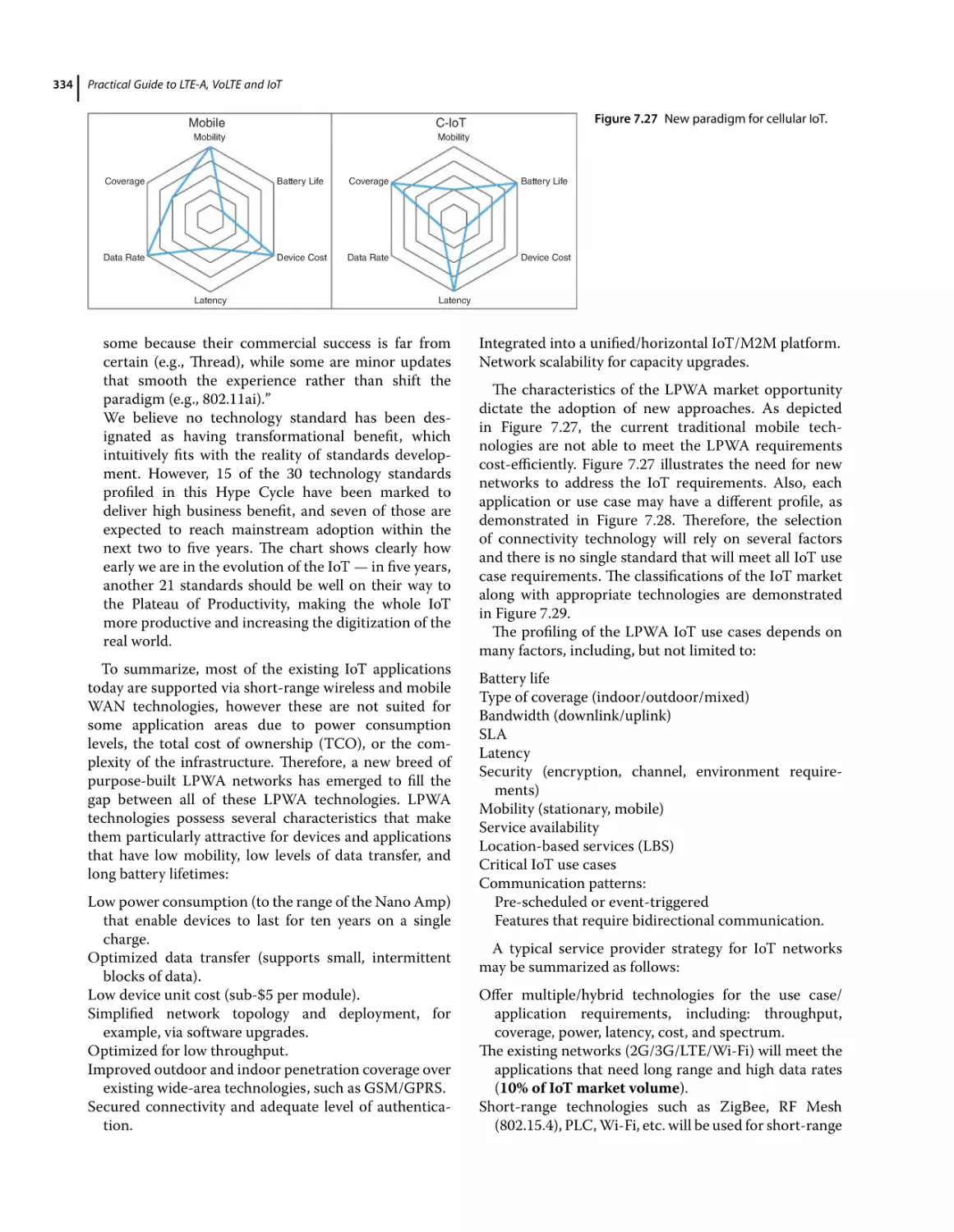
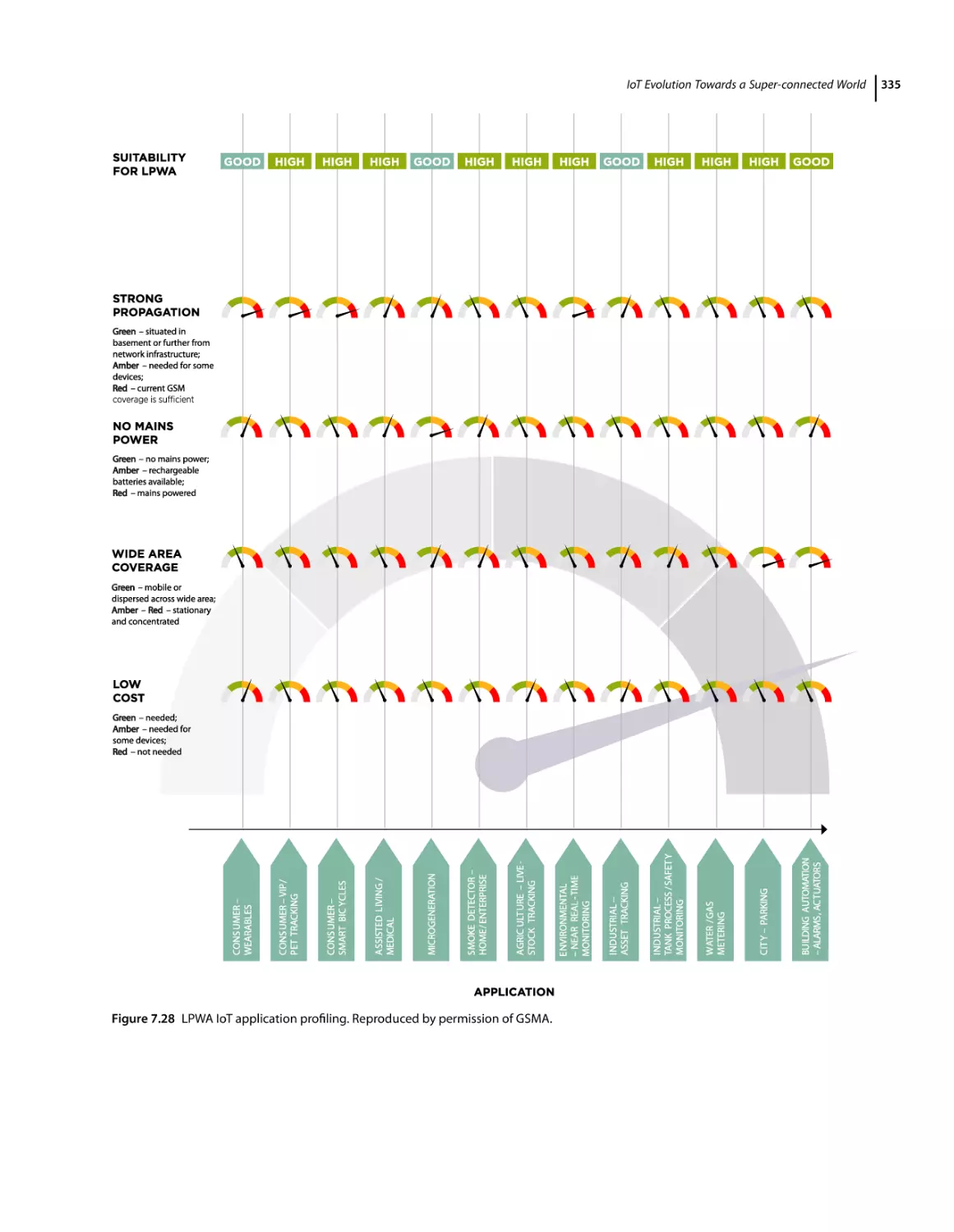
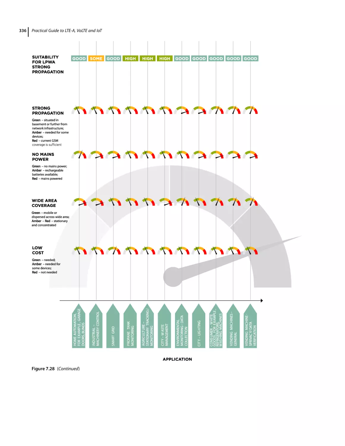
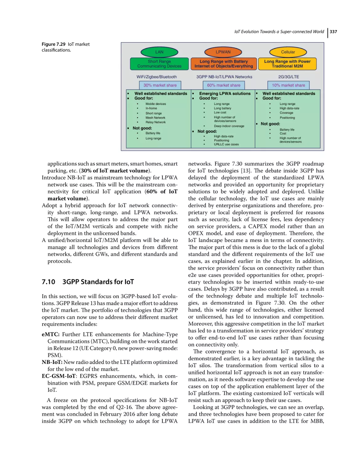
Text
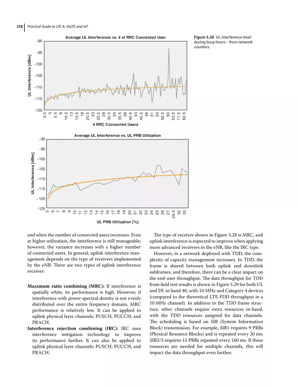
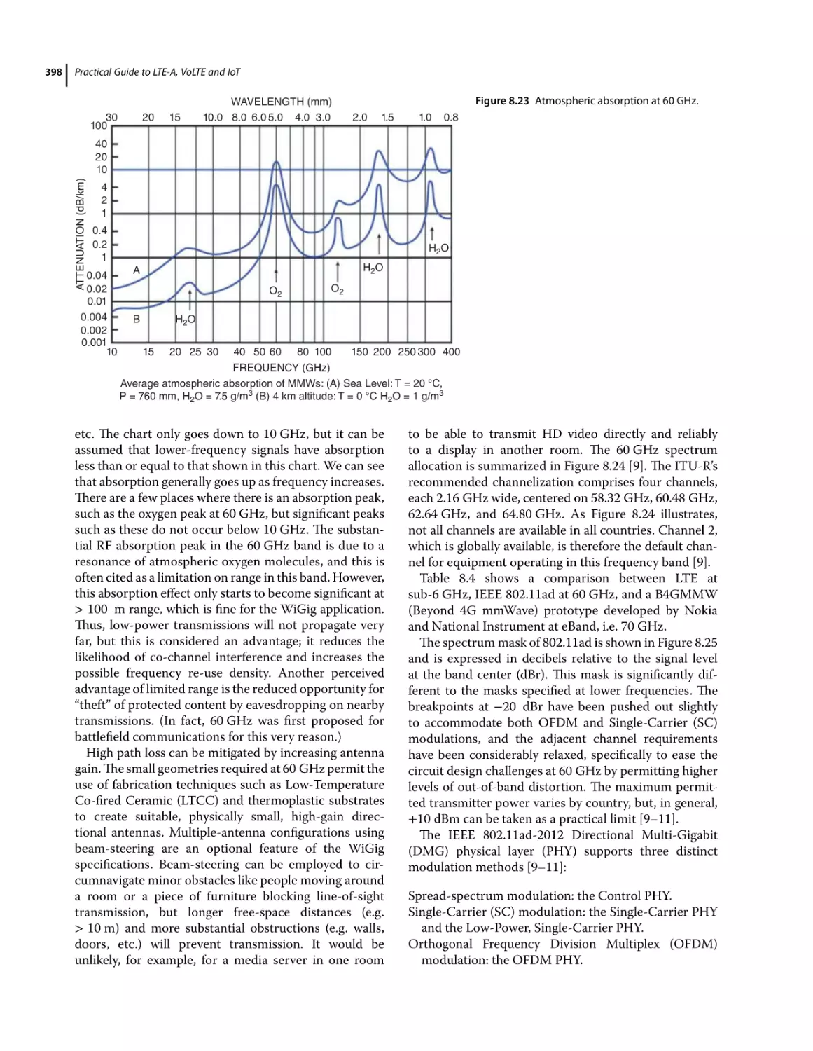
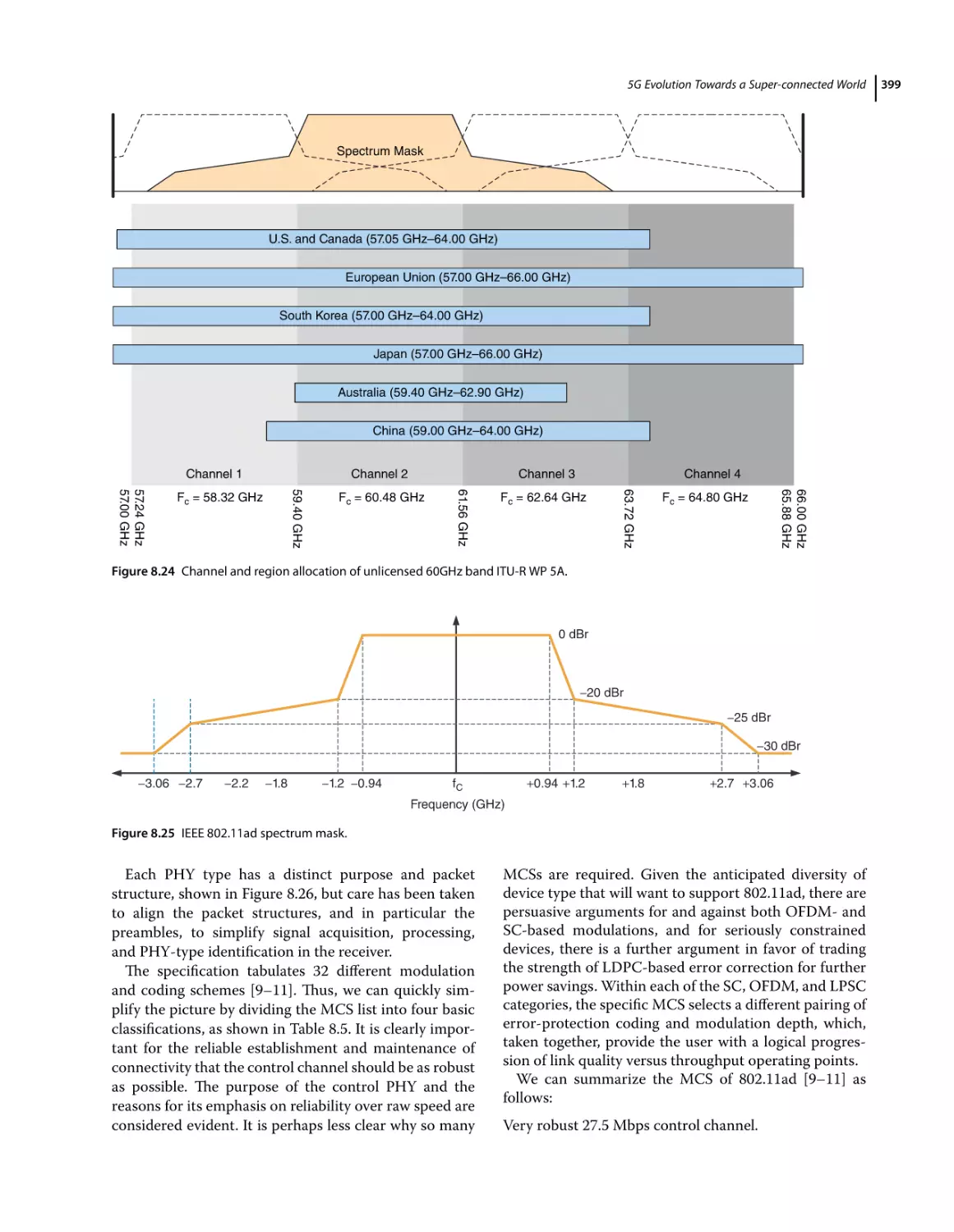
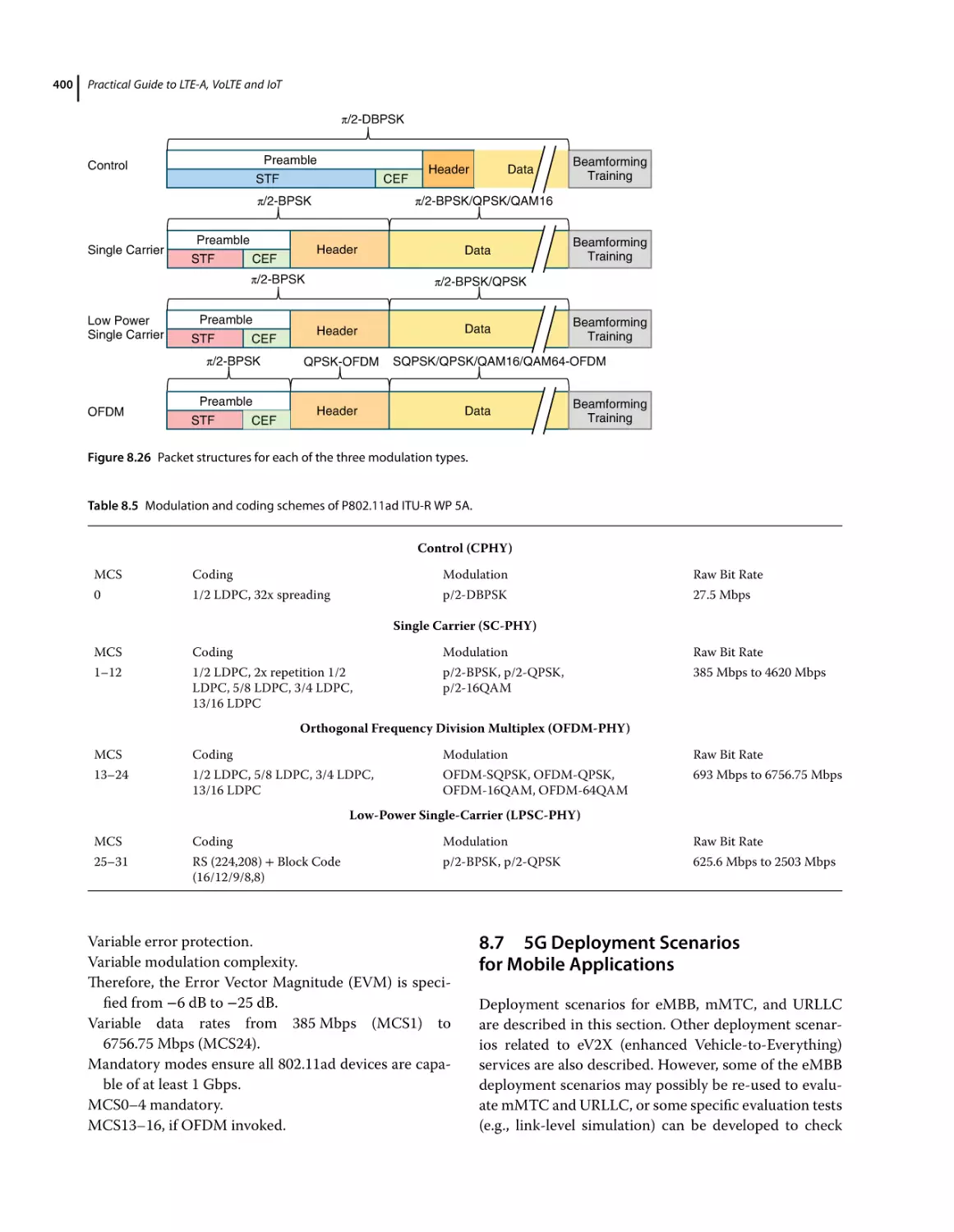
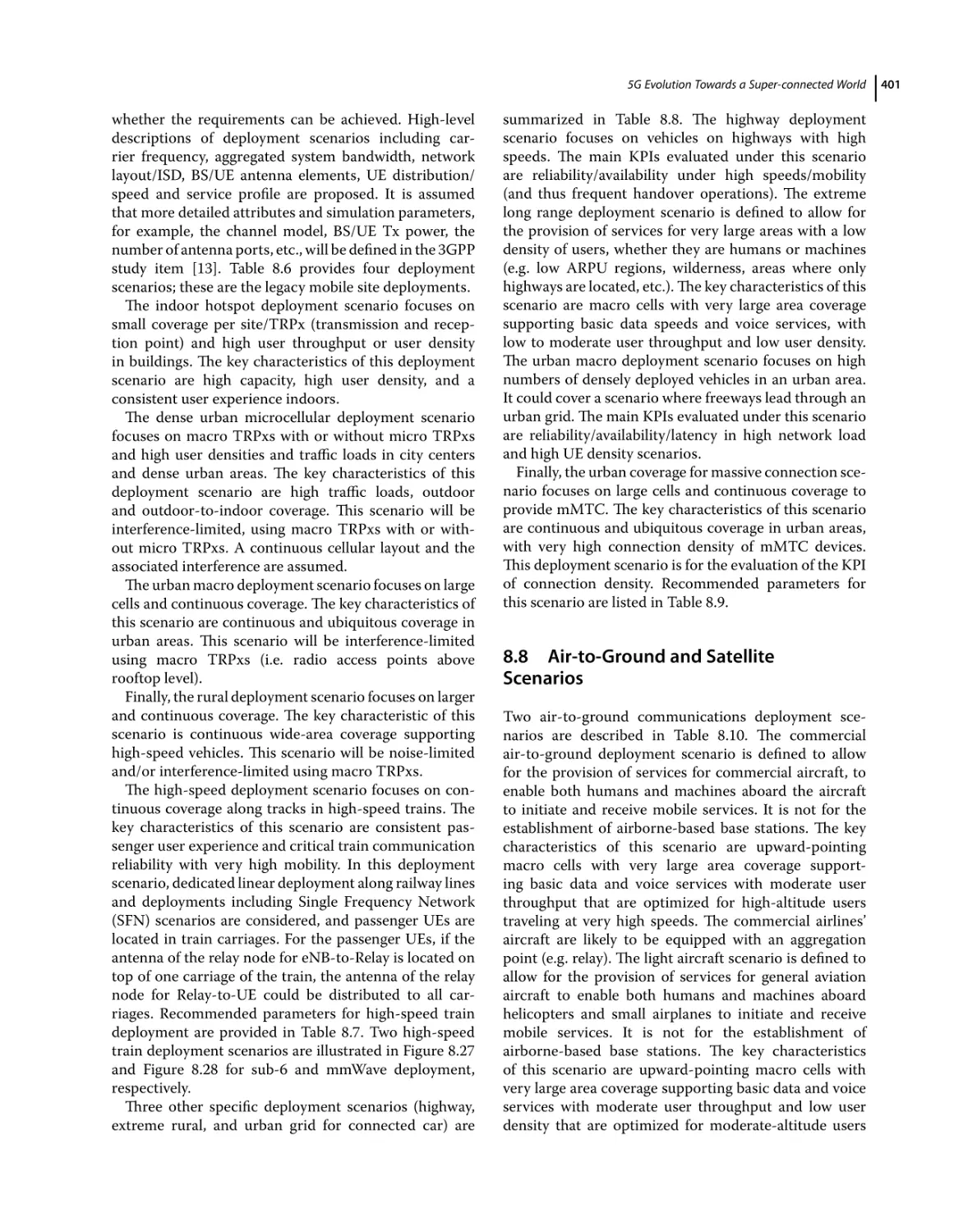
Practical Guide to LTE-A, VoLTE and IoT
Practical Guide to LTE-A, VoLTE and IoT
Paving the Way Towards 5G
Ayman Elnashar
Emirates Integrated Telecommunications Company (EITC)
Dubai Media City
Dubai
UAE
Mohamed El-saidny
MediaTek
Dubai Internet City
Dubai
UAE
This edition first published 2018
© 2018 John Wiley & Sons Ltd.
All rights reserved. No part of this publication may be reproduced, stored in a retrieval system, or transmitted, in any form or by any means,
electronic, mechanical, photocopying, recording or otherwise, except as permitted by law. Advice on how to obtain permission to reuse material
from this title is available at http://www.wiley.com/go/permissions.
The right of Ayman Elnashar and Mohamed El-saidny to be identified as the authors of this work has been asserted in accordance with law.
Registered Offices
John Wiley & Sons, Inc., 111 River Street, Hoboken, NJ 07030, USA
John Wiley & Sons Ltd, The Atrium, Southern Gate, Chichester, West Sussex, PO19 8SQ, UK
Editorial Office
The Atrium, Southern Gate, Chichester, West Sussex, PO19 8SQ, UK
For details of our global editorial offices, customer services, and more information about Wiley products visit us at www.wiley.com.
Wiley also publishes its books in a variety of electronic formats and by print-on-demand. Some content that appears in standard print versions of
this book may not be available in other formats.
Limit of Liability/Disclaimer of Warranty
While the publisher and authors have used their best efforts in preparing this work, they make no representations or warranties with respect to the
accuracy or completeness of the contents of this work and specifically disclaim all warranties, including without limitation any implied warranties
of merchantability or fitness for a particular purpose. No warranty may be created or extended by sales representatives, written sales materials or
promotional statements for this work. The fact that an organization, website, or product is referred to in this work as a citation and/or potential
source of further information does not mean that the publisher and authors endorse the information or services the organization, website, or
product may provide or recommendations it may make. This work is sold with the understanding that the publisher is not engaged in rendering
professional services. The advice and strategies contained herein may not be suitable for your situation. You should consult with a specialist where
appropriate. Further, readers should be aware that websites listed in this work may have changed or disappeared between when this work was
written and when it is read. Neither the publisher nor authors shall be liable for any loss of profit or any other commercial damages, including but
not limited to special, incidental, consequential, or other damages.
Library of Congress Cataloging-in-Publication Data applied for
Hardback ISBN: 9781119063308
Cover design by Wiley
Cover image: © jamesteohart/Shutterstock
Set in 10/12pt WarnockPro by SPi Global, Chennai, India
Printed in the UK by Bell & Bain Ltd, Glasgow
10 9 8 7 6 5 4 3 2 1
This book is dedicated to the memory of my parents (God bless their souls). They gave me the strong foundation and
unconditional love, which remains the source of motivation and is the guiding light of my life.
To my dearest wife, my pillar of strength, your encouragement and patience has strengthened me always.
To my beloved children Noursin, Amira, Yousef, and Yasmina. You are the inspiration!
I want to offer my sincerest appreciation to the innovation and vision of UAE. It has provided me with a fulfilling
career, an unmatched lifestyle and the inspiration to author this book.
– Ayman Elnashar, PhD
I would like to dedicate this book to my amazing family for their continuous support and encouragement. To my
beloved wife, you have guided and inspired me throughout the years. To my beautiful daughter, you always surprise me
with your motivational spirit and hard work.
“The scientific man does not aim at an immediate result. He does not expect that his advanced ideas will be readily
taken up. His work is like that of the planter—for the future. His duty is to lay the foundation for those who are to come,
and point the way”. – Nikola Tesla
Mohamed El-saidny
vii
Contents
About the Authors xvii
Preface xix
Acknowledgments xxi
1
1.1
1.2
1.3
1.3.1
1.3.2
1.3.2.1
1.3.3
1.4
1.5
1.6
1.7
1.7.1
1.7.2
1.7.3
1.8
1.8.1
1.8.1.1
1.8.1.2
1.8.2
1.8.3
1.8.3.1
1.8.3.2
1.8.4
1.8.5
1.9
1.9.1
1.9.2
1.10
1.10.1
1.10.2
1.10.3
1.11
1.11.1
1.11.2
1.11.3
1.11.4
1.11.5
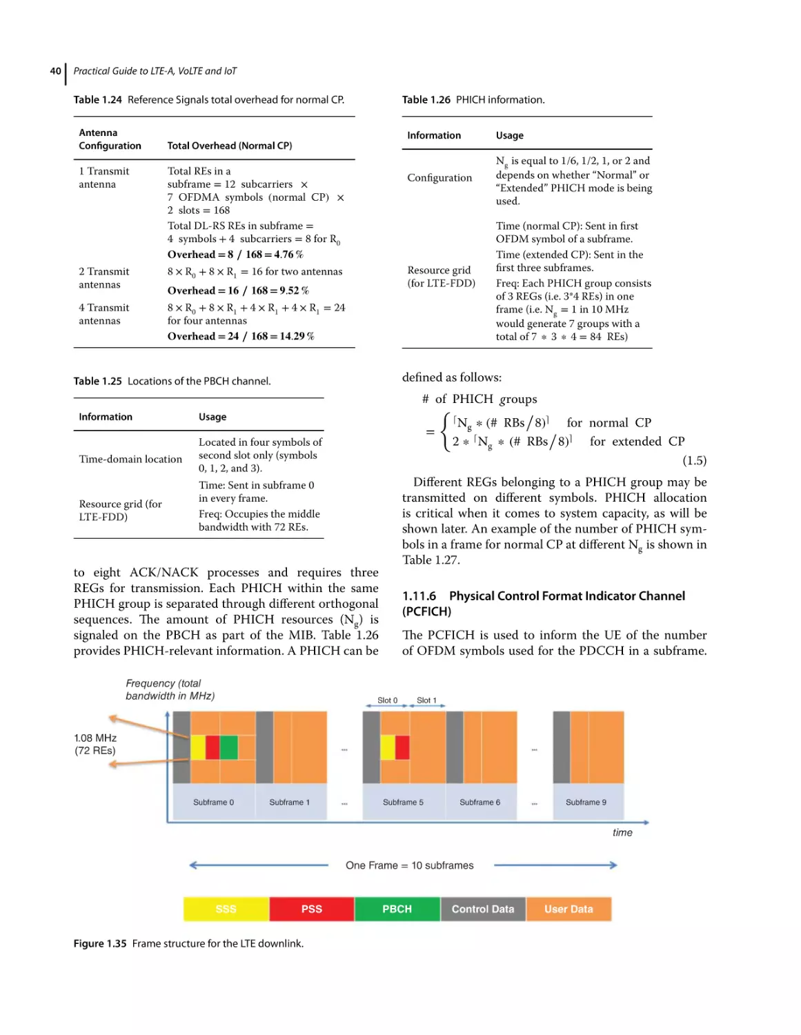
1.11.6
1
Introduction 1
Link Spectrum Efficiency 3
LTE-Advanced and Beyond 4
LTE and Wi-Fi 6
Wi-Fi Calling 7
QoS Challenges in VoWiFi 8
Internet of Things (IoT) 8
Evolved Packet System (EPS) Overview 9
Network Architecture Evolution 11
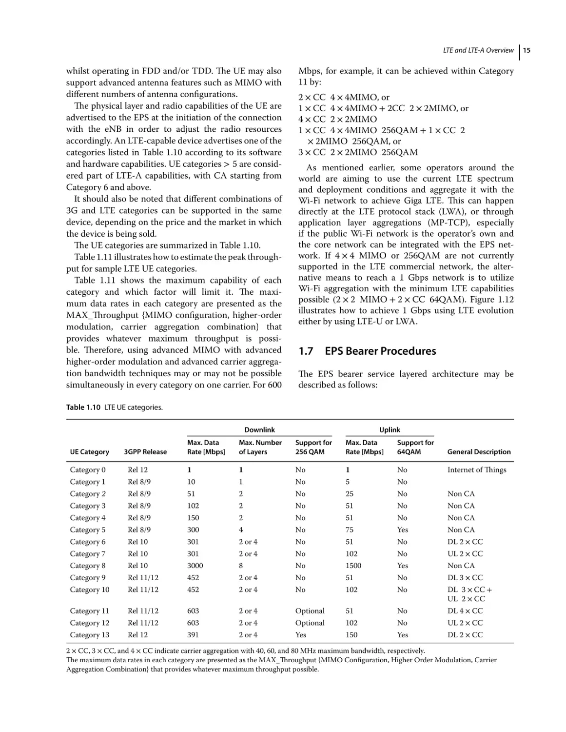
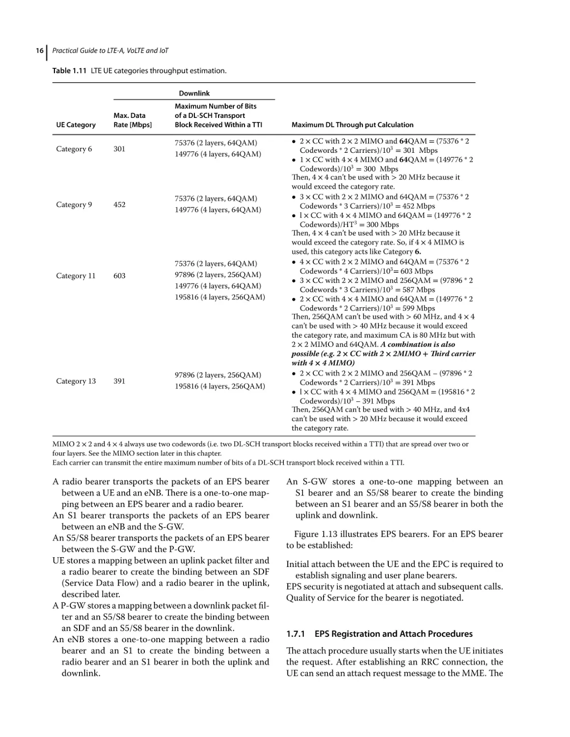
LTE UE Description 14
EPS Bearer Procedures 15
EPS Registration and Attach Procedures 16
EPS Security Basics 19
EPS QoS 20
Access and Non-access Stratum Procedures 20
EMM Procedures and Description 21
Definitions 21
ESM Procedures and Description 22
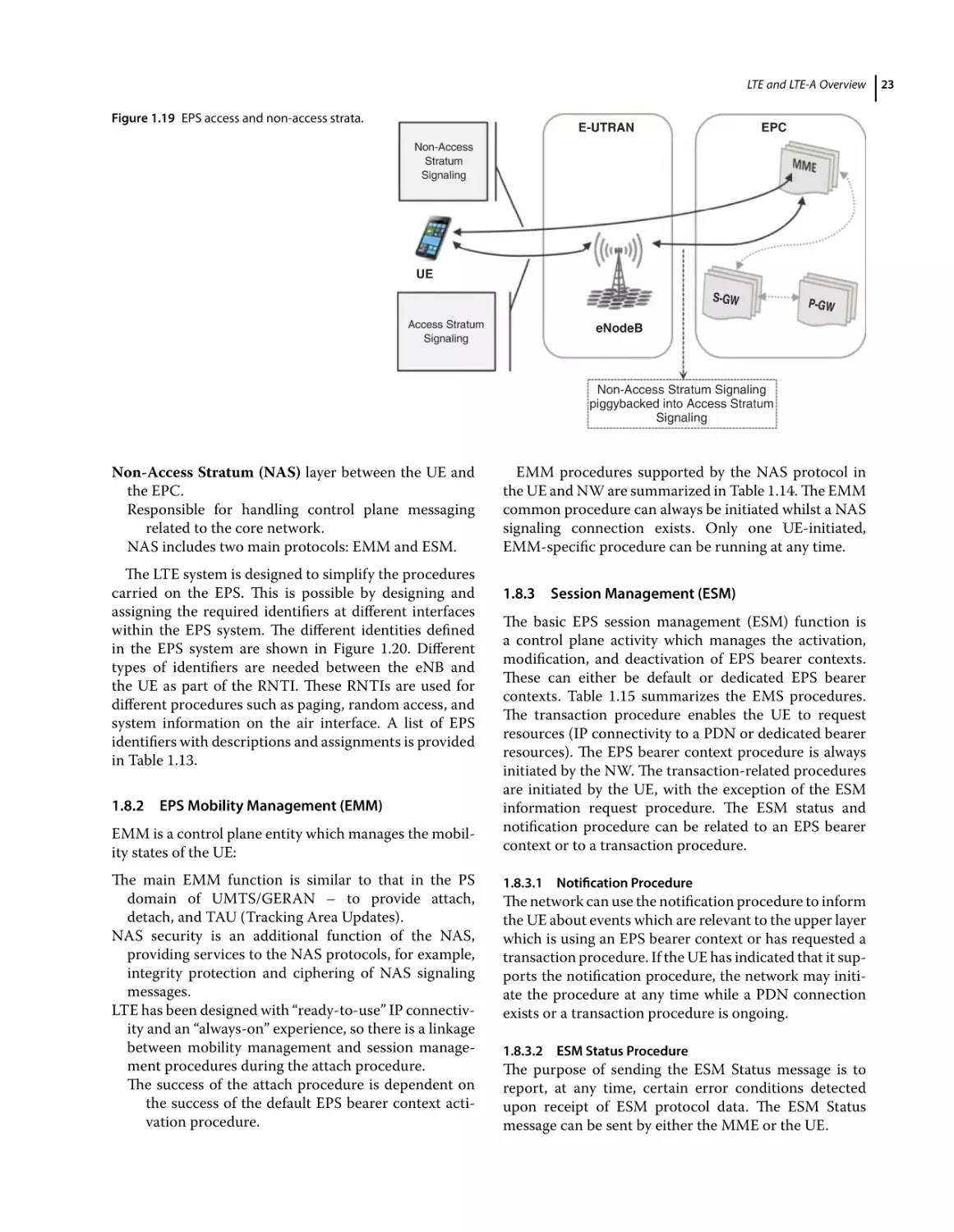
EPS Mobility Management (EMM) 23
Session Management (ESM) 23
Notification Procedure 23
ESM Status Procedure 23
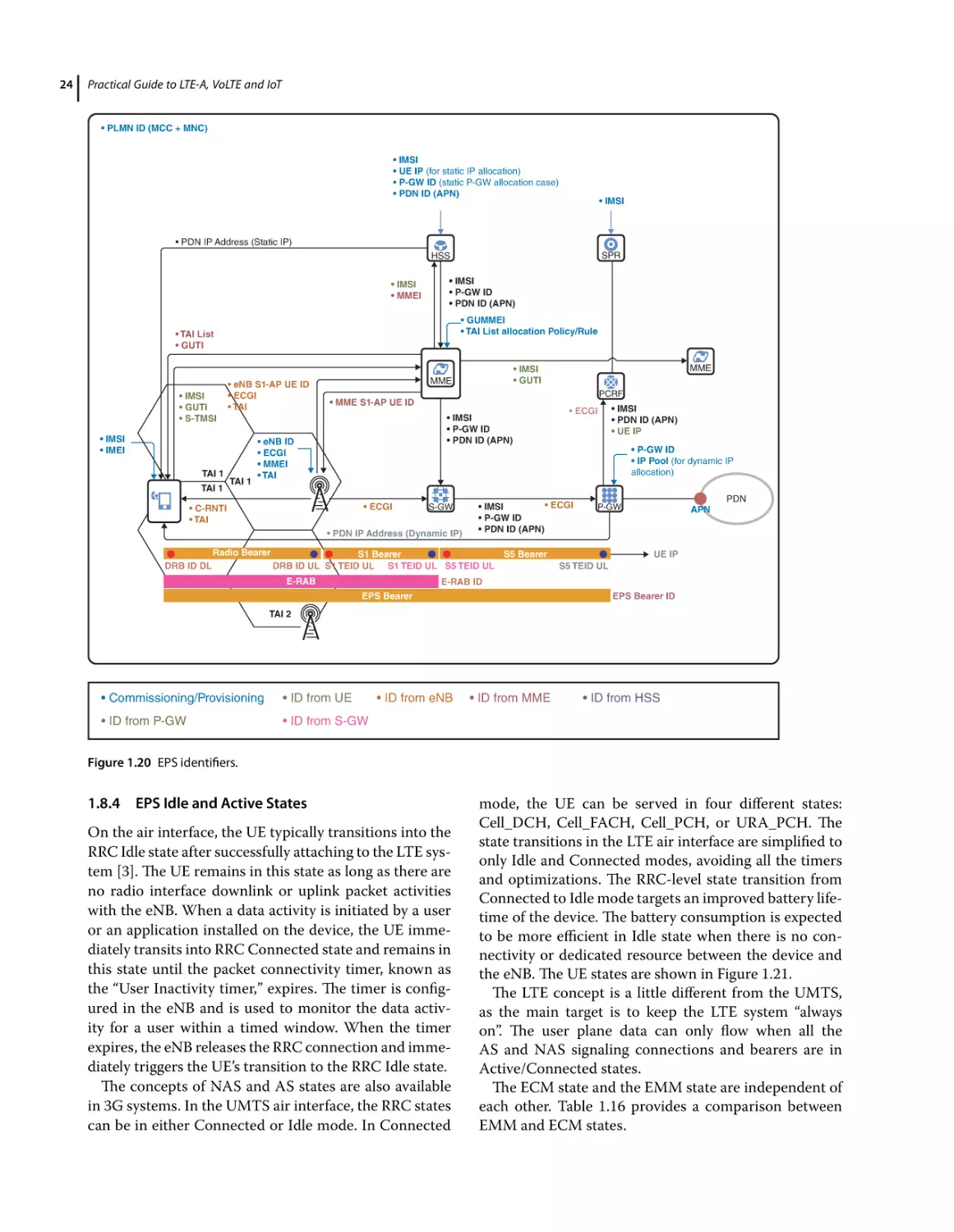
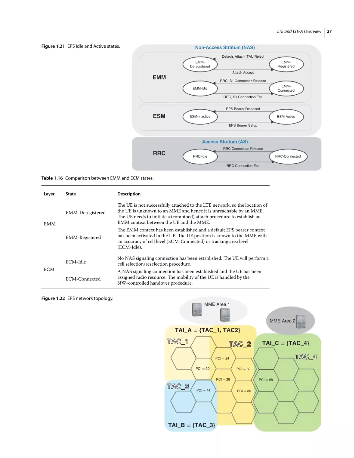
EPS Idle and Active States 24
EPS Network Topology for Mobility Procedures 25
LTE Air Interface 26
Multiple Access in 3GPP Systems 26
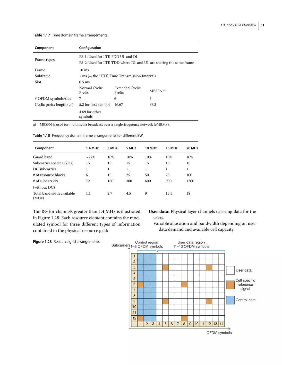
Time–Frequency Domain Resources 28
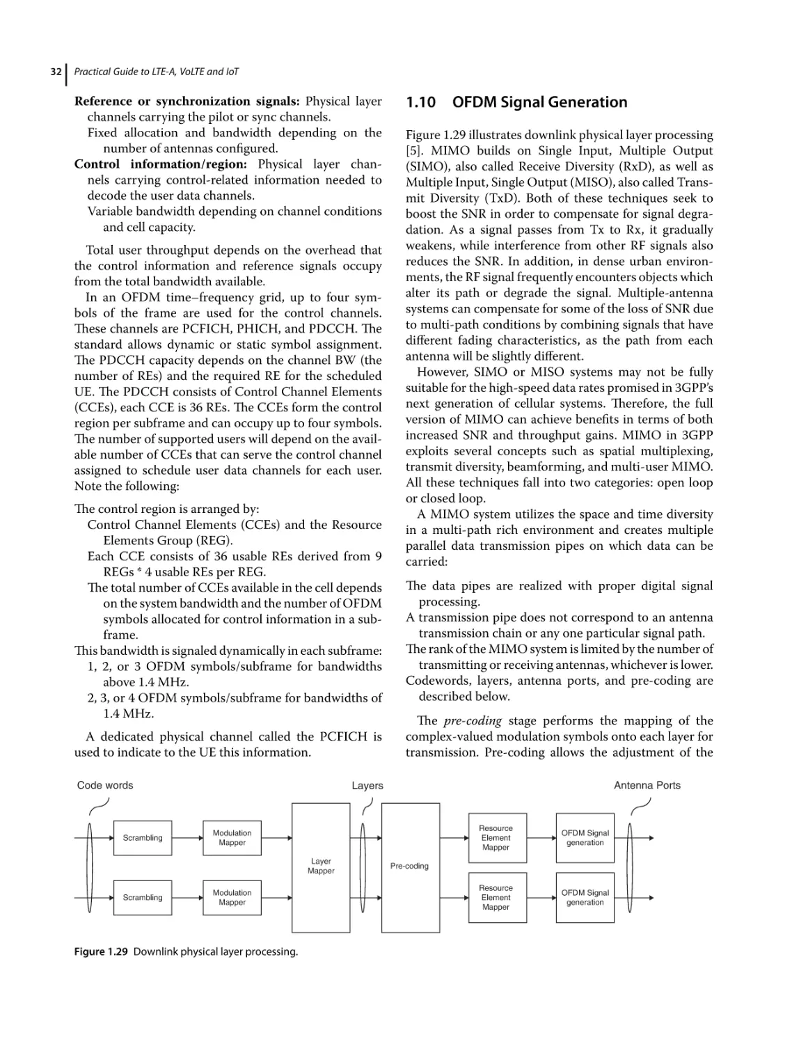
OFDM Signal Generation 32
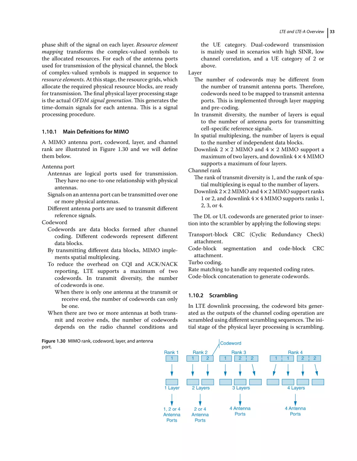
Main Definitions for MIMO 33
Scrambling 33
Higher-order Modulation 34
LTE Channels and Procedures 34
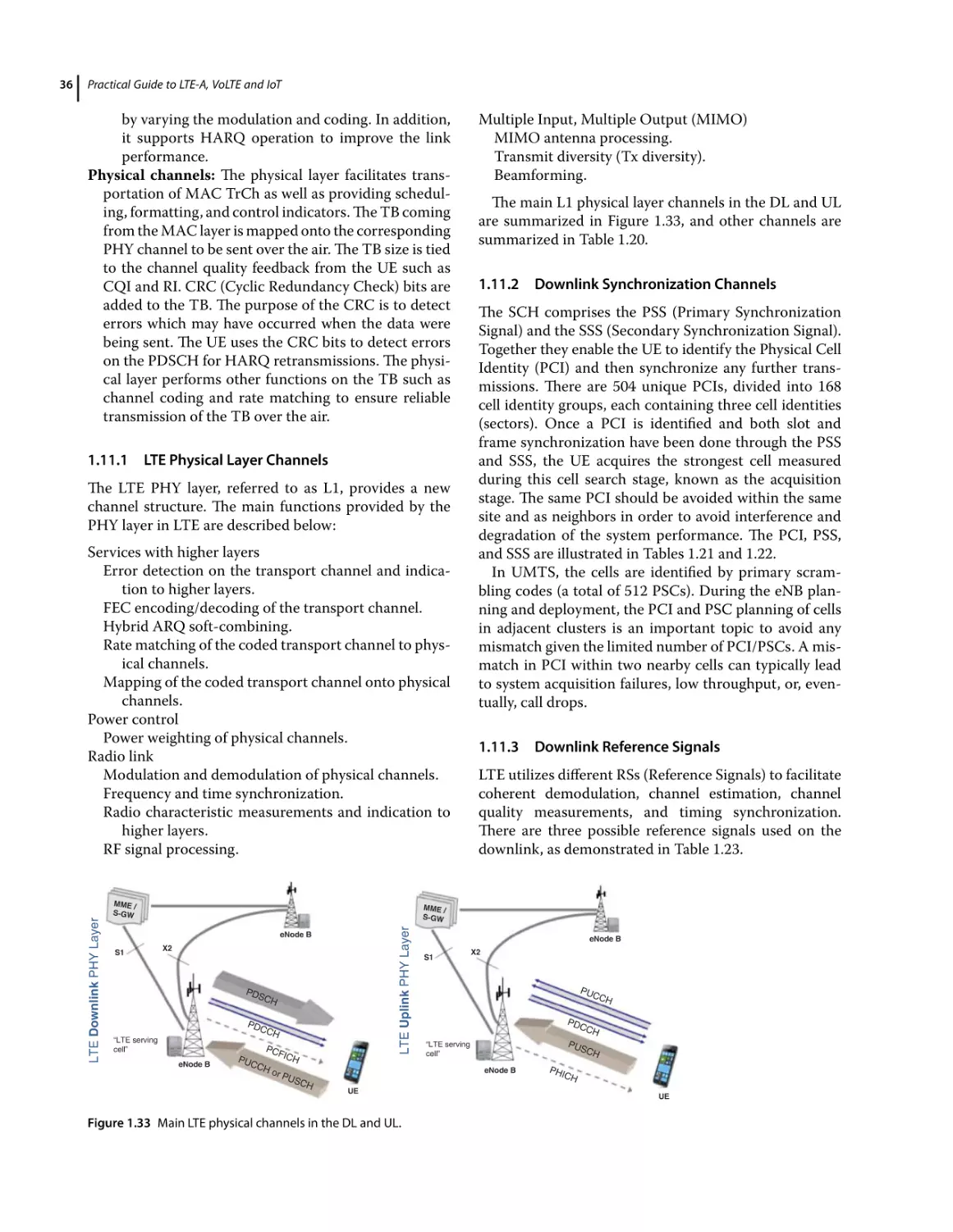
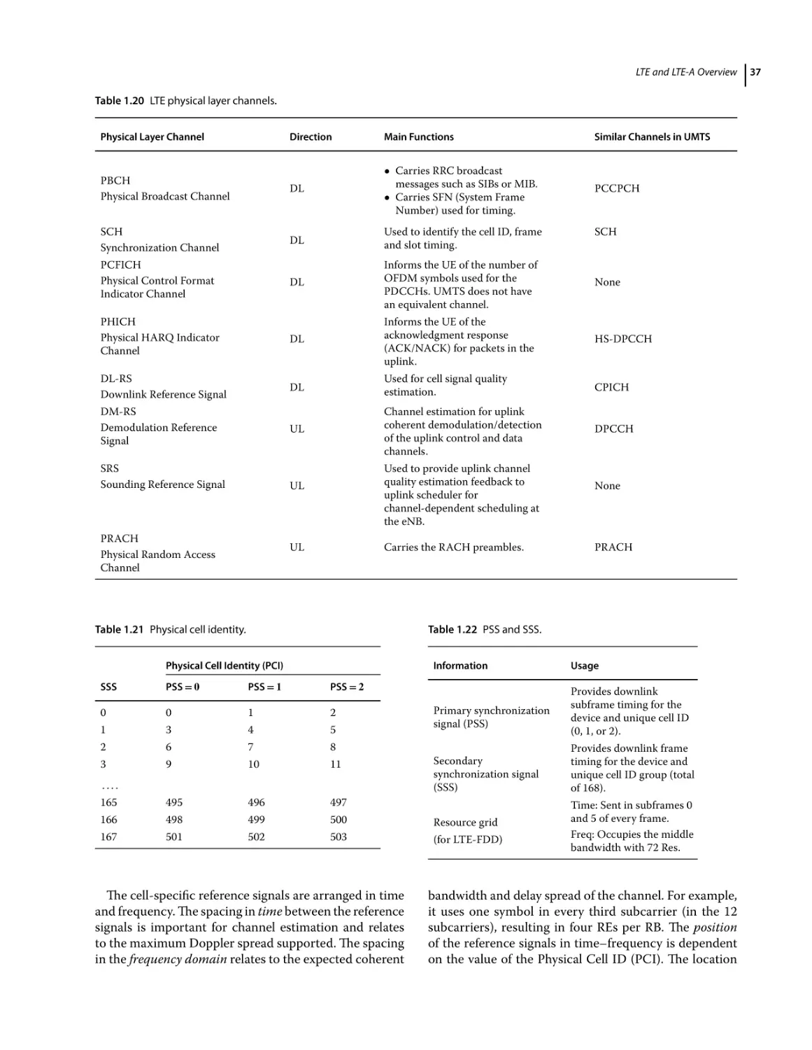
LTE Physical Layer Channels 36
Downlink Synchronization Channels 36
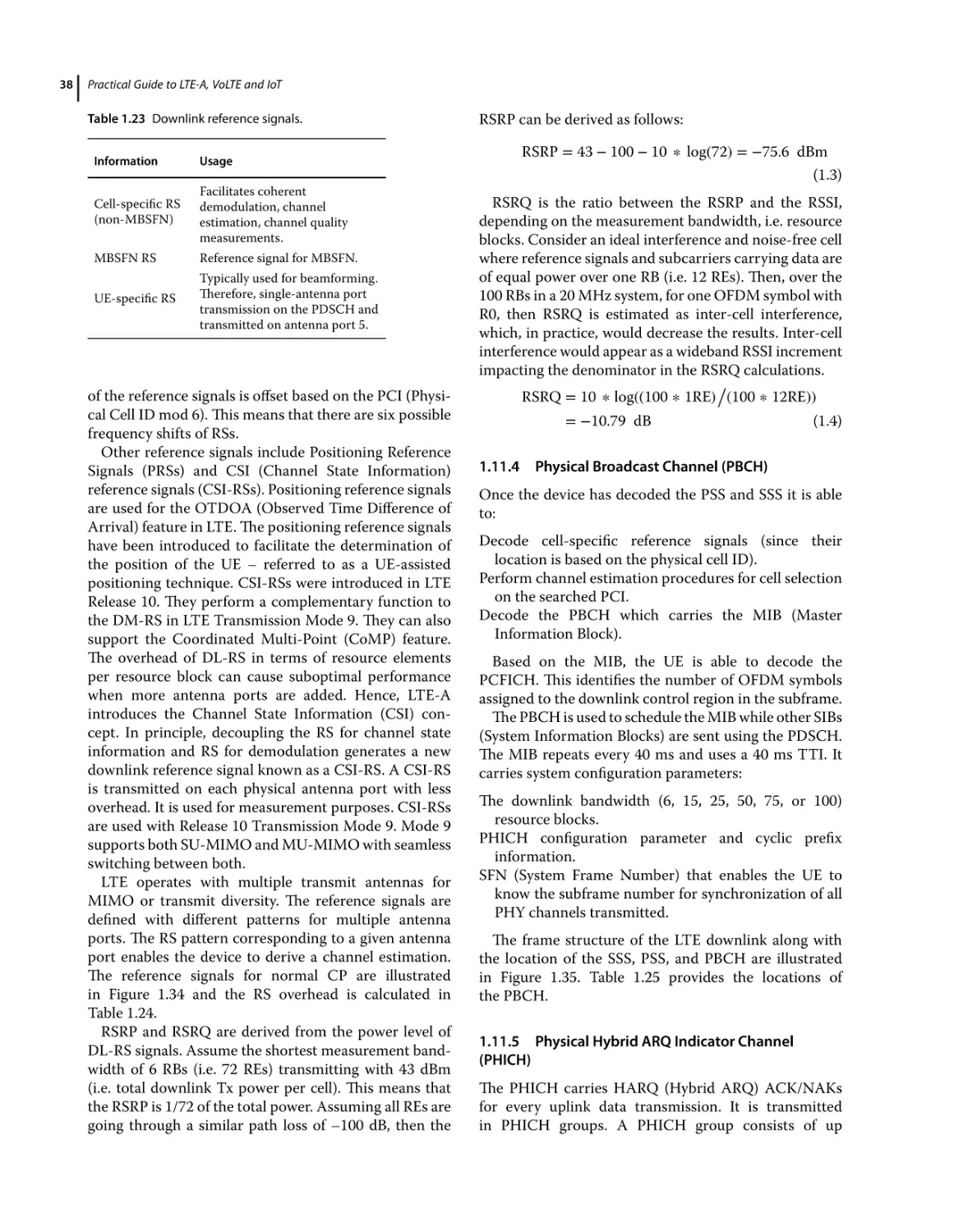
Downlink Reference Signals 36
Physical Broadcast Channel (PBCH) 38
Physical Hybrid ARQ Indicator Channel (PHICH) 38
Physical Control Format Indicator Channel (PCFICH) 40
LTE and LTE-A Overview
viii
Contents
1.11.7
1.11.8
1.12
1.12.1
1.12.2
1.12.3
1.12.4
1.13
1.13.1
1.13.2
1.13.3
1.13.4
1.13.5
1.13.6
1.14
1.14.1
1.14.2
1.14.3
1.14.4
1.14.5
1.14.6
1.14.7
1.14.8
1.15
1.15.1
1.15.2
1.15.3
1.15.3.1
1.15.4
1.15.4.1
1.15.4.2
1.15.5
1.15.6
1.15.7
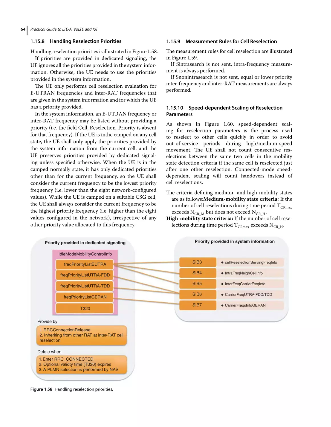
1.15.8
1.15.9
1.15.10
1.15.11
1.15.12
1.15.13
1.15.14
1.15.15
1.16
1.16.1
1.16.2
1.16.3
1.16.4
1.16.5
1.16.6
1.16.7
1.16.8
1.16.9
1.16.10
1.16.11
1.16.12
1.16.13
Physical Downlink Control Channel (PDCCH) 41
Physical Downlink Shared Channel (PDSCH) 43
Uplink Physical Channels 43
Uplink Reference Signals 43
Physical Random Access Channel (PRACH) 44
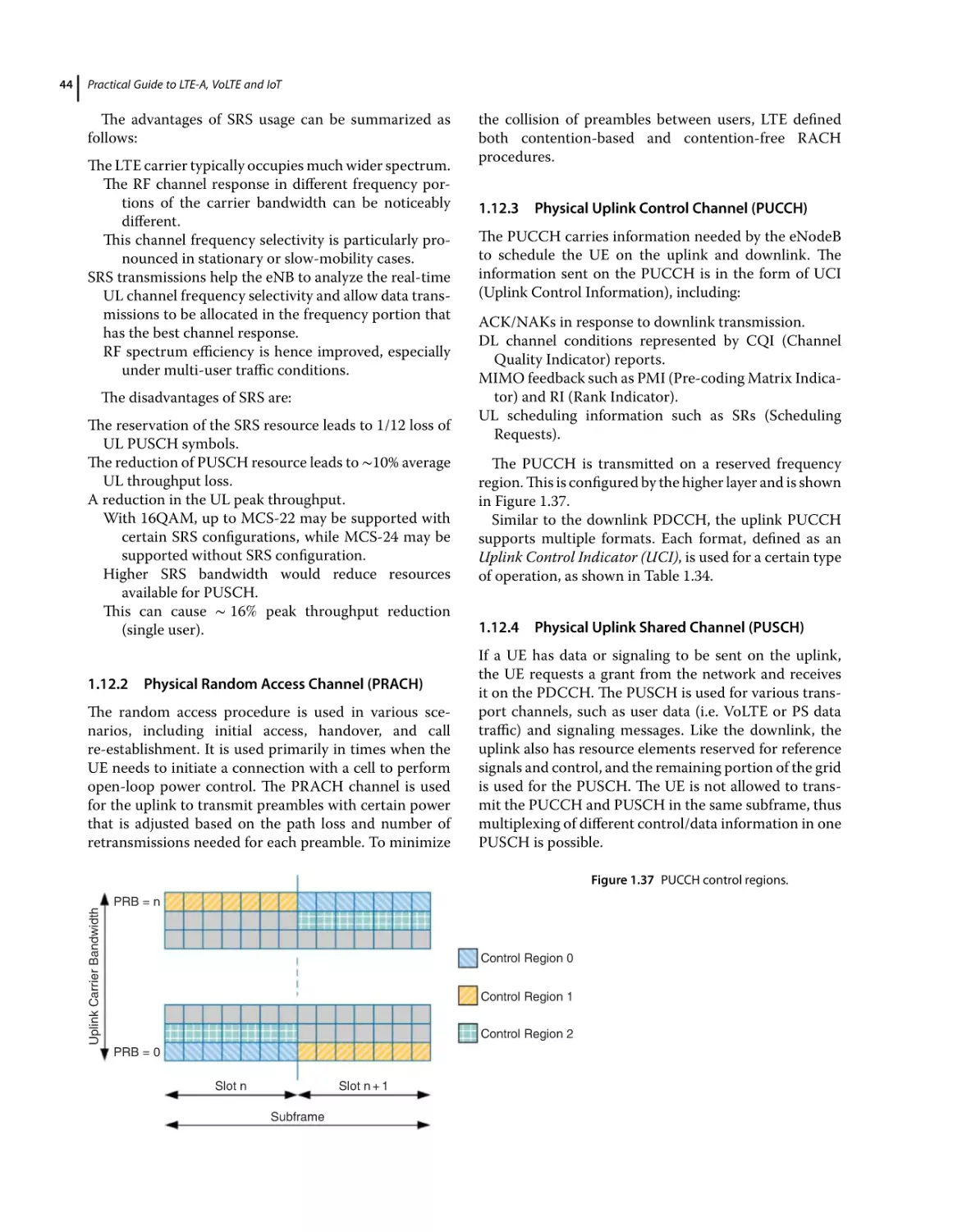
Physical Uplink Control Channel (PUCCH) 44
Physical Uplink Shared Channel (PUSCH) 44
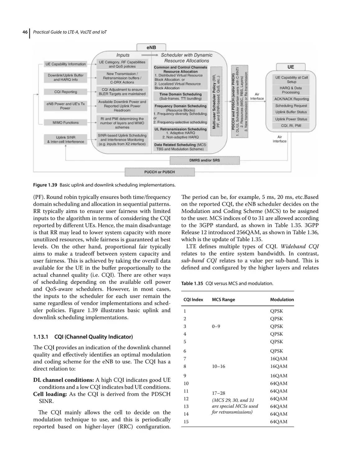
Physical Layer Procedures 45
CQI (Channel Quality Indicator) 46
DL Scheduling 47
UL Scheduling 47
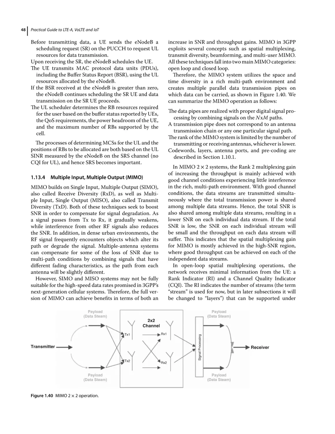
Multiple Input, Multiple Output (MIMO) 48
Uplink Power Control 50
Techniques for Data Retransmission on the UL 51
RRC Layer and Mobility Procedures 51
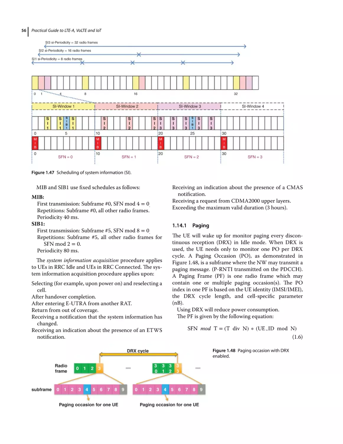
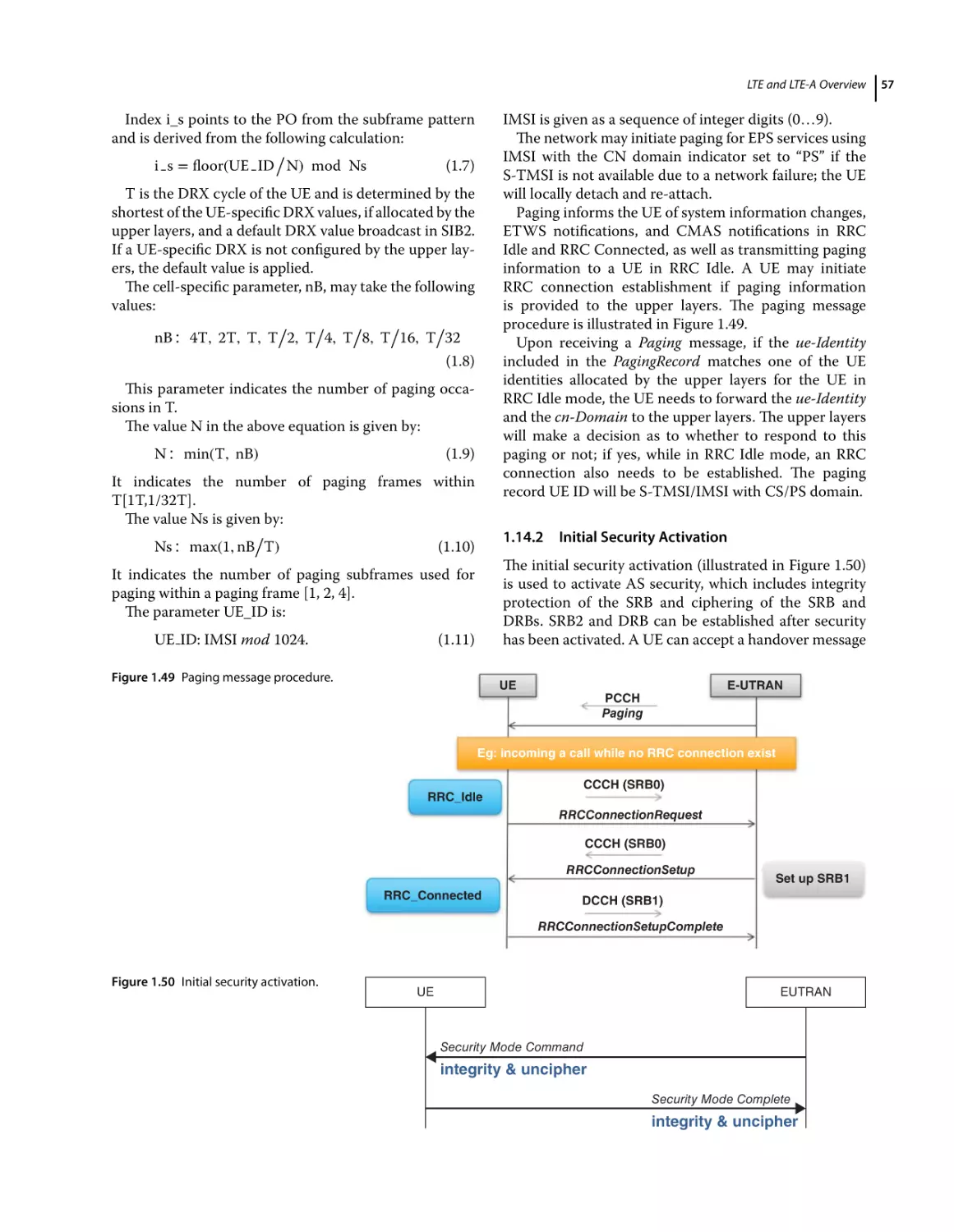
Paging 56
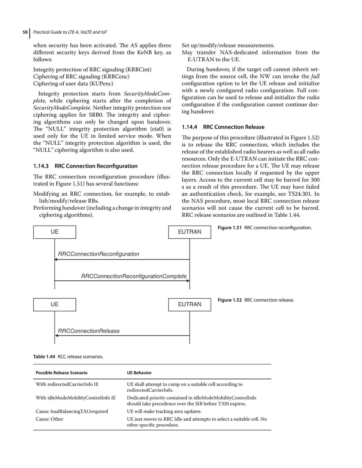
Initial Security Activation 57
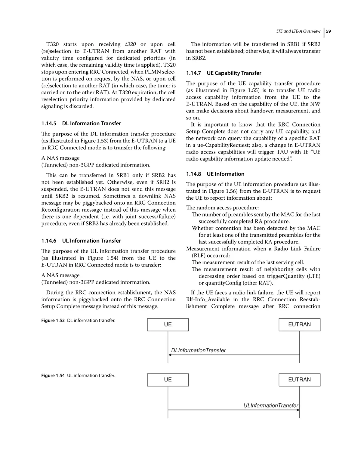
RRC Connection Reconfiguration 58
RRC Connection Release 58
DL Information Transfer 59
UL Information Transfer 59
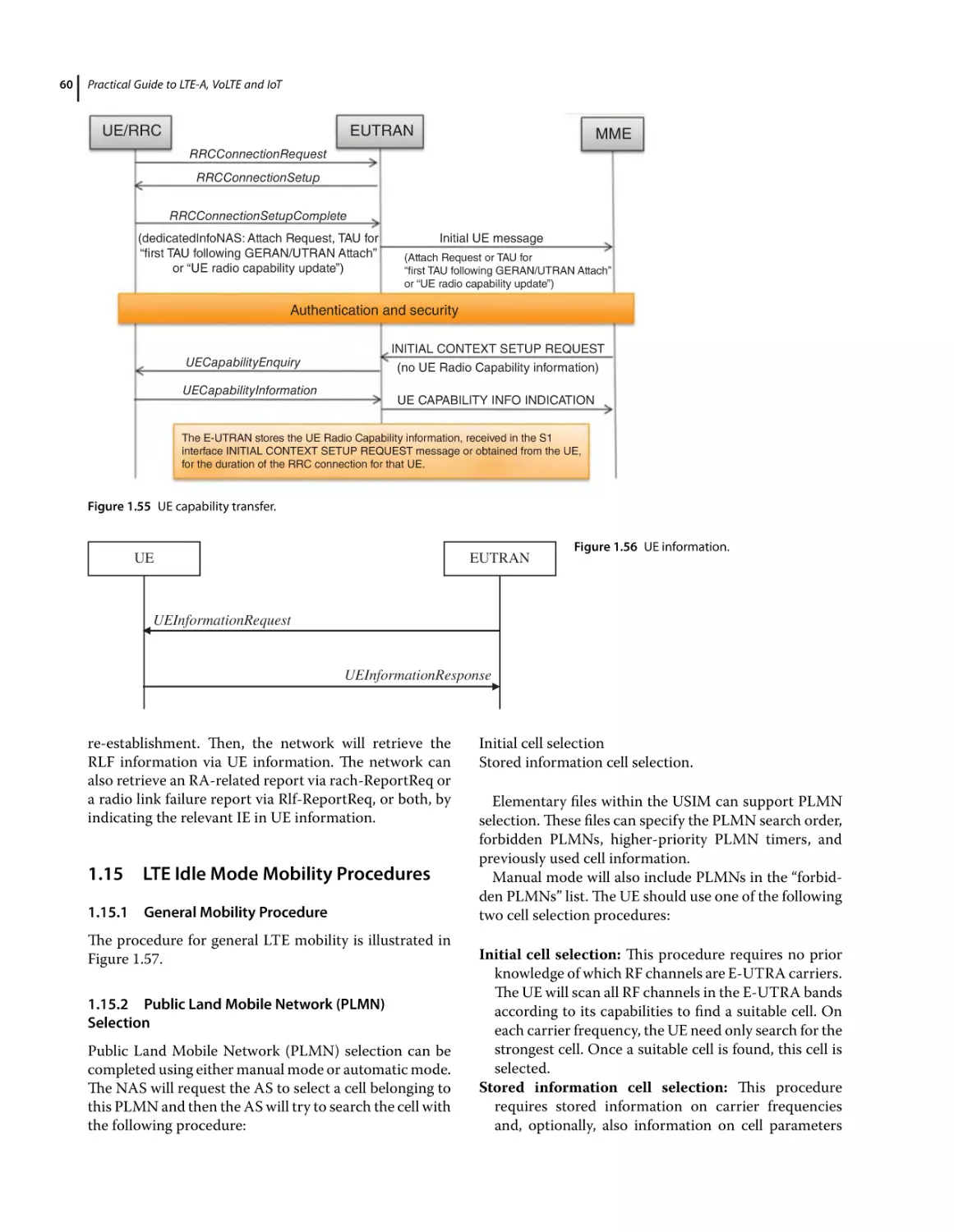
UE Capability Transfer 59
UE Information 59
LTE Idle Mode Mobility Procedures 60
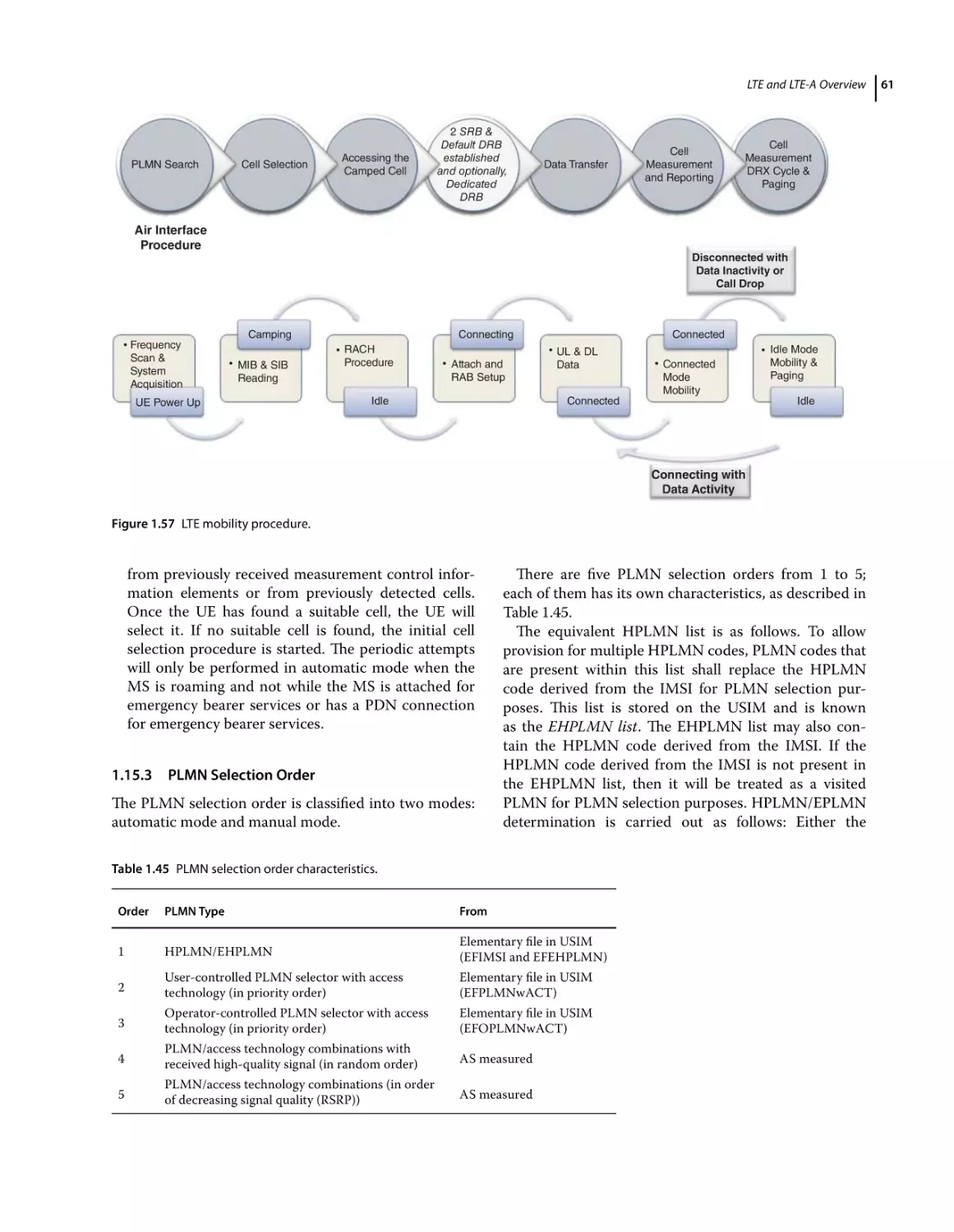
General Mobility Procedure 60
Public Land Mobile Network (PLMN) Selection 60
PLMN Selection Order 61
High Quality Criterion 62
Service Type and Cell Categories 62
Acceptable Cell, Exception 62
Suitable Cell, Exception 62
Cell Selection – S-criteria 62
Camping on a Suitable Cell 62
Cell Reselection in Idle Mode 63
Handling Reselection Priorities 64
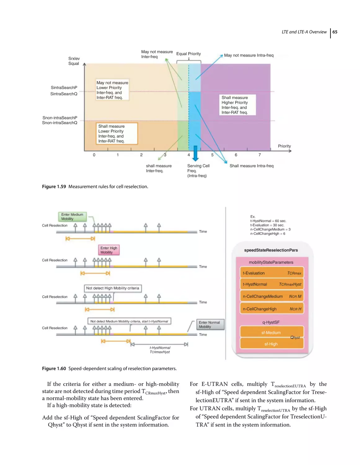
Measurement Rules for Cell Reselection 64
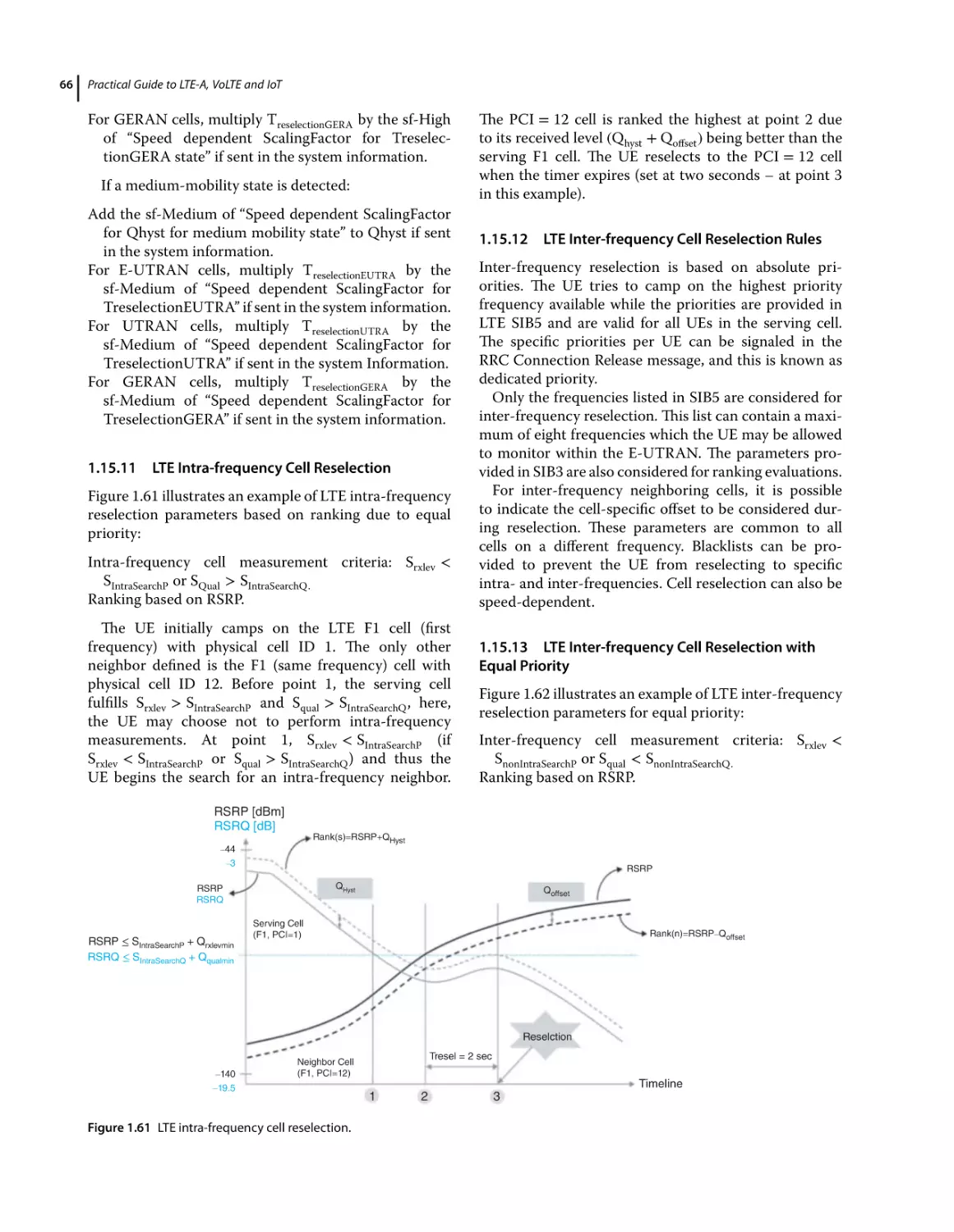
Speed-dependent Scaling of Reselection Parameters 64
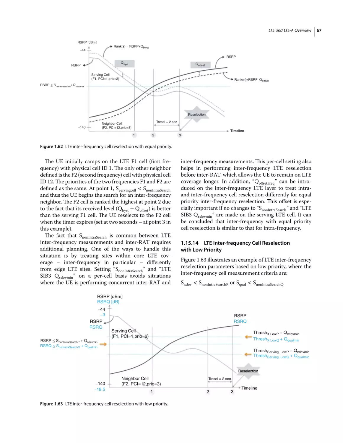
LTE Intra-frequency Cell Reselection 66
LTE Inter-frequency Cell Reselection Rules 66
LTE Inter-frequency Cell Reselection with Equal Priority 66
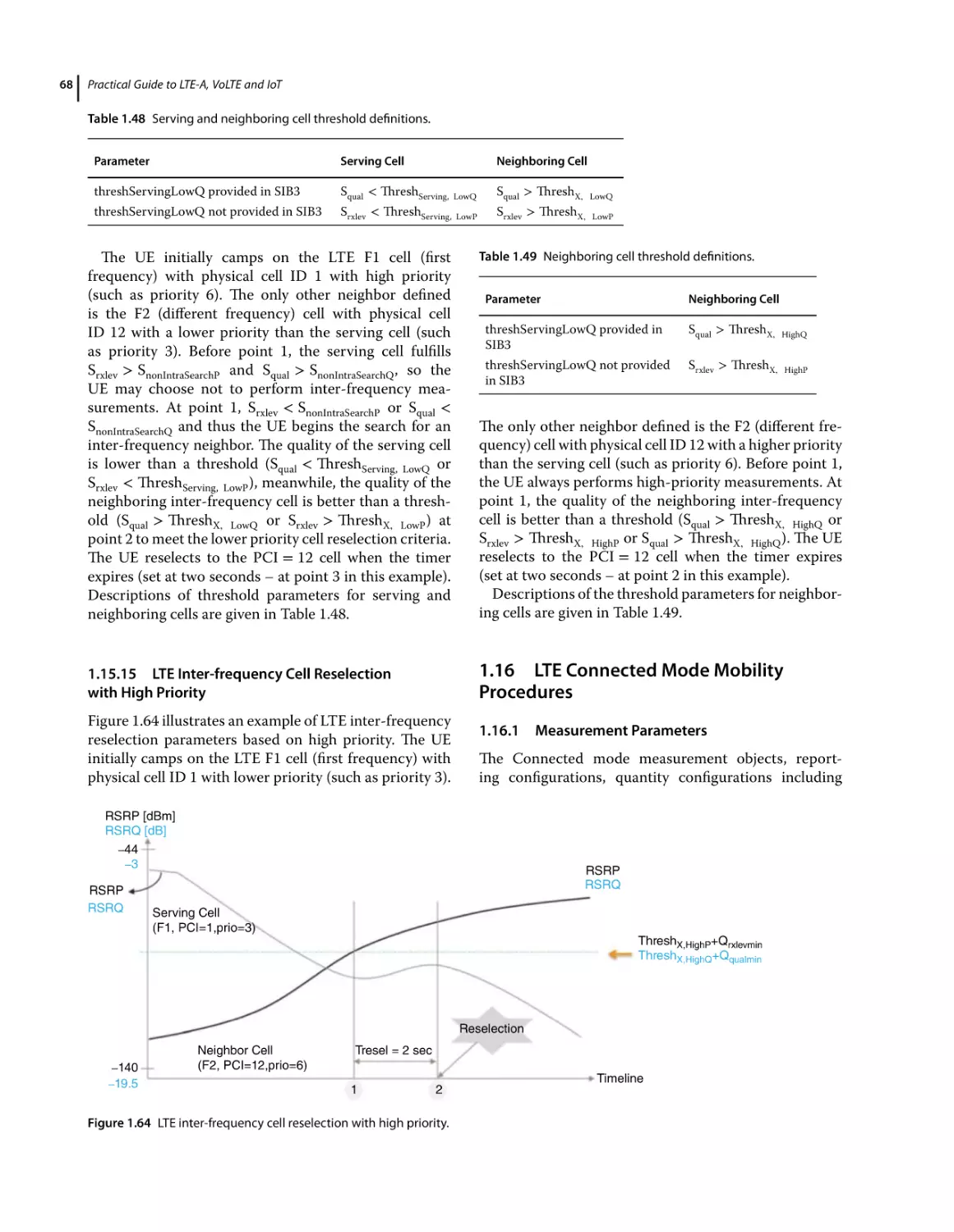
LTE Inter-frequency Cell Reselection with Low Priority 67
LTE Inter-frequency Cell Reselection with High Priority 68
LTE Connected Mode Mobility Procedures 68
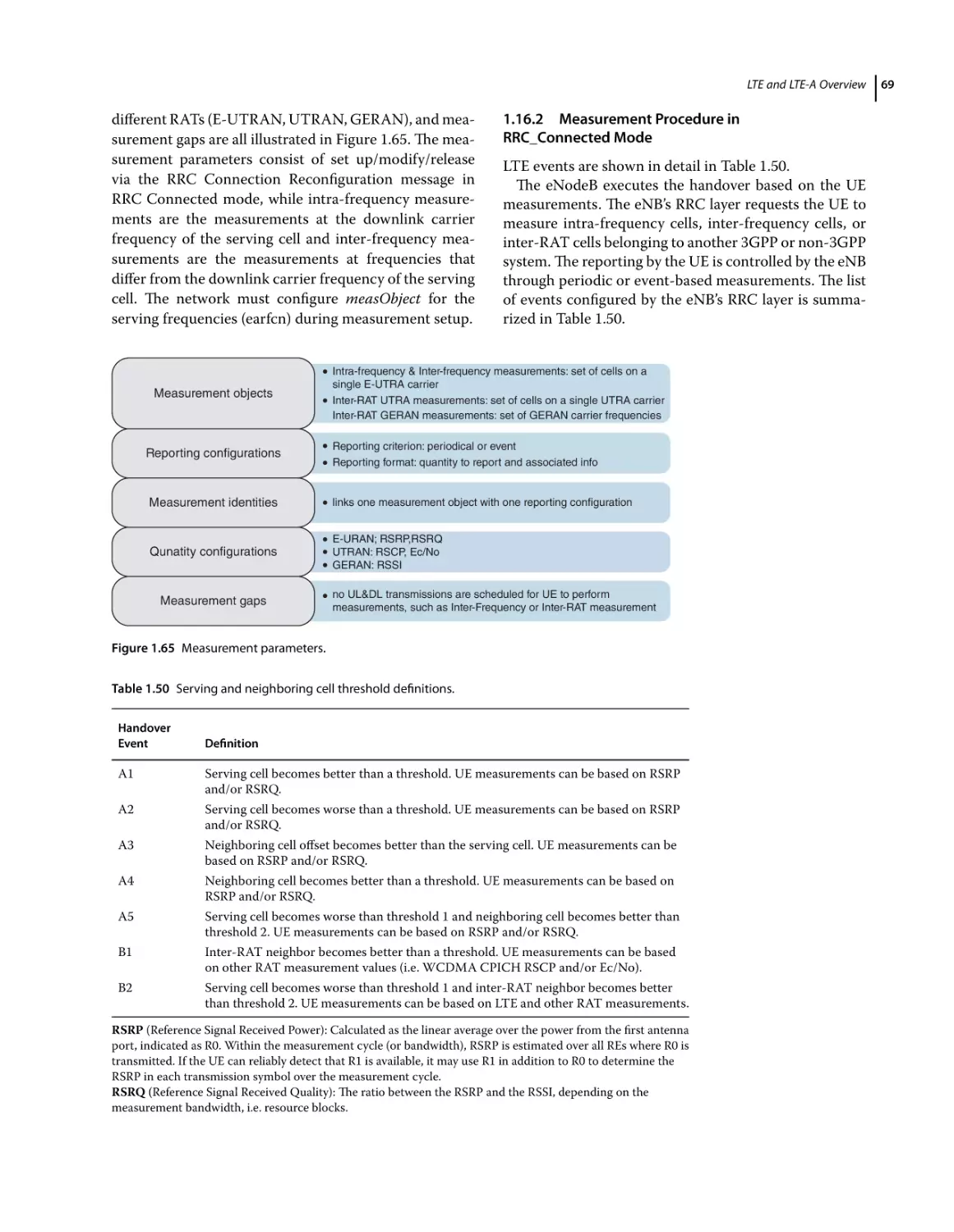
Measurement Parameters 68
Measurement Procedure in RRC_Connected Mode 69
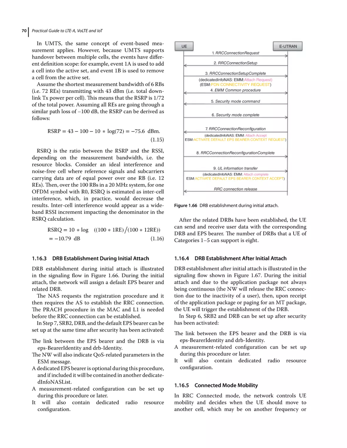
DRB Establishment During Initial Attach 70
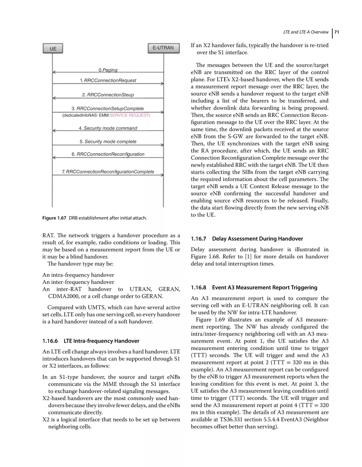
DRB Establishment After Initial Attach 70
Connected Mode Mobility 70
LTE Intra-frequency Handover 71
Delay Assessment During Handover 71
Event A3 Measurement Report Triggering 71
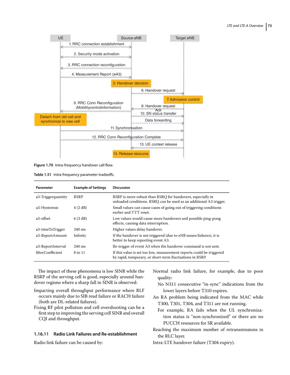
Intra-frequency Handover Call Flow 72
Intra-frequency Parameter Tradeoffs 72
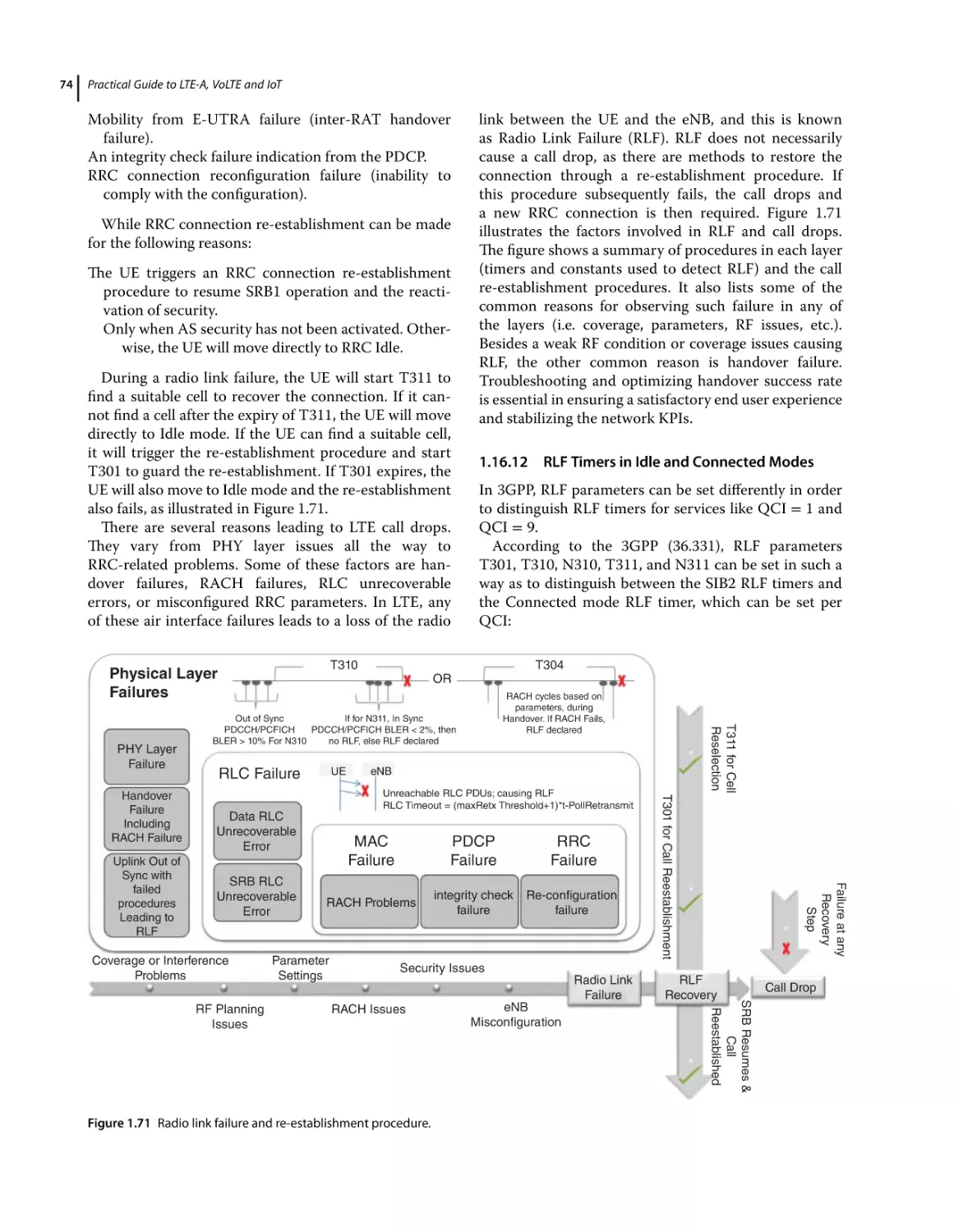
Radio Link Failures and Re-establishment 73
RLF Timers in Idle and Connected Modes 74
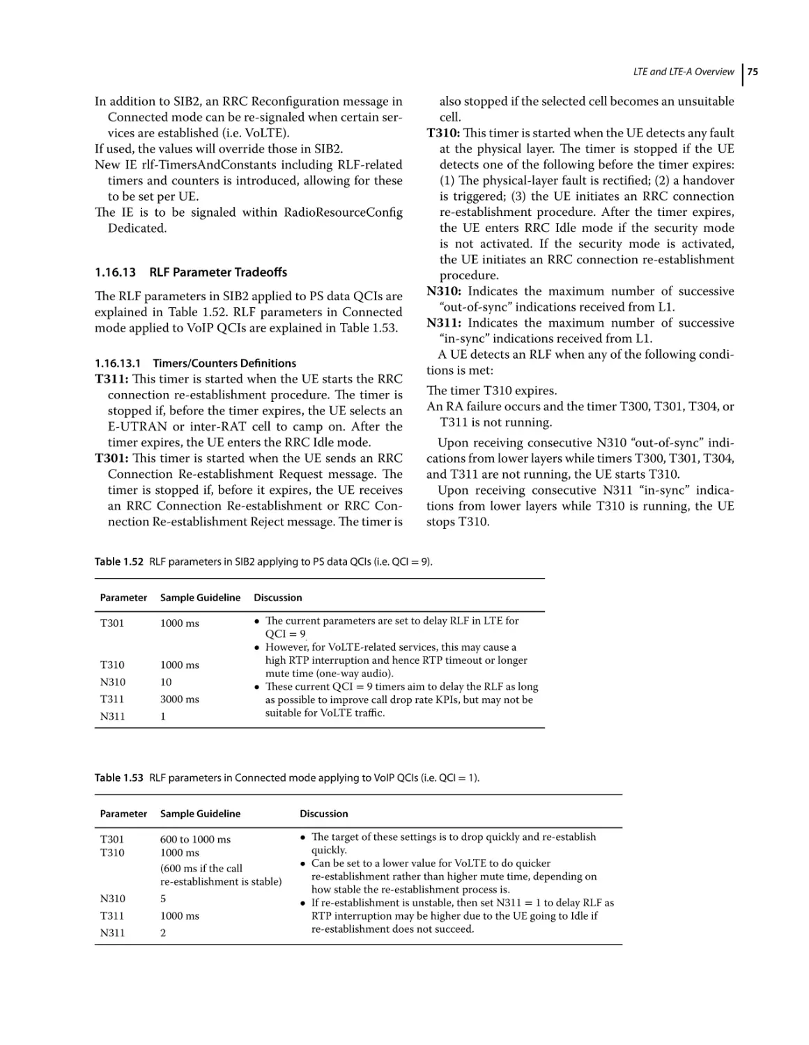
RLF Parameter Tradeoffs 75
Contents
1.16.13.1
1.17
1.17.1
1.17.2
1.17.3
1.17.4
1.17.5
1.17.6
1.17.7
1.17.8
1.17.9
1.17.10
1.17.11
1.17.12
1.17.13
1.17.14
1.17.15
1.17.16
1.17.17
1.17.18
Timers/Counters Definitions 75
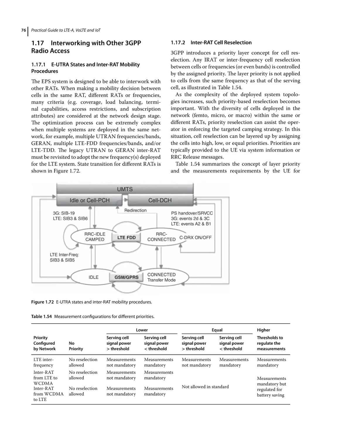
Interworking with Other 3GPP Radio Access 76
E-UTRA States and Inter-RAT Mobility Procedures 76
Inter-RAT Cell Reselection 76
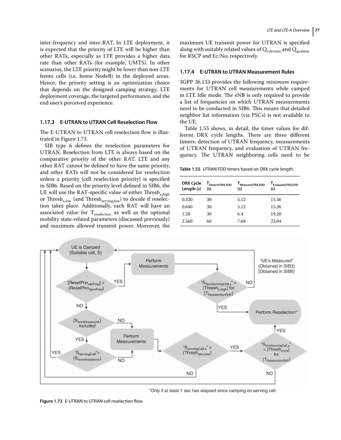
E-UTRAN to UTRAN Cell Reselection Flow 77
E-UTRAN to UTRAN Measurement Rules 77
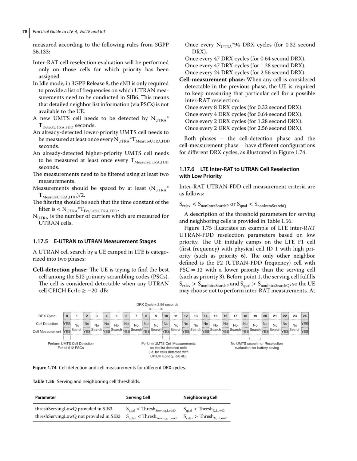
E-UTRAN to UTRAN Measurement Stages 78
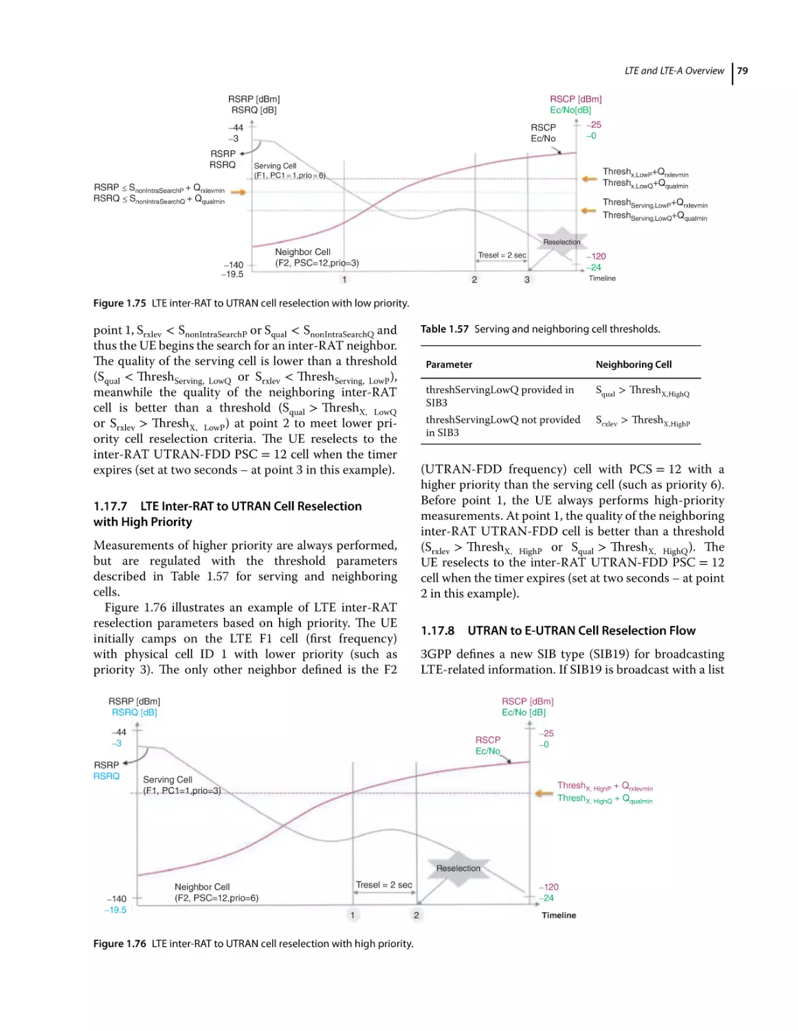
LTE Inter-RAT to UTRAN Cell Reselection with Low Priority
LTE Inter-RAT to UTRAN Cell Reselection with High Priority
UTRAN to E-UTRAN Cell Reselection Flow 79
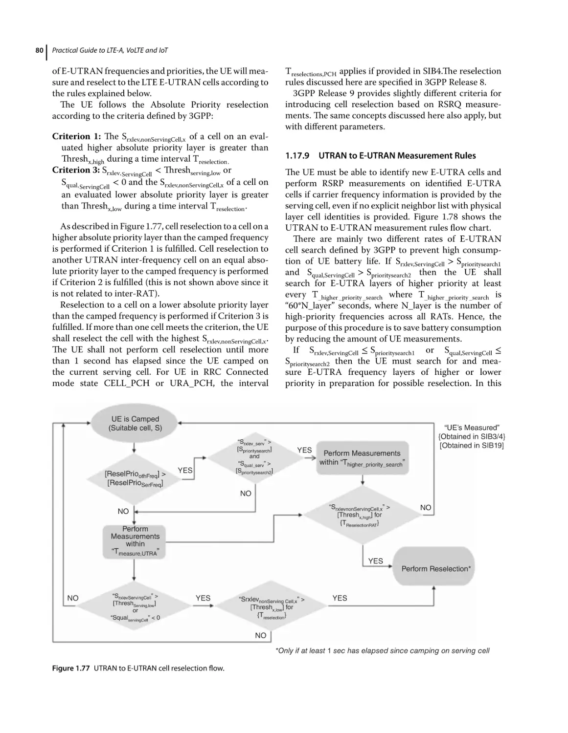
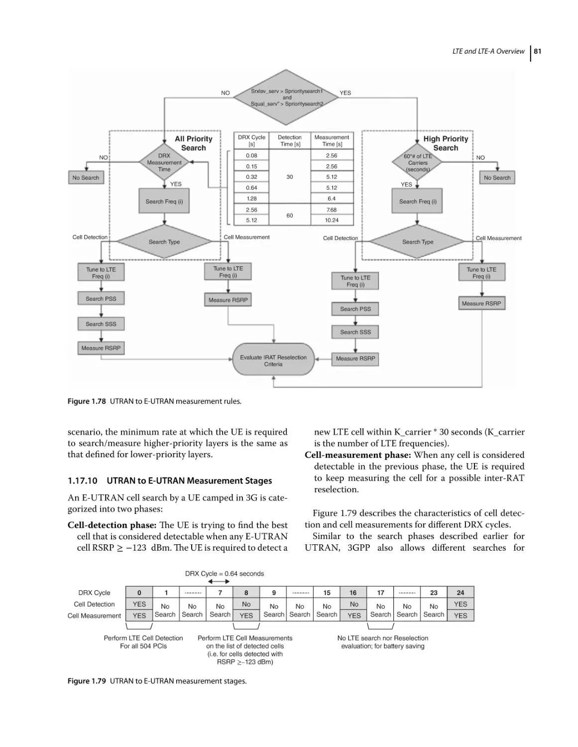
UTRAN to E-UTRAN Measurement Rules 80
UTRAN to E-UTRAN Measurement Stages 81
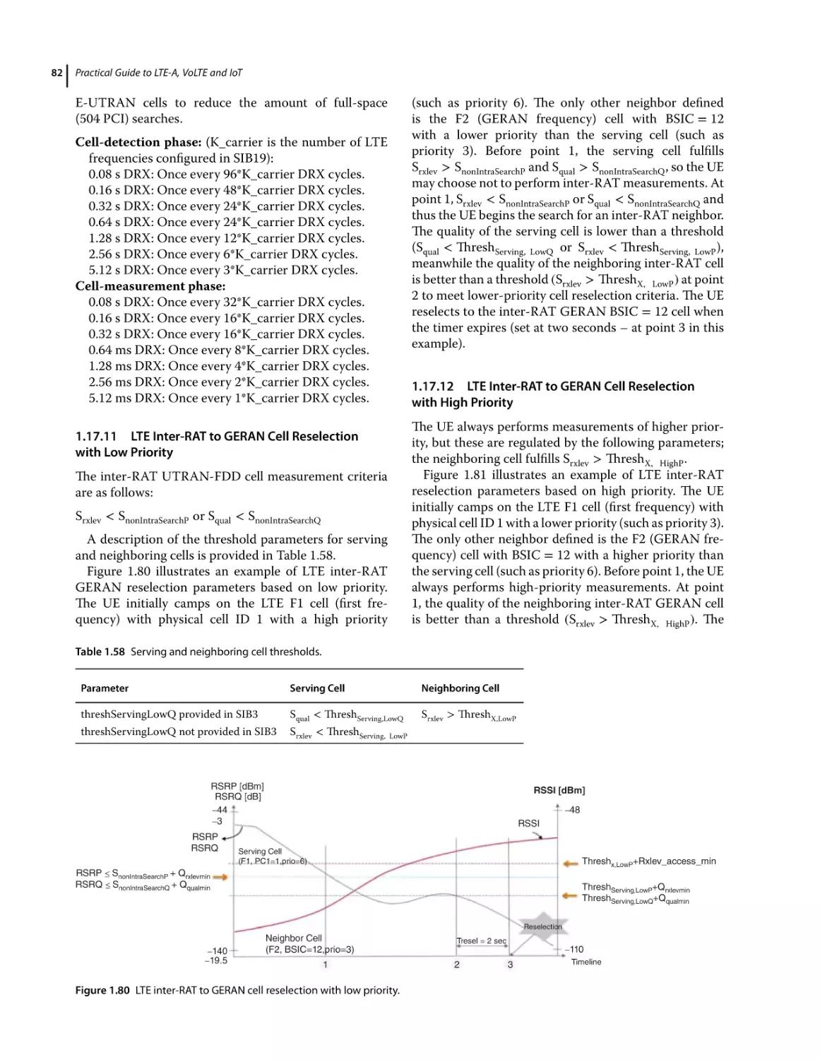
LTE Inter-RAT to GERAN Cell Reselection with Low Priority
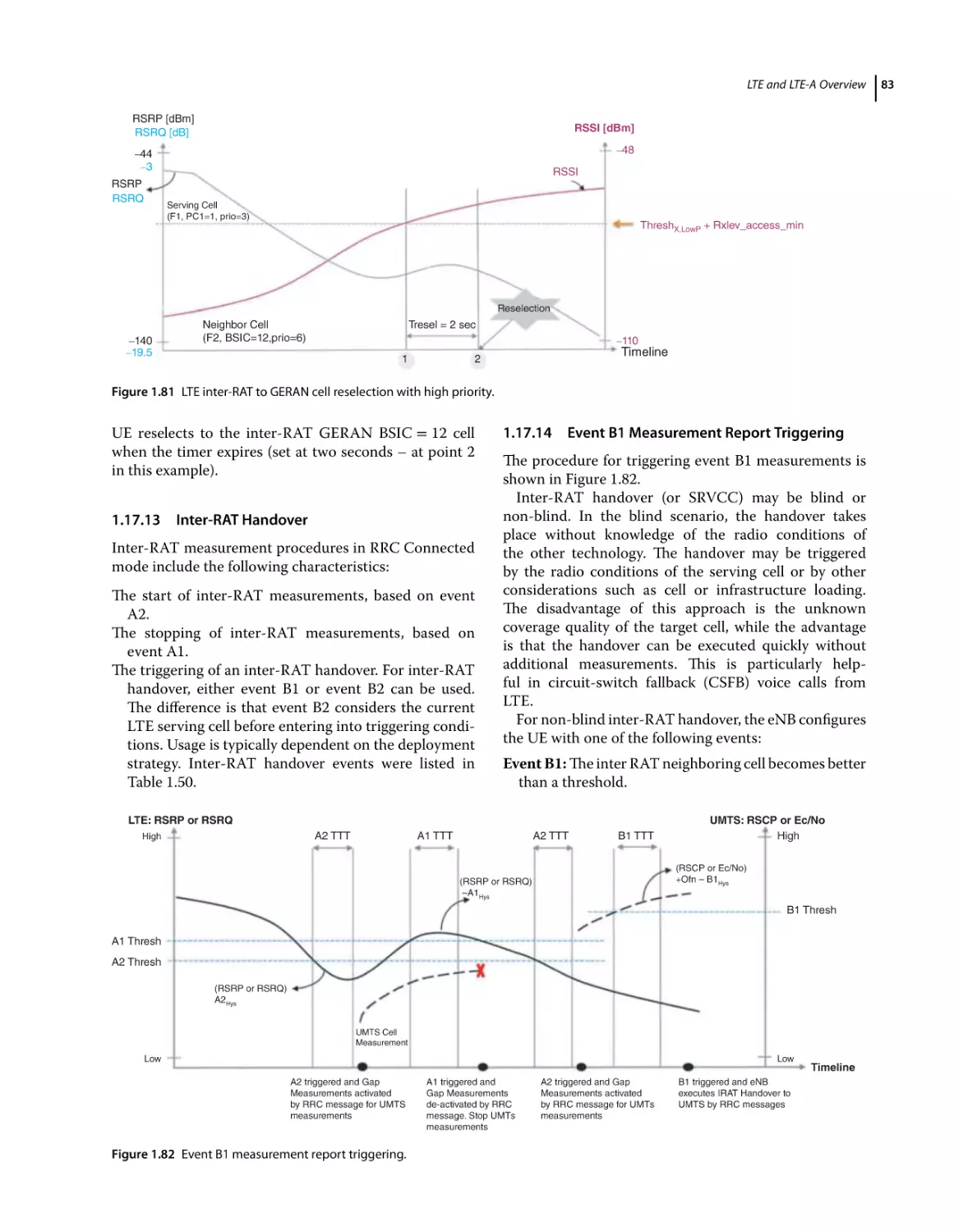
LTE Inter-RAT to GERAN Cell Reselection with High Priority
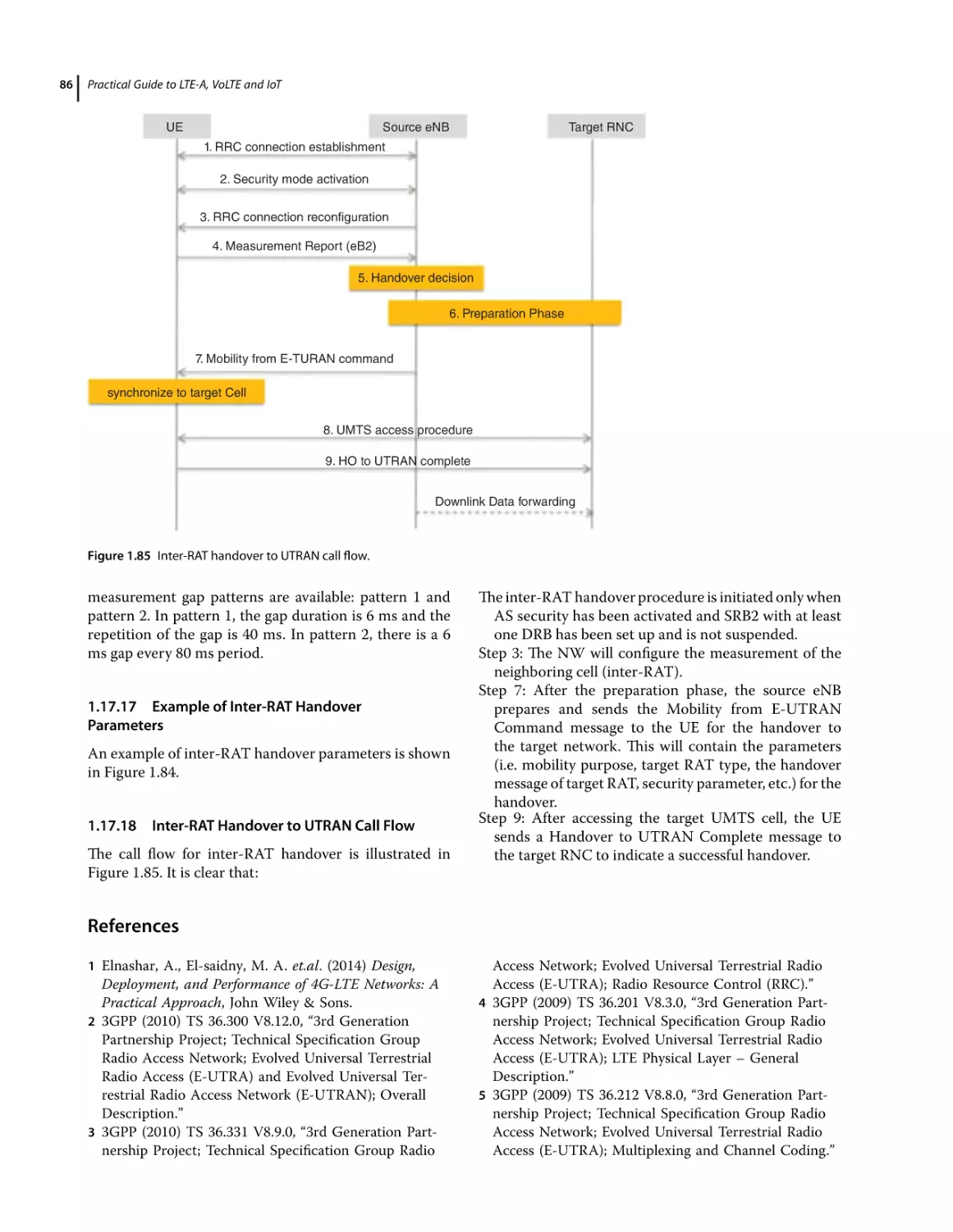
Inter-RAT Handover 83
Event B1 Measurement Report Triggering 83
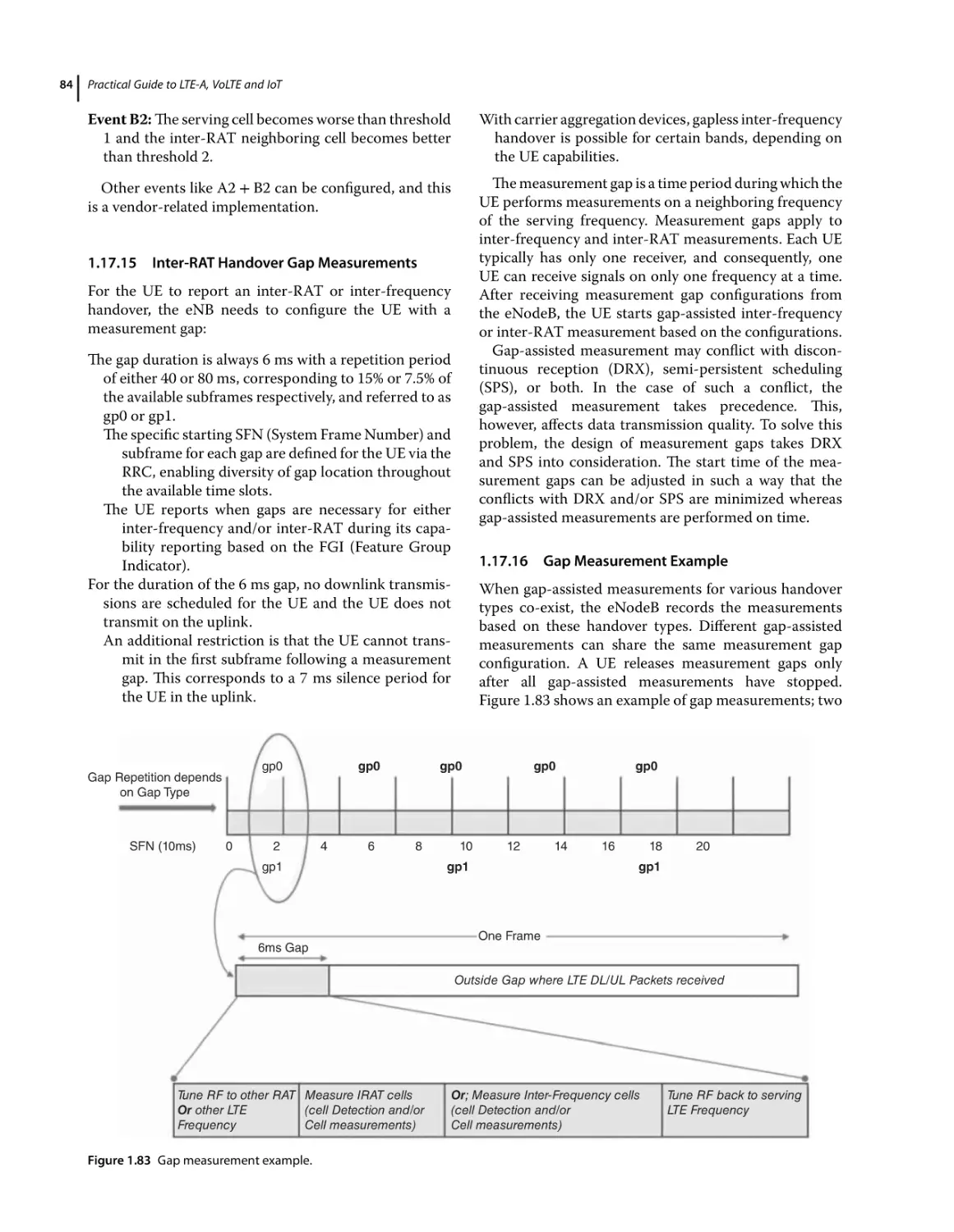
Inter-RAT Handover Gap Measurements 84
Gap Measurement Example 84
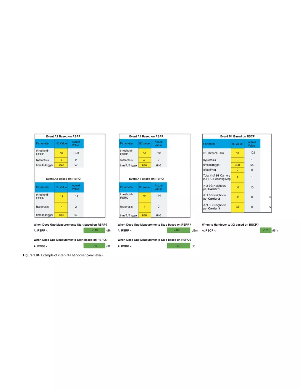
Example of Inter-RAT Handover Parameters 86
Inter-RAT Handover to UTRAN Call Flow 86
References 86
2
Introduction to the IP Multimedia Subsystem (IMS) 87
2.1
2.1.1
2.1.2
2.1.3
2.1.4
2.1.5
2.2
2.2.1
2.2.2
2.2.3
2.2.4
2.2.5
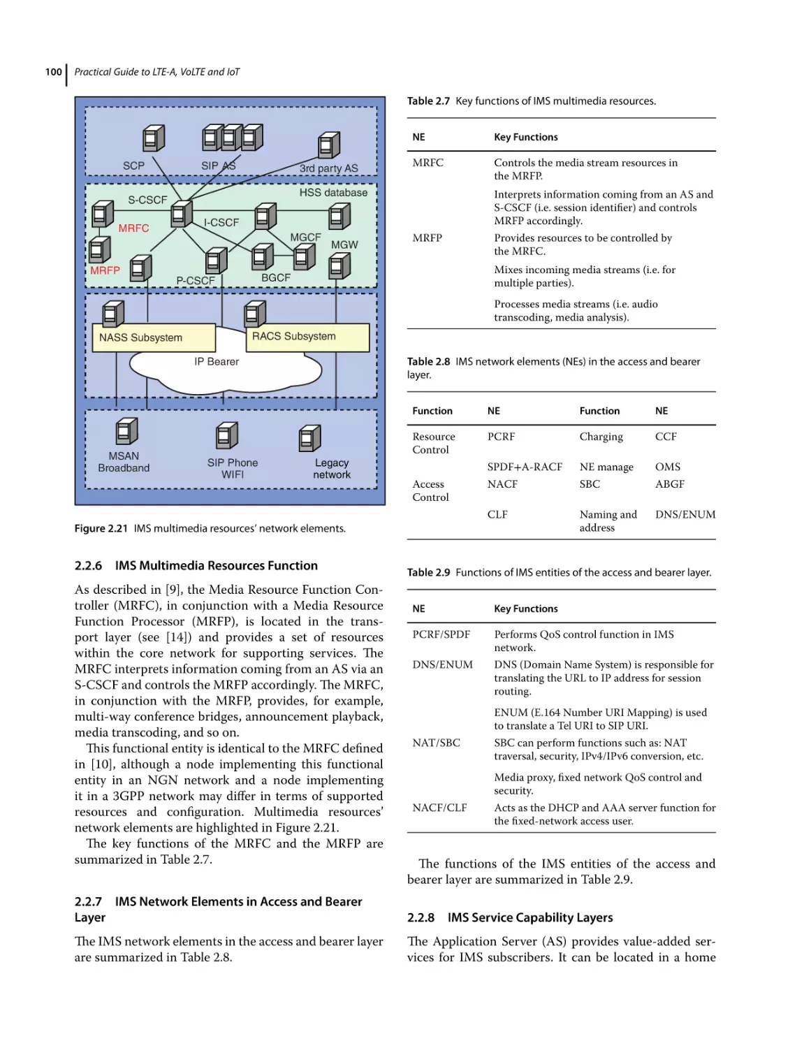
2.2.6
2.2.7
2.2.8
2.2.9
2.2.10
2.2.10.1
2.2.10.2
2.2.10.3
2.2.10.4
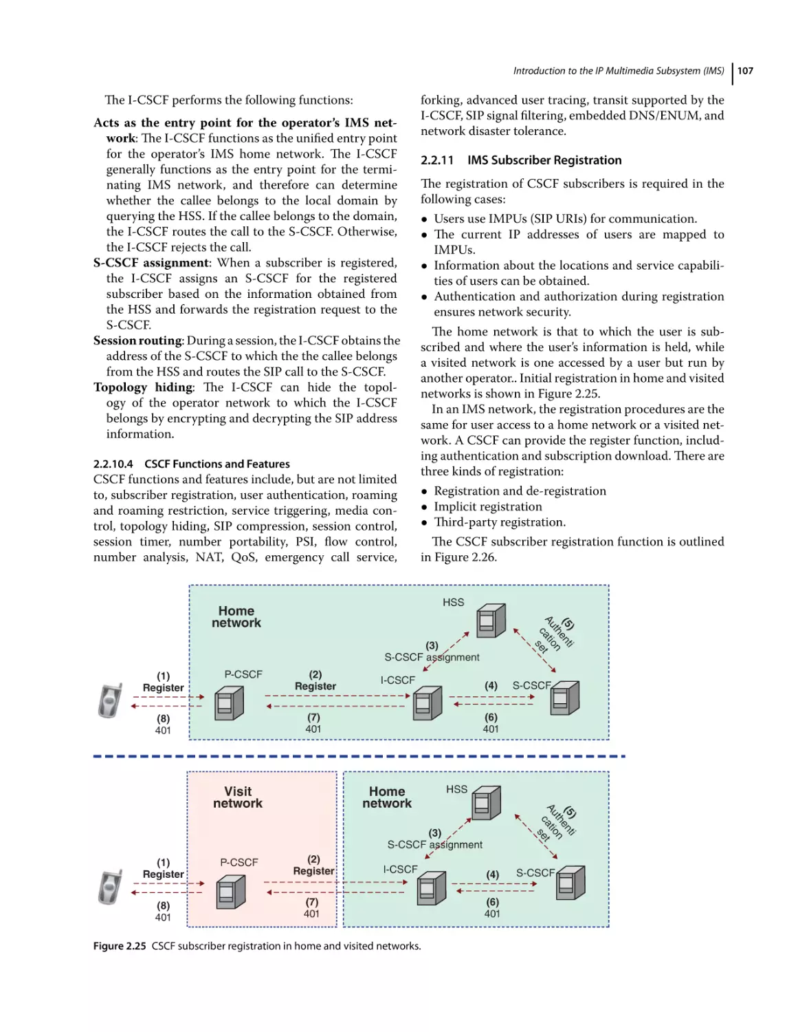
2.2.11
2.2.12
2.2.13
2.2.14
2.2.14.1
2.2.15
2.2.16
2.2.17
2.2.18
2.2.19
2.2.20
2.2.21
Introduction 87
Voice over LTE Overview 87
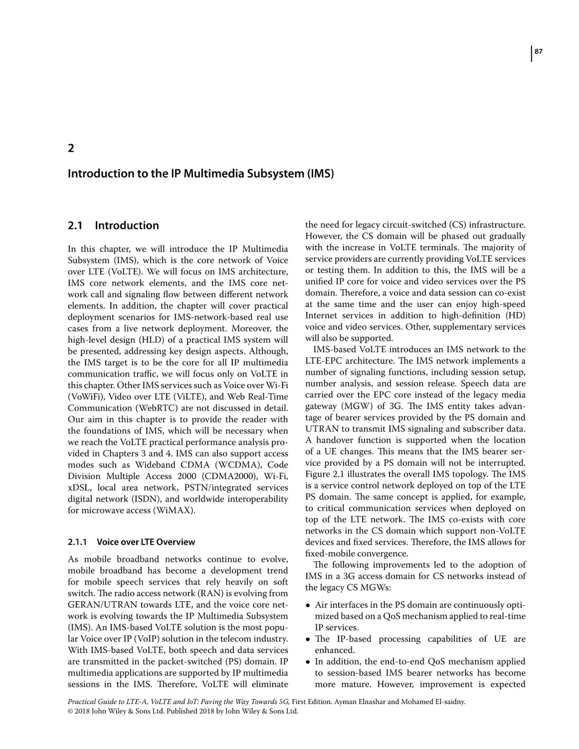
SIP Protocol 88
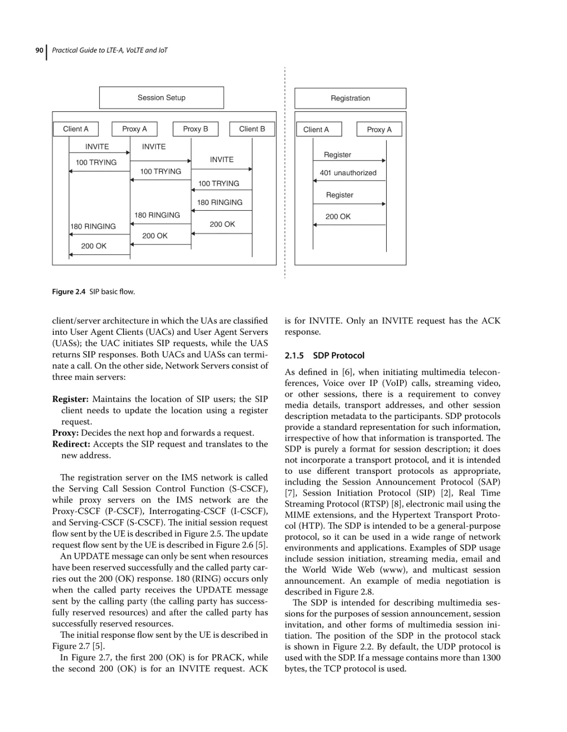
SIP Basic Flow 88
SIP Session Flow in IMS 89
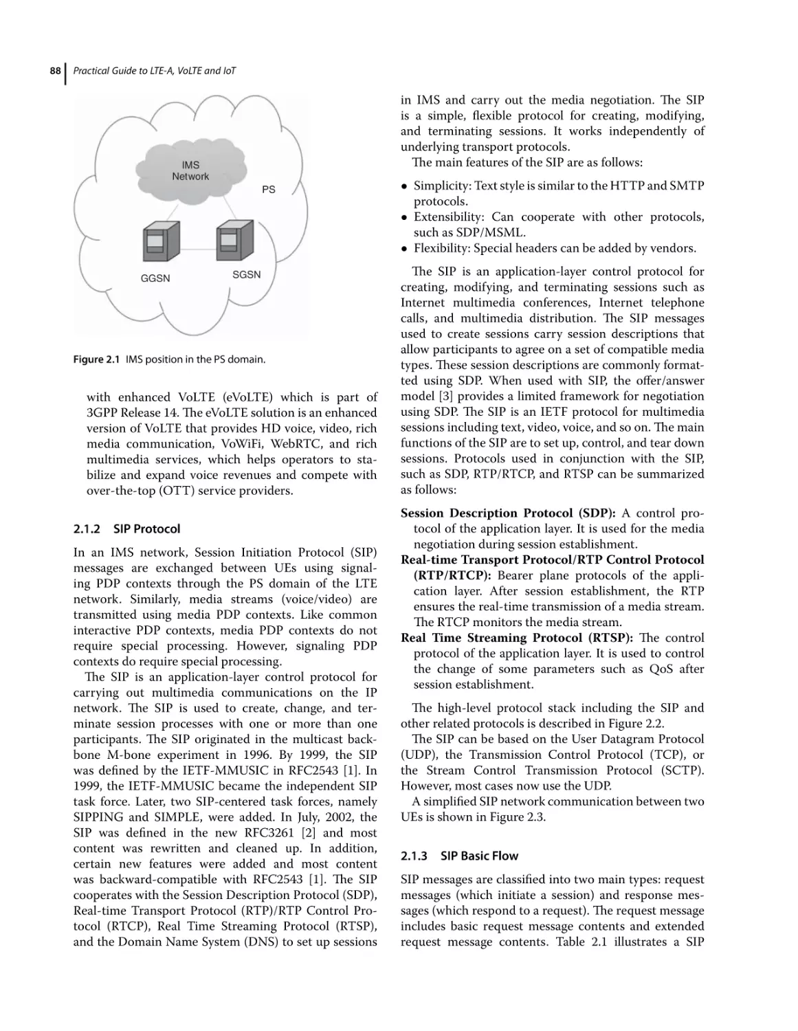
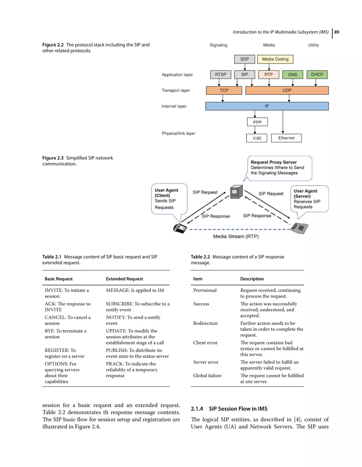
SDP Protocol 90
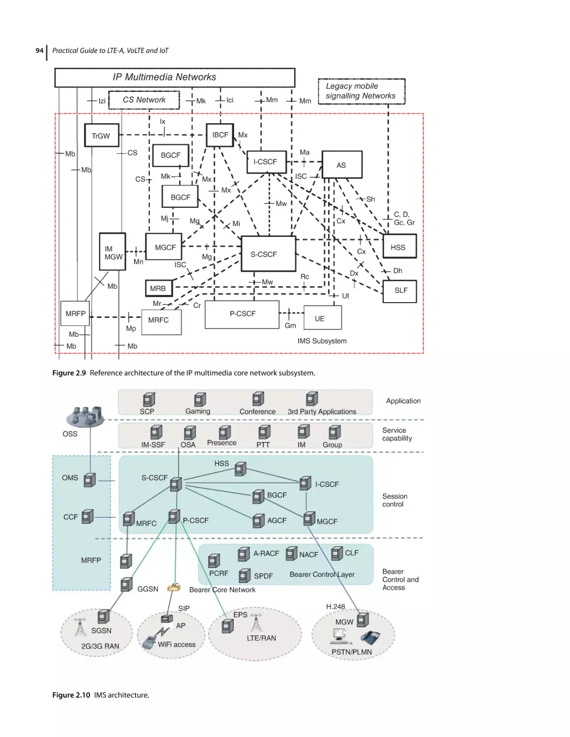
IMS Network Description 91
IMS Network Architecture 91
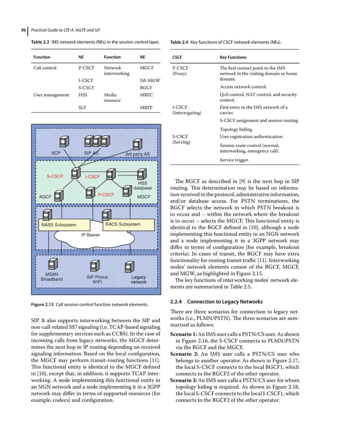
Call Session Control Function – CSCF 92
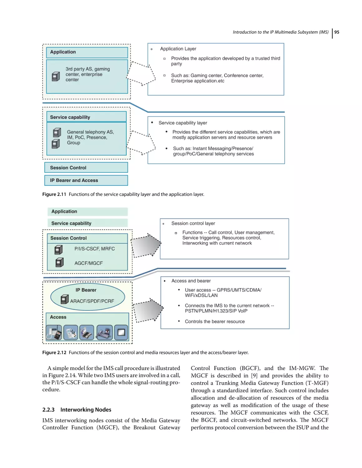
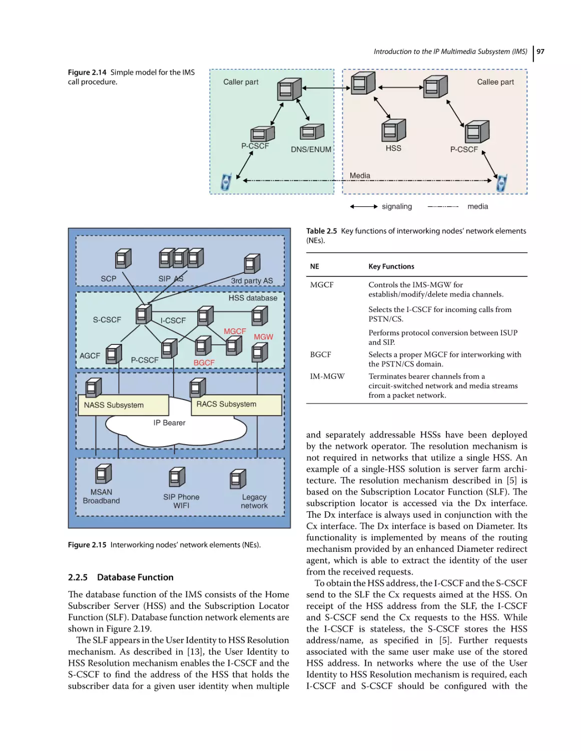
Interworking Nodes 95
Connection to Legacy Networks 96
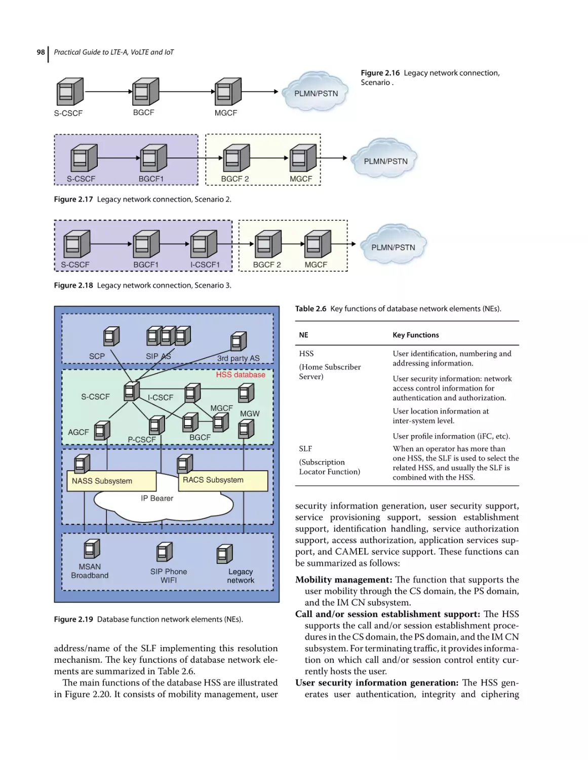
Database Function 97
IMS Multimedia Resources Function 100
IMS Network Elements in Access and Bearer Layer 100
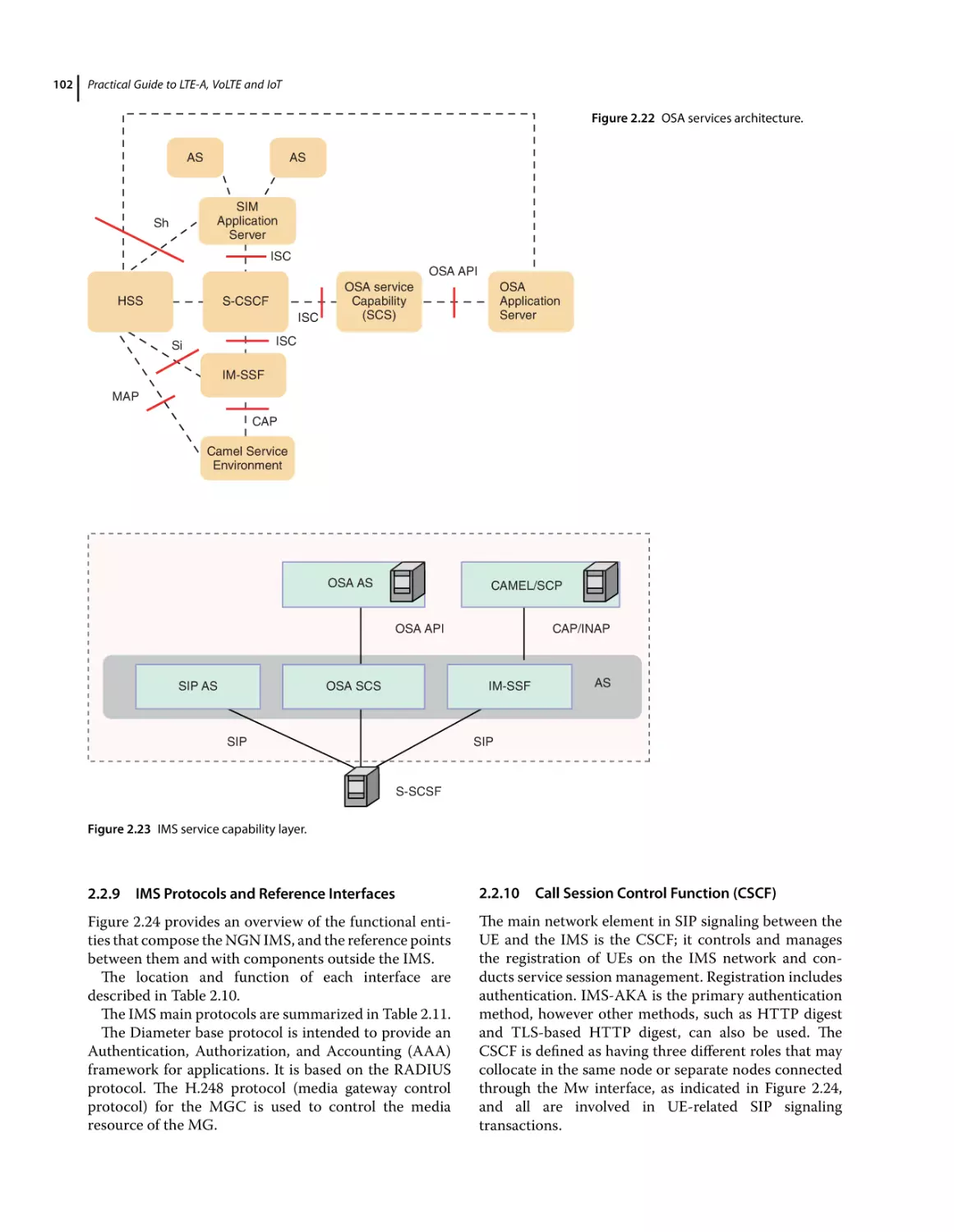
IMS Service Capability Layers 100
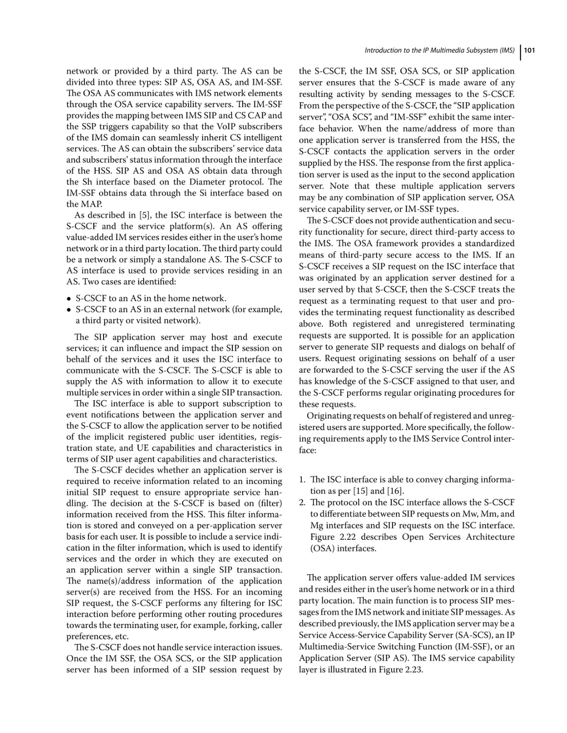
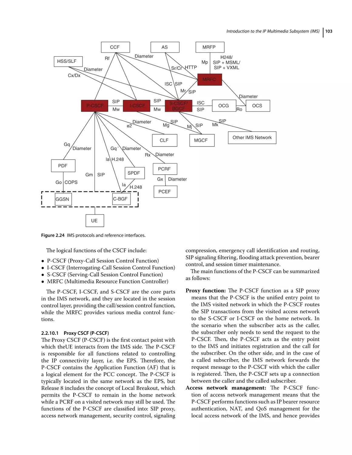
IMS Protocols and Reference Interfaces 102
Call Session Control Function (CSCF) 102
Proxy CSCF (P-CSCF) 103
Serving CSCF (S-CSCF) 106
Interrogating CSCF (I-CSCF) 106
CSCF Functions and Features 107
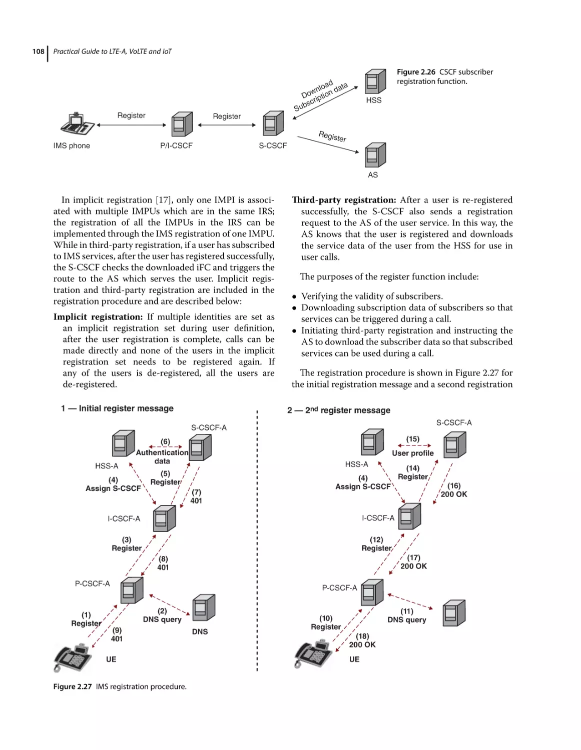
IMS Subscriber Registration 107
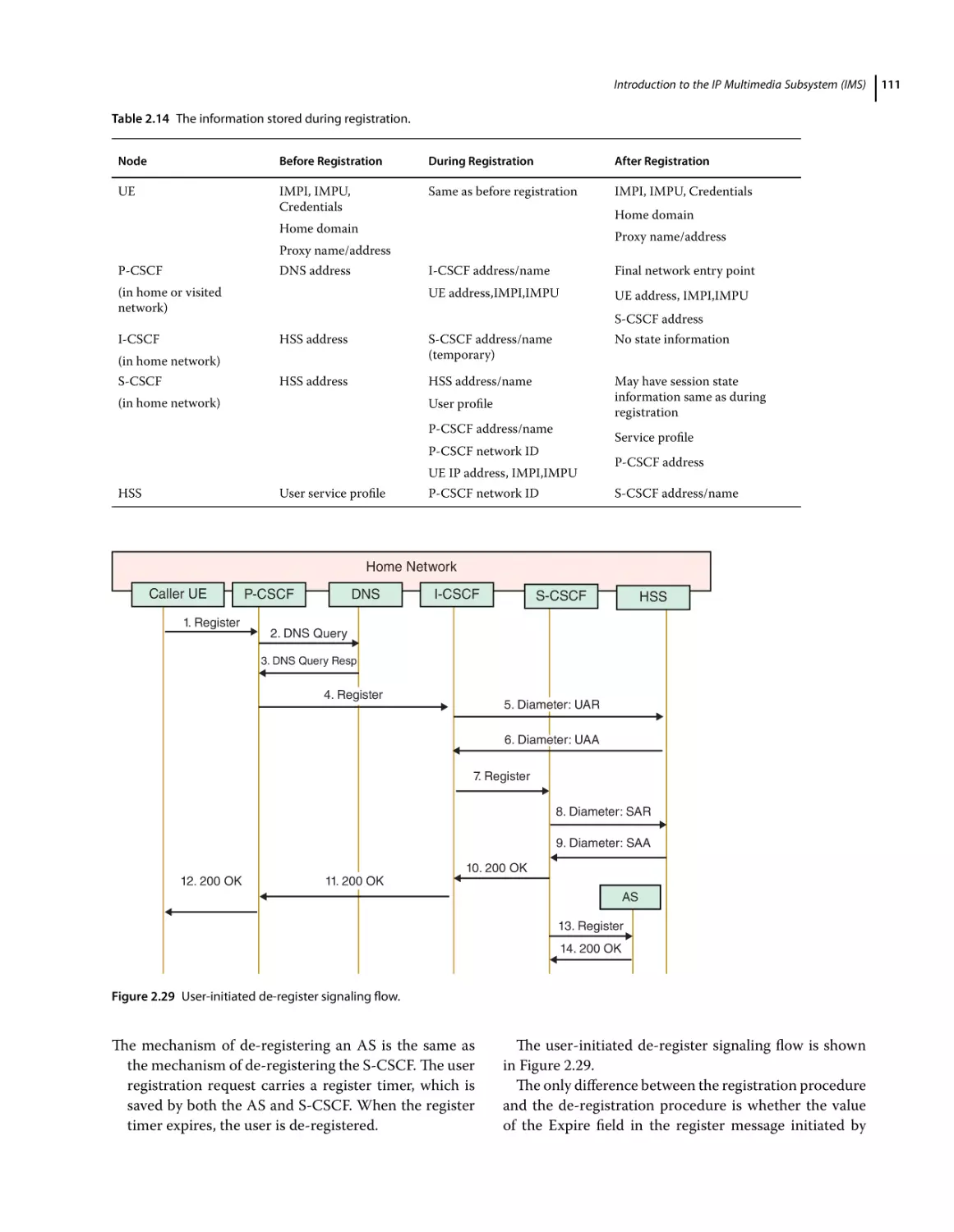
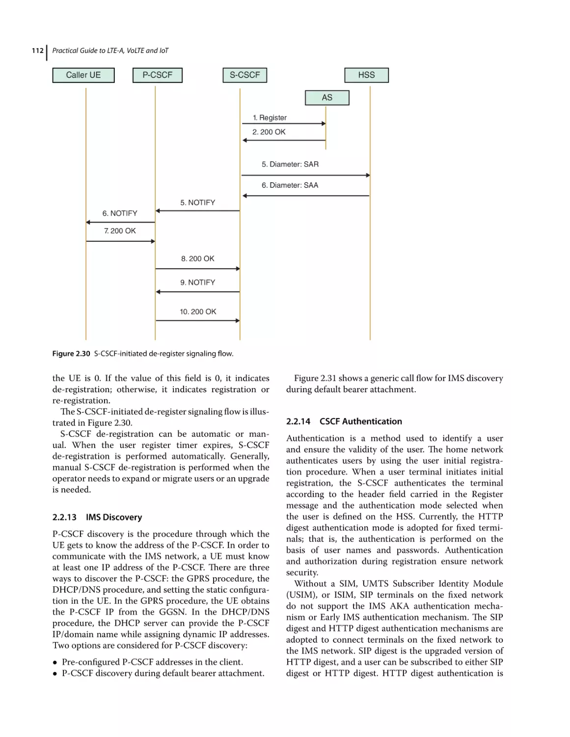
IMS Subscriber De-registration 110
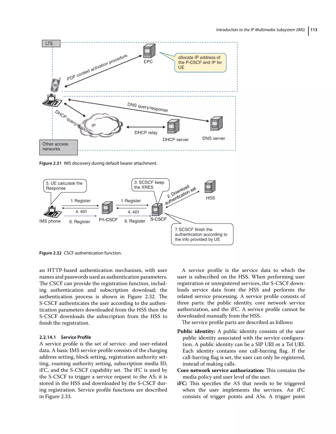
IMS Discovery 112
CSCF Authentication 112
Service Profile 113
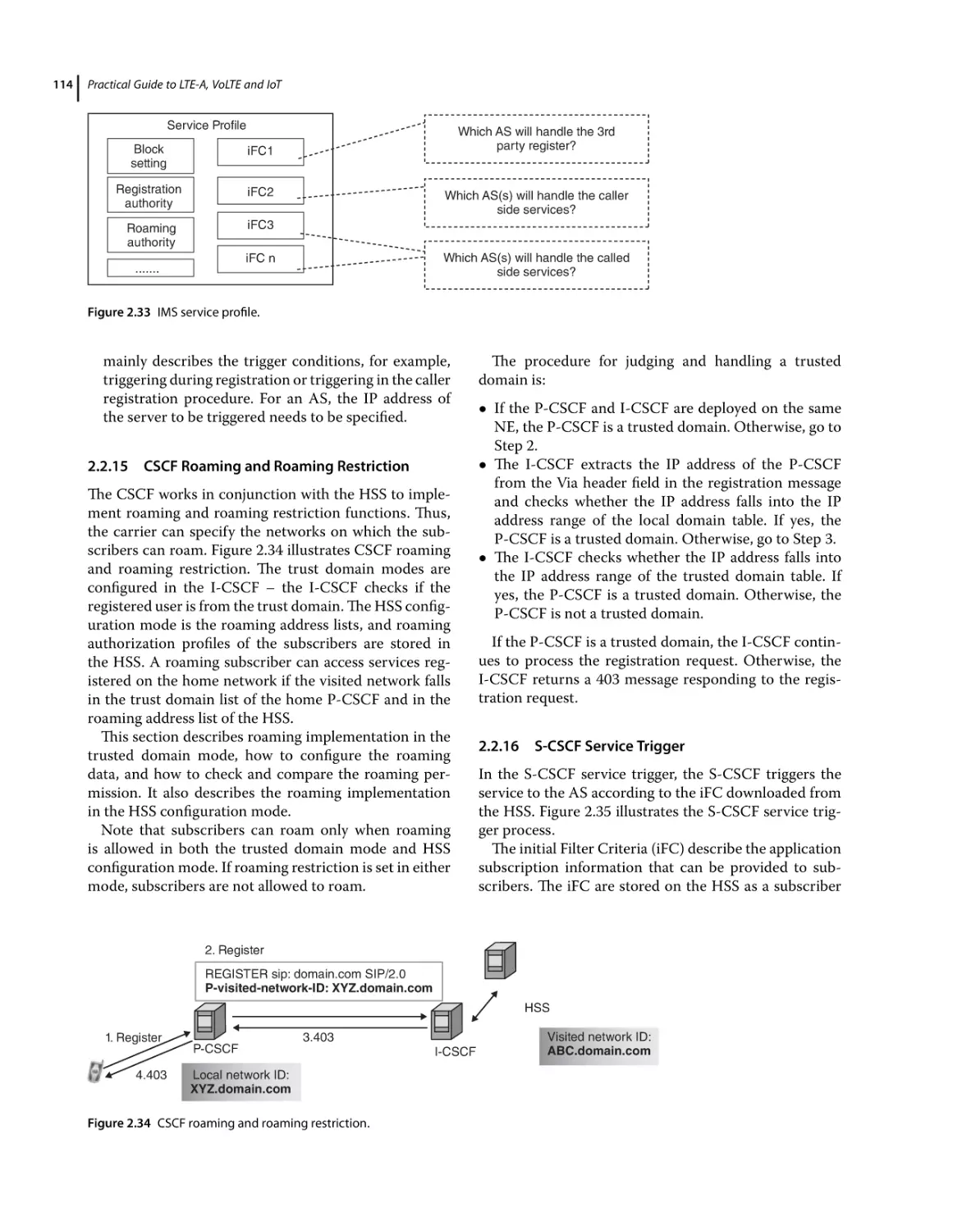
CSCF Roaming and Roaming Restriction 114
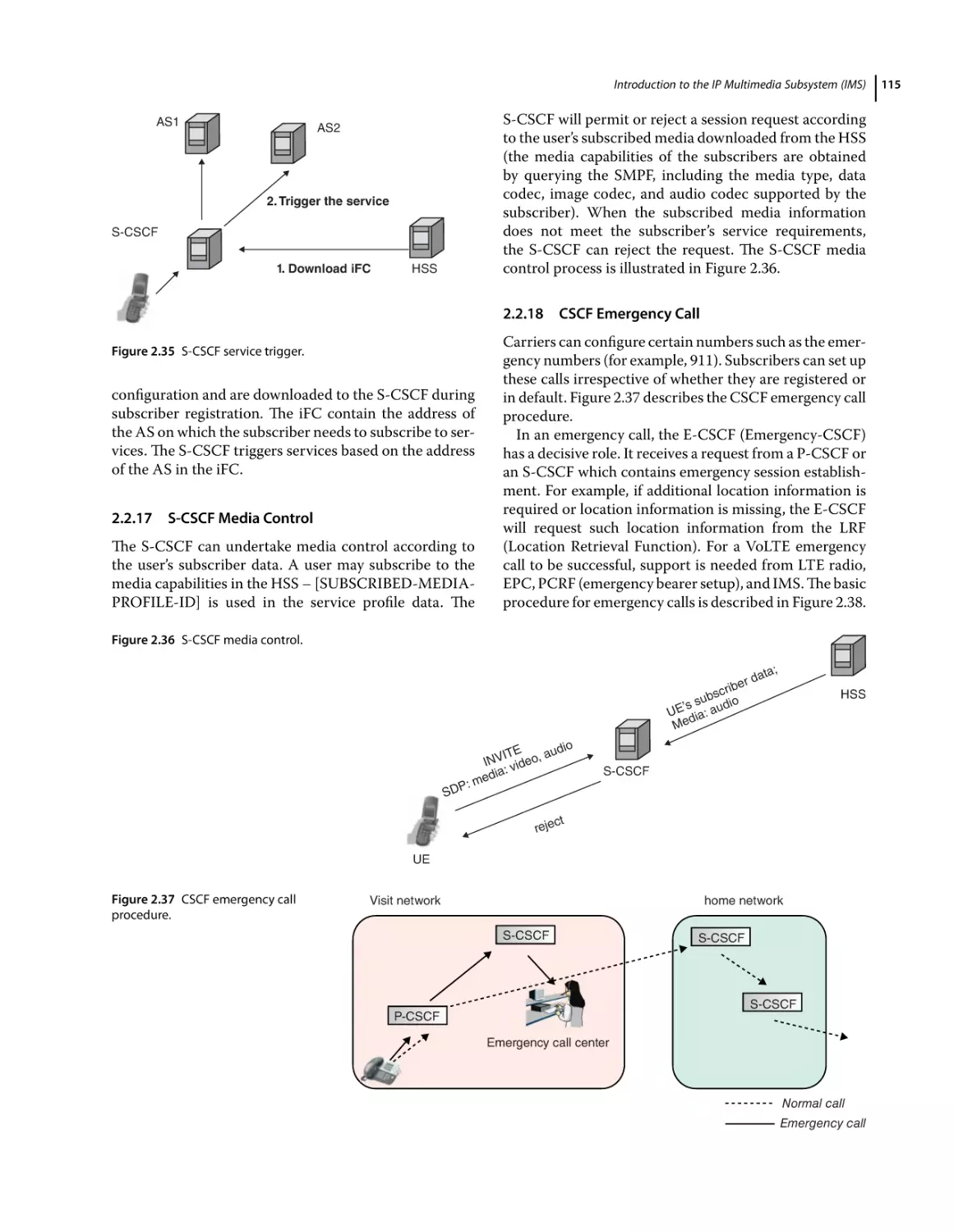
S-CSCF Service Trigger 114
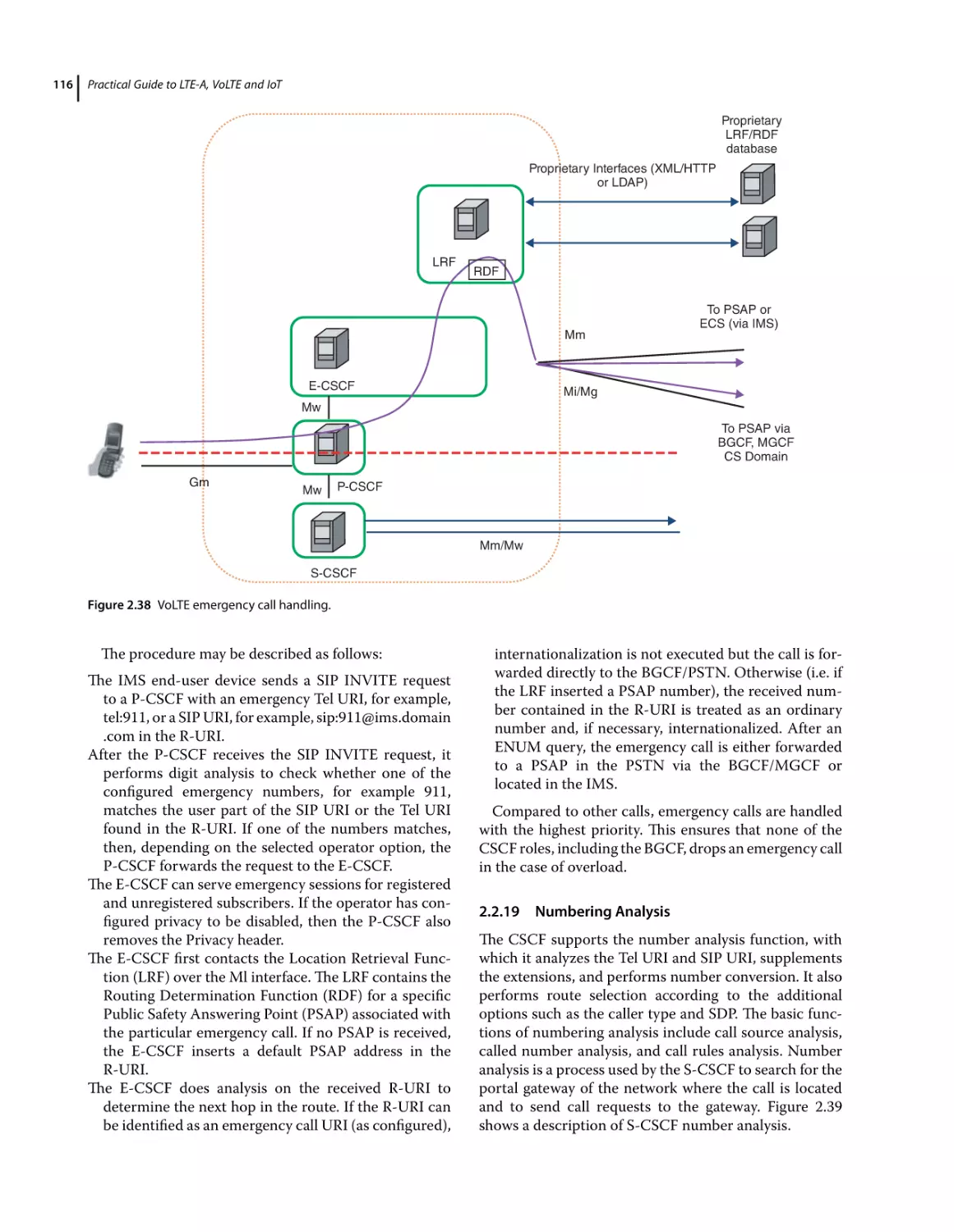
S-CSCF Media Control 115
CSCF Emergency Call 115
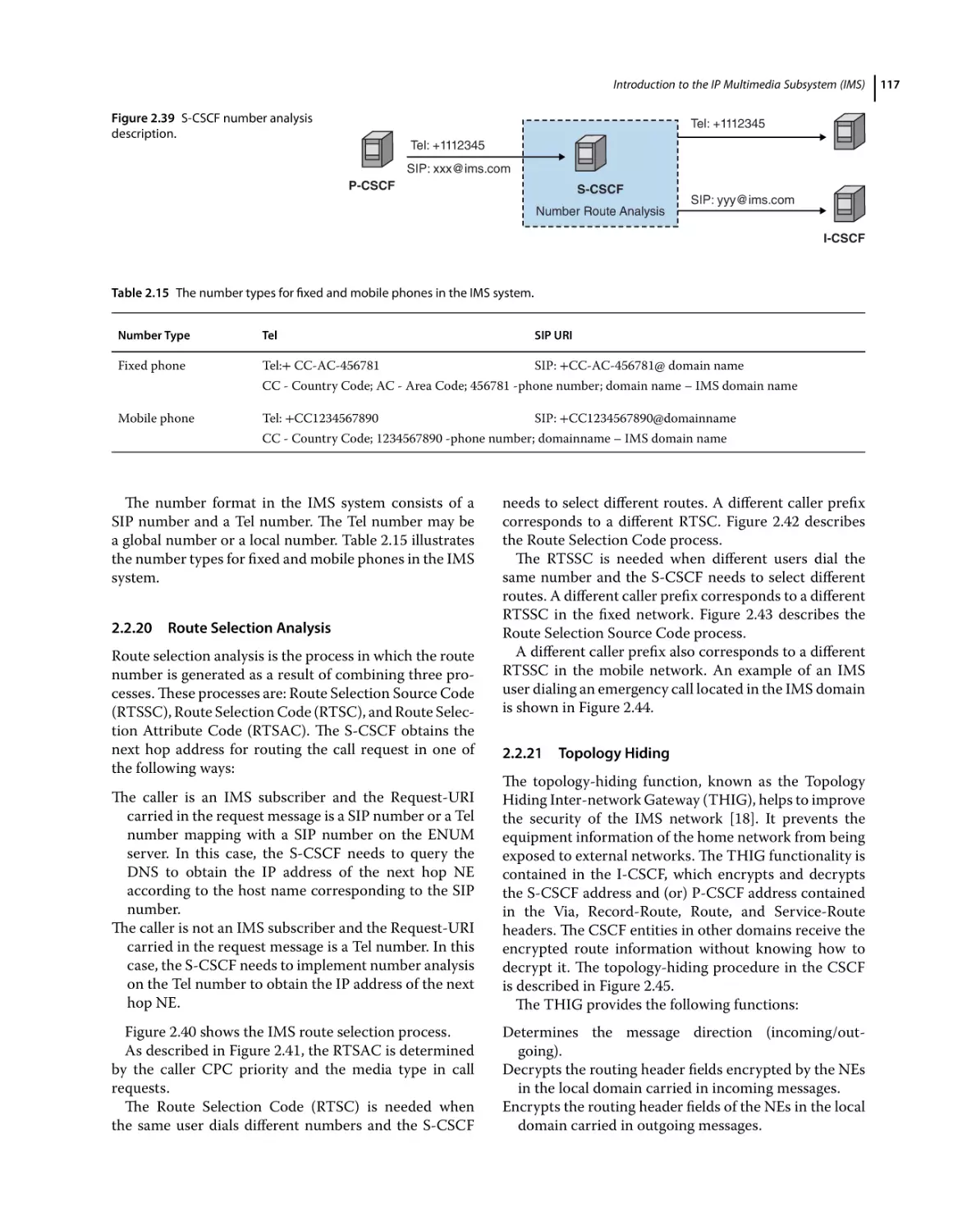
Numbering Analysis 116
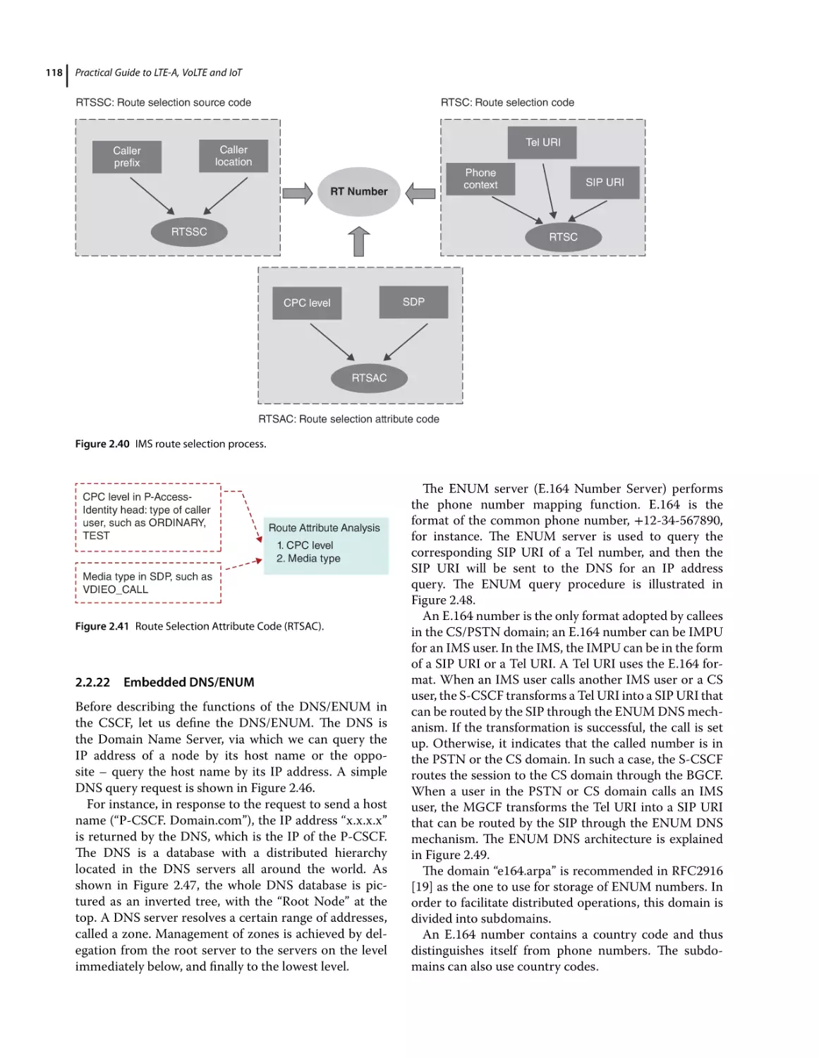
Route Selection Analysis 117
Topology Hiding 117
78
79
82
82
ix
x
Contents
2.2.22
2.2.23
2.2.24
2.2.25
2.2.26
2.2.27
2.2.27.1
2.2.27.2
2.2.28
2.2.29
2.2.30
2.2.31
2.2.32
2.2.33
2.2.34
2.2.35
2.2.36
2.2.37
2.2.38
2.3
2.3.1
2.3.2
2.4
2.4.1
2.4.2
2.4.3
2.4.4
2.4.5
2.4.6
2.4.7
2.5
2.5.1
2.5.2
2.5.3
2.5.4
2.5.5
2.5.6
2.5.6.1
2.6
2.6.1
2.6.2
2.6.3
2.6.4
2.6.4.1
2.6.4.2
2.6.4.3
2.7
2.7.1
2.7.2
2.7.3
2.7.4
2.7.5
2.7.5.1
2.7.6
2.7.7
Embedded DNS/ENUM 118
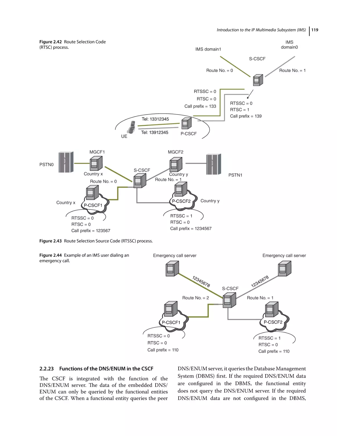
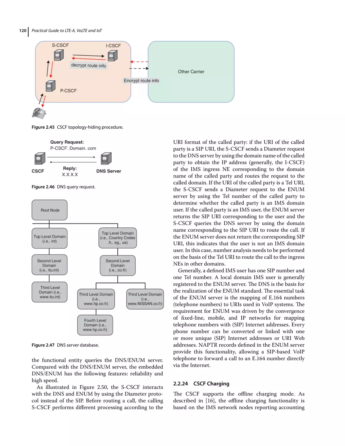
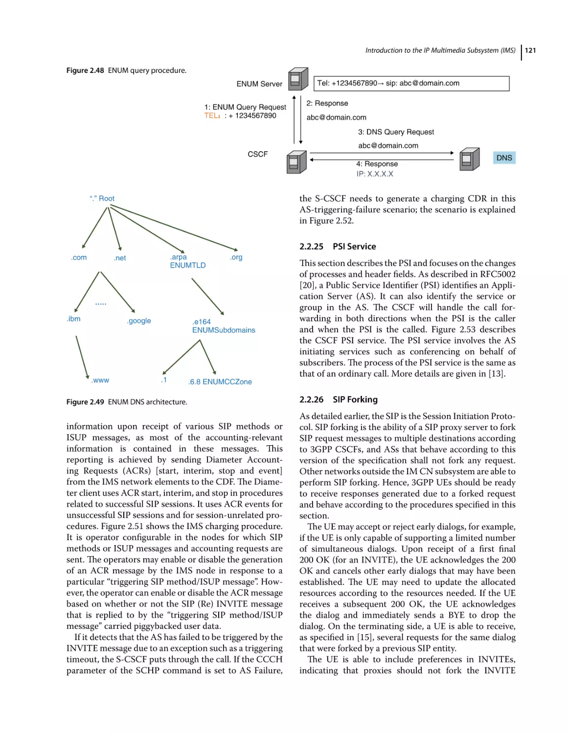
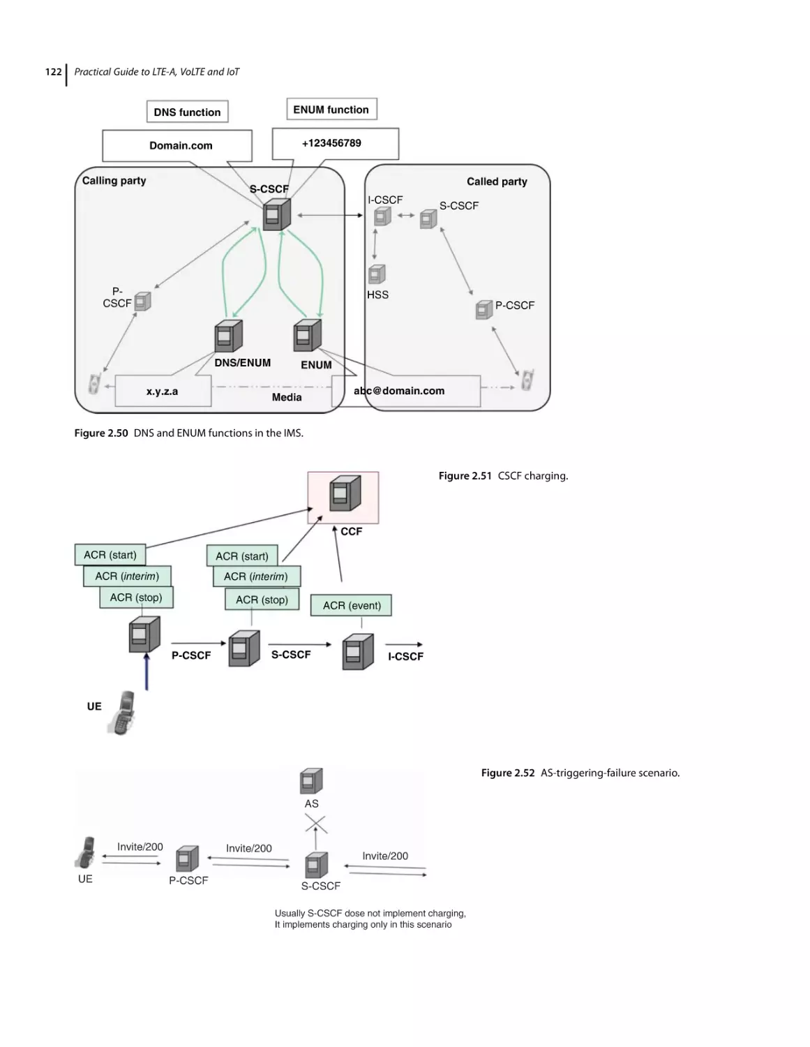
Functions of the DNS/ENUM in the CSCF 119
CSCF Charging 120
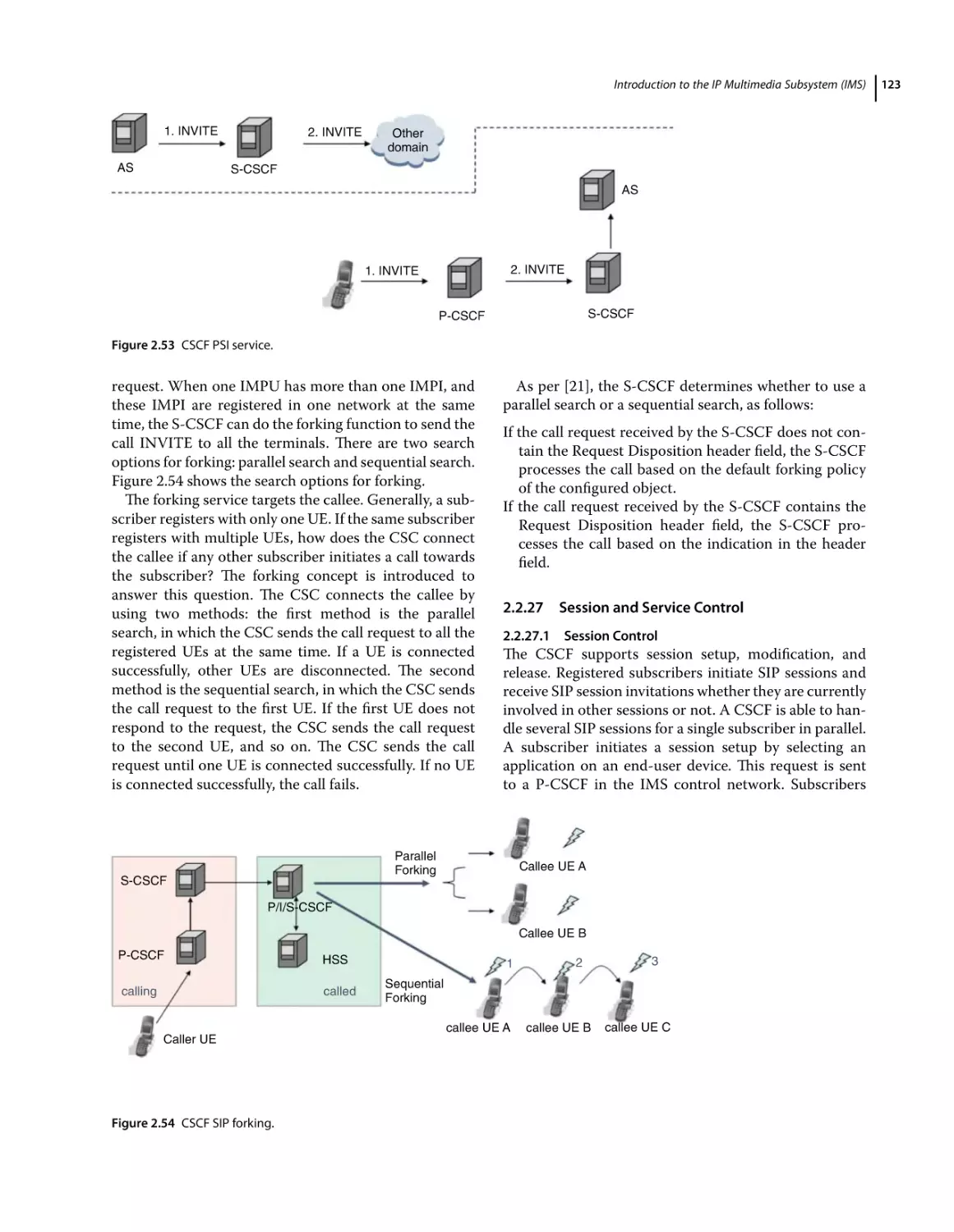
PSI Service 121
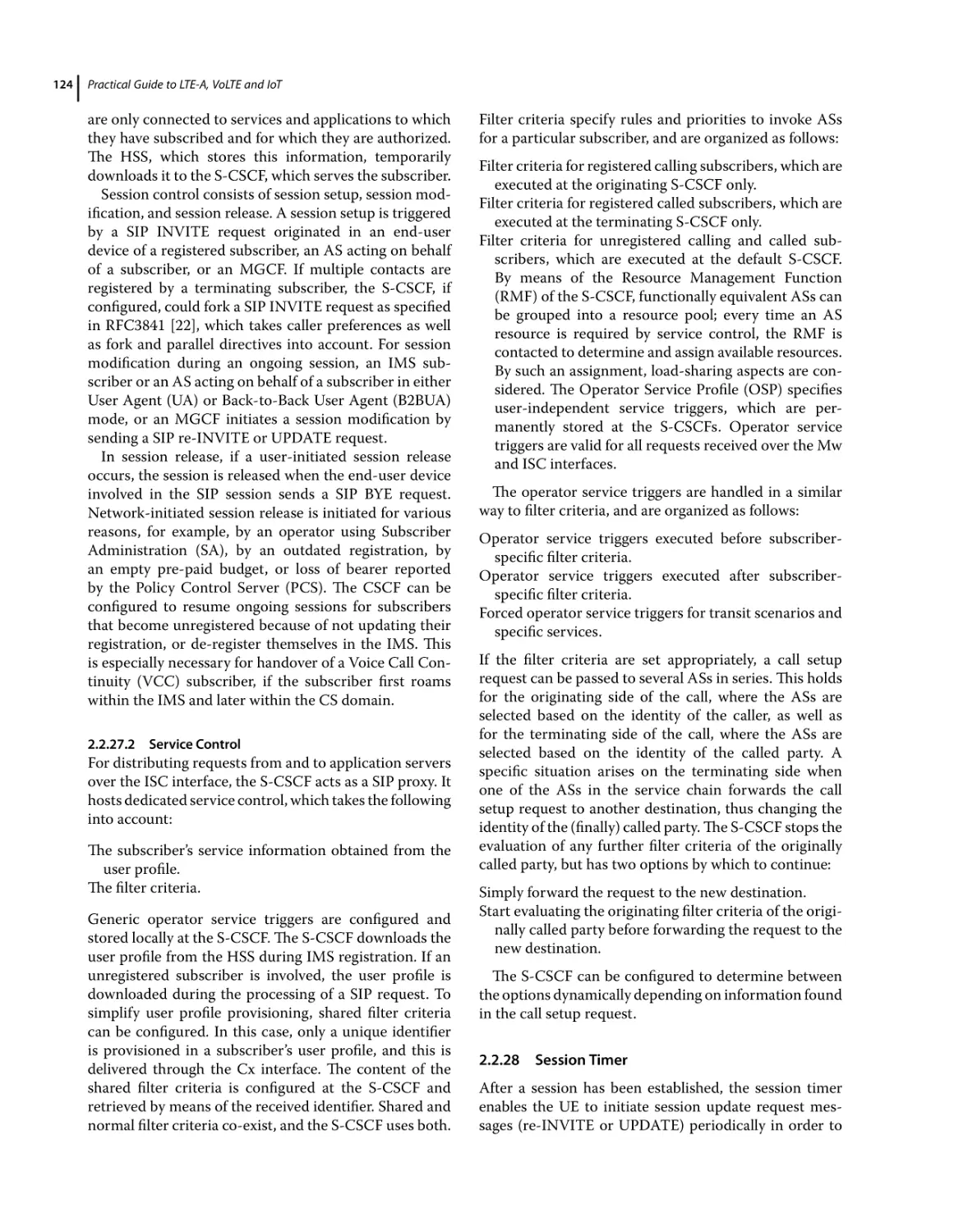
SIP Forking 121
Session and Service Control 123
Session Control 123
Service Control 124
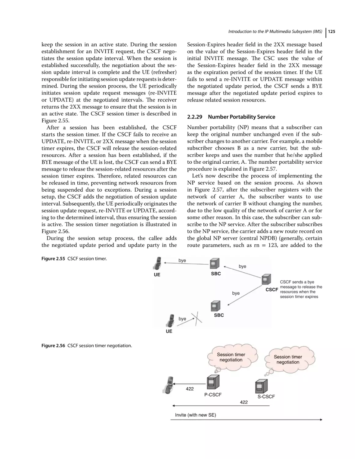
Session Timer 124
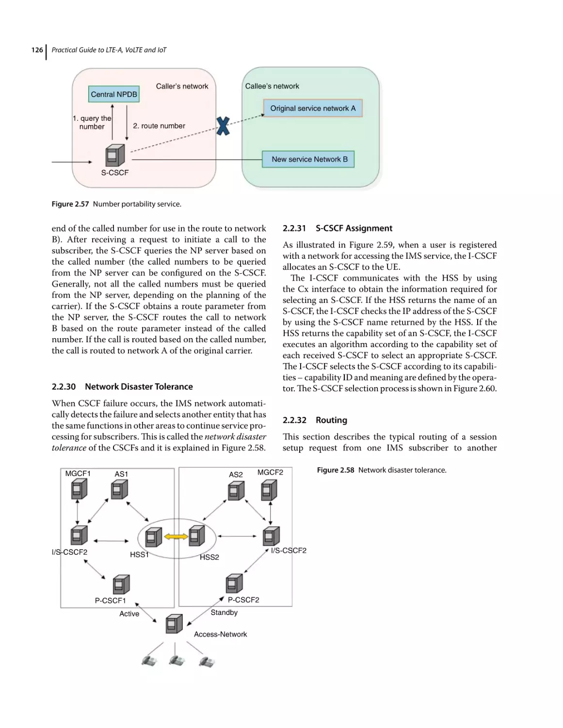
Number Portability Service 125
Network Disaster Tolerance 126
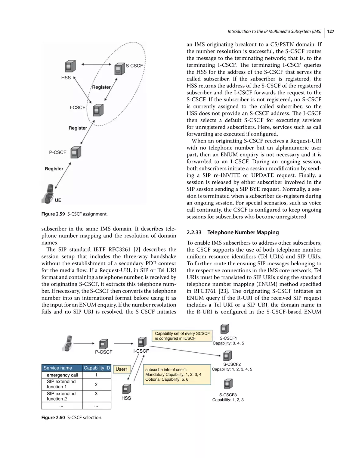
S-CSCF Assignment 126
Routing 126
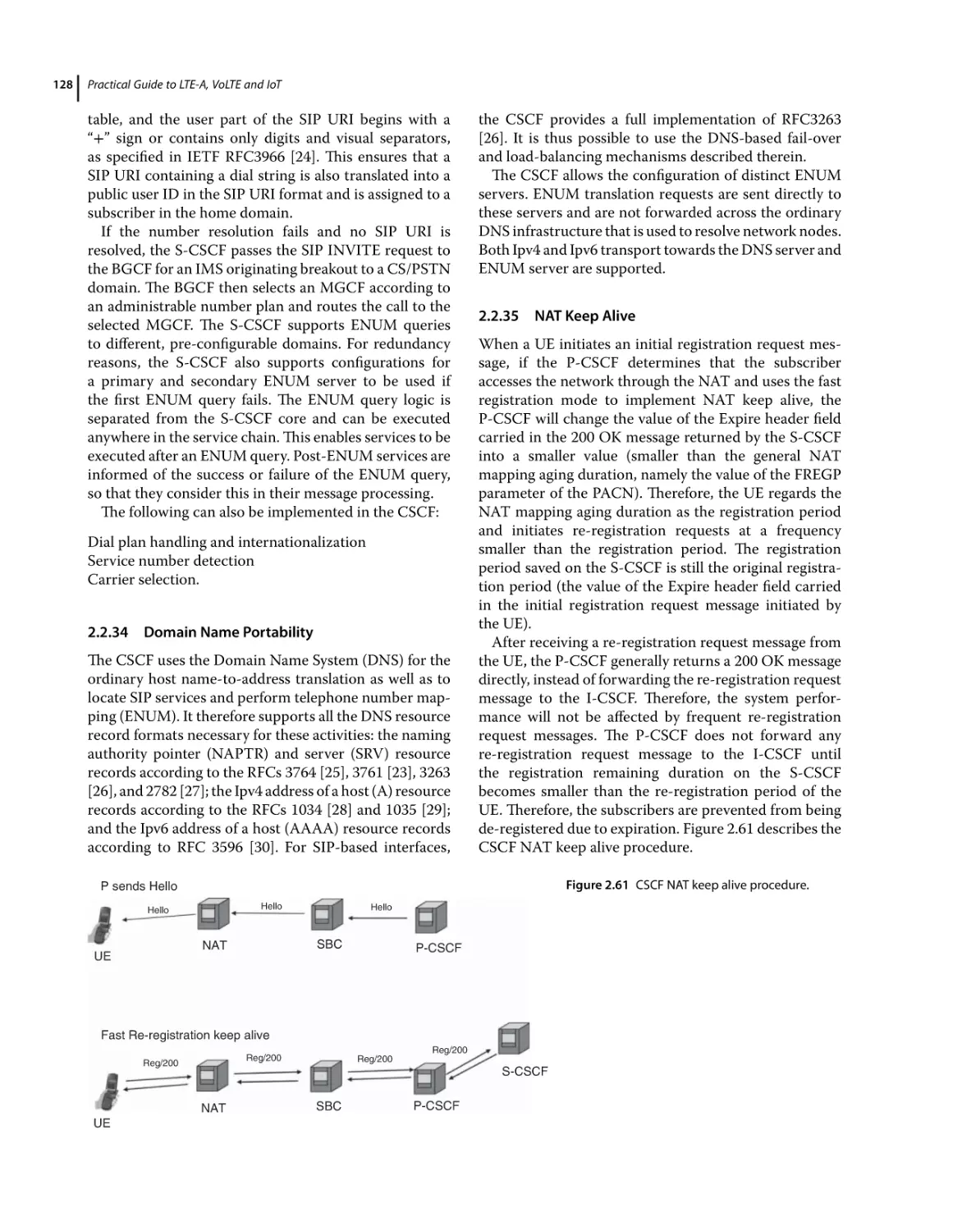
Telephone Number Mapping 127
Domain Name Portability 128
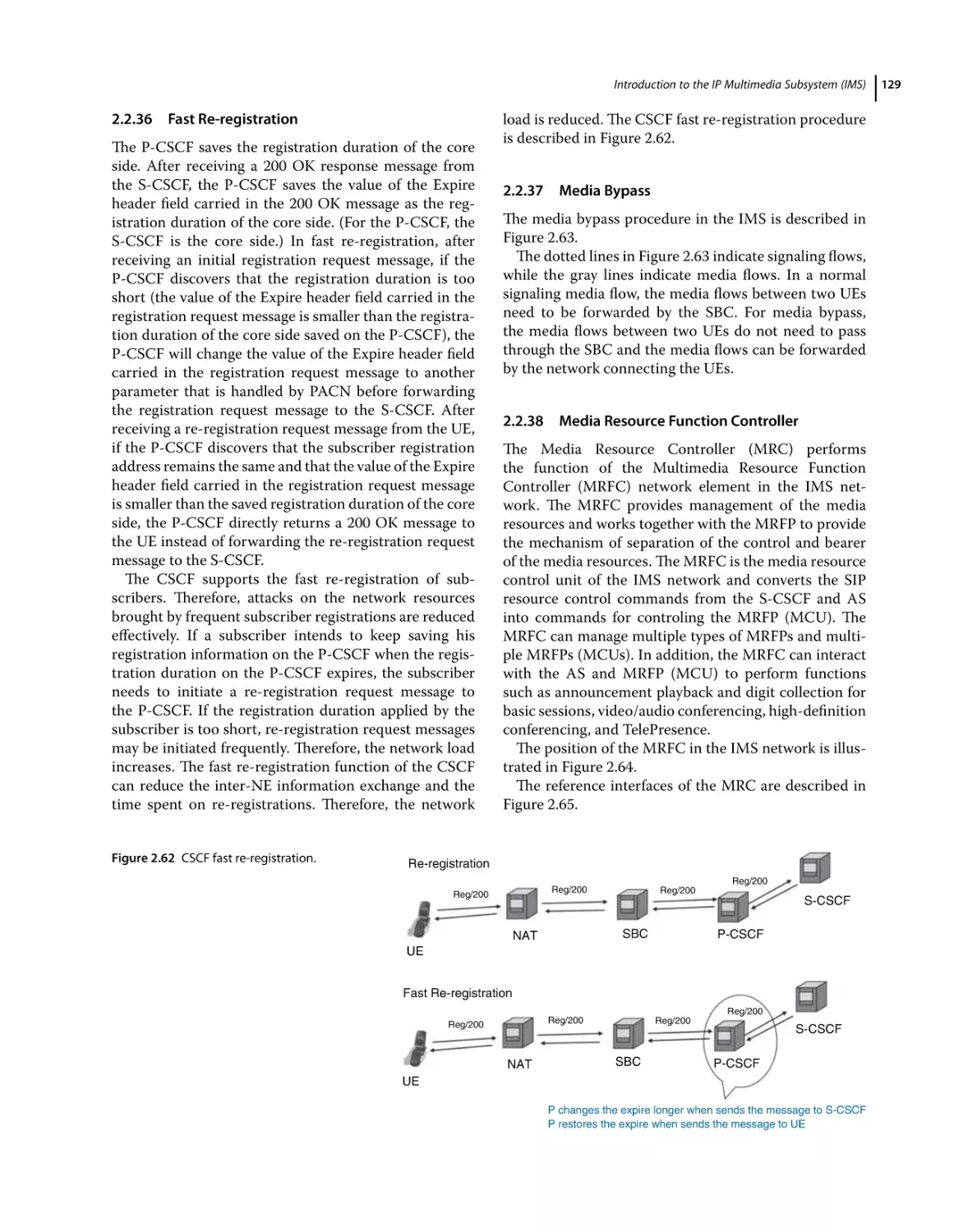
NAT Keep Alive 128
Fast Re-registration 129
Media Bypass 129
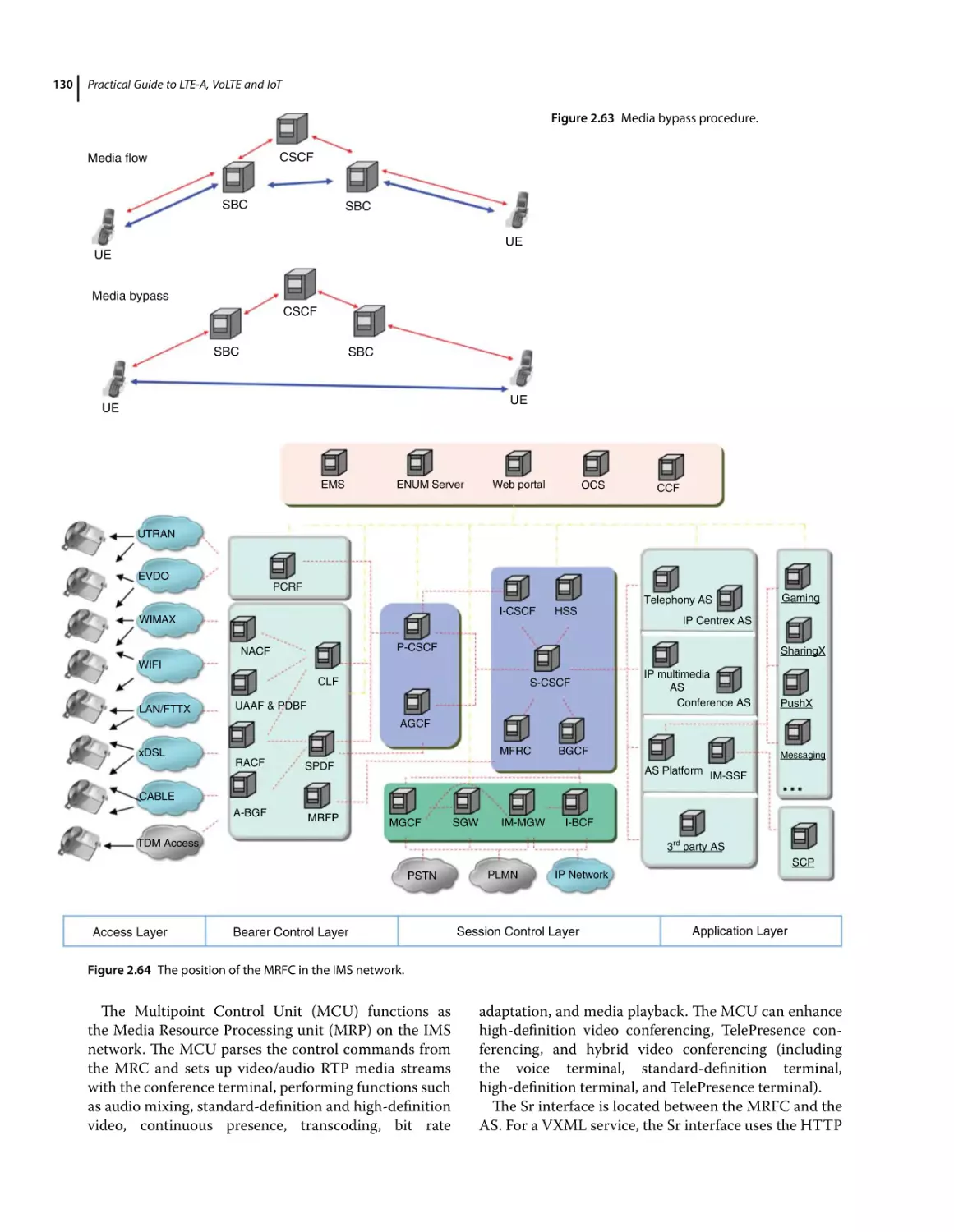
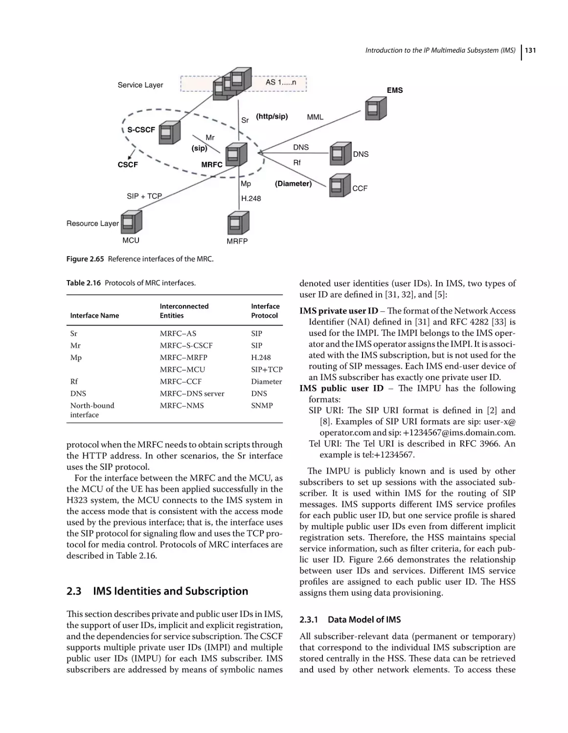
Media Resource Function Controller 129
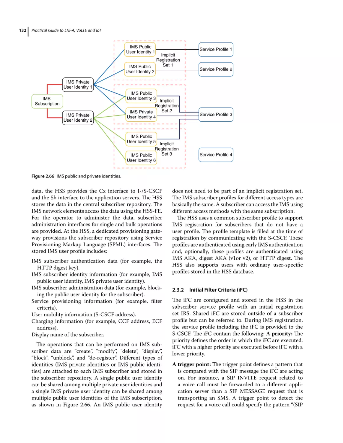
IMS Identities and Subscription 131
Data Model of IMS 131
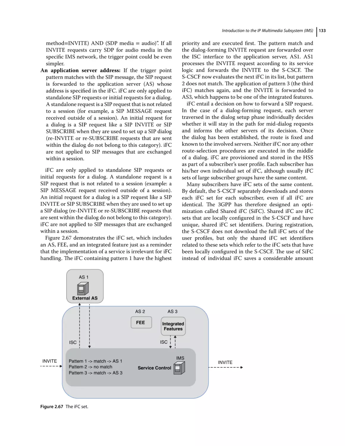
Initial Filter Criteria (iFC) 132
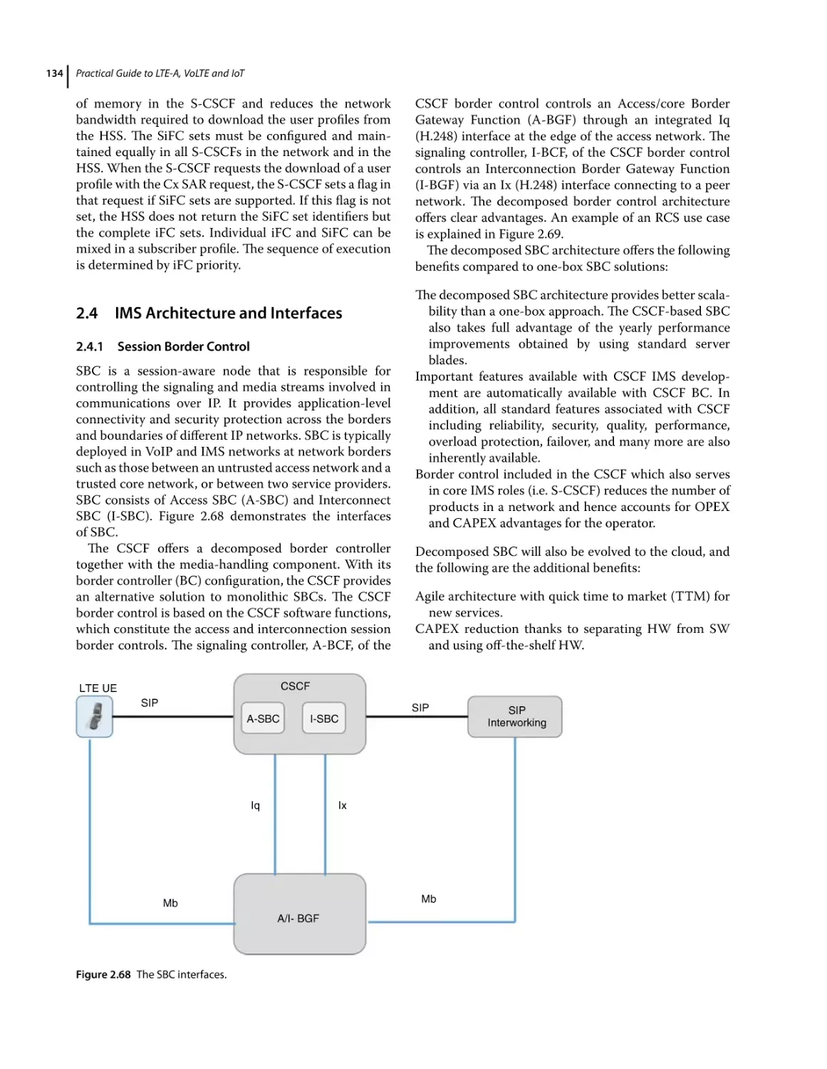
IMS Architecture and Interfaces 134
Session Border Control 134
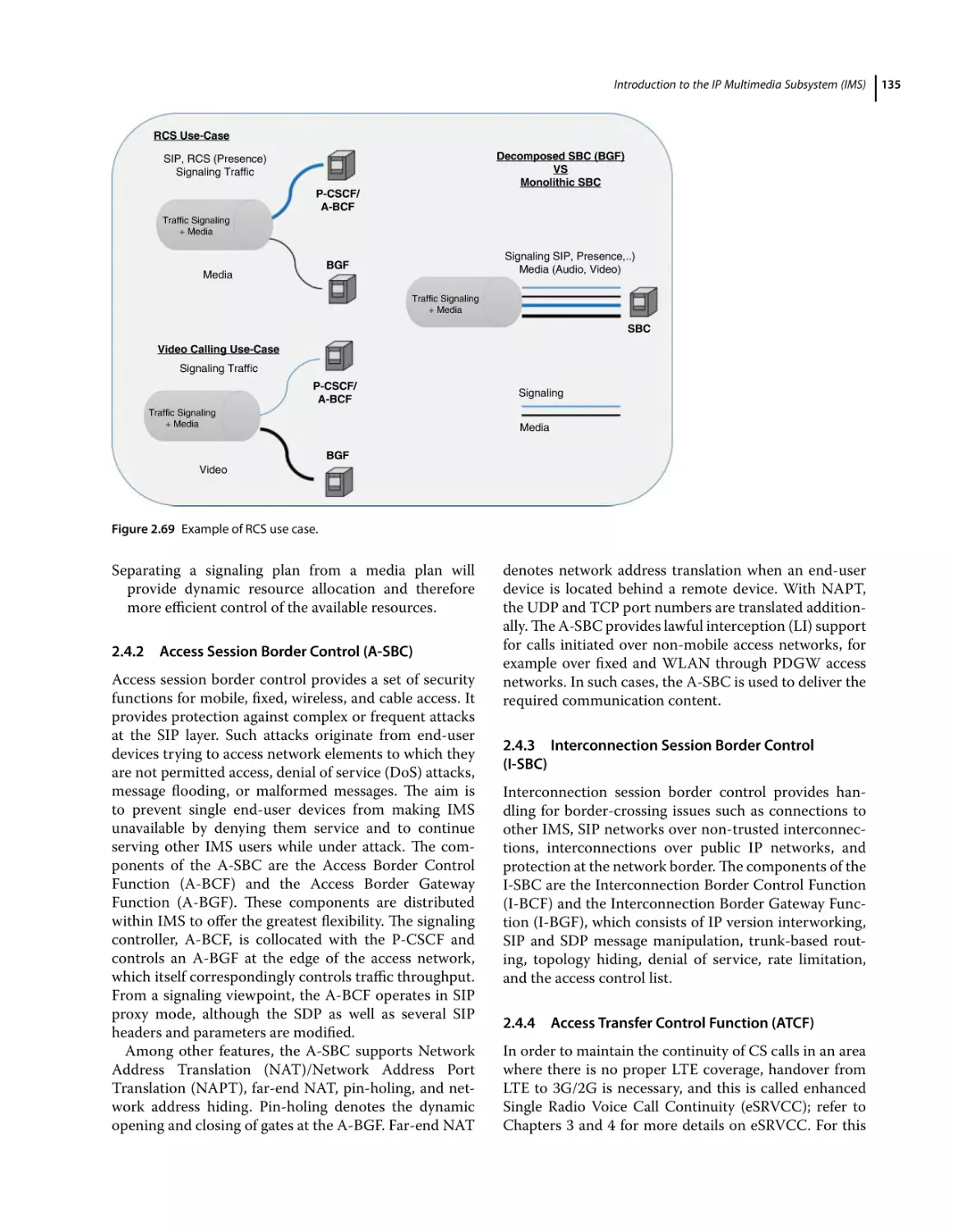
Access Session Border Control (A-SBC) 135
Interconnection Session Border Control (I-SBC) 135
Access Transfer Control Function (ATCF) 135
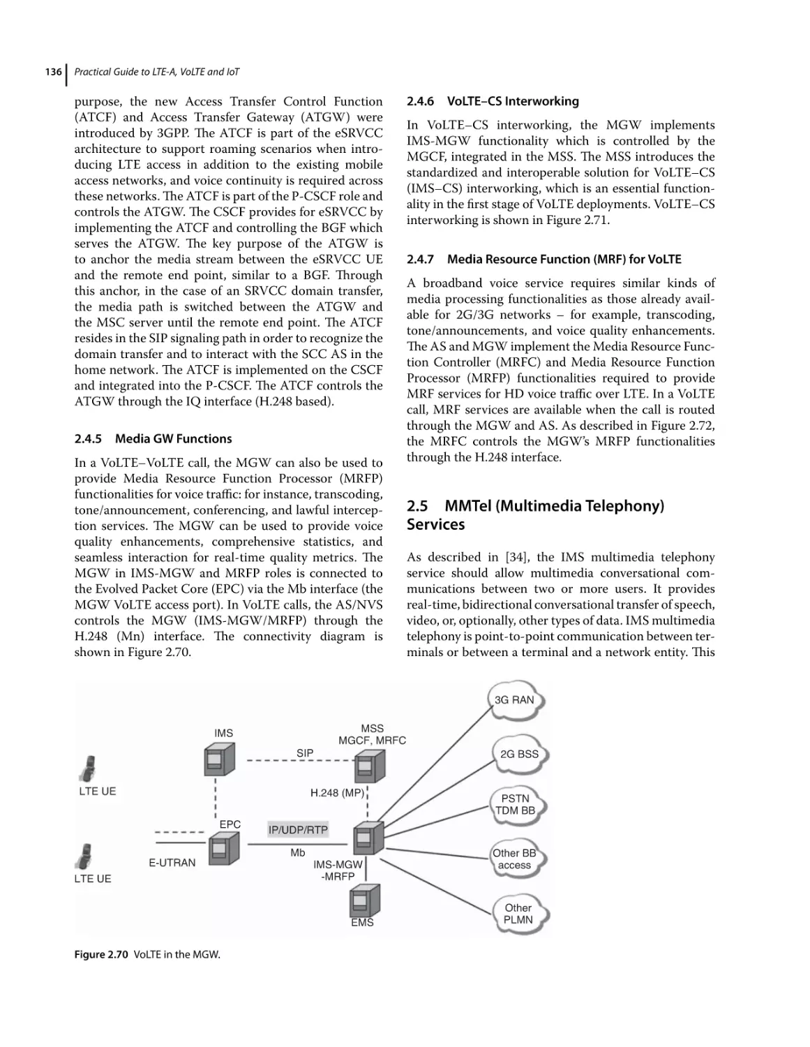
Media GW Functions 136
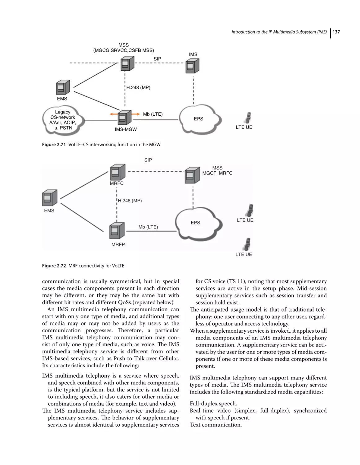
VoLTE–CS Interworking 136
Media Resource Function (MRF) for VoLTE 136
MMTel (Multimedia Telephony) Services 136
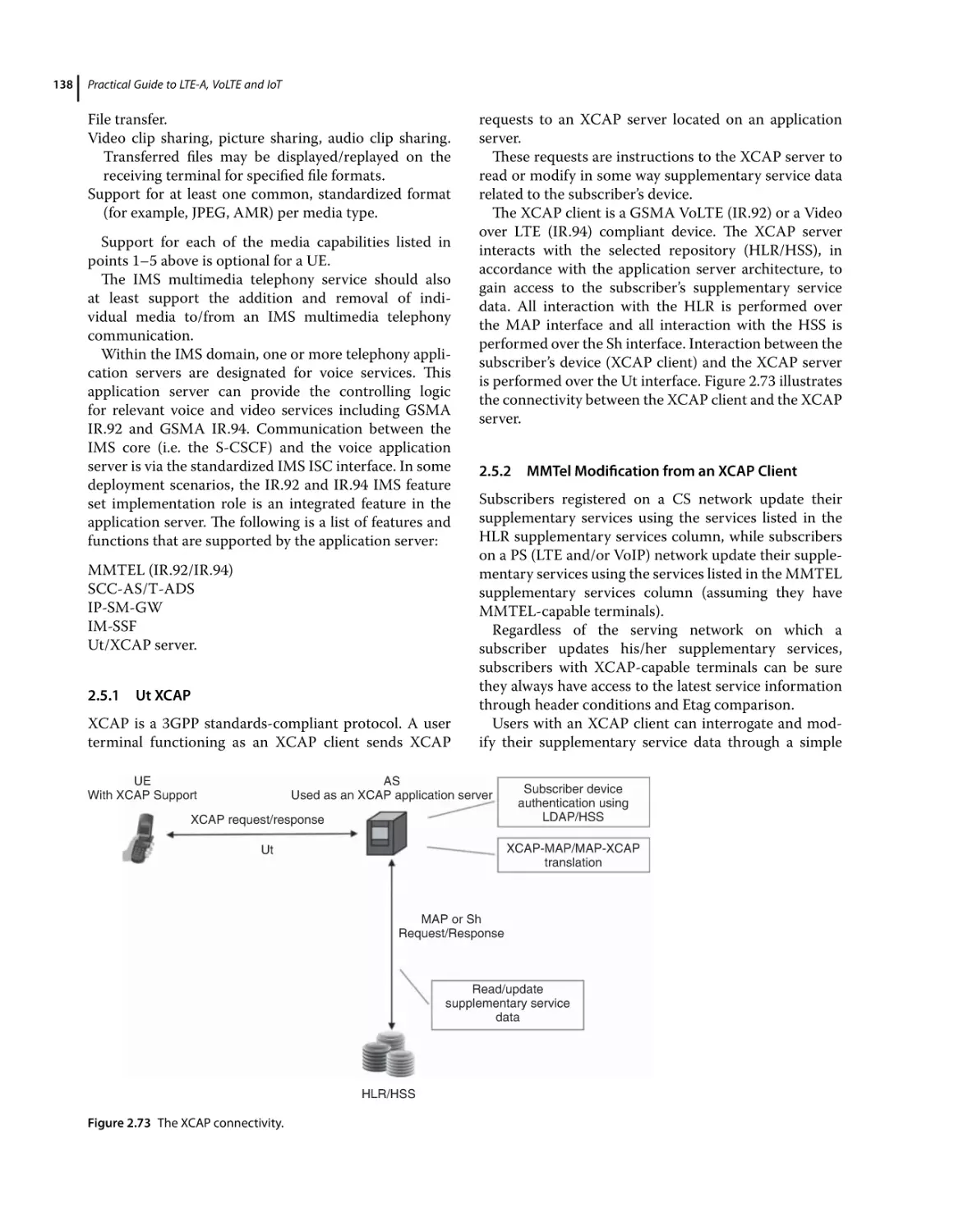
Ut XCAP 138
MMTel Modification from an XCAP Client 138
MMTel Data Synchronization Between XCAP Client and Server 139
Location Mapping 139
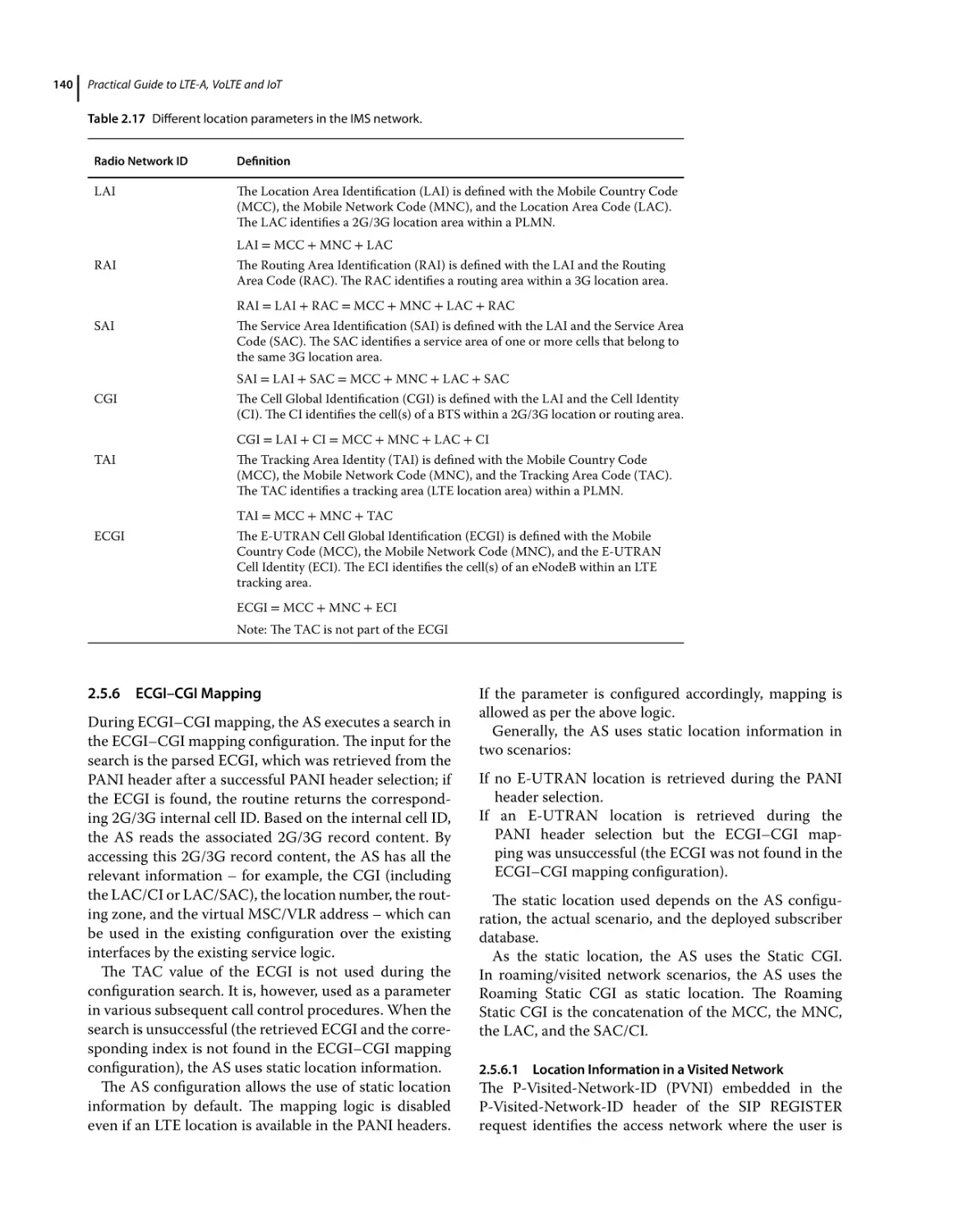
Location Parameters 139
ECGI–CGI Mapping 140
Location Information in a Visited Network 140
Service Centralization and Continuity AS (SCC AS) 141
SCC AS Homing 141
T-ADS/Domain Selection 141
SRVCC 141
Policy Control 142
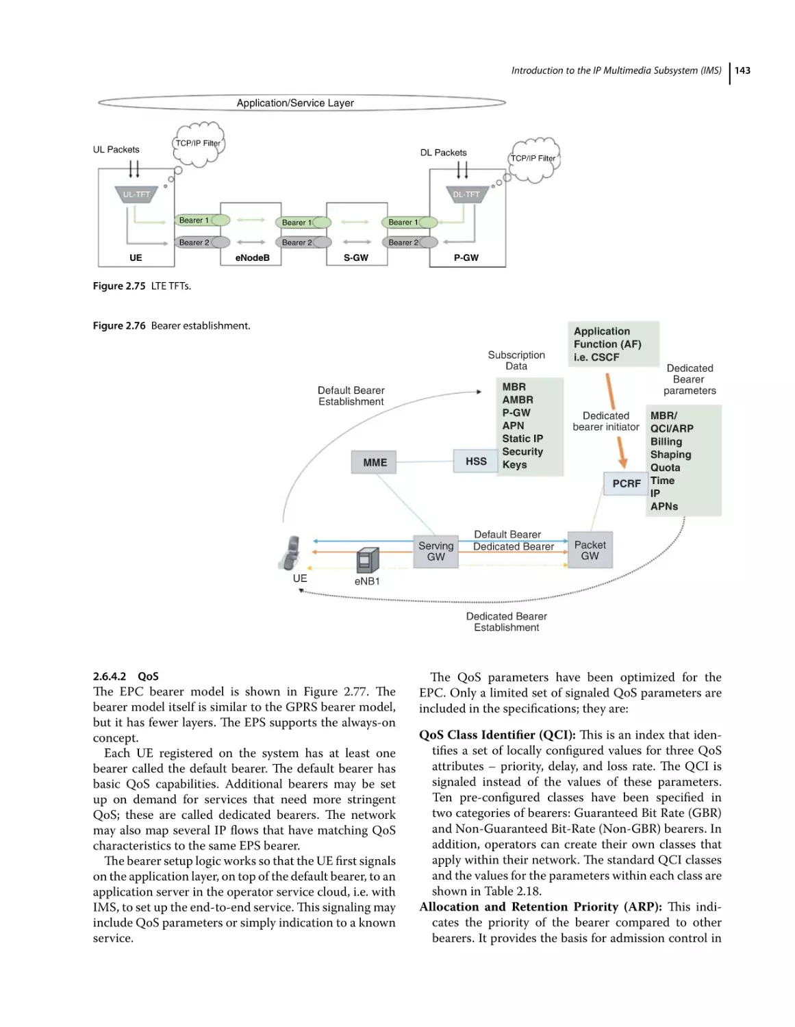
Bearer Establishment 142
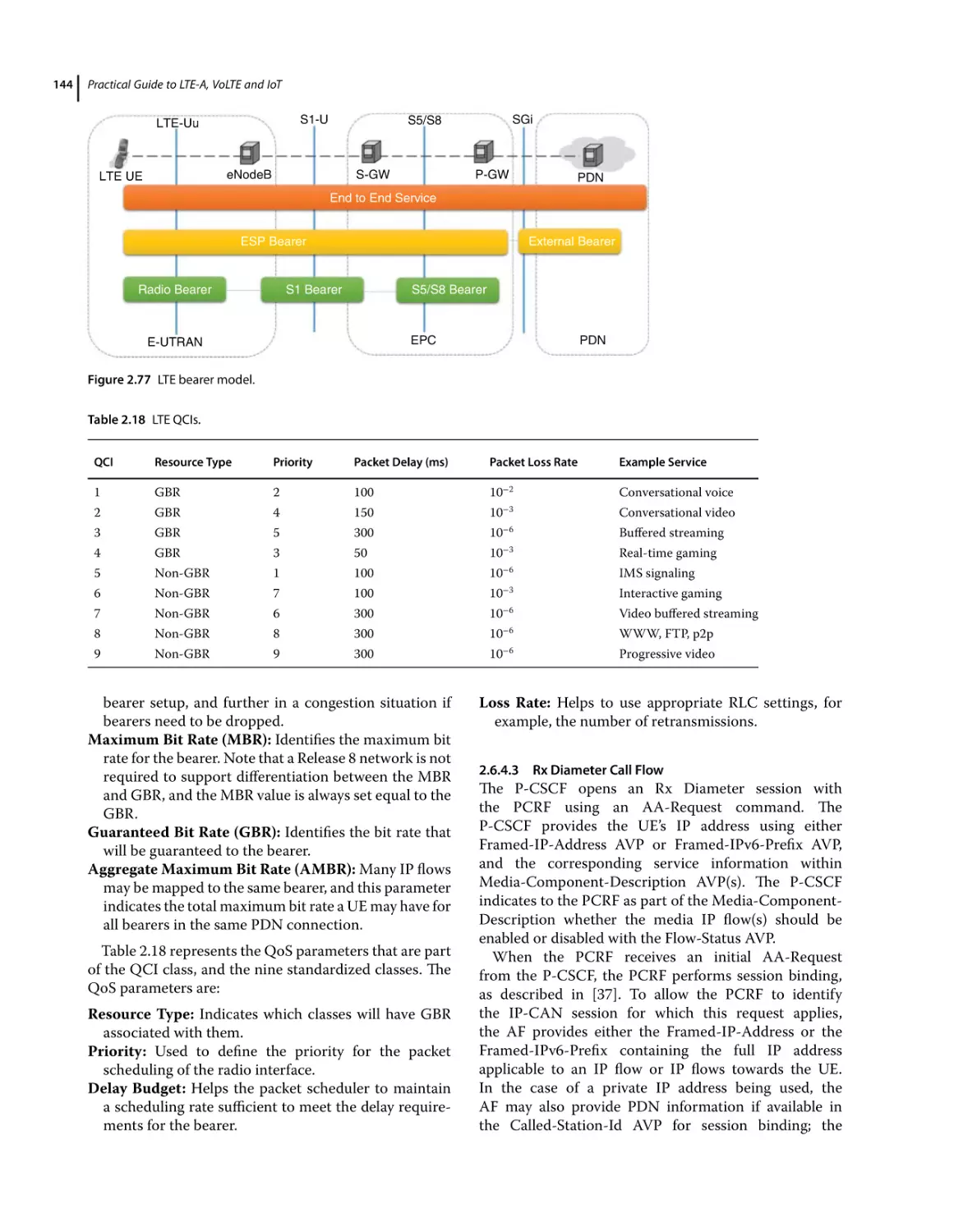
QoS 143
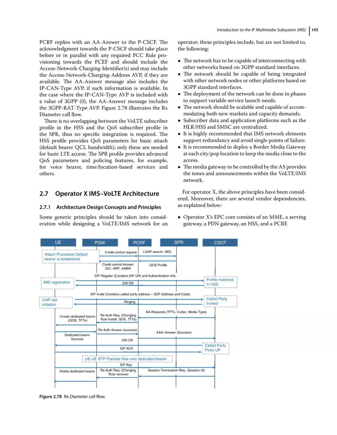
Rx Diameter Call Flow 144
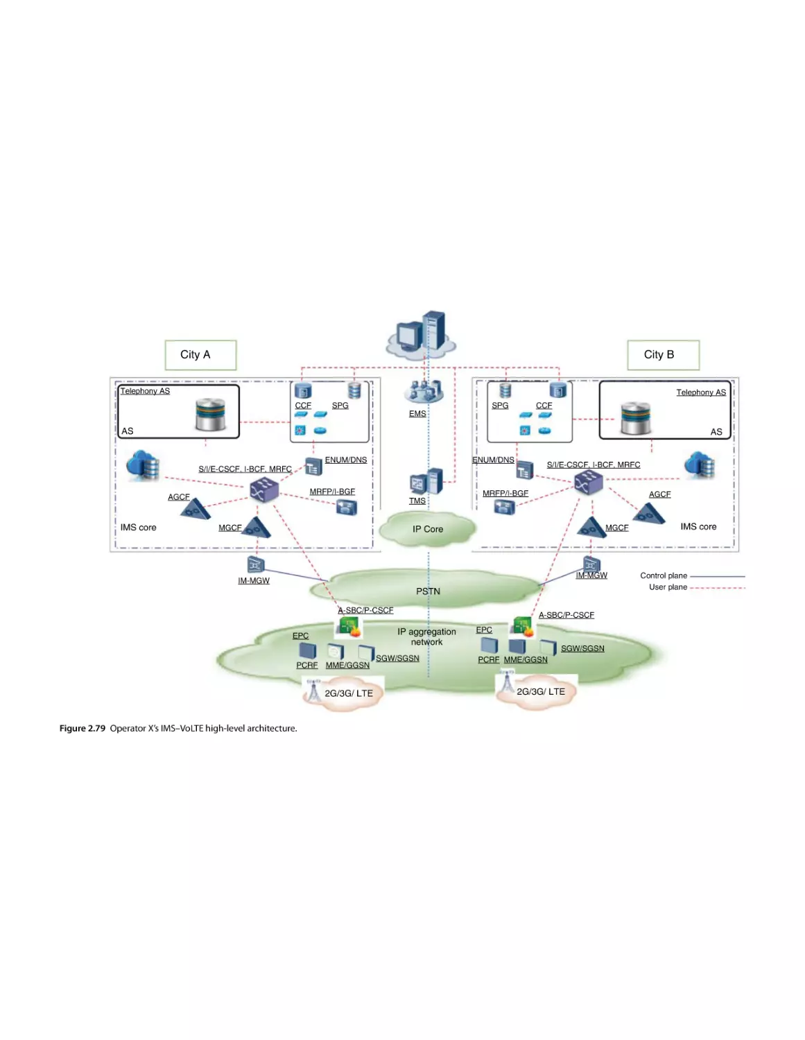
Operator X IMS–VoLTE Architecture 145
Architecture Design Concepts and Principles 145
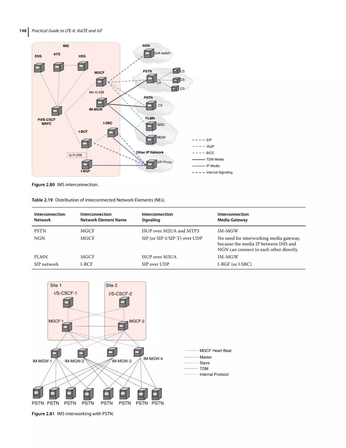
Interconnection Topology 146
Topology of Interworking with PSTN 146
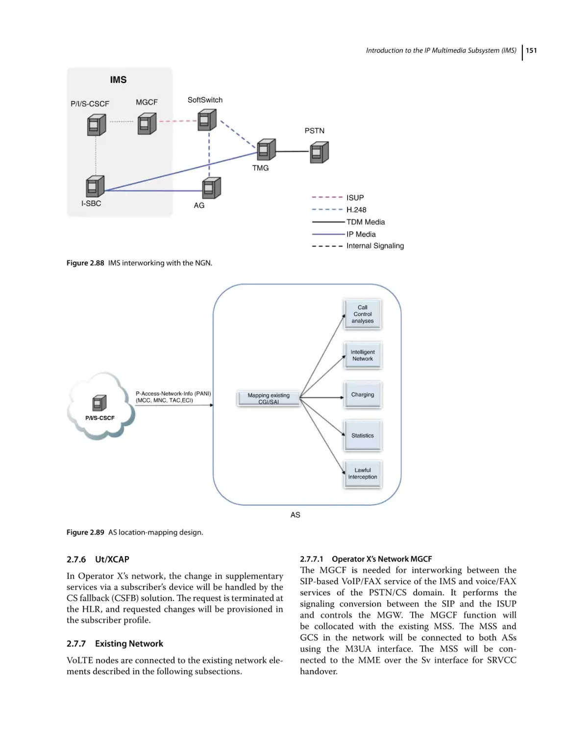
Topology of Interworking with NGN 146
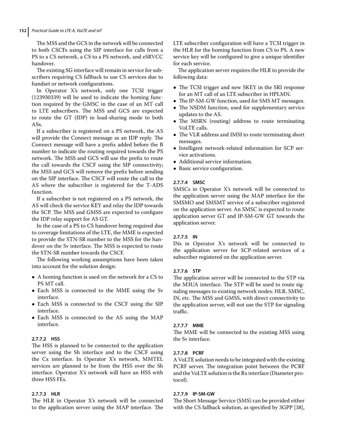
Location-based Routing 146
Routing Zone and Use of LTE Location 146
Ut/XCAP 151
Existing Network 151
Contents
2.7.7.1
2.7.7.2
2.7.7.3
2.7.7.4
2.7.7.5
2.7.7.6
2.7.7.7
2.7.7.8
2.7.7.9
2.7.7.10
2.7.7.11
2.7.7.12
2.7.7.13
2.7.7.14
2.7.7.15
2.7.8
2.7.8.1
2.7.9
Operator X’s Network MGCF 151
HSS 152
HLR 152
SMSC 152
IN 152
STP 152
MME 152
PCRF 152
IP-SM-GW 152
Messaging Profile 153
IP-SM-GW and User Types 153
IP-SM-GW Interworking with Multi-SIM/ONS 153
HLR Support for IP-SM-GW 153
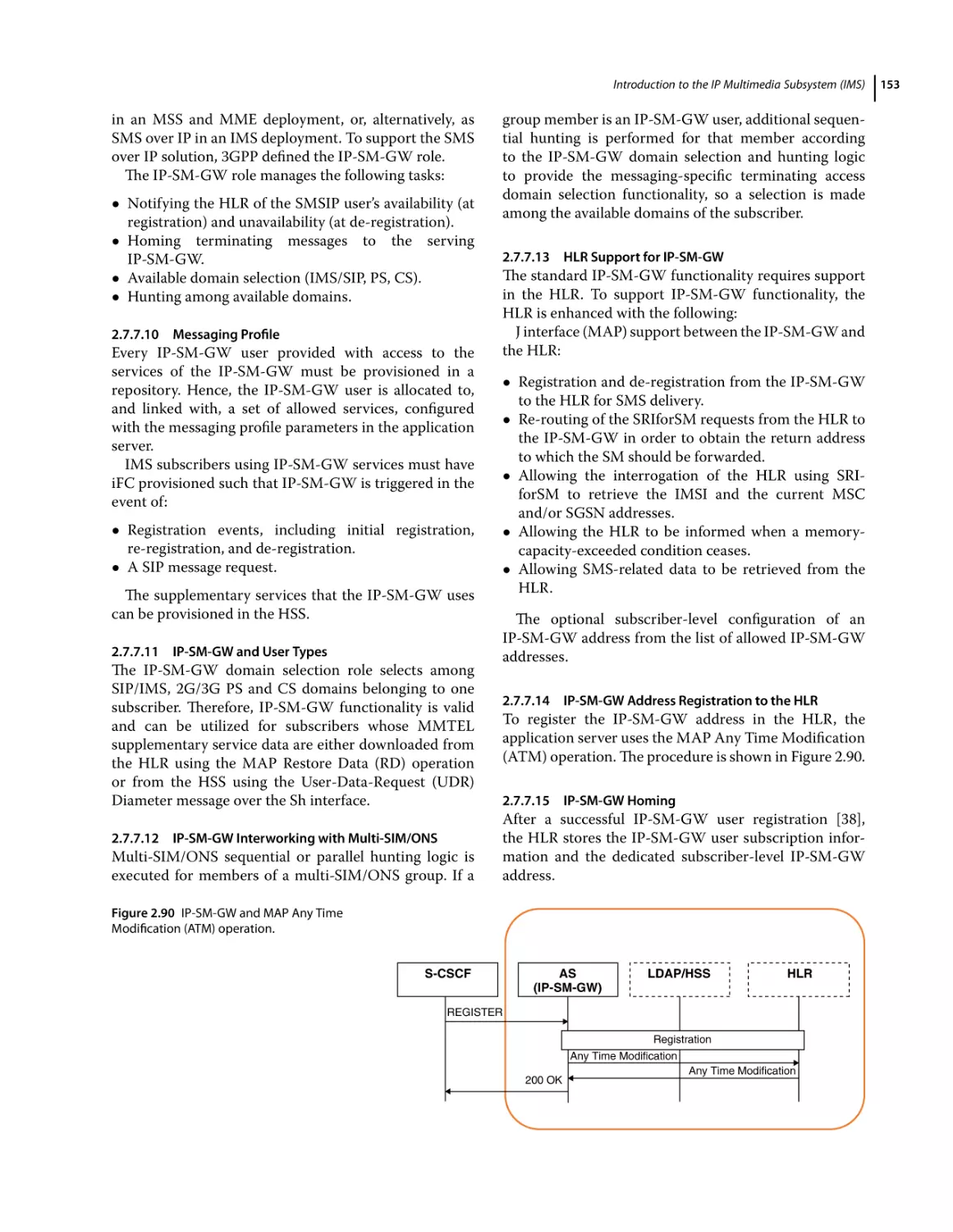
IP-SM-GW Address Registration to the HLR 153
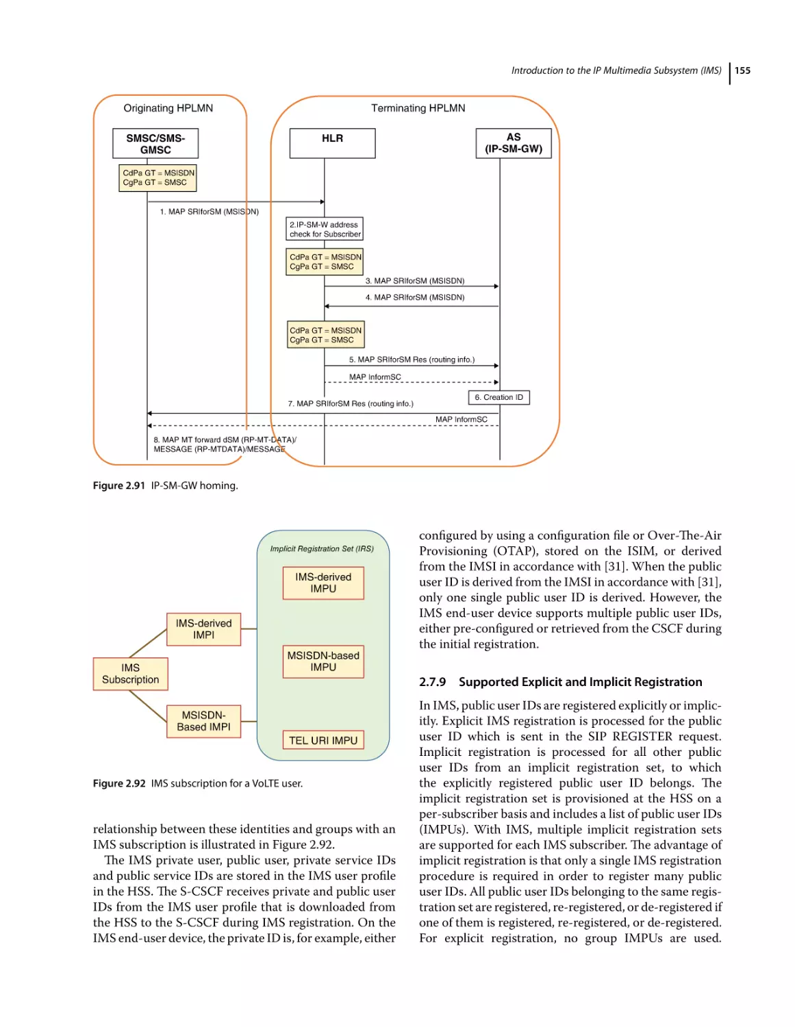
IP-SM-GW Homing 153
External Network Connections 154
PSTN and IMS Subscription 154
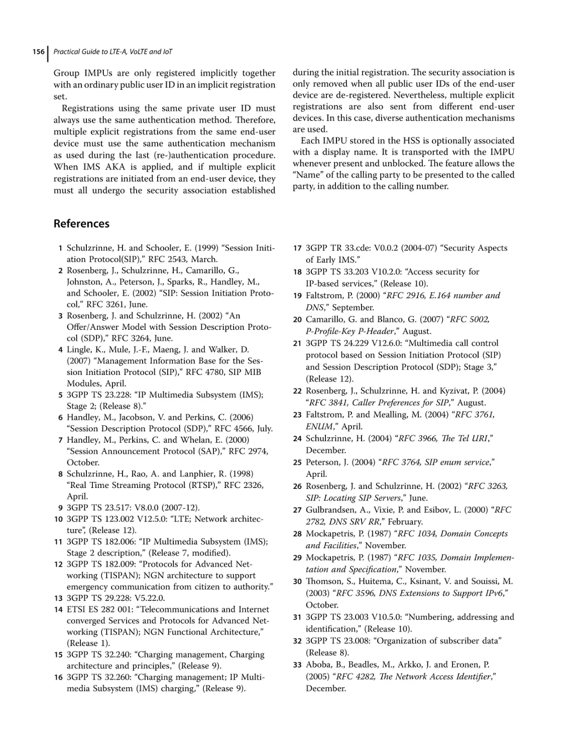
Supported Explicit and Implicit Registration 155
References 156
3
VoLTE/CSFB Call Setup Delay and Handover Analysis 158
3.1
3.2
3.3
3.4
3.5
3.5.1
3.6
3.7
3.7.1
3.7.2
3.7.3
3.7.4
3.8
3.8.1
3.8.2
3.8.3
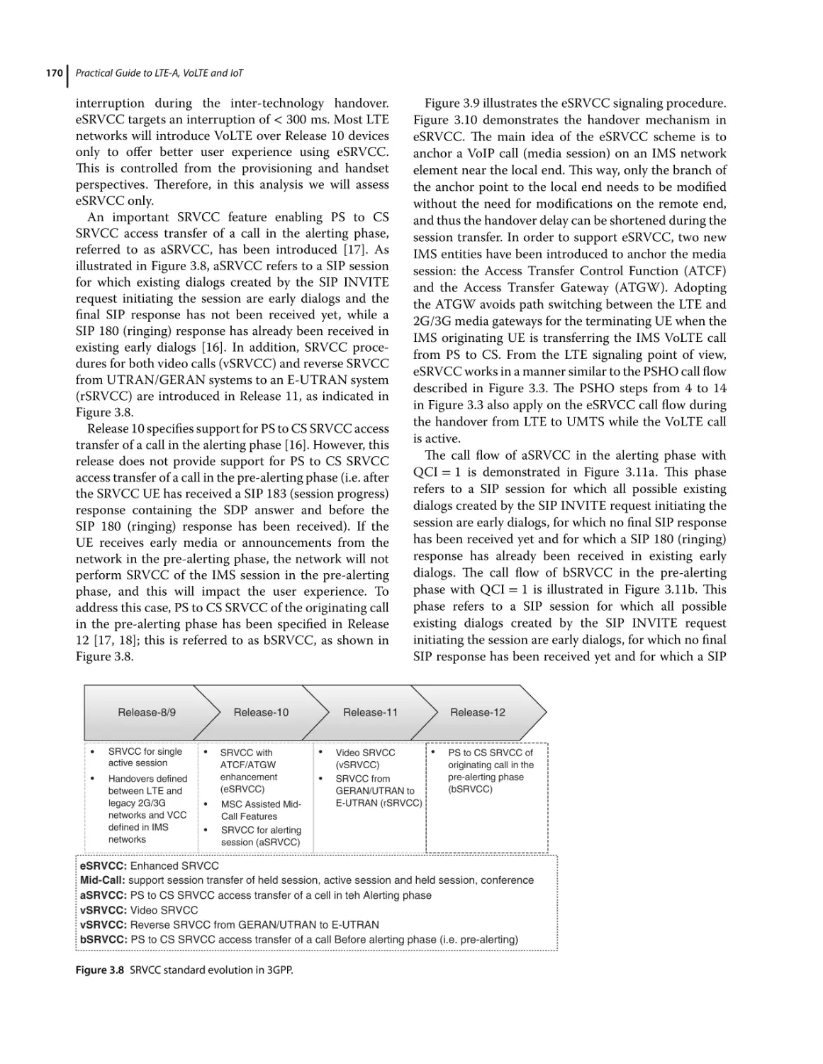
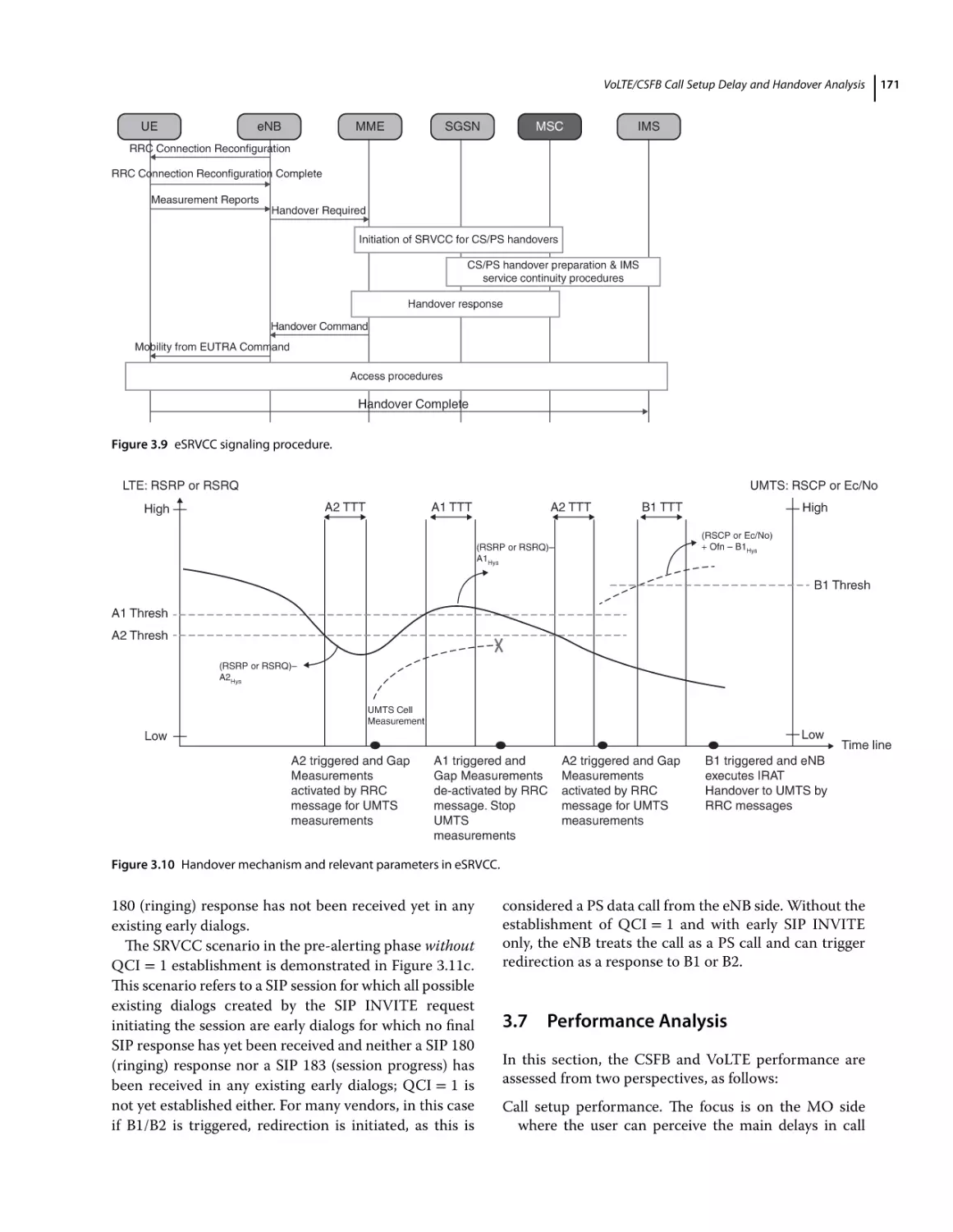
3.9
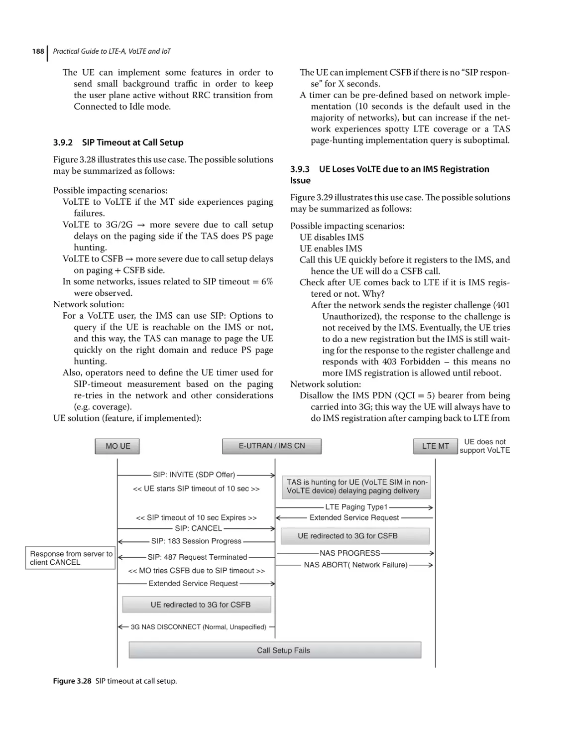
3.9.1
3.9.2
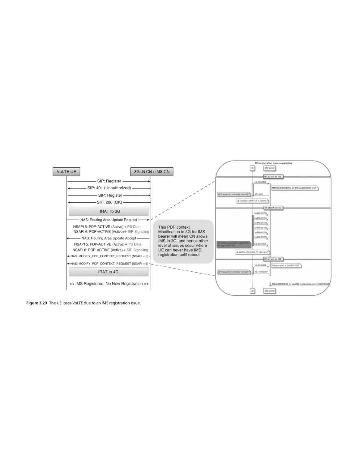
3.9.3
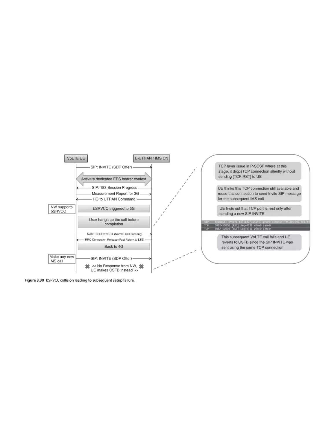
3.9.4
3.9.5
3.9.6
3.9.7
3.9.8
3.10
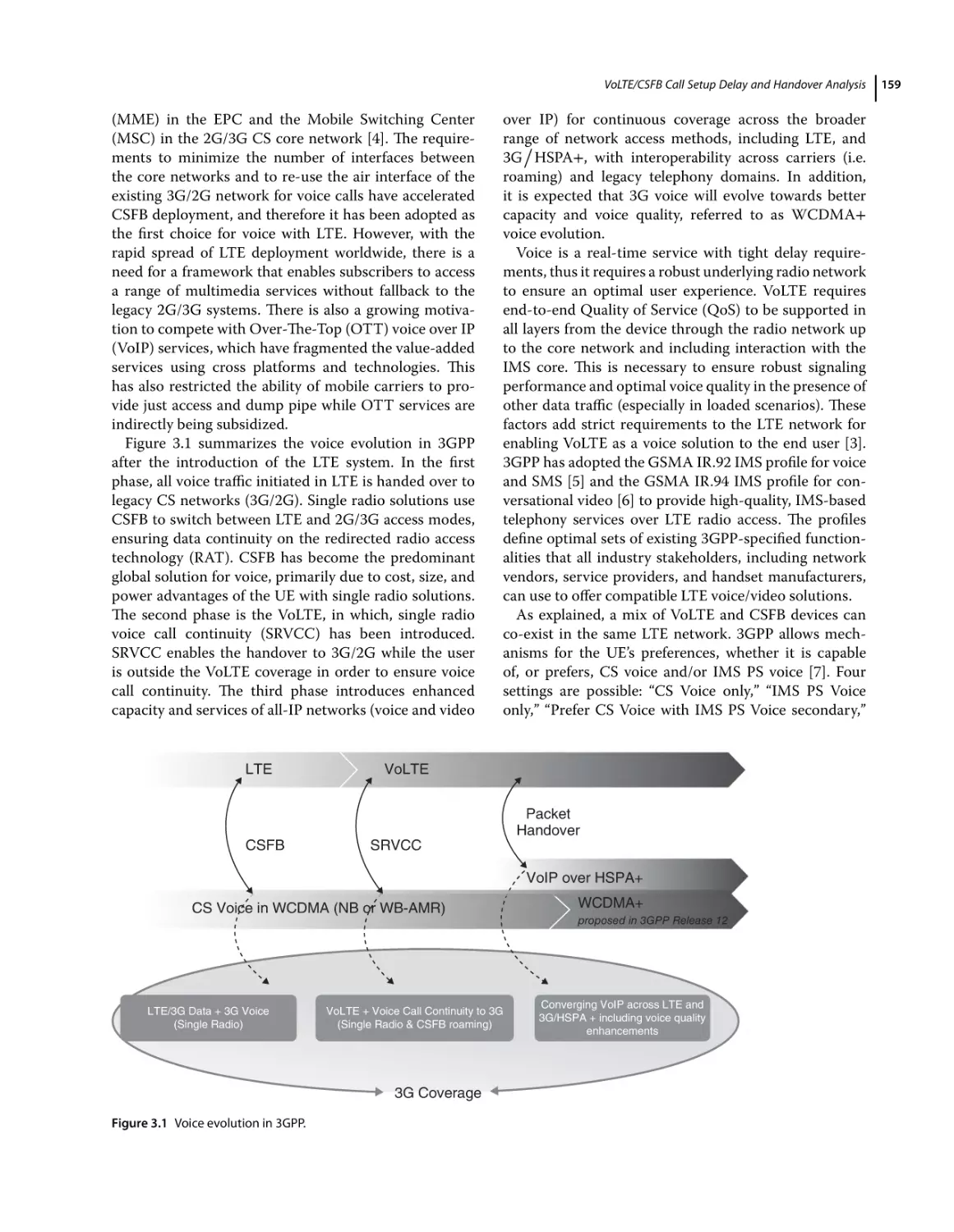
Overview 158
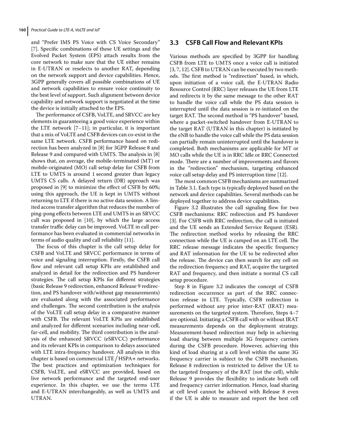
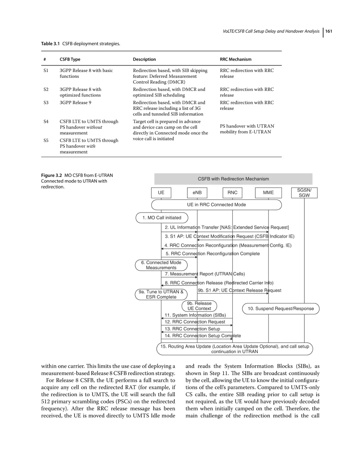
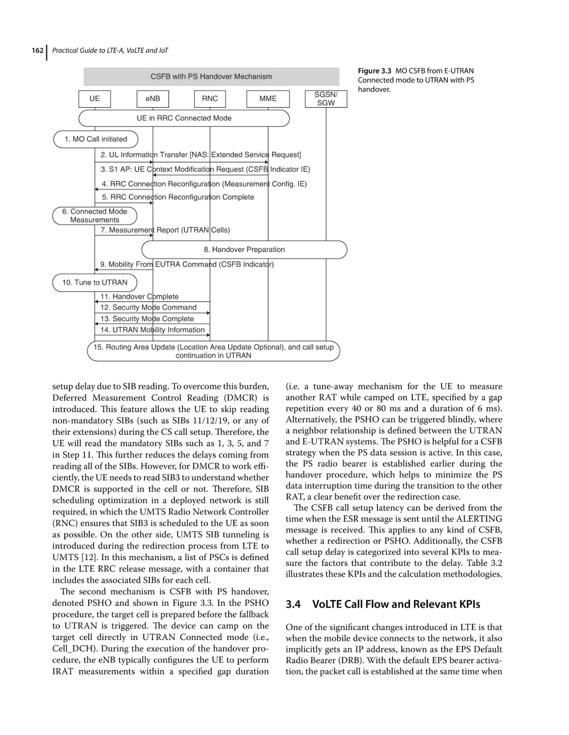
Introduction 158
CSFB Call Flow and Relevant KPIs 160
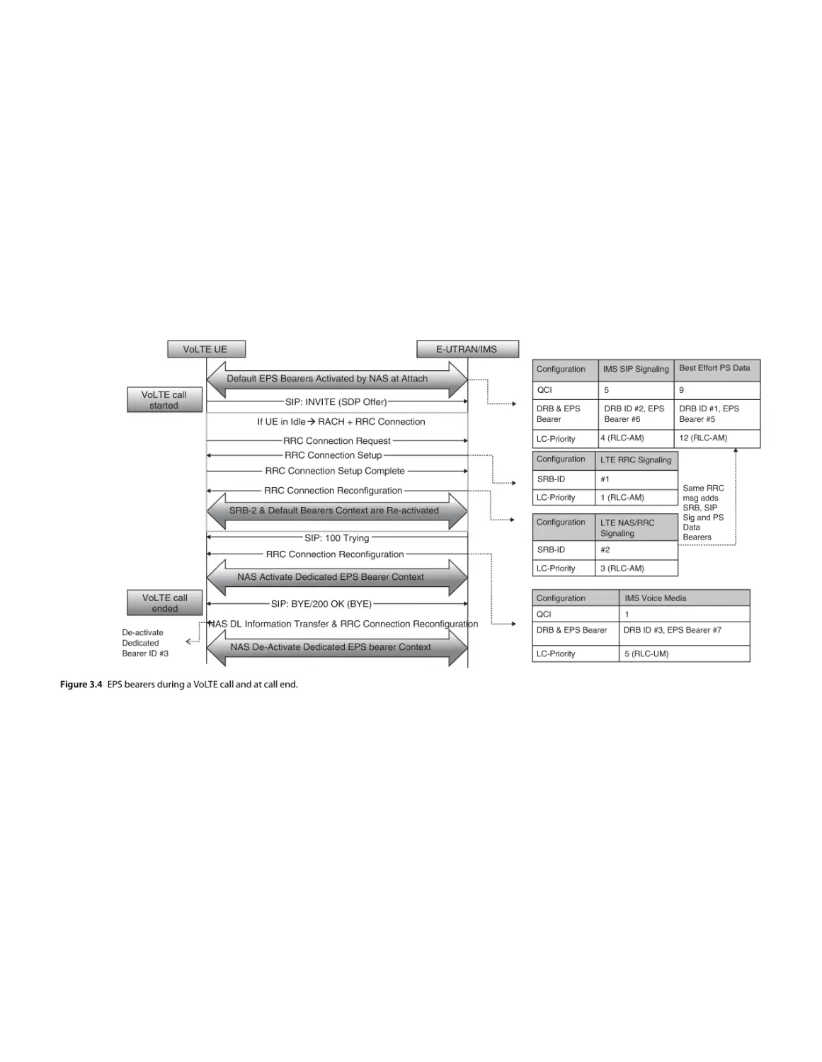
VoLTE Call Flow and Relevant KPIs 162
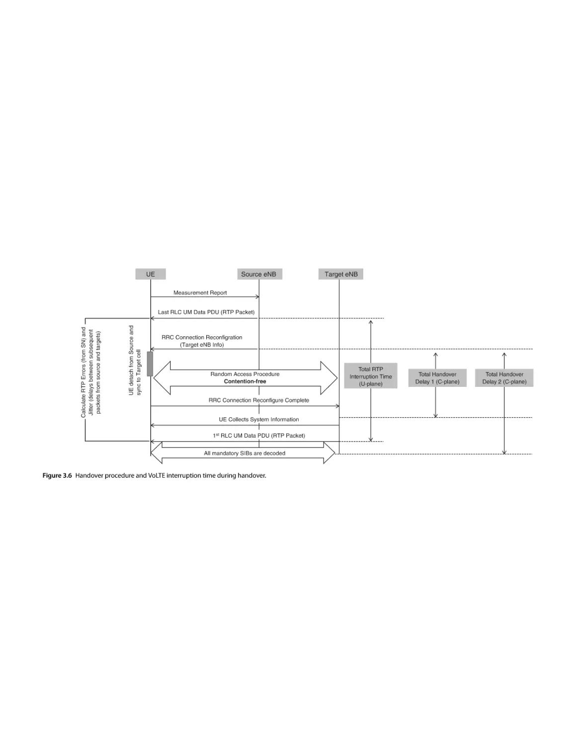
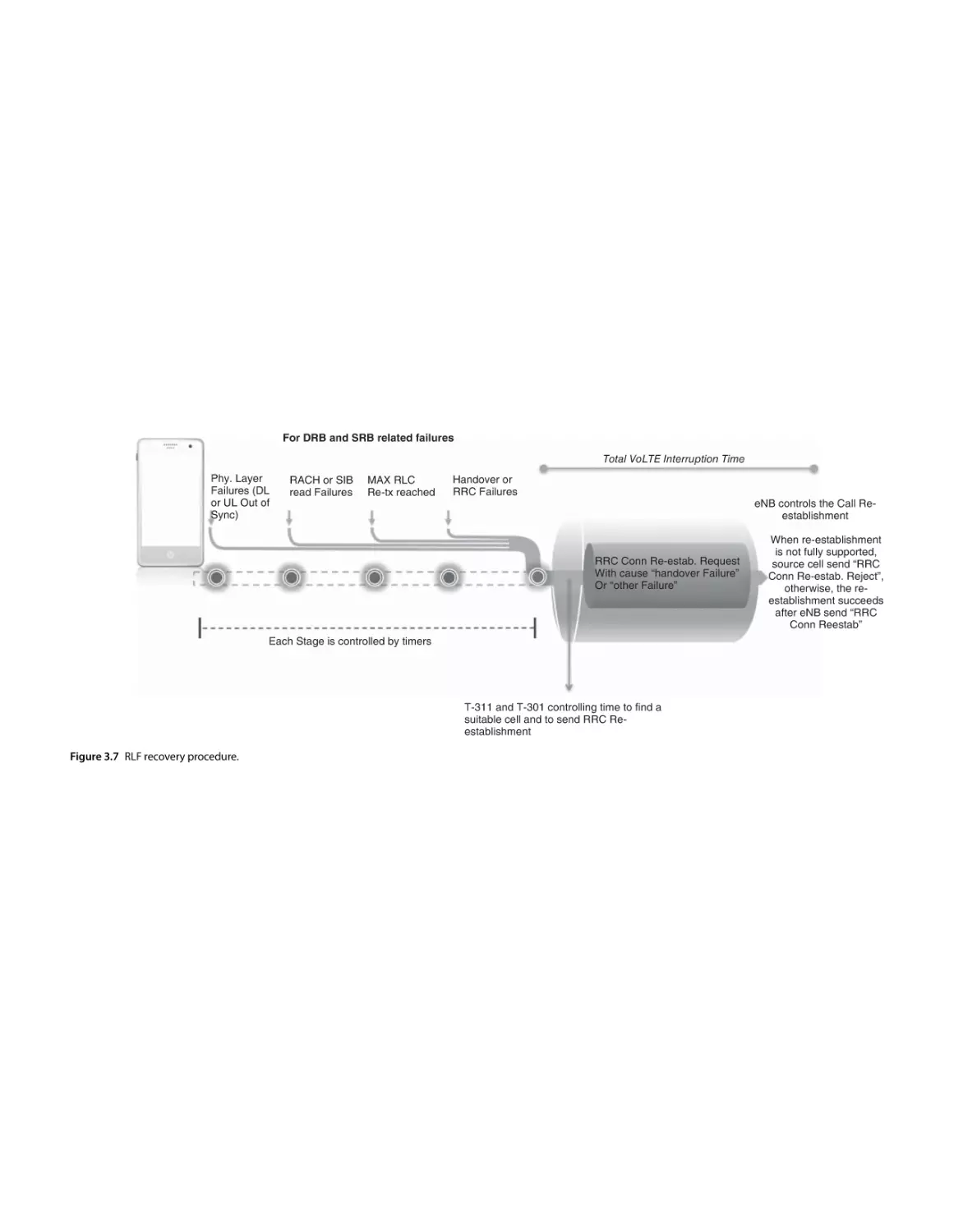
VoLTE Handover and Data Interruption Time 166
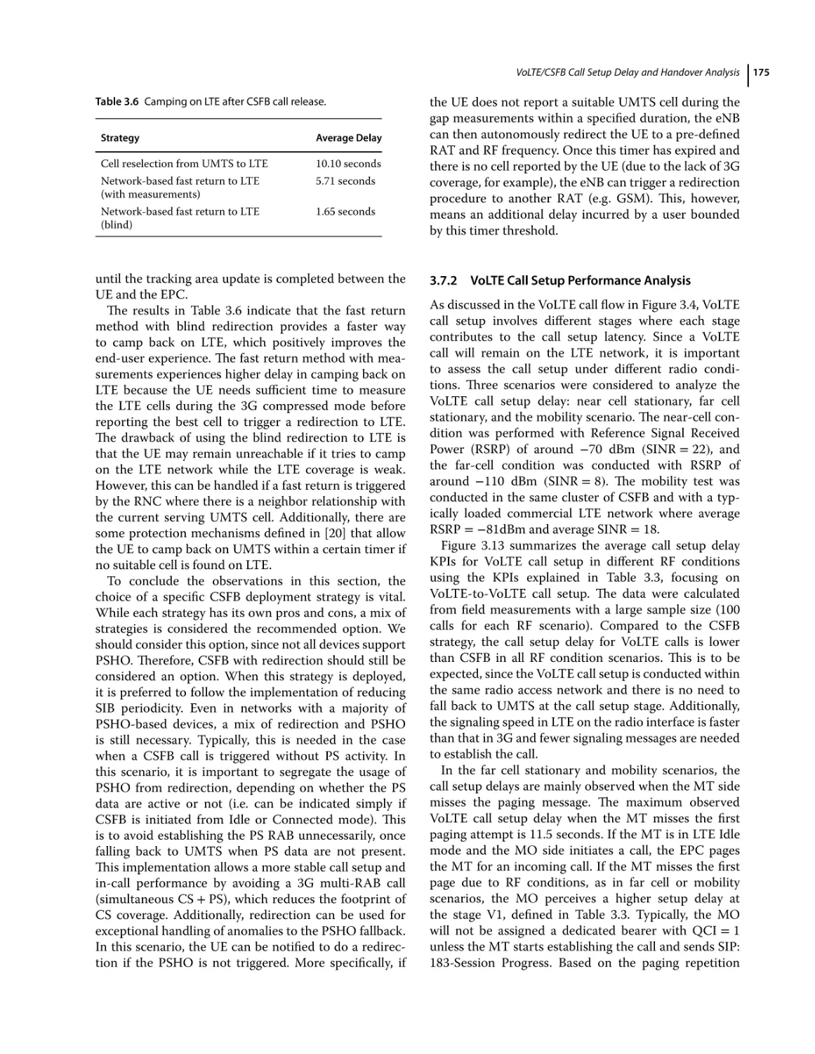
Recommendations on Call Re-establishment 166
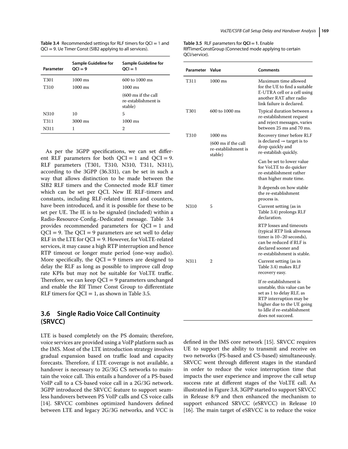
Single Radio Voice Call Continuity (SRVCC) 169
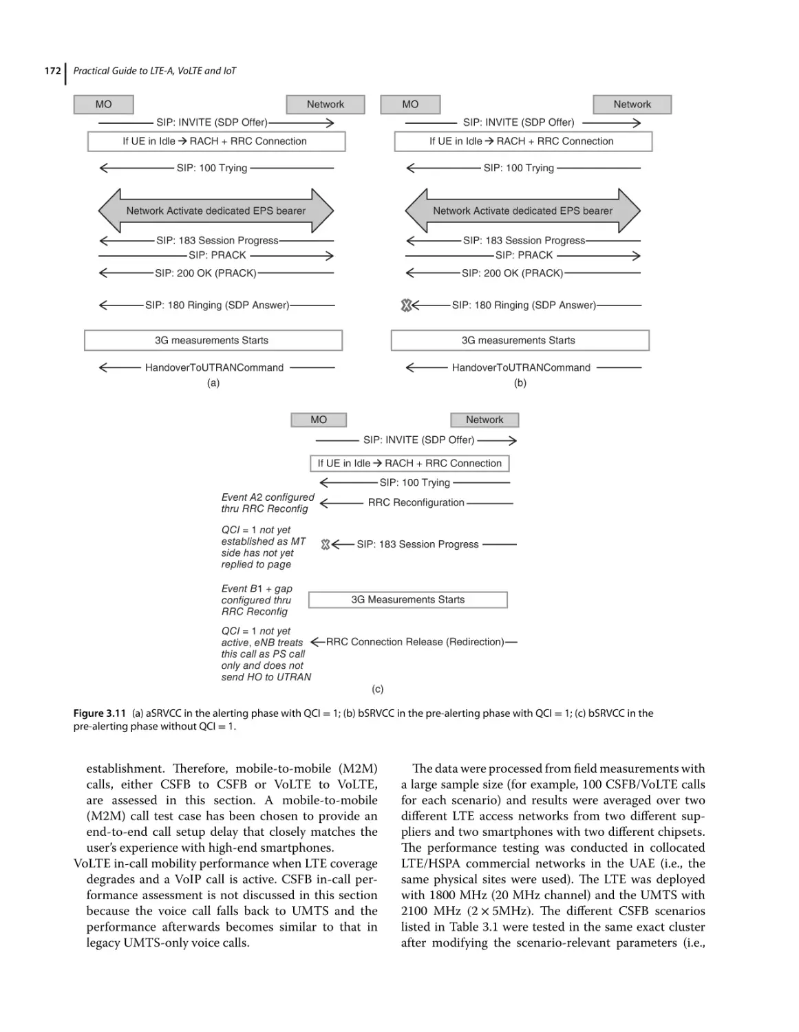
Performance Analysis 171
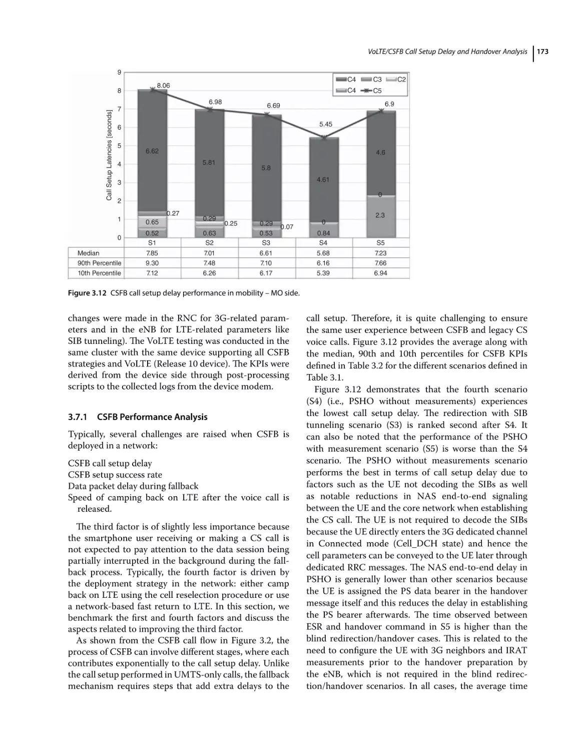
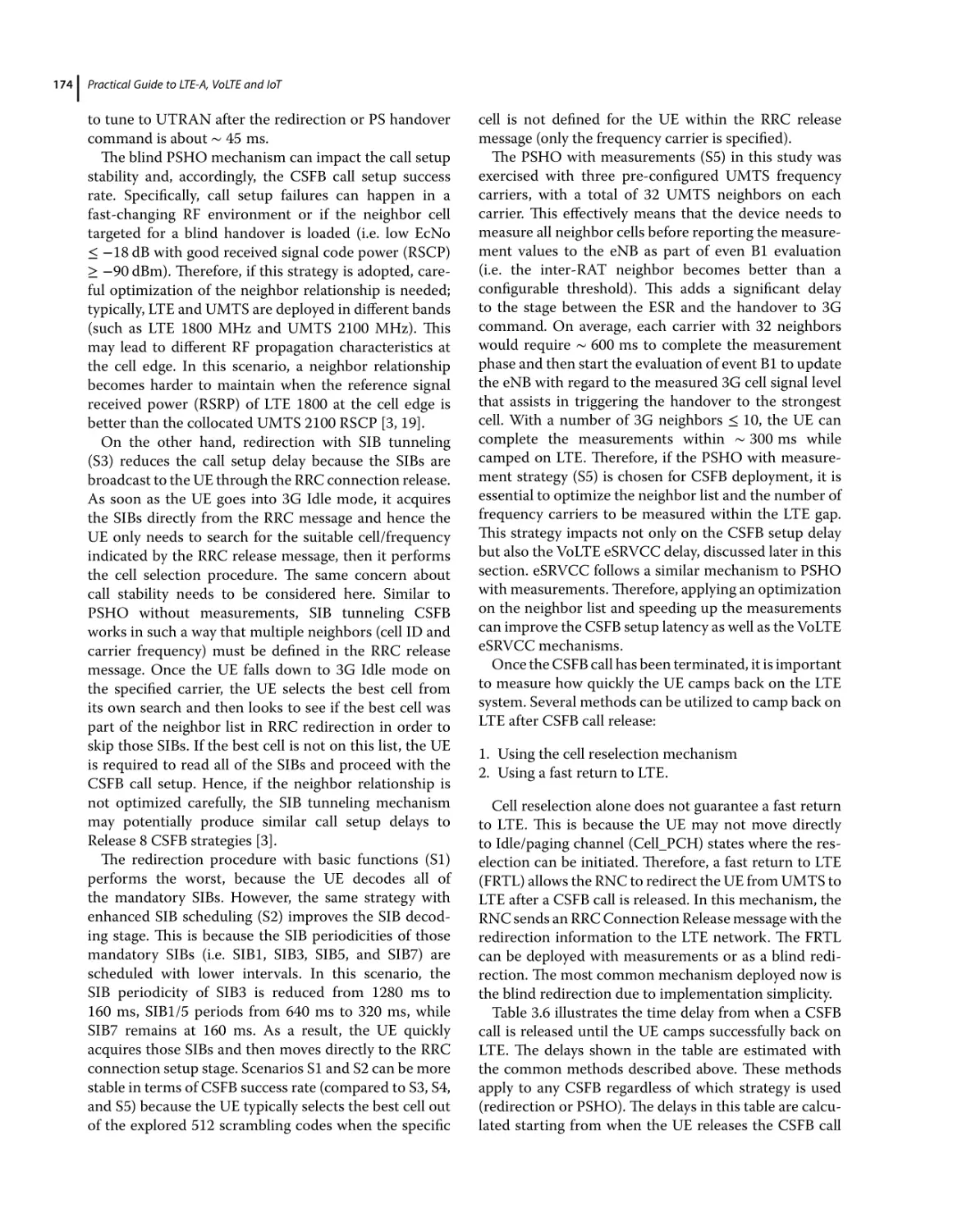
CSFB Performance Analysis 173
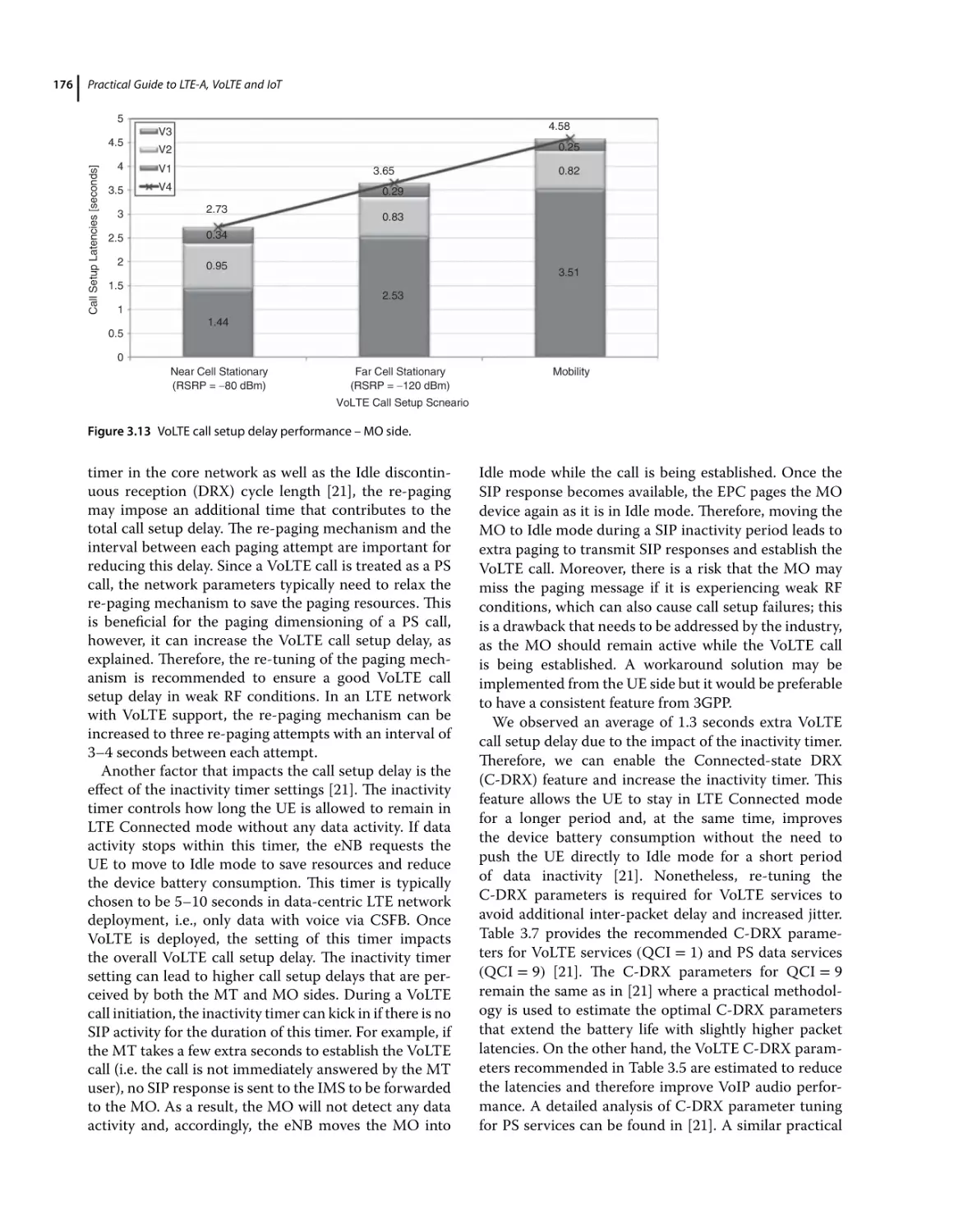
VoLTE Call Setup Performance Analysis 175
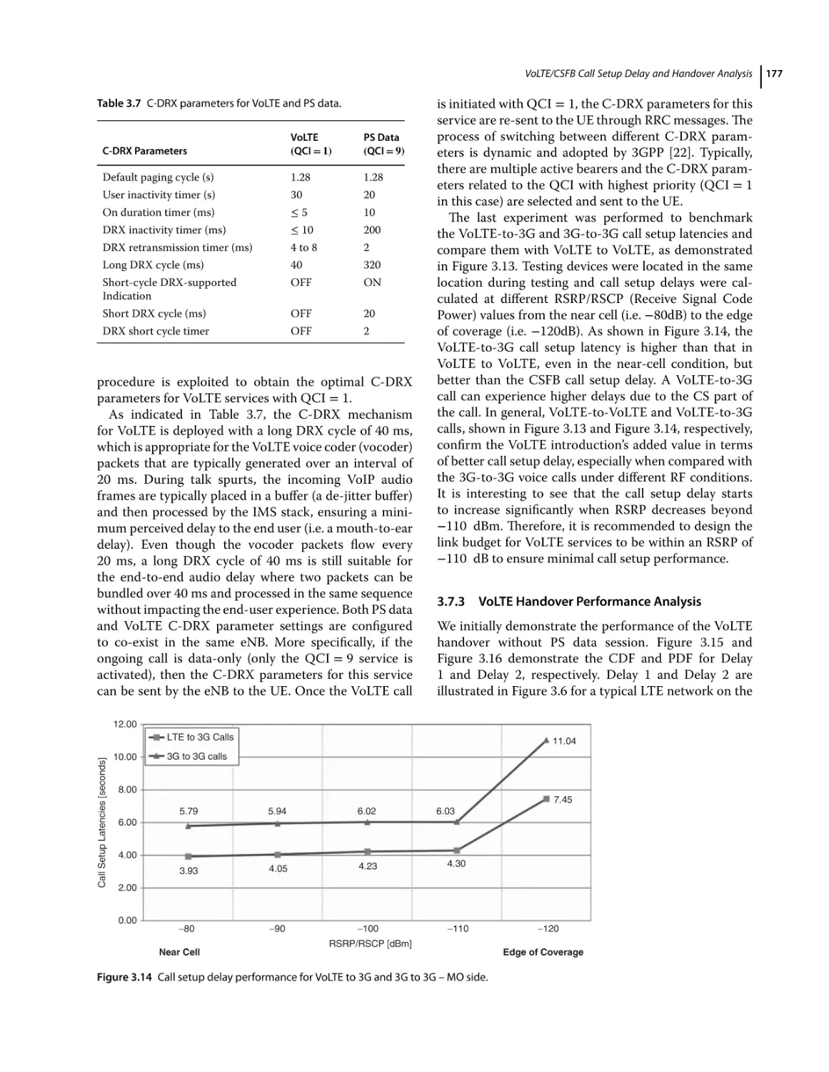
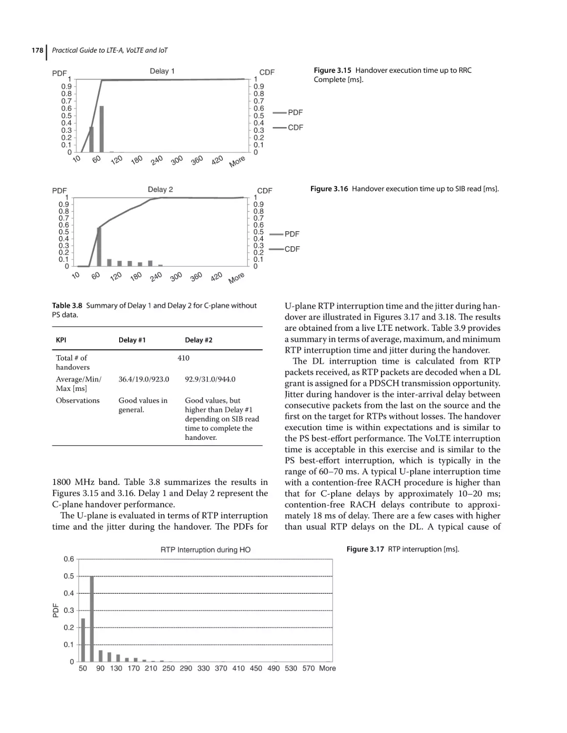
VoLTE Handover Performance Analysis 177
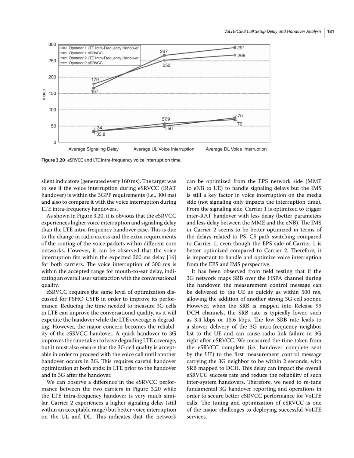
eSRVCC Performance Analysis 180
Latency Reduction During Handover 182
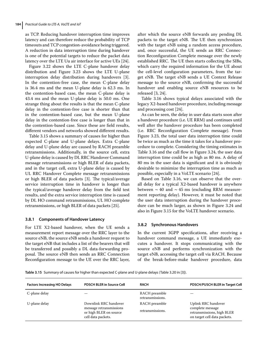
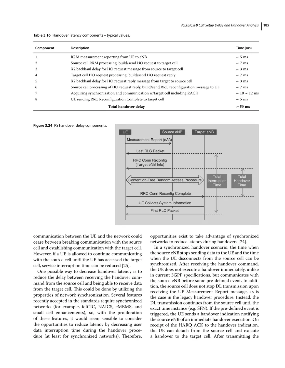
Components of Handover Latency 184
Synchronous Handovers 184
Synchronized Handover with Early Handover Command (EHC) 186
Practical Use Cases and Recommendations 187
State Transition at Call Setup 187
SIP Timeout at Call Setup 188
UE Loses VoLTE due to an IMS Registration Issue 188
bSRVCC Collision Leading to Subsequent Setup Failure 190
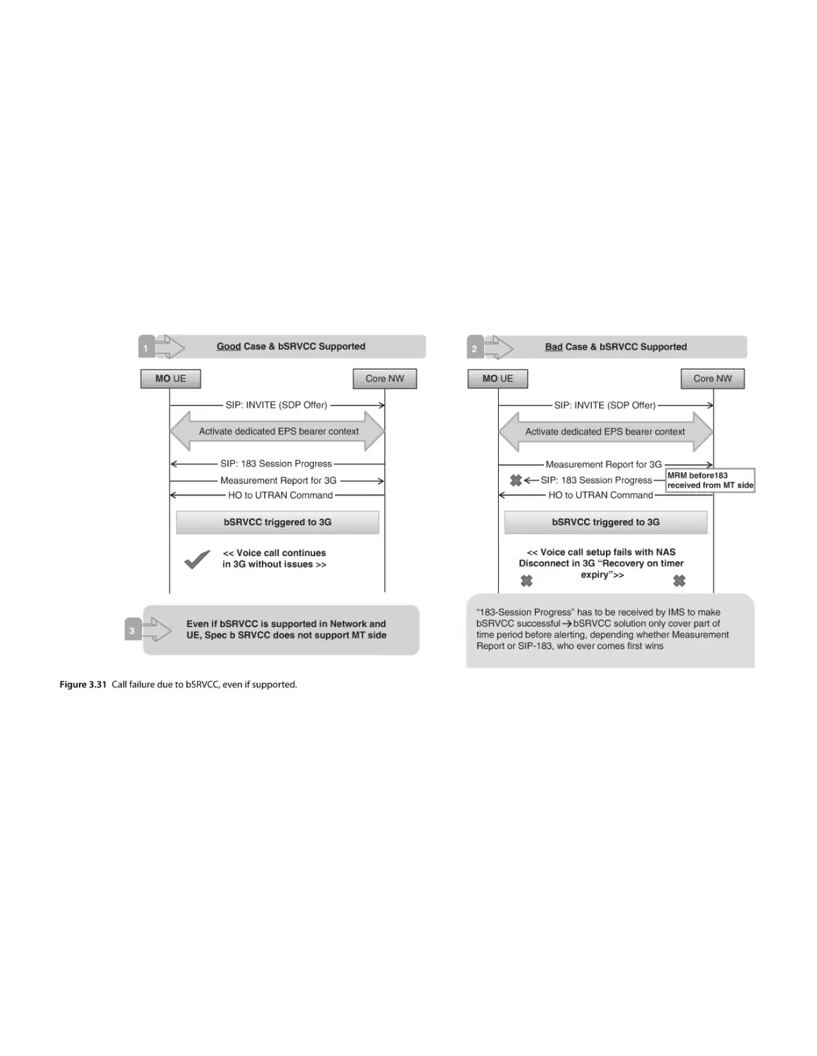
Call Failure due to bSRVCC, Even if Supported 190
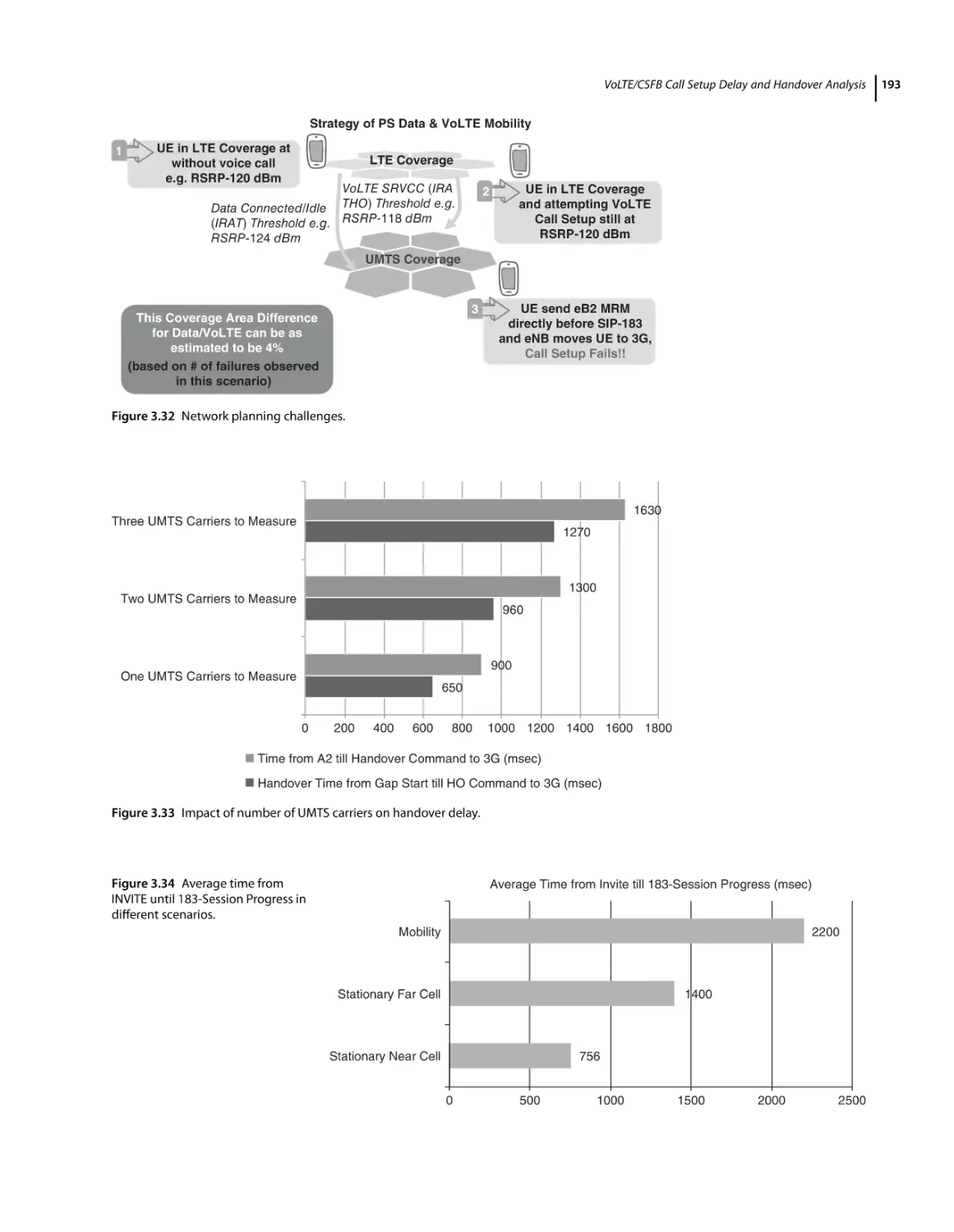
Network Planning Challenges 190
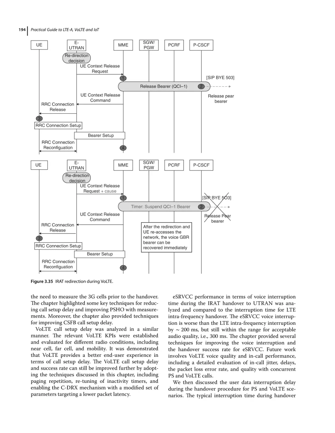
IRAT Redirection During VoLTE 190
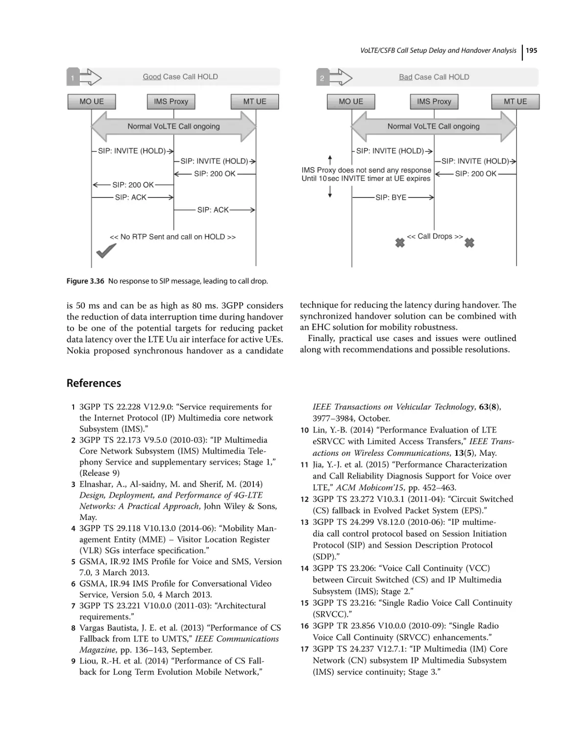
No Response to SIP Message, Leading to Call Drop 190
Conclusions 190
References 195
4
Comprehensive Performance Evaluation of VoLTE
4.1
4.2
4.3
4.4
4.4.1
Overview 197
Introduction 197
VoLTE Principles 198
Main VoLTE Features 200
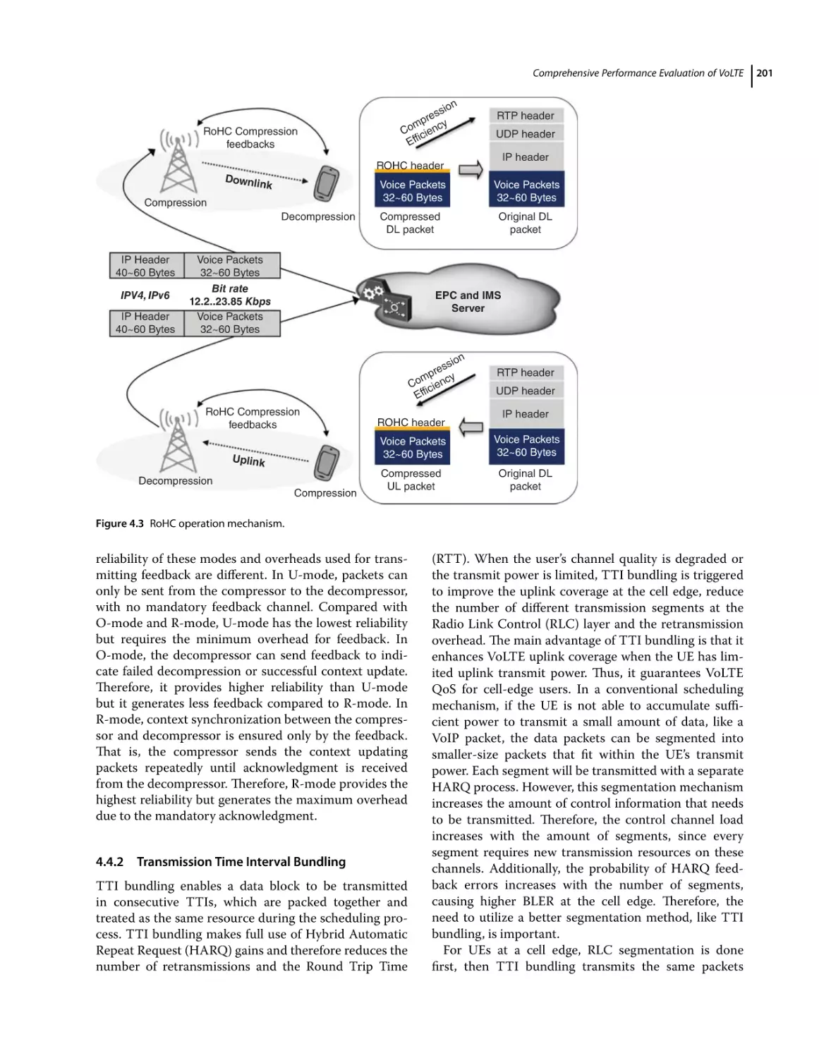
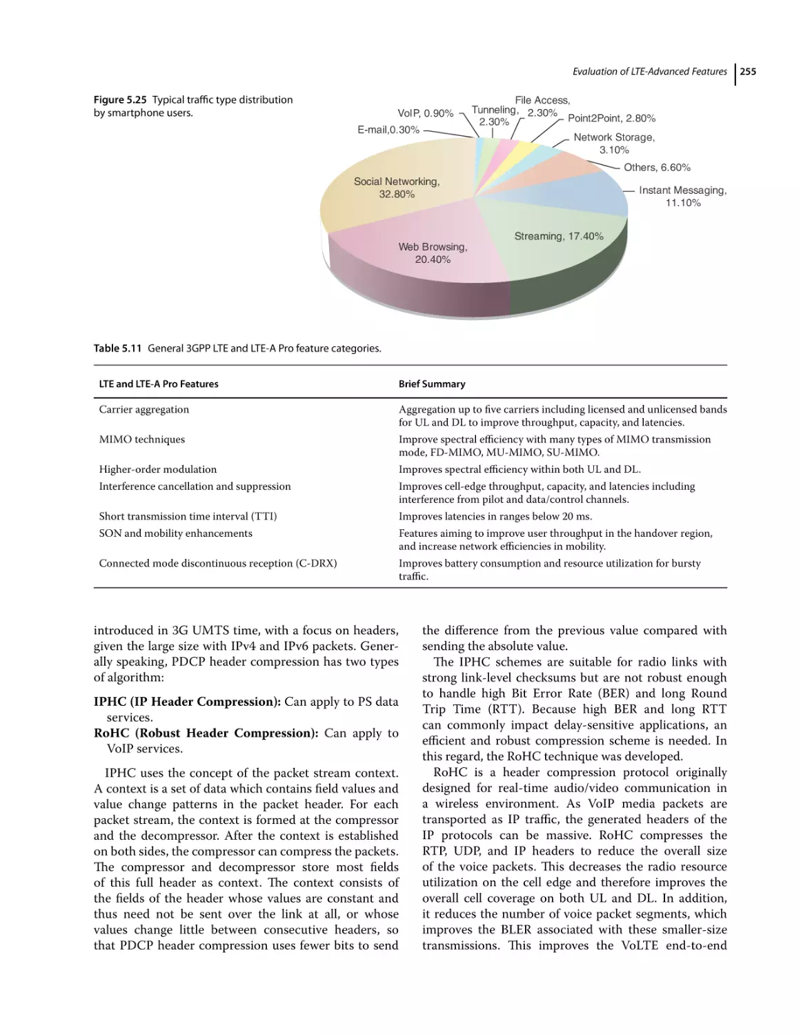
Robust Header Compression 200
197
xi
xii
Contents
4.4.2
4.4.3
4.5
4.6
4.6.1
4.6.2
4.6.3
4.6.4
4.6.5
4.6.6
4.6.7
4.7
4.8
4.9
4.10
4.11
4.12
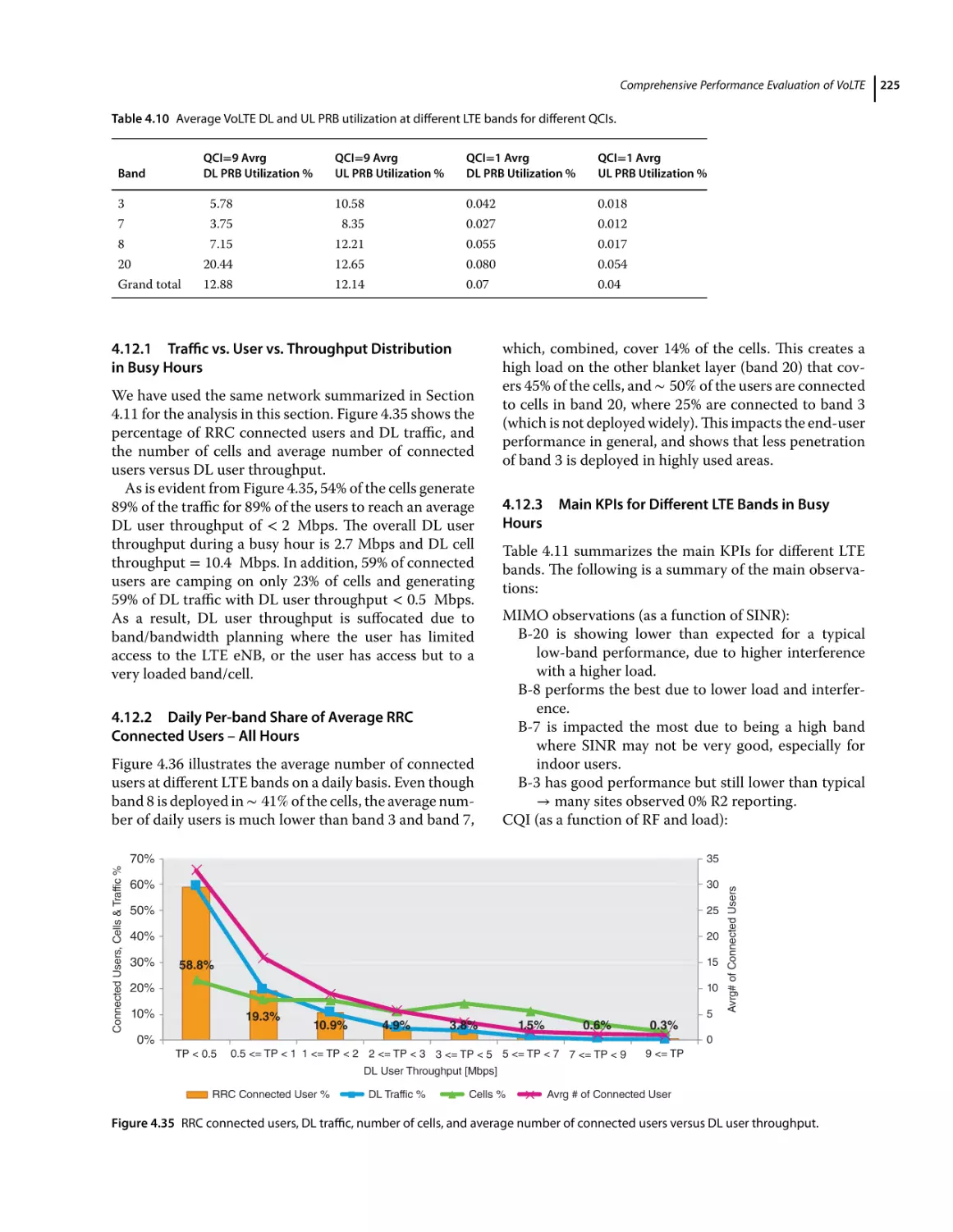
4.12.1
4.12.2
4.12.3
4.12.4
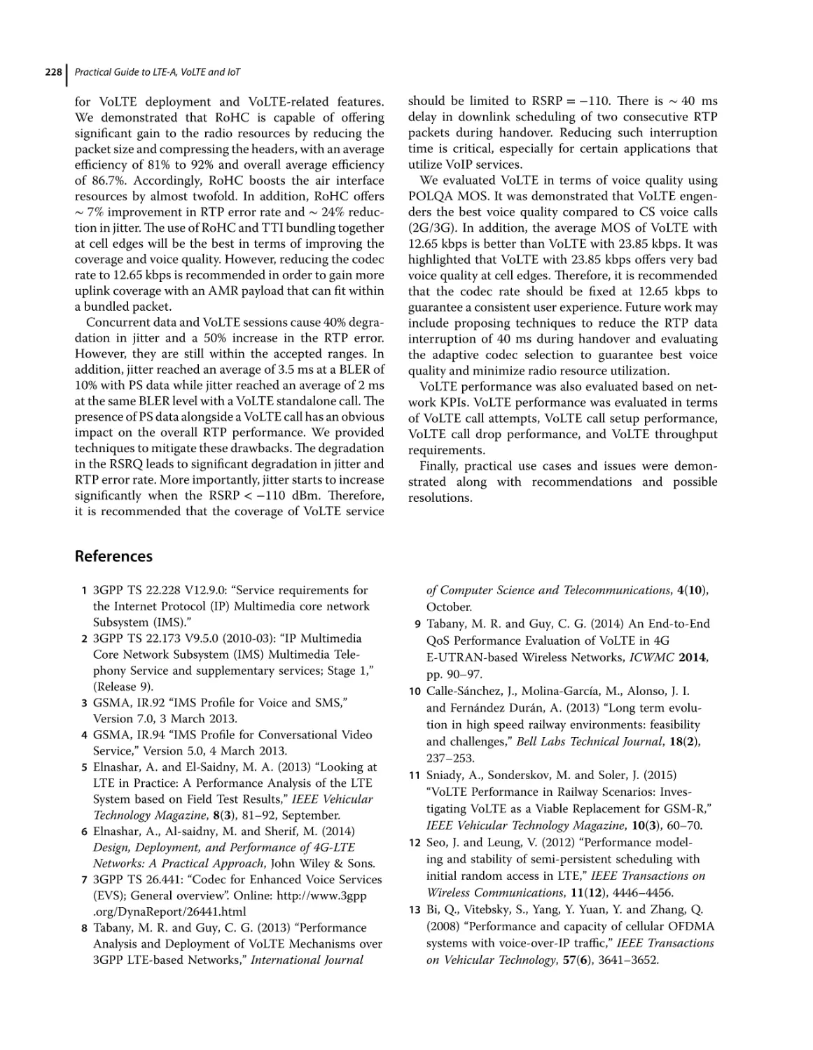
4.12.5
4.13
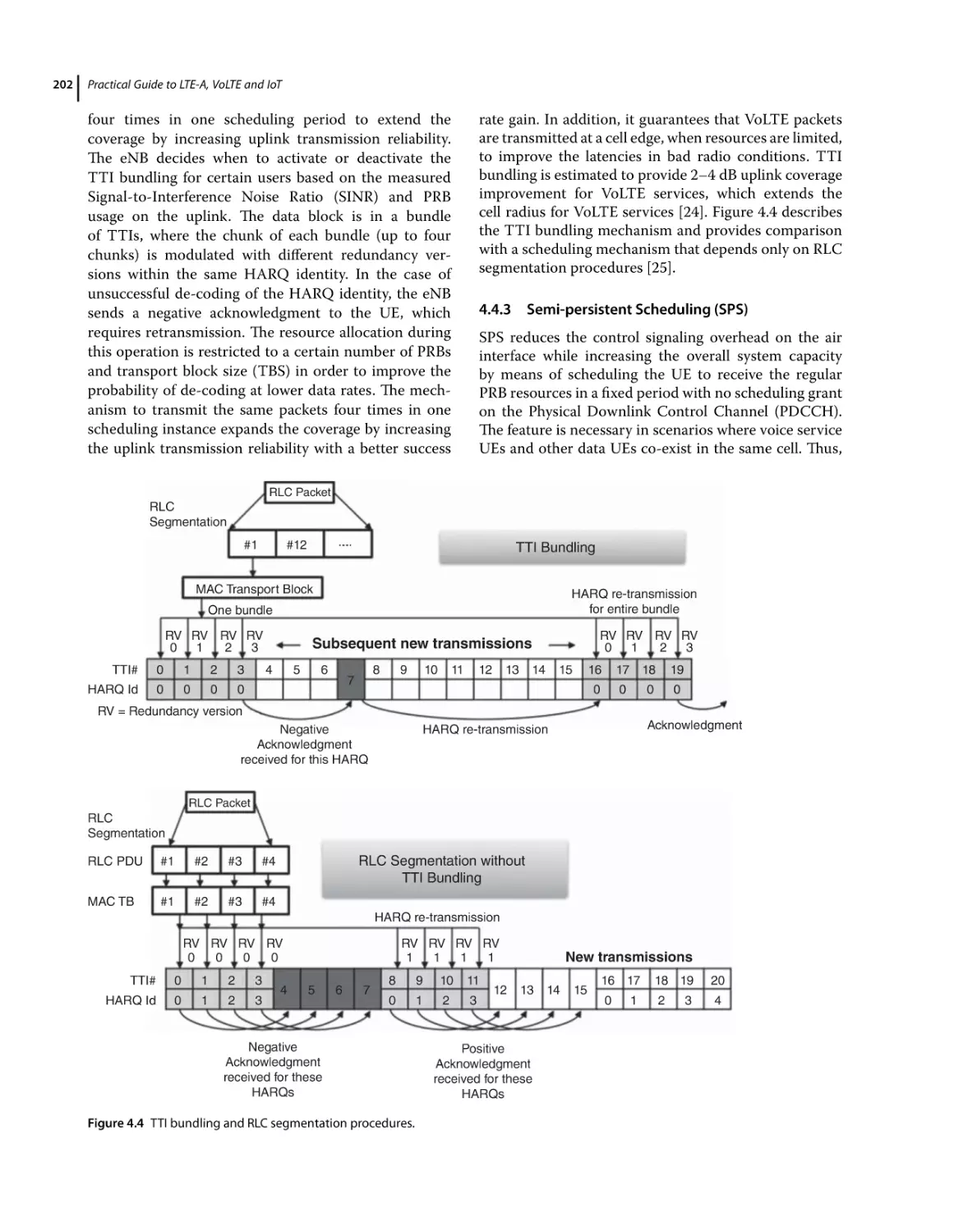
Transmission Time Interval Bundling 201
Semi-persistent Scheduling (SPS) 202
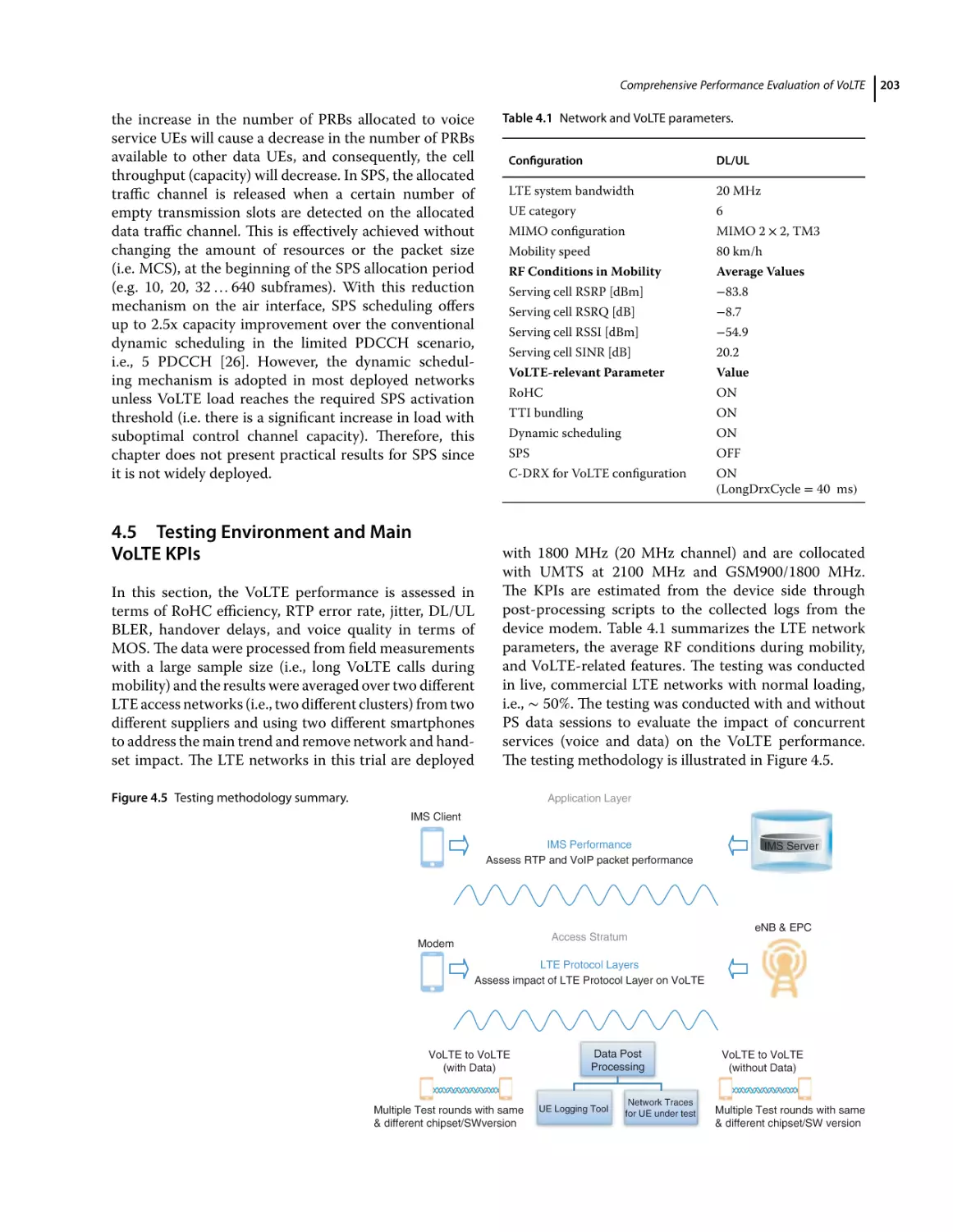
Testing Environment and Main VoLTE KPIs 203
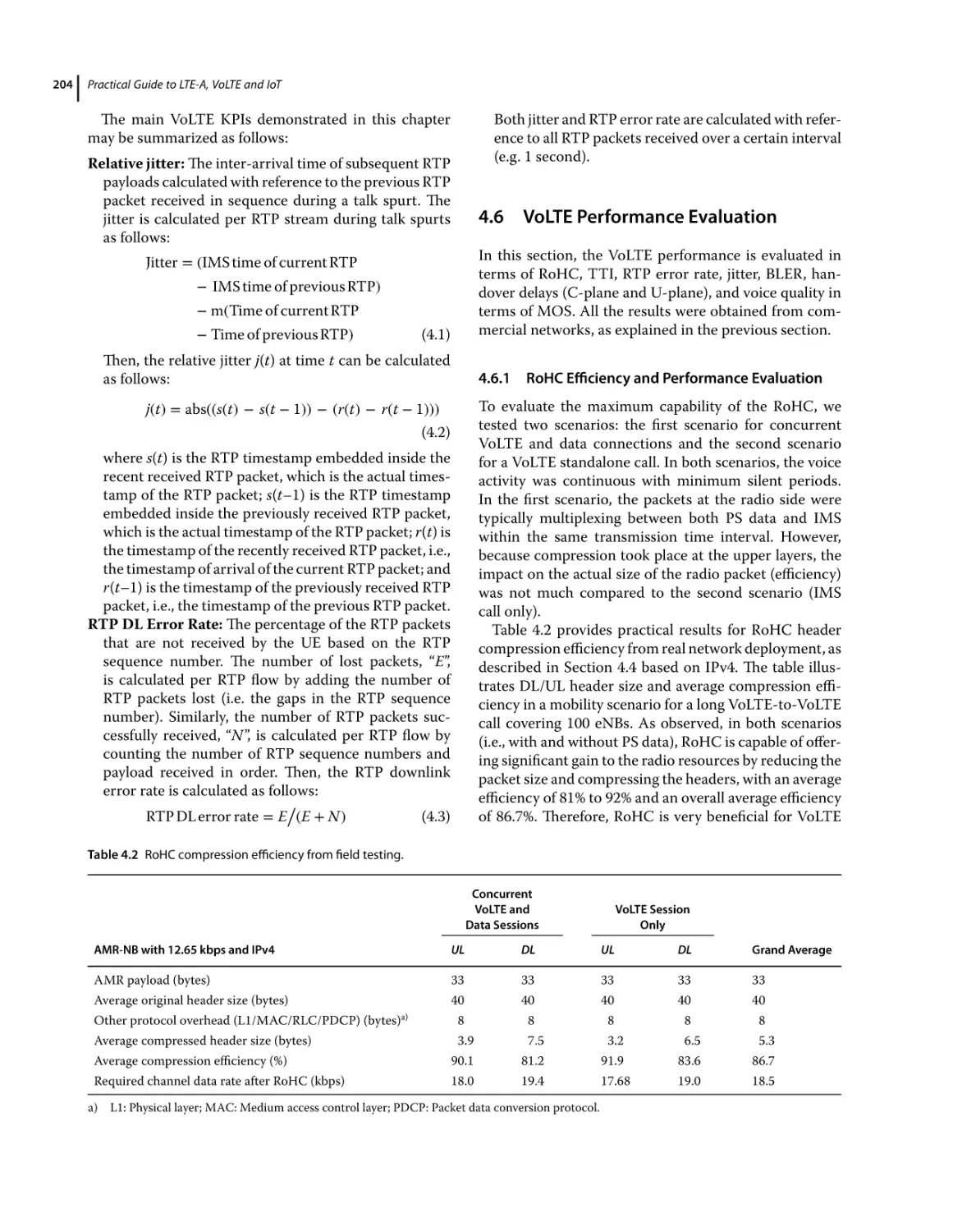
VoLTE Performance Evaluation 204
RoHC Efficiency and Performance Evaluation 204
TTI Bundling 205
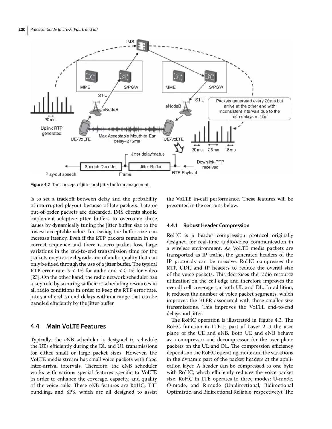
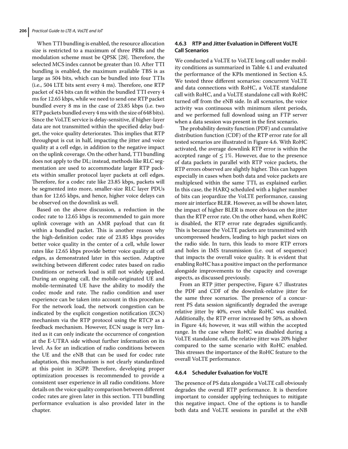
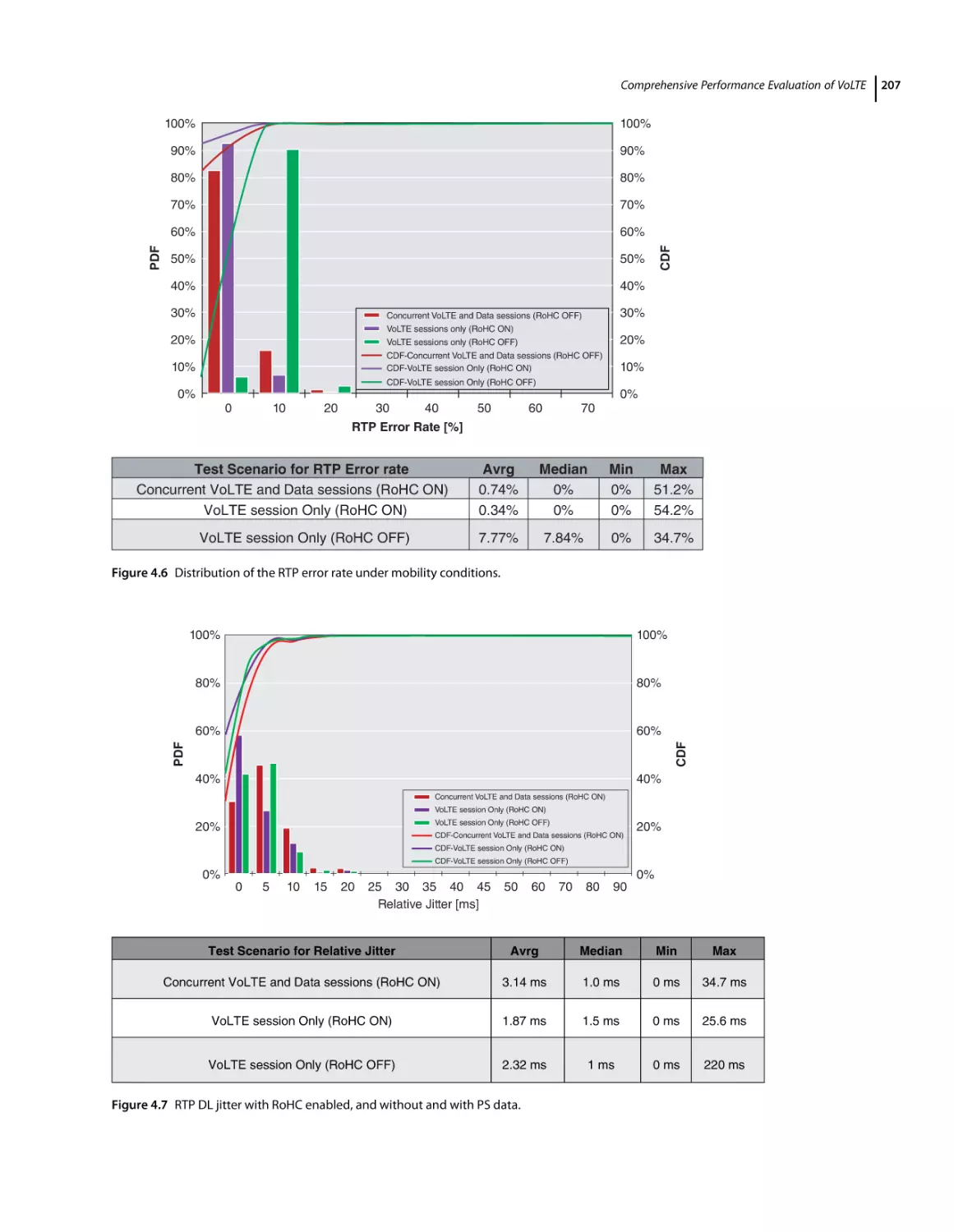
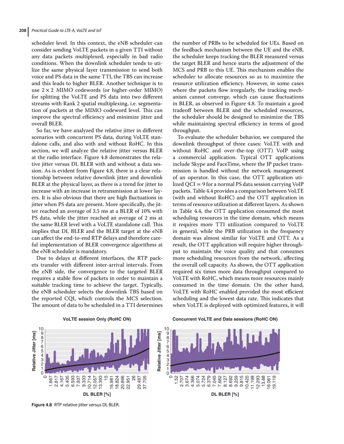
RTP and Jitter Evaluation in Different VoLTE Call Scenarios 206
Scheduler Evaluation for VoLTE 206
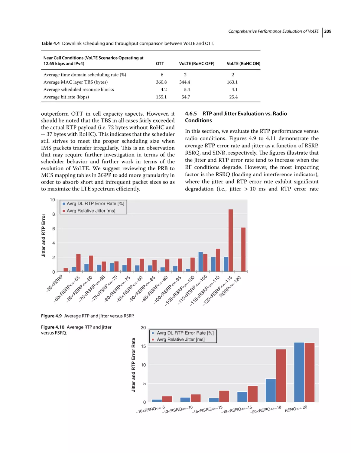
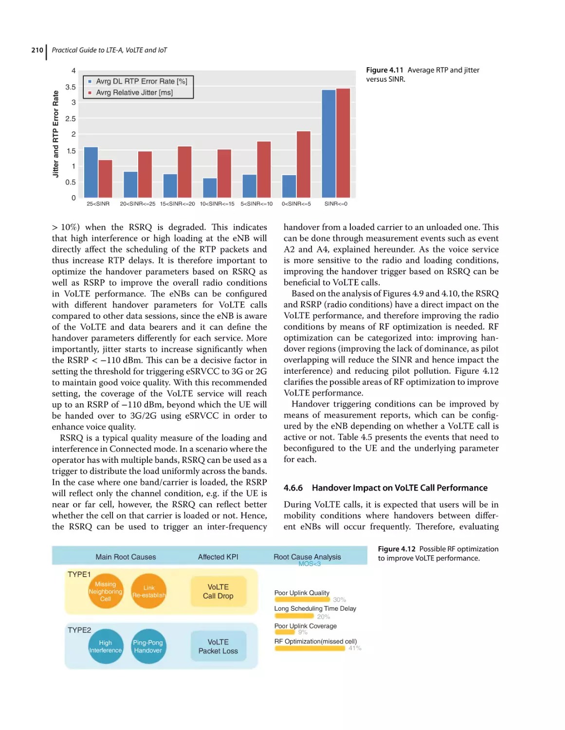
RTP and Jitter Evaluation vs. Radio Conditions 209
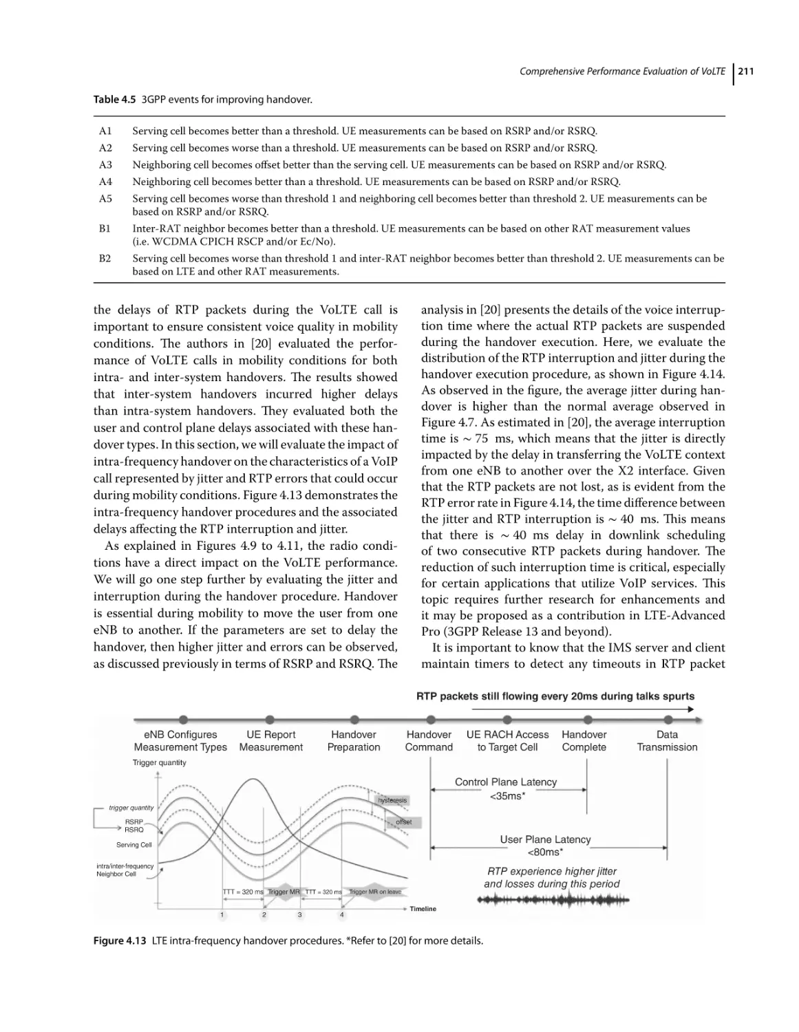
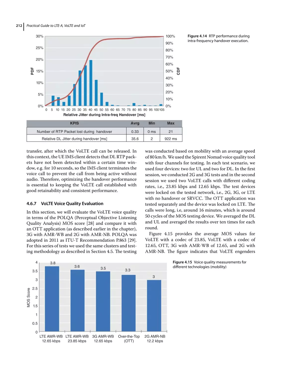
Handover Impact on VoLTE Call Performance 210
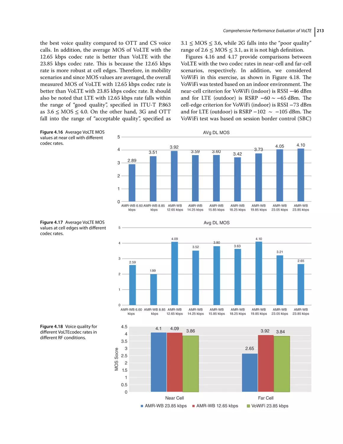
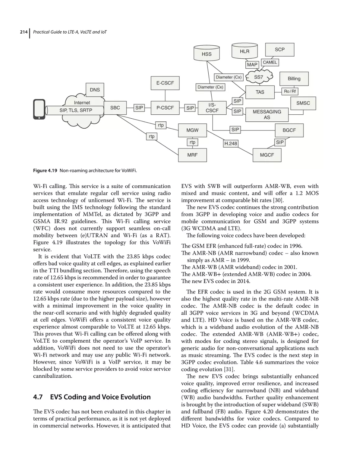
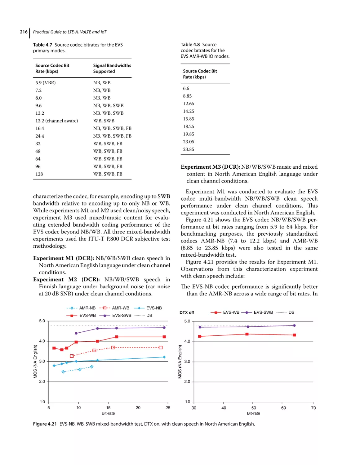
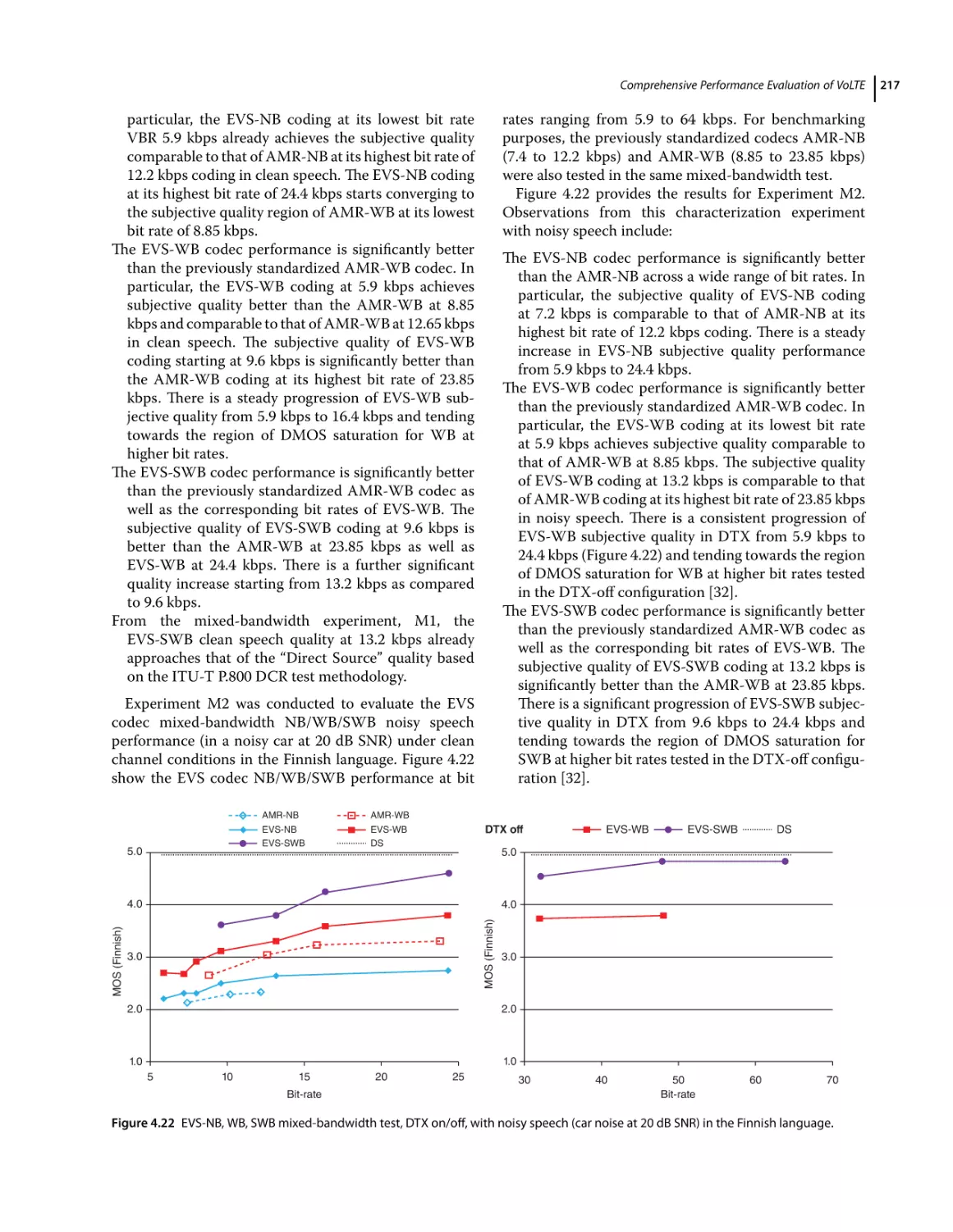
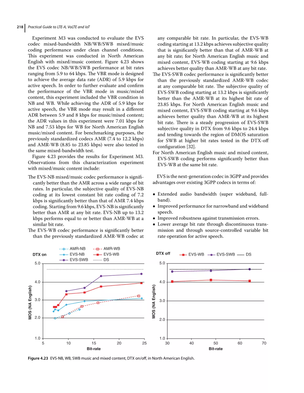
VoLTE Voice Quality Evaluation 212
EVS Coding and Voice Evolution 214
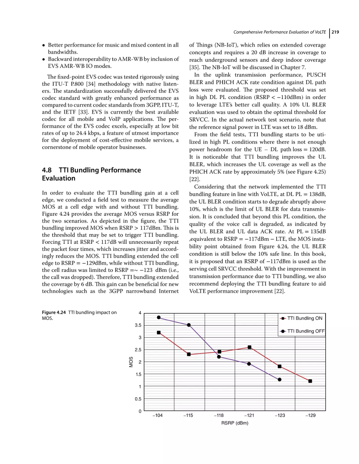
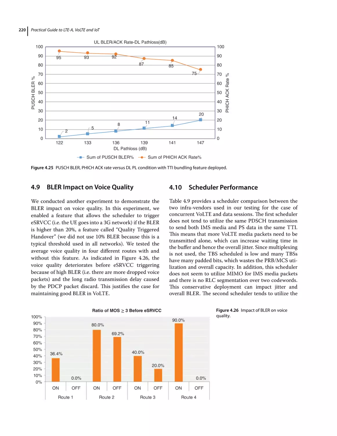
TTI Bundling Performance Evaluation 219
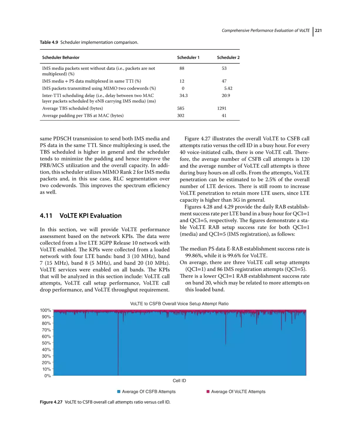
BLER Impact on Voice Quality 220
Scheduler Performance 220
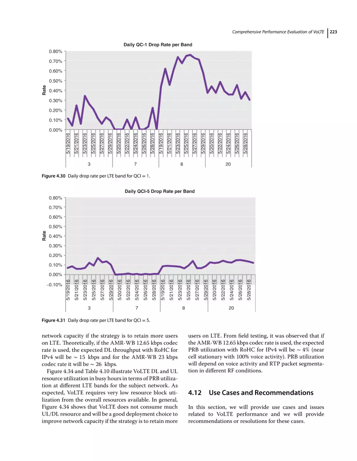
VoLTE KPI Evaluation 221
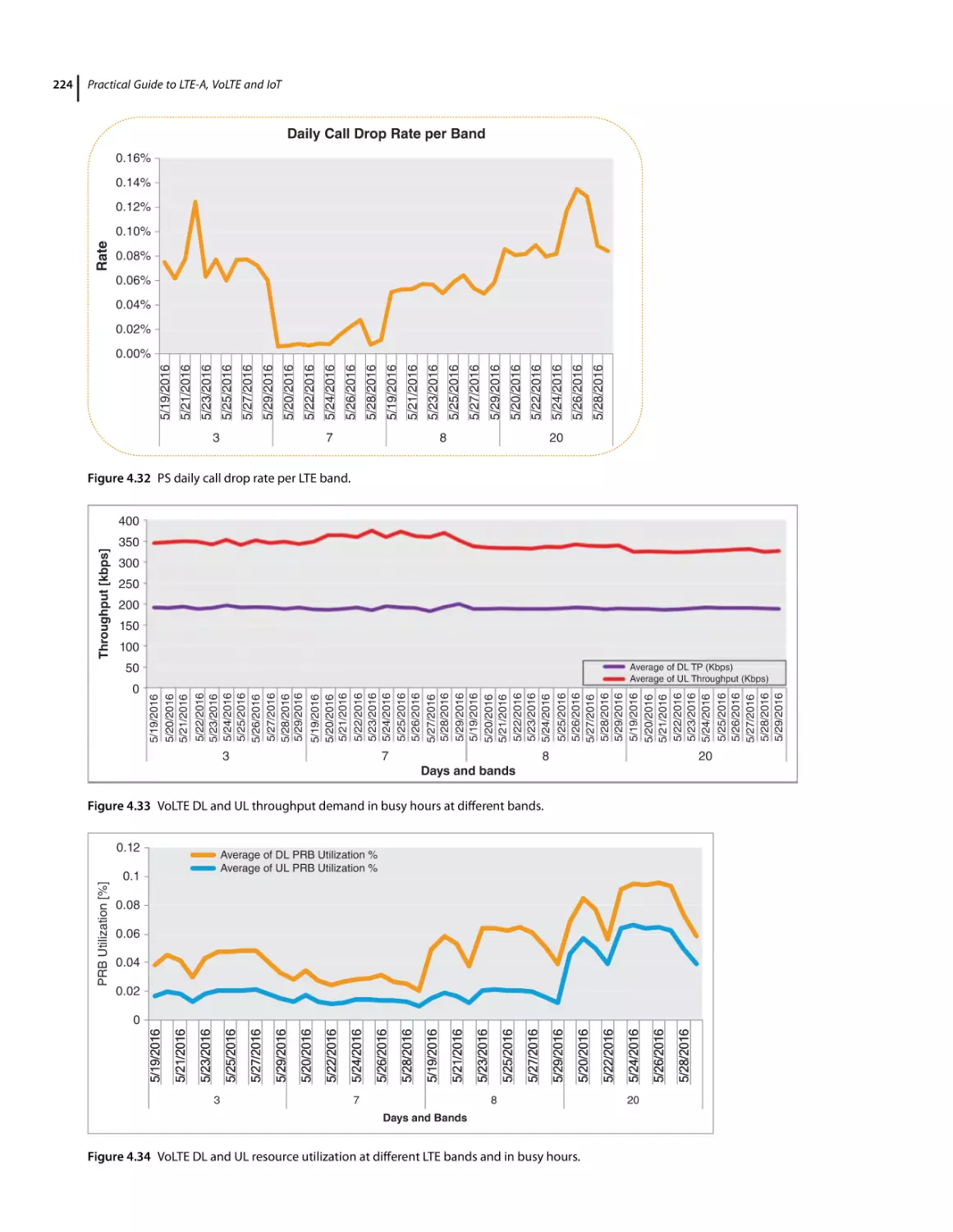
Use Cases and Recommendations 223
Traffic vs. User vs. Throughput Distribution in Busy Hours 225
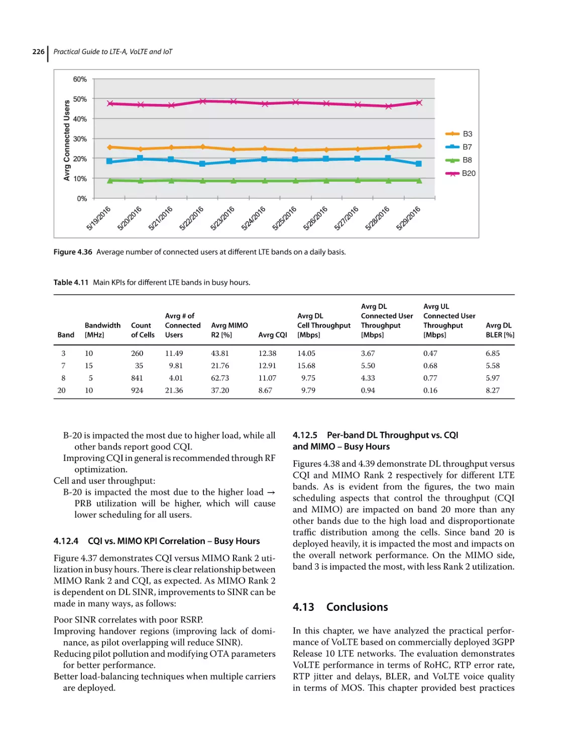
Daily Per-band Share of Average RRC Connected Users – All Hours 225
Main KPIs for Different LTE Bands in Busy Hours 225
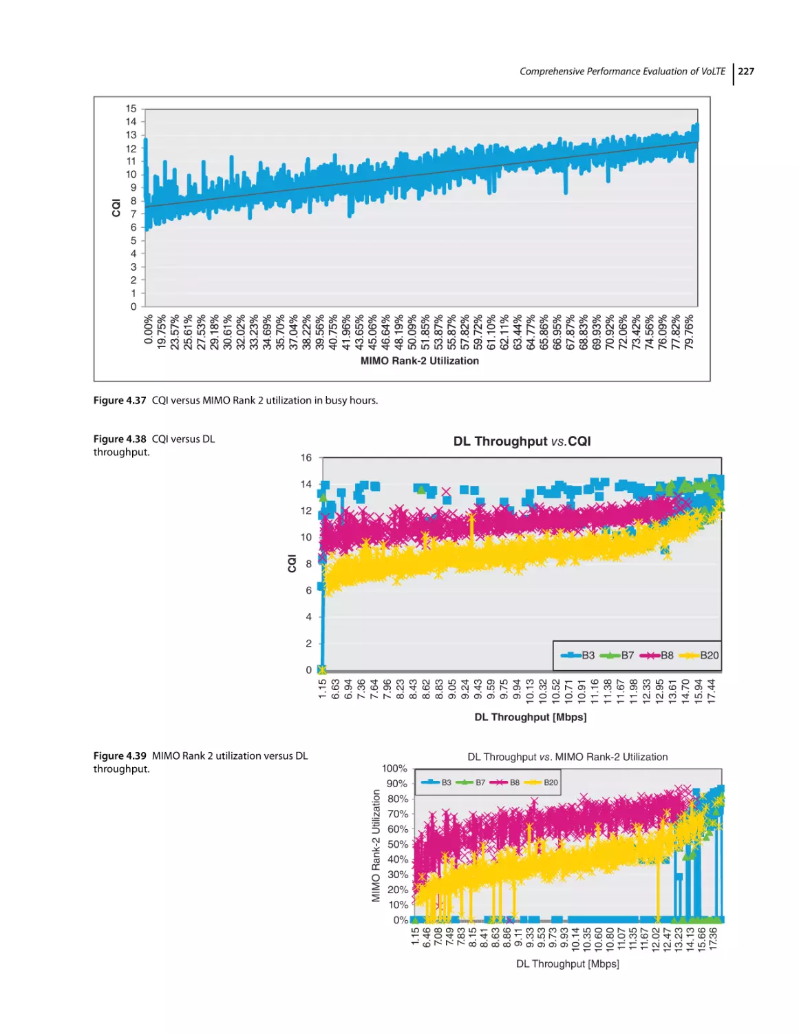
CQI vs. MIMO KPI Correlation – Busy Hours 226
Per-band DL Throughput vs. CQI and MIMO – Busy Hours 226
Conclusions 226
References 228
5
5.1
5.2
5.2.1
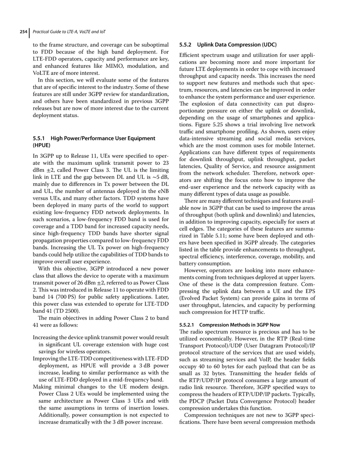
5.2.2
5.2.2.1
5.2.2.2
5.2.2.3
5.2.3
5.2.4
5.3
5.3.1
5.3.2
5.4
5.4.1
5.4.2
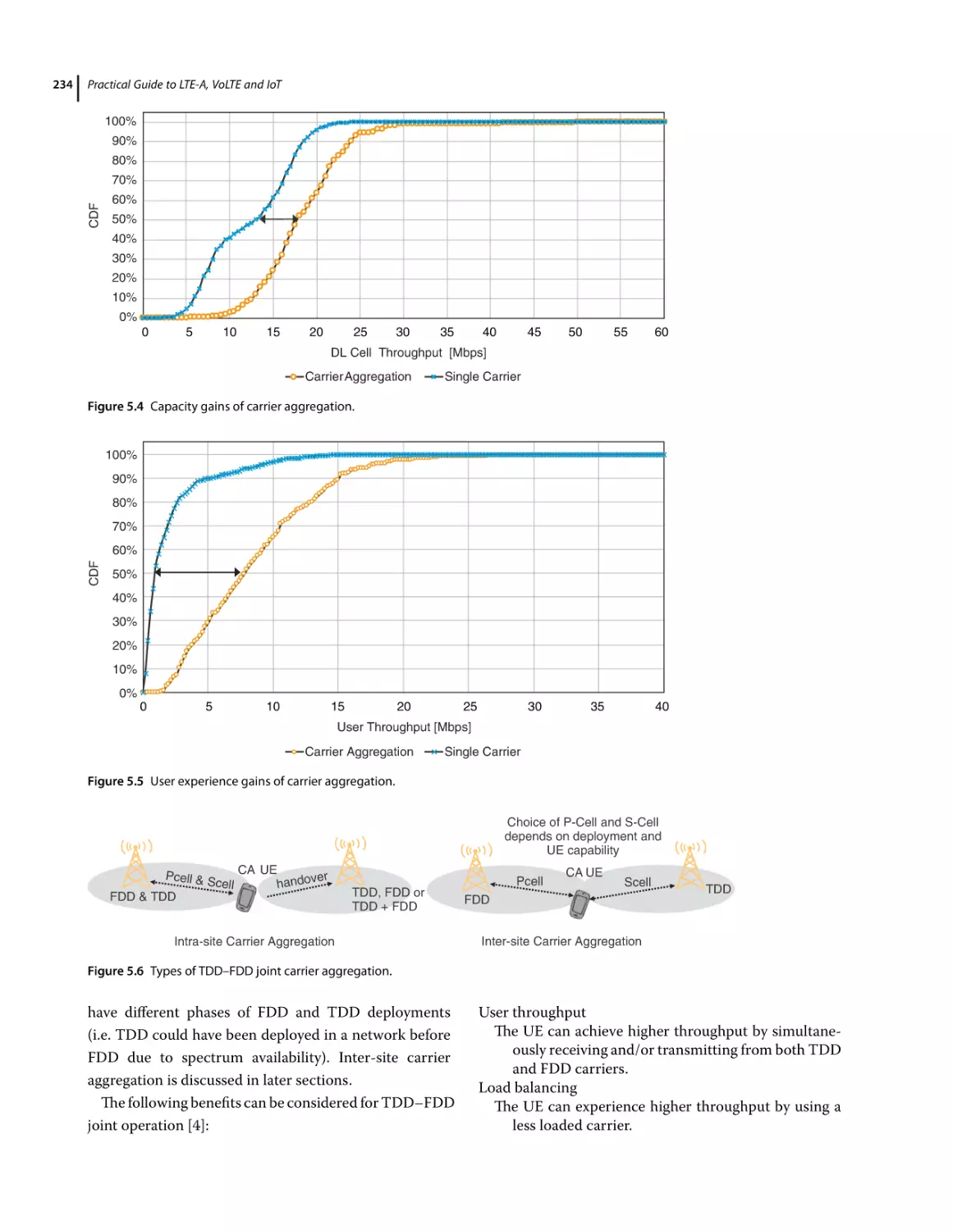
5.5
5.5.1
5.5.2
5.5.2.1
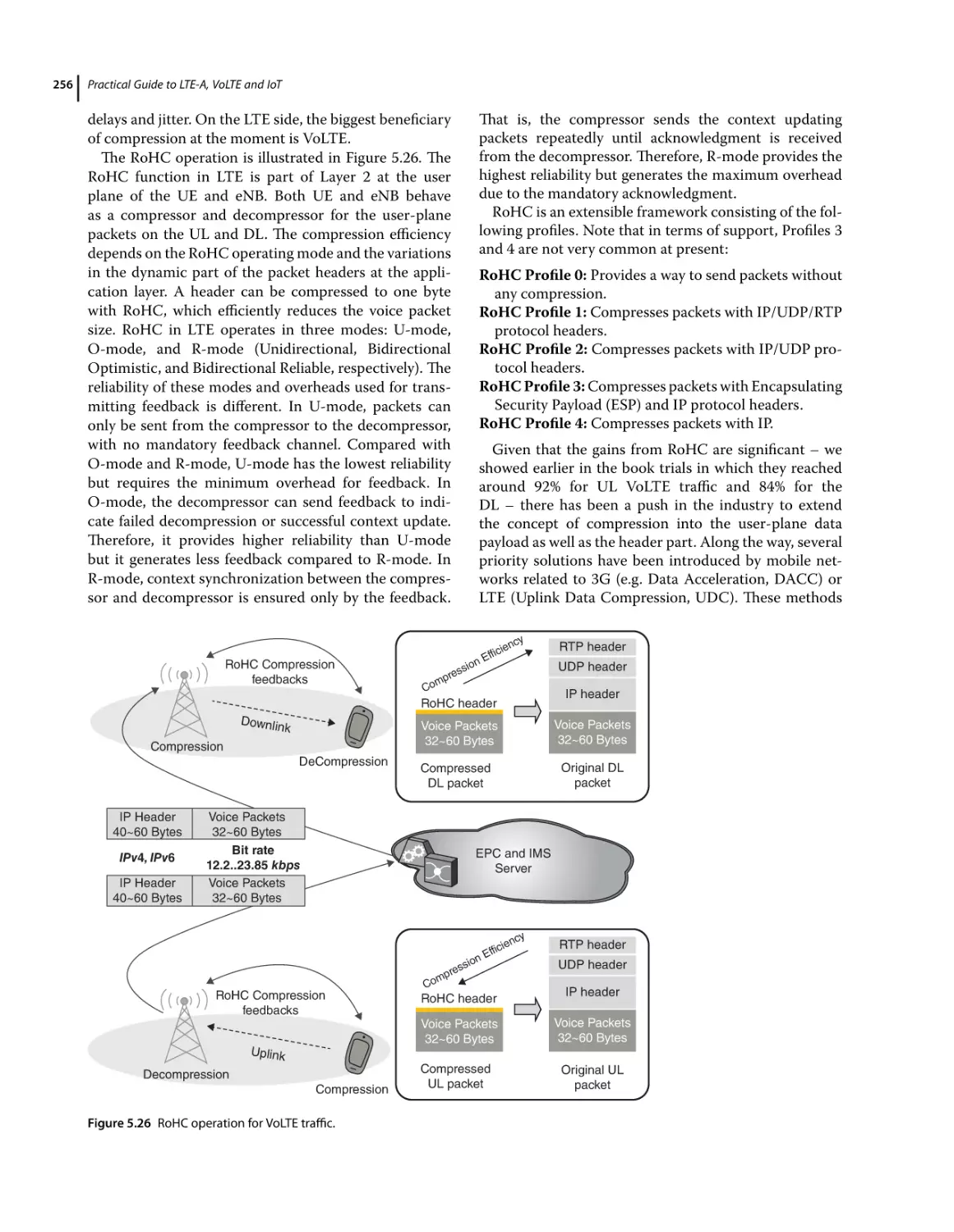
5.5.2.2
5.5.2.3
5.5.2.4
5.5.2.5
5.5.3
230
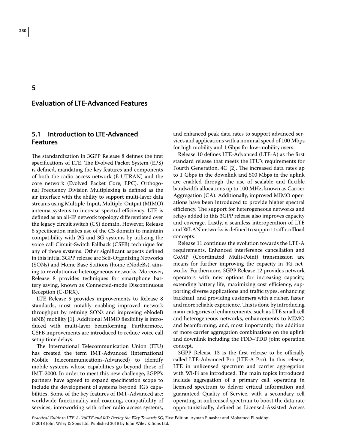
Introduction to LTE-Advanced Features 230
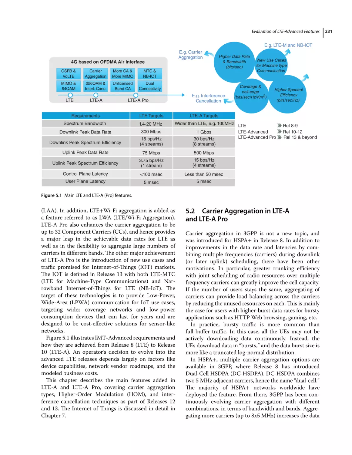
Carrier Aggregation in LTE-A and LTE-A Pro 231
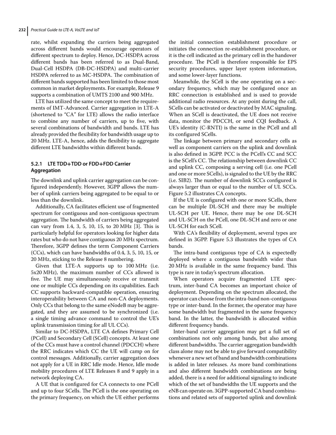
LTE TDD+TDD or FDD+FDD Carrier Aggregation 232
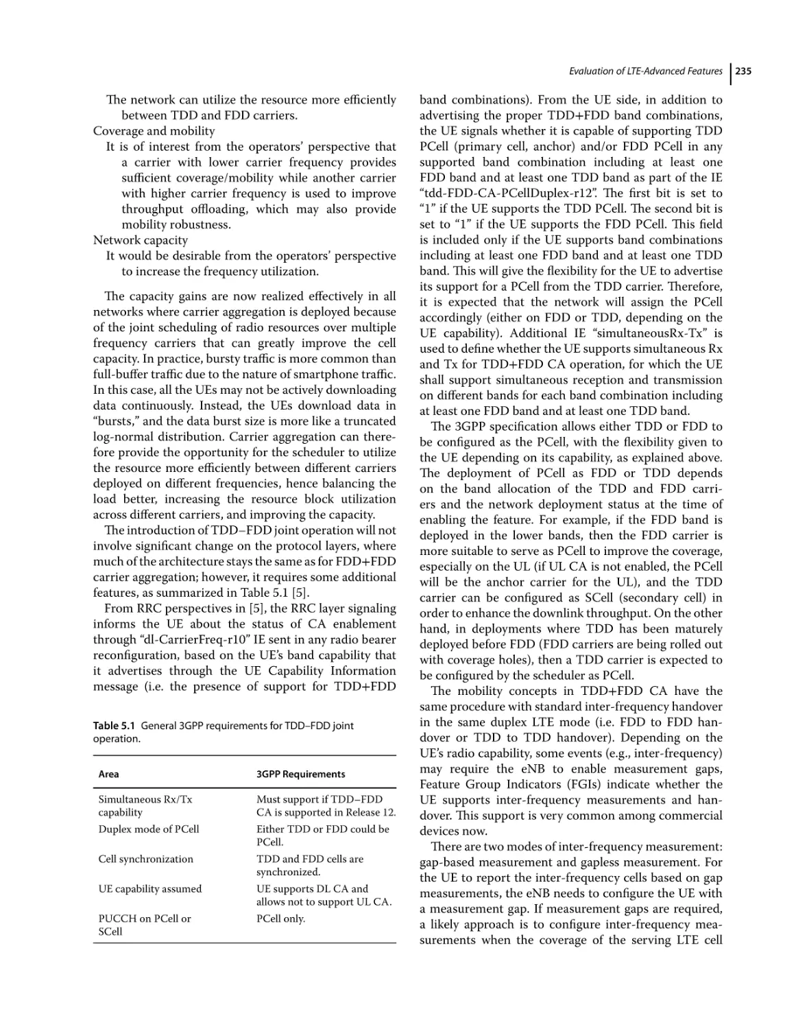
FDD–TDD Joint Operation 233
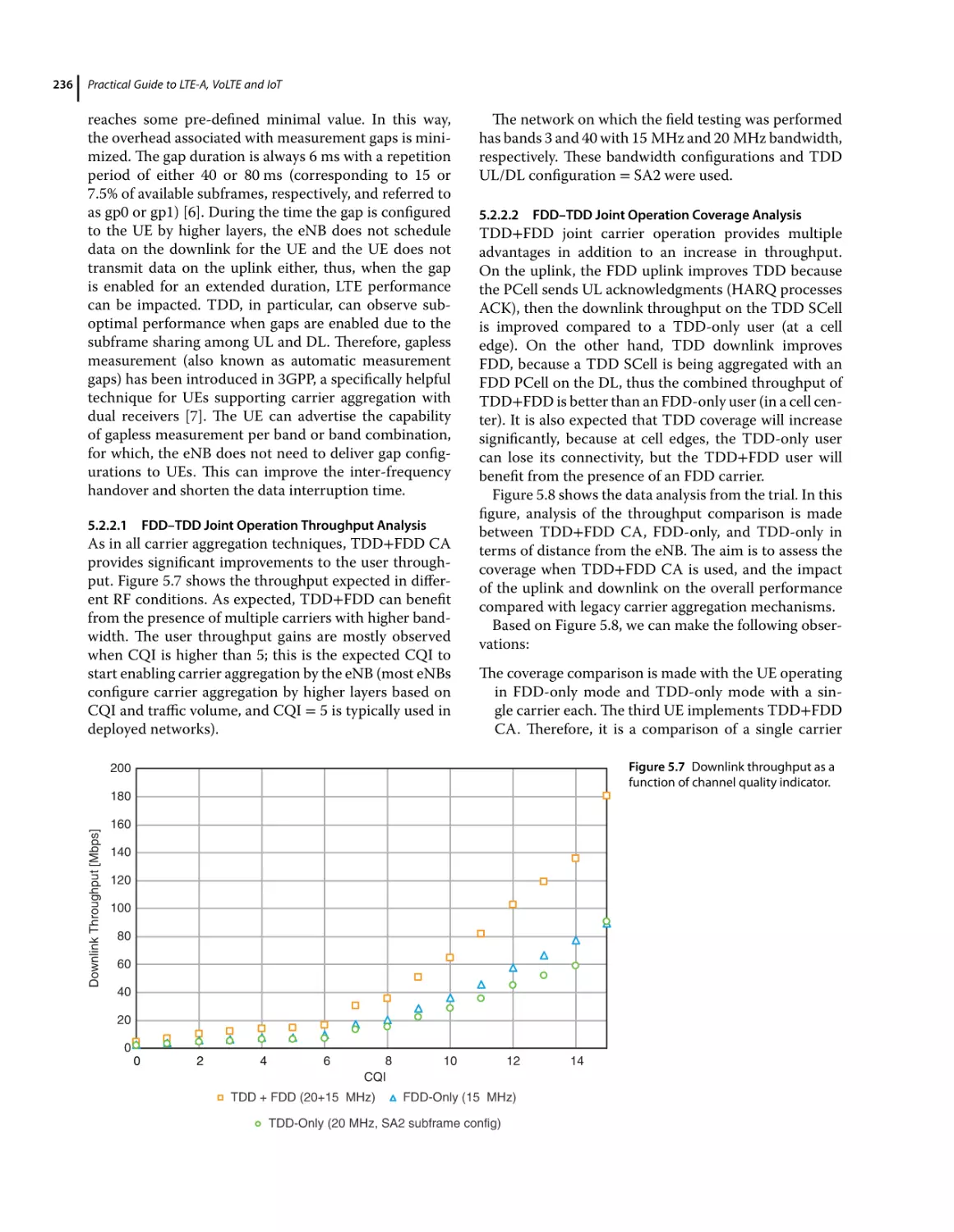
FDD–TDD Joint Operation Throughput Analysis 236
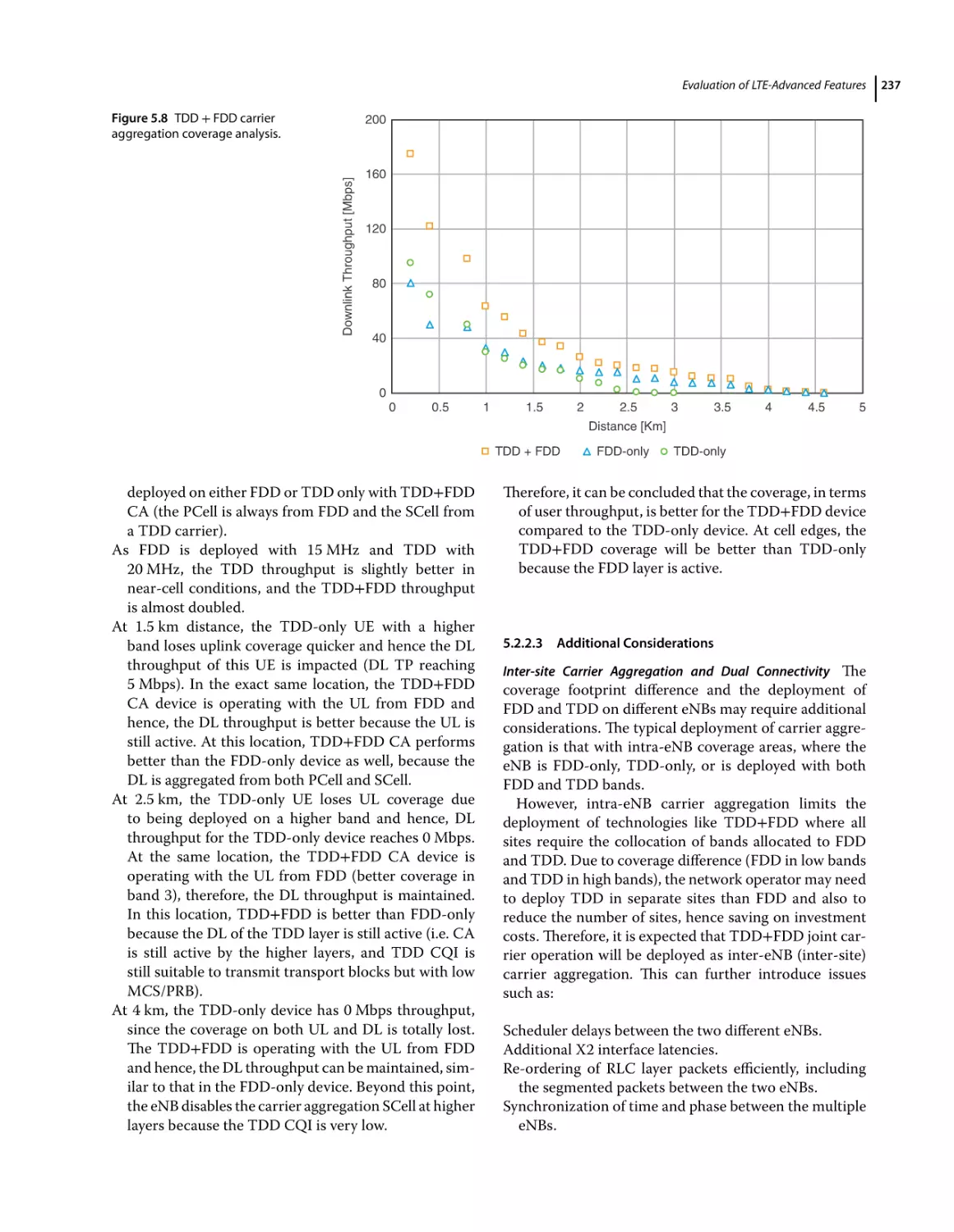
FDD–TDD Joint Operation Coverage Analysis 236
Additional Considerations 237
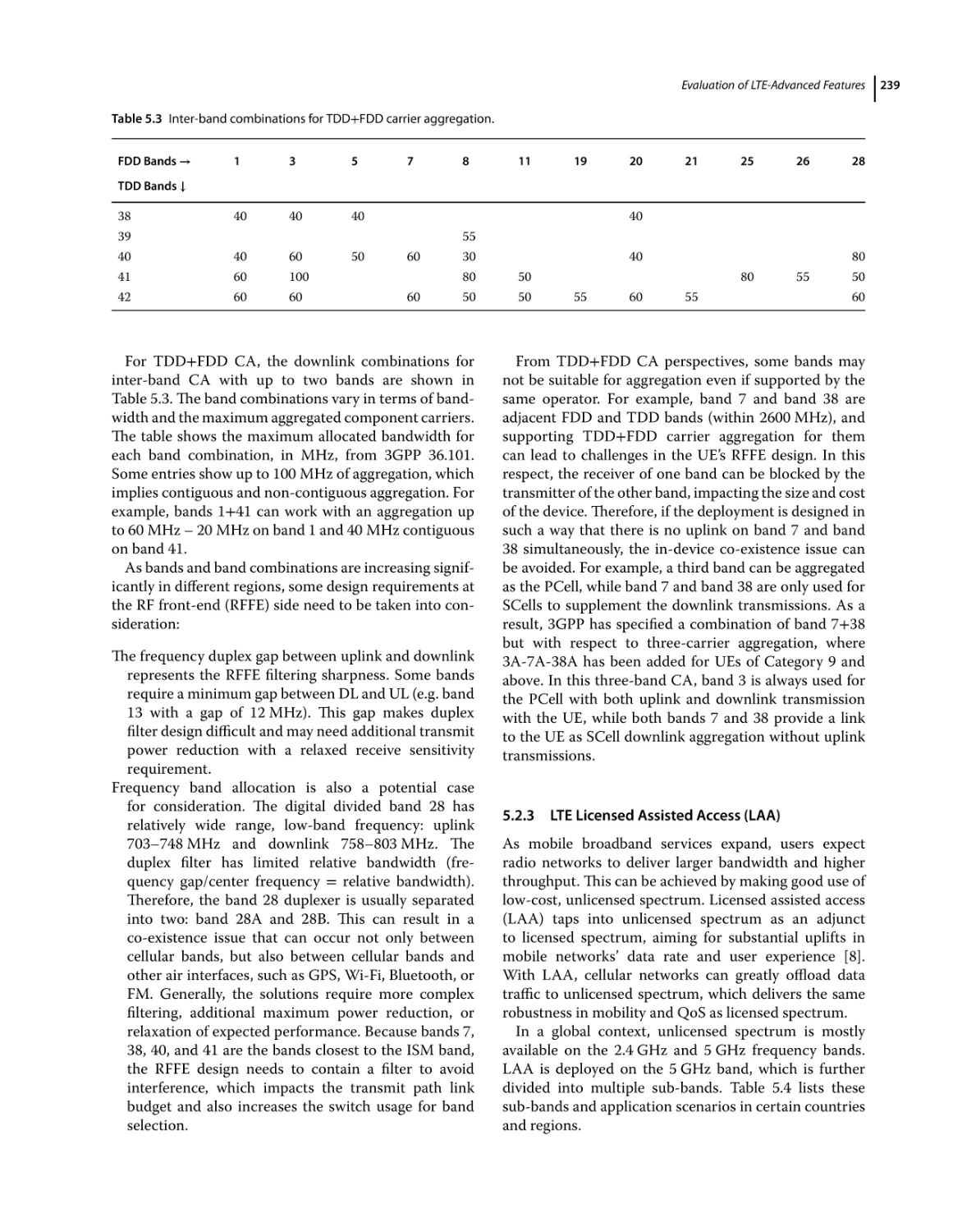
LTE Licensed Assisted Access (LAA) 239
LTE and Wi-Fi Aggregation (LWA) 241
Higher-order Modulation (HOM) for Uplink and Downlink 242
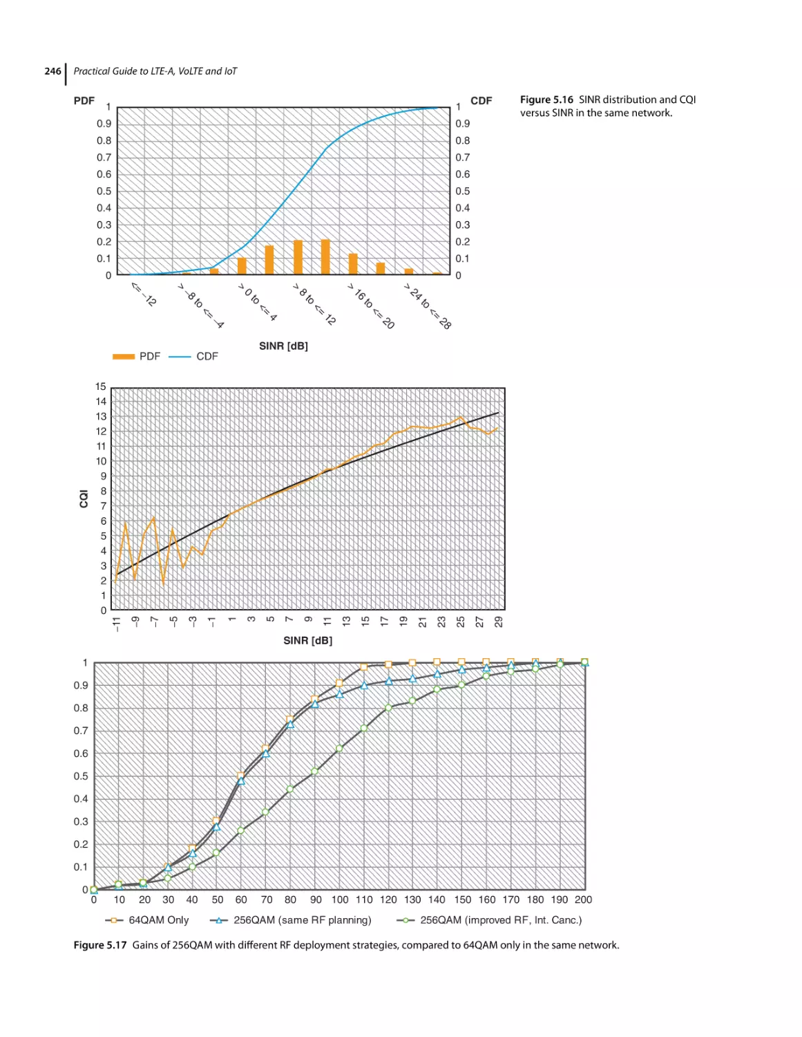
Downlink 256QAM 243
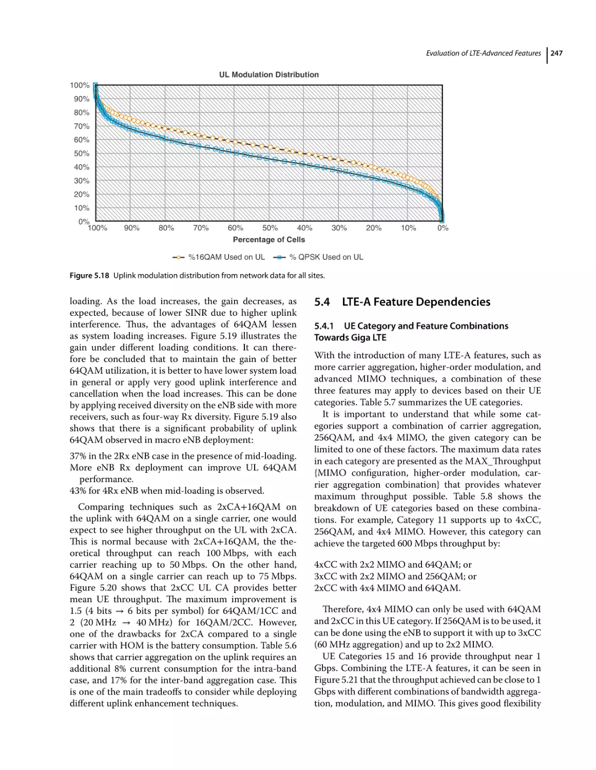
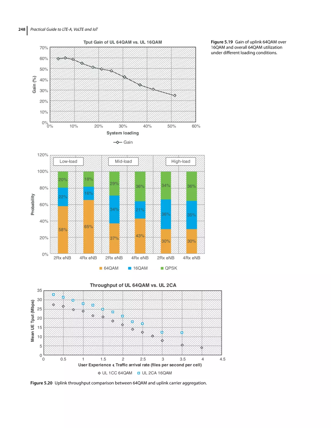
Uplink 64QAM 244
LTE-A Feature Dependencies 247
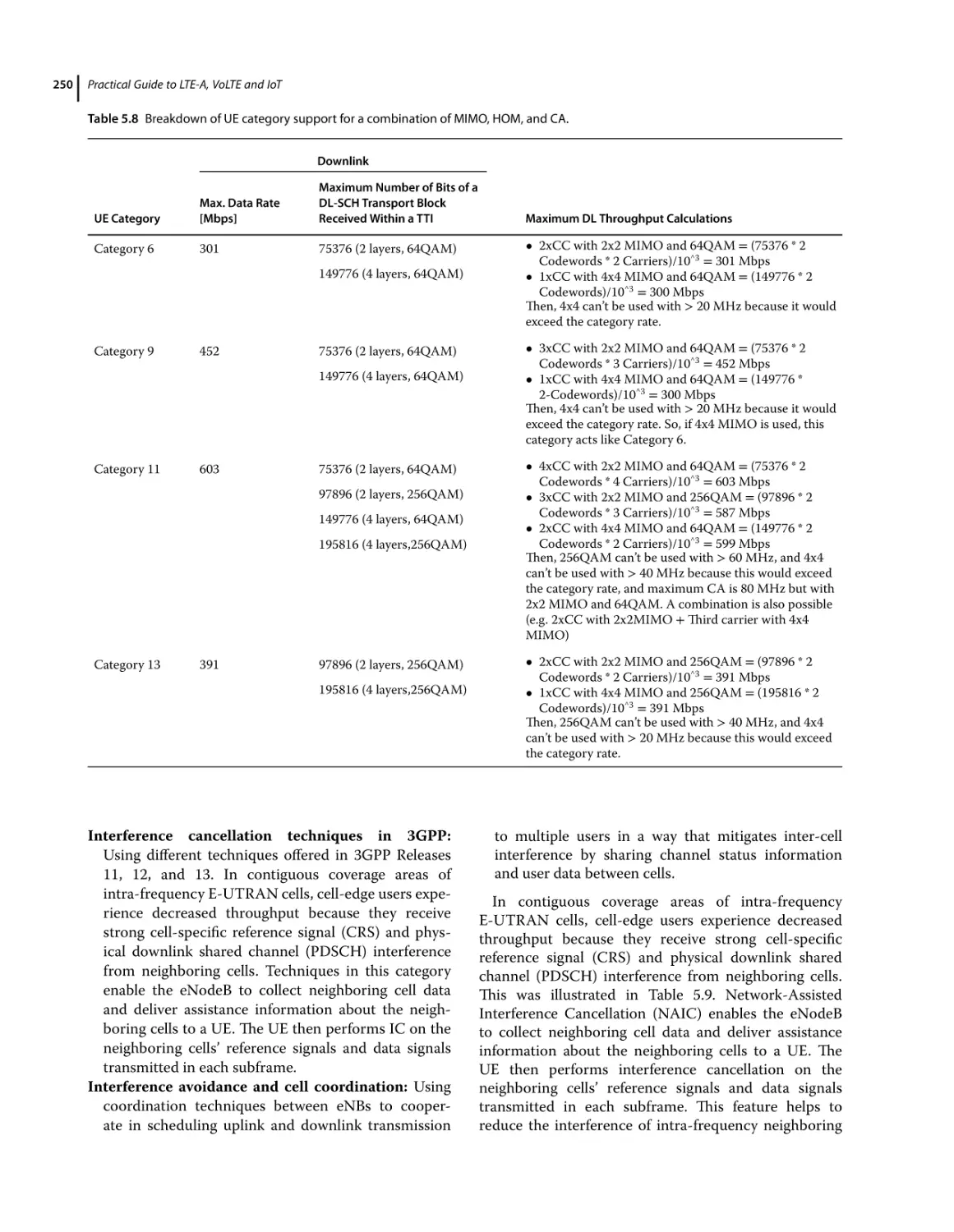
UE Category and Feature Combinations Towards Giga LTE 247
Interference Cancellation and Coordination Techniques 249
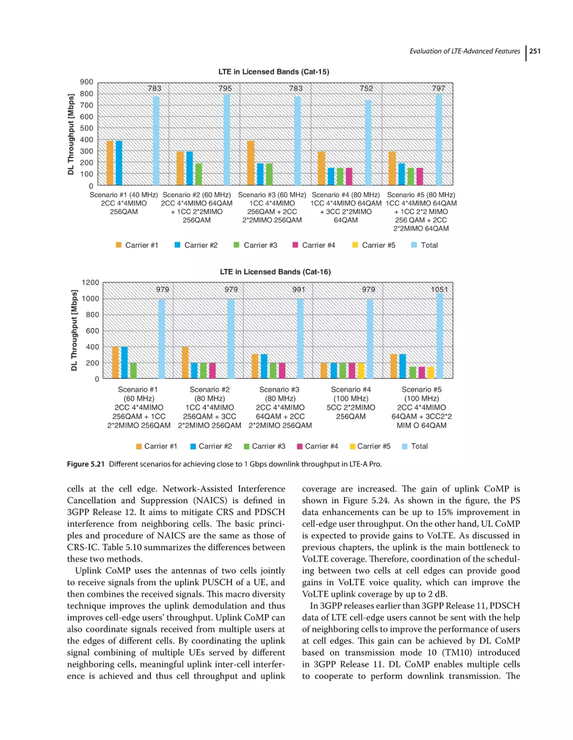
Other Enhancements Towards Advanced LTE Deployments 252
High Power/Performance User Equipment (HPUE) 254
Uplink Data Compression (UDC) 254
Compression Methods in 3GPP Now 254
Possible Applicable LTE Mode of Data Compression 257
Uplink Data Compression Performance Analysis Using RoHC 259
Performance Aspects of Uplink Data RoHC 259
Highlights of UDC Development and Challenges 260
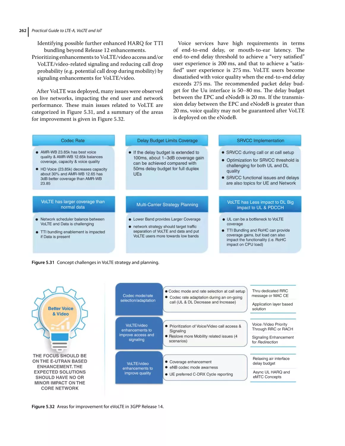
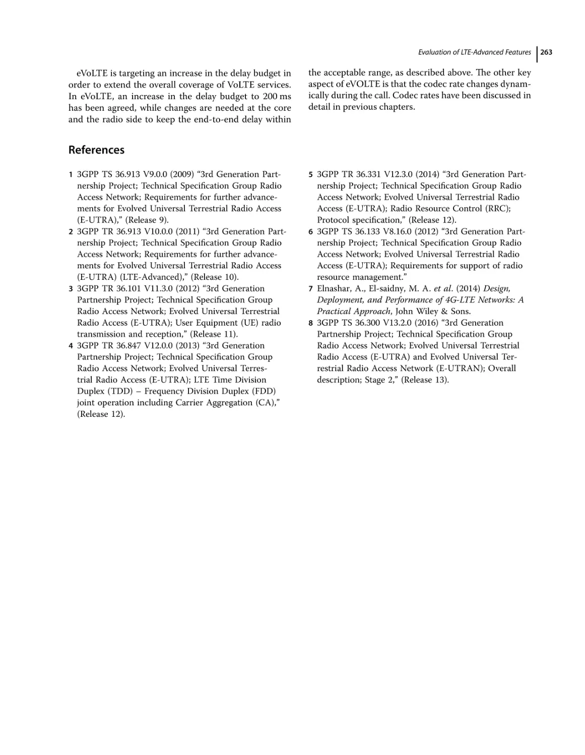
Enhanced VoLTE (eVoLTE) 261
References 263
6
LTE Network Capacity Analysis
6.1
6.2
Overview 264
Introduction 264
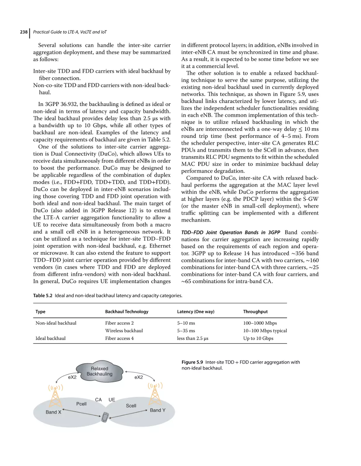
Evaluation of LTE-Advanced Features
264
Contents
6.3
6.3.1
6.3.2
6.3.3
6.3.4
6.4
6.4.1
6.4.2
6.4.3
6.4.4
6.4.5
6.5
6.5.1
6.5.2
6.5.3
6.5.4
6.5.5
6.5.6
6.5.6.1
6.5.6.2
6.5.7
6.5.8
6.5.9
6.5.10
6.5.11
6.6
6.6.1
6.6.2
6.6.3
6.6.4
6.6.5
6.6.6
6.6.7
6.6.8
6.6.8.1
6.6.8.2
6.6.9
6.6.10
6.7
6.7.1
6.7.2
6.7.3
6.7.4
6.8
6.8.1
6.8.1.1
6.9
6.9.1
6.9.2
6.9.3
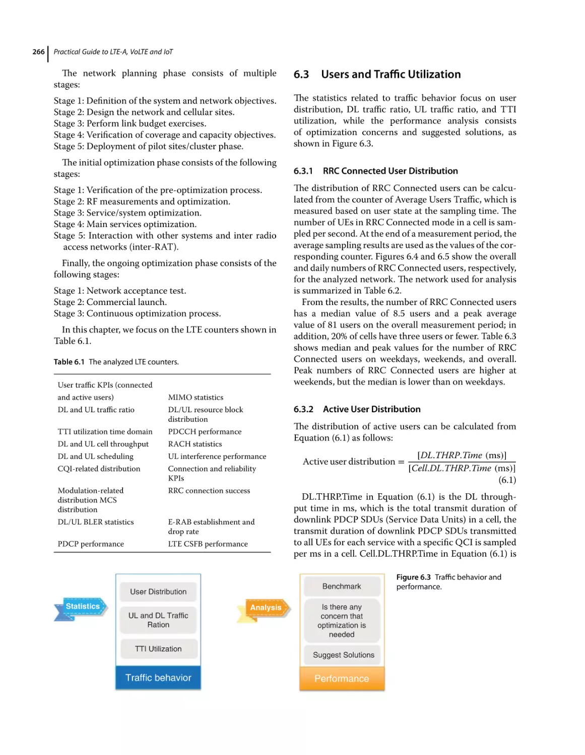
Users and Traffic Utilization 266
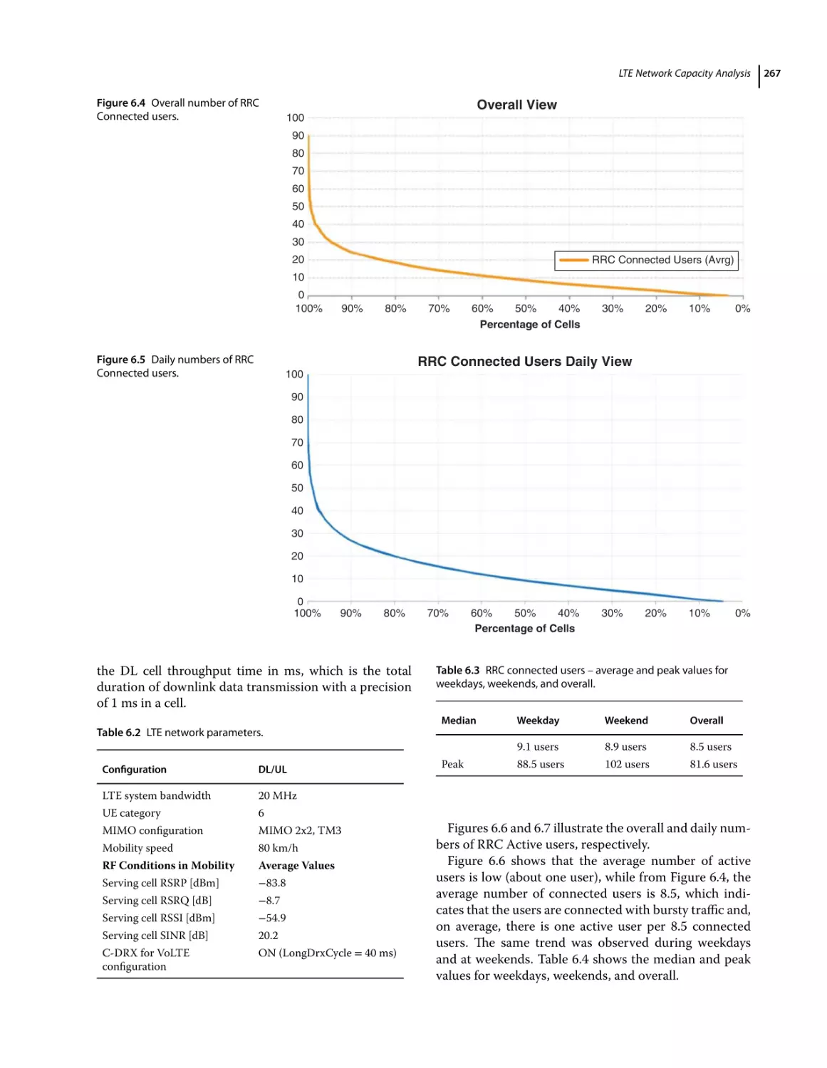
RRC Connected User Distribution 266
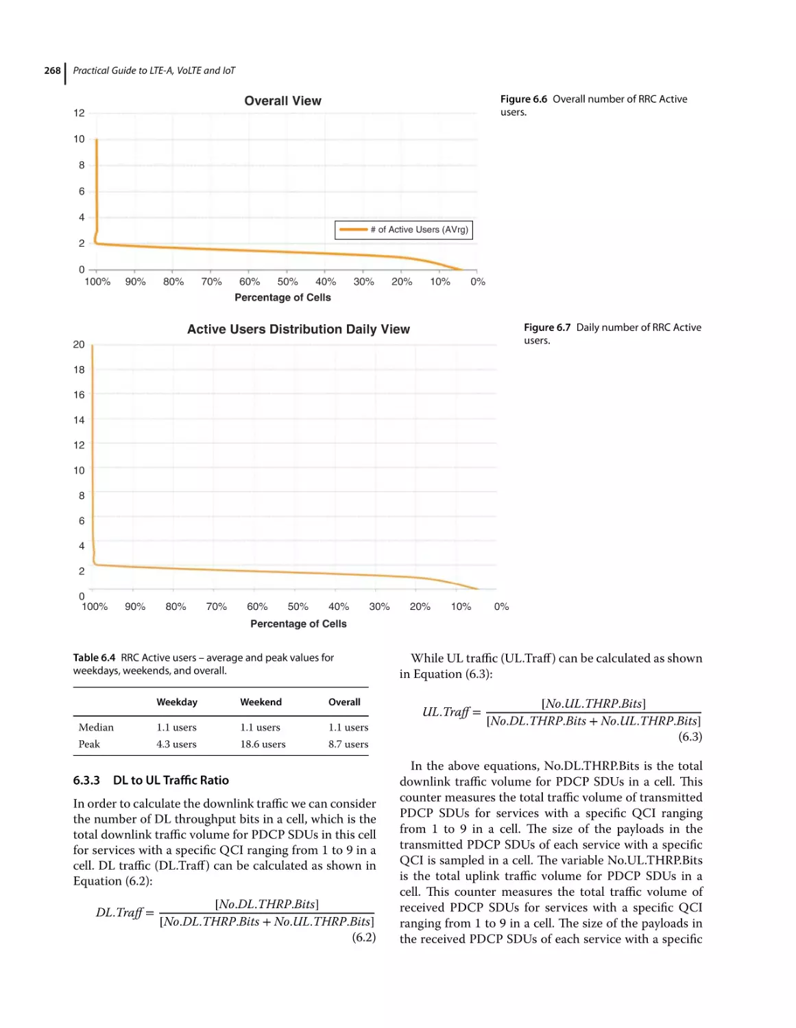
Active User Distribution 266
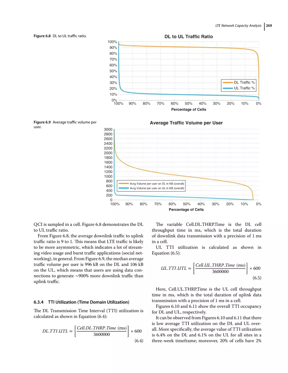
DL to UL Traffic Ratio 268
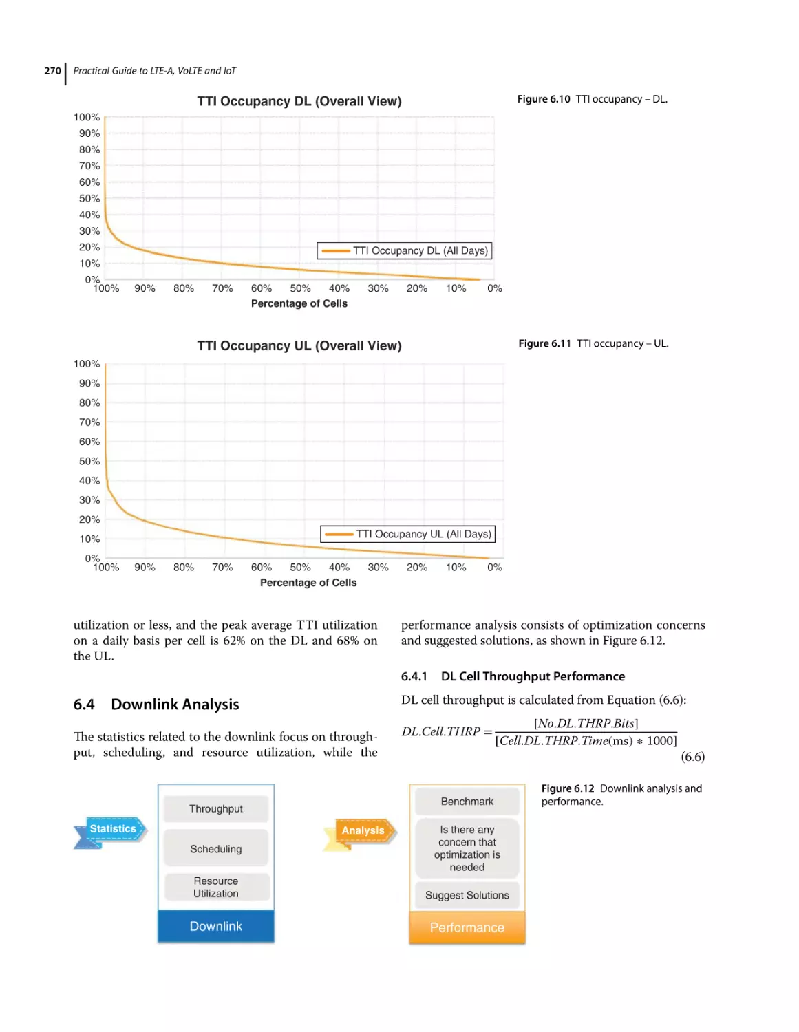
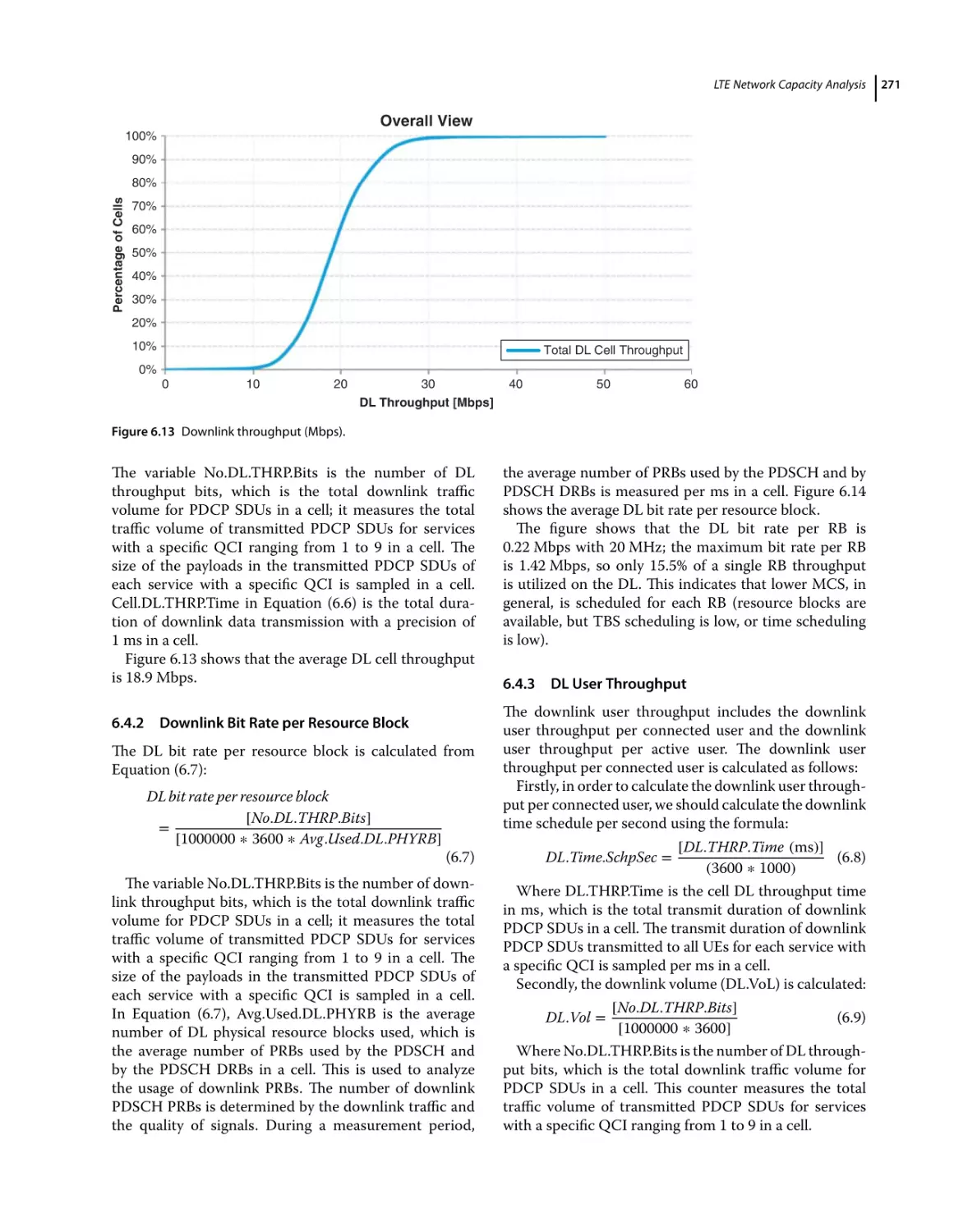
TTI Utilization (Time Domain Utilization) 269
Downlink Analysis 270
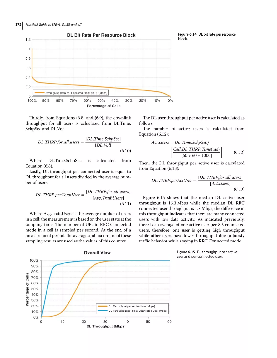
DL Cell Throughput Performance 270
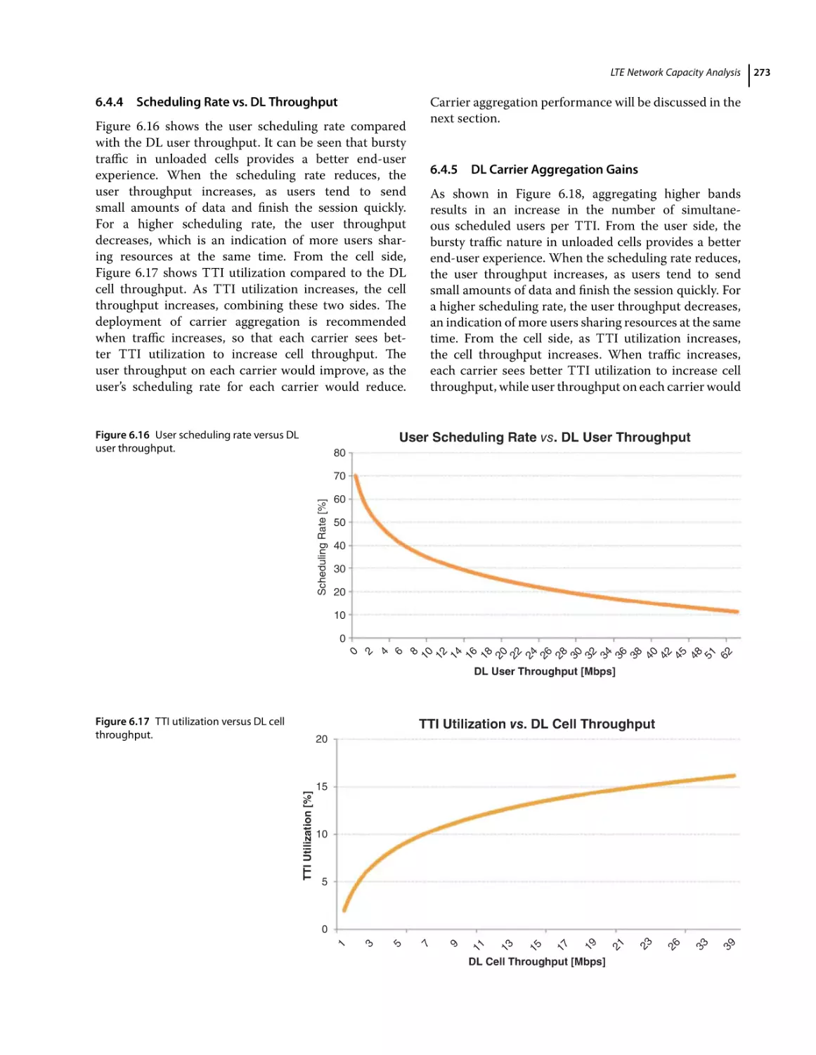
Downlink Bit Rate per Resource Block 271
DL User Throughput 271
Scheduling Rate vs. DL Throughput 273
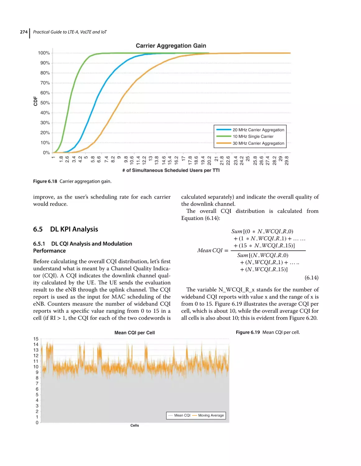
DL Carrier Aggregation Gains 273
DL KPI Analysis 274
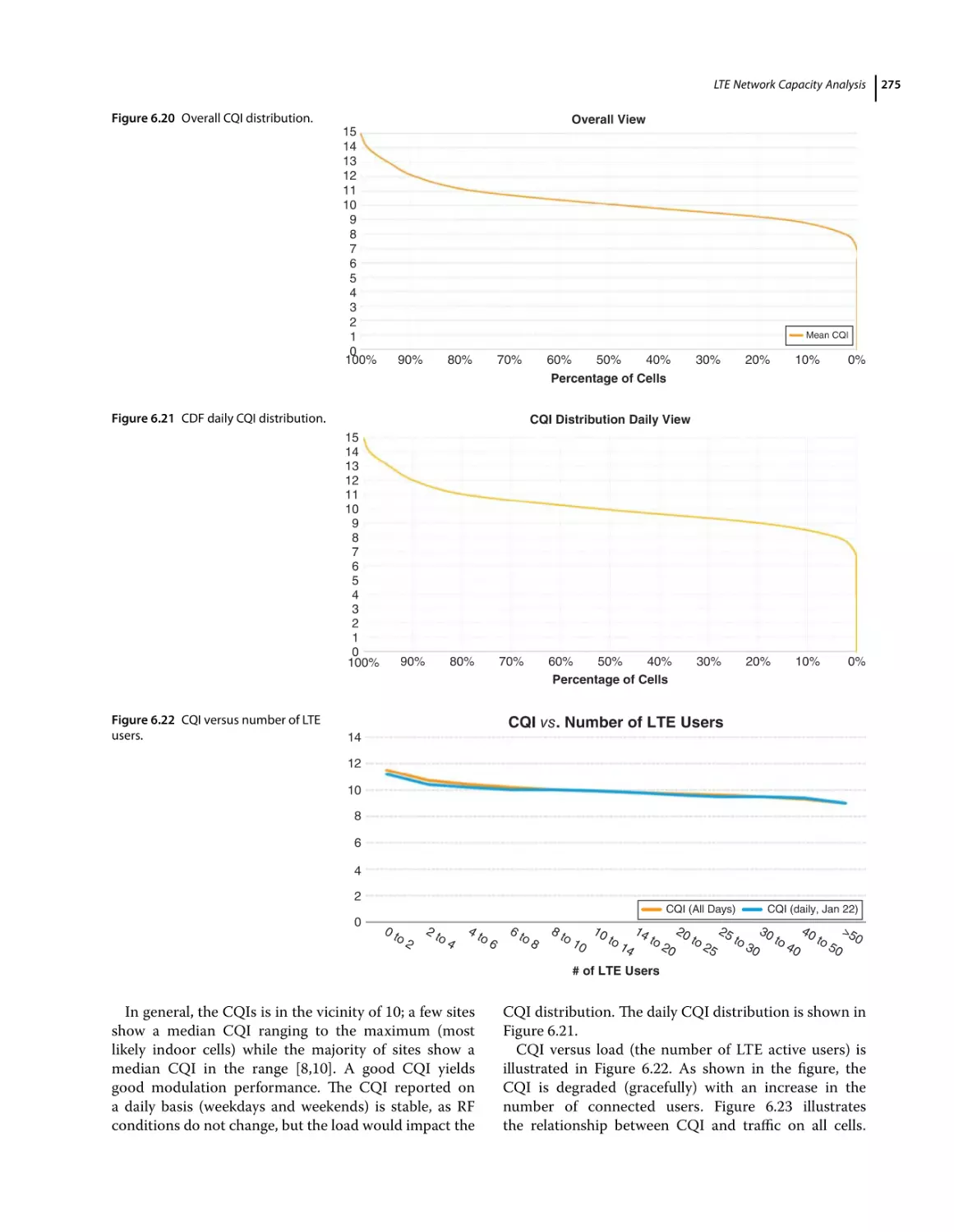
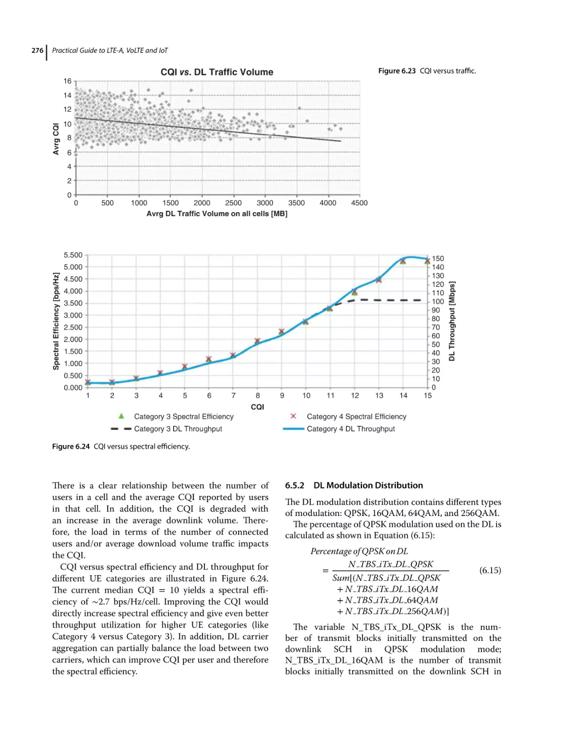
DL CQI Analysis and Modulation Performance 274
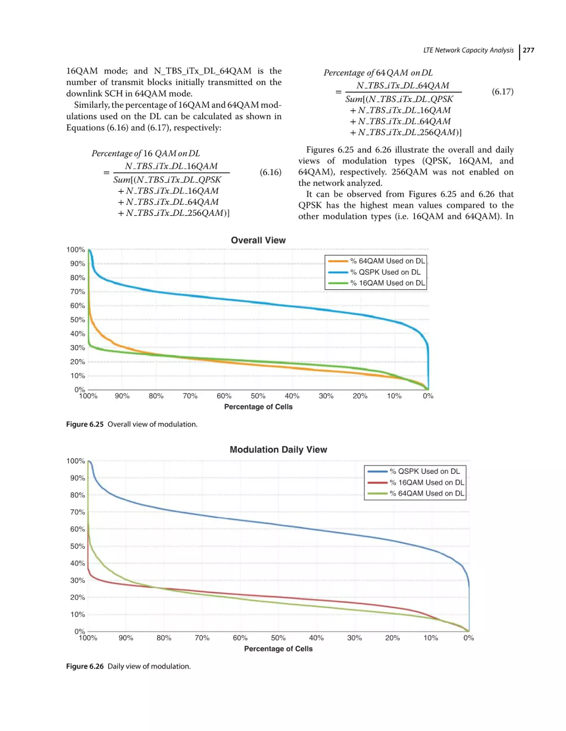
DL Modulation Distribution 276
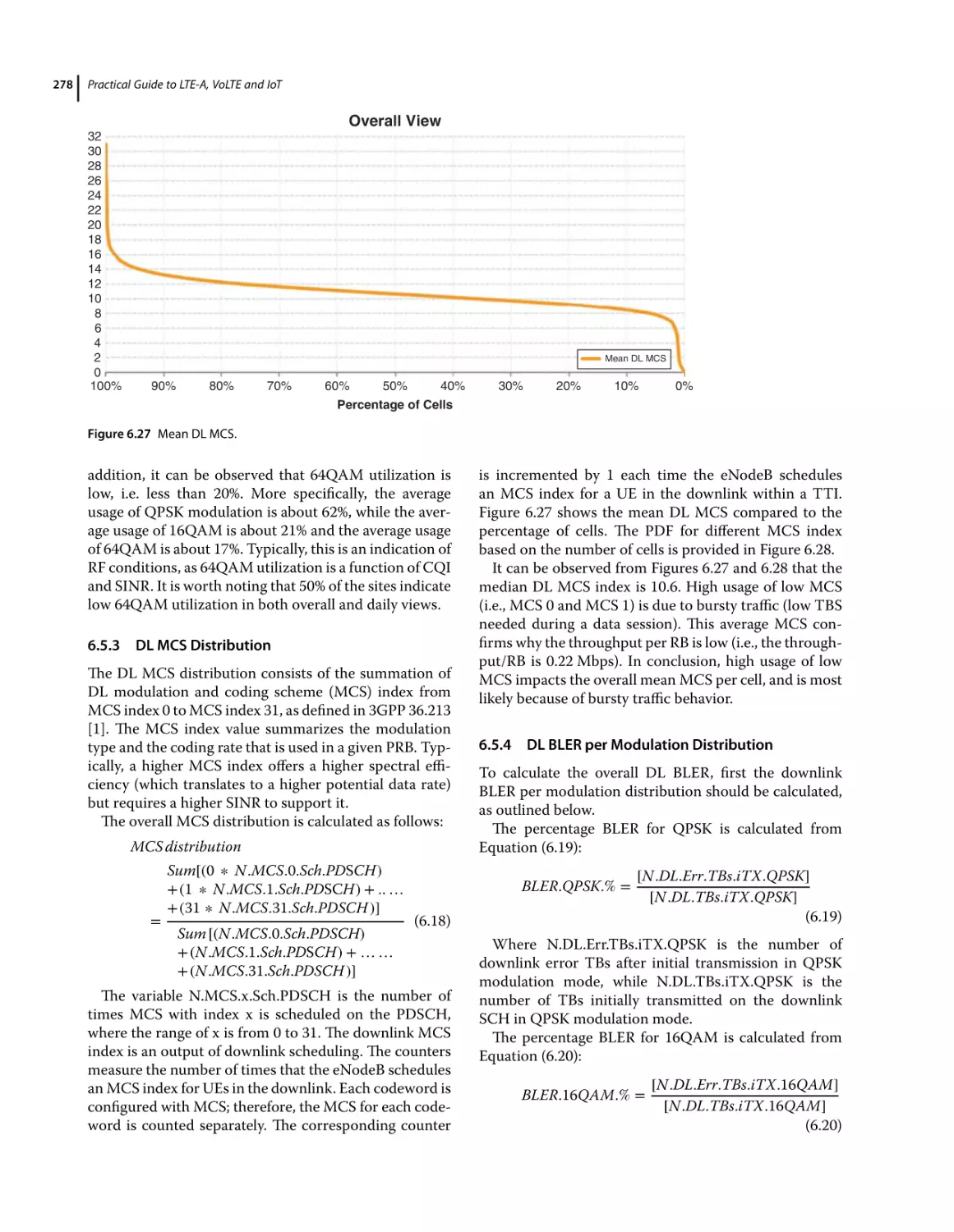
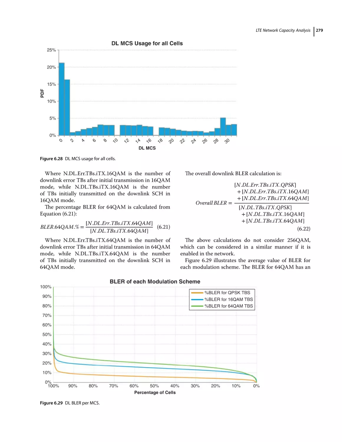
DL MCS Distribution 278
DL BLER per Modulation Distribution 278
DL Resource Block Utilization 280
Introduction to MIMO 280
MIMO Techniques: Open-loop MIMO and Closed-loop MIMO 280
MIMO Techniques: Single-user MIMO and Multi-user MIMO 281
MIMO Utilization 282
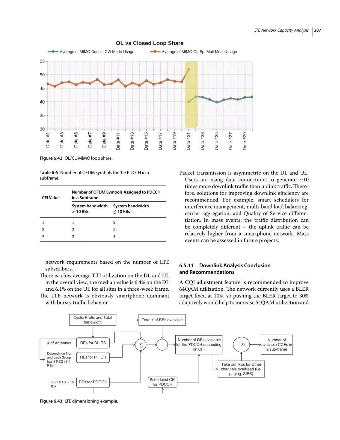
CL MIMO (TM4) Trial 283
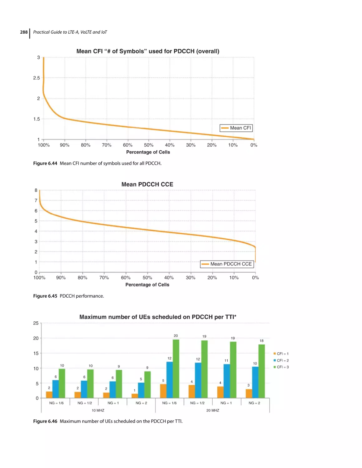
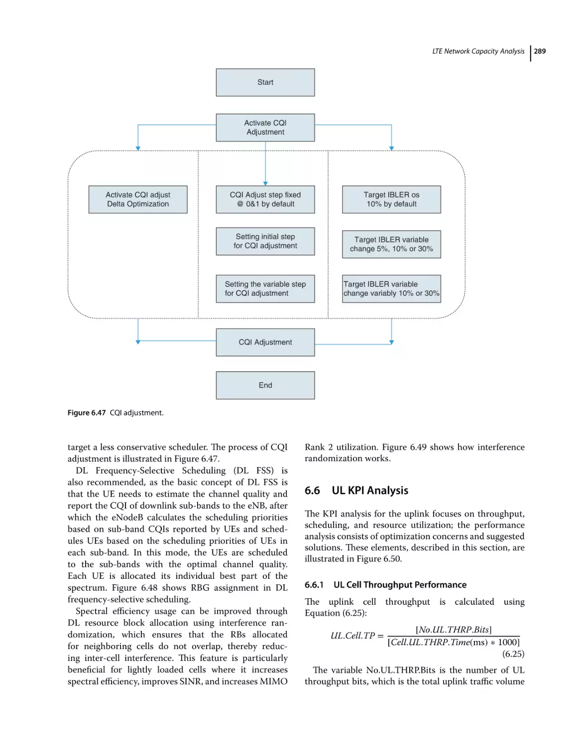
PDCCH Performance 284
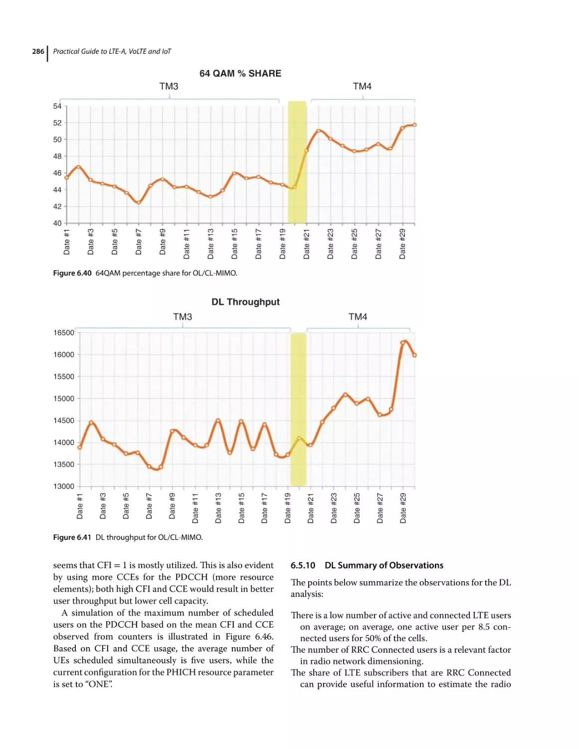
DL Summary of Observations 286
Downlink Analysis Conclusion and Recommendations 287
UL KPI Analysis 289
UL Cell Throughput Performance 289
UL Bit Rate per Resource Block 290
UL MCS Distribution 291
UL User Throughput 292
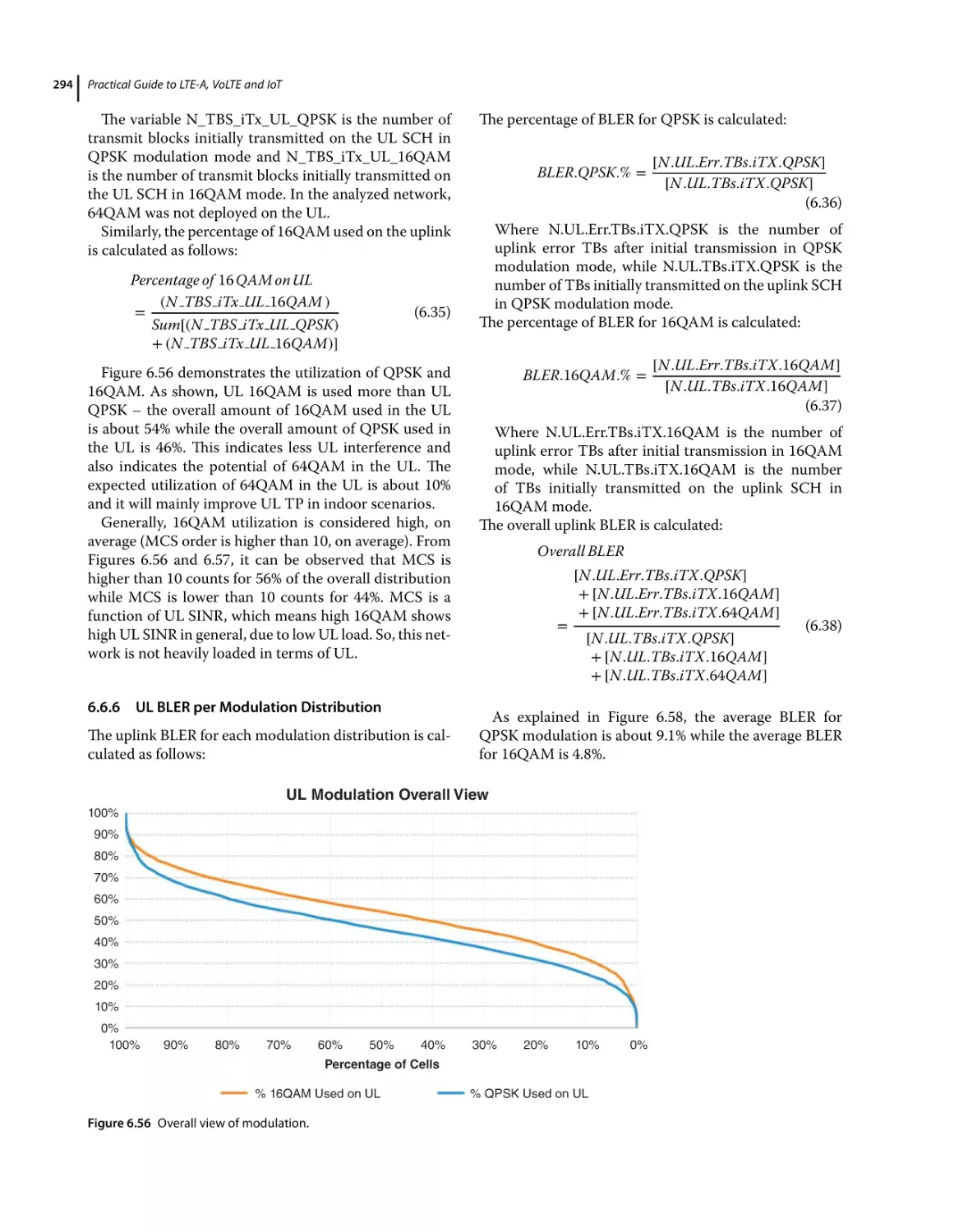
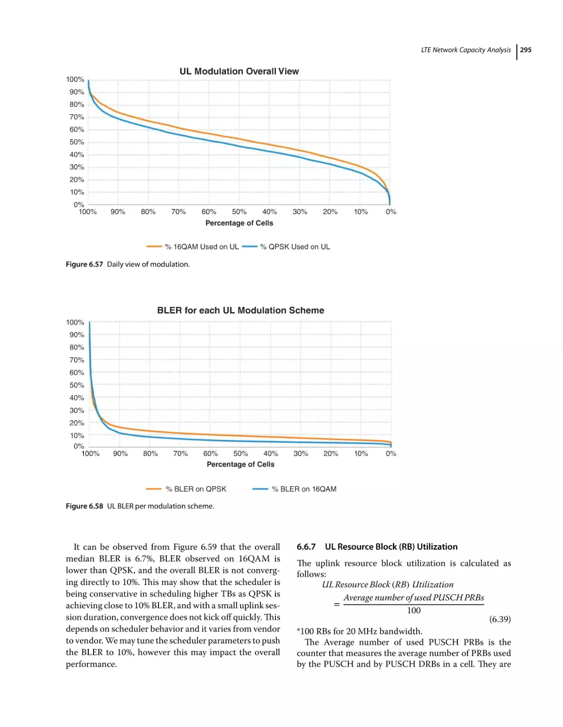
UL Modulation Distribution 293
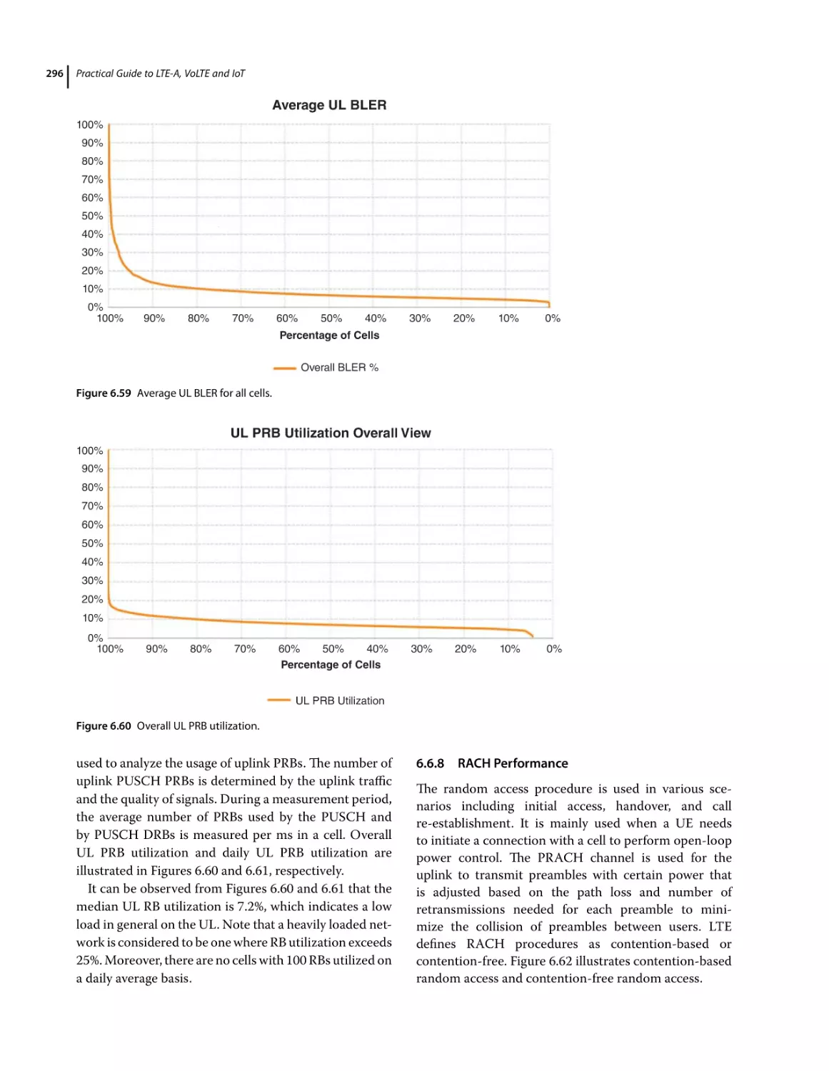
UL BLER per Modulation Distribution 294
UL Resource Block (RB) Utilization 295
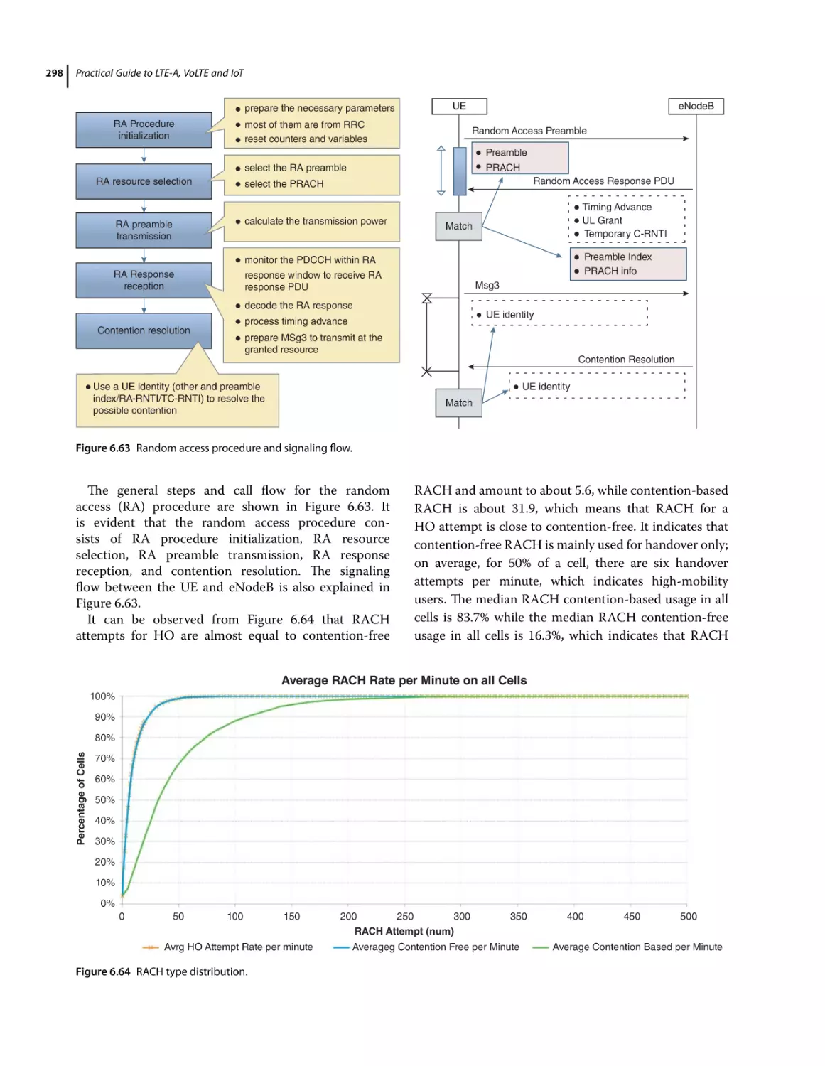
RACH Performance 296
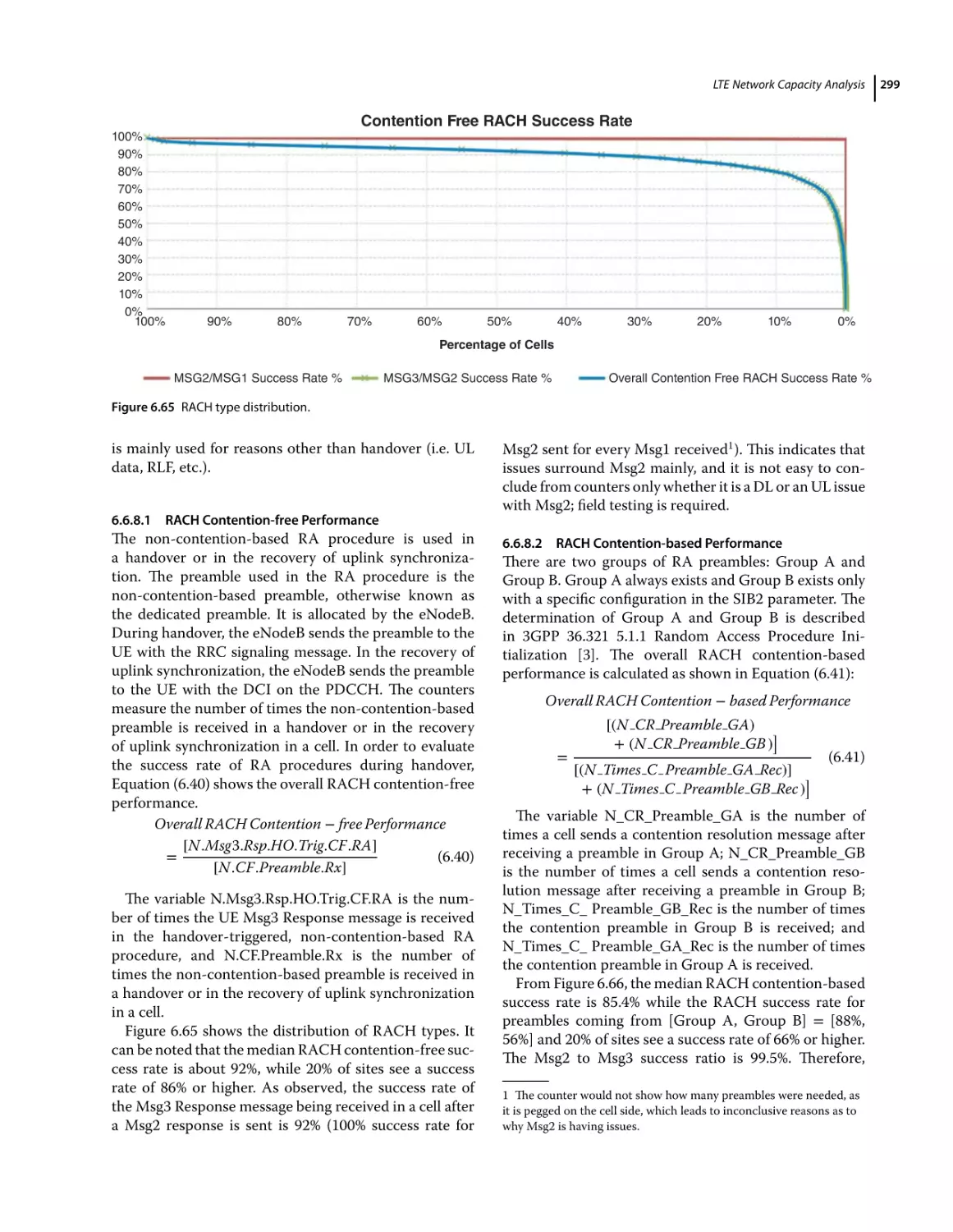
RACH Contention-free Performance 299
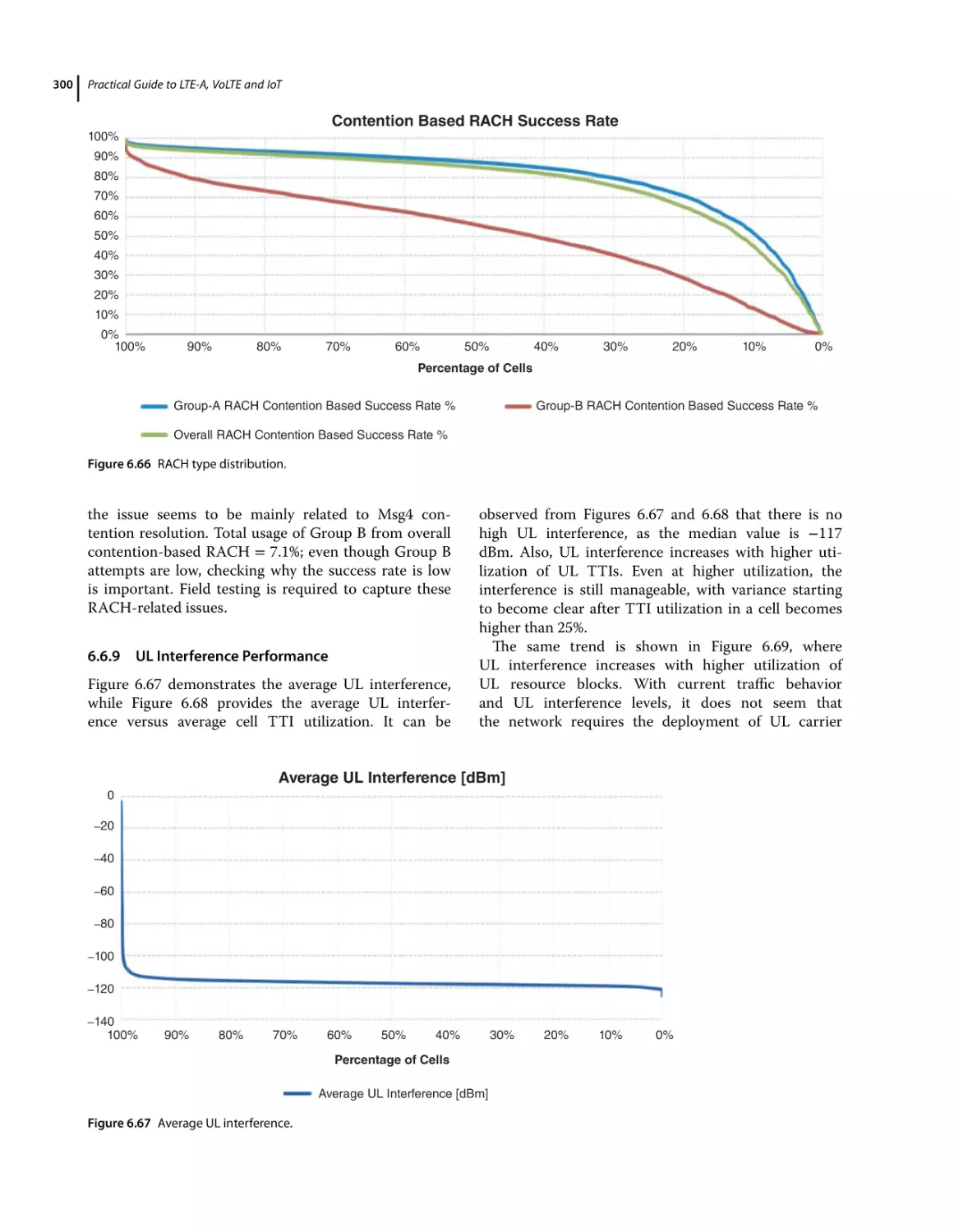
RACH Contention-based Performance 299
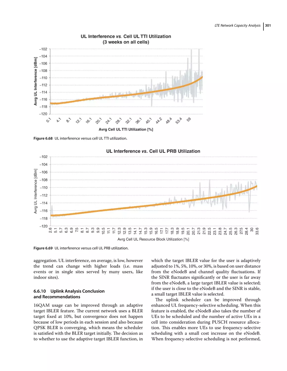
UL Interference Performance 300
Uplink Analysis Conclusion and Recommendations 301
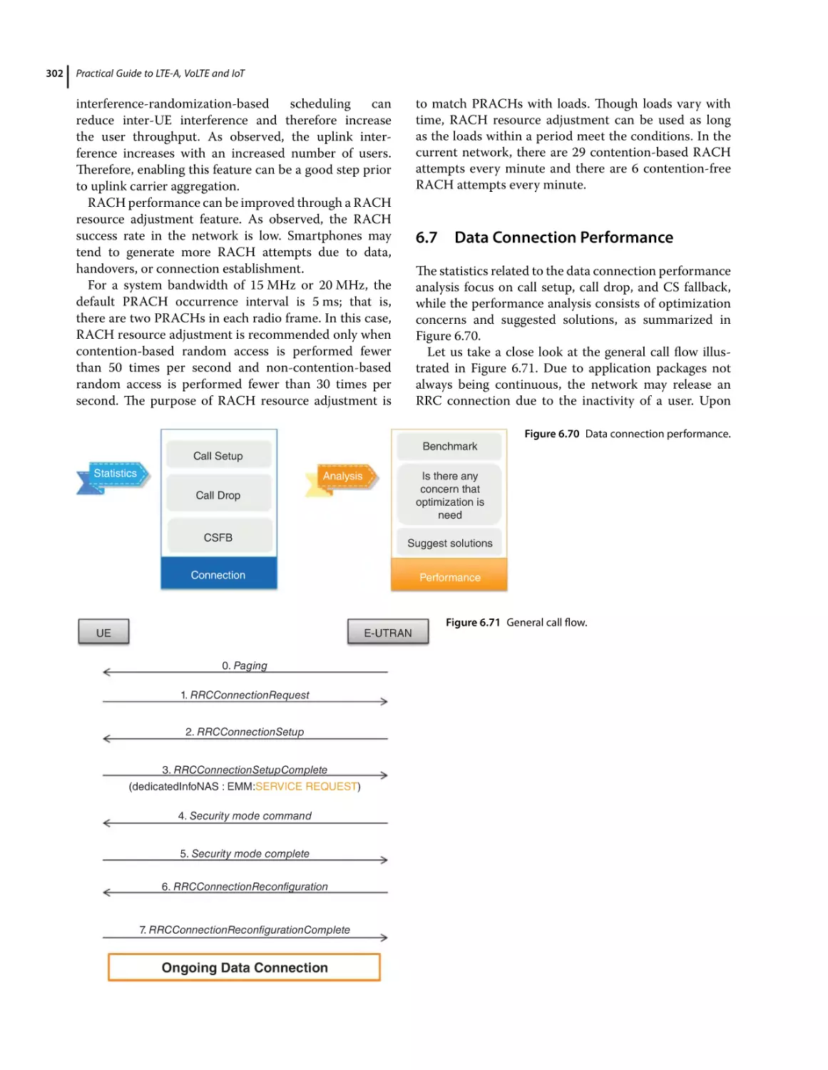
Data Connection Performance 302
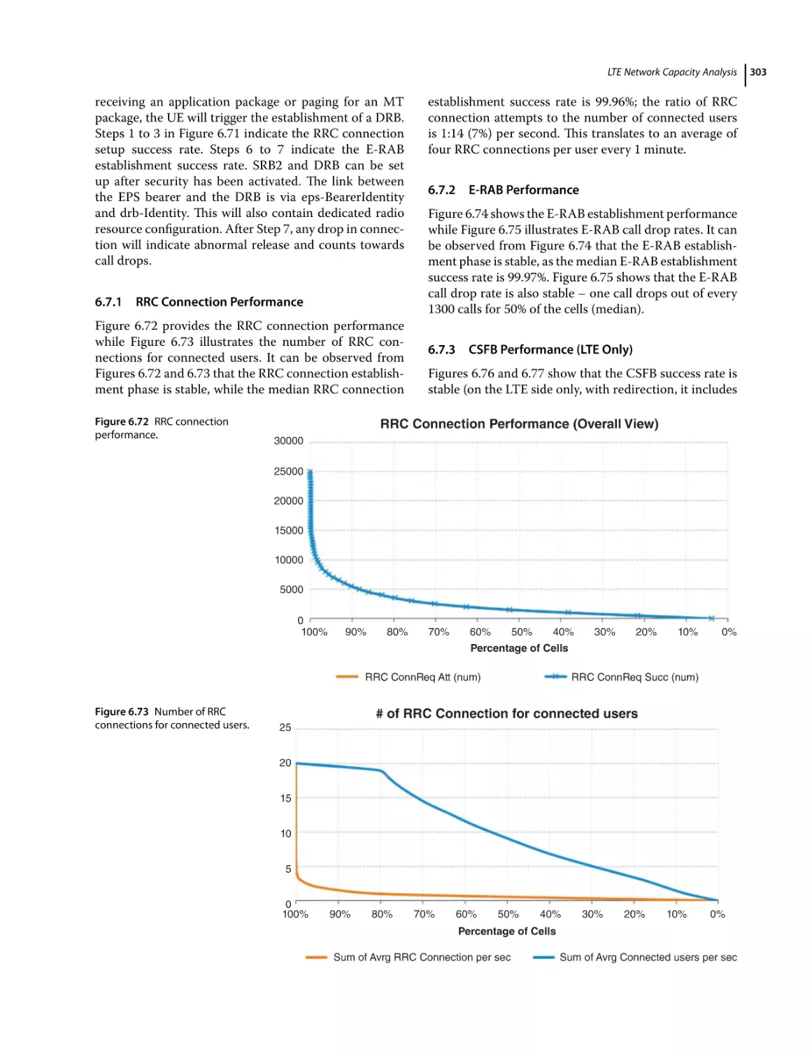
RRC Connection Performance 303
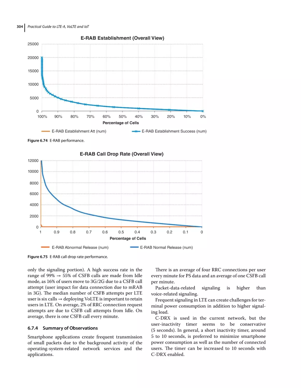
E-RAB Performance 303
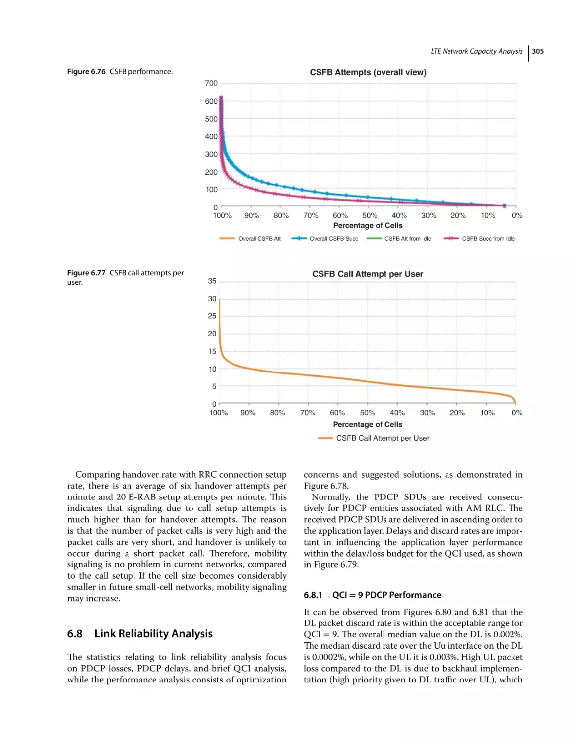
CSFB Performance (LTE Only) 303
Summary of Observations 304
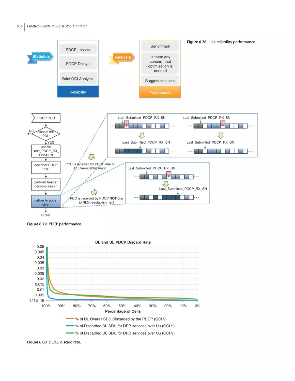
Link Reliability Analysis 305
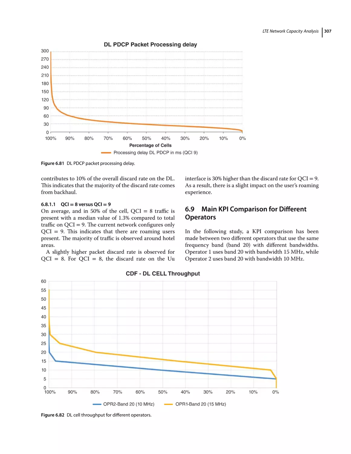
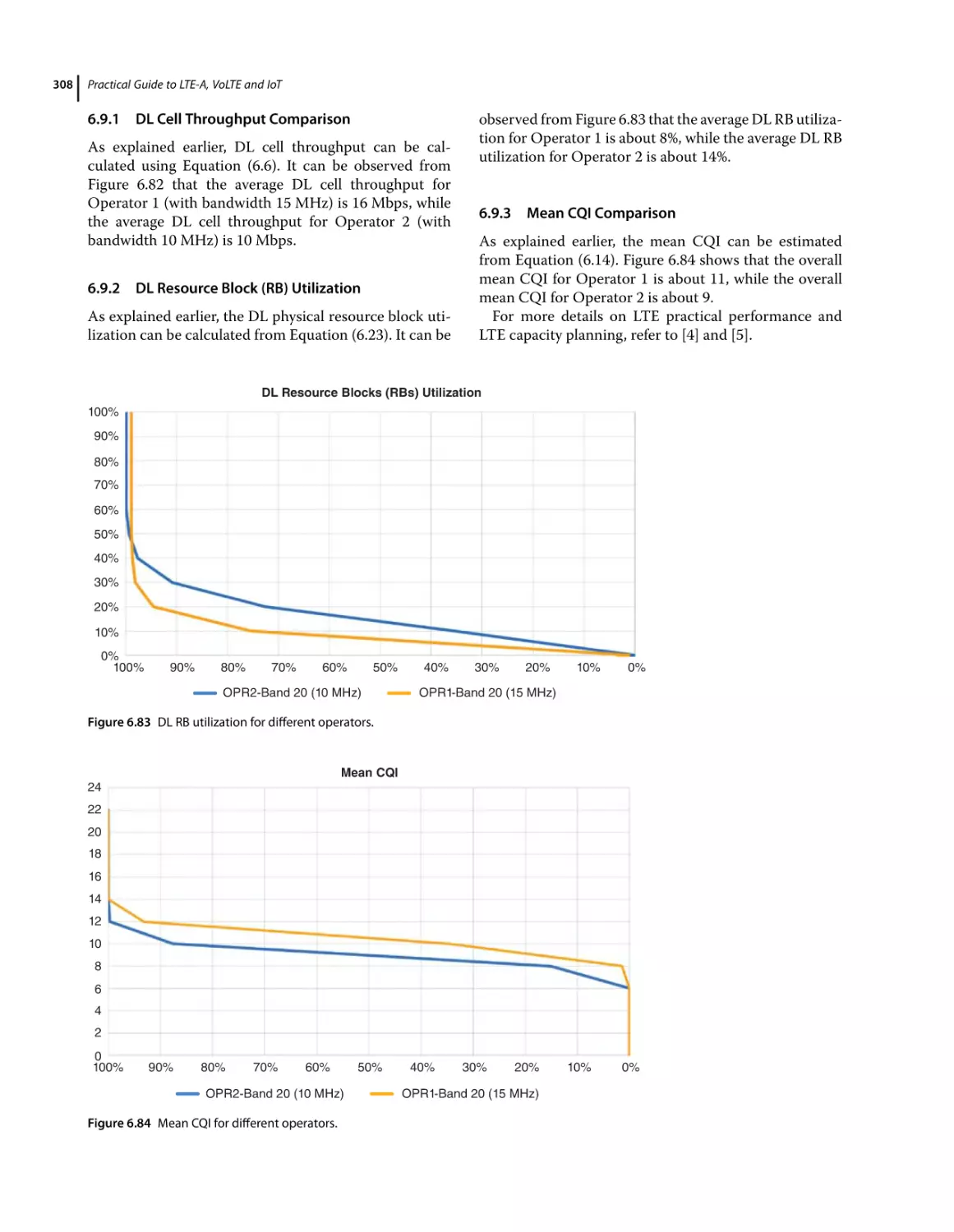
QCI = 9 PDCP Performance 305
QCI = 8 versus QCI = 9 307
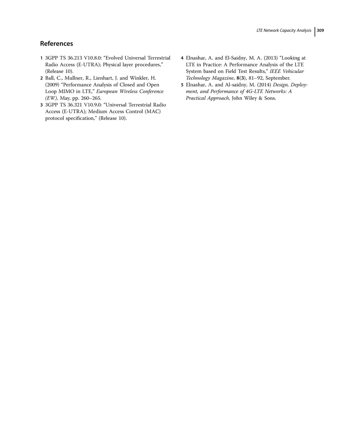
Main KPI Comparison for Different Operators 307
DL Cell Throughput Comparison 308
DL Resource Block (RB) Utilization 308
Mean CQI Comparison 308
References 309
7
IoT Evolution Towards a Super-connected World 310
7.1
7.2
Overview 310
Introduction to the IoT
310
xiii
xiv
Contents
7.3
7.3.1
7.3.2
7.3.3
7.4
7.4.1
7.5
7.6
7.7
7.8
7.9
7.10
7.11
7.12
7.12.1
7.12.2
7.12.3
7.12.4
7.12.5
7.12.6
7.12.7
7.12.8
7.13
7.13.1
7.13.2
7.13.3
7.13.4
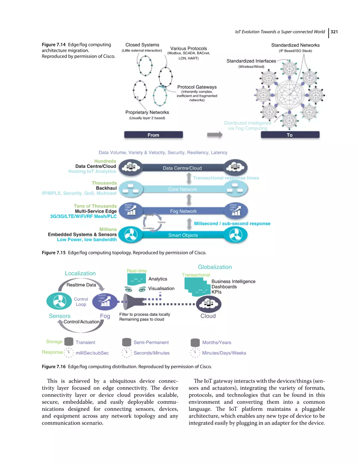
7.14
7.15
7.16
7.16.1
7.17
7.17.1
7.17.1.1
7.17.1.2
7.17.1.3
7.17.1.4
7.17.1.5
7.17.1.6
7.17.1.7
7.17.1.8
7.17.1.9
7.17.1.10
7.17.1.11
7.17.2
7.17.2.1
7.17.2.2
7.17.2.3
7.17.2.4
7.17.2.5
7.18
7.18.1
7.18.2
7.18.3
IoT Standards 312
IEEE 312
ETSI 312
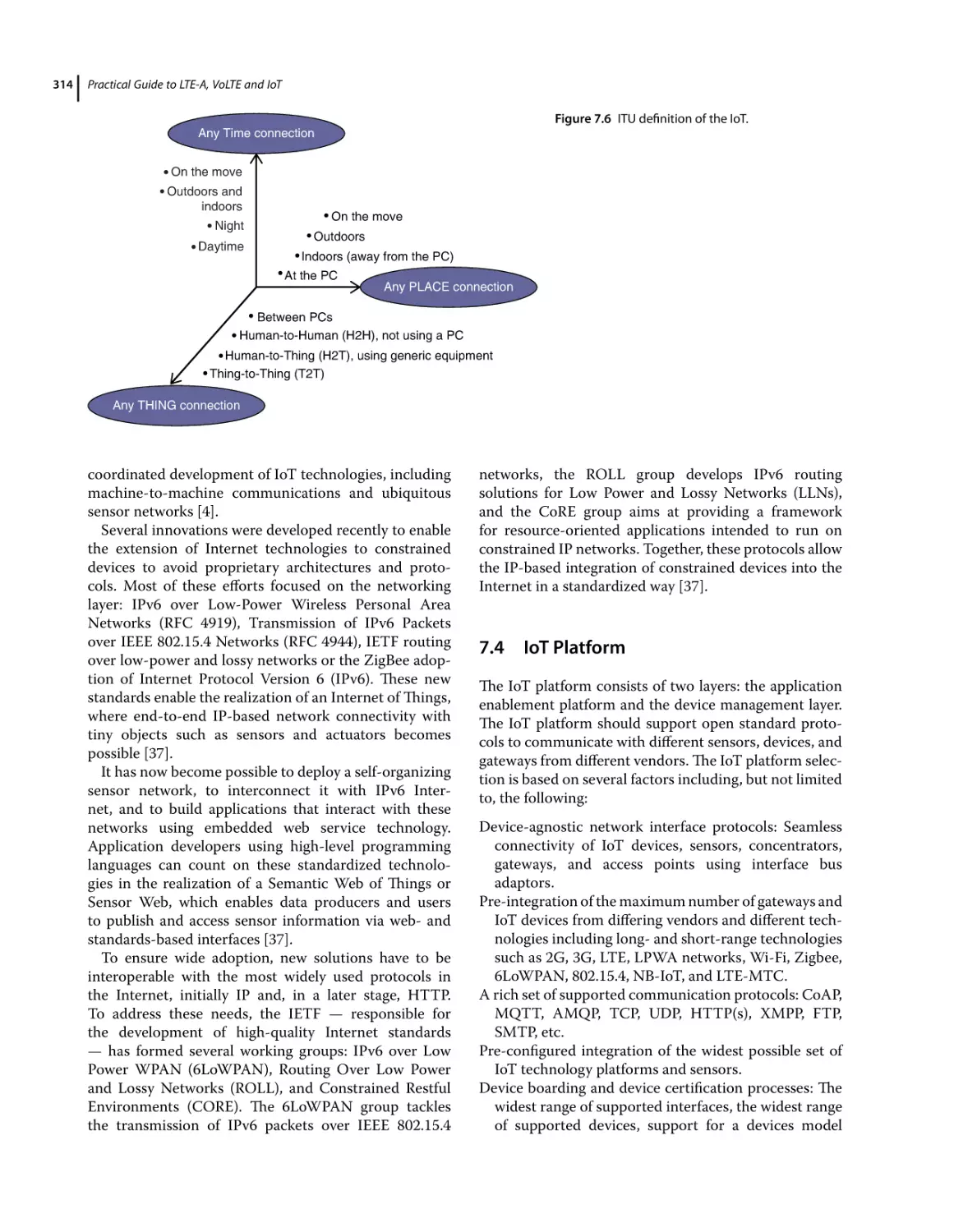
ITU 313
IoT Platform 314
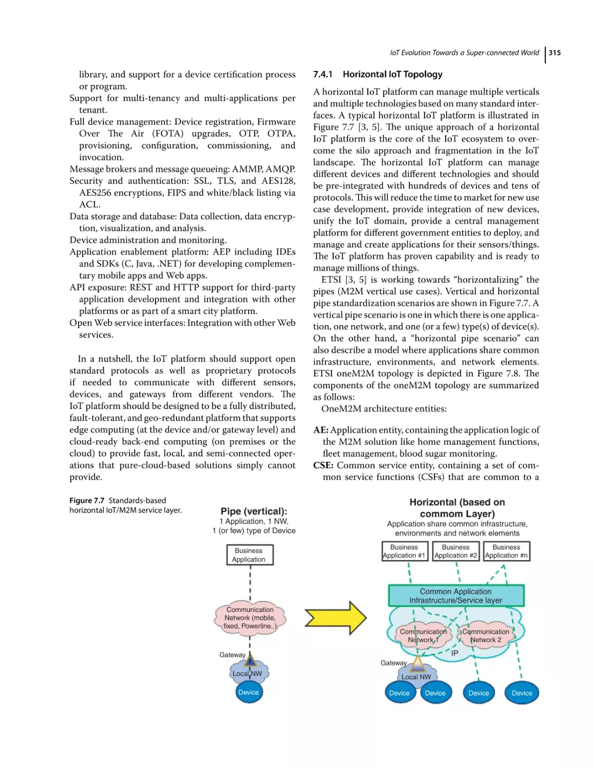
Horizontal IoT Topology 315
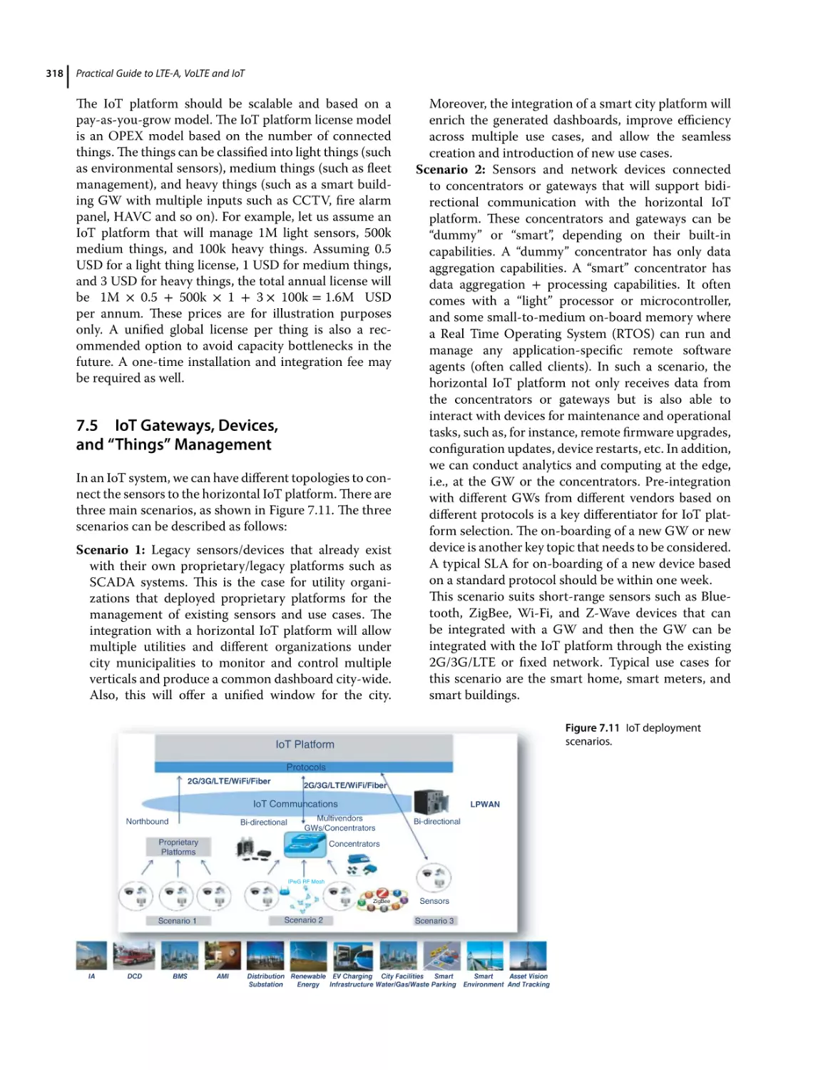
IoT Gateways, Devices, and “Things” Management 318
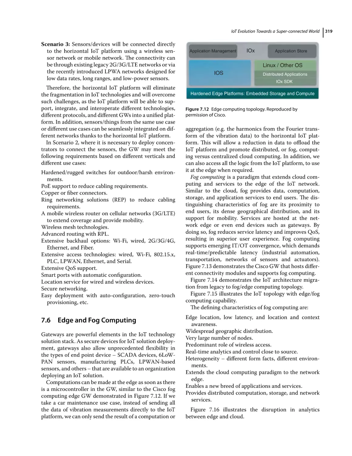
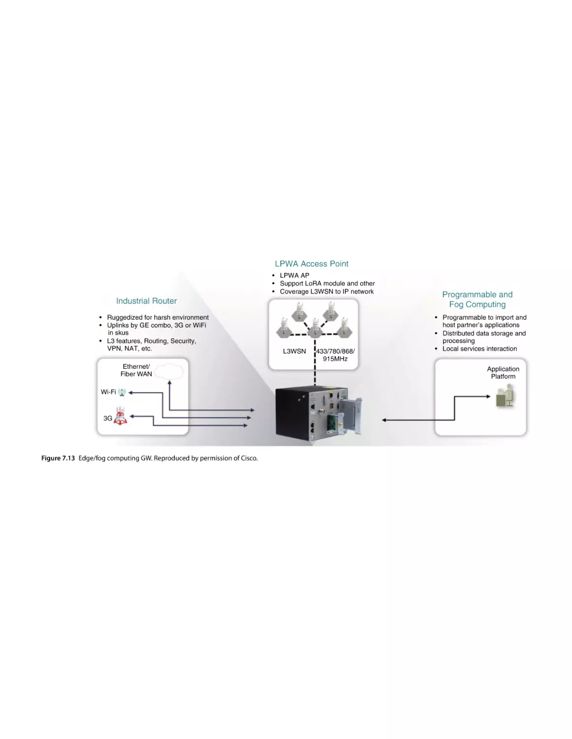
Edge and Fog Computing 319
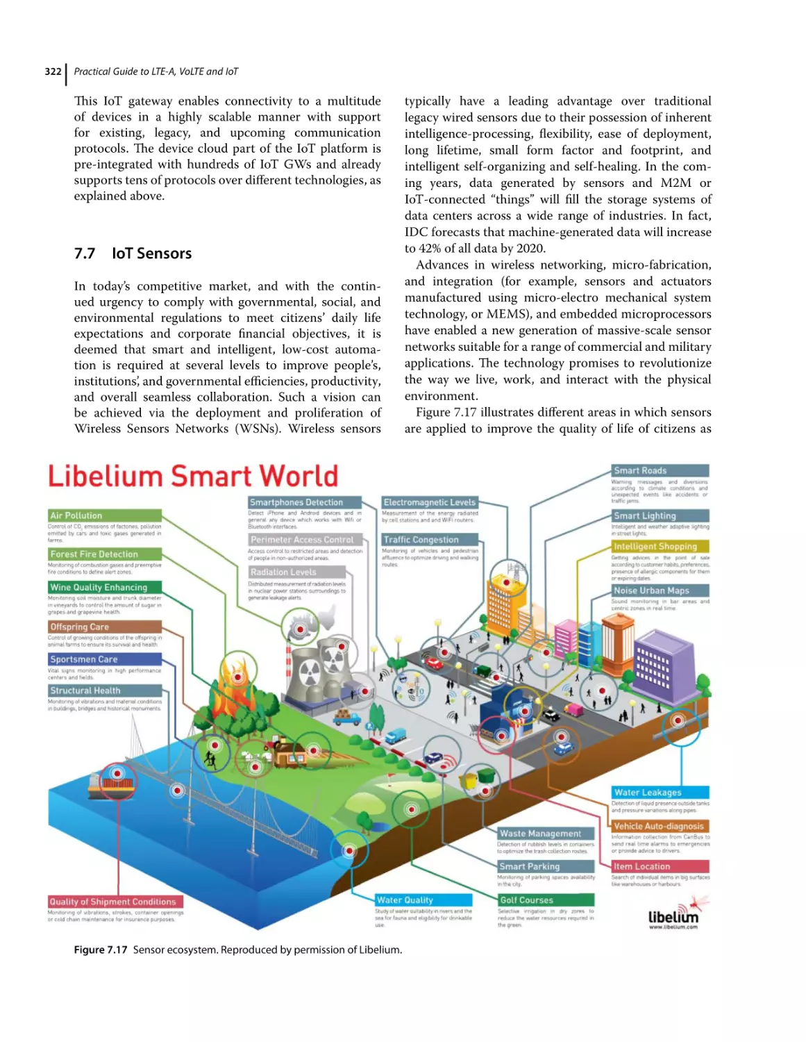
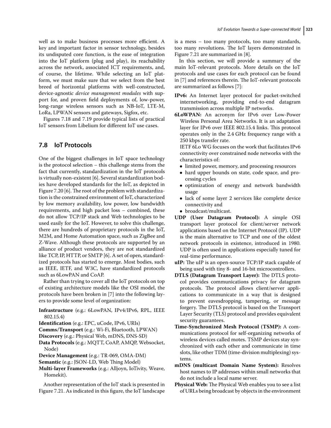
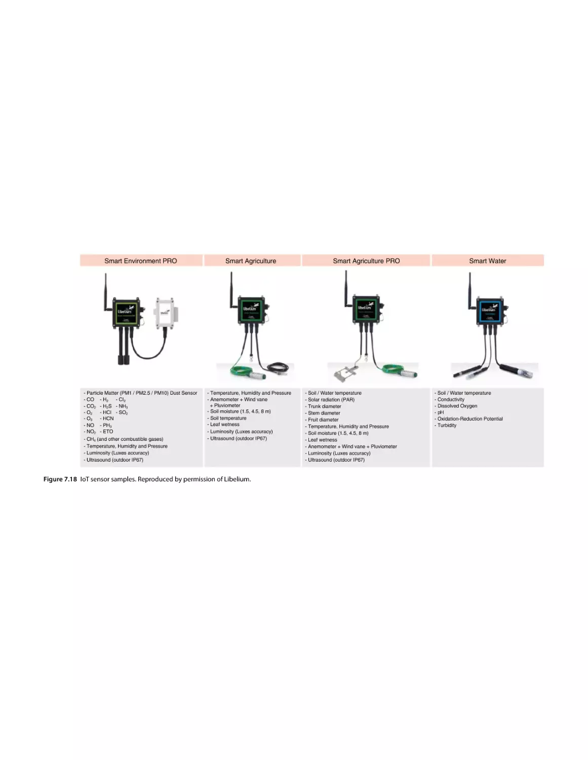
IoT Sensors 322
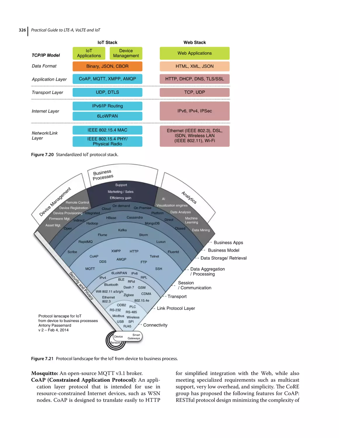
IoT Protocols 323
IoT Networks 327
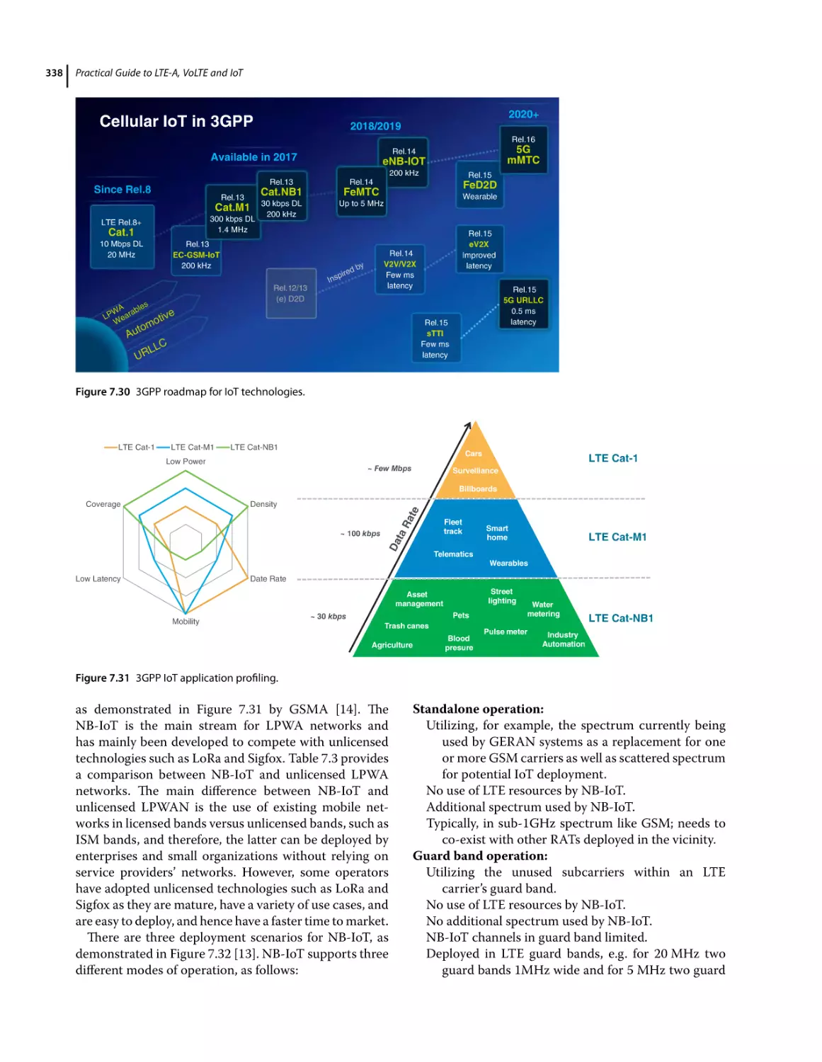
3GPP Standards for IoT 337
3GPP NB-IoT 341
NB-IoT DL Specifications 343
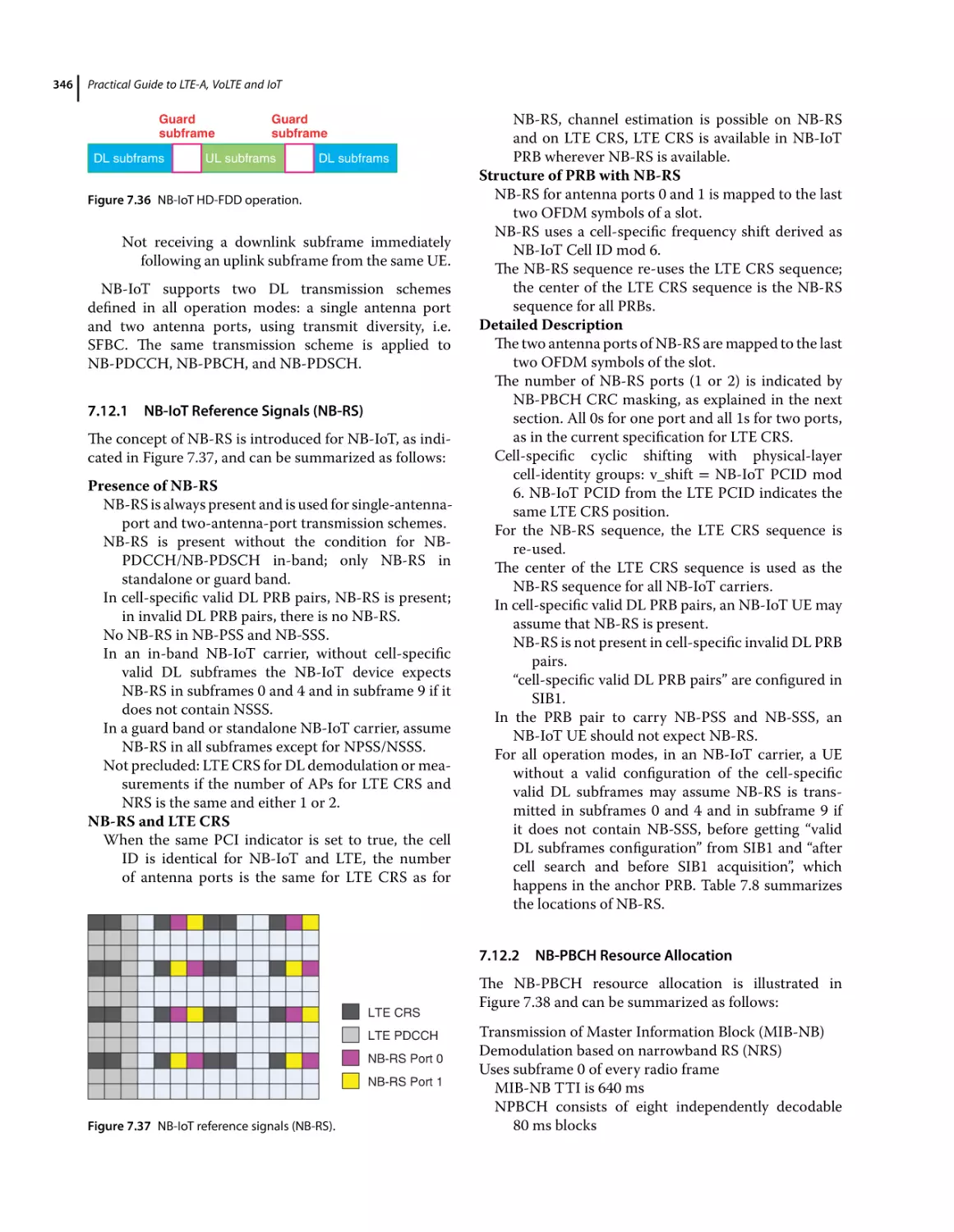
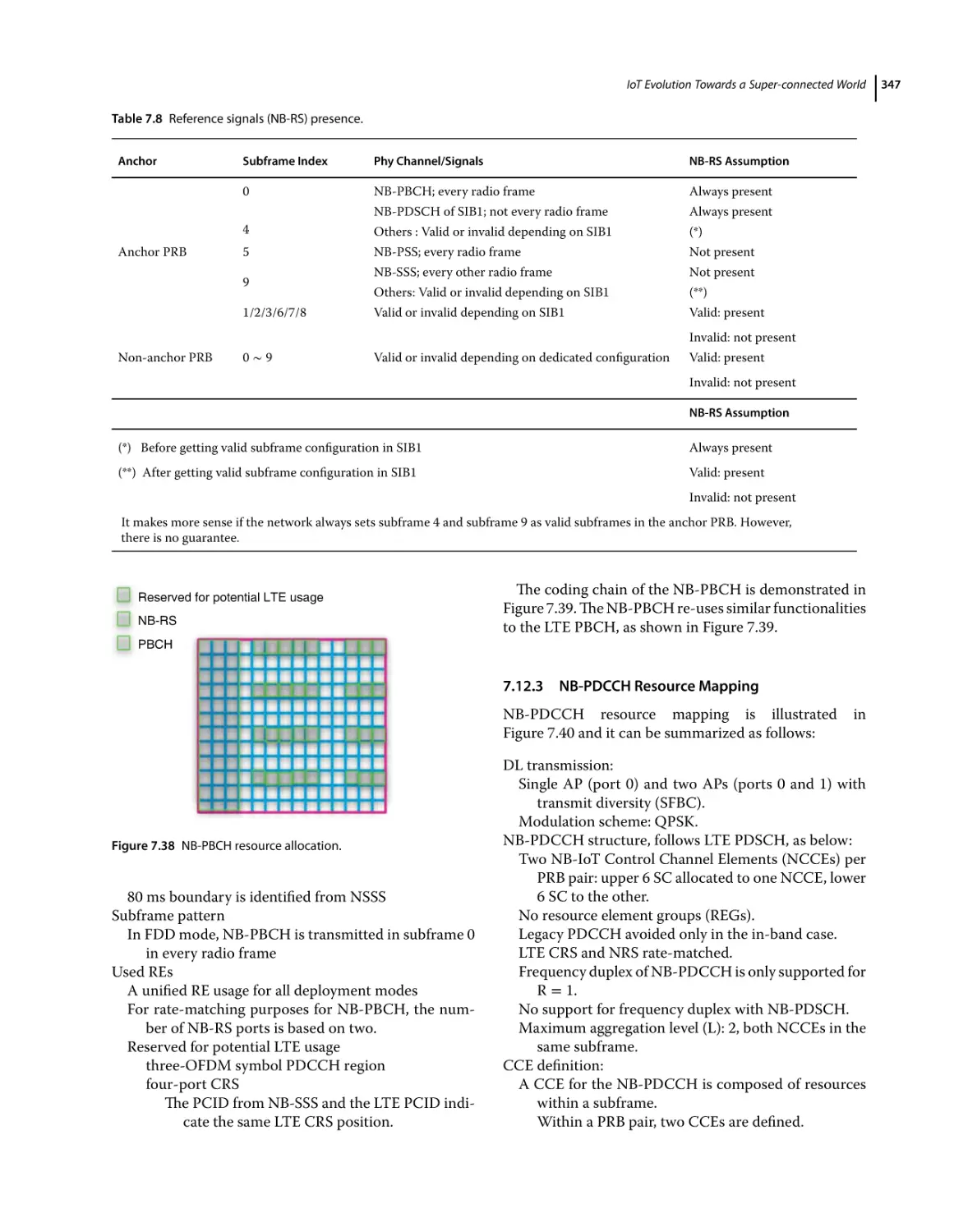
NB-IoT Reference Signals (NB-RS) 346
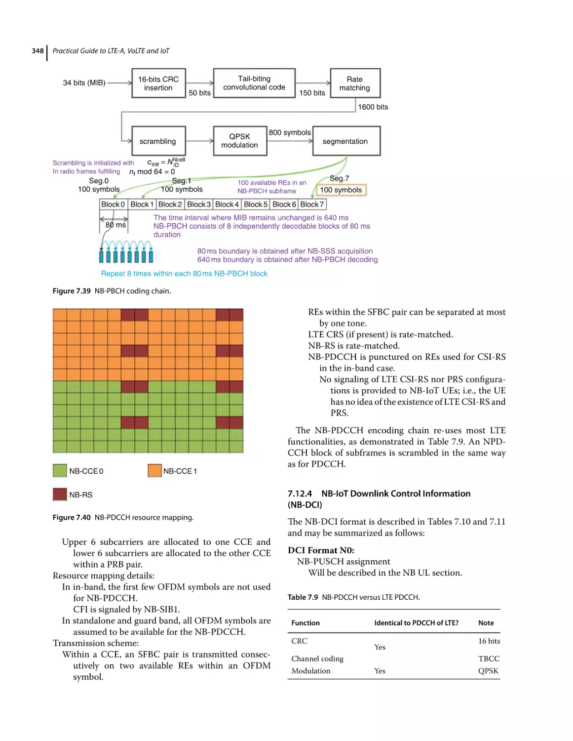
NB-PBCH Resource Allocation 346
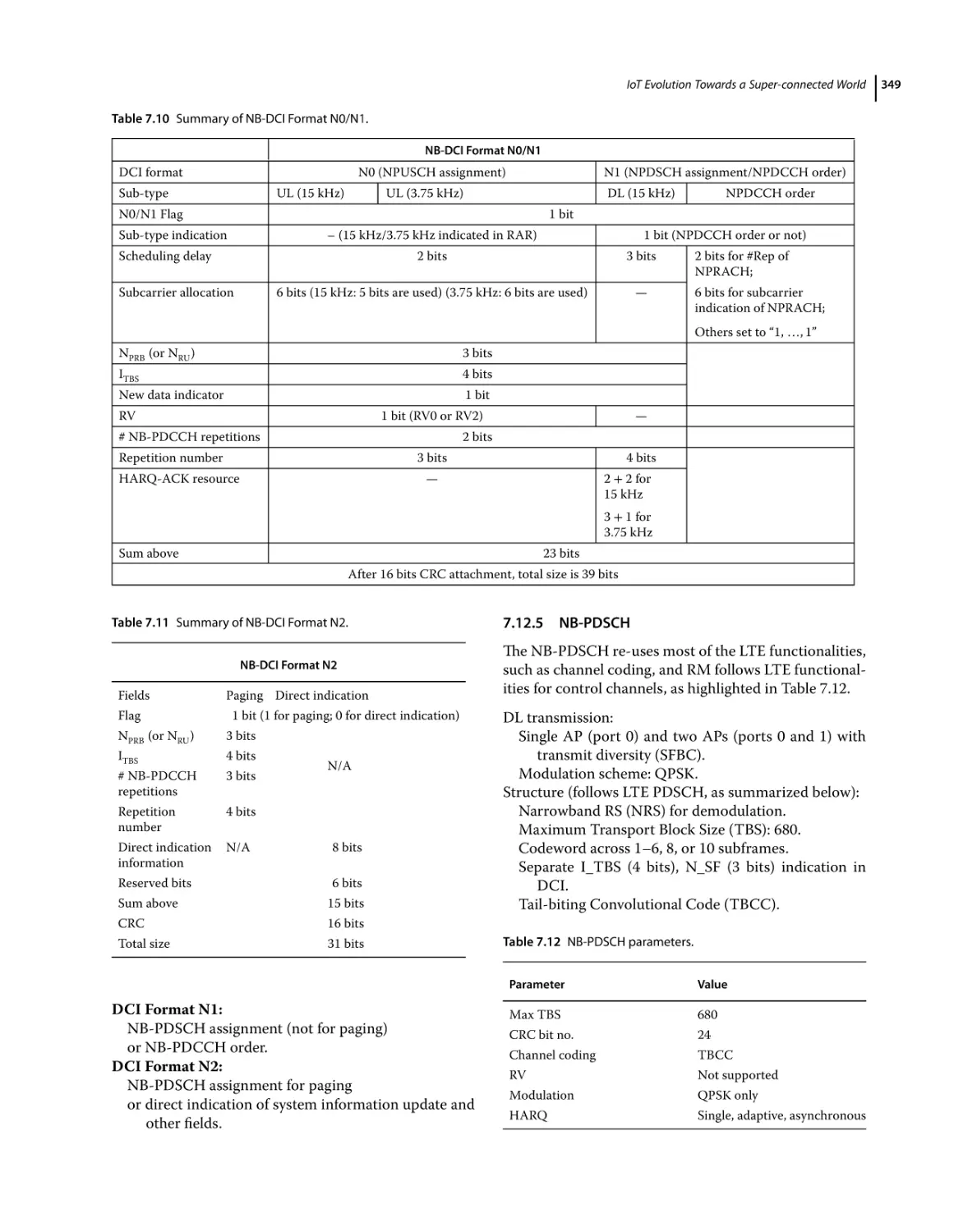
NB-PDCCH Resource Mapping 347
NB-IoT Downlink Control Information (NB-DCI) 348
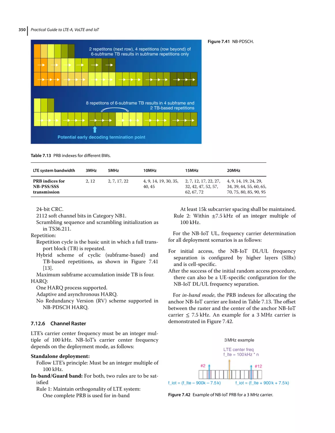
NB-PDSCH 349
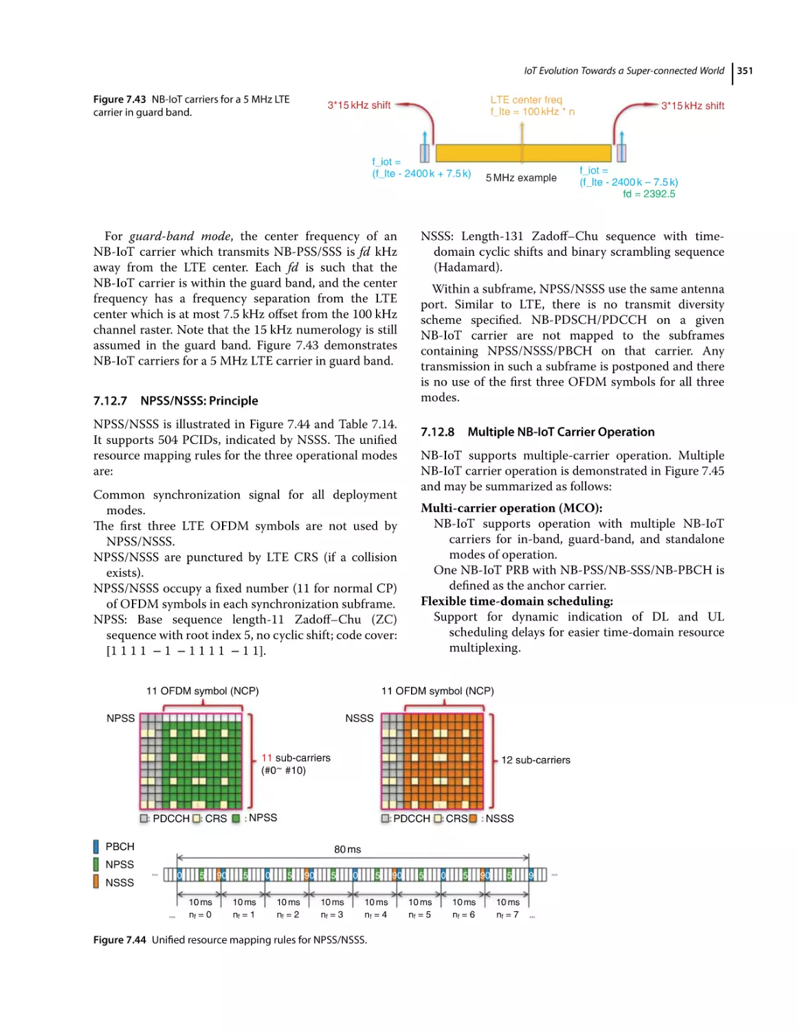
Channel Raster 350
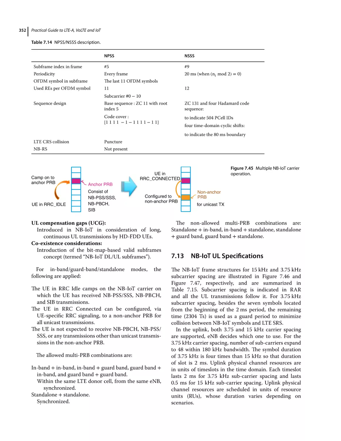
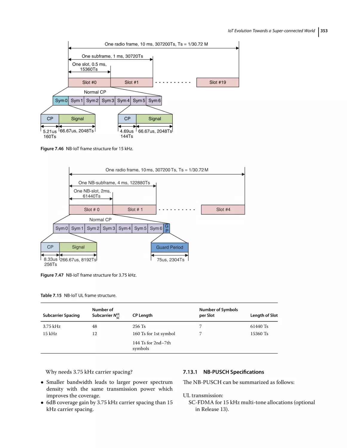
NPSS/NSSS: Principle 351
Multiple NB-IoT Carrier Operation 351
NB-IoT UL Specifications 352
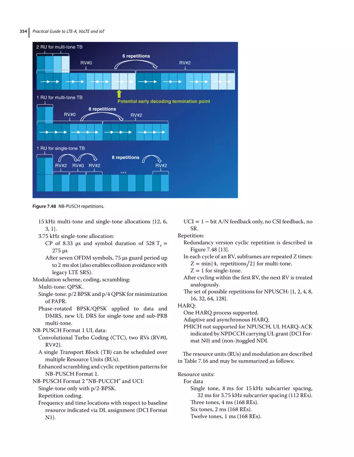
NB-PUSCH Specifications 353
NB-IoT Physical Random Access Channel (NPRACH) 355
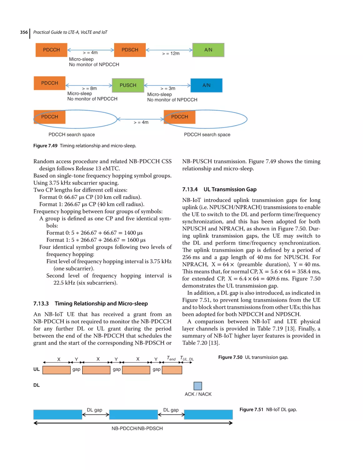
Timing Relationship and Micro-sleep 356
UL Transmission Gap 356
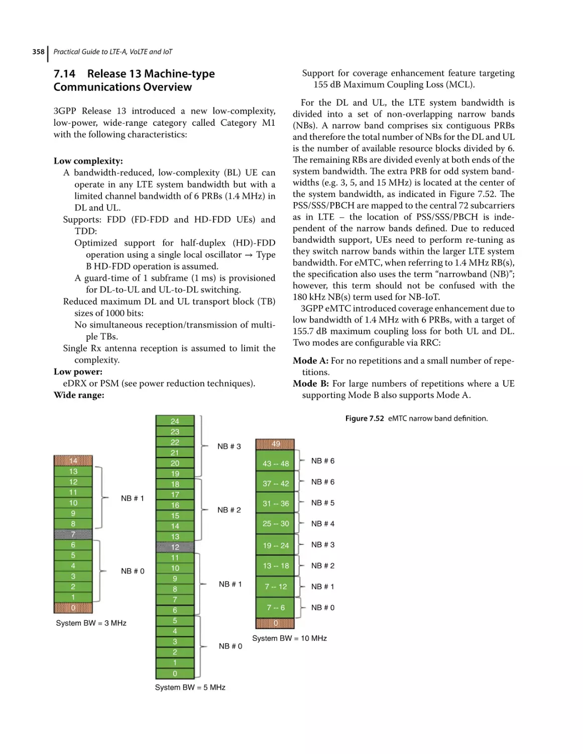
Release 13 Machine-type Communications Overview 358
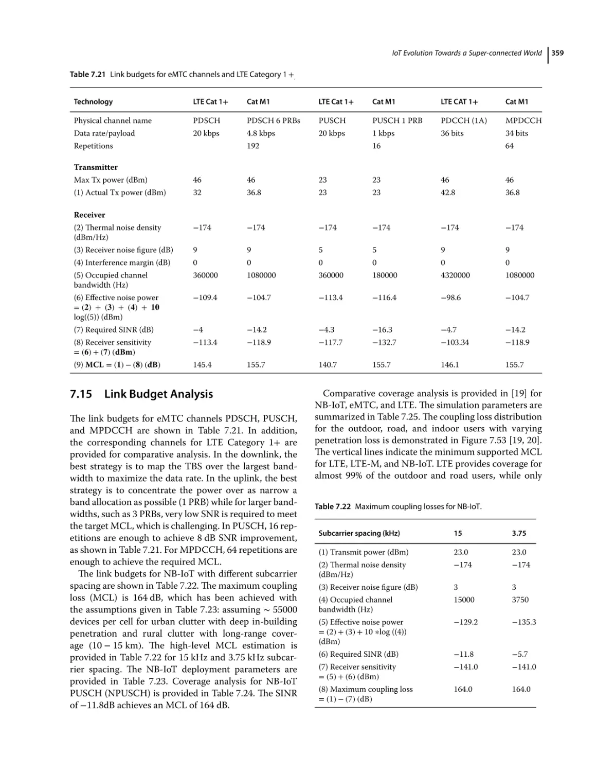
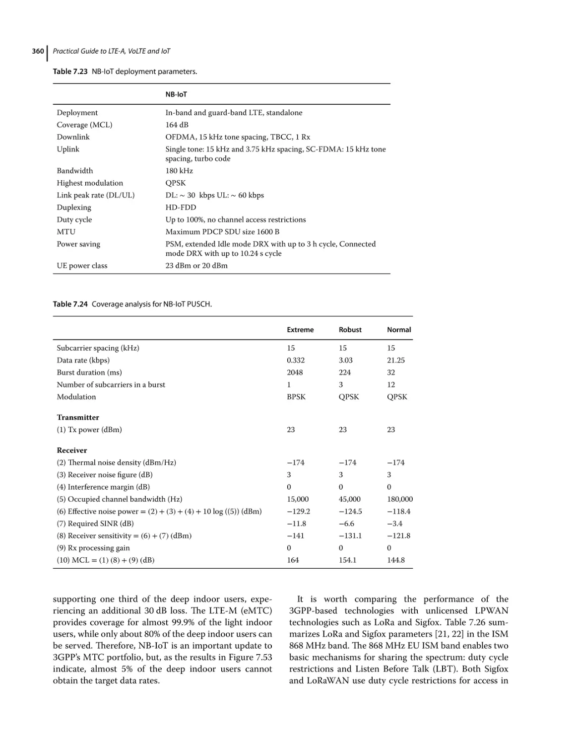
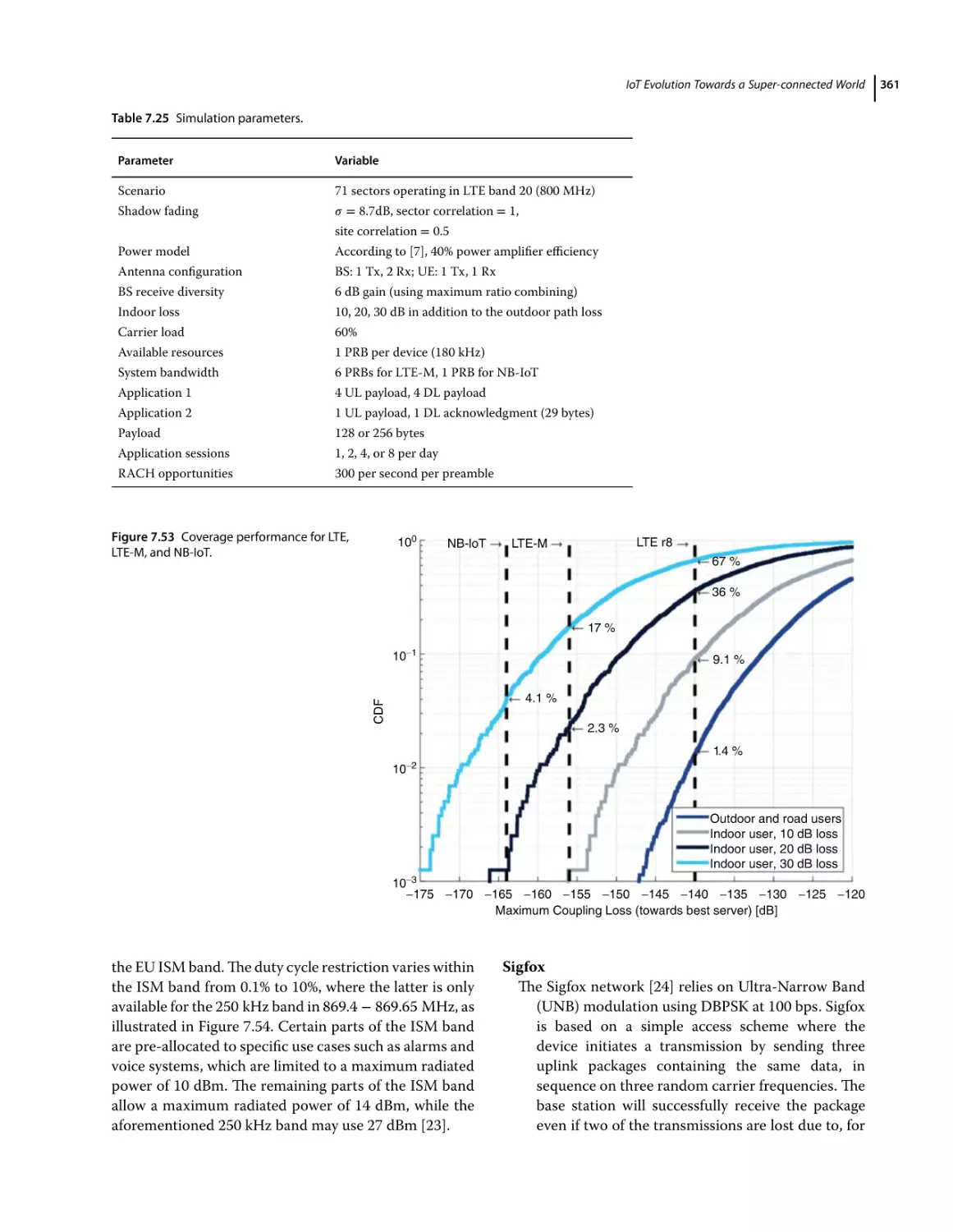
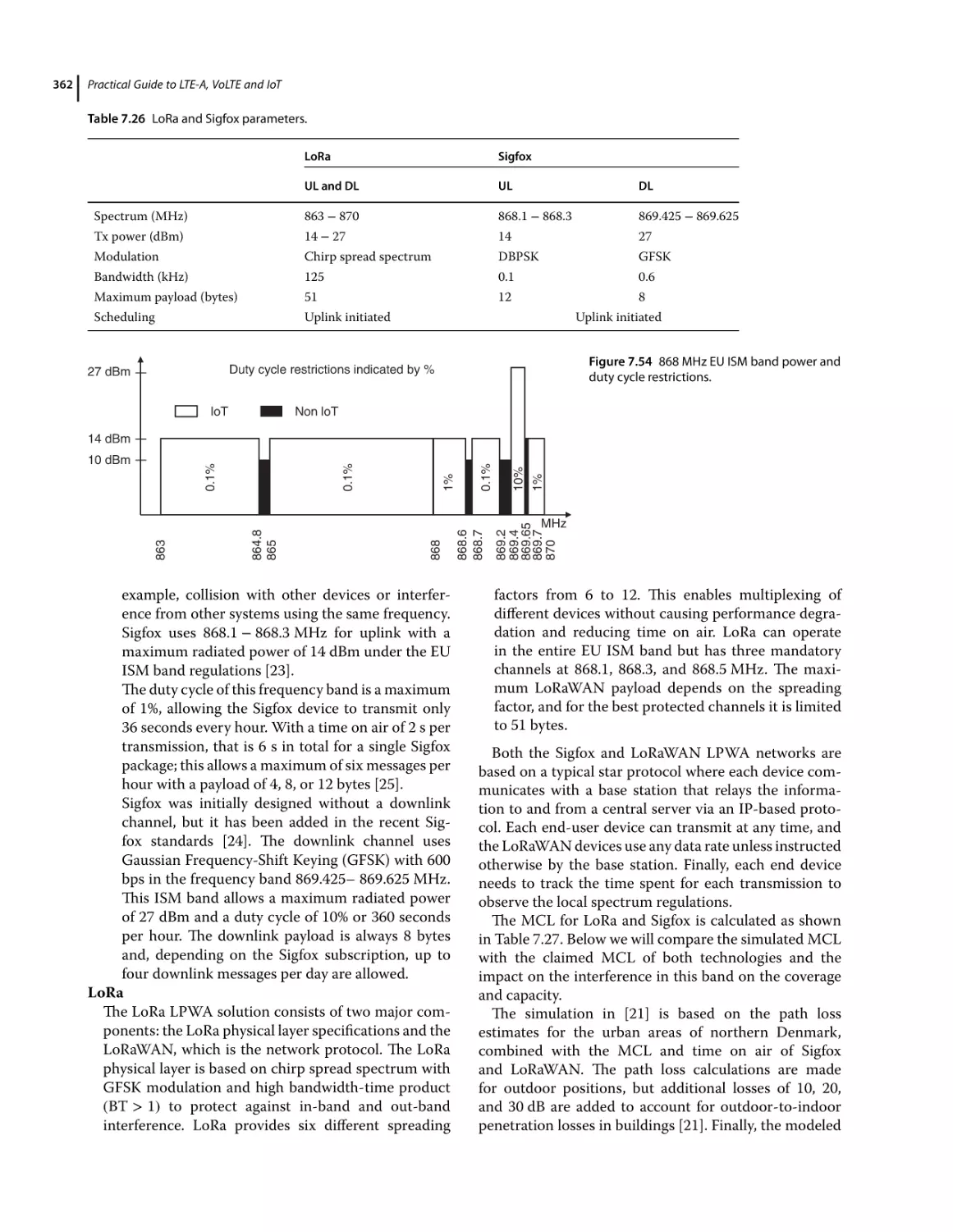
Link Budget Analysis 359
NB-IoT Network Topology 364
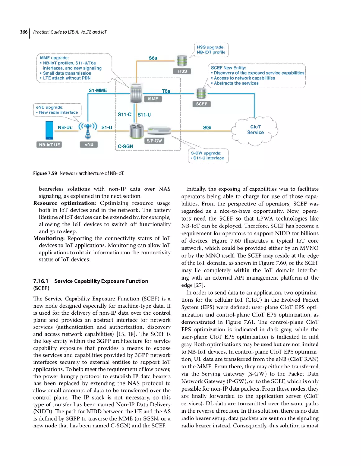
Service Capability Exposure Function (SCEF) 366
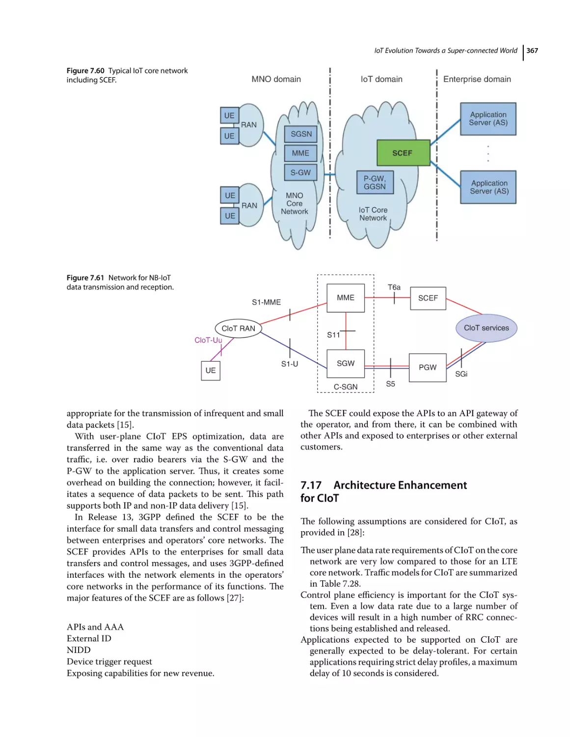
Architecture Enhancement for CIoT 367
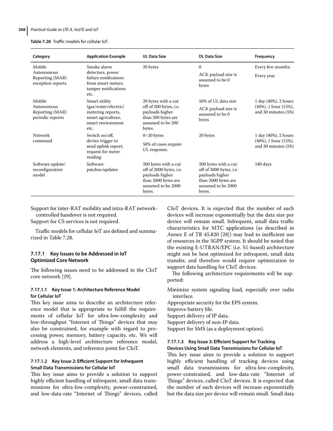
Key Issues to be Addressed in IoT Optimized Core Network 368
Key Issue 1: Architecture Reference Model for Cellular IoT 368
Key Issue 2: Efficient Support for Infrequent Small Data Transmissions for Cellular IoT 368
Key Issue 3: Efficient Support for Tracking Devices Using Small Data Transmissions for Cellular IoT 368
Key Issue 4: Support for Efficient Paging Area Management for Cellular IoT 369
Key Issue 5: Selection of CIoT–EPC Dedicated Core Network 369
Key Issue 6: Support for Non-IP Data 369
Key Issue 7: Support for SMS 369
Key Issue 8: Control of Small Data Misuse 369
Key Issue 9: Optimized Support for SMS Transmission 369
Key Issue 10: Authorization of Use of Coverage Enhancement 370
Key Issue 11: Header Compression Enhancements for CIoT 370
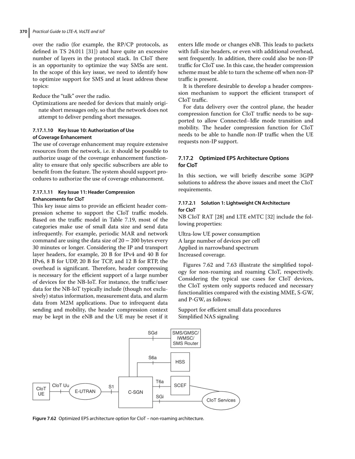
Optimized EPS Architecture Options for CIoT 370
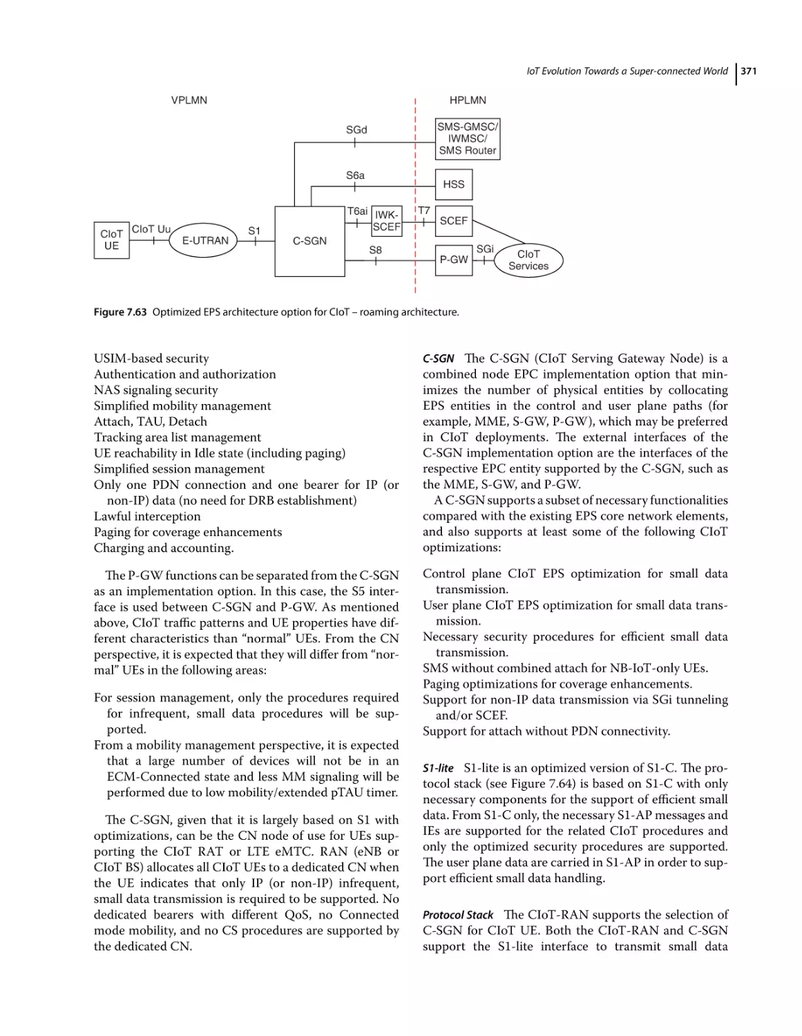
Solution 1: Lightweight CN Architecture for CIoT 370
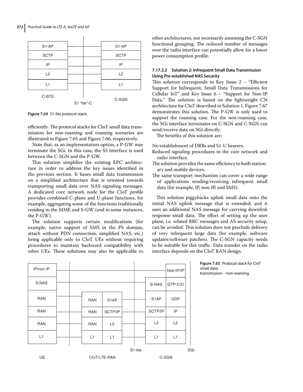
Solution 2: Infrequent Small Data Transmission Using Pre-established NAS Security 372
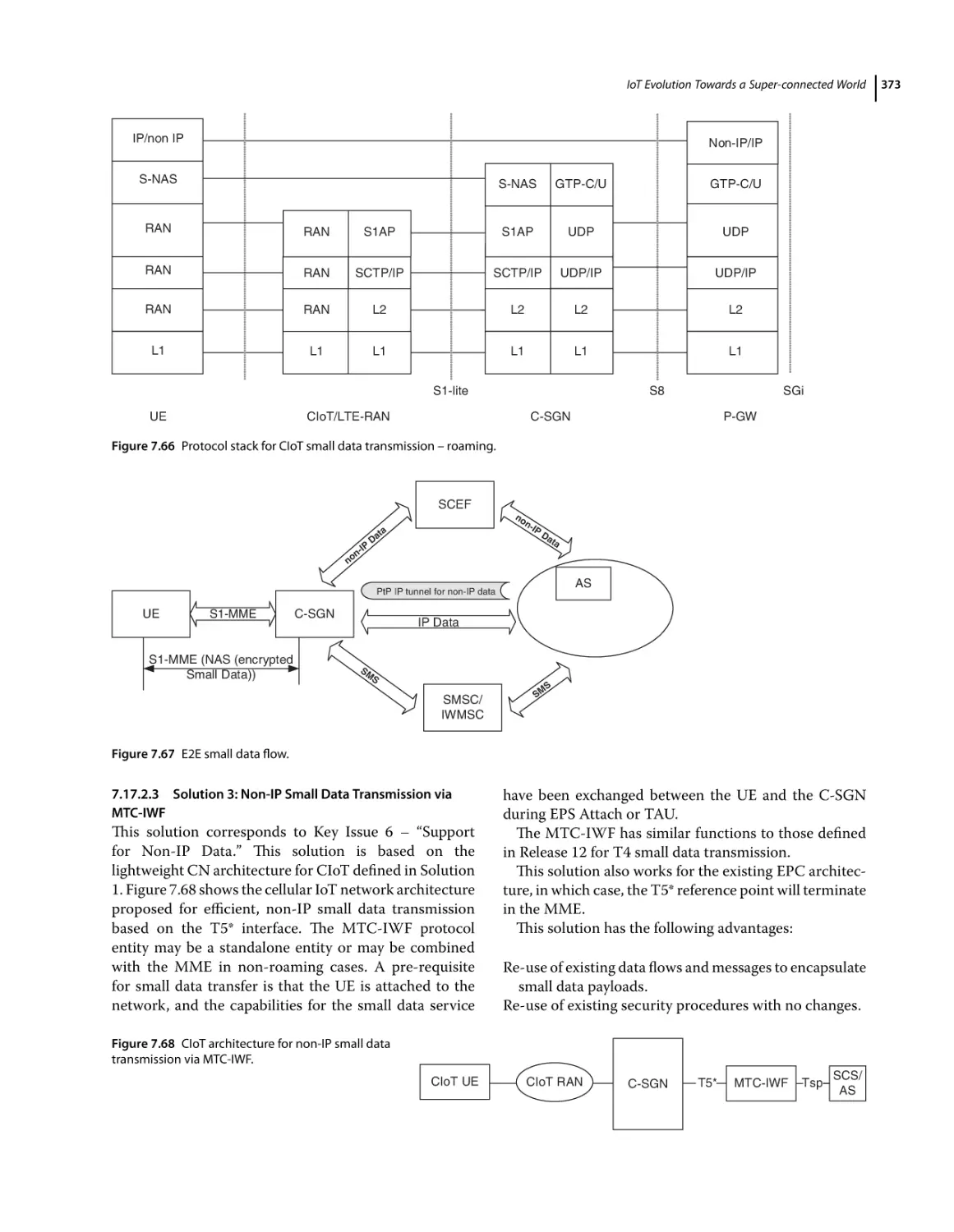
Solution 3: Non-IP Small Data Transmission via MTC-IWF 373
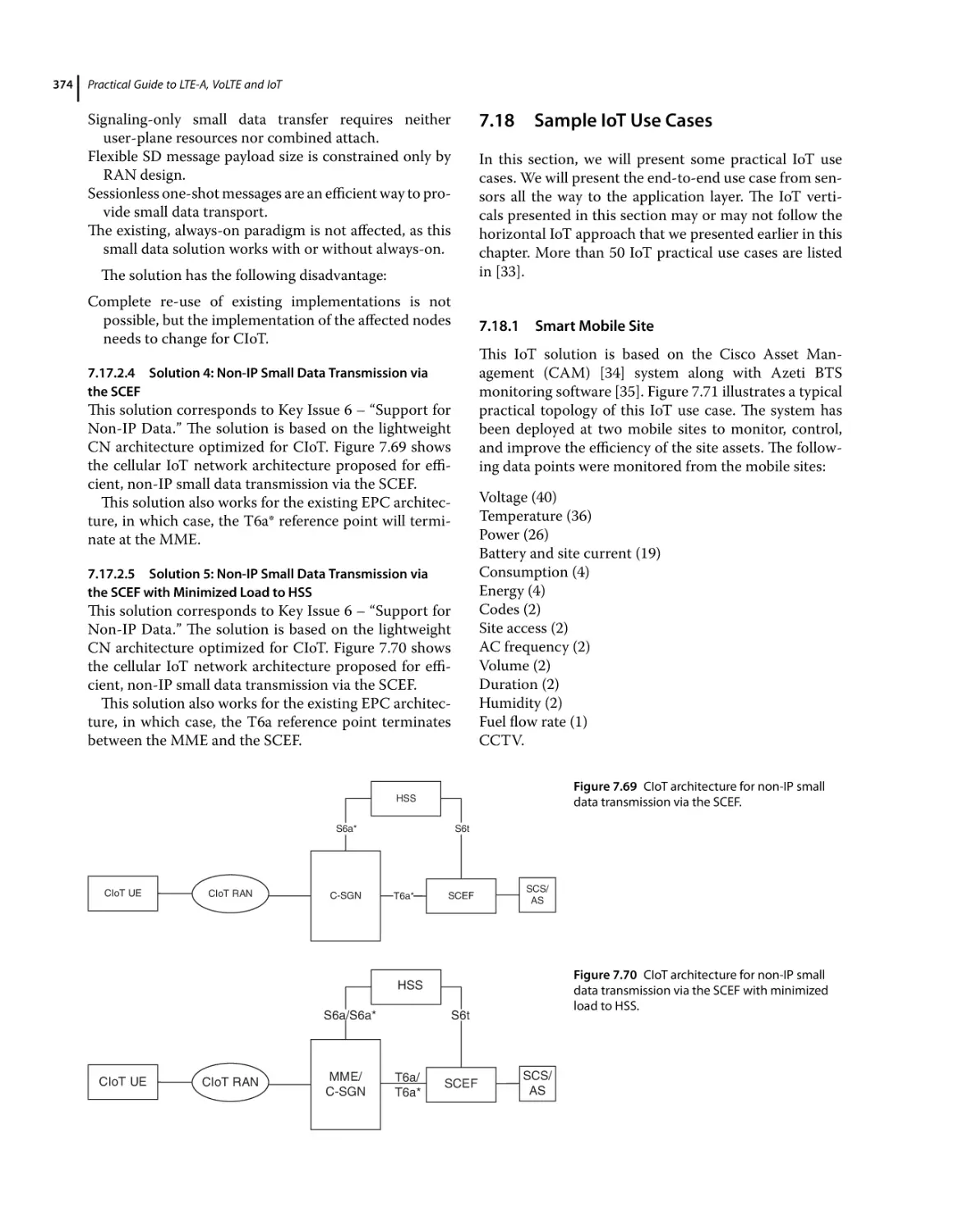
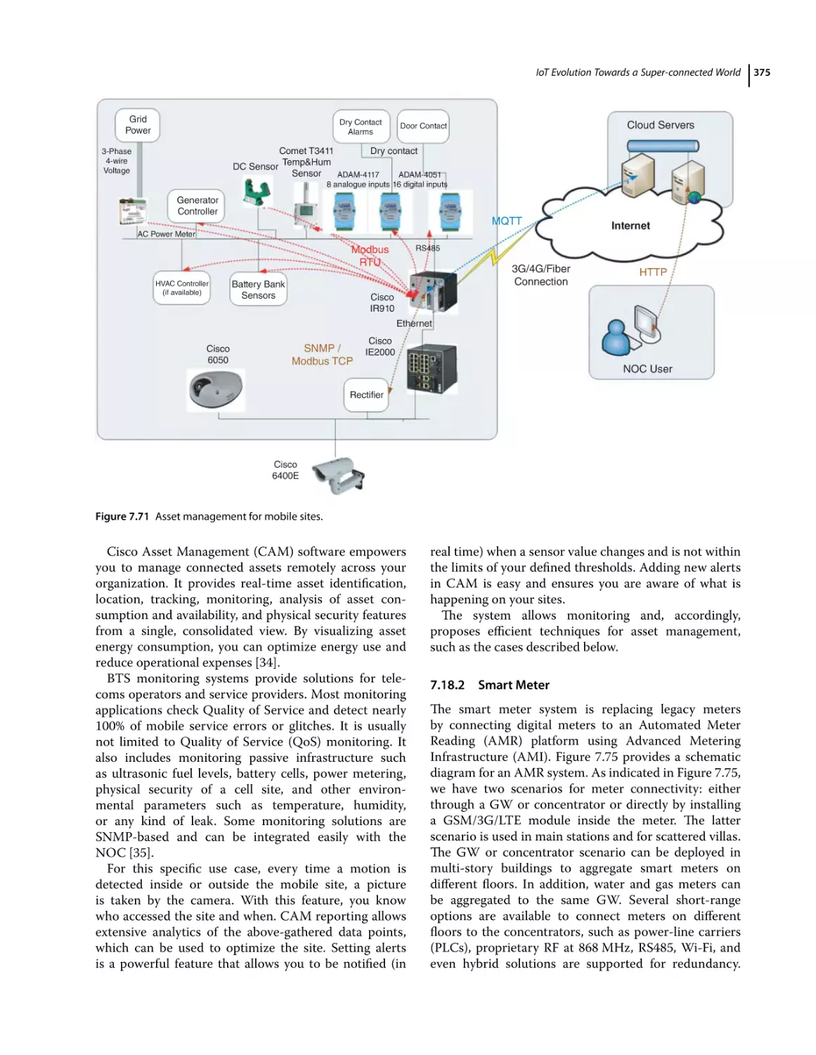
Solution 4: Non-IP Small Data Transmission via the SCEF 374
Solution 5: Non-IP Small Data Transmission via the SCEF with Minimized Load to HSS 374
Sample IoT Use Cases 374
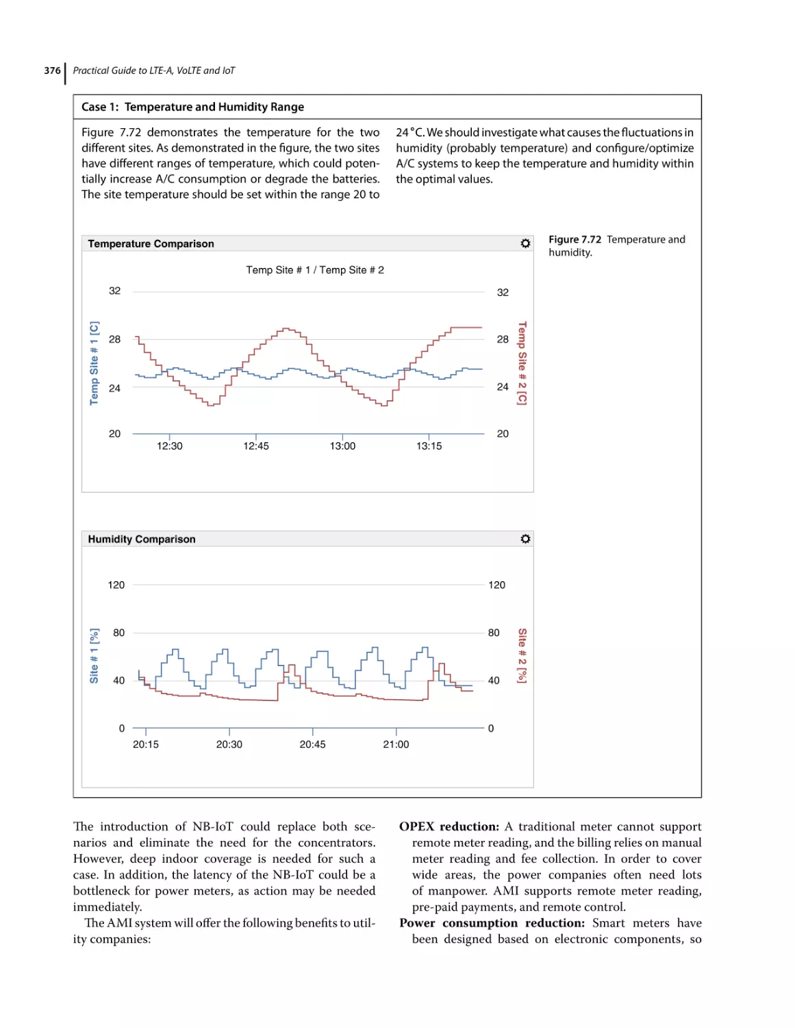
Smart Mobile Site 374
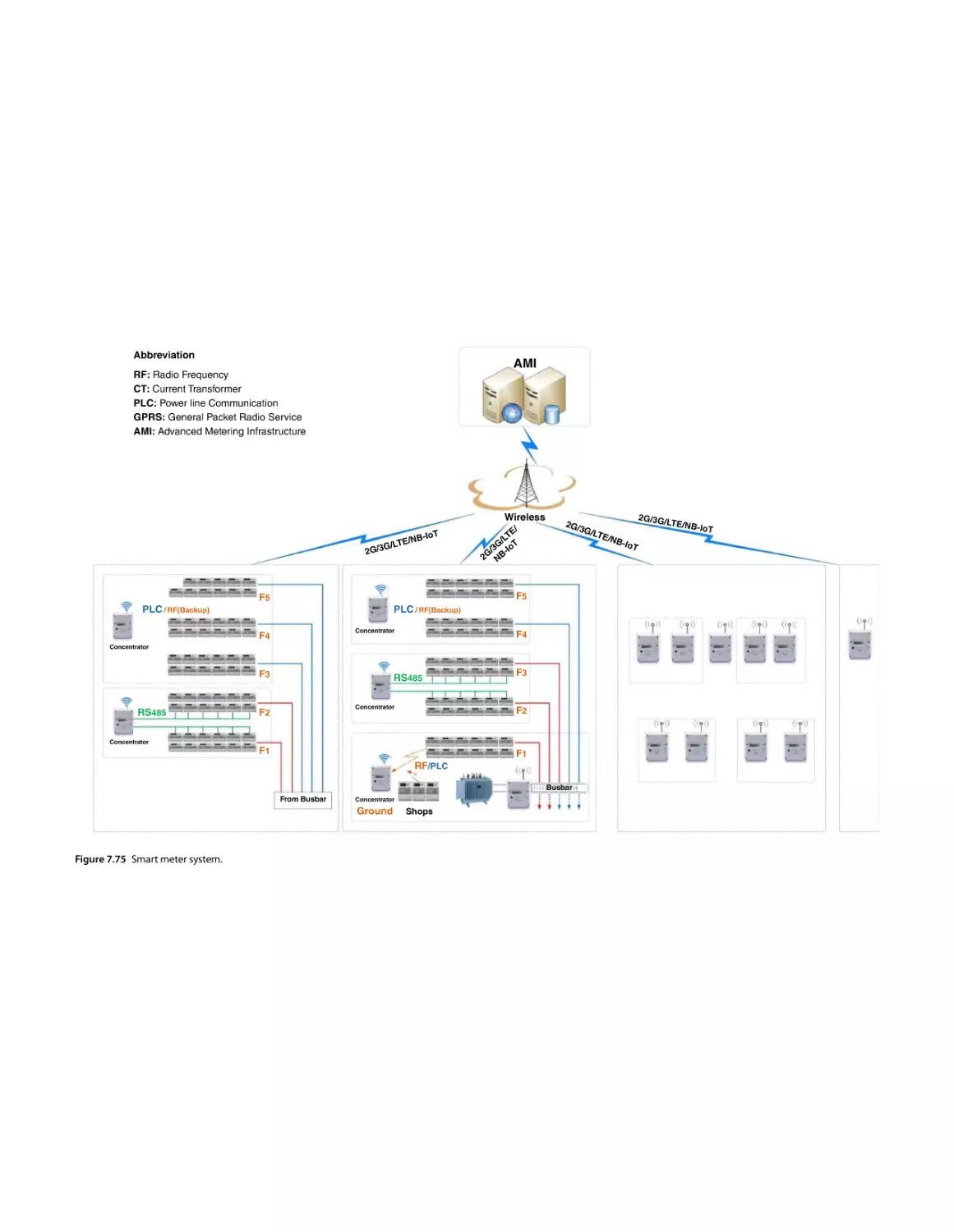
Smart Meter 375
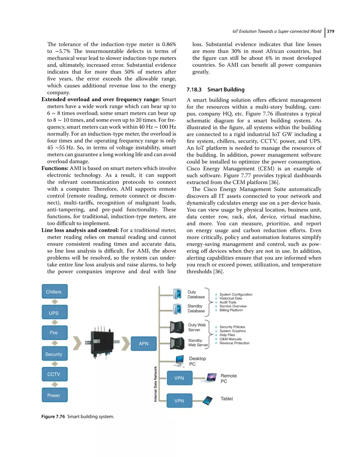
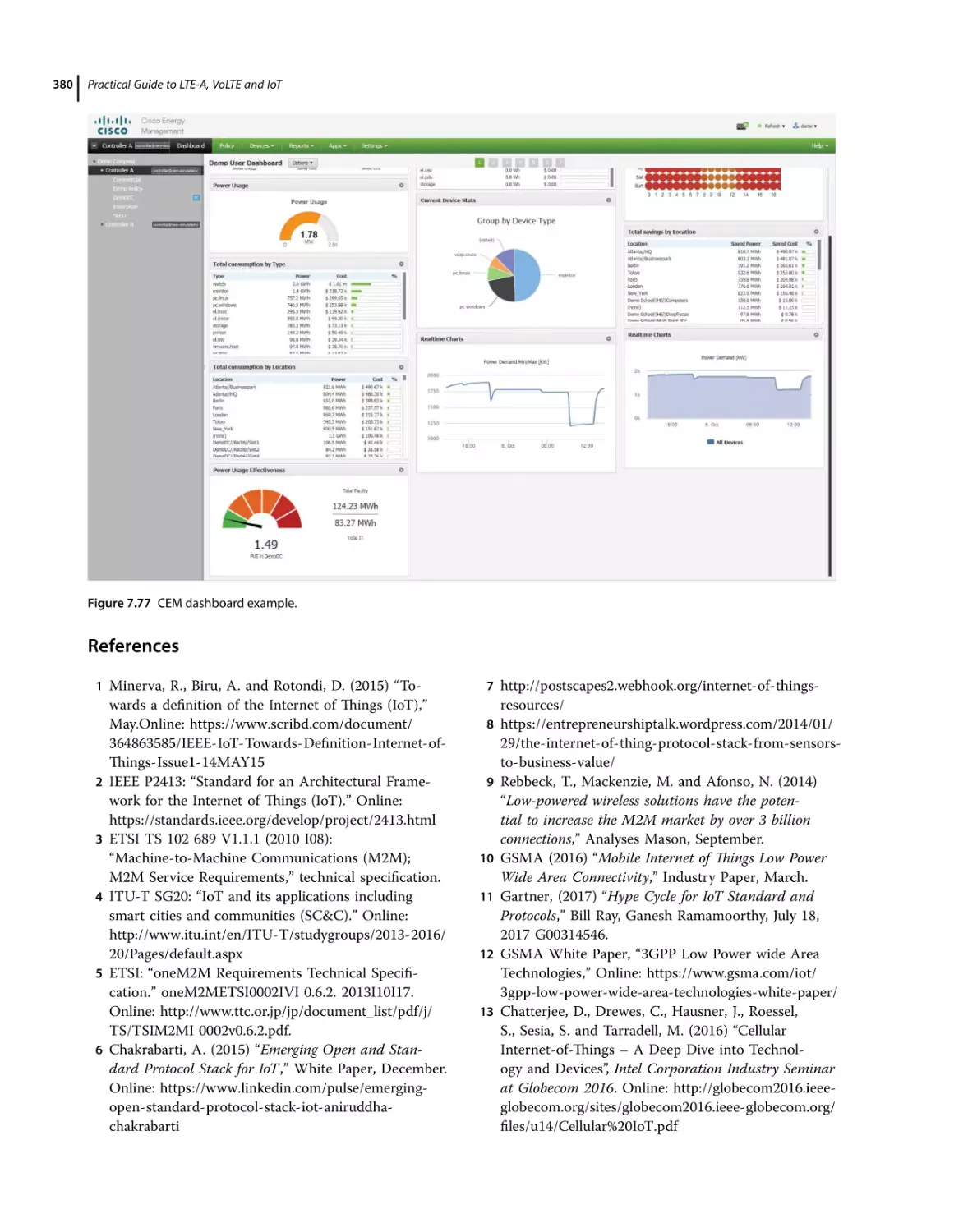
Smart Building 379
References 380
Contents
8
5G Evolution Towards a Super-connected World 382
8.1
8.2
8.2.1
8.2.2
8.2.3
8.3
8.4
8.5
8.6
8.6.1
8.7
8.8
8.9
8.10
8.10.1
8.10.1.1
8.10.1.2
8.10.1.3
8.10.1.4
8.10.2
8.10.3
8.10.4
8.10.5
8.11
8.11.1
8.11.1.1
8.11.1.2
8.11.1.3
8.11.1.4
8.11.1.5
8.11.2
8.11.2.1
8.11.2.2
8.11.2.3
8.11.2.4
8.12
8.12.1
8.12.2
8.12.3
8.12.3.1
8.12.3.2
8.12.3.3
8.12.3.4
8.12.3.5
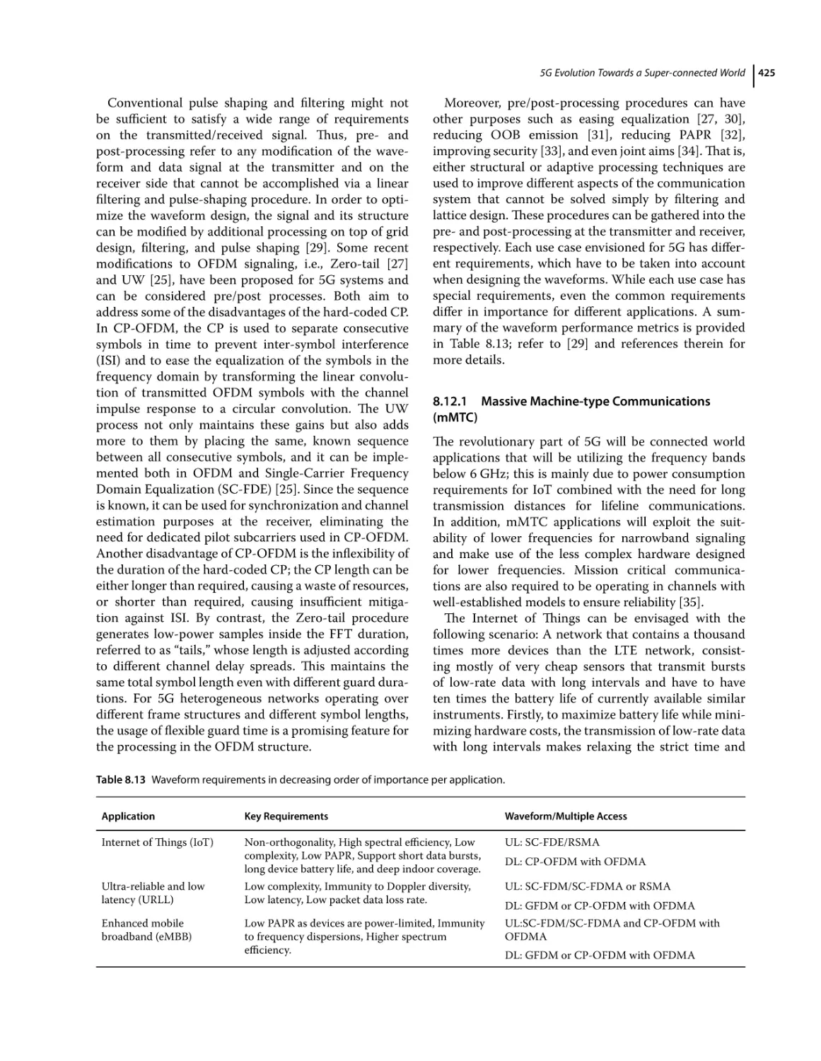
8.13
8.13.1
8.14
Overview 382
Introduction 382
Definition and Use Cases for 5G 382
LTE Evolution to Enable 5G Use Cases 382
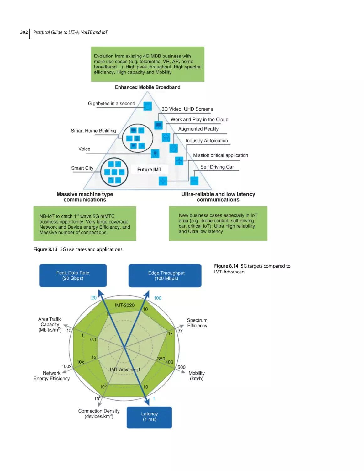
Massive Machine-type Communication (mMTC) 384
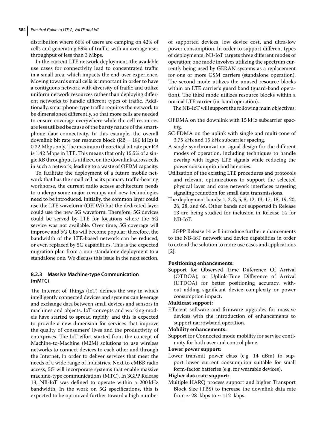
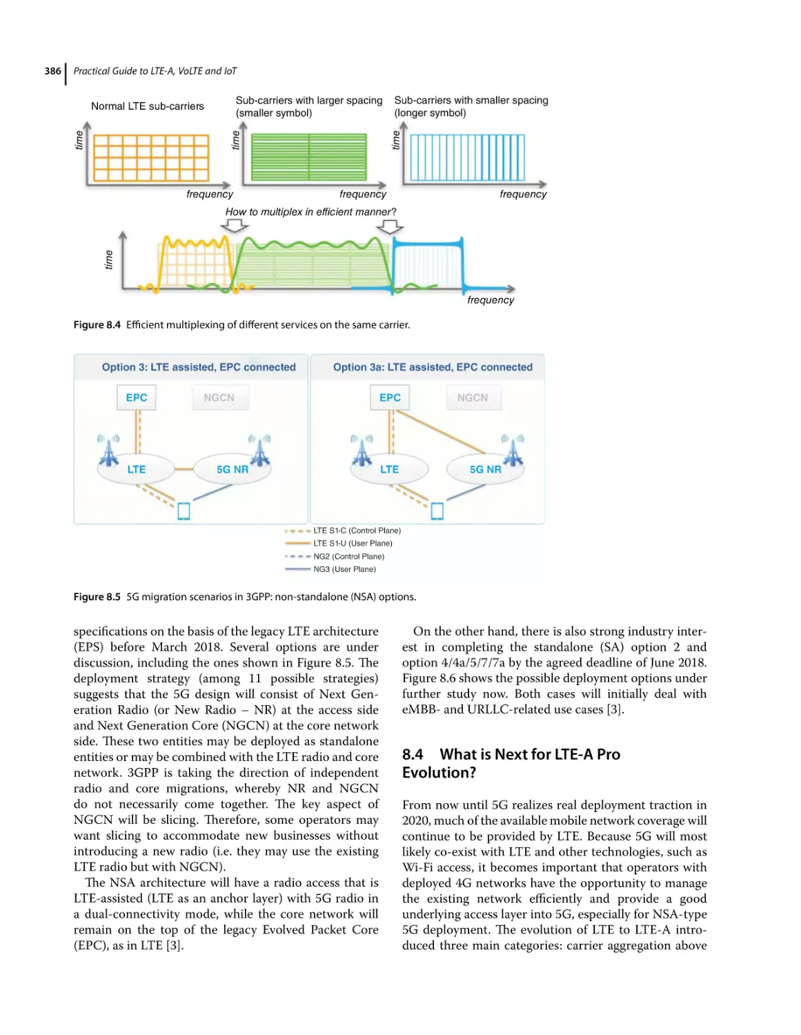
5G New Radio (NR) and Air Interface 385
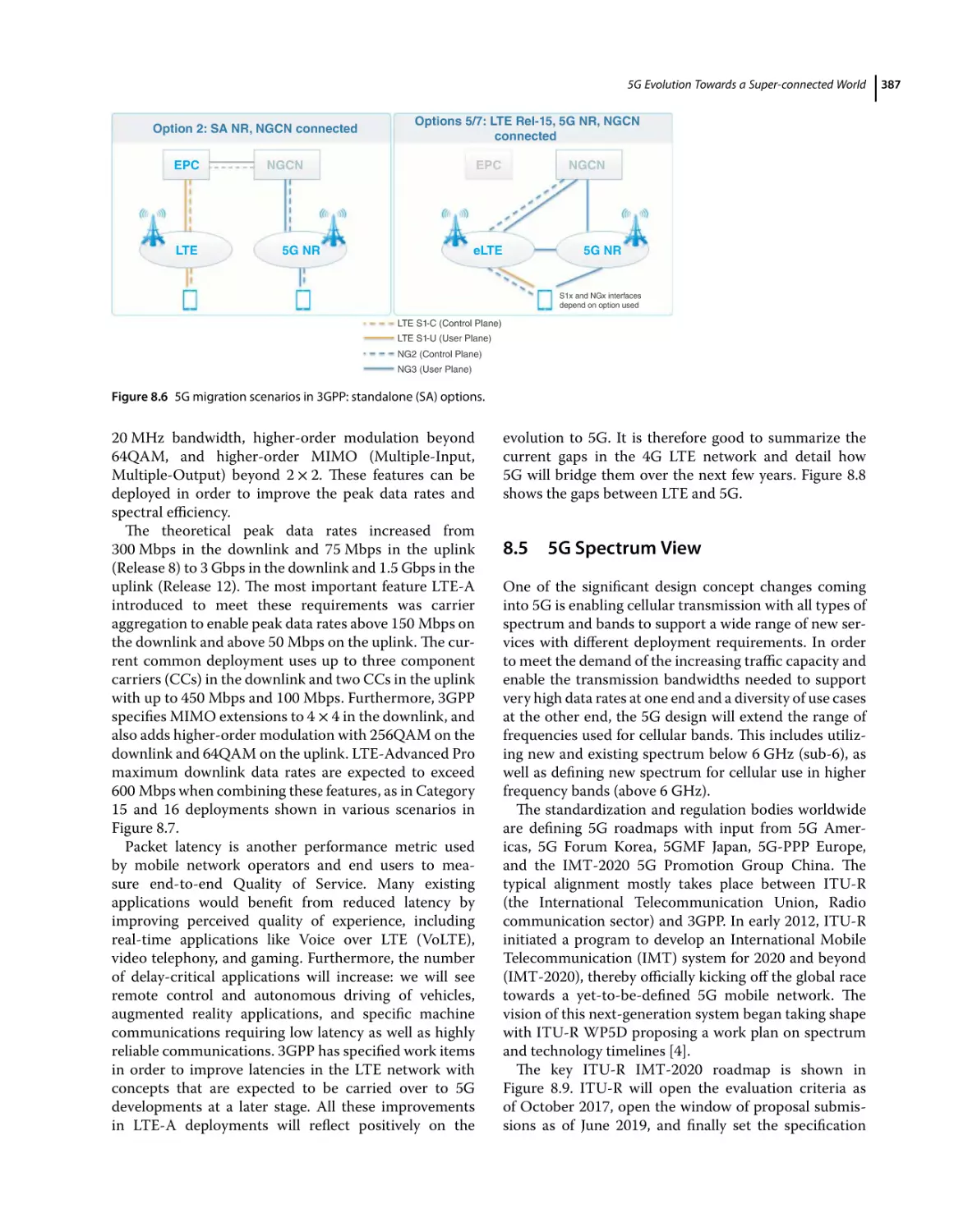
What is Next for LTE-A Pro Evolution? 386
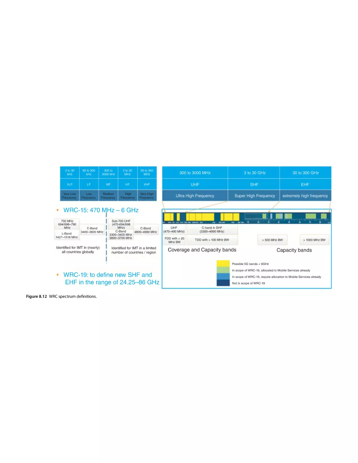
5G Spectrum View 387
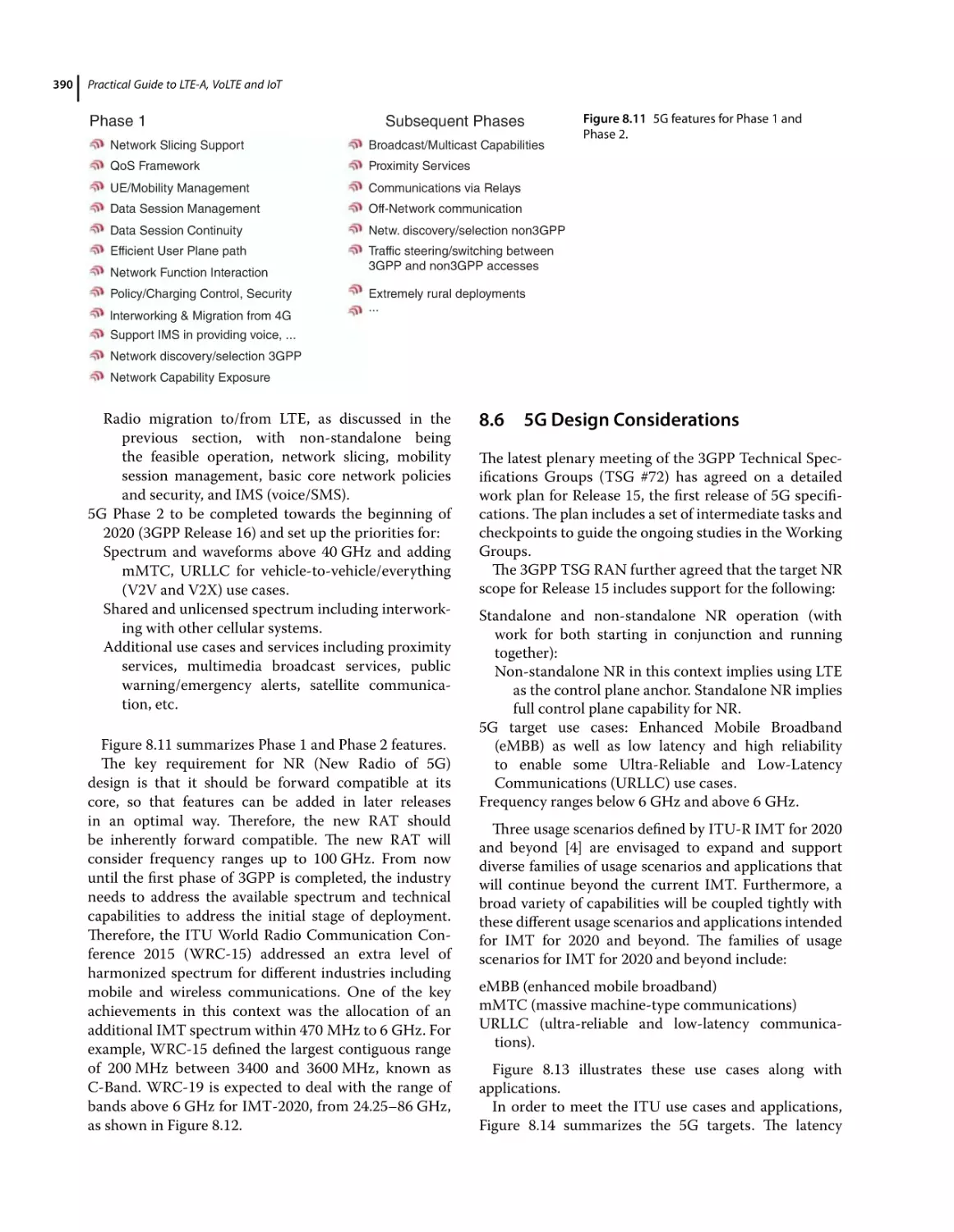
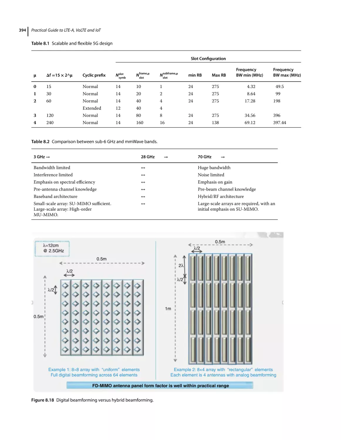
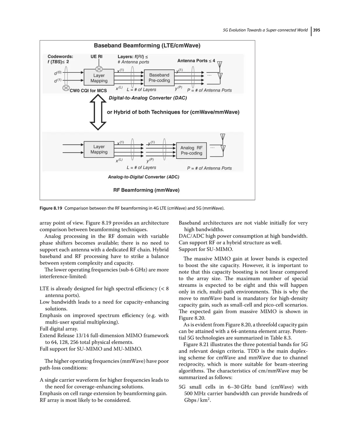
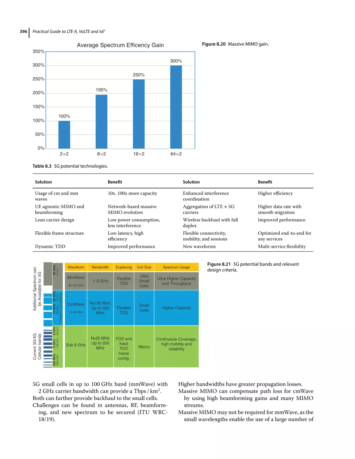
5G Design Considerations 390
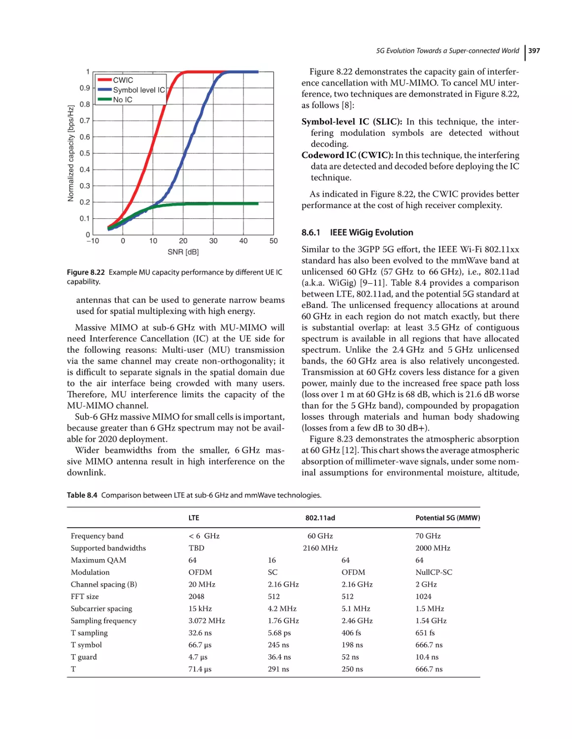
IEEE WiGig Evolution 397
5G Deployment Scenarios for Mobile Applications 400
Air-to-Ground and Satellite Scenarios 401
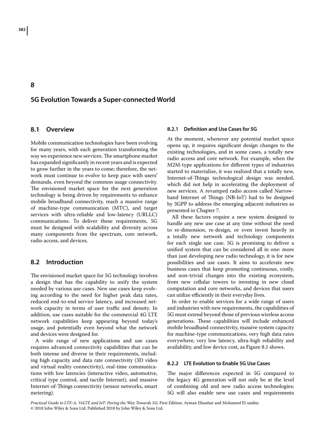
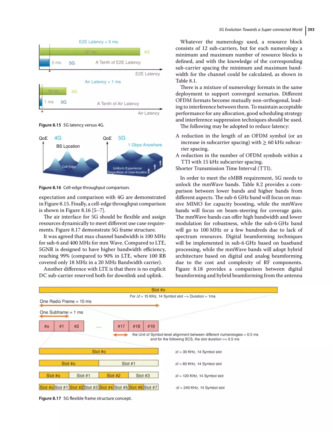
5G Evaluation KPIs 405
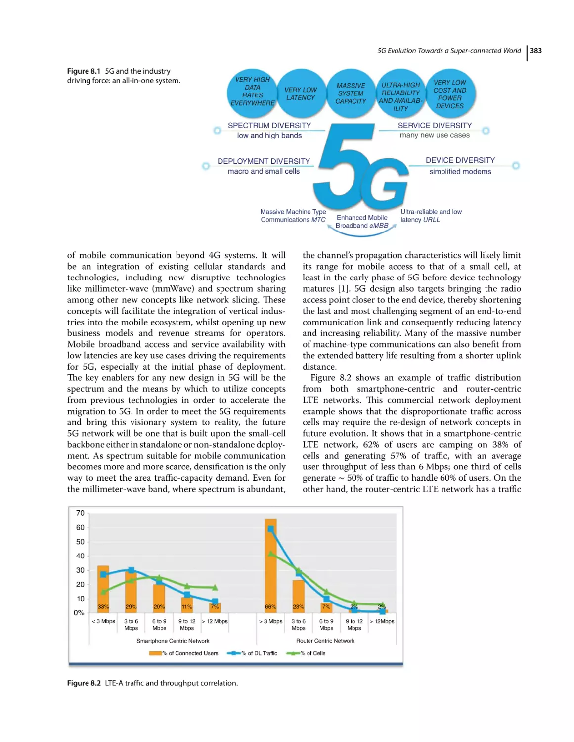
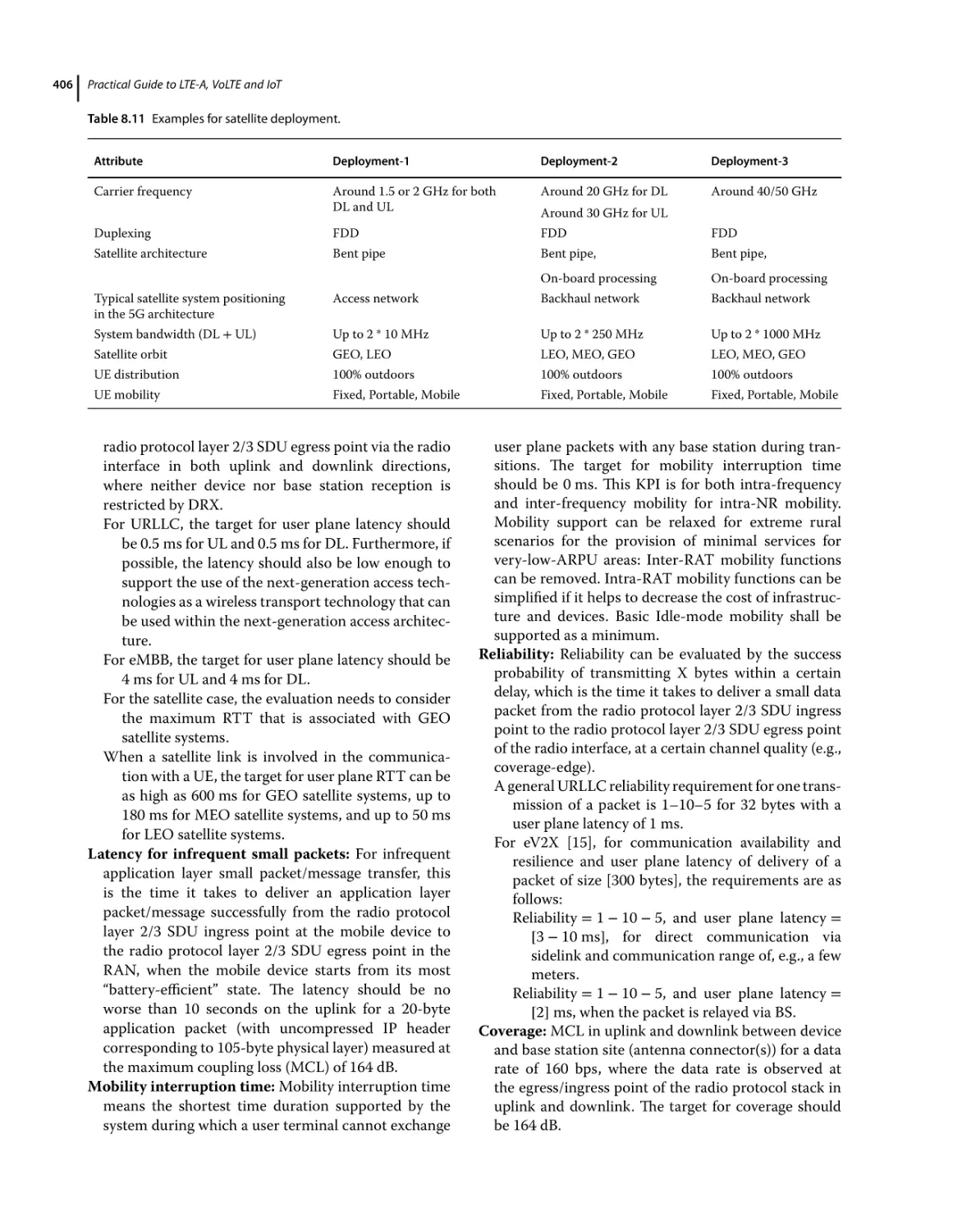
Next-generation Radio Access Requirements 407
Deployment Scenarios for 5G NR 409
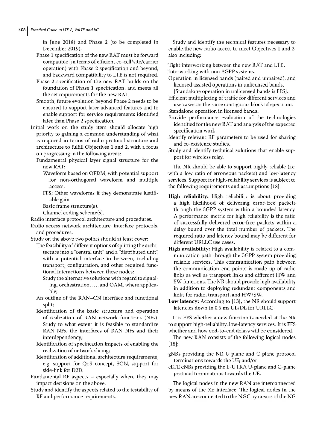
Non-centralized Deployment 409
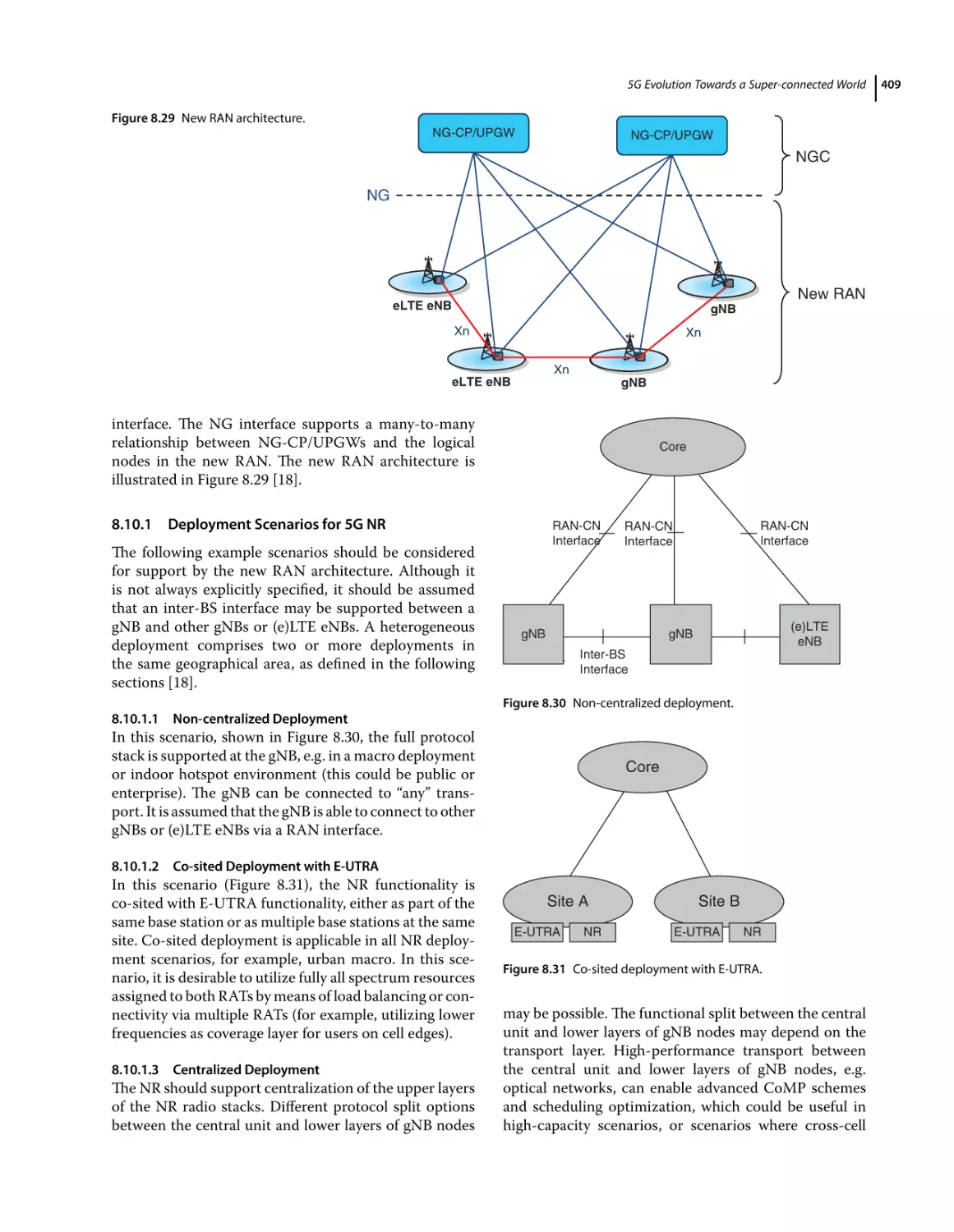
Co-sited Deployment with E-UTRA 409
Centralized Deployment 409
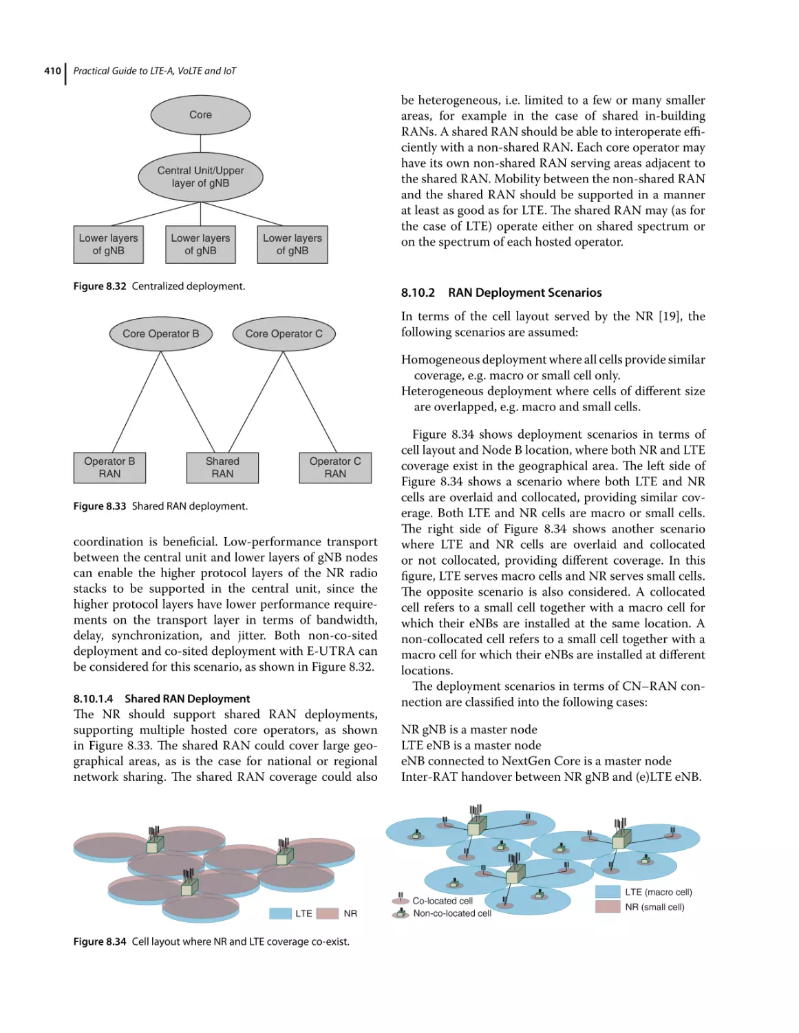
Shared RAN Deployment 410
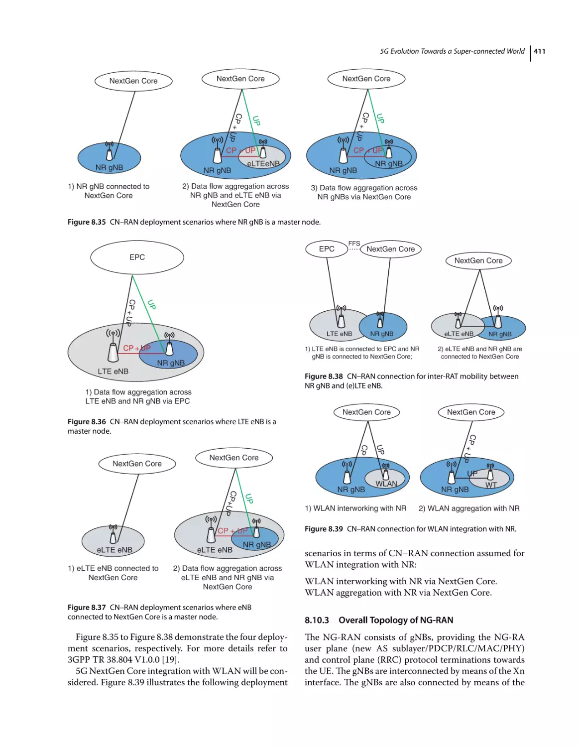
RAN Deployment Scenarios 410
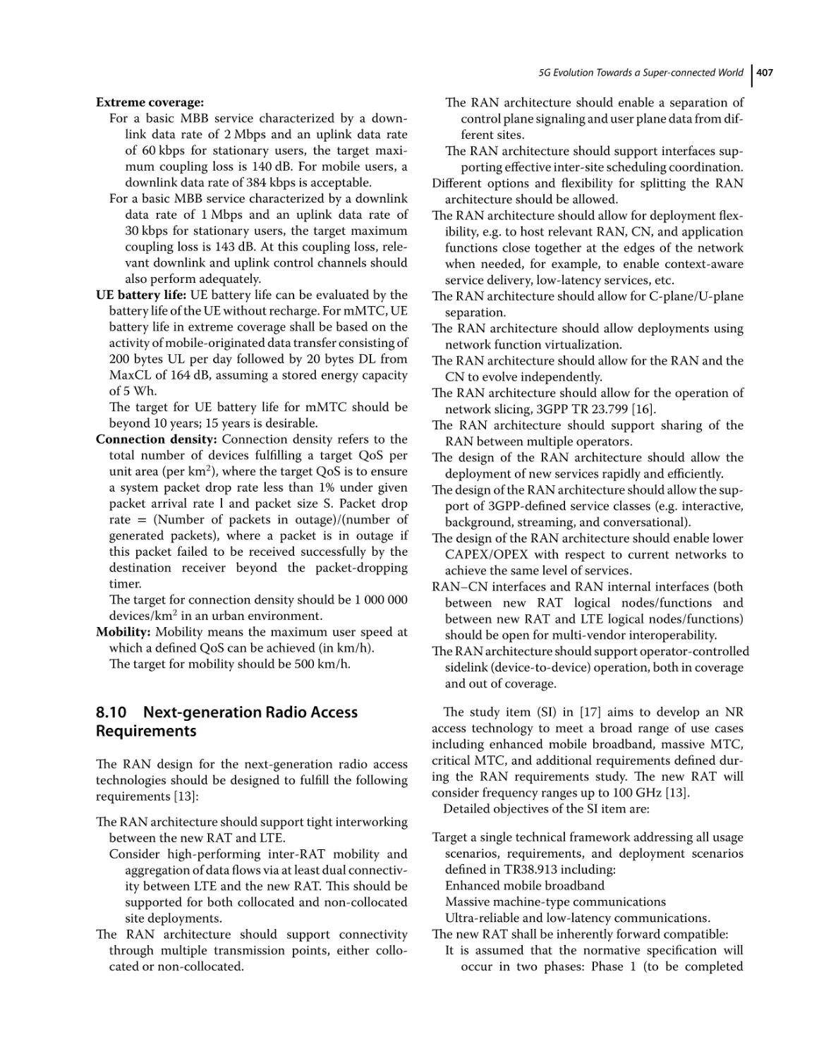
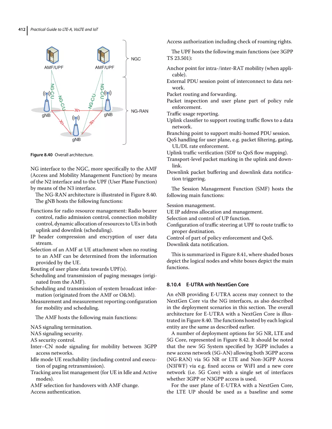
Overall Topology of NG-RAN 411
E-UTRA with NextGen Core 412
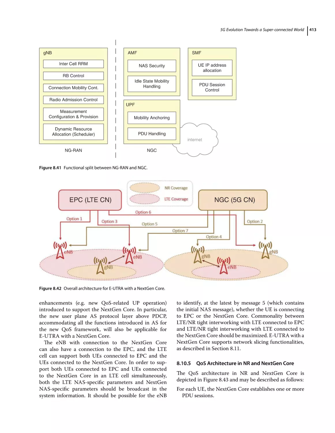
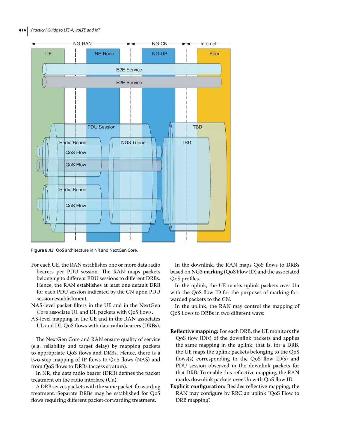
QoS Architecture in NR and NextGen Core 413
5G NextGen Core Network Architecture 416
Core Deployment Scenarios 417
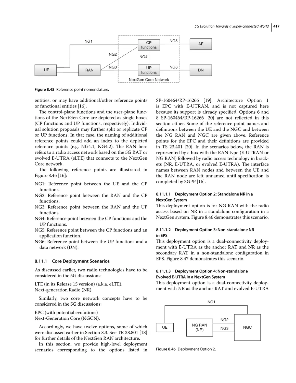
Deployment Option 2: Standalone NR in a NextGen System 417
Deployment Option 3: Non-standalone NR in EPS 417
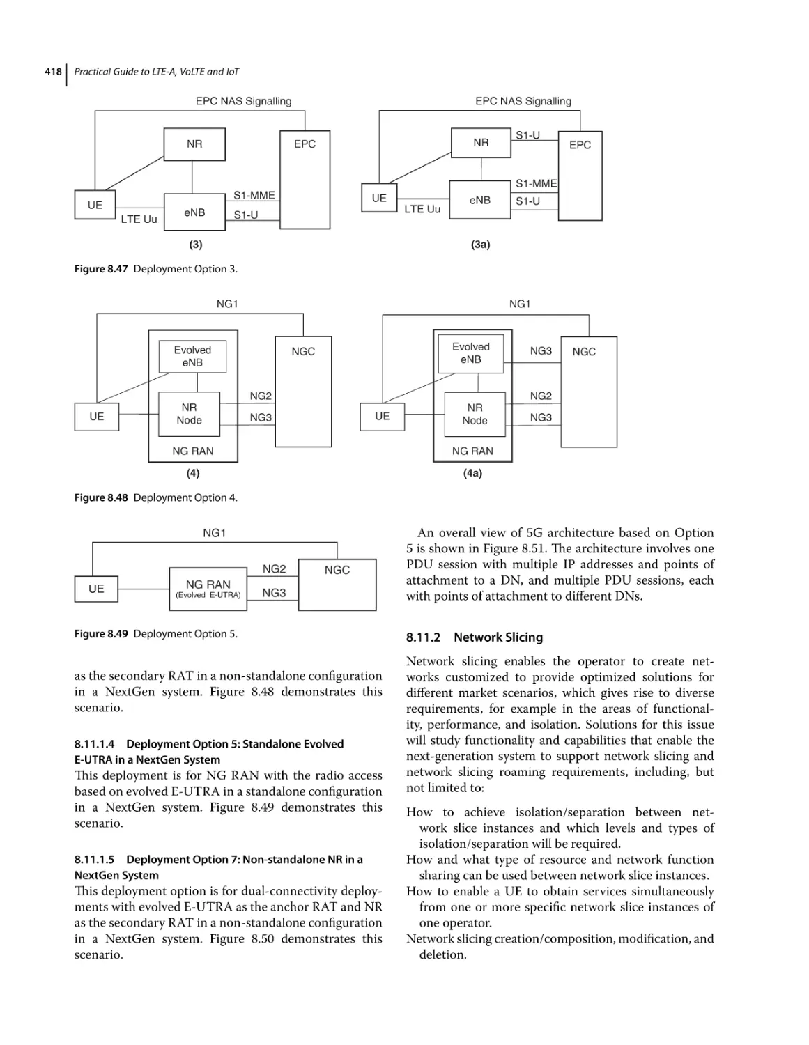
Deployment Option 4: Non-standalone Evolved E-UTRA in a NextGen System 417
Deployment Option 5: Standalone Evolved E-UTRA in a NextGen System 418
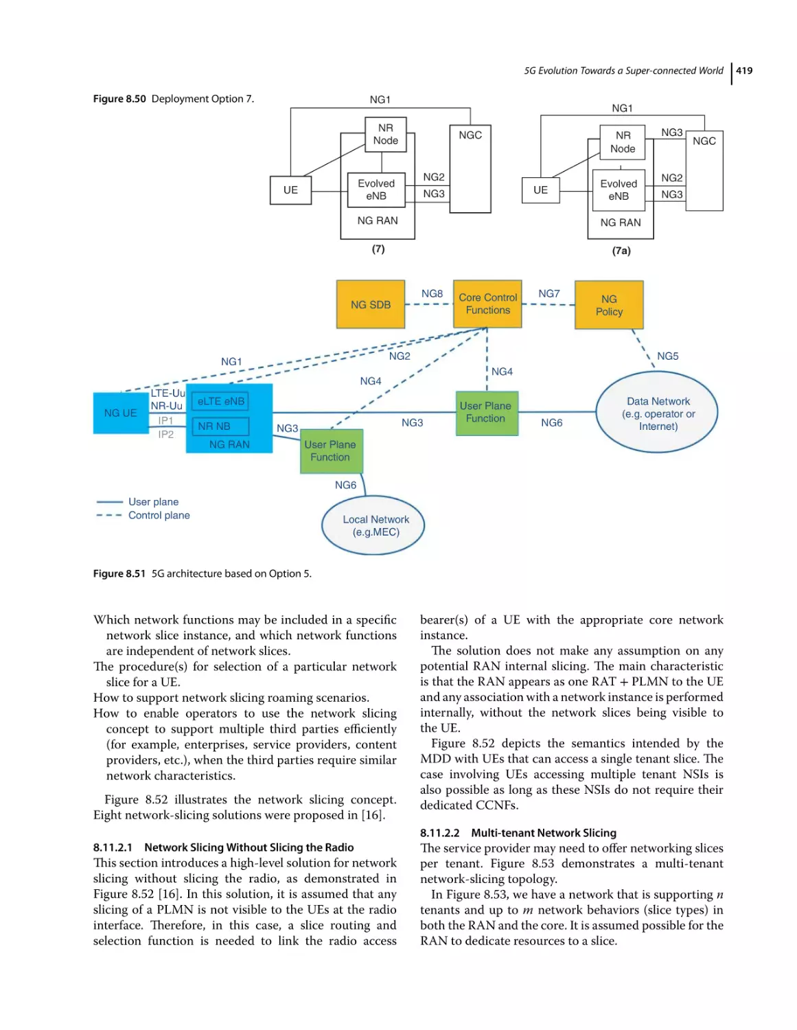
Deployment Option 7: Non-standalone NR in a NextGen System 418
Network Slicing 418
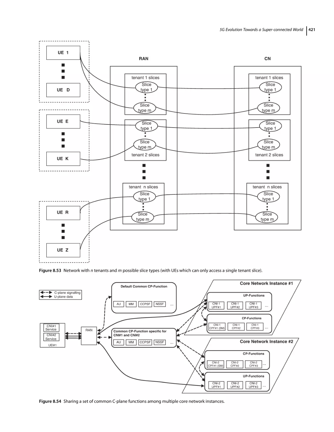
Network Slicing Without Slicing the Radio 419
Multi-tenant Network Slicing 419
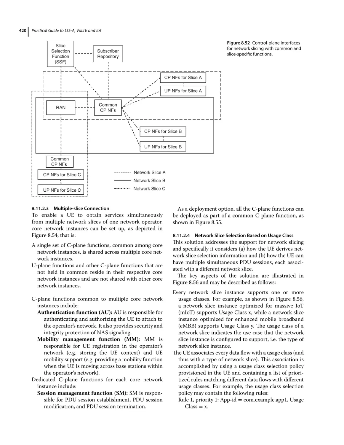
Multiple-slice Connection 420
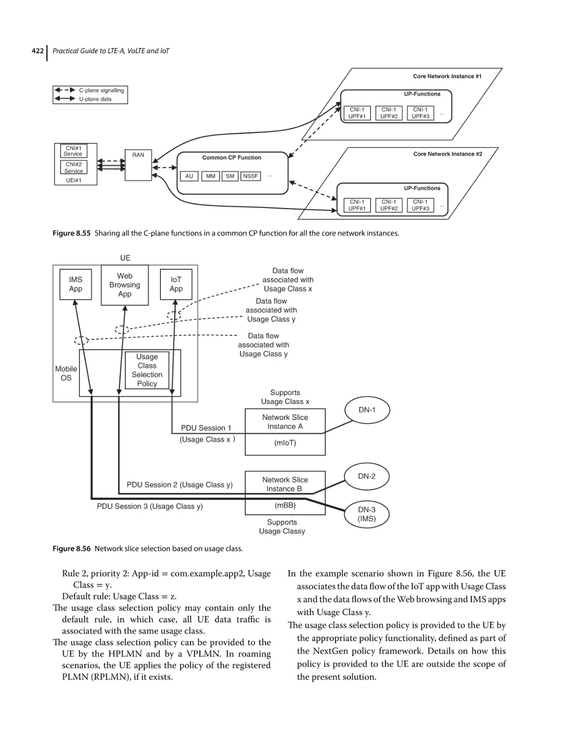
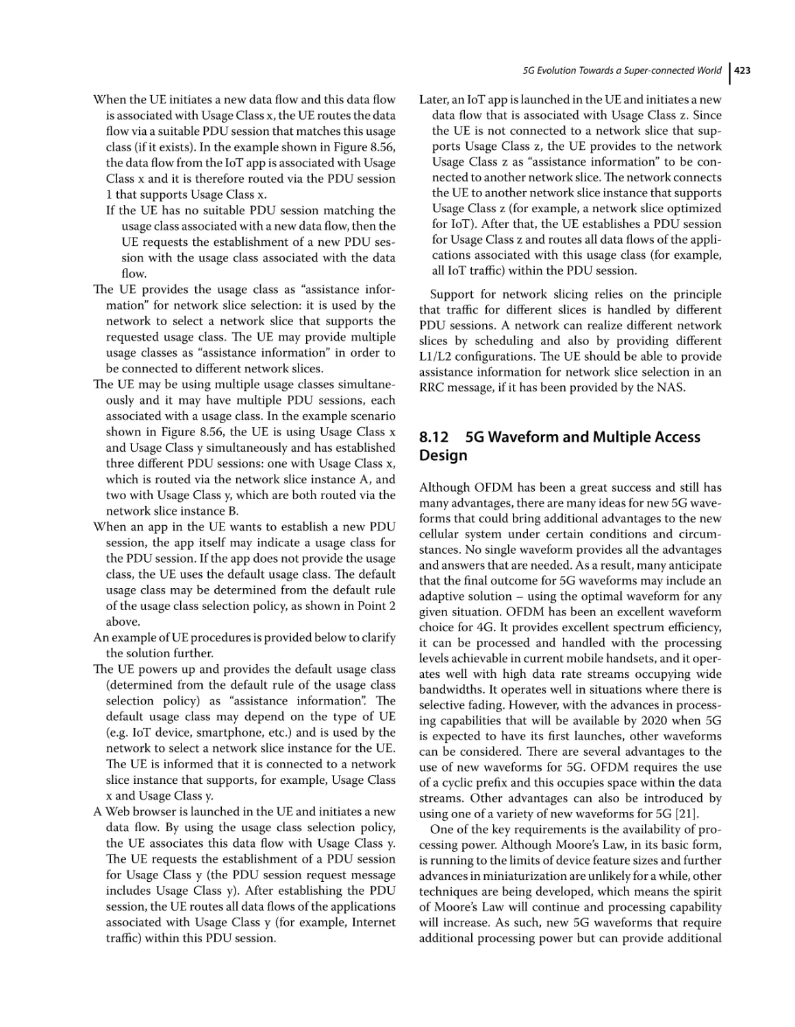
Network Slice Selection Based on Usage Class 420
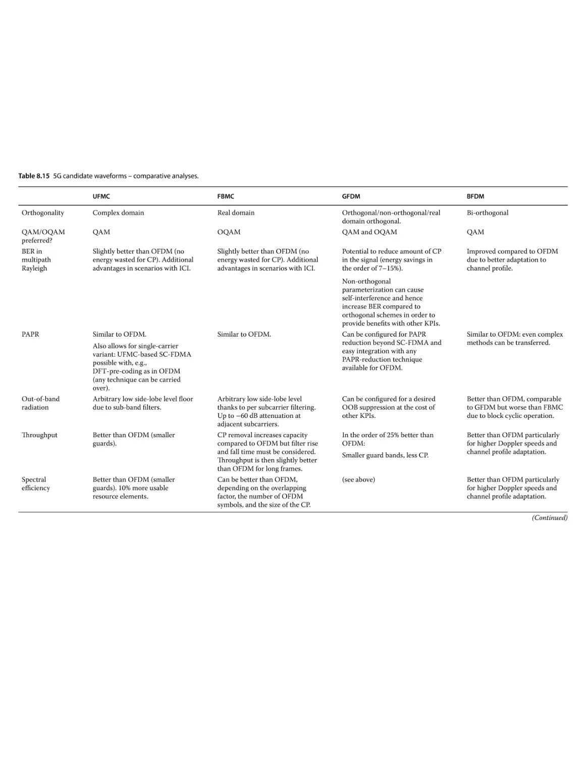
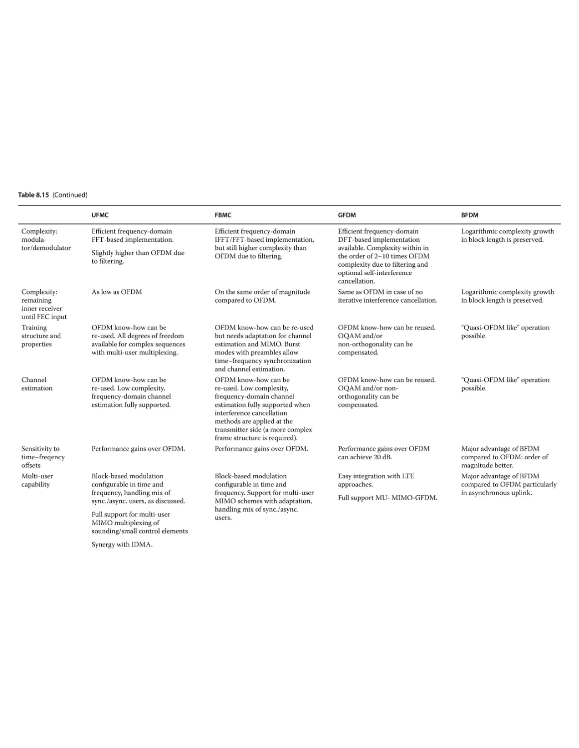
5G Waveform and Multiple Access Design 423
Massive Machine-type Communications (mMTC) 425
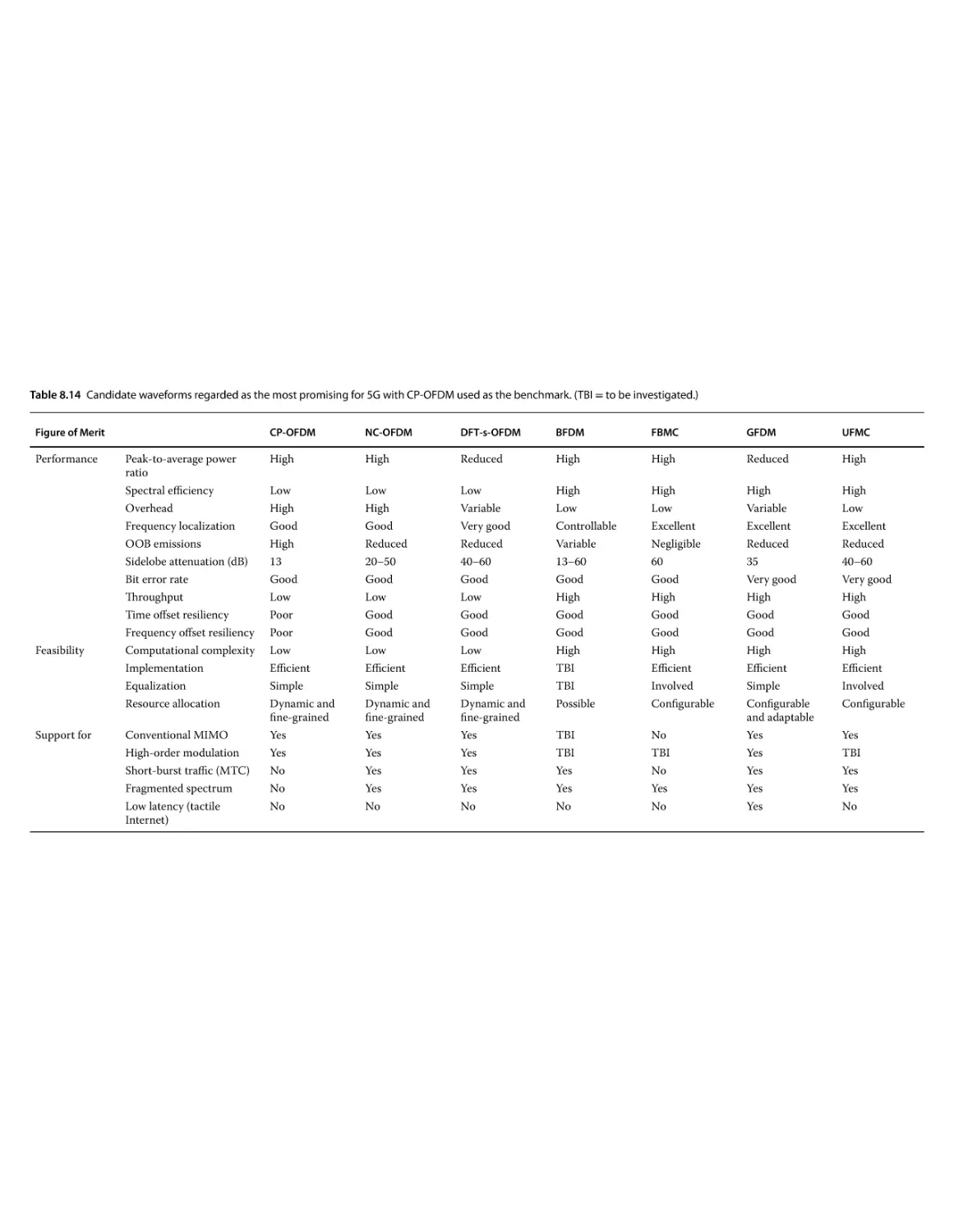
Enhanced Mobile Broadband (eMBB) 426
Multiple Access Techniques 426
Non-orthogonal Multiple Access (NOMA) 426
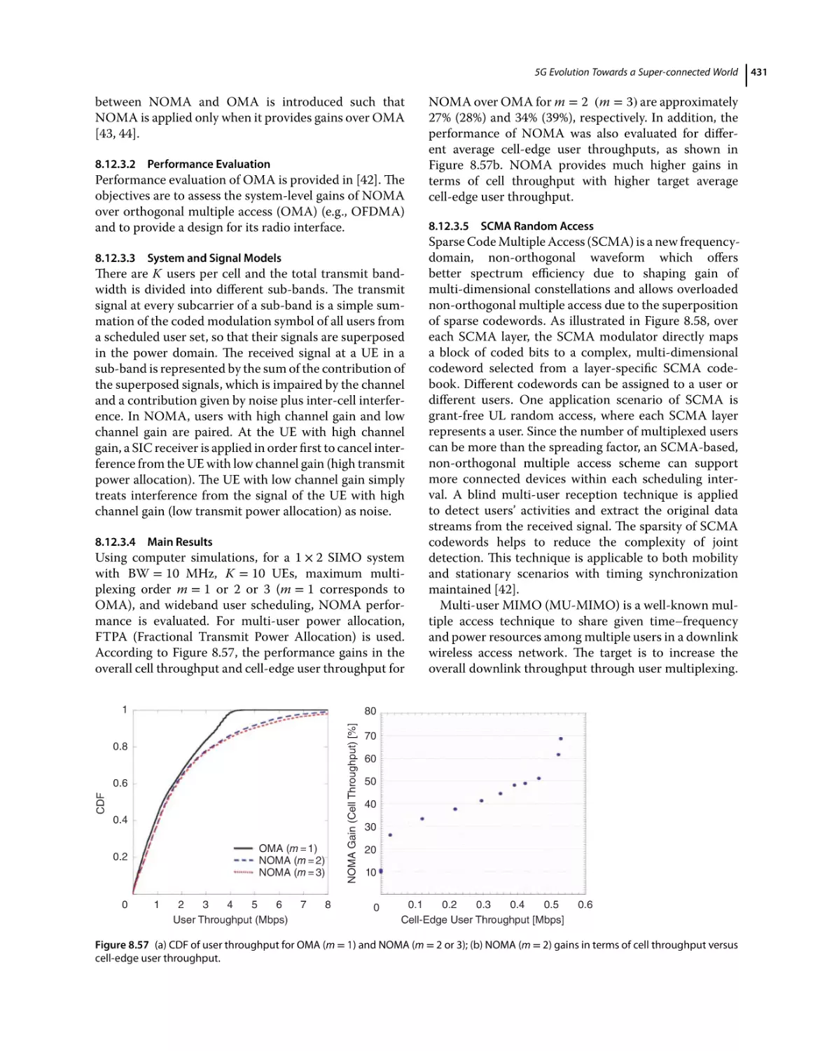
Performance Evaluation 431
System and Signal Models 431
Main Results 431
SCMA Random Access 431
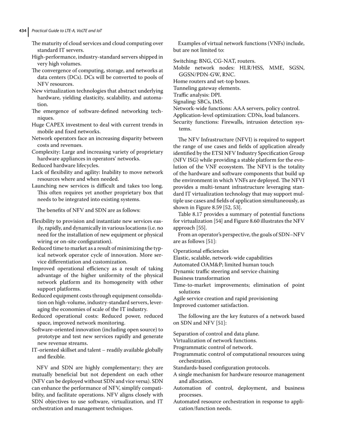
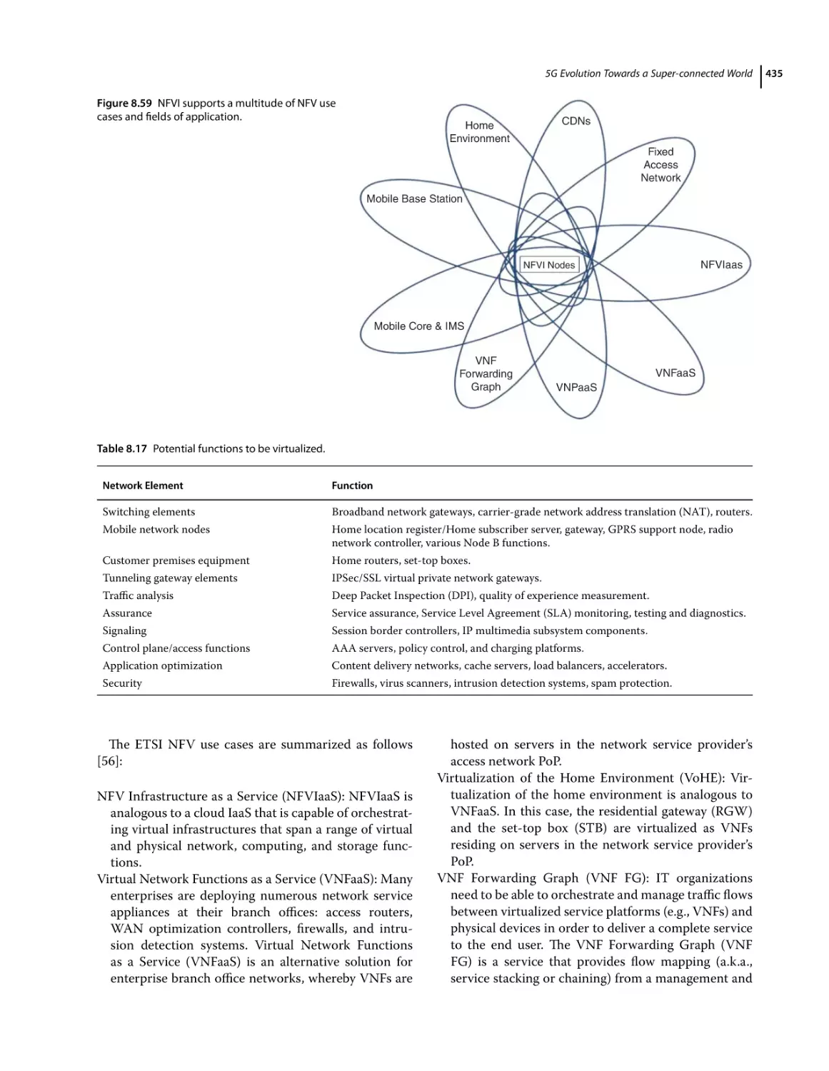
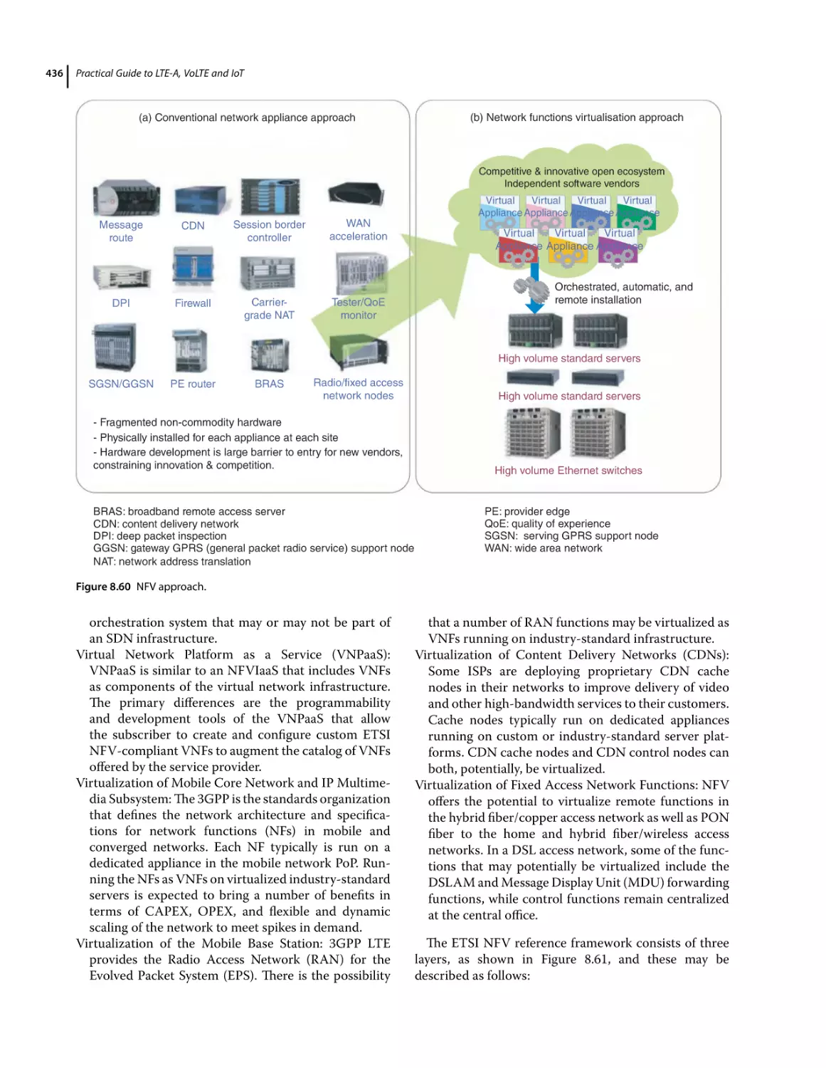
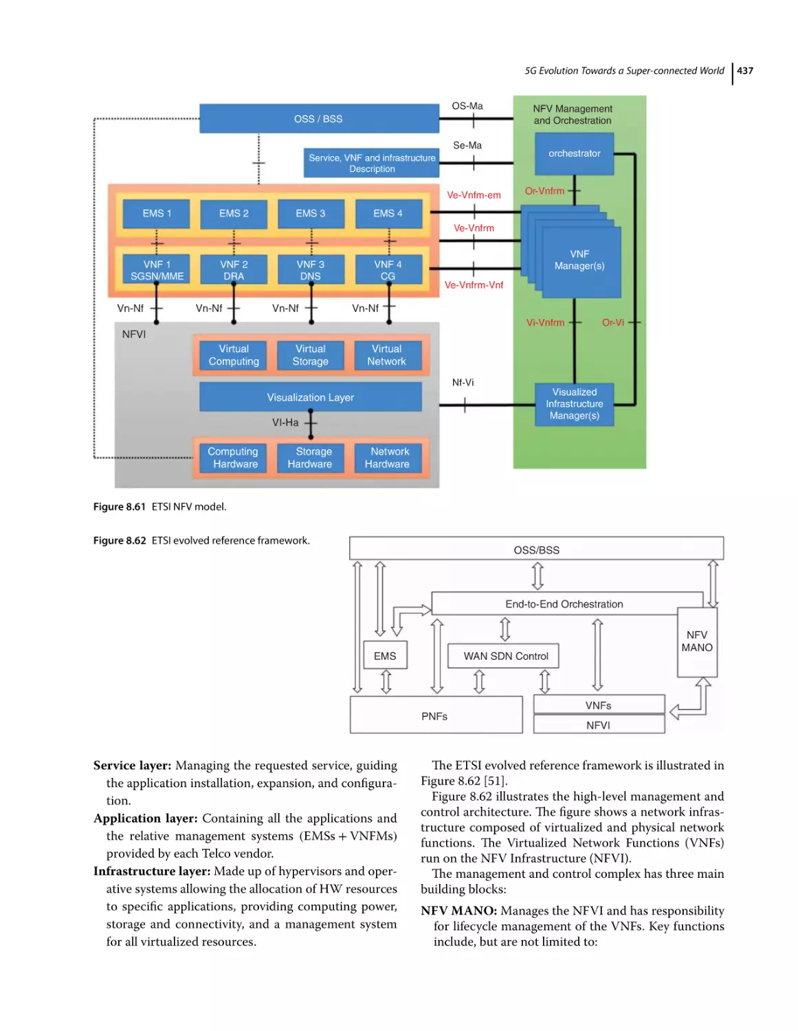
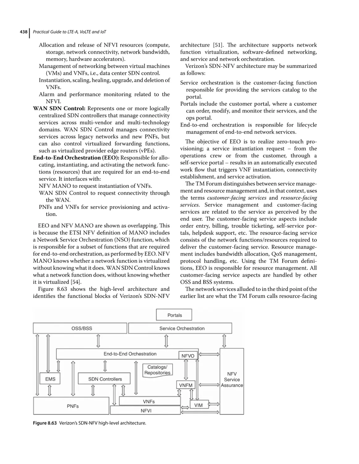
NFV and SDN 433
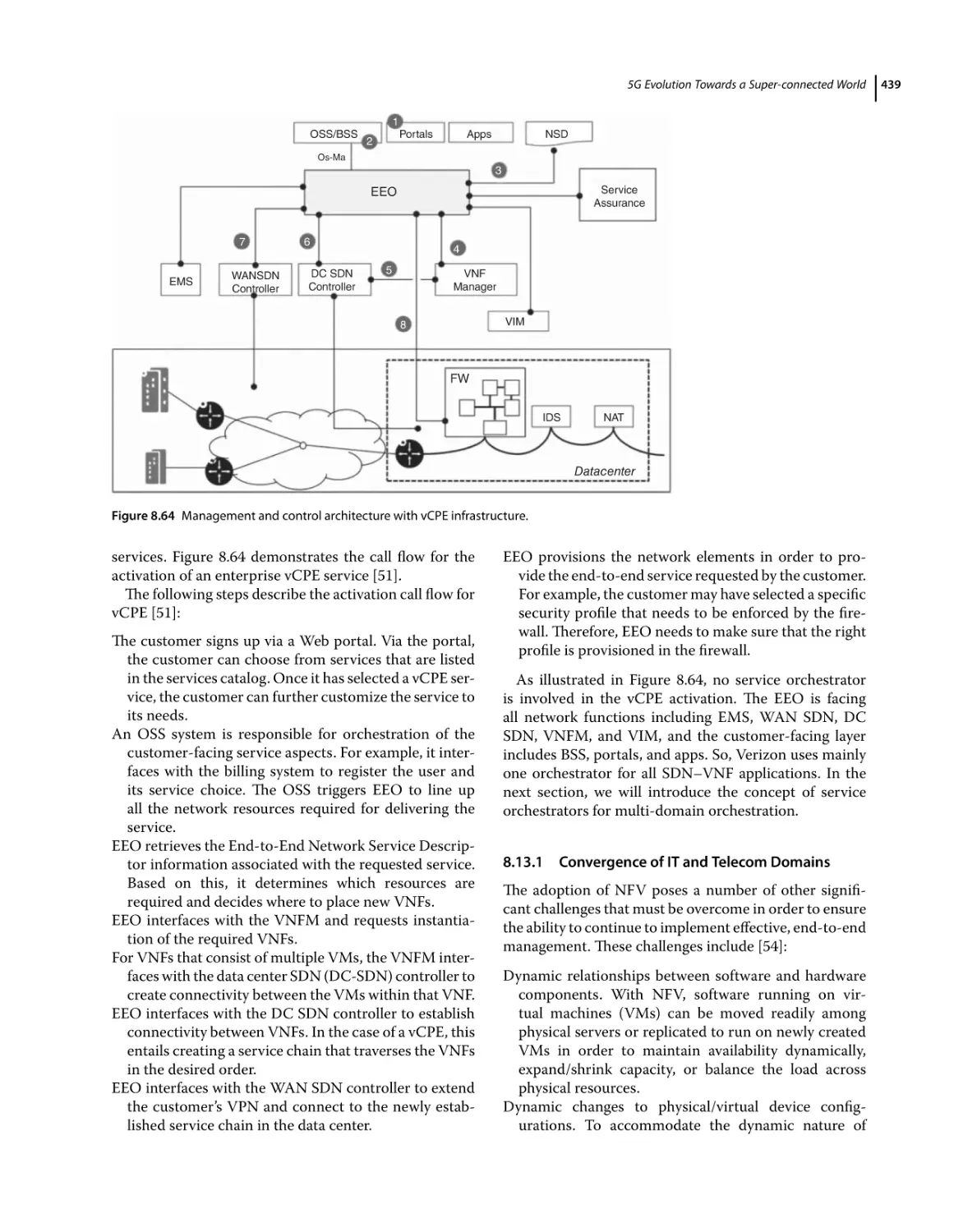
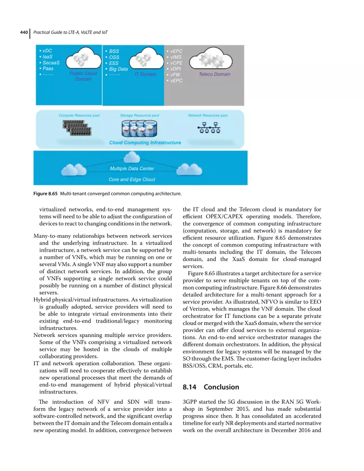
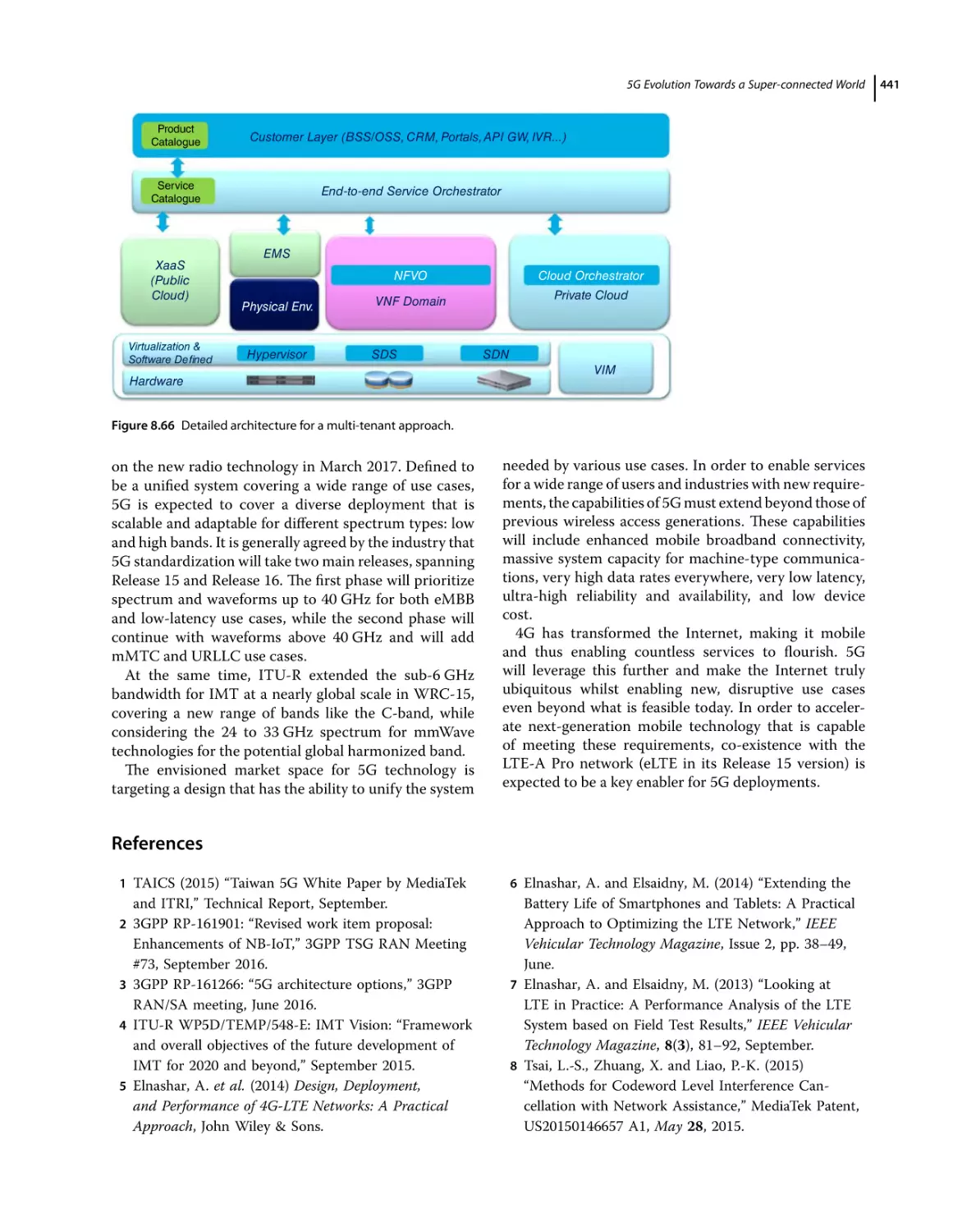
Convergence of IT and Telecom Domains 439
Conclusion 440
References 441
Index 445
xv
xvii
About the Authors
Ayman Elnashar, PhD, has 20+ years of experience in
telecoms industry including 2G/3G/LTE/WiFi/IoT/5G.
He was part of three major start-up telecom operators in the MENA region (Orange/Egypt, Mobily/KSA,
and du/UAE). Currently, he is Head of Infrastructure
Planning: ICT and Cloud with the Emirates Integrated Telecommunications Co. “du”, UAE. He is the
founder of the Terminal Innovation Lab and UAE 5G
innovation Gate (U5GIG). Prior to this, he was Sr.
Director – Wireless Networks, Terminals and IoT where
he managed and directed the evolution, evaluation,
and introduction of du wireless networks including
LTE/LTE-A, HSPA+, WiFi, NB-IoT and is currently
working towards deploying 5G network in UAE.
Prior to this, he was with Mobily, Saudi Arabia, from
June 2005 to Jan 2008, as Head of Projects. He played key
role in contributing to the success of the mobile broadband network of Mobily/KSA. From March 2000 to June
2005, he was with Orange Egypt.
He published 30+ papers in the wireless communications arena in highly ranked journals and international
conferences. He is the author of Design, Deployment, and
Performance of 4G-LTE Networks: A Practical Approach
published by Wiley & Sons, and Simplified Robust Adaptive Detection and Beamforming for Wireless Communications to be published in May 2018.
His research interests include practical performance
analysis, planning and optimization of wireless networks
(3G/4G/WiFi/IoT/5G), digital signal processing for
wireless communications, multiuser detection, smart
antennas, massive MIMO, and robust adaptive detection
and beamforming.
Mohamed El-saidny, M.Sc., is a leading technical
expert in wireless communication systems for modem
chipsets and network design. He established and managed the Carrier Engineering Services Business Unit
at MediaTek, the department responsible for product
business development and strategy alignment with
network operators and direct customers. He has 15+
years of technical, analytical and business experience,
with an international working experience in the United
States, Europe, Middle East, Africa, and South-East Asia
markets.
Mohamed is the inventor of numerous patents in
CDMA and OFDM systems and the co-author of Design,
Deployment and Performance of 4G-LTE Networks: A
Practical Approach book by Wiley & Sons. He published
several international research papers in IEEE Communications Magazine, IEEE Vehicular Technology Magazine,
other IEEE Transactions, in addition to contributions to
3GPP specifications.
xix
Preface
This book is a practical guide to the design, deployment, and performance of LTE-A, VoLTE/IMS and
IoT. A comprehensive practical performance analysis
for VoLTE is conducted based on field measurement
results from live LTE networks. Also, it provides a
comprehensive introduction to IoT, 3GPP NB-IoT and
5G evolutions. Practical aspects and best practice of
LTE-A/IMS/VoLTE/IoT, plus LTE-Advanced features
such as Carrier Aggregation (CA), are presented. In
addition, LTE/LTE-A network capacity dimensioning
and analysis are demonstrated based on live LTE/LTE-A
networks KPIs. A comprehensive foundation for 5G
technologies is provided including massive MIMO,
eMBB, URLLC, mMTC, NGCN and network slicing,
cloudification, virtualization and SDN.
Chapter 1 provides an overview of LTE/LTE-A networks. This chapter is the foundation for the chapters 2
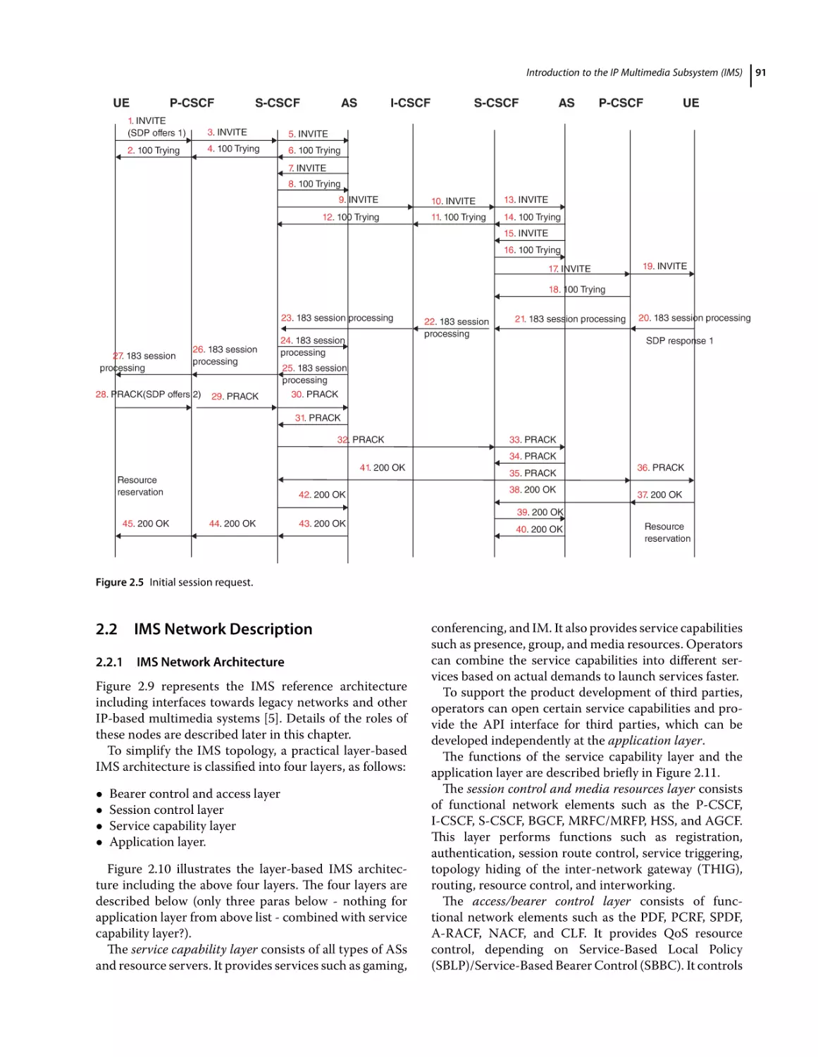
to 6. In Chapter 2, we will introduce the IP Multimedia
Subsystem (IMS), which is the core network of Voice
over LTE (VoLTE) and other advanced voice evolutions.
The IMS architecture, core network elements, call and
signaling flow between different network elements are
comprehensively presented. The chapter provides the
foundation for VoLTE performance analysis highlighted
in chapter 3 and chapter 4. Other IMS services such
as Voice over Wi-Fi (VoWiFi), Video over LTE (ViLTE),
and Web Real-Time, Communication (WebRTC) are not
discussed in detail. In addition, practical deployment
scenarios for IMS-network-based on real use cases from
a live network deployment are presented.
Chapter 3 presents practical performance analysis
including an end-to-end assessment of call setup delay
in different radio conditions, main challenges impacting
the in-call performance, and performance aspects of
Single Radio Voice Call Continuity (SRVCC) and its
evolution releases. Therefore, Chapter 3 provides comprehensive analysis for call setup delay including CSFB
and VoLTE with different scenarios (stationary and
mobility), and handover analysis including SRVCC in
terms of data interruption time. Finally, recent topics in
handover performance and data interruption reduction
during handover are presented. Synchronized handover
is introduced as a potential solution to reduce data
interruption time during handover.
Chapter 4 presents comprehensive practical analysis
of VoLTE performance based on commercially deployed
3GPP Release 10 LTE networks. The analysis in chapter
4 demonstrates VoLTE performance in terms of RTP
error rate, RTP jitter and delays, BLER, and VoLTE voice
quality in terms of MOS. In Chapter 4, we will also evaluate key VoLTE features such as RoHC, TTI bundling,
and SPS.
Chapter 5 analyzes the new features in LTE-A including carrier aggregation (CA), LAA, downlink 256QAM,
uplink 64QAM modulation, uplink data compression
(UDC), and eVoLTE.
Chapter 6 evaluates LTE counters collected for a commercially deployed 3GPP Release 10 LTE network. The
analysis in this chapter includes LTE users (connected
and active), LTE scheduling, LTE traffic downlink/uplink,
TTI utilizations, physical resource block utilization,
modulation and codec scheme, channel quality indicator
(CQI), MIMO, and CSFB performance.
Chapter 7 will cover the evolution of the Internet of
Things (IoT) from different aspects. The aim is to provide the reader with a holistic overview of IoT evolution
and a guide on how to build, design, and customize a successful IoT use case from all perspectives including technical and commercial aspects. We will focus on 3GPP
cellular IoT evolution for connectivity, i.e., narrowband
IoT (NB-IoT). However, we will initially summarize the
IoT evolution from an end-to-end perspective, including
the IoT platform, IoT protocols, connectivity, and sensors layer. The IoT evolution is different from the regular mobile evolution; the latter is focusing on connectivity only, while IoT evolution should be addressed from
an end-to-end prospective. This is because the IoT connectivity is only 5% to 10% of the IoT value chain and
therefore, the service provider should offer an end-to-end
use case. We will present in this chapter practical IoT
use cases along with dashboards to demonstrate the value
of IoT.
xx
Preface
Chapter 8 will provide a comprehensive introduction
to 5G access and core networks. Advanced 5G technologies such as massive MIMO, 5G flexible frame design,
URLLC, mMTC, NGCN and network slicing are also
presented. Finally, virtualization and software defined
network are summarized along with service provider
roadmap for converged native cloud.
xxi
Acknowledgments
Many people volunteered their time and talent to make
this project a reality, and we thank each and every one
of them for their invaluable support. We acknowledge
the huge contribution of Mohamed Yehia from du for
chapters two and six. We also appreciate the support of
Mohanad ElSakka from du for reviewing chapters two
and six. We acknowledge the support of our colleagues at
du from different sections for providing feedback, practical results and conducting testing scenarios. Without
their support, this book could not be produced with such
practical scenarios from live network. du is a vibrant and
multiple award-winning telecommunications service
provider in UAE, serving nine million individual customers with its mobile, fixed line, broadband Internet,
and Home services. du also caters to over 100,000 UAE
businesses with its vast range of ICT solutions. Finally,
we would like to thank the organizations that provided
permission for use of their copyrighted material which
significantly improved the presentation of this book.
1
1
LTE and LTE-A Overview
1.1 Introduction
Cellular mobile networks have been evolving for many
years. As the smartphone market has expanded significantly in recent years and is expected to grow more in
the years to come, network evolution needs to keep up
with the pace of users’ demands. This chapter provides an
overview for network operators and interested others on
the evolution of cellular networks, with particular focus
on 3GPP for the main technologies of WCDMA/UMTS
and LTE. In addition, it highlights the interaction of 3GPP
with non-3GPP technology (i.e. Wi-Fi).
The initial networks are referred to collectively as the
First Generation (1G) system. The 1G mobile system was
designed to utilize analog; it included AMPS (Advanced
Mobile Telephone System). The Second Generation (2G)
mobile system was developed to utilize digital multiple
access technology: TDMA (Time Division Multiple
Access) and CDMA (Code Division Multiple Access).
The main 2G networks were GSM (Global System for
Mobile communications) and CDMA, also known as
cdmaOne or IS-95 (Interim Standard 95). The GSM
system still has worldwide support and is available for
deployment on several frequency bands, such as 900
MHz, 1800 MHz, 850 MHz, and 1900 MHz. CDMA systems in 2G networks use a spread-spectrum technique
and utilize a mixture of codes and timing to identify cells
and channels. In addition to being digital and improving
capacity and security, these digital 2G systems also offer
enhanced services such as SMS (Short Message Service)
and circuit-switched data. Different variations of the
2G technology have evolved to extend the support of
efficient packet data services and to increase the data
rates. GPRS (General Packet Radio System) and EDGE
(Enhanced Data Rates for Global Evolution) systems
have evolved from GSM. The theoretical data rate of
473.6 kbps enables operators to offer multimedia services efficiently. Since it does not comply with all the
features of a 3G system, EDGE is usually categorized as
2.75G.
The Third Generation (3G) system is defined by
IMT2000 (International Mobile Telecommunications).
IMT2000 requires a 3G system to provide higher transmission rates in the range of 2 Mbps for stationary use
and 348 kbps under mobile conditions. The main 3G
technologies are [1]:
WCDMA (Wideband CDMA): This was developed
by the 3GPP (Third Generation Partnership Project).
WCDMA is the air interface of the 3G UMTS (Universal Mobile Telecommunications System). The UMTS
system has been deployed based on the existing GSM
communication core network (CN) but with a new
radio access technology in the form of WCDMA. Its
radio access is based on FDD (Frequency Division
Duplex). Current deployments are mainly in 2.1 GHz
bands. Deployments at lower frequencies are also
possible, such as UMTS900. UMTS supports voice
and multimedia services.
TD-CDMA (Time Division CDMA): This is typically
referred to as UMTS TDD (Time Division Duplex)
and is part of the UMTS specifications. The system
utilizes a combination of CDMA and TDMA to enable
efficient allocation of resources.
TD-SCDMA (Time Division Synchronous CDMA):
This has links to the UMTS specifications and is
often identified as UMTS-TDD Low Chip Rate. Like
TD-CDMA, it is also best suited to low-mobility
scenarios in micro or pico cells.
CDMA2000 (C2K): This is a multi-carrier technology
standard which uses CDMA. It is part of the 3GPP2
standardization body. CDMA2000 is a set of standards
including CDMA2000 EV-DO (Evolution-Data Optimized) which has various revisions. It is backward
compatible with cdmaOne.
WiMAX (Worldwide Interoperability for Microwave
Access): This is another wireless technology which satisfies IMT2000 3G requirements. The air interface is
part of the IEEE (Institute of Electrical and Electronics
Engineers) 802.16 standard, which originally defined
PTP (Point-To-Point) and PTM (Point-To-Multipoint)
systems. This was later enhanced to address multiple
Practical Guide to LTE-A, VoLTE and IoT: Paving the Way Towards 5G, First Edition. Ayman Elnashar and Mohamed El-saidny.
© 2018 John Wiley & Sons Ltd. Published 2018 by John Wiley & Sons Ltd.
2
Practical Guide to LTE-A, VoLTE and IoT
issues related to a user’s mobility. The WiMAX Forum
is the organization formed to promote interoperability
between vendors.
Fourth Generation (4G) cellular wireless systems have
been introduced as the latest version of mobile technologies. 4G technology is defined as meeting the requirements set by the ITU (International Telecommunication
Union) as part of IMT Advanced (International Mobile
Telecommunications Advanced).
The main drivers for the network architecture evolution in 4G systems are: all-IP based, reduced network
cost, reduced data latencies and signaling load, interworking mobility among other access networks in 3GPP
and non-3GPP, always-on user experience with flexible Quality of Service (QoS) support, and worldwide
roaming capability. 4G systems include different access
technologies:
LTE and LTE-Advanced (Long Term Evolution): This
is part of 3GPP. LTE, as it stands now, does not meet
all IMT Advanced features. However, LTE-Advanced
is part of a later 3GPP release and has been designed
specifically to meet 4G requirements.
WiMAX 802.16m: The IEEE and the WiMAX Forum
have identified 802.16m as the main technology for a
4G WiMAX system.
UMB (Ultra Mobile Broadband): This is identified as
EV-DO Rev C. It is part of 3GPP2. Most vendors
and network operators have decided to promote LTE
instead.
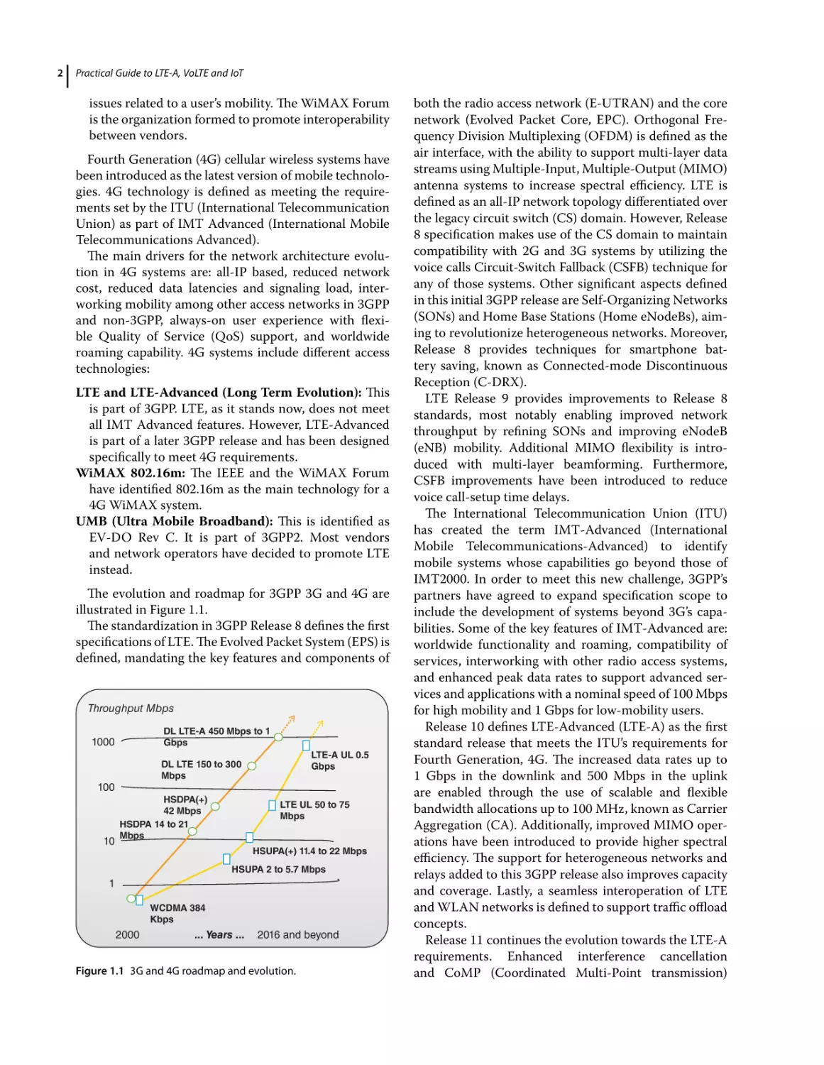
The evolution and roadmap for 3GPP 3G and 4G are
illustrated in Figure 1.1.
The standardization in 3GPP Release 8 defines the first
specifications of LTE. The Evolved Packet System (EPS) is
defined, mandating the key features and components of
Throughput Mbps
DL LTE-A 450 Mbps to 1
Gbps
1000
LTE-A UL 0.5
Gbps
DL LTE 150 to 300
Mbps
100
10
HSDPA(+)
42 Mbps
HSDPA 14 to 21
Mbps
LTE UL 50 to 75
Mbps
HSUPA(+) 11.4 to 22 Mbps
HSUPA 2 to 5.7 Mbps
1
WCDMA 384
Kbps
2000
... Years ...
2016 and beyond
Figure 1.1 3G and 4G roadmap and evolution.
both the radio access network (E-UTRAN) and the core
network (Evolved Packet Core, EPC). Orthogonal Frequency Division Multiplexing (OFDM) is defined as the
air interface, with the ability to support multi-layer data
streams using Multiple-Input, Multiple-Output (MIMO)
antenna systems to increase spectral efficiency. LTE is
defined as an all-IP network topology differentiated over
the legacy circuit switch (CS) domain. However, Release
8 specification makes use of the CS domain to maintain
compatibility with 2G and 3G systems by utilizing the
voice calls Circuit-Switch Fallback (CSFB) technique for
any of those systems. Other significant aspects defined
in this initial 3GPP release are Self-Organizing Networks
(SONs) and Home Base Stations (Home eNodeBs), aiming to revolutionize heterogeneous networks. Moreover,
Release 8 provides techniques for smartphone battery saving, known as Connected-mode Discontinuous
Reception (C-DRX).
LTE Release 9 provides improvements to Release 8
standards, most notably enabling improved network
throughput by refining SONs and improving eNodeB
(eNB) mobility. Additional MIMO flexibility is introduced with multi-layer beamforming. Furthermore,
CSFB improvements have been introduced to reduce
voice call-setup time delays.
The International Telecommunication Union (ITU)
has created the term IMT-Advanced (International
Mobile Telecommunications-Advanced) to identify
mobile systems whose capabilities go beyond those of
IMT2000. In order to meet this new challenge, 3GPP’s
partners have agreed to expand specification scope to
include the development of systems beyond 3G’s capabilities. Some of the key features of IMT-Advanced are:
worldwide functionality and roaming, compatibility of
services, interworking with other radio access systems,
and enhanced peak data rates to support advanced services and applications with a nominal speed of 100 Mbps
for high mobility and 1 Gbps for low-mobility users.
Release 10 defines LTE-Advanced (LTE-A) as the first
standard release that meets the ITU’s requirements for
Fourth Generation, 4G. The increased data rates up to
1 Gbps in the downlink and 500 Mbps in the uplink
are enabled through the use of scalable and flexible
bandwidth allocations up to 100 MHz, known as Carrier
Aggregation (CA). Additionally, improved MIMO operations have been introduced to provide higher spectral
efficiency. The support for heterogeneous networks and
relays added to this 3GPP release also improves capacity
and coverage. Lastly, a seamless interoperation of LTE
and WLAN networks is defined to support traffic offload
concepts.
Release 11 continues the evolution towards the LTE-A
requirements. Enhanced interference cancellation
and CoMP (Coordinated Multi-Point transmission)
LTE and LTE-A Overview
Release-8
Release-9
LTE-Advanced (Rel 10–12)
LTE-Advanced Pro (Rel-13 and beyond)
Long Term Evolution (LTE)
•
•
OFDMA Air Interface
Scalable Bandwidth up to
20 MHz
Flexible MIMO Modes
Support for FDD and TDD
All-IP Core Network
Voice Solution with CSFB
support
Interworking with legacy
2G/3G radio
Self-optimizing,
organizing Networks
(SON)
•
•
•
•
•
•
•
Enhanced Multimedia
Broadcast (eMBMS)
•
Enhanced Home eNB and
SON
Enhanced MIMO
techniques
•
•
•
•
CSFB Improvements to
reduce call setup latency
VoLTE and IMS related
services
SRVCC for voice call
continuity with legacy
radio
Release-11 and
beyond
Release-10
•
•
•
•
•
•
•
•
Meets 4G requirements
Carrier aggregation up to
100 MHz
Additional MIMO
techniques
Heterogeneous Networks
(Het-Net)
Support of Enhanced ICIC
Relays for HeNB
Seamless interworking of
LTE and WLAN (Wi-Fi
Calling)
More advanced UE
Categories
•
Enhanced Interference
cancellation (FeICIC)
•
Coordinated Multi-point
Transmission (CoMP)
targets macro-pico
deployment
•
Further SRVCC
Enhancements
FDD-TDD Carrier
Aggregation
LTE+WiFi Link
Aggregation
•
•
•
Higher Order Modulation
on DL
Figure 1.2 3GPP LTE releases.
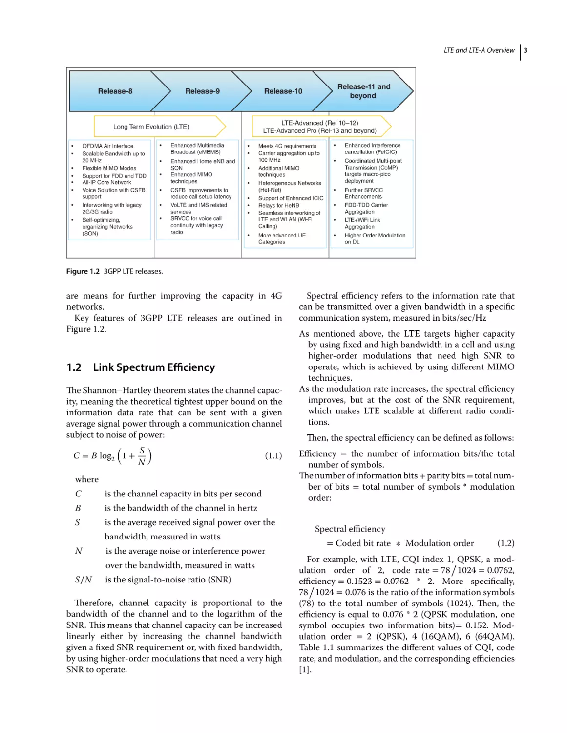
are means for further improving the capacity in 4G
networks.
Key features of 3GPP LTE releases are outlined in
Figure 1.2.
1.2 Link Spectrum Efficiency
The Shannon–Hartley theorem states the channel capacity, meaning the theoretical tightest upper bound on the
information data rate that can be sent with a given
average signal power through a communication channel
subject to noise of power:
)
(
S
(1.1)
C = B log2 1 +
N
where
C
is the channel capacity in bits per second
B
is the bandwidth of the channel in hertz
S
is the average received signal power over the
bandwidth, measured in watts
N
is the average noise or interference power
over the bandwidth, measured in watts
S∕N
is the signal-to-noise ratio (SNR)
Therefore, channel capacity is proportional to the
bandwidth of the channel and to the logarithm of the
SNR. This means that channel capacity can be increased
linearly either by increasing the channel bandwidth
given a fixed SNR requirement or, with fixed bandwidth,
by using higher-order modulations that need a very high
SNR to operate.
Spectral efficiency refers to the information rate that
can be transmitted over a given bandwidth in a specific
communication system, measured in bits/sec/Hz
As mentioned above, the LTE targets higher capacity
by using fixed and high bandwidth in a cell and using
higher-order modulations that need high SNR to
operate, which is achieved by using different MIMO
techniques.
As the modulation rate increases, the spectral efficiency
improves, but at the cost of the SNR requirement,
which makes LTE scalable at different radio conditions.
Then, the spectral efficiency can be defined as follows:
Efficiency = the number of information bits/the total
number of symbols.
The number of information bits + parity bits = total number of bits = total number of symbols * modulation
order:
Spectral efficiency
= Coded bit rate ∗ Modulation order
(1.2)
For example, with LTE, CQI index 1,/ QPSK, a modulation order of 2, code rate = 78 1024 = 0.0762,
efficiency
= 0.1523 = 0.0762 * 2. More specifically,
/
78 1024 = 0.076 is the ratio of the information symbols
(78) to the total number of symbols (1024). Then, the
efficiency is equal to 0.076 * 2 (QPSK modulation, one
symbol occupies two information bits)= 0.152. Modulation order = 2 (QPSK), 4 (16QAM), 6 (64QAM).
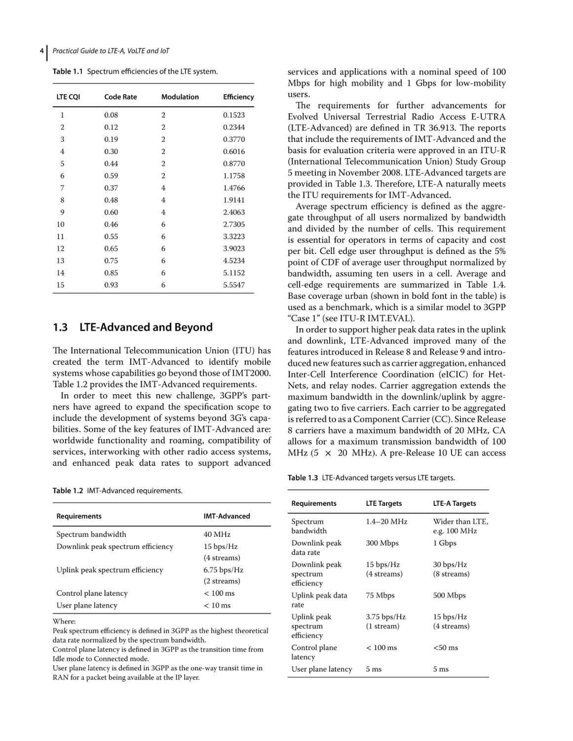
Table 1.1 summarizes the different values of CQI, code
rate, and modulation, and the corresponding efficiencies
[1].
3
4
Practical Guide to LTE-A, VoLTE and IoT
Table 1.1 Spectrum efficiencies of the LTE system.
LTE CQI
Code Rate
Modulation
Efficiency
1
0.08
2
0.1523
2
0.12
2
0.2344
3
0.19
2
0.3770
4
0.30
2
0.6016
5
0.44
2
0.8770
6
0.59
2
1.1758
7
0.37
4
1.4766
8
0.48
4
1.9141
9
0.60
4
2.4063
10
0.46
6
2.7305
11
0.55
6
3.3223
12
0.65
6
3.9023
13
0.75
6
4.5234
14
0.85
6
5.1152
15
0.93
6
5.5547
1.3 LTE-Advanced and Beyond
The International Telecommunication Union (ITU) has
created the term IMT-Advanced to identify mobile
systems whose capabilities go beyond those of IMT2000.
Table 1.2 provides the IMT-Advanced requirements.
In order to meet this new challenge, 3GPP’s partners have agreed to expand the specification scope to
include the development of systems beyond 3G’s capabilities. Some of the key features of IMT-Advanced are:
worldwide functionality and roaming, compatibility of
services, interworking with other radio access systems,
and enhanced peak data rates to support advanced
services and applications with a nominal speed of 100
Mbps for high mobility and 1 Gbps for low-mobility
users.
The requirements for further advancements for
Evolved Universal Terrestrial Radio Access E-UTRA
(LTE-Advanced) are defined in TR 36.913. The reports
that include the requirements of IMT-Advanced and the
basis for evaluation criteria were approved in an ITU-R
(International Telecommunication Union) Study Group
5 meeting in November 2008. LTE-Advanced targets are
provided in Table 1.3. Therefore, LTE-A naturally meets
the ITU requirements for IMT-Advanced.
Average spectrum efficiency is defined as the aggregate throughput of all users normalized by bandwidth
and divided by the number of cells. This requirement
is essential for operators in terms of capacity and cost
per bit. Cell edge user throughput is defined as the 5%
point of CDF of average user throughput normalized by
bandwidth, assuming ten users in a cell. Average and
cell-edge requirements are summarized in Table 1.4.
Base coverage urban (shown in bold font in the table) is
used as a benchmark, which is a similar model to 3GPP
“Case 1” (see ITU-R IMT.EVAL).
In order to support higher peak data rates in the uplink
and downlink, LTE-Advanced improved many of the
features introduced in Release 8 and Release 9 and introduced new features such as carrier aggregation, enhanced
Inter-Cell Interference Coordination (eICIC) for HetNets, and relay nodes. Carrier aggregation extends the
maximum bandwidth in the downlink/uplink by aggregating two to five carriers. Each carrier to be aggregated
is referred to as a Component Carrier (CC). Since Release
8 carriers have a maximum bandwidth of 20 MHz, CA
allows for a maximum transmission bandwidth of 100
MHz (5 × 20 MHz). A pre-Release 10 UE can access
Table 1.3 LTE-Advanced targets versus LTE targets.
Table 1.2 IMT-Advanced requirements.
Requirements
IMT-Advanced
Spectrum bandwidth
40 MHz
Downlink peak spectrum efficiency
15 bps/Hz
(4 streams)
Uplink peak spectrum efficiency
6.75 bps/Hz
(2 streams)
Control plane latency
< 100 ms
User plane latency
< 10 ms
Where:
Peak spectrum efficiency is defined in 3GPP as the highest theoretical
data rate normalized by the spectrum bandwidth.
Control plane latency is defined in 3GPP as the transition time from
Idle mode to Connected mode.
User plane latency is defined in 3GPP as the one-way transit time in
RAN for a packet being available at the IP layer.
Requirements
LTE Targets
LTE-A Targets
Spectrum
bandwidth
1.4–20 MHz
Wider than LTE,
e.g. 100 MHz
Downlink peak
data rate
300 Mbps
1 Gbps
Downlink peak
spectrum
efficiency
15 bps/Hz
(4 streams)
30 bps/Hz
(8 streams)
Uplink peak data
rate
75 Mbps
500 Mbps
Uplink peak
spectrum
efficiency
3.75 bps/Hz
(1 stream)
15 bps/Hz
(4 streams)
Control plane
latency
< 100 ms
<50 ms
User plane latency
5 ms
5 ms
LTE and LTE-A Overview
Table 1.4 Average and cell-edge requirements.
Scenario
Average
spectrum
efficiency
(bit/s/Hz/cell)
Cell-edge user
spectrum
efficiency
(bit/s/Hz)
Downlink and
Uplink
DL
UL
DL
UL
Antenna
Configuration
LTE Targets a)
2×2
1.69
2.4
—
4×2
1.87
2.6
[3, 2.6, 2.2, 1.1]
LTE-A Targets a)
IMT-Advanced b)
4×4
2.67
3.7
—
1×2
0.74
1.2
—
2×4
—
2.0
[2.25, 1.8, 1.4, 0.7]
2×2
0.05
0.07
—
4×2
0.06
0.09
[0.1, 0.075, 0.06, 0.04]
4×4
0.08
0.12
—
1×2
0.024
0.04
—
2×4
—
0.07
[0.07, 0.05, 0.03, 0.015]
a) Based on radio environment of “Case 1”: Inter-cell distance: 500 m, carrier frequency: 2 GHz, bandwidth: 10 MHz, DL
Tx power: 46 dBm, penetration loss: 20 dB: mobility speed: 3 km/h (see 3GPP TR 25.814).
b) [Indoor, Microcellular, Base coverage urban, High speed].
one of the component carriers, while CA-capable UEs
can operate with multiple component carriers. The CCs
can be of the same or different bandwidths, adjacent or
non-adjacent CCs in the same or different frequency
band, or CCs in different frequency bands. Carrier
aggregation can also benefit from both TDD and FDD
joint operation. Enhanced MIMO provides higher spatial gains, increased peak data rates, higher spectral
efficiency, and increased capacity.
The main goal of heterogeneous networks is to manage traffic between macro and small cell networks.
Controlling the interference scenarios within these
heterogeneous networks due to different power levels
of macro and small cells can be managed with features
Higher Data Rate & Bandwidth (bits/sec)
such as ICIC/eICIC/feICIC and CoMP (Coordinated
Multi-Point transmission), which further improve
capacity at cell edges.
The Release 8 specification makes use of the CS domain
to maintain compatibility with 2G and 3G systems by utilizing the voice calls circuit-switch fallback (CSFB) technique for any of those systems. As LTE has evolved into
an all-IP network and IMS implementation has matured,
Voice over IP over LTE has been implemented to carry
voice packets natively over the LTE network. At an LTE
cell edge, the ability to fall back into a circuit-switched
network is possible with features such as Single Radio
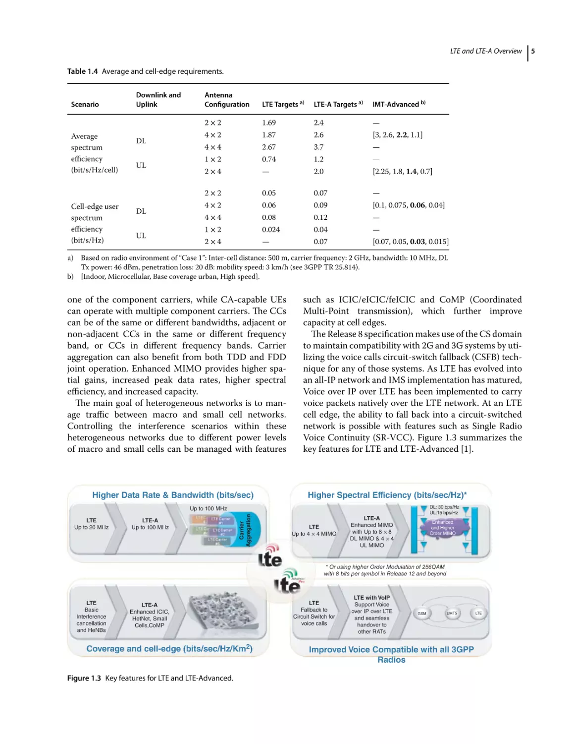
Voice Continuity (SR-VCC). Figure 1.3 summarizes the
key features for LTE and LTE-Advanced [1].
Higher Spectral Efficiency (bits/sec/Hz)*
DL: 30 bps/Hz
UL:15 bps/Hz
LTE
Up to 20 MHz
LTE-A
Up to 100 MHz
Carrier
Aggregation
Up to 100 MHz
LTE
Up to 4 × 4 MIMO
LTE-A
Enhanced MIMO
with Up to 8 × 8
DL MIMO & 4 × 4
UL MIMO
Enhanced
and Higher
Order MIMO
* Or using higher Order Modulation of 256QAM
with 8 bits per symbol in Release 12 and beyond
LTE
Basic
Interference
cancellation
and HeNBs
LTE-A
Enhanced ICIC,
HetNet, Small
Cells,CoMP
Coverage and cell-edge (bits/sec/Hz/Km2)
Figure 1.3 Key features for LTE and LTE-Advanced.
LTE
Fallback to
Circuit Switch for
voice calls
LTE with VoIP
Support Voice
over IP over LTE
and seamless
handover to
other RATs
GSM
UMTS
Improved Voice Compatible with all 3GPP
Radios
LTE
5
Practical Guide to LTE-A, VoLTE and IoT
1.3.1
LTE and Wi-Fi
regulators to study the feasibility of this deployment
and the impact of LTE on Wi-Fi spectrum. However,
it is expected that the feature will gain strong momentum in the upcoming years, especially as it brings a
substantial capacity boost from the unlicensed band, if
it is proven that the quality of service for the end user
is not impacted by the interference situation between
the two bands.
LWA (LTE–Wi-Fi Aggregation): Dual connectivity
between LTE and Wi-Fi. LWA can be enabled at the
radio level and can split the data plane traffic so that
some LTE traffic is tunneled over Wi-Fi and the rest
runs over LTE. The Wi-Fi data rate can go up to
867 Mbps in 802.11ac and the LTE currently being
deployed with 300 to 450 Mbps (two- or three-carrier
aggregation), and when both are aggregated, the total
aggregated throughput can go beyond 1 Gbps. This is,
in some networks, called Giga LTE (G-LTE).
There is plenty of spectrum in the 5 GHz band, which is
especially suited to small-cell deployments. For the last
few years, Wi-Fi has been actively used to offload cellular
traffic, and several operators are using it as part of mobile
plans. The idea of LTE/Wi-Fi aggregation arose so that
smartphones could receive data from a cellular network
and a Wi-Fi network at the same time. Therefore, different phases for increasing carrier aggregation in the 5 GHz
band have been studied in 3GPP to utilize 5 GHz solely
for LTE or jointly with Wi-Fi. The amount of spectrum
available in the 5 GHz band per region is summarized in
Table 1.5.
The two main options for LTE to use the 5 GHz band
are as follows:
LAA (Licensed Assisted Access): A standalone LTE
operation in unlicensed spectrum. Several challenges
occur with this implementation. In particular, there
is a need for eNB and access points (AP) to be collocated, which requires new devices. This would allow
operators to benefit from the additional capacity
available from the unlicensed spectrum, particularly
in hotspots and corporate environments. With LAA,
the extra spectrum resource, especially on the 5 GHz
frequency band, can complement licensed-band LTE
operation to provide additional data plane performance. The use of this technology has prompted
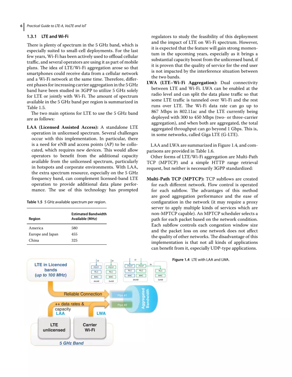
LAA and LWA are summarized in Figure 1.4, and comparisons are provided in Table 1.6.
Other forms of LTE/Wi-Fi aggregation are Multi-Path
TCP (MPTCP) and a simple HTTP range retrieval
request, but neither is necessarily 3GPP standardized:
Multi-Path TCP (MPTCP): TCP subflows are created
for each different network. Flow control is operated
for each subflow. The advantages of this method
are good aggregation performance and the ease of
configuration in the network (it may require a proxy
server to apply multiple kinds of services which are
non-MPTCP capable). An MPTCP scheduler selects a
path for each packet based on the network condition.
Each subflow controls each congestion window size
and the packet loss on one network does not affect
the quality of other networks. The disadvantage of this
implementation is that not all kinds of applications
can benefit from it, especially UDP-type applications.
Table 1.5 5 GHz available spectrum per region.
Region
Estimated Bandwidth
Available (MHz)
America
580
Europe and Japan
455
China
325
SI
LTE in Licenced
bands
(up to 100 MHz)
PDCP
RLC
MAC
MAC
MeNB
SeNB
Reliable Connection
++ data rates &
capacity
LAA
LTE
unlicensed
LWA
PDCP
Xn
RLC
RLC
RLC
MAC
MAC
MAC
MeNB
Pipe #1
Pipe #2
Carrier
Wi-Fi
5 GHz Band
PDCP
PDCP
RLC
Figure 1.4 LTE with LAA and LWA.
SI
SI
SeNB
Aggregated
Bandwidth
6
LTE and LTE-A Overview
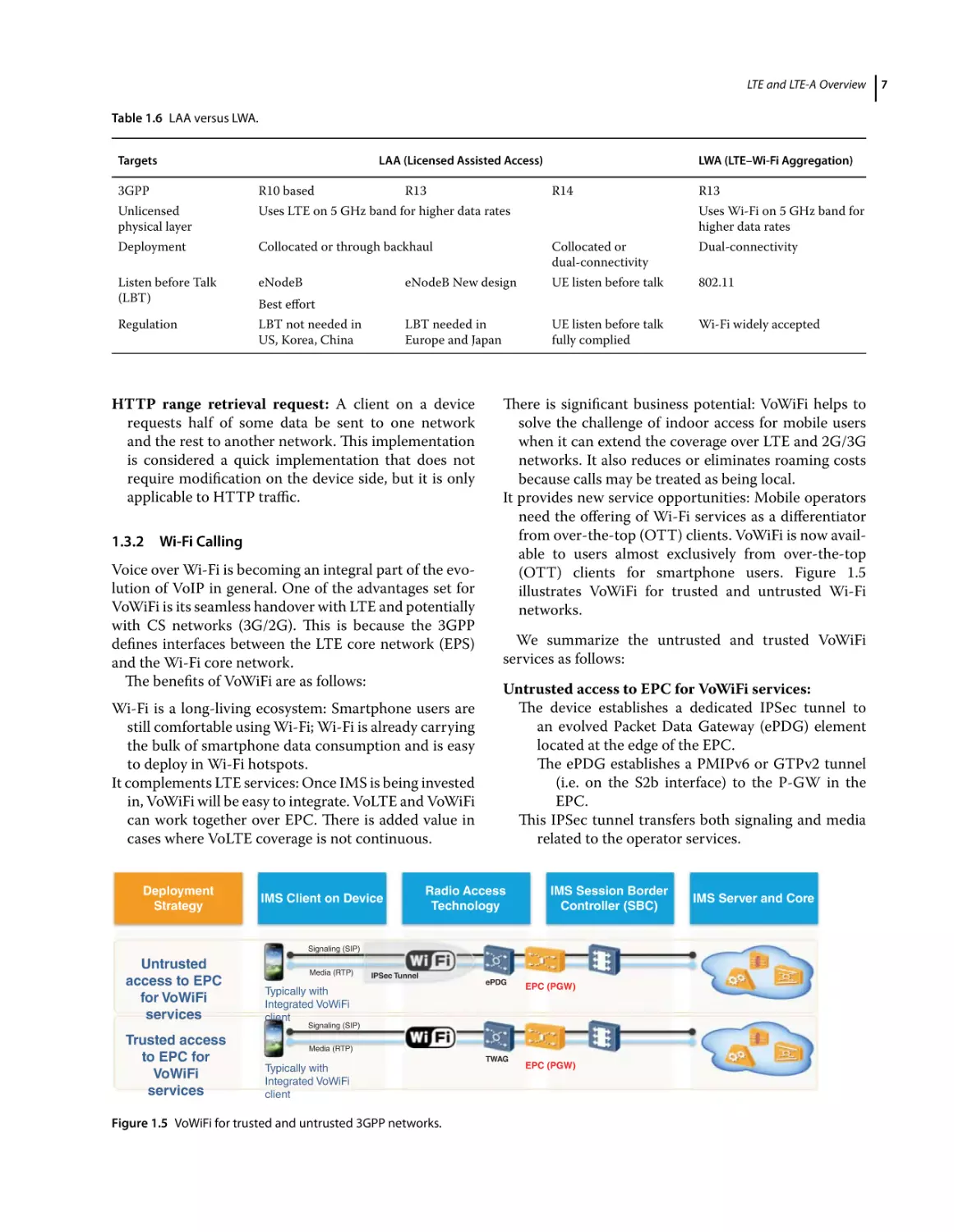
Table 1.6 LAA versus LWA.
Targets
LAA (Licensed Assisted Access)
R13
LWA (LTE–Wi-Fi Aggregation)
3GPP
R10 based
Unlicensed
physical layer
Uses LTE on 5 GHz band for higher data rates
Deployment
Collocated or through backhaul
Collocated or
dual-connectivity
Dual-connectivity
Listen before Talk
(LBT)
eNodeB
eNodeB New design
UE listen before talk
802.11
Regulation
LBT not needed in
US, Korea, China
LBT needed in
Europe and Japan
UE listen before talk
fully complied
Wi-Fi widely accepted
Wi-Fi Calling
Voice over Wi-Fi is becoming an integral part of the evolution of VoIP in general. One of the advantages set for
VoWiFi is its seamless handover with LTE and potentially
with CS networks (3G/2G). This is because the 3GPP
defines interfaces between the LTE core network (EPS)
and the Wi-Fi core network.
The benefits of VoWiFi are as follows:
Wi-Fi is a long-living ecosystem: Smartphone users are
still comfortable using Wi-Fi; Wi-Fi is already carrying
the bulk of smartphone data consumption and is easy
to deploy in Wi-Fi hotspots.
It complements LTE services: Once IMS is being invested
in, VoWiFi will be easy to integrate. VoLTE and VoWiFi
can work together over EPC. There is added value in
cases where VoLTE coverage is not continuous.
Deployment
Strategy
Uses Wi-Fi on 5 GHz band for
higher data rates
IMS Client on Device
There is significant business potential: VoWiFi helps to
solve the challenge of indoor access for mobile users
when it can extend the coverage over LTE and 2G/3G
networks. It also reduces or eliminates roaming costs
because calls may be treated as being local.
It provides new service opportunities: Mobile operators
need the offering of Wi-Fi services as a differentiator
from over-the-top (OTT) clients. VoWiFi is now available to users almost exclusively from over-the-top
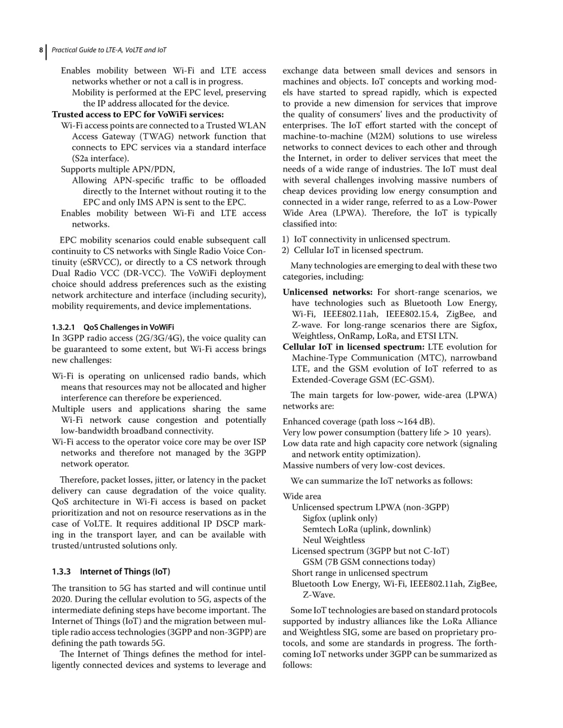
(OTT) clients for smartphone users. Figure 1.5
illustrates VoWiFi for trusted and untrusted Wi-Fi
networks.
We summarize the untrusted and trusted VoWiFi
services as follows:
Untrusted access to EPC for VoWiFi services:
The device establishes a dedicated IPSec tunnel to
an evolved Packet Data Gateway (ePDG) element
located at the edge of the EPC.
The ePDG establishes a PMIPv6 or GTPv2 tunnel
(i.e. on the S2b interface) to the P-GW in the
EPC.
This IPSec tunnel transfers both signaling and media
related to the operator services.
Radio Access
Technology
IMS Session Border
Controller (SBC)
Signaling (SIP)
Untrusted
access to EPC
for VoWiFi
services
Media (RTP)
IPSec Tunnel
ePDG
Typically with
Integrated VoWiFi
client
EPC (PGW)
Signaling (SIP)
Trusted access
to EPC for
VoWiFi
services
R13
Best effort
HTTP range retrieval request: A client on a device
requests half of some data be sent to one network
and the rest to another network. This implementation
is considered a quick implementation that does not
require modification on the device side, but it is only
applicable to HTTP traffic.
1.3.2
R14
Media (RTP)
TWAG
Typically with
Integrated VoWiFi
client
Figure 1.5 VoWiFi for trusted and untrusted 3GPP networks.
EPC (PGW)
IMS Server and Core
7
8
Practical Guide to LTE-A, VoLTE and IoT
Enables mobility between Wi-Fi and LTE access
networks whether or not a call is in progress.
Mobility is performed at the EPC level, preserving
the IP address allocated for the device.
Trusted access to EPC for VoWiFi services:
Wi-Fi access points are connected to a Trusted WLAN
Access Gateway (TWAG) network function that
connects to EPC services via a standard interface
(S2a interface).
Supports multiple APN/PDN,
Allowing APN-specific traffic to be offloaded
directly to the Internet without routing it to the
EPC and only IMS APN is sent to the EPC.
Enables mobility between Wi-Fi and LTE access
networks.
exchange data between small devices and sensors in
machines and objects. IoT concepts and working models have started to spread rapidly, which is expected
to provide a new dimension for services that improve
the quality of consumers’ lives and the productivity of
enterprises. The IoT effort started with the concept of
machine-to-machine (M2M) solutions to use wireless
networks to connect devices to each other and through
the Internet, in order to deliver services that meet the
needs of a wide range of industries. The IoT must deal
with several challenges involving massive numbers of
cheap devices providing low energy consumption and
connected in a wider range, referred to as a Low-Power
Wide Area (LPWA). Therefore, the IoT is typically
classified into:
EPC mobility scenarios could enable subsequent call
continuity to CS networks with Single Radio Voice Continuity (eSRVCC), or directly to a CS network through
Dual Radio VCC (DR-VCC). The VoWiFi deployment
choice should address preferences such as the existing
network architecture and interface (including security),
mobility requirements, and device implementations.
1) IoT connectivity in unlicensed spectrum.
2) Cellular IoT in licensed spectrum.
1.3.2.1
QoS Challenges in VoWiFi
In 3GPP radio access (2G/3G/4G), the voice quality can
be guaranteed to some extent, but Wi-Fi access brings
new challenges:
Wi-Fi is operating on unlicensed radio bands, which
means that resources may not be allocated and higher
interference can therefore be experienced.
Multiple users and applications sharing the same
Wi-Fi network cause congestion and potentially
low-bandwidth broadband connectivity.
Wi-Fi access to the operator voice core may be over ISP
networks and therefore not managed by the 3GPP
network operator.
Therefore, packet losses, jitter, or latency in the packet
delivery can cause degradation of the voice quality.
QoS architecture in Wi-Fi access is based on packet
prioritization and not on resource reservations as in the
case of VoLTE. It requires additional IP DSCP marking in the transport layer, and can be available with
trusted/untrusted solutions only.
1.3.3
Internet of Things (IoT)
The transition to 5G has started and will continue until
2020. During the cellular evolution to 5G, aspects of the
intermediate defining steps have become important. The
Internet of Things (IoT) and the migration between multiple radio access technologies (3GPP and non-3GPP) are
defining the path towards 5G.
The Internet of Things defines the method for intelligently connected devices and systems to leverage and
Many technologies are emerging to deal with these two
categories, including:
Unlicensed networks: For short-range scenarios, we
have technologies such as Bluetooth Low Energy,
Wi-Fi, IEEE802.11ah, IEEE802.15.4, ZigBee, and
Z-wave. For long-range scenarios there are Sigfox,
Weightless, OnRamp, LoRa, and ETSI LTN.
Cellular IoT in licensed spectrum: LTE evolution for
Machine-Type Communication (MTC), narrowband
LTE, and the GSM evolution of IoT referred to as
Extended-Coverage GSM (EC-GSM).
The main targets for low-power, wide-area (LPWA)
networks are:
Enhanced coverage (path loss ∼164 dB).
Very low power consumption (battery life > 10 years).
Low data rate and high capacity core network (signaling
and network entity optimization).
Massive numbers of very low-cost devices.
We can summarize the IoT networks as follows:
Wide area
Unlicensed spectrum LPWA (non-3GPP)
Sigfox (uplink only)
Semtech LoRa (uplink, downlink)
Neul Weightless
Licensed spectrum (3GPP but not C-IoT)
GSM (7B GSM connections today)
Short range in unlicensed spectrum
Bluetooth Low Energy, Wi-Fi, IEEE802.11ah, ZigBee,
Z-Wave.
Some IoT technologies are based on standard protocols
supported by industry alliances like the LoRa Alliance
and Weightless SIG, some are based on proprietary protocols, and some are standards in progress. The forthcoming IoT networks under 3GPP can be summarized as
follows:
LTE and LTE-A Overview
Cellular IoT in licensed spectrum
3GPP eRAN (Release 12/13).
LTE evolution for MTC (machine-type communication).
Category 1 but it does not meet the IoT requirement (battery/cost/range).
Release 12 with Category 0.
Release 13 to meet LPWA requirement
(Category M).
NB-CIoT and NB-LTE.
Will be evolved into NB-IoT as per latest 3GPP
RAN meeting, and is expected to be released
with 3GPP Release 13.
3GPP GERAN (Release 13).
GSM evolution: upgrade of GSM by using one
carrier for IoT with Extended-Coverage GSM
(EC-GSM) is expected with 3GPP Release 13.
For the unlicensed networks, some of the highlighted
technologies have already been deployed and meet the
four factors for LPWA (long range, very low power, low
data rate, and very low cost). . For 3GPP evolution of cellular IoT, the LTE-MTC is defined with the first version
released with 3GPP Release 8 based on Category 1 but it
does not meet the IoT requirement (battery/cost/range).
This idea took an additional turn by providing a new
Release 12 Category 0. The ongoing enhanced version
(eMTC) is under evaluation in Release 13 to meet the
LPWA requirement (i.e. Category M).
On the other hand, narrowband LTE introduces two
underlying technologies being discussed in 2015/2016
3GPP Release 13: NB-CIoT and NB-LTE, where the main
difference lies in the physical layer. It is expected that
the two will merge and provide a final version referred
to as NB-IoT. This technology is targeting three different
modes such as utilizing the spectrum currently being
used by GERAN systems as a replacement for one or
more GSM carriers (standalone operation). The second
mode utilizes the unused resource blocks within an
LTE carrier’s guard band (guard-band operation). The
final mode utilizes resource blocks within a normal LTE
carrier (in-band operation). The NB-IoT should support
the following main objectives:
180 kHz UE RF bandwidth for both downlink and uplink.
OFDMA on the downlink with either 15 kHz or 3.75 kHz
subcarrier spacing.
For the uplink, two options will be considered: FDMA
with GMSK modulation, and SC-FDMA (including single-tone transmission as a special case of
SC-FDMA).
A single synchronization signal design for the different
modes of operation, including techniques to handle
overlap with legacy LTE signals while reducing the
power consumption and latencies.
Utilization of the existing LTE procedures and protocols
and relevant optimizations to support the selected
physical layer and core network interfaces targeting
signaling reduction for small data transmissions.
EC-GSM has been introduced as cellular system
support for ultra-low-complexity and low-throughput
Internet of Things. It targets the following:
Re-using existing designs: Only changing them when
necessary to comply with the study item objectives; a
reduction in functionality in the GERAN specification
to minimize implementation effort and complexity.
Backward compatibility and co-existence with GSM:
Multiplexing traffic from legacy GSM devices and
CIoT devices on the same physical channels. No
impact on the radio units already deployed in the
field. Speed the same as supported today (in normal
coverage).
Achieving extended coverage: Provide EC by using control channels with blind repetitions and data channels:
blind repetitions of MCS-1 (lowest MCS in EGPRS)
and HARQ retransmissions. EC has different coverage classes (CCs). The total number of blind transmissions for a given CC can differ between different logical
channels.
Figure 1.6 summarizes the LTE UE categories with
differing 3GPP evolutions.
With the developments in cellular networks, the doors
have been opened wide for the development of 5G
architecture and its requirements. The envisioned market space for 5G technology is driven by requirements
to enhance the mobile broadband smartphone, with
a massive range of machine-type communication and
LPWA growth, and the need to provide ultra-reliable,
low-latency communications. 3GPP expects the evolution to start from Release 14/15 and is aiming to meet
the IMT2020 requirements in Release 16. Figure 1.7
summarizes the main targets for 5G, and the main use
cases are summarized in Figure 1.8.
1.4 Evolved Packet System (EPS)
Overview
3GPP Release 8 is the starting point when defining the
standardization for the Long Term Evolution (LTE)
specifications:
The Evolved Packet System (EPS) is defined, mandating
the key features and components of both the radio
access network (E-UTRAN) and the core network
(Evolved Packet Core, EPC).
Orthogonal Frequency Division Multiplexing (OFDM) is
defined as the air interface.
9
10
Practical Guide to LTE-A, VoLTE and IoT
Release 8
Release 12
Release 13
Release 13
UE Category 1
UE Category 0
UE Category M
NB-loT
10 Mbps
5 Mbps
2
Full duplex
1 Mbps
1 Mbps
1
Half duplex
1 Mbps
1 Mbps
1
Half duplex
200 kbps
100 kbps
1
Half duplex
20 MHz
20 MHz
1.4 MHz
0.2 MHz
Downlink peak rate
Uplink peak rate
Number of antennas
Duplex mode
UE receive bandwidth
LTE Release 13 will further reduce
complexity with narrowband RF and
lower data rate
LTE Release 12 introduced low
complexity UE category with lower data
rate, half duplex and single antenna
GSM evolution for loT kicked off
with Extended Coverage GSM (ECGSM) in Rel-13
Different deployment options
will be available for Cellular IOT
Figure 1.6 Different LTE UE categories for IoT.
Peak Data Rate
(20 Gbps)
Edge Throughput
(100 Mbps)
20
100
IMT-2020
Figure 1.9 summarizes FDD and TDD operation. The
FDD system:
10
1
Area Traffic
Capacity
(Mbit/s/m2) 10
1x
1
3x
Spectrum
Efficiency
0.1
1x
350
10x
100x
Network
Energy Efficiency
105
106
Connection Density
(devices/km2)
400
500
IMT-Advanced
TDD mode enables full-duplex operation using a single
frequency band and time division multiplexing for
the uplink and downlink signals.
Mobility
(km/h)
10
1
Latency
(1 ms)
ITU-R document 5D/TEMP/625
Figure 1.7 Main targets for 5G compared to IMT-Advanced.
In OFDM, the carriers are packed much closer
together (subcarriers).
This increases spectral efficiency by utilizing a carrier spacing that is the inverse of the symbol or
modulation rate.
LTE uses a variable channel bandwidth of 1.4, 3, 5, 10, 15,
or 20 MHz.
LTE radio access is designed to operate in two main
modes of operation: FDD (Frequency Division Duplex)
and TDD (Time Division Duplex).
In FDD, separate uplink and downlink channels are
utilized, enabling a device to transmit and receive
data at the same time.
Can operate in full-duplex or half-duplex modes.
Half-duplex FDD is where the mobile can only transmit
or receive; i.e.
The user cannot transmit and receive at the same time.
There is reduced mobile complexity since no duplex
filter is required.
TDD mode enables full-duplex operation using a
single frequency band and time division multiplexing of
the uplink and downlink signals. The basic principle of
TDD is to use the same frequency band for transmission
and reception but to alternate the transmission direction
in time. This is a fundamental difference compared to
FDD, where different frequencies are used for continuous UE reception and transmission. Like FDD, LTE
TDD supports bandwidths from 1.4 MHz up to 20 MHz
depending on the frequency band. One advantage of
TDD is its ability to provide asymmetrical uplink and
downlink allocation. Depending on the system, other
advantages include dynamic allocation, increased spectral efficiency, and the improved use of beamforming
techniques. This is due to having the same uplink and
downlink frequency characteristics.
Since the bandwidth is shared between the uplink and
downlink and the maximum bandwidth is specified to be
20 MHz in Release 8, the maximum achievable data rates
are lower than in LTE FDD. Therefore, to improve LTE
TDD performance, it can be seen that FDD + TDD joint
operation (carrier aggregation) will be useful in markets
using TDD.
LTE and LTE-A Overview
Figure 1.8 Main use cases for 5G.
Enhanced Mobile Broadband
Gigabytes in a second
3D Video, UHD Screens
Work and Play in the Cloud
Augmented Reality
Smart Home Building
Industry Automation
Voice
Mission critical application
Smart City
Massive machine type
communications
Time
LTE-FDD with Full Duplex
1.4 – 20 MHz
1.4 – 20 MHz
Uplink
Downlink
Frequency
Duplex Spacing
Time
LTE-TDD
1.4 – 20 MHz
Uplink
Downlink
Guard Period for
switching transients
Frequency
Figure 1.9 FDD and TDD operation.
It is worth noting that the same receiver and transmitter processing capability can be used with both TDD
and FDD modes, enabling faster deployment of LTE.
However, in an FDD UE implementation, this normally
requires a duplex filter when simultaneous transmission
and reception is facilitated. In a TDD system, the UE
does not need such a duplex filter.
One of the main factors in any cellular system is the
deployed frequency spectrum. 2G, 3G, and 4G systems
offer multiple band options. The frequency band choice
depends on the regulator in each country and the availability of spectrum sharing among network operators in
the same country. The device’s support for the frequency
bands is driven by the hardware capabilities. Therefore,
not all bands are supported by a single device. The
demands of a multi-mode and multi-band device depend
on the market where the device is being sold.
Future IMT
Self Driving Car
Ultra-reliable and low latency
communications
LTE uses a variable channel bandwidth of 1.4, 3, 5,
10, 15, or 20 MHz. Most common worldwide network
deployments are in 5 or 10 MHz, given the bandwidth
available in the allocated spectrum for the operator. LTE
in 20 MHz is being deployed increasingly, especially in
bands like 2.6 GHz as well as 1.8 GHz after frequency
re-farming.
LTE-FDD requires two center frequencies, one for
the downlink and one for the uplink. These carrier
frequencies are each given an EARFCN (E-UTRA Absolute Radio Frequency Channel Number). In contrast,
LTE-TDD has only one EARFCN. The channel raster
for LTE is 100 kHz for all bands. The carrier center
frequency must be an integer multiple of 100 kHz.
Tables 1.7 and 1.8 summarize the LTE band allocation
for FDD and TDD, respectively.
As was the case with UMTS, LTE supports both FDD
and TDD modes. FDD frequency bands are paired, which
enables simultaneous transmission on two frequencies:
one for the downlink and one for the uplink. The paired
bands are also specified with sufficient separations for
improved receiver performance. TDD frequency bands
are unpaired, as uplink and downlink transmissions
share the same channel and carrier frequency. The
transmissions in uplink and downlink directions are
time-multiplexed. The unpaired bands used in TDD
mode start from band 33. Note that band 6 is not applicable to LTE (a UMTS-only band) and bands 15 and 16
are dedicated to ITU Region 1.
1.5 Network Architecture Evolution
Figure 1.10 illustrates the network topologies for
3G/Evolved HSPA/LTE. In a 3G network, prior to the
11
12
Practical Guide to LTE-A, VoLTE and IoT
Table 1.7 LTE-FDD band allocation.
Operating
Band
Band Name
Uplink Operating
Band (MHz)
Downlink Operating
Band (MHz)
1
2100
1920–1980
2110–2170
2
1900
1850–1910
1930–1990
3
1800
1710–1785
1805–1880
4
AWS
1710–1755
2110–2155
5
850
824–849
869–894
7
2600
2500–2570
2620–2690
8
900
880–915
925–960
9
1800
1749.9–1784.9
1844.9–1879.9
10
AWS
1710–1770
2110–2170
11
1500
1427.9–1452.9
1475.9–1500.9
12
700
698–716
728–746
13
700
777–787
746–756
14
700
788–798
758–768
17
700
704–716
734–746
18
800
815–830
860–875
19
800
830–845
857–890
20
800
832–862
791–821
21
1500
1447.9–1462.9
1495.9–1510.9
22
3500
3410–3490
3510–3590
23
2000
2000–2020
2180–2200
24
1600
1626.5–1660.5
1525–1559
25
1900
1850–1915
1930–1995
Table 1.8 LTE-TDD band allocation.
Operating Band
Band Name
Uplink and Downlink
Operating Band (MHz)
33
1900
1900–1920
34
2000
2010–2025
35
PCS
1850–1910
36
PCS
1930–1990
37
PCS
1910–1930
38
2600
2570–2620
39
1900
1880–1920
40
2300
2300–2400
41
2500
2496–2690
42
3500
3400–3600
43
3700
3600–3800
44
700
703–803
introduction of the HSPA system, the network architecture is divided into circuit-switched and packet-switched
domains. Depending on the service offered to the end
user, the domains interact with the corresponding core
network entities. The circuit-switched elements are the
Mobile services Switching Center (MSC), the Visitor
Location Register (VLR), and the Gateway MSC. The
packet-switched elements are the Serving GPRS Support
Node (SGSN) and the Gateway GPRS Support Node
(GGSN).
Furthermore, the control plane and user plane data are
forwarded between the core and access networks. The
Radio Access Technology (RAT) in the 3G system uses
Wideband Code Division Multiple Access (WCDMA).
The access network includes all of the radio equipment
necessary for accessing the network, and is referred
to as the Universal Terrestrial Radio Access Network
(UTRAN).
UTRAN consists of one or more Radio Network Subsystems (RNSs). Each RNS consists of a Radio Network
Controller (RNC) and one or more NodeBs. Each NodeB
controls one or more cells and provides the WCMDA
radio link to the UE.
After the introduction of HSPA and HSPA+ systems
in 3GPP, some optional changes have been added to the
core network as well as mandatory changes to the access
network. On the core network side, an evolved direct tunneling architecture has been introduced whereby the user
data can flow between the GGSN and the RNC or directly
to the NodeB. On the access network side, some of the
RNC functions, such as the network scheduler, have been
moved to the NodeB side for faster radio resource management (RRM) operations.
Figure 1.11 provides the LTE Evolved Packet System
(EPS) network topology. In summary, EPS consists of:
The E-UTRAN access network (Evolved UTRAN).
The E-UTRAN consists of one or more eNodeBs
(eNBs).
An eNB consists typically of three cells.
The eNBs can, optionally, interconnect to each other
via the X2 interface.
The EPC core network (Evolved Packet Core).
The EPC core network consists of the main network
entities: MME, S-GW, and P-GW.
The EPS can also interconnect with other radio access
networks: 3GPP (GERAN, UTRAN) and non-3GPP
(e.g. CDMA, Wi-Fi).
The EPC includes the MME, S-GW, and P-GW entities. They are responsible for different functionalities
during a call or registration process. The EPC and the
E-UTRAN interconnect with the S1 interface. The S1
interface supports a many-to-many relationship between
MMEs, serving gateways, and eNBs.
The MME connects to the E-UTRAN by means of
the S1 interface. This interface is referred to as S1-C
or S1-MME. When a UE attaches to the LTE network,
UE-specific logical S1-MME connections are established. This bearer, known as an EPS bearer, is used to
exchange the necessary UE-specific signaling messages
between the UE and the EPC.
LTE and LTE-A Overview
CS
CS
PS
Control
Plane
Optional IMS
Optional IMS
Control
Plane
User
Plane
GGSN
User
Plane
Control
Plane
User
Plane
GGSN
SGSN
SGSN
RNC
RNC
Part of RNC
function
NodeB
PS
PS
MME
Core
Network
Access
Network
S-GW
eNodeB
Part of RNC
function
NodeB
3G/HSPA
P-GW
Evolved HSPA
LTE EPS
Figure 1.10 3G/Evolved HSPA/ LTE network topology.
HSS
Sp
Other
MME
Control Plane
PCRF
S6a
User Plane
S10
Rx
Gx
S1-MME
UE
LTE Uu
MME
S11
S-GW
eNB
S5
P-GW
SGi
Operators’
IP Services
/ Internet
S1-U
X2
EPC Entities & Interfaces
Other
eNB
E-UTRAN
HSS: Home Subscriber Server
PCRF: Policy and Charging Rules
Function
Figure 1.11 LTE/EPS network topology.
Each UE is then assigned a unique pair of eNB and
MME identifications during S1-MME control connection. The identifications are used by the MME to send the
UE-specific S1 control messages and by the E-UTRAN
to send messages to the MME. The identification is
released when the UE transitions to Idle state, where the
dedicated connection with the EPC is also released. This
process may repetitively take place when the UE sets up
a signaling connection for any type of LTE call.
The MME and E-UTRAN handle signaling for control
plane procedures established for the UE on the S1-MME
interface, including:
Initial context setup/UE context release
E-RAB setup/release/modify
Handover preparation/notification
eNB/MME status transfer
Paging UE capability information indication.
13
14
Practical Guide to LTE-A, VoLTE and IoT
The HSS is considered to lie outside the EPC entities
and is used to update new EPS subscription data and
functions to the EPC. The HSS is located within the HLR
of the mobile network and has recently become part of
the converged database (CDB) for the entire subscriber
services. The PCRF provides QoS policy and charging
control (PCC), similar to the 3G PS domain.
The main features of EPS are summarized in Table 1.9.
S1-MME uses S1-AP over SCTP as the transport layer
protocol for guaranteed delivery of signaling messages
between the MME and the eNodeB. One logical S1-AP
connection per UE is established and multiple UEs are
supported via a single SCTP association. The following
functionalities are conducted in S1-AP:
Setup, modification, and release of E-RABS.
Establishment of an initial S1 UE context.
Paging and S1 management functions.
NAS signaling transport functions between the UE and
the MME.
Status transfer functionality.
Trace of active UEs and location reporting.
Mobility functions for UE to enable inter- and intra-RAT
HO.
MMEs can also periodically send MME loading information to the E-UTRAN for mobility management
procedures. This is not UE-specific information. The
S-GW is connected to the E-UTRAN by means of the
S1-U interface. After the EPS bearer is established for
control plane information, the user data packets start
flowing between the EPC and the UE through this
interface.
1.6 LTE UE Description
Like that in UMTS, the mobile device in LTE is referred
to as the UE (User Equipment) and is comprised of two
distinct elements: the USIM (Universal Subscriber Identity Module) and the ME (Mobile Equipment). The ME
supports a number of functional entities and protocols
including:
RR (Radio Resource): This supports both the control
and user planes. It is responsible for all low-level
protocols including RRC, PDCP, RLC, MAC, and
PHY layers. The layers are similar to those in the eNB
protocol layer.
EMM (EPS Mobility Management): A control plane
entity which manages the mobility states of the UE;
LTE Idle, LTE Active, and LTE Detached. Transactions
within these states include procedures such as TAU
(Tracking Area Updates) and handovers.
ESM (EPS Session Management): A control plane
activity which manages the activation, modification,
and deactivation of EPS bearer contexts. These can
either be default or dedicated EPS bearer contexts.
The physical layer capabilities of the UE may be
defined in terms of the frequency bands and data rates
supported. Devices may also be capable of supporting adaptive modulation including QPSK (Quadrature
Phase Shift Keying), 16QAM (16 Quadrature Amplitude
Modulation), and 64QAM (64 Quadrature Amplitude
Modulation). Modulation capabilities are defined separately in 3GPP for the uplink and downlink. The UE is
able to support several scalable channels including 1.4
MHz, 3 MHz, 5 MHz, 10 MHz, 15 MHz, and 20 MHz
Table 1.9 Main features of EPS entities.
EPS Element
Element
MME
Mobility Management
Entity
EPC
S-GW
Serving Gateway
P-GW
Packet Data Network
(PDN) Gateway
E-UTRAN
eNodeB
Evolved Node B
Basic Functionality
• Signaling and security control
• Tracking area management
• Inter core network signaling for mobility between 3GPP access
networks
• EPS bearer management
• Roaming and authentication
• Packet routing and forwarding
• Transport level Quality of Service mapping
• IP address allocation
• Packet filtering and policy enforcement
• User plane anchoring for mobility between 3GPP access
networks
• Provides user plane protocol layers: PDCP, RLC, MAC, physical
and control plane (RRC) with the user
• Radio resource management
• E-UTRAN synchronization and interface control
• MME selection
LTE and LTE-A Overview
whilst operating in FDD and/or TDD. The UE may also
support advanced antenna features such as MIMO with
different numbers of antenna configurations.
The physical layer and radio capabilities of the UE are
advertised to the EPS at the initiation of the connection
with the eNB in order to adjust the radio resources
accordingly. An LTE-capable device advertises one of the
categories listed in Table 1.10 according to its software
and hardware capabilities. UE categories > 5 are considered part of LTE-A capabilities, with CA starting from
Category 6 and above.
It should also be noted that different combinations of
3G and LTE categories can be supported in the same
device, depending on the price and the market in which
the device is being sold.
The UE categories are summarized in Table 1.10.
Table 1.11 illustrates how to estimate the peak throughput for sample LTE UE categories.
Table 1.11 shows the maximum capability of each
category and which factor will limit it. The maximum data rates in each category are presented as the
MAX_Throughput {MIMO configuration, higher-order
modulation, carrier aggregation combination} that
provides whatever maximum throughput is possible. Therefore, using advanced MIMO with advanced
higher-order modulation and advanced carrier aggregation bandwidth techniques may or may not be possible
simultaneously in every category on one carrier. For 600
Mbps, for example, it can be achieved within Category
11 by:
2 × CC 4 × 4MIMO, or
1 × CC 4 × 4MIMO + 2CC 2 × 2MIMO, or
4 × CC 2 × 2MIMO
1 × CC 4 × 4MIMO 256QAM + 1 × CC 2
× 2MIMO 256QAM, or
3 × CC 2 × 2MIMO 256QAM
As mentioned earlier, some operators around the
world are aiming to use the current LTE spectrum
and deployment conditions and aggregate it with the
Wi-Fi network to achieve Giga LTE. This can happen
directly at the LTE protocol stack (LWA), or through
application layer aggregations (MP-TCP), especially
if the public Wi-Fi network is the operator’s own and
the core network can be integrated with the EPS network. If 4 × 4 MIMO or 256QAM are not currently
supported in the LTE commercial network, the alternative means to reach a 1 Gbps network is to utilize
Wi-Fi aggregation with the minimum LTE capabilities
possible (2 × 2 MIMO + 2 × CC 64QAM). Figure 1.12
illustrates how to achieve 1 Gbps using LTE evolution
either by using LTE-U or LWA.
1.7 EPS Bearer Procedures
The EPS bearer service layered architecture may be
described as follows:
Table 1.10 LTE UE categories.
Downlink
UE Category
3GPP Release
Uplink
Max. Data
Rate [Mbps]
Max. Number
of Layers
Support for
256 QAM
Max. Data
Rate [Mbps]
Support for
64QAM
General Description
Internet of Things
Category 0
Rel 12
1
1
No
1
No
Category 1
Rel 8/9
10
1
No
5
No
Category 2
Rel 8/9
51
2
No
25
No
Non CA
Category 3
Rel 8/9
102
2
No
51
No
Non CA
Category 4
Rel 8/9
150
2
No
51
No
Non CA
Category 5
Rel 8/9
300
4
No
75
Yes
Non CA
Category 6
Rel 10
301
2 or 4
No
51
No
DL 2 × CC
Category 7
Rel 10
301
2 or 4
No
102
No
UL 2 × CC
Category 8
Rel 10
3000
8
No
1500
Yes
Non CA
Category 9
Rel 11/12
452
2 or 4
No
51
No
DL 3 × CC
Category 10
Rel 11/12
452
2 or 4
No
102
No
DL 3 × CC +
UL 2 × CC
Category 11
Rel 11/12
603
2 or 4
Optional
51
No
DL 4 × CC
Category 12
Rel 11/12
603
2 or 4
Optional
102
No
UL 2 × CC
Category 13
Rel 12
391
2 or 4
Yes
150
Yes
DL 2 × CC
2 × CC, 3 × CC, and 4 × CC indicate carrier aggregation with 40, 60, and 80 MHz maximum bandwidth, respectively.
The maximum data rates in each category are presented as the MAX_Throughput {MIMO Configuration, Higher Order Modulation, Carrier
Aggregation Combination} that provides whatever maximum throughput possible.
15
16
Practical Guide to LTE-A, VoLTE and IoT
Table 1.11 LTE UE categories throughput estimation.
Downlink
Maximum Number of Bits
of a DL-SCH Transport
Block Received Within a TTI
UE Category
Max. Data
Rate [Mbps]
Category 6
301
75376 (2 layers, 64QAM)
149776 (4 layers, 64QAM)
Category 9
452
75376 (2 layers, 64QAM)
149776 (4 layers, 64QAM)
Category 11
603
Category 13
391
75376 (2 layers, 64QAM)
97896 (2 layers, 256QAM)
149776 (4 layers, 64QAM)
195816 (4 layers, 256QAM)
97896 (2 layers, 256QAM)
195816 (4 layers, 256QAM)
Maximum DL Through put Calculation
• 2 × CC with 2 × 2 MIMO and 64QAM = (75376 * 2
Codewords * 2 Carriers)/103 = 301 Mbps
• 1 × CC with 4 × 4 MIMO and 64QAM = (149776 * 2
Codewords)/103 = 300 Mbps
Then, 4 × 4 can’t be used with > 20 MHz because it
would exceed the category rate.
• 3 × CC with 2 × 2 MIMO and 64QAM = (75376 * 2
Codewords * 3 Carriers)/103 = 452 Mbps
• l × CC with 4 × 4 MIMO and 64QAM = (149776 * 2
Codewords)/HT3 = 300 Mbps
Then, 4 × 4 can’t be used with > 20 MHz because it
would exceed the category rate. So, if 4 × 4 MIMO is
used, this category acts like Category 6.
• 4 × CC with 2 × 2 MIMO and 64QAM = (75376 * 2
Codewords * 4 Carriers)/103 = 603 Mbps
• 3 × CC with 2 × 2 MIMO and 256QAM = (97896 * 2
Codewords * 3 Carriers)/103 = 587 Mbps
• 2 × CC with 4 × 4 MIMO and 64QAM = (149776 * 2
Codewords * 2 Carriers)/103 = 599 Mbps
Then, 256QAM can’t be used with > 60 MHz, and 4 × 4
can’t be used with > 40 MHz because it would exceed
the category rate, and maximum CA is 80 MHz but with
2 × 2 MIMO and 64QAM. A combination is also
possible (e.g. 2 × CC with 2 × 2MIMO + Third carrier
with 4 × 4 MIMO)
• 2 × CC with 2 × 2 MIMO and 256QAM – (97896 * 2
Codewords * 2 Carriers)/103 = 391 Mbps
• l × CC with 4 × 4 MIMO and 256QAM = (195816 * 2
Codewords)/103 – 391 Mbps
Then, 256QAM can’t be used with > 40 MHz, and 4x4
can’t be used with > 20 MHz because it would exceed
the category rate.
MIMO 2 × 2 and 4 × 4 always use two codewords (i.e. two DL-SCH transport blocks received within a TTI) that are spread over two or
four layers. See the MIMO section later in this chapter.
Each carrier can transmit the entire maximum number of bits of a DL-SCH transport block received within a TTI.
A radio bearer transports the packets of an EPS bearer
between a UE and an eNB. There is a one-to-one mapping between an EPS bearer and a radio bearer.
An S1 bearer transports the packets of an EPS bearer
between an eNB and the S-GW.
An S5/S8 bearer transports the packets of an EPS bearer
between the S-GW and the P-GW.
UE stores a mapping between an uplink packet filter and
a radio bearer to create the binding between an SDF
(Service Data Flow) and a radio bearer in the uplink,
described later.
A P-GW stores a mapping between a downlink packet filter and an S5/S8 bearer to create the binding between
an SDF and an S5/S8 bearer in the downlink.
An eNB stores a one-to-one mapping between a radio
bearer and an S1 to create the binding between a
radio bearer and an S1 bearer in both the uplink and
downlink.
An S-GW stores a one-to-one mapping between an
S1 bearer and an S5/S8 bearer to create the binding
between an S1 bearer and an S5/S8 bearer in both the
uplink and downlink.
Figure 1.13 illustrates EPS bearers. For an EPS bearer
to be established:
Initial attach between the UE and the EPC is required to
establish signaling and user plane bearers.
EPS security is negotiated at attach and subsequent calls.
Quality of Service for the bearer is negotiated.
1.7.1
EPS Registration and Attach Procedures
The attach procedure usually starts when the UE initiates
the request. After establishing an RRC connection, the
UE can send an attach request message to the MME. The
LTE and LTE-A Overview
DL Throughput per Carrier [Mbps]
LTE in Licensed Band
UE Category
16
1051
1200
979
1000
979
979
Carrier #1
800
Carrier #2
600
Carrier #3
400
Carrier #4
Carrier #5
200
Total
0
Scenario #1
Scenario #2
(60 MHz)
(80 MHz)
2CC 4*4MIMO
1CC 4*4MIMO
256QAM + 1CC
256QAM + 3CC
2*2MIMO 256QAM 2*2MIMO 256QAM
Scenario #3
(100 MHz)
5CC 2*2MIMO
256QAM
Scenario #4
(100 MHz)
2CC 4*4MIMO
64QAM + 3CC 2*2
MIMO 64QAM
DL Throughput per Carrier/Technology [Mbps]
LTE and Wi-Fi (LWA) Aggregation
1400
1168
1200
LTE Carrier #1
902
1000
LTE Carrier #2
800
LTE Carrier #3
600
Wi-Fi
400
Giga Wi-Fi
200
Total
0
Scenario #1 (60 MHz)
3CC 2*2MIMO 64QAM
Scenario #2 (40 MHz)
2CC 2*2MIMO 64QAM
Figure 1.12 Giga LTE roadmap in licensed and unlicensed bands.
Figure 1.13 EPS bearers.
E-UTRAN
UE
EPC
S-GW
eNB
Internet
P-GW
Peer
Entity
End-to-end Service
EPS Bearer
External Bearer
Radio Bearer
S1 Bearer
S5/S8 Bearer
Radio
S1
S5/S8
Gi
17
18
Practical Guide to LTE-A, VoLTE and IoT
UE also requests PDN connectivity along with the attach
request.
After all necessary signaling connections have been
established, the EPC may trigger security functions.
The HSS (Home Subscriber Service) downloads user
subscriber information to the MME, which processes
the UE request for default EPS bearer setup. After the
default EPS bearer and QoS have been negotiated and
agreed to among the MME and S-GW/P-GW, the MME
forwards the default bearer setup request to the eNB
and UE.
The eNB and the UE then acknowledge the default
bearer setup and communicate the attach accept messages to the EPC. The EPS bearer is finally active and
data can flow between the UE and the IP network, in
both uplink and downlink directions.
At this point, the UE typically registers with a default
APN, as per the subscription policies. If an additional
APN is available, the process needs to continue setting
up another EPS bearer.
Figure 1.14 illustrates the registration and attach procedure in the EPS [2]. When the UE enters LTE coverage or
powers up, it first registers with the EPS network through
the “Initial EPS Attach” procedure:
Once the SRBs have been established, control plane
messages and parameters are sent to the UE from the
EPC or E-UTRAN. The UE will adhere to these parameters to continue the protocol procedures on the access
stratum. The parameters sent to the UE in the SRB
messages will control all protocol layers for the data
transmission.
Due to the mapping between the radio bearer and
lower-layer logical channels, up to eight DRBs can be set
up to carry user plane data connected to multiple PDNs
(for example, they may be divided into one default EPS
bearer and seven dedicated EPS bearers, or two default
bearers and six dedicated bearers).
In 3G systems, the mobile registers on the network
first. Then, based on downlink or uplink activities, the
IP address allocation procedure starts as part of “PDP
context activation”. This procedure is referred to in 3G
systems as establishing a PS data call (packet-switched
data call). The procedure for a PS data call setup follows
that for a circuit-switched call setup. When the user
initiates or receives a call, the CS or PS call is established
and all resources are then allocated at the call-setup
stage.
The LTE procedure, compared to 3G, can provide a
significant signaling reduction on the protocol layers and
also improves the end user experience in terms of data
reactivation after a certain period of inactivity. In 3G,
when the user disconnects the data call and then initiates
a new one, the PDP context activation may start all over
Register the UE for packet services in the EPS.
Establish (at a minimum) a default EPS bearer that a UE
could use to send and receive the user application data.
IPv4 and/or IPv6 address allocation.
UE
LTE-Uu
eNB
S1
MME/
S-GW
S5
P-GW
HSS
RRC Connection Establishment
Access
Stratum
(AS)
Signaling Radio Bearer
(SRB1) Activated
Attach Request + PDN Connectivity Request
S1 Signaling Connection Setup
NAS EMM
Signaling S1
bearer
Authentication
Subscriber Info
NAS ESM
Default EPS Bearer Setup
User Plane Data Ready
NAS EMM/ESM
NAS EMM
AttachAccept + EPS Default Bearer Setup
Attach Complete
Internet
Access
Stratum (AS)
Signaling Radio Bearer
(SRB2) & EPS Default
Bearer Activated
Figure 1.14 Registration and attach procedure in the EPS system.
UL/DL Data
LTE and LTE-A Overview
again. However, in LTE, if the same procedure is done
by the user, the call-setup time for a data call is reduced
because the default DRB has already been assigned to
the user when it first attached to the EPS system.
The dedicated DRB does not necessarily require an
extra IP address. The protocol stack uses the Traffic Flow
Template (TFT) information to decide what to do with
each IP packet. Uplink and downlink traffic are mapped
onto proper bearers based on TFT filters configured at
the UE and P-GW.
This concept makes the dedicated bearer activation
similar to the secondary PDP context activation in 3G
that can be used by the IMS, for example, to ensure
real-time data are delivered promptly. LTE radio bearers
are summarized in Figure 1.15.
1.7.2
EPS Security Basics
Authentication and Key Agreement (AKA) involves
interworking with the subscriber’s HSS in order to
obtain Access Authorization and Accounting (AAA)
information to authenticate the subscriber. During AKA,
keys are created for AS and NAS integrity protection
and ciphering.
The integrity and ciphering procedures involve both
NAS and AS:
NAS security context activation provides both integrity
protection and ciphering for NAS signaling. The procedure takes place between the UE and the MME.
AS security context activation provides integrity and
ciphering protection for RRC signaling in addition to
ciphering for user plane data to be sent over the air
SRB
• SRB ID 0
• used to establish the RRC
connection request when the
UE has transitioned into
connected mode. SRB0 carries
commom control information
required to establish the RRC
connection
• SRB ID 1
• used for RRC messages, as well
as RRC messages carrying high
priority NAS signaling
• SRB ID 2
• used for RRC carrying low
priority NAS signaling. Prior to
its establishment, low priority
signaling is sent on SRB1
Figure 1.15 LTE radio bearer description.
interface. The procedure takes place between the UE
and the eNB.
The MME selects a NAS integrity algorithm and a NAS
ciphering algorithm for the UE. The MME is expected to
select the NAS algorithms that have the highest priority
according to the ordered lists. The selected algorithm is
indicated in the NAS Security Mode Command message
to the UE and that message also includes the UE security
capabilities. The integrity of this message is protected by
the MME with the selected algorithm.
The UE verifies that the message from the MME contains the correct UE security capabilities. This enables
detection of attacks in the case where an attacker has
modified the UE security capabilities in the initial NAS
message.
The UE then generates NAS security keys based on
the algorithms indicated in the NAS Security Mode
Command and replies with an integrity-protected and
ciphered NAS Security Mode Complete message. NAS
security is activated at this point.
After this point, the eNB creates the AS security context when it receives the keys from the MME. The eNB
generates the integrity and encryption keys and selects
the highest priority ciphering and integrity protection
algorithms from its configured list that are also present
in the UE’s EPS security capabilities.
Upon receipt of the AS Security Mode Command, the
UE generates integrity and encryption keys and sends an
AS Security Mode Complete message to the eNB.
Figure 1.16 demonstrates key security basics for the
EPS. We can summarize the key security basics as
follows:
Default EPS DRB
• One of the significant changes
introduced in LTE is that when
the mobile device connects to
the network it also implicitly gets
an IP address. This is called
“Default EPS Bearer Activation”
• With the default bearer
activation, the packet call is
established the same time when
the UE attaches to the EPS. This is
the concept that makes the LTE’s
connectivity to be known as
“always-on”
• Even though the default DRB is
enough for the downlink and
uplink data transfer, it comes
without any quality of Service
guarantees
Dedicated EPS DRB
• For real time streaming
applications, QoS may be needed
especially on the air interface
• Such IP packets associated with
these types of applications may
need to be assigned with a
higher priority than other
packets, especially when the
bandwidth is limited
• The dedicated bearer becomes
important in order to support
different types of applications in
EPS network. Dedicated DRB can
be set up right after Default DRB
19
20
Practical Guide to LTE-A, VoLTE and IoT
UE
LTE-Uu
eNB
S1
MME/
S-GW
S5
P-GW
HSS
RRC Connection Establishment
Signaling Radio Bearer
(SRB1) Activated
Attach Request + PDN Connectivity Request
Authentication & Key Agreement
NAS EMM
carried on
SRB1
Access
Stratum
carried on
SRB1
NAS Security Mode Command
Message is integrity protected
NAS Security Mode Complete
Message is ciphered and integrity protected
AS Security Mode Command
AS Security Mode Complete
All subsequent RRC messages are ciphered and integrity protected
AttachAccept + EPS Default Bearer Setup
Attach Complete
Internet
Signaling Radio Bearer
(SRB2) & EPS Default
Bearer Activated
UL/DL Data
Figure 1.16 EPS security basics.
AKA: To prevent fraud that occurs when a third party
obtains a copy of a subscriber’s network identification information and uses it to access the system
fraudulently.
Ciphering: Used to protect all user data and signaling
from being overheard by an unauthorized entity.
Integrity: Protects signaling information from being
corrupted. It is a message authentication function that
prevents a signaling message from being intercepted
and altered by an unauthorized device.
1.7.3
EPS QoS
In order to support a mixture of non-real-time and
real-time applications such as voice and multimedia,
delay and jitter may become excessive if the flows of
traffic are not coordinated. Packet switches should be
able to classify, schedule, and forward traffic based on the
destination address, as well as the type of media being
transported. This becomes possible with QoS-aware
systems.
The QoS for data radio bearers is provided to the eNB
by the MME using the standardized QoS attributes.
Based on these attributes configured by the EPS, the
protocol layers between the UE and the eNB can manage
the ongoing scheduling of uplink and downlink traffic.
Figure 1.17 summarizes the QoS aspects of EPS. Different QoS Class Identifier (QCI) values are provided in
Table 1.12.
1.8 Access and Non-access Stratum
Procedures
Figure 1.18 illustrates an overview of the LTE protocol stack. The LTE air interface provides connectivity
between the user equipment and the eNB. It is split into
a control plane and a user plane. Of the two types of
control plane signaling, the first is provided by the Access
Stratum (AS) and carries signaling between the UE and
the eNB; the second carries Non-Access Stratum (NAS)
signaling messages between the UE and the MME, which
is piggybacked onto an RRC message. The user plane
delivers the IP packets to and from the EPC, S-GW, and
PDN-GW.
The structure of the lower-layer protocols for the control and user planes in the AS is the same. Both planes
utilize the protocols of PDCP (Packet Data Convergence
Protocol), RLC (Radio Link Control), and MAC (Medium
Access Control) as well as the PHY (Physical Layer) for
the transmission of signaling and data packets.
The NAS is the layer above the AS layers. There are also
two planes in the NAS: the higher-layer signaling related
to the control plane and the IP data packets of the user
plane. NAS signaling exists in two protocol layers, EMM
and ESM. The NAS user plane is IP-based. The IP data
packets pass directly into the PDCP layer for processing
and transmission to or from the user.
LTE and LTE-A Overview
Figure 1.17 QoS aspects in EPS.
Subscribed QoS:
eNode B
• UE-AMBR per IMSI
• EPS QoS
QCI, ARP, GBR/MBR
UE
EPC
Subscribed QoS
HSS
Dedicated QoS: QCI, GBR/MBR
Default QoS: QCI, APN/AMBR
Uplink & Downlink
QCI
Non-GBR QoS
• QoS Class Identifier (QCI)
• Allocation/Retention Priority (ARP)
• Guaranteed bit Rate (GBR)
• Maximum Bit Rate (MBR)
• UE Aggregate MBR (UE-AMBR)
• Access Point Name Aggregate MBR
(APN-MBR)
ARP
GBR
QCI
ARP
UE-AMBR
APN-AMBR
MBR
Uplink & Downlink
EPS QoS Parameters
GBR QoS
Table 1.12 Different QCI values and corresponding service requirements.
Priority
Packet Delay
Budget (PDB)
Packet Error
Loss Rate (PELR)
Examples of Services
1
2
100 ms
10−2
Conversational voice
2
4
150 ms
10−3
Conversational video (live
streaming)
3
3
50 ms
10−3
Real-time gaming
4
5
300 ms
10−6
Non-conversational video
(buffered streaming)
5
1
100 ms
10−6
IMS signaling
6
300 ms
10
−6
7
100 ms
10−3
Voice, Video, Interactive
gaming
8
8
300 ms
10−6
Same as QCI 6 but used
for further differentiation
9
9
300 ms
10−6
QCI
Resource Type
GBR
6
7
1.8.1
1.8.1.1
Non-GBR
EMM Procedures and Description
Definitions
Attach: Used by the UE to attach to the EPC for packet
services in the EPS. It can also be used to attach to
non-EPS services, for example, CSFB/SMS.
Detach: Used by the UE to detach from EPS services. It
can also be used for other procedures such as disconnecting from non-EPS services.
Tracking Area Updating: Initiated by the UE and used for
identifying the UE location at eNB level for paging purposes in Idle mode.
Video (buffered streaming,
TCP-based (www, e-mail,
ftp, p2p file sharing)
Service Request (PS call): Used by the UE to get connected and establish the radio and S1 bearers when
uplink user data or signaling is to be sent.
Extended Service Request: Used by the UE to initiate a
circuit-switched fallback call or respond to a mobile
terminated circuit-switched fallback request from the
network, i.e. non-EPS services (CSFB).
GUTI Allocation: Allocate a GUTI (Globally Unique
Temporary Identifier) and optionally to provide a new
TAI (Tracking Area Identity) list to a
particular UE.
21
22
Practical Guide to LTE-A, VoLTE and IoT
Application Data
Application Layer
Application Layer
TCP/IP Stack
EMM & ESM
RRC
SRB DRB Setup
Access
Stratum
Layer 2
PDCP
Integrity &
Ciphering
PDCP
SDU
RLC
RLC
Logical Channels
TCP/IP Stack
EMM &
ESM
Access
Stratum
Layer 3
SRB DRB Setup
Ciphering
& RoHC
EPS Bearer
NON Access
Stratum
NAS Layer
RRC
Radio Bearer
TCP/IP Stack
Signaling Packets
(Control Plane)
Data Packets
(User Plane)
PDU
MAC
MAC
Transport Channels
PHY
Access
Stratum
Layer 1
Physical Channels
LTE-Uu
PHY
S1
SGi
Internet &
CNs
MME- S-GW/
P-GW
Figure 1.18 LTE protocol stack overview.
Authentication: Used for AKA (Authentication and Key
Agreement) between the user and the network.
Identification: Used by the network to request a particular UE to provide specific identification parameters,
for example, the IMSI (International Mobile Subscriber Identity) or the IMEI (International Mobile
Equipment Identity).
Security Mode Control: Used to take an EPS security
context into use and initialize NAS signaling security
between the UE and the MME with the corresponding
NAS keys and security algorithms.
EMM Status: Sent by the UE or by the network at any
time to report certain error conditions.
EMM Information: Allows the network to provide
information to the UE.
NAS Transport: Carries SMS (Short Message Service)
messages in an encapsulated form between the MME
and the UE.
Paging: Used by the network to request the establishment of a NAS signaling connection to the UE. Is also
includes the circuit-switched service notification.
1.8.1.2
ESM Procedures and Description
Default EPS Bearer Context Activation: Used to establish
a default EPS bearer context between the UE and the
EPC.
Dedicated EPS Bearer Context Activation: Establishes an
EPS bearer context with specific QoS (Quality of Service) between the UE and the EPC. The dedicated EPS
bearer context activation procedure is initiated by the
network, but may be requested by the UE by means
of the UE-requested bearer resource allocation procedure.
EPS Bearer Context Modification: Modifies an EPS
bearer context with a specific QoS.
EPS Bearer Context Deactivation: Deactivates an EPS
bearer context or disconnects from a PDN by deactivating all EPS bearer contexts.
UE-Requested PDN Connectivity: Used by the UE to
request the setup of a default EPS bearer to a PDN.
UE-Requested PDN Disconnect: Used by the UE to
request disconnection from one PDN. The UE can
initiate this procedure to disconnect from any PDN as
long as it is connected to at least one other PDN.
UE-Requested Bearer Resource Allocation: Used by the
UE to request an allocation of bearer resources for a
traffic flow aggregate.
UE-Requested Bearer Resource Modification: Used by
the UE to request a modification or release of bearer
resources for a traffic flow aggregate or modification
of a traffic flow aggregate by replacing a packet filter.
ESM Information Request: Used by the network to
retrieve ESM information, i.e. protocol configuration
options, APN (Access Point Name), or both from the
UE during the attach procedure.
ESM Status: Report, at any time, certain error conditions
detected upon receipt of ESM protocol data.
Figure 1.19 summarizes the EPS access and non-access
strata and we can summarize them as follows:
Access Stratum (AS) resides between the UE and the
E-UTRAN.
Consists of multiple protocol layers: RRC, PDCP, RLC,
MAC, and the PHY (physical) layer.
The AS signaling provides a mechanism to deliver
NAS signaling messages intended for control plane
procedures as well as the lower-layer signaling
and parameters required to set up, maintain, and
manage the connections with the UE.
LTE and LTE-A Overview
Figure 1.19 EPS access and non-access strata.
E-UTRAN
EPC
Non-Access
Stratum
Signaling
UE
S-GW
Access Stratum
Signaling
P-GW
eNodeB
Non-Access Stratum Signaling
piggybacked into Access Stratum
Signaling
Non-Access Stratum (NAS) layer between the UE and
the EPC.
Responsible for handling control plane messaging
related to the core network.
NAS includes two main protocols: EMM and ESM.
The LTE system is designed to simplify the procedures
carried on the EPS. This is possible by designing and
assigning the required identifiers at different interfaces
within the EPS system. The different identities defined
in the EPS system are shown in Figure 1.20. Different
types of identifiers are needed between the eNB and
the UE as part of the RNTI. These RNTIs are used for
different procedures such as paging, random access, and
system information on the air interface. A list of EPS
identifiers with descriptions and assignments is provided
in Table 1.13.
1.8.2
EPS Mobility Management (EMM)
EMM is a control plane entity which manages the mobility states of the UE:
The main EMM function is similar to that in the PS
domain of UMTS/GERAN – to provide attach,
detach, and TAU (Tracking Area Updates).
NAS security is an additional function of the NAS,
providing services to the NAS protocols, for example,
integrity protection and ciphering of NAS signaling
messages.
LTE has been designed with “ready-to-use” IP connectivity and an “always-on” experience, so there is a linkage
between mobility management and session management procedures during the attach procedure.
The success of the attach procedure is dependent on
the success of the default EPS bearer context activation procedure.
EMM procedures supported by the NAS protocol in
the UE and NW are summarized in Table 1.14. The EMM
common procedure can always be initiated whilst a NAS
signaling connection exists. Only one UE-initiated,
EMM-specific procedure can be running at any time.
1.8.3
Session Management (ESM)
The basic EPS session management (ESM) function is
a control plane activity which manages the activation,
modification, and deactivation of EPS bearer contexts.
These can either be default or dedicated EPS bearer
contexts. Table 1.15 summarizes the EMS procedures.
The transaction procedure enables the UE to request
resources (IP connectivity to a PDN or dedicated bearer
resources). The EPS bearer context procedure is always
initiated by the NW. The transaction-related procedures
are initiated by the UE, with the exception of the ESM
information request procedure. The ESM status and
notification procedure can be related to an EPS bearer
context or to a transaction procedure.
1.8.3.1
Notification Procedure
The network can use the notification procedure to inform
the UE about events which are relevant to the upper layer
which is using an EPS bearer context or has requested a
transaction procedure. If the UE has indicated that it supports the notification procedure, the network may initiate the procedure at any time while a PDN connection
exists or a transaction procedure is ongoing.
1.8.3.2
ESM Status Procedure
The purpose of sending the ESM Status message is to
report, at any time, certain error conditions detected
upon receipt of ESM protocol data. The ESM Status
message can be sent by either the MME or the UE.
23
24
Practical Guide to LTE-A, VoLTE and IoT
• PLMN ID (MCC + MNC)
• IMSI
• UE IP (for static IP allocation)
• P-GW ID (static P-GW allocation case)
• PDN ID (APN)
• IMSI
• PDN IP Address (Static IP)
SPR
HSS
• IMSI
• MMEI
• IMSI
• P-GW ID
• PDN ID (APN)
• GUMMEI
• TAI List allocation Policy/Rule
• TAI List
• GUTI
• IMSI
• GUTI
• S-TMSI
• eNB S1-AP UE ID
• ECGI
• TAI
• IMSI
• IMEI
TAI 1
TAI 1
TAI 1
PCRF
• MME S1-AP UE ID
• IMSI
• P-GW ID
• PDN ID (APN)
• eNB ID
• ECGI
• MMEI
• TAI
• ECGI
S-GW
• PDN IP Address (Dynamic IP)
DRB ID DL
• ECGI
• IMSI
• PDN ID (APN)
• UE IP
• P-GW ID
• IP Pool (for dynamic IP
allocation)
• C-RNTI
• TAI
Radio Bearer
MME
• IMSI
• GUTI
MME
• ECGI
• IMSI
• P-GW ID
• PDN ID (APN)
S1 Bearer
S5 Bearer
DRB ID UL S1 TEID UL S1 TEID UL S5 TEID UL
E-RAB
PDN
P-GW
APN
UE IP
S5 TEID UL
E-RAB ID
EPS Bearer
EPS Bearer ID
TAI 2
• Commissioning/Provisioning
• ID from UE
• ID from P-GW
• ID from S-GW
• ID from eNB
• ID from MME
• ID from HSS
Figure 1.20 EPS identifiers.
1.8.4
EPS Idle and Active States
On the air interface, the UE typically transitions into the
RRC Idle state after successfully attaching to the LTE system [3]. The UE remains in this state as long as there are
no radio interface downlink or uplink packet activities
with the eNB. When a data activity is initiated by a user
or an application installed on the device, the UE immediately transits into RRC Connected state and remains in
this state until the packet connectivity timer, known as
the “User Inactivity timer,” expires. The timer is configured in the eNB and is used to monitor the data activity for a user within a timed window. When the timer
expires, the eNB releases the RRC connection and immediately triggers the UE’s transition to the RRC Idle state.
The concepts of NAS and AS states are also available
in 3G systems. In the UMTS air interface, the RRC states
can be in either Connected or Idle mode. In Connected
mode, the UE can be served in four different states:
Cell_DCH, Cell_FACH, Cell_PCH, or URA_PCH. The
state transitions in the LTE air interface are simplified to
only Idle and Connected modes, avoiding all the timers
and optimizations. The RRC-level state transition from
Connected to Idle mode targets an improved battery lifetime of the device. The battery consumption is expected
to be more efficient in Idle state when there is no connectivity or dedicated resource between the device and
the eNB. The UE states are shown in Figure 1.21.
The LTE concept is a little different from the UMTS,
as the main target is to keep the LTE system “always
on”. The user plane data can only flow when all the
AS and NAS signaling connections and bearers are in
Active/Connected states.
The ECM state and the EMM state are independent of
each other. Table 1.16 provides a comparison between
EMM and ECM states.
LTE and LTE-A Overview
Table 1.13 EPS identifiers.
Identifier
Description
Assignment
IMSI
International Mobile Subscriber Identity
Unique identification of mobile (LTE) subscriber.
PLMN ID
Public Land Mobile Network Identifier
Unique identification of PLMN.
MCC
Mobile Country Code
Assigned by regulator.
MNC
Mobile Network Code
Assigned by regulator.
MSIN
Mobile Subscriber Identification Number
Assigned by operator.
GUTI
Globally Unique Temporary UE Identity
Identifies a UE between the UE and the MME on behalf
of the IMSI for security reasons.
TIN
Temporary Identity used in Next Update
GUTI is stored in the TIN parameter of the UE’s MM
context. The TIN indicates which temporary ID to use
in the next update.
S-TMSI
SAE Temporary Mobile Subscriber Identity
Locally identifies a UE in short within an MME group
(unique within an MME pool).
Network (MME) gets the PLMN of the subscriber.
M-TMSI
MME Mobile Subscriber Identity
Unique within an MME.
GUMMEI
Globally Unique MME Identity
Identifies an MME uniquely in global terms.
MMEI
MME Identifier
GUTI contains GUMMEI.
Identifies an MME uniquely within a PLMN.
Operator commissions at eNB.
MMEGI
MME Group Identifier
Unique within PLMN.
MMEC
MME Code
Identifies an MME uniquely within an MME group.
C-RNTI
Cell-Radio Network Temporary Identifier
Identifies a UE uniquely in a cell.
eNB S1AP UE ID
eNB S1 Application Protocol UE ID
Uniquely identifies a UE on the S1-MME interface in
the eNB.
MME S1AP UE ID
MME S1 Application Protocol UE ID
Uniquely identifies a UE on the S1-MME interface in
the MME.
IMEI
International Mobile Equipment Identity
Identifies an ME (Mobile Equipment) uniquely.
IMEI/SV
IMEI/Software Version
Identifies an ME uniquely.
ECGI
E-UTRAN Cell Global Identifier
Identifies a cell globally.
ECI
E-UTRAN Cell Identifier
Global eNB ID
Global eNodeB Identifier
Identifies an eNB globally in the network.
eNB ID
eNodeB Identifier
Identifies an eNB within a PLMN.
P-GW ID
PDN GW Identifier
Identifies a specific PDN-GW.
S-TMSI contains MMEC.
EPC knows the UE location based on the ECGI.
Identifies a cell within a PLMN.
HSS assigns P-GW for PDN connection of each UE.
1.8.5 EPS Network Topology for Mobility
Procedures
In the example shown in Figure 1.22, if the UE performs
EPS registration from TAI_A, the MMEs send TAC_1
and TAC_2 in the TAI list, implying that the UE can
roam around in the eNBs with the TACs belonging to
this TAI list without having to re-register with the EPS
network. This procedure saves on the signaling load. The
UE re-registers with a tracking area update procedure if
the UE enters into the coverage areas of eNBs that are
part of TAC_3 (in TAI_B) and TAC_4 (in TAI_C).
The TA dimensioning and planning in the network are
performed in the optimization stage. TA planning can
prevent the ping-pong effect of tracking area updating to
achieve optimization between paging load, registration
overhead, the UE battery, and an improved paging success rate. In the same example, the paging area for the UE
served in TAI_A will be for all cells belonging to TAC_1
and TAC_2, but the registration area will be limited to
25
26
Practical Guide to LTE-A, VoLTE and IoT
Table 1.14 EMM procedures supported by the NAS
protocol in both the UE and NW.
EMM Procedure Type
EMM common
procedure
EMM Message
GUTI reallocation
Authentication
Security mode control
Identification
EMM information
EMM specific
procedure
Attach
Tracking area updating
Detach
EMM connection
management
procedure
Service request
Paging procedure
Transport of NAS
messages
Table 1.15 EPS session management (ESM).
ESM Procedure Type
Procedures related
to EPS bearer
contexts
ESM Message
Default EPS bearer context
activation
Dedicated EPS bearer
context activation
EPS bearer context
modification
EPS bearer context
deactivation
ESM status procedure
Notification procedure
Transaction-related
procedures
PDN connectivity
procedure
PDN disconnect
procedure
Bearer resource allocation
procedure
Bearer resource
modification procedure
ESM information request
procedure
TAI_A only. TA updating can be either periodical or
based on the mobility conditions of the device. An MME
area consists of one or more tracking areas. All cells
served by an eNB are included in an MME area. There is
no one-to-one relationship between an MME area and
an MSC/VLR area. Multiple MMEs may have the same
MME area (pool area).
A tracking area corresponds to the concept of the Routing Area (RA) used in UMTS.
The TA consists of a cluster of eNBs having the same
Tracking Area Code (TAC).
The TAC provides a means of tracking a UE’s location
in Idle mode.
TAC information is used by the MME when paging an
idle UE to notify it of incoming data connections.
The MME sends the tracking area identity list, abbreviated to the TAI list, to the UE during the TA update
procedure or the attach procedure.
TA updates occur periodically or when a UE enters a
cell with a TAC not in the current TAI list.
The TAI list makes it possible to avoid frequent TA
updates due to ping-pong effects along TA borders.
This is achieved by including the old TAC in the new
TAI list received at TA update. When the MME
pages a UE, a paging message is sent to all cells in
the TAI list.
1.9 LTE Air Interface
1.9.1
Multiple Access in 3GPP Systems
UMTS, cdmaOne, and CDMA2000 all use the CDMA
air interface. The implementation of the codes and
the bandwidths used is different among these systems.
UMTS utilizes a 5 MHz channel bandwidth, whereas
cdmaOne uses only 1.25 MHz.
The LTE air interface utilizes two different multiple
access techniques, both based on OFDM (Orthogonal
Frequency Division Multiplexing):
OFDMA (Orthogonal Frequency Division Multiple
Access) – used on the downlink.
SC-FDMA (Single Carrier-Frequency Division Multiple
Access) – used on the uplink.
CDMA and OFDM are summarized in Figure 1.23.
OFDMA on the downlink has the following advantages:
OFDM is almost completely resistant to multi-path interference due to very long symbol duration.
Higher spectral efficiency for wideband channels.
Flexible spectrum utilization.
However, an OFDM system can suffer from high PAPR
(Peak-to-Average Power Ratio) when compared to typical single-carrier systems.
OFDMA generates multiple frequencies, used to
transmit useful information simultaneously. It increases
spectral efficiency by reducing the spacing between
the subcarriers that carry different information. Theoretically, this ensures that each subcarrier does not
interfere with the adjacent subcarrier. The downlink can
use resource blocks freely from different parts of the
spectrum.
SC-FDMA was specified for the uplink because of its
PA (Power Amplifier) characteristics. An SC-FDMA signal will operate with a lower PAPR, thus increasing the
LTE and LTE-A Overview
Figure 1.21 EPS Idle and Active states.
Non-Access Stratum (NAS)
Detach, Attach, TAU Reject
EMMRegistered
EMMDeregistered
Attach Accept
EMM
RRC, S1 Connection Release
EMMConnected
EMM-Idle
RRC, S1 Connection Est.
EPS Bearer Released
ESM
ESM-Inactive
ESM-Active
EPS Bearer Setup
Access Stratum (AS)
RRC Connection Release
RRC
RRC-Connected
RRC-Idle
RRC Connection Est.
Table 1.16 Comparison between EMM and ECM states.
Layer
State
Description
EMM-Deregistered
The UE is not successfully attached to the LTE network, so the location of
the UE is unknown to an MME and hence it is unreachable by an MME.
The UE needs to initiate a (combined) attach procedure to establish an
EMM context between the UE and the MME.
EMM-Registered
The EMM context has been established and a default EPS bearer context
has been activated in the UE. The UE position is known to the MME with
an accuracy of cell level (ECM-Connected) or tracking area level
(ECM-Idle).
ECM-Idle
No NAS signaling connection has been established. The UE will perform a
cell selection/reselection procedure.
ECM-Connected
A NAS signaling connection has been established and the UE has been
assigned radio resource. The mobility of the UE is handled by the
NW-controlled handover procedure.
EMM
ECM
Figure 1.22 EPS network topology.
MME Area 1
MME Area 2
TAI_A = {TAC_1, TAC2}
TAC_1
TAC_2
TAI_C = {TAC_4}
TAC_4
PCI = 24
PCI = 20
PCI = 32
PCI = 28
TAC_3
PCI = 44
TAI_B = {TAC_3}
PCI = 58
PCI = 36
27
28
Practical Guide to LTE-A, VoLTE and IoT
Time
Power
Time
Power
OFDMA
Each user allocated
a different resource
group which can
vary in time and
frequency
CDMA
Each user allocated
a different code in
the same frequency
band
Frequency
Frequency
The narrowband signals are spread with a
wideband code and then transmitted
The bandwidth is broken down to
smaller units known as “subcarriers”
The receivers are designed to extract the
encoded signal (with the specific code) and
treat everything else as noise
These are grouped together and
allocated as a resource to a device. The
device can be allocated different
resources in both the time and
frequency domain
Figure 1.23 CDMA and OFDM.
battery life for users, allowing efficient terminal power
amplifier design, and providing a better uplink cell coverage.
SC-FDMA produces a waveform associated with a
single-carrier system:
Each symbol is sent one at a time, in a similar manner to
Time Division Multiple Access (TDMA).
The uplink user-specific allocation is continuous to
enable single-carrier transmission.
Figure 1.24 illustrates the difference between OFDMA
and SC-FDMA.
1.9.2
Time–Frequency Domain Resources
The LTE air interface has procedures similar to those in
HSPA. The main difference is that LTE uses OFDMA
instead of WCDMA. This requires changes in the physical layer as well as enhancements in some of the MAC
and RLC functionality.
Figure 1.25 shows a possible allocation of the PHY
layer downlink channels into the OVSF code tree. In this
figure, each channel is assigned a separate OVSF code.
For example, the HSDPA channel is assigned spreading
factor (SF) 16. All SFs below the used codes of SF 16
will be blocked, as they would not maintain channel
orthogonality. Consequently, SF allocation between the
channels is important to ensure all channels and users
are allocated a separate code when a call is initiated in
the cell.
The LTE-FDD frame structure is demonstrated in
Figure 1.26. The E-UTRA air interface is based on
OFDMA. The LTE-FDD frame structure has the following characteristics:
Figure 1.24 OFDMA versus SC-FDMA.
OFDMA
Orthogonal
Subcarriers
Centre Subcarrier
Not Orthogonal
Frequency
Channel
Bandwidth
User 1
User 2
Channel
Bandwidth
SC-FDMA
User 3
LTE and LTE-A Overview
Time
Radio frame = 10 ms = 38,400 chips
Transmission Timer Interval (TTI)
OVSF Code
Subframe = 2 ms = 7680 chips
0
1
2
3
4
Slot = 0.67 ms = 2560 chips
0
1
2
3
4
5
6
7
8
9
10
11
12
13
OVSF Code
14
SF = 1
SF = 2
CCh,4,0 = (1,1,1,1)
SF = 4
Cch,2,0 = (1,1)
SF = 8
Cch,4,1 = (1,1,–1,–1)
SF = 16
15 HS-PDSCH Codes
Cch,1,0 = (1)
Cch,4,2 = (1,–1,1,–1)
DPCH required for each HSDPA UE
Probably SF = 128 or SF = 256
Cch,4,3 = (1,–1,–1,1)
SF = 1
SF = 2
SF = 32
X — blocked by lower code in tree
Cch,2,1 = (1,–1)
SF = 4 ...
SF = 16 for
HS-PDSCH
Voice UE typically uses SF = 128
SF = 64
SF = 128
SF = 256
HSSCCH
SCC
PCH
CPICH,
PICH, AICH,
PCCPCH
Figure 1.25 WCDMA frame structure.
Time
Radio frame = 10 ms
Transmission Timer Interval (TTI)
Frequency
Subframe = 1 ms
0
1
3
2
4
5
6
7
8
9
Slot = 0.5 ms
0
1
2
3
4
5
6
7
8
9
10
11
12
13
14
15
16
17
18
19
Frequency Grids
1.4 .. 20 MHZ
Figure 1.26 LTE-FDD frame structure.
It enables multiple devices to receive information at the
same time but on different parts of the radio channel.
In most OFDMA systems, this is referred to as a “subchannel”, i.e. a collection of subcarriers.
However, in E-UTRA, the term subchannel is replaced by
the term PRB (Physical Resource Block).
A PRB is used in LTE to describe the physical resource in
the time/frequency grid.
E-UTRA uses a variable channel bandwidth of 1.4, 3, 5,
10, 15, or 20 MHz with an OFDMA downlink and an
SC-FDMA uplink.
Figure 1.27 illustrates physical resource blocks and
resource elements (REs) in LTE-FDD. A PRB consists
of 12 consecutive subcarriers and lasts for one slot, 0.5
ms. Each subcarrier is spaced by 15 kHz. The NRB DL
parameter is used to define the number of RBs (resource
blocks) used in the downlink. This is dependent on the
channel bandwidth. In contrast, NRB UL is used to identify
the number of resource blocks in the uplink. Each RB
consists of NSC RB subcarriers, which, for standard operation, is set to 12 or a total of 180 kHz lasting in the 0.5 ms
slot. The PRB is used to identify an allocation. It typically
29
Practical Guide to LTE-A, VoLTE and IoT
Time
Radio frame = 10 ms
Transmission Timer Interval (TTI)
Subframe = 1 ms One Radio Frame in 20 MHz = Ts = 1/(15000 * 2048)
seconds [15 KHz sub carrier spacing * 2048 possible
subcarrier inputs to IFFT/FFT]
Frequency
1
0
3
2
4
5
6
7
8
9
Slot = 0.5 ms
0
1
2
3
4
5
6
7
8
9
10
11
12
13
14
15
16
17
18
19
Physical Resource block PRB
Subcarrier (15 KHz)
12
11
10
NRBDL
NSCRB Subcarriers = 12
30
9
8
7
PHY Layer Channels
mapped to this
time/freq grids in one
RB with 180 KHz
(12 subcarriers*15 KHz)
6
Resource
Element (RE)
5
4
3
2
1
2
3
4
5
6
7
NsymbDL OFDM Symbols
Figure 1.27 Physical resource block and resource element in LTE-FDD.
includes six or seven symbols, depending on whether an
extended or normal cyclic prefix is configured [4].
The term RE (resource element) is used to describe one
subcarrier lasting one symbol. This can then be assigned
to carry modulated information, reference information,
or nothing. The RB resources assigned to a specific UE
by the eNodeB scheduler can be contiguous, where
subcarriers from one RB to another are sequential; this
is referred to as a “Localized Virtual Resource Block”.
Alternatively, the RB resources scheduled to a UE can
be distributed in such a way that some resources are
continuous and some are assigned a pre-defined distance away; this is referred to as a “Distributed Virtual
Resource Block”.
For the control information channel, such as the
PDCCH, the time/frequency grid shares parts of the
bandwidth with the data channels, such as PDSCH.
Therefore, the control region is limited up to the first
three symbols of the subframe for large bandwidths and
up to four symbols for small bandwidths. This allocation
is defined by the Control Channel Element (CCE) and
the Resource Element Group (REG). Each CCE consists
of 36 usable REs derived from 9 REGs * 4 usable REs per
REG [5].
Time domain frame arrangements are illustrated in
Table 1.17. The type 2 radio frame structure is used for
TDD. One key addition to the TDD frame structure
is the concept of “special subframes”. This includes a
DwPTS (Downlink Pilot Time Slot), GP (Guard Period),
and UpPTS (Uplink Pilot Time Slot). These have configurable individual lengths and a combined total length
of 1 ms. There are various frame configuration options
supported for TDD. Configuration options 0, 1, 2, and 6
have a 5 ms switching point and therefore require two
special subframes, whereas the rest are based on a 10 ms
switching point. In Table 1.17, the letter “D” is reserved
for downlink transmissions, “U” denotes subframes
reserved for uplink transmissions, and “S” denotes a
special subframe with the three fields: DwPTS, GP, and
UpPTS.
Frequency domain frame arrangements are shown in
Table 1.18. A DC (direct current) subcarrier is located at
the center of the frequency band. It can be used by the UE
to locate the center of the frequency band. There are two
guard bands at the edges of the band to avoid interference
with adjacent bands.
The LTE transmission scheme provides a time resolution of 12 or 14 OFDM symbols for each subframe
of 1 ms, depending on the length of the OFDM cyclic
prefix. The frequency resolution provides for a number
of resource blocks ranging from 6 to 100, depending on
the bandwidth, each containing 12 subcarriers with 15
kHz spacing. Different types of data occupy the resource
elements that make up the resource grid. The various
physical channels and signals that constitute the content
of the resource grid are described in the next section.
LTE and LTE-A Overview
Table 1.17 Time domain frame arrangements.
Component
Frame types
Configuration
FS-1: Used for LTE-FDD UL and DL
FS-2: Used for LTE-TDD where DL and UL are sharing the same frame
Frame
10 ms
Subframe
1 ms (= the “TTI”, Time Transmission Interval)
Slot
0.5 ms
Normal Cyclic
Prefix
Extended Cyclic
Prefix
MBSFN a)
# OFDM symbols/slot
7
6
3
Cyclic prefix length (μs)
5.2 for first symbol
16.67
33.3
4.69 for other
symbols
a) MBSFN is used for multimedia broadcast over a single-frequency network (eMBMS).
Table 1.18 Frequency domain frame arrangements for different BW.
Component
1.4 MHz
3 MHz
5 MHz
10 MHz
15 MHz
20 MHz
Guard band
∼22%
10%
10%
10%
10%
10%
Subcarrier spacing (kHz)
15
15
15
15
15
15
DC subcarrier
1
1
1
1
1
1
# of resource blocks
6
15
25
50
75
100
# of subcarriers
72
180
300
600
900
1200
1.1
2.7
4.5
9
13.5
18
(without DC)
Total bandwidth available
(MHz)
User data: Physical layer channels carrying data for the
users.
Variable allocation and bandwidth depending on user
data demand and available cell capacity.
The RG for channels greater than 1.4 MHz is illustrated
in Figure 1.28. Each resource element contains the modulated symbol for three different types of information
contained in the physical resource grid:
Figure 1.28 Resource grid arrangements.
Control region
Subcarriers 1–3 OFDM symbols
User data region
11–13 OFDM symbols
1
2
3
User data
4
5
6
7
Cell specific
reference
signal
8
9
Control data
10
11
12
1
2
3
4
5
6
7
8
9 10 11 12 13 14
OFDM symbols
31
32
Practical Guide to LTE-A, VoLTE and IoT
Reference or synchronization signals: Physical layer
channels carrying the pilot or sync channels.
Fixed allocation and bandwidth depending on the
number of antennas configured.
Control information/region: Physical layer channels carrying control-related information needed to
decode the user data channels.
Variable bandwidth depending on channel conditions
and cell capacity.
Total user throughput depends on the overhead that
the control information and reference signals occupy
from the total bandwidth available.
In an OFDM time–frequency grid, up to four symbols of the frame are used for the control channels.
These channels are PCFICH, PHICH, and PDCCH. The
standard allows dynamic or static symbol assignment.
The PDCCH capacity depends on the channel BW (the
number of REs) and the required RE for the scheduled
UE. The PDCCH consists of Control Channel Elements
(CCEs), each CCE is 36 REs. The CCEs form the control
region per subframe and can occupy up to four symbols.
The number of supported users will depend on the available number of CCEs that can serve the control channel
assigned to schedule user data channels for each user.
Note the following:
The control region is arranged by:
Control Channel Elements (CCEs) and the Resource
Elements Group (REG).
Each CCE consists of 36 usable REs derived from 9
REGs * 4 usable REs per REG.
The total number of CCEs available in the cell depends
on the system bandwidth and the number of OFDM
symbols allocated for control information in a subframe.
This bandwidth is signaled dynamically in each subframe:
1, 2, or 3 OFDM symbols/subframe for bandwidths
above 1.4 MHz.
2, 3, or 4 OFDM symbols/subframe for bandwidths of
1.4 MHz.
A dedicated physical channel called the PCFICH is
used to indicate to the UE this information.
Code words
Scrambling
Figure 1.29 illustrates downlink physical layer processing
[5]. MIMO builds on Single Input, Multiple Output
(SIMO), also called Receive Diversity (RxD), as well as
Multiple Input, Single Output (MISO), also called Transmit Diversity (TxD). Both of these techniques seek to
boost the SNR in order to compensate for signal degradation. As a signal passes from Tx to Rx, it gradually
weakens, while interference from other RF signals also
reduces the SNR. In addition, in dense urban environments, the RF signal frequently encounters objects which
alter its path or degrade the signal. Multiple-antenna
systems can compensate for some of the loss of SNR due
to multi-path conditions by combining signals that have
different fading characteristics, as the path from each
antenna will be slightly different.
However, SIMO or MISO systems may not be fully
suitable for the high-speed data rates promised in 3GPP’s
next generation of cellular systems. Therefore, the full
version of MIMO can achieve benefits in terms of both
increased SNR and throughput gains. MIMO in 3GPP
exploits several concepts such as spatial multiplexing,
transmit diversity, beamforming, and multi-user MIMO.
All these techniques fall into two categories: open loop
or closed loop.
A MIMO system utilizes the space and time diversity
in a multi-path rich environment and creates multiple
parallel data transmission pipes on which data can be
carried:
The data pipes are realized with proper digital signal
processing.
A transmission pipe does not correspond to an antenna
transmission chain or any one particular signal path.
The rank of the MIMO system is limited by the number of
transmitting or receiving antennas, whichever is lower.
Codewords, layers, antenna ports, and pre-coding are
described below.
The pre-coding stage performs the mapping of the
complex-valued modulation symbols onto each layer for
transmission. Pre-coding allows the adjustment of the
Antenna Ports
Layers
Modulation
Mapper
Layer
Mapper
Scrambling
1.10 OFDM Signal Generation
Modulation
Mapper
Figure 1.29 Downlink physical layer processing.
Resource
Element
Mapper
OFDM Signal
generation
Resource
Element
Mapper
OFDM Signal
generation
Pre-coding
LTE and LTE-A Overview
phase shift of the signal on each layer. Resource element
mapping transforms the complex-valued symbols to
the allocated resources. For each of the antenna ports
used for transmission of the physical channel, the block
of complex-valued symbols is mapped in sequence to
resource elements. At this stage, the resource grids, which
allocate the required physical resource blocks, are ready
for transmission. The final physical layer processing stage
is the actual OFDM signal generation. This generates the
time-domain signals for each antenna. This is a signal
processing procedure.
1.10.1
Main Definitions for MIMO
A MIMO antenna port, codeword, layer, and channel
rank are illustrated in Figure 1.30 and we will define
them below.
Antenna port
Antennas are logical ports used for transmission.
They have no one-to-one relationship with physical
antennas.
Signals on an antenna port can be transmitted over one
or more physical antennas.
Different antenna ports are used to transmit different
reference signals.
Codeword
Codewords are data blocks formed after channel
coding. Different codewords represent different
data blocks.
By transmitting different data blocks, MIMO implements spatial multiplexing.
To reduce the overhead on CQI and ACK/NACK
reporting, LTE supports a maximum of two
codewords. In transmit diversity, the number
of codewords is one.
When there is only one antenna at the transmit or
receive end, the number of codewords can only
be one.
When there are two or more antennas at both transmit and receive ends, the number of codewords
depends on the radio channel conditions and
the UE category. Dual-codeword transmission
is mainly used in scenarios with high SINR, low
channel correlation, and a UE category of 2 or
above.
Layer
The number of codewords may be different from
the number of transmit antenna ports. Therefore,
codewords need to be mapped to transmit antenna
ports. This is implemented through layer mapping
and pre-coding.
In transmit diversity, the number of layers is equal
to the number of antenna ports for transmitting
cell-specific reference signals.
In spatial multiplexing, the number of layers is equal
to the number of independent data blocks.
Downlink 2 × 2 MIMO and 4 × 2 MIMO support a
maximum of two layers, and downlink 4 × 4 MIMO
supports a maximum of four layers.
Channel rank
The rank of transmit diversity is 1, and the rank of spatial multiplexing is equal to the number of layers.
Downlink 2 × 2 MIMO and 4 × 2 MIMO support ranks
1 or 2, and downlink 4 × 4 MIMO supports ranks 1,
2, 3, or 4.
The DL or UL codewords are generated prior to insertion into the scrambler by applying the following steps:
Transport-block CRC (Cyclic Redundancy Check)
attachment.
Code-block segmentation and code-block CRC
attachment.
Turbo coding.
Rate matching to handle any requested coding rates.
Code-block concatenation to generate codewords.
1.10.2
Scrambling
In LTE downlink processing, the codeword bits generated as the outputs of the channel coding operation are
scrambled using different scrambling sequences. The initial stage of the physical layer processing is scrambling.
Figure 1.30 MIMO rank, codeword, layer, and antenna
port.
Codeword
Rank 1
1
Rank 2
1
2
1 Layer
2 Layers
3 Layers
4 Layers
1, 2 or 4
Antenna
Ports
2 or 4
Antenna
Ports
4 Antenna
Ports
4 Antenna
Ports
1
Rank 3
2
2
1
Rank 4
1
2
2
33
34
Practical Guide to LTE-A, VoLTE and IoT
Less
Interference
eNB
PRB
Cell RNTI
specific
scrambling
eNB
PRB
Figure 1.31 Scrambling operation.
This stage is applied to the signal in order to provide
interference rejection properties. Scrambling effectively
randomizes interfering signals using a pseudo-random
scrambling process. Different scrambling sequences
are used in neighboring cells to ensure that the interference is randomized and that transmissions from
different cells are separated prior to decoding. In order
to achieve this, data bits are scrambled with a sequence
that is unique to each cell by initializing the sequence
generators in the cell based on the PHY cell identity.
Different channels are transmitted with different associated RNTIs (Radio Network Temporary Identifiers)
obtained for each procedure: paging, system information
blocks, data information, RACH, SPS, etc. Different
RNTI assignments for each cell scramble the channels
with a sequence that is unique to each cell (RNTIs are
described in the next section). The scrambling improves
the interference by scrambling the user data information with a scrambling code based on the physical cell
ID and RNTI. Figure 1.31 highlights the scrambling
operation.
1.10.3
Table 1.19 Modulation schemes.
Modulation
Bits per
Symbol
BPSK
1
Uplink or downlink control
channels
QPSK
2
Uplink or downlink control and
data channels
16QAM
4
Uplink and downlink data
channels
64QAM
6
Uplink and downlink data
channels
256QAM
8
Uplink and downlink data
channels (introduced in LTE-A)
Typical Channel Usage in LTE
Spatial multiplexing: Mapping multiple codewords
onto multiple antennas to improve the data throughput of the channel.
Transmit diversity: There is only one codeword and the
number of layers is equal to the number of antenna
ports used for transmission of the physical channel.
Higher-order Modulation
For the downlink, up to 3GPP Release 11, only 64QAM
was used. Later, 256QAM was introduced by 3GPP. UE
Categories 11, 12, and 13 utilize 256QAM to achieve
higher downlink throughput. 64QAM is used in the UL
as the maximum modulation technique. The modulation
stage converts the scrambled bits into complex-valued
modulated symbols using one of: BPSK, QPSK, 16QAM,
64QAM, or 256QAM. Table 1.19 presents different
modulation schemes.
The layer-mapping stage effectively maps the
complex-valued modulated symbols onto one or several
transmission layers. It splits the data into a number of
layers that are configured depending on the transmission
mode of the MIMO used. There are several options for
layer mapping:
Single antenna mapping: For transmission on a single
antenna port.
1.11 LTE Channels and Procedures
The LTE air interface provides connectivity between the
user equipment and the eNB. It is split into a control
plane and a user plane. Among the two types of control
plane signaling, the first is provided by the access stratum
and carries signaling between the UE and the eNB. The
second carries non-access stratum signaling messages
between the UE and the MME, which are piggybacked
onto an RRC message. The user plane delivers the IP
packets to and from the EPC, S-GW, and PDN-GW.
The structure of the lower-layer protocols for the control and user planes in the AS is the same. Both planes
utilize the protocols of PDCP (Packet Data Convergence
Protocol), RLC (Radio Link Control), and MAC (Medium
Access Control) as well as the PHY (Physical Layer) for
the transmission of the signaling and data packets.
LTE and LTE-A Overview
The NAS is the layer above the AS layers. There are also
two planes in the NAS: the higher-layer signaling related
to the control plane and the IP data packets of the user
plane. NAS signaling exists in two protocol layers, the
EMM and the ESM. The NAS user plane is IP-based. The
IP data packets pass directly into the PDCP layer for processing and transmission to or from the user.
The concept of “channels” is not new. Both GSM and
UMTS define various channel categories; however, LTE
terminology is closer to UMTS. There are three main categories of channels in addition to the radio bearer configured by the RRC and NAS, described in detail in the
previous section. Figure 1.32 illustrates the LTE channel
mapping of protocol layers.
Three layers of channels are defined in the downlink, as
follows:
are activated. One is used for SRB1 carrying RRC
messages, as well as high-priority NAS signaling.
The other is used for SRB2 carrying low-priority
NAS signaling piggybacked onto RRC messages.
Prior to its establishment, low-priority signaling
is sent on SRB1.
Traffic logical channels:
DTCH (Dedicated Traffic Channel) – Used to carry
DRB (Dedicated Radio Bearer) IP packets. The
DTCH is configured for uplink and downlink.
Transport channels: In UMTS, transport channels
(TrCh) were split between common and dedicated
channels. However, LTE has moved away from dedicated channels in favor of common/shared channels.
BCH (Broadcast Channel) – A fixed-format channel
which occurs once per frame and carries the MIB
(Master Information Block). Note that the majority
of system information messages are carried on the
DL-SCH.
PCH (Paging Channel) – Used to carry the PCCH, i.e.
paging messages.
DL-SCH (Downlink-Shared Channel) – This is the
main downlink channel for data and signaling. It
supports dynamic scheduling as well as dynamic
link adaptation. In addition, it supports HARQ
operation to improve performance. As previously
mentioned, it also facilitates the system information
messages.
RACH (Random Access Channel) – Carries limited
information and is used in conjunction with physical channels and preambles to provide contention
resolution procedures.
UL-SCH (Uplink-Shared Channel) – Similar to the
DL-SCH, this channel supports dynamic scheduling (eNB controlled) and dynamic link adaptation
Logical channels: The interface between the MAC and
the RLC provides the logical channels.
Control logical channels – The various forms of these
channels include:
BCCH (Broadcast Control Channel) – A downlink
channel used to send SI (System Information)
messages from the eNB. These are defined by
the RRC.
PCCH (Paging Control Channel) – A downlink channel used by the eNB to send paging
information.
CCCH (Common Control Channel) – Used to
establish an RRC (Radio Resource Control)
connection, SRB. The SRB is also used for
re-establishment procedures after any call drop.
SRB0 maps to the CCCH. These are for both
uplink and downlink.
DCCH (Dedicated Control Channel) – Provides a
bidirectional channel for signaling. Two DCCHs
LTE Control Plane (RRC)
LTE User Plane
Downlink Common Uplink Common Downlink Dedicated Uplink Dedicated
Control Channel Control Channel
Control Channel Control Channel
Paging
Control
Channel
PCCH
Broadcast
Control Channel
Downlink Dedicated
Traffic Channel
Uplink Dedicated
Traffic Channel
BCCH
CCCH
CCCH
DCCH
DCCH
DTCH
DTCH
TM
TM
TM
TM
AM
AM
AM or UM
AM or UM
PCCH
BCCH
CCCH
CCCH
DCCH
DCCH
DTCH
DTCH
Radio Bearers
RLC
Logical Channels
MAC
BCH
PCH
RACH
DL-SCH
Transport Channels
UL-SCH
PHY
Downlink Physical
Signals
DL-RS
SCH
Uplink Physical
Signals
DM-RS
SRS
PBCH
PRACH
PDSCH
PCFICH
PDCCH
PUSCH
PUCCH
Downlink Channel for
Uplink
Acknowledgements
Physical Channels
PHICH
Radio link
Figure 1.32 LTE channel mapping of protocol layers.
35
Practical Guide to LTE-A, VoLTE and IoT
by varying the modulation and coding. In addition,
it supports HARQ operation to improve the link
performance.
Physical channels: The physical layer facilitates transportation of MAC TrCh as well as providing scheduling, formatting, and control indicators. The TB coming
from the MAC layer is mapped onto the corresponding
PHY channel to be sent over the air. The TB size is tied
to the channel quality feedback from the UE such as
CQI and RI. CRC (Cyclic Redundancy Check) bits are
added to the TB. The purpose of the CRC is to detect
errors which may have occurred when the data were
being sent. The UE uses the CRC bits to detect errors
on the PDSCH for HARQ retransmissions. The physical layer performs other functions on the TB such as
channel coding and rate matching to ensure reliable
transmission of the TB over the air.
1.11.1
LTE Physical Layer Channels
The LTE PHY layer, referred to as L1, provides a new
channel structure. The main functions provided by the
PHY layer in LTE are described below:
Services with higher layers
Error detection on the transport channel and indication to higher layers.
FEC encoding/decoding of the transport channel.
Hybrid ARQ soft-combining.
Rate matching of the coded transport channel to physical channels.
Mapping of the coded transport channel onto physical
channels.
Power control
Power weighting of physical channels.
Radio link
Modulation and demodulation of physical channels.
Frequency and time synchronization.
Radio characteristic measurements and indication to
higher layers.
RF signal processing.
MME /
S-GW
eNode B
S1
Multiple Input, Multiple Output (MIMO)
MIMO antenna processing.
Transmit diversity (Tx diversity).
Beamforming.
The main L1 physical layer channels in the DL and UL
are summarized in Figure 1.33, and other channels are
summarized in Table 1.20.
1.11.2
Downlink Synchronization Channels
The SCH comprises the PSS (Primary Synchronization
Signal) and the SSS (Secondary Synchronization Signal).
Together they enable the UE to identify the Physical Cell
Identity (PCI) and then synchronize any further transmissions. There are 504 unique PCIs, divided into 168
cell identity groups, each containing three cell identities
(sectors). Once a PCI is identified and both slot and
frame synchronization have been done through the PSS
and SSS, the UE acquires the strongest cell measured
during this cell search stage, known as the acquisition
stage. The same PCI should be avoided within the same
site and as neighbors in order to avoid interference and
degradation of the system performance. The PCI, PSS,
and SSS are illustrated in Tables 1.21 and 1.22.
In UMTS, the cells are identified by primary scrambling codes (a total of 512 PSCs). During the eNB planning and deployment, the PCI and PSC planning of cells
in adjacent clusters is an important topic to avoid any
mismatch given the limited number of PCI/PSCs. A mismatch in PCI within two nearby cells can typically lead
to system acquisition failures, low throughput, or, eventually, call drops.
1.11.3
Downlink Reference Signals
LTE utilizes different RSs (Reference Signals) to facilitate
coherent demodulation, channel estimation, channel
quality measurements, and timing synchronization.
There are three possible reference signals used on the
downlink, as demonstrated in Table 1.23.
MME /
S-GW
LTE Uplink PHY Layer
LTE Downlink PHY Layer
36
X2
PDS
CH
PDC
CH
“LTE serving
cell”
eNode B
PUC
PCF
CH
ICH
or P
USC
eNode B
S1
X2
PUC
CH
PDC
CH
PUS
“LTE serving
cell”
CH
eNode B
H
UE
Figure 1.33 Main LTE physical channels in the DL and UL.
PHI
CH
UE
LTE and LTE-A Overview
Table 1.20 LTE physical layer channels.
Physical Layer Channel
Direction
Main Functions
Similar Channels in UMTS
PBCH
Physical Broadcast Channel
DL
• Carries RRC broadcast
messages such as SIBs or MIB.
• Carries SFN (System Frame
Number) used for timing.
PCCPCH
SCH
Synchronization Channel
DL
Used to identify the cell ID, frame
and slot timing.
PCFICH
Physical Control Format
Indicator Channel
DL
Informs the UE of the number of
OFDM symbols used for the
PDCCHs. UMTS does not have
an equivalent channel.
None
PHICH
Physical HARQ Indicator
Channel
DL
Informs the UE of the
acknowledgment response
(ACK/NACK) for packets in the
uplink.
HS-DPCCH
DL-RS
Downlink Reference Signal
DL
Used for cell signal quality
estimation.
CPICH
DM-RS
Demodulation Reference
Signal
UL
Channel estimation for uplink
coherent demodulation/detection
of the uplink control and data
channels.
DPCCH
SRS
Sounding Reference Signal
Used to provide uplink channel
quality estimation feedback to
uplink scheduler for
channel-dependent scheduling at
the eNB.
UL
PRACH
Physical Random Access
Channel
UL
Carries the RACH preambles.
Table 1.21 Physical cell identity.
SCH
None
PRACH
Table 1.22 PSS and SSS.
Physical Cell Identity (PCI)
Information
SSS
PSS = 𝟎
PSS = 𝟏
PSS = 𝟐
0
0
1
2
1
3
4
5
2
6
7
8
3
9
10
11
165
495
496
497
166
498
499
500
Resource grid
167
501
502
503
(for LTE-FDD)
....
The cell-specific reference signals are arranged in time
and frequency. The spacing in time between the reference
signals is important for channel estimation and relates
to the maximum Doppler spread supported. The spacing
in the frequency domain relates to the expected coherent
Primary synchronization
signal (PSS)
Secondary
synchronization signal
(SSS)
Usage
Provides downlink
subframe timing for the
device and unique cell ID
(0, 1, or 2).
Provides downlink frame
timing for the device and
unique cell ID group (total
of 168).
Time: Sent in subframes 0
and 5 of every frame.
Freq: Occupies the middle
bandwidth with 72 Res.
bandwidth and delay spread of the channel. For example,
it uses one symbol in every third subcarrier (in the 12
subcarriers), resulting in four REs per RB. The position
of the reference signals in time–frequency is dependent
on the value of the Physical Cell ID (PCI). The location
37
38
Practical Guide to LTE-A, VoLTE and IoT
Table 1.23 Downlink reference signals.
Information
Usage
Cell-specific RS
(non-MBSFN)
Facilitates coherent
demodulation, channel
estimation, channel quality
measurements.
MBSFN RS
Reference signal for MBSFN.
UE-specific RS
Typically used for beamforming.
Therefore, single-antenna port
transmission on the PDSCH and
transmitted on antenna port 5.
of the reference signals is offset based on the PCI (Physical Cell ID mod 6). This means that there are six possible
frequency shifts of RSs.
Other reference signals include Positioning Reference
Signals (PRSs) and CSI (Channel State Information)
reference signals (CSI-RSs). Positioning reference signals
are used for the OTDOA (Observed Time Difference of
Arrival) feature in LTE. The positioning reference signals
have been introduced to facilitate the determination of
the position of the UE – referred to as a UE-assisted
positioning technique. CSI-RSs were introduced in LTE
Release 10. They perform a complementary function to
the DM-RS in LTE Transmission Mode 9. They can also
support the Coordinated Multi-Point (CoMP) feature.
The overhead of DL-RS in terms of resource elements
per resource block can cause suboptimal performance
when more antenna ports are added. Hence, LTE-A
introduces the Channel State Information (CSI) concept. In principle, decoupling the RS for channel state
information and RS for demodulation generates a new
downlink reference signal known as a CSI-RS. A CSI-RS
is transmitted on each physical antenna port with less
overhead. It is used for measurement purposes. CSI-RSs
are used with Release 10 Transmission Mode 9. Mode 9
supports both SU-MIMO and MU-MIMO with seamless
switching between both.
LTE operates with multiple transmit antennas for
MIMO or transmit diversity. The reference signals are
defined with different patterns for multiple antenna
ports. The RS pattern corresponding to a given antenna
port enables the device to derive a channel estimation.
The reference signals for normal CP are illustrated
in Figure 1.34 and the RS overhead is calculated in
Table 1.24.
RSRP and RSRQ are derived from the power level of
DL-RS signals. Assume the shortest measurement bandwidth of 6 RBs (i.e. 72 REs) transmitting with 43 dBm
(i.e. total downlink Tx power per cell). This means that
the RSRP is 1/72 of the total power. Assuming all REs are
going through a similar path loss of –100 dB, then the
RSRP can be derived as follows:
RSRP = 43 − 100 − 10 ∗ log(72) = −75.6 dBm
(1.3)
RSRQ is the ratio between the RSRP and the RSSI,
depending on the measurement bandwidth, i.e. resource
blocks. Consider an ideal interference and noise-free cell
where reference signals and subcarriers carrying data are
of equal power over one RB (i.e. 12 REs). Then, over the
100 RBs in a 20 MHz system, for one OFDM symbol with
R0, then RSRQ is estimated as inter-cell interference,
which, in practice, would decrease the results. Inter-cell
interference would appear as a wideband RSSI increment
impacting the denominator in the RSRQ calculations.
/
RSRQ = 10 ∗ log((100 ∗ 1RE) (100 ∗ 12RE))
= −10.79 dB
1.11.4
(1.4)
Physical Broadcast Channel (PBCH)
Once the device has decoded the PSS and SSS it is able
to:
Decode cell-specific reference signals (since their
location is based on the physical cell ID).
Perform channel estimation procedures for cell selection
on the searched PCI.
Decode the PBCH which carries the MIB (Master
Information Block).
Based on the MIB, the UE is able to decode the
PCFICH. This identifies the number of OFDM symbols
assigned to the downlink control region in the subframe.
The PBCH is used to schedule the MIB while other SIBs
(System Information Blocks) are sent using the PDSCH.
The MIB repeats every 40 ms and uses a 40 ms TTI. It
carries system configuration parameters:
The downlink bandwidth (6, 15, 25, 50, 75, or 100)
resource blocks.
PHICH configuration parameter and cyclic prefix
information.
SFN (System Frame Number) that enables the UE to
know the subframe number for synchronization of all
PHY channels transmitted.
The frame structure of the LTE downlink along with
the location of the SSS, PSS, and PBCH are illustrated
in Figure 1.35. Table 1.25 provides the locations of
the PBCH.
1.11.5 Physical Hybrid ARQ Indicator Channel
(PHICH)
The PHICH carries HARQ (Hybrid ARQ) ACK/NAKs
for every uplink data transmission. It is transmitted
in PHICH groups. A PHICH group consists of up
One antenna port
R0
R0
R0
R0
R0
R0
R0
R0
l=0
l=6l=0
l=6
Two antenna ports
Resource element (k,l)
R0
R0
R0
R0
R1
R1
l=0
R2
R1
R3
R2
R3
R2
R1
l=6l=0
R3
R2
R1
R1
l=6
l=6
R1
R1
R0
Reference symbols on this antenna port
l=6l=0
R1
R0
Not used for transmission on this antenna port
R1
l=0
R0
l=6l=0
R1
R1
l=6
R0
R0
R0
R1
R0
l=6l=0
R0
R1
R1
R0
R0
l=0
R1
R0
l=0
Four antenna ports
R0
l=6
l=0
R3
l=6l=0
l=6
l=0
l=6l=0
l=6
even-numbered slots odd-numbered slots
even-numbered slots odd-numbered slots
even-numbered slots odd-numbered slots
even-numbered slots odd-numbered slots
Antenna port 0
Antenna port 1
Antenna port 2
Antenna port 3
Figure 1.34 Reference signals for normal CP.
40
Practical Guide to LTE-A, VoLTE and IoT
Table 1.24 Reference Signals total overhead for normal CP.
Antenna
Configuration
1 Transmit
antenna
2 Transmit
antennas
4 Transmit
antennas
Table 1.26 PHICH information.
Information
Usage
Configuration
Ng is equal to 1/6, 1/2, 1, or 2 and
depends on whether “Normal” or
“Extended” PHICH mode is being
used.
Resource grid
(for LTE-FDD)
Time (normal CP): Sent in first
OFDM symbol of a subframe.
Time (extended CP): Sent in the
first three subframes.
Freq: Each PHICH group consists
of 3 REGs (i.e. 3*4 REs) in one
frame (i.e. Ng = 1 in 10 MHz
would generate 7 groups with a
total of 7 ∗ 3 ∗ 4 = 84 REs)
Total Overhead (Normal CP)
Total REs in a
subframe = 12 subcarriers ×
7 OFDMA symbols (normal CP) ×
2 slots = 168
Total DL-RS REs in subframe =
4 symbols + 4 subcarriers = 8 for R0
Overhead = 𝟖 ∕ 𝟏𝟔𝟖 = 𝟒.𝟕𝟔 %
8 × R0 + 8 × R1 = 16 for two antennas
Overhead = 𝟏𝟔 ∕ 𝟏𝟔𝟖 = 𝟗.𝟓𝟐 %
8 × R0 + 8 × R1 + 4 × R1 + 4 × R1 = 24
for four antennas
Overhead = 𝟐𝟒 ∕ 𝟏𝟔𝟖 = 𝟏𝟒.𝟐𝟗 %
defined as follows:
Table 1.25 Locations of the PBCH channel.
Information
Usage
Time-domain location
Located in four symbols of
second slot only (symbols
0, 1, 2, and 3).
Resource grid (for
LTE-FDD)
Time: Sent in subframe 0
in every frame.
Freq: Occupies the middle
bandwidth with 72 REs.
# of PHICH groups
{
/
⌈
Ng ∗ (# RBs 8)⌉ for normal CP
/
=
2 ∗ ⌈ Ng ∗ (# RBs 8)⌉ for extended CP
(1.5)
Different REGs belonging to a PHICH group may be
transmitted on different symbols. PHICH allocation
is critical when it comes to system capacity, as will be
shown later. An example of the number of PHICH symbols in a frame for normal CP at different Ng is shown in
Table 1.27.
to eight ACK/NACK processes and requires three
REGs for transmission. Each PHICH within the same
PHICH group is separated through different orthogonal
sequences. The amount of PHICH resources (Ng ) is
signaled on the PBCH as part of the MIB. Table 1.26
provides PHICH-relevant information. A PHICH can be
Frequency (total
bandwidth in MHz)
1.11.6 Physical Control Format Indicator Channel
(PCFICH)
The PCFICH is used to inform the UE of the number
of OFDM symbols used for the PDCCH in a subframe.
Slot 0
Slot 1
1.08 MHz
(72 REs)
Subframe 0
Subframe 1
Subframe 5
Subframe 6
Subframe 9
time
One Frame = 10 subframes
SSS
PSS
Figure 1.35 Frame structure for the LTE downlink.
PBCH
Control Data
User Data
LTE and LTE-A Overview
Table 1.27 Example of number of PHICH symbols in a
frame (normal CP).
Example of Number of PHICH Symbols in a
Frame (Normal CP)
Ng
10 MHz bandwidth
(total overhead)
20 MHz bandwidth
(total overhead)
1/6
240 (0.29%)
360 (0.21%)
1/2
480 (0.57%)
840 (0.5%)
1
840 (1%)
1560 (0.93%)
2
1560 (1.86%)
3000 (1.79%)
Since the PDCCH time domain allocation (depending
on capacity) is not fixed, this channel indicates how
the UE is scheduled. It indicates the UE CFI (Control
Format Indicator), which determines the number of
OFDM symbols assigned to the PDCCH in a subframe.
Specifically, it defines the number of OFDM symbols
that the DCI occupies in a subframe. PCFICH-relevant
information is defined in Table 1.28. Table 1.29 provides
the number of OFDM symbols assigned for the PDCCH
in a subframe for different CFI values.
1.11.7 Physical Downlink Control Channel
(PDCCH)
The PDCCH carries scheduling assignments and other
control information. It is the main channel used to schedule the UE for user data, signaling, paging, system information blocks, and Random Access (RACH) responses.
Table 1.28 PCFICH information.
Information
Usage
Frequency-domain
location
The location of these varies depending
on the system bandwidth and cell ID.
Resource grid
(for LTE-FDD)
Time: Sent in first OFDM symbol in
every subframe.
Freq: Requires four REGs, i.e. 16
resource elements, which are distributed
over the channel bandwidth.
Table 1.29 Number of OFDM symbols assigned for
the PDCCH in a subframe.
Number of OFDM Symbols Assigned
to PDCCH in a Subframe
CFI Value
System bandwidth System bandwidth
> 10 RBs
≤ 10 RBs
1
1
2
2
2
3
3
3
4
In the frequency domain, the PDCCH is transmitted on
an aggregation of one or several consecutive CCEs (Control Channel Elements). One CCE corresponds to nine
REGs (36 REs). In the time domain, the PDCCH occupies one to four symbols per subframe. The PCFICH is
used to inform the UE of the PDCCH control region.
The PDCCH supports multiple formats (called aggregation levels), which vary depending on the information
sent in the channel, as follows:
PDCCH Format 0 → This consists of one CCE (9 REGs).
PDCCH Format 1 → This consists of two CCEs
(18 REGs).
PDCCH Format 2 → This consists of four CCEs
(36 REGs).
PDCCH Format 3 → This consists of eight CCEs
(72 REGs).
The information sent over the PDCCH is sent as an
indicator called a Downlink Control Indicator (DCI).
Each DCI conveys control and/or scheduling information to the UE. Once the UE knows the DCI, it knows
how to use the data channel (PDSCH). The size of the
DCI format depends on its function as well as the system
bandwidth. The different DCI values and a relevant
description for each value are provided in Table 1.30.
The eNB first encodes the PDCCH message by scrambling the CRC bits with the configured RNTI(s). For each
DCI and based on the purpose of the PDSCH transmission, different RNTI configurations are used by the eNB.
On the UE side, multiple RNTIs can be associated with
one PDCCH decoding, and hence, multiple CRC checks
are performed to retrieve the PDSCH data associated
with the purpose of the transmission. Different RNTI
format values and their usage are provided in Table 1.31.
The common search space corresponds to CCEs 0–15
at two levels:
4-CCE: CCEs 0–3, 4–7, 8–11, 12–15
8-CCE: CCEs 0–7, 8–15
These are monitored by all UEs in the cell and can
be used for any PDCCH signaling. In addition, a UE
must monitor one UE-specific search space at each of
the aggregation levels 1, 2, 4, and 8. This may overlap
with the common control search space. The location of
the UE-specific search space is based on the C-RNTI, as
illustrated in Table 1.32.
Putting together the explanations of DCI and RNTI
thus far, we can now derive the number of PDCCH
decoding hypotheses. For the user-specific search, a
maximum of two payload sizes can be available for
decoding, with the combination of aggregation level
decoding candidates creating a search space up to
[2 payloads ∗ (6 + 6 + 2 + 2 PDCCH candidates) =
32]. On the common search side, any RNTI combination can only use up to two payload sizes, and
41
42
Practical Guide to LTE-A, VoLTE and IoT
Table 1.30 Different DCI values.
DCI Format
Description
0
PUSCH resource assignment/Aperiodic CQI/RI request.
1
PDSCH resources with no spatial multiplexing. Scheduling of one PDSCH codeword.
1A
Compact scheduling of one PDSCH codeword and random access procedure initiated by a PDCCH order.
1B
PDSCH with one codeword transmission and closed-loop SU-MIMO.
1C
Special purpose (paging, random access, system information). Very compact scheduling of one PDSCH codeword.
1D
Compact scheduling of one PDSCH codeword in MU-MIMO.
2
PDSCH with two-codeword transmission and closed-loop spatial multiplexing in SU-MIMO.
2A
PDSCH with two-codeword transmission and open-loop spatial multiplexing in SU-MIMO.
3
Transmission of TPC (Transmit Power Control) commands for PUCCH and PUSCH with 2-bit power adjustments.
3A
Transmission of TPC (Transmit Power Control) commands for PUCCH and PUSCH with 1-bit power adjustments.
Table 1.31 Different RNTI format values and their usage.
RNTI Format
SI-RNTI
Usage
System Information-Radio Network Temporary
Identifier
Used when System Information Blocks (SIBs) are
carried on DL-SCH.
P-RNTI
Paging-Radio Network Temporary Identifier
Used when a paging message is carried on DL-SCH.
RA-RNTI
Random Access-Radio Network Temporary Identifier
Used when a random access response is carried on
DL-SCH.
C-RNTI
Cell-Radio Network Temporary Identifier
Uniquely used for identifying an RRC connection and
user plane scheduling on DL-SCH.
TC-RNTI
Temporary Cell-Radio Network Temporary Identifier
Used for the random access procedure.
TPC-PUCCH-RNTI
Transmit Power Control for PUCCH-Radio Network
Temporary Identifier
Used for the uplink power control of PUCCH.
TPC-PUSCH-RNTI
Transmit Power Control for PUSCH-Radio Network
Temporary Identifier
Used for the uplink power control of PUSCH.
Table 1.32 The location of the UE-specific search space.
Downlink or Uplink
Common
SI-RNTI,
P-RNTI,
RA-RNTI
UE-Specific
C-RNTI,
TC-RNTI
TC-RNTI
Downlink
DCI 1A, 1C
Uplink
DCI 1A
DCI 1A, 1
C-RNTI,
TC-RNTI
TPC-PUCCH-RNTI
TPC-PUSCH-RNTI
C-RNTI
DCI 0
DCI 3, 3A
DCI 0
a) MIMO transmission modes are discussed in the following sections.
C-RNTI
MIMO
transmission
mode a)
DCI 1A, 1
1
DCI 1A, 1
2
DCI 1A, 2A
3
DCI 1A, 2
4
DCI 1A, 1D
5
DCI 1A, 1B
6
DCI 1A, 1
7
LTE and LTE-A Overview
with the combination of aggregation level decoding
candidates, the common search space can be up to
[2 payloads ∗ (4 + 2 PDCCH candidates) = 12].
As
a result, there is a total of up to 44 PDCCH decoding
hypotheses exercised for each subframe for the entire
control region. Unlike HSDPA, where H-RNTI is configured by the RRC, LTE’s RNTIs are mostly derived from
the MAC layer based on computed or pre-configured
values.
1.11.8 Physical Downlink Shared Channel
(PDSCH)
After decoding the PDCCH, it is now easy to read the
PDSCH. The PDSCH is used for various transport channels, such as paging, user data (i.e. VoLTE or PS data
traffic), and signaling messages. The PDSCH will utilize
the remaining available resource blocks in a cell after
assigning the control regions. The PDSCH is shared
among users, and the eNB scheduler decides how much
bandwidth is given to the PDSCH. The PDSCH is scheduled based on MIMO modulation and can be sent from
different carriers if carrier aggregation is enabled, based
on UE-reported channel conditions (channel quality
indicators and rank indicators).
1.12 Uplink Physical Channels
1.12.1
Uplink Reference Signals
There are two types of RSs in the uplink of the LTE. The
first type is Demodulation Reference Signals (DM-RSs),
which are used to enable coherent signal demodulation
at the eNodeB side, similar to the UE-specific reference
signals in the DL. These signals are time multiplexed
with uplink data and are transmitted on the fourth or
third SC-FDMA symbol of an uplink slot for normal or
extended CP, respectively, using the same bandwidth as
the data.
The second type is the Sounding Reference Signal
(SRS), which is used to allow channel-dependent (i.e.
frequency-selective) uplink scheduling. The DM-RSs
cannot be used for this purpose since they are assigned
over the assigned bandwidth to a UE. The SRS is
introduced as a wider-band reference signal typically
transmitted in the last SC-FDMA symbol of a 1 ms
subframe. User data transmission is not allowed in this
block, which results in about a 7% reduction in uplink
capacity. The SRS is an optional feature and is highly
Figure 1.36 LTE subframe with SRS and
DM-RS signals.
Data
Data
Data
DMRS
configurable to control overhead – it can be turned off in
a cell. Users with different transmission bandwidth share
this sounding channel in the frequency domain.
LTE utilizes different RSs (reference signals) on the
uplink to facilitate coherent demodulation at the eNodeB
and channel estimation for channel-dependent scheduling by the eNodeB. There are two possible reference
signals used on the uplink, as shown in Table 1.33 and
Figure 1.36.
The SRS provides the eNB with uplink channel quality information which can be used for scheduling. The
UE sends an SRS in different parts of the allocated bandwidth where no uplink data transmission is available. Two
modes for transmitting an SRS are supported, as follows:
Wideband mode: The SRS occupies the bandwidth
required. This could, however, lead to poor channel
quality estimates.
Frequency hopping mode: Sends multiple SRS signals
using a narrowband transmission. This will, over time,
cover the same bandwidth.
The configuration of the sounding signal (bandwidth,
duration, and periodicity) is signaled to the UE by higher
layers (RRC). The SRS is transmitted in the last symbol
of the subframe. Since the SRS can be sent when the UE
has no current PUSCH or PUCCH assignment, mechanisms must exist to stop the UE interfering with other
users’ PUSCHs. This is done by making sure all UEs know
when the SRSs are transmitted, such that the last symbol of the subframe where an SRS is transmitted is not
used by any UEs for their PUSCH. The SRS may need
to interact with ACK/NACK, CQI, or SR information. If
interacting with ACK/NACK, the SRS may be dropped or
the ACK/NACK punctured. When interacting with CQI
and SR information, the SRS is dropped.
Table 1.33 Uplink Reference Signal.
Information
Usage
DM-RS
(Demodulation
Reference Signal)
Associated with transmission of
PUSCH or PUCCH and used by the
eNodeB for coherent signal
demodulation.
SRS (Sounding
Reference Signal)
Not associated with transmission of
PUSCH or PUCCH. This channel is
power controlled and used by
eNodeB for uplink channel quality
information which can be used for
scheduling (i.e. UL SINR estimation).
Data
PRB
Symbol
Data
Data
Data
Subframe
Data
Data
DMRS
Data
Data
SRS
43
Practical Guide to LTE-A, VoLTE and IoT
The advantages of SRS usage can be summarized as
follows:
The LTE carrier typically occupies much wider spectrum.
The RF channel response in different frequency portions of the carrier bandwidth can be noticeably
different.
This channel frequency selectivity is particularly pronounced in stationary or slow-mobility cases.
SRS transmissions help the eNB to analyze the real-time
UL channel frequency selectivity and allow data transmissions to be allocated in the frequency portion that
has the best channel response.
RF spectrum efficiency is hence improved, especially
under multi-user traffic conditions.
The disadvantages of SRS are:
The reservation of the SRS resource leads to 1/12 loss of
UL PUSCH symbols.
The reduction of PUSCH resource leads to ∼10% average
UL throughput loss.
A reduction in the UL peak throughput.
With 16QAM, up to MCS-22 may be supported with
certain SRS configurations, while MCS-24 may be
supported without SRS configuration.
Higher SRS bandwidth would reduce resources
available for PUSCH.
This can cause ∼ 16% peak throughput reduction
(single user).
1.12.2
Physical Random Access Channel (PRACH)
The random access procedure is used in various scenarios, including initial access, handover, and call
re-establishment. It is used primarily in times when the
UE needs to initiate a connection with a cell to perform
open-loop power control. The PRACH channel is used
for the uplink to transmit preambles with certain power
that is adjusted based on the path loss and number of
retransmissions needed for each preamble. To minimize
the collision of preambles between users, LTE defined
both contention-based and contention-free RACH
procedures.
1.12.3
Physical Uplink Control Channel (PUCCH)
The PUCCH carries information needed by the eNodeB
to schedule the UE on the uplink and downlink. The
information sent on the PUCCH is in the form of UCI
(Uplink Control Information), including:
ACK/NAKs in response to downlink transmission.
DL channel conditions represented by CQI (Channel
Quality Indicator) reports.
MIMO feedback such as PMI (Pre-coding Matrix Indicator) and RI (Rank Indicator).
UL scheduling information such as SRs (Scheduling
Requests).
The PUCCH is transmitted on a reserved frequency
region. This is configured by the higher layer and is shown
in Figure 1.37.
Similar to the downlink PDCCH, the uplink PUCCH
supports multiple formats. Each format, defined as an
Uplink Control Indicator (UCI), is used for a certain type
of operation, as shown in Table 1.34.
1.12.4
Physical Uplink Shared Channel (PUSCH)
If a UE has data or signaling to be sent on the uplink,
the UE requests a grant from the network and receives
it on the PDCCH. The PUSCH is used for various transport channels, such as user data (i.e. VoLTE or PS data
traffic) and signaling messages. Like the downlink, the
uplink also has resource elements reserved for reference
signals and control, and the remaining portion of the grid
is used for the PUSCH. The UE is not allowed to transmit the PUCCH and PUSCH in the same subframe, thus
multiplexing of different control/data information in one
PUSCH is possible.
Figure 1.37 PUCCH control regions.
Uplink Carrier Bandwidth
44
PRB = n
Control Region 0
Control Region 1
Control Region 2
PRB = 0
Slot n + 1
Slot n
Subframe
LTE and LTE-A Overview
Table 1.34 PUCCH formats.
UCI Format
Description
1
Scheduling request (SR)
1a
ACK/NACK
/
ACK NACK + SR
With 1 bit per subframe
1b
ACK/NACK
/
ACK NACK + SR
With 2 bits per subframe
2
2a
2b
CQI/PMI or RI
/
/
(CQI PMI or RI) + ACK NACK
(extended CP only)
/
/
(CQI PMI or RI) + ACK NACK
(normal CP only)
/
/
(CQI PMI or RI) + ACK NACK
(normal CP only)
Figure 1.38 illustrates a combination of control signals
and user data on the PUSCH. In this example, three additional types of signaling are added:
ACK/NACK – These are part of the HARQ process
and are located next to the RS. This ensures that they
benefit from the best possible channel estimation.
The information is punctured to make way for the
ACK/NACK information.
CQI/PMI – The CQI (Channel Quality Indicator) and
PMI (Pre-coding Matrix Indicator) can also be multiplexed onto the PUSCH. These are rate matched with
the UL-SCH. The mapping of these is sequential on
one subcarrier before continuing on the next.
RI (Rank Indicator) – These are placed next to the
ACK/NACK.
Various rules on the mapping and coding of control
information exist. In addition, it is possible to send control information on the PUSCH without data, i.e. not the
UL-SCH.
1.13 Physical Layer Procedures
The network scheduler used for the uplink and downlink
is the main differentiator in terms of the performance
of one infra-vendor over another. Hence, each vendor
tends to utilize different mechanisms when assigning
the data for a user or group of users. There are many
policies to ensure fair scheduling among users, taking
into account the available resources. The most common
schedulers are Round Robin (RR) and Proportional Fair
Frequency
Multiplexing of Control Signaling and
User Data on PUSCH
CQI/PMI
RI (Rank Indicator)
Reference Signals
ACK/NACK
Available for PUSCH (User Data)
Time
One Subframe
Figure 1.38 A combination of control signals and user data on the PUSCH.
45
Practical Guide to LTE-A, VoLTE and IoT
eNB
UE Capability Information
UE Category, RF Capabilities
and QoS policies
Downlink/Uplink Buffer
and HARQ Info
New Transmission /
Retransmission buffers /
C-DRX Actions
CQI Reporting
CQI Adjustment to ensure
BLER Targets are maintained
eNB Power and UE's Tx
Power
Available Downlink Power and
Reported Uplink Power
Headroom
MIMO Functions
RI and PMI determining the
number of layers and MIMO
schemes
Uplink SINR
& Inter-cell Interference
SINR-based Uplink Scheduling
and Interference Monitoring
(e.g. inputs from X2 interface)
Scheduler with Dynamic
Resource Allocations
Common and Control Channels
Resource Allocation
1. Distributed Virtual Resource
Block Allocation. or
2. Localized Virtual Resource
Block Allocation
Time Domain Scheduling
(Sub-frames. TTI bundling)
Frequency Domain Scheduling
(Resource Blocks)
1. Frequency-diversity Scheduling.
or
2. Frequency-selective scheduling
UL Retransmission Scheduling
1. Adaptive HARQ
2. Non-adaptive HARQ
PDCCH and PDSCH (and/or PHICH)
1. DL/UL Scheduler certain users with C-RNTI
2. Resources (MSC, RBS, Layers)
3. New transmission or Re-transmission
Inputs
Multi-user Scheduler Policy (RR,
PF, and SINR-based, QoS, etc.,)
46
UE
UE Capability at Call
Setup
HARQ & Data
Processing
Air
Interface
ACK/NACK Reporting
Scheduling Request
Uplink Buffer Status
Uplink Power Status
CQI, RI, PMI
Air
Interface
Data Related Scheduling (MCS:
TBS and Modulation Scheme)
DMRS and/or SRS
PUCCH or PUSCH
Figure 1.39 Basic uplink and downlink scheduling implementations.
(PF). Round robin typically ensures both time/frequency
domain scheduling and allocation in sequential patterns.
RR typically aims to ensure user fairness with limited
inputs to the algorithm in terms of considering the CQI
reported by different UEs. Hence, the main disadvantage
is that RR may lead to lower system capacity with more
unutilized resources, while fairness is guaranteed at best
levels. On the other hand, proportional fair typically
aims to make a tradeoff between system capacity and
user fairness. This is achieved by taking the overall data
available for the UE in the buffer proportionally to the
actual channel quality (i.e. CQI). There are other ways
of scheduling depending on the available cell power
and QoS-aware schedulers. However, in most cases,
the inputs to the scheduler for each user remain the
same regardless of vendor implementations and scheduler policies. Figure 1.39 illustrates basic uplink and
downlink scheduling implementations.
The period can be, for example, 5 ms, 20 ms, etc.Based
on the reported CQI, the eNB scheduler decides on the
Modulation and Coding Scheme (MCS) to be assigned
to the user. MCS indices of 0 to 31 are allowed according
to the 3GPP standard, as shown in Table 1.35. 3GPP
Release 12 introduced 256QAM, as shown in Table 1.36,
which is the update of Table 1.35.
LTE defines multiple types of CQI. Wideband CQI
relates to the entire system bandwidth. In contrast,
sub-band CQI relates to a value per sub-band. This is
defined and configured by the higher layers and relates
Table 1.35 CQI versus MCS and modulation.
CQI Index
1
CQI (Channel Quality Indicator)
The CQI provides an indication of the downlink channel
quality and effectively identifies an optimal modulation
and coding scheme for the eNB to use. The CQI has a
direct relation to:
DL channel conditions: A high CQI indicates good UE
conditions and a low CQI indicates bad UE conditions.
Cell loading: As the CQI is derived from the PDSCH
SINR.
The CQI mainly allows the cell to decide on the
modulation technique to use, and this is periodically
reported based on higher-layer (RRC) configuration.
Modulation
QPSK
2
3
1.13.1
MCS Range
QPSK
0–9
QPSK
4
QPSK
5
QPSK
6
QPSK
7
16QAM
8
10–16
16QAM
9
16QAM
10
64QAM
11
12
13
14
15
17–28
(MCS 29, 30, and 31
are special MCSs used
for retransmissions)
64QAM
64QAM
64QAM
64QAM
64QAM
LTE and LTE-A Overview
Table 1.36 CQI versus MCS and modulation
for 256QAM.
CQI Index
0
MCS Range
0–4
Modulation
QPSK
1
QPSK
2
QPSK
3
QPSK
4
5–10
16QAM
5
16QAM
6
16QAM
7
11–19
64QAM
8
64QAM
9
64QAM
10
64QAM
11
64QAM
12
20–27
256QAM
13
256QAM
14
256QAM
15
256QAM
to the number of resource blocks. One CQI per codeword is reported for MIMO spatial multiplexing and
depends on MIMO transmission modes. Also, depending on the scheduling mode, periodic and aperiodic CQI
reporting can be used. In “Frequency non-selective” and
“Frequency-selective” mode, the PUCCH is used to carry
periodic CQI reports. For “Frequency-selective” mode,
the PUSCH is used to carry aperiodic CQI reports.
1.13.2
DL Scheduling
The DL scheduling implementation follows the following
steps:
Determining MCS:
The eNB selects an MCS based on the reported CQI as
follows:
If frequency-diverse scheduling is used, the eNB
selects an MCS based on the wideband CQI
reported by the UE.
If frequency-selective scheduling is used, the eNB
selects an MCS based on the sub-band CQIs
reported by the UE.
The eNB determines whether to adjust the CQI
reported by the UE based on the setting of the CQI
adjustment algorithm and parameters:
If this algorithm is turned on, the eNB adjusts the
CQI reported by the UE and selects an MCS
based on the adjusted CQI.
If this algorithm is turned off, the eNB does not
adjust the CQI reported by the UE and selects
an MCS based on the reported CQI.
The eNB maps the CQI reported by the UE to the
Transport Block Size Index (ITBS) and then maps
the ITBS to the IMCS.
The IMCS is the MCS used to schedule the UE.
Determining the number of RBs:
The amount of data to be scheduled in a TTI determines the number of RBs to be scheduled for UEs.
Before determining the user data to be scheduled,
the scheduler estimates the RLC overhead and
MAC header overhead. This enables the scheduler to allocate scheduling resources as precisely
as possible, maximizing the resource utilization
efficiency.
The scheduler then obtains the amount of data
to be scheduled and the IMCS, and estimates
the number of RBs to schedule based on 3GPP
36.213. Based on the remaining power of the cell,
the scheduler determines the number of RBs to
schedule for the UE. The scheduler selects the
positions of the RBs to be scheduled based on the
scheduling mode: frequency-diverse scheduling or
frequency-selective scheduling.
There are two types of DL scheduling that are related
to CQI, and these are defined as follows:
Frequency-diverse scheduling (FDS)
Does not consider the differences in the frequencydomain channel quality for UEs.
The eNodeB calculates the scheduling priorities based
on the wideband CQIs reported by UEs.
Based on the priority calculation results, the eNodeB
allocates DL resources to the UEs from a low frequency band to a high frequency band.
Frequency-selective scheduling (FSS)
Considers the differences in the frequency-domain
channel quality for UEs.
The eNodeB calculates the scheduling priorities based
on sub-band CQIs reported by UEs.
The UEs are scheduled to the sub-bands with the
optimal channel quality.
1.13.3
UL Scheduling
Data-related inputs from a UE to the eNodeB are as
follows:
SR/BSR (UL)
A Scheduling Request (SR) is a 1-bit message sent by a
UE to the eNodeB to request UL resources for data
transmission.
A Buffer Status Report (BSR) is sent by a UE to the
eNodeB to show the data amount in the UL buffer
of the UE.
The procedure for triggering UL scheduling is as
follows:
47
Practical Guide to LTE-A, VoLTE and IoT
Before transmitting data, a UE sends the eNodeB a
scheduling request (SR) on the PUCCH to request UL
resources for data transmission.
Upon receiving the SR, the eNodeB schedules the UE.
The UE transmits MAC protocol data units (PDUs),
including the Buffer Status Report (BSR), using the UL
resources allocated by the eNodeB.
If the BSR received at the eNodeB is greater than zero,
the eNodeB continues scheduling the SR UE and data
transmission on the SR UE proceeds.
The UL scheduler determines the RB resources required
for the user based on the buffer status reported by UEs,
the QoS requirements, the power headroom of the UE,
and the maximum number of RBs supported by the
cell.
increase in SNR and throughput gains. MIMO in 3GPP
exploits several concepts such as spatial multiplexing,
transmit diversity, beamforming, and multi-user MIMO.
All these techniques fall into two main MIMO categories:
open loop and closed loop.
Therefore, the MIMO system utilizes the space and
time diversity in a rich multi-path environment and
creates multiple parallel data transmission pipes on
which data can be carried, as shown in Figure 1.40. We
can summarize the MIMO operation as follows:
The data pipes are realized with proper digital signal processing by combining signals on the NxM paths.
A transmission pipe does not correspond to an antenna
transmission chain or any one particular signal path.
The rank of the MIMO system is limited by the number of
transmitting or receiving antennas, whichever is lower.
Codewords, layers, antenna ports, and pre-coding are
described in Section 1.10.1.
The processes of determining MCSs for the UL and the
positions of RBs to be allocated are both based on the UL
SINR measured by the eNodeB on the SRS channel (no
CQI for UL), and hence SRS becomes important.
1.13.4
In MIMO 2 × 2 systems, the Rank 2 multiplexing gain
of increasing the throughput is mainly achieved with
good channel conditions experiencing little interference
in the rich, multi-path environment. With good channel
conditions, the data streams are transmitted simultaneously where the total transmission power is shared
among multiple data streams. Hence, the total SNR is
also shared among multiple data streams, resulting in a
lower SNR on each individual data stream. If the total
SNR is low, the SNR on each individual stream will
be small and the throughput on each data stream will
suffer. This indicates that the spatial multiplexing gain
for MIMO is mostly achieved in the high-SNR region,
where good throughput can be achieved on each of the
independent data streams.
In open-loop spatial multiplexing operations, the
network receives minimal information from the UE: a
Rank Indicator (RI) and a Channel Quality Indicator
(CQI). The RI indicates the number of streams (the term
“stream” is used for now, but in later subsections it will
be changed to “layers”) that can be supported under
Multiple Input, Multiple Output (MIMO)
MIMO builds on Single Input, Multiple Output (SIMO),
also called Receive Diversity (RxD), as well as Multiple Input, Single Output (MISO), also called Transmit
Diversity (TxD). Both of these techniques seek to boost
SNR in order to compensate for signal degradation. As
a signal passes from Tx to Rx, it gradually weakens,
while interference from other RF signals also reduces
the SNR. In addition, in dense urban environments, the
RF signal frequently encounters objects which alter its
path or degrade the signal. Multiple-antenna systems
can compensate for some of the loss of SNR due to
multi-path conditions by combining signals that have
different fading characteristics, as the path from each
antenna will be slightly different.
However, SIMO and MISO systems may not be fully
suitable for the high-speed data rates promised in 3GPP’s
next-generation cellular systems. Therefore, the full version of MIMO can achieve benefits in terms of both an
Payload
(Data Steam)
Payload
(Data Steam)
2x2
Channel
Tx1
Rx1
Transmitter
Tx2
Payload
(Data Steam)
Figure 1.40 MIMO 2 × 2 operation.
Signal Processing
48
Receiver
Rx2
Payload
(Data Steam)
LTE and LTE-A Overview
the current channel conditions and modulation scheme.
The CQI indicates the channel conditions under the
current transmission scheme, roughly indicative of the
corresponding SNR. Hence, only one CQI is reported by
the UE, which is the spatial average of all the streams.
The network scheduler then uses the CQI to select the
corresponding modulation and coding scheme for the
channel conditions. The network adjusts its transmission
scheme and resources for the UE to match the reported
CQI and RI with an acceptable block error rate.
On the other hand, at a cell edge or in other low-SNR
or poor multi-path conditions, instead of increasing the
data rate or capacity, MIMO is used to exploit diversity
and increase the robustness of data transmission. In
transmit diversity mode, MIMO functions much like a
MISO system. Each antenna transmits essentially the
same stream of data, so the receiver gets replicas of the
same signal. This increases the SNR at the receiver side
and thus the robustness of data transmission, especially
in fading scenarios. Typically, additional antenna-specific
coding is applied to the signals before transmission to
increase the diversity effect and to minimize co-channel
interference. The UE receives the signals from both Tx
at both Rx and reconstructs a single data stream from all
multi-path signals.
The most popular open-loop transmit diversity scheme
is space/time coding, where a code known to the receiver
is applied at the transmitter. Of the many types of
space/time codes, the most popular are orthogonal
space/time block codes (OSTBCs) or Alamouti codes.
This type of code has become the most popular transmit
diversity scheme, with its ease of implementation and
linearity at both the transmitter and the receiver.
Dual-layer beamforming combines beamforming
with 2 × 2 MIMO spatial multiplexing capabilities and
Open Loop MIMO
• Supports Transmit Diversity
and Open-loop Spatial
Multiplexing
• The use for either one of
these two mechanisms
depends on the channel
conditions and rank
• In rank-2 channel, single
codeword is sent and TxD
gains are achieved
• In rank-1 channel, two
codewords are sent and
Spatial multiplexing gains are
achieved with higher
throughput
• No Pre-coding Matrix
Indicator (PMI) reported
Figure 1.41 MIMO types in LTE.
Closed Loop MIMO
• Similar to Open loop, closed
loop also supports Transmit
Diversity and Closed-loop
Spatial Multiplexing
• UE provides an RI as well as a
Precoding Matrix Indicator
(PMI), which determines the
optimum precoding for the
current channel conditions
• PMI can cause higher
overhead on Uplink, but
better channel estimation
generally
appears in more advanced 3GPP versions (starting
in Release 9, as shown in the next section) for both
MU-MIMO and SU-MIMO. These beamforming techniques require the deployment of beamforming antenna
arrays as well as special configurations of the network and
UEs. The four types of MIMO in LTE are summarized in
Figure 1.41.
A codeword represents an output from the channel
coder. With multiple-layer transmissions, data arrive
from higher-level processes in one or more codewords.
In Release 8/9, one codeword is used for Rank 1 transmission, and two codewords for Rank 2/3/4 transmissions.
Each codeword is then mapped onto one or more layers.
The number of layers depends on the number of transmit
antenna ports and the channel rank report by the UE
(RI). There is a fixed mapping scheme of codewords
to layers depending on the transmission mode used.
Each layer is then mapped onto one or more antennas
using a pre-coding matrix. In Release 8/9, there are a
maximum of four antenna ports which potentially form
up to four layers. Pre-coding is used to support spatial
multiplexing. When the UE detects a similar SNR from
both Tx, the pre-coding matrix will map each layer onto
a single antenna. However, when one Tx has a high SNR
and another has a low SNR, the pre-coding matrix will
divide the layers between the Tx antennas in an effort
to equalize the SNR between the layers. In Release 10,
a non-codebook pre-coding with seamless switching
between SU-MIMO and MU-MIMO with up to Rank 8
is defined. The MIMO transmission modes are provided
in Table 1.37.
MIMO 2 × 2 is commonly used with TM3 (open-loop
(OL) spatial multiplexing) or TM4 (closed-loop (CL)
spatial multiplexing). Table 1.38 provides a comparison
between TM3 and TM4. CL-MIMO is better suited for
Multi-User MIMO
• While SU-MIMO (Single User
–MIMO) increases the data
rate of one user, MU-MIMO
allows increasing the overall
system capacity
Beamforming
• Similar to the Rank-1
Spatial Multiplexing (i.e.
Closed Loop MIMO), the
beamforming gain is
realized because both
antenna paths carry the
same information in low
SNR or in less multipath
conditions
• Beamforming and Spatial
Multiplexing have conflicting
antenna configuration
requirements
• Beamforming requires
antenna to be correlated
with same polarization.
While Spatial Multiplexing
requires transmit antennas
to be de-correlated with
cross-polarization
49
50
Practical Guide to LTE-A, VoLTE and IoT
Table 1.37 MIMO DL TxM mode.
Downlink Transmission
Mode
PDSCH Transmission On
3GPP
Release
UE Feedback
Mode 1
Single antenna port (SISO, SIMO)
CQI
Mode 2
Transmit diversity
CQI
Mode 3
Open-loop (OL) spatial multiplexing
CQI, RI
Mode 4
Closed-loop (CL) spatial multiplexing
CQI, RI, PMI
Mode 5
MU-MIMO (Rank-1 to the UE)
CQI, PMI
Mode 6
CL, with Rank 1 spatial multiplexing (pre-coding)
CQI, PMI
Mode 7
Beamforming with single antenna port
(non-codebook based)
CQI
Mode 8
Dual-layer beamforming
CQI, RI, PMI
Release 9
Mode 9
Non-codebook pre-coding with seamless switching
between SU-MIMO and MU-MIMO up to Rank 8
CQI, RI, PMI
Release 10
Release 8
Table 1.38 Comparison between TM3 and TM4.
Transmission Mode 3
Transmission Mode 4
2
# of Antenna Ports
2
# of Antenna Ports
2A
PDCCH DCI Format
Pre-coding information
2
PDCCH DCI Format
Pre-coding information decides
not sent
on the # of layers
# Codewords
# Layers
MIMO
Technique
# Codewords
# Layers
MIMO
Technique
One codeword when UE
reports RI = 1 and no
PMI (fixed pre-coding)
2 layers
Transmit
diversity
One codeword when UE
reports RI = 1 with
unreliable PMI
2 layers
Transmit
diversity
2 layers
OL spatial
multiplexing
Two codewords when UE
reports RI = 2 with reliable
PMI (3 pre-coding choices)
2 layers
Rank 2 CL
spatial
multiplexing
One codeword when UE
reports RI = 1 with reliable
PMI (4 pre-coding choices)
1 layer
Rank 1 CL
spatial
multiplexing
Two codewords when UE
reports RI = 2 and no
PMI (fixed pre-coding)
low-speed scenarios when the PMI feedback is accurate,
while OL-MIMO provides robustness in high-speed
scenarios when the feedback may be less accurate. The
advantage of CL-MIMO over OL-MIMO is limited due
to the small number of PMI choices for 2 × 2 configurations in the current LTE standard. The adaptive mode
selection between modes 2, 3, 4, and 6 requires the eNB
to reconfigure the mode through RRC messages, which
can produce increasing signaling load and additional
delay in adapting to the best RF conditions suitable for
the selected mode.
1.13.5
Uplink Power Control
Uplink power control reduces interference and enables it
to be managed/optimized by the eNB. Downlink power
control is achieved by varying the MCS and changing
MIMO techniques adaptively based on the RF conditions and cell load. The PUSCH, PUCCH, and SRS are all
channels that use closed-loop power control. Open-loop
power control is used for the PRACH to determine the
initial and ramping up power of the preambles.
The following factors impact UL power control:
System bandwidth and the maximum allowed power
(by the eNB or the UE power class).
PUSCH/PUCCH/SRS channel configurations.
Downlink path loss estimate calculated in the UE.
TPC (Transmit Power Control) sent by the eNodeB to
increase or decrease the power.
Other higher-layer parameters configured by the eNodeB
based on the network configurations.
LTE and LTE-A Overview
Table 1.39 LTE DL quality KPIs.
KPI
Definition
Serving cell RSRP, RSRQ, RSSI, SINR,
CQI, path loss, uplink transmit power
Reflect RF and channel conditions observed by the UE.
Rank 2 request by UE
Distribution of the UE’s samples requesting Rank 2 MIMO
(two codewords).
Rank 2 served by eNB
Distribution of the eNB’s samples requesting Rank 2 MIMO
(two codewords).
Physical layer throughput
Throughput at PHY including all new transmissions and
retransmissions.
MAC layer throughput
Throughput at MAC including only new transmissions and
excluding MAC headers.
Upper layer throughput
Throughput at RLC, PDCP, and application layers.
Scheduling rate in time domain
PDCCH scheduling rate in the time domain (samples of TTIs
for how frequently the UE is receiving PDCCH with C-RNTI
for data scheduling) for either uplink or downlink.
Normalized physical throughput
PHY layer throughput/scheduling rate
BLER on all transmissions
Distributions of BLER on all transmissions over all packets
with C-RNTI (PDSCH on downlink and PUSCH on uplink).
Number of RBs scheduled
Distribution of the samples of resource blocks assigned by
the eNB scheduler for uplink or downlink.
MCS
Modulation scheme assigned by the eNB for uplink or
downlink.
1.13.6
UL
Techniques for Data Retransmission on the
Two techniques are defined, as follows:
UL Non-adaptive HARQ
The RB positions and MCS for retransmissions are
identical to those for the initial transmission.
If the RB positions conflict with positions of the
PRACH and PUCCH resources, the retransmission
is suspended, affecting UL throughput.
The eNodeB uses the PHICH channel for ACK/NACK.
UL Adaptive HARQ
If data to be retransmitted are allocated resources that
conflict with other UL resources, the eNodeB adaptively adjusts the number of RBs, their positions,
and the MCS for retransmission.
This way, UL resources are scheduled in a timely manner to reduce UL transmission delay and increase
UL throughput.
With adaptive HARQ retransmission, the eNodeB uses
PDCCH scheduling to act as NACK for the UE, as
the retransmission will have different resource from
the retransmitted data.
Therefore, adaptive retransmission utilizes the special
MCS of {29 “QPSK”, 30 “16QAM”, 31 “64QAM”}.
During the assessment of downlink and uplink
throughput performance, several quality and system
KPIs become important in order to benchmark the performance or troubleshoot certain issues raised during
field testing. Table 1.39 lists several of these quality KPIs.
Different tools can be used to collect these KPIs from
either the UE or the network tracing point of view.
All layers above the physical layer are discussed in the
following sections, so turn to those for an overview of the
overheads in each one.
When multiple users are present, they share either the
time or frequency domain scheduling, which reduces the
peak throughput. BLER is always expected to be at 10% to
improve the cell capacity. MCS typically depends on the
CQI and channel conditions. MIMO TM3 above assumes
near-cell conditions where Rank 2 is reported and two
codewords are used for scheduling. An example to estimate the DL TP for Category 4 terminals is shown in
Figure 1.42 and the factors impacting the DL TP are summarized in Table 1.40. Figure 1.43 and Table 1.41 illustrate the same for an LTE-A Category 6 terminal with
carrier aggregation.
1.14 RRC Layer and Mobility
Procedures
The LTE air interface provides connectivity between the
user equipment and the eNB. It is split into a control
plane and a user plane. Among the two types of control
51
52
Practical Guide to LTE-A, VoLTE and IoT
Figure 1.42 DL peak TP at
differing layers for Category 4
terminals.
Total Throughput per layer
150.75
Physical Layer
MAC Layer
137.03
RLC Layer
136.86
PDCP Layer
136.66
132.65
Application Layer(TCP/IP)
120
125
130
Mbps
135
140
145
All Factors Impacting DL Peak Throughput
20
UE category
4
2 × 2 MIMO transmission mode
3
Maximum MCS – DL
28
Maximum resource blocks
100
DL PHY layer PDSCH BLER (%)
10
DL PDCCH time domain scheduling rate (%)
100
155
the transmission of signaling and data packets. The NAS
is the layer above the AS layers. There are also two planes
in the NAS: the higher-layer signaling related to the control plane and the IP data packets of the user plane. NAS
signaling exists in two protocol layers, the EMM and the
ESM. The NAS user plane is IP-based. The IP data packets pass directly into the PDCP layer for processing and
transmission to or from the user.
Table 1.40 DL peak TP factors for Category 4 terminals.
LTE bandwidth (MHz)
150
Table 1.41 DL peak TP factors for a Category 6 terminal.
All Factors Impacting DL Peak Throughput
Carrier 1
plane signaling, the first is provided by the access stratum
and carries signaling between the UE and the eNB. The
second carries non-access stratum signaling messages
between the UE and the MME, which are piggybacked
onto an RRC message. The user plane delivers the IP
packets to and from the EPC, S-GW, and PDN-GW.
The structure of the lower-layer protocols for the control and user planes in AS is the same. Both planes utilize
the protocols of PDCP (Packet Data Convergence Protocol), RLC (Radio Link Control), and MAC (Medium
Access Control) as well as the PHY (Physical Layer) for
LTE bandwidth (MHz)
20
20
UE category
6
N/A
MIMO transmission mode
3
3
Maximum MCS – DL
28
28
Maximum resource blocks
100
100
DL PHY layer PDSCH BLER (%)
10
10
DL PDCCH time domain scheduling
rate (%)
100
100
Total Throughput Breakdown
301.50
Physical Layer
MAC Layer
274.07
RLC Layer
273.74
PDCP Layer
273.34
265.31
Application Layer(TCP/IP)
240
250
260
270
Figure 1.43 DL peak TP at differing layers for a Category 6 terminal.
Mbps
280
Carrier 2
290
300
310
LTE and LTE-A Overview
layers, and a default DRX value broadcast in the system
information.
The RRC constitutes the main air interface protocol
for the control plane signaling messages. In general, signaling messages are needed to regulate the UE’s behavior
in order to comply with the network procedures. Each
signaling message the UE sends to the EPS, or vice versa,
comprises a set of system parameters. For example, the
eNB needs to communicate the parameters related to
mobility procedures as and when the UE needs to hand
over from one cell to another. These parameters will be
sent to the UE in a specific RRC message.
The RRC handles all the signaling between the UE
and the E-UTRAN. Additionally, the core network NAS
signaling is also carried by a dedicated RRC message.
When carrying NAS signaling, the RRC does not alter
the information but instead provides the delivery mechanism. SRB1 is used for RRC messages as well as for NAS
messages prior to the establishment of SRB2. After SRB2
has been established, the NAS message will transfer: a
UL NAS message will always transfer to SRB2; a DL NAS
message will transfer to SRB2 or be piggybacked on an
RRC Connection Reconfiguration message (depending
The RRC constitutes the main air interface protocol for
the control plane signaling messages. The RRC functions
are similar to those in UMTS. Each signaling message
the UE sends to the EPS, and vice versa, comprises a set
of system parameters. In order for the messages to be
transferred between the UE and the eNB, the RRC layer
uses the services of PDCP, RLC, MAC, and PHY. During the course of this mapping, the packets are directed
on a Signaling Radio Bearer (SRB). The RRC handles all
the signaling between the UE and the E-UTRAN. Additionally, the core network NAS signaling is carried by a
dedicated RRC message (piggybacked). When carrying
NAS signaling, the RRC does not alter the information
but instead provides the delivery mechanism.
The state transitions including inter-RAT are demonstrated in Figure 1.44. Since CELL_FACH in UTRAN
is considered a very short period, a direct transition
from UTRAN CELL_FACH to E-UTRAN RRC state is
not supported. The main states for the RRC layer are
provided in Figure 1.45. The upper layers can define
specific DRX in RRC Idle mode, then the UE will monitor the paging DRX cycle depending on the shortest of
the UE-specific DRX values, if allocated by the upper
Figure 1.44 State transitions LTE, 3G, 2G.
UTRAN
E-UTRAN
CELL_DCH
E-UTRA
RRC CONNECTED
Handover
GERAN
GSM_Connected
Handover
GPRS Packet
transfer mode
CELL_FACH
CCO, with
optional
NACC
CELL_PCH
URA_PCH
CCO,
Reselection
Reselection
Connection
establishment/release
Connection
establishment/release
Reselection
UTRA_Idle
E-UTRA
RRC IDLE
Connection
establishment/release
Reselection
GSM_Idle/GPRS
Packet_Idle
CCO, Reselection
RRC connection establish
RRC_Idle
RRC_Connected
RRC connection release
RRC_IDLE
•
•
•
•
•
•
•
PLMN selection
Acquires of System Information messages
Cell selection and Cell reselection
Monitors of paging messages(incoming calls, system
information change, ETWS notification, CMAS notification)
Registration (requires RRC connection establishment)
Routing area updates (requires RRC connection
establishment)
Reception of MBMS services if UE is interested to receive
Figure 1.45 Comparison between RRC Idle and RRC Connected.
RRC_CONNECTED
•
•
•
•
•
•
•
Acquires of System Information messages
Monitors of paging messages(incoming calls, system
information change, ETWS notification, CMAS notification)
Transfers/receives data to/from network
Connected mode DRX may be configured
Network controlled mobility Inter-system and inter-frequency
handover, inter-RAT cell change order to GERAN with NACC
Performs neighboring cell measurements and measurement
reporting
Reception of MBMS services if UE is interested to receive
53
54
Practical Guide to LTE-A, VoLTE and IoT
Table 1.42 Signaling bearers (SRBs) and data bearers (DRBs).
Direction
General
Downlink
Uplink
Function
SRB0
SRB1
SRB2
DRB
Transfer NAS message
No
Yes
Yes
No
High priority
Yes
Yes
No
No
PDCP
N/A
Yes
Yes
Yes
RLC
TM
AM
AM
AM/UM
Logical channel
CCCH
DCCH
DCCH
DTCH
Transport channel
DL-SCH
DL-SCH
DL-SCH
DL-SCH
Physical channel
PDSCH
PDSCH
PDSCH
PDSCH
PDCP
N/A
Yes
Yes
Yes
RLC
TM
AM
AM
AM/UM
Logical channel
CCCH
DCCH
DCCH
DCCH
Transport channel
UL-SCH
UL-SCH
UL-SCH
UL-SCH
Physical channel
PUSCH
PUSCH
PUSCH
PUSCH
on the NW). SRB2 and DRBs are only configured after
security activation. An initial UL NAS message is piggybacked on an RRC Connection Setup Complete message.
The relevant signaling bearers (SRBs) and data bearers
(DRBs) are provided in Table 1.42.
SRB1 is used for RRC messages (which may include a
piggybacked NAS message) or NAS messages prior to the
establishment of SRB2 (DCCH). In the downlink, piggybacking of NAS messages is used only for one dependent (i.e. with joint success/ failure) procedure: bearer
establishment/modification/ release. In the uplink, NAS
message piggybacking is used only for transferring the
initial NAS message during connection setup. The RRC
constitutes the main air interface protocol for the control plane signaling messages. In general, signaling messages are needed to regulate the UE’s behavior in order
to comply with the network procedures. Each signaling
message the UE sends to the EPS, or vice versa, comprises
a set of system parameters. For example, the eNB needs
to communicate the parameters related to mobility procedures as and when the UE needs to hand over from one
cell to another. These parameters will be sent to the UE
in a specific RRC message. The RRC handles all the signaling between the UE and the E-UTRAN. Additionally,
the core network NAS signaling is carried by a dedicated
RRC message. When carrying NAS signaling, the RRC
does not alter the information but instead provides the
delivery mechanism.
After the UE decodes the required SIBs successfully,
it camps on the selected cell. But to verify measured
cell levels, the UE performs a procedure known as cell
selection. The criteria for this process are based on the
UE’s downlink measurements and threshold values configured in the SIBs. Cell selection is needed to ensure that
a UE that passes the acquisition stage (UE-dependent
implementation) can only camp on the cell within a coverage threshold conveyed in the SIBs. A cell measured
with levels lower than the threshold is not suitable for
selection and the UE may then try another LTE acquisition or another PLMN search on other technologies. The
main System Information Blocks (SIBs) are summarized
in Table 1.43.
The PBCH carries the master information block. The
MIB repeats every 40 ms and uses a 40 ms TTI in subframe 0 of each radio frame. It carries system configuration parameters:
The downlink bandwidth: 6, 15, 25, 50, 75, or 100
resource blocks.
PHICH configuration parameter and cyclic prefix
information.
SFN (System Frame Number): The SFN is used by the UE
to know the subframe number for synchronization of
all PHY channels transmitted.
SIBs are carried in system information (SI) messages
which are then transmitted on the DL-SCH based on various system parameters. Other than SIB1, the UE uses
the SI-RNTI to decode the SIBs carried on the PDSCH.
SIB1 is broadcast with 80 ms periodicity in subframe 5
of every radio frame. Scheduling of all other SIBs is specified in SIB1, except for SIB2 which is always contained
in the first SI. System information transmission is illustrated in Figure 1.46. SIB1 has a fixed broadcast period
(80 ms). SIB1 configures the periodicity and windows of
other SIBs. The UE knows which one is the new one by
means of the SI-windows. Scheduling of system information is demonstrated in Figure 1.47.
The scheduling of SI may be summarized as follows:
Determine the entry order number, n, of the considered
SI configured by schedulingInfoList in SIB1.
LTE and LTE-A Overview
Table 1.43 Main system information blocks.
Main LTE SIBs
Common Information Broadcast
Equivalent SIB in UMTS
MIB
Dl bandwidth, PHICH configuration parameter and cyclic prefix information.
N/A
SFN (System Frame Number).
SIB1
PLMN list, tracking area code, intra-frequency reselection, closed subscriber group,
frequency band indicator, SI periodicity and mapping information.
MIB and SIB 1/2
SIB2
RACH information, reference signals information, paging channel information,
uplink PHY channel information, access timers and constants.
SIB 1/5/7
SIB3
Cell reselection information.
SIB 3/4
SIB4
Neighboring cell related information only for intra-frequency cell reselection. It
includes cells with specific reselection parameters and blacklisted cells.
SIB 11/12
SIB5
Contains information relevant only for inter-frequency cell reselection.
SIB 11/12
SIB6
Contains information relevant only for inter-RAT cell reselection to UTRAN.
SIB 19 for UTRAN to
E-UTRAN cell reselection
SIB7
Contains information relevant only for inter-RAT cell reselection to GERAN.
SIB 3/11/12
SIB8
Contains information relevant only for inter-RAT cell reselection to CDMA 2000.
SIB 3/11/12
SIB9
Contains home eNB identifier (HNBID).
SIB 20
SIB10
Contains an ETWS primary notification.
N/A
SIB11
Contains an ETWS secondary notification.
N/A
SIB12
Contains a CMAS warning notification.
N/A
SIB13
Contains MBMS-related information.
N/A
Logical
channels
BCCH
MIB
SIBs
Transport
channels
BCH
MIB
PBCH
SIB2
SIB3
SIB4
Radio resource configuration
info
(AC-Barringlnfo
radioResourceConfigCommon
Ue-TImerAndConstants...)
Cell-reselection information
common
intra-frequency
neighboring cell info
SIB6
SIB7
SIB5
Inter-frequency neighboring cell
info
Bs
SI
PDSCH
Physical
channels
SI
dl-Bandwidth
phich-Config
systemFrameNumber
Inter-RAT (GERAN) info.
SIB8
SIB9
SIB10
Inter-RAT (CDMA2000) info.
a home eNB Name
ETWS primary notification
SIB11
SIB12
SIB13
ETWS secondary notification
MIB
Inter-RAT (UTRA) info. :
carrierFreqListUTRA-FDD,
carrierFreqListUTRA-TDD,tReselectionUTRA, tReselectionUTRA-SF
CMAS notification
MBMS control information
SIB1
Cell access
related
parameters and
scheduling of
other SIBs
scheduling
Figure 1.46 System information (SI) transmission.
Determine the integer value x = (n − 1) ∗
(si - WindowLength).
The start SI-window of the considered SI is:
Radio frame: SFN
/ mod (si -Periodicity)
= FLOOR(x 10).
Subframe: x mod 10.
Duration of SI-window: si-WindowLength.
Based on the SI message order and periodicity, this will
make sure that different SI messages never overlap.
55
56
Practical Guide to LTE-A, VoLTE and IoT
SI3 si-Periodicity = 32 radio frames
SI2 si-Periodicity = 16 radio frames
SI1 si-Periodicity = 8 radio frames
0
1
8
4
16
SI-Window 1
S
I
1
S
I
1
0
S
I
B
1
SI-Window 2
5
10
S S
I I
2 3
20
M
I
B
M
I
B
10
SFN = 0
SI-Window 3
S
I
2
S
I
2
S
I
1
M
I
B
0
32
S
I
3
25
S
I
3
30
M
I
B
20
SFN = 1
S
I
B
1
S
I
3
S
I
3
SI-Window 4
30
SFN = 2
SFN = 3
Figure 1.47 Scheduling of system information (SI).
MIB and SIB1 use fixed schedules as follows:
Receiving an indication about the presence of a CMAS
notification.
Receiving a request from CDMA2000 upper layers.
Exceeding the maximum valid duration (3 hours).
MIB:
First transmission: Subframe #0, SFN mod 4 = 0.
Repetitions: Subframe #0, all other radio frames.
Periodicity 40 ms.
SIB1:
First transmission: Subframe #5, SFN mod 8 = 0.
Repetitions: Subframe #5, all other radio frames for
SFN mod 2 = 0.
Periodicity 80 ms.
1.14.1
Paging
The UE will wake up for monitor paging every discontinuous reception (DRX) in Idle mode. When DRX is
used, the UE needs only to monitor one PO per DRX
cycle. A Paging Occasion (PO), as demonstrated in
Figure 1.48, is a subframe where the NW may transmit a
paging message. (P-RNTI transmitted on the PDCCH).
A Paging Frame (PF) is one radio frame which may
contain one or multiple paging occasion(s). The PO
index in one PF is based on the UE identity (IMSI/IMEI),
the DRX cycle length, and cell-specific parameter
(nB).
Using DRX will reduce power consumption.
The PF is given by the following equation:
The system information acquisition procedure applies
to UEs in RRC Idle and UEs in RRC Connected. The system information acquisition procedure applies upon:
Selecting (for example, upon power on) and reselecting a
cell.
After handover completion.
After entering E-UTRA from another RAT.
Return from out of coverage.
Receiving a notification that the system information has
changed.
Receiving an indication about the presence of an ETWS
notification.
SFN mod T = (T div N) ∗ (UE ID mod N)
(1.6)
Figure 1.48 Paging occasion with DRX
enabled.
DRX cycle
Radio
frame
subframe
0
1
0
2
3
1
4
2
5
3
0
3
6
7
8
Paging occasion for one UE
9
0
1
2
3
3
1
4
3
2
5
3
3
6
7
8
Paging occasion for one UE
9
LTE and LTE-A Overview
Index i_s points to the PO from the subframe pattern
and is derived from the following calculation:
/
(1.7)
i s = floor(UE ID N) mod Ns
IMSI is given as a sequence of integer digits (0…9).
The network may initiate paging for EPS services using
IMSI with the CN domain indicator set to “PS” if the
S-TMSI is not available due to a network failure; the UE
will locally detach and re-attach.
Paging informs the UE of system information changes,
ETWS notifications, and CMAS notifications in RRC
Idle and RRC Connected, as well as transmitting paging
information to a UE in RRC Idle. A UE may initiate
RRC connection establishment if paging information
is provided to the upper layers. The paging message
procedure is illustrated in Figure 1.49.
Upon receiving a Paging message, if the ue-Identity
included in the PagingRecord matches one of the UE
identities allocated by the upper layers for the UE in
RRC Idle mode, the UE needs to forward the ue-Identity
and the cn-Domain to the upper layers. The upper layers
will make a decision as to whether to respond to this
paging or not; if yes, while in RRC Idle mode, an RRC
connection also needs to be established. The paging
record UE ID will be S-TMSI/IMSI with CS/PS domain.
T is the DRX cycle of the UE and is determined by the
shortest of the UE-specific DRX values, if allocated by the
upper layers, and a default DRX value broadcast in SIB2.
If a UE-specific DRX is not configured by the upper layers, the default value is applied.
The cell-specific parameter, nB, may take the following
values:
/
/
/
/
/
nB∶ 4T, 2T, T, T 2, T 4, T 8, T 16, T 32
(1.8)
This parameter indicates the number of paging occasions in T.
The value N in the above equation is given by:
N∶ min(T, nB)
(1.9)
It indicates the number of paging frames within
T[1T,1/32T].
The value Ns is given by:
/
Ns∶ max(1, nB T)
(1.10)
1.14.2
The initial security activation (illustrated in Figure 1.50)
is used to activate AS security, which includes integrity
protection of the SRB and ciphering of the SRB and
DRBs. SRB2 and DRB can be established after security
has been activated. A UE can accept a handover message
It indicates the number of paging subframes used for
paging within a paging frame [1, 2, 4].
The parameter UE_ID is:
UE ID: IMSI mod 1024.
Initial Security Activation
(1.11)
Figure 1.49 Paging message procedure.
UE
E-UTRAN
PCCH
Paging
Eg: incoming a call while no RRC connection exist
CCCH (SRB0)
RRC_Idle
RRCConnectionRequest
CCCH (SRB0)
RRCConnectionSetup
RRC_Connected
Set up SRB1
DCCH (SRB1)
RRCConnectionSetupComplete
Figure 1.50 Initial security activation.
UE
EUTRAN
Security Mode Command
integrity & uncipher
Security Mode Complete
integrity & uncipher
57
58
Practical Guide to LTE-A, VoLTE and IoT
when security has been activated. The AS applies three
different security keys derived from the KeNB key, as
follows:
Set up/modify/release measurements.
May transfer NAS-dedicated information from the
E-UTRAN to the UE.
Integrity protection of RRC signaling (KRRCint)
Ciphering of RRC signaling (KRRCenc)
Ciphering of user data (KUPenc)
During handover, if the target cell cannot inherit settings from the source cell, the NW can invoke the full
configuration option to let the UE release and initialize
with a newly configured radio configuration. Full configuration can be used to release and initialize the radio
configuration if the configuration cannot continue during handover.
Integrity protection starts from SecurityModeComplete, while ciphering starts after the completion of
SecurityModeComplete. Neither integrity protection nor
ciphering applies for SRB0. The integrity and ciphering algorithms can only be changed upon handover.
The “NULL” integrity protection algorithm (eia0) is
used only for the UE in limited service mode. When
the “NULL” integrity protection algorithm is used, the
“NULL” ciphering algorithm is also used.
1.14.3
RRC Connection Reconfiguration
The RRC connection reconfiguration procedure (illustrated in Figure 1.51) has several functions:
Modifying an RRC connection, for example, to establish/modify/release RBs.
Performing handover (including a change in integrity and
ciphering algorithms).
UE
1.14.4
RRC Connection Release
The purpose of this procedure (illustrated in Figure 1.52)
is to release the RRC connection, which includes the
release of the established radio bearers as well as all radio
resources. Only the E-UTRAN can initiate the RRC connection release procedure for a UE. The UE may release
the RRC connection locally if requested by the upper
layers. Access to the current cell may be barred for 300
s as a result of this procedure. The UE may have failed
an authentication check, for example, see TS24.301. In
the NAS procedure, most local RRC connection release
scenarios will not cause the current cell to be barred.
RRC release scenarios are outlined in Table 1.44.
EUTRAN
Figure 1.51 RRC connection reconfiguration.
RRCConnectionReconfiguration
RRCConnectionReconfigurationComplete
UE
EUTRAN
Figure 1.52 RRC connection release.
RRCConnectionRelease
Table 1.44 RCC release scenarios.
Possible Release Scenario
UE Behavior
With redirectedCarrierInfo IE
UE shall attempt to camp on a suitable cell according to
redirectedCarrierInfo.
With idleModeMobilityControlInfo IE
Dedicated priority contained in idleModeMobilityControlInfo
should take precedence over the SIB before T320 expires.
Cause: loadBalancingTAUrequired
UE will make tracking area updates.
Cause: Other
UE just moves to RRC Idle and attempts to select a suitable cell. No
other specific procedure.
LTE and LTE-A Overview
T320 starts upon receiving t320 or upon cell
(re)selection to E-UTRAN from another RAT with
validity time configured for dedicated priorities (in
which case, the remaining validity time is applied). T320
stops upon entering RRC Connected, when PLMN selection is performed on request by the NAS, or upon cell
(re)selection to another RAT (in which case, the timer is
carried on to the other RAT). At T320 expiration, the cell
reselection priority information provided by dedicated
signaling is discarded.
1.14.5
DL Information Transfer
The purpose of the DL information transfer procedure
(as illustrated in Figure 1.53) from the E-UTRAN to a UE
in RRC Connected mode is to transfer the following:
A NAS message
(Tunneled) non-3GPP dedicated information.
This can be transferred in SRB1 only if SRB2 has
not been established yet. Otherwise, even if SRB2 is
suspended, the E-UTRAN does not send this message
until SRB2 is resumed. Sometimes a downlink NAS
message may be piggybacked onto an RRC Connection
Reconfiguration message instead of this message when
there is one dependent (i.e. with joint success/failure)
procedure, even if SRB2 has already been established.
The information will be transferred in SRB1 if SRB2
has not been established; otherwise, it will always transfer
in SRB2.
1.14.7
UE Capability Transfer
The purpose of the UE capability transfer procedure
(as illustrated in Figure 1.55) is to transfer UE radio
access capability information from the UE to the
E-UTRAN. Based on the capability of the UE, the NW
can make decisions about handover, measurement, and
so on.
It is important to know that the RRC Connection
Setup Complete does not carry any UE capability, and
the network can query the capability of a specific RAT
in a ue-CapabilityRequest; also, a change in E-UTRAN
radio access capabilities will trigger TAU with IE “UE
radio capability information update needed”.
1.14.8
UE Information
The purpose of the UE information procedure (as illustrated in Figure 1.56) from the E-UTRAN is to request
the UE to report information about:
A NAS message
(Tunneled) non-3GPP dedicated information.
The random access procedure:
The number of preambles sent by the MAC for the last
successfully completed RA procedure.
Whether contention has been detected by the MAC
for at least one of the transmitted preambles for the
last successfully completed RA procedure.
Measurement information when a Radio Link Failure
(RLF) occurred:
The measurement result of the last serving cell.
The measurement result of neighboring cells with
decreasing order based on triggerQuantity (LTE)
or quantityConfig (other RAT).
During the RRC connection establishment, the NAS
information is piggybacked onto the RRC Connection
Setup Complete message instead of this message.
If the UE faces a radio link failure, the UE will report
Rlf-Info_Available in the RRC Connection Reestablishment Complete message after RRC connection
1.14.6
UL Information Transfer
The purpose of the UL information transfer procedure
(as illustrated in Figure 1.54) from the UE to the
E-UTRAN in RRC Connected mode is to transfer:
Figure 1.53 DL information transfer.
UE
EUTRAN
DLInformationTransfer
Figure 1.54 UL information transfer.
UE
EUTRAN
ULInformationTransfer
59
60
Practical Guide to LTE-A, VoLTE and IoT
UE/RRC
EUTRAN
MME
RRCConnectionRequest
RRCConnectionSetup
RRCConnectionSetupComplete
(dedicatedInfoNAS: Attach Request, TAU for
“first TAU following GERAN/UTRAN Attach”
or “UE radio capability update”)
Initial UE message
(Attach Request or TAU for
“first TAU following GERAN/UTRAN Attach”
or “UE radio capability update”)
Authentication and security
INITIAL CONTEXT SETUP REQUEST
(no UE Radio Capability information)
UECapabilityEnquiry
UECapabilityInformation
UE CAPABILITY INFO INDICATION
The E-UTRAN stores the UE Radio Capability information, received in the S1
interface INITIAL CONTEXT SETUP REQUEST message or obtained from the UE,
for the duration of the RRC connection for that UE.
Figure 1.55 UE capability transfer.
UE
EUTRAN
Figure 1.56 UE information.
UEInformationRequest
UEInformationResponse
re-establishment. Then, the network will retrieve the
RLF information via UE information. The network can
also retrieve an RA-related report via rach-ReportReq or
a radio link failure report via Rlf-ReportReq, or both, by
indicating the relevant IE in UE information.
1.15 LTE Idle Mode Mobility Procedures
1.15.1
General Mobility Procedure
The procedure for general LTE mobility is illustrated in
Figure 1.57.
1.15.2 Public Land Mobile Network (PLMN)
Selection
Public Land Mobile Network (PLMN) selection can be
completed using either manual mode or automatic mode.
The NAS will request the AS to select a cell belonging to
this PLMN and then the AS will try to search the cell with
the following procedure:
Initial cell selection
Stored information cell selection.
Elementary files within the USIM can support PLMN
selection. These files can specify the PLMN search order,
forbidden PLMNs, higher-priority PLMN timers, and
previously used cell information.
Manual mode will also include PLMNs in the “forbidden PLMNs” list. The UE should use one of the following
two cell selection procedures:
Initial cell selection: This procedure requires no prior
knowledge of which RF channels are E-UTRA carriers.
The UE will scan all RF channels in the E-UTRA bands
according to its capabilities to find a suitable cell. On
each carrier frequency, the UE need only search for the
strongest cell. Once a suitable cell is found, this cell is
selected.
Stored information cell selection: This procedure
requires stored information on carrier frequencies
and, optionally, also information on cell parameters
LTE and LTE-A Overview
PLMN Search
Cell Selection
Accessing the
Camped Cell
2 SRB &
Default DRB
established
and optionally,
Dedicated
DRB
Data Transfer
Cell
Measurement
and Reporting
Cell
Measurement
DRX Cycle &
Paging
Air Interface
Procedure
Disconnected with
Data Inactivity or
Call Drop
Camping
Frequency
Scan &
System
Acquisition
MIB & SIB
Reading
UE Power Up
Connecting
RACH
Procedure
Attach and
RAB Setup
Idle
Connected
UL & DL
Data
Connected
Mode
Mobility
Connected
Idle Mode
Mobility &
Paging
Idle
Connecting with
Data Activity
Figure 1.57 LTE mobility procedure.
from previously received measurement control information elements or from previously detected cells.
Once the UE has found a suitable cell, the UE will
select it. If no suitable cell is found, the initial cell
selection procedure is started. The periodic attempts
will only be performed in automatic mode when the
MS is roaming and not while the MS is attached for
emergency bearer services or has a PDN connection
for emergency bearer services.
1.15.3
PLMN Selection Order
The PLMN selection order is classified into two modes:
automatic mode and manual mode.
There are five PLMN selection orders from 1 to 5;
each of them has its own characteristics, as described in
Table 1.45.
The equivalent HPLMN list is as follows. To allow
provision for multiple HPLMN codes, PLMN codes that
are present within this list shall replace the HPLMN
code derived from the IMSI for PLMN selection purposes. This list is stored on the USIM and is known
as the EHPLMN list. The EHPLMN list may also contain the HPLMN code derived from the IMSI. If the
HPLMN code derived from the IMSI is not present in
the EHPLMN list, then it will be treated as a visited
PLMN for PLMN selection purposes. HPLMN/EPLMN
determination is carried out as follows: Either the
Table 1.45 PLMN selection order characteristics.
Order
PLMN Type
From
1
HPLMN/EHPLMN
Elementary file in USIM
(EFIMSI and EFEHPLMN)
2
User-controlled PLMN selector with access
technology (in priority order)
Elementary file in USIM
(EFPLMNwACT)
3
Operator-controlled PLMN selector with access
technology (in priority order)
Elementary file in USIM
(EFOPLMNwACT)
4
PLMN/access technology combinations with
received high-quality signal (in random order)
AS measured
5
PLMN/access technology combinations (in order
of decreasing signal quality (RSRP))
AS measured
61
62
Practical Guide to LTE-A, VoLTE and IoT
HPLMN (if the EHPLMN list is not present or is empty)
or the highest priority EHPLMN that is available (if the
EHPLMN list is present).
1.15.3.1
High Quality Criterion
For an E-UTRAN cell, the measured RSRP value should
be greater than or equal to –110 dBm. The UE needs to
read related SIBs such as MIB and SIB1 to obtain the
PLMN ID of the cell and the related S-criteria , as well
as SIB2. For more details, refer back to the RRC SIB
description.
1.15.4
Classes 0–9, for home and visited PLMNs.
Classes 11 and 15, for the home PLMN only if the
EHPLMN list is not present, or any EHPLMN.
Classes 12, 13, and 14, for home PLMN and visited
PLMNs of the home country only. For this purpose,
the home country is defined as the country of the
MCC part of the IMSI.
1.15.5
In LTE, cell selection criteria can be calculated from the
equations below:
Srxlev > 0 AND Squal > 0
Service Type and Cell Categories
1.15.4.1
Acceptable Cell, Exception
If a UE has an ongoing emergency call, all acceptable cells
of that PLMN are treated as suitable for cell reselection
for the duration of the emergency call.
1.15.4.2
Suitable Cell, Exception
A cell that belongs to an RA that is forbidden for regional
provision service is suitable but provides only limited
service.
Access classes are applicable, as follows:
(1.12)
Srxlev = Qrxlevmeas − (Qrxlevmin + Qrxlevminoffset )
Different service types have different cell categories, as
described in Table 1.46. The levels of services defined for
a UE are as follows:
Limited service (emergency calls, ETWS, and CMAS on
an acceptable cell).
Normal service (for public use on a suitable cell).
Operator service (for operators only on a reserved cell).
Cell Selection – S-criteria
− Pcompensation
(1.13)
Squal = Qqualmeas − (Qqualmin + Qqualminoffset ) (1.14)
Descriptions and sources for each term are given in
Table 1.47.
The values Qrxlevminoffset and Qqualminoffset are only signaled when a cell is evaluated for cell selection as a
result of a periodic search for a higher priority PLMN
while camped normally in a VPLMN. The combination
of Qrxlevminoffset and Qqualminoffset is an offset to avoid a
ping-pong effect in a higher priority PLMN search.
1.15.6
Camping on a Suitable Cell
When a UE is camping on a suitable cell, the UE performs
the following tasks:
Register on the PLMN (done by the NAS).
Table 1.46 Service type vs cell categories.
Service Type
Cell Categories
Limited service
Acceptable cell
The cell is not barred
The cell selection criteria are fulfilled
Normal service
Suitable cell
The cell is not barred
The cell selection criteria are fulfilled
In SPLMN or RPLMN or EPLMN
Not in “forbidden tracking areas for roaming”
For a CSG cell, the CSG ID broadcast by the cell is present in the
CSG white list associated with the PLMN for which the above
condition is satisfied
Operator service
Reserved cell (SIB1 -> cellReservedForOperatorUse)
A cell on which camping is not allowed, except for particular UE
X
Barred cell (SIB1 → cellBarred)
A cell a UE is not allowed to camp on
LTE and LTE-A Overview
Table 1.47 Parameter descriptions for cell selection criteria.
Parameter
Description
Source
Srxlev
Cell selection Rx level value (dB)
Based on S-criteria
calculation
Squal
Cell selection quality value (dB)
Based on S-criteria
calculation
Qrxlevmeas
Measured cell Rx level value (RSRP)
Based on L1 measurement
Qqualmeas
Measured cell quality value (RSRQ)
Based on L1 measurement
Qrxlevmin
Minimum required Rx level in the cell (dBm)
q-RxLevMin in SIB1
Qqualmin
Minimum required quality level in the cell (dB)
q-QualMin in SIB1
Qrxlevminoffset
Offset to the signaled Qrxlevmin taken into account in the Srxlev evaluation as a
result of a periodic search for a higher priority PLMN while camped normally
in a VPLMN
q-RxLevMinOffset in SIB1
Qqualminoffset
Offset to the signaled Qqualmin taken into account in the Squal evaluation as a
result of a periodic search for a higher priority PLMN while camped normally
in a VPLMN
q-QualMinOffset in SIB1
Pcompensation
max(PEMAX − PPowerClass , 0) (dB)
Based on PPowerClass and
PEMAX
PEMAX
Maximum Tx power level a UE may use when transmitting on the uplink in
the cell (dBm)
P-Max in SIB1
PPowerClass
Maximum RF output power of the UE (dBm) according to the UE power class
For example, 23 dBm
(Power class 3)
Select and monitor the indicated paging channels of the
cell in the registered routing area.
Monitor relevant system information.
Perform measurements necessary for the cell reselection
evaluation procedure:
Using UE internal triggers; evaluate the cell selection
criterion, S, for the serving cell at least every DRX
cycle.
When information on the BCCH used for the cell reselection evaluation procedure has been modified.
Execute the cell reselection evaluation process.
Reselection can be intra-frequency, inter-frequency, or
inter-rat cells.
Camping on a cell in Idle mode has several purposes:
It enables the UE to receive system information from the
PLMN.
When registered and if the UE wishes to establish an RRC
connection, it can do this by initially accessing the network on the control channel of the cell on which it is
camped.
If the PLMN receives a call for the registered UE, it knows
(in most cases) the set of tracking areas in which the UE
is camped. It can then send a “paging” message for the
UE on the control channels of all the cells in this set
of tracking areas. The UE will then receive the paging
message because it is tuned to the control channel of a
cell in one of the registered tracking areas and the UE
can respond on that control channel.
It enables the UE to receive ETWS and CMAS
notifications.
It enables the UE to receive MBMS services.
Registration on the PLMN is performed by the Attach
procedure of the EMM.
1.15.7
Cell Reselection in Idle Mode
The cell reselection evaluation process in Idle mode
involves the following:
Handling reselection priorities
Knowing the priorities of different E-UTRAN frequencies or inter-RAT frequencies.
Measurement rules for cell reselection
Knowing which kind of measurements should
be performed, for example: intra-frequency,
inter-frequency, inter-RAT.
Mobility states of a UE
If the UE is in a high- or medium-mobility state, the
UE applies the speed-dependent scaling rules.
Cell reselection criteria
E-UTRAN inter-frequency and inter-RAT cell reselection criteria:
Choose the highest priority frequency among those
fulfilling the cell reselection criteria.
Intra-frequency and equal priority inter-frequency cell
reselection criteria:
Choose the best-ranked cell in the selected
frequency.
63
64
Practical Guide to LTE-A, VoLTE and IoT
1.15.8
Handling Reselection Priorities
Handling reselection priorities is illustrated in Figure 1.58.
If priorities are provided in dedicated signaling, the
UE ignores all the priorities provided in the system information. Otherwise, the UE needs to use the priorities
provided in the system information.
The UE only performs cell reselection evaluation for
E-UTRAN frequencies and inter-RAT frequencies that
are given in the system information and for which the UE
has a priority provided.
In the system information, an E-UTRAN frequency or
inter-RAT frequency may be listed without providing a
priority (i.e. the field Cell_Reselection_Priority is absent
for that frequency). If the UE is inthe camped on any cell
state, the UE shall only apply the priorities provided by
the system information from the current cell, and the
UE preserves priorities provided by dedicated signaling unless specified otherwise. When the UE is in the
camped normally state, it has only dedicated priorities
other than for the current frequency, so the UE shall
consider the current frequency to be the lowest priority
frequency (i.e. lower than the eight network-configured
values). While the UE is camped on a suitable CSG cell,
the UE shall always consider the current frequency to be
the highest priority frequency (i.e. higher than the eight
values configured in the network), irrespective of any
other priority value allocated to this frequency.
Priority provided in dedicated signaling
1.15.9
Measurement Rules for Cell Reselection
The measurement rules for cell reselection are illustrated
in Figure 1.59.
If Sintrasearch is not sent, intra-frequency measurement is always performed.
If Snonintrasearch is not sent, equal or lower priority
inter-frequency and inter-RAT measurements are always
performed.
1.15.10 Speed-dependent Scaling of Reselection
Parameters
As shown in Figure 1.60, speed-dependent scaling for reselection parameters is the process used
to reselect to other cells quickly in order to avoid
out-of-service periods during high/medium-speed
movement. The UE shall not count consecutive reselections between the same two cells in the mobility
state detection criteria if the same cell is reselected just
after one other reselection. Connected-mode speeddependent scaling will count handovers instead of
cell reselections.
The criteria defining medium- and high-mobility states
are as follows:Medium-mobility state criteria: If the
number of cell reselections during time period TCRmax
exceeds NCR_M but does not exceed NCR_H .
High-mobility state criteria: If the number of cell reselections during time period TCRmax exceeds NCR_H .
Priority provided in system information
IdleModeMobilityControlInfo
freqPriorityListEUTRA
freqPriorityListUTRA-FDD
freqPriorityListUTRA-TDD
freqPriorityListGERAN
T320
Provide by
1. RRCConnectionRelease
2. Inheriting from other RAT at inter-RAT cell
reselection
Delete when
1. Enter RRC_CONNECTED
2. Optional validty time (T320) expires
3. A PLMN selection is performed by NAS
Figure 1.58 Handling reselection priorities.
SIB3
cellReselectionServingFreqInfo
SIB4
IntraFreqNeighCellInfo
SIB5
InterFreqCarrierFreqInfo
SIB6
CarrierFreqUTRA-FDD/TDD
SIB7
CarrierFreqsInfoGERAN
LTE and LTE-A Overview
May not measure Equal Priority
Inter-freq
Srxlev
Squal
May not measure Intra-freq
May not measure
Lower Priority
Inter-freq. and
Inter-RAT freq.
SintraSearchP
SintraSearchQ
Snon-intraSearchP
Snon-intraSearchQ
Shall measure
Higher Priority
Inter-freq. and
Inter-RAT freq.
Shall measure
Lower Priority
Inter-freq. and
Inter-RAT freq.
Priority
0
1
2
3
shall measure
Inter-freq.
4
5
Serving Cell
Freq.
(Intra-freq)
6
7
Shall measure Intra-freq
Figure 1.59 Measurement rules for cell reselection.
Enter Medium
Mobility
Cell Reselection
Time
Enter High
Mobility
Ex.
t-HystNormal = 60 sec.
t-Evaluation = 30 sec.
n-CellChangeMedium = 3
n-CellChangeHigh = 6
speedStateReselectionPars
Cell Reselection
mobilityStateParameters
Time
TCRmax
t-Evaluation
t-HystNormal
Not detect High Mobility criteria
Cell Reselection
TCRmaxHyst
n-CellChangeMedium
NCR M
n-CellChangeHigh
NCR H
Time
Not detect Medium Mobility criteria, start t-HystNormal
Cell Reselection
Enter Normal
Mobility
Time
t-HystNormal
TCRmaxHyst
q-HystSF
sf-Medium
Qhyst
sf-High
Figure 1.60 Speed-dependent scaling of reselection parameters.
If the criteria for either a medium- or high-mobility
state are not detected during time period TCRmaxHyst , then
a normal-mobility state has been entered.
If a high-mobility state is detected:
Add the sf-High of “Speed dependent ScalingFactor for
Qhyst” to Qhyst if sent in the system information.
For E-UTRAN cells, multiply TreselectionEUTRA by the
sf-High of “Speed dependent ScalingFactor for TreselectionEUTRA” if sent in the system information.
For UTRAN cells, multiply TreselectionUTRA by the sf-High
of “Speed dependent ScalingFactor for TreselectionUTRA” if sent in the system information.
65
66
Practical Guide to LTE-A, VoLTE and IoT
For GERAN cells, multiply TreselectionGERA by the sf-High
of “Speed dependent ScalingFactor for TreselectionGERA state” if sent in the system information.
If a medium-mobility state is detected:
Add the sf-Medium of “Speed dependent ScalingFactor
for Qhyst for medium mobility state” to Qhyst if sent
in the system information.
For E-UTRAN cells, multiply TreselectionEUTRA by the
sf-Medium of “Speed dependent ScalingFactor for
TreselectionEUTRA” if sent in the system information.
For UTRAN cells, multiply TreselectionUTRA by the
sf-Medium of “Speed dependent ScalingFactor for
TreselectionUTRA” if sent in the system Information.
For GERAN cells, multiply TreselectionGERA by the
sf-Medium of “Speed dependent ScalingFactor for
TreselectionGERA” if sent in the system information.
1.15.11
LTE Intra-frequency Cell Reselection
Figure 1.61 illustrates an example of LTE intra-frequency
reselection parameters based on ranking due to equal
priority:
Intra-frequency cell measurement criteria: Srxlev <
SIntraSearchP or SQual > SIntraSearchQ.
Ranking based on RSRP.
The UE initially camps on the LTE F1 cell (first
frequency) with physical cell ID 1. The only other
neighbor defined is the F1 (same frequency) cell with
physical cell ID 12. Before point 1, the serving cell
fulfills Srxlev > SIntraSearchP and Squal > SIntraSearchQ , here,
the UE may choose not to perform intra-frequency
measurements. At point 1, Srxlev < SIntraSearchP (if
Srxlev < SIntraSearchP or Squal > SIntraSearchQ ) and thus the
UE begins the search for an intra-frequency neighbor.
The PCI = 12 cell is ranked the highest at point 2 due
to its received level (Qhyst + Qoffset ) being better than the
serving F1 cell. The UE reselects to the PCI = 12 cell
when the timer expires (set at two seconds – at point 3
in this example).
1.15.12
LTE Inter-frequency Cell Reselection Rules
Inter-frequency reselection is based on absolute priorities. The UE tries to camp on the highest priority
frequency available while the priorities are provided in
LTE SIB5 and are valid for all UEs in the serving cell.
The specific priorities per UE can be signaled in the
RRC Connection Release message, and this is known as
dedicated priority.
Only the frequencies listed in SIB5 are considered for
inter-frequency reselection. This list can contain a maximum of eight frequencies which the UE may be allowed
to monitor within the E-UTRAN. The parameters provided in SIB3 are also considered for ranking evaluations.
For inter-frequency neighboring cells, it is possible
to indicate the cell-specific offset to be considered during reselection. These parameters are common to all
cells on a different frequency. Blacklists can be provided to prevent the UE from reselecting to specific
intra- and inter-frequencies. Cell reselection can also be
speed-dependent.
1.15.13 LTE Inter-frequency Cell Reselection with
Equal Priority
Figure 1.62 illustrates an example of LTE inter-frequency
reselection parameters for equal priority:
Inter-frequency cell measurement criteria: Srxlev <
SnonIntraSearchP or Squal < SnonIntraSearchQ.
Ranking based on RSRP.
RSRP [dBm]
RSRQ [dB]
Rank(s)=RSRP+QHyst
–44
–3
RSRP
QHyst
RSRP
RSRQ
RSRP ≤ SIntraSearchP + Qrxlevmin
RSRQ ≤ SIntraSearchQ + Qqualmin
Qoffset
Serving Cell
(F1, PCI=1)
Rank(n)=RSRP–Qoffset
Reselction
–140
Tresel = 2 sec
Neighbor Cell
(F1, PCI=12)
–19.5
Figure 1.61 LTE intra-frequency cell reselection.
Timeline
1
2
3
LTE and LTE-A Overview
RSRP [dBm]
Rank(s) = RSRP+QHyst
–44
RSRP
QHyst
RSRP
Qoffset
Serving Cell
(F1, PCI=1,prio=3)
Rank(n)=RSRP–Qoffset
RSRP ≤ Snonintrasearch+Qrxlevmin
Reselection
Tresel = 2 sec
Neighbor Cell
(F2, PCI=12,prio=3)
–140
Timeline
1
2
3
Figure 1.62 LTE inter-frequency cell reselection with equal priority.
The UE initially camps on the LTE F1 cell (first frequency) with physical cell ID 1. The only other neighbor
defined is the F2 (second frequency) cell with physical cell
ID 12. The priorities of the two frequencies F1 and F2 are
defined as the same. At point 1, SServingcell < SnonIntraSearch
and thus the UE begins the search for an inter-frequency
neighbor. The F2 cell is ranked the highest at point 2 due
to the fact that its received level (Qhyst + Qoffset ) is better
than the serving F1 cell. The UE reselects to the F2 cell
when the timer expires (set at two seconds – at point 3 in
this example).
The fact that SnonIntraSearch is common between LTE
inter-frequency measurements and inter-RAT requires
additional planning. One of the ways to handle this
situation is by treating sites within core LTE coverage – inter-frequency in particular – differently
from edge LTE sites. Setting “SnonIntraSearch ” and “LTE
SIB3 Qrxlevmin ” on a per-cell basis avoids situations
where the UE is performing concurrent inter-RAT and
inter-frequency measurements. This per-cell setting also
helps in performing inter-frequency LTE reselection
before inter-RAT, which allows the UE to remain on LTE
coverage longer. In addition, “QoffsetFreq ” can be introduced on the inter-frequency LTE layer to treat intraand inter-frequency cell reselection differently for equal
priority inter-frequency reselection. This offset is especially important if no changes to “SnonIntraSearch ” and “LTE
SIB3 Qrxlevmin ” are made on the serving LTE cell. It can
be concluded that inter-frequency with equal priority
cell reselection is similar to that for intra-frequency.
1.15.14 LTE Inter-frequency Cell Reselection
with Low Priority
Figure 1.63 illustrates an example of LTE inter-frequency
reselection parameters based on low priority, where the
inter-frequency cell measurement criteria are:
Srxlev < SnonIntraSearchP or Squal < SnonIntraSearchQ
RSRP [dBm]
RSRQ [dB]
–44
–3
RSRP
RSRQ
RSRP ≤ SnonIntraSearchP + Qrxlevmin
RSRQ ≤ SnonIntraSearchQ + Qqualmin
RSRP
RSRQ
Serving Cell
(F1, PCI=1,prio=6)
ThreshX,LowP + Qrxlevmin
ThreshX,LowQ + Qqualmin
ThreshServing, LowP + Qrxlevmin
ThreshServing, LowQ + Qqualmin
Reselection
–140
–19.5
Neighbor Cell
(F2, PCI=12,prio=3)
1
Figure 1.63 LTE inter-frequency cell reselection with low priority.
Tresel = 2 sec
2
3
Timeline
67
68
Practical Guide to LTE-A, VoLTE and IoT
Table 1.48 Serving and neighboring cell threshold definitions.
Parameter
Serving Cell
Neighboring Cell
threshServingLowQ provided in SIB3
Squal < ThreshServing,
threshServingLowQ not provided in SIB3
Srxlev < ThreshServing,
LowQ
Squal > ThreshX,
LowQ
LowP
Srxlev > ThreshX,
LowP
The UE initially camps on the LTE F1 cell (first
frequency) with physical cell ID 1 with high priority
(such as priority 6). The only other neighbor defined
is the F2 (different frequency) cell with physical cell
ID 12 with a lower priority than the serving cell (such
as priority 3). Before point 1, the serving cell fulfills
Srxlev > SnonIntraSearchP and Squal > SnonIntraSearchQ , so the
UE may choose not to perform inter-frequency measurements. At point 1, Srxlev < SnonIntraSearchP or Squal <
SnonIntraSearchQ and thus the UE begins the search for an
inter-frequency neighbor. The quality of the serving cell
is lower than a threshold (Squal < ThreshServing, LowQ or
Srxlev < ThreshServing, LowP ), meanwhile, the quality of the
neighboring inter-frequency cell is better than a threshold (Squal > ThreshX, LowQ or Srxlev > ThreshX, LowP ) at
point 2 to meet the lower priority cell reselection criteria.
The UE reselects to the PCI = 12 cell when the timer
expires (set at two seconds – at point 3 in this example).
Descriptions of threshold parameters for serving and
neighboring cells are given in Table 1.48.
Table 1.49 Neighboring cell threshold definitions.
1.15.15 LTE Inter-frequency Cell Reselection
with High Priority
1.16 LTE Connected Mode Mobility
Procedures
Figure 1.64 illustrates an example of LTE inter-frequency
reselection parameters based on high priority. The UE
initially camps on the LTE F1 cell (first frequency) with
physical cell ID 1 with lower priority (such as priority 3).
Parameter
Neighboring Cell
threshServingLowQ provided in
SIB3
Squal > ThreshX,
HighQ
threshServingLowQ not provided
in SIB3
Srxlev > ThreshX,
HighP
The only other neighbor defined is the F2 (different frequency) cell with physical cell ID 12 with a higher priority
than the serving cell (such as priority 6). Before point 1,
the UE always performs high-priority measurements. At
point 1, the quality of the neighboring inter-frequency
cell is better than a threshold (Squal > ThreshX, HighQ or
Srxlev > ThreshX, HighP or Squal > ThreshX, HighQ ). The UE
reselects to the PCI = 12 cell when the timer expires
(set at two seconds – at point 2 in this example).
Descriptions of the threshold parameters for neighboring cells are given in Table 1.49.
1.16.1
The Connected mode measurement objects, reporting configurations, quantity configurations including
RSRP [dBm]
RSRQ [dB]
–44
–3
RSRP
RSRQ
Measurement Parameters
RSRP
RSRQ
Serving Cell
(F1, PCI=1,prio=3)
ThreshX,HighP+Qrxlevmin
ThreshX,HighQ+Qqualmin
Reselection
–140
–19.5
Neighbor Cell
(F2, PCI=12,prio=6)
Tresel = 2 sec
1
2
Figure 1.64 LTE inter-frequency cell reselection with high priority.
Timeline
LTE and LTE-A Overview
different RATs (E-UTRAN, UTRAN, GERAN), and measurement gaps are all illustrated in Figure 1.65. The measurement parameters consist of set up/modify/release
via the RRC Connection Reconfiguration message in
RRC Connected mode, while intra-frequency measurements are the measurements at the downlink carrier
frequency of the serving cell and inter-frequency measurements are the measurements at frequencies that
differ from the downlink carrier frequency of the serving
cell. The network must configure measObject for the
serving frequencies (earfcn) during measurement setup.
Measurement objects
Reporting configurations
1.16.2 Measurement Procedure in
RRC_Connected Mode
LTE events are shown in detail in Table 1.50.
The eNodeB executes the handover based on the UE
measurements. The eNB’s RRC layer requests the UE to
measure intra-frequency cells, inter-frequency cells, or
inter-RAT cells belonging to another 3GPP or non-3GPP
system. The reporting by the UE is controlled by the eNB
through periodic or event-based measurements. The list
of events configured by the eNB’s RRC layer is summarized in Table 1.50.
Intra-frequency & Inter-frequency measurements: set of cells on a
single E-UTRA carrier
Inter-RAT UTRA measurements: set of cells on a single UTRA carrier
Inter-RAT GERAN measurements: set of GERAN carrier frequencies
Reporting criterion: periodical or event
Reporting format: quantity to report and associated info
Measurement identities
links one measurement object with one reporting configuration
Qunatity configurations
E-URAN; RSRP,RSRQ
UTRAN: RSCP, Ec/No
GERAN: RSSI
Measurement gaps
no UL&DL transmissions are scheduled for UE to perform
measurements, such as Inter-Frequency or Inter-RAT measurement
Figure 1.65 Measurement parameters.
Table 1.50 Serving and neighboring cell threshold definitions.
Handover
Event
Definition
A1
Serving cell becomes better than a threshold. UE measurements can be based on RSRP
and/or RSRQ.
A2
Serving cell becomes worse than a threshold. UE measurements can be based on RSRP
and/or RSRQ.
A3
Neighboring cell offset becomes better than the serving cell. UE measurements can be
based on RSRP and/or RSRQ.
A4
Neighboring cell becomes better than a threshold. UE measurements can be based on
RSRP and/or RSRQ.
A5
Serving cell becomes worse than threshold 1 and neighboring cell becomes better than
threshold 2. UE measurements can be based on RSRP and/or RSRQ.
B1
Inter-RAT neighbor becomes better than a threshold. UE measurements can be based
on other RAT measurement values (i.e. WCDMA CPICH RSCP and/or Ec/No).
B2
Serving cell becomes worse than threshold 1 and inter-RAT neighbor becomes better
than threshold 2. UE measurements can be based on LTE and other RAT measurements.
RSRP (Reference Signal Received Power): Calculated as the linear average over the power from the first antenna
port, indicated as R0. Within the measurement cycle (or bandwidth), RSRP is estimated over all REs where R0 is
transmitted. If the UE can reliably detect that R1 is available, it may use R1 in addition to R0 to determine the
RSRP in each transmission symbol over the measurement cycle.
RSRQ (Reference Signal Received Quality): The ratio between the RSRP and the RSSI, depending on the
measurement bandwidth, i.e. resource blocks.
69
70
Practical Guide to LTE-A, VoLTE and IoT
In UMTS, the same concept of event-based measurement applies. However, because UMTS supports
handover between multiple cells, the events have different definition scope: for example, event 1A is used to add
a cell into the active set, and event 1B is used to remove
a cell from the active set.
Assume the shortest measurement bandwidth of 6 RBs
(i.e. 72 REs) transmitting with 43 dBm (i.e. total downlink Tx power per cell). This means that the RSRP is 1/72
of the total power. Assuming all REs are going through a
similar path loss of –100 dB, the RSRP can be derived as
follows:
RSRP = 43 − 100 − 10 ∗ log(72) = −75.6 dBm.
(1.15)
RSRQ is the ratio between the RSRP and the RSSI,
depending on the measurement bandwidth, i.e. the
resource blocks. Consider an ideal interference and
noise-free cell where reference signals and subcarriers
carrying data are of equal power over one RB (i.e. 12
REs). Then, over the 100 RBs in a 20 MHz system, for one
OFDM symbol with R0, RSRQ is estimated as inter-cell
interference, which, in practice, would decrease the
results. Inter-cell interference would appear as a wideband RSSI increment impacting the denominator in the
RSRQ calculation.
/
RSRQ = 10 ∗ log ((100 ∗ 1RE) (100 ∗ 12RE))
= −10.79 dB
1.16.3
(1.16)
DRB Establishment During Initial Attach
DRB establishment during initial attach is illustrated
in the signaling flow in Figure 1.66. During the initial
attach, the network will assign a default EPS bearer and
related DRB.
The NAS requests the registration procedure and it
then requires the AS to establish the RRC connection.
The PRACH procedure in the MAC and L1 is needed
before the RRC connection can be established.
In Step 7, SRB2, DRB, and the default EPS bearer can be
set up at the same time after security has been activated:
The link between the EPS bearer and the DRB is via
eps-BearerIdentity and drb-Identity.
The NW will also indicate QoS-related parameters in the
ESM message.
A dedicated EPS bearer is optional during this procedure,
and if included it will be contained in another dedicatedInfoNASList.
A measurement-related configuration can be set up
during this procedure or later.
It will also contain dedicated radio resource
configuration.
E-UTRAN
UE
1. RRCConnectionRequest
2. RRCConnectionSetup
3. RRCConnectionSetupComplete
(dedicatedInfoNAS: EMM:Attach Request)
(ESM:PDN CONNECTIVITY REQUEST)
4. EMM Common procedure
5. Security mode command
6. Security mode complete
7. RRCConnectionReconfiguration
(dedicatedInfoNAS: EMM: Attach Accept
ESM:ACTIVATE DEFAULT EPS BEARER CONTEXT REQUEST)
8. RRCConnectionReconfigurationComplete
9. UL information transfer
(dedicatedInfoNAS: EMM: Attach complete
ESM:ACTIVATE DEFAULT EPS BEARER CONTEXT ACCEPT)
RRC connection release
Figure 1.66 DRB establishment during initial attach.
After the related DRBs have been established, the UE
can send and receive user data with the corresponding
DRB and EPS bearer. The number of DRBs that a UE of
Categories 1–5 can support is eight.
1.16.4
DRB Establishment After Initial Attach
DRB establishment after initial attach is illustrated in the
signaling flow shown in Figure 1.67. During the initial
attach and due to the application package not always
being continuous (the NW will release the RRC connection due to the inactivity of a user), then, upon receipt
of the application package or paging for an MT package,
the UE will trigger the establishment of the DRB.
In Step 6, SRB2 and DRB can be set up after security
has been activated:
The link between the EPS bearer and the DRB is via
eps-BearerIdentity and drb-Identity.
A measurement-related configuration can be set up
during this procedure or later.
It will also contain dedicated radio resource
configuration.
1.16.5
Connected Mode Mobility
In RRC Connected mode, the network controls UE
mobility and decides when the UE should move to
another cell, which may be on another frequency or
LTE and LTE-A Overview
E-UTRAN
UE
0.Paging
1. RRCConnectionRequest
2. RRCConnectionSteup
3. RRCConnectionSetupComplete
(dedicatedInfoNAS: EMM:SERVICE REQUEST)
4. Security mode command
5. Security mode complete
6. RRCConnectionReconfiguration
7. RRCConnectionReconfigurationComplete
Figure 1.67 DRB establishment after initial attach.
RAT. The network triggers a handover procedure as a
result of, for example, radio conditions or loading. This
may be based on a measurement report from the UE or
it may be a blind handover.
The handover type may be:
An intra-frequency handover
An inter-frequency handover
An inter-RAT handover to UTRAN, GERAN,
CDMA2000, or a cell change order to GERAN.
Compared with UMTS, which can have several active
set cells, LTE only has one serving cell, so every handover
is a hard handover instead of a soft handover.
1.16.6
LTE Intra-frequency Handover
An LTE cell change always involves a hard handover. LTE
introduces handovers that can be supported through S1
or X2 interfaces, as follows:
In an S1-type handover, the source and target eNBs
communicate via the MME through the S1 interface
to exchange handover-related signaling messages.
X2-based handovers are the most commonly used handovers because they involve fewer delays, and the eNBs
communicate directly.
X2 is a logical interface that needs to be set up between
neighboring cells.
If an X2 handover fails, typically the handover is re-tried
over the S1 interface.
The messages between the UE and the source/target
eNB are transmitted on the RRC layer of the control
plane. For LTE’s X2-based handover, when the UE sends
a measurement report message over the RRC layer, the
source eNB sends a handover request to the target eNB
including a list of the bearers to be transferred, and
whether downlink data forwarding is being proposed.
Then, the source eNB sends an RRC Connection Reconfiguration message to the UE over the RRC layer. At the
same time, the downlink packets received at the source
eNB from the S-GW are forwarded to the target eNB.
Then, the UE synchronizes with the target eNB using
the RA procedure, after which, the UE sends an RRC
Connection Reconfiguration Complete message over the
newly established RRC with the target eNB. The UE then
starts collecting the SIBs from the target eNB carrying
the required information about the cell parameters. The
target eNB sends a UE Context Release message to the
source eNB confirming the successful handover and
enabling source eNB resources to be released. Finally,
the data start flowing directly from the new serving eNB
to the UE.
1.16.7
Delay Assessment During Handover
Delay assessment during handover is illustrated in
Figure 1.68. Refer to [1] for more details on handover
delay and total interruption times.
1.16.8
Event A3 Measurement Report Triggering
An A3 measurement report is used to compare the
serving cell with an E-UTRAN neighboring cell. It can
be used by the NW for intra-LTE handover.
Figure 1.69 illustrates an example of A3 measurement reporting. The NW has already configured the
intra/inter-frequency neighboring cell with an A3 measurement event. At point 1, the UE satisfies the A3
measurement entering condition until time to trigger
(TTT) seconds. The UE will trigger and send the A3
measurement report at point 2 (TTT = 320 ms in this
example). An A3 measurement report can be configured
by the eNB to trigger A3 measurement reports when the
leaving condition for this event is met. At point 3, the
UE satisfies the A3 measurement leaving condition until
time to trigger (TTT) seconds. The UE will trigger and
send the A3 measurement report at point 4 (TTT = 320
ms in this example). The details of A3 measurement are
available at TS36.331 section 5.5.4.4 EventA3 (Neighbor
becomes offset better than serving).
71
Practical Guide to LTE-A, VoLTE and IoT
UE
Source eNB
Target eNB
Measurement Report (eA3)
Last RLC Data PDU
UE detach from Source
and sync to Target cell
72
RRC Conn Reconfig
(Target eNB Info)
Random Access Procedure
Contention-free or Contention-based
Total Interruption
Time (U-plane)
Total Handover
Time (C-plane)
RRC Conn Reconfig Complete
UE Collects System Information
1st RLC Data PDU
Figure 1.68 Delay assessment during handover.
Trigger quantity
hysteresis
triggerQuantity
RSRP
RSRQ
offset
Serving Cell
intra/inter-frequency Neighbor Cell
TTT = 320 ms
Trigger MR
Tigger MR on leave
TTT = 320 ms
Timeline
1
2
3
4
Figure 1.69 Event A3 measurement report triggering.
1.16.9
Intra-frequency Handover Call Flow
The intra-frequency handover call flow is illustrated in
Figure 1.70. Refer to [1] for more details on
intra-frequency handover.
In Step 2, handover can only occur after security
has been activated. In Step 3, the NW configures the
measurement of the neighboring cell (intra-frequency
and/or inter-frequency) and in Step 9, the target eNB
generates an RRC Connection Reconfiguration message
including the mobilityControlInformation to perform
the handover. This is sent by the source eNB to the
UE and it contains the necessary parameters (i.e. new
C-RNTI, target eNB security algorithm identifiers, and
optionally dedicated RACH preamble, target eNB SIBs,
etc.) for handover. Meanwhile, the UE will start the T304
safeguard for the handover execution phase.
In Steps 11 and 12, the random access procedure can be
contention-free or contention-based depending on the
RA configuration in Step 9. After a successful RA procedure, T304 will be stopped.
1.16.10
Intra-frequency Parameter Tradeoffs
Intra-frequency parameter tradeoffs are described in
Table 1.51.
The main areas to consider while optimizing event A3
are:
Reducing pilot pollution areas that can impact SINR and
therefore the throughput.
Reducing the amount of handover ping-pongs.
Reducing call drops.
Data interruption time during handover.
LTE and LTE-A Overview
UE
Source eNB
Target eNB
1. RRC connection establishment
2. Security mode activation
3. RRC connection reconfiguration
4. Measurement Report (eA3)
5. Handover decision
6. Handover request
9. RRC Conn Reconfiguration
(Mobilitycontrolinformation)
Detach from old cell and
synchronize to new cell
7. Admission control
8. Handover request
Ack
10. SN status transfer
Data forwarding
11. Synchronisation
12. RRC Conn Reconfiguration Complete
13. UE context release
14. Release resource
Figure 1.70 Intra-frequency handover call flow.
Table 1.51 Intra-frequency parameter tradeoffs.
Parameter
Example of Settings
Discussion
a3-Triggerquantity
RSRP
RSRP is more robust than RSRQ for handovers, especially in
unloaded conditions. RSRQ can be used as an additional A3 trigger.
a3-Hysteresis
4 (2 dB)
Small values can cause cases of going out of triggering conditions
earlier and TTT reset.
a3-offset
6 (3 dB)
Low values would cause more handovers and possible ping-pong
effects, causing data interruption.
a3-timeToTrigger
240 ms
Higher values delay handover.
a3-ReportAmount
Infinity
If the handover is not triggered (due to eNB issues/failures), it is
better to keep reporting event A3.
a3-ReportInterval
240 ms
Re-trigger of event A3 when the handover command is not sent.
filterCoefficient
8 to 11
If this value is set too low, measurement reports could be triggered
by rapid, temporary, or short-term fluctuations in RSRP.
The impact of these phenomena is low SINR while the
RSRP of the serving cell is good, especially around handover regions where a sharp fall in SINR is observed:
Impacting overall throughput performance where RLF
occurs mainly due to SIB read failure or RACH failure
(both are DL-related failures).
Fixing RF pilot pollution and cell overshooting can be a
first step to improving the serving cell SINR and overall
CQI and throughput.
1.16.11
Radio Link Failures and Re-establishment
Radio link failure can be caused by:
Normal radio link failure, for example, due to poor
quality:
No N311 consecutive “in-sync” indications from the
lower layers before T310 expires.
An RA problem being indicated from the MAC while
T300, T301, T304, and T311 are not running.
For example, RA fails when the UL synchronization status is “non-synchronized” or there are no
PUCCH resources for SR available.
Reaching the maximum number of retransmissions in
the RLC layer.
Intra-LTE handover failure (T304 expiry).
73
74
Practical Guide to LTE-A, VoLTE and IoT
Mobility from E-UTRA failure (inter-RAT handover
failure).
An integrity check failure indication from the PDCP.
RRC connection reconfiguration failure (inability to
comply with the configuration).
While RRC connection re-establishment can be made
for the following reasons:
The UE triggers an RRC connection re-establishment
procedure to resume SRB1 operation and the reactivation of security.
Only when AS security has not been activated. Otherwise, the UE will move directly to RRC Idle.
During a radio link failure, the UE will start T311 to
find a suitable cell to recover the connection. If it cannot find a cell after the expiry of T311, the UE will move
directly to Idle mode. If the UE can find a suitable cell,
it will trigger the re-establishment procedure and start
T301 to guard the re-establishment. If T301 expires, the
UE will also move to Idle mode and the re-establishment
also fails, as illustrated in Figure 1.71.
There are several reasons leading to LTE call drops.
They vary from PHY layer issues all the way to
RRC-related problems. Some of these factors are handover failures, RACH failures, RLC unrecoverable
errors, or misconfigured RRC parameters. In LTE, any
of these air interface failures leads to a loss of the radio
In 3GPP, RLF parameters can be set differently in order
to distinguish RLF timers for services like QCI = 1 and
QCI = 9.
According to the 3GPP (36.331), RLF parameters
T301, T310, N310, T311, and N311 can be set in such a
way as to distinguish between the SIB2 RLF timers and
the Connected mode RLF timer, which can be set per
QCI:
T304
OR
RACH cycles based on
parameters, during
Handover. If RACH Fails,
RLF declared
If for N311, In Sync
Out of Sync
PDCCH/PCFICH BLER < 2%, then
PDCCH/PCFICH
no RLF, else RLF declared
BLER > 10% For N310
UE
RLC Failure
eNB
Unreachable RLC PDUs; causing RLF
RLC Timeout = (maxRetx Threshold+1)*t-PollRetransmit
Data RLC
Unrecoverable
Error
Coverage or Interference
Problems
PDCP
Failure
RRC
Failure
RACH Problems
integrity check
failure
Re-configuration
failure
Parameter
Settings
Security Issues
RACH Issues
Figure 1.71 Radio link failure and re-establishment procedure.
eNB
Misconfiguration
Radio Link
Failure
RLF
Recovery
SRB Resumes &
Call
Reestablished
RF Planning
Issues
MAC
Failure
Failure at any
Recovery
Step
SRB RLC
Unrecoverable
Error
T311 for Cell
Reselection
Uplink Out of
Sync with
failed
procedures
Leading to
RLF
RLF Timers in Idle and Connected Modes
T301 for Call Reestablishment
Handover
Failure
Including
RACH Failure
1.16.12
T310
Physical Layer
Failures
PHY Layer
Failure
link between the UE and the eNB, and this is known
as Radio Link Failure (RLF). RLF does not necessarily
cause a call drop, as there are methods to restore the
connection through a re-establishment procedure. If
this procedure subsequently fails, the call drops and
a new RRC connection is then required. Figure 1.71
illustrates the factors involved in RLF and call drops.
The figure shows a summary of procedures in each layer
(timers and constants used to detect RLF) and the call
re-establishment procedures. It also lists some of the
common reasons for observing such failure in any of
the layers (i.e. coverage, parameters, RF issues, etc.).
Besides a weak RF condition or coverage issues causing
RLF, the other common reason is handover failure.
Troubleshooting and optimizing handover success rate
is essential in ensuring a satisfactory end user experience
and stabilizing the network KPIs.
Call Drop
LTE and LTE-A Overview
In addition to SIB2, an RRC Reconfiguration message in
Connected mode can be re-signaled when certain services are established (i.e. VoLTE).
If used, the values will override those in SIB2.
New IE rlf-TimersAndConstants including RLF-related
timers and counters is introduced, allowing for these
to be set per UE.
The IE is to be signaled within RadioResourceConfig
Dedicated.
1.16.13
RLF Parameter Tradeoffs
The RLF parameters in SIB2 applied to PS data QCIs are
explained in Table 1.52. RLF parameters in Connected
mode applied to VoIP QCIs are explained in Table 1.53.
1.16.13.1
Timers/Counters Definitions
T311: This timer is started when the UE starts the RRC
connection re-establishment procedure. The timer is
stopped if, before the timer expires, the UE selects an
E-UTRAN or inter-RAT cell to camp on. After the
timer expires, the UE enters the RRC Idle mode.
T301: This timer is started when the UE sends an RRC
Connection Re-establishment Request message. The
timer is stopped if, before it expires, the UE receives
an RRC Connection Re-establishment or RRC Connection Re-establishment Reject message. The timer is
also stopped if the selected cell becomes an unsuitable
cell.
T310: This timer is started when the UE detects any fault
at the physical layer. The timer is stopped if the UE
detects one of the following before the timer expires:
(1) The physical-layer fault is rectified; (2) a handover
is triggered; (3) the UE initiates an RRC connection
re-establishment procedure. After the timer expires,
the UE enters RRC Idle mode if the security mode
is not activated. If the security mode is activated,
the UE initiates an RRC connection re-establishment
procedure.
N310: Indicates the maximum number of successive
“out-of-sync” indications received from L1.
N311: Indicates the maximum number of successive
“in-sync” indications received from L1.
A UE detects an RLF when any of the following conditions is met:
The timer T310 expires.
An RA failure occurs and the timer T300, T301, T304, or
T311 is not running.
Upon receiving consecutive N310 “out-of-sync” indications from lower layers while timers T300, T301, T304,
and T311 are not running, the UE starts T310.
Upon receiving consecutive N311 “in-sync” indications from lower layers while T310 is running, the UE
stops T310.
Table 1.52 RLF parameters in SIB2 applying to PS data QCIs (i.e. QCI = 9).
Parameter
Sample Guideline
Discussion
T301
1000 ms
• The current parameters are set to delay RLF in LTE for
QCI = 9.
• However, for VoLTE-related services, this may cause a
high RTP interruption and hence RTP timeout or longer
mute time (one-way audio).
• These current QCI = 9 timers aim to delay the RLF as long
as possible to improve call drop rate KPIs, but may not be
suitable for VoLTE traffic.
T310
1000 ms
N310
10
T311
3000 ms
N311
1
Table 1.53 RLF parameters in Connected mode applying to VoIP QCIs (i.e. QCI = 1).
Parameter
Sample Guideline
Discussion
T301
T310
600 to 1000 ms
1000 ms
(600 ms if the call
re-establishment is stable)
N310
5
T311
1000 ms
N311
2
• The target of these settings is to drop quickly and re-establish
quickly.
• Can be set to a lower value for VoLTE to do quicker
re-establishment rather than higher mute time, depending on
how stable the re-establishment process is.
• If re-establishment is unstable, then set N311 = 1 to delay RLF as
RTP interruption may be higher due to the UE going to Idle if
re-establishment does not succeed.
75
76
Practical Guide to LTE-A, VoLTE and IoT
1.17 Interworking with Other 3GPP
Radio Access
1.17.2
1.17.1 E-UTRA States and Inter-RAT Mobility
Procedures
The EPS system is designed to be able to interwork with
other RATs. When making a mobility decision between
cells in the same RAT, different RATs or frequencies,
many criteria (e.g. coverage, load balancing, terminal capabilities, access restrictions, and subscription
attributes) are considered at the network design stage.
The optimization process can be extremely complex
when multiple systems are deployed in the same network, for example, multiple UTRAN frequencies/bands,
GERAN, multiple LTE-FDD frequencies/bands, and/or
LTE-TDD. The legacy UTRAN to GERAN inter-RAT
must be revisited to adopt the new frequency(s) deployed
for the LTE system. State transition for different RATs is
shown in Figure 1.72.
Inter-RAT Cell Reselection
3GPP introduces a priority layer concept for cell reselection. Any IRAT or inter-frequency cell reselection
between cells or frequencies (or even bands) is controlled
by the assigned priority. The layer priority is not applied
to cells from the same frequency as that of the serving
cell, as illustrated in Table 1.54.
As the complexity of the deployed system topologies increases, such priority-based reselection becomes
important. With the diversity of cells deployed in the
network (femto, micro, or macro) within the same or
different RATs, priority reselection can assist the operator in enforcing the targeted camping strategy. In this
situation, cell reselection can be layered up by assigning
the cells into high, low, or equal priorities. Priorities are
typically provided to the UE via system information or
RRC Release messages.
Table 1.54 summarizes the concept of layer priority
and the measurements requirements by the UE for
UMTS
Idle or Cell-PCH
Cell-DCH
Redirection
3G: SIB-19
LTE: SIB3 & SIB6
PS handover/SRVCC
3G: events 2d & 3C
LTE: events A2 & B1
RRCCONNECTED C-DRX ON/OFF
RRC-IDLE
CAMPED
LTE FDD
IDLE
GSM/GPRS
LTE Inter-Freq:
SIB3 & SIB5
CONNECTED
Transfer Mode
Figure 1.72 E-UTRA states and inter-RAT mobility procedures.
Table 1.54 Measurement configurations for different priorities.
Lower
Equal
Higher
Priority
Configured
by Network
No
Priority
Serving cell
signal power
> threshold
Serving cell
signal power
< threshold
Serving cell
signal power
> threshold
Serving cell
signal power
< threshold
Thresholds to
regulate the
measurements
LTE interfrequency
No reselection
allowed
Measurements
not mandatory
Measurements
mandatory
Measurements
not mandatory
Measurements
mandatory
Measurements
mandatory
Inter-RAT
from LTE to
WCDMA
Inter-RAT
from WCDMA
to LTE
No reselection
allowed
Measurements
not mandatory
Measurements
mandatory
No reselection
allowed
Measurements
not mandatory
Measurements
mandatory
Not allowed in standard
Measurements
mandatory but
regulated for
battery saving
LTE and LTE-A Overview
inter-frequency and inter-RAT. In LTE deployment, it
is expected that the priority of LTE will be higher than
other RATs, especially as LTE provides a higher data
rate than other RATs (for example, UMTS). In other
scenarios, the LTE priority might be lower than non-LTE
femto cells (i.e. home NodeB) in the deployed areas.
Hence, the priority setting is an optimization choice
that depends on the designed camping strategy, LTE
deployment coverage, the targeted performance, and the
end user’s perceived experience.
1.17.3
E-UTRAN to UTRAN Cell Reselection Flow
The E-UTRAN to UTRAN cell reselection flow is illustrated in Figure 1.73.
SIB type 6 defines the reselection parameters for
UTRAN. Reselection from LTE is always based on the
comparative priority of the other RAT. LTE and any
other RAT cannot be defined to have the same priority,
and other RATs will not be considered for reselection
unless a priority (cell reselection priority) is specified
in SIB6. Based on the priority level defined in SIB6, the
UE will use the RAT-specific value of either Threshx,high
or Threshx,low (and Threshserving,low ) to decide if reselection takes place. Additionally, each RAT will have an
associated value for Treselection as well as the optional
mobility state-related parameters (discussed previously)
and maximum allowed transmit power. Moreover, the
maximum UE transmit power for UTRAN is specified
along with suitably related values of Qrxlevmin and Qqualmin
for RSCP and Ec/No, respectively.
1.17.4
E-UTRAN to UTRAN Measurement Rules
3GPP 36.133 provides the following minimum requirements for UTRAN cell measurements while camped
in LTE Idle mode. The eNB is only required to provide
a list of frequencies on which UTRAN measurements
need to be conducted in SIB6. This means that detailed
neighbor list information (via PSCs) is not available to
the UE.
Table 1.55 shows, in detail, the timer values for different DRX cycle lengths. There are three different
timers: detection of UTRAN frequency, measurements
of UTRAN frequency, and evaluation of UTRAN frequency. The UTRAN neighboring cells need to be
Table 1.55 UTRAN FDD timers based on DRX cycle length.
DRX Cycle
Length (s)
TDetectUTRA,FDD
(s)
TMeasureUTRA,FDD
(s)
TEvaluateUTRA,FDD
(s)
0.320
30
5.12
15.36
0.640
30
5.12
15.36
1.28
30
6.4
19.20
2.560
60
7.68
23.04
UE is Camped
(Suitable cell, S)
Perform
Measurements
[ReselPrioothFreq] >
(ReselPrioServFreq)
“UE’s Measured”
{Obtained in SIB3}
[Obtained in SIB6]
YES
“SNonServingCell,x” >
[Threshx,high] for
[TReselectionRAT]
NO
NO
YES
Perform Reselection*
{Snonintrasearch}
included
NO
YES
YES
YES
“SservingCell”>
{Snonintrasearch}
Perform
Measurements
“SservingCell,x” <
{Threshserv,low}
NO
NO
YES
“SNonServingCell,x”
> [Threshx,low]
for
[TReselectionRAT]
NO
*Only if at least 1 sec has elapsed since camping on serving cell
Figure 1.73 E-UTRAN to UTRAN cell reselection flow.
77
78
Practical Guide to LTE-A, VoLTE and IoT
measured according to the following rules from 3GPP
36.133:
Once every NUTRA *94 DRX cycles (for 0.32 second
DRX).
Once every 47 DRX cycles (for 0.64 second DRX).
Once every 47 DRX cycles (for 1.28 second DRX).
Once every 24 DRX cycles (for 2.56 second DRX).
Cell-measurement phase: When any cell is considered
detectable in the previous phase, the UE is required
to keep measuring that particular cell for a possible
inter-RAT reselection:
Once every 8 DRX cycles (for 0.32 second DRX).
Once every 4 DRX cycles (for 0.64 second DRX).
Once every 2 DRX cycles (for 1.28 second DRX).
Once every 2 DRX cycles (for 2.56 second DRX).
Inter-RAT cell reselection evaluation will be performed
only on those cells for which priority has been
assigned.
In Idle mode, in 3GPP Release 8, the eNB is only required
to provide a list of frequencies on which UTRAN measurements need to be conducted in SIB6. This means
that detailed neighbor list information (via PSCs) is not
available to the UE.
A new UMTS cell needs to be detected by NUTRA *
TDetectUTRA,FDD seconds.
An already-detected lower-priority UMTS cell needs to
be measured at least once every NUTRA *TMeasureUTRA,FDD
seconds.
An already-detected higher-priority UMTS cell needs
to be measured at least once every TMeasureUTRA,FDD
seconds.
The measurements need to be filtered using at least two
measurements.
Measurements should be spaced by at least (NUTRA *
TMeasureUTRA,FDD )/2.
The filtering should be such that the time constant of the
filter is < NUTRA *TEvaluateUTRA,FDD .
NUTRA is the number of carriers which are measured for
UTRAN cells.
1.17.5
Both phases – the cell-detection phase and the
cell-measurement phase – have different configurations
for different DRX cycles, as illustrated in Figure 1.74.
1.17.6 LTE Inter-RAT to UTRAN Cell Reselection
with Low Priority
Inter-RAT UTRAN-FDD cell measurement criteria are
as follows:
Srxlev < SnonIntraSearchP or Squal < SnonIntraSearchQ
A description of the threshold parameters for serving
and neighboring cells is provided in Table 1.56.
Figure 1.75 illustrates an example of LTE inter-RAT
UTRAN-FDD reselection parameters based on low
priority. The UE initially camps on the LTE F1 cell
(first frequency) with physical cell ID 1 with high priority (such as priority 6). The only other neighbor
defined is the F2 (UTRAN-FDD frequency) cell with
PSC = 12 with a lower priority than the serving cell
(such as priority 3). Before point 1, the serving cell fulfills
Srxlev > SnonIntraSearchP and Squal > SnonIntraSearchQ , so the UE
may choose not to perform inter-RAT measurements. At
E-UTRAN to UTRAN Measurement Stages
A UTRAN cell search by a UE camped in LTE is categorized into two phases:
Cell-detection phase: The UE is trying to find the best
cell among the 512 primary scrambling codes (PSCs).
The cell is considered detectable when any UTRAN
cell CPICH Ec/Io ≥ −20 dB:
DRX Cycle = 2.56 seconds
DRX Cycle
0
Cell Detection
YES
Cell Measurement YES
1
2
3
4
5
6
7
8
9
10
11
12
13
14
15
16
17
18
19
20
21
22
23
24
No
No
No
No
No
No
No
No
No
No
No
No
No
No
No
No
No
No
No
No
No
No
No YES
Search
Search
Search
Search
Search
Search
Search
Search
Search
Search
Search
Search
YES
YES
YES
YES
YES
YES
YES
YES
YES
YES
YES
YES
Perform UMTS Cell Detection
For all 512 PSCs
Perform UMTS Cell Measurements
on the list detected cells
(i.e. for cells detected with
CPICH Ec/Io ≥ –20 dB)
No UMTS search nor Reselection
evaluation; for battery saving
Figure 1.74 Cell detection and cell measurements for different DRX cycles.
Table 1.56 Serving and neighboring cell thresholds.
Parameter
Serving Cell
Neighboring Cell
threshServingLowQ provided in SIB3
Squal < ThreshServing,LowQ
Squal > ThreshX,LowQ
threshServingLowQ not provided in SIB3
Srxlev < ThreshServing,
Srxlev > ThreshX,
LowP
LowP
LTE and LTE-A Overview
RSRP [dBm]
RSRQ [dB]
RSCP [dBm]
Ec/No[dB]
–44
–3
RSRP
RSRQ
–25
–0
RSCP
Ec/No
Serving Cell
(F1, PC1 = 1,prio = 6)
Threshx,LowP+Qrxlevmin
Threshx,LowQ+Qqualmin
RSRP ≤ SnonIntraSearchP + Qrxlevmin
RSRQ ≤ SnonIntraSearchQ + Qqualmin
ThreshServing,LowP+Qrxlevmin
ThreshServing,LowQ+Qqualmin
Reselection
–140
–19.5
Neighbor Cell
(F2, PSC=12,prio=3)
–120
–24
Tresel = 2 sec
1
2
Timeline
3
Figure 1.75 LTE inter-RAT to UTRAN cell reselection with low priority.
point 1, Srxlev < SnonIntraSearchP or Squal < SnonIntraSearchQ and
thus the UE begins the search for an inter-RAT neighbor.
The quality of the serving cell is lower than a threshold
(Squal < ThreshServing, LowQ or Srxlev < ThreshServing, LowP ),
meanwhile the quality of the neighboring inter-RAT
cell is better than a threshold (Squal > ThreshX, LowQ
or Srxlev > ThreshX, LowP ) at point 2 to meet lower priority cell reselection criteria. The UE reselects to the
inter-RAT UTRAN-FDD PSC = 12 cell when the timer
expires (set at two seconds – at point 3 in this example).
Table 1.57 Serving and neighboring cell thresholds.
Parameter
Neighboring Cell
threshServingLowQ provided in
SIB3
Squal > ThreshX,HighQ
threshServingLowQ not provided
in SIB3
Srxlev > ThreshX,HighP
(UTRAN-FDD frequency) cell with PCS = 12 with a
higher priority than the serving cell (such as priority 6).
Before point 1, the UE always performs high-priority
measurements. At point 1, the quality of the neighboring
inter-RAT UTRAN-FDD cell is better than a threshold
(Srxlev > ThreshX, HighP or Squal > ThreshX, HighQ ). The
UE reselects to the inter-RAT UTRAN-FDD PSC = 12
cell when the timer expires (set at two seconds – at point
2 in this example).
1.17.7 LTE Inter-RAT to UTRAN Cell Reselection
with High Priority
Measurements of higher priority are always performed,
but are regulated with the threshold parameters
described in Table 1.57 for serving and neighboring
cells.
Figure 1.76 illustrates an example of LTE inter-RAT
reselection parameters based on high priority. The UE
initially camps on the LTE F1 cell (first frequency)
with physical cell ID 1 with lower priority (such as
priority 3). The only other neighbor defined is the F2
1.17.8
UTRAN to E-UTRAN Cell Reselection Flow
3GPP defines a new SIB type (SIB19) for broadcasting
LTE-related information. If SIB19 is broadcast with a list
RSRP [dBm]
RSRQ [dB]
RSCP [dBm]
Ec/No [dB]
–44
–3
RSRP
RSRQ
RSCP
Ec/No
Serving Cell
(F1, PC1=1,prio=3)
–25
–0
ThreshX, HighP + Qrxlevmin
ThreshX, HighQ + Qqualmin
Reselection
–140
–19.5
Tresel = 2 sec
Neighbor Cell
(F2, PSC=12,prio=6)
1
Figure 1.76 LTE inter-RAT to UTRAN cell reselection with high priority.
–120
–24
2
Timeline
79
80
Practical Guide to LTE-A, VoLTE and IoT
of E-UTRAN frequencies and priorities, the UE will measure and reselect to the LTE E-UTRAN cells according to
the rules explained below.
The UE follows the Absolute Priority reselection
according to the criteria defined by 3GPP:
Criterion 1: The Srxlev,nonServingCell,x of a cell on an evaluated higher absolute priority layer is greater than
Threshx,high during a time interval Treselection.
Criterion 3: Srxlev, ServingCell < Threshserving,low or
Squal, ServingCell < 0 and the Srxlev,nonServingCell,x of a cell on
an evaluated lower absolute priority layer is greater
than Threshx,low during a time interval Treselection .
As described in Figure 1.77, cell reselection to a cell on a
higher absolute priority layer than the camped frequency
is performed if Criterion 1 is fulfilled. Cell reselection to
another UTRAN inter-frequency cell on an equal absolute priority layer to the camped frequency is performed
if Criterion 2 is fulfilled (this is not shown above since it
is not related to inter-RAT).
Reselection to a cell on a lower absolute priority layer
than the camped frequency is performed if Criterion 3 is
fulfilled. If more than one cell meets the criterion, the UE
shall reselect the cell with the highest Srxlev,nonServingCell,x .
The UE shall not perform cell reselection until more
than 1 second has elapsed since the UE camped on
the current serving cell. For UE in RRC Connected
mode state CELL_PCH or URA_PCH, the interval
Treselections,PCH applies if provided in SIB4.The reselection
rules discussed here are specified in 3GPP Release 8.
3GPP Release 9 provides slightly different criteria for
introducing cell reselection based on RSRQ measurements. The same concepts discussed here also apply, but
with different parameters.
1.17.9
UTRAN to E-UTRAN Measurement Rules
The UE must be able to identify new E-UTRA cells and
perform RSRP measurements on identified E-UTRA
cells if carrier frequency information is provided by the
serving cell, even if no explicit neighbor list with physical
layer cell identities is provided. Figure 1.78 shows the
UTRAN to E-UTRAN measurement rules flow chart.
There are mainly two different rates of E-UTRAN
cell search defined by 3GPP to prevent high consumption of UE battery life. If Srxlev,ServingCell > Sprioritysearch1
and Squal,ServingCell > Sprioritysearch2 then the UE shall
search for E-UTRA layers of higher priority at least
every T_higher _priority _search where T_higher _priority _search is
“60*N_layer” seconds, where N_layer is the number of
high-priority frequencies across all RATs. Hence, the
purpose of this procedure is to save battery consumption
by reducing the amount of UE measurements.
If Srxlev,ServingCell ≤ Sprioritysearch1 or Squal,ServingCell ≤
Sprioritysearch2 then the UE must search for and measure E-UTRA frequency layers of higher or lower
priority in preparation for possible reselection. In this
UE is Camped
(Suitable cell, S)
[ReselPrioothFreq] >
[ReselPrioSerFreq]
“Srxlev_serv” >
[Sprioritysearch]
and
“Squal_serv” >
[Sprioritysearch2]
YES
YES
“UE’s Measured”
{Obtained in SIB3/4}
[Obtained in SIB19]
Perform Measurements
within “Thigher_priority_search”
NO
“SrxlevnonServingCell,x” >
[Threshx,high] for
{TReselectionRAT}
NO
Perform
Measurements
within
“Tmeasure,UTRA”
NO
YES
Perform Reselection*
NO
“SrxlevServingCell” >
[ThreshServing,low]
or
“SqualservingCell” < 0
YES
“SrxlevnonServing Cell,x” >
[Threshx,low] for
{Treselection}
YES
NO
*Only if at least 1 sec has elapsed since camping on serving cell
Figure 1.77 UTRAN to E-UTRAN cell reselection flow.
LTE and LTE-A Overview
Srxlev_serv > Sprioritysearch1
and
Squal_serv” > Sprioritysearch2
NO
DRX Cycle
[s]
All Priority
Search
DRX
Measurement
Time
NO
Detection
Time [s]
YES
2.56
0.15
2.56
1.28
6.4
2.56
7.68
60
Tune to LTE
Freq (i)
Search PSS
Measure RSRP
NO
No Search
YES
Search Freq (i)
10.24
Cell Measurement
Tune to LTE
Freq (i)
60*# of LTE
Carriers
(seconds)
5.12
5.12
Search Type
High Priority
Search
5.12
30
0.64
Search Freq (i)
Cell Detection
Measurement
Time [s]
0.08
0.32
No Search
YES
Cell Detection
Cell Measurement
Search Type
Tune to LTE
Freq (i)
Tune to LTE
Freq (i)
Measure RSRP
Search PSS
Search SSS
Search SSS
Measure RSRP
Evaluate IRAT Reselection
Criteria
Measure RSRP
Figure 1.78 UTRAN to E-UTRAN measurement rules.
scenario, the minimum rate at which the UE is required
to search/measure higher-priority layers is the same as
that defined for lower-priority layers.
1.17.10
UTRAN to E-UTRAN Measurement Stages
An E-UTRAN cell search by a UE camped in 3G is categorized into two phases:
Cell-detection phase: The UE is trying to find the best
cell that is considered detectable when any E-UTRAN
cell RSRP ≥ −123 dBm. The UE is required to detect a
new LTE cell within K_carrier * 30 seconds (K_carrier
is the number of LTE frequencies).
Cell-measurement phase: When any cell is considered
detectable in the previous phase, the UE is required
to keep measuring the cell for a possible inter-RAT
reselection.
Figure 1.79 describes the characteristics of cell detection and cell measurements for different DRX cycles.
Similar to the search phases described earlier for
UTRAN, 3GPP also allows different searches for
DRX Cycle = 0.64 seconds
DRX Cycle
0
Cell Detection
YES
Cell Measurement
YES
1
No
No
Search Search
Perform LTE Cell Detection
For all 504 PCls
7
8
No
Search
No
YES
9
No
No
No
Search Search Search
Perform LTE Cell Measurements
on the list of detected cells
(i.e. for cells detected with
RSRP ≥–123 dBm)
Figure 1.79 UTRAN to E-UTRAN measurement stages.
15
16
No
YES
17
23
No
No
No
Search Search Search
No LTE search nor Reselection
evaluation; for battery saving
24
YES
YES
81
82
Practical Guide to LTE-A, VoLTE and IoT
E-UTRAN cells to reduce the amount of full-space
(504 PCI) searches.
(such as priority 6). The only other neighbor defined
is the F2 (GERAN frequency) cell with BSIC = 12
with a lower priority than the serving cell (such as
priority 3). Before point 1, the serving cell fulfills
Srxlev > SnonIntraSearchP and Squal > SnonIntraSearchQ , so the UE
may choose not to perform inter-RAT measurements. At
point 1, Srxlev < SnonIntraSearchP or Squal < SnonIntraSearchQ and
thus the UE begins the search for an inter-RAT neighbor.
The quality of the serving cell is lower than a threshold
(Squal < ThreshServing, LowQ or Srxlev < ThreshServing, LowP ),
meanwhile the quality of the neighboring inter-RAT cell
is better than a threshold (Srxlev > ThreshX, LowP ) at point
2 to meet lower-priority cell reselection criteria. The UE
reselects to the inter-RAT GERAN BSIC = 12 cell when
the timer expires (set at two seconds – at point 3 in this
example).
Cell-detection phase: (K_carrier is the number of LTE
frequencies configured in SIB19):
0.08 s DRX: Once every 96*K_carrier DRX cycles.
0.16 s DRX: Once every 48*K_carrier DRX cycles.
0.32 s DRX: Once every 24*K_carrier DRX cycles.
0.64 s DRX: Once every 24*K_carrier DRX cycles.
1.28 s DRX: Once every 12*K_carrier DRX cycles.
2.56 s DRX: Once every 6*K_carrier DRX cycles.
5.12 s DRX: Once every 3*K_carrier DRX cycles.
Cell-measurement phase:
0.08 s DRX: Once every 32*K_carrier DRX cycles.
0.16 s DRX: Once every 16*K_carrier DRX cycles.
0.32 s DRX: Once every 16*K_carrier DRX cycles.
0.64 ms DRX: Once every 8*K_carrier DRX cycles.
1.28 ms DRX: Once every 4*K_carrier DRX cycles.
2.56 ms DRX: Once every 2*K_carrier DRX cycles.
5.12 ms DRX: Once every 1*K_carrier DRX cycles.
1.17.12 LTE Inter-RAT to GERAN Cell Reselection
with High Priority
The UE always performs measurements of higher priority, but these are regulated by the following parameters;
the neighboring cell fulfills Srxlev > ThreshX, HighP .
Figure 1.81 illustrates an example of LTE inter-RAT
reselection parameters based on high priority. The UE
initially camps on the LTE F1 cell (first frequency) with
physical cell ID 1 with a lower priority (such as priority 3).
The only other neighbor defined is the F2 (GERAN frequency) cell with BSIC = 12 with a higher priority than
the serving cell (such as priority 6). Before point 1, the UE
always performs high-priority measurements. At point
1, the quality of the neighboring inter-RAT GERAN cell
is better than a threshold (Srxlev > ThreshX, HighP ). The
1.17.11 LTE Inter-RAT to GERAN Cell Reselection
with Low Priority
The inter-RAT UTRAN-FDD cell measurement criteria
are as follows:
Srxlev < SnonIntraSearchP or Squal < SnonIntraSearchQ
A description of the threshold parameters for serving
and neighboring cells is provided in Table 1.58.
Figure 1.80 illustrates an example of LTE inter-RAT
GERAN reselection parameters based on low priority.
The UE initially camps on the LTE F1 cell (first frequency) with physical cell ID 1 with a high priority
Table 1.58 Serving and neighboring cell thresholds.
Parameter
Serving Cell
Neighboring Cell
threshServingLowQ provided in SIB3
Squal < ThreshServing,LowQ
Srxlev > ThreshX,LowP
threshServingLowQ not provided in SIB3
Srxlev < ThreshServing,
LowP
RSRP [dBm]
RSRQ [dB]
–44
–3
RSRP
RSRQ
RSSI [dBm]
–48
RSSI
Serving Cell
(F1, PC1=1,prio=6)
Threshx,LowP+Rxlev_access_min
RSRP ≤ SnonIntraSearchP + Qrxlevmin
RSRQ ≤ SnonIntraSearchQ + Qqualmin
ThreshServing,LowP+Qrxlevmin
ThreshServing,LowQ+Qqualmin
Reselection
–140
–19.5
Neighbor Cell
(F2, BSIC=12,prio=3)
1
Figure 1.80 LTE inter-RAT to GERAN cell reselection with low priority.
Tresel = 2 sec
2
–110
3
Timeline
LTE and LTE-A Overview
RSRP [dBm]
RSRQ [dB]
RSSI [dBm]
–48
–44
–3
RSRP
RSRQ
RSSI
Serving Cell
(F1, PC1=1, prio=3)
ThreshX,LowP + Rxlev_access_min
Reselection
–140
–19.5
Neighbor Cell
(F2, BSIC=12,prio=6)
Tresel = 2 sec
–110
1
Timeline
2
Figure 1.81 LTE inter-RAT to GERAN cell reselection with high priority.
UE reselects to the inter-RAT GERAN BSIC = 12 cell
when the timer expires (set at two seconds – at point 2
in this example).
1.17.13
Inter-RAT Handover
Inter-RAT measurement procedures in RRC Connected
mode include the following characteristics:
The start of inter-RAT measurements, based on event
A2.
The stopping of inter-RAT measurements, based on
event A1.
The triggering of an inter-RAT handover. For inter-RAT
handover, either event B1 or event B2 can be used.
The difference is that event B2 considers the current
LTE serving cell before entering into triggering conditions. Usage is typically dependent on the deployment
strategy. Inter-RAT handover events were listed in
Table 1.50.
1.17.14
Event B1 Measurement Report Triggering
The procedure for triggering event B1 measurements is
shown in Figure 1.82.
Inter-RAT handover (or SRVCC) may be blind or
non-blind. In the blind scenario, the handover takes
place without knowledge of the radio conditions of
the other technology. The handover may be triggered
by the radio conditions of the serving cell or by other
considerations such as cell or infrastructure loading.
The disadvantage of this approach is the unknown
coverage quality of the target cell, while the advantage
is that the handover can be executed quickly without
additional measurements. This is particularly helpful in circuit-switch fallback (CSFB) voice calls from
LTE.
For non-blind inter-RAT handover, the eNB configures
the UE with one of the following events:
Event B1: The inter RAT neighboring cell becomes better
than a threshold.
LTE: RSRP or RSRQ
A2 TTT
A1 TTT
A2 TTT
High
B1 TTT
UMTS: RSCP or Ec/No
High
(RSCP or Ec/No)
+Ofn – B1Hys
(RSRP or RSRQ)
–A1Hys
B1 Thresh
A1 Thresh
A2 Thresh
(RSRP or RSRQ)
A2Hys
UMTS Cell
Measurement
Low
Low
A2 triggered and Gap
Measurements activated
by RRC message for UMTS
measurements
Figure 1.82 Event B1 measurement report triggering.
A1 triggered and
Gap Measurements
de-activated by RRC
message. Stop UMTs
measurements
A2 triggered and Gap
Measurements activated
by RRC message for UMTs
measurements
B1 triggered and eNB
executes IRAT Handover to
UMTS by RRC messages
Timeline
83
84
Practical Guide to LTE-A, VoLTE and IoT
Event B2: The serving cell becomes worse than threshold
1 and the inter-RAT neighboring cell becomes better
than threshold 2.
With carrier aggregation devices, gapless inter-frequency
handover is possible for certain bands, depending on
the UE capabilities.
Other events like A2 + B2 can be configured, and this
is a vendor-related implementation.
The measurement gap is a time period during which the
UE performs measurements on a neighboring frequency
of the serving frequency. Measurement gaps apply to
inter-frequency and inter-RAT measurements. Each UE
typically has only one receiver, and consequently, one
UE can receive signals on only one frequency at a time.
After receiving measurement gap configurations from
the eNodeB, the UE starts gap-assisted inter-frequency
or inter-RAT measurement based on the configurations.
Gap-assisted measurement may conflict with discontinuous reception (DRX), semi-persistent scheduling
(SPS), or both. In the case of such a conflict, the
gap-assisted measurement takes precedence. This,
however, affects data transmission quality. To solve this
problem, the design of measurement gaps takes DRX
and SPS into consideration. The start time of the measurement gaps can be adjusted in such a way that the
conflicts with DRX and/or SPS are minimized whereas
gap-assisted measurements are performed on time.
1.17.15
Inter-RAT Handover Gap Measurements
For the UE to report an inter-RAT or inter-frequency
handover, the eNB needs to configure the UE with a
measurement gap:
The gap duration is always 6 ms with a repetition period
of either 40 or 80 ms, corresponding to 15% or 7.5% of
the available subframes respectively, and referred to as
gp0 or gp1.
The specific starting SFN (System Frame Number) and
subframe for each gap are defined for the UE via the
RRC, enabling diversity of gap location throughout
the available time slots.
The UE reports when gaps are necessary for either
inter-frequency and/or inter-RAT during its capability reporting based on the FGI (Feature Group
Indicator).
For the duration of the 6 ms gap, no downlink transmissions are scheduled for the UE and the UE does not
transmit on the uplink.
An additional restriction is that the UE cannot transmit in the first subframe following a measurement
gap. This corresponds to a 7 ms silence period for
the UE in the uplink.
gp0
Gap Repetition depends
on Gap Type
SFN (10ms)
0
2
gp0
4
6
1.17.16
When gap-assisted measurements for various handover
types co-exist, the eNodeB records the measurements
based on these handover types. Different gap-assisted
measurements can share the same measurement gap
configuration. A UE releases measurement gaps only
after all gap-assisted measurements have stopped.
Figure 1.83 shows an example of gap measurements; two
gp0
8
gp1
6ms Gap
Gap Measurement Example
10
gp0
12
gp1
14
gp0
16
18
20
gp1
One Frame
Outside Gap where LTE DL/UL Packets received
Tune RF to other RAT Measure IRAT cells
(cell Detection and/or
Or other LTE
Cell measurements)
Frequency
Figure 1.83 Gap measurement example.
Or; Measure Inter-Frequency cells
(cell Detection and/or
Cell measurements)
Tune RF back to serving
LTE Frequency
Event A2 Based on RSRP
Parameter
IE Value
thresholdRSRP
32
–108
thresholdRSRP
36
–104
hysteresis
4
2
hysteresis
4
2
640
640
640
640
timeToTrigger
Event B1 Based on RSCP
Event A1 Based on RSRP
Actual
Value
Parameter
IE Value
Actual
Value
timeToTrigger
Event A2 Based on RSRQ
IE Value
Actual
Value
B1-ThreshUTRA
13
–102
hysteresis
2
1
320
320
offsetFreq
0
0
Total # of 3G Carriers
in RRC Reconfig Msg
1
1
Parameter
timeToTrigger
Event A1 Based on RSRQ
Parameter
IE Value
Actual
Value
Parameter
IE Value
Actual
Value
# of 3G Neighbors
per Carrier 1
10
10
thresholdRSRQ
12
–14
thresholdRSRQ
12
–14
# of 3G Neighbors
per Carrier 2
32
0
0
hysteresis
4
2
hysteresis
4
2
# of 3G Neighbors
per Carrier 3
32
0
0
640
640
640
640
timeToTrigger
timeToTrigger
When Does Gap Measurements Start based on RSRP?
At RSRP <
–110
dBm
When Does Gap Measurements Start based on RSRQ?
At RSRQ <
–16
Figure 1.84 Example of inter-RAT handover parameters.
dB
When to Handover to 3G based on RSCP?
When Does Gap Measurements Stop based on RSRP?
At RSRP <
–102
dBm
When Does Gap Measurements Stop based on RSRQ?
At RSRQ <
–12
dB
At RSCP <
–101
dBm
86
Practical Guide to LTE-A, VoLTE and IoT
UE
Source eNB
Target RNC
1. RRC connection establishment
2. Security mode activation
3. RRC connection reconfiguration
4. Measurement Report (eB2)
5. Handover decision
6. Preparation Phase
7. Mobility from E-TURAN command
synchronize to target Cell
8. UMTS access procedure
9. HO to UTRAN complete
Downlink Data forwarding
Figure 1.85 Inter-RAT handover to UTRAN call flow.
measurement gap patterns are available: pattern 1 and
pattern 2. In pattern 1, the gap duration is 6 ms and the
repetition of the gap is 40 ms. In pattern 2, there is a 6
ms gap every 80 ms period.
1.17.17 Example of Inter-RAT Handover
Parameters
An example of inter-RAT handover parameters is shown
in Figure 1.84.
1.17.18
Inter-RAT Handover to UTRAN Call Flow
The call flow for inter-RAT handover is illustrated in
Figure 1.85. It is clear that:
The inter-RAT handover procedure is initiated only when
AS security has been activated and SRB2 with at least
one DRB has been set up and is not suspended.
Step 3: The NW will configure the measurement of the
neighboring cell (inter-RAT).
Step 7: After the preparation phase, the source eNB
prepares and sends the Mobility from E-UTRAN
Command message to the UE for the handover to
the target network. This will contain the parameters
(i.e. mobility purpose, target RAT type, the handover
message of target RAT, security parameter, etc.) for the
handover.
Step 9: After accessing the target UMTS cell, the UE
sends a Handover to UTRAN Complete message to
the target RNC to indicate a successful handover.
References
1 Elnashar, A., El-saidny, M. A. et.al. (2014) Design,
Deployment, and Performance of 4G-LTE Networks: A
Practical Approach, John Wiley & Sons.
2 3GPP (2010) TS 36.300 V8.12.0, “3rd Generation
Partnership Project; Technical Specification Group
Radio Access Network; Evolved Universal Terrestrial
Radio Access (E-UTRA) and Evolved Universal Terrestrial Radio Access Network (E-UTRAN); Overall
Description.”
3 3GPP (2010) TS 36.331 V8.9.0, “3rd Generation Partnership Project; Technical Specification Group Radio
Access Network; Evolved Universal Terrestrial Radio
Access (E-UTRA); Radio Resource Control (RRC).”
4 3GPP (2009) TS 36.201 V8.3.0, “3rd Generation Partnership Project; Technical Specification Group Radio
Access Network; Evolved Universal Terrestrial Radio
Access (E-UTRA); LTE Physical Layer – General
Description.”
5 3GPP (2009) TS 36.212 V8.8.0, “3rd Generation Partnership Project; Technical Specification Group Radio
Access Network; Evolved Universal Terrestrial Radio
Access (E-UTRA); Multiplexing and Channel Coding.”
87
2
Introduction to the IP Multimedia Subsystem (IMS)
2.1 Introduction
In this chapter, we will introduce the IP Multimedia
Subsystem (IMS), which is the core network of Voice
over LTE (VoLTE). We will focus on IMS architecture,
IMS core network elements, and the IMS core network call and signaling flow between different network
elements. In addition, the chapter will cover practical
deployment scenarios for IMS-network-based real use
cases from a live network deployment. Moreover, the
high-level design (HLD) of a practical IMS system will
be presented, addressing key design aspects. Although,
the IMS target is to be the core for all IP multimedia
communication traffic, we will focus only on VoLTE in
this chapter. Other IMS services such as Voice over Wi-Fi
(VoWiFi), Video over LTE (ViLTE), and Web Real-Time
Communication (WebRTC) are not discussed in detail.
Our aim in this chapter is to provide the reader with
the foundations of IMS, which will be necessary when
we reach the VoLTE practical performance analysis provided in Chapters 3 and 4. IMS can also support access
modes such as Wideband CDMA (WCDMA), Code
Division Multiple Access 2000 (CDMA2000), Wi-Fi,
xDSL, local area network, PSTN/integrated services
digital network (ISDN), and worldwide interoperability
for microwave access (WiMAX).
2.1.1
Voice over LTE Overview
As mobile broadband networks continue to evolve,
mobile broadband has become a development trend
for mobile speech services that rely heavily on soft
switch. The radio access network (RAN) is evolving from
GERAN/UTRAN towards LTE, and the voice core network is evolving towards the IP Multimedia Subsystem
(IMS). An IMS-based VoLTE solution is the most popular Voice over IP (VoIP) solution in the telecom industry.
With IMS-based VoLTE, both speech and data services
are transmitted in the packet-switched (PS) domain. IP
multimedia applications are supported by IP multimedia
sessions in the IMS. Therefore, VoLTE will eliminate
the need for legacy circuit-switched (CS) infrastructure.
However, the CS domain will be phased out gradually
with the increase in VoLTE terminals. The majority of
service providers are currently providing VoLTE services
or testing them. In addition to this, the IMS will be a
unified IP core for voice and video services over the PS
domain. Therefore, a voice and data session can co-exist
at the same time and the user can enjoy high-speed
Internet services in addition to high-definition (HD)
voice and video services. Other, supplementary services
will also be supported.
IMS-based VoLTE introduces an IMS network to the
LTE-EPC architecture. The IMS network implements a
number of signaling functions, including session setup,
number analysis, and session release. Speech data are
carried over the EPC core instead of the legacy media
gateway (MGW) of 3G. The IMS entity takes advantage of bearer services provided by the PS domain and
UTRAN to transmit IMS signaling and subscriber data.
A handover function is supported when the location
of a UE changes. This means that the IMS bearer service provided by a PS domain will not be interrupted.
Figure 2.1 illustrates the overall IMS topology. The IMS
is a service control network deployed on top of the LTE
PS domain. The same concept is applied, for example,
to critical communication services when deployed on
top of the LTE network. The IMS co-exists with core
networks in the CS domain which support non-VoLTE
devices and fixed services. Therefore, the IMS allows for
fixed-mobile convergence.
The following improvements led to the adoption of
IMS in a 3G access domain for CS networks instead of
the legacy CS MGWs:
• Air interfaces in the PS domain are continuously optimized based on a QoS mechanism applied to real-time
IP services.
• The IP-based processing capabilities of UE are
enhanced.
• In addition, the end-to-end QoS mechanism applied
to session-based IMS bearer networks has become
more mature. However, improvement is expected
Practical Guide to LTE-A, VoLTE and IoT: Paving the Way Towards 5G, First Edition. Ayman Elnashar and Mohamed El-saidny.
© 2018 John Wiley & Sons Ltd. Published 2018 by John Wiley & Sons Ltd.
88
Practical Guide to LTE-A, VoLTE and IoT
in IMS and carry out the media negotiation. The SIP
is a simple, flexible protocol for creating, modifying,
and terminating sessions. It works independently of
underlying transport protocols.
The main features of the SIP are as follows:
IMS
Network
PS
GGSN
SGSN
Figure 2.1 IMS position in the PS domain.
with enhanced VoLTE (eVoLTE) which is part of
3GPP Release 14. The eVoLTE solution is an enhanced
version of VoLTE that provides HD voice, video, rich
media communication, VoWiFi, WebRTC, and rich
multimedia services, which helps operators to stabilize and expand voice revenues and compete with
over-the-top (OTT) service providers.
2.1.2
SIP Protocol
In an IMS network, Session Initiation Protocol (SIP)
messages are exchanged between UEs using signaling PDP contexts through the PS domain of the LTE
network. Similarly, media streams (voice/video) are
transmitted using media PDP contexts. Like common
interactive PDP contexts, media PDP contexts do not
require special processing. However, signaling PDP
contexts do require special processing.
The SIP is an application-layer control protocol for
carrying out multimedia communications on the IP
network. The SIP is used to create, change, and terminate session processes with one or more than one
participants. The SIP originated in the multicast backbone M-bone experiment in 1996. By 1999, the SIP
was defined by the IETF-MMUSIC in RFC2543 [1]. In
1999, the IETF-MMUSIC became the independent SIP
task force. Later, two SIP-centered task forces, namely
SIPPING and SIMPLE, were added. In July, 2002, the
SIP was defined in the new RFC3261 [2] and most
content was rewritten and cleaned up. In addition,
certain new features were added and most content
was backward-compatible with RFC2543 [1]. The SIP
cooperates with the Session Description Protocol (SDP),
Real-time Transport Protocol (RTP)/RTP Control Protocol (RTCP), Real Time Streaming Protocol (RTSP),
and the Domain Name System (DNS) to set up sessions
• Simplicity: Text style is similar to the HTTP and SMTP
protocols.
• Extensibility: Can cooperate with other protocols,
such as SDP/MSML.
• Flexibility: Special headers can be added by vendors.
The SIP is an application-layer control protocol for
creating, modifying, and terminating sessions such as
Internet multimedia conferences, Internet telephone
calls, and multimedia distribution. The SIP messages
used to create sessions carry session descriptions that
allow participants to agree on a set of compatible media
types. These session descriptions are commonly formatted using SDP. When used with SIP, the offer/answer
model [3] provides a limited framework for negotiation
using SDP. The SIP is an IETF protocol for multimedia
sessions including text, video, voice, and so on. The main
functions of the SIP are to set up, control, and tear down
sessions. Protocols used in conjunction with the SIP,
such as SDP, RTP/RTCP, and RTSP can be summarized
as follows:
Session Description Protocol (SDP): A control protocol of the application layer. It is used for the media
negotiation during session establishment.
Real-time Transport Protocol/RTP Control Protocol
(RTP/RTCP): Bearer plane protocols of the application layer. After session establishment, the RTP
ensures the real-time transmission of a media stream.
The RTCP monitors the media stream.
Real Time Streaming Protocol (RTSP): The control
protocol of the application layer. It is used to control
the change of some parameters such as QoS after
session establishment.
The high-level protocol stack including the SIP and
other related protocols is described in Figure 2.2.
The SIP can be based on the User Datagram Protocol
(UDP), the Transmission Control Protocol (TCP), or
the Stream Control Transmission Protocol (SCTP).
However, most cases now use the UDP.
A simplified SIP network communication between two
UEs is shown in Figure 2.3.
2.1.3
SIP Basic Flow
SIP messages are classified into two main types: request
messages (which initiate a session) and response messages (which respond to a request). The request message
includes basic request message contents and extended
request message contents. Table 2.1 illustrates a SIP
Introduction to the IP Multimedia Subsystem (IMS)
Figure 2.2 The protocol stack including the SIP and
other related protocols.
Signaling
Media
SDP
RTSP
Application layer
Media Coding
SIP
RTP
DNS
DHCP
UDP
TCP
Transport layer
Utility
IP
Internet layer
PPP
Physical/link layer
V.90
Ethernet
Figure 2.3 Simplified SIP network
communication.
Table 2.1 Message content of SIP basic request and SIP
extended request.
Table 2.2 Message content of a SIP response
message.
Basic Request
Extended Request
Item
Description
INVITE: To initiate a
session
MESSAGE: Is applied to IM
Provisional
Request received, continuing
to process the request.
ACK: The response to
INVITE
SUBSCRIBE: To subscribe to a
notify event
Success
CANCEL: To cancel a
session
NOTIFY: To send a notify
event
The action was successfully
received, understood, and
accepted.
Redirection
BYE: To terminate a
session
UPDATE: To modify the
session attributes at the
establishment stage of a call
Further action needs to be
taken in order to complete the
request.
Client error
REGISTER: To
register on a server
PUBLISH: To distribute its
event state to the status server
The request contains bad
syntax or cannot be fulfilled at
this server.
OPTIONS: For
querying servers
about their
capabilities
PRACK: To indicate the
reliability of a temporary
response
Server error
The server failed to fulfill an
apparently valid request.
Global failure
The request cannot be fulfilled
at any server.
session for a basic request and an extended request.
Table 2.2 demonstrates th response message contents.
The SIP basic flow for session setup and registration are
illustrated in Figure 2.4.
2.1.4
SIP Session Flow in IMS
The logical SIP entities, as described in [4], consist of
User Agents (UA) and Network Servers. The SIP uses
89
90
Practical Guide to LTE-A, VoLTE and IoT
Session Setup
Client A
Proxy A
INVITE
Registration
Client B
Proxy B
Client A
Proxy A
INVITE
Register
INVITE
100 TRYING
100 TRYING
401 unauthorized
100 TRYING
Register
180 RINGING
180 RINGING
200 OK
200 OK
180 RINGING
200 OK
200 OK
Figure 2.4 SIP basic flow.
client/server architecture in which the UAs are classified
into User Agent Clients (UACs) and User Agent Servers
(UASs); the UAC initiates SIP requests, while the UAS
returns SIP responses. Both UACs and UASs can terminate a call. On the other side, Network Servers consist of
three main servers:
Register: Maintains the location of SIP users; the SIP
client needs to update the location using a register
request.
Proxy: Decides the next hop and forwards a request.
Redirect: Accepts the SIP request and translates to the
new address.
The registration server on the IMS network is called
the Serving Call Session Control Function (S-CSCF),
while proxy servers on the IMS network are the
Proxy-CSCF (P-CSCF), Interrogating-CSCF (I-CSCF),
and Serving-CSCF (S-CSCF). The initial session request
flow sent by the UE is described in Figure 2.5. The update
request flow sent by the UE is described in Figure 2.6 [5].
An UPDATE message can only be sent when resources
have been reserved successfully and the called party carries out the 200 (OK) response. 180 (RING) occurs only
when the called party receives the UPDATE message
sent by the calling party (the calling party has successfully reserved resources) and after the called party has
successfully reserved resources.
The initial response flow sent by the UE is described in
Figure 2.7 [5].
In Figure 2.7, the first 200 (OK) is for PRACK, while
the second 200 (OK) is for an INVITE request. ACK
is for INVITE. Only an INVITE request has the ACK
response.
2.1.5
SDP Protocol
As defined in [6], when initiating multimedia teleconferences, Voice over IP (VoIP) calls, streaming video,
or other sessions, there is a requirement to convey
media details, transport addresses, and other session
description metadata to the participants. SDP protocols
provide a standard representation for such information,
irrespective of how that information is transported. The
SDP is purely a format for session description; it does
not incorporate a transport protocol, and it is intended
to use different transport protocols as appropriate,
including the Session Announcement Protocol (SAP)
[7], Session Initiation Protocol (SIP) [2], Real Time
Streaming Protocol (RTSP) [8], electronic mail using the
MIME extensions, and the Hypertext Transport Protocol (HTP). The SDP is intended to be a general-purpose
protocol, so it can be used in a wide range of network
environments and applications. Examples of SDP usage
include session initiation, streaming media, email and
the World Wide Web (www), and multicast session
announcement. An example of media negotiation is
described in Figure 2.8.
The SDP is intended for describing multimedia sessions for the purposes of session announcement, session
invitation, and other forms of multimedia session initiation. The position of the SDP in the protocol stack
is shown in Figure 2.2. By default, the UDP protocol is
used with the SDP. If a message contains more than 1300
bytes, the TCP protocol is used.
Introduction to the IP Multimedia Subsystem (IMS)
UE
P-CSCF
S-CSCF
I-CSCF
AS
1. INVITE
(SDP offers 1)
3. INVITE
5. INVITE
2. 100 Trying
4. 100 Trying
6. 100 Trying
S-CSCF
AS
P-CSCF
UE
7. INVITE
8. 100 Trying
9. INVITE
12. 100 Trying
10. INVITE
13. INVITE
11. 100 Trying
14. 100 Trying
15. INVITE
16. 100 Trying
17. INVITE
19. INVITE
18. 100 Trying
23. 183 session processing
27. 183 session
processing
26. 183 session
processing
28. PRACK(SDP offers 2)
24. 183 session
processing
22. 183 session
processing
21. 183 session processing
20. 183 session processing
SDP response 1
25. 183 session
processing
29. PRACK
30. PRACK
31. PRACK
32. PRACK
33. PRACK
34. PRACK
41. 200 OK
Resource
reservation
42. 200 OK
35. PRACK
38. 200 OK
36. PRACK
37. 200 OK
39. 200 OK
45. 200 OK
44. 200 OK
43. 200 OK
40. 200 OK
Resource
reservation
Figure 2.5 Initial session request.
2.2 IMS Network Description
2.2.1
IMS Network Architecture
Figure 2.9 represents the IMS reference architecture
including interfaces towards legacy networks and other
IP-based multimedia systems [5]. Details of the roles of
these nodes are described later in this chapter.
To simplify the IMS topology, a practical layer-based
IMS architecture is classified into four layers, as follows:
•
•
•
•
Bearer control and access layer
Session control layer
Service capability layer
Application layer.
Figure 2.10 illustrates the layer-based IMS architecture including the above four layers. The four layers are
described below (only three paras below - nothing for
application layer from above list - combined with service
capability layer?).
The service capability layer consists of all types of ASs
and resource servers. It provides services such as gaming,
conferencing, and IM. It also provides service capabilities
such as presence, group, and media resources. Operators
can combine the service capabilities into different services based on actual demands to launch services faster.
To support the product development of third parties,
operators can open certain service capabilities and provide the API interface for third parties, which can be
developed independently at the application layer.
The functions of the service capability layer and the
application layer are described briefly in Figure 2.11.
The session control and media resources layer consists
of functional network elements such as the P-CSCF,
I-CSCF, S-CSCF, BGCF, MRFC/MRFP, HSS, and AGCF.
This layer performs functions such as registration,
authentication, session route control, service triggering,
topology hiding of the inter-network gateway (THIG),
routing, resource control, and interworking.
The access/bearer control layer consists of functional network elements such as the PDF, PCRF, SPDF,
A-RACF, NACF, and CLF. It provides QoS resource
control, depending on Service-Based Local Policy
(SBLP)/Service-Based Bearer Control (SBBC). It controls
91
92
Practical Guide to LTE-A, VoLTE and IoT
UE
P-CSCF
1. UPDATE
S-CSCF
2. UPDATE
(The third SDP offers it.)
AS
I-CSCF
S-CSCF
AS
P-CSCF
UE
3. UPDATE
4. UPDATE
5. UPDATE
6. UPDATE
7. UPDATE
8. UPDATE
11. 200 (OK)
9. UPDATE
10. 200 (OK)
12. 200 (OK)
14. 200 (OK)
13. 200 (OK)
20. 180 (RING)
15. 200 (OK)
18. 200 (OK)
17. 200 (OK)
19. 180 (RING)
21. 180 (RING)
16. 200 (OK)
23. 180 (RING)
24. 180 (RING)
22. 180 (RING)
25. 180 (RING)
26. 180 (RING)
28. 180 (RING)
29. PRACK
27. 180 (RING)
30. PRACK
34. PRACK
31. PRACK
35. PRACK
32. PRACK
33. PRACK
36. PRACK
37. PRACK
Figure 2.6 Update request flow.
the resources of the access network through the PDF,
PCRF, SPDF, and A-RACF.
The functions of the session control and media
resources layer and the access/bearer layer are outlined
briefly in Figure 2.12.
If fixed networks access the IMS, the access and bearer
control layer can include the Network Attachment
Subsystem (NASS). The NASS consists of the CLF and
NACF, and performs the functions of location management and network access configuration to access
fixed networks. This layer also performs the NAT control function to support transversal NAT in enterprise
networks.
The main IMS network elements in the session control
layer are summarized in Table 2.3.
2.2.2
Call Session Control Function – CSCF
As described in [9], the Call Session Control Function
(CSCF) establishes, monitors, supports, and releases
multimedia sessions and manages the user’s service
interactions. For more details, see clause 4a.7.1 in [10].
The CSCF can act as Proxy CSCF (P-CSCF), Serving CSCF (S-CSCF), or Interrogating CSCF (I-CSCF).
The P-CSCF is the first contact point for the UE within
the IMS system; the S-CSCF handles the session states
in the network; the I-CSCF is mainly the contact point
within an operator’s network for all IMS connections
destined for a subscriber of that network operator, or
a roaming subscriber currently located within that network operator’s service area. This functional entity is
identical to the CSCF defined in [10], except for when
acting as a P-CSCF. The P-CSCF behavior differs from the
behavior in TS 123 002 [10] by the following main points:
• The e2 reference point is supported to enable the
P-CSCF to retrieve information (for example, the physical location of the user equipment) from the NASS.
• The Gq and Iq reference points are not supported but
are replaced by the Gq’ reference point.
Introduction to the IP Multimedia Subsystem (IMS)
UE
P-CSCF
S-CSCF
AS
I-CSCF
S-CSCF
AS
2. 200 (OK)
P-CSCF
UE
1. 200 (OK)
3. 200 (OK)
5. 200 (OK)
4. 200 (OK)
6. 200 (OK)
9. 200 (OK)
8. 200 (OK)
11. 200 (OK)
10. 200 (OK)
7. 200 (OK)
12. 200 (OK)
15. 200 (OK)
14. 200 (OK)
13. 200 (OK)
16. 200 (OK)
19. 200 (OK)
20. ACK
18. 200 (OK)
21. ACK
17. 200 (OK)
22. ACK
26. ACK
23. ACK
24. ACK
25. ACK
27. ACK
28. ACK
29. ACK
Figure 2.7 Initial response flow.
Figure 2.8 Example of media
negotiation.
Calling UE
Called UE
INVITE
SDP 1: video (MPV and H.261) , audio (PCMU, G.726, and AMR-WB)
Session183 is in progress
ACK to SDP 1: not support the vide (MPV and H.261) or the audio (AMR-WB and G.726)
PRACK
SDP 2: audio (AMR-WB)
200 OK
ACK to SDP 2: support the audio (AMR-WB)
Based on the local configuration, the I-CSCF may
perform transit routing functions [11]. Further specifications of the P-, S-, and I-CSCF are provided in [11].
Support for emergency communications requires the use
of an E-CSCF, as described in [12]. Call session control
function entities are shown in Figure 2.13.
The key functions of CSCF network elements are summarized in Table 2.4.
93
94
Practical Guide to LTE-A, VoLTE and IoT
IP Multimedia Networks
CS Network
Izi
Mm
Ici
Mk
Legacy mobile
signalling Networks
Mm
Ix
IBCF
TrGW
CS
Mb
Mx
Ma
BGCF
Mb
I-CSCF
Mk
CS
AS
ISC
Mx
Mx
BGCF
Mj
IM
MGW
Sh
Mw
Mg
C, D,
Gc, Gr
Cx
Mi
MGCF
Cx
S-CSCF
Mg
Mn
ISC
Mb
MRB
Dx
Rc
Mw
Ut
Mr
MRFP
P-CSCF
SLF
UE
Gm
Mp
Mb
Dh
Cr
MRFC
Mb
HSS
IMS Subsystem
Mb
Figure 2.9 Reference architecture of the IP multimedia core network subsystem.
Application
Gaming
SCP
Conference
3rd Party Applications
Service
capability
OSS
IM-SSF
OSA
Presence
PTT
IM
Group
HSS
S-CSCF
OMS
I-CSCF
BGCF
CCF
AGCF
P-CSCF
MRFC
A-RACF
MRFP
PCRF
GGSN
AC
2G/3G RAN
Figure 2.10 IMS architecture.
MGCF
CLF
NACF
Bearer Control Layer
Bearer Core Network
SIP
SGSN
SPDF
Session
control
H.248
EPS
MGW
AP
WiFi access
LTE/RAN
PSTN/PLMN
Bearer
Control and
Access
Introduction to the IP Multimedia Subsystem (IMS)
Application
Application Layer
Provides the application developed by a trusted third
party
3rd party AS, gaming
center, enterprise
center
Such as: Gaming center, Conference center,
Enterprise application.etc
Service capability
Service capability layer
General telephony AS,
IM, PoC, Presence,
Group
Provides the different service capabilities, which are
mostly application servers and resource servers
Such as: Instant Messaging/Presence/
group/PoC/General telephony services
Session Control
IP Bearer and Access
Figure 2.11 Functions of the service capability layer and the application layer.
Application
Service capability
Session control layer
Functions -- Call control, User management,
Service triggering, Resources control,
Interworking with current network
Session Control
P/I/S-CSCF, MRFC
AGCF/MGCF
Access and bearer
IP Bearer
ARACF/SPDF/PCRF
Access
User access -- GPRS/UMTS/CDMA/
WiFi/xDSL/LAN
Connects the IMS to the current network -PSTN/PLMN/H1.323/SIP VolP
Controls the bearer resource
Figure 2.12 Functions of the session control and media resources layer and the access/bearer layer.
A simple model for the IMS call procedure is illustrated
in Figure 2.14. While two IMS users are involved in a call,
the P/I/S-CSCF can handle the whole signal-routing procedure.
2.2.3
Interworking Nodes
IMS interworking nodes consist of the Media Gateway
Controller Function (MGCF), the Breakout Gateway
Control Function (BGCF), and the IM-MGW. The
MGCF is described in [9] and provides the ability to
control a Trunking Media Gateway Function (T-MGF)
through a standardized interface. Such control includes
allocation and de-allocation of resources of the media
gateway as well as modification of the usage of these
resources. The MGCF communicates with the CSCF,
the BGCF, and circuit-switched networks. The MGCF
performs protocol conversion between the ISUP and the
95
96
Practical Guide to LTE-A, VoLTE and IoT
Table 2.3 IMS network elements (NEs) in the session control layer.
Table 2.4 Key functions of CSCF network elements (NEs).
Function
NE
Function
NE
CSCF
Key Functions
Call control
P-CSCF
Network
interworking
MGCF
P-CSCF
(Proxy)
User management
I-CSCF
IM-MGW
The first contact point to the IMS
network in the visiting domain or home
domain.
S-CSCF
BGCF
Access network control.
MRFC
QoS control, NAT control, and security
control.
HSS
Media
resource
SLF
MRFP
I-CSCF
(Interrogating)
First entry to the IMS network of a
carrier.
S-CSCF assignment and session routing.
Topology hiding.
S-CSCF
(Serving)
SCP
SIP AS
3rd party AS
User registration authentication.
Session route control (normal,
interworking, emergency call).
Service trigger.
S-CSCF
I-CSCF
HSS
database
AGCF
P-CSCF
MGCF
RACS Subsystem
NASS Subsystem
IP Bearer
MSAN
Broadband
SIP Phone
WIFI
Legacy
network
Figure 2.13 Call session control function network elements.
SIP. It also supports interworking between the SIP and
non-call-related SS7 signaling (i.e. TCAP-based signaling
for supplementary services such as CCBS). In the case of
incoming calls from legacy networks, the MGCF determines the next hop in IP routing depending on received
signaling information. Based on the local configuration,
the MGCF may perform transit-routing functions [11].
This functional entity is identical to the MGCF defined
in [10], except that, in addition, it supports TCAP interworking. A node implementing this functional entity in
an NGN network and a node implementing it in a 3GPP
network may differ in terms of supported resources (for
example, codecs) and configuration.
The BGCF as described in [9] is the next hop in SIP
routing. This determination may be based on information received in the protocol, administrative information,
and/or database access. For PSTN terminations, the
BGCF selects the network in which PSTN breakout is
to occur and – within the network where the breakout
is to occur – selects the MGCF. This functional entity is
identical to the BGCF defined in [10], although a node
implementing this functional entity in an NGN network
and a node implementing it in a 3GPP network may
differ in terms of configuration (for example, breakout
criteria). In cases of transit, the BGCF may have extra
functionality for routing transit traffic [11]. Interworking
nodes’ network elements consist of the BGCF, MGCF,
and MGW, as highlighted in Figure 2.15.
The key functions of interworking nodes’ network elements are summarized in Table 2.5.
2.2.4
Connection to Legacy Networks
There are three scenarios for connection to legacy networks (i.e., PLMN/PSTN). The three scenarios are summarized as follows:
Scenario 1: An IMS user calls a PSTN/CS user. As shown
in Figure 2.16, the S-CSCF connects to PLMN/PSTN
via the BGCF and the MGCF.
Scenario 2: An IMS user calls a PSTN/CS user who
belongs to another operator. As shown in Figure 2.17,
the local S-CSCF connects to the local BGCF1, which
connects to the BGCF2 of the other operator.
Scenario 3: An IMS user calls a PSTN/CS user for whom
topology hiding is required. As shown in Figure 2.18,
the local S-CSCF connects to the local I-CSCF1, which
connects to the BGCF2 of the other operator.
Introduction to the IP Multimedia Subsystem (IMS)
Figure 2.14 Simple model for the IMS
call procedure.
Caller part
P-CSCF
Callee part
HSS
DNS/ENUM
P-CSCF
Media
signaling
media
Table 2.5 Key functions of interworking nodes’ network elements
(NEs).
SCP
SIP AS
3rd party AS
NE
Key Functions
MGCF
Controls the IMS-MGW for
establish/modify/delete media channels.
HSS database
S-CSCF
Selects the I-CSCF for incoming calls from
PSTN/CS.
I-CSCF
MGCF
AGCF
P-CSCF
Performs protocol conversion between ISUP
and SIP.
MGW
BGCF
Selects a proper MGCF for interworking with
the PSTN/CS domain.
IM-MGW
Terminates bearer channels from a
circuit-switched network and media streams
from a packet network.
BGCF
RACS Subsystem
NASS Subsystem
IP Bearer
MSAN
Broadband
SIP Phone
WIFI
Legacy
network
Figure 2.15 Interworking nodes’ network elements (NEs).
2.2.5
Database Function
The database function of the IMS consists of the Home
Subscriber Server (HSS) and the Subscription Locator
Function (SLF). Database function network elements are
shown in Figure 2.19.
The SLF appears in the User Identity to HSS Resolution
mechanism. As described in [13], the User Identity to
HSS Resolution mechanism enables the I-CSCF and the
S-CSCF to find the address of the HSS that holds the
subscriber data for a given user identity when multiple
and separately addressable HSSs have been deployed
by the network operator. The resolution mechanism is
not required in networks that utilize a single HSS. An
example of a single-HSS solution is server farm architecture. The resolution mechanism described in [5] is
based on the Subscription Locator Function (SLF). The
subscription locator is accessed via the Dx interface.
The Dx interface is always used in conjunction with the
Cx interface. The Dx interface is based on Diameter. Its
functionality is implemented by means of the routing
mechanism provided by an enhanced Diameter redirect
agent, which is able to extract the identity of the user
from the received requests.
To obtain the HSS address, the I-CSCF and the S-CSCF
send to the SLF the Cx requests aimed at the HSS. On
receipt of the HSS address from the SLF, the I-CSCF
and S-CSCF send the Cx requests to the HSS. While
the I-CSCF is stateless, the S-CSCF stores the HSS
address/name, as specified in [5]. Further requests
associated with the same user make use of the stored
HSS address. In networks where the use of the User
Identity to HSS Resolution mechanism is required, each
I-CSCF and S-CSCF should be configured with the
97
98
Practical Guide to LTE-A, VoLTE and IoT
Figure 2.16 Legacy network connection,
Scenario .
PLMN/PSTN
BGCF
S-CSCF
MGCF
PLMN/PSTN
S-CSCF
BGCF1
BGCF 2
MGCF
Figure 2.17 Legacy network connection, Scenario 2.
PLMN/PSTN
S-CSCF
BGCF1
I-CSCF1
BGCF 2
MGCF
Figure 2.18 Legacy network connection, Scenario 3.
Table 2.6 Key functions of database network elements (NEs).
SCP
SIP AS
3rd party AS
HSS database
S-CSCF
Key Functions
HSS
User identification, numbering and
addressing information.
(Home Subscriber
Server)
I-CSCF
MGCF
AGCF
NE
User location information at
inter-system level.
MGW
User profile information (iFC, etc).
BGCF
P-CSCF
SLF
(Subscription
Locator Function)
RACS Subsystem
NASS Subsystem
IP Bearer
MSAN
Broadband
SIP Phone
WIFI
User security information: network
access control information for
authentication and authorization.
When an operator has more than
one HSS, the SLF is used to select the
related HSS, and usually the SLF is
combined with the HSS.
security information generation, user security support,
service provisioning support, session establishment
support, identification handling, service authorization
support, access authorization, application services support, and CAMEL service support. These functions can
be summarized as follows:
Legacy
network
Figure 2.19 Database function network elements (NEs).
address/name of the SLF implementing this resolution
mechanism. The key functions of database network elements are summarized in Table 2.6.
The main functions of the database HSS are illustrated
in Figure 2.20. It consists of mobility management, user
Mobility management: The function that supports the
user mobility through the CS domain, the PS domain,
and the IM CN subsystem.
Call and/or session establishment support: The HSS
supports the call and/or session establishment procedures in the CS domain, the PS domain, and the IM CN
subsystem. For terminating traffic, it provides information on which call and/or session control entity currently hosts the user.
User security information generation: The HSS generates user authentication, integrity and ciphering
Introduction to the IP Multimedia Subsystem (IMS)
HSS
Mobility Management
Identification handling
User security info. generation
Service authorization support
User security support
Access authorization
Service Provisioning support
Application Services Support
Session establishment support
CAMEL Services Support
C
D
GMSC
Gr
Gc
Si
Cx
SIP AS
MSC / VLR
SGSN
CS Domain
Sh
GGSN
IM-SSF
CSCF
OSA-SCS
PS Domain
IMS Domain
Figure 2.20 Main functions of the HSS database.
data for the CS and PS domains and for the IM CN
subsystem.
User security support: The HSS supports the authentication procedures to access the CS domain, the PS
domain, and the IM CN subsystem services by storing the generated data for authentication, integrity, and
ciphering and by providing these data to the appropriate entity in the CN (i.e. MSC/VLR, SGSN, 3GPP AAA
server, or CSCF).
User identification handling: The HSS provides the
appropriate relations among all the identifiers uniquely
determining the user in the system, i.e. the CS domain,
the PS domain, and the IM CN subsystem (IMSI and
MSISDNs for the CS domain; IMSI, MSISDNs and
IP addresses for the PS domain; private identity and
public identities for the IM CN subsystem).
Access authorization: The HSS authorizes the user
for mobile access when requested by the MSC/VLR,
SGSN, 3GPP AAA server, or CSCF, by checking that
the user is allowed to roam to that visited network.
Service authorization support: The HSS provides basic
authorization for MT call/session establishment and
service invocation. In addition, the HSS updates the
appropriate serving entities (i.e., MSC/VLR, SGSN,
3GPP AAA server, CSCF) with relevant information
related to the services to be provided to the user.
Service provisioning support: The HSS provides access
to the service profile data for use within the CS domain,
the PS domain, and/or the IM CN subsystem.
Application services and CAMEL services support:
The HSS communicates with the SIP application
server and the OSA-SCS to support application services in the IM CN subsystem. It communicates with
the IM-SSF to support the CAMEL services related
to the IM CN subsystem. It also communicates with
the gsmSCF to support CAMEL services in the CS
domain and the PS domain.
The HSS can save IMS subscription information of
carriers, and can support carriers or end users in customizing or modifying the subscription information
through the interface connected to the service management system as well. Moreover, the HSS provides the
Cx interface based on the Diameter protocol to connect
I-CSCF. The I-CSCF can provide subscribers with the
S-CSCF information through the Cx interface, which
is used as proof that subscribers use S-CSCF. Also, the
HSS provides the service of querying the routes of called
parties for IMS subscribers, such as S-CSCF domain
name or address information.
The HSS can register the S-CSCF domain name and
routing information through the Cx interface during the
IMS registry process, and support the download of IMS
subscription information to the S-CSCF through the
Cx interface as well. It can also calculate authentication
tuples according to subscriber security contexts, and
provide authentication tuples required by subscribers or
networks to the S-CSCF through the Cx interface based
on the Diameter protocol as well. The HSS provides the
Sh interface based on the Diameter protocol to connect
the SIP AS so as to provide subscription information for
value-added services. The HSS is also responsible for
transparently storing the AS’s value-added service data
of special subscribers, but not translating semantically.
99
100
Practical Guide to LTE-A, VoLTE and IoT
Table 2.7 Key functions of IMS multimedia resources.
SCP
SIP AS
3rd party AS
Key Functions
MRFC
Controls the media stream resources in
the MRFP.
HSS database
S-CSCF
Interprets information coming from an AS and
S-CSCF (i.e. session identifier) and controls
MRFP accordingly.
I-CSCF
MRFC
MRFP
NE
MGCF
MGW
MRFP
Provides resources to be controlled by
the MRFC.
Mixes incoming media streams (i.e. for
multiple parties).
BGCF
P-CSCF
Processes media streams (i.e. audio
transcoding, media analysis).
RACS Subsystem
NASS Subsystem
Table 2.8 IMS network elements (NEs) in the access and bearer
layer.
IP Bearer
MSAN
Broadband
SIP Phone
WIFI
Legacy
network
Function
NE
Function
NE
Resource
Control
PCRF
Charging
CCF
SPDF+A-RACF
NE manage
OMS
NACF
SBC
ABGF
CLF
Naming and
address
DNS/ENUM
Access
Control
Figure 2.21 IMS multimedia resources’ network elements.
2.2.6
IMS Multimedia Resources Function
As described in [9], the Media Resource Function Controller (MRFC), in conjunction with a Media Resource
Function Processor (MRFP), is located in the transport layer (see [14]) and provides a set of resources
within the core network for supporting services. The
MRFC interprets information coming from an AS via an
S-CSCF and controls the MRFP accordingly. The MRFC,
in conjunction with the MRFP, provides, for example,
multi-way conference bridges, announcement playback,
media transcoding, and so on.
This functional entity is identical to the MRFC defined
in [10], although a node implementing this functional
entity in an NGN network and a node implementing
it in a 3GPP network may differ in terms of supported
resources and configuration. Multimedia resources’
network elements are highlighted in Figure 2.21.
The key functions of the MRFC and the MRFP are
summarized in Table 2.7.
Table 2.9 Functions of IMS entities of the access and bearer layer.
NE
Key Functions
PCRF/SPDF
Performs QoS control function in IMS
network.
DNS/ENUM
DNS (Domain Name System) is responsible for
translating the URL to IP address for session
routing.
ENUM (E.164 Number URI Mapping) is used
to translate a Tel URI to SIP URI.
NAT/SBC
SBC can perform functions such as: NAT
traversal, security, IPv4/IPv6 conversion, etc.
Media proxy, fixed network QoS control and
security.
NACF/CLF
Acts as the DHCP and AAA server function for
the fixed-network access user.
The functions of the IMS entities of the access and
bearer layer are summarized in Table 2.9.
2.2.7 IMS Network Elements in Access and Bearer
Layer
2.2.8
The IMS network elements in the access and bearer layer
are summarized in Table 2.8.
The Application Server (AS) provides value-added services for IMS subscribers. It can be located in a home
IMS Service Capability Layers
Introduction to the IP Multimedia Subsystem (IMS)
network or provided by a third party. The AS can be
divided into three types: SIP AS, OSA AS, and IM-SSF.
The OSA AS communicates with IMS network elements
through the OSA service capability servers. The IM-SSF
provides the mapping between IMS SIP and CS CAP and
the SSP triggers capability so that the VoIP subscribers
of the IMS domain can seamlessly inherit CS intelligent
services. The AS can obtain the subscribers’ service data
and subscribers’ status information through the interface
of the HSS. SIP AS and OSA AS obtain data through
the Sh interface based on the Diameter protocol. The
IM-SSF obtains data through the Si interface based on
the MAP.
As described in [5], the ISC interface is between the
S-CSCF and the service platform(s). An AS offering
value-added IM services resides either in the user’s home
network or in a third party location. The third party could
be a network or simply a standalone AS. The S-CSCF to
AS interface is used to provide services residing in an
AS. Two cases are identified:
• S-CSCF to an AS in the home network.
• S-CSCF to an AS in an external network (for example,
a third party or visited network).
The SIP application server may host and execute
services; it can influence and impact the SIP session on
behalf of the services and it uses the ISC interface to
communicate with the S-CSCF. The S-CSCF is able to
supply the AS with information to allow it to execute
multiple services in order within a single SIP transaction.
The ISC interface is able to support subscription to
event notifications between the application server and
the S-CSCF to allow the application server to be notified
of the implicit registered public user identities, registration state, and UE capabilities and characteristics in
terms of SIP user agent capabilities and characteristics.
The S-CSCF decides whether an application server is
required to receive information related to an incoming
initial SIP request to ensure appropriate service handling. The decision at the S-CSCF is based on (filter)
information received from the HSS. This filter information is stored and conveyed on a per-application server
basis for each user. It is possible to include a service indication in the filter information, which is used to identify
services and the order in which they are executed on
an application server within a single SIP transaction.
The name(s)/address information of the application
server(s) are received from the HSS. For an incoming
SIP request, the S-CSCF performs any filtering for ISC
interaction before performing other routing procedures
towards the terminating user, for example, forking, caller
preferences, etc.
The S-CSCF does not handle service interaction issues.
Once the IM SSF, the OSA SCS, or the SIP application
server has been informed of a SIP session request by
the S-CSCF, the IM SSF, OSA SCS, or SIP application
server ensures that the S-CSCF is made aware of any
resulting activity by sending messages to the S-CSCF.
From the perspective of the S-CSCF, the “SIP application
server”, “OSA SCS”, and “IM-SSF” exhibit the same interface behavior. When the name/address of more than
one application server is transferred from the HSS, the
S-CSCF contacts the application servers in the order
supplied by the HSS. The response from the first application server is used as the input to the second application
server. Note that these multiple application servers
may be any combination of SIP application server, OSA
service capability server, or IM-SSF types.
The S-CSCF does not provide authentication and security functionality for secure, direct third-party access to
the IMS. The OSA framework provides a standardized
means of third-party secure access to the IMS. If an
S-CSCF receives a SIP request on the ISC interface that
was originated by an application server destined for a
user served by that S-CSCF, then the S-CSCF treats the
request as a terminating request to that user and provides the terminating request functionality as described
above. Both registered and unregistered terminating
requests are supported. It is possible for an application
server to generate SIP requests and dialogs on behalf of
users. Request originating sessions on behalf of a user
are forwarded to the S-CSCF serving the user if the AS
has knowledge of the S-CSCF assigned to that user, and
the S-CSCF performs regular originating procedures for
these requests.
Originating requests on behalf of registered and unregistered users are supported. More specifically, the following requirements apply to the IMS Service Control interface:
1. The ISC interface is able to convey charging information as per [15] and [16].
2. The protocol on the ISC interface allows the S-CSCF
to differentiate between SIP requests on Mw, Mm, and
Mg interfaces and SIP requests on the ISC interface.
Figure 2.22 describes Open Services Architecture
(OSA) interfaces.
The application server offers value-added IM services
and resides either in the user’s home network or in a third
party location. The main function is to process SIP messages from the IMS network and initiate SIP messages. As
described previously, the IMS application server may be a
Service Access-Service Capability Server (SA-SCS), an IP
Multimedia-Service Switching Function (IM-SSF), or an
Application Server (SIP AS). The IMS service capability
layer is illustrated in Figure 2.23.
101
102
Practical Guide to LTE-A, VoLTE and IoT
Figure 2.22 OSA services architecture.
AS
AS
SIM
Application
Server
Sh
ISC
OSA API
HSS
S-CSCF
ISC
OSA
Application
Server
OSA service
Capability
(SCS)
ISC
Si
IM-SSF
MAP
CAP
Camel Service
Environment
OSA AS
CAMEL/SCP
OSA API
SIP AS
OSA SCS
CAP/INAP
IM-SSF
SIP
AS
SIP
S-SCSF
Figure 2.23 IMS service capability layer.
2.2.9
IMS Protocols and Reference Interfaces
Figure 2.24 provides an overview of the functional entities that compose the NGN IMS, and the reference points
between them and with components outside the IMS.
The location and function of each interface are
described in Table 2.10.
The IMS main protocols are summarized in Table 2.11.
The Diameter base protocol is intended to provide an
Authentication, Authorization, and Accounting (AAA)
framework for applications. It is based on the RADIUS
protocol. The H.248 protocol (media gateway control
protocol) for the MGC is used to control the media
resource of the MG.
2.2.10
Call Session Control Function (CSCF)
The main network element in SIP signaling between the
UE and the IMS is the CSCF; it controls and manages
the registration of UEs on the IMS network and conducts service session management. Registration includes
authentication. IMS-AKA is the primary authentication
method, however other methods, such as HTTP digest
and TLS-based HTTP digest, can also be used. The
CSCF is defined as having three different roles that may
collocate in the same node or separate nodes connected
through the Mw interface, as indicated in Figure 2.24,
and all are involved in UE-related SIP signaling
transactions.
Introduction to the IP Multimedia Subsystem (IMS)
CCF
AS
Diameter
Rf
HSS/SLF
MRFP
Mp
Sr/Cr HTTP
Diameter
Cx/Dx
H248/
SIP + MSML/
SIP + VXML
MRFC
ISC SIP
Mr SIP
Diameter
SIP
SIP
P-CSCF
I-CSCF
Mw
e2
Gq
Diameter
S-CSCF/
BGCF
Mw
Mg
SIP
ISC
SIP
Mj SIP
CLF
MGCF
OCG
Mk
Ro
OCS
SIP
Other IMS Network
Gq ’ Diameter
Diameter
Rx
Diameter
Ia H.248
PDF
SPDF
Gm SIP
PCRF
Gx
Go COPS
Ia
Diameter
H.248
PCEF
C-BGF
GGSN
UE
Figure 2.24 IMS protocols and reference interfaces.
The logical functions of the CSCF include:
•
•
•
•
P-CSCF (Proxy-Call Session Control Function)
I-CSCF (Interrogating-Call Session Control Function)
S-CSCF (Serving-Call Session Control Function)
MRFC (Multimedia Resource Function Controller)
The P-CSCF, I-CSCF, and S-CSCF are the core parts
in the IMS network, and they are located in the session
control layer, providing the call/session control function,
while the MRFC provides various media control functions.
2.2.10.1
Proxy CSCF (P-CSCF)
The Proxy CSCF (P-CSCF) is the first contact point with
which theUE interacts from the IMS side. The P-CSCF
is responsible for all functions related to controlling
the IP connectivity layer, i.e. the EPS. Therefore, the
P-CSCF contains the Application Function (AF) that is
a logical element for the PCC concept. The P-CSCF is
typically located in the same network as the EPS, but
Release 8 includes the concept of Local Breakout, which
permits the P-CSCF to remain in the home network
while a PCRF on a visited network may still be used. The
functions of the P-CSCF are classified into: SIP proxy,
access network management, security control, signaling
compression, emergency call identification and routing,
SIP signaling filtering, flooding attack prevention, bearer
control, and session timer maintenance.
The main functions of the P-CSCF can be summarized
as follows:
Proxy function: The P-CSCF function as a SIP proxy
means that the P-CSCF is the unified entry point to
the IMS visited network in which the P-CSCF routes
the SIP transactions from the visited access network
to the S-CSCF or I-CSCF on the home network. In
the scenario when the subscriber acts as the caller,
the subscriber only needs to send the request to the
P-CSCF. Then, the P-CSCF acts as the entry point
to the IMS and initiates registration and the call for
the subscriber. On the other side, and in the case of
a called subscriber, the IMS network forwards the
request message to the P-CSCF with which the caller
is registered. Then, the P-CSCF sets up a connection
between the caller and the called subscriber.
Access network management: The P-CSCF function of access network management means that the
P-CSCF performs functions such as IP bearer resource
authentication, NAT, and QoS management for the
local access network of the IMS, and hence provides
103
104
Practical Guide to LTE-A, VoLTE and IoT
Table 2.10 Location and function of IMS interfaces.
Interface
Location and Function
Protocol
Gm
Between IMS user terminals and the P-CSCF. It is used for the registration and session control
of the IMS user.
SIP
Mw
Used for message communication and proxy forwarding between the CSCFs in the IMS
registration and session flows.
SIP
Gq
Between the P-CSCF and the PDF. The P-CSCF informs the PDF of the current session and
bearer-related information through the Gq interface. Therefore, the PDF can execute SBLP,
interwork with PDFs in other backbone networks, and find out the QoS guarantee path to the
peer access network or interworking node.
Diameter
Gq’
Between the P-CSCF and the SPDF. It performs similar functions to the Gq interface.
Diameter
Go
Used between the PDF and the GGSN to send QoS policies to the convergence node in the IP
access network to execute policies.
COPS
Gx
Between the PCRF and PCEF. The PCRF sends instructions indicating the installation or
removal of related charging policies. The PCEF reports related bearer events to the PCRF.
Diameter
Cx
Used to transfer the following information to and fro between the CSCF and the HSS:
Diameter
All the information required when the I-CSCF selects the S-CSCF.
Information of the route from the CSCF to the HSS.
Information related to roaming authorization that the CSCF obtains from the HSS.
Security parameters that the CSCF downloads from the HSS which are required for the access
authentication of IMS subscribers.
Subscription data of the IMS session filter that the HSS sends to the CSCF.
Dx
Between the CSCF and the SLF. When the IMS operator has multiple HSS subscription
databases, the Dx interface is used for the CSCF to obtain from the SLF the address of the HSS
that has the subscription data of the subscriber being processed. When the operator has only
one HSS (server array), this interface is not required.
Diameter
Mg
Between the CSCF and the MGCF. Through the interface, the CSCF indirectly controls other
non-IMS networks, such as the CS network, mobile 3G R4 network based on IP, and fixed
NGN.
SIP
Mj
Between the S-CSCF and the BGCF. Through the interface, the S-CSCF forwards session
control signaling to the BGCF. Then the BGCF selects the MGCF required for interworking
with the PSTN and 3G/2G CS network.
SIP
Mk
Between the BGCFs. Through the interface, the BGCF in the same network with the calling
S-CSCF forwards session control signaling to the BGCF in the same network with the
interworking node MGCF.
SIP
Mm
Between the CSCF and other external non-IMS IP networks. Through the interface, the CSCF
interworks with other IMS networks or non-SIP IMS networks.
SIP
Mr
Between the CSCF and the MRFC. Through the interface, the S-CSCF obtains related network
resource services, such as announcement playing, digit collection, conference bridging, and
video stream media.
SIP
Mx
Between the I-BCF and other entities such as the CSCF, AGCF, and BGCF. It implements
interworking between the IMS and other packet networks.
SIP
ISC
Between the S-CSCF and the AS. According to the rules of triggering IMS subscription
obtained from the HSS and the SIP service request sent from the IMS terminal, the S-CSCF
decides whether to trigger the service and then directs the session to a specific AS for final
processing of the value-added service.
SIP
Rf
Between the CCF and other entities such as the CSCF, MRFC, BGCF, and AS. It implements
session-related offline charging.
Diameter
Ro
Between the OCS and other entities such as the AS, MRFC, and OCG to implement
session-related online charging.
Diameter
Rx
Between the PCRF and the AF to exchange session information in the application layer. The
information is required when the PCRF determines policies and charging control rules. The
PCRF exchanges the determined policies and charging control rules with the PCEF.
Diameter
(Continued)
Introduction to the IP Multimedia Subsystem (IMS)
Table 2.10 (Continued)
Interface
Location and Function
Protocol
Sh
Between the HSS and the SIP AS or OSA-SCS. Through the interface, the AS queries the HSS to
obtain the data relevant to value-added service logic and synchronizes relevant data to the HSS.
Diameter
Dh
Between the SLF and the AS or OSA-SCS. According to the given subscriber identity and home
domain information, the AS confirms the address of the HSS where the user data is located.
Diameter
BOSS
Between the HSS/AS and the business hall server. It is used to transfer corresponding
communication information.
SOAP
Mn
Between the MGCF and the IM-MGW. Through the interface, the MGCF controls the
interworking of the media streams on the IM-MGW and the invoking of special resources.
H.248
Mp
Between the MRFC and the MRFP. Through the interface, the MRFC controls announcement
playing, conferencing, and DTMF receiving and sending of the MRFP.
H.248 or SIP
Mb
Between the IMS access network and the IPv6 network. Through the interface, the data on the
control plane and user plane in the IMS network can be transmitted over the IPv6 network.
IPv6
Ut
Between the UE and the AS. Terminal users can manage and customize service options on the
AS through the interface.
HTTPs
e2
Between the P-CSCF and the CLF. The P-CSCF obtains location information of fixed users
through the interface.
Diameter/SOAP
e4
Between the A-RACF and the CLF. The A-RACF obtains user configuration information
through the interface.
Diameter
Rq
Between the SPDF and the A-RACF. The SPDF interacts with the A-RACF through the
interface to control QoS resources in the access network.
Diameter
Ia
Used between the SPDF and the C-BGF to send QoS policies to the C-BGF so as to implement
policies.
H.248
a1
Between the NACF and the access network. The access network obtains such information as
the IP address of the UE through the interface.
DHCP
a2
Between the NACF and the CLF. The NACF registers the association between the allocated IP
address and the user identity to the CLF.
Diameter
Table 2.11 IMS main protocols.
Protocol
Location and Function
SIP
Used to control calls between the CSCF and other entities such as the UE, AS, and MGCF.
COPS
Used for NAT control between the CSCF and NAT network devices. It is also used for the policies
between the PDF and the GGSN to interact with each other.
Diameter
Used to exchange information between the CSCF and the HSS or PDF. It is also used to transfer
charging information between the CCF/OCS and the CSCF, MRFC, BGCF, MGCF, or AS.
ENUM
Used to change an E.164 number to a SIP domain name between the CSCF and the ENUM server.
DNS
Used to change a domain name to an IP address between the CSCF/AS and the DNS server.
H.248
Used to control messages between the MGCF and the MGW, and between the MRFC and the MRFP.
SNMP
Used for the NMS in the IMS to interwork with managed elements.
IPv6
Defines the IP address scheme of the next generation.
IPsec
Used to protect network security between the UE and the CSCF and between security gateways.
SOAP
Used to exchange information between the P-CSCF and the CLF, the NACF and the CLF, and
between the AS and service portal. The exchange is over the extensible mark-up language or the
Hypertext Transfer Protocol.
NTP
Used to support the time synchronization between the OMS2600 and the NTP server such that all
IMS equipment can synchronize with each other.
105
106
Practical Guide to LTE-A, VoLTE and IoT
end-to-end service assurance for the IMS. Since the
P-CSCF is the entry node to the IMS, it can categorize
subscribers into different access types based on the
access network configuration. The access types are
registration and de-registration, implicit registration,
and third party registration. The P-CSCF can then
perform different NAT, QoS management, and security authentication policies for these different access
types.
Security control function: The security control function of P-CSCF means that the P-CSCF sets up and
maintains a security association between the UE
and the P-CSCF, and performs the required security
encryption policies for the access networks that do
not provide the security protection mechanism on the
link layer. The P-CSCF can compress and decompress
the SIP messages from the UE that are included in the
P-CSCF signaling compression function.
Emergency control: The emergency call identification
and routing function of the P-CSCF means that the
P-CSCF, as an entry node to the IMS, can identify
emergency calls and ordinary calls and route different
calls to different S-CSCFs/E-CSCFs. The P-CSCF can
determine whether the current call is an emergency
call based on the emergency call flag in the priority
header field in the INVITE message sent by the UE. If
the INVITE message does not contain the emergency
call flag, the P-CSCF can determine whether the current call is an emergency call for mobile subscribers
by querying the universal emergency call number
table or the emergency call number table based on
the Request-URI and P-Access-Network-Info header
fields. For fixed subscribers, the P-CSCF can determine whether the current call is an emergency call by
querying the universal emergency call number table
based on the Request-URI header field. For emergency call routing when a subscriber is roaming on
a visited domain, the P-CSCF routes the emergency
call request to the S-CSCF of the visited domain
instead of the S-CSCF in the home domain of the
subscriber.
SIP filtering: SIP signal filtering means that the P-CSCF
can filter SIP messages based on the source office
direction of received SIP messages and the destination
office direction of transmitted SIP messages. The
operator can effectively prevent subscribers from
using invalid SIP messages based on this feature. The
P-CSCF has a role in flooding attack prevention, by
means of the P-CSCF protecting SIP messages against
flooding attack, which protects the IMS network
against attacks resulting from external networks. In
addition, the P-CSCF adds the IP addresses from
which the IMS network is being attacked to a blacklist
and then the P-CSCF rejects service requests directly
from the IP addresses on the blacklist.
Bearer control: The bearer control function of the
P-CSCF means that the P-CSCF interacts with
the Policy Decision Function (PDF) to implement
authorization decisions (i.e. enabling, disabling, and
updating the bearer) on the media layer. The P-CSCF
function of session timer maintenance means that,
for a long-duration session, the P-CSCF starts a timer
to perform periodical detection so that the scenario
where the session is released but the resources are not
released can be prevented.
2.2.10.2
Serving CSCF (S-CSCF)
The S-CSCF is located in the user’s home network;
it maintains the user’s registration and session. At
registration, it interfaces with the HSS to receive the subscription profile, including authentication information,
and it authenticates the UE. For service sessions, the
S-CSCF interacts with the UE through the other CSCFs,
and may also interact with the application servers or
the MRFCs to set up the service session properly. It also
carries the main responsibility for controlling the interworking elements. The S-CSCF may also need to interact
with the MGCF for interworking with CS networks,
or with other multimedia networks for UE-requested
services. The S-CSCF acts as the central node on the
session control layer of the entire IMS core.
The S-CSCF performs the following functions:
Subscriber registration: The S-CSCF accepts the subscriber registration request forwarded by the P-CSCF.
Then, the S-CSCF interacts with the HSS to authenticate IMS end users and downloads the basic subscription data of IMS end users from the HSS.
Session processing: The S-CSCF performs the basic
session-routing function for originating and terminating IMS subscribers.
Service triggering: The S-CSCF downloads the subscription data of subscribers from the HSS and triggers
different subscribed services to the related application
servers based on the iFC policy in the subscription
data.
2.2.10.3
Interrogating CSCF (I-CSCF)
The I-CSCF is located at the border of the home network;
it is responsible for finding out the UE’s registration status and either assigning a new S-CSCF or routing to the
right existing S-CSCF. The request may come from the
P-CSCF, from other multimedia networks, or from CS
networks through the MGCF. In addition, the I-CSCF
may need to interact with the application servers for
service handling. The Ma interface is used for this when
the Public Service Identity (PSI) is used to identify the
service, and the I-CSCF can route the request directly to
the proper AS. The I-CSCF acts as an entry point to the
IMS network operator.
Introduction to the IP Multimedia Subsystem (IMS)
The I-CSCF performs the following functions:
Acts as the entry point for the operator’s IMS network: The I-CSCF functions as the unified entry point
for the operator’s IMS home network. The I-CSCF
generally functions as the entry point for the terminating IMS network, and therefore can determine
whether the callee belongs to the local domain by
querying the HSS. If the callee belongs to the domain,
the I-CSCF routes the call to the S-CSCF. Otherwise,
the I-CSCF rejects the call.
S-CSCF assignment: When a subscriber is registered,
the I-CSCF assigns an S-CSCF for the registered
subscriber based on the information obtained from
the HSS and forwards the registration request to the
S-CSCF.
Session routing: During a session, the I-CSCF obtains the
address of the S-CSCF to which the the callee belongs
from the HSS and routes the SIP call to the S-CSCF.
Topology hiding: The I-CSCF can hide the topology of the operator network to which the I-CSCF
belongs by encrypting and decrypting the SIP address
information.
2.2.10.4
CSCF Functions and Features
CSCF functions and features include, but are not limited
to, subscriber registration, user authentication, roaming
and roaming restriction, service triggering, media control, topology hiding, SIP compression, session control,
session timer, number portability, PSI, flow control,
number analysis, NAT, QoS, emergency call service,
forking, advanced user tracing, transit supported by the
I-CSCF, SIP signal filtering, embedded DNS/ENUM, and
network disaster tolerance.
2.2.11
IMS Subscriber Registration
The registration of CSCF subscribers is required in the
following cases:
• Users use IMPUs (SIP URIs) for communication.
• The current IP addresses of users are mapped to
IMPUs.
• Information about the locations and service capabilities of users can be obtained.
• Authentication and authorization during registration
ensures network security.
The home network is that to which the user is subscribed and where the user’s information is held, while
a visited network is one accessed by a user but run by
another operator.. Initial registration in home and visited
networks is shown in Figure 2.25.
In an IMS network, the registration procedures are the
same for user access to a home network or a visited network. A CSCF can provide the register function, including authentication and subscription download. There are
three kinds of registration:
• Registration and de-registration
• Implicit registration
• Third-party registration.
The CSCF subscriber registration function is outlined
in Figure 2.26.
HSS
) i
(5 ent
th n
Au atio t
c se
Home
network
(3)
S-CSCF assignment
(1)
Register
P-CSCF
(2)
Register
I-CSCF
(4)
(7)
401
(8)
401
(6)
401
Home
network
HSS
) i
(5 ent
th n
Au atio t
c se
Visit
network
(3)
S-CSCF assignment
(1)
Register
(8)
401
P-CSCF
(2)
Register
S-CSCF
I-CSCF
(7)
401
Figure 2.25 CSCF subscriber registration in home and visited networks.
(4)
(6)
401
S-CSCF
107
108
Practical Guide to LTE-A, VoLTE and IoT
Figure 2.26 CSCF subscriber
registration function.
d ta
loa
wn ion da
o
D ipt
cr
ubs
Register
HSS
S
Register
Regis
te
IMS phone
P/I-CSCF
r
S-CSCF
AS
In implicit registration [17], only one IMPI is associated with multiple IMPUs which are in the same IRS;
the registration of all the IMPUs in the IRS can be
implemented through the IMS registration of one IMPU.
While in third-party registration, if a user has subscribed
to IMS services, after the user has registered successfully,
the S-CSCF checks the downloaded iFC and triggers the
route to the AS which serves the user. Implicit registration and third-party registration are included in the
registration procedure and are described below:
Implicit registration: If multiple identities are set as
an implicit registration set during user definition,
after the user registration is complete, calls can be
made directly and none of the users in the implicit
registration set needs to be registered again. If
any of the users is de-registered, all the users are
de-registered.
1 — Initial register message
Third-party registration: After a user is re-registered
successfully, the S-CSCF also sends a registration
request to the AS of the user service. In this way, the
AS knows that the user is registered and downloads
the service data of the user from the HSS for use in
user calls.
The purposes of the register function include:
• Verifying the validity of subscribers.
• Downloading subscription data of subscribers so that
services can be triggered during a call.
• Initiating third-party registration and instructing the
AS to download the subscriber data so that subscribed
services can be used during a call.
The registration procedure is shown in Figure 2.27 for
the initial registration message and a second registration
2 — 2nd register message
S-CSCF-A
S-CSCF-A
HSS-A
(15)
(6)
Authentication
data
(4)
Assign S-CSCF
User profile
HSS-A
(5)
Register
(7)
401
(14)
Register
(4)
Assign S-CSCF
I-CSCF-A
I-CSCF-A
(12)
Register
(3)
Register
(17)
200 OK
(8)
401
P-CSCF-A
(1)
Register
P-CSCF-A
(2)
DNS query
(9)
401
UE
Figure 2.27 IMS registration procedure.
DNS
(11)
DNS query
(10)
Register
(18)
200 OK
UE
(16)
200 OK
Introduction to the IP Multimedia Subsystem (IMS)
Home Network
Caller UE
Initiate
register
P-CSCF
1. Register
DNS
I-CSCF
S-CSCF
HSS
2. DNS Query
3. DNS Query Resp
4. Register
5. Diameter: UAR
S-CSCF
assignment
6. Diameter: UAA
Send the
authentication
parameters to UE
12. 401
unauthorized
13. Register
7. Register
8. Diameter: MAR
9. Diameter: MAA
11. 401 unauthorized
10. 401
unauthorized
Download the
authentication
sets
14. DNS Query
15. DNS Query Resp
16. Register
S-CSCF
assignment
17. Diameter: UAR
18. Diameter: UAA
Authentication
response
19. Register
20. Diameter: SAR
21. Diameter: SAA
Download
service profile
(iFC etc..)
22. 200 OK
AS
24. 200 OK
23. 200 OK
25. Register
3rd party
registration
26. 200 OK
Figure 2.28 IMS registration signaling flow.
message. The registration is considered successful when
the UE receives a 200 OK message from the P-CSCF.
The registration signaling flow is illustrated in
Figure 2.28. In Step 1, the caller UE initiates a registration request to the P-CSCF. For Steps 2 to 4, based
on the registration server domain name (configured on
the caller UE) carried in the registration request, the
P-CSCF routes the request to the I-CSCF. In Step 5,
the I-CSCF queries the HSS by using UAR messages. In
Step 6, the HSS returns a UAA message that carries the
S-CSCF capability set required by the user. In Step 7,
based on the subscribed requirements of the user, the
I-CSCF selects the appropriate S-CSCF and sends the
registration request to the S-CSCF. In Step 8, based on
the user information carried in the registration request,
the S-CSCF sends an MAR message to request the
download of the user authentication vector from the
HSS. In Step 9, the HSS returns an MAA message that
carries the user authentication vector to the S-CSCF (the
HSS calculates the user authentication vector according
to the password specified during user definition). In Step
10, after obtaining the authentication vector, the S-CSCF
generates a random value and performs an encryption
operation by using the random value and authentication
vector to obtain a verification code and store the code.
Then, the S-CSCF returns a 401 authentication challenge
that carries the randomly generated value (the nonce
parameter in the WWW-Authenticate header field in
the 401 message).
In Steps 11 and 12, the P-CSCF returns the 401 message to the UE. In Step 13, the UE obtains a verification
code by using the random value and its authentication
vector in the 401 message and sends the second registration request carrying this verification code (the
response parameter in the authorization header field in
the second registration request) to the P-CSCF. Steps 14
109
110
Practical Guide to LTE-A, VoLTE and IoT
to 19 are the same as Steps 2 to 7. In Step 20, the S-CSCF
checks whether the verification code carried in the user
registration request and verification code generated by
the S-CSCF are the same. If yes, the authentication is
successful and it indicates that the user is valid. The
reason is that only a valid user knows his user definition information. After successful authentication, the
S-CSCF sends an SAR message to the HSS to download
the subscription data of the user for triggering ASs
in calls. In Step 21, the HSS returns an SAA message
carrying the user subscription data. In Steps 22 to 24,
the S-CSCF saves the user subscription data and returns
a 200 message to the UE, which means that registration
authentication is successful. In Steps 25 to 26, after
successful registration, the S-CSCF initiates third-party
registration to the AS to which the user is subscribed,
instructing the AS to download user data for use in calls.
The DNS queries in Steps 2, 3, 14, and 15 are the same.
The UE may initiate a secondary registration by using different domain names, and the requests may be routed
to different I-CSCFs. In most cases, however, the same
domain names are used.
Diameter message explanations are given in Table 2.12.
The functions of the different nodes during registration
are described in Table 2.13.
The information stored during the registration is
detailed in Table 2.14.
After the P-CSCF registration has been completed
successfully, the following information is stored:
S-CSCF IP address: After being registered successfully,
the user initiates a call to the P-CSCF and the P-CSCF
knows to which S-CSCF to route the call (instead of
selecting any S-CSCF as it would during registration).
The S-CSCF sends its IP address in the Service-Route
header field in a registration 200 message to the
P-CSCF.
UE information, including the IMPI and IMPU of the UE,
access network information, and UE IP address: When
the user serves as the called party, the P-CSCF knows
how to route the call to the UE.
After the S-CSCF registration has been completed
successfully, the following information is stored:
Table 2.13 Functions of different nodes during registration.
Node
Function
P-CSCF
Checking the IMPI, IMPU, and home domain.
Querying the DNS to obtain the I-CSCF IP
address based on the home domain and
forwarding the initial registration request.
I-CSCF
Forwarding the registration request to the
S-CSCF.
S-CSCF
Message
Explanation
UAR
User Authorization Request
UAA
User Authorization Answer
MAR
Multimedia Authentication Request
MAA
Multimedia Authentication Answer
SAR
Server Assignment Request
SAA
Server Assignment Answer
Downloading authentication data from the
HSS to authenticate the terminal.
Downloading the service subscription data
(service profile) of the user from the HSS.
Performing third-party authentication based
on the iFC.
HSS
Interacting with the I-CSCF (delivering the
S-CSCF list and the functions supported by
each S-CSCF) to determine the S-CSCF.
Delivering authentication data and user service
subscription data and recording the user
registration status.
P-CSCF IP address: When the user is the called party, the
S-CSCF knows the P-CSCF that serves the called party.
The P-CSCF sends its IP address in the Path header
field in a calling message to the S-CSCF.
UE information, including authentication information (authentication information does not need to
be downloaded during user re-registration) and
service-triggering data (service triggering during a
call).
After the HSS registration has been completed successfully, the S-CSCF IP address is stored. During user
re-registration, the HSS directly returns a UAA message
carrying the S-CSCF IP address and, unlike in the initial
registration, the I-CSCF does not need to select any
S-CSCF.
2.2.12
Table 2.12 Diameter message explanations.
Querying the HSS to select an S-CSCF and
specifying the S-CSCF.
IMS Subscriber De-registration
There are two types of de-registration: UE-initiated
de-registration and network-initiated de-registration.
When de-registration is performed:
A user is not de-registered unless the UE is powered
off.
The HSS generally de-registers a user for an administration or security reason. For example, the user has modified the authentication information. In this case, the
user is de-registered so that the user is re-registered to
use new authentication information.
Introduction to the IP Multimedia Subsystem (IMS)
Table 2.14 The information stored during registration.
Node
Before Registration
During Registration
After Registration
UE
IMPI, IMPU,
Credentials
Same as before registration
IMPI, IMPU, Credentials
Home domain
Home domain
Proxy name/address
Proxy name/address
DNS address
P-CSCF
(in home or visited
network)
I-CSCF
Final network entry point
UE address,IMPI,IMPU
UE address, IMPI,IMPU
S-CSCF address
HSS address
S-CSCF address/name
(temporary)
No state information
HSS address
HSS address/name
May have session state
information same as during
registration
(in home network)
S-CSCF
I-CSCF address/name
(in home network)
User profile
P-CSCF address/name
Service profile
P-CSCF network ID
UE IP address, IMPI,IMPU
HSS
User service profile
P-CSCF network ID
P-CSCF address
S-CSCF address/name
Home Network
Caller UE
1. Register
P-CSCF
DNS
I-CSCF
S-CSCF
HSS
2. DNS Query
3. DNS Query Resp
4. Register
5. Diameter: UAR
6. Diameter: UAA
7. Register
8. Diameter: SAR
9. Diameter: SAA
10. 200 OK
12. 200 OK
11. 200 OK
AS
13. Register
14. 200 OK
Figure 2.29 User-initiated de-register signaling flow.
The mechanism of de-registering an AS is the same as
the mechanism of de-registering the S-CSCF. The user
registration request carries a register timer, which is
saved by both the AS and S-CSCF. When the register
timer expires, the user is de-registered.
The user-initiated de-register signaling flow is shown
in Figure 2.29.
The only difference between the registration procedure
and the de-registration procedure is whether the value
of the Expire field in the register message initiated by
111
112
Practical Guide to LTE-A, VoLTE and IoT
Caller UE
P-CSCF
HSS
S-CSCF
AS
1. Register
2. 200 OK
5. Diameter: SAR
6. Diameter: SAA
5. NOTIFY
6. NOTIFY
7. 200 OK
8. 200 OK
9. NOTIFY
10. 200 OK
Figure 2.30 S-CSCF-initiated de-register signaling flow.
the UE is 0. If the value of this field is 0, it indicates
de-registration; otherwise, it indicates registration or
re-registration.
The S-CSCF-initiated de-register signaling flow is illustrated in Figure 2.30.
S-CSCF de-registration can be automatic or manual. When the user register timer expires, S-CSCF
de-registration is performed automatically. Generally,
manual S-CSCF de-registration is performed when the
operator needs to expand or migrate users or an upgrade
is needed.
2.2.13
IMS Discovery
P-CSCF discovery is the procedure through which the
UE gets to know the address of the P-CSCF. In order to
communicate with the IMS network, a UE must know
at least one IP address of the P-CSCF. There are three
ways to discover the P-CSCF: the GPRS procedure, the
DHCP/DNS procedure, and setting the static configuration in the UE. In the GPRS procedure, the UE obtains
the P-CSCF IP from the GGSN. In the DHCP/DNS
procedure, the DHCP server can provide the P-CSCF
IP/domain name while assigning dynamic IP addresses.
Two options are considered for P-CSCF discovery:
• Pre-configured P-CSCF addresses in the client.
• P-CSCF discovery during default bearer attachment.
Figure 2.31 shows a generic call flow for IMS discovery
during default bearer attachment.
2.2.14
CSCF Authentication
Authentication is a method used to identify a user
and ensure the validity of the user. The home network
authenticates users by using the user initial registration procedure. When a user terminal initiates initial
registration, the S-CSCF authenticates the terminal
according to the header field carried in the Register
message and the authentication mode selected when
the user is defined on the HSS. Currently, the HTTP
digest authentication mode is adopted for fixed terminals; that is, the authentication is performed on the
basis of user names and passwords. Authentication
and authorization during registration ensure network
security.
Without a SIM, UMTS Subscriber Identity Module
(USIM), or ISIM, SIP terminals on the fixed network
do not support the IMS AKA authentication mechanism or Early IMS authentication mechanism. The SIP
digest and HTTP digest authentication mechanisms are
adopted to connect terminals on the fixed network to
the IMS network. SIP digest is the upgraded version of
HTTP digest, and a user can be subscribed to either SIP
digest or HTTP digest. HTTP digest authentication is
Introduction to the IP Multimedia Subsystem (IMS)
LTE
e
dur
ce
pro
tion
allocate IP address of
the P-CSCF and IP for
UE
EPC
a
ctiv
PD
a
ext
ont
Pc
DNS qu
ery/resp
DH
CP
qu
er y
/re
IP
sp
on
se
onse
DHCP relay
DHCP server
DNS server
Other access
networks
Figure 2.31 IMS discovery during default bearer attachment.
3. SCSCF keep
the XRES
5. UE calculate the
Response
1. Register
1. Register
4. 401
IMS phone
6. Register
d
loa et
wn tion s
o
2. D ntica
e
uth
HSS
a
4. 401
P/I-CSCF
6. Register
S-CSCF
7. SCSCF finish the
authentication according to
the info provided by UE
Figure 2.32 CSCF authentication function.
an HTTP-based authentication mechanism, with user
names and passwords used as authentication parameters.
The CSCF can provide the registration function, including authentication and subscription download; the
authentication process is shown in Figure 2.32. The
S-CSCF authenticates the user according to the authentication parameters downloaded from the HSS then the
S-CSCF downloads the subscription from the HSS to
finish the registration.
2.2.14.1
Service Profile
A service profile is the set of service- and user-related
data. A basic IMS service profile consists of the charging
address setting, block setting, registration authority setting, roaming authority setting, subscription media ID,
iFC, and the S-CSCF capability set. The iFC is used by
the S-CSCF to trigger a service request to the AS; it is
stored in the HSS and downloaded by the S-CSCF during registration. Service profile functions are described
in Figure 2.33.
A service profile is the service data to which the
user is subscribed on the HSS. When performing user
registration or unregistered services, the S-CSCF downloads service data from the HSS and performs the
related service processing. A service profile consists of
three parts: the public identity, core network service
authorization, and the iFC. A service profile cannot be
downloaded manually from the HSS.
The service profile parts are described as follows:
Public identity: A public identity consists of the user
public identity associated with the service configuration. A public identity can be a SIP URI or a Tel URI.
Each identity contains one call-barring flag. If the
call-barring flag is set, the user can only be registered,
instead of making calls.
Core network service authorization: This contains the
media policy and user level of the user.
iFC: This specifies the AS that needs to be triggered
when the user implements the services. An iFC
consists of trigger points and ASs. A trigger point
113
114
Practical Guide to LTE-A, VoLTE and IoT
Service Profile
Block
setting
iFC1
Registration
authority
iFC2
Roaming
authority
iFC3
Which AS will handle the 3rd
party register?
Which AS(s) will handle the caller
side services?
Which AS(s) will handle the called
side services?
iFC n
.......
Figure 2.33 IMS service profile.
mainly describes the trigger conditions, for example,
triggering during registration or triggering in the caller
registration procedure. For an AS, the IP address of
the server to be triggered needs to be specified.
2.2.15
CSCF Roaming and Roaming Restriction
The CSCF works in conjunction with the HSS to implement roaming and roaming restriction functions. Thus,
the carrier can specify the networks on which the subscribers can roam. Figure 2.34 illustrates CSCF roaming
and roaming restriction. The trust domain modes are
configured in the I-CSCF – the I-CSCF checks if the
registered user is from the trust domain. The HSS configuration mode is the roaming address lists, and roaming
authorization profiles of the subscribers are stored in
the HSS. A roaming subscriber can access services registered on the home network if the visited network falls
in the trust domain list of the home P-CSCF and in the
roaming address list of the HSS.
This section describes roaming implementation in the
trusted domain mode, how to configure the roaming
data, and how to check and compare the roaming permission. It also describes the roaming implementation
in the HSS configuration mode.
Note that subscribers can roam only when roaming
is allowed in both the trusted domain mode and HSS
configuration mode. If roaming restriction is set in either
mode, subscribers are not allowed to roam.
The procedure for judging and handling a trusted
domain is:
• If the P-CSCF and I-CSCF are deployed on the same
NE, the P-CSCF is a trusted domain. Otherwise, go to
Step 2.
• The I-CSCF extracts the IP address of the P-CSCF
from the Via header field in the registration message
and checks whether the IP address falls into the IP
address range of the local domain table. If yes, the
P-CSCF is a trusted domain. Otherwise, go to Step 3.
• The I-CSCF checks whether the IP address falls into
the IP address range of the trusted domain table. If
yes, the P-CSCF is a trusted domain. Otherwise, the
P-CSCF is not a trusted domain.
If the P-CSCF is a trusted domain, the I-CSCF continues to process the registration request. Otherwise, the
I-CSCF returns a 403 message responding to the registration request.
2.2.16
S-CSCF Service Trigger
In the S-CSCF service trigger, the S-CSCF triggers the
service to the AS according to the iFC downloaded from
the HSS. Figure 2.35 illustrates the S-CSCF service trigger process.
The initial Filter Criteria (iFC) describe the application
subscription information that can be provided to subscribers. The iFC are stored on the HSS as a subscriber
2. Register
REGISTER sip: domain.com SIP/2.0
P-visited-network-ID: XYZ.domain.com
HSS
1. Register
4.403
P-CSCF
3.403
Local network ID:
XYZ.domain.com
Figure 2.34 CSCF roaming and roaming restriction.
I-CSCF
Visited network ID:
ABC.domain.com
Introduction to the IP Multimedia Subsystem (IMS)
AS1
S-CSCF will permit or reject a session request according
to the user’s subscribed media downloaded from the HSS
(the media capabilities of the subscribers are obtained
by querying the SMPF, including the media type, data
codec, image codec, and audio codec supported by the
subscriber). When the subscribed media information
does not meet the subscriber’s service requirements,
the S-CSCF can reject the request. The S-CSCF media
control process is illustrated in Figure 2.36.
AS2
2. Trigger the service
S-CSCF
1. Download iFC
HSS
2.2.18
Figure 2.35 S-CSCF service trigger.
configuration and are downloaded to the S-CSCF during
subscriber registration. The iFC contain the address of
the AS on which the subscriber needs to subscribe to services. The S-CSCF triggers services based on the address
of the AS in the iFC.
2.2.17
S-CSCF Media Control
The S-CSCF can undertake media control according to
the user’s subscriber data. A user may subscribe to the
media capabilities in the HSS – [SUBSCRIBED-MEDIAPROFILE-ID] is used in the service profile data. The
CSCF Emergency Call
Carriers can configure certain numbers such as the emergency numbers (for example, 911). Subscribers can set up
these calls irrespective of whether they are registered or
in default. Figure 2.37 describes the CSCF emergency call
procedure.
In an emergency call, the E-CSCF (Emergency-CSCF)
has a decisive role. It receives a request from a P-CSCF or
an S-CSCF which contains emergency session establishment. For example, if additional location information is
required or location information is missing, the E-CSCF
will request such location information from the LRF
(Location Retrieval Function). For a VoLTE emergency
call to be successful, support is needed from LTE radio,
EPC, PCRF (emergency bearer setup), and IMS. The basic
procedure for emergency calls is described in Figure 2.38.
Figure 2.36 S-CSCF media control.
ta;
r da
ibe
r
c
ubs dio
’s s
UE ia: au
d
Me
HSS
io
aud
ITE
INV video,
dia:
: me
S-CSCF
SDP
t
c
reje
UE
Figure 2.37 CSCF emergency call
procedure.
Visit network
home network
S-CSCF
S-CSCF
S-CSCF
P-CSCF
Emergency call center
Normal call
Emergency call
115
116
Practical Guide to LTE-A, VoLTE and IoT
Proprietary
LRF/RDF
database
Proprietary Interfaces (XML/HTTP
or LDAP)
LRF
RDF
Mm
E-CSCF
To PSAP or
ECS (via IMS)
Mi/Mg
Mw
To PSAP via
BGCF, MGCF
CS Domain
Gm
Mw
P-CSCF
Mm/Mw
S-CSCF
Figure 2.38 VoLTE emergency call handling.
The procedure may be described as follows:
The IMS end-user device sends a SIP INVITE request
to a P-CSCF with an emergency Tel URI, for example,
tel:911, or a SIP URI, for example, sip:911@ims.domain
.com in the R-URI.
After the P-CSCF receives the SIP INVITE request, it
performs digit analysis to check whether one of the
configured emergency numbers, for example 911,
matches the user part of the SIP URI or the Tel URI
found in the R-URI. If one of the numbers matches,
then, depending on the selected operator option, the
P-CSCF forwards the request to the E-CSCF.
The E-CSCF can serve emergency sessions for registered
and unregistered subscribers. If the operator has configured privacy to be disabled, then the P-CSCF also
removes the Privacy header.
The E-CSCF first contacts the Location Retrieval Function (LRF) over the Ml interface. The LRF contains the
Routing Determination Function (RDF) for a specific
Public Safety Answering Point (PSAP) associated with
the particular emergency call. If no PSAP is received,
the E-CSCF inserts a default PSAP address in the
R-URI.
The E-CSCF does analysis on the received R-URI to
determine the next hop in the route. If the R-URI can
be identified as an emergency call URI (as configured),
internationalization is not executed but the call is forwarded directly to the BGCF/PSTN. Otherwise (i.e. if
the LRF inserted a PSAP number), the received number contained in the R-URI is treated as an ordinary
number and, if necessary, internationalized. After an
ENUM query, the emergency call is either forwarded
to a PSAP in the PSTN via the BGCF/MGCF or
located in the IMS.
Compared to other calls, emergency calls are handled
with the highest priority. This ensures that none of the
CSCF roles, including the BGCF, drops an emergency call
in the case of overload.
2.2.19
Numbering Analysis
The CSCF supports the number analysis function, with
which it analyzes the Tel URI and SIP URI, supplements
the extensions, and performs number conversion. It also
performs route selection according to the additional
options such as the caller type and SDP. The basic functions of numbering analysis include call source analysis,
called number analysis, and call rules analysis. Number
analysis is a process used by the S-CSCF to search for the
portal gateway of the network where the call is located
and to send call requests to the gateway. Figure 2.39
shows a description of S-CSCF number analysis.
Introduction to the IP Multimedia Subsystem (IMS)
Figure 2.39 S-CSCF number analysis
description.
Tel: +1112345
Tel: +1112345
SIP: xxx@ims.com
P-CSCF
S-CSCF
Number Route Analysis
SIP: yyy@ims.com
I-CSCF
Table 2.15 The number types for fixed and mobile phones in the IMS system.
Number Type
Fixed phone
Tel
SIP URI
Tel:+ CC-AC-456781
SIP: +CC-AC-456781@ domain name
CC - Country Code; AC - Area Code; 456781 -phone number; domain name – IMS domain name
Mobile phone
Tel: +CC1234567890
SIP: +CC1234567890@domainname
CC - Country Code; 1234567890 -phone number; domainname – IMS domain name
The number format in the IMS system consists of a
SIP number and a Tel number. The Tel number may be
a global number or a local number. Table 2.15 illustrates
the number types for fixed and mobile phones in the IMS
system.
2.2.20
Route Selection Analysis
Route selection analysis is the process in which the route
number is generated as a result of combining three processes. These processes are: Route Selection Source Code
(RTSSC), Route Selection Code (RTSC), and Route Selection Attribute Code (RTSAC). The S-CSCF obtains the
next hop address for routing the call request in one of
the following ways:
needs to select different routes. A different caller prefix
corresponds to a different RTSC. Figure 2.42 describes
the Route Selection Code process.
The RTSSC is needed when different users dial the
same number and the S-CSCF needs to select different
routes. A different caller prefix corresponds to a different
RTSSC in the fixed network. Figure 2.43 describes the
Route Selection Source Code process.
A different caller prefix also corresponds to a different
RTSSC in the mobile network. An example of an IMS
user dialing an emergency call located in the IMS domain
is shown in Figure 2.44.
2.2.21
Topology Hiding
The caller is an IMS subscriber and the Request-URI
carried in the request message is a SIP number or a Tel
number mapping with a SIP number on the ENUM
server. In this case, the S-CSCF needs to query the
DNS to obtain the IP address of the next hop NE
according to the host name corresponding to the SIP
number.
The caller is not an IMS subscriber and the Request-URI
carried in the request message is a Tel number. In this
case, the S-CSCF needs to implement number analysis
on the Tel number to obtain the IP address of the next
hop NE.
The topology-hiding function, known as the Topology
Hiding Inter-network Gateway (THIG), helps to improve
the security of the IMS network [18]. It prevents the
equipment information of the home network from being
exposed to external networks. The THIG functionality is
contained in the I-CSCF, which encrypts and decrypts
the S-CSCF address and (or) P-CSCF address contained
in the Via, Record-Route, Route, and Service-Route
headers. The CSCF entities in other domains receive the
encrypted route information without knowing how to
decrypt it. The topology-hiding procedure in the CSCF
is described in Figure 2.45.
The THIG provides the following functions:
Figure 2.40 shows the IMS route selection process.
As described in Figure 2.41, the RTSAC is determined
by the caller CPC priority and the media type in call
requests.
The Route Selection Code (RTSC) is needed when
the same user dials different numbers and the S-CSCF
Determines the message direction (incoming/outgoing).
Decrypts the routing header fields encrypted by the NEs
in the local domain carried in incoming messages.
Encrypts the routing header fields of the NEs in the local
domain carried in outgoing messages.
117
118
Practical Guide to LTE-A, VoLTE and IoT
RTSSC: Route selection source code
RTSC: Route selection code
Tel URI
Caller
location
Caller
prefix
Phone
context
RT Number
RTSSC
SIP URI
RTSC
SDP
CPC level
RTSAC
RTSAC: Route selection attribute code
Figure 2.40 IMS route selection process.
CPC level in P-AccessIdentity head: type of caller
user, such as ORDINARY,
TEST
Route Attribute Analysis
1. CPC level
2. Media type
Media type in SDP, such as
VDIEO_CALL
Figure 2.41 Route Selection Attribute Code (RTSAC).
2.2.22
Embedded DNS/ENUM
Before describing the functions of the DNS/ENUM in
the CSCF, let us define the DNS/ENUM. The DNS is
the Domain Name Server, via which we can query the
IP address of a node by its host name or the opposite – query the host name by its IP address. A simple
DNS query request is shown in Figure 2.46.
For instance, in response to the request to send a host
name (“P-CSCF. Domain.com”), the IP address “x.x.x.x”
is returned by the DNS, which is the IP of the P-CSCF.
The DNS is a database with a distributed hierarchy
located in the DNS servers all around the world. As
shown in Figure 2.47, the whole DNS database is pictured as an inverted tree, with the “Root Node” at the
top. A DNS server resolves a certain range of addresses,
called a zone. Management of zones is achieved by delegation from the root server to the servers on the level
immediately below, and finally to the lowest level.
The ENUM server (E.164 Number Server) performs
the phone number mapping function. E.164 is the
format of the common phone number, +12-34-567890,
for instance. The ENUM server is used to query the
corresponding SIP URI of a Tel number, and then the
SIP URI will be sent to the DNS for an IP address
query. The ENUM query procedure is illustrated in
Figure 2.48.
An E.164 number is the only format adopted by callees
in the CS/PSTN domain; an E.164 number can be IMPU
for an IMS user. In the IMS, the IMPU can be in the form
of a SIP URI or a Tel URI. A Tel URI uses the E.164 format. When an IMS user calls another IMS user or a CS
user, the S-CSCF transforms a Tel URI into a SIP URI that
can be routed by the SIP through the ENUM DNS mechanism. If the transformation is successful, the call is set
up. Otherwise, it indicates that the called number is in
the PSTN or the CS domain. In such a case, the S-CSCF
routes the session to the CS domain through the BGCF.
When a user in the PSTN or CS domain calls an IMS
user, the MGCF transforms the Tel URI into a SIP URI
that can be routed by the SIP through the ENUM DNS
mechanism. The ENUM DNS architecture is explained
in Figure 2.49.
The domain “e164.arpa” is recommended in RFC2916
[19] as the one to use for storage of ENUM numbers. In
order to facilitate distributed operations, this domain is
divided into subdomains.
An E.164 number contains a country code and thus
distinguishes itself from phone numbers. The subdomains can also use country codes.
Introduction to the IP Multimedia Subsystem (IMS)
Figure 2.42 Route Selection Code
(RTSC) process.
IMS
domain0
IMS domain1
S-CSCF
Route No. = 0
Route No. = 1
RTSSC = 0
RTSC = 0
Call prefix = 133
Tel: 13312345
UE
Tel: 13912345
MGCF1
RTSSC = 0
RTSC = 1
Call prefix = 139
P-CSCF
MGCF2
PSTN0
Country x
S-CSCF
Country y
Route No. = 1
Route No. = 0
Country x
PSTN1
Country y
P-CSCF2
P-CSCF1
RTSSC = 1
RTSC = 0
Call prefix = 1234567
RTSSC = 0
RTSC = 0
Call prefix = 123567
Figure 2.43 Route Selection Source Code (RTSSC) process.
Figure 2.44 Example of an IMS user dialing an
emergency call.
Emergency call server
12
3
Emergency call server
45
8
Route No. = 2
P-CSCF1
RTSSC = 0
RTSC = 0
Call prefix = 110
2.2.23
Functions of the DNS/ENUM in the CSCF
The CSCF is integrated with the function of the
DNS/ENUM server. The data of the embedded DNS/
ENUM can only be queried by the functional entities
of the CSCF. When a functional entity queries the peer
S-CSCF
3
12
8
67
45
67
Route No. = 1
P-CSCF2
RTSSC = 1
RTSC = 0
Call prefix = 110
DNS/ENUM server, it queries the Database Management
System (DBMS) first. If the required DNS/ENUM data
are configured in the DBMS, the functional entity
does not query the DNS/ENUM server. If the required
DNS/ENUM data are not configured in the DBMS,
119
120
Practical Guide to LTE-A, VoLTE and IoT
S-CSCF
I-CSCF
decrypt route info
Other Carrier
Encrypt route info
P-CSCF
Figure 2.45 CSCF topology-hiding procedure.
Query Request:
P-CSCF. Domain. com
CSCF
Reply:
X.X.X.X
DNS Server
Figure 2.46 DNS query request.
Root Node
Top Level Domain
(i.e., int)
Top Level Domain
(i.e., Country Codes
.fr,. eg,. us)
Second Level
Domain
(i.e., itu.int)
Second Level
Domain
(i.e., co.fr)
Third Level
Domain (i.e.,
www.itu.int)
Third Level Domain
(i.e.,
www.hp.co.fr)
Third Level Domain
(i.e.,
www.NISSAN.co.fr)
Fourth Level
Domain (i.e.,
www.hp.co.fr)
Figure 2.47 DNS server database.
the functional entity queries the DNS/ENUM server.
Compared with the DNS/ENUM server, the embedded
DNS/ENUM has the following features: reliability and
high speed.
As illustrated in Figure 2.50, the S-CSCF interacts
with the DNS and ENUM by using the Diameter protocol instead of the SIP. Before routing a call, the calling
S-CSCF performs different processing according to the
URI format of the called party: if the URI of the called
party is a SIP URI, the S-CSCF sends a Diameter request
to the DNS server by using the domain name of the called
party to obtain the IP address (generally, the I-CSCF)
of the IMS ingress NE corresponding to the domain
name of the called party and routes the request to the
called domain. If the URI of the called party is a Tel URI,
the S-CSCF sends a Diameter request to the ENUM
server by using the Tel number of the called party to
determine whether the called party is an IMS domain
user. If the called party is an IMS user, the ENUM server
returns the SIP URI corresponding to the user and the
S-CSCF queries the DNS server by using the domain
name corresponding to the SIP URI to route the call. If
the ENUM server does not return the corresponding SIP
URI, this indicates that the user is not an IMS domain
user. In this case, number analysis needs to be performed
on the basis of the Tel URI to route the call to the ingress
NEs in other domains.
Generally, a defined IMS user has one SIP number and
one Tel number. A local domain IMS user is generally
registered to the ENUM server. The DNS is the basis for
the realization of the ENUM standard. The essential task
of the ENUM server is the mapping of E.164 numbers
(telephone numbers) to URIs used in VoIP systems. The
requirement for ENUM was driven by the convergence
of fixed-line, mobile, and IP networks for mapping
telephone numbers with (SIP) Internet addresses. Every
phone number can be converted or linked with one
or more unique (SIP) Internet addresses or URI Web
addresses. NAPTR records defined in the ENUM server
provide this functionality, allowing a SIP-based VoIP
telephone to forward a call to an E.164 number directly
via the Internet.
2.2.24
CSCF Charging
The CSCF supports the offline charging mode. As
described in [16], the offline charging functionality is
based on the IMS network nodes reporting accounting
Introduction to the IP Multimedia Subsystem (IMS)
Figure 2.48 ENUM query procedure.
ENUM Server
1: ENUM Query Request
TEL : + 1234567890
Tel: +1234567890→ sip: abc@domain.com
2: Response
abc@domain.com
3: DNS Query Request
abc@domain.com
CSCF
4: Response
IP: X.X.X.X
the S-CSCF needs to generate a charging CDR in this
AS-triggering-failure scenario; the scenario is explained
in Figure 2.52.
“.” Root
2.2.25
.com
.arpa
ENUMTLD
.net
.ibm
.google
.www
DNS
.org
.e164
ENUMSubdomains
.1
PSI Service
This section describes the PSI and focuses on the changes
of processes and header fields. As described in RFC5002
[20], a Public Service Identifier (PSI) identifies an Application Server (AS). It can also identify the service or
group in the AS. The CSCF will handle the call forwarding in both directions when the PSI is the caller
and when the PSI is the called. Figure 2.53 describes
the CSCF PSI service. The PSI service involves the AS
initiating services such as conferencing on behalf of
subscribers. The process of the PSI service is the same as
that of an ordinary call. More details are given in [13].
.6.8 ENUMCCZone
Figure 2.49 ENUM DNS architecture.
2.2.26
SIP Forking
information upon receipt of various SIP methods or
ISUP messages, as most of the accounting-relevant
information is contained in these messages. This
reporting is achieved by sending Diameter Accounting Requests (ACRs) [start, interim, stop and event]
from the IMS network elements to the CDF. The Diameter client uses ACR start, interim, and stop in procedures
related to successful SIP sessions. It uses ACR events for
unsuccessful SIP sessions and for session-unrelated procedures. Figure 2.51 shows the IMS charging procedure.
It is operator configurable in the nodes for which SIP
methods or ISUP messages and accounting requests are
sent. The operators may enable or disable the generation
of an ACR message by the IMS node in response to a
particular “triggering SIP method/ISUP message”. However, the operator can enable or disable the ACR message
based on whether or not the SIP (Re) INVITE message
that is replied to by the “triggering SIP method/ISUP
message” carried piggybacked user data.
If it detects that the AS has failed to be triggered by the
INVITE message due to an exception such as a triggering
timeout, the S-CSCF puts through the call. If the CCCH
parameter of the SCHP command is set to AS Failure,
As detailed earlier, the SIP is the Session Initiation Protocol. SIP forking is the ability of a SIP proxy server to fork
SIP request messages to multiple destinations according
to 3GPP CSCFs, and ASs that behave according to this
version of the specification shall not fork any request.
Other networks outside the IM CN subsystem are able to
perform SIP forking. Hence, 3GPP UEs should be ready
to receive responses generated due to a forked request
and behave according to the procedures specified in this
section.
The UE may accept or reject early dialogs, for example,
if the UE is only capable of supporting a limited number
of simultaneous dialogs. Upon receipt of a first final
200 OK (for an INVITE), the UE acknowledges the 200
OK and cancels other early dialogs that may have been
established. The UE may need to update the allocated
resources according to the resources needed. If the UE
receives a subsequent 200 OK, the UE acknowledges
the dialog and immediately sends a BYE to drop the
dialog. On the terminating side, a UE is able to receive,
as specified in [15], several requests for the same dialog
that were forked by a previous SIP entity.
The UE is able to include preferences in INVITEs,
indicating that proxies should not fork the INVITE
121
122
Practical Guide to LTE-A, VoLTE and IoT
ENUM function
DNS function
+123456789
Domain.com
Calling party
Called party
S-CSCF
I-CSCF
PCSCF
S-CSCF
HSS
P-CSCF
DNS/ENUM
x.y.z.a
ENUM
abc@domain.com
Media
Figure 2.50 DNS and ENUM functions in the IMS.
Figure 2.51 CSCF charging.
CCF
ACR (start)
ACR (start)
ACR (interim)
ACR (interim)
ACR (stop)
ACR (stop)
P-CSCF
ACR (event)
S-CSCF
I-CSCF
UE
Figure 2.52 AS-triggering-failure scenario.
AS
Invite/200
UE
Invite/200
P-CSCF
Invite/200
S-CSCF
Usually S-CSCF dose not implement charging,
It implements charging only in this scenario
Introduction to the IP Multimedia Subsystem (IMS)
1. INVITE
AS
2. INVITE
Other
domain
S-CSCF
AS
2. INVITE
1. INVITE
S-CSCF
P-CSCF
Figure 2.53 CSCF PSI service.
request. When one IMPU has more than one IMPI, and
these IMPI are registered in one network at the same
time, the S-CSCF can do the forking function to send the
call INVITE to all the terminals. There are two search
options for forking: parallel search and sequential search.
Figure 2.54 shows the search options for forking.
The forking service targets the callee. Generally, a subscriber registers with only one UE. If the same subscriber
registers with multiple UEs, how does the CSC connect
the callee if any other subscriber initiates a call towards
the subscriber? The forking concept is introduced to
answer this question. The CSC connects the callee by
using two methods: the first method is the parallel
search, in which the CSC sends the call request to all the
registered UEs at the same time. If a UE is connected
successfully, other UEs are disconnected. The second
method is the sequential search, in which the CSC sends
the call request to the first UE. If the first UE does not
respond to the request, the CSC sends the call request
to the second UE, and so on. The CSC sends the call
request until one UE is connected successfully. If no UE
is connected successfully, the call fails.
As per [21], the S-CSCF determines whether to use a
parallel search or a sequential search, as follows:
If the call request received by the S-CSCF does not contain the Request Disposition header field, the S-CSCF
processes the call based on the default forking policy
of the configured object.
If the call request received by the S-CSCF contains the
Request Disposition header field, the S-CSCF processes the call based on the indication in the header
field.
2.2.27
2.2.27.1
Session Control
The CSCF supports session setup, modification, and
release. Registered subscribers initiate SIP sessions and
receive SIP session invitations whether they are currently
involved in other sessions or not. A CSCF is able to handle several SIP sessions for a single subscriber in parallel.
A subscriber initiates a session setup by selecting an
application on an end-user device. This request is sent
to a P-CSCF in the IMS control network. Subscribers
Parallel
Forking
S-CSCF
Session and Service Control
Callee UE A
P/I/S-CSCF
Callee UE B
P-CSCF
HSS
calling
called
Caller UE
Figure 2.54 CSCF SIP forking.
1
2
3
Sequential
Forking
callee UE A
callee UE B
callee UE C
123
124
Practical Guide to LTE-A, VoLTE and IoT
are only connected to services and applications to which
they have subscribed and for which they are authorized.
The HSS, which stores this information, temporarily
downloads it to the S-CSCF, which serves the subscriber.
Session control consists of session setup, session modification, and session release. A session setup is triggered
by a SIP INVITE request originated in an end-user
device of a registered subscriber, an AS acting on behalf
of a subscriber, or an MGCF. If multiple contacts are
registered by a terminating subscriber, the S-CSCF, if
configured, could fork a SIP INVITE request as specified
in RFC3841 [22], which takes caller preferences as well
as fork and parallel directives into account. For session
modification during an ongoing session, an IMS subscriber or an AS acting on behalf of a subscriber in either
User Agent (UA) or Back-to-Back User Agent (B2BUA)
mode, or an MGCF initiates a session modification by
sending a SIP re-INVITE or UPDATE request.
In session release, if a user-initiated session release
occurs, the session is released when the end-user device
involved in the SIP session sends a SIP BYE request.
Network-initiated session release is initiated for various
reasons, for example, by an operator using Subscriber
Administration (SA), by an outdated registration, by
an empty pre-paid budget, or loss of bearer reported
by the Policy Control Server (PCS). The CSCF can be
configured to resume ongoing sessions for subscribers
that become unregistered because of not updating their
registration, or de-register themselves in the IMS. This
is especially necessary for handover of a Voice Call Continuity (VCC) subscriber, if the subscriber first roams
within the IMS and later within the CS domain.
2.2.27.2
Service Control
For distributing requests from and to application servers
over the ISC interface, the S-CSCF acts as a SIP proxy. It
hosts dedicated service control, which takes the following
into account:
The subscriber’s service information obtained from the
user profile.
The filter criteria.
Generic operator service triggers are configured and
stored locally at the S-CSCF. The S-CSCF downloads the
user profile from the HSS during IMS registration. If an
unregistered subscriber is involved, the user profile is
downloaded during the processing of a SIP request. To
simplify user profile provisioning, shared filter criteria
can be configured. In this case, only a unique identifier
is provisioned in a subscriber’s user profile, and this is
delivered through the Cx interface. The content of the
shared filter criteria is configured at the S-CSCF and
retrieved by means of the received identifier. Shared and
normal filter criteria co-exist, and the S-CSCF uses both.
Filter criteria specify rules and priorities to invoke ASs
for a particular subscriber, and are organized as follows:
Filter criteria for registered calling subscribers, which are
executed at the originating S-CSCF only.
Filter criteria for registered called subscribers, which are
executed at the terminating S-CSCF only.
Filter criteria for unregistered calling and called subscribers, which are executed at the default S-CSCF.
By means of the Resource Management Function
(RMF) of the S-CSCF, functionally equivalent ASs can
be grouped into a resource pool; every time an AS
resource is required by service control, the RMF is
contacted to determine and assign available resources.
By such an assignment, load-sharing aspects are considered. The Operator Service Profile (OSP) specifies
user-independent service triggers, which are permanently stored at the S-CSCFs. Operator service
triggers are valid for all requests received over the Mw
and ISC interfaces.
The operator service triggers are handled in a similar
way to filter criteria, and are organized as follows:
Operator service triggers executed before subscriberspecific filter criteria.
Operator service triggers executed after subscriberspecific filter criteria.
Forced operator service triggers for transit scenarios and
specific services.
If the filter criteria are set appropriately, a call setup
request can be passed to several ASs in series. This holds
for the originating side of the call, where the ASs are
selected based on the identity of the caller, as well as
for the terminating side of the call, where the ASs are
selected based on the identity of the called party. A
specific situation arises on the terminating side when
one of the ASs in the service chain forwards the call
setup request to another destination, thus changing the
identity of the (finally) called party. The S-CSCF stops the
evaluation of any further filter criteria of the originally
called party, but has two options by which to continue:
Simply forward the request to the new destination.
Start evaluating the originating filter criteria of the originally called party before forwarding the request to the
new destination.
The S-CSCF can be configured to determine between
the options dynamically depending on information found
in the call setup request.
2.2.28
Session Timer
After a session has been established, the session timer
enables the UE to initiate session update request messages (re-INVITE or UPDATE) periodically in order to
Introduction to the IP Multimedia Subsystem (IMS)
keep the session in an active state. During the session
establishment for an INVITE request, the CSCF negotiates the session update interval. When the session is
established successfully, the negotiation about the session update interval is complete and the UE (refresher)
responsible for initiating session update requests is determined. During the session process, the UE periodically
initiates session update request messages (re-INVITE
or UPDATE) at the negotiated intervals. The receiver
returns the 2XX message to ensure that the session is in
an active state. The CSCF session timer is described in
Figure 2.55.
After a session has been established, the CSCF
starts the session timer. If the CSCF fails to receive an
UPDATE, re-INVITE, or 2XX message when the session
timer expires, the CSCF will release the session-related
resources. After a session has been established, if the
BYE message of the UE is lost, the CSCF can send a BYE
message to release the session-related resources after the
session timer expires. Therefore, related resources can
be released in time, preventing network resources from
being suspended due to exceptions. During a session
setup, the CSCF adds the negotiation of session update
interval. Subsequently, the UE periodically originates the
session update request, re-INVITE or UPDATE, according to the determined interval, thus ensuring the session
is active. The session timer negotiation is illustrated in
Figure 2.56.
During the session setup process, the callee adds
the negotiated update period and update party in the
Figure 2.55 CSCF session timer.
Session-Expires header field in the 2XX message based
on the value of the Session-Expires header field in the
initial INVITE message. The CSC uses the value of
the Session-Expires header field in the 2XX message
as the expiration period of the session timer. If the UE
fails to send a re-INVITE or UPDATE message within
the negotiated update period, the CSCF sends a BYE
message after the negotiated update period expires to
release related session resources.
2.2.29
Number Portability Service
Number portability (NP) means that a subscriber can
keep the original number unchanged even if the subscriber changes to another carrier. For example, a mobile
subscriber chooses B as a new carrier, but the subscriber keeps and uses the number that he/she applied
to the original carrier, A. The number portability service
procedure is explained in Figure 2.57.
Let’s now describe the process of implementing the
NP service based on the session process. As shown
in Figure 2.57, after the subscriber registers with the
network of carrier A, the subscriber wants to use
the network of carrier B without changing the number,
due to the low quality of the network of carrier A or for
some other reason. In this case, the subscriber can subscribe to the NP service. After the subscriber subscribes
to the NP service, the carrier adds a new route record on
the global NP server (central NPDB) (generally, certain
route parameters, such as rn = 123, are added to the
bye
bye
SBC
UE
CSCF sends a bye
message to release the
CSCF resources when the
bye
bye
session timer expires
SBC
UE
Figure 2.56 CSCF session timer negotiation.
Session timer
negotiation
Session timer
negotiation
422
P-CSCF
S-CSCF
422
Invite (with new SE)
125
126
Practical Guide to LTE-A, VoLTE and IoT
Callee’s network
Caller’s network
Central NPDB
Original service network A
1. query the
number
2. route number
New service Network B
S-CSCF
Figure 2.57 Number portability service.
end of the called number for use in the route to network
B). After receiving a request to initiate a call to the
subscriber, the S-CSCF queries the NP server based on
the called number (the called numbers to be queried
from the NP server can be configured on the S-CSCF.
Generally, not all the called numbers must be queried
from the NP server, depending on the planning of the
carrier). If the S-CSCF obtains a route parameter from
the NP server, the S-CSCF routes the call to network
B based on the route parameter instead of the called
number. If the call is routed based on the called number,
the call is routed to network A of the original carrier.
2.2.30
Network Disaster Tolerance
When CSCF failure occurs, the IMS network automatically detects the failure and selects another entity that has
the same functions in other areas to continue service processing for subscribers. This is called the network disaster
tolerance of the CSCFs and it is explained in Figure 2.58.
MGCF1
AS1
I/S-CSCF2
AS2
HSS1
P-CSCF1
Active
2.2.31
As illustrated in Figure 2.59, when a user is registered
with a network for accessing the IMS service, the I-CSCF
allocates an S-CSCF to the UE.
The I-CSCF communicates with the HSS by using
the Cx interface to obtain the information required for
selecting an S-CSCF. If the HSS returns the name of an
S-CSCF, the I-CSCF checks the IP address of the S-CSCF
by using the S-CSCF name returned by the HSS. If the
HSS returns the capability set of an S-CSCF, the I-CSCF
executes an algorithm according to the capability set of
each received S-CSCF to select an appropriate S-CSCF.
The I-CSCF selects the S-CSCF according to its capabilities – capability ID and meaning are defined by the operator. The S-CSCF selection process is shown in Figure 2.60.
2.2.32
I/S-CSCF2
P-CSCF2
Standby
Access-Network
Routing
This section describes the typical routing of a session
setup request from one IMS subscriber to another
MGCF2
HSS2
S-CSCF Assignment
Figure 2.58 Network disaster tolerance.
Introduction to the IP Multimedia Subsystem (IMS)
an IMS originating breakout to a CS/PSTN domain. If
the number resolution is successful, the S-CSCF routes
the message to the terminating network; that is, to the
terminating I-CSCF. The terminating I-CSCF queries
the HSS for the address of the S-CSCF that serves the
called subscriber. If the subscriber is registered, the
HSS returns the address of the S-CSCF of the registered
subscriber and the I-CSCF forwards the request to the
S-CSCF. If the subscriber is not registered, no S-CSCF
is currently assigned to the called subscriber, so the
HSS does not provide an S-CSCF address. The I-CSCF
then selects a default S-CSCF for executing services
for unregistered subscribers. Here, services such as call
forwarding are executed if configured.
When an originating S-CSCF receives a Request-URI
with no telephone number but an alphanumeric user
part, then an ENUM enquiry is not necessary and it is
forwarded to an I-CSCF. During an ongoing session,
both subscribers initiate a session modification by sending a SIP re-INVITE or UPDATE request. Finally, a
session is released by either subscriber involved in the
SIP session sending a SIP BYE request. Normally, a session is terminated when a subscriber de-registers during
an ongoing session. For special scenarios, such as voice
call continuity, the CSCF is configured to keep ongoing
sessions for subscribers who become unregistered.
S-CSCF
HSS
Register
I-CSCF
Register
P-CSCF
Register
UE
Figure 2.59 S-CSCF assignment.
subscriber in the same IMS domain. It describes telephone number mapping and the resolution of domain
names.
The SIP standard IETF RFC3261 [2] describes the
session setup that includes the three-way handshake
without the establishment of a secondary PDP context
for the media flow. If a Request-URI, in SIP or Tel URI
format and containing a telephone number, is received by
the originating S-CSCF, it extracts this telephone number. If necessary, the S-CSCF then converts the telephone
number into an international format before using it as
the input for an ENUM enquiry. If the number resolution
fails and no SIP URI is resolved, the S-CSCF initiates
2.2.33
Telephone Number Mapping
To enable IMS subscribers to address other subscribers,
the CSCF supports the use of both telephone number
uniform resource identifiers (Tel URIs) and SIP URIs.
To further route the ensuing SIP messages belonging to
the respective connections in the IMS core network, Tel
URIs must be translated to SIP URIs using the standard
telephone number mapping (ENUM) method specified
in RFC3761 [23]. The originating S-CSCF initiates an
ENUM query if the R-URI of the received SIP request
includes a Tel URI or a SIP URI, the domain name in
the R-URI is configured in the S-CSCF-based ENUM
Capability set of every SCSCF
is configured in ICSCF
I-CSCF
P-CSCF
Service name
emergency call
SIP extendind
function 1
SIP extendind
function 2
...
Capability ID
1
S-CSCF1
Capability: 3, 4, 5
User1
subscribe info of user1:
Mandatory Capability: 1, 2, 3, 4
Optional Capability: 5, 6
S-CSCF2
Capability: 1, 2, 3, 4, 5
2
3
HSS
...
Figure 2.60 S-CSCF selection.
S-CSCF3
Capability: 1, 2, 3
127
128
Practical Guide to LTE-A, VoLTE and IoT
table, and the user part of the SIP URI begins with a
“+” sign or contains only digits and visual separators,
as specified in IETF RFC3966 [24]. This ensures that a
SIP URI containing a dial string is also translated into a
public user ID in the SIP URI format and is assigned to a
subscriber in the home domain.
If the number resolution fails and no SIP URI is
resolved, the S-CSCF passes the SIP INVITE request to
the BGCF for an IMS originating breakout to a CS/PSTN
domain. The BGCF then selects an MGCF according to
an administrable number plan and routes the call to the
selected MGCF. The S-CSCF supports ENUM queries
to different, pre-configurable domains. For redundancy
reasons, the S-CSCF also supports configurations for
a primary and secondary ENUM server to be used if
the first ENUM query fails. The ENUM query logic is
separated from the S-CSCF core and can be executed
anywhere in the service chain. This enables services to be
executed after an ENUM query. Post-ENUM services are
informed of the success or failure of the ENUM query,
so that they consider this in their message processing.
The following can also be implemented in the CSCF:
Dial plan handling and internationalization
Service number detection
Carrier selection.
2.2.34
Domain Name Portability
The CSCF uses the Domain Name System (DNS) for the
ordinary host name-to-address translation as well as to
locate SIP services and perform telephone number mapping (ENUM). It therefore supports all the DNS resource
record formats necessary for these activities: the naming
authority pointer (NAPTR) and server (SRV) resource
records according to the RFCs 3764 [25], 3761 [23], 3263
[26], and 2782 [27]; the Ipv4 address of a host (A) resource
records according to the RFCs 1034 [28] and 1035 [29];
and the Ipv6 address of a host (AAAA) resource records
according to RFC 3596 [30]. For SIP-based interfaces,
the CSCF provides a full implementation of RFC3263
[26]. It is thus possible to use the DNS-based fail-over
and load-balancing mechanisms described therein.
The CSCF allows the configuration of distinct ENUM
servers. ENUM translation requests are sent directly to
these servers and are not forwarded across the ordinary
DNS infrastructure that is used to resolve network nodes.
Both Ipv4 and Ipv6 transport towards the DNS server and
ENUM server are supported.
2.2.35
NAT Keep Alive
When a UE initiates an initial registration request message, if the P-CSCF determines that the subscriber
accesses the network through the NAT and uses the fast
registration mode to implement NAT keep alive, the
P-CSCF will change the value of the Expire header field
carried in the 200 OK message returned by the S-CSCF
into a smaller value (smaller than the general NAT
mapping aging duration, namely the value of the FREGP
parameter of the PACN). Therefore, the UE regards the
NAT mapping aging duration as the registration period
and initiates re-registration requests at a frequency
smaller than the registration period. The registration
period saved on the S-CSCF is still the original registration period (the value of the Expire header field carried
in the initial registration request message initiated by
the UE).
After receiving a re-registration request message from
the UE, the P-CSCF generally returns a 200 OK message
directly, instead of forwarding the re-registration request
message to the I-CSCF. Therefore, the system performance will not be affected by frequent re-registration
request messages. The P-CSCF does not forward any
re-registration request message to the I-CSCF until
the registration remaining duration on the S-CSCF
becomes smaller than the re-registration period of the
UE. Therefore, the subscribers are prevented from being
de-registered due to expiration. Figure 2.61 describes the
CSCF NAT keep alive procedure.
Figure 2.61 CSCF NAT keep alive procedure.
P sends Hello
Hello
Hello
SBC
NAT
UE
Hello
P-CSCF
Fast Re-registration keep alive
Reg/200
S-CSCF
NAT
UE
Reg/200
Reg/200
Reg/200
SBC
P-CSCF
Introduction to the IP Multimedia Subsystem (IMS)
2.2.36
Fast Re-registration
The P-CSCF saves the registration duration of the core
side. After receiving a 200 OK response message from
the S-CSCF, the P-CSCF saves the value of the Expire
header field carried in the 200 OK message as the registration duration of the core side. (For the P-CSCF, the
S-CSCF is the core side.) In fast re-registration, after
receiving an initial registration request message, if the
P-CSCF discovers that the registration duration is too
short (the value of the Expire header field carried in the
registration request message is smaller than the registration duration of the core side saved on the P-CSCF), the
P-CSCF will change the value of the Expire header field
carried in the registration request message to another
parameter that is handled by PACN before forwarding
the registration request message to the S-CSCF. After
receiving a re-registration request message from the UE,
if the P-CSCF discovers that the subscriber registration
address remains the same and that the value of the Expire
header field carried in the registration request message
is smaller than the saved registration duration of the core
side, the P-CSCF directly returns a 200 OK message to
the UE instead of forwarding the re-registration request
message to the S-CSCF.
The CSCF supports the fast re-registration of subscribers. Therefore, attacks on the network resources
brought by frequent subscriber registrations are reduced
effectively. If a subscriber intends to keep saving his
registration information on the P-CSCF when the registration duration on the P-CSCF expires, the subscriber
needs to initiate a re-registration request message to
the P-CSCF. If the registration duration applied by the
subscriber is too short, re-registration request messages
may be initiated frequently. Therefore, the network load
increases. The fast re-registration function of the CSCF
can reduce the inter-NE information exchange and the
time spent on re-registrations. Therefore, the network
Figure 2.62 CSCF fast re-registration.
load is reduced. The CSCF fast re-registration procedure
is described in Figure 2.62.
2.2.37
Media Bypass
The media bypass procedure in the IMS is described in
Figure 2.63.
The dotted lines in Figure 2.63 indicate signaling flows,
while the gray lines indicate media flows. In a normal
signaling media flow, the media flows between two UEs
need to be forwarded by the SBC. For media bypass,
the media flows between two UEs do not need to pass
through the SBC and the media flows can be forwarded
by the network connecting the UEs.
2.2.38
Media Resource Function Controller
The Media Resource Controller (MRC) performs
the function of the Multimedia Resource Function
Controller (MRFC) network element in the IMS network. The MRFC provides management of the media
resources and works together with the MRFP to provide
the mechanism of separation of the control and bearer
of the media resources. The MRFC is the media resource
control unit of the IMS network and converts the SIP
resource control commands from the S-CSCF and AS
into commands for controling the MRFP (MCU). The
MRFC can manage multiple types of MRFPs and multiple MRFPs (MCUs). In addition, the MRFC can interact
with the AS and MRFP (MCU) to perform functions
such as announcement playback and digit collection for
basic sessions, video/audio conferencing, high-definition
conferencing, and TelePresence.
The position of the MRFC in the IMS network is illustrated in Figure 2.64.
The reference interfaces of the MRC are described in
Figure 2.65.
Re-registration
Reg/200
Reg/200
Reg/200
Reg/200
S-CSCF
SBC
NAT
P-CSCF
UE
Fast Re-registration
Reg/200
Reg/200
Reg/200
NAT
Reg/200
SBC
S-CSCF
P-CSCF
UE
P changes the expire longer when sends the message to S-CSCF
P restores the expire when sends the message to UE
129
130
Practical Guide to LTE-A, VoLTE and IoT
Figure 2.63 Media bypass procedure.
CSCF
Media flow
SBC
SBC
UE
UE
Media bypass
CSCF
SBC
SBC
UE
UE
EMS
ENUM Server
Web portal
OCS
CCF
UTRAN
EVDO
PCRF
Telephony AS
I-CSCF
WIMAX
HSS
SharingX
WIFI
CLF
LAN/FTTX
IP Centrex AS
P-CSCF
NACF
Gaming
S-CSCF
UAAF & PDBF
IP multimedia
AS
Conference AS
PushX
AGCF
xDSL
MFRC
RACF
SPDF
A-BGF
MRFP
BGCF
Messaging
AS Platform IM-SSF
CABLE
MGCF
SGW
IM-MGW
I-BCF
TDM Access
3rd party AS
SCP
PSTN
Access Layer
Bearer Control Layer
PLMN
IP Network
Session Control Layer
Application Layer
Figure 2.64 The position of the MRFC in the IMS network.
The Multipoint Control Unit (MCU) functions as
the Media Resource Processing unit (MRP) on the IMS
network. The MCU parses the control commands from
the MRC and sets up video/audio RTP media streams
with the conference terminal, performing functions such
as audio mixing, standard-definition and high-definition
video, continuous presence, transcoding, bit rate
adaptation, and media playback. The MCU can enhance
high-definition video conferencing, TelePresence conferencing, and hybrid video conferencing (including
the voice terminal, standard-definition terminal,
high-definition terminal, and TelePresence terminal).
The Sr interface is located between the MRFC and the
AS. For a VXML service, the Sr interface uses the HTTP
Introduction to the IP Multimedia Subsystem (IMS)
AS 1.....n
Service Layer
EMS
Sr
(http/sip)
MML
S-CSCF
Mr
(sip)
CSCF
DNS
Mp
SIP + TCP
DNS
Rf
MRFC
(Diameter)
CCF
H.248
Resource Layer
MCU
MRFP
Figure 2.65 Reference interfaces of the MRC.
denoted user identities (user IDs). In IMS, two types of
user ID are defined in [31, 32], and [5]:
Table 2.16 Protocols of MRC interfaces.
Interconnected
Entities
Interface
Protocol
Sr
MRFC–AS
SIP
Mr
MRFC–S-CSCF
SIP
MRFC–MRFP
H.248
Interface Name
Mp
MRFC–MCU
SIP+TCP
Rf
MRFC–CCF
Diameter
DNS
MRFC–DNS server
DNS
North-bound
interface
MRFC–NMS
SNMP
protocol when the MRFC needs to obtain scripts through
the HTTP address. In other scenarios, the Sr interface
uses the SIP protocol.
For the interface between the MRFC and the MCU, as
the MCU of the UE has been applied successfully in the
H323 system, the MCU connects to the IMS system in
the access mode that is consistent with the access mode
used by the previous interface; that is, the interface uses
the SIP protocol for signaling flow and uses the TCP protocol for media control. Protocols of MRC interfaces are
described in Table 2.16.
2.3 IMS Identities and Subscription
This section describes private and public user IDs in IMS,
the support of user IDs, implicit and explicit registration,
and the dependencies for service subscription. The CSCF
supports multiple private user IDs (IMPI) and multiple
public user IDs (IMPU) for each IMS subscriber. IMS
subscribers are addressed by means of symbolic names
IMS private user ID – The format of the Network Access
Identifier (NAI) defined in [31] and RFC 4282 [33] is
used for the IMPI. The IMPI belongs to the IMS operator and the IMS operator assigns the IMPI. It is associated with the IMS subscription, but is not used for the
routing of SIP messages. Each IMS end-user device of
an IMS subscriber has exactly one private user ID.
IMS public user ID – The IMPU has the following
formats:
SIP URI: The SIP URI format is defined in [2] and
[8]. Examples of SIP URI formats are sip: user-x@
operator.com and sip: +1234567@ims.domain.com.
Tel URI: The Tel URI is described in RFC 3966. An
example is tel:+1234567.
The IMPU is publicly known and is used by other
subscribers to set up sessions with the associated subscriber. It is used within IMS for the routing of SIP
messages. IMS supports different IMS service profiles
for each public user ID, but one service profile is shared
by multiple public user IDs even from different implicit
registration sets. Therefore, the HSS maintains special
service information, such as filter criteria, for each public user ID. Figure 2.66 demonstrates the relationship
between user IDs and services. Different IMS service
profiles are assigned to each public user ID. The HSS
assigns them using data provisioning.
2.3.1
Data Model of IMS
All subscriber-relevant data (permanent or temporary)
that correspond to the individual IMS subscription are
stored centrally in the HSS. These data can be retrieved
and used by other network elements. To access these
131
132
Practical Guide to LTE-A, VoLTE and IoT
IMS Public
User Identity 1
IMS Public
User Identity 2
Service Profile 1
Implicit
Registration
Set 1
Service Profile 2
IMS Private
User Identity 1
IMS Public
User Identity 3
IMS
Subscription
IMS Private
User Identity 2
Implicit
Registration
Set 2
IMS Private
User Identity 4
Service Profile 3
IMS Public
User Identity 5
Implicit
Registration
Set 3
IMS Public
User Identity 6
Service Profile 4
Figure 2.66 IMS public and private identities.
data, the HSS provides the Cx interface to I-/S-CSCF
and the Sh interface to the application servers. The HSS
stores the data in the central subscriber repository. The
IMS network elements access the data using the HSS-FE.
For the operator to administer the data, subscriber
administration interfaces for single and bulk operations
are provided. At the HSS, a dedicated provisioning gateway provisions the subscriber repository using Service
Provisioning Markup Language (SPML) interfaces. The
stored IMS user profile includes:
IMS subscriber authentication data (for example, the
HTTP digest key).
IMS subscriber identity information (for example, IMS
public user identity, IMS private user identity).
IMS subscriber administration data (for example, blocking the public user identity for the subscriber).
Service provisioning information (for example, filter
criteria).
User mobility information (S-CSCF address).
Charging information (for example, CCF address, ECF
address).
Display name of the subscriber.
The operations that can be performed on IMS subscriber data are “create”, “modify”, “delete”, “display”,
“block”, “unblock”, and “de-register”. Different types of
identities (IMS private identities or IMS public identities) are attached to each IMS subscriber and stored in
the subscriber repository. A single public user identity
can be shared among multiple private user identities and
a single IMS private user identity can be shared among
multiple public user identities of the IMS subscription,
as shown in Figure 2.66. An IMS public user identity
does not need to be part of an implicit registration set.
The IMS subscriber profiles for different access types are
basically the same. A subscriber can access the IMS using
different access methods with the same subscription.
The HSS uses a common subscriber profile to support
IMS registration for subscribers that do not have a
user profile. The profile template is filled at the time of
registration by communicating with the S-CSCF. These
profiles are authenticated using early IMS authentication
and, optionally, these profiles are authenticated using
IMS AKA, digest AKA (v1or v2), or HTTP digest. The
HSS also supports users with ordinary user-specific
profiles stored in the HSS database.
2.3.2
Initial Filter Criteria (iFC)
The iFC are configured and stored in the HSS in the
subscriber service profile with an initial registration
set IRS. Shared iFC are stored outside of a subscriber
profile but can be referred to. During IMS registration,
the service profile including the iFC is provided to the
S-CSCF. The iFC contain the following: A priority: The
priority defines the order in which the iFC are executed.
iFC with a higher priority are executed before iFC with a
lower priority.
A trigger point: The trigger point defines a pattern that
is compared with the SIP message the iFC are acting
on. For instance, a SIP INVITE request related to
a voice call must be forwarded to a different application server than a SIP MESSAGE request that is
transporting an SMS. A trigger point to detect the
request for a voice call could specify the pattern “(SIP
Introduction to the IP Multimedia Subsystem (IMS)
priority and are executed first. The pattern match and
the dialog-forming INVITE request are forwarded over
the ISC interface to the application server, AS1. AS1
processes the INVITE request according to its service
logic and forwards the INVITE to the S-CSCF. The
S-CSCF now evaluates the next iFC in its list, but pattern
2 does not match. The application of pattern 3 (the third
iFC) matches again, and the INVITE is forwarded to
AS3, which happens to be one of the integrated features.
iFC entail a decision on how to forward a SIP request.
In the case of a dialog-forming request, each server
traversed in the dialog setup phase individually decides
whether it will stay in the path for mid-dialog requests
and informs the other servers of its decision. Once
the dialog has been established, the route is fixed and
known to the involved servers. Neither iFC nor any other
route-selection procedures are executed in the middle
of a dialog. iFC are provisioned and stored in the HSS
as part of a subscriber’s user profile. Each subscriber has
his/her own individual set of iFC, although usually iFC
sets of large subscriber groups have the same content.
Many subscribers have iFC sets of the same content.
By default, the S-CSCF separately downloads and stores
each iFC set for each subscriber, even if all iFC are
identical. The 3GPP has therefore designed an optimization called Shared iFC (SiFC). Shared iFC are iFC
sets that are locally configured in the S-CSCF and have
unique, shared iFC set identifiers. During registration,
the S-CSCF does not download the full iFC sets of the
user profiles, but only the shared iFC set identifiers
related to these sets which refer to the iFC sets that have
been locally configured in the S-CSCF. The use of SiFC
instead of individual iFC saves a considerable amount
method=INVITE) AND (SDP media = audio)”. If all
INVITE requests carry SDP for audio media in the
specific IMS network, the trigger point could be even
simpler.
An application server address: If the trigger point
pattern matches with the SIP message, the SIP request
is forwarded to the application server (AS) whose
address is specified in the iFC. iFC are only applied to
standalone SIP requests or initial requests for a dialog.
A standalone request is a SIP request that is not related
to a session (for example, a SIP MESSAGE request
received outside of a session). An initial request for
a dialog is a SIP request like a SIP INVITE or SIP
SUBSCRIBE when they are used to set up a SIP dialog
(re-INVITE or re-SUBSCRIBE requests that are sent
within the dialog do not belong to this category). iFC
are not applied to SIP messages that are exchanged
within a session.
iFC are only applied to standalone SIP requests or
initial requests for a dialog. A standalone request is a
SIP request that is not related to a session (example: a
SIP MESSAGE request received outside of a session).
An initial request for a dialog is a SIP request like a SIP
INVITE or SIP SUBSCRIBE when they are used to set up
a SIP dialog (re-INVITE or re-SUBSCRIBE requests that
are sent within the dialog do not belong to this category).
iFC are not applied to SIP messages that are exchanged
within a session.
Figure 2.67 demonstrates the iFC set, which includes
an AS, FEE, and an integrated feature just as a reminder
that the implementation of a service is irrelevant for iFC
handling. The iFC containing pattern 1 have the highest
AS 1
External AS
ISC
INVITE
Pattern 1 -> match -> AS 1
Pattern 2 -> no match
Pattern 3 -> match -> AS 3
Figure 2.67 The iFC set.
AS 2
AS 3
FEE
Integrated
Features
ISC
IMS
Service Control
INVITE
133
134
Practical Guide to LTE-A, VoLTE and IoT
of memory in the S-CSCF and reduces the network
bandwidth required to download the user profiles from
the HSS. The SiFC sets must be configured and maintained equally in all S-CSCFs in the network and in the
HSS. When the S-CSCF requests the download of a user
profile with the Cx SAR request, the S-CSCF sets a flag in
that request if SiFC sets are supported. If this flag is not
set, the HSS does not return the SiFC set identifiers but
the complete iFC sets. Individual iFC and SiFC can be
mixed in a subscriber profile. The sequence of execution
is determined by iFC priority.
2.4 IMS Architecture and Interfaces
2.4.1
Session Border Control
SBC is a session-aware node that is responsible for
controlling the signaling and media streams involved in
communications over IP. It provides application-level
connectivity and security protection across the borders
and boundaries of different IP networks. SBC is typically
deployed in VoIP and IMS networks at network borders
such as those between an untrusted access network and a
trusted core network, or between two service providers.
SBC consists of Access SBC (A-SBC) and Interconnect
SBC (I-SBC). Figure 2.68 demonstrates the interfaces
of SBC.
The CSCF offers a decomposed border controller
together with the media-handling component. With its
border controller (BC) configuration, the CSCF provides
an alternative solution to monolithic SBCs. The CSCF
border control is based on the CSCF software functions,
which constitute the access and interconnection session
border controls. The signaling controller, A-BCF, of the
CSCF border control controls an Access/core Border
Gateway Function (A-BGF) through an integrated Iq
(H.248) interface at the edge of the access network. The
signaling controller, I-BCF, of the CSCF border control
controls an Interconnection Border Gateway Function
(I-BGF) via an Ix (H.248) interface connecting to a peer
network. The decomposed border control architecture
offers clear advantages. An example of an RCS use case
is explained in Figure 2.69.
The decomposed SBC architecture offers the following
benefits compared to one-box SBC solutions:
The decomposed SBC architecture provides better scalability than a one-box approach. The CSCF-based SBC
also takes full advantage of the yearly performance
improvements obtained by using standard server
blades.
Important features available with CSCF IMS development are automatically available with CSCF BC. In
addition, all standard features associated with CSCF
including reliability, security, quality, performance,
overload protection, failover, and many more are also
inherently available.
Border control included in the CSCF which also serves
in core IMS roles (i.e. S-CSCF) reduces the number of
products in a network and hence accounts for OPEX
and CAPEX advantages for the operator.
Decomposed SBC will also be evolved to the cloud, and
the following are the additional benefits:
Agile architecture with quick time to market (TTM) for
new services.
CAPEX reduction thanks to separating HW from SW
and using off-the-shelf HW.
CSCF
LTE UE
SIP
SIP
A-SBC
I-SBC
Iq
Ix
Mb
Mb
A/I- BGF
Figure 2.68 The SBC interfaces.
SIP
Interworking
Introduction to the IP Multimedia Subsystem (IMS)
RCS Use-Case
Decomposed SBC (BGF)
VS
Monolithic SBC
SIP, RCS (Presence)
Signaling Traffic
P-CSCF/
A-BCF
Traffic Signaling
+ Media
Signaling SIP, Presence,..)
Media (Audio, Video)
BGF
Media
Traffic Signaling
+ Media
SBC
Video Calling Use-Case
Signaling Traffic
P-CSCF/
A-BCF
Traffic Signaling
+ Media
Signaling
Media
BGF
Video
Figure 2.69 Example of RCS use case.
Separating a signaling plan from a media plan will
provide dynamic resource allocation and therefore
more efficient control of the available resources.
2.4.2
Access Session Border Control (A-SBC)
Access session border control provides a set of security
functions for mobile, fixed, wireless, and cable access. It
provides protection against complex or frequent attacks
at the SIP layer. Such attacks originate from end-user
devices trying to access network elements to which they
are not permitted access, denial of service (DoS) attacks,
message flooding, or malformed messages. The aim is
to prevent single end-user devices from making IMS
unavailable by denying them service and to continue
serving other IMS users while under attack. The components of the A-SBC are the Access Border Control
Function (A-BCF) and the Access Border Gateway
Function (A-BGF). These components are distributed
within IMS to offer the greatest flexibility. The signaling
controller, A-BCF, is collocated with the P-CSCF and
controls an A-BGF at the edge of the access network,
which itself correspondingly controls traffic throughput.
From a signaling viewpoint, the A-BCF operates in SIP
proxy mode, although the SDP as well as several SIP
headers and parameters are modified.
Among other features, the A-SBC supports Network
Address Translation (NAT)/Network Address Port
Translation (NAPT), far-end NAT, pin-holing, and network address hiding. Pin-holing denotes the dynamic
opening and closing of gates at the A-BGF. Far-end NAT
denotes network address translation when an end-user
device is located behind a remote device. With NAPT,
the UDP and TCP port numbers are translated additionally. The A-SBC provides lawful interception (LI) support
for calls initiated over non-mobile access networks, for
example over fixed and WLAN through PDGW access
networks. In such cases, the A-SBC is used to deliver the
required communication content.
2.4.3 Interconnection Session Border Control
(I-SBC)
Interconnection session border control provides handling for border-crossing issues such as connections to
other IMS, SIP networks over non-trusted interconnections, interconnections over public IP networks, and
protection at the network border. The components of the
I-SBC are the Interconnection Border Control Function
(I-BCF) and the Interconnection Border Gateway Function (I-BGF), which consists of IP version interworking,
SIP and SDP message manipulation, trunk-based routing, topology hiding, denial of service, rate limitation,
and the access control list.
2.4.4
Access Transfer Control Function (ATCF)
In order to maintain the continuity of CS calls in an area
where there is no proper LTE coverage, handover from
LTE to 3G/2G is necessary, and this is called enhanced
Single Radio Voice Call Continuity (eSRVCC); refer to
Chapters 3 and 4 for more details on eSRVCC. For this
135
136
Practical Guide to LTE-A, VoLTE and IoT
purpose, the new Access Transfer Control Function
(ATCF) and Access Transfer Gateway (ATGW) were
introduced by 3GPP. The ATCF is part of the eSRVCC
architecture to support roaming scenarios when introducing LTE access in addition to the existing mobile
access networks, and voice continuity is required across
these networks. The ATCF is part of the P-CSCF role and
controls the ATGW. The CSCF provides for eSRVCC by
implementing the ATCF and controlling the BGF which
serves the ATGW. The key purpose of the ATGW is
to anchor the media stream between the eSRVCC UE
and the remote end point, similar to a BGF. Through
this anchor, in the case of an SRVCC domain transfer,
the media path is switched between the ATGW and
the MSC server until the remote end point. The ATCF
resides in the SIP signaling path in order to recognize the
domain transfer and to interact with the SCC AS in the
home network. The ATCF is implemented on the CSCF
and integrated into the P-CSCF. The ATCF controls the
ATGW through the IQ interface (H.248 based).
2.4.5
Media GW Functions
In a VoLTE–VoLTE call, the MGW can also be used to
provide Media Resource Function Processor (MRFP)
functionalities for voice traffic: for instance, transcoding,
tone/announcement, conferencing, and lawful interception services. The MGW can be used to provide voice
quality enhancements, comprehensive statistics, and
seamless interaction for real-time quality metrics. The
MGW in IMS-MGW and MRFP roles is connected to
the Evolved Packet Core (EPC) via the Mb interface (the
MGW VoLTE access port). In VoLTE calls, the AS/NVS
controls the MGW (IMS-MGW/MRFP) through the
H.248 (Mn) interface. The connectivity diagram is
shown in Figure 2.70.
2.4.6
VoLTE–CS Interworking
In VoLTE–CS interworking, the MGW implements
IMS-MGW functionality which is controlled by the
MGCF, integrated in the MSS. The MSS introduces the
standardized and interoperable solution for VoLTE–CS
(IMS–CS) interworking, which is an essential functionality in the first stage of VoLTE deployments. VoLTE–CS
interworking is shown in Figure 2.71.
2.4.7
Media Resource Function (MRF) for VoLTE
A broadband voice service requires similar kinds of
media processing functionalities as those already available for 2G/3G networks – for example, transcoding,
tone/announcements, and voice quality enhancements.
The AS and MGW implement the Media Resource Function Controller (MRFC) and Media Resource Function
Processor (MRFP) functionalities required to provide
MRF services for HD voice traffic over LTE. In a VoLTE
call, MRF services are available when the call is routed
through the MGW and AS. As described in Figure 2.72,
the MRFC controls the MGW’s MRFP functionalities
through the H.248 interface.
2.5 MMTel (Multimedia Telephony)
Services
As described in [34], the IMS multimedia telephony
service should allow multimedia conversational communications between two or more users. It provides
real-time, bidirectional conversational transfer of speech,
video, or, optionally, other types of data. IMS multimedia
telephony is point-to-point communication between terminals or between a terminal and a network entity. This
3G RAN
MSS
MGCF, MRFC
IMS
SIP
LTE UE
2G BSS
H.248 (MP)
EPC
IP/UDP/RTP
Mb
E-UTRAN
LTE UE
IMS-MGW
-MRFP
EMS
Figure 2.70 VoLTE in the MGW.
PSTN
TDM BB
Other BB
access
Other
PLMN
Introduction to the IP Multimedia Subsystem (IMS)
MSS
(MGCG,SRVCC,CSFB MSS)
SIP
IMS
H.248 (MP)
EMS
Legacy
CS-network
A/Aer, AOIP,
Iu, PSTN
Mb (LTE)
EPS
LTE UE
IMS-MGW
Figure 2.71 VoLTE–CS interworking function in the MGW.
SIP
MSS
MGCF, MRFC
MRFC
H.248 (MP)
EMS
Mb (LTE)
EPS
LTE UE
MRFP
LTE UE
Figure 2.72 MRF connectivity for VoLTE.
communication is usually symmetrical, but in special
cases the media components present in each direction
may be different, or they may be the same but with
different bit rates and different QoSs.(repeated below)
An IMS multimedia telephony communication can
start with only one type of media, and additional types
of media may or may not be added by users as the
communication progresses. Therefore, a particular
IMS multimedia telephony communication may consist of only one type of media, such as voice. The IMS
multimedia telephony service is different from other
IMS-based services, such as Push to Talk over Cellular.
Its characteristics include the following:
for CS voice (TS 11), noting that most supplementary
services are active in the setup phase. Mid-session
supplementary services such as session transfer and
session hold exist.
The anticipated usage model is that of traditional telephony: one user connecting to any other user, regardless of operator and access technology.
When a supplementary service is invoked, it applies to all
media components of an IMS multimedia telephony
communication. A supplementary service can be activated by the user for one or more types of media components if one or more of these media components is
present.
IMS multimedia telephony is a service where speech,
and speech combined with other media components,
is the typical platform, but the service is not limited
to including speech, it also caters for other media or
combinations of media (for example, text and video).
The IMS multimedia telephony service includes supplementary services. The behavior of supplementary
services is almost identical to supplementary services
IMS multimedia telephony can support many different
types of media. The IMS multimedia telephony service
includes the following standardized media capabilities:
Full-duplex speech.
Real-time video (simplex, full-duplex), synchronized
with speech if present.
Text communication.
137
138
Practical Guide to LTE-A, VoLTE and IoT
File transfer.
Video clip sharing, picture sharing, audio clip sharing.
Transferred files may be displayed/replayed on the
receiving terminal for specified file formats.
Support for at least one common, standardized format
(for example, JPEG, AMR) per media type.
Support for each of the media capabilities listed in
points 1–5 above is optional for a UE.
The IMS multimedia telephony service should also
at least support the addition and removal of individual media to/from an IMS multimedia telephony
communication.
Within the IMS domain, one or more telephony application servers are designated for voice services. This
application server can provide the controlling logic
for relevant voice and video services including GSMA
IR.92 and GSMA IR.94. Communication between the
IMS core (i.e. the S-CSCF) and the voice application
server is via the standardized IMS ISC interface. In some
deployment scenarios, the IR.92 and IR.94 IMS feature
set implementation role is an integrated feature in the
application server. The following is a list of features and
functions that are supported by the application server:
MMTEL (IR.92/IR.94)
SCC-AS/T-ADS
IP-SM-GW
IM-SSF
Ut/XCAP server.
2.5.1
Ut XCAP
XCAP is a 3GPP standards-compliant protocol. A user
terminal functioning as an XCAP client sends XCAP
UE
With XCAP Support
requests to an XCAP server located on an application
server.
These requests are instructions to the XCAP server to
read or modify in some way supplementary service data
related to the subscriber’s device.
The XCAP client is a GSMA VoLTE (IR.92) or a Video
over LTE (IR.94) compliant device. The XCAP server
interacts with the selected repository (HLR/HSS), in
accordance with the application server architecture, to
gain access to the subscriber’s supplementary service
data. All interaction with the HLR is performed over
the MAP interface and all interaction with the HSS is
performed over the Sh interface. Interaction between the
subscriber’s device (XCAP client) and the XCAP server
is performed over the Ut interface. Figure 2.73 illustrates
the connectivity between the XCAP client and the XCAP
server.
2.5.2
MMTel Modification from an XCAP Client
Subscribers registered on a CS network update their
supplementary services using the services listed in the
HLR supplementary services column, while subscribers
on a PS (LTE and/or VoIP) network update their supplementary services using the services listed in the MMTEL
supplementary services column (assuming they have
MMTEL-capable terminals).
Regardless of the serving network on which a
subscriber updates his/her supplementary services,
subscribers with XCAP-capable terminals can be sure
they always have access to the latest service information
through header conditions and Etag comparison.
Users with an XCAP client can interrogate and modify their supplementary service data through a simple
AS
Used as an XCAP application server
XCAP request/response
Subscriber device
authentication using
LDAP/HSS
XCAP-MAP/MAP-XCAP
translation
Ut
MAP or Sh
Request/Response
Read/update
supplementary service
data
HLR/HSS
Figure 2.73 The XCAP connectivity.
Introduction to the IP Multimedia Subsystem (IMS)
user interface that issues HTTP requests, like HTTP
GET, HTTP PUT, and HTTP DELETE to the XCAP
server. The XCAP server then accesses and modifies
the user’s service data, stored in the selected repository,
in accordance with the request sent from the XCAP
client. This means that the XCAP server then interacts
with the subscriber’s supplementary service data, maintained in the Home Location Register (HLR), and either
downloads or updates it depending on the nature of the
request.
2.5.3 MMTel Data Synchronization Between XCAP
Client and Server
The XCAP client stores a copy of the XML document
that contains the user’s own supplementary service data.
This XML document is downloaded whenever the XCAP
client issues the HTTP GET request. However, it is possible that another client might change the XML document
at the source – that is, in the HLR or in the HSS – by using
facility codes.
In such a case, the version cached by the XCAP client
may not be up to date. It is imperative, therefore, for
the service data to be synchronized between the XCAP
client and the network. This synchronization is achieved
by assigning an entity tag (Etag) header to the XML document. This Etag acts as a version identifier for the XML
document. Each time the XML document is updated,
the Etag value is updated.
The same subscriber could change their supplementary service settings using a different UE as well. In
fact, the subscriber can even change their settings by
submitting Man Machine Interface (MMI) instructions
from their CS mobile phone, in accordance with the
standard [35]. The XCAP client can use conditional
headers like If-Match and If-None-Match when performing HTTP requests. For example, when using the
HTTP GET request, If-None-Match is used to indicate
to the XCAP server that the XML document should only
be returned – downloaded – if the Etag of the client
and the Etag of the XML document, cached with the
subscriber’s data on the XCAP server, are different. This
helps to minimize network traffic. If-Match is used with
HTTP PUT and HTTP DELETE requests. If the Etag
value given in the request, issued by the client, matches
the Etag value of the cached XML document, the XML
document is modified.
2.5.4
Location Mapping
Location information is very important and plays a key
role in CS routing as well as many other services including call routing, charging, LI, statistics, IN, and other
location-based services. In VoLTE architecture, providing CS-comparable services – that is, service parity – is
a must. E-UTRAN location information management
over the external interfaces, however, is not yet fully
standardized for VoLTE. Importantly, in early VoLTE
deployments, it would put a heavy burden on the backend infrastructure. The AS can provide location-based
services in various roles: MMTEL, SCC-AS, and IM-SSF
without the need to implement major changes to the
backend infrastructure.
The AS is enabled to support two means to manage
location information in IMS VoLTE. The PANI-based
solution allows the AS to retrieve E-UTRAN location
information from the P-Access-Network-Info header,
which is then utilized for the purposes of location-based
charging, location-based routing, and location-based
interaction with the Intelligent Network SCP platform.
The PVNI-based solution allows the AS to retrieve location identifiers from the P-Visited-Network-ID header,
which is then utilized for the purposes of providing
roaming-specific services, like subscriber-controlled
and operator-determined barring, number formatting,
and IN interworking, for example, for pre-paid charging
management.
The AS is also enabled to retrieve and generate location information when an LTE user is camping on CS
access. The AS supports location information retrieval
over the SIP ISC interface, and allows the interworking of
both solutions. This allows the integration of existing IN
and AS services to VoLTE without the necessity of service
adaptation to LTE location.
2.5.5
Location Parameters
Location parameters in the IMS network are described in
Table 2.17.
The IMS network can connect to various access networks and thus, access-network-specific information
is relayed to the AS over the SIP interface. As defined
by RFC3455, over the SIP interface, the access network
information and the location information are transferred in the P-Access-Network-Info (PANI) header. To
include information that is specific to particular access
technologies, for example, E-UTRAN, [21] extends the
standard definition and the usage of the PANI header
field. PANI headers are distinguished by being provided
either by the network or the user (UE). From the perspective of the AS, this means that the source of the
location information, embedded in the PANI header
of the SIP request/response, is the network or the UE.
Hence, the following two types of PANI header are
differentiated:
Network-provided PANI header: This contains
network-provided location information (NPLI).
UE-provided PANI header: This contains UE-provided
location information (UPLI).
139
140
Practical Guide to LTE-A, VoLTE and IoT
Table 2.17 Different location parameters in the IMS network.
Radio Network ID
Definition
LAI
The Location Area Identification (LAI) is defined with the Mobile Country Code
(MCC), the Mobile Network Code (MNC), and the Location Area Code (LAC).
The LAC identifies a 2G/3G location area within a PLMN.
LAI = MCC + MNC + LAC
RAI
The Routing Area Identification (RAI) is defined with the LAI and the Routing
Area Code (RAC). The RAC identifies a routing area within a 3G location area.
SAI
The Service Area Identification (SAI) is defined with the LAI and the Service Area
Code (SAC). The SAC identifies a service area of one or more cells that belong to
the same 3G location area.
CGI
The Cell Global Identification (CGI) is defined with the LAI and the Cell Identity
(CI). The CI identifies the cell(s) of a BTS within a 2G/3G location or routing area.
TAI
The Tracking Area Identity (TAI) is defined with the Mobile Country Code
(MCC), the Mobile Network Code (MNC), and the Tracking Area Code (TAC).
The TAC identifies a tracking area (LTE location area) within a PLMN.
RAI = LAI + RAC = MCC + MNC + LAC + RAC
SAI = LAI + SAC = MCC + MNC + LAC + SAC
CGI = LAI + CI = MCC + MNC + LAC + CI
TAI = MCC + MNC + TAC
ECGI
The E-UTRAN Cell Global Identification (ECGI) is defined with the Mobile
Country Code (MCC), the Mobile Network Code (MNC), and the E-UTRAN
Cell Identity (ECI). The ECI identifies the cell(s) of an eNodeB within an LTE
tracking area.
ECGI = MCC + MNC + ECI
Note: The TAC is not part of the ECGI
2.5.6
ECGI–CGI Mapping
During ECGI–CGI mapping, the AS executes a search in
the ECGI–CGI mapping configuration. The input for the
search is the parsed ECGI, which was retrieved from the
PANI header after a successful PANI header selection; if
the ECGI is found, the routine returns the corresponding 2G/3G internal cell ID. Based on the internal cell ID,
the AS reads the associated 2G/3G record content. By
accessing this 2G/3G record content, the AS has all the
relevant information – for example, the CGI (including
the LAC/CI or LAC/SAC), the location number, the routing zone, and the virtual MSC/VLR address – which can
be used in the existing configuration over the existing
interfaces by the existing service logic.
The TAC value of the ECGI is not used during the
configuration search. It is, however, used as a parameter
in various subsequent call control procedures. When the
search is unsuccessful (the retrieved ECGI and the corresponding index is not found in the ECGI–CGI mapping
configuration), the AS uses static location information.
The AS configuration allows the use of static location
information by default. The mapping logic is disabled
even if an LTE location is available in the PANI headers.
If the parameter is configured accordingly, mapping is
allowed as per the above logic.
Generally, the AS uses static location information in
two scenarios:
If no E-UTRAN location is retrieved during the PANI
header selection.
If an E-UTRAN location is retrieved during the
PANI header selection but the ECGI–CGI mapping was unsuccessful (the ECGI was not found in the
ECGI–CGI mapping configuration).
The static location used depends on the AS configuration, the actual scenario, and the deployed subscriber
database.
As the static location, the AS uses the Static CGI.
In roaming/visited network scenarios, the AS uses the
Roaming Static CGI as static location. The Roaming
Static CGI is the concatenation of the MCC, the MNC,
the LAC, and the SAC/CI.
2.5.6.1
Location Information in a Visited Network
The P-Visited-Network-ID (PVNI) embedded in the
P-Visited-Network-ID header of the SIP REGISTER
request identifies the access network where the user is
Introduction to the IP Multimedia Subsystem (IMS)
camping. During a third party registration, the AS parses
the PVNI header and stores it in the SPD. In order for
this ID to be a meaningful input for service execution,
the AS implements the visited network configuration
and a logic, based on which the PVNI header is mapped
to those existing parameters that can be used in the
existing configuration over the existing interfaces by
the existing service logic. 3GPP defines that the PVNI
is inserted only in REGISTER requests. The AS also
supports PVNI in INVITE/MESSAGE requests. If no
PVNI is received in the INVITE/MESSAGE during call
and message-related service execution, the AS uses the
PVNI stored in the SPD, which was retrieved as part of
the registration procedure.
2.6 Service Centralization
and Continuity AS (SCC AS)
2.6.1
SCC AS Homing
Users with LTE terminals that support Voice over LTE
(VoLTE), that is, VoLTE subscribers, can be registered
under CS and PS networks at the same time. This simultaneous registration presents a challenge for mobility
management, since the core network has to be able to
determine the location of each Idle mode terminal in the
network for, among other reasons, originating and terminating call delivery purposes. This is normally achieved
by querying the HLR for the subscriber’s location, but
the HLR only contains the location information for
one network registration – usually the circuit-switched
network registration – since the subscriber’s HLR record
can contain only one VMSC/VLR address. Thus, when
calls have to be routed to LTE terminals in Idle mode,
the core network needs to know which access network to
route them to. Likewise, when a call is performed from
the CS side of a VoLTE subscriber, the network needs to
associate it with the correct access networks.
2.6.2
T-ADS/Domain Selection
Terminating-Access Domain Selection, or T-ADS [36], is
a functionality which determines where a call will be terminated for a VoLTE user. T-ADS ensures that the IMS
can route the call to the UE even when it is in 2G/3G
coverage.
In order to route MT calls appropriately, the IMS must
know whether the UE is in LTE (VoIP-capable packet
access network) or UTRAN/GERAN CS coverage.
T-ADS is the function that provides this information.
T-ADS belongs to the functional block of the SCC-AS
and is implemented within the AS product. The MMTel
AS functionality of the application server is responsible
for providing the ringing tone in T-ADS use cases; this
includes interacting with a media gateway.
2.6.3
SRVCC
Single Radio Voice Call Continuity (SRVCC) provides the continuation of voice services when the
terminal/UE is moving between a packet-switched (PS)
and circuit-switched (CS) network in overlapping radio
coverage areas. SRVCC requires that the voice service is
anchored in an IP Multimedia Subsystem (IMS) application server enhanced with SRVCC functionality. SRVCC
specifies that the terminal/UE will transmit/receive
information from/to the core network using a single
radio access technology at any given time.
The SRVCC procedure requires network-element-level
support. Besides the MSS (SRVCC), the LTE eNodeB, the
MME, the registers (HLR/HSS), the SCC AS, the ATCF
and the ATGW, and also the user terminal are required
to be compliant to support SRVCC.
When the subscriber moves from LTE to 2G/3G, the
SRVCC-capable terminal measures the signal strength
of the neighboring cells and sends measurement reports
to E-UTRAN. When the inter-system access change criteria from LTE to 2G/3G are met, the eNodeB initiates
a PS to CS handover request to the MME. Based on the
Session Transfer Number for SRVCC (STN-SR) – that
is, SRVCC-specific subscription information stored in
the HSS and the HLR – the MME knows whether the
SRVCC procedure can be applied to the terminal and
hence to the subscriber. If the subscriber is entitled to
SRVCC based on the STN-SR information, a radio access
change is required based on the measurement reports,
and also a real-time bearer exists, the MME triggers the
SRVCC procedure for the voice component with the
MSS (SRVCC) over the Sv interface.
The MSS (SRVCC) coordinates the SRVCC procedure
with the CS handover procedure. It can reserve the target cell resources from 2G/3G access in the same MSS
(intra-MSS handover) or in the target MSS (inter-MSS
handover).
The MSS (SRVCC) also initiates the session transfer
procedure to the Voice Call Continuity anchoring point.
The anchoring point is responsible for the session continuity from PS to CS bearer. To facilitate session transfer of the voice component to the CS domain, depending
on the deployment setup, the IMS multimedia telephony
sessions need to be anchored in the IMS in either the SCC
AS or the ATCF.
The MSS (SRVCC) then sends a PS to CS handover
response to the MME, which includes the necessary CS
handover command information for the UE to access
UTRAN/GERAN.
Enhanced SRVCC (eSRVCC) or Release 10-based
SRVCC has introduced two main components: the
Access Transfer Control Function (ATCF) and the
Access Transfer Gateway Function (ATGW). eSRVCC is
intended to improve the handover between PS and CS
141
142
Practical Guide to LTE-A, VoLTE and IoT
dedicated bearer. However, the CSCF also needs to
specify Framed-IP-address AVP in the AAR so that the
PCRF can match the subscriber session in the P-GW
and apply the changes via a Re-authentication message
to the correct subscriber session. For this reason, two
AARs are needed: one for each UE end point. Each AAR
contains TFTs that are applicable only to one UE end
point.
The principle for mapping TFTs to LTE bearers is
shown in Figure 2.75.
when a subscriber is roaming. In eSRVCC, the ATCF
and the ATGW are located on the visited network.
2.6.4
Policy Control
LTE is an all-IP flat network architecture. LTE provides
the user with IP connectivity to a PDN for accessing the
Internet, as well as for running services such as VoIP. The
LTE network layout with PCS-relevant elements is shown
in Figure 2.74.
The target is to establish an IMS-based voice/video call
over LTE infrastructure with appropriate QoS: i.e., voice
quality, delay, jitter, etc. Call signaling and payload messages are packet switched over LTE infrastructure using
IP encapsulation.
A dedicated bearer is used to maintain QoS for a voice
call. The call establishment procedure is similar to a standard IMS procedure with extra steps for dedicated bearer
establishment. A dedicated bearer is associated with:
2.6.4.1
Bearer Establishment
As illustrated in Figure 2.76, the bearer establishment
process in the IMS involves default bearer establishment
and dedicated bearer establishment. The UE subscription data are stored in the HSS, while dedicated bearer
parameters are pre-defined in the PCRF.
Policy and Charging Control (PCC) has a key role in the
way users’ services are handled in the Release LTE/SAE
system. PCC determines how bearer resources are allocated for a given service, including how the service flows
are partitioned to bearers, what QoS characteristics those
bearers will have, and finally, what kind of accounting and
charging will be applied. A PCRF allows the operator to
set these parameters dynamically for each service, and
even each user, separately.
The PCRF makes the decision on which policy to use
for the service in question. If subscriber-specific policies
are used, the PCRF may request subscription-related
policies from the Subscription Profile Repository (SPR).
Based on the decision, the PCRF creates the PCC rules
that determine the handling in the EPS.
QoS Class Identifier (QCI)
Allocation and Retention Priority (ARP).
The ARP is used for call admission control while the
QCI defines the QoS treatment.
Traffic Flow Templates (TFTs) are used to filter packets into different bearers at the end points of the EPS,
i.e., at the UE or P-GW. TFTs use IP header information such as source and destination IP and TCP port.
TFTs define the UE end points’ IP address and port;
these pieces of information are copied to the P-GW
to set up filters for the VoLTE-dedicated bearer so
that only packets related to the VoLTE call go to the
SCP
SIP AS
Ut
SLF
Dx
Cx
Mw
I-CSCF
Rx
Gx
GGSN
UE
Mw
ISC ISC
S-CSCF
SIP Terminal
Figure 2.74 LTE network layout.
CCF
Rf
MRFC
Mp
MRFP
Mi
Mg
BGCF
Mk
BGCF
Mj
SGSN
UTRAN
ISC
Mr
PCRF
SBC
GM
Cx
Mg
Mx
OSA-SCS
Sh
Rf
HSS
P-CSCF
GM
IM-SSF
Si
Sh
Dh
3rd party AS
MGCF
Mn
Other IP/IMS
Network
IM-MGW
PLMN/PSTN
Introduction to the IP Multimedia Subsystem (IMS)
Application/Service Layer
UL Packets
TCP/IP Filter
DL Packets
UL-TFT
TCP/IP Filter
DL-TFT
Bearer 1
Bearer 2
UE
Bearer 1
Bearer 1
Bearer 2
eNodeB
Bearer 2
S-GW
P-GW
Figure 2.75 LTE TFTs.
Figure 2.76 Bearer establishment.
Subscription
Data
Default Bearer
Establishment
HSS
MME
Serving
GW
UE
MBR
AMBR
P-GW
APN
Static IP
Security
Keys
Default Bearer
Dedicated Bearer
Application
Function (AF)
i.e. CSCF
Dedicated
Bearer
parameters
Dedicated
bearer initiator
MBR/
QCl/ARP
Billing
Shaping
Quota
PCRF Time
IP
APNs
Packet
GW
eNB1
Dedicated Bearer
Establishment
2.6.4.2
QoS
The EPC bearer model is shown in Figure 2.77. The
bearer model itself is similar to the GPRS bearer model,
but it has fewer layers. The EPS supports the always-on
concept.
Each UE registered on the system has at least one
bearer called the default bearer. The default bearer has
basic QoS capabilities. Additional bearers may be set
up on demand for services that need more stringent
QoS; these are called dedicated bearers. The network
may also map several IP flows that have matching QoS
characteristics to the same EPS bearer.
The bearer setup logic works so that the UE first signals
on the application layer, on top of the default bearer, to an
application server in the operator service cloud, i.e. with
IMS, to set up the end-to-end service. This signaling may
include QoS parameters or simply indication to a known
service.
The QoS parameters have been optimized for the
EPC. Only a limited set of signaled QoS parameters are
included in the specifications; they are:
QoS Class Identifier (QCI): This is an index that identifies a set of locally configured values for three QoS
attributes – priority, delay, and loss rate. The QCI is
signaled instead of the values of these parameters.
Ten pre-configured classes have been specified in
two categories of bearers: Guaranteed Bit Rate (GBR)
and Non-Guaranteed Bit-Rate (Non-GBR) bearers. In
addition, operators can create their own classes that
apply within their network. The standard QCI classes
and the values for the parameters within each class are
shown in Table 2.18.
Allocation and Retention Priority (ARP): This indicates the priority of the bearer compared to other
bearers. It provides the basis for admission control in
143
144
Practical Guide to LTE-A, VoLTE and IoT
S1-U
LTE-Uu
eNodeB
LTE UE
SGi
S5/S8
S-GW
P-GW
PDN
End to End Service
ESP Bearer
Radio Bearer
External Bearer
S1 Bearer
S5/S8 Bearer
EPC
E-UTRAN
PDN
Figure 2.77 LTE bearer model.
Table 2.18 LTE QCIs.
QCI
Resource Type
Priority
Packet Delay (ms)
Packet Loss Rate
Example Service
1
GBR
2
100
10−2
Conversational voice
2
GBR
4
150
10−3
Conversational video
−6
3
GBR
5
300
10
Buffered streaming
4
GBR
3
50
10−3
Real-time gaming
5
Non-GBR
1
100
10−6
IMS signaling
6
Non-GBR
7
100
10−3
Interactive gaming
−6
Video buffered streaming
7
Non-GBR
6
300
10
8
Non-GBR
8
300
10−6
WWW, FTP, p2p
9
Non-GBR
9
300
10−6
Progressive video
bearer setup, and further in a congestion situation if
bearers need to be dropped.
Maximum Bit Rate (MBR): Identifies the maximum bit
rate for the bearer. Note that a Release 8 network is not
required to support differentiation between the MBR
and GBR, and the MBR value is always set equal to the
GBR.
Guaranteed Bit Rate (GBR): Identifies the bit rate that
will be guaranteed to the bearer.
Aggregate Maximum Bit Rate (AMBR): Many IP flows
may be mapped to the same bearer, and this parameter
indicates the total maximum bit rate a UE may have for
all bearers in the same PDN connection.
Table 2.18 represents the QoS parameters that are part
of the QCI class, and the nine standardized classes. The
QoS parameters are:
Resource Type: Indicates which classes will have GBR
associated with them.
Priority: Used to define the priority for the packet
scheduling of the radio interface.
Delay Budget: Helps the packet scheduler to maintain
a scheduling rate sufficient to meet the delay requirements for the bearer.
Loss Rate: Helps to use appropriate RLC settings, for
example, the number of retransmissions.
2.6.4.3
Rx Diameter Call Flow
The P-CSCF opens an Rx Diameter session with
the PCRF using an AA-Request command. The
P-CSCF provides the UE’s IP address using either
Framed-IP-Address AVP or Framed-IPv6-Prefix AVP,
and the corresponding service information within
Media-Component-Description AVP(s). The P-CSCF
indicates to the PCRF as part of the Media-ComponentDescription whether the media IP flow(s) should be
enabled or disabled with the Flow-Status AVP.
When the PCRF receives an initial AA-Request
from the P-CSCF, the PCRF performs session binding,
as described in [37]. To allow the PCRF to identify
the IP-CAN session for which this request applies,
the AF provides either the Framed-IP-Address or the
Framed-IPv6-Prefix containing the full IP address
applicable to an IP flow or IP flows towards the UE.
In the case of a private IP address being used, the
AF may also provide PDN information if available in
the Called-Station-Id AVP for session binding; the
Introduction to the IP Multimedia Subsystem (IMS)
PCRF replies with an AA-Answer to the P-CSCF. The
acknowledgment towards the P-CSCF should take place
before or in parallel with any required PCC Rule provisioning towards the PCEF and should include the
Access-Network-Charging-Identifier(s) and may include
the Access-Network-Charging-Address AVP, if they are
available. The AA-Answer message also includes the
IP-CAN-Type AVP, if such information is available. In
the case where the IP-CAN-Type AVP is included with
a value of 3GPP (0), the AA-Answer message includes
the 3GPP-RAT-Type AVP. Figure 2.78 illustrates the Rx
Diameter call flow.
There is no overlapping between the VoLTE subscriber
profile in the HSS and the QoS subscriber profile in
the SPR, thus no specific integration is required. The
HSS profile provides QoS parameters for basic attach
(default bearer QCI, bandwidth); only these are needed
for basic LTE access. The SPR profile provides advanced
QoS parameters and policing features, for example,
for voice bearer, time/location-based services and
others.
operator; these principles include, but are not limited to,
the following:
2.7 Operator X IMS–VoLTE Architecture
For operator X, the above principles have been considered. Moreover, there are several vendor dependencies,
as explained below:
2.7.1
• The network has to be capable of interconnecting with
other networks based on 3GPP standard interfaces.
• The network should be capable of being integrated
with other network nodes or other platforms based on
3GPP standard interfaces.
• The deployment of the network can be done in phases
to support variable service launch needs.
• The network should be scalable and capable of accommodating both new markets and capacity demands.
• Subscriber data and application platforms such as the
HLR/HSS and SMSC are centralized.
• It is highly recommended that IMS network elements
support redundancy and avoid single points of failure.
• It is recommended to deploy a Border Media Gateway
at each city/pop location to keep the media close to the
access.
• The media gateway to be controlled by the AS provides
the tones and announcements within the VoLTE/IMS
network.
Architecture Design Concepts and Principles
• Operator X’s EPC core consists of an MME, a serving
gateway, a PDN gateway, an HSS, and a PCRF.
Some generic principles should be taken into consideration while designing a VoLTE/IMS network for an
UE
PGW
Credit control request
Attach Procedure Default
bearer is established
SPR
PCRF
Credit control Answer
QCI, ARP, AMBR
CSCF
LDAP search: IMSI
QOS Profile
SIP Register (Contains SIP URI and Authentication info.
IMS registration
Profile matched
in HSS
200 OK
SIP Invite (Contains called party address + SDP Address and Codec
VoIP call
initiation
Called Party
Invited
Ringing
AA-Requests (TFTs, Codec, Media Type)
Create dedicated bearer
(QOS, TFTs)
Re-Auth Req. (Charging,
Rule install, QOS, TFTs)
Re-Auth Answer (success)
Dedicated bearer
Success
AAA–Answer (Success)
200 OK
Called Party
Picks UP
SIP ACK
UE-UE RTP Packets flow over dedicated bearer
SIP Bye
Delete dedicated bearer
Re-Auth Req. (Charging,
Rule remove)
Figure 2.78 Rx Diameter call flow.
Session Termination Req. (Session-Id)
145
146
Practical Guide to LTE-A, VoLTE and IoT
• All Diameter-related signaling exchanges are done by
one vendor (Vendor A).
• The Mobility Management Entity (MME) is provided
by another vendor (Vendor B).
• The serving gateway (S-GW) is provided by another
vendor (Vendor B).
• The Packet Data Network Gateway (P-GW) is provided by another vendor (Vendor B).
• The Home Subscriber Server (HSS) is provided by
Vendor A.
• The Policy Charging and Rules Function (PCRF) is provided by Vendor A.
Figure 2.79 represents the VoLTE/IMS high-level
architecture for operator X; it can be seen that redundancy exists for core network elements of the IMS
network, i.e. S/I/E–CSCF, MGCF, AGCF, MRFP, I-BGF
and SBCs connect City A with City B via the IP network.
Operator X’s VoLTE/IMS network was built on top
of the existing wireless IP network, which includes the
following:
• Evolved Universal Terrestrial Radio Access Network (E-UTRAN): Operator X has already deployed
an E-UTRAN.
• Evolved Packet Core (EPC): Operator X’s packet core
is an Evolved Packet Core, consisting of Vendor A’s
MME, S-GW, HSS, and policy control provided by the
PCRF.
• 3G circuit-switched network (3G CS): Operator X’s
circuit-switched network is provided by Vendor C and
consists of Vendor C’s MSS and MGW.
2.7.2
Interconnection Topology
IMS users interconnect with the existing users of the current network, as shown in Figure 2.80. The interconnection design rules are as follows:
• IMS users interconnect with the former PSTN through
the MGCF and IM-MGW. The MGCF completes the
conversion of broadband/narrowband signaling;
the IM-MGW completes the conversion of broadband/narrowband media and codec conversion.
• IMS users interconnect with the former PSTN through
the MGCF. The MGCF implements signaling conversion and interconnection. The media IP between
the IMS and NGN can connect to each other directly.
The IMS interworks with the PLMN through the
BICC protocol via the MGCF and IM-MGW. The IMS
interworks with other IP networks through the SIP
protocol via the I-BCF and I-BGF (or by the I-BCF and
I-SBC). (Other SIP networks include the IMS of other
carriers and the SIP networks of present carriers.)
The distribution of interconnected network elements is
explained in Table 2.19.
2.7.3
Topology of Interworking with PSTN
The topology of IMS interworking with the PSTN is
described in Figure 2.81.
An IMS signaling connection to the PSTN can be made
in three ways:
• Through M2UA by the STP, as shown in Figure 2.82.
The ISUP signaling stack between the MGCF and
the PSTN through M2UA by the STP is shown in
Figure 2.83.
• Through M3UA by the SG, as shown in Figure 2.84.
The ISUP signaling stack between the MGCF and
the PSTN through M3UA by the SG is shown in
Figure 2.85.
• Through M2UA by the IM-MGW, as shown in
Figure 2.86. The ISUP signaling stack between
the MGCF and the PSTN through M2UA by the
IM-MGW is shown in Figure 2.87.
2.7.4
Topology of Interworking with NGN
The IMS topology of interworking with the NGN is
described in Figure 2.88.
2.7.5
2.7.5.1
Location-based Routing
Routing Zone and Use of LTE Location
The routing zone (RZ) is a logical parameter with range
from 0 to 2999 used to identify service area coverage. The
RZ parameter is defined in the service area configuration
using the MMI interface of the MSS and the application
server.
In order to re-use RZs with VoLTE (LTE access), the
following are required:
• Current LTE radio access location information needs
to be delivered to the application server. Without this
information, the application server is not able to determine the RZ.
• The routing zone configuration is defined for the
application server in a manner similar to the MSS
today. This can be done with the same MMI (ZEPR,
for example, to modify the RZ).
• The application server has the M16.2 feature 2037
implemented and activated. This feature provides mapping configuration from the received
E-UTRAN cell global identification (part of the SIP
P-Access-Network-Info header) to the service area,
which then has the proper routing zone configured.
Figure 2.89 represents this process in the application
server.
In Operator X’s network, 800 series location-based
services are being used on the existing network. For
LTE-subscriber-originated calls, the application server
will be configured for 800 series location-based service
routing.
City A
City B
Telephony AS
Telephony AS
CCF
SPG
SPG
CCF
EMS
AS
AS
ENUM/DNS
ENUM/DNS
S/I/E-CSCF, I-BCF, MRFC
S/I/E-CSCF, I-BCF, MRFC
MRFP/I-BGF
AGCF
IMS core
TMS
MGCF
MRFP/I-BGF
AGCF
MGCF
IP Core
IM-MGW
IM-MGW
PSTN
A-SBC/P-CSCF
EPC
PCRF
MME/GGSN
2G/3G/ LTE
Figure 2.79 Operator X’s IMS–VoLTE high-level architecture.
A-SBC/P-CSCF
IP aggregation
network
SGW/SGSN
EPC
SGW/SGSN
PCRF MME/GGSN
2G/3G/ LTE
IMS core
Control plane
User plane
148
Practical Guide to LTE-A, VoLTE and IoT
NGN
IMS
ATS
ENS
Soft switch
HSS
PSTN
MGCF
C5
C4
C5
C5
Mn-H.248
PSTN
C5
IM-MGW
PLMN
P/I/S-CSCF
MRFC
I-SBC
MSC
I-BCF
MGW
SIP
ISUP
Other IP Network
Ia-H.248
BICC
TDM Media
SIP Proxy
IP Media
I-BGF
Internal Signaling
Figure 2.80 IMS interconnection.
Table 2.19 Distribution of interconnected Network Elements (NEs).
Interconnection
Network
Interconnection
Network Element Name
Interconnection
Signaling
Interconnection
Media Gateway
PSTN
MGCF
ISUP over M2UA and MTP3
IM-MGW
NGN
MGCF
SIP (or SIP-I/SIP-T) over UDP
No need for interworking media gateway,
because the media IP between IMS and
NGN can connect to each other directly.
PLMN
MGCF
ISUP over M3UA
IM-MGW
SIP network
I-BCF
SIP over UDP
I-BGF (or I-SBC)
Site 1
Site 2
I/S-CSCF-1
I/S-CSCF-2
MGCF-1
MGCF-2
MGCF Heart Beat
IM-MGW-1
IM-MGW-2
PSTN PSTN
PSTN
PSTN
IM-MGW-3
PSTN
Figure 2.81 IMS interworking with PSTN.
PSTN
IM-MGW-4
PSTN PSTN
Master
Slave
TDM
Internal Protocol
Introduction to the IP Multimedia Subsystem (IMS)
Figure 2.82 IMS signaling connection to
the PSTN through M2UAby the STP.
Site 1
Site 2
MGCF-1
IM-MGW-1
MGCF-2
IM-MGW-2
IM-MGW-3
IM-MGW-4
MGCF Heart Beat
Master M3UA
Slave M3UA
MTP
PSTN
MGCF
PSTN
IM-MGW
PSTN
PSTN
STP
M2UA
STP-A1
STP-A1 STP-A1
STP-A1
PSTN
PSTN
PSTP
MTP
MTP
ISUP
MTP3
MTP3
ISUP
M2UA
M2UA
MTP3
MTP3
MTP3
MTP3
SCTP
SCTP
MTP2
MTP2
MTP2
MTP2
IP
IP
MTP1
MTP1
MTP1
MTP1
Figure 2.83 ISUP signaling stack between the MGCF and the PSTNthrough M2UA by the STP.
Figure 2.84 IMS signaling connection
to the PSTN through M3UA by the SG.
Site 1
Site 2
MGCF-1
MGCF-2
MGCF Heart Beat
Master M3UA
Slave M3UA
PSTN PSTN
Mast MTP
SG-2
SG-1
PSTN
PSTN
PSTN
PSTN
PSTN
PSTN
149
150
Practical Guide to LTE-A, VoLTE and IoT
MGCF
SG(IM-MGW)
M2UA
PSTN
MTP
ISUP
ISUP
MTP3
MTP3
ISUP
ISUP
M2UA
M2UA
MTP3
MTP3
SCTP
SCTP
MTP2
MTP2
IP
IP
MTP1
MTP1
Site 1
Figure 2.86 IMS signaling
connection to the PSTN through
M2UA by the IM-MGW.
Site 2
MGCF-1
Figure 2.85 SUP signaling stack
between the MGCF and the PSTN
through M3UA by the SG.
MGCF-2
MGCF Heart Beat
Master MTP over M2UA
Slave MTP over M2UA
PSTN PSTN
Mast MTP over TDM
IM-MGW-2
IM-MGW-1
Slave MTP over TDM
PSTN
PSTN
PSTN
MGCF
PSTN
PSTN
PSTN
IM-MGW
M2UA
PSTN
MTP
ISUP
ISUP
MTP3
MTP3
ISUP
ISUP
M2UA
M2UA
MTP3
MTP3
SCTP
SCTP
MTP2
MTP2
IP
IP
MTP1
MTP1
Figure 2.87 ISUP signaling stack
between the MGCF and the PSTN
through M2UA by the IM-MGW.
Introduction to the IP Multimedia Subsystem (IMS)
IMS
P/I/S-CSCF
MGCF
SoftSwitch
PSTN
TMG
ISUP
I-SBC
AG
H.248
TDM Media
IP Media
Internal Signaling
Figure 2.88 IMS interworking with the NGN.
Call
Control
analyses
Intelligent
Network
P-Access-Network-Info (PANI)
(MCC, MNC, TAC,ECI)
Charging
Mapping existing
CGI/SAI
P/I/S-CSCF
Statistics
Lawful
Interception
AS
Figure 2.89 AS location-mapping design.
2.7.6
Ut/XCAP
In Operator X’s network, the change in supplementary
services via a subscriber’s device will be handled by the
CS fallback (CSFB) solution. The request is terminated at
the HLR, and requested changes will be provisioned in
the subscriber profile.
2.7.7
Existing Network
VoLTE nodes are connected to the existing network elements described in the following subsections.
2.7.7.1
Operator X’s Network MGCF
The MGCF is needed for interworking between the
SIP-based VoIP/FAX service of the IMS and voice/FAX
services of the PSTN/CS domain. It performs the
signaling conversion between the SIP and the ISUP
and controls the MGW. The MGCF function will
be collocated with the existing MSS. The MSS and
GCS in the network will be connected to both ASs
using the M3UA interface. The MSS will be connected to the MME over the Sv interface for SRVCC
handover.
151
152
Practical Guide to LTE-A, VoLTE and IoT
The MSS and the GCS in the network will be connected
to both CSCFs using the SIP interface for calls from a
PS to a CS network, a CS to a PS network, and eSRVCC
handover.
The existing SG interface will remain in service for subscribers requiring CS fallback to use CS services due to
handset or network configurations.
In Operator X’s network, only one TCSI trigger
(123930339) will be used to indicate the homing function required by the GMSC in the case of an MT call
to LTE subscribers. The MSS and GCS are expected
to route the GT (IDP) in load-sharing mode to both
ASs.
If a subscriber is registered on a PS network, the AS
will provide the Connect message as an IDP reply. The
Connect message will have a prefix added before the B
number to indicate the routing required towards the PS
network. The MSS and GCS will use the prefix to route
the call towards the CSCF using the SIP connectivity;
the MSS and GCS will remove the prefix before sending
on the SIP interface. The CSCF will route the call to the
AS where the subscriber is registered for the T-ADS
function.
If a subscriber is not registered on a PS network, the
AS will check the service KEY and relay the IDP towards
the SCP. The MSS and GMSS are expected to configure
the IDP relay support for AS GT.
In the case of a PS to CS handover being required due
to coverage limitations of the LTE, the MME is expected
to provide the STN-SR number to the MSS for the handover on the Sv interface. The MSS is expected to route
the STN-SR number towards the CSCF.
The following working assumptions have been taken
into account for the solution design:
LTE subscriber configuration will have a TCSI trigger in
the HLR for the homing function from CS to PS. A new
service key will be configured to give a unique identifier
for each service.
The application server requires the HLR to provide the
following data:
• A homing function is used on the network for a CS to
PS MT call.
• Each MSS is connected to the MME using the Sv
interface.
• Each MSS is connected to the CSCF using the SIP
interface.
• Each MSS is connected to the AS using the MAP
interface.
The application server will be connected to the STP via
the M3UA interface. The STP will be used to route signaling messages to existing network nodes: HLR, SMSC,
IN, etc. The MSS and GMSS, with direct connectivity to
the application server, will not use the STP for signaling
traffic.
2.7.7.2
HSS
The HSS is planned to be connected to the application
server using the Sh interface and to the CSCF using
the Cx interface. In Operator X’s network, MMTEL
services are planned to be from the HSS over the Sh
interface. Operator X’s network will have an HSS with
three HSS FEs.
2.7.7.3
HLR
The HLR in Operator X’s network will be connected
to the application server using the MAP interface. The
• The TCSI trigger and new SKEY in the SRI response
for an MT call of an LTE subscriber in HPLMN.
• The IP-SM-GW function, used for SMS MT messages.
• The NSDM function, used for supplementary service
updates to the AS.
• The MSRN (routing) address to route terminating
VoLTE calls.
• The VLR address and IMSI to route terminating short
messages.
• Intelligent network-related information for SCP service activations.
• Additional service information.
• Basic service configuration.
2.7.7.4
SMSC
SMSCs in Operator X’s network will be connected to
the application server using the MAP interface for the
SMSMO and SMSMT service of a subscriber registered
on the application server. An SMSC is expected to route
application server GT and IP-SM-GW GT towards the
application server.
2.7.7.5
IN
INs in Operator X’s network will be connected to
the application server for SCP-related services of a
subscriber registered on the application server.
2.7.7.6
2.7.7.7
STP
MME
The MME will be connected to the existing MSS using
the Sv interface.
2.7.7.8
PCRF
A VoLTE solution needs to be integrated with the existing
PCRF server. The integration point between the PCRF
and the VoLTE solution is the Rx interface (Diameter protocol).
2.7.7.9
IP-SM-GW
The Short Message Service (SMS) can be provided either
with the CS fallback solution, as specified by 3GPP [38],
Introduction to the IP Multimedia Subsystem (IMS)
in an MSS and MME deployment, or, alternatively, as
SMS over IP in an IMS deployment. To support the SMS
over IP solution, 3GPP defined the IP-SM-GW role.
The IP-SM-GW role manages the following tasks:
• Notifying the HLR of the SMSIP user’s availability (at
registration) and unavailability (at de-registration).
• Homing terminating messages to the serving
IP-SM-GW.
• Available domain selection (IMS/SIP, PS, CS).
• Hunting among available domains.
2.7.7.10
Messaging Profile
Every IP-SM-GW user provided with access to the
services of the IP-SM-GW must be provisioned in a
repository. Hence, the IP-SM-GW user is allocated to,
and linked with, a set of allowed services, configured
with the messaging profile parameters in the application
server.
IMS subscribers using IP-SM-GW services must have
iFC provisioned such that IP-SM-GW is triggered in the
event of:
• Registration events, including initial registration,
re-registration, and de-registration.
• A SIP message request.
The supplementary services that the IP-SM-GW uses
can be provisioned in the HSS.
2.7.7.11
IP-SM-GW and User Types
The IP-SM-GW domain selection role selects among
SIP/IMS, 2G/3G PS and CS domains belonging to one
subscriber. Therefore, IP-SM-GW functionality is valid
and can be utilized for subscribers whose MMTEL
supplementary service data are either downloaded from
the HLR using the MAP Restore Data (RD) operation
or from the HSS using the User-Data-Request (UDR)
Diameter message over the Sh interface.
2.7.7.12
IP-SM-GW Interworking with Multi-SIM/ONS
Multi-SIM/ONS sequential or parallel hunting logic is
executed for members of a multi-SIM/ONS group. If a
group member is an IP-SM-GW user, additional sequential hunting is performed for that member according
to the IP-SM-GW domain selection and hunting logic
to provide the messaging-specific terminating access
domain selection functionality, so a selection is made
among the available domains of the subscriber.
2.7.7.13
HLR Support for IP-SM-GW
The standard IP-SM-GW functionality requires support
in the HLR. To support IP-SM-GW functionality, the
HLR is enhanced with the following:
J interface (MAP) support between the IP-SM-GW and
the HLR:
• Registration and de-registration from the IP-SM-GW
to the HLR for SMS delivery.
• Re-routing of the SRIforSM requests from the HLR to
the IP-SM-GW in order to obtain the return address
to which the SM should be forwarded.
• Allowing the interrogation of the HLR using SRIforSM to retrieve the IMSI and the current MSC
and/or SGSN addresses.
• Allowing the HLR to be informed when a memorycapacity-exceeded condition ceases.
• Allowing SMS-related data to be retrieved from the
HLR.
The optional subscriber-level configuration of an
IP-SM-GW address from the list of allowed IP-SM-GW
addresses.
2.7.7.14
IP-SM-GW Address Registration to the HLR
To register the IP-SM-GW address in the HLR, the
application server uses the MAP Any Time Modification
(ATM) operation. The procedure is shown in Figure 2.90.
2.7.7.15
IP-SM-GW Homing
After a successful IP-SM-GW user registration [38],
the HLR stores the IP-SM-GW user subscription information and the dedicated subscriber-level IP-SM-GW
address.
Figure 2.90 IP-SM-GW and MAP Any Time
Modification (ATM) operation.
S-CSCF
AS
(IP-SM-GW)
LDAP/HSS
HLR
REGISTER
Registration
Any Time Modification
200 OK
Any Time Modification
153
154
Practical Guide to LTE-A, VoLTE and IoT
The IP-SM-GW homing logic is as follows:
• The SMSC/SMS-GMSC makes an HLR inquiry
to retrieve routing information, using the MAP
SRIforSM.
• The HLR checks the calling party address (CgPA =
SMS-GMSC).
– The subscriber has an IP-SM-GW address registered in the HLR so the target of the MAP operation
is the subscriber’s IP-SM-GW address.
• The HLR sends SRIforSM to the IP-SM-GW.
– The IP-SM-GW accepts the SRIforSM operation
from the HLR if the called party GT address is the
same as its own virtual IP-SM-GW address.
– The CdPA GT address (used for SCCP-level GT
routing) is changed from the MSISDN to the registered IP-SM-GW address. Hence, the HLR relays
the SRIforSM request to the retrieved IP-SM-GW
address.
– If the called party address and the own virtual
IP-SM-GW address do not correspond, an error is
returned with the “facilityNotSupported” reason.
• The IP-SM-GW sends back the MAP SRIforSM
request to the HLR to retrieve routing information,
including IMSI, VMSC, and/or SGSN addresses
and MWD.
– The CdPA GT address is exchanged back to the
MSISDN (used for SCCP-level routing towards the
HLR) and the CgPA GT is set to the own logical
IP-SM-GW address.
• The HLR receives the SRIforSM request and checks the
CgPA GT address (= IP-SM-GW). The request is from
the IP-SM-GW so the HLR processes the request.
• The HLR responds with an SRIforSM to the IP-SM-GW.
– The SRIforSM response contains subscriber and
SMSC/SMS-GMSC related information. The
IP-SM-GW saves this information:
⚬ IMSI
⚬ SGSN/VMSC address
⚬ MNRG/MNRF flag.
• The IP-SM-GW generates a correlation ID.
• After saving the subscriber and SMSC/SMS-GMSC
related information, the IP-SM-GW puts a unique correlation ID and its own IP-SM-GW address into the
SRIforSM response instead of the real IMSI number
and VMSC/SGSN addresses.
• The IP-SM-GW sends back a MAP SRIforSMRes operation to the SMSC/SMS-GMSC – that is, to the CgPA
GT address of the originally received MAP SRIforSM
forwarded by the HLR.
• The SRIforSM response now contains IP-SM-GWrelated information:
– Correlation ID
– IP-SM-GW address.
• As a result of this, the SMS-GMSC sends the
MTForwardSM operation to the IP-SM-GW (and only
to the IP-SM-GW) instead of the MT-VMSC/SGSN.
• The SMSC/SMS-GMSC sends the MTForwardSM to
the IP-SM-GW.
Figure 2.91 illustrates IP-SM-GW homing, in which,
if the IP-SM-GW address in the MTForwardSM operation is its own IP-SM-GW address and the IP-SM-GW
Domain Selection (FEA3855) license is active, then
the processing of the received MTForwardSM is
started.
The previously saved data are compared to the data in
the received MT-SM. If the information corresponds,
then the IP-SM-GW starts the selection logic. If there is
any difference, the MT-SM is rejected by the IP-SM-GW.
2.7.8
2.7.8.1
External Network Connections
PSTN and IMS Subscription
Operator X’s network will interconnect with the PSTN
using the existing connectivity with the GMSS.
For the IMS subscription of Operator X’s network, each
subscriber will be provisioned with two IMPIs and three
IMPUs. Each IMPI corresponds to a specific authentication method – AKA or digest – and whenever subscribers
use any of these two IMPIs to register, the three IMPUs
will be registered implicitly in the IMS domain. The two
IMPIs and three IMPUs are as follows:
IMPIs:
The IMSI-derived IMPI to be used for USIM AKA
authentication.
Example: 1234567890@ims.mnc:xyz.mcc:123.3gpp
network.org.
The MSISDN-based IMPI to be used for HTTP digest
authentication and ISIM AKA authentication.
Example: +123-1234567@ims.domain.com.
IMPUs:
The IMSI-derived IMPU to be used for USIM AKA
authentication. This IMPU is only used for AKA
authentication and should not be used for VoIP
sessions; therefore, it has to be barred for such
scenarios. For VoIP sessions, a user can use the
other two IMPUs below.
Example: 1234567890@ims.mncxyz.mcc123.3gppnet
work.org.
The MSISDN-based IMPU to be used for the VoIP
service.
Example: sip:+123-1234567@ims.domain.com.
The Telephone URI.
Example: tel: +123-1234567.
The three IMPUs described above will be provisioned as part of one implicit registration set (IRS). The
Introduction to the IP Multimedia Subsystem (IMS)
Originating HPLMN
Terminating HPLMN
SMSC/SMSGMSC
AS
(IP-SM-GW)
HLR
CdPa GT = MSISDN
CgPa GT = SMSC
1. MAP SRIforSM (MSISDN)
2.IP-SM-W address
check for Subscriber
CdPa GT = MSISDN
CgPa GT = SMSC
3. MAP SRIforSM (MSISDN)
4. MAP SRIforSM (MSISDN)
CdPa GT = MSISDN
CgPa GT = SMSC
5. MAP SRIforSM Res (routing info.)
MAP InformSC
6. Creation ID
7. MAP SRIforSM Res (routing info.)
MAP InformSC
8. MAP MT forward dSM (RP-MT-DATA)/
MESSAGE (RP-MTDATA)/MESSAGE
Figure 2.91 IP-SM-GW homing.
Implicit Registration Set (IRS)
IMS-derived
IMPU
IMS-derived
IMPI
configured by using a configuration file or Over-The-Air
Provisioning (OTAP), stored on the ISIM, or derived
from the IMSI in accordance with [31]. When the public
user ID is derived from the IMSI in accordance with [31],
only one single public user ID is derived. However, the
IMS end-user device supports multiple public user IDs,
either pre-configured or retrieved from the CSCF during
the initial registration.
MSISDN-based
IMPU
IMS
Subscription
2.7.9
MSISDNBased IMPI
TEL URI IMPU
Figure 2.92 IMS subscription for a VoLTE user.
relationship between these identities and groups with an
IMS subscription is illustrated in Figure 2.92.
The IMS private user, public user, private service IDs
and public service IDs are stored in the IMS user profile
in the HSS. The S-CSCF receives private and public user
IDs from the IMS user profile that is downloaded from
the HSS to the S-CSCF during IMS registration. On the
IMS end-user device, the private ID is, for example, either
Supported Explicit and Implicit Registration
In IMS, public user IDs are registered explicitly or implicitly. Explicit IMS registration is processed for the public
user ID which is sent in the SIP REGISTER request.
Implicit registration is processed for all other public
user IDs from an implicit registration set, to which
the explicitly registered public user ID belongs. The
implicit registration set is provisioned at the HSS on a
per-subscriber basis and includes a list of public user IDs
(IMPUs). With IMS, multiple implicit registration sets
are supported for each IMS subscriber. The advantage of
implicit registration is that only a single IMS registration
procedure is required in order to register many public
user IDs. All public user IDs belonging to the same registration set are registered, re-registered, or de-registered if
one of them is registered, re-registered, or de-registered.
For explicit registration, no group IMPUs are used.
155
156
Practical Guide to LTE-A, VoLTE and IoT
Group IMPUs are only registered implicitly together
with an ordinary public user ID in an implicit registration
set.
Registrations using the same private user ID must
always use the same authentication method. Therefore,
multiple explicit registrations from the same end-user
device must use the same authentication mechanism
as used during the last (re-)authentication procedure.
When IMS AKA is applied, and if multiple explicit
registrations are initiated from an end-user device, they
must all undergo the security association established
during the initial registration. The security association is
only removed when all public user IDs of the end-user
device are de-registered. Nevertheless, multiple explicit
registrations are also sent from different end-user
devices. In this case, diverse authentication mechanisms
are used.
Each IMPU stored in the HSS is optionally associated
with a display name. It is transported with the IMPU
whenever present and unblocked. The feature allows the
“Name” of the calling party to be presented to the called
party, in addition to the calling number.
References
1 Schulzrinne, H. and Schooler, E. (1999) “Session Initi2
3
4
5
6
7
8
9
10
11
12
13
14
15
16
ation Protocol(SIP),” RFC 2543, March.
Rosenberg, J., Schulzrinne, H., Camarillo, G.,
Johnston, A., Peterson, J., Sparks, R., Handley, M.,
and Schooler, E. (2002) “SIP: Session Initiation Protocol,” RFC 3261, June.
Rosenberg, J. and Schulzrinne, H. (2002) “An
Offer/Answer Model with Session Description Protocol (SDP),” RFC 3264, June.
Lingle, K., Mule, J.-F., Maeng, J. and Walker, D.
(2007) “Management Information Base for the Session Initiation Protocol (SIP),” RFC 4780, SIP MIB
Modules, April.
3GPP TS 23.228: “IP Multimedia Subsystem (IMS);
Stage 2; (Release 8).”
Handley, M., Jacobson, V. and Perkins, C. (2006)
“Session Description Protocol (SDP),” RFC 4566, July.
Handley, M., Perkins, C. and Whelan, E. (2000)
“Session Announcement Protocol (SAP),” RFC 2974,
October.
Schulzrinne, H., Rao, A. and Lanphier, R. (1998)
“Real Time Streaming Protocol (RTSP),” RFC 2326,
April.
3GPP TS 23.517: V8.0.0 (2007-12).
3GPP TS 123.002 V12.5.0: “LTE; Network architecture”, (Release 12).
3GPP TS 182.006: “IP Multimedia Subsystem (IMS);
Stage 2 description,” (Release 7, modified).
3GPP TS 182.009: “Protocols for Advanced Networking (TISPAN); NGN architecture to support
emergency communication from citizen to authority.”
3GPP TS 29.228: V5.22.0.
ETSI ES 282 001: “Telecommunications and Internet
converged Services and Protocols for Advanced Networking (TISPAN); NGN Functional Architecture,”
(Release 1).
3GPP TS 32.240: “Charging management, Charging
architecture and principles,” (Release 9).
3GPP TS 32.260: “Charging management; IP Multimedia Subsystem (IMS) charging,” (Release 9).
17 3GPP TR 33.cde: V0.0.2 (2004-07) “Security Aspects
18
19
20
21
22
23
24
25
26
27
28
29
30
31
32
33
of Early IMS.”
3GPP TS 33.203 V10.2.0: “Access security for
IP-based services,” (Release 10).
Faltstrom, P. (2000) “RFC 2916, E.164 number and
DNS,” September.
Camarillo, G. and Blanco, G. (2007) “RFC 5002,
P-Profile-Key P-Header,” August.
3GPP TS 24.229 V12.6.0: “Multimedia call control
protocol based on Session Initiation Protocol (SIP)
and Session Description Protocol (SDP); Stage 3,”
(Release 12).
Rosenberg, J., Schulzrinne, H. and Kyzivat, P. (2004)
“RFC 3841, Caller Preferences for SIP,” August.
Faltstrom, P. and Mealling, M. (2004) “RFC 3761,
ENUM,” April.
Schulzrinne, H. (2004) “RFC 3966, The Tel URI,”
December.
Peterson, J. (2004) “RFC 3764, SIP enum service,”
April.
Rosenberg, J. and Schulzrinne, H. (2002) “RFC 3263,
SIP: Locating SIP Servers,” June.
Gulbrandsen, A., Vixie, P. and Esibov, L. (2000) “RFC
2782, DNS SRV RR,” February.
Mockapetris, P. (1987) “RFC 1034, Domain Concepts
and Facilities,” November.
Mockapetris, P. (1987) “RFC 1035, Domain Implementation and Specification,” November.
Thomson, S., Huitema, C., Ksinant, V. and Souissi, M.
(2003) “RFC 3596, DNS Extensions to Support IPv6,”
October.
3GPP TS 23.003 V10.5.0: “Numbering, addressing and
identification,” (Release 10).
3GPP TS 23.008: “Organization of subscriber data”
(Release 8).
Aboba, B., Beadles, M., Arkko, J. and Eronen, P.
(2005) “RFC 4282, The Network Access Identifier,”
December.
Introduction to the IP Multimedia Subsystem (IMS)
34 3GPP TS 22.173 V10.3.0: “Multimedia Core Network
37 3GPP TS 29.213 V11.4.0: “Policy and charging control
Subsystem (IMS) Multimedia Telephony Service and
supplementary services; Stage 1,” (Release 10).
35 3GPP TS 22.030 V7.0.1: “Man–Machine Interface
(MMI) of the User Equipment (UE),” (Release 7).
36 3GPP TS 23.292: “IP Multimedia Subsystem (IMS)
Centralized Services; Stage 2” (Release 8).
signalling flows and Quality of Service (QoS) parameter mapping,” (Release 11).
38 3GPP TS 23.204: “Support of Short Message Service (SMS) over generic 3GPP Internet Protocol (IP)
access; Stage 2,” (Release 7).
157
158
3
VoLTE/CSFB Call Setup Delay and Handover Analysis
3.1 Overview
3.2 Introduction
The IP Multimedia Subsystem (IMS) is a framework
for delivering all-IP-based services. Voice via IMS has
been defined as a possible solution from 3GPP Release
5, prior to LTE. However, the cost and immediate need
for IMS services prevented carriers from migration to
IMS-based services, especially with the widespread presence of circuit-switched (CS) services offered in GSM
and UMTS networks. CS fallback (CSFB), introduced in
3GPP Release 8, enables the support of a voice service
without IMS. This is the commonly deployed scenario
for many existing LTE networks. Voice over LTE (VoLTE)
is compulsory in terms of offering rich communication
services (RCS) via IMS in addition to improving the performance of the already-deployed CSFB voice solution.
However, CSFB and VoLTE are deployed concurrently,
so carriers can gradually roll out an LTE/IMS system
while still supporting a 2G/3G fallback mechanism. It
is therefore important to benchmark the performance
of both solutions, highlight the deployment challenges,
and study the impacts on the end-user experience. This
chapter provides performance analysis, deployment challenges, and comparisons between these voice solutions.
The chapter presents practical performance analysis
including end-to-end assessment of call setup delay in
different radio conditions, main challenges impacting
the in-call performance, and performance aspects of
Single Radio Voice Call Continuity (SRVCC) and its
evolution releases. Therefore, the chapter provides comprehensive analysis for call setup delay including CSFB
and VoLTE with different scenarios including stationary
and mobility scenarios, and handover analysis including
SRVCC in terms of data interruption time. Finally, recent
topics in handover performance and data interruption
reduction during handover are presented. Synchronized
handover is introduced as a potential solution to reduce
data interruption time during handover.
The IP Multimedia Subsystem (IMS) is an all-IP system designed to assist mobile carriers in delivering
next-generation interactive and interoperable services
cost-effectively and over an architecture providing the
flexibility of the Internet [1, 2]. Although the IMS was
initiated in 3GPP in the early releases (Release 5), it has
not yet been widely implemented. The main reason is the
use of the well-established 2G/3G circuit-switched (CS)
networks offering voice and other CS services. Network
carriers need to invest to deploy a complete IMS-based
network consisting of multiple core network elements.
An IMS client also needs to be incorporated in the UE
to interact with the network. Various key telephony
functions should be supported by the IMS core network
and the IMS client on the UE to ensure a satisfactory
customer telephony experience. Therefore, IMS deployment requires major investment from carriers, network
vendors, and device manufacturers. Both the Long Term
Evolution (LTE) device and the network need to support
various features across the LTE protocol stack to ensure
satisfactory voice over LTE (VoLTE) performance. Some
features are also needed to ensure optimal LTE system
capacity for large numbers of VoLTE users. Moreover,
Single Radio Voice Call Continuity (SRVCC) provides an
interim solution for handing over a VoLTE call to legacy
2G/3G networks.
On the other hand, circuit-switched fallback (CSFB) to
2G/3G networks has been widely deployed as an interim
voice solution within the deployed LTE PS networks.
As soon as the UE originates or receives a voice call,
the eNodeB redirects the UE to UMTS or a GSM network, depending on the configuration and underlying
coverage [3]. Therefore, the CSFB architecture requires
interworking between the evolved packet core (EPC) and
the 2G/3G CS core network. Specifically, it requires the
SGi interface between the Mobility Management Entity
Practical Guide to LTE-A, VoLTE and IoT: Paving the Way Towards 5G, First Edition. Ayman Elnashar and Mohamed El-saidny.
© 2018 John Wiley & Sons Ltd. Published 2018 by John Wiley & Sons Ltd.
VoLTE/CSFB Call Setup Delay and Handover Analysis
(MME) in the EPC and the Mobile Switching Center
(MSC) in the 2G/3G CS core network [4]. The requirements to minimize the number of interfaces between
the core networks and to re-use the air interface of the
existing 3G/2G network for voice calls have accelerated
CSFB deployment, and therefore it has been adopted as
the first choice for voice with LTE. However, with the
rapid spread of LTE deployment worldwide, there is a
need for a framework that enables subscribers to access
a range of multimedia services without fallback to the
legacy 2G/3G systems. There is also a growing motivation to compete with Over-The-Top (OTT) voice over IP
(VoIP) services, which have fragmented the value-added
services using cross platforms and technologies. This
has also restricted the ability of mobile carriers to provide just access and dump pipe while OTT services are
indirectly being subsidized.
Figure 3.1 summarizes the voice evolution in 3GPP
after the introduction of the LTE system. In the first
phase, all voice traffic initiated in LTE is handed over to
legacy CS networks (3G/2G). Single radio solutions use
CSFB to switch between LTE and 2G/3G access modes,
ensuring data continuity on the redirected radio access
technology (RAT). CSFB has become the predominant
global solution for voice, primarily due to cost, size, and
power advantages of the UE with single radio solutions.
The second phase is the VoLTE, in which, single radio
voice call continuity (SRVCC) has been introduced.
SRVCC enables the handover to 3G/2G while the user
is outside the VoLTE coverage in order to ensure voice
call continuity. The third phase introduces enhanced
capacity and services of all-IP networks (voice and video
LTE
over IP) for continuous coverage across the broader
range
/ of network access methods, including LTE, and
3G HSPA+, with interoperability across carriers (i.e.
roaming) and legacy telephony domains. In addition,
it is expected that 3G voice will evolve towards better
capacity and voice quality, referred to as WCDMA+
voice evolution.
Voice is a real-time service with tight delay requirements, thus it requires a robust underlying radio network
to ensure an optimal user experience. VoLTE requires
end-to-end Quality of Service (QoS) to be supported in
all layers from the device through the radio network up
to the core network and including interaction with the
IMS core. This is necessary to ensure robust signaling
performance and optimal voice quality in the presence of
other data traffic (especially in loaded scenarios). These
factors add strict requirements to the LTE network for
enabling VoLTE as a voice solution to the end user [3].
3GPP has adopted the GSMA IR.92 IMS profile for voice
and SMS [5] and the GSMA IR.94 IMS profile for conversational video [6] to provide high-quality, IMS-based
telephony services over LTE radio access. The profiles
define optimal sets of existing 3GPP-specified functionalities that all industry stakeholders, including network
vendors, service providers, and handset manufacturers,
can use to offer compatible LTE voice/video solutions.
As explained, a mix of VoLTE and CSFB devices can
co-exist in the same LTE network. 3GPP allows mechanisms for the UE’s preferences, whether it is capable
of, or prefers, CS voice and/or IMS PS voice [7]. Four
settings are possible: “CS Voice only,” “IMS PS Voice
only,” “Prefer CS Voice with IMS PS Voice secondary,”
VoLTE
Packet
Handover
CSFB
SRVCC
VoIP over HSPA+
CS Voice in WCDMA (NB or WB-AMR)
LTE/3G Data + 3G Voice
(Single Radio)
VoLTE + Voice Call Continuity to 3G
(Single Radio & CSFB roaming)
3G Coverage
Figure 3.1 Voice evolution in 3GPP.
WCDMA+
proposed in 3GPP Release 12
Converging VoIP across LTE and
3G/HSPA + including voice quality
enhancements
159
160
Practical Guide to LTE-A, VoLTE and IoT
and “Prefer IMS PS Voice with CS Voice Secondary”
[7]. Specific combinations of these UE settings and the
Evolved Packet System (EPS) attach results from the
core network to make sure that the UE either remains
in E-UTRAN or reselects to another RAT, depending
on the network support and device capabilities. Hence,
3GPP generally covers all possible combinations of UE
and network capabilities to ensure voice continuity to
the best level of support. Such alignment between device
capability and network support is negotiated at the time
the device is initially attached to the EPS.
The performance of CSFB, VoLTE, and SRVCC are key
elements in guaranteeing a good voice experience within
the LTE network [7–11]; in particular, it is important
that a mix of VoLTE and CSFB devices can co-exist in the
same LTE network. CSFB performance based on redirection has been analyzed in [8] for 3GPP Release 8 and
Release 9 and compared with UMTS. The analysis in [8]
shows that, on average, the mobile-terminated (MT) or
mobile-originated (MO) call setup delay for CSFB from
LTE to UMTS is around 1 second greater than legacy
UMTS CS calls. A delayed return (DR) approach was
proposed in [9] to minimize the effect of CSFB by 60%;
using this approach, the UE is kept in UMTS without
returning to LTE if there is no active data session. A limited access transfer algorithm that reduces the number of
ping-pong effects between LTE and UMTS in an SRVCC
call was proposed in [10], by which the large access
transfer traffic delay can be improved. VoLTE in call performance has been evaluated in commercial networks in
terms of audio quality and call reliability [11].
The focus of this chapter is the call setup delay for
CSFB and VoLTE and SRVCC performance in terms of
voice and signaling interruption. Firstly, the CSFB call
flow and relevant call setup KPIs are established and
analyzed in detail for the redirection and PS handover
strategies. The call setup KPIs for different strategies
(basic Release 9 redirection, enhanced Release 9 redirection, and PS handover with/without gap measurements)
are evaluated along with the associated performance
and challenges. The second contribution is the analysis
of the VoLTE call setup delay in a comparative manner
with CSFB. The relevant VoLTE KPIs are established
and analyzed for different scenarios including near-cell,
far-cell, and mobility. The third contribution is the analysis of the enhanced SRVCC (eSRVCC) performance
and its relevant KPIs in comparison to delays associated
with LTE intra-frequency handover./All analysis in this
chapter is based on commercial LTE HSPA+ networks.
The best practices and optimization techniques for
CSFB, VoLTE, and eSRVCC are provided, based on
live network performance and the targeted end-user
experience. In this chapter, we use the terms LTE
and E-UTRAN interchangeably, as well as UMTS and
UTRAN.
3.3 CSFB Call Flow and Relevant KPIs
Various methods are specified by 3GPP for handling
CSFB from LTE to UMTS once a voice call is initiated
[3, 7, 12]. CSFB to UTRAN can be executed by two methods. The first method is “redirection” based, in which,
upon initiation of a voice call, the E-UTRAN Radio
Resource Control (RRC) layer releases the UE from LTE
and redirects it by the same message to the other RAT
to handle the voice call while the PS data session is
interrupted until the data session is re-initiated on the
target RAT. The second method is “PS handover” based,
where a packet-switched handover from E-UTRAN to
the target RAT (UTRAN in this chapter) is initiated by
the eNB to handle the voice call while the PS data session
can partially remain uninterrupted until the handover is
completed. Both mechanisms are applicable for MT or
MO calls while the UE is in RRC Idle or RRC Connected
mode. There are a number of improvements and flavors
in the “redirection” mechanism, targeting enhanced
voice call setup delay and PS interruption time [12].
The most common CSFB mechanisms are summarized
in Table 3.1. Each type is typically deployed based on the
network and device capabilities. Several methods can be
deployed together to address device capabilities.
Figure 3.2 illustrates the call signaling flow for two
CSFB mechanisms: RRC redirection and PS handover
[3]. For CSFB with RRC redirection, the call is initiated
and the UE sends an Extended Service Request (ESR).
The redirection method works by releasing the RRC
connection while the UE is camped on an LTE cell. The
RRC release message indicates the specific frequency
and RAT information for the UE to be redirected after
the release. The device can then search for any cell on
the redirection frequency and RAT, acquire the targeted
RAT and frequency, and then initiate a normal CS call
setup procedure.
Step 8 in Figure 3.2 indicates the concept of CSFB
redirection occurrence as part of the RRC connection release in LTE. Typically, CSFB redirection is
performed without any prior inter-RAT (IRAT) measurements on the targeted system. Therefore, Steps 4–7
are optional. Initiating a CSFB call with or without IRAT
measurements depends on the deployment strategy.
Measurement-based redirection may help in achieving
load sharing between multiple 3G frequency carriers
during the CSFB procedure. However, achieving this
kind of load sharing at a cell level within the same 3G
frequency carrier is subject to the CSFB mechanism.
Release 8 redirection is restricted to deliver the UE to
the targeted frequency of the RAT (not the cell), while
Release 9 provides the flexibility to indicate both cell
and frequency carrier information. Hence, load sharing
at cell level cannot be achieved with Release 8 even
if the UE is able to measure and report the best cell
VoLTE/CSFB Call Setup Delay and Handover Analysis
Table 3.1 CSFB deployment strategies.
#
CSFB Type
Description
RRC Mechanism
S1
3GPP Release 8 with basic
functions
Redirection based, with SIB skipping
feature: Deferred Measurement
Control Reading (DMCR)
RRC redirection with RRC
release
S2
3GPP Release 8 with
optimized functions
Redirection based, with DMCR and
optimized SIB scheduling
RRC redirection with RRC
release
S3
3GPP Release 9
Redirection based, with DMCR and
RRC release including a list of 3G
cells and tunneled SIB information
RRC redirection with RRC
release
S4
CSFB LTE to UMTS through
PS handover without
measurement
S5
CSFB LTE to UMTS through
PS handover with
measurement
Target cell is prepared in advance
and device can camp on the cell
directly in Connected mode once the
voice call is initiated
Figure 3.2 MO CSFB from E-UTRAN
Connected mode to UTRAN with
redirection.
PS handover with UTRAN
mobility from E-UTRAN
CSFB with Redirection Mechanism
UE
eNB
MME
RNC
SGSN/
SGW
UE in RRC Connected Mode
1. MO Call initiated
2. UL Information Transfer [NAS: Extended Service Request]
3. S1 AP: UE Context Modification Request (CSFB Indicator IE)
4. RRC Connection Reconfiguration (Measurement Config. IE)
5. RRC Connection Reconfiguration Complete
6. Connected Mode
Measurements
7. Measurement Report (UTRAN Cells)
8. RRC Connection Release (Redirected Carrier Info)
9a. Tune to UTRAN &
ESR Complete
9b. S1 AP: UE Context Release Request
9b. Release
UE Context
11. System Information (SIBs)
12. RRC Connection Request
10. Suspend Request/Response
13. RRC Connection Setup
14. RRC Connection Setup Complete
15. Routing Area Update (Location Area Update Optional), and call setup
continuation in UTRAN
within one carrier. This limits the use case of deploying a
measurement-based Release 8 CSFB redirection strategy.
For Release 8 CSFB, the UE performs a full search to
acquire any cell on the redirected RAT (for example, if
the redirection is to UMTS, the UE will search the full
512 primary scrambling codes (PSCs) on the redirected
frequency). After the RRC release message has been
received, the UE is moved directly to UMTS Idle mode
and reads the System Information Blocks (SIBs), as
shown in Step 11. The SIBs are broadcast continuously
by the cell, allowing the UE to know the initial configurations of the cell’s parameters. Compared to UMTS-only
CS calls, the entire SIB reading prior to call setup is
not required, as the UE would have previously decoded
them when initially camped on the cell. Therefore, the
main challenge of the redirection method is the call
161
162
Practical Guide to LTE-A, VoLTE and IoT
CSFB with PS Handover Mechanism
UE
eNB
RNC
SGSN/
SGW
MME
Figure 3.3 MO CSFB from E-UTRAN
Connected mode to UTRAN with PS
handover.
UE in RRC Connected Mode
1. MO Call initiated
2. UL Information Transfer [NAS: Extended Service Request]
3. S1 AP: UE Context Modification Request (CSFB Indicator IE)
4. RRC Connection Reconfiguration (Measurement Config. IE)
5. RRC Connection Reconfiguration Complete
6. Connected Mode
Measurements
7. Measurement Report (UTRAN Cells)
8. Handover Preparation
9. Mobility From EUTRA Command (CSFB Indicator)
10. Tune to UTRAN
11. Handover Complete
12. Security Mode Command
13. Security Mode Complete
14. UTRAN Mobility Information
15. Routing Area Update (Location Area Update Optional), and call setup
continuation in UTRAN
setup delay due to SIB reading. To overcome this burden,
Deferred Measurement Control Reading (DMCR) is
introduced. This feature allows the UE to skip reading
non-mandatory SIBs (such as SIBs 11/12/19, or any of
their extensions) during the CS call setup. Therefore, the
UE will read the mandatory SIBs such as 1, 3, 5, and 7
in Step 11. This further reduces the delays coming from
reading all of the SIBs. However, for DMCR to work efficiently, the UE needs to read SIB3 to understand whether
DMCR is supported in the cell or not. Therefore, SIB
scheduling optimization in a deployed network is still
required, in which the UMTS Radio Network Controller
(RNC) ensures that SIB3 is scheduled to the UE as soon
as possible. On the other side, UMTS SIB tunneling is
introduced during the redirection process from LTE to
UMTS [12]. In this mechanism, a list of PSCs is defined
in the LTE RRC release message, with a container that
includes the associated SIBs for each cell.
The second mechanism is CSFB with PS handover,
denoted PSHO and shown in Figure 3.3. In the PSHO
procedure, the target cell is prepared before the fallback
to UTRAN is triggered. The device can camp on the
target cell directly in UTRAN Connected mode (i.e.,
Cell_DCH). During the execution of the handover procedure, the eNB typically configures the UE to perform
IRAT measurements within a specified gap duration
(i.e. a tune-away mechanism for the UE to measure
another RAT while camped on LTE, specified by a gap
repetition every 40 or 80 ms and a duration of 6 ms).
Alternatively, the PSHO can be triggered blindly, where
a neighbor relationship is defined between the UTRAN
and E-UTRAN systems. The PSHO is helpful for a CSFB
strategy when the PS data session is active. In this case,
the PS radio bearer is established earlier during the
handover procedure, which helps to minimize the PS
data interruption time during the transition to the other
RAT, a clear benefit over the redirection case.
The CSFB call setup latency can be derived from the
time when the ESR message is sent until the ALERTING
message is received. This applies to any kind of CSFB,
whether a redirection or PSHO. Additionally, the CSFB
call setup delay is categorized into several KPIs to measure the factors that contribute to the delay. Table 3.2
illustrates these KPIs and the calculation methodologies.
3.4 VoLTE Call Flow and Relevant KPIs
One of the significant changes introduced in LTE is that
when the mobile device connects to the network, it also
implicitly gets an IP address, known as the EPS Default
Radio Bearer (DRB). With the default EPS bearer activation, the packet call is established at the same time when
VoLTE/CSFB Call Setup Delay and Handover Analysis
Table 3.2 KPIs impacting the CSFB call setup latency.
KPI
CSFB Stage
From Event
To Event
C1
LTE ESR to redirection of PSHO
command + tune to UMTS
ESR
RRC Connection Release
(redirection) or Mobility From
E-UTRA (PSHO) + time to tune
to 3G
C2
SIB read time including cell
selection (redirection case only)
First SIB decoded
[Last SIB decoded (according to
the total SIBs broadcast in a cell,
typically MIB, SIB1, 2, 3, 5, 7, 11)]
+ [Cell selection completed]
C3
UMTS RRC latency (redirection
case only)
RRC Connection
Request
RRC Connection Setup Complete
C4
Non-access stratum end-to-end
time
CM Service Request
ALERTING message
C5
Total call setup delay
ESR
ALERTING message
the UE attaches to the EPS (i.e., always on). Although,
the default DRB is enough for the downlink and uplink
data transfer in an EPS network, it comes without any
guaranteed Quality of Service (QoS). For real-time applications such as voice, QoS is needed especially on the
air interface. To exploit service differentiation, LTE has
also introduced another EPS bearer known as the Dedicated EPS Data Bearer, which is initiated for any additional data radio bearer. To guarantee voice quality, the IP
voice traffic needs to be carried over guaranteed bit rate
(GBR) bearers with QoS class identifier (QCI = 1). The
default bearer is a non-GBR bearer (i.e. with QCI = 9)
and is used for the best-effort PS traffic [3]. The network
resources associated with the VoLTE voice GBR bearer
must be allocated when this bearer is established, and
can be released once the voice call is ended. Additionally, another bearer is necessary to ensure that the IMS
signaling part is transmitted with a different QoS. As a
VoLTE call is initiated on a different Access Point Name
(APN), the IMS signaling is mapped into a different QCI.
The common configuration to transport the IMS signaling uses a default EPS bearer with QCI = 5.
For a VoLTE-capable device, the UE should be configured with the proper EPS bearers to transport LTE signaling and data, IMS signaling, and media traffic. The LTE
signaling messages are mapped to the pre-allocated signaling radio bearers (SRBs). Therefore, a VoLTE-capable
UE must support: SRB1 + SRB2 + 4x AM (Acknowledge Mode) DRB + 1x UM (Unacknowledged Mode)
DRB [5, 13]. Figure 3.4 illustrates an example of the
configurations and mapping for each EPS bearer during
a VoLTE call across different LTE layers. The DRBs
can be further mapped into layer-3 Radio Link Control
(RLC) as AM or UM modes. The eNB links the choice
of the RLC mode to certain QCIs in order to maintain
the desired QoS. RLC AM mode ensures an in-sequence
delivery of the packets subject to delay sensitivity (like
the PS data, LTE/IMS signaling), while RLC UM mode
provides a reduction in processing time and overheads,
suitable for VoLTE media packets.
The Session Initiation Protocol (SIP) is utilized in
the IMS to manage all aspects of a session, including
creation, modification, and termination. The UE and
the network act as client and server using a standard
set of requests, which are answered by a standard set
of responses. The IMS in the client and server must
support the SIP preconditions framework, as specified
in [5]. Through an exchange of messages, both the originating and the terminating devices are aware of any
preconditions associated with a specific session and
their current status. The Session Description Protocol
(SDP) is utilized within the SIP message to enable the
characteristics of a session and the associated media to
be specified. The SDP is referred to as an Offer/Answer
model in which the client proposes a set of characteristics to which the server responds. There is no guarantee
that the answer contains the same characteristics as the
offer.
To initiate a VoLTE call, as illustrated in Figure 3.5,
the UE sends a SIP INVITE with SDP information.
The SDP information carries the media QoS requirement for the audio and its source transport address.
The source of the transport address information for
the IMS signaling bearer can be determined from the
SIP INVITE. The terminating UE responds with a SIP
100 TRYING, acknowledging that the SIP INVITE has
been received successfully. Now the MT UE sends a
183-Session progress message that includes the SDP
answer (to indicate the selected codec – a set of wideband or narrowband adaptive multi-rate (AMR)). The
IMS server then triggers the setup of a dedicated bearer
to carry the voice call payload for both MO and MT
UEs. The MO UE sends a provisional acknowledgment
to the MT UE via the IMS core network to confirm that
163
VoLTE UE
E-UTRAN/IMS
Configuration
IMS SIP Signaling
Best Effort PS Data
Default EPS Bearers Activated by NAS at Attach
VoLTE call
started
SIP: INVITE (SDP Offer)
If UE in Idle
RACH + RRC Connection
QCI
5
9
DRB & EPS
Bearer
DRB ID #2, EPS
Bearer #6
DRB ID #1, EPS
Bearer #5
RRC Connection Request
LC-Priority
4 (RLC-AM)
RRC Connection Setup
Configuration
LTE RRC Signaling
SRB-ID
#1
LC-Priority
1 (RLC-AM)
Configuration
LTE NAS/RRC
Signaling
SRB-ID
#2
LC-Priority
3 (RLC-AM)
RRC Connection Setup Complete
RRC Connection Reconfiguration
SRB-2 & Default Bearers Context are Re-activated
SIP: 100 Trying
RRC Connection Reconfiguration
12 (RLC-AM)
Same RRC
msg adds
SRB, SIP
Sig and PS
Data
Bearers
NAS Activate Dedicated EPS Bearer Context
VoLTE call
ended
SIP: BYE/200 OK (BYE)
NAS DL Information Transfer & RRC Connection Reconfiguration
De-activate
Dedicated
Bearer ID #3
NAS De-Activate Dedicated EPS bearer Context
Figure 3.4 EPS bearers during a VoLTE call and at call end.
Configuration
IMS Voice Media
QCI
1
DRB & EPS Bearer
DRB ID #3, EPS Bearer #7
LC-Priority
5 (RLC-UM)
VoLTE MO
E-UTRAN/IMS CN
VoLTE MT
SIP: INVITE (SDP Offer)
Call Initiation
Stage
If UE in Idle
RACH + RRC Connection
If UE in Idle
Page Received + RACH + RRC Connection
SIP: INVITE (SDP Offer)
SIP: 100 Trying
SIP: 100 Trying
SIP: 183 Session Progress
Call
Proceeding
Stage
Network Activate dedicated EPS bearer
Network Activate dedicated EPS bearer
SIP: 183 Session Progress
SIP: PRACK
SIP: PRACK
SIP: 200 OK (PRACK)
SIP: 200 OK (PRACK)
Call Alerting &
Answer Stage
SIP: Update
SIP: Update (200 OK)
Ring-back Tone
stops Ring-back Tone
SIP: 180 Ringing (SDP Answer)
SIP: Update
SIP: Update (200 OK)
SIP: 180 Ringing (SDP Answer)
MT answers after hearing the ring
SIP: 200 OK (Invite)
SIP: 200 OK (Invite)
SIP: ACK (Ok 200)
Bi-directional RTP Packets & Audio
SIP: ACK (OK 200)
Figure 3.5 VoLTE to VoLTE call setup flow with QoS-aware devices, preconditions enabled, and network-initiated QoS.
166
Practical Guide to LTE-A, VoLTE and IoT
codec selection is complete. Once the establishment of
the media-dedicated bearer for the originating UE is
complete, it sends a SIP UPDATE to the terminating
UE to indicate that resource reservation has also been
completed. Upon receipt of the SIP UPDATE, the terminating UE generates a user alert and responds with a 200
OK (for the SIP UPDATE message). The terminating UE
then sends a 180-ringing SIP message to the originating
UE, which triggers a ring-back tone to the originator.
The terminating UE then sends a 200 OK for the original
SIP INVITE and, after this point, the voice call path can
be considered fully established.
The VoLTE call setup delay can be estimated from
the SIP INVITE to the SIP 180-ringing message. It is
important to measure the perceived delay after the user
answers the call. This is because a VoLTE call can experience inactivity that triggers an RRC state transition
to Idle while the call is being set up (VoLTE is a data
session). Hence, we add the additional delay from when
the SIP 200 OK is sent until the user receives the first
downlink packet. Table 3.3 illustrates the VoLTE-related
KPIs and their methods of calculation. The main reason
to include the first downlink packet after call setup is to
check a unique issue in VoLTE that is not there in CSFB
or legacy CS calls. The VoLTE SIP messages are all IP
and hence the eNB does not see the actual SIP message
content. Therefore, if the MT party takes a long time to
answer the call, the MO can go to Idle mode due to the
expiry of the user-inactivity timer (i.e., there is no more
data activity, which moves the UE from Connected to
Idle mode).
3.5 VoLTE Handover and Data
Interruption Time
In this section, we will revisit the VoLTE handover with
and without PS data. The data interruption time will
be defined in order to evaluate the impact on VoLTE
services. Figure 3.6 illustrates the VoLTE handover
mechanism without a PS data session. The control-plane
(C-plane) interruption times are represented in two
KPIs, as follows:
Delay 1: From the RRC Connection Reconfiguration
message until the RCC Connection Reconfiguration
Complete. This delay impacts the interruption time.
Delay 2: From the RRC Connection Reconfiguration
message until all mandatory SIBs have been decoded
by the UE. This delay does not impact the interruption
time but can affect the handover performance and
stability, as SIBs on the target cell are needed for the
UE to declare it is fully camped on the cell.
The user-plane (U-plane) interruption time is typically
higher than the C-plane interruption time and starts
from the last RTP packet on the source eNB to the first
RTP packet on the target eNB.
3.5.1
Recommendations on Call Re-establishment
Call re-establishment is essential in VoLTE calls to avoid
RTP timeouts. We should audit call re-establishment
for both QCI = 1 and QCI = 9. In general, the call
re-establishment procedure is the same for both
QCI = 9 and QCI = 1 from air interface perspectives.
From previous LTE trials, we have not seen frequent
re-establishment reject on QCI = 9. Hence, investigation is recommended to see if QCI = 1 is impacted by
any other issues.
It is essential for VoLTE to target quick RLF with a stable re-establishment procedure to ensure VoLTE continuity with less mute time. This can be done with RLF
parameters and good RF planning, a similar concept to
the legacy AMR situation in 3G, where carriers target
quick RLF and stable re-establishment to avoid a high
mute time and one of the callers ending the call. If call
re-establishment is not stable, it is preferable to delay the
RLF, as the RTP performance can still be acceptable in
degrading RF conditions. Figure 3.7 summarizes the RLF
recovery procedure.
Table 3.3 KPIs impacting VoLTE call setup latency.
KPI
VoLTE Stage
From Event
To Event
V1
SIP INVITE or session start to
dedicated bearer setup
SIP: INVITE
Dedicated bearer established
(QCI = 1)
V2
Dedicated bearer to ringing
Dedicated bearer established
SIP: 180 ringing
V3
Conversation delay after call
answer
SIP: 200 OK (INVITE)
First DL packet after call setup
V4
Total call setup delay
From [SIP: INVITE] to [SIP: 180 ringing]
+
From [SIP: 200 OK] to [First DL packet after
call setup]
UE
Source eNB
Target eNB
Measurement Report
UE detach from Source and
sync to Target cell
Calculate RTP Errors (from SN) and
Jitter (delays between subsequent
packets from source and targets)
Last RLC UM Data PDU (RTP Packet)
RRC Connection Reconfigration
(Target eNB Info)
Random Access Procedure
Contention-free
RRC Connection Reconfigure Complete
UE Collects System Information
1st RLC UM Data PDU (RTP Packet)
All mandatory SIBs are decoded
Figure 3.6 Handover procedure and VoLTE interruption time during handover.
Total RTP
Interruption Time
(U-plane)
Total Handover
Delay 1 (C-plane)
Total Handover
Delay 2 (C-plane)
For DRB and SRB related failures
Total VoLTE Interruption Time
Phy. Layer
Failures (DL
or UL Out of
Sync)
RACH or SIB
read Failures
MAX RLC
Re-tx reached
Handover or
RRC Failures
eNB controls the Call Reestablishment
RRC Conn Re-estab. Request
With cause “handover Failure”
Or “other Failure”
Each Stage is controlled by timers
T-311 and T-301 controlling time to find a
suitable cell and to send RRC Reestablishment
Figure 3.7 RLF recovery procedure.
When re-establishment
is not fully supported,
source cell send “RRC
Conn Re-estab. Reject”,
otherwise, the reestablishment succeeds
after eNB send “RRC
Conn Reestab”
VoLTE/CSFB Call Setup Delay and Handover Analysis
Table 3.4 Recommended settings for RLF timers for QCI = 1 and
QCI = 9. Ue Timer Const (SIB2 applying to all services).
Table 3.5 RLF parameters for QCI = 1. Enable
RlfTimerConstGroup (Connected mode applying to certain
QCI/service).
Parameter
Sample Guideline for
QCI = 9
Sample Guideline for
QCI = 1
Parameter Value
Comments
T301
1000 ms
600 to 1000 ms
T311
1000 ms
T310
1000 ms
1000 ms
Maximum time allowed
for the UE to find a suitable
E-UTRA cell or a cell using
another RAT after radio
link failure is declared.
T301
600 to 1000 ms
Typical duration between a
re-establishment request
and reject messages, varies
between 25 ms and 70 ms.
1000 ms
Recovery timer before RLF
is declared → target is to
drop quickly and
re-establish quickly.
(600 ms if the call
re-establishment is
stable)
N310
10
5
T311
3000 ms
1000 ms
N311
1
2
T310
As per the 3GPP specifications, we can set different RLF parameters for both QCI = 1 and QCI = 9.
RLF parameters (T301, T310, N310, T311, N311),
according to the 3GPP (36.331), can be set in such a
way that allows distinction to be made between the
SIB2 RLF timers and the Connected mode RLF timer
which can be set per QCI. New IE RLF-timers and
constants, including RLF-related timers and counters,
have been introduced, and it is possible for these to be
set per UE. The IE is to be signaled (included) within a
Radio-Resource-Config.-Dedicated message. Table 3.4
provides recommended parameters for QCI = 1 and
QCI = 9. The QCI = 9 parameters are set well to delay
RLF in the LTE for QCI = 9. However, for VoLTE-related
services, it may cause a high RTP interruption and hence
RTP timeout or longer mute period (one-way audio).
More specifically, the QCI = 9 timers are designed to
delay the RLF as long as possible to improve call drop
rate KPIs but may not be suitable for VoLTE traffic.
Therefore, we can keep QCI = 9 parameters unchanged
and enable the Rlf Timer Const Group to differentiate
RLF timers for QCI = 1, as shown in Table 3.5.
3.6 Single Radio Voice Call Continuity
(SRVCC)
LTE is based completely on the PS domain; therefore,
voice services are provided using a VoIP platform such as
the IMS. Most of the LTE introduction strategy involves
gradual expansion based on traffic load and capacity
forecasts. Therefore, if LTE coverage is not available, a
handover is necessary to 2G/3G CS networks to maintain the voice call. This entails a handover of a PS-based
VoIP call to a CS-based voice call in a 2G/3G network.
3GPP introduced the SRVCC feature to support seamless handovers between PS VoIP calls and CS voice calls
[14]. SRVCC combines optimized handovers defined
between LTE and legacy 2G/3G networks, and VCC is
(600 ms if the call
re-establishment is
stable)
Can be set to lower value
for VoLTE to do quicker
re-establishment rather
than higher mute time.
It depends on how stable
the re-establishment
process is.
N310
5
Current setting (as in
Table 3.4) prolongs RLF
declaration.
RTP losses and timeouts
(typical RTP link aliveness
timer is 10–20 seconds),
can be reduced if RLF is
declared sooner and
re-establishment is stable.
N311
2
Current setting (as in
Table 3.4) makes RLF
recovery easy.
If re-establishment is
unstable, this value can be
set as 1 to delay RLF, as
RTP interruption may be
higher due to the UE going
to Idle if re-establishment
does not succeed.
defined in the IMS core network [15]. SRVCC requires
UE to support the ability to transmit and receive on
two networks (PS-based and CS-based) simultaneously.
SRVCC went through different stages in the standard
in order to reduce the voice interruption time that
impacts the user experience and improve the call setup
success rate at different stages of the VoLTE call. As
illustrated in Figure 3.8, 3GPP started to support SRVCC
in Release 8/9 and then enhanced the mechanism to
support enhanced SRVCC (eSRVCC) in Release 10
[16]. The main target of eSRVCC is to reduce the voice
169
170
Practical Guide to LTE-A, VoLTE and IoT
interruption during the inter-technology handover.
eSRVCC targets an interruption of < 300 ms. Most LTE
networks will introduce VoLTE over Release 10 devices
only to offer better user experience using eSRVCC.
This is controlled from the provisioning and handset
perspectives. Therefore, in this analysis we will assess
eSRVCC only.
An important SRVCC feature enabling PS to CS
SRVCC access transfer of a call in the alerting phase,
referred to as aSRVCC, has been introduced [17]. As
illustrated in Figure 3.8, aSRVCC refers to a SIP session
for which existing dialogs created by the SIP INVITE
request initiating the session are early dialogs and the
final SIP response has not been received yet, while a
SIP 180 (ringing) response has already been received in
existing early dialogs [16]. In addition, SRVCC procedures for both video calls (vSRVCC) and reverse SRVCC
from UTRAN/GERAN systems to an E-UTRAN system
(rSRVCC) are introduced in Release 11, as indicated in
Figure 3.8.
Release 10 specifies support for PS to CS SRVCC access
transfer of a call in the alerting phase [16]. However, this
release does not provide support for PS to CS SRVCC
access transfer of a call in the pre-alerting phase (i.e. after
the SRVCC UE has received a SIP 183 (session progress)
response containing the SDP answer and before the
SIP 180 (ringing) response has been received). If the
UE receives early media or announcements from the
network in the pre-alerting phase, the network will not
perform SRVCC of the IMS session in the pre-alerting
phase, and this will impact the user experience. To
address this case, PS to CS SRVCC of the originating call
in the pre-alerting phase has been specified in Release
12 [17, 18]; this is referred to as bSRVCC, as shown in
Figure 3.8.
Release-8/9
SRVCC for single
active session
Handovers defined
between LTE and
legacy 2G/3G
networks and VCC
defined in IMS
networks
Release-10
SRVCC with
ATCF/ATGW
enhancement
(eSRVCC)
MSC Assisted MidCall Features
SRVCC for alerting
session (aSRVCC)
Figure 3.9 illustrates the eSRVCC signaling procedure.
Figure 3.10 demonstrates the handover mechanism in
eSRVCC. The main idea of the eSRVCC scheme is to
anchor a VoIP call (media session) on an IMS network
element near the local end. This way, only the branch of
the anchor point to the local end needs to be modified
without the need for modifications on the remote end,
and thus the handover delay can be shortened during the
session transfer. In order to support eSRVCC, two new
IMS entities have been introduced to anchor the media
session: the Access Transfer Control Function (ATCF)
and the Access Transfer Gateway (ATGW). Adopting
the ATGW avoids path switching between the LTE and
2G/3G media gateways for the terminating UE when the
IMS originating UE is transferring the IMS VoLTE call
from PS to CS. From the LTE signaling point of view,
eSRVCC works in a manner similar to the PSHO call flow
described in Figure 3.3. The PSHO steps from 4 to 14
in Figure 3.3 also apply on the eSRVCC call flow during
the handover from LTE to UMTS while the VoLTE call
is active.
The call flow of aSRVCC in the alerting phase with
QCI = 1 is demonstrated in Figure 3.11a. This phase
refers to a SIP session for which all possible existing
dialogs created by the SIP INVITE request initiating the
session are early dialogs, for which no final SIP response
has been received yet and for which a SIP 180 (ringing)
response has already been received in existing early
dialogs. The call flow of bSRVCC in the pre-alerting
phase with QCI = 1 is illustrated in Figure 3.11b. This
phase refers to a SIP session for which all possible
existing dialogs created by the SIP INVITE request
initiating the session are early dialogs, for which no final
SIP response has been received yet and for which a SIP
Release-11
Video SRVCC
(vSRVCC)
SRVCC from
GERAN/UTRAN to
E-UTRAN (rSRVCC)
Release-12
PS to CS SRVCC of
originating call in the
pre-alerting phase
(bSRVCC)
eSRVCC: Enhanced SRVCC
Mid-Call: support session transfer of held session, active session and held session, conference
aSRVCC: PS to CS SRVCC access transfer of a cell in teh Alerting phase
vSRVCC: Video SRVCC
vSRVCC: Reverse SRVCC from GERAN/UTRAN to E-UTRAN
bSRVCC: PS to CS SRVCC access transfer of a call Before alerting phase (i.e. pre-alerting)
Figure 3.8 SRVCC standard evolution in 3GPP.
VoLTE/CSFB Call Setup Delay and Handover Analysis
UE
eNB
MME
SGSN
MSC
171
IMS
RRC Connection Reconfiguration
RRC Connection Reconfiguration Complete
Measurement Reports
Handover Required
Initiation of SRVCC for CS/PS handovers
CS/PS handover preparation & IMS
service continuity procedures
Handover response
Handover Command
Mobility from EUTRA Command
Access procedures
Handover Complete
Figure 3.9 eSRVCC signaling procedure.
LTE: RSRP or RSRQ
UMTS: RSCP or Ec/No
A2 TTT
High
A1 TTT
A2 TTT
B1 TTT
High
(RSCP or Ec/No)
+ Ofn – B1Hys
(RSRP or RSRQ)–
A1Hys
B1 Thresh
A1 Thresh
A2 Thresh
(RSRP or RSRQ)–
A2Hys
UMTS Cell
Measurement
Low
Low
A2 triggered and Gap
Measurements
activated by RRC
message for UMTS
measurements
A1 triggered and
Gap Measurements
de-activated by RRC
message. Stop
UMTS
measurements
A2 triggered and Gap
Measurements
activated by RRC
message for UMTS
measurements
Time line
B1 triggered and eNB
executes IRAT
Handover to UMTS by
RRC messages
Figure 3.10 Handover mechanism and relevant parameters in eSRVCC.
180 (ringing) response has not been received yet in any
existing early dialogs.
The SRVCC scenario in the pre-alerting phase without
QCI = 1 establishment is demonstrated in Figure 3.11c.
This scenario refers to a SIP session for which all possible
existing dialogs created by the SIP INVITE request
initiating the session are early dialogs for which no final
SIP response has yet been received and neither a SIP 180
(ringing) response nor a SIP 183 (session progress) has
been received in any existing early dialogs; QCI = 1 is
not yet established either. For many vendors, in this case
if B1/B2 is triggered, redirection is initiated, as this is
considered a PS data call from the eNB side. Without the
establishment of QCI = 1 and with early SIP INVITE
only, the eNB treats the call as a PS call and can trigger
redirection as a response to B1 or B2.
3.7 Performance Analysis
In this section, the CSFB and VoLTE performance are
assessed from two perspectives, as follows:
Call setup performance. The focus is on the MO side
where the user can perceive the main delays in call
172
Practical Guide to LTE-A, VoLTE and IoT
MO
Network
MO
Network
SIP: INVITE (SDP Offer)
If UE in Idle
SIP: INVITE (SDP Offer)
RACH + RRC Connection
If UE in Idle
SIP: 100 Trying
RACH + RRC Connection
SIP: 100 Trying
Network Activate dedicated EPS bearer
Network Activate dedicated EPS bearer
SIP: 183 Session Progress
SIP: PRACK
SIP: 183 Session Progress
SIP: PRACK
SIP: 200 OK (PRACK)
SIP: 200 OK (PRACK)
SIP: 180 Ringing (SDP Answer)
SIP: 180 Ringing (SDP Answer)
3G measurements Starts
3G measurements Starts
HandoverToUTRANCommand
(a)
HandoverToUTRANCommand
(b)
MO
Network
SIP: INVITE (SDP Offer)
If UE in Idle
RACH + RRC Connection
SIP: 100 Trying
Event A2 configured
thru RRC Reconfig
QCI = 1 not yet
established as MT
side has not yet
replied to page
Event B1 + gap
configured thru
RRC Reconfig
QCI = 1 not yet
active, eNB treats
this call as PS call
only and does not
send HO to UTRAN
RRC Reconfiguration
SIP: 183 Session Progress
3G Measurements Starts
RRC Connection Release (Redirection)
(c)
Figure 3.11 (a) aSRVCC in the alerting phase with QCI = 1; (b) bSRVCC in the pre-alerting phase with QCI = 1; (c) bSRVCC in the
pre-alerting phase without QCI = 1.
establishment. Therefore, mobile-to-mobile (M2M)
calls, either CSFB to CSFB or VoLTE to VoLTE,
are assessed in this section. A mobile-to-mobile
(M2M) call test case has been chosen to provide an
end-to-end call setup delay that closely matches the
user’s experience with high-end smartphones.
VoLTE in-call mobility performance when LTE coverage
degrades and a VoIP call is active. CSFB in-call performance assessment is not discussed in this section
because the voice call falls back to UMTS and the
performance afterwards becomes similar to that in
legacy UMTS-only voice calls.
The data were processed from field measurements with
a large sample size (for example, 100 CSFB/VoLTE calls
for each scenario) and results were averaged over two
different LTE access networks from two different suppliers and two smartphones with two different chipsets.
The performance testing was conducted in collocated
LTE/HSPA commercial networks in the UAE (i.e., the
same physical sites were used). The LTE was deployed
with 1800 MHz (20 MHz channel) and the UMTS with
2100 MHz (2 × 5MHz). The different CSFB scenarios
listed in Table 3.1 were tested in the same exact cluster
after modifying the scenario-relevant parameters (i.e.,
VoLTE/CSFB Call Setup Delay and Handover Analysis
9
8
8.06
Call Setup Latencies [seconds]
6.98
C5
C2
6.9
5.45
6
6.62
4.6
5.81
4
5.8
4.61
3
0
2
1
C3
C4
6.69
7
5
C4
0.27
0.65
0.29
2.3
0
0.52
S1
0.63
S2
0.29
0.53
S3
Median
90th Percentile
10th Percentile
7.85
9.30
7.12
7.01
7.48
6.26
6.61
7.10
6.17
0.25
0.07
0
0.84
S4
S5
5.68
6.16
5.39
7.23
7.66
6.94
Figure 3.12 CSFB call setup delay performance in mobility – MO side.
changes were made in the RNC for 3G-related parameters and in the eNB for LTE-related parameters like
SIB tunneling). The VoLTE testing was conducted in the
same cluster with the same device supporting all CSFB
strategies and VoLTE (Release 10 device). The KPIs were
derived from the device side through post-processing
scripts to the collected logs from the device modem.
3.7.1
CSFB Performance Analysis
Typically, several challenges are raised when CSFB is
deployed in a network:
CSFB call setup delay
CSFB setup success rate
Data packet delay during fallback
Speed of camping back on LTE after the voice call is
released.
The third factor is of slightly less importance because
the smartphone user receiving or making a CS call is
not expected to pay attention to the data session being
partially interrupted in the background during the fallback process. Typically, the fourth factor is driven by
the deployment strategy in the network: either camp
back on LTE using the cell reselection procedure or use
a network-based fast return to LTE. In this section, we
benchmark the first and fourth factors and discuss the
aspects related to improving the third factor.
As shown from the CSFB call flow in Figure 3.2, the
process of CSFB can involve different stages, where each
contributes exponentially to the call setup delay. Unlike
the call setup performed in UMTS-only calls, the fallback
mechanism requires steps that add extra delays to the
call setup. Therefore, it is quite challenging to ensure
the same user experience between CSFB and legacy CS
voice calls. Figure 3.12 provides the average along with
the median, 90th and 10th percentiles for CSFB KPIs
defined in Table 3.2 for the different scenarios defined in
Table 3.1.
Figure 3.12 demonstrates that the fourth scenario
(S4) (i.e., PSHO without measurements) experiences
the lowest call setup delay. The redirection with SIB
tunneling scenario (S3) is ranked second after S4. It
can also be noted that the performance of the PSHO
with measurement scenario (S5) is worse than the S4
scenario. The PSHO without measurements scenario
performs the best in terms of call setup delay due to
factors such as the UE not decoding the SIBs as well
as notable reductions in NAS end-to-end signaling
between the UE and the core network when establishing
the CS call. The UE is not required to decode the SIBs
because the UE directly enters the 3G dedicated channel
in Connected mode (Cell_DCH state) and hence the
cell parameters can be conveyed to the UE later through
dedicated RRC messages. The NAS end-to-end delay in
PSHO is generally lower than other scenarios because
the UE is assigned the PS data bearer in the handover
message itself and this reduces the delay in establishing
the PS bearer afterwards. The time observed between
ESR and handover command in S5 is higher than the
blind redirection/handover cases. This is related to the
need to configure the UE with 3G neighbors and IRAT
measurements prior to the handover preparation by
the eNB, which is not required in the blind redirection/handover scenarios. In all cases, the average time
173
174
Practical Guide to LTE-A, VoLTE and IoT
to tune to UTRAN after the redirection or PS handover
command is about ∼ 45 ms.
The blind PSHO mechanism can impact the call setup
stability and, accordingly, the CSFB call setup success
rate. Specifically, call setup failures can happen in a
fast-changing RF environment or if the neighbor cell
targeted for a blind handover is loaded (i.e. low EcNo
≤ −18 dB with good received signal code power (RSCP)
≥ −90 dBm). Therefore, if this strategy is adopted, careful optimization of the neighbor relationship is needed;
typically, LTE and UMTS are deployed in different bands
(such as LTE 1800 MHz and UMTS 2100 MHz). This
may lead to different RF propagation characteristics at
the cell edge. In this scenario, a neighbor relationship
becomes harder to maintain when the reference signal
received power (RSRP) of LTE 1800 at the cell edge is
better than the collocated UMTS 2100 RSCP [3, 19].
On the other hand, redirection with SIB tunneling
(S3) reduces the call setup delay because the SIBs are
broadcast to the UE through the RRC connection release.
As soon as the UE goes into 3G Idle mode, it acquires
the SIBs directly from the RRC message and hence the
UE only needs to search for the suitable cell/frequency
indicated by the RRC release message, then it performs
the cell selection procedure. The same concern about
call stability needs to be considered here. Similar to
PSHO without measurements, SIB tunneling CSFB
works in such a way that multiple neighbors (cell ID and
carrier frequency) must be defined in the RRC release
message. Once the UE falls down to 3G Idle mode on
the specified carrier, the UE selects the best cell from
its own search and then looks to see if the best cell was
part of the neighbor list in RRC redirection in order to
skip those SIBs. If the best cell is not on this list, the UE
is required to read all of the SIBs and proceed with the
CSFB call setup. Hence, if the neighbor relationship is
not optimized carefully, the SIB tunneling mechanism
may potentially produce similar call setup delays to
Release 8 CSFB strategies [3].
The redirection procedure with basic functions (S1)
performs the worst, because the UE decodes all of
the mandatory SIBs. However, the same strategy with
enhanced SIB scheduling (S2) improves the SIB decoding stage. This is because the SIB periodicities of those
mandatory SIBs (i.e. SIB1, SIB3, SIB5, and SIB7) are
scheduled with lower intervals. In this scenario, the
SIB periodicity of SIB3 is reduced from 1280 ms to
160 ms, SIB1/5 periods from 640 ms to 320 ms, while
SIB7 remains at 160 ms. As a result, the UE quickly
acquires those SIBs and then moves directly to the RRC
connection setup stage. Scenarios S1 and S2 can be more
stable in terms of CSFB success rate (compared to S3, S4,
and S5) because the UE typically selects the best cell out
of the explored 512 scrambling codes when the specific
cell is not defined for the UE within the RRC release
message (only the frequency carrier is specified).
The PSHO with measurements (S5) in this study was
exercised with three pre-configured UMTS frequency
carriers, with a total of 32 UMTS neighbors on each
carrier. This effectively means that the device needs to
measure all neighbor cells before reporting the measurement values to the eNB as part of even B1 evaluation
(i.e. the inter-RAT neighbor becomes better than a
configurable threshold). This adds a significant delay
to the stage between the ESR and the handover to 3G
command. On average, each carrier with 32 neighbors
would require ∼ 600 ms to complete the measurement
phase and then start the evaluation of event B1 to update
the eNB with regard to the measured 3G cell signal level
that assists in triggering the handover to the strongest
cell. With a number of 3G neighbors ≤ 10, the UE can
complete the measurements within ∼ 300 ms while
camped on LTE. Therefore, if the PSHO with measurement strategy (S5) is chosen for CSFB deployment, it is
essential to optimize the neighbor list and the number of
frequency carriers to be measured within the LTE gap.
This strategy impacts not only on the CSFB setup delay
but also the VoLTE eSRVCC delay, discussed later in this
section. eSRVCC follows a similar mechanism to PSHO
with measurements. Therefore, applying an optimization
on the neighbor list and speeding up the measurements
can improve the CSFB setup latency as well as the VoLTE
eSRVCC mechanisms.
Once the CSFB call has been terminated, it is important
to measure how quickly the UE camps back on the LTE
system. Several methods can be utilized to camp back on
LTE after CSFB call release:
1. Using the cell reselection mechanism
2. Using a fast return to LTE.
Cell reselection alone does not guarantee a fast return
to LTE. This is because the UE may not move directly
to Idle/paging channel (Cell_PCH) states where the reselection can be initiated. Therefore, a fast return to LTE
(FRTL) allows the RNC to redirect the UE from UMTS to
LTE after a CSFB call is released. In this mechanism, the
RNC sends an RRC Connection Release message with the
redirection information to the LTE network. The FRTL
can be deployed with measurements or as a blind redirection. The most common mechanism deployed now is
the blind redirection due to implementation simplicity.
Table 3.6 illustrates the time delay from when a CSFB
call is released until the UE camps successfully back on
LTE. The delays shown in the table are estimated with
the common methods described above. These methods
apply to any CSFB regardless of which strategy is used
(redirection or PSHO). The delays in this table are calculated starting from when the UE releases the CSFB call
VoLTE/CSFB Call Setup Delay and Handover Analysis
Table 3.6 Camping on LTE after CSFB call release.
Strategy
Average Delay
Cell reselection from UMTS to LTE
10.10 seconds
Network-based fast return to LTE
(with measurements)
5.71 seconds
Network-based fast return to LTE
(blind)
1.65 seconds
until the tracking area update is completed between the
UE and the EPC.
The results in Table 3.6 indicate that the fast return
method with blind redirection provides a faster way
to camp back on LTE, which positively improves the
end-user experience. The fast return method with measurements experiences higher delay in camping back on
LTE because the UE needs sufficient time to measure
the LTE cells during the 3G compressed mode before
reporting the best cell to trigger a redirection to LTE.
The drawback of using the blind redirection to LTE is
that the UE may remain unreachable if it tries to camp
on the LTE network while the LTE coverage is weak.
However, this can be handled if a fast return is triggered
by the RNC where there is a neighbor relationship with
the current serving UMTS cell. Additionally, there are
some protection mechanisms defined in [20] that allow
the UE to camp back on UMTS within a certain timer if
no suitable cell is found on LTE.
To conclude the observations in this section, the
choice of a specific CSFB deployment strategy is vital.
While each strategy has its own pros and cons, a mix of
strategies is considered the recommended option. We
should consider this option, since not all devices support
PSHO. Therefore, CSFB with redirection should still be
considered an option. When this strategy is deployed,
it is preferred to follow the implementation of reducing
SIB periodicity. Even in networks with a majority of
PSHO-based devices, a mix of redirection and PSHO
is still necessary. Typically, this is needed in the case
when a CSFB call is triggered without PS activity. In
this scenario, it is important to segregate the usage of
PSHO from redirection, depending on whether the PS
data are active or not (i.e. can be indicated simply if
CSFB is initiated from Idle or Connected mode). This
is to avoid establishing the PS RAB unnecessarily, once
falling back to UMTS when PS data are not present.
This implementation allows a more stable call setup and
in-call performance by avoiding a 3G multi-RAB call
(simultaneous CS + PS), which reduces the footprint of
CS coverage. Additionally, redirection can be used for
exceptional handling of anomalies to the PSHO fallback.
In this scenario, the UE can be notified to do a redirection if the PSHO is not triggered. More specifically, if
the UE does not report a suitable UMTS cell during the
gap measurements within a specified duration, the eNB
can then autonomously redirect the UE to a pre-defined
RAT and RF frequency. Once this timer has expired and
there is no cell reported by the UE (due to the lack of 3G
coverage, for example), the eNB can trigger a redirection
procedure to another RAT (e.g. GSM). This, however,
means an additional delay incurred by a user bounded
by this timer threshold.
3.7.2
VoLTE Call Setup Performance Analysis
As discussed in the VoLTE call flow in Figure 3.4, VoLTE
call setup involves different stages where each stage
contributes to the call setup latency. Since a VoLTE
call will remain on the LTE network, it is important
to assess the call setup under different radio conditions. Three scenarios were considered to analyze the
VoLTE call setup delay: near cell stationary, far cell
stationary, and the mobility scenario. The near-cell condition was performed with Reference Signal Received
Power (RSRP) of around −70 dBm (SINR = 22), and
the far-cell condition was conducted with RSRP of
around −110 dBm (SINR = 8). The mobility test was
conducted in the same cluster of CSFB and with a typically loaded commercial LTE network where average
RSRP = −81dBm and average SINR = 18.
Figure 3.13 summarizes the average call setup delay
KPIs for VoLTE call setup in different RF conditions
using the KPIs explained in Table 3.3, focusing on
VoLTE-to-VoLTE call setup. The data were calculated
from field measurements with a large sample size (100
calls for each RF scenario). Compared to the CSFB
strategy, the call setup delay for VoLTE calls is lower
than CSFB in all RF condition scenarios. This is to be
expected, since the VoLTE call setup is conducted within
the same radio access network and there is no need to
fall back to UMTS at the call setup stage. Additionally,
the signaling speed in LTE on the radio interface is faster
than that in 3G and fewer signaling messages are needed
to establish the call.
In the far cell stationary and mobility scenarios, the
call setup delays are mainly observed when the MT side
misses the paging message. The maximum observed
VoLTE call setup delay when the MT misses the first
paging attempt is 11.5 seconds. If the MT is in LTE Idle
mode and the MO side initiates a call, the EPC pages
the MT for an incoming call. If the MT misses the first
page due to RF conditions, as in far cell or mobility
scenarios, the MO perceives a higher setup delay at
the stage V1, defined in Table 3.3. Typically, the MO
will not be assigned a dedicated bearer with QCI = 1
unless the MT starts establishing the call and sends SIP:
183-Session Progress. Based on the paging repetition
175
Practical Guide to LTE-A, VoLTE and IoT
5
4.58
V3
4.5
Call Setup Latencies [seconds]
176
0.25
V2
4
V1
3.5
V4
3.65
0.82
0.29
3
2.73
2.5
0.34
2
0.95
1.5
0.83
3.51
2.53
1
1.44
0.5
0
Near Cell Stationary
(RSRP = −80 dBm)
Far Cell Stationary
(RSRP = −120 dBm)
Mobility
VoLTE Call Setup Scneario
Figure 3.13 VoLTE call setup delay performance – MO side.
timer in the core network as well as the Idle discontinuous reception (DRX) cycle length [21], the re-paging
may impose an additional time that contributes to the
total call setup delay. The re-paging mechanism and the
interval between each paging attempt are important for
reducing this delay. Since a VoLTE call is treated as a PS
call, the network parameters typically need to relax the
re-paging mechanism to save the paging resources. This
is beneficial for the paging dimensioning of a PS call,
however, it can increase the VoLTE call setup delay, as
explained. Therefore, the re-tuning of the paging mechanism is recommended to ensure a good VoLTE call
setup delay in weak RF conditions. In an LTE network
with VoLTE support, the re-paging mechanism can be
increased to three re-paging attempts with an interval of
3–4 seconds between each attempt.
Another factor that impacts the call setup delay is the
effect of the inactivity timer settings [21]. The inactivity
timer controls how long the UE is allowed to remain in
LTE Connected mode without any data activity. If data
activity stops within this timer, the eNB requests the
UE to move to Idle mode to save resources and reduce
the device battery consumption. This timer is typically
chosen to be 5–10 seconds in data-centric LTE network
deployment, i.e., only data with voice via CSFB. Once
VoLTE is deployed, the setting of this timer impacts
the overall VoLTE call setup delay. The inactivity timer
setting can lead to higher call setup delays that are perceived by both the MT and MO sides. During a VoLTE
call initiation, the inactivity timer can kick in if there is no
SIP activity for the duration of this timer. For example, if
the MT takes a few extra seconds to establish the VoLTE
call (i.e. the call is not immediately answered by the MT
user), no SIP response is sent to the IMS to be forwarded
to the MO. As a result, the MO will not detect any data
activity and, accordingly, the eNB moves the MO into
Idle mode while the call is being established. Once the
SIP response becomes available, the EPC pages the MO
device again as it is in Idle mode. Therefore, moving the
MO to Idle mode during a SIP inactivity period leads to
extra paging to transmit SIP responses and establish the
VoLTE call. Moreover, there is a risk that the MO may
miss the paging message if it is experiencing weak RF
conditions, which can also cause call setup failures; this
is a drawback that needs to be addressed by the industry,
as the MO should remain active while the VoLTE call
is being established. A workaround solution may be
implemented from the UE side but it would be preferable
to have a consistent feature from 3GPP.
We observed an average of 1.3 seconds extra VoLTE
call setup delay due to the impact of the inactivity timer.
Therefore, we can enable the Connected-state DRX
(C-DRX) feature and increase the inactivity timer. This
feature allows the UE to stay in LTE Connected mode
for a longer period and, at the same time, improves
the device battery consumption without the need to
push the UE directly to Idle mode for a short period
of data inactivity [21]. Nonetheless, re-tuning the
C-DRX parameters is required for VoLTE services to
avoid additional inter-packet delay and increased jitter.
Table 3.7 provides the recommended C-DRX parameters for VoLTE services (QCI = 1) and PS data services
(QCI = 9) [21]. The C-DRX parameters for QCI = 9
remain the same as in [21] where a practical methodology is used to estimate the optimal C-DRX parameters
that extend the battery life with slightly higher packet
latencies. On the other hand, the VoLTE C-DRX parameters recommended in Table 3.5 are estimated to reduce
the latencies and therefore improve VoIP audio performance. A detailed analysis of C-DRX parameter tuning
for PS services can be found in [21]. A similar practical
VoLTE/CSFB Call Setup Delay and Handover Analysis
Table 3.7 C-DRX parameters for VoLTE and PS data.
C-DRX Parameters
VoLTE
(QCI = 𝟏)
PS Data
(QCI = 𝟗)
Default paging cycle (s)
1.28
1.28
User inactivity timer (s)
30
20
On duration timer (ms)
≤5
10
DRX inactivity timer (ms)
≤ 10
200
DRX retransmission timer (ms)
4 to 8
2
Long DRX cycle (ms)
40
320
Short-cycle DRX-supported
Indication
OFF
ON
Short DRX cycle (ms)
OFF
20
DRX short cycle timer
OFF
2
procedure is exploited to obtain the optimal C-DRX
parameters for VoLTE services with QCI = 1.
As indicated in Table 3.7, the C-DRX mechanism
for VoLTE is deployed with a long DRX cycle of 40 ms,
which is appropriate for the VoLTE voice coder (vocoder)
packets that are typically generated over an interval of
20 ms. During talk spurts, the incoming VoIP audio
frames are typically placed in a buffer (a de-jitter buffer)
and then processed by the IMS stack, ensuring a minimum perceived delay to the end user (i.e. a mouth-to-ear
delay). Even though the vocoder packets flow every
20 ms, a long DRX cycle of 40 ms is still suitable for
the end-to-end audio delay where two packets can be
bundled over 40 ms and processed in the same sequence
without impacting the end-user experience. Both PS data
and VoLTE C-DRX parameter settings are configured
to co-exist in the same eNB. More specifically, if the
ongoing call is data-only (only the QCI = 9 service is
activated), then the C-DRX parameters for this service
can be sent by the eNB to the UE. Once the VoLTE call
is initiated with QCI = 1, the C-DRX parameters for this
service are re-sent to the UE through RRC messages. The
process of switching between different C-DRX parameters is dynamic and adopted by 3GPP [22]. Typically,
there are multiple active bearers and the C-DRX parameters related to the QCI with highest priority (QCI = 1
in this case) are selected and sent to the UE.
The last experiment was performed to benchmark
the VoLTE-to-3G and 3G-to-3G call setup latencies and
compare them with VoLTE to VoLTE, as demonstrated
in Figure 3.13. Testing devices were located in the same
location during testing and call setup delays were calculated at different RSRP/RSCP (Receive Signal Code
Power) values from the near cell (i.e. −80dB) to the edge
of coverage (i.e. −120dB). As shown in Figure 3.14, the
VoLTE-to-3G call setup latency is higher than that in
VoLTE to VoLTE, even in the near-cell condition, but
better than the CSFB call setup delay. A VoLTE-to-3G
call can experience higher delays due to the CS part of
the call. In general, VoLTE-to-VoLTE and VoLTE-to-3G
calls, shown in Figure 3.13 and Figure 3.14, respectively,
confirm the VoLTE introduction’s added value in terms
of better call setup delay, especially when compared with
the 3G-to-3G voice calls under different RF conditions.
It is interesting to see that the call setup delay starts
to increase significantly when RSRP decreases beyond
−110 dBm. Therefore, it is recommended to design the
link budget for VoLTE services to be within an RSRP of
−110 dB to ensure minimal call setup performance.
3.7.3
VoLTE Handover Performance Analysis
We initially demonstrate the performance of the VoLTE
handover without PS data session. Figure 3.15 and
Figure 3.16 demonstrate the CDF and PDF for Delay
1 and Delay 2, respectively. Delay 1 and Delay 2 are
illustrated in Figure 3.6 for a typical LTE network on the
12.00
Call Setup Latencies [seconds]
LTE to 3G Calls
10.00
11.04
3G to 3G calls
8.00
7.45
5.79
5.94
6.02
6.03
3.93
4.05
4.23
4.30
−80
−90
−100
−110
6.00
4.00
2.00
0.00
Near Cell
RSRP/RSCP [dBm]
Figure 3.14 Call setup delay performance for VoLTE to 3G and 3G to 3G – MO side.
−120
Edge of Coverage
177
Practical Guide to LTE-A, VoLTE and IoT
Delay 1
PDF
1
0.9
0.8
0.7
0.6
0.5
0.4
0.3
0.2
0.1
0
10
60
0
12
0
18
0
24
0
0
0
42
36
30
re
10
60
0
12
0
18
0
24
CDF
1
0.9
0.8
0.7
0.6
0.5
0.4
0.3
0.2
0.1
0
CDF
1
0.9
0.8
0.7
0.6
0.5
0.4
0.3
0.2
0.1
0
0
0
36
30
0
42
Delay #1
CDF
Figure 3.16 Handover execution time up to SIB read [ms].
PDF
CDF
re
Delay #2
Total # of
handovers
PDF
Mo
Table 3.8 Summary of Delay 1 and Delay 2 for C-plane without
PS data.
KPI
Figure 3.15 Handover execution time up to RRC
Complete [ms].
Mo
Delay 2
PDF
1
0.9
0.8
0.7
0.6
0.5
0.4
0.3
0.2
0.1
0
410
Average/Min/
Max [ms]
36.4/19.0/923.0
92.9/31.0/944.0
Observations
Good values in
general.
Good values, but
higher than Delay #1
depending on SIB read
time to complete the
handover.
1800 MHz band. Table 3.8 summarizes the results in
Figures 3.15 and 3.16. Delay 1 and Delay 2 represent the
C-plane handover performance.
The U-plane is evaluated in terms of RTP interruption
time and the jitter during the handover. The PDFs for
U-plane RTP interruption time and the jitter during handover are illustrated in Figures 3.17 and 3.18. The results
are obtained from a live LTE network. Table 3.9 provides
a summary in terms of average, maximum, and minimum
RTP interruption time and jitter during the handover.
The DL interruption time is calculated from RTP
packets received, as RTP packets are decoded when a DL
grant is assigned for a PDSCH transmission opportunity.
Jitter during handover is the inter-arrival delay between
consecutive packets from the last on the source and the
first on the target for RTPs without losses. The handover
execution time is within expectations and is similar to
the PS best-effort performance. The VoLTE interruption
time is acceptable in this exercise and is similar to the
PS best-effort interruption, which is typically in the
range of 60–70 ms. A typical U-plane interruption time
with a contention-free RACH procedure is higher than
that for C-plane delays by approximately 10–20 ms;
contention-free RACH delays contribute to approximately 18 ms of delay. There are a few cases with higher
than usual RTP delays on the DL. A typical cause of
RTP Interruption during HO
0.6
0.5
0.4
PDF
178
0.3
0.2
0.1
0
50
90 130 170 210 250 290 330 370 410 450 490 530 570 More
Figure 3.17 RTP interruption [ms].
VoLTE/CSFB Call Setup Delay and Handover Analysis
Figure 3.18 Jitter during the handover [ms].
Jitter During HO: Inter-Arrival Delay between Consecutive packet from last on
Source and first on Target for RTPs without losses
0.25
PDF
0.2
0.15
0.1
100
More
95
85
90
75
80
70
60
65
50
55
45
40
35
25
30
20
15
5
0
10
0.05
Table 3.9 Summary of U-plane performance without PS data.
KPI
# RTP Errors During HO
RTP Interruption Delays [ms]
Average/Min/Max
0.33/0/21
73.8/10.0/942.0
35.6/2.0/922.0
Observations
Up to 21 RTP packets lost
during HO. Median = 0 as
most cases did not observe
RTP errors.
Values are similar to data
interruption time of PS calls.
Time difference between jitter
and RTP interruption on
average = 38 ms. This means
that there is ∼ 38 ms delay in
DL scheduling during HO.
Figure 3.19 UL data interruption [ms].
Relative DL Jitter [ms]
PDF
UL RLC UM interruption Time
0.5
0.45
0.4
0.35
0.3
0.25
0.2
0.15
0.1
0.05
0
5 10 15 20 25 30 35 40 45 50 55 60 65 70 75 80 85 90 95 00 re
1 Mo
higher than expected U-plane delay is areas of low SINR
during handover.
The UL RTP performance during handovers is demonstrated in Figure 3.19 and the summary is provided in
Table 3.10. The factors that may impact the handover
delay are summarized in Table 3.11.
As handover execution time, on average, is 36.4 ms
then, excluding this time, the new serving cell delays
the UL grant needed to send the UL RTP packet by
Table 3.10 Summary of UL interruption time without PS
data.
KPI
UL RTP Interruption
Average/Min/Max [ms]
64.1/16.0/225.0
approximately 28 ms on average, after the handover is
completed. This delay also contributes to the relative jitter at the receiving end; however, this is an acceptable
delay given that the UE would send UL RTP packets in
intervals of 20 ms. After handover, it is observed that,
in general, the new eNB makes the UL grant available in
consecutive subframes, however, with low TBS size (typically 18 bytes), which requires the UE to send one complete RTP packet in multiple TBSs in consecutive subframes. Note that the UL interruption time is calculated
from the RLC, as RLC PDUs for RTP packets are only sent
when the UL grant is assigned for a PUSCH transmission
opportunity.
The VoLTE handover performance with PS data is summarized in Tables 3.12 to 3.14. These results correspond
to the results in Tables 3.8 to 3.10 that represent VoLTE
179
180
Practical Guide to LTE-A, VoLTE and IoT
Table 3.11 Factors impacting handover delay.
Factors
Increasing
HO Delays
U-plane
delay
Delayed
Handover
Core
Delays
PDSCH BLER
in Source Cell
Weak RF
coverage on
serving cell and
neighbor cells.
Delays from IMS
or LTE core in
delivering
packets on DL.
Downlink RRC
Handover
message
retransmissions
or high BLER on
source cell data
packets.
Handover
parameters.
Table 3.12 Summary of Delay 1 and Delay 2 for C-plane with PS
data.
Handover Execution Time (C-plane)
Test
Delay #1
Delay #2
Without PS data
(Average/Min/Max) [ms]
36.4/19.0/923.0
92.9/31.0/944.0
With PS data
(Average/Min/Max) [ms]
32.7/26.0/137.0
118.4/47.0/390.0
Table 3.13 Summary of U-plane performance with PS data.
DL Data Interruption Time (U-plane)
# RTP Errors
During
HO
RTP
Interruption
Delays [ms]
Relative
DL Jitter
[ms]
Without PS data
(Average/Min/Max)
[ms]
0.33/0/21
73.8/10.0/
942.0
35.6/2.0/
922.0
With PS data
(Average/Min/Max)
[ms]
0.40/0/15
68.8/20.0/
456.0
31.6/1.0/
136.0
Test
Table 3.14 Summary of UL interruption time with PS data.
UL Data Interruption Time (U-plane)
Test
UL RTP Interruption
Without PS data
(Average/Min/Max) [ms]
64.1/16.0/225.0
With PS data
(Average/Min/Max) [ms]
71.1/16.0/225.0
handover performance without PS data. As is evident
from these tables, there is no visible impact on VoLTE
performance during the handover stage when PS data
are active.
3.7.4
RACH
RACH preamble
retransmissions
PDSCH/PUSCH
BLER in Target
Cell
Uplink RRC
Handover
Complete
message
retransmissions
or high BLER on
target cell DL
data packets.
Delayed
Scheduler
Delay in
scheduling DL
packets during
talk spurts
within handover
region.
eSRVCC Performance Analysis
To benchmark the overall eSRVCC performance, we
start by evaluating the voice interruption during LTE
intra-frequency handover. LTE intra-frequency handover occurs when VoLTE UE is moving between
different cells within the same network inside the LTE
coverage area. This is calculated from the last downlink/uplink voice packet received on the source LTE cell
to the first downlink/uplink voice packet received on
the target LTE cell. This KPI is calculated for LTE cells
deployed with the X2 interface [3].
The eSRVCC voice interruption time is calculated
from the last downlink/uplink voice packet received on
the source LTE cell to the first downlink/uplink voice
packet received on the target UTRAN cell.
On the other side, we evaluate the impact of the
signaling delay on the overall voice packet latency. The
signaling delay in LTE intra-frequency handover is calculated from the handover command received by the
UE (i.e., the RRC Reconfiguration message) until the UE
sends the handover complete (i.e., the RRC Reconfiguration Complete message). The eSRVCC signaling delay is
derived from the handover command (i.e., the Mobility
From E-UTRA command) until the handover complete
is sent by the UE.
Figure 3.20 illustrates the UL/DL voice interruption
and signaling delay in mobility conditions for both
eSRVCC to UTRAN and LTE intra-frequency handover
for two different carriers. The results were obtained from
field testing with voice activity of 100%. To measure
the interruption time accurately, we generated 100%
RTP packets where each RTP packet corresponded to
a 20 ms voice frame. We connected the testing device
to a source of voice loop-back to generate UL and DL
RTP packets continuously. Using this setup, we ensured
that the measured interruption was accurate. Otherwise,
the measured values may have been inaccurate with a
typical voice activity factor of approximately 50%. In
this scenario and during the intra-frequency handover
or eSRVCC, the voice interruption delays may include
VoLTE/CSFB Call Setup Delay and Handover Analysis
300
250
msec
200
150
Operator 1 LTE Intra-Frequency Handover
Operator 1 eSRVCC
Operator 2 LTE Intra-Frequency Handover
Operator 2 eSRVCC
291
267
268
252
179
167
100
75
57.9
50
34
33.8
70
50
0
Average Signaling Delay
Average UL Voice Interruption
Average DL Voice Interruption
Figure 3.20 eSRVCC and LTE intra-frequency voice interruption time.
silent indicators (generated every 160 ms). The target was
to see if the voice interruption during eSRVCC (IRAT
handover) is within the 3GPP requirements (i.e., 300 ms)
and also to compare it with the voice interruption during
LTE intra-frequency handovers.
As shown in Figure 3.20, it is obvious that the eSRVCC
experiences higher voice interruption and signaling delay
than the LTE intra-frequency handover case. This is due
to the change in radio access and the extra requirements
of the routing of the voice packets within different core
networks. However, it can be observed that the voice
interruption fits within the expected 300 ms delay [16]
for both carriers. The voice interruption of 300 ms is
within the accepted range for mouth-to-ear delay, indicating an overall user satisfaction with the conversational
quality.
eSRVCC requires the same level of optimization discussed for PSHO CSFB in order to improve its performance. Reducing the time needed to measure 3G cells
in LTE can improve the conversational quality, as it will
expedite the handover while the LTE coverage is degrading. However, the major concern becomes the reliability of the eSRVCC handover. A quick handover to 3G
improves the time taken to leave degrading LTE coverage,
but it must also ensure that the 3G cell quality is acceptable in order to proceed with the voice call until another
handover occurs in 3G. This requires careful handover
optimization at both ends: in LTE prior to the handover
and in 3G after the handover.
We can observe a difference in the eSRVCC performance between the two carriers in Figure 3.20 while
the LTE intra-frequency handover is very much similar. Carrier 2 experiences a higher signaling delay (still
within an acceptable range) but better voice interruption
on the UL and DL. This indicates that the network
can be optimized from the EPS network side (MME
to eNB to UE) to handle signaling delays but the IMS
is still a key factor in voice interruption on the media
side (not signaling only impacts the interruption time).
From the signaling side, Carrier 1 is optimized to trigger
inter-RAT handover with less delay (better parameters
and less delay between the MME and the eNB). The IMS
in Carrier 2 seems to be better optimized in terms of
the delays related to PS–CS path switching compared
to Carrier 1, even though the EPS side of Carrier 1 is
better optimized compared to Carrier 2. Therefore, it
is important to handle and optimize voice interruption
from the EPS and IMS perspective.
It has been observed from field testing that if the
3G network maps SRB over the HSPA channel during
the handover, the measurement control message can
be delivered to the UE as quickly as within 500 ms,
allowing the addition of another strong 3G cell sooner.
However, when the SRB is mapped into Release 99
DCH channels, the SRB rate is typically lower, such
as 3.4 kbps or 13.6 kbps. The low SRB rate leads to
a slower delivery of the 3G intra-frequency neighbor
list to the UE and can cause radio link failure in 3G
right after eSRVCC. We measured the time taken from
the eSRVCC complete (i.e. handover complete sent
by the UE) to the first measurement control message
carrying the 3G neighbor to be within 2 seconds, with
SRB mapped to DCH. This delay can impact the overall
eSRVCC success rate and reduce the reliability of such
inter-system handovers. Therefore, we need to re-tune
fundamental 3G handover reporting and operations in
order to secure better eSRVCC performance for VoLTE
calls. The tuning and optimization of eSRVCC is one
of the major challenges to deploying successful VoLTE
services.
181
182
Practical Guide to LTE-A, VoLTE and IoT
Similar challenges can also occur in the case of call
setup. As discussed previously, SRVCC can occur at
the alerting or pre-alerting phase of the VoLTE call.
The main issue of initiating SRVCC during VoLTE call
setup is that the eNB is not aware of the session phase
status: alerting, pre-alerting, or post-alerting. The eNB
determines that a UE is running a voice service if the eNB
detects a service with QCI = 1 running on the UE. As
QCI = 1 is typically established before the 180-ringing,
the eNB can instruct the UE to do IRAT measurements
and trigger SRVCC while the call setup has not been
completed.
Since the IMS and Mobile Switching Center (MSC)
may not support the aSRVCC or bSRVCC procedures,
the call setup will fail in this scenario. The failure symptom is that the Mobile Switching Center (MSC) cannot
proceed with SRVCC in the alerting or pre-alerting
phase, and hence sends a “Disconnect” message to the
UE as soon as it falls back to the 3G or 2G system after
SRVCC is complete. There are two problematic scenarios
in SRVCC during VoLTE call setup (in the alerting or
pre-alerting phase):
1. The UE supports any of these two features (a/bSRVCC)
but the IMS does not support either of them.
2. The IMS supports any of these features but the UE
does not support either of them.
In both scenarios, SIP messages are transparent to the
eNB and hence it cannot delay the SRVCC procedure if
either the UE or the IMS does not support a/bSRVCC.
Solutions are not yet widely available in the EPS for
these scenarios, and hence it is important to validate
these scenarios in the early stage of VoLTE deployment.
The situation becomes worse with the mix of devices
in the network, since these features are introduced in
two different 3GPP releases. One workaround by delaying the SRVCC procedure after QCI = 1 is established
for a fixed duration of time. However, this can lead to
call drops instead of call setup failure if the LTE signal
degrades quickly after the call setup and SRVCC is not
yet initiated based on this fixed timer solution. Another
workaround involving the Mobile Switching Center
(MSC) detects that a/bSRVCC is not supported and the
procedure cannot be completed, and hence the Mobile
Switching Center (MSC) can request the cancellation of
the SRVCC procedure itself and avoid further failures
until the call has been established successfully. Finally,
parameter optimization can be undertaken to relax the
SRVCC trigger, but the tradeoff can hit the VoLTE in-call
performance, where more call drops can occur with
relaxed SRVCC parameters. Therefore, SRVCC thresholds can be adjusted in a smart way to accommodate
both cases that greatly impact the VoLTE KPIs: call drops
due to delayed SRVCC or call setup failure due to faster
SRVCC.
3.8 Latency Reduction During
Handover
Release 13 on latency reduction [23] has the following
high-level objective:
To study enhancements to the E-UTRAN radio system in
order to:
Significantly reduce the packet data latency over the
LTE Uu air interface for an active UE.
Significantly reduce the packet data transport round
trip latency for UEs that have been inactive for a
longer period (in Connected state).
The study area covers resource efficiency, including
air interface capacity, battery lifetime, control channel
resources, specification impact, and technical feasibility.
Both FDD and TDD duplex modes are considered. Further, the study item in [23] suggests that the following
aspects are considered. First, the potential gains, like
reduced response time and improved TCP throughput
due to latency improvements on typical applications and
use cases, should be identified and documented. Latency
reductions may be achieved by protocol enhancements
as well as shortened TTIs. In [24], the latency aspects
related to the protocol enhancements, particularly to
the handover procedure, for active UEs are considered. Packet data latency is one of the key performance
metrics for vendors and operators. As part of HetNet
mobility, several features were introduced to improve
inter-eNB coordination (eICIC) to minimize interference, to ensure robust mobility with a low probability
of radio link failure, handover failure, and ping-pongs,
as well as efficient recovery from errors via successful
RRC re-establishments, and signaling of UE mobility
information from the UE to the network upon transition
from RRC Idle to RRC Connected. Most of these features
aimed to improve mobility and reduce interference.
One particular aspect of latency is the service interruption time during mobility. Improvements related to
reducing user data interruption time during a handover
procedure have not yet been well addressed in the recent
3GPP work. A recent study in [3] and [19] suggests
that handover latency is a serious concern. Figure 3.21
summarizes the PS handover time and data interruption
time in [19], and we provide recent results in Figure 3.22
and Figure 3.23 for the C-plane and U-plane, respectively. Figures 3.15 to 3.19 provide corresponding results
for the VoLTE handover scenario. These X2-based handovers were performed in an asynchronous commercial
network.
It can be seen from Figure 3.21 that the median handover interruption time is 50 ms, with values reaching
up to 80 ms for 10% of the cases. Data interruption
during handover can have a significant impact on the
performance of higher-layer transmission protocols such
PDF
Figure 3.21 A study of interruption time during
handover for an LTE system [19].
Figure 3.22 LTE C-plane handover
delay distribution (Figure 3.37 in [3]).
1
0.9
0.8
0.7
0.6
0.5
0.4
0.3
0.2
0.1
0
Handover Time PDF
Data Interruption PDF
Handover Time CDF
Data Interruption CDF
1
0.9
0.8
0.7
0.6
0.5
0.4
0.3
0.2
0.1
0
30
40
50
60
70
80
90 100 >100
Handover Time/Data Interruption Time (ms)
20
CDF
VoLTE/CSFB Call Setup Delay and Handover Analysis
PDF
1
CDF
1
0.9
0.9
0.8
0.8
0.7
0.7
0.6
0.6
0.5
0.5
0.4
0.4
0.3
0.3
0.2
0.2
0.1
0.1
0
20
25
30
35
40
45
50
55
60
65
70
e
0
80 Mor
75
C-plane Handover (HO) Time [ms]
Figure 3.23 LTE U-plane interruption
delay distribution during handovers
(Figure 3.38 in [3]).
Contention-based HO (PDF)
Contention-free HO (PDF)
Contention-free HO (CDF)
Contention-based HO (CDF)
PDF
1
0.9
0.8
0.7
0.6
0.5
0.4
0.3
0.2
0.1
0
CDF
1
0.9
0.8
0.7
0.6
0.5
0.4
0.3
0.2
0.1
30
40
50
90
80
70
60
U-plane Interruption Time [ms]
0
10
re
0
Mo
Contention-based HO (PDF)
Contention-free HO (PDF)
Contention-free HO (CDF)
Contention-based HO (CDF)
183
184
Practical Guide to LTE-A, VoLTE and IoT
as TCP. Reducing handover interruption time improves
latency and can therefore reduce the probability of TCP
timeouts and TCP congestion-avoidance being triggered.
A reduction in data interruption time during handover
is one of the potential targets to reduce the packet data
latency over the LTE Uu air interface for active UEs [24].
Figure 3.22 shows the LTE C-plane handover delay
distribution and Figure 3.23 shows the LTE U-plane
interruption delay distribution during handovers [3].
In the contention-free case, the mean C-plane delay
is 36.4 ms and the mean U-plane delay is 62.3 ms. In
the contention-based case, the mean C-plane delay is
43.4 ms and the mean U-plane delay is 50.0 ms. One
strange thing about the results is that the mean C-plane
delay in the contention-free case is shorter than that
in the contention-based case, but the mean U-plane
delay in the contention-free case is longer than that in
the contention-based case. Since these are field results,
different vendors and networks showed different results.
Table 3.15 shows a summary of causes for higher than
expected C-plane and U-plane delays. Extra C-plane
delay and U-plane delay are caused by RACH preamble
retransmissions. Additionally, in the source cell, extra
U-plane delay is caused by DL RRC Handover Command
message retransmissions or high BLER of data packets,
and in the target cell, extra U-plane delay is caused by
UL RRC Handover Complete message retransmissions
or high BLER of data packets [3]. The typical/average
service interruption time in handover is longer than
the typical/average handover delay from the field test
results, and the extra service interruption time is caused
by DL HO command retransmissions, UL HO complete
retransmissions, or high BLER of data packets [25].
3.8.1
after which the source eNB forwards any pending DL
packets to the target eNB. The UE then synchronizes
with the target eNB using a random access procedure,
and, once successful, the UE sends an RRC Connection Reconfiguration Complete message over the newly
established RRC. The UE then starts collecting the SIBs,
which carry the required information for the UE about
the cell-level configuration parameters, from the target eNB. The target eNB sends a UE Context Release
message to the source eNB, confirming the successful
handover and enabling source eNB resources to be
released [3, 24].
Table 3.16 shows typical delays associated with the
legacy X2-based handover procedure, including message
and processing cost [24].
As can be seen, the delay in user data starts soon after
a handover procedure (i.e. UE RRM) and continues until
well after the handover procedure has been completed
(i.e. RRC Reconfiguration Complete message). From
Figure 3.23, the total user data interruption time could
be twice as much as the time it takes for a handover procedure to complete. Considering the timing estimates in
Table 3.16 and the call flow in Figure 3.24, the user data
interruption time could be as high as 80 ms. A delay of
80 ms in the user data is significant and it is obviously
desirable to minimize the interruption time as much as
possible, especially in a VoLTE scenario [24].
Based on Table 3.16, we can observe that the overall delay for a typical X2-based handover is anywhere
between ∼ 40 and ∼ 45 ms (excluding RRM measurement reporting delay). However, it must be noted that
the user data interruption during the handover procedure can be much larger, as shown in Figure 3.24 and
also in Figure 3.15 for the VoLTE handover scenario.
Components of Handover Latency
For LTE X2-based handover, when the UE sends a
measurement report message over the RRC layer to the
source eNB, the source eNB sends a handover request to
the target eNB that includes a list of the bearers that will
be transferred and possibly a DL data-forwarding proposal. The source eNB then sends an RRC Connection
Reconfiguration message to the UE over the RRC layer,
3.8.2
Synchronous Handovers
In the current 3GPP specifications, after receiving a
handover command message, a UE immediately executes a handover. It stops communicating with the
source eNB and performs synchronization with the
target eNB, accessing the target cell via RACH. Because
of the break-before-make handover procedure, data
Table 3.15 Summary of causes for higher than expected C-plane and U-plane delays (Table 3.20 in [3]).
Factors Increasing HO Delays
PDSCH BLER in Source Cell
RACH
PDSCH/PUSCH BLER in Target Cell
C-plane delay
—
RACH preamble
retransmissions.
—
U-plane delay
Downlink RRC handover
message retransmissions
or high BLER on source
cell data packets.
RACH preamble
Uplink RRC handover
complete message
retransmissions, high BLER
on target cell data packets.
retransmissions.
VoLTE/CSFB Call Setup Delay and Handover Analysis
Table 3.16 Handover latency components – typical values.
Component
Description
Time (ms)
∼ 5 ms
1
RRM measurement reporting from UE to eNB
2
Source cell RRM processing, build/send HO request to target cell
∼ 7 ms
3
X2 backhaul delay for HO request message from source to target cell
∼ 3 ms
4
Target cell HO request processing, build/send HO request reply
∼ 7 ms
5
X2 backhaul delay for HO request reply message from target to source cell
∼ 3 ms
6
Source cell processing of HO request reply, build/send RRC reconfiguration message to UE
∼ 7 ms
7
Acquiring synchronization and communication w/target cell including RACH
∼ 10 ∼ 12 ms
8
UE sending RRC Reconfiguration Complete to target cell
∼ 5 ms
∼ 𝟓𝟎 ms
Total handover delay
Figure 3.24 PS handover delay components.
Source eNB
UE
Target eNB
Measurement Report (eA3)
Last RLC Packet
RRC Conn Reconfig
(Target eNB Info)
Contention-Free Random Access Procedure
Total
Interruption
Time
Total
Handover
Time
RRC Conn Reconfig Complete
UE Collects System Information
First RLC Packet
communication between the UE and the network could
cease between breaking communication with the source
cell and establishing communication with the target cell.
However, if a UE is allowed to continue communicating
with the source cell until the UE has accessed the target
cell, service interruption time can be reduced [25].
One possible way to decrease handover latency is to
reduce the delay between receiving the handover command from the source cell and being able to receive data
from the target cell. This could be done by utilizing the
properties of network synchronization. Several features
recently accepted in the standards require synchronized
networks (for example, feICIC, NAICS, eMBMS, and
small cell enhancements), so, with the proliferation
of these features, it would seem sensible to consider
the opportunities to reduce latency by decreasing user
data interruption time during the handover procedure (at least for synchronized networks). Therefore,
opportunities exist to take advantage of synchronized
networks to reduce latency during handovers [24].
In a synchronized handover scenario, the time when
the source eNB stops sending data to the UE and the time
when the UE disconnects from the source cell can be
synchronized. After receiving the handover command,
the UE does not execute a handover immediately, unlike
in current 3GPP specifications, but communicates with
the source eNB before some pre-defined event. In addition, the source cell does not stop DL transmission upon
receiving the UE Measurement Report message, as is
the case in the legacy handover procedure. Instead, the
DL transmission continues from the source cell until the
exact time instance (e.g. SFN). If the pre-defined event is
triggered, the UE sends a handover indication notifying
the source eNB of an immediate handover execution. On
receipt of the HARQ ACK to the handover indication,
the UE can detach from the source cell and execute
a handover to the target cell. After transmitting the
185
186
Practical Guide to LTE-A, VoLTE and IoT
HARQ ACK to the handover indication, the source eNB
can stop sending data to the UE and start forwarding
data to the target eNB. Therefore, the time of handover
execution in the UE and the source eNB can be synchronized [25]. As a second step, the random access to
the target cell could also be skipped due to the network
synchronization. Instead, when accessing the target cell,
the UE would simply listen to the PDCCH and wait for
a scheduling command. This would allow a reduction in
the data interruption time, which, as shown in the call
flow above, can be quite long.
This synchronization is achieved between the two eNB
cells over X2 signaling and the UE via RRC signaling. The
fact that all three nodes are in sync means that the source
cell stops DL transmission to the UE, the target cell provides an uplink grant to the UE, and the UE acquires
the target. Synchronous handovers without random
access can be used to improve the user experience by
minimizing the overall handover delay. A RACH attempt
procedure during handovers typically takes ∼10∼12 ms.
An average handover procedure takes ∼40∼45 ms to
complete. Continuous transmission of user data from the
source cell well after the handover procedure starts, and
the elimination of ∼10∼12 ms of RACH delay during a
handover procedure can significantly minimize the data
interruption during handovers and improve the user
experience.
The UE can derive the Timing Advance (TA) value to be
used in the target cell. With the TA value known, the UE
can acquire the target cell without performing a random
access procedure, as is done today in legacy handovers.
In order to derive the TA to be used in the target cell, it
is assumed that the UE can measure the time difference
(TDIFF ) in the signals received from the source (TRX,SRC )
and target cells (TRX,TGT ) while connected to the source
cell (Figure 3.25).
TDIFF = TRX,SRC − TRX,TGT
(3.1)
The timing of the target cell can be derived from, for
example, measurements of the reference signals transmitted by the corresponding cell. The TA to be used in
the target cell (TATGT ) is then calculated based on the TA
Target Cell
Source Cell
TRX,SRC
TRX,TGT
UE
Figure 3.25 Propagation delays between the UE and the source
and target cells.
used in the source cell (TASRC ). The timing advance compensates for the round trip time between the eNB and
the UE; therefore, the required value is TAX = 2 TX . This
gives:
TASRC − TATGT = 2 TRX,SRC − 2 TRX,TGT
TATGT = TASRC − 2 TDIFF
(3.2)
(3.3)
Nokia proposed the consideration of synchronous handover as a candidate technique for reducing latency during handover [24]. One possible area of improvement in
which several existing and new applications could benefit is minimizing latency during handovers for a moving
mobile.
3.8.3 Synchronized Handover with Early
Handover Command (EHC)
The synchronized handover solution can be combined
with an EHC solution. With an EHC solution, after
receiving the “early” handover command, the UE does
not execute a handover immediately, unlike in current
3GPP specifications, but communicates with the source
eNB and performs measurements continually before
some pre-configured event. In addition, the source eNB
keeps sending data to the UE until that event. If the
pre-configured handover execution event is triggered,
the UE sends a handover indication notifying the source
eNB of an immediate handover execution. On receipt
of the HARQ ACK to the handover indication, the UE
can detach from the source cell and execute a handover
to the target cell. In turn, the source eNB, after transmitting the HARQ ACK to the handover indication,
can stop sending data to the UE and start data forwarding to the target eNB. With this solution, the service
interruption time is the same as for a synchronized
handover.
The strength of this solution is that it is helpful not
only in terms of latency reduction but also in terms of
mobility robustness. With regard to mobility robustness, this solution can theoretically achieve a zero
handover-failure rate regardless of the UE velocity and
the size of the handover region. This solution can solve
the tradeoff between the handover failure rate and the
ping-pong rate, achieving a zero handover-failure rate
without increasing the ping-pong rate. Furthermore,
if the solution is extended to keep fast-moving users
out of small cells, the solution can accomplish a zero
handover-failure rate and a zero ping-pong rate simultaneously. For more details on EHC, refer to [25] and the
references therein.
Figure 3.26 [24] captures the typical interruption time
for legacy handover compared to gains achieved by
synchronous handover. As can be seen from the figure,
the interruption time is much higher for UEs with more
speed and a higher number of small cells under a macro
VoLTE/CSFB Call Setup Delay and Handover Analysis
Figure 3.26 Average percentage of
interruption time.
Average Percentage of
Interruption Time
3,00
Typical Interruption Time Current Handover
2,50
Typical Interruption Time Sync RACH-less Handover
2,00
1,50
1,00
0,50
0,00
2 Small Cells per
Macro (30 kmph)
SIP: INVITE (SDP Offer)
Activate dedicated EPS bearer context
10 Small Cells per
Macro (30 kmph)
SIP: 200 OK (PRACK)
SIP: Update
SIP: Update (200 OK)
SIP: 180 Ringing (SDP Answer)
10 Small Cells per
Macro (60 kmph)
MT UE
SIP: INVITE (SDP Offer)
Activate dedicated EPS bearer context
SIP: 183 Session Progress
SIP: PRACK
User Inactivity
timer expires on
eNB (5sec)
2 Small Cells per
Macro (60 kmph)
E-UTRAN/IMS CN
MO UE
Ring-back Tone
187
SIP: PRACK
SIP: 200 OK (PRACK)
SIP: Update
SIP: Update (200 OK)
SIP: 180 Ringing (SDP Answer)
SIP message not delivered to UE
(UE is not scheduled on DL)
SIP: 200 OK (Invite)
SIP: 200 OK (Invite)
MT answers after few
seconds of hearing the ring
RRC Connection Release (cause: Other)
eNB re-configures UE to Idle Mode
Paging Message (due to DL
SIP msg pending)
SIP: 503 “Service Unavailable”
Figure 3.27 State transition at call setup.
cell. This is because if a UE is moving at higher speed, it
will experience more frequent handovers than a UE with
a lower speed. The increased number of handovers, each
introducing some interruption time, adds up to a higher
overall delay. However, the interruption time is significantly lower for the case of synchronized handover.
The fact remains that the higher number of handovers
a UE experiences, the higher will be the data interruption time. However, comparing the two scenarios, the
benefits are obvious with synchronized handover.
3.9 Practical Use Cases
and Recommendations
In this section, we will provide use cases and issues
related to call setup and handover, and we will provide
recommendations and resolutions for these cases.
3.9.1
State Transition at Call Setup
Figure 3.27 illustrates this use case. The possible solutions
may be summarized as follows:
Possible impacting scenarios:
VoLTE to VoLTE
VoLTE to landline
VoLTE to 3G/2G
VoLTE to CSFB → will be more severe due to call setup
delays on the CSFB side.
Network solution:
User inactivity timer for PS data (e.g. QCI = 9) can be
short in order to improve UE battery and network
resources.
Increasing user inactivity timer for VoLTE with
QCI = 1 is recommended.
UE solution (feature, if implemented):
188
Practical Guide to LTE-A, VoLTE and IoT
The UE can implement some features in order to
send small background traffic in order to keep
the user plane active without RRC transition from
Connected to Idle mode.
3.9.2
SIP Timeout at Call Setup
Figure 3.28 illustrates this use case. The possible solutions
may be summarized as follows:
Possible impacting scenarios:
VoLTE to VoLTE if the MT side experiences paging
failures.
VoLTE to 3G/2G → more severe due to call setup
delays on the paging side if the TAS does PS page
hunting.
VoLTE to CSFB → more severe due to call setup delays
on paging + CSFB side.
In some networks, issues related to SIP timeout = 6%
were observed.
Network solution:
For a VoLTE user, the IMS can use SIP: Options to
query if the UE is reachable on the IMS or not,
and this way, the TAS can manage to page the UE
quickly on the right domain and reduce PS page
hunting.
Also, operators need to define the UE timer used for
SIP-timeout measurement based on the paging
re-tries in the network and other considerations
(e.g. coverage).
UE solution (feature, if implemented):
The UE can implement CSFB if there is no “SIP response” for X seconds.
A timer can be pre-defined based on network implementation (10 seconds is the default used in the
majority of networks), but can increase if the network experiences spotty LTE coverage or a TAS
page-hunting implementation query is suboptimal.
3.9.3 UE Loses VoLTE due to an IMS Registration
Issue
Figure 3.29 illustrates this use case. The possible solutions
may be summarized as follows:
Possible impacting scenarios:
UE disables IMS
UE enables IMS
Call this UE quickly before it registers to the IMS, and
hence the UE will do a CSFB call.
Check after UE comes back to LTE if it is IMS registered or not. Why?
After the network sends the register challenge (401
Unauthorized), the response to the challenge is
not received by the IMS. Eventually, the UE tries
to do a new registration but the IMS is still waiting for the response to the register challenge and
responds with 403 Forbidden – this means no
more IMS registration is allowed until reboot.
Network solution:
Disallow the IMS PDN (QCI = 5) bearer from being
carried into 3G; this way the UE will always have to
do IMS registration after camping back to LTE from
E-UTRAN / IMS CN
MO UE
LTE MT
SIP: INVITE (SDP Offer)
<< UE starts SIP timeout of 10 sec >>
LTE Paging Type1
Extended Service Request
<< SIP timeout of 10 sec Expires >>
SIP: CANCEL
UE redirected to 3G for CSFB
SIP: 183 Session Progress
Response from server to
client CANCEL
TAS is hunting for UE (VoLTE SIM in nonVoLTE device) delaying paging delivery
NAS PROGRESS
SIP: 487 Request Terminated
<< MO tries CSFB due to SIP timeout >>
NAS ABORT( Network Failure)
Extended Service Request
UE redirected to 3G for CSFB
3G NAS DISCONNECT (Normal, Unspecified)
Call Setup Fails
Figure 3.28 SIP timeout at call setup.
UE does not
support VoLTE
VoLTE UE
3G4G CN / IMS CN
SIP: Register
SIP: 401 (Unauthorized)
SIP: Register
SIP: 200 (OK)
IRAT to 3G
NAS: Routing Area Update Request
NSAPI 5: PDP-ACTIVE (Active) PS Data
NSAPI 6: PDP-ACTIVE (Active) SIP Signaling
NAS: Routing Area Update Accept
NSAPI 5: PDP-ACTIVE (Active)
NSAPI 6: PDP-ACTIVE (Active)
PS Data
SIP Signaling
NAS: MODIFY_PDP_CONTEXT_REQUEST (NSAPI = 5)
NAS: MODIFY_PDP_CONTEXT_REQUEST (NSAPI = 6)
IRAT to 4G
<< IMS Registered, No New Registration >>
Figure 3.29 The UE loses VoLTE due to an IMS registration issue.
This PDP context
Modification in 3G for IMS
bearer will mean CN allows
IMS in 3G, and hence other
level of issues occur where
UE can never have IMS
registration until reboot
190
Practical Guide to LTE-A, VoLTE and IoT
3G → there is VoIP in 3G, hence no need to keep
PDP active for IMS PDN.
If a server response of 403_Forbidden because of
attempted IMS registration is too frequent, it could
follow 34.229 TC10_1, responding with 503 Service
Unavailable and retry-after = 60s. The UE would
delay for a period of time according to the value of
“retry-after” and would then trigger the next IMS
registration.
UE solution (feature, if implemented):
The UE can locally deactivate IMS PDN (with proper
IE in 3G/2G Routing Area Update Request) once it
moves to 3G/2G, which will not allow the core to
modify the PDP corresponding to SIP signaling, and
this way, the UE will always undertake IMS registration upon coming back to LTE.
3.9.4 bSRVCC Collision Leading to Subsequent
Setup Failure
Figure 3.30 illustrates this use case. The possible solutions
may be summarized as follows:
Possible impacting scenarios:
MO UE makes a call and triggers bSRVCC to 3G (or
aSRVCC).
Then the MO hangs up before the call gets connected,
and the RNC triggers a fast return to LTE.
The UE makes a subsequent VoLTE call that fails, and
instead could trigger a CSFB call.
Network solution:
Graceful handling by the P-CSCF is required in order
to inform the UE about resetting the TCP connection by sending a TCP RST to the UE prior to
leaving 4G.
UE solution (feature, if implemented):
The UE can locally establish a new TCP connection
and use it to send an INVITE SIP message for the
subsequent IMS call.
3.9.5 Call Failure due to bSRVCC, Even if
Supported
Figure 3.31 shows the call failure scenario due to
bSRVCC, even when it is supported.
3.9.6
Network Planning Challenges
Figure 3.32 demonstrates network planning challenges
for PS data and VoLTE.
As observed in Figures 3.33 and 3.34, the probability of
triggering a measurement report before the IMS receives
the 183-Session Progress is high.
Network solution:
Optimize thresholds for SRVCC.
Possible features such as bSRVCC-Flash SRVCC (network initiates CSFB instead of bSRVCC).
Another possible feature is HO Delay Timer, where the
eNB avoids the bSRVCC phase until call setup is
complete (timer-bounded).
3.9.7
IRAT Redirection During VoLTE
Figure 3.35 illustrates this issue and possible resolution.
The case is addressed in 3GPP Release 14 – Signaling
Enhancement to Support Redirection. The case may be
summarized as follows:
Redirection is mainly useful in cases where there are no
available measurement results in the eNB.
In this case, it makes sense for the eNB to perform redirection instead of handover.
During the redirection procedure, the eNB can only indicate the frequency layer, which can be independent
from measurement results to the UE.
The UE can then select and access a suitable cell on the
indicated frequency layer during redirection.
These principles of redirection should also be applied to
voice services. However, redirection for VoLTE will
cause call drops, which needs to be addressed.
3.9.8 No Response to SIP Message, Leading to Call
Drop
This issue is illustrated in Figure 3.36. The issue typically
arises during mobility and after several repetitive runs
due to race conditions in the IMS server.
3.10 Conclusions
In this chapter we have analyzed the different aspects of
the voice solutions offered by the LTE system – CSFB,
VoLTE, and SRVCC. All of the results presented
/ in the
chapter are based on commercial, live LTE HSPA+
networks. The KPIs defined in this chapter were adopted
to evaluate the CSFB and VoLTE call setup delay; several
techniques were then discussed in order to improve the
overall call setup delay and voice interruption during
eSRVCC.
The CSFB call flow and relevant call setup KPIs were
established and evaluated. The call setup KPIs for different scenarios were analyzed. Based on detailed field
testing and analysis, the best CSFB method was found to
be blind PSHO, which minimizes the radio delays when
moving from LTE to UMTS and also reduces core network delays when establishing the CS call, given that the
PS bearer is activated during the handover itself. PSHO
with measurements minimizes the core network delays
but can potentially increase air interface delays due to
E-UTRAN / IMS CN
VoLTE UE
SIP: INVITE (SDP Offer)
Activate dedicated EPS bearer context
SIP: 183 Session Progress
Measurement Report for 3G
HO to UTRAN Command
NW supports
bSRVCC
bSRVCC triggered to 3G
TCP layer issue in P-SCSF where at this
stage, it dropsTCP connection silently without
sending [TCP RST] to UE
UE thinks this TCP connection still available and
reuse this connection to send Invite SIP message
for the subsequent IMS call
UE finds out that TCP port is rest only after
sending a new SIP INVITE
User hangs up the call before
completion
NAS: DISCONNECT (Normal Call Clearing)
RRC Connection Release (Fast Return to LTE)
Back to 4G
Make any new
IMS call
SIP: INVITE (SDP Offer)
<< No Response from NW,
UE makes CSFB instead >>
Figure 3.30 bSRVCC collision leading to subsequent setup failure.
This subsequent VoLTE call fails and UE
reverts to CSFB since the SIP INVITE was
sent using the same TCP connection
Good Case & bSRVCC Supported
1
MO UE
Core NW
MO UE
Core NW
SIP: INVITE (SDP Offer)
SIP: INVITE (SDP Offer)
Activate dedicated EPS bearer context
Activate dedicated EPS bearer context
SIP: 183 Session Progress
Measurement Report for 3G
HO to UTRAN Command
bSRVCC triggered to 3G
<< Voice call continues
in 3G without issues >>
3
Bad Case & bSRVCC Supported
2
Even if bSRVCC is supported in Network and
UE, Spec b SRVCC does not support MT side
Figure 3.31 Call failure due to bSRVCC, even if supported.
Measurement Report for 3G
SIP: 183 Session Progress
MRM before183
received from MT side
HO to UTRAN Command
bSRVCC triggered to 3G
<< Voice call setup fails with NAS
Disconnect in 3G “Recovery on timer
expiry”>>
“183-Session Progress” has to be received by IMS to make
bSRVCC successful bSRVCC solution only cover part of
time period before alerting, depending whether Measurement
Report or SIP-183, who ever comes first wins
VoLTE/CSFB Call Setup Delay and Handover Analysis
Strategy of PS Data & VoLTE Mobility
1
UE in LTE Coverage at
without voice call
e.g. RSRP-120 dBm
LTE Coverage
VoLTE SRVCC (IRA
Data Connected/Idle THO) Threshold e.g.
(IRAT) Threshold e.g. RSRP-118 dBm
RSRP-124 dBm
UE in LTE Coverage
and attempting VoLTE
Call Setup still at
RSRP-120 dBm
2
UMTS Coverage
3
This Coverage Area Difference
for Data/VoLTE can be as
estimated to be 4%
(based on # of failures observed
in this scenario)
UE send eB2 MRM
directly before SIP-183
and eNB moves UE to 3G,
Call Setup Fails!!
Figure 3.32 Network planning challenges.
1630
Three UMTS Carriers to Measure
1270
1300
Two UMTS Carriers to Measure
960
900
One UMTS Carriers to Measure
650
0
200
400
600
800
1000 1200 1400 1600 1800
Time from A2 till Handover Command to 3G (msec)
Handover Time from Gap Start till HO Command to 3G (msec)
Figure 3.33 Impact of number of UMTS carriers on handover delay.
Figure 3.34 Average time from
INVITE until 183-Session Progress in
different scenarios.
Average Time from Invite till 183-Session Progress (msec)
Mobility
2200
Stationary Far Cell
1400
Stationary Near Cell
756
0
500
1000
1500
2000
2500
193
194
Practical Guide to LTE-A, VoLTE and IoT
UE
EUTRAN
MME
SGW/
PGW
PCRF
P-CSCF
Re-direction
decision
UE Context Release
Request
[SIP BYE 503]
1
Release Bearer (QCI–1)
RRC Connection
Release
2
UE Context Release
Command
Release pear
bearer
3
RRC Connection Setup
Bearer Setup
RRC Connection
Reconfiguation
UE
4
EUTRAN
MME
SGW/
PGW
PCRF
P-CSCF
Re-direction
decision
UE Context Release
Request + cause
[SIP BYE 5O3]
1
Timer: Suspend QCI–1 Bearer
UE Context Release
Command
2
Release Pear
bearer
RRC Connection
Release
After the redirection and
UE re-accesses the
network, the voice GBR
bearer can be
recovered immediately
3
RRC Connection Setup
Bearer Setup
RRC Connection
Reconfiguation
4
Figure 3.35 IRAT redirection during VoLTE.
the need to measure the 3G cells prior to the handover.
The chapter highlighted some key techniques for reducing call setup delay and improving PSHO with measurements. Moreover, the chapter also provided techniques
for improving CSFB call setup delay.
VoLTE call setup delay was analyzed in a similar
manner. The relevant VoLTE KPIs were established
and evaluated for different radio conditions, including
near cell, far cell, and mobility. It was demonstrated
that VoLTE provides a better end-user experience in
terms of call setup delay. The VoLTE call setup delay
and success rate can still be improved further by adopting the techniques discussed in this chapter, including
paging repetition, re-tuning of inactivity timers, and
enabling the C-DRX mechanism with a modified set of
parameters targeting a lower packet latency.
eSRVCC performance in terms of voice interruption
time during the IRAT handover to UTRAN was analyzed and compared to the interruption time for LTE
intra-frequency handover. The eSRVCC voice interruption is worse than the LTE intra-frequency interruption
by ∼ 200 ms, but still within the range for acceptable
audio quality, i.e., 300 ms. The chapter provided several
techniques for improving the voice interruption and
the handover success rate for eSRVCC. Future work
involves VoLTE voice quality and in-call performance,
including a detailed evaluation of in-call jitter, delays,
the packet loss error rate, and quality with concurrent
PS and VoLTE calls.
We then discussed the user data interruption delay
during the handover procedure for PS and VoLTE scenarios. The typical interruption time during handover
VoLTE/CSFB Call Setup Delay and Handover Analysis
Good Case Call HOLD
1
MO UE
IMS Proxy
Bad Case Call HOLD
2
MO UE
MT UE
Normal VoLTE Call ongoing
IMS Proxy
MT UE
Normal VoLTE Call ongoing
SIP: INVITE (HOLD)
SIP: INVITE (HOLD)
SIP: INVITE (HOLD)
SIP: 200 OK
SIP: 200 OK
SIP: INVITE (HOLD)
IMS Proxy does not send any response
Until 10 sec INVITE timer at UE expires
SIP: ACK
SIP: 200 OK
SIP: BYE
SIP: ACK
<< Call Drops >>
<< No RTP Sent and call on HOLD >>
Figure 3.36 No response to SIP message, leading to call drop.
is 50 ms and can be as high as 80 ms. 3GPP considers
the reduction of data interruption time during handover
to be one of the potential targets for reducing packet
data latency over the LTE Uu air interface for active UEs.
Nokia proposed synchronous handover as a candidate
technique for reducing the latency during handover. The
synchronized handover solution can be combined with
an EHC solution for mobility robustness.
Finally, practical use cases and issues were outlined
along with recommendations and possible resolutions.
References
1 3GPP TS 22.228 V12.9.0: “Service requirements for
2
3
4
5
6
7
8
9
the Internet Protocol (IP) Multimedia core network
Subsystem (IMS).”
3GPP TS 22.173 V9.5.0 (2010-03): “IP Multimedia
Core Network Subsystem (IMS) Multimedia Telephony Service and supplementary services; Stage 1,”
(Release 9)
Elnashar, A., Al-saidny, M. and Sherif, M. (2014)
Design, Deployment, and Performance of 4G-LTE
Networks: A Practical Approach, John Wiley & Sons,
May.
3GPP TS 29.118 V10.13.0 (2014-06): “Mobility Management Entity (MME) – Visitor Location Register
(VLR) SGs interface specification.”
GSMA, IR.92 IMS Profile for Voice and SMS, Version
7.0, 3 March 2013.
GSMA, IR.94 IMS Profile for Conversational Video
Service, Version 5.0, 4 March 2013.
3GPP TS 23.221 V10.0.0 (2011-03): “Architectural
requirements.”
Vargas Bautista, J. E. et al. (2013) “Performance of CS
Fallback from LTE to UMTS,” IEEE Communications
Magazine, pp. 136–143, September.
Liou, R.-H. et al. (2014) “Performance of CS Fallback for Long Term Evolution Mobile Network,”
10
11
12
13
14
15
16
17
195
IEEE Transactions on Vehicular Technology, 63(8),
3977–3984, October.
Lin, Y.-B. (2014) “Performance Evaluation of LTE
eSRVCC with Limited Access Transfers,” IEEE Transactions on Wireless Communications, 13(5), May.
Jia, Y.-J. et al. (2015) “Performance Characterization
and Call Reliability Diagnosis Support for Voice over
LTE,” ACM Mobicom’15, pp. 452–463.
3GPP TS 23.272 V10.3.1 (2011-04): “Circuit Switched
(CS) fallback in Evolved Packet System (EPS).”
3GPP TS 24.299 V8.12.0 (2010-06): “IP multimedia call control protocol based on Session Initiation
Protocol (SIP) and Session Description Protocol
(SDP).”
3GPP TS 23.206: “Voice Call Continuity (VCC)
between Circuit Switched (CS) and IP Multimedia
Subsystem (IMS); Stage 2.”
3GPP TS 23.216: “Single Radio Voice Call Continuity
(SRVCC).”
3GPP TR 23.856 V10.0.0 (2010-09): “Single Radio
Voice Call Continuity (SRVCC) enhancements.”
3GPP TS 24.237 V12.7.1: “IP Multimedia (IM) Core
Network (CN) subsystem IP Multimedia Subsystem
(IMS) service continuity; Stage 3.”
196
Practical Guide to LTE-A, VoLTE and IoT
18 3GPP TS 24.008 V12.7.0: “Mobile radio interface
Layer 3 specification; Core network protocols;
Stage 3.”
19 Elnashar, A. and El-Saidny, M. A. (2013) “Looking at LTE in Practice: A Performance Analysis
of the LTE System based on Field Test Results,”
IEEE Vehicular Technology Magazine, 8(3), 81–92,
September.
20 3GPP TS 25.331 V10.18.0: “Radio Resource Control
(RRC); Protocol specification.”
21 Elnashar, A. and El-Saidny, M. A. (2014) “Extending the Battery Life of Smartphones and Tablets: A
22
23
24
25
Practical Approach to Optimizing the LTE Network,”
IEEE Vehicular Technology Magazine, Issue 2, pp.
38–49, June.
3GPP TS 36.331: “Evolved Universal Terrestrial Radio
Access (E-UTRA); Radio Resource Control (RRC);
Protocol specification.”
RP-150465: “SI proposal: Study on Latency reduction
techniques for LTE.”
R2-154259: “Latency reduction during handover,”
Nokia Networks.
R2-156412: “Synchronized Handover for Latency
Reduction,” ETRI.
197
4
Comprehensive Performance Evaluation of VoLTE
4.1 Overview
Voice over LTE (VoLTE) has been witnessing a rapid
deployment by network carriers worldwide. During the
phases of VoLTE deployment, carriers typically face
challenges in understanding the factors affecting the
VoLTE performance and then optimizing it to meet or
exceed the performance of the legacy circuit-switched
network (i.e., 2G/3G). The main challenges in terms of
VoLTE service quality are the LTE network optimization
and the performance aspects of the service in different
LTE deployment scenarios. In this chapter we present
a detailed, practical performance analysis of VoLTE
based on commercially deployed 3GPP Release 10 LTE
networks. The analysis evaluates VoLTE performance in
terms of the Real-time Transport Protocol (RTP) error
rate, RTP jitter and delays, the Block Error Rate (BLER)
for different radio conditions, and VoLTE voice quality
in terms of Mean Opinion Score (MOS). In addition, the
chapter evaluates key VoLTE features such as Robust
Overhead Compression (RoHC) and Transmission Time
Interval (TTI) bundling. The chapter provides guidelines
for best practice in VoLTE deployment as well as practical
performance evaluation in commercial networks.
4.2 Introduction
VoLTE is an IP Multimedia System (IMS)-based voice
service over the LTE network [1]. The IMS supports
various access and multimedia services and has recently
become the standard architecture of the Evolved Packet
Core (EPC) [1, 2]. 3GPP has adopted the GSMA IR.92
IMS profile for voice and SMS [3] and the GSMA IR.94
IMS profile for conversational video [4] to provide
high-quality, IMS-based telephony services over the LTE
radio access network. The profiles define optimal sets
of existing 3GPP-specified functionalities that network
vendors, service providers, and handset manufacturers
can use to offer compatible LTE voice/video solutions.
Therefore, the commercial deployment of VoLTE mandates extensive testing between terminals and networks,
including the LTE radio access network (i.e., eNodeB),
LTE EPC, and IMS. In addition to these challenges, the
VoLTE optimization for different radio/loading conditions to find an acceptable tradeoff between the user’s
experience and network deployment complexities has
led to a substantial delay in the widespread adoption of
the VoLTE service. In this chapter, we address these challenges by providing the best practices for VoLTE-related
features and practical performance evaluation based on
field-testing results from commercial LTE 3GPP Release
10 networks.
The deployment of VoLTE brings a variety of benefits
to telecom operators, as voice is still the main source of
revenue. Hence, telecom carriers need voice evolution
to compete effectively with over-the-top (OTT) Voice
over IP (VoIP) applications that create a significant load
on the mobile broadband networks and, accordingly,
affect other services. VoLTE also improves the spectral
efficiency and reduces network costs compared to legacy
circuit-switched (CS) networks. Moreover, the spectral
efficiency of LTE networks is higher than the traditional
GSM/UMTS networks, which makes VoLTE a really
suitable voice solution in 4G networks [5, 6]. For the
same channel bandwidth, an LTE cell offers twice the
cell-edge throughput of a UMTS cell [5, 6].
VoLTE enhances the end-user experience by providing
a better Quality of Experience (QoE). VoLTE is equipped
with numerous sets of integrated features that improve
QoE aspects, such as better call setup time, higher efficiency in deep-coverage conditions, and lower battery
consumption. Moreover, VoLTE supports a different
range of speech codec rates, i.e., Adaptive Multi-Rate
(AMR) with both wideband (AMR-WB) and narrowband (AMR-NB) and the Enhanced Voice Services (EVS)
codec. While high-definition (HD) voice is being rolled
out by telecom operators using AMR-WB with audio
bandwidth of up to 7 kHz, 3GPP Release 12 introduced
the EVS codec to offer up to 20 kHz audio bandwidth [7].
EVS at 13.2 kbps provides super-wideband (SWB) voice
quality at a comparable bit rate to AMR and AMR-WB,
and offers high robustness to jitter and packet losses.
Practical Guide to LTE-A, VoLTE and IoT: Paving the Way Towards 5G, First Edition. Ayman Elnashar and Mohamed El-saidny.
© 2018 John Wiley & Sons Ltd. Published 2018 by John Wiley & Sons Ltd.
198
Practical Guide to LTE-A, VoLTE and IoT
Feasible solutions for providing voice call and service
continuity over LTE-based networks, a comparison
between various aspects of these solutions, and a possible roadmap that mobile operators can adopt to provide
seamless voice over LTE are provided in [8]. A comprehensive evaluation and validation of VoLTE Quality
of Service (QoS) is provided in [9]. The results in [9]
give clear evidence that the VoLTE service fulfills the
ITU-R and 3GPP standard requirements in terms of
end-to-end delay, jitter, and packet loss rate. The VoLTE
performance in terms of QoS is evaluated and validated
using the OPNET modeler wireless suite in [9]. Railway
voice communication based on VoLTE is proposed in
[10]. The simulation results in [10] indicate that VoLTE is
a viable option for providing railway voice communication, i.e., GSM-R. Therefore, LTE is proven to be a strong
candidate for the future communication network on railways [11]. The feasibility of Semi-Persistent Scheduling
(SPS) for VoIP is analyzed in [12], which evaluates its
performance in terms of throughput of random access
delays and traffic channels. A methodology to evaluate the VoIP capacity and performance of Orthogonal
Frequency Division Multiple Access (OFDMA)-based
systems is provided in [13]. This methodology can also
be applied to VoLTE. A method for estimating cell
capacity from network measurements in a multi-service,
long-term evolution (LTE) system is presented in [14].
The performance of circuit-switched fallback (CSFB),
VoLTE, and enhanced Single Radio Voice Call Continuity (eSRVCC) is key to guaranteeing a seamless voice
experience within LTE/UMTS/2G networks [15–20],
especially the concept that a mix of VoLTE and CSFB
devices can co-exist in the same LTE network. The three
features mentioned above were analyzed in [6, 20] to
evaluate the call setup delays and the details behind
the interruption time within the LTE network or over
eSRVCC. It is demonstrated in [20] that VoLTE provides
a better end-user experience in terms of call setup delay.
However, the eSRVCC voice interruption is higher than
the LTE intra-frequency interruption by ∼ 200 ms, but
still within the acceptable audio quality range of 300
ms. A comprehensive performance evaluation of Robust
Overhead Compression (RoHC) for VoLTE by means
of a testbed implementation is presented in [21]. In
[22], it is envisaged that the quality of a call measured
through the Mean Opinion Score (MOS) is always better
in LTE compared with the UMTS network. The VoLTE
MOS condition only becomes unstable upon reaching
very poor RF conditions – where the Reference Signal
Received Power (RSRP) < −117dBm and the Reference
Signal Received Quality (RSRQ) < −12dB. The implementation of the Transmission Time Interval (TTI)
bundling feature helps to improve the uplink coverage
and minimizes the BLER. It is proposed in [22] that the
serving cell SRVCC threshold RSRP = −108dBm for
networks without TTI bundling and RSRP = −117dBm
for networks with TTI bundling deployment. However,
this chapter demonstrates that RSRP = −110 dBm is
the optimal threshold to maintain voice quality even
with TTI bundling deployment, as Real-time Transport
Protocol (RTP) performance can be impacted adversely
beyond this level.
In this chapter, we present comprehensive practical
analysis of VoLTE performance based on commercially
deployed 3GPP Release 10 LTE networks. The analysis
demonstrates VoLTE performance evaluation in terms
of RTP error rate, RTP jitter and delays, BLER, and
VoLTE voice quality in terms of MOS. In addition, this
chapter evaluates key VoLTE features such as RoHC, TTI
bundling, and SPS. The remainder of the chapter is organized as follows: VoLTE principles are summarized in
Section 4.3. The main VoLTE features along with deployment best practices are outlined in Section 4.4. The
testing environment is explained in Section 4.5. Practical
performance analysis is provided in Section 4.6. EVS
coding and voice evolution are covered in Section 4.7
and TTI bundling performance evaluation is provided in
Section 4.8. BLER impact on voice quality is discussed in
Section 4.9. Scheduler performance and VoLTE KPIs are
analyzed in Sections 4.10 and 4.11, respectively. Finally,
use cases and conclusions are provided in Sections 4.12
and 4.13, respectively.
4.3 VoLTE Principles
The IMS server carries all sources of VoLTE traffic and
provides functions including subscribers’ registration,
authentication, control, routing, switching, media negotiation, and conversion. The voice codec type and rate
of VoLTE service are negotiated at call setup by the UE
and the IMS. The eNB provides only the media-plane
bearer channel and the IMS signaling is transparent to
the air interface. The VoLTE call includes an end-to-end
voice/media flow transmitted on a dedicated Guaranteed Bit Rate (GBR) bearer with QoS class identifier
(QCI) = 1 through the RTP protocol, User Datagram
Protocol (UDP), or IP protocol. Another default bearer
for Session Initiation Protocol (SIP) signaling is established beforehand using QCI = 5, through the UDP
protocol, the Transmission Control Protocol (TCP), or
the IP protocol. The IMS network and Evolved Packet
System (EPS) transfer the IMS Access Point Name (APN)
as well as the IMS PDN connection that hosts the two
IMS bearers. Packet-switched (PS) services continue
to use the default packet data network (PDN) connection with a non-GBR bearer (e.g. QCI = 9). Figure 4.1
illustrates the radio bearer concept for VoLTE and PS
services within the EPC and IMS.
Comprehensive Performance Evaluation of VoLTE
Data APN
Data PDN connectivity
Default IP
Internet
Default Bearer (Non GBR, e.g. QCI = 9)
Radio Interface
IMS client/
modem
UE eNodeB
SIP Signalling
IMS IP12
VoIP Media
IMS PDN connectivity
IMS
Server
Default Bearer (Non GBR, QCI = 5)
Dedicated Bearer (GBR, QCI = 1)
SGW/PGW
IMS APN Session Border
Controller (SBC)
Figure 4.1 VoLTE bearers within the EPC/IMS.
The IMS clients on both sides of the VoLTE call determine the speech codec scheme (i.e., AMR type and codec
rate). The IMS server is an optional entity in this process. During the attach procedure, the UE negotiates with
the Mobile Management Entity (MME) and determines
whether to select VoLTE as the voice policy or restrict the
calls to CSFB calls. Radio bearers with QCIs of 1, 2, and 5
are established between two VoLTE UEs to carry conversational voice, signaling, and video, respectively. The eNB
performs admission and congestion control for conversational voice (QCI = 1), signaling (QCI = 5), and video
(QCI = 2). Moreover, the eNB performs dynamic or SPS
scheduling and uses power control policies that are suitable for dynamic or SPS scheduling.
Several protocol interfaces are used between the UE’s
IMS client and the network’s IMS server. They are the language between the IMS client/server to exchange either
signaling information or actual media packets (i.e. voice
packets). A summary of these protocols can be given as
follows:
SIP: Delivers IMS signaling to negotiate a media session
between two users.
RTP: Delivers IMS media packets.
RTP Control Protocol (RTCP): Used to synchronize
streams by providing feedback on QoS information.
IP Security (IPSec): Used to carry the authentication
and key agreement (AKA) as a secured tunnel for IMS
clients.
The SIP protocol is used to create, modify, and terminate multimedia sessions between two users. It is
a text-based client/server protocol and does not actually deliver IMS media. Every SIP request begins with
a starting line that includes the name of the method
(request type). Typically, a response is needed to complete the process. The actual SIP message describing
the request/response is called the Session Description
Protocol (SDP). The session requires certain information to be shared between the sender and the receiver,
which goes through the SDP protocol. SDP information
may also include contact information and bandwidth
requirements for the session. Both SIP and SDP contents
are transferred between the IMS client and server to
complete the signaling part of the IMS call. After the call
has been established and the media packets (i.e. voice
packets) start flowing, the RTP protocol is used in the
IMS to carry the media. The RTP is a standardized packet
format used for carrying the media streams (i.e., audio,
video). The User Datagram Protocol (UDP) provides a
transport layer mechanism for the RTP stream between
two IP end points. In the case of VoLTE, this is between
the IMS voice client in the UE and a media gateway in
the IMS core network.
After the VoLTE call has been established and the
media packets start flowing, the eNB performs dynamic
scheduling and uses power control policies that are
suitable for such scheduling. The eNB selects a modulation and coding scheme (MCS) index and physical
resource blocks (PRBs) for voice users, similar to the
mechanism in scheduling the PS data. The main purpose of the VoLTE scheduling technique is to maintain
continuous transmission on the uplink and downlink in
a way that minimizes packet delays. The data packets
for voice services have a relatively small and fixed size,
therefore, scheduling RTP packets on the radio and core
network requires a stringent delay budget to control the
inter-arrival time that minimizes jitter.
Due to delays in the VoLTE network from different
network elements (i.e., eNB, EPC, IMS, and the transport
network), the RTP packets’ inter-arrival time can vary in
time. The RTP packets during talk spurts are generated
every 20 ms. However, the packets do not arrive precisely
in that exact interval. This means that the VoLTE packets
cannot be played out as they arrive due to variance in
packet arrivals. Jitter is defined as a statistical variance of
the RTP data packet inter-arrival time. In PS networks,
the occurrence of variable delay is much higher than
the values in CS networks. Figure 4.2 illustrates the
concept of jitter and the delay requirements to keep
the inter-arrival time within an acceptable range for
better jitter buffer management. Jitter buffers are used to
change asynchronous packet arrivals into a synchronous
stream by tuning variable network delays into constant
delays at the destination. The role of the jitter buffer
199
200
Practical Guide to LTE-A, VoLTE and IoT
IMS
S/PGW
MME
MME
S/PGW
S1-U
S1-U
eNodeB
eNodeB
20ms
Uplink RTP
generated
UE-VoLTE
Max Acceptable Mouth-to-Ear
delay~275 ms
Packets generated every 20 ms but
arrive at the other end with
inconsistent intervals due to the
path delays = Jitter
UE-VoLTE
20 ms
25 ms
18 ms
Jitter delay/status
Speech Decoder
Play-out speech
Jitter Buffer
Frame
Downlink RTP
received
RTP Payload
Figure 4.2 The concept of jitter and jitter buffer management.
is to set a tradeoff between delay and the probability
of interrupted playout because of late packets. Late or
out-of-order packets are discarded. IMS clients should
implement adaptive jitter buffers to overcome these
issues by dynamically tuning the jitter buffer size to the
lowest acceptable value. Increasing the buffer size can
increase latency. Even if the RTP packets remain in the
correct sequence and there is zero packet loss, large
variations in the end-to-end transmission time for the
packets may cause degradation of audio quality that can
only be fixed through the use of a jitter buffer. The typical
RTP error rate is < 1% for audio and < 0.1% for video
[23]. On the other hand, the radio network scheduler has
a key role by securing sufficient scheduling resources in
all radio conditions in order to keep the RTP error rate,
jitter, and end-to-end delays within a range that can be
handled efficiently by the jitter buffer.
4.4 Main VoLTE Features
Typically, the eNB scheduler is designed to schedule
the UEs efficiently during the DL and UL transmissions
for either small or large packet sizes. However, the
VoLTE media stream has small voice packets with fixed
inter-arrival intervals. Therefore, the eNB scheduler
works with various special features specific to VoLTE
in order to enhance the coverage, capacity, and quality
of the voice calls. These eNB features are RoHC, TTI
bundling, and SPS, which are all designed to assist
the VoLTE in-call performance. These features will be
presented in the sections below.
4.4.1
Robust Header Compression
RoHC is a header compression protocol originally
designed for real-time audio/video communication in
a wireless environment. As VoLTE media packets are
transported as IP traffic, the generated headers of the
IP protocols can be massive. RoHC compresses the
RTP, UDP, and IP headers to reduce the overall size
of the voice packets. This decreases the radio resource
utilization on the cell edge and therefore improves the
overall cell coverage on both UL and DL. In addition,
it reduces the number of voice packet segments, which
improves the BLER associated with these smaller-size
transmissions. This improves the VoLTE end-to-end
delays and jitter.
The RoHC operation is illustrated in Figure 4.3. The
RoHC function in LTE is part of Layer 2 at the user
plane of the UE and eNB. Both UE and eNB behave
as a compressor and decompressor for the user-plane
packets on the UL and DL. The compression efficiency
depends on the RoHC operating mode and the variations
in the dynamic part of the packet headers at the application layer. A header can be compressed to one byte
with RoHC, which efficiently reduces the voice packet
size. RoHC in LTE operates in three modes: U-mode,
O-mode, and R-mode (Unidirectional, Bidirectional
Optimistic, and Bidirectional Reliable, respectively). The
Comprehensive Performance Evaluation of VoLTE
n
RoHC Compression
feedbacks
sio
res
p
y
m
Co cienc
i
f
f
E
RTP header
UDP header
IP header
ROHC header
Downli
nk
Compression
Decompression
IP Header
40~60 Bytes
IPV4, IPv6
IP Header
40~60 Bytes
Voice Packets
32~60 Bytes
Voice Packets
32~60 Bytes
Compressed
DL packet
Original DL
packet
Voice Packets
32~60 Bytes
Bit rate
12.2..23.85 Kbps
Voice Packets
32~60 Bytes
EPC and IMS
Server
n
sio
res
p
y
m
Co cienc
i
Eff
RoHC Compression
feedbacks
Uplink
Decompression
Compression
ROHC header
RTP header
UDP header
IP header
Voice Packets
32~60 Bytes
Voice Packets
32~60 Bytes
Compressed
UL packet
Original DL
packet
Figure 4.3 RoHC operation mechanism.
reliability of these modes and overheads used for transmitting feedback are different. In U-mode, packets can
only be sent from the compressor to the decompressor,
with no mandatory feedback channel. Compared with
O-mode and R-mode, U-mode has the lowest reliability
but requires the minimum overhead for feedback. In
O-mode, the decompressor can send feedback to indicate failed decompression or successful context update.
Therefore, it provides higher reliability than U-mode
but it generates less feedback compared to R-mode. In
R-mode, context synchronization between the compressor and decompressor is ensured only by the feedback.
That is, the compressor sends the context updating
packets repeatedly until acknowledgment is received
from the decompressor. Therefore, R-mode provides the
highest reliability but generates the maximum overhead
due to the mandatory acknowledgment.
4.4.2
Transmission Time Interval Bundling
TTI bundling enables a data block to be transmitted
in consecutive TTIs, which are packed together and
treated as the same resource during the scheduling process. TTI bundling makes full use of Hybrid Automatic
Repeat Request (HARQ) gains and therefore reduces the
number of retransmissions and the Round Trip Time
(RTT). When the user’s channel quality is degraded or
the transmit power is limited, TTI bundling is triggered
to improve the uplink coverage at the cell edge, reduce
the number of different transmission segments at the
Radio Link Control (RLC) layer and the retransmission
overhead. The main advantage of TTI bundling is that it
enhances VoLTE uplink coverage when the UE has limited uplink transmit power. Thus, it guarantees VoLTE
QoS for cell-edge users. In a conventional scheduling
mechanism, if the UE is not able to accumulate sufficient power to transmit a small amount of data, like a
VoIP packet, the data packets can be segmented into
smaller-size packets that fit within the UE’s transmit
power. Each segment will be transmitted with a separate
HARQ process. However, this segmentation mechanism
increases the amount of control information that needs
to be transmitted. Therefore, the control channel load
increases with the amount of segments, since every
segment requires new transmission resources on these
channels. Additionally, the probability of HARQ feedback errors increases with the number of segments,
causing higher BLER at the cell edge. Therefore, the
need to utilize a better segmentation method, like TTI
bundling, is important.
For UEs at a cell edge, RLC segmentation is done
first, then TTI bundling transmits the same packets
201
202
Practical Guide to LTE-A, VoLTE and IoT
four times in one scheduling period to extend the
coverage by increasing uplink transmission reliability.
The eNB decides when to activate or deactivate the
TTI bundling for certain users based on the measured
Signal-to-Interference Noise Ratio (SINR) and PRB
usage on the uplink. The data block is in a bundle
of TTIs, where the chunk of each bundle (up to four
chunks) is modulated with different redundancy versions within the same HARQ identity. In the case of
unsuccessful de-coding of the HARQ identity, the eNB
sends a negative acknowledgment to the UE, which
requires retransmission. The resource allocation during
this operation is restricted to a certain number of PRBs
and transport block size (TBS) in order to improve the
probability of de-coding at lower data rates. The mechanism to transmit the same packets four times in one
scheduling instance expands the coverage by increasing
the uplink transmission reliability with a better success
rate gain. In addition, it guarantees that VoLTE packets
are transmitted at a cell edge, when resources are limited,
to improve the latencies in bad radio conditions. TTI
bundling is estimated to provide 2–4 dB uplink coverage
improvement for VoLTE services, which extends the
cell radius for VoLTE services [24]. Figure 4.4 describes
the TTI bundling mechanism and provides comparison
with a scheduling mechanism that depends only on RLC
segmentation procedures [25].
4.4.3
Semi-persistent Scheduling (SPS)
SPS reduces the control signaling overhead on the air
interface while increasing the overall system capacity
by means of scheduling the UE to receive the regular
PRB resources in a fixed period with no scheduling grant
on the Physical Downlink Control Channel (PDCCH).
The feature is necessary in scenarios where voice service
UEs and other data UEs co-exist in the same cell. Thus,
RLC Packet
RLC
Segmentation
#1
#12
TTI Bundling
MAC Transport Block
HARQ re-transmission
for entire bundle
One bundle
RV RV RV RV
0
1
2
3
TTI#
0
1
2
3
HARQ Id
0
0
0
0
RV RV RV RV
0
1
2
3
Subsequent new transmissions
4
5
6
8
7
9
10
11
12
13
14
15
16
17
18
19
0
0
0
0
RV = Redundancy version
Negative
Acknowledgment
received for this HARQ
Acknowledgment
HARQ re-transmission
RLC Packet
RLC
Segmentation
RLC PDU
#1
#2
#3
#4
MAC TB
#1
#2
#3
#4
RLC Segmentation without
TTI Bundling
HARQ re-transmission
RV RV RV RV
0
0
0
0
TTI#
0
1
2
3
HARQ Id
0
1
2
3
4
RV RV RV RV
1
1
1
1
5
6
7
8
9
10
11
0
1
2
3
Negative
Acknowledgment
received for these
HARQs
Figure 4.4 TTI bundling and RLC segmentation procedures.
12
New transmissions
13
Positive
Acknowledgment
received for these
HARQs
14
15
16 17
18 19
20
0
2
4
1
3
Comprehensive Performance Evaluation of VoLTE
the increase in the number of PRBs allocated to voice
service UEs will cause a decrease in the number of PRBs
available to other data UEs, and consequently, the cell
throughput (capacity) will decrease. In SPS, the allocated
traffic channel is released when a certain number of
empty transmission slots are detected on the allocated
data traffic channel. This is effectively achieved without
changing the amount of resources or the packet size
(i.e. MCS), at the beginning of the SPS allocation period
(e.g. 10, 20, 32 … 640 subframes). With this reduction
mechanism on the air interface, SPS scheduling offers
up to 2.5x capacity improvement over the conventional
dynamic scheduling in the limited PDCCH scenario,
i.e., 5 PDCCH [26]. However, the dynamic scheduling mechanism is adopted in most deployed networks
unless VoLTE load reaches the required SPS activation
threshold (i.e. there is a significant increase in load with
suboptimal control channel capacity). Therefore, this
chapter does not present practical results for SPS since
it is not widely deployed.
4.5 Testing Environment and Main
VoLTE KPIs
In this section, the VoLTE performance is assessed in
terms of RoHC efficiency, RTP error rate, jitter, DL/UL
BLER, handover delays, and voice quality in terms of
MOS. The data were processed from field measurements
with a large sample size (i.e., long VoLTE calls during
mobility) and the results were averaged over two different
LTE access networks (i.e., two different clusters) from two
different suppliers and using two different smartphones
to address the main trend and remove network and handset impact. The LTE networks in this trial are deployed
Table 4.1 Network and VoLTE parameters.
Configuration
DL/UL
LTE system bandwidth
20 MHz
UE category
6
MIMO configuration
MIMO 2 × 2, TM3
Mobility speed
80 km/h
RF Conditions in Mobility
Average Values
Serving cell RSRP [dBm]
−83.8
Serving cell RSRQ [dB]
−8.7
Serving cell RSSI [dBm]
−54.9
Serving cell SINR [dB]
20.2
VoLTE-relevant Parameter
Value
RoHC
ON
TTI bundling
ON
Dynamic scheduling
ON
SPS
OFF
C-DRX for VoLTE configuration
ON
(LongDrxCycle = 40 ms)
with 1800 MHz (20 MHz channel) and are collocated
with UMTS at 2100 MHz and GSM900/1800 MHz.
The KPIs are estimated from the device side through
post-processing scripts to the collected logs from the
device modem. Table 4.1 summarizes the LTE network
parameters, the average RF conditions during mobility,
and VoLTE-related features. The testing was conducted
in live, commercial LTE networks with normal loading,
i.e., ∼ 50%. The testing was conducted with and without
PS data sessions to evaluate the impact of concurrent
services (voice and data) on the VoLTE performance.
The testing methodology is illustrated in Figure 4.5.
Figure 4.5 Testing methodology summary.
Application Layer
IMS Client
IMS Performance
Assess RTP and VoIP packet performance
Access Stratum
Modem
IMS Server
eNB & EPC
LTE Protocol Layers
Assess impact of LTE Protocol Layer on VoLTE
VoLTE to VoLTE
(with Data)
Multiple Test rounds with same
& different chipset/SWversion
Data Post
Processing
UE Logging Tool
Network Traces
for UE under test
VoLTE to VoLTE
(without Data)
Multiple Test rounds with same
& different chipset/SW version
203
204
Practical Guide to LTE-A, VoLTE and IoT
The main VoLTE KPIs demonstrated in this chapter
may be summarized as follows:
Both jitter and RTP error rate are calculated with reference to all RTP packets received over a certain interval
(e.g. 1 second).
Relative jitter: The inter-arrival time of subsequent RTP
payloads calculated with reference to the previous RTP
packet received in sequence during a talk spurt. The
jitter is calculated per RTP stream during talk spurts
as follows:
4.6 VoLTE Performance Evaluation
In this section, the VoLTE performance is evaluated in
terms of RoHC, TTI, RTP error rate, jitter, BLER, handover delays (C-plane and U-plane), and voice quality in
terms of MOS. All the results were obtained from commercial networks, as explained in the previous section.
Jitter = (IMS time of current RTP
− IMS time of previous RTP)
− m(Time of current RTP
− Time of previous RTP)
(4.1)
Then, the relative jitter j(t) at time t can be calculated
as follows:
4.6.1
RoHC Efficiency and Performance Evaluation
To evaluate the maximum capability of the RoHC, we
tested two scenarios: the first scenario for concurrent
VoLTE and data connections and the second scenario
for a VoLTE standalone call. In both scenarios, the voice
activity was continuous with minimum silent periods.
In the first scenario, the packets at the radio side were
typically multiplexing between both PS data and IMS
within the same transmission time interval. However,
because compression took place at the upper layers, the
impact on the actual size of the radio packet (efficiency)
was not much compared to the second scenario (IMS
call only).
Table 4.2 provides practical results for RoHC header
compression efficiency from real network deployment, as
described in Section 4.4 based on IPv4. The table illustrates DL/UL header size and average compression efficiency in a mobility scenario for a long VoLTE-to-VoLTE
call covering 100 eNBs. As observed, in both scenarios
(i.e., with and without PS data), RoHC is capable of offering significant gain to the radio resources by reducing the
packet size and compressing the headers, with an average
efficiency of 81% to 92% and an overall average efficiency
of 86.7%. Therefore, RoHC is very beneficial for VoLTE
j(t) = abs((s(t) − s(t − 1)) − (r(t) − r(t − 1)))
(4.2)
where s(t) is the RTP timestamp embedded inside the
recent received RTP packet, which is the actual timestamp of the RTP packet; s(t–1) is the RTP timestamp
embedded inside the previously received RTP packet,
which is the actual timestamp of the RTP packet; r(t) is
the timestamp of the recently received RTP packet, i.e.,
the timestamp of arrival of the current RTP packet; and
r(t–1) is the timestamp of the previously received RTP
packet, i.e., the timestamp of the previous RTP packet.
RTP DL Error Rate: The percentage of the RTP packets
that are not received by the UE based on the RTP
sequence number. The number of lost packets, “E”,
is calculated per RTP flow by adding the number of
RTP packets lost (i.e. the gaps in the RTP sequence
number). Similarly, the number of RTP packets successfully received, “N”, is calculated per RTP flow by
counting the number of RTP sequence numbers and
payload received in order. Then, the RTP downlink
error rate is calculated as follows:
/
(4.3)
RTP DL error rate = E (E + N)
Table 4.2 RoHC compression efficiency from field testing.
Concurrent
VoLTE and
Data Sessions
VoLTE Session
Only
AMR-NB with 12.65 kbps and IPv4
UL
DL
UL
DL
Grand Average
AMR payload (bytes)
33
33
33
33
33
Average original header size (bytes)
40
40
40
40
40
Other protocol overhead (L1/MAC/RLC/PDCP) (bytes)a)
8
8
8
8
8
Average compressed header size (bytes)
3.9
7.5
3.2
6.5
5.3
Average compression efficiency (%)
90.1
81.2
91.9
83.6
86.7
Required channel data rate after RoHC (kbps)
18.0
19.4
17.68
19.0
18.5
a) L1: Physical layer; MAC: Medium access control layer; PDCP: Packet data conversion protocol.
Comprehensive Performance Evaluation of VoLTE
traffic transmitted alone or alongside other data traffic,
which is a typical case in a smartphone (i.e. background
data are ongoing while the user is on a voice call).
In terms of channel rate saving, and using the practical
values in Table 4.2, it is obvious that RoHC can reduce
the transmission data rate on the radio interface from:
Physical channel data rate
/
= (P + H + O) ∗ 8 I = 32.4 kbps
(4.4)
where P = AMR payload, H = average original header
size, O = other protocol headers, and I = RTP packet
interval (i.e., 20 ms), to:
Physical channel data rate
/
= (P + RH + O) ∗ 8 I = 18.5 kbps
(4.5)
where RH is the average of the compressed RoHC headers in all scenarios listed in Table 4.2, which is 5.3 bytes.
This indicates that RoHC boosts the air interface
resources by almost twofold. This air interface saving is
converted directly to enhanced capacity and coverage
provided by RoHC. It is expected that RoHC will even
offer higher gain with IPv6, since the header is 60 bytes
[27].
As is evident from these results, the original voice
packet sizes on the UL and DL are the same; however,
the compression rate is different. It can be observed
that the UL has slightly better compression efficiency
than the DL in both scenarios, which is attributed to the
different compression methods used by the UE and by
the eNB. In addition, the volume of information carried
by the compressed data packets varies with the state
in which the data packets are compressed. The decision about compression state transitions (from sending
uncompressed data to compressing data with maximum
compression efficiency) is made by the compressor based
on many factors, such as variations in the static part or
dynamic part of packet headers and the acknowledgment
feedback status from the decompressor.
Due to the robust performance of RoHC in any scenario, there are ongoing discussions now that may go into
3GPP later. More specifically, RoHC can be added into
PDCP packets carrying data connections (see below).
RoHC applies to VoLTE packets only at the moment, and
the other way to compress data is being designed under
proprietary solutions in the industry, now called “Uplink
Data Compression (UDC)”.
Table 4.3 provides the gain in DL and UL data compression for different data types. As indicated in the table,
the gain in DL compression is minimal since the data are
already compressed in the DL, while the gain in the UL is
significant. There is ongoing discussion now in the 3GPP
to apply the UL compression to PDCP packets carrying
data connections. The discussion also concerns whether
we can apply the compression to the header only, similar
to VoLTE, or to the header and the payload.
4.6.2
TTI Bundling
In general, TTI bundling can achieve very good coverage
and reliability [22]. However, careful optimization is
required, especially in the choice of the codec rate for
VoLTE calls. For example, a VoLTE call with AMR-WB
codec rate of 23.85 kbps may face voice quality challenges
even when TTI bundling is applied. In this scenario,
every RTP packet sent on the UL will require an extra 8
ms to be transmitted. Assume that the maximum TBS of
63 bytes is granted to the UE during the TTI bundling
operation (the typical size during this operation) and that
when RoHC is not used (either it is not configured or it
is not applied due to RoHC state transition), the PDCP
protocol data unit (PDU) size (including AMR payload
and IPv4 RTP/UDP/IP headers) will be 102 bytes. In this
scenario, one AMR payload cannot fit within one TTI
and hence, segmentation is needed. If RoHC is applied
with the best compression efficiency (as demonstrated
previously), the header size can be reduced to 3 bytes,
meaning the PDU arrives at the MAC layer with a size
of 65 bytes. In both cases, the TTI bundling grant will
not be sufficient over a single 4 ms bundle to transmit
a complete AMR payload. Therefore, it requires more
than one bundle to transmit one AMR payload (i.e. one
RTP packet); hence, it can take ≥ 8 ms, which increases
delays and deteriorates the voice quality at a cell edge. In
all cases, it is obvious that the usage of RoHC and TTI
bundling together at a cell edge engenders the optimal
performance in terms of coverage and voice quality
[21, 26, 27].
The lower codec rates provide larger coverage and better radio robustness because fewer voice information bits
need to be sent over the air. Since media packets are generated in 20 ms intervals, the total RTP packet size (TPS)
(i.e., one voice frame) can be estimated as follows:
TPS = Payload + AMR header
RTP header + protocol header
(4.6)
Then, the total RTP packet sizes for 12.65 kbps and
23.85 kbps codec rates can be estimated, respectively, as
follows:
TPS = 12.65 × 20 ms + 11 bits
+ 96 bits + 64 bits = 424 bits
(4.7)
TPS = 23.85 × 20 ms + 11 bits
+ 96 bits + 64 bits = 648 bits
(4.8)
Table 4.3 DL and UL compression gain on the PS domain.
Scenario
Video
Social Network
DL compression gain
3%
4%
UL compression gain
392%
86%
205
206
Practical Guide to LTE-A, VoLTE and IoT
When TTI bundling is enabled, the resource allocation
size is restricted to a maximum of three PRBs and the
modulation scheme must be QPSK [28]. Therefore, the
selected MCS index cannot be greater than 10. After TTI
bundling is enabled, the maximum available TBS is as
large as 504 bits, which can be bundled into four TTIs
(i.e., 504 LTE bits sent every 4 ms). Therefore, one RTP
packet of 424 bits can fit within the bundled TTI every 4
ms for 12.65 kbps, while we need to send one RTP packet
bundled every 8 ms in the case of 23.85 kbps (i.e. two
RTP packets bundled every 4 ms with the size of 648 bits).
Since the VoLTE service is delay-sensitive, if higher-layer
data are not transmitted within the specified delay budget, the voice quality deteriorates. This implies that RTP
throughput is cut in half, impacting the jitter and voice
quality at a cell edge, in addition to the negative impact
on the uplink coverage. On the other hand, TTI bundling
does not apply to the DL; instead, methods like RLC segmentation are used to accommodate larger RTP packets within smaller protocol layer packets at cell edges.
Therefore, for a codec rate like 23.85 kbps, packets will
be segmented into more, smaller-size RLC layer PDUs
than for 12.65 kbps, and hence, higher voice delays can
be observed on the downlink as well.
Based on the above discussion, a reduction in the
codec rate to 12.65 kbps is recommended to gain more
uplink coverage with an AMR payload that can fit
within a bundled packet. This is another reason why
the high-definition codec rate of 23.85 kbps provides
better voice quality in the center of a cell, while lower
rates like 12.65 kbps provide better voice quality at cell
edges, as demonstrated later in this section. Adaptive
switching between different codec rates based on radio
conditions or network load is still not widely applied.
During an ongoing call, the mobile-originated UE and
mobile-terminated UE have the ability to modify the
codec mode and rate. The radio condition and user
experience can be taken into account in this procedure.
For the network load, the network congestion can be
indicated by the explicit congestion notification (ECN)
mechanism via the RTP protocol using the RTCP as a
feedback mechanism. However, ECN usage is very limited as it can only indicate the occurrence of congestion
at the E-UTRA side without further information on its
level. As for an indication of radio conditions between
the UE and the eNB that can be used for codec rate
adaptation, this mechanism is not clearly standardized
at this point in 3GPP. Therefore, developing proper
optimization processes is recommended to provide a
consistent user experience in all radio conditions. More
details on the voice quality comparison between different
codec rates are given later in this section. TTI bundling
performance evaluation is also provided later in the
chapter.
4.6.3 RTP and Jitter Evaluation in Different VoLTE
Call Scenarios
We conducted a VoLTE to VoLTE long call under mobility conditions as summarized in Table 4.1 and evaluated
the performance of the KPIs mentioned in Section 4.5.
We tested three different scenarios: concurrent VoLTE
and data connections with RoHC, a VoLTE standalone
call with RoHC, and a VoLTE standalone call with RoHC
turned off from the eNB side. In all scenarios, the voice
activity was continuous with minimum silent periods,
and we performed full download using an FTP server
when a data session was present in the first scenario.
The probability density function (PDF) and cumulative
distribution function (CDF) of the RTP error rate for all
tested scenarios are illustrated in Figure 4.6. With RoHC
activated, the average downlink RTP error is within the
accepted range of ≤ 1%. However, due to the presence
of data packets in parallel with RTP voice packets, the
RTP errors observed are slightly higher. This can happen
especially in cases when both data and voice packets are
multiplexed within the same TTI, as explained earlier.
In this case, the HARQ scheduled with a higher number
of bits can jeopardize the VoLTE performance, causing
more air interface BLER. However, as will be shown later,
the impact of higher BLER is more obvious on the jitter
than the RTP error rate. On the other hand, when RoHC
is disabled, the RTP error rate degrades significantly.
This is because the VoLTE packets are transmitted with
uncompressed headers, leading to high packet sizes on
the radio side. In turn, this leads to more RTP errors
and holes in IMS transmission (i.e. out of sequence)
that impacts the overall voice quality. It is evident that
enabling RoHC has a positive impact on the performance
alongside improvements to the capacity and coverage
aspects, as discussed previously.
From an RTP jitter perspective, Figure 4.7 illustrates
the PDF and CDF of the downlink-relative jitter for
the same three scenarios. The presence of a concurrent PS data session significantly degraded the average
relative jitter by 40%, even while RoHC was enabled.
Additionally, the RTP error increased by 50%, as shown
in Figure 4.6; however, it was still within the accepted
range. In the case where RoHC was disabled during a
VoLTE standalone call, the relative jitter was 20% higher
compared to the same scenario with RoHC enabled.
This stresses the importance of the RoHC feature to the
overall VoLTE performance.
4.6.4
Scheduler Evaluation for VoLTE
The presence of PS data alongside a VoLTE call obviously
degrades the overall RTP performance. It is therefore
important to consider applying techniques to mitigate
this negative impact. One of the options is to handle
both data and VoLTE sessions in parallel at the eNB
100%
100%
90%
90%
80%
80%
70%
70%
60%
60%
50%
50%
40%
40%
30%
CDF
PDF
Comprehensive Performance Evaluation of VoLTE
30%
Concurrent VoLTE and Data sessions (RoHC OFF)
VoLTE sessions only (RoHC ON)
20%
VoLTE sessions only (RoHC OFF)
20%
10%
CDF-Concurrent VoLTE and Data sessions (RoHC OFF)
CDF-VoLTE session Only (RoHC ON)
10%
CDF-VoLTE session Only (RoHC OFF)
0%
0%
0
10
20
30
40
50
60
70
RTP Error Rate [%]
Test Scenario for RTP Error rate
Concurrent VoLTE and Data sessions (RoHC ON)
VoLTE session Only (RoHC ON)
VoLTE session Only (RoHC OFF)
Avrg
0.74%
0.34%
Median
0%
0%
Min
0%
0%
Max
51.2%
54.2%
7.77%
7.84%
0%
34.7%
Figure 4.6 Distribution of the RTP error rate under mobility conditions.
100%
80%
80%
60%
60%
PDF
CDF
100%
40%
40%
Concurrent VoLTE and Data sessions (RoHC ON)
VoLTE session Only (RoHC ON)
VoLTE session Only (RoHC OFF)
20%
CDF-Concurrent VoLTE and Data sessions (RoHC ON)
20%
CDF-VoLTE session Only (RoHC ON)
CDF-VoLTE session Only (RoHC OFF)
0%
0%
0
5
10
15
20
25 30 35 40 45
Relative Jitter [ms]
50
60
70
80
90
Test Scenario for Relative Jitter
Avrg
Median
Min
Max
Concurrent VoLTE and Data sessions (RoHC ON)
3.14 ms
1.0 ms
0 ms
34.7 ms
VoLTE session Only (RoHC ON)
1.87 ms
1.5 ms
0 ms
25.6 ms
VoLTE session Only (RoHC OFF)
2.32 ms
1 ms
0 ms
220 ms
Figure 4.7 RTP DL jitter with RoHC enabled, and without and with PS data.
207
Practical Guide to LTE-A, VoLTE and IoT
scheduler level. In this context, the eNB scheduler can
consider sending VoLTE packets in a given TTI without
any data packets multiplexed, especially in bad radio
conditions. When the downlink scheduler tends to utilize the same physical layer transmission to send both
voice and PS data in the same TTI, the TBS can increase
and this leads to higher BLER. Another technique is to
use 2 × 2 MIMO codewords (or higher-order MIMO)
for splitting the VoLTE and PS data into two different
streams with Rank 2 spatial multiplexing, i.e. segmentation of packets at the MIMO codeword level. This can
improve the spectral efficiency and minimize jitter and
overall BLER.
So far, we have analyzed the relative jitter in different
scenarios with concurrent PS data, during VoLTE standalone calls, and also with and without RoHC. In this
section, we will analyze the relative jitter versus BLER
at the radio interface. Figure 4.8 demonstrates the relative jitter versus DL BLER with and without a data session. As is evident from Figure 4.8, there is a clear relationship between relative downlink jitter and downlink
BLER at the physical layer, as there is a trend for jitter to
increase with an increase in retransmission at lower layers. It is also obvious that there are high fluctuations in
jitter when PS data are present. More specifically, the jitter reached an average of 3.5 ms at a BLER of 10% with
PS data, while the jitter reached an average of 2 ms at
the same BLER level with a VoLTE standalone call. This
implies that DL BLER and the BLER target at the eNB
can affect the end-to-end RTP delays and therefore careful implementation of BLER convergence algorithms at
the eNB scheduler is mandatory.
Due to delays at different interfaces, the RTP packets transfer with different inter-arrival intervals. From
the eNB side, the convergence to the targeted BLER
requires a stable flow of packets in order to maintain a
suitable tracking time to achieve the target. Typically,
the eNB scheduler selects the downlink TBS based on
the reported CQI, which controls the MCS selection.
The amount of data to be scheduled in a TTI determines
the number of PRBs to be scheduled for UEs. Based on
the feedback mechanism between the UE and the eNB,
the scheduler keeps tracking the BLER measured versus
the target BLER and hence starts the adjustment of the
MCS and PRB to this UE. This mechanism enables the
scheduler to allocate resources so as to maximize the
resource utilization efficiency. However, in some cases
where the packets flow irregularly, the tracking mechanism cannot converge, which can cause fluctuations
in BLER, as observed in Figure 4.8. To maintain a good
tradeoff between BLER and the scheduled resources,
the scheduler should be designed to minimize the TBS
while maintaining spectral efficiency in terms of good
throughput.
To evaluate the scheduler behavior, we compared the
downlink throughput of three cases: VoLTE with and
without RoHC and over-the-top (OTT) VoIP using
a commercial application. Typical OTT applications
include Skype and FaceTime, where the IP packet transmission is handled without the network management
of an operator. In this case, the OTT application utilized QCI = 9 for a normal PS data session carrying VoIP
packets. Table 4.4 provides a comparison between VoLTE
(with and without RoHC) and the OTT application in
terms of resource utilization at different layers. As shown
in Table 4.4, the OTT application consumed the most
scheduling resources in the time domain, which means
it requires more TTI utilization compared to VoLTE
in general, while the PRB utilization in the frequency
domain was almost similar for VoLTE and OTT. As a
result, the OTT application will require higher throughput to maintain the voice quality and that consumes
more scheduling resources from the network, affecting
the overall cell capacity. As shown, the OTT application
required six times more data throughput compared to
VoLTE with RoHC, which means more resources mainly
consumed in the time domain. On the other hand,
VoLTE with RoHC enabled provided the most efficient
scheduling and the lowest data rate. This indicates that
when VoLTE is deployed with optimized features, it will
0
1.667
2.817
4.167
5.405
6.593
7.937
9.333
10.714
12.057
13.393
15
16.981
18.824
20.896
22.951
26
29.487
37.705
Relative Jitter [ms]
10
9
8
7
6
5
4
3
2
1
0
Concurrent VoLTE and Data sessions (RoHC ON)
DL BLER [%]
Figure 4.8 RTP relative jitter versus DL BLER.
10
9
8
7
6
5
4
3
2
1
0
0
1.52
2.707
3.674
4.366
5.074
5.724
6.379
7.045
7.662
8.127
8.692
9.259
9.815
10.425
11.198
12.293
13.88
16.061
19.119
VoLTE session Only (RoHC ON)
Relative Jitter [ms]
208
DL BLER [%]
Comprehensive Performance Evaluation of VoLTE
Table 4.4 Downlink scheduling and throughput comparison between VoLTE and OTT.
Near Cell Conditions (VoLTE Scenarios Operating at
12.65 kbps and IPv4)
OTT
Average time domain scheduling rate (%)
Average MAC layer TBS (bytes)
6
2
2
344.4
163.1
4.2
5.4
4.1
155.1
54.7
25.4
outperform OTT in cell capacity aspects. However, it
should be noted that the TBS in all cases fairly exceeded
the actual RTP payload (i.e. 72 bytes without RoHC and
∼ 37 bytes with RoHC). This indicates that the scheduler
still strives to meet the proper scheduling size when
IMS packets transfer irregularly. This is an observation
that may require further investigation in terms of the
scheduler behavior and further work in terms of the
evolution of VoLTE. We suggest reviewing the PRB to
MCS mapping tables in 3GPP to add more granularity in
order to absorb short and infrequent packet sizes so as
to maximize the LTE spectrum efficiently.
10
4.6.5 RTP and Jitter Evaluation vs. Radio
Conditions
In this section, we evaluate the RTP performance versus
radio conditions. Figures 4.9 to 4.11 demonstrate the
average RTP error rate and jitter as a function of RSRP,
RSRQ, and SINR, respectively. The figures illustrate that
the jitter and RTP error rate tend to increase when the
RF conditions degrade. However, the most impacting
factor is the RSRQ (loading and interference indicator),
where the jitter and RTP error rate exhibit significant
degradation (i.e., jitter > 10 ms and RTP error rate
Avrg DL RTP Error Rate [%]
Avrg Relative Jitter [ms]
8
Jitter and RTP Error
VoLTE (RoHC ON)
360.8
Average scheduled resource blocks
Average bit rate (kbps)
VoLTE (RoHC OFF)
6
4
2
5< P<=
R
SR –55
–7
0< P<=
R
SR –60
–7
5< P<=
R
SR –65
–8
P<
0<
=
R
SR –70
–8
P
5<
<=
R
SR –75
–9
0< P<=
R
SR –80
–9
5< P<=
R
SR –85
–1
P<
00
=–
<R
90
SR
–1
05
P<
<R
=–
95
– 1 SR
P
10
<R <=–
SR 10
–1
P< 0
15
<R
=–
10
SR
–1
5
P
20
<R <=–
11
SR
0
R P<=
SR –
P< 11
=– 5
12
0
–6
–6
0<
R
–5
SR
5<
R
SR
P
0
Figure 4.9 Average RTP and jitter versus RSRP.
Figure 4.10 Average RTP and jitter
versus RSRQ.
Jitter and RTP Error Rate
20
Avrg DL RTP Error Rate [%]
Avrg Relative Jitter [ms]
15
10
5
0
10
13
15
–18
=–20
<=–5
RQ<=–
RQ<=–
RQ<=–
SRQ<=
RSRQ<
–13<RS
–15<RS
–18<RS
–20<R
RQ
–10<RS
209
Practical Guide to LTE-A, VoLTE and IoT
Figure 4.11 Average RTP and jitter
versus SINR.
4
Jitter and RTP Error Rate
210
Avrg DL RTP Error Rate [%]
3.5
Avrg Relative Jitter [ms]
3
2.5
2
1.5
1
0.5
0
25<SINR
20<SINR<=25 15<SINR<=20 10<SINR<=15
5<SINR<=10
> 10%) when the RSRQ is degraded. This indicates
that high interference or high loading at the eNB will
directly affect the scheduling of the RTP packets and
thus increase RTP delays. It is therefore important to
optimize the handover parameters based on RSRQ as
well as RSRP to improve the overall radio conditions
in VoLTE performance. The eNBs can be configured
with different handover parameters for VoLTE calls
compared to other data sessions, since the eNB is aware
of the VoLTE and data bearers and it can define the
handover parameters differently for each service. More
importantly, jitter starts to increase significantly when
the RSRP < −110 dBm. This can be a decisive factor in
setting the threshold for triggering eSRVCC to 3G or 2G
to maintain good voice quality. With this recommended
setting, the coverage of the VoLTE service will reach
up to an RSRP of −110 dBm, beyond which the UE will
be handed over to 3G/2G using eSRVCC in order to
enhance voice quality.
RSRQ is a typical quality measure of the loading and
interference in Connected mode. In a scenario where the
operator has with multiple bands, RSRQ can be used as a
trigger to distribute the load uniformly across the bands.
In the case where one band/carrier is loaded, the RSRP
will reflect only the channel condition, e.g. if the UE is
near or far cell, however, the RSRQ can reflect better
whether the cell on that carrier is loaded or not. Hence,
the RSRQ can be used to trigger an inter-frequency
Main Root Causes
Affected KPI
0<SINR<=5
SINR<=0
handover from a loaded carrier to an unloaded one. This
can be done through measurement events such as event
A2 and A4, explained hereunder. As the voice service
is more sensitive to the radio and loading conditions,
improving the handover trigger based on RSRQ can be
beneficial to VoLTE calls.
Based on the analysis of Figures 4.9 and 4.10, the RSRQ
and RSRP (radio conditions) have a direct impact on the
VoLTE performance, and therefore improving the radio
conditions by means of RF optimization is needed. RF
optimization can be categorized into: improving handover regions (improving the lack of dominance, as pilot
overlapping will reduce the SINR and hence impact the
interference) and reducing pilot pollution. Figure 4.12
clarifies the possible areas of RF optimization to improve
VoLTE performance.
Handover triggering conditions can be improved by
means of measurement reports, which can be configured by the eNB depending on whether a VoLTE call is
active or not. Table 4.5 presents the events that need to
beconfigured to the UE and the underlying parameter
for each.
4.6.6
Handover Impact on VoLTE Call Performance
During VoLTE calls, it is expected that users will be in
mobility conditions where handovers between different eNBs will occur frequently. Therefore, evaluating
Root Cause Analysis
MOS<3
TYPE1
Missing
Neighboring
Cell
Link
Re-establish
VoLTE
Call Drop
Ping-Pong
Handover
VoLTE
Packet Loss
TYPE2
High
Interference
Poor Uplink Quality
30%
Long Scheduling Time Delay
20%
Poor Uplink Coverage
9%
RF Optimization(missed cell)
41%
Figure 4.12 Possible RF optimization
to improve VoLTE performance.
Comprehensive Performance Evaluation of VoLTE
Table 4.5 3GPP events for improving handover.
A1
Serving cell becomes better than a threshold. UE measurements can be based on RSRP and/or RSRQ.
A2
Serving cell becomes worse than a threshold. UE measurements can be based on RSRP and/or RSRQ.
A3
Neighboring cell becomes offset better than the serving cell. UE measurements can be based on RSRP and/or RSRQ.
A4
Neighboring cell becomes better than a threshold. UE measurements can be based on RSRP and/or RSRQ.
A5
Serving cell becomes worse than threshold 1 and neighboring cell becomes better than threshold 2. UE measurements can be
based on RSRP and/or RSRQ.
B1
Inter-RAT neighbor becomes better than a threshold. UE measurements can be based on other RAT measurement values
(i.e. WCDMA CPICH RSCP and/or Ec/No).
B2
Serving cell becomes worse than threshold 1 and inter-RAT neighbor becomes better than threshold 2. UE measurements can be
based on LTE and other RAT measurements.
analysis in [20] presents the details of the voice interruption time where the actual RTP packets are suspended
during the handover execution. Here, we evaluate the
distribution of the RTP interruption and jitter during the
handover execution procedure, as shown in Figure 4.14.
As observed in the figure, the average jitter during handover is higher than the normal average observed in
Figure 4.7. As estimated in [20], the average interruption
time is ∼ 75 ms, which means that the jitter is directly
impacted by the delay in transferring the VoLTE context
from one eNB to another over the X2 interface. Given
that the RTP packets are not lost, as is evident from the
RTP error rate in Figure 4.14, the time difference between
the jitter and RTP interruption is ∼ 40 ms. This means
that there is ∼ 40 ms delay in downlink scheduling
of two consecutive RTP packets during handover. The
reduction of such interruption time is critical, especially
for certain applications that utilize VoIP services. This
topic requires further research for enhancements and
it may be proposed as a contribution in LTE-Advanced
Pro (3GPP Release 13 and beyond).
It is important to know that the IMS server and client
maintain timers to detect any timeouts in RTP packet
the delays of RTP packets during the VoLTE call is
important to ensure consistent voice quality in mobility
conditions. The authors in [20] evaluated the performance of VoLTE calls in mobility conditions for both
intra- and inter-system handovers. The results showed
that inter-system handovers incurred higher delays
than intra-system handovers. They evaluated both the
user and control plane delays associated with these handover types. In this section, we will evaluate the impact of
intra-frequency handover on the characteristics of a VoIP
call represented by jitter and RTP errors that could occur
during mobility conditions. Figure 4.13 demonstrates the
intra-frequency handover procedures and the associated
delays affecting the RTP interruption and jitter.
As explained in Figures 4.9 to 4.11, the radio conditions have a direct impact on the VoLTE performance.
We will go one step further by evaluating the jitter and
interruption during the handover procedure. Handover
is essential during mobility to move the user from one
eNB to another. If the parameters are set to delay the
handover, then higher jitter and errors can be observed,
as discussed previously in terms of RSRP and RSRQ. The
RTP packets still flowing every 20ms during talks spurts
eNB Configures
Measurement Types
UE Report
Measurement
Handover
Preparation
Handover
Command
UE RACH Access
to Target Cell
Handover
Complete
Trigger quantity
Control Plane Latency
<35ms*
hysteresis
trigger quantity
RSRP
RSRQ
offset
User Plane Latency
<80ms*
Serving Cell
intra/inter-frequency
Neighbor Cell
TTT = 320 ms Trigger MR TTT = 320 ms
1
2
3
4
RTP experience higher jitter
and losses during this period
Trigger MR on leave
Timeline
Figure 4.13 LTE intra-frequency handover procedures. *Refer to [20] for more details.
Data
Transmission
211
Practical Guide to LTE-A, VoLTE and IoT
Figure 4.14 RTP performance during
intra-frequency handover execution.
100%
30%
90%
25%
80%
70%
20%
50%
15%
CDF
PDF
60%
40%
10%
30%
20%
5%
10%
0%
0%
0
5 10 15 20 25 30 35 40 45 50 55 60 65 70 75 80 85 90 95 100105
Relative Jitter during Intra-freq Handover [ms]
KPIS
Avrg
Min
Max
Number of RTP Packet lost during handover
0.33
0 ms
21
Relative DL Jitter during handover [ms]
35.6
2
922 ms
transfer, after which the VoLTE call can be released. In
this context, the UE IMS client detects that DL RTP packets have not been detected within a certain time window, e.g. for 10 seconds, so the IMS client terminates the
voice call to prevent the call from being active without
audio. Therefore, optimizing the handover performance
is essential to keeping the VoLTE call established with
good retainability and consistent performance.
4.6.7
VoLTE Voice Quality Evaluation
In this section, we will evaluate the VoLTE voice quality
in terms of the POLQA (Perceptual Objective Listening
Quality Analysis) MOS score [28] and compare it with
an OTT application (as described earlier in the chapter),
3G with AMR-WB and 2G with AMR-NB. POLQA was
adopted in 2011 as ITU-T Recommendation P.863 [29].
For this series of tests we used the same clusters and testing methodology as described in Section 4.5. The testing
4
3.5
3.8
3.6
3.5
was conducted based on mobility with an average speed
of 80 km/h. We used the Spirent Nomad voice quality tool
with four channels for testing. In each test scenario, we
used four devices: two for UL and two for DL. In the first
session, we conducted 2G and 3G tests and in the second
session we used two VoLTE calls with different coding
rates, i.e., 23.85 kbps and 12.65 kbps. The test devices
were locked on the tested network, i.e., 2G, 3G, or LTE
with no handover or SRVCC. The OTT application was
tested separately and the device was locked on LTE. The
calls were long, i.e, around 16 minutes, which is around
50 cycles of the MOS testing device. We averaged the DL
and UL and averaged the results over ten times for each
round.
Figure 4.15 provides the average MOS values for
VoLTE with a codec of 23.85, VoLTE with a codec of
12.65, OTT, 3G with AMR-WB of 12.65, and 2G with
AMR-NB. The figure indicates that VoLTE engenders
Figure 4.15 Voice quality measurements for
different technologies (mobility)
3.3
3
3
MOS Score
212
2.5
2
1.5
1
0.5
0
LTE AMR-WB LTE AMR-WB 3G AMR-WB
12.65 kbps
23.85 kbps
12.65 kbps
Over-the-Top
(OTT)
2G AMR-NB
12.2 kbps
Comprehensive Performance Evaluation of VoLTE
3.1 ≤ MOS ≤ 3.6, while 2G falls into the “poor quality”
range of 2.6 ≤ MOS ≤ 3.1, as it is not high definition.
Figures 4.16 and 4.17 provide comparisons between
VoLTE with the two codec rates in near-cell and far-cell
scenarios, respectively. In addition, we considered
VoWiFi in this exercise, as shown in Figure 4.18. The
VoWiFi was tested based on an indoor environment. The
near-cell criterion for VoWiFi (indoor) is RSSI −46 dBm
and for LTE (outdoor) is RSRP −60 ∼ −65 dBm. The
cell-edge criterion for VoWiFi (indoor) is RSSI −73 dBm
and for LTE (outdoor) is RSRP −102 ∼ −105 dBm. The
VoWiFi test was based on session border control (SBC)
the best voice quality compared to OTT and CS voice
calls. In addition, the average MOS of VoLTE with the
12.65 kbps codec rate is better than VoLTE with the
23.85 kbps codec rate. This is because the 12.65 kbps
rate is more robust at cell edges. Therefore, in mobility
scenarios and since MOS values are averaged, the overall
measured MOS of VoLTE with 12.65 kbps codec rate is
better than VoLTE with 23.85 kbps codec rate. It should
also be noted that LTE with 12.65 kbps rate falls within
the range of “good quality”, specified in ITU-T P.863
as 3.6 ≤ MOS ≤ 4.0. On the other hand, 3G and OTT
fall into the range of “acceptable quality”, specified as
Figure 4.16 Average VoLTE MOS
values at near cell with different
codec rates.
AVg DL MOS
5
3.92
4
3.51
3.59
3.60
AMR-WB 6.60 AMR-WB 8.85 AMR-WB
kbps
kbps
12.65 kbps
AMR-WB
14.25 kbps
AMR-WB
15.85 kbps
4.05
4.10
AMR-WB
23.05 kbps
AMR-WB
23.85 kbps
3.73
3.42
2.89
3
2
1
0
Figure 4.17 Average VoLTE MOS
values at cell edges with different
codec rates.
AMR-WB
18.25 kbps
AMR-WB
19.85 kbps
Avg DL MOS
5
4.10
4.09
3.80
4
3.63
3.52
3.21
3
2.65
2.59
1.99
2
1
0
AMR-WB 6.60 AMR-WB 8.85 AMR-WB
kbps
kbps
12.65 kbps
Figure 4.18 Voice quality for
different VoLTEcodec rates in
different RF conditions.
4.5
4.1
4.09
4
AMR-WB
14.25 kbps
AMR-WB
15.85 kbps
AMR-WB
18.25 kbps
AMR-WB
19.85 kbps
3.86
AMR-WB
23.05 kbps
3.92
3.84
MOS Socre
3.5
2.65
3
2.5
2
1.5
1
0.5
0
Far Cell
Near Cell
AMR-WB 23.85 kbps
AMR-WB 12.65 kbps
VoWiFi 23.85 kbps
AMR-WB
23.85 kbps
213
214
Practical Guide to LTE-A, VoLTE and IoT
SCP
HLR
HSS
MAP
Diameter (Cx)
E-CSCF
SS7
Billing
Diameter (Cx)
DNS
Ro / Rf
TAS
Internet
SIP, TLS, SRTP
CAMEL
SBC
P-CSCF
SIP
SIP
rtp
MGW
I/SCSCF
SIP
SIP
SMSC
MESSAGING
AS
SIP
BGCF
rtp
rtp
MRF
SIP
H.248
MGCF
Figure 4.19 Non-roaming architecture for VoWiFi.
Wi-Fi calling. This service is a suite of communication
services that emulate regular cell service using radio
access technology of unlicensed Wi-Fi. The service is
built using the IMS technology following the standard
implementation of MMTel, as dictated by 3GPP and
GSMA IR.92 guidelines. This Wi-Fi calling service
(WFC) does not currently support seamless on-call
mobility between (e)UTRAN and Wi-Fi (as a RAT).
Figure 4.19 illustrates the topology for this VoWiFi
service.
It is evident that VoLTE with the 23.85 kbps codec
offers bad voice quality at cell edges, as explained earlier
in the TTI bundling section. Therefore, using the speech
rate of 12.65 kbps is recommended in order to guarantee
a consistent user experience. In addition, the 23.85 kbps
rate would consume more resources compared to the
12.65 kbps rate (due to the higher payload size), however
with a minimal improvement in the voice quality in
the near-cell scenario and with highly degraded quality
at cell edges. VoWiFi offers a consistent voice quality
experience almost comparable to VoLTE at 12.65 kbps.
This proves that Wi-Fi calling can be offered along with
VoLTE to complement the operator’s VoIP service. In
addition, VoWiFi does not need to use the operator’s
Wi-Fi network and may use any public Wi-Fi network.
However, since VoWiFi is a VoIP service, it may be
blocked by some service providers to avoid voice service
cannibalization.
4.7 EVS Coding and Voice Evolution
The EVS codec has not been evaluated in this chapter in
terms of practical performance, as it is not yet deployed
in commercial networks. However, it is anticipated that
EVS with SWB will outperform AMR-WB, even with
mixed and music content, and will offer a 1.2 MOS
improvement at comparable bit rates [30].
The new EVS codec continues the strong contribution
from 3GPP in developing voice and audio codecs for
mobile communication for GSM and 3GPP systems
(3G WCDMA and LTE).
The following voice codecs have been developed:
The GSM EFR (enhanced full-rate) codec in 1996.
The AMR-NB (AMR narrowband) codec – also known
simply as AMR – in 1999.
The AMR-WB (AMR wideband) codec in 2001.
The AMR-WB+ (extended AMR-WB) codec in 2004.
The new EVS codec in 2014.
The EFR codec is used in the 2G GSM system. It is
also the highest quality rate in the multi-rate AMR-NB
codec. The AMR-NB codec is the default codec in
all 3GPP voice services in 3G and beyond (WCDMA
and LTE). HD Voice is based on the AMR-WB codec,
which is a wideband audio evolution of the AMR-NB
codec. The extended AMR-WB (AMR-WB+) codec,
with modes for coding stereo signals, is designed for
generic audio for non-conversational applications such
as music streaming. The EVS codec is the next step in
3GPP codec evolution. Table 4.6 summarizes the voice
coding evolution [31].
The new EVS codec brings substantially enhanced
voice quality, improved error resilience, and increased
coding efficiency for narrowband (NB) and wideband
(WB) audio bandwidths. Further quality enhancement
is brought by the introduction of super wideband (SWB)
and fullband (FB) audio. Figure 4.20 demonstrates the
different bandwidths for voice codecs. Compared to
HD Voice, the EVS codec can provide (a) substantially
Comprehensive Performance Evaluation of VoLTE
Table 4.6 3GPP codecs.
AMR-NB (Adaptive
Multi-Rate –
GSM/GERAN EFR
(Enhanced Full-Rate) Narrowband)
AMR-WB
(Adaptive MultiRate – Wideband)
Extended
AMR-WB
(AMR-WB+)
EVS (Enhanced
Voice Services)
Standardized
1996
1999
2001
2004
2014
Audio bandwidth
Narrowband
Narrowband
Wideband
Fullband
Fullband
Super wideband
Wideband
Narrowband
Use in 3GPP
Used in the
GSM system.
Default codec for
voice in 3G and
beyond (WCDMA,
LTE).
The HD Voice codec.
Default codec for
wideband voice in 3G
and beyond (WCDMA,
LTE).
Recommended codec
for generic audio in 3G
and beyond (PS
services over
WCDMA, LTE).
The evolved HD
Voice codec for
LTE.
Bit rate(s) [kbps]
12.2
4.75–12.2
6.6–23.85
6–48
5.9–128
Fullband (FB)
Super wideband (SWB)
Wideband (WB)
Narrowband (NB)
0
4000
8000
Frequency (Hz)
16000
20000
Figure 4.20 Theoretical audio bandwidths: narrowband, wideband, super wideband, and fullband. (The actual bandwidths in use may be
somewhat narrower than these; for example, for narrowband, the bandwidth is typically about 300–3400 Hz.)
improved quality at similar bit rates, (b) quality raised to
an unprecedented level at increased bit rates, and (c) significantly improved network capacity while maintaining
the same quality as in HD Voice.
An important goal in EVS codec development was to
enable the further-evolved HD Voice (brought by the EVS
codec) to interact with the HD Voice service. The resulting EVS codec is fully interoperable with the AMR-WB
codec of HD Voice. The EVS codec therefore represents a
continuous evolution of HD Voice to even higher quality
and more natural communication; it is a complementary,
and not a competing, solution to reach even higher levels
of voice and audio quality [31].
The features of the EVS codec are as follows [32]:
Support for input–output sampling at 8, 16, 32, 48 kHz
independent of coded audio bandwidth.
Support for narrowband (NB), wideband (WB), super
wideband (SWB), and fullband (FB) coded bandwidths.
Support for bit rates of 5.9 (VBR), 7.2, 8, 9.6, 13.2, 16.4,
24.4, 32, 48, 64, 96, and 128 kbps for the EVS primary
modes.
Support for 9 AMR-WB bit rates for the EVS AMR-WB
interoperable modes.
A jitter buffer management (JBM) solution conforming
to TS 26.114 [33].
Rate switching at arbitrary frame boundaries.
Packet loss concealment.
Discontinuous transmission (DTX) operation for rates
up to 24.4 kbps.
Table 4.7 shows the EVS primary modes and the signal bandwidth supported for each codec bit rate. Discontinuous transmission (DTX) operation is supported for
each bit rate of the standardized codec (primary modes
and interop modes). Source codec bit rates for the EVS
AMR-WB interop (IO) modes are shown in Table 4.8.
Extensive testing has been performed within 3GPP to
verify the performance of the EVS codec over a wide
range of operating points and content types [32], including multi-bandwidth tests conducted with the P.800
DCR method [34]. Three experiments, M1, M2, and M3,
have been conducted to evaluate the mixed bandwidth
performance of the EVS codec. Across a wide range
of bit rates, the mixed-bandwidth tests may effectively
215
Practical Guide to LTE-A, VoLTE and IoT
Table 4.8 Source
codec bitrates for the
EVS AMR-WB IO modes.
Table 4.7 Source codec bitrates for the EVS
primary modes.
Source Codec Bit
Rate (kbps)
Signal Bandwidths
Supported
5.9 (VBR)
NB, WB
7.2
NB, WB
6.6
8.0
NB, WB
8.85
9.6
NB, WB, SWB
12.65
13.2
NB, WB, SWB
14.25
13.2 (channel aware)
WB, SWB
15.85
16.4
NB, WB, SWB, FB
18.25
24.4
NB, WB, SWB, FB
19.85
32
WB, SWB, FB
23.05
48
WB, SWB, FB
23.85
64
WB, SWB, FB
96
WB, SWB, FB
128
WB, SWB, FB
Source Codec Bit
Rate (kbps)
Experiment M3 (DCR): NB/WB/SWB music and mixed
content in North American English language under
clean channel conditions.
characterize the codec, for example, encoding up to SWB
bandwidth relative to encoding up to only NB or WB.
While experiments M1 and M2 used clean/noisy speech,
experiment M3 used mixed/music content for evaluating extended bandwidth coding performance of the
EVS codec beyond NB/WB. All three mixed-bandwidth
experiments used the ITU-T P.800 DCR subjective test
methodology.
Experiment M1 (DCR): NB/WB/SWB clean speech in
North American English language under clean channel
conditions.
Experiment M2 (DCR): NB/WB/SWB speech in
Finnish language under background noise (car noise
at 20 dB SNR) under clean channel conditions.
AMR-NB
AMR-WB
EVS-NB
EVS-WB
EVS-SWB
DS
Experiment M1 was conducted to evaluate the EVS
codec multi-bandwidth NB/WB/SWB clean speech
performance under clean channel conditions. This
experiment was conducted in North American English.
Figure 4.21 shows the EVS codec NB/WB/SWB performance at bit rates ranging from 5.9 to 64 kbps. For
benchmarking purposes, the previously standardized
codecs AMR-NB (7.4 to 12.2 kbps) and AMR-WB
(8.85 to 23.85 kbps) were also tested in the same
mixed-bandwidth test.
Figure 4.21 provides the results for Experiment M1.
Observations from this characterization experiment
with clean speech include:
The EVS-NB codec performance is significantly better
than the AMR-NB across a wide range of bit rates. In
DTX off
5.0
5.0
4.0
4.0
MOS (NA English)
MOS (NA English)
216
3.0
2.0
EVS-WB
EVS-SWB
DS
3.0
2.0
1.0
1.0
5
10
15
Bit-rate
20
25
30
40
50
Bit-rate
Figure 4.21 EVS-NB, WB, SWB mixed-bandwidth test, DTX on, with clean speech in North American English.
60
70
Comprehensive Performance Evaluation of VoLTE
particular, the EVS-NB coding at its lowest bit rate
VBR 5.9 kbps already achieves the subjective quality
comparable to that of AMR-NB at its highest bit rate of
12.2 kbps coding in clean speech. The EVS-NB coding
at its highest bit rate of 24.4 kbps starts converging to
the subjective quality region of AMR-WB at its lowest
bit rate of 8.85 kbps.
The EVS-WB codec performance is significantly better
than the previously standardized AMR-WB codec. In
particular, the EVS-WB coding at 5.9 kbps achieves
subjective quality better than the AMR-WB at 8.85
kbps and comparable to that of AMR-WB at 12.65 kbps
in clean speech. The subjective quality of EVS-WB
coding starting at 9.6 kbps is significantly better than
the AMR-WB coding at its highest bit rate of 23.85
kbps. There is a steady progression of EVS-WB subjective quality from 5.9 kbps to 16.4 kbps and tending
towards the region of DMOS saturation for WB at
higher bit rates.
The EVS-SWB codec performance is significantly better
than the previously standardized AMR-WB codec as
well as the corresponding bit rates of EVS-WB. The
subjective quality of EVS-SWB coding at 9.6 kbps is
better than the AMR-WB at 23.85 kbps as well as
EVS-WB at 24.4 kbps. There is a further significant
quality increase starting from 13.2 kbps as compared
to 9.6 kbps.
From the mixed-bandwidth experiment, M1, the
EVS-SWB clean speech quality at 13.2 kbps already
approaches that of the “Direct Source” quality based
on the ITU-T P.800 DCR test methodology.
rates ranging from 5.9 to 64 kbps. For benchmarking
purposes, the previously standardized codecs AMR-NB
(7.4 to 12.2 kbps) and AMR-WB (8.85 to 23.85 kbps)
were also tested in the same mixed-bandwidth test.
Figure 4.22 provides the results for Experiment M2.
Observations from this characterization experiment
with noisy speech include:
The EVS-NB codec performance is significantly better
than the AMR-NB across a wide range of bit rates. In
particular, the subjective quality of EVS-NB coding
at 7.2 kbps is comparable to that of AMR-NB at its
highest bit rate of 12.2 kbps coding. There is a steady
increase in EVS-NB subjective quality performance
from 5.9 kbps to 24.4 kbps.
The EVS-WB codec performance is significantly better
than the previously standardized AMR-WB codec. In
particular, the EVS-WB coding at its lowest bit rate
at 5.9 kbps achieves subjective quality comparable to
that of AMR-WB at 8.85 kbps. The subjective quality
of EVS-WB coding at 13.2 kbps is comparable to that
of AMR-WB coding at its highest bit rate of 23.85 kbps
in noisy speech. There is a consistent progression of
EVS-WB subjective quality in DTX from 5.9 kbps to
24.4 kbps (Figure 4.22) and tending towards the region
of DMOS saturation for WB at higher bit rates tested
in the DTX-off configuration [32].
The EVS-SWB codec performance is significantly better
than the previously standardized AMR-WB codec as
well as the corresponding bit rates of EVS-WB. The
subjective quality of EVS-SWB coding at 13.2 kbps is
significantly better than the AMR-WB at 23.85 kbps.
There is a significant progression of EVS-SWB subjective quality in DTX from 9.6 kbps to 24.4 kbps and
tending towards the region of DMOS saturation for
SWB at higher bit rates tested in the DTX-off configuration [32].
Experiment M2 was conducted to evaluate the EVS
codec mixed-bandwidth NB/WB/SWB noisy speech
performance (in a noisy car at 20 dB SNR) under clean
channel conditions in the Finnish language. Figure 4.22
show the EVS codec NB/WB/SWB performance at bit
5.0
AMR-NB
AMR-WB
EVS-NB
EVS-SWB
EVS-WB
DS
DTX off
EVS-SWB
DS
5.0
4.0
4.0
MOS (Finnish)
MOS (Finnish)
EVS-WB
3.0
2.0
3.0
2.0
1.0
1.0
5
10
15
Bit-rate
20
25
30
40
50
Bit-rate
60
70
Figure 4.22 EVS-NB, WB, SWB mixed-bandwidth test, DTX on/off, with noisy speech (car noise at 20 dB SNR) in the Finnish language.
217
Practical Guide to LTE-A, VoLTE and IoT
Experiment M3 was conducted to evaluate the EVS
codec mixed-bandwidth NB/WB/SWB mixed/music
coding performance under clean channel conditions.
This experiment was conducted in North American
English with mixed/music content. Figure 4.23 shows
the EVS codec NB/WB/SWB performance at bit rates
ranging from 5.9 to 64 kbps. The VBR mode is designed
to achieve the average data rate (ADR) of 5.9 kbps for
active speech. In order to further evaluate and confirm
the performance of the VBR mode in music/mixed
content, this experiment included the VBR condition in
NB and WB. While achieving the ADR of 5.9 kbps for
active speech, the VBR mode may result in a different
ADR between 5.9 and 8 kbps for music/mixed content;
the ADR values in this experiment were 7.01 kbps for
NB and 7.53 kbps for WB for North American English
music/mixed content. For benchmarking purposes, the
previously standardized codecs AMR (7.4 to 12.2 kbps)
and AMR-WB (8.85 to 23.85 kbps) were also tested in
the same mixed-bandwidth test.
Figure 4.23 provides the results for Experiment M3.
Observations from this characterization experiment
with mixed/music content include:
any comparable bit rate. In particular, the EVS-WB
coding starting at 13.2 kbps achieves subjective quality
that is significantly better than that of AMR-WB at
any bit rate; for North American English music and
mixed content, EVS-WB coding starting at 9.6 kbps
achieves better quality than AMR-WB at any bit rate.
The EVS-SWB codec performance is significantly better
than the previously standardized AMR-WB codec
at any comparable bit rate. The subjective quality of
EVS-SWB coding starting at 13.2 kbps is significantly
better than the AMR-WB at its highest bit rate of
23.85 kbps. For North American English music and
mixed content, EVS-SWB coding starting at 9.6 kbps
achieves better quality than AMR-WB at its highest
bit rate. There is a steady progression of EVS-SWB
subjective quality in DTX from 9.6 kbps to 24.4 kbps
and tending towards the region of DMOS saturation
for SWB at higher bit rates tested in the DTX-off
configuration [32].
For North American English music and mixed content,
EVS-SWB coding performs significantly better than
EVS-WB at the same bit rate.
The EVS-NB mixed/music codec performance is significantly better than the AMR across a wide range of bit
rates. In particular, the subjective quality of EVS-NB
coding at its lowest constant bit rate coding of 7.2
kbps is significantly better than that of AMR 7.4 kbps
coding. Starting from 9.6 kbps, EVS-NB is significantly
better than AMR at any bit rate. EVS-NB up to 13.2
kbps performs equal to or better than AMR-WB at a
similar bit rate.
The EVS-WB codec performance is significantly better
than the previously standardized AMR-WB codec at
EVS is the next-generation codec in 3GPP and provides
advantages over existing 3GPP codecs in terms of:
DTX on
5.0
AMR-NB
EVS-NB
EVS-SWB
• Extended audio bandwidth (super wideband, fullband).
• Improved performance for narrowband and wideband
speech.
• Improved robustness against transmission errors.
• Lower average bit rate through discontinuous transmission and through source-controlled variable bit
rate operation for active speech.
AMR-WB
EVS-WB
DS
DTX off
EVS-WB
EVS-SWB
DS
5.0
4.0
MOS (NA English)
4.0
MOS (NA English)
218
3.0
2.0
1.0
3.0
2.0
1.0
5
10
15
Bit-rate
20
25
30
40
Figure 4.23 EVS-NB, WB, SWB music and mixed content, DTX on/off, in North American English.
50
Bit-rate
60
70
Comprehensive Performance Evaluation of VoLTE
• Better performance for music and mixed content in all
bandwidths.
• Backward interoperability to AMR-WB by inclusion of
EVS AMR-WB IO modes.
The fixed-point EVS codec was tested rigorously using
the ITU-T P.800 [34] methodology with native listeners. The standardization successfully delivered the EVS
codec standard with greatly enhanced performance as
compared to current codec standards from 3GPP, ITU-T,
and the IETF [33]. EVS is currently the best available
codec for all mobile and VoIP applications. The performance of the EVS codec excels, especially at low bit
rates of up to 24.4 kbps, a feature of utmost importance
for the deployment of cost-effective mobile services, a
cornerstone of mobile operator businesses.
4.8 TTI Bundling Performance
Evaluation
In order to evaluate the TTI bundling gain at a cell
edge, we conducted a field test to measure the average
MOS at a cell edge with and without TTI bundling.
Figure 4.24 provides the average MOS versus RSRP for
the two scenarios. As depicted in the figure, the TTI
bundling improved MOS when RSRP > 117dBm. This is
the threshold that may be set to trigger TTI bundling.
Forcing TTI at RSRP < 117dB will unnecessarily repeat
the packet four times, which increases jitter and accordingly reduces the MOS. TTI bundling extended the cell
edge to RSRP = −129dBm, while without TTI bundling,
the cell radius was limited to RSRP =∼ −123 dBm (i.e.,
the call was dropped). Therefore, TTI bundling extended
the coverage by 6 dB. This gain can be beneficial for new
technologies such as the 3GPP narrowband Internet
Figure 4.24 TTI bundling impact on
MOS.
of Things (NB-IoT), which relies on extended coverage
concepts and requires a 20 dB increase in coverage to
reach underground sensors and deep indoor coverage
[35]. The NB-IoT will be discussed in Chapter 7.
In the uplink transmission performance, PUSCH
BLER and PHICH ACK rate condition against DL path
loss were evaluated. The proposed threshold was set
in high DL PL condition (RSRP < −110dBm) in order
to leverage LTE’s better call quality. A 10% UL BLER
evaluation was used to obtain the optimal threshold for
SRVCC. In the actual network test scenario, note that
the reference signal power in LTE was set to 18 dBm.
From the field tests, TTI bundling starts to be utilized in high PL conditions where there is not enough
power headroom for the UE – DL path loss = 120dB.
It is noticeable that TTI bundling improves the UL
BLER, which increases the UL coverage as well as the
PHICH ACK rate by approximately 5% (see Figure 4.25)
[22].
Considering that the network implemented the TTI
bundling feature in line with VoLTE, at DL PL = 138dB,
the UL BLER condition starts to degrade abruptly above
10%, which is the limit of UL BLER for data transmission. It is concluded that beyond this PL condition, the
quality of the voice call is degraded, as indicated by
the UL BLER and UL data ACK rate. At PL = 135dB
,equivalent to RSRP = −117dBm − LTE, the MOS instability point obtained from Figure 4.24, the UL BLER
condition is still below the 10% safe line. In this book,
it is proposed that an RSRP of −117dBm is used as the
serving cell SRVCC threshold. With the improvement in
transmission performance due to TTI bundling, we also
recommend deploying the TTI bundling feature to aid
VoLTE performance improvement [22].
4
TTI Bundling ON
3.5
TTI Bundling OFF
3
MOS
2.5
2
1.5
1
0.5
0
–104
–115
–118
–121
RSRP (dBm)
–123
–129
219
Practical Guide to LTE-A, VoLTE and IoT
UL BLER/ACK Rate-DL Pathloss(dB)
100
100
90
92
93
95
87
80
80
85
75
70
70
60
60
50
50
40
40
30
20
14
20
10
5
2
20
11
8
30
PHICH ACK Rate %
90
PUSCH BLER %
220
10
0
0
122
133
136
139
DL Pathloss (dB)
Sum of PUSCH BLER%
141
147
Sum of PHICH ACK Rate%
Figure 4.25 PUSCH BLER, PHICH ACK rate versus DL PL condition with TTI bundling feature deployed.
4.9 BLER Impact on Voice Quality
4.10 Scheduler Performance
We conducted another experiment to demonstrate the
BLER impact on voice quality. In this experiment, we
enabled a feature that allows the scheduler to trigger
eSRVCC (i.e. the UE goes into a 3G network) if the BLER
is higher than 20%, a feature called “Quality Triggered
Handover” (we did not use 10% BLER because this is a
typical threshold used in all networks). We tested the
average voice quality in four different routes with and
without this feature. As indicated in Figure 4.26, the
voice quality deteriorates before eSRVCC triggering
because of high BLER (i.e. there are more dropped voice
packets) and the long radio transmission delay caused
by the PDCP packet discard. This justifies the case for
maintaining good BLER in VoLTE.
Table 4.9 provides a scheduler comparison between the
two infra-vendors used in our testing for the case of
concurrent VoLTE and data sessions. The first scheduler
does not tend to utilize the same PDSCH transmission
to send both IMS media and PS data in the same TTI.
This means that more VoLTE media packets need to be
transmitted alone, which can increase waiting time in
the buffer and hence the overall jitter. Since multiplexing
is not used, the TBS scheduled is low and many TBSs
have many padded bits, which wastes the PRB/MCS utilization and overall capacity. In addition, this scheduler
does not seem to utilize MIMO for IMS media packets
and there is no RLC segmentation over two codewords.
This conservative deployment can impact jitter and
overall BLER. The second scheduler tends to utilize the
Ratio of MOS ≥ 3 Before eSRVCC
100%
90%
80%
70%
60%
50%
40%
30%
20%
10%
0%
Figure 4.26 Impact of BLER on voice
quality.
90.0%
80.0%
69.2%
40.0%
36.4%
20.0%
0.0%
0.0%
ON
OFF
Route 1
ON
OFF
Route 2
ON
OFF
Route 3
ON
OFF
Route 4
Comprehensive Performance Evaluation of VoLTE
Table 4.9 Scheduler implementation comparison.
Scheduler Behavior
Scheduler 1
Scheduler 2
IMS media packets sent without data (i.e., packets are not
multiplexed) (%)
88
53
IMS media + PS data multiplexed in same TTI (%)
12
47
IMS packets transmitted using MIMO two codewords (%)
0
Inter-TTI scheduling delay (i.e., delay between two MAC
layer packets scheduled by eNB carrying IMS media) (ms)
34.3
5.42
20.9
Average TBS scheduled (bytes)
585
1291
Average padding per TBS at MAC (bytes)
302
41
same PDSCH transmission to send both IMS media and
PS data in the same TTI. Since multiplexing is used, the
TBS scheduled is higher in general and the scheduler
tends to minimize the padding and hence improve the
PRB/MCS utilization and the overall capacity. In addition, this scheduler utilizes MIMO Rank 2 for IMS media
packets and, in this use case, RLC segmentation over
two codewords. This improves the spectrum efficiency
as well.
Figure 4.27 illustrates the overall VoLTE to CSFB call
attempts ratio versus the cell ID in a busy hour. For every
40 voice-initiated calls, there is one VoLTE call. Therefore, the average number of CSFB call attempts is 120
and the average number of VoLTE call attempts is three
during busy hours on all cells. From the attempts, VoLTE
penetration can be estimated to be 2.5% of the overall
number of LTE devices. There is still room to increase
VoLTE penetration to retain more LTE users, since LTE
capacity is higher than 3G in general.
Figures 4.28 and 4.29 provide the daily RAB establishment success rate per LTE band in a busy hour for QCI=1
and QCI=5, respectively. The figures demonstrate a stable VoLTE RAB setup success rate for both QCI=1
(media) and QCI=5 (IMS registration), as follows:
4.11 VoLTE KPI Evaluation
In this section, we will provide VoLTE performance
assessment based on the network KPIs. The data were
collected from a live LTE 3GPP Release 10 network with
VoLTE enabled. The KPIs were collected from a loaded
network with four LTE bands: band 3 (10 MHz), band
7 (15 MHz), band 8 (5 MHz), and band 20 (10 MHz).
VoLTE services were enabled on all bands. The KPIs
that will be analyzed in this section include: VoLTE call
attempts, VoLTE call setup performance, VoLTE call
drop performance, and VoLTE throughput requirement.
The median PS data E-RAB establishment success rate is
99.86%, while it is 99.6% for VoLTE.
On average, there are three VoLTE call setup attempts
(QCI=1) and 86 IMS registration attempts (QCI=5).
There is a lower QCI=1 RAB establishment success rate
on band 20, which may be related to more attempts on
this loaded band.
VoLTE to CSFB Overall Voice Setup Attempt Ratio
100%
90%
80%
70%
60%
50%
40%
30%
20%
10%
0%
Cell ID
Average Of CSFB Attempts
Figure 4.27 VoLTE to CSFB overall call attempts ratio versus cell ID.
Average Of VoLTE Attempts
221
Practical Guide to LTE-A, VoLTE and IoT
Daily QC-1 RAB Establishment Success Rate per Band
100.00%
99.90%
99.80%
Rate
99.70%
99.60%
99.50%
99.40%
99.30%
99.20%
5/26/2016
5/28/2016
5/28/2016
8
5/24/2016
5/22/2016
5/20/2016
5/29/2016
5/27/2016
5/25/2016
5/23/2016
5/21/2016
5/19/2016
5/28/2016
5/26/2016
7
5/26/2016
3
5/24/2016
5/22/2016
5/20/2016
5/29/2016
5/27/2016
5/25/2016
5/23/2016
5/21/2016
99.00%
5/19/2016
99.10%
20
Figure 4.28 Daily RAB establishment success rate per LTE band for QCI = 1.
Daily QC-1 RAB Establishment Success Rate per Band
100.00%
99.90%
99.80%
99.70%
Rate
99.60%
99.50%
99.40%
99.30%
99.20%
3
7
8
5/24/2016
5/22/2016
5/20/2016
5/29/2016
5/27/2016
5/25/2016
5/23/2016
5/21/2016
5/19/2016
5/28/2016
5/26/2016
5/24/2016
5/22/2016
5/20/2016
5/29/2016
5/27/2016
5/25/2016
5/23/2016
5/21/2016
99.10%
5/19/2016
222
20
Figure 4.29 Daily RAB establishement success rate per LTE band for QCI = 5.
Figures 4.30 and 4.31 provide the daily drop rate per
LTE band in a busy hour for QCI=1 and QCI=5, respectively. Figure 4.32 provides the PS daily call drop rate per
LTE band. The figures illustrate a higher VoLTE call drop
rate and IMS registration drop rate than PS data call drop
rate, as follows:
The PS data average call drop rate is 0.07% while the
VoLTE average call drop rate is 0.45%.
The QCI=5 drop rate (i.e. call drops during the IMS registration procedure) is still higher than PS data, with
an average of 0.11%.
A review of VoLTE deployment is important. As there is
low penetration at the moment, it may not be a current
cause for alarm, but it is something we recommend
monitoring.
There is a higher VoLTE drop rate on band 8 due to the
load on this band.
Figure 4.33 shows VoLTE DL and UL throughput demand in busy hours for different bands. As
expected, VoLTE requires higher throughput on the
UL than the DL. It is therefore essential for a good
VoLTE deployment to take good care of UL optimization. On average, DL throughput = 189 kbps and
UL throughput = 333 kbps. In general, this shows that
VoLTE does not consume much resource from the network and will be a good deployment choice to improve
Comprehensive Performance Evaluation of VoLTE
Daily QC-1 Drop Rate per Band
0.80%
0.70%
0.60%
Rate
0.50%
0.40%
0.30%
0.20%
0.10%
7
8
5/28/2016
5/26/2016
5/24/2016
5/22/2016
5/20/2016
5/29/2016
5/27/2016
5/25/2016
5/21/2016
5/23/2016
5/19/2016
5/28/2016
5/26/2016
5/22/2016
3
5/24/2016
5/20/2016
5/29/2016
5/27/2016
5/23/2016
5/25/2016
5/21/2016
5/19/2016
0.00%
20
Figure 4.30 Daily drop rate per LTE band for QCI = 1.
Daily QCI-5 Drop Rate per Band
0.80%
0.70%
0.60%
Rate
0.50%
0.40%
0.30%
0.20%
0.10%
3
7
8
5/28/2016
5/26/2016
5/24/2016
5/22/2016
5/20/2016
5/29/2016
5/27/2016
5/25/2016
5/23/2016
5/21/2016
5/19/2016
5/28/2016
5/26/2016
5/24/2016
5/22/2016
5/20/2016
5/29/2016
5/27/2016
5/23/2016
5/25/2016
5/21/2016
–0.10%
5/19/2016
0.00%
20
Figure 4.31 Daily drop rate per LTE band for QCI = 5.
network capacity if the strategy is to retain more users
on LTE. Theoretically, if the AMR-WB 12.65 kbps codec
rate is used, the expected DL throughput with RoHC for
IPv4 will be ∼ 15 kbps and for the AMR-WB 23 kbps
codec rate it will be ∼ 26 kbps.
Figure 4.34 and Table 4.10 illustrate VoLTE DL and UL
resource utilization in busy hours in terms of PRB utilization at different LTE bands for the subject network. As
expected, VoLTE requires very low resource block utilization from the overall resources available. In general,
Figure 4.34 shows that VoLTE does not consume much
UL/DL resource and will be a good deployment choice to
improve network capacity if the strategy is to retain more
users on LTE. From field testing, it was observed that if
the AMR-WB 12.65 kbps codec rate is used, the expected
PRB utilization with RoHC for IPv4 will be ∼ 4% (near
cell stationary with 100% voice activity). PRB utilization
will depend on voice activity and RTP packet segmentation in different RF conditions.
4.12 Use Cases and Recommendations
In this section, we will provide use cases and issues
related to VoLTE performance and we will provide
recommendations or resolutions for these cases.
223
PRB Utilization [%]
0
3
0.12
0.1
3
5/19/2016
5/20/2016
5/21/2016
5/22/2016
5/23/2016
5/24/2016
5/25/2016
5/26/2016
5/27/2016
5/28/2016
5/29/2016
5/19/2016
5/20/2016
5/21/2016
5/22/2016
5/23/2016
5/24/2016
5/25/2016
5/26/2016
5/27/2016
5/28/2016
5/29/2016
5/19/2016
5/20/2016
5/21/2016
5/22/2016
5/23/2016
5/24/2016
5/25/2016
5/26/2016
5/27/2016
5/28/2016
5/29/2016
5/22/2016
5/23/2016
5/24/2016
5/25/2016
5/26/2016
5/27/2016
5/28/2016
5/29/2016
5/19/2016
5/20/2016
5/21/2016
Throughput [kbps]
3
7
7
7
8
50
Days and Bands
8
Figure 4.34 VoLTE DL and UL resource utilization at different LTE bands and in busy hours.
5/28/2016
5/26/2016
5/24/2016
5/22/2016
5/20/2016
5/29/2016
5/27/2016
5/25/2016
5/23/2016
5/21/2016
5/19/2016
5/28/2016
5/26/2016
5/24/2016
5/22/2016
5/20/2016
5/29/2016
5/27/2016
5/25/2016
5/23/2016
5/21/2016
5/19/2016
Rate
224
Practical Guide to LTE-A, VoLTE and IoT
Daily Call Drop Rate per Band
0.16%
0.14%
0.12%
0.10%
0.08%
0.06%
0.04%
0.02%
0.00%
20
Figure 4.32 PS daily call drop rate per LTE band.
400
350
300
250
200
150
100
Average of DL TP (Kbps)
Average of UL Throughput (Kbps)
Days and bands
8
20
Figure 4.33 VoLTE DL and UL throughput demand in busy hours at different bands.
Average of DL PRB Utilization %
Average of UL PRB Utilization %
0.08
0.06
0.04
0.02
0
20
Comprehensive Performance Evaluation of VoLTE
Table 4.10 Average VoLTE DL and UL PRB utilization at different LTE bands for different QCIs.
QCI=9 Avrg
UL PRB Utilization %
QCI=1 Avrg
DL PRB Utilization %
QCI=1 Avrg
UL PRB Utilization %
3
5.78
10.58
0.042
0.018
7
3.75
8.35
0.027
0.012
8
7.15
12.21
0.055
0.017
20
20.44
12.65
0.080
0.054
Grand total
12.88
12.14
0.07
0.04
4.12.1 Traffic vs. User vs. Throughput Distribution
in Busy Hours
We have used the same network summarized in Section
4.11 for the analysis in this section. Figure 4.35 shows the
percentage of RRC connected users and DL traffic, and
the number of cells and average number of connected
users versus DL user throughput.
As is evident from Figure 4.35, 54% of the cells generate
89% of the traffic for 89% of the users to reach an average
DL user throughput of < 2 Mbps. The overall DL user
throughput during a busy hour is 2.7 Mbps and DL cell
throughput = 10.4 Mbps. In addition, 59% of connected
users are camping on only 23% of cells and generating
59% of DL traffic with DL user throughput < 0.5 Mbps.
As a result, DL user throughput is suffocated due to
band/bandwidth planning where the user has limited
access to the LTE eNB, or the user has access but to a
very loaded band/cell.
4.12.2 Daily Per-band Share of Average RRC
Connected Users – All Hours
Connected Users, Cells & Traffic %
Figure 4.36 illustrates the average number of connected
users at different LTE bands on a daily basis. Even though
band 8 is deployed in ∼ 41% of the cells, the average number of daily users is much lower than band 3 and band 7,
which, combined, cover 14% of the cells. This creates a
high load on the other blanket layer (band 20) that covers 45% of the cells, and ∼ 50% of the users are connected
to cells in band 20, where 25% are connected to band 3
(which is not deployed widely). This impacts the end-user
performance in general, and shows that less penetration
of band 3 is deployed in highly used areas.
4.12.3
Hours
Main KPIs for Different LTE Bands in Busy
Table 4.11 summarizes the main KPIs for different LTE
bands. The following is a summary of the main observations:
MIMO observations (as a function of SINR):
B-20 is showing lower than expected for a typical
low-band performance, due to higher interference
with a higher load.
B-8 performs the best due to lower load and interference.
B-7 is impacted the most due to being a high band
where SINR may not be very good, especially for
indoor users.
B-3 has good performance but still lower than typical
→ many sites observed 0% R2 reporting.
CQI (as a function of RF and load):
70%
35
60%
30
50%
25
40%
20
30%
15
58.8%
20%
10
10%
19.3%
5
10.9%
4.9%
3.8%
1.5%
0.6%
Avrg# of Connected Users
QCI=9 Avrg
DL PRB Utilization %
Band
0.3%
0%
0
TP < 0.5
0.5 <= TP < 1 1 <= TP < 2 2 <= TP < 3 3 <= TP < 5 5 <= TP < 7 7 <= TP < 9
9 <= TP
DL User Throughput [Mbps]
RRC Connected User %
DL Traffic %
Cells %
Avrg # of Connected User
Figure 4.35 RRC connected users, DL traffic, number of cells, and average number of connected users versus DL user throughput.
225
Practical Guide to LTE-A, VoLTE and IoT
Avrg Connected Users
226
B3
B7
B8
B20
Figure 4.36 Average number of connected users at different LTE bands on a daily basis.
Table 4.11 Main KPIs for different LTE bands in busy hours.
Avrg DL
Cell Throughput
[Mbps]
Avrg DL
Connected User
Throughput
[Mbps]
Avrg UL
Connected User
Throughput
[Mbps]
Bandwidth
[MHz]
Count
of Cells
Avrg # of
Connected
Users
3
10
260
11.49
43.81
12.38
14.05
3.67
0.47
6.85
7
15
35
9.81
21.76
12.91
15.68
5.50
0.68
5.58
8
5
841
4.01
62.73
11.07
9.75
4.33
0.77
5.97
20
10
924
21.36
37.20
8.67
9.79
0.94
0.16
8.27
Band
Avrg MIMO
R2 [%]
Avrg CQI
B-20 is impacted the most due to higher load, while all
other bands report good CQI.
Improving CQI in general is recommended through RF
optimization.
Cell and user throughput:
B-20 is impacted the most due to the higher load →
PRB utilization will be higher, which will cause
lower scheduling for all users.
4.12.4
CQI vs. MIMO KPI Correlation – Busy Hours
Figure 4.37 demonstrates CQI versus MIMO Rank 2 utilization in busy hours. There is clear relationship between
MIMO Rank 2 and CQI, as expected. As MIMO Rank 2
is dependent on DL SINR, improvements to SINR can be
made in many ways, as follows:
Poor SINR correlates with poor RSRP.
Improving handover regions (improving lack of dominance, as pilot overlapping will reduce SINR).
Reducing pilot pollution and modifying OTA parameters
for better performance.
Better load-balancing techniques when multiple carriers
are deployed.
Avrg DL
BLER [%]
4.12.5 Per-band DL Throughput vs. CQI
and MIMO – Busy Hours
Figures 4.38 and 4.39 demonstrate DL throughput versus
CQI and MIMO Rank 2 respectively for different LTE
bands. As is evident from the figures, the two main
scheduling aspects that control the throughput (CQI
and MIMO) are impacted on band 20 more than any
other bands due to the high load and disproportionate
traffic distribution among the cells. Since band 20 is
deployed heavily, it is impacted the most and impacts on
the overall network performance. On the MIMO side,
band 3 is impacted the most, with less Rank 2 utilization.
4.13 Conclusions
In this chapter, we have analyzed the practical performance of VoLTE based on commercially deployed 3GPP
Release 10 LTE networks. The evaluation demonstrates
VoLTE performance in terms of RoHC, RTP error rate,
RTP jitter and delays, BLER, and VoLTE voice quality
in terms of MOS. This chapter provided best practices
CQI
Comprehensive Performance Evaluation of VoLTE
15
14
13
12
11
10
9
8
7
6
5
4
3
2
1
0
MIMO Rank-2 Utilization
Figure 4.37 CQI versus MIMO Rank 2 utilization in busy hours.
DL Throughput vs.CQI
Figure 4.38 CQI versus DL
throughput.
16
14
12
CQI
10
8
6
4
2
B3
B7
B8
B20
1.15
6.63
6.94
7.36
7.64
7.96
8.23
8.43
8.62
8.83
9.05
9.24
9.43
9.59
9.75
9.94
10.13
10.32
10.52
10.71
10.91
11.16
11.38
11.67
11.98
12.33
12.95
13.61
14.70
15.94
17.44
0
DL Throughput [Mbps]
DL Throughput vs. MIMO Rank-2 Utilization
100%
90%
80%
70%
60%
50%
40%
30%
20%
10%
0%
B3
B7
B8
B20
1.15
6.46
7.08
7.49
7.83
8.15
8.41
8.63
8.86
9.11
9.33
9.53
9.73
9.93
10.14
10.35
10.60
10.80
11.07
11.35
11.67
12.02
12.47
13.23
14.13
15.66
17.36
MIMO Rank-2 Utilization
Figure 4.39 MIMO Rank 2 utilization versus DL
throughput.
DL Throughput [Mbps]
227
228
Practical Guide to LTE-A, VoLTE and IoT
for VoLTE deployment and VoLTE-related features.
We demonstrated that RoHC is capable of offering
significant gain to the radio resources by reducing the
packet size and compressing the headers, with an average
efficiency of 81% to 92% and overall average efficiency
of 86.7%. Accordingly, RoHC boosts the air interface
resources by almost twofold. In addition, RoHC offers
∼ 7% improvement in RTP error rate and ∼ 24% reduction in jitter. The use of RoHC and TTI bundling together
at cell edges will be the best in terms of improving the
coverage and voice quality. However, reducing the codec
rate to 12.65 kbps is recommended in order to gain more
uplink coverage with an AMR payload that can fit within
a bundled packet.
Concurrent data and VoLTE sessions cause 40% degradation in jitter and a 50% increase in the RTP error.
However, they are still within the accepted ranges. In
addition, jitter reached an average of 3.5 ms at a BLER of
10% with PS data while jitter reached an average of 2 ms
at the same BLER level with a VoLTE standalone call. The
presence of PS data alongside a VoLTE call has an obvious
impact on the overall RTP performance. We provided
techniques to mitigate these drawbacks. The degradation
in the RSRQ leads to significant degradation in jitter and
RTP error rate. More importantly, jitter starts to increase
significantly when the RSRP < −110 dBm. Therefore,
it is recommended that the coverage of VoLTE service
should be limited to RSRP = −110. There is ∼ 40 ms
delay in downlink scheduling of two consecutive RTP
packets during handover. Reducing such interruption
time is critical, especially for certain applications that
utilize VoIP services.
We evaluated VoLTE in terms of voice quality using
POLQA MOS. It was demonstrated that VoLTE engenders the best voice quality compared to CS voice calls
(2G/3G). In addition, the average MOS of VoLTE with
12.65 kbps is better than VoLTE with 23.85 kbps. It was
highlighted that VoLTE with 23.85 kbps offers very bad
voice quality at cell edges. Therefore, it is recommended
that the codec rate should be fixed at 12.65 kbps to
guarantee a consistent user experience. Future work may
include proposing techniques to reduce the RTP data
interruption of 40 ms during handover and evaluating
the adaptive codec selection to guarantee best voice
quality and minimize radio resource utilization.
VoLTE performance was also evaluated based on network KPIs. VoLTE performance was evaluated in terms
of VoLTE call attempts, VoLTE call setup performance,
VoLTE call drop performance, and VoLTE throughput
requirements.
Finally, practical use cases and issues were demonstrated along with recommendations and possible
resolutions.
References
1 3GPP TS 22.228 V12.9.0: “Service requirements for
2
3
4
5
6
7
8
the Internet Protocol (IP) Multimedia core network
Subsystem (IMS).”
3GPP TS 22.173 V9.5.0 (2010-03): “IP Multimedia
Core Network Subsystem (IMS) Multimedia Telephony Service and supplementary services; Stage 1,”
(Release 9).
GSMA, IR.92 “IMS Profile for Voice and SMS,”
Version 7.0, 3 March 2013.
GSMA, IR.94 “IMS Profile for Conversational Video
Service,” Version 5.0, 4 March 2013.
Elnashar, A. and El-Saidny, M. A. (2013) “Looking at
LTE in Practice: A Performance Analysis of the LTE
System based on Field Test Results,” IEEE Vehicular
Technology Magazine, 8(3), 81–92, September.
Elnashar, A., Al-saidny, M. and Sherif, M. (2014)
Design, Deployment, and Performance of 4G-LTE
Networks: A Practical Approach, John Wiley & Sons.
3GPP TS 26.441: “Codec for Enhanced Voice Services
(EVS); General overview”. Online: http://www.3gpp
.org/DynaReport/26441.html
Tabany, M. R. and Guy, C. G. (2013) “Performance
Analysis and Deployment of VoLTE Mechanisms over
3GPP LTE-based Networks,” International Journal
9
10
11
12
13
of Computer Science and Telecommunications, 4(10),
October.
Tabany, M. R. and Guy, C. G. (2014) An End-to-End
QoS Performance Evaluation of VoLTE in 4G
E-UTRAN-based Wireless Networks, ICWMC 2014,
pp. 90–97.
Calle-Sánchez, J., Molina-García, M., Alonso, J. I.
and Fernández Durán, A. (2013) “Long term evolution in high speed railway environments: feasibility
and challenges,” Bell Labs Technical Journal, 18(2),
237–253.
Sniady, A., Sonderskov, M. and Soler, J. (2015)
“VoLTE Performance in Railway Scenarios: Investigating VoLTE as a Viable Replacement for GSM-R,”
IEEE Vehicular Technology Magazine, 10(3), 60–70.
Seo, J. and Leung, V. (2012) “Performance modeling and stability of semi-persistent scheduling with
initial random access in LTE,” IEEE Transactions on
Wireless Communications, 11(12), 4446–4456.
Bi, Q., Vitebsky, S., Yang, Y. Yuan, Y. and Zhang, Q.
(2008) “Performance and capacity of cellular OFDMA
systems with voice-over-IP traffic,” IEEE Transactions
on Vehicular Technology, 57(6), 3641–3652.
Comprehensive Performance Evaluation of VoLTE
14 Fernández-Segovia, J. A., Luna-Ramírez, S., Toril,
15
16
17
18
19
20
21
22
M. and Sánchez-Sánchez, J. J. (2015) “Estimating
Cell Capacity From Network Measurements in a
Multi-Service LTE System,” IEEE Communications
Letters, 19(3), 431, March.
Sanchez-Esguevillas, A., Carro, B., Camarillo, G., Lin,
Y.-B., Garcia-Martin, M. A. and Hanzo, L. (2013)
“IMS: the new generation of Internet-protocol-based
multimedia services,” Proceedings of the IEEE, 101(8),
1860–1881.
Vargas Bautista, J. E. et al. (2013) “Performance of CS
Fallback from LTE to UMTS,” IEEE Communications
Magazine, pp. 136–143, September.
Liou, R.-H. et al. (2014) “Performance of CS Fallback for Long Term Evolution Mobile Network,”
IEEE Transactions on Vehicular Technology, 63(8),
3977–3984, October.
Lin, Y.-B. (2014) “Performance Evaluation of LTE
eSRVCC with Limited Access Transfers,” IEEE
Transactions on Wireless Communications, 13(5),
May.
3GPP TS 23.272 V10.3.1 (2011-04): “Circuit Switched
(CS) fallback in Evolved Packet System (EPS).”
Elnashar, A., El-Saidny, M. A. and Mahmoud, M.
(in press) “Practical Performance Analyses of Circuit Switched Fallback (CSFB) and Voice over LTE
(VoLTE),” accepted for publication in IEEE Transactions on Vehicular Technology.
Maeder, A. and Felber, A. (2013) “Performance
Evaluation of ROHC Reliable and Optimistic Mode
for Voice over LTE,” Proceedings of the 77th IEEE
Vehicular Technology Conference (VTC Spring).
Villaluz, M. et al. (2015) “VoLTE SRVCC Optimization as Interim Solution for LTE Networks with
Coverage Discontinuity,” International Conference
on Information and Communication Technology
Convergence (ICTC), pp. 212–216.
23 3GPP TS 26.114: “IP Multimedia Subsystem
24
25
26
27
28
29
30
31
32
33
34
35
(IMS); Multimedia telephony; Media handling and
interaction.”
NSN (2013) “From voice over IP to voice over LTE,”
White Paper, November.
3GPP TS 36.321 V12.5.0: “Medium Access Control
(MAC) protocol specification,” (Release 12).
Ozturk, O. and Vajapeyam, M. (2013) “Performance
of VoLTE and data traffic in LTE heterogeneous
networks,” IEEE GLOBECOM.
Venmani, D. P. et al. (2012) “Impacts of IPv6
on Robust Header Compression in LTE Mobile
Networks,” ICNS 2012: The Eighth International
Conference on Networking and Services, pp. 175–180.
ETSI CTI Plugtests Report, VoLTE QoS Assessment,
0.1.0 (2013-12).
ITU-T POLQA Recommendation P.863. Online:
http://www.itu.int/rec/T-REC-P.863/en
Fraunhofer Institute for Integrated Circuits IIS,
Enhanced Voice Services (EVS) Codec, Technical
Paper. Online: http://www.iis.fraunhofer.de/content/
dam/iis/de/doc/ame/wp/FraunhoferIIS_TechnicalPaper_EVS.pdf
Nokia Networks (2015) “The 3GPP Enhanced Voice
Services (EVS) codec,” White Paper.
3GPP TR 26.952 V13.1.0 (2016-03): “Codec for
Enhanced Voice Services (EVS); Performance
Characterization.”
3GPP TS 26.114: “IP Multimedia Subsystem
(IMS); Multimedia telephony; Media handling and
interaction.”
ITU-T Recommendation P.800, “Methods for Subjective Determination of Transmission Quality,” August
1996.
TR 45.820 V13.1.0 (2015): “Cellular system support
for ultra low complexity and low throughput internet
of things,” November.
229
230
5
Evaluation of LTE-Advanced Features
5.1 Introduction to LTE-Advanced
Features
The standardization in 3GPP Release 8 defines the first
specifications of LTE. The Evolved Packet System (EPS)
is defined, mandating the key features and components
of both the radio access network (E-UTRAN) and the
core network (Evolved Packet Core, EPC). Orthogonal Frequency Division Multiplexing is defined as the
air interface with the ability to support multi-layer data
streams using Multiple-Input, Multiple-Output (MIMO)
antenna systems to increase spectral efficiency. LTE is
defined as an all-IP network topology differentiated over
the legacy circuit switch (CS) domain. However, Release
8 specification makes use of the CS domain to maintain
compatibility with 2G and 3G systems by utilizing the
voice call Circuit-Switch Fallback (CSFB) technique for
any of those systems. Other significant aspects defined
in this initial 3GPP release are Self-Organizing Networks
(SONs) and Home Base Stations (home eNodeBs), aiming to revolutionize heterogeneous networks. Moreover,
Release 8 provides techniques for smartphone battery saving, known as Connected-mode Discontinuous
Reception (C-DRX).
LTE Release 9 provides improvements to Release 8
standards, most notably enabling improved network
throughput by refining SONs and improving eNodeB
(eNB) mobility [1]. Additional MIMO flexibility is introduced with multi-layer beamforming. Furthermore,
CSFB improvements are introduced to reduce voice call
setup time delays.
The International Telecommunication Union (ITU)
has created the term IMT-Advanced (International
Mobile Telecommunications-Advanced) to identify
mobile systems whose capabilities go beyond those of
IMT-2000. In order to meet this new challenge, 3GPP’s
partners have agreed to expand specification scope to
include the development of systems beyond 3G’s capabilities. Some of the key features of IMT-Advanced are:
worldwide functionality and roaming, compatibility of
services, interworking with other radio access systems,
and enhanced peak data rates to support advanced services and applications with a nominal speed of 100 Mbps
for high mobility and 1 Gbps for low-mobility users.
Release 10 defines LTE-Advanced (LTE-A) as the first
standard release that meets the ITU’s requirements for
Fourth Generation, 4G [2]. The increased data rates up
to 1 Gbps in the downlink and 500 Mbps in the uplink
are enabled through the use of scalable and flexible
bandwidth allocations up to 100 MHz, known as Carrier
Aggregation (CA). Additionally, improved MIMO operations have been introduced to provide higher spectral
efficiency. The support for heterogeneous networks and
relays added to this 3GPP release also improves capacity
and coverage. Lastly, a seamless interoperation of LTE
and WLAN networks is defined to support traffic offload
concepts.
Release 11 continues the evolution towards the LTE-A
requirements. Enhanced interference cancellation and
CoMP (Coordinated Multi-Point) transmission are
means for further improving the capacity in 4G networks. Furthermore, 3GPP Release 12 provides network
operators with new options for increasing capacity,
extending battery life, maximizing cost efficiency, supporting diverse applications and traffic types, enhancing
backhaul, and providing customers with a richer, faster,
and more reliable experience. This is done by introducing
main categories of enhancements, such as LTE small cell
and heterogeneous networks, enhancements to MIMO
and beamforming, and, most importantly, the addition
of more carrier aggregation combinations on the uplink
and downlink including the FDD–TDD joint operation
concept.
3GPP Release 13 is the first release to be officially
called LTE-Advanced Pro (LTE-A Pro). In this release,
LTE in unlicensed spectrum and carrier aggregation
with Wi-Fi are introduced. The main topics introduced
include aggregation of a primary cell, operating in
licensed spectrum to deliver critical information and
guaranteed Quality of Service, with a secondary cell
operating in unlicensed spectrum to boost the data rate
opportunistically, defined as Licensed-Assisted Access
Practical Guide to LTE-A, VoLTE and IoT: Paving the Way Towards 5G, First Edition. Ayman Elnashar and Mohamed El-saidny.
© 2018 John Wiley & Sons Ltd. Published 2018 by John Wiley & Sons Ltd.
Evaluation of LTE-Advanced Features
E.g. LTE-M and NB-IOT
E.g. Carrier
Aggregation
4G based on OFDMA Air Interface
CSFB &
VoLTE
Carrier
Aggregation
More CA &
More MIMO
MTC &
NB-IOT
MIMO &
64QAM
256QAM &
Interf. Canc.
Unlicensed
Band CA
Dual
Connectivity
LTE
LTE-A
E.g. Interference
Cancellation
LTE-A Pro
Requirements
LTE Targets
Spectrum Bandwidth
1.4-20 MHz
Downlink Peak Data Rate
300 Mbps
Downlink Peak Spectrum Efficiency
15 bps/Hz
(4 streams)
Higher Data Rate
& Bandwidth
(bits/sec)
New Use Cases
for Machine Type
Communication
Coverage &
cell-edge
(bits/sec/Hz/Km2)
Higher Spectral
Efficiency
(bits/sec/Hz)
LTE-A Targets
Wider than LTE, e.g. 100MHz LTE
LTE-Advanced
1 Gbps
LTE-Advanced Pro
30 bps/Hz
(8 streams)
Uplink Peak Data Rate
75 Mbps
500 Mbps
Uplink Peak Spectrum Efficiency
3.75 bps/Hz
(1 stream)
15 bps/Hz
(4 streams)
Control Plane Latency
<100 msec
Less than 50 msec
User Plane Latency
5 msec
5 msec
Rel 8-9
Rel 10-12
Rel 13 & beyond
Figure 5.1 Main LTE and LTE-A (Pro) features.
(LAA). In addition, LTE+Wi-Fi aggregation is added as
a feature referred to as LWA (LTE/Wi-Fi Aggregation).
LTE-A Pro also enhances the carrier aggregation to be
up to 32 Component Carriers (CCs), and hence provides
a major leap in the achievable data rates for LTE as
well as in the flexibility to aggregate large numbers of
carriers in different bands. The other major achievement
of LTE-A Pro is the introduction of new use cases and
traffic promised for Internet-of-Things (IOT) markets.
The IOT is defined in Release 13 with both LTE-MTC
(LTE for Machine-Type Communications) and Narrowband Internet-of-Things for LTE (NB-IoT). The
target of these technologies is to provide Low-Power,
Wide-Area (LPWA) communication for IoT use cases,
targeting wider coverage networks and low-power
consumption devices that can last for years and are
designed to be cost-effective solutions for sensor-like
networks.
Figure 5.1 illustrates IMT-Advanced requirements and
how they are achieved from Release 8 (LTE) to Release
10 (LTE-A). An operator’s decision to evolve into the
advanced LTE releases depends largely on factors like
device capabilities, network vendor roadmaps, and the
modeled business costs.
This chapter describes the main features added in
LTE-A and LTE-A Pro, covering carrier aggregation
types, Higher-Order Modulation (HOM), and interference cancellation techniques as part of Releases 12
and 13. The Internet of Things is discussed in detail in
Chapter 7.
5.2 Carrier Aggregation in LTE-A
and LTE-A Pro
Carrier aggregation in 3GPP is not a new topic, and
was introduced for HSPA+ in Release 8. In addition to
improvements in the data rate and latencies by combining multiple frequencies (carriers) during downlink
(or later uplink) scheduling, there have been other
motivations. In particular, greater trunking efficiency
with joint scheduling of radio resources over multiple
frequency carriers can greatly improve the cell capacity.
If the number of users stays the same, aggregating of
carriers can provide load balancing across the carriers
by reducing the unused resources on each. This is mainly
the case for users with higher-burst data rates for bursty
applications such as HTTP Web browsing, gaming, etc.
In practice, bursty traffic is more common than
full-buffer traffic. In this case, all the UEs may not be
actively downloading data continuously. Instead, the
UEs download data in “bursts,” and the data burst size is
more like a truncated log-normal distribution.
In HSPA+, multiple carrier aggregation options are
available in 3GPP, where Release 8 has introduced
Dual-Cell HSDPA (DC-HSDPA). DC-HSDPA combines
two 5 MHz adjacent carriers, hence the name “dual-cell.”
The majority of HSPA+ networks worldwide have
deployed the feature. From there, 3GPP has been continuously evolving carrier aggregation with different
combinations, in terms of bandwidth and bands. Aggregating more carriers (up to 8x5 MHz) increases the data
231
232
Practical Guide to LTE-A, VoLTE and IoT
rate, whilst expanding the carriers being aggregated
across different bands would encourage operators of
different spectrum to deploy. Hence, DC-HSDPA across
different bands has been referred to as Dual-Band,
Dual-Cell HSDPA (DB-DC-HSDPA) and multi-carrier
HSDPA referred to as MC-HSDPA. The combination of
different bands supported has been limited to those most
common in market deployments. For example, Release 9
supports a combination of UMTS 2100 and 900 MHz.
LTE has utilized the same concept to meet the requirements of IMT-Advanced. Carrier aggregation in LTE-A
(shortened to “CA” for LTE) allows the radio interface
to combine any number of carriers, up to five, with
several combinations of bandwidth and bands. LTE has
already provided the flexibility for bandwidth usage up to
20 MHz. LTE-A, hence, adds the flexibility to aggregate
different LTE bandwidths within different bands.
5.2.1 LTE TDD+TDD or FDD+FDD Carrier
Aggregation
The downlink and uplink carrier aggregation can be configured independently. However, 3GPP allows the number of uplink carriers being aggregated to be equal to or
less than the downlink.
Additionally, CA facilitates efficient use of fragmented
spectrum for contiguous and non-contiguous spectrum
aggregation. The bandwidth of carriers being aggregated
can vary from 1.4, 3, 5, 10, 15, to 20 MHz [3]. This is
particularly helpful for operators looking for higher data
rates but who do not have contiguous 20 MHz spectrum.
Therefore, 3GPP defines the term Component Carriers
(CCs), which can have bandwidths of 0.4, 3, 5, 10, 15, or
20 MHz, sticking to the Release 8 numbering.
Given that LTE-A supports up to 100 MHz (i.e.
5x20 MHz), the maximum number of CCs allowed is
five. The UE may simultaneously receive or transmit
one or multiple CCs depending on its capabilities. Each
CC supports backward-compatible operation, ensuring
interoperability between CA and non-CA deployments.
Only CCs that belong to the same eNodeB may be aggregated, and they are assumed to be synchronized (i.e.
a single timing advance command to control the UE’s
uplink transmission timing for all UL CCs).
Similar to DC-HSDPA, LTE CA defines Primary Cell
(PCell) and Secondary Cell (SCell) concepts. At least one
of the CCs must have a control channel (PDCCH) where
the RRC indicates which CC the UE will camp on for
control messages. Additionally, carrier aggregation does
not apply for a UE in RRC Idle mode. Hence, Idle mode
mobility procedures of LTE Releases 8 and 9 apply in a
network deploying CA.
A UE that is configured for CA connects to one PCell
and up to four SCells. The PCell is the one operating on
the primary frequency, on which the UE either performs
the initial connection establishment procedure or
initiates the connection re-establishment procedure, or
it is the cell indicated as the primary cell in the handover
procedure. The PCell is therefore responsible for EPS
security procedures, upper layer system information,
and some lower-layer functions.
Meanwhile, the SCell is the one operating on a secondary frequency, which may be configured once an
RRC connection is established and is used to provide
additional radio resources. At any point during the call,
SCells can be activated or deactivated by MAC signaling.
When an SCell is deactivated, the UE does not receive
data, monitor the PDCCH, or send CQI feedback. A
UE’s identity (C-RNTI) is the same in the PCell and all
its configured SCells.
The linkage between primary and secondary cells as
well as component carriers on the uplink and downlink
is also defined in 3GPP. PCC is the PCell’s CC and SCC
is the SCell’s CC. The relationship between downlink CC
and uplink CC, composing a serving cell (i.e. one PCell
and one or more SCells), is signaled to the UE by the RRC
(i.e. SIB2). The number of downlink SCCs configured is
always larger than or equal to the number of UL SCCs.
Figure 5.2 illustrates CA concepts.
If the UE is configured with one or more SCells, there
can be multiple DL-SCH and there may be multiple
UL-SCH per UE. Hence, there may be one DL-SCH
and UL-SCH on the PCell, one DL-SCH and zero or one
UL-SCH for each SCell.
With CA’s flexibility of deployment, several types are
defined in 3GPP. Figure 5.3 illustrates the types of CA
bands.
The intra-band contiguous type of CA is expectedly
deployed where a contiguous bandwidth wider than
20 MHz is available in the same frequency band. This
type is rare in today’s spectrum allocation.
When operators acquire fragmented LTE spectrum, inter-band CA becomes an important choice of
deployment. Depending on the spectrum allocated, the
operator can choose from the intra-band non-contiguous
type or inter-band. In the former, the operator may have
some bandwidth but fragmented in the same frequency
band. In the latter, the bandwidth is allocated within
different frequency bands.
Inter-band carrier aggregation may get a full set of
combinations not only among bands, but also among
different bandwidths. The carrier aggregation bandwidth
class alone may not be able to give forward compatibility
whenever a new set of band and bandwidth combinations
is added in later releases. As more band combinations
and also different bandwidth combinations are being
added, there is a need for additional signaling to indicate
which of the set of bandwidths the UE supports and the
eNB can operate on. 3GPP-supported CA band combinations and related sets of supported uplink and downlink
Evaluation of LTE-Advanced Features
Figure 5.2 Carrier aggregation concept.
Pipe #1
Primary Carrier
Secondary Carrier(s)
2CC 3CC
Upto
20
MHz
Upto
20
MHz
Aggregated
Bandwidth
Up to 20 MHz
Component
Carrier
Pipe #2..4
4CC
5CC
Upto
20
MHz
Upto
20
MHz
Up to
100 MHz
Flexible bandwidth
2xCC Intra-band
Contiguous
2xCC Intra-band
non-Contiguous
2xCC Inter-band
3xCC Inter-band
Band-3
3C
CC-2
Band-3
3A+3A
5,10,15,
20 MHz
CC-1
Band-3
Band-3
5,10,15,
20 MHz
5,10,15,20 MHz
Band-3
CC-1
CC-2
5,10,15,
20 MHz
CC-2
CC-1
5,10,15,20 MHz
Band-3
5,10,15,20 MHz
CC-1
5,10,15,20 MHz
5,10,15,20 MHz
5,10,15,20 MHz
Class
Band-7
3A+7A
CC-2
Band-3
Maximum
Bandwidth
Maximum
number of
CC
A
20
1
B
20
2
C
40
2
D
60
3
E
80
4
F
100
5
CC-3
Band-7
3A+3A+7A
Figure 5.3 Types of carrier aggregation.
bandwidth combinations are specified in TS36.101. UE
capability signaling is specified in TS36.331. With the
existing signaling, it is not possible to indicate support for
additional bandwidth combinations for already-existing
band combinations, assuming that such additions in
future releases are to be expected. Therefore, a new field,
BandwidthCombinationSet (bitmap), is introduced per
band combination as a non-critical extension for Release
10. This allows a Release 10 UE to signal support for new
bandwidth combinations introduced in later releases.
For example, for 3A–20A, there are two bandwidth
combination sets (BCSs): BCS-0 and BCS-1. BCS-0 was
added to Release 11, supporting up to 30 MHz aggregation (up to 20 MHz on B-3 and 10 MHz on B-20). BCS-1
was added into Release 12, supporting up to 40 MHz
aggregation (up to 20 MHz on B-3 and 20 MHz on B-20).
This way, the same class A (up to 40 MHz) can support
both BCSs added in different 3GPP releases.
Carrier aggregation is expected to enhance both the
capacity and user experience, as shown in Figures 5.4
and 5.5. In terms of capacity, a field trial conducted on a
network supporting 2xCC CA with bands 20+3 showed
that 49% was the average gain to the overall capacity in
sites with carrier aggregation. In addition, three times
better end-user DL throughput for carrier aggregation
users over a single carrier was observed in the same trial.
5.2.2
FDD–TDD Joint Operation
Efficient TDD and FDD spectrum usage and utilization
of different technologies jointly are becoming more and
more important for future LTE deployments in order
to cope with increased throughput and capacity needs.
This increases the need to support LTE TDD–FDD joint
operation such that both spectrum resources can be
fully utilized to improve system performance and user
experience. The overall structure of TDD+FDD joint
carrier operation is shown in Figure 5.6. As shown, a
choice of deployment depends on the network topology,
but it is expected that both deployments will be available
in different markets because network operators may
233
Practical Guide to LTE-A, VoLTE and IoT
100%
90%
80%
CDF
70%
60%
50%
40%
30%
20%
10%
0%
0
5
10
15
20
25
30
35
45
40
50
55
60
DL Cell Throughput [Mbps]
Carrier Aggregation
Single Carrier
Figure 5.4 Capacity gains of carrier aggregation.
100%
90%
80%
70%
60%
CDF
234
50%
40%
30%
20%
10%
0%
0
5
10
15
20
25
30
35
40
User Throughput [Mbps]
Carrier Aggregation
Single Carrier
Figure 5.5 User experience gains of carrier aggregation.
Choice of P-Cell and S-Cell
depends on deployment and
UE capability
Pcell & S
c
ell
CA UE
er
handov
FDD & TDD
TDD, FDD or
TDD + FDD
Intra-site Carrier Aggregation
Pcell
CA UE
Scell
FDD
TDD
Inter-site Carrier Aggregation
Figure 5.6 Types of TDD–FDD joint carrier aggregation.
have different phases of FDD and TDD deployments
(i.e. TDD could have been deployed in a network before
FDD due to spectrum availability). Inter-site carrier
aggregation is discussed in later sections.
The following benefits can be considered for TDD–FDD
joint operation [4]:
User throughput
The UE can achieve higher throughput by simultaneously receiving and/or transmitting from both TDD
and FDD carriers.
Load balancing
The UE can experience higher throughput by using a
less loaded carrier.
Evaluation of LTE-Advanced Features
The network can utilize the resource more efficiently
between TDD and FDD carriers.
Coverage and mobility
It is of interest from the operators’ perspective that
a carrier with lower carrier frequency provides
sufficient coverage/mobility while another carrier
with higher carrier frequency is used to improve
throughput offloading, which may also provide
mobility robustness.
Network capacity
It would be desirable from the operators’ perspective
to increase the frequency utilization.
The capacity gains are now realized effectively in all
networks where carrier aggregation is deployed because
of the joint scheduling of radio resources over multiple
frequency carriers that can greatly improve the cell
capacity. In practice, bursty traffic is more common than
full-buffer traffic due to the nature of smartphone traffic.
In this case, all the UEs may not be actively downloading
data continuously. Instead, the UEs download data in
“bursts,” and the data burst size is more like a truncated
log-normal distribution. Carrier aggregation can therefore provide the opportunity for the scheduler to utilize
the resource more efficiently between different carriers
deployed on different frequencies, hence balancing the
load better, increasing the resource block utilization
across different carriers, and improving the capacity.
The introduction of TDD–FDD joint operation will not
involve significant change on the protocol layers, where
much of the architecture stays the same as for FDD+FDD
carrier aggregation; however, it requires some additional
features, as summarized in Table 5.1 [5].
From RRC perspectives in [5], the RRC layer signaling
informs the UE about the status of CA enablement
through “dl-CarrierFreq-r10” IE sent in any radio bearer
reconfiguration, based on the UE’s band capability that
it advertises through the UE Capability Information
message (i.e. the presence of support for TDD+FDD
Table 5.1 General 3GPP requirements for TDD–FDD joint
operation.
Area
3GPP Requirements
Simultaneous Rx/Tx
capability
Must support if TDD–FDD
CA is supported in Release 12.
Duplex mode of PCell
Either TDD or FDD could be
PCell.
Cell synchronization
TDD and FDD cells are
synchronized.
UE capability assumed
UE supports DL CA and
allows not to support UL CA.
PUCCH on PCell or
SCell
PCell only.
band combinations). From the UE side, in addition to
advertising the proper TDD+FDD band combinations,
the UE signals whether it is capable of supporting TDD
PCell (primary cell, anchor) and/or FDD PCell in any
supported band combination including at least one
FDD band and at least one TDD band as part of the IE
“tdd-FDD-CA-PCellDuplex-r12”. The first bit is set to
“1” if the UE supports the TDD PCell. The second bit is
set to “1” if the UE supports the FDD PCell. This field
is included only if the UE supports band combinations
including at least one FDD band and at least one TDD
band. This will give the flexibility for the UE to advertise
its support for a PCell from the TDD carrier. Therefore,
it is expected that the network will assign the PCell
accordingly (either on FDD or TDD, depending on the
UE capability). Additional IE “simultaneousRx-Tx” is
used to define whether the UE supports simultaneous Rx
and Tx for TDD+FDD CA operation, for which the UE
shall support simultaneous reception and transmission
on different bands for each band combination including
at least one FDD band and at least one TDD band.
The 3GPP specification allows either TDD or FDD to
be configured as the PCell, with the flexibility given to
the UE depending on its capability, as explained above.
The deployment of PCell as FDD or TDD depends
on the band allocation of the TDD and FDD carriers and the network deployment status at the time of
enabling the feature. For example, if the FDD band is
deployed in the lower bands, then the FDD carrier is
more suitable to serve as PCell to improve the coverage,
especially on the UL (if UL CA is not enabled, the PCell
will be the anchor carrier for the UL), and the TDD
carrier can be configured as SCell (secondary cell) in
order to enhance the downlink throughput. On the other
hand, in deployments where TDD has been maturely
deployed before FDD (FDD carriers are being rolled out
with coverage holes), then a TDD carrier is expected to
be configured by the scheduler as PCell.
The mobility concepts in TDD+FDD CA have the
same procedure with standard inter-frequency handover
in the same duplex LTE mode (i.e. FDD to FDD handover or TDD to TDD handover). Depending on the
UE’s radio capability, some events (e.g., inter-frequency)
may require the eNB to enable measurement gaps,
Feature Group Indicators (FGIs) indicate whether the
UE supports inter-frequency measurements and handover. This support is very common among commercial
devices now.
There are two modes of inter-frequency measurement:
gap-based measurement and gapless measurement. For
the UE to report the inter-frequency cells based on gap
measurements, the eNB needs to configure the UE with
a measurement gap. If measurement gaps are required,
a likely approach is to configure inter-frequency measurements when the coverage of the serving LTE cell
235
Practical Guide to LTE-A, VoLTE and IoT
reaches some pre-defined minimal value. In this way,
the overhead associated with measurement gaps is minimized. The gap duration is always 6 ms with a repetition
period of either 40 or 80 ms (corresponding to 15 or
7.5% of available subframes, respectively, and referred to
as gp0 or gp1) [6]. During the time the gap is configured
to the UE by higher layers, the eNB does not schedule
data on the downlink for the UE and the UE does not
transmit data on the uplink either, thus, when the gap
is enabled for an extended duration, LTE performance
can be impacted. TDD, in particular, can observe suboptimal performance when gaps are enabled due to the
subframe sharing among UL and DL. Therefore, gapless
measurement (also known as automatic measurement
gaps) has been introduced in 3GPP, a specifically helpful
technique for UEs supporting carrier aggregation with
dual receivers [7]. The UE can advertise the capability
of gapless measurement per band or band combination,
for which, the eNB does not need to deliver gap configurations to UEs. This can improve the inter-frequency
handover and shorten the data interruption time.
5.2.2.1
FDD–TDD Joint Operation Throughput Analysis
As in all carrier aggregation techniques, TDD+FDD CA
provides significant improvements to the user throughput. Figure 5.7 shows the throughput expected in different RF conditions. As expected, TDD+FDD can benefit
from the presence of multiple carriers with higher bandwidth. The user throughput gains are mostly observed
when CQI is higher than 5; this is the expected CQI to
start enabling carrier aggregation by the eNB (most eNBs
configure carrier aggregation by higher layers based on
CQI and traffic volume, and CQI = 5 is typically used in
deployed networks).
The network on which the field testing was performed
has bands 3 and 40 with 15 MHz and 20 MHz bandwidth,
respectively. These bandwidth configurations and TDD
UL/DL configuration = SA2 were used.
5.2.2.2
FDD–TDD Joint Operation Coverage Analysis
TDD+FDD joint carrier operation provides multiple
advantages in addition to an increase in throughput.
On the uplink, the FDD uplink improves TDD because
the PCell sends UL acknowledgments (HARQ processes
ACK), then the downlink throughput on the TDD SCell
is improved compared to a TDD-only user (at a cell
edge). On the other hand, TDD downlink improves
FDD, because a TDD SCell is being aggregated with an
FDD PCell on the DL, thus the combined throughput of
TDD+FDD is better than an FDD-only user (in a cell center). It is also expected that TDD coverage will increase
significantly, because at cell edges, the TDD-only user
can lose its connectivity, but the TDD+FDD user will
benefit from the presence of an FDD carrier.
Figure 5.8 shows the data analysis from the trial. In this
figure, analysis of the throughput comparison is made
between TDD+FDD CA, FDD-only, and TDD-only in
terms of distance from the eNB. The aim is to assess the
coverage when TDD+FDD CA is used, and the impact
of the uplink and downlink on the overall performance
compared with legacy carrier aggregation mechanisms.
Based on Figure 5.8, we can make the following observations:
The coverage comparison is made with the UE operating
in FDD-only mode and TDD-only mode with a single carrier each. The third UE implements TDD+FDD
CA. Therefore, it is a comparison of a single carrier
Figure 5.7 Downlink throughput as a
function of channel quality indicator.
200
180
Downlink Throughput [Mbps]
236
160
140
120
100
80
60
40
20
0
0
2
4
6
8
CQI
TDD + FDD (20+15 MHz)
10
12
FDD-Only (15 MHz)
TDD-Only (20 MHz, SA2 subframe config)
14
Evaluation of LTE-Advanced Features
Figure 5.8 TDD + FDD carrier
aggregation coverage analysis.
Downlink Throughput [Mbps]
200
160
120
80
40
0
0
0.5
1
1.5
2
2.5
3
3.5
4
4.5
5
Distance [Km]
TDD + FDD
deployed on either FDD or TDD only with TDD+FDD
CA (the PCell is always from FDD and the SCell from
a TDD carrier).
As FDD is deployed with 15 MHz and TDD with
20 MHz, the TDD throughput is slightly better in
near-cell conditions, and the TDD+FDD throughput
is almost doubled.
At 1.5 km distance, the TDD-only UE with a higher
band loses uplink coverage quicker and hence the DL
throughput of this UE is impacted (DL TP reaching
5 Mbps). In the exact same location, the TDD+FDD
CA device is operating with the UL from FDD and
hence, the DL throughput is better because the UL is
still active. At this location, TDD+FDD CA performs
better than the FDD-only device as well, because the
DL is aggregated from both PCell and SCell.
At 2.5 km, the TDD-only UE loses UL coverage due
to being deployed on a higher band and hence, DL
throughput for the TDD-only device reaches 0 Mbps.
At the same location, the TDD+FDD CA device is
operating with the UL from FDD (better coverage in
band 3), therefore, the DL throughput is maintained.
In this location, TDD+FDD is better than FDD-only
because the DL of the TDD layer is still active (i.e. CA
is still active by the higher layers, and TDD CQI is
still suitable to transmit transport blocks but with low
MCS/PRB).
At 4 km, the TDD-only device has 0 Mbps throughput,
since the coverage on both UL and DL is totally lost.
The TDD+FDD is operating with the UL from FDD
and hence, the DL throughput can be maintained, similar to that in the FDD-only device. Beyond this point,
the eNB disables the carrier aggregation SCell at higher
layers because the TDD CQI is very low.
FDD-only
TDD-only
Therefore, it can be concluded that the coverage, in terms
of user throughput, is better for the TDD+FDD device
compared to the TDD-only device. At cell edges, the
TDD+FDD coverage will be better than TDD-only
because the FDD layer is active.
5.2.2.3
Additional Considerations
Inter-site Carrier Aggregation and Dual Connectivity The
coverage footprint difference and the deployment of
FDD and TDD on different eNBs may require additional
considerations. The typical deployment of carrier aggregation is that with intra-eNB coverage areas, where the
eNB is FDD-only, TDD-only, or is deployed with both
FDD and TDD bands.
However, intra-eNB carrier aggregation limits the
deployment of technologies like TDD+FDD where all
sites require the collocation of bands allocated to FDD
and TDD. Due to coverage difference (FDD in low bands
and TDD in high bands), the network operator may need
to deploy TDD in separate sites than FDD and also to
reduce the number of sites, hence saving on investment
costs. Therefore, it is expected that TDD+FDD joint carrier operation will be deployed as inter-eNB (inter-site)
carrier aggregation. This can further introduce issues
such as:
Scheduler delays between the two different eNBs.
Additional X2 interface latencies.
Re-ordering of RLC layer packets efficiently, including
the segmented packets between the two eNBs.
Synchronization of time and phase between the multiple
eNBs.
237
238
Practical Guide to LTE-A, VoLTE and IoT
Several solutions can handle the inter-site carrier
aggregation deployment, and these may be summarized
as follows:
Inter-site TDD and FDD carriers with ideal backhaul by
fiber connection.
Non-co-site TDD and FDD carriers with non-ideal backhaul.
In 3GPP 36.932, the backhauling is defined as ideal or
non-ideal in terms of latency and capacity bandwidth.
The ideal backhaul provides delay less than 2.5 μs with
a bandwidth up to 10 Gbps, while all other types of
backhaul are non-ideal. Examples of the latency and
capacity requirements of backhaul are given in Table 5.2.
One of the solutions to inter-site carrier aggregation is Dual Connectivity (DuCo), which allows UEs to
receive data simultaneously from different eNBs in order
to boost the performance. DuCo may be designed to
be applicable regardless of the combination of duplex
modes (i.e., FDD+FDD, TDD+TDD, and TDD+FDD).
DuCo can be deployed in inter-eNB scenarios including those covering TDD and FDD joint operation with
both ideal and non-ideal backhaul. The main target of
DuCo (also added in 3GPP Release 12) is to extend
the LTE-A carrier aggregation functionality to allow a
UE to receive data simultaneously from both a macro
and a small cell eNB in a heterogeneous network. It
can be utilized as a technique for inter-site TDD–FDD
joint operation with non-ideal backhaul, e.g. Ethernet
or microwave. It can also extend the feature to support
TDD–FDD joint carrier operation provided by different
vendors (in cases where TDD and FDD are deployed
from different infra-vendors) with non-ideal backhaul.
In general, DuCo requires UE implementation changes
in different protocol layers; in addition, eNBs involved in
inter-eNB CA must be synchronized in time and phase.
As a result, it is expected to be some time before we see
it at a commercial level.
The other solution is to enable a relaxed backhauling technique to serve the same purpose, utilizing the
existing non-ideal backhaul used in currently deployed
networks. This technique, as shown in Figure 5.9, uses
backhaul links characterized by lower latency, and utilizes the independent scheduler functionalities residing
in each eNB. The common implementation of this technique is to utilize relaxed backhauling in which the
eNBs are interconnected with a one-way delay ≤ 10 ms
round trip time (best performance of 4–5 ms). From
the scheduler perspective, inter-site CA generates RLC
PDUs and transmits them to the SCell in advance, then
transmits RLC PDU segments to fit within the scheduled
MAC PDU size in order to minimize backhaul delay
performance degradation.
Compared to DuCo, inter-site CA with relaxed backhaul performs the aggregation at the MAC layer level
within the eNB, while DuCo performs the aggregation
at higher layers (e.g. the PDCP layer) within the S-GW
(or the master eNB in small-cell deployment), where
traffic splitting can be implemented with a different
mechanism.
TDD–FDD Joint Operation Bands in 3GPP Band combi-
nations for carrier aggregation are increasing rapidly
based on the requirements of each region and operator. 3GPP up to Release 14 has introduced ∼356 band
combinations for inter-band CA with two carriers, ∼160
combinations for inter-band CA with three carriers, ∼25
combinations for inter-band CA with four carriers, and
∼65 combinations for intra-band CA.
Table 5.2 Ideal and non-ideal backhaul latency and capacity categories.
Type
Backhaul Technology
Non-ideal backhaul
Ideal backhaul
eX2
Pcell
Band X
Throughput
Fiber access 2
5–10 ms
100–1000 Mbps
Wireless backhaul
5–35 ms
10–100 Mbps typical
Fiber access 4
less than 2.5 μs
Up to 10 Gbps
Relaxed
Backhauling
CA
Latency (One way)
Figure 5.9 Inter-site TDD + FDD carrier aggregation with
non-ideal backhaul.
eX2
UE
Scell
Band Y
Evaluation of LTE-Advanced Features
Table 5.3 Inter-band combinations for TDD+FDD carrier aggregation.
FDD Bands →
1
3
5
40
40
40
7
8
11
19
20
21
25
26
28
TDD Bands ↓
38
40
39
55
40
40
60
41
60
100
42
60
60
50
60
60
30
40
80
50
50
50
For TDD+FDD CA, the downlink combinations for
inter-band CA with up to two bands are shown in
Table 5.3. The band combinations vary in terms of bandwidth and the maximum aggregated component carriers.
The table shows the maximum allocated bandwidth for
each band combination, in MHz, from 3GPP 36.101.
Some entries show up to 100 MHz of aggregation, which
implies contiguous and non-contiguous aggregation. For
example, bands 1+41 can work with an aggregation up
to 60 MHz – 20 MHz on band 1 and 40 MHz contiguous
on band 41.
As bands and band combinations are increasing significantly in different regions, some design requirements at
the RF front-end (RFFE) side need to be taken into consideration:
The frequency duplex gap between uplink and downlink
represents the RFFE filtering sharpness. Some bands
require a minimum gap between DL and UL (e.g. band
13 with a gap of 12 MHz). This gap makes duplex
filter design difficult and may need additional transmit
power reduction with a relaxed receive sensitivity
requirement.
Frequency band allocation is also a potential case
for consideration. The digital divided band 28 has
relatively wide range, low-band frequency: uplink
703–748 MHz and downlink 758–803 MHz. The
duplex filter has limited relative bandwidth (frequency gap/center frequency = relative bandwidth).
Therefore, the band 28 duplexer is usually separated
into two: band 28A and 28B. This can result in a
co-existence issue that can occur not only between
cellular bands, but also between cellular bands and
other air interfaces, such as GPS, Wi-Fi, Bluetooth, or
FM. Generally, the solutions require more complex
filtering, additional maximum power reduction, or
relaxation of expected performance. Because bands 7,
38, 40, and 41 are the bands closest to the ISM band,
the RFFE design needs to contain a filter to avoid
interference, which impacts the transmit path link
budget and also increases the switch usage for band
selection.
80
80
55
60
55
55
50
60
From TDD+FDD CA perspectives, some bands may
not be suitable for aggregation even if supported by the
same operator. For example, band 7 and band 38 are
adjacent FDD and TDD bands (within 2600 MHz), and
supporting TDD+FDD carrier aggregation for them
can lead to challenges in the UE’s RFFE design. In this
respect, the receiver of one band can be blocked by the
transmitter of the other band, impacting the size and cost
of the device. Therefore, if the deployment is designed in
such a way that there is no uplink on band 7 and band
38 simultaneously, the in-device co-existence issue can
be avoided. For example, a third band can be aggregated
as the PCell, while band 7 and band 38 are only used for
SCells to supplement the downlink transmissions. As a
result, 3GPP has specified a combination of band 7+38
but with respect to three-carrier aggregation, where
3A-7A-38A has been added for UEs of Category 9 and
above. In this three-band CA, band 3 is always used for
the PCell with both uplink and downlink transmission
with the UE, while both bands 7 and 38 provide a link
to the UE as SCell downlink aggregation without uplink
transmissions.
5.2.3
LTE Licensed Assisted Access (LAA)
As mobile broadband services expand, users expect
radio networks to deliver larger bandwidth and higher
throughput. This can be achieved by making good use of
low-cost, unlicensed spectrum. Licensed assisted access
(LAA) taps into unlicensed spectrum as an adjunct
to licensed spectrum, aiming for substantial uplifts in
mobile networks’ data rate and user experience [8].
With LAA, cellular networks can greatly offload data
traffic to unlicensed spectrum, which delivers the same
robustness in mobility and QoS as licensed spectrum.
In a global context, unlicensed spectrum is mostly
available on the 2.4 GHz and 5 GHz frequency bands.
LAA is deployed on the 5 GHz band, which is further
divided into multiple sub-bands. Table 5.4 lists these
sub-bands and application scenarios in certain countries
and regions.
239
240
Practical Guide to LTE-A, VoLTE and IoT
Table 5.4 Unlicensed sub-bands on the 5 GHz band.
Sub-band (MHz)
5150–5250
Application scenario
5250–5350
5470–5725
US/Canada
Indoor/Outdoor
Indoor/Outdoor
Indoor/Outdoor
Indoor/Outdoor
EU
Indoor
Indoor/Outdoor
Indoor/Outdoor
N/A
Korea
Indoor
Indoor/Outdoor
Indoor/Outdoor
Indoor/Outdoor
Japan
Indoor
Indoor
Indoor/Outdoor
N/A
China
Indoor
Indoor
N/A
Indoor/Outdoor
Australia
Indoor
Indoor/Outdoor
Indoor/Outdoor
Indoor/Outdoor
India
Indoor
Indoor
N/A
Indoor/Outdoor
Carrier aggregation with at least one SCell operating
in the unlicensed spectrum (e.g. 5 GHz) is referred to as
licensed assisted access (LAA), as shown in Figure 5.10.
In LAA, the configured set of serving cells for a UE always
includes at least one SCell operating in the unlicensed
spectrum, also called the LAA SCell. LAA SCells act as
regular SCells and are limited to downlink transmissions
in 3GPP Release 13.
LAA provides the following advantages in terms of network deployment:
Reduces operators’ costs in extending LTE spectrum.
Builds on existing licensed LTE networks, making them
easier to deploy and manage. On one hand, licensed
LTE networks still manage user authentication, UE
access, transmission, and security. On the other
hand, extra unlicensed spectrum allows licensed LTE
networks to accommodate more carriers and cells.
Improves the downlink throughput and mobile broadband experience of UEs.
Enables larger coverage areas and cell capacity under
the same conditions thanks to the use of LTE physical
layer techniques and multi-UE centralized scheduling
as well as the PCell in CA.
In Release 13, if the maximum number of unlicensed
channels on which the E-UTRAN can simultaneously
transmit is equal to or less than four, the maximum
frequency separation between any two carrier center
frequencies on which LAA SCell transmissions are
performed should be less than or equal to 62 MHz.
Therefore, LAA downlink CA can involve up to three
LTE and LAA component carriers (CCs) to deliver a maximum CA capability of 60 MHz bandwidth. LAA CA in
the downlink supports three types of CC combination:
2CCs: One LTE CC plus one LAA CC.
3CCs: Two LTE CCs plus one LAA CC.
3CCs: One LTE CC plus two LAA CCs.
The LAA SCell configuration procedure is based on the
UE measurement of the LTE PCell. An LAA cell operates
in unlicensed spectrum, which may also be used by Wi-Fi
cells. This calls for fair co-existence between LAA and
other radio access technologies (RATs). The LAA eNB
applies Listen-Before-Talk (LBT) before performing a
transmission on an LAA SCell. When LBT is applied, the
transmitter listens to/senses the channel to determine
whether the channel is free or busy. If the channel is
determined to be free, the transmitter may perform
the transmission; otherwise, it does not perform the
transmission. If an LAA eNB uses channel access signals
of other technologies for the purpose of LAA channel
access, it should continue to meet the LAA maximum
energy detection threshold requirement.
Figure 5.10 Overall LTE LAA concept.
eNB
LTE (Licensed)
LAA (unlicensed Band)
Up
k
wn
lin
Do
lin
k
D
5725–5825
n
ow
lin
k
Evaluation of LTE-Advanced Features
5.2.4
LTE and Wi-Fi Aggregation (LWA)
LWA is an approach introduced in 3GPP Release 13
which is capable of leveraging legacy devices and network architecture, allowing the aggregation of LTE and
Wi-Fi traffic on the downlink in licensed and unlicensed
bands, respectively.
For LTE traffic transmission, LWA uses unlicensed
bands just like LAA, but transmission is made through
Wi-Fi unlike LAA. This means LWA does not need new
LTE-enabled 5 GHz hardware, and it can transmit LTE
traffic through Wi-Fi Access Points (APs) connected to
the LWA network. This provides an advantage in that
the Wi-Fi APs can use LTE core network functions (e.g.
authentication, security, etc.) without a dedicated gateway, depending on the type of deployment. The other
advantages of LWA are:
Better control and utilization of resources on both LTE
and WLAN links – hence good load balance across
traffic in the network.
Increased aggregated throughput for a single user and
multi-users, which improves the system capacity.
Fair co-existence between different technologies operating in different bands, where interference in the 5 GHz
unlicensed band does not become an issue.
Cost savings, as new hardware may not be required,
and existing eNBs and Wi-Fi APs can become
LWA-enabled with a software upgrade. This depends
on the deployment scenario, as will be described next.
E-UTRAN supports LTE-WLAN aggregation operation whereby a UE is configured by the eNB to utilize
radio resources of LTE and WLAN [8]. Two scenarios
are supported depending on the backhaul connection
between LTE and WLAN, as illustrated in the overall
architecture in Figure 5.11:
Non-collocated LWA scenario for a non-ideal backhaul.
Collocated LWA scenario for an ideal/internal backhaul.
In the collocated scenario, the LTE eNB and the Wi-Fi
AP are integrated. The LWA eNB performs scheduling
Collocated LWA Scenario Architecture
for PDCP packets on the PDCP layer, and transmits
some over LTE and others over Wi-Fi via the APs after
encapsulating them in Wi-Fi frames. This is referred
to as the L2-forwarding mechanism. All the packets
received, over either LTE or Wi-Fi, are then aggregated
at the PDCP layer of the LWA UE. In the collocated
LWA scenario, the interface between LTE and WLAN
depends on the implementation. For LWA, the only
required interfaces to the core network are S1-U and
S1-MME, which are terminated at the eNB. No core network interface is required for the WLAN. The protocol
layer architecture is shown in Figure 5.12.
In the non-collocated LWA scenario, as shown in
Figure 5.12, the eNB is connected to one or more WTs
via an Xw interface. The Xw user plane interface (Xw-U)
is defined between the eNB and WT. The Xw-U interface
supports flow control based on feedback from WT. The
Xw-U interface is used to deliver LWA PDUs between
the eNB and WT. For LWA, the S1-U terminates in the
eNB and, if Xw-U user data bearers are associated with
E-RABs for which the LWA bearer option is configured,
the user plane data are transferred from the eNB to
WT using the Xw-U interface. In the non-collocated
LWA scenario, the Xw control plane interface (Xw-C) is
defined between the eNB and WT. The application layer
signaling protocol is referred to as Xw-AP (Xw Application Protocol). There is only one S1-MME connection
per LWA UE between the eNB and the MME. Respective
coordination between the eNB and WT is performed
by means of Xw interface signaling. The S1-MME is
terminated in the eNB; the eNB and the WT are interconnected via the Xw-C interface. The transport network
layer of Xw-C is built on SCTP on top of IP. The application layer signaling protocol is referred to as Xw-AP [8].
A WLAN mobility set is a set of one or more WLAN
Access Points (APs) identified by one or more SSIDs,
within which WLAN mobility mechanisms apply while
the UE is configured with LWA bearer(s), i.e., the UE
may perform mobility between WLAN APs belonging
to the mobility set without informing the eNB. The
Non-Collocated LWA Scenario Architecture
MAC
Forwarding
GTP-U
Tunnel
Ethernet PHY
eNB
Xw Interface
Legacy Wifi AP
No SW/FW upgrade
R13 LWA supported UE
Figure 5.11 Overall architecture for each LWA deployment scenario.
eNB
R13 LWA Wifi AP
Need SW/FW upgrade
R13 LWA supported UE
241
242
Practical Guide to LTE-A, VoLTE and IoT
Collocated LWA Scenario Protocol Architecture
S1-MME
S1-MME
S1-U
RRC
TCP/IP
PDCP
PDCP
User plane
(MAC layer only)
RLC
MAC
Physical Layer
802.11 MAC
eNB
WT
802.11 PHY
UE
WLAN
Termination
802.11 PHY
802.11 MAC
PDCP
RRC
TCP/IP
TCP/IP
PDCP
RLC
MAC
Physical Layer
Control plane (Xw-C)
User
plane
(Xw-U)
LTE-WLAN
Aggregation
Function
LTE-WLAN
Aggregation
Function
802.11 MAC
802.11 PHY
WT
eNB
UE
Physical Layer
MAC
WLAN
Termination
WLAN Link
LTE Link
RLC
RLC
PDCP
RRC
PDCP
WLAN Link
LTE Link
RLC
S1-U
RLC
RLC
Physical Layer
MAC
Non-Collocated LWA Scenario Protocol Architecture
802.11 PHY
802.11 MAC
RLC
PDCP
PDCP
RRC
TCP/IP
LTE-WLAN
Aggregation
Function
Figure 5.12 Overall protocol for each LWA deployment scenario.
eNB provides the UE with a WLAN mobility set. When
the UE is configured with a WLAN mobility set, it will
attempt to connect to a WLAN whose identifiers match
those of the configured mobility set. UE mobility to
WLAN APs not belonging to the UE mobility set is
controlled by the eNB, e.g. updating the WLAN mobility
set based on measurement reports provided by the UE.
A UE is connected to at most one mobility set at a time.
All APs belonging to a mobility set share a common
WT which terminates Xw-C and Xw-U. The termination
end points for Xw-C and Xw-U may differ. The WLAN
identifiers belonging to a mobility set may be a subset
of all WLAN identifiers associated with the WT. A UE
supporting LWA may be configured by the E-UTRAN
to perform WLAN measurements. WLAN measurement objects can be configured using WLAN identifiers
(e.g. SSIDs), WLAN channel numbers, and WLAN
bands. WLAN measurement reporting is triggered using
RSSI. A WLAN measurement report may contain RSSI,
channel utilization, station count, admission capacity,
backhaul rate, and a WLAN identifier. WLAN measurements may be configured to support the following
functions that can be interchanged as over-the-air
messages from eNB to UE through the Xw-C interface:
LWA activation
Inter-WLAN mobility set mobility
LWA deactivation.
5.3 Higher-order Modulation (HOM)
for Uplink and Downlink
Cellular technology evolution depends greatly on the
modulation and coding schemes in order to leverage
more bits per symbol transmission depending on channel conditions. Common early digital modulation types
include ASK (amplitude shift keying) and FSK (frequency shift keying). These schemes cause the carrier to
assume one of two possible states depending on whether
the system must transmit a binary 1 or a binary 0; each
discrete carrier state is referred to as a symbol. Quadrature phase shift keying (QPSK) is another modulation
technique, and this transmits two bits per symbol. In
other words, a QPSK symbol does not represent 0 or 1,
but 00, 01, 10, or 11. This two-bits-per-symbol transmission is possible because the carrier variations are not
limited to two states. In ASK, for example, the carrier
amplitude is either amplitude option A (representing a 1)
or amplitude option B (representing a 0). In QPSK, the
carrier varies in terms of phase, not frequency, and
there are four possible phase shifts. Phase shift keying techniques provide advantages in terms of higher
bandwidth and spectral efficiency that can be a factor in
terms of the many bits transmitted per symbol. Beyond
QPSK, higher-order modulations (HOM) like 16QAM,
64QAM, and 256QAM (QAM stands for Quadrature
Amplitude Modulation) enable a larger access channel
rate in high-SNR (Signal-to-Noise Ratio) areas, which
better approximates the Shannon channel capacity in
very good radio environments. These QAM techniques
can transmit more bits per symbol but are bounded by
the SNR of the radio channel. Hence, adaptive modulation and coding schemes are typically used in today’s
cellular networks like 3G and 4G. Adaptive modulation means that the network scheduler can adaptively
schedule the device with a different modulation scheme
depending on the channel condition feedback from the
device.
Evaluation of LTE-Advanced Features
However, the higher bandwidth utilization through
using HOM leads to a reduced minimum distance
between modulated symbols with an increased sensitivity to noise and interference, inter-symbol interference,
as shown clearly in Figure 5.13. Consequently, adaptive
modulation and coding and other link adaptation strategies can be used in the eNB scheduler to decide when
to use lower- or higher-order modulation based on the
UE’s feedback through CQI reports for the downlink
and the SINR estimation on the uplink. By applying
these adaptive methods, the scheduler can substantially
improve the throughput and achievable data rates in a
communication link for both downlink and uplink.
For the data channels in LTE, QPSK, 16QAM, and
64QAM were supported up to 3GPP Release 11. In
Release 12 and beyond, 3GPP introduced 256QAM
modulation for both downlink and uplink data channels.
Historically, GPRS technology evolved into Enhanced
Data Rates for Global Evolution (EDGE), which introduced a higher-rate modulation scheme (8-PSK, phase
shift keying) and further enhanced the peak data rate to
384 kbps. When 3G HSPA was introduced in Release 5,
the peak data rates of 14.4 Mbps offered by this standard
were made possible by introducing faster scheduling with
shorter subframes and the use of a 16QAM modulation
scheme. High-Speed Uplink Packet Access (HSUPA)
was standardized in Release 6, with a maximum rate
of 5.76 Mbps with QPSK modulation. Both of these
standards, together known as HSPA (High-Speed Packet
Access), were then upgraded in Release 7 of the 3GPP
standard to HSPA+, which used many techniques to
increase data rates on the uplink and downlink. Among
these was adding an even higher modulation scheme
(64QAM) on the downlink and 16QAM on the uplink.
In LTE, Release 8 came with 64QAM support for
both uplink and downlink. However, the majority of
devices available in the market up to 2016 did not have
64QAM on the uplink with UE category 4. As LTE
started to evolve more and more towards higher speed,
better spectral efficiency, and capacity requirements, a
rather straightforward way of providing higher data rates
within a given transmission bandwidth was the use of
higher-order modulation schemes. Using higher-order
modulation allows us to represent more bits with a single
modulated symbol and directly increases bandwidth
utilization. Thus, it is expected that more devices will
start supporting 64QAM on the uplink and even higher
modulation schemes like 256QAM on the downlink
beyond 2016. Figure 5.13 shows the constellation of
16QAM, 64QAM, and 256QAM.
16AM Constellation = 4bits/symbol
I
–4
–3
–2
Downlink 256QAM
In 3GPP Release 12, 256QAM utilization is allowed
in conjunction with carrier aggregation as part of UE
Category 12, for example. Compared to carrier aggregation with UE Category 6, providing 64QAM only, the
throughput can reach 391.6 Mbps at the physical layer
for Category 12, as shown in Figure 5.14. Therefore,
applying 256QAM provides an extra 90 Mbps increase
in a single-user throughput in very good radio conditions. However, this gain depends greatly on the channel
conditions.
Let’s take a closer look at measurements from a live
Release 11 network with 64QAM in the downlink as
a maximum modulation scheme user. As shown in
Figure 5.15, there is a clear relationship between the
number of users in a cell and the average CQI reported
by users. Additionally, 64QAM utilization can be very
low depending on RF conditions and loading in cells. As
shown in the figure, on average, the 64QAM utilization
is 20% for 50% of the cells. In real-life deployment, if the
average CQI is at 10, then 256QAM utilization will be
very low in general. Modulation has a dependency on
64AM Constellation = 6 bits/symbol
256QAM Constellation = 8 bits/symbol
4
8
20
3
6
15
2
4
10
1
2
5
0
–1
5.3.1
1
2
3
4
I
–8
–6
–4
0
–2
2
4
6
8
I
–20 –15
–10
–5
0
–1
–2
–5
–2
–4
–10
–3
–6
–15
–4
Q
Figure 5.13 Higher-order modulation, QAM concepts.
–8
Q
–20
Q
5
10
15
20
243
244
Practical Guide to LTE-A, VoLTE and IoT
CAT.6 DL THEORETICAL THROUGHPUT
Physical Layer
301.5
MAC Layer
274.1
RLC Layer
273.7
PDCP Layer
273.3
Application Layer (TCP/IP)
Figure 5.14 Theoretical downlink throughput
for Category 6 (64QAM) and Category 12
(256QAM).
265.3
240
250
260
270
280
Mbps
290
300
310
CAT.12 DL THEORETICAL THROUGHPUT
Physical Layer
391.6
MAC Layer
356.0
RLC Layer
355.5
PDCP Layer
355.0
Application Layer (TCP/IP)
320
344.6
330
340
350
360 370
Mbps
the MCS chosen based on the UE-reported CQI. Therefore, network optimization is crucial before deploying
higher-order modulation like 256QAM.
In 3GPP Release 12, 256QAM utilization starts at CQI
12, as shown in Table 5.5.
This means that to realize higher utilization of
256QAM, the channel conditions need to be above
CQI = 12. To evaluate this in terms of SINR levels, let’s
look at the live network data shown in Figure 5.16. As
observed, there is a clear relationship between SINR and
CQI, as expected. Improving channel conditions will
improve the SINR and hence increase the CQI in order
to realize higher utilization of 256QAM.
SINR improvements can be made in many ways:
Poor SINR correlates with poor RSRP.
Improving handover regions (improving lack of dominance, as pilot overlapping will reduce SINR).
Reducing pilot pollution and modifying OTA parameters
for better performance.
Better load-balancing techniques in cases where multiple
carriers are deployed.
Therefore, it is crucial to clean up the radio conditions
when deploying such HOM techniques, or deploying
256QAM for indoor cells where interference and load
are maintained.
Additional consideration should be given to applying
interference cancellation techniques. These techniques are discussed later. One experiment is shown
in Figure 5.17. In this deployment, without applying
interference cancellation, the performance of 256QAM
380
390
400
is very similar to 64QAM in most radio conditions.
However, after applying interference cancellation techniques and improving radio conditions in a way that
improves the HOM utilization, higher throughput gains
are observed. With 256QAM optimized to work in
macro cells with proper RF planning and interference
cancellation, a gain of 40% to throughput compared to
256QAM and 64QAM without RF planning can be seen.
This signifies the importance of deploying HOM with
improved RF planning, as discussed above.
5.3.2
Uplink 64QAM
Uplink enhancements have two strands: LTE-FDD
and LTE-TDD. In LTE-TDD it becomes important to
improve the uplink because of the frame structure where
the uplink can be the bottleneck in general, as discussed
earlier. 64QAM is part of the enhancements needed to
improve the user and cell throughput.
In a smartphone-centric network, uplink traffic utilization is lower than the downlink due to the application
usage in normal hours. Also, in LTE-FDD networks, in
particular with high bandwidth like 20 MHz, the uplink
SINR is not very high during normal hours. As shown in
Figure 5.18 for a network deployed with up to 16QAM,
the utilization of HOM is very high, reaching 54%. This is
because high 16QAM shows high UL SINR in general,
due to low uplink load. Therefore, this encourages the
deployment of even more HOM like 64QAM.
When 64QAM is deployed, one expects to see a 40%
mean throughput improvement observed for 30% system
Evaluation of LTE-Advanced Features
Figure 5.15 CQI versus number of
LTE connected users and downlink
modulation distribution in the same
network.
CQl vs. Number of LTE Users
14
12
10
CQI
8
6
4
2
0
0t
o2
4t
o6
14
to
2
8t
o1
0
25
0
40
to
3
0
to
5
0
# of LTE Users
DL Modulation Distribution (64QAM Only Network)
100%
90%
80%
70%
60%
50%
40%
30%
20%
10%
0%
100%
90%
80%
70%
60%
50%
40%
30%
20%
10%
0%
Percentage of Cells
% 64QAM Used on DL
% QPSK Used on DL
Table 5.5 CQI to modulation mapping in 3GPP.
Category 6 CQI Index
Category 6 Modulation
Category 12 Modulation
1
QPSK
QPSK
2
QPSK
QPSK
3
QPSK
QPSK
4
QPSK
16QAM
5
QPSK
16QAM
6
QPSK
16QAM
7
16QAM
64QAM
8
16QAM
64QAM
9
16QAM
64QAM
10
64QAM
64QAM
11
64QAM
64QAM
12
64QAM
256QAM
13
64QAM
256QAM
14
64QAM
256QAM
15
64QAM
256QAM
% 16QAM Used on DL
245
Practical Guide to LTE-A, VoLTE and IoT
PDF
1
1
0.9
0.9
0.8
0.8
0.7
0.7
0.6
0.6
0.5
0.5
0.4
0.4
0.3
0.3
0.2
0.2
0.1
0.1
0
Figure 5.16 SINR distribution and CQI
versus SINR in the same network.
CDF
0
>
>
>
>
>
24
to
<=
28
20
12
<=
<=
to
to
–4
4
<=
<=
to
to
16
0
–8
2
–1
8
<=
SINR [dB]
29
27
25
23
21
19
17
15
11
13
9
7
5
3
1
–1
–3
CDF
–5
–7
–9
15
14
13
12
11
10
9
8
7
6
5
4
3
2
1
0
–11
PDF
CQI
246
SINR [dB]
1
0.9
0.8
0.7
0.6
0.5
0.4
0.3
0.2
0.1
0
0
10
20
30
40
64QAM Only
50
60
70
80
90 100 110 120 130 140 150 160 170 180 190 200
256QAM (same RF planning)
256QAM (improved RF, Int. Canc.)
Figure 5.17 Gains of 256QAM with different RF deployment strategies, compared to 64QAM only in the same network.
Evaluation of LTE-Advanced Features
UL Modulation Distribution
100%
90%
80%
70%
60%
50%
40%
30%
20%
10%
0%
100%
90%
80%
70%
60%
50%
40%
30%
20%
10%
0%
Percentage of Cells
%16QAM Used on UL
% QPSK Used on UL
Figure 5.18 Uplink modulation distribution from network data for all sites.
loading. As the load increases, the gain decreases, as
expected, because of lower SINR due to higher uplink
interference. Thus, the advantages of 64QAM lessen
as system loading increases. Figure 5.19 illustrates the
gain under different loading conditions. It can therefore be concluded that to maintain the gain of better
64QAM utilization, it is better to have lower system load
in general or apply very good uplink interference and
cancellation when the load increases. This can be done
by applying received diversity on the eNB side with more
receivers, such as four-way Rx diversity. Figure 5.19 also
shows that there is a significant probability of uplink
64QAM observed in macro eNB deployment:
37% in the 2Rx eNB case in the presence of mid-loading.
More eNB Rx deployment can improve UL 64QAM
performance.
43% for 4Rx eNB when mid-loading is observed.
Comparing techniques such as 2xCA+16QAM on
the uplink with 64QAM on a single carrier, one would
expect to see higher throughput on the UL with 2xCA.
This is normal because with 2xCA+16QAM, the theoretical throughput can reach 100 Mbps, with each
carrier reaching up to 50 Mbps. On the other hand,
64QAM on a single carrier can reach up to 75 Mbps.
Figure 5.20 shows that 2xCC UL CA provides better
mean UE throughput. The maximum improvement is
1.5 (4 bits → 6 bits per symbol) for 64QAM/1CC and
2 (20 MHz → 40 MHz) for 16QAM/2CC. However,
one of the drawbacks for 2xCA compared to a single
carrier with HOM is the battery consumption. Table 5.6
shows that carrier aggregation on the uplink requires an
additional 8% current consumption for the intra-band
case, and 17% for the inter-band aggregation case. This
is one of the main tradeoffs to consider while deploying
different uplink enhancement techniques.
5.4 LTE-A Feature Dependencies
5.4.1 UE Category and Feature Combinations
Towards Giga LTE
With the introduction of many LTE-A features, such as
more carrier aggregation, higher-order modulation, and
advanced MIMO techniques, a combination of these
three features may apply to devices based on their UE
categories. Table 5.7 summarizes the UE categories.
It is important to understand that while some categories support a combination of carrier aggregation,
256QAM, and 4x4 MIMO, the given category can be
limited to one of these factors. The maximum data rates
in each category are presented as the MAX_Throughput
{MIMO configuration, higher-order modulation, carrier aggregation combination} that provides whatever
maximum throughput possible. Table 5.8 shows the
breakdown of UE categories based on these combinations. For example, Category 11 supports up to 4xCC,
256QAM, and 4x4 MIMO. However, this category can
achieve the targeted 600 Mbps throughput by:
4xCC with 2x2 MIMO and 64QAM; or
3xCC with 2x2 MIMO and 256QAM; or
2xCC with 4x4 MIMO and 64QAM.
Therefore, 4x4 MIMO can only be used with 64QAM
and 2xCC in this UE category. If 256QAM is to be used, it
can be done using the eNB to support it with up to 3xCC
(60 MHz aggregation) and up to 2x2 MIMO.
UE Categories 15 and 16 provide throughput near 1
Gbps. Combining the LTE-A features, it can be seen in
Figure 5.21 that the throughput achieved can be close to 1
Gbps with different combinations of bandwidth aggregation, modulation, and MIMO. This gives good flexibility
247
Practical Guide to LTE-A, VoLTE and IoT
Figure 5.19 Gain of uplink 64QAM over
16QAM and overall 64QAM utilization
under different loading conditions.
Tput Gain of UL 64QAM vs. UL 16QAM
70%
60%
Gain (%)
50%
40%
30%
20%
10%
0%
0%
10%
20%
30%
40%
50%
60%
System loading
Gain
120%
Low-load
Mid-load
High-load
100%
20%
18%
29%
36%
Probability
80%
22%
34%
36%
36%
35%
30%
30%
2Rx eNB
4Rx eNB
16%
60%
34%
21%
40%
58%
65%
20%
0%
43%
37%
2Rx eNB
4Rx eNB
2Rx eNB
4Rx eNB
64QAM
16QAM
QPSK
Throughput of UL 64QAM vs. UL 2CA
35
Mean UE Tput (Mbps)
248
30
25
20
15
10
5
0
0
0.5
1
1.5
User Experience
2
2.5
3
3.5
4
Traffic arrival rate (files per second per cell)
UL 1CC 64QAM
UL 2CA 16QAM
Figure 5.20 Uplink throughput comparison between 64QAM and uplink carrier aggregation.
4.5
Evaluation of LTE-Advanced Features
Table 5.6 Power consumption comparison between different uplink schemes – UE side.
Baseline: 16QAM/1CC (150 mA)
Additional current (total)
64QAM/1CC
16QAM/2CC intra-band
16QAM/2CC inter-band
1.5%
9.4%
18.6%
Table 5.7 LTE UE categories and corresponding technology for each category.
Downlink
Uplink
UE Category
3GPP Release
Max. Data
Rate [Mbps]
Max. Number
of Layers
Support for
256QAM
Max. Data
Rate [Mbps]
Support for
64QAM
General Description
Category 0
Release 12
1
1
No
1
No
Internet of Things
Category 1
Release 8/9
10
1
No
5
No
Category 2
Release 8/9
51
2
No
25
No
Non CA
Category 3
Release 8/9
102
2
No
51
No
Non CA
Category 4
Release 8/9
150
2
No
51
No
Non CA
Category 5
Release 8/9
300
4
No
75
Yes
Non CA
Category 6
Release 10
301
2 or 4
No
51
No
DL 2xCC
Category 7
Release 10
301
2 or 4
No
102
No
UL 2xCC
Category 8
Release 10
3000
8
No
1500
Yes
Non CA
Category 9
Release 11/12
452
2 or 4
No
51
No
DL 3xCC
Category 10
Release 11/12
452
2 or 4
No
102
No
DL 3xCC + UL 2xCC
Category 11
Release 11/12
603
2 or 4
Optional
51
No
DL 4xCC
Category 12
Release 11/12
603
2 or 4
Optional
102
No
UL 2xCC
Category 13
Release 12
391
2 or 4
Yes
150
Yes
DL 2xCC
to the operators in terms of mixing and matching these
features to achieve the targeted throughput and capacity.
On the other hand, 1 Gbps throughput can be achieved
by aggregating LTE with Wi-Fi through the LWA, as
discussed earlier. With this licensed+unlicensed band
aggregation, high throughput can be achieved depending
on the capability of the Wi-Fi AP, as shown in Figure 5.22.
5.4.2 Interference Cancellation and Coordination
Techniques
In LTE systems, the users occupy physical resource
blocks in both the downlink (OFDMA) and the uplink
(SC-FDMA) in a cell. The eNB ensures orthogonality
in the frequency domain, and therefore, the intra-cell
interference is typically low. However, the inter-cell
interference can be relatively high, because all neighboring cells can provide services over the entire system
band (i.e. the frequency re-use factor is 1). As a result,
the inter-cell interference is severe for cell-edge users,
in particular. Table 5.9 shows the impact of inter-cell
interference. In this trial, it is illustrated that a single user
camped on a single cell while all other neighboring cells
are turned off can reach the maximum throughput on a
single carrier of 147 Mbps. When adding a neighboring
cell within 10 dB of the serving cell, and when that
neighbor does not schedule any user, the serving cell
incurs higher interference, impacting the SINR. When
the SINR is impacted, the single user camped on the
serving cell starts to see lower scheduling, cutting the
throughput down to 75 Mbps. This shows how critical
inter-cell interference is in LTE networks. Adding a
third cell further reduced the single user throughput
to 60 Mbps. Since these three cells cannot be in soft
handover (unlike a 3G system) and power controlled,
there must be other ways to control this interference.
This section describes some of the techniques to reduce
the interference in either the uplink or the downlink.
We categorize the interference in LTE into three areas,
as shown in Figure 5.23:
High interference mitigation efficiency through
advanced receivers: Using IRC (Interference Rejection Combining), for example, offers higher interference mitigation gains than MRC (Maximum
Ratio Combining). IRC is more efficient if there are
more antennas and fewer interference sources in the
directions opposite to the desired beam.
249
250
Practical Guide to LTE-A, VoLTE and IoT
Table 5.8 Breakdown of UE category support for a combination of MIMO, HOM, and CA.
Downlink
UE Category
Max. Data Rate
[Mbps]
Maximum Number of Bits of a
DL-SCH Transport Block
Received Within a TTI
Category 6
301
75376 (2 layers, 64QAM)
149776 (4 layers, 64QAM)
Category 9
452
75376 (2 layers, 64QAM)
149776 (4 layers, 64QAM)
Category 11
603
75376 (2 layers, 64QAM)
97896 (2 layers, 256QAM)
149776 (4 layers, 64QAM)
195816 (4 layers,256QAM)
Category 13
391
97896 (2 layers, 256QAM)
195816 (4 layers,256QAM)
Interference cancellation techniques in 3GPP:
Using different techniques offered in 3GPP Releases
11, 12, and 13. In contiguous coverage areas of
intra-frequency E-UTRAN cells, cell-edge users experience decreased throughput because they receive
strong cell-specific reference signal (CRS) and physical downlink shared channel (PDSCH) interference
from neighboring cells. Techniques in this category
enable the eNodeB to collect neighboring cell data
and deliver assistance information about the neighboring cells to a UE. The UE then performs IC on the
neighboring cells’ reference signals and data signals
transmitted in each subframe.
Interference avoidance and cell coordination: Using
coordination techniques between eNBs to cooperate in scheduling uplink and downlink transmission
Maximum DL Throughput Calculations
• 2xCC with 2x2 MIMO and 64QAM = (75376 * 2
Codewords * 2 Carriers)/10^3 = 301 Mbps
• 1xCC with 4x4 MIMO and 64QAM = (149776 * 2
Codewords)/10^3 = 300 Mbps
Then, 4x4 can’t be used with > 20 MHz because it would
exceed the category rate.
• 3xCC with 2x2 MIMO and 64QAM = (75376 * 2
Codewords * 3 Carriers)/10^3 = 452 Mbps
• 1xCC with 4x4 MIMO and 64QAM = (149776 *
2-Codewords)/10^3 = 300 Mbps
Then, 4x4 can’t be used with > 20 MHz because it would
exceed the category rate. So, if 4x4 MIMO is used, this
category acts like Category 6.
• 4xCC with 2x2 MIMO and 64QAM = (75376 * 2
Codewords * 4 Carriers)/10^3 = 603 Mbps
• 3xCC with 2x2 MIMO and 256QAM = (97896 * 2
Codewords * 3 Carriers)/10^3 = 587 Mbps
• 2xCC with 4x4 MIMO and 64QAM = (149776 * 2
Codewords * 2 Carriers)/10^3 = 599 Mbps
Then, 256QAM can’t be used with > 60 MHz, and 4x4
can’t be used with > 40 MHz because this would exceed
the category rate, and maximum CA is 80 MHz but with
2x2 MIMO and 64QAM. A combination is also possible
(e.g. 2xCC with 2x2MIMO + Third carrier with 4x4
MIMO)
• 2xCC with 2x2 MIMO and 256QAM = (97896 * 2
Codewords * 2 Carriers)/10^3 = 391 Mbps
• 1xCC with 4x4 MIMO and 256QAM = (195816 * 2
Codewords)/10^3 = 391 Mbps
Then, 256QAM can’t be used with > 40 MHz, and 4x4
can’t be used with > 20 MHz because this would exceed
the category rate.
to multiple users in a way that mitigates inter-cell
interference by sharing channel status information
and user data between cells.
In contiguous coverage areas of intra-frequency
E-UTRAN cells, cell-edge users experience decreased
throughput because they receive strong cell-specific
reference signal (CRS) and physical downlink shared
channel (PDSCH) interference from neighboring cells.
This was illustrated in Table 5.9. Network-Assisted
Interference Cancellation (NAIC) enables the eNodeB
to collect neighboring cell data and deliver assistance
information about the neighboring cells to a UE. The
UE then performs interference cancellation on the
neighboring cells’ reference signals and data signals
transmitted in each subframe. This feature helps to
reduce the interference of intra-frequency neighboring
Evaluation of LTE-Advanced Features
LTE in Licensed Bands (Cat-15)
DL Throughput [Mbps]
900
783
800
795
783
752
797
700
600
500
400
300
200
100
0
Scenario #1 (40 MHz) Scenario #2 (60 MHz) Scenario #3 (60 MHz) Scenario #4 (80 MHz) Scenario #5 (80 MHz)
1CC 4*4MIMO 64QAM 1CC 4*4MIMO 64QAM
1CC 4*4MIMO
2CC 4*4MIMO 64QAM
2CC 4*4MIMO
+ 1CC 2*2 MIMO
+ 3CC 2*2MIMO
256QAM + 2CC
+ 1CC 2*2MIMO
256QAM
256 QAM + 2CC
64QAM
2*2MIMO 256QAM
256QAM
2*2MIMO 64QAM
Carrier #1
Carrier #2
Carrier #3
Carrier #4
Carrier #5
Total
LTE in Licensed Bands (Cat-16)
DL Throughput [Mbps]
1200
979
979
991
979
1051
1000
800
600
400
200
0
Scenario #2
Scenario #3
Scenario #1
(80 MHz)
(80 MHz)
(60 MHz)
1CC 4*4MIMO
2CC 4*4MIMO
2CC 4*4MIMO
256QAM + 3CC
64QAM + 2CC
256QAM + 1CC
2*2MIMO 256QAM 2*2MIMO 256QAM 2*2MIMO 256QAM
Carrier #1
Carrier #2
Carrier #3
Scenario #4
(100 MHz)
5CC 2*2MIMO
256QAM
Carrier #4
Carrier #5
Scenario #5
(100 MHz)
2CC 4*4MIMO
64QAM + 3CC2*2
MIM O 64QAM
Total
Figure 5.21 Different scenarios for achieving close to 1 Gbps downlink throughput in LTE-A Pro.
cells at the cell edge. Network-Assisted Interference
Cancellation and Suppression (NAICS) is defined in
3GPP Release 12. It aims to mitigate CRS and PDSCH
interference from neighboring cells. The basic principles and procedure of NAICS are the same as those of
CRS-IC. Table 5.10 summarizes the differences between
these two methods.
Uplink CoMP uses the antennas of two cells jointly
to receive signals from the uplink PUSCH of a UE, and
then combines the received signals. This macro diversity
technique improves the uplink demodulation and thus
improves cell-edge users’ throughput. Uplink CoMP can
also coordinate signals received from multiple users at
the edges of different cells. By coordinating the uplink
signal combining of multiple UEs served by different
neighboring cells, meaningful uplink inter-cell interference is achieved and thus cell throughput and uplink
coverage are increased. The gain of uplink CoMP is
shown in Figure 5.24. As shown in the figure, the PS
data enhancements can be up to 15% improvement in
cell-edge user throughput. On the other hand, UL CoMP
is expected to provide gains to VoLTE. As discussed in
previous chapters, the uplink is the main bottleneck to
VoLTE coverage. Therefore, coordination of the scheduling between two cells at cell edges can provide good
gains in VoLTE voice quality, which can improve the
VoLTE uplink coverage by up to 2 dB.
In 3GPP releases earlier than 3GPP Release 11, PDSCH
data of LTE cell-edge users cannot be sent with the help
of neighboring cells to improve the performance of users
at cell edges. This gain can be achieved by DL CoMP
based on transmission mode 10 (TM10) introduced
in 3GPP Release 11. DL CoMP enables multiple cells
to cooperate to perform downlink transmission. The
251
Practical Guide to LTE-A, VoLTE and IoT
Figure 5.22 Expected aggregated
throughput in LWA.
LTE and Wi-Fi (LWA) Aggregation
1400
DL Throughput [Mbps]
252
1168
1200
1000
920
866
800
600
450
400
200
0
Scenario #1 (60 MHz)
3CC 2*2MIMO 64QAM
LTE Carrier #1
LTE Carrier #2
Scenario #2 (40 MHz)
2CC 2*2MIMO 64QAM
LTE Carrier #3
Wi-Fi
Giga Wi-Fi
Total
Table 5.9 Impact of inter-cell interference in LTE.
Case No
Scenario
User (DL FTP)
PCI
RSRP
RSRQ
MCS
DL Throughput (Mbps)
1
One cell active
1 active
39
−74
−10
28
147
2
Two cells active
21–22
75
19
60
3
Three cells active
1 active
39
−74
−10
0 active
35
−86
−17
1 active
39
−74
−10
0 active
35
−84
−16
0 active
31
−85
−20
Treating Interference as Noise in at UE or eNB
3GP Interference Cancellation Techniques
» From RAKE to Equalizers into more advanced receivers
» Improved Minimum Performance Requirements for E-UTRA:
» Pilot or Data Network-Assisted Interference Cancellation (NAIC
Interference Rejection (IRC Receiver, Rel-11)
» Interference Mitigation for Downlink Control Channels of LTE
(Rel-13)
» 3/4-way RX diversity
in Rel-11 & NAICS in Rel-12)
» Further Enhanced Inter-cell Interference Coordination (FelCIC,
Rel-11)
» Multi-User Superposition Transmission (MUST, Rel-13)
Interference Avoidance by eNBs Coordination
» Coordinated Multi Points Transmission (CoMP, Rel-11)
» Enhanced Coordinated Multi Points Transmission (eCoMP, Rel-12)
» Inter-Cell Interference Coordination between overlapping cells
Figure 5.23 Categories of interference cancellation.
feature is yet to realize commercial launch and hence is
not assessed in this book.
5.5 Other Enhancements Towards
Advanced LTE Deployments
With the success of LTE deployment worldwide, the
industry is seeing LTE networks as the main stream of
investment. Operators, networks, and chipset vendors
are driving new features in the LTE ecosystem to cover
topics of performance, capacity, coverage, and enhanced
spectral efficiency. As operators have different LTE
radio deployments, TDD or FDD, they view the need
for features from different perspectives. LTE-TDD
operators look more into features that increase uplink
efficiency and coverage, as these are the main bottlenecks. In LTE-TDD, the uplink can be a bottleneck due
Evaluation of LTE-Advanced Features
Table 5.10 Comparison between NAIC and NAICS interference cancellation.
Network-Assisted Interference
Cancellation (NAIC)
Network-Assisted Interference Cancellation and
Suppression (NAICS)
Enables the identification of most interfering cells for a
given UE, using X2 information from neighboring cells, and
provides relevant cell information for the UE to cancel the
Cell-specific Reference Signal (C-RS) from these
neighboring cells.
Enables the cancellation of the interference of data channels
(PDSCH) from other cells or from other users in the
same cell.
Release 12 feature requiring support n UE and network.
Higher-layer signaling of parameters related to interference
PDSCH:
Release 11 feature requiring support in UE and network.
Feedback given to UE from eNB: PCI and # of antenna port.
Resource allocation (PRB), system bandwidth, PCI, power
control parameters.
UE indicates its support for feature in
UECapabilityInformation RRC message.
Blind detection for some other PDSC parameters by UE, to
reduce scheduling restriction and signaling overhead.
Boosts the capacity in heavily loaded networks and improves
cell spectral efficiency.
Improvement of LTE DL performance for NAIC-capable
terminals in macro–macro scenarios (FeICIC is the
corresponding feature for HetNet scenarios.
Co-channel interference, either from inter-cell or
co-scheduled intra-cell users, is expected to improve with
NAICS.
Reduces handover failures and call drops caused by
downlink interference in bad coverage areas.
Figure 5.24 Uplink CoMP gains for
PS data and for VoLTE.
Uplink Throughput for PS Data
Uplink Throughput [Kbps]
1400
1200
1000
800
600
400
200
CoMP OFF
Day13
Day12
Day11
Day10
Day9
Day8
Day7
Day6
Day5
Day4
Day3
Day2
Day1
0
CoMP ON
VoLTE Voice Quality
4
3.5
MOS
UL CoMP ON
UL CoMP OFF
3
2.5
2
–108 –109 –110 –111 –112 –113 –114 –115 –116 –117 –118 –119 –120 –121 –122
RSRP [dBm]
253
254
Practical Guide to LTE-A, VoLTE and IoT
to the frame structure, and coverage can be suboptimal
to FDD because of the high band deployment. For
LTE-FDD operators, capacity and performance are key,
and enhanced features like MIMO, modulation, and
VoLTE are of more interest.
In this section, we will evaluate some of the features
that are of specific interest to the industry. Some of these
features are still under 3GPP review for standardization,
and others have been standardized in previous 3GPP
releases but are now of more interest due to the current
deployment status.
5.5.1 High Power/Performance User Equipment
(HPUE)
In 3GPP up to Release 11, UEs were specified to operate with the maximum uplink transmit power to 23
dBm ±2, called Power Class 3. The UL is the limiting
link in LTE and the gap between DL and UL is ∼5 dB,
mainly due to differences in Tx power between the DL
and UL, the number of antennas deployed in the eNB
versus UEs, and many other factors. TDD systems have
been deployed in many parts of the world to support
existing low-frequency FDD network deployments. In
such scenarios, a low-frequency FDD band is used for
coverage and a TDD band for increased capacity needs,
since high-frequency TDD bands have shorter signal
propagation properties compared to low-frequency FDD
bands. Increasing the UL Tx power on high-frequency
bands could help utilize the capabilities of TDD bands to
improve overall user experience.
With this objective, 3GPP introduced a new power
class that allows the device to operate with a maximum
transmit power of 26 dBm ±2, referred to as Power Class
2. This was introduced in Release 11 to operate with FDD
band 14 (700 PS) for public safety applications. Later,
this power class was extended to operate for LTE-TDD
band 41 (TD 2500).
The main objectives in adding Power Class 2 to band
41 were as follows:
Increasing the device uplink transmit power would result
in significant UL coverage extension with huge cost
savings for wireless operators.
Improving the LTE-TDD competitiveness with LTE-FDD
deployment, as HPUE will provide a 3 dB power
increase, leading to similar performance as with the
use of LTE-FDD deployed in a mid-frequency band.
Making minimal changes to the UE modem design.
Power Class 2 UEs would be implemented using the
same architecture as Power Class 3 UEs and with
the same assumptions in terms of insertion losses.
Additionally, power consumption is not expected to
increase dramatically with the 3 dB power increase.
5.5.2
Uplink Data Compression (UDC)
Efficient spectrum usage and utilization for user applications are becoming more and more important for
future LTE deployments in order to cope with increased
throughput and capacity needs. This increases the need
to support new features and methods such that spectrum, resources, and latencies can be improved in order
to enhance the system performance and user experience.
The explosion of data connectivity can put disproportionate pressure on either the uplink or downlink,
depending on the usage of smartphones and applications. Figure 5.25 shows a trial involving live network
traffic and smartphone profiling. As shown, users enjoy
data-intensive streaming and social media services,
which are the most common uses for mobile Internet.
Applications can have different types of requirements
for downlink throughput, uplink throughput, packet
latencies, Quality of Service, and resource assignment
from the network scheduler. Therefore, network operators are shifting the focus onto how to improve the
end-user experience and the network capacity with as
many different types of data usage as possible.
There are many different techniques and features available now in 3GPP that can be used to improve the areas
of throughput (both uplink and downlink) and latencies,
in addition to improving capacity, especially for users at
cell edges. The categories of these features are summarized in Table 5.11; some have been deployed and others have been specified in 3GPP already. The categories
listed in the table provide enhancements to throughput,
spectral efficiency, interference, coverage, mobility, and
battery consumption.
However, operators are looking into more enhancements coming from techniques deployed at upper layers.
One of these is the data compression feature. Compressing the uplink data between a UE and the EPS
(Evolved Packet System) can provide gains in terms of
user throughput, latencies, and capacity by performing
such compression for HTTP traffic.
5.5.2.1
Compression Methods in 3GPP Now
The radio spectrum resource is precious and has to be
utilized economically. However, in the RTP (Real-time
Transport Protocol)/UDP (User Datagram Protocol)/IP
protocol structure of the services that are used widely,
such as streaming services and VoIP, the header fields
occupy 40 to 60 bytes for each payload that can be as
small as 32 bytes. Transmitting the header fields of
the RTP/UDP/IP protocol consumes a large amount of
radio link resource. Therefore, 3GPP specified ways to
compress the headers of RTP/UDP/IP packets. Typically,
the PDCP (Packet Data Convergence Protocol) header
compression undertakes this function.
Compression techniques are not new to 3GPP specifications. There have been several compression methods
Evaluation of LTE-Advanced Features
Figure 5.25 Typical traffic type distribution
by smartphone users.
VoIP, 0.90%
E‐mail,0.30%
File Access,
Tunneling, 2.30%
Point2Point, 2.80%
2.30%
Network Storage,
3.10%
Others, 6.60%
Social Networking,
32.80%
Instant Messaging,
11.10%
Streaming, 17.40%
Web Browsing,
20.40%
Table 5.11 General 3GPP LTE and LTE-A Pro feature categories.
LTE and LTE-A Pro Features
Brief Summary
Carrier aggregation
Aggregation up to five carriers including licensed and unlicensed bands
for UL and DL to improve throughput, capacity, and latencies.
MIMO techniques
Improve spectral efficiency with many types of MIMO transmission
mode, FD-MIMO, MU-MIMO, SU-MIMO.
Higher-order modulation
Improves spectral efficiency within both UL and DL.
Interference cancellation and suppression
Improves cell-edge throughput, capacity, and latencies including
interference from pilot and data/control channels.
Short transmission time interval (TTI)
Improves latencies in ranges below 20 ms.
SON and mobility enhancements
Features aiming to improve user throughput in the handover region,
and increase network efficiencies in mobility.
Connected mode discontinuous reception (C-DRX)
Improves battery consumption and resource utilization for bursty
traffic.
introduced in 3G UMTS time, with a focus on headers,
given the large size with IPv4 and IPv6 packets. Generally speaking, PDCP header compression has two types
of algorithm:
IPHC (IP Header Compression): Can apply to PS data
services.
RoHC (Robust Header Compression): Can apply to
VoIP services.
IPHC uses the concept of the packet stream context.
A context is a set of data which contains field values and
value change patterns in the packet header. For each
packet stream, the context is formed at the compressor
and the decompressor. After the context is established
on both sides, the compressor can compress the packets.
The compressor and decompressor store most fields
of this full header as context. The context consists of
the fields of the header whose values are constant and
thus need not be sent over the link at all, or whose
values change little between consecutive headers, so
that PDCP header compression uses fewer bits to send
the difference from the previous value compared with
sending the absolute value.
The IPHC schemes are suitable for radio links with
strong link-level checksums but are not robust enough
to handle high Bit Error Rate (BER) and long Round
Trip Time (RTT). Because high BER and long RTT
can commonly impact delay-sensitive applications, an
efficient and robust compression scheme is needed. In
this regard, the RoHC technique was developed.
RoHC is a header compression protocol originally
designed for real-time audio/video communication in
a wireless environment. As VoIP media packets are
transported as IP traffic, the generated headers of the
IP protocols can be massive. RoHC compresses the
RTP, UDP, and IP headers to reduce the overall size
of the voice packets. This decreases the radio resource
utilization on the cell edge and therefore improves the
overall cell coverage on both UL and DL. In addition,
it reduces the number of voice packet segments, which
improves the BLER associated with these smaller-size
transmissions. This improves the VoLTE end-to-end
255
256
Practical Guide to LTE-A, VoLTE and IoT
That is, the compressor sends the context updating
packets repeatedly until acknowledgment is received
from the decompressor. Therefore, R-mode provides the
highest reliability but generates the maximum overhead
due to the mandatory acknowledgment.
RoHC is an extensible framework consisting of the following profiles. Note that in terms of support, Profiles 3
and 4 are not very common at present:
delays and jitter. On the LTE side, the biggest beneficiary
of compression at the moment is VoLTE.
The RoHC operation is illustrated in Figure 5.26. The
RoHC function in LTE is part of Layer 2 at the user
plane of the UE and eNB. Both UE and eNB behave
as a compressor and decompressor for the user-plane
packets on the UL and DL. The compression efficiency
depends on the RoHC operating mode and the variations
in the dynamic part of the packet headers at the application layer. A header can be compressed to one byte
with RoHC, which efficiently reduces the voice packet
size. RoHC in LTE operates in three modes: U-mode,
O-mode, and R-mode (Unidirectional, Bidirectional
Optimistic, and Bidirectional Reliable, respectively). The
reliability of these modes and overheads used for transmitting feedback is different. In U-mode, packets can
only be sent from the compressor to the decompressor,
with no mandatory feedback channel. Compared with
O-mode and R-mode, U-mode has the lowest reliability
but requires the minimum overhead for feedback. In
O-mode, the decompressor can send feedback to indicate failed decompression or successful context update.
Therefore, it provides higher reliability than U-mode
but it generates less feedback compared to R-mode. In
R-mode, context synchronization between the compressor and decompressor is ensured only by the feedback.
RoHC Profile 0: Provides a way to send packets without
any compression.
RoHC Profile 1: Compresses packets with IP/UDP/RTP
protocol headers.
RoHC Profile 2: Compresses packets with IP/UDP protocol headers.
RoHC Profile 3: Compresses packets with Encapsulating
Security Payload (ESP) and IP protocol headers.
RoHC Profile 4: Compresses packets with IP.
Given that the gains from RoHC are significant – we
showed earlier in the book trials in which they reached
around 92% for UL VoLTE traffic and 84% for the
DL – there has been a push in the industry to extend
the concept of compression into the user-plane data
payload as well as the header part. Along the way, several
priority solutions have been introduced by mobile networks related to 3G (e.g. Data Acceleration, DACC) or
LTE (Uplink Data Compression, UDC). These methods
ncy
RoHC Compression
feedbacks
ie
ffic
E
ion
m
Co
IP header
RoHC header
Downlin
Compression
DeCompression
IP Header
40~60 Bytes
IPv4, IPv6
IP Header
40~60 Bytes
Voice Packets
32~60 Bytes
Voice Packets
32~60 Bytes
k
Original DL
packet
Compressed
DL packet
Voice Packets
32~60 Bytes
Bit rate
12.2..23.85 kbps
Voice Packets
32~60 Bytes
RTP header
UDP header
ss
pre
EPC and IMS
Server
ncy
ie
ffic
nE
o
ssi
pre
RoHC Compression
feedbacks
m
Co
RoHC header
Voice Packets
32~60 Bytes
RTP header
UDP header
IP header
Voice Packets
32~60 Bytes
Uplink
Decompression
Compression
Figure 5.26 RoHC operation for VoLTE traffic.
Compressed
UL packet
Original UL
packet
Evaluation of LTE-Advanced Features
focus on performing UL data compression between
the UE and the radio access network. However, these
algorithms have not yet made it into the 3GPP standard,
which makes it difficult to scale them up for a wider
deployment, given their proprietary nature. In brief,
these algorithms target compression only for the payload of the TCP, UDP, and IPv4/v6 packets. Hence, the
compression and decompression layers need to parse
the TCP, UDP, and IPv4/v6 headers to identify the start
and end of the payload. The type of application used also
manifests difficulties.
These features can compress original IP-level packets
into compressed packets. The compressed packets are
sent on the air interface in the uplink and decompressed
to reconstruct the original IP-level packets. IP-level
traffic can consist of compressible data. The uplink can
have repetitive (TCP ACKs) or textual data, which are
good targets for compression. Other kinds of traffic,
for example pictures or secure data connections, have
little or no benefit from compression. Some data files,
such as text files, picture files in the BMP format, and
certain text-style database files, can be compressed to
a large extent. Other types of files are not compressed
well; for example, most multimedia files, as they exist in
a highly compressed state. These file types use efficient
techniques to compress the data they contain. Files that
are already compressed cannot be further compressed to
any significant extent.
Therefore, 3GPP started efforts to unify the type of data
compression and what it can achieve for different types of
files and applications. The main targets of the proposed
algorithm are to:
(on the downlink the benefits come from shorter TCP
ACKs, needed for the same amount of downlink data).
Improve uplink interference and coverage by reducing
the uplink transmit power (Tx power) for the data
channels when the amount of uplink data is reduced.
Improve latencies by sending the same amount of information with less round trip time.
5.5.2.2 Possible Applicable LTE Mode of Data
Compression
Traffic [GB]
Increase uplink capacity when the amount of data sent in
the uplink is reduced.
Increase the uplink and downlink throughput by sending
less uplink data with the same amount of information
25000
250
20000
200
15000
150
10000
100
5000
50
0
Sum of DL Traffic in GB
Sum of UL Traffic in GB
6
5/
29
/2
01
/2
5/
28
27
5/
01
6
6
01
/2
/2
26
5/
5/
25
/2
01
01
6
6
6
01
/2
24
5/
/2
23
5/
5/
22
/2
01
01
6
6
6
01
5/
21
/2
/2
20
5/
5/
19
/2
01
01
6
6
0
Average of All Daily Connected Users
Figure 5.27 Uplink and downlink traffic distribution in a live network – from network counters.
Connected Users
In many applications deployed in today’s networks, the
compression is already performed at the application
layer for most downlink traffic. For example, websites
are designed in such a way to send HTML data in a
compressed format and transmit all multimedia data (for
example, images, video, and audio) in an encoded form.
However, on the uplink most of the data are typically
pieces of protocol information such as IP/TCP/HTTP
headers, and these are quite compressible. Therefore, the
benefits of data compression will come mainly for the
uplink packets, while little or no benefit is expected from
compression on the downlink.
From live FDD network trials in a 20 MHz channel
(band 3), it has been observed that the traffic generated
on the downlink can be ten times the traffic generated
on the uplink. This information was gathered during
busy hours. Additionally, due to the small-size packets
(bursty traffic) generated on the uplink, the modulation
and the overall block error rate are maintained very
well. Figure 5.27 shows the overall traffic distribution
in a typical FDD network deployed with smartphones.
Of course, the uplink-to-downlink ratio can be totally
different during mass events, where users tend to send
heavy traffic on the uplink (for example, videos).
In terms of uplink interference in the same network
trial (FDD), Figure 5.28 shows that UL interference during busy hours increases with higher UL PRB utilization
257
Practical Guide to LTE-A, VoLTE and IoT
Average UL Interference vs. # of RRC Connected User
Figure 5.28 UL interference level
during busy hours – from network
counters.
–95
–100
–105
–110
–115
–120
0.5
3
5.5
8
10.5
13
15.5
18
20.5
23
25.5
28
30.5
33
35.5
38
40.5
43
45.5
48
51
54
56.5
60
63.5
71.5
82.5
UL Interference [dBm]
–90
# RRC Connected Users
–90
Average UL Interference vs. UL PRB Utilization
–95
UL Interference [dBm]
–100
–105
–110
–115
–120
–125
5
6
7
8
9
10
11
12
13
14
15
16
17
18
19
20
21
22
23
24
25
26
27
28.5
32
35
258
UL PRB Utilization [%]
and when the number of connected users increases. Even
at higher utilization, the interference is still manageable;
however, the variance increases with a higher number
of connected users. In general, uplink interference management depends on the type of receivers implemented
by the eNB. There are two types of uplink interference
receiver:
Maximum ratio combining (MRC): If interference is
spatially white, its performance is high. However, if
interference with power spectral density is not evenly
distributed over the entire frequency domain, MRC
performance is relatively low. It can be applied to
uplink physical layer channels: PUSCH, PUCCH, and
PRACH.
Interference rejection combining (IRC): IRC uses
interference mitigation technology to improve
its performance further. It can also be applied to
uplink physical layer channels: PUSCH, PUCCH, and
PRACH.
The type of receiver shown in Figure 5.28 is MRC, and
uplink interference is expected to improve when applying
more advanced receivers in the eNB, like the IRC type.
However, in a network deployed with TDD, the complexity of capacity management increases. In TDD, the
frame is shared between both uplink and downlink
subframes, and therefore, there can be a clear impact on
the end-user throughput. The data throughput for TDD
from field test results is shown in Figure 5.29 for both UL
and DL in band 40, with 10 MHz and Category 4 devices
(compared to the theoretical LTE-FDD throughput in a
10 MHz channel). In addition to the TDD frame structure, other channels require extra resources in-band,
with the TDD resources assigned for data channels.
The scheduling is based on SIB (System Information
Block) transmission. For example, SIB1 requires 9 PRBs
(Physical Resource Blocks) and is repeated every 20 ms;
SIB2/3 requires 15 PRBs repeated every 160 ms. If these
resources are needed for multiple channels, this will
impact the data throughput even further.
Evaluation of LTE-Advanced Features
Max Theoretical DL = 73.39 Max Theoretical UL = 25.46
Mbps
Mbps
FDD Throughput in 10MHz
TDD THROUGHPUT IN 10MHZ
Max Theoretical = 4.9 Mbps
Max Theoretical = 44 Mbps
Single User Measured = 4.3
Mbps
Single User Measured = 36
Mbps
50%
50%
Multi-users Measured (each) =
2 Mbps
UL PHYSICAL LAYER
THROUGHPUT IN NEAR CELL
Multi-users Measured (each) =
18 Mbps
DL PHYSICAL LAYER
THROUGHPUT IN NEAR CELL
Figure 5.29 LTE-TDD uplink and downlink throughput measurements.
The radio and cell-loading conditions also have an
impact on the scheduling for TDD. As per 3GPP, the
UE may skip decoding a transport block in an initial
transmission if the effective channel code rate is higher
than 0.931. Therefore, the eNB scheduler may tend to
avoid using a combination of MCS/PRBs that would lead
to a scheduled TBS (Transport Block Size) of > 0.931.
As a result, in different loading conditions where the
control channel is assigned a higher CFI (Control Format
Indicator; i.e. more resource is needed for the control
channel PDCCH), the scheduler will limit the MCS even
further, impacting the overall end-user throughput.
Therefore, applying data compression techniques in
a TDD network can be more beneficial in terms of
the targets of the feature discussed previously. For this
reason, the industry has been considering applying data
compression algorithms in TDD-only mode, especially
in the first phase of standardization.
5.5.2.3 Uplink Data Compression Performance Analysis
Using RoHC
We have studied applying RoHC into the headers of
data services and not restricting it to VoLTE traffic. The
method is expected to be applicable to most types of
application and can be used as a means of achieving a
higher compression ratio among different file transfers.
As discussed previously, the effort to introduce a pure
data compression method to the payload may be limited
to a few applications, but standardizing header compression for PS data (not just VoLTE, as is currently the case
in 3GPP), will bring significant gains and will be scalable
to a wide range of deployments, and not restricted to
proprietary applications.
RFC 4995 has configuration parameters that are
mandatory and that must be configured by upper layers
between compressor and decompressor peers. These
parameters define the RoHC channel. The RoHC channel is a unidirectional channel, i.e. there is one channel
for the downlink and one for the uplink. There is thus
one set of parameters for each channel, and the same
values are used for both channels belonging to the same
PDCP entity. This would follow the RoHC compression
mechanism in the PDCP layer, similar to what is used
for VoLTE traffic. Therefore, the network-side overhead
from adding RoHC into data traffic and packets is not
expected to be impacted, as most networks have already
exercised it for VoLTE deployment.
5.5.2.4
Performance Aspects of Uplink Data RoHC
As RoHC has matured enough on the network side, it is
expected that the network scheduler impact will be minimal. The compression and decompression operations
are entirely implemented in the PDCP layer. Therefore,
the only entities that require additional software changes
as a result of this feature are the UE and the eNB. All
other entities such as the mobile operating system (e.g.
Android) and other network entities such as proxy
servers, IP NATs, and firewalls are unaffected by the
compression/decompression in this algorithm.
In this regard, the trials included different types of
file transfer: video streaming, HTTP Web browsing, and
text over instant messaging. The testing was extensive to
cover hours of active loading of these applications. The
259
260
Practical Guide to LTE-A, VoLTE and IoT
Table 5.12 Results for uplink data RoHC trial.
Applications
DL
UL
Average Packet Size (Bytes)
TCP/IP Header Ratio (%)
Compression Gain (%)
Video streaming
1422.77
3.66
3.18
Web browsing
1156.54
4.49
3.96
Instant messaging
1136.69
4.58
4.02
Video streaming
54.77
95.09
392.25
Web browsing
121.59
43.07
53.322
Instant messaging
92.90
56.19
86.392
overall gains are given by the KPI related to the overall
compression gain, as follows:
compression
)
]
[( gain
bytes before compression
−
1
× 100%
=
bytes after compression
(5.1)
Live network data show the gains in Table 5.12
across these applications. The trials were performed
with LTE-TDD, 20 MHz (theoretical DL throughput =
110 Mbps, UL throughput = 10 Mbps).
The following points summarize the observations that
can be made from the testing results shown in Table 5.12:
Observations on packet size distribution:
DL: More than 70% of packets are of a size larger than
1400 bytes.
UL: More than 90% of packets are smaller than 100
bytes.
Observations on RoHC performance evaluation:
UL RoHC (53%∼392%) is more effective than DL
RoHC (3%∼4%).
Compression gain increases as the TCP/IP header
ratio increases.
As expected, the gains will come mainly for the uplink,
with little or no benefit from compression on the downlink. The reason is, as discussed previously, related to the
fact that these services use efficient techniques to compress the data they contain. Files that are already compressed cannot be further compressed to any significant
extent on the downlink.
Figure 5.30 summarizes the distribution of the contents of the uplink traffic carrying packets related to each
service. The figure shows that the three services – video
streaming, HTTP Web browsing, and instant messaging – have headers that contribute to 94.4%, 36.1%, and
53.9% of the overall content of the packets, respectively.
As a result, RoHC for these IP data services showed
that video streaming benefitted the most from uplink
compression. The gains were substantial and would be
expected to improve the end-user experience, especially
in an LTE-TDD network deployment.
5.5.2.5
Highlights of UDC Development and Challenges
In RAN plenary #73 in September 2016, the Study on UL
data compression in LTE (UDC) was proposed, highlighting the following:
As the number of LTE subscribers increases, the uplink
interference level reaches 5∼10 dB in practical networks, making uplink transportation in poor radio
conditions difficult.
The typical UL/DL configuration in a TD-LTE network is
configuration 2, i.e. 3DL: 1UL. Quite often, the uplink
becomes a bottleneck in cases of, for example, file
uploading.
Due to power limitations, RLC segmentation is a common way to extend uplink coverage.
For this 3GPP work item, the investigation of UDC
solutions and the way forward was set, and it included,
at a minimum: identifying compression algorithms or
compressed data formats for the purpose of performance
evaluation, evaluating the performance of the identified
compression solutions with compressed data formats
based on traffic characteristics in a practical network,
and evaluating the probability of decompression failure
and the performance impact on the application layer
traffic based on agreed-upon traffic types and traffic
modeling.
Until this point, there was no agreement on adopting
UDC in 3GPP. The evaluation of all of the above points
needs to be agreed by the standard body and this may
take time; it could be introduced in Release 14. Therefore,
at the moment, only proprietary solutions are applied
with gains that vary depending on several factors: most
importantly, whether the traffic generated between the
client and server is encrypted at the application layer
or not. Taking HTTP as a baseline for comparison,
one of the major aspects is that the ratio of end-to-end
encrypted traffic has risen sharply. The introduction of
HTTP 2.0 further accelerates the development of more
encrypted applications where operators can lose insight
into real-time customer experience per application.
Table 5.13 shows this trend between 2011 and 2016.
How does this trend impact data compression? Certain types of encrypted data files cannot be compressed
Evaluation of LTE-Advanced Features
WEB BROWSING
VIDEO STREAMING
HTTP
TLSv1
3%
DNS
4%
DNS
HTTP
HTTP
ICMP
IGMPv3
MSNMS
NTP
TCP
94%
TCP
45%
HTTP
49%
IRC
SSL
TCP
SSDP
TLSv1
TCP
IP/TCP/UDP header: 36.1%
IP/TCP/UDP header: 94.4%
UDP
1%
TLSv1.2 HTTP
14%
19%
ICMP IPA
0% 0% QUIC
2%
TCP
51%
DNS
HTTP
RSL
2%
ICMP
SSL
9%
QUIC
IPA
INSTANT MESSAGING
IP/TCP/UDP header: 53.9%
RSL
SSL
SSLv2
Figure 5.30 Uplink traffic volume distribution for different services.
Table 5.13 Encrypted traffic ratio.
Encrypted Traffic Ratio
2011
2016
Clear-text HTTP and TCP
85%
49%
HTTPS
8%
43%
UDP
7%
7%
very much. In practice, there are several methods of
encryption used in HTTP-type traffic – application
layer encryption or transport layer encryption – and
the application of each method depends on the type
of Web application used. Encryption turns data into
high-entropy data, usually indistinguishable from a
random stream. Compression relies on patterns in order
to gain any size reduction. Since encryption destroys
such patterns, the compression algorithm is unable to
give much (if any) reduction in size if you apply it to
encrypted data. Therefore, it is expected to have very
minimal gains in terms of compression for such traffic,
even if the compression takes place at the air interface
(probably limited to compression of the GET Request
and Response of the HTTP protocol only).
On the other hand, if any UDC type of algorithm is
introduced in 3GPP, it is expected to have a significant
change on the protocol layers in both the UE and the
eNB. In practice, the RRC and PDCP layer must be
impacted; new signaling IEs must be introduced to
negotiate the data compression in addition to having
new PDCP PDU types. RoHC, on the other hand, will
utilize the same changes that have already been made
in the UE and eNB (inherited from VoLTE), and the
RRC is the only side that could be impacted. Hence, the
complexity of deployment lessens with RoHC applied to
IP data bearers.
5.5.3
Enhanced VoLTE (eVoLTE)
Additional work is being added into Release 14 in order
to improve VoLTE and ViLTE performance. The study in
the specification considers enhancing performance in the
following areas:
Enabling VoLTE/video codec mode and codec rate selection and change over E-UTRA.
Improving the VoLTE/video quality perceived by the user
by reducing packet loss or allowing the use of higher
codec rates.
Prioritizing VoLTE/video access and/or VoLTE/videorelated signaling and reducing call drop probability.
Investigating mechanisms that are applicable to different
codec types including AMR, EVS, and video in both
downlink and uplink to enable:
Codec mode and rate selection at call setup.
Codec rate adaptation during an ongoing call.
Coder adaptation can be triggered cell-wide or on a
per-UE or per-DRB basis.
Up/down-side tuning of the codec rate.
Enhancing the perceived VoLTE/video quality, focusing
on:
Identifying whether it is possible to re-use the coverage
enhancement techniques that have been discussed
in previous releases.
261
262
Practical Guide to LTE-A, VoLTE and IoT
Identifying possible further enhanced HARQ for TTI
bundling beyond Release 12 enhancements.
Prioritizing enhancements to VoLTE/video access and/or
VoLTE/video-related signaling and reducing call drop
probability (e.g. potential call drop during mobility) by
signaling enhancements for VoLTE/video.
After VoLTE was deployed, many issues were observed
on live networks, impacting the end user and network
performance. These main issues related to VoLTE are
categorized in Figure 5.31, and a summary of the areas
for improvement is given in Figure 5.32.
Codec Rate
AMR-WB 23.85k has best voice
quality & AMR-WB 12.65k balances
coverage, capacity & voice quality
HD Voice (23.85k) decreases capacity
about 30% and AMR-WB 12.65 has
3dB better coverage than AMR-WB
23.85
VoLTE has larger coverage than
normal data
Network scheduler balance between
VoLTE and Data is challenging
TTI bundling enablement is impacted
if Data is present
Voice services have high requirements in terms
of end-to-end delay, or mouth-to-ear latency. The
end-to-end delay threshold to achieve a “very satisfied”
user experience is 200 ms, and that to achieve a “satisfied” user experience is 275 ms. VoLTE users become
dissatisfied with voice quality when the end-to-end delay
exceeds 275 ms. The recommended packet delay budget for the Uu interface is 50–80 ms. The delay budget
between the EPC and eNodeB is 20 ms. If the transmission delay between the EPC and eNodeB is greater than
20 ms, voice quality may not be guaranteed after VoLTE
is deployed on the eNodeB.
Delay Budget Limits Coverage
SRVCC Implementation
If the delay budget is extended to
100ms, about 1~3dB coverage gain
can be achieved compared with
50ms delay budget for full duplex
UEs
SRVCC during call or at call setup
Multi-Carrier Strategy Planning
Lower Band provides Larger Coverage
network strategy should target traffic
separation of VoLTE and data and put
VoLTE users more towards low bands
Optimization for SRVCC threshold is
challenging for both UL and DL
quality
SRVCC functional issues and delays
are also topics for UE and Network
VoLTE has Less impact to DL Big
impact to UL & PDCCH
UL can be a bottleneck to VoLTE
coverage
TTI Bundling and RoHC can provide
coverage gains, but load can also
impact the functionality (i.e. RoHC
impact on CPU load)
Figure 5.31 Concept challenges in VoLTE strategy and planning.
Codec mode and rate selection at call setup
Codec mode/rate
selection/adaptation
Codec rate adaptation during an on-going
call (UL & DL Decrease and Increase)
Better Voice
& Video
VoLTE/video
enhancements to
improve access and
signaling
THE FOCUS SHOULD BE
ON THE E-UTRAN BASED
ENHANCEMENT. THE
EXPECTED SOLUTIONS
SHOULD HAVE NO OR
MINOR IMPACT ON THE
CORE NETWORK
VoLTE/video
enhancements to
improve quality
Figure 5.32 Areas for improvement for eVoLTE in 3GPP Release 14.
Prioritization of Voice/Video call access &
Signaling
Reslove more Mobility related issues (4
scenarios)
Coverage enhancement
eNB codec mode awarness
UE preferred C-DRX Cycle reporting
Thru dedicated RRC
message or MAC CE
Application layer based
solution
Voice /Video Priority
Through RRC or RACH
Signaling Enhancement
for Redirection
Relaxing air interface
delay budget
Async UL HARQ and
eMTC Concepts
Evaluation of LTE-Advanced Features
eVoLTE is targeting an increase in the delay budget in
order to extend the overall coverage of VoLTE services.
In eVoLTE, an increase in the delay budget to 200 ms
has been agreed, while changes are needed at the core
and the radio side to keep the end-to-end delay within
the acceptable range, as described above. The other key
aspect of eVOLTE is that the codec rate changes dynamically during the call. Codec rates have been discussed in
detail in previous chapters.
References
1 3GPP TS 36.913 V9.0.0 (2009) “3rd Generation Part-
5 3GPP TR 36.331 V12.3.0 (2014) “3rd Generation Part-
nership Project; Technical Specification Group Radio
Access Network; Requirements for further advancements for Evolved Universal Terrestrial Radio Access
(E-UTRA),” (Release 9).
2 3GPP TR 36.913 V10.0.0 (2011) “3rd Generation Partnership Project; Technical Specification Group Radio
Access Network; Requirements for further advancements for Evolved Universal Terrestrial Radio Access
(E-UTRA) (LTE-Advanced),” (Release 10).
3 3GPP TR 36.101 V11.3.0 (2012) “3rd Generation
Partnership Project; Technical Specification Group
Radio Access Network; Evolved Universal Terrestrial
Radio Access (E-UTRA); User Equipment (UE) radio
transmission and reception,” (Release 11).
4 3GPP TR 36.847 V12.0.0 (2013) “3rd Generation
Partnership Project; Technical Specification Group
Radio Access Network; Evolved Universal Terrestrial Radio Access (E-UTRA); LTE Time Division
Duplex (TDD) – Frequency Division Duplex (FDD)
joint operation including Carrier Aggregation (CA),”
(Release 12).
nership Project; Technical Specification Group Radio
Access Network; Evolved Universal Terrestrial Radio
Access (E-UTRA); Radio Resource Control (RRC);
Protocol specification,” (Release 12).
6 3GPP TS 36.133 V8.16.0 (2012) “3rd Generation Partnership Project; Technical Specification Group Radio
Access Network; Evolved Universal Terrestrial Radio
Access (E-UTRA); Requirements for support of radio
resource management.”
7 Elnashar, A., El-saidny, M. A. et al. (2014) Design,
Deployment, and Performance of 4G-LTE Networks: A
Practical Approach, John Wiley & Sons.
8 3GPP TS 36.300 V13.2.0 (2016) “3rd Generation
Partnership Project; Technical Specification Group
Radio Access Network; Evolved Universal Terrestrial
Radio Access (E-UTRA) and Evolved Universal Terrestrial Radio Access Network (E-UTRAN); Overall
description; Stage 2,” (Release 13).
263
264
6
LTE Network Capacity Analysis
6.1 Overview
Network capacity analysis based on KPIs is essential for
cellular network performance optimization. It aims to
reflect network status and to eliminate network issues.
Network capacity analysis based on KPIs can be done
on a network-wide basis or a cell basis (via monitoring
top cells). It not only helps to figure out and understand network data easily but also helps to align the
performance with the pre-defined SLA (Service Level
Agreements). By analyzing network KPIs, we can find
out how the network is performing and plan/forecast
network capacity.
Understanding user behavior and forecast analysis for
different services are key factors during the deployment
phase of different technologies. Network KPIs measure
and monitor targeted performance while ensuring and
maintaining user experience enhancement through a
continuous optimization process. This chapter focuses
on LTE network KPI analysis to evaluate and detect LTE
performance. The analysis in this chapter can be used to
benchmark LTE network performance.
The analyzed LTE counters in this chapter were
collected for a commercially deployed 3GPP Release
10 LTE network. The analysis in this chapter includes
LTE users (connected and active), LTE scheduling,
LTE traffic downlink/uplink analysis, TTI utilizations,
throughput analysis, physical resource block utilization analysis, modulation and codec scheme, channel
quality indicator (CQI), “MIMO” analysis, data connection performance, CSFB performance, and packet data
convergence protocol (PDCP) performance.
6.2 Introduction
The importance of network capacity analysis based on
KPIs appears in the measurement and monitoring phase
in order to keep the network performance within the
targeted service level agreement. Before the network
deployment phase, it is important to understand the
user behavior and the traffic forecast per service and to
estimate signaling to traffic utilization based on available
resources. In addition, it is important to understand
smartphone behavior and penetration of smartphones
in the network, as this plays a key role in estimating
signaling and traffic overhead in the network. For any
network during the deployment phase there are optimization targets per technology, i.e. GSM, UMTS, LTE,
and IRAT. These optimization targets should include
different services per technology.
The necessary optimization actions will be highly
dependent on user traffic; there could be significant
differences between forecast and actual traffic patterns.
New features may be needed to cope with the actual traffic trend compared to the original estimations, hence,
continuous optimization attempts should be made
to maximize the utilization of the deployed network
while adequately planning for the necessary CAPEX
investments.
In the measurement and monitoring phase, it is always
important to find a balance between target performance
KPIs and enhanced user experience. Target performance
objectives also include other important factors such as
reducing signaling overhead, increasing DL/UL traffic,
reducing congestion, and improving resource utilization.
From a user experience perspective, it is important to
consider battery power consumption and to achieve a
good mean opinion score (MOS) for voice quality per different technology, i.e., 2G/3G/VoLTE/VoWiFi. Call drop
rate, call setup time, throughput, and connectivity counters are also core factors for monitoring and improving
user experience. Figure 6.1 demonstrates the relationship between user behavior, network deployment, and
targeted performance. The figure illustrates three phases:
understand and forecast, design and optimize, and then
measure and monitor KPIs. The key remaining factor
is the analysis of the KPIs for the network capacity and
dimensioning.
There are three main network deployment phases: the
network planning phase, the initial optimization phase,
and the ongoing optimization phase. Figure 6.2 illustrates
these three phases in detail.
Practical Guide to LTE-A, VoLTE and IoT: Paving the Way Towards 5G, First Edition. Ayman Elnashar and Mohamed El-saidny.
© 2018 John Wiley & Sons Ltd. Published 2018 by John Wiley & Sons Ltd.
LTE Network Capacity Analysis
User Behavior
65%
70%
PS Call attempt Distribution
Device Distribution
60%
50%
13%
18%
40%
Understand
and
forecast
27%
30%
20%
8%
10%
82%
87%
0%
Resource & Multi-RAB
Other Device
PS
CS
Signaling
Resource
Smart phone behavior
Other Device
Smart phone behavior
Throughput & Signaling
Network Deployment
Domain
Optimization Target
GSM
GSM
UMTS
LTE
CS Centric
UMTS
PS, CS, Multi RAB,
Call Drops, Call setup Performance
LTE
Data, VoLTE, CSFB Performance
IRAT
Mobility Performance
Design
and
optimize
Targeted Performance
Reduce
Signaling
Battery
Drop Rate and
Call setup time
Enhance User
Experience
Throughput and
connectivity
Improve resources (Power,
Interference, Hardware)
Network KPI
Increase 3G/4G
traffic
Measure
and
monitor
Reduce
Congestions
Voice Quality
Network
Planning
Phase
Define System and
Network Objectives
Design Network and
Cellular Sites
Perform Link Budget
exercises
verify Coverage and
Capacity objectives
Deploy Pilot phase
Initial
Optimization
Phase
Pre-Optimization
verification
RF Measurements and
optimization
System/Service
Optimization
Main Services
Optimizations
Interaction with Other
System and InterRadio Access
Networks (Inter-RAT)
Ongoing
Optimization
Phase
Figure 6.1 Relationship between user behavior, network deployment, and targeted performance.
Network Acceptance
Test
Commercial Launch
Continuous
Optimization process
Figure 6.2 Network phases – network deployment, initial and ongoing optimization.
265
266
Practical Guide to LTE-A, VoLTE and IoT
The network planning phase consists of multiple
stages:
6.3 Users and Traffic Utilization
Stage 1: Definition of the system and network objectives.
Stage 2: Design the network and cellular sites.
Stage 3: Perform link budget exercises.
Stage 4: Verification of coverage and capacity objectives.
Stage 5: Deployment of pilot sites/cluster phase.
The statistics related to traffic behavior focus on user
distribution, DL traffic ratio, UL traffic ratio, and TTI
utilization, while the performance analysis consists
of optimization concerns and suggested solutions, as
shown in Figure 6.3.
The initial optimization phase consists of the following
stages:
6.3.1
Stage 1: Verification of the pre-optimization process.
Stage 2: RF measurements and optimization.
Stage 3: Service/system optimization.
Stage 4: Main services optimization.
Stage 5: Interaction with other systems and inter radio
access networks (inter-RAT).
Finally, the ongoing optimization phase consists of the
following stages:
Stage 1: Network acceptance test.
Stage 2: Commercial launch.
Stage 3: Continuous optimization process.
In this chapter, we focus on the LTE counters shown in
Table 6.1.
Table 6.1 The analyzed LTE counters.
User traffic KPIs (connected
and active users)
MIMO statistics
DL and UL traffic ratio
DL/UL resource block
distribution
TTI utilization time domain
PDCCH performance
DL and UL cell throughput
RACH statistics
DL and UL scheduling
UL interference performance
CQI-related distribution
Connection and reliability
KPIs
Modulation-related
distribution MCS
distribution
RRC connection success
DL/UL BLER statistics
E-RAB establishment and
drop rate
PDCP performance
LTE CSFB performance
TTI Utilization
Traffic behavior
Active User Distribution
The distribution of active users can be calculated from
Equation (6.1) as follows:
Active user distribution =
[DL.THRP.Time (ms)]
[Cell.DL.THRP.Time (ms)]
(6.1)
DL.THRP.Time in Equation (6.1) is the DL throughput time in ms, which is the total transmit duration of
downlink PDCP SDUs (Service Data Units) in a cell, the
transmit duration of downlink PDCP SDUs transmitted
to all UEs for each service with a specific QCI is sampled
per ms in a cell. Cell.DL.THRP.Time in Equation (6.1) is
Benchmark
Analysis
UL and DL Traffic
Ration
The distribution of RRC Connected users can be calculated from the counter of Average Users Traffic, which is
measured based on user state at the sampling time. The
number of UEs in RRC Connected mode in a cell is sampled per second. At the end of a measurement period, the
average sampling results are used as the values of the corresponding counter. Figures 6.4 and 6.5 show the overall
and daily numbers of RRC Connected users, respectively,
for the analyzed network. The network used for analysis
is summarized in Table 6.2.
From the results, the number of RRC Connected users
has a median value of 8.5 users and a peak average
value of 81 users on the overall measurement period; in
addition, 20% of cells have three users or fewer. Table 6.3
shows median and peak values for the number of RRC
Connected users on weekdays, weekends, and overall.
Peak numbers of RRC Connected users are higher at
weekends, but the median is lower than on weekdays.
6.3.2
User Distribution
Statistics
RRC Connected User Distribution
Is there any
concern that
optimization is
needed
Suggest Solutions
Performance
Figure 6.3 Traffic behavior and
performance.
LTE Network Capacity Analysis
Figure 6.4 Overall number of RRC
Connected users.
Overall View
100
90
80
70
60
50
40
30
20
RRC Connected Users (Avrg)
10
0
100%
Figure 6.5 Daily numbers of RRC
Connected users.
90%
80%
70%
60%
50%
40%
Percentage of Cells
30%
20%
10%
0%
20%
10%
0%
RRC Connected Users Daily View
100
90
80
70
60
50
40
30
20
10
0
100%
90%
80%
the DL cell throughput time in ms, which is the total
duration of downlink data transmission with a precision
of 1 ms in a cell.
70%
60%
50%
40%
Percentage of Cells
30%
Table 6.3 RRC connected users – average and peak values for
weekdays, weekends, and overall.
Median
Weekday
Weekend
Overall
9.1 users
8.9 users
8.5 users
88.5 users
102 users
81.6 users
Table 6.2 LTE network parameters.
Configuration
DL/UL
LTE system bandwidth
20 MHz
UE category
6
MIMO configuration
MIMO 2x2, TM3
Mobility speed
80 km/h
RF Conditions in Mobility
Average Values
Serving cell RSRP [dBm]
−83.8
Serving cell RSRQ [dB]
−8.7
Serving cell RSSI [dBm]
−54.9
Serving cell SINR [dB]
20.2
C-DRX for VoLTE
configuration
ON (LongDrxCycle = 40 ms)
Peak
Figures 6.6 and 6.7 illustrate the overall and daily numbers of RRC Active users, respectively.
Figure 6.6 shows that the average number of active
users is low (about one user), while from Figure 6.4, the
average number of connected users is 8.5, which indicates that the users are connected with bursty traffic and,
on average, there is one active user per 8.5 connected
users. The same trend was observed during weekdays
and at weekends. Table 6.4 shows the median and peak
values for weekdays, weekends, and overall.
267
268
Practical Guide to LTE-A, VoLTE and IoT
Figure 6.6 Overall number of RRC Active
users.
Overall View
12
10
8
6
4
# of Active Users (AVrg)
2
0
100%
90%
80%
70%
60%
50%
40%
30%
20%
10%
0%
Percentage of Cells
Figure 6.7 Daily number of RRC Active
users.
Active Users Distribution Daily View
20
18
16
14
12
10
8
6
4
2
0
100%
90%
80%
70%
60%
50%
40%
30%
20%
10%
0%
Percentage of Cells
Table 6.4 RRC Active users – average and peak values for
weekdays, weekends, and overall.
Weekday
Weekend
Overall
Median
1.1 users
1.1 users
1.1 users
Peak
4.3 users
18.6 users
8.7 users
6.3.3
DL to UL Traffic Ratio
In order to calculate the downlink traffic we can consider
the number of DL throughput bits in a cell, which is the
total downlink traffic volume for PDCP SDUs in this cell
for services with a specific QCI ranging from 1 to 9 in a
cell. DL traffic (DL.Traff ) can be calculated as shown in
Equation (6.2):
DL.Traff =
[No.DL.THRP.Bits]
[No.DL.THRP.Bits + No.UL.THRP.Bits]
(6.2)
While UL traffic (UL.Traff ) can be calculated as shown
in Equation (6.3):
UL.Traff =
[No.UL.THRP.Bits]
[No.DL.THRP.Bits + No.UL.THRP.Bits]
(6.3)
In the above equations, No.DL.THRP.Bits is the total
downlink traffic volume for PDCP SDUs in a cell. This
counter measures the total traffic volume of transmitted
PDCP SDUs for services with a specific QCI ranging
from 1 to 9 in a cell. The size of the payloads in the
transmitted PDCP SDUs of each service with a specific
QCI is sampled in a cell. The variable No.UL.THRP.Bits
is the total uplink traffic volume for PDCP SDUs in a
cell. This counter measures the total traffic volume of
received PDCP SDUs for services with a specific QCI
ranging from 1 to 9 in a cell. The size of the payloads in
the received PDCP SDUs of each service with a specific
LTE Network Capacity Analysis
Figure 6.8 DL to UL traffic ratio.
DL to UL Traffic Ratio
100%
90%
80%
70%
60%
50%
40%
30%
DL Traffic %
20%
UL Traffic %
10%
0%
100%
90%
80%
70%
60%
50%
40%
30%
20%
10%
0%
20%
10%
0%
Percentage of Cells
Figure 6.9 Average traffic volume per
user.
Average Traffic Volume per User
3000
2800
2600
2400
2200
2000
1800
1600
1400
1200
1000
800
600
400
200
0
100%
Avrg Volume per user on DL in KB (overall)
Avrg Volume per user on UL in KB (overall)
90%
80%
QCI is sampled in a cell. Figure 6.8 demonstrates the DL
to UL traffic ratio.
From Figure 6.8, the average downlink traffic to uplink
traffic ratio is 9 to 1. This means that LTE traffic is likely
to be more asymmetric, which indicates a lot of streaming video usage and burst traffic applications (social networking), in general. From Figure 6.9, the median average
traffic volume per user is 996 kB on the DL and 106 kB
on the UL, which means that users are using data connections to generate ∼900% more downlink traffic than
uplink traffic.
6.3.4
TTI Utilization (Time Domain Utilization)
The DL Transmission Time Interval (TTI) utilization is
calculated as shown in Equation (6.4):
[
]
Cell.DL.THRP.Time (ms)
DL.TTI.UTL =
∗ 600
3600000
(6.4)
70%
60%
50%
40%
Percentage of Cells
30%
The variable Cell.DL.THRP.Time is the DL cell
throughput time in ms, which is the total duration
of downlink data transmission with a precision of 1 ms
in a cell.
UL TTI utilization is calculated as shown in
Equation (6.5):
[
UL.TTI.UTL =
]
Cell.UL.THRP.Time (ms)
∗ 600
3600000
(6.5)
Here, Cell.UL.THRP.Time is the UL cell throughput
time in ms, which is the total duration of uplink data
transmission with a precision of 1 ms in a cell.
Figures 6.10 and 6.11 show the overall TTI occupancy
for DL and UL, respectively.
It can be observed from Figures 6.10 and 6.11 that there
is low average TTI utilization on the DL and UL overall. More specifically, the average value of TTI utilization
is 6.4% on the DL and 6.1% on the UL for all sites in a
three-week timeframe; moreover, 20% of cells have 2%
269
270
Practical Guide to LTE-A, VoLTE and IoT
Figure 6.10 TTI occupancy – DL.
TTI Occupancy DL (Overall View)
100%
90%
80%
70%
60%
50%
40%
30%
20%
TTI Occupancy DL (All Days)
10%
0%
100%
90%
80%
70%
30%
60%
50%
40%
Percentage of Cells
20%
10%
0%
Figure 6.11 TTI occupancy – UL.
TTI Occupancy UL (Overall View)
100%
90%
80%
70%
60%
50%
40%
30%
20%
TTI Occupancy UL (All Days)
10%
0%
100%
90%
80%
70%
60%
50%
40%
Percentage of Cells
30%
utilization or less, and the peak average TTI utilization
on a daily basis per cell is 62% on the DL and 68% on
the UL.
20%
10%
0%
performance analysis consists of optimization concerns
and suggested solutions, as shown in Figure 6.12.
6.4.1
DL Cell Throughput Performance
6.4 Downlink Analysis
DL cell throughput is calculated from Equation (6.6):
The statistics related to the downlink focus on throughput, scheduling, and resource utilization, while the
DL.Cell.THRP =
Analysis
Scheduling
(6.6)
Benchmark
Throughput
Statistics
[No.DL.THRP.Bits]
[Cell.DL.THRP.Time(ms) ∗ 1000]
Is there any
concern that
optimization is
needed
Resource
Utilization
Suggest Solutions
Downlink
Performance
Figure 6.12 Downlink analysis and
performance.
LTE Network Capacity Analysis
Overall View
100%
90%
Percentage of Cells
80%
70%
60%
50%
40%
30%
20%
10%
Total DL Cell Throughput
0%
0
10
20
30
DL Throughput [Mbps]
40
50
60
Figure 6.13 Downlink throughput (Mbps).
The variable No.DL.THRP.Bits is the number of DL
throughput bits, which is the total downlink traffic
volume for PDCP SDUs in a cell; it measures the total
traffic volume of transmitted PDCP SDUs for services
with a specific QCI ranging from 1 to 9 in a cell. The
size of the payloads in the transmitted PDCP SDUs of
each service with a specific QCI is sampled in a cell.
Cell.DL.THRP.Time in Equation (6.6) is the total duration of downlink data transmission with a precision of
1 ms in a cell.
Figure 6.13 shows that the average DL cell throughput
is 18.9 Mbps.
6.4.2
Downlink Bit Rate per Resource Block
The DL bit rate per resource block is calculated from
Equation (6.7):
DL bit rate per resource block
[No.DL.THRP.Bits]
=
[1000000 ∗ 3600 ∗ Avg.Used.DL.PHYRB]
(6.7)
The variable No.DL.THRP.Bits is the number of downlink throughput bits, which is the total downlink traffic
volume for PDCP SDUs in a cell; it measures the total
traffic volume of transmitted PDCP SDUs for services
with a specific QCI ranging from 1 to 9 in a cell. The
size of the payloads in the transmitted PDCP SDUs of
each service with a specific QCI is sampled in a cell.
In Equation (6.7), Avg.Used.DL.PHYRB is the average
number of DL physical resource blocks used, which is
the average number of PRBs used by the PDSCH and
by the PDSCH DRBs in a cell. This is used to analyze
the usage of downlink PRBs. The number of downlink
PDSCH PRBs is determined by the downlink traffic and
the quality of signals. During a measurement period,
the average number of PRBs used by the PDSCH and by
PDSCH DRBs is measured per ms in a cell. Figure 6.14
shows the average DL bit rate per resource block.
The figure shows that the DL bit rate per RB is
0.22 Mbps with 20 MHz; the maximum bit rate per RB
is 1.42 Mbps, so only 15.5% of a single RB throughput
is utilized on the DL. This indicates that lower MCS, in
general, is scheduled for each RB (resource blocks are
available, but TBS scheduling is low, or time scheduling
is low).
6.4.3
DL User Throughput
The downlink user throughput includes the downlink
user throughput per connected user and the downlink
user throughput per active user. The downlink user
throughput per connected user is calculated as follows:
Firstly, in order to calculate the downlink user throughput per connected user, we should calculate the downlink
time schedule per second using the formula:
[DL.THRP.Time (ms)]
(6.8)
(3600 ∗ 1000)
Where DL.THRP.Time is the cell DL throughput time
in ms, which is the total transmit duration of downlink
PDCP SDUs in a cell. The transmit duration of downlink
PDCP SDUs transmitted to all UEs for each service with
a specific QCI is sampled per ms in a cell.
Secondly, the downlink volume (DL.VoL) is calculated:
DL.Time.SchpSec =
[No.DL.THRP.Bits]
(6.9)
[1000000 ∗ 3600]
Where No.DL.THRP.Bits is the number of DL throughput bits, which is the total downlink traffic volume for
PDCP SDUs in a cell. This counter measures the total
traffic volume of transmitted PDCP SDUs for services
with a specific QCI ranging from 1 to 9 in a cell.
DL.Vol =
271
Practical Guide to LTE-A, VoLTE and IoT
Figure 6.14 DL bit rate per resource
block.
DL Bit Rate Per Resource Block
1.2
1
0.8
0.6
0.4
0.2
Average bit Rate per Resource Block on DL [Mbps)
0
100%
90%
80%
70%
60%
50%
40%
Percentage of Cells
30%
Thirdly, from Equations (6.8) and (6.9), the downlink
throughput for all users is calculated from DL.Time.
SchpSec and DL.Vol:
[DL.Time.SchpSec]
[DL.Vol]
(6.10)
DL.THRP.for.all.users =
Where DL.Time.SchpSec is calculated from
Equation (6.8).
Lastly, DL throughput per connected user is equal to
DL throughput for all users divided by the average number of users:
DL.THRP.perConnUser =
[DL.THRP.for.all.users]
[Avg.Traff.Users]
(6.11)
Where Avg.Traff.Users is the average number of users
in a cell; the measurement is based on the user state at the
sampling time. The number of UEs in RRC Connected
mode in a cell is sampled per second. At the end of a
measurement period, the average and maximum of these
sampling results are used as the values of this counter.
20%
10%
0%
The DL user throughput per active user is calculated as
follows:
The number of active users is calculated from
Equation (6.12):
/
Act.Users = DL.Time.SchpSec
[
]
Cell.DL.THRP.Time(ms)
(6.12)
[60 ∗ 60 ∗ 1000]
Then, the DL throughput per active user is calculated
from Equation (6.13):
DL.THRP.perActUser =
Figure 6.15 DL throughput per active
user and per connected user.
100%
90%
80%
70%
60%
50%
40%
30%
20%
DL Throughput per Active User [Mbps]
10%
DL Throughput per RRC Connected User [Mbps]
0%
0
10
20
30
40
DL Throughput [Mbps]
[DL.THRP.for.all.users]
[Act.Users]
(6.13)
Figure 6.15 shows that the median DL active user
throughput is 16.3 Mbps while the median DL RRC
connected user throughput is 1.8 Mbps; the difference in
this throughput indicates that there are many connected
users with low data activity. As indicated previously,
there is an average of one active user per 8.5 connected
users, therefore, one user is getting high throughput
while other users have lower throughput due to bursty
traffic behavior while staying in RRC Connected mode.
Overall View
Percentage of Cells
272
50
60
LTE Network Capacity Analysis
6.4.4
Scheduling Rate vs. DL Throughput
Carrier aggregation performance will be discussed in the
next section.
Figure 6.16 shows the user scheduling rate compared
with the DL user throughput. It can be seen that bursty
traffic in unloaded cells provides a better end-user
experience. When the scheduling rate reduces, the
user throughput increases, as users tend to send
small amounts of data and finish the session quickly.
For a higher scheduling rate, the user throughput
decreases, which is an indication of more users sharing resources at the same time. From the cell side,
Figure 6.17 shows TTI utilization compared to the DL
cell throughput. As TTI utilization increases, the cell
throughput increases, combining these two sides. The
deployment of carrier aggregation is recommended
when traffic increases, so that each carrier sees better TTI utilization to increase cell throughput. The
user throughput on each carrier would improve, as the
user’s scheduling rate for each carrier would reduce.
6.4.5
DL Carrier Aggregation Gains
As shown in Figure 6.18, aggregating higher bands
results in an increase in the number of simultaneous scheduled users per TTI. From the user side, the
bursty traffic nature in unloaded cells provides a better
end-user experience. When the scheduling rate reduces,
the user throughput increases, as users tend to send
small amounts of data and finish the session quickly. For
a higher scheduling rate, the user throughput decreases,
an indication of more users sharing resources at the same
time. From the cell side, as TTI utilization increases,
the cell throughput increases. When traffic increases,
each carrier sees better TTI utilization to increase cell
throughput, while user throughput on each carrier would
User Scheduling Rate vs. DL User Throughput
Figure 6.16 User scheduling rate versus DL
user throughput.
80
Scheduling Rate [%]
70
60
50
40
30
20
10
0
2
4
6
8
10
12
14
16
18
20
22
24
26
28
30
32
34
36
38
40
42
45
48
51
62
0
DL User Throughput [Mbps]
TTI Utilization vs. DL Cell Throughput
Figure 6.17 TTI utilization versus DL cell
throughput.
15
10
5
DL Cell Throughput [Mbps]
39
33
26
23
21
19
17
15
13
11
9
7
5
3
0
1
TTI Utilization [%]
20
273
Practical Guide to LTE-A, VoLTE and IoT
Carrier Aggregation Gain
100%
90%
80%
70%
60%
CDF
50%
40%
30%
20 MHz Carrier Aggregation
20%
10 MHz Single Carrier
10%
30 MHz Carrier Aggregation
25.8
26.6
27.4
28.2
29
29.8
23.4
24.2
25
17
17.8
18.6
19.4
20.2
21
21.8
22.6
14.6
15.4
16.2
7.4
8.2
9
9.8
10.6
11.4
12.2
13
13.8
1
0%
1.8
2.6
3.4
4.2
5
5.8
6.6
274
# of Simultaneous Scheduled Users per TTI
Figure 6.18 Carrier aggregation gain.
improve, as the user’s scheduling rate for each carrier
would reduce.
calculated separately) and indicate the overall quality of
the downlink channel.
The overall CQI distribution is calculated from
Equation (6.14):
6.5 DL KPI Analysis
6.5.1 DL CQI Analysis and Modulation
Performance
Before calculating the overall CQI distribution, let’s first
understand what is meant by a Channel Quality Indicator (CQI). A CQI indicates the downlink channel quality calculated by the UE. The UE sends the evaluation
result to the eNB through the uplink channel. The CQI
report is used as the input for MAC scheduling of the
eNB. Counters measure the number of wideband CQI
reports with a specific value ranging from 0 to 15 in a
cell (if RI > 1, the CQI for each of the two codewords is
Mean CQI =
The variable N_WCQI_R_x stands for the number of
wideband CQI reports with value x and the range of x is
from 0 to 15. Figure 6.19 illustrates the average CQI per
cell, which is about 10, while the overall average CQI for
all cells is also about 10; this is evident from Figure 6.20.
Figure 6.19 Mean CQI per cell.
Mean CQI
Cells
Sum [(N WCQI R 0)
+ (N WCQI R 1) + … ..
+ (N WCQI R 15)]
(6.14)
Mean CQI per Cell
15
14
13
12
11
10
9
8
7
6
5
4
3
2
1
0
Sum [(0 ∗ N WCQI R 0)
+ (1 ∗ N WCQI R 1) + … …
+ (15 ∗ N WCQI R 15)]
Moving Average
LTE Network Capacity Analysis
Figure 6.20 Overall CQI distribution.
Overall View
15
14
13
12
11
10
9
8
7
6
5
4
3
2
1
0
100%
Mean CQI
90%
80%
70%
Figure 6.21 CDF daily CQI distribution.
30%
20%
10%
0%
30%
20%
10%
0%
CQI Distribution Daily View
15
14
13
12
11
10
9
8
7
6
5
4
3
2
1
0
100%
Figure 6.22 CQI versus number of LTE
users.
60%
50%
40%
Percentage of Cells
90%
80%
70%
60%
50%
40%
Percentage of Cells
CQI vs. Number of LTE Users
14
12
10
8
6
4
2
CQI (daily, Jan 22)
CQI (All Days)
0
0t
o2
2t
o4
4t
o6
6t
o8
8t
o1
10
0
to
14
14
to
20
20
to
25
25
to
30
30
to
40
40
to
>5
50
0
# of LTE Users
In general, the CQIs is in the vicinity of 10; a few sites
show a median CQI ranging to the maximum (most
likely indoor cells) while the majority of sites show a
median CQI in the range [8,10]. A good CQI yields
good modulation performance. The CQI reported on
a daily basis (weekdays and weekends) is stable, as RF
conditions do not change, but the load would impact the
CQI distribution. The daily CQI distribution is shown in
Figure 6.21.
CQI versus load (the number of LTE active users) is
illustrated in Figure 6.22. As shown in the figure, the
CQI is degraded (gracefully) with an increase in the
number of connected users. Figure 6.23 illustrates
the relationship between CQI and traffic on all cells.
275
Practical Guide to LTE-A, VoLTE and IoT
CQI vs. DL Traffic Volume
16
Figure 6.23 CQI versus traffic.
14
Avrg CQI
12
10
8
6
4
2
0
500
1000
1500
2000
2500
3000
3500
Avrg DL Traffic Volume on all cells [MB]
4000
4500
5.500
5.000
4.500
4.000
3.500
3.000
2.500
2.000
1.500
1.000
0.500
0.000
1
2
3
4
5
6
7
8
9
10
11
12
13
14
150
140
130
120
110
100
90
80
70
60
50
40
30
20
10
0
15
DL Throughput [Mbps]
0
Spectral Efficiency [bps/Hz]
276
CQI
Category 3 Spectral Efficiency
Category 4 Spectral Efficiency
Category 3 DL Throughput
Category 4 DL Throughput
Figure 6.24 CQI versus spectral efficiency.
There is a clear relationship between the number of
users in a cell and the average CQI reported by users
in that cell. In addition, the CQI is degraded with
an increase in the average downlink volume. Therefore, the load in terms of the number of connected
users and/or average download volume traffic impacts
the CQI.
CQI versus spectral efficiency and DL throughput for
different UE categories are illustrated in Figure 6.24.
The current median CQI = 10 yields a spectral efficiency of ∼2.7 bps/Hz/cell. Improving the CQI would
directly increase spectral efficiency and give even better
throughput utilization for higher UE categories (like
Category 4 versus Category 3). In addition, DL carrier
aggregation can partially balance the load between two
carriers, which can improve CQI per user and therefore
the spectral efficiency.
6.5.2
DL Modulation Distribution
The DL modulation distribution contains different types
of modulation: QPSK, 16QAM, 64QAM, and 256QAM.
The percentage of QPSK modulation used on the DL is
calculated as shown in Equation (6.15):
Percentage of QPSK on DL
N TBS iTx DL QPSK
=
Sum[(N TBS iTx DL QPSK
+ N TBS iTx DL 16QAM
+ N TBS iTx DL 64QAM
+ N TBS iTx DL 256QAM)]
(6.15)
The variable N_TBS_iTx_DL_QPSK is the number of transmit blocks initially transmitted on the
downlink SCH in QPSK modulation mode;
N_TBS_iTx_DL_16QAM is the number of transmit
blocks initially transmitted on the downlink SCH in
LTE Network Capacity Analysis
16QAM mode; and N_TBS_iTx_DL_64QAM is the
number of transmit blocks initially transmitted on the
downlink SCH in 64QAM mode.
Similarly, the percentage of 16QAM and 64QAM modulations used on the DL can be calculated as shown in
Equations (6.16) and (6.17), respectively:
Percentage of 16 QAM on DL
N TBS iTx DL 16QAM
=
Sum[(N TBS iTx DL QPSK
+ N TBS iTx DL 16QAM
+ N TBS iTx DL 64QAM
+ N TBS iTx DL 256QAM)]
(6.16)
Percentage of 64 QAM on DL
N TBS iTx DL 64QAM
=
Sum[(N TBS iTx DL QPSK
+ N TBS iTx DL 16QAM
+ N TBS iTx DL 64QAM
+ N TBS iTx DL 256QAM)]
(6.17)
Figures 6.25 and 6.26 illustrate the overall and daily
views of modulation types (QPSK, 16QAM, and
64QAM), respectively. 256QAM was not enabled on
the network analyzed.
It can be observed from Figures 6.25 and 6.26 that
QPSK has the highest mean values compared to the
other modulation types (i.e. 16QAM and 64QAM). In
Overall View
100%
90%
% 64QAM Used on DL
80%
% QSPK Used on DL
% 16QAM Used on DL
70%
60%
50%
40%
30%
20%
10%
0%
100%
90%
80%
70%
60%
50%
40%
Percentage of Cells
30%
20%
10%
0%
Figure 6.25 Overall view of modulation.
Modulation Daily View
100%
% QSPK Used on DL
90%
% 16QAM Used on DL
% 64QAM Used on DL
80%
70%
60%
50%
40%
30%
20%
10%
0%
100%
90%
80%
Figure 6.26 Daily view of modulation.
70%
60%
50%
40%
Percentage of Cells
30%
20%
10%
0%
277
278
Practical Guide to LTE-A, VoLTE and IoT
Overall View
32
30
28
26
24
22
20
18
16
14
12
10
8
6
4
2
0
100%
Mean DL MCS
90%
80%
70%
60%
50%
40%
30%
20%
10%
0%
Percentage of Cells
Figure 6.27 Mean DL MCS.
addition, it can be observed that 64QAM utilization is
low, i.e. less than 20%. More specifically, the average
usage of QPSK modulation is about 62%, while the average usage of 16QAM is about 21% and the average usage
of 64QAM is about 17%. Typically, this is an indication of
RF conditions, as 64QAM utilization is a function of CQI
and SINR. It is worth noting that 50% of the sites indicate
low 64QAM utilization in both overall and daily views.
6.5.3
DL MCS Distribution
The DL MCS distribution consists of the summation of
DL modulation and coding scheme (MCS) index from
MCS index 0 to MCS index 31, as defined in 3GPP 36.213
[1]. The MCS index value summarizes the modulation
type and the coding rate that is used in a given PRB. Typically, a higher MCS index offers a higher spectral efficiency (which translates to a higher potential data rate)
but requires a higher SINR to support it.
The overall MCS distribution is calculated as follows:
MCS distribution
=
Sum[(0 ∗ N.MCS.0.Sch.PDSCH)
+ (1 ∗ N.MCS.1.Sch.PDSCH) + .. …
+ (31 ∗ N.MCS.31.Sch.PDSCH )]
Sum [(N.MCS.0.Sch.PDSCH)
+ (N.MCS.1.Sch.PDSCH) + … …
+ (N.MCS.31.Sch.PDSCH )]
is incremented by 1 each time the eNodeB schedules
an MCS index for a UE in the downlink within a TTI.
Figure 6.27 shows the mean DL MCS compared to the
percentage of cells. The PDF for different MCS index
based on the number of cells is provided in Figure 6.28.
It can be observed from Figures 6.27 and 6.28 that the
median DL MCS index is 10.6. High usage of low MCS
(i.e., MCS 0 and MCS 1) is due to bursty traffic (low TBS
needed during a data session). This average MCS confirms why the throughput per RB is low (i.e., the throughput/RB is 0.22 Mbps). In conclusion, high usage of low
MCS impacts the overall mean MCS per cell, and is most
likely because of bursty traffic behavior.
6.5.4
DL BLER per Modulation Distribution
To calculate the overall DL BLER, first the downlink
BLER per modulation distribution should be calculated,
as outlined below.
The percentage BLER for QPSK is calculated from
Equation (6.19):
BLER.QPSK.% =
(6.18)
The variable N.MCS.x.Sch.PDSCH is the number of
times MCS with index x is scheduled on the PDSCH,
where the range of x is from 0 to 31. The downlink MCS
index is an output of downlink scheduling. The counters
measure the number of times that the eNodeB schedules
an MCS index for UEs in the downlink. Each codeword is
configured with MCS; therefore, the MCS for each codeword is counted separately. The corresponding counter
[N.DL.Err.TBs.iTX.QPSK]
[N.DL.TBs.iTX.QPSK]
(6.19)
Where N.DL.Err.TBs.iTX.QPSK is the number of
downlink error TBs after initial transmission in QPSK
modulation mode, while N.DL.TBs.iTX.QPSK is the
number of TBs initially transmitted on the downlink
SCH in QPSK modulation mode.
The percentage BLER for 16QAM is calculated from
Equation (6.20):
BLER.16QAM.% =
[N.DL.Err.TBs.iTX.16QAM]
[N.DL.TBs.iTX.16QAM]
(6.20)
LTE Network Capacity Analysis
DL MCS Usage for all Cells
25%
20%
PDF
15%
10%
5%
8
6
4
2
0
0%
10
12
16
18
14
DL MCS
20
22
24
26
28
30
Figure 6.28 DL MCS usage for all cells.
Where N.DL.Err.TBs.iTX.16QAM is the number of
downlink error TBs after initial transmission in 16QAM
mode, while N.DL.TBs.iTX.16QAM is the number
of TBs initially transmitted on the downlink SCH in
16QAM mode.
The percentage BLER for 64QAM is calculated from
Equation (6.21):
The overall downlink BLER calculation is:
Overall BLER =
[N.DL.Err.TBs.iTX.QPSK]
+ [N.DL.Err.TBs.iTX.16QAM]
+ [N.DL.Err.TBs.iTX.64QAM]
[N.DL.Err.TBs.iTX.64QAM]
(6.21)
[N.DL.TBs.iTX.64QAM]
[N.DL.TBs.iTX.QPSK]
+ [N.DL.TBs.iTX.16QAM]
+ [N.DL.TBs.iTX.64QAM]
(6.22)
Where N.DL.Err.TBs.iTX.64QAM is the number of
downlink error TBs after initial transmission in 64QAM
mode, while N.DL.TBs.iTX.64QAM is the number
of TBs initially transmitted on the downlink SCH in
64QAM mode.
The above calculations do not consider 256QAM,
which can be considered in a similar manner if it is
enabled in the network.
Figure 6.29 illustrates the average value of BLER for
each modulation scheme. The BLER for 64QAM has an
BLER.64QAM.% =
BLER of each Modulation Scheme
100%
%BLER for QPSK TBS
90%
%BLER for 16QAM TBS
%BLER for 64QAM TBS
80%
70%
60%
50%
40%
30%
20%
10%
0%
100%
90%
80%
Figure 6.29 DL BLER per MCS.
70%
60%
50%
40%
Percentage of Cells
30%
20%
10%
0%
279
280
Practical Guide to LTE-A, VoLTE and IoT
Average DL BLER
100%
90%
80%
70%
60%
50%
40%
30%
20%
Overall BLER %
10%
0%
100%
90%
80%
70%
60%
50%
40%
Percentage of Cells
30%
20%
10%
0%
Figure 6.30 Average DL BLER per cell.
average value of 19.6%, while the BLER for 16QAM has
an average value of 15.1% and the BLER for QPSK has an
average value of 5.6%; the overall BLER for all modulation
schemes is 10.1%, which is inline with the threshold for
the BLER.
Figure 6.30 illustrates the average DL BLER versus the
percentage of cells. As is evident, the average DL BLER
for all cells is 10.1%. It can also be observed that the
BLER for 64QAM is higher than for 16QAM and both
are higher than for QPSK. This justifies why 64QAM is
being used conservatively in the scheduler, due to the
higher BLER. To converge to the overall BLER of 10%,
the scheduler may tend to reduce MCS and hence push
the modulation to a lower level.
6.5.5
DL Resource Block Utilization
The downlink physical resource block (PRB) utilization is
calculated as shown in Equation (6.23) below:
DL.RB.UTL =
Avg.Used.DL.PHYRB
100
(6.23)
*100 RBs for 20 MHz bandwidth.
The variable DL.RB.Ut is the downlink resource block
utilization and Avg.Used.DL.PHYRB is the average
number of PDSCH physical resource blocks used. The
average number of PDSCH PRBs used is the counter
that measures the average number of PRBs used by the
PDSCH and by PDSCH DRBs in a cell. They are used
to analyze the usage of downlink PRBs. The number of
downlink PDSCH PRBs is determined by the downlink
traffic and the quality of signals. During the measurement period, the average number of PRBs used by the
PDSCH and by PDSCH DRBs is measured per millisecond in a cell. Figure 6.31 illustrates daily RB utilization
for all cells. Only a few cells are utilizing 100 RBs on a
daily average basis, which means this LTE network is not
heavily loaded.
Overall RB utilization is illustrated in Figure 6.32,
where the median DL RB utilization is 6%, which indicates that the amount of data to be scheduled in a TTI
is low, on average. A heavily loaded LTE network is
considered to be one where RB utilization exceeds 25%.
6.5.6
Introduction to MIMO
MIMO techniques can be divided into two types: diversity and multiplexing. For beamforming or transmit
diversity (Rank = 1), a single stream with high gain is
sent for low SINR. Transmit diversity increases the SINR
through diversity gain while beamforming increases the
SINR through array gain by dynamically steering the
beam towards a certain user.
In spatial multiplexing (Rank > 1), multiple streams
are multiplexed with high gain for high SINR. Capacity
enhancement is achieved through multiple increments
in peak throughput of a single user. Thanks to rich,
multi-path environments, two streams or more can be
multiplexed using the same frequency to the same user
(SU-MIMO) or multiple users with multi-user MIMO
(MU-MIMO). The difference between transmit diversity
and spatial multiplexing is illustrated in Figure 6.33.
6.5.6.1 MIMO Techniques: Open-loop MIMO
and Closed-loop MIMO
In open-loop MIMO (OL-MIMO), the uplink feedback overhead is low, since only the Rank Indicator
(RI)/CQI report is available from UEs. The pre-coding
matrix indication (PMI) report is not required from UEs
(channel phase information). Therefore, the channel
information is not utilized to improve MIMO multiplexing performance. OL-MIMO is insensitive to the
LTE Network Capacity Analysis
DL RB Utilization Daily View
120
100
DL # of RBS
80
60
40
20
0
Cells
Figure 6.31 Daily RB utilization.
DL RB Utilization Overall View
100%
90%
80%
70%
60%
50%
40%
30%
20%
DL PRB Utilization
10%
0%
100%
90%
80%
70%
60%
50%
40%
Percentage of Cells
30%
20%
10%
0%
Figure 6.32 Overall RB utilization.
speed of movement and is applicable to low-speed and
high-speed scenarios.
In closed-loop MIMO (CL-MIMO), the uplink feedback overhead is high, since UEs provide RI/CQI/PMI
reports. UE channel information is fully utilized to
improve MIMO multiplexing performance. CL-MIMO
is sensitive to the speed of movement and is applicable
to low-speed or static scenarios in order to be able to
measure and report the channel information accurately.
CL-MIMO depends on UEs and requires accurate PMIs
from UEs. For fast-fading channels, it will be difficult
to measure the channel information accurately and
therefore, OL-MIMO will be a better choice.
It has been shown in [2] that ideal CL-MIMO provides
a 2 dB theoretical performance gain over OL-MIMO.
Nevertheless, MIMO has proven to be an appropriate
method of boosting user throughput, especially for low
to medium system loads; moreover, the dynamic MIMO
switch has proven to be very robust against variations
in parameter settings. Figure 6.34 illustrates OL-MIMO
versus CL-MIMO.
6.5.6.2 MIMO Techniques: Single-user MIMO
and Multi-user MIMO
For single-user MIMO (SU-MIMO), one user occupies resources exclusively, a single user can transmit
a single data stream or multiple streams, and it also
supports only a single data stream in the LTE Release
8/9 uplink due to the single transmission antenna
configuration of UEs.
281
282
Practical Guide to LTE-A, VoLTE and IoT
Throughput
Spatial
Multiplexing
Transmit
Diversity
SINR
Transmit
Diversity
Spatial
Multiplexing
Figure 6.33 Transmit diversity versus spatial multiplexing.
Throughput
Closed loop
MIMO
Open loop
MIMO
Moving Speed
Open loop
MIMO
Closed loop
MIMO
Figure 6.34 OL-MIMO versus CL-MIMO.
For multi-user MIMO (MU-MIMO), multiple users
share resources in the downlink, and space diversity is exploited via Space Division Multiple Access
(SDMA). The total cell throughput increases when
there is a large number of users. Figure 6.35 illustrates the difference between single-user MIMO and
multi-user MIMO.
6.5.7
MIMO Utilization
MIMO Rank 2 or higher utilization is the main KPI that
indicates enhancement of the capacity due to MIMO
multiplexing and is calculated as follows:
MIMO.Ut =
⎡Tot.N.DL.PRB.CL.R2 + ⎤
⎢ Tot.N.DL.PRB.BF.R2 +⎥
⎢
⎥
⎣ Tot.N.DL.PRB.OL.R2 ⎦
⎡Tot.N.DL.PRB.CL.R2 + ⎤
⎢ Tot.N.DL.PRB.BF.R2 + ⎥
⎢
⎥
⎢ Tot.N.DL.PRB.OL.R2 +⎥
⎢ Tot.N.DL.PRB.CL.R1 + ⎥
⎢ Tot.N.DL.PRB.BF.R1 + ⎥
⎢
⎥
⎣ Tot.N.DL.PRB.OL.R1 ⎦
(6.24)
where Tot.N.DL.PRB.CL.R2 is the total number
of used downlink PRBs in closed-loop Rank 2;
Tot.N.DL.PRB.BF.R2 is the total number of used downlink PRBs in BF Rank 2 mode; Tot.N.DL.PRB.OL.R2 is
the total number of used downlink PRBs in open-loop
Rank 2; Tot.N.DL.PRB.CL.R1 is the total number of used
downlink PRBs in closed-loop Rank 1; Tot.N.DL.PRB.
BF.R1 is the total number of used downlink PRBs in
BF Rank 1 mode; and Tot.N.DL.PRB.OL.R1 is the
total number of used downlink PRBs in open-loop
Rank 1.
Figure 6.36 shows overall MIMO utilization while
Figure 6.37 shows daily MIMO utilization. It can be
noted that the median MIMO Rank 2 utilization is 46%,
which indicates good SINR levels in general. Lower cell
overlap produces good SINR and hence, high MIMO
Rank 2 reporting by UEs. More than 10% of cells have
zero Rank 2 utilizations, which is usually the indoor
sites, as only legacy IBS sites were deployed with single
antennas and therefore it is difficult to deploy MIMO
over these systems.
A comparison between OL-MIMO (transmit mode 3
(TM3)) and CL-MIMO (TM4) is shown in Table 6.5.
LTE Network Capacity Analysis
Throughput
Multi User
MIMO
Single User
MIMO
Multi User
MIMO
Single User
MIMO
No. of Users
Figure 6.35 SU-MIMO versus MU-MIMO.
DL MIMO Utilization Overall View
100%
90%
80%
70%
60%
50%
40%
30%
20%
10%
MIMO Utilization on DL
0%
100%
90%
80%
70%
60%
50%
40%
30%
20%
10%
0%
Percentage of Cells
Figure 6.36 Overall DL MIMO Rank 2 utilization.
6.5.8
CL MIMO (TM4) Trial
In this section, a study has been undertaken to compare
LTE KPI performance statistics for OL-MIMO (TM3)
and CL-MIMO (TM4).
As illustrated in Figure 6.38, average CQI improved
after the activation of CL-MIMO (TM4). In addition,
as indicated in Figure 6.39, DL traffic increased by 25%
after the activation of CL-MIMO (TM4). As illustrated in
Figure 6.40, 64QAM utilization increased by an average
of 5% after the activation of CL-MIMO (TM4). Finally,
as illustrated in Figure 6.41, DL throughput increased
by an average of 7% after the activation of CL-MIMO
(TM4). As indicated in Figure 6.42, CL-MIMO Rank
2 decreased due to accurate reporting of the channel
information.
These results are applicable to a specific scenario and
for the network under test. Other scenarios could produce better or degraded performance.
In conclusion, there is a visible improvement in DL
quality KPIs (i.e. CQI), which is being translated into a
better user experience. There is a significant improvement in DL throughput, and better spectral efficiency is
achieved without any additional resources or cost. The
fact that double-codeword share is reduced compared to
the special multiplexing indicates the effect of a delayed
decision on bursty traffic which is not perceived by
the user.
283
284
Practical Guide to LTE-A, VoLTE and IoT
DL MIMO Utilization Daily View
100%
90%
80%
70%
60%
50%
40%
30%
20%
10%
0%
100%
MIMO Utilization on DL
90%
80%
70%
60%
50%
40%
30%
20%
10%
0%
Percentage of Cells
Figure 6.37 Daily MIMO utilization.
Table 6.5 OL-MIMO vs. CL- MIMO.
Transmission Mode 3
Transmission Mode 4
Number of
antenna ports
2
Number of antenna ports
PDCCH DCI
format
2A
PDCCH DCI format
Number of
codewords
Number of layers
MIMO technique
Number of codewords
Number of layers
MIMO technique
One codeword
when UE reports
RI=1 and no PMI
(fixed pre-coding)
2 layers
Transmit diversity
One codeword when UE
reports RI=1 with
unreliable PMI
2 layers
Transmit diversity
Two codewords
when UE reports
RI=2 and no PMI
(fixed pre-coding)
2 layers
OL spatial
multiplexing
Two codewords when UE 2 layers
reports RI=2 with reliable
PMI (3 pre-coding choices)
Rank 2 CL spatial
multiplexing
One codeword when UE
1 layer
reports RI=1 with reliable
PMI (4 pre-coding choices)
Rank 1 CL spatial
multiplexing
Pre-coding information not sent
2
2
Pre-coding information decides on the
number of layers
6.5.9
PDCCH Performance
The Physical Control Format Indicator Channel
(PCFICH) is used to inform the UE about the number of OFDM symbols used for the Physical Downlink
Control Channel (PDCCH) in a subframe. Since PDCCH
time domain allocation (depending on capacity) is not
fixed, this channel indicates how the UE is scheduled. It
indicates to the UE the CFI (Control Format Indicator)
that determines the number of OFDM symbols assigned
to the PDCCH in a subframe. Specifically, it defines
the number of OFDM symbols that the DCI occupies
in a subframe. Table 6.6 shows the number of OFDM
symbols assigned for the PDCCH in a subframe.
The PDCCH carries the scheduling assignments and
other control information. It is the main channel used
to schedule the UE for user data, signaling, paging,
system information blocks, and random access (RACH)
responses. In the frequency domain, the PDCCH is
transmitted on an aggregation of one or several consecutive CCEs (Control Channel Elements) and one CCE
corresponds to nine REGs (36 REs). In the time domain,
the PDCCH occupies one to four symbols per subframe
LTE Network Capacity Analysis
CQI
TM3
TM4
11.1
11
10.9
10.8
10.7
10.6
10.5
10.4
10.3
10.2
Date #29
Date #27
Date #25
Date #23
Date #21
Date #19
Date #17
Date #15
Date #13
Date #11
Date #9
Date #7
Date #5
Date #3
Date #1
10.1
Figure 6.38 Mean CQI for OL/CL-MIMO.
DL TRAFFIC
GBs
TM3
TM4
550
500
450
400
350
Date #29
Date #27
Date #25
Date #23
Date #21
Date #19
Date #17
Date #15
Date #13
Date #11
Date #9
Date #7
Date #5
Date #3
Date #1
300
Figure 6.39 Downlink traffic for OL/CL-MIMO.
and the PCFICH is used to inform the UE of the PDCCH
control region. The PDCCH supports multiple formats
(called aggregation levels) which vary depending on the
information sent in the channel:
PDCCH Format 0 → This consists of one CCE (9 REGs).
PDCCH Format 1 → This consists of two CCEs (18
REGs).
PDCCH Format 2 → This consists of four CCEs (36
REGs).
PDCCH Format 3 → This consists of eight CCEs (72
REGs).
Let us consider LTE PDCCH channel dimensioning
as an example of LTE dimensioning. Once we know
the number of resource elements (REs) available for the
PDCCH, we can calculate how many available CCEs,
and hence how many UEs, we can fit in a subframe, as
shown in Figure 6.43.
In the analyzed network, the PDCCH symbol adaptation is done dynamically, which means the number of
occupied symbols by the PDCCH is adjusted based on
the required CCEs.
It can be observed from Figure 6.44 that the CFI
usage is dynamic, and its mean is varying between 1∼3,
which is good in terms of allowing dimensioning of the
PDCCH depending on the user’s RF conditions and the
total cell load.
It can be observed from Figure 6.45 that the mean
PDCCH CCE usage is about 4. As the cell load is low, it
285
Practical Guide to LTE-A, VoLTE and IoT
64 QAM % SHARE
TM3
TM4
54
52
50
48
46
44
42
Date #27
Date #29
Date #27
Date #29
Date #25
Date #23
Date #21
Date #19
Date #17
Date #15
Date #13
Date #11
Date #9
Date #7
Date #5
Date #3
Date #1
40
Figure 6.40 64QAM percentage share for OL/CL-MIMO.
DL Throughput
TM3
TM4
16500
16000
15500
15000
14500
14000
13500
Date #25
Date #23
Date #21
Date #19
Date #17
Date #15
Date #13
Date #11
Date #9
Date #7
Date #5
Date #3
13000
Date #1
286
Figure 6.41 DL throughput for OL/CL-MIMO.
seems that CFI = 1 is mostly utilized. This is also evident
by using more CCEs for the PDCCH (more resource
elements); both high CFI and CCE would result in better
user throughput but lower cell capacity.
A simulation of the maximum number of scheduled
users on the PDCCH based on the mean CFI and CCE
observed from counters is illustrated in Figure 6.46.
Based on CFI and CCE usage, the average number of
UEs scheduled simultaneously is five users, while the
current configuration for the PHICH resource parameter
is set to “ONE”.
6.5.10
DL Summary of Observations
The points below summarize the observations for the DL
analysis:
There is a low number of active and connected LTE users
on average; on average, one active user per 8.5 connected users for 50% of the cells.
The number of RRC Connected users is a relevant factor
in radio network dimensioning.
The share of LTE subscribers that are RRC Connected
can provide useful information to estimate the radio
LTE Network Capacity Analysis
OL vs Closed Loop Share
Average of MIMO Double CW Mode Usage
Average of MIMO OL Spt Mult Mode Usage
55
50
45
40
35
Date #29
Date #27
Date #25
Date #23
Date #21
Date #19
Date #17
Date #15
Date #13
Date #11
Date #9
Date #7
Date #5
Date #3
Date #1
30
Figure 6.42 OL/CL-MIMO loop share.
Packet transmission is asymmetric on the DL and UL.
Users are using data connections to generate ∼10
times more downlink traffic than uplink traffic. Therefore, solutions for improving downlink efficiency are
recommended. For example, smart schedulers for
interference management, multi-band load balancing,
carrier aggregation, and Quality of Service differentiation. In mass events, the traffic distribution can
be completely different – the uplink traffic can be
relatively higher from a smartphone network. Mass
events can be assessed in future projects.
Table 6.6 Number of OFDM symbols for the PDCCH in a
subframe.
CFI Value
Number of OFDM Symbols Assigned to PDCCH
in a Subframe
System bandwidth
> 10 RBs
System bandwidth
≤ 10 RBs
1
1
2
2
2
3
3
3
4
network requirements based on the number of LTE
subscribers.
There is a low average TTI utilization on the DL and UL
in the overall view; the median value is 6.4% on the DL
and 6.1% on the UL for all sites in a three-week frame.
The LTE network is obviously smartphone dominant
with bursty traffic behavior.
Cyclic Prefix and Total
bandwidth
# of Antennas
Depends on Ng,
and each Group
has 3 REG (3*4
REs)
Four REGs = 16
REs
REs for DL-RS
6.5.11 Downlink Analysis Conclusion
and Recommendations
A CQI adjustment feature is recommended to improve
64QAM utilization. The network currently uses a BLER
target fixed at 10%, so pushing the BLER target to 30%
adaptively would help to increase 64QAM utilization and
Total # of REs available
Σ
–
Number of REs available
for the PDCCH depending
on CFI
÷36
Number of
available CCEs in
a sub-frame
REs for PHICH
Take out REs for Other
channels overhead (i.e.
paging, SIBS)
REs for PCFICH
Figure 6.43 LTE dimensioning example.
Scheduled CFI
for PDCCH
287
288
Practical Guide to LTE-A, VoLTE and IoT
Mean CFI “# of Symbols” used for PDCCH (overall)
3
2.5
2
1.5
Mean CFI
1
100%
90%
80%
70%
60%
50%
40%
Percentage of Cells
30%
20%
10%
0%
Figure 6.44 Mean CFI number of symbols used for all PDCCH.
Mean PDCCH CCE
8
7
6
5
4
3
2
1
Mean PDCCH CCE
0
100%
90%
80%
70%
60%
50%
30%
40%
20%
10%
0%
Percentage of Cells
Figure 6.45 PDCCH performance.
Maximum number of UEs scheduled on PDCCH per TTI*
25
20
20
19
19
18
15
CFI = 1
12
10
10
10
6
9
6
6
2
2
11
10
5
5
4
4
3
1
0
NG = 1/6
NG = 1/2
NG = 1
NG = 2
CFI = 2
CFI = 3
9
5
2
12
NG = 1/6
10 MHZ
Figure 6.46 Maximum number of UEs scheduled on the PDCCH per TTI.
NG = 1/2
NG = 1
20 MHZ
NG = 2
LTE Network Capacity Analysis
Start
Activate CQI
Adjustment
Activate CQI adjust
Delta Optimization
CQI Adjust step fixed
@ 0&1 by default
Target IBLER os
10% by default
Setting initial step
for CQI adjustment
Target IBLER variable
change 5%, 10% or 30%
Setting the variable step
for CQI adjustment
Target IBLER variable
change variably 10% or 30%
CQI Adjustment
End
Figure 6.47 CQI adjustment.
target a less conservative scheduler. The process of CQI
adjustment is illustrated in Figure 6.47.
DL Frequency-Selective Scheduling (DL FSS) is
also recommended, as the basic concept of DL FSS is
that the UE needs to estimate the channel quality and
report the CQI of downlink sub-bands to the eNB, after
which the eNodeB calculates the scheduling priorities
based on sub-band CQIs reported by UEs and schedules UEs based on the scheduling priorities of UEs in
each sub-band. In this mode, the UEs are scheduled
to the sub-bands with the optimal channel quality.
Each UE is allocated its individual best part of the
spectrum. Figure 6.48 shows RBG assignment in DL
frequency-selective scheduling.
Spectral efficiency usage can be improved through
DL resource block allocation using interference randomization, which ensures that the RBs allocated
for neighboring cells do not overlap, thereby reducing inter-cell interference. This feature is particularly
beneficial for lightly loaded cells where it increases
spectral efficiency, improves SINR, and increases MIMO
Rank 2 utilization. Figure 6.49 shows how interference
randomization works.
6.6 UL KPI Analysis
The KPI analysis for the uplink focuses on throughput,
scheduling, and resource utilization; the performance
analysis consists of optimization concerns and suggested
solutions. These elements, described in this section, are
illustrated in Figure 6.50.
6.6.1
UL Cell Throughput Performance
The uplink cell throughput is calculated using
Equation (6.25):
UL.Cell.TP =
[No.UL.THRP.Bits]
[Cell.UL.THRP.Time(ms) ∗ 1000]
(6.25)
The variable No.UL.THRP.Bits is the number of UL
throughput bits, which is the total uplink traffic volume
289
290
Practical Guide to LTE-A, VoLTE and IoT
UE1 UEn UEn UE2 UEn
Figure 6.48 RBG assignment for DL FSS.
UE1 UEn UE2
1RBG or 1 Subband
UE1
9
11
12
5
10
....
7
13
8
UE2
6
13
8
7
12
....
8
9
11
UEn
10
5
9
8
7
....
11
6
5
Start point cell0
Start point cell1
Start point cell2
PCI Mod 3
bandwidth
Start point cell0
Start point cell1
Start point cell2
Start point cell3
PCI Mod 4
bandwidth
cell0
cell5
cell3
PCI Mod 6
bandwidth
Figure 6.49 Interference randomization.
Benchmark
Throughput
Statistics
Is there any
concern that
optimization is
needed
Analysis
Scheduling
Resource
Utilization
Suggest Solutions
Uplink
Performance
for PDCP SDUs in a cell. It measures the total traffic
volume of transmitted PDCP SDUs for services with a
specific QCI ranging from 1 to 9 in a cell. The size of the
payloads in the transmitted PDCP SDUs of each service
with a specific QCI is sampled in a cell. The variable
Cell.UL.THRP.Time (ms) is the total duration of uplink
data transmission with a precision of 1 ms in a cell.
The CDF of the UL throughput distribution is illustrated in Figure 6.51. As shown in Figure 6.51, the median
UL cell throughput is ∼2.0 Mbps.
Figure 6.50 Uplink analysis and
performance.
6.6.2
UL Bit Rate per Resource Block
The uplink bit rate per resource block is calculated from
Equation (6.26):
UL.BRPRB =
[No.UL.THRP.Bits]
[1000000 ∗ 3600 ∗ Avg.Used.UL.PHYRB]
(6.26)
The variable UL.BRPRB is the uplink bit rate per
resource block, while the Avg.Used.UL.PHYRB is the
LTE Network Capacity Analysis
Percentage of Cells
UL Throughput Overall view
100%
90%
80%
70%
60%
50%
40%
30%
20%
10%
0%
0
5
10
15
20
25
30
35
40
UL Throughput [Mbps]
Total UL Cell Throughput
Figure 6.51 Uplink cell throughput.
6.6.3
average number of UL physical resource blocks used,
which is the average number of PRBs used by the PUSCH
and by PUSCH DRBs in a cell. They are used to analyze
the usage of uplink PRBs. The number of uplink PUSCH
PRBs is determined by the uplink traffic and the quality
of signals. During a measurement period, the average
number of PRBs used by the PUSCH and by PUSCH
DRBs is measured per ms in a cell. Figure 6.52 shows the
average UL bit rate per resource block.
From Figure 6.52, the UL bit rate per RB is 0.017 Mbps.
Therefore, with a 20 MHz carrier, the maximum bit rate
per RB is 0.52 Mbps. Only 3.3% of a single RB throughput
is utilized on the UL, which means very low UL utilization. This indicates that lower MCS, in general, is scheduled for each RB (resource blocks are available, but TBS
scheduled is low, or time scheduling is low).
UL MCS Distribution
We can calculate the overall UL MCS distribution as follows:
MCS distribution =
Sum[(0 ∗ N.MCS.0.Sch.PUSCH)
+ (1 ∗ N.MCS.1.Sch.PUSCH) + .. …
+ (31 ∗ N.MCS.31.Sch.PUSCH )]
Sum [(N.MCS.0.Sch.PUSCH)
+ (N.MCS.1.Sch.PUSCH) + … …
+ (N.MCS.31.Sch.PUSCH )]
(6.27)
The variable N.MCS.x.Sch.PUSCH is the number of
times MCS with index x is scheduled on the PUSCH,
and the x value ranges from 0 to 31. The uplink MCS
index is an output of uplink scheduling. The counters
measure the number of times that the eNodeB schedules
UL Bit Rate per Resource Block
0.16
0.14
0.12
0.1
0.08
0.06
0.04
0.02
0
100%
90%
80%
70%
60%
50%
40%
30%
20%
Percentage of Cells
Average bit Rate per Resource Block on UL [Mbps]
Figure 6.52 Uplink bit rate per resource block.
10%
0%
291
Practical Guide to LTE-A, VoLTE and IoT
Mean UL MCS over all view
30
28
26
24
22
20
18
16
14
12
10
8
6
4
2
0
100%
90%
80%
70%
60%
50%
40%
Percentage of Cells
30%
20%
10%
0%
Mean UL MCS
Figure 6.53 Mean UL MCS.
UL MCS Usage for all Cells
14%
12%
10%
PDF
8%
6%
4%
2%
0%
0
1
2
3
4
5
6
7
8
9
10
11
12
13
14
15
16
17
18
19
20
21
22
23
24
29
30
31
292
UL MCS
Figure 6.54 UL MCS usage for all cells.
an MCS index for UEs in the uplink, and the MCS index
ranges from 0 to 31. Each codeword is configured with an
MCS. Therefore, the MCS for each codeword is counted
separately. The counters are used to analyze the uplink
scheduling condition.
The corresponding counter is incremented by one each
time the eNodeB schedules an MCS index for a UE in
the uplink within a TTI. Figures 6.53 and 6.54 demonstrate, respectively, the mean UL MCS and the PDF of
MCS index.
It can be observed from Figures 6.53 and 6.54 that
the median UL MCS is 13.1. The scheduler seems to
maximize UL MCS due to good UL SINR within the
session. This average MCS confirms throughput per RB
is low due to a low scheduling rate combined with low
MCS scheduled. With MCS 11.7, throughput/RB with
100% scheduling = 0.18 Mbps; in other words, with MCS
11.7, throughput/RB with 10% scheduling = 0.018 Mbps,
which means UL bursty traffic in general.
6.6.4
UL User Throughput
The uplink user throughput includes the UL user
throughput per connected user and the UL user throughput per active user. The uplink user throughput per
connected user is calculated as follows:
LTE Network Capacity Analysis
Firstly, the uplink time schedule per second is calculated:
[UL.THRP.Time (ms)]
(6.28)
(3600 ∗ 1000)
Where UL.THRP.Time (ms) is the cell UL throughput
time in ms, which is the total transmit duration of
uplink PDCP SDUs in a cell; the transmit duration of
uplink PDCP SDUs transmitted to all UEs for each
service with a specific QCI is sampled per ms in a cell.
Secondly, the uplink volume (UL.VoL) is calculated:
[No.UL.THRP.Bits]
(6.29)
UL.Vol =
[1000000 ∗ 3600]
Thirdly, from Equations (6.28) and (6.29), the uplink
throughput for all users is calculated:
UL.Time.SchpSec =
UL.THRP.for.all.users =
[UL.Time.SchpSec]
[UL.Vol]
(6.30)
Where UL.Time.SchpSec is calculated from
Equation (6.28).
Lastly, the UL throughput per connected user is equal to
the UL throughput for all users divided by the average
number of traffic users, as follows:
UL.THRP.perConnUser =
[UL.THRP.for.all.users]
[Avg.Traff.Users]
(6.31)
Where Avg.Traff.Users is the average number of users
in a cell. The measurement is based on the user state at
the sampling time.
The number of UEs in RRC Connected mode in a cell
is sampled per second. At the end of a measurement
period, the average and maximum of these sampling
results are used as the values of this counter.
The UL user throughput per active user can be calculated as follows:
Firstly, the number of active users is calculated:
Act.Users
]
/[
Cell.UL.THRP.Time(ms)
= UL.Time.SchpSec
[60 ∗ 60 ∗ 1000]
(6.32)
Then, the UL throughput per active user is calculated as
follows:
[UL.THRP.for.all.users]
[Act.Users]
(6.33)
Figure 6.55 explains that the median UL active user
throughput is 1.8 Mbps while the median UL RRC Connected user throughput is 0.19 Mbps. The difference in
this throughput indicates that many connected users
have low data activity (most likely DL only activity).
As is evident, there is, on average, one active user per
8.5 connected users. Therefore, one user is getting
high throughput while others have lower throughput
due to bursty traffic behavior while staying in RRC
Connected mode.
UL.THRP.perActUser =
6.6.5
UL Modulation Distribution
The UL modulation distribution contains different types
of modulation: QPSK, 16QAM, and 64QAM if it is
deployed. The percentage of QPSK modulation used on
the uplink is calculated as follows:
Percentage of QPSK on UL
(N TBS iTx UL QPSK )
=
Sum[(N TBS iTx UL QPSK)
+ (N TBS iTx UL 16QAM )]
UL Throughput Overall View
100%
90%
Percentage of Cells
80%
70%
60%
50%
40%
30%
20%
10%
0%
0
3
6
9
UL Throughput [Mbps]
UL Throughput per Active User [Mbps]
Figure 6.55 UL throughput.
12
15
UL Throughput per Connected User [Mbps]
(6.34)
293
294
Practical Guide to LTE-A, VoLTE and IoT
The variable N_TBS_iTx_UL_QPSK is the number of
transmit blocks initially transmitted on the UL SCH in
QPSK modulation mode and N_TBS_iTx_UL_16QAM
is the number of transmit blocks initially transmitted on
the UL SCH in 16QAM mode. In the analyzed network,
64QAM was not deployed on the UL.
Similarly, the percentage of 16QAM used on the uplink
is calculated as follows:
Percentage of 16 QAM on UL
(N TBS iTx UL 16QAM )
=
Sum[(N TBS iTx UL QPSK)
+ (N TBS iTx UL 16QAM)]
(6.35)
Figure 6.56 demonstrates the utilization of QPSK and
16QAM. As shown, UL 16QAM is used more than UL
QPSK – the overall amount of 16QAM used in the UL
is about 54% while the overall amount of QPSK used in
the UL is 46%. This indicates less UL interference and
also indicates the potential of 64QAM in the UL. The
expected utilization of 64QAM in the UL is about 10%
and it will mainly improve UL TP in indoor scenarios.
Generally, 16QAM utilization is considered high, on
average (MCS order is higher than 10, on average). From
Figures 6.56 and 6.57, it can be observed that MCS is
higher than 10 counts for 56% of the overall distribution
while MCS is lower than 10 counts for 44%. MCS is a
function of UL SINR, which means high 16QAM shows
high UL SINR in general, due to low UL load. So, this network is not heavily loaded in terms of UL.
6.6.6
UL BLER per Modulation Distribution
The uplink BLER for each modulation distribution is calculated as follows:
The percentage of BLER for QPSK is calculated:
BLER.QPSK.% =
Where N.UL.Err.TBs.iTX.QPSK is the number of
uplink error TBs after initial transmission in QPSK
modulation mode, while N.UL.TBs.iTX.QPSK is the
number of TBs initially transmitted on the uplink SCH
in QPSK modulation mode.
The percentage of BLER for 16QAM is calculated:
BLER.16QAM.% =
Overall BLER
=
[N.UL.Err.TBs.iTX.QPSK]
+ [N.UL.Err.TBs.iTX.16QAM]
+ [N.UL.Err.TBs.iTX.64QAM]
[N.UL.TBs.iTX.QPSK]
+ [N.UL.TBs.iTX.16QAM]
+ [N.UL.TBs.iTX.64QAM]
90%
80%
70%
60%
50%
40%
30%
20%
10%
80%
70%
60%
50%
40%
30%
20%
10%
Percentage of Cells
% 16QAM Used on UL
Figure 6.56 Overall view of modulation.
(6.38)
As explained in Figure 6.58, the average BLER for
QPSK modulation is about 9.1% while the average BLER
for 16QAM is 4.8%.
UL Modulation Overall View
90%
[N.UL.Err.TBs.iTX.16QAM]
[N.UL.TBs.iTX.16QAM]
(6.37)
Where N.UL.Err.TBs.iTX.16QAM is the number of
uplink error TBs after initial transmission in 16QAM
mode, while N.UL.TBs.iTX.16QAM is the number
of TBs initially transmitted on the uplink SCH in
16QAM mode.
The overall uplink BLER is calculated:
100%
0%
100%
[N.UL.Err.TBs.iTX.QPSK]
[N.UL.TBs.iTX.QPSK]
(6.36)
% QPSK Used on UL
0%
LTE Network Capacity Analysis
UL Modulation Overall View
100%
90%
80%
70%
60%
50%
40%
30%
20%
10%
0%
100%
90%
80%
70%
60%
50%
40%
30%
20%
10%
0%
10%
0%
Percentage of Cells
% 16QAM Used on UL
% QPSK Used on UL
Figure 6.57 Daily view of modulation.
BLER for each UL Modulation Scheme
100%
90%
80%
70%
60%
50%
40%
30%
20%
10%
0%
100%
90%
80%
70%
60%
50%
40%
Percentage of Cells
% BLER on QPSK
30%
20%
% BLER on 16QAM
Figure 6.58 UL BLER per modulation scheme.
It can be observed from Figure 6.59 that the overall
median BLER is 6.7%, BLER observed on 16QAM is
lower than QPSK, and the overall BLER is not converging directly to 10%. This may show that the scheduler is
being conservative in scheduling higher TBs as QPSK is
achieving close to 10% BLER, and with a small uplink session duration, convergence does not kick off quickly. This
depends on scheduler behavior and it varies from vendor
to vendor. We may tune the scheduler parameters to push
the BLER to 10%, however this may impact the overall
performance.
6.6.7
UL Resource Block (RB) Utilization
The uplink resource block utilization is calculated as
follows:
UL Resource Block (RB) Utilization
Average number of used PUSCH PRBs
=
100
(6.39)
*100 RBs for 20 MHz bandwidth.
The Average number of used PUSCH PRBs is the
counter that measures the average number of PRBs used
by the PUSCH and by PUSCH DRBs in a cell. They are
295
296
Practical Guide to LTE-A, VoLTE and IoT
Average UL BLER
100%
90%
80%
70%
60%
50%
40%
30%
20%
10%
0%
100%
90%
80%
70%
60%
50%
40%
30%
20%
10%
0%
20%
10%
0%
Percentage of Cells
Overall BLER %
Figure 6.59 Average UL BLER for all cells.
UL PRB Utilization Overall View
100%
90%
80%
70%
60%
50%
40%
30%
20%
10%
0%
100%
90%
80%
70%
60%
50%
40%
Percentage of Cells
30%
UL PRB Utilization
Figure 6.60 Overall UL PRB utilization.
used to analyze the usage of uplink PRBs. The number of
uplink PUSCH PRBs is determined by the uplink traffic
and the quality of signals. During a measurement period,
the average number of PRBs used by the PUSCH and
by PUSCH DRBs is measured per ms in a cell. Overall
UL PRB utilization and daily UL PRB utilization are
illustrated in Figures 6.60 and 6.61, respectively.
It can be observed from Figures 6.60 and 6.61 that the
median UL RB utilization is 7.2%, which indicates a low
load in general on the UL. Note that a heavily loaded network is considered to be one where RB utilization exceeds
25%. Moreover, there are no cells with 100 RBs utilized on
a daily average basis.
6.6.8
RACH Performance
The random access procedure is used in various scenarios including initial access, handover, and call
re-establishment. It is mainly used when a UE needs
to initiate a connection with a cell to perform open-loop
power control. The PRACH channel is used for the
uplink to transmit preambles with certain power that
is adjusted based on the path loss and number of
retransmissions needed for each preamble to minimize the collision of preambles between users. LTE
defines RACH procedures as contention-based or
contention-free. Figure 6.62 illustrates contention-based
random access and contention-free random access.
LTE Network Capacity Analysis
UL PRB Utilization Daily View
60
50
40
30
20
10
0
Cells
Figure 6.61 Daily UL PRB utilization.
Contention-based
Random Access
PHY Channel
E.g. “RRC Connection
Request” on CCCH, SRB0
7. PUCCH
6. PDCCH, PDSCH
5. PHICH
4. PUSCH
3. PDCCH, PDSCH
2. PRACH
1. PDCCH, PDSCH
PDCCH with RA-RNTI
Random Access Response on
PDSCH containing TC-RNTI
and grant
RACH
Configuration
PDCCH with TC-RNTI
Contention Resolution ID on
PDSCH
Power
Ramp
Step Size
1. SIB2
2. Preambles (MSG1)
3. MSG2
4. MSG3
Configurable maximum number
of retransmitted preambles
5. MSG3 ACK
6. MSG4
7. MSG4 ACK
Contention Resolution
Contention Resolution Timer
Contention-free
Random Access
PHY Channel
E.g. “RRC Connection
Reconfiguration Complete”
DCCH, SRBI
5. PHICH
4. PUSCH
3. PDCCH, PDSCH
2. PRACH
1. PDCCH, PDSCH
RRC Message, e.g.
“RRC Connection
Reconfiguration” with
a preamble Index
PDCCH with RA-RNTI
Random Access Response on
PDSCH containing C-RNTI
and grant
Power
Ramp
Step Size
UE Time /
Procedure
1. RRC Msg
2. Preambles (MSG1)
3. MSG2
4. MSG3 5. MSG3 ACK
Configurable maximum number
of retransmitted preambles
Figure 6.62 Contention-based random access versus contention-free random access.
297
Practical Guide to LTE-A, VoLTE and IoT
prepare the necessary parameters
RA Procedure
initialization
UE
most of them are from RRC
reset counters and variables
eNodeB
Random Access Preamble
Preamble
select the RA preamble
RA resource selection
PRACH
Random Access Response PDU
select the PRACH
calculate the transmission power
RA preamble
transmission
Timing Advance
UL Grant
Temporary C-RNTI
Match
Preamble Index
PRACH info
monitor the PDCCH within RA
RA Response
reception
response window to receive RA
response PDU
Msg3
decode the RA response
UE identity
process timing advance
Contention resolution
prepare MSg3 to transmit at the
granted resource
Contention Resolution
UE identity
Use a UE identity (other and preamble
index/RA-RNTI/TC-RNTI) to resolve the
possible contention
Match
Figure 6.63 Random access procedure and signaling flow.
The general steps and call flow for the random
access (RA) procedure are shown in Figure 6.63. It
is evident that the random access procedure consists of RA procedure initialization, RA resource
selection, RA preamble transmission, RA response
reception, and contention resolution. The signaling
flow between the UE and eNodeB is also explained in
Figure 6.63.
It can be observed from Figure 6.64 that RACH
attempts for HO are almost equal to contention-free
RACH and amount to about 5.6, while contention-based
RACH is about 31.9, which means that RACH for a
HO attempt is close to contention-free. It indicates that
contention-free RACH is mainly used for handover only;
on average, for 50% of a cell, there are six handover
attempts per minute, which indicates high-mobility
users. The median RACH contention-based usage in all
cells is 83.7% while the median RACH contention-free
usage in all cells is 16.3%, which indicates that RACH
Average RACH Rate per Minute on all Cells
100%
90%
80%
Percentage of Cells
298
70%
60%
50%
40%
30%
20%
10%
0%
0
50
100
150
Avrg HO Attempt Rate per minute
Figure 6.64 RACH type distribution.
300
200
250
RACH Attempt (num)
350
Averageg Contention Free per Minute
400
450
500
Average Contention Based per Minute
LTE Network Capacity Analysis
Contention Free RACH Success Rate
100%
90%
80%
70%
60%
50%
40%
30%
20%
10%
0%
100%
90%
80%
70%
60%
40%
50%
30%
20%
10%
0%
Percentage of Cells
MSG2/MSG1 Success Rate %
MSG3/MSG2 Success Rate %
Overall Contention Free RACH Success Rate %
Figure 6.65 RACH type distribution.
is mainly used for reasons other than handover (i.e. UL
data, RLF, etc.).
6.6.8.1
Msg2 sent for every Msg1 received1 ). This indicates that
issues surround Msg2 mainly, and it is not easy to conclude from counters only whether it is a DL or an UL issue
with Msg2; field testing is required.
RACH Contention-free Performance
The non-contention-based RA procedure is used in
a handover or in the recovery of uplink synchronization. The preamble used in the RA procedure is the
non-contention-based preamble, otherwise known as
the dedicated preamble. It is allocated by the eNodeB.
During handover, the eNodeB sends the preamble to the
UE with the RRC signaling message. In the recovery of
uplink synchronization, the eNodeB sends the preamble
to the UE with the DCI on the PDCCH. The counters
measure the number of times the non-contention-based
preamble is received in a handover or in the recovery
of uplink synchronization in a cell. In order to evaluate
the success rate of RA procedures during handover,
Equation (6.40) shows the overall RACH contention-free
performance.
Overall RACH Contention − free Performance
[N.Msg3.Rsp.HO.Trig.CF.RA]
=
(6.40)
[N.CF.Preamble.Rx]
The variable N.Msg3.Rsp.HO.Trig.CF.RA is the number of times the UE Msg3 Response message is received
in the handover-triggered, non-contention-based RA
procedure, and N.CF.Preamble.Rx is the number of
times the non-contention-based preamble is received in
a handover or in the recovery of uplink synchronization
in a cell.
Figure 6.65 shows the distribution of RACH types. It
can be noted that the median RACH contention-free success rate is about 92%, while 20% of sites see a success
rate of 86% or higher. As observed, the success rate of
the Msg3 Response message being received in a cell after
a Msg2 response is sent is 92% (100% success rate for
6.6.8.2
RACH Contention-based Performance
There are two groups of RA preambles: Group A and
Group B. Group A always exists and Group B exists only
with a specific configuration in the SIB2 parameter. The
determination of Group A and Group B is described
in 3GPP 36.321 5.1.1 Random Access Procedure Initialization [3]. The overall RACH contention-based
performance is calculated as shown in Equation (6.41):
Overall RACH Contention − based Performance
=
[(N CR Preamble GA) ]
+ (N CR Preamble GB )
[(N Times C Preamble GA Rec)] ]
+ (N Times C Preamble GB Rec )
(6.41)
The variable N_CR_Preamble_GA is the number of
times a cell sends a contention resolution message after
receiving a preamble in Group A; N_CR_Preamble_GB
is the number of times a cell sends a contention resolution message after receiving a preamble in Group B;
N_Times_C_ Preamble_GB_Rec is the number of times
the contention preamble in Group B is received; and
N_Times_C_ Preamble_GA_Rec is the number of times
the contention preamble in Group A is received.
From Figure 6.66, the median RACH contention-based
success rate is 85.4% while the RACH success rate for
preambles coming from [Group A, Group B] = [88%,
56%] and 20% of sites see a success rate of 66% or higher.
The Msg2 to Msg3 success ratio is 99.5%. Therefore,
1 The counter would not show how many preambles were needed, as
it is pegged on the cell side, which leads to inconclusive reasons as to
why Msg2 is having issues.
299
300
Practical Guide to LTE-A, VoLTE and IoT
Contention Based RACH Success Rate
100%
90%
80%
70%
60%
50%
40%
30%
20%
10%
0%
100%
90%
80%
70%
60%
40%
50%
30%
20%
10%
0%
Percentage of Cells
Group-A RACH Contention Based Success Rate %
Group-B RACH Contention Based Success Rate %
Overall RACH Contention Based Success Rate %
Figure 6.66 RACH type distribution.
the issue seems to be mainly related to Msg4 contention resolution. Total usage of Group B from overall
contention-based RACH = 7.1%; even though Group B
attempts are low, checking why the success rate is low
is important. Field testing is required to capture these
RACH-related issues.
6.6.9
UL Interference Performance
Figure 6.67 demonstrates the average UL interference,
while Figure 6.68 provides the average UL interference versus average cell TTI utilization. It can be
observed from Figures 6.67 and 6.68 that there is no
high UL interference, as the median value is −117
dBm. Also, UL interference increases with higher utilization of UL TTIs. Even at higher utilization, the
interference is still manageable, with variance starting
to become clear after TTI utilization in a cell becomes
higher than 25%.
The same trend is shown in Figure 6.69, where
UL interference increases with higher utilization of
UL resource blocks. With current traffic behavior
and UL interference levels, it does not seem that
the network requires the deployment of UL carrier
Average UL Interference [dBm]
0
–20
–40
–60
–80
–100
–120
–140
100%
90%
80%
70%
60%
50%
40%
Percentage of Cells
Average UL Interference [dBm]
Figure 6.67 Average UL interference.
30%
20%
10%
0%
LTE Network Capacity Analysis
UL Interference vs. Cell UL TTI Utilization
(3 weeks on all cells)
Avrg UL Interference [dBm]
–102
–104
–106
–108
–110
–112
–114
–116
–118
59
.4
53
.4
48
.2
44
.1
40
.1
36
.1
32
.1
28
.1
24
1
.1
20
1
16
.
12
.
1
8.
1
4.
0.
1
–120
Avrg Cell UL TTI Utilization [%]
Figure 6.68 UL interference versus cell UL TTI utilization.
UL Interference vs. Cell UL PRB Utilization
–102
Avrg UL Interference [dBm]
–104
–106
–108
–110
–112
–114
–116
–120
2.6
5.1
5.7
6.3
6.9
7.5
8.1
8.7
9.3
9.9
10.5
11.1
11.7
12.3
12.9
13.5
14.1
14.7
15.3
15.9
16.5
17.1
17.7
18.3
18.9
19.5
20.1
20.7
21.3
21.9
22.5
23.1
23.8
24.7
25.5
26.3
27.5
28.4
30
33.6
–118
Avrg Cell UL Resource Block Utilization [%]
Figure 6.69 UL interference versus cell UL PRB utilization.
aggregation. UL interference, on average, is low, however
the trend can change with higher loads (i.e. mass
events or in single sites served by many users, like
indoor sites).
6.6.10 Uplink Analysis Conclusion
and Recommendations
16QAM usage can be improved through an adaptive
target IBLER feature. The current network uses a BLER
target fixed at 10%, but convergence does not happen
because of low periods in each session and also because
QPSK BLER is converging, which means the scheduler
is satisfied with the BLER target initially. The decision as
to whether to use the adaptive target IBLER function, in
which the target IBLER value for the user is adaptively
adjusted to 1%, 5%, 10%, or 30%, is based on user distance
from the eNodeB and channel quality fluctuations. If
the SINR fluctuates significantly or the user is far away
from the eNodeB, a large target IBLER value is selected;
if the user is close to the eNodeB and the SINR is stable,
a small target IBLER value is selected.
The uplink scheduler can be improved through
enhanced UL frequency-selective scheduling. When this
feature is enabled, the eNodeB also takes the number of
UEs to be scheduled and the number of active UEs in a
cell into consideration during PUSCH resource allocation. This enables more UEs to use frequency-selective
scheduling with a small cost increase on the eNodeB.
When frequency-selective scheduling is not performed,
301
302
Practical Guide to LTE-A, VoLTE and IoT
interference-randomization-based
scheduling
can
reduce inter-UE interference and therefore increase
the user throughput. As observed, the uplink interference increases with an increased number of users.
Therefore, enabling this feature can be a good step prior
to uplink carrier aggregation.
RACH performance can be improved through a RACH
resource adjustment feature. As observed, the RACH
success rate in the network is low. Smartphones may
tend to generate more RACH attempts due to data,
handovers, or connection establishment.
For a system bandwidth of 15 MHz or 20 MHz, the
default PRACH occurrence interval is 5 ms; that is,
there are two PRACHs in each radio frame. In this case,
RACH resource adjustment is recommended only when
contention-based random access is performed fewer
than 50 times per second and non-contention-based
random access is performed fewer than 30 times per
second. The purpose of RACH resource adjustment is
to match PRACHs with loads. Though loads vary with
time, RACH resource adjustment can be used as long
as the loads within a period meet the conditions. In the
current network, there are 29 contention-based RACH
attempts every minute and there are 6 contention-free
RACH attempts every minute.
6.7 Data Connection Performance
The statistics related to the data connection performance
analysis focus on call setup, call drop, and CS fallback,
while the performance analysis consists of optimization
concerns and suggested solutions, as summarized in
Figure 6.70.
Let us take a close look at the general call flow illustrated in Figure 6.71. Due to application packages not
always being continuous, the network may release an
RRC connection due to the inactivity of a user. Upon
Figure 6.70 Data connection performance.
Benchmark
Call Setup
Statistics
Analysis
Is there any
concern that
optimization is
need
Call Drop
CSFB
Suggest solutions
Connection
Performance
Figure 6.71 General call flow.
UE
E-UTRAN
0. Paging
1. RRCConnectionRequest
2. RRCConnectionSetup
3. RRCConnectionSetupComplete
(dedicatedInfoNAS : EMM:SERVICE REQUEST)
4. Security mode command
5. Security mode complete
6. RRCConnectionReconfiguration
7. RRCConnectionReconfigurationComplete
Ongoing Data Connection
LTE Network Capacity Analysis
receiving an application package or paging for an MT
package, the UE will trigger the establishment of a DRB.
Steps 1 to 3 in Figure 6.71 indicate the RRC connection
setup success rate. Steps 6 to 7 indicate the E-RAB
establishment success rate. SRB2 and DRB can be set
up after security has been activated. The link between
the EPS bearer and the DRB is via eps-BearerIdentity
and drb-Identity. This will also contain dedicated radio
resource configuration. After Step 7, any drop in connection will indicate abnormal release and counts towards
call drops.
6.7.1
RRC Connection Performance
Figure 6.72 provides the RRC connection performance
while Figure 6.73 illustrates the number of RRC connections for connected users. It can be observed from
Figures 6.72 and 6.73 that the RRC connection establishment phase is stable, while the median RRC connection
Figure 6.72 RRC connection
performance.
establishment success rate is 99.96%; the ratio of RRC
connection attempts to the number of connected users
is 1:14 (7%) per second. This translates to an average of
four RRC connections per user every 1 minute.
6.7.2
E-RAB Performance
Figure 6.74 shows the E-RAB establishment performance
while Figure 6.75 illustrates E-RAB call drop rates. It can
be observed from Figure 6.74 that the E-RAB establishment phase is stable, as the median E-RAB establishment
success rate is 99.97%. Figure 6.75 shows that the E-RAB
call drop rate is also stable – one call drops out of every
1300 calls for 50% of the cells (median).
6.7.3
CSFB Performance (LTE Only)
Figures 6.76 and 6.77 show that the CSFB success rate is
stable (on the LTE side only, with redirection, it includes
RRC Connection Performance (Overall View)
30000
25000
20000
15000
10000
5000
0
100%
90%
80%
70%
60%
50%
40%
30%
20%
10%
0%
Percentage of Cells
RRC ConnReq Att (num)
Figure 6.73 Number of RRC
connections for connected users.
RRC ConnReq Succ (num)
# of RRC Connection for connected users
25
20
15
10
5
0
100%
90%
80%
70%
60%
50%
40%
30%
20%
10%
0%
Percentage of Cells
Sum of Avrg RRC Connection per sec
Sum of Avrg Connected users per sec
303
304
Practical Guide to LTE-A, VoLTE and IoT
E-RAB Establishment (Overall View)
25000
20000
15000
10000
5000
0
100%
90%
80%
70%
60%
50%
40%
30%
20%
10%
0%
Percentage of Cells
E-RAB Establishment Att (num)
E-RAB Establishment Success (num)
Figure 6.74 E-RAB performance.
E-RAB Call Drop Rate (Overall View)
12000
10000
8000
6000
4000
2000
0
1
0.9
0.8
0.7
0.6
0.5
0.4
0.3
0.2
0.1
0
Percentage of Cells
E-RAB Abnormal Release (num)
E-RAB Normal Release (num)
Figure 6.75 E-RAB call drop rate performance.
only the signaling portion). A high success rate in the
range of 99% → 55% of CSFB calls are made from Idle
mode, as 16% of users move to 3G/2G due to a CSFB call
attempt (user impact for data connection due to mRAB
in 3G). The median number of CSFB attempts per LTE
user is six calls → deploying VoLTE is important to retain
users in LTE. On average, 2% of RRC connection request
attempts are due to CSFB call attempts from Idle. On
average, there is one CSFB call every minute.
6.7.4
Summary of Observations
Smartphone applications create frequent transmission
of small packets due to the background activity of the
operating-system-related network services and the
applications.
There is an average of four RRC connections per user
every minute for PS data and an average of one CSFB call
per minute.
Packet-data-related signaling is higher than
voice-related signaling.
Frequent signaling in LTE can create challenges for terminal power consumption in addition to higher signaling load.
C-DRX is used in the current network, but the
user-inactivity timer seems to be conservative
(5 seconds). In general, a short inactivity timer, around
5 to 10 seconds, is preferred to minimize smartphone
power consumption as well as the number of connected
users. The timer can be increased to 10 seconds with
C-DRX enabled.
LTE Network Capacity Analysis
Figure 6.76 CSFB performance.
CSFB Attempts (overall view)
700
600
500
400
300
200
100
0
100%
90%
80%
Overall CSFB Att
Figure 6.77 CSFB call attempts per
user.
70%
60%
50%
40%
Percentage of Cells
Overall CSFB Succ
30%
CSFB Att from Idle
20%
10%
0%
CSFB Succ from Idle
CSFB Call Attempt per User
35
30
25
20
15
10
5
0
100%
90%
80%
70%
60%
50%
40%
30%
20%
10%
0%
Percentage of Cells
CSFB Call Attempt per User
Comparing handover rate with RRC connection setup
rate, there is an average of six handover attempts per
minute and 20 E-RAB setup attempts per minute. This
indicates that signaling due to call setup attempts is
much higher than for handover attempts. The reason
is that the number of packet calls is very high and the
packet calls are very short, and handover is unlikely to
occur during a short packet call. Therefore, mobility
signaling is no problem in current networks, compared
to the call setup. If the cell size becomes considerably
smaller in future small-cell networks, mobility signaling
may increase.
6.8 Link Reliability Analysis
The statistics relating to link reliability analysis focus
on PDCP losses, PDCP delays, and brief QCI analysis,
while the performance analysis consists of optimization
concerns and suggested solutions, as demonstrated in
Figure 6.78.
Normally, the PDCP SDUs are received consecutively for PDCP entities associated with AM RLC. The
received PDCP SDUs are delivered in ascending order to
the application layer. Delays and discard rates are important in influencing the application layer performance
within the delay/loss budget for the QCI used, as shown
in Figure 6.79.
6.8.1
QCI = 9 PDCP Performance
It can be observed from Figures 6.80 and 6.81 that the
DL packet discard rate is within the acceptable range for
QCI = 9. The overall median value on the DL is 0.002%.
The median discard rate over the Uu interface on the DL
is 0.0002%, while on the UL it is 0.003%. High UL packet
loss compared to the DL is due to backhaul implementation (high priority given to DL traffic over UL), which
305
306
Practical Guide to LTE-A, VoLTE and IoT
Figure 6.78 Link reliability performance.
Benchmark
PDCP Losses
Statistics
Analysis
PDCP Delays
Brief QCI Analysis
Is there any
concern that
optimization is
needed
Suggest solutions
Reliability
Performance
Last_Submitted_PDCP_RX_SN
PDCP PDU
Last_Submitted_PDCP_RX_SN
NO discard this
PDU
YES
update
Next_PDCP_RX_
SN&HFN
Last_Submitted_PDCP_RX_SN
PDU is received by PDCP due to
RLC-reestablishment
decipher PDCP
PDU
Last_Submitted_PDCP_RX_SN
Last_Submitted_PDCP_RX_SN
perform header
decompression
Last_Submitted_PDCP_RX_SN
PDC is received by PDCP NOT due
to RLC-reestablishment
deliver to upper
layer
DONE
Figure 6.79 PDCP performance.
DL and UL PDCP Discard Rate
0.05
0.045
0.04
0.035
0.03
0.025
0.02
0.015
0.01
0.005
–1.11E–16
100%
90%
80%
70%
60%
50%
40%
Percentage of Cells
30%
20%
% of DL Overall SDU Discarded by the PDCP (QCI 9)
% of Discarded DL SDU for DRB services over Uu (QCI 9)
% of Discarded UL SDU for DRB services over Uu (QCI 9)
Figure 6.80 DL/UL discard rate.
10%
0%
LTE Network Capacity Analysis
DL PDCP Packet Processing delay
300
270
240
210
180
150
120
90
60
30
0
100%
90%
80%
70%
60%
50%
40%
30%
20%
10%
0%
Percentage of Cells
Processing delay DL PDCP in ms (QCI 9)
Figure 6.81 DL PDCP packet processing delay.
contributes to 10% of the overall discard rate on the DL.
This indicates that the majority of the discard rate comes
from backhaul.
6.8.1.1
QCI = 8 versus QCI = 9
On average, and in 50% of the cell, QCI = 8 traffic is
present with a median value of 1.3% compared to total
traffic on QCI = 9. The current network configures only
QCI = 9. This indicates that there are roaming users
present. The majority of traffic is observed around hotel
areas.
A slightly higher packet discard rate is observed for
QCI = 8. For QCI = 8, the discard rate on the Uu
interface is 30% higher than the discard rate for QCI = 9.
As a result, there is a slight impact on the user’s roaming
experience.
6.9 Main KPI Comparison for Different
Operators
In the following study, a KPI comparison has been
made between two different operators that use the same
frequency band (band 20) with different bandwidths.
Operator 1 uses band 20 with bandwidth 15 MHz, while
Operator 2 uses band 20 with bandwidth 10 MHz.
CDF - DL CELL Throughput
60
55
50
45
40
35
30
25
20
15
10
5
0
100%
90%
80%
70%
60%
OPR2-Band 20 (10 MHz)
Figure 6.82 DL cell throughput for different operators.
50%
40%
30%
20%
OPR1-Band 20 (15 MHz)
10%
0%
307
308
Practical Guide to LTE-A, VoLTE and IoT
6.9.1
DL Cell Throughput Comparison
As explained earlier, DL cell throughput can be calculated using Equation (6.6). It can be observed from
Figure 6.82 that the average DL cell throughput for
Operator 1 (with bandwidth 15 MHz) is 16 Mbps, while
the average DL cell throughput for Operator 2 (with
bandwidth 10 MHz) is 10 Mbps.
6.9.2
DL Resource Block (RB) Utilization
As explained earlier, the DL physical resource block utilization can be calculated from Equation (6.23). It can be
observed from Figure 6.83 that the average DL RB utilization for Operator 1 is about 8%, while the average DL RB
utilization for Operator 2 is about 14%.
6.9.3
Mean CQI Comparison
As explained earlier, the mean CQI can be estimated
from Equation (6.14). Figure 6.84 shows that the overall
mean CQI for Operator 1 is about 11, while the overall
mean CQI for Operator 2 is about 9.
For more details on LTE practical performance and
LTE capacity planning, refer to [4] and [5].
DL Resource Blocks (RBs) Utilization
100%
90%
80%
70%
60%
50%
40%
30%
20%
10%
0%
100%
90%
80%
70%
60%
50%
OPR2-Band 20 (10 MHz)
40%
30%
20%
10%
0%
OPR1-Band 20 (15 MHz)
Figure 6.83 DL RB utilization for different operators.
Mean CQI
24
22
20
18
16
14
12
10
8
6
4
2
0
100%
90%
80%
70%
60%
OPR2-Band 20 (10 MHz)
Figure 6.84 Mean CQI for different operators.
50%
40%
30%
20%
OPR1-Band 20 (15 MHz)
10%
0%
LTE Network Capacity Analysis
References
1 3GPP TS 36.213 V10.8.0: “Evolved Universal Terrestrial
4 Elnashar, A. and El-Saidny, M. A. (2013) “Looking at
Radio Access (E-UTRA); Physical layer procedures,”
(Release 10).
2 Ball, C., Mullner, R., Lienhart, J. and Winkler, H.
(2009) “Performance Analysis of Closed and Open
Loop MIMO in LTE,” European Wireless Conference
(EW), May, pp. 260–265.
3 3GPP TS 36.321 V10.9.0: “Universal Terrestrial Radio
Access (E-UTRA); Medium Access Control (MAC)
protocol specification,” (Release 10).
LTE in Practice: A Performance Analysis of the LTE
System based on Field Test Results,” IEEE Vehicular
Technology Magazine, 8(3), 81–92, September.
5 Elnashar, A. and Al-saidny, M. (2014) Design, Deployment, and Performance of 4G-LTE Networks: A
Practical Approach, John Wiley & Sons.
309
310
7
IoT Evolution Towards a Super-connected World
7.1 Overview
The Internet of Things (IoT) is one of the key components of digital and digital transformation along with big
data and analytics. Together with big data, analytics, and
the cloud, the IoT can help enable numerous possibilities
and new opportunities. These possibilities will impact
our daily lives substantially and open new business models for enterprises; the number of connected IoT devices
could go up to 50 billion by 2022.
In this chapter, we will cover the evolution of the
Internet of Things from different aspects. We will focus
on 3GPP cellular IoT evolution for connectivity, i.e.,
narrowband IoT (NB-IoT). Prior to a detailed technical
description of the NB-IoT, we will summarize the IoT
evolution from an end-to-end perspective, including the
IoT platform, IoT protocols, connectivity, and the sensors layer. The IoT evolution is different from the regular
mobile evolution; the latter is focusing on connectivity
only, while the IoT evolution should be addressed from
end to end. This is because the IoT connectivity is only
5% to 10% of the IoT value chain and therefore, a service
provider should focus on the end-to-end use case. From
a customer perspective, the most important factor is the
outcome of the IoT use case and the associated business
case (BC) behind it. Therefore, the focus on connectivity
has been driven by the legacy telecom vendor as the
main factor, while this is not the case from a commercial
point of view. There are a lot of successful and innovative
IoT use cases which have been implemented by small
companies. Thus, service providers should adopt a digital
transformation strategy aimed at providing end-to-end
IoT use cases instead of focusing on connectivity only.
The focus on connectivity is in the DNA of the legacy
mobile operators, but it is no longer valid for the current
digital evolution, and the connectivity portion is just a
small fraction of the IoT use case.
The classical telecom vendors are still focusing on
dump pipe expansion and they are describing this as
an evolution such as 4.5G, but this is just a capacity
expansion that will be deployed based on network traffic
increase. Telecom service providers should instead adopt
a digital transformation strategy and focus on monetizing connectivity and data by offering OTT applications
and IoT use cases. Unfortunately, the legacy telecom vendors are struggling to adopt such a digital transformation
and they are still promoting connectivity as the key factor, however this is not the case with the current decline
in voice and data revenue. Therefore, service providers
should change their operating models and address the
enterprise market with a different approach. The majority
of IoT use cases target enterprise customers and therefore a new model is mandatory to customize the use
case to address the enterprise customer requirements.
More importantly, a positive BC is a real challenge
for the IoT use cases, especially for the enterprise
market.
With all that in mind, this chapter will be organized
using a different approach. We will cover the IoT evolution from technical and commercial points of view
and we will cover 3GPP and non-3GPP technologies to
address all IoT use cases. The aim is to provide the reader
with an holistic overview of IoT evolution from end to
end and a guide to how to build, design, and customize
a successful IoT use case from all perspectives including
technical and commercial aspects.
7.2 Introduction to the IoT
The IoT is defined as the interconnection of uniquely
identifiable, embedded computing devices within
the existing Internet infrastructure. Typically, the
IoT is expected to offer advanced connectivity of
devices, systems, and services that goes beyond
machine-to-machine communications (M2M) and covers a variety of protocols, domains, and applications. The
IoT topology includes the IoT Application Enablement
Platform (AEP), the IoT device management layer, IoT
data aggregation, and connectivity and sensors layers. In
recent developments, the majority of IoT platforms have
offered both AEP and device management, sometimes
termed the device cloud.
Practical Guide to LTE-A, VoLTE and IoT: Paving the Way Towards 5G, First Edition. Ayman Elnashar and Mohamed El-saidny.
© 2018 John Wiley & Sons Ltd. Published 2018 by John Wiley & Sons Ltd.
IoT Evolution Towards a Super-connected World
In this chapter, we will provide detailed descriptions
and guiding principles for each of the major layers of the
IoT topology, including the IoT platform, IoT connectivity, and differing IoT technologies, with a focus on the
Wireless Sensors Network (WSN) and the IoT sensors
layer.
The IoT/M2M network will aggregate the information
from different IoT devices and sensor networks. These
will vary in network architecture (i.e. infrastructure,
topology, transport/communication methods, network
QoS, bandwidth requirements, transmit intervals, processing capacity, and “north-bound” IP connectivity)
based on their functional needs. The WSN will have a
key role in this area because of its low-power sensor
requirements, and with the scalability to connect a
multitude of sensors to the IoT infrastructure or use
a gateway-based architecture, where a single gateway
(or a cascading gateway solution) collects data from a
multitude of different sensor types and technologies.
The IoT covers many areas, as demonstrated in
Figure 7.1 [1] ranging from enabling technologies and
components to several mechanisms to effectively integrate these low-level components. Software is then a
discriminating factor for IoT systems. IoT operating
systems are designed to run on small-scale components
in the most efficient way possible, while at the same time
Figure 7.1 Technological and
social aspects related to the IoT.
providing basic functionalities to simplify and support
the global IoT system in its objectives and purposes.
Middleware, programmability – in terms of Application
Programming Interfaces (APIs) – and data management seem to be key factors for building a successful
system in the IoT domain. Management capabilities are
needed in order to properly handle systems that can
potentially grow up to millions of different components.
In this context, self-management and self-optimization
of each individual component and/or subsystem may
be strong requirements. In other words, autonomic
behaviors could become the norm in large and complex
IoT systems. Data security and privacy will play an
important role in IoT deployments. IoT systems will
produce and deal with personally identifiable information, therefore, data security and privacy will be critical
from the very beginning. Services and applications will
be built on top of this powerful and secure platform to
satisfy and address business needs. Many applications
are envisioned as well as generic and reusable services.
This outcome will require new, viable business models for IoT and its related ecosystems of stakeholders.
Finally, the IoT will have an impact on people and the
society they live in, and so it must be conceived and
conducted within the constraints and regulations of each
country [1].
Social
impacts of
loT
Impacts and Acceptance of Users
Change in the societal organization
Democratization and control of the
infrastructure
...
Software
Architecture
Operating Systems
Middleware
Cloud Solutions
APIs and Interfaces
Data Management and Big Data
...
Enabling Technologies
and System
Architecture
Sensors
Gateways and MicroSystems
Protocols
Energy Management
Organization of Sensors
networks
...
Management of personal data
Privacy and Security Framework
for loT
...
Services and
Applications
Trials
Specific Services (e.g., Smart
Cities, Social loT)
Applications
...
Security and Privacy
Management
O-Touch management==
Autonomics and self-organization
of large IoT systems
New processes and organizations
...
Business Models and
ecosystems
New Business Models
New Value Chains
Creation of new Ecosystems
Application domains
...
311
312
Practical Guide to LTE-A, VoLTE and IoT
7.3 IoT Standards
IEEE P2413 also currently suggests the extent of an
IoT market and the stakeholders of IoT, as demonstrated
in Figure 7.3 [1, 2]. IEEE is also standardizing PHY and
MAC layers technologies relevant to IoT, for example:
IEEE 802.11 (Wi-Fi Task Group), IEEE 802.15 Task
groups (Wi-SUN, VLC).
Many organizations work on the IoT standardization.
Accordingly, we considered IoT definitions from the
European Telecommunications Standards Institute
(ETSI), ITU, and IEEE. Other organizations include the
Internet Engineering Task Force (IETF), the National
Institute of Standards and Technology (NIST), the Organization for the Advancement of Structured Information
Standards (OASIS), and the World Wide Web Consortium (W3C) [1]. In the following sections, we will summarize the IoT LoRa Alliance and Wi-SUN alliance effort
in the three main organizations: IEEE, ETSI, and ITU.
7.3.1
7.3.2
ETSI
ETSI does not explicitly mention the words “Internet of
Things” in its document; it discusses a similar concept
under the name “machine-to-machine (M2M) communication” [3]. Accordingly, ETSI defines M2M communication as:
IEEE
“Machine-to-Machine (M2M) communications is
the communication between two or more entities
that do not necessarily need any direct human
intervention. M2M services intend to automate
decision and communication processes.”
IEEE P2413 – Standard for an Architectural Framework
for the Internet of Things (IoT) [2] – is currently considering the architecture of the IoT as being three-tiered,
with the layers explained in Figure 7.2 [1].
From a practical perspective, M2M usually refers to
devices that have an embedded SIM card, while the IoT
goes beyond classical SIM-based devices to sensors and
is sometimes termed the “Internet of Everything (IoE).”
OneM2M is a global partnership developing standards
for machine-to-machine (M2M) communications,
enabling large-scale implementation of the IoT. OneM2M
works in partnership with various standardization organizations, vendors, and service providers like ETSI,
IEEE, and others. OneM2M does not offer a precise
definition of M2M/IoT systems; instead it provides an
exhaustive list of requirements that an M2M/IoT system
fulfills [1].
Applications
Networking and Data
Communications
Sensing
Figure 7.2 IEEE P2413 three-tier architecture of the IoT.
Hospitals & Doctors
Consumer equipment providers
Insurance companies
Consumers
Healthcare
Home &
Building
Media
ICT infrastructure
providers
Appliances
providers
Facility
management
Regulators
Logistics
companies
Logistics
Public transport
companies
IoT
architecture
frame work
Retail stores
Application
developers
Mobility/
Transportation
City authorities
Retail
Energy
Utilities
Manufacturing
Manufacturing industries
Figure 7.3 IEEE P2413 IoT markets and stakeholders.
Automation equipment providers
IoT Evolution Towards a Super-connected World
etc. The IoT platform in the smart city platform can be
used for device management only, while applications
can be created in the application layer. Alternatively,
applications can be created on top of the IoT platform to
offload the smart city platform.
Application
Layer
Common Services
Layer
7.3.3
Network Services
Layer
Figure 7.4 OneM2M layered architecture.
OneM2M provides a detailed standard for M2M/
IoT in relation to architecture, interfaces, security,
communication protocols and so on. OneM2M has a
three-layer model, which is illustrated in Figure 7.4.
The three layers of the oneM2M model are described
as follows:
Application layer: Comprises oneM2M applications
and related business and operational logic.
Common services layer: Consists of oneM2M service
functions that enable oneM2M applications (e.g.,
management, discovery, and policy enforcement).
Network services layer: Provides transport, connectivity,
and service functions.
Therefore, the IoT can be simplified into mainly three
horizontal layers: the IoT platform layer, a connectivity
layer, and a sensors layer. In the context of the smart
city, the IoT system is part of the infrastructure layer in
a smart city platform. Figure 7.5 illustrates a smart city
platform. The upper layers of the smart city platform
include a data orchestration layer, a service enablement layer, and an application layer. The infrastructure
layer includes data sources such as IoT sensors, service
provider networks, government platforms, social media,
ITU
The ITU defines the IoT as a network that is “Available
anywhere, anytime, by anything and anyone.” In this
context, consumer products might be tracked using tiny
radio transmitters or tagged with embedded hyperlinks
and sensors. As illustrated in Figure 7.6, showing the
ITU definition of the IoT, connectivity will take on an
entirely new dimension. Today, users can connect at any
time and at any location. Tomorrow’s global network
will not only consist of humans and electronic devices,
but all sorts of inanimate things as well (hence, the
term Internet of Everything, IoE). These things will be
able to communicate with other things, for example,
fridges with grocery stores, laundry machines with
clothing, implanted tags with medical equipment, and
vehicles with stationary and moving objects. However,
device-to-device or thing-to-thing communication will
usually be through the IoT platform, which acts as the
brain for the IoT use case. In certain cases, an edge device
may be equipped with some intelligence to reduce the
load on the IoT platform and for immediate response. In
fact, the current trend is to move from a centralized IoT
solution to distributed or edge computing IoT solutions.
The same concept is being evolved in cloud computing,
where the concept of core cloud and edge cloud is being
adopted to reduce latency and increase reliability.
The ITU has announced the formation of a new ITU-T
study group to address standardization requirements
of IoT technologies. The group, ITU-T SG20, will focus
on IoT standards as related to smart cities. It will be
responsible for international standards to enable the
Application Layer
Dashboards (Personal and Public), Big Data Applications, Transactional Applications
Data Analytics, Data APls, Payment GW, PaaS, Security Rules, Identity Management, Authentication
Data Orchestration Layer
Structured Data, Unstructured Data, Data Transformation, Data Store
Open Standards Data ingestion Interfaces and Storage
Infrastructure and Data Sources Layer
IoT lnfrastructure, ICT (Fixed & Mobile) Infrastructure, Data Sources (Social, Government, Commercial Systems)
IoT Platform
Figure 7.5 Smart city platform.
Security Management
Service Enablement Layer
Window to the City
313
314
Practical Guide to LTE-A, VoLTE and IoT
Figure 7.6 ITU definition of the IoT.
Any Time connection
On the move
Outdoors and
indoors
Night
Daytime
On the move
Outdoors
Indoors (away from the PC)
At the PC
Any PLACE connection
Between PCs
Human-to-Human (H2H), not using a PC
Human-to-Thing (H2T), using generic equipment
Thing-to-Thing (T2T)
Any THING connection
coordinated development of IoT technologies, including
machine-to-machine communications and ubiquitous
sensor networks [4].
Several innovations were developed recently to enable
the extension of Internet technologies to constrained
devices to avoid proprietary architectures and protocols. Most of these efforts focused on the networking
layer: IPv6 over Low-Power Wireless Personal Area
Networks (RFC 4919), Transmission of IPv6 Packets
over IEEE 802.15.4 Networks (RFC 4944), IETF routing
over low-power and lossy networks or the ZigBee adoption of Internet Protocol Version 6 (IPv6). These new
standards enable the realization of an Internet of Things,
where end-to-end IP-based network connectivity with
tiny objects such as sensors and actuators becomes
possible [37].
It has now become possible to deploy a self-organizing
sensor network, to interconnect it with IPv6 Internet, and to build applications that interact with these
networks using embedded web service technology.
Application developers using high-level programming
languages can count on these standardized technologies in the realization of a Semantic Web of Things or
Sensor Web, which enables data producers and users
to publish and access sensor information via web- and
standards-based interfaces [37].
To ensure wide adoption, new solutions have to be
interoperable with the most widely used protocols in
the Internet, initially IP and, in a later stage, HTTP.
To address these needs, the IETF — responsible for
the development of high-quality Internet standards
— has formed several working groups: IPv6 over Low
Power WPAN (6LoWPAN), Routing Over Low Power
and Lossy Networks (ROLL), and Constrained Restful
Environments (CORE). The 6LoWPAN group tackles
the transmission of IPv6 packets over IEEE 802.15.4
networks, the ROLL group develops IPv6 routing
solutions for Low Power and Lossy Networks (LLNs),
and the CoRE group aims at providing a framework
for resource-oriented applications intended to run on
constrained IP networks. Together, these protocols allow
the IP-based integration of constrained devices into the
Internet in a standardized way [37].
7.4 IoT Platform
The IoT platform consists of two layers: the application
enablement platform and the device management layer.
The IoT platform should support open standard protocols to communicate with different sensors, devices, and
gateways from different vendors. The IoT platform selection is based on several factors including, but not limited
to, the following:
Device-agnostic network interface protocols: Seamless
connectivity of IoT devices, sensors, concentrators,
gateways, and access points using interface bus
adaptors.
Pre-integration of the maximum number of gateways and
IoT devices from differing vendors and different technologies including long- and short-range technologies
such as 2G, 3G, LTE, LPWA networks, Wi-Fi, Zigbee,
6LoWPAN, 802.15.4, NB-IoT, and LTE-MTC.
A rich set of supported communication protocols: CoAP,
MQTT, AMQP, TCP, UDP, HTTP(s), XMPP, FTP,
SMTP, etc.
Pre-configured integration of the widest possible set of
IoT technology platforms and sensors.
Device boarding and device certification processes: The
widest range of supported interfaces, the widest range
of supported devices, support for a devices model
IoT Evolution Towards a Super-connected World
library, and support for a device certification process
or program.
Support for multi-tenancy and multi-applications per
tenant.
Full device management: Device registration, Firmware
Over The Air (FOTA) upgrades, OTP, OTPA,
provisioning, configuration, commissioning, and
invocation.
Message brokers and message queueing: AMMP, AMQP.
Security and authentication: SSL, TLS, and AES128,
AES256 encryptions, FIPS and white/black listing via
ACL.
Data storage and database: Data collection, data encryption, visualization, and analysis.
Device administration and monitoring.
Application enablement platform: AEP including IDEs
and SDKs (C, Java, .NET) for developing complementary mobile apps and Web apps.
API exposure: REST and HTTP support for third-party
application development and integration with other
platforms or as part of a smart city platform.
Open Web service interfaces: Integration with other Web
services.
In a nutshell, the IoT platform should support open
standard protocols as well as proprietary protocols
if needed to communicate with different sensors,
devices, and gateways from different vendors. The
IoT platform should be designed to be a fully distributed,
fault-tolerant, and geo-redundant platform that supports
edge computing (at the device and/or gateway level) and
cloud-ready back-end computing (on premises or the
cloud) to provide fast, local, and semi-connected operations that pure-cloud-based solutions simply cannot
provide.
Figure 7.7 Standards-based
horizontal IoT/M2M service layer.
7.4.1
Horizontal IoT Topology
A horizontal IoT platform can manage multiple verticals
and multiple technologies based on many standard interfaces. A typical horizontal IoT platform is illustrated in
Figure 7.7 [3, 5]. The unique approach of a horizontal
IoT platform is the core of the IoT ecosystem to overcome the silo approach and fragmentation in the IoT
landscape. The horizontal IoT platform can manage
different devices and different technologies and should
be pre-integrated with hundreds of devices and tens of
protocols. This will reduce the time to market for new use
case development, provide integration of new devices,
unify the IoT domain, provide a central management
platform for different government entities to deploy, and
manage and create applications for their sensors/things.
The IoT platform has proven capability and is ready to
manage millions of things.
ETSI [3, 5] is working towards “horizontalizing” the
pipes (M2M vertical use cases). Vertical and horizontal
pipe standardization scenarios are shown in Figure 7.7. A
vertical pipe scenario is one in which there is one application, one network, and one (or a few) type(s) of device(s).
On the other hand, a “horizontal pipe scenario” can
also describe a model where applications share common
infrastructure, environments, and network elements.
ETSI oneM2M topology is depicted in Figure 7.8. The
components of the oneM2M topology are summarized
as follows:
OneM2M architecture entities:
AE: Application entity, containing the application logic of
the M2M solution like home management functions,
fleet management, blood sugar monitoring.
CSE: Common service entity, containing a set of common service functions (CSFs) that are common to a
Horizontal (based on
commom Layer)
Pipe (vertical):
1 Application, 1 NW,
1 (or few) type of Device
Business
Application
Application share common infrastructure,
environments and network elements
Business
Application #1
Business
Application #2
Business
Application #n
Common Application
Infrastructure/Service layer
Communication
Network (mobile,
fixed, Powerline..)
Communication
Network 1
Communication
Network 2
IP
Gateway
Gateway
Local NW
Device
Local NW
Device
Device
Device
Device
315
Practical Guide to LTE-A, VoLTE and IoT
Figure 7.8 OneM2M simplified architecture.
M2M Applications
AE
AE
Mca
AE
Mca
Mca
Mcc
Mcc
M2M Service layer
CSE
CSE
Mcn
Mcn
CSE
Mcn
NSE
Network Service Entity
Mcn
NSE
Underlying Transport
broad range of M2M environments (verticals). This is
the main part of the oneM2M specification.
CSF: Common service functions included in a CSE.
CSFs can be mandatory or optional; a CSF can contain
sub-functions (mandatory or optional).
NSE: Network service entity, provides network services
to the CSE, like device triggering, device management
support, and location services. These services are
related to the underlying network capabilities.
via the Mcc reference point are dependent on the
functionality supported by the CSEs.
Mcn reference points: This is the reference point
between a CSE and the underlying network services
entity. The Mcn reference point allows a CSE to use
the services (other than transport and connectivity
services) provided by the underlying network services
entity in order to fulfill the necessary functionality.
Mcc reference points: The interface between two
M2M service providers; as similar as possible to the
Mcc reference point. However, due to the nature of
inter-M2M service provider communications, some
differences are anticipated.
OneM2M architecture reference points:
Mca reference points: The interface points between the
AE and the CSE, the Mca point provides the M2M
applications with access to the common services
included in the CSE. The AE and CSE may be collocated in the same physical entity or in different
entities.
Mcc reference points: This is the reference point
between two CSEs. The Mcc reference point allows
a CSE to use the services of another CSE in order to
fulfill necessary functionality. Accordingly, the Mcc
reference point between two CSEs is supported over
different M2M physical entities. The services offered
A simplified typical IoT topology that aligns with
ETSI/IEEE and other standardization bodies is illustrated
in Figure 7.9. The proposed IoT platform will support
existing technologies including 2G/3G/LTE/Wi-Fi/PLC/
Fixed and low-power, wide-area (LPWA) networks
such as long-range (LoRaWAN) and Sigfox as well as
3GPP standardized technologies such as LTE-MTC
(Release 13) and 3GPP NB-IoT (Release 13). The horizontal IoT platform architecture approach ensures an
Figure 7.9 Horizontal IoT
topology/architecture.
Unified & Horizontal loT Platform
Device Management/Cloud
3GPP NB-loT
/LT
/3G
+ 20dB Link
budget gain
2G
2G/3G
E/F
ixe
/LT
/3G
Concentrator
RF Mesh
Unlicensed LPWA Networks
d
E
2G/3G/LTE/Wifi/Fixed
2G
316
Chillers
UPS
Fire
Security
Smart Meters
CCTV
Power
Smart Meter
Smart Building
Management
Fleet Management
Smart Waste
Management with
battery-powered sensors
Smart Parking with
battery-powered
sensors
IoT Evolution Towards a Super-connected World
IoT platform makes it easy to create solutions, greatly
reducing the amount of custom code required to achieve
results. In addition to the AEP layer, the IoT platform
offers a device cloud for the management of connected
“things”. All lead to the following benefits:
inter-operability framework for the diverse set of gateways and sensors across different sets of applications and
network connectivities.
The horizontal IoT platform will enable customers
to build, evolve, and operate scalable and secure IoT
solutions rapidly, for any thing, any data, any network,
and any application. A purpose-built and horizontal IoT
platform enables users to build connected applications;
these applications can be fully integrated into the network and business processes. Such a solution is secure,
scalable, and flexible. Enterprise customers can enjoy
enhanced IoT services without the additional burden of
managing complex IT infrastructures, applications, and
connectivity issues. The IoT platform is a horizontal platform, which factorizes re-usable services across different
domains, such as device management, data abstraction,
protocol translation, data storage and queries, business
rules, multi-tenancy, and many others. The IoT platform
connects with any device through standard protocols, or
through an embedded agent, or using adapters. Once the
device is connected and on-board, the platform starts
to collect data, process and transform these data, and
feed applications and integration connectors. The Intel
reference architecture IoT platform is demonstrated in
Figure 7.10.
Figure 7.10 IoT platform reference architecture.
Source: Intel.
The IoT platform architecture enables the rapid creation of IoT solutions to reduce customers’ development
costs and deployment times. The horizontal multi-layered
Simplified solution creation
Reduced development costs
Minimized deployment time
Suitability for all verticals, including smart cities and
other use cases
Data that are interchangeable between different use cases
and that create cross-use cases.
In addition, the IoT platform should be device/gateway
agnostic; it may be hosted within premises or on a public
or private cloud. It can be integrated with a choice of
M2M connectivity platform for mobile SIM provisioning
and management, tariff management, and connectivity
management. However, it should be noted that the IoT
platform is completely different from the M2M platform
designed mainly for SIM and connectivity management.
The IoT platform enables a broad range of public and
privately managed IoT services, including provisions for
everything from dynamic security, healthcare, hospitality, education, retail, transportation, and infrastructure
to financial applications. Delivery of critical real-time
data from diverse urban assets to decision makers,
business stakeholders, and citizens enables significant
new operational efficiencies, more effective services,
and reduced operating costs for cities and enterprises.
Vertical Packaged Apps
Analytics Systems Business Systems
Custom Apps
Remote Services, Vehicle Telematics,
UBI, Asset Tracking, M-health,
Smart Building
Hadoop,
Greenplum
GE, Philips, EMC,
Diebold, Carefusion,
NCR
Salesforce,
SAP
SOLUTIONS
IoT Application Services
Web Services API
Scripting API
BUILD
IoT Data Management
IoT Rules Engine
IoT Data Model
IOT PLATFORM
CONNECT
IoT Connectivity
Agents
MANAGE
Any Device Service
Service Delivery Platforms
Billing, Provisioning, Device Management
NETWORK
Network Services
Northbound
Data/Rate Plans
Communications Hardware
EDGE DEVICES
(Cellular, Wi-Fi, Satellite, Internet, ZigBee, Bluetooth, etc.)
ASSETS
Southbound
Medical
Finance
Heavy Equipment
Insurance
Consumer
M-health
Figure 7.10 IoT platform reference architecture. Reproduced by permission of Intel.
317
318
Practical Guide to LTE-A, VoLTE and IoT
The IoT platform should be scalable and based on a
pay-as-you-grow model. The IoT platform license model
is an OPEX model based on the number of connected
things. The things can be classified into light things (such
as environmental sensors), medium things (such as fleet
management), and heavy things (such as a smart building GW with multiple inputs such as CCTV, fire alarm
panel, HAVC and so on). For example, let us assume an
IoT platform that will manage 1M light sensors, 500k
medium things, and 100k heavy things. Assuming 0.5
USD for a light thing license, 1 USD for medium things,
and 3 USD for heavy things, the total annual license will
be 1M × 0.5 + 500k × 1 + 3 × 100k = 1.6M USD
per annum. These prices are for illustration purposes
only. A unified global license per thing is also a recommended option to avoid capacity bottlenecks in the
future. A one-time installation and integration fee may
be required as well.
7.5 IoT Gateways, Devices,
and “Things” Management
In an IoT system, we can have different topologies to connect the sensors to the horizontal IoT platform. There are
three main scenarios, as shown in Figure 7.11. The three
scenarios can be described as follows:
Scenario 1: Legacy sensors/devices that already exist
with their own proprietary/legacy platforms such as
SCADA systems. This is the case for utility organizations that deployed proprietary platforms for the
management of existing sensors and use cases. The
integration with a horizontal IoT platform will allow
multiple utilities and different organizations under
city municipalities to monitor and control multiple
verticals and produce a common dashboard city-wide.
Also, this will offer a unified window for the city.
Moreover, the integration of a smart city platform will
enrich the generated dashboards, improve efficiency
across multiple use cases, and allow the seamless
creation and introduction of new use cases.
Scenario 2: Sensors and network devices connected
to concentrators or gateways that will support bidirectional communication with the horizontal IoT
platform. These concentrators and gateways can be
“dummy” or “smart”, depending on their built-in
capabilities. A “dummy” concentrator has only data
aggregation capabilities. A “smart” concentrator has
data aggregation + processing capabilities. It often
comes with a “light” processor or microcontroller,
and some small-to-medium on-board memory where
a Real Time Operating System (RTOS) can run and
manage any application-specific remote software
agents (often called clients). In such a scenario, the
horizontal IoT platform not only receives data from
the concentrators or gateways but is also able to
interact with devices for maintenance and operational
tasks, such as, for instance, remote firmware upgrades,
configuration updates, device restarts, etc. In addition,
we can conduct analytics and computing at the edge,
i.e., at the GW or the concentrators. Pre-integration
with different GWs from different vendors based on
different protocols is a key differentiator for IoT platform selection. The on-boarding of a new GW or new
device is another key topic that needs to be considered.
A typical SLA for on-boarding of a new device based
on a standard protocol should be within one week.
This scenario suits short-range sensors such as Bluetooth, ZigBee, Wi-Fi, and Z-Wave devices that can
be integrated with a GW and then the GW can be
integrated with the IoT platform through the existing
2G/3G/LTE or fixed network. Typical use cases for
this scenario are the smart home, smart meters, and
smart buildings.
Figure 7.11 IoT deployment
scenarios.
IoT Platform
Protocols
2G/3G/LTE/WiFi/Fiber
2G/3G/LTE/WiFi/Fiber
IoT Communcations
Northbound
Bi-directional
LPWAN
Multivendors
GWs/Concentrators
Proprietary
Platforms
Bi-directional
Concentrators
IPwG RF Mesh
ZigBee
Scenario 2
Scenario 1
IA
DCD
BMS
AMI
Sensors
Scenario 3
Distribution Renewable EV Charging City Facilities
Smart
Substation
Energy
Infrastructure Water/Gas/Waste Parking
Smart
Asset Vision
Environment And Tracking
IoT Evolution Towards a Super-connected World
Scenario 3: Sensors/devices will be connected directly
to the horizontal IoT platform using a wireless sensor network or mobile network. The connectivity can
be through existing legacy 2G/3G/LTE networks or via
the recently introduced LPWA networks designed for
low data rates, long ranges, and low-power sensors.
Therefore, the horizontal IoT platform will eliminate
the fragmentation in IoT technologies and will overcome
such challenges, as the IoT platform will be able to support, integrate, and interoperate different technologies,
different protocols, and different GWs into a unified platform. In addition, sensors/things from the same use case
or different use cases can be seamlessly integrated on different networks thanks to the horizontal IoT platform.
In Scenario 2, where it is necessary to deploy concentrators to connect the sensors, the GW may meet the
following requirements based on different verticals and
different use cases:
Hardened/rugged switches for outdoor/harsh environments.
PoE support to reduce cabling requirements.
Copper or fiber connectors.
Ring networking solutions (REP) to reduce cabling
requirements.
A mobile wireless router on cellular networks (3G/LTE)
to extend coverage and provide mobility.
Wireless mesh technologies.
Advanced routing with RPL.
Extensive backhaul options: Wi-Fi, wired, 2G/3G/4G,
Ethernet, and Fiber.
Extensive access technologies: wired, Wi-Fi, 802.15.x,
PLC, LPWAN, Ethernet, and Serial.
Extensive QoS support.
Smart ports with automatic configuration.
Location service for wired and wireless devices.
Secure networking.
Easy deployment with auto-configuration, zero-touch
provisioning, etc.
7.6 Edge and Fog Computing
Gateways are powerful elements in the IoT technology
solution stack. As secure devices for IoT solution deployment, gateways also allow unprecedented flexibility in
the types of end point device – SCADA devices, 6LoWPAN sensors, manufacturing PLCs, LPWAN-based
sensors, and others – that are available to an organization
deploying an IoT solution.
Computations can be made at the edge as soon as there
is a microcontroller in the GW, similar to the Cisco fog
computing edge GW demonstrated in Figure 7.12. If we
take a car maintenance use case, instead of sending all
the data of vibration measurements directly to the IoT
platform, we can only send the result of a computation or
Application Management
IOx
Application Store
Linux / Other OS
IOS
Distributed Applications
IOx SDK
Hardened Edge Platforms: Embedded Storage and Compute
Figure 7.12 Edge computing topology. Reproduced by
permission of Cisco.
aggregation (e.g. the harmonics from the Fourier transform of the vibration data) to the horizontal IoT platform. This will allow a reduction in data to offload the
IoT platform and promote distributed, or fog, computing versus centralized cloud computing. In addition, we
can also access all the logic from the IoT platform, to use
it at the edge when required.
Fog computing is a paradigm that extends cloud computing and services to the edge of the IoT network.
Similar to the cloud, fog provides data, computation,
storage, and application services to end users. The distinguishing characteristics of fog are its proximity to
end users, its dense geographical distribution, and its
support for mobility. Services are hosted at the network edge or even end devices such as gateways. By
doing so, fog reduces service latency and improves QoS,
resulting in superior user experience. Fog computing
supports emerging IT/OT convergence, which demands
real-time/predictable latency (industrial automation,
transportation, networks of sensors and actuators).
Figure 7.13 demonstrates the Cisco GW that hosts different connectivity modules and supports fog computing.
Figure 7.14 demonstrates the IoT architecture migration from legacy to fog/edge computing topology.
Figure 7.15 illustrates the IoT topology with edge/fog
computing capability.
The defining characteristics of fog computing are:
Edge location, low latency, and location and context
awareness.
Widespread geographic distribution.
Very large number of nodes.
Predominant role of wireless access.
Real-time analytics and control close to source.
Heterogeneity – different form facts, different environments.
Extends the cloud computing paradigm to the network
edge.
Enables a new breed of applications and services.
Provides distributed computation, storage, and network
services.
Figure 7.16 illustrates the disruption in analytics
between edge and cloud.
319
LPWA Access Point
• LPWA AP
• Support LoRA module and other
• Coverage L3WSN to IP network
Industrial Router
• Ruggedized for harsh environment
• Uplinks by GE combo, 3G or WiFi
in skus
• L3 features, Routing, Security,
VPN, NAT, etc.
Ethernet/
Fiber WAN
Wi-Fi
3G
Figure 7.13 Edge/fog computing GW. Reproduced by permission of Cisco.
L3WSN
433/780/868/
915MHz
Programmable and
Fog Computing
• Programmable to import and
host partner’s applications
• Distributed data storage and
processing
• Local services interaction
Application
Platform
IoT Evolution Towards a Super-connected World
Figure 7.14 Edge/fog computing
architecture migration.
Reproduced by permission of Cisco.
Closed Systems
Standardized Networks
Various Protocols
(Little external interaction)
(Modbus, SCADA, BACnet,
LON, HART)
(IP Based/ISO Stack)
Standardized Interfaces
(Wireless/Wired)
Protocol Gateways
(Inherently complex,
inefficient and fragmented
networks)
Proprietary Networks
(Usually layer 2 based)
Distributed Intelligence
via Fog Computing
From
To
Data Volume, Variety & Velocity, Security, Resiliency, Latency
Hundreds
Data Centre/Cloud
Hosting IoT Analytics
Data Centre/Cloud
Transactional response times
Thousands
Backhaul
IP/MPLS, Security, QoS, Multicast
Tens of Thousands
Multi-Service Edge
3G/3G/LTE/WiFi/RF Mesh/PLC
Core Network
010101
11001
001
010101
11001
001
Fog Network
Sensing
Control
Millsecond / sub-second response
Correlation
Millions
Embedded Systems & Sensors
Low Power, low bandwidth
Smart Objects
Figure 7.15 Edge/fog computing topology. Reproduced by permission of Cisco.
_--_-
Realtime Data
Control
Globalization
Real-time
Localization
Analytics
Visualisation
010101
11001
001
Transactional
Business Intelligence
_--__--_- Dashboards
_--_- KPIs
Loop
Sensors
Fog
Control/Actuation
Storage
Response
Filter to process data locally
Remaining pass to cloud
Cloud
Transient
Semi-Permanent
Months/Years
milliSec/subSec
Seconds/Minutes
Minutes/Days/Weeks
Figure 7.16 Edge/fog computing distribution. Reproduced by permission of Cisco.
This is achieved by a ubiquitous device connectivity layer focused on edge connectivity. The device
connectivity layer or device cloud provides scalable,
secure, embeddable, and easily deployable communications designed for connecting sensors, devices,
and equipment across any network topology and any
communication scenario.
The IoT gateway interacts with the devices/things (sensors and actuators), integrating the variety of formats,
protocols, and technologies that can be found in this
environment and converting them into a common
language. The IoT platform maintains a pluggable
architecture, which enables any new type of device to be
integrated easily by plugging in an adapter for the device.
321
322
Practical Guide to LTE-A, VoLTE and IoT
This IoT gateway enables connectivity to a multitude
of devices in a highly scalable manner with support
for existing, legacy, and upcoming communication
protocols. The device cloud part of the IoT platform is
pre-integrated with hundreds of IoT GWs and already
supports tens of protocols over different technologies, as
explained above.
7.7 IoT Sensors
In today’s competitive market, and with the continued urgency to comply with governmental, social, and
environmental regulations to meet citizens’ daily life
expectations and corporate financial objectives, it is
deemed that smart and intelligent, low-cost automation is required at several levels to improve people’s,
institutions’, and governmental efficiencies, productivity,
and overall seamless collaboration. Such a vision can
be achieved via the deployment and proliferation of
Wireless Sensors Networks (WSNs). Wireless sensors
Figure 7.17 Sensor ecosystem. Reproduced by permission of Libelium.
typically have a leading advantage over traditional
legacy wired sensors due to their possession of inherent
intelligence-processing, flexibility, ease of deployment,
long lifetime, small form factor and footprint, and
intelligent self-organizing and self-healing. In the coming years, data generated by sensors and M2M or
IoT-connected “things” will fill the storage systems of
data centers across a wide range of industries. In fact,
IDC forecasts that machine-generated data will increase
to 42% of all data by 2020.
Advances in wireless networking, micro-fabrication,
and integration (for example, sensors and actuators
manufactured using micro-electro mechanical system
technology, or MEMS), and embedded microprocessors
have enabled a new generation of massive-scale sensor
networks suitable for a range of commercial and military
applications. The technology promises to revolutionize
the way we live, work, and interact with the physical
environment.
Figure 7.17 illustrates different areas in which sensors
are applied to improve the quality of life of citizens as
IoT Evolution Towards a Super-connected World
well as to make business processes more efficient. A
key and important factor in sensor technology, besides
its undisputed core function, is the ease of integration
into the IoT platform (plug and play), its reachability
across the network, associated ICT requirements, and,
of course, the lifetime. While selecting an IoT platform, we must make sure that we select from the best
breed of horizontal platforms with well-constructed,
device-agnostic device management modules with support for, and proven field deployments of, low-power,
long-range wireless sensors such as NB-IoT, LTE-M,
LoRa, LPWAN sensors and gateways, Sigfox, etc.
Figures 7.18 and 7.19 provide typical lists of practical
IoT sensors from Libelium for different IoT use cases.
7.8 IoT Protocols
One of the biggest challenges in IoT space technology
is the protocol selection – this challenge stems from the
fact that currently, standardization in the IoT protocols
is virtually non-existent [6]. Several standardization bodies have developed standards for the IoT, as depicted in
Figure 7.20 [6]. The root of the problem with standardization is the constrained environment of IoT, characterized
by low memory availability, low power, low bandwidth
requirements, and high packet loss – combined, these
do not allow TCP/IP stack and Web technologies to be
used easily for the IoT. However, to solve this challenge,
there are hundreds of proprietary protocols in the IoT,
M2M, and Home Automation space, such as ZigBee and
Z-Wave. Although these protocols are supported by an
alliance of product vendors, they are not standardized
like TCP, IP, HTTP, or SMTP [6]. A set of open, standardized protocols has started to emerge. Most bodies, such
as IEEE, IETF, and W3C, have standardized protocols
such as 6LowPAN and CoAP.
Rather than trying to cover all the IoT protocols on top
of existing architecture models like the OSI model, the
protocols have been broken in [7] into the following layers to provide some level of organization:
Infrastructure (e.g.: 6LowPAN, IPv4/IPv6, RPL, IEEE
802.15.4)
Identification (e.g.: EPC, uCode, IPv6, URIs)
Comms/Transport (e.g.: Wi-Fi, Bluetooth, LPWAN)
Discovery (e.g.: Physical Web, mDNS, DNS-SD)
Data Protocols (e.g.: MQTT, CoAP, AMQP, Websocket,
Node)
Device Management (e.g.: TR-069, OMA-DM)
Semantic (e.g.: JSON-LD, Web Thing Model)
Multi-layer Frameworks (e.g.: Alljoyn, IoTivity, Weave,
Homekit).
Another representation of the IoT stack is presented in
Figure 7.21. As indicated in this figure, the IoT landscape
is a mess – too many protocols, too many standards,
too many revolutions. The IoT layers demonstrated in
Figure 7.21 are summarized in [8].
In this section, we will provide a summary of the
main IoT-relevant protocols. More details on the IoT
protocols and use cases for each protocol can be found
in [7] and references therein. The IoT-relevant protocols
are summarized as follows [7]:
IPv6: An Internet layer protocol for packet-switched
internetworking, providing end-to-end datagram
transmission across multiple IP networks.
6LoWPAN: An acronym for IPv6 over Low-Power
Wireless Personal Area Networks. It is an adaptation
layer for IPv6 over IEEE 802.15.4 links. This protocol
operates only in the 2.4 GHz frequency range with a
250 kbps transfer rate.
IETF 6Lo WG focuses on the work that facilitates IPv6
connectivity over constrained node networks with the
characteristics of:
• limited power, memory, and processing resources
• hard upper bounds on state, code space, and processing cycles
• optimization of energy and network bandwidth
usage
• lack of some layer 2 services like complete device
connectivity and
• broadcast/multicast.
UDP (User Datagram Protocol): A simple OSI
transport layer protocol for client/server network
applications based on the Internet Protocol (IP). UDP
is the main alternative to TCP and one of the oldest
network protocols in existence, introduced in 1980.
UDP is often used in applications especially tuned for
real-time performance.
uIP: The uIP is an open-source TCP/IP stack capable of
being used with tiny 8- and 16-bit microcontrollers.
DTLS (Datagram Transport Layer): The DTLS protocol provides communications privacy for datagram
protocols. The protocol allows client/server applications to communicate in a way that is designed
to prevent eavesdropping, tampering, or message
forgery. The DTLS protocol is based on the Transport
Layer Security (TLS) protocol and provides equivalent
security guarantees.
Time-Synchronized Mesh Protocol (TSMP): A communications protocol for self-organizing networks of
wireless devices called motes. TSMP devices stay synchronized with each other and communicate in time
slots, like other TDM (time-division multiplexing) systems.
mDNS (multicast Domain Name System): Resolves
host names to IP addresses within small networks that
do not include a local name server.
Physical Web: The Physical Web enables you to see a list
of URLs being broadcast by objects in the environment
323
Smart Environment PRO
- Particle Matter (PM1 / PM2.5 / PM10) Dust Sensor
- CO - H2
- CI2
- CO2 - H2S - NH3
- O2
- HCI - SO2
- O3
- HCN
- NO - PH3
- NO2 - ETO
- CH4 (and other combustible gases)
- Temperature, Humidity and Pressure
- Luminosity (Luxes accuracy)
- Ultrasound (outdoor IP67)
Smart Agriculture
- Temperature, Humidity and Pressure
- Anemometer + Wind vane
+ Pluviometer
- Soil moisture (1.5, 4.5, 8 m)
- Soil temperature
- Leaf wetness
- Luminosity (Luxes accuracy)
- Ultrasound (outdoor IP67)
Figure 7.18 IoT sensor samples. Reproduced by permission of Libelium.
Smart Agriculture PRO
- Soil / Water temperature
- Solar radiation (PAR)
- Trunk diameter
- Stem diameter
- Fruit diameter
- Temperature, Humidity and Pressure
- Soil moisture (1.5, 4.5, 8 m)
- Leaf wetness
- Anemometer + Wind vane + Pluviometer
- Luminosity (Luxes accuracy)
- Ultrasound (outdoor IP67)
Smart Water
- Soil / Water temperature
- Conductivity
- Dissolved Oxygen
- pH
- Oxidation-Reduction Potential
- Turbidity
IoT Evolution Towards a Super-connected World
Smart Water lons
- Ammonium (NH4+)
- Bromide (Br-)
- Calcium (Ca2+)
- Chloride (Cl-)
- Cupric (Cu2+)
- Fluoride (F-)
- Iodide (I-)
- Fluoroborate (BF4-)
- Lithium (Li+)
- Nitrate (NO3-)
- Nitrite (NO2-)
- Magnesium (Mg2+)
- Perchlorate (CIO4+)
- Potassium (K+)
- Silver (Ag+)
- Sodium (Na+)
- pH
- Soil / Water Temperature
Radiation Control
- Geiger tube [β, γ]
(Beta and Gramma)
Smart Cities PRO
Smart Parking
- Magnetic field
- Nosie / Sound Level
- Particle Matter (Pm1 / PM2.5 / Pm10) – (3 axis):
· X axis
Dust Sensor
· Y axis
- CO
- NH3
· Z axis
- CO2 - H2
- O2
- H2S
- HCI
- O3
- NO
- HCN
- NO2 - PH3
- SO2 - ETO
- CI2
- CH4 (and other combustible gases)
- Temperature, Humidity and Pressure
- Luminosity (Luxes accuracy)
- Ultrasound (outdoor IP67)
Smart Security
4 - 20 mA (Current Loop)
- Temperature, Humidity and
Pressure
- Presence (PIR)
- Horizontal liquid level (water/
combustibles
- Water leakage (point / line)
- Hall effect
- Water flow small
- Water flow medium
- Sensors and instruments
- Remote transducers
- Monitoring processes
- Data transmission in
industrial ambients
- The user can choose among
a wide variety of standard
sensors
- Water flow large
- Relay Input-Output
- Luminosity (Luxes accuracy)
- Ultrasound (outdoor IP67)
Traffic Congestion
Ambient Control
- Temperature, Humidity and - As well as working as loT gateway for the Waspmote
and Plug & Sense! sensor nodes, Meshlium can detect
Pressure
WiFi and Bluetooth devices, like smart-phones and
- Luminosity (LDR)
tablets. This enables the user to calculate the number of
- Luminosity (Luxes
people passing through the range area.
accuracy)
Figure 7.19 IoT sensor samples. Reproduced by permission of Libelium.
around you with a Bluetooth Low Energy (BLE) beacon.
HyperCat: An open, lightweight JSON-based hypermedia catalog format for exposing collections of URIs.
UPnP (Universal Plug and Play): Now managed by
the Open Connectivity Foundation, this is a set of
networking protocols that permits networked devices
to discover each other’s presence seamlessly on the
network and establish functional network services for
data sharing, communications, and entertainment.
MQTT (Message Queuing Telemetry Transport): The
MQTT protocol enables a publish/subscribe messaging model in an extremely lightweight way. It is useful
for connections with remote locations where a small
code footprint is required and/or network bandwidth
is at a premium.
MQTT-SN (MQTT for Sensor Networks): An open
and lightweight publish/subscribe protocol designed
specifically for machine-to-machine and mobile
applications.
325
326
Practical Guide to LTE-A, VoLTE and IoT
IoT Stack
IoT
Applications
TCP/IP Model
Data Format
Application Layer
Web Stack
Device
Management
Web Applications
Binary, JSON, CBOR
HTML, XML, JSON
CoAP, MQTT, XMPP, AMQP
HTTP, DHCP, DNS, TLS/SSL
UDP, DTLS
TCP, UDP
Transport Layer
IPv6/IP Routing
IPv6, IPv4, IPSec
Internet Layer
6LoWPAN
IEEE 802.15.4 MAC
Network/Link
Layer
Ethernet (IEEE 802.3), DSL,
ISDN, Wireless LAN
(IEEE 802.11), Wi-Fi
IEEE 802.15.4 PHY/
Physical Radio
Figure 7.20 Standardized IoT protocol stack.
ss
Busine s
se
Proces
Support
t
en
v
De
ice
M
An
Marketing / Sales
em
ag
n
Remote Control
a
Efficiency gain
Device Registration
Cloud
On demand
On Premise
Device Provisioning Integrated
tic
Data Analysis
Platform
Machine
Learning
Direct
MongoDB
Closed
Kafka
Flume
s
Visualization engines
Cassandra
HBase
Firmware Mgt. Indirect
Hadoop
Asset Mgt.
Open
aly
AI
Data Mining
Storm
RapidMQ
Luxun
XMPP
Scribe
CoAP
HTTP
Fluentd
Telnet
AMQP
DDS
Business Apps
Data Storage/ Retrieval
FTP
Data Aggregation
/ Processing
SSH
MQTT
Se
6LoWPAN
BLE
y
rit
cu
IPv4
d
an
Bluetooth
IPv6
RPL
RFid
Dash 7
cy
iva
Pr
Protocol lanscape for IoT
from device to business processes
Antony Passemard
v 2 – Feb 4, 2014
Session
/ Communication
GSM
Wifi 802.11 a/b/g/n
CDMA
Zigbee
Ethernet
802.3
Business Model
Transport
802.15.4e
ODB2
PLC
RS-232
RS-485
Modbus Wireless
USB SPI
RJ45
Device
Link Protocol Layer
Connectivity
Smart
Gateways
Sensors
Figure 7.21 Protocol landscape for the IoT from device to business process.
Mosquitto: An open-source MQTT v3.1 broker.
CoAP (Constrained Application Protocol): An application layer protocol that is intended for use in
resource-constrained Internet devices, such as WSN
nodes. CoAP is designed to translate easily to HTTP
for simplified integration with the Web, while also
meeting specialized requirements such as multicast
support, very low overhead, and simplicity. The CoRE
group has proposed the following features for CoAP:
RESTful protocol design minimizing the complexity of
IoT Evolution Towards a Super-connected World
mapping with HTTP, low header overhead and parsing
complexity, URI and content-type support, support
for the discovery of resources provided by known
CoAP services, simple subscription for a resource and
resulting push notifications, simple caching based on
max-age.
XMPP (Extensible Messaging and Presence Protocol):
An open technology for real-time communication,
which powers a wide range of applications including
instant messaging, presence, multi-party chat, voice
and video calls, collaboration, lightweight middleware,
content syndication, and generalized routing of XML
data.
XMPP-IoT: In the same manner as XMPP, has silently
created people-to-people interoperable communication: “We are aiming to make communication machine
to people and machine to machine interoperable.”
Mihini/M3DA: The Mihini agent is a software component that acts as a mediator between an M2M server
and the applications running on an embedded gateway. M3DA is a protocol optimized for the transport
of binary M2M data. It is made available in the Mihini
project both for device management, by easing the
manipulation and synchronization of a device’s data
model, and for asset management, by allowing user
applications to exchange typed data/commands back
and forth with an M2M server in a way that optimizes
the use of bandwidth.
AMQP (Advanced Message Queuing Protocol):
An open standard application layer protocol for
message-oriented middleware. The defining features
of AMQP are message orientation, queuing, routing
(including point-to-point and publish-and-subscribe),
reliability, and security.
DDS (Data-Distribution Service for Real-Time Systems): The first open international middleware
standard directly addressing publish–subscribe communications for real-time and embedded systems.
LLAP (Lightweight Local Automation Protocol): A
simple, short message that is sent between intelligent
objects using normal text; it’s not like TCP/IP, Bluetooth, ZigBee, 6LowPAN, Wi-Fi, etc., which achieve,
at a low level, “how” to move data around. LLAP
can run over any communication medium. The three
strengths of LLAP are: it will run on anything now,
anything in the future, and it’s easily understandable
by humans.
LWM2M (Lightweight M2M): A system standard in
the Open Mobile Alliance. It includes DTLS, CoAP,
Block, Observe, SenML, and Resource Directory and
weaves them into a device–server interface along with
an object structure.
SSI (Simple Sensor Interface): A simple communications protocol designed for data transfer between computers or user terminals and smart sensors.
REST (Representational State Transfer) and RESTful
HTTP: Additional resources in the context of the IoT.
HTTP/2: Enables a more efficient use of network
resources and a reduced perception of latency by introducing header field compression and allowing multiple
concurrent exchanges on the same connection.
SOAP (Simple Object Access Protocol): JSON/XML,
WebHooks, Jelastic, MongoDB.
WebSocket: Developed as part of the HTML5 initiative,
this introduced the WebSocket JavaScript interface,
which defines a full-duplex, single-socket connection
over which messages can be sent between client and
server. The WebSocket standard simplifies much of the
complexity around bidirectional Web communication
and connection management.
7.9 IoT Networks
IoT deployments currently use a broad variety of communication technologies depending on the use case,
requirements, availability of networks, etc. The most
important factor is the end-to-end use case rather than
the connectivity, as highlighted earlier. Figure 7.22
demonstrates the typical IoT value chain. As depicted in
Figure 7.22, the connectivity part is not the main revenue
stream and therefore this model drives telecom operators
to change their strategy from being legacy connectivity providers to end-to-end digital service providers.
However, building a positive BC for IoT use cases is
the main challenge that may hamper their delivery. To
overcome this challenge, service providers may bundle
the IoT use cases with other services for the enterprise.
In addition, building a nationwide standard IoT network
such as NB-IoT based on the 3GPP standard may reduce
the OPEX and CAPEX compared to using proprietary
protocols or connectivity. However, the service providers
should expect a touch of competition from vertical vendors that build and customize a single use case. The
enterprises or the IoT customers may prefer to build
their own, controlled use cases rather than relying on
service providers’ global networks. Adopting a horizontal
IoT platform will reduce the TCO but will need software
development expertise to develop customized use cases.
The multinational operators have better opportunities
in this regard, since their investment can be justified by
deploying the same use cases in different countries or
even having different instances of the same IoT platform
based on a global deal. Amazon and software giants such
as Microsoft and IBM deployed their IoT platforms on
their public clouds, and this is another thread for service
providers. In this section, we will analyze the different
IoT connectivity networks and provide the reader with
a strategy for IoT connectivity based on the use case
requirements and other relevant factors.
327
328
Practical Guide to LTE-A, VoLTE and IoT
Figure 7.22 SK Telecom’s E2E IoT architecture. Reproduced by permission of Netmanias.
We can classify the IoT/M2M connectivity into three
classes based on the use case requirements in terms of
throughput, as indicated in Figure 7.23. The first and second classes can be covered by existing 2G/3G/LTE/Wi-Fi
networks. The third class of IoT connectivity should consider new, smart approaches to cater for low power, low
throughput, a very high number of connections, and a
very low cost for the end unit or modem. As indicated in
Figure 7.22, there is a need for new, low-power, wide-area
networks (LPWANs) to meet the requirements of WSNs,
which need massive numbers of sensors, low power
consumption, batteries that can last for five to ten years,
low-cost modems/modules, and long ranges for wide
area coverage. In this section, we will focus on the last
class of connectivity, which addresses the LPWAN and
similar technologies for wireless sensors. This is the current evolving domain of the IoT and many technologies
are available in licensed and unlicensed bands.
Over the next decade, the LPWAN will play an important role in connecting a range of IoT devices that have
low mobility, low power consumption, long range, low
cost, and are secured. The LPWAN connections are
expected to serve a diverse range of vertical industries and cover a range of smart city applications and
deployment scenarios in which existing mobile network
technology may not be best placed to provide such
connectivity. Analyses Mason, in its study for the GSMA
published in April 2015 [9], identified seven categories
of LPWAN applications: agriculture and environment,
consumer, industrial, logistics, smart building, smart
city, and utilities, as illustrated in Figure 7.24.
Although the average revenue per LPWAN connection is likely to be relatively low, this new technology will
enable the mobile industry to add substantial value to the
IoT. Analyses Mason forecasts LPWA technologies will
generate $970 million globally in connectivity revenue
in 2018, rising to $7.5 billion in 2022 [9]. By that time,
Strategy Analytics estimates network operators could
be generating more than $13 billion from LPWA connectivity, as well as significant additional revenues from
value-added services, such as data analytics and security
[10]. It is worth considering the points listed earlier in
this section that may impact these forecasts.
LPWA connectivity is particularly well-suited to IoT
applications, such as environmental sensors, parking
sensors, energy meters, logistics tracking and animal and
crop monitoring, that require large numbers of widely
dispersed devices to send occasional status updates. It
can also be used to activate devices remotely, such as
sprinklers, lights, and air conditioning. As many sensors
IoT Evolution Towards a Super-connected World
Figure 7.23 IoT connectivity classification.
are scattered, they need to be run on batteries for years.
As well as enabling many more devices to be connected,
LPWA will be used to provide backup connectivity, or
more robust connectivity, for some applications, such as
intruder alarms or vehicle accident alerts [10].
The LPWA technologies will have the following characteristics [10]:
Very low power consumption – a battery life of more
than 10 years for some use cases such as smart parking,
smart bins, smart environment, etc.
Optimized for brief messages – about the length of an
SMS.
Very low device unit cost – the connectivity module will
eventually cost a few dollars.
Good coverage outdoors and indoors – enabling connectivity in rural and underground locations and building
basements.
Easy network installation – re-using existing cellular
infrastructure wherever possible.
Scalable – able to support large numbers of devices over
a wide geographic area.
Secure connectivity and support for authentication
appropriate to the IoT application.
The ability to be integrated into a unified, horizontal IoT
platform.
The main LPWAN technologies can be summarized as
follows:
3GPP-based, licensed technologies:
NB-IoT (Narrowband IoT): A technology being standardized by the 3GPP standards body.
:LTE-MTC (LTE-Machine-Type Communication):
Standards-based family of technologies supporting
several technology categories, such as Category 1
and Category M1, suitable for the IoT.
EC-GSM-IoT (Extended Coverage-GSM-IoT):
Enables new capabilities for existing cellular
networks with LPWA (low-power, wide-area)
329
330
Practical Guide to LTE-A, VoLTE and IoT
Figure 7.24 Low-power, wide-area network (LPWAN) applications. Reproduced by permission of GSMA.
IoT applications. EC-GSM-IoT can be activated
through new software deployed over a very large
GSM footprint, adding even more coverage to serve
IoT devices.
Non-3GPP-based, unlicensed technologies:
LoRaWAN: Network protocol intended for wireless
battery-operated things in regional, national, or
global networks. LoRaWAN is promoted by the
LoRa Alliance.
Sigfox: A single global network based on proprietary technology from Sigfox. Sigfox is among
the early promoters of LPWA networks and the
company partners with local service providers to
build a global IoT network. However, they may face
resistance from operators due to the proprietary
technology and also from local authorities, as they
have a global IoT platform although they recently
IoT Evolution Towards a Super-connected World
Table 7.1 Comparison between 3GPP IoT licensed technologies.
Technology
LTE MTC Cat 0
LTE eMTC Cat M
EC-GPRS
NB-IoT
Governing
body/Standards
3GPP Release 12
3GPP Release 13
3GPP Release 13
3GPP Release 13
Frequency (MHz)
Uses LTE technology and frequency bands
GSM bands
DL bandwidth
UL bandwidth
In-band LTE carrier, or
within LTE guard bands,
or standalone in re-farmed
GSM spectrum
180 kHz (15 kHz
subcarrier spacing)
20 MHz
1.4 MHz
200 kHz
Single-tone: 180 kHz
(3.75 kHz or 15 kHz
spacing)
Or Multi-tone: 180 kHz
(15 kHz subcarrier
spacing)
Multiple access DL
OFDMA
Multiple access UL
SC-FDMA
Modulation DL
QPSK, 16QAM, 64QAM
Modulation UL
1 Mbps
Maximum
range/Coverage
(link budget)
−41 dB
LTE enhancements for
MTC with new
power-saving mode
Comments
GMSK, optional
8PSK
QPSK, 16QAM
Peak data rate
Description
TDMA
OFDMA
Single-tone FDMA or
multi-toned SC-FDMA
BPSK, QPSK, optional
16QAM
BPSK, QPSK, 8PSK
optional 16QAM
10 kbps to 240 kbps
DL up to 250 kbps; UL
single tone up to 20 kbps,
multi-toned up to 250 kbps
−156 dB
−164 dB
−164 dB
Further LTE
enhancements for
MTC building on the
work started in
Category 0, long
battery life, low device
cost, extended coverage
compared to LTE MTC
Category 0
Low device cost,
long battery life and
extended coverage
compared to
GPRS/GSM devices
Clean-state technology
added to the LTE platform
optimized for the low end
of the IoT market; provides
lower cost, extended
coverage and long battery
life compared to eMTC
Category M
Also, referred to as
Category M1
became open for local deployment based on the
market size.
RPMA (Random Phase Multiple Access): A
technology communication system employing
Direct-Sequence Spread Spectrum (DSSS) with
multiple access. It is now offered by Ingenu company.
Weightless: A proposed proprietary open wireless
technology standard for exchanging data between
a base station and thousands of machines around it
(using wavelength radio transmissions in unoccupied TV transmission channels) with high levels of
security.
Also, referred to as
Category M2
A comparison between 3GPP-based technologies for
IoT networks is provided in Table 7.1. A summary of unlicensed LPWAN is provided in Table 7.2.
The Gartner Hype Cycle: Figure 7.25 demonstrates
generic Gartner’s Hype Cycle. Gartner’s July 2017
Hype Cycle for IoT standards and Protocols, 2017 can
be downloaded by Gartner clients or subscribers from
[11].
Because IoT is a combination of multiple technologies, there are a plethora of standards available, and
a considerable amount of consolidation and attrition
is to be expected. Each standard is seeking to de
ne the way that devices are designed, and how they
331
Practical Guide to LTE-A, VoLTE and IoT
Table 7.2 Comparison between unlicensed LPWA technologies.
Technology
LoRaWAN
Governing body/Standards
Sigfox
LoRa Alliance
OnRamp/Ingenu
Sigfox
Frequency (MHz)
Ingenu (formerly OnRamp)
Regional sub-GHz bands
Global band: 2.4 GHz
Base station listening
bandwidth: 200 kHz,
DL bandwidth
125, 500 kHz
UL bandwidth
125, 250, 500 kHz
600 Hz DL channels
Multiple access DL
Proprietary Chirp Spread
Spectrum (CSS)
Proprietary UNB/FHSS
100 Hz UL channels;
Multiple access UL
Modulation DL
GFSK
LoRa; (G)FSK
Modulation UL
Peak data rate
100 bps up, 600 bps down
3
1 MHz
Random Phase Multiple
Access (RPMA)
BPSK, OQPSK, FSK, GFSK,
P-FSK, P-GFSK
DBPSK
0.3 kbps − 50 kbps
− 146 − 162 dB
3
20 kbps
Maximum range/Coverage
(link budget)
− 150 − 157 dB
Description
Long-range, low-power
connectivity
Good fit for any application
that needs to send smack,
infrequent burst of data such
as alarm systems or simple
metering
Long range connectivity for
smart grid, intelligent lighting,
advanced metering
infrastructure, oil and gas
automation plus more
Comments
LoRa physical layer
LoRaWAN is the MAC layer.
The intellectual property (IP)
for LoRaWAN PHY layer is
owned by Semtech While
LoRaWAN MAC layer is
defined by LoRa Alliance.
Sigfox is an LPWAN
dedicated to IoT
Solution includes machine
network, management
platform and
chipset/modules; OnRamp
wireless rebranded to Ingenu
in September 2015
e
op
Sl
Innovation
Trigger
∼ 4 km (urban)
Figure 7.25 Generic Gartner’s
Hype Cycle. Reproduced by
permission of Gartner. Source:
Gartner Methodologies, Gartner
Hype Cycle, http://www.gartner
.com/technology/research/
methodologies/hype-cycle.jsp
Peak of Inflated
Expectations
Expectations
332
Trough of
Disillusionment
Time
En
of
ent
nm
e
t
h
lig
Plateau of
Productivity
IoT Evolution Towards a Super-connected World
communicate with each other, with the cloud, and
with other products.
In many cases, the standards overlap or compete,
especially in areas with large commercial potential.
There are also areas of the IoT in which standards
are incomplete (such as security). Consequently, new
standards will likely emerge in the coming years.
Most IoT projects are currently custom projects, so
integration of technologies plays a vital role. This
means consultants and system integrators often play
a vital role. Enterprises can therefore use the Hype
Cycle to get an overall perspective and examine how
certain standards are faring in adoption compared
with others.
The Hype Cycle for IoT Standards and Protocols,
2017, includes standards that impact the design and
development of IoT hardware products — the basic
building blocks of an IoT hardware device. The Hype
Cycle includes only standards that are supported
across manufacturers, even if some of them have a
single patent or license holder.
Several standards on the Hype Cycle appear to be
tightly packed just after exiting the Peak of Inflated
Expectations. We believe this reflects the way that the
IoT itself continues to rise in hype and mind share.
We feel technologies near the Peak of Inflated Expectations are not necessarily more important than the
other technologies, they are simply enjoying a greater
degree of hype, market expectation and press interest
than other technologies.
The Hype Cycle for IoT Standards and Protocols, 2017
provides a glimpse into tomorrow’s technology standards and represents Gartner’s view of the progress of
some of the most interesting and significant standards
and protocols relating to IoT. Most of the technologies on this Hype Cycle should be viewed as underlying
and enabling technologies that facilitate and support a
wide range of IoT products and solutions. We believe
their adoption rates will vary across different industries.
The Priority Matrix: Gartner’s Priority Matrix is
demonstrated in Figure 7.26 (figure 2 of the report
[11]). The Priority Matrix “maps the time to mainstream adoption of a technology against its benefit
rating. Five technology standards have been designated with a low benefit rating in this Hype Cycle,
Figure 2. Priority matrix for IoT standards and protocols, 2017
benefit
years to mainstream adoption
less than 2 years
2 to 5 years
5 to 10 years
6LoWPAN
5G
Contiki
802.11ax
LiteOS
Bluetooth 5
oneM2M
FIDO
Random Phase Multiple
LoRa
Access (RPMA)
LPWA
Sigfox
NB-loT
more than 10 years
transformational
high
Wi-SUN
moderate
802.11ad
802.15.4
SCOTA
Li-Fi
AMQP
Constrained Application
Protocol
Data Distribution Service
LTE-M
MatrixSSL
Message Queue
Telemetry Transport
Open Mobile Alliance
Lightweight M2M
TinyOS
ZigBee
low
802.11ai
802.11ah
IPv6
Thread
As of July 2017
@ 2017 Gartner, Inc.
Source: Gartner (July 2017)
Figure 7.26 Priority matrix for IoT standards and protocols. Reproduced by permission of Gartner.
333
334
Practical Guide to LTE-A, VoLTE and IoT
Mobile
C-loT
Mobility
Mobility
Figure 7.27 New paradigm for cellular IoT.
Coverage
Battery Life
Coverage
Battery Life
Data Rate
Device Cost
Data Rate
Device Cost
Latency
Latency
some because their commercial success is far from
certain (e.g., Thread), while some are minor updates
that smooth the experience rather than shift the
paradigm (e.g., 802.11ai).”
We believe no technology standard has been designated as having transformational benefit, which
intuitively fits with the reality of standards development. However, 15 of the 30 technology standards
profiled in this Hype Cycle have been marked to
deliver high business benefit, and seven of those are
expected to reach mainstream adoption within the
next two to five years. The chart shows clearly how
early we are in the evolution of the IoT — in five years,
another 21 standards should be well on their way to
the Plateau of Productivity, making the whole IoT
more productive and increasing the digitization of the
real world.
To summarize, most of the existing IoT applications
today are supported via short-range wireless and mobile
WAN technologies, however these are not suited for
some application areas due to power consumption
levels, the total cost of ownership (TCO), or the complexity of the infrastructure. Therefore, a new breed of
purpose-built LPWA networks has emerged to fill the
gap between all of these LPWA technologies. LPWA
technologies possess several characteristics that make
them particularly attractive for devices and applications
that have low mobility, low levels of data transfer, and
long battery lifetimes:
Low power consumption (to the range of the Nano Amp)
that enable devices to last for ten years on a single
charge.
Optimized data transfer (supports small, intermittent
blocks of data).
Low device unit cost (sub-$5 per module).
Simplified network topology and deployment, for
example, via software upgrades.
Optimized for low throughput.
Improved outdoor and indoor penetration coverage over
existing wide-area technologies, such as GSM/GPRS.
Secured connectivity and adequate level of authentication.
Integrated into a unified/horizontal IoT/M2M platform.
Network scalability for capacity upgrades.
The characteristics of the LPWA market opportunity
dictate the adoption of new approaches. As depicted
in Figure 7.27, the current traditional mobile technologies are not able to meet the LPWA requirements
cost-efficiently. Figure 7.27 illustrates the need for new
networks to address the IoT requirements. Also, each
application or use case may have a different profile, as
demonstrated in Figure 7.28. Therefore, the selection
of connectivity technology will rely on several factors
and there is no single standard that will meet all IoT use
case requirements. The classifications of the IoT market
along with appropriate technologies are demonstrated
in Figure 7.29.
The profiling of the LPWA IoT use cases depends on
many factors, including, but not limited to:
Battery life
Type of coverage (indoor/outdoor/mixed)
Bandwidth (downlink/uplink)
SLA
Latency
Security (encryption, channel, environment requirements)
Mobility (stationary, mobile)
Service availability
Location-based services (LBS)
Critical IoT use cases
Communication patterns:
Pre-scheduled or event-triggered
Features that require bidirectional communication.
A typical service provider strategy for IoT networks
may be summarized as follows:
Offer multiple/hybrid technologies for the use case/
application requirements, including: throughput,
coverage, power, latency, cost, and spectrum.
The existing networks (2G/3G/LTE/Wi-Fi) will meet the
applications that need long range and high data rates
(10% of IoT market volume).
Short-range technologies such as ZigBee, RF Mesh
(802.15.4), PLC, Wi-Fi, etc. will be used for short-range
IoT Evolution Towards a Super-connected World
Figure 7.28 LPWA IoT application profiling. Reproduced by permission of GSMA.
335
336
Practical Guide to LTE-A, VoLTE and IoT
Figure 7.28 (Continued)
IoT Evolution Towards a Super-connected World
Figure 7.29 IoT market
classifications.
LAN
LPWAN
Cellular
Short Range
Communicating Devices
Long Range with Battery
Internet of Objects/Everything
Long Range with Power
Traditional M2M
WiFi/Zigbee/Bluetooth
3GPP NB-IoT/LPWA Networks
2G/3G/LTE
30% market share
60% market share
10% market share
Well established standards
Good for:
Emerging LPWA solutions
Good for:
Well established standards
Good for:
•
•
Mobile devices
In-home
•
•
•
Short range
Mesh Network
Relay Network
Not good:
•
Battery life
•
Long range
applications such as smart meters, smart homes, smart
parking, etc. (30% of IoT market volume).
Introduce NB-IoT as mainstream technology for LPWA
network use cases. This will be the mainstream connectivity for critical IoT application (60% of IoT
market volume).
Adopt a hybrid approach for IoT network connectivity short-range, long-range, and LPWA networks.
This will allow operators to address the major part
of the IoT/M2M verticals and compete with niche
deployment in the unlicensed bands.
A unified/horizontal IoT/M2M platform will be able to
manage all technologies and devices from different
networks, different GWs, and different standards and
protocols.
7.10 3GPP Standards for IoT
In this section, we will focus on 3GPP-based IoT evolutions. 3GPP Release 13 has made a major effort to address
the IoT market. The portfolio of technologies that 3GPP
operators can now use to address their different market
requirements includes:
eMTC: Further LTE enhancements for Machine-Type
Communications (MTC), building on the work started
in Release 12 (UE Category 0, new power-saving mode:
PSM).
NB-IoT: New radio added to the LTE platform optimized
for the low end of the market.
EC-GSM-IoT: EGPRS enhancements, which, in combination with PSM, prepare GSM/EDGE markets for
IoT.
A freeze on the protocol specifications for NB-IoT
was completed by the end of Q2-16. The above agreement was concluded in February 2016 after long debate
inside 3GPP on which technology to adopt for LPWA
•
•
•
Long range
Long battery
Low cost
•
High number of
devices/sensors
•
Deep indoor coverage
Not good:
•
•
•
High data-rate
Positioning
URLLC use cases
•
•
•
Long range
High data-rate
Coverage
•
Positioning
Not good:
•
•
•
Battery life
Cost
High number of
devices/sensors
networks. Figure 7.30 summarizes the 3GPP roadmap
for IoT technologies [13]. The debate inside 3GPP has
delayed the deployment of the standardized LPWA
networks and provided an opportunity for proprietary
solutions to be widely adopted and deployed. Unlike
the cellular technology, the IoT use cases are mainly
derived by enterprise organizations and therefore, proprietary or local deployment is preferred for reasons
such as security, lack of license fees, less dependency
on service providers, a CAPEX model rather than an
OPEX model, and ease of deployment. Therefore, the
IoT landscape became a mess in terms of connectivity.
The major part of this mess is due to the lack of a global
standard and the different requirements of the IoT use
cases, as explained earlier in the chapter. In addition,
the service providers’ focus on connectivity rather than
e2e use cases provided opportunities for other, proprietary technologies to be inserted within ready-to-use
cases. Delays by 3GPP have also contributed, as a result
of the technology debate and multiple IoT technologies, as demonstrated in Figure 7.30. On the other
hand, this wide range of technologies, either licensed
or unlicensed, has led to innovation and competition.
Moreover, this aggressive competition in the IoT market
has led to a transformation in service providers’ strategy
to offer end-to-end IoT use cases rather than focusing
on connectivity only.
The convergence to a horizontal IoT approach, as
demonstrated earlier, is a key advantage in tackling the
IoT silos. The transformation from vertical silos to a
unified horizontal IoT approach is not an easy transformation, as it needs software expertise to develop the use
cases on top of the application enablement layer of the
IoT platform. The existing customized IoT verticals will
resist such an approach to keep their use cases.
Looking at 3GPP technologies, we can see an overlap,
and three technologies have been proposed to cater for
LPWA IoT use cases in addition to the LTE for MBB,
337
Practical Guide to LTE-A, VoLTE and IoT
2020+
Cellular IoT in 3GPP
2018/2019
Rel.16
5G
mMTC
Rel.14
Available in 2017
eNB-IOT
200 kHz
Since Rel.8
Rel.13
Cat.M1
300 kbps DL
1.4 MHz
LTE Rel.8+
Cat.1
10 Mbps DL
20 MHz
Rel.13
Rel.14
Cat.NB1
FeMTC
30 kbps DL
200 kHz
Up to 5 MHz
Rel.13
EC-GSM-IoT
200 kHz
ired
Wearable
by
Rel.12/13
(e) D2D
tive
mo
to
Au
Rel.15
eV2X
Improved
latency
Rel.14
V2V/V2X
Few ms
latency
p
Ins
les
WA ab
LP ear
W
Rel.15
FeD2D
Rel.15
5G URLLC
0.5 ms
latency
Rel.15
sTTI
Few ms
latency
C
LL
UR
Figure 7.30 3GPP roadmap for IoT technologies.
LTE Cat-1
LTE Cat-M1
LTE Cat-NB1
Cars
Low Power
~ Few Mbps
LTE Cat-1
Survelliance
Billboards
Density
Ra
te
Coverage
Fleet
track
ta
~ 100 kbps
Da
338
Smart
home
LTE Cat-M1
Telematics
Wearables
Low Latency
Date Rate
Street
lighting
Asset
management
Mobility
~ 30 kbps
Pets
Trash canes
Agriculture
Blood
presure
Water
metering
Pulse meter
LTE Cat-NB1
Industry
Automation
Figure 7.31 3GPP IoT application profiling.
as demonstrated in Figure 7.31 by GSMA [14]. The
NB-IoT is the main stream for LPWA networks and
has mainly been developed to compete with unlicensed
technologies such as LoRa and Sigfox. Table 7.3 provides
a comparison between NB-IoT and unlicensed LPWA
networks. The main difference between NB-IoT and
unlicensed LPWAN is the use of existing mobile networks in licensed bands versus unlicensed bands, such as
ISM bands, and therefore, the latter can be deployed by
enterprises and small organizations without relying on
service providers’ networks. However, some operators
have adopted unlicensed technologies such as LoRa and
Sigfox as they are mature, have a variety of use cases, and
are easy to deploy, and hence have a faster time to market.
There are three deployment scenarios for NB-IoT, as
demonstrated in Figure 7.32 [13]. NB-IoT supports three
different modes of operation, as follows:
Standalone operation:
Utilizing, for example, the spectrum currently being
used by GERAN systems as a replacement for one
or more GSM carriers as well as scattered spectrum
for potential IoT deployment.
No use of LTE resources by NB-IoT.
Additional spectrum used by NB-IoT.
Typically, in sub-1GHz spectrum like GSM; needs to
co-exist with other RATs deployed in the vicinity.
Guard band operation:
Utilizing the unused subcarriers within an LTE
carrier’s guard band.
No use of LTE resources by NB-IoT.
No additional spectrum used by NB-IoT.
NB-IoT channels in guard band limited.
Deployed in LTE guard bands, e.g. for 20 MHz two
guard bands 1MHz wide and for 5 MHz two guard
IoT Evolution Towards a Super-connected World
Table 7.3 Comparison between NB-IoT and unlicensed LPWA networks.
Criteria
NB-IoT
Unlicensed LPWA Networks
Standardization body
3GPP
Proprietary or industry alliance.
Frequency type
Licensed
Unlicensed
Exact frequency band
In-band, guard band, and standalone.
ISM bands such as 868 MHz and 915 MHz
Network type
Public LTE network with NB-IoT upgrade.
Public/Private LPWA network.
Hosting
Only sensors are deployed at enterprise and
other network elements, and IoT platform is
hosted and managed by the service provider.
Can be fully hosted at enterprise including
sensors, GWs, and IoT platform.
HW/SW
SW upgrade to LTE network for most of the
infra-vendors. Some vendors will need an
upgrade to baseband.
New network to be deployed, however small
GW with omni antennas and any available
backhauling such as LTE/Wi-Fi/Fiber/MW.
Status
Standardization was completed in June 2016
and commercial deployment was expected by
Q1 2017, although only POCs materialized.
Deployed for several LPWA use cases.
bands 250 kHz wide; co-existence of 3.75 kHz
subcarrier spacing in UL and LTE system to be
studied.
Up to 6 dB boost in Tx power compared to LTE
PRBs.
In-band operation:
Utilizing resource blocks within a normal LTE carrier.
Trade NB-IoT carriers versus LTE capacity.
No additional spectrum used by NB-IoT.
Close to 100 kHz grid single PRB locations within LTE
transmission BW, DL supposed to be orthogonal;
co-existence of 3.75 kHz subcarrier spacing in UL
and LTE system to be studied.
Up to 6 dB boost in Tx power compared to other LTE
PRBs.
The 100 kHz carrier allocation grid is maintained from
legacy LTE for NB-IoT. The distance of the PRB center
from the 100 kHz grid varies with PRB instance and LTE
channel bandwidth. Hence, only a subset of PRBs is eligible for NB-IoT anchor carrier:
For 10 MHz and 20 MHz channels, the NB-IoT anchor
PRB shall only be 2.5 kHz off the nearest 100 kHz grid
point.
For 3 MHz, 5 MHz, and 15 MHz channels, the NB-IoT
anchor PRB shall only be 7.5 kHz off the nearest
100 kHz grid point.
The central 6 PRBs cannot be assigned an NB-IoT
anchor carrier as they carry the legacy PSS/SSS/PBCH
channels.
For example, the in-band scenario with LTE-800 MHz
network to provide deep indoor coverage is an optimal
solution for operators that have an LTE network in
this band. Another option is to use one GSM carrier at
900 MHz, but the issue here is the RF head of the GSM
900 MHz needs to support NB-IoT.
The NB-IoT is introduced with the promise of a
smooth upgrade for existing networks and it is mainly
based on the LTE standard. Some vendors claim it is
only a software upgrade to an LTE base station, while
others need a hardware upgrade to the base band unit
to support the NB-IoT processing. The service provider
needs to benchmark the CAPEX of NB-IoT versus the
unlicensed LPWA networks. The latter offer very attractive, low-cost deployment with a variety of backhauling
options such as Wi-Fi, LTE modem, and Ethernet. In
addition, since the unlicensed LPWA networks were
developed from scratch, a lite core network is needed or
the GW will be directly connected to the IoT platform.
On the other hand, the core of NB-IoT will need an
upgrade to existing LTE evolved packet switch (EPS) or
an additional slice will need to be added for the NB-IoT
core. The latter is the preferred option to avoid major
interruption and upgrades to the mobile broadband
EPC core, which is not designed to accommodate such
a high volume of connectivity. In addition, the license
model of NB-IoT connectivity is different from the MBB
license and it should be a fraction of the MBB license.
Figure 7.33 provides a typical network topology for the
EPC core based on a virtualized environment with different slices for different services. Since the NB-IoT is being
introduced while most operators are exploring network
virtualization evolution, it makes sense to deploy the
NB-IoT as a virtualized node from day one. So, even
if the legacy MBB EPC is not virtualized, the NB-IoT
core can be introduced as a separate, virtualized slice,
as indicated in Figure 7.33. (Please refer to Chapter 8,
where network slicing evolution is addressed in detail.)
A summary of 3GPP LTE-based technologies for the
IoT is provided in Table 7.4 and the corresponding UE
categories are summarized in Table 7.5. EC-GSM is not
included as it is intended for LTE evolutions only. In
addition, there are no commercial plans for EC-GSM so
339
NB-IOT stand-alone
NB-IOT guard band
TX:
SEM,ACLR
spurious emissions
Up to 6 dB boost
RX:
ACS, blocking
spurious response
LTE TX
Channel
BW
Transmisson
BW
Figure 7.32 NB-IoT deployment scenarios.
LTE Transmission BW
LTE Channel BW
Guard
band
NB-IOT in-band
1 PRB
Up to 6 dB boost
LTE TX
LTE Transmission BW, e.g. 50 PRB
LTE Channel BW, e.g. 10 MHz
IoT Evolution Towards a Super-connected World
MBB
S6a
S1-MME /
Iu-PS CP / Gb SGSN/MME S11
VNF
2G. 3G, 4G
UGWVNF
S5 GGSN/P-GW SGi
S-GW
component
component
www
S1-U / Iu-PS UP
Wireless Fixed Broadband
4G
UGWVNF
S11
S5 GGSN / P-GW SGi
S-GW
component
component
www
S1-U
C-IoT (M2M)
2G. 3G, 4G
SGi
Access
eNB
S5
MPLS / IPSec
GGSN/
P-GW VNF
Gy
corporate
S6a
NB-IoT
CloT UE
LTE NB-loT
S1-lite
Sensor NB-IoT Chipset
S6T
T6a
MME
component
C-SGN VNF
S11-U
S5
S-GW
component
SCEF
VNF
SGi
S6T
IoT platform
(App Server)
M2M
platform VNF
P-GW
component
Figure 7.33 Core network slicing to support NB-IoT.
far and it is expected that NB-IoT will be the mainstream
for LPWA networks for mobile operators. Several use
cases require higher data rates (e.g. audio streaming),
broadcast support (e.g. for software updates), positioning (e.g. asset tracking, fleet management), and support
for voice (e.g. wearables); FeMTC (Release 14) is being
developed for this purpose while guaranteeing low power
consumption, low complexity, and extended coverage.
NB-IoT is designed with three main factors in mind:
low cost, low power consumption for battery-operated
sensors, and extended coverage. Table 7.6 provides a
summary of technologies explored by 3GPP to meet
these requirements. The uplink and downlink parameters of NB-IoT are summarized in Table 7.7. As indicated,
NB-IoT will accommodate latency up to 10 seconds, and
therefore it is not designed for critical IoT applications.
In addition, only Idle mode reselection for mobility is
adopted. Most importantly, the link budget is improved
by 20 dB to support deep indoor coverage. Therefore, the
planning of NB-IoT sites overlaid on normal LTE sites
will be different, and fewer sites will be needed thanks to
the 20 dB improvement in the link budget.
7.11 3GPP NB-IoT
Based on the above discussion for LPWA networks, the
following standard specific requirements for NB-IoT are
derived [15]:
Minimize the signaling overhead, especially over the
radio interface.
Provide appropriate security for the complete system,
including the core network.
Improve battery life.
Support delivery of IP and non-IP data [16, 17].
Support for SMS as a deployment option [18].
To fulfill these requirements, many advanced and even
basic features of LTE Release 8/9 are not supported [5].
The main mobility feature, which is the handover for
UEs in the Connected state, is not included in NB-IoT.
Only cell reselection in the Idle state is supported within
the NB-IoT with no inter-RAT handover and without
relevant features. Examples are the lack of LTE-WLAN
interworking, interference avoidance for in-device
co-existence, and measurements to monitor the channel
quality. Most LTE-Advanced features are not supported
either, such as carrier aggregation (CA), dual connectivity, and device-to-device communications. In addition,
there is no Quality of Service (QoS) concept, because
NB-IoT is not used for delay-sensitive data packets. Consequently, all services requiring a guaranteed bit rate, like
real-time IMS, are not offered in NB-IoT. Therefore, the
air interface for small, non-delay-sensitive data packets
is split off and optimized separately. UEs which support
working on NB-IoT technology are tagged with the new
UE category, Category NB1 [15].
3GPP NB-IoT evaluation provides the following benefits to service providers:
341
342
Practical Guide to LTE-A, VoLTE and IoT
Table 7.4 Comparison between 3GPP IoT technologies for LPWAN.
Criterion
Category 1
(Release 8+)
Category M1
(Release 13)
Category NB1
(Release 13)
FeMTC
(Release 14)
eNB-IoT
(Release 14)
Bandwidth
20 MHz
1.4 MHz
180 kHz
Up to 5 MHz
180 kHz
(CE Mode A and
B for PDSCH and
A only for
PUSCH)
Deployments/
HD-FDD
LTE
channel/No
HD-FDD
Standalone, in
LTE
channel/HD-FDD
preferred
Standalone, in
LTE channel,
LTE guard
bands, HD-FDD
Standalone, in
LTE
channel/HD-FDD,
FD-FDD, TDD
Standalone, in
LTE channel,
LTE guard
bands, HD-FDD
preferred
MOP
23 dBm
23 dBm/20 dBm
23 dBm/20 dBm
23 dBm/20 dBm
23 dBm/20
dBm/14 dBm
Rx ant/layers
2/1/
1/1
1/1
1/1
1/1
Coverage,
MCL
145.4 dB DL,
140.7 dB UL
(20 kbps,
FDD]
155.7 dB
Deep coverage:
164 dB +3
155.7 dB (at 23
dBm)
Deep coverage:
164 dB
Data rates
(peak)
DL: 10 Mbps,
∼800 kbps
(FD-FDD)
300/375 kbps
DL/UL (HD-FDD)
30 kbps
(HD-FDD)
DL/UL: 4 Mbps
FD-FDD@5 MHz
TBS in
80/105 kbps
1352/1800
Latency
Legacy LTE:
< 1s
∼ 5s at 155 dB
< 10s at 164 dB
At least the same
as Category M1
legacy LTE
(normal MCL)
At least the same
as Category
NB1, some
improvements
are FFS
Mobility
Legacy
support
Legacy support
Cell selection,
reselection only
Legacy support
More mobility
compared to
Category NB1
Positioning
Legacy
support
Partial support
Partial support
OTDA with
legacy PRS and
frequency
hopping
50 m H target,
new PRS
introduced,
details FSS.
UTDOA under
study
Voice
Yes (possible]
No
No
Yes
No
Optimizations
N/A
MPDCCH
structure,
frequency
hopping,
repetitions
NPDCCH,
NPSS/NSSS,
NPDSCH,
NPUSCH,
NPRACH etc.,
frequency
hopping,
repetitions,
MCO
Higher
bandwidth will be
DCI or RRC
configured,
multi-cast, e.g.
SC-PTM
Multi-cast, e.g.
SC-PTM
UL: 5 Mbps
peak rates t.b.d.
Power saving
DRX
eDRX, PSM
eDRX, PSM
eDRX, PSM
eDRX, PSM
UE complexity
BB
100%
−45%
< 25%
∼ 55%
∼ 25%
IoT Evolution Towards a Super-connected World
Table 7.5 Summary of 3GPP IoT module categories.
Terminal
3GPP Release
Availability
Details
LTE Category 1
Release 8
Available
Cat 1 devices have been launched for both data
applications and VoLTE/voice applications.
Cat 1 will continue for VoLTE/voice application
devices, i.e., not replaced by NB-IoT/Cat 0/Cat M.
Cat 1 single Rx also launched for certain applications..
LTE Category 0
Release 12
2H16/1H17
Cat 0/power save mode/half duplex/extended
ACB/1Rx.
Cat 0 is used for replacing data application devices of
Cat 1, but cannot replace voice/VoLTE.
Cat 0 is the interim solution prior to Cat M rollout,
i.e., a short lifecycle. It may be dropped to go direct to
Cat M.
Category M
Release 13
Q1 2017
1.4 MHz BW, reduced power, extended DRX,
coverage enhancements.
Cat M is used for replacing data application devices of
Cat 1/Cat 0, but cannot support VoLTE either for sure.
NB-IoT
Release 13
Q1 2017
Overlaps LTE, 1 PRB is used, reduced power, coverage
enhancements, 200 kbps.
The differentiators of Cat M and NB-IoT are
“mobility” and throughput. Cat M is still needed
unless the evolution of NB-IoT will provide sufficient
mobility support.
Table 7.6 Summary of NB-IoT exploited technologies.
Criteria
Low Cost
Low Power
Target
< $1USD
10+years battery life
20 dB enhanced coverage
Solutions
HD-FDD
Extended DRX
Repetition
Single-Rx antenna
Power-saving mode
PSD boosting
Reduced BW (200 kHz)
Reduced BW (200 kHz)
Maximum spectrum utilization: NB-IoT supports
standalone deployment, LTE guard-band deployment,
and LTE in-band deployment, which fully utilize
operators’ spectrum resources and increase spectrum
efficiency.
Support for many low-rate users: The low-rate and
low-activity machine-to-machine (M2M) application
service model supports many users.
Deep coverage: The coverage gains provided by NB-IoT
are 20 dB greater than those provided by GSM with the
help of time-domain repetition and power spectrum
density (PSD) increase.
Low power consumption of UEs: NB-IoT optimizes
the protocol stack, streamlines signaling processing
and signaling interaction, and reduces the power
consumption of UEs.
Coverage Extension
7.12 NB-IoT DL Specifications
For the DL, three physical channels are defined, as
follows:
NPBCH, the narrowband physical broadcast channel.
NPDCCH, the narrowband physical downlink control
channel.
NPDSCH, the narrowband physical downlink shared
channel.
Two physical signals are defined, as follows:
NRS, the narrowband reference signal,
NPSS and NSSS, the primary and secondary synchronization signals.
343
344
Practical Guide to LTE-A, VoLTE and IoT
Table 7.7 UL and DL parameters of NB-IoT.
Parameter
DL
UL
RF bandwidth
180 kHz
Duplex mode
HD-FDD only
Multiple access
OFDMA 15 kHz
SC-FDMA 3.75 kHz and 15 kHz
Modulation
QPSK
Pi/2 BPSK, Pi/4 QPSK for single tone
HARQ process
number
1 HARQ process
QPSK for multi-tone
1 HARQ process
Max TBS
680 bits
1000 bits
Channel coding
TBCC
Turbo for PUSCH Format 1
Repetition for PUSCH Format 2
(ACK/NACK)
Peak data rate
In-band: 26 kbps
Standalone/Guard band: 27 kbps
Single-tone: 16.6 kbps
Multi-tone: 58.6 kbps
Coverage
164 dB
164 dB
Mobility
Idle mode cell reselection
Battery life
Up to 10 years
Latency
< 10 seconds
There are fewer channels compared to LTE; the
physical multicast channel, PMCH, is not included
because there is no MBMS service for NB-IoT. Figure 7.34
demonstrates the connection between the transport
channels and the physical channels [15].
MIB information is always transmitted over the
NPBCH, the remaining signaling information and data
over the NPDSCH. The NPDCCH controls the data
transfer between the UE and eNB. The physical DL channels are always QPSK modulated. NB-IoT supports the
operation with either one or two antenna ports, AP0 and
AP1. For the latter case, Space Frequency Block Coding
(SFBC) is applied. Once selected, the same transmission
scheme applies to NPBCH, NPDCCH, and NPDSCH.
Like in LTE, each cell has an assigned physical cell ID
(PCI), the narrowband physical cell ID (NCellID). In
total, 504 different values for NCellID are defined. Its
value is provided by the secondary synchronization
signal (NSSS) [15].
The NB-IoT DL and UL characteristics are illustrated
in Figure 7.35 and can be summarized as follows:
NB-IoT DL:
OFDMA on the downlink
Subcarrier bandwidth = 15 kHz
Usable subcarriers = 12 = 180 kHz
Guard bandwidth at either end = 10 kHz.
Only applicable to standalone.
Time-domain frame/slot structure
Same as LTE
1 slot = 0.5 ms
1 subframe = 2 slots
1 frame = 10 subframes
CP length for DL
Only normal CP is supported for both downlink and
uplink in Release 13.
NB-IoT UL:
Single-tone and multi-tone transmissions are both
supported
Single-tone transmission: Supports 15 kHz and
3.75 kHz tone spacing
Multi-tone transmission: Supports 15 kHz only
For 15 kHz tone spacing
OFDM/SC-FDMA symbol boundary is no change
from LTE
For 3.75 kHz tone spacing
1 NB-slot = 2 ms = 7 symbols.
NB-IoT supports the half-duplex FDD (HD-FDD)
operation, as described in Figure 7.36, which can be
summarized as follows:
The HD-FDD guard period is Type B. In Release 13,
NB-IoT supports FDD only.
When an NB-IoT UE is transmitting, the UE is not
expected to monitor or receive any downlink channels.
For Type B half-duplex FDD operation:
Guard periods, each referred to as a half-duplex guard
subframe, are created by the UE by:
Not receiving a downlink subframe immediately
preceding an uplink subframe from the same
UE, and
IoT Evolution Towards a Super-connected World
Figure 7.34 NB-IoT Channel Mapping of Protocol Layers.
15 kHz
180 kHz
3.75 kHz UL frame structure
Ts =
1/1.92 MHz
1 ms subframe
for legacy LTE
1 ms subframe
for legacy LTE
Legacy LTE
subframe
structure
2ms NB-slot for
3.75 kHz UL
528
Ts
3.75 kHz uplink
subframe
structure
15 kHz OFDM
symbol with 9Ts CP
15 kHz OFDM
symbol with 10Ts
CP
3.75 kHz
OFDM
symbol
Guard period = 144
16Ts
CP
512Ts
data
Figure 7.35 NB-IoT numerology.
To minimize the collision
between NB-loT symbols
and LTE SRS
345
346
Practical Guide to LTE-A, VoLTE and IoT
Guard
subframe
DL subframs
Guard
subframe
UL subframs
DL subframs
Figure 7.36 NB-IoT HD-FDD operation.
Not receiving a downlink subframe immediately
following an uplink subframe from the same UE.
NB-IoT supports two DL transmission schemes
defined in all operation modes: a single antenna port
and two antenna ports, using transmit diversity, i.e.
SFBC. The same transmission scheme is applied to
NB-PDCCH, NB-PBCH, and NB-PDSCH.
7.12.1
NB-IoT Reference Signals (NB-RS)
The concept of NB-RS is introduced for NB-IoT, as indicated in Figure 7.37, and can be summarized as follows:
Presence of NB-RS
NB-RS is always present and is used for single-antennaport and two-antenna-port transmission schemes.
NB-RS is present without the condition for NBPDCCH/NB-PDSCH in-band; only NB-RS in
standalone or guard band.
In cell-specific valid DL PRB pairs, NB-RS is present;
in invalid DL PRB pairs, there is no NB-RS.
No NB-RS in NB-PSS and NB-SSS.
In an in-band NB-IoT carrier, without cell-specific
valid DL subframes the NB-IoT device expects
NB-RS in subframes 0 and 4 and in subframe 9 if it
does not contain NSSS.
In a guard band or standalone NB-IoT carrier, assume
NB-RS in all subframes except for NPSS/NSSS.
Not precluded: LTE CRS for DL demodulation or measurements if the number of APs for LTE CRS and
NRS is the same and either 1 or 2.
NB-RS and LTE CRS
When the same PCI indicator is set to true, the cell
ID is identical for NB-IoT and LTE, the number
of antenna ports is the same for LTE CRS as for
NB-RS, channel estimation is possible on NB-RS
and on LTE CRS, LTE CRS is available in NB-IoT
PRB wherever NB-RS is available.
Structure of PRB with NB-RS
NB-RS for antenna ports 0 and 1 is mapped to the last
two OFDM symbols of a slot.
NB-RS uses a cell-specific frequency shift derived as
NB-IoT Cell ID mod 6.
The NB-RS sequence re-uses the LTE CRS sequence;
the center of the LTE CRS sequence is the NB-RS
sequence for all PRBs.
Detailed Description
The two antenna ports of NB-RS are mapped to the last
two OFDM symbols of the slot.
The number of NB-RS ports (1 or 2) is indicated by
NB-PBCH CRC masking, as explained in the next
section. All 0s for one port and all 1s for two ports,
as in the current specification for LTE CRS.
Cell-specific cyclic shifting with physical-layer
cell-identity groups: v_shift = NB-IoT PCID mod
6. NB-IoT PCID from the LTE PCID indicates the
same LTE CRS position.
For the NB-RS sequence, the LTE CRS sequence is
re-used.
The center of the LTE CRS sequence is used as the
NB-RS sequence for all NB-IoT carriers.
In cell-specific valid DL PRB pairs, an NB-IoT UE may
assume that NB-RS is present.
NB-RS is not present in cell-specific invalid DL PRB
pairs.
“cell-specific valid DL PRB pairs” are configured in
SIB1.
In the PRB pair to carry NB-PSS and NB-SSS, an
NB-IoT UE should not expect NB-RS.
For all operation modes, in an NB-IoT carrier, a UE
without a valid configuration of the cell-specific
valid DL subframes may assume NB-RS is transmitted in subframes 0 and 4 and in subframe 9 if
it does not contain NB-SSS, before getting “valid
DL subframes configuration” from SIB1 and “after
cell search and before SIB1 acquisition”, which
happens in the anchor PRB. Table 7.8 summarizes
the locations of NB-RS.
7.12.2
LTE CRS
LTE PDCCH
NB-RS Port 0
NB-RS Port 1
Figure 7.37 NB-IoT reference signals (NB-RS).
NB-PBCH Resource Allocation
The NB-PBCH resource allocation is illustrated in
Figure 7.38 and can be summarized as follows:
Transmission of Master Information Block (MIB-NB)
Demodulation based on narrowband RS (NRS)
Uses subframe 0 of every radio frame
MIB-NB TTI is 640 ms
NPBCH consists of eight independently decodable
80 ms blocks
IoT Evolution Towards a Super-connected World
Table 7.8 Reference signals (NB-RS) presence.
Anchor
Subframe Index
0
4
Anchor PRB
5
9
1/2/3/6/7/8
Phy Channel/Signals
NB-RS Assumption
NB-PBCH; every radio frame
Always present
NB-PDSCH of SIB1; not every radio frame
Always present
Others : Valid or invalid depending on SIB1
(*)
NB-PSS; every radio frame
Not present
NB-SSS; every other radio frame
Not present
Others: Valid or invalid depending on SIB1
(**)
Valid or invalid depending on SIB1
Valid: present
Invalid: not present
Non-anchor PRB
0∼9
Valid or invalid depending on dedicated configuration
Valid: present
Invalid: not present
NB-RS Assumption
(*) Before getting valid subframe configuration in SIB1
Always present
(**) After getting valid subframe configuration in SIB1
Valid: present
Invalid: not present
It makes more sense if the network always sets subframe 4 and subframe 9 as valid subframes in the anchor PRB. However,
there is no guarantee.
Reserved for potential LTE usage
NB-RS
The coding chain of the NB-PBCH is demonstrated in
Figure 7.39. The NB-PBCH re-uses similar functionalities
to the LTE PBCH, as shown in Figure 7.39.
PBCH
7.12.3
NB-PDCCH Resource Mapping
NB-PDCCH resource mapping is illustrated
Figure 7.40 and it can be summarized as follows:
Figure 7.38 NB-PBCH resource allocation.
80 ms boundary is identified from NSSS
Subframe pattern
In FDD mode, NB-PBCH is transmitted in subframe 0
in every radio frame
Used REs
A unified RE usage for all deployment modes
For rate-matching purposes for NB-PBCH, the number of NB-RS ports is based on two.
Reserved for potential LTE usage
three-OFDM symbol PDCCH region
four-port CRS
The PCID from NB-SSS and the LTE PCID indicate the same LTE CRS position.
in
DL transmission:
Single AP (port 0) and two APs (ports 0 and 1) with
transmit diversity (SFBC).
Modulation scheme: QPSK.
NB-PDCCH structure, follows LTE PDSCH, as below:
Two NB-IoT Control Channel Elements (NCCEs) per
PRB pair: upper 6 SC allocated to one NCCE, lower
6 SC to the other.
No resource element groups (REGs).
Legacy PDCCH avoided only in the in-band case.
LTE CRS and NRS rate-matched.
Frequency duplex of NB-PDCCH is only supported for
R = 1.
No support for frequency duplex with NB-PDSCH.
Maximum aggregation level (L): 2, both NCCEs in the
same subframe.
CCE definition:
A CCE for the NB-PDCCH is composed of resources
within a subframe.
Within a PRB pair, two CCEs are defined.
347
348
Practical Guide to LTE-A, VoLTE and IoT
34 bits (MIB)
16-bits CRC
insertion
50 bits
Tail-biting
convolutional code
Rate
matching
150 bits
1600 bits
QPSK
modulation
scrambling
800 symbols
segmentation
cinit = N ID
Scrambling is initialized with
In radio frames fulfilling nf mod 64 = 0
Ncell
Seg.0
100 symbols
Seg.1
100 symbols
100 available REs in an
NB-PBCH subframe
Seg.7
100 symbols
Block 0 Block 1 Block 2 Block 3 Block 4 Block 5 Block 6 Block 7
80 ms
The time interval where MIB remains unchanged is 640 ms
NB-PBCH consists of 8 independently decodable blocks of 80 ms
duration
80 ms boundary is obtained after NB-SSS acquisition
640 ms boundary is obtained after NB-PBCH decoding
Repeat 8 times within each 80 ms NB-PBCH block
Figure 7.39 NB-PBCH coding chain.
REs within the SFBC pair can be separated at most
by one tone.
LTE CRS (if present) is rate-matched.
NB-RS is rate-matched.
NB-PDCCH is punctured on REs used for CSI-RS
in the in-band case.
No signaling of LTE CSI-RS nor PRS configurations is provided to NB-IoT UEs; i.e., the UE
has no idea of the existence of LTE CSI-RS and
PRS.
NB-CCE 0
NB-CCE 1
NB-RS
Figure 7.40 NB-PDCCH resource mapping.
Upper 6 subcarriers are allocated to one CCE and
lower 6 subcarriers are allocated to the other CCE
within a PRB pair.
Resource mapping details:
In in-band, the first few OFDM symbols are not used
for NB-PDCCH.
CFI is signaled by NB-SIB1.
In standalone and guard band, all OFDM symbols are
assumed to be available for the NB-PDCCH.
Transmission scheme:
Within a CCE, an SFBC pair is transmitted consecutively on two available REs within an OFDM
symbol.
The NB-PDCCH encoding chain re-uses most LTE
functionalities, as demonstrated in Table 7.9. An NPDCCH block of subframes is scrambled in the same way
as for PDCCH.
7.12.4 NB-IoT Downlink Control Information
(NB-DCI)
The NB-DCI format is described in Tables 7.10 and 7.11
and may be summarized as follows:
DCI Format N0:
NB-PUSCH assignment
Will be described in the NB UL section.
Table 7.9 NB-PDCCH versus LTE PDCCH.
Function
CRC
Identical to PDCCH of LTE?
Yes
Channel coding
Modulation
Note
16 bits
TBCC
Yes
QPSK
IoT Evolution Towards a Super-connected World
Table 7.10 Summary of NB-DCI Format N0/N1.
NB-DCI Format N0/N1
DCI format
N0 (NPUSCH assignment)
Sub-type
UL (15 kHz)
N1 (NPDSCH assignment/NPDCCH order)
UL (3.75 kHz)
DL (15 kHz)
N0/N1 Flag
NPDCCH order
1 bit
Sub-type indication
– (15 kHz/3.75 kHz indicated in RAR)
Scheduling delay
Subcarrier allocation
1 bit (NPDCCH order or not)
2 bits
3 bits
6 bits (15 kHz: 5 bits are used) (3.75 kHz: 6 bits are used)
—
2 bits for #Rep of
NPRACH;
6 bits for subcarrier
indication of NPRACH;
Others set to “1, …, 1”
NPRB (or NRU )
3 bits
ITBS
4 bits
New data indicator
1 bit
RV
1 bit (RV0 or RV2)
# NB-PDCCH repetitions
—
2 bits
Repetition number
3 bits
HARQ-ACK resource
4 bits
—
2 + 2 for
15 kHz
3 + 1 for
3.75 kHz
Sum above
23 bits
After 16 bits CRC attachment, total size is 39 bits
Table 7.11 Summary of NB-DCI Format N2.
NB-DCI Format N2
Fields
Flag
Paging Direct indication
1 bit (1 for paging; 0 for direct indication)
NPRB (or NRU )
3 bits
ITBS
4 bits
# NB-PDCCH
repetitions
3 bits
Repetition
number
4 bits
Direct indication
information
N/A
Reserved bits
N/A
8 bits
6 bits
Sum above
15 bits
CRC
16 bits
Total size
31 bits
DCI Format N1:
NB-PDSCH assignment (not for paging)
or NB-PDCCH order.
DCI Format N2:
NB-PDSCH assignment for paging
or direct indication of system information update and
other fields.
7.12.5
NB-PDSCH
The NB-PDSCH re-uses most of the LTE functionalities,
such as channel coding, and RM follows LTE functionalities for control channels, as highlighted in Table 7.12.
DL transmission:
Single AP (port 0) and two APs (ports 0 and 1) with
transmit diversity (SFBC).
Modulation scheme: QPSK.
Structure (follows LTE PDSCH, as summarized below):
Narrowband RS (NRS) for demodulation.
Maximum Transport Block Size (TBS): 680.
Codeword across 1–6, 8, or 10 subframes.
Separate I_TBS (4 bits), N_SF (3 bits) indication in
DCI.
Tail-biting Convolutional Code (TBCC).
Table 7.12 NB-PDSCH parameters.
Parameter
Value
Max TBS
680
CRC bit no.
24
Channel coding
TBCC
RV
Not supported
Modulation
QPSK only
HARQ
Single, adaptive, asynchronous
349
350
Practical Guide to LTE-A, VoLTE and IoT
Figure 7.41 NB-PDSCH.
2 repetitons (next row), 4 repetitions (row beyond) of
6-subframe TB results in subframe repetitions only
8 repetitons of 6-subframe TB results in 4 subframe and
2 TB-based repetitions
Potential early decoding termination point
Table 7.13 PRB indexes for different BWs.
LTE system bandwidth
3MHz
5MHz
10MHz
15MHz
20MHz
PRB indices for
NB-PSS/SSS
transmission
2, 12
2, 7, 17, 22
4, 9, 14, 19, 30, 35,
40, 45
2, 7, 12, 17, 22, 27,
32, 42, 47, 52, 57,
62, 67, 72
4, 9, 14, 19, 24, 29,
34, 39, 44, 55, 60, 65,
70, 75, 80, 85, 90, 95
24-bit CRC.
2112 soft channel bits in Category NB1.
Scrambling sequence and scrambling initialization as
in TS36.211.
Repetition:
Repetition cycle is the basic unit in which a full transport block (TB) is repeated.
Hybrid scheme of cyclic (subframe-based) and
TB-based repetitions, as shown in Figure 7.41
[13].
Maximum subframe accumulation inside TB is four.
HARQ:
One HARQ process supported.
Adaptive and asynchronous HARQ.
No Redundancy Version (RV) scheme supported in
NB-PDSCH HARQ.
7.12.6
Channel Raster
At least 15k subcarrier spacing shall be maintained.
Rule 2: Within ±7.5 kHz of an integer multiple of
100 kHz.
For the NB-IoT UL, frequency carrier determination
for all deployment scenarios is as follows:
For initial access, the NB-IoT DL/UL frequency
separation is configured by higher layers (SIBx)
and is cell-specific.
After the success of the initial random access procedure,
there can also be a UE-specific configuration for the
NB-IoT DL/UL frequency separation.
For in-band mode, the PRB indexes for allocating the
anchor NB-IoT carrier are listed in Table 7.13. The offset
between the raster and the center of the anchor NB-IoT
carrier ≤ 7.5 kHz. An example for a 3 MHz carrier is
demonstrated in Figure 7.42.
LTE’s carrier center frequency must be an integer multiple of 100 kHz. NB-IoT’s carrier center frequency
depends on the deployment mode, as follows:
Standalone deployment:
Follow LTE’s principle: Must be an integer multiple of
100 kHz.
In-band/Guard band: For both, two rules are to be satisfied
Rule 1: Maintain orthogonality of LTE system:
One complete PRB is used for in-band
3 MHz example
LTE center freq
f_lte = 100 kHz * n
#2
f_iot = (f_lte – 900k – 7.5 k)
#12
f_iot = (f_lte + 900 k + 7.5 k)
Figure 7.42 Example of NB-IoT PRB for a 3 MHz carrier.
IoT Evolution Towards a Super-connected World
Figure 7.43 NB-IoT carriers for a 5 MHz LTE
carrier in guard band.
LTE center freq
f_lte = 100 kHz * n
3*15 kHz shift
f_iot =
(f_lte - 2400 k + 7.5 k)
For guard-band mode, the center frequency of an
NB-IoT carrier which transmits NB-PSS/SSS is fd kHz
away from the LTE center. Each fd is such that the
NB-IoT carrier is within the guard band, and the center
frequency has a frequency separation from the LTE
center which is at most 7.5 kHz offset from the 100 kHz
channel raster. Note that the 15 kHz numerology is still
assumed in the guard band. Figure 7.43 demonstrates
NB-IoT carriers for a 5 MHz LTE carrier in guard band.
7.12.7
NPSS/NSSS: Principle
NPSS/NSSS is illustrated in Figure 7.44 and Table 7.14.
It supports 504 PCIDs, indicated by NSSS. The unified
resource mapping rules for the three operational modes
are:
Common synchronization signal for all deployment
modes.
The first three LTE OFDM symbols are not used by
NPSS/NSSS.
NPSS/NSSS are punctured by LTE CRS (if a collision
exists).
NPSS/NSSS occupy a fixed number (11 for normal CP)
of OFDM symbols in each synchronization subframe.
NPSS: Base sequence length-11 Zadoff–Chu (ZC)
sequence with root index 5, no cyclic shift; code cover:
[1 1 1 1 − 1 − 1 1 1 1 − 1 1].
11 OFDM symbol (NCP)
5 MHz example
Within a subframe, NPSS/NSSS use the same antenna
port. Similar to LTE, there is no transmit diversity
scheme specified. NB-PDSCH/PDCCH on a given
NB-IoT carrier are not mapped to the subframes
containing NPSS/NSSS/PBCH on that carrier. Any
transmission in such a subframe is postponed and there
is no use of the first three OFDM symbols for all three
modes.
7.12.8
Multiple NB-IoT Carrier Operation
NB-IoT supports multiple-carrier operation. Multiple
NB-IoT carrier operation is demonstrated in Figure 7.45
and may be summarized as follows:
Multi-carrier operation (MCO):
NB-IoT supports operation with multiple NB-IoT
carriers for in-band, guard-band, and standalone
modes of operation.
One NB-IoT PRB with NB-PSS/NB-SSS/NB-PBCH is
defined as the anchor carrier.
Flexible time-domain scheduling:
Support for dynamic indication of DL and UL
scheduling delays for easier time-domain resource
multiplexing.
NSSS
11 sub-carriers
(#0~ #10)
PDCCH
12 sub-carriers
NPSS
CRS
PDCCH
PBCH
CRS
NSSS
80 ms
NPSS
NSSS
0
5
10 ms
nf = 0
90
5
10 ms
nf = 1
0
5
10 ms
nf = 2
90
5
10 ms
nf = 3
0
5
10 ms
nf = 4
Figure 7.44 Unified resource mapping rules for NPSS/NSSS.
90
f_iot =
(f_lte - 2400 k – 7.5 k)
fd = 2392.5
NSSS: Length-131 Zadoff–Chu sequence with timedomain cyclic shifts and binary scrambling sequence
(Hadamard).
11 OFDM symbol (NCP)
NPSS
3*15 kHz shift
5
10 ms
nf = 5
0
5
10 ms
nf = 6
90
5
10 ms
nf = 7
9
351
352
Practical Guide to LTE-A, VoLTE and IoT
Table 7.14 NPSS/NSSS description.
NPSS
NSSS
Subframe index in frame
#5
#9
Periodicity
Every frame
20 ms (when (nf mod 2) = 0)
OFDM symbol in subframe
The last 11 OFDM symbols
Used REs per OFDM symbol
11
12
Subcarrier #0 − 10
Sequence design
Base sequence : ZC 11 with root
index 5
ZC 131 and four Hadamard code
sequence:
Code cover :
[1 1 1 1 − 1 − 1 1 1 1 − 1 1]
to indicate 504 PCell IDs
four time-domain cyclic shifts:
to indicate the 80 ms boundary
LTE CRS collision
Puncture
NB-RS
Not present
Camp on to
anchor PRB
UE in RRC_IDLE
Figure 7.45 Multiple NB-IoT carrier
operation.
UE in
RRC_CONNECTED
Anchor PRB
Consist of
NB-PSS/SSS,
NB-PBCH,
SIB
Configured to
non-anchor PRB
Non-anchor
PRB
for unicast TX
UL compensation gaps (UCG):
Introduced in NB-IoT in consideration of long,
continuous UL transmissions by HD-FDD UEs.
Co-existence considerations:
Introduction of the bit-map-based valid subframes
concept (termed “NB-IoT DL/UL subframes”).
The non-allowed multi-PRB combinations are:
Standalone + in-band, in-band + standalone, standalone
+ guard band, guard band + standalone.
For in-band/guard-band/standalone
following are applied:
The NB-IoT frame structures for 15 kHz and 3.75 kHz
subcarrier spacing are illustrated in Figure 7.46 and
Figure 7.47, respectively, and are summarized in
Table 7.15. Subcarrier spacing is indicated in RAR
and all the UL transmissions follow it. For 3.75 kHz
subcarrier spacing, besides the seven symbols located
from the beginning of the 2 ms period, the remaining
time (2304 Ts) is used as a guard period to minimize
collision between NB-IoT symbols and LTE SRS.
In the uplink, both 3.75 and 15 kHz carrier spacing
are supported, eNB decides which one to use. For the
3.75 kHz carrier spacing, number of sub-carriers expand
to 48 within 180 kHz bandwidth. The symbol duration
of 3.75 kHz is four times than 15 kHz so that duration
of slot is 2 ms. Uplink physical channel resources are
in units of timeslots in the time domain. Each timeslot
lasts 2 ms for 3.75 kHz sub-carrier spacing and lasts
0.5 ms for 15 kHz sub-carrier spacing. Uplink physical
channel resources are scheduled in units of resource
units (RUs), whose duration varies depending on
scenarios.
modes,
the
The UE in RRC Idle camps on the NB-IoT carrier on
which the UE has received NB-PSS/SSS, NB-PBCH,
and SIB transmissions.
The UE in RRC Connected can be configured, via
UE-specific RRC signaling, to a non-anchor PRB for
all unicast transmissions.
The UE is not expected to receive NB-PBCH, NB-PSS/
SSS, or any transmissions other than unicast transmissions in the non-anchor PRB.
The allowed multi-PRB combinations are:
In-band + in-band, in-band + guard band, guard band +
in-band, and guard band + guard band.
Within the same LTE donor cell, from the same eNB,
synchronized.
Standalone + standalone.
Synchronized.
7.13 NB-IoT UL Specifications
IoT Evolution Towards a Super-connected World
One radio frame, 10 ms, 307200Ts, Ts = 1/30.72 M
One subframe, 1 ms, 30720Ts
One slot, 0.5 ms,
15360Ts
Slot #1
Slot #0
Slot #19
Normal CP
Sym 0 Sym 1 Sym 2 Sym 3 Sym 4 Sym 5 Sym 6
CP
Signal
5.21us 66.67us, 2048Ts
160Ts
CP
Signal
4.69us
144Ts
66.67us, 2048Ts
Figure 7.46 NB-IoT frame structure for 15 kHz.
One radio frame, 10 ms, 307200 Ts, Ts = 1/30.72 M
One NB-subframe, 4 ms, 122880Ts
One NB-slot, 2ms,
61440Ts
Slot # 0
Slot # 1
Slot #4
Normal CP
Sym 0 Sym 1 Sym 2 Sym 3 Sym 4 Sym 5 Sym 6
CP
Signal
G
P
Guard Period
8.33us 266.67us, 8192Ts
256Ts
75us, 2304Ts
Figure 7.47 NB-IoT frame structure for 3.75 kHz.
Table 7.15 NB-IoT UL frame structure.
Subcarrier Spacing
Number of
UL
Subcarrier NSC
CP Length
Number of Symbols
per Slot
Length of Slot
3.75 kHz
48
256 Ts
7
61440 Ts
15 kHz
12
160 Ts for 1st symbol
7
15360 Ts
144 Ts for 2nd–7th
symbols
Why needs 3.75 kHz carrier spacing?
• Smaller bandwidth leads to larger power spectrum
density with the same transmission power which
improves the coverage.
• 6dB coverage gain by 3.75 kHz carrier spacing than 15
kHz carrier spacing.
7.13.1
NB-PUSCH Specifications
The NB-PUSCH can be summarized as follows:
UL transmission:
SC-FDMA for 15 kHz multi-tone allocations (optional
in Release 13).
353
354
Practical Guide to LTE-A, VoLTE and IoT
2 RU for multi-tone TB
6 repetitions
RV#0
RV#2
1 RU for multi-tone TB
Potential early decoding termination point
8 repetitions
RV#0
RV#2
1 RU for single-tone TB
8 repetitions
RV#2
RV#0
RV#2
RV#2
Figure 7.48 NB-PUSCH repetitions.
15 kHz multi-tone and single-tone allocations {12, 6,
3, 1}.
3.75 kHz single-tone allocation:
CP of 8.33 μs and symbol duration of 528 Ts =
275 μs
After seven OFDM symbols, 75 μs guard period up
to 2 ms slot (also enables collision avoidance with
legacy LTE SRS).
Modulation scheme, coding, scrambling:
Multi-tone: QPSK.
Single-tone: p/2 BPSK and p/4 QPSK for minimization
of PAPR.
Phase-rotated BPSK/QPSK applied to data and
DMRS, new UL DRS for single-tone and sub-PRB
multi-tone.
NB-PUSCH Format 1 UL data:
Convolutional Turbo Coding (CTC), two RVs (RV#0,
RV#2).
A single Transport Block (TB) can be scheduled over
multiple Resource Units (RUs).
Enhanced scrambling and cyclic repetition patterns for
NB-PUSCH Format 1.
NB-PUSCH Format 2 “NB-PUCCH” and UCI:
Single-tone only with p/2-BPSK.
Repetition coding.
Frequency and time locations with respect to baseline
resource indicated via DL assignment (DCI Format
N1).
UCI = 1 − bit A/N feedback only, no CSI feedback, no
SR.
Repetition:
Redundancy version cyclic repetition is described in
Figure 7.48 [13].
In each cycle of an RV, subframes
are repeated Z times:
/
Z = min{4, repetitions 2} for multi-tone.
Z = 1 for single-tone.
After cycling within the first RV, the next RV is treated
analogously.
The set of possible repetitions for NPUSCH: {1, 2, 4, 8,
16, 32, 64, 128}.
HARQ:
One HARQ process supported.
Adaptive and asynchronous HARQ.
PHICH not supported for NPUSCH, UL HARQ-ACK
indicated by NPDCCH carrying UL grant (DCI Format N0) and (non-)toggled NDI.
The resource units (RUs) and modulation are described
in Table 7.16 and may be summarized as follows:
Resource units:
For data
Single tone, 8 ms for 15 kHz subcarrier spacing,
32 ms for 3.75 kHz subcarrier spacing (112 REs).
Three tones, 4 ms (168 REs).
Six tones, 2 ms (168 REs).
Twelve tones, 1 ms (168 REs).
IoT Evolution Towards a Super-connected World
Table 7.16 NB-IoT resource and modulation.
Physical Channel
NB-PUSCH Format 1 (Data)
NB-PUSCH Format 2 (UCI)
𝚫f
NRU
SC
NUL
slots
3.75 kHz
1
16
Pi/2 BPSK
1
16
Pi/4 QPSK
3
8
6
4
12
2
15 kHz
3.75 kHz
1
4
15 kHz
1
4
Table 7.17 MCS/TBS mapping table for
multi-tone (four bits for ITBS ).
NUL
Symb
7
Modulation
QPSK
Pi/2 BPSK
Table 7.18 MCS/TBS mapping table for
single-tone (four bits for ITBS )
Imcs
Modulation
Itbs
IMCS
Modulation
Itbs
0
QPSK
0
0
Pi/2-BPSK
0
1
QPSK
1
1
Pi/2-BPSK
2
2
QPSK
2
2
Pi/4-QPSK
1
QPSK
Pi/4-QPSK
QPSK
4
Pi/4-QPSK
4
QPSK
Pi/4-QPSK
QPSK
6
Pi/4-QPSK
6
QPSK
7
Pi/4-QPSK
7
QPSK
Pi/4-QPSK
QPSK
9
Pi/4-QPSK
9
10
QPSK
10
10
Pi/4-QPSK
10
11
QPSK
11
12
QPSK
12
For UCI
Single tone (28 REs).
2 ms for 15 kHz
8 ms for 3.75 kHz.
Modulation:
Data
Single tone: Pi/2 BPSK; Pi/4 QPSK.
Multi-tone: QPSK.
UCI
Single tone: Pi/2 BPSK.
The MCS/TBS mapping tables for multi-tone and
single-tone NB-IoT are provided in Table 7.17 and
Table 7.18, respectively. Adaptive HARQ is supported
for the uplink. The HARQ retransmissions in the
uplink are asynchronous. PHICH is not supported for
NB-PUSCH.
The existing timing advance procedure is re-used for
NB-IoT. The timing advance update does not impact
the phase settings. For example, phase is determined
in the same way with or without timing advance. The
adjustment of the uplink transmission timing is applied
from the start of the first NPUSCH transmission which
starts at least 12 ms after the end of the corresponding
timing advance command transmission.
7.13.2 NB-IoT Physical Random Access Channel
(NPRACH)
The NPRACH is introduced in NB-IoT and the physical
transmission scheme is as follows:
Single-tone NPRACH preamble with 3.75 kHz subcarrier spacing.
Coverage extension by NPRACH symbol group repetitions (NPRACH symbol = 266.7 μs).
NPRACH transmissions identified by their starting subcarrier location (i.e., FDM instead of CDM).
Multi-level NB-PRACH frequency hopping:
Single-subcarrier hopping between the first and second and between the third and fourth symbol
groups.
Six-subcarrier hopping between the second and
thirdsymbol groups.
Pseudo-random hopping used every four symbol
groups.
UE support for single-/multi-tone Msg3 indicated via
NB-PRACH resource partitioning.
Up to three NB-PRACH resource configurations in a cell.
355
356
Practical Guide to LTE-A, VoLTE and IoT
PDCCH
PDSCH
> = 4m
Micro-sleep
No monitor of NPDCCH
PDCCH
> = 8m
Micro-sleep
No monitor of NPDCCH
PUSCH
A/N
> = 12m
> = 3m
Micro-sleep
No monitor of NPDCCH
PDCCH
A/N
PDCCH
> = 4m
PDCCH search space
PDCCH search space
Figure 7.49 Timing relationship and micro-sleep.
Random access procedure and related NB-PDCCH CSS
design follows Release 13 eMTC.
Based on single-tone frequency hopping symbol groups.
Using 3.75 kHz subcarrier spacing.
Two CP lengths for different cell sizes:
Format 0: 66.67 μs CP (10 km cell radius).
Format 1: 266.67 μs CP (40 km cell radius).
Frequency hopping between four groups of symbols:
A group is defined as one CP and five identical symbols:
Format 0: 5 ∗ 266.67 + 66.67 = 1400 μs
Format 1: 5 ∗ 266.67 + 266.67 = 1600 μs
Four identical symbol groups following two levels of
frequency hopping:
First level of frequency hopping interval is 3.75 kHz
(one subcarrier).
Second level of frequency hopping interval is
22.5 kHz (six subcarriers).
7.13.3
Timing Relationship and Micro-sleep
An NB-IoT UE that has received a grant from an
NB-PDCCH is not required to monitor the NB-PDCCH
for any further DL or UL grant during the period
between the end of the NB-PDCCH that schedules the
grant and the start of the corresponding NB-PDSCH or
X
UL
Y
X
gap
Y
gap
X
Y
NB-PUSCH transmission. Figure 7.49 shows the timing
relationship and micro-sleep.
7.13.4
UL Transmission Gap
NB-IoT introduced uplink transmission gaps for long
uplink (i.e. NPUSCH/NPRACH) transmissions to enable
the UE to switch to the DL and perform time/frequency
synchronization, and this has been adopted for both
NPUSCH and NPRACH, as shown in Figure 7.50. During uplink transmission gaps, the UE may switch to
the DL and perform time/frequency synchronization.
The uplink transmission gap is defined by a period of
256 ms and a gap length of 40 ms for NPUSCH. For
NPRACH, X = 64 × (preamble duration), Y = 40 ms.
This means that, for normal CP, X = 5.6 × 64 = 358.4 ms,
for extended CP, X = 6.4 × 64 = 409.6 ms. Figure 7.50
demonstrates the UL transmission gap.
In addition, a DL gap is also introduced, as indicated in
Figure 7.51, to prevent long transmissions from the UE
and to block short transmissions from other UEs; this has
been adopted for both NPDCCH and NPDSCH.
A comparison between NB-IoT and LTE physical
layer channels is provided in Table 7.19 [13]. Finally, a
summary of NB-IoT higher layer features is provided in
Table 7.20 [13].
Tend TUL_DL
Figure 7.50 UL transmission gap.
gap
DL
ACK / NACK
DL gap
DL gap
NB-PDCCH/NB-PDSCH
Figure 7.51 NB-IoT DL gap.
IoT Evolution Towards a Super-connected World
Table 7.19 Comparison between NB-IoT and LTE physical layer channels.
Channel
NB-IoT
Legacy LTE
NPSS
•
•
•
•
New ZC sequence for single PRB fit
All cells share one NPSS
New ZC sequence for single PRB fit
NSSS provides three least significant
bits of SFN
• 640 ms TTI (decodable 80 ms blocks)
•
•
•
•
• Uses single PRB on multiple
subframes in TD
• QPSK, TBCC, only one redundancy
version, single-layer transmission,
max TBS 680 bits
• Uses a single subframe with multiple
PRBs in FD
• Up to 64QAM [256QAM], CTC,
multiple RVs, multi-layer
transmission, max TBS per layer
> 70,000 bits
NSSS
DL
NPBCH
NPDCCH
NPDSCH
NPRACH
UL
NPUSCH
Format 1
Format 2
[PUCCH]
• New preamble format based on
3.75 kHz single-tone frequency
hopping
• Coverage extension by NPRACH
symbol group repetitions (NPRACH
symbol = 266.7 μs)
• Min allocation: single-tone, max TBS
1000 bits, 15 kHz, 3.75 kHz
(single-tone), Pi/2 BPSK, Pi/4 QPSK,
single-layer transmission
• Single-tone, repetition coding, 1-bit
A/N
• N/A
LTE PSS part of six center PRBs
Three different LTE PSSs
LTE NSS part of six center PRBs
N/A for LTE NSS
• 40 ms TTI
• LTE PRACH occupies six PRBs using
multi-tone format based on 1.25 kHz
SCS
• Min allocation: 1 PRB, max TBS per
layer > 70,000 bits, 15 kHz SCS only,
QPSK up-to 64QAM [256QAM],
multi-layer transmission
• N/A
• LTE PUCCH dedicated channel for
A/N, SR, CSI FB
Table 7.20 Summary of NB-IoT of higher layer features.
Feature
Description
Power savings
PSM, DRX in Connected mode, DRX in Idle mode
Max PSM time: 310 hours (> 12 days)
Release 13 extended C-DRX and I-DRX operation
Connected mode (C-eDRX): Extended DRX cycles of 5.12 s and 10.24 s are supported
Idle mode (I-eDRX): Extended DRX cycles up to ∼ 44 min for Category M1, up to ∼ 3 hrs for Category NB1
Limited mobility
support
Intra-frequency and inter-frequency cell reselection.
Support for dedicated priorities.
MFBI (Multi-frequency Band Information) not supported:
Network-controlled HO, inter-RAT cell reselection and mobility in Connected mode, speed-dependent scaling of
mobility parameters and mobility
Limited
positioning
support
UE and network implementation to support positioning for NB-IoT.
Subject to the final NB-IoT design, all methods and protocols (LPP, LPPa) can be used where applicable, e.g. the
RAT-independent methods such as GNSS, WLAN, BT, MBS, and RAT-dependent methods such as E-CID.
eNB-assisted methods such as E-CID using the TA Type 2 method can be supported if dedicated RACH for
positioning purposes is supported.
On the other hand, E-CID using the TA Type 1 method cannot be supported, as in Release 13 no UE support for
RAT-measurements (such as UE Rx–Tx time difference measurement) was assumed.
Not supported
PWS, ETWS, CMAS, CSG, relaying, RS services, MBMS, CS services, CSFB, limited service state and
emergency call.
VoLTE, dual connectivity, IDC, RAN-assisted WLAN interworking, D2D/ProSe, MDT.
357
358
Practical Guide to LTE-A, VoLTE and IoT
7.14 Release 13 Machine-type
Communications Overview
Support for coverage enhancement feature targeting
155 dB Maximum Coupling Loss (MCL).
3GPP Release 13 introduced a new low-complexity,
low-power, wide-range category called Category M1
with the following characteristics:
Low complexity:
A bandwidth-reduced, low-complexity (BL) UE can
operate in any LTE system bandwidth but with a
limited channel bandwidth of 6 PRBs (1.4 MHz) in
DL and UL.
Supports: FDD (FD-FDD and HD-FDD UEs) and
TDD:
Optimized support for half-duplex (HD)-FDD
operation using a single local oscillator → Type
B HD-FDD operation is assumed.
A guard-time of 1 subframe (1 ms) is provisioned
for DL-to-UL and UL-to-DL switching.
Reduced maximum DL and UL transport block (TB)
sizes of 1000 bits:
No simultaneous reception/transmission of multiple TBs.
Single Rx antenna reception is assumed to limit the
complexity.
Low power:
eDRX or PSM (see power reduction techniques).
Wide range:
14
13
12
11
10
9
8
7
6
5
4
3
2
1
0
NB # 1
NB # 0
System BW = 3 MHz
24
23
22
21
20
19
18
17
16
15
14
13
12
11
10
9
8
7
6
5
4
3
2
1
0
For the DL and UL, the LTE system bandwidth is
divided into a set of non-overlapping narrow bands
(NBs). A narrow band comprises six contiguous PRBs
and therefore the total number of NBs for the DL and UL
is the number of available resource blocks divided by 6.
The remaining RBs are divided evenly at both ends of the
system bandwidth. The extra PRB for odd system bandwidths (e.g. 3, 5, and 15 MHz) is located at the center of
the system bandwidth, as indicated in Figure 7.52. The
PSS/SSS/PBCH are mapped to the central 72 subcarriers
as in LTE – the location of PSS/SSS/PBCH is independent of the narrow bands defined. Due to reduced
bandwidth support, UEs need to perform re-tuning as
they switch narrow bands within the larger LTE system
bandwidth. For eMTC, when referring to 1.4 MHz RB(s),
the specification also uses the term “narrowband (NB)”;
however, this term should not be confused with the
180 kHz NB(s) term used for NB-IoT.
3GPP eMTC introduced coverage enhancement due to
low bandwidth of 1.4 MHz with 6 PRBs, with a target of
155.7 dB maximum coupling loss for both UL and DL.
Two modes are configurable via RRC:
Mode A: For no repetitions and a small number of repetitions.
Mode B: For large numbers of repetitions where a UE
supporting Mode B also supports Mode A.
Figure 7.52 eMTC narrow band definition.
NB # 3
NB # 2
NB # 1
49
43 -- 48
NB # 6
37 -- 42
NB # 6
31 -- 36
NB # 5
25 -- 30
NB # 4
19 -- 24
NB # 3
13 -- 18
NB # 2
7 -- 12
NB # 1
7 -- 6
NB # 0
0
System BW = 10 MHz
NB # 0
System BW = 5 MHz
IoT Evolution Towards a Super-connected World
Table 7.21 Link budgets for eMTC channels and LTE Category 1 +.
Technology
LTE Cat 1+
Cat M1
Physical channel name
PDSCH
PDSCH 6 PRBs
PUSCH
PUSCH 1 PRB
PDCCH (1A)
MPDCCH
Data rate/payload
20 kbps
4.8 kbps
20 kbps
1 kbps
36 bits
34 bits
Repetitions
LTE Cat 1+
192
Cat M1
LTE CAT 1+
16
Cat M1
64
Transmitter
Max Tx power (dBm)
46
46
23
23
46
46
(1) Actual Tx power (dBm)
32
36.8
23
23
42.8
36.8
(2) Thermal noise density
(dBm/Hz)
−174
−174
−174
−174
−174
−174
(3) Receiver noise figure (dB)
9
9
5
5
9
9
(4) Interference margin (dB)
0
0
0
0
0
0
(5) Occupied channel
bandwidth (Hz)
360000
1080000
360000
180000
4320000
1080000
(6) Effective noise power
= (𝟐) + (𝟑) + (𝟒) + 𝟏𝟎
log((5)) (dBm)
−109.4
−104.7
−113.4
−116.4
−98.6
−104.7
Receiver
(7) Required SINR (dB)
−4
−14.2
−4.3
−16.3
−4.7
−14.2
(8) Receiver sensitivity
= (𝟔) + (𝟕) (dBm)
−113.4
−118.9
−117.7
−132.7
−103.34
−118.9
(9) MCL = (𝟏) − (𝟖) (dB)
145.4
155.7
140.7
155.7
146.1
155.7
7.15 Link Budget Analysis
The link budgets for eMTC channels PDSCH, PUSCH,
and MPDCCH are shown in Table 7.21. In addition,
the corresponding channels for LTE Category 1+ are
provided for comparative analysis. In the downlink, the
best strategy is to map the TBS over the largest bandwidth to maximize the data rate. In the uplink, the best
strategy is to concentrate the power over as narrow a
band allocation as possible (1 PRB) while for larger bandwidths, such as 3 PRBs, very low SNR is required to meet
the target MCL, which is challenging. In PUSCH, 16 repetitions are enough to achieve 8 dB SNR improvement,
as shown in Table 7.21. For MPDCCH, 64 repetitions are
enough to achieve the required MCL.
The link budgets for NB-IoT with different subcarrier
spacing are shown in Table 7.22. The maximum coupling
loss (MCL) is 164 dB, which has been achieved with
the assumptions given in Table 7.23: assuming ∼ 55000
devices per cell for urban clutter with deep in-building
penetration and rural clutter with long-range coverage (10 − 15 km). The high-level MCL estimation is
provided in Table 7.22 for 15 kHz and 3.75 kHz subcarrier spacing. The NB-IoT deployment parameters are
provided in Table 7.23. Coverage analysis for NB-IoT
PUSCH (NPUSCH) is provided in Table 7.24. The SINR
of −11.8dB achieves an MCL of 164 dB.
Comparative coverage analysis is provided in [19] for
NB-IoT, eMTC, and LTE. The simulation parameters are
summarized in Table 7.25. The coupling loss distribution
for the outdoor, road, and indoor users with varying
penetration loss is demonstrated in Figure 7.53 [19, 20].
The vertical lines indicate the minimum supported MCL
for LTE, LTE-M, and NB-IoT. LTE provides coverage for
almost 99% of the outdoor and road users, while only
Table 7.22 Maximum coupling losses for NB-IoT.
Subcarrier spacing (kHz)
15
3.75
(1) Transmit power (dBm)
23.0
23.0
(2) Thermal noise density
(dBm/Hz)
−174
−174
(3) Receiver noise figure (dB)
3
3
(4) Occupied channel
bandwidth (Hz)
15000
3750
(5) Effective noise power
= (2) + (3) + 10 ∗log ((4))
(dBm)
−129.2
−135.3
(6) Required SINR (dB)
−11.8
−5.7
(7) Receiver sensitivity
= (5) + (6) (dBm)
−141.0
−141.0
(8) Maximum coupling loss
= (1) − (7) (dB)
164.0
164.0
359
360
Practical Guide to LTE-A, VoLTE and IoT
Table 7.23 NB-IoT deployment parameters.
NB-IoT
Deployment
In-band and guard-band LTE, standalone
Coverage (MCL)
164 dB
Downlink
OFDMA, 15 kHz tone spacing, TBCC, 1 Rx
Uplink
Single tone: 15 kHz and 3.75 kHz spacing, SC-FDMA: 15 kHz tone
spacing, turbo code
Bandwidth
180 kHz
Highest modulation
QPSK
Link peak rate (DL/UL)
DL: ∼ 30 kbps UL: ∼ 60 kbps
Duplexing
HD-FDD
Duty cycle
Up to 100%, no channel access restrictions
MTU
Maximum PDCP SDU size 1600 B
Power saving
PSM, extended Idle mode DRX with up to 3 h cycle, Connected
mode DRX with up to 10.24 s cycle
UE power class
23 dBm or 20 dBm
Table 7.24 Coverage analysis for NB-IoT PUSCH.
Extreme
Robust
Normal
Subcarrier spacing (kHz)
15
15
15
Data rate (kbps)
0.332
3.03
21.25
Burst duration (ms)
2048
224
32
Number of subcarriers in a burst
1
3
12
Modulation
BPSK
QPSK
QPSK
23
23
23
Transmitter
(1) Tx power (dBm)
Receiver
(2) Thermal noise density (dBm/Hz)
−174
−174
−174
(3) Receiver noise figure (dB)
3
3
3
(4) Interference margin (dB)
0
0
0
(5) Occupied channel bandwidth (Hz)
15,000
45,000
180,000
(6) Effective noise power = (2) + (3) + (4) + 10 log ((5)) (dBm)
−129.2
−124.5
−118.4
(7) Required SINR (dB)
−11.8
−6.6
−3.4
(8) Receiver sensitivity = (6) + (7) (dBm)
−141
−131.1
−121.8
(9) Rx processing gain
0
0
0
(10) MCL = (1) (8) + (9) (dB)
164
154.1
144.8
supporting one third of the deep indoor users, experiencing an additional 30 dB loss. The LTE-M (eMTC)
provides coverage for almost 99.9% of the light indoor
users, while only about 80% of the deep indoor users can
be served. Therefore, NB-IoT is an important update to
3GPP’s MTC portfolio, but, as the results in Figure 7.53
indicate, almost 5% of the deep indoor users cannot
obtain the target data rates.
It is worth comparing the performance of the
3GPP-based technologies with unlicensed LPWAN
technologies such as LoRa and Sigfox. Table 7.26 summarizes LoRa and Sigfox parameters [21, 22] in the ISM
868 MHz band. The 868 MHz EU ISM band enables two
basic mechanisms for sharing the spectrum: duty cycle
restrictions and Listen Before Talk (LBT). Both Sigfox
and LoRaWAN use duty cycle restrictions for access in
IoT Evolution Towards a Super-connected World
Table 7.25 Simulation parameters.
Parameter
Variable
Scenario
71 sectors operating in LTE band 20 (800 MHz)
Shadow fading
𝜎 = 8.7dB, sector correlation = 1,
site correlation = 0.5
Power model
According to [7], 40% power amplifier efficiency
Antenna configuration
BS: 1 Tx, 2 Rx; UE: 1 Tx, 1 Rx
BS receive diversity
6 dB gain (using maximum ratio combining)
Indoor loss
10, 20, 30 dB in addition to the outdoor path loss
Carrier load
60%
Available resources
1 PRB per device (180 kHz)
System bandwidth
6 PRBs for LTE-M, 1 PRB for NB-IoT
Application 1
4 UL payload, 4 DL payload
Application 2
1 UL payload, 1 DL acknowledgment (29 bytes)
Payload
128 or 256 bytes
Application sessions
1, 2, 4, or 8 per day
RACH opportunities
300 per second per preamble
Figure 7.53 Coverage performance for LTE,
LTE-M, and NB-IoT.
100
NB-loT
LTE r8
LTE-M
67 %
36 %
17 %
10−1
9.1 %
CDF
4.1 %
2.3 %
1.4 %
10−2
Outdoor and road users
Indoor user, 10 dB loss
Indoor user, 20 dB loss
Indoor user, 30 dB loss
10−3
−175 −170 −165 −160 −155 −150 −145 −140 −135 −130 −125 −120
Maximum Coupling Loss (towards best server) [dB]
the EU ISM band. The duty cycle restriction varies within
the ISM band from 0.1% to 10%, where the latter is only
available for the 250 kHz band in 869.4 − 869.65 MHz, as
illustrated in Figure 7.54. Certain parts of the ISM band
are pre-allocated to specific use cases such as alarms and
voice systems, which are limited to a maximum radiated
power of 10 dBm. The remaining parts of the ISM band
allow a maximum radiated power of 14 dBm, while the
aforementioned 250 kHz band may use 27 dBm [23].
Sigfox
The Sigfox network [24] relies on Ultra-Narrow Band
(UNB) modulation using DBPSK at 100 bps. Sigfox
is based on a simple access scheme where the
device initiates a transmission by sending three
uplink packages containing the same data, in
sequence on three random carrier frequencies. The
base station will successfully receive the package
even if two of the transmissions are lost due to, for
361
Practical Guide to LTE-A, VoLTE and IoT
Table 7.26 LoRa and Sigfox parameters.
LoRa
Sigfox
UL and DL
UL
DL
869.425 − 869.625
Spectrum (MHz)
863 − 870
868.1 − 868.3
Tx power (dBm)
14 − 27
14
27
Modulation
Chirp spread spectrum
DBPSK
GFSK
Bandwidth (kHz)
125
0.1
0.6
Maximum payload (bytes)
51
12
8
Scheduling
Uplink initiated
Uplink initiated
Figure 7.54 868 MHz EU ISM band power and
duty cycle restrictions.
Duty cycle restrictions indicated by %
27 dBm
loT
Non loT
1%
0.1%
10%
MHz
869.2
869.4
869.65
869.7
870
1%
example, collision with other devices or interference from other systems using the same frequency.
Sigfox uses 868.1 − 868.3 MHz for uplink with a
maximum radiated power of 14 dBm under the EU
ISM band regulations [23].
The duty cycle of this frequency band is a maximum
of 1%, allowing the Sigfox device to transmit only
36 seconds every hour. With a time on air of 2 s per
transmission, that is 6 s in total for a single Sigfox
package; this allows a maximum of six messages per
hour with a payload of 4, 8, or 12 bytes [25].
Sigfox was initially designed without a downlink
channel, but it has been added in the recent Sigfox standards [24]. The downlink channel uses
Gaussian Frequency-Shift Keying (GFSK) with 600
bps in the frequency band 869.425– 869.625 MHz.
This ISM band allows a maximum radiated power
of 27 dBm and a duty cycle of 10% or 360 seconds
per hour. The downlink payload is always 8 bytes
and, depending on the Sigfox subscription, up to
four downlink messages per day are allowed.
LoRa
The LoRa LPWA solution consists of two major components: the LoRa physical layer specifications and the
LoRaWAN, which is the network protocol. The LoRa
physical layer is based on chirp spread spectrum with
GFSK modulation and high bandwidth-time product
(BT > 1) to protect against in-band and out-band
interference. LoRa provides six different spreading
868.6
868.7
868
864.8
865
0.1%
10 dBm
0.1%
14 dBm
863
362
factors from 6 to 12. This enables multiplexing of
different devices without causing performance degradation and reducing time on air. LoRa can operate
in the entire EU ISM band but has three mandatory
channels at 868.1, 868.3, and 868.5 MHz. The maximum LoRaWAN payload depends on the spreading
factor, and for the best protected channels it is limited
to 51 bytes.
Both the Sigfox and LoRaWAN LPWA networks are
based on a typical star protocol where each device communicates with a base station that relays the information to and from a central server via an IP-based protocol. Each end-user device can transmit at any time, and
the LoRaWAN devices use any data rate unless instructed
otherwise by the base station. Finally, each end device
needs to track the time spent for each transmission to
observe the local spectrum regulations.
The MCL for LoRa and Sigfox is calculated as shown
in Table 7.27. Below we will compare the simulated MCL
with the claimed MCL of both technologies and the
impact on the interference in this band on the coverage
and capacity.
The simulation in [21] is based on the path loss
estimates for the urban areas of northern Denmark,
combined with the MCL and time on air of Sigfox
and LoRaWAN. The path loss calculations are made
for outdoor positions, but additional losses of 10, 20,
and 30 dB are added to account for outdoor-to-indoor
penetration losses in buildings [21]. Finally, the modeled
IoT Evolution Towards a Super-connected World
Table 7.27 Link budget for Sigfox and LoRaWAN.
Technology
LoRa
Sigfox
UL/DL
UL
DL
UL
DL
Transmitter
14
14
14
27
(2) Thermal noise
density (dBm/Hz)
−174
−174
−174
−174
(3) Receiver noise
figure (dB)
3
5
3
5
(4) Occupied channel
bandwidth (kHz)
125
125
0.1
0.6
(5) Effective noise
power
−120
−118
−118
−141
(6) Required SINR
(dB)
−20
−20
7
7
(7) Receiver sensitivity
= (5) + (6) (dBm)
−140
−138
−144
−134
(8) MCL = (l) − (7)
(dB)
154
152
158
161
(1) Tx power (dbm)
Receiver
= (2) + (3) + (4) + 10
1og((4)) (dBm)
interference is included to determine the impact on
coverage and capacity.
Coverage analysis [21]
The estimated Sigfox and LoRaWAN uplink coverage
in the urban areas of northern Denmark is illustrated in Figure 7.55. Both technologies provide
more than 99% coverage for up to 20 dB indoor
penetration loss when interference is not included,
as illustrated by the solid lines. For deep indoor coverage (penetration loss of 30 dB), Sigfox provides
96% coverage and LoRaWAN 90% coverage under
ideal conditions without interference. Considering
the interference from external sources, as modeled
in [21], reduces the coverage area, as shown by
the dashed lines in Figure 7.55. Sigfox only covers
90% of the outdoor area while LoRaWAN provides
95% coverage. According to the modeling, Sigfox is
more sensitive to interference than LoRaWAN, as
LoRaWAN uses spread-spectrum techniques. Even
though Sigfox transmits three times on random
frequencies, each Sigfox message is likely to collide
with interference units during the transmission
[21]. For indoor coverage (20 dB penetration loss),
the impact from interference is even worse, as the
link budget is reduced and LoRaWAN has 78%
coverage and Sigfox less than 50% coverage.
Figure 7.56 shows the coverage of Sigfox and
LoRaWAN in downlink. The observations are
like those made for the uplink in Figure 7.55, but
Sigfox performs slightly better in the downlink due
to the higher transmit power of the base station (27
dBm versus 14 dBm according to Table 7.27).
Capacity analysis [21]
The uplink failure rate is shown in Figure 7.57 for both
LoRaWAN and Sigfox. Without interference (solid
lines) both Sigfox and LoRaWAN are able to provide
one 10-byte message every hour per device for both
indoor (20 dB indoor penetration loss) and outdoor
locations with 95 percentile uplink failure (combination of collision and lack of coverage) less than
1%.
Considering the external interference (dashed lines),
the LoRaWAN outdoor devices have a 95-percentile
uplink failure of about 7% while Sigfox has an
uplink failure rate of 17%. For indoor deployment,
LoRaWAN has 95-percentile uplink failure rate of
50% while Sigfox has an uplink failure rate of more
than 60%.
Figure 7.58 shows the capacity of Sigfox and LoRaWAN
in the downlink. Generally, the downlink failure
rate is like the uplink in Figure 7.57, but again,
Sigfox performs slightly better in the downlink due
to the higher transmit power.
The analysis in this section indicates a major gap in
coverage and reliability between 3GPP-based technologies and unlicensed LPWA technologies, mainly due to
the interference in the unlicensed bands. Therefore, coverage and capacity cannot be guaranteed in ISM bands
due to external interference, and therefore such drawbacks need to be considered while adopting use cases in
these bands. However, it is a viable option to use the ISM
bands for specific use cases such as inside a campus or
within an enterprise HQ where the interference can be
controlled. In addition, low-priority use cases can be considered in such a band, or when the customer is asking
for a fully controlled IoT network. Since the 3GPP-based
technologies are based on the evolution of the cellular
network, the business model will be different and it will
be based on an OPEX model. On the other hand, the
LPWA networks in unlicensed bands such as the ISM
band can be based on a CAPEX model and there is no
need to rely on service provider networks. More importantly, LPWAN technologies have rich, customized use
cases which will take some time before being realized for
3GPP-based technologies. Also, the simplified topology
of the LPWA networks allows many small organizations
to jump into this boat and to offer quick, user-friendly use
cases, which is the main differentiator for IoT use cases.
Although the NB-IoT standardization was concluded
in June 2016, the availability of its use cases is still limited. In other words, the IoT use cases have been overestimated and many use cases have failed due to negative
business cases. The next few years until 2020 will allow us
to better evaluate the early forecast of the IoT market size.
363
Practical Guide to LTE-A, VoLTE and IoT
Figure 7.55 Uplink coverage relative to penetration
loss with and without interference.
1
0.95
0.9
Coverage [%]
0.85
0.8
0.75
0.7
0.65
SigFox UL - no interference
SigFox UL - interference
LoRa UL - no interference
LoRa UL - interference
0.6
0.55
0.5
0
5
10
15
20
Penetration loss [dB]
25
30
Figure 7.56 Downlink coverage relative to
penetration loss with and without interference.
1
0.95
0.9
0.85
Coverage [%]
364
0.8
0.75
0.7
0.65
SigFox UL - interference
SigFox UL - interference
LoRa UL - no interference
LoRa UL - interference
0.6
0.55
0.5
0
5
10
15
20
Penetration loss [dB]
25
7.16 NB-IoT Network Topology
Figure 7.59 illustrates the end-to-end network topology
of NB-IoT and relevant protocols. The NB-IoT architecture can be summarized as follows:
NB-IoT UE communicates with the eNodeB over the air
interface.
The eNB performs functions such as air interface access
processing and cell management. The eNB communicates with the IoT core through the S1-lite interface
and sends Non-Access Stratum (NAS) data to the IoT
core for processing. The IoT core could be an upgraded
version of the LTE EPC or a new, overlaid virtual EPC
(vEPC).
30
The IoT core interacts with the NAS of the UE and forwards IoT data to the IoT platform for processing.
The IoT platform converges IoT data from access networks and forwards different data to corresponding
application servers based on protocol and use case
requirements.
The application server receives and processes IoT data.
The use case could use different protocols. In addition,
the application server or Application Enablement Platform (AEP) could be part of the horizontal IoT platform.
The IoT platform will be connected to the NB-IoT core
and to the unified PS core (2G/3G/LTE) and therefore
multiple use cases over 2G/3G/LTE/NB-IoT can be
connected to the same horizontal IoT platform.
IoT Evolution Towards a Super-connected World
Figure 7.57 CDF of the total uplink failure from
random access collision and coverage limitations. The
penetration loss is 20 dB for indoor devices.
1
0.95
CDF
0.9
0.85
SigFox - outdoor - no int.
SigFox - outdoor - int.
SigFox - indoor - no int.
SigFox - indoor - int.
LoRa - outdoor - no int.
LoRa - outdoor - int.
LoRa - indoor - no int.
LoRa - indoor - int.
0.8
0.75
0.7
Figure 7.58 CDF of the total downlink failure from
blocking and coverage limitations. The penetration
loss is 20 dB for indoor devices.
0
0.05
0.1
0.15
0.2 0.25 0.3 0.35
UL failure propability
0.4
0.45
0.5
1
0.95
CDF
0.9
0.85
SigFox - outdoor - no int.
SigFox - outdoor - int.
SigFox - indoor - no int.
SigFox - indoor - int.
LoRa - outdoor - no int.
LoRa - outdoor - int.
LoRa - indoor - no int.
LoRa - indoor - int.
0.8
0.75
0.7
0
0.05
0.1
0.15
0.2
0.25
0.3
0.35
0.4
0.45
0.5
DL failure propability
The NB-IoT core network has been optimized as follows [26]:
Dedicated core network: Overlaid core to serve and
fulfill requirements of IoT devices. A dedicated core
network can be deployed to serve IoT devices in
an optimized manner. Typically, the dedicated core
network contains the P-GW and HSS but may also
contain the MME and control elements. IoT-specific
features are supported in the dedicated core network. Cloud deployment is beneficial for IoT, as it
brings scalable capacity, elasticity, and efficient use of
resources.
Subscription optimization: Optimizations for subscriber data storage and retrieval. For a large number
of IoT devices sharing the same subscriber attributes,
the subscriber data storage can be optimized in the
HSS as well as the signaling to retrieve subscriber
data.
Signaling reduction/overload control: Prevention
of overload situations caused by signaling storms.
Signaling can be reduced by guiding IoT devices to
perform periodic location updates less frequently and
by optimizing paging. Reducing signaling destined
for overloaded elements can help avoid overload
situations.
Small data transmission: Transmission of small data
from/to IoT devices. Network resource utilization
can be optimized for IoT devices sending small data
transmissions infrequently using methods such as
365
366
Practical Guide to LTE-A, VoLTE and IoT
HSS upgrade:
NB-IOT profile
S6a
MME upgrade:
• NB-IoT profiles, S11-U/T6a
interfaces, and new signaling
• Small data transmission
• LTE attach without PDN
SCEF New Entity:
• Discovery of the exposed service capabilities
• Access to network capabilities
• Abstracts the services
HSS
S1-MME
T6a
MME
SCEF
eNB upgrade:
• New radio interface
S11-C
S1-U
NB-Uu
NB-IoT UE
S11-U
eNB
SGi
CIoT
Service
S/P-GW
C-SGN
S-GW upgrade:
• S11-U interface
Figure 7.59 Network architecture of NB-IoT.
bearerless solutions with non-IP data over NAS
signaling, as explained in the next section.
Resource optimization: Optimizing resource usage
both in IoT devices and in the network. The battery
lifetime of IoT devices can be extended by, for example,
allowing the IoT devices to switch off functionality
and go to sleep.
Monitoring: Reporting the connectivity status of IoT
devices to IoT applications. Monitoring can allow IoT
applications to obtain information on the connectivity
status of IoT devices.
7.16.1 Service Capability Exposure Function
(SCEF)
The Service Capability Exposure Function (SCEF) is a
new node designed especially for machine-type data. It
is used for the delivery of non-IP data over the control
plane and provides an abstract interface for network
services (authentication and authorization, discovery
and access network capabilities) [15, 18]. The SCEF is
the key entity within the 3GPP architecture for service
capability exposure that provides a means to expose
the services and capabilities provided by 3GPP network
interfaces securely to external entities to support IoT
applications. To help meet the requirement of low power,
the power-hungry protocol to establish IP data bearers
has been replaced by extending the NAS protocol to
allow small amounts of data to be transferred over the
control plane. The IP stack is not necessary, so this
type of transfer has been named Non-IP Data Delivery
(NIDD). The path for NIDD between the UE and the AS
is defined by 3GPP to traverse the MME (or SGSN, or a
new node that has been named C-SGN) and the SCEF.
Initially, the exposing of capabilities was to facilitate
operators being able to charge for use of those capabilities. From the perspective of operators, SCEF was
regarded as a nice-to-have opportunity. Now, operators need the SCEF so that LPWA technologies like
NB-IoT can be deployed. Therefore, SCEF has become a
requirement for operators to support NIDD for billions
of devices. Figure 7.60 illustrates a typical IoT core
network, which could be provided either by an MVNO
or by the MNO itself. The SCEF may reside at the edge
of the IoT domain, as shown in Figure 7.60, or the SCEF
may lie completely within the IoT domain interfacing with an external API management platform at the
edge [27].
In order to send data to an application, two optimizations for the cellular IoT (CIoT) in the Evolved Packet
System (EPS) were defined: user-plane CIoT EPS optimization and control-plane CIoT EPS optimization, as
demonstrated in Figure 7.61. The control-plane CIoT
EPS optimization is indicated in dark gray, while the
user-plane CIoT EPS optimization is indicated in mid
gray. Both optimizations may be used but are not limited
to NB-IoT devices. In control-plane CIoT EPS optimization, UL data are transferred from the eNB (CIoT RAN)
to the MME. From there, they may either be transferred
via the Serving Gateway (S-GW) to the Packet Data
Network Gateway (P-GW), or to the SCEF, which is only
possible for non-IP data packets. From these nodes, they
are finally forwarded to the application server (CIoT
services). DL data are transmitted over the same paths
in the reverse direction. In this solution, there is no data
radio bearer setup, data packets are sent on the signaling
radio bearer instead. Consequently, this solution is most
IoT Evolution Towards a Super-connected World
Figure 7.60 Typical IoT core network
including SCEF.
MNO domain
IoT domain
Enterprise domain
Application
Server (AS)
UE
RAN
SGSN
UE
MME
SCEF
S-GW
UE
RAN
UE
P-GW,
GGSN
MNO
Core
Network
Application
Server (AS)
IoT Core
Network
Figure 7.61 Network for NB-IoT
data transmission and reception.
T6a
MME
S1-MME
CloT RAN
S1-U
SGW
C-SGN
appropriate for the transmission of infrequent and small
data packets [15].
With user-plane CIoT EPS optimization, data are
transferred in the same way as the conventional data
traffic, i.e. over radio bearers via the S-GW and the
P-GW to the application server. Thus, it creates some
overhead on building the connection; however, it facilitates a sequence of data packets to be sent. This path
supports both IP and non-IP data delivery [15].
In Release 13, 3GPP defined the SCEF to be the
interface for small data transfers and control messaging
between enterprises and operators’ core networks. The
SCEF provides APIs to the enterprises for small data
transfers and control messages, and uses 3GPP-defined
interfaces with the network elements in the operators’
core networks in the performance of its functions. The
major features of the SCEF are as follows [27]:
APIs and AAA
External ID
NIDD
Device trigger request
Exposing capabilities for new revenue.
CloT services
S11
CloT-Uu
UE
SCEF
PGW
SGi
S5
The SCEF could expose the APIs to an API gateway of
the operator, and from there, it can be combined with
other APIs and exposed to enterprises or other external
customers.
7.17 Architecture Enhancement
for CIoT
The following assumptions are considered for CIoT, as
provided in [28]:
The user plane data rate requirements of CIoT on the core
network are very low compared to those for an LTE
core network. Traffic models for CIoT are summarized
in Table 7.28.
Control plane efficiency is important for the CIoT system. Even a low data rate due to a large number of
devices will result in a high number of RRC connections being established and released.
Applications expected to be supported on CIoT are
generally expected to be delay-tolerant. For certain
applications requiring strict delay profiles, a maximum
delay of 10 seconds is considered.
367
368
Practical Guide to LTE-A, VoLTE and IoT
Table 7.28 Traffic models for cellular IoT.
Category
Application Example
UL Data Size
Mobile
Autonomous
Reporting (MAR)
exception reports
Smoke alarm
detectors, power
failure notifications
from smart meters,
tamper notifications
etc.
20 bytes
Mobile
Autonomous
Reporting (MAR)
periodic reports
Smart utility
(gas/water/electric)
metering reports,
smart agriculture,
smart environment
etc.
Network
command
Software update/
reconfiguration
model
DL Data Size
Frequency
0
Every few months;
ACK payload size is
assumed to be 0
bytes
Every year
20 bytes with a cut
off of 200 bytes, i.e.
payloads higher
than 200 bytes are
assumed to be 200
bytes.
50% of UL data size
1 day (40%), 2 hours
(40%), 1 hour (15%),
and 30 minutes (5%)
Switch on/off,
device trigger to
send uplink report,
request for meter
reading
0–20 bytes
20 bytes
1 day (40%), 2 hours
(40%), 1 hour (15%),
and 30 minutes (5%)
Software
patches/updates
200 bytes with a cut
off of 2000 bytes, i.e.
payloads higher
than 2000 bytes are
assumed to be 2000
bytes.
200 bytes with a cut
off of 2000 bytes, i.e.
payloads higher
than 2000 bytes are
assumed to be 2000
bytes.
180 days
ACK payload size is
assumed to be 0
bytes
50% of cases require
UL response.
Support for inter-RAT mobility and intra-RAT networkcontrolled handover is not required.
Support for CS services is not required.
Traffic models for cellular IoT are defined and summarized in Table 7.28.
7.17.1 Key Issues to be Addressed in IoT
Optimized Core Network
The following issues need to be addressed in the CIoT
core network [29].
7.17.1.1 Key Issue 1: Architecture Reference Model
for Cellular IoT
This key issue aims to describe an architecture reference model that is appropriate to fulfill the requirements of cellular IoT for ultra-low-complexity and
low-throughput “Internet of Things” devices that may
also be constrained, for example with regard to processing power, memory, battery capacity, etc. We will
address a high-level architecture reference model,
network elements, and reference point for CIoT.
7.17.1.2 Key Issue 2: Efficient Support for Infrequent
Small Data Transmissions for Cellular IoT
This key issue aims to provide a solution to support
highly efficient handling of infrequent, small data transmissions for ultra-low-complexity, power-constrained,
and low-data-rate “Internet of Things” devices, called
CIoT devices. It is expected that the number of such
devices will increase exponentially but the data size per
device will remain small. Infrequent, small data traffic
characteristics for MTC applications (as described in
Annex E of TR 45.820 [28]) may lead to inefficient use
of resources in the 3GPP system. It should be noted that
the existing E-UTRAN/EPC (i.e. S1-based) architecture
might not be best optimized for infrequent, small data
transfer, and therefore would require optimization to
support data handling for CIoT devices.
The following architecture requirements will be supported:
Minimize system signaling load, especially over radio
interface.
Appropriate security for the EPS system.
Improve battery life.
Support delivery of IP data.
Support delivery of non-IP data.
Support for SMS (as a deployment option).
7.17.1.3 Key Issue 3: Efficient Support for Tracking
Devices Using Small Data Transmissions for Cellular IoT
This key issue aims to provide a solution to support
highly efficient handling of tracking devices using
small data transmissions for ultra-low-complexity,
power-constrained, and low-data-rate “Internet of
Things” devices, called CIoT devices. It is expected that
the number of such devices will increase exponentially
but the data size per device will remain small. Small data
IoT Evolution Towards a Super-connected World
traffic characteristics for tracking MTC applications may
lead to inefficient use of resources in the 3GPP system.
It should be noted that the existing E-UTRAN/EPC (i.e.
S1-based) architecture might not be best optimized for
tracking devices using small data transfer, and therefore
would require optimization to support data handling
for CIoT devices. Support for tracking devices is not
expected to fit within the TR 45.820 [28] traffic models
for the inter-arrival time periodicity. Periodic uplink
reporting is expected to be common for tracking cellular
IoT applications in different sectors, e.g. transportation (automotive industry, fleet management, railroad),
health and medical (patient monitoring, sports), and
asset management (tracking/location management).
in order to limit the paging area is required for paging
optimization in cellular IoT devices.
The following paging area management requirements
need to be met:
7.17.1.4 Key Issue 4: Support for Efficient Paging Area
Management for Cellular IoT
There may be one or more EPC dedicated core networks supporting CIoT (CIoT–EPC). Depending on
RAN work, a CIoT–EPC DCN may be connected to
both the E-UTRAN and CIoT RAN. This key issue is
to determine how to select a CIoT–EPC DCN for IoT
devices. Redirection of CIoT devices is assumed to use
the existing DECOR functionality. Redirection of CIoT
devices between DCNs should be reduced.
3GPP SA2 has been discussing the paging optimization
issue due to the scarcity of radio interface resources
and core network interface resources in regard to
no/low-mobility devices. Accordingly, the idea of making paging available only to the last-used eNB/cell rather
than whole cells in tracking areas of the UE in order to
save paging resources both for the radio interface and
the core network interface has been discussed.
The “scarcity of paging resource” issue is more serious
for cellular IoT due to the following reasons:
The number of CIoT devices is much higher than the
number of legacy cellular devices in a given area.
A CIoT RAT operating in narrowband spectrum may not
supply enough paging resources and the number of UE
identities (S-TMSI, IMSI) included in a single paging
message would be very limited due to the small message size compared to the legacy access system (e.g.
E-UTRAN).
Coverage enhancement is a mandatory requirement, so
each paging message may occupy a long period of time
(e.g. repetition of the same paging message).
The majority of cellular IoT devices would have
no/low-mobility characteristics. Therefore, limiting the
paging area to cell(s) rather than paging all eNB(s)/cell(s)
in tracking area(s) is more appropriate and beneficial in terms of saving paging resources. However, the
last-known cell information, given to the MME when
the UE is entering Idle mode, may not be accurate, even
for a stationary CIoT device. The serving cell can change
while the UE is not moving due to various reasons,
such as a change in radio load conditions or a change in
neighboring conditions (i.e. blocked by a new building).
In addition to no-mobility UEs, limiting paging areas
is also beneficial and necessary for low-mobility UEs,
since a low-mobility UE will not move across a wide
area in a given time. Therefore, paging area management
The system needs to support an efficient paging area
management procedure for no/low-mobility UEs.
The system needs to consider dynamic environment
radio condition changes, even for no-mobility UEs.
The system should consider the CIoT UE not sending a
measurement report to CIoT RAT.
The system should consider avoiding frequent signaling
exchange.
7.17.1.5 Key Issue 5: Selection of CIoT–EPC Dedicated
Core Network
7.17.1.6
Key Issue 6: Support for Non-IP Data
It is not uncommon to find applications in the machineto-machine world which utilize non-IP data, for example,
6LowPAN, MQTT-SN, etc. When such applications are
deployed in the mobile domain (over CIoT), non-IP data
need to be transferred between application/service capability servers and CIoT devices. Therefore, the means of
facilitating the transfer of such non-IP data needs to be
investigated.
7.17.1.7
Key Issue 7: Support for SMS
In the scope of this key issue, we need to identify how to
support SMS efficiently and at least address these topics:
Whether the combined attach is used to obtain an SMS
transfer service or just a PS attach.
Whether CIoT devices will exist which do not need any
PDN connection and just operate using SMS-based
data transfer, and identify related solutions.
7.17.1.8
Key Issue 8: Control of Small Data Misuse
This key issue aims to provide a solution to controlling
small data misuse. For CIoT in the scope of this key issue,
we need to identify how to control the misuse of small
data as a result of misuse in relation to the service level
agreement.
7.17.1.9 Key Issue 9: Optimized Support for SMS
Transmission
The current Short Message Service standard, as defined
in TS 23.060 [30] uses protocols that are quite “talkative”
369
370
Practical Guide to LTE-A, VoLTE and IoT
over the radio (for example, the RP/CP protocols, as
defined in TS 24.011 [31]) and have quite an excessive
number of layers in the protocol stack. In CIoT there
is an opportunity to optimize the way SMSs are sent.
In the scope of this key issue, we need to identify how
to optimize support for SMS and at least address these
topics:
Reduce the “talk” over the radio.
Optimizations are needed for devices that mainly originate short messages only, so that the network does not
attempt to deliver pending short messages.
7.17.1.10 Key Issue 10: Authorization of Use
of Coverage Enhancement
The use of coverage enhancement may require extensive
resources from the network, i.e. it should be possible to
authorize usage of the coverage enhancement functionality to ensure that only specific subscribers are able to
benefit from the feature. The system should support procedures to authorize the use of coverage enhancement.
7.17.1.11 Key Issue 11: Header Compression
Enhancements for CIoT
This key issue aims to provide an efficient header compression scheme to support the CIoT traffic models.
Based on the traffic model in Table 7.19, most of the
categories make use of small data size and send data
infrequently. For example, periodic MAR and network
command are using the data size of 20 − 200 bytes every
30 minutes or longer. Considering the IP and transport
layer headers, for example, 20 B for IPv4 and 40 B for
IPv6, 8 B for UDP, 20 B for TCP, and 12 B for RTP, the
overhead is significant. Therefore, header compressing
is necessary for the efficient support of a large number
of devices for the NB-IoT. For instance, the traffic/user
data for the NB-IoT typically include (though not exclusively) status information, measurement data, and alarm
data from M2M applications. Due to infrequent data
sending and mobility, the header compression context
may be kept in the eNB and the UE may be reset if it
SGd
S6a
CloT
UE
T6a
CloT Uu
S1
E-UTRAN
C-SGN
enters Idle mode or changes eNB. This leads to packets
with full-size headers, or even with additional overhead,
sent frequently. In addition, there could also be non-IP
traffic for CIoT use. In this case, the header compression
scheme must be able to turn the scheme off when non-IP
traffic is present.
It is therefore desirable to develop a header compression mechanism to support the efficient transport of
CIoT traffic.
For data delivery over the control plane, the header
compression function for CIoT traffic needs to be supported to allow Connected–Idle mode transition and
mobility. The header compression function for CIoT
needs to be able to handle non-IP traffic when the UE
requests non-IP support.
7.17.2 Optimized EPS Architecture Options
for CIoT
In this section, we will briefly describe some 3GPP
solutions to address the above issues and meet the CIoT
requirements.
7.17.2.1
for CIoT
Solution 1: Lightweight CN Architecture
NB CIoT RAT [28] and LTE eMTC [32] include the following properties:
Ultra-low UE power consumption
A large number of devices per cell
Applied in narrowband spectrum
Increased coverage.
Figures 7.62 and 7.63 illustrate the simplified topology for non-roaming and roaming CIoT, respectively.
Considering the typical use cases for CIoT devices,
the CIoT system only supports reduced and necessary
functionalities compared with the existing MME, S-GW,
and P-GW, as follows:
Support for efficient small data procedures
Simplified NAS signaling
SMS/GMSC/
IWMSC/
SMS Router
HSS
SCEF
SGi
Figure 7.62 Optimized EPS architecture option for CIoT – non-roaming architecture.
CloT Services
IoT Evolution Towards a Super-connected World
VPLMN
HPLMN
SMS-GMSC/
IWMSC/
SMS Router
SGd
S6a
CIoT CIoT Uu
UE
E-UTRAN
S1
HSS
T6ai IWKSCEF
C-SGN
S8
T7
SCEF
SGi
P-GW
CIoT
Services
Figure 7.63 Optimized EPS architecture option for CIoT – roaming architecture.
USIM-based security
Authentication and authorization
NAS signaling security
Simplified mobility management
Attach, TAU, Detach
Tracking area list management
UE reachability in Idle state (including paging)
Simplified session management
Only one PDN connection and one bearer for IP (or
non-IP) data (no need for DRB establishment)
Lawful interception
Paging for coverage enhancements
Charging and accounting.
C-SGN The C-SGN (CIoT Serving Gateway Node) is a
combined node EPC implementation option that minimizes the number of physical entities by collocating
EPS entities in the control and user plane paths (for
example, MME, S-GW, P-GW), which may be preferred
in CIoT deployments. The external interfaces of the
C-SGN implementation option are the interfaces of the
respective EPC entity supported by the C-SGN, such as
the MME, S-GW, and P-GW.
A C-SGN supports a subset of necessary functionalities
compared with the existing EPS core network elements,
and also supports at least some of the following CIoT
optimizations:
The P-GW functions can be separated from the C-SGN
as an implementation option. In this case, the S5 interface is used between C-SGN and P-GW. As mentioned
above, CIoT traffic patterns and UE properties have different characteristics than “normal” UEs. From the CN
perspective, it is expected that they will differ from “normal” UEs in the following areas:
Control plane CIoT EPS optimization for small data
transmission.
User plane CIoT EPS optimization for small data transmission.
Necessary security procedures for efficient small data
transmission.
SMS without combined attach for NB-IoT-only UEs.
Paging optimizations for coverage enhancements.
Support for non-IP data transmission via SGi tunneling
and/or SCEF.
Support for attach without PDN connectivity.
For session management, only the procedures required
for infrequent, small data procedures will be supported.
From a mobility management perspective, it is expected
that a large number of devices will not be in an
ECM-Connected state and less MM signaling will be
performed due to low mobility/extended pTAU timer.
The C-SGN, given that it is largely based on S1 with
optimizations, can be the CN node of use for UEs supporting the CIoT RAT or LTE eMTC. RAN (eNB or
CIoT BS) allocates all CIoT UEs to a dedicated CN when
the UE indicates that only IP (or non-IP) infrequent,
small data transmission is required to be supported. No
dedicated bearers with different QoS, no Connected
mode mobility, and no CS procedures are supported by
the dedicated CN.
S1-lite S1-lite is an optimized version of S1-C. The pro-
tocol stack (see Figure 7.64) is based on S1-C with only
necessary components for the support of efficient small
data. From S1-C only, the necessary S1-AP messages and
IEs are supported for the related CIoT procedures and
only the optimized security procedures are supported.
The user plane data are carried in S1-AP in order to support efficient small data handling.
Protocol Stack The CIoT-RAN supports the selection of
C-SGN for CIoT UE. Both the CIoT-RAN and C-SGN
support the S1-lite interface to transmit small data
371
372
Practical Guide to LTE-A, VoLTE and IoT
S1-AP
S1-AP
SCTP
SCTP
IP
IP
L2
L2
L1
L1
C-BTS
other architectures, not necessarily assuming the C-SGN
functional grouping. The reduced number of messages
over the radio interface can potentially allow for a lower
power consumption profile.
7.17.2.2 Solution 2: Infrequent Small Data Transmission
Using Pre-established NAS Security
C-SGN
S1 “lite”-C
Figure 7.64 S1-lite protocol stack.
efficiently. The protocol stacks for CIoT small data transmission for non-roaming and roaming scenarios are
illustrated in Figure 7.65 and Figure 7.66, respectively.
Note that, as an implementation option, a P-GW may
terminate the SGi. In this case, the S5 interface is used
between the C-SGN and the P-GW.
This solution simplifies the existing EPC architecture in order to address the key issues identified in
the previous section. It bases small data transmission
on a simplified architecture that is oriented towards
transporting small data over NAS signaling messages.
A dedicated core network node for the CIoT profile
provides combined C-plane and U-plane functions, for
example, aggregating some of the functions traditionally
residing in the MME and S-GW (and in some instances,
the P-GW).
The solution supports certain modifications (for
example, native support of SMS in the PS domain,
attach without PDN connection, simplified NAS, etc.)
being applicable only to CIoT UEs without requiring
procedures to maintain backward compatibility with
other UEs. These solutions may also be applicable to
This solution corresponds to Key Issue 2 – “Efficient
Support for Infrequent, Small Data Transmissions for
Cellular IoT” and Key Issue 6 – “Support for Non-IP
Data.” The solution is based on the lightweight CN
architecture for CIoT described in Solution 1. Figure 7.67
demonstrates this solution. The P-GW is only used to
support the roaming case. For the non-roaming case,
the SGi interface terminates on C-SGN and C-SGN can
send/receive data on SGi directly.
The benefits of this solution are:
No establishment of DRBs and S1-U bearers.
Reduced signaling procedures in the core network and
radio interface.
The solution provides the same efficiency to both stationary and mobile devices.
The same transport mechanism can cover a wide range
of applications sending/receiving infrequent small
data (for example, IP, non-IP, and SMS).
This solution piggybacks uplink small data onto the
initial NAS uplink message that is extended, and it
uses an additional NAS message for carrying downlink
response small data. The effort of setting up the user
plane, i.e. related RRC messages and AS security setup,
can be avoided. This solution does not preclude delivery
of very infrequent large data (for example, software
updates/software patches). The C-SGN capacity needs
to be suitable for this traffic. Data transfer on the radio
interface depends on the CIoT RAN design.
IP/non IP
Figure 7.65 Protocol stack for CIoT
small data
transmission – non-roaming.
Non-IP/IP
S-NAS
S-NAS
GTP-C/U
RAN
RAN
S1AP
S1AP
UDP
RAN
RAN
SCTP/IP
SCTP/IP
IP
RAN
RAN
L2
L2
L2
L1
L1
L1
L1
L1
UE
CIoT/LTE-RAN
S1-lite
SGi
C-SGN
IoT Evolution Towards a Super-connected World
IP/non IP
Non-IP/IP
S-NAS
S-NAS
GTP-C/U
GTP-C/U
RAN
RAN
S1AP
S1AP
UDP
UDP
RAN
RAN
SCTP/IP
SCTP/IP
UDP/IP
UDP/IP
RAN
RAN
L2
L2
L2
L2
L1
L1
L1
L1
L1
L1
S8
S1-lite
UE
SGi
C-SGN
CIoT/LTE-RAN
P-GW
Figure 7.66 Protocol stack for CIoT small data transmission – roaming.
SCEF
no
IP
nno
n-
ta
Da
IP
Da
ta
AS
PtP IP tunnel for non-IP data
UE
S1-MME
S1-MME (NAS (encrypted
Small Data))
C-SGN
IP Data
SM
S
S
SMSC/
IWMSC
SM
Figure 7.67 E2E small data flow.
7.17.2.3 Solution 3: Non-IP Small Data Transmission via
MTC-IWF
This solution corresponds to Key Issue 6 – “Support
for Non-IP Data.” This solution is based on the
lightweight CN architecture for CIoT defined in Solution
1. Figure 7.68 shows the cellular IoT network architecture
proposed for efficient, non-IP small data transmission
based on the T5* interface. The MTC-IWF protocol
entity may be a standalone entity or may be combined
with the MME in non-roaming cases. A pre-requisite
for small data transfer is that the UE is attached to the
network, and the capabilities for the small data service
have been exchanged between the UE and the C-SGN
during EPS Attach or TAU.
The MTC-IWF has similar functions to those defined
in Release 12 for T4 small data transmission.
This solution also works for the existing EPC architecture, in which case, the T5* reference point will terminate
in the MME.
This solution has the following advantages:
Re-use of existing data flows and messages to encapsulate
small data payloads.
Re-use of existing security procedures with no changes.
Figure 7.68 CIoT architecture for non-IP small data
transmission via MTC-IWF.
CIoT UE
CIoT RAN
C-SGN
T5*
MTC-IWF
Tsp
SCS/
AS
373
374
Practical Guide to LTE-A, VoLTE and IoT
7.18 Sample IoT Use Cases
Signaling-only small data transfer requires neither
user-plane resources nor combined attach.
Flexible SD message payload size is constrained only by
RAN design.
Sessionless one-shot messages are an efficient way to provide small data transport.
The existing, always-on paradigm is not affected, as this
small data solution works with or without always-on.
In this section, we will present some practical IoT use
cases. We will present the end-to-end use case from sensors all the way to the application layer. The IoT verticals presented in this section may or may not follow the
horizontal IoT approach that we presented earlier in this
chapter. More than 50 IoT practical use cases are listed
in [33].
The solution has the following disadvantage:
Complete re-use of existing implementations is not
possible, but the implementation of the affected nodes
needs to change for CIoT.
7.18.1
Smart Mobile Site
This IoT solution is based on the Cisco Asset Management (CAM) [34] system along with Azeti BTS
monitoring software [35]. Figure 7.71 illustrates a typical
practical topology of this IoT use case. The system has
been deployed at two mobile sites to monitor, control,
and improve the efficiency of the site assets. The following data points were monitored from the mobile sites:
7.17.2.4 Solution 4: Non-IP Small Data Transmission via
the SCEF
This solution corresponds to Key Issue 6 – “Support for
Non-IP Data.” The solution is based on the lightweight
CN architecture optimized for CIoT. Figure 7.69 shows
the cellular IoT network architecture proposed for efficient, non-IP small data transmission via the SCEF.
This solution also works for the existing EPC architecture, in which case, the T6a* reference point will terminate at the MME.
Voltage (40)
Temperature (36)
Power (26)
Battery and site current (19)
Consumption (4)
Energy (4)
Codes (2)
Site access (2)
AC frequency (2)
Volume (2)
Duration (2)
Humidity (2)
Fuel flow rate (1)
CCTV.
7.17.2.5 Solution 5: Non-IP Small Data Transmission via
the SCEF with Minimized Load to HSS
This solution corresponds to Key Issue 6 – “Support for
Non-IP Data.” The solution is based on the lightweight
CN architecture optimized for CIoT. Figure 7.70 shows
the cellular IoT network architecture proposed for efficient, non-IP small data transmission via the SCEF.
This solution also works for the existing EPC architecture, in which case, the T6a reference point terminates
between the MME and the SCEF.
Figure 7.69 CIoT architecture for non-IP small
data transmission via the SCEF.
HSS
S6a*
CIoT UE
CIoT RAN
C-SGN
S6t
T6a*
SCEF
SCS/
AS
Figure 7.70 CIoT architecture for non-IP small
data transmission via the SCEF with minimized
load to HSS.
HSS
S6a/S6a*
CIoT UE
CIoT RAN
MME/
C-SGN
S6t
T6a/
T6a*
SCEF
SCS/
AS
IoT Evolution Towards a Super-connected World
Grid
Power
Dry Contact
Alarms
Cloud Servers
Door Contact
Comet T3411
Dry contact
DC Sensor Temp&Hum
Sensor
ADAM-4117
ADAM-4051
3-Phase
4-wire
Voltage
8 analogue inputs 16 digital inputs
Generator
Controller
MQTT
AC Power Meter
RS485
Modbus
RTU
HVAC Controller
(if available)
Battery Bank
Sensors
Internet
3G/4G/Fiber
Connection
HTTP
Cisco
IR910
Ethernet
Cisco
6050
SNMP /
Modbus TCP
Cisco
IE2000
NOC User
Rectifier
Cisco
6400E
Figure 7.71 Asset management for mobile sites.
Cisco Asset Management (CAM) software empowers
you to manage connected assets remotely across your
organization. It provides real-time asset identification,
location, tracking, monitoring, analysis of asset consumption and availability, and physical security features
from a single, consolidated view. By visualizing asset
energy consumption, you can optimize energy use and
reduce operational expenses [34].
BTS monitoring systems provide solutions for telecoms operators and service providers. Most monitoring
applications check Quality of Service and detect nearly
100% of mobile service errors or glitches. It is usually
not limited to Quality of Service (QoS) monitoring. It
also includes monitoring passive infrastructure such
as ultrasonic fuel levels, battery cells, power metering,
physical security of a cell site, and other environmental parameters such as temperature, humidity,
or any kind of leak. Some monitoring solutions are
SNMP-based and can be integrated easily with the
NOC [35].
For this specific use case, every time a motion is
detected inside or outside the mobile site, a picture
is taken by the camera. With this feature, you know
who accessed the site and when. CAM reporting allows
extensive analytics of the above-gathered data points,
which can be used to optimize the site. Setting alerts
is a powerful feature that allows you to be notified (in
real time) when a sensor value changes and is not within
the limits of your defined thresholds. Adding new alerts
in CAM is easy and ensures you are aware of what is
happening on your sites.
The system allows monitoring and, accordingly,
proposes efficient techniques for asset management,
such as the cases described below.
7.18.2
Smart Meter
The smart meter system is replacing legacy meters
by connecting digital meters to an Automated Meter
Reading (AMR) platform using Advanced Metering
Infrastructure (AMI). Figure 7.75 provides a schematic
diagram for an AMR system. As indicated in Figure 7.75,
we have two scenarios for meter connectivity: either
through a GW or concentrator or directly by installing
a GSM/3G/LTE module inside the meter. The latter
scenario is used in main stations and for scattered villas.
The GW or concentrator scenario can be deployed in
multi-story buildings to aggregate smart meters on
different floors. In addition, water and gas meters can
be aggregated to the same GW. Several short-range
options are available to connect meters on different
floors to the concentrators, such as power-line carriers
(PLCs), proprietary RF at 868 MHz, RS485, Wi-Fi, and
even hybrid solutions are supported for redundancy.
375
Practical Guide to LTE-A, VoLTE and IoT
Case 1: Temperature and Humidity Range
24 ∘ C. We should investigate what causes the fluctuations in
humidity (probably temperature) and configure/optimize
A/C systems to keep the temperature and humidity within
the optimal values.
Figure 7.72 demonstrates the temperature for the two
different sites. As demonstrated in the figure, the two sites
have different ranges of temperature, which could potentially increase A/C consumption or degrade the batteries.
The site temperature should be set within the range 20 to
Figure 7.72 Temperature and
humidity.
Temperature Comparison
32
32
28
28
24
24
20
Temp Site # 2 [C]
Temp Site # 1 [C]
Temp Site # 1 / Temp Site # 2
20
12:30
12:45
13:00
13:15
Humidity Comparison
120
120
80
80
40
40
Site # 2 [%]
Site # 1 [%]
376
0
0
20:15
20:30
20:45
The introduction of NB-IoT could replace both scenarios and eliminate the need for the concentrators.
However, deep indoor coverage is needed for such a
case. In addition, the latency of the NB-IoT could be a
bottleneck for power meters, as action may be needed
immediately.
The AMI system will offer the following benefits to utility companies:
21:00
OPEX reduction: A traditional meter cannot support
remote meter reading, and the billing relies on manual
meter reading and fee collection. In order to cover
wide areas, the power companies often need lots
of manpower. AMI supports remote meter reading,
pre-paid payments, and remote control.
Power consumption reduction: Smart meters have
been designed based on electronic components, so
IoT Evolution Towards a Super-connected World
Case 2: Power Consumption Comparison
Figure 7.73 demonstrates the power for the two different
sites. As illustrated in the figure, the two sites have different patterns, as the cycle of A/C is different. The average
is different due to the different configurations of the sites,
but site # 2864 has less peak time due to the cycle of the
A/C. Relaxing the A/C cycle of the other site could potentially reduce the average power consumption.
12
12
8
8
4
4
0
Power Site # 2 [kW]
Power Site # 1 [kW]
Power
0
03:00
06:00
09:00
12:00
Figure 7.73 Power consumption.
Case 3: Phase Voltage
Figure 7.74 demonstrates the three-phase voltage. The
difference in phase voltage is called “voltage imbalance”.
The difference between the highest voltage phase and
the lowest voltage phase cannot be more than 2% of
the lowest voltage, otherwise defects in equipment can
occur.
Grid voltage / phase
Reset
Phase 1 / Phase 2 / Phase 3 (UTC + 4)
229
228.5
228
227.5
227
226.5
18:23:00
18:23:30
18:24:00
18:24:30
Phase 1
18:25:00
Phase 2
18:25:30
18:26:00
18:26:30
Phase 3
Figure 7.74 Three-phase voltage from the grid.
the average power consumption is 0.6–0.7 Watts. But
traditional induction-type meters will be 1.7–2 Watts.
Therefore, the power consumption from the meter
will be reduced greatly by smart meters. For example,
there are 500,000 meters in the energy network, so
the average saved power consumption will be 500,000
Watts.
Reading accuracy: Normally, a meter of level 2 means
the measurement error is ±2% within the 5% to 400%
current range; smart meters are normally level 1.
377
Abbreviation
AMI
RF: Radio Frequency
CT: Current Transformer
PLC: Power line Communication
GPRS: General Packet Radio Service
AMI: Advanced Metering Infrastructure
Wireless
2G
B-IoT
TE/N
/3G/L
/
TE
/L
G T
/3 -Io
2G NB
2G/
F5
F5
PLC / RF(Backup)
PLC / RF(Backup)
Concentrator
F4
F4
Concentrator
F3
RS485
RS485
Concentrator
F2
F3
F2
Concentrator
F1
F1
RF/PLC
Busbar
From Busbar
Concentrator
Ground
Figure 7.75 Smart meter system.
Shops
3G/
2G/3G
LTE
/
NB-
IoT
/LTE/N
B
-IoT
IoT Evolution Towards a Super-connected World
The tolerance of the induction-type meter is 0.86%
to −5.7% The insurmountable defects in terms of
mechanical wear lead to slower induction-type meters
and, ultimately, increased error. Substantial evidence
indicates that for more than 50% of meters after
five years, the error exceeds the allowable range,
which causes additional revenue loss to the energy
company.
Extended overload and over frequency range: Smart
meters have a wide work range which can bear up to
6 ∼ 8 times overload; some smart meters can bear up
to 8 ∼ 10 times, and some even up to 20 times. For frequency, smart meters can work within 40 Hz ∼ 100 Hz
normally. For an induction-type meter, the overload is
four times and the operating frequency range is only
45 ∼55 Hz. So, in terms of voltage instability, smart
meters can guarantee a long working life and can avoid
overload damage.
Functions: AMI is based on smart meters which involve
electronic technology. As a result, it can support
the relevant communication protocols to connect
with a computer. Therefore, AMI supports remote
control (remote reading, remote connect or disconnect), multi-tariffs, recognition of malignant loads,
anti-tampering, and pre-paid functionality. These
functions, for traditional, induction-type meters, are
too difficult to implement.
Line loss analysis and control: For a traditional meter,
meter reading relies on manual reading and cannot
ensure consistent reading times and accurate data,
so line loss analysis is difficult. For AMI, the above
problems will be resolved, so the system can undertake entire line loss analysis and raise alarms, to help
the power companies improve and deal with line
Chillers
A smart building solution offers efficient management
for the resources within a multi-story building, campus, company HQ, etc. Figure 7.76 illustrates a typical
schematic diagram for a smart building system. As
illustrated in the figure, all systems within the building
are connected to a rigid industrial IoT GW including a
fire system, chillers, security, CCTV, power, and UPS.
An IoT platform is needed to manage the resources of
the building. In addition, power management software
could be installed to optimize the power consumption.
Cisco Energy Management (CEM) is an example of
such software. Figure 7.77 provides typical dashboards
extracted from the CEM platform [36].
The Cisco Energy Management Suite automatically
discovers all IT assets connected to your network and
dynamically calculates energy use on a per-device basis.
You can view usage by physical location, business unit,
data center row, rack, slot, device, virtual machine,
and more. You can measure, prioritize, and report
on energy usage and carbon reduction efforts. Even
more critically, policy and automation features simplify
energy-saving management and control, such as powering off devices when they are not in use. In addition,
alerting capabilities ensure that you are informed when
you reach or exceed power, utilization, and temperature
thresholds [36].
Duty Web
Server
Standby
Web Server
APN
Internal Data Network
Security
Figure 7.76 Smart building system.
Smart Building
Standby
Database
Fire
Power
7.18.3
Duty
Database
UPS
CCTV
loss. Substantial evidence indicates that line losses
are more than 30% in most African countries, but
the figure can still be about 6% in most developed
countries. So AMI can benefit all power companies
greatly.
System Configuration
Historical Data
Audit Trails
Service Overview
Billing Platform
Security Policies
System Graphics
Help Files
O&M Manuals
Revenue Protection
Desktop
PC
VPN
Remote
PC
VPN
Tablet
379
380
Practical Guide to LTE-A, VoLTE and IoT
Figure 7.77 CEM dashboard example.
References
1 Minerva, R., Biru, A. and Rotondi, D. (2015) “To-
2
3
4
5
6
wards a definition of the Internet of Things (IoT),”
May.Online: https://www.scribd.com/document/
364863585/IEEE-IoT-Towards-Definition-Internet-ofThings-Issue1-14MAY15
IEEE P2413: “Standard for an Architectural Framework for the Internet of Things (IoT).” Online:
https://standards.ieee.org/develop/project/2413.html
ETSI TS 102 689 V1.1.1 (2010 I08):
“Machine-to-Machine Communications (M2M);
M2M Service Requirements,” technical specification.
ITU-T SG20: “IoT and its applications including
smart cities and communities (SC&C).” Online:
http://www.itu.int/en/ITU-T/studygroups/2013-2016/
20/Pages/default.aspx
ETSI: “oneM2M Requirements Technical Specification.” oneM2METSI0002IVI 0.6.2. 2013I10I17.
Online: http://www.ttc.or.jp/jp/document_list/pdf/j/
TS/TSIM2MI 0002v0.6.2.pdf.
Chakrabarti, A. (2015) “Emerging Open and Standard Protocol Stack for IoT,” White Paper, December.
Online: https://www.linkedin.com/pulse/emergingopen-standard-protocol-stack-iot-aniruddhachakrabarti
7 http://postscapes2.webhook.org/internet-of-things-
resources/
8 https://entrepreneurshiptalk.wordpress.com/2014/01/
9
10
11
12
13
29/the-internet-of-thing-protocol-stack-from-sensorsto-business-value/
Rebbeck, T., Mackenzie, M. and Afonso, N. (2014)
“Low-powered wireless solutions have the potential to increase the M2M market by over 3 billion
connections,” Analyses Mason, September.
GSMA (2016) “Mobile Internet of Things Low Power
Wide Area Connectivity,” Industry Paper, March.
Gartner, (2017) “Hype Cycle for IoT Standard and
Protocols,” Bill Ray, Ganesh Ramamoorthy, July 18,
2017 G00314546.
GSMA White Paper, “3GPP Low Power wide Area
Technologies,” Online: https://www.gsma.com/iot/
3gpp-low-power-wide-area-technologies-white-paper/
Chatterjee, D., Drewes, C., Hausner, J., Roessel,
S., Sesia, S. and Tarradell, M. (2016) “Cellular
Internet-of-Things – A Deep Dive into Technology and Devices”, Intel Corporation Industry Seminar
at Globecom 2016. Online: http://globecom2016.ieeeglobecom.org/sites/globecom2016.ieee-globecom.org/
files/u14/Cellular%20IoT.pdf
IoT Evolution Towards a Super-connected World
14 GSMA: “Emerging Mobile IoT Technologies: Use
15
16
17
18
19
20
21
22
23
Cases, Business and Security Requirements,”
GSMA ETSI M2M Workshop, 9 December
2015. Online: https://docbox.etsi.org/Workshop/
2015/201512_M2MWORKSHOP/S04_
WirelessTechnoforIoTandSecurityChallenges/GSMA_
GRANT.pdf
Rohde & Schwarz (2016) “Narrowband Internet of
Things,” White Paper, August. Online: www.rohdeschwarz.com/appnote/ 1MA266.
3GPP TS 23.272 V13.3.0 (2016-03) “Circuit Switched
(CS) Fallback in Evolved Packet System (EPS).”
3GPP TS 23.401 V13.6.1 (2016-03) “General Packet
Radio Service (GPRS) Enhancements for Evolved
Universal Terrestrial Radio Access Network.”
3GPP TS 23.682 V13.5.0 (2016-03) “Architecture
enhancements to facilitate communications with
packet data networks and applications.”
Lauridsen, M. et al. (2016) “Coverage and Capacity
Analysis of LTE-M and NB-IoT in a Rural Area,” 84th
IEEE Vehicular Technology Conference (VTC-Fall).
Lauridsen, M. et al. (2017) “From LTE to 5G for Connected Mobility,” IEEE Communications Magazine,
55(3), March.
Vejlgaard, B. et al. (2017) “Interference Impact on
Coverage and Capacity for Low Power Wide Area
IoT Networks,” IEEE Wireless Communications and
Networking Conference (WCNC).
Lauridsen, M. et al. (2017) “Interference Measurements in the European 868 MHz ISM Band with
Focus on LoRa and Sigfox,” IEEE Wireless Communications and Networking Conference (WCNC).
ETSI EN 300 220-1 V2.4.1 (2012-01) “Electromagnetic Compatibility and Radio Spectrum Matters;
24
25
26
27
28
29
30
31
32
33
34
35
36
37
Short Range Devices; Radio equipment to be used
in the 25 MHz to 1 000 MHz frequency range with
power levels ranging up to 500 mW; Part 1.”
Sigfox: accessed January 4 2017. Online: https://www
.sigfox.com/
Libelium Comunicaciones Distribuidas (2015) “Waspmote Sigfox Networking Guide.” Online: v4.1.
3GPP: “SCEF: “Primer: Definition Networks. Online:
http://definitionnetworks.com/3gpp-scef-primer/
Nokia: “LTE evolution for IoT connectivity,” White
Paper.
3GPP TR 45.820 (2015-11) “Cellular System Support for Ultra Low Complexity and Low Throughput
Internet of Things.”
3GPP TR 23.720 V13 (2016-03) “Study on architecture enhancements for Cellular Internet of Things.”
3GPP TS 23.060 (2017-09) “General Packet Radio
Service (GPRS); Service description; Stage 2.”
3GPP TS 24.011 (2017-06) “Point-to-Point (PP) Short
Message Service (SMS) support on mobile radio
interface.”
3GPP TR 36.888 (2013-06) “Study on provision of
low-cost Machine-Type Communications (MTC) User
Equipment (UEs) based on LTE.”
Libelium (2017) “50 real IoT success stories after ten
years of experience in the market,” White Paper.
http://www.cisco.com/c/en/us/products/switches/
asset-management-suite/index.html
http://www.azeti.net/bts-monitoring.html
http://www.cisco.com/c/en/us/products/switches/
energy-management-technology/index.html
Ishaq, I. et al. (2013) “IETF Standardization in the
Field of the Internet of Things (IoT): A Survey,”
J. Sens. Actuator Netw. 2, pp. 235–287.
381
382
8
5G Evolution Towards a Super-connected World
8.1 Overview
Mobile communication technologies have been evolving
for many years, with each generation transforming the
way we experience new services. The smartphone market
has expanded significantly in recent years and is expected
to grow further in the years to come; therefore, the network must continue to evolve to keep pace with users’
demands, even beyond the common usage connectivity.
The envisioned market space for the next generation
technology is being driven by requirements to enhance
mobile broadband connectivity, reach a massive range
of machine-type communication (MTC), and target
services with ultra-reliable and low-latency (URLLC)
communications. To deliver these requirements, 5G
must be designed with scalability and diversity across
many components from the spectrum, core network,
radio access, and devices.
8.2 Introduction
The envisioned market space for 5G technology involves
a design that has the capability to unify the system
needed by various use cases. New use cases keep evolving according to the need for higher peak data rates,
reduced end-to-end service latency, and increased network capacity in terms of user traffic and density. In
addition, use cases suitable for the commercial 4G LTE
network capabilities keep appearing beyond today’s
usage, and potentially even beyond what the network
and devices were designed for.
A wide range of new applications and use cases
requires advanced connectivity capabilities that can be
both intense and diverse in their requirements, including high capacity and data rate connectivity (3D video
and virtual reality connectivity), real-time communications with low latencies (interactive video, automotive,
critical type control, and tactile Internet), and massive
Internet-of-Things connectivity (sensor networks, smart
metering).
8.2.1
Definition and Use Cases for 5G
At the moment, whenever any potential market space
opens up, it requires significant design changes to the
existing technologies, and in some cases, a totally new
radio access and core network. For example, when the
M2M-type applications for different types of industries
started to materialize, it was realized that a totally new,
Internet-of-Things technological design was needed,
which did not help in accelerating the deployment of
new services. A revamped radio access called Narrowband Internet of Things (NB-IoT) had to be designed
by 3GPP to address the emerging adjacent industries as
presented in Chapter 7.
All these factors require a new system designed to
handle any new use case at any time without the need
to re-dimension, re-design, or even invest heavily in
a totally new network and technology components
for each single use case. 5G is promising to deliver a
unified system that can be considered all in one: more
than just developing new radio technology, it is for new
possibilities and use cases. It aims to accelerate new
business cases that keep promoting continuous, costly,
and non-trivial changes into the existing ecosystem,
from new cellular towers to investing in new cloud
computation and core networks, and devices that users
can utilize efficiently in their everyday lives.
In order to enable services for a wide range of users
and industries with new requirements, the capabilities of
5G must extend beyond those of previous wireless access
generations. These capabilities will include enhanced
mobile broadband connectivity, massive system capacity
for machine-type communications, very high data rates
everywhere, very low latency, ultra-high reliability and
availability, and low device cost, as Figure 8.1 shows.
8.2.2
LTE Evolution to Enable 5G Use Cases
The major differences expected in 5G compared to
the legacy 4G generation will not only be at the level
of combining old and new radio access technologies;
5G will also enable new use cases and requirements
Practical Guide to LTE-A, VoLTE and IoT: Paving the Way Towards 5G, First Edition. Ayman Elnashar and Mohamed El-saidny.
© 2018 John Wiley & Sons Ltd. Published 2018 by John Wiley & Sons Ltd.
5G Evolution Towards a Super-connected World
Figure 8.1 5G and the industry
driving force: an all-in-one system.
VERY HIGH
DATA
RATES
EVERYWHERE
MASSIVE
SYSTEM
CAPACITY
VERY LOW
LATENCY
ULTRA-HIGH
RELIABILITY
AND AVAILABILITY
SPECTRUM DIVERSITY
low and high bands
SERVICE DIVERSITY
many new use cases
DEVICE DIVERSITY
simplified modems
DEPLOYMENT DIVERSITY
macro and small cells
Massive Machine Type
Communications MTC
of mobile communication beyond 4G systems. It will
be an integration of existing cellular standards and
technologies, including new disruptive technologies
like millimeter-wave (mmWave) and spectrum sharing
among other new concepts like network slicing. These
concepts will facilitate the integration of vertical industries into the mobile ecosystem, whilst opening up new
business models and revenue streams for operators.
Mobile broadband access and service availability with
low latencies are key use cases driving the requirements
for 5G, especially at the initial phase of deployment.
The key enablers for any new design in 5G will be the
spectrum and the means by which to utilize concepts
from previous technologies in order to accelerate the
migration to 5G. In order to meet the 5G requirements
and bring this visionary system to reality, the future
5G network will be one that is built upon the small-cell
backbone either in standalone or non-standalone deployment. As spectrum suitable for mobile communication
becomes more and more scarce, densification is the only
way to meet the area traffic-capacity demand. Even for
the millimeter-wave band, where spectrum is abundant,
Enhanced Mobile
Broadband eMBB
60
50
40
30
20
10
33%
29%
20%
11%
7%
66%
23%
7%
2%
2%
< 3 Mbps
3 to 6
Mbps
6 to 9
Mbps
9 to 12
Mbps
> 12 Mbps
> 3 Mbps
3 to 6
Mbps
6 to 9
Mbps
9 to 12
Mbps
> 12Mbps
Router Centric Network
Smartphone Centric Network
% of Connected Users
Figure 8.2 LTE-A traffic and throughput correlation.
% of DL Traffic
Ultra-reliable and low
latency URLL
the channel’s propagation characteristics will likely limit
its range for mobile access to that of a small cell, at
least in the early phase of 5G before device technology
matures [1]. 5G design also targets bringing the radio
access point closer to the end device, thereby shortening
the last and most challenging segment of an end-to-end
communication link and consequently reducing latency
and increasing reliability. Many of the massive number
of machine-type communications can also benefit from
the extended battery life resulting from a shorter uplink
distance.
Figure 8.2 shows an example of traffic distribution
from both smartphone-centric and router-centric
LTE networks. This commercial network deployment
example shows that the disproportionate traffic across
cells may require the re-design of network concepts in
future evolution. It shows that in a smartphone-centric
LTE network, 62% of users are camping on 38% of
cells and generating 57% of traffic, with an average
user throughput of less than 6 Mbps; one third of cells
generate ∼ 50% of traffic to handle 60% of users. On the
other hand, the router-centric LTE network has a traffic
70
0%
VERY LOW
COST AND
POWER
DEVICES
% of Cells
383
384
Practical Guide to LTE-A, VoLTE and IoT
distribution where 66% of users are camping on 42% of
cells and generating 59% of traffic, with an average user
throughput of less than 3 Mbps.
In the current LTE network deployment, the available
use cases for connectivity lead to concentrated traffic
in a small area, which impacts the end-user experience.
Moving towards small cells is important in order to have
a contiguous network with diversity of traffic and utilize
uniform network resources rather than deploying different networks to handle different types of traffic. Additionally, smartphone-type traffic requires the network to
be dimensioned differently, so that more cells are needed
to ensure coverage everywhere while the cell resources
are less utilized because of the bursty nature of the smartphone data connectivity. In this example, the overall
downlink bit rate per resource block (RB = 180 kHz) is
0.22 Mbps only. The maximum theoretical bit rate per RB
is 1.42 Mbps in LTE. This means that only 15.5% of a single RB throughput is utilized on the downlink across cells
in such a network, leading to a waste of OFDM capacity.
To facilitate the deployment of a future mobile network that has the small cell as its primary traffic-bearing
workhorse, the current radio access architecture needs
to undergo some major revamps and new technologies
need to be introduced. Initially, the common layer could
use the LTE waveform (OFDM) but the dedicated layer
could use the new 5G waveform. Therefore, 5G devices
could be served by LTE for locations where the 5G
service was not available. Over time, 5G coverage will
improve and 5G UEs will become popular; therefore, the
bandwidth of the LTE-based network can be reduced,
or even replaced by 5G capabilities. This is the expected
migration plan from a non-standalone deployment to a
standalone one. We discuss this issue in the next section.
8.2.3 Massive Machine-type Communication
(mMTC)
The Internet of Things (IoT) defines the way in which
intelligently connected devices and systems can leverage
and exchange data between small devices and sensors in
machines and objects. IoT concepts and working models have started to spread rapidly, and this is expected
to provide a new dimension for services that improve
the quality of consumers’ lives and the productivity of
enterprises. The IoT effort started from the concept of
Machine-to-Machine (M2M) solutions to use wireless
networks to connect devices to each other and through
the Internet, in order to deliver services that meet the
needs of a wide range of industries. Next to eMBB radio
access, 5G will incorporate systems that enable massive
machine-type communications (MTC). In 3GPP Release
13, NB-IoT was defined to operate within a 200 kHz
bandwidth. In the work on 5G specifications, this is
expected to be optimized further toward a high number
of supported devices, low device cost, and ultra-low
power consumption. In order to support different types
of deployments, NB-IoT targets three different modes of
operation; one mode involves utilizing the spectrum currently being used by GERAN systems as a replacement
for one or more GSM carriers (standalone operation).
The second mode utilizes the unused resource blocks
within an LTE carrier’s guard band (guard-band operation). The third mode utilizes resource blocks within a
normal LTE carrier (in-band operation).
The NB-IoT will support the following main objectives:
OFDMA on the downlink with 15 kHz subcarrier spacing.
SC-FDMA on the uplink with single and multi-tone of
3.75 kHz and 15 kHz subcarrier spacing.
A single synchronization signal design for the different
modes of operation, including techniques to handle
overlap with legacy LTE signals while reducing the
power consumption and latencies.
Utilization of the existing LTE procedures and protocols
and relevant optimizations to support the selected
physical layer and core network interfaces targeting
signaling reduction for small data transmissions.
The deployment bands: 1, 2, 3, 5, 8, 12, 13, 17, 18, 19, 20,
26, 28, and 66. Other bands not supported in Release
13 are being studied for inclusion in Release 14 for
NB-IoT.
3GPP Release 14 will introduce further enhancements
to the NB-IoT network and device capabilities in order
to extend the solution to more use cases and applications
[2]:
Positioning enhancements:
Support for Observed Time Difference Of Arrival
(OTDOA), or Uplink-Time Difference of Arrival
(UTDOA) for better positioning accuracy, without adding significant device complexity or power
consumption impact.
Multicast support:
Efficient software and firmware upgrades for massive
devices with the introduction of enhancements to
support narrowband operation.
Mobility enhancements:
Support for Connected mode mobility for service continuity for both user and control plane.
Lower power support:
Lower transmit power class (e.g. 14 dBm) to support lower current consumption suitable for small
form-factor batteries (e.g. for wearable devices).
Higher data rate support:
Multiple HARQ process support and higher Transport
Block Size (TBS) to increase the downlink data rate
from ∼ 28 kbps to ∼ 112 kbps.
5G Evolution Towards a Super-connected World
8.3 5G New Radio (NR) and Air Interface
The evolution of LTE in Release 14 is expected to offer
a first step towards 5G by enabling wireless access
for frequency bands below 6 GHz (sub-6). Hence,
LTE-Advanced Pro (LTE-A Pro) might be considered a
special case of 5G in those frequency bands. For higher
bands, a new radio-access technology (RAT) and inherent support and integration solutions will be introduced.
Therefore, the 5G architecture will be an integration of
multi-RAT, supporting the simultaneous operation of
multiple heterogeneous technologies.
It is therefore expected that 5G will initially work on
three areas of improvement, taking the LTE-A Pro design
concepts into consideration:
Radio access that provides service multiplexing for
eMBB, mMTC, and URLLC. This requirement is
expected to provide scalable numerology and a flexible time–frequency grid. The target is to design a
waveform that is flexible for different subsystems
within the same carrier, where the same spectrum
resource is used to deploy new services.
Radio access that is designed to have lossless physical
layer transmission to reduce the pilot overhead and
utilize connectionless transmission to reduce the
control channel overhead, similar to that in NB-IoT.
This requirement is expected to provide a reduction
in overhead and achieve high efficiency in 5G networks. In the current LTE deployment, the overhead
of control and pilot channel in 20 MHz bandwidth
deployment can reach up to 28%. Therefore, 5G may
aim to reduce the transmission overhead of the control/pilot channels, restricting the necessary overhead
in the narrow band for initial access and dynamically
configuring a wider bandwidth operation for eMBB.
Radio access that is capable of low-latency transmission.
This can be achieved by having shorter OFDM symbol length, shorter Transmission Time Interval (TTI),
contention-based uplink, and modified carrier spacing
in order to meet latency requirements of < 10 ms for
eMBB services.
Therefore, 5G is a portfolio of access and connectivity
solutions addressing the demands and requirements of
mobile communication for a wide range of services and
applications. Current and future mobile networks have to
overcome several challenges:
How to manage highly diverse deployment strategies and
topologies.
How to maintain a consistent user experience across
all network layers and locations in dense interference
environments.
How to reduce cost per bit, increase the capacity, and at
the same time maximize the return on investment.
Therefore, the options for 5G architecture may be summarized as follows:
Two radio technology migration plans have to be considered in the 5G discussions:
LTE (in its Release 15 version), known for now as
“eLTE”. LTE is still capable of attracting capacity
and coverage layers.
Next Generation Radio (or New Radio – NR).
Two core network concepts have to be considered in
the 5G discussions:
EPC (with potential evolutions).
Next Generation Core Network (NGCN).
Standalone and non-standalone NR operation: Initially, both starting in conjunction and running
together:
Target use cases: Enhanced Mobile Broadband
(eMBB) as well as low latency and high reliability
to enable some Ultra-Reliable and Low-Latency
Communications (URLLC).
Frequency ranges below 6 GHz and above 6 GHz.
Figure 8.3 illustrates the NR air interface concepts,
whereas Figure 8.4 demonstrates co-existence with the
legacy LTE waveform by keeping the OFDM structure
where LTE will occupy most low-band spectrum in the
next decade. The 5G NR will be flexible in terms of
supporting different subsystems/use cases within the
same carrier by re-using the same spectrum resource to
deploy new services as, demonstrated in Figure 8.3.
In order to accelerate next-generation mobile technology that is capable of meeting these challenges, a
network that co-exists with LTE-A Pro (eLTE in its
Release 15 version) is expected to be a key enabler for
5G. There is strong industry interest in completing the
non-standalone (NSA) version of the 5G new radio
5G New Radio (NR) = NextGen Radio
Service
Multiplexing
for eMBB,
mMTC and
URLL
Lossless
Physical
Layer
Transmission
Reduced
Latency
Scalable
Numerology
Reduce
overhead
Shorter
OFDM symbol
length
Flexible timefrequency
grid
Add flexibility
for forward
compatibility
Shorter
Transmission
Time Interval
(TTI)
Figure 8.3 5G NR design concepts.
385
Practical Guide to LTE-A, VoLTE and IoT
Sub-carriers with smaller spacing
(longer symbol)
time
frequency
time
Sub-carriers with larger spacing
(smaller symbol)
Normal LTE sub-carriers
time
frequency
frequency
How to multiplex in efficient manner?
time
386
frequency
Figure 8.4 Efficient multiplexing of different services on the same carrier.
Option 3: LTE assisted, EPC connected
EPC
LTE
Option 3a: LTE assisted, EPC connected
NGCN
EPC
5G NR
NGCN
LTE
5G NR
LTE S1-C (Control Plane)
LTE S1-U (User Plane)
NG2 (Control Plane)
NG3 (User Plane)
Figure 8.5 5G migration scenarios in 3GPP: non-standalone (NSA) options.
specifications on the basis of the legacy LTE architecture
(EPS) before March 2018. Several options are under
discussion, including the ones shown in Figure 8.5. The
deployment strategy (among 11 possible strategies)
suggests that the 5G design will consist of Next Generation Radio (or New Radio – NR) at the access side
and Next Generation Core (NGCN) at the core network
side. These two entities may be deployed as standalone
entities or may be combined with the LTE radio and core
network. 3GPP is taking the direction of independent
radio and core migrations, whereby NR and NGCN
do not necessarily come together. The key aspect of
NGCN will be slicing. Therefore, some operators may
want slicing to accommodate new businesses without
introducing a new radio (i.e. they may use the existing
LTE radio but with NGCN).
The NSA architecture will have a radio access that is
LTE-assisted (LTE as an anchor layer) with 5G radio in
a dual-connectivity mode, while the core network will
remain on the top of the legacy Evolved Packet Core
(EPC), as in LTE [3].
On the other hand, there is also strong industry interest in completing the standalone (SA) option 2 and
option 4/4a/5/7/7a by the agreed deadline of June 2018.
Figure 8.6 shows the possible deployment options under
further study now. Both cases will initially deal with
eMBB- and URLLC-related use cases [3].
8.4 What is Next for LTE-A Pro
Evolution?
From now until 5G realizes real deployment traction in
2020, much of the available mobile network coverage will
continue to be provided by LTE. Because 5G will most
likely co-exist with LTE and other technologies, such as
Wi-Fi access, it becomes important that operators with
deployed 4G networks have the opportunity to manage
the existing network efficiently and provide a good
underlying access layer into 5G, especially for NSA-type
5G deployment. The evolution of LTE to LTE-A introduced three main categories: carrier aggregation above
5G Evolution Towards a Super-connected World
Option 2: SA NR, NGCN connected
EPC
LTE
Options 5/7: LTE Rel-15, 5G NR, NGCN
connected
NGCN
EPC
5G NR
eLTE
NGCN
5G NR
S1x and NGx interfaces
depend on option used
LTE S1-C (Control Plane)
LTE S1-U (User Plane)
NG2 (Control Plane)
NG3 (User Plane)
Figure 8.6 5G migration scenarios in 3GPP: standalone (SA) options.
20 MHz bandwidth, higher-order modulation beyond
64QAM, and higher-order MIMO (Multiple-Input,
Multiple-Output) beyond 2 × 2. These features can be
deployed in order to improve the peak data rates and
spectral efficiency.
The theoretical peak data rates increased from
300 Mbps in the downlink and 75 Mbps in the uplink
(Release 8) to 3 Gbps in the downlink and 1.5 Gbps in the
uplink (Release 12). The most important feature LTE-A
introduced to meet these requirements was carrier
aggregation to enable peak data rates above 150 Mbps on
the downlink and above 50 Mbps on the uplink. The current common deployment uses up to three component
carriers (CCs) in the downlink and two CCs in the uplink
with up to 450 Mbps and 100 Mbps. Furthermore, 3GPP
specifies MIMO extensions to 4 × 4 in the downlink, and
also adds higher-order modulation with 256QAM on the
downlink and 64QAM on the uplink. LTE-Advanced Pro
maximum downlink data rates are expected to exceed
600 Mbps when combining these features, as in Category
15 and 16 deployments shown in various scenarios in
Figure 8.7.
Packet latency is another performance metric used
by mobile network operators and end users to measure end-to-end Quality of Service. Many existing
applications would benefit from reduced latency by
improving perceived quality of experience, including
real-time applications like Voice over LTE (VoLTE),
video telephony, and gaming. Furthermore, the number
of delay-critical applications will increase: we will see
remote control and autonomous driving of vehicles,
augmented reality applications, and specific machine
communications requiring low latency as well as highly
reliable communications. 3GPP has specified work items
in order to improve latencies in the LTE network with
concepts that are expected to be carried over to 5G
developments at a later stage. All these improvements
in LTE-A deployments will reflect positively on the
evolution to 5G. It is therefore good to summarize the
current gaps in the 4G LTE network and detail how
5G will bridge them over the next few years. Figure 8.8
shows the gaps between LTE and 5G.
8.5 5G Spectrum View
One of the significant design concept changes coming
into 5G is enabling cellular transmission with all types of
spectrum and bands to support a wide range of new services with different deployment requirements. In order
to meet the demand of the increasing traffic capacity and
enable the transmission bandwidths needed to support
very high data rates at one end and a diversity of use cases
at the other end, the 5G design will extend the range of
frequencies used for cellular bands. This includes utilizing new and existing spectrum below 6 GHz (sub-6), as
well as defining new spectrum for cellular use in higher
frequency bands (above 6 GHz).
The standardization and regulation bodies worldwide
are defining 5G roadmaps with input from 5G Americas, 5G Forum Korea, 5GMF Japan, 5G-PPP Europe,
and the IMT-2020 5G Promotion Group China. The
typical alignment mostly takes place between ITU-R
(the International Telecommunication Union, Radio
communication sector) and 3GPP. In early 2012, ITU-R
initiated a program to develop an International Mobile
Telecommunication (IMT) system for 2020 and beyond
(IMT-2020), thereby officially kicking off the global race
towards a yet-to-be-defined 5G mobile network. The
vision of this next-generation system began taking shape
with ITU-R WP5D proposing a work plan on spectrum
and technology timelines [4].
The key ITU-R IMT-2020 roadmap is shown in
Figure 8.9. ITU-R will open the evaluation criteria as
of October 2017, open the window of proposal submissions as of June 2019, and finally set the specification
387
Practical Guide to LTE-A, VoLTE and IoT
DL Throughput [Mbps]
LTE in Licensed Bands (Cat-15)
900
800
700
600
500
400
300
200
100
0
783
795
783
797
752
Scenario #1 (40 MHz) Scenario #2 (60 MHz) Scenario #3 (60 MHz) Scenario #4 (80 MHz) Scenario #5 (80 MHz)
2CC 4*4MIMO
2CC 4* 4MIMO
1CC 4* 4MIMO
1CC 4* 4MIMO
1CC 4* 4MIMO
256QAM
64QAM + 1CC
256QAM + 2CC
64QAM + 3CC
64QAM + 1CC 2*2
2*2MIMO 256QAM
2*2MIMO 256QAM
2*2MIMO 64QAM
MIMO 256QAM + 2CC
2*2MIMO 64QAM
Carrier #1
Carrier #2
Carrier #3
Carrier #4
Carrier #5
Total
LTE in Licensed Bands (Cat-16)
DL Throughput [Mbps]
388
1200
1000
979
979
1051
979
991
800
600
400
200
0
Scenario #1 (60 MHz) Scenario #2 (80 MHz) Scenario #3 (80 MHz)
2CC 4* 4MIMO
2CC 4* 4MIMO
1CC 4* 4MIMO
256QAM + 1CC
64QAM + 2CC
256QAM + 3CC
2*2MIMO 256QAM
2*2MIMO 256QAM
2*2MIMO 256QAM
Carrier #1
Carrier #2
Carrier #3
Scenario #4
(100 MHz)
5CC 2*2 2MIMO
256QAM
Carrier #4
Carrier #5
Scenario #5
(100 MHz)
2CC 4* 4MIMO
64QAM + 3CC 2*2
MIMO 64QAM
Total
Figure 8.7 LTE-Advanced Pro peak throughput deployment scenarios.
Practical LTE Throughput & Latency
Targeted 5G Throughput & Latency
• Peak Throughput is ≤ 1 Gbps now available
• Active User data rate in 20 MHz ~35 Mbps
• Measured E2E Latency ~30 ms
• Measured User plane mobility interruption
~40 ms
• Peak Throughput is > 10 Gbps
• User Data Rate = 5% user spectrum
efficiency × bandwidth
• E2E Latency ~0.5 to 10 ms
• Mobility interruption is targeted to be 0 ms
4G to 5G
Practical LTE Capacity and Reliability
• Daily Busy hour traffic on DL ~200 GB in Routercentric network & average of ~95 GB
• Daily Busy hour traffic on DL ~110 GB in
Smartphone-centric network & average of ~52 GB
• Packet loss on DL ~0.0002% (target is 0.0001%) and
processing delay ~28 ms (better than target 300 ms)
Figure 8.8 5G and LTE gap analysis.
Targeted 5G Capacity and Reliability
• 10,000x more traffic and a Tbps/Km2 more Network
Capacity
• 10-100x More Devices in the same network with
target reliability of 10−5 within 1ms
5G Evolution Towards a Super-connected World
ITU for Spectrum
2014
2015
2016
2017
2018
2019
ITU
Workshop
Naming, Vision WRC-15
Technical
Feasibility
WRC-19
Evaluations
Evaluation
Criteria
Proposals
Specifications
Design
Rel-14
3GPP for 5G
Rel-12 and 13
2020
Rel-15
Feedback
Rel-16
Rel-17
5G Study Items
5G Phase 1
Non-standalone NR
3GPP for
LTE
Standalone NR
5G Phase 2
LTE Advanced Pro (4.5G and eLTE)
Figure 8.9 Timeline for IMT-2020 (5G) development.
details as of October 2020. In the meantime, 3GPP set
up its roadmap to address 5G in two phases, with the
final phase in 2019 having its specifications ready for
submission to ITU-R as part of IMT-2020 in February 2020. 3GPP started work on 5G in September
2015. The 3GPP specifications for 5G will come in two
phases; Figure 8.10 highlights the release timing for
5G Phase 1 and Phase 2. 5G standardization for Phase
2017
TSG# 75
76
1 and Phase 2 will be in Releases 15 and 16, respectively, based on the outcome of the Release 14 study
items.
The two 5G phases may be summarized as follows:
5G Phase 1 to be completed towards the end of 2018
(3GPP Release 15) and set up the priorities for:
Spectrum and waveforms up to 40 GHz for both eMBB
and low-latency use cases.
2018
77
78 TSG# 79
80
2019
81
82
TSG# 83
84
85
86
Release 14
Rel-14 St.3
Extension
Release 15 (5G Phase 1)
Rel-15 Stage 1
Rel-15 Stage 2
Rel-15 Stage 3
Freezing
Non-Stand Alone (NSA)
Radio
Rel-15 ASN.1
Release 16 (5G Phase 2)
Rel-16 Stage 1
Rel-16 Stage 2
Rel-16 Stage 3
Rel-16 ASN.1
(TSG#87)
Figure 8.10 3GPP timelines for 5G standardization.
389
390
Practical Guide to LTE-A, VoLTE and IoT
Phase 1
Subsequent Phases
Network Slicing Support
Broadcast/Multicast Capabilities
QoS Framework
Proximity Services
UE/Mobility Management
Communications via Relays
Data Session Management
Off-Network communication
Data Session Continuity
Netw. discovery/selection non3GPP
Efficient User Plane path
Traffic steering/switching between
3GPP and non3GPP accesses
Network Function Interaction
Policy/Charging Control, Security
lnterworking & Migration from 4G
Figure 8.11 5G features for Phase 1 and
Phase 2.
Extremely rural deployments
...
Support IMS in providing voice, ...
Network discovery/selection 3GPP
Network Capability Exposure
Radio migration to/from LTE, as discussed in the
previous section, with non-standalone being
the feasible operation, network slicing, mobility
session management, basic core network policies
and security, and IMS (voice/SMS).
5G Phase 2 to be completed towards the beginning of
2020 (3GPP Release 16) and set up the priorities for:
Spectrum and waveforms above 40 GHz and adding
mMTC, URLLC for vehicle-to-vehicle/everything
(V2V and V2X) use cases.
Shared and unlicensed spectrum including interworking with other cellular systems.
Additional use cases and services including proximity
services, multimedia broadcast services, public
warning/emergency alerts, satellite communication, etc.
Figure 8.11 summarizes Phase 1 and Phase 2 features.
The key requirement for NR (New Radio of 5G)
design is that it should be forward compatible at its
core, so that features can be added in later releases
in an optimal way. Therefore, the new RAT should
be inherently forward compatible. The new RAT will
consider frequency ranges up to 100 GHz. From now
until the first phase of 3GPP is completed, the industry
needs to address the available spectrum and technical
capabilities to address the initial stage of deployment.
Therefore, the ITU World Radio Communication Conference 2015 (WRC-15) addressed an extra level of
harmonized spectrum for different industries including
mobile and wireless communications. One of the key
achievements in this context was the allocation of an
additional IMT spectrum within 470 MHz to 6 GHz. For
example, WRC-15 defined the largest contiguous range
of 200 MHz between 3400 and 3600 MHz, known as
C-Band. WRC-19 is expected to deal with the range of
bands above 6 GHz for IMT-2020, from 24.25–86 GHz,
as shown in Figure 8.12.
8.6 5G Design Considerations
The latest plenary meeting of the 3GPP Technical Specifications Groups (TSG #72) has agreed on a detailed
work plan for Release 15, the first release of 5G specifications. The plan includes a set of intermediate tasks and
checkpoints to guide the ongoing studies in the Working
Groups.
The 3GPP TSG RAN further agreed that the target NR
scope for Release 15 includes support for the following:
Standalone and non-standalone NR operation (with
work for both starting in conjunction and running
together):
Non-standalone NR in this context implies using LTE
as the control plane anchor. Standalone NR implies
full control plane capability for NR.
5G target use cases: Enhanced Mobile Broadband
(eMBB) as well as low latency and high reliability
to enable some Ultra-Reliable and Low-Latency
Communications (URLLC) use cases.
Frequency ranges below 6 GHz and above 6 GHz.
Three usage scenarios defined by ITU-R IMT for 2020
and beyond [4] are envisaged to expand and support
diverse families of usage scenarios and applications that
will continue beyond the current IMT. Furthermore, a
broad variety of capabilities will be coupled tightly with
these different usage scenarios and applications intended
for IMT for 2020 and beyond. The families of usage
scenarios for IMT for 2020 and beyond include:
eMBB (enhanced mobile broadband)
mMTC (massive machine-type communications)
URLLC (ultra-reliable and low-latency communications).
Figure 8.13 illustrates these use cases along with
applications.
In order to meet the ITU use cases and applications,
Figure 8.14 summarizes the 5G targets. The latency
3 to 30
kHz
30 to 300
kHz
300 to
3000 kHz
3 to 30
MHz
30 to 300
MHz
300 to 3000 MHz
3 to 30 GHz
30 to 300 GHz
VLF
LF
MF
HF
VHF
UHF
SHF
EHF
Very Low
Frequency
Low
Frequency
Medium
Frequency
High
Frequency
Very High
Frequency
Ultra High Frequency
Super High Frequency
extremely high frequency
• WRC-15: 470 MHz – 6 GHz
700 MHz
694/698–790
MHz
L-Band
1427–1518 MHz
C-Band
3400–3600 MHz
Identified for IMT in (nearly)
all countries globally
Sub-700 UHF
(470-694/698
MHz)
C-Band
C-Band
4800–4990 MHz
3300–3400 MHz
3600–3700 MHz
Identified for IMT in a limited
number of countries / region
UHF
(470–490 MHz)
C-band in SHF
(3300–4990 MHz)
FDD with > 20
MHz BW
TDD with > 100 MHz BW
> 500 MHz BW
Coverage and Capacity bands
> 1000 MHz BW
Capacity bands
Possible 5G bands < 6GHz
In scope of WRC-19, allocated to Mobile Services already
• WRC-19: to define new SHF and
EHF in the range of 24.25–86 GHz
Figure 8.12 WRC spectrum definitions.
In scope of WRC-19, require allocation to Mobile Services already
Not in scope of WRC-19
392
Practical Guide to LTE-A, VoLTE and IoT
Evolution from existing 4G MBB business with
more use cases (e.g. telemetric, VR, AR, home
broadband…): High peak throughput, High spectral
efficiency, High capacity and Mobility
Enhanced Mobile Broadband
Gigabytes in a second
3D Video, UHD Screens
Work and Play in the Cloud
Augmented Reality
Smart Home Building
Industry Automation
Voice
Mission critical application
Smart City
Self Driving Car
Future IMT
Massive machine type
communications
Ultra-reliable and low latency
communications
NB-IoT to catch 1st wave 5G mMTC
business opportunity: Very large coverage,
Network and Device energy Efficiency, and
Massive number of connections.
New business cases especially in IoT
area (e.g. drone control, self-driving
car, critical IoT): Ultra High reliability
and Ultra low latency
Figure 8.13 5G use cases and applications.
Peak Data Rate
(20 Gbps)
Figure 8.14 5G targets compared to
IMT-Advanced
Edge Throughput
(100 Mbps)
20
100
IMT-2020
10
1
Area Traffic
Capacity
(Mbit/s/m2) 10
Spectrum
Efficiency
1
1x
0.1
1x
100x
3x
350
10x
Network
Energy Efficiency
105
106
Connection Density
(devices/km2)
400
500
IMT-Advanced
Mobility
(km/h)
10
1
Latency
(1 ms)
5G Evolution Towards a Super-connected World
E2E Latency < 5 ms
4G
50 ms
5 ms
A Tenth of E2E Latency
5G
E2E Latency
Air Latency < 1 ms
10 ms
4G
1 ms
5G
A Tenth of Air Latency
Air Latency
Figure 8.15 5G latency versus 4G.
QoE
4G
QoE
5G
1 Gbps Anywhere
BS Location
Cell Edge
Uniform Experience
Regardless of User-location
Figure 8.16 Cell-edge throughput comparison.
expectation and comparison with 4G are demonstrated
in Figure 8.15. Finally, a cell-edge throughput comparison
is shown in Figure 8.16 [5–7].
The air interface for 5G should be flexible and assign
resources dynamically to meet different use case requirements. Figure 8.17 demonstrate 5G frame structure.
It was agreed that max channel bandwidth is 100 MHz
for sub-6 and 400 MHz for mm Wave. Compared to LTE,
5GNR is designed to have higher bandwidth efficiency,
reaching 99% (compared to 90% in LTE, where 100 RB
covered only 18 MHz in a 20 MHz Bandwidth carrier).
Another difference with LTE is that there is no explicit
DC sub-carrier reserved both for downlink and uplink.
Whatever the numerology used, a resource block
consists of 12 sub-carriers, but for each numerology a
minimum and maximum number of resource blocks is
defined, and with the knowledge of the corresponding
sub-carrier spacing the minimum and maximum bandwidth for the channel could be calculated, as shown in
Table 8.1.
There is a mixture of numerology formats in the same
deployment to support converged scenarios. Different
OFDM formats become mutually non-orthogonal, leading to interference between them. To maintain acceptable
performance for any allocation, good scheduling strategy
and interference suppression techniques should be used.
The following may be adopted to reduce latency:
A reduction in the length of an OFDM symbol (or an
increase in subcarrier spacing) with ≥ 60 kHz subcarrier spacing.
A reduction in the number of OFDM symbols within a
TTI with 15 kHz subcarrier spacing.
Shorter Transmission Time Interval (TTI).
In order to meet the eMBB requirement, 5G needs to
unlock the mmWave bands. Table 8.2 provides a comparison between lower bands and higher bands from
different aspects. The sub-6 GHz band will focus on massive MIMO for capacity boosting, while the mmWave
bands will focus on beam-steering for coverage gain.
The mmWave bands can offer high bandwidth and lower
modulation for robustness, while the sub-6 GHz band
will go to 100 MHz or a few hundreds due to lack of
spectrum resources. Digital beamforming techniques
will be implemented in sub-6 GHz based on baseband
processing, while the mmWave bands will adopt hybrid
architecture based on digital and analog beamforming
due to the cost and complexity of RF components.
Figure 8.18 provides a comparison between digital
beamforming and hybrid beamforming from the antenna
Slot #o
For Δf = 15 KHz, 14 Symbol slot --> Duration = 1ms
One Radio Frame = 10 ms
One Subframe = 1 ms
#o
#1
#2
#17
#18
#19
the Unit of Symbol-level alignment between different numerologies = 0.5 ms
and for the following SCS, the slot duration =< 0.5 ms
Δf = 30 KHz, 14 Symbol slot
Slot #o
Slot #o
Δf = 60 KHz, 14 Symbol slot
Slot #1
Slot #o
Slot #1
Slot #2
Slot #3
Slot #o Slot #1 Slot #2 Slot #3 Slot #4 Slot #5 Slot #6 Slot #7
Figure 8.17 5G flexible frame structure concept.
Δf = 120 KHz, 14 Symbol slot
Δf = 240 KHz, 14 Symbol slot
393
394
Practical Guide to LTE-A, VoLTE and IoT
Table 8.1 Scalable and flexible 5G design
Slot Configuration
frame,𝛍
subframe,𝛍
Frequency
BW min (MHz)
Frequency
BW max (MHz)
𝛍
𝚫f =15 × 2^𝛍
Cyclic prefix
slot
Nsymb
Nslot
Nslot
min RB
Max RB
0
15
Normal
14
10
1
24
275
4.32
49.5
1
30
Normal
14
20
2
24
275
8.64
99
2
60
24
275
17.28
198
Normal
14
40
4
Extended
12
40
4
3
120
Normal
14
80
8
24
275
34.56
396
4
240
Normal
14
160
16
24
138
69.12
397.44
Table 8.2 Comparison between sub-6 GHz and mmWave bands.
3 GHz →
28 GHz
→
Bandwidth limited
↔
Huge bandwidth
Interference limited
↔
Noise limited
Emphasis on spectral efficiency
↔
Emphasis on gain
Pre-antenna channel knowledge
↔
Pre-beam channel knowledge
Baseband architecture
↔
Hybrid/RF architecture
Small-scale array: SU-MIMO sufficient.
Large-scale array: High-order
MU-MIMO.
↔
Large-scale arrays are required, with an
initial emphasis on SU-MIMO.
70 GHz
→
0.5m
λ=12cm
@ 2.5GHz
λ/2
0.5m
2λ
λ/2
λ/2
λ/2
1m
0.5m
Example 1: 8×8 array with “uniform” elements
Full digital beamforming across 64 elements
Example 2: 8×4 array with “rectangular” elements
Each element is 4 antennas with analog beamforming
FD-MIMO antenna panel form factor is well within practical range
Figure 8.18 Digital beamforming versus hybrid beamforming.
5G Evolution Towards a Super-connected World
Baseband Beamforming (LTE/cmWave)
Codewords:
f {TBS}≤ 2
d (0)
d (1)
UE RI
Layers: f{RI} ≤
# Antenna ports
Antenna Ports ≤ 4
x (1)
y(1)
Layer
Mapping
Baseband
Pre-coding
x (L) L = # of Layers
CW0 CQI for MCS
y (P)
…
P = # of Antenna Ports
Digital-to-Analog Converter (DAC)
or Hybrid of both Techniques for (cmWave/mmWave)
Layer
Mapping
x (1)
y (1)
Analog RF
Pre-coding
x (L)
…
y (P)
L = # of Layers
P = # of Antenna Ports
Analog-to-Digital Converter (ADC)
RF Beamforming (mmWave)
Figure 8.19 Comparison between the RF beamforming in 4G LTE (cmWave) and 5G (mmWave).
array point of view. Figure 8.19 provides an architecture
comparison between beamforming techniques.
Analog processing in the RF domain with variable
phase shifters becomes available; there is no need to
support each antenna with a dedicated RF chain. Hybrid
baseband and RF processing have to strike a balance
between system complexity and capacity.
The lower operating frequencies (sub-6 GHz) are more
interference-limited:
LTE is already designed for high spectral efficiency (< 8
antenna ports).
Low bandwidth leads to a need for capacity-enhancing
solutions.
Emphasis on improved spectrum efficiency (e.g. with
multi-user spatial multiplexing).
Full digital array.
Extend Release 13/14 full-dimension MIMO framework
to 64, 128, 256 total physical elements.
Full support for SU-MIMO and MU-MIMO.
The higher operating frequencies (mmWave) have poor
path-loss conditions:
A single carrier waveform for higher frequencies leads to
the need for coverage-enhancing solutions.
Emphasis on cell range extension by beamforming gain.
RF array is most likely to be considered.
Baseband architectures are not viable initially for very
high bandwidths.
DAC/ADC high power consumption at high bandwidth.
Can support RF or a hybrid structure as well.
Support for SU-MIMO.
The massive MIMO gain at lower bands is expected
to boost the site capacity. However, it is important to
note that this capacity boosting is not linear compared
to the array size. The maximum number of special
streams is expected to be eight and this will happen
only in rich, multi-path environments. This is why the
move to mmWave band is mandatory for high-density
capacity gain, such as small-cell and pico-cell scenarios.
The expected gain from massive MIMO is shown in
Figure 8.20.
As is evident from Figure 8.20, a threefold capacity gain
can be attained with a 64-antenna element array. Potential 5G technologies are summarized in Table 8.3.
Figure 8.21 illustrates the three potential bands for 5G
and relevant design criteria. TDD is the main duplexing scheme for cmWave and mmWave due to channel
reciprocity, which is more suitable for beam-steering
algorithms. The characteristics of cm/mmWave may be
summarized as follows:
5G small cells in 6–30 GHz band (cmWave) with
500 MHz carrier bandwidth can provide hundreds of
Gbps / km2 .
395
Practical Guide to LTE-A, VoLTE and IoT
Figure 8.20 Massive MIMO gain.
Average Spectrum Efficency Gain
350%
300%
300%
250%
250%
195%
200%
150%
100%
100%
50%
0%
2×2
8×2
16×2
64×2
Table 8.3 5G potential technologies.
Solution
Benefit
Usage of cm and mm
waves
10x. 100x more capacity
Enhanced interference
coordination
Higher efficiency
UE agnostic MIMO and
beamforming
Network-based massive
MIMO evolution
Aggregation of LTE + 5G
carriers
Higher data rate with
smooth migration
Lean carrier design
Low power consumption,
less interference
Wireless backhaul with full
duplex
Improved performance
Flexible frame structure
Low latency, high
efficiency
Flexible connectivity,
mobility, and sessions
Optimized end-to-end for
any services
Dynamic TDD
Improved performance
New waveforms
Multi-service flexibility
Waveform
3 mm*
90 GHz
Benefit
MmWave
Bandwidth
Duplexing
Cell Size
Spectrum Usage
1–2 GHz
Flexible
TDD
Ultra
Small
Cells
Ultra Higher Capacity
and Throughput
Small
Cells
Higher Capacity
10 mm*
30 mm*
50 mm*
100 mm*
10 GHz 30 GHz
6 GHz
3 GHz
1000 mm*
* Frequency in Full wavelength
30–100 GHz
300 MHz
Additional Spectrum can
be Available for 5G
Solution
Current 3G/4G
Cellular bands
396
CmWave
~6–30 GHz
Sub 6 GHz
Nx100 MHz
Up to 500
MHz
Nx20 MHz
Up to 200
MHz
Flexible
TDD
FDD and
fixed
TDD
frame
config.
Macro
Figure 8.21 5G potential bands and relevant
design criteria.
Continuous Coverage,
high mobility and
reliability
5G small cells in up to 100 GHz band (mmWave) with
2 GHz carrier bandwidth can provide a Tbps / km2 .
Both can further provide backhaul to the small cells.
Challenges can be found in antennas, RF, beamforming, and new spectrum to be secured (ITU WRC18/19).
Higher bandwidths have greater propagation losses.
Massive MIMO can compensate path loss for cmWave
by using high beamforming gains and many MIMO
streams.
Massive MIMO may not be required for mmWave, as the
small wavelengths enable the use of a large number of
5G Evolution Towards a Super-connected World
Figure 8.22 demonstrates the capacity gain of interference cancellation with MU-MIMO. To cancel MU interference, two techniques are demonstrated in Figure 8.22,
as follows [8]:
1
Normalized capacity [bps/Hz]
0.9
0.8
CWIC
Symbol level IC
No IC
0.7
Symbol-level IC (SLIC): In this technique, the interfering modulation symbols are detected without
decoding.
Codeword IC (CWIC): In this technique, the interfering
data are detected and decoded before deploying the IC
technique.
0.6
0.5
0.4
0.3
As indicated in Figure 8.22, the CWIC provides better
performance at the cost of high receiver complexity.
0.2
0.1
0
−10
8.6.1
0
10
20
SNR [dB]
30
40
IEEE WiGig Evolution
50
Figure 8.22 Example MU capacity performance by different UE IC
capability.
antennas that can be used to generate narrow beams
used for spatial multiplexing with high energy.
Massive MIMO at sub-6 GHz with MU-MIMO will
need Interference Cancellation (IC) at the UE side for
the following reasons: Multi-user (MU) transmission
via the same channel may create non-orthogonality; it
is difficult to separate signals in the spatial domain due
to the air interface being crowded with many users.
Therefore, MU interference limits the capacity of the
MU-MIMO channel.
Sub-6 GHz massive MIMO for small cells is important,
because greater than 6 GHz spectrum may not be available for 2020 deployment.
Wider beamwidths from the smaller, 6 GHz massive MIMO antenna result in high interference on the
downlink.
Similar to the 3GPP 5G effort, the IEEE Wi-Fi 802.11xx
standard has also been evolved to the mmWave band at
unlicensed 60 GHz (57 GHz to 66 GHz), i.e., 802.11ad
(a.k.a. WiGig) [9–11]. Table 8.4 provides a comparison
between LTE, 802.11ad, and the potential 5G standard at
eBand. The unlicensed frequency allocations at around
60 GHz in each region do not match exactly, but there
is substantial overlap: at least 3.5 GHz of contiguous
spectrum is available in all regions that have allocated
spectrum. Unlike the 2.4 GHz and 5 GHz unlicensed
bands, the 60 GHz area is also relatively uncongested.
Transmission at 60 GHz covers less distance for a given
power, mainly due to the increased free space path loss
(loss over 1 m at 60 GHz is 68 dB, which is 21.6 dB worse
than for the 5 GHz band), compounded by propagation
losses through materials and human body shadowing
(losses from a few dB to 30 dB+).
Figure 8.23 demonstrates the atmospheric absorption
at 60 GHz [12]. This chart shows the average atmospheric
absorption of millimeter-wave signals, under some nominal assumptions for environmental moisture, altitude,
Table 8.4 Comparison between LTE at sub-6 GHz and mmWave technologies.
LTE
Frequency band
< 6 GHz
Supported bandwidths
TBD
Maximum QAM
64
802.11ad
Potential 5G (MMW)
60 GHz
70 GHz
2160 MHz
16
2000 MHz
64
64
Modulation
OFDM
SC
OFDM
NullCP-SC
Channel spacing (B)
20 MHz
2.16 GHz
2.16 GHz
2 GHz
FFT size
2048
512
512
1024
Subcarrier spacing
15 kHz
4.2 MHz
5.1 MHz
1.5 MHz
Sampling frequency
3.072 MHz
1.76 GHz
2.46 GHz
1.54 GHz
T sampling
32.6 ns
5.68 ps
406 fs
651 fs
T symbol
66.7 μs
245 ns
198 ns
666.7 ns
T guard
4.7 μs
36.4 ns
52 ns
10.4 ns
T
71.4 μs
291 ns
250 ns
666.7 ns
397
Practical Guide to LTE-A, VoLTE and IoT
30
100
20
15
WAVELENGTH (mm)
10.0 8.0 6.0 5.0 4.0 3.0
Figure 8.23 Atmospheric absorption at 60 GHz.
2.0
1.5
1.0
0.8
40
20
10
ATTENUATION (dB/km)
398
4
2
1
0.4
0.2
1
0.04
0.02
0.01
0.004
0.002
0.001
10
H2O
H2O
A
O2
O2
H2O
B
15
20 25 30
40 50 60
80 100
150 200 250 300 400
FREQUENCY (GHz)
Average atmospheric absorption of MMWs: (A) Sea Level: T = 20 °C,
P = 760 mm, H2O = 7.5 g/m3 (B) 4 km altitude: T = 0 °C H2O = 1 g/m3
etc. The chart only goes down to 10 GHz, but it can be
assumed that lower-frequency signals have absorption
less than or equal to that shown in this chart. We can see
that absorption generally goes up as frequency increases.
There are a few places where there is an absorption peak,
such as the oxygen peak at 60 GHz, but significant peaks
such as these do not occur below 10 GHz. The substantial RF absorption peak in the 60 GHz band is due to a
resonance of atmospheric oxygen molecules, and this is
often cited as a limitation on range in this band. However,
this absorption effect only starts to become significant at
> 100 m range, which is fine for the WiGig application.
Thus, low-power transmissions will not propagate very
far, but this is considered an advantage; it reduces the
likelihood of co-channel interference and increases the
possible frequency re-use density. Another perceived
advantage of limited range is the reduced opportunity for
“theft” of protected content by eavesdropping on nearby
transmissions. (In fact, 60 GHz was first proposed for
battlefield communications for this very reason.)
High path loss can be mitigated by increasing antenna
gain. The small geometries required at 60 GHz permit the
use of fabrication techniques such as Low-Temperature
Co-fired Ceramic (LTCC) and thermoplastic substrates
to create suitable, physically small, high-gain directional antennas. Multiple-antenna configurations using
beam-steering are an optional feature of the WiGig
specifications. Beam-steering can be employed to circumnavigate minor obstacles like people moving around
a room or a piece of furniture blocking line-of-sight
transmission, but longer free-space distances (e.g.
> 10 m) and more substantial obstructions (e.g. walls,
doors, etc.) will prevent transmission. It would be
unlikely, for example, for a media server in one room
to be able to transmit HD video directly and reliably
to a display in another room. The 60 GHz spectrum
allocation is summarized in Figure 8.24 [9]. The ITU-R’s
recommended channelization comprises four channels,
each 2.16 GHz wide, centered on 58.32 GHz, 60.48 GHz,
62.64 GHz, and 64.80 GHz. As Figure 8.24 illustrates,
not all channels are available in all countries. Channel 2,
which is globally available, is therefore the default channel for equipment operating in this frequency band [9].
Table 8.4 shows a comparison between LTE at
sub-6 GHz, IEEE 802.11ad at 60 GHz, and a B4GMMW
(Beyond 4G mmWave) prototype developed by Nokia
and National Instrument at eBand, i.e. 70 GHz.
The spectrum mask of 802.11ad is shown in Figure 8.25
and is expressed in decibels relative to the signal level
at the band center (dBr). This mask is significantly different to the masks specified at lower frequencies. The
breakpoints at −20 dBr have been pushed out slightly
to accommodate both OFDM and Single-Carrier (SC)
modulations, and the adjacent channel requirements
have been considerably relaxed, specifically to ease the
circuit design challenges at 60 GHz by permitting higher
levels of out-of-band distortion. The maximum permitted transmitter power varies by country, but, in general,
+10 dBm can be taken as a practical limit [9–11].
The IEEE 802.11ad-2012 Directional Multi-Gigabit
(DMG) physical layer (PHY) supports three distinct
modulation methods [9–11]:
Spread-spectrum modulation: the Control PHY.
Single-Carrier (SC) modulation: the Single-Carrier PHY
and the Low-Power, Single-Carrier PHY.
Orthogonal Frequency Division Multiplex (OFDM)
modulation: the OFDM PHY.
5G Evolution Towards a Super-connected World
Spectrum Mask
U.S. and Canada (57.05 GHz–64.00 GHz)
European Union (57.00 GHz–66.00 GHz)
South Korea (57.00 GHz–64.00 GHz)
Japan (57.00 GHz–66.00 GHz)
Australia (59.40 GHz–62.90 GHz)
China (59.00 GHz–64.00 GHz)
Channel 1
Channel 3
Channel 2
66.00 GHz
65.88 GHz
Fc = 62.64 GHz
63.72 GHz
Fc = 60.48 GHz
61.56 GHz
59.40 GHz
57.24 GHz
57.00 GHz
Fc = 58.32 GHz
Channel 4
Fc = 64.80 GHz
Figure 8.24 Channel and region allocation of unlicensed 60GHz band ITU-R WP 5A.
0 dBr
−20 dBr
−25 dBr
−30 dBr
−3.06 −2.7
−2.2
−1.8
−1.2 −0.94
+0.94 +1.2
fC
+1.8
+2.7 +3.06
Frequency (GHz)
Figure 8.25 IEEE 802.11ad spectrum mask.
Each PHY type has a distinct purpose and packet
structure, shown in Figure 8.26, but care has been taken
to align the packet structures, and in particular the
preambles, to simplify signal acquisition, processing,
and PHY-type identification in the receiver.
The specification tabulates 32 different modulation
and coding schemes [9–11]. Thus, we can quickly simplify the picture by dividing the MCS list into four basic
classifications, as shown in Table 8.5. It is clearly important for the reliable establishment and maintenance of
connectivity that the control channel should be as robust
as possible. The purpose of the control PHY and the
reasons for its emphasis on reliability over raw speed are
considered evident. It is perhaps less clear why so many
MCSs are required. Given the anticipated diversity of
device type that will want to support 802.11ad, there are
persuasive arguments for and against both OFDM- and
SC-based modulations, and for seriously constrained
devices, there is a further argument in favor of trading
the strength of LDPC-based error correction for further
power savings. Within each of the SC, OFDM, and LPSC
categories, the specific MCS selects a different pairing of
error-protection coding and modulation depth, which,
taken together, provide the user with a logical progression of link quality versus throughput operating points.
We can summarize the MCS of 802.11ad [9–11] as
follows:
Very robust 27.5 Mbps control channel.
399
400
Practical Guide to LTE-A, VoLTE and IoT
π/2-DBPSK
Preamble
Control
STF
CEF
Preamble
STF
Header
CEF
π/2-BPSK
Low Power
Single Carrier
Preamble
STF
CEF
π/2-BPSK
OFDM
Preamble
STF
CEF
Beamforming
Training
π/2-BPSK/QPSK/QAM16
π/2-BPSK
Single Carrier
Data
Header
Data
Beamforming
Training
π/2-BPSK/QPSK
Data
Header
QPSK-OFDM
Beamforming
Training
SQPSK/QPSK/QAM16/QAM64-OFDM
Header
Data
Beamforming
Training
Figure 8.26 Packet structures for each of the three modulation types.
Table 8.5 Modulation and coding schemes of P802.11ad ITU-R WP 5A.
Control (CPHY)
MCS
Coding
Modulation
Raw Bit Rate
0
1/2 LDPC, 32x spreading
p/2-DBPSK
27.5 Mbps
Single Carrier (SC-PHY)
MCS
Coding
Modulation
Raw Bit Rate
1–12
1/2 LDPC, 2x repetition 1/2
LDPC, 5/8 LDPC, 3/4 LDPC,
13/16 LDPC
p/2-BPSK, p/2-QPSK,
p/2-16QAM
385 Mbps to 4620 Mbps
Orthogonal Frequency Division Multiplex (OFDM-PHY)
MCS
Coding
Modulation
Raw Bit Rate
13–24
1/2 LDPC, 5/8 LDPC, 3/4 LDPC,
13/16 LDPC
OFDM-SQPSK, OFDM-QPSK,
OFDM-16QAM, OFDM-64QAM
693 Mbps to 6756.75 Mbps
Low-Power Single-Carrier (LPSC-PHY)
MCS
Coding
Modulation
Raw Bit Rate
25–31
RS (224,208) + Block Code
(16/12/9/8,8)
p/2-BPSK, p/2-QPSK
625.6 Mbps to 2503 Mbps
Variable error protection.
Variable modulation complexity.
Therefore, the Error Vector Magnitude (EVM) is specified from −6 dB to −25 dB.
Variable data rates from 385 Mbps (MCS1) to
6756.75 Mbps (MCS24).
Mandatory modes ensure all 802.11ad devices are capable of at least 1 Gbps.
MCS0–4 mandatory.
MCS13–16, if OFDM invoked.
8.7 5G Deployment Scenarios
for Mobile Applications
Deployment scenarios for eMBB, mMTC, and URLLC
are described in this section. Other deployment scenarios related to eV2X (enhanced Vehicle-to-Everything)
services are also described. However, some of the eMBB
deployment scenarios may possibly be re-used to evaluate mMTC and URLLC, or some specific evaluation tests
(e.g., link-level simulation) can be developed to check
5G Evolution Towards a Super-connected World
whether the requirements can be achieved. High-level
descriptions of deployment scenarios including carrier frequency, aggregated system bandwidth, network
layout/ISD, BS/UE antenna elements, UE distribution/
speed and service profile are proposed. It is assumed
that more detailed attributes and simulation parameters,
for example, the channel model, BS/UE Tx power, the
number of antenna ports, etc., will be defined in the 3GPP
study item [13]. Table 8.6 provides four deployment
scenarios; these are the legacy mobile site deployments.
The indoor hotspot deployment scenario focuses on
small coverage per site/TRPx (transmission and reception point) and high user throughput or user density
in buildings. The key characteristics of this deployment
scenario are high capacity, high user density, and a
consistent user experience indoors.
The dense urban microcellular deployment scenario
focuses on macro TRPxs with or without micro TRPxs
and high user densities and traffic loads in city centers
and dense urban areas. The key characteristics of this
deployment scenario are high traffic loads, outdoor
and outdoor-to-indoor coverage. This scenario will be
interference-limited, using macro TRPxs with or without micro TRPxs. A continuous cellular layout and the
associated interference are assumed.
The urban macro deployment scenario focuses on large
cells and continuous coverage. The key characteristics of
this scenario are continuous and ubiquitous coverage in
urban areas. This scenario will be interference-limited
using macro TRPxs (i.e. radio access points above
rooftop level).
Finally, the rural deployment scenario focuses on larger
and continuous coverage. The key characteristic of this
scenario is continuous wide-area coverage supporting
high-speed vehicles. This scenario will be noise-limited
and/or interference-limited using macro TRPxs.
The high-speed deployment scenario focuses on continuous coverage along tracks in high-speed trains. The
key characteristics of this scenario are consistent passenger user experience and critical train communication
reliability with very high mobility. In this deployment
scenario, dedicated linear deployment along railway lines
and deployments including Single Frequency Network
(SFN) scenarios are considered, and passenger UEs are
located in train carriages. For the passenger UEs, if the
antenna of the relay node for eNB-to-Relay is located on
top of one carriage of the train, the antenna of the relay
node for Relay-to-UE could be distributed to all carriages. Recommended parameters for high-speed train
deployment are provided in Table 8.7. Two high-speed
train deployment scenarios are illustrated in Figure 8.27
and Figure 8.28 for sub-6 and mmWave deployment,
respectively.
Three other specific deployment scenarios (highway,
extreme rural, and urban grid for connected car) are
summarized in Table 8.8. The highway deployment
scenario focuses on vehicles on highways with high
speeds. The main KPIs evaluated under this scenario
are reliability/availability under high speeds/mobility
(and thus frequent handover operations). The extreme
long range deployment scenario is defined to allow for
the provision of services for very large areas with a low
density of users, whether they are humans or machines
(e.g. low ARPU regions, wilderness, areas where only
highways are located, etc.). The key characteristics of this
scenario are macro cells with very large area coverage
supporting basic data speeds and voice services, with
low to moderate user throughput and low user density.
The urban macro deployment scenario focuses on high
numbers of densely deployed vehicles in an urban area.
It could cover a scenario where freeways lead through an
urban grid. The main KPIs evaluated under this scenario
are reliability/availability/latency in high network load
and high UE density scenarios.
Finally, the urban coverage for massive connection scenario focuses on large cells and continuous coverage to
provide mMTC. The key characteristics of this scenario
are continuous and ubiquitous coverage in urban areas,
with very high connection density of mMTC devices.
This deployment scenario is for the evaluation of the KPI
of connection density. Recommended parameters for
this scenario are listed in Table 8.9.
8.8 Air-to-Ground and Satellite
Scenarios
Two air-to-ground communications deployment scenarios are described in Table 8.10. The commercial
air-to-ground deployment scenario is defined to allow
for the provision of services for commercial aircraft, to
enable both humans and machines aboard the aircraft
to initiate and receive mobile services. It is not for the
establishment of airborne-based base stations. The key
characteristics of this scenario are upward-pointing
macro cells with very large area coverage supporting basic data and voice services with moderate user
throughput that are optimized for high-altitude users
traveling at very high speeds. The commercial airlines’
aircraft are likely to be equipped with an aggregation
point (e.g. relay). The light aircraft scenario is defined to
allow for the provision of services for general aviation
aircraft to enable both humans and machines aboard
helicopters and small airplanes to initiate and receive
mobile services. It is not for the establishment of
airborne-based base stations. The key characteristics
of this scenario are upward-pointing macro cells with
very large area coverage supporting basic data and voice
services with moderate user throughput and low user
density that are optimized for moderate-altitude users
401
402
Practical Guide to LTE-A, VoLTE and IoT
Table 8.6 5G deployment scenarios for legacy mobile clusters.
Attributes
Indoor Hotspot
Dense Urban
Urban Macro
Rural
Carrier frequency
Around 30 GHz or
around 70 GHz or
around 4 GHz
Around 4GHz+ around
30 GHz (two layers)
Around 2 GHz or around
4 GHz or around 30 GHz
Around 700 MHz or
around 4 GHz (for ISD 1)
Around 700 MHz and
around 2 GHz combined
(for ISD 2)
Aggregated system
bandwidth
Around 30 GHz or
around 70 GHz: Up to
1 GHz (DL + UL)
Around 4 GHz: Up to
200 MHz (DL + UL)
Around 30 GHz: Up to
1 GHz (DL + UL)
Around 4 GHz: Up to
200 MHz (DL + UL)
Around 4 GHz: Up to
200 MHz (DL + UL)
Around 30 GHz: Up to
1 GHz (DL + UL)
Around 700 MHz: Up to
20 MHz (DL + UL)
Around 4 GHz: Up to
200 MHz (DL + UL)
Layout
Single layer: – Indoor
floor (Open office)
Two layers: – Macro
layer: Hex. Grid – Micro
layer: Random drop Step
1 : Around 4 GHz in
Macro layer Step 2: Both
around 4 GHz and
around 30 GHz may be
available in Macro and
Micro layers (including 1
macro layer, macro cell
only)
Single layer: – Hex. Grid
Single layer: – Hex. Grid
ISD
20 m (Equivalent to 12
TRPxs per 120 m × 50 m)
Macro layer: 200 m
Micro layer: 3 micro
TRPxs per macro TRPx
All micro TRPxs are
outdoor
500 m
ISD 1: 1732 m ISD 2:
5000 m
BS antenna
elements
Around 30 GHz or
around 70 GHz: Up to
256 Tx and Rx antenna
elements Around 4 GHz:
Up to 256 Tx and Rx
antenna elements
Around 30 GHz: Up to
256 Tx and Rx antenna
elements Around 4 GHz:
Up to 256 Tx and Rx
antenna elements
Around 30 GHz: Up to
256 Tx and Rx antenna
elements Around 4 GHz
or around 2 GHz: Up to
256 Tx and Rx antenna
elements
Around 4 GHz: Up to
256 Tx and Rx antenna
elements Around
700 MHz: Up to 64 Tx
and Rx antenna elements
UE antenna
elements
Around 30 GHz or
around 70 GHz: Up to
32 Tx and Rx antenna
elements Around 4 GHz:
Up to 8 Tx and Rx
antenna elements
Around 30 GHz: Up to
32 Tx and Rx antenna
elements Around 4 GHz:
Up to 8 Tx and Rx
antenna elements
Around 30 GHz: Up to
32 Tx and Rx antenna
elements Around 4 GHz:
Up to 8 Tx and Rx
antenna elements
Around 4 GHz: Up to
8 Tx and Rx antenna
elements Around
700 MHz: Up to 4 Tx and
Rx antenna elements
User distribution
and UE speed
100% indoor, 3 km/h,
10 users per TRPx
Step1: Uniform/macro
TRPx, 10 users per TRPx
Step2: Uniform/macro
TRPx+ Clustered/micro
TRPx, 10 users per TRPx
80% indoor (3 km/h),
20% outdoor (30 km/h)
20% outdoor in cars:
30 km/h, 80% indoor in
houses: 3 km/h 10 users
per TRPx
50% outdoor vehicles
(120 km/h) and 50%
indoor (3 km/h), 10 users
per TRPx
Service profile
Whether to use
full-buffer traffic or
non-full-buffer traffic is
FFS. For certain KPIs,
full-buffer traffic is
desirable to enable
comparison with
IMT-Advanced values.
Whether to use
full-buffer traffic or
non-full-buffer traffic is
FFS. For certain KPIs,
full-buffer traffic is
desirable to enable
comparison with
IMT-Advanced values.
Whether to use
full-buffer traffic or
non-full-buffer traffic is
FFS. For certain KPIs,
full-buffer traffic is
desirable to enable
comparison with
IMT-Advanced values.
Whether to use
full-buffer traffic or
non-full-buffer traffic is
FFS. For certain KPIs,
full-buffer traffic is
desirable to enable
comparison with
IMT-Advanced values.
5G Evolution Towards a Super-connected World
Table 8.7 5G deployment scenario for high-speed trains.
Parameter
Recommendations for High-speed Train Deployment
Carrier frequency
Macro only: Around 4 GHz
Macro +relay nodes:
1) For BS to relay: Around 4 GHz
For relay to UE: Around 30 GHz or around 70 GHz or around 4 GHz
2) For BS to relay: Around 30 GHz
For relay to UE: Around 30 GHz or around 70 GHz or around 4 GHz.
Aggregated system bandwidth
Around 4 GHz: Up to 200 MHz (DL + UL)
Around 30 GHz or around 70 GHz: Up to 1GHz (DL + UL)
Layout
Macro only:
Around 4 GHz: Dedicated linear deployment along the railway line, as in Figure 8.27.
RRH site to railway track distance: 100 m.
Macro + relay nodes:
Around 4 GHz: Dedicated linear deployment along the railway line, as in Figure 8.27. RRH site to
railway track distance: 100 m.
Around 30 GHz: Dedicated linear deployment along the railway line, as in Figure 8.28.
RRH site to railway track distance: 5 m.
ISD
Around 4 GHz: ISD 1732 m between RRH sites, two TRPxs per RRH site. See Figure 8.27. Around
30 GHz: 1732 m between BBU sites, 3 RRH sites connected to 1 BBU, one TRPx per RRH site,
inter-RRH site distance (580 m, 580 m, 572 m). See Figure 8.28.
Small cell within carriages: ISD = 25 m.
BS antenna elements
Around 30 GHz: Up to 256 Tx and Rx antenna elements
Around 4 GHz: Up to 256 Tx and Rx antenna elements
UE antenna elements
Relay Tx: Up to 256 antenna elements
Relay Rx: Up to 256 antenna elements
Around 30 GHz: Up to 32 Tx and Rx antenna elements
Around 4 GHz: Up to 8 Tx and Rx antenna elements
User distribution and UE speed
100% of users in train
For non-full buffer, 300 UEs per macro cell (assuming 1000 passengers per high-speed train and at
least 10% activity ratio)
Maximum mobility speed: 500 km/h
Service profile
Option 1: Full buffer
Option 2: FTP model 1/2/3 with packet size 0.5 Mbytes, 0.1 Mbytes (another value is not precluded)
Other traffic models are not precluded, e.g., for critical train communications.
BBU
BBU
RRH1 RRH2
866 m
100 m
1732 m
Site
RRH1
6m
RRH2
3.38 m
866 m
1732 m
Figure 8.27 4 GHz deployment.
who might be traveling at high speeds. General regime
aircraft are not equipped with relays.
The satellite extension to the terrestrial deployment
scenario (see Table 8.11) is defined to allow for the
provision of services for those areas where the terrestrial
service is not available and also for those services that
can be more efficiently supported by satellite systems,
such as the broadcasting service. Satellite acts as a fill-in,
especially on roadways and in rural areas where the terrestrial service is not available. The supported services via
the satellite system are not limited to just data and voice,
but also include others such as machine-type communications, broadcasting, and other delay-tolerant services.
“Bent pipe” refers to the architecture where the satellite
403
404
Practical Guide to LTE-A, VoLTE and IoT
BBU
BBU
RRH2
RRH1
RRH3
5m
3.38 m
RRH1
RRH3
6m
RRH1
RRH2
580 m
580 m
572 m
BBU
RRH3
RRH2
1732 m
Figure 8.28 30 GHz deployment.
Table 8.8 Highway, extreme rural, and urban grid for connected car deployment scenarios.
Parameter
Highway Scenario
Extreme Rural
Urban Grid for Connected Car
Carrier frequency
Macro only: Below 6 GHz
(around 6 GHz)
Macro + RSUs:
1) For BS to RSU: Below 6 GHz
(around 6 GHz)
2) RSU to vehicles or among
vehicles: Below 6 GHz
Below 3 GHz With a priority on
bands below 1 GHz
Around 700 MHz
Macro only: Below 6 GHz (around
6 GHz)
Macro + RSUs:
1) For BS to RSU: Below 6 GHz
(around 6 GHz)
2) RSU to vehicles or among
vehicles/pedestrians: Below 6 GHz
Aggregated system
bandwidth
Up to 200MHz (DL + UL)
Up to 100 MHz (SL)
40 MHz (DL + UL)
Up to 200 MHz (DL + UL)
Up to 100 MHz (SL)
Layout
Option 1: Macro only
Option 2: Macro + RSUs
Single layer:
Isolated macro cells
Option 1: Macro only
Option 2: Macro + RSUs
ISD/Cell range
Macro cell: ISD = 1732m,
500 m (Optional) Inter-RSU
distance = 50 m or 100 m
100 km range (isolated cell) to be
evaluated through system-level
simulations.
Feasibility of higher range will be
evaluated through link-level
evaluation (for example, in some
scenarios ranges up to 150–300 km
may be required).
Macro cell: ISD = 500 m
RSU at each intersection for
Option 2. Other values (50 m and
100 m) should also be considered
for Option 2
BS antenna
elements
Tx: Up to 256 Tx
Rx: Up to 256 Rx
Tx: Up to 256 Tx
Rx: Up to 256 Rx
UE antenna
elements
RSU Tx: Up to 8 Tx
RSU Rx: Up to 8 Rx
Vehicle Tx: Up to 8 Tx
Vehicle Rx: Up to 8 Rx
RSU Tx: Up to 8 Tx
RSU Rx: Up to 8 Rx
Vehicle Tx: Up to 8 Tx
Vehicle Rx: Up to 8 Rx
Pedestrian/bicycle Tx: Up to 8 Tx
Pedestrian/bicycle Rx: Up to 8 Rx
User distribution
and UE speed
100% in vehicles Average
inter-vehicle distance (between
two vehicles’ center) in the same
lane is 0.5 seconds or 1 second *
average vehicle speed (average
speed: 100–300 km/h)
User density:
Speed up to 160 km/h
Urban grid model (car lanes and
pedestrian/bicycle sidewalks are
placed around a road block. Two
lanes in each direction, four lanes
in total, one sidewalk, one block
size: 433 m × 250 m)
Average inter-vehicle distance
(between two vehicles’ center) in
the same lane is 1 second * average
vehicle speed (average speed
15–120 km/h) Pedestrian/bicycle
dropping: Average distance
between UEs is 20 m
Traffic model
50 messages per 1 second with
absolute average speed of either
100–250 km/h (relative speed:
200–500 km/h) or −30 km/h
Average data throughput at busy
hours/user: 30 kbps
User experienced data rate: Up to
2 Mbps DL while stationary and
384 kbps DL while moving
50 messages per 1 second with
60 km/h, 10 messages per 1 second
with 15 km/h
5G Evolution Towards a Super-connected World
Table 8.9 Parameters for the urban coverage for massive
connection deployment scenario.
Attribute
Values or Assumptions
Carrier frequency
700 MHz, 2100 MHz as an option
Network
deployment
including ISD
Macro only, ISD = 1732 m, 500 m
Device deployment
Indoor and outdoor in-car
devices
Maximum mobility
speed
20% of users are outdoor in cars
(100 km/h) or 20% of users are
outdoors (3 km/h)
80% of users are indoors (3 km/h)
Users dropped uniformly in
entire cell
Service profile
Non-full buffer with small packets
BS antenna elements
2 and 4 Rx ports (8 Rx ports as
optional)
UE antenna
elements
1 Tx
transponders are transparent – they only amplify and
change frequency but preserve the waveform. On-board
processing satellite transponders incorporate regeneration – including modulating and coding the waveform. A
“mobile” constitutes both handhelds and other moving
platform receivers such as automobiles, ships, planes,
etc. Currently, handhelds are limited to L and S bands but
research is ongoing to support higher bands. The carrier
frequencies noted here are for evaluation purposes only;
satellites are deployed in a wide range of frequency
bands including L band (1–2 GHz), S band (2–4 GHz),
C band (3.4–6.725 GHz), Ku band (10.7–14.8 GHz), Ka
band (17.3–21.2 GHz, 27.0–31.0 GHz), and Q/V bands
(37.5–43.5 GHz, 47.2–50.2 GHz, and 50.4–51.4 GHz)
and more.
8.9 5G Evaluation KPIs
Some of the 5G key performance indicators that are
mostly used for benchmarking and evaluation are listed
below:
Peak data rate: The target for peak data rate should be
20 Gbps for downlink and 10 Gbps for uplink.
Peak spectral efficiency: The target for peak spectral
efficiency should be 30 bps/Hz for downlink and 15
bps/Hz for uplink.
Control plane latency: Control plane latency refers to
the time to move from a battery-efficient state (e.g.,
Idle) to the start of continuous data transfer (e.g.,
Active).
The target for control plane latency should be 10 ms.
For a satellite communications link, the control plane
should be able to support RTT of up to 600 ms in
the case of GEO and HEO, up to 180 ms in the case
of MEO, and up to 50 ms in the case of LEO satellite
systems.
User plane latency: The time it takes to deliver an
application layer packet/message successfully from
the radio protocol layer 2/3 SDU ingress point to the
Table 8.10 Air-to-ground deployment scenarios
Parameter
Commercial Air-to-Ground Deployment Scenario
Light Aircraft Scenario
Carrier frequency
Macro + relay: For BS to relay: Below ITU-R
report M.2135 [4] GHz, for relay to UE: [TBD]
GHz
Macro only: Below [4 GHz]
System bandwidth
[40] MHz (DL + UL)
[40 MHz] (DL + UL)
Layout
Macro [layout including number of base
stations is FFS] + relay nodes
Single layer: Macro cell [layout including
number of base stations is FFS]
Cell range
Macro cell: [100] km range to be evaluated
through system-level simulations. Feasibility of
higher range will be evaluated through
link-level evaluation.
[100 km] range to be evaluated through
system-level simulations. Feasibility of higher
range will be evaluated through link-level
evaluation.
User density and UE speed
End user density per macro:
End user density per aircraft: Up to [6 users]
UE speed: Up to [1000] km/h
UE speed: Up to [370 km/h]
Relay: up to [80] m
Traffic model
Altitude: Up to 3GPP TS 22.268 [14] km
Altitude: Up to [3 km]
Average data throughput at busy hours/user:
[TBD] kbps
Average data throughput at busy hours/user:
[TBD] kbps
End user experienced data rate: [384 kbps] DL.
End user experienced data rate: [384 kbps] DL.
405
406
Practical Guide to LTE-A, VoLTE and IoT
Table 8.11 Examples for satellite deployment.
Attribute
Deployment-1
Deployment-2
Deployment-3
Carrier frequency
Around 1.5 or 2 GHz for both
DL and UL
Around 20 GHz for DL
Around 40/50 GHz
Around 30 GHz for UL
Duplexing
FDD
FDD
FDD
Satellite architecture
Bent pipe
Bent pipe,
Bent pipe,
Typical satellite system positioning
in the 5G architecture
Access network
On-board processing
On-board processing
Backhaul network
Backhaul network
System bandwidth (DL + UL)
Up to 2 * 10 MHz
Up to 2 * 250 MHz
Up to 2 * 1000 MHz
Satellite orbit
GEO, LEO
LEO, MEO, GEO
LEO, MEO, GEO
UE distribution
100% outdoors
100% outdoors
100% outdoors
UE mobility
Fixed, Portable, Mobile
Fixed, Portable, Mobile
Fixed, Portable, Mobile
radio protocol layer 2/3 SDU egress point via the radio
interface in both uplink and downlink directions,
where neither device nor base station reception is
restricted by DRX.
For URLLC, the target for user plane latency should
be 0.5 ms for UL and 0.5 ms for DL. Furthermore, if
possible, the latency should also be low enough to
support the use of the next-generation access technologies as a wireless transport technology that can
be used within the next-generation access architecture.
For eMBB, the target for user plane latency should be
4 ms for UL and 4 ms for DL.
For the satellite case, the evaluation needs to consider
the maximum RTT that is associated with GEO
satellite systems.
When a satellite link is involved in the communication with a UE, the target for user plane RTT can be
as high as 600 ms for GEO satellite systems, up to
180 ms for MEO satellite systems, and up to 50 ms
for LEO satellite systems.
Latency for infrequent small packets: For infrequent
application layer small packet/message transfer, this
is the time it takes to deliver an application layer
packet/message successfully from the radio protocol
layer 2/3 SDU ingress point at the mobile device to
the radio protocol layer 2/3 SDU egress point in the
RAN, when the mobile device starts from its most
“battery-efficient” state. The latency should be no
worse than 10 seconds on the uplink for a 20-byte
application packet (with uncompressed IP header
corresponding to 105-byte physical layer) measured at
the maximum coupling loss (MCL) of 164 dB.
Mobility interruption time: Mobility interruption time
means the shortest time duration supported by the
system during which a user terminal cannot exchange
user plane packets with any base station during transitions. The target for mobility interruption time
should be 0 ms. This KPI is for both intra-frequency
and inter-frequency mobility for intra-NR mobility.
Mobility support can be relaxed for extreme rural
scenarios for the provision of minimal services for
very-low-ARPU areas: Inter-RAT mobility functions
can be removed. Intra-RAT mobility functions can be
simplified if it helps to decrease the cost of infrastructure and devices. Basic Idle-mode mobility shall be
supported as a minimum.
Reliability: Reliability can be evaluated by the success
probability of transmitting X bytes within a certain
delay, which is the time it takes to deliver a small data
packet from the radio protocol layer 2/3 SDU ingress
point to the radio protocol layer 2/3 SDU egress point
of the radio interface, at a certain channel quality (e.g.,
coverage-edge).
A general URLLC reliability requirement for one transmission of a packet is 1–10–5 for 32 bytes with a
user plane latency of 1 ms.
For eV2X [15], for communication availability and
resilience and user plane latency of delivery of a
packet of size [300 bytes], the requirements are as
follows:
Reliability = 1 − 10 − 5, and user plane latency =
[3 − 10 ms], for direct communication via
sidelink and communication range of, e.g., a few
meters.
Reliability = 1 − 10 − 5, and user plane latency =
[2] ms, when the packet is relayed via BS.
Coverage: MCL in uplink and downlink between device
and base station site (antenna connector(s)) for a data
rate of 160 bps, where the data rate is observed at
the egress/ingress point of the radio protocol stack in
uplink and downlink. The target for coverage should
be 164 dB.
5G Evolution Towards a Super-connected World
Extreme coverage:
For a basic MBB service characterized by a downlink data rate of 2 Mbps and an uplink data rate
of 60 kbps for stationary users, the target maximum coupling loss is 140 dB. For mobile users, a
downlink data rate of 384 kbps is acceptable.
For a basic MBB service characterized by a downlink
data rate of 1 Mbps and an uplink data rate of
30 kbps for stationary users, the target maximum
coupling loss is 143 dB. At this coupling loss, relevant downlink and uplink control channels should
also perform adequately.
UE battery life: UE battery life can be evaluated by the
battery life of the UE without recharge. For mMTC, UE
battery life in extreme coverage shall be based on the
activity of mobile-originated data transfer consisting of
200 bytes UL per day followed by 20 bytes DL from
MaxCL of 164 dB, assuming a stored energy capacity
of 5 Wh.
The target for UE battery life for mMTC should be
beyond 10 years; 15 years is desirable.
Connection density: Connection density refers to the
total number of devices fulfilling a target QoS per
unit area (per km2 ), where the target QoS is to ensure
a system packet drop rate less than 1% under given
packet arrival rate l and packet size S. Packet drop
rate = (Number of packets in outage)/(number of
generated packets), where a packet is in outage if
this packet failed to be received successfully by the
destination receiver beyond the packet-dropping
timer.
The target for connection density should be 1 000 000
devices/km2 in an urban environment.
Mobility: Mobility means the maximum user speed at
which a defined QoS can be achieved (in km/h).
The target for mobility should be 500 km/h.
The RAN architecture should enable a separation of
control plane signaling and user plane data from different sites.
The RAN architecture should support interfaces supporting effective inter-site scheduling coordination.
Different options and flexibility for splitting the RAN
architecture should be allowed.
The RAN architecture should allow for deployment flexibility, e.g. to host relevant RAN, CN, and application
functions close together at the edges of the network
when needed, for example, to enable context-aware
service delivery, low-latency services, etc.
The RAN architecture should allow for C-plane/U-plane
separation.
The RAN architecture should allow deployments using
network function virtualization.
The RAN architecture should allow for the RAN and the
CN to evolve independently.
The RAN architecture should allow for the operation of
network slicing, 3GPP TR 23.799 [16].
The RAN architecture should support sharing of the
RAN between multiple operators.
The design of the RAN architecture should allow the
deployment of new services rapidly and efficiently.
The design of the RAN architecture should allow the support of 3GPP-defined service classes (e.g. interactive,
background, streaming, and conversational).
The design of the RAN architecture should enable lower
CAPEX/OPEX with respect to current networks to
achieve the same level of services.
RAN–CN interfaces and RAN internal interfaces (both
between new RAT logical nodes/functions and
between new RAT and LTE logical nodes/functions)
should be open for multi-vendor interoperability.
The RAN architecture should support operator-controlled
sidelink (device-to-device) operation, both in coverage
and out of coverage.
8.10 Next-generation Radio Access
Requirements
The study item (SI) in [17] aims to develop an NR
access technology to meet a broad range of use cases
including enhanced mobile broadband, massive MTC,
critical MTC, and additional requirements defined during the RAN requirements study. The new RAT will
consider frequency ranges up to 100 GHz [13].
Detailed objectives of the SI item are:
The RAN design for the next-generation radio access
technologies should be designed to fulfill the following
requirements [13]:
The RAN architecture should support tight interworking
between the new RAT and LTE.
Consider high-performing inter-RAT mobility and
aggregation of data flows via at least dual connectivity between LTE and the new RAT. This should be
supported for both collocated and non-collocated
site deployments.
The RAN architecture should support connectivity
through multiple transmission points, either collocated or non-collocated.
Target a single technical framework addressing all usage
scenarios, requirements, and deployment scenarios
defined in TR38.913 including:
Enhanced mobile broadband
Massive machine-type communications
Ultra-reliable and low-latency communications.
The new RAT shall be inherently forward compatible:
It is assumed that the normative specification will
occur in two phases: Phase 1 (to be completed
407
408
Practical Guide to LTE-A, VoLTE and IoT
in June 2018) and Phase 2 (to be completed in
December 2019).
Phase 1 specification of the new RAT must be forward
compatible (in terms of efficient co-cell/site/carrier
operation) with Phase 2 specification and beyond,
and backward compatibility to LTE is not required.
Phase 2 specification of the new RAT builds on the
foundation of Phase 1 specification, and meets all
the set requirements for the new RAT.
Smooth, future evolution beyond Phase 2 needs to be
ensured to support later advanced features and to
enable support for service requirements identified
later than Phase 2 specification.
Initial work on the study item should allocate high
priority to gaining a common understanding of what
is required in terms of radio protocol structure and
architecture to fulfill Objectives 1 and 2, with a focus
on progressing in the following areas:
Fundamental physical layer signal structure for the
new RAT:
Waveform based on OFDM, with potential support
for non-orthogonal waveform and multiple
access.
FFS: Other waveforms if they demonstrate justifiable gain.
Basic frame structure(s).
Channel coding scheme(s).
Radio interface protocol architecture and procedures.
Radio access network architecture, interface protocols,
and procedures.
Study on the above two points should at least cover:
The feasibility of different options of splitting the architecture into a “central unit” and a “distributed unit”,
with a potential interface in between, including
transport, configuration, and other required functional interactions between these nodes:
Study the alternative solutions with regard to signaling, orchestration, …, and OAM, where applicable;
An outline of the RAN–CN interface and functional
split;
Identification of the basic structure and operation
of realization of RAN network functions (NFs).
Study to what extent it is feasible to standardize
RAN NFs, the interfaces of RAN NFs and their
interdependency;
Identification of specification impacts of enabling the
realization of network slicing;
Identification of additional architecture requirements,
e.g. support for QoS concept, SON, support for
side-link for D2D.
Fundamental RF aspects – especially where they may
impact decisions on the above.
Study and identify the aspects related to the testability of
RF and performance requirements.
Study and identify the technical features necessary to
enable the new radio access to meet Objectives 1 and 2,
also including:
Tight interworking between the new RAT and LTE.
Interworking with non-3GPP systems.
Operation in licensed bands (paired and unpaired), and
licensed assisted operations in unlicensed bands.
[Standalone operation in unlicensed bands is FFS].
Efficient multiplexing of traffic for different services and
use cases on the same contiguous block of spectrum.
Standalone operation in licensed bands.
Provide performance evaluation of the technologies
identified for the new RAT and analysis of the expected
specification work.
Identify relevant RF parameters to be used for sharing
and co-existence studies.
Study and identify technical solutions that enable support for wireless relay.
The NR should be able to support highly reliable (i.e.
with a low ratio of erroneous packets) and low-latency
services. Support for high-reliability services is subject to
the following requirements and assumptions [18]:
High reliability: High reliability is about providing
a high likelihood of delivering error-free packets
through the 3GPP system within a bounded latency.
A performance metric for high reliability is the ratio
of successfully delivered error-free packets within a
delay bound over the total number of packets. The
required ratio and latency bound may be different for
different URLLC use cases.
High availability: High availability is related to a communication path through the 3GPP system providing
reliable services. This communication path between
the communication end points is made up of radio
links as well as transport links and different HW and
SW functions. The NR should provide high availability
in addition to deploying redundant components and
links for radio, transport, and HW/SW.
Low latency: According to [13], the NR should support
latencies down to 0.5 ms UL/DL for URLLC.
It is FFS whether a new function is needed at the NR
to support high-reliability, low-latency services. It is FFS
whether and how end-to-end delays will be considered.
The new RAN consists of the following logical nodes
[18]:
gNBs providing the NR U-plane and C-plane protocol
terminations towards the UE; and/or
eLTE eNBs providing the E-UTRA U-plane and C-plane
protocol terminations towards the UE.
The logical nodes in the new RAN are interconnected
by means of the Xn interface. The logical nodes in the
new RAN are connected to the NGC by means of the NG
5G Evolution Towards a Super-connected World
Figure 8.29 New RAN architecture.
NG-CP/UPGW
NG-CP/UPGW
NGC
NG
New RAN
eLTE eNB
gNB
Xn
Xn
Xn
eLTE eNB
gNB
interface. The NG interface supports a many-to-many
relationship between NG-CP/UPGWs and the logical
nodes in the new RAN. The new RAN architecture is
illustrated in Figure 8.29 [18].
8.10.1
Core
Deployment Scenarios for 5G NR
The following example scenarios should be considered
for support by the new RAN architecture. Although it
is not always explicitly specified, it should be assumed
that an inter-BS interface may be supported between a
gNB and other gNBs or (e)LTE eNBs. A heterogeneous
deployment comprises two or more deployments in
the same geographical area, as defined in the following
sections [18].
RAN-CN
Interface
RAN-CN
Interface
RAN-CN
Interface
gNB
(e)LTE
eNB
gNB
Inter-BS
Interface
Figure 8.30 Non-centralized deployment.
8.10.1.1
Non-centralized Deployment
In this scenario, shown in Figure 8.30, the full protocol
stack is supported at the gNB, e.g. in a macro deployment
or indoor hotspot environment (this could be public or
enterprise). The gNB can be connected to “any” transport. It is assumed that the gNB is able to connect to other
gNBs or (e)LTE eNBs via a RAN interface.
8.10.1.2
Co-sited Deployment with E-UTRA
In this scenario (Figure 8.31), the NR functionality is
co-sited with E-UTRA functionality, either as part of the
same base station or as multiple base stations at the same
site. Co-sited deployment is applicable in all NR deployment scenarios, for example, urban macro. In this scenario, it is desirable to utilize fully all spectrum resources
assigned to both RATs by means of load balancing or connectivity via multiple RATs (for example, utilizing lower
frequencies as coverage layer for users on cell edges).
8.10.1.3
Core
Centralized Deployment
The NR should support centralization of the upper layers
of the NR radio stacks. Different protocol split options
between the central unit and lower layers of gNB nodes
Site A
E-UTRA
NR
Site B
E-UTRA
NR
Figure 8.31 Co-sited deployment with E-UTRA.
may be possible. The functional split between the central
unit and lower layers of gNB nodes may depend on the
transport layer. High-performance transport between
the central unit and lower layers of gNB nodes, e.g.
optical networks, can enable advanced CoMP schemes
and scheduling optimization, which could be useful in
high-capacity scenarios, or scenarios where cross-cell
409
410
Practical Guide to LTE-A, VoLTE and IoT
be heterogeneous, i.e. limited to a few or many smaller
areas, for example in the case of shared in-building
RANs. A shared RAN should be able to interoperate efficiently with a non-shared RAN. Each core operator may
have its own non-shared RAN serving areas adjacent to
the shared RAN. Mobility between the non-shared RAN
and the shared RAN should be supported in a manner
at least as good as for LTE. The shared RAN may (as for
the case of LTE) operate either on shared spectrum or
on the spectrum of each hosted operator.
Core
Central Unit/Upper
layer of gNB
Lower layers
of gNB
Lower layers
of gNB
Lower layers
of gNB
Figure 8.32 Centralized deployment.
Core Operator B
8.10.2
RAN Deployment Scenarios
In terms of the cell layout served by the NR [19], the
following scenarios are assumed:
Core Operator C
Homogeneous deployment where all cells provide similar
coverage, e.g. macro or small cell only.
Heterogeneous deployment where cells of different size
are overlapped, e.g. macro and small cells.
Operator B
RAN
Shared
RAN
Operator C
RAN
Figure 8.33 Shared RAN deployment.
coordination is beneficial. Low-performance transport
between the central unit and lower layers of gNB nodes
can enable the higher protocol layers of the NR radio
stacks to be supported in the central unit, since the
higher protocol layers have lower performance requirements on the transport layer in terms of bandwidth,
delay, synchronization, and jitter. Both non-co-sited
deployment and co-sited deployment with E-UTRA can
be considered for this scenario, as shown in Figure 8.32.
8.10.1.4
Shared RAN Deployment
The NR should support shared RAN deployments,
supporting multiple hosted core operators, as shown
in Figure 8.33. The shared RAN could cover large geographical areas, as is the case for national or regional
network sharing. The shared RAN coverage could also
LTE
NR
Figure 8.34 Cell layout where NR and LTE coverage co-exist.
Figure 8.34 shows deployment scenarios in terms of
cell layout and Node B location, where both NR and LTE
coverage exist in the geographical area. The left side of
Figure 8.34 shows a scenario where both LTE and NR
cells are overlaid and collocated, providing similar coverage. Both LTE and NR cells are macro or small cells.
The right side of Figure 8.34 shows another scenario
where LTE and NR cells are overlaid and collocated
or not collocated, providing different coverage. In this
figure, LTE serves macro cells and NR serves small cells.
The opposite scenario is also considered. A collocated
cell refers to a small cell together with a macro cell for
which their eNBs are installed at the same location. A
non-collocated cell refers to a small cell together with a
macro cell for which their eNBs are installed at different
locations.
The deployment scenarios in terms of CN–RAN connection are classified into the following cases:
NR gNB is a master node
LTE eNB is a master node
eNB connected to NextGen Core is a master node
Inter-RAT handover between NR gNB and (e)LTE eNB.
Co-located cell
Non-co-located cell
LTE (macro cell)
NR (small cell)
5G Evolution Towards a Super-connected World
NextGen Core
NextGen Core
NextGen Core
UP
UP
NR gNB
NR gNB
CP + UP
eLTEeNB
2) Data flow aggregation across
NR gNB and eLTE eNB via
NextGen Core
1) NR gNB connected to
NextGen Core
UP
CP
+
UP
CP
+
CP + UP
NR gNB
NR gNB
3) Data flow aggregation across
NR gNBs via NextGen Core
Figure 8.35 CN–RAN deployment scenarios where NR gNB is a master node.
EPC
FFS
NextGen Core
EPC
NextGen Core
UP
P
CP + U
NR gNB
LTE eNB
CP + UP
eLTE eNB
1) LTE eNB is connected to EPC and NR
gNB is connected to NextGen Core;
NR gNB
2) eLTE eNB and NR gNB are
connected to NextGen Core
NR gNB
LTE eNB
Figure 8.38 CN–RAN connection for inter-RAT mobility between
NR gNB and (e)LTE eNB.
1) Data flow aggregation across
LTE eNB and NR gNB via EPC
NextGen Core
NextGen Core
CP
Figure 8.36 CN–RAN deployment scenarios where LTE eNB is a
master node.
+ UP
NextGen Core
UP
CP
NextGen Core
UP
UP
1) WLAN interworking with NR
CP + UP
eLTE eNB
1) eLTE eNB connected to
NextGen Core
eLTE eNB
NR gNB
WT
UP
CP+
NR gNB
WLAN
2) WLAN aggregation with NR
Figure 8.39 CN–RAN connection for WLAN integration with NR.
NR gNB
2) Data flow aggregation across
eLTE eNB and NR gNB via
NextGen Core
Figure 8.37 CN–RAN deployment scenarios where eNB
connected to NextGen Core is a master node.
Figure 8.35 to Figure 8.38 demonstrate the four deployment scenarios, respectively. For more details refer to
3GPP TR 38.804 V1.0.0 [19].
5G NextGen Core integration with WLAN will be considered. Figure 8.39 illustrates the following deployment
scenarios in terms of CN–RAN connection assumed for
WLAN integration with NR:
WLAN interworking with NR via NextGen Core.
WLAN aggregation with NR via NextGen Core.
8.10.3
Overall Topology of NG-RAN
The NG-RAN consists of gNBs, providing the NG-RA
user plane (new AS sublayer/PDCP/RLC/MAC/PHY)
and control plane (RRC) protocol terminations towards
the UE. The gNBs are interconnected by means of the Xn
interface. The gNBs are also connected by means of the
411
Practical Guide to LTE-A, VoLTE and IoT
Access authorization including check of roaming rights.
NGC
AMF/UPF
NG-C/U
C/U
NG-
NG-C/U
Xn
NGC/U
AMF/UPF
gNB
gNB
NG-RAN
Xn
Xn
412
gNB
Figure 8.40 Overall architecture.
NG interface to the NGC, more specifically to the AMF
(Access and Mobility Management Function) by means
of the N2 interface and to the UPF (User Plane Function)
by means of the N3 interface.
The NG-RAN architecture is illustrated in Figure 8.40.
The gNB hosts the following functions:
Functions for radio resource management: Radio bearer
control, radio admission control, connection mobility
control, dynamic allocation of resources to UEs in both
uplink and downlink (scheduling).
IP header compression and encryption of user data
stream.
Selection of an AMF at UE attachment when no routing
to an AMF can be determined from the information
provided by the UE.
Routing of user plane data towards UPF(s).
Scheduling and transmission of paging messages (originated from the AMF).
Scheduling and transmission of system broadcast information (originated from the AMF or O&M).
Measurement and measurement reporting configuration
for mobility and scheduling.
The AMF hosts the following main functions:
NAS signaling termination.
NAS signaling security.
AS security control.
Inter–CN node signaling for mobility between 3GPP
access networks.
Idle mode UE reachability (including control and execution of paging retransmission).
Tracking area list management (for UE in Idle and Active
modes).
AMF selection for handovers with AMF change.
Access authentication.
The UPF hosts the following main functions (see 3GPP
TS 23.501):
Anchor point for intra-/inter-RAT mobility (when applicable).
External PDU session point of interconnect to data network.
Packet routing and forwarding.
Packet inspection and user plane part of policy rule
enforcement.
Traffic usage reporting.
Uplink classifier to support routing traffic flows to a data
network.
Branching point to support multi-homed PDU session.
QoS handling for user plane, e.g. packet filtering, gating,
UL/DL rate enforcement.
Uplink traffic verification (SDF to QoS flow mapping).
Transport-level packet marking in the uplink and downlink.
Downlink packet buffering and downlink data notification triggering.
The Session Management Function (SMF) hosts the
following main functions:
Session management.
UE IP address allocation and management.
Selection and control of UP function.
Configuration of traffic steering at UPF to route traffic to
proper destination.
Control of part of policy enforcement and QoS.
Downlink data notification.
This is summarized in Figure 8.41, where shaded boxes
depict the logical nodes and white boxes depict the main
functions.
8.10.4
E-UTRA with NextGen Core
An eNB providing E-UTRA access may connect to the
NextGen Core via the NG interfaces, as also described
in the deployment scenarios in this section. The overall
architecture for E-UTRA with a NextGen Core is illustrated in Figure 8.40. The functions hosted by each logical
entity are the same as described earlier.
A number of deployment options for 5G NR, LTE and
5G Core, represented in Figure 8.42. It should be noted
that the new 5G System specified by 3GPP includes a
new access network (5G-AN) allowing both 3GPP access
(NG-RAN) via 5G NR or LTE and Non-3GPP Access
(N3IWF) via e.g. fixed access or WiFI and a new core
network (i.e. 5G Core) with a single set of interfaces
whether 3GPP or N3GPP access is used.
For the user plane of E-UTRA with a NextGen Core,
the LTE UP should be used as a baseline and some
5G Evolution Towards a Super-connected World
gNB
AMF
Inter Cell RRM
SMF
UE IP address
allocation
NAS Security
RB Control
Connection Mobility Cont.
Idle State Mobility
Handling
PDU Session
Control
Radio Admission Control
UPF
Measurement
Configuration & Provision
Mobility Anchoring
Dynamic Resource
Allocation (Scheduler)
PDU Handling
internet
NG-RAN
NGC
Figure 8.41 Functional split between NG-RAN and NGC.
EPC (LTE CN)
NGC (5G CN)
Figure 8.42 Overall architecture for E-UTRA with a NextGen Core.
enhancements (e.g. new QoS-related UP operation)
introduced to support the NextGen Core. In particular,
the new user plane AS protocol layer above PDCP,
accommodating all the functions introduced in AS for
the new QoS framework, will also be applicable for
E-UTRA with a NextGen Core.
The eNB with connection to the NextGen Core
can also have a connection to the EPC, and the LTE
cell can support both UEs connected to EPC and the
UEs connected to the NextGen Core. In order to support both UEs connected to EPC and UEs connected
to the NextGen Core in an LTE cell simultaneously,
both the LTE NAS-specific parameters and NextGen
NAS-specific parameters should be broadcast in the
system information. It should be possible for the eNB
to identify, at the latest by message 5 (which contains
the initial NAS message), whether the UE is connecting
to EPC or the NextGen Core. Commonality between
LTE/NR tight interworking with LTE connected to EPC
and LTE/NR tight interworking with LTE connected to
the NextGen Core should be maximized. E-UTRA with a
NextGen Core supports network slicing functionalities,
as described in Section 8.11.
8.10.5
QoS Architecture in NR and NextGen Core
The QoS architecture in NR and NextGen Core is
depicted in Figure 8.43 and may be described as follows:
For each UE, the NextGen Core establishes one or more
PDU sessions.
413
414
Practical Guide to LTE-A, VoLTE and IoT
NG-RAN
UE
NG-CN
NR Node
Internet
NG-UP
Peer
E2E Service
E2E Service
PDU Session
Radio Bearer
TBD
NG3 Tunnel
TBD
QoS Flow
QoS Flow
Radio Bearer
QoS Flow
Figure 8.43 QoS architecture in NR and NextGen Core.
For each UE, the RAN establishes one or more data radio
bearers per PDU session. The RAN maps packets
belonging to different PDU sessions to different DRBs.
Hence, the RAN establishes at least one default DRB
for each PDU session indicated by the CN upon PDU
session establishment.
NAS-level packet filters in the UE and in the NextGen
Core associate UL and DL packets with QoS flows.
AS-level mapping in the UE and in the RAN associates
UL and DL QoS flows with data radio bearers (DRBs).
The NextGen Core and RAN ensure quality of service
(e.g. reliability and target delay) by mapping packets
to appropriate QoS flows and DRBs. Hence, there is a
two-step mapping of IP flows to QoS flows (NAS) and
from QoS flows to DRBs (access stratum).
In NR, the data radio bearer (DRB) defines the packet
treatment on the radio interface (Uu).
A DRB serves packets with the same packet-forwarding
treatment. Separate DRBs may be established for QoS
flows requiring different packet-forwarding treatment.
In the downlink, the RAN maps QoS flows to DRBs
based on NG3 marking (QoS Flow ID) and the associated
QoS profiles.
In the uplink, the UE marks uplink packets over Uu
with the QoS flow ID for the purposes of marking forwarded packets to the CN.
In the uplink, the RAN may control the mapping of
QoS flows to DRBs in two different ways:
Reflective mapping: For each DRB, the UE monitors the
QoS flow ID(s) of the downlink packets and applies
the same mapping in the uplink; that is, for a DRB,
the UE maps the uplink packets belonging to the QoS
flows(s) corresponding to the QoS flow ID(s) and
PDU session observed in the downlink packets for
that DRB. To enable this reflective mapping, the RAN
marks downlink packets over Uu with QoS flow ID.
Explicit configuration: Besides reflective mapping, the
RAN may configure by RRC an uplink “QoS Flow to
DRB mapping”.
5G Evolution Towards a Super-connected World
If an incoming UL packet matches neither an
RRC-configured mapping nor a reflective “QoS Flow
ID to DRB mapping”, the UE shall map that packet to the
default DRB of the PDU session.
Within each PDU session, it is up to the RAN to decide
how to map multiple QoS flows to a DRB. The RAN may
map a GBR flow and a non-GBR flow, or more than one
GBR flow to the same DRB, but mechanisms to optimize
these cases are not within the scope of standardization.
The timing of establishing non-default DRB(s) between
the RAN and the UE for a QoS flow configured during
the establishment of a PDU session can be different from
the time when the PDU session is established. It is up
to the RAN when non-default DRBs are established.
The QoS functions of the current 3GPP architecture are
distributed between the UE, the RAN, and the CN [16].
This solution describes an overall QoS solution for the
NextGen system, describing how the QoS functionality
is distributed between the CN, the RAN, and the UE; see
Figure 8.44 for a high-level view of such a functional split.
Table 8.12 lists the QoS functional split corresponding
to Figure 8.44. The split may be described as follows:
Subscription (including default QoS profile): The
subscription contains information about which QoS
parameters are included in the subscription terms.
The subscription QoS is an input for the network
when authorizing the QoS for a PDU session and a
non-service-specific PDU flow in the QoS operator
control function.
QoS operator control: With the input from the
subscription, operator policies and application
requirements input from the service layer, the QoS
parameters for PDU sessions and PDU flows are
authorized in the QoS operator control function. The
QoS operator control function is also responsible for
distributing the authorized QoS parameters in the
network. In the case where PDU connectivity services
are provided via network sharing and/or roaming
across, the QoS operator control function also allows
the QoS offered by the network providing the access
to be limited.
Access and admission control (AN): The access control
in the AN regulates the conditions on which the UE
establishes a request for connection in the random
access channel based on the QoS parameters applied
for the session and flows. The admission control
function controls which PDU flows shall be admitted
on the access network when resources are scarce,
based on the QoS parameters applied for the session
and flows. Admission control also includes sacrificing
already-admitted flows to allow flows with higher
priority.
Control plane
Services
App requirements from
server
Subscription
CN
User plane
Operator control
incl. configure QoS
params
Classify
Max rate
Transport marking
Transport marking
Max rate
Transport marking
RAN
Admission cntl
Configure QoS
params
Radio Resource Mgnt
(prioritization,
GBR and max rate)
Radio Resource Mgnt
(prioritization,
GBR and max rate)
Max rate
UE
Configure UL params
App requirements from
terminal
Figure 8.44 QoS functional split including 3GPP RAN.
Classify
415
416
Practical Guide to LTE-A, VoLTE and IoT
Table 8.12 QoS functional split between the UE, AN, CN, and the SL.
Function
Distribution
Subscription (incl default QoS profile)
CN
QoS operator control
CN
Access and admission control
AN
Configuration of QoS parameters
UE, AN, CN
Application requirements input
From CN/SL to CN
From UE/SL to CN
Comment
Access and admission to AN resources
The application requirements input may be sent from
either the server or the client.
From UE/SL to CN/SL
Classification:
Maximum rate control
CN (DL), UE (UL)
Provides classification of packets for QoS purposes
CN (DL, UL)
AN (DL, UL)
UE (UL)
Transport marking
AN (UL), CN (UL, DL)
Resource management
AN
Packet scheduling with regards to resource utilization
and availability (RRM)
Resource management is also performed in the transport
domain
Configuration of QoS parameters: Each network element in the end-to-end solution is configured with
expected behavior with respect to QoS, i.e. how the
QoS parameters received from the QoS operator
control function will be handled and applied to the
PDUs.
Application requirements input: To know the requirements for service data flows transmitted through the
network, the network may be informed by the service
layer about service behavior and service requirements.
The application requirements input is used by the QoS
operator control function when authorizing the QoS
parameters for PDU sessions and PDU flows.
Classification: Indicates which service data flow and
PDU flow each packet belongs to. The classification
is used to select which authorized QoS parameters to
apply to each PDU in the CN-UP, AN-UP, and UE-UP.
Deducible SDFs may be classified based on TFT filters
in the DL and UL. Non-deducible SDFs may be classified in the DL based on packet inspection. CN-CP
may also provide application-layer information (for
example, application identity) to the UE for UL traffic
classification. UE-reflective QoS, equivalent to what is
described in TS 24.139 for a fixed broadband network
and packet inspection in CN-UP, may be used for
classification of non-deducible IP or non-IP flows in
the UL.
Maximum rate control: The maximum rate control
function ensures that the maximum bit rate in the
authorized QoS parameters is maintained.
Transport marking: The transport marking function
indicates the expected treatment in IP networks as
well as in non-3GPP accesses with a stateless QoS
mechanism, for example, routers between the network elements. Each PDU is marked by the CN_UP
(DL) or AN (UL) based on the QoS associated with
the PDU flow.
Resource management: The resource management
function is responsible for how the resources are
distributed in the access network based on the authorized QoS parameters from the QoS operator control
function and the monitoring of the fulfillment of the
QoS targets. The resource management function can
be different in 3GPP and non-3GPP ANs with regard
to the possibilities for controlling resource utilization
and availability. Resource management is also done in
the transport network.
8.11 5G NextGen Core Network
Architecture
Figure 8.45 depicts a reference model of a potential
architecture, including potential functional entities and
potential reference points, with the intention that the
nomenclature, in particular for the reference points,
may be used in individual solution proposals for better
understanding and comparison. This reference model
does not make any assumption with regard to the actual
target architecture, i.e. the target architecture may not
have all of the depicted reference points or functional
5G Evolution Towards a Super-connected World
NG1
NG2
UE
RAN
NG5
CP
functions
NG3
AF
NG4
NG6
UP
functions
DN
NextGen Core Network
Figure 8.45 Reference point nomenclature.
entities, or may have additional/other reference points
or functional entities [16].
The control-plane functions and the user-plane functions of the NextGen Core are depicted as single boxes
(CP functions and UP functions, respectively). Individual solution proposals may further split or replicate CP
or UP functions. In that case, the naming of additional
reference points could add an index to the depicted
reference points (e.g. NG4.1, NG4.2). The RAN here
refers to a radio access network based on the 5G RAT or
evolved E-UTRA (eLTE) that connects to the NextGen
Core network.
The following reference points are illustrated in
Figure 8.45 [16]:
NG1: Reference point between the UE and the CP
functions.
NG2: Reference point between the RAN and the CP
functions.
NG3: Reference point between the RAN and the UP
functions.
NG4: Reference point between the CP functions and the
UP functions.
NG5: Reference point between the CP functions and an
application function.
NG6: Reference point between the UP functions and a
data network (DN).
8.11.1
Core Deployment Scenarios
SP-160464/RP-16266 [19]. Architecture Option 1
is EPC with E-UTRAN, and is not captured here
because its support is already specified. Options 6 and
8 SP-160464/RP-16266 [20] are not reflected in this
section either. Some of the reference point names and
definitions between the UE and the NGC and between
the NG RAN and NGC are given above. Reference
points for the EPC and their definitions are provided
in TS 23.401 [20]. In the scenarios below, the RAN is
represented by a box with the RAN type (E-UTRAN or
NG RAN) followed by radio access technology in brackets (NR, E-UTRA, or evolved E-UTRA). The interface
names between RAN nodes and between the UE and
the RAN node are left unnamed until specification is
completed by 3GPP [16].
8.11.1.1 Deployment Option 2: Standalone NR in a
NextGen System
This deployment option is for NG RAN with the radio
access based on NR in a standalone configuration in a
NextGen system. Figure 8.46 demonstrates this scenario.
8.11.1.2
in EPS
Deployment Option 3: Non-standalone NR
This deployment option is a dual-connectivity deployment with E-UTRA as the anchor RAT and NR as the
secondary RAT in a non-standalone configuration in
EPS. Figure 8.47 demonstrates this scenario.
As discussed earlier, two radio technologies have to be
considered in the 5G discussions:
8.11.1.3 Deployment Option 4: Non-standalone
Evolved E-UTRA in a NextGen System
LTE (in its Release 15 version) (a.k.a. eLTE).
Next-generation Radio (NR).
This deployment option is a dual-connectivity deployment with NR as the anchor RAT and evolved E-UTRA
Similarly, two core network concepts have to be
considered in the 5G discussions:
NG1
EPC (with potential evolutions)
Next-Generation Core (NGCN).
Accordingly, we have twelve options, some of which
were discussed earlier in Section 8.3. See TR 38.801 [18]
for further details of the NextGen RAN architecture.
In this section, we provide high-level deployment
scenarios corresponding to the options listed in
NG2
UE
NG RAN
(NR)
Figure 8.46 Deployment Option 2.
NG3
NGC
417
418
Practical Guide to LTE-A, VoLTE and IoT
EPC NAS Signalling
NR
EPC NAS Signalling
NR
EPC
S1-U
EPC
S1-MME
S1-MME
UE
LTE Uu
eNB
UE
LTE Uu
S1-U
(3)
eNB
S1-U
(3a)
Figure 8.47 Deployment Option 3.
NG1
NG1
Evolved
eNB
Evolved
eNB
NGC
UE
NGC
NG2
NG2
NR
Node
NG3
NR
Node
UE
NG3
NG RAN
NG RAN
(4)
(4a)
NG3
Figure 8.48 Deployment Option 4.
NG1
NG2
UE
NG RAN
(Evolved E-UTRA)
NGC
NG3
Figure 8.49 Deployment Option 5.
as the secondary RAT in a non-standalone configuration
in a NextGen system. Figure 8.48 demonstrates this
scenario.
8.11.1.4 Deployment Option 5: Standalone Evolved
E-UTRA in a NextGen System
This deployment is for NG RAN with the radio access
based on evolved E-UTRA in a standalone configuration
in a NextGen system. Figure 8.49 demonstrates this
scenario.
8.11.1.5 Deployment Option 7: Non-standalone NR in a
NextGen System
This deployment option is for dual-connectivity deployments with evolved E-UTRA as the anchor RAT and NR
as the secondary RAT in a non-standalone configuration
in a NextGen system. Figure 8.50 demonstrates this
scenario.
An overall view of 5G architecture based on Option
5 is shown in Figure 8.51. The architecture involves one
PDU session with multiple IP addresses and points of
attachment to a DN, and multiple PDU sessions, each
with points of attachment to different DNs.
8.11.2
Network Slicing
Network slicing enables the operator to create networks customized to provide optimized solutions for
different market scenarios, which gives rise to diverse
requirements, for example in the areas of functionality, performance, and isolation. Solutions for this issue
will study functionality and capabilities that enable the
next-generation system to support network slicing and
network slicing roaming requirements, including, but
not limited to:
How to achieve isolation/separation between network slice instances and which levels and types of
isolation/separation will be required.
How and what type of resource and network function
sharing can be used between network slice instances.
How to enable a UE to obtain services simultaneously
from one or more specific network slice instances of
one operator.
Network slicing creation/composition, modification, and
deletion.
5G Evolution Towards a Super-connected World
Figure 8.50 Deployment Option 7.
NG1
NG1
NR
Node
NGC
NG2
Evolved
eNB
UE
UE
NG3
NG RAN
(7)
(7a)
NG8
Core Control
Functions
NG RAN
NGC
NG2
NG3
NG
Policy
NG5
eLTE eNB
NG3
NG3
NG3
NG4
NG4
NR NB
NG7
NG2
NG1
NG UE
Evolved
eNB
NG RAN
NG SDB
LTE-Uu
NR-Uu
IP1
IP2
NR
Node
User Plane
Function
NG6
Data Network
(e.g. operator or
Internet)
User Plane
Function
NG6
User plane
Control plane
Local Network
(e.g.MEC)
Figure 8.51 5G architecture based on Option 5.
Which network functions may be included in a specific
network slice instance, and which network functions
are independent of network slices.
The procedure(s) for selection of a particular network
slice for a UE.
How to support network slicing roaming scenarios.
How to enable operators to use the network slicing
concept to support multiple third parties efficiently
(for example, enterprises, service providers, content
providers, etc.), when the third parties require similar
network characteristics.
Figure 8.52 illustrates the network slicing concept.
Eight network-slicing solutions were proposed in [16].
bearer(s) of a UE with the appropriate core network
instance.
The solution does not make any assumption on any
potential RAN internal slicing. The main characteristic
is that the RAN appears as one RAT + PLMN to the UE
and any association with a network instance is performed
internally, without the network slices being visible to
the UE.
Figure 8.52 depicts the semantics intended by the
MDD with UEs that can access a single tenant slice. The
case involving UEs accessing multiple tenant NSIs is
also possible as long as these NSIs do not require their
dedicated CCNFs.
8.11.2.2
8.11.2.1
Network Slicing Without Slicing the Radio
This section introduces a high-level solution for network
slicing without slicing the radio, as demonstrated in
Figure 8.52 [16]. In this solution, it is assumed that any
slicing of a PLMN is not visible to the UEs at the radio
interface. Therefore, in this case, a slice routing and
selection function is needed to link the radio access
Multi-tenant Network Slicing
The service provider may need to offer networking slices
per tenant. Figure 8.53 demonstrates a multi-tenant
network-slicing topology.
In Figure 8.53, we have a network that is supporting n
tenants and up to m network behaviors (slice types) in
both the RAN and the core. It is assumed possible for the
RAN to dedicate resources to a slice.
419
420
Practical Guide to LTE-A, VoLTE and IoT
Slice
Selection
Function
(SSF)
Figure 8.52 Control-plane interfaces
for network slicing with common and
slice-specific functions.
Subscriber
Repository
CP NFs for Slice A
UP NFs for Slice A
RAN
Common
CP NFs
CP NFs for Slice B
UP NFs for Slice B
Common
CP NFs
CP NFs for Slice C
Network Slice A
Network Slice B
UP NFs for Slice C
8.11.2.3
Network Slice C
Multiple-slice Connection
To enable a UE to obtain services simultaneously
from multiple network slices of one network operator,
core network instances can be set up, as depicted in
Figure 8.54; that is:
A single set of C-plane functions, common among core
network instances, is shared across multiple core network instances.
U-plane functions and other C-plane functions that are
not held in common reside in their respective core
network instances and are not shared with other core
network instances.
C-plane functions common to multiple core network
instances include:
Authentication function (AU): AU is responsible for
authenticating and authorizing the UE to attach to
the operator’s network. It also provides security and
integrity protection of NAS signaling.
Mobility management function (MM): MM is
responsible for UE registration in the operator’s
network (e.g. storing the UE context) and UE
mobility support (e.g. providing a mobility function
when the UE is moving across base stations within
the operator’s network).
Dedicated C-plane functions for each core network
instance include:
Session management function (SM): SM is responsible for PDU session establishment, PDU session
modification, and PDU session termination.
As a deployment option, all the C-plane functions can
be deployed as part of a common C-plane function, as
shown in Figure 8.55.
8.11.2.4
Network Slice Selection Based on Usage Class
This solution addresses the support for network slicing
and specifically it considers (a) how the UE derives network slice selection information and (b) how the UE can
have multiple simultaneous PDU sessions, each associated with a different network slice.
The key aspects of the solution are illustrated in
Figure 8.56 and may be described as follows:
Every network slice instance supports one or more
usage classes. For example, as shown in Figure 8.56,
a network slice instance optimized for massive IoT
(mIoT) supports Usage Class x, while a network slice
instance optimized for enhanced mobile broadband
(eMBB) supports Usage Class y. The usage class of a
network slice indicates the use case that the network
slice instance is configured to support, i.e. the type of
network slice instance.
The UE associates every data flow with a usage class (and
thus with a type of network slice). This association is
accomplished by using a usage class selection policy
provisioned in the UE and containing a list of prioritized rules matching different data flows with different
usage classes. For example, the usage class selection
policy may contain the following rules:
Rule 1, priority 1: App-id = com.example.app1, Usage
Class = x.
5G Evolution Towards a Super-connected World
UE 1
RAN
tenant 1 slices
tenant 1 slices
Slice
type 1
Slice
type 1
Slice
type m
Slice
type m
Slice
type 1
Slice
type 1
Slice
type m
Slice
type m
tenant 2 slices
tenant 2 slices
UE D
UE E
UE K
CN
tenant n slices
tenant n slices
Slice
type 1
Slice
type 1
Slice
type m
Slice
type m
UE R
UE Z
Figure 8.53 Network with n tenants and m possible slice types (with UEs which can only access a single tenant slice).
Core Network Instance #1
Default Common CP-Function
C-plane signalling
U-plane data
UP-Functions
AU
MM
CCPSF
NSSF
...
CNI-1
UPF#1
CNI-1
UPF#2
CNI-1
UPF#3
...
CP-Functions
CNI#1
Service
CNI#2
Service
UEI#1
RAN
CNI-1
CPF#1 (SM)
CNI-1
CPF#2
CNI-1
CPF#3
...
Common CP-Function specific for
CNI#1 and CNI#2
AU
MM
CCPSF
NSSF
Core Network Instance #2
...
CP-Functions
CNI-2
CPF#1 (SM)
CNI-2
CPF#2
CNI-2
UPF#1
CNI-2
UPF#2
CNI-2
CPF#3
...
UP-Functions
Figure 8.54 Sharing a set of common C-plane functions among multiple core network instances.
CNI-2
UPF#3
...
421
422
Practical Guide to LTE-A, VoLTE and IoT
Core Network Instance #1
C-plane signalling
UP-Functions
U-plane data
CNI-1
UPF#1
CNI#1
Service
RAN
CNI-1
UPF#2
AU
UEI#1
MM
SM
NSSF
...
Core Network Instance #2
Common CP Function
CNI#2
Service
CNI-1
UPF#3
...
UP-Functions
CNI-1
UPF#1
CNI-1
UPF#2
CNI-1
UPF#3
...
Figure 8.55 Sharing all the C-plane functions in a common CP function for all the core network instances.
UE
IMS
App
Web
Browsing
App
Data flow
associated with
Usage Class x
IoT
App
Data flow
associated with
Usage Class y
Mobile
OS
Data flow
associated with
Usage Class y
Usage
Class
Selection
Policy
Supports
Usage Class x
DN-1
PDU Session 1
(Usage Class x )
PDU Session 2 (Usage Class y)
Network Slice
Instance A
(mIoT)
Network Slice
Instance B
(mBB)
PDU Session 3 (Usage Class y)
Supports
Usage Classy
DN-2
DN-3
(IMS)
Figure 8.56 Network slice selection based on usage class.
Rule 2, priority 2: App-id = com.example.app2, Usage
Class = y.
Default rule: Usage Class = z.
The usage class selection policy may contain only the
default rule, in which case, all UE data traffic is
associated with the same usage class.
The usage class selection policy can be provided to the
UE by the HPLMN and by a VPLMN. In roaming
scenarios, the UE applies the policy of the registered
PLMN (RPLMN), if it exists.
In the example scenario shown in Figure 8.56, the UE
associates the data flow of the IoT app with Usage Class
x and the data flows of the Web browsing and IMS apps
with Usage Class y.
The usage class selection policy is provided to the UE by
the appropriate policy functionality, defined as part of
the NextGen policy framework. Details on how this
policy is provided to the UE are outside the scope of
the present solution.
5G Evolution Towards a Super-connected World
When the UE initiates a new data flow and this data flow
is associated with Usage Class x, the UE routes the data
flow via a suitable PDU session that matches this usage
class (if it exists). In the example shown in Figure 8.56,
the data flow from the IoT app is associated with Usage
Class x and it is therefore routed via the PDU session
1 that supports Usage Class x.
If the UE has no suitable PDU session matching the
usage class associated with a new data flow, then the
UE requests the establishment of a new PDU session with the usage class associated with the data
flow.
The UE provides the usage class as “assistance information” for network slice selection: it is used by the
network to select a network slice that supports the
requested usage class. The UE may provide multiple
usage classes as “assistance information” in order to
be connected to different network slices.
The UE may be using multiple usage classes simultaneously and it may have multiple PDU sessions, each
associated with a usage class. In the example scenario
shown in Figure 8.56, the UE is using Usage Class x
and Usage Class y simultaneously and has established
three different PDU sessions: one with Usage Class x,
which is routed via the network slice instance A, and
two with Usage Class y, which are both routed via the
network slice instance B.
When an app in the UE wants to establish a new PDU
session, the app itself may indicate a usage class for
the PDU session. If the app does not provide the usage
class, the UE uses the default usage class. The default
usage class may be determined from the default rule
of the usage class selection policy, as shown in Point 2
above.
An example of UE procedures is provided below to clarify
the solution further.
The UE powers up and provides the default usage class
(determined from the default rule of the usage class
selection policy) as “assistance information”. The
default usage class may depend on the type of UE
(e.g. IoT device, smartphone, etc.) and is used by the
network to select a network slice instance for the UE.
The UE is informed that it is connected to a network
slice instance that supports, for example, Usage Class
x and Usage Class y.
A Web browser is launched in the UE and initiates a new
data flow. By using the usage class selection policy,
the UE associates this data flow with Usage Class y.
The UE requests the establishment of a PDU session
for Usage Class y (the PDU session request message
includes Usage Class y). After establishing the PDU
session, the UE routes all data flows of the applications
associated with Usage Class y (for example, Internet
traffic) within this PDU session.
Later, an IoT app is launched in the UE and initiates a new
data flow that is associated with Usage Class z. Since
the UE is not connected to a network slice that supports Usage Class z, the UE provides to the network
Usage Class z as “assistance information” to be connected to another network slice. The network connects
the UE to another network slice instance that supports
Usage Class z (for example, a network slice optimized
for IoT). After that, the UE establishes a PDU session
for Usage Class z and routes all data flows of the applications associated with this usage class (for example,
all IoT traffic) within the PDU session.
Support for network slicing relies on the principle
that traffic for different slices is handled by different
PDU sessions. A network can realize different network
slices by scheduling and also by providing different
L1/L2 configurations. The UE should be able to provide
assistance information for network slice selection in an
RRC message, if it has been provided by the NAS.
8.12 5G Waveform and Multiple Access
Design
Although OFDM has been a great success and still has
many advantages, there are many ideas for new 5G waveforms that could bring additional advantages to the new
cellular system under certain conditions and circumstances. No single waveform provides all the advantages
and answers that are needed. As a result, many anticipate
that the final outcome for 5G waveforms may include an
adaptive solution – using the optimal waveform for any
given situation. OFDM has been an excellent waveform
choice for 4G. It provides excellent spectrum efficiency,
it can be processed and handled with the processing
levels achievable in current mobile handsets, and it operates well with high data rate streams occupying wide
bandwidths. It operates well in situations where there is
selective fading. However, with the advances in processing capabilities that will be available by 2020 when 5G
is expected to have its first launches, other waveforms
can be considered. There are several advantages to the
use of new waveforms for 5G. OFDM requires the use
of a cyclic prefix and this occupies space within the data
streams. Other advantages can also be introduced by
using one of a variety of new waveforms for 5G [21].
One of the key requirements is the availability of processing power. Although Moore’s Law, in its basic form,
is running to the limits of device feature sizes and further
advances in miniaturization are unlikely for a while, other
techniques are being developed, which means the spirit
of Moore’s Law will continue and processing capability
will increase. As such, new 5G waveforms that require
additional processing power but can provide additional
423
424
Practical Guide to LTE-A, VoLTE and IoT
advantages are still viable. The potential applications
for 5G, including high-speed video downloads, gaming, car-to-car/car-to-infrastructure communications,
general cellular communications, IoT/M2M communications and the like, all place requirements on the form
of 5G waveform scheme that can provide the required
performance. Some of the key requirements that need
to be supported by the modulation scheme and overall
waveform include [21]:
Handling high-data-rate, wide-bandwidth signals.
Providing low-latency transmissions for long and short
data bursts, i.e. very short TTIs are needed.
Switching quickly between uplink and downlink for TDD
systems that are likely to be used.
Enabling the possibility of energy-efficient communications by minimizing the on-times for low-data-rate
devices.
Reducing the peak-to-average power ratio (PAPR).
Increasing spectrum efficiency by eliminating the cyclic
prefix (CP).
Supporting different service types by modifying the
waveform dynamically.
The limitations of OFDM-based waveforms have been
identified as research topics for future 5G waveforms.
One aspect is the requirement for much shorter latency
to enable new services and applications like autonomous
driving, which demands an ultra-low latency and a highly
resilient communication link. Another approach is to
make the cyclic prefix optional and work with shorter
symbol durations. All this has led to several candidate
waveforms, such as [22]:
Generalized frequency division multiplex (GFDM):
GFDM is a flexible, multi-carrier transmission technique which bears many similarities to OFDM. The
main difference is that the carriers are not orthogonal
to each other. GFDM provides better control of the
out-of-band emissions and reduces the PAPR. These
issues are the major drawbacks of OFDM technology
[21]. The carriers are not orthogonal to each other,
which makes it difficult for the receiver to handle ISI
and large guard bands.
Filter bank multi-carrier (FBMC): FBMC has gained a
high degree of interest as a potential 5G waveform candidate. This waveform scheme provides many advantages. In many ways, FBMC has many similarities to
CP-OFDM (OFDM using a cyclic prefix), which is used
as the 4G waveform. Instead of filtering the whole band
as in the case of OFDM, FBMC filters each subcarrier
individually. FBMC does not have a cyclic prefix and, as
a result, it is able to provide a very high level of spectral
efficiency. The subcarrier filters are very narrow and
require long filter time constants. Typically, the time
constant is four times that of the basic multi-carrier
symbol length and, as a result, single symbols overlap
in time. To achieve orthogonality, offset-QAM is used
as the modulation scheme, so FBMC is not orthogonal
with respect to the complex plane [21].
Universal filtered multi-carrier (UFMC): This 5G
waveform can be considered an enhancement of
CP-OFDM. It differs from FBMC in that, instead of
filtering each subcarrier individually, UFMC splits
the signal into a number of sub-bands, which it then
filters. UFMC does not have to use a cyclic prefix,
although one can be used to improve the inter-symbol
interference protection [21].
Filtered OFDM (f-OFDM): As the name, f-OFDM,
indicates, this form of OFDM uses filtering to provide
its unique characteristics. Using f-OFDM, the bandwidth available for the channel on which the signal is
to be transmitted is split up into several sub-bands.
Different types of services are accommodated in different sub-bands with the most suitable waveform and
numerology. This enables a much better utilization of
the spectrum for the variety of services to be carried
[21]. A sub-band digital filter is applied to shape the
spectrum, which leads to a corruption of the subcarriers toward band edges. The bandwidth available for
the channel on which the signal is to be transmitted is
split up into several sub-bands.
The performance of these waveform candidates is
currently being analyzed and evaluated. At the same
time, new multiple access schemes are also being
researched, including Sparse Code Multiple Access
(SCMA), Non-Orthogonal Multiple Access (NOMA),
and Resource Spread Multiple Access (RSMA) [22].
However, at this point it has not been decided if any of
these waveform candidates or multiple access schemes
will be utilized in a future 5G system. It is up to the
standardization committees to submit their proposal to
the IMT-2020 group within the International Telecommunication Union (ITU). They will decide if the proposal
is accepted as a technology for a 5G mobile communications system that can use the frequency bands identified
by the ITU at the World Radio Conferences (WRC). It
is expected that this will take place between now and
November 2019.
Some of the new waveforms proposed to address
challenges associated with 5G are enhanced flavors of
OFDM, such as f-OFDM [23], Universal Filtered-OFDM
(UF-OFDM) [24], and Unique Word-OFDM (UWOFDM) [25]. These enhanced flavors maintain the main
structure of the OFDM frame, which makes them backward compatible. Some other proposed waveforms do
not have the same frame structure, such as FBMC [26],
Zero-tail DFT-Spread-OFDM (ZT-DFTs-OFDM) [27],
and GFDM [28]. In 5G, a hybrid kind of waveform may
be a promising vision, where different waveforms can
co-exist to support a wide variety of applications [29].
5G Evolution Towards a Super-connected World
Conventional pulse shaping and filtering might not
be sufficient to satisfy a wide range of requirements
on the transmitted/received signal. Thus, pre- and
post-processing refer to any modification of the waveform and data signal at the transmitter and on the
receiver side that cannot be accomplished via a linear
filtering and pulse-shaping procedure. In order to optimize the waveform design, the signal and its structure
can be modified by additional processing on top of grid
design, filtering, and pulse shaping [29]. Some recent
modifications to OFDM signaling, i.e., Zero-tail [27]
and UW [25], have been proposed for 5G systems and
can be considered pre/post processes. Both aim to
address some of the disadvantages of the hard-coded CP.
In CP-OFDM, the CP is used to separate consecutive
symbols in time to prevent inter-symbol interference
(ISI) and to ease the equalization of the symbols in the
frequency domain by transforming the linear convolution of transmitted OFDM symbols with the channel
impulse response to a circular convolution. The UW
process not only maintains these gains but also adds
more to them by placing the same, known sequence
between all consecutive symbols, and it can be implemented both in OFDM and Single-Carrier Frequency
Domain Equalization (SC-FDE) [25]. Since the sequence
is known, it can be used for synchronization and channel
estimation purposes at the receiver, eliminating the
need for dedicated pilot subcarriers used in CP-OFDM.
Another disadvantage of CP-OFDM is the inflexibility of
the duration of the hard-coded CP; the CP length can be
either longer than required, causing a waste of resources,
or shorter than required, causing insufficient mitigation against ISI. By contrast, the Zero-tail procedure
generates low-power samples inside the FFT duration,
referred to as “tails,” whose length is adjusted according
to different channel delay spreads. This maintains the
same total symbol length even with different guard durations. For 5G heterogeneous networks operating over
different frame structures and different symbol lengths,
the usage of flexible guard time is a promising feature for
the processing in the OFDM structure.
Moreover, pre/post-processing procedures can have
other purposes such as easing equalization [27, 30],
reducing OOB emission [31], reducing PAPR [32],
improving security [33], and even joint aims [34]. That is,
either structural or adaptive processing techniques are
used to improve different aspects of the communication
system that cannot be solved simply by filtering and
lattice design. These procedures can be gathered into the
pre- and post-processing at the transmitter and receiver,
respectively. Each use case envisioned for 5G has different requirements, which have to be taken into account
when designing the waveforms. While each use case has
special requirements, even the common requirements
differ in importance for different applications. A summary of the waveform performance metrics is provided
in Table 8.13; refer to [29] and references therein for
more details.
8.12.1 Massive Machine-type Communications
(mMTC)
The revolutionary part of 5G will be connected world
applications that will be utilizing the frequency bands
below 6 GHz; this is mainly due to power consumption
requirements for IoT combined with the need for long
transmission distances for lifeline communications.
In addition, mMTC applications will exploit the suitability of lower frequencies for narrowband signaling
and make use of the less complex hardware designed
for lower frequencies. Mission critical communications are also required to be operating in channels with
well-established models to ensure reliability [35].
The Internet of Things can be envisaged with the
following scenario: A network that contains a thousand
times more devices than the LTE network, consisting mostly of very cheap sensors that transmit bursts
of low-rate data with long intervals and have to have
ten times the battery life of currently available similar
instruments. Firstly, to maximize battery life while minimizing hardware costs, the transmission of low-rate data
with long intervals makes relaxing the strict time and
Table 8.13 Waveform requirements in decreasing order of importance per application.
Application
Key Requirements
Waveform/Multiple Access
Internet of Things (IoT)
Non-orthogonality, High spectral efficiency, Low
complexity, Low PAPR, Support short data bursts,
long device battery life, and deep indoor coverage.
UL: SC-FDE/RSMA
Ultra-reliable and low
latency (URLL)
Low complexity, Immunity to Doppler diversity,
Low latency, Low packet data loss rate.
UL: SC-FDM/SC-FDMA or RSMA
Enhanced mobile
broadband (eMBB)
Low PAPR as devices are power-limited, Immunity
to frequency dispersions, Higher spectrum
efficiency.
UL:SC-FDM/SC-FDMA and CP-OFDM with
OFDMA
DL: CP-OFDM with OFDMA
DL: GFDM or CP-OFDM with OFDMA
DL: GFDM or CP-OFDM with OFDMA
425
426
Practical Guide to LTE-A, VoLTE and IoT
frequency synchronism requirements a viable option.
Although not compulsory, to satisfy the aforementioned requirements, such applications are envisioned
to work in an asynchronous network [36]. Considering the capabilities and limitations of the IoT devices
under the network operations, relaxing the orthogonality of the waveform itself becomes crucial. Secondly,
to support such device density while satisfying the
aforementioned requirements, the waveform has to
have minimal out-of-band emission. Finally, the power
consumption and cost requirements also put waveforms
with low complexity and PAPR ahead of others [28].
These requirements will be met initially by NB-IoT of
3GPP Release 13 and its evolution in Release 14.
Another set of applications for 5G has reliability and
low latency as key requirements. One example of this
scenario is self-driving smart vehicles, since it is considered that operational instructions and information about
surroundings will be delivered to the vehicle via the
network [37]. Firstly, compared to LTE-A, the five-fold
increase in end-to-end latency requirement heavily
restricts the computational complexity of the waveform
to be used [37]. The five-fold increase in mobility support
introduces fast, time-varying, doubly dispersive fading
and carrier frequency offset to the channel. This makes
maintaining the orthogonality between subcarriers of
orthogonal multi-carrier waveforms a challenge, and one
that needs to be considered when designing the waveform. The newly introduced Doppler diversity makes
achieving the reliability requirement a difficult task, even
though the increase in reliability requirement is less than
1% compared to LTE [37].
8.12.2
Enhanced Mobile Broadband (eMBB)
eMBB applications are mainly concerned with transmitting huge volumes of data at much higher data rates,
both indoors and outdoors [36]. While this scenario
does not push special requirements other than supporting high-volume traffic, a high percentage of such
applications is considered to operate above 6 GHz at
cm/mmWave, which makes certain characteristics of
a candidate waveform important. Firstly, the limited
linear range of power amplifiers at such frequencies
enforces low PAPR of the waveform used [38], making
this an important criterion. Shared MIMO architecture
[39] also enforces the low PAPR requirement. Secondly, the phase noise and frequency offset problem
present in high-frequency oscillators [38] raise interest
in waveforms that are immune to frequency-domain
dispersions.
Table 8.14 provides a comparison between 5G waveform candidates. Comparisons in Table 8.14 are based
on the best possible performance of each waveform,
with OFDM with cyclic prefix (CP-OFDM) used as the
benchmark [40]. In addition to the above waveforms,
Biorthogonal Frequency Division Multiplexing (BFDM)
waveforms have been regarded as being suitable for supporting sporadic data traffic and asynchronous signaling.
One appealing feature of BFDM is time and spectral
localization balancing through iterative interference cancellation, which, in turn, allows control of degradations
due to time and frequency offsets [40]. Non-contiguous
OFDM (NC-OFDM) is also presented [40].
Another detailed and practical comparative analysis
between 5G waveform candidates was conducted by
5GNOW and is summarized in Table 8.15 [41]. For more
details refer to [41], in particular the part where some
detailed reports are provided along with MatLab and
LabVIEW scripts. A practical performance analysis was
conducted on an NI PXI system.
8.12.3
Multiple Access Techniques
The 5G small-cell scenarios envision ultra-dense
networks handling large numbers of simultaneous
transmissions in a small geographical area. This imposes
new challenges for the multiple access (MA), where large
numbers of users connect to the cloud, device-to-device
(D2D) and a massive set of IoT communications takes
place. Such massive amounts of communications place
great demands on current multiple access schemes,
which need to evolve to permit the deployment of IoT.
A non-orthogonal design for multiple access can potentially increase system capacity and spectrum efficiency
while exploiting the expected future evolution in the
receiver processing capability. Relaxed synchronization
requirements between users/services as well as a flexible
system design are also desirable in order to adapt the
amount of overhead and signaling. Considering the
already-congested frequency spectrum, especially at
sub-6 GHz, reliable communication is possible by using
the underutilized white spaces. This needs a frequencyagile front end and MA using such architecture as well
as an opportunistic MA for a cognitive architecture [42].
8.12.3.1
Non-orthogonal Multiple Access (NOMA)
For the downlink, non-orthogonal multiple access
(NOMA) is proposed, where multiple users are multiplexed in the power domain on the base station side and
multi-user signal separation at the UE side is conducted
based on successive interference cancellation (SIC).
Signaling aspects, multi-user transmit power allocation,
MCS selection, and candidate user set selection are key
component technologies that need further analysis in
NOMA. At the transmitter side, based on the channel
gain (SNR) feedback information from users, multi-user
power allocation and MCS selection are conducted, and
the user set that maximizes multi-user proportional
fairness is scheduled. In addition, dynamic switching
Table 8.14 Candidate waveforms regarded as the most promising for 5G with CP-OFDM used as the benchmark. (TBI = to be investigated.)
Figure of Merit
Performance
Feasibility
Support for
Peak-to-average power
ratio
CP-OFDM
NC-OFDM
DFT-s-OFDM
BFDM
FBMC
GFDM
UFMC
High
High
Reduced
High
High
Reduced
High
Spectral efficiency
Low
Low
Low
High
High
High
High
Overhead
High
High
Variable
Low
Low
Variable
Low
Frequency localization
Good
Good
Very good
Controllable
Excellent
Excellent
Excellent
OOB emissions
High
Reduced
Reduced
Variable
Negligible
Reduced
Reduced
Sidelobe attenuation (dB)
13
20–50
40–60
13–60
60
35
40–60
Bit error rate
Good
Good
Good
Good
Good
Very good
Very good
Throughput
Low
Low
Low
High
High
High
High
Time offset resiliency
Poor
Good
Good
Good
Good
Good
Good
Frequency offset resiliency
Poor
Good
Good
Good
Good
Good
Good
Computational complexity
Low
Low
Low
High
High
High
High
Implementation
Efficient
Efficient
Efficient
TBI
Efficient
Efficient
Efficient
Equalization
Simple
Simple
Simple
TBI
Involved
Simple
Involved
Resource allocation
Dynamic and
fine-grained
Dynamic and
fine-grained
Dynamic and
fine-grained
Possible
Configurable
Configurable
and adaptable
Configurable
Conventional MIMO
Yes
Yes
Yes
TBI
No
Yes
Yes
High-order modulation
Yes
Yes
Yes
TBI
TBI
Yes
TBI
Short-burst traffic (MTC)
No
Yes
Yes
Yes
No
Yes
Yes
Fragmented spectrum
No
Yes
Yes
Yes
Yes
Yes
Yes
Low latency (tactile
Internet)
No
No
No
No
No
Yes
No
Table 8.15 5G candidate waveforms – comparative analyses.
UFMC
FBMC
GFDM
BFDM
Orthogonality
Complex domain
Real domain
Orthogonal/non-orthogonal/real
domain orthogonal.
Bi-orthogonal
QAM/OQAM
preferred?
QAM
OQAM
QAM and OQAM
QAM
BER in
multipath
Rayleigh
Slightly better than OFDM (no
energy wasted for CP). Additional
advantages in scenarios with ICI.
Slightly better than OFDM (no
energy wasted for CP). Additional
advantages in scenarios with ICI.
Potential to reduce amount of CP
in the signal (energy savings in
the order of 7–15%).
Improved compared to OFDM
due to better adaptation to
channel profile.
Non-orthogonal
parameterization can cause
self-interference and hence
increase BER compared to
orthogonal schemes in order to
provide benefits with other KPIs.
PAPR
Similar to OFDM.
Similar to OFDM.
Can be configured for PAPR
reduction beyond SC-FDMA and
easy integration with any
PAPR-reduction technique
available for OFDM.
Similar to OFDM: even complex
methods can be transferred.
Also allows for single-carrier
variant: UFMC-based SC-FDMA
possible with, e.g.,
DFT-pre-coding as in OFDM
(any technique can be carried
over).
Out-of-band
radiation
Arbitrary low side-lobe level floor
due to sub-band filters.
Arbitrary low side-lobe level
thanks to per subcarrier filtering.
Up to −60 dB attenuation at
adjacent subcarriers.
Can be configured for a desired
OOB suppression at the cost of
other KPIs.
Better than OFDM, comparable
to GFDM but worse than FBMC
due to block cyclic operation.
Throughput
Better than OFDM (smaller
guards).
CP removal increases capacity
compared to OFDM but filter rise
and fall time must be considered.
Throughput is then slightly better
than OFDM for long frames.
In the order of 25% better than
OFDM:
Better than OFDM particularly
for higher Doppler speeds and
channel profile adaptation.
Can be better than OFDM,
depending on the overlapping
factor, the number of OFDM
symbols, and the size of the CP.
(see above)
Spectral
efficiency
Better than OFDM (smaller
guards). 10% more usable
resource elements.
Smaller guard bands, less CP.
Better than OFDM particularly
for higher Doppler speeds and
channel profile adaptation.
(Continued)
Table 8.15 (Continued)
UFMC
FBMC
GFDM
BFDM
Complexity:
modulator/demodulator
Efficient frequency-domain
FFT-based implementation.
Efficient frequency-domain
IFFT/FFT-based implementation,
but still higher complexity than
OFDM due to filtering.
Efficient frequency-domain
DFT-based implementation
available. Complexity within in
the order of 2–10 times OFDM
complexity due to filtering and
optional self-interference
cancellation.
Logarithmic complexity growth
in block length is preserved.
Complexity:
remaining
inner receiver
until FEC input
As low as OFDM
On the same order of magnitude
compared to OFDM.
Same as OFDM in case of no
iterative interference cancellation.
Logarithmic complexity growth
in block length is preserved.
Training
structure and
properties
OFDM know-how can be
re-used. All degrees of freedom
available for complex sequences
with multi-user multiplexing.
OFDM know-how can be re-used
but needs adaptation for channel
estimation and MIMO. Burst
modes with preambles allow
time–frequency synchronization
and channel estimation.
OFDM know-how can be reused.
OQAM and/or
non-orthogonality can be
compensated.
“Quasi-OFDM like” operation
possible.
Channel
estimation
OFDM know-how can be
re-used. Low complexity,
frequency-domain channel
estimation fully supported.
OFDM know-how can be
re-used. Low complexity,
frequency-domain channel
estimation fully supported when
interference cancellation
methods are applied at the
transmitter side (a more complex
frame structure is required).
OFDM know-how can be reused.
OQAM and/or nonorthogonality can be
compensated.
“Quasi-OFDM like” operation
possible.
Sensitivity to
time–freqency
offsets
Performance gains over OFDM.
Performance gains over OFDM.
Performance gains over OFDM
can achieve 20 dB.
Major advantage of BFDM
compared to OFDM: order of
magnitude better.
Multi-user
capability
Block-based modulation
configurable in time and
frequency, handling mix of
sync./async. users, as discussed.
Block-based modulation
configurable in time and
frequency. Support for multi-user
MIMO schemes with adaptation,
handling mix of sync./async.
users.
Easy integration with LTE
approaches.
Major advantage of BFDM
compared to OFDM particularly
in asynchronous uplink.
Slightly higher than OFDM due
to filtering.
Full support for multi-user
MIMO multiplexing of
sounding/small control elements
Synergy with IDMA.
Full support MU- MIMO-GFDM.
Multi-point
capability
Performance gains over OFDM.
Performance gains over OFDM:
avoid multiple access interference
in uplink, less complex than
equivalent CP-OFDM with MAI
cancellation, better than OFDM
for given scenario with
impairments (e.g. precision of
local oscillators).
Open topic
No specific advantage of BFDM
in synchronous operation.
Resource
allocation
mechanisms/channel
adaptive
scheduling
As for OFDM
Same as OFDM
Two-dimensional data block
structure enables more degrees of
freedom regarding resource
allocation than OFDM.
“Quasi-OFDM like” operation
possible.
Adaptivity
potential
Sub-band-specific waveform
parameters possible.
Subcarrier/sub-band-specific
waveform parameters possible.
Flexible parameters: number of
symbols per block, number of
subcarriers, …
Extremely flexible waveform with
a large number of degrees of
freedom allows, on the one hand,
consideration of classical OFDM
and SC-FDE as corner cases and,
on the other hand, exploration of
parameter sets optimized for
specific scenarios, e.g.
low-latency communication.
Better than OFDM, particularly
for higher Doppler speeds and
channel profile adaptation.
Co-existence
with legacy
systems
Good, due to low out-of-band
radiation. Can re-use LTE
parameter settings, signaling, and
pilot symbols.
Very good, due to very low
out-of-band radiation. Can re-use
LTE parameter settings and part
of the signaling and pilot symbols.
Can be parameterized for optimal
protection of legacy frequency
bands in asynchronous operation
mode [MLR + 11].
Similar to GFDM
Can be parameterized to re-use
the LTE master clock and
resource grid.
5G Evolution Towards a Super-connected World
between NOMA and OMA is introduced such that
NOMA is applied only when it provides gains over OMA
[43, 44].
8.12.3.2
Performance Evaluation
Performance evaluation of OMA is provided in [42]. The
objectives are to assess the system-level gains of NOMA
over orthogonal multiple access (OMA) (e.g., OFDMA)
and to provide a design for its radio interface.
8.12.3.3
System and Signal Models
There are K users per cell and the total transmit bandwidth is divided into different sub-bands. The transmit
signal at every subcarrier of a sub-band is a simple summation of the coded modulation symbol of all users from
a scheduled user set, so that their signals are superposed
in the power domain. The received signal at a UE in a
sub-band is represented by the sum of the contribution of
the superposed signals, which is impaired by the channel
and a contribution given by noise plus inter-cell interference. In NOMA, users with high channel gain and low
channel gain are paired. At the UE with high channel
gain, a SIC receiver is applied in order first to cancel interference from the UE with low channel gain (high transmit
power allocation). The UE with low channel gain simply
treats interference from the signal of the UE with high
channel gain (low transmit power allocation) as noise.
8.12.3.4
Main Results
Using computer simulations, for a 1 × 2 SIMO system
with BW = 10 MHz, K = 10 UEs, maximum multiplexing order m = 1 or 2 or 3 (m = 1 corresponds to
OMA), and wideband user scheduling, NOMA performance is evaluated. For multi-user power allocation,
FTPA (Fractional Transmit Power Allocation) is used.
According to Figure 8.57, the performance gains in the
overall cell throughput and cell-edge user throughput for
1
8.12.3.5
SCMA Random Access
Sparse Code Multiple Access (SCMA) is a new frequencydomain, non-orthogonal waveform which offers
better spectrum efficiency due to shaping gain of
multi-dimensional constellations and allows overloaded
non-orthogonal multiple access due to the superposition
of sparse codewords. As illustrated in Figure 8.58, over
each SCMA layer, the SCMA modulator directly maps
a block of coded bits to a complex, multi-dimensional
codeword selected from a layer-specific SCMA codebook. Different codewords can be assigned to a user or
different users. One application scenario of SCMA is
grant-free UL random access, where each SCMA layer
represents a user. Since the number of multiplexed users
can be more than the spreading factor, an SCMA-based,
non-orthogonal multiple access scheme can support
more connected devices within each scheduling interval. A blind multi-user reception technique is applied
to detect users’ activities and extract the original data
streams from the received signal. The sparsity of SCMA
codewords helps to reduce the complexity of joint
detection. This technique is applicable to both mobility
and stationary scenarios with timing synchronization
maintained [42].
Multi-user MIMO (MU-MIMO) is a well-known multiple access technique to share given time–frequency
and power resources among multiple users in a downlink
wireless access network. The target is to increase the
overall downlink throughput through user multiplexing.
CDF
0.6
0.4
OMA (m = 1)
NOMA (m = 2)
NOMA (m = 3)
0.2
1
2
3
4
5
6
User Throughput (Mbps)
7
8
NOMA Gain (Cell Throughput) [%]
80
0.8
0
NOMA over OMA for m = 2 (m = 3) are approximately
27% (28%) and 34% (39%), respectively. In addition, the
performance of NOMA was also evaluated for different average cell-edge user throughputs, as shown in
Figure 8.57b. NOMA provides much higher gains in
terms of cell throughput with higher target average
cell-edge user throughput.
70
60
50
40
30
20
10
0
0.1
0.2
0.3
0.4
0.5
Cell-Edge User Throughput [Mbps]
0.6
Figure 8.57 (a) CDF of user throughput for OMA (m = 1) and NOMA (m = 2 or 3); (b) NOMA (m = 2) gains in terms of cell throughput versus
cell-edge user throughput.
431
432
Practical Guide to LTE-A, VoLTE and IoT
FEC Encoder
FEC Encoder
FEC Encoder
FEC Encoder
FEC Encoder
b1_1b1_2 .... SCMA Modulation
Codeword1
UE1
Codeword2
UE2
Codeword3
UE3
Codeword4
UE4
Codebook of UE1
with 4 codewords
Codebook Mapping
b2_1b2_2 .... SCMA Modulation
UE2
UE3
UE4
UE5
UE6
Codebook Mapping
b3_1b3_2 .... SCMA Modulation
Codebook Mapping
b4_1b4_2 .... SCMA Modulation
Codebook Mapping
b5_1b5_2 .... SCMA Modulation
Codeword5
UE5
Codebook Mapping
(b1,b2) = (1,1)
(1,0)
(1,0)
(0,0)
An SCMA codeword
of length 4 with
2 non-zero elements
(0,1)
(1,1)
A pair of random input
bits mapped to codewords
Everycodewords
maps to 2 coded bits
+
+
+
+
+
Supper-imposed
codewords after
multiplexing
Figure 8.58 SCMA modulation and multiple access using non-orthogonal multiplexing of codewords in the frequency domain. Sparsity
facilitates efficient joint detection.
Multiple beams are formed over an array of antennas at
a Transmit Point (TP) to serve multiple users distributed
within a cell. Every MIMO layer is assigned to a user
while layers are orthogonally separated in the space
domain, assuming MIMO beamforming pre-coders are
properly selected according to the channels of target
users. At the receive side, every user can simply match
itself to its intended layer while other MIMO layers are
seemingly totally muted with no cross-layer interference,
provided the pre-coders are properly designed.
Despite the promising throughput gain and the simplicity of detection at user nodes, MU-MIMO as a
closed-loop system suffers from some practical difficulties in terms of channel aging and high overhead to
feedback channel state information (CSI) of users to
a serving TP. CSI is required to form the best set of
pre-coders for a selected set of paired users. If CSI is not
well estimated, cross-layer interference practically limits
the potential performance gain of MU-MIMO [45–50].
Open-loop user multiplexing is a desired approach
to avoid the practical limitations of MU-MIMO.
Non-orthogonal, code-domain multiple access is an
open-loop scheme to pair multiple users over shared
time–frequency resources. Sparse Code Multiple
Access (SCMA) is a non-orthogonal, codebook-based
multiple-access technique with near-optimal spectral
efficiency. In SCMA, incoming bits are mapped directly
to multi-dimensional complex codewords selected from
pre-defined codebook sets. Co-transmitted spread data
are carried over superimposed layers [45–50].
SCMA is well matched to user multiplexing, as we can
allocate code-domain layers to different users without
the need for CSI knowledge of paired users. In this
chapter, multi-user SCMA (MU-SCMA) is proposed to
improve network throughput. With a very limited need
for channel knowledge in terms of channel quality indicators, TP simply pairs users while the transmit downlink
power is properly shared among multiplexed layers.
Compared to MU-MIMO, this system is more robust
against channel variations. In addition, the problem of
CSI feedback is totally removed for this open-loop multiple access scheme. Since layers are not fully separated
in a non-orthogonal multiple access system, a nonlinear
receiver is required to detect the intended layer of every
user. Therefore, further complexity of detection is the
cost of non-orthogonal multiple access, especially when
a system is heavily overloaded with a large number of
multiplexed layers. Sparsity of SCMA codewords lets us
take advantage of the low-complexity Message-Passing
Algorithm (MPA) detector with ML-like performance.
MPA performs well even if the system is overloaded with
a large number of layers [45–50].
Low-Density Spreading (LDS) is a special form of
SCMA. In LDS, codewords are built by spreading
modulated QAM symbols using low-density spreading
signatures with a few non-zero elements within a large
signature length. Despite the moderate complexity of
detection, LDS suffers from poor performance, especially
for large constellation sizes above QPSK.
All CDMA schemes, and in particular LDS, can be
considered different types of repetition coding in which
different variations of a QAM symbol are generated by a
spreading signature. Repetition coding is not able to provide desirable spectral efficiency for a wide range of SNR.
To overcome this problem, in SCMA the QAM mapper
and linear operation of sparse spreading are merged to
map incoming bits directly to a complex sparse vector
called a codeword. This enables SCMA to benefit from
the shaping gain of multi-dimensional constellations
as opposed to simple repetition coding of linear sparse
sequences. Consequently, SCMA substantially improves
the spectral efficiency of linear sparse sequences through
multi-dimensional shaping gain of codebooks while still
providing other benefits in terms of overloading and
moderate complexity of detection [45 –50].
Interference management and robustness of the link
quality are concerns in lightly loaded networks. When
the traffic demand is low, the resource utilization drops;
within the long-term evolution (LTE) context, using an
example of an OFDMA system, that is equivalent to muting some resource blocks across the bandwidth of a TP.
5G Evolution Towards a Super-connected World
In this situation, the interference level at a downlink user
changes rapidly within every scheduling interval even if
fading channels are quite stable with very slow variation.
The interference level at an RB rises if most RBs of neighboring cells are occupied and drops if the corresponding
RBs of neighboring cells are empty. This rapid variation in
interference level in time and frequency is not predictable
in practice, when there is no dynamic cooperation among
the neighboring cells. The system has no choice but to
adapt itself to the worst-case scenario of channel quality.
Poor link adaptation inherently decreases the efficiency
of a link [45–50].
Spreading over OFDMA tones can potentially improve
the quality of the link-adaptation procedure due to the
interference averaging. By using an SCMA spreading
technique, interference from different TPs is averaged
out over the spread tones. This makes the interference
white, which has the advantage of better and more
robust link adaptation. In addition, layer multiplexing
adds another degree of freedom to the link-adaptation
capability of an SCMA system. The number of layers
along with codebook sizes, coding rates, and power
levels of multiplexed layers are the parameters dictating
the rate and quality of a link [45–50].
System-level evaluations are performed in [42] to
compare SCMA-based and OFDMA-based UL random
access schemes in terms of supported system loading,
considering QoE requirements such as maximum latency
and average packet drop rate of the overall system. The
details of the simulation assumptions and methodology
are described in the annex to [42]. In the SCMA case,
users share the same time/frequency resources while
they are separated in the code domain. Users randomly
pick a codebook set and transmit one layer of SCMA
signal to the target cell. The instantaneous loading of
the system depends on the number of active users in
each particular transmission time period. An advanced
multi-user detector blindly detects the active users and
their corresponding data streams even if users randomly
select the same codebook sets. Therefore, the SCMA
system is able to tolerate more collisions between users
and meanwhile maintain a good quality of detection with
affordable complexity, due to the sparsity of colliding
codewords. For example, with 6 QPSK user collision,
the detection complexity of SCMA can be 150 times less
than multi-user detection of multi-carrier CDMA. In
the OFDMA random access scenario, a user randomly
picks an RB among the available RBs for transmission. A
collision happens if two or more users select the same RB
for a particular transmission time. A sophisticated MLD
receiver is used to separate users even if they collide, but
the performance capability of the receiver is limited. In
OFDMA, the complexity of multi-user MLD detection
grows exponentially with the number of colliding users.
Table 8.16 Supported loading for UL contention-based SCMA and
OFDMA.
Average System Drop Rate: −1%
Latency <= 5 ms
Latency <= 10 ms
OFDMA (packets/TTI)
2.222
2.985
SCMA (packets/TTI)
8
9.09
SCMA capacity over
OFDMA (times)
3.6
3.0
Some techniques can be applied to reduce the
complexity further while maintaining the performance
gain and other advantages of SCMA. As shown in
Table 8.16, SCMA is able to support around three times
more loading compared to OFDMA. The gain is higher
with a tighter delay requirement. Further performance
analyses for MU-SCMA in the downlink are conducted
in [50].
8.13 NFV and SDN
The intersection of telecommunications, the Internet,
and IT networking paradigms combined with advances
in hardware and software technologies has created
an environment that is ripe for rapid innovation and
disruption. “Software-defined Networking” (SDN)
and “Network Function Virtualization” (NFV) are two
promising concepts developed in the telecommunications industry. SDN is based on the separation of
control and media planes. The control plane, in turn,
lays the foundation for dynamically orchestrating the
media flows in real time. NFV, on the other hand,
separates software from hardware, enabling flexible network deployment and dynamic operation [51]. Network
function virtualization is about implementing network
functions in software that run today on proprietary hardware, leveraging (high-volume) standard servers and IT
virtualization. NFV supports multi-versioning and
multi-tenancy of network functions. It allows the use of a
single physical platform for different applications, users,
and tenants. Moreover, it enables new ways to implement
resilience, service assurance, test and diagnostics, and
security surveillance. NFV facilitates innovation towards
new network functions and services that are only practical in a pure software network environment. It can be
applied to any data plane and control plane functions
(fixed or mobile networks). Automation of management
and configuration of functions is important in order
for NFV to scale. NFV aims ultimately to transform
the way network operators design and operate their
networks – though change will be incremental.
The reasons behind NFV and SDN are as follows:
Mobility and an explosion in devices and traffic require
new ways to expand and automate the network.
433
434
Practical Guide to LTE-A, VoLTE and IoT
The maturity of cloud services and cloud computing over
standard IT servers.
High-performance, industry-standard servers shipped in
very high volumes.
The convergence of computing, storage, and networks at
data centers (DCs). DCs will be converted to pools of
NFV resources.
New virtualization technologies that abstract underlying
hardware, yielding elasticity, scalability, and automation.
The emergence of software-defined networking techniques.
Huge CAPEX investment to deal with current trends in
mobile and fixed networks.
Network operators face an increasing disparity between
costs and revenues.
Complexity: Large and increasing variety of proprietary
hardware appliances in operators’ networks.
Reduced hardware lifecycles.
Lack of flexibility and agility: Inability to move network
resources where and when needed.
Launching new services is difficult and takes too long.
This often requires yet another proprietary box that
needs to be integrated into existing systems.
The benefits of NFV and SDN are as follows:
Flexibility to provision and instantiate new services easily, rapidly, and dynamically in various locations (i.e. no
need for the installation of new equipment or physical
wiring or on-site configuration).
Reduced time to market as a result of minimizing the typical network operator cycle of innovation. More service differentiation and customization.
Improved operational efficiency as a result of taking
advantage of the higher uniformity of the physical
network platform and its homogeneity with other
support platforms.
Reduced equipment costs through equipment consolidation on high-volume, industry-standard servers, leveraging the economies of scale of the IT industry.
Reduced operational costs: Reduced power, reduced
space, improved network monitoring.
Software-oriented innovation (including open source) to
prototype and test new services rapidly and generate
new revenue streams.
IT-oriented skillset and talent – readily available globally
and flexible.
NFV and SDN are highly complementary; they are
mutually beneficial but not dependent on each other
(NFV can be deployed without SDN and vice versa). SDN
can enhance the performance of NFV, simplify compatibility, and facilitate operations. NFV aligns closely with
SDN objectives to use software, virtualization, and IT
orchestration and management techniques.
Examples of virtual network functions (VNFs) include,
but are not limited to:
Switching: BNG, CG-NAT, routers.
Mobile network nodes: HLR/HSS, MME, SGSN,
GGSN/PDN-GW, RNC.
Home routers and set-top boxes.
Tunneling gateway elements.
Traffic analysis: DPI.
Signaling: SBCs, IMS.
Network-wide functions: AAA servers, policy control.
Application-level optimization: CDNs, load balancers.
Security functions: Firewalls, intrusion detection systems.
The NFV Infrastructure (NFVI) is required to support
the range of use cases and fields of application already
identified by the ETSI NFV Industry Specification Group
(NFV ISG) while providing a stable platform for the evolution of the VNF ecosystem. The NFVI is the totality
of the hardware and software components that build up
the environment in which VNFs are deployed. The NFVI
provides a multi-tenant infrastructure leveraging standard IT virtualization technology that may support multiple use cases and fields of application simultaneously, as
shown in Figure 8.59 [52, 53].
Table 8.17 provides a summary of potential functions
for virtualization [54] and Figure 8.60 illustrates the NFV
approach [55].
From an operator’s perspective, the goals of SDN–NFV
are as follows [51]:
Operational efficiencies
Elastic, scalable, network-wide capabilities
Automated OAM&P; limited human touch
Dynamic traffic steering and service chaining
Business transformation
Time-to-market improvements; elimination of point
solutions
Agile service creation and rapid provisioning
Improved customer satisfaction.
The following are the key features of a network based
on SDN and NFV [51]:
Separation of control and data plane.
Virtualization of network functions.
Programmatic control of network.
Programmatic control of computational resources using
orchestration.
Standards-based configuration protocols.
A single mechanism for hardware resource management
and allocation.
Automation of control, deployment, and business
processes.
Automated resource orchestration in response to application/function needs.
5G Evolution Towards a Super-connected World
Figure 8.59 NFVI supports a multitude of NFV use
cases and fields of application.
CDNs
Home
Environment
Fixed
Access
Network
Mobile Base Station
NFVIaas
NFVI Nodes
Mobile Core & IMS
VNF
Forwarding
Graph
VNFaaS
VNPaaS
Table 8.17 Potential functions to be virtualized.
Network Element
Function
Switching elements
Broadband network gateways, carrier-grade network address translation (NAT), routers.
Mobile network nodes
Home location register/Home subscriber server, gateway, GPRS support node, radio
network controller, various Node B functions.
Customer premises equipment
Home routers, set-top boxes.
Tunneling gateway elements
IPSec/SSL virtual private network gateways.
Traffic analysis
Deep Packet Inspection (DPI), quality of experience measurement.
Assurance
Service assurance, Service Level Agreement (SLA) monitoring, testing and diagnostics.
Signaling
Session border controllers, IP multimedia subsystem components.
Control plane/access functions
AAA servers, policy control, and charging platforms.
Application optimization
Content delivery networks, cache servers, load balancers, accelerators.
Security
Firewalls, virus scanners, intrusion detection systems, spam protection.
The ETSI NFV use cases are summarized as follows
[56]:
NFV Infrastructure as a Service (NFVIaaS): NFVIaaS is
analogous to a cloud IaaS that is capable of orchestrating virtual infrastructures that span a range of virtual
and physical network, computing, and storage functions.
Virtual Network Functions as a Service (VNFaaS): Many
enterprises are deploying numerous network service
appliances at their branch offices: access routers,
WAN optimization controllers, firewalls, and intrusion detection systems. Virtual Network Functions
as a Service (VNFaaS) is an alternative solution for
enterprise branch office networks, whereby VNFs are
hosted on servers in the network service provider’s
access network PoP.
Virtualization of the Home Environment (VoHE): Virtualization of the home environment is analogous to
VNFaaS. In this case, the residential gateway (RGW)
and the set-top box (STB) are virtualized as VNFs
residing on servers in the network service provider’s
PoP.
VNF Forwarding Graph (VNF FG): IT organizations
need to be able to orchestrate and manage traffic flows
between virtualized service platforms (e.g., VNFs) and
physical devices in order to deliver a complete service
to the end user. The VNF Forwarding Graph (VNF
FG) is a service that provides flow mapping (a.k.a.,
service stacking or chaining) from a management and
435
436
Practical Guide to LTE-A, VoLTE and IoT
(a) Conventional network appliance approach
(b) Network functions virtualisation approach
Competitive & innovative open ecosystem
Independent software vendors
Virtual
Virtual
Virtual
Virtual
Appliance Appliance Appliance Appliance
Message
route
CDN
Session border
controller
WAN
acceleration
DPI
Firewall
Carriergrade NAT
Tester/QoE
monitor
Virtual
Virtual
Virtual
Appliance Appliance Appliance
Orchestrated, automatic, and
remote installation
High volume standard servers
SGSN/GGSN
PE router
BRAS
Radio/fixed access
network nodes
- Fragmented non-commodity hardware
- Physically installed for each appliance at each site
- Hardware development is large barrier to entry for new vendors,
constraining innovation & competition.
BRAS: broadband remote access server
CDN: content delivery network
DPI: deep packet inspection
GGSN: gateway GPRS (general packet radio service) support node
NAT: network address translation
High volume standard servers
High volume Ethernet switches
PE: provider edge
QoE: quality of experience
SGSN: serving GPRS support node
WAN: wide area network
Figure 8.60 NFV approach.
orchestration system that may or may not be part of
an SDN infrastructure.
Virtual Network Platform as a Service (VNPaaS):
VNPaaS is similar to an NFVIaaS that includes VNFs
as components of the virtual network infrastructure.
The primary differences are the programmability
and development tools of the VNPaaS that allow
the subscriber to create and configure custom ETSI
NFV-compliant VNFs to augment the catalog of VNFs
offered by the service provider.
Virtualization of Mobile Core Network and IP Multimedia Subsystem: The 3GPP is the standards organization
that defines the network architecture and specifications for network functions (NFs) in mobile and
converged networks. Each NF typically is run on a
dedicated appliance in the mobile network PoP. Running the NFs as VNFs on virtualized industry-standard
servers is expected to bring a number of benefits in
terms of CAPEX, OPEX, and flexible and dynamic
scaling of the network to meet spikes in demand.
Virtualization of the Mobile Base Station: 3GPP LTE
provides the Radio Access Network (RAN) for the
Evolved Packet System (EPS). There is the possibility
that a number of RAN functions may be virtualized as
VNFs running on industry-standard infrastructure.
Virtualization of Content Delivery Networks (CDNs):
Some ISPs are deploying proprietary CDN cache
nodes in their networks to improve delivery of video
and other high-bandwidth services to their customers.
Cache nodes typically run on dedicated appliances
running on custom or industry-standard server platforms. CDN cache nodes and CDN control nodes can
both, potentially, be virtualized.
Virtualization of Fixed Access Network Functions: NFV
offers the potential to virtualize remote functions in
the hybrid fiber/copper access network as well as PON
fiber to the home and hybrid fiber/wireless access
networks. In a DSL access network, some of the functions that may potentially be virtualized include the
DSLAM and Message Display Unit (MDU) forwarding
functions, while control functions remain centralized
at the central office.
The ETSI NFV reference framework consists of three
layers, as shown in Figure 8.61, and these may be
described as follows:
5G Evolution Towards a Super-connected World
OS-Ma
OSS / BSS
NFV Management
and Orchestration
Se-Ma
orchestrator
Service, VNF and infrastructure
Description
Ve-Vnfm-em
EMS 1
EMS 2
Or-Vnfrm
EMS 4
EMS 3
Ve-Vnfrm
VNF 1
SGSN/MME
Vn-Nf
VNF 2
DRA
Vn-Nf
VNF 3
DNS
Vn-Nf
VNF 4
CG
VNF
Manager(s)
Ve-Vnfrm-Vnf
Vn-Nf
Vi-Vnfrm
Or-Vi
NFVI
Virtual
Computing
Virtual
Storage
Virtual
Network
Nf-Vi
Visualized
Infrastructure
Manager(s)
Visualization Layer
VI-Ha
Computing
Hardware
Storage
Hardware
Network
Hardware
Figure 8.61 ETSI NFV model.
Figure 8.62 ETSI evolved reference framework.
OSS/BSS
End-to-End Orchestration
EMS
NFV
MANO
WAN SDN Control
VNFs
PNFs
Service layer: Managing the requested service, guiding
the application installation, expansion, and configuration.
Application layer: Containing all the applications and
the relative management systems (EMSs + VNFMs)
provided by each Telco vendor.
Infrastructure layer: Made up of hypervisors and operative systems allowing the allocation of HW resources
to specific applications, providing computing power,
storage and connectivity, and a management system
for all virtualized resources.
NFVI
The ETSI evolved reference framework is illustrated in
Figure 8.62 [51].
Figure 8.62 illustrates the high-level management and
control architecture. The figure shows a network infrastructure composed of virtualized and physical network
functions. The Virtualized Network Functions (VNFs)
run on the NFV Infrastructure (NFVI).
The management and control complex has three main
building blocks:
NFV MANO: Manages the NFVI and has responsibility
for lifecycle management of the VNFs. Key functions
include, but are not limited to:
437
438
Practical Guide to LTE-A, VoLTE and IoT
Allocation and release of NFVI resources (compute,
storage, network connectivity, network bandwidth,
memory, hardware accelerators).
Management of networking between virtual machines
(VMs) and VNFs, i.e., data center SDN control.
Instantiation, scaling, healing, upgrade, and deletion of
VNFs.
Alarm and performance monitoring related to the
NFVI.
WAN SDN Control: Represents one or more logically
centralized SDN controllers that manage connectivity
services across multi-vendor and multi-technology
domains. WAN SDN Control manages connectivity
services across legacy networks and new PNFs, but
can also control virtualized forwarding functions,
such as virtualized provider edge routers (vPEs).
End-to-End Orchestration (EEO): Responsible for allocating, instantiating, and activating the network functions (resources) that are required for an end-to-end
service. It interfaces with:
NFV MANO to request instantiation of VNFs.
WAN SDN Control to request connectivity through
the WAN.
PNFs and VNFs for service provisioning and activation.
EEO and NFV MANO are shown as overlapping. This
is because the ETSI NFV definition of MANO includes
a Network Service Orchestration (NSO) function, which
is responsible for a subset of functions that are required
for end-to-end orchestration, as performed by EEO. NFV
MANO knows whether a network function is virtualized
without knowing what it does. WAN SDN Control knows
what a network function does, without knowing whether
it is virtualized [54].
Figure 8.63 shows the high-level architecture and
identifies the functional blocks of Verizon’s SDN-NFV
architecture [51]. The architecture supports network
function virtualization, software-defined networking,
and service and network orchestration.
Verizon’s SDN-NFV architecture may be summarized
as follows:
Service orchestration is the customer-facing function
responsible for providing the services catalog to the
portal.
Portals include the customer portal, where a customer
can order, modify, and monitor their services, and the
ops portal.
End-to-end orchestration is responsible for lifecycle
management of end-to-end network services.
The objective of EEO is to realize zero-touch provisioning; a service instantiation request – from the
operations crew or from the customer, through a
self-service portal – results in an automatically executed
work flow that triggers VNF instantiation, connectivity
establishment, and service activation.
The TM Forum distinguishes between service management and resource management and, in that context, uses
the terms customer-facing services and resource-facing
services. Service management and customer-facing
services are related to the service as perceived by the
end user. The customer-facing service aspects include
order entry, billing, trouble ticketing, self-service portals, helpdesk support, etc. The resource-facing service
consists of the network functions/resources required to
deliver the customer-facing service. Resource management includes bandwidth allocation, QoS management,
protocol handling, etc. Using the TM Forum definitions, EEO is responsible for resource management. All
customer-facing service aspects are handled by other
OSS and BSS systems.
The network services alluded to in the third point of the
earlier list are what the TM Forum calls resource-facing
Portals
OSS/BSS
Service Orchestration
End-to-End Orchestration
NFVO
Catalogs/
Repositories
EMS
NFV
Service
Assurance
SDN Controllers
VNFM
VNFs
PNFs
NFVI
Figure 8.63 Verizon’s SDN-NFV high-level architecture.
VIM
5G Evolution Towards a Super-connected World
1
OSS/BSS
Apps
Portals
2
NSD
Os-Ma
3
Service
Assurance
EEO
7
EMS
WANSDN
Controller
6
DC SDN
Controller
4
5
VNF
Manager
VIM
8
FW
IDS
NAT
Datacenter
Figure 8.64 Management and control architecture with vCPE infrastructure.
services. Figure 8.64 demonstrates the call flow for the
activation of an enterprise vCPE service [51].
The following steps describe the activation call flow for
vCPE [51]:
The customer signs up via a Web portal. Via the portal,
the customer can choose from services that are listed
in the services catalog. Once it has selected a vCPE service, the customer can further customize the service to
its needs.
An OSS system is responsible for orchestration of the
customer-facing service aspects. For example, it interfaces with the billing system to register the user and
its service choice. The OSS triggers EEO to line up
all the network resources required for delivering the
service.
EEO retrieves the End-to-End Network Service Descriptor information associated with the requested service.
Based on this, it determines which resources are
required and decides where to place new VNFs.
EEO interfaces with the VNFM and requests instantiation of the required VNFs.
For VNFs that consist of multiple VMs, the VNFM interfaces with the data center SDN (DC-SDN) controller to
create connectivity between the VMs within that VNF.
EEO interfaces with the DC SDN controller to establish
connectivity between VNFs. In the case of a vCPE, this
entails creating a service chain that traverses the VNFs
in the desired order.
EEO interfaces with the WAN SDN controller to extend
the customer’s VPN and connect to the newly established service chain in the data center.
EEO provisions the network elements in order to provide the end-to-end service requested by the customer.
For example, the customer may have selected a specific
security profile that needs to be enforced by the firewall. Therefore, EEO needs to make sure that the right
profile is provisioned in the firewall.
As illustrated in Figure 8.64, no service orchestrator
is involved in the vCPE activation. The EEO is facing
all network functions including EMS, WAN SDN, DC
SDN, VNFM, and VIM, and the customer-facing layer
includes BSS, portals, and apps. So, Verizon uses mainly
one orchestrator for all SDN–VNF applications. In the
next section, we will introduce the concept of service
orchestrators for multi-domain orchestration.
8.13.1
Convergence of IT and Telecom Domains
The adoption of NFV poses a number of other significant challenges that must be overcome in order to ensure
the ability to continue to implement effective, end-to-end
management. These challenges include [54]:
Dynamic relationships between software and hardware
components. With NFV, software running on virtual machines (VMs) can be moved readily among
physical servers or replicated to run on newly created
VMs in order to maintain availability dynamically,
expand/shrink capacity, or balance the load across
physical resources.
Dynamic changes to physical/virtual device configurations. To accommodate the dynamic nature of
439
440
Practical Guide to LTE-A, VoLTE and IoT
•
•
•
•
•
vDC
IaaS
SecaaS
Paas
…….
Public Cloud
Domain
Compute Resources pool
•
•
•
•
•
BSS
OSS
ESS
Big Data
…….
IT Domain
•
•
•
•
•
•
vEPC
vIMS
vCPE
vDPI
vFW
vEPC
Storage Resources pool
Teleco Domain
Network Resources pool
Cloud Computing Infrastructure
Multiple Data Center
Core and Edge Cloud
Figure 8.65 Multi-tenant converged common computing architecture.
virtualized networks, end-to-end management systems will need to be able to adjust the configuration of
devices to react to changing conditions in the network.
Many-to-many relationships between network services
and the underlying infrastructure. In a virtualized
infrastructure, a network service can be supported by
a number of VNFs, which may be running on one or
several VMs. A single VNF may also support a number
of distinct network services. In addition, the group
of VNFs supporting a single network service could
possibly be running on a number of distinct physical
servers.
Hybrid physical/virtual infrastructures. As virtualization
is gradually adopted, service providers will need to
be able to integrate virtual environments into their
existing end-to-end traditional/legacy monitoring
infrastructures.
Network services spanning multiple service providers.
Some of the VNFs comprising a virtualized network
service may be hosted in the clouds of multiple
collaborating providers.
IT and network operation collaboration. These organizations will need to cooperate effectively to establish
new operational processes that meet the demands of
end-to-end management of hybrid physical/virtual
infrastructures.
The introduction of NFV and SDN will transform the legacy network of a service provider into a
software-controlled network, and the significant overlap
between the IT domain and the Telecom domain entails a
new operating model. In addition, convergence between
the IT cloud and the Telecom cloud is mandatory for
efficient OPEX/CAPEX operating models. Therefore,
the convergence of common computing infrastructure
(computation, storage, and network) is mandatory for
efficient resource utilization. Figure 8.65 demonstrates
the concept of common computing infrastructure with
multi-tenants including the IT domain, the Telecom
domain, and the XaaS domain for cloud-managed
services.
Figure 8.65 illustrates a target architecture for a service
provider to serve multiple tenants on top of the common computing infrastructure. Figure 8.66 demonstrates
detailed architecture for a multi-tenant approach for a
service provider. As illustrated, NFVO is similar to EEO
of Verizon, which manages the VNF domain. The cloud
orchestrator for IT functions can be a separate private
cloud or merged with the XaaS domain, where the service
provider can offer cloud services to external organizations. An end-to-end service orchestrator manages the
different domain orchestrators. In addition, the physical
environment for legacy systems will be managed by the
SO through the EMS. The customer-facing layer includes
BSS/OSS, CRM, portals, etc.
8.14 Conclusion
3GPP started the 5G discussion in the RAN 5G Workshop in September 2015, and has made substantial
progress since then. It has consolidated an accelerated
timeline for early NR deployments and started normative
work on the overall architecture in December 2016 and
5G Evolution Towards a Super-connected World
Product
Catalogue
Customer Layer (BSS/OSS, CRM, Portals, API GW, IVR...)
Service
Catalogue
End-to-end Service Orchestrator
XaaS
(Public
Cloud)
Virtualization &
Software Defined
EMS
Physical Env.
Hypervisor
NFVO
Cloud Orchestrator
VNF Domain
Private Cloud
SDS
Hardware
SDN
VIM
Figure 8.66 Detailed architecture for a multi-tenant approach.
on the new radio technology in March 2017. Defined to
be a unified system covering a wide range of use cases,
5G is expected to cover a diverse deployment that is
scalable and adaptable for different spectrum types: low
and high bands. It is generally agreed by the industry that
5G standardization will take two main releases, spanning
Release 15 and Release 16. The first phase will prioritize
spectrum and waveforms up to 40 GHz for both eMBB
and low-latency use cases, while the second phase will
continue with waveforms above 40 GHz and will add
mMTC and URLLC use cases.
At the same time, ITU-R extended the sub-6 GHz
bandwidth for IMT at a nearly global scale in WRC-15,
covering a new range of bands like the C-band, while
considering the 24 to 33 GHz spectrum for mmWave
technologies for the potential global harmonized band.
The envisioned market space for 5G technology is
targeting a design that has the ability to unify the system
needed by various use cases. In order to enable services
for a wide range of users and industries with new requirements, the capabilities of 5G must extend beyond those of
previous wireless access generations. These capabilities
will include enhanced mobile broadband connectivity,
massive system capacity for machine-type communications, very high data rates everywhere, very low latency,
ultra-high reliability and availability, and low device
cost.
4G has transformed the Internet, making it mobile
and thus enabling countless services to flourish. 5G
will leverage this further and make the Internet truly
ubiquitous whilst enabling new, disruptive use cases
even beyond what is feasible today. In order to accelerate next-generation mobile technology that is capable
of meeting these requirements, co-existence with the
LTE-A Pro network (eLTE in its Release 15 version) is
expected to be a key enabler for 5G deployments.
References
1 TAICS (2015) “Taiwan 5G White Paper by MediaTek
2
3
4
5
and ITRI,” Technical Report, September.
3GPP RP-161901: “Revised work item proposal:
Enhancements of NB-IoT,” 3GPP TSG RAN Meeting
#73, September 2016.
3GPP RP-161266: “5G architecture options,” 3GPP
RAN/SA meeting, June 2016.
ITU-R WP5D/TEMP/548-E: IMT Vision: “Framework
and overall objectives of the future development of
IMT for 2020 and beyond,” September 2015.
Elnashar, A. et al. (2014) Design, Deployment,
and Performance of 4G-LTE Networks: A Practical
Approach, John Wiley & Sons.
6 Elnashar, A. and Elsaidny, M. (2014) “Extending the
Battery Life of Smartphones and Tablets: A Practical
Approach to Optimizing the LTE Network,” IEEE
Vehicular Technology Magazine, Issue 2, pp. 38–49,
June.
7 Elnashar, A. and Elsaidny, M. (2013) “Looking at
LTE in Practice: A Performance Analysis of the LTE
System based on Field Test Results,” IEEE Vehicular
Technology Magazine, 8(3), 81–92, September.
8 Tsai, L.-S., Zhuang, X. and Liao, P.-K. (2015)
“Methods for Codeword Level Interference Cancellation with Network Assistance,” MediaTek Patent,
US20150146657 A1, May 28, 2015.
441
442
Practical Guide to LTE-A, VoLTE and IoT
9 Agilent (2013) “Wireless LAN at 60 GHz – IEEE
10
11
12
13
14
15
16
17
18
19
20
21
22
23
24
25
802.11ad Explained,” Application Note, May.
IEEE 802.11 working group: “IEEE 802.11ad, Amendment 3: Enhancements for Very High Throughput in
the 60 GHz Band,” December 2012.
IEEE 802.11 working group: “Wireless LAN Medium
Access Control (MAC) and Physical Layer (PHY)
Specifications,” March 2012.
Rosenblum, E. S. (1961) “Atmospheric Absorption of
10–400 kMCPS Radiation: Summary and Bibliography to 1961,” Microwave Journal, March.
3GPP TR 38.913 V14.0.0 (2016-10) “Study on Scenarios and Requirements for Next Generation Access
Technologies.”
3GPP TR 36.878 (2016-01) “Study on performance
enhancements for high speed scenario in LTE.”
3GPP TS 22.886 (2017-03) “Study on enhancement of
3GPP Support for 5G V2X Services.”
3GPP TR 23.799 V14.0.0 (2016-12) “Study on Architecture for Next Generation System.”
3GPP RP-160671 (2016-03) “New SID Proposal: Study
on New Radio Access Technology.”
3GPP TR 38.801 (2017-04) “Study on New Radio
Access Technology; Radio Access Architecture and
Interfaces.”
3GPP TR 38.804 V1.0.0 (2017-03) “Radio Interface
Protocol Aspects.”
3GPP TS 23.401 (2017-09) “General Packet Radio
Service (GPRS) enhancements for Evolved Universal Terrestrial Radio Access Network (E-UTRAN)
access.”
https://www.rohde-schwarz.com/us/solutions/
wireless-communications/5g/5g-waveforms/5gwaveforms_230224.html
http://www.radio-electronics.com/info/
cellulartelecomms/5g-mobile-cellular/modulationwaveforms.php
Zhang, X., Jia, M., Chen, L., Ma, J. and Qiu, J. (2015)
“Filtered-OFDM – Enabler for Flexible Waveform in The 5th Generation Cellular Networks,”
arXiv:1508.07387 [cs, math], August 2015, arXiv:
1508.07387. Online: http://arxiv.org/abs/1508.07387
Schaich, F., Wild, T. and Chen, Y. (2014) “Waveform
Contenders for 5G – Suitability for Short Packet and
Low Latency Transmissions,” in 79th IEEE Vehicular
Technology Conference (VTC Spring), May 2014, pp.
1–5.
Dias, R. and Eschbach, B. (2013) “A Comparison of
OFDM with Cyclic Prefix and Unique Word Based
on the Physical Layer of DVB-T.” Czech Technical
University, Prague. Online: http://publications.rwthaachen.de/record/226459
26 Schaich, F. and Wild, T. (2014) “Waveform contenders
27
28
29
30
31
32
33
34
35
36
37
38
for 5G – OFDM vs. FBMC vs. UFMC,” in 6th International Symposium on Communications, Control and
Signal Processing (ISCCSP), May 2014, pp. 457–460.
Berardinelli, G., Tavares, F., Sørensen, T., Mogensen,
P. and Pajukoski, K. (2015) “On the Potential of
Zero-Tail DFT-Spread-OFDM in 5G Networks,” in
80th IEEE Vehicular Technology Conference (VTC
Fall), September 2014, pp. 1–6.
Gaspar, I., Mendes, L., Matthé, M., Michailow, N.,
Zhang, D., Alberti, A. and Fettweis, G. (2015)_
“GFDM – A Framework for Virtual PHY Services
in 5G Networks,” arXiv:1507.04608 [cs, math], July
2015, arXiv: 1507.04608. Online: http://arxiv.org/abs/
1507.04608.
Elkourdi, M. et al. (2016) “Waveform Design Principles for 5G and Beyond,” 17th annual IEEE Wireless
and Microwave Technology Conference (WAMICON).
Benvenuto, N., Tomasin, S. and Tomba, L. (2002)
“Equalization methods in OFDM and FMT systems for broadband wireless communications,” IEEE
Transactions on Communications, 50(9), 1413–1418,
September.
Sahin, T. A. and Arslan, H. (2013) “Mask Compliant Precoder for OFDM Spectrum Shaping,” IEEE
Communications Letters, 17(3), 447–450, March.
Berardinelli, G., Ruiz de Temino, L., Frattasi, S.,
Rahman, M. and Mogensen, P. (2008) “OFDMA vs.
SC-FDMA: Performance comparison in local area
IMT-A scenarios,” IEEE Wireless Communications,
15(5), 64–72, October.
Ankaral, Z., Karabacak, M. and Arslan, H. (2014)
“Cyclic Feature Concealing CP Selection for Physical
Layer Security,” in IEEE Military Communications
Conference (MILCOM), October 2014, pp. 485–489.
Guvenkaya, E., Tom, A. and Arslan, H. (2013) “Joint
Sidelobe Suppression and PAPR Reduction in OFDM
Using Partial Transmit Sequences,” in IEEE Military
Communications Conference (MILCOM), November
2013, pp. 95–100.
Future Mobile Communication Forum (2014) “5G
White Paper – Rethink Mobile Communications for
2020+,” Technical Report, November. Online: http://
www.euchina-fire.eu/wp-content/uploads/2015/03/
5G-SIG-white-paper-20141102-v0.compressed.pdf
Wunder, G. et al. (2014) “5GNOW: non-orthogonal,
asynchronous waveforms for future mobile applications,” IEEE Communications Magazine, 52(2),
97–105, February.
NGMN Alliance (2015) “5G White Paper,” Next
Generation Mobile Networks, White Paper. Online:
http://ngmn.org/uploads/media/NGMN_5G_White_
Paper_V1_0.pdf
Huang, K.-C. and Wang, Z. (2011) Millimeter Wave
Communication Systems, John Wiley & Sons.
5G Evolution Towards a Super-connected World
39 Ho, K.-P., Cheng, S. and Liu, J. (2014) “MIMO Beam-
40
41
42
43
44
45
46
forming in Millimeter-Wave Directional Wi-Fi,”
arXiv:1403.7697 [cs, math], March 2014, arXiv:
1403.7697. Online: http://arxiv.org/abs/1403.7697.
Farhan, A., Marchetti, N., Figueiredo, F. and
Miranada, J.-P. (2014) “Massive MIMO and Waveform
Design for 5th Generation Wireless Communication
Systems”, 1st International Conference on 5G.
5GNOW – 5th Generation Non-Orthogonal Waveforms for Asynchronous Signalling. Online: http://
www.5gnow.eu/
METIS (2014) Components of a New Air Interface – Building Blocks and Performance.
Saito, Y., Kishiyama, Y., Benjebbour, A. et al. (2013)
“Non-orthogonal multiple access (NOMA) for cellular future radio access,” IEEE Vehicular Technology
Conference (VTC Spring), pp. 1–5.
Benjebbour, A., Saito, Y., Kishiyama, Y. et al.
(2013) “Concept and practical considerations of
non-orthogonal multiple access (NOMA) for future
radio access,” IEEE International Symposium on Intelligent Signal Processing and Communications Systems
(ISPACS), pp. 770–774.
Nikopour, H., Yi, E., Bayesteh, A., Au, K. et al. (2014)
“SCMA for downlink multiple access of 5G wireless
networks,” IEEE Globecom’14, pp. 3940–3945.
Nikopour, H. and Baligh, H. (2013) “Sparse code multiple access,” 24th IEEE International Symposium on
Personal Indoor and Mobile Radio Communications
(PIMRC), pp. 332–336.
47 Taherzadeh, M., Nikopour, H., Bayesteh, A. and
48
49
50
51
52
53
54
55
56
Baligh, H. (2014) “SCMA codebook design,” IEEE
Vehicular Technology Conference (VTC Fall), pp. 1–5.
Nikopour, H. and Baligh, M. (2014) “System and
Method for Sparse Code Multiple Access,” U.S. Patent
Application 2014/0140360, May 22.
Au, K., Zhang, L., Nikopour, H., Yi, E. et al. (2014)
“Uplink contention-based SCMA for 5G radio
access,” IEEE Globecom’13 Workshops, pp. 900–905.
Nikopour, H., Yi, E., Bayesteh, A., Au, K. et al. (2014)
“SCMA for downlink multiple access of 5G wireless
networks,” IEEE Globecom’14, pp. 3940–3945.
Verizon (2016) “SDN-NFV Reference Architecture,”
Version 1.0, White Paper, February 2016.
ETSI (2014) “NFVI Supports Multiplicity of NFV
Use Cases and Fields of Application,” White Paper
presented at the SDN & OpenFlow World Congress,
October 14–17, Dusseldorf, Germany. Online: http://
portal.etsi.org/NFV/NFV_White_Paper3.pdf
ETSI NFV ISG Architectural Framework. Online:
www.etsi.org/deliver/etsi_gs/ NFV/001_099/
002/01.01.01_60/gs_NFV002v010101p.pdf
Metzler, J. (2015) “The 2015 Guide to SDN and NFV”,
webtorials, January.
Obana, K., Kinoshita, T. and Shimano, K. (2014) “A
Brief Overview of Network Function Virtualizations,”
NTT Technical Review, 12(3), March.
ETSI GS NFV 001, Use Cases. Online: http://www
.etsi.org/deliver/etsi_gs/NFV/001_099/001/01.01.01_
60/gs_NFV001v010101p.pdf
443
445
Index
a
access
1, 2, 4, 6–10, 12–14, 18–23,
26–28, 34, 35, 37, 41, 42, 44, 52,
55, 58, 59, 61, 62, 72, 76, 82, 83,
86, 87, 91, 92, 94–96, 98–101,
103–107, 110, 113, 114,
130–132, 134–141, 145, 146,
153, 156, 157, 159, 160, 163,
167, 170–172, 175, 181,
184–186, 190, 195–198, 203,
204, 211, 214, 225, 228–230,
238–243, 255, 257, 261–263,
265, 266, 282, 284, 296–299,
302, 309, 314, 316, 319, 320,
327, 331–333, 341, 344, 350,
355, 356, 360, 361, 364–366,
369, 374, 381–386, 401,
406–408, 412, 414–419, 421,
423–426, 430–433, 435, 436,
441–443
access-network 42, 101, 126, 139,
145
acknowledgment (ACK) 33, 35, 37,
38, 40, 43–46, 73, 89, 90, 93,
121, 145, 163, 165, 185, 186,
195, 201, 202, 205, 219, 220,
236, 256, 257, 297, 344, 356,
361, 368
Advanced Message Queuing Protocol
(AMQP) 314, 315, 323, 326,
327, 333
Advanced Mobile Telephone System
(AMPS) 1
Aggregate Maximum Bit Rate (AMBR)
21, 143–145
aircraft 401, 403, 405
airlines 401
airplanes 401
air-to-ground 15, 401, 405
Alamouti 49
all-IP 2, 3, 5, 142, 158, 159, 230
Allocation/Retention Priority (ARP)
21, 142, 143, 145
always-on 2, 19, 23, 143, 374
Amp 334
amplitude 14, 242
amplifier 26, 28, 361, 426
amplify 405
analog 1, 393–395
Analog-to-Digital 395
Android 259
annual 318, 442
antenna 2, 5, 10, 15, 32–34, 36,
38–40, 48–50, 69, 230, 249, 251,
253, 254, 281, 282, 284, 287,
339, 343, 344, 346, 351, 358,
361, 393–398, 401–406, 432
anti-tampering 379
application-layer 88, 416
ARPU 401
ARQ 36, 38
AS-level 414
audio 75, 93, 100, 115, 129, 130, 133,
135, 138, 160, 163, 165, 169,
176, 177, 194, 197–200, 212,
214, 215, 218, 255, 257, 341
Adaptive Multi-Rate (AMR) 138,
163, 166, 197, 199, 204–206,
214, 218, 228, 261, 375
narrowband (AMR-NB) 197, 204,
212, 214–218
wideband (AMR-WB) 93, 197,
205, 212–219, 223, 262
b
backend 139, 315
backhaul(ing) 7, 185, 230, 238, 241,
242, 305, 307, 319, 321, 339,
396, 406
BACnet 321
band 5–7, 9–12, 17, 28, 30, 31, 47, 55,
178, 210, 221–226, 231–233,
235–241, 249, 254, 257, 258,
262, 307, 332, 338–340, 344,
346, 348, 350–352, 357–363,
381, 383–385, 393, 395–399,
405, 424, 441, 442
low-band 225, 239, 385
out-of-band 398, 424, 426, 428,
430
sub-band 46, 47, 239, 240, 289,
424, 428, 431
bandwidth 2–6, 9–11, 15, 19, 26,
28–32, 37, 38, 40, 41, 43, 44, 46,
50, 52, 54, 55, 69, 70, 134, 145,
197, 199, 203, 215, 216, 218,
225, 226, 230–233, 236,
238–240, 242–244, 247, 253,
267, 280, 287, 290, 295, 302,
307, 308, 311, 321, 323, 325,
327, 331, 332, 334, 339, 342,
344, 350, 352, 353, 358–363,
384, 385, 387, 388, 393–396,
401–406, 410, 424, 431, 432,
438, 441
low-bandwidth 8
barred 58, 62, 154
barring 139
baseband 339, 393–395
battery 2, 8, 9, 24, 25, 28, 76, 78, 80,
81, 176, 182, 187, 196, 197, 230,
247, 254, 255, 264, 265, 328,
329, 331, 334, 337, 341, 343,
344, 366, 368, 374–376, 383,
384, 407, 425, 441
battery-efficient 405, 406
battery-operated 330, 341
battery-powered 316
beacon 325
beam 249, 280, 397, 432
beamforming 2, 17, 32, 36, 38,
48–50, 77, 230, 280, 393–396,
400, 432, 443
beam-steering 393, 395, 398
beamwidth 397
Sidelobe 427, 428, 442
Practical Guide to LTE-A, VoLTE and IoT: Paving the Way Towards 5G, First Edition. Ayman Elnashar and Mohamed El-saidny.
© 2018 John Wiley & Sons Ltd. Published 2018 by John Wiley & Sons Ltd.
446
Index
benchmark(ing) 4, 51, 158, 173, 177,
180, 216–218, 264, 266, 270,
290, 302, 306, 339, 405, 426, 427
best-effort 163, 178
bidirectional 35, 165, 200, 256, 318,
327, 334
binary 242, 326, 327, 351
Biorthogonal Frequency Division
Multiplexing (BFDM)
426–430
Block-based modulation 429
Bluetooth 8, 239, 317, 318, 323,
325–327, 333, 337
Breakout Gateway Control Function
(BGCF) 91, 94–98, 100,
103–105, 116, 118, 128, 130,
142, 214
broadband 2, 8, 9, 11, 15, 17, 21, 87,
96–98, 100, 136, 146, 197, 239,
240, 339, 341, 382, 383, 385,
390, 392, 407, 416, 420, 425,
426, 435, 436, 441, 442
broadcast(ing) 3, 7, 31, 35, 37, 38,
53–55, 57, 62, 79, 161, 163, 174,
323, 341, 343, 390, 403, 412,
413
BSS 136, 437–441
BT 357, 362
BTS-monitoring 381
bursty 231, 235, 255, 257, 267, 269,
272, 273, 278, 283, 287, 292,
293, 332, 360, 384, 424, 425, 429
Busbar 378
BW 31, 32, 339, 340, 343, 350, 358,
391, 394, 431
bytes 90, 179, 200, 201, 204, 205, 209,
221, 254, 256, 260, 361, 362,
368, 370, 406, 407
c
call-barring 113
Called-Station-Id AVP 144
Call Session Control Function (CSCF)
92, 93, 95, 96, 99, 102–108,
112–131, 134, 136, 142, 143,
145, 152, 155
Serving Call Session Control
Function (S-CSCF) 80, 90,
103
CAMEL 98, 99, 102, 214
camping 8, 61–63, 76, 77, 80, 139,
141, 173, 175, 188, 225, 383, 384
cannibalization 214
CAPEX 134, 264, 327, 337, 339, 363,
407, 434, 436, 440
carrier
2–6, 9–11, 15–17, 30, 43, 44,
51, 52, 60, 69, 78, 80–82, 85, 96,
99, 114, 115, 125, 126, 128, 142,
146, 158–161, 166, 174, 180,
181, 193, 197, 210, 226,
230–240, 242–244, 247–252,
255, 263, 273, 274, 276, 287,
291, 300, 302, 331, 338, 339,
341, 346, 350–353, 361, 375,
384–388, 393, 395, 396,
400–406, 408, 424, 426
carrier aggregation (CA) 234
carrier-grade 435, 436
subcarrier 9, 10, 26, 28–31, 37, 38,
40, 45, 70, 331, 338, 339, 344,
348–350, 352–354, 356,
358–360, 384, 393, 397,
424–426, 428, 430, 431
car-to-car, 424
car-to-infrastructure 424
CCTV 316, 318, 374, 379
cdmaOne 1, 26
cell 3–5, 24–28, 31, 32, 34, 36–38, 41,
43, 44, 46–51, 53–56, 58–84,
86, 140, 141, 146, 160–163, 166,
168–171, 173–177, 179–181,
184–187, 190, 193, 194, 197,
198, 200–203, 205, 206,
208–211, 213, 214, 219, 221,
223, 225, 226, 228–232,
234–238, 240, 243, 244,
248–255, 259, 264, 266–274,
276, 278, 280, 282, 285, 286,
289–291, 293, 295, 296,
298–301, 305, 307, 308, 341,
342, 344, 346, 352, 355–357,
359, 364, 369, 370, 375, 383,
384, 393, 395, 396, 402–405,
409, 410, 413, 431–433
Cell Barred 62
Cell-DCH 76
cell-detection 78, 81, 82
cell-edge 4, 5, 10, 49, 67, 134, 135,
174, 177, 197, 200–202, 205,
206, 213, 219, 231, 236,
249–251, 255, 392, 393,
431
cell-identity (CI) 140, 324, 346
cell-level 184
cell-loading 259
cell-measurement 78, 81, 82
Cell-PCH 76
Cell-Radio Network Temporary
Identifier (C-RNTI ) 25, 42
Cell-reselection 55
cell-specific 33, 37, 38, 56, 57, 66,
250, 253, 346, 350
cell-wide 261
near-cell 51, 160, 175, 177, 213,
214, 237
cellular 1, 2, 6, 8–11, 14, 19, 32, 48,
137, 228, 229, 239, 242,
264–266, 310, 317, 319, 329,
334, 337, 338, 363, 366, 368,
369, 372, 374, 380–383, 387,
390, 396, 401, 423, 424, 442, 443
cellular IoT (CIoT) 8, 9, 14, 341,
366–374
CIoT–EPC 14, 369
CIoT-RAN 371
CG-NAT 434
channel 3, 10, 11, 26, 28–30, 32–38,
40, 41, 43–51, 54, 55, 63, 86,
172–174, 181, 182, 197, 198,
201–205, 210, 216–218, 232,
236, 240, 242–244, 250,
256–259, 264, 274, 280, 281,
283–285, 289, 296, 297, 301,
334, 339–352, 355, 357–360,
362, 363, 383, 385, 393–395,
397–399, 401, 406, 408, 415,
424–426, 428–433
channel-dependent 37, 43
channelization 398
reciprocity 395
chipset 172, 203, 252, 332, 341
cipher 19, 20, 22, 23, 57, 58, 98, 99
circuit-switch 1, 2, 5, 12, 18, 21, 22,
83, 87, 95, 97, 141, 146, 158,
197, 198, 230
Circuit-Switch Fallback (CSFB) 2,
3, 5, 21, 83, 137, 151, 158–163,
166, 169, 171–177, 179, 181,
183, 185, 187, 188, 190, 191,
193–195, 198, 199, 221,
229–231, 264–266, 302–305,
357
Cisco 319–321, 374, 375, 379, 381
cloudification 19
CmWave 395, 396
Code Division Multiple Access
(CDMA) 1, 12, 17, 26, 28, 55,
87, 95, 326, 432, 433
coding 33, 36, 45, 46, 49, 86, 89, 198,
199, 212, 214, 216–218, 242,
243, 278, 344, 347–349, 354,
357, 399, 400, 405, 408, 432, 433
turbo 33, 344, 354, 360
coherent 36–38, 43
Index
Connected-mode Discontinuous
Reception (C-DRX) 2, 46, 76,
176, 177, 194, 203, 230, 255,
262, 267, 304, 357
content delivery network (CDN)
434–436
Control Format Indicator (CFI) 41,
259, 284–288, 348
converged database (CDB) 14
cumulative distribution function
(CDF) 4, 121, 177, 178, 183,
206, 207, 212, 234, 246, 274,
275, 290, 307, 361, 365, 431
d
dashboard 313, 318, 321, 379, 380
databases 9, 14, 96–100, 104, 116,
118–142, 257, 315, 379
data centers (DCs) 439
data center SDN(DC-SDN) 439
data-centric 176
datagram 88, 198, 199, 254, 323
Datagram Transport Layer (DTLS)
323, 326, 327
dB 5, 8, 38, 63, 66–68, 70, 73, 78, 79,
82, 83, 85, 174, 177, 202, 203,
216, 217, 219, 220, 246, 249,
251, 254, 260, 267, 281, 331,
339–344, 358–365, 397, 398,
400, 406, 407, 427–429
dBm 5, 38, 62, 63, 66–68, 70, 79,
81–83, 85, 174–177, 193, 198,
203, 210, 213, 219, 228, 253,
254, 258, 267, 300, 301, 342,
359–363, 384, 398
DBPSK 332, 361, 362
Dedicated Traffic Channel (DTCH)
35, 54
Deep Packet Inspection (DPI)
434–436
Default Radio Bearer (DRB) 18, 19,
22, 24, 35, 54, 57, 61, 70, 71, 86,
162–164, 168, 271, 280, 291,
295, 296, 303, 306, 371, 372,
414, 415
drb-Identity 70, 303
delayed return (DR) 160
demodulation 36–38, 43, 251, 346,
349
demodulator 429
de-register 108, 110–112, 124, 127,
128, 132, 155, 156
de-registration 9, 105, 107, 110–112,
153
DFT 429
DFT-pre-coding 428
DFT-s-OFDM 427
DFT-Spread-OFDM 424, 442
diameter 10, 97, 99, 101–105,
109–112, 121, 131, 142, 144,
145, 152, 153, 214, 324
diameter-related 146
Digital-to-Analog 395
digitization 334
direct current (DC) 30, 31, 375, 393,
434
Direct-Sequence Spread Spectrum
(DSSS) 331
discontinuous reception (DRX) 53,
56, 57, 61, 63, 77, 78, 81, 82, 84,
176, 177, 342, 343, 357, 360, 406
C-eDRX 357
DRX-supported 177
eDRX 342, 358
I-DRX 357
I-eDRX 357
short-cycle 177
Discontinuous transmission (DTX)
215–218
Domain Name System (DNS) 88, 89,
97, 100, 105, 107–113,
117–122, 128, 131, 147, 156,
214, 261, 326, 418, 437
DNS-SD 323
double-codeword 283
downlink 2, 4, 5, 8–12, 14–16, 18–21,
24, 26, 28–30, 32–38, 40–46,
50, 51, 54, 59, 69–71, 84, 86,
163, 166, 180, 184, 199–202,
204, 206, 208, 209, 211, 228,
230–232, 235–237, 239–245,
249–254, 256–261, 264,
266–272, 274, 276–280, 282,
284, 285, 287, 289, 334, 341,
343, 344, 346, 348, 359, 360,
362–365, 372, 384, 387, 393,
397, 405–407, 412, 414, 424,
426, 431–433, 443
downlink-relative 206
downlink-shared 35
Downlink Control Indicator (DCI)
41, 42, 50, 284, 299, 342, 348,
349, 354
Downlink Pilot Time Slot (DwPTS)
30
download 18, 99, 104, 106–110,
113–115, 124, 133, 134, 139,
153, 155, 206, 231, 235, 276,
331, 424
DSCP 8
DSL 326, 436
DSLAM 436
DTMF 105
DTX-off 217, 218
Dual-Band 232
dual-cell 231, 232
Dual-Cell HSDPA (DC-HSDPA) 231,
232
Dual-codeword 33
dual-connectivity 7, 386, 417, 418
Dual-layer 49, 50
Dual Radio VCC (DR-VCC) 8
duplex 1, 10, 11, 182, 235, 238, 239,
262, 263, 343, 344, 347, 396
duplexer 239
duplexing 360, 395, 396, 406
Dust 324, 325
DVB-T 442
dynamic 10, 24, 32, 35, 46, 112, 135,
177, 199, 200, 203, 205, 256,
281, 285, 317, 351, 369, 396,
412, 413, 426, 427, 433, 434,
436, 439
dynamically 32, 124, 142, 200, 263,
280, 285, 379, 385, 393, 424,
433, 439
e
eavesdropping 323, 398
eBand 397, 398
E-CID 357
ECM 24, 27
ECM-Connected 27, 371
ECM-Idle 27
EcNo 174
eCoMP 252
ecosystem 7, 252, 311, 315, 322, 382,
383, 434, 436
efficiency 1–5, 10, 14, 24, 26, 28, 44,
47, 135, 182, 197, 200, 201,
203–205, 208, 214, 221, 228,
230–233, 242, 243, 249,
252–257, 260, 276, 283, 287,
289, 311, 318, 323, 326, 327,
343, 361, 365, 367–375, 379,
384–388, 392–396, 405, 408,
423–429, 431–434, 440
effciencies 3, 4, 255, 317, 322, 434
elasticity 365, 434
electromagnetic 381
embedded 10, 107, 118–142, 204,
310, 312–314, 317, 319, 321,
322, 327
447
448
Index
emergency 9, 61, 62, 93, 96, 103, 106,
107, 115–117, 119, 127, 156,
357, 390
Emergency-CSCF (E-CSCF) 93, 106,
115, 116, 146, 147, 214
emission 340, 424–427
EMS 23, 130, 131, 136, 137, 147, 437
Encapsulating Security Payload (ESP)
144, 256
encoded 28, 36, 41, 216, 257, 348
Encoder 432
encryption 19, 106, 107, 109, 117,
142, 260, 261, 315, 334,
373, 412
End-to-EndOrchestration (EEO)
438–440
end-user 116, 123, 124, 131, 135, 155,
156, 158, 160, 175, 177, 194,
197, 198, 233, 254, 258–260,
273, 362, 384
energy 8, 10, 240, 311, 312, 318, 323,
325, 328, 374, 375, 377, 379,
392, 397, 407, 428
energy-efficient 424
energy-saving 379
Enhanced Interference cancellation
(FeICIC) 3, 5, 185, 253
Enhanced Multimedia Broadcast
(eMBMS) 3, 31, 185
Enhanced Voice Services (EVS) 197,
198, 214–219, 228, 229, 261
EVS-NB 216–218
EVS-SWB 216–218
EVS-WB 216–218
eNodeB (eNB) 2, 3, 6, 7, 12–20,
23–26, 30, 34–37, 41, 43, 44,
46–48, 50–55, 69, 71–74, 77,
78, 83, 84, 86, 140, 141, 143,
144, 158, 160–163, 166–168,
171–177, 179, 181, 182,
184–187, 190, 193, 197–200,
202–206, 208, 210, 211, 221,
225, 230, 232, 235–238,
240–243, 247–250, 252–254,
256, 258, 259, 261, 262, 274,
278, 289, 291, 292, 298, 299,
301, 341, 344, 352, 364, 366,
369–371, 408–413, 418, 419
eNB-assisted 357
eNB-to-Relay 401
eNode 21, 36
enterprise 8, 92, 95, 310, 317, 327,
333, 337–339, 363, 367, 384,
409, 419, 435, 439
EPLMN 61, 62
equalization 425, 427, 442
equalize 49
Equalizers 252
E-RAB 13, 14, 24, 221, 241, 266,
303–305
eRAN 9
Error Vector Magnitude (EVM) 400
European Telecommunications
Standards Institute (ETSI) 8,
14, 156, 229, 312, 315, 316, 380,
381, 434–438, 443
E-UTRAN Cell Global Identifier
(ECGI) 24, 25, 140
ECGI–CGI 10, 140
E-UTRAN Cell Identity (ECI) 25,
140, 151
EVDO 130
event 8, 9, 23, 69–73, 76, 83–85, 89,
101, 104, 121, 122, 153, 163,
166, 172, 174, 185, 186, 210,
211, 235, 257, 287, 301
event-triggered 334
Evolved Packet System (EPS) 2, 7, 9,
12–27, 53, 57, 70, 76, 94, 103,
137, 142, 143, 160, 162–165,
172, 181, 182, 187, 191, 192,
195, 198, 229, 230, 232, 254,
303, 339, 366–368, 370, 371,
373, 381, 386, 417, 436
EPS Mobility Management (EMM)
14, 18, 20–24, 26, 27, 35, 52, 63,
70, 71, 302
EMM-Connected 27
EMM-Deregistered 27
EMM-Idle 27
EMM-Registered 27
EMM-specific 23
EPS session management (ESM) 7,
14, 18, 20, 22, 23, 26, 27, 35, 52,
70
Evolved Packet Core (EPC) 2,
7–9, 12–14, 16–18, 20–23, 25,
34, 52, 87, 113, 115, 136,
143–147, 158, 159, 175, 176,
197–199, 201, 203, 230, 256,
262, 323, 339, 364, 368, 369,
371–374, 385–387, 411, 413,
417, 418
evolved Packet Data Gateway
(ePDG) 7
Serving Gateway (S-GW)
12–14, 16–18, 20, 22–24, 34,
36, 52, 71, 130, 143, 144, 146,
147, 161, 162, 194, 199, 238,
341, 366, 367, 370–372
explicit congestion notification (ECN)
206
Extended-Coverage GSM (EC-GSM)
8–10, 339
EC-GPRS 331
Extended Coverage-GSM-IoT
(EC-GSM-IoT) 329, 330, 337,
338
Extended Service Request (ESR)
160–163, 173, 174
Extensible Messaging and Presence
Protocol (XMPP) 314, 326,
327
XMPP-IoT 327
f
fading 32, 48, 361, 423, 426, 433
fast-fading 281
fast-moving 186
Rayleigh 428
far-cell 160, 175, 213
fault-tolerant 315
FD-FDD 342, 358
FDM 355
FDMA 9, 331
FD-MIMO 255, 394
FEC 36, 429, 432
femto 76, 77
FFT 30, 397, 425, 429
FHSS 332
field-testing 197
Filter bank multi-carrier (FBMC)
424, 427–429, 442
Filtered OFDM (f-OFDM) 424
firewall 259, 434–436, 439
firmware 315, 318, 326, 384
5G 1, 8–11, 87, 158, 197, 230, 264,
310, 333, 338, 381–397,
399–403, 405–407, 409,
411–413, 415–419, 421,
423–428, 431, 433, 435, 437,
439–443
5G-AN 412
5GMF 387
5GNOW 426, 442, 443
fixed-line 142
fixed-network 100
fixed-point 219
fixed-mobile 87
fog 14, 319–321
4G 2, 3, 8, 11, 189–191, 197, 228, 230,
231, 242, 265, 319, 341, 375,
382, 383, 386–388, 390, 392,
393, 395, 396, 398, 423, 424, 441
Index
4G-LTE 17, 86, 195, 228, 263, 309,
441
Fourier 319
frame 28–32, 35–38, 40, 41, 54–57,
84, 177, 180, 200, 205, 215, 241,
244, 254, 258, 287, 302, 312,
344–348, 352, 353, 393, 396,
408, 424, 425, 428, 429
Framed-IP-address 142, 144
subframe 29–32, 37, 38, 40, 41,
43–45, 54–57, 84, 236, 250, 284,
285, 287, 344–348, 350–353,
357, 358, 393
free-space 398
frequency 1, 2, 5, 6, 9–11, 14, 26,
28–31, 36–38, 40, 41, 43–47,
51, 55, 60, 61, 63–70, 76–82, 84,
128, 160, 161, 174, 175, 190,
198, 208, 215, 230–232, 235,
239, 240, 242, 249, 258, 263,
280, 284, 307, 323, 331, 332,
339, 342, 344, 346, 347, 350,
351, 354–357, 361–363, 368,
374, 378, 379, 381, 385–387,
390, 391, 394–407, 409,
424–427, 429, 430, 432, 433
frequency-agile 426
frequency-diverse 47
frequency-diversity 46
frequency-domain 41, 47, 426, 429
Frequency-selective scheduling
(FSS) 43, 46, 47, 289, 290, 301,
342
frequency-shift 362
lower-frequency 254, 398
Frequency Division Duplex (FDD) 1,
3, 5, 10, 11, 15, 76–78, 182,
232–239, 252, 254, 257, 259,
263, 342, 344, 347, 358, 391,
396, 406
FDD–TDD 3, 12, 230, 233, 236
frequency shift keying (FSK) 242, 332
FRTL 174
fuel 374, 375
fullband 214, 215, 218
full-buffer 231, 235, 402
full-duplex 10, 137, 327
full-rate 214, 215
g
gain
6, 48, 49, 138, 202, 204–206,
219, 228, 233, 243, 244, 247,
248, 251, 260–262, 274, 280,
281, 316, 326, 353, 360, 361,
393–398, 408, 426, 431–433
Gartner 331–333, 380
Gateway 7, 8, 12, 14, 87, 91, 95, 102,
105, 116, 117, 132, 134–136,
141, 145, 146, 148, 170, 199,
241, 311, 314, 315, 317–319,
321–323, 325–327, 366, 367,
371, 434–436
Gateway GPRS Support Node (GGSN)
12, 13, 88, 94, 99, 103–105, 112,
142, 147, 341, 367, 434, 436
Gaussian 362
GMSK 9, 331
Gaussian Frequency-Shift Keying
(GFSK) 332, 362
GB 257, 299, 341, 388
Gbps 2, 4, 6, 10, 15, 230, 231, 238,
247, 249, 251, 387, 388, 392,
393, 395, 400, 405
Generalized frequency division
multiplex (GFDM) 424, 425,
427–430, 442
General Packet Radio System (GPRS)
1, 12, 53, 76, 95, 112, 143, 243,
331, 334, 378, 381, 435, 436, 442
geo-redundant 315
GHz 1, 5–7, 11, 239–241, 323, 332,
385, 387, 389–391, 393–399,
402–407, 425, 426, 441, 442
Giga 6, 15, 17, 247, 252
Gigabytes 11, 392
Giga LTE (G-LTE) 6
glitches 375
Global System for Mobile
communications (GSM) 1, 5,
8–10, 35, 53, 76, 158, 175, 197,
214, 215, 264, 265, 326, 330,
331, 334, 337–339, 343, 375,
384
GSM-R 198, 228
GMSS 152, 154
gNB 408–413
GNSS 357
GPS 239
Grand 204, 225
grant 44, 178, 179, 186, 202, 205, 297,
298, 356, 381
grant-free 431
grid 29–33, 37, 40, 41, 44, 332, 339,
375, 377, 385, 401, 402, 404,
425, 430
GSMA 138, 159, 195, 197, 214, 228,
328, 330, 335, 338, 380, 381
GT 152, 154, 155
GTP-C 372, 373
GTP-U 241
Guaranteed Bit Rate (GBR) 21, 143,
144, 163, 194, 198, 199, 415
guard 9, 11, 30, 31, 74, 331, 338–340,
342, 344–346, 348, 350–354,
384, 397, 424, 425, 428
guard-band 9, 343, 351, 352, 360,
384
guard period (GP) 30
guard-time 358
GW (Gateway) 10, 25, 136, 143, 313,
318–320, 322, 337, 339, 375,
379, 441
Gx 13, 103, 104, 142
Gy 341
h
half-duplex FDD (HD-FDD) 10,
342–344, 346, 352, 358, 360
handover 5, 7, 13, 14, 27, 44, 53,
56–59, 64, 69–76, 83–87, 124,
135, 141, 151, 152, 158–163,
166–171, 173–175, 177–187,
190, 193–196, 203, 204,
210–212, 220, 226, 228, 232,
234–236, 244, 249, 253, 255,
296, 298, 299, 302, 305, 341,
368, 401, 410, 412
handover-failure 186
handover-related 71
handover-triggered 299
handset 152, 159, 170, 197, 203, 423
handshake 127
hard-coded 425
hardware 11, 15, 241, 265, 317, 333,
339, 425, 433, 434, 436–439,
441
harmonics 319
harmonized 390, 441
HART 321
header 47, 51, 88, 106, 109, 110, 112,
114, 116, 117, 121, 123, 125,
128, 129, 135, 138–142, 146,
200, 201, 204–206, 228, 229,
254–257, 259–261, 306, 327,
370, 400, 406, 412
healthcare 312, 317
Heart Beat 148–150
helicopters 401
heterogeneity 319
heterogeneous 2, 3, 5, 229, 230, 238,
385, 409, 410, 425
HetNet 3–5, 182, 253
high-altitude 401
high-bandwidth 436
high-capacity 409
449
450
Index
high-data-rate 424
high-definition 87, 88, 129, 130, 136,
197, 206, 214, 215, 262, 358, 398
high-density 395
high-end 172
high-entropy 261
higher-burst 231
higher-layer 20, 35, 46, 50, 52, 182,
206, 253
higher-level 49
higher-order 3, 7, 12, 15, 34, 208,
231, 242–244, 247, 255, 387
higher-priority 60, 78, 81
higher-rate 243
high-frequency 254, 426
high-gain 398
high-load 248
high-mobility 64, 65, 298
high-order 394, 427
High-Speed Packet Access (HSPA)
11–13, 28, 159, 160, 172, 181,
190, 231, 243
High-Speed Uplink Packet Access
(HSUPA) 2, 243
HSDPA 2, 28, 29, 43, 231, 232
HS-DPCCH 37
HS-PDSCH 29
HSSCCH 29
highway 401, 404
Home Subscriber Service (HSS) 13,
14, 18–21, 24, 25, 91, 94,
96–115, 122–124, 126, 127,
130–134, 138, 139, 141–143,
145, 146, 148, 152, 153, 155,
156, 214, 365, 366, 370, 371,
374, 434
homogeneous 410
hop 90, 96, 116, 117
horizontal 313, 315–319, 323, 325,
327, 329, 334, 337, 364, 374
host 98, 101, 117, 118, 124, 128, 198,
317, 319–321, 323, 339, 407,
410, 412, 435, 440
hotspot 6, 7, 401, 402, 409
H-RNTI 43
HTML 257, 326, 381
HTTP 6, 7, 88, 102, 103, 105, 112,
113, 116, 130–132, 139, 154,
231, 254, 257, 259–261, 314,
315, 323, 326, 327, 332, 375,
380, 381, 442
HTTP-type 261
Human-to-Human (H2H) 314
Human-to-Thing (H2T) 314
humidity 324, 325, 374–376
HVAC 375
HW 134, 339, 408, 437
off-the-shelf 134
hybrid 36, 38, 130, 201, 334, 337, 350,
375, 393–395, 424, 436, 440
hyperlinks 313
Hypertext Transport Protocol (HTP)
90, 105
Hypervisor 437, 441
Hz 3–5, 215, 231, 276, 332, 359, 360,
363, 379, 397, 405
i
IaaS 435, 440
IBLER 289, 301
IBS 282
ICI 428
ICIC 3, 5
ICT 17, 21, 312, 313, 323
Idle 4, 13, 14, 21, 24, 26, 27, 53,
56–58, 60, 61, 63, 74–78, 141,
160, 161, 164–166, 169, 172,
174–176, 182, 187, 188, 193,
232, 304, 305, 341, 344, 352,
357, 360, 369–371, 405, 412,
413
Idle-mode 406
IETF-MMUSIC 88
IFFT 30, 429
in-band 9, 258, 331, 339, 340, 343,
344, 346–348, 350–352, 360,
362, 384
in-building 359, 410
in-call 158, 172, 175, 182, 194, 200
in-car 405
indoor 5, 7, 213, 219, 225, 240, 244,
275, 282, 294, 301, 334, 337,
339, 341, 359–361, 363, 365,
376, 401, 402, 405, 409, 425, 443
industry 8, 11, 17, 87, 159, 176, 205,
252, 254, 256, 259, 312, 322,
328, 333, 338, 339, 369, 380,
382–386, 390, 392, 433, 434,
441
industrial 319, 320, 325, 328, 379
industry-standard 434, 436
infrastructures 83, 87, 128, 139, 142,
310–313, 315, 317, 318, 323,
329, 332, 334, 375, 378, 406,
434–437, 439, 440
infra-vendors 45, 220, 238, 339
Ingenu 331, 332
inherent 322, 385
inherently 134, 321, 390, 407, 433
inherited 261
inheriting 64
innovation 314, 332, 337, 433, 434,
436
innovative 310, 436
in-sequence 163
Institute of Electrical and Electronics
Engineers (IEEE) 1, 2, 195,
196, 228, 229, 309, 312, 314,
323, 326, 380, 381, 397–399,
441–443
802.15.4 8
802.11ac 6
802.11ad 333, 397–400, 442
802.11ad-2012 398
802.11ah 8, 333
802.11ai 333, 334
802.11ax 333
802.15.4e 326
802.16m 2
802.15.x 319
802.11xx 397
in-sync 73, 75
inter-band 232, 233, 238, 239, 247,
249
inter-BS 409
inter-cell 4, 5, 38, 46, 70, 249–253,
289, 431
inter-eNB 182, 237, 238
interception 20, 135, 136, 151, 371
Inter–CN 412
Interconnection Border Control
Function (I-BCF) 94, 104,
130, 134, 135, 146–148
Interconnection Border Gateway
Function (I-BGF) 134, 135,
146–148
Interconnection Session Border
Control (I-SBC) 134, 135,
146, 148, 151
interference 2–6, 8, 26, 30, 32, 34, 36,
38, 46, 48–50, 70, 74, 182, 209,
210, 225, 230, 231, 239, 241,
243, 244, 247, 249–255, 257,
258, 260, 265, 266, 287, 289,
290, 294, 300–302, 341, 359,
360, 362–364, 381, 385, 393,
394, 396–398, 401, 424–426,
429–433, 441
interference-limited 395, 401
interference-randomization-based
302
inter-frequency 53, 55, 63–69, 71, 72,
76, 77, 80, 84, 210, 211, 235,
236, 357, 406
inter-MSS 141
Index
International Mobile Subscriber
Identity (IMSI) 21, 22, 24, 25,
56, 57, 61, 62, 99, 145, 152–155,
369
International Mobile
Telecommunication (IMT) 2,
4, 11, 387, 390–392, 441, 442
International Mobile
Telecommunications Advanced
(IMT Advanced) 2, 4, 5, 10,
230–232, 392, 402
International Telecommunication
Union (ITU) 2, 4, 11, 142,
212, 213, 216, 217, 219, 229,
230, 312–314, 380, 389, 390,
396, 424
ITU-R 4, 10, 198, 387, 389, 390,
398–400, 405, 441
ITU-T 212, 213, 216, 217, 219,
229, 313, 380
Internet of Everything (IoE) 312, 313
Internet of Things (IoT) 9, 86–88,
196–198, 230–232, 310–319,
321–339, 341–377, 379–382
silos 337
Thing-to-Thing (T2T) 313, 314
Internet Protocol (IP) 4, 5, 8, 13, 14,
18–20, 22–24, 34, 35, 52,
87–91, 93–101, 103–107,
109–115, 117–121, 123,
125–127, 129–131, 133–137,
139, 141–151, 153, 155–159,
162, 163, 166, 195, 197–201,
205, 208, 228, 229, 241, 242,
244, 254–257, 259–261, 311,
314, 315, 320, 321, 323, 326,
327, 332, 341, 362, 366–368,
370–373, 406, 412–414, 416,
418, 435, 436
IP-CAN 144
IP-CAN-Type 145
IP Header Compression (IPHC)
255
IP-level 257
IP Security (IPSec) 7, 105, 199,
326, 341, 435
IP-SM-GW 11, 138, 152–155
inter-network 91, 117
inter-RAT (IRAT) 9, 53, 55, 63–65,
67, 69, 71, 74–86, 160, 174, 181,
211, 265, 266, 341, 357, 368,
406, 407, 410–412
interrogate 92, 96, 106, 138, 153
Interrogating-Call Session Control
Function (I-CSCF) 90, 103
inter-RRH 403
Inter-RSU 404
inter-site 234, 237, 238, 407
inter-symbol 243, 424, 425
inter-system 53, 98, 141, 181, 211
Inter-TTI 221
interval 29–31, 80, 125, 174, 176,
177, 179, 197–201, 204, 205,
208, 255, 269, 302, 311, 348,
356, 385, 393, 425, 431, 433
inter-vehicle 404
inter-WLAN 242
intra-band 232, 233, 238, 247, 249
intra-cell 249, 253
intra-eNB 237
intra-frequency 55, 63–67, 69,
71–73, 160, 180, 181, 194, 198,
211, 212, 250, 357, 406
intra-LTE 71, 73
intra-MSS 141
intra-RAT 14, 368, 406
intra-site 234
intra-system 211
intruder 329
intrusion 434, 435
IP Multimedia Subsystem (IMS) 3, 5,
7, 8, 13, 19, 21, 87–97, 99–151,
153–160, 163–165, 169–171,
176, 177, 180–182, 187–192,
195, 197–201, 203, 204, 206,
209, 211, 212, 214, 220–222,
228, 229, 256, 341, 390, 422,
434, 435
IMS-AKA 102
IMS–CS 136
IMS-MGW 97, 136, 137
IMS-network-based 19, 87
IMS–VoLTE 10, 145, 147
IPv6 over Low Power WPAN
(6LoWPAN) 314, 319, 323,
326, 327, 333, 369
ISP 8, 436
ISUP 95, 97, 121, 146, 148–151
Iu-PS 341
j
jitter 8, 20, 142, 176, 178–180, 194,
197–200, 203, 204, 206–212,
215, 219, 220, 226, 228, 256,
410
jitter buffer management (JBM)
215
JPEG 138
JSON 325–327
JSON-LD 323
k
KPI
51, 74, 75, 160, 162, 163, 166,
169, 173, 175, 178–180, 182,
190, 194, 198, 203, 204, 206,
210, 212, 221, 225, 226, 228,
260, 264–266, 274, 282, 283,
289, 307, 321, 401, 402, 405,
406, 428
l
latency
3, 4, 8, 10, 11, 162, 163, 166,
174, 175, 177, 180, 182,
184–186, 194–196, 200, 211,
231, 238, 262, 313, 319, 321,
327, 334, 338, 341, 342, 344,
376, 382, 383, 385, 387, 388,
390, 392, 393, 396, 401, 405,
406, 408, 424–427, 433, 441,
442
low-latency 9, 382, 385, 389, 390,
407, 408, 424, 430, 441
lawful 135, 136, 151, 371
L-Band 391
LDAP 116, 138, 145, 153
LDPC 399, 400
LEO 405, 406
Libelium 322–325, 381
license 6–9, 12, 17, 154, 230,
239–241, 249, 251, 255, 318,
328, 329, 331, 333, 337–339,
388, 408
licensed assisted access (LAA) 230
licensed-band 6
lifecycle 343, 434, 437, 438
lifetime 24, 182, 322, 323, 334, 366
Li-Fi 333
line-of-sight 398
link-adaptation 433
Linux 319
load 2, 14, 25, 46, 50, 71, 76, 83, 129,
159, 160, 169, 174, 175, 197,
201, 203, 206, 209, 210, 221,
222, 225, 226, 231, 234, 235,
241, 243, 244, 247, 248, 253,
259, 262, 275, 276, 280, 281,
285, 287, 289, 294, 296, 301,
302, 304, 313, 361, 368, 369,
374, 379, 401, 409, 432–435,
439
load-balancing 128, 226, 244
load-sharing 124, 152
low-load 248
location 12, 14, 25–27, 37, 38, 40–42,
84, 87, 90, 92, 98, 101, 102, 104,
105, 107, 115, 116, 118,
451
452
Index
location (contd.)
139–141, 145, 146, 161, 162,
177, 195, 237, 313, 316, 319,
325, 329, 339, 346, 354, 355,
358, 363, 365, 369, 375, 379,
384, 385, 393, 410, 435
location-based 10, 139, 145, 146,
334
location-mapping 151
Location-based services (LBS) 334
logarithm 3, 173, 203, 429
log-normal 231, 235
LongDrxCycle 203, 267
long-range 8, 316, 323, 332, 337, 359
long term evolution (LTE) 1–31,
33–38, 40, 41, 43–47, 49–55,
57, 59–63, 65–69, 71, 73–84,
86–88, 94, 113, 115, 134–147,
152, 156, 158–164, 166,
169–178, 180–184, 188, 190,
191, 193–198, 200, 203, 206,
209, 211–215, 219, 221–226,
228–233, 235, 236, 239–243,
245, 247, 249, 251–257, 260,
263–267, 269, 271, 273, 275,
277, 279–281, 283, 285–287,
289, 291, 293, 295–297, 299,
301, 303–305, 307–309, 314,
316, 318, 319, 321, 328, 331,
334, 337–352, 354, 356–361,
364, 366, 367, 370, 371, 375,
378, 381–390, 393, 395–398,
407–413, 417, 418, 425, 426,
429, 430, 432, 436, 441, 442
LTE-Advanced (LTE-A) 1–38,
40–84, 86–88, 211, 230, 231,
233, 235, 237, 239, 241, 243,
245, 247, 249, 251, 253, 255,
257, 259, 261, 263, 341, 385,
387, 388
LTE-assisted 386
LTE-based 198, 228, 339, 384
LTE-capable 15
LTE-enabled 241
LTE-EPC 87
LTE-FDD 11, 12, 28–31, 37, 40, 41,
76, 244, 254, 258
LTE for Machine-Type
Communications (LTE-MTC)
9, 231, 314, 316, 329
LTE-M 231, 323, 333, 359–361,
381
LTE-RAN 372, 373
LTE scheduling 19
LTE-TDD 11, 12, 31, 76, 244, 252,
254, 259, 260
LTE-U 15
LTE-Uu 18, 20, 22, 144, 419
LTE–Wi-Fi Aggregation (LWA) 6,
7
LTE-WLAN 241, 242, 341
loop 32, 48, 49, 282, 287, 309, 321,
325
loop-back 180
LoRa 8, 312, 320, 323, 330, 332, 333,
338, 360, 362–365, 381
LoRaWAN 316, 330, 332, 360, 362,
363
low-complexity 358, 432
low-cost 8, 239, 322, 328, 339, 381
low-data-rate 368, 424
low-density 432
low-powered 380
Low-Power Wide Area (LPWA) 8, 9,
231, 314, 316, 319, 320,
328–330, 332–335, 337–339,
341, 362, 363, 366
low-power 8, 231, 311, 314, 316,
319, 323, 328–330, 332, 358,
398, 400, 425
low-power, wide-area networks
(LPWANs) 318, 319, 323,
328–332, 337, 338, 342, 360,
363
wide-area 8, 231, 316, 328–330,
334, 401
LTE–Wi-Fi Aggregation (LWA) 6, 7,
15, 17, 231, 241, 242, 249, 252
LWA-enabled 241
m
machine-to-machine (M2M) 8, 172,
310–317, 322, 323, 325, 327,
328, 333, 334, 337, 341, 343,
369, 370, 380, 381, 384, 424
machine-type 8, 9, 231, 337, 358,
366, 381–384, 390, 403, 407,
425, 441
Machine-Type Communications
(MTC) 8, 9, 231, 331, 337,
360, 368, 369, 381–384, 407,
427
eMTC 9, 262, 331, 337, 356,
358–360, 370, 371
MTC-IWF 14, 373
MBB 337, 339, 341, 392, 407, 422
enhanced mobile broadband
(eMBB) 383–386, 389, 390,
393, 400, 406, 420, 425, 426, 441
MC-HSDPA 232
Mean Opinion Score (MOS) 197,
198, 203, 204, 210, 212–214,
216–220, 226, 228, 253, 264
Media Resource Function Controller
(MRFC) 91, 94–96, 100,
103–105, 129–131, 136, 137,
142, 147, 148
Media Resource Function Processor
(MRFP) 91, 94, 96, 100, 103,
105, 129–131, 136, 137, 142,
146, 147
microcellular 5, 401
microcontroller 318, 319, 323
millimeter-wave (mmWave) 383,
397, 443
MIMO-GFDM 429
mobile 1, 2, 4, 6, 7, 9–12, 14, 18, 19,
21, 22, 25, 60, 87, 94, 99, 104,
106, 117, 120, 125, 135, 136,
139, 140, 158, 159, 162, 182,
186, 195–199, 214, 219, 229,
230, 239, 240, 254, 256, 259,
310, 313, 315, 317, 319, 325,
327, 328, 333, 334, 337–339,
341, 368, 369, 372, 374, 375,
380–387, 390–392, 400–402,
405–407, 420, 422–426,
433–436, 441–443
mobile-originated (MO) 160, 206,
407
mobile-terminated (MT) 160, 206
mobile-to-mobile (M2M) 172
mobility 2, 4, 5, 8, 10, 14, 23, 25–27,
51, 53, 54, 60, 61, 63–66, 68, 70,
74, 76, 77, 86, 98, 99, 132, 141,
146, 158, 160–163, 171–173,
175, 176, 180, 182, 186, 190,
193–195, 203, 204, 206, 207,
210–214, 230, 232, 235, 239,
241, 242, 254, 255, 262, 265,
267, 305, 312, 319, 328, 334,
338, 341–344, 357, 368, 370,
371, 381, 384, 388, 390, 392,
396, 401, 403, 405–407,
410–413, 420, 426, 431, 433
low-mobility 1, 2, 4, 230, 369
Modbus 321, 326, 375
MSISDN 99, 154, 155
multipath 6, 26, 32, 48, 49, 280, 395,
428
Multiple Input, Multiple Output
(MIMO) 2, 3, 5, 15–17,
32–34, 36, 38, 42–44, 46–52,
203, 208, 220, 221, 225–227,
Index
230, 231, 247, 250, 251, 254,
255, 264, 266, 267, 280–284,
287, 289, 309, 387, 388, 393,
395–397, 426, 427, 429, 431,
432, 443
multi-user MIMO (MU-MIMO)
38, 42, 49, 50, 255, 280, 282,
283, 394, 395, 397, 431, 432
single user (SU-MIMO) 38, 42, 49,
50, 255, 280, 281, 283, 394, 395
multi-RAB 175, 265
multi-RAT 385
multi-SIM 11, 153
multi-tenancy 315, 317, 433
multi-tenant 419, 434, 440, 441
multi-tone 331, 344, 353–355, 357,
384
multiuser 32, 44, 46, 48, 49, 241, 252,
259, 280–282, 395, 397, 426,
429, 431–433
multi-user SCMA (MU-SCMA) 432,
433
MVNO 366
n
narrowband (NB) 8–10, 28, 43, 146,
159, 163, 197, 214–219, 231,
310, 329, 343, 344, 346, 348,
349, 358, 369, 370, 381, 382,
384, 419, 425
narrowband IoT (NB-IoT) 9, 10,
219, 231, 310, 314, 316, 323,
327, 329, 331, 333, 337–341,
343–348, 350–353, 355–361,
363–367, 370, 371, 376, 378,
381, 382, 384, 385, 392, 426,
441
NB-CIoT 9
NB-IoT Downlink Control
Information (NB-DCI) 348,
349
NB-IoT Reference Signals (NB-RS)
14, 346–348, 352
NB-PBCH 346–348, 351, 352
NB-PDCCH 14, 346–349, 356
NB-PDSCH 14, 346, 347,
349–351, 356
NB-PRACH 355
NB-PSS 346, 347, 350–352
NB-PUCCH 354
NB-PUSCH 348, 353–356
NB-SSS 346–348, 351
NB-Uu 366
network 1–3, 5–15, 18–23, 25, 27,
31, 34, 42, 44, 45, 48–51, 53, 54,
57, 59, 60, 63, 64, 69–71, 74, 76,
86–107, 109–117, 121, 123,
125–136, 138–148, 151, 152,
154, 156–160, 162, 163, 165,
169, 170, 172–178, 180–182,
185–188, 190, 192–200, 203,
205, 206, 208, 212, 214, 215,
219–223, 225, 226, 228–238,
240–247, 253–255, 257–260,
262–267, 269, 271, 273, 275,
277, 279–281, 283, 285–287,
289, 291, 293–295, 297,
299–305, 307, 309–311,
313–321, 323, 325–330, 332,
334, 337, 339, 341, 347, 357,
361–374, 377, 379, 381–388,
390, 392, 401, 405–408, 410,
412, 413, 415–423, 425, 426,
431–443
Network-Assisted Interference
Cancellation (NAIC)
250–253
Network-Assisted Interference
Cancellation and Suppression
(NAICS) 250–253
network-based 173, 175, 396
network-configured 64
network-controlled 357, 368
network-initiated 110, 124, 165
network-provided 139
network-related 152
network-slicing 419
network-wide 264, 434
Network Attachment Subsystem
(NASS) 92, 96–98, 100
network functions (NFs) 408, 420,
436
Network Function Virtualization
(NFV) 433–440, 443
Nf-Vi 437
NFV Infrastructure (NFVI) 434, 435,
437, 438, 443
NFVO 438, 440, 441
noise 3, 28, 202, 216, 217, 243, 252,
359, 360, 363, 394, 426, 431
noise-free 38, 70
noise-limited 401
noisy 216, 217
Non-access Stratum (NAS) 14,
18–20, 22–24, 26, 27, 35,
52–54, 58–60, 62, 64, 70, 161,
162, 164, 173, 188, 189, 191,
192, 364, 366, 370–373,
412–414, 418, 420, 423
NAS-dedicated 58
NAS-level 414
NAS-specific 413
Non-contiguous OFDM (NC-OFDM)
426, 427
o
offload 2, 6, 8, 230, 235, 239, 313, 319
orchestration 313, 408, 434, 436–439
orchestrator 437, 439–441
orthogonal 2, 9, 26, 28, 40, 49, 198,
230, 339, 398, 400, 424, 426,
428, 431
Orthogonal Frequency Division
Multiplexing (OFDM) 2, 9,
10, 26, 28, 30–33, 37, 38, 40, 41,
70, 284, 287, 344–346, 348, 351,
352, 354, 384, 385, 393,
397–400, 408, 423–426,
428–430, 442
Orthogonal Frequency Division
Multiple Access (OFDMA) 3,
9, 26, 28, 29, 40, 198, 228, 231,
249, 331, 344, 360, 384, 424,
425, 431–433, 442
Quasi-OFDM 429, 430
OSS 94, 437–441
over-the-top (OTT) 7, 88, 159, 197,
208, 209, 212, 213, 310
p
packet
1, 2, 4–9, 12, 14, 16, 18–22,
24, 34, 35, 37, 51–53, 71, 84, 97,
104, 136, 141–146, 158–160,
162, 163, 165–167, 173,
176–182, 184, 185, 194, 195,
197–206, 208–212, 215,
219–221, 223, 228–230, 237,
241, 243, 254–256, 259–262,
264, 287, 304, 305, 307, 314,
323, 339, 341, 366, 367, 370,
378, 381, 386–388, 399, 400,
403, 405–408, 412, 414–416,
425, 433, 435, 436, 442
packet-dropping 407
packet-forwarding 414
packet-switched 12, 18, 87, 141,
160, 198, 323
Packet Data Network (PDN) 8, 14,
18, 20, 22–26, 61, 70, 142, 144,
145, 188, 190, 198, 199, 366,
369, 371, 372
PDN-GW 20, 25, 34, 52, 434
packet-switched (PS) 13, 14, 18, 21,
23, 43, 44, 57, 75, 76, 87, 88, 98,
99, 138, 141, 152, 153, 158–164,
453
454
Index
packet-switched (PS) (contd.)
166, 169–180, 182, 185,
187–190, 193, 194, 198, 199,
203–208, 215, 220–222, 224,
228, 251, 253–255, 259, 265,
304, 364, 369, 372, 397
paging 13, 14, 22, 23, 25, 26, 34, 35,
41–43, 53, 55–57, 61, 63, 70,
174–177, 187, 188, 194, 284,
287, 302, 303, 349, 365, 369,
371, 412
Pathloss 220, 395
pay-as-you-grow 318
payload 41, 43, 48, 142, 163, 200,
204–206, 209, 214, 228, 254,
256, 257, 259, 268, 271, 290,
359, 361, 362, 368, 373, 374
PDP 18, 19, 88, 113, 127, 189, 190
PDP-ACTIVE 189
peak-to-average power ratio (PAPR)
26, 424, 427
pedestrian 404
P-FSK 332
P-GFSK 332
PGW 7, 12–14, 16–20, 22–25,
142–146, 194, 199, 200, 341,
365–367, 370–373
physical 7, 9, 14, 15, 20, 22, 28–38,
40, 41, 43–45, 51, 52, 54, 55,
66–68, 74, 75, 78–80, 82, 86, 89,
92, 172, 199, 202, 204, 205, 208,
240, 242–244, 249, 250, 258,
259, 264, 271, 280, 284, 291,
308, 309, 316, 322, 323, 326,
332, 343, 344, 352, 355–357,
359, 362, 371, 375, 379, 384,
385, 395, 398, 406, 408,
433–435, 437, 439–442
physical-layer 75, 346
Physical Downlink Shared Channel
(PDSCH) 30, 35, 36, 38,
41–43, 46, 50–52, 54, 55, 178,
180, 184, 220, 221, 250, 251,
253, 271, 278, 280, 297, 342,
347, 349, 356, 359
Physical Uplink Control Channel
(PUCCH) 35, 36, 42–48, 50,
51, 73, 235, 258, 297, 357
Physical Uplink Shared Channel
(PUSCH) 35, 36, 42–47, 50,
51, 54, 179, 180, 184, 219, 220,
251, 258, 291, 295–297, 301,
342, 344, 356, 359, 360
ping-pong 25, 26, 62, 72, 73, 160,
182, 186, 210
pin-holing 135
point-to-point (PP) 1, 136, 327, 381
Point-To-Multipoint (PTM) 1
Point-To-Point (PTP) 1, 373
polarization 49
policy and charging control (PCC)
14, 103, 142, 145, 232
Policy Charging and Rules Function
(PCRF) 13, 14, 24, 91, 92, 94,
95, 100, 103, 104, 115, 130,
142–147, 152, 194
portal 105, 116, 130, 438, 439, 443
self-service 438
post-processing 173, 203, 425
preamble 35, 37, 44, 50, 59, 72, 180,
184, 296–299, 355–357, 361,
399, 400, 429
primary scrambling codes (PSCs) 36,
77–79, 161, 162
protocol data units (PDUs) 22, 48,
72, 74, 167, 202, 205, 206, 238,
241, 261, 298, 306, 412–416,
418, 420, 422, 423
proxy 6, 9, 90, 92, 96, 100, 103, 104,
111, 121, 124, 135, 148, 195, 259
P-SCSF 191
Proxy CSCF (P-CSCF) 90–94, 96–98,
100, 103–107, 109–120, 122,
123, 125, 127–130, 135, 136,
142, 144, 145, 147, 190, 194, 214
pseudo-random 34, 355
PSHO 162, 163, 170, 173–175, 181,
190, 194
8PSK 331
PSTN 10, 11, 87, 94–98, 104, 116,
118, 127, 128, 130, 136, 137,
142, 146–151, 154
publish-and-subscribe 327
P-Visited-Network-ID (PVNI)
139–141
q
QoS Class Identifier (QCI) 20, 21, 74,
75, 142–145, 163, 164, 166,
169–172, 175–177, 182, 187,
188, 198, 199, 208, 221–223,
225, 266, 268, 269, 271, 290,
293, 305–307
Quadrature Amplitude Modulation
(QAM) 15, 242, 243, 251, 277,
286, 294, 397, 428, 432
Quadrature Phase Shift Keying
(QPSK) 3, 14, 34, 46, 47, 51,
206, 242, 243, 245, 247, 248,
276–280, 293–295, 301, 331,
344, 347–349, 354, 355, 357,
360, 400, 432, 433
QPSK-OFDM 400
Quality of Service (QoS) 2, 8, 14,
18–22, 46, 48, 87, 88, 91, 96,
100, 103–107, 137, 142–145,
157, 159, 163, 165, 198, 199,
201, 228, 229, 239, 311, 319,
321, 341, 371, 375, 390, 407,
408, 412–416, 438
QoS-aware 20, 46, 165
QoS-related 70, 413
r
RAB 61, 175, 221, 222, 265
radio 1–12, 14–22, 24, 27, 29, 30,
33–36, 52–56, 58–60, 70, 71,
73, 74, 76, 83, 86, 87, 115, 135,
140, 141, 144, 146, 158–160,
162, 163, 169, 175, 181, 182,
190, 194–202, 204–206,
208–211, 214, 220, 228,
230–232, 235, 239–244, 252,
254, 255, 257, 259, 260, 263,
266, 286, 302, 303, 309, 313,
326, 331, 337, 341, 346–348,
353, 366–370, 372, 378,
381–387, 389, 390, 393, 401,
405–410, 412–415, 417–419,
424, 431, 435, 436, 441–443
radio-access 385
radio access network (RAN) 4, 9, 87,
94, 136, 260, 366, 367, 369,
371–374, 390, 406–410, 414,
415, 417–422, 436, 440, 441
RAN-assisted 357
RAN-CN 407–409
Radio Frequency (RF) 9, 10, 32, 36,
44, 46, 48, 50, 51, 60, 63, 73, 74,
84, 103, 104, 131, 142, 166,
174–177, 180, 198, 203, 209,
210, 213, 214, 223, 225, 226,
236, 239, 243, 244, 246,
265–267, 275, 278, 285, 316,
318, 321, 334, 339, 344, 375,
378, 393–396, 398, 408
RF front-end (RFFE) 239
RFID 326
Radio Link Control (RLC) 6, 14, 20,
22, 28, 34, 35, 47, 51–54, 72–74,
144, 163, 167, 168, 179, 185,
201, 202, 204, 206, 220, 221,
237, 238, 242, 244, 260, 305, 411
Radio Link Failure (RLF) 8, 59, 60,
73–75, 166, 168, 169, 299
Index
Radio Network Subsystems (RNSs)
12
Radio Network Temporary
Identifiers (RNTIs) 23, 34,
41–43
RLF-Info 59
RLF-related 75, 169
RLF-timers 169
Radio Resource Control (RRC) 14,
16, 18–20, 22, 24, 27, 34, 35, 37,
42, 43, 46, 50–54, 56–60, 62, 64,
66, 69–76, 80, 83–86, 160–168,
171–174, 177, 178, 180, 182,
184–188, 191, 194, 196, 225,
232, 235, 242, 253, 258,
261–263, 266–268, 272, 286,
293, 297–299, 302–305, 342,
352, 358, 367, 372, 411, 414, 423
RRC-connected 27, 76
RRC-level 24
RRC-related 74
RRC 58, 166
RRC-idle 27, 76
Real Time Operating System (RTOS)
318
Real Time Streaming Protocol (RTSP)
88–90, 156
Real-time Transport Protocol (RTP)
7, 75, 88, 89, 130, 136, 145,
165–167, 169, 178–180, 195,
197–201, 203–212, 214, 223,
226, 228, 254–256, 370
received signal code power (RSCP)
69, 77, 79, 83, 85, 171, 174, 177,
211
Reference Signal Received Power
(RSRP) 38, 51, 61–63, 66–70,
72, 73, 79–83, 85, 171, 174–177,
198, 203, 209–211, 213, 219,
226, 228, 244, 252, 253, 267
Reference Signal Received Quality
(RSRQ) 38, 51, 63, 66–70, 72,
73, 79, 80, 82, 83, 85, 171, 198,
203, 209–211, 228, 252, 267
relay 2–4, 113, 152, 154, 230, 325,
337, 362, 390, 401, 403, 405, 408
Relay-to-UE 401
re-paging 176
Resource Block (RB) 30, 37, 38, 40,
41, 46–48, 51, 58, 70, 271, 278,
280, 281, 287, 289, 291, 292,
295, 296, 308, 358, 384, 393,
394, 413, 433
Resource Spread Multiple Access
(RSMA) 424, 425
retransmission 8, 9, 36, 44, 46, 51, 73,
144, 177, 180, 184, 201, 202,
208, 296, 297, 355, 412
re-tune 176, 181, 194, 358
rich communication services (RCS)
134, 135, 158
R-mode 200, 201, 256
roadmap 2, 17, 198, 231, 337, 338,
387, 389
roaming 2, 4, 7, 9, 14, 61, 62, 92, 104,
106, 107, 113, 114, 136, 139,
140, 142, 159, 230, 307,
370–373, 412, 415, 418, 419,
422
robust 73, 159, 182, 197, 198, 200,
205, 213, 229, 255, 281, 329,
360, 399, 432, 433
robustness 49, 50, 186, 195, 197,
205, 218, 235, 239, 393, 432
Robust Overhead Compression
(RoHC) 22, 197, 198, 200,
201, 203–209, 223, 226, 228,
229, 255, 256, 259–262
Round Trip Time (RTT) 201, 255,
405, 406
router 319, 320, 370, 371, 383, 388,
416, 434–436, 438
Route Selection Source Code (RTSSC)
117–119
RSL 261
RSSI 38, 51, 69, 70, 82, 83, 203, 213,
242, 267
RSU 404
RTP Control Protocol (RTCP) 88,
199, 206
Rural 329, 359, 381, 390, 401–404,
406
Rx 10, 13, 32, 48, 49, 63, 103, 104,
142, 144, 145, 152, 235, 247,
252, 299, 306, 340, 342, 343,
358, 360, 361, 402–405
Receive Diversity (RxD) 32, 48
Rxlev 82, 83
RxLevMin 66, 67, 79, 82
s
sampling 215, 266, 272, 293, 397
satellite 317, 390, 401, 403, 405, 406
SCADA 318, 319, 321
SC-FDM 425
Single Carrier-Frequency Division
Multiple Access (SC-FDMA)
9, 26, 28, 29, 43, 249, 331, 344,
353, 360, 384, 425, 428, 442
scheduler 6, 12, 30, 37, 43, 45–49, 51,
144, 180, 198, 200, 206, 208,
209, 220, 221, 235, 237, 238,
242, 243, 254, 259, 262, 280,
289, 292, 295, 301, 413
semi-persistent 84, 198, 202, 228
SDS (Software-Defined Storage) 441
2G 1–3, 5, 7, 8, 11, 53, 94, 104, 135,
136, 140, 141, 147, 153, 158,
159, 169, 170, 182, 187, 188,
190, 197, 198, 210, 212–214,
228, 230, 264, 304, 314, 316,
318, 319, 328, 334, 337, 341,
364, 378
self-driving 11, 392, 426
self-healing 322
self-interference 428, 429
self-optimization 3, 311
self-organization 2, 230, 311, 314,
322, 323
sensor 8, 219, 310–319, 321–328,
337, 339, 341, 374, 375, 382,
384, 425
Serving CSCF (S-CSCF) 90–104,
106–134, 138, 142, 148, 151,
153, 155, 214
Serving GPRS Support Node (SGSN)
12, 13, 88, 94, 99, 142, 147, 153,
154, 161, 162, 171, 341, 366,
367, 434, 436, 437
session 7, 14, 23, 26, 87–96, 98–104,
106, 107, 111, 115, 118, 121,
123–127, 130, 133–135, 137,
141, 142, 144, 145, 156, 160,
162, 163, 165, 166, 170–173,
177, 182, 187, 188, 191, 192,
195, 198, 199, 204, 206–208,
212, 213, 273, 278, 292, 295,
301, 326, 371, 390, 412–415,
418, 420, 422, 423, 435, 436
Session Description Protocol (SDP)
88–93, 115, 116, 118, 133, 135,
145, 156, 163–165, 170, 172,
187, 188, 191, 192, 195, 199
Session Initiation Protocol (SIP) 7,
9–11, 88–90, 94–107, 112–114,
116–118, 121, 123, 124,
127–129, 131–137, 139, 140,
142, 145, 146, 148, 151–156,
163–166, 170–172, 175, 176,
182, 187–192, 194, 195, 198,
199, 214
Session Management Function (SMF)
412, 413
455
456
Index
SGi
13, 22, 144, 146, 149, 150, 152,
158, 341, 366, 367, 370–373
Shannon 3, 242
Short Message Service (SMS) 1, 21,
22, 132, 152, 153, 157, 159, 195,
197, 228, 329, 341, 368–373,
381, 390
SMSC 11, 145, 152, 154, 155, 214,
373
SMS-GMSC 154, 155, 371
short-range 8, 314, 318, 334, 337, 375
Sigfox 8, 316, 323, 330, 332, 333, 338,
360–365, 381
Signal-to-Interference Noise Ratio
(SINR) 33, 43, 46, 48, 51, 72,
73, 175, 179, 202, 203, 209, 210,
225, 226, 243, 244, 246, 247,
249, 267, 278, 280, 282, 289,
292, 294, 301, 359, 360, 363
Signal-to-Interference 202
signal-to-noise ratio (SNR) 3, 32, 48,
49, 216, 217, 242, 359, 397, 426,
432
SIM 102, 112, 188, 312, 317
Simple Object Access Protocol (SOAP)
105, 327
Single-Carrier Frequency Domain
Equalization (SC-FDE) 425,
430
Single Radio Voice Call Continuity
(SRVCC) 3, 76, 83, 136, 137,
141, 151, 158–160, 169–171,
182, 190, 192, 193, 195, 198,
212, 219, 229, 262
bSRVCC 170, 172, 182, 190–192
bSRVCC-Flash 190
eSRVCC 8, 135, 136, 141, 142, 152,
160, 169–171, 174, 180, 181,
190, 194, 195, 198, 210, 220, 229
rSRVCC 170
vSRVCC 170
single-tone 9, 331, 344, 354–357
smart 11, 182, 265, 287, 311, 313,
315–319, 321, 322, 324–329,
332, 337, 338, 368, 374–380,
382, 392, 426
agriculture 324, 328, 338, 368
smartphone 1, 2, 6, 7, 9, 172, 173,
196, 203, 205, 230, 235, 254,
255, 257, 264, 287, 302, 304,
325, 382–384, 423, 441
smartphone-centric 244, 383, 388
Smoke 368
SMTP 88, 314, 323
SNMP 105, 131, 375
SoftSwitch 151
software 15, 25, 134, 241, 259, 311,
318, 327, 330, 334, 337, 339,
341, 368, 372, 374, 375, 379,
384, 433, 434, 436, 439, 441
Software-defined Networking (SDN)
433, 434, 436–441, 443
SDN-NFV 434, 438, 443
SDN–VNF 439
Space Frequency Block Coding (SFBC)
344, 346–349
Sparse Code Multiple Access (SCMA)
424, 431–433, 443
spread-spectrum 1, 363, 398
chirp 332, 362
standalone 6, 9, 101, 133, 204, 206,
208, 228, 331, 338, 339,
342–344, 346, 348, 350–352,
360, 373, 383–387, 389, 390,
408, 417, 418
successive interference cancellation
(SIC) 426
surveillance 338, 433
System Frame Number (SFN) 37, 38,
54–56, 84, 185, 357, 401
System Information Blocks (SIBs) 37,
42, 54, 55, 58, 61, 62, 71–73, 77,
79, 161–163, 166–168,
173–175, 178, 184, 258, 287,
352
t
TD-LTE 260
TelePresence 129, 130
temperature 324, 325, 374–376, 379
Low-Temperature Co-fired Ceramic
(LTCC) 398
terrestrial 4, 12, 86, 146, 196, 263,
309, 381, 403, 442
3G 1–3, 5, 7, 8, 11–15, 18, 19, 24, 53,
76, 81, 85, 87, 94, 104, 135, 136,
140, 141, 146, 147, 153,
158–161, 163, 166, 169, 170,
172–175, 177, 181, 182,
187–194, 197, 210, 212–215,
220, 221, 228, 230, 242, 243,
249, 255, 256, 264, 265, 304,
314, 316, 318–321, 328, 334,
337, 341, 364, 375, 378, 396
Third Generation Partnership Project
(3GPP) 1–9, 12, 14, 15, 26, 32,
34, 46–50, 69, 74, 76–81, 86, 88,
96, 99, 100, 121, 133, 136, 138,
141, 145, 152, 153, 156–161,
169, 170, 176, 177, 181, 182,
184–186, 190, 195–198, 205,
206, 209, 211, 214, 215, 218,
219, 221, 226, 228–233, 235,
236, 238–241, 243–245,
249–251, 254, 255, 257,
259–264, 278, 299, 309, 310,
316, 327, 329, 331, 337–339,
341–343, 358, 360, 363,
366–370, 380–382, 384, 386,
387, 389, 390, 397, 405, 407,
408, 411, 412, 415–417, 426,
436, 440–442
throughput 2, 4, 6, 10, 15–17, 32, 34,
36, 44, 48, 49, 51, 52, 72, 73,
135, 182, 197, 198, 203, 206,
208, 209, 221–230, 233–241,
243, 244, 247–255, 257–260,
264–273, 276, 278, 280–283,
286, 289–293, 302, 307, 308,
328, 334, 343, 381, 383, 384,
388, 392, 393, 396, 399, 401,
404, 405, 427, 428, 431, 432, 442
low-throughput 9, 368
Time Division CDMA (TD-CDMA)
1
TPS 205, 433
Tracking Area Code (TAC) 25–27,
140, 151
Tracking Area Identity (TAI) 21,
24–27, 140
Tracking Area Updates (TAU) 14, 23,
27, 59, 60, 371, 373
traffic 10, 35, 135, 225, 248, 257, 262,
264–266, 269, 276, 285, 325,
383, 388, 390, 392
Traffic Flow Template (TFT) 19, 142,
143, 145, 416
Transmission Control Protocol (TCP)
6, 22, 52, 88–90, 131, 135, 142,
143, 182, 184, 190, 191, 198,
242, 244, 257, 260, 261, 314,
323, 326, 327, 370, 375
Transmit Power Control (TPC) 42,
50
transport block (TB) 36, 202, 350,
354, 358
transport block size (TBS) 46, 179,
202, 205, 206, 208, 209, 220,
221, 259, 271, 276–279, 291,
293–295, 342, 344, 349, 355,
357–359, 384, 395
Transport Block Size Index (ITBS)
47, 349
Index
Tx
5, 32, 36, 38, 46, 48, 49, 63, 70,
186, 235, 254, 257, 339, 340,
352, 359–363, 401–405
Transmit Diversity (TxD) 32, 48,
49
TxM 50
u
ultra-reliable and low-latency
(URLLC) 337, 338, 382, 385,
386, 390, 400, 406, 408, 441
U-mode 200, 201, 256
unidirectional 200, 256, 259
Universal filtered multi-carrier
(UFMC) 424, 427–429, 442
Universal Filtered-OFDM (UF-OFDM)
424, 442
Universal Mobile Telecommunications
System (UMTS) 1, 5, 11, 14,
23, 24, 26, 35–37, 53, 55, 70, 71,
76–78, 83, 86, 95, 112, 158,
160–163, 170–172, 174, 175,
190, 193, 195, 197, 198, 203,
229, 232, 255, 264, 265
Universal Subscriber Identity Module
(USIM) 14, 60, 61, 112, 154,
371
unlicensed 6–9, 17, 214, 230, 231,
239–241, 249, 255, 316, 328,
330, 332, 337–339, 360, 363,
390, 397, 399, 408
U-plane 72, 166, 167, 178–180,
182–184, 204, 372, 407, 408,
420–422
uplink 2, 4, 5, 8–12, 14–16, 18–21,
24, 26, 28–30, 34–38, 42–46,
49–51, 54, 55, 63, 74, 84, 163,
180, 184, 186, 198–202, 205,
206, 210, 219, 228, 230–232,
236, 237, 239, 240, 242–244,
247–254, 256–261, 264, 268,
269, 274, 280, 281, 287,
289–296, 299, 301, 302, 334,
341, 344–346, 352, 355, 356,
359–365, 368, 369, 372,
383–385, 387, 393, 405–407,
412, 414, 424, 429, 430, 443
Uplink-Time Difference of Arrival
(UTDOA) 342, 384
urban 4, 5, 32, 48, 317, 332, 359, 362,
363, 401, 402, 404, 405, 407, 409
User Datagram Protocol (UDP)
88–90, 135, 136, 148, 198–201,
205, 254–257, 261, 314, 323,
326, 370, 372, 373
UTRA 53, 55, 69, 80
E-UTRAN 2, 9, 12–14, 17, 18, 22,
23, 25, 53–55, 57–60, 62–66,
69–71, 75, 77–82, 86, 136,
139–141, 144, 146, 160–162,
164, 165, 170, 182, 187, 188,
191, 194, 228, 230, 240–242,
250, 262, 263, 302, 368–371,
417, 442
Universal Terrestrial Radio Access
Network (UTRAN) 12, 53,
55, 60, 65, 66, 69, 71, 76–81, 86,
87, 130, 141, 142, 160–162, 170,
172, 174, 180, 191, 192, 194, 214
UTRAN-FDD 78, 79, 82
v
vehicle
313, 317, 329, 387, 401, 402,
404, 426
Vehicle-to-Everything 400
vehicle-to-vehicle 390
Vehicular 17, 195, 196, 228, 229,
309, 381, 441–443
velocity 186, 321
vendor 2, 45, 46, 88, 145, 146, 158,
159, 171, 182, 184, 197, 231,
238, 252, 295, 310, 312, 314,
315, 318, 323, 327, 339, 436, 437
vendor-related 84
video 11, 21, 87, 88, 90, 93, 104, 115,
129, 130, 135–138, 142, 144,
159, 170, 195, 197, 199, 200,
205, 228, 255, 257, 259–262,
269, 327, 382, 387, 392, 398,
424, 436
video-related 261, 262
virtualization 20, 339, 407, 433–436,
438, 440, 441, 443
vCPE 439, 440
vDC 440
vDPI 440
vFW 440
virtual EPC (vEPC) 364, 440
virtualize 339, 435–438, 440
virtual machines (VMs) 438–440
Virtual Network Functions as a
Service (VNFaaS) 435
Virtual Network Platform as a
Service (VNPaaS) 435, 436
VNF 341, 434–441
VNFM 437–439
vocoder 177
voice 1–3, 5, 7, 8, 11, 20, 21, 29, 83,
87, 88, 90, 124, 127, 130, 132,
135–138, 141, 142, 144, 145,
151, 158–161, 163, 164, 166,
169, 172, 173, 176, 177,
180–182, 190, 192–195,
197–206, 208, 210–215,
219–221, 223, 226, 228–230,
251, 253, 255, 256, 262, 264,
265, 310, 327, 341–343, 361,
387, 390, 392, 401, 403
voice-initiated 221
voice-over-IP 228
voice-related 304
Voice Call Continuity (VCC) 8, 124,
169, 170, 195
Voice over IP (VoIP) 5, 7, 75, 87, 90,
95, 101, 134, 138, 142, 145, 151,
154, 159, 169, 170, 172, 176,
177, 190, 197–199, 201, 203,
208, 211, 214, 219, 228, 254, 255
VoIP-capable 141
Voice over LTE (VoLTE) 1–4, 6–8,
10, 12, 14, 16, 18, 20, 22, 24, 26,
28, 30, 32, 34, 36, 38, 40, 42–44,
74–76, 86–88, 114–116,
136–142, 144–146, 148,
150–152, 154–156, 158–191,
193–232, 250–256, 258–268,
342–344, 386–388
Enhanced VoLTE (eVoLTE) 12, 19,
88, 261–263
VoLTE-capable 163
VoLTE codec 213
VoLTE–CS 10, 136, 137
VoLTE-dedicated 142
VoLTE-related 75, 166, 169, 197,
203, 228
VoLTE-relevant 203
VoLTE-to-VoLTE 175, 177, 204
Voice over Wi-Fi (VoWiFi) 7, 8, 19,
87, 88, 213, 214, 264
voltage 374, 375, 377, 379
VPN 320, 379, 439
VR 392
w
watts 3, 377
wave 392, 393, 396, 442
waveform 15, 28, 384, 385, 389,
390, 395, 396, 405, 408,
423–428, 430, 431, 441–443
wavelength 331, 396, 398
wearable 338, 341, 384
web 19, 87, 90, 130, 142, 231, 255,
259–261, 312, 314, 315, 317,
323, 326, 327, 379, 422, 423, 439
457
458
Index
web (contd.)
Web Real-Time Communication
(WebRTC) 19, 87, 88
website 4, 257
Websocket 323, 327
wideband 1, 12, 26, 28, 38, 43, 46, 47,
70, 87, 163, 197, 214, 215, 218,
274, 431
wide-bandwidth 424
Wideband CDMA (WCDMA) 1, 2,
12, 28, 29, 69, 76, 87, 159, 211,
214, 215
WiFi 1, 3, 6–8, 12, 15, 17, 19, 87,
94–98, 100, 130, 214, 230, 231,
239–241, 249, 252, 312, 314,
316–321, 323, 325–328, 334,
337, 339, 375, 386, 397, 412, 443
WiGig 15, 397, 398
Wi-Fi calling service (WFC) 214
wireless 2, 8, 135, 146, 195, 198,
200, 228, 229, 238, 254, 255,
309, 311, 314, 319, 321–323,
326, 328, 330–332, 334, 341,
378, 380–382, 384, 385, 390,
396, 406, 408, 431, 436,
441–443
Wireless Sensors Network (WSN)
322, 328
Wi-SUN 312, 333
Worldwide Interoperability for
Microwave Access (WiMAX)
1, 2, 87, 130
x
XaaS 440, 441
XCAP 10, 138, 139, 151
XCAP-capable 138
XCAP-MAP 138
xDSL 87, 95, 130
XML 116, 139, 326, 327
Xw 241
Xw Application Protocol (Xw-AP)
241
Xw control plane interface (Xw-C)
241, 242
Xw user plane interface (Xw-U)
241, 242
z
Zadoff-Chu (ZC) 351, 352, 357
Zero-tail 424, 425, 442
Zero-tail DFT-Spread-OFDM
(ZT-DFTs-OFDM) 424
zero-touch 319, 438
Zigbee 8, 314, 317, 318, 323, 326,
327, 333, 334, 337
Z-wave 8, 318, 323
WILEY END USER LICENSE AGREEMENT
Go to www.wiley.com/go/eula to access Wiley’s ebook EULA.