/


Text
I
ι ι ■■
'ft A».
ι ■
SPECIAL FUNCTIONS
for Engineers and
Applied Mathematicians
LARRY С ANDREWS
University of Central Florida
MACMILLAN PUBLISHING COMPANY
A Division of Macmillan, Inc.
NEW YORK
Collier Macmillan Publishers
LONDON
For Louise
Copyright © 1985 by Macmillan Publishing Company
A division of Macmillan, Inc.
All rights reserved. No part of this book may be reproduced
or transmitted in any form or by any means, electronic or
mechanical, including photocopying, recording, or by any
information storage and retrieval system, without permission
in writing from the Publisher.
Macmillan Publishing Company
866 Third Avenue, New York, NY 10022
Collier Macmillan Canada, Inc.
Printed in the United States of America
printing number
123456789 10
Library of Congress Cataloging in Publication Data
Andrews, Larry C.
Special functions for engineers and
applied mathematicians.
Bibliography: p.
Includes index.
1. Functions, Special. I. Title.
QA351.A75 1984 515.9 84-15435
ISBN 0-02-948650-5
Contents
Preface vii
1 INFINITE SERIES, IMPROPER INTEGRALS, AND
INFINITE PRODUCTS 1
1.1 Introduction 1
1.2 Infinite Series of Constants 2
1.3 Infinite Series of Functions 15
1.4 Asymptotic Series 26
1.5 Fourier Trigonometric Series 32
1.6 Improper Integrals 38
1.7 Infinite Products 45
2 THE GAMMA FUNCTION AND
RELATED FUNCTIONS 50
2.1 Introduction 50
2.2 Gamma Function 51
2.3 Beta Function 66
2.4 Incomplete Gamma Function 71
2.5 Digamma and Polygamma Functions 74
3 OTHER FUNCTIONS DEFINED BY INTEGRALS 92
3.1 Introduction 92
3.2 The Error Function and Related Functions 93
Special Functions for Engineers and Applied Mathematicians
The Exponential Integral and Related Functions 103
Elliptic Integrals 108
LEGENDRE POLYNOMIALS AND
RELATED FUNCTIONS 116
Introduction 116
The Generating Function 117
Other Representations of the Legendre Polynomials 132
Legendre Series 137
Convergence of the Series 147
Legendre Functions of the Second Kind 155
Associated Legendre Functions 160
OTHER ORTHOGONAL POLYNOMIALS 166
Introduction 166
Hermite Polynomials 167
Laguerre Polynomials 176
Generalized Polynomial Sets 184
BESSEL FUNCTIONS 195
Introduction 195
Bessel Functions of the First Kind 196
Integral Representations and Integrals of Bessel Functions 205
Bessel Series 215
Bessel Functions of the Second and Third Kinds 220
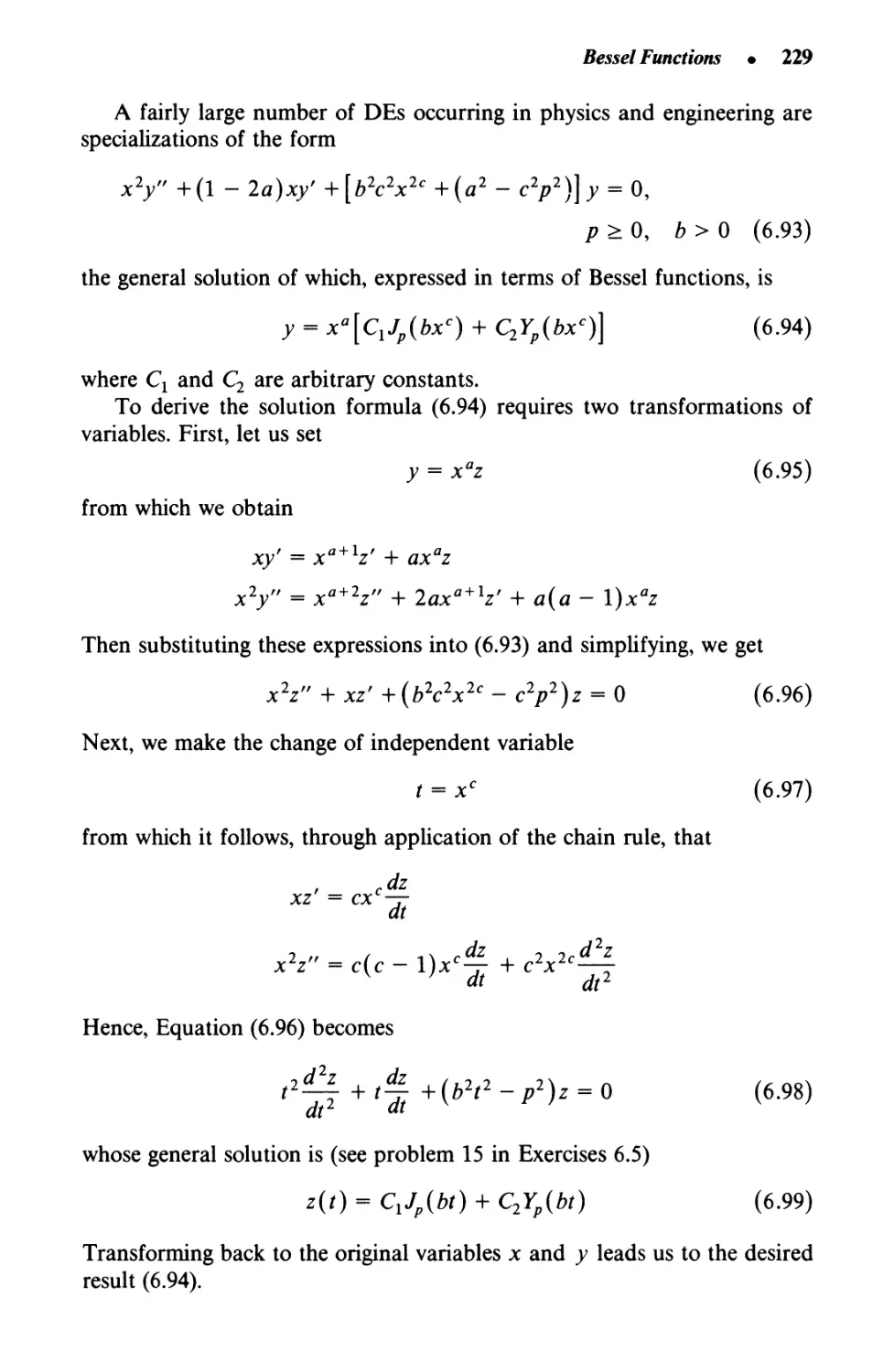
Differential Equations Related to Bessel's Equation 228
Modified Bessel Functions 232
Other Bessel Functions 241
Asymptotic Formulas 248
BOUNDARY-VALUE PROBLEMS 252
Introduction 252
Spherical Domains: Legendre Functions 253
Circular and Cylindrical Domains: Bessel Functions 264
THE HYPERGEOMETRIC FUNCTION 272
Introduction 272
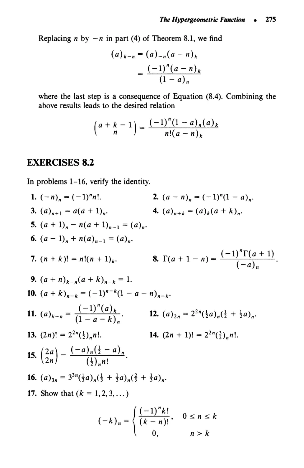
The Pochhammer Symbol 273
The Function F(a, b\ c\ x) 276
Contents · ν
8.4
8.5
9
9.1
9.2
9.3
9.4
10
10.1
10.2
10.3
Relation to Other Functions
Summing Series
THE CONFLUENT HYPERGEOMETRIC FUNCTION
Introduction
The Functions M(a; c; x) and U(a; c; x)
Relation to Other Functions
Whittaker Functions
GENERALIZED HYPERGEOMETRIC FUNCTIONS
Introduction
The Set of FunctionsF
Other Generalizations
BIBLIOGRAPHY
APPENDIX: A LIST OF SPECIAL-FUNCTION FORMULAS
SELECTED ANSWERS TO EXERCISES
INDEX
285
292
298
298
299
308
315
321
321
322
327
333
335
348
351
Preface
Modern engineering and physics applications demand a more
thorough knowledge of applied mathematics than ever before. In particular, it is
important to have a good understanding of the basic properties of special
functions. These functions commonly arise in such areas of application as
heat conduction, communication systems, electro-optics, nonlinear wave
propagation, electromagnetic theory, quantum mechanics, approximation
theory, probability theory, and electric circuit theory, among others. Special
functions are sometimes discussed in certain engineering and physics courses,
and math courses like partial differential equations, but the treatment of
special functions in such courses is usually too brief to focus upon many of
the important aspects such as the interconnecting relations between various
special functions and elementary functions. This book is an attempt to
present, at the elementary level, a more comprehensive treatment of special
functions than can ordinarily be done within the context of another course.
It provides a systematic introduction to most of the important special
functions that commonly arise in practice and explores many of their salient
properties. I have tried to present the special functions in a broader sense
than is often done by not introducing them as simply solutions of certain
differential equations. Many special functions are introduced by the
generating function method, and the governing differential equation is then
obtained as one of the important properties associated with the particular
function.
In addition to discussing special functions, I have injected throughout
the text by way of examples and exercises some of the techniques of applied
analysis that are useful in the evaluation of nonelementary integrals,
summing series, and so on. All too often in practice a problem is labeled
"intractable" simply because the practitioner has not been exposed to the
Vll
viii · Special Functions for Engineers and Applied Mathematicians
"bag of tricks" that helps the applied analyst deal with formidable-looking
mathematical expressions.
During the last ten years or so at the University of Central Florida we
have offered an introductory course in Special Functions to a mix of
advanced undergraduates and first-year graduate students in mathematics,
engineering, and physics. A set of lecture notes developed for that course
has finally led to this textbook. The prerequisites for our course are the basic
calculus sequence and a first course in differential equations. Although
complex-variable theory is often utilized in studying special functions,
knowledge of complex variables beyond some simple algebra and Euler's
formulas is not required here. By not developing special functions in the
language of complex variables, the text should be accessible to a wider
audience. Naturally, some of the beauty of the subject is lost by this
omission.
The text is not intended to be an exhaustive treatment of special
functions. It concentrates heavily on a few functions, using them as
illustrative examples, rather than attempting to give equal treatment to all. For
instance, an entire chapter is devoted to the Legendre polynomials (and
related functions), while the other orthogonal polynomial sets, including
Hermite, Laguerre, Chebyshev, Gegenbauer, and Jacobi polynomials, are all
lumped together in a single separate chapter. However, once the student is
familiar with Legendre polynomials (which are perhaps the simplest set) and
their properties, it is easy to extend these properties to other polynomial
sets. Some applications occur throughout the text, often in the exercises, and
Chapter 7 is devoted entirely to applications involving boundary-value
problems. Other interesting applications which lead to special functions
have been omitted, since they generally presuppose knowledge beyond the
stated prerequisites.
Because of the close association of infinite series and improper integrals
with the special functions, a brief review of these important topics is
presented in the first chapter. In addition to reviewing some familiar
concepts from calculus, this first chapter also contains material that is
probably new to the student, such as the Cauchy product, index
manipulation, asymptotic series, Fourier trigonometric series, and infinite products.
Of course, our discussion of such topics is necessarily brief.
I owe a debt of gratitude to the many students who took my course on
Special Functions over the years while this manuscript was being developed.
Their patience, understanding, and helpful suggestions are greatly
appreciated. I want to thank my colleague and friend, Patrick J. O'Hara, who
graciously agreed on several occasions to teach from the lecture notes in
their early rough form, and who made several helpful suggestions for
improving the final version of the manuscript. Finally, I wish to express my
appreciation to Ken Werner, Senior Editor of Scientific and Technical
Books Department, for his continued faith in this project and efforts in
getting it published.
1
Infinite Series,
Improper Integrals,
and Infinite Products
1.1 Introduction
Because of the close relation of infinite series and improper integrals to the
special functions, it is useful to review some basic concepts of series and
integrals. Infinite products, which are generally less well known, are
introduced here mostly for the sake of completeness. Infinite series are
important, of course, in almost all areas of pure and applied mathematics. In
addition to numerous other uses, they are used to define functions and to
calculate accurate numerical values of transcendental functions. In
beginning courses dealing with infinite series the primary problem is deciding
whether a given series converges or diverges. In practice, however, the more
crucial problem may actually be summing the series. If a convergent series
converges too slowly, the series may be worthless for computational
purposes. On the other hand, the first few terms of a divergent series in some
instances may give excellent results. Improper integrals and infinite
products are used in much the same fashion as infinite series, and in fact, their
basic theory closely parallels that of infinite series.
In the application of mathematics it frequently happens that two or
more limiting processes have to be performed successively. For example, we
often perform the derivative (or integral) of an infinite sum of functions by
taking the sum of derivatives (or integrals) of the individual terms of the
series. However, in many cases of interest, performing two limit operations
in one order may yield an answer different from that obtained from the
other order. That is, the order in which the limiting processes are carried out
1
2 · Special Functions for Engineers and Applied Mathematicians
is critical. Therefore, it is of utmost importance to know the conditions
under which such interchanges are permissible, and that is one of the
considerations of this chapter.
Because our coverage of topics here is primarily a review, the treatment
is intentionally cursory. In this regard we will state only the most relevant
theorems, and then usually without proof. For a deeper discussion of the
subject matter, the reader is advised to consult one of the standard texts on
advanced calculus.
1.2 Infinite Series of Constants
If to each positive integer η we can associate a number Sn9 then the ordered
arrangement
•Si» »>2,..., Sn>... (1-1)
is called an infinite sequence, and we call Sn the general term of the
sequence. Should it happen that
lim S„ = S (1.2)
и-»оо
where 5 is finite, the sequence (1.1) is said to converge to 5, and is said to
diverge otherwise.
An infinite series results when an infinite sequence of numbers
ul9 w2,..., uk,... is summed, i.e.,
00
щ + w2 + ··· + и* + ··· = Σ "к (1.3)
к=\
In this case the number uk is called the general term of the series. Closely
associated with the infinite series (1.3) is a particular sequence
S2 = Щ + u2
: (1-4)
η
Sn = Щ + w2+ ··· +w„= Σ "к
к=\
called the sequence of partial sums. If the partial sums (1.4) converge to a
Infinite Series, Improper Integrals, and Infinite Products · 3
finite limit 5, we say the infinite series (1.3) converges, or sums, to the value
S. The series (1.3) diverges when the limit of partial sums fails to exist, i.e.,
fails to approach a unique finite value.
Example 1: Determine whether the following series converges or diverges:
Solution: To show convergence or divergence we need to find the sum
of the first η terms and examine its limit. Here we see that
= i- 1
n + 1
where only the first and last term do not cancel. Thus,
limS„= limil-—pr) = l
and we conclude that the series converges, and in particular, converges
to the value unity.
When a series diverges, it may do so for different reasons. For example,
making use of the well-known formula
Sn= tk = \n{n + \) (1.5)
k = l
it is clear that Sn -> oo as η -> oo, and therefore the infinite series Lk
diverges.* In other instances the partial sums may not approach any
particular limit, as for the series
00
Σ (-i)*-1 = i - ι + i -i + ··· +(-i)*'1 + ··· (1.6)
k = l
The partial sums are Sx = 1, S2 = 0, S3 = 1,..., so that in general Sn = 1
for odd η and Sn = 0 for even n. Hence, we say that (1.6) diverges, since a
unique limit of Sn does not exist.
1.2.1 The Geometric Series
The special series
00
1 + r + r2 + · · · +rk + · · · = Σ rk (1-7)
* = 0
*We will occasionally find it convenient to use the symbol Luk to denote Lf=iUk.
4 · Special Functions for Engineers and Applied Mathematicians
is called a geometric series. The value r is called the common ratio since it is
the ratio between the (k + l)th term and the kth term. This series is
important because it has a wide variety of applications, and because it can
be summed exactly in those cases for which it converges.
From elementary algebra we know that the sum of the first η terms of
(1.7) is given by (see problem 1)
n~l 1 - rn
* - Σ'* --T37 (1-8)
* = 0
where we stop the summation at η - 1, since the series begins at к = 0.
Taking the limit of (1.8) as η tends to infinity leads to
limS„= {T^~r> И<1 (1.9)
"~*°° 1 no finite limit, \r\ > 1
where we are using the fact that rn -> 0 for increasing η when \r\ < 1.
Hence, we have derived the important result
ΣΓ" = γ—, |г|<1 (1.10)
which not only establishes the values of r for which the series converges, but
also provides the actual sum of the series.
Example 2: Test the series 3 - 2 + f - | + · · · +3(- §)* + · · · for
convergence.
Solution: By writing the series in the form
3-2 + f-f+··· =3(1-§ + !-£+···)
we recognize it as a geometric series (multiplied by 3) with r = - §.
Since r is less than unity in absolute value, we deduce that the series
converges, and moreover, converges to the value
1.2.2 Summary of Convergence Tests
Generally speaking, the only series that are useful in practice are those that
converge. For that reason we attach a great deal of importance to the task of
deciding whether a particular series converges or not. In the case of the
geometric series we were able to get the nth partial sum Sn into "closed
Infinite Series, Improper Integrals, and Infinite Products · 5
form" and examine its limit directly as η -> oo. By so doing, we not only
answered the question of convergence or divergence, but actually summed
the series. Unfortunately, the geometric series is one of the rare examples for
which we are able to get Sn into a form from which we can evaluate its limit
for large n. What is required then is a handful of tests that can be applied
to the series in question, from which its convergence or divergence can be
established. A great many such convergence tests have been developed over
the years, some simple to apply and others quite sophisticated.
The development of various convergence tests is taken up in courses on
calculus (both elementary and advanced). Our intention here is to simply
recall some of the elementary tests for reference purposes.
We first observe that if Luk = 5, where 5 is finite, then Sn -» S and
Sn_x -» S as η -> oo; hence, necessarily,
lim (Sn- S^J-S- 5 = 0
n—*■ oo
But, since Sn - Sn_! = w„, we find that a necessary condition (but not a
sufficient condition) for the series Σμ„ to converge is that*
lim w„ = 0 (1.11)
Remark: The general term of a series can be denoted by uk or w„, or
any other dummy index can be used. We will switch back and forth between
indices for convenience.
A series is called positive if the terms of the series are either all positive
or all negative. In other cases the terms of the series will vary in sign, some
terms positive and some negative. If the consecutive terms have opposite
signs, we call the series an alternating series. Series containing terms both
positive and negative converge more rapidly (when they converge) than
do positive series, due to the partial cancellation of the negative terms with
the positive terms. Because of these distinctions, we introduce notions of
different kinds of convergence.
Definition 1.1. The series Ew„ is said to converge absolutely if the
associated series of positive terms Σ|μ„| converges.
Definition 1.2. If the series Ew„ converges but the related series Σ|μ„|
diverges, the original series is said to converge conditionally.
For alternating series, we have the following important theorem.
*If lim„ ^oo un Φ 0, then of course the series Ew„ diverges.
6 · Special Functions for Engineers and Applied Mathematicians
Theorem 1.1 (Alternating-series test). If after a certain point the absolute
values of the terms of an alternating series decrease monotonically to zero,
the series converges (conditionally at least). Also, the sum of a convergent
alternating series always lies between the partial sums Sn and Sn+l for
each n.
If an alternating series converges by the alternating-series test, we must
further investigate its convergence to determine whether it converges
absolutely. This we do by testing the related series of positive terms, for which
we have the following convergence tests.
Remark: If a positive series converges, it necessarily converges
absolutely. (Why?) Hence, the term conditional convergence applies only to
series that vary in sign, such as alternating series.
Theorem 1.2 (Comparison test). A positive series Σηη converges absolutely
if each term (after a finite number) is less than or equal to the corresponding
term of a known convergent positive series Σαη, i.e.,
un<an, n>N
The positive series Σμ„ diverges if each term (after a finite number) is
greater than or equal to the corresponding term of a known divergent
positive series Σ6„, i.e.,
un>bn, n> N
Theorem 1.3 (Comparison test). If Σμ„ and Σαη are positive series and
lim — = с Ф О,
then Lun and Σαη converge or diverge together.
Remark: Theorem 1.3 can be extended to the case where с is either
zero or infinity. That is, if с = 0 and Σαη converges, then Σμ„ also
converges; if с -» oo and Σαη diverges, then Σμ„ diverges.
The following theorem is probably the most widely used test of
convergence.
Theorem 1.4 (Ratio test). Let Σμ„ denote any series for which
n—> oo
Infinite Series, Improper Integrals, and Infinite Products · 7
(1) If L < 1, the series Lun converges absolutely.
(2) If L > 1, the series Lun diverges.
(3) If L = 1, the test fails (no conclusion).
The ratio test is a particularly useful test for those series involving
factorials or exponentials, but fails in those case where the general term is a
rational function of n.
Theorem 1.5 (Integral test). Let f(n) denote the general term of the series
Σμ„. If the function f(x) is positive, continuous, and nonincreasing for
χ > a, then the positive series Σμ„ converges or diverges according to the
convergence or divergence of the improper integral f™f(x) dx.*
An important series for comparison purposes is the p-series*
n = \
To find the values of ρ for which this series converges, we can take
f(x) = \/xp and use the integral test. Thus, for a > Ο,φ
/•00
χ1-ρ
ΡΦ\
x~pdx= { 1 ~ P\
logx|", p = \
from which we deduce that the series converges for ρ > 1 and diverges for
ρ < 1. The special value ρ = 1 leads to
00 l 11 ι
Ι- = ι + ^ + 4+···+1+··· (1ЛЗ)
, η 2 3 η ;
called the harmonic series. It plays an important role in the use of
comparison tests. Although the series diverges, it does so at a very slow rate. For
example, the first million terms add up to a number only slightly larger than
14.
1.2.3 Operations with Series
In applications the need arises to combine various series by such operations
as addition and multiplication. To perform these operations it is usually
"The convergence of improper integrals is discussed in Section 1.6.
tFor ρ > 1, the /7-series is also called the Riemann zeta function (see Section 2.5.4).
$We use log χ to denote the natural logarithm, also commonly denoted by In x.
8 · Special Functions for Engineers and Applied Mathematicians
important to establish the absolute convergence of all series involved in the
process, since such operations can then be performed by the familiar rules
of algebra or arithmetic. Specifically, we have that:
1. The sum of an absolutely convergent series is independent of the
order in which terms are added.
2. Two absolutely convergent series may be added termwise, and the
resulting series will converge absolutely.
3. Two absolutely convergent series may be multiplied (Cauchy product),
and the resulting series will also converge absolutely.
The significance of property 1 above can best be realized by considering
what can happen if the series we wish to sum is not absolutely convergent.
The classic example of a series converging conditionally, but not absolutely,
is the alternating harmonic series Σ%=γ( — \)η~ι/η. Generally we associate
the sum of this series with the value log 2 (see Section 1.3), i.e., we write
f^ = l4 + |-l + M+- =log2 (1.14)
n = \
However, if we rearrange the terms of the series according to
1_i + I_i+... =(1_I) _!+(!_ I) _!+(!_ X)
__. 4./Ί _ _Λ _ J_ + ...
12 ^ V7 U) 16 ^
_I_I_i_l_l_i_J L.L.J L_i_ ...
~ 2 4^6 8 ^ 10 12T 14 16 ^
= L(l _I4.I_I4.I_I4. . . . \
we may conclude that the sum of the series is \ log 2. We arrive at this
conclusion not because we have cleverly omitted some terms of the series.
Indeed, each term of the series (1.14) does eventually appear exactly once,
but in the final arrangement the whole series appears multiplied by the
factor \.
What is being illustrated here is that by rearranging the terms of a
conditionally convergent series, that series may be made to converge to any
desired numerical value, or can even be made to diverge. Thus it is clear that
conditionally convergent series must be handled very carefully.
Also, if the series is not positive and diverges, we can sometimes produce
a convergent series from it by rearranging or regrouping the terms. For
example, if we write
00
Σ(-ι)""1 = (ι-ι)+(ι-ι)+···+(ι-ι)+···
w = l
the partial sums (of terms in parentheses) are all zero, and hence we may
Infinite Series, Improper Integrals, and Infinite Products · 9
deduce that the series convergences to the value zero. If a series is positive
and diverges, no rearrangement of terms can make the series converge.
If two series are absolutely convergent, no rearrangement of their terms
will alter the sum or difference of the two series. But again, if both of the
series forming the sum or difference are divergent, it is not clear what will
happen. For instance, by writing
/7 = 1 Ч
OO-i 00 -ι
Σ: ^
η + 1 / Λ η , /ι + 1
we can treat the series on the left as the difference of two divergent series, as
shown on the right. Although we might be tempted to say that the series on
the left diverges because of its relation to the divergent series on the right,
we have actually shown (in Example 1) that the series on the left converges,
and in fact converges absolutely.
In forming the product of two series, we are led to double infinite series
of the form*
00 00 00 00
L·, Um L·, Vk = L·, L· ^m,k
w = 0 A: = 0 m = 0A: = 0
where the summand Amk = umvk can be treated as a function of two
variables. We find that by making a change of index the above double sum
can often be simplified, or even partially summed. For example, suppose we
introduce the change of index m = η — /с, or equivalently, η = m + k.
Now, since m > 0, the index к must satisfy the condition η — к > 0, or
к < п. Hence, we deduce that (for absolutely convergent series)
00 00 00 Π
Σ ΣΛ,,*= Σ Σ Λ-*.* (ΐ·ΐ5)
m = 0A: = 0 n = 0 k = 0
Equation (1.15) illustrates that all absolutely convergent double infinite
sums can be replaced by a single infinite series of finite sums. This property
is particularly useful in numerical computations. If the two series forming
the product are each absolutely convergent, we can also interchange the
order of the infinite sums and then apply (1.15). In fact, all possibilities of
this kind should be explored when trying to simplify double infinite series.
On rare occasions we find it necessary to make a different change of
indices in our double infinite sums than illustrated above. For example, if
we set m = η - 2/с, it follows that к < η/2. But since η/2 is not always an
integer, it is conventional to introduce the bracket notation
I и/2, п even
[n/2]= I / ' „ ΆΆ (1.16)
L 7 J \(n - l)/2, η odd v ;
*Many of the infinite series that we encounter will start with the index value zero.
10 · Special Functions for Engineers and Applied Mathematicians
Hence, with this index change we deduce that (for absolutely convergent
series)
oo oo oo [и/2]
Σ Σ Amk = Σ Σ ^n-2k,k (1-17)
w = 0 £ = 0 л = 0 £ = 0
and upon combining (1.15) and (1.17), it also follows that
oo л oo [η/2]
Σ Σ An_kk= Σ Σ ^п-2к,к (1-18)
л = 0 £ = 0 n = 0 k = 0
Theorem 1.6 (Cauchy product). If Σ™=0αη and L™=0bn are both absolutely
convergent series, then so is their Cauchy product defined by
00 00 00
Σ an - Σ Κ = Σ cn
/ϊ = 0 л = 0 л = 0
where
η
cn = Σ <*kb„_k
k = 0
Other theorems on the product of two infinite series have been
developed. For example, it has been shown that if both Σαη and Σ6„ converge,
and if one of them converges absolutely, then Ec„ converges. Also, it is
possible for both Σαη and Lbn to converge while the product series Lcn
diverges.
1.2.4 Factorials and Binomial Coefficients
In simplifying products of infinite series, as well as numerous other
applications, we frequently encounter series involving binomial coefficients. Perhaps
the simplest way of introducing these coefficients is by considering the
expanded product of (a + b)n. For example,
(a + bf = a + b
(a + bf = a1 + lab + b2
(a + bf = a3 + 3a2b + ЪаЪ2 + b3
and in general,
(a + b)n = an + nan~lb + "("2~ 1} a"~2b2 + · · ·
+ я(я-1)..(я-Н1)д^ + |||+у (119)
The coefficient of the general term in (1.19) can be expressed more simply in
Infinite Series, Improper Integrals, and Infinite Products · 11
terms of factorials by writing
n(n - I) · - (n - к + 1) n\
k\ k\(n-k)\
for which we also introduce the notation*
(1) = Щ^У.> "-О»1·2.-. к-0,1,...,« (1.20)
Adopting this notation, we can now write (1.19) more compactly as
(* + *)"- i(nk)"n-kbk (1.21)
The symbol I , I is what we call a binomial coefficient. Besides its
connection in (1.21) with the expansion of (a + b)n, the binomial coefficient
also occurs in combinatory problems, probability theory, and algorithm
development. In these other applications the upper index is often not an
integer, or even a positive number. For such situations we cannot use (1.20)
to define the binomial coefficient, but rather we resort to
(J).,, (,К(,-1)-;(,-* + 1), ,.,.„,...
(1.22)
As simple consequences of the definition of binomial coefficient and
properties of factorials, we have the following useful relations:
(J)-C)-1 <123>
(;)-L-i)-» »·24>
им»-*) <'·25>
(ι:ικΐι)+(ί)· ·***«-> <>·*>
Example 3: Show that
(гн-ч'т
*0! = 1.
12 · Special Functions for Engineers and Applied Mathematicians
Solution: From (1.22), we have
/ -r\ _ -r{-r- !)···(-*·- к + 1)
l к ! к\
( ukr(r+\)---(r + k-l)
К ' к\
k(r + k-l)(r + k-2)---(r + l)r
{ ' к\
-<-«'(Γ + ί_Ι)
where the last step again follows from (1.22).
There are literally thousands of identities involving binomial coefficients
that have been discovered over the years. Fortunately, only a few of these
are required in most applications. In addition to (1.23)—(1.27) above, the
following summation formulas are also very important:
έ(ϊ)-2· <«·)
έ„('ΐ*)-('+:+1) <"»>
&tt)-(:Vi)· —си,... а.зо)
ZjiK'^*)(-!)'-(-l)"Ui„) (1-32)
Equation (1.28) follows directly from (1.21) with a = b = 1. To prove (1.29)
requires repeated application of (1.26), whereas (1.30) follows from (1.29)
with two applications of (1.25). Equation (1.31) is verified below (Example
4), and (1.32) is left to the exercises.
Remark: In Section 8.5 we will present another method of summing
certain series of binomial coefficients by use of the hypergeometric function.
Example 4: Verify Equation (1.31) above.
Solution: Starting with the obvious identity
(i + jc)r(i + *;r = (i + ;c)r+i
A: = 0
η
Infinite Series, Improper Integrals, and Infinite Products · 13
and replacing each binomial with its series, we find*
00 00 00
Σ('α)χ··Σ('„)χ·-Σ('+α')*·
и = 0 n = 0 n = 0
The left-hand side can be simplified by use of the Cauchy product
(Theorem 1.6), which leads to
00 П . ч . N 00
w = 0 A: = 0 n = 0
and now, by comparing coefficients of like terms of xn, we obtain the
result
i (It'->)-('*·')■ "-0·1·2-·
EXERCISES 1.2
1. Show that the nth partial sum of a geometric series satisfies
1 — rn
1 + r + r2 + ··· + /·"-1 = - , r # 1
1 - r
Hint: Observe that
Sn = 1 + r + /*2 + ··· +/·""1
r5w = r + /*2 + ··· +r"-1 + rn
and subtract termwise.
In problems 2-5, find the sum of the geometric series.
10 100
2. Σ 2*. 3. Σ(-1)*.
A: = 0 A: = 0
10 oo
4. £ (i)*. 5. Σ sin2"*, |x|<*/2.
A: = 2 « = 0
In problems 6 and 7, use geometric series to express the repeating decimal
as a rational number.
6. 3.42121212... 7. 2.123123123...
*When r and 5 are not integers the binomial series becomes an infinite series, and in this
case χ is restricted to the interval \x\ < 1 (see Section 1.3.2).
t We are actually using Theorem 1.13 in Section 1.3.2.
14 · Special Functions for Engineers and Applied Mathematicians
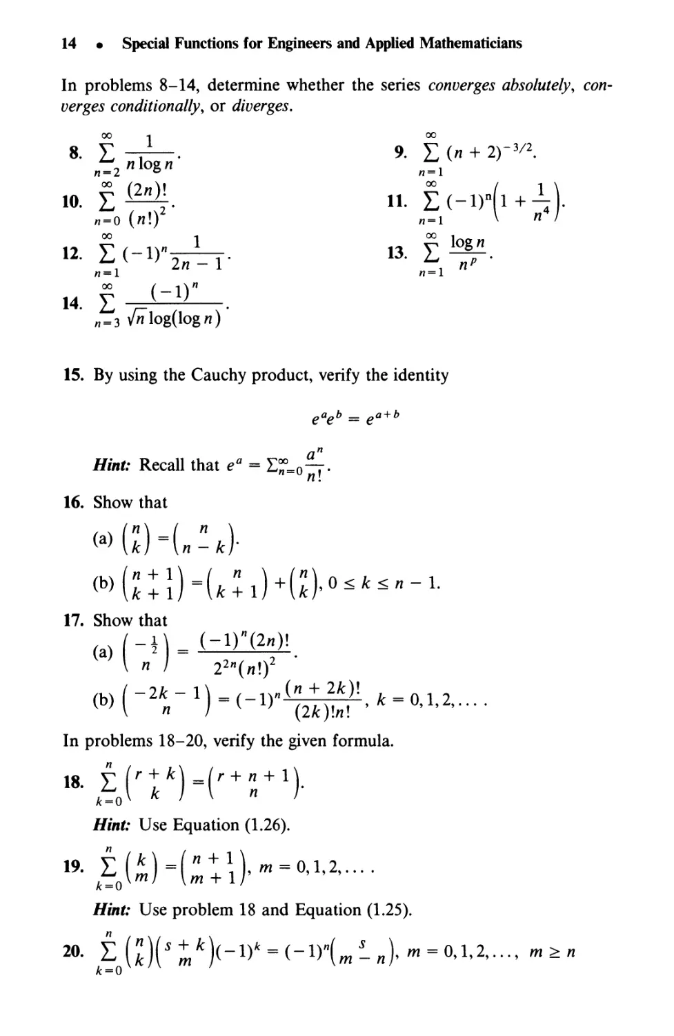
In problems 8-14, determine whether the series converges absolutely,
converges conditionally, or diverges.
OO-i 00
.·. Σ&$. ". Σ(-ΐ)·(ι+Λ).
n-o (и!Г «=i V η I
14- Σ
n=o (л!)
(-1)"
12. IC-iry-^r· 13. Σ^.
,2/1 — 1 л пр
„=3 v^"log(log/7)'
15. By using the Cauchy product, verify the identity
eaeb = ^a + 6
Я/iif: Recall that ea = Е?_0^т.
16. Show that
«(!)-U*)·
»)(;:!)-(*:ι)+(:)··**«- >·
17. Show that
(-П=(-1Г(2„)!
<b)(-"„-1) = <-1>-ig^^ = ^·2
In problems 18-20, verify the given formula.
*έ,('ί*)-(Γ+:+1)·
#ι#ιί; Use Equation (1.26).
#wi; Use problem 18 and Equation (1.25).
20. EJiK'i^i-l^-i-irUi „).*»-0,1,2,..., m*„
Infinite Series, Improper Integrals, and Infinite Products · 15
1.3 Infinite Series of Functions
Of special importance to us are those series that result when the general
term un is a function of jc, i.e., un = un(x). The n\h partial sum then
defines the function
$,(*)= £«*(*) (1-33)
k = \
and similarly, the sum of the series becomes
lim £„(*)-/(*) (1.34)
n-* oo
The question of concern here is whether there exists any values of χ for
which (1.34) is meaningful. If the value of χ is fixed and the resulting series
sums to /(*), we say the series converges pointwise to f(x). All such values
of χ for which the series converges pointwise constitute the domain of the
function /.
Example 5: Test the series Σ™=0χη for convergence.
Solution: Applying the ratio test, we find
lim
П-КХ)
Xn + l
lim \x\ = \x\
and deduce that the series converges pointwise for \x\ < 1 and diverges
for |jc| > 1. The cases |jc| = 1 must be treated separately, but it can
easily be established that the series diverges for both χ = 1 and χ = -1.
Our conclusion here is consistent with previous results, since the series in
question is just the geometric series once again with f(x) = 1/(1 - x).
In some applications it is important to establish a different kind of
convergence of the series, for which we have the following definition.
Definition 1.3. If, given some ε > 0, there exists a number N = N(e)
independent of *, and if
\f(x)-Sn(x)\<e
for all χ in a < χ < b and all η > Ν, we say that Sn(x) converges uniformly
to f(x) in a < χ < b as η -> oo.
Uniform convergence is illustrated in Fig. 1.1. It is clearly a stronger
requirement than is pointwise convergence, which treats convergence at
16 · Special Functions for Engineers and Applied Mathematicians
Figure 1.1
individual points, but it is also more difficult to establish in practice. The
key to uniform convergence is continuity of the function / (see Theorem
1.8).
The most commonly used test for establishing uniform convergence of
an infinite series of functions is the famous Weierstrass M-test.
Theorem 1.7 (Weierstrass M-test). If ΣΜη is a convergent series of
positive constants such that |w„(;c)| < Af„ (w = 1,2,3,...) for all χ in a < χ <
b, then the series Lun(x) is uniformly (and absolutely) convergent over the
interval a < χ < b.
Normally, if a series converges uniformly it converges absolutely, but
not always. That is, neither type of convergence necessarily implies the
other. For example, the series L™=i(-l)n~1xn/n = log(l + x) converges
uniformly for 0 < χ < 1, but not absolutely. (Why?) Also, the series
L(1-jc)jc«
л = 0
1,
0 < χ < 1
x = 1
converges absolutely but not uniformly in the interval 0 < χ < 1. Thus the
Weierstrass M-test is not suitable for series that converge uniformly but not
absolutely.
Infinite Series, Improper Integrals, and Infinite Products · 17
1.3.1 Properties of Uniformly Convergent series
Establishing that a given series converges uniformly in an interval is useful
for performing certain operations on the series termwise.
Theorem 1.8. If each term un(x) is continuous in a < χ < b and the series
/(*)= £«„(*)
n = \
converges uniformly in a < χ < b, then / is a continuous function in this
same interval.
Note that Theorem 1.8 requires uniform convergence to conclude that /
is continuous. To show that pointwise convergence is not sufficient, consider
the series
00
/(*) = *+ Σ (xn-xn~l), 0<jc<1 (1.35)
л-2
Clearly each term of the series is a continuous function. Also, the sum of the
first η terms is Sn(x) = jc", which converges to zero in the interval 0 < χ < 1
and to unity when χ = 1. Hence, the sum of the series is
/(*)-{?; °xiVl (1·36)
which is clearly not a continuous function in the closed interval 0 < χ < 1.
Theorem 1.9. If each term un(x) is continuous in a < χ < b and the
infinite series Ew„(jc) converges uniformly in a < χ < b, then termwise
integration of the series is permitted, i.e.,
/| Ek„(*)U*= Σ fbun{x)dx
a \n=\ I л-1 а
. Theorem 1.9 is particularly important in applied mathematics, since the
integral of an infinite series arises frequently there. The difficulty in many
situations, however, is that we may not be able to show that the given series
converges uniformly prior to performing termwise integration. In such
situations we tacitly assume the conditions of Theorem 1.9 and formally
carry out all computations. It is essential in these situations to justify the
derived result by some independent means.
In order to illustrate the use of Theorem 1.9, consider the infinite series
γ^= £(-l)V, -1<*<1 (1-37)
w = 0
It can be shown that this series converges uniformly in any closed interval
18 · Special Functions for Engineers and Applied Mathematicians
contained within the indicated open interval (see Section 1.3.2). Hence,
termwise integration of (1.37) leads to
f~-= Σ(-ΐ)7>^ -k*<i
where we introduce the dummy variable t to avoid confusion. Completing
the integration, we obtain
«♦Ί-ΣΙ-ΐ)·^
л = 0
and by making the change of index η -> η — 1, we get the more familiar
form
log(l + jc) = Σ ("Ι)"'1 γ> -1 < jc < 1 (1.38)
w = l
Notice that setting χ = 1 in (1.38) leads to
log 2= Σ1"^— (1.39)
w = l
where the right-hand side is the alternating harmonic series (see Section
1.2.3). It is interesting to observe that the result (1.39) is valid even though
the value χ = 1 is outside the original interval of (pointwise) convergence.
This example illustrates that the process of integration of an infinite series
can sometimes extend the interval of convergence of the integrated series
beyond that of the original series.
The conditions stated in Theorem 1.9 are satisfied for many of the series
that commonly arise in practice, and for this reason we find that most of the
time termwise integration of the series is permitted. The same is not true,
however, for termwise differentiation of a series, even under the same
conditions. That is, uniform convergence of the series does not validate its
differentiation.
Theorem 1.10. If un(x) and u'n(x) are continuous functions in the interval
a < χ < b for each л, and if
fix) = Σ «„(*)
n = \
converges in a < χ < b and the series Ew^(jc) converges uniformly in
a < χ < b, then
fix) = Σ <(*)
n = \
Infinite Series, Improper Integrals, and Infinite Products · 19
Basically, the requirement for termwise differentiation of a series is the
uniform convergence of the differentiated series. For example, the series
f(x) - Σ ^^ (1.40)
n-l n
converges uniformly in every finite interval (by the Weierstrass M-test),
whereas the series
00
/'(*)= Σ cosk2jc (1.41)
n = \
diverges for all x. Clearly, termwise differentiation of an infinite series must
be handled with caution.
1.3.2 Power Series
By a power series, we mean an expression of the form
00
c0 + Cl(x - я) + · · · +cn(x - a)" + · · · = Σ cH(x - a)" (1.42)
n = 0
where the c's are constants and a is some fixed value.
Theorem 1.11. Every power series has a radius of convergence ρ such that
the series converges absolutely when \x — a\ < ρ and diverges when |jc - a\
>P·*
If ρ > 0, then for every ρλ such that 0 < ρλ < ρ, the power series
converges uniformly for \x - a\ < pv The question of convergence of a
power series when \x - a\ = ρ can be answered separately by one of our
previous convergence tests, since (1.42) is just a series of constants in this
case.
Theorem 1.12 (Abel's theorem). If the radius of convergence of a power
series is p, then the sum
00
/(*)= Σ cn(x- a)n
n = 0
is a continuous function for |jc - a\ < p.
Proof: Since the series converges uniformly for|;c — я| < pl5 0 < Pi <
p, it follows (from Theorem 1.8) that / is a continuous function on this
*In some cases ρ = 0, and hence the series converges only for χ = a.
20 · Special Functions for Engineers and Applied Mathematicians
interval. But since this is true for every ρλ between 0 and p, we conclude
that / is continuous for all χ in the interval \x - a\ < p. Ш
As simple consequences of Theorem 1.9 and 1.10, it follows that
convergent power series can always be differentiated and integrated term-
wise. If the power series converges uniformly for all χ such that \x — a\ < p,
the integrated series will also converge uniformly for \x — a\ < p. On the
other hand, the differentiated series may not converge at the endpoints. For
example, the series
00 xn
converges uniformly for all \x\ < 1, but the related series
/'(*)= Σγ. -ι<*<ι
n = \
does not converges at χ = 1. Moreover, the series
00
/"(*) = Σ *"> -ι < jc < ι
n = 0
does not converge at either endpoint.
One way of generating a power series for a given function / is illustrated
in the following discussion.
If / is continuous and differentiable, then
ff'(t)dt=f(x)-f(a) (1.43)
which we can rearrange as
/(*)=/(«) + ff'(t)dt (1.44)
If / also has a second derivative /", we can then replace / in (1.44) by the
function /' to obtain
f'(x)=f'(a) + ff"(t)dt
The substitution of this last expression for /' in (1.44) leads to
f(x)=f(a) + fX\f'(a) + ff"(tl)dtl
J η J η
dt
f(a) +f'(a)(x -a) + f ff"(t)(dtf (1.45)
Infinite Series, Improper Integrals, and Infinite Products · 21
where we are using the notation
rf'nt){*)2-r\ff'Vi)*i
* /7 •'Λ * Π I * Π
dt (1.46)
Now assuming the function / has η derivatives, we can repeat this process
over and over until we obtain
/(*)-/(«)+/'(<■)(* - «) + ^r <* - ")' + ·''
(я- !)!
where
K = f-· j'f(n)(t){dt)n (1.48)
Equation (1.47) is known as Taylor's formula with remainder.
If the function f(n)(t) satisfies the inequality
m </(w)(0 <M, a<t<x (1.49)
where w and Μ are constants, then it can be shown that
mf--- j\dt)n<R„<Mf---j\dt)n
Ja Ja Ja Ja
which reduces to
w(*Ta)" < R„ < M(x7a)" (1.50)
я! w я!
Hence, if f(n)(t) is also continuous over a < t < x, then there exists some
value ξ such that
Rn=l-AV(x-a)\ α<ξ<χ (1.51)
known as the Lagrangian form of the remainder after η terms.
Finally, if the function / has the property that, for |x - я| < p, Rn -* 0
as η -> oo, then it follows that
/(*) = Σ J—^rL(* - «)"· I* - «I < ρ (ΐ·52)
rt = 0 "*
We refer to (1.52) as the Taylor series for the function /. The special case of
(1.52) that occurs when a = 0 is known as Maclaurin's series, i.e.,
/(*)= Σ}—Ρ-χ\ W<p (1-53)
я = 0 "·
22 · Special Functions for Engineers and Applied Mathematicians
Most of the elementary functions that arise in the calculus can be
represented by a Taylor series, where the interval of convergence is
determined by the ratio test. Many of the special functions that we will
encounter in subsequent chapters can also be represented by a Taylor series
(or a Maclaurin series).
Example 6: Expand f(x) = (1 + x)a in a Maclaurin series, where a is a
parameter not restricted to integer values.
Solution: Repeated differentiation of the function reveals that
/'(*) = a(1 + x)a~l
f"(x) = a(a-l)(l+x)a-2
fw(x) = a(a - 1) · · · (a - η + 1)(1 + x)a~n
Hence, by setting χ = 0 in / and all its derivatives, we find that the
series (1.53) leads to
(1 + x) = 1 + ax + -^—Lx2 + · · ■
+ α(α-1)···(α-η + 1)χΗ +
n\
which we can express more compactly in the form
00
n = 0
where ( an j denotes the binomial coefficient (see Section 1.2.4).
By applying the ratio test to the above series, known as the binomial
series, we find that it converges for \x\ < 1.
The binomial series in Example 6 is important in much of our work to
follow, and we will have many occasions to refer back to this result.
The following theorem assures us of the uniqueness of representation of
a function by a Taylor series for a fixed value of a.
Theorem 1.13 (Uniqueness). If f(x) = Lcn(x - a)n and g(x) = Lbn(x -
a)n both have nonzero radii of convergence, and f(x) = g(x) wherever the
two series converge, then cn = bn, η = 0,1,2,... .*
*If Lcn(x - a)" = 0, then necessarily cn = 0 for all n.
Infinite Series, Improper Integrals, and Infinite Products · 23
1.3.3 Operations with Power Series
If
/(*)= Σαηχη
n = 0
and
g(x) = ΣΚχη
n = 0
(1.54)
(1.55)
have a common interval of convergence, then the series of their sum and
product, i.e.,
and
f{x) + g(x)= Z(a„ + bn)x"
n = 0
f(*)g(x)= Σ Σ «A-*)*"
w = 0 \A: = 0
(1.56)
(1.57)
also converge on this common interval of convergence. We recognize (1.57)
as simply the Cauchy product introduced in Theorem 1.6. Finally, since
power series are merely a special type of infinite series, the theorems in
Section 1.3.1 concerning integration and differentiation of infinite series
apply directly to convergent power series.
Example 7: Find the Maclaurin series for e*sin;c.
Solution: By using well-known results, we have
£ x" A . £ (-1)V+1
V —- and sin χ = V
w = 0
я-о (2« + l)!
However, we cannot directly apply (1.57), since the series for sinjc
involves only odd powers of x. To remedy this situation, we rewrite the
sine series in the form
sinx = 52 cos (л - 1)
7Г
n = 0
n\
where
cos
(»-Df
(-1)'
0, η even
("-1)/2, «odd
24 · Special Functions for Engineers and Applied Mathematicians
Thus, the Cauchy product now leads to
00
exsinx = Σ cnx"
w = 0
where
Λ cos[(ft- l)y/2]
Cn So kl(n-k)l
Although it often happens that the expression for cn cannot be
simplified, here we find that we can actually evaluate the finite sum. By
using the Euler formula cos л: = \{elx + e~lx\ together with properties
of the binomial series, we find
k = 0
2„! ty)e 2„! £Q(k)e
= VrP + eiw/2)H + Vri1 + e~lw/2)H
Now writing
(1 + eiv/2)n = einv/4(eiv/4 + е_,7г/4)" = 2V,7r/4cos"(7r/4)
(1 + е"'"/2)" = 2ne-,nw/4GOSn(w/4)
we deduce that
cn = уТ[в,"(я"2),г/4 + e-,("-2)7r/4]2"cos4V4)
= -^rcos[(«-2)V4]
and hence, we obtain our result*
exsin;c = Σ —— cos[(fl - 2)77/4] x"
w = 0 П'
which converges for all x.
*Notice that the terms corresponding to η = 0,4,8,... are all zero.
Infinite Series, Improper Integrals, and Infinite Products · 25
Closely related to the Cauchy product defined by Equation (1.57) is the
power formula
00 \n 00
Σν* = Lckxk (1.58)
where
1 k
Со = Яо> ck = -j^- Σ (nm ~ к + т)атск_т, к = 1,2,3,...
(1.59)
The reader should verify that this power formula is equivalent to the
Cauchy product for η = 2. By repeated application of the Cauchy product
for η = 3,4,5,..., the above result can readily be obtained.
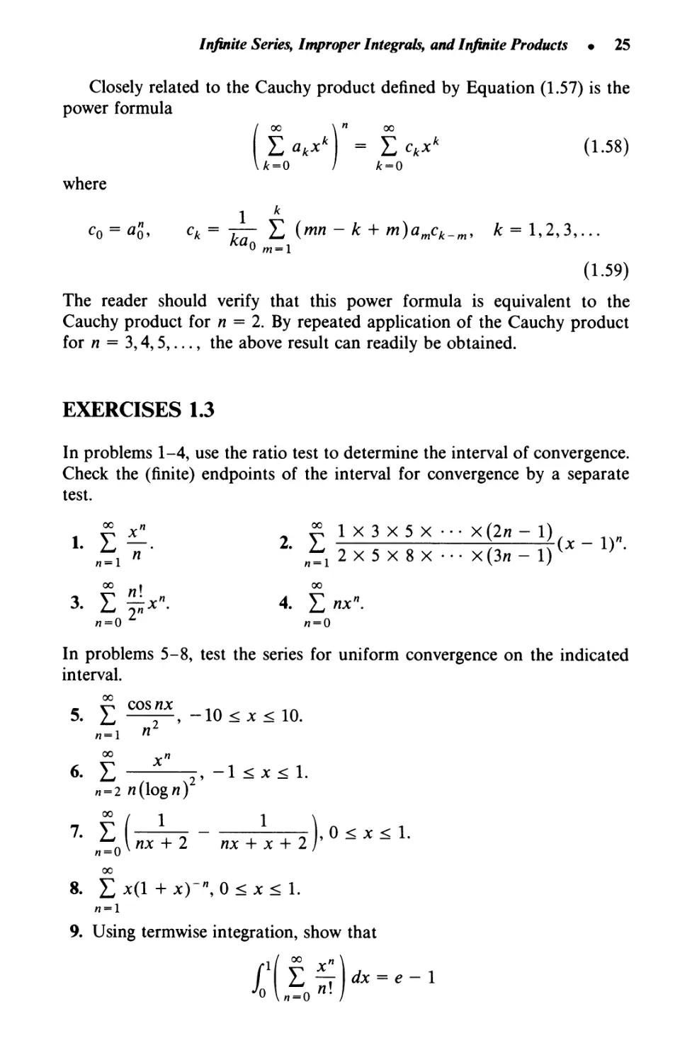
EXERCISES 1.3
In problems 1-4, use the ratio test to determine the interval of convergence.
Check the (finite) endpoints of the interval for convergence by a separate
test.
1 ? £! 2 У 1хЗх5х---х(2я-1) п„
tin' „-i 2 x 5 x 8 X · · · X(3" - !)
3. Ε £*". 4. Σ "*"'
In problems 5-8, test the series for uniform convergence on the indicated
interval.
5. Σ Г~> -Ю < χ < 10.
6. Σ 2> _1 -x- 1-
n = 2 li(logn)
7. Σ (—rr / ^ До<*<1.
_n\ nx + 2 л* + jc + 2 /
w = 0
00
8. Σ *(! + *)""> 0 < x < 1.
9. Using termwise integration, show that
йт
dx = e — 1
26 · Special Functions for Engineers and Applied Mathematicians
In problems 10-13, indicate those series that can be differentiated termwise
in the indicated interval.
00 xn °° e~nx
10. £ 7=, -l<x<0. Π. Σ -,0<x<10.
n=o v« „=o n(n + 1)
12. Ё(^Ц-)". -4<x< -3. 13. f f— -^-),0<x<l.
„-ЛЛ-W „fill! И + 1/
14. Starting with the geometric series
1
1 -*
и = 0
£x",-l<x<l
(a) make a change of variable to derive the Maclaurin series for
1
/(*)
1 + x2
(b) Use the answer in (a) to determine the Maclaurin series for arctan x.
Give the interval of convergence.
15. Starting with the binomial series
(ΐ + *)β= Σ(αη)χ", -k*<i
w = 0
(a) find the Maclaurin series for f(x) = (1 - x2)~l/2.
(b) Use the answer in (a) to determine the Maclaurin series for arcsin x.
Give the interval of convergence.
In problems 16-19, use the Cauchy product to find the Maclaurin series
representation for the given function.
16. f(x) = (1 - jc)"2. 17. f(x) = cos2jc.
18. f(x) = sin2jc. 19. f(x) = e*cosjc.
20. Use (1.58) and (1.59) to determine the first four terms of cos3 jc.
1.4 Asymptotic Series
In computational analysis we often seek to represent a given function /(jc)
by some simpler function, say g(jc), that accurately describes the numerical
values of /(jc) in the vicinity of a particular point χ = a. Thus we write
/(jc) - g(jc) as jc -> a to mean
■«44-1
Infinite Series, Improper Integrals, and Infinite Products · 27
Generally we confine our attention to either the case χ -» 0 or χ -> oo,
although we could also choose any other value of x.
For the case χ near zero, we seek a representation of the form
/(*)~ Lcnx\ x-*0, (1.60)
n = 0
from which we can deduce the simple asymptotic formulas f(x) ~ c0 or
f(x) ~ c0 + qjc, and so on. Ordinarily we might obtain the representation
(1.60) from the Maclaurin series expansion of /(*). In such cases the series
converges for all values of χ such that \x\ < p. That is, if
η
S„(x) = Σ Ck*k
k=0
then
lim |/(*)-S„(*)|=0 (1.61)
и-»оо
for each fixed χ in the region |jc| < p. By taking a sufficient number of
terms of the series, our calculations for f(x) can be as accurate as desired.
However, the representation (1.60) does not have to be a Maclaurin series,
nor is there any requirement that the series converge in order to be useful
for computations. That is, we define (1.60) to be an' asymptotic power series
for f(x) as χ -> 0 if and only if
■J'"-*<*>'-. (1.62)
x-*0 \X\
for each fixed n. By this condition we are requiring the sum of the terms of
(1.60) out to the term cnxn to approximate the function f(x) more closely
than \x\n approximates zero, by choosing χ sufficiently close to zero. Hence,
if the series (1.60) diverges, we find that the accuracy of computation is
closely tied to the actual value of χ and number of terms n. This means that
after a certain number of terms the accuracy of computation will actually
get worse instead of better—a sharp contrast as compared with convergent
series.
1.4.1 Large A rguments
For large values of χ we seek representations of the form
00 a
/(*)~ Στί.*-» (1.63)
w = 0 Л
28 · Special Functions for Engineers and Applied Mathematicians
We call (1.63) an asymptotic series for large arguments; it is also commonly
called a semiconvergent series. A precise definition of asymptotic series was
first provided by J. H. Poincare (1854-1912) in 1886; he stated that (1.63) is
an asymptotic series if and only if, for each fixed л,
\imxn\f(x)-Sn(x)\=0 (1.64)
.x->oo
where
sn(*) = i Ц
k = 0 x
Asymptotic series like (1.63) are intriguing in that they usually diverge
for all values of x, but are still useful for computational purposes. In such
cases, once again, too many terms of the series can lead to gross errors in
computations, and therefore it is important to know just how many terms to
retain for a particular computation. The error incurred in most cases turns
out to be less than the first term omitted in the approximation.
Not all functions have an asymptotic series of the form (1.63). For
example, neither ex nor sinjc has such an asymptotic expansion. If the
function f(x) itself has no asymptotic series, it may happen that there exists
a suitable function h(x) such that the quotient f(x)/h(x) has an
asymptotic series. In this case we write
00 a
ί{χ)~Η{χ)Σ—η, x^°o (1.65)
n = 0 X
Necessary and sufficient conditions for f(x) to possess an asymptotic series
have been developed, but we will not discuss them.*
If f(x) has an asymptotic series, it may turn out that other functions
have the same asymptotic series. That is to say, an asymptotic series does
not uniquely determine the function from which it was generated. However,
if a function has an asymptotic series, it has only one such series.
There are several ways in which asymptotic series can be derived. For
our first example, we wish to consider the case where the function is defined
by an integral of the form
/00
f(t)dt (1.66)
A simple and often effective way of developing the series in such cases
consists of repeated integration by parts. Each new integration yields the
next term in the expansion, and the error committed in stopping after η
*See F.W.J. Olver, Asymptotics and Special Functions, New York: Academic, 1974.
Infinite Series, Improper Integrate, and Infinite Products
29
terms can be expressed by the remaining integral, for which error bounds
can often be deduced.
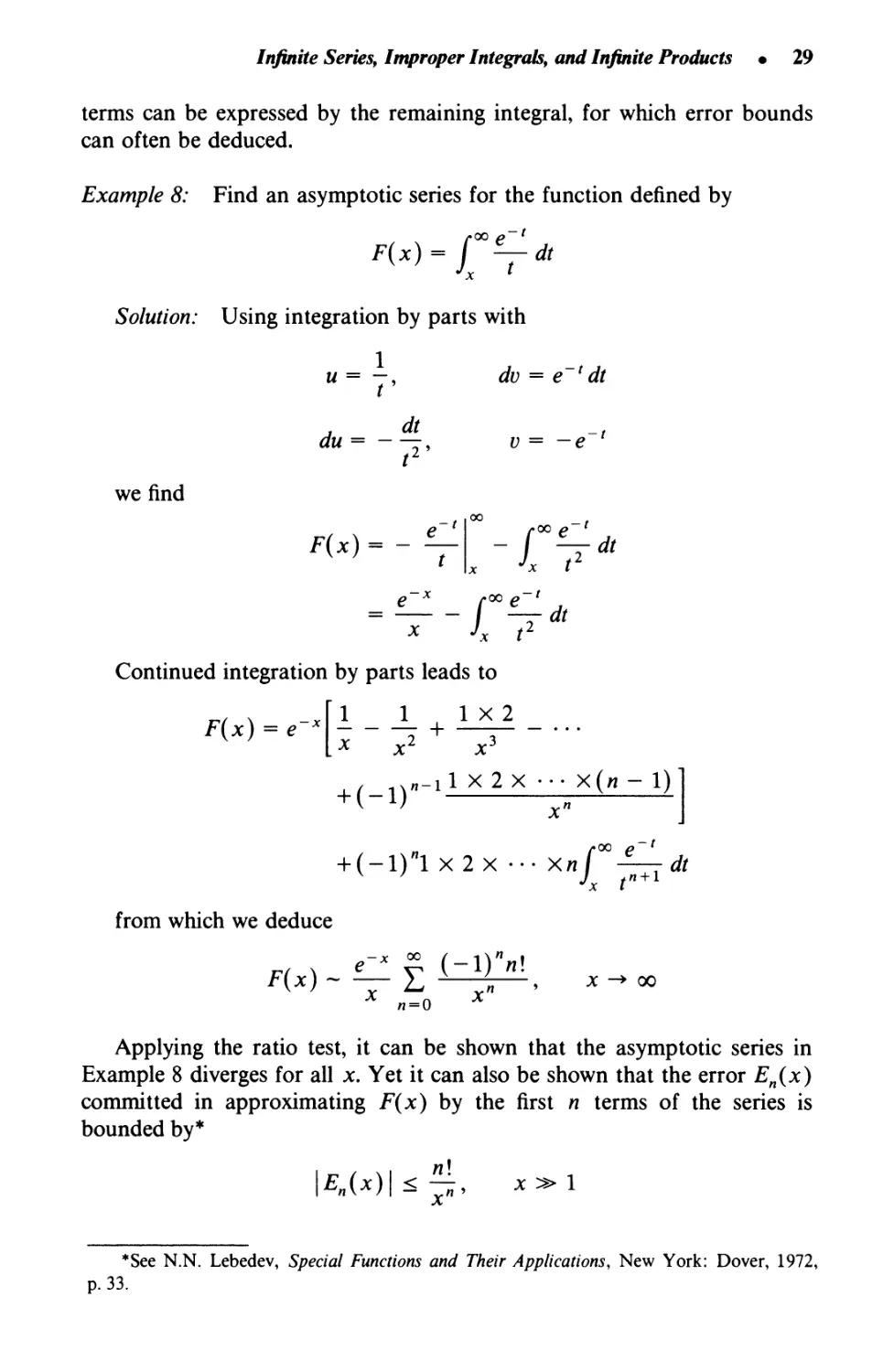
Example 8: Find an asymptotic series for the function defined by
J/»00 ρ *
Τ*
Solution: Using integration by parts with
we find
F(x) = e-
1
и = —,
t
do = e~'dt
A dt ~t
du = —-, υ = —e
r
e~l
F(x) =-e—
X XI
X Jx t2
on by parts leads to
I _ J_ 1 X 2 _
.x x2 x3
.( ι4<·-ι1 Χ 2Χ ··· Х(я - 1)1
+ (-1) -η j
+ (-!)"! X
r00 e t
2 X ··· Хл / dt
*x I
from which we deduce
v 7 χ η χ"
n = 0
00
Applying the ratio test, it can be shown that the asymptotic series in
Example 8 diverges for all x. Yet it can also be shown that the error En(x)
committed in approximating F(x) by the first η terms of the series is
bounded by*
n\
\En{x)\ < -^, x» 1
*See N.N. Lebedev, Special Functions and Their Applications, New York: Dover, 1972,
p. 33.
30 · Special Functions for Engineers and Applied Mathematicians
For large enough χ and small л, the error En(x) can be made quite small.
On the other hand, if η is too large, the use of the asymptotic series to
compute F(x) can lead to extremely large errors.
Another way in which the asymptotic series is sometimes derived is
illustrated by the following example.
Example 9: Find an asymptotic series for the function defined by
Г°° ~ -1
F(x)= I e~xt{\ + t2) ldt, x>0
Solution: Here we find it convenient to start by making the change of
variable s = xt, which leads to the expression
ι r°° I
Fw=x/0eii+
s2
X2
-1
ds
Then, by expanding (1 + s2/x2) l in a binomial series (see Example 6)
and integrating the result termwise, we obtain
This last integral can be evaluated by repeated integration by parts.*
Upon so doing, we finally deduce that
*,) - Σ Ц»
л = 0 x
00
where we have made use of the identity
(VH-d'CH-1)·
The technique used in Example 9 is nonrigorous, and even somewhat
incorrect in that the particular binomial series in the example converges
only for s < χ and we are allowing s to be arbitrarily large. Moreover, as is
usual, it has led to a series that diverges for all values of jc.
In spite of the fact that they usually diverge, asymptotic series behave
very much like convergent power series. For example, the asymptotic
expansions of two functions can be added to form the asymptotic series of
the sum of two functions. These same asymptotic series can be multiplied to
form an asymptotic series of the product of the two functions. Also, the
asymptotic series of a function can be integrated termwise (as if it were a
*J?e-ss2nds = {2n)l « = 0,1,2,... .
Infinite Series, Improper Integrals, and Infinite Products · 31
uniformly convergent series of continuous functions), and the result will be
an asymptotic expansion of the integral of the original function. Under
more stringent conditions, the asymptotic series may even be differentiated
termwise to produce the asymptotic series of the derivative of the original
function.
EXERCISES 1.4
In problems 1-7, derive the given asymptotic series. Check convergence.
roo ~ (-1)"
1. / e~xtcostdt ~ Σ ' , x -> oo.
r°° £ (-D"~l
2. / e xtsintdt ~ Σ —£;—> x ~* °°-
n = \ x
2w
+ rx e' ex £ л!
w = 0
4 fJ^^y
Λι log* log* _,
И!
й. *"* «·
о log/ log* nf0 (logjc)
/fihf; Let и = log f.
_ Г e'x' j £ (-1)""'
5·/0 τπ*~£0-ιϊ*-'*■*">■
6. (™е-*Г-1А~ ха-1е~х
JX
χ -> cx), a > 0.
i+ Σ
(a-l)(a-2) ···(<?-*)
/1 = 1
7. /V·'* *
8. Given
2x
ι + V ( ι)'1χ3χ··· х(2я-1)
^ ^ ' (2χ2)"
w = l
, JC -* 00.
show that
fw-/0tt^*· ^°
F(jc)~ Σ n\(-l)"x", x-+0+
n = 0
Hint: Verify that Equation (1.62) is satisfied by first establishing
*(*) = Σ *!(-i)V = /V' Σ {-\)k{xt)kdt
k = 0
A: = 0
32 · Special Functions for Engineers and Applied Mathematicians
1.5 Fourier Trigonometric Series
The expansion of a function / in a power series requires (at least) that / be
infinitely differentiable. However, many functions of practical interest do
not satisfy such strong differentiability requirements, due to discontinuities,
lack of smoothness, etc., and therefore cannot be represented in a power
series. For such cases there are other types of series representations.
A particular type of series having a wide range of applications is the
Fourier trigonometric series (or simply Fourier series)*
/(*) = **o + Σ kcos^ + Κήη'ψ) (1-67)
where the constants я0, я„, and bn are called the Fourier coefficients of the
series. If the series representation is to be valid for all values of jc, then
clearly / must be a periodic function with period 2/?, since the right-hand
side of (1.67) has this property. In other cases, the series (1.67) is useful for
representing the function / only in the interval -ρ < χ < /?, so that the
periodicity is of no concern.
Formally identifying the Fourier coefficients depends upon the
evaluation of the integrals
rP nmx , rP . ηπχ , cp . n*nx κπχ ,
/ cos ax = / sin ax = / sin cos ax = 0
J-p Ρ J-p Ρ J-p Ρ Ρ
(1.68a)
and
rP nmx кттх . rP . ηπχ . ктгх , (0, кФп
I cos cos αχ = / sin sin αχ = { ,
J-p Ρ Ρ J-p Ρ Ρ \ρ, k = n
(1.68b)
where n and k both assume positive integer values. The details of verifying
these integral relations are left to the exercises.
Assuming that termwise integration of (1.67) is permitted, we find
I f(x)dx=\a0\ dx + Σ\αη\ zo/~ dx + bn\ sin dx\
j-p j-p я-ι' у p γ ρ '
from which we deduce
*ο-^Γ/(*)Λ (1-69)
Ρ J -ρ
*It is customary to write the constant term in (1.67) as \a{
Infinite Series, Improper Integrals, and Infinite Products · 33
If we now multiply (1.67) by cos(kvx/p) and integrate once again, we have
С7ГХ
J f(x)cos— dx = \a0J_ εψ—
dx
,0(пФк) О
£ I rP ηπχ / кттх , , rP . ηττχ/ кттх , \
+ > д„ / cos—-7C0S dx + b„l sin—-^xos dx
η=Λ "J-ρ / p "J-ρ у ρ ι
This time all terms on the right go to zero except for the coefficient of an
corresponding to η = к, and here we find
rP ( ν кттх гр 2 ι k<rrx\
I /(jc)cos dx = ak\ cos \dx
= P<*k
or
ak= — l /(jc)cos dx, к = 1,2,3,... (1.70a)
By a similar process, the multiplication of (1.67) by sin(kvx/p) and
subsequent integration provides the final formula
bk= - jP f(x)sin— dx, k = 1,2,3,... (1.70b)
In summary, we have formally shown that if / has the representation
then the Fourier coefficients are given by [changing the index back to η and
combining (1.69) and (1.70a)]
1 cp
and
f f(x)cos—dx, n = 0,1,2,... (1.72)
J-P Ρ
bn=^fPf(x)sm^ydx, η = 1,2,3,... (1.73)
Example 10: Find the Fourier trigonometric series for the periodic
function
34 · Special Functions for Engineers and Applied Mathematicians
Solution: The Fourier coefficients computed from (1.72) and (1.73)
with ρ = π lead to
a0 = — / f(x) dx = — I xdx = —
I 0, n = 2,4,6,...
a„ = — Ι χ cos nxdx = { 2
7rJ0
πη2
η = 1,3,5,..
and
7Γ Jc\
(-i)n+l
χ sin nxdx = , η = 1,2,3,.
о n
Substituting these results into (1.71), we obtain
w ч π 2/ cos3;c cos 5л:
f(X) = — COS* + — -h r— +
4 7Г\ 32 52
, . sin 2л: sin3x \
+ Sin X h г
sin jc -
or more compactly,
/w-5-Ις
Αί = 1
i + l
cos(2w - 1)д: (-1)"
τ— + sinwjc
(In - 1)
2
П
We might observe that the function / in Example 10 is not differentiable
at χ = 0 and multiples of π. Thus, while it surely doesn't have a power-series
expansion over any interval containing these points, its Fourier series
converges for all x, even at the points of discontinuity (see Theorem 1.14
below).
Theorem 1.14 (Pointwise convergence). If f(x + 2p) = f(x) for some /?,
and if / and /' are at least piecewise continuous in -ρ < χ < p, then the
Fourier series of / converges pointwise to f(x) at all points of continuity of
/. At points of discontinuity of /, the series converges to the average value
Remark: A function / is said to be piecewise continuous in an interval
if it has only a finite number of discontinuities, and further, if all
discontinuities are finite. This class of functions is discussed in more detail in
*For a proof of Theorem 1.14, see H.S. Carslaw, introduction to the Theory of Fourier's
Series and integrals, New York: Dover, 1950.
Infinite Series, Improper Integrals, and Infinite Products · 35
Section 4.5.1. Also, f(x+) and f(x ) denote the limits of / at χ from the
right and left, respectively.
Theorem 1.14 is also valid for nonperiodic functions which satisfy the
other stated conditions in some interval с < χ < с + 2/?, where с is any
real number. In such cases the convergence at the endpoints of the interval
will lead to the value \[f(c+) + /(c + 2p~)]. The Fourier coefficients are
then computed by performing the integrations over the interval с < χ < с
+ 2p. Finally, we remark that if we add to Theorem 1.14 the condition that
/ is also continuous, the Fourier series will then converge uniformly.
1.5.1 Cosine and Sine Series
If f{-x) = /(*), we say that / is an even function, whereas if /(-*) =
—f(x), we say that / is an odd function. If the function / falls into one of
these two classifications, certain simplifications in handling Fourier series
takes place. Such simplifications are primarily consequences of the following
result (see problems 8 and 9):
,p 12/ f(x)dx if fix) is even
fPf(x)dx = { VV (1.74)
-p \0 if /(л:) is odd
If / is an even function, the product f(x)cos(nvx/p) is an even
function while the product f(x)sin(nvx/p) is an odd function. (Why?) In
this case, using (1.74), we see that the Fourier coefficients satisfy
1 (p // \ П7ГХ a
an= -J f(x)cos—dx
= - f/(*)cos—<&, at = 0,1,2,... (1.75)
Ρ Jo Ρ
and
bn= -f /(x)sin— dx = 0, η = 1,2,3,... (1.76)
Hence, for an even function / the Fourier series reduces to
/(*) = K+ f>„cos-^ (1.77)
where an (n = 0,1,2,...) is defined by (1.75). We call such a series a cosine
series.
36 · Special Functions for Engineers and Applied Mathematicians
Using a similar argument, when / is an odd function, the Fourier series
reduces to the sine series
/00 = ΣΜη^? (1-78)
n = \
where an = 0 (n = 0,1,2,...) and
K=\ (Pf(x)sm^ dx, η = 1,2,3,... (1.79)
Ρ Jo Ρ
EXERCISES 1.5
In problems 1-6, determine the Fourier trigonometric series of each
function.
/1, -ρ < χ < 0,
1. /(*) = U - ^ 2. f{x) = x> -π < χ < 7г,
( i, 0 < χ < p.
3. /(л:) = |jc|, -π < χ < π. 4. /(χ) = χ2, -1 < χ < 1.
ς f(Y\ = f χ> -2<χ<0, , {(ύΛ=[χ + 'π, —η < χ < 0,
* /W \2-jc, 0<χ<2. °· /W \χ-7Γ, 0 < jc < тт.
7. Verify the integral relations (1.68a) and (1.68b).
Hint: Use the trigonometric identities
sin A sin 5 = ^[cos(A - B) - cos(A + B)}
cos^icosi? = ^[cos(yi - B) + cos(,4 4- 5)]
sin Λ cos В = ^[sin(A - B) + sin(^ + 5)]
8. Prove that if / is an even function,
rP- w ч . - rP .
f f(x)dx = 2f f(x)dx
J -p J0
-p
9. Prove that if / is an odd function,
fPf(x)dx = 0
j-p
10. Prove that
(a) the product of two odd functions is even,
(b) the product of two even functions is even,
(c) the product of an even and an odd function is odd.
Infinite Series, Improper Integrals, and Infinite Products · 37
11. To what numerical value will the Fourier series in problem 1 converge
at
(a) x = 0?
(b) χ = -pi
(c) χ = ρΊ
12. A sinusoidal voltage Esint is passed through a half-wave rectifier,
which clips the negative portion of the wave. Find the Fourier series of
the resulting waveform: /(0 = 0, -тг < t < 0; f{t) = Esint, 0 < t <
тг; and f(t + 2тг) = f(t).
13. Find the Fourier series of the periodic function resulting from passing
the voltage v(t) = ZscoslOOTri through a half-wave rectifier (see
problem 12).
14. A certain type of full-wave rectifier converts the input voltage v(t) to its
absolute value at the output, i.e., \v(t)\. Assuming the input voltage is
given by v(t) = Ε sinωί, determine the Fourier series of the periodic
output voltage.
15. From the Fourier series developed in Example 10, show that
(a) 1 + 4 + Λ + Λ + ·
З2 52 72
,L4 , 1 1 1
m1
8
7Г
~ 4"
16. Starting with the Fourier series representation
vw-l
-z = 2_i Sin их, —7Г < χ < -π
2 , η
Π = \
obtain a Fourier series for л:2, — тг < χ < тг, by integrating termwise.
17. If f(x 4- 2p) = /(*), show that for any constant с
"c-p
Hint: Write
f*Pf(x)dx = fPf(x)dx
/c+p r-p f£+P
f(x)dx- I f(x)dx+ I f(x)dx
к.-р JC~p J~p
and let χ = t 4- 2ρ in the first integral on the right-hand side.
38 · Special Functions for Engineers and Applied Mathematicians
1.6 Improper Integrals
Integrals which have an infinite limit of integration or an infinite
discontinuity in the integrand between the limits of integration are called improper
integrals. If a certain amount of care is not exercised in the evaluation of
such integrals, we may derive results like
n/2dx_ _ _ j_
'-i x2 " x
1/2
= -3
-1
This is clearly an absurd result, since the integrand is always positive and
therefore cannot lead to a negative value for the integral.
Our treatment of improper integrals here will be brief, since the theory
so closely parallels that of infinite series.
1.6.1 Types of Improper Integrals
We say the function / is bounded on the interval a < t < b provided there
is some constant В such that
|/(0| ^B, a<t<b
If this is not true, we say that / is unbounded on a < t < b. For example,
the function f(t) = e~l is bounded for all t > 0, since \e~'\ < 1, t > 0,
whereas g(t) = \/t is unbounded on any interval containing t = 0.
If / is unbounded on a < t < b, then its integral over this interval is by
definition improper. If / has only one infinite discontinuity and it occurs at
/ = c, then we write*
fbf(t)dt= lim fC~ef(t)dt+ lim fb f(t)dt (1.80)
Ja ε->0+ Ja ε-0+ Λ: + ε
If both limits on the right exist, we say the integral converges to the sum of
the limits; otherwise, it diverges.
Another type of improper integral arises when one or both limits of
integration are infinite. In such cases we write
/•00 rh
I f{t)dt= lim ff(t)dt (1.81a)
J a b-* oo J a
Cb w ч , ,. Cb,
f f(t)dt= Urn (f(t)dt (1.81b)
/00 rC fh
f{t)dt= lim lf(t)dt+ lim I f(t)dt (1.82)
— ю a—* — oo Л? Ь—>оо^г
*If / has several infinite discontinuities, the interval can be decomposed and each limit
evaluated separately.
Infinite Series, Improper Integrals, and Infinite Products · 39
Once again, the integrals are said to converge when the limits on the right
exist, and diverge otherwise.
In some cases an integral may be classified improper for more than one
reason. For example, the integral
Ce-H-^dt
Jo
is improper because of the infinite limit of integration, but also because the
integrand has an infinite discontinuity at t = 0.
As we did for infinite series, we distinguish between conditional and
absolute convergence of improper integrals. For example, if the integral
f™\f(t)\dt converges, we say that j™f{t)dt converges absolutely. However,
if j™f{t)dt converges but j™\f(t)\dt diverges, we say the first integral
converges conditionally.
1.6.2 Convergence Tests
Thus far our discussion of convergence and divergence of improper integrals
has been based upon direct evaluation of the integral and appropriate limits.
For many integrals this is not possible. For example, the integral
f -f dt
о r2 + 1
cannot be evaluated by any direct method of integration from the calculus,
and yet we may still wish to arrive at a conclusion regarding its convergence.
For instance, it would be a waste of time (and money) to attempt to
evaluate this integral numerically if it could be shown that the integral in
fact diverges. For this reason, various tests of convergence or divergence
have been developed which answer the question without directly evaluating
the integral and taking appropriate limits.
Improper integrals involving either cos t or sin t are quite prevalent in
practice. Such integrals are analogous to alternating series which contain the
factor (-1)". Without proof, we state the following important theorem
concerning the convergence of these integrals.
Theorem 1.15. If / is continuous and decreasing for all t > a, and
furthermore, if \\mt_^O0f{t) = 0, then the integrals
/00 rOG
f(t)costdt and / f(t)sintdt
и ^а
both converge (at least conditionally).
40 · Special Functions for Engineers and Applied Mathematicians
If f™f(t) dt converges, then the integrals in Theorem 1.15 both converge
absolutely. The convergence is only conditional, however, if f™f(t)dt
diverges.
The following two limit tests are quite useful in proving either absolute
convergence or divergence of certain improper integrals.
Theorem 1.16. If / is continuous for all t > a, and if
linW'/(0=^, ρ>\
/-♦oo
where A is finite, then f™f(t)dt converges absolutely.
Theorem 1.17. If / is continuous for all t > a, and if
Urn tf(t) = Α Φ 0
r->oo
where A can be finite or infinite, then j™f(t)dt diverges. If A = 0, the test
fails.
We have stated the above theorems for improper integrals of a particular
type; similar theorems have been developed for other types. Also, there are
numerous other convergence tests that have been devised over the years, but
we will not discuss them.
Example 11: Show that Jo°e~t dt converges absolutely.
Solution: By taking ρ = 2 and applying the hypothesis of Theorem
1.16, we see that
lim r V2 = 0
r->oo
and thus we conclude that the integral converges absolutely.
Example 12: Show that f ^l/(log t)dt does not converge.
Solution: Here we find that
lim -t = oo
t^oo logr
and thus by Theorem 1.17 the integral diverges.
1.6.3 Pointwise and Uniform Convergence
It frequently happens that the integral of interest is of the form
/00
f(x,t)dt (1.83)
a
Infinite Series, Improper Integrals, and Infinite Products · 41
where χ is a parameter that can assume various values. Such integrals may
converge for certain values of χ and diverge for other values. Hence, if for
certain fixed values of χ the integral sums to F(x\ we say the integral
convergespointwise to F(x). The collection of all such points constitutes the
domain of the function F.
Remark: Integrals of the type (1.83) are similar to the series of
functions discussed in Section 1.3.
For many purposes it is important to establish uniform convergence of
integrals like (1.83). The notion of uniform convergence of improper
integrals can be introduced by analogy with infinite series. Here we find it
convenient to define the "partial integral"
SR(x)-fRf{x,t)dt (1.84)
Ja
Definition 1.4. If, given some ε > 0, there exists a number Q, independent
of χ in the interval с < χ < d, such that
\F(x)-SR(x)\ <e
whenever R > Q, then the integral (1.83) is said to converge uniformly to
F(x) in the interval с < χ < d.
Analogous to Theorem 1.7 is the following Weierstrass M-test for
improper integrals.
Theorem 1.18 (Weierstrass M-test). Let /(л:, t) be a continuous function
of χ and t, for all t > a and all χ in the interval с < χ < d, for which
\f{x,t)\< M{t) when t > t0> a, where t0 is some fixed value. Then, if the
improper integral f™M(t)dt converges, it follows that f™f(x,t)dt
converges uniformly in с < χ < d.
Example 13: Show that f™e~'tx~l dt converges uniformly in 1 < χ < 2.
Solution: If we select M(t) = t2e~\ then clearly
\е~Чх~1\ < iV, 1<jc<2, t>\
Also,
Urn t2M(t) = 0
r-»oo
so by virtue of Theorem 1.16 (with ρ = 2) the integral j™M(t)dt
converges. It now follows from the Weierstrass M-test that the given
integral j™e~ltx~l dt converges uniformly in 1 < χ < 2.
42 · Special Functions for Engineers and Applied Mathematicians
The following three theorems on uniform convergence are important in
much of our work in later chapters.
Theorem 1.19. If f(x, t) is continuous in с < χ < d, t > a, and
f™f(x,t)dt converges uniformly to F(x) in с < χ < d, then F(x) is
continuous in с < χ < d.
Theorem 1.20. If /(*, t) is continuous in с < χ < d, t > я, and
f™f{x> t) dt converges uniformly to F(x) in с < χ < d, then
fdF(x)dx= Γ (df{x,t)dxc
:dt
Theorem 1.21. If
Й f
f(x,t) and j^{xJ)
are continuous in с < χ < d, t > a, the integral j™f(x, t)dt converges to
F(x) in с < χ < d, and if
r°° df.
/ ±{x,t)dt
converges uniformly in the interval с < χ < d, then
F\x) = j*^-(x,t)dt, c<x<d
Notice that the conditions required to justify differentiation under the
integral sign are much more stringent than those to justify integration under
the integral sign. Analogously to infinite series, we see that the basic
requirement for differentiation under the integral sign is uniform
convergence of the integral of the derivative of /.
Example 14: Derive the integral formula
Solution: Because the integral is not an elementary integral, we cannot
derive the result directly. However, an indirect approach can be used
which relies on the notion of uniform convergence.
To begin, we observe that the integral
1 r°°
- = I e~xtdt
χ J0
Infinite Series, Improper Integrals, and Infinite Products · 43
converges uniformly for 0 < ρ < χ < q. Hence, by application of
Theorem 1.20 we have that
сяах г00 гя
ся ах г00 ся
/ — = / e xtdxdt
Jp X Jq Jp
from which we deduce our result
roo е~Р* — е~Я*
HfH
dt
EXERCISES 1.6
In problems 1-6, determine if the integrals exist, and if so, evaluate them by
an appropriate method.
ndt
1. (\-l/2dt. 2. f1^.
Jq Jq t
г00 <, о г00 dt
3. / t(t2 + iy3dt. 4. / -^—.
5. f2(4-/2)"1/2ώ. 6. Cuntdt.
In problems 7-10, use the limit tests (Theorems 1.16 and 1.17) to prove
absolute convergence or divergence of the integrals.
„ r00 cost , « /*°° $e~' -3 j
7. / A. 8. / —A.
•Ό v/l + i3 ^ (l + 2r2)1/3
9. / е~'Г1/2Л. 10. / Г2(1 + Г)е'Л.
η problems 11-15, use Theorem 1.18 to prove that the integral converges
uniformly in the indicated interval.
. / —; r, 1 < x < 2.
Λ 3jc2 + t2
1
00 sin xt
- r00 sin x. . л
2. / Л, 1 < χ < 10.
ίιβ-4χ-ιώ90Λ <χ<ι.
4. Γβ-χ2ί2ώ,1 <χ< 10.
Λ)
_ /-00 cos χ/ ,
5. / — Α, -10 < χ < 10.
^ο t2 + 4
44 · Special Functions for Engineers and Applied Mathematicians
16. Use the integral relation
= / e 'cos xtdt
1 + x2 Jo
to deduce the function F(x) represented by
F(x)= / e '——dt
Jq t
17. Use the integral relation
χ r°°
— = / e xtcos idt, χ > 0
x2 + 1 ^ο
to deduce the value of the integral
' te 2tcos tdt
о
18. Use the integral relation
(b2-x2)~l/2= rcos(xt)J0(bt)dt, b>x>0
00
0
where J0(x) is a Bessel function (see Chapter 6), to deduce the relation
♦ -i/ 1 \ _ f00 sint
sin-1(|) = /o°°^y0(fcO^ b>\
19. Given that
l,-i/2_ Г-^L·, χ>0
2 Л) Г + χ
show that (for η = 1,2,3,...)
r°° <ft w(2w)!
Λ> (;2 + χ)"+1 22л+1(и!)2
20. Given that (for η = 0,1,2,...)
show that
*/>;(*)-/>;_Д*) = <(*)
[/>„(.*) is the nth Legendre polynomial. See Chapter 4.]
Infinite Series, Improper Integrals, and Infinite Products · 45
1.7 Infinite Products
Given the infinite sequence of positive numbers uly w2,..., w„,..., we can
express their product by the notation
00
ux X u2X u3 ··· un ··· = Π«„ (1.85)
n = \
By analogy with infinite series, we define the partial product
Pn = Π 4 (1.86)
k = l
and investigate the limit
Urn Pn = P (1.87)
и->оо
If Ρ is finite (but not zero) we say the infinite product (1.85) converges to P\
otherwise, that it diverges. The product (1.85) may diverge because the limit
(1.87) fails to exist, but also because Ρ = 0, in which case we say the infinite
product diverges to zero. We will not discuss infinite products that diverge to
zero.
Because the infinite product will become infinite if lim^^w,, > 1 or
diverge to zero if 0 < lim^^w,, < 1, we find it convenient to write un = 1
+ an and then discuss infinite products of the form Π^=1(1 + an). Based
upon the above remarks, it is clear that a necessary (but not sufficient)
condition for the infinite product Π^=1(1 + an) to converge is that (see
problem 1)
lim an = 0 (1.88)
Remark: Our original assumption was that the sequence ul9 w2,
... ,w„,... was composed of positive numbers. Hence it follows that an >
-1 for all n. However, should m of the original numbers be negative, we
can replace their product by (-l)w times the product of their absolute
values.
Example 15: Find the value of the infinite product Π^=2(1 _ V^2)·
Solution: We first make the observation that
lim an = — lim — = 0
и-*оо и-*оо П
which is required for convergence. To find the value of the product, we
try to obtain an expression for the partial product Pn and take its limit.
46 · Special Functions for Engineers and Applied Mathematicians
The product of the first η terms leads to
k-2\ kL
= ft (k-i)(k + \)
k = 2 k2
_ 1 X2x3x ■·· Х(и-1)х3х4х5х ··· x(n + 1)
~ 2Χ2Χ3Χ3Χ4Χ4Χ·"Χ«Χ«
= n + l
In
where in the last step we have canceled all common factors. Thus, by
taking the limit
r _ r n + 1 1
lim Pn = Urn -r—- = -
we conclude that
1.7.1 Associated Infinite Series
In many cases of interest we are unable to find an explicit expression for the
partial product Pn and examine its limit as we did in Example 15. When this
is the case, it is useful to have tests of convergence as we did in studying
infinite series. Although we could devise convergence tests based directly on
the product, there are related infinite series whose convergence or
divergence will settle the question in regards to the infinite product.
For example, closely associated with all infinite products is the infinite
series of logarithms derived from
00 00
log Π (! + «»)= Elog(l + flJ (1.89)
where it is assumed that noa„= -1. If we denote the partial product and
partial sum, respectively, by
Pn- Π(i + **)> sn= Ltog(i + *J
k=\ k=i
then clearly
lim Pn = lim exp(S„) = expi lim S„)
Infinite Series, Improper Integrals, and Infinite Products · 47
through properties of limits. Therefore we see that Pn approaches a limit
value Ρ (Ρ Φ 0) if and only if Sn has a limit value S.
A result more useful than considering the associated series of logarithms
is contained in the following theorem.
Theorem 1.22. If 0 < an < 1 for all η > Ν, the infinite products Π*=1
(1 + an) and Π^=1(1 - an) converge or diverge according to whether the
infinite series Е^=1я„ converges or diverges.
1.7.2 Products of Functions
When the general term of the product is a function of *, we are led to
infinite products of the form
/(*)= Π [! + «„(*)] (1-90)
n = \
If, for a fixed value of x, the product (1.90) equals f(x\ we say the product
converges pointwise to /(jc). The general theory of representing functions by
infinite products of the form (1.90) goes beyond the intended scope of this
text, and thus we will treat only some special cases.
Remark: The notion of uniform convergence of infinite products plays
an important role in the theory of infinite products, much as it does in the
theory of infinite series and improper integrals. The usual way in which
uniform convergence is established for infinite products is by (another)
Weierstrass M-test. The interested reader should consult E.D. Rainville,
Special Functions, New York: Chelsea, 1960, p. 6.
Recall from algebra that an wth-degree polynomial pn(x) with η real
roots (zeros) can be expressed in the product form*
η
Pn(x) = (x- X\)(x ~ *i) '' * (x ~ xn) = Π (x - xk) С1·91)
к = 1
We might well wonder if functions with an infinite number of zeros have
similar product representations. It turns out this is sometimes indeed the
case. For example, the zeros of sin77\x occur at χ = ±n (n = 0,1,2,...),
and it can be shown that (see problem 8)
00
sitiTTX = πχ
Ж1-^;)
*For simplicity of notation we are assuming pn{x) = xn + · · · , where the leading
coefficient is unity.
48 · Special Functions for Engineers and Applied Mathematicians
or
Sin 7TJC = TTX Y\ 1 ~
n = \
whereas for the cosine function
COS 7ΓΧ = Y\
n = \
4jc2
(1.92)
(1.93)
{In - \Y
An interesting result can be derived from (1.92) by setting χ = \. That
is,
ι-τΠ
n = \
1 -
1
(2я)2
π Д (2n - l)(2n + 1)
w = l
(2«Г
and by solving for я/2, we see that
v_ _ 2x2 4X4 6X6
2~1ХЗ'ЗХ5'5Х7
(1.94)
which is Wallis's famous formula for я/2. In Section 2.2.4 we will again use
(1.92) to derive another interesting relation between the sine function and
the gamma function.
EXERCISES 1.7
1. ΙίΠ^=1(1 + an) converges to the value Ρ Φ 0, show that
lim an = 0
л-♦oo
Π(ΐ + «*)
Hint: Consider the ratio lim
k = \
n-\
Π(ΐ+β*)
k = \
In problems 2-6, show that the infinite product converges by finding its
value.
2. Π
П = \
00
3. Π
n = l
1 -
1 +
4. Π 1
/1 = 1
(n + l)(n + 2)\
6
(л + 1)(2л + 9) J
J_
4и
2 *
Infinite Series, Improper Integrals, and Infinite Products · 49
00
5- Π
n = \
00
6. Π
n = \
\\ ι l
(An - 1)(4л -
Π
-3)J
7. Use (1.92) and (1.93) to verify the identity
2sinjccosx = sin2x.
8. Given the function /(*) = cos/cjc, -m < χ < π, where к is not an
integer,
(a) find its Fourier trigonometric series.
(b) Letting к = ζ in (a), and substituting χ = 0 and χ = π, obtain the
series expansions
1 2z £ (-1)"
CSC 7ΓΖ = + 2^ -1" '—
Я-Z 7Γ n = l z2 _ „2
1 2Z £
COt 7ΓΖ = — Η 2^
n = \
mz 7Γ „τ, z2 - n2
(c) Assume 0 < ζ < 1 and integrate the series in (b) for cot mz from 0 to
jc, 0 < χ < 1, and show that
, Sin 77\X v^ ι l-i
log-^r= ΣΗ1
л? = 1
so that
sin πχ = πχ Υ\ (1
n = \
(d) From (c), deduce that
sin jc = jc
n = \
Πι-
Я 7Г
9. By using the results of problem 8, show that
00 xz
( 1
J0 1
+ χ
dx = —
Sin7TZ
0 < ζ < 1
ЯшГ: Express the integral as a sum of two integrals, the first having (0,1)
as the interval of integration and the second (1, oo). Then let χ = \/t in
the second integral, and use the geometric series for (1 + л:)-1.
2
The Gamma Function and
Related Functions
2.1 Introduction
In the eighteenth century, L. Euler (1707-1783) concerned himself with the
problem of interpolating between the numbers
л! = Fe'^dt, n = 0,1,2,...
with nonintegral values of n. This problem led Euler in 1729 to the now
famous gamma function, a generalization of the factorial function that gives
meaning to x\ when χ is any positive number. His result can be extended to
certain negative numbers and even to complex numbers. The notation T(x)
that is now widely accepted for the gamma function is not due to Euler,
however, but was introduced in 1809 by A. Legendre (1752-1833), who was
also responsible for the duplication formula for the gamma function. Nearly
150 years after Euler's discovery of it, the theory concerning the gamma
function was greatly expanded by means of the theory of entire functions
developed by K. Weierstrass (1815-1897).
Because it is a generalization of л!, the gamma function has been
examined over the years as a means of generalizing certain functions,
operations, etc., that are commonly defined in terms of factorials. In
addition to these applications, the gamma function is useful in the
evaluation of many nonelementary integrals; the same is true of the related beta
function, often called the Eulerian integral of the first kind. In 1771,
50
The Gamma Function and Related Functions · 51
forty-three years after discovering the gamma function, Euler discovered
that the beta function is actually a particular combination of gamma
functions.
The logarithmic derivative of the gamma function leads to the digamma
function. Further differentiation of the digamma function produces the
family of polygamma functions, all of which are also related to the zeta
function of G. Riemann (1826-1866).
2.2 Gamma Function
One of the simplest but very important special functions is the gamma
function. It appears occasionally by itself in physical applications (mostly in
the form of some integral), but much of its importance stems from its
usefulness in developing other functions such as Bessel functions (Chapter 6)
and hypergeometric functions (Chapters 8-10), which have more direct
physical application.
The gamma function has several equivalent definitions, most of which
are due to Euler. To begin, we define it by*
η ^nx
T(x) = lim — —7 L— г (2.1)
v ; и-00 jc(jc + l)(x + 2) ··· (χ + η) ν '
If χ is not zero or a negative integer, it can be shown that the limit (2.1)
exists.* It is apparent, however, that T(x) cannot be defined at χ =
0, -1, -2,..., since the limit becomes infinite for any of these values. Let
us formalize this last statement as a theorem.
Theorem 2.1. If χ = -η (η = 0,1,2,...), then |Γ(χ)| = oo, or
equivalent^,
1 =0, л = 0,1,2,...
T(-n)
By setting jc = 1 in Equation (2.1), we see that
n\n
Г(1) = lim —— - = lim
1 X 2 X 3 X ··· Xn(n + 1) n-* 00 n + 1
*A variation of (2.1), called Euler's infinite product (see problem 43), was actually the
starting point of Euler's work on the interpolation problem for η!.
tSee E.D. Rainville, Special Functions. New York: Chelsea, 1960, p. 5.
52 · Special Functions for Engineers and Applied Mathematicians
from which we deduce the special value
Γ(1) = 1 (2.2)
Other values of T(x) are not so easily obtained, but the substitution of
χ + 1 for χ in (2.1) leads to
T(x + 1) = lim
n\nx+1
(x + 1)(jc + 2) · · · (x + n)(x + η + 1)
ял: ,. η\ηχ
hm —■ —r · lim
и-*оо
Χ Η" Я Η" 1 η-*οο χ(χ + 1) ··· (jc + я)
from which we deduce the recurrence formula
T(x + 1) = хГ(х) (2.3)
Equation (2.3) is the basic functional relation for the gamma function; it is
in the form of a difference equation. While many of the special functions
satisfy some linear differential equation, it has been shown that the gamma
function does not satisfy any linear differential equation with rational
coefficients.*
A direct connection between the gamma function and factorials can be
obtained from (2.2) and (2.3). That is, if we combine these relations, we
have
Г(2) = 1 Χ Γ(1) = 1
Г(3) = 2 Χ Γ(2) = 2X1 = 2!
Г(4) = 3 Χ Γ(3) = 3 Χ 2! = 3!
and through mathematical induction it can be shown that
Г(л + 1) = я!, п = 0,1,2,... (2.4)
Thus the gamma function is a generalization of the factorial function from
the domain of positive integers to the domain of all real numbers (except as
noted in Theorem 2.1). Also, Equation (2.4) confirms a result which
beginning algebra students often find puzzling to understand, viz., 0! = 1.
It is sometimes considered a nuisance that n\ is not Г(я), but T(n + 1).
Because of this, some authors adopt the notation x\ for the gamma
*See R. Campbell, Les integrals Euleriennes et leurs applications, Paris: Dunod, 1966, pp.
152-159.
The Gamma Function and Related Functions · 53
function, whether or not χ is an integer. C. Gauss (1777-1855) introduced
the notation Π (л:), where ΐΐ(χ) = x\, but this notation is seldom utilized.
The symbol Γ, due to Legendre, is the most widely used today. We will not
use the notation of Gauss, nor will we use the factorial notation except
when dealing with nonnegative integer values.
2.2.1 Integral Representations
Our reason for using the limit definition (2.1) of the gamma function is
mostly historical, but also that it defines the gamma function for negative
values of χ as well as positive values. The gamma function rarely appears in
the form (2.1) in applications. Instead, it most often arises in the evaluation
of certain integrals; for example, Euler was able to show that*
П
e-'tx-ldt9 x>0 (2.5)
о
This integral representation of T(x) is the most common way in which the
gamma function is now defined. Since integrals are fairly easy to
manipulate, (2.5) is often preferred to (2.1) for developing properties of this
function. Equation (2.5) is less general than (2.1), however, since the
variable χ is restricted in (2.5) to positive values. Lastly, we note that (2.5) is
an improper integral, due to the infinite limit of integration and also
because the factor tx~l becomes infinite at t = 0 for values of χ in the
interval 0 < χ < 1. Nonetheless, the integral (2.5) is uniformly convergent
for all a < χ < b, where 0 < a < b < oo.
Let us first establish the equivalence of (2.1) and (2.5) for positive values
of x. To do so, we set
F(x)= Ce-4X-Xdt
(2.6)
= lim ffl --) tx~ldt, χ>0
where we are making the observation
е~'= Urn (l --Γ (2.7)
Using successive integration by parts, after making the change of variable
*Legendre termed the right-hand side of (2.5) the Eulerian integral of the second kind.
54 · Special Functions for Engineers and Applied Mathematicians
ζ = t/n, we find
F(x) = lim nxf\l - z)nzx~ldx
lim nx
n—> oo
lim n>
л-»оо
(i-^);
0 x J0
zxdz
(2.8)
л(л-1)---2х! (\χ + η-χ
x(x + 1) ··· (χ +
χι η
L</z
lim
»#7X
n\n
n^oo x(x + l)(x + 2) · · · (x + n)
and thus we have shown that
/•00
F(x)= e-'tx-1dt = T(x), x>0
(2.9)
It follows from the uniform convergence of the integral (2.5) that T(x) is
a continuous function for all χ > 0 (see Theorem 1.19). To investigate the
behavior of Г(л:) as χ approaches the value zero from the right, we use the
recurrence formula (2.3) written in the form
T(x)
Γ(* + 1)
Thus, we see that
,. w ч ,. Γ(* + 1)
hm T(jc)= hm —- '-= + oo
*->0 + x-0+ X
(2.10)
Another consequence of the uniform convergence of the defining
integral for T(x) is that we may differentiate the function under the integral
sign to obtain*
and
/•00
Г(х)= / e-'tx-llogtdty x>0
/•00 0
Г"(л:)=/ e-'tx-\\ogt) dt, χ > 0
•Ό
(2.11)
(2.12)
*Actually, to completely justify the derivative relations (2.11) and (2.12) requires that we
first establish the uniform convergence of the integrals in them. See Theorem 1.21 in Section
1.6.3.
The Gamma Function and Related Functions · 55
The integrand in (2.12) is positive over the entire interval of integration, and
thus it follows that Г"(л:) > 0. This implies that the graph of у = Τ (χ) is
concave upward for all χ > 0. While maxima and minima are ordinarily
found by setting the derivative of the function to zero, here we make the
observation that, since Г(1) = Г(2) = 1 and Τ (χ) is always concave
upward, the gamma function has only a minimum on the interval χ > 0.
Moreover, the minimum occurs on the interval 1 < χ < 2. The exact
position of the minimum was first computed by Gauss and found to be
x0 = 1.4616..., which leads to the minimum value T(x0) = 0.8856... .
Lastly, from the continuity of T(x) and its concavity, we deduce that
lim T(x)
x-* + oo
+ 00
(2.13)
With this last result, we have determined the fundamental characteristics of
the graph of the gamma function for χ > 0 (see Fig. 2.1).
The gamma function is defined for negative values of χ by Equation
(2.1), but can be evaluated more conveniently by using the recurrence
formula
Г(х) =
Г(* + 1)
χ Φ 0, -1, -2,.
(2.14)
Τ(χ)
12 3 4
А
h-2
h-4
Figure 2.1 The Gamma Function
56 · Special Functions for Engineers and Applied Mathematicians
We are particularly interested in the behavior of the gamma function in the
vicinity of the discontinuities at дс = 0, — 1, — 2,... . From the above
expression, we immediately obtain
lim Г(х)= lim Σίΐ±Ά = _ <» (2.15)
and
lim Γ(χ)= lim Γ(* + 1) = -oo (2.16)
By replacing χ with χ + 1 in (2.14), we get
which leads to
Г(х + 1) _Г(х + 2)
4 ' x x(x + l)
Using this last expression, we find the limiting values
lim Г(х)= lim Г.(* + ^ = + oo (2.17)
*--i- *--i- x(x + 1)
and
lim Г(л)= lim Г{* + *\ = + oo (2.18)
*--2+ ' *--2 + x(x+ 1) V '
Continuing this process, we finally derive the formula
Π νϊ = Г(л: + k) к = ι ? 3
4 ' *(jc + l)(x + 2) · · · (x + A - 1) * 1,Z'J'···
(2.19)
which defines the gamma firnction over the interval - к < χ < 0, except for
χ = — 1, — 2, — 3,..., -k + 1.
Example 1: Evaluate Γ(- j).
Solution: Making use of (2.19) with к = 2 yields*
r(-i)-(-!)(-2)r(i)-^
*Γ(|) = ν/5Γ. See Equation (2.23).
The Gamma Function and Related Functions · 57
If we now assemble all the information we have on the gamma function
for both positive and negative values of jc, we obtain the graph of this
function shown in Fig. 2.1. Values of T(x) are commonly tabulated for the
interval 1 < χ < 2, and other values of T(x) can then be generated through
use of the recurrence formulas.
In addition to
/•00
T(x) = / e-'tx-ldty x> 0
there are a variety of other integral representations of Г(л:), most of which
can be derived from that one by simple changes of variable. For example, if
we set t = u2 in the above integral, we get
T(x) = 2Ге-и2и2х-Ыи, х>0 (2.20)
whereas the substitution t = log(l/w) yields
Г(х)= j"1 (log ^ Г du, x>0 (2.21)
A slightly more complicated relation can be derived by using the
representation (2.20) and forming the product
/•00 -4 /»00 -4
T(x)T(y) = 2l e-uu2x-ldu-2\ e-°O2]'-ldo
/»00 /»00 7 7
= 4/ / e~(u +v)u2x-lv2y-ldudv
The presence of the term u2 + v2 in the integrand suggests the change of
coordinates
и = /*cos0, υ = rsind
which leads to
fv/2 Г00 _r2
T(x)T(y) = *( f e-r2r2x-lcos2x-ler2y-lsin2y-lerdrde
= АГе-г2г2(х+у)-1аг · r/2cos2x-lesin2y-lede
= 2Г(х + у) r/2cos2x-lesin2y-lede
Finally, solving for the integral, we get the interesting relation
r/2cos2x-lesin2y-lede = Ц*)Т(У\ , *>0, y>0 (2.22)
58 · Special Functions for Engineers and Applied Mathematicians
By setting χ = у = \ in (2.22), we have
r/2 rq)r(j)
Jo de~^m~
from which we deduce the special value
r(i) = ^ (2.23)
Example 2: Evaluate fo°e~t dt.
Solution: By comparison with (2.20), we see that
/ν'2Λ = Κ(έ) = ^
Example 3: Evaluate f™x4e~x dx.
Solution: Let t = jc3, and then
Г00 л _.з , 1 /·«>
/•00 0 I уОО
f xAe~x3dx = \ e-tt2^dt = \T{l)
2.2.2 Legendre Duplication Formula
A formula involving gamma functions that is somewhat comparable to the
double-angle formulas for trigonometric functions is the Legendre
duplication formula
22χ-1Γ(χ)Γ(χ + i) = firT(2x) (2.24)
In order to derive this relation, we first set у = χ in (2.22) to get
Γ(χ)Γ(.χ) rir/2 2 x . 2хЧ
2Г(2лг) J(\
2T{2x)
2ι-1χΓ/2ύη1χ-ι2θάθ
where we have used the double-angle formula for the sine function. Next we
make the variable change φ = 20, which yields
2Γ(2*) Λ)
= 21-^Γ/2δΐη2-1φ^Φ
J0
2T(x + %)
The Gamma Function and Related Functions · 59
where the last step results from (2.22). Simplification of this identity leads to
(2.24).
An important special case of (2.24) occurs when χ = η (η = 0,1,2,...),
i.e.,
Γ(" + *) = -§Γ7^' « = 0Л,2,... (2.25)
the verification of which is left to the exercises (see problem 39).
Example 4: Compute Γ(^).
Solution: The substitution of η = 1 in (2.25) yields
ГШ - r(i + i) - ^ - iVSF
2.2.3 The Weierstrass Infinite Product
Although it was originally found by Schlomilch in 1844, thirty-two years
before Weierstrass's famous work on entire functions, Weierstrass is usually
credited with the infinite-product definition of the gamma function
= xeyx
ft (l+£)«-*/" (2.26)
Цх)
where γ is the Euler-Mascheroni constant defined by*
" 1
Υ = Hm Σ Τ - log η = 0.577215 ... (2.27)
"-°° k = i к
We can derive this representation of T(x) directly from (2.1) by first
observing that
1 x(x+ !)(* +2) ···(* +л)
-ΖΓ7—г = lim :—ζ
T(JC) n->oc П\ПХ
= x lim η χ
(jc + 1) (jc + 2) (jc + n)
= x lim exp[-(logn)x] Π U +T) (2-28)
where we have written n~x = cxp[-(logn)x]. Next, relying on properties
The constant γ is commonly called (simply) Euler's constant.
60 · Special Functions for Engineers and Applied Mathematicians
of exponentials, we recognize the identity
exp
,?>
n.
k=l
,x/k
Thus, if we multiply (2.28) by the left-hand side of this expression and
divide by the right-hand side, we arrive at
1
T(x)
x lim exp
" 1
Σ j-\ogn\x
lim Π(ΐ+£)*"*·
-χ/к
which reduces to (2.26).
An important identity involving the gamma function and sine function
can now be derived by using (2.26). We begin with the product of gamma
functions
ВДГ(-дс)
xe}
■jn;(i + f).-'-(-*).-n(i-f)."·
or
1
ВДГ(-дс)
n=l
*2П 1-Л
(2.29)
where we assume that χ is nonintegral. Recalling Equation (1.92) in Section
1.7.2, which gives the infinite-product definition of the sine function, we
have
n = l
Πι4
sm7rx
πχ
Comparison of (2.29) and (2.30) reveals that
ВДГ(-Х) =
(x nonintegral)
χ sin πχ
Also, by writing the recurrence formula (2.3) in the form
-д:Г(-д:) = Г(1 - jc)
we deduce the identity
(2.30)
(2.31)
Г(х)Г(1 - x) =
sm7rx
(x nonintegral)
(2.32)
Example 5: Evaluate the integral №/21ап1/2вав.
The Gamma Function and Related Functions · 61
Solution: Making use of (2.22) and (2.32), we get
/•π/2 ι/θ/» jл /*7Г/2 .
ftarf/2W9 = /sin^cos-1/2^
rq)r(i)
2Г(1)
1 тг
2 sin(7r/4)
_ ^
Remark: An entire function is one that is analytic for all finite values of
its argument. Weierstrass was the first to show that any entire function
(under appropriate restrictions) with an infinite number of zeros, such as
sinjc and cos л:, is essentially determined by its zeros. This result led to the
infinite-product representations of such functions, and in particular, to the
infinite-product representation of the gamma function.
2.2.4 Fractional-Order Derivatives
Besides generalizing the notion of factorials, the gamma function can be
used in a variety of situations to generalize discrete processes into the
continuum. Such generalizations are not new, however: mathematicians over
the years have concerned themselves with this concept. In particular, the
question concerning derivatives of nonintegral order was first raised by
Leibniz in 1695, many years before Euler introduced the gamma function.
The general procedure for developing fractional derivatives is too
involved for our purposes.* However, we can illustrate the concept by first
recalling the familiar derivative formula from calculus,
Dnxa = α(α-1)··-(α- η + l)xa~n9 a > 0 (2.33)
where Dn = dn/dxn. In terms of the gamma function, we can rewrite (2.33)
as (see problem 10)
_„ „ T(a + 1) „ „
T(a - η + 1)
The right-hand side of this expression is meaningful for any real number η
for which Τ (a - η + 1) is defined. Hence, we will assume that the same is
*For a deeper discussion of fractional derivatives, see L. Debnath, Generalized Calculus
and Its Applications, Int. J. Math. Educ. Sci. TechnoL, 9, No. 4, pp. 399-416 (1978).
62 · Special Functions for Engineers and Applied Mathematicians
true of the left-hand side and write
Dvxa = WF^+ l\^xa~\ я > 0 (2.34)
T(a - ν + 1)
where ν is not restricted to integer values. Equation (2.34) provides a simple
method of computing fractional-order derivatives of polynomials.
Example 6: Compute Dl/2x2.
Solution: Directly from (2.34), we obtain
r(i)
the simplification of which yields
DX/2X2 _ JLx3/2
Generalization of the differentiation formula for D"x~a, which covers
the case of negative exponents, is left to the exercises (see problem 52).
EXERCISES 2.2
1. Use Equation (2.1) directly to evaluate
(а) Г(2). (b) Г(3).
In problems 2-7, give numerical values for the expressions.
2. Г(6)/Г(3). 3. Г(7)/Г(4)Г(3).
4· Γ(1). 5. T(-i).
6. Г(-|)/Гф. 7. Г(!)/Г(§).
In problems 8-14, verify the given identity.
8. Γ(α + л) = a{a + l)(a + 2) ■ ■ ■ (a + η - 1)Γ(α), η = 1,2,3,... .
9. Ц^—γ- -(-1)"α(β-ΐΧβ-2)···(β-ϋ + 1), и = 1,2,3,....
Τ{-α)
10· г^Г(й) ι - (β "IXfl-2) ··■(«-л), л = 1,2,3,....
Γ(α - и)
The Gamma Function and Related Functions · 63
, л non-negative integers),
0, А:>л.
Я/яГ: See problem 9.
U-(n)= ,n(g + 1liv"-°'1'2'····
V"' л!Г(я - л + 1)
Я/яГ: See problem 10.
lj(_n (^iTfi*)!
I n I 22"(n!)!
«*(-2ί,-1)4-')"1^·*·-^·ί
15. In problems in electromagnetic theory it is quite common to come
across products like
2 X 4 X 6 X ··· X2n = (2л)!!
and
1 X 3 X 5 X · · · х(2л + 1) = (2л + 1)!!
Use these definitions of the !! notation to show that
(а) (2л)!! = 2-я!, (b) (2л + 1)!! = (2^y1)!,
(с) (-2л - 1)!! = l (2' ', (d) (-1)!! = 1.
Hint: See problem 10 for (c) and (d).
J/» 00
' e~itx~1 dt converges uniformly in 1 < χ < 2.
о
In problems 17-20, verify the given integral representation.
17. T(x) = sx Ге~5Чх-l dt, x, s > 0.
18. T(x) = f exp(jc/ - e')dt, χ > 0.
•'-oo
Яш*: Let и = e*.
oo °° f — 1 ^n
19. Г(х) = /" е~Чх-1<и + Σ -г,—^—г. * > 0.
Λ и=0и!(х + л)
20. Г(х) = (log6)* Γίχ-^-'ώ, х>0, b>l.
•Ό
ЯотГ: Let и = t log 6.
64 · Special Functions for Engineers and Applied Mathematicians
In problems 21-29, use properties of the gamma function to obtain the
result.
e2ax-x dx = l^ea ^
и
Hint: lax — x2 = -(x — a)2 + a2.
r00 ^ 45
22. / e~2xx6dx = -£.
23. / {xe~x dx = -r-.
24. /■-=*= - Л.
•Ό yj-logw
25. /Vflogjcydc» ( ^ "' Λ > -1, л = 0,1,2,-
Л) (* + ΐΓ+1
V2 _ΛΛ _,Л 5яг
32'
26. /cos60</0 =
27. r/2sin3ecos2ede= ^r.
28. / cos4**/* = —.
y0 is
29. r/2sm2»+4de= r/2cos2"+4de = T{n'L » " = 0,1,2,... .
Л> Λ> (2л + 1)!
In problems 30-35, evaluate the integral in terms of the gamma function
and simplify when possible.
J сoo p~st /·οο /7γ
Γ 1—<ft,j>o. 31. / —=—.
о ft Jo 1 + χ4
Hint: Let x2 = tan0.
32. r/2yfsh)Jx dx. 33. /V-^log-)'"1*, jc, >> > 0,
/•тг/2 r°° η
34. ί οοΙι/2θάθ. 35. / e~stPtx-ldt, p,s9x>0.
36. Using the recurrence formula (2.3), deduce that
(a) T(x) = Г(х + 1) - xT'(xl
(b) T(x) = / e~\t - x)tx-llogtdt, x> 0.
The Gamma Function and Related Functions · 65
In problems 37 and 38, use the Euler formulas
eix + e-ix ei
cos χ = , sin χ = —
2/
and properties of the gamma function to derive the result. Assume that
b, χ > 0 and - \<n < a < \<n.
37. r(jc)cosax = bx Γtx-le-btcosacos(bt sin a) dt.
f tx-le-btcosasm(btsina)dt.
о
39. Based on the Legendre duplication formula, show that (for η =
0,1,2,...)
1ч _ (2n)l^
(a) T(n + i) =
(b) r(i - л)
22"л! '
(-l)^2"-1^-!)!^
(2л - 1)!
(с) Γ(*+*)Γ(ί-/ι) = (-1)ν
40. Show that
41. Show that
Γ(3χ)=^33-1/2Γ(χ)Γ(χ+^)Γ(χ+|)
|Г(х)|2< Г(х)Г"(х), x>0
42. Show that
(a) Г(1 + x)T(l - x) = π* esc π* (л: nonintegral),
(b) Г(^ + x)T(j - χ) = π sec π*, χ Φ η + i, я = 0,1,2,... .
43. Derive Euler's infinite-product representation
ι fi t1 + ί)
Г(дс)
44. Derive the recurrence relation Г(х + 1) = xT(x\ by use of the
(a) integral definition (2.5),
(b) Weierstrass infinite product (2.26).
45. A particle of mass m starts from rest at r = 1 and moves along a radial
line toward the origin r = 0 under the reciprocal force law / = - k/r9
where A: is a positive constant. The energy equation of the particle is
66 · Special Functions for Engineers and Applied Mathematicians
given by
dr
H^) +*1ο8Γ = 0
(a) Show that the time required for the particle to reach the origin is
(ттг/2к)1/2.
(b) If the particle starts from rest at r = a (a > 0), the energy equation
becomes
^\~dt) + kio?>r = klo&a
Again find the time required for the particle to reach the origin.
46. Find the area enclosed by the curve x4 + y4 = I.
47. Find the total arclength of the lemniscate r2 = a2cos20.
48. Find the area inside the curve х2/ъ + у2/ъ = 1.
49. Find the volume in the first octant below the surface
xl/2 + yl/2 + zl/2 = !
50. Compute the fractional-order derivatives
(a) D1/2c, where с is constant,
(b) D1/2(3x2 - Ix + 4),
(c) Ζ)3'2*2,
(d) Dvxv, where ν is not a positive integer.
51. Show that
(a) Z)1/2(Z)1/2jc2) = Dx2,
(b) D-l'2(Dl/2x2) = x2,
(c) Όν{Ώμχα) = Dv+»xa.
52. By generalizing the formula for Dnx~a, show that
D*X-* = (-1уЩ±Лх~(а + ,)9 a>Q
T{a)
2.3 Beta Function
A useful function of two variables is the beta function*
B(x,y) = fltx~l(l - t)y~ldt, χ > 0, у > 0 (2.35)
*This is called the Eulerian integral of the first kind.
The Gamma Function and Related Functions · 67
The utility of the beta function is often overshadowed by that of the gamma
function, partly perhaps because it can be evaluated in terms of the gamma
function. However, since it occurs so frequently in practice, a special
designation for it is widely accepted.
If we make the change of variable и = 1 - /in (2.35), we find
B(x,y) = (\l-u)x-lu*-ldu
from which we deduce the symmetry property
B{x9y) = B{y9x) (2.36)
Another representation of the beta function results if we make the variable
change t = и/(1 + w), leading to
B(x,y)= Г "X l du> x>0, y>0 (2.37)
Jo (1 + u)
Finally, to show how the beta function is related to the gamma function, we
set t = cos20 in (2.35) to find
В(х,у) = 2Γ/2οο$2χ-ιθ$ϊη2?-ιθάθ
and hence from (2.22) we obtain the relation
B(x,y)= yff/г X>0' y>0 (238)
Example 6: Evaluate the integral / = /0°°д:"1/2(1 + x)~2 dx.
Solution: By comparison with (2.37), we recognize
/ = *(U)
Г(2)
Hence, we deduce that
J0 2
Example 7: Show that
r00 cos*
J С COS X IT
^dx= 2T(v)cos(D,/2)' °<P<1
68 · Special Functions for Engineers and Applied Mathematicians
Solution: Making the observation (problem 17 in Exercises 2.2)
xp T(p)Jo
it follows that
/ —— dx = w ч / cosjc/ e "f ^d*
Л> ■*' T\P)Jo Jo
1 /*°° _i /*°°
= w ч / tp l I e xtcosxdxdt
Г(/?)Л) Jo
= 1 Г00 tp
" Г(р)А 1 + ί2
where we have reversed the order of integration. If we now let и = r2,
then
f00 COSJC _ 1 roo ц!</» D
i0 x' 2Г(/>)Л) 1 + и
<fa
(ρ) \ 2 2 /
2Γ(/>)
However (see problem 10),
and thus we have our result.
Example 7 illustrates one of the basic approaches we use in the
evaluation of nonelementary integrals. That is, we replace part (or all) of the
integrand by its series representation or integral representation and then
interchange the order in which the operations are carried out.
EXERCISES 2.3
In problems 1-4, evaluate the beta function.
1. *(U). 2. *(U).
3. B{\, 1). 4. B(x, 1 - jc), 0 < χ < 1.
In problems 5-10, verify the identity.
5. B(x + 1, y) + £(jc, у + 1) = Я(л:, }>), *> 7 > 0.
The Gamma Function and Related Functions · 69
6. B(x, y + l)= ^B(x + 1, y) = j^rjB(x, y), x,y>0.
7. B(x,x) = 21~2хВ(х,\), χ > 0.
s. ц*,^*+»*>*(*+,+*,»)- Г^^(;^;}.
л:, }>, ζ, νν > 0.
9. Β(η,η)Β(η+ i,n + ^) = τγ21-4^-1, л = 1,2,3,... .
10. ^(^^'^Τ^) = ^sec(W2),0</?< 1.
In problems 11-18, use properties of the beta and gamma functions to
evaluate the integral.
11. [lJx(l - x) dx.
12. flx4(l-x2y^2dx.
Jr°° χ
' = :ώ.
о (1 + x3)2
Hint: Set t = x3/(l + x3).
Hint: Set χ = It - 1.
15. I (b - x)m~l(x — a)n~l dx, where w, я are positive integers.
Ja
16. f2x2(2- x)~l/2dx.
17. fjcVfl2 - *2 Λ.
18. f 2д:\/8 - jc3 dx.
In problems 19-30, verify the integral formula.
19. / -τ— dx = 7TCSC/77T, 0 < ρ < 1.
^Q 1 Τ X
^л Г00 Sin Χ , 7Γ
J0 xp 2Γ(/?)διη(/?7Γ/2)
21. Γάηχΐάχ-^.
Hint: Use problem 20.
70 · Special Functions for Engineers and Applied Mathematicians
22. I~«*x*dx-\J\.
frr/2 /*π/2 77"
23. / tenpxdx = / cotpxdx = —, 0 < ρ < 1.
Λ) Jo 2cos(/?tt/2)
/> oo χ Ρ ~ *■ Jog χ
24. / dx = -7T2CSC/?7TCOt/?7r, 0 < /7 < 1.
•/0 1 -Η л:
о 1 + xfl as\n(pv/a)
26. (°V5'(1 " е'О"* = w ,4, where j >0, л = 0,1,2,..
/oo p2x ^ __
—^ dx = ~a"2/V1/3, where a, ft > 0.
-oofl*3x + ft 3l/3
^o Г00 ^2х ^ 27Г
28. / -dx=—=r.
}-°о(еЪх + \)2 9i/3
jffifif; Differentiate with respect to b in problem 27.
29· / "7 -T3i+7*SB2i?(x,ev),wherex,ev>0.
•Ό (* + 1)
•Ό (i + /?) ' /?x(l + /?) '
31. Using the notation of problem 15 in Exercises 2.2, show that
Τ' w = о,
(In - I)"
(2л7 + 2)!! ' 1>Z>J>····
(b) Г (1 - x*)-Wx**dx = / (2л-1)!! П ^
J~l \ (2n)\\ ' i,A^.·.·
32. Show that
С fl - χ2)"*/* = 22w + 1—^ η = 0 1 2
33. The incomplete beta function is defined by
ВХ(Р>Я) = /V^tt " О*'1 <*> 0 < χ < 1, p,q > 0
The Gamma Function and Related Functions · 71
(a) Show that
^"'""("^,-'.xX).i'li"1
(b) From (a), deduce that
- (-1)" T(p)
n%T(q-n)(p + n)n\ T(p + q)
2.4 Incomplete Gamma Function
Generalizing the Euler integral (2.5), we introduce the related function
y(a,x) = Ce'H^dt, a > 0 (2.39)
called the incomplete gamma function. This function most commonly arises
in probability theory, particularly those applications involving the chi-square
distribution. It is customary to also introduce the companion function
/00
е~Ча-хаХ, а>0 (2.40)
which is known as the complementary incomplete gamma function. Thus, it
follows that
у(я,*) + Г(я,.х) = Τ(α) (2.41)
Because of the close relationship between these two functions, the choice of
using y(a, x) or Г(я, jc) in practice is simply a matter of convenience.
By substituting the series representation for e~* in (2.39), we get
'<··*>-jct!^·"*-')*
and then, performing termwise integration, we are led to the series
representation
7(α,χ) = χ°Σ \, Λ» *>0 (2.42)
n=0n\{n + a)
It immediately follows from (2.41) that
Γ(0,χ) = Γ(0)-*αΣ (,Τ1*"*" α>0 (2.43)
n=0n\(n + a)
72 · Special Functions for Engineers and Applied Mathematicians
2.4.1 Asymptotic Series
The integration of Equation (2.40) by parts gives us
/00
e'H^^dt
X
= -е-Ча~1\? +(а - 1)У°%-'Г"-2<Й
= e~xxa~l +(a- l)f°Ce-tta-2dt (2.44)
Jx
while continued integration by parts yields
Т(а,х) = е-Хха~1 +(a- l)e~xxa-2 +(a - l)(e - 2)1 e-'fe-3<U
•'л
and so on. Thus we generate the asymptotic series*
T(a,x) ~ e~xxa-1
j + a^J_ + (fl-l)(fl-2) +
JC -» 00
(2.45)
which can be expressed as
Г(я,х)~ T(a)xa-le-x £
k=0 T(a - k)x
к >
a > 0, jc -» oo
If we set д = η + 1 (л = 0,1,2,...) in (2.46), we find that
П -L·
Г(и + 1,л) = n!x"e~x Σ
.to (и - k)\ '
(2.46)
(2.47)
where the series truncates because 1/Г(и + 1 - k) = 0 for к > η
(Theorem 2.1). The change of variable j = η - к further simplifies (2.47) to
T(n + 1,χ)-ιι!ί-'Σ 4r
(2.48)
7 = 0 J·
or
Г(л + 1,jc) = n\e~xen(x), η = 0,1,2,... (2.49)
where en(x) denotes the first η + 1 terms of the Maclaurin series for e*.t
The asymptotic series (2.45) or (2.46) diverges for all finite x.
tFor additional properties of the function en(x)y see problems 11 and 12 in Exercises 4.2.
The Gamma Function and Related Functions · 73
By a similar analysis, it can be shown that
y(n + 1,jc) = n\[l - e-*en(x)]9 η = 0,1,2,... (2.50)
Remark: It is interesting to note that both (2.49) and (2.50) are valid
representations for all χ > 0, while the asymptotic series (2.46) [from which
(2.49) and (2.50) were derived] diverges for all x.
EXERCISES 2.4
1. Show that
(a) y(a + 1, x) = ay(a9 x) - xae~x9
(b) T(a + 1, x) = aT(a9 χ) + xae~\
2. Show that
(a) 4-[χ~αΤ(α9χ)] = -χ-°-ιΤ(α + 19χ)9
(b) j^[x-aT(a9x)] = {-\Гх-а~тТ{а + m9x)9 m = 1,2,3,....
3. Show that
T(a)T(a + л,*) - T(a + л)Г(я,л;) = T(a + n)y(a9x)
-T(a)y(a + n9x)
4. Verify the integral formula
T(a9 xy) = yae~xy Ге~у'{1 + x)a~ldt9 x9 у > 0, a > 1
5. Verify the integral representation
' e-lua-xJa{2{xl)dt9 a>0
π
00
0
where Ja(z) is the Bessel function defined by (see Chapter 6)
^Z) ntO я!Г(И + β + 1)
6. Formally derive the asymptotic series (2.46) by setting у = 1 in the result
of problem 4 and using the binomial series
a-l oo
X > t
Κ) -£('ϊ'№)·
74 · Special Functions for Engineers and Applied Mathematicians
2.5 Digamma and Polygamma Functions
Closely associated with the derivative of the gamma function is the
logarithmic-derivative function, or digamma function, defined by*
ψ(χ) - ^logr(x) = Ц£, χ * 0, -1, -2,... (2.51)
In order to find an infinite series representation of ψ(χ), we first take the
natural logarithm of both sides of the Weierstrass infinite product
xe^ Ι Ι π + - \e'x/n
T(x)
which yields
*n(1+f)'
00 Γ / x\ χ
-\ogT(x) = log* + yx + £ logll + — I
n = \
x> 0 (2.52)
Then, negating both sides of (2.52) and differentiating the result with respect
to jc, we find
t(x) = -flogT(x) = ---γ+ Σ (---^-)
v/ dx v ' χ ι \ w χ + η
which we choose to write as
Ψ00 = -у + Σ ί-гт " Ч—)» * > ° (2·53)
л? = 0 χ
The restriction χ > 0 follows from Equation (2.52).1"
Noteworthy here is the special value
*(1)"τ^"_γ (2·54)
and by recalling Equation (2.11), we see that
/•00
Γ(1) = -γ= / e-'logtdt (2.55)
'о
Based upon Equation (2.51), it is clear that the digamma function has
the same domain of definition as the gamma function. It has characteristics
quite distinct from those of the gamma function, however, since it is related
"The function ψ(χ) is also commonly called the psi function.
actually, (2.53) is valid for all χ except χ = 0, - 1, - 2,..., although we will not prove it.
The Gamma Function and Related Functions · 75
to the derivative of T(x). For example, unlike the gamma function, the
function ψ(χ) crosses the jc-axis. In fact, it has infinitely many zeros,
corresponding to the extrema of Γ(*), i.e., points where Г'(л;) = 0. For
positive χ the only extremum of the gamma function occurs at x0 =
1.4616... . Because x0 corresponds to a minimum of T(x\ it follows that
Г'(л;) and ψ(*) are both negative on the interval 0 < χ < x0 and both
positive for χ > x0. For large values of x, it can be shown that the digamma
function is approximately equal to log* [see Equation (2.74) below]. The
general characteristics of ψ(χ) for both positive and negative values of χ
are illustrated in Fig. 2.2.
The function ψ(χ) satisfies relations somewhat analogous to those for
the gamma function, which can be derived by taking logarithmic derivatives
of the latter. As an illustrative example, let us consider the recurrence
formula
Γ(χ + 1) = xT(x)
(2.56)
By taking the logarithm we have
logr(x + 1) = log* + logr(x)
Figure 2.2 The Digamma Function
76 · Special Functions for Engineers and Applied Mathematicians
which upon differentiation yields
Thus,
iw(x + i)-± + £w(X)
ψ(χ + 1) = ψ(χ) + ± (2.57)
Also, the logarithmic derivative of
Γ(χ)Γ(1 - X) = 7TCSC77\X
results in the identity
ψ(1 -χ) -ψ(χ) = TrcotTrjc (2.58)
and finally, the logarithmic derivative of the Legendre duplication formula
(2.24) leads to
ψ(χ) + ψ(χ + i) + 21og2 = 2ψ(2*) (2.59)
The details of deriving (2.58) and (2.59) are left to the exercises.
If η denotes a positive integer, it follows from (2.57) that
ψ(κ + 1) = ψ(κ) + ^
= ψ(π-1) + —Ц- + ±
v ; /i - 1 η
= ψ(Λ7 " 2) + —Ц- -h ^— -h -
v ; η - 2 η - 1 η
and so forth. By repeated application of (2.57), we finally deduce that
ψ(Λ + 1)-ψ(1) + 1 + ^ + !+···+£
Since ψ(1) = -γ, we can write this as
ψ(κ + 1) = -γ + Σ h n = 1.2,3,... (2.60)
k-ι K
Example 8: Use properties of the digamma function to sum the series
_1
„2
n = 2
Σ 2 1
nL - 1
Solution: By use of partial fractions,
1 1/1
n2 - I 2\n - I n + 1
The Gamma Function and Related Functions · 11
and therefore
00
,n2-\ 2 Мл- 1 л + lj
1 £ / 1 1
Я ΪΤΤ-
2.^η*+1 Α: + 3
A: = 0
where we have introduced the change of index η — 2 = к. Now, from
Equations (2.53) and (2.60), it follows that
00 -.
Σ-τ-τ = ΗΨ(3) + γ]
n = 2
η2-I
= ι[-γ+ΐ + ί + γ]
or
У 1 _ 3
„=2«2-l 4
2.5.1 Integral Representations
Like the gamma function, the digamma function also has various integral
representations. Let us start with the known relation
' е-*1х~х\о%1а1, x>0 (2.61)
о
and replace log Г with the Frullani integral representation (see Example 14 in
Section 1.6.3)
/•00 p~u — p~ut
logr=/ —du, t>0 (2.62)
Hence,
roo J r<*> e~u — e~ut \
П*)-/ое-',*-'(/о —— *)*
Jr00 r°° A e~u — e~ut \
where we have reversed the order of integration. Next, splitting the inside
integral into a sum of integrals, and recalling the integral relation (see
problem 17 in Exercises 2.2)
Γ°%-,(Μ+ΐ),χ-ιΛ = /(*) χ > 0 (2.63)
Jo (u + 1)
78 · Special Functions for Engineers and Applied Mathematicians
we see that
/•00 1 Γ /·00 /·00
Г(х)=1 -\e-uf e-'tx-ldt-l *-'<"+ι>,*-ι dt
du
ool
L и
е~иТ(х)
du
Finally, division of this last result by T(x) leads to the desired integral
relation
/•oo 1 r _ ,
ψ(χ)=/ -[e-u-(u+ 1) ]du9 x>0 (2.64)
J0 и
Another integral representation can be derived by first writing (2.64) as
r™e~u , r™ (u + 1)~Y
/•00 g " /·0(
J0 U Jq
du
and then making the substitution и + 1 = e* in the second integral to get
Ψ(^)=/ —du-\ -7~νώ
Jo u Jo e — 1
Combining the last two integrals once again as a single integral yields
roo ί p-t p-t(x-l)\
л: > О
(2.65)
Remark: Although (2.64) is a convergent integral, it is not technically
correct to write it as the difference of two integrals, since each integral by
itself is divergent. We are simply using a mathematical gimmick here in
order to formally derive (2.65), which happens also to be a convergent
integral.
2.5.2 Asymptotic Series for ψ and Γ
Our next task is to derive asymptotic series for both the digamma and
gamma functions. We begin with the integral representation
ψ(χ + 1)= f
Ψν ' Jo \ t e'-l
dt
(2.66)
which comes from (2.65) with χ replaced by χ + 1. We then rewrite (2.66)
in the form
J/»00 [ ρ l Ρ Xt
L
00 ρ
t e< - χ
r°°/l 1
dt
о '
log χ + /
л + Γμ——
Jo \t e' - 1
'dt
(2.67)
The Gamma Function and Related Functions · 79
where we recognize the Frullani integral (2.62) and define
I=C{i-^4)e~x'du x>0 {2M)
In order to perform the integration in (2.68), we need to represent the
function (e* — 1)_1 in a series and integrate termwise. Since this function is
not defined at t = 0, it does not have a Maclaurin series about this point.
However, the related function t(e' - l)"1 and all its derivatives are well
defined at t = 0, so we write
/ °° t"
-Γ^Γ=ΣΒΗ-τ, И<оо (2.69)
where
r = 0
η = 0,1,2,... (2.70)
The constants Bn are called the Bernoulli numbers;* the first few are found
to be
(2.71)
*0
*1
B2
Вг
в4
=
=
=
=
=
1
-
1
6
0
-
1
2
1
30
All Bernoulli numbers with odd index, except Bl9 are zero. To show this, we
simply replace t by -t in (2.69) and then subtract the result from (2.69)
itself, finding
el-\ <T'-1
-<=Σ[ι-(-ιΓ]*Λ
n = 0
and by equating coefficients of like powers of r, we see that Bx = - \ and
Въ = B5 = ΒΊ = · · =0.
If we divide both sides of (2.69) by t, we get
e'-l ~n" n\
Li
n = 0
oo r,
LbJ-
oo fn-\
■-b^
*The Bernoulli numbers are named after Jacob Bernoulli (1654-1705), who first
introduced them.
80 · Special Functions for Engineers and Applied Mathematicians
and since all odd Bn are zero for η greater than one, we replace η by 2n in
the sum to obtain the result
(2.72)
ι 11, у д ίΖ_1
e'-l ' 2 + ^(2n)\
Hence, the substitution of (2.72) into (2.68) gives us
, r(i li £ D t2"'1] _xtA
= ϊ/.ν"ώ-|,(&/.ν"'Ι"",Λ
Evaluating the above integrals in terms of gamma functions, the expression
for / becomes
'-i4f%4; (2.73)
n = \
2x 2 , η χ2η
and this in turn, substituted into (2.67), leads to the asymptotic series
1 1 °° /? 1
ψ(χ + 1)~1ο8χ + — -2 Σ -f—n> *-<*> (2-74)
Unlike many of the asymptotic series that we derive, (2.74) converges for all
χ > 0.
In statistical mechanics, probability theory, and so forth, it often
happens that we are dealing with large factorials, or gamma functions with large
arguments. To facilitate the computations involving such expressions it is
helpful to have an accurate asymptotic formula from which to approximate
T(x). Our approach to finding such a formula will be to first find a suitable
asymptotic relation for logT(x + 1) and then exponentiate this result.
Since, by definition,
ψ(χ + 1) = ^1ο8Γ(χ + 1)
it follows that the indefinite integral of (2.74) leads to the asymptotic series
lognx + V-C + ix + Vlogx-x + ^l^^^J^
(2-75)
where С is a constant of integration. In order to evaluate C, we would
normally need to know the exact behavior of the series (2.75) for some value
The Gamma Function and Related Functions · 81
of x. However, by allowing χ -» oo, we can eliminate the series in (2.75),
and thus we see that
С = lim [logT(jc + !)-(* + i)logx + x]
lim
x-*oo
, , Г(л + 1) .
(2.76)
Now, by defining
К = ec = lim Г(х+,1)е" (2.77)
we have the limit relation
Urn T(x + 1) = A: lim (e~xxx^) (2.78)
X-*CC X-*QG
The constant К can be determined by substituting (2.78) into the Legendre
duplication formula written as
* - i?L —Щх)— (2·79)
The result is К = у[Ът (see problem 21), and therefore (2.78) leads to the
asymptotic formula
T(jc + 1) - yibncxxe~\ χ -> oo (2.80)
In particular, if we set χ = η, where η is a large positive integer, we get the
well-known expression
л! - y[bmnne-\ η » 1 (2.81)
called Stirling9s formula.*
It is interesting to note that Stirling's formula is remarkably accurate
even for small values of n. For example, when /i = 6we find 6! - 710.08,
an error of only 1.4% from the exact value of 720. Of course, for larger
values of η the formula is even more accurate.
Our original intent was to find an asymptotic series for the gamma
function, and to do this we substitute К = у/Ът into (2.77), which identifies
C=log# = ilog27r (2.82)
*Equation (2.81), which is a special case of the asymptotic series for the gamma function,
was published in 1730 by James Stirling (1692-1770).
82 · Special Functions for Engineers and Applied Mathematicians
Then, returning to the series (2.75), we have
B,„ 1
ι #?
logT(x + 1) ~ ±1оё2тг +(x + i)logjc - x + y Σ -ΤΓ11 л\ ш-ι >
χ -> oo (2.83)
This last expression is called Stirling's series. It represents a convergent
series for logr(;c + 1) for all positive values of jc. Moreover, the absolute
value of the error incurred in using this series to evaluate log Y(x + 1) is less
than the absolute value of the first term neglected in the series.
Although Stirling's series is valid for all positive x, it is used primarily
for evaluating the gamma function for large arguments. We can eliminate
the logarithm terms by exponentiating both sides to get (retaining only the
first few terms of the series)
T(x + 1) ~ Д^сх+^"лехр(-| 1— + ... )
112* 360jc3 /
or
V ; \ Ux 288jc2 /
(X)
(2.84)
In this final step, we have replaced the last exponential function by the first
few terms of its Maclaurin series.
Finally, if we set χ = η, where η is a large positive integer, and retain
only the first two terms of (2.84), we get a more accurate version of Stirling's
formula [Equation (2.81)]:
л! - yi2^nne-"(l + уУ, η » 1 (2.85)
Here we find for η = 6 that 6! - 719.94, which has an error of only
8.3 x 10"3 %. Perhaps even more remarkable is that if we let η = 1,2,3,...,
we calculate from (2.85) the values
1! = 0.99898
2! ^ 1.99896
3! - 5.99833
and thus conclude that (2.85) is accurate enough for many applications for
all positive integers.
The Gamma Function and Related Functions · 83
2.5.3 Poly gamma Functions
By repeated differentiation of the digamma function
ψ(χ) = ^1ο8Γ(χ) (2.86)
we form the family of poly gamma functions
/w + l
*(m)(*) = ^77logr(x), m- 1,2,3,... (2.87)
Recalling Equation (2.53),
*<")=-ν+Σ(^-^) (2.88)
w = 0 ч '
we readily determine the representation
00
v w + l
^(x) = (-l)m + 1m\Z- Ц^ТТ. m = 1,2,3,... (2.89)
n = 0 {n + X)
Of special interest is the evaluation of (2.89) when χ = 1, i.e.,
00
ψ<·">(1)-(-1)«! Σ
1
„=o (и + 1)
m + l
= (-l)m+1m!£ -Ц-
v ' *-* „m+1
w = l W
or
ψ<"0(1) = (-l)w + 1w!f(w + 1), m = 1,2,3,... (2.90)
where
oo Ί
?(/»)= Σ i, ^>l (2-91)
w = l
is the Riemann zeta function (see Section 2.5.4). The evaluation of \p{m)(x)
for other values of χ also leads to the zeta function (see problems 29 and
30).
Although (2.88) and (2.89) are valid representations of ψ(χ) and ψ("°(*),
respectively, for all values of χ except χ = 0, -1, - 2,..., they are not the
most convenient series to use for computational purposes, particularly in the
neighborhood of χ = 1. Instead, it may be preferable to have power-series
expansions for such calculations.
To begin, we seek a power series of the form
00
logr(jc + l)= Ec/ (2.92)
n = 0
where we choose logr(;c + 1) instead of logr(jc) so that we can expand
84 · Special Functions for Engineers and Applied Mathematicians
about χ = 0. The constants in this Maclaurin expansion are defined by
с0 = 1о8Г(х + 1)|,_о = 1о8Г(1) = 0
cl"^logr(* + 1)
X
= ψ(1) =
= 0
and for η > 2,
1 d"
n\ dxn ь v '
x=o "'
which in view of (2.90), becomes
с.-Ц£«.>.
л = 2,3,4,.
-γ
"«(Ι)
(2.93)
(2.94)
Hence, the substitution of (2.93) and (2.94) into (2.92) yields the result
logr(;c+ 1)= -yx+ Σ *\ -1<jc<1 (2.95)
n = 2 П
where the interval of convergence is shown.
Termwise differentiation of (2.95) is permitted, and leads to
ψ(χ+1) = ^1ο8Γ(χ+1)
00
и = 2
or, by making a change of index,
ψ(χ + 1)= -γ+ Σ (-1)" + Ιξ(η + 1)χ\ -1<jc<1 (2.96)
л? = 1
This last series no longer converges at the endpoint χ = 1 as was the case in
(2.95). Continued differentiation of (2.96) finally leads to the following
relation for m = 1,2,3,... (see problem 23):
ψ<»>(* + 1) = (-l)m+1 Σ (-1)"(т^Я)Ч(т + η + \)χ\
-1 < jc< 1 (2.97)
which also converges for -1 < χ < 1.
Both the digamma and polygamma functions are used at times for
summing series, particularly those series involving rational functions with
the power of the denominator at least two greater than that in the
numerator. In such cases, the infinite series can be expressed as a finite sum of
digamma or polygamma functions by the use of partial-fraction expansions
The Gamma Function and Related Functions · 85
(see Example 8). Of course, the values of the digamma and polygamma
functions must usually be obtained from tables.*
2.5.4 Riemann Zeta Function
The Riemann zeta function
ί(*)=Σ^. *>1 (2-98)
n = \
first arose in Section 1.2.2 as a series that is useful in proving convergence or
divergence of other series by means of a comparison test. We also found
that the zeta function is closely related to the logarithm of the gamma
function and to the polygamma functions. Although the zeta function was
known to Euler, it was Riemann in 1859 who established most of its
properties, which now are very important in the field of number theory,
among others. Thus it bears his name.
An interesting relation for the zeta function can be derived by first
making the observation
?(*)(l-2-*)-l + £ + £ + £+...
/Ill \
where all terms are eliminated from (2.98) in which η is a multiple of 2.
Therefore we deduce that
«*)(! " 2-*) - Σ 7~Τ7 (2.99)
я-1 (2л - 1)
One of the advantages of (2.99) is that, using it, ζ(χ) can be computed to
the same accuracy as given by (2.98), but with only half as many terms.
Similarly, the product
£(дс)(1-2-*)(1-3-)-1+£ + £ + £+···
-(f + ^ + t^+···) (2Л0О>
eliminates all terms from (2.99) in which η is a multiple of 3. Continuing in
this fashion, it can eventually be shown that the infinite product over all
prime numbers greater than one leads to
ξ(χ)(1 - 2-*)(l - 3-*) · · · (1 - P~x) · · · = 1 (2.101)
where Ρ denotes a prime number. Hence, we have Euler's infinite-product
*See M. Abramowitz and LA. Stegun (Eds.), Handbook of Mathematical Tables, New
York: Dover, 1965, Chapter 6.
86 · Special Functions for Engineers and Applied Mathematicians
Figure 2.3 The Graphs ot ξ(χ) - 1 <md2x (Note
the logarithmic scale on the vertical axis.)
representation
?(*)= П(1-Р-ХУ\ Р Prime
P = 2
(2.102)
It can readily be shown that the zeta function has the integral
representation (see problem 17)
ί(χ)
1 z·00 t
T(x)
Jr°° tx 1
' dt, χ
о e* - 1
> 1
(2.103)
Also, by using complex-variable methods, it can be shown that*
ξ(1 -χ) = 21-xv-xcos(±7tx) Τ(χ)ζ(χ) (2.104)
which is the famous formula of Riemann. Other relations involving this
function, as well as some special values, are taken up in the exercises.
The graph of ζ(χ) — 1 is shown in Fig. 2.3 for χ > 1. For comparison,
the dotted line is the graph of 2"x.
*See E.T. Whittaker and G.N. Watson, Λ Course of Modern Analysis, Cambridge:
Cambridge U.P., 1965, p. 269.
The Gamma Function and Related Functions · 87
EXERCISES 2.5
1. Show that
♦<*>-♦<>>-Е0(тттггЬ)
2. Take the logarithmic derivative of Γ(χ)Γ(1 - jc) = 7tcsc7tjc to deduce
the identity
ψ(1 — χ) — \p(x) = ttcoIttx
3. By taking the logarithmic derivative of the Legendre duplication
formula
22χ-ιΤ(χ)Τ(χ + ±) = yfcT(2x)
(a) deduce that
ψ(χ) + ψ(χ + i) + 21og2 = 2ψ(2*)
(b) From (a), deduce that ψ(ι) = -γ - 2log2.
(c) For η = 1,2,3,..., show that
η
Ψ(" + i) = -ϊ " 21og2 + 2 Σ (2* " !)-1
A: = l
4. Derive the formula
3ψ(3) = ψ(χ) + ψ(χ + i) + ψ(χ + f) + 31og3
Hint: Recall problem 40 in Exercises 2.2.
In problems 5-8, verify the given relation.
00 η
5. ψ(/ι + 1)=-γ + £ ———^, л = 0,1,2,....
6. lim [ψ(* + л) - log л] = 0.
n->oo
7. ψ(£ + /?) = ψ(£ - /?) + 7Γ tan7T/7.
8. βχρ[ψ(χ)] = χ ft (l + 7^)*~1/(дс+я)·
9. Show that
(a) γ= - I'logjlogyjrfr.
1 ~ Г00 *Л
(b)Y=2+2i0 (1 + ,2)(е--1)·
88 · Special Functions for Engineers and Applied Mathematicians
10. Starting with Equation (2.55), use integration by parts followed by a
change of variable to show that
γ = / dt
Jq I
11. Derive the Maclaurin series expansion
42w
(20
w = 0
Hint: First show that
'COth'= ΣΒ^-(2^
е1 + е~1 1 1
coth t = = — +
et _ e-t ei<-\ \-e-2t
12. Starting with the infinite product representation
sinx = *n l· " ~T7
(a) show that the logarithmic derivative leads to
^ v^ (χ/ηπ)
*cotx = 1 - 2 2^ , , , , -π < χ <π
η = ι 1 - xL/nL<nL
(b) From (a), deduce that
jccotx = l -2 £ f(2»0(J)
13. By using the identity cothix = -/cotχ (i2 = -1) and the result of
problem 11,
(a) deduce that
00 (_ i\w
xcotx = l+ E£2mi-^(2,)2"
(b) Comparing the result of (a) with that of problem 12(b), deduce the
relation
f(2w) = {2*)22(2т)Г lj?2"" m = 1'2'3'···
The Gamma Function and Related Functions · 89
14. Show that
(a) ξ(2) = тг2/6, (b) f(4) = 7Γ4/90, (c) f(6) = тг6/945.
Я/яГ: Use problem 13(b).
15. Show that
y= l^M
n = 2
16. The total energy radiated by a blackbody (Stefan-Boltzmann law) is
proportional to the integral
1 = [ ——Τ dx
Jo ex - 1
Show that / = тг4/15.
00
Hint: Observe that (1 - e~x)~l = Σ e~nx and use problem 14.
n = 0
17. Starting with the observation
1 1 r00
— = ψΓ^ e-nttx~ldt, χ>19 η = 1,2,3,...
nx T(x)JQ
sum over all values of η to deduce that
ξ{χ) = τω{—ιώ< χ>1
18. Show that (p > 1)
Jo \ el - 1 el + \ J
19. Using the results of problems 17 and 18, deduce that (p > 1)
Γ(/?)Λ) е' + 1 „ = 1 л'
20. By expressing log(l + x) in its Maclaurin series, show that
rilog(l + x) ^_ 7^
•o * 12
ffeit See problems 14 and 19.
90 · Special Functions for Engineers and Applied Mathematicians
21. By substituting the limit expression
lim Г(х + \) = К lim (e~xxx+^)
X-* 00 X-»00
into the Legendre duplication formula written in the form
x->oo Г(2л:)
deduce that К = у27г.
22. Use problem 21 to establish that
iim ^^+;+;; = ι
x-oo Γ(* + 6+ΐ)
23. Show that the wth derivative of Equation (2.96) leads to
ψ<»>(* + ι) = (-i)m+1 Σ (-iy{mtn)lttm +" + Vх"
24. Show that
(a) ψ'(1) = 7Γ2/6, (b) ψ'(2) = ^ - 1,
(c) ψ'α) = ττ2/2, ((1)ψ-(2)=^-6.
25. Write the sum of the series in terms of the digamma and polygamma
functions and evaluate:
OO-i OO-i
(a) Σ -Γλ-ττ> (b) Σ
nt>(* + l)' ,tO(» + 2)(B + 4)'
00 ч 00 ч
(c) Σ . (d) Σ
nfin(n + l)2' „_! n(4n2-l)'
26. Show that (m = 1,2,3,...)
, , roo imt>~xt
t^(x) = (-l)m + 4 γ^-τ,Λ
Jo 1 - e l
27. Derive the asymptotic series
1 1 °°
*'(x + l) - i - -^ + Σ B2nx~^\ χ - oo
Note: This series diverges for all л:.
The Gamma Function and Related Functions · 91
28. Use the first four terms of the series in problem 27 (including the terms
outside the summation) to approximate ψ'(4), and compare with the
exact value ψ'(4) = π2/6 - з§.
29. For к = 2,3,4,..., show that
^™)(k) = (-\)m+m\
30. For к = 2,3,4,..., show that
k-\
f(« + i)- Σ
(-l)w+1m!
n-l П
k-\
w + 1
(2m+1-l)f(w + l)-2m+1 £
1
„ = i (2« — 1)
m+1
3
Other Functions Defined
by Integrals
3.1 Introduction
In addition to the gamma function, there are numerous other special
functions whose primary definition involves an integral. Some of these other
functions were introduced in Chapter 2 along with the gamma function, and
in the present chapter we wish to consider several other such functions
defined by integrals.
The error function derives its name from its importance in the theory of
errors, but it also occurs in probability theory and in certain
heat-conduction problems on infinite domains. The closely related Fresnel integrals,
which are fundamental in the theory of optics, can be derived directly from
the error function. A special case of the incomplete gamma function
(Section 2.4) leads to the exponential integral and related functions—the
logarithmic integral, which is important in analysis and number theory, and
the sine and cosine integrals, which arise in Fourier-transform theory.
Elliptic integrals first arose in the problems associated with computing
the arc length of an ellipse and a lemniscate (a curve in the shape of a figure
eight). Some early results concerning elliptic integrals were discovered by L.
Euler and J. Landen, but virtually the whole theory of these integrals was
developed by Legendre over a period spanning 40 years. The inverses of the
elliptic integrals, called elliptic functions, were independently introduced in
1827 by C.G.J. Jacobi (1802-1859) and N.H. Abel (1802-1829). Many of
the properties of elliptic functions, however, had already been developed as
early as 1809 by Gauss. Elliptic functions have the distinction of being
92
Other Functions Defined by Integrals · 93
doubly periodic, with one real period and one imaginary period. Among
other areas of application, the elliptic functions are important in solving the
pendulum problem (Section 3.4.2).
3.2 The Error Function and Related Functions
The error function is defined by the integral
_2
erf(x) = — f e~'2dt9 - oo < χ < oo (3.1)
This function is encountered in probability theory, the theory of errors, the
theory of heat conduction, and various branches of mathematical physics.
By representing the exponential function in (3.1) in terms of its power-series
expansion, we have
2 ,x °° (-1)"
«fW-7/ EM2-'2"*
from which we deduce (termwise integration of power series is permitted)
Examination of the series (3.2) reveals that the error function is an odd
function, i.e.,
erf(-jc)= -erf(x) (3.3)
Also, we see that
erf(0) = -^/V'2</r = 0 (3.4)
Sir Jo
and by using properties of the gamma function, we find that (in the limit)
erf(oo) = -pr( е~1 dt = -)^-=l (3.5)
The graph of erf(x) is shown in Fig. 3.1.
In some applications it is useful to introduce the complementary error
function
erfc(x) = -^ Ce'*1 dt (3.6)
94 · Special Functions for Engineers and Applied Mathematicians
erf(x)
1
Figure 3.1 The Error Function
Clearly it follows that
erfc(x) = ^( e-*dt--==={ e-'
dt
from which we deduce
erfc(x) = 1 - erf(x) (3.7)
Hence, all properties of erfc(x) can be derived from those of erf(jc).
Example 1: Find the Laplace transform of f(t) = erfc(i"1/2).
Solution: The Laplace transform is defined by
/•00
J?{erfc(rl/2);s} = f <T*'erfc(r ^2) dt
= I e~st-^ I e~u dudt
Jo Η Λ"1/2
If we interpret this last expression as an iterated integral, we can then
interchange the order of integration (see Fig. 3.2). Hence,
-^(еггф-1/2);*} =-pfV"2fV"A
2
2
tdu
du
SY7T Λ)
and by calling upon the integral formula (see problem 6)
f
2a
a > 0, b > 0
Other Functions Defined by Integrals · 95
Figure 3.2
we deduce that
^{еггф"1/2);*} =-e~2^, s>0
3.2.1 Asymptotic Series
An asymptotic series for the complementary error function can be obtained
through repeated integration by parts. To obtain this series, we first observe
that integration by parts leads to
е-' dt =
1 /»Г'
2x
_ f e
2JX Τ
dt
and by integrating by parts again, we get
Г00 2
/ е- Л
1X3 г*>е~*
ι χ ό /·°° е '
V+ jc2 λ ~Й
Л
2* 22>
Continuing this process indefinitely, we finally derive the asymptotic series
„1X3 X ■■· X(2n - 1)
erfc(x) ~
/77 л
i+ Σ(-ΐ)"
л = 1
(2x2)
2\"
X ~> (X)
(3.8)
96 · Special Functions for Engineers and Applied Mathematicians
3.2.2 Applications
The error function is important in problems involving the normal
distribution in probability theory. A normal (also called Gaussian) random variable
χ is one described by the probability density function
/>(*) =-zL-e-^-"1^2 (3.9)
ν2ττσ
where m is the mean value of jc, and σ2 the variance. The probability that
χ < X is defined to be
P(x < Jf)= fX p(x)dx (3.10)
"'-00
Hence, for a normal distribution this probability integral leads to
P(x <X) = -pL- [* e-^-^^dx
= —L- Γ e-^-^^dx - -L- f°e-ix-m)1/2eldx
l/O *П rt J — лл \l/ ГГГ rt J V
(3.11)
/2тг σ ^-oo γΐπσ^χ
X- m
/2σ
where the last step is obtained after making the change of variable t = (x -
m)/ yflo. By using (3.7), we can rewrite (3.11) in the form
P{x<X)=\
л , c[ X - m
1 + erf| —=—
γ/2σ
(3.12)
As we expect, the probability (3.12) approaches unity in the limit as
X -> oo.
Another application involving the error function concerns the problem
of heat flow in the infinite medium — oo < χ < oo when the initial
distribution of temperature f(x) is known and the region is free of any heat
sources. Physically, this problem might represent the linear flow of heat in a
very long slender rod whose lateral surface is insulated. The problem is
mathematically characterized by
д2и _9 ди
—7=az—, -oo<x<oo, t>0
d*2 dt (3.13)
w(x,0) =f(x), —oo < χ < oo
where a2 is a physical constant. The formal solution of (3.13) for any
Other Functions Defined by Integrals · 97
piecewise smooth function / is known to be*
и(*,0= -^=Г /(Ve-t'-V/^dS (3.14)
which can be verified by direct substitution into (3.13).
As a specific example, let us suppose the initial temperature distribution
in (3.13) is prescribed by
/W = U W>i (315)
where T0 is constant. The substitution of (3.15) into (3.14) yields
h(jc, 0 = —Ц= С β-<χ-&'4α2'ίΙξ (3.16)
2ανπί ''-ι
which, following the change of variable ζ = (χ — £)/2я\/7, becomes
u{x,t)=^j=({x + l)/lai'e->>dz (3.17)
2V77 J{x-l)/2ayft
Finally, evaluating (3.17), we obtain (see problem 1)
w(x,0 = \T0
«<Ш)-!Ш <3·18»
Physical intuition suggests that w(x, t) -» 0 as t -> oo, which we leave to the
reader to verify. Also, it is interesting to note that the solution (3.18) is a
continuous function for all χ and for all t > 0, even though the input
temperature distribution (3.15) is discontinuous.
3.2.3 Fresnel Integrals
Closely associated with the error function are the Fresnel integrals
C(x) = fXcos(\7Tt2)dt (3.19)
and
S(x) = fXsm(\irt2)dt (3.20)
These integrals come up in various branches of physics and engineering,
such as in diffraction theory and the theory of vibrations, among others.
*See D. Powers, Boundary Value Problems, 2nd ed., New York: Academic, 1979, p. 134.
98 · Special Functions for Engineers and Applied Mathematicians
1 2
Figure 3.3 The Fresnel Integrals
From definition, we have the immediate results
C(0) = 5(0) = 0
The derivatives of these functions are
C'(jc) = cos(!t7\x2), S'(x) = sin(^
and thus we deduce that both C(x) and S(x) are oscillatory. Namely, C(x)
has extrema at the points where x2 = In + 1 (w = 0,1,2,...), and S(x)
has extrema where x2 = In (n = 1,2, 3,...). The largest maxima occur first
and are found to be C(l) = 0.77989... and S(yfl) = 0.71397... . For
χ -> oo, we can use the integral formulas (see problem 19)
!)
(3.21)
(3.22)
/ cos г2 <Л = / sin t2 dt =—χΗ-
J0 J0 2 V 2
(3.23)
(3.24)
to obtain the results
C(oo) = S(oo)= \
The graphs of C(x) and S(x) for positive χ are shown in Fig. 3.3.
To derive the relation between the Fresnel integrals and the error
function, we start with
erf(z) = -r=7 / e
du
τ/π ·Ό
where ζ may be real or complex.* Substituting ζ
(3.25)
0V/2)1/2x and и =
*For a discussion of the error function with complex argument, see N.N. Lebedev, Special
Functions and Their Applications, New York: Dover, 1972, Chapter 2.
Other Functions Defined by Integrals · 99
(iir/2)l/2t into (3.25) leads to
ν 1/2
erf(f) x\ = (2i)1/2fy^dt
(20
1/2
f cos(\7rt2)dt - if sm(^7rt2)dt
from which it follows that
(2/)"1/2erf[(/7r/2)1/2x] = C(x) - iS(x). (3.26)
Other properties of these functions are taken up in the exercises.
EXERCISES 3.2
1. Show that
(a) Г e~t2dt = \/^erf(fl),
J -a
(b) /V'2 A = iv^[erf(Z>) - erf(a)],
(c) -r-erf(x) = -^e~x\
dx yfn
2. Evaluate
(a) erfc(0),
(b) erfc(oo).
3. Establish the relations (see Section 2.4)
(a)erf(x)= -LyG,*2),
(b)erfc(x)= -}=та,х2).
4. Show that (s ^ 0)
/•00 7 / 7
/ β""-' /4Λ = ^Verfc(i)
Hint: Write ir2 + 5/ = (^f + 5)—5 and make the change of variable
5. Show that (s > 0)
1 i.
f e-5'erf(i)</i= -ei52erfc(i?)
Hint: Reverse the order of integration.
100 · Special Functions for Engineers and Applied Mathematicians
6. Considering the integral
лОО 11 ι—ι
1(b) = e~ax-bx~ dx, a>0, b>0
Jo
as a function of the parameter b,
(a) show that / satisfies the first-order linear differential equation (DE)
^r + 2al = 0
db
(b) Evaluate 1(0) directly from the integral.
(c) Solve the DE in (a) subject to the initial condition in (b) to deduce
the result
1{b) = ^е~™
2a
7. Considering the integral
/oo ρ~°2χ2
— dx, a > 0, b > 0
-oo X + b2
as a function of the parameter a,
(a) show that / satisfies the first-order linear DE
-^ - 2ab2I = -l^fn
da
(b) Evaluate 1(0) directly from the integral.
(c) Solve the DE in (a) subject to the initial condition in (b) to deduce
that
1(a) = jealb\nc(ab)
8. Use the result of problem 7 to show that
Γ/\-αΗ^χάχ = Γ/\-^*άχ = ^e^rfc(a), a > 0
9. Solve the problem described by (3.13) when
10. The temperature distribution in a very long rod, initially at zero
temperature and subject to a time-varying heat reservoir at one end, is
Other Functions Defined by Integrals
101
governed by
д2и _2ди
—г = a 2—, 0 < χ < oo, t > 0
dx2 3t
w(jc,0) = 0, 0 < jc < oo
i/(0,f)=/(f), i>0
with formal solution
w(x,r) =
■/'■
f(r)
-exp
4a2(t- τ)
2fl^;o (ί-τ)3/2
Solve this problem when /(/) = 7\ (constant).
11. If the boundary condition in problem 10 is
w(0,0 =/(0 = { l
\ 0, f > Z>
show that the subsequent temperature distribution is given by
j T^n^x/laft), 0 < t < b
\ T^er^x/laJT^b) - en(x/2aft)\, t > b
Verify that u(x, t) is continuous at t = b.
12. If the boundary condition in problem 10 is modified to
du
dx
(0,0= -/(0
the formal solution becomes
a rt /(τ)
u(x,t)= — / тА=^ехр
4я2(г- т)
(a) For the special case f(t) = K (constant), show that
u(x,t) = K[2a(t/7r)1/2e-x2/4a2t - jcerfc(jc/2fli/7)]
(b) What is the temperature in the rod at the end χ = 0 as a function of
time?
13. Use integration by parts to obtain
с 1 2
Qvf(x)dx = xerf(jc) + ~j=e~x + С
102 · Special Functions for Engineers and Applied Mathematicians
In problems 14-16, derive the integral representation.
,, ч 2 /·» ,2sin(2;ci) ,
14. erf(x) = - / e~l —- dt.
π J0 t
Hint: Write sin(2.xi) in a power series.
4 fie-x2(l + <2)
15. [erf(*)]2 = \- -i e—
π J0 ι
+ Г2
A.
Hint: Write the expansion on the left as a double integral and
transform to polar coordinates.
4 2 /*°° 2 /~~
16. [erfc(x)]2 = -^e~2x I e~' ~2}/2xterf(t)dt, x> 0.
//ι#ι£· Use the result of problem 4.
17. Show that the Fresnel integrals satisfy
(a) C(-x)= -C(jc).
(h)S(-x)= -S(x).
18. Obtain the series representations
„_o (2и)!(4и + 1)
(Ъ)ЗД- Σ
(-l)"(»/2)
2w+l
„4w + 3
„to (2и + 1)!(4и + 3)
19. Establish the integral formula (see problem 6)
J0 2a
Then, writing a = (1 — i)/ yfl and separating into real and imaginary
parts, deduce that
£со^<И = 1~птЧг=Щ
20. Establish the integral formula
— / e~a ' dt = -erf(ax)
^ Jo a
Then, following the suggestion in problem 19 and using the asymptotic
Other Functions Defined by Integrals · 103
series (3.8), derive the asymptotic series
C(x) ~~ — [B(x)cos(^7rx2) - A(x)sin(^7rx2)], χ -
S(x) ~ [a(x)cos(^ttx2) + £(jc)sin(i7rjc2)], χ -
where A(x) and B(x) are each asymptotic series related to (3.8).
00
00
3.3 The Exponential Integral and Related Functions
The exponential integral is defined by*
e'
Ei(x)=f — dt, χΦΟ
J — an I
(3.27)
Another definition that is often given results from the replacement of χ by
- χ and t by - i, which leads to
/.00 ρ l
■Ei(-x) = El(x)= dt, x>0
J γ t
(3.28)
The exponential integral (3.27) or (3.28) is encountered in several areas,
including antenna theory and some astrophysical problems. Also, many
integrals of a more complicated nature can be expressed in terms of the
exponential integrals.
Comparison of (3.28) with Equation (2.40) in Section 2.4 reveals that
Ex(x) is related to the incomplete gamma functions according to
£!(*) = Г(0,х)= lim[r(fl)-y(*,jc)] (3.29)
α —Ο
Thus, properties of Ελ(χ) сап be deduced from those of the incomplete
gamma functions. For example, from the series for у (a, x) [see Equation
(2.42) in Section 2.4], we have
Ex{x) = lim
a —0
lim
T(a)-
aT(a) — χ
л = 1
П\П
(3.30)
Using the recurrence formula for the gamma function and L'HopitaPs rule,
♦Technically, Equation (3.27) does not define Έλ(χ) for χ > 0 unless we interpret the
integral as its Cauchy principal value, i.e.,
Г '-л- iim \r'e-dt+fel
•'-oo t e^0+ [/-ос t Je t
dt
104 · Special Functions for Engineers and Applied Mathematicians
Ex(x)
Figure 3.4 The Exponential Integral EY(x)
it follows that*
lim
a-»0 L
αΤ(α)-χύ
lim [Γ(β + l)-;cfllogjc]
= -y - log*
Hence we have derived the series representation
Ei(x) = -Y - l°g* ~ Σ
(-i)V
n\n
x> 0
(3.31)
(3.32)
Equation (3.32) illustrates the logarithmic behavior of Ελ{χ) for small
arguments, i.e.,
Ex{x) logjc, jc ->0+ (3.33)
For large arguments, we can use Equation (2.46) in Section 2.4 to deduce
thatt
Ei(x)~
χ -> oo
(3.34)
The graph of Ελ{χ) for positive χ is shown in Fig. 3.4.
"Recall from Equation(2.55) in Section 2.5 that Γ'(1) = -γ.
^The complete asymptotic series for Ex(x) was developed in Example 8 in Section 1.4.1
Other Functions Defined by integrals · 105
3.3.1 Logarithmic Integral
Closely related to the exponential integral is the logarithmic integral
li(jc) = f 7^-, x* 1 (3.35)
V ' h log/'
Setting и = log/, we see that (3.35) becomes
* — oo "
and thus deduce that
li(jc) = Ei(logjc) = -JS^-logx), 0 < jc < 1 (3.36)
By using (3.36), we can immediately deduce properties of li(x) from
those developed for the exponential integrals. In particular, Equation (3.32)
leads to
00 ПоехГ
H(jc) = γ + log(-logjt) + Σ „,„ , 0 < χ < 1 (3.37)
n = l
The graph of \i(x) is shown in Fig. 3.5.
li(x)
1
0
-1
-2
Figure 3.5 The Logarithmic Integral
106 · Special Functions for Engineers and Applied Mathematicians
3.3.2 Sine and Cosine Integrals
Another set of special functions that are related to the exponential integral
are the sine integral and cosine integral defined, respectively, by
Si(jc) = Γ—dt, x>0 (3.38)
J0 t
and
Ci(jc)= f—Λ, x>0 (3.39)
To relate these integrals to the exponential integral requires complex-
variable theory, and thus we omit the derivation.*
It is convenient in some applications to introduce another sine integral
defined by
si(jc) = - Γ—dt (3.40)
J X *
which is related to (3.38) by (see problem 6)
Si(jc) = | +si(jc) (3.41)
Special values of these functions include (see problem 7)
Si(0) = 0, Si(oo) = | (3.42a)
Q(0 + ) = -oo, Ci(oo) = 0 (3.42b)
Also, taking derivatives, we obtain
_.,, ν sin χ _.„ ч cos χ /f> A^
&'(*) = ——, Ci'(x) = — (3.43)
which shows that both functions are oscillatory. We observe that Si(jc) has
extrema at χ = ηττ (η = 0, 1,2,...), while Ci(x) has extrema at χ =
(η + \)π {η = 0,1,2,...). The graphs of these functions are shown in Fig.
3.6.
EXERCISES 3.3
1. Show that (x > 0)
/.00 £~Xt
*'(*>-e~70 ΪΤ7*
*See N.N. Lebedev, Special Functions and Their Applications, New York: Dover, 1972, pp.
33-37.
Other Functions Defined by Integrals
7Г/2Ь
Figure 3.6 The Sine and Cosine Integrals
2. Derive the asymptotic formula
X °° I
Ei(*)~ 7Σ7. x^ °°
Λ η Λ
л = 0
3. From the result of problem 2, show that
«—о
χ -» oo
4. Derive the asymptotic formula
ВД-
log* n_0 (log*)'
JC -> 00
5. Let
/(0 = /
00 sin Dc
dx, t > 0
(a) By taking the Laplace transform of both sides, show that
•4)
(b) Evaluate the integral in (a), and by taking the inverse
transform, deduce the value f(t) = π/2.
108 · Special Functions for Engineers and Applied Mathematicians
6. Using the result of problem 5, show that
Si(jc) = | + si(jc)
7. Show that
(a) Si(oo)= |, (b) Ci(oo) = 0,
(c) Si(0) = 0, (d) Ci(0 + )= -oo.
8. Derive the series representation
ВД-Σ^^
"2/1+1
„to (2и + 1)(2л + 1)!
In problems 9-14, derive the integral relation.
f°° 1
9. / e-s'E1(t)dt= -log(l +s), s>0.
Jo s
10. jXe-s,Si(t)dt = -tan-'i-l s > 0.
11. / e-"si(f)</f = tan"1^), s> 0.
r00 1
12. / e-5tCi{t)dt = - ^-log(l + s2), s > 0.
/oo /.oo 77»
cosjcCi(jc)<ix = / sinxsi(x)i/x = - —·
/•00 /.OO ят
14. / [Ci(jc)]2^jc= / [si(x)]2dx= -.
In problems 15-20, express the given integral in terms of Si(x) and/or
Ci(jc).
._ /-fcsini , ., /-fcsini2 ,
15. / dt. 16. / dt.
Hint: Let t2 = u.
._ rbcost2 , .- rbsint ,
17. / dt. 18. / -—dt.
Ja * Ja Г
Hint: Use integration by parts.
19. / sin at dt. 20. / dt.
Jo \ t J J2 ι - t2
Hint: Start with partial fractions.
3.4 Elliptic Integrals
The parametric equations for an elliptic arc are given by (b > a)
χ = a cos θ
, . a ,, 0 < 0 < φ (3.44)
>> = 6sin0 /' ^ v '
Using the formula for arclength from calculus, we find the length of the
Other Functions Defined by Integrals · 109
elliptic arc (3.44) leads to the integral
r
'0
L = I ]/a2sm20 + Z>2cos20 άθ (3.45)
which can also be expressed in the form
L = b (Vl - e2sin20 </0 (3.46)
where e is the eccentricity of the ellipse defined by
e= \jb2 -a2 (3.47)
b
The integral in (3.46) cannot be evaluated in terms of elementary functions.
Because of its origin, it is called an elliptic integral.
There are three classifications of elliptic integrals, called elliptic integrals
of the first, second, and third kinds, and defined respectively by
F(m^) = f* . άθ —, 0 < m < 1 (3.48)
Jo VI - m2sin20
and
άθ
0 < m < 1, a^ m,0
Е(т,ф) = (Vl - m2sin20 rffl, 0<m<l (3.49)
П(т,ф,я) = [*-=
Jo VI - m2sin20(l + a2sin20)
(3.50)
The parameter φ is called the amplitude, and m the modulus. When
φ = 7г/2 we refer to (3.48)-(3.50) as complete elliptic integrals, and they are
often given the special designations
K(m) = Г/2 . d0 =, 0 < m < 1 (3.51)
•Ό VI - m2sin20
E(m) = Γ/2\/ΐ - m2sin20 άθ, 0 < m<l (3.52)
and
U(m,a)= = , 0 < m < 1, α Φ m,0
Jo Vl - m2sin20 (1 + a2sin20)
(3.53)
Sometimes these integrals are designated by simply the letters K, E, and Π.
Some of the importance connected with these integrals lies in the
following theorem, which we state without proof.*
*For a proof of Theorem 3.1, see F. Bowman, Introduction to Elliptic Functions with
Applications, New York: Dover, 1961.
ПО · Special Functions for Engineers and Applied Mathematicians
Theorem 3.1. If R(x, y) is a rational function in χ and y9 and P(x) is a
polynomial of degree four or less, then the integral
can always be expressed in terms of elliptic integrals.
3.4.1 Limiting Values and Series Representations
For the limiting case m -> 0, we find that (3.51) leads to
"/2^=? (3.54)
*(0) = f
and similarly,
E(0) = | (3.55)
In the other limiting case where m -> 1 we obtain the results (see problem
1)
K{\) = oo (3.56)
£(1) = 1 (3.57)
We can generate an infinite-series representation for К and Ε by first
expanding the integrands in (3.51) and (3.52) in binomial series and then
using termwise integration. For example,
00 / χ
(1 - m2sin2ey1/2 = Σ " 4(-l)"m2"sin2^ (3.58)
and hence, by using the integral formula (see problem 16)
/"/2sin2"9J=^(-l)"(-ij (3.59)
we deduce the series representation
кЫ^еН)2™2" (3.60)
In the same fashion, it follows that
E(m)- f.l.(i)( "»')-!· <3·61)
3.4.2 The Pendulum Problem
A mass μ is suspended from the end of a rod of constant length b (whose
weight is negligible). Summing forces (see Fig. 3.7) makes it clear that the
weight component μgcosφ acting in the normal direction to the path is
offset by the force of restraint in the rod.* Therefore, the only weight
*Here g is the gravitational constant.
Other Functions Defined by integrals · 111
111 111 11 (i I
μ g cos φ
Figure 3.7 Swinging Pendulum
component contributing to the motion is μgsinφ9 which acts in the
direction of the tangent to the path. If we denote the arclength of the path by s,
then Newton's second law of motion (F = ma) leads to
d2s
μ— = -μgsmφ
dt2
where the minus sign signifies that the tangential force component opposes
the motion for increasing s. The arclength s of a circle of radius b is related
to the central angle φ through the formula s = Ьф, and so the equation of
motion (after simplification) becomes
ά2φ ,2.
—7- + Α:28ΐηφ
dt2
0
(3.62)
where k2 = g/b.
Equation (3.62) is nonlinear and cannot be solved in terms of elementary
functions. To solve it, we first note that it is equivalent to
dt)
k2cos<j> = С
(3.63)
i.e., (3.62) is the derivative of (3.63). (The constant С is proportional to the
energy of the system.) Solving (3.63) for (άφ/dt)2, we have
№'=
1С + 2k2cos<t> = 1С + Ik1 - 4£2sin2(i<i>)
112 · Special Functions for Engineers and Applied Mathematicians
or
2Г-
2(C+ A:2)
1
2k1
С + к
-ύη2{\φ)\
If we now introduce the parameter
C + k2
2k2
and make the change of dependent variable
У = -8Ш(гФ)
the chain rule demands that
dt dty ''
1/2
(3.64)
(3.65)
(3.66)
(3.67)
Upon making these replacements and taking the (positive) square root,
(3.64) becomes
f -*/(1-Л(1-«У)
л
(3.68)
If we assume the position of the pendulum is φ = 0 at time t = 0 and
position φ = Φ at time t = Γ, then the separation of variables applied to
(3.68) leads to [Y = (l/m)sin(|0)]
kT
-ι
dy
о /(1-/)(1-тУ)
(3.69)
This integral is another form of the elliptic integral of the first kind
F(m, У), as can be verified by making the substitution у = sin χ (see
problem 4).
Equation (3.69) gives the total time of motion of the pendulum in terms
of an elliptic integral. If we wish to solve explicitly for the angle of motion
Φ = 2sin-1(my), we need to define an inverse function for F(m, Y). Such
a function exists and is called a Jacobian elliptic function. If in general we
set
и = F(m,<t>)
then we can define three elliptic functions by the relations
snw = sin φ
en и = cos φ
(3.70)
(3.71)
(3.72)
Other Functions Defined by Integrals · 113
and
dn w = yl - m2sin2<i>
(3.73)
These elliptic functions belong to the class of doubly periodic functions with
one real period and one imaginary period. In this respect, they have
characteristics of both the circular and hyperbolic functions. Much of the
theory of elliptic functions is couched in the language of complex variables,
and thus we will not pursue their general theory. Some elementary
properties, however, are taken up in the exercises.
EXERCISES 3.4
1. Show that
(a) *(1) = oo, (b) £(1) = 1.
2. Show that
Km {-±ψ- - \
m-o m2 4
3. Verify that
F(m,<i> + тг) - F(m,<j>) = IK
In problems 4-9, derive the integral relation.
dy
л» ay
k Jh - y2)h Ζ
Л1-Л(1-"У)
F(m, χ).
x / 1 - mzt
2,2
;·/oVτ^V'""E<'"'*,·
L
Φ sinzx
/
о V1 — m2sin2x
w/2 dx
dx
;[F(m,<t>)-E(m,<t>)].
о y/2 - cosjc yfb
2
■![*(/})-4/Γ../4)].
;. f (4 - x2)-1/2(9 - x2yl/2dx = \Щ).
Jo
10. Show that
1 Г
f/
cos 0^0
о (a2 + b2 + z2 - 2abcos0)
1/2
ктг
1-£W
114 · Special Functions for Engineers and Applied Mathematicians
where
4ab
kz =
2
T2
(έΐ + by 4- ζ
11. Find the perimeter of the ellipse 8jc2 + 9y2 = 72.
12. Find the area enclosed by one loop of the curve y2 = 1 - 4sin2;c.
13. Find the arclength of the lemniscate r2 = cos20, 0 < θ < π/2.
14. Find the length of the curve у = sin jc, 0 < χ < π/3.
15. Find the surface area of a right circular cylinder of radius r intercepted
by a sphere of radius a (a > r) whose center lies on the cylinder.
16. Show that (n = 0,1,2,...)
Γ^-ίι-'Ί".1)
Hint: See problem 17(a) in Exercises 1.2.
17. Show that
(a) sn(0) = 0. (b) cn(0) = dn(0) = 1.
18. Verify the identities
(a) sn2 и + en2 и = 1,
(b) m2 sn2 и + dn2 и = 1,
(c) dn2 и - га2 en2 и = 1 - т2.
19. Derive the derivative relations
(a) — sn и = en и dn w,
(b) — cni/= — sni/dni/,
(c) — dnw= —msnucnu.
du
20. Show that
(a) sn(t/ Η- 4ΑΓ) = sni/,
(b) cn(i/ + 4АГ) = en ι/,
(c) dn(w + 2K) = dnu.
21. Verify the addition formulae
sn и en ν dn t> 4- sn t> en ι/ dn и
(a) sn(w + i>) =
(b) cn(w 4- v) =
(c) dn(i/ 4- t>) =
1 - m2sn2i/sn2i>
en и en ν — sn ι/ dn и sn t> dn t>
1 - w2sn2 wsn2t>
dn и dn t> — m2 sn и en м sn ν en t>
1 — m2sn2 usn2v
Other Functions Defined by Integrals · 115
22. Show that
(a) lim sn и = tanh w,
m—1
(b) lim en и = sech ι/,
m— 1
(c) lim dn w = sech w.
4
Legendre Polynomials and
Related Functions
4.1 Introduction
The Legendre polynomials are closely associated with physical phenomena
for which spherical geometry is important. In particular, these polynomials
first arose in the problem of expressing the Newtonian potential of a
conservative force field in an infinite series involving the distance variables
of two points and their included central angle (see Section 4.2). Other
similar problems dealing with either gravitational potentials or electrostatic
potentials also lead to Legendre polynomials, as do certain steady-state
heat-conduction problems in spherical-shaped solids, and so forth.
There exists a whole class of polynomial sets which have many
properties in common, and for which the Legendre polynomials represent the
simplest example. Each polynomial set satisfies several recurrence formulas,
is involved in numerous integral relationships, and forms the basis for series
expansions resembling Fourier trigonometric series where the sines and
cosines are replaced by members of the polynomial set. Because of all the
similarities in these polynomial sets, and because the Legendre polynomials
are the simplest such set, our development of the properties associated with
the Legendre polynomials will be more extensive than similar developments
in Chapter 5, where we introduce other polynomial sets.
In addition to the Legendre polynomials, we will present a brief
discussion of the Legendre functions of the second kind and associated Legendre
functions. The Legendre functions of the second kind arise as a second
116
Legendre Polynomials and Related Functions · 117
solution set of Legendre's differential equation, and the associated functions
are related to derivatives of the Legendre polynomials.
4.2 The Generating Function
Among other areas of application, the subject of potential theory is
concerned with the forces of attraction due to the presence of a gravitational
field. Central to the discussion of problems of gravitational attraction is
Newton's law of universal gravitation:
"Every particle of matter in the universe attracts every other particle with a
force whose direction is that of the line joining the two, and whose
magnitude is directly as the product of their masses and inversely as the
square of their distance from each other."
The force field generated by a single particle is usually considered to be
conservative. That is, there exists a potential function V such that the
gravitational force fata point of free space (i.e., free of point masses) is
related to the potential function according to
F= -vV (4.1)
where the minus sign is conventional. If r denotes the distance between a
point mass and a point of free space, the potential function can be shown to
have the form*
V(r) = * (4.2)
where к is a constant whose numerical value does not concern us. Because
of spherical symmetry of the gravitational field, the potential function V
depends only upon the radial distance r.
Valuable information on the properties of potentials like (4.2) may be
inferred from developments of the potential function into power series of
certain types. In 1785, A.M. Legendre published his "Sur Tattraction des
spheroides," in which he developed the gravitational potential (4.2) in a
power series involving the ratio of two distance variables. He found that the
coefficients appearing in this expansion were polynomials that exhibited
interesting properties.
In order to obtain Legendre's results, let us suppose that a particle of
mass m is located at point P, which is a units from the origin of our
*See O.D. Kellogg, Foundations of Potential Theory, New York: Dover, 1953, Chapter III.
118
Special Functions for Engineers and Applied Mathematicians
Ρ
coordinate system (see Fig. 4.1). Let the point Q represent a point of free
space r units from Ρ and b units from the origin O. For the sake of
definiteness, let us assume b > a. Then, from the law of cosines, we find the
relation
lab cos φ
(4.3)
where φ is the central angle between the rays OP and OQ. By rearranging
the terms and factoring out Z>2, it follows that
1
2-cos*+(-)
a < b
For notational simplicity, we introduce the parameters
'-*·
COS φ
and thus, upon taking the square root,
r = b{\ - 2xt + t2)1/2
Finally, the substitution of (4.6) into (4.2) leads to the expression
V=t(l-2xt + t2yl/\ 0<f<l
(4.4)
(4.5)
(4.6)
(4.7)
for the potential function. For reasons that will soon be clear, we refer to
the function w(x, t) = (1 - 2xt + t2)~l/1 as the generating function of the
Legendre polynomials. Our task at this point is to develop w(x, t) in a
power series in the variable t.
4.2.1 Legendre Polynomials
From Example 6 in Section 1.3.2, we recall the binomial series
(1--Г1/а-£(-*)(-!)"«", M<i
(4.8)
Legendre Polynomials and Related Functions · 119
Hence, by setting и = t(2x — /), we find that
w
(jc,i) = (1 - 2xt + t1)
24-1/2
= £("M(-l)V(2x-0W (4.9)
which is valid for \2xt - t2\ < 1. For |r| < 1, it follows that |jc| < 1. The
factor (2x - t)n is simply a finite binomial series, and thus (4.9) can further
be expressed as
Ф.0 = Σ (-M(-i)V Σ (J)(-i)*(2x)"-V
or
»(*.')= Σ Σ("Μ(ϊ)(-1)" + Λ(2χ)"-ν + * (4.10)
Since our goal is to obtain a power series involving powers of / to a single
index, the change of indice η -> η — к is suggested. Thus, recalling
Equation (1.18) in Section 1.2.3, i.e.,
oo η oo [л/2]
L·^ L· An-k,k = L> L· An_2k,k
n = 0 A: = 0 w = 0 k = 0
we see that (4.10) can be written in the equivalent form
"(*.0- \[l"fo(n 1*J(";*)(-1)"(2*)"-2*J/" (*·")
The innermost summation in (4.11) is of finite length and therefore
represents a polynomial in jc, which happens to be of degree n. If we denote
this polynomial by the symbol
[n/2]( ι \/ ι \
P.(x) = Σ (я~_\)(n ~k к)(-1У(2ху-2к (4.12)
then (4.11) leads to the intended result
00
w(x,t)= Σ?η(χ)ίη> M^i, И<1 (4.13)
n = 0
where w(x, t) = (1 - 2xi + i2)~1/2.
The polynomials Pn(x) are called the Legendre polynomials in honor of
their discoverer. By recognizing that [see Equation (1.27) in Section 1.2 and
120 · Special Functions for Engineers and Applied Mathematicians
Equation (2.25) in Section 2.2.2]
(Vl-^t;1)
= (_u»Eii±jl
{ } п\Щ)
(-1)"(2я)!
22п(и!)2
it follows that the product of binomial coefficients in (4.12) is
n-k .
(4.14)
f ~\ )l»-k)= (-D-K(2n-2k)l
\n-k)\ * ) 22"-2k(n - k)\k\{n - 2k)\ V' '
and hence, (4.12) becomes
[n/}] (-1)*(2и - 2k^x"-2k
P(x)= У K ' K =^ (416)
to 2"*«(и " k)\(n - 2k)\ [ '
The first few Legendre polynomials are listed in Table 4.1.
Making an observation, we note that when η is an even number the
polynomial Pn(x) is an even function, and when η is odd the polynomial is
an odd function. Therefore,
Р„(-х) = (-1)яРн(х), п = 0,1,2,... (4.17)
The graphs of Pn(x), η = 0,1,2,3,4, are sketched in Fig. 4.2 over the
interval -1 < χ < 1.
Returning now to Equation (4.7) with χ = cos φ and / = a/b, we find
that the potential function has the series expansion
V = \ ΣΛ(«*φ)(§)", a<b (4.18)
In terms of the argument cos φ, the Legendre polynomials can be expressed
Table 4.1 Legendre polynomials
P0(x)=l
Pi(x)~x
p2(x)=№x2-i)
Рз(х)= i(5x3 ~ 3jc)
Pa(x) = i(35x4 - 30χ2 + 3)
P5(x) = i(63x5 - ΊΟχ3 + 15л)
Legendre Polynomials and Related Functions · 121
Figure 4.2 Graph of Pn(x), η = 0,1,2,3,4
as trigonometric polynomials of the form shown in Table 4.2 (see problem
3).
In Fig. 4.3 the first few polynomials Pn(cos<j>) are plotted as a function
of the angle φ.
4.2.2 Special Values and Recurrence Formulas
The Legendre polynomials are rich in recurrence relations and identities.
Central to the development of many of these is the generating-function
Table 4.2 Legendre trigonometric polynomials.
P0(cos<(>) = 1
Τ*! (cos φ) = cos φ
Р2(со8ф)= ^(Зсо82ф - 1)
= ^(Зсоз2ф + 1)
Р3(со8ф) = ^(5α>δ3φ - Зсо8ф)
= |(5 cos Зф + Зсо8ф)
122 · Special Functions for Engineers and Applied Mathematicians
/>„(cos φ)
Figure 4.3 Graph of Pn(cos ф), л = 0,1,2,3,4
relation
00
(1 - 2xt + t2)~1/2 = £/>„(*)*", |x|<l, |/|<1 (4.19)
w = 0
Special values of the Legendre polynomials can be derived directly from
(4.19) by substituting particular values for x. For example, the substitution
of χ = 1 yields
(1 - It + t2yl/2 = (1 - r)"1 = £ Pn{\)t" (4.20)
n = 0
However, we recognize that (1 - i)"1 is the sum of a geometric series, so
that (4.20) is equivalent to
OO 00
Σ '" = Σ ^(1)'" (4.21)
п=0 п=0
Hence, from the uniqueness theorem of power series (Theorem 1.13), we can
compare like coefficients of tn in (4.21) to deduce the result
/>„(!) = 1> « = 0,1,2,... (4.22)
Also, from (4.17) we see that
Pn{-\) = (-\)\ « = 0,1,2,... (4.23)
Legendre Polynomials and Related Functions · 123
The substitution of χ = 0 into (4.19) leads to
00
(ΐ + ί2Γ1/2= ΣΡ„(0)ί" (4.24)
w = 0
but the term on the left-hand side has the binomial series expansion
(1 + ί2Γ1/2= Σ "Mi2" (4.25)
*=(Λ n I
Comparing terms of the series on the right in (4.24) and (4.25), we note that
(4.25) has only even powers of t. Thus we conclude that Pn(0) = 0 for
η = 1,3,5,..., or equivalently,
^2„+i(0) = 0, « = 0,1,2,... (4.26)
Since all odd terms in (4.24) are zero, we can replace η by 2 я in the series
and compare with (4.25), from which we deduce
/U0) = (-M = ^^, « = 0,1,2,... (4.27)
\ η J 22n(n\)2
where we are recalling (4.14).
Remark: Actually, (4.26) could have been deduced from the fact that
Pln + \{x) is an odd (continuous) function, and therefore must necessarily
pass through the origin. (Why?)
In order to obtain the desired recurrence relations, we first make the
observation that the function w(jc, t) = (1 - 2xt + i2)_1/2 satisfies the
derivative relation
(1 -2xt+ t2)-^+(t- x)w = 0 (4.28)
ot
Direct substitution of the series (4.13) for w(xf t) into (4.28) yields
00 00
(1 - 2xt + t2) Σ "Pn(x)t"~l +(' - x) Σ P„(x)tH = 0
Carrying out the indicated multiplications and simplifying gives us
00 00
Σ nPn(x)t"-1 - 2x Σ nP„(x)t"
n = 0
+ Σ nPn(x)tn+1+ ΣΡΛχ)^-χΣΡΛχ)^=ο
η -* η — 2 η -* η — 2 η -* η — 1
(4.29)
124 · Special Functions for Engineers and Applied Mathematicians
We now wish to change indices so that powers of / are the same in each
summation. We accomplish this by leaving the first sum in (4.29) as it is,
replacing η with η — 1 in the second and last sums, and replacing η with
η — 2 in the remaining sums; thus, (4.29) becomes
00 00 00
Σ nPn{x)tn-' -2χΣ(η~ lR-xWr""1 + Σ (η - 2)P„-2{x)t"-1
л = 0 и=1 л? = 2
00 00
+ Σν2(*)<"-1-*Σ^-ι(*)'',-1 = ο
n=2 n = \
Finally, combining all summations, we have
00
Σ [nPn(x) ~ 2x(n - l)/^*) +(n - 2)Pn_2(x)
+ Pn_2(x) - χΡη-Λ*)] tn~l + Рг(х) ~ xPo(x) = 0 (4.30)
But Ρχ(χ) — xP0(x) = x - x = 0, and the validity of (4.30) demands that
the coefficient of tn~l be zero for all jc. Hence, after simplification we arrive
at
nPn{x) ~{2n - \)xPn_M +(и " l)^-2(*) = 0, η = 2,3,4,...
or, replacing η by η + 1, we obtain the more conventional form
(n + l)PH + l(x) -{In + l)xPn(x) + ηΡη_χ(χ) = 0 (4.31)
where η = 1,2,3,... .
We refer to (4.31) as a three-term recurrence formula, since it forms a
connecting relation between three successive Legendre polynomials. One of
the primary uses of (4.31) in computations is to produce higher-order
Legendre polynomials from lower-order ones by expressing them in the
form
Pn+M = (ттгЦ(*) "(γϊτ) ViW (4-32)
where w = 1,2,3,... . In practice, (4.32) is generally preferred to (4.16) in
making computer calculations when several polynomials are involved.*
*Actually, to avoid excessive roundoff error in making computer calculations, Equation
(4.32) should be rewritten in the form
P„ + i(x) = 2xP„(x) - />„_,(*) - *f-(*>-V'(*>.
Legendre Polynomials and Related Functions · 125
A relation similar to (4.31) involving derivatives of the Legendre
polynomials can be derived in the same fashion by first making the observation
that w(x, t) satisfies
(l-2xi + /2)|^-iu; = 0 (4.33)
where this time the differentiation is with respect to x. Substituting the
series for w(xf t) directly into (4.33) leads to
00 00
(i - ixt +11) ς p;(x)f - Σ ^(*)'л+1 = о
л = 0 л = 0
or, after carrying out the multiplications,
00 00 00 00
Σp;(x)r-2χΣ p;(*)tn+l + Σ PX*)tn+2- Σ ^(*)'"+1 = о
η -* η — \ η -» η — 2 η -* η - I
(4.34)
Next, making an appropriate change of index in each summation, we get
00
Σ [Pax) - 2xP;_1(x) + Λ'_2(*) - ^-ι(*)]'" = О (4.35)
п = 2
where all terms outside this summation add to zero. Thus, by equating the
coefficient of tn to zero in (4.35), we find
P;(x) - IxP^ix) + P„'_2(*) - PH_x(x) = 0, и = 2,3,4,...
or, by a change of index,
P;+l(x) - 2xP;(x) + Р;_г{х) - PH(x) = О (4.36)
for η = 1,2,3,... .
Certain combinations of (4.21) and (4.36) can lead to further recurrence
relations. For example, suppose we first differentiate (4.31), i.e.,
(n + l)P:+l(x) -(In + l)P„(x) -(In + l)xP;(x) + nPU(x) = 0
(4.37)
From (4.36) we find
PU(*) = Pn(*) + МЛ*) - P;+i(x) (4-38a)
^'+iW = Pn(x) + 2xP;(x) - Pt-i(x) (4.38b)
and the successive replacement of P^_x{x) and P„'+1(jc) in (4.37) by (4.38a)
126 · Special Functions for Engineers and Applied Mathematicians
and (4.38b) leads to the two relations
P;+l(x) - xP;(x) = (и + l)Pn{x) (4.39a)
χρ;(χ) - ρ;-Αχ) = nPn(x) (4.3%)
The addition of (4.39a) and (4.39b) yields the more symmetric formula
P;+1(x) - Pt-M = (2n + l)P„(x) (4.40)
Finally, replacing η by η - 1 in (4.39a) and then eliminating the term
Ρ^-ι(χ) by use of (4.39b), we obtain
(1 - χ2)Ρ;(χ) = ηΡη_λ{χ) - nxPn(x) (4.41)
This last relation allows us to express the derivative of a Legendre
polynomial in terms of Legendre polynomials.
4.2.3 Legendre's Differential Equation
All the recurrence relations that we have derived thus far involve successive
Legendre polynomials. We may well wonder if any relation exists between
derivatives of the Legendre polynomials and Legendre polynomials of the
same index. The answer is in the affirmative, but to derive this relation we
must consider second derivatives of the polynomials.
By taking the derivative of both sides of (4.41), we get
£[(1 - x2)P;(x)\ = nPU(x) - nP„(x) - nxP;(x)
and then, using (4.39b) to eliminate Ρ^_λ(χ\ we arrive at the derivative
relation
£[(1 - x2)P;(x)\ + n(n + l)P„(x) = 0 (4.42)
which holds for η = 0,1,2,... . Expanding the product term in (4.42) yields
(1 - x2)P^{x) - 2jcP;(jc) + n(n + 1)P„(jc) = 0 (4.43)
and thus we deduce that the Legendre polynomial у = Pn(x) (n =
0,1,2,...) is a solution of the linear second-order DE
(1 - x2)y" - 2xy' + n(n + \)y = 0 (4.44)
called Legendre *s differential equation.*
Perhaps the most natural way in which Legendre polynomials arise in
practice is as solutions of Legendre's equation. In such problems the basic
*In Section 4.6 we will discuss other solutions of Legendre's equation.
Legendre Polynomials and Related Functions · 127
model is generally a partial differential equation. Solving the partial DE by
the separation-of-variables technique leads to a system of ordinary DEs,
and sometimes one of these is Legendre's DE. This is precisely the case, for
example, in solving for the steady-state temperature distribution
(independent of the azimuthal angle) in a solid sphere. We will delay any further
discussion of such problems, however, until Chapter 7.
Remark: Any function fn(x) that satisfies Legendre's equation, i.e.,
(1 - x2)fn"(x) - 2xfn'(x) + n{n + l)f„(x) = 0
will also satisfy all previous recurrence formulas given above, provided that
fn(x) is properly normalized. Consequently, any further solutions of
Legendre's equation can be selected in such a way that they automatically
satisfy the whole set of recurrence relations already derived. The set of
solutions Qn(x) introduced in Section 4.6 is a case in point.
EXERCISES 4.2
1. Use the series (4.16) to determine Pn(x) directly for the specific cases
η = 0, 1, 2, 3, 4, and 5.
2. Given that P0(x) = 1 and Px(x) = x, use the recurrence formula (4.33)
to determine P2(x), Р3(х), and PA(x).
3. Verify that
(a) />0(со8ф)=1.
(b) Р1(с08ф) = COS φ.
(c) P2(cos0) = ^(3cos2<i> + 1).
(d) P3(cos<i>) = |(5 cos Зф Н- Зсо8ф).
4. Given the function w(x, t) = (1 - 2xt + i2)"1/2,
(a) show that w(-x, -t) = w(x, t).
(b) Use the result in (a) and the generating function relation (4.19) to
deduce that (for η = 0,1,2,...)
ρη{-χ) = (-ι)"ΡΛ*)-
5. Verify the special values (n = 0,1,2,...)
(a) i>„'(l) = l2»(n + 1), (b) i>„'(-l) = (-I)""1 \n{n + 1).
6. Verify the special values (n = 0,1,2,...)
(а) ад = о. (b) Pim+M = ("ir2(22; + 1)(2;).
128 · Special Functions for Engineers and Applied Mathematicians
7. Establish the generating-function relation
00
(1-2χί + /2)_1 = Σ Un(x)t\ |r|<l, M<1
n = 0
where L^(jc) is the wth Chebyshev polynomial of the second kind* defined
by
Λ ' to k\{n-2k)\ {lX)
8. Given the generating function w(x, t) = (1 - 2xt + i2)-1,
(a) show that it satisfies the identity
(1 - 2xt + t2)^- + lit - x)w = 0
ot
(b) Substitute the series in problem 7 into the identity in (a) and derive
the recurrence formula (for η = 1,2, 3,...)
l/„+1(x)-2xt/„(*)+t4-i(*) = 0
9. Show that the generating function in problem 8 also satisfies the
identity
(1 - 2xt + t2)-^- - 2/w = 0
(a) and deduce the relation (for η = 1,2,3,...)
U„'+1(x) - 2xU„'(x) + £/;_!(*) - 2U„(x) = 0
(b) Show that (a) can be obtained directly from problem 8(b) by
differentiation.
10. Using the results of problems 7-9, show that
(a) (1 - x2)Un'(x) = -nxUn(x) + (n + Щ..^*),
(b) (1 - χ2)ϋ-{χ) - 3xUn'(x) + n(n + 2)1/й(*) = 0.
11. Using the Cauchy product of two power series (Section 1.3.3), show that
xt oo
n = 0
where en(x) is the polynomial equal to the first η + 1 terms of the
*We will discuss these polynomials further in Section 5.4.2.
Legendre Polynomials and Related Functions · 129
Maclaurin series for ex, i.e.,
η к
en(*) = Σ -Γ7
k=o K-
12. Given the generating function w(x, t) = ext/(l — t),
(a) show that it satisfies the identity
(l-r)^-[jc(l-/) + l]» = 0
(b) Substitute the series in problem 11 into the identity in (a) and derive
the recurrence formula (n = 1,2,3,...)
(n + l)en + l(x) -(n + 1 4- x)en(x) + xen_x(x) = 0
(c) Show directly from the series definition of en(x) that
e'n(x) = en_l(x), η = 1,2,3,...
13. Using the results of problems 11 and 12, show that у = en(x) is a
solution of the second-order linear DE
xy" — (jc 4- n)y' + ny = 0
14. Make the change of variable χ = cos φ in the DE
-τ" βιηφ-τ- + n(n + 1) ν = 0
and show that it reduces to Legendre's DE (4.44).
15. Determine the values of η for which у = Pn(x) is a solution of
(a) (1 - x2)y" - 2xy' + л(я + 1)^ = 0, y(0) = 0, у (I) = 1,
(b) (1 - jc2)/' - 2jc;/ + n(n + 1)^ = 0, /(0) = 0, .y(l) = 1-
16. When a tightly stretched string is rotating with uniform angular speed ω
about its rest position along the x-axis, the DE governing the
displacements of the string in the vertical plane is approximately
^[T(x)y']+p<o2y = 0
where T(x) is the tension in the string and ρ the linear density
(constant) of the string. If T(x) = 1 - x2 and the boundary condition
y{ — 1) = .y(l) is prescribed, determine the two lowest possible critical
speeds ω. What shape does the string assume in the vertical plane in
each case?
Hint: Assume that ρω2 = η (η + 1).
130 · Special Functions for
Engineers and Applied Mathematicians
χ = —α Ο χ = a
17. An electric dipole consists of electric charges q and - q located along
the x-axis as shown in the figure above. The potential induced at point
Ρ due to the charges is known to be (r > a)
-Mb £)
where к is a constant. Express the potential in terms of the coordinates
r and φ and show that it leads to an infinite series involving Legendre
polynomials. Also show that if only the first nonzero term of the series
is retained, the dipole potential is
lakq
V - —-^-cos<i>, r » a
r2
18. The electrostatic potential induced at point Ρ for the array of charges
shown in the figure below is given by (r > a)
where к is constant. Expressing V entirely in terms of r and φ, show
χ = —α Ο χ = a
Legendre Polynomials and Related Functions
that the first nonzero term of the resulting series is
rz k^2
2r3
(3cos2<J> +1), r » a
19. Show that the even and odd Legendre polynomials have the
representations (for η = 0,1,2,...)
(a) Ρ (χ) = Ь^ У i-Vk(2n + 2k-iy.
W Ы*) lln-, L·^ {2ky{n + k_ 1)!(и _k),x ,
l,2"tlW 22" лТо (2* + 1)!(« + k)l(n - k)\ '
20. Derive the identity (и = 0,1,2,...)
(1 - x2)P;(x) = (n + l)[xP„(x) ~ Рп+Л*)]
21. Show that
(a) Σ (2k + l)Pk(x) = P;+1(x) + Pt(x),
k = 0
(b) (1-х) Σ (2k + l)Pk(x) = (n + l)[Pn(x) - Pn+1(x)].
k = 0
22. Show that
00
(a) Σ [xP:(x) - nP„(x)]t" = '2(1 - 2xt + i2)"3/2,
n = 0
=o [л/2]
(b) Σ Σ(2η-^+\)Ρ„_2,{χ)ίη = {\-2χί+ί1)-'/1.
п = 0 k=0
23. Using the result of problem 22, deduce that
il(n-2)]
xP;(x) - nPn(x) = Σ (2п-4к-3)Рп_2_2к(х)
k = 0
24. Show that
[5<*-l)]
PA*)' Σ (2n-4k-l)Pn_l_2k(x)
k = 0
25. Show that
Σ (2л + l)Pn{x)tn = (1 - t2){\ - 2xt + i2)"3/2
A?=0
132 · Special Functions for Engineers and Applied Mathematicians
4.3 Other Representations of the Legendre Polynomials
For each w, the Legendre polynomials can be defined either by the series
_ '"£' (-l)*(2„-2fc)! x„_2k
or by the recurrence formula
р„+м = (^ττ)χρΛχ) -(-ϊτϊ)ρ.-Λ*) (4·46)
where P0(x) = I and Ρλ(χ) = χ. In some situations, however, it is
advantageous to have other representations from which further properties of the
polynomials are more readily found.
4.3.1 Rodrigues's Formula
A representation of the Legendre polynomials involving differentiation is
given by the Rodhgues formula
ρΛχ) = rbS[(*2 -ir]' n=°·1·2·- (4·47)
In order to verify (4.47), we start with the binomial series
/v2_i\"= V^ (~1) n' 2n-2k
and differentiate η times. Noting that
\ 0, n> m
we infer
d" \(J 11"! - f (-1) "K2w-2fc)! „
ахлух ,l ~nk\(n-k)\(n-2k)\
= 2'n\P„(x)
from which (4.47) now follows.
4.3.2 Laplace Integral Formula
An integral representation of Pn(x) is given by
1 r«\
Pn(x)= ~ Г\х+(х2- l)1/2cos^l "^/φ, η = 0,1,2,... (4.48)
7Г Уп L J
Legendre Polynomials and Related Functions · 133
which is called the Laplace integral formula. This relation is easily verified
for η = 0 and /i = l, but more difficult to prove in the general case.
Let us call the integral / and expand the integrand in a finite binomial
series to get
/= 1 Γίχ+(χ2-1)1/2со8ф|^ф
= Σ (l)x"-k(x2 - I)*7'" f со8*ф<*Ф (4.49)
k=oyKJ Wo
The residual integral in (4.49) can be shown to satisfy
- Гсоькфаф = 0, к = 1,3,5,... (4.50)
and for even values of к we set к = 2j to find
1 Г k , 2 /чг/2
— ι cos*φ άφ = — ι coszy£ ί/φ
(2у)!
22J(jl)
2 '
у = 0,1,2,... (4.51)
The verification of (4.50) and (4.51) is left to the exercises (see problems
5 and 6). Thus, all odd terms in (4.49) are zero, and by setting к = 2j and
using (4.51), we see that
/= Σ — -^ (4-52)
y-o 2lj{n - 2j)\(j\)2
What remains now is to show that (4.52) is a series representation of Pn(x)9
and this we leave also to the exercises (problem 7).
4.3.3 Some Bounds on Pn(x)
One of the uses of the Laplace integral formula (4.48) is to establish some
inequalities for the Legendre polynomials which furnish certain bounds on
them. Of particular interest is the interval |jc| < 1, but since the integrand in
(4.48) is not real for this restriction on x, we first rewrite (4.48) in the form
(«2= -1)
Ρ(*)= -Πχ + ι(1-χ2)1/2ακφ]"</φ, 1*1 <1 (4.53)
134 · Special Functions for Engineers and Applied Mathematicians
Now, using the fact that the absolute value of an integral is less than or
equal to the integral of the absolute value of the integrand, we get
\Pn{x)\ < - C\x + /(1 - *2)1/2cosφ\"άφ (4.54)
From the algebra of complex numbers, it is known that \a + ib\ = {a2 +
Z>2)1/2, and thus for |jc| < 1 it follows that
|jc + /(1 - х2)1/2со8ф|" = [χ2 + (1 - х2)со82ф]"/2
= (cos^ + x2sin^)"/2
< (С082ф + 81П2ф)"/2
< 1
Returning now to (4.54), we have shown that
\Pn(x)\z^fd*
it J0
or
\P„(x)\<l, W^l, и = 0,1,2,... (4.55)
which is our intended result. The equality in (4.55) holds only when
x= ±1.
Another inequality, less obvious and more difficult to prove, is given by
]l/2
|*| <1, « = 1,2,3,... (4.56)
Ρη(χ) <
■n
2n{\ -x2)
Again the Legendre integral representation is used to derive this inequality,
although we will not do so here (see problem 10).
EXERCISES 4.3
1. Using Rodrigues's formula (4.47), derive the identities (n = 1,2,3,...)
(a) (и + l)Pn+1(x) = (In + \)xP„(x) - ηΡη_γ(χ\
(b) /»„'(*) = xP;_x(x) + "Pn-i(x)>
(c) xP;(x) = nP„(x) + P;_l(x),
(d) Ρ;+Ϊ(χ) - Ρ^(χ) = (2л + 1)P„(*).
2. Representing P„(x) by Rodrigues's formula (4.47), show that
Г Pn{x)dx = 0, « = 1,2,3,...
•'-ι
Legendre Polynomials and Related Functions · 135
3. Using Rodrigues's formula (4.47) and integration by parts, show that
f_[Pn(x)]2dx= ^^γ, « = 0,1,2,...
4. By defining t; = (jc2 — 1)", show that
(a) (1 - x2)^- + 2nxv = 0.
dx
(b) Differentiating the result in (a) η + 1 times and defining и = v(n\
show that и satisfies Legendre's equation
(1 - x2)u" - 2xu' + n(n + \)u = 0
5. Verify that
1 г*
6. Verify that
(a) - Γζο^θάθ = - Г/2со82пвав.
(b) Using properties of the gamma function, show that
- fcos2w + 10rf0 = O, n = 0,1,2,.
vJo 2ln{n\f
η = 0,1,2,...
7. Show that the generating function for the Legendre polynomials can be
written in the form
η-1/2
t2{x2-\)
(a) (1 - 2xt + t2yl/1 = (1 - xty1
1
(1 - xtf
(b) Using the result in (a), expand the expression on the right in powers
of t. Then, by comparing your result with Equation (4.19) in Section
4.2.1, deduce that
[nJ}] nix"-2k(x2 - \Ϋ
ρη(χ)= Σ ——-——2
k%22k(n-2k)\(k\)2
8. (Jordan inequality) If 0 < φ < 7г/2, show that
2<f>
sin φ > —
Hint: Prove that (8ΐηφ)/φ is a decreasing function on the given interval
by showing its derivative is always negative. Hence, the minimum value
occurs at φ = 77/2.
136 · Special Functions for Engineers and Applied Mathematicians
9. Derive the inequality
\-y<e~y, y>0
10. By using the Laplace integral formula (4.48), show that for \x\ < 1,
(a) \Ря(х)\ * ίΗ1 -(1 " *W*r/2^·
π J0
(b) Show that application of the Jordan inequality (problem 8) reduces
(a) to
2 rir/2
0
j_MLi!)
7Γ
«/2
έ/φ
(с) Making use of the inequality in problem 9 together with an
appropriate change of variables, show that
and from this result, deduce that (n = 1,2,3,...)
№,(*)!<
11/2
2и(1 -л:2)
W<i
11. Starting with the identity
(1 - x2)P„'(x) = иД.^дс) - ихР„(*)
show that
|P„'(x)| < y^, \χ\<1, и = 1,2,3,
12. Starting with the identities
"2 j^'-ii*)
^(*) = *^-ι(*)+ — „
Λ'(*) = *^'-ι(*) + <-ι(*)
(a) show that (for и = 1,2,3,...)
1-х2
[p;(x)]2+ [ρη(χ)Ϋ
1-х2
n~ η
(b) From (a), establish the inequality
1-х2
k'-iW]2+[n-i(*)]:
[P„'(x)]2+[P„(*)]2<1, \x\<\
η
(с) From (b), deduce that
\ρη(χ)\ <ι, W<i
Legendre Polynomials and Related Functions · 137
4.4 Legendre Series
In this section we wish to show how to represent certain functions by series
of Legendre polynomials, called Legendre series. Because the general term
in such series is a polynomial, we can interpret a Legendre series as some
generalization of a power series for which the general term is also a
polynomial, viz., (jc — a)n. However, to develop a given function / in a
power series requires that the function / be at least continuous and
differentiable in the interval of convergence. In the case of Legendre series
we make no such requirement. In fact, many functions of practical interest
exhibiting (finite) discontinuities may be represented by convergent Legendre
series. Legendre series are only one member of a fairly large and special
class of series collectively referred to as generalized Fourier series, all of
which have many properties in common. In Section 1.5 we encountered
Fourier trigonometric series, which are perhaps the best known members of
this class, and in the following chapters we will come across several other
members of this general class. Besides their obvious mathematical interest, it
turns out that the applications of generalized Fourier series are very
extensive—so much so, in fact, that they involve almost every facet of
applied mathematics.
4.4.1 Orthogonality
Although we have already derived many identitities associated with the
Legendre polynomials, none of these is so fundamental and far-reaching in
practice as is the orthogonality property
fl Pn(x)Pk(x) dx = 0, кФп (4.57)
Remark: It is sometimes helpful to think of (4.57) as a generalization of
the scalar (dot) product of vector analysis. In fact, much of the following
discussion has a vector analog in three-dimensional vector space.
To prove (4.57), we first take note of the fact that both Pk(x) and Pn(x)
satisfy Legendre's DE (4.42), and thus we write
j-x [(1 - x2)P'k{x)\ + k(k + l)Pk(x) = 0 (4.58a)
j-x [(1 - x2)P;(x)\ +n(n + l)Pn(x) = 0 (4.58b)
If we multiply the first of these equations by Pn(x) and the second by
138 · Special Functions for Engineers and Applied Mathematicians
Pk(x), subtract the results, and integrate from -1 to 1, we find
/4(*)^[(i - χ2)Ρ'Μ\ dx - /4(*)£[(i - x2)p;(x)\ dx
+ [k(k + 1) - n(n + l)]/1 Pn(x)Pk(x)dx = 0
•'-1
(4.59)
On integrating the first integral above by parts, we have
0
fpn{*)-^l(i - x2)Pl(x)} dx = ΡΑχ)(ιχ£2)Ρί(χ)(-ι
-f (\-x2)P'(x)PMdx
(4.60a)
and similarly for the second integral,
/4(*)^[(1 " *2)PM\ dx = -fjl - x2)P;{x)P'k{x)dx
(4.60b)
and therefore the difference of these two integrals is clearly zero. Hence,
(4.59) reduces to
[k(k + \)-n{n + 1)] С Pn(x)Pk(x)dx = 0
J-i
and since к Φ η by hypothesis, the result (4.57) follows immediately.
When к = л, the situation is different. Let us define
An = f [Pn(x)Ydx (4.61)
and replace one of the Pn(x) in (4.61) by use of the identity [replace η with
η - 1 in (4.32)]
Pn(x) = ^^хРп-М ~ ^Рп-гМ (4.62)
to get
A- - /'^(^[^r1^-^) - ^jr^w]dx
1 ^r°
= ^Чг1 f xPAx)P*-i(x)d* ~ 'ЧтС pnix)^-2{x)dx
(4.63)
Legendre Polynomials and Related Functions · 139
The second integral above vanishes because of the orthogonality property
(4.57). To further simplify (4.63), we rewrite (4.62) in the form
and substitute it into (4.63), from which we deduce
or
A"=^T1A-1' " = 2,3,4,... (4.64)
Equation (4.64) is simply a recurrence formula for An. Using the fact that
J-l J-l
and
^ι= С [Pl{x)\2dx= Ρ x2dx=\
Equation (64) yields
**■ "\ ^ ^ ^ "5 "3 =: Τ
while in general it can be verified by mathematical induction that
_ ln ~ λ 2n - 3 In- 5 1^ 2
2л + 1 2w - 1 2η - 3 3 2л + 1 '
л = 0,1,2,... (4.65)
Thus, we have derived the important result
f1[P„(x)]2dx= 2^y, « = 0,1,2,... (4.66)
4.4.2 F/wte Legendre Series
Because of the special properties associated with Legendre polynomials, it
may be useful in certain situations to represent arbitrary polynomials as
140 · Special Functions for Engineers and Applied Mathematicians
linear combinations of Legendre polynomials. For example, if qm{x)
denotes an arbitrary polynomial of degree ra, then, since P0(x\
Px{x\..., Pm{x) are all polynomials of degree m or less, we might expect to
find a representation of the form*
qm(x) = c0P0(x) + c^ix) + · · · +cmPm(x) (4.67)
Let us illustrate with a simple example.
Example 1: Express л:2 in a series of Legendre polynomials.
Solution: We write
x2 = c0P0(x) + c^x) + c2P2(x)
= c0 + cxx + c2 \{Ъх2 - 1)
= (co~ hci) + cix + ic2^2
Now equating like coefficients, we see that
from which we deduce c0 = ^, q = 0, and c2 = f. Hence,
x2 = ^0(дс) + \P2(x)
When the polynomial qm(x) is of a high degree, solving a system of
simultaneous equations for the с 's as we did in Example 1 is very tedious. A
more systematic procedure can be developed by using the orthogonality
property (4.57). We begin by writing (4.67) in the form
m
ЯЛ*)- LcnP„(x) (4-68)
n = 0
Next, we multiply both sides of (4.68) by Pk(x), 0 < к < m, and integrate
the result termwise (which is justified because the series is finite) from -1 to
1 to get
,i m tx Л{пФк)
j_qm{x)Pk{x)dx= ZcnJ_Pn(x)K(x)dx (4.69)
Because of the orthogonality property (4.57), each term of the series in
Two polynomials can be equated if and only if they are of the same degree.
Legendre Polynomials and Related Functions · 141
(4.69) vanishes except the term corresponding to η = /с, and here we find
С qm(x)Pk(x)dx = ckf [Pk(x)]2dx
J-l J-l
where the last step is a consequence of (4.66). Hence, we deduce that
(changing the dummy index back to n)
cn = {n+\)jlqm{x)Pn{x)dx, л = 0,1,2,...,m (4.70)
Remark: If the polynomial qm(x) in (4.70) is even (odd), then only
those cn with even (odd) suffixes are nonzero, due to the even-odd property
of the Legendre polynomials (see problems 25 and 26).
As a consequence of the fact that a polynomial of degree m can be
expressed as a Legendre series involving only Pm(x) and lower-order
Legendre polynomials, we have the following theorem.*
Theorem 4.1. If qm(x) is a polynomial of degree m and m < r, then
J-l
Proof: Since ^rw(jc) is a polynomial of degree m, we can write
m
Ят(х) = Σ CHPH(x)
n = 0
Then, multiplying both sides of this expression by Pr(x) and integrating
from -1 to 1, we get
The largest value of η is w, and since m < /*, the right-hand side is zero for
each η [due to the orthogonality property (4.57)], and the theorem is proved.
"Theorem 4.1 says that Pr(x) is orthogonal to every polynomial of degree less than r.
142 · Special Functions for Engineers and Applied Mathematicians
4.4.3 Infinite Legendre Series
In some applications we will find it necessary to represent a function /,
other than a polynomial, as a linear combination of Legendre polynomials.
Such a representation will lead to an infinite series of the general form
/(*)= tc„Pn(*) (4.71)
л = 0
where the coefficients can be formally derived by a process similar to the
derivation of (4.70), leading to
cn = (n + \)jl f{x)Pn(x)dx9 η = 0,1,2,... (4.72)
Conditions under which the representation (4.71) and (4.72) is valid will be
taken up in the next section. For now it suffices to say that for certain
functions the series (4.71) will converge throughout the interval -1 < χ < 1,
even at points of finite discontinuities of the given function. Series of this
type are called Legendre series, and because they belong to the larger class
of generalized Fourier series, the coefficients (4.72) are commonly called the
Fourier coefficients of the series.
In practice, the evaluation of integrals like (4.72) must be performed
numerically. However, if the function / is not too complicated, we can
sometimes use various properties of the Legendre polynomials to evaluate
such integrals in closed form. The following example illustrates the point.
Remark: Because the interval of convergence of (4.71) is confined to
— 1 < χ < 1, it really doesn't matter if the function / is defined outside this
interval. That is, even if / is defined for all jc, the representation will not be
valid beyond the interval -1 < jc < 1 (unless / is a polynomial).
Example 2: Find the Legendre series for
J[X) \ 1, 0<jc<1
Solution: The function / is an odd function. Hence, owing to the
even-odd property of the Legendre polynomials depending upon the
index л, we note that f(x)Pn(x) is an odd function when η is even, and
in this case it follows that (see problem 25)
<*„=(" + \)j[ f{x)Pn(*)dx = 0, η = 0,2,4,...
Legendre Polynomials and Related Functions · 143
For odd index w, the product f(x)Pn(x) is even and therefore
= (2n+l)f1Pn(x)dx, « = 1,3,5,...
Let us use the identity [see Equation (4.40)]
and set η = 2 k + 1, thereby obtaining the result (for к = 0,1,2,...)
c2* + i - (4^ + 3) /" Ρ2* + ι(*) <**
= (1[Р2к+г(х)-РгЛх)]<Ь
= [Pik + 2(x) - Pik(x)]\l
= ^2.(0) - P2,+2(0)
where we have used the property Pn(l) = 1 for all n. Referring to
Equation (4.27), we have
L2A + 1
(-l)*(2fc)! _ (-l)* + 1(2A: + 2)!
22к(к\)2 22к + 2[(к + l)\]2
(-l)*(2fe)!
22k(k\f
(~1)*(2*)!
22*(*!)2
t | (2fc + 2)(2fc + 1)
22(£+l)2
1 +
2k + 1
2A: + 2
(-l)*(2*)!(4fc + 3)
22A+1£!(A: + 1)!
and thus
/(*)= Σ
(-l)*(2*)!(4* + 3)
_o 2" + 1A:!(A: + 1)!
^2* + i(-«). -1<х<1
144 · Special Functions for Engineers and Applied Mathematicians
EXERCISES 4.4
In problems 1-15, use the orthogonality property and/or any other
relations to derive the integral formula.
Γ xPn(x)Pn_l(x)dx = " η = 1,2,3,... .
•'-ι 4аг — 1
Γ Pn(x)P;+1(x)dx = 2, и = 0,1,2,....
•'-ι
4. fxP^x)P„(x)dx = 27^Т' " = °'1'2'·· ·
5. Ρ (1 - x2)P^(x)P^(x)dx = 0, кФп.
J-i
6. f (1 - 2χί + t2y^2Pn{x)dx = ^Ι^γ, « = 0,1,2,... .
7. J1 (1 - л)-1^^)^ = ^γ, и = 0,1,2,... .
Я/яГ: Let Г —> 1 in problem 6.
9. /ν,' - 1),„1(дг)/.;Мл - (2„2;(;)(^з)·" - '·2·3·
ю. S_rP»{x)dx=W^rn = °'1'2'-·
Яш*: Use problem 31.
и.if* *я.цр^тх)*={k{k°i 1)t::te0vdedn;
-! /0, А:<л,
12. / P„(x)Pl(x)dx =0, k>n, k + n even,
1 12, A:> и, А: + и odd.
13. (lP2n(x)dx = 0, и = 1,2,3,... .
•Ό
14./4ι-^)[ρ;(,)]'λ-^^, «-0,1,2,....
Legendre Polynomials and Related Functions · 145
2
In + 3 In - 1
y-i (2л + 1) L
« = 0,1,2,... .
16. Show that the orthogonality relation (4.57) for the functions P„(cos<i>) is
/•7Γ
/ Р„(со8ф)РА:(со8ф)8тфг/ф = 0, Α: Φ η
In problems 17-21, derive the given integral formula.
17. ζρ2η(οο*φ)άφ= ^(2„w), « = 0,1,2,... .
18. /о2>2и(со8ф)^ф = ^Т(2„и)2, л = 1,2,3,... .
19. /о2>2л(со5ф)со5ф^= -^{21){1Пп^\ η = 1,2,3,... .
20. Г/2Р2п(со$ф)ппфаф = 0, η = 1,2,3,... .
•Ό
21. ( Pn(cos<j>)cosn<j>d<l> = В(п + \, \\ η = 0,1,2,... .
22. Using Rodrigues's formula (4.47) for Pn(x\
(a) show that integration by parts leads to
fpn{x)Pk{x)dx = -^£pi{x)j^[ix2 _ !)-] dx
(b) Show, by continued integration by parts, that
f1_Pn(x)Pk(x)dx=i^f^£;;[Pk(x)](x2-iydx
(c) For к Φ η, show that the integral on the right in (b) is zero.
23. For к = и, show that problem 22(b) leads to (n = 0,1,2,...)
(a) Г [P„(*)]2^ = "TT^/1 t1 " *2)V*·
(b) By making an appropriate change of variable, evaluate the integral
in (a) through use of the gamma function and hence derive
Equation (4.66).
24. Starting with the expression
(i-2xt + t2yl= Σ Σ P„(x)Pk(x)tn+k
я = 0 к = 0
use the orthogonality property (4.57) to deduce Equation (4.66).
„· , 1 + ' л £ t2"+1
ft* log—- 2 Σ з^п;.
w = 0
146 · Special Functions for Engineers and Applied Mathematicians
25. Show that if / is an odd function
(a) flf(x)Pn(x)dx = 0, « = 0,2,4,...,
J-i
(b) Γ f(x)Pn(x) dx = 2 flf(x)Pn(x) dx, η = 1,3,5,... .
26. Show that if / is an even function
(a) С f(x)Pn(x)dx = 2[lf(x)Pn(x)dx, η = 0,2,4,...,
J -1 J0
(b) Γ f(x)Pn(x)dx = 0, n = 1,3,5,....
In problems 27-30, find the Legendre series for the given polynomial.
27. ^(jc) = x\ 29. q(x) = 12jc4 - Sx2 + 7.
28. ?(jc) = 9jc3 - 8jc2 + Ix - 6. 30. ^(jc) =1 + *+§7 + §7 + 4ρ
31. Using Rodrigues's formula (4.47) and integration by parts, show
that
Hint: See problem 22.
32. From the result of problem 31, deduce that
f xmPn{x)dx = 0 if m < η
J-ι
33. From the result of problem 31, deduce that
J-ι 2"(2Α:)!Γ(« + * + f)
Jt = 0,1,2,...
34. Show that
„=o (2m + 2и + 1)(|и - и)!
_ " 22"+Ч4и + 3)(2ш + 1)!(т + я + 1)!
( } " „=„ (2т + 2и + 3)!(т - и)! ^-+ι(*)·
#ι/ιί: Use problem 33.
Legendre Polynomials and Related Functions · 147
In problems 35-40, develop the Legendre series for the given function.
35. f{x) = P6(x). 36. f{x) = |jc|, -1 < χ < 1.
T7 /Υνϊ-/°> -1<^<0, ™ f(r\-ll> -1<*<0,
37·/(χ)-\ι, ο<*<ι. 38·/(χ)-\ο, ο<*<ι.
yv ' U, 0 < jc < 1. yv ' U, 0 < χ < 1.
41. Show that the Legendre series of a function / defined in the interval
- a < χ < a is given by
00
/(*)= Σ*ηΡη(χ/<*)> ~α<χ<α
n = 0
where
c*=^rf_f(*)r»(x/a)<b> « = 0,1,2,...
42. Making the change of variable χ = cos φ, show that the Legendre series
for a function /(φ) is given by
00
/(Φ)= Σ С„/>„(с08ф), 0<ф<7Г
и = 0
where
<*„ = (" + *)ГДф)^я(<»8ф)япф</ф, л = 0,1,2,...
Я/лГ: See problem 16.
43. Using the result of problem 42, find the Legendre series for
(a) /(♦)-{ J; lf2 11 *^_ (b) /(φ) = со52ф, 0 < φ < ,.
44. Show that
\2
JC*.
«ο-«π·4^)-4ς(;)!
(b) Letting χ -> 1, use part (a) to derive the identity
£(ϊΗϊ)
4.5 Convergence of the Series
Given the Legendre series of some function /, we now wish to discuss the
validity of such a representation. What we mean is—if a value of χ is
148 · Special Functions for Engineers and Applied Mathematicians
selected in the chosen interval and each term of the series is evaluated for
this value of jc, will the sum of the series be /(jc)? If so, we say the series
convergespointwise to /(jc).* In order to establish pointwise convergence of
the series, we need to obtain an expression for the partial suirf
$,(*)= LckPk(x) (4.73)
k = 0
and then for a fixed value of jc, show that
Mm Sn(x) = f(x)
Π-* 00
4.5.1 Piecewise Continuous and Piecewise Smooth Functions
To be sure the Legendre series converges to the function which generates the
series, it is essential to place certain restrictions on the function /. From a
practical point of view, such conditions should be broad enough to cover
most situations of concern and still simple enough to be easily checked for
the given function.
Definition 4.1. A function / is said to be piecewise continuous in the
interval a < χ < b, provided that
(1) /(jc) is defined and continuous at all but a finite number of points in
the interval, and
(2) the left-hand and right-hand limits exist at each point in the interval.
Remark: The left-hand and right-hand limits are defined, respectively,
by
lim /(jc - ε) =/(jc"), lim /(jc + ε) =f(x+)
ε->0+ ε^0 +
Furthermore, when jc is a point of continuity, f(x~)=f(x + )=f(x).
It is not essential that a piecewise continuous function / be defined at
every point in the interval of interest. In particular, it is often not defined at
a point of discontinuity, and even when it is, it really doesn't matter what
functional value is assigned at such a point. Also, the interval of interest
may be open or closed, or open at one end and closed at the other (see Fig.
4.4).
(4.74)
*See also the discussion in Section 1.3.
although (4.73) has η + 1 terms, we still designate it by the symbol Sn(x).
Legendre Polynomiab and Related Functions · 149
/(*)
Figure 4.4 A Piecewise Continuous Function
Definition 4.2. A function / is said to be smooth in the interval a < χ < b
if it has a continuous derivative there. We say the function is piecewise
smooth if / and/or its derivative /' are only piecewise continuous in
a < χ < b.
Example 3: Classify the following functions as smooth, piecewise smooth,
or neither in -1 < χ < 1: (a) f(x) = jc,(b) f(x) = |jc|, (c) f(x) = \x\1/2.
Solution: In (a), the function f(x) = χ and its derivative f\x)= 1 are
both continuous, and thus / is smooth. The function in (b) is also
continuous, but because the derivative is discontinuous, i.e.,
/'(*)
■1,
1,
-1 < χ < 0
0 < χ < 1
it is not smooth but only piecewise smooth. In (c), the function is once
again continuous, but \f\x)\ -* oo as χ -> 0, so it is neither smooth nor
piecewise smooth.
4.5.2 Λ Theorem on Pointwise Convergence
Before stating and proving our main theorem on convergence, we must first
establish two lemmas.
Lemma 4.1 (Riemann). If the function / is piecewise continuous in the
closed interval -1 < χ < 1, then
lim (n+ \)l/2C f{x)Pn{x)dx = 0
«—►oo * — 1
Proof: Let the wth partial sum be denoted by
η
k = 0
150 · Special Functions for Engineers and Applied Mathematicians
and consider the nonnegative quantity
Γ [f(x)-Sn(x)}2dx>0
or
Now
С f2(x) dx-lf1 f(x)Sn(x) dx + С S„2(jc) dx>0
J-l J-l J-l
С f(x)Sn(x)dx= ickflf(x)Pk(x)dx
Ec/c
Α;=0 Κ Τ 2
and
f1 S„2(*V* = Σ Σ cjCk С Pj(/fpk(x)dx
-ι j=o k=o -1
= Σ^/ΜλΟΟ]2*
» ,.2
= Σ
A;=0 ^ + 2
Accordingly, we have
-1 A: = 0 К + 2 A: = 0 * + 2
from which we deduce
η „2
Because this last inequality is valid for all w, we simply pass to the limit to
get
oo „2
c-0* + 2 ''-I
The integral on the right is necessarily bounded, since / is assumed to be
piecewise continuous in the closed interval of integration. Hence, the series
on the left is a convergent series (because its sum is finite), and therefore it
Legendre Polynomials and Related Functions · 151
follows that
lim -£- = 0
A:-oo к + \
or equivalently (changing the index back to n\
lim (n + \)l/1 fl f(x)Pn(x) dx = 0 Ш
Lemma 4.2 {Christoffel-Darboux). The Legendre polynomials satisfy the
identity
Σ (ik + i)pk(*)Pk(x) = τ^[Ρ*+ι(*)ΡΑχ) - Pn(t)P„+l(*)]
k=o l x
Proof: We begin by multiplying the recurrence relation (4.31) by Pk(t)
to get
(2k + l)xPk(t)Pk(x) = (k + l)Pk(t)Pk + 1(x) + *Λ('Κ-ι(*)
If we now interchange the roles of χ and t in this expression and subtract
the two results, we obtain
(2k + 1)(/ - x)Pk(t)Pk(x) = (k + l)[Pk+l(t)Pk(x) ~ Pk(t)Pk + A*)]
-k[Pk(t)Pk-i(x)-rk-i(t)Pk(x)]
Finally, summing both sides of this identity as к runs from 0 to π and
setting P-i(x) = 0, we find
(t-x)t(2k + l)Pk(t)Pk(x)
k=0
= (» + 1)[ря+Л')рЛ*)-рЛ*)гн+Ах)]
and the lemma is proved. ■
We note that integration of the Christoffel-Darboux formula leads to
i(2k + l)Pk(x)f Pk(t)dt
= (η + 1)/_\
ι P* + i(t)P„(x)-Pn(t)P*+i(x) л
t - χ
from which we deduce
ί Pn+i(t)Pn(x) - ΡΛ')Ρη+ι(χ)
(n + vp^'W^™*™*' dt = 2 (4.75)
152 · Special Functions for Engineers and Applied Mathematicians
where we are using the orthogonality property
We are now prepared to state and prove our main result.
Theorem 4.2 If the function / is piecewise smooth in the closed interval
-1 < χ < 1, then the Legendre series
n = 0
where
cn = (" + \)jl f(x)Pn{x)dx, η = 0,1,2,...
converges pointwise to f(x) at every continuity point of the function / in
the interval -1 < χ < 1. At points of discontinuity of / in the interval
-1 < χ < 1, the series converges to the average value \[f(x + ) +/(*")].
Finally, at χ = — 1 the series converges to /(-1+), and at χ = 1 it
converges to /(1~).
Proof (for a point of continuity): Let us assume that χ is a point of
continuity of the function /, and consider the nth partial sum ( — 1 < jc < 1)
η
s„(x)= LckPk(x)
k = 0
4(*)
= Σ
k = 0
(k+k)ff(t)Pk(t)dt
where we have replaced the constants ck by their integral representation.
Interchanging the order of summation and integration, and recalling the
Christoffel-Darboux formula (Lemma 4.2), we obtain
Sn(x) = j/1 /(0 Σ (2k + l)Pk(t)Pk(x)dt
n ,,.,pn+i(t)Pn(x)-Pn(t)Pn+i(x)
= H« + i)/_/(0:
t - χ
dt
If we add and subtract the function f(x) (which is independent of the
variable of integration), we get
Π PH + i(t)Pn(x)-Pn(t)P„ + i(x)
s„(x) = H" + i)/U)/_i
t - χ
ι №-f(x)
+Ня + 1)/_1л I_J;X) {pn+l(t)pn(x) -ρη(<)ρη+Λχ)}
dt
"dt
Legendre Polynomials and Related Functions · 153
For notational convenience we introduce the function
and use (4.75) to obtain
S„(x) =f(x) + \{n + l)PAx)f\g(t)Pn+iU) dt
-h{n + \)Pn+l{x)fg{t)Pn{t)dt
At this point we wish to show that g satisfies the conditions of Riemann's
lemma, i.e., that g is at least piecewise continuous. Because / is at least
piecewise smooth, it follows that g is also piecewise smooth for all t Φ χ.
To investigate the behavior of g at t = jc, we consider the limit
(remembering that jc is a point of continuity of /)
r-»x 1-Х
Since by hypothesis /' is at least piecewise continuous (why?), we see that g
is indeed a piecewise continuous function.
Letting
b„ = (n+b)1/2(lg(t)PH(t)dt
we can express the nth partial sum in the form
о/И {(хЛ , (п + 1)Р„(х). (n + l)Pn + l(x),
S"(X) f(x)+ 2{п^Г "+1_ 2(«+|Г "
By recognizing that the Legendre polynomials are bounded on the interval
-1 < χ < 1 [see Equation (4.56)], and applying Riemann's lemma, it can
now be shown that the last two terms in the expression for Sn(x) vanish in
the limit as η -> oo (see problem 10), and hence we deduce our intended
result
\xmSn{x)=f{x)
и->оо
at a point of continuity of /. ■
To prove that*
limS„(x) = H/(*+)+/(*-)]
n—* oo
*For details, see D. Jackson, Fourier Series and Orthogonal Polynomials, Cams Math.
Monogr. 6, LaSalle, 111.: Math. Assoc. Amer., Open Court Publ. Co., 1941.
154 · Special Functions for Engineers and Applied Mathematicians
at a point of discontinuity of / requires only a slight modification of the
above proof. Similar comments can be made about the points χ = +1.
EXERCISES 4.5
In problems 1-8, discuss whether the function is piecewise continuous,
continuous, piecewise smooth, smooth, or none of these in the interval
-1 < χ < 1.
1. f(x) = tan2x. 2. f(x) = sinx.
3. /(*)= fl^l *#ι. 4. f(x) = 11 ^«rational
J v ' χ - 1 J v ' \ 0 if χ is irrational.
5. /(x) = ^, x # 0, /(0) = 1. 6. /(χ) = ~, χ # 0.
7. /(jc) = sin(l/jc), jc Φ 0. 8. /(jc) = xe~x/x, χ Φ 0.
9. Suppose that a piecewise smooth function / is to be approximated on
the interval -1 < χ < 1 by the finite sum
η
sn(x)= Lbkpk(x), -i<*<i
* = 0
Determine the constants bk so that the mean square error is minimized,
i.e., minimize
En = f [f(x)-Sn(x)]2dx
Hint: Set dEn/dbk = 0, к = 1,2,..., п.
10. Given that
11/2
Ря(х)<
and
2n(l - jc2)
W<1
K = (n + \)j[g(t)Pn(t)A
where g(t) is piecewise continuous, deduce that
Μ Km ("+')*.(*)■, „
(b)llm(^iR;.W^ = 0
Legendre Polynomials and Related Functions · 155
4.6 Legendre Functions of the Second Kind
The Legendre polynomial Pn(x) represents only one solution of Legendre's
equation
(1 - x2)y" - 2xy' + n(n + \)y = 0 (4.77)
Because the equation is second-order, we know from the general theory of
differential equations that there exists a second linearly independent
solution Qn(x) such that the combination
у = C.P^x) + C2Qn{x) (4.78)
where Q and C2 are arbitrary constants, is a general solution of (4.77).
Also from the theory of second-order linear DEs it is well known that if
yx{x) is a nontrivial solution of
y" + a(x)y' + b(x)y = 0 (4.79)
then a second linearly independent solution can be defined by*
exp
л(*)=л(*)/—
■fa(x)
dx
L dx (4.80)
У" - ~гУ + -τ г-У = °
Hence, if we express (4.77) in the form
2x , л(л + 1)
-у' -h -^ '-
1-х2 1-х
and let yx(x) = /^(jc), it follows that
Л(*) - Л(*)/- 2^B/ λΊ2 (4-81)
у (1-х2)[/>„(х)]2
is a second solution, linearly independent of Pn(x). Because any linear
combination of solutions is also a solution of a homogeneous DE, it has
become customary to define the second solution of (4.77), not by (4.81), but
by
Q„(x) = Ря{х)[ля + Β„ί- dx | (4.82)
I J (1 - x2)[P„(x)]Ί
where An and Bn are constants to be chosen for each n. We refer to Qn(x)
as the Legendre function of the second kind of integral order.
Accordingly, when η = 0 we choose A0 = 0 and B0 = 1, and hence
а.м-1-гЧ
J 1 - xz
*See Theorem 4.5 in L.C. Andrews, Ordinary Differential Equations with Applications,
Glenview, 111.: Scott, Foresman and Co., 1982.
156 · Special Functions for Engineers and Applied Mathematicians
which leads to
Q0(x) = ±log\±j, \x\<l (4.83)
For η = 1, we set Ax = 0 and Bx = 1, from which we obtain
-ijlog}^-1 (4-M)
or
βι(*) = *β0(*)-1, W<:1 (4·85)
Rather than continuing in this fashion, which leads to more difficult
integrals to evaluate, we recall the Remark made at the end of Section 4.2.3
which stated that all (properly normalized) solutions of Legendre's equation
automatically satisfy the recurrence formulas for Pn(x). Hence, we will
select the Legendre functions Qn(x) so that necessarily
e„+iW = lj£yxQn(*) - jTiQ*-i(x) (4·86)
for η = 1,2,3,... . With Q0(x) and Qx(x) already defined, the substitution
of η = 1 into (4.86) yields
Qi(x) - ixQAx) - hQo(x)
= \(Ъх2 - l)Q0(x) - \x
which we recognize as
Q2(x) = P2(x)Q0(x) - lx, \x\ < 1 (4.87)
For η = 2, we find
0з(х) = Р3(х)<2о(х)-§;с2+!, |*| <1 (4.88)
whereas in general it has been shown that*
Qn{x) = РЛ*Шх) - 'Τ' $~νΙ\%ρ.-»-Μ'
\χ\ < 1 (4.89)
for η = 1,2,3,... .
*See W.W. Bell, Special Functions for Scientists and Engineers, London: Van Nostrand,
1968, pp. 71-77.
Legendre Polynomials and Related Functions · 157
Figure 4.5 Graph of Qn(x\ η = 0,1,2,3,4
Because of the logarithm term in Q0(x), it becomes clear that all Qn{x)
have infinite discontinuities at χ = ±1. However, within the interval -1 <
χ < 1 these functions are well defined. The first few Legendre functions of
the second kind are sketched in Fig. 4.5 for the interval 0 < χ < 1.
In some applications it is important to consider Qn(x) defined on the
interval χ > 1. While Equation (4.89) is not valid for χ > 1, the functions,
Qn(x) can be expanded in a convergent asymptotic series (problem 16).
Based on this series, it can then be shown that all Qn(x) approach zero as
χ -> oo. Such behavior for large χ is quite distinct from that of the
Legendre polynomials Pn{x\ which become unbounded as χ -> oo except
for P0(jc) = 1.
4.6.1 Basic Properties
We have already mentioned that the Legendre functions Qn(x) satisfy all
recurrence relations given in Section 4.2.2 for Pn(x). In addition, there are
several relations that directly involve both Pn(x) and Qn{x). For example,
if |r| < μ|, then*
^ = Σ (2η + l)Pn(t)QH(x) (4.90)
w = 0
♦See ET. Whittaker and G.N. Watson, A Course of Modern Analysis, Cambridge U.P.,
1965, pp. 321-322.
158 · Special Functions for Engineers and Applied Mathematicians
From this result, it is easily shown that (see problem 13)
Q»ix)=lf_lT=ldt' " = 0'1'2'·· (4·91)
which is called the Neumann formula. Other properties are taken up in the
exercises.
EXERCISES 4.6
In problems 1-4, find a general solution of the DE in terms of Pn(x) and
QnW-
1. (1 - x2)y" - 2xy' = 0. 2. (1 - x2)y" - 2xy' + 2y = 0.
3. (1 - x2)y" - 2xy' + 12у = 0. 4. (1 - x2)y" - 2xy' + 30y = 0.
5. Given P0(x) = 1 and Q0(x) = \ log[(l + x)/{\ ~ *)]> verify directly
that their Wronskian* satisfies
W{P0,Q0){x)=—^—2
1-х
6. Use Equation (4.82) for Q„(x) to deduce that, in general, the Wronskian
of P„(x) and Q„(x) is given by
W(Pn,Qn)(x)=—^—2, и = 0,1,2,...
1-х
7. Show that Qn(x) satisfies the relations (n = 1,2,3,...)
(a) Q'n+1(x) ~ 2xQ'n(x) + Qn-i(x) ~ QAx) = 0.
(b) Q'n+l(x) - xQ'„(x) - (« + l)Qn(x) = 0,
(c) xQ'n(x) ~ Q'n-iM ~ »Qn(x) = 0,
(d) Q'n + l(x) - Q'n_M) = (2« + l)Qn(x),
(e) (1 - x2)Q'n(x) = n[Qn-i(x) ~ xQ„{x)\
8. Show that
(a) Q0(-x)= -Q0(x),
(b)e„(-*) = (-l)"+1e,,(*X и = 1,2,3,....
9. Show that (for η = 1,2,3,...)
«[βΒ(*)^-ι(*)-β»-ι(*)Λ(*)]
= (и " 1)[β„-ι(*)^-2(*) " β„-2(*)Λ-ι(*)]
♦Recall that the Wronskian is defined by W{yx, y2) = д^Я ~ Кл·
Legendre Polynomials and Related Functions · 159
10. From the result of problem 9, deduce that (n = 1,2,3,...)
Qn(x)Pn_l(x)-Qn_l(x)Pn(x) = -\
11. Deduce the result of problem 10 by using the Wronskian relation in
problem 6 and appropriate recurrence relations.
12. Show that Qn(x) satisfies the Christoffel-Darboux formula
L (2k + \)Qk{t)Qk{x) = j^[QH+l(t)QH(x) ~ Qn(')Q* + i(x)]
k=o l л
13. Use the result of Equation (4.90) to deduce the Neumann formula
Q^) = \l[^t^ w>i
14. For χ > 1, use the Neumann formula in problem 13 to show that
1 /i (I"'2)"
2"+lJ-Ux-tY+l
(x-tY
15. Using the result of problem 14, deduce that (x > 1)
άθ
(a) Q„(x) = f
Hint: Set t
° [x+(jc2-l)1/2cosh0]"+1
ев(х + 1)1/2-(х-1)1/2
!/2 , / , ч1/2 '
ев(х + \)1/' +{х-\)
/кл η , л 2" £ (η + А:)!(л + 2Α:)! 1
0») β.<*) ~ ^ Σο И2и + 2^ + 1)!^> - - «·
16. Solve Legendre's equation
(1 - x2)y" - 2xy' + n(n + 1)^ = 0
00
by assuming a power series solution of the form у = Σ cmxm-
m = 0
(a) Show that the general solution is
у = Ay^x) + By2(x)
where A and В are any constants and
WH-1 - л(я + 1)г2 , (я - 2)я(л + 1)(и + 3) 4
160 · Special Functions for Engineers and Applied Mathematicians
and
y2(X) = X-in-li\n + 2)*>
(n - 3)(/i - l)(n + 2)(n + 4) 5
5!
(b) For η = 0, show that
*Ό(*) = Τ7ΤΓ. бо(*)=л(1)*00
Л(1) '
(с) For w = 1, show that
Л(х)" лОГ 6ι(*)"-λ(ι)λ(*)
4.7 Associated Legendre Functions
In applications involving either the Laplace or the Helmholtz equation in
spherical, oblate spheroidal, or prolate spheroidal coordinates, it is not
Legendre's equation (4.44) that ordinarily arises but rather the associated
Legendre equation
(1 - x2)y" - 2xy' +
л(л + 1)
m
0
(4.92)
Observe that for m = 0, (4.92) reduces to Legendre's equation (4.44). The
DE (4.92) and its solutions, called associated Legendre functions, can be
developed directly from Legendre's equation and its solutions. To show this
we will need the Leibniz formula for the wth derivative of a product,
£=t(/*)- ς (7)
m\dm-kf dkg
t-k J„k '
k=0"— dxm-k dxk
m = 1,2,3,.
If ζ is a solution of Legendre's equation, i.e., if
(1 - x2)z" - 2xz' + n{n + l)z = 0
we wish to show that
y = (l-x2)'
2 \ m/2 dmZ
dxm
is then a solution of (4.92). By taking m derivatives of (4.94), we get
(4.93)
(4.94)
(4.95)
Legendre Polynomials and Related Functions
which, applying the Leibniz formula (4.93), becomes
161
(1-х2)
dxr
2mx
dm + l
dx
w + l
ζ dmz
m(m — l)-r-T7
v } dxm
jm+l.
+ m
dmz
dxm
dmz
v J dxm
dxm + l
Collecting like terms gives us
(1 - *2)0 - 2(m + \)x^ + [n(n + 1) - m(m + 1)]« = 0
(4.96)
where, for notational convenience, we have set и = dmz/dxm. Next, by
introducing the new variable у = (1 - x2)m/2u, or equivalently,
u=y(l-x2ym/2
we find that (4.96) takes the form
t±
dx2
+ [n(n + l)-m(m + l)]y{l - x2ym/1 = 0 (4.97)
Carrying out the indicated derivatives in (4.97) leads to
d
(1 - x2)£[y(l ~ *Tm/2] - 2(m + D*f [Л1 - x2Vm/2}
dx
[y(l - x2ym/2] = y'(\ - x2Ym/1 + mxy(\ - x2yl-m/2
У' +
mxy
1-х7
(1-х2)
2\-m/2
(4.98)
and similarly
d2
dx2
[у(\-х2Ут/1\
+ m(2xy' +y) + m(m + 2)x2y
1 -x2
(1-х2)
2Л2
(1-х2)
2\-m/2
(4.99)
Finally, the substitution of (4.98) and (4.99) into (4.97), and cancellation of
the common factor (l-x2)"w/2, then yields
(1-х2)
„ , m(2xy' +y) m(m + 2)x2y
У \-χ> и_„2^
-2(m + l)x
y' +
mxy
(l-x2Y
+ [n(n + 1) -m(m + 1)]^ = 0
1-х2
which reduces to (4.92) upon algebraic simplification
162 · Special Functions for Engineers and Applied Mathematicians
We define the associated Legendre functions of the first and second kinds,
respectively, by (m = 0,1,2,..., n)
Р^х) = (1-Хг)^±^.рп{х) (4.1()o)
and
ρ-(*) = (ι-*2Γ/2^β„(*) (4.Ю1)
Since Pn{x) and Qn(x) are solutions of Legendre's equation, it follows from
(4.95) that P™(x) and Q™(x) are solutions of the associated Legendre
equation (4.92).
The associated Legendre functions have many properties in common
with the simpler Legendre polynomials Pn{x) and Legendre functions of the
second kind Qn(x). Many of these properties can be developed directly
from the corresponding relation involving either Pn(x) or Qn(x) by taking
derivatives and applying the definitions (4.100) and (4.101).
4.7.1 Basic Properties of P™(x)
Using the Rodrigues formula (4.47), it is possible to write (4.100) in the
form
ι jn + m
Pnm(*) - 2^(1 " *T/2J^[(*2 - 1)1 (4.102)
Here we make the interesting observation that the right-hand side of (4.102)
is well defined for all values of m such that η + m > 0, i.e., for m > —n9
whereas (4.100) is valid only for m > 0. Thus, (4.102) may be used to extend
the definition of P™(x) to include all integer values of m such that
- η < m < n. (If m > n, then necessarily P™{x) = 0, which we leave to the
reader to prove.) Moreover, using the Leibniz formula (4.93) once again, it
can be shown that (see problem 5)
prix) = (-i)m^~™];e(*) (4.ЮЗ)
Lastly, we note that for m = 0 we get the special case
Pn°(x) = Pn(x) (4.104)
The associated Legendre functions P™(x) satisfy many recurrence
relations, several of which are generalizations of the recurrence formulas for
Pn(x). But because P™(x) has two indices instead of just one, there exists a
wider variety of possible relations than for Pn(x).
Legendre Polynomials and Related Functions · 163
To derive the three-term recurrence formula for P„w(jc), we start with the
known relation [see Equation (4.31)]
(n + l)PH + l(x) -(2л + 1)хРн(х) + nP*-i(x) = 0 (4.105)
and differentiate it m times to obtain
dm dm
{n + l)l^p-+M ~{ln + 1)χώ^ΡΛχ)
dm~l dm
-m(2n + 1)^—тРл(л) + η—ρ^χ) = о (4.106)
Now recalling [Equation (4.40)]
{in + ι)ρη(χ) = ρ;+1(χ) - ρ;-ι(χ)
we find that taking m — 1 derivatives leads to
dm~l dm dm
(4.107)
and using this result, (4.106) becomes
dm dm
(n-m + l)-jp;Pn+1(x) ~(2n + l)x—Pn{x)
dm
Finally, multiplication of this last result by (1 - x2)m/2 yields the desired
recurrence formula
(n-m + l)P?+l(x) ~(2n + l)xPnm(x) +(n + m)Pnm_l(x) = 0
(4.108)
Additional recurrence relations, which are left to the exercises for
verification, include the following:
(1 - x2)l/2Pnm(x) = 2^[[Pnm+\\x) ~ P„m-V(x)] (4.109)
(i -x2)l/2pnm(x) = 2^Tlt(" + mK" + m~ 1)рпт-'Лх)
-(η- m + l)(n - m + 2)P„m+~i4·*)] (4.110)
P„m + 1(x) = 2mx(l - x2)'1/2Pnm(x)
-[л(и +l)-m(m-l)]^"1"1^) (4.111)
164 · Special Functions for Engineers and Applied Mathematicians
By constructing a proof exactly analogous to the proof of orthogonality
of the Legendre polynomials, it can be shown that
С Pnm{x)P?{x) dx = 09 кФп (4.112)
J-\
Also, the evaluation of
dx = 7^ ЧтТ— 77 (4.113)
{In + \){n - m)\ v '
follows exactly our derivation of (4.66) given in Section 4.4.1. The details of
proving (4.112) and (4.113) are left for the exercises.
As a final comment we mention that, although it is essentially only a
mathematical curiosity, there is another orthogonality relation for the
associated Legendre functions given by
/ 0, к Φ т
f P™(x)Pnk(x)(l-x2)-ldx = l (n + m)\ k = m (4.114)
1 I m(n — m)\ '
EXERCISES 4.7
1. Directly from Equation (4.100), show that
(a) Pl(x) = (1 - x2)1/2, (b) P*(x) = 3jc(1 - x2)1/2,
(c) P2(x) = 3(1 - x2). (d) P}(x) = i(5x2 - ΐχΐ - x2)1/2,
(e) P?(x) = 15jc(1 - л:2),
2. Show that
(a) Pnm(-x) = (-iy+mPnm(x),
(b) Pnm( ± 1) = 0, m > 0.
3. Show that (for η = 0,1,2,...)
(а)л(о)=о, (b)^+l(o)-(-i);(/2,,;i)!.
22"(и!)2
4. Show that
(a) P„m(0) = 0, η + w odd,
(b) P„m(0) = (-l)("-m)/2—τ- V \ 7/ χ—Г. и + w even·
v' " 2"[(и-1и)/2]![(и + »|)/2]!
5. By applying the Leibniz formula (4.93) to the product (x + 1)"(л: - 1)"
and using (4.102), verify that
p-m/ \ = (-i)m(n ~ m)1 p™(x)
Legendre Polynomiab and Related Functions ·
6. Derive the generating function
(2m)!(l-x2)m/2
Σ Pnm+m(x)t"
2mw!(l -2xt + t2)m+> »=o
In problems 7-11, derive the given recurrence formula.
7. (1 - x2)Pnm\x) = (л + m)Pnm_i(x) - nxPnm(x).
8. (1 - x2)Pnm'(x) = (я + l)xPem(x) -(n-m + l)Pnm+1(x).
9. (1 - χ2γ/2Ρη"·(χ) = ^-L-jiP^Wx) - P?_\\x)].
10. (1 - x2)l^2Pnm(x) = ^VlK" + «X» + m ~ VPnm-~A*)
-(n-m + 1Хи - m + г^ГЛ*)]·
11. Pnm + \x) = 2mx(l - x2y^2Pnm(x) - [n(n + 1) - m(m -l)]Pnm
12. Prove the orthogonality relation
Г P™(x)PF(x)dx = 0, к Φ η
J-i
13. Prove the orthogonality relation
Γ P„m(x)P„k(x)(\ - x2)~1dx = 0, кФт
14. By defining
A„= С [P„m(x)]2dx, η = 0,1,2,...
•'-ι
show that
, ч л (2л - 1)(и + m) л „ „ ,
(b) Evaluate A0 and Ax directly and use (a) to deduce that
2(n + m)\ Λ , „
Л„ = „ \w ч,> " = 0,1,2,...
(2w + 1)(л - m)\
15. Show that
-i , _ (n + m)\
o™k-*)-'*-■%£§
5
Other Orthogonal
Polynomials
5.1 Introduction
A set of functions {фп(х)}у η = 0,1,2,..., is said to be orthogonal on the
interval a < χ < b, with respect to a weight function r(x) > 0, if*
(Ьг(х)фп(х)фк(х)ах = 09 кФп
Sets of orthogonal functions play an extremely important role in analysis,
primarily because functions belonging to a very general class can be
represented by series of orthogonal functions, called generalized Fourier
series.
A special case of orthogonal functions consists of the sets of orthogonal
polynomials {pn(x)}> where η denotes the degree of the polynomial pn(x).
The Legendre polynomials discussed in Chapter 4 are probably the simplest
set of polynomials belonging to this class. Other polynomial sets which
commonly occur in applications are the Hermite, Laguerre, and Chebyshev
polynomials. More general polynomial sets are defined by the Gegenbauer
and Jacobi polynomials, which include the others as special cases.
The study of general polynomial sets like the Jacobi polynomials
facilitates the study of each polynomial set by focusing upon those properties
*In some cases the interval of orthogonality may be of infinite extent.
166
Other Orthogonal Polynomials · 167
that are characteristic of all the individual sets. For example, the sets
{/?„(*)} that we will study all satisfy a second-order linear DE and
Rodrigues formula, and the related set {(dm/dxm)pn(x)} (e.g., the
associated Legendre functions) is also orthogonal. Moreover, it can be shown that
any orthogonal polynomial set satisfying these three conditions is
necessarily a member of the Jacobi polynomial set, or a limiting case such as the
Hermite and Laguerre polynomials.
5.2 Hermite Polynomials
The Hermite polynomials play an important role in problems involving
Laplace's equation in parabolic coordinates, in various problems in
quantum mechanics, and in probability theory.
We define the Hermite polynomials Hn(x) by means of the generating
function*
exp(2xi - t2) = Σ Ηη(χ)~^> Η < °°> \χ\ < °° (5Л)
By writing
n = 0
exp(2jcr - t2) = e2xt · e '2
(2xt)'
Σ
m = 0 / \ k = 0
oo [л/2] ( _л\кО „\п~2к
nh0h к\(п-2ку. [52)
where the last step follows from the index change m = η - 2 k [see
Equation (1.17) in Section 1.2.3], we identify
Examination of the series (5.3) reveals that Hn(x) is a polynomial of
degree л, and further, is an even function of χ for even η and an odd
function of χ for odd n. Thus, it follows that
H„(-x) = (-l)nH„(x) (5.4)
The first few Hermite polynomials are listed in Table 5.1 for easy reference.
There is another definition of the Hermite polynomials that uses the generating function
exp(*f - \t2). This definition occurs most often in statistical applications.
168 · Special Functions for Engineers and Applied Mathematicians
Table 5.1 Hermite polynomials
H0(x)=l
Hl(x) = 2x
H2(x) = 4x2 - 2
Я3(х) = 8x3 - 12л:
H4(x) = 16.x 4 - 48jc2 + 12
H5(x) = 32x5 - 160х3 + 120*
In addition to the series (5.3), the Hermite polynomials can be defined
by the Rodrigues formula (see problem 3)
H„(x) = (-l)V2£^(e-2), η = 0,1,2,... (5.5)
and the integral representation (see problem 5)
Hn(x)=K 4- [ e-' +2ixtt"dt, n = 0,1,2,... (5.6)
V77 •'-oo
The Hermite polynomials have many properties in common with the
Legendre polynomials, and in fact, there are many relations connecting the
two sets of polynomials. For example, two of the simplest relations are given
by (at = 0,1,2,...)
-1-Ге-'2ГНн(*)Л = Рн(х) (5.7)
nly/π Jo
and
2n+le*2 re-t2tn+lPn(x/t)dt = Hn(x) (5.8)
the verifications of which are left for the exercises.
Example 1: Use the generating function to derive the relation
, ψ n\Hn-2k{x)
X k% 2"k\(n - 2k)\
Solution: From (5.1) we have
л
Π"
exp(2xi-r2)= Σ ΗΑ*)γ}
k = 0
or
oo fk
e2*' = e'2 Σ Hk(x)jj
k = 0
Other Orthogonal Polynomials · 169
Expressing both exponentials in power series leads to
n=0 ' m = 0 ' k=0
oo [и/2] tj (Y\tn
= Υ Υ nn-2k\x)1
„п|Г0Ил-2Л)!
л = 0 к =
where the last step results from the change of index m = η - 2 k.
Finally, by comparing the coefficients of tn in the two series, we deduce
that
„ ψ пШя-2к(х)
X к% 2"к\(п - 2k)\
5.2.1 Recurrence Relations
By substituting the series for w(x, f) = exp(2*i - t2) into the identity
*£-2(x-t)w-0 (5.9)
we obtain (after some manipulation)
oo tn
Σ [Hn+1(x) - 2xHn(x) + InH^ix)] -j + Η,(χ) - 2xH0(x) = 0
w = l
(5.10)
But Ηλ(χ) - 2xH0(x) = 0, and thus we deduce the recurrence formula
Hn+l(x) - 2xHn(x) + 2nHn_l(x) = 0 (5.11)
for η = 1,2,3,... .
Another recurrence relation satisfied by the Hermite polynomials follows
the substitution of the series for w(x, t) into
^ - 2tw = 0 (5.12)
ot
This time we find
00
L[Hn(x)-2nH„_,(x)}- = 0
/7=1
which leads to
Щ(х) = 2пНн_х(х)9 at = 1,2,3,... (5.13)
The elimination of Ηη._λ(χ) from (5.11) and (5.13) yields
Hn+l(x) - 2xHn(x) + Щ(х) = 0 (5.14)
and by differentiating this expression and using (5.13) once again, we find
Щ(х) - 2хЩ(х) + 2nHn(x) = 0 (5.15)
for η = 0,1,2,... . Therefore we see that у = Hn(x) (n = 0,1,2,...) is a
170 · Special Functions for Engineers and Applied Mathematicians
solution of the linear second-order DE
y" - 2xy' + Iny = 0 (5.16)
called Hermite9s equation.
5.2.2 Hermite Series
The orthogonality property of the Hermite polynomials is given by*
/00 ,
е~хНп{х)Нк{х) dx = 0, кФп (5.17)
-oo
We could construct a proof of (5.17) analogous to that given in Section 4.4.1
for the Legendre polynomials, but for the Hermite polynomials an
interesting alternative proof exists.
Let us start with the generating-function relations
oo fn
Σ ^Hn(x) = г2""'2 (5.18a)
Σπ^) = ^2 (5.18b)
*-o Кл
and multiply these two series to obtain
Σ t£jiHn(x)Hk(x) = cxp[-(t> + s2) + 2x(t + s)] (5.19)
л = 0 * = 0
Next, we multiply both sides of (5.19) by the weight function e~x and
integrate (assuming that termwise integration is permitted), to find
Σ Σ ~Ге-'!Я,(1)й4(1)Л = ^+'!»Г{-'1+2'('+'>а
= yfce2,s
where we have made the observation (see Example 2 below)
Γ e-x2+2bxdx = yfceb2 (5.20)
Finally, expanding elts in a power series, we have
ΣΣ^ττί e-*\(x)Hk(x)dx = ^Z^
*The function e x in (5.17) is called a we/g/ff function. In the case of the Legendre
polynomials, the weight function is unity.
Other Orthogonal Polynomials · 171
and by comparing like coefficients of tnsk9 we deduce that
Г е-х2Нп(х)Нк(х) dx = 0, кФп
•'-oo
As a bonus, we find that when к = η in (5.21), we get the additional
important result (for η = 0,1,2,...)
Γ e-x2[H„(x)]2dx = 2ηη\)/π (5.22)
•'-oo
Based upon the relations (5.17) and (5.22), we can generate a theory
concerning the expansion of arbitrary polynomials, or functions in general,
in a series of Hermite polynomials. Specifically, if / is a suitable function
defined for all x, we look for expansions of the general form
00
f(x)=ZcnHn(x), -«,<*<«, (5.23)
n = 0
where the (Fourier) coefficients are given by*
сп = —±—Ге-*У(х)Нп(х)с1х, n = 0,1,2,... (5.24)
2ηη\]/π J-oo
Series of this type are called Hermite series. We have the following theorem
for them.
Theorem 5.1. If / is piecewise smooth in every finite interval and
/°° 2
e~xf2(x)dx < oo
-oo
then the Hermite series (5.23) with constants defined by (5.24) converges
pointwise to f(x) at every continuity point of /. At points of discontinuity,
the series converges to the average value |[/(* + ) +/(* ")]·
The proof of Theorem 5.1 closely follows that of Theorem 4.1 [see N.N.
Lebedev, Special Functions and Their Applications, New York: Dover, 1972,
pp. 71-73].
Example 2: Express f(x) = e2bx in a Hermite series and use this result to
deduce the value of the integral
лОО
f е-х2+26хЯ„(;с)</х
J — on
*The constants cn can be formally derived through use of the orthogonality property
analogous to the technique used in Section 4.4.2.
172 · Special Functions for Engineers and Applied Mathematicians
Solution: In this case we can obtain the series in an indirect way. We
simply set t = b in the generating function (5.1) to obtain
exp(2foc - b2) = Σ £#»(*)
and hence we have our intended series
oo b„
elbx - ebl Σ ^Hn(x)
h2
n = 0
The direct derivation of this result from (5.24) leads to
1 r°° о ~,
c„ = —— / e-x+2b*Hn(x)dx, η = 0,1,2,...
However, we have already shown that
Cn = —\e
and thus it follows that
Г e-x2+2bxHn(x)dx = ^{2b)neb\ л = 0,1,2,...
•'-oo
In particular, for η = 0 we get the result of Equation (5.20).
5.2.3 Simple Harmonic Oscillator
A fundamental problem in quantum mechanics involving Schrodinger's
equation concerns the one-dimensional motion of a particle bound in a
potential well. It has been established that bounded solutions of
Schrodinger's equation for such problems are obtainable only for certain
discrete energy levels of the particle within the well. A particular example of
this important class of problems is the harmonic oscillator problem, the
solutions of which lead to Hermite polynomials.
In terms of dimensionless parameters, Schrodinger's equation for the
harmonic-oscillator problem takes the form
ψ" +(λ-.χ2)ψ = 0, -oo < x < oo (5.25)
The parameter λ is proportional to the possible energy levels of the
oscillator and ψ is related to the corresponding wave function. In addition
to (5.25), the solution ψ must satisfy the boundary condition
Urn ψ(χ) = 0 (5.26)
|x|->oo
Other Orthogonal Polynomials · 173
In looking for bounded solutions of (5.25), we start with the observation
that λ becomes negligible compared with x2 for large values of jc. Thus,
asymptotically we expect the solution of (5.25) to behave like
ψ(χ)~ e±xl/1, |jc|-> oo (5.27)
where only the negative sign in the exponent is appropriate in order that
(5.26) be satisfied. Based upon this observation, we make the assumption
that (5.25) has solutions of the form
xP(x)=y(x)e-x2/2 (5.28)
for suitable y. The substitution of (5.28) into (5.25) yields the DE
y" -2xy' +(λ- l)y = 0 (5.29)
The boundary condition (5.26) suggests that whatever functional form у
assumes, it must either be finite for all χ or approach infinity at a rate
slower than e~x /2 approaches zero. It has been shown* that the only
solutions of (5.29) satisfying this condition are those for which λ - 1 = 2/i,
or
λ = λη = 2η + 1, л = 0,1,2,... (5.30)
These allowed values of λ are called eigenvalues, or energy levels, of the
oscillator. With λ so restricted, we see that (5.29) becomes
y" - 2xy' + 2ny = 0 (5.31)
which is Hermite's equation with solutions у = Hn(x). (The other solutions
of Hermite's equation are not appropriate in this problem.) Hence, we
conclude that to each eigenvalue λ„ given by (5.30), there corresponds the
solution of (5.25) (called an eigenfunction or eigenstate) given by
ψ„(*) = H„{x)e-*2/2, η = 0,1,2,... (5.32)
EXERCISES 5.2
1. Show that (for η = 0,1,2,...)
(а) Я2я(0) = (-1)"-^-, (b) Я2я+1(0) = 0,
(с) я2'„(0) = о, (d) я2'л+1(0) = (-i)"^^,'·
*See E.C. Kemble, The Fundamental Principles of Quantum Mechanics with Elementary
Applications, New York: Dover, 1958, p. 87.
174 · Special Functions for Engineers and Applied Mathematicians
2. Derive the generating-function relations
(a) e'coslxt = Σ (-Ι)"^*)^, И < oo,
(b) e'unlxt = Σ (-l)"H2n+l(x) '*"**, \t\ < oo.
3. Derive the Rodrigues formula (for /i = 0,1,2,...)
^W-i-lJV^ie-*1)
4. Starting with the integral formula
Γ e-'2+2b,dt = yfceb2
•'-oo
(a) show that differentiating both sides with respect to b leads to
Γ te-t2+2btdt = yfcbeb2
•'-oo
(b) For η = 1,2,3,..., show that
^ dn
/>-*"''-£s^>
2" dbn
5. Set b = uc in the result of problem 4(b) to deduce that (for η =
0,1,2,...)
Hn(x) = ( ^"2"e' Г е-'2+2'"г"Л
6. Using the result of problem 5, show that (for /i = 0,1,2,...)
ί-ΐ)Λ22Λ+1 2 Г00 2.
(a) H2n(x)= ± '— ex / *-'/2,lcos2jtfA,
V7T •'θ
(b)
( —1)л22" + 2 ζ»
Η2η + ι(χ)= ~F e*l e-'2t2n+lsin2xtdt.
]/π Jo
7. Derive the Fourier transform relations
(a) -== / β-ϊ' +,xtH„(t)dt = /-β"* /2Я„(х),
27Г " - оо
Г г00 _..
о
2 /оо _,,
-I -'
о
(Ь) ι/- /" e-J'^2n(Ocosxii/i = (-1)"е-х2/2Я2„(х),
<с> /J Г*Ч,2Я2я+1(Ояп*/А = (-1)"е^2/2Я2я+1(х).
Other Orthogonal Polynomials · 175
In problems 8-11, verify the integral relation.
8. Г хке~х2Нп(х)с1х = 0, Л = 0,1,..·,я - 1.
•'-oo
9. Г x2e-x2[Hn(x)]2dx = yfc2"n\(n + }).
- oo
/•00
yfnn\
/•oo 2 V7TW
10. / t"e-'Hn(xt)dt= ^2-P„(*)·
11. re-t2t"+lP„(x/t)dt= -^e-'Xix).
12. Use the result of problem 5 to deduce that
2xyt -{x2 + y2)t2
(a) (1 - r2)~1/2exp
1
Σ Hn{x)Hn(y)
n = 0
(t/2)"
(b) (1 - i2)-^exp(^i) = £ [НЛх)]гШ1.
13. Use problem 12 to show that (n = 0,1,2,...)
Г.-^2[Ял(х)]2Л = 2«^Г(« + 1)
•'-oo
14. Derive the Hermite series relations
(b) x2k+1
2k = (2*)! £ Я2„(*)
2" ntO(2n)!(/r-/i)!'
(2k + 1)! £ Я2я+1(х)
2lk+l n%(2n + l)\(k-n)\·
15. Show that the functions ψ„(χ) = Hn(x)e~x /2 satisfy the relations
(a) 2ηψ„_1(χ) = χψ„(χ) + ψ;(χ),
(b) 2χψ„(Λ:) - 2«ψ„_!(χ) = ψ„+1(χ),
(ο)ψ;(*) = *ψ„(Λ)-ψβ+1(*).
16. For m < η, prove that
ί/л:'
■Μ*)
2mn\
{n- m)\
Hn-m(x)
In problems 17-20, derive the series relationship.
17. [H„(x)f = 2»(«!)2 Σ kl Hl£X) ч ·
*=o 2k{k\f{n - k)\
ш £ H,{x)HjXy) _ H„(x)Hn+l(y)-Hn+l(x)Hn(y)
k = 0
2kk\
2"+ln\(y- x)
176 · Special Functions for Engineers and Applied Mathematicians
19. Hn(x+y) = -±-2 tn(nk)Hn-k(xJ2)Hk(yJ2)·
Hlk+P{x)
k = 0
20. Η„(χ)ΗΗ+ρ{χ) = 2"ηΚη+ρ)\Σ
к%2кк\(к+р)\(п-к)\
5.3 Laguerre Polynomials
The generating function
(1-/) Xexp
xt
1 -/
= Σ M*)'"> Щ< 1. 0<x< oo
n = 0
(5.33)
leads to yet another important class of polynomials, called Laguerre
polynomials. By expressing the exponential function in a series, we have
(1-0 *exp
xt
1 -/
00
= Σ
Цт^О'О-О-'-1
A: = 0
oo / ι \ A: oo
00/ -ι \ * 007 .
- Σ/^-(»)'Σ -*,-1 (-»■'-
Α: = 0 w = 0
(5.34)
but since [see Equation (1.27) in Section 1.2.4]
(л-1)-<-«"(* i")
it follows that (5.34) becomes
(1-0 exp
xt
1 - f
= Σ Σ
w = 0 £ = 0
ит+Ф! ,*+
k + m
(*!) m!
(5.35)
where we have reversed the order of summation. Finally, the change of
index m = η - к leads to (5.33) where
*=o(*!)2(*-*)!
In Table 5.2 we have listed the first few Laguerre polynomials Ln(x).
The Rodrigues formula for the polynomials Ln(x) is given by
(5.36)
(5.37)
Other Orthogonal Polynomials · 177
Table 5.2 Laguerre polynomials
L0(x) = 1
Ll(x)= -x + 1
L2(x)=±(x2-4x + 2)
L3(x) = ^(~χ3 + 9χ2 ~ 18* + 6)
L4(x) = ^(x4 - 16x3 + 12x2 - %x + 24)
which can be verified by application of the Leibniz formula
d" ,, \ £ (n\dn-kf dkg л . , /с/5оЧ
5.3.1 Recurrence Relations
It is easily verified that the generating function
w
(x,0 = (1 "О exp
xt
1 - r
satisfies the identity
(l-O2-^ +(jc-1 + /)w = 0 (5.39)
By substituting the series (5.33) for w(x, t) into (5.39), we find upon
simplification that
00
Σ [(„ + l)Ln+l(x) + (x - 1 - 2n)L„(x) + nL^ix^r = 0
n = \
(5.40)
Hence, equating the coefficient of tn to zero, we obtain the recurrence
formula
(n + l)LH + l{x)+(x - 1 - 2n)Ln(x) + nLn_x(x) = 0 (5.41)
for n = 1,2,3,... .
Similarly, substituting (5.33) into the identity
(l-0f^+m> = 0 (5.42)
leads to the derivative relation
^(x)-L;_1(x) + L„_1(x) = 0 (5.43)
where /i = 1,2,3,... .
178 · Special Functions for Engineers and Applied Mathematicians
If we now differentiate (5.41), we obtain
(я + l)L'H+1(x) +(x - 1 - 2n)L'„(x) + Ln(x) + nL'n_x{x) = 0
(5.44)
and by writing (5.43) in the equivalent forms
L'„+i(x) = К(х) - L„(x) (5.45a)
L'^x) = L'n{x) + L„_x{x) (5.45b)
we can eliminate L'n+l(x) and ип_х(х) from (5.44), which yields
xL'n(x) = nLn(x) - nLn_x{x) (5.46)
This last relation allows us to express the derivative of a Laguerre
polynomial in terms of Laguerre polynomials.
To obtain the governing DE for the Laguerre polynomials, we begin by
differentiating (5.46) and using (5.43) to get
xL'^x) + L'n(x) = nL'n(x) - nL'n_x{x)
= -nLn^(x)
We can eliminate Ln_x(x) by use of (5.46), which leads to
xL't(x)+(l - x)K(x) + nLn(x) = 0 (5.47)
Hence we conclude that у = Ln(x) (n = 0,1,2,...) is a solution of
Laguerre 9s equation
xy" +(1 -x)y9 + ny = 0 (5.48)
5.3.2 Laguerre Series
Like the Legendre polynomials and Hermite polynomials, various functions
satisfying rather general conditions can be expanded in a series of Laguerre
polynomials. Fundamental to the theory of such series is the orthogonality
property
/•00
/ e-xLn(x)Lk(x)dx = 0, к Φ η (5.49)
•Ό
Our proof of (5.49) will parallel that given for the Hermite polynomials.
We begin by multiplying the two series
Σ Ln{x)t" = (1 - Ο^οφί-γ^Ι (5.50a)
л = 0 J
Σ Lk(x)sk = (1 - ^^expi-^-l (5.50b)
*-0 L ι aj
Other Orthogonal Polynomials · 179
to obtain
expl
:(l^7 + i^)l
„=o*=o (1-0(1-*)
Next, multiplication of both sides of (5.51) by the weight function e~x and
subsequent integration leads to (see problem 29)
Σ Σ*"*"! e-xLn{x)Lk{x)dx = (\-tsYl
= Σ tnsn (5.52)
n = 0
By comparing the coefficient of tnsk on both sides of (5.52) we deduce the
result (5.49), while for к = л, we also see that (for η = 0,1,2,...)
f°e-*[LH(x)]2dx = l (5.53)
By a Laguerre series, we mean a series of the form
00
/(*)= LcnLn(x)9 0<x< oo (5.54)
л = 0
where
^= Ге-х/(х)Ьп(х)с1х, n = 0,l,2,... (5.55)
A)
Without proof, we state the following theorem.
Theorem 5.2. If / is piecewise smooth in every finite interval xx < χ < x2>
0 < xx < x2 < oo, and
/ e~xf2(x)dx < oo
then the Laguerre series (5.54) with constants defined by (5.55) converges
pointwise to f(x) at every continuity point of /. At points of discontinuity,
the series converges to the average value i[/(*+) +/(*")]·
5.3.3 Associated Laguerre Polynomials
In many applications, particularly in quantum-mechanical problems, we
need a generalization of the Laguerre polynomials called the associated
Laguerre polynomials, i.e.,
L™(x) = (-l)mJ^K+m(*)b m = 0,1,2,... (5.56)
180
Special Functions for Engineers and Applied Mathematicians
By repeated differentiation of the series representation (5.36), it readily
follows that (see problem 4)
A generating function for the Laguerre polynomials L(nm)(x) can be
derived from that for Ln(x). We first replace η by η + m in (5.33) to get
(1-0 *exp
;ci
= Σ LH + m(x)t"+*
and then differentiate both sides m times with respect to *, i.e.,
(-l)w'w(l -0
-l-m
exp
1 - t
Σ ^[4,+m(*)]'n+*
The terms of the series for which η = -1, -2,..., - m are all zero, since
the wth derivative of a polynomial of degree less than m is zero, and hence
we deduce that
(i-O'
l-m
exp
xt
1 - t
Σ Lim>(x)t"9 \t\ < 1 (5.58)
л = 0
The associated Laguerre polynomials have many properties that are
simple generalizations of those for the Laguerre polynomials. Among these
are the recurrence relations*
(n + l)Lil\(x)
+ {x-l-2n- m)L(nm){x) +(n + т)Ц,1\(х) = 0 (5.59)
xL[m)'(x) - nL(nm\x) +{n + т)Ц,Ч\(х) = 0 (5.60)
and the Rodrigues formula
1
L(nm)(x)= -xexx-m—M-xxn+m)
11
dx"
(5.61)
The polynomials L(nm)(x) also satisfy numerous relations where the upper
index does not remain constant. Two such relations are given by
and
Li"L\(x) + Li"-l>(x)-L^(x) = 0
L™'(x)--L<X»(x)
(5.62)
(5.63)
♦Note that for m = 0, (5.59) reduces to (5.41).
Other Orthogonal Polynomials · 181
The second-order DE satisfied by the polynomials L(nm)(x) is the
associated Laguerre 's equation
xy" +(m + 1 - x)y' + ny = 0 (5.64)
To show this, we first note that the polynomial ζ = L„+W(.x) is a solution of
Laguerre's equation
xz" +(1 - x)z' +(n + m)z = 0 (5.65)
By differentiating (5.65) m times, using the Leibniz rule (5.38), we obtain
dm+2z dm+lz ,„ ,dm+lz dmz
x-
—- + m +(1 - jc) + w-T-— = 0
' dxm+2 dxm+l dxm+l dxr
or equivalently,
Comparing (5.64) and (5.66), we see that any function у = Cl(dmz/dxm) is
a solution of (5.64) where Cx is arbitrary. In particular, у = L(nm)(x) is a
solution.
Example 3: Prove the addition formula
Ц,'+ь+1Чх+у)= Σ LP(x)Li%(y), a,b> -1
* = 0
Solution: From the generating function (5.58), we have
£ L<rb+lK* + >)'" = e*Pl-(* + ^/(i-0]
и=0 (1 - t)
= exp[-sf/(l-Q] exp[-j*/(l-Q]
(i-0e+1 (i-06+1
00 00
= Σ WW ■ Σ mw
00 00
- Σ Σ ^ОО^Ы'"**
w = 0 k = Q
Next, making the change of index m = η — к leads to
00 00 П
Σ lt*+I)(*+ >)'"- Σ Σ4α)(*)46Λω<"
n=0 n=0k=0
182 · Special Functions for Engineers and Applied Mathematicians
and by comparing the coefficient of tn in each series, we get our
intended result.
Remark: The associated Laguerre polynomial L(nm)(x) can be
generalized to the case where m is not restricted to integer values by writing
L(.)(jc), у (-1)*Г(И + а + 1)х*
Most of the above relations are also valid for this more general polynomial.
EXERCISES 5.3
1. Show that (for и = 0,1,2,...)
(a) L„(0) = 1,
(b)L;(0)= -л,
(c) L;'(0) = \n{n - 1).
2. Derive the Rodrigues formula
ex dn
(a)L„(*)=-—(^-*),
(b) L<nm)(x) = ^x-me-x-j^(xn + me-x).
Hint: Use the Leibniz formula (5.38).
3. Derive the recurrence formulas
(a) L'n(x)-L'n_l(x) + Ln_l(x) = 0.
(b) L'n{x) = - Σ Lk{x).
k = 0
4. By repeated differentiation of the series (5.36), show that
" (-l)*(m + n)!x* w = 0 12
5. Show that
dk
n\—Ae-xxmL^\x)\ = (n + *)!e-*jcw-*Ljfo*>(jc)
6. Show that
(г? + m)!
LJ>«)(0)
л!т!
Other Orthogonal Polynomials · 183
In problems 7-10, verify the given recurrence relation.
7. (« + l)Li"\(jc) + (x - 1 - In - m)L(nm\x) + (n + m)L[m_\{x) = 0.
8. xL(nm)'(x) - nL[m\x) + (n + m)L(„1\(x) = 0.
9. Ц,"\(х) + L\m-l\x) - L[m)(x) = 0.
0. Ц,т)'(х)~ -L{nm_\l\x).
η problems 11-18, verify the integral formula.
к < n,
k = n.
X
2. '
l e"xL^x)dx-\(-iyni,
(XLk(t)Ln(x -t)dt= fXLn+k(t)dt = Ln+k(x) - Ln+k + 1(x).
' e~%(nm\t)dt = e~x[L[m\x)- ϋη™\(χ)1 m = 0,1,2,... .
л:
J/» .X i*7 f и f
Г (x - t)mLn{t)dt = ——-—— xm+1L<m+1>(x), m = 0,1,2,... .
о (m τ я + lj!
,/v(i-о»-ч4->(*о*=У';',1!^^ «>-ι,
5,
b>0.
6. (°°e-xxaLia\x)Lka)(x)dx = 0, к Φ η, α > -1.
•Ό
.7. [i-V^W* = r(W+J + 1), α > -1.
j*V*xe+1[4e)(x)]2</x = Τ(η + °+ λ\2η + α + 1), α > -1.
η problems 19-23, derive the given relation between the Hermite and
Laguerre polynomials.
19.Li-W(x)-t£-H2l,(G).
2Lnn\
20. LM(x)- }-?'гЯ2п+1(^).
2Z" LnWx
о
8.
21. (V'2[#„(0]2cos(v/Txr)^ = yfc2"-ln\e-x/2Ln(x).
f1 (i - t*Y-\HlH<frt)A - (^)Vf^rifii'>W
'-1 1 (/! + fl + 1)
22,
2·
и.^.Ч^-НГ^М^-^)
22" ,t„ *!(«-*)!
184 · Special Functions for Engineers and Applied Mathematicians
In problems 24 and 25, derive the Laguerre series.
ρ
24. *'=/>! Σ (£)(-1)"Μ*)·
n=0
25.
e~" = (α + Ι)"1 Σ (^t)"l-(*). « > - *·
/7 = 0
Hint: Set Г = я/(я + 1) in the generating function.
26. Show that (x > 0)
<£ L„(*)
/07TT"\?07TT
#inf: Use problem 25.
27. Show that {x > 0)
Пт)(х) ,„
n% (" + w)!
/", m = 0,l,2,...
where Jm{x) is the Bessel function defined by (see Chapter 6)
2А + Л
g (-l)'(*/2)
28. Show that for m > 1,
rtn+m/2Jm(2yfxt)e-'dt = л!е-л;ст/24т)(*)
Я/яГ: See problem 27.
29. Show that
I уоо Г / * с \1
dfx =
1 f°° Г / t s \
(l-t)(l-s)f0 ^ΓΎ + —t + —s)
30. Show that the Laplace transform of Ln(t) leads to
/ое-МО*" 7(1-7). ^>0
1 - ts
5.4 Generalized Polynomial Sets
The many properties that are shared by the Legendre, Hermite, and
Laguerre polynomials suggest that there may exist more general polynomial
Other Orthogonal Polynomials · 185
sets of which these are certain specializations. Indeed, the Gegenbauer and
Jacobi polynomials are two such generalizations. The Gegenbauer
polynomials are closely connected with axially symmetric potentials in η dimensions
and contain the Legendre, Hermite, and Chebyshev polynomials as special
cases. The Jacobi polynomials are more general yet, as they contain the
Gegenbauer polynomials as a special case.
5.4.1 Gegenbauer Polynomials
The Gegenbauer polynomials* C^(x) are defined by the generating function
00
(1 -2jcr + /2)"λ= Σ^(χ)ί\ |/|<1, |jc|<1 (5.67)
w = 0
where λ > - \. By expanding the function w(jc, t) = (1 - 2xt + /2)"λ in
a binomial series, and following our approach in Section 4.2.1, we find
»(*,')= f(-x)(-i)V(2*-0"
л = 0
= Σ £(-λ)(ί)(-ΐ)"+*(2Χ)-*/-+*
w = 0 k = 0
oo [я/2] χ ,
= Σ, Z.(„-_\)(V)(->)-(2,)"-",· <«8>
and thus deduce that
[η/2]ί л W ι \
CW = ("Ι)" Σ („~Д)(П ~к k)(2x)n-2k (5.69)
By substituting the series (5.67) into the identity
(1 - 2xt + t1)^- + 2A(r - jc)w = 0 (5.70)
where w(jc, f) = (1 - 2xt + ί2)~\ we obtain the three-term recurrence
formula (n = 1,2,3,...)
(« + l)C„x+1(x) - 2(λ + n)xC„x(x) +(2λ + η- lJdOO = 0
(5.71)
Other recurrence formulas satisfied by the Gegenbauer polynomials include
The polynomials C*{x) are also called ultrasphericalpolynomials.
186 · Special Functions for Engineers and Applied Mathematicians
the following:
(и + l)C„\i(*) - 2\xC„x+\x) + 2\C„\\1(x) = 0 (5.72)
(n + 2\)C?(x) - 2AC„x+1(x) + 2XxC^l1(x) = 0 (5.73)
C?'(x) = 2λς,λ+Υ(*) (5.74)
The orthogonality property is given by (see problem 13)
С (1 - x2)X~{Cnx(x)C£(x) </jc = О, кФп (5.75)
•'-ι
and the governing DE is
(1 - x2)y" -(2λ + \)xy' + n(n + 2X)y = 0 (5.76)
which can be verified by substituting the series (5.69) directly into (5.76).
One of the main advantages of developing properties of the Gegenbauer
polynomials is that each recurrence formula, etc., becomes a master formula
for all the polynomial sets that are generated as special cases. For example,
when λ = \ we see that (5.67) is the generating function for the Legendre
polynomials, and thus
Рп(х) = СУ2(х), at = 0,1,2,... (5.77)
By setting λ = \ in (5.71), (5.75), and (5.76), we immediately obtain the
recurrence formula, orthogonality property, and governing DE, respectively,
for the Legendre polynomials.
The Hermite polynomials can also be generated from the Gegenbauer
polynomials through the limit relation
Hn(x) = n\ Ит\-"/2С?(х/)/\), п = 0,1,2,... (5.78)
λ-» oo
To show this, we start with the series representation
λ-^^ν^) = (-1)"Τ(/Λ)(%^)ί^^ (5-79)
From Equation (1.27) in Section 1.2.4, we obtain the relation
(-1)"( -λ \_ (-1)*(λ + η-*-1\
λ»-* [η-к) λ"-* Ι η-к I
_ ( —1)*Γ(λ + и — Аг)
λ"-*Γ(λ)(«-*)!
Other Orthogonal Polynomials · 187
and thus establish that (see problem 3)
,imizli!( -\)-±J±- (5.80)
λ-οο \n~k \n - k) (n - k)\ v '
Hence, from (5.79) we now deduce our intended result
- я„и)
Properties of the Hermite polynomials can be obtained from properties of
the Gegenbauer polynomials, although most such relations are more difficult
to deduce than for the Legendre polynomials.
5.4.2 Chebyshev Polynomials*
An important subclass of Gegenbauer polynomials are the Chebyshev
polynomials, of which there are two kinds. The Chebyshev polynomials of the
first kind are defined by
Г0(х) = 1, Tn(x) = ^lim^4^, η = 1,2,3,... (5.81)
Because the Gegenbauer polynomials vanish when λ = 0, we cannot just
simply define the polynomials Tn(x) by Q°(x). The choice T0(x) = 1 is
made to preserve the recurrence relation (5.85) given below. By following a
procedure similar to that used to verify the relation (5.78), it can be
established that (see problem 15)
Τ (x) = 1 ψ] (-V"(n-k- 1)! {2y-ik (582)
The Chebyshev polynomials of the second kind are simply *
UH(x) = Ct(x)9 η = 0,1,2,... (5.83)
and thus by setting λ = 1 in (5.69) we immediately deduce that
[n/2]
Μ*)- Σ Г~к К-1)к(2ху-2к (5.84)
*=ov K '
There are numerous spellings of Chebyshev that occur throughout the literature, e.g.,
Tchebysheff, Tchebycheff, Tchebichef, and Chebysheff, among others.
tSome authors call (1 - x2)l/2U„{x) the Chebyshev functions of the second kind.
I
I
кФ п
к Φ η
(5.85)
(5.86)
(5.87)
(5.88)
188 · Special Functions for Engineers and Applied Mathematicians
By using properties previously cited for the Gegenbauer polynomials, we
readily obtain the recurrence formulas
Tn + l(x)-2xTn(x) + T„_l(x) = 0
Un + l(x)-2xU„(x) + Un_l(x) = 0
orthogonality properties
f(l-x1V1/2Tn(x)Tk{x)dx = 0,
f(l-x2)l/2Un(x)Uk(x)dx = 0,
and governing DE for Tn(x),
(1 - x2)y" - xy' + n2y = 0 (5.89)
and for Un(x\
(1 - x2)y" - 3xy' + n(n + 2)y = 0 (5.90)
There are also several recurrence-type formulas connecting the polynomials
Tn(x) and Un(x\ such as
Г„(*) =№)-*£/„_!(*) (5.91)
and
(1 - x2)U„(x) = xT„(x) - Tn + l(x) (5.92)
the proofs of which are left for the exercises.
By making the substitution χ = cos φ in (5.89), we find it reduces to
^4- + n2y = 0
άφ2 У
with solutions cos ηφ and sin лф. Thus we speculate that
r„(cos<i>) = с „cos η φ
for some constant cn. But since Tn{\) = 1 for all η (see problem 26), it
follows that cn = 1 for all n. It turns out that this speculation is correct, and
in general we write
Tn(x) = cosnφ = cos(wcos_1x) (5.93)
Similarly, it can be shown that
, ч sin[(fl 4- 1)cos_1jc1
Un(x) = 1У , !— L (5.94)
\/l -x2
Other Orthogonal Polynomials · 189
The significance of these observations is that the properties of sines and
cosines can be used to establish many of the properties of the Chebyshev
polynomials.
The Chebyshev polynomials have acquired great practical importance in
polynomial approximation methods. Specifically, it has been shown that a
series of Chebyshev polynomials converges more rapidly than any other
series of Gegenbauer polynomials, and converges much more rapidly than
power series.*
5.4.3 Jacobi Polynomials
The Jacobi polynomials, which are generalizations of the Gegenbauer
polynomials, are defined by the generating function
V-(i -1 + *P(i + * + *) = Σ p{naM(x)t\
R и-0
a> -1, b> -1 (5.95)
where
R = (l-2xt + t2)1/2 (5.96)
The Jacobi polynomials have the following three series representations
(among others), which are somewhat involved to derive:
ρ?'»(χ) = έο(-ΐ)η"Λ(:-i)(n+k+ka+b)(41)k <5·")
By examination of the generating function (5.95), we observe that the
Legendre polynomials are a specialization of the Jacobi polynomials for
which a = b = 0, i.e.,
Pn(x) = P^(x), at = 0,1,2,... (5.100)
*For theory and applications involving the Chebyshev polynomials, see L. Fox and LB.
Parker, Chebyshev Polynomials in Numerical Analysis, London: Oxford U.P., 1968.
190
Special Functions for Engineers and Applied Mathematicians
whereas the associated Laguerre polynomials arise as the limit (see problem
37)
L^)(jc)= lim P^'^(1 - Ix/b), n = 0,1,2,... (5.101)
/>->oc
In addition to the Legendre and Laguerre polynomials, the Gegenbauer
polynomials are also a special case of the Jacobi polynomials. To derive the
relation between the Gegenbauer and Jacobi polynomials, we start with the
identity
2\-* =
(1 -2xr + r2p = (l-0
-2λ
1 -
2t(x- 1)
(1 - t)'
and expand the right-hand side in a series. This action leads to
(5.102)
(1 -2xt + t2)~x
m)
-\\(-\)k(2t)k(x-lY
k = 0
00 00
Σ Σ
w = 0 k = 0
(1 - tfk + X)
)(~2km 2X)(-1)W + /C24^ - l)ktm + k
(5.103)
where we have expanded (1 - t)~2(k+X) in another binomial series and
interchanged the order of summation. Next, replacing the left-hand side of
(5.103) by the series (5.67) and making the change of index m = η - /с, we
get
£c(*)'-= Σ Σ(~λ)(~2*_-2A)(-i)"24^-i)V
from which we deduce
Cn\x) - (-1)" Σ ( "/)( -2nk_-k2X)2k{x - l)k (5.104)
* = 0
Recalling Equation (1.27) in Section 1.2.4 and the Legendre duplication
formula, we see that
λ + к - 1\ίη + к + 2λ- 1
<-»"UT2/-V4 = m(
Γ(λ + Α:)Γ(κ + Α: + 2λ)
Γ(λ)Α:!Γ(2λ + 2к)(п - к)\
Γ(λ+ j)r(w + Λ: + 2λ)
Γ(2λ)Γ(λ + Α:+ \)k\(n-k)\2
2к
Other Orthogonal Polynomials · 191
and hence (5.104) can be expressed in the form
C„x(x)
.л,.л_ ЦХ+\)Г(п + 2\)
Γ(2λ)Γ(η + λ+ i)
or, by comparing with (5.98),
The basic recurrence formula for the polynomials P^a'b)(x) is
2(я + 1)(α + b + η + \)(a + b + 2л)Р„(^>(х) = (a + b + In + 1)
Χ [α2 -b2 + x(a + b + 2n + 2)(a + b + 2n)] РУ'Ь)(х)
-2(a + n)(b + n)(a + b + 2n + 2)P<t\b)(x) (5.107)
for η = 1,2,3,... . Also, the orthogonality property and governing DE are
given respectively by
f1 (1 - x)a(l + x)bPy-^(x)PJia-h\x) dx = 0, к Φ η
(5.108)
and
(1 - x2)y" +[b- a-(a + b + 2)x]y' + n{n + a + b + l) у = 0
(5.109)
Some additional properties concerning the Jacobi polynomials are taken up
in the exercises.
EXERCISES 5.4
1. Show that (for я = 0,1,2,...)
c„4-x) = (-i)"c„x(*)
2. Show that (for η = 0,1,2,...)
(a) Cx„(0) = ( -λ), (b) C2x„+i(0) = 0,
(c) c„x(i) = (-1)-( "и2Х), (d) c*( -1) = ("Iх).
192 · Special Functions for Engineers and Applied Mathematicians
3. Show that
lim Γ<λ+/" fc) - 1
In problems 4-8, derive the given recurrence relation.
4. xC„x'(x) = nC„\x) + C^1(x).
5. 2(λ + п)С„\х) = C&xiJc) - C^ix).
6. xC„x'(x) = C?U(x) ~ (2λ + n)Cn\x).
7. (x2 - l)C„x'(x) = nxCn\x) - (2λ - 1 + «)С„х_х(л).
8. nCx(x) = 2x(X + η - l)C„x_!(x) - (2λ + η - 2)C„x_2(x).
9. Use any of the results of problems 4-8 and the recurrence formula
(5.71) to show that у = Cx(x) is a solution of
(1 - x2)y" -(2λ + 1)*/ + n(n + 2X)y = 0
10. Show that (for к = 1,2,3,...)
£,Сп\х) = 2к^Щ^С^к(х)
Hint: Use Equation (5.74).
11. Verify that (for A: = 1,2,3,...)*
ck+Ux) = — ρ (χ)
»~kK ' (2k - 1)!! dxk Л '
12. Derive the recurrence relation
f {n . Хчгх/И (n + 2X)Cnx(x)-(n + l)Cn\l(x)
L,\n + K)Lkyx) - ( _ л
13. Verify the orthogonality property
f (1 - х2)х~'С?(х)С£(х) dx = 0, &*и
14. Show that (for л = 0,1,2,...)
2ι~2λπ Τ(η + 2λ)
/:<'-''»Hi«"i!i=ii7f)
[Γ(Α)]2„!
*See problem 15 in Exercises 2.2 for definition of the symbol!!.
Other Orthogonal Polynomials · 193
15. By using Equation (5.69) and the definition
Тп(х)=^шЩ^, « = 1,2,3,...
show that
"{X) = 2 £0 *'(" " 2*)! (2X)
16. Using the recurrence formula (5.71), deduce the relations
(a) Tn+l(x)-2xTn(x)+Tn_l(x) = 0.
(b) Un + l(x) - 2xUn(x) + I/^x) = 0.
In problems 17-22, derive the given relation for the Chebyshev
polynomials.
17. Tn(x)=Un(x)-xUn_l(x).
18. (l-x2)Un(x) = xTn(x)-Tn + l(x).
19. Τη'(χ) = ηυη_λ(χ).
20. 2[Tn(x)]2 = 1 + T2n(x).
21. [Tn(x)]2 - Τη+ι(χ)Τη_χ(χ) = 1 - χ2.
22. [ί/„(χ)]2- ί/„+1(*)ί/„-!(*)=1.
23. By making the substitution χ = cos φ in the orthogonality relation
(5.87), show that
JrTT
' cos яф cos /сф г/ф = 0, к Ф η
о
In problems 24 and 25, derive the generating-function relation.
*· т^т? - .?/■<*>·"■
26. Show that Tn(\) = 1, η = 0,1,2,..., by using
(a) problem 24,
(b) problem 25.
27. Verify the special values (for η = 0,1,2,...)
(а) Г„(-1) = (-1Г,
(Ь)Г2„(0) = (-1Г,
(c) T2n+l(0) = 0.
194 · Special Functions for Engineers and Applied Mathematicians
28. Verify the special values (for η = 0,1,2,...)
(a) (/„(1) = η + 1,
(b) i/2n(0) = (-l)",
(c) t/2n+i(0) = 0.
29. Show that
30. Show that
fl_(i-x2)-1/2[T,,(x)]2dx~lzt Li
j\l - Χψ2[υη(χ)\2dx = I
In problems 31-38, verify the given relation for the Jacobi polynomials.
31. P<a'b\-x) = (-\)"Ρ^·α)(χ).
32. Py-h\\)=(a + nn + 1).
33. />„<eft)(-i) = (-i)"(6 +Jj +1)·
34. p^b\x) = -^f(i - ХУ(1 + ХУЬ£*№ ~ хУ+п(1 + *>6+,Ί·
35. 4p(0)(^)=IiA±^±^±A±i)er,ft+.,(x).
Л* " 2kT{n + a + b + l) " k
36. piQ'b-l\x) - pi'-l'bXx) = P}l\b)(x).
37. L{na\x) = lim Ρ„(α·6)(1 - 2x/b)
^Tn(x)=^fp(-l-4x).
6
Bessel Functions
6.1 Introduction
The German astronomer F.W. Bessel (1784-1846) first achieved fame by
computing the orbit of Halley's comet. In addition to many other
accomplishments in connection with his studies of planetary motion, he is credited
with deriving the differential equation bearing his name.* It is known,
however, that Bessel's equation was first investigated in 1703 by J. Bernoulli,
who was studying the oscillatory behavior of a hanging chain. In fact,
Bernoulli solved Bessel's equation by an infinite series that now defines the
Bessel function of the first kind. Bessel functions were also met with by Euler
and others who were concerned with various problems in mechanics.
Nonetheless, it was Bessel in 1824 who carried out the first systematic study
of the properties of these functions, and thus they are named in his honor.
Bessel functions are closely associated with problems possessing circular
or cylindrical symmetry. For example, they arise in the study of free
vibrations of a circular membrane and in finding the temperature
distribution in a circular cylinder. They also occur in electromagnetic theory and
numerous other areas of physics and engineering. In fact, Bessel functions
occur so frequently in practice that they are undoubtedly the most
important functions beyond the elementary ones.
*A short historical account of Bessel's problem of planetary motion is given in N.W.
McLachlan, Bessel Functions for Engineers, London: Oxford, 1961, Chapter 1.
195
1% · Special Functions for Engineers and Applied Mathematicians
Because of their close association with cylindrical-shaped domains, all
solutions of Bessel's equation are collectively called cylinder functions. The
Bessel functions, of which there are several varieties, are certain special
cases of cylinder functions. In addition to Bessel functions of the first kind,
there are Bessel functions of the second and third kinds, modified Bessel
functions of the first and second kinds, spherical Bessel functions, and so
on.
6.2 Bessel Functions of the First Kind
Although Bessel functions arise in practice most frequently as solutions of
certain DEs, it is both instructive and convenient to develop them from the
same point of view that we adopted in introducing the orthogonal
polynomials in Chapters 4 and 5, viz., by a generating function.
6.2.1 The Generating Function
By expanding the function
w(x, t) = exp \x it I , t Φ 0
(6.1)
in a series involving both positive and negative powers of /, we wish to
establish the relation
»(*,*)= Σ Jn(*)tn (6.2)
where Jn(x) denotes the Bessel function we want to define.
To begin, we write w(x, t) as the product of two exponential functions
and expand each in a Maclaurin series to get
w
(*>0
= ρ**/*
x/2t
g (*t/2)J £ {-x/itY
y-o
_ £ £ (-ir(v2)j t,_k
y = 0 * = 0
j\k\
We now make the change of index η =j - k. Because of the range of
values on j and /с, it follows that - oo < η < oo, and thus
- - (-l)k(x/2)2k + H n
(6.3)
Bessel Functions · 197
By defining the Bessel function of the first kind of order η by the series
'м-Ц~нХ'· -°°<x<™ (6'4)
we see that (6.3) leads to the desired generating-function relation
ехр[Ц;-у)]= Σ Λ(*)'". '*0 (6.5)
Since (6.5) involves both positive and negative values of л, we may wish
to investigate the definition of Jn(x) specifically when η < 0. The formal
replacement of η with —n in (6.4) yields
,=o k\{k-n)\
(-l)"(x/2)'
L· k\{k-n)\
where we have used the fact that \/{k - n)\ = 0 (k = 0,1,..., η - 1) by
virtue of Theorem 2.1. Finally, the change of index к = m + η gives us
- (-1Г+"(У2)2-+"
from which it follows that
/_„(*) = (-1)4(*)> « = 0,1,2,... (6.7)
Graphs of /w(x) for certain values of η are provided in Fig. 6.1. Observe
that only /0(jc) is nonzero when χ = 0. To prove this, we simply set χ = 0
in the generating-function relation (6.5) to get
00
1= Σ Λ(ο)/-
η— - oo
and by comparing like terms we deduce the results
У0(0) = 1, Л(0) = 0, пФО (6.8)
6.2.2 Bessel Functions of Nonintegral Order
Thus far we have only discussed Bessel functions of integral order. We can
generalize the series definition [Equation (6.4)] of the Bessel function Jn(x)
198 · Special Functions for Engineers and Applied Mathematicians
Figure 6.1 Graph of Jn{x\ η = 0,1,2
to include nonintegral values of η by replacing (k + n)\ with its gamma
function equivalent. Hence, if ρ is any real number for which ρ > 0, we
then define
400- Σ
2k+p
k = 0
(-1HV2)
k\T(k+p + 1)
(6.9)
as the Bessel function of the first kind of order p.
The formal replacement of ρ with —p in (6.9) yields
*-.{x)- Σ
(-l)*(x/2)"-'
*t0 *!Γ(* -/> + !)
(6.10)
which for ρ Φ 0,1,2,... is not a multiple of Jp(x). That is, since J-p(x)
becomes infinite at χ = 0 while /Д*) remains finite, the two functions are
not proportional, and hence are linearly independent for nonintegral values
of p. The ramifications of this observation will become clear in Section 6.5.
Although Jp(x) and J-p(x) do not satisfy any generating-function
relation, they are completely defined by their series representations and
share most of the properties of Jn(x) and J_n(x).
6.2.3 Recurrence Relations
There are many recurrence relations connecting the Bessel functions,
analogous to those for the orthogonal polynomials. For example, suppose we
multiply the series for Jp(x) by xp and then differentiate with respect to jc.
Bessel Functions · 199
This gives us
_d_\ pI( \]=Αγ (~l)V*+2p
dx I* J»KX)\ dx k% 2^Pk\T(k +p + l)
£0 2"+'*!Γ(*+;> + 1)
_χ,g (-l)»(*/2)™+"-'> (6n)
*£0 *!Г(*+/>) (6Л1)
or
rf [*%(*)] = *%_X(JC) (6.12)
dx
Similarly, if we multiply Jp(x) by x~p, we find that (problem 14)
d
dx
\x-?Jp{x)\ = -x-"Jp+l(x) (6.13)
If we carry out the differentiation in (6.12) and (6.13), and divide the
results by the factors xp and x~p, respectively, we deduce that
and
j;(x) + £jp(x) = jp-Λχ) (6.i4)
Jp'(x) - £jp(x) = -Jp+l(x) (6.15)
The substitution of ρ = 0 in (6.15) leads to the special result
JoM = -4(*) (6.16)
Finally, the sum of (6.14) and (6.15) yields the relation
2Jp'(x) = Jp^(x) - Jp+l(x) (6.17)
whereas the difference of (6.14) and (6.15) gives us
^(х)-/г1Ы+/,+1(х) (6.18)
This last relation is the three-term recurrence formula for the Bessel
functions.
200 · Special Functions for Engineers and Applied Mathematicians
Repeated application of the above recurrence relations can lead to the
additional results*
(d \m
—^) [*%(*)] -*'-Ч-«(*) (6.19)
and
(^Π*"νΉ = (-1)"χ~'~%+Λχ) (6-20)
where m = 1,2,3,... .
6.2.4 Bessel ys Differential Equation
By using the above recurrence formulas, we can derive a derivative relation
involving only the Bessel function Jp(x). To start, we rewrite Equation
(6.14) in the form
xJp'(x) - xJp-,{x) + pJp(x) = 0 (6.21)
and differentiate to find
xj;'{x) +(p + i)j;(x) - xj;-M - jp.x(x) = о (6.22)
Multiplying (6.22) by χ and subtracting (6.21) multiplied by ρ yields
x2j;>(x) + xj;(x) -P2Jp(x) +(p ~ ι)4-ι(χ) - x2jp-M = °
(6.23)
Now if we rewrite Equation (6.15) in the form
xJp'-i(x) = (P~ l)^-i(^) - xJp(x)
and use it to eliminate Jp_x(x) and Jp_x{x) from (6.23), we obtain
x2j;\x) + xj;(x) +(x2 - p2)Jp(x) = 0 (6.24)
Hence, we deduce that the Bessel function Jp(x) is a solution of the
second-order linear DEf
x2y" + xy' +(x2 - p2)y = 0 (6.25)
Equation (6.25) is called Bessel·s equation. Among other areas of
application, it arises in the solution of various partial differential equations
.Wemt«prct(^)>-^(if),andsoon.
tSince only p2 appears in (6.25), it is customary to make the assumption that ρ > 0.
Bessel Functions · 201
of mathematical physics, particularly those problems displaying either
circular or cylindrical symmetry (see Section 7.3).
EXERCISES 6.2
1. Show that the generating-function relation (6.5) can also be written in
the form (t Φ 0)
zxpUxlt - y)l = J0(x) + Σ /.(*)[*" +(-l)V"]
2. Show that /„(*) is an even function for even η and an odd function foi
odd n, i.e.,
Jn(-x) = (-l)nJn(x)9 л = 0,±1,±2,...
(a) by using the generating function (6.5),
(b) by using the series representation (6.4).
3. By using the series representation (6.4), show that
(a) J{(0) = i, (b) /ДО) = 0 for η > 1.
4. For w(jc, t) = exp[^jc(r - 1/r)],
(a) show that w(x + y9t) = w(x. t)w(y9 t).
(b) From (a), deduce the addition theorem
00
Jn(x + y)= Σ Jk(x)Jn-k(y)
k= — oo
(c) From (b), derive the result
J0(2x) = [J0(x)}2 + 2 Σ (-1)'[Λ(*)]2
k = \
5. Given the generating function w(x, t) = cxp[\x(t - 1/0]»
(a) show that it satisfies the identity
2-ц, + 1,„-.
(b) Using (a), derive the recurrence relation
^4(*)=4-ι(*) + Λ+ι(*), « = 1,2,3,...
202 · Special Functions for Engineers and Applied Mathematicians
6. Given the generating function w(x, t) = c\p[^x(t - 1/0]»
(a) show that it satisfies the identity
dw 1/ 1\
(b) Using (a), derive the relation
2Jn'(x)=Jn^(x)-Jn+l(x)9 η = 1,2,3,...
7. Show that (k Φ 0, t Φ 0)
*■ ^ ' J n= - oo л = - oo
8. From the product of the generating functions w(x, t)w(-x, t\
(a) show that
00
i = [/0(*)]2 + 2£[/„(*)]2
n = \
(b) From (a), deduce that (for all л:)
|/0(х)|<1 and \Jn(x)\<—, « = 1,2,3,...
9. Use the generating function (6.5) to derive the Jacobi-Anger expansion
00
exp( ix sin θ) = £ /„ ( jc ) einB
n= - oo
10. Use the result of problem 9 to deduce that
00
(a) cos(*sin0) = J0(x) + 2 Σ J2„(x)cos(2ne),
n = \
00
(b) sin(jcsin0) = 2 Σ /2*-i(*)sin[(2" - 1)#L
л? = 1
00
(c) cos χ = /0(л) + 2 Σ (-1)V2„(*),
n = l
(<1)!тх = 2Е(-1)"и4
λϊ = 1
11. Use the results of problem 10 to deduce that
(a) x = 2£(2«-l)U4
n = \
Hint: Differentiate problem 10(b).
00
(b) χ sin χ = 2 52 (2л)2/2„(·*).
/7=1
Bessel Functions ·
12. Set / = ee in the generating function (6.5) and deduce that
00
(a) cosh(xsinh0) = J0(x) + 2 Σ /2„(.х)со8Ь(2л0Х
w = l
00
(b) sinh(jcsinh0) = 2 Σ /2„_1(jc)sinh[(2w - 1)0].
n = \
13. Derive LommeVs formula
14. Show that
15. Show that
16. Show that
j^[x-PJp{x)\ = -x-»Jp+l(x)
Ujp{kx)] = -kJp+l(kx) + £jp{kx)
dx
(a) -£[xJp(x)Jp+l(x)] = x{[Jp(x))2 - μ„+ι(*)]2},
(b) ^[χ2/ρ_^μρ+1(χ)ΐ = 2x2jp(x)j;(x).
17. Show that
(a) ^(^J,(x)]2-Jp-x(x)J,+i(x)})-WP(x)}2·
(b) ^{[Jp(x)}2 + Wp+i(x)]2} = 2{|[Jp(x)}2 - Ejp-}[Jp+1
18. Show directly that у = J-P(x) is a solution of
x2/' + xy' + (jc2 - /?2)j> = 0
19. Show directly that у = Jp(kx) is a solution of
jc2/' + jc/ +(A:2;c2 -/?2)}> = 0
20. Establish the following identities:
~2" . Г2
(a) Jl/2(x) = у — sin л:, (b) /_1/2(x) = у — cos x,
(c) /i/2(^)/-i/2(^)= -~^~>
(d)[/1/2(x)]2 + [/_1/2(x)]2=^.
204 · Special Functions for Engineers and Applied Mathematicians
21. By using the Cauchy product, show that
n=o (л!) ΧΔ'
иш, έο(;)42;)·
In problems 22-24, derive the given identity.
22. JQ(Jx2-2xt)= £/„(*)-£.
и = 0
23. ' M
(^ΊΓ1)"' JP(^rzr^)= Σ',+Μ%
n = 0
24. e'cos%(isin<£)= £ i>„(cos<£)—, where Pn(x) is the wth Legendre
polynomial.
25. A waveform with phase modulation distortion may be represented by*
s(t) = cos[co0r + e(t)]
where e(t) represents the "distortion term." In much of the analysis of
such waveforms it suffices to approximate the distortion term by the
first term of its Fourier series, i.e.,
e(t) - яsincowi
where a denotes the peak phase error and cow is the fundamental
frequency of the phase error. Thus, the original waveform becomes
s(t) — cos(<o0r + я sincowi)
(a) Show that this last form for s(t) can be decomposed into its
harmonic components with Bessel functions representing the
corresponding amplitudes, i.e., show that
00
s(t) = /0(fl)cOS<00r + Σ Λ(α)[00δ(ωθ' + "«mO
n = \
+ (-l)"cos(<V- no)mt)]
Hint: Use problem 10.
(b) Whenever the peak phase error satisfies a < 0.4 radians, we can use
the approximations
J0(a) = l9 /!(e)-f, Jn(a)~0 (n = 2,3,4,...)
*For a further discussion of this kind of problem, see C.E. Cook and M. Bernfeld, Radar
Signals, New York: Academic, 1967.
Bessel Functions · 205
Show that under these conditions the phase modulation error term
produces only the effect of "paired sidebands" with a frequency
displacement of ±ωηι with respect to co0, and a relative amplitude of
a/2.
6.3 Integral Representations and Integrals of Bessel Functions
There are several integral representations of Jp(x) that are especially useful
in practice. Foremost among these is one involving the Bessel function of
integral order. To derive it, we start with the generating-function relation
e\*«-i/*)= £ jk(x)tK
k= — oo
and set t = e ,φ to get
e-/*sin*= £ Jk(x)e-ik+ (6.26)
k= - oo
where we have made the observation
t = е~1ф - е* = -2/sin φ
Next, we multiply both sides of (6.26) by е1пф and integrate the result from
0 to π, obtaining
f еЦпф-хшшф)аф = £ j^ f еКп-к)Фаф (627)
assuming that termwise integration is permitted. Now using Euler's formula,
we can express (6.27) in terms of sines and cosines, i.e.,
/•7Г /·7Γ
/ cos(h<£ - Λ^ίηφ) άφ + i I sm(n<t> — χύχνφ) d<j>
= Σ Ik(x) I cos(n - к)фаф + i Σ Ik(x) I sin(n - k)<j>d<j>
(6.28)
Equating the real parts of (6.28), and using the result
£.«<.-*)♦*-(£ **="η (6.29)
we find all terms of the infinite sum vanish except for the term correspond-
206 · Special Functions for Engineers and Applied Mathematicians
ing to к = л, and thus we are left with the integral representation (for
η = 0,1,2,...)
1 /*π
Jn(x) = — I cos(fl<i> - xsin<j>)d<j> (6.30)
When η = 0, we get the special case
1 cm
Jq(x) = ~~ / cos(jcsin<£) d<j> (6.31)
The representation (6.30) is restricted to Bessel functions of integral
order. A less restrictive representation, due to S.D. Poisson (1781-1840), is
given by
Jp(x)= {X/2)P fl(l-tiy-^*'dt> p>-\, x>0
■ HT(p + $)J-i
(6.32)
where ρ is not restricted to integral values. To derive (6.32), we start with
the relation
fl (1 -t2)p~{eixtdt = 2(\\ -t2)p~lcosxtdt
J-l J0
(6.33)
where we are using properties of even and odd functions and have expressed
cosjci in a power series. The residual integral in (6.33) can be evaluated in
terms of the beta function by making the change of variable и = t2, from
which we get (for ρ > - \)
[\l - t2)p~42kdt = i [\l - u)p~{uk-Uu
= hB{k+\,p + h)
2T(k+p + 1)
From the Legendre duplication formula, we have
(6.34)
Г(* + 2) = ^Г' к = 0ЛЛ,... (6.35)
Bessel Functions · 207
and by substituting the results of (6.34) and (6.35) into (6.33), we obtain
-Vfr(, + J)(§)~4<*) C·3*)
from which we deduce (6.32).
A variant of (6.32) results if we make the change of variable / = cos Θ:
(x/lY г*
JJx) = ^V / }—- / cos(jccos0)sin2'0</0, /?>-i, x> 0
]/πΤ(ρ + \) Jo
(6.37)
the verification of which is left to the reader (problem 2).
6.3.1 Indefinite Integrals Involving Bessel Functions
Many of the indefinite integrals that arise in practice are simple products of
some Bessel function and χ raised to a power. In particular, we find as a
general rule that any integral of the form
/= fxmJn(x)dx (6.38)
where m and η are integers such that m + η > 0, can be integrated in
closed form when m + η is odd, but will ultimately depend upon the
residual integral fJ0(x)dx when m + η is even.*
By starting with the identities [see (6.12) and (6.13)]
dx
and
-£[*>/,(*)]-*%_!(*) (6.39)
^[*-%(*)] = -*-'/,+1(*) (6.40)
we can derive two useful integration formulas for handling integrals of the
form (6.38). Direct integration of (6.39) and (6.40) leads to
fxVp-i(x) dx = *%(*) + c (6·41)
The integral foJ0(t)dt has been tabulated. See, for example, M. Abramowitz and I.
Stegun, (Eds.), Handbook of Mathematical Functions, New York: Dover, 1965.
208 · Special Functions for Engineers and Applied Mathematicians
and
fx-pJp+l(x) dx = -x~pJp(x) + С (6.42)
where С denotes a constant of integration.
Example I: Reduce jx2J2(x) dx to an integral involving only /0(jc).
Solution: To use (6.42), we first write
fx2J2(x)dx = fx3[x~lJ2(x)]dx
and use integration by parts with
и = л:3, dv = x~lJ2(x)dx
du = Ъх2 dx, ν = -χ~ι^(χ)
Thus we have
Ix2J2(x) dx = — χ2^(χ) + 3 IxJx(x) dx
and a second integration by parts finally gives
Ix2J2(x) dx = —χ2^(χ) - 3xJ0(x) + 3 I J0(x) dx
The last integral involving J0(x) cannot be evaluated in closed form,
and so our integration is complete.
6.3.2 Definite Integrals Involving Bessel Functions
In practice we are often faced with the necessity of evaluating definite
integrals involving Bessel functions in combinations with various elementary
functions or, in some instances, special functions of other kinds. The usual
procedure in such integrals is to replace the Bessel function by its series
representation (or an integral representation) and then interchange the order
in which the operations are carried out.
To illustrate the technique, let us consider the Laplace transform integral
/ = Ге~аххЧАЪх) dx, ρ > - i, a > 0, b > 0 (6.43)
Here we replace Jp{bx) by its series representation (6.9) and integrate the
Bessel Functions · 209
resulting series termwise to get
» (-l)k(b/2)2k+" Г 2t+2
£Qk\T(k+p + l)Jo
= b, £ (-1)^(2^ + 2^1) (p+b-,.
A=o 22*+^!Γ(Α: + /> + 1) V ' \ ) \ )
where the integral has been evaluated through properties of the gamma
function. We wish to show that the series (6.44) is a binomial series, and
hence it can be summed. Recalling the Legendre duplication formula and
Equation (1.27) in Section 1.2.4, it follows that (p > - j)
(-l)kT(2k + 2p + l) = (-l)V T(p + k+ $)
22k+pk\T(k + ρ + 1) ι/ίτ k-
= Ь^2'Г(/>М)(/, + *-")
_ 20Γ(ρ+ϊ)Ι-(ρ+ΐ)
yfH \ к
Thus, (6.44) becomes
(6.45)
1=(2Ь)РТ(р+12)
£[~(р + Щ(а2)-{р+Ь-к(Ь2)к (6.46)
t-o\ к I
re-axxpJ.(bx)dx= -^—^P + 2\ , Ρ>-\, α>0, b > 0
•Ό ' ,/W„2 , /,2\/>+5
V^ *:=0
and by summing this binomial series, we are led to*
(2b)'T(p+\)
^{а2 + Ь2)рЛ
(6.47)
Setting p = 0 in (6.47) yields the special result
Ге~аЧ0{Ьх) dx = (a2 + 62)"1/2, a > 0, ft > 0 (6.48)
Strictly speaking, the validity of (6.48) rests upon the condition that
a > 0 (or at least the real part of a positive if a is complex). Yet it is
possible to justify a limiting procedure whereby the real part of a
approaches zero. Thus, if we formally replace a in (6.48) with the pure
* Summing the series (6.46) requires that α Φ b, although the result (6.47) is valid even
when a = b.
210 · Special Functions for Engineers and Applied Mathematicians
imaginary number ш, we get
re-iaxJ0(bx)dx = {b2-a2yl/2
The separation of this expression into real and imaginary parts leads to
' cos(ax) J0(bx) dx - i I sin(ax) J0(bx) dx
о Jo
/ (b2-a2y"\ b>a , v
and by equating the real and imaginary parts of (6.49), we deduce the pair
of integral formulas
f°o . ...... ( (h2 _ л2\-1/2
and
rcos(ax)J0(bx)dx={(b ~а2У · b>a (6.50)
Jo { 0, 6 < д
/•oo / 0, b > a
J^ sin(ax) J0(bx) dx = ( 2 _ ft2\-i/2 ft < д (6·51)
These last two formulas are important in the theory of Fourier integrals.
Both (6.50) and (6.51) diverge when b = a.
Example 2: Derive Weber's integral formula
f x2»-P-%(x)dx=jr, H^> 0<m<i, p>-\
Jo μ T(p - m + 1)
Solution: Replacing Jp(x) by its integral representation (6.37), we have
/ x2m~'>-lJJx)dx~-=-/ -
x f x2™-1 ( cos(xcose)sm2pededx
2-е
[-11 yOO
X / sin2/70/ jc2w_1cos(jccose)i/jci/e
where we have reversed the order of integration. By making the
substitution t = χ cos θ in the inner integral and using the result of problem 37
Bessel Functions · 211
in Exercises 2.2, we obtain
/•00 y»00
/ jc2w-1cos(jccos0)</jc = cos"2w0/ t2m~lcostdi
= cos~2wer(2w)cosw7r
= 7r-l/222m-lT(m)T(m + ^coswTrcos-2^
The last step follows from the Legendre duplication formula. The
remaining integral above now leads to
f sin2'0cos-2w0</0 = 2r/2sin2Pecos-2mede
r(/> + i)rq-«)
T(p- m + 1)
and hence, we deduce that
rxim-,-ij (x) dx _ 2^-адГ(тЧ)Га-т)оо8тУ
^o ' *T(/? - m + 1)
= 22т"/?"1Г(т)
Г(/?-m + 1)
where we are recalling the identity [problem 42(b) in Exercises 2.2]
Γ(ι + *w)r(i - m) = 7rsecw77·
(Although we won't show it, Weber's integral is valid for a much wider
range of values on m and ρ than indicated above.)
EXERCISES 6.3
1. Using Equation (6.30), deduce the following results:
(a) [1 + (-1)"]/„(jc)= - Γοο$ηθζο$(χύηθ)άθ (n = 0,1,2,...).
(b) [1 - (-\)n]JJx)= - Tsui«0sin(jcsin0)</0 (n = 0,1,2,...).
(c) /2*(*) = - rcos2A:0cos(jcsin0)</0 (* = 0,1,2,...).
77" У0
(d)^2* + i(*) = - Гетр* + l)0]sin(jcsin0)</0 (A: = 0,1,2,...).
0
(e) Гсо8[(2Л + 1)0]cos(jc sin0) </0 = 0 (A: = 0,1,2,...).
•Ό
(0 (%in2A:0sin(;csin0)</0 = 0 (Λ = 0,1,2,...).
212 · Special Functions for Engineers and Applied Mathematicians
2. By setting t = cos θ in (6.32), show that
JJx) = (*/2)—- rCos(jccos0)sin2'0</0, ρ > -i, x> 0
νττΓ(/? + i) ^o
3. By writing cosxi in an infinite series and using termwise integration,
deduce that
r , ν 2 ri cosxr
yo(*) = τ I , τ dt
4. Replacing Jm{xt) by its series representation and using termwise
integration, deduce the integral relation
p- m
J»ix) - T^y/01(1" <2)p-m-lt^Uxt)<it,
ρ > m> -1, χ > 0
In problems 5-16, use recurrence relations, integration by parts, etc., to
verify the given result.
5. jxJ0(x)dx = xJx(x) + C.
6. jx2J0(x)dx = x2Jx{x) + х/0(л:) - jJ0(x)dx + C.
7. jx3J0(x)dx = (jc3 - 4jc)/1(jc) + 2jc2/0(jc) + C.
8. jjx{x)dx = -/0(jc) + C.
9. I xJx(x)dx = —хУ0(х) + jJ0(x)dx + С
10. Ix2Jx(x)dx = 2дсУ1(х) — jc2/0(.x) + С
11. jx%(x)dx = 3jc2/!(jc) - (jc3 - 3jc)/0(jc) - 3JJ0(x)dx + C.
12. jj3(x)dx = -/2(jc) - г*"1/^*) + С.
13. (χ~%{χ)άχ = -^(jc)* jj0(x)dx + С.
2
14. J* 2J2(x)dx = - —^(χ)" ιΛ(χ)
1 1
+ 3^/ο(·χ)+ ^jJoix)dx + c·
Bessel Functions · 213
15. jJ0(x)cosxdx = xJ0(x)cosx + x/1(x)sinx + C.
16. fJ0(x)smxdx = x/0(x)sinx - x/^x^osx + C.
17. Show that
/*{[/Д*)]2 - [Jp + l(*)]2} dx = */»/, + 1(*) + C
ЯшГ: Use the result of problem 16(a) in Exercises 6.2.
18. Show that
fx[jp(x)]2dx = $x2{[Jp(x)]2 ~ Jp-i(x)Jp + i(x)} + С
Яш*: Use the result of problem 17(a) in Exercises 6.2.
19. Show that (using repeated integration by parts)
U(x) dx = л(*) + ^ + Ц^3(*) + · · ·
J x χ
(2n-2)\Jn(x) (2n)\ rJn(x) άχ
2η~ι(η- l)\x"-1 2nn\ J xn
In problems 20-35, derive the given integral formula.
20. f°°J0(bx)dx = i b>0.
J0 b
Hint: Let a -> 0+ in Equation (6.48).
/•00 /»00
21. / /я+1(х)Л= / Jn_x(x)dx9 n = l92,3,·.· .
Hint: Use Equation (6.17).
22. (*Jn(x)dx = 1, π = 0,1,2,... .
Яш*: Use problem 21.
23. f^)^=I,„ = i,2,3,....
ЯспГ; Use problems 21 and 22.
24. Ге-*Х>Ч,{Ьх)*-2'+1Т\Е + » abP „,> -1,
α > 0, b > 0.
#mf: Differentiate both sides of Equation (6.47) with respect to a.
214 · Special Functions for Engineers and Applied Mathematicians
г°° . (2a2 - b2)
25. / x2e-axJ0(bx)dx= л f-9 a > 0, b > 0.
Jo (a2 + b2)5/2
Hint: Differentiate both sides of Equation (6.48) with respect to a.
/•00 -, hP j
26. / e~ax xp+lJAbx)dx = — -e~b /4β, ρ > -1, a > 0, b > 0.
•Ό ' (2a)p+l
27. f~e-'*x>+>J,mdx = ^n(/> + 1 - ^Υ*'"' P > ~l>
a > 0, b > 0.
#wf: Differentiate both sides of problem 26 with respect to a.
28. Γ x~lunxJ0(bx)dx = arcsin — I, b > 1.
Я/яГ: Integrate Equation (6.50) with respect to a.
~л /*w/2 _ , ч . sin л:
29. / /0(л;со8ф)со8фаф = .
Jc\ X
J0
[π/2τ / |Ч л ( 1 - COSJC
'0
30. / /1(л:со8ф)г/ф
•Ό
fa , ι ?ч ι/7*,, . ч , Sin(/cflSinri)
31. J х(я2 - x2yl/2J0{kxsm<t>)d<t> = ^8Шф ·
32. /V™V0(f 8Ϊηφ)8ΐηφί/φ = 2.
•Ό
Hint: Use problem 24 in Exercises 6.2.
33. (™e~tcos%(tun<t>)tndt = я!Р„(со8ф), 0 < φ < ττ, where P„(jc) is the
nth Legendre polynomial.
Hint: Use problem 24 in Exercises 6.2.
34. Гх(х2 + a2yl/2J0(bx)dx = \e~a\ a > 0, b > 0.
•'o ^
Я/пГ: Use the integral representation
(jc2 + a2yl/2 = -L fV(*2+a2)'rl/2^
and then interchange the order of integration.
(p + l-m\
fccJ (x) l{ 2 / ,
35. / JL——dx= —t : '—, m > \, ρ - m > -1.
Bessel Functions · 215
36. The amplitude of a diffracted wave through a circular aperture is given
by
U=k[ai2veibrun$rdedr
where A: is a physical constant, a is the radius of the aperture, θ is the
azimuthal angle in the plane of the aperture, and b is a constant
inversely proportional to the wavelength of the incident wave. Show
that the intensity of light in the diffraction pattern is given by
/ = |(/|2~M
bL
6.4 Bessel Series
A Bessel series, which is a member of the class of generalized Fourier
series,* has the form
00
/(*) = Σ cHJp(kHx)9 0<x<b, p> -\ (6.52)
n = \
where the c's are constants to be determined and the kn (n = 1,2,3,...)
are solutions of the equation^
Jp(knb) = 0, n = 1,2,3,... (6.53)
The theory of Bessel series closely parallels that of Legendre series. For
example, the Bessel functions satisfy an orthogonality relation, and the
constants (Fourier coefficients) cn are defined by a formula similar to that
for Legendre series. The conditions under which the series (6.52) converges
will be stated (see Theorem 6.1 below), although we will not present the
formal proof.
6.4.1 Orthogonality
The theory of all generalized Fourier series rests heavily upon the
orthogonality property of the particular special functions. In the case of Bessel
functions, we have (p > -1)
fbxJp(kmx)Jp(knx) dx = 0, m Φ η (6.54)
where km and kn are distinct roots satisfying (6.53).
*See the discussion in Section 4.4 on generalized Fourier series.
tThe Bessel function Jp(x) has an infinite number of zeros for χ > 0. See Theorem 5.6 in
L.C. Andrews, Ordinary Differential Equations with Applications, Glenview, 111.: Scott,
Foresman, 1982.
216
Special Functions for Engineers and Applied Mathematicians
In order to prove (6.54), we first note that since у = Jp(x) is a solution
of Bessel's equation
x2y" + xy' +{x2 ~ p2)y = 0 (6.55)
it follows that у = Jp(kx) satisfies the more general equation (see problem
19 in Exercises 6.2)
x2y" + xy' + (k2x2 - p2)y = 0 (6.56)
For our purposes we wish to rewrite (6.56) in the more useful form
x£(xy')+(k2x2-p2)y = 0
and hence, J (kmx) and J (k„x) satisfy respectively the DEs
dx
dx
x-faJp{kmx)
x~dx~Jp(knx)
+ (k2mx2-p2)jp(kmx) = 0
+ (k2nx2-p2)jp(knx) = 0
(6.57)
(6.58)
(6.59)
If we multiply (6.58) by x~lJp(k„x) and (6.59) by x~lJ (kmx), subtract the
resulting equations, and integrate from 0 to b, we find upon rearranging the
terms
(*« - kn)f xJp(kmX)Jp(k"X}dx = f Jp(kmX)-^[x-^Jp(knX)
dx
l>.*)i
X~faJp(k™X)
dx
Carrying out the integrations (by parts) on the right-hand side and dividing
by the factor кгт- кгп leads to
[ xJ (kmx)J (knx)dx
Jp(kmX)-j;Jp(knX) ~ Jp(knX)-J:Jp(kmX)
dx Py
dx Py
x = 0
(6.60)
By hypothesis, km Φ kn and Jp(kmb) = Jp(knb) = 0, and thus the right-
hand side of (6.60) vanishes, which proves the orthogonality property (6.54).
When km = /c„, the resulting integral
/= fbx[jp(knx)]2dx
is also of interest to us. To deduce its value we take the limit of (6.60) as
Bessel Functions · 217
km -> kn. Because the right-hand side of (6.60) approaches the
indeterminate form 0/0 in the limit, we need to employ L'Hopitars rule, which
leads to (treating km as the variable and all other parameters constant)
2kM
^(M)^(M) -^(M)^-^(*-x)
x = b
jc = 0
(6.61)
Now, using the recurrence relations (see problem 15 in Exercises 6.2)
d
d-JP(kx) = f JP(kx) ~ kJP+i(kx)
we find that (6.61) reduces to
1 - [\£1Мк*х)]2 + \x2[J,+i(k·*)]'
Ik
-fJp(knx)Jp+l(knx)
x = 0
or finally
fbx[jp(knx)]2dx = \b2[jp+1(knb)Y
(6.62a)
(6.62b)
(6.63)
6.4.2 A Convergence Theorem
Returning now to the series
/(*)= Σα(Μ). 0<x<b, p>-\ (6.64)
/i-l
where Jp(knb) = 0 (n = 1,2,3,...), let us assume the validity of this
representation and attempt to formally find the Fourier coefficients. To
begin, we multiply both sides of (6.64) by xJp(kmx) and integrate from 0 to
b. Under the assumption that termwise integration is permitted, we obtain
f xf{x)Jp{kmx) dx= Σ^ηί xJp{kmxyjp{knx) dx
■Ό ' „_i Jo y ' '
= cmfbx[jp(kmx)]2dx (6.65)
218 · Special Functions for Engineers and Applied Mathematicians
and hence deduce that (changing the index back to n)
2 rb
c--v>
-f xf(x)J(k„x)dx, « = 1,2,3,... (6.66)
Theorem 6.1. If / is a piecewise smooth function in the interval 0 < χ < b9
then the Bessel series (6.64) with constants defined by (6.66) converges
pointwise to f(x) at points of continuity of /, and to \[f(x+) +/(*")] at
points of discontinuity of /.*
Example 3: Find the Bessel series for
f(Y\ = fx> 0 < χ < 1
JKX) \θ, 1 < jc < 2
corresponding to the set of functions {J\(knx)}, where kn satisfies
Л(2/с„) = 0 (п = 1,2,3,...).
Solution: The series we seek is
/00= tcMk„x), 0<*<2
where
c» = „r ,~ m2 / */(*Vi(M) dx
= —— — (\\{кпх) dx (let t = k„x)
2[M2kn)]2jo
= ;\(k't2Ji{t)dt
Recalling the formula t%(t) = (d/dt)[t2J2(t)], we find that
j\\{t)dt = fok"jt[t2Mt)} dt = ф2{кп)
and thus
c„ = , η = 1,2, 3,...
2kn[M2kn)]2
The series always converges to zero for χ = b, and converges to zero at χ = 0 if ρ > 0.
Bessel Functions · 219
The desired Bessel series is therefore given by
™-5i1ife**",)
Generalizations of the Bessel series can be developed where the kn
(n = 1,2,3,...) satisfy the more general condition
hJp(knb) + knJp'(knb) = 0 (h constant) (6.67)
The theory in such cases requires only a slight modification of that
presented here and is taken up in the exercises.
EXERCISES 6.4
In problems 1 and 2, verify the series relation given that J0(kn) = 0
(n = 1,2,3,...).
л = 1 KnJl\Kn)
2. log* = -2 Σ J°iknX) ,. 0 < χ < 1.
-i [Mi(*J]
In problems 3-5, find the Bessel series for f(x) in terms of {J0(knx)},
given that /0(A:„) = 0 (n = 1,2,3,...).
3. /(*) = (Ш0(*зх), 0 < χ < 1.
4. f{x) - 1, 0 < * < 1.
5. f(x) = x4, 0 < χ < 1.
6. If /> > - | and ./,(£„) = 0 (n = 1,2,3,...), show that
*'-2Σ*/ αν 0<χ<1
7. If /? > - i and Jp(fc„) = 0 (л = 1,2,3,...), show that
(а),^-2'<, + 1)£^±1^,0<*<1,
w = l кп^р + А^п)
oo у (A: jc)
(b) *'+2 = 2\p + \){p + 2) Σ ,f,;,, 0 < χ < 1.
*-l fCnJp + l\fCn)
220 · Special Functions for Engineers and Applied Mathematicians
8. Expand f{x) = x~p, 0 < χ < 1, in the series
00
x~p = Σ cnJp{knx), 0<x < 1
n = \
where //&„) = 0 (n = 1,2,3,... and /? > 0).
9. Given that (/? > - £)
//(*„*) = 0, η = 1,2,3,...
show that
(a) J xJp(kmx)Jp(knx)dx = 0, w # л,
(b) /**[/,(*я*)]2Жс = *"*/ [/,(*и&)]2-
10. Given that(/? > - \)
hJp{knb) + k„Jp(k„b) = 0, я = 1,2,3,... (A constant)
show that
(a) J xJp(kmx)Jp(knx)dx = 0, w # л,
(b) fbx[J,{kHx)Ydx = (^2 + ^2-^[у(М)]2<
11. Under the assumption that (p > 0)
/;(£„) = 0, at = 1,2,3,...
use the result of problem 9 to derive the Bessel series
χΡ = 2Σ — — —2Jp{knx), 0 < χ < 1
-i(*2-P2)[^(*j]
12. Does the expansion in problem 11 hold when ρ = 0? Explain.
6.5 Bessel Functions of the Second and Third Kinds
We have previously shown that
Bessel Functions · 221
is a solution of Bessel's equation
хгу" + xy' +(jc2 - p2)y = 0 (6.69)
Because J-p(x) satisfies the same recurrence relations as Jp(x\ it follows
that J-p(x) is also a solution of (6.69). Moreover, for ρ not an integer, we
have already established that J_p(x) is linearly independent of Jp{x), and
hence, under these conditions a general solution of (6.69) is given by
у = CxJp(x) + C2J_p(x)9 рФп (п = 0,1,2,...) (6.70)
where Cx and C2 are arbitrary constants.
For ρ = η (η = 0,1,2,...), the solutions Jn(x) and J-n(x) are related
by [see Section 6.2.1]
J.n(x) = (-l)"jn(x), « = 0,1,2,... (6.71)
and thus are not linearly independent. Therefore, (6.70) cannot represent a
general solution of (6.69) in this case.
For purposes of constructing a general solution of (6.69), it is preferable
to find a second solution whose independence of Jp(x) is not restricted to
certain values of /?. Hence, we introduce the function
_ (cos/?7r)y/?(x)-y_/?(x)
W - 1L ~P (6.72)
called the Bessel function of the second kind of order p. Because Yp(x) is a
linear combination of Jp(x) and J_p(x\ it is clearly a solution of (6.69).
Furthermore, it is linearly independent of Jp(x) when ρ is not an integer.
(Why?) When ρ = η (η = 0,1,2,...), however, it requires further
investigation. That is, when ρ = η we find that (6.72) assumes the indeterminate
form 0/0. Nonetheless, the limit as ρ -> η does exist and we define (see
Section 6.5.1)
Yn(x) = lim Yp(x) (6.73)
p-*n
The function Yn(x) is linearly independent of Jn(x),* and we conclude
therefore that for arbitrary values of /?, the general solution of (6.69) is
у = CxJJx) + C2YJx) (6.74)
6.5.1 Series Expansion for Yn(x)
We wish to derive an expression for the Bessel function of the second kind
when ρ takes on integer values. Because the limit (6.73) leads to the
*The Wronskian of Jp and Yp is 2/πχ (see problem 8), and thus the functions are linearly
independent for all p.
222 · Special Functions for Engineers and Applied Mathematicians
indeterminate form 0/0, we must apply L'Hopital's rule, from which we
deduce
YH(x) = lim Y(x)
p^n
= lim
p^n
(-vanpv)Jp(x) +(cos/?7r)-^//7(x) - j^J_p(x)
lim —
7TCOS/77T
£/,00 -(-!)";£-/_,(*)
dp
dp'
(6.75)
The derivative of the Bessel function with respect to its order leads to
(x >0)
dp
Jp(x)
00
(-1)" f (x/2)2k+plog(x/2) {х/2)1к+рГ{к+р + \)
k = 0
oo
k\ \ T(k + p + l)
[r(* + P + i)l2
k = 0
where ψ(χ) is the digamma function (see Section 2.5). We can further write
this last expression as
9 Jp{x) = Jp(x)log(x/2) - Σ ^(*^Г,+'*(* + Ρ + 1)
By a similar analysis, it follows that
dp
(6.76)
£/_,(*) = -/_,(,)log(V2) + Σ/'γ^^^-^ *>
(6.77)
At this point we wish to first consider the special case when ρ -» 0. Here
we see that (6.75) reduces to
or by using (6.76), we obtain (x > 0)
Y0(x) = |./0(x)log(V2) -It {~1)k{x{2)2\(k + 1) (6.78)
k = 0
(k\y
Bessel Functions · 223
Another form of (6.78) can be obtained by making the observation5*
Е'-чУ^ + ч
*=0
» (-l)k(x/2)2k
tx (*!)2
(-γ + ι + ι + ... + i;
-υΣ
A: = 0
(-l)\x/2)2k
+ Σ
* = 1
{k\y
from which we deduce (x > 0)
:(l + i + ...+i)
(6.79)
1Ό(*) = -/0(x)[log(V2) + γ]
2 g (-l)*(*/2)2*
ff*=i (A:!)2
1+2+···+Ι
(6.80)
The derivation of the series for Y„(x), η = 1,2,3,..., is a little more
difficult to obtain. Proceeding as before and taking the limit in (6.75) by
using (6.76) and (6.77), we find
Y*(x) = iUnix) +(-l)V_„(x)]log(V2)
° (-l)k(x/2)2k + '
^ k\T(k + η + 1)
t(k + η + 1)
*-o Л!Г(* - я + 1)
Recalling that
IГ(A: - η + 1)| -» oo, к = 0,!,...,«- 1
and
(6.81)
|ψ(Α: - л + 1)| -> оо, А: = 0,l,...,w - 1
we see that the first η terms in the last series in (6.81) become inde-
* γ is Euler's constant.
224 · Special Functions for Engineers and Applied Mathematicians
terminate. However, it can be shown that (see problem 9)
Цт ί((ϊ~Ρ1]\ =(-l)"-k(n-k-l)\, k-0,l,...,n-l
p^n 1 yk — ρ + I)
(6.82)
and therefore
(6.83)
Finally, making the change of index m = к - η in the last sum in (6.83), we
obtain the desired result (for η = 1,2,3,... and χ > 0)
r.(x) = k(*)iog(*/2) -\"ϊ {n ~ k~ 1)l(x/2)2k-
~\ Σ/ X:i\ [♦(„ + ,, + ■) +♦(■. + 1)1
(6.84)
Graphs of Yn(x) for various values of η are shown in Fig. 6.2. Observe
the logarithmic behavior as χ -> 0+. Also note that these functions have
oscillatory characteristics similar to those of Jn(x).
6.5.2 Hankel Functions
Another class of Bessel functions is the class of Bessel functions of the third
kind, or Hankel functions, defined by
H^(x) = Jp(x) + iYp(x) (6.85)
and
H?\x) = Jp{x)-iYp{x) (6.86)
The primary motivation for introducing the Hankel functions is that these
linear combinations of Jp(x) and Yp(x) lend themselves more readily to the
Bessel Functions · 225
YnW
Figure 6.2 Graph of Yn(x), η = 0,1,2
development of asymptotic formulas for large x> from which we can deduce
the asymptotic formulas for Jp(x) and Yp(x) (see Section 6.9.2). Also, the
Hankel functions are occasionally encountered directly in applications.
It follows from their definition that the Hankel functions are solutions of
BessePs equation (6.69). Moreover, they are linear independent solutions of
this DE. Thus we can choose to write the general solution of Bessel's
equation in the alternate form
у = С.НЩХ) + C2Hf\x)
(6.87)
where Cx and C2 are arbitrary constants.
6.5.3 Recurrence Relations
Because Yp(x) is a linear combination of Jp{x) and J-p{x) for nonintegral
/?, it follows that Yp(x) satisfies the same recurrence formulas as Jp(x) and
J-P(x). For example, it is easily established that
■j-lx'Yrix)] - x'Yp-M
dx
j-[x-pYp(x)]- -χ-ρΥρ+ι(χ)
dx
(6.88)
(6.89)
226 · Special Functions for Engineers and Applied Mathematicians
and also that
X
r„-i(*)-w*) = 2l,;(*) (6·91)
r,-i(*) +W*)- r W (6·90)
For ρ equal to an integer л, the validity of these formulas can be deduced
by considering the limit ρ -> л, noting that all functions are continuous
with respect to the index p. Furthermore, it can be shown that (problem 14)
Г_„(*) = (-1Г№)> я = 0,1,2,... (6.92)
The Hankel functions H^l)(x) and H{2\x) are simply linear
combinations of Jp(x) and Yp(x). Therefore it follows that they too satisfy the same
recurrence formulas as Jp(x) and Yp(x) (see problems 12 and 13).
EXERCISES 6.5
In problems 1-4, write the general solution of the DE in terms of Bessel
functions.
1. x2y" + xy' + (jc2 - \)y = 0.
2. xy" + / + xy = 0.
3. I6x2y" + I6xy' + (16jc2 - \)y = 0.
4. x2y" + xy' + (4jc2 - \)y = 0.
Hint: Let t = 2x.
5. Show that the change of variable у = u(x)/ yfx reduces Bessel·s
equation (6.69) to
w" +
4jc2
w = 0
6. Use the result of problem 5 to find a general solution of BesseFs
equation (6.69) when ρ = \ that does not involve Bessel functions.
7. The Wronskian of the solutions of the second-order DE
y" + a(x)y' + b(x)y = 0
is given by (Abel's formula)
ЩУи Л)(*) = Cexpj- fa(x) </*)
for some constant C. Use this result to deduce that the Wronskian of
Bessel Functions · 227
the solutions of Bessel's equation is
Ил,л)(*) = 7
8. From the result of problem 7, show that
(a) W(Jp9 J_pXx) = - ^f1, Ρ * integer.
Hint: Use the relation С = limx^0+xW(Jp, J_p)(x).
(b) From (a), deduce that W(Jp, Yp){x) = 2/ttjc.
9. Using the identities Γ(*)Γ(1 - jc) = 7tcsc7tjc and ψ(1 - χ) - ψ(χ) =
7rcot7rjc, show that
\p(k - ρ + I) , л,п-к, , -χ.
Л — 0,1 л — 1
10. Show that
(a) -£[x>Yp(x)] = χ'Υ,.άχ),
(b) ±[χ-ργρ(χ)] = -дГ>У,+1(*).
11. From the results of problem 10, deduce that
2p
(a) Yp.l(x)+Yp+l(x)=-^Yp(x),
(b) Yp_l(x)-Yp+1(x) = 2Y.\x).
12. Show that the identities in problem 10 for Yp(x) are also true for
Щ1\х) and Щ2\х).
13. Show that the identities in problem 11 for Yp(x) are also true for
Щ»(х) and Hf>(x).
14. Verify that
Y-n{x) = (-VX(x), « = 0,1,2,...
15. By making the change of variable / = bx, show that (b > 0)
у = CxJp{bx) + С2У,(*дс)
is the general solution of
x2y" + jc/ + (62jc2 -/?2)}> = 0, /? > 0
228 · Special Functions for Engineers and Applied Mathematicians
16. Show that the boundary value problem (ρ > 0)
x2y" + xy' +(k2x2 - p2)y = 0, 0 < χ < 1
y(x) finite as χ -> 0+, }>(1) = 0
has only the set of solutions yn(x) = Jp{knx\ η = 1,2,3,..., where
the к 's are chosen to satisfy the relation
Jp(k) = 09 k>0
Hint: See problem 15.
17. Solve Bessel's equation
x2y" + jc/ + (jc2-/?2)}> = 0, /? > 0
by assuming a power-series solution of the form (Frobenius method)*
00
^ = *5 Σ cnxn
n = 0
and
(a) show that one solution corresponding to s = ρ is
л(*) = ■/,(*)
(b) For /? = 0, show that the method of Frobenius leads to the general
solution
+Jg(-i)'-W'(1+i+„. + i)
where ^4 and 5 are arbitrary constants.
6.6 Differential Equations Related to Bessel's Equation
Elementary problems are regarded as solved when their solutions can be
expressed in terms of tabulated functions, such as trigonometric and
exponential functions. The same can be said of many problems of a more
complicated nature when their solutions can be expressed in terms of Bessel
functions, since extensive tables of Bessel functions have been compiled for
various values of χ and ρϊ
*For an introductory discussion of the Frobenius method, see L.C. Andrews, Ordinary
Differential Equations with Applications, Glenview, 111.: Scott, Foresman, 1982, Chapter 9.
fFor example, see M. Abramowitz and I. Stegun (eds.), Handbook of Mathematical
Functions, Dover Pub. Co., New York (1965), Chapters 9 and 10.
Bessel Functions · 229
A fairly large number of DEs occurring in physics and engineering are
specializations of the form
x2y" + (1 - 2a)xy' + [b2c2x2c +(a2 - c2p2)]y = 0,
ρ > 0, b > 0 (6.93)
the general solution of which, expressed in terms of Bessel functions, is
у = х'[С^р(Ьх<) + C2Yp{bxc)] (6.94)
where Cx and C2 are arbitrary constants.
To derive the solution formula (6.94) requires two transformations of
variables. First, let us set
у = xaz (6.95)
from which we obtain
xy' = xa+lz' + axaz
x2yn = xa+2z" + 2axa+lz' + a(a - \)xaz
Then substituting these expressions into (6.93) and simplifying, we get
x2z" + xz' + (b2c2x2c - c2p2)z = 0 (6.96)
Next, we make the change of independent variable
t = xc (6.97)
from which it follows, through application of the chain rule, that
cdz
xz = ex -г
dt
x2z" = c(c - \)xc^ + c2x2c^
V } dt dt2
Hence, Equation (6.96) becomes
,2$" + 'f +(b2{2-p2)z = ° (6·98)
whose general solution is (see problem 15 in Exercises 6.5)
z(t) = CxJp(bt) + C2Yp(bt) (6.99)
Transforming back to the original variables χ and у leads us to the desired
result (6.94).
230 · Special Functions for Engineers and Applied Mathematicians
Remark: For those cases when ρ is not an integer, we can express the
general solution (6.94) in the alternate form
у = х'[с^р(Ьхс) + ^_р(Ьх<)]
Example 4: Find the general solution of Airy's equation*
/' + xy = 0
Solution: In order to compare this equation with (6.93), we must
multiply through by x29 putting it in the form
x2y" + x3y = 0
Thus, we see that
1-2я = 0, b2c2 = \, 2c = 3, a2-c2p2 = 0
from which we calculate a = \, b = f, с = f, and jp = 3. The general
solution therefore has the form
7 = х1/2[С1Л/з(алз/2) + С2У1/з(|хз/2)]
or, since /? is not an integer, we also can represent the general solution in
the form
EXERCISES 6.6
In problems 1-12, express the general solution in terms of Bessel functions.
1. xy" + / + iy = 0.
2. Ax2y" + 4xy' + (jc2 - л2)}> = О.
3. jc V' + jc/ + 4(jc4 - A:2)}> = 0.
4. .xy" — y' + xy = 0.
5. xy" + (1 + 2л)/ + jcy = 0.
6. jc2/' + (jc2 + \)y = 0.
7. jc2/' - 7jc/ + (36jc6 - ^)y = 0.
"The solutions of this DE, called Airy functions, are important in the theory of diffraction
of radio waves around the earth's surface.
Bessel Functions · 231
8. у" + у = 0.
9. у" + A:2jc2jh = 0.
10. /' + *2jcV = 0.
11. 4x2y" + (1 + 4x)j> = 0.
12. χ2/' + 5jcy" + (9jc2 - 12)y = 0.
13. Given the DE
y" + <н?т*у = 0, m > О
(a) show that the substitution t = emx transforms it into
d2y dy a
Λ2 ^ w2
(b) Solve the DE in (a) in terms of Bessel functions.
(c) Write the general solution of the original DE in terms of Bessel
functions.
14. Given the DE
x2y" + jc(1 - 2jctanjc)/ -(xtanjc + n2)y = 0
(a) show that the transformation у = w(jc)secx leads to an equation in
и solvable in terms of Bessel functions.
(b) Write the general solution for у in terms of Bessel functions.
15. A particle of variable mass m = {a + bt)~l9 where a and b are positive
constants, starting from rest at a distance r0 from the origin 0, is
attracted to О by a force always directed toward О and whose
magnitude is k2mr (k > 0). The equation of motion is given by
|(mf)=-*W
Solve this equation for r subject to the prescribed initial conditions.
Hint: Make the change of variable bx = a + bt, transforming the
equation of motion to x2r" - xr' + k2x2r = 0.
16. In a problem on the stability of a tapered strut, the displacement у
satisfies the boundary-value problem
y"+(C)-v=°' y{a)=°'y,{b)=°(o < a < b)
For solutions to exist, show that the constant К must satisfy
J0(Kfi)Y0(Kfi) = J0{K4b)Y0{K^), K>0
232 · Special Functions for Engineers and Applied Mathematicians
17. The small deflections of a uniform column of length b bending under its
own weight are governed by
Θ" + Κ2χθ = 0, 0'(O) = 0, 6(b) = 0
where θ is the angle of deflection from the vertical and К is a positive
constant.
(a) Show that the solution of the DE satisfying the first boundary
condition at χ = 0 is
θ(χ) = Cxl/2J-1/3(!#*3/2)
where С is an arbitrary constant.
(b) Show that the shortest column length for which buckling may occur
(denoted by b0) is b0 « 1.99/Г 2Л
Hint: The first zero of /_1/3(w) is и - 1.87.
18. An axial load Ρ is applied to a column whose circular cross section is
tapered so that the moment of inertia is I(x) = (x/a)4. If the column is
simply supported at the ends χ = 1 and χ = a (a > 1), the deflections
are governed by
хУ + *2, = 0, Я1) = 0, У(а) = 0
where k2 = Pa4/Ε (constant).
(a) Express the general solution (not satisfying the boundary
conditions) in terms of Bessel functions.
(b) By making the substitution у = xu(x) followed by χ = 1/ί, show
that the general solution of the DE can also be expressed in terms of
sines and cosines.
(c) Apply the prescribed boundary conditions to the solution in (b) and
show that the first buckling mode is described by
Я,) = л81п[_£^_(1_1)]
Remark: For additional applications like problems 16-18, consult N.W.
McLachlan, Bessel Functions for Engineers, 2nd ed., London: Oxford U.P.,
1961.
6.7 Modified Bessel Functions
In the previous section we found that the general solution of
x2y" + xy' +{b2x2 -p2)y = 0, p>09 b>0 (6.100)
Bessel Functions · 233
is given by
у = CxJp{bx) + C2Yp{bx) (6.101)
where C\ and C2 are any constants. The DE
x2y" + xy' ~{x2 +p2)y = 0, ρ > 0 (6.102)
which bears great resemblance to Bessel's equation, is Bessel·s modified
equation. It is of the form (6.100) with b2 = — 1, and so we can formally
write the solution of (6.102) as
у = CxJp(ix) + C2Yp(ix) (6.103)
The disadvantage of the general solution (6.103) is that it is expressed in
terms of complex functions, and in most situations we prefer real functions.
The problem is similar to stating that
у = Cxeix + C2e~ix
is the general solution of у" + у = 0. In order to avoid the imaginary
arguments in (6.103), we first define the modified Bessel function of the first
kind of order /?,
/,(,)-/-V»- ΣοΧ2|,+ 1) («04)
When ρ is not an integer, the function I-p(x) [obtained by replacing ρ
with —p in (6.104)] is another solution of (6.102) which is linearly
independent of Ip(x\ since Jp(ix) and J_p(ix) are linearly independent. However,
when ρ = η (η = 0,1,2,...), we find that
/.„(*) = ι·ν_„(ίχ)
= i-(-l)4(")
-(-1)Ч(*)
or
/_„(*) = /„(*), at = 0,1,2,... (6.105)
Rather than use Yp(ix) to define a second linearly independent solution
of (6.102) which is not restricted to certain values of /?, in most applications
it is preferable to introduce Macdonald's function, or the modified Bessel
function of the second kind of order /?,
K{x)=*LA^zlM (бЛ0б)
pX ' 2 sin ρπ ν '
When /? takes on integer values, we define
Kn(x)= UmKp(x)9 at = 0,1,2,... (6.107)
234 · Special Functions for Engineers and Applied Mathematicians
Following a procedure analogous to that in Section 6.5.1 (see problems 15
and 16), it can be shown that (x > 0)
K0(x)=-I0(x)[y + log(x/2)] + £ίί£^(ι+ Ι+...+I)
*-i (k\)2 V 2 *'
(6.108)
and for η = 1,2,3,... (χ > 0)
*„(*) - (-1Г Ч(*)М*/2) + \ Σ1 (-1)"(^-^-1)!(V2)^
z *-o *·
w=0 V ' (6.109)
Thus, for all values of ρ (ρ > 0) we write the general solution of Bessel's
modified equation (6.102) as
у = CJ^x) + C2Kp(x) (6.110)
The graphs of In(x) and Kn(x) for η = 0, 1, and 2 are shown in Figs.
6.3 and 6.4. Observe the negative exponential decay of Kn(x) as χ -> + oo,
while the graphs of In(x) appear to grow exponentially for large values of jc.
None of the modified Bessel functions displays the oscillatory characteristics
that are associated with Jn(x) and Yn{x). Because Jn(x) and Yn(x) have
characteristics more closely associated with the sine and cosine, and In(x)
and Kn(x) have characteristics similar to the hyperbolic sine and hyperbolic
cosine, the former are sometimes referred to as circular Bessel functions and
the latter as hyperbolic Bessel functions.
An important relation between the modified Bessel function of the
second kind and the Hankel functions can be derived through relations
between Ip(x) and Kp(x) and the Bessel functions of the first and second
kinds. We start with the relation
HV(ix) - Jp(ix) + iYp(ix)
_ J_p(ix) - e-""Jp(ix)
i sin ρ π
_ e-ipm/1I_p(x) - e~ipm/1lp{x)
/sin pm
Bessel Functions · 235
/„(*>
0 1 2 3 χ
Figure 63 Graph of In(x), η = 0,1,2
*„(*)
1 2 3 χ
Figure 6.4 Graph of Kn(x), η = 0,1,2
236 · Special Functions for Engineers and Applied Mathematicians
or equivalently,
Kp(x) = \m'+lHV(ix) (6.111a)
Similarly, it can be shown that
Kp(x) = -±iril-pHV>(-ix) (6.111b)
6.7.1 Recurrence Relations
The recurrence formulas for the modified Bessel functions are very similar
to those of the standard Bessel functions. By using techniques analogous to
those in Section 6.2, it can be shown that
■£[x>Ip(x)\ - χ'Ι,-Αχ) (6.112)
-^\χ-·Ίρ{χ)]=χ-ΡΙρ + ι{χ) (6.113)
/;(*) + £/„(*) = /,_х(*) (6.114)
i;(x) - £lp(x) = Ip+1(x) (6.115)
/„_!(*)+ /,+1(*) = 2/;(*) (6.П6)
Ip-i(x)-Ip+i(x)=^Ip(x) (6-117)
Also, by using the relation (6.106) and the above recurrence formulas for
Ip(x), it likewise can be shown that
±[х'Кр(х)\ = -x'K^x) (6.118)
£[x-PKp(x)} = -x-PKp+l{x) (6.119)
Κ;(χ) + £κρ(χ) = -ί,.,(ί) (6.120)
Κ;(χ) - £κρ(χ) = -Kp+l(x) (6Л21)
Kp_M + Kp+l(x) = -2K;{x) (6.122)
Vi(*) - ^+i(*) = - ιτκ'(χ) (6·123)
6.7.2 Integral Representations
By starting with the integral representation
jp(x) = {*/2)P f (i-ey-^dt, p>-\, x>o
Bessel Functions · 237
replacing χ with be, and multiplying both sides by i p, we can derive the
integral representation
/,(*)- IY2)' il(l-t>y-^e-*<dt, р>-Ъ x>0
HT(p + \)J-\
(6.124)
Other integral representations for the modified Bessel function Ip(x) can be
derived in a similar manner.
A result for Kp(x) which is similar to (6.124), but more complicated to
derive, is the integral representation
*,(*)= f({Xi%r(t2-l)p-{e-4t9 p>-i, x>0
T(p+b)Ji
(6.125)
Another representation for К (x\ which is valid for arbitrary /?, is given by
*,(*) = \[±)P 1™е-*-1*г'А*Н-Р-Чг, х> 0 (6.126)
The derivations of (6.125) and (6.126) without the use of complex variable
theory are quite involved and therefore will be omitted.*
EXERCISES 6.7
1. Verify directly that yx = Ip(x) and y2 = I-p(x) are solutions of Bessel's
modified equation (6.102).
In problems 2-5, write the general solution of the DE in terms of
modified Bessel functions.
2. x2y" + xy' - (x2 + \)y = 0. 3. xy" + / - xy = 0.
4. 4x2y" + 4jc/ - (4jc2 + \)y = 0. 5. jc2^" + xy' - (4x2 + 1)^ = 0.
6. If yx and ^2 аге апУ two solutions of Bessel's modified equation (6.102),
show that for some constant C, the Wronskian is
Ил,л)(*)-7
Hint: See problem 7 in Exercises 6.5
The derivations of (6.125) and (6.126) are discussed in N.N. Lebedev, Special Functions
and Their Applications, New York: Dover, 1972, pp. 116-120.
238 · Special Functions for Engineers and Applied Mathematicians
7. Using the result of problem 6, deduce that
/ \ иг/ж τ \ί \ 2 sin pit
(a) W{Ip,l_p\x) ^—,
(b) W(Ip,KpXx)= -i.
8. Show that
Ip(x)Kp+1(x) + Ip+1{x)Kp(x)-±
9. Show that K_p(x) = Kp(x).
10. Show that
(a) /1/2(x) = у — sinhx, (b) /_1/2(x) = у — cosh л:,
(c) tf1/20) = y^e^, (d) [/_1/2(*)]2 - [Il/2(x)\2 = ^.
11. Show that
(a) £[*%(*)] = x"Ip-i(x),
(b) ^[дс-%(*)]-*-%+1(дс).
12. Using the results of problem 11, show that
(a)/,'(*)-Vi(*)- f/,(*),
(b)/;(x)= £ι,(χ) + ιρ+ι(χ),
(c) /;(*)=«/,_!(*)+ /,+i(jc)i
(d)//,_1(x)-//, + 1(x)= ^f/„(*)·
13. Verify that
(a) £[χΡΚρ(χ)] = -χ"Κρ_Λ(χ),
(b) £[χ-»Κρ(χ))= -χ-ΡΚρ+ι(χ).
14. Using the results of problem 13, show that
(a) *;(*)= -*,_!(*)- f *„(*),
(b) *;<*) = £κρ(χ) - κρ+ι(χ),
(c) *;<*) = - ftK^ix) + κρ+ι{χ)\,
(d) tf^O) - Kp+1(x) = - ^ *,(*).
Bessel Functions
239
15. Show that
^o op μ
and use this result to deduce that (jc > 0)
κ0(χ)= -/0(*)[iog(*/2) + y] + t v^f1 + \ + ··' + τ)
16. Show that (for я = 1,2,3,...)
(-\Y
Kn(x) = ^- Um
and deduce that (jc > 0)
κη(χ) = (-ΐ)"-ιιη(χ№(χ/2) + τΣ
lVHlVA-ill/ ^K-n
k=0
k\
(х/2У
\2m + n
(-■\\n °° (x/2Y
m = 0
w!(w + л)!
17. Given
F(jc) = jc'f°(i2- 1)''1/2<Г"А, />>-*, Jc>0
verify that F(x) is a solution of Bessel's modified equation (6.102), and
hence conclude that
F(x) = AIp(x) + BKp(x)
for some constants A and B.
18. Derive the generating-function relation
ехр[Ыг+у)|= Σ h{*)t\ ίΦΟ
19. Use the result of problem 7 in Exercises 6.2 to deduce that
oo xm
Ιη(χ)= Σ ■ΖτΛ+ιΛ*). л = 0,1,2,...
m = 0
W!
20. Show that
и = 1
ЯшГ: Use problem 12(d).
240 · Special Functions for Engineers and Applied Mathematicians
21. Use problem 18 to show that
00
(a) exp(*cos0) = Σ In(x)cosn6y
n= — oo
(b) ex = I0(x) + 2 Σ /„(*),
n = \
00
(c) Г = /0М + 2Е(-1)ВД
rt=l
22. Use problem 21 to verify the identities
00
(a) l = /0(*) + 2£(-l)-/2ll(x),
rt=l
00
(b) cosh* = /0(x) + 2 52 ^2*(*)>
/1 = 1
oo
(c) sinhx = 2 £ /2„-ι(*)·
23. If 6 in the DE
x2y" +(1 - 2e)*y' +[i2A2c+(a2-cV)]; = 0, p > 0
is allowed to be pure imaginary, say b = /j8, show that the general
solution can be expressed as {β > 0)
у = ^χ'Ι^βχ') + Сгх°Кр^хс)
In problems 24-28, use the result of problem 23 to express the general
solution of each DE in terms of modified Bessel functions.
24. y" - у = 0. 25. у" -ху = 0.
26. x2y" + xy' - (4 + 36x4)y = 0. 27. xy" - 3/ - 9x5y = 0.
28. y" - k2xAy = 0.
29. Evaluate:
(a) Jxl0(x)dx, (b) jx2I0(x)dxt
(c) fxll(x)dx, (d) Jx2I1(x)dx.
In problems 30-35, verify the integral relation.
30. /„(*) = (*/2^—- Ге±хсо&ейп2Рваву х>0.
31. /„(л:) = r-,2'—- Гcosh(xcose)sin2pθdO, χ > 0.
Bessel Functions · 241
roo xp + 1JD(bx) ap~mbm
32. / p-—— dx = ", ^KD_m{ab\ a > 0, b > 0,
Jo (x2 + a2)m + l 2mT(m + l) p mK
-1 < ρ < 2m + f.
33. Г#Й^л-!«-·», β*ο,*>ο.
Я/л*.· Use problem 32.
,xKm(a]lx2 + у2)
34. Γ -^ L±j(bx)xp+idx
Jo (x2+y2)m/2 P
= &' / yja2 + b2
am\ у
y>0, p> -1.
,m—p —1
^y^j Km.p.l(y^T^),a>0tb>0,
roo exp(-я/х2 + у2) expf-Wfl2 + 62)
35. / V LJ0(bx)xdx = v . S α > 0,
•Ό /χ2 + }>2 V<z2 + b2
y>0.
Hint: Use problem 34.
6.8 Other Bessel Functions
In addition to the Bessel functions introduced thus far, there are a host of
related functions also belonging to the same general family. This family
includes spherical Bessel functions, Kelvin's functions, Struve functions,
Lommel functions, and the Anger and Weber functions. Our treatment in
this section, however, will only involve the spherical Bessel functions; some
of the related functions mentioned above will be introduced in the exercises.
6.8.1 Spherical Bessel Functions
Spherical Bessel functions are commonly associated with solving the
Helmholtz partial differential equation (PDE) in spherical coordinates.* The
separation of variables solution technique applied to this PDE leads to an
ordinary DE in the radial variable which has the form
x2y" + 2xy' +\k2x2 - n(n + l)]y = 0, n = 0,1,2,...
(6.127)
where the constant к enters directly from the Helmholtz equation and the
*See Section 7.2.3.
242 · Special Functions for Engineers and Applied Mathematicians
integer η is a separation constant which often has the physical
interpretation of angular momentum. We recognize (6.127) as a special case of (6.93)
for which я = — i, b = к, с = 1, and ρ = η + \. Hence, the general
solution of (6.127) can be expressed as
у = С1Х-Щп+1(кх) + C2x-^2Yn+l(kx) (6.128)
Because this combination of Bessel functions arises so often in practice,
it is customary to define new functions
j-{x)={Έ^{χ) (6Л29)
Уп(*) = {ζ Υ*Φ) (6·130)
called, respectively, spherical Bessel functions of the first and second kind of
order n. Spherical Hankel functions can then be defined by
hV(x)=j„(x) + iy„(x) (6-131)
h{?{*)=jn{x)-iyn{x) (6.132)
Recurrence relations analogous to those for Bessel functions can be
derived directly from the Bessel relations for the spherical Bessel functions.
If we let fn(x) denote any of jn(x)> yn(x\ h{^{x\ or й^2)(*)> we readily
find that (see the exercises)
χ[*"+1/β(*)]-*"+1Λ-ι(*) (6-133)
dx
dx
;£[*-ув(*)] = -*"Уя+1(*) (6134)
fn,(x)=fn-i(*)-!}JpLfn(x) (6-135)
/Λ*)= f/„(*)-/,,+i(*) (6-136)
(In + 1)/Д*) = «/„.Λ*) -(« + l)/„+1(x) (6.137)
fn-M +Λ+ι(*) = ^τ'/Λχ) (6.138)
By using the series representation
л.™- ς (-!>;(^r:;' «»'>
m = 0
W
!Г(т +л + |)
Bessel Functions · 1АЪ
together with the Legendre duplication formula
yfcT(2x) = 22x-lT(x)T(x+ i)
it follows that
/ ч ™ η £ (-l)m(m + n)\x2m лг,,лч
A(jt)"2V,Vm!(L + 2Jl)! (6Л40)
Because of the factorials occurring in both numerator and denominator in
(6.140), it becomes an awkward expression for numerical computations.
However, it turns out that the spherical Bessel functions are closely related
to the trigonometric functions. For instance, by setting η = 0 in (6.140), we
find
00 (_l\mY2m
and thus deduce that
7oW = ^ (6-142)
With the aid of the above recurrence formulas, it can easily be shown that
(see problem 7)
. , ν sin* cos*
jAx) =
x2
y2W=(^-^)sin*-
3
— cosjc
xL
(6.143)
Similarly, it follows that (see problem 8)
cosjc
λ(*) =
χ
, ν cos* sin* , ллл.
Ух{*)= ; — (6Л44)
χ2
»«-(έ-ϊ)
cos χ sin χ
χ2
Other properties of these functions are taken up in the exercises. The
graphs of some of the spherical Bessel functions are shown in Figures 6.5
and 6.6.
244 · Special Functions for Engineers and Applied Mathematicians
j«(x)
Figure 6.5 Graph of j„(x), η = 0,1,2
У«(х)
0.2h
Figure 6.6 Graph of y„(x), η = 0,1,2
Bessel Functions · 245
EXERCISES 6.8
In problems 1-6, verify the given recurrence relation.
ι. ^[*"+1λ(*)]-*"+!/;,-ι(*)·
2. -^[χ-'Μχ)}^ -x-V„+l(x).
3. jn(x) ~ j„-i(x) - ^—_/„(■*)·
5. (2л + l)jn(x) = «/„-i(x) - (я + 1)Λ+ι(·*)·
* · / ч _._ · / ч 2w + l .
6. Λ-ι(·*)+Λ+ι(·*) = —"—Λ(*)·
7. Show that
sin χ cos χ
(а) Л(х)
x2
(b)y2(jc) = i— - -Jsinjc jcosx.
Я/иГ: Use any of the recurrence formulas in problems 1-6.
8. Show that
cosx
(a) y0(x) =
χ
cos* sin*
(Ъ)У1(х)=- ,
xL x
(С) У2(Х)= ~{— ~ -JCOSX 2UnX'
9. Show that (for л = 0,1,2,...)
jn(x) = ^^- fcos(xcose)sin2n+lede, x>0
10. Show that the Wronskian of the spherical Bessel functions is given by
W{jn,yn){x)= —2
χλ
11. The spherical modified Bessel functions of the first and second kinds are
defined, respectively, by (n = 0,1,2,...)
ΓΊΓ I 2
'*(*) = y^tn+lix) and kn(x)= у^Κη + \(χ)
246 · Special Functions for Engineers and Applied Mathematicians
Show that
/ . sinhx e~*
(a) i0(jc) = ——. (b) k0(x) = —.
12. Show that the Wronskian of the spherical modified Bessel functions is
given by (see problem 11)
W(iH,k„)(x)~ l
2
13. The Struve function of order ρ is defined by
H.(jc) = ^Х/2У [w/2sin(xcose)sin2Pede9
]/πΤ(ρ + \) Jo
ρ > -£, χ > 0
Show that it has the series representation*
* (-l)k(x/2)2k+>+l
p() £0T{k + №k + P + i)
14. Show that (see problem 13)
(a) Н_1/2(*) = /1/2(л:),
(b) Г/2 e~ixcosecosede = 2 - π[Ηλ(χ) + /^(jc)].
•'-w/2
15. Verify that H^jc) is a particular solution of (see problem 13)
хЪ" + */ +(*2 - р2)у = ДУ)/+'. p>-h
16. The integral Bessel function of order ^ is defined by
/·*Λ(0
Л,(*)-/-^А
Verify that
(a) pJip(x) = p -£±-Ldt-l9
(b) ρJi,(x) = jfVi(0* " ·£(*) " I·
Я/пГ; Recall problem 35 in Exercises 6.3.
The series representation is actually valid for all p.
Bessel Functions
17. Referring to problem 16, show that
2~
(a) Ji0(x) = log(χ/2) + γ + Σ V '/ V
k-ι 2k(k\)
,ич xw ч 1 £ (-l)k(x/2)2k+n
ь )hn(x = - - + Σ ,Л.; ч\;/ ' ,ч,, я = 1,2,з,....
л л=0 (2/c + л)А:!(л + /с)!
18. Kelvin's functions (named after Lord Kelvin) are defined by
ber(jc) + i bei(jc) = 10(хе*"*)
ker(jc) + /kei(jc) = Κ0(χβ*πί)
Verify that у = CJberi*) + /bei(x)] + C2[ker(x) + ikd(x)] is a
eral solution of
x2y" + xy' — ix2y = 0
19. Show that (see problem 18)
vb ,~\4k
,mw ч V (-1) (*/2>
(a) ber(x) = 2, ; \//
*=o [(2A:)!]2
to [(2k + l)!]2
20. Using the results of problem 19, show that
ber2(;c) + bei2(x) = £ ^
k-o(k\y(2k + 1)!
21. The Anger function is defined by
1 r
1 /*7r
J»(*) = — / cos(/?0 - jcsin0)i/0, χ > 0
Show that
(a) 2^(χ) = J^x) - 3p+l{x\
^4<*)--
Χ Ρ ΊΤΧ
22. The Weber function is defined by
(b) J/,_1(x) + Jp+iix)» — Jp(x)- — sin/?7r.
1 /·π
Ε. (χ) = — / ήη(ρθ - jcsin0W0, χ > 0
248 · Special Functions for Engineers and Applied Mathematicians
Show that
(ζ)2Ε'ρ(χ) = Ερ_1(χ)-Ερ+1(χ).
πχ
(b) Ερ_λ(χ) + E,+ 1(x) = "f E,(X) " — (1 " COS/777).
6.9 Asymptotic Formulas
For numerical computations it is usually convenient to use simplified
asymptotic formulas when the argument of the Bessel function is either very
small or very large. In fact, it can be shown that almost all computations
involving Bessel functions can be performed with the use of these
asymptotic formulas.*
6.9.1 Small Arguments
Let us first examine the cases where л: is a positive small number, i.e.,
x«l. Here we simply utilize the first term or so of the series
representation. For example, retaining only the first term of the series (6.9) for Jp(x\
we obtain the asymptotic formula
Jp(x)~ F(*/*}' , *-0+, />* -1,-2,-3,... (6.145)
I(/? + l)
Similarly, for the modified Bessel function Ip(x) we obtain the same
asymptotic formula
Ip(x)~ SX/2/u, *-0+, ρ Φ -1,-2,-3,... (6.146)
1(/> + 1)
For the Bessel function of the second kind, we start with the series
representation (6.80) for Y0(x), and write
2
r0(*)=fjo(*)[log(§)+Yj
However, since J0(x) - 1 and |log jc| » γ - log2 for χ <c 1, we deduce
the result
70(jc)~ -logjc, x-*0+ (6.147)
In the general case where ρ > 0, we start with
cos( pv)Jp(x)-J-p(x)
Sin(/?77·)
*For example, see Chapter 11 in G. Arfken, Mathematical Methods for Physicists, New
York: Academic, 1970.
Bessel Functions · 249
Here we make the observation that for small x, Jp{x) — 0 and thus
x->0+
1рУл)
Recalling the identity
we finally arrive at
y,(*)~
sin(/?7r)
{x/2)-p
sin(/?7r)r(l -p)9
Γ( ιΛΓΠ И — π
ιyx)i yi χ) · / \
Sin(7TJC)
-Ψ(\1 »»·
Without providing the details, it can also readily be shown that (see the
exercises)
K0(x) log*, л: -» 0+ (6.149)
*,(*)- ^(f)'. p>0, *-0+ (6.150)
'»(Д°~(2^П)П· X^°+ (6Л51)
Уп(х) ~ ~ {2П~+1УЛ , *-0+ (6.152)
6.9.2 Large Arguments
In order to derive asymptotic formulas for large arguments, we start with
the integral representation
Γ(/> + ϊ)·Ί
(6.153)
The substitution / = 1 + u/x leads to
^(У2)\.-,Г-..(«2 , 2и Г'* *
Γ(/> + i) U/ * Jo ' 2jc/
(6.154)
250 · Special Functions for Engineers and Applied Mathematicians
Now, for χ » w, we use the approximation (1 + u/2x)p~~2 = 1, and thus
# (x\ _ JL 1 / e-uup-2du
from which we deduce
ρ > 0, * -» oo
(6.155)
Based upon the asymptotic formula (6.155), we can derive asymptotic
formulas for the other Bessel functions. That is, starting with the relation
[from Equation (6.111a)]
Kp(x)-\m>+lHV(ix)
it then follows that (replacing χ by -ix)
HWx)-±rWKJ-ix)
(6.156)
Assuming the validity of (6.155) for complex arguments, we are led to
2. .,„„/ 7Γ \V2
w~f<"'+1)(^y e>
~ Ш1/2<-('+^
and by writing i = e/7r/2, we obtain
00
(6.157)
ч"<*>-Ш ·*
- t^rv
л: —
_ (/> + *)*
2
+ /' sin
л: —
(/> + *)*
Finally, recalling the relation
H^(x)^Jp(x) + iYp(x)
χ -> oo (6.158)
(6.159)
we see that equating real and imaginary parts of (6.158) and (6.159) leads to
the set of asymptotic formulas (ρ > 0)
cos
and
J,(x)
γΛχ) ~ \i —sin
(/> + *)*
(p + i)g
00
00
(6.160)
(6.161)
Bessel Functions · 251
Also, from the relation
Ip(X) = !-%(«)
we find that
l(x)~-^=, p>0, x^oo (6.162)
ilirx
Lastly, again using (6.160) and (6.161), it can be shown that
j„(x) sinlx γ\, χ -* oo (6.163)
and
уЛх) ~ ~ *cos(* ~ Ц}> x ~* °° (6.164)
EXERCISES 6.9
In problems 1-4, derive the asymptotic formula for small arguments.
1. K0(x) log*, x-0+.
2. Κρ(χ)~£ψ-(1}Ρ,ρ>0, *-»0+.
3-J"(x)~(27TIJ!!'^0+·
Hint: See problem 15 in Exercises 2.2 for the definition of the !!
notation.
^)--^,-ο·.
xn l
5. By expressing the factor (1 + u/2x)p~* in a binomial series in Equation
(6.154), show that (p > - i)
K»{X) Пх T{p + t)H%[ η J (2x)"
00
6. Show that
1 .
(a) j„(x) ~ -sin(x ~ ^f)» * ~* °°»
(b) л(*) cosjx - ™ J, χ -> oo.
7. Show that
(a) Ъет(х) -—; e^^cosl -=■ - -5- , л: -* oo,
7
Boundary-Value Problems
7.1 Introduction
It was during the nineteenth century that problems of heat conduction and
electromagnetic theory were first formulated in terms of partial differential
equations (PDEs), the solutions of which often led to one or more special
function. Since that time, the study of special functions has been closely
linked with the study of differential equations, particularly those arising in
mathematical physics. It turns out that the geometry of the problem, rather
than the PDE itself, has the most influence on which special function will
arise in the solution of such PDEs. For example, we find Legendre functions
associated with problems displaying spherical symmetry, Bessel functions
for circular or cylindrical domains, and Hermite polynomials for parabolic
cylinders.
Finding the solution of a differential equation subject to certain boundary
conditions is what we call a boundary-value problem. The study of this class
of problems reduces primarily to the study of the heat equation, the wave
equation, and Laplace's equation (or the potential equation). In the space of
a single chapter we cannot hope to do justice to this vast subject. Therefore
our approach will be largely heuristic, even though many of the
mathematical concepts that we use have deep mathematical significance. Nonetheless,
it is believed that the few examples presented here will illustrate to some
degree how this important field of application can provide a unifying
framework in which to introduce many of the special functions.
252
Boundary- Value Problems · 253
7.2 Spherical Domains: Legendre Functions
The flow of heat in thermally conducting regions of space is described by
solutions of the heat equation
V2« = «-2^ (7.1)
where и denotes the temperature at all spatial points and time within the
region of interest and a2 is a physical constant. The quantity V2w is called
the Laplacian, and in rectangular coordinates takes the form
2 d2u d2u d2u
VU = J72 + J? + ^
The fundamental problem of heat conduction in solids is the solution of
(7.1) when the distribution of temperature throughout the solid is known at
time / = 0 and at the surfaces of the solid certain boundary conditions are
prescribed.
When steady-state conditions prevail (no heat flow), we have ди/dt = 0,
and in this case (7.1) reduces to Laplace's equation
V2w = 0 (7.2)
Laplace's equation also arises in the study of the gravitational potential in
free space, the electrostatic potential in a uniform dielectric, and the electric
potential in the theory of steady flow of currents in solid conductors, among
other areas.
In this section we wish to discuss solutions of Laplace's equation and
related equations in spherical domains. For solution purposes it is
convenient to formulate such problems in spherical coordinates (r, 0, φ) as shown
in Fig. 7.1.
7.2.1 Electric Potential Due to a Sphere
Suppose that on the surface of a hollow sphere of unit radius, a fixed
distribution of electric potential is maintained in such a way that it is
Figure 7.1 Spherical Coordinates
254 · Special Functions for Engineers and Applied Mathematicians
independent of the polar azimuthal angle θ shown in Fig. 7.1. In the
absence of any further charges within the sphere, we wish to find the
potential distribution w(r,<f>) within the sphere. Laplace's equation (7.2) is
the governing equation for this problem; in spherical coordinates
(independent of Θ) it becomes (see problems 11 and 12)
Тг(гъ)+ШфЩ™+1ф)-0 (7*3)
If the electric potential on the spherical shell is described by /(Ф), then we
impose the boundary condition
н(1,ф)=/(ф), 0<ф<7г (7.4)
The solution of (7.3) subject to the boundary condition (7.4) is known as a
Dirichlet problem, or boundary-value problem of the first kind.
To solve (7.3), we start with the assumption that the solution can be
expressed in the product form
и(г,ф) = Л(г)Ф(ф) (7.5)
(this is called the method of separation of variables). The direct substitution
of (7.5) into Laplace's equation (7.3) leads to*
which, by rearranging and dividing by the product Л(/*)Ф(ф), becomes
R(r) Ф(Ф) (7,6)
We now make the observation that the left-hand side of (7.6) involves only
functions of r and the right-hand side only functions of φ. Thus we have
"separated the variables." Because r and φ are independent variables, it
follows that the only way (7.6) can be valid is if both sides are constant.
Equating each side of (7.6) to the constant λ, and simplifying, we obtain
two ordinary DEs:
r2R"(r) + 2rR'(r) - \R(r) = 0, 0 < r < 1 (7.7)
and
-Д- -^-ίβίηφΦ'ίφ)] +λΦ(φ) = 0, 0 <ф<тг (7.8)
8ΐηφ άφ l v J
Our problem has now been reduced to solving (7.7) and (7.8).
*A11 partial derivatives become ordinary derivatives under the assumption (7.5), and thus
we can resort to the prime notation for derivatives when convenient.
Boundary- Value Problems · 255
By setting χ = cos φ in (7.8), we get the more recognizable form (see
problem 14 in Exercises 4.2)
d_
dx
<.-*')£
+ λΦ = 0, -1<jc<1 (7.9)
Physical considerations demand that the potential и everywhere on and
inside the sphere remain bounded. The only bounded solutions of (7.9)
occur when λ assumes one of the values (called eigenvalues)
\n = n(n + 1), л = 0,1,2,... (7.10)
and in this case we recognize (7.9) as Legendre's equation. Hence, the
bounded solutions are given by the Legendre polynomials*
Ф„(ф) = Pn(x) = />„(сю8ф), n = 0,1,2,... (7.11)
With the separation constant λ defined by (7.10), Equation (7.7)
becomes
r2R"(r) + 2rR'(r) - n(n + l)R(r) = 0 (7.12)
This DE is a Cauchy-Euler equation with general solution (see problems 4
and 5)
Rn(r) = anrn + V~("+1), η = 0,1,2,... (7.13)
where an and bn denote arbitrary constants. To avoid infinite values of
Rn(r) at r = 0, we must select bn = 0 for all n. Therefore,
Rn(r) = anr\ η = 0,1,2,... (7.14)
and by forming the product of (7.11) and (7.14) we generate the family of
solutions
ип(г9ф) = anrnPn(cos4>), η = 0,1,2,...
Finally, summing over all possible values of η (superposition principle*), we
get
и(г,ф)- Σ anr"Pn(cos<t>) (7.15)
n = 0
Equation (7.15) represents a bounded solution of Laplace's equation
(7.3) for any choice of the constants an. To satisfy the boundary condition
♦Recall that the Legendre functions Q„(x) are not bounded at χ = ±1, i.e., for φ = 0 or
φ = π (see Section 4.6).
* The superposition principle states that if wx, w2,..., un,..., are all solutions of a
homogeneous linear PDE, then и = Σμ„ is also a solution.
256 · Special Functions for Engineers and Applied Mathematicians
(7.4), however, we must select constants an such that
00
ιι(Ι,φ) = /(φ) = Σ апРп(со$ф), 0 < φ < тг (7.16)
и = 0
This last expression is recognized as a Legendre series for /(Ф), and
therefore the Fourier coefficients of (7.16) are given by (see problem 42 in
Exercises 4.4)
*„ = (* + i) Г/(ф)Рп(соьф)ьтфс1ф, η = 0,1,2,... (7.17)
•Ό
Example 1: Find the electric potential inside a unit sphere when the
boundary potential is prescribed by
н(1,ф)=/(ф) =
t/0, 0<ф<2"
■i/0, 2"<Ф<тг
Solution: The solution is given by Equation (7.15), where the constants
are determined from (7.17), which yields
*„ = (л + i)l/0
' /^(с08ф)81Пф^ф - / Ρ„(ΰ08φ)δίηφ</φ
О Лг/2
(" + *)^о[/Ч(*) dx - /° />„(*) л|
I/O y-i J
The last step follows from the change of variables χ = cos φ. Owing to
the even-odd character of the Legendre polynomials, we see that the
replacement of χ by -x in the last integral leads to the conclusion
and
an = 09 п = 0,2,4,...
an = (2л + l)U0[lPn(x)dx9 n = 1,3,5,...
Recalling Example 2 in Section 4.4.3, the evaluation of this integral
yields (setting η = 2k + 1)
(-l)*(2fc)!(4* + 3)
and hence, the solution we seek becomes
/ ч „г (-l)*(2*)!(4* + 3) 2t + 1„ , ч
Boundary- Value Problems · 257
For problems involving electric potentials it is also natural to inquire
about the potential outside the sphere (r > 1). To determine the potential in
this region we must again solve Laplace's equation (7.3) subject to the
boundary condition (7.4). In this case, however, our boundedness condition
is not prescribed at r = 0 (which is outside the region of interest), but for
r -> oo. Hence, this time we set an = 0 (n = 0,1,2,...) in Equation (7.13)
and obtain
Rn(r) = -^TT> и = 0,1,2,... (7.18)
Combining (7.11) and (7.18) by the superposition principle leads to
00 b
и(г9ф)= Σ -^РЛсоьф) (7.19)
л = 0 r
The determination of the constants bn from the boundary condition (7.4)
leads to the same integral as before [see (7.17)].
7.2.2 Steady-State Temperatures in a Sphere
Let us now consider the case where the temperature distribution on the
surface of a homogeneous solid sphere of unit radius is maintained at a
fixed distribution independent of time. Assuming the sphere is void of any
heat sources, we wish to determine the (steady-state) temperature
distribution everywhere within the sphere. The general form of Laplace's equation
in spherical coordinates is given by (see problem 12)
д ( 2du\ ι д ( . du\ ι д2и л ,„лЧ
and the temperatures on the surface of the sphere are prescribed by the
boundary condition
м(1,0,ф)=/(0,ф), -7г<0<7г, 0<φ<π (7.21)
To solve (7.20) by the separation-of-variables method, we initially
assume the product form
м(г,в,ф) = Р(г,ф)в(в) (7.22)
The substitution of (7.22) into (7.20) and subsequent division by the product
Ρ(Γ,φ)θ(β) leads to*
dp
. 2 д ( 2дР\ . д I .
smMr ^) + διηφΜδιηφ
дф} 0"
-^=-^- (7.23)
*For notational convenience, we will no longer display the arguments of the functions
involved in the separation of variables.
258
Special Functions for Engineers and Applied Mathematicians
In (7.23) we have separated the variables r, φ from Θ, and thus by equating
both sides to the constant λ, we obtain
Θ" + λΘ = 0,
-7г < V < π
and
д ι 2 dp \ ι д ι. ж
зр_
дф
вт2ф
Р = 0
(7.24)
(7.25)
То preserve the single-valuedness of the temperature distribution
и(г,в,ф), we must require that θ(θ) be a periodic function with period 2ет.
Hence, we impose the periodic boundary conditions
Θ(-7γ) = Θ(τγ), Θ'(-ττ) = Θ'(π)
(7.26)
The solution of (7.24) satisfying the periodic conditions (7.26) demands that
λ be restricted to the values
Xm = w2, m = 0,1,2,...
and thus we obtain the solutions
wV ; ^ amcosme + 6msinm0,
m = 0
m = 1,2,3,.
(7.27)
(7.28)
Equation (7.25) is still a PDE, and so we apply the separation-of-varia-
bles method once more in the hopes of reducing (7.25) to a system of
ordinary DEs. Writing λ = m2 and setting
/>(/·,φ) = *(/·)Φ(φ)
(7.29)
we find that
dr
(r2R')
1
sin φ άφ
(βίηφΦ')
R
Φ
+
m
and consequently,
r2R" + 2rR' - μΛ = 0, 0 < r < 1
(7.30)
and
1
-^ίηφΦ') +
m
sin φ άφ
where μ is the new separation constant
81П2ф
Ф = 0, 0<ф<тг (7.31)
Boundary- Value Problems
259
The change of variable χ = cos φ in (7.31) puts it in the form
d_
dx
(i-*2)
ΛΦ
dx
m
1-х2
Φ = 0, -1<jc<1 (7.32)
The temperature distribution throughout the sphere must remain bounded,
and this condition requires that μ be restricted to the set of values
μ„ = n(n + l), η = 0,1,2,.
(7.33)
However, for these values of μ we see that (7.32) is the associated Legendre
equation (Section 4.7), and its bounded solutions are the associated Legendre
functions defined by
Фтп(ф) - P?(x) = Рят(со*ф)9 т9п = 0,1,2,... (7.34)
For μ = n(n + 1), the bounded solutions of (7.30) are of the form
RnH = cnr»
and thus we see that итп(г9в9ф) = Яп(г)@т(в)Фтп(ф) gives us the family
of solutions
итя(г,в,ф)
\А0пг"Рп(со$ф), т = 0
(Amncosme + Втпъ\птв)гпР™{о,оъф), т = 1,2,3,...
(7.35)
where A0n = a0cn, Amn = amc„, and Bmn = bmcn. Finally, summing over all
such solutions by invoking the superposition principle, we arrive at
00
κΜ,φ)= Σ а0пгпрп(™*ф)
/7 = 0
00 00
+ Σ Σ (Am„cosme + Втп&ттв)г"Рпт{со5ф)
m=ln=0
(7.36)
The constants A0m, Amn, and Bmn have to be selected in such a way
that the boundary condition (7.21) is satisfied, which leads to
/(*,♦)- Ел0,Л(со8ф)
/7 = 0
00 00
+ Σ ΣΜ™^™^^^™*)?;"^,») (7.37)
m=ln=0
This last relation is what is known as a generalized Fourier series in two
260 · Special Functions for Engineers and Applied Mathematicians
variables. Although the theory associated with such series follows in a
natural way from the theory of one variable, it goes beyond the intended
scope of this text. The interested reader might consult one of the standard
texts in PDEs, such as A.G. Webster, Partial Differential Equations of
Mathematical Physics, New York: Dover, 1955. As a final observation here,
we note that for the special case where the prescribed temperatures are
independent of the angle 0, the temperatures inside the sphere will also be
independent of Θ. This condition necessitates that we allow only m = 0 in
the solution (7.36), and in this case our solution (7.36) reduces to the result
(7.15).
7.2.3 Solutions of the Helmholtz Equation
The Legendre functions are prominent not only in problems featuring
Laplace's equation, but also with other equations. For example, solutions of
the Helmholtz equation*
ν2ψ + Α:2ψ = 0
(7.38)
which is of particular importance in mathematical physics, also lead to
Legendre functions.
By assuming that (7.38) has solutions of the form
ψΜ,φ) = Λ(/·)θ(*)Φ(φ)
(7.39)
the separation-of-variables technique leads to the system of ordinary DEs
(see problem 16)
1
sin ψ d<p
(βΐηφΦ') +
and
Θ" + λΘ
λ
sin2 φ
Φ
0
0
(7.40)
(7.41)
dr
(r2R')+{k2r2- μ)ϋ = 0
(7.42)
where λ and μ denote separation constants. If we require that the solutions
be bounded and periodic with period 27г, we once again arrive at the
conclusion that the separation constants are restricted to
m
m
0,1,2,...
(7.43)
The Helmholtz equation arises in the separation-of-variables technique applied to both
the heat and the wave equation. See problems 13 and 14.
Boundary- Value Problems · 261
and
μη = η(η + 1), η = ОД, 2,... (7.44)
With these restrictions, we see that (7.40) has the solutions given by (7.28)
and that (7.41) is the associated Legendre equation with bounded solutions
Фтя(Ф) = /,Лсо8ф).
Also, for μ = n(n + 1), Equation (7.42) is recognized as a special case of
Bessel's equation whose bounded solutions are (see Section 6.8.1)
R„H=jn(kr) (7.45)
where j„(kr) is the spherical Bessel function of the first kind. We conclude,
therefore, that all bounded periodic solutions of the Helmholtz equation
(7.38) in spherical coordinates are various linear combinations of the family
of solutions
= (A0njn(kr)Pn(cos<t>), m = 0
\(Amncosme + Bm„sinme)j„(kr)P„m(cos<t>), m = 1,2,3,...
(7-46)
where η = 0,1,2,... .
EXERCISES 7.2
1. Find the electric potential in the interior of the unit sphere assuming the
potential on the surface is
(а) /(ф)=1, (Ь)/(ф) = со8ф,
(с) /(φ) = со82ф, (d) /(φ) = cos 2φ.
2. Find the electric potential in the exterior of the unit sphere assuming
the potential on the surface is prescribed as given in problem 1.
3. The base φ = \<п, г < 1, of a solid hemisphere r < 1, 0 < φ < ^π, is
kept at temperature и = 0, while и = T0 on the hemispherical surface
/*=1,0<ф<^7г. Show that the steady-state temperature distribution
is given by
«('.♦) - Ti £o(-l)"(^D^^"^.,(cos*)
262 · Special Functions for Engineers and Applied Mathematicians
4. The DE
ax2y" + bxy' + cy = 0
where a, ft, and с are constants, is called a Cauchy-Euler equation.
(a) Show that the change of variable χ = el leads to
xy' = /)>>, x2y" = D(D-l)y, D = ^
(b) Using the result of part (a), show that the Cauchy-Euler equation
can be transformed into the constant-coefficient DE
[aD2 +(b- a)D + c]y = 0
5. Use the result of problem 4 to verify that (7.13) is the general solution
of the Cauchy-Euler equation
r2R" + 2rR' - n(n + 1)R = 0
6. Solve the electric-potential problem in Section 7.2.1 for a sphere of
radius c.
7. If the potential on the surface of a sphere of unit radius is kept at
constant potential i/0, show that at points far from the spherical surface
the potential is (approximately) given by
и(г,ф)~ —f, r»l
8. For a long period of time, the temperature м(/*, φ) on the surface of a
sphere of radius с has been maintained at w(c, ф)= Г0(1 - cos2$),
where T0 is a constant and φ is the cone angle in spherical coordinates.
Find the temperature inside the sphere.
9. A spherical shell has an inner radius of 1 unit and an outer radius of 2
units. The prescribed temperatures on the inner and outer surfaces are
given respectively by
м(1,ф) = 30 + 10со8ф, м(2,ф) = 50 - 20со8ф
Determine the steady-state temperature everywhere within the spherical
shell.
10. Show that the Laplacian v2w in cylindrical coordinates defined by
χ = rcosfl, у = /*sin0, ζ = z
is given by
2 d2u 1 du 1 d2u d2u
V и = —- + --τ- + -τ—τ + —τ
дг2 г дг ri эв2 dz2
*w. о д2и д2и д2и , , , . ,
Hint: Start with V и = —- Η + —- and use the chain rule.
dx2 dy2 dz2
Boundary- Value Problems · 263
11. Show that the Laplacian v2w in spherical coordinates defined by
χ = /*cos#sin<£, у = rsin0sin$, ζ = /*cos<£
is given by
9 d2w 2 du , 1 d2w , cot φ dw , 1 d2u
дг2 г дг г2 дф2 г2 дф r2sin2<t> 3Θ2
12. Show that the Laplacian in problem 11 can also be expressed as
2 1
V2w = —
rL
d/*\ or J sin^
д ( . ^du\ 1 d2w
81Пф — +
Φ #Φ \ 9φ / δίη2φ #0
13. Show that by assuming the product form u(r, 0, φ, /) = ψ(/% β, ф)Ж(0,
the heat equation
9 _9 du
reduces to the two equations
ν2ψ + λψ = о
14. Show that by assuming the product form и(г, 0, φ, t) = ψ(/% β, ф)Ж(г),
the wave equation
V2u = с 2—-
dt2
reduces to the two equations
W + Ас2Ж=0
ν2ψ + λψ = о
15. Let м(/\ φ, 0 denote the temperature distribution in a sphere of unit
radius (independent of Θ) whose surface is maintained at 0°C, and
whose initial temperature distribution is described by
н(/%ф,0)=/(г,ф)
(a) Show that the temperature distribution throughout the sphere is of
the general form (see problem 13)
00 00
u(rA,t)= Σ Σ V„(cos«U(*m(,r)e-e2*4
m=\ n=0
where kmn denotes the wth solution of jn(k) = 0, η = 0,1,2,... .
264 · Special Functions for Engineers and Applied Mathematicians
(b) If the initial temperature distribution is constant, i.e., /(r, φ) = Γ0,
show that the solution in (a) is independent of φ and that it reduces
to
v 7 77- , v 7 \ mr
mr
16. Verify that the separation-of-variables technique applied to the Helm-
holtz equation (7.38) by the substitution (7.39) leads to the three
equations (7.40)-(7.42).
7.3 Circular and Cylindrical Domains: В esse I Functions
Heat conduction in a circular plate and the vibrations of a circular
membrane are mathematically similar problems. Among other similarities, both
problems lead to solutions in terms of Bessel functions. Parallelisms of this
nature exist for many geometries, and thus for purposes of illustrating the
mathematical techniques, it generally doesn't matter whether we solve a
heat-conduction problem or a vibration problem.
In this section we wish to discuss two problems, each of which leads to a
different kind of Bessel function. One problem involves the vibrations of a
circular membrane, and the other the steady-state temperature distribution
in a cylinder.
7.3.1 Radial Symmetric Vibrating Membrane
We wish to determine the small displacements и of a thin circular
membrane (such as a drumhead) of unit radius whose edge is rigidly fixed. The
governing equation for this problem is the wave equation
V2u = c~2^ (7.47)
dt2
where с is a physical constant having the dimensions of velocity.
The shape of the region (Fig. 7.2) suggests the use of polar coordinates.
Moreover, if the displacement и depends only upon the radial distance r
from the center of the membrane and on time r, then (7.47) expressed in
terms of polar coordinates becomes
d2u 1 du _jd2u _ Λ Λ ζ* лп\
-τ + --д- =с 2—-г, 0<г<1, Г>0 (7.48)
дг2 г дг dt2
Since we have assumed the membrane is rigidly fixed on the boundary, we
Boundary- Value Problems · 265
+* χ
Figure 7.2 A Circular Membrane
impose the boundary condition
ii(1,0 = 0, r>0
(7.49)
If the membrane is also initially deflected to the form /(/*) with velocity
g(/*), we prescribe the additional (initial) conditions
n(r,0) =/(r), |r(r,0) = g(r), 0<r<l (7.50)
Expressing и in the product form u(r,t) = R(r)W(t) and substituting
into (7.48), the separation-of-variables technique leads to
R" + -R'
r
W"
(7.51)
R c2w
where -λ is the separation constant. (The choice of the negative sign is
conventional.) Hence, (7.51) is equivalent to the system of ordinary DEs
rR" + R' + XrR = 0 (7.52)
W" + Xc2W = 0 (7.53)
The boundary condition (7.49) becomes
u(l,t) = R(l)W(t) = 0
from which we deduce
R(l) = 0 (7.54)
Equation (7.52) is recognized as Bessel's equation of order zero, with
general solution (upon setting λ = к2 > 0 *)
R(r) = С^{кг) + C2Y0(kr) (7.55)
♦Equation (7.52) subject to the condition (7.54) has no nontrivial bounded solutions for
λ < 0. See problem 14.
266 · Special Functions for Engineers and Applied Mathematicians
In order to maintain finite displacements of the membrane at r = 0, we
must set C2 = 0, since Y0 becomes unbounded when the argument is zero.
The remaining solution, R(r) = С^0(кг)у must then satisfy the boundary
condition (7.54), i.e.,
R(l) = С^0(к) = 0 (7.56)
The Bessel function J0 has infinitely many zeros (not evenly spaced) on the
positive axis. Thus, for C\ Φ 0, (7.56) is satisfied by selecting к as one of the
zeros of /0, which are denoted by к19к29>..^кп9... . With к so restricted,
we set λ = k2n (n = 1,2,3,...) in (7.53) to obtain
W" + klc2W=0 (7.57)
which has the general solution
Wn(t) = a ncos к nct + bnsinknct (7.58)
Combining our results, we have the family of solutions
ия(М) = (ancosknct + bnsinknct)J0(knr) (7.59)
for η = 1,2,3,... . These solutions are called standing waves, since each can
be viewed as having fixed shape J0(knr) with varying amplitude Wn(t). The
zeros of a standing wave, i.e., curves where J0(knr) = 0, are referred to as
nodal lines. Clearly, the number of nodal lines depends upon the value of n.
For example, when η = 1 there is no nodal line for 0 < r < 1. When η = 2,
there is one nodal line, when η = 3 there are two nodal lines, and so forth
(see Fig. 7.3.).
By forming a linear combination of the solutions (7.59) through the
superposition principle, we obtain
00
u{r,t) = Σ (ancosknct + bnsinknct)J0(knr) (7.60)
n = \
n = \ л = 2 Ai = 3
Figure 7.3 Nodal Lines for a Circular Membrane
Boundary- Value Problems · 267
The constants an and bn are selected in such a way that the initial
conditions (7.50) are satisfied. Hence,
„(r,0)-/(r)= Z«nMKr), 0<r<l (7.61)
n = l
and
du
dt
(r,0) = g(r)= Σ kncb„J0(k„r), 0<r<l (7.62)
n = l
which are recognized as Bessel series for /(/*) and g(r% respectively, where
2
a»= r / 4l2/V(0^o(V)^ « = 1,2,3,... (7.63)
and
*^*я =
г /2 ,uilrg(r)Jo(knr)dr9 n = 1,2,3,... (7,
64)
7.3.2 Radial Symmetric Problem in a Cylinder
Let us consider a solid homogeneous cylinder with unit radius and height
flunks (see Fig. 7.4). If the temperatures on the surfaces of the cylinder are
prescribed in such a way that they are a function of only the radial distance
r and height z, the temperatures inside the cylinder will also depend on only
these variables. The problem described is one of steady-states, which is
governed by Laplace's equation. In cylindrical coordinates, Laplace's equa-
Figure 7.4 A Solid Cylinder
268 · Special Functions for Engineers and Applied Mathematicians
tion has the form (see problem 10, Exercises 7.2)
^ + I|i + J_^ + ^=0 (7.65)
dr2 r dr ri дв1 dz2 v ;
but under the conditions just stated, it follows that д2и/дв2 = О, and thus
(7.65) reduces to
d2u 1 ди д2и л л ,~, ^^\
—=- + --5- +—r=0, 0<r<l, 0<ζ<π (7.66)
dr2 r dr dz2
We will assume the boundary temperatures are prescribed by
tt(r,0) = 0, u(r,ir) = 0, k(1,z) =/(z) (7.67)
If we set w(/\ z) = R{r)Z{z), then separation of variables leads to
rR" + R' -XrR = 0 (7.68)
Ζ" + λΖ = 0, Ζ(0) = 0, Ζ(ττ) = 0 (7.69)
where λ is once again the separation constant. By assuming λ = к2 > 0, the
general solution of (7.69) is
Z(z) = Cxcoskz + C2sinA:z (7.70)
Imposing the first boundary condition in (7.69), we see that
Z(0) = Cx = 0 (7.71)
whereas the second condition leads to
Z(v) = C2sinA:7r = 0 (7.72)
For C2 Φ 0, we can satisfy this relation by choosing к = η (η = 1,2,3,...).
Hence, we find that
λ = k2 = n2y n = 1,2,3,... (7.73)
and
Zn(z) = sin«z, « = 1,2,3,... (7.74)
where we set Cx = 1 for convenience. For λ = 0 and λ < 0 there are no
further (nontrivial) solutions of (7.69), the proof of which we leave to the
exercises.
For values of λ given by (7.73), we see that (7.68) becomes
rR" + R' - n2rR = 0 (7.75)
which we recognize as BesseVs modified equation of order zero, with general
Boundary- Value Problems · 269
solution
Rn{r) = cnI0(nr) + dnK0(nr) (7.76)
However, because K0 is unbounded at r = 0, we must select dn = 0 for all
n. Then, combining solutions (7.74) and (7.76) through use of the
superposition principle, we obtain
00
u(r,z)= £ cnI0(nr)sinnz (7.77)
n = \
The remaining task at this point is the determination of the constants cn.
By imposing the last boundary condition in (7.67), we have
00
w(l,z)=/(z) = Σ cnI0(n)sinnz9 0<z<7T (7.78)
n = \
which is a Fourier sine series for the function f(z). Hence,
cnIo(")= ~ Cf(z)sinnzdz, n = 1,2,3,... (7.79)
π J0
EXERCISES 7.3
1. If the initial conditions (7.50) are given by /(/*) = AJ0{kxr) {A
constant) and g(r) = 0, show that the subsequent displacements of the
membrane are described by
w(r, t) = y4/0(/c1/*)cos(A:1cr)
where J0{kx) = 0.
2. If the initial conditions (7.50) are given by /(/*) = 0, g(r) = 1, show
that the subsequent displacements of the membrane are described by
2 у sin(knct)
cn=ik2nJi(knY
t ч l ^ b\YL\KnCl)
u(r,t)= - Σ κ2τ/,_ '4)(V)
where J0(kn) = 0 (n = 1,2,3,...).
3. Solve the problem described in Section 7.3.1 for a circular membrane of
radius p.
4. The temperature distribution in a circular plate, independent of the
polar angle 0, is described by solutions of
d2u 1 ди _7 ди
-г + --г- =а 2^-, 0<г<1, r>0
dr2 r or at
^(1,0-0, и(г,0)-/(г)
270 · Special Functions for Engineers and Applied Mathematicians
Show that solutions are of the form
и(г,/)-с0+ Σ сМКг)е-аЧЬ
и = 1
where Jo(kn) = 0 (η = 1,2,3,...).
5. Solve explicitly for the c's in problem 4 when the initial temperature
distribution is (see problem 9 in Exercise 6.4)
(a) /(/·) = /0(V)> where JftkJ = 0,
(b)/(r)= T0 (constant),
(c) f(r) =\-r\
6. Over a long, solid cylinder of unit radius at uniform temperature Tx is
fitted a long, hollow cylinder 1 < r < 2 of the same material at uniform
temperature Γ2. Show that the temperature distribution throughout the
two cylinders is given by
n(M) = T2 + I(7i - T2) Σ , /l(/^\i2jro(V)e-A-'
where J0(2kn) = 0 (л = 1,2,3,...). What temperature is approached in
the limit as t -> oo?
7. The temperature distribution м(г, ί) in a thin circular plate with heat
exchanges from its faces into the surrounding medium at 0°C satisfies
the boundary-value problem
d2u 13m , du
—- + --5 bu=^-y 0<r<l, i>0
dr2 r or at
w(l,0 = 0, n(r,0) = l
where ft is a positive constant. Show that the solution is given by
u(r t) = 2e~bt У J°(k"r>) e-kl*
where J0(kn) = 0 (« = 1,2,3,...).
8. Solve the problem described in Section 7.3.2 when f(z) = sin3z.
9. A right circular cylinder is 1 m long and 2 m in diameter. One end and
its lateral surface are maintained at a temperature of 0°C and its other
end at 100°C. Calculate the first three terms in the series solution giving
the temperature distribution at an interior point.
10. Show that the solutions of
d2u 1 du , д2и л л л л
—г + --τ- + —τ = 0» 0<г<1, 0<ζ<β
З/·2 г dr dz2
м(г,0) = 0, м(г, а) =/(г), w(l,z) = 0
Boundary- Value Problems · 271
are given by
( \ V Hi 4sinhM
П = \ n
where J0(kn) = 0 (n = 1,2,3,...). Find an expression for cn.
11. Find the solution forms for the boundary value problem
d2u 1 du , д2и л л
—г + --j- +—т=0, 0<r<l, 0<ζ<α
дг2 г дг dz2
м(г,0)=/(г), м(г,а) = 0, w(1,z) = 0
12. Suppose a cylindrical column of unit radius is considered to be of
infinite height extending along the z-axis. If the lateral surface is
maintained at zero temperature and the initial temperature distribution
inside the column is prescribed by /(r, 0), show that the subsequent
temperature distribution of the column has the form
00 00
и(г,0,О= Σ Σ (атпсо$пв + Ьтп$тпв)^(ктпг)е-а2к""<
where Jn(kmn) = 0 (т = 1,2,3,...,л = 0,1,2,...).
13. A long hollow cylinder of inner radius a and outer radius b is initially
heated to a temperature distribution w(/\0) =/(/*). If both the inner
and outer surfaces are maintained at temperature zero, show that the
temperature distribution throughout the cylinder has solutions of the
form
00
«(M)= Zcn[YQ{kna)J0(knr)-JQ{kna)Y0{knr)\e-ai^
n-l
where Y0(kna)J0(k„b) - J0(k„a)Y0(k„b) = 0 (и = 1,2,3,... )·
14. Given the boundary-value problem
rR" + R' + XrR = 0, R(l) = 0
show that R(r) = 0 is the only bounded solution for
(a) λ = 0,
(b) λ = -к2 < 0.
15. Given the boundary-value problem
Ζ" + λΖ = 0, Z(0) = 0, Z(tt) = 0
show that Z(z) = 0 is the only solution for
(a) λ = 0,
(Ь)Л= -к2 <0.
8
The Hypergeometric
Function
8.1 Introduction
Because of the many relations connecting the special functions to each
other, and to the elementary functions, it is natural to inquire whether more
general functions can be developed so that the special functions and
elementary functions are merely specializations of these general functions.
General functions of this nature have in fact been developed and are
collectively referred to as functions of the hypergeometric type. There are
several varieties of these functions, but the most common are the standard
hypergeometric function (which we discuss in this chapter) and the confluent
hypergeometric function (Chapter 9). Still, other generalizations exist, such as
MacRobert's E-function and Meijer's G-function, for which even
generalized hypergeometric functions are certain specializations (Chapter 10).
The major development of the theory of the hypergeometric function
was carried out by Gauss and published in his famous memoir of 1812, a
memoir that is also noted as being the real beginning of rigor in
mathematics.* Some important results concerning the hypergeometric function
had been developed earlier by Euler and others, but it was Gauss who made
the first systematic study of the series that defines this function.
*C.F. Gauss, Disquisitiones Generates circa Seriem Infinitam..., Comment. Soc. Reg.
Sci. Gottingensis Recent., 2 (1812).
272
The Hypergeometric Function · 273
8.2 The Pochhammer Symbol
In dealing with certain product forms, factorials, and gamma functions, it is
useful to introduce the abbreviation
(fl)0 = 1, (a)n = a(a + 1) · · · (a + η - 1), η = 1,2,3,...
(8.1)
called the Pochhammer symbol. Using properties of the gamma function, it
follows that this symbol can also be defined by
(")n=T{Z(\n\ " = 0,1,2,... (8.2)
T{a)
Remark: For typographical convenience the symbol (a)n is sometimes
replaced by AppeVs symbol (я, л).
The Pochhammer symbol (a)n is important in most of the following
material in this text. Because of its close association with the gamma
function, it clearly satisfies a large number of identities. Some of the special
properties are listed in Theorem 8.1 below, while other relations are taken
up in the exercises.
Theorem 8.1. The Pochhammer symbol (a)n satisfies the identities:
(1) (1), = nl
(2) (a + n)(a)n = a(a + 1)„,
(4) (a)n+k = (a)k(a + k)n = (a)n(a + n)k (addition formula),
(5) (*)*_„ = (-1)п(а)к/(1-а-к)п,
(6) (a)2n = 22n(\a)n{\ + \a)n (duplication formula).
(Partial) proof: We will prove only parts (1), (2), and (3). The
remaining proofs are left to the exercises.
From the definition, it follows that
(1): (1)„ = 1Х2Х-ХЯ = л!,
(2): (a + n)(a)n = a(a + 1) · · · (a + η - l)(a + n)
= я(я + 1)„,
274 · Special Functions for Engineers and Applied Mathematicians
(3): (7) =
■a(-a - 1) ··· (-a - η + 1)
n\
= ^^a(a + \)---(a + n-\)
я!
From the definition, we see that the parameter a can be either positive
or negative, but generally we assume α Φ 0. An exception to this is the
special value (0)0 = 1. If a is a negative integer, we find that (see problem
17)
{-k)A\k±^r °*И** (8.3)
I 0, η > к
Part (5) of Theorem 8.1 can be used to give meaning to the Pochhammer
symbol for negative index: by setting к = 0 we obtain
(«)_„= (-1) , n = 1,2,3,... (8.4)
Like the binomial coefficient, the Pochhammer symbol plays a very
important role in combinatorial problems, probability theory, and algorithm
development. In developing certain relations it is more convenient to use the
Pochhammer symbol than it is to use the binomial coefficient. The use of
this symbol (and the hypergeometric function) in the evaluation of certain
series and combinatorial relations is illustrated in Section 8.5.
The Pochhammer symbol and binomial coefficient are related directly by
the formula given in part (3) of Theorem 8.1. A more complex relation
between these symbols is developed in the next example.
Example I: Based on the properties of the Pochhammer symbol listed in
Theorem 8.1, show that
Solution:
η ) п\(а-п)к
From (3) and (5) of Theorem 8.1, we first obtain
(* "Г1)-^1-<■-*>·
_ («К
«'(«)*-«
The Hypergeometric Function · 275
Replacing л by -n in part (4) of Theorem 8.1, we find
{a)k-n = (a)-„(a-n)k
(-l)"(fl-«h
(1-е),
where the last step is a consequence of Equation (8.4). Combining the
above results leads to the desired relation
ia + k-1)^ (-1)"(1 -fl)„(a)fc
EXERCISES 8.2
In problems 1-16, verify the identity.
1. (-л)„ = (-l)-n!. 2. (a - л), = (-l)-(l - a)n.
3. (a)„+i = а(а + 1)„· 4. (α)„+Λ = (a)k(a + £)„.
5. (a + 1)„ - n(a + 1)„_, = (e)„.
6. (a - 1)„ + π(β)η_! = (β)„.
7. (л + /с)! = л!(л + 1)к. 8. Г(в + 1 - л) = ίζ^2_Εΐ£±Ι),
9. (а + л),_„(а + *)„_* = 1.
10. (« + *)„_*-(-1)-*(1-*-«),_*.
»· («)*-» = ,!"1Г(а?ч · 12. (в)2и = 22"(i«)„(i + ie)
(1-е-*)/
13. (2л)! = 22n(i)„n!. 14. (2и + 1)! = 22"(§)„л!.
15 (2а\_ (-Д)«(? -о).
И*
2л/ (})„„! ·
16. (а)3п = 33"(ia)„(i + le)e(f + \а)п.
17. Show that (к = 1,2,3,...)
0 < л < λ:
(-*)»-{ (А:-л)!'
0, л > А:
276 · Special Functions for Engineers and Applied Mathematicians
18. Show that
19. Show that
n + а- 1\ _ (ί!)η
\ η ) n\
8.3 The Function F(a, b\ c; x)
The series defined by*
ab a(a + l)b(b + 1) x2
с c(c + l) 2! +
у {а)ЛЬ)п хп ,я ^
„?0-ω7"^ (8·5)
is called the hypergeometric series. It gets its name from the fact that for
a = 1 and с = fc the series reduces to the elementary geometric series
1 + χ + jc2 +
= Σ**
и = 0
(8.6)
Denoting the general term of (8.5) by w„(jc) and applying the ratio test,
we see that
lim
и-*оо
M„+i(·*)
"„(*)
lim
n-»oo
(«K-nWx + l*
n + 1
(c)„n!
|jc| lim
n->oo
(с)я + 1(и + 1)! (a)n(b)nxn
(a + /?)(Z> + г?)
(c + λι)(λι + 1)
where we have made use of property (4) of Theorem 8.1. Completing the
limit process reveals that
lim
rt-»00
M„+i(*)
un(x)
\x\
(8.7)
under the assumption that none of a9 b9 or с is zero or a negative integer.
Therefore, we conclude that the series (8.5) converges under these
circumstances for all |a:| < 1 and diverges for all |x| > 1. For |x| = 1, it can be
shown that a sufficient condition for convergence of the series is с - a - b
>0.t
Throughout our discussion the parameters a, b, с are assumed to be real.
tSee ED. Rainville, Special Functions, New York: Chelsea, 1971, p. 46.
The Hypergeometric Function · 277
The function
F(a,b;c;x) = £ <£Ш*£, W<1 (8.8)
defined by the hypergeometric series is called the hypergeometric junction. It
is also commonly denoted by the symbol
1Fl(a,b\c\x) = F(a,b\c\x) (8.9)
where the 2 and 1 refer to the number of numerator and denominator
parameters, respectively, in its series representation. The semicolons
separate the numerator parameters a and b (which are themselves separated by
a comma), the denominator parameter c, and the argument jc.
If с is zero or a negative integer, the series (8.8) generally does not exist,
and hence the function F(a, b\ c\ x) is not defined. However, if either aoxb
(or both) is zero or a negative integer, the series is finite and thus converges
for all x. That is, if a = —m (m = 0,1,2,...) then (~m)n = 0 when
η > m, and in this case (8.8) reduces to the hypergeometric polynomial
defined by
F{-m,b\c;x)= £ ^Y^HT» -oo<jc<oo (8.10)
„ = 0 \C)n П'
8.3.1 Elementary Properties
There are several properties of the hypergeometric function that are
immediate consequences of its definition (8.8). First, we note the symmetry
property of the parameters a and 6, i.e.,
F(a, b\ c\ x) = F(b9 a\ c\ x). (8.11)
Second, by differentiating the series (8.8) termwise, we find that
dAa,b;c;X)= £<«>.<»>. *"
* V ' ' „f, W. <"-!)'
and hence,
η -* η + 1
= у (a)n+i(6)w+1 χ"
_ abZ (fl+l),(Hl),x'
-^F{a,b\c\x) = yf(e + l,H l;c + 1;*) (8.12)
278 · Special Functions for Engineers and Applied Mathematicians
Repeated application of (8.12) leads to the general formula (see problem 1)
— F{a,b\c\x) = (a]k{b>>kF(a + k,b + k;c + k\x)9
dxk (c)k
к = 1,2,3,... (8.13)
The parameters я, b, and с in the definition of the hypergeometric
function play much the same role in the relationships of this function in that
the parameters η от р did for the Legendre polynomials and Bessel
functions. The usual nomenclature for the hypergeometric functions in
which one parameter changes by +1 or -1 is "contiguous functions."
There are six contiguous functions, defined by F(a ± 1, b; c; x), F(a, b ±
1; c; x\ and F(a9 b\ с ± 1; x). Gauss was the first to show that between
F(a9 b\ c; x) and any two contiguous functions there exists a linear relation
with coefficients at most linear in x. The six contiguous functions, taken two
at a time, lead to a total of fifteen recurrence relations of this kind, i.e.,
(2И5·*
In order to derive one of the fifteen recurrence relations, we first observe
that
x-j-F(a, b\ c; x) + aF(a, b\ c; x)
= " (a)n(b)„nx" » a(a)n(b)nx"
to (c). n\ £0 (c)„ л!
= f {a + n){a)n{b)nxn
» (a + l)„(b)nx"
= a L· 7~\ Г
from which we deduce
x-j-F(a, b\ c\ x) + 6LF(tf, fc; с; л:) = aF(a + 1, fc; c\ x) (8.14)
Similarly, from the symmetry property (8.11),
x-r-F(a9 b\ c; x) + frF(fl, ft; c; x) = 6F(fl, b + 1; c; *) (8.15)
and by subtracting (8.15) from (8.14), it follows at once that
{a - b)F(a, b\ c; x) = 0^(0 + 1, b\ c; jc) - bF(a,b + 1; c; x)
(8.16)
*For a listing of all 15 relations, see A. Erdelyi et al., Higher Transcendental Functions,
Vol. I, New York: McGraw-Hill, 1953, pp. 103-104.
The Hypergeometric Function · 279
which is one of the simplest recurrence relations involving the contiguous
functions. Some of the other recurrence relations are taken up in the
exercises.
8.3.2 Integral Representation
To derive an integral representation for the hypergeometric function, we
start with the beta-function relation (see Section 2.3)
B(n + b9c - b) = [ltn+b-\l - t)c~b~ldt, c> b > 0 (8.17)
from which we deduce (for η = 0,1,2,...)
The substitution of (8.18) into (8.8) yields
F(a b- г x) = ^ У ^-x" /V+ft_1fl - tY~b~1dt
-г«щ^)/„,"-'<1-')'-,1„|Д<")')<"
(8.19)
where we have reversed the order of integration and summation. Now, using
the relation (from Theorem 8.1)
(«)„
ψ =(-α)(-1)" (8.20)
we recognize the series in (8.19) as a binomial series which has the sum
Σ ^(*0" = Σ (~„e)(-*0" = α - *<Г (8·2ΐ)
rt = 0 /7 = 0
provided |xf | < 1. Hence, (8.19) gives us the integral representation
«-•*пх) ' Г(»Щс-»)£''"'(1 ' ,)'"ί"'(1 " Я)"*·
c> b>0 (8.22)
Although (8.22) was derived under the assumption that |xf | < 1, it can
be shown that the integral converges for all |x| < 1.*. The convergence of
(8.22) for χ = 1 is important in our proof of the following useful theorem.
♦See ED. Rainville, Special Functions, New York: Chelsea, 1971, pp. 48-49.
280 · Special Functions for Engineers and Applied Mathematicians
Theorem 8.2. For с Φ 0, -1, -2,... and с - a - b > 0,
F(a, b, c, I) - — r— —
T(c — a)T(c - b)
Proof: We will prove the theorem only with the added restriction
с > b > 0, although it is valid without this restriction. We simply set χ = 1
in (8.22) to get
Г(с)
■fltb-1(\-t)e-a-b-ldt
T(b)T(c-b)J0
which, evaluated as a beta integral, yields our result, viz.,
Fin h-r-λλ- Т(с)ПЬ)Т(с-а-Ь)
F(a,b,c9l)- T{b)T{c _ b)T{c _ q)
_ T(c)T(c-a-b)
T(c - a)T(c - b)
8.3.3 The Hypergeometric Equation
The linear second-order DE
jc(1 -x)y" +[c-(a + b + l)x]y'- aby = 0 (8.23)
is called the hypergeometric equation of Gauss. It is so named because the
function
y, = F{a, b\ c;x)9 с Φ 0, -1, -2,... (8.24)
is a solution. To verify that (8.24) is indeed a solution, we can substitute the
series for F(a, b\ c\ x) directly into (8.23).
Examination of the coefficient of y" reveals that both χ = 0 and χ = 1
are (finite) singular points of the equation. Therefore, to find a second series
solution about χ = 0 would normally require use of the Frobenius method.*
Under special restrictions on the parameter c, however, we can produce a
second (linearly independent) solution of (8.23) without resorting to this
more general method. We simply make the change of dependent variable
y = xl~cz (8.25)
*For an introductory discussion of the Frobenius method, see L.C. Andrews, Ordinary
Differential Equations with Applications, Glenview, 111.: Scott, Foresman, 1982, Chapter 9.
The Hypergeometric Function · 281
from which we calculate
y' = xx~cz' +(1 - c)x~cz (8.26a)
y" = xx~czn + 2(1 - c)x~cz' - c(l - c)x~c-lz (8.26b)
The substitution of (8.25), (8.26a), and (8.26b) into (8.23) leads to (upon
algebraic simplification)
jc(1 -x)z" +[2- c-(a + b-2c + 3)x]z'
-(1 + a - c)(l + b - c)z = 0 (8.27)
which we recognize as another form of (8.23). Hence, Equation (8.27) has
the solution
ζ = F(l + a - c,l + b - c;2 - c;jc), c* 2,3,4,... (8.28)
and so we deduce that
y2 = xl~cF{\ + д - c,l + fc - c;2 - с; х), с # 2,3,4,...
(8.29)
is a second solution of (8.23). For с = 2,3,4,..., the hypergeometric
function in (8.29) does not usually exist, while for с = 1 the solutions (8.29)
and (8.24) are identical. However, if we restrict с to с Ф 0, ±1, ±2,...,
then (8.29) is linearly independent of (8.24) and
у = СхР(а,Ь\с\х) + C2x1-CF(1 + a - c,l + b - c\ 2 - c\ x)
(8.30)
is a general solution of Equation (8.23).
To cover the cases when с = 2,3,4,..., a hypergeometric function of the
second kind can be introduced (see problem 28). However, beyond its
connection as a solution to the hypergeometric equation of Gauss, the
hypergeometric function of the second kind has limited usefulness in
applications.
Remark: Actually, yx = F(a, b\ c\ x) and y2 = x1-cF(l + a - c, 1 +
b - c; 2 - c; x) are only two of a total of 24 solutions of Equation (8.23)
that can be expressed in terms of the hypergeometric function. For a listing
of all 24 solutions, see W.W. Bell, Special Functions for Scientists and
Engineers, London: Van Nostrand, 1968, pp. 208-209.
282 · Special Functions for Engineers and Applied Mathematicians
EXERCISES 8.3
1. Show that (for к = 1,2,3,...)
— F{a9b\c\x) = (a}k[b>>kF(a + k9b + k9c + k9x)
dxk (c)k
2. Show that (for к = 1,2,3,...)
(a) -^[xaF(a9 b\ c\ x)] = axa~lF{a + 1, b\ c; jc),
(b> -Tr[xa~l + kF(a9b;c9x)] = {a)kxa~lF{a + *,6;c;x),
ajc*
In problems 3-6, verify the differentiation formula.
3. x-r-F(a9 b\ c\ x) + (1 - c)F(a, b\ c; *) = aF(a + 1, fc; c; jc)
+ (1 - c)F{a,b\c- 1; jc).
4. x-j-F(a - 1, 6; c; *) = (я - 1)/Хя, 6; c; *)
— (β — l).F(tf — 1, b\ c\ jc).
5. (1 - x)x-j-F(a9 b\c\x) = {a + b - c)xF(a9 b\ c; x)
+ c~l(c — a){c - b)xF{a,b\ с + 1; *).
6. x—F(a — 1, 6; с; л:) = (a - \)xF{a, b\ c\ x)
-c~\a - l)(c - b)xF(a, Ъ\ с + 1; jc).
In problems 7-13, verify the given contiguous relation by using the results
of problems 3-6, or by series representations.
7. (b — я)(1 - x)F(ay b\ c\ x) = (c - a)F{a - 1, b\ c\ x)
-{c- b)F(a,b- 1;c;jc).
8. (1 — x)F(a9 b\ c\ x) = F(a — 1, b\ c\ x)
— c~l(c - b)xF(a, b\ с + 1; jc).
9. (1 - x)F(a9 b\ c\ x) = F(a> b - 1; c; x)
— c~l(c — a)xF(a9 b\ с + 1; *).
10. (с - д - b)F(a9 b\ с; jc) + a{\ - x)F(a + 1, 6; с; x)
= (c — b)F{a9 b - 1; c; *).
The Hypergeometric Function · 283
11. (c - a - b)F(a9 6; c\ x) + 6(1 - x)F(a, 6 + 1; c; jc)
= (c — a)F(a - 1, 6; c; x).
12. (c - b - l)F(a, 6; c\ x) + 6F(tf, 6 + 1; с; *)
= (с - l)F(fl, b\ с - 1; *).
13. [26 - с Η- {α — b)x]F(a, 6; с; х) = 6(1 - Jc)F(tf, b + 1; с; jc)
-(с - b)F(a, b - 1; c; *).
In problems 14 and 15, verify the formula by direct substitution of the series
representations.
cix
14. F(a, 6 + 1; с; л:) - F(a, 6; c; x) = —F(a + 1, 6 + 1; с + 1; χ).
15. F(a9 6; с; jc) — F(a, 6; с - 1; л:)
= " ,atX ^F(<> + 1,6 + 1; с + 1; jc).
c(c- 1)
In problems 16 and 17, use term wise integration to derive the given integral
representation.
16. F(a9b;c;x)= T^_ jfV^a ~ О'"'"1^*, b\ d\ xt) dt,
c> d > 0.
17. F(a, 6; с + 1; jc) = с f F(a, 6; c\ xt)tc~l dt, c> 0.
18. Show that (s > 0)
(a) J°V5'F[fl,6;l;jc(l - *>"')]* = ^F(a,b;s + 1; jc),
(b) fW(a, ft; l; 1 - e"')* = w^^w" I 7 ^V
^o Γ(ί + 1 - α)Γ(ί + 1 - b)
Hint: Set χ = 1 in (a).
19. Show that (for η = 0,1,2,...)
(a) F(-h,6;c;1)= (c ~ 6)и
(с). '
(b) Д-η,β + η; с; 1) = (-1)"(1+/* ~ с)я,
(c) F(-n,l-b- η; с; 1) = i^Ajllk"
(c)„(c + ft-l)„'
20. Show that
F(-\nA ~ W,b+ bl)= %$*, « = 0,1,2,...
284 · Special Functions for Engineers and Applied Mathematicians
n=p9
21. Using the result of problem 19(a), show that (for ρ = 0,1,2,...)
/ 0, 0 < л </? - 1,
(a) F(-p,a + η + 1;я + 1;1)= I (-l)V
((e + 1)/
(b) F(-p,a + w + 2; я + 1;1)
0,
(-!)> + !)!
(я + 1)> + 1-/>)!
22. Given the generating function
0 < η < ρ - 2,
η = ρ - \,ρ.
w(x,t) = (1- t)b c(l - Г -h jcO *, с* 0,-1,-2,...
show that
00 Ы
rt = 0
Л!
where F( — n, b\ c\ x) denotes the hyper geometric polynomials defined by
Equation (8.10).
23. Show that, for \x\ < 1 and \x/(l - x)\ < 1,
(1-х) aFi а, с — b\c\ -r—-— I = F{a,b\ c; x)
1A. By substituting у = jc/(jc - 1) in problem 23, deduce that
(a) F(a,c - b;c;x) = (1 - x)b-cF(c - a,c - b,c; γ^-У
(b) fia9c- Ъ\с\^-А = (1 - jc)c~*F(c-д,с-*;с;х),
(c) F(a, b\ c\ x) = (1 - Jc)c-fl-feF(c - а, с - b\ c\ x).
25. Show that
-4jc
(1-xpF
\a9 \ + \a — b\ 1 + a - b\
(1-х)2
= F(a,b; 1 + a - b\ x)
26. Use problems 23-25 to deduce that
Г(1 + a-b)T(l + \a)
Γ(1 + β)Γ(ΐ + \a-b)'
T(jc)T(bc+h)
(a) F(a,b\\ + a- b;-1)
(b)F(a,l-«;c;i)
r(ifl + ic)r(i-ifl + ic)'
(c) F(2a,2Z>;a + 6 + i;i)
r(fl + fc + ^)^
r(e + i)r(* + i)·
The Hypergeometric Function · 285
27. By assuming a power-series solution of the form
y- ΣΑηχ"
n = 0
show that у = F(a, b\ c; x) is a solution of the hypergeometric equation
jc(1 - x)y" +[c -(a + b+ \)x\y' - aby = 0
28. The hypergeometric function of the second kind is defined by
G(.^;c;x)=r(fl_c + 1)r(;_c + 1)F(.^;c;x)
Г(я)Г(6)
(a) Show that G(tf, b\ c; jc) is a solution of the hypergeometric equation
in problem 27, с Φ 0, ± 1, ± 2,... .
(b) Show that G(a,b; c; *) = jc1-cG(1 + я - с, 1 + 6 - c;2 - с; x).
29. Show that the Wronskian of Дя, b\ с; л:) and G(tf, b\ c\ x) is given by
(see problem 28)
fw-^1-'»""
30. Derive the generating function relation
(1 -xt)~aF
..u+1-Λ.φ^ι
(1 - xt)
where Pn(x) is the wth Legendre polynomial.
8.4 Relation to Other Functions
The hypergeometric function is important in many areas of mathematical
analysis and its applications. Partly this is a consequence of the fact that so
many elementary and special functions are simply special cases of the
hypergeometric function. For example, the specialization
00 /-.4 00
F(l9b;b-x)= Σ ^rxn= Σ*"
„ = 0 П' n = Q
reveals that
F(l,b;b;x) = (1 - jc)"1 (8.31)
286 · Special Functions for Engineers and Applied Mathematicians
Similarly, it can be established that
arcsin jc = xF(\>\\ \\x2) (8.32)
and
log(l-jc)= -jcF(1,1;2;jc) (8.33)
Example 2: Show that arcsinx = xF{\, h'A\x2)-
Solution: From the calculus, we recall
S (2n)\x2n+l
arcsin χ
n=o 22"(n\)2(2n + 1)
In order to recognize this series as a hypergeometric series, we need to
express the coefficient of x2n+l/n\ in terms of Pochhammer symbols.
Thus, using the results of problems 13 and 14 in Exercises 8.2, we have
(2n)! = 2u{\)Hn\
[2П 1} (2л)! (*).
and making these substitutions leads to
arcsin jc = jc 52
from which we deduce
-o (*)■ и!
arcsin л: = xF(i, \; £; x2)
The verification of (8.33) along with several other such relations
involving elementary functions is left to the exercises.
A more involved relationship to establish is given by
Pn(x) = f(-/i, я + 1;1; -Ц^) (8.34)
where Pn(x) is the nth Legendre polynomial. To prove (8.34), we first
observe that
1-1/2
(1 - 2xt + t2)~l/2 = [(1 - tf - 2t(x - 1)]
= (1-Нь^1/2
(i-02
(8.35)
The Hypergeometric Function
287
and thus we deduce the relation
Σ Pn{*)tn = (i - ixt + t2yl/2
n = 0
(ι-'Γ1
00
Σ
1
2t(x~l)
-1/2
(i - tf
-iU-l)k(2t)k(x-lY
k=o\ к ) (i-t)2
42A: + 1
(8.36)
Our object now is to recognize the right-hand side of (8.36) as a power series
in t which has the coefficient F(-n,n + 1; 1; (1 — x)/2). To obtain powers
of r, we further expand (1 - t)~2k~l in a binomial series and interchange
the order of summation. Hence,
00 00 00 / ι \ .
ΣΛΟΦ"- Σ Σ 7 -2*-1 (-i)m+A2*(x-i)V+»
= Σ Σ f ~* )( "и * "^ Χ)(-l)"2*U - 1)*ί" (8.37)
„=ο*=ο\ к }\ η- Κ Ι
where the last step is a result of the index change m = η — к. Next, from
part (3) of Theorem 8.1, we can write
\\l-2k-l\_ (-1)"Ш*(2*+1)Я-
[Ίϊ-T-V)-
k\(n-k)\
but from problems 7 and 13 in Exercises 8.2, we further have
VK + i)„-k {2k)[ 22k(\)kk\
Finally, setting a = 1 in problem 11 in Exercises 8.2 leads to
( Mi J'1)""·
(8.38)
(8.39)
(8.40)
so by combining the results of (8.38), (8.39), and (8.40), we find that (8.37)
becomes
Σ^(*Κ= Σ
n = 0
n = 0
V (-лЫл + lWl-x
A: = 0
(1)^!
m'
r
л=0 V Z '
(8.41)
from which (8.34) follows.
288 · Special Functions for Engineers and Applied Mathematicians
8.4.1 Legendre Functions
The relation (8.34) between the nth Legendre polynomial and hypergeomet-
ric function provides us with a natural way of introducing the more general
function
P9(x) = F[-r9r + 1;1\1-^·) (8.42)
where ν is not restricted to integer values. We call Pv(x) a Legendre function
of the first kind of degree v\ it is not a polynomial except in the special case
when ν = η (η = 0,1,2,...). A Legendre function of the second kind,
denoted by Qv{x\ can also be defined in terms of the hypergeometric
function, although we will not discuss it.*
The function Pv(x) has many properties in common with the Legendre
polynomial Pn(x). For example, by setting χ = 1 in (8.42), we obtain
P„(l) = F(-v,v + 1;1;0) = 1 (8.43)
The substitution of χ = 0 in (8.42) leads to
P,(0) = F(-i>,* + l;l;i) (8.44)
and by using the relation [see problem 26(b) in Exercises 8.3]
F{a,l -a\c\\)- ( . ( . (8.45)
we deduce that
PM = Wl—,1. , ,ч (8·46)
Recalling the identity
Γ(χ)Γ(1-χ)=^- (8.47)
Sin77\X
we can express (8.46) in the alternative form
PM- ^**>cos(W) (8.48)
V77-r(^ + 1)
When ^ is a nonnegative integer, we find that (8.48) reduces to the results
that we previously derived for the Legendre polynomials (see problem 22).
Various recurrence formulas for Pv(x) can be derived by expressing this
function in its series representation, or by using properties of the hypergeo-
*See T.M. MacRobert, Spherical Harmonics, Oxford: Pergamon, 1967, Chapter VI.
The Hypergeometric Function · 289
metric function. For example, it can be verified that
{v + l)P,+l(x) ~{2v + \)xP,{x) + νΡ,.Μ = 0 (8.49)
p;+1(x)-xp;(x) = (v + i)p„(x)
(8.50)
xP,'(x) - Ρ,'.^χ) = fP,(x) (8.51)
and so forth.
The Legendre functions Pv(x) are important for theoretical purposes in
the general study of spherical harmonics. Their properties are important
also from a more practical point of view, since these functions are
prominent in solving Laplace's equation in various coordinate systems, such as
toroidal coordinates.*
EXERCISES 8.4
In problems 1-8, compare series to deduce the result.
1. 1 = F(0, b\ c; x).
2. (1 -x)-" = F(a,b;b;x).
3. log(l -x)= -xF(l,\;2;x).
4. log}^ =2xF{\y\-\\x2).
5. arctanx = xF(j,l; §; x1).
6. (1 +x)(l - χ)-2"'1 = F(2a,a + \\a\x).
7. i(l + JxY2a + id " &Γ2α = F(a,a+^-A;x).
1 + yl - χ !
2 = F(a - \,a\2a\x).
9. Show that
where #(*) is the complete elliptic integral of the first kind defined by
K(x)= Γ/2(ι - xhin2<t>yl/2d<t>
10. Show that
z?(jc) = i*F(-U;i;*2)
8.
*See Chapter 8 in N.N. Lebedev, Special Functions and Their Applications, Dover, 1972.
290 · Special Functions for Engineers and Applied Mathematicians
where Ε (χ) is the complete elliptic integral of the second kind defined by
Ε{χ)= Γ/2(1 - χ28ίη2φ)1/2 άφ
11. Show that the associated Legendre functions
/л И™
satisfy the relation
pm(x) = (n + m)\ _ 2 m/2
ι 1-х
XF\m — n,m + n + 1; m + 1;
2
12. Show that the Chebyshev polynomials of the first kind
T"{X) = So k\(n-2k)\ {2X) '"-l
satisfy the relation
Tn{x) = Fy-n,n\ 2^—y^)
13. Show that the Chebyshev polynomials of the second kind
[n/2]
1400- Σ (п7к)(-1)к(2хГ
satisfy the relation
-2k
t/w(x) = (n + l)F(-n,n + 2;i;^-^)
14. Show that the Gegenbauer polynomials
[n/2] t
qnx)-Е(я-\)(";*)<-·)·^'
satisfy the relations
(a) C$„(x) = (-i)-iMuF(-n.A + и; *; χ2),
(b)C2x„+1W = (-ir^pF(-«,A + n;|;x2),
(с) С„Нх) -(» + 2„λ - !)^-«,2λ + и; λ + i; Ц^).
The Hypergeometric Function · 291
15. Show that the Jacobi polynomials
P<a>b)W = γη Σο("η lak)(nn+_ >)(* + i)""*(* - D*
satisfy the relations
(a) P<°'»\x) = (-1)»(я +ьЬу(-п,п + а + Ь + \;1 + Ь; ^),
(b) #'·*>(*) =(" J a)F(-«,« + a + b + 1; 1 + a; ±-^).
16. Given the incomplete beta function
BX(P>4)- ftp-\\-t)q-ldt> p,q>0
show that
xp
(a) Bx(p9q)= —Р(РЛ ~ q'A + />;*),
(h\ R ( η пЛ - ЦрШз!
0»Вг(р9д)- T{p + qy
17. Show that
/7-1
A: = 0
18. Verify that
Σ (l)xk = (1 + x)a -(i)x"F(n - β,Ι; π + 1; -χ)
'^-i^^m
*-o (*!>
In problems 19-21, use the series representation in problem 18 to deduce
the given recurrence formula.
19. {v + 1)P,+1(jc) - (2r + l)xP,(x) + vPv_x(x) = 0.
20. p;+1(x) - xp;(x) = (f + 1)РДх).
21. хРД*)-Л-1(*)-<(*)·
22. Using the relation (8.48), show that (for к = 0,1,2,...)
(a) ^2*+i(0) = 0, k
(h)P2k(0)=t=j^-a)k.
23. Show that
292 · Special Functions for Engineers and Applied Mathematicians
24. Show that Pv(x) = P_¥_x(x).
Hint: Recall that F(a, b\ c\x) = F(b, a\ c; x).
25. By making the substitution χ = 1 - 2 ζ in the generalized form of
Legendre's equation
(1 - x2)y" - 2xy' + v{v + \)y = 0
show that it transforms to Gauss' hypergeometric equation and thus
deduce that у = F\—v>v + \\\\ —-— is one solution of the
generalized Legendre equation.
26. Show that
— = 2 Г
^βίη^φέ/φ, к = 0,1,2,.
and then, by expressing Pv{x) in its series representation (problem 18),
deduce that
n(^)=^/oVV(-,,, + l;i;^sin2<i>)^
8.5 Summing Series
The hypergeometric function obviously has many areas of application due
to its connection with other functions like inverse trigonometric functions,
logarithmic functions, and the Legendre polynomials. However, it is also a
useful tool in the evaluation or recognition of various series, both finite and
infinite.
Example 3: Prove the combinatorial formula
io(-VVk)(amk)-(-W(ma-n). - = 0,1,2,...
Solution: From part (3) of Theorem 8.1 and Example 1,
(!)-^<->
к
V m } m\(a + l-m)k
The Hypergeometric Function · 293
and therefore
f (-л\к(п\(а + к\- (-ΐΠ-flL f (-n)k(<* + l)k
1Д 1) UJl m J- ml Д (a + l-m)k
= С"1) ("fl^F(-n>fl-H;fl-H-/ii;l)
Recalling Theorem 8.2,
„, „4 T(a + 1 — m)T(n — m)
F -л,я + 1;я + 1-т;1 = ,v Mr^ ^~
(w - л)!(я + 1 - m)„
where the last step follows from Equation (8.1) and problem 11 in
Exercises 2.2. Part (5) of Theorem 8.1 leads to
(-*)m = (-l)"(-a)m-n(a + 1 - m)n
and thus by combining results, we obtain
£<-ч'(г)(':*)-Й<-.>.-.
-(-D"(ma-„)
following another application of part (3) in Theorem 8.1.
The hypergeometric function is useful also in the evaluation of certain
integrals, as illustrated in the next example.
Example 4: Show that for a > — 1,
Гх-№(х)]2е-<Ь = r(/> + f + 1), Ρ = 0,1,2,...
where L^a)(jc) is the generalized Laguerre polynomial.
Solution: By writing
\n(P + a\x"
294 · Special Functions for Engineers and Applied Mathematicians
we have
f°°xa[L^(x)]2e-xdx
= (P + a\2 f (-P)n f (-P)k rxa+n+ke-*dx
This last integral can be evaluated by using properties of the gamma
function and two applications of problem 7 in Exercises 8.2, to get
/•00
/ xa+n+ke-xdx = T(a + η + к + 1)
Jo
= Γ(α + η + 1)(α + η + l)k
= T(a + l)(a + l)n(a + n + l)k
Hence,
^ха\ьра\х)\ге-хах
= (p + a\\(n + л\ У (~P)" Υ (-P)k(a + n + l)k
Ι Ρ I { 'L· n\ L (e + lU!
«=ο "· *=ο (α + !)*
и-0
= (' + α)2Γ(α + 1) Σ L-£kFi-Pta + „ + ι; β + ι-, 1)
and by using the result of problem 21(a) in Exercises 8.3, we see that
(0, 0<n<p-l
F(-p9a + η + 1;д + !;!) = ( (-l)V „ = n
(« + !)/ '
Finally, the substitution of this last expression for the hypergeometric
function leads us to our intended result,
(-/>),(-i)V
/ν[^)(χ)]ν*Λ-(^β)Γ(β + ΐ)^
= //> + α\2Γ(α + !)/>!
I P I (a + l)p
(a + l)pp\
T(p + a + 1)
Px-
The Hypergeometric Function
EXERCISES 8.5
1. Show that
у (-»)ЛЬ)к _ (c-b)„
*=o (c)kk\ (c)„
2. Show that
у (а)ЛЬ)„-к _ (а + Ь)п
кГ0(п-к)\к\ п\
3. Show that
" (a)k(b)n_k = a(a + b + l)„_1
k% (n ~ *)!(* - 1)! (n-1)! ' "-
In problems 4-20, verify the given identity.
5. f(2%+1)-22"·
*&(i)-C++i)-
7· £ (-D'(^)-(-D-(",-1).ш>".
».to(x™t)-m.
296 · Special Functions for Engineers and Applied Mathematicians
Λέ.(";4)(':*)-(::',:Ί)·'·'-"·2
»· Σ (Π(Γ+/)(-1)4-(-!)"(„-rm),0Sm<».
k=0
Hint: Use problem 26 in Exercises 8.3.
£ 1 X3 X 5 X ··· Х(2л- 1)/1|"_ /2"
' „_o 2X4X6 X ··· Х(2л) 12/ V 3 ·
19. Σ
2„
(я!Г2"
n%(2n + l)\ 2-
Hint: Use problem 26 in Exercises 8.3.
' „=o(2n + l)!(n!)2Ui 4 ·
#mf: Use problem 26 in Exercises 8.3.
21. Show that (a > -1)
/V+1[l(-)(x)] ν*Λ - Ιί£±£±!) (2/, + β + ι)
22. Show that* (/и = 0,1,2,...)
f (-/?Ы"* + " + \)к а
* = 0
(w+ !),*!
n xk
where <= Σ ΤΤ-
k=o Λ·
*The evaluation of this integral is important in determining the total energy contained
within the spot size of a Laguerre Gaussian beam. See R.L. Phillips and L.C. Andrews, Spot
Size and Divergence for Laguerre Gaussian Beams of Any Order, Applied Optics, 22, No. 5,
643-644 (Mar. 1983).
The Hypergeometric Function · 297
23. Show that the Bessel function Jp(x) satisfies
г ]2= a {-X)n{2n)\{x/2)ln+lp
[λΆ ~ h («!)2[Г(» + ρ + I)]2
24. Show that the product of zero-order Bessel functions leads to
\2
J0(ax)J0(bx)- Σ ( 1)"("/2)V(-H,-H;l;^/fla)
и=о (л!)
25. Show that
„-о (с)п(с)гп(с + п- t)n n'
xF(2a + 2л,26 + 2л;2с + 4л; х)
26. Show that
Г/2Г г/„:-л\12_л .л_ 1 Л(2*)
Г [^(jcsinfl^cscfluW
•'η
/0 - - 2 2л:
ЯшГ: Use problem 23.
27. Show that (л = 0,1,2,...)
— / ./0(2.χ sin φ )cos 2 лф^ф = [/„(χ)]'
Hint: Use problem 23.
9
The Confluent
Hypergeometric Functions
9.1 Introduction
Whereas Gauss was largely responsible for the systematic study of the
hypergeometric function, E.E. Kummer (1810-1893) is the person most
associated with developing properties of the related confluent hypergeometric
function. Kummer published his work on this function in 1836,* and since
that time it has been commonly referred to as Kummer's function. Like the
hypergeometric function, the confluent hypergeometric function is related to
a large number of other functions.
Kummer's function satisfies a second-order linear differential equation
called the confluent hypergeometric equation. A second solution of this DE
leads to the definition of the confluent hypergeometric function of the second
kind, which is also related to many other functions. At the beginning of the
twentieth century (1904), Whittaker introduced another pair of confluent
hypergeometric functions that now bear his name.* The Whittaker functions
arise as solutions of the confluent hypergeometric equation after a
transformation to Liouville's standard form of the DE.
*E.E. Kummer, Uber die Hypergeometrische Reihe F(a\ b; .x), J. Reine Angew. Math.,
15,39-83,127-172(1836).
^E.T. Whittaker, An Expression of Certain Known Functions as Generalized
Hypergeometric Series, Bull· Amer. Math. Soc, 10,125-134(1904).
298
The Confluent Hypergeometric Function · 299
9.2 The Functions M(a\ c; x) and U(a\ c; x)
Perhaps even more important in applications than the hypergeometric
function is the related function
(*)■
η
M(a;c;x)= £ τΨ^Τ* -oo <jc< oo (9.1)
called the confluent hypergeometric function.* It is related to the
hypergeometric function according to
M{a\c\ jc) = Urn F(a,b\c\x/b) (9.2)
b-*oo
To see this, we note that
HmF(a,b;c;x/b)- lim Σ Ж^^Г
ЯГ0 (с)я я! Л« 6-
where clearly (b)„/bn = ft(ft + 1) · · · (b + η - \)/bn -> 1 as b -> oo.
Remark: The function М(я; с; jc) is also designated by Ф(я; с; х) or
xFx{a\c\x\ and commas are sometimes used in place of semicolons.
As was the case for the hypergeometric function, the series (9.1) is
normally not defined for с = 0, -1, -2,..., and if a is a negative integer,
the series truncates. By application of the ratio test, it can be shown that the
confluent hypergeometric series (9.1) converges for all (finite) χ (see
problem 1).
9.2.1 Elementary Properties
Because of the similarity of definition to that of F(a, b\ c\ *), the function
M{a\c\x) obviously has many properties analogous to those of the
hypergeometric function. For example, it is easy to show that
-~M(a\c;x) = ^M(a-l· l;c + 1;jc) (9.3)
The term "confluent" refers to the fact that, due to the transformation (9.2), two
singularities in the hypergeometric differential equation (viz., at one and infinity) are merged
into one singularity (at infinity) in the confluent hypergeometric differential equation. See
Section 9.2.2.
300 · Special Functions for Engineers and Applied Mathematicians
whereas in general
dk (a)
^М(а\с\х) = ±-¥-М(а + к;с + к;х), A: = l,2,3,... (9.4)
dxk (c)k
The function M{a\ c\ x) also satisfies recurrence relations involving the
contiguous functions M(a ± 1; c\ x) and M(a\ с ± 1; *). From these four
contiguous functions, taken two at a time, we find six recurrence relations
with coefficients at most linear in x:
(c — a — \)M(a\ c; jc) + ahtia + 1; c; x)
= (c- \)M{a\c- 1; jc) (9.5)
cM(a\ c; x) - сМ(я - 1; c; x) = xM(a\ с + 1; χ) (9.6)
(д - 1 + jc)M(a; с; jc) +(c - a)M(a - \\c\x)
= (c- \)M{a\c- 1; jc) (9.7)
с(я + *)М(я; с; χ) - acM(a + 1; с; χ)
= (с- <z)jcM(<z;c + l; jc) (9.8)
(с - а)М(а - 1; с; л) +(2я - с + х)М(я; с; х)
= аМ(а + 1; с; jc) (9.9)
с(с - \)М(а\ с - \\х) — с(с — 1 + х)М(а\с\х)
= (<z-c)jcM(<z;c + 1; jc) (9.10)
The verification of these relations is left to the exercises.
To obtain an integral representation of M(a\ c\ x\ we first recall the
identity [Equation (8.18) in Section 8.3.2]
TV - W i\C) JV+-41 " О'-1*. с > a > 0
(c)„ Г(а)Г(с-а)Л)
(9.11)
for η = 0,1,2,... . Thus it follows from (9.1) that
Μία· с χ) = ^ Υ — ί\α+η-Η\ - t)c~a~l
М(а,с,х) г(в)г(с_а)и^оЛ!;/ ^ ^
= Г(с) ri ч _ r-a-i/ £ {χή
Т(а)Цс-а)^ U П „-ο "!
'rf?
(9.12)
where we have interchanged the order of integration and summation.
Recognizing the infinite sum in (9.12) as that of an exponential, we deduce
the integral representation
M(a; c; x) = У (\»t°-\\ - f )ί_β_1Λ, c> a > 0
1 (a)l (c - α) Λ)
(9.13)
The Confluent Hypergeometric Function · 301
The integral formula (9.13) can now be used to derive a very important
result concerning confluent hypergeometric functions. We simply make the
change of variable t = 1 - и to get
M(<*> c\ x) = w ЧУ rex (le~xuuc-a-\\ - u)a~l du (9.14)
Г(я)1 (с - a) Л)
which implies
M(a\ c\ x) = exM(c - a\ c\ -x) (9.15)
known as Rummer's transformation. Even though (9.13) requires that
с > a > 0, the result (9.15) is valid for all values of the parameters for
which the confluent hypergeometric function is defined.
9.2.2 Confluent Hypergeometric Function of the Second Kind
The hypergeometric function у = F(ay b\c\t) is a solution of Gauss's
equation
'(1 " ,}S +[c-(" + * + 1)'] f - °ЬУ = О (9-16)
By making the change of variable t = x/b, (9.16) becomes
x(l--b)y" +
(a + l)
С — X ~ : -X
у' - ay = 0
and then allowing b -> oo, we find
xy" +(c - jc)/ - fly = 0 (9.17)
Now since
M(a\c\x) = limFfl,i);c;T I
/7-*00 V b)
it follows that j^ = M(a\c\ x) is a solution of Equation (9.17), which is
called the confluent hypergeometric equation.
By making the change of variable у = xl~cz, we find that (9.17)
becomes (after simplification)
xz" +(2 - с - x)zf -(1 + a - c)z = 0 (9.18)
Thus, by comparing (9.18) with (9.17), it is clear that
ζ = M(l + a - c; 2 — c; *), с # 2,3,4,...
is a solution of (9.18), and hence
y2 = xl-cM(l + A- c;2- c;;c), c* 2,3,4,... (9.19)
302 · Special Functions for Engineers and Applied Mathematicians
is a second solution of Equation (9.17). Furthermore, if с is not an integer
(positive, zero, or negative), then y2 is linearly independent of yx =
M{a\ c\ jc), and in this case the general solution of (9.17) is
у = CxM(a\ c\ x) + C2jc1-cM(1 + a - c\ 2 - c\ jc),
сФО, ±1,±2,... (9.20)
where Cx and C2 are any constants.
To remove the restriction с Φ 1,2,3,... in the general solution (9.20),
we introduce the function (с Ф 0, -1,-2,...)
M(a\ c\ jc) jc1-cM(1 + a — c\ 2 — c\ x)
Г(1 + а-с)Т(с) Г(в)Г(2-с)
(9.21)
U{a\ c\ x) =
sinc77-
called the confluent hypergeometric function of the second kind. For nonin-
tegral values of c, U(a; c; jc) is surely a solution of (9.17), since it is simply a
linear combination of two solutions. For с = 1,2,3,..., we find that (9.21)
assumes the indeterminant form 0/0, and in this case we define (analogous
to Bessel functions of the second kind)
U(a;n + 1;jc) = lim U(a;c;x)y n = 0,1,2,... (9.22)
c-*n + 1
which can also be shown to be a solution of (9.17).
To investigate the behavior of U(a\c\x) when α is a nonpositive
integer, we set a = - η (η = 0,1,2,...) in (9.21) to find
jj( _ ϊ = π M(-n\c\x)
Uy П'С'Х) 8Ш7гсГ(1-л-с)Г(с)
which, by use of the identity r(jc)T(l — jc) = π/ύηπχ, becomes
U{-n\c\x) = {-\)n{c)nM{-n\c\x)> η = 0,1,2,... (9.23)
Hence, the functions U(a; c\ x) and M{a\ c; x) are clearly linearly
dependent for a = 0, -1, -2,..., and therefore do not constitute a fundamental
set of solutions of (9.17) in this case. Nonetheless, for both а, с Ф
0, -1, -2,..., it can be shown that U(a\ c; x) and M(a\ c\ x) are linearly
independent functions, and in this case the general solution of (9.17) is (see
problem 22)
у = C^ia.c; jc) + C2U(a; c; jc), а,с Ф 0, -1, -2,... (9.24)
The function U{a\c\x) has many properties like M(a\c\x). Directly
from its definition (9.21), we first note that (problem 21)*
U(a\ c\ jc) = jc1"^! + a - c; 2 - c; jc) (9.25)
*From (9.25), it follows that U(a; c\ x) is defined also for с = 0, -1, - 2,
The Confluent Hypergeometric Function · 303
while the derivative relations are readily found to be (problem 23)
-^U(a;c;x) = -aU(a + l;c + 1; jc) (9.26)
and
— U{a\c\x) = (-l)k(a)kU{a + к\ с + k\ jc), к = 1,2,3,...
dxk
(9.27)
Although more difficult to show, it has the integral representation
U(a;c;x) = -j— Ге-х11а-\\ + t)c~a~ldt, a > 0, jc> 0
I (a) J0
(9.28)
Some additional properties are taken up in the exercises.
9.2.3 Asymptotic Formulas
From the series representation (9.1) of M(a\ c; x\ it follows immediately
that for small values of *,
M(a\c\x)~ 1, jc->0 (9.29a)
or
M{a\ c\ x) - 1 + -jc, jc -» 0 (9.29b)
by retaining only the first term or two of the series. A similar result can be
derived for U(a\ c; jc), but in this case the functional form of the asymptotic
formula will vary somewhat, depending upon the numerical value of с (see
problem 27).
To derive an asymptotic formula valid for large values of *, we begin
with the integral representation [see (9.14)]
M{a\ c\ jc) = w ЧУ rex /V*"^-*-1^ - u)a~l du (9.30)
1 (a)l (c - a) Jq
This integral can further be expressed as the difference of two integrals by
writing
П-х„ис-а-Ц1 _ uy-ldu = Ге-хиис-а-\\ - u)a~ldu
Jo Jo
- Ге-хиис-а~\\ -u)a~ldu
304 · Special Functions for Engineers and Applied Mathematicians
Next, we make the substitution s = xu in the first integral on the right and
the substitution t = x(u - 1) in the second integral on the right. This action
yields
ds
c-a- 1 / + \ a-\
dt
(le-xuuc-"-\\ -u)" ldu = xa-cre-ssc-a-l(\ --)
J0 Jo \ X '
-·~Γ·-ΉΓΗ)
(9.31)
Hence, for χ » s and χ » /, we make the approximations
('-Г'-· КГ-
and find that (9.31) leads to
[1е-хиис-а-Ц1 _ u)a-ldu _ xa-cre-ssc-a-lds
~~ xa-cT(c-a)
Substituting this result into (9.30), we deduce that
M(a; c\ x) ~ ^r\xa~ce\ χ -> oo (9.32)
T(a)
for а, с Φ 0, -1, - 2,.... If instead of approximating the term (1 - s/x)a~l
by unity, we choose to expand it in a binomial series for χ > s, then we
obtain the full asymptotic series (see problem 28)
Κ ' ' } Τ(α) η% η\χη ' °°
(9.33)
where again я, с, Φ 0, -1, - 2,... .
Lastly, if we utilize the integral representation (9.28) for U{a\ c; x\ it
follows in a like manner that (see problem 30)
л = 0
(-i)"(#+«-4
n\x'
U(a;r,X)~X-°Zy-i,Ka,:\:a-C,\ x-oo (9.34)
The Confluent Hypergeometric Function · 305
EXERCISES 9.2
1. By applying the ratio test to Equation (9.1), show that the confluent
hypergeometric series converges for all x.
2. Show that
(a) -r-M(a\ c\ x) = -M(a + 1; с + 1; χ),
(b) -4-гМ(а\с\х)= Щ^М{а + £; с + *;jc), к = 1,2,3,... .
rfx* (c)k
In problems 3-7, verify the differentiation formula.
3. x—M(a\ c\ x) + aht{a\ c\ x) = aM(a + 1; с; χ).
4. x-j-M(a\ с; χ) + (с — a - х)М(а\ с; χ) = (с - а)М(а — 1; с; х).
5. с—М(а\ с; х) - сМ(я; с; х) = {а - с)М(а\ с + 1; х).
6. х—М{а\ с\ х) + (с — 1)М(я; с; х) = (с — 1)М(я; с — 1; х).
7. x-j-M(a\ с; х) + (с — 1 - х)М(я; с; х)
= (с- 1)М(я - 1;с- 1;х).
In problems 8-13, verify the contiguous relation by using the results of
problems 3-7, or by using series representations.
8. (c - a - \)M(a\ c\ x) + aM(a + 1; с; х) = (с - \)М{а\ с - 1; х).
9. сМ(а\ с; х) - сМ(я - 1; с; jc) = хМ(а\ с + 1; jc).
10. (л - 1 + х)М(я; с; jc) + (с - я)М(я - 1; с; jc)
= (с- 1)М(я;с- 1; jc).
11. с(а + х)М(я; с; л;) - асМ{а + 1; с; jc) = (с - а)хМ(а\ с + 1; jc).
12. (с - а)М{а - 1; с; jc) + (2я - с + х)М(я; с; х) = яМ(я + 1; с; jc).
13. с(с - 1)М(я; с - 1; jc) + с(с - 1 + х)М(я; с; х)
= (а — с)хМ(а\ с + 1; х).
14. Show that
Μ {а + 1;с;х) - М(я;с;х) = -М(а + 1;с + 1; х)
306 · Special Functions for Engineers and Applied Mathematicians
15. Show that
M(a\c\ x) = -—-M{a\c + l;x) + -M(a + l;c + l;x)
In problems 16-18, derive the integral relation.
16. М(я;с;х)= ГЛ(^2 ' \е*ПГ e~xt/1(\ + 0c~a_1(l - 0е'1 Л,
T(a)T{c-a) J-χ
c> a> 0.
17. M{a\c\x) = ^Л χχ(ΐ-ο/2/Ύ^-ΐ)-α; (2^)ά>
Г(с-а) Λ)
с > д > 0, χ > 0.
;. fC°e-"M(a;c\t)dt= ^-Яя,!; с;-Μ, s> 1.
18
'о
19. By substituting its series representation, show directly that у =
M{a\ c\ x) is a solution of
jcy" + (c - x)y' - ay = 0
20. Show that the confluent hypergeometric function of the second kind
(9.21) is also given by
U{a\ c; x) = —-\ С-1—гМ(а\ с; x)
1 (1 + a — c)
+ р/'Л1"^ + я-с;2-с;х)
Г(я)
21. Verify the Kummer relation
t/(<z; c; x) = ^"^(l + a - c\ 2 - c; x)
22. Show that the Wronskian of the confluent hypergeometric functions is
given by
W(M,U)(x)=-^x-'ex
Hint: See problem 7 in Exercises 6.5.
23. Show that
(a) -j- U{a\ c; x) = -aU(a + 1; с + 1; χ),
(b) —uU{a\ c\x) = (-l)k(a)kU(a + Л; с + Λ; χ), Λ = 1,2,3,... .
The Confluent Hypergeometric Function · 307
24. Show that U{a\ c\x) has (among others) the contiguous relations
(a) U(a\ c\ x) - aU(a + 1; c\ x) = U{a\ с - 1; x\
(b) (c - a)U{a\ c\ x) + U(a - 1; c; *) = ;ci/(tf; с + 1; *).
25. From the well-known result of calculus
f(x + y)= Σ/("4*);τ.Μ<ρ
n = 0
derive the addition formulas
£ (a)„ y"
(a) М(я; с; χ + j>) = Г ^Т^ ^М(я + л; с + л; χ),
00 / \
(b) (/(a;c; jc -hy) = Σ ±-^-(-\)пупЩа + n;c + n; χ).
л = 0 П'
26. From the result of problem 25, deduce the multiplication formulas
00 (a) x"( ν - 1)"
(a) M{a\ c\ xy) = Σ V )n, У . ' M(g + л; с + л; х),
„=ο (Он"!
(b) Ι/(β; с; xy) = I V )n \ П- U(a + л; с + л; х).
w = 0 "*
27. For small arguments, show that
(a) U(a\c\x)~ ^"^х1^, с>1, x->0+,
T(a)
(b) U(a; 1; x) - - ^[logx + ψ(*)], χ -> 0+.
T{a)
28. Starting with Equation (9.31), show by expanding (1 - s/x)a~l in a
binomial series that
χ -» oo
d!v"
w = 0
ВД я=0 nbc-
29. Using the integral representation (9.28), show that
U(a; c\ x) ~ x~a, χ -> oo
30. Following the technique suggested in problem 28, derive the asymptotic
series
00 / i\"/
n = 0
(-l)"(fl),(l + fl-c),
n\x"
U(a;c;x) - дс- Σ ν ч ν"Μ' χ _ «,
308 · Special Functions for Engineers and Applied Mathematicians
31. The probability density function for the combined phase of a signal
embedded in narrowband Gaussian noise is calculated from*
(Θ) = Гр(г,в)аг, 0 <θ < 2π
where /?(/*, θ) is the joint density of the envelope and phase of the signal
and noise. If the amplitude of the signal is A and the variance of the
noise ψ, it is known that
P{rj)= 2^CXP
rl + A1 - 2Arcos θ
2ψ
0 < г < сх), Ο<0<2π
Show that, under these conditions,
n = \
0 < θ < 2тг
where 5 = Α2/2ψ represents the signal-to-noise ratio.
00
Hint: Use the relation eacosx = I0(a) + Σ In(a)cosnx.
w = l
9.3 Relation to Other Functions
Specializations of either M(a\ c; x) or U(a\ c\ x) lead to most of the other
special functions that have been introduced in earlier chapters. For example,
it can readily be verified by comparing series or integral representations that
ex = M{a\a\x) (9.35)
erfc(jc)= -L<r*2i/Q;i;jc2) (9.36)
V77-
Hln{x) = {-\Y^M{-n-\-x') (9.37)
Ln(x) = M(-n;\;x) (9.38)
Ei(;c)= -e*t/(l;l; -*) (9.39)
Kp(x) = yfc(2x)pe-xU(p+ ±;2p + l;2x) (9.40)
among many other such relations (see the exercises).
*For a discussion of narrowband Gaussian noise processes, see D. Middleton, An
Introduction to Statistical Communication Theory, New York: McGraw-Hill, 1960, pp. 335-512.
The Confluent Hypergeometric Function · 309
The validity of (9.35) follows directly from
M(a;a;x) = Σ тЦ1^ = Σ π" = **
while (9.36) and (9.37) are proved in Examples 1 and 2 below. Verifying
(9.38), (9.39) and (9.40) is left to the exercises.
Example I: Show that erfc(jc) = (1/ ^)e~xU(\\ \\ x1).
Solution: By introducing the substitution t = x^l + s, we find
2 r°° ->
erfc(x)= -*=) β"' Λ
V 77" ·\χ
= -^-^/"V^i + *)"
V7T Λ)
1/2 *
Comparing this last integral with the integral representation (9.28)
identifies the parameters a = 1 and с = f, and hence
erfc(jc)= -Ljc<T*2i/(l;l;jc2)
V77-
However, by using the identity U(a\ c\ x) = xl~cU(l + a - c\2 - c;x\
we can also write
erfc(x)= -±=re-xlU(\\\\x2)
V77-
Example 2: Show that H2n(x) = (-1)пЩ^М(-п; \\ x1).
Solution: From the series definition of the Hermite polynomials, we
have
Η (x)= Υ (~1)"(2^)! (2x)2"-2k
= (-1)η(2ηΥ Υ ^"^ ^
ι υ ^Д(„_у)!(2у)!
where the last step has resulted from the index change j = η - к. In
terms of Pochhammer symbols, we write
(2y)! = 22>(i),y!
, ... (-1)уи!
310 · Special Functions for Engineers and Applied Mathematicians
and therefore it follows that
*.W-<-l)'i$i£^f .(.„.fi-iV,;!;,»)
7 = 0
9.3.1 Hermite Functions
TheDE
y" - 2xy' + 2vy = 0 (9.41)
arises in the solution of Laplace's equation in parabolic coordinates. For
ν = η (/ι = 0,1,2,...), this is just the DE satisfied by the Hermite
polynomials studied in Chapter 5. Therefore, in the general case where ν is
arbitrary we will refer to the solutions of (9.41) as Hermite functions.
To find a general solution of (9.41), we start with the change of variable
t = jc2, which converts the DE to the confluent hypergeometric form
Hence, (9.42) is just a special case of (9.17) for which a = - ν/2 and с = \.
Recalling Equation (9.20), we see that a general solution of (9.42) is
7(/) = C1M(-|;i;i) + C//2M(^;i;i) (9.43)
and so the general solution of (9.41) is
y(x) = QMJ-^;^2) + С2хм{^^; 1;χή (9.44)
It is customary to choose the constants Cx and C2 to be
2'fa „ 2"+1^
Q =
■M' ' Ή)
ΓΙ
and then define
h( \ Г^ "I v ι Λ 2"+1S" ,.(!-" 3 2\
г(л)"7(П?)M("2;i;x ГТГТТ*"!—;*;*)
(9.45)
which is called the Hermite function of degree v.
Various properties of the Hermite functions can be derived directly from
the definition (9.45) in terms of confluent hypergeometric functions. For
The Confluent Hypergeometric Function · 311
example, we can immediately deduce that
r(V) Γ(-ι)
Also, by expressing the confluent hypergeometric functions in (9.45) in
series form, a series for Hv{x) can be derived for ν not zero or a positive
integer (see problem 36).
By comparing (9.45) with the definition of the confluent hypergeometric
function of the second kind, it follows that the Hermite function can also be
expressed as
tf,(x) = 2"i/(-f;i;x2) (9.47)
Hence, recalling the result of Example 1, we see that, for example,
H_x(x) = ^y-ex2erfc(jc) (9.48)
The basic recurrence formulas for the Hermite polynomials are satisfied
as well by the Hermite functions; the proofs are left to the exercises.
9.3.2 Laguerre Functions
The associated Laguerre polynomials are related to the confluent
hypergeometric function by (see problem 8)
L^(x)-^^M(-n;a + l;x)
T(n + a + 1) . w ν /л ,лЧ
-ЦП + 1)Т(а + 1)М(-Я-а + 1-х) (9·49)
If we choose to replace the index η by the more general index ν (not
restricted to nonnegative integer values), we have
4"<*>-r(?+7mtV(-'" + liJ1> (9'50)
called the Laguerre function of degree v.
For ν Φ η (η = 0,1,2,...), it is clear that the Laguerre function is not a
polynomial, since the series for M{ — v\ a + 1; jc) will be infinite in this case.
Nonetheless, the basic recurrence formulas for the associated Laguerre
polynomials (Section 5.3.3) continue to hold for the more general Laguerre
function. In the case where ν is a negative integer, some immediate
312 · Special Functions for Engineers and Applied Mathematicians
consequences of the defining relation (9.50) are
L^l(x) = 0, л = 1,2,3,..., a > -1, and α Φ 0,1,2,..
and (for m = 1,2,3,...)
0, η = 1,2,3,..., m
ml
(9.51)
*--'(*)- K-l)-(-)-, „ = , + l,m + 2,... <9·52>
the proofs of which are left to the exercises.
EXERCISES 9.3
In problems 1-15, verify the given relation.
xa
1. у(я, x) = —M{a\ a + 1; -x).
2. Г(я, jc) = e~xU{\ - a\\- a\ x\
3. erf(x)= ^=xM{\\\\ -x2).
4. Щх)= -ехЩ\\\; -x).
5. li(x) = — xU(l;l; -log*).
<>· #2„+ι(*) - (-1)" ^"Jj 1)! 2xM(-w; |; x2).
7. Ln(x) = M{-n\ \;x).
8. L<,a)(;c) = ^"l",1^M(-w; a + 1; x).
9. /,(*) = w / /ue-ixM(p +h2p + 1;2«).
Ηίπί: Start with the integral representation (6.32) in Section 6.3 and
make the change of variable t = 2s - 1.
10. /„(*)= 'Ζ*7 ~\.e-*M(p + \\2p + l;2x).
'>""' 4p + \)p
11. ^(x) = ^{2х)ре-хи{р + i;2/> + l;2x).
12. C(x) = f[M(i;t;^7rx2) + M(^;-i/™2)].
The Confluent Hypergeometric Function
13. S(x)- ^[M(±;§;i/V;c2)-M(±;§;-3'·™2)]·
14. Ci(x) = - \[e'ixU{\\ 1; ix) + e'xU(\; 1; -ix)].
15. Si(x)= | + ^τ[β-''*£/(1;1;«)-ε"ί/(1;1; -«)].
In problems 16-23, verify the special cases.
313
-x)= -(1 - e~x).
χ
-x) = (l - x)e~x.
-x)= —Ax + e-*- 1).
χ
-x) = {\ - x/2)e~x.
-x) = e-x/2I0(x/2).
-x) = e-*/2[/0(x/2) + h{x/2)\
-χ) = β-χ/2[Ι0(χ/2)-Ι1(χ/2)].
-χ) = ^e-'^ix/l).
16. M(l;2;
17. M(2;l;
18. M(l;3;
19. M(3;2;
20. Щ\\\\
21. M(i;2;
22. M(|;2;
23. M(|;3;
24. Show that (x > 0)
(a) lim M(a; с; -х/а) = Г(с)х(1-с)/2/с_1(2/х),
(b) \m M(a;c;x/a)= Цс)*'1""^.,^).
α->οο
In problems 25 and 26, use properties of the confluent hypergeometric
function to sum the series.
25· Σ (2и + I)!*'""1 = ^eXV4erf^/2).
26. Σ (я + А:|!(-1)*** = e*L„(x), и = 0,1,2,... .
*=o n!(A:!)2
In problems 27-29, verify the integral relation.
α > 0.
27. rx2n+lcosbxe-ax2/2dx = ^4м(л + l;i; --J-
J0 an+l \ 2a
28. / x2nsinbxe-ax /2dx= -ЬМ \n + 1; f; - =- , α > 0.
29. FMaxtf^e-**1 dx = ^4^-M( μ; 1; - Лг I, α > 0, b > 0,
Jo 262μ \ 462/
μ# 0,-1,-2,... .
314 · Special Functions for Engineers and Applied Mathematicians
In problems 30 and 31, use the result of problem 28 in Exercises 9.2 to
derive the asymptotic formula.
30. erf(jc) - 1, χ -> oo.
31. ip(x) ~ -== L 77Г-Т-П > χ -> °°-
]/2πχ n=0 n\(2x)
In problems 32-35, use the result of problem 30 in Exercises 9.2 to derive
the asymptotic formula.
p-x oo (_л\"(1\
32. erfc(jc) ~ i-= Σ ~ ^Γ^> * ^ °°·
xH п=0 х
χ оо |
33. Ei(*) Σ ~η у х "* °°·
п = 0
00 ·
*7!
35.Kp(x)^-e Σο ^ ·*-«·
36. By expressing the confluent hypergeometric functions in (9.45) by their
series representations, deduce that
νΦη (η = 0,1,2,...)
In problems 37-39, use the result of problem 36 to deduce the given
relation.
37. H;(x) = 2i>H„_l(x).
38. 2vHv'_l(x) = 2хН;(х) - 2vHv(x).
39. Hv+l(x) - 2xHv{x) + 2vHv_x{x) = 0.
40. For ν < 0, show that
41. Using the result of problem 40, deduce the asymptotic series (for ν < 0)
w-wiLmzub.
__ 2n x -» oo
и=о л!(2*) "
The Confluent Hypergeometric Function · 315
42. Show that
H-l/2(x)={^e'2»Kl/4(x*/2)
43. Derive the series representation (a > -1)
Ь> УХ) Γ(-,)Γ(, + 1)£οΓ(* + α + 1)*!
In problems 44-46, use the result of problem 43 to deduce the given
relation.
44. Ца)'(х)= -Ца_\1\х).
45. xL(va)'(x) - vL[a\x) + (v + a)Lia_\(x) = 0.
46. (v + l)Lla+\(x) + (jc - 1 - 2v - а)Ца\х) + (ν + a)L[a\{x) = 0.
47. Show that
L(_^(jc) = 0, л = 1,2,3,..., л > -1 and α Φ 0,1,2,...
48. Show that (for m = 1,2,3,...)
I 0, η = 1,2,3, ...,w
ag<*>-1 (-'>>>., „ = m + i,m + 2,...
9.4 Whittaker Functions
For purposes of developing certain theories concerning DEs, it is sometimes
helpful to transform the equation to what is called the Liouville standard
form.* To derive this form, we first write the DE in normal form
y" + A(x)y' + B(x)y = 0 (9.53)
Next, we set у = u(x)v(x\ for which
y' = uv' + u'v
y" = uv" + 2wV + w"*;
and when these expressions are substituted into (9.53), we get
m" +(2u' + Au)u' +(ό" +Av' + Bv)u = 0 (9.54)
*Sometimes called the normal form, not to be confused with (9.53).
316 · Special Functions for Engineers and Applied Mathematicians
By selecting 2υ' + Αν = 0, the coefficient of u' can be made to vanish. A
function υ which gives this result is
v(x) = exp - -г- jA(x) dx
and thus (9.54) reduces to the Liouville standard form
u" + Q(x)u = 0
where
Q(x) = B(x) - \[A(x)]2 - ±А'(х)
If we rewrite the confluent hypergeometric DE
xy" +(c - x)yf - ay = 0
in normal form, i.e.,
we can then identify the functions
(9.55)
(9.56)
(9.57)
A(x)
1, B(x)=-
(9.58)
(9.59)
Hence, the Liouville standard form of the confluent hypergeometric DE is
u" +
j_ с - 2a 2c - c2
u = 0
From (9.55), we calculate
o(jc) = exp[-·|/(£ - l) dx\ = ^/2x"c/2
(9.60)
(9.61)
and since у = u(x)v(x) (от и = у /ν), it follows that one solution of (9.60)
is given by
щ = е-х/2хс/2М(а;с;х), с Ф 0, -1, -2,...
(9.62)
It is customary to introduce new parameters m and к by means of the
transformations
- = m + \ (c = 2m + 1)
— — a = к , (a = j + m — к)
(9.63)
The Confluent Hypergeometrk Function · 317
so that in terms of these parameters, Equation (9.60) becomes
""+[-1 + ! + 1^1"=о (9·64)
L x J
with solution щ = Mkm(x)9 where
Mkm(x) = e-x/2xm+l*M(± + m- k\2m + 1;jc),
2m Φ -1,-2,-3,... (9.65)
We call Mk m(x) a Whittaker function of the first kind.
We have previously shown (Section 9.2.3) that when с Φ 2,3,4,..., the
function
y2 = jc1-cM(1 + a - c;2 - c; jc)
is a second linearly independent solution of (9.58). Using the parameters m
and /с, and the relation и = у /υ, it follows that when 2 m is not an integer,
the function
u2 = e-x/2x-m+lm($ - m-k\ -2m + 1; jc) (9.66)
is a second linearly independent solution of (9.64). However, comparison of
(9.66) with (9.65) identifies u2 = Mk -m(x\ and therefore a general solution
of (9.64) is
^^ClMktm(x) + C2Mk9_m(x)9 2тФ09±19±29... (9.67)
The solutions Мк% ±т(х) of (9.64) are not always the most convenient
ones to use in forming a general solution, because of the restriction that 2 m
cannot be an integer. Therefore, in certain situations we find it preferable to
introduce the Whittaker function of the second kind
Wkm(x) = e-x/2xm+^U(\ + m- k\2m + 1; jc) (9.68)
It can be shown that Wkm{x) is a solution of (9.64) that is linearly
independent of Mkm(x), even when 2m = 0,1,2,... . That this is so
follows from the linear independence of the confluent hypergeometric
functions of the first and second kinds. In terms of Wkm(x\ the general
solution of (9.64) reads
М = СД» + СД», 2m Φ -1,-2,-3,... (9.69)
The Whittaker functions clearly have many properties which follow
directly from those of Kummer's functions, some of which are discussed in
the exercises. In most applications the choice of using Kummer's functions
or Whittaker's functions is mostly a matter of convenience. Both sets of
318 · Special Functions for Engineers and Applied Mathematicians
functions commonly occur in reference material, although the functions of
Whittaker are somewhat less prominent.
EXERCISES 9.4
1. Given Bessel's equation
x2y" + xy' +(jc2 - p2)y = 0
(a) find the Liouville standard form.
(b) For ρ = i, use (a) to deduce that the general solution of Bessel's
DE for this special case can be expressed as
у = Cxx~l/2cosx + C2x~l/2sinx
2. It can be shown that oscillatory solutions of u" + Q(x)u = 0 exist only
if Q(x) > 0. Use this criterion to deduce that
my" + cy' + ky = 0
has oscillatory solutions only if c2 - 4mk < 0.
3. Use the criterion stated in problem 2 to deduce that Bessel's modified
equation
x2y" + xy' -(jc2 + p2)y = 0
has no oscillatory solutions.
In problems 4-8, verify the given relation.
4. erf(jc)= ~e"*2/2M ι ^x2y
У/7ГХ 4'4
5. erfc(jc)= -^=re-xl/2W_i i(jc2).
V7TJC 4'4
6. γίβ,ή-Γίβ)-^-1^^.^^).
7. M0,w(2x) = Г(т + l)22-+^/w(x).
8. W0^m(2x)=]J^Km(x).
9. Show that
(a) ^,m(x)=^,_wW,
(b) W_k,m{-x)=W_k%_m(-x).
12. Mktm(x) ~ J? _ \_лх-ке-х/2, x - οο.
The Confluent Hypergeometric Function » 319
10. Show that (и = 1,2,3,...)
(a) £;[e*/2xm-'wk,m(x)]
= (-1Г(-2т)пх'"-^-^/2Мк_^т_,п(х),
(b) £;[ex/2xm-'wk,Jx)}
= (-l)-(i - m - Л)„х"-^-^^2ЖА_.Я1т_.п(х).
In problems 11-13, derive the asymptotic formula.
11. Мк,т(х)~хт+Кх^0+.
Г(2т + 1)
TQ +m-k)'
13. Wkm(x) ~ xke~x/2, χ - oo.
14. Show that the parabolic cylinder function defined by
D„(x) = 2^l'x-l/2W{n+l_h{x2/2), η = 0, ±1, ±2,...
satisfies the DE
/"+("+5-t)'-°
15. Verify that (see problem 14)
Γ [D0(x)]2dx = fa
16. Verify that (see problem 14)
(a) Dn(x) = 2-"/2e-x2/*Hn(x/yf2).
(b) D_l(x)=][^ex2/4erfc(x/yf2)
17. Show that (for ν + i + w > 0, к - ν > 0)
f е-Ь,/2Г-1М {bt)dt
00
0
_ V{k-v)Y(\ + w + у)Г(2т + 1)
T(i + m + *)r(i + m-v)
18. Evaluate the integrals
(a) Г[Мкщт{х)\2ах,
Jo
(b) Гх-\Мкт{х)]Чх.
320 · Special Functions for Engineers and Applied Mathematicians
19. Show that the Wronskian of Whittaker's functions is
nMktm,wk,m){x)- - J(2m + *\
T[m - к + j)
2m Φ -1, -2, -3,...
20. Using the integral representation for U(a\ c\ jc), show that
ykp-x/2 -qo
(a) Wktm(x) = — —— / *-'*-*-*(l + t/xr+k->dt,
- T[m - к + j) Jo
m - к + \ > 0.
(b) From (a), deduce the asymptotic series
21. Given the set of polynomials*
n = 0 HX
η
00
G?(x)- L(m+Z~%
k = 0
show that
(a) G™(x) = -^ jcm+"+1i/(m + 1; m + η + 2; χ),
(b) G»<*) = ^ *V"X.+.(*), « = ^, b = ^ψ-.
The polynomials G™{x) arise in the problem of finding the probability density function
for the output of a cross correlator. For example, see L.E. Miller and J.S. Lee, The Probability
Density Function for the Output of an Analog Cross Correlator, IEEE Trans. Inform. Theory,
IT-20, 433-440 (July 1974), and L.C. Andrews and C.S. Brice, "The PDF and CDF for the
Sum of N Filtered Outputs of an Analog Cross Correlator with Bandpass Inputs, IEEE Trans.
Inform. Theory, IT-29, 299-306 (March 1983).
10
Generalized
Hypergeometric Functions
10.1 Introduction
The special properties associated with the hypergeometric and confluent
hypergeometric functions have spurred a number of investigations into
developing functions even more generalized than these. Some of this work
was done in the nineteenth century by Clausen, Appell, and Lauricella
(among others), but much of it has occurred during the last seventy years.
Even the most recent names are too numerous to mention, but those of
MacRobert and Meijer are among the most famous.
The importance of working with generalized functions of any kind stems
from the fact that the majority of special functions are simply special cases
of them, and thus each recurrence formula or identity developed for the
generalized function becomes a master formula from which a large number
of relations for other functions can be deduced. New relations for some of
the special functions have been discovered in just this way. Also, the use of
generalized functions often facilitates the analysis by permitting complex
expressions to be represented more simply in terms of some generalized
function. Operations such as differentiation and integration can sometimes
be performed more readily on the resulting generalized functions than on
the original complex expression, even though the two are equivalent.
Finally, in many situations we resort to expressing our results in terms of these
321
322
Special Functions for Engineers and Applied Mathematicians
generalized functions because there are no simpler functions that we can call
upon.
Our treatment of generalized hypergeometric functions is brief. For a
deeper discussion the interested reader should consult one of the many
publications devoted entirely to functions of this nature.*
10.2 The Set of Functions nFn
j ρ q
In general, we say that a series Lun(x) is a hypergeometric-type series if the
ratio un+l(x)/un(x) is a rational function of n. A general series of this type
is
F(al9...9a ;cl9...9c ;x) = £
(*i)„ "-Ы
p)n X"
Ρ Я
n% {cl)n'"{cq)n n\
(10.1)
where ρ and q are nonnegative integers and no ck (k = 1,2,..., q) is zero
or a negative integer. The function defined by (10.1), which we denote
simply pF, is called a generalized hypergeometric function. Clearly, (10.1)
includes the special cases 2FX and xFl9 which are the hypergeometric and
confluent hypergeometric functions, respectively.
Applying the ratio test to (10.1) leads to
lim
n-* oo
«■+i(*)
«„(*)
= |jc| lim
{ax + „)... (a. + n)
(с1 + и)---(с, + п)(1 + л)
(10.2)
and hence, provided the series does not terminate, we see that if:
1. ρ < q + 1, the series converges for all (finite) x.
2. ρ = q + 1, the series converges for |jc| < 1 and diverges for |jc| > 1.
3. ρ > q + 1, the series diverges for all χ except χ = 0.
The series (10.1) is therefore meaningful when ρ > q + 1 only if it truncates
[see (10.9) below].
Because of its generality, the function F includes a great variety of
functions as special cases. Some of these special cases are given by the
*For example, see A.M. Mathai and R.K. Saxena, Generalized Hypergeometric Functions
with Applications in Statistics and Physical Sciences, Lecture Notes in Mathematics, New York:
Springer, 1973.
GeneralizedHypergeometric Functions · 323
following:*
00 x"
e*= Σ^τ=ο^ο(-;-;*) (юз)
n = 0
00
(i-*P= Σ(«)Α=Λ(«;-;*) (Ю.4)
л = 0
00
и'
^■Σ^ψ-,φΐ;-) (Ю.6)
ПМ;с;*) = f ^j'f^^f.^t;^) (10.7)
n-o (c)« и!
М(«;с;х)= I i^iL-^toc;*) (10.8)
n-0 (C)« "!
An important terminating series for the case ρ > q + 1 is the Hermite
polynomial
tf„(*)-(2*)Vo(-§.-4^;-;-^) (Ю.9)
The series (10.1) has been studied extensively over the years, and many
of the important properties associated with various pFq have been
developed. For this reason it is often advantageous to express a given series in
the form of (10.1), since it provides a standard form by which to classify the
series. In this standard form one may then be able to identify the function
that the series defines; if not, at least some general theory concerning the
specific function pF is probably available.
If the ratio of successive terms is a rational function of л, a given series
can always be expressed in terms of Pochhammer symbols such as Equation
(10.1). There are several ways in which this can be accomplished, but
perhaps the easiest way in general is to examine the ratio
Here we can quickly identify the parameters аъ..., api q,..., cq, and the
argument jc. If the factor 1 + η is not in the denominator, it can be
The absence of a parameter in pFq is emphasized by a dash.
324 · Special Functions for Engineers and Applied Mathematicians
introduced by multiplying both numerator and denominator by it. Let us
illustrate the technique with an example.
Example 1: Determine the function pF defined by the series
_ - (-l)"(2n)!(V2)2"
n-o (л!)2[Г(л + ρ + Ι)]2
Solution: Using properties of factorials and the gamma function, we
find
un+1(x) _ (2я + 2)\{x/2)ln+1 (и!)2[Г(и +Р + 1)}2
«»(*) [(η + 1)!]2[Γ(η +p + 2)]2 {2n)\{x/2)ln
G + O(-*2)
(p + 1 + n)2(l + л)
and thus deduce that
f(x)=lF2(±2;p + hp + U-x2)
EXERCISES 10.2
1. Show that
d_
dx
-^\pFq{^...,ap\c^...,cq\x)\
Π β*
,Fq(ai + l,-.-,a + l;q + l,...,c + l;x)
Я Ρ Я*
д*
2. For a + b Φ 1, show that
0^(-;д;х)0^(-;*;х)
rla + b- 1 д + fr. \
= 2^31 2 ' 2 ;a l,a,b\4x\
3. Use the result of problem 2 to deduce that
U(*)]2=i*>(i;i,i;-*2)
Generalized Hypergeometric Functions · 325
4. Verify Ramanujan 9s theorem
rw , \ ^ / , \ ~ I , , b b + 1 jc2 \
^(a; b; x) ^{a; b\ -x) = 2F3\a,b - а\Ъ,-^,—^-\ — I
5. Show that (for я = 0,1,2,...)
2F0(-n,a\-;x) = (a)n(-l)nxnlFl^-n\l - a - n\ - -)
6. Use the result of problem 5 to show that (n = 0,1,2,...)
(a) L[a\x) = i^*"2F0(-n, -я - β; - ±),
7. Verify Kummer's second formula [2a Φ -(2 л + 1), /i = 0,1,2,... ]
еГ^^я^я^.*) =0/г1(-;л + i; jc2/4)
8. Use the result of problem 7 to show that (jc > 0)
о^(-; a + i; x2/4) = (x/2Y~aT(a + *)/,_«(*)
9. Show that (for л = 0,1,2,...)
3F2(-n9a9 6; с, 1 - с + a + b - η; 1) = (c " fl)"(c " *)я
J№if; Expand the relation
F(c - а, с - b\ c\ x) = (1 - x)a cF(a>b\ c\x)
in series form and compare like coefficients.
10. Show that
л
X
sm2
f\Fl[-\\\-\t{x-t)\dt = x(tFl\-\\\-^ = 2ai
11. Show that
/V(x - 0"1/2[i - '2(* - 02]"1/2л = f *2*i(U;i; £)
12. Show that (s > 1)
re-stfpFq(al,...,ap\cl,...,cq;t)dt
T{v+\) „/ 1\
= ,+1 p+lFq^ + l,al,...,ap;c1,...,ci);-j
326 · Special Functions for Engineers and Applied Mathematicians
In problems 13-16, express the series as a function pFq.
13 g (2n)\(2n + 1)! „„
' я-о 24"(л!)4
S 1 x 3 x ··· х(2и- l)x2n+1
*"· 4-X + „t'1(2W + l)(2W + 3)---(4n + l)
15. Σ
iln
\2k
k\xk.
16 '"£> (-1)*η!(2χ)
л-2Л
*=o — *=o (})*(«-2*)!
17. Bessel polynomials are defined by*
*я(^)=2/го(-я»1 + "^ "f)
Show that
(a) *я+«(*)- ^"^(l/*),
xn
(b) GH(x) = — fc„(2/jc), where the polynomials G™(x) are defined in
problem 21, Exercises 9.4.
18. For the polynomials defined by*
zn(x) =2рг(-пЛ + л; 1,1; л)
show that
(a) fiZ„'(x) - nZ„(x) = -wZ^^J-xZ;.^),
(b)(l-r)-11JF1|i;l;Tr^^T)= Ь„МЛ
n = 0
•2xt
(c) (l-O^exp
-4jcr
(1 - tf
-2xt
(i - 02
La- o2
= Σ zn{X)t\
n = 0
In problems 19-22, verify the formulas for products of Bessel functions.
ρ + Ι,ν + Ι,ρ + ν + 1; -χ2).
20. [JD(x)]2 = ЛЛ/^ .„, i^(/> +!;/» + 1,2/» + 1; -x2).
/> + ν + 1 /> + ν + 2
I 2 ' 2 '
(*/2)2
[r(/> + i)]:
*Bessel polynomials were first studied by H.L. Krall and O. Frink, A New Class of
Orthogonal Polynomials: The Bessel Polynomials, Trans. Amer. Math. Soc.y 65, 100-115
(1949). See also E. Grosswald, The Bessel Polynomials, Lecture Notes in Mathematics, New
York: Springer, 1978.
* These polynomials were introduced by H. Bateman, Two Systems of Polynomials for the
Solution of Laplace's Integral Equation, Duke Math. /., 2, 569-577 (1936).
Generalized Hypergeometric Functions · 327
21. Jp(x)Jp+l(x) = Г(Д 1)Г(/> + 2) lFl(P +2>P + 2,2p + 2; -x2).
22. /,(*)/,(*)-——__oF3^,^_,^_^ + i,-_j.
10.3 Other Generalizations
In the first half of the twentieth century new theories concerning generalized
functions began to flourish. Most of this work followed Barnes's use of the
gamma function in 1907 to develop a new theory of the hypergeometric
function 2FX. In the 1930s, both the E-function of MacRobert and the
G-function of Meijer were introduced in an attempt to give meaning to the
symbol pF for the case ρ > q + 1. The E-function is actually a special case
of the G-function, and for that reason is less prominent in the literature.
10.3.1 The Meijer G-Function
In 1936, C.S. Meijer introduced the G-function*
m
р.я Iх
alf...,ap\_ ™ ;_i
П'Г(сГс,)ПГ(1 + сга>'
Cl,""C"l *-ι Π T(l + ck-Cj) Π Г(а,-с,)
j = m + l j = n+l
Χ/,-ιΙ1 + ck-alt...,l + ck- ap;\ + ck - clf. ..,*,...,
1 + с,-<у,(-1Гт-"*] (10.11)
where \ < m < q, 0<n<p<q — 1, no two of the q's (/с = 1,2,..., m)
differ by zero or an integer, and aj - ck Φ 1,2,3,... for j = 1,2,..., η and
/c = 1,2,..., m. If ρ = q, we restrict |x| < 1. For notational convenience,
we often write
Gpm'q"\x
c;i-9%-i*
or, if confusion is not likely, we simply write G™,n(x),
*C.S. Meijer, Einige Integraldarstellungen aus der Theorie der Besselschen und der
Whittaker Funktionen, K. Akad. Wet. Amst. Proc, 39, 394-403, 519-527 (1936). The prime
in the product symbol IT denotes the omission of the term when j = k. Also, in the parameter
set of pFq-i the parameter corresponding to 1 + ck - ck (indicated by *) is to be omitted.
Lastly, an empty product is interpreted as unity.
328
Special Functions for Engineers and Applied Mathematicians
Some relations between the G-function and other functions are given by
the following:
G$(x\a) = xae~x
G[[\x
1 -a
0
G\\ I x
Γ(α)(1 + χ)-°
Gll{x\a,b) = x^+»Ja_b{2jx~)
= yfce-x/2Ip(x/2)
'12
p,-p,
G${x\a>b) = 2x^VKa_b(2^)
\-a \_Ца)
0,1
Г(с)
\FM\c; -χ)
(10.13
(10.14
(10.15
(10.16
(10.17
(10.18
G\h
Meijer redefined the G-function in 1941* in terms of a Barnes contour
integral in the complex plane that ultimately led to an interpretation of the
symbol pF when ρ > q + 1. In particular, as a consequence of his more
general definition, we have the important property
Gr·" . χ
Gn.m v
1 -an
(10.20)
which allows us to transform from a G-function for which ρ > q to one for
which ρ < q (and vice versa).
The basic properties of the G-function are far too numerous for us to
discuss in any detail. Also, the proofs of many of these properties (and any
real understanding of this function) require knowledge of complex-variable
theory. Hence, for our purposes, we will be content to merely list a few of
the simplest properties, and them without justification.
If one of the parameters in the numerator set coincides with one of the
parameters in the denominator set, the order of the G-function may
decrease. For example, if aj = ck for some j: = 1,2,..., η and some к =
m + 1, m + 2,...,#, then
р,я
^p-l,q-l\X
al9...9aj_l9aJ + l9...,aF
Cl > · · · > Ck - 1 > Ck + 1 > * · · > Cq
(10.21)
An analogous relationship exists if aj = ck for some у = w + 1, w + 2,...,/?
and some к = 1,2,..., п. In this case it is w, and not л, that decreases by
one unit in addition to ρ and q decreasing by one unit.
*C.S. Meijer, Neue Integraldarstellungen fur WHiTTAKERsche Funktionen, Proc. Ned.
Akad. υ. Wetensch., Amsterdam, 44, 81-92 (1941).
Generalized Hypergeometric Functions · 329
Multiplication of the Meijer G-function by powers of χ leads to the
simple relation
xrG,
p,q
"Р,Я
ap + r
cq + r
(10.22)
where the implication is that each numerator and denominator parameter is
increased by the power r. Differentiation of this function is also easily
performed, although there are several varieties of formulas. A particularly
simple differentiation formula is given by
d_
dx
x-ClG£>qn\x
•x'l'ClG^\x
al9...,ap
(10.23)
As an illustration of the use of the last two properties, consider the
special example
d:G$(x\a,0)=-x-iG$(x\a,l)
dx
= -G$(x\a-1,0)
(10.24)
To give a check on this result, and also to emphasize the efficiency of the
G-function notation, we note from (10.17) above that
G™{x\a,Q) = 2x°/2Ka{2xl/2)
Thus, (10.24) is equivalent to the formula
j-[2x^Ka{2x^)\ = -Ixb-bK^lx^)
dx
(10.25)
Of course, we can derive this result directly through application of the
product formula and chain rule, which yields
■£[2xa/2Ka(2x^2)] = 2ха'гК'а{2хх/г)х-Уг + αχ-^^Κ^Ιχ1/2)
= 2x°/2[-x-V2Ka_l(2x1/2)] (10.26)
where the last step is obtained through application of the identity
κ;{χ)= -κρ_λ(χ)-^κρ(χ)
(10.27)
Further simplification of (10.26) yields the same result as (10.25).
This last example gives some hint of the power and economy in using
the G-function as a tool of analysis. The difficulty that often exists in
working with this function is the recognition of the particular G^m^(jc) as
one of the elementary or special functions. However, there are countless
instances in which the G-function of interest is not related to any known
function.
330 · Special Functions for Engineers and Applied Mathematicians
One of the major areas of application where the G-function has proven
to be effective is in probability theory. For example, the probability density
function associated with the product of η random variables of the same
distribution has been found in terms of G-functions.* While certain special
cases of the G-functions associated with such products can be expressed in
terms of simpler functions, the general case most likely cannot. In such
instances, the G-functions must be dealt with directly for computational
purposes.
10.3.2 The MacRobert E-Function
In the late 1930s, T.M. MacRobert also made an attempt to give meaning to
the symbol pFq when ρ > q + l.* For the values ρ < q + 1, he introduced
the function (called the E-function)
f\TM I i\
E(al,...,ap:cl,...,cq:x) = ±Y FA au...,a ; clt...,c ; - -
7 = 1
(10.28)
where χ Φ 0 if ρ < q and |jc| > 1 if ρ = q + 1, while for the values
Ρ > Я+ 1,*
E(al9...,a :cl9...,c : x)
П'г(в*-ви)
= Σ -*? г(вя)*·.
п = \
Пг(сгО
7 = 1
Xq+ifp-i[an,an- сх + l,...,aw- cq+ 1;
an-al9...,*,...,an-ap + l;(-l)p + qx]
(10.29)
where |jc| < 1 if p = q + 1.
*M.D. Springer and W.E. Thompson, The Distribution of Products of Beta, Gamma and
Gaussian Random Variables, SI AM J. Appl. Math., 18, No. 4 (June 1970).
+ T.M. MacRobert, Induction Proofs of the Relations between Certain Asymptotic
Expansions and Corresponding Generalized Hypergeometric Series, Proc. Roy. Soc. Edinburgh, 58,
1-13 (1937-1938).
*See the footnote at the beginning of Section 10.3.1.
Generalized Hypergeometric Functions · 331
MacRobert's /^-function never gained wide acceptance in the literature,
mostly because it was found to be a special case of the Meijer G-function,
i.e.,
I 1 > c\ > · · · > cq
E(al9...9a :cl9...9c :x) = Gfr\ \x
al9...9ap
(10.30)
Hence, all properties of the ^-function are simple consequences of
properties of the G-function.
EXERCISES 10.3
1. From the definition (10.11), show that
F(al9...9a ;cl9...9c \x)
ρ я
Π T(aj) \
7 = 1
l-al9...9l-ap |
0,1 -cl9...9l -cq\
In problems 2-15, use the result of problem 1 and properties of the
G-function to deduce the given relation.
2. <&°(*|0) = e~\
3. G$(x\a) =xae~x, x>0.
Gio(x\a + b + l)= *"(! ~ x)" 0<x<1
• G\\Ul-a]j = r(aXl + xya,\x\<l.
6. <7#| 4
7- <ВД t
2,01 = -7=- sin χ, χ >0.
_1_
•fn
0, \ I = — cos*.
8. G™{x2\\p,-\p)=Jp(lx),x>Q.
9. G™{x2\a,b) = xa+bJa_b(2x), χ > 0.
10. GJJU
}>Jl = log(l + x), |*| <1.
332 · Special Functions for Engineers and Applied Mathematicians
1-е \_ Γ(β)
11. G\\\x
12. Gg\x
0,1 -с/ Г(с)
l-a,l-b\_ Г(а)Г(6)
0,1-с j Г(с)
2Fl(a,b;c; -χ), \χ\ < 1.
13. G£[jc 2_ = ^e-x/2Ip(x/2), χ>0.
α ^ = Γ(1 - a + 6)
Γ(1 -c + 6)
ζ*!^(1 - α + 6; 1 + b - с; -х).
15. G}JL·
^[УД^)]2, χ>0.
/>,0, -pt
In problems 16-21, verify the relation.
/ ~2
16. /;(*) = <?1J^-
H/>-i),-M/> + iU
17. *,(2^) = {x-P/2G$(x\p,0).
Hint: Use problem 8 in Exercises 10.2.
p,-p
18. Kp(x) = ^ e^Ggp J
^<^)=-^e^(,|-«_7).
, M (jc) = Г(2т + 1) 2 /
21. Ж (x) =
19
20,
1 -A:
^ + w, J — m
,-x/l
G2 χ
1 + k
\ + m,\ - m)'
T{\ - к + m)T(\ - к - m) n
22. Use the results of problems 6 and 8 to deduce that (x > 0)
Л/г(*)= у— sin*
23. Verify that (ρ < q + 1)
d_
Λ-ν-ι.···.-,·~ι.···.~,·
= x"2£(a! + l,...,o + l:q + l,...,c + l:x)
:£(e1,...,a.:c1,...,c :*)
Bibliography
The available literature on special functions is vast, both in
textbooks and in research papers. Rather than attempt to list any
substantial part of it, we have opted to give a short list of some of the classical
books as well as some more recent references. However, each of these
references in turn supplies numerous additional references, including many
of the early research papers on special functions.
M. Abramowitz, and LA. Stegun (Eds.), Handbook of Mathematical Functions, New
York: Dover, 1965.
G. Arfken, Mathematical Methods for Physicists, 2nd ed., New York: Academic,
1970.
E. Artin, The Gamma Function, New York: Holt, Rinehart and Winston, 1964.
R.A. Askey (Ed.), Theory and Application of Special Functions, New York: Academic,
1975.
W.W. Bell, Special Functions for Scientists and Engineers, London: Van Nostrand,
1968.
B.C. Carlson, Special Functions of Applied Mathematics, New York: Academic,
1977.
A. Erdelyi et al., Higher Transcendental Functions, 3 vols., Bateman Manuscript
Project, New York: McGraw-Hill, 1953,1955.
I.S. Gradshteyn and I.M. Ryzhik, Table of Integrals, Series, and Products, New
York: Academic, 1980.
H. Hochstadt, The Functions of Mathematical Physics, New York: Wiley, 1971.
D. Jackson, Fourier Series and Orthogonal Polynomials, Cams Math. Monogr. 6,
Menasha, Wis.: Math. Assoc. Amer., 1941.
E. Jahnke et al., Tables of Higher Functions, 6th ed., New York: McGraw-Hill, 1960.
333
334 · Special Functions for Engineers and Applied Mathematicians
N.N. Lebedev, Special Functions and Their Applications (R.A. Silverman, Transl.
and Ed.) New York: Dover, 1972.
Y.L. Luke, The Special Functions and Their Approximations, 2 vols., New York:
Academic, 1969.
F.W.J. Olver, Asymptotics and Special Functions, New York: Academic, 1974.
W. Magnus and F. Oberhettinger, Formulas and Theorems for the Special Functions
of Mathematical Physics, New York: Springer, 1969.
E.D. Rainville, Special Functions, New York: Chelsea, 1960.
L.J. Slater, Confluent Hypergeometric Functions, London: Cambridge U.P., 1966.
I.N. Sneddon, Special Functions of Mathematical Physics and Chemistry, 2nd ed.,
Edinburgh: Oliver and Boyd, 1961.
G.N. Watson, A Treatise on the Theory of Bessel Functions, 2nd ed., London:
Cambridge U.P., 1952.
Appendix: A List of
Special-Function Formulas
For easy reference, the following is a selected list of formulas for many of
the special functions discussed in the text.
Gamma Function
/•00
1. T(jc)= / e-'tx-ldt, x>0
r°° ■> ^
2. T(x) = 2f e-'t2x-ldt, x>0
3. Г(д:)= J1 (logy) dt, x>0
4. T(x) = lim
tMx
n\n
n—со x(x + l){x + 2) ■ · · (x + n)
Λν СП il + -\e~x/n
T(x) ΜΓ η Г
1
6. Т(х + 1) = хТ(х)
7. Г(х)Г(1 - х) <
sinwA:
335
336 · Special Functions for Engineers and Applied Mathematicians
8. r(i + x)T($ - x) = ——
9. \faT{2x) = 22х_1Г(*)Г(л + i)
10. Г(1) = 1
11. r(i)=^
12. Г(л + 1) = л!, η = 0,1,2,...
13. Г(и + *)= ^jy^, л = 0,1,2,...
14. Γ/2οο*2χ-ιθύη2>-ιθάθ = Г^)Г(^, х > 0, у > 0
•Ό 2Г(х + .у)
15. Г(х + 1) ~ ]/Шсххе~х(1 + ут- + ···)>*-><»
16. и! ~ у/Ътпп"е~п, η » 1
Beta Function
17. B(jc, 7) = /V_1(l - Ο'-1 Λ, χ > 0, >> > 0
•Ό
/■00 /Х_^
18. В(х,у)= f dt,x>0>y>0
•Ό (1 + ί)
19. B(x, у) = 2 r/2cos2x-lesin2>'-lede, χ > 0, у > О
•Ό
20. Я(х, .у) = Я(У, *)
21. 2?(x,j0 = У^,*>0, .у>0
Г(.х+>>)
Incomplete Gamma Function
22. γ(β,Λ) = /"V'fe-1A, a > 0
/°°
e~'ta-ldtt a> 0
24. γ(α,χ) + Γ(β,*)- Γ(β)
26. Γ(α,*)=Γ(α)-*βΣ \ ' *
в.0л!(л + в)
27. γ(α + 1, χ) = αγ(α, χ) — хае~х
Appendix: A List of Special-Function Formulas · 337
28. Γ(α + 1, χ) = αΓ(α, χ) + хае~х
29. γ(η + 1, χ) = η![1 - е~хе„(х)], η = 0,1,2,...
30. Γ(η + 1,л:) = п!е-хея(х), и = 0,1,2,...
00 χ""
31. Γ(α,χ)~ Γ(α)*β_1«-* £ =7 7. α > Ο, χ ^ οο
„=οΓ(«-«)
Digamma and Polygamma Functions
32.ψ(*)=^1οΕΓ(*)=ΐω
00 / 1 Ί \
33. ψ(χ) = -γ + L —-τ - —-
Λ η + 1 л + * /
34. ψ(χ + 1) = ψ(χ) + \
35. ψ(1 — χ) — ψ(·0 = wcotffx
36. ψ(Λ) + ψ(χ + |) - 21og2 = 2ψ(2χ)
37. ψ(1)= -γ
38. ψ(η + 1) = -γ+ Σ j, л-1,2,3,...
00
39. ψ(χ + 1) = -γ + £ (-1)"+1£(л + 1)jc", -1 < л < 1
w = l
1 1 °° /?
40. ψ(χ + 1) - log* + ^ - 2 Σ -f1^"2"' * -* °°
rt = l
jm + 1
41. ψ<™>(*) = -^1ο8Γ(*),ιιι = 1,2,3,...
42. i//(w)(;c) = (-ir + 1m! £
— / . \w+l
rt = 0 (Л + X)
43. ψ("°(1) = (-l)w + 1m!f(m + 1)
44. ф(т\х + l) = (-l)m + 1 Σ (-1)я-^Ц-^£(/и +л + 1)хя,
rt = 0
-1 < jc< 1
Error Functions
45. erf(x)= -jLr /V'2A
V7T •'O
338 · Special Functions for Engineers and Applied Mathematicians
л* ,< ч 2 ν (-1)V"+1
46. erf(x) = — Σ u' , ,ч , -оо < χ < оо
Η η=0 η\{2η + 1)
47. erf(0) = 0
48. erf(oo) = 1
49. erfc(jc)= -^/ <Γ' Λ
50. erfc(jc) = 1 - erf(jc)
51. erfc(x)
JC -> 00
/тгл
ι + У /■ ,чЛхЗХ---Х(2п-1)
^ V ' (2х2)"
п = \
Exponential Integrals
52. Ei(jc) = Г — Λ, jc*0
53. £'1(jc)= -Ei(-jc)= ί°° — ώ,χ>0
J γ I
54. E^x)- Γ(Ο,χ)
(-l)V
55. £t(x) = -γ - log* - £ v „',7 " , * > 0
л = 1
n\n
ex £ и!
56. Ei(x)~ — £ -^, x-> oo
Λ n = 0 *
-"* °° (-l)"n!
57. £t(*) ~ — Σ χ
rt = 0
W
, χ -» oo
Elliptic Integrals
58. F(m,*)= ^-7=
•Ό vi
Ψ άθ
m2sin20
-, 0 < m < 1
59. £(m, φ) = (Vl - m2sin20 </0, 0 < w < 1
60. П(ш,ф,в)= f * , ^-
д # w,0
π/2 i/0
m2sin20(l + <z2sin20)
-, 0 < m <
61
. K(m) = /
о \/l - m2sin20
■, 0 < w < 1
Appendix: A List of Special-Function Formulas · 339
62. E(m) = fv/ ]/l - m2sin2e άθ, 0 < m < 1
ti τι, ч Γπ/2 rf*
63. П(т, я) = /
α Φ m,0
64. tf(m)= ^ Σ "4 w2w
\/l - m2sin20(l + <z2sin20)
, 0 < w < 1,
2w
Legendre Polynomials
66. p„(x)- Σο rkl(n _ k)l(n _ 2k)l
67- №)" 2^1^-1)-]
00
68. (1 - 2xf + t2yl/1 = Σ ^и(*)<"
69. Ря(1)-1; Ря(-1) = (-1)"
70. Р„'(1) = i/i(/i + 1); />„'(-1) = (-1)""Н«(« + 1)
71. р2„(0)= {~l\i2")l; р2в+1(0) = о
72. (л + 1)Λ+ι(*) - (2и + 1)х^(*) + <,-ι(*) = О
73. Р;+1(*) - 2хРя'(дс) + ?„'_!(*) - Р„(дс) = О
74. Р„'+1(*) - xPt(x) - (п + 1)Р„(х) = О
75. хРД*)-^(х)-<(*) = О
76. Р„'+1(х) - Ря'_х(*) = (2и + \)Р„(х)
77. (1 - х2)Р;(х) = пР^х) - пхР„(х)
78. (1 - х2)Р?(х) - 2хР;(х) + п(п + 1)Р„(х) = О
79. Р„(х) = - Г[х + (х2 - l)1/2cosφ]"άφ
80. |Ря(дс)| < 1, |х| < 1
7Г
81. |Р„(х)| <
Ί1/2
[2л(1 - х2)\
, \χ\<1, η = 1,2,3,...
340 · Special Functions for Engineers and Applied Mathematicians
82. С Pn(x)Pk(x)dx = 0, к Φ η
J-i
83. /_уя(л)12Л-_1_
84. Σ № + 1)Рк«)РкМ = TTTl^+iCW*) - ^(O^+iOOl
к = 0
Associated Legendre Functions
85. Pnm(x) = (1 - x2)m/2—[P„(x)), m = 1,2,3,...
86. P„°(*) = />„(x)
87. Р-(х) = (-1Г^~™|;РЛ*)
88. (л - да + l)Cli(*) - (2 л + l)xP„m(;t) + (и + ηι)Ρ^Ιγ{χ) = 0
89. (1 - х2)Р„т"(х) - 2хР„т\х) +
90. Г P„m(x)Pkm(x)dx = 0, к Φ η
J-i
91L[P»M]dX=(2nll)(n-m)!
n(n + 1)-
m
1-х2
Pnm(*) = 0
Hermite Polynomials
ln/2] (-l)kn'
92. H„(x)= Σ ,Λ %λ,(2*)"~2*
93. Яи(л) = (-1Ге^(^2)
94. ехр(2дс/ - ί2) = £ #η(*)4
95. я2п(0) = (-ir-^r1; я2л+1(0) = о
96. Нп+1(х)-2хН„(х) + 2пНп_1(х) = 0
97. Яя'(х) = 2иЯя_1(х)
98. Я„"(х) - 2лЯя'(х) + 2пН„(х) = 0
99. /"" e-x2H„(x)Hk(x)dx = 0, к Φ η
Appendix: A List of Special-Function Formulas
100. Γ e-x2[Hn(x)]2dx = 2nn\yfH
•'-00
Laguerre Polynomials
ιοί.Ln(x) = l *;
*=o (A:!)2(« - it)!
102L^)=^t^(^X)
103. (1 - 0" exp
xt
1^7
Σ L„(x)t-
n = 0
104. L„(0) = 1
105. (n + 1)L„+1(jc) + (jc - 1 - 2n)Ln(x) + л^.^дс) = О
106. l;(x)-l;_1(x) + lw_1(x) = o
107. xl;(x) = «lw(x)-wlw_1(x)
108. хЩх) + (1 - jc)L;(jc) + wLw(jc) = 0
109. Ге-хЬп{х)Ьк{х)ах = 0, Λ Φ η
Jo
110. (°Vx[L„(jc)]2</jc = 1
Associated Laguerre Polynomials
111. L<r\x) = (-\r—[Ln+m(x)],m = 1,2,3,...
112 L(»>(X) - Σ (-l)'O"+ *)»*'
112. L„ (*) Д (я _ ^)!(m + к)т
113. L<-")(*)= e-nl^m-£-n^n+m^x)
114. (1 - г)"т_1ехр
115. L<,m)(0)
;ci
1 - f
(и + т)\
Σ 4т)(*)'"
n=0
л!т!
116. (η + 1)Ц,1\(х) + (jc - 1 - 2л - m)L<m)(x)
+ (n + m)L<"!)1(jc) = 0
117. L<*\(*) + ££т_1)(х) - Lim>(jc) = 0
342 · Special Functions for Engineers and Applied Mathematicians
118. L(nm)\x) = -LfL\l\x)
119. xL(„m)"(x) + (m + 1 - x)L[m)\x) + nL(„m)(x) = 0
/•00
120. / e-xxmL(nm\x)L[m)(x)dx = 0, к Φ η
121. / e xjcw[L<,w)(jc)]2</jc = — { -
Gegenbauer Polynomials
122. Cn\x) = (-1Г"£\П~_\)(П l к)(2хУ-2к
00
123. (1 - 2xt + ί2Γλ = Σ Cf(x)tn
/i = 0
124. Cn\l) = (-1)"( -2λ); Cx(-1) =( _„2λ)
125. С2\(0) = (-Л);С2Ап+1(0) = 0
126. (и + l)C„x+1(x) - 2(λ + n)xCf(x) + (2λ + η - VC^^x) = О
127. Спх'(х) = 2\Сп\\\х)
128. (1 - х2)С?"(х) - (2λ + 1)*ς,λ'(χ) + п(п + 2Х)С„Х(*) = О
129. Г (1 - х2)х-±С?(х)С£(х)с1х = Q, к Φ η
J-i
^-l (и Η- λ)
[Γ(λ)]2*!
Chebyshev Polynomials
131 Γ (χ) = - У ^ ^ ^ -—^-(2х)"-2к « = 123
[«/2]
-2*
132. ί/„(*)= Ε (и *)(-1)*(2дс)"-
1 - xt
Л2 = 0
133· 7^1777 + Σ ад»-
134. (1 - 2xt + t2yl = Σ U„(x)t"
л = 0
Appendix: A List of Special-Function Formulas
35. Γ„(1)=1; U„(l) = n + l
36. 7-2η(0) = (-1)";Τ2„+1(0) = 0
37. ί/2„(0) = (-1)"; ί/2π+1(0) = 0
38. Tn + 1(x)-2xTn(x)+Tn_1(x) = 0
39. Un + l(x)-2xUn(x)+Un^(x) = 0
40. Γ„(χ)=(/„(χ)-χί/„_1(χ)
41. (1-χ2)ί/„(χ) = ΛΓ„(Λ)-Γη+1(χ)
42. (1 - x2)Tn"(x) - xTn'(x) + η2Τη{χ) = 0
43. (1 - x2)U„"(x) - 3xU„'(x) + η(η + 2)U„(x) = 0
44. f1 (1 - x2y1/2T„(x)Tk(x)dx = 0, к Φ η
45. Γ (1 - x2)l/2U„(x)Uk(x)dx = 0, к Φ η
J-i
η Ι π, η = 0
46. ] (Ι - x2y^2[Tn(x)]2dx = Ν η > j
47. f\\-x2r2[Un{x)Ydx=\
Bessel Functions of the First Kind
148 /<*)- f izii!i£^2
149. expUxif )
Σ Jn(x)t", t Φ 0
150. /_„(*) = (-l)V„(;c), « = 0,1,2,...
151. /0(0) = 1; 7,(0) = 0, ρ > 0
152. ~[xpJp(x)] = x"Jp-M)
153. ^[*-%(x)l = -*-%+1(*)
151 (^Г[Х"^(Х)] = (-^"'""W*)
344 · Special Functions for Engineers and Applied Mathematicians
156.
157.
JP'(X)+^JP(X) = JP-1(X)
Jp'(x)- f ./„(*)= ~Jp+l(x)
Jp-i(x) + Jp + l{x)=-£jp{x)
2£
л:
158
159. Jp_1(x)-Jp+l(x) = 2J;(x)
160.
161.
x2j;'(x) + xj;(x) + (x2 - P2)Jp(x) = о
1 r1"
JJx) = — / COS(n<i> - XSin<f>)d<f>, Π = 0,1,2,. . .
162.
163.
164.
165.
166.
167.
168.
/,(*)- г*/1)Р ..С еш(1 ~ t2y~Ut, р>-\,х>0
HT(p + i) •'-ι
fXPJp_l(x)dx = XPJp(x) + C
fx~pJp+i(x)<ix = -x'pJp(x) + С
fbxJp(kmx)Jp(k„x)dx = 0, m Φ η; Jp(k„b) = 0, η = 1,2,3,..
f\[Jp(k„x))2dx = \b2[Jp+l{knb)]2\ Jp(knb) = 0, и = 1,2,3,.
(*/2)'
Г(/> + 1)
, /># -1,-2,-3,..., x^0+
cos[x - (ρ + ΐ)π/2], χ -» οο
Bessel Functions of the Second Kind
(cospv)Jp(x)-J_p(x)
169. YJx)
Sin/777
170. У0О)= £/0(*)[Ц§)+у]
+
(*!)'
171. Уй(х)=^Уп(х)Щ)- £
(я -Ас- 1)!
k\
(л/2)
2Ar-n
1 £ (-1)*(jc/2)2*+"
A = 0
А:!(А: + и)!
[ψ(* + η + 1) + ψ(* + 1)],
η = 1,2,3,...
Appendix: A List of Special-Function Formulas
172. Υ_„(χ) = (-1)»Υ„(χ), « = 0,1,2,...
173. £[xpYp(x)] = x»Yp-l(x)
174. ^[x-"Yp(x)]= -x-PYp+l(x)
175. Yp'(x)+^Yp(x)=Yp.l(x)
176. Υρ\χ)-£ΥΡ(Χ)=-Υρ+Ι(χ)
177. Yp.l(x)+Yp+l(x)~^-Yp(x)
178. Yp-l(x)-Yp+l(x) = 2Yp'(x)
179. д:2У;'(л:) + xYp\x) + (*2 - />2)у.*) = 0
180. Y0(x)~ -log*, x->0+
181. У,(дс) ~ - ^^(|)', i> > 0, х -» 0+
182. У.(л) - ι/ — sin
р V WX
χ —
(P+i)«
, χ -» оо
Modified Bessel Functions of the First Kind
183. /,<x) = £ (^)"+/ _
t0k\T{k + p + \)
k=0
184. exp
Ц'+ y)l = Σ /e(x)r-, ί ^ 0
* ' * η = — rv~i
185. /_„(*) = /„(*), « = 0,1,2,...
186. /0(0) = 1; /p(0) = Ο, ρ > 0
187. ^[*'/,(*)] = *%-iOO
188. -НдГ'/,(*)]-*-'/,+1(дс)
189. /,'(*)+f/,(*)-/,-i<*)
190. /;oo-f/,(*) = w*)
191. /,_!(*)+ /,+1(*) = 2/;(л)
192. 1р.1(х)-1р+1(х)=Ц-1Лх)
346 · Special Functions for Engineers and Applied Mathematicians
193. x2i;\x) + xi;(x) - (x2 + p2)Ip(x) = 0
194.
195. /,
(x/2)P fi
196. IJx) ~
197. IJx) ~
HY{p + \)J-\
(x/2)'
Г(р + \)
, ρ Φ -1,-2,-3,..., л: ->0Н
Д
-, * -* оо
πχ
Modified Bessel Functions of the Second Kind
π I_p(x)-Ip(x)
198. KJx)
199. K0(x)= -IQ(x)
sin ρ π
Ч!)
+ γ
£ (л/2) Λ 1 Μ
*-! (Λ!)2 12 λ/
200. *„(*) = (-irAWiogif)
+
{-\)κ(η- k-l)\(x\2k-"
1
(-Ϊ)" й (дс/2)"
А:!
(!)
2к + п
η = 1,2,3,...
201. *_,(*) = Кр(х)
202. ^[*'tf,(*)] = -χ"Κρ.λ{χ)
203. ^[дс-^(дс)] = -*-'К,+1(*)
204. К;(х)+ f *,(*) = -Кр_х{х)
205. К;(х)-£кр(х)- -Кр+1(х)
206. *,_!(*) + *,+!<*> = -2А,'(дс)
207. Κ,-Μ-Κ,Λχ)- - Ц-Кр(х)
208. х2К'р'(х) + хА:;(д:) - (х2 + р2)Кр{х) = 0
Appendix: A List of Special-Function Formulas · 347
209. *,(*)= w(*fy/V*'('2 " \V-*dt, p>-hx>0
210. K0(x) log*, x-0+
211. *„(*) ~ Щ^[\ J, P>0,x^0+
212. Kp(x)~ /J*"*'*~>C0
Hypergeometric Function
2.13. F(e, 6; c; jc) = Σ Щ4^^> W < 1
214. F(a,b\c\x) = F{b,a\c\x)
215. ^-F(fl, ft; с; л:) = ^ ; , ^F(a + k,b + k\c + k\ jc),
Л = 1,2,3,...
216. F(a,b;c;x) = щщ}_ b) f^b'ld ~ 0c~»~4l ~ ^)"fl^
о ft > 0
oi7 г(, h-r-\\- r(c)T(c-fl-ft)
217. Дя, ft, с, 1) = —τ г—; -т-
Т(с - а)Т(с - ft)
Confluent Hypergeometric Function
00 ία) χ"
218. М(я;с;х)= £ Vr^-r» -oo < jc< oo
219. M(a; c\ x) = exM(c — a\ c\ —x)
220. ^-гМ(а\ с; jc) = т~^М{а + k;c + k\ jc), /c = 1,2,3,...
Же* (0*
221. М(я; c; x) = У г (\χίία~\\ - ty~a~ldty c>a>0
T(a)T(c - a) J0
222. M{a\c\ x)~~ 1, χ -> 0
223. »,«„. ffWg(1"Vr,,)·
, * -> oo
rt = 0
T(a) „to и'·*"
Selected Answers
to Exercises
Chapter 1
EXERCISES 1.2
3. 1 7. 2121/999 9. converges absolutely
12. converges conditionally
EXERCISES 1.3
3. converges only for χ = 0 6. converges uniformly
oo >)2n-\ In
is. Σ (-i)"+1 V-тг 20·! - ^2 + й*4 - ik*6 +
EXERCISES 1.5
3. \ - Ι Σ co;(2w + g* п. C)3 (b)l (0
2 "n-i (2и + 1)2
348
Selected Answers to Exercises · 349
Chapter 2
EXERCISES 2.2
3. 60 7. ψ 31. W2/4
ЖД£Л1 «.ИМ!
psx/p 2ifc
EXERCISES 2.3
1. 2тг/^ 11. тг/8 14. тг 17. ττα6/16
Chapter 3
EXERCISES 3.3
15. Si(6) - Si(a)
EXERCISES 3.4
11. 12£(l/v/3)
Chapter 4
EXERCISES 4.2
15. (a) n = 1,3,5,... (b) л = 0,2,4,...
EXERCISES 4.4
27. x3 = §Л(*) + iP3(x)
_ » (-1Г> + 1)(2«-2)!
^^ £0 2'-(» + l)!(»-l)! 2"()
EXERCISES 4.5
1. none of these 5. smooth
EXERCISES 4.6
3. у = адоо + c2c3(x)
350 · Special Functions for Engineers and Applied Mathematicians
Chapter 6
EXERCISES 6.4
4. f(x) = 2 Σ J°(k"X^
„=o k„J\\kn)
EXERCISES 6.5
3. У = Q./1/4(x) + C2/_1/4(x)
EXERCISES 6.6
3. у = CxJk{x2) + C2Yk(x2) 5. у = х~"[СМх) + C2Y„(x))
8. у = x^C,/^*) + C2/_1/2(x)]
П. у = xl/2[C1J0(2x1/2) + C2Y0{2xl/1)]
13. (b) y(t) = C^ilyfa/mt) + C2Y0(2yfa/mt)
(c) y(x) = ClJ0{2yfa/memx) + C2Y0(2]/a/memx)
EXERCISES 6.7
2. у = ад*) + Q/sf^x)
25. ^ = x^HCJ^x^2) + Q^/jdx3^)]
27. >> = x^CJ^ix3) + С2К2/г{хг)]
Chapter 7
EXERCISES 7.2
1. (а) и(г,ф) = 1 (b) и(г,ф) = rcos<f>
(с) м(г,ф) = fr2i>2(cos<f>) + ^ (d) и(г,ф) = fr2P2(cos0) - ^
8. и(г,ф) = §Г0[1 - (г/с)2Р2(со8ф)]
EXERCISES 7.3
Ό(30 . „
8-M(r'z)= M3)sin3z
Index
Abel, Ν. Η., 92
Abel's formula, 226
Abel's theorem, 19
Abramowitz, M, 207
Absolute convergence, 5, 39, 40
Addition theorems for Bessel functions, 201
confluent hypergeometric functions, 307
Hermite polynomials, 176
Laguerre polynomials, 181
Alternating harmonic series, 8, 18
series test, 6
Airy's equation, 230
Andrews, L. C, 155, 215, 228, 280, 296, 320
Anger function, 247
Appel's symbol, 273
Arfken, G., 248
Associated Laguerre polynomials, 179-182,
293-294, 296, 312, 325, 332
addition formula for, 181
definition of, 179
differential equation for, 181
generating function for, 180
orthogonality of, 183
recurrence relations for, 180
relation to confluent hypergeometric
function, 312
Rodrigues's formula for, 180
series representation of, 180
Associated Legendre functions, 160-165,
259-261, 290
definition of, 162
differential equation for, 160, 259-260
generating function for, 165
orthogonality of, 164
recurrence relations for, 163
relation to hypergeometric function, 290
Rodrigues's formula for, 162
Asymptotic series, 26-31, 72, 78-80, 82,
90, 95, 103-104, 107, 248-251,
303-304
about infinity, 27-31
zero, 27
definition of, 27-28
for Bessel functions, 248-251, 314
confluent hypergeometric functions,
303-304
digamma function, 78-80
error functions, 95, 314
exponential integrals, 104, 107, 314
Fresnel integrals, 103
gamma function, 82
incomplete gamma function, 72
logarithmic integral, 107, 314
polygamma functions, 90
Bateman, H., 326
Bell, W. W., 156, 281
Bernfeld, M, 204
Bernoulli, J., 79, 195
352 · Special Functions for Engineers and Applied Mathematicians
Bernoulli numbers, 79
relation to zeta function, 88
Bessel, F. W., 195
Bessel functions, 44, 73, 184, 195-251,
265-271, 297, 312-315, 323, 326-329,
331-332
Anger, 247
asymptotic formulas for, 248-251, 314
Hankel, 224-225, 234-236, 242
integral, 246
Kelvin, 247
modified, 232-241, 268-271, 308, 312,
314, 318, 326, 328, 332
of the first kind, 44, 73,184,196-222,
224, 226-232, 236, 248-251
addition theorem for, 201
argument zero, 197
differential equation for, 200, 216, 221,
228, 265, 318
generating function for, 196-197
graph of, 198
half-integral order, 203
infinite series of, 215-220, 267
integral representations of, 205-207,
211-212
integrals of, 207-214
Jacobi-Anger expansion for, 201
Lommel's formula for, 203
negative order, 197-198
orthogonality of, 215
recurrence relations for, 198-200
relation to confluent hypergeometric
function, 312
series representation of, 197-198
Weber's integral formula for, 210
of the second kind, 220-228
definition of, 221
graph of, 225
recurrence formulas for, 225-226
series representation of, 221-224
of the third kind, 224-225
spherical, 241-248, 260-261
Struve, 246
Weber, 247
Wronskians of, 226-227, 237-238, 245-246
Bessel polynomials, 326
Bessel series, 215-220, 267
convergence of, 218
Beta function, 66-71, 206, 279, 291
definition of, 66-67
incomplete, 70-71, 291
relation to gamma function, 67
symmetry property of, 67
Binomial coefficients, 10-13
Binomial series, 13, 22, 26, 118, 209, 279
Boundary-value problems, 252-271
circular domains, 264-271
cylindrical domains, 264-271
of the first kind, 254
spherical domains, 253-264
Campbell, R., 52
Cauchy-Euler equation, 255, 262
Cauchy product, 10, 23
Chebyshev polynomials, 128,187-189,193,
290
argument negative one, 193-194
unity, 193-194
zero, 193-194
differential equations for, 188
generating functions for, 128, 193
orthogonality of, 188
relation to hypergeometric function, 290
series representation of, 187
Christoffel-Darboux lemma, 151
Comparison tests, 6
Confluent hypergeometric function, 298-320,
323, 325, 328, 332
addition formulas for, 303-304
as limit of hypergeometric function, 299
asymptotic formulas for, 303-304
contiguous function relations for, 300,
305
convergence of series for, 299
derivatives of, 299-300, 305
differential equation for, 301, 306, 316
Liouville standard form of, 317
integral representation of, 300-301, 306
Rummer's transformation for, 301
multiplication formulas for, 307
of the second kind, 301-303, 307-315
asymptotic formulas for, 304, 307
contiguous relations for, 307
derivatives of, 303, 306
integral representations of, 303
Kummer relation for, 306
relation to other functions, 308-315
relation to other functions, 308-315
series representation of, 299
Whittaker functions, 315-320
Wronskian of, 306
Contiguous function relations, 278, 282-283,
300, 305, 307
confluent hypergeometric functions, 300,
307
hypergeometric function, 278, 282-283
Index · 353
Convergence, 2, 4-7, 15, 34-35, 39-41
absolute, 5, 39-40
conditional, 5, 39-40
pointwise, 15, 34, 40-43, 148
tests of, 4-7, 16, 39-41
uniform, 15-19, 35, 40-43
Cook, С. Е., 204
Cosine integral, 106, 108, 313
Cylinder function {see Bessel functions)
Debnath, L., 61
Differential equation,
Airy, 230
associated Laguerre, 181
associated Legendre, 160, 259-260
Bessel, 200, 216, 221, 228, 265, 318
Liouville standard form of, 318
second solution of, 221
Cauchy-Euler, 259, 262
Chebyshev, 188
confluent hypergeometric, 301, 306, 316
Liouville standard form of, 317
second solution of, 301-302
Gegenbauer, 186
heat, 96, 101, 253, 263
Helmholtz, 241, 260
Hermite, 170, 173, 310
hypergeometric, 280, 285
second solution of, 281, 285
Jacobi, 191
Laguerre, 178
Laplace, 253, 257, 268
Legendre, 126, 129, 135, 137, 158-159,
255
modified Bessel, 233, 268, 318
related to Bessel's equation, 228-232, 240
spherical Bessel, 241, 260-261
Digamma function, 74-91, 222-224
argument positive integer, 76
zero, 75
asymptotic series for, 78-80
definition of, 74
graph of, 75
integral representations of, 77-78
recurrence formula for, 76
series representation of, 74, 84
Dirichlet problem, 254
Double infinite series, 9, 259
Duplication formula, 58
E-function, 330-331
Elliptic functions, 112-115
Elliptic integrals, 108-115, 289-290
complete, 109, 289-290
limiting values of, 110
relations to hypergeometric function,
289-290
series representation of, 110
definition of, 109
Erdelyi, Α., 278
Error function, 93-102, 308-309, 312-314,
318-319
argument infinite, 93, 314
negative, 93
zero, 93
complementary, 93, 95, 308-309, 311,
314, 319
asymptotic series for, 95, 314
relation to confluent hypergeometric
function, 309, 318
definition of, 93
derivative of, 99
graph of, 94
integral of, 101
relation to confluent hypergeometric
function, 312, 318
Fresnel integrals, 99
series representation of, 93
Euler, L., 50, 92, 195, 272
Euler formulas, 24, 65
Euler-Mascheroni constant, 59, 74, 88-89,
223
Euler product for gamma function, 65
Even function, 35-36
Exponential integral, 103-104, 106-108,
308, 312, 314
asymptotic formula for, 104, 107
definition of, 103
graph of, 104
relation to confluent hypergeometric
function, 312
incomplete gamma function, 103
series representation of, 104
Fourier coefficients, 32, 35, 142, 171, 179,
218
Fourier trigonometric series, 32-37, 49, 269
convergence of, 34-35
Fox, L., 189
Fractional-order derivatives, 61-62
Fresnel integrals, 97-99,102-103, 312-313
asymptotic series for, 103
definition of, 97
graph of, 98
354 · Special Functions for Engineers and Applied Mathematicians
relation to confluent hypergeometric
function, 312-313
error function, 99
series representation of, 102
Frink, O., 326
Frullani integral representation, 77
G-function (see Meijer G-function)
Gamma function, 50-67, 71-73, 81-82, 99,
103, 312, 318
argument infinite, 55
negative, 51, 56, 59, 65
negative integer, 51
odd half-integer, 59
one-half, 58
positive integer, 52
zero, 54, 56
asymptotic series for, 82
definition of, 51, 53, 59
derivatives of, 54
duplication formula for, 58
graph of, 55
incomplete, 71-73, 99, 103, 312, 318
infinite product for, 59, 65
integral representations of, 53-58, 63
minimum value of, 55
recurrence formula for, 52
relation to beta function, 67
Stirling's formula for, 81-82
Gauss, C, 53, 55, 92, 272, 278, 298
Gegenbauer polynomials, 185-187,190-193,
290
differential equation for, 186, 192
generating function for, 185
orthogonality of, 186
recurrence relations for, 185-186
relation to Chebyshev polynomials, 187
Hermite polynomials, 186-187
hypergeometric function, 290
Jacobi polynomials, 191
Legendre polynomials, 186
series representation of, 185
Generalized hypergeometric functions,
321-332
convergence of series for, 322
derivative of, 324
MacRobert E-function, 330-331
Meijer G-function, 327-330
relations to other functions, 323-327
Generating functions for
associated Laguerre polynomials, 180
associated Legendre functions, 165
Bessel functions, 196, 239
Chebyshev polynomials, 128, 193
Gegenbauer polynomials, 185
Hermite polynomials, 167,174
hypergeometric polynomials, 284
Jacobi polynomials, 189
Laguerre polynomials, 176, 180
Legendre polynomials, 117-119,135, 285
Geometric series, 3-4, 13, 15, 26, 276
Grosswald, E., 326
Hankel functions, 224-225, 234-236, 242
Harmonic oscillator, 172-173
Harmonic series, 7
Heat equation, 96, 101, 253, 263
Helmholtz equation, 241, 260
Hermite functions, 310-311, 314-315
recurrence relations for, 314
series representation of, 314
Hermite polynomials, 167-176, 183,186,
308-310, 312, 319
addition formula for, 176
argument zero, 173
differential equation for, 170,173, 310
generating function for, 167, 174
infinite series of, 170-172
integral representations of, 168, 174
orthogonality of, 170
recurrence relations for, 169-170
relation to confluent hypergeometric
function, 308-309, 312
Gegenbauer polynomials, 186
Laguerre polynomials, 183
Legendre polynomials, 168
Rodrigues's formula for, 168
series representation of, 167
table of, 168
Hermite series, 170-172
convergence of, 171
Hypergeometric functions, 272-297, 299,
323, 325, 328, 332
argument negative one, 284
one-half, 284
unity, 280, 283-284
contiguous function relations for, 278,
282-283
convergence of series for, 276
derivatives of, 277-278, 282
differential equation for, 280, 285
integral representations of, 279, 283
of the second kind, 285
relation to other functions, 285-292
symmetry property of, 277
Index · 355
Wronskian of, 285
(see also generalized hypergeometric
functions)
Hypergeometric polynomials, 277, 284
generating function for, 284
Hypergeometric series, 276, 322
generalized, 322
Improper integrals, 38-44
convergence of, 38-43
differentiation of, 42
divergence of, 38-43
integration of, 42
partial integral of, 41
Weierstrass M-test for, 41
Incomplete gamma function, 71-73, 99,103,
312,318
complementary, 71
asymptotic series for, 72
relation to confluent hypergeometric
function, 312, 318
series representation of, 71
Infinite product, 45-49
associated series, 46
convergence of, 45, 47
divergence of, 45
for cosine function, 59, 65
gamma function, 59, 65
sine function, 48, 49, 60, 88
partial product of, 45
Infinite sequence, 2
Infinite series, 2-37
alternating, 5
harmonic, 8, 18
series test, 6
asymptotic, 26-31, 72, 78-80, 95,103-104,
107, 248-251, 303-304
binomial, 22, 26, 118, 209, 279
confluent hypergeometric, 299
convergence of, 2, 4-7, 19, 34
differentiation of, 18
divergence of, 3, 4-7
double, 9, 259
Fourier, 32-37, 49, 269
geometric, 3-4, 13, 15, 26, 276
harmonic, 7
hypergeometric, 276, 322
integration of, 17
of constants, 1-4
functions, 15-26, 32-37
operations with, 7-10, 23-25
partial sum of, 2, 15, 149, 154
p-series, 7
positive, 5
power, 19-26
product of, 9-10
uniqueness of, 22
Weierstrass M-test for, 16
Integral Bessel function, 246
Integral test for series, 7
Jackson, D., 153
Jacobi-Anger expansion, 202
Jacobian elliptic functions, 112-115
Jacobi, С G. J., 92
Jacobi polynomials, 189-191, 194, 291
differential equation for, 191
generating function for, 189
orthogonality of, 191
recurrence formula for, 191
relation to associated Laguerre polynomials,
190
Gegenbauer polynomials, 191
hypergeometric function, 291
Legendre polynomials, 189
series representation of, 189
Jordan inequality, 135
Kemble, E. C, 173
Kellogg, O. D., 117
Kelvin functions, 247
Krall, H. L., 326
Kummer, Ε. Ε., 298
Rummer's function (see confluent
hypergeometric functions)
Rummer's relation, 306
Kummer's second formula, 325
Kummer's transformation, 301
Laguerre functions, 311-312, 315
recurrence relations for, 315
series representation of, 315
Laguerre polynomials, 176-184, 308, 312
argument zero, 182
associated, 179-182, 293-294, 296, 312,
325, 332
differential equation for, 178
generating function for, 176
infinite series of, 179
orthogonality of, 178
recurrence relations for, 177-178
relation to confluent hypergeometric
function, 312
Hermite polynomials, 183
Rodrigues's formula for, 176
356 · Special Functions for Engineers and Applied Mathematicians
series representation of, 176
table of, 177
Laguerre series, 178-179
convergence of, 179
Landen, J., 92
Laplacian, 253, 262-263
Laplace integral formula, 132
Laplace's equation, 253-254, 257, 268
Lebedev, N. N., 29, 98, 106,171, 237, 289
Lee, J. S., 320
Legendre, Α., 50, 53, 92, 117
Legendre duplication formula, 58
Legendre functions, 155-165, 288-289, 292
associated, 160-165, 259-261, 290
of the first kind, 288-289, 292
of the second kind, 155-160, 288
graph of, 157
recurrence relations for, 289
Wronskian of, 158
Legendre polynomials, 44,116-165,186,
204, 214, 255, 285-287, 313
argument minus one, 122
negative, 120
unity, 122
zero, 123
bounds on, 133-134
differential equation for, 126,129,135,
137, 158-159, 255
finite series of, 139-141
generating function for, 117-119, 135,
285
graph of, 121-122
infinite series of, 142-143, 147, 256
convergence of, 147-154
integral representation of, 132
orthogonality of, 137, 145
recurrence relations for, 124-126
relation to Gegenbauer polynomials, 186
Hermite polynomials, 168
hypergeometric function, 286
Jacobi polynomials, 189
Rodrigues's formula for, 132
series representation of, 119-120,131,
135
tables of, 120-121
trigonometric argument, 121
Legendre series, 137-154, 256
convergence of, 147-154
Leibniz formula, 160, 177
Liouville standard form, 315-318
for Bessel's equation, 318
confluent hypergeometric equation, 317
Logarithmic derivative function (see digamma
function)
Logarithmic integral, 105, 107, 312, 314
asymptotic formula for, 107, 314
relation to confluent hypergeometric
function, 312
Lommel's formula, 203
MacdonakTs function, 233
MacRobert E-function, 330-331
MacRobert, Т. М, 288, 327, 330
Mathai, A. M., 322
Meijer, C. S., 327
Meijer G-function, 327-330
definition of, 327
relation to other functions, 328, 331-332
Modified Bessel function, 232-241, 248-251,
268, 308, 312-315, 318
asymptotic formulas for, 248-251, 314
differential equation for, 233, 268, 318
generating function for, 239
graphs of, 235
half-integral order, 238
integral representations of, 236-237
of the first kind, 233
second kind, 233
recurrence relations for, 236
relation to confluent hypergeometric
function, 312, 318
series representation of, 233-234
spherical, 245-246
Wronskian of, 237-238
Multiplication formulas, 307
Neuman formula, 158
Normal form, 315
Odd function, 35-36
Olver, R. W. J., 28
Orthogonal polynomials, 137,166,170,178,
186, 188, 191
P-series, 7
Parabolic cylinder function, 319
Parker, I. B., 189
Partial integral, 41
product, 45
sum, 2, 15, 149, 154
Phillips, R. L., 296
Piecewise continuous function, 34,148-149
smooth function, 149
Pochhammer symbol, 273-276
Poincare, J. H., 28
Pointwise convergence, 15, 34, 40-43,148
Poisson, S. D., 206
Index · 357
Polygamma functions, 83-85, 90-91
argument unity, 83
asymptotic series for, 90
definition of, 83
series representation of, 83-84
(see also digamma function)
Power formula for series, 25
Powers, D., 97
Product (see infinite product)
Psi function (see digamma function)
Rainville, E. D., 47, 51, 276, 279
Ramanujan's theorem, 325
Ratio test, 6
Riemann, G., 51
Riemann lemma, 149
Riemann zeta function, 83-91
definition of, 85
graph of, 86
infinite product representation of, 86
integral representation of, 86, 89
relation to Bernoulli numbers, 88
special values of, 89
Saxena, R. K., 322
Semiconvergent series (see asymptotic series)
Separation of variables, 254, 257-258, 260,
265, 268
Sequence, 2
Series (see infinite series)
Sine integral, 106, 108, 313
Smooth function, 149
Spherical Bessel functions, 241-251, 260-261
asymptotic formulas for, 249, 251
definition of, 242
differential equation for, 241, 260
graphs of, 244
Hankel, 242
modified, 245-246
recurrence relations for, 242
relation to trigonometric functions, 243
series representation of, 243
Wronskian of, 245
Springer, M. D., 330
Stegun, I., 207
Stirling, J., 81
Stirling's formula, 81-82
Stirling's series, 82
Struve function, 246
Superposition principle, 255
Taylor series, 21
Tchebysheff(^ee Chebyshev)
Tests of convergence for
improper integrals, 39-41
infinite series, 4-7, 16
Ultraspherical polynomials (see Gegenbauer
polynomials)
Uniform convergence, 15-19, 35, 41-43
Wallis's formula, 48
Watson, G. N., 86, 157
Wave equation, 263, 264
Weber function, 247-248
Weber's integral formula, 210
Webster, A. G., 260
Weierstrass infinite product, 59, 74
Weierstrass, K., 50, 59, 61
Weierstrass M-test for
improper integrals, 41
infinite series, 16
Whittaker, E. Т., 86, 157, 298
Whittaker functions, 315-320, 332
asymptotic formulas for, 319
definitions of, 317
relations to other functions, 318-320
Wronskian of, 320
Wronskian of
Bessel functions, 226-227
confluent hypergeometric functions, 306
hypergeometric functions, 285
Legendre functions, 158
modified Bessel functions, 237-238
spherical Bessel functions, 245-246
Whittaker functions, 320
Zeta function (see Riemann zeta function)