)
An Introduction to
the Classical Functions
of Mathematical
Physics
Nico M. Temme

SPECIAL FUNCTIONS
AN INTRODUCTION
TO THE CLASSICAL
FUNCTIONS OF
MATHEMATICAL PHYSICS
NICO M. ТЕММЕ
Centrum voor Wiskunde en Information
Center for Mathematics and Computer Science
Amsterdam, The Netherlands
A Wiley-Interscience Publication
JOHN WILEY & SONS, Inc.
New York • Chichester • Brisbane • Toronto • Singapore
This text is printed on acid-free paper.
Copyright © 1996 by John Wiley & Sons, Inc.
All rights reserved. Published simultaneously in Canada.
Reproduction or translation of any part of this work
beyond that permitted by Section 107 or 108 of the 1976 United
States Copyright Act without the permission of the copyright
owner is unlawful. Requests for permission or further
information should be addressed to the Permissions Department,
John Wiley & Sons, Inc., 605 Third Avenue, New York, NY
10158-0012
Library of Congress Cataloging in Publication Data:
Temme, N. M.
Special functions : an introduction to the classical functions of
mathematical physics I Nico M. Temme
p. cm.
Includes bibliographical references and index.
ISBN 0-471-11313-1 (cloth : alk. paper)
1. Functions, Special. 2. Boundary value problems.
3. Mathematical physics. I. Title.
QC20.7.F87T46 1996
515.5—dc20	95-42939
CIP
Printed in the United States of America
10 987654321
CONTENTS
1	Bernoulli, Euler and Stirling Numbers	1
1.1.	Bernoulli Numbers and Polynomials, 2
1.1.1.	Definitions and Properties, 3
1.1.2.	A Simple Difference Equation, 6
1.1.3.	Euler’s Summation Formula, 9
1.2.	Euler Numbers and Polynomials, 14
1.2.1.	Definitions and Properties, 15
1.2.2.	Boole’s Summation Formula, 17
1.3.	Stirling Numbers, 18
1.4.	Remarks and Comments for Further Reading, 21
1.5.	Exercises and Further Examples, 22
2	Useful Methods and Techniques	29
2.1.	Some Theorems from Analysis, 29
2.2.	Asymptotic Expansions of Integrals, 31
2.2.1.	Watson’s Lemma, 32
2.2.2.	The Saddle Point Method, 34
2.2.3.	Other Asymptotic Methods, 38
2.3.	Exercises and Further Examples, 39
3	The Gamma Function	41
3.1.	Introduction, 41
3.1.1.	The Fundamental Recursion Property, 42
3.1.2.	Another Look at the Gamma Function, 42
3.2.	Important Properties, 43
3.2.1.	Prym’s Decomposition, 43
3.2.2.	The Cauchy-Saalschiitz Representation, 44
vi
CONTENTS
3.2.3.	The Beta Integral, 45
3.2.4.	The Multiplication Formula, 46
3.2.5.	The Reflection Formula, 46
3.2.6.	The Reciprocal Gamma Function, 48
3.2.7.	A Complex Contour for the Beta Integral, 49
3.3.	Infinite Products, 50
3.3.1.	Gauss’ Multiplication Formula, 52
3.4.	Logarithmic Derivative of the Gamma Function, 53
3.5.	Riemann’s Zeta Function, 57
3.6.	Asymptotic Expansions, 61
3.6.1.	Estimations of the Remainder, 64
3.6.2.	Ratio of Two Gamma Functions, 66
3.6.3.	Application of the Saddle Point Method, 69
3.7.	Remarks and Comments for Further Reading, 71
3.8.	Exercises and Further Examples, 72
4	Differential Equations	79
4.1.	Separating the Wave Equation, 79
4.1.1.	Separating the Variables, 81
4.2.	Differential Equations in the Complex Plane, 83
4.2.1.	Singular Points, 83
4.2.2.	Transformation of the Point at Infinity, 84
4.2.3.	The Solution Near a Regular Point, 85
4.2.4.	Power Series Expansions Around a Regular Point, 90
4.2.5.	Power Series Expansions Around a Regular Singular Point, 92
4.3.	Sturm’s Comparison Theorem, 97
4.4.	Integrals as Solutions of Differential Equations, 98
4.5.	The Liouville Transformation, 103
4.6.	Remarks and Comments for Further Reading, 104
4.7.	Exercises and Further Examples, 104
5	Hypergeometric Functions	107
5.1.	Definitions and Simple Relations, 107
5.2.	Analytic Continuation, 109
5.2.1.	Three Functional Relations, 110
5.2.2.	A Contour Integral Representation, 111
5.3.	The Hypergeometric Differential Equation, 112
5.4.	The Singular Points of the Differential Equation, 114
5.5.	The Riemann-Papperitz Equation, 116
5.6.	Barnes’ Contour Integral for F(a, b; c; z), 119
5.7.	Recurrence Relations, 121
5.8.	Quadratic Transformations, 122
5.9.	Generalized Hypergeometric Functions, 124
5.9.1.	A First Introduction to ^-functions, 125
CONTENTS
vii
5.10.	Remarks and Comments for Further Reading, 127
5.11.	Exercises and Further Examples, 128
6	Orthogonal Polynomials	133
6.1.	General Orthogonal Polynomials, 133
6.1.1.	Zeros of Orthogonal Polynomials, 137
6.1.2.	Gauss Quadrature, 138
6.2.	Classical Orthogonal Polynomials, 141
6.3.	Definitions by the Rodrigues Formula, 142
6.4.	Recurrence Relations, 146
6.5.	Differential Equations, 149
6.6.	Explicit Representations, 151
6.7.	Generating Functions, 154
6.8.	Legendre Polynomials, 156
6.8.1.	The Norm of the Legendre Polynomials, 156
6.8.2.	Integral Expressions for the Legendre Polynomials, 156
6.8.3.	Some Bounds on Legendre Polynomials, 157
6.8.4.	An Asymptotic Expansion as n is Large, 158
6.9.	Expansions in Terms of Orthogonal Polynomials, 160
6.9.1.	An Optimal Result in Connection with Legendre Polynomials, 160
6.9.2.	Numerical Aspects of Chebyshev Polynomials, 162
6.10.	Remarks and Comments for Further Reading, 164
6.11.	Exercises and Further Examples, 164
7	Confluent Hypergeometric Functions	171
7.1.	The Л/-function, 172
7.2.	The ^-function, 175
7.3.	Special Cases and Further Relations, 177
7.3.1.	Whittaker Functions, 178
7.3.2.	Coulomb Wave Functions, 178
7	3.3. Parabolic Cylinder Functions, 179
7	3.4. Error Functions, 180
7.3.5.	Exponential Integrals, 180
7.3.6.	Fresnel Integrals, 182
7.3.7.	Incomplete Gamma Functions, 185
7.3.8.	Bessel Functions, 186
7.3.9.	Orthogonal Polynomials, 186
7.4.	Remarks and Comments for Further Reading, 186
7.5.	Exercises and Further Examples, 187
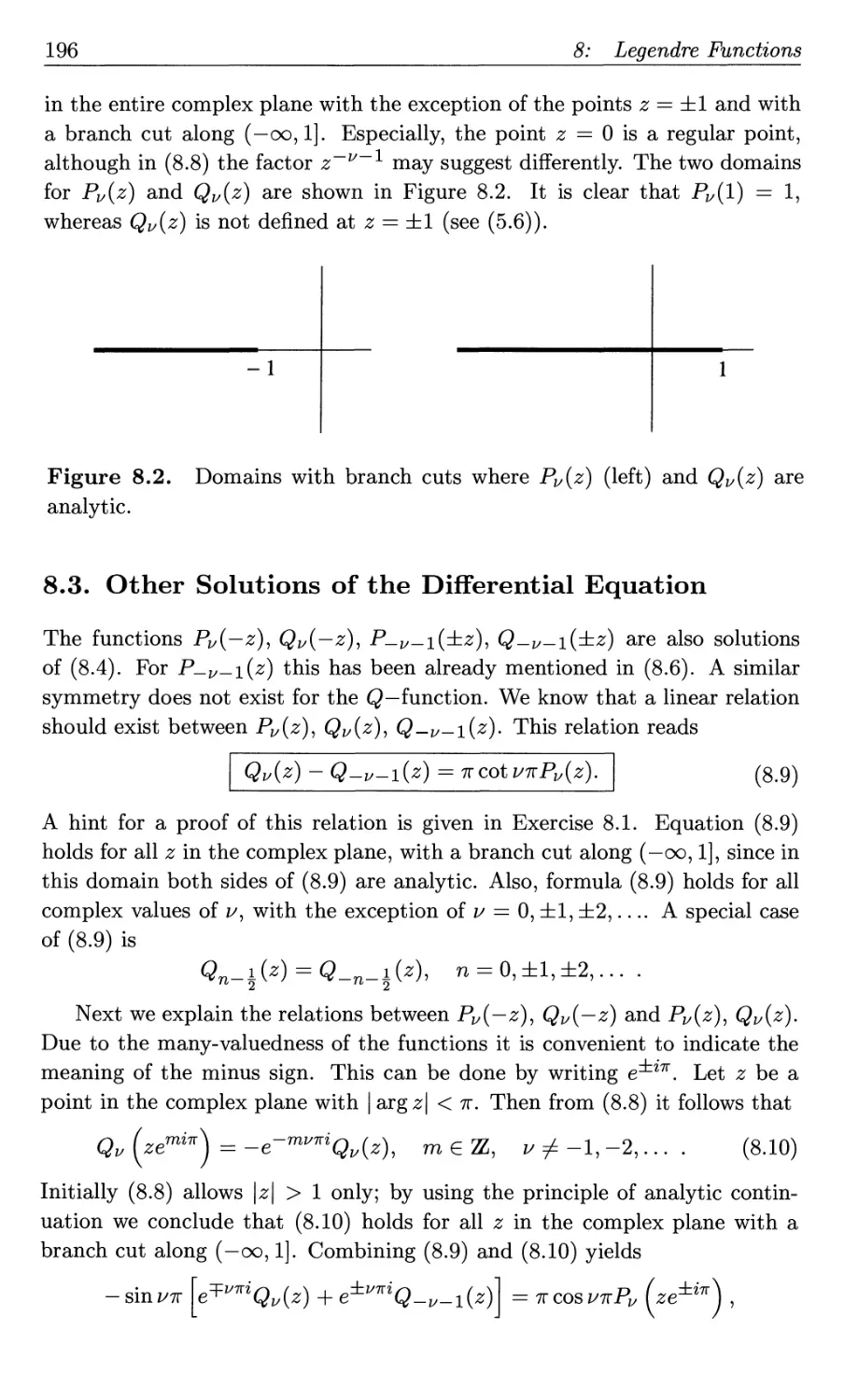
8	Legendre Functions
8.1.	The Legendre Differential Equation, 194
8.2.	Ordinary Legendre Functions, 194
193
viii
CONTENTS
8.3.	Other Solutions of the Differential Equation, 196
8.4.	A Few More Series Expansions, 198
8.5.	The function Qn(z), 200
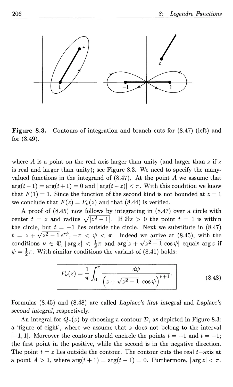
8.6.	Integral Representations, 202
8.7.	Associated Legendre Functions, 209
8.8.	Remarks and Comments for Further Reading, 213
8.9.	Exercises and Further Examples, 214
9	Bessel Functions	219
9.1.	Introduction, 219
9.2.	Integral Representations, 220
9.3.	Cylinder Functions, 223
9.4.	Further Properties, 227
9.5.	Modified Bessel Functions, 232
9.6.	Integral Representations for the I- and ^-Functions, 234
9.7.	Asymptotic Expansions, 238
9.8.	Zeros of Bessel Functions, 241
9.9.	Orthogonality Relations, Fourier-Bessel Series, 244
9.10.	Remarks and Comments for Further Reading, 247
9.11.	Exercises and Further Examples, 247
10	Separating the Wave Equation	257
10.1.	General Transformations, 258
10.2.	Special Coordinate Systems, 259
10.2.1.	Cylindrical Coordinates, 259
10.2.2.	Spherical Coordinates, 261
10.2.3.	Elliptic Cylinder Coordinates, 263
10.2.4.	Parabolic Cylinder Coordinates, 264
10.2.5.	Oblate Spheroidal Coordinates, 266
10.3.	Boundary Value Problems, 268
10.3.1.	Heat Conduction in a Cylinder, 268
10.3.2.	Diffraction of a Plane Wave Due to a Sphere, 270
10.4.	Remarks and Comments for Further Reading, 271
10.5.	Exercises and Further Examples, 272
11	Special Statistical Distribution Functions	275
11.1.	Error Functions, 275
11.1.1.	The Error Function and Asymptotic Expansions, 276
11.2.	Incomplete Gamma Functions, 277
11.2.1.	Series Expansions, 279
11.2.2.	Continued Fraction for Г(а, z), 280
11.2.3.	Contour Integral for the Incomplete Gamma Functions, 282
11.2.4.	Uniform Asymptotic Expansions, 283
CONTENTS	ix
11.2.5.	Numerical Aspects, 286
11.3.	Incomplete Beta Functions, 288
11.3.1.	Recurrence Relations, 289
11.3.2.	Contour Integral for the Incomplete Beta Function, 290
11.3.3.	Asymptotic Expansions, 291
11.3.4.	Numerical Aspects, 297
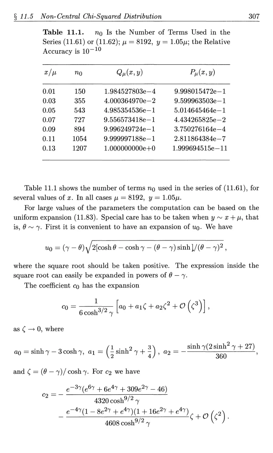
11.4.	Non-Central Chi-Squared Distribution, 298
11.4.1.	A Few More Integral Representations, 300
11.4.2.	Asymptotic Expansion; m Fixed, j Large, 302
11.4.3.	Asymptotic Expansion; j Large, m Arbitrary, 303
11.4.4.	Numerical Aspects, 305
11.5.	An Incomplete Bessel Function, 308
11.6.	Remarks and Comments for Further Reading, 309
11.7.	Exercises and Further Examples, 310
12	Elliptic Integrals and Elliptic Functions
12.1.	Complete Integrals of the First and Second Kind, 315
12.1.1.	The Simple Pendulum, 316
12.1.2.	Arithmetic Geometric Mean, 318
12.2.	Incomplete Elliptic Integrals, 321
12.3.	Elliptic Functions and Theta Functions, 322
12.3.1.	Elliptic Functions, 323
12.3.2.	Theta Functions, 324
12.4.	Numerical Aspects, 328
12.5.	Remarks and Comments for Further Reading, 329
12.6.	Exercises and Further Examples, 330
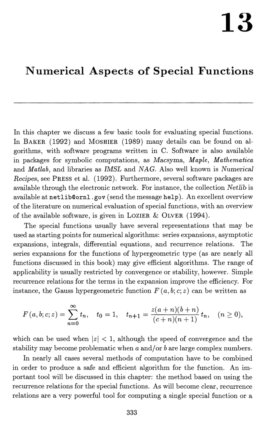
13	Numerical Aspects of Special Functions	333
13.1.	A Simple Recurrence Relation, 334
13.2.	Introduction to the General Theory, 335
13.3.	Examples, 338
13.4.	Miller’s Algorithm, 343
13.5.	How to Compute a Continued Fraction, 347
Bibliography	349
Notations and Symbols	361
Index
365

PREFACE
This book gives an introduction to the classical well-known special functions which
play a role in mathematical physics, especially in boundary value problems. Usually
we call a function “special” when the function, just as the logarithm, the exponential
and trigonometric functions (the elementary transcendental functions), belongs to
the toolbox of the applied mathematician, the physicist or engineer. Usually there is
a particular notation, and a number of properties of the function are known. This
branch of mathematics has a respectable history with great names such as Gauss,
Euler, Fourier, Legendre, Bessel and Riemann. They all have spent much time on
this subject. A great part of their work was inspired by physics and the resulting dif-
ferential equations. About 70 years ago these activities culminated in the standard
work A Course of Modern Analysis by Whittaker and Watson, which has had great
influence and is still important.
This book has been written with students of mathematics, physics and engineer-
ing in mind, and also researchers in these areas who meet special functions in their
work, and for whom the results are too scattered in the general literature. Calculus
and complex function theory are the basis for all this: integrals, series, residue cal-
culus, contour integration in the complex plane, and so on.
The selection of topics is based on my own preferences, and of course, on what
in general is needed for working with special functions in applied mathematics,
physics and engineering. This book gives more than a selection of formulas. In the
many exercises hints for solutions are often given. In order to keep the book to a
modest size, no attention is paid to special functions which are solutions of periodic
differential equations such as Mathieu and Lame functions; these functions are only
mentioned when separating the wave equation. The current interest in ^-hypergeo-
metric functions would justify an extensive treatment of this topic. It falls outside
the scope of the present work, but a short introduction is given nevertheless.
xi
xii
PREFACE
Today students and researchers have computers with formula processors at their
disposal. For instance, Matlab and Mathematica are powerful packages, with pos-
sibilities of computing and manipulating special functions. It is very useful to ex-
ploit this software, but often extra analysis and knowledge of special functions are
needed to obtain optimal results.
At several occasions in the book I have paid attention to the asymptotic and nu-
merical aspects of special functions. When this becomes too specialistic in nature
the references to recent literature are given. A separate chapter discusses the stabili-
ty aspects of recurrence relations for several special functions are discussed. It is
explained that a given recursion cannot always be used for computations. Much of
this information is available in the literature, but it is difficult for beginners to lo-
cate.
Part of the material for this book is collected from well-known books, such as
from Hochstadt, Lebedev, Olver, Rainville, Szego and Whittaker & Watson.
In addition to these I have used Dutch university lecture notes, in particular those by
Prof. H.A. Lauwerier (University of Amsterdam) and Prof J. Boersma (Technical
University Eindhoven).
The enriching and supporting comments of Dick Askey, Johannes Boersma, Tom
Koomwinder, Adri Olde Daalhuis, Frank Olver, and Richard Paris on earlier ver-
sions of the manuscript are much appreciated. When there are still errors in the
many formulas I have myself to blame. But I hope that the extreme standpoint of
Dick Askey, who once advised me: never trust a formula from a book or table; it
only gives you an idea how the exact result looks like, is not applicable to the set of
formulas in this book. However, this is a useful warning.
Nico M. Темме
Amsterdam, The Netherlands
SPECIAL FUNCTIONS
AN INTRODUCTION
TO THE CLASSICAL
FUNCTIONS OF
MATHEMATICAL PHYSICS

1
Bernoulli, Euler and Stirling Numbers
A well-known result from calculus is the alternating series
2n — 1 ’
which can be used for the computation of the number тг, although the series
converges very slowly. However, summing the first 50 000 terms gives the
remarkable result
50 ooo
2 E
71=1
(-I)""1
2n — 1
= 1.5707 86326 79489 76192 31321 19163 97520 52098 58331 46876.
Using a criterion for convergence of this type of series, we may conclude that
this answer is correct to only six significant digits. When you compare the
answer on the right-hand side with a 50-d approximation of ^7r, you will reach
the surprising conclusion that nearly all digits in the above approximation are
correct, except for those underlined. In this chapter this intriguing aspect will
be explained with the help of simple properties of Euler numbers and Boole’s
summation method. Another example is the series
oo
ln2 = E
71=1
(-l)n+1
n
You may try to sum the first 50 000 terms with high precision, and compare
the answer with an accurate approximation of In 2.
In this chapter we discuss basic properties of the Bernoulli, Euler and
Stirling numbers, with applications to the summation methods of Euler and
Boole. These methods are based on the polynomials of Euler and Bernoulli.
1
2
1: Bernoulli, Euler and Stirling Numbers
Such topics are extensively discussed in classical books on the calculus of
differences, the subject that played a prominent part in numerical analysis.
A short introduction to difference equations is given §1.1.2.
Just as many other special numbers, polynomials and functions, the special
numbers and polynomials of this chapter can be introduced by generating
functions. Usually these are power series of the form
oo
F(x,t)= ^fn(x)tn,
n=Q
where each fn is independent of t. The radius of convergence with respect
to (complex) values of t may be finite or infinite. We say that F(x, t) is the
function which the sequence {fn} generates, and F is called the generating
function. Often, F and the coefficients fn are analytic functions in a certain
domain.
1.1. Bernoulli Numbers and Polynomials
The Bernoulli numbers are named after Jakob Bernoulli, who mentioned the
numbers in his posthumous Ars conjectandi of 1713; see Bernoulli (1713).
He discussed summae potestatum, sums of equal powers of the first n integers.
For instance, we know from elementary calculus that
71 — 1
V i = -n(n - 1) = -n2 - -n,
2	2	2
i=1
71—1
E-2	1 3	12.1
I = -П-----П + -n,
3	2	6 ’
7=1
71—1
У г3 =	_ 1 n3 + 1 n2
=	4	2	4	’
7=1
71—1
E-4	1-5	1 4 . 1 3	1
г = -n-----n + -n-------n,
5	2	3	30 ’
7=1
and so on. Bernoulli was, in particular, interested in the numbers multiplying
the linear terms n at the right-hand sides: —. Euler
(1755) called them Bernoulli numbers By B2, B3, B4,.... As we know from
the general result
§ 1.1 Bernoulli Numbers and Polynomials
they show up in other terms also; see Exercise 1.3.
The Bernoulli numbers occur in practically every field of mathematics,
in particular, in combinatorial theory, finite difference calculus, numerical
analysis, analytical number theory, and probability theory. We discuss their
role in the summation formula of Euler.
1.1.1. Definitions and Properties
Instead of introducing the Bernoulli numbers Bn as above, we use a generating
function for their definition:
(1-1)
Because the function
is even (prove it!), all Bernoulli numbers with odd index > 3 vanish:
B2n+i =0, n = 1,2,3,... .
The first nonvanishing numbers are
B8 = -l, B10 = A, =	= ви = ^
30	66	2730	6	510
The Bernoulli polynomials are defined by the generating function
= ez - 1	n!	11 n=0	(1-2)
The first few polynomials are
В0(ж) = 1,
Bi (ж) = x —
B2(x) = x2 - x + j,
В3(я:) = ж3 - |m2 + ^x,
B4(x) = x4 — 2x3 + я:2-——.
4
1: Bernoulli, Euler and Stirling Numbers
A further step yields the generalized Bernoulli polynomials:
(1-3)
where cr is any complex number. By taking x = 0 we obtain the generalized
Bernoulli numbers B^ = B^\o), which are polynomials of degree n of the
complex variable a.
We now give some relations which easily follow from the definitions through
the generating functions.
1
Bn(x) dx = 0, n = 1,2,3,... .	(1.4)
= £ Q ВкхП~к> B^x+^ = i(k) BkW~k-
fc=0 ' '	k=0 ' '
Bn(0) - Bn, Bn(l) = (-l)nBn.	(1.6)
Bn(l -x) = (-l)nBn(xl Bn(-x) = (-l)n [BnCr) + n/-1] . (1.7)
Bn(i) = - (1 - 21-n) Bn.	(1.8)
^-Bn(x) = nBn_i(i), Bn(x + 1) - Bn(x) = пхп~г.	(1.9)
ax
n
k=0
The proof of (1.4) follows for example by integrating the left-hand side of (1.2)
with respect to x. The properties (1.5)-(1.10) all hold for n = 0,1,2,... .
Property (1.10) gives for x = 0 the identity for the Bernoulli numbers:
(1-10)
(1-11)
with which the numbers can be generated by means of a simple recursion.
Symbolic manipulation on the computer may be very useful here. Numerical
computations with finite precision will yield very inaccurate results, due to
instability of (1.11).
In Exercise 1.1c you can prove that
, ~2n+l
ала,
71=0
§7.7 Bernoulli Numbers and Polynomials
5
where the relation between the tangent numbers Tn and the Bernoulli numbers
Bn is defined by
Tn is an integer with Tin = 0, n > 0. This follows from differentiating tan г:
all even derivatives at z = 0 vanish and the odd derivatives are integers. The
same holds for the coefficients of the MacLaurin expansion. We have
7b = 1, Ti = -1, T3 = 2, T5 = -16, T7 = 272, T9 =—7936.
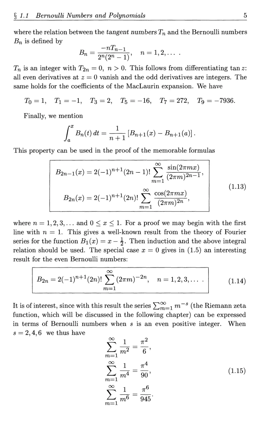
Finally, we mention
dt =	1 (ж) — Bn+1 (a)].
n + 1
This property can be used in the proof of the memorable formulas
R M-<)(	niV sin(27rma:)
B2n-i(x) - 2(—1)	(2n - 1)! 2^ (2тгт)2"-1’
m=l '
(1-13)
where n = 1,2,3,... and 0 < x < 1. For a proof we may begin with the first
line with n = 1. This gives a well-known result from the theory of Fourier
series for the function B± (ж) = x — -J,. Then induction and the above integral
relation should be used. The special case x = 0 gives in (1.5) an interesting
result for the even Bernoulli numbers:
в2п = 2(-1)”+1(2п)! У2 (2тгт)-2п, n = 1,2,3,... .
m=l
(1-14)
It is of interest, since with this result the series Ylm=l m~S (l^e Rlem&nn
function, which will be discussed in the following chapter) can be expressed
in terms of Bernoulli numbers when s is an even positive integer. When
s = 2,4,6 we thus have
OO-i	9
El _ r
m2 6
m=l
°°	i	4
El	7Г4	/
90’	(L15)
m=l
oo л	6
1	7Г°
m6 945
m=l
6
1: Bernoulli, Euler and Stirling Numbers
Figure 1.1. The functions Bn(x), n = 1 and n = 3.
For odd s—values a similar relation is never found.
The Fourier series for Bernoulli polynomials in (1.13) can be defined for
all real values of x. Outside the interval [0,1] the series do not represent
polynomials, of course, but periodic functions of x. These periodic functions
are very important, and we introduce a special notation Bn(x) by defining for
n = 0,l,2,...
Bn(x) = Bn(x), 0 < x < 1,
and
Bn(x +1) = Bn(x), x e IB.	(1.16)
The functions Bn(x) have continuous derivatives up to order n — 1. This easily
follows from the earlier properties, for instance from (1.13). They become
smoother as n increases. As will follow from §1.1.3, the periodic functions
Bn(x) play an important part in Euler’s summation formula.
In Figures 1.1 and 1.2 we show the first four functions Bn(x), n = 1,2,3,4.
1.1.2. A Simple Difference Equation
One of the results of the previous subsection (see (1.9)) reads
f(x + 1) - f(x) = nxn~ l,
a difference equation with solution f(x) = Bn(x). It follows that the Bernoulli
polynomials can be used to construct a solution of the difference equation
f(x+ 1) - f(x) = Pn(x),
where Рп(ж) is a polynomial. When Pn(x) =	we can write the
general solution in the form
л*) = 52 v+iBk+i^+
k=Q
§7.7 Bernoulli Numbers and Polynomials
7
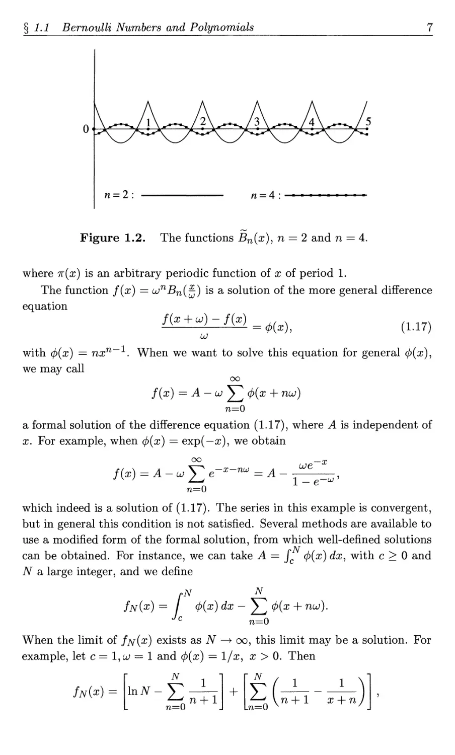
Figure 1.2. The functions Bn(x), n = 2 and n = 4.
where тг(ж) is an arbitrary periodic function of x of period 1.
The function f(x) = cjnBn(~) is a solution of the more general difference
equation
=	(1.17)
(jj
with ф(х) = nir72-1. When we want to solve this equation for general </>(#),
we may call
oo
f(x) — A — ш ф(х + ncA)
n=0
a formal solution of the difference equation (1.17), where A is independent of
x. For example, when ф(х) = exp(—ж), we obtain
OO	__
71=0
which indeed is a solution of (1.17). The series in this example is convergent,
but in general this condition is not satisfied. Several methods are available to
use a modified form of the formal solution, from which well-defined solutions
can be obtained. For instance, we can take A = ф(х) dx, with c > 0 and
N a large integer, and we define
p7V	N
/n(x) = / ф(х) dx — 57 <KX + пш)-
Jc	n=0
When the limit of /уу(ж) exists as N oo, this limit may be a solution. For
example, let c = l,o> = 1 and ф(х) = 1/ж, x > 0. Then
Г N 1 1 Г N / 1	1 \1
fN(x)= lnJV-£ — + 52 (-— --—) ,
n + 1	\ n + 1 x + n J
71=0 J L7l=0	J
8
1: Bernoulli, Euler and Stirling Numbers
and each quantity between square brackets tends to a finite limit, as N —> oo;
see the next subsection, Example 1.2. From Chapter 3, formula (3.10), we
infer that the function /уу(ж) tends to a special function, the logarithmic
derivative of the gamma function ф(х), which indeed satisfies the difference
equation f(x + 1) — /(ж) = 1/ж.
In a second method the function ф(х) in (1.17) is replaced with ф{х,р}
that satisfies Нт^_^о Ф(х,^) = ф(х\ For instance, we can take
ф(х,/л) = (^(.т)е”м'г, /z > 0.
Let c be a number independent of x, and assume that
ф(х, /z) dx,
oo
and ^2 Ф(х + пса, /Ф)
п-0
both converge. Then we define as the solution of (1.17) the function f(x) =
lim^o/(z,/z), where
/(ж,м)) =
лОО	°°^
/ ф(х, dx — У2 Ф(х + пса, ji)
Jc	n=0
(1.18)
provided that this limit exists. It is shown in the classical literature (for
instance, in Norlund (1924)) that this /(ж) indeed satisfies (1.17), and that
this solution is independent of the particular choice of ф(х,ц). Other choices
are also possible. It is easily verified that for (1.17) with c = 1, ca = 1, ф(х) = 1,
the function f(x, /a) is given by

and that lim^—>o JC7^/2) = x —	a Bernoulli polynomial.
Example 1.1. Consider the difference equation
f(x + 1) - f(x) — nxn ге 1ЛХ, Ц > 0, x > 0,
§7.7 Bernoulli Numbers and Polynomials
9
which for = 0 reduces to the difference equation of the Bernoulli polynomi-
als. We try to find /(^,/z) of (1.18). Take c = 0, then
	POO	00 /0>Az) = / nt^e-^dt- V n{x + m)n~1e-^x+m^ J°	m=0 ^n—1	POO	00 Lm= 1 ny m(m — nY. m=n	v	7
In this derivation we have used the generating function (1.2). When > 0,
we have /(ir,/z) = Вп(ж), which again shows that Bn(x) satisfies the second
relation in (1.9).
1.1.3. Euler’s Summation Formula
A striking application of Bernoulli numbers and polynomials is Euler’s sum-
mation formula, that links a finite or infinite series and an integral. This
formula yields an efficient method for evaluating some slowly convergent se-
ries by means of an integral. Turning it round, by this method also an integral
can be approximated by discretization, which leads to the trapezoidal rule.
In Euler (1732) the proof of the formula can be found.
Theorem 1.1. Let the function f: [0,1] —> (D have к continuous derivatives
(к = 0,1,2,...). Then for к > 1
/(1) = [ /(я) dx + ^	(0)] + Rk,
J°	i=l г'
with
Rk = —^,fc+1- f P\x)Bk(x) dx.
Proof. The proof runs with induction with respect to к. For к = 1 the
claim is true, which follows from integrating by parts. Then the property
Bm(x) =
is used to go from к = т>]Ло к = mil.	g
10
1: Bernoulli, Euler and Stirling Numbers
With similar conditions for f on the interval [j — 1,J] we have
k
/(j) = f dx + £	-1)1 + Rk,
Jj-1	i=1
with
Rk =	d^
where Вд.(ж) is the function introduced in (1.16).
The next step joins a number of these intervals:
£/G) = Г ^х + £^	+Rk,
i=l Jo	i=l
with
Rk =	[nfW^Bk^dx.
Jo
For к = 1 this gives the formula
/(l) + /(2) + ..- + /(n)= / /(x)dx + |[/(n)-/(0)]+ / Bi(x)f'(x)dx,
Jo	2	Jo
with Bi (ж) a sawtooth function on [0,n]. This is Euler’s summation formula
in its simplest form. The formula expresses a connection between the sum
of the first n terms of a series and the integral of the corresponding function
over the interval [0, n\.
Example 1.2. Take
and replace in the above formula n with n — 1. Then we obtain the classical
example
i+i+i+i+..-+i=i»»+i+i- РЧмпА,.
2	3	4	n	2n 2 Jo 1V 7(l + x)2
The integral is convergent when n —> oo. From this we infer that
7 = lim fl + - + - + - + -- - + -— In7?)
n—>oo \	2	3	4	n /
exists as well. The limit 7 = 0.5772 15664 90153... is called Euler’s constant.
From this example also follows that
1 f°° Я I , iz 1 Г
,2 ‘
§7.7 Bernoulli Numbers and Polynomials
11
Since
Вд.(О) = 0, к = 3,5,7,...
all terms with odd index can be deleted in the summation formula, except the
term with index i = 1. And at both sides we can add the term /(0). Then
the result is
Theorem 1.2. Let the function f: [0, n] —> ф have (2k + 1) continuous
derivatives (k > 0, n > 1). Then
n	fn
E	dX + 9	+ Я°)]
1^0
k	(i-19)
Rk = (2ГП)! /о Nk+1^x^+^ dx-
The summation formula is usually presented in this form, and is connected
with the trapezoidal rule (Exercise 1.7).
Example 1.3. We take f(x) = x2. Since f^(x) = 0 for each x, the
contribution of the remainder in (1.19) is zero when к > 1. For к = 1
(1.19) then reads
E*2 = / x2dx+ in2 + ^B2[f'(n) - /'(0)] = |n3 + |n2 + ±n.
i=0 J°
An alternative summation formula for infinite series arises through the
intermediate form
E = [ № dx +1 t/(n) + A™)]
dm
к	(i-20)
+E^[/(2i’1)w-/(2i"1)H+^
z9. 1 n, Г f2k+1\x)B2k+1(x)dx.
' JJ- Jm
12
1: Bernoulli, Euler and Stirling Numbers
In this formula we replace n with oo, which is allowed when the infinite series
and the indefinite integrals
°o	roo	ЛОО	~
£/(«).	/ f(x)dx, /	f(2k+1\x)B2k+1(x)dx
i=m	Jm	Jm
exist. In addition we assume that f and the derivatives occurring in the
formula tend to zero when their arguments tend to infinity. The result is
°o	к Fl
f(x) dx + l/(m) - £	+ Rk, (1.21)
This form of Euler’s summation formula can be fruitfully applied in summing
infinite series. It is important to have information on the remainder R^. It
is not always necessary to know the integral in exactly. Also, it is not
necessary to know whether
lim Rfc — 0.
k-^oo
In many cases this condition is not fulfilled, or the limit does not even exist.
An estimate of the remainder can be obtained through the following theorem.
Theorem 1.3. Let f and. all its derivatives be defined on the interval [0, oo)
on which they should be monotonic and tend to zero when x oo. Then R^
of (1.19) satisfies
Rk =	[/(2fc+1,W - /(2fc+1)(0)] , with 0 < 0k < 1.
Proof. First we remark that
/(fc)(a:), /(/c+1)(z), k = 0,1,2,...
have fixed and different signs on [0, oo). Let f(x) > 0, x > 0. Then it is easily
verified (consider the graph of the sine function) that the sign of
/ sin(27r?7iir)/(ir) dx, 777 = 1,2,3,...
JO
is also positive. From (1.13) and (1-16) then follows that the sign of
[ В2п+1(ж) f (x) dx,	77 = 1,2,3,... , 777 = 0,1,2,...
Jo
§ 1.1 Bernoulli Numbers and Polynomials
13
equals the sign of (—l)n+1. From this we also conclude that the remainder
Rk of (1.19) have different signs for subsequent values of k. This implies that
Rk and (Rfc — Rk-\-i) have the same sign and hence that
\Rk\ < l-Rfc - .Rfc+il-
From (1.19) it follows, however, that
Rt - R^ = -/(и+1,(»)] 
This is exactly the ‘first neglected term’ in Euler’s summation formula. The
sign of this term equals the sign of R^ and the absolute value of this term at
least equals the absolute value of R^.	g
A similar result holds for formula (1.21). In this case we have
Rk =	with O<0*<1.	(1.22)
\ZiK -f- ZjI
The theorem says that, with the conditions on /, the error in taking in (1.21)
к terms of the series in the right-hand side is smaller than the first neglected
(k + 1)—th term. In practical problems one tries to find this (k + 1)—th term
that falls below the requested accuracy, and one sums the series on the right-
hand side of (1.21) as far as the th term. In other words, one may sum the
series until a particular term falls below the accuracy. This naive criterion,
which is very popular in summing infinite series, is fully legitimate here.
Example 1.4. Sum the series
oo л
ЕЙ
i=i1
with an error less than IO-9. First we compute
Vto = 1.19653198567-•• .
Z—/ 7o
2=1 1
Next we apply (1.21) with /(я:) — and m = 10. Namely, (1.21) should
not be used with the low value m = 1, but with one that makes R^ small
enough (for an acceptable value of k). Our f fulfills the conditions of Theorem
1.3. Verify that the third term in the series of the right-hand side of (1.21)
equals
———2520 x 10-8 = —- x 10-8 = -0.83 x 10~9.
42 6!	12
14
1: Bernoulli, Euler and Stirling Numbers
Hence, we apply (1.21) with к = 2, and we obtain
= 1.19653198567-••
dx i i
X3 + 2000 + 40000
1
12000000
= 1.20205690234,
with an error that is smaller than 0.83 x 10 9. The actual error is 0.82 x 10 9.
From this example we see that the error estimate can be very sharp. An-
other point is that Euler’s summation formula may produce a quite accurate
result, with almost no effort. To obtain the same accuracy, straightforward
numerical summation of the series requires about 22360 terms.
Not all series can be evaluated by Euler’s formula in this favorable way.
Although the class of series for which the formula is applicable is quite interest-
ing, Euler’s method has its limitations. Alternating series should be tackled
through Boole’s summation method, which is based on the Euler polynomials
(see §1.2.2).
Several other summation formulas have been invented to improve the con-
vergence of slowly convergent series. Each method has a favorite class of series
for which the method is extremely successful. Monotonicity and regularity of
the derivatives of the function f that generates the terms of the series always
is a good starting point.
To obtain information on how many terms one needs using (1.22) one may
use estimates of the Bernoulli numbers. Since the radius of convergence of
the series in (1.1) equals 2тг, one can use the rough estimate
= O [(2,)^] , as
IZ /и "I Z J •	L	J
This estimate can be refined by using the first series in (1.13). Since the series
assumes values between 1 and 2, we have (see also Exercise 1.2)
(2^ < (“1)”+1(2§! <2(2^p n = 1,2,3,... .	(1.23)
When also estimates of the derivatives of f are known, much information on
Rk of (1.22) may become available.
1.2. Euler Numbers and Polynomials
The Euler numbers have a less dominant place in mathematics than those
of Bernoulli, although the definitions are quite similar. Again definitions
§1.2 Euler Numbers and Polynomials
15
are based on generating functions. A short introduction is worthwhile, in
particular in connection with the summation of alternating series.
1.2.1. Definitions and Properties
The Euler numbers are introduced through the series:
cosh z e2z + 1 n\ '	2
71=0
The Euler numbers are integers, in contrast to the Bernoulli numbers. The
first few are
Eq = 1, E2 = -1, E4 = 5, Eq = -61, E% = 1385,
while those with odd index are zero:
^271+1=0, n = 0,1,2,... .
The Euler polynomials are defined by
with as relation between numbers and polynomials
En = 2nEn(i).
(1-24)
The first few Euler polynomials are:
E0(z) = 1,
Ei(x) = x-
£^2 (^) = X2 — Ж,
Е3(я;) = x3 - |я;2 + i,
E4 (ж) = ж4 — 2ж3 + х.
Further generalizations give:
16
1: Bernoulli, Euler and Stirling Numbers
Figure 1.3. The functions En(x\ n = 1 and n = 3.
Note that the system of generalizations is not as clear as in the Bernoulli case.
However, the numbers of Bernoulli and Euler do share many properties, such
as for example the analogs of the Fourier series in (1.13)
r? M A(	nlV cos[(2m + 1)7T®]
E^x) = 4(—1)	(2n - 1)!	[(2m + 1)7r]2„
m=Q LV 1	/ J
which hold for n = 1,2,3,... and x € [0,1]. We see that E'^x) = 0 for x =
and with (1.24) it follows that
|^2nM| < |-К2п(|)|=2“2П£;2п, n= 1,2,3,... .
We define as in (1.16) the periodic Euler functions En(x) by writing
En(x) = En(x), 0 < x < 1,
and
En(x + 1) = En(x), x e IR.
The function En(x) has n — 1 continuous derivatives.
In Figures 1.3 and 1.4 we show the first four functions En(x), n = 1,2,3,4.
§ 1.2 Euler Numbers and Polynomials
17
Figure 1.4. The functions En(x), n = 2 and n = 4.
1.2.2. Boole’s Summation Formula
This method is given in BOOLE (1860), but Euler knew the method also.
The analog of Theorem 1.1 is given in the form:
Theorem 1.4. Let the function ft [0,1] —> (D have к continuous derivatives,
(к = 0,1,2,...). Then, for к > 1,
with
k—1
/(1) = | E [/(i)(1) + /(i)(0)] + Rk,
i=Q
Rk = 9/. 1 n, [ f('k\x)Ek_1{x)dx.
~ -U- Jo
Proof. Use induction with respect to k. For к = 1 the claim is obvious, and
for the induction step we can use (n + l)2£n(ir) = ^+1(ж).	В
The theory for Boole’s summation formula is developed in the same way as
in Euler’s case. The striking difference is that in the Boole version of Theorem
1.2 the left-hand side of (1.19) now shows an alternating series. Moreover an
integral of f is missing. We write a final result similar to (1.21), with an extra
parameter h, which enables a shift in the argument of f. In this way we obtain
Euler numbers in Boole’s summation formula (taking h = ^), instead of the
quantities En(l). The proof of the following theorem is left to the reader.
Theorem 1.5. Let f: [m, oo) —> IR, have к continuous derivatives, (k =
0,1,2,...). Assume that f^(x) —> 0 as x —> oo for each i = 0,1,..., k. Let
18
1: Bernoulli, Euler and Stirling Numbers
h e [0,1]. Then
oo	к 1 у—, / 7 \
+	+ jRfc (i,25)
i=m	г=0
with
2 Jm
Applying this with h = ^, f(x) = 1/x we obtain after some algebra
2y (~1)fc	flyV E2k
(2fc + 1)	1	(2n)2*+x	’
k=n	k=Q
where, on account of earlier given estimates of the Euler polynomials and
evaluation of the derivatives of /, it easily follows that
This result holds for each positive n and N. With n = 50000 and N > 1
we obtain an explanation of the intriguing phenomenon we observed at the
beginning of this chapter. The error equals
10-5 - 10-15 + 5 x 10-25 - 61 x IO-35 + 1385 x IO-45 ....
Adding this to the computed 50-d approximation of jtt, we will see that the
result indeed is correct to an accuracy of 50 digits. The striking point is that
the digits in the asymptotic correction represent integers (the Euler numbers).
That is why the indicated effect is clearly visible. In this example we can also
take other values of n = 0.5 x 10ш. Only sufficiently large values of m show
the effect appropriately.
1.3. Stirling Numbers
James Stirling introduced in the beginning of Methodus Differentialis (Stir-
ling (1730)) certain coefficients that became famous and now bear his name.
We define the Stirling numbers of the first and second kind, respectively de-
noted by S<m) and , as the coefficients in the expansions
§ 1.3 Stirling Numbers
19
x(x - 1) • • • (ж - n + 1) = S^xm,
m=Q
xn = У2 &n^x(x - 1) • • • (x - m + 1),
m=0
(1-26)
(1-27)
where we give the left-hand side of (1.26) the value 1 if n = 0; similarly the
factors on the right-hand side of (1.27) have the value 1 if m = 0. This gives
the ‘boundary values’
= 1, n > 0, and = e£0) = 0, n > 1.
Furthermore it is convenient to agree on S^ =	= 0 if m > n.
The Stirling numbers are integer numbers; apart from the above mentioned
zero values, the numbers of the second kind are positive, and those of the first
kind have the sign of (—l)n+m. We have the following recurrence relations
- nS^,	(1.28)
= тб(™} + e^m-1).	(1.29)
A proof of (1.28) follows from
x(x -1) • • • (® - n) = 57 ^n+ixm = (x - n) 57 &т)хт
m=0	m=Q
and comparing corresponding powers of x. A similar proof can be used for
(1.29).
The Stirling numbers of the first and second kind satisfy an interesting
orthogonality relation. Substitution of (1.26) into (1.27) yields
n	m	n n
= E s!™1 E = E E
m=0	k=Q	k=Q m=k
Comparison of corresponding powers of x gives
V fi(w) a(*) _ c
/	— °k,n-
m=k
20
1: Bernoulli, Euler and Stirling Numbers
In a similar way one proves
£ eSM”’ =
m=k
These properties lead to a general inversion which can be applied to sequences
of numbers. Let
be two number sequences, then we have the Stirling inversion
n	n
an = ^T S^bk <=> bn = У2
k=0	fc=0
with as alternative for infinite sequences (the formal) inversion
oo	oo
an = 52 skn>>bk bn = 52
k=n	k=n
For example, it is not difficult to verify from (1.26) that
n
52 (-i)n-m^m) = ni.
Then from the inversion relation we obtain
= 1.
m=0
Several other generating functions are available for Stirling numbers. We
have	№ + r =	(1.30) ml	nl n=m (1.3!) ml	t—**	nl n=m
When (1.31) is proved, one can use (with some imagination) the inversion
formula for infinite sequences to verify (1.30). To do so, write in (1.31) z =
ex — 1, x = ln(z + 1).
We sketch the proof of (1.31). Call Fm(x) the (unknown) left-hand side
of (1.31). Then we know that F$(x) = 1 and furthermore (since = 1)
F'i(rr) = ex — 1. Using the recurrence relation in (1.29) we arrive at
, Fm^x) ~ m^rn(^) + Fm—
dx
§ 1.4 Remarks and Comments for Further Reading
21
Considering the condition at x = 0, we obtain a solution of this recursion,
which is indeed in the form of the left-hand side of (1.31).
A closed expression for the numbers of the second kind reads
1 m	/ \
’k=Q	V 7
A proof follows simply by expanding the left-hand side of (1.31) by Newton’s
binomial formula and by comparing the power series of the resulting expo-
nential functions on the right-hand side of (1.31). A similar closed expression
for the numbers of the first kind is not known.
The Stirling numbers play an important role in difference calculus, com-
binatorics, and probability theory. An example from combinatorics is:
is the number of ways of partitioning a set of n elements into m non-empty
subsets. We find for m = 2, n = 4 the value 64 —	7,	since
{a, 6, c, d}	= {a} U {b, c, d}	=	{b} U {a, c, d}
= {c} U {a, 6, d}	=	{d} U {a, 6, c}
= {a, b} U {c, d}	=	{a, c} U {6, d}	=	{a, d} U {6, c}.
1.4.	Remarks and Comments for Further Reading
1.1.	An extensive bibliography on Bernoulli numbers (and the other quan-
tities treated in this chapter) is given in Dilcher et al. (1991).
1.2.	Further information on classical difference calculus can be found in Jor-
dan (1947), Norlund (1924), and Milne-Thomson (1933), where also
the summation methods of Euler and Boole are considered. Euler’s method
can be found in Knopp (1946).
1.3.	Euler’s name is connected with another method for applying transfor-
mations on series: the Euler transformation, which should not be confused
with the summation methods discussed earlier in this chapter. Euler’s trans-
formation is a powerful method to improve the convergence of series, in par-
ticular of slowly convergent alternating series. Let the given convergent series
beS = SXo(-1)”«n- Then
Д”а0
°	2^ 2n+1 ’
71=0
where Д is the forward difference operator defined by
Дад. = а^ — Ufc-i-i, Д (Lfe =	— Дад._|_1 = а^ — 2пд._|_^ + u^-i-2?
22
1: Bernoulli, Euler and Stirling Numbers
and, in general
Л“ао = Ё(-1)-‘ (“К
k=Q	v 7
For example, when an = l/(n + 1), then Anao = l/(n + 1), which gives
In 2 = V -___~ = V_______________
n + 1 (n + 1) 2n+1 ’
n=0	n=Q 4
a startling improvement with respect to convergence; see Knopp (1946).
1.4.	Yet another method for transforming finite and infinite sums into inte-
grals, based on residue calculus, is the Abel-Plana formula. See Chapter 8 in
Olver (1974), where also the connection with Euler’s summation method is
described.
1.5.	The remarkable phenomenon observed in summing the series in the
introduction of this chapter, and in Exercise 1.9, which is explained in §1.2.2
with the help of Boole’s summation formula, seems to be discussed for the
first time in Borwein, Borwein & Dilcher (1989).
1.6.	More information on Stirling numbers can be found in Jordan (1947,
Ch. 4) and Comtet (1974). See also Chapter 24 of Abramowitz & Stegun
(1964), for tables and more formulas. Knuth (1992) discusses the notation
and other interesting historical aspects. Asymptotic expansions have been
given by Moser & Wyman (1958a, 1958b). They consider several overlap-
ping domains in the n, m-plane with n > m. See also Dingle (1973, p. 199).
A more recent result is given in Темме (1993), where approximations are
given for Stirling numbers of both kinds, with n large, uniformly with respect
to m, 0 < m < n.
1.5.	Exercises and Further Examples
1.1.	A number of Taylor series for elementary functions can be derived from
the generating functions for the Bernoulli and Euler numbers. A few impor-
tant series follow from the following results.
a.	Show that the function f(z) introduced in connection with (1.1) can be
written in the form
f(z) = — z coth — z - 1.
J v 7	2	2
b.	Determine via (1.1) the Taylor series of the function г coth г.
c.	Show that tanh z = 2 coth 2г — coth z and determine the Taylor series of
the function tanh г.
d.	Show that 2/ sinh 2г = coth г — tanh г and determine the Taylor series of
the function г/ sinh г.
§1.5 Exercises and Further Examples
23
e.	Integrate cothz — 1/z and determine the Taylor series of In [sinh (г)/г].
f.	Determine the Taylor series of the functions In cosh г and ln[tanh(z)/z].
g.	Determine with these results corresponding expansions for trigonometric
functions.
1.2.	Evaluate as for (1.14), the following series:
(-l)m+l _ (-1)п+1(2тг)2п (1 - 21—2n) B2n
m?n	2 (2n)!	’
m=l	x
1	_ (—1)п+1(2тг)2п (1 — 2-2”) B2n
2-(2m+l)2"“	2(2n)!
For the first formula you will need the result
B„(|) = - (1 - 21-”) Bn, n = 0,l,2,....
With these results improve the inequalities in (1.23) to obtain the rather
accurate estimates (at least, when n is large)
2	1	< Z_nn+1 <	2	1
(27r)2n 1 - 2~2ri	1	}	(2п)!	(2тг)2п 1 - 21-2n ’
n = 1,2,3,... .
1.3.	Show that from both equations in (1.9) follows:
ГУ	1	r^+1
/ Bp(t)dt = —— [Bp+1(y) - Bp+i(o:)] ,	/ Bp(t)dt = xp,
Jx	P + 1	Jx
p = 0,1,2,..., and that, hence, for n = 1,2,3,...
1	1 /»i+l	pTl	1
= 5Z / BpW^t=	=	।	[^p+i(n)- ^p+i] •
г=0 i=0Ji	70	P±
Expand in powers of n:
This formula holds for p = 0 when we put 0° = 1.
1.4.	The series
oo	2
El _ 7Г2
г2 6
24
1: Bernoulli, Euler and Stirling Numbers
can be computed with Euler’s formula. Determine a value of m that satisfies
|^/(5)(m)| < IO-10, with f(x) =
1.5.	Compute Euler’s constant
7 = lim n —>OO	1+1 +1+11 -1„(„+1)'	
by treating the series
oo
52 «n,
71—1
with un — i + In n — ln(n + 1)
n
via Euler’s summation formula. Show that the series converges and that the
corresponding function f satisfies the conditions of Theorem 1.4. If you find
it difficult to prove that the derivatives of /(ж) = \/х + \nx — 1п(ж + 1) are
monotonic, you may use the representation
f1 /1	1 \
/(ir) = /----------------dt.
k 7 Jo t + xj
Now it easily shown that all derivatives have fixed signs on (0, oo) and that
and have different signs.
1.6.	Prove Stirling’s formula ( Stirling (1730, page 135))
n! ~ л/2тгп nne n, as n —> oo
with the help of Euler’s summation formula. Prove first Wallis’ product
22 42 62 ... (2n)2	_ 7Г
n-^oo l2 32 52 • • • (2n — l)2 (2n +1)	2
Consider for this the integral
Р7Г/2
In = I smnxdx, n = 0,1,2,....
JO
Integrating by parts we can show that the recursion In = [(n — l)/n]In-2
holds, with initial values Iq = тг/2,	= 1. From In+i < In < In-1 it then
follows that the ratio hn+i/hn tends to 1 as n tends to infinity. This proves
Wallis’ product; a more concise notation is
v (n!)2 22n
hm —	—— = V7r.
ti—>oo (2n)I y/n
§ 1.5 Exercises and Further Examples
25
Now apply (1.20) with /(ж) = In ж, n = 2m, к = 0. The result is
In 7^—= 2m In 2 + (m + 1) In m — m + - In 2 + Rq ,
\m — 1)!	2
with
Ro = /
Jm
dx =
2ra l*ms^
m

2x
J m
Since B2(m) = l?2(2m) = the integrated term equals — 2477- Because of
- and 2x2 > 2m2,
6
1
“12
we see that the integral with B^x) lies between — 24m and So,
1 1
~ 12m - 0 - 24m’
Application of Wallis’ product finally gives
v	m-
hm --------------- = 1,
a different way of writing Stirling’s formula.
1.7.	Apply (1.19) with the function f(x) = g(x/ri). The result is the ex-
tended trapezoidal rule on the interval [0,1] in the form
g(t) dt= h [ jp(O) + g(h) + p(2/i) H-+ p(l - h) + |<z(l)]
b2fc+l /-1	ч
-pTiWo 9<2‘+1)(‘)-B2i+i(n«M
Here, h = 1/n. Notice that as more derivatives of g vanish at 0 and 1 the
trapezoidal rule progressively improves in accuracy. For a C°°— function with
compact support in (0,1), all terms in the sum disappear, whatever i and k.
Only the integral remains on the right-hand side , in which we may take к as
large as we please.
1.8.	Verify the following relations for the Euler polynomials:
^n+lW = (n+E)En(x),
En(x + 1) + E(x) = 2xn,
En(l — x) — (-V)nEn(x'),
/0\2n+l 00	(_ nm
E2n = 2(—1)” (2n)! (-)	+ 2n+1,
x z m=04
26
1: Bernoulli, Euler and Stirling Numbers
for n = 0,1,2,..and
= I [En(m + 1) + (-l)m-M0)], m,n > 1.
k=l
1.9.	Summing the first 50 000 terms in the series In 2 =	— gives
50 000
n
П=1
= 0.69313 71806 59945 30939 72321 21474 17656 80483 00134 43962.
Show that the error (for obtaining a correct 50-d result) equals
10-5 - 10“10 + 2 x IO-20 - 16 x IO-30 + 272 x IO-40 - 7936 x IO-50.
Apply Theorem 1.5 with h = 1. The integer numbers in the asymptotic
expansion of the error are the tangent numbers introduced in (1.12). Namely,
Tn = (-lf2^n(l),
which relation follows from
1.10.	Verify the following relations for the Stirling numbers:
- 1)!, ©^ = 1,	= 6^-1) = Q
У2 = 0, lim m~n&^ = T
'	n-^oo	rn\
m=l
For the final relation you may use (1.32).
1.11.	Show, with the help of (1.31) that the =Stirling numbers of the
second kind, in fact, are special cases of the generalized Bernoulli numbers
defined in (1.3) with x — 0, and show that a similar relation exists for the
Stirling numbers of the first kind. That is,
e(m) _ fn - 1\ n	_ fn\ m
Лп ~ I ™ _ 1 I an-m^	“Il ^n-m-
\ 11 и X /	\ 11U /
§ 1.5 Exercises and Further Examples
27
1.12.	Verify that, for n > 1, the Fourier series of Bn(x) in (1.13) can be
obtained by the calculus of residues. Consider f(z) dz with
/(г) = z~nexz(ez - l)-1, n an integer > 1,
the contour C being a (large) circle with radius (2#+1)тг (N an integer), center
at the origin. The poles of the integrand are zr = 2тггг, (r = 0, ±1, ±2,...)
and the residues of /(г) at these poles are (2тггг)“п ехр(2тгггж); the residue at
z = 0 is Вп(ж)/п!. The integral around the circle C tends to zero as V —> oo
provided 0 < x < 1. Verify that, by the theorem of residues,
Bn(x) = ~n\	(2тггг)-пe27nnr, n > 1, 0 < x < 1,
T=OQ
where the prime indicates that the term corresponding to r = 0 must be
omitted. This gives the expansions in (1.13).

Useful Methods and Techniques
When manipulating series and integrals we often encounter problems con-
nected with
•	interchanging summation and integration,
•	interchanging the order of integration, and
•	differentiation of integrals with respect to a parameter.
In this chapter we quote some tools that are frequently used in advanced calcu-
lus and analysis. The first two topics can be considered from the point of view
of Lebesgue or Stieltjes integrals, for which Fubini’s theorem or Lebesgue’s
dominated convergence theorem can be applied. For readers more familiar
with Riemann integration it is useful to reformulate these theorems.
We also give an introduction to asymptotic analysis of integrals, which
is also a basic tool in the theory of special functions. In particular we con-
sider Watson’s lemma and the saddle point method. In subsequent chapters
asymptotic methods will be applied to obtain asymptotic expansions for the
gamma function, Bessel functions, and so forth.
2.1. Some Theorems from Analysis
The first theorem gives the conditions for justification of what is usually named
interchanging summation and integration, a technique that is used very fre-
quently in applied analysis and in the field of special functions. It is called
the theorem of dominated convergence of Lebesgue in the setting of Riemann
integrals. A proof can be found in the standard works of classical analysis,
for instance in Bromwich (1926, §§175 and 176) or Titchmarsh (1939,
§1-77).
29
30
2: Useful Methods and Techniques
Theorem 2.1	. Let (a, b) be a given finite or infinite interval, and. let {Un(t)}
be a sequence of real or complex valued continuous functions, which satisfy
the following conditions:
(1)	converges uniformly on any compact interval in (a, 6).
(2)	At least one of the following two quantities is finite:
oo J)
n=0Ja
Then we have
pb oo	oo	Jj
/ 52 ад	52	/ un(t)dt.
J(1 71=0	71=0
The second theorem treats the interchanging of the order of integration
for improper Riemann integrals. For the principles of Lebesgue theory, mea-
surable functions, and so on, we refer to Rudin (1976). We have
Theorem 2.2	. If f(x,y) is measurable (in particular continuous) on the
open quadrant (0, oo) x (0, oo), and the repeated improper Riemann integrals
pOO pOO	pOO pOO
/ dx f(x,y)dy / dy / f(x,y)dx
Jo Jo	Jo Jo
both exist and are both absolutely convergent, then these integrals are equal.
This theorem is given in Love (1970), where also instructive comments
on this theorem are given.
The third theorem is an extension to complex variables of a standard
theorem concerning differentiation of an integral over an infinite contour with
respect to a parameter; for proofs see, for example, Levinson & Redheffer
(1970, Ch. 6) or Copson (1935, §5.51).
Theorem 2.3	. Let t be a real variable ranging over a finite or infinite in-
terval (a, 6) and z a complex variable ranging over a domain Q. Assume that
the function f: (Q x (a, 6)) —> C satisfies the following conditions:
(1) f is a continuous function of both variables.
(2) For each fixed value of t, f(.,t) is a holomorphic function of the first
variable.
(3) The integral
F(z) — I f(z,t)dt, z € LI
J a
converges uniformly at both limits in any compact set in Q.
§ 2.2 Asymptotic Expansions of Integrals
31
Then F(z) is holomorphic in Q, and its derivatives of all orders may be found
by differentiating under the sign of integration.
Often, the theorem will be applied to a contour integral in the complex
plane, for which the contour of integration can be parameterized by a real
parameter t.
2.2. Asymptotic Expansions of Integrals
The next topic is from the theory of asymptotics for Laplace integrals. We
mention a very useful result known as Watson’s Lemma and we discuss the
basic elements of the method of saddle points. First we give a definition of
an asymptotic expansion.
Definition 2.1. Let F be function of a real or complex variable z\ let
anz~n denote a (convergent or divergent) formal power series, of which
the sum of the first n terms is denoted by Sn(z); let
Rn(z) = F(z) — Sn(z).
That is,
F(z) = aoH—- H—| + • • • -1——г + Rn(z), n = 0,1,2 ... ,	(2.1)
z zz	Zn~L
where we assume that when n = 0 we have F(z) = Rq(z). Next, assume that
for each n = 0,1, 2,... the following relation holds
Rn(z) = О (z~n) i as z —> oo	(2.2)
in some unbounded domain Д. Then anz~~n is called an asymptotic
expansion of the function F(z) and we denote this by
oo
F(z) ~ 52 anZ~n^ z —> °o, z € Д.	(2-3)
71=0
This definition is due to Poincare (1886). Analogous definitions can be
given for z —> 0, and so on.
Observe that we do not assume that the infinite series V~n con-
verges for certain г—values. This is not relevant in asymptotics; in the defi-
nition only a property of Rn(z} is requested, with n fixed.
Example 2.1. The classical example is the so-called exponential integral,
that is,
F(x) = x /* t~1ex~t dt = x exEi(x),
Jx
32
2: Useful Methods and Techniques
(see §7.3.5) where x is real and positive. Repeatedly using integration by
parts, we obtain
F(x) — 1-----1—
X xz
(—l)ra~x(n — 1)!
жп-1
ex-t
—dt.
Zn+1
In this case we have, since t > x,
/OO X-t	I /*OO	I
(-1Гед = п!а:/ ^dt<-	=
Jx b	Jx
Indeed, Rn(x) = O(x n) as ж —> oo. Hence
fOO	00	|
"	n.o 1
X —> oo.
This series is divergent for any finite value of x. However, when x is sufficiently
large and n is fixed, the finite part of the series Sn(x) given by
Sn(x) = F(x) - Rn(x),
approximates the function F(x) with any desired accuracy.
In this example we can derive the asymptotic expansion in a different way.
We write (using the transformation t = t(1 + u)) F(x) as a Laplace integral
F(x) = x [ e xuf{u)du, f(u) = 1/(1 + u).
Jo
(2.4)
We now write
f(u) = 1 - U + u2 - • • • + (-If-1^-1 + (-1) V/(l + u),
and we obtain exactly the same expansion, with the same expression and
upper bound for |Rn(ir)|.
2.2.1. Watson’s Lemma
The second approach above gives the set-up for the following result (the Euler
gamma function appearing in (2.7) is treated in the next chapter).
Theorem 2.4. (Watson’s lemma). Assume that:
(i) f(t) is a real or complex function of the positive real variable t with a
finite number of discontinuities and infinities.
(ii) As t 0+
/(f) ~ ?”x ^2 antn, > 0.	(2.5)
n=0
§ 2.2 Asymptotic Expansions of Integrals	33
(Hi)	The integral
/•OO
F(z)= f(t)e~ztdt	(2.6)
Jo
is convergent for sufficiently large values oftftz.
Then
oo
+	г ^oo	(2.7)
n=0	Z
in the sector | argz| < ^тг — <5(< ^тг), where zn+^ has its principal value.
A larger г—sector can be obtained when we know that f is analytic in
a certain domain of the complex plane. For example, when f is analytic in
the sector |argz| < tv/2 and f(f) = O[exp(a|f|)] in that sector, for some
number cr, then the asymptotic expansion in Watson’s lemma holds in the
sector | argz| < tv — £(< тг).
For a proof we refer to Olver (1974, p. 113), where a more general
condition (ii) is assumed.
When applying Watson’s lemma in the theory of special functions, condi-
tion (i) often holds, since the function f(t) is, up to the factor ZA-1, usually
an analytic function in a domain containing [0, oo). Compare Example 2.1 for
the exponential integral with f(t) = 1/(1 +t). In that case /(Z) is analytic in
the sector | argt| < тг.
Next we formulate a second theorem in which a much larger domain than
in the previous theorem for the phase of the large parameter z is possible. For
a proof we refer to Olver (1974, p. 114).
Theorem 2.5. Assume that:
(i) f(t) is analytic inside a sector Q:«i < argt < 02, where eq < 0 and
02 > 0.
(ii) For each 8 € (0, ^02 — ^«i) (2.5) holds as t 0 in the sector
: eq + 8 < argt <012 — 8,
for A we again assume that У1A > 0.
(Hi) There is a real number o’ such that f(t) = O(ecr^l) as Z —> 00 in
Then the integral (2.6), or its analytic continuation, has the asymptotic ex-
pansion (2.7) in the sector
1 1
—02 — -tv + 8 < arg z < —eq + -tv — 8.	(2.8)
In this result the many-valued functions tn+\ zn+^ have their principal values
on the positive real axis and are defined by continuity elsewhere.
34
2: Useful Methods and Techniques
Figure 2.1. Contour C in the complex plane; the dots indicate singularities
of ф or ф or saddle points of ф.
To explain how the bounds in (2.8) arise, we write argZ = r and arg г = 0,
where eq < r < оц. The condition for convergence in (2.6) is cos(r + 0) > 0,
that is, — ^7г < т + 0 < ^7r. Combining this with the bounds for r we obtain
the bounds for 0 in (2.8).
For the exponential integral in (2.4) we can take eq = —7Г, = тг. Hence,
the asymptotic expansion given in Example 2.1 holds in the sector | argz| <
|тг — 8. This range is much larger than the usual domain of definition for
the exponential integral, which reads: | argz| < 7г. The phrase or its analytic
continuation is indeed important in this theorem.
2.2.2. The Saddle Point Method
The saddle point method is usually applied to contour integrals in the complex
plane:
F(lj) = y* e~^^z^{z)dz
where </>, ф are functions of the complex variable z and which are analytic in
a domain V of the complex plane. The integral is taken along a path C in the
г—plane, as shown in Figure 2.1, and avoids the singularities of the integrand;
w is a real or complex large parameter. Integrals of this type arise naturally
in the context of linear wave propagation.
§ 2.2 Asymptotic Expansions of Integrals
35
The first ideas of the saddle point method have been sketched by Riemann
(1863). Debye (1909) has used the method for Bessel functions of large orders.
Consider this problem from the view point of numerical quadrature of the
above integral. Assume that w is real. Separating ф into its real and imaginary
parts, writing
z = x + iy, </>(z) = R(x,y) + il(x,y),
we know that, when cj is large, the evaluation of the integral is hampered
by the strong oscillatory behavior of the integrand, caused by the expression
ехр[ш>1(я,у)]. Usually we have much freedom in choosing the path C in the
complex plane (by invoking Cauchy’s theorem). When the contour C can be
chosen such that
/(ж, у) = /0 = constant for z = x + iy E C,
we can write
F(w)=e-^o у e-^Wv>(2) dz,
where the dominant part exp[—wR(x, yf] of the integral is non-oscillating (in
some cases the new path C is split up in more branches, each branch being
defined by a different Iq, resulting in a sum of integrals of the above type).
From a numerical point of view the new representation of ф(сФ) is very at-
tractive. The question that remains is: which constant Iq should be used?
Luckily, there is not much choice.
Considering the real part of the phase function Я(ж, у), and the landscape
of mountains and valleys defined by exp[—oJ?(#, г/)], we may assume that, if
the original contour C extends to infinity, C will certainly extend to infinity by
descending into one of the valleys. Recall from complex function theory that
R(x,y) is a harmonic function, ДЯ(ж,г/) = 0 and that, hence, R(x,y) cannot
have local maxima. When the path C runs in two different valleys, the path
should pass the saddle point between these two valleys.
This can be seen as follows. When C is defined by I(x,y) = constant, we
have Ixdx + Iydy = 0. Using the Cauchy-Riemann equations Rx = Iy, Ry =
—Ix this gives Rydx — Rxdy = 0. Hence the path C runs orthogonal to the
level curves R(x, y) = constant] in other words, C is a steepest descent path.
Such a path, joining two valleys, should pass through the saddle point. The
constant Iq used above should be equal to I(xq, t/q) where zq = xq + iyo is a
saddle point: 0'(го) = 0.
Summarizing, one tries to deform the contour C through one or more points
where the dominant part of the integrand locally behaves like a Gaussian
curve. These points are found at the saddle points of the integrand. The
method is best learned from clear examples.
36
2: Useful Methods and Techniques
Example 2.2. It is instructive to see what happens in a simple example.
Let
</>(z) = -z2 — iz and C = (—oo,+oo).
We have
I(x, у) = c when x(y — 1) = c.
The path C can be deformed into the path у = 1, corresponding with c = 0.
Otherwise, when c / 0, the path C will be such that the integral is divergent.
Observe that the saddle point is z = г, at which point I(x,y) = 0. In this
case we have, integrating along the path у = 1 and substituting z = x + i:
г+оо+г zi 2	 \	i f°° i 2	I Oar i
= J е-ш(5г -™)dz = e-2“ J e—^x dx=^e~^.
In the following case
F0(w)= / e-^-i^dz
Jo
the best contour of integration is constituted by two parts: one part from 0 to
i and a second part from i to i + oo. In Exercise 2.1 we consider this example
again.
In §3.6.3 of Chapter 3 we give a detailed example of the saddle point
method for the reciprocal gamma function. In the present subsection we give
another example, involving Hankel functions with large argument and fixed
order.
Example 2.3. Consider the Hankel function defined by
Hp\z) = — [°° e-zsinhw + PWdw,	(2.9)
J—oo—ivi
with i/ a fixed real number and z a large positive number. This function
will be considered in Chapter 9 on Bessel functions. The dominant part of
the integrand is exp(—z sinh w), which has saddle points at the zeros of its
derivative; that is at the zeros of coshw. The saddle points are
1 . , . 7 _
uifc = — -7П + &7П,	к E7L.
We concentrate on the point wq; we have exp(—z sinh wo) = ехр(гг). We try
to choose the contour of integration such that along this contour S sinh w =
S sinh wq = — 1. When this is satisfied, the dominant part of the integrand
has a constant phase; this gives a very convenient representation, as we will
§ 2.2 Asymptotic Expansions of Integrals
37
Figure 2.2. Contour for the integral in (2.9), w = и + iv.
shortly see. We note, writing w = и + w, that equation ^sinhw = — 1 is
equivalent to cosh и sin v = — 1. A suitable solution for the present problem is
v(u) = — ^7г + arctan sinh u, и E IR.	(2.10)
We integrate (2.9) on the path defined by this relation; see Figure 2.2. It
is straightforward to verify that, on this path,
?R(—z sinh w) = —z sinh2 и I cosh u.
It follows that, when we integrate with respect to u, (2.9) can be written as
H^\z) = — [°° e-*sinh2»/coshu+^u+w)	(2.11)
J—oo
where
pz Ч dw „ .dv „ i
f(u) = ~r~ = 1 +1—- = 1 4------------------------j—
du du cosh и
and with v = v(u) given in (2.10). It is also possible to write (2.11) as an
integral with respect to v over the finite interval (—тг, 0).
The dominant part of the integrand in (2.11) has the desired Gaussian
shape. The integral is a suitable starting point for numerical quadrature.
The oscillations are only caused by exp(zz/u); this factor is quite harmless
with i/ fixed and v in the bounded interval (—тг, 0).
38
2: Useful Methods and Techniques
A few manipulations then give
z v p3/2„zx roo	2
= ----— e^sinh “/cosh“ff(u)dM, (2.12)
7Г Jo
where
g(u) = —cosh,(u + i arctan sinh ?z) (14----) e~^\ #(0) = 1,
and x — z — (^z/ + |)tt. A further transformation sinh2u/ coshzz = 2Z, or
cosh и — t + л/l + t2 , brings this integral in the form of a Laplace integral, on
which Watson’s lemma can be applied. This eventually leads to a well-known
asymptotic representation of the Hankel function. We do not give details on
the computation of the coefficients, because in Chapter 10 on Bessel functions
the coefficients are obtained rather straightforwardly.
Remark 2.1. The choice of saddle point Zq is rather obvious in this case.
In more complicated cases it is not always clear which saddle point should
be chosen. In the present case Zq is the only saddle point through which the
contour can pass such that the contour ends at — oo — тгг and Too, and on
which S sinh t is constant.
Several monographs give extensive treatments of the saddle point method.
See, for instance, De Bruijn (1961), Dingle (1973), Bleistein &
Handelsman (1975), Lauwerier (1974), Olver (1974), and Wong
(1989).
2.2.3.	Other Asymptotic Methods
Other standard methods in this area of asymptotics of integrals, such as the
method of stationary phase, Laplace’s method, can be found in the literature.
•	Olver (1974) treats all topics and is very thorough and rigorous. Many
results for special functions are derived from their differential equations.
It is an important book for uniform asymptotics.
•	Erdelyi (1956) is a very concise book, and of interest for the method
of stationary phase.
•	De Bruijn (1961) gives several very interesting topics, in particular
the saddle point method, asymptotic inversion and asymptotic iteration.
•	Dingle (1973) has developed its own terminology and has recently
received much interest in connection with the study and re-expansion of
remainders in asymptotic expansions.
•	Bleistein & Handelsman (1975) gives a nice treatment of the sad-
dle point method; this book is also important because of the exten-
sive discussion of Mellin transformation techniques with applications to
asymptotics.
§ 2.3 Exercises and Further Examples
39
•	Lauwerier (1974) is an attractive practical introduction to several
methods in asymptotics of integrals.
•	Wong (1989) is a sequel to Olver’s book, with a sound mathematical
approach; a distinctive and important feature is the application of dis-
tributional and summation methods; no other book on asymptotics pays
attention to this. Wong also treats uniform asymptotics and asymptotics
for multi-dimensional integrals.
New interest in several aspects of asymptotics arose recently, starting with
the paper Berry (1989), in which the so-called Stokes phenomenon has been
given a new interpretation. We return to these new developments in §11.1,
when we discuss properties of the error function.
2.3. Exercises and Further Examples
2.1.	Let zq = xq + iyo be any point in the finite plane. Describe the path
such that the integral
r+oo
F’zo(w) = / exp-w[</>(x)] dz, ф(г) = -z2 - iz
Jzo	2
converges, and on which path the integrand does not oscillate.
2.2.	Consider the Hankel function defined in (2.9) for the case that order
and argument are equal; that is, z = v > 0. Describe the path of steepest
descent for this case.

The Gamma Function
3.1.	Introduction
The first occurrence of the gamma function happens in 1729 in a correspon-
dence between Euler and Goldbach. We take as the definition of the gamma
function the integral
tz 1e 1 dt,
> 0.
(3.1)
Closely connected with this is the beta integral (Euler (1772)) with defini-
tion
(3-2)
B(p,q) = [ ^(l-ty1-1 dt, №p>0, Xtq > 0.
Jo
The latter is called the Euler integral of the first kind, and (3.1) the Euler
integral of the second kind.
The gamma function is the most obvious generalization of the factorial.
Euler was confronted with this matter when he was offered a seemingly simple
problem. It was expected that n! (this notation was not used at that time)
could be expressed in terms of simple algebraic quantities. This was possible
for the so-called triangular numbers Tn = l + 2 + 3 + -- -+ n, which can
be written as Tn = Jp(n + 1). In Euler’s days one paid much attention
to problems of this kind. First, because a formula like the one for Tn gives
the opportunity for quick computations. Second, because of the possibility
of interpolating. The formula Tn = Jp(n + 1) also can be interpreted for
non-integer values of n.
In 1729 Euler proved that for n! such a simple formula does not exist.
That is, there is no formula with a finite number of algebraic terms available
41
42
3: The Gamma Function
for n!, and he derived the formula
n! = f (— kix)ndx.
Jo
The right-hand side is indeed defined for non-negative real values of n. Nowa-
days Euler’s integral is usually written as (3.1), a notation, in fact, due to
Legendre (1809a), who also introduced the name gamma function.
3.1.1.	The Fundamental Recursion Property
Integrating by parts in (3.1), we obtain
pOO	лОО
T(z + 1) = — / tz de~~t = z I tz~1e~t dt = гГ(г),
Jo	Jo
and this immediately gives the fundamental property Г(г + 1) = гГ(г) of the
factorial. From Г(1) = 1 then we have Г(п + 1) = n\.
This does not make clear why Euler’s choice of generalization is the best
one. But, afterwards, this became abundantly clear. Time and again, the
Euler gamma function shows up in a very natural way in all kinds of problems.
Moreover, the function has a number of interesting properties.
One of the striking properties of the gamma function is that it cannot
satisfy a differential equation with algebraic coefficients (this result is due to
Holder (1887)). This property makes the gamma function completely differ-
ent from other well-known transcendental functions, such as the exponential
and trigonometric functions. While the functional relation Г(г + 1) = гГ(г)
is so simple! From a certain point of view, the gamma function is at the basis
of a theory of a class of difference equations, just as the exponential function,
the solution of the simple equation у' = у, plays a principal role in the theory
of differential equations.
3.1.2.	Another Look at the Gamma Function
Apart from (3.1), various other starting points are available for defining the
generalization of the factorial. For instance, for positive values of the argu-
ment we have a definition in the form:
The gamma function Г: (0, oo) —> (0, oo) is the function f with /(1) = 1 that,
for x > 0, satisfies the following three conditions
•	/(®) > 0,
•	f(x + 1) = xf(x),
•	/ is log-convex (this means, In / is convex).
In this way the gamma function is introduced in the legendary works of Bour-
baki. In Bohr & Mollerup (1922) it is shown that these three properties
§3.2 Important Properties
43
characterize Г (ж) completely. The interested reader may verify the equiva-
lence of this definition with the other ones, say (3.1), by consulting Rudin
(1976). There it is also observed that the log-convexity of Г(ж) on (0,oo)
follows from
г(- + -)
\p <u
if 1 < p < oo and (1/p) + (1/#) = 1. This inequality is easily derived from
Euler’s integral (3.1) and Holder’s inequality:
f(x)g(x) dx
л i/p
l/(*)W
i/q
\g(x)\qdx >
where /, g are (complex) integrable functions on [a, b]
3.2.	Important Properties
The gamma function is defined via (3.1) in the half-plane $lz > 0; in this
domain the function is analytic. This follows from a well-known theorem
of complex function theory for integrals that depend on a parameter; see
Theorem 2.3. Using the recursion T(z) = Г(г + 1)/г we can enter the left half-
plane step by step. The first step, and the principal of analytic continuation,
shows that the gamma function is analytic in the strip — 1 < ^z < 0. The
question about the nature of the singularities is not answered in this way.
From T(z) = T(z + l)/z and Г(1) = 1, we expect the origin to be a pole of
first order.
3.2.1.	Prym’s Decomposition
More insight gives Prym’s decomposition (Prym (1877)):
r(z) = /* tz~1e~tdt+ /* tz~1e~tdt.
Jo	Ji
The second integral represents an entire function of г. In the first integral we
substitute the series of the exponential function. Since this series converges
uniformly, we can interchange summation and integration when z is in the
domain 0 < 6 < $lz < A, where 8 and A are arbitrary numbers. For these
г—values we obtain the expansion due to Mittag-Leffler
oo
rw = E
71=0
(~l)w
n! (n + z)
tz 1e f dt,
+
44
3: The Gamma Function
Figure 3.1. Graphs of Г(ж) and 1/Г(ж), x real.
which holds for all z / — n, n = 0,1, 2,... . From this analysis it follows that
the gamma function has simple poles in the left half-plane at each non-positive
integer value of z. Furthermore,
(-1У1
lim (z + п)Г(г) = -—
z-^—n	n\
In other words, the residue at the pole — n equals (—l)n/n!.
In Figure 3.1 we show the graphs of the gamma function and the reciprocal
gamma function.
3.2.2.	The Cauchy-Saalschiitz Representation
There is another way to consider the analytic continuation of the gamma
function. In Cauchy (1827) and Saalschutz (1887-1888) it has been
shown that for (3.1) an analogous representation exists for negative values of
Iftz. Consider the integral
f tz~r (е~1 - 1) dt, -1 < sRz < 0.
Jo
Integration by parts gives (the integrated terms vanish at both limits)
ГОО	POO
/ f-1	- 1) dt = - / dt = ^Г(г + 1) = Г(г).
Jo	z Jo	z
§3.2 Important Properties
45
It follows that the left-hand side defines the gamma function in the strip
— 1 < sRz < 0. In general we can write the Cauchy - Saalschiitz representation,
which holds for any integer n > 0 with — (n + 1) < $lz < —n,
Г(г) = f tz~x Ге~* - 1 +1 - -t2 + ... + (-1)п+Ц<п] dt.
Id	L	2.	71. J
3.2.3.	The Beta Integral
The beta integral defined in (3.2) can be expressed in terms of the gamma
function:	.
This will be shown by computing the double integral
ПОО	,9	9
x‘2p~1y2q~1e~^x +y ^dxdy
in two ways. On the one hand we know that I(p,q) = I(p)I(q), with /(p) =
^Г(р; see Exercise 3.2. On the other hand we can introduce polar coordinates
x = r cos 0, У ~ r sin 0
in I(p, q), with the result
fOO	2	Г71?2
I(p,q) = /	r2^+2^-1e“r dr / cos2p-1 0sin2^-1 0d0.
Using the substitution t = cos2 0 we then arrive at the required result (3.3).
An alternative proof is based on a simple theorem from Laplace transforms.
Consider
/(£) = / tP 1(^ — T)Q 1 dr = B(p, q)tp+q 1.
We compute, via (3.1), the Laplace transform of /, that is,
F(S) = /	dt = B(p, д)Г(р + q)S-P~4
On the other hand, we can also recognize the integral representation of f as
a convolution of two simple functions, and use the convolution theorem for
Laplace transformations. This reads: If f can be written in the form
/(0= / /1W/2G - T)dr,
46
3: The Gamma Function
where the following Laplace transforms
POO
= / fj^-stdt, j = 1,2
Jo
exist, then, under mild conditions on /j, we have F(s) = Fi(s)F2(5)- Apply-
ing this to the function f just introduced we again arrive at (3.3).
3.2.4.	The Multiplication Formula
Next we prove Legendre’s multiplication formula for the gamma function
(Legendre (1809b))
22г-гГ^Г (г+|) =Г(0 Г(2г).
(3-4)
The proof follows from
B(z,z) = /* [t(l — £)]2-1 dt = 2 f [2(1 — £)]2-1 dt.
Jo	Jo
Substitute s = 42(1 — £); then we see that
B(z,z) = 21~2zB(z, i),
which is equivalent with (3.4). A generalization of the multiplication formula
is given in §3.3.1.
3.2.5.	The Reflection Formula
Another interesting formula is the reflection formula for the gamma function
(Euler (1771, page 136)):
Г(г)Г(1 - г) =	(3.5)
from which immediately follows
rGW-
With the functional equation (3.5) the gamma function can easily be com-
puted for negative values of flz. For a proof we first take 0 < flz < 1 and
write
1 / t y1 dt _ r°° зг-1
, О 1^7 Jo 1+7 '
§ 3.2 Important Properties
47
Figure 3.2. Contour for the proof of (3.5).
where we have substituted s = t/(l — t). The final integral can be treated
with a standard method from complex function theory. The function
/($) = s2-1/(l + s), 0 < args < 2тг
has a pole at s = ег7Г, which is inside the contour C of Figure 3.2. Hence,
f f(s) ds = 2тп Res /($) = —2тп ег7Г2.
JC	s=e27r
On the other hand, we can integrate along £. Since 0 < sRz < 1, the
contributions from the small and the large circles tend to zero when their
radii become smaller and larger, respectively. The contributions from the
upper and lower sides of the branch cut (0, oo) give together
. POO z-l
(1 - e2™) / f---------ds,
Jo 1 + 3
from which follows
B(z, 1 - z) (1 - e2™2) = -27П ег7Г2.
48
3: The Gamma Function
Figure 3.3. Hankel contour for the proof of (3.6).
This is equivalent to (3.5). For the remaining г—values (z 2Z) we use the
principle of analytic continuation.
A symmetric version of the reflection formula (3.5) reads
Г(1 + г)Г(1-г) =
TVZ
sin tvz '
with generalization
n—1 z 2\
Г(п + z)r(n — z) = [(n — l)!]2 TT (1 —-Д), n = 1,2,3,...,
sin7TZ	J
m=l
where, in the case of n = 1, 0! and the empty product are equal to unity.
Other forms of the reflection formula are given in Exercises 3.7 and 3.8.
For instance,
rG~z)r(14 =
7Г
COS 7TZ
z - - ft 7L.
2
3.2.6.	The Reciprocal Gamma Function
Hankel’s contour integral (Hankel (1863)) is one of the beautiful represen-
tations of the gamma function. In fact it is an integral for the reciprocal
gamma function:
—Ц = Л7 f s~zesds,
Г(г) 27П Jc
z e C.
(3.6)
The contour of integration £ is the Hankel contour that runs (see Figure 3.3)
from —oo,args = —7Г, encircles the origin in positive direction (that is,
counter-clockwise) terminates at —oo, now with args = +?r. For this we
also use the notation instead of= fg. The many-valued function s~z
is assumed to be real for real values of z and s, s > 0.
§3.2 Important Properties
49
A proof of (3.6) follows immediately from the theory of Laplace transforms:
from the well-known integral
r(z) = f°°
sz Jo
tz~1e~stdt
(3.6)	follows as a special case of the inversion formula. A direct proof follows
from a special choice of £: the negative real axis. This is only possible when
$lz < 1. Under this condition, the contribution from a small circle around the
origin, with radius tending to zero, can be neglected. Thus we obtain for the
right-hand side of (3.6):
= — sIuttz T(1 — z).
7Г
Using (3.5) we infer that this indeed equals the left-hand side of (3.6). In
a final step the principle of analytic continuation is used to show that (3.6)
holds for all finite complex values of z. Namely, both the left-hand side and
the right-hand side of (3.6) are entire functions of z.
Another form of (3.6) is
T(z) = ——------- [ sz 1es ds.
2г sin 7rz
The substitution s = — t gives an integrand as in the starting point (3.1).
The message is, that the many-valued function tz~^ in (3.1) can be used to
“open” the original contour along [0, oo), and to obtain a representation that
is valid in a larger domain of the parameter z. This approach can be useful
with other special functions.
3.2.7.	A Complex Contour for the Beta Integral
We give here another demonstration of complex contours. Consider the inte-
gral
= / wP 1(w ~ 1)9 1 dw’
2яг Jo
with У1р > 0 and q € C. The contour starts and ends at the origin, and
encircles the point 1 in positive direction; see Figure 3.4. The phase of w — 1
is zero at positive points larger than 1. When $lq > 0 we can deform the
contour along (0,1). Then we obtain Ip^q = B(p, q) sm(7vq)/q. It follows that
q 1	r(1+)
В(p, q) = —-------—: / wp (w - V)q 1 dw.
smTrq 2тгг Jq	y
50
3: The Gamma Function
The integral is defined for any complex value of q. For q = 1,2,... the
integral vanishes; this absorbs the infinite values of the term in front of the
integral at these points.
3.3.	Infinite Products
An alternative approach for introducing the gamma function goes via infinite
products. Weierstrass (1856) defined the gamma function in the form
e~z/n
(3-7)
We say that an infinite product UaXi(1 + uk) is convergent if there exists
a non-zero limit of the sequence of partial products pn = Hfc=i(l + щ) as
n —> oo. The value of the infinite product is the limit limnpn = P, and one
writes	+ ик) — P- The infinite product Пл—i (1 + uk) converges if
and only if the series 52/Х1 ln(l + is convergent. (Requiring a non-zero
limit of the sequence {pn} we exclude the special cases = — 1 for one or
more values of & or гц. —> — 1 if & —> oo, although the sequence {pn} may then
converge.)
In the above product we have
ln(l + un) = In (1 +	- - = О (n-2) ,
\ n/ n X /
as n —> oo, with z fixed, from which follows that the product in (3.7) converges.
In (3.7), 7 is Euler’s constant, which is defined by
§ 3.3 Infinite Products
51
7= lim V --ln(n + l) = 0.5772157-••	(3.8)
Tl OO ' fv
k=l
and which has already appeared in Chapter 1, Exercise 1.5.
We now derive a representation of the gamma function in the form of a
limit of products. This result is due to Euler. From (3.7) it follows that
-1^=2 lim Je(1+i+-+m-bm). TT Г(1 + Г)е-z/n\ I
r(z)	rn—>oo	L\ nJ J
V 7	I	72—1	)
= z lim m~z TT fl + —	.
m—>oo	\ nJ
n=l
From this we derive after some algebra
T) It) %
Hz) = lim —----------(з 9)
n—>oo z(z + 1) • • • (z + n)	' ’ '
which Euler used as the definition Euler (1729)). We shall verify
Theorem 3.1. Ifflz > 0, then (3.9) and (3.1) represent the same function.
Proof. Consider for this purpose
II(z,n) = y* ^1 -tz 1 dt = nz У (1 - u)nuz 1 du.
With the help of the beta integral (3.2) or by integrating by parts it can
be verified that П(г,п) equals the fraction on the right-hand side of (3.9).
On the other hand, it follows from the second integral, via the substitution
и = 1 — e~v, that
POO
II(z,n) = nz / vz nvf(v)dv, f(v)= (--------------------) e v.
Jo	\ v J
Watson’s lemma (see Theorem 2.4) now gives the result (notice that /(0) = 1)
II(z,n) = n2/(0) У vz nv dv [1 + О (n = Г(г) [1 + О (n 1
as n
oo. This shows that when ftz > 0 (3.1) and (3.9) are equivalent.
52
3: The Gamma Function
3.3.1. Gauss’ Multiplication Formula
The infinite product can be used to prove a generalization of (3.4):
TT r(z + -) =(27г)5(то-1>т5-^Г(тод m = 2,3,4,- •
A A \ mJ
k=Q
This formula is called Gauss’ multiplication formula (Gauss (1812)). The
proof is not so straightforward. We denote the left-hand side by G(z). Then
by the use of (3.9) we have
1 _ tt (z + k/m)(z + k/m + 1) • • • (z + k/m + ri)
~ ™ /=0
1
n\ nz+k/m
(z + k/m)
k=0
nmim-1
}mn(mz+Y,Zo k/m)
(mz + k)
k=Q
(n\)m
By a slight modification of (3.9) we also have
Ttmz) = lim
n—>OO
(mn)\ (mn)mz
I^=0(mz + k)
so that
rw = lim (m)! (™Г n^1
G(z) n-+oo	('ni)rnnm2+(m-l)/2mm(n+l)
Since
nmim-1
lim П
L—>OO
k=nm-\-l
mz + к
n
we obtain
Г(тг)	(mn)lrSm -1)/2
mmz G(z) ~~ П	’
which is independent of z. The right-hand side can be evaluated by using
Stirling’s formula (see Exercise 1.6 or §3.6). We have
(jnn)\n(m 1)/2 у/2тгтп (тп/e)mnn^m 1)/2
(n!)m mmn+l (2тгп)ш/2 (n/e)mn ттп+г
= (2%)	-L)/2 m -L/2
= mm-1
§ 3.4 Logarithmic Derivative of the Gamma Function
53
so that finally
G(z) = (27r)^m-^m^-mzr(mz).
There is another method to compute the constant mentioned in the final step
of the proof. We can try to evaluate r(mz)/[mmz G(z)], which is independent
of г, for a particular value of г, say z = 1/m. Then
r(mz)	1
mmz G(z) тГ(1/т)Г(2/т) • • • T([(m - l)/m) ’
Euler simplified this by observing that
d	m—1	1	m— 1 .	7 /
1	y-r	1	_ TT sm7r^/m
G2(l/m)	Г(&/т)Г(1 — k/m)	тг
(see (3.5)) and by simplifying the product with the sine functions. Let e =
exp(z7r/m) so that smirk/m =	— e~k)/2i. Note that
^1+24---\-m— 1 _ £m(m—1)/2 _	1)/2 _ jm-l
Then we have after straightforward manipulations
m— 1
№=<2^\пм-
Because the ek are certain roots of unity we can write
m— 1
x2m - 1 = JJ (x2 - e2k^ ,
k=0
so that
i	2m _ i
^2/1/ < = (27Г)1"Ш lim X 2	/ = m(27r)1"m.
G2(l/m)	v	x2 - 1	7
This again yields the multiplication formula.
3.4.	Logarithmic Derivative of the Gamma Function
The derivative the gamma function itself does not play an important role in
the theory of special functions. It is not a very manageable function. Much
more interesting is the logarithmic derivative of the gamma function:
, / x d л x r7(z)
*<z> = s‘"r« = W
54
3: The Gamma Function
Figure 3.5. Graph of 'ф(х), x real; is a meromorphic function with poles
at x = 0, —1, —2,...
A graph of this function is shown in Figure 3.5. By using the product (3.7)
it follows that
00	/ I	i \
V<z) = -7+y4^7^0,-1,-2,... .	(3.10)
\ /6	± Z- i lb /
71=0 X	7
The ^—function possesses simple poles at all non-positive integers.
We have the recursion relation
i/j(z + 1) = 'ф(г) + -.
z
Special values at positive integers at once follow from the series in (3.10):
t/j(1) = -7, <ф(к + 1) = -7 + 1 + | + | н----------------1- к e IN.
The derivative of 'ifj(z) is also a meromorphic function and has double
poles. This follows, for example, from
oo 1
k(0 = у \2 •
§3.4 Logarithmic Derivative of the Gamma Function
55
Observe that the right-hand side is positive on (0, oo) and that 'ijj'(z) is the
second derivative of 1пГ(г). This again shows that Г(ж) is log-convex on
(0, oo).
The function ^(z) has the integral representation
r1 I _ +z
^(г + 1) = -7+ / ------------ dt, %lz > -1.	(3.11)
Jo 1 “ t
The proof follows from
Since (1 - tz)/(l — t) is bounded on t e [0,1], we have
fl I _ 4-Z
lim / --------tN dt = 0.
N^oo Jq 1 — t
Hence, formula (3.10) is obtained by integrating in (3.11) each term of the
series ]£(1 — tz)tn.
Of great interest is also (Binet (1839))
1	f00
^(z + 1) = In г + ----/ t/3(t]e~ztdt) > 0,	(3.12)
2^ Jo
with
/3(f) = - (-J-----1 + 1) = _L _ J_f2 + _J_Z4 +
t \e* - 1 t	2 J 12	720	30240
We have encountered a similar function when introducing the Bernoulli num-
bers, namely,
00 Bn
w = £ tS^2"-2’ n <2?r-	<313>
yznjl
n=l
A proof of (3.12) runs as follows. From (3.11) one has when e 0:
pi-s tz
^(z + 1) = -7 - Ins - /	----- dt + 0(1)
Jo 1 - *
ГОО e-zt
= -7 - Ins - / —t--------- dt + 0(1),
Je e — 1
where o(l) represents quantities which vanish when s —> 0. Since
Гх(1) = — 7 = /* \nte~tdt^
0
56
3: The Gamma Function
which can be verified by using (3.10) and (3.1), we have similarly (if $flz > 0):
/•°°
-7 = ln(sz) + /	e-*—-+o(l)
J ez *
.	.	Г°° —ztdt
= In s + In z + / e 1------1-0(1),
J£ t
again as s —> 0. Combining these two results we obtain
/*°°	/1
t/j^z + 1) = Inz + / e~zt I -
Jo	V
dt,
which is equivalent to (3.12).
With the help of (3.10) we can
rational terms.
evaluate series with more complicated
Example 3.1. Consider the series
00	1	00
$ (n + 1) (2n + 1) (4n + 1) Un"
71=1	71=1
with
1	1	2
u - _3_________1	1	3
u7l — I 1	1 I	1
72 T 1 n -|- 2	72 H-
_ 1 / 1	1 \	/ 1	1 \	2 / 1	1
3\n + l nJ	n J	3\n+|	n
Application of (3.10) then gives
5 = -^(2)+^(|)-^О=|тг-1.
О	\ Zt /	О \	/	О
These values follow from relations of the 7^—function given in Exercise 3.17.
Alternating series can be evaluated by using
(3-14)
This formula can be verified with the help of (3.11). The reader can prove
that the right-hand side of (3.14) can be brought into the form
f1 tz~r
/ I---7^.
Jo + 1
Expansion of l/(t + 1) in powers of t concludes the proof of (3.14).
§5.5 Riemann’s Zeta Function
57
3.5. Riemann’s Zeta Function
The Riemann zeta function is defined by the series
(3.15)
under the condition flz > 1. The function was known to Euler, but its main
properties were discovered by Riemann (1859) (an English translation of
this paper is given in Edwards (1974)). The series converges absolutely and
uniformly in each compact domain inside the half-plane ?ftz > 1, and hence
defines there an analytic function.
An integral representation for £(z) is obtained by using an integral for the
gamma function in the form
— =	/ tz~1e~nt dt, SRz > 0,
nz Г(г) Jo
and by substituting this in (3.15). With the help of Theorem 2.1 we can verify
that, if ?fcz > 1, summation and integration may be interchanged. The result
is
1 POO jZ — 1
№> = гы/0 Ж2>1'	(ЗЛ6)
A direct proof easily follows from
,. Д 1	..	1	f°° .z-l1 - e-W+W ,,
hm > — = hm ——— / t --------------------7--------dt.
TV—>OO T(z) Jo	et — 1
Again, when ?fcz > 1, the limit on the right-hand side can be evaluated.
The analytic continuation of the zeta function into the left half-plane is
obtained through a different integral. As with the gamma function we consider
the contour integral:
r(0+) tz-l
J — oo c x
where the contour does not enclose the points ±2тгг, ±4тгг,.... This integral
is an entire function of z (Theorem 2.3). When $flz > 1 we can deform the
contour along the negative real axis. As in the proof of (3.6) we have
POO sz— 1
I(z) = 2i sinvrz J —-------- ds = 2i sinvrz T(z) £(z).
58
3: The Gamma Function
Using the reflection formula (3.5) we get
ф) =
Г(1 - г)
2тгг
tz~r
—f-----Adt'
e 1 — 1
(3-17)
As remarked earlier, the integral is an entire function of z. The only sin-
gularities in the above representation are produced by the gamma function,
and occur at z = 1,2,... . But we know already that Q(z) is analytic when
?ftz > 1. Hence, the points z = 2,3,... must be removable singularities. When
z = 1 the integral in (3.17) gives
r(°+) i
/	—i—- dt = — 2тп.
J — OO &	1
From this we infer that z = 1 is the only singularity of £(z); it is a simple
pole with residue 1. That is, (z — l)C(z) is an entire function and
lim (2- l)C(z) = 1.
Z^>1
The zeta function satisfies, just as the gamma function, a functional equa-
tion in the form of a reflection formula. This arises when we deform the
contour in (3.17) into a vertical line in the right half-plane. In doing so we
pass singularities at t = ±2птгг. At these points the residues of tz~^/(e~t — 1)
equal — (±2птгг)2-1. Since the integral over the vertical line converges only
if ?fcz < 0, we take this condition for the time being. Also, this condition is
needed to be able to neglect the contributions at infinity. The result of this
operation is
Ф) = Г(1 - г)
OO	oo
^2(2ш7г)2-1 + У^(-2ттг)г~1
-71=1	71=1
plus an integral over the vertical line in the right half-plane. When $Rz < 0
this vertical line can be shifted to the right as far as we please, without passing
singularities. It is easily verified that the contribution from this vertical line
equals zero. The two series in the above result can be expressed in terms of
Ш - Д giving
£(z) = 2(2тг)г-1Г(1 — z) £(1 — z) sin ^z,	< 0.
Because the product £(1 — z) sin can be interpreted as an entire function,
the right-hand side has a removable singularity at z = 0. Hence, invoking
the principle of analytic continuation, we infer that in the above relation the
§3.5 Riemann’s Zeta Function
59
condition ?fcz < 0 can be replaced by z ф 1. Changing z 1 — z we obtain
the reflection formula for the Riemann zeta function:
£(1 - z) = 2 (2тг) гГ(г) cos |ttz £(z), z 0.
(3.18)
The restriction z 0 is now given because both sides have a simple pole
at the origin. By multiplying both sides of this equation by г, both sides
become entire functions. This gives, with the definition in (3.15), a complete
description of the Riemann zeta function in the complex plane.
By using (3.4) and Exercise 3.7 the reflection formula can be written in
the more symmetric form
тг-^Г (^) ф) =	(1 -	C(1 - z).
The function on the left side is unchanged when we replace z by 1 — z. Also,
it is meromorphic with simple poles at z = 0 and z = 1.
The above residue method can be approached more rigorously by consid-
ering the integral
where Cyy is a contour described by a rectangle with corners at ±7V±(27V—1)тп
and a loop around the origin (see Figure 3.6), with TV a large positive integer.
Since for t e Cn we have \e~l — 1| > 1 — e~N, the above integral (except
the contribution from the loop) tends to zero as N oo, again under the
condition %lz < 0. The residue method again produces two series, and finally
(3.18) is obtained.
Special values of the zeta function follow for example from (3.18). When
z = 1 we use lim2^i(^ — l)£(z) = 1. It follows that £(0) = — It is also
easily verified that £(—2m) = 0,m > 1 and
C(1 - 2m) = (-l)m21-2m7r-2m (2m - 1)! <(2m), m = 1,2,... .
As we know from Chapter 1, can be expressed in terms of the Bernoulli
numbers (see (1.14)):
(3.19)
a relation known to Euler in 1737. It follows that in general we can write
60
3: The Gamma Function
Figure 3.6. Contour for proving the reflection formula (3.18).
Finally, we give an infinite product due to Euler. Assume that ?fcz > 1.
Subtract the series for 2~zC,(z) from the one in (3.15). Then we obtain
(1-2 г) £(z) = 77 + ^7 + 77 + ^^-•
lz	bz 7Z
Similarly, we obtain
(1-2—) (1-з-)ф) = £^,
where now the summation runs over n > 1, except for multiples of 2 and
3. Now, let wn denote the n—th prime number, starting with = 2. By
repeating the above procedure we obtain
m	1
Ф) П = 1+£^>
n=l
§3.6 Asymptotic Expansions
61
where in the series no terms are used with n = 1 or multiples of the primes
The sum of this series vanishes as m oo (since wm oo). From this we
obtain the required result
1 oo
= ПО-"»1)' fc>1-
This formula is of fundamental importance for the relation between Riemann’s
zeta function and the theory of prime numbers.
An immediate consequence is that £(z) does not have zeros in the half-
plane yiz > 1. The reflection formula (3.18) makes clear that the only zeros
in the half-plane < 0 occur at the points —2, —4, —6,.... These are called
the trivial zeros of the zeta functions.
For the remaining strip 0 < %lz < 1 we have no information at the moment.
Riemann conjectured that in this strip all zeros (it is known that there are
infinitely many of them) are located on the line %lz = 1/2. Until now this
conjecture has not been proved. An important part of number theory is based
on this conjecture. Much time has been spent on attempting to verify the
Riemann hypothesis, analytically and numerically. For example, at CWI in
Amsterdam it has been verified numerically that Riemann’s conjecture holds
for the first 1^ billion (plus 1) zeros; that is, these zeros are located indeed
on the vertical line $ftz =
A generalization of Riemann’s zeta function and a few properties of this
function are considered in Exercise 3.16.
3.6. Asymptotic Expansions
A well-known result from calculus is Stirling’s formula (Stirling (1730, page
135); in fact Stirling obtained a result for the logarithm of the gamma func-
tion; see (3.23))
nl ~ у/2ттппе n, as n oo.
In many applications this formula proves to be extremely useful. In this
section we treat more general forms of this formula, by giving general results
for the gamma function and related functions. For instance, Stirling’s formula
follows from the asymptotic expansion (3.24) below; a proof based on Euler’s
summation method can be found in Exercise 1.6.
62
3: The Gamma Function
It will appear that the gamma function can be computed very efficiently
by using asymptotic expansions. The relation T(z) = T(z + l)/z and the
reflection formula (3.5) are useful when the argument is not large enough to
apply the asymptotic expansions.
Integration of (3.12) gives
1пГ(г + 1) = (г + |) Inz — z + К +
/3(t)e zt dt.
(3.20)
where К is a constant of integration, which has to be determined. To find К
we apply the multiplication formula (3.4), which can be written in the form
22zr(z + 1) r(z + j)
П Г(2г + 1)
= - 1П7Г.
2
(3.21)
Since /?(/) is bounded for t > 0, it is easy to verify that the integral in (3.20)
vanishes as z oo. Substituting (3.20) in (3.21) and letting z oo, we
obtain К = 1п2тг. Hence we can write (3.20) in the form
/	i \	7 00
InT(z) = In ^л/2тг zz~ 2 e~zj + J /3(t)e~zt dt.
(3.22)
Using (3.13) we find, via Watson’s lemma (Theorem 2.4) an asymptotic
expansion for the logarithm of the gamma function(Stirling’s series):
00 R	1
InT(z) - In (y/2^zz~h~z) + V Q	1
\	2n(2n - 1) г2™-1
тг=1
as z oo. Since the singularities (poles) of /?(/) are located on the imaginary
axis, this expansion holds for | argz| < 7r.
Because of the importance of this expansion, we explicitly mention an
extra number of terms:
ll,rw ~ 1.	+ 2. _ -Lj + -2-j. _
1	691	1	3617	43867
+ 1188г9 ~ 360360г11 + 156г13 ” 122400г15 + 244188г17 + ‘‘ ’
(3.23)
as z —> oo, | arg г| < 7r. Taking the exponential of this result, we get the
generalization of Stirling’s formula
x	-7	( 1	1	\
Г(г) л/2тгг ‘2e exp —--------------- q H---- ,
' ’	F \ 12г	360г3	) ’
§3.6 Asymptotic Expansions
63
Table 3.1. Approximating Г (г) via (3.23) and
(3-24)
г	(3.23)	(3.24)
1	1.0002878	0.9997110
2	1.0000036	0.9999927
3	2.0000005	1.9999995
4	6.0000002	6.0000009
5	24.0000002	24.0000028
or
4 A— 2_1 A 1	1	139	571	\
(г)~	% z 2 e ^ + __ +	_ 51g4(k3 - 2488320г4 +• •)•
(3.24)
A remarkable feature is that in 1пГ(г) only odd negative powers of z
occur, whereas in the expansion of Г(г) both even and odd powers can be
seen. That is why (3.23) is much more efficient for numerical calculations
than (3.24). Moreover, the remainder of (3.23) (which we did not introduce
thus far; see the next subsection) can be estimated more easily than that of
(3.24).
It is also useful to have the asymptotic expansion for the reciprocal gamma
function. We have
1	1 z+i z Л 1	1	139	571 A
Г(г) ~	2 6 \ ” 12г + 288г2 + 51840г3 “ 2488320г4 + ” J ’
(3.25)
We observe that the series in (3.25) has the same coefficients as (3.24), with
different signs of the coefficients with odd index.
To explain this we note that the series in (3.23) has odd powers only. The
series for 1/Г(г) follows from exponentiation of the series in (3.23) with all
signs changed. But changing the signs in the odd series in (3.23) can also
be done by formally changing the sign of г. (We do not use (3.23) with г
replaced by —г; we only perform operations on formal power series to explain
the similarity between the series in (3.24) and (3.25).)
In Table 3.1 we show the results of applying (3.23) (with terms up to and
including the term 1/1260г-5) and (3.24) (with terms up to and including
-139/51840г-3), for г = 1,2,3,4, 5. It follows that the accuracy is already
quite interesting for these small values of the large asymptotic parameter.
64
3: The Gamma Function
3.6.1. Estimations of the Remainder
Because of the importance of (3.23) for numerical applications we now inves-
tigate the remainder, and we construct upper bounds. First we introduce a
different representation of the function /?(/), which shows up in (3.12). We
show that this function can be written in the form
ж = pN(t) +
where
TV	oo	2
= E (^!/2П“2’	= E (/2 +4/c27r2)(2^fc)2W’
(3.26)
This representation of /?(/) is in the form of a truncated Taylor series (see
(3.13)) where /z/y(t) is a remainder in a form that suits us quite well in the
following analysis. We prove this representation of /xjv(t) via Taylor’s formula
for the remainder of a power series:
(_i)^w = _L f
2тгг J (t — r)r2JV
where, initially, the contour of integration is a closed curve (for instance, an
ellipse) that encloses the points т = 0 and т = t, and that does not enclose
the points 2Ат7гг, к e Ж\{0}. The contour of integration is described in the
positive sense. We deform the ellipse by bringing the intersection with the
positive real axis to +oo; afterwards, the parabola is deformed into a vertical
line in the left half-plane. This operation is allowed when we take into account
the residues from the points 2/стп. On shifting the vertical line to — oo, we see
that this makes no contribution. The result is
__________1_________ _____________1___________’
(27rik — t)(27rik)2NF1	(—2ivik — t)(—2ttzA;)27V+1 _
which easily leads to the desired formula. The proof is valid for N > 0.
When N = 0 we have the well-known result
00	2
(3(t) =	79----- , 9 9 , t ф 2k7li.
^Z2+4/c27T2
k=l
This is one of the many examples of partial fraction decomposition for a class
of trigonometric functions. In this connection, observe that we can write
= (i/cotl4/-1) '
= - E
§3.6 Asymptotic Expansions
65
We write (3.22) in the form
InF(z) = In zz~% e~z^ + Ф(г),
with
Ф(г) = I (3(t)e~zt dt, №z > 0.	(3.27)
JO
Using (3.26) we obtain
N ТЪ	1
n=l 4	'
with
Rn — (-l)7^ / e~ztt2N dt = ^2^+1 / e~uu2NTN(u, z)du,
and
TN{Z,U) - Л, u2 + 47r2fc2^2 (27rfc^+2 •
If z > 0 we can write Тдг(г, и) in the form
т (7 \ _ a	1	л	Аш+2
TN(z,u) ^2_> (27rfc)2W+2 eN 2 (22V+ 2)! ’
with 0 < On < 1. Hence, in this case we have
о д	В27У+2_______1_
N ^(W + ^W + l^2^1’
In other words, has the sign of the first neglected term in (3.28) and its
absolute value is smaller than that term. Moreover, for each n, the value of
Ф(г) lies always between the value of the sum of n terms and that of the sum
of n +1 terms of the series in (3.28). This follows from the fact that the series
is alternating.
This is an ideal situation in asymptotics. In these circumstances one ver-
ifies for a real г—value which term in (3.23) is smaller than the required
precision, and one knows that that term, and all subsequent terms, can be
neglected. For example, when z > 10, all terms in (3.23) after that of г-11
can be neglected for obtaining an accuracy of 1.92 x 10“14, or less.
For complex values of z the situation is somewhat more complicated. To
obtain insight in this case we introduce the quantity
z1
Kz = max -75--□ .
s>0 s2 + z2
66
3: The Gamma Function
Observe that Kz does not change when in z2/(s2 + z2) the variables z and/or
s are multiplied by arbitrary real numbers 0). Now we obtain
-^z|-B2n+2|
2(n + l)(2n + l)^|2n+x ’
To determine Kz one can use
,_2	.	+ (^2 - У2) 2 + 4ж2?/2
z = mm-------------—ту-----, z = x + гу,
z u>0	(ж2 + ?/2)2
and consequently
if x2 > y2\
ч 4x2y2/(x2 + y2)2.
if x2 < y2.
Hence, if | argz| < |тг then (as in the case of real z = x) Kz = 1. From this
it follows that when | argz| < |тг, the remainder Rn of (3.28) is again smaller
than the first neglected term in the series. When |тг < arg г < the above
method gives an increasingly unfavorable estimate of Rn as z approaches the
imaginary axis.
The expansion in (3.23) has an asymptotic character in the sector | arg z\ <
7Г, but this does not follow from the above analysis. See Spira (1971), where
the following simple result is derived:

2|B2JV/(2W - 1)| l^l1"2*,
|B22V/(2W - 1)|
if ?fcz <0, Ssz 0;
if Viz > 0.
Of course, for computations with $flz < 0, the reflection formula (3.5) should
be used.
3.6.2. Ratio of Two Gamma Functions
In applications one frequently meets expressions with the ratio of two gamma
functions. When the arguments of both functions are large it is not always
possible to use numerical approximations of both functions, since they may
become too large for the computer’s number system. Moreover, loss of accu-
racy may occur when we divide two large numbers obtained via (3.24). This
is due to the inaccuracy with which the dominant term (in front of the series
in (3.24)) will be computed when z is large.
It is of great help when an algorithm for computing
r*(z) =-----, >J?z > 0.
2e~z
(3.29)
§3.6 Asymptotic Expansions
67
is available. From (3.24) it follows that T*(z) = 1 + (9(l/z), as z oo.
Suppose that we need to compute T(z + a)/T(z + 6) for large values of z.
Then from (3.29) it follows that
Г(/ + а) ~а-6Г*(г + a)n/~ n
г(7Тб)=г F(7W0( ’ ’ ’’	( }
where
Q(z,a,b) = fl + fl + *ГЬ+1 еф(1+«-«-1п(1+|) + 4].
It is not difficult to verify that Q(z,a, 6) = 1 + (9(l/z), as z —> oo; (3.30)
shows quite well which contributions play a role in the ratio of the gamma
functions.
Although Q(z,a, 6) is composed of elementary functions, one should be
careful when evaluating the above expression when z is large. The point is
that, for small values of г, the function ln(l + z) — z cannot be accurately
computed directly from the log-function (a loss in relative accuracy occurs).
However, it is rather easy to write a code for the function ln(l + z) — z.
Nevertheless, it is of great importance to have available an asymptotic
expansion for the ratio Г(г + а)/Г (г + 6). Consider the beta integral in the
form
+	1 f1 e+a-\l - t)^-1 dt, &(b - a) > 0
Г(г + Ь) r(b-a)J0 {	’ i \	)
1	r°°
= VtiT^	ub~a~1e~zu f(u)du,
Г(о - a) Jo
where
/1 —	u^~ a~ 1
/(u) = e~au	)
у и J
Using the series in (1.3) we obtain
oo	(a-5+l)
/(U) = 52CnU", ^ = (-1)^—p-W.
'	n\
71=0
Watson’s lemma (in the form of Theorem 2.5) gives the result (under the
condition Ji(6 — a) > 0)
Г(г +а) ~ za-b У' Г(Ь-а + n) 1	,	.
Г(г + &)	n Г(Ь-а) z”’	{	}
68
3: The Gamma Function
in the sector | argz| < 7r.
By representing f(u) in a different way a more efficient expansion is pos-
sible. To obtain that expansion we write
— e-u(b+a-l)/2 sinh(u/2)
Again via (1.3) we can write
f(u) = e-«(b+a-l)/2	Cn = (_1)та 2n W
where p = (a — b + l)/2. Application of Watson’s lemma now gives
r(z + a) a_b^( ,n Г(Ь-а + 2п) 1
——---— w / (—1) C/i —------------г— —о—, as z —> 00,	(o.o2)
T(z + 6)	T(6-a) w2n’	V 7
in the sector | argz| < 7r, with w = z +(a+ b— l)/2 and 3?(6 — a) > 0.
Since only even negative powers of the large parameter occur (in this case
w), the series in (3.32) gives a more efficient expansion than (3.31). Another
favorable feature of (3.32) is that for real a, b and г, with 0 < a — 6 + 1 < 1
the remainder can be estimated. Let N = 0,1, 2,... and let be defined
by writing
Г(г + а) b Гу-1/ nnr Г(6-а + 2п) 1
Г(7Тц w <-1) C" Г(Ь-а)	
Then, when z + min[a, (a + b — l)/2] > 0 and 0 < a — 6 + 1 < 1, we have
(Frenzen (1987))
Rn - f)N(-VNcN r(& ~ a +	-4v ’ 0<^<l.	(3.33)
1 (o — a) wZ1^
Below we give some coefficients Cn of (3.32). From 0 < p < 1/2 it follows
that the series is alternating. This restriction on p is not very important,
since by recursion the parameters a and b may be changed in order to bring
the new p in the desired interval. In (3.32) the gamma function ratio Г(6 —
a + 2n)/T(6 — a) can of course be generated by recursion as well.
9	9	9
Cb =1, C. = C2 = ^ + ^, c3 = -^ + -^- + -?—,
u 11	12	2	1440	288’ 3	90720	17280	10368’
c p	+ 101p2 + p3	+ p4
4 4838400	87091200	414720	497664’
c p + 13p2 + 61^3	, p4 , p5
5 239500800	522547200	1045094400	14929920	29859840’
_	691p	7999p2	59p3
6 “ 7846046208000 + 14485008384000 + 41803776000+
143p4	p5	p6
75246796800 + 716636160 + 2149908480’
§3.6 Asymptotic Expansions
69
3.6.3. Application of the Saddle Point Method
For a short introduction to the saddle point method we refer to §2.2.2. We
use Hankel’s integral (3.6) for the reciprocal gamma function. We consider
positive values of г. A first transformation s = zt gives
1	ezzr~z
-A- = —------ / ez^ dt,
r(z) 2тгг J_oo
where
</>(t) = t — 1 — hit,
and the contour is the same as in Figure 3.3. The saddle point of the integrand
is the solution of the equation ф' (t) = 0. The only solution is t = 1. We try to
define a contour through this saddle point on which ^ф(Е) is constant. Since
</>(1) = 0, this constant must be 0. Writing t = peie, we find that the equation
^</>(t) = 0 is satisfied when the polar coordinates of t satisfy
e
sin#’
— 7Г < 0 < 7Г.
(3.34)
This defines the path of steepest descent. Next we define a mapping t u(t)
by writing ifU2 = </>(/). Near the saddle point t = 1 we can expand
Hence, the mapping just defined can be rewritten in terms of
z /2(/-l-lnO
where the square root is positive for positive values of t. This definition of
the mapping gives a better description of which branch of the function u(t)
will be used. For complex values of t the mapping is defined by analytic
continuation. Observe that for positive values of t we have sigmz = sign(Z — 1)
and for complex values signal = signet. The positive t—axis is mapped in
the it—plane onto the whole real axis. The saddle point contour described by
(3.34) is mapped onto the whole imaginary axis. So we can write
where
ezz1 z
2тгг
du,
(3.35)
(3.36)
dt
du
tu
t - 1*
1
гИ
/Ы =
70
3: The Gamma Function
We obtain the asymptotic expansion of the reciprocal gamma function by
expanding f(u) = cnun, and substituting this in the above integral.
The result is
1
гИ
ezz^ z
2тгг
77=0
which can be written in the form
1
гИ
—n
f 'j C2ti,
\z / n
as z —> oo. The coefficients cn can be computed by using (3.36). We know
that t = 1 + cW(n + l)un+1. Then (3.36) gives the relation
(oo
1 + 52
77=0
_£ZL_un+i
n + 1
n + 1
By equating equal powers of и we find the recursion
n
cn—l __ y' ck cn—k
П	k 1
k=0
which can be written in the form
It follows that
_	1	_ 1	_ 139	.571
’	71	12’	72	288’	73	51840’	74	2488320’	'
Indeed, we find the values as in (3.25).
Using the same transformation t u(t) we can derive an expansion for
the gamma function itself. Let us write
Г(г + 1) = zz+1e~z f°° e~z<№ dt,
Jo
where again, </>(/) = t — Int — 1. This representation easily follows from (3.1).
The mapping t u(t) given by ^u2 = </>(/) now gives
T(z + 1) = zz+1e~z / e~zzu f(u) du,
— oo
§ 3..7 Remarks and Comments for Further Reading
71
with f given in (3.36). Further steps are as in the case of the reciprocal
gamma function.
From the above analysis it again easily follows that in the asymptotic
expansions of T(z) and 1/Г(г) the same coefficients occur; see also the
explanation after (3.25). We have for both functions
z ±—Z oo	oo
E ^z~n,	~	£(-1)п7пг-п,
v27r n=0	n=0
where the first coefficients are given in (3.37).
The saddle point analysis of the reciprocal gamma function gives a further
interesting integral. When we integrate in the /—plane over the saddle point
contour with respect to 0, using (3.34), we have
dt =
dO
de = eie (	+ ip ) do = [i + 7i(0)] do,
\ du )
where h(0) is an odd function of 0. It follows that
1 ezz^ z
Г(г) ~ 2тг
(3.38)
where
Ф(0) = -$)?</>(/) = i-0cot0 + ln-A;.
sm0
To evaluate Ф(0) for small values of 0 we have
ф(0) =	+ —я4 + J-#6 + — e8 + —!—e10...,
V 7	2	36	405	4200	42525	’
where all coefficients are positive. In general we have
ад^Е^г^^2"
which follows from well-known expansions for the trigonometric functions.
Representation (3.38) is very useful when one wants to evaluate the gamma
function by means of a simple quadrature rule. As explained in Exercise 1.7,
the trapezoidal rule gives extremely high accuracy in this case.
3.7.	Remarks and Comments for Further Reading
3.1.	Readers interested in the history of the gamma function should consult
the entertaining paper of Davis (1959) or Godefroy (1901). In almost
72
3: The Gamma Function
every book on special functions the gamma function receives a lot of attention.
The classic Whittaker & Watson (1927) is still an interesting source of
information. The proof of the bounds for the remainder in the expansion for
the logarithm of the gamma function in §3.6.1 is based on this reference. Our
proof, however, is based on (3.26), which is a different starting point.
3.2.	The analysis for the ratio of two gamma functions, resulting in (3.31),
may also be based on a contour integral. See Tricomi & Erdelyi (1951);
Fields (1966) has given the more efficient expansion (3.32). Frenzen
(1987) has shown that the remainder in expansion (3.32) can be estimated
as in (3.33). In Frenzen (1992) this is extended to the case of complex
parameters.
3.3.	Recent papers on asymptotics in connection with the gamma function
are Berry (1991), Paris & Wood (1992), and Boyd (1994).
3.4.	In §5.9.1 of Chapter 5 we mention so-called q—extensions of the gamma
function and the beta integral.
3.8.	Exercises and Further Examples
3.1.	The shifted, factorial (а)п = Г(а + п)/Г(а) is also called Pochhammer’s
symbol. It is defined for а e C, n e IN. We have (a)o = 1, and in general
(а)п = а(а + l)(a + 2) • • • (a + n — 1) = (a + n — l)(a)n-i, n = 1, 2,... .
Verify that for а e C, m, n = 0,1, 2,...:
	' o,	if n > m,
(-m)n, = <		(1)
	(—l)nm!/(m - n)!,	if n < m;
( — a)n = (	-l)n(a - n+ l)n;	(2)
(а)2тг = 2	\z / n \z	/ n	;	(3)
a)2n+l = 2	2n+l ПЛ Pa + \2 /n+l	D • 2 / n
3.2.
7°°	1 / 2 \
/ tz-1e-°ltXdt= -V{-\orz/x, &a>Q,	> 0,	> 0.
0	X \ X /
§ 3.8 Exercises and Further Examples
73
3.3.	Let JJce > 0, $R/3 > 0. Verify the following alternatives for the beta
integral:
[°° ta-1(t+l)-a~f3dt = B(a,l3y,	(1)
Jo
[ (x- £)a-1 (t -	(3) (ж - y)a+(3~\ 0 < ?/ < ж; (2)
Jy
2 [	(sin t)2a-1 (cos t)2^-1 dt = B(ce,/3).	(3)
Jo
3.4.
гК) = н№!-(^ "'O’1-2......................
3.5.
3.6.	The binomial coefficients are defined, for a e (D and n = 0,1, 2,...,
by
Other useful relations are
a
n
n\
— (_i }n ~
} п\Г(-а)
= Г(а + 1)
n\ Г (a + 1 — n)
Show that the binomial coefficients appear in the expansion:
oo
n=0
For general complex values of w and z one defines, as for the binomial numbers
in Pascal’s triangle,
'^=______Г<* +	-1-2-3
w) Г(«. + 1)Г(г-«. + 1)’ Г ’	...
74
3: The Gamma Function
3.7.	Verify the reflection formula for the gamma function
with as variant
r(i - w)r(- + iy) = —г—•
v2 y’ v2 y! coshTry
3.8.	Verify the reflection formula, the more general form of (3.5),
r(z -n) =	__^2
(	’	(	} r(n+l-z)
(-1)^
sinvrz Г(п + 1 — z) ’
n = 0,1,2,... .
3.9.	Show, by using the reflection formula (3.5), that
|Г(гу)| ~ e as У->±oo.
3.10.	Verify with the help of (3.7) the following infinite products for the sine
and cosine functions:
• /	\	OO	/	9
sm(7rz)	TT	[ i	z
7VZ	,	\	П2
n=l x
oo
cos(7rz) = П
72—0
(«+ |)2
3.11.	Show that
fl*,	, 7Г	Г(ж+1)
/ (cos£) cos yt dt = n —77--------————— ------------——,	> -1.
Jo	2^+1	+ y)/2 + 1]Г[(ж - y)/2 + 1]
The right-hand side can be expressed in terms of the reciprocal of the beta
function. To prove this interesting formula integrate f (cos z)x exp(iyz) dz
along a contour consisting of the half-lines ±^7r + is, s > 0 and the interval
[—тг/2, тг/2]. For the time being, take Jfy >	> 0. Formula (3.5) is needed
also. Analytic continuation gives the result for each complex y, since both
left- and right-hand sides are entire functions of y.
3.12.	00
[	dt = 22x~2B(x — y,x + y),	> |Э?у|.
Jo cosht
First write the integral over (—00,00) and replace cosh(2?/Z) with e2yt. The
substitution и = and Exercise 3.3 (1) conclude the proof.
3.13.	Verify the following contour integral representation:
Sin 7TQ
Г(Р)
Г(р + д)Г(1 - q)
(1+)
wp	1 dw,
§ 3.8 Exercises and Further Examples
75
where the contour is as in Figure 3.4. At the point where the contour cuts
the positive real axis (at the right of 1) the phases of w and w — 1 are both
zero. This representation holds for any complex q and for Jip > 0. By writing
in the integral w = 1/u, verify that
Ш	1 rc+ioG	.
------4^--------- = — /	- vy-1 dv, 0 < c < 1.
Г(р + д)Г(1 - q)	2-тгг Jc_ioo
In other words,
1	= Г(Р + ,) =	,
</В(м)	Г(р)Г(,+ 1) iri. j,.	1	>
with + q) > 0.
3.14.	Show that the alternating series
can be expressed in terms of the Riemann zeta function:
r](z) = (1 - 21-г) <(z).
Verify that 77(1) = In 2 by using lim2^i(z: — l)£(z) = 1, an already known
result.
3.15.	Verify the following integral representation of the Riemann zeta func-
tion :
= Ъ +	+ r7^ /	dt' > -1’
2	2-1	1 (z) Jo
where /?(/) is the function used in (3.12). This gives the analytic continuation
of the zeta function given in (3.16) and the residue of the pole at z = 1.
3.16.	The Hurwitz zeta function (Hurwitz (1882)), which is also called
the generalized Riemann zeta function, C(z,ct) is defined by
£(z, a) = ^P(n + a)-2, %lz > 1, а ф 0,-1, -2, -3,... .
77=0
The function (Sz,oi) reduces to £(z) for а = 1. Show that the following
recurrence relation holds
m—1
C(z, m + a) = £(z, a) - (n + m = 1, 2,3,... .
71=0
76
3: The Gamma Function
Derive the following integral representation
1 /-ОО	-atf
>Rz >1,	> 0,
the analog of (3.16). Derive the analogous result of the previous exercise:
1	a1-z 1	f00
£(z,a) = -a z H-------7 + r./ \	at dt, > —1, Жа > 0.
2	z — 1	r(z) Jo
This shows that the residue at the simple pole z = 1 again equals 1. Verify
the contour integral representation
л. .	Г(1 - z) /‘(°+) tz~xeai ,
C(z, a) =----—— /	—7----— dt,
’	Im	e4 — 1
which generalizes (3.17).
3.17.	Recall and verify the following properties of the ^—function:
recurrence relation:
^(z + 1) = ^(^) + -•
z
Multiplication formula:
т/>(2г) = ii/’U) +	(^ + ^) + In 2.
Reflection formula:
^(z) = ^(1 — z) — 7TCOt(7rz).
Special values:
= “7, W;;) =-7-2 In 2, ф'(Г) = ±тг2,	= |тг2.
\2 /	о	\2 /	2
Asymptotic expansion:
// \	1	1	B2n	I I
^(г)~!пг- —	z —> oo, |argz|<7r.
n=l
3.18.	Compute the integrals /0°° ^-1/(t) dt for the cases
f(t) = In |1 — t\, f(t)=cost, f(t) = smt.
For the first case take for a start — 1 < $flz < 0, and split up the interval
of integration into (0,1 — s),(l + oo); integrate by parts to remove the
logarithm. Substitute on the infinite interval t 1/t and combine the results
§ 3.8 Exercises and Further Examples
77
of both intervals; at a certain moment you can let s —> 0; use (3.11) and the
reflection formula from the previous exercise; the answer is: 7Г cot(7rz)/z. For
the two remaining cases integrate f tz-1 dt over a path composed of
(0, Я), (0, iR) and a circular arc with radius R in the first quadrant; first take
> 1. The answers are:
1 1
/ tz~^ cost dt = T(z) cos -тгг, / tz-1 sint dt = T(z) sin -irz.
JO	2 Jo	2
For the sine integral: compute the limit as z —> 0. Determine for both in-
tegrals the г—domain of validity. Integrals of the kind considered here are
Mellin transforms (see Sneddon (1972) for a good introduction, and Ober-
hettinger (1974) for tables of Melllin transforms).

4
Differential Equations
In this chapter we are concerned with the theory of regular and singular points
of linear second order differential equations in the complex plane. First we
explain how these differential equations arise in mathematical physics.
4.1.	Separating the Wave Equation
The functions which will be introduced in later chapters are of importance
in physical problems. Many problems in classical mathematical physics are
connected with one of the following linear partial differential equations:
•	the Laplace equation or potential equation: Au = 0,
•	the diffusion equation or equation of conduction of heat: Au = щ, or
•	the wave equation: Au = utt-
The symbol A is the Laplace operator. For instance, in three-dimensional
space:
d2u	d2u	d2u
U dx2	dy2	dz2
with a similar form in spaces of other dimensions. The time variable t in
the diffusion and wave equations, the so-called evolution equations, is often
removed by using a Fourier or Laplace transformation, or by introducing
special solutions with a time dependent factor eikt. The result can then be
written in terms of the Helmholtz equation
(A + k2)v = 0,
which is also called the time-independent wave equation. Writing, for instance,
in the wave equation и = veikt, with v not depending on t, then v indeed has
to satisfy the Helmholtz equation. Similarly, the time-independent function
v in the representation и = ve~k 1 of the solution of the diffusion equation
should satisfy the Helmholtz equation.
79
80
4: Differential Equations
The Helmholtz equation is a special case of the Schrodinger equation, a
fundamental equation in quantum mechanics, of which the three dimensional
time-independent form reads
2m
Д^ + [E — V(x, y, z)]^ = 0,
n
where is the wave function, m is the mass of the particle in the potential
field V, h is Planck’s constant and E is the energy. The special functions
treated in this book, in particular, the functions from the Chapters 7, 8 and
9, play an important part in the construction of solutions of the Helmholtz
and Schrodinger equations.
To obtain a solution by using the Laplace transformation, we usually pro-
ceed as follows. Let v(x, y, z, s) be the Laplace transform with respect to t of
the solution u(u,y,z,t) of the diffusion equation. That is, we write
/•OO
v(x, y, z,s) = / e~stu(x, y, z, t) dt.
Jo
Then, at least formally,
/•OO	/»OO
Ди(ж, у, z, s) = / e~st£vudt = / e~stut{x,y,z,f) dt.
Jo	Jo
Integrating by parts in the final integral, we obtain
Ди(ж, у, z, s) = ~uq(x, y, z) + sv(x, y, z, s),
where uq is the value of и at time t = 0 (the initial value). When we take
uq = 0, we again arrive at the Helmholtz equation; when uq 0 we obtain the
nonhomogeneous Helmholtz equation. When we can solve the equation for v,
we can obtain и by using the formula for the inverse Laplace transformation
1 /*с+гоо
u(x,y,z,t) = —; / estv(x, y, z, s) ds,
Jc—ioo
where the contour of integration is a vertical line at the right of the s—singular-
ities of v.
Example 4.1. The transport of heat in a homogeneous isotropic one di-
mensional medium (say, an infinite rod) is described by the equation
kuxx = t > 0, —oo < x < oo
where и is the temperature and к is a coefficient of heat conduction. At time
t = 0 we prescribe the initial condition и = uq = sign(a?) = ±1, according
§ ^.7 Separating the Wave Equation
81
to the sign of x. We take к = 1. The Laplace transform v of u satisfies the
equation vxx = sv — sign(a?), which has the solution
v(x, s) = Ae~x^ + Bex^ +-, x > 0
s
with a similar solution for x < 0. Observing that the initial condition implies
that и and v are odd functions of x and that the solution should be bounded
as x oo, we conclude that A = — 1/s, В = 0, and that, hence,
1 _ e-Xy/s
v(x,s) =-----------, x > 0.
s
The function u(x,t) follows from Laplace inversion, but it is easier to work
with the inversion of vx. From the derived result for v(x,s) it follows that
vx(x, s) = 5-1/2 exp(—Xy/s). Hence, by Laplace inversion,
1 /*с+гоо	1 ус+гоо 2
ux(x,t) = —- / estvx(x, s') ds = -— / etw ~xw dw, c > 0.
2?TZ Jc—ioQ	Jc—ioo
The final integral is easily evaluated: ux(x,t) = 1/д/тг£ exp[—ж2/(4/)]. Be-
cause u(x,t) is an odd function of ж, we obtain
u(x,t) = f e~^ d£ = erf—
Jo	2y/i
which holds for all x G IR and t > 0. The symbol erf denotes the error
function, which will be introduced in §7.3.4.
4.1.1. Separating the Variables
Trial solutions of the Helmholtz or Schrodinger equation can be found by using
a method called separation of variables, or Bernoulli’s method or Fourier’s
method. In this method we assume that the solution v can be written as
a product of functions of one variable, that is, that the variables can be
separated:
v(x,y,z) =
The Helmholtz equation then reads
A dx2 f2 dy2 f3 dz2
with possible solutions
h(x) = e±iax, f2(y)=e^,	/3(^=6^,
82
4: Differential Equations
where the separation constants а, (3, у should satisfy k2 = a2 + /32 + y2. On
account of physical evidence or boundary conditions it may happen that the
separation constants cannot be chosen freely. For instance, one condition may
be that the solution should be periodic with respect to x with period 2тг. Then
the range of a may be the set of integers.
A next step is to build a new solution by taking linear combinations of
the building blocks Д, /2? /з- By summing or integrating with respect to
the separation constants one obtains a solution that may satisfy the imposed
boundary conditions.
Example 4.2. Consider the problem of Example 4.1 and write u(x,t) =
f(t)g(x). The we obtain fgxx = ftg, or f / ft = g/gxx. Putting both sides
equal to a constant —A2, we obtain /(t) = exp(—A2f) and g(x) = A(A) sin Аж+
B(A)cosAa?. Since и is an odd function of ж, we take B(A) = 0 and we
compose:
/•00
u(X) t) = /
JO
e Л 1 sin XxA(X) dX.
The initial condition u0(x) = sign(a?) yields the value A(X) = 2/(Лтг), giving
sin Xx
dX.
It is not difficult to verify that this function again can be written in terms of
the error function. For instance, ux can be evaluated in closed form:
9 r°°	9	1	О	/(4t)
ux(x, t) = — I e~X 1 cos Xx dX = — / e~x t+iXx dX =-----------------------7=—
к Jo	'ТГ J-OQ	y/irt
In this example the building blocks /, g are elementary transcendental
functions. These building blocks are indeed quite natural when the Helmholtz
equation is written in terms of a Cartesian system. However, when the
Helmholtz equation has to be solved in domains corresponding with inte-
rior or exterior parts of configurations such as spheres or cylinders, it often is
necessary to write the Helmholtz equation in terms of a different coordinate
system (it, u, w), in place of the Cartesian system (ж, ?/, z). When we apply the
method of separation of variables to the new form of the Helmholtz equation,
usually higher transcendental functions arise as building blocks of solutions.
In Chapter 10, after we have learned more about Legendre and Bessel
functions, we treat more boundary and initial value problems. There we
also give details on separating the Helmholtz equation for a wide range of
coordinate systems, such as cylindrical, spherical, parabolic and spheroidal
coordinates.
Differential Equations in the Complex Plane	83
4.2.	Differential Equations in the Complex Plane
By using the above mentioned method of separation of variables in particular
system of coordinates, the Helmholtz or Schrodinger equation may split up in
several linear ordinary differential equations of the form
f"+p{z)f' + q{z)f = Q.	(4.1)
A small set of equations of the form (4.1) governs the well-known functions
of mathematical physics. We have the following important examples:
the hypergeometric differential equation
z(l - z)fH + [c - (a + b + L)z\f - abf = 0,	(4.2)
the Bessel differential equation
Z2f" + zf + (z2 -v2)f = 0,	(4.3)
the Legendre differential equation
(1 - г2) /" - 2zf' + p(p+ 1)/ = 0,	(4.4)
the Kummer differential equation
zf" + (c - z)f - a/ = 0, and	(4.5)
the Hermite differential equation
f" - 2zf' + 2vf = 0.	(4.6)
The solutions of these equations will be treated in later chapters. Here we are
concerned with general properties of the solutions of the equations.
4.2.1.	Singular Points
Consider equation (4.1), where p: G C and q: G C are given meromorphic
functions in a simply connected domain G of the complex plane. With respect
to (4.1) the following questions are relevant:
•	Has the differential equation a solution /, that is, can we find a function
f defined in G (or in a subdomain of G) which satisfies the differential
equation?
•	Where is such a solution analytic?
•	Is this solution f unique?
84
Differential Equations
As will be shown in this section, the answers to these questions will depend
on the nature of the points in G. We define regular and singular points.
Definition 4.1. A point zq e G where p and q are analytic is called a regular
point of the differential equation. When z = zq is not a regular point, it is
called a singular point. When z = zq is a singular point but both (z — zq)p(z)
and (г — zo)2q(z) are analytic there, then zq is called a regular singular point.
If zq is neither a regular point nor a regular singular point, then it is said to
be an irregular singular point.
Especially important in the theory of special functions are the expansions
in terms of power series in the neighborhood of regular singular points. At
regular points the solutions can be represented rather straightforwardly in
terms of power series. At regular singular points the situation is more com-
plicated. The general set-up for these points is to represent the solution as a
formal power series multiplied by an algebraic term. Next the convergence of
the series is established.
The proof of existence of solutions of (4.1) will be given in two versions.
In §4.2.2 we give a method based on successive approximation; in §4.2.3 we
give a power series method, which is also used in §4.2.4. Experience with both
methods is of great importance.
It is sufficient to consider the solutions in a neighborhood of the point
zq = 0; a simple transformation Q — z — zq or ( = 1/z can map any finite or
infinite point to the origin.
4.2.2.	Transformation of the Point at Infinity
The transformation £ = 1/z yields for (4.1):
+P(0^+QO = °,	(4-7)
where
2	1	1
!7(C) = /(*) = /(1/C), Ж) =	? РШ, Q(0 = ^9(i/0-
A decisive answer about the nature of the point z = oo of (4.1) is obtained
from investigating the functions P and Q in the neighborhood of £ = 0.
Definition 4.2. The point z = oo is called a regular point, or a regular
singular point of differential equation (4.1) when the point £ = 0 is a regular
point, or a regular singular point, respectively, of the differential equation
(4-7).
§ 4-2 Differential Equations in the Complex Plane
85
To decide about the nature of the point at infinity, let p, q of (4.1) have
the expansions
zp(z) = Po +pi/z + p2/z2 + • • •, z2q(z) — qo + qi /z + 42/z2 +   ,
which converge for sufficiently large values of \z\. Then P, Q of (4.7) have the
expansions
C-P(C) = 2-po -piC -P2C2 + , C2Q(C) = qo + qiC + 72 C2 + • • •,
which converge for sufficiently small values of |£|. It follows that, when p,q
have the above expansions, (4.7) has a regular singular point at zero, and,
that, hence, (4.1) has a regular singular point at infinity.
Example 4.3. The hypergeometric differential equation (4.2) has a regular
singularity at infinity. The point at infinity is not a regular singularity for
Kummer’s differential equation (4.5).
4.2.3.	The Solution Near a Regular Point
Let z = 0 be a regular point of the differential equation (4.1). Then we can
find a number R > 0 such that the functions p and q are analytic in the disc
|z| < R. Choose a number r satisfying 0 < r < R, and let S be the closed
disc \z\ < r. Instead on f we concentrate on a new function у = y(z) which
is defined by
/(*) = j/(z)exp
Ц ГP(O<K
, * Jo
Since p is analytic in S, the value of the integral does not depend on the
choice of the path of integration, as long this path is contained within S. The
differential equation (4.1) is transformed into (verify this!)
^ + 7(^ = 0,
(4,8)
where
7/ \	/ \	1 dp(z) 1 r / м2
J(z) = g(z) -	- ~[p(z)]2.
Observe that the new differential equation does not have a term involving the
first derivative yf. The transformation of (4.1) into (4.8) is also mentioned in
§4.5 where the Liouville transformation is given. The function J is defined in
G and also is meromorphic there. A regular point of (4.1) is also a regular
point of (4.8).
86
4: Differential Equations
4.2.3.1.	Existence of a Solution
We convert the differential equation (4.8) into an integral equation by inte-
grating the differential equation yff = —J(z)y twice with respect to z. Then
we obtain, after integrating by parts, the equation
y(z) = b0 + b1z+ [ (C- z)J(£)y(£)d£,	(4.9)
JO
where 6q, b± are arbitrary complex numbers. It is also easily verified directly
that (4.9) fulfills (4.8). Furthermore we have
y(O) = bo, 3/'(0) = bi-
The integral equation (4.9) will be solved by the method of successive
approximation. This method is based on constructing a sequence of functions
{?м}, n = 0,1,2,... defined by
Vo(z) = b0 + 61г,
Уп&) = f (C-W)?/n-l(M, n>l,
Jo
and showing that the sum Y(z) =	2/^(^) a solution of (4.8). This
expansion is called the Liouville-Neumann expansion.
The quantities bo and 61 are arbitrary complex numbers; the path of in-
tegration in the integral defining yn(z) can be chosen to be the straight line
between 0 and z. Since J is known, all functions yn can be determined in this
way. All functions yn are analytic in S.
Next we introduce constants M and /1 by putting
M = max 1J(z)|,	= max |?/o(z)|.
z^S	zES
Then we will prove that the functions yn can be bounded as follows:
Ь(г)|</1----z^S, n>0.	(4.10)
ni
For n = 0 the bound is trivial. Assume that the bound holds for ?/n_iwith
n > 1. Then it follows, when the path of integration indeed is a straight line,
|j/nU)| = [ (C-
Jo
< Л'к-г! |J(C)|	KI2"-2 KI
Jo	\n~ty
-<^'4l!l|<|2"-2«
^и.Г‘2"-2^<^
Differential Equations in the Complex Plane
87
So, we have verified the induction step, and we conclude that (4.10) holds for
n = 0,1,2,... . Furthermore we have, since |z| < r if z e S, the uniform
bound
|j/n(z)| < M, г e S, n > 0.
n\
Since the series 1лМпг2п/n\ is convergent, it follows that the series
is uniformly convergent with respect to z e S. Since all yn are
analytic, the sum Y(z) =	Уп(%) constitutes an analytic function in the
disc |z| < r and the series may be differentiated term by term. That is,
y(k\z) =	|z| < r, fc = l,2,3,... .
n=0
Since r is an arbitrary number satisfying 0 < r < R, we infer that Y is analytic
in the open disc |z| < R.
From the definition of yn it follows that
yo(z) = bi, yo(z)=O,
y'n(z>) = - [ J(Oyn-i(C)dC,
y'n(z) = -d(z)yn_1(z),
for n > 1. Hence we obtain
oo	oo
= E = - E J^yn-i^ = -im.
71=0	77=1
We conclude that the function У is a solution of the differential equation (4.8).
Also,
oo	oo
HO) = E^(0) = b0, У'(0) = E Уп(0) = bi,
72=0	72=0
and, hence, the solution Y fulfills the initial conditions
У(0)=60, Y,(0)=b1.	(4.11)
With the solution Y there corresponds the function F defined by
L 2 Jo
a solution of the original differential equation (4.1). The function F is analytic
in the disc |z| < R and has initial values
Г(0)=У(0)=60,
F'(0) = У'(0) - ly(0)p(0) = 6i - h0p(0).
88
4: Differential Equations
We denote these values by uq , ai; then F fulfills the initial conditions
F(O) = ao, F\Q)=ai.
(4-12)
We now show that the analytic solution F of the differential equation (4.1)
with initial conditions (4.12) is unique. Let us assume that the differential
equation (4.1) has a second solution F* with the same initial values uq and
a±. Then we know that the function V(z) = F(z) — F*(z) is analytic in S
and satisfies
v"(z) + p(^)^z(^) +	= о
with the initial values
V(0) = 0, V'(0) = 0.
Substituting z = 0 in the differential equation we obtain V'^O) — 0. By
differentiating the differential equation, and substituting afterwards z = 0,
we obtain V7"^) = 0. This process can be repeated, and we conclude that
v(")(o) =0, n = 0,1,2,.... Considering the power series of V we infer that all
terms in the series vanish. Hence V(z) ~ 0, that is, F(z) — F*(z) in the open
disc |z| < R. This shows that the solution F is determined unambiguously by
the initial conditions (4.12).
We summarize the previous results as follows.
Theorem 4.1. Let the functionsp and q be analytic in the open disc |z| < R
and let ao and ai by arbitrary complex numbers. Then, there exists one and
only one function f with the properties:
1)	f satisfies the differential equation (4.1);
2)	f satisfies the initial conditions /(0) = ag, /z(0) = ai and
3)	f is analytic in |z| < R.
Remark 4.1. When applying this theorem we can take R in an optimal
way. Then R is the radius of the largest disc around the origin in G, such
that no poles of p and q lie inside this disc.
Remark 4.2. When zq e G is an arbitrary regular point, zq e G, and p
and q are analytic inside a disc with positive radius around zg, we can use
a simple translation and again prove that the solution of (4.1) exists and is
analytic inside this disc. Since any two points in the simply connected domain
can be joined by a finite sequence of intersecting discs, we can continue the
solution of (4.1) throughout G.
Differential Equations in the Complex Plane
89
4.2.3.2. The Wronskian of Two Solutions
We now apply Theorem 4.1 twice:
1) with initial conditions uq = 1, ai = 0; giving a unique solution, which we
call /i;
2) with initial conditions uq = 0, ai = 1; giving a unique solution, which we
call /2-
Then the functions Д and /2 are linearly independent solutions of (4.1). To
verify this, let A/i(z) + /2/2(2) = 0 in |z| < R. Then the initial conditions
yield necessarily A = ц = 0. Each solution of (4.1) can be written as a linear
combination of /1 and /2- When, for instance, we try to construct a solution
/ with initial values /(0) = A, /z(0) = В then we have f = A fa + В fa.
Each pair {/1, fa} such that any solution of (4.1) can be written in the
form
/(z)=A/i(z)+B/2A),
where A and В are constants is called a fundamental system of solutions; that
is, the pair {fa, fa} is a basis for the linear space of solutions.
Let us consider two arbitrary solutions fa and fa of the second order
differential equation (4.1). We construct with this pair the expression
W1,A](A =
A A)
/((A
A(A
Л(А
= A(A/2(A-/1(AA(A,
(4-13)
which is called the Wronskian of the pair {/1, /2}- W[fa,fa] plays an im-
portant part when investigating the linear independence of a pair of solutions
{/1, fa} of a differential equation. We can consider this expression also for
differential equations of higher order (again by using determinants).
It is quite simple to verify, by using (4.1), that the function W[fa, fa] is a
solution of the equation w' = —pw. It follows that, when z, zq G G,
W[fa,fa](z) = Cexp
(4-14)
which is Abel's identity (1827), where C does not depend on z; C equals
the value of W[fa, fa](z) at the point z = zq. Consequently, the Wronskian
vanishes identically (when C = 0) or it never vanishes in a domain where p is
analytic. Another consequence is that the Wronskian of each pair of solutions
{/1, /2} of (4.1) reduces to a constant when the term with the first derivative
in (4.1) is missing (p = 0).
Now let {/1, fa} constitutes a linearly dependent pair in G. This means
there exist two complex numbers A and В with |Л| + \B\ Ф 0, such that
А/1(г)+В/2(*) = 0, WeG.
90
4: Differential Equations
Differentiation gives
Af^z)+Bf^z)=0, VzeG.
These two equations for A and В can be interpreted as a linear system. We
have assumed that a solution {Л, В} ф {0, 0} exists. Consequently, the
determinant of the system should vanish. That is, W[/l,/2](^) = 0, z e
G when {/i, /2} constitutes a linearly dependent pair of solutions of (4.1).
On the other hand, the Wronskian cannot vanish for a fundamental system
{/1, /2}- Summarizing we have:
Theorem 4.2. The solutions {/1, /2} of the differential equation (4.1) are
linearly independent if and only if the Wronskian (4.13) does not vanish iden-
tically in a domain where the solutions are analytic.
4.2.4. Power Series Expansions Around a Regular Point
The method of this and the following subsection is called Frobenius method
(Frobenius (1873)). We consider a solution of (4.1) with given initial values
/(0) = cq, /z(0) = ci. We prove the convergence of the power series f(z) =
when z = 0 is a regular point. In fact this follows from Theorem
4.1. However, in connection with the treatment of power series around regular
singular points it is convenient to have a separate proof.
The series
00	00
?(*) = 52pnzn-- = 52qnzn
n=0	n=0
are convergent in the disc |z| < R. Cauchy’s inequality for the coefficients of
a Maclaurin series gives the bounds
|?n| < Ar~n, |qn| < Br~n,
where A, В do not depend on n and r is an arbitrary number satisfying
0 < r < R. Next we pose the induction hypothesis: we can assign positive
constants C and m such that for all indices n we have
Ы <C'(n + l)mr-n.
The series J2(n + l)m(z/r)n converges in |z| < r, and will be used for com-
parison with the series	When the hypothesis is verified we know
that the series for f converges.
To verify the bound for |cn| we use induction with respect to n. The
constant C will be adapted such that the bound holds for cq and ci, without
regard to the value of m > 0. Substitute the series for f,p,q into (4.1) and
Differential Equations in the Complex Plane
91
compare equal powers. When, indeed, f has a convergent power series, the
coefficients must satisfy the relation
n	n—1
n(n + l)cn+i + 52 kckPn-k + 52 скЧп-к = 0, n=l,2,... .
k=l	k=0
The induction step from n to n + 1 runs as follows. Using this recursion for
Cn we obtain from the above bounds for рп,Цп and from the hypothesis for
q, 0 > к > n
i i/ C
Cn+1 S /	-.x
n(n+l)
< Cr~n
~ n (n + 1)
Ar~n 52 +1)m+Br~n+152fcro
jt=i	fc=i
^(n + 2)m+2
m + 2
m + 1
where we have used the estimate
n
5>’"<
k=l
•71+1
xm dx =
m +1
The estimate for |cn+i| will be elaborated by writing
.	, Cr~n(n + 2')m
—STI—
 (n + 2)2
n (n + 1)
+ Br —
n
< Cr-n~1(n + 2)m
^Ar + Br2
m + 1
So, when we take m + 1 > ^Ar + Br2, we conclude that acceptance of the
hypothesis as far as n yields a similar bound for the index value n + 1. This
proves the absolute convergence of c^z77, in |z| < r, and hence in |z| < R.
Example 4.4. From the theory of this chapter we conclude that Legendre’s
differential equation (4.4) has analytic solutions in |z| < 1. The solutions
hence have convergent power series inside the unit disc. Equation (4.1) is not
convenient as a starting point now, since

q(t) =
v(y +1)
1 — Z2
have infinite series expansions. It is more convenient to take (4.4). Substitu-
tion of /(г) = EXo CnZn into (4.4) yields the simple recursion
n(n + l)cn+i = (n - z/ - l)(n + i/)cn_i.
92
4: Differential Equations
The starting values cq = 1, ci = 0 produce an even function
Л W = 2+	+ ,4„-2)(„ + w + 3)24_
The starting values cq = 0, ci = 1 give the odd solution
(y - l)(z/ + 2) з (z/ - l)(z/ - 3)(z/ + 2)(z/ + 4) 5
Mz) = z------------------z 4------------------------------z - • • • •
It is easily verified that this pair {/i, /2} constitutes a fundamental system
with Wronskian
which indeed never vanishes. For integer values of v one of these expansions
terminates, and we obtain the Legendre polynomial:
fi{z) = AP^z)
/2(2) = BPW(z}
if 77 = 2n,
if v = 2n + 1,
where A and В do not depend on z. So, when v = n, one of the above
solutions is a polynomial of degree n, and the other solution has an infinite
convergent power series in the unit disc.
4.2.5. Power Series Expansions Around a Regular Singular Point
Let z = 0 be a regular singular point of (4.1). With a slight change in notation
we write the differential equation (4.1) in the form
г2/" + zp(z)f' + ?(г)/ = 0,
(4-15)
where we assume that p and q are analytic in |z| < R with power series
00	00
p(z) = zL Рпг”’ q(-z') = zL qnZn-
n=0	n=0
We assume that at least one of the coefficients po, qo and q± is different from
0. We may expect that, for values of z near the regular singular point z = 0,
the solutions of (4.15) behave as the solutions of the equation
z2yz + zpog' + qog = 0.
This is Euler’s differential equation, with exact solutions g(z) — z^, where
satisfies the quadratic equation
- 1) + ppo + qo = 0.
(4-16)
§4-2 Differential Equations in the Complex Plane
93
Actually we try to find a solution of (4.15) of the form
oo
/(*) = z» 52	(4-17)
n=0
in which the series converges in a neighborhood of the origin, and defines an
analytic function there. The result is as follows.
Theorem 4.3. Let the functionsp and. q be analytic in |z| < R. Then (4.15)
has a solution of the form (4.17), where /z satisfies equation (4.16), and the
series converges for all z in \z\ < R.
Equation (4.16) is called the indicial equation and the roots /zi and /12 are
called the exponents of the differential equation (4.15) at the point z = 0.
Proof. Substitution of (4.17) into (4.15) gives for n > 0
n	n
(n +	+ /J.- l)cn +	+ 52 9n-fccfc = °-	(4-18)
k=0	k=0
For n = 0 (and cq ф 0) this corresponds to the indicial equation (4.16).
When /1 is a solution of this equation, we can choose cq arbitrarily. Usually,
co cannot assume the value of f at z = 0, since f may be singular at this
point. For special functions cq will be often chosen so that f has a convenient
normalization.
We proceed formally, and we assume that the power series makes sense;
that is, we assume that it converges in a neighborhood of z = 0. Collecting
the coefficients of cn in (4.18), we obtain (n + /z)(n + /z — 1) + (n + ff)po + Qo-
Using (4.16) and the exponents /zi,/Z2, we can write:
m(m - 1) + MPO + 90 = (м - M1)(M - М2)-
It follows that the coefficients of cn in (4.18) can be written as
(n + ffffn + /z - 1) + (n + /z)p0 + Q0 = (™ + /z - /zi)(n + /z - /z2).
Hence, equation (4.18) can be written as
n— 1	n— 1
(n + (J, - /zi)(n + fj, - /z2)cn = - ^к + ^рп_кск - 52^-fcCfc- (4-19)
fc=0	k=0
By choosing /z = /zi, (4.19) becomes
n—1	n—1
n(n + Ml - M2)c« = - 52 + ^Pn-kCk - 52 Чп-кСк- (4-20)
k=0	k=0
94
4: Differential Equations
For n = 1,2,3,... the coefficients cn can be computed successively from this
relation. Apart from the free choice of cq we obtain just one formal series
solution of the differential equation. By choosing, on the other hand, fi = fi^
(4.19) becomes
n—1	n—1
n(n + № - Ml)c« = - 52 (^ + V2)Pn-kCk - 52 Чп-кск- (4-21)
k=0	k=0
In this way we obtain, in general, a second (independent) solution.
However, the method breaks down when p,i — /л 2 is an element of 7L. Let
/И = №• Then both schemes for calculating the coefficients (4.20) and (4.21)
are the same. Consequently, in this case at least one of the solutions is not
of the form (4.17). Let m = /11 — /12 = 1,2,3,... ; then we find via (4.20)
a solution. In (4.21), however, the coefficient of cn has the form n(n — m).
We see that at the value n = m the recurrence relation may break down
(it may happen that the right-hand side of (4.21) vanishes as well). When
indeed the method breaks down two different solutions of (4.15) cannot have
the representation (4.17). A further discussion of this case is given in the next
section.
We proceed with (4.20) and we assume that /11 — /12 / — 1, —2, —3,... .
We use the estimates for the coefficients pn, qn of §4.2.4, that is,
\pn\ < Ar~n, \qn\ < Br~n,
and we again verify the hypothesis with respect to cn:
\сп\<С(,П+1-)тг~п.
From (4.20) it follows that
Ы - Dr.2
Ar~nY^ \k + Mll(fc + l)m + Br~n ^(k + l)m
k=0	k=0
Cr~n A(n + l)m+2 + (A|/zi I + B)(n + l)ro+1
Dn2
m + 1
< Cr~n(n +
k J (m + l)Z)
where D is chosen such that \n + щ — /121 > Dn. We conclude that, in this
case also, it is possible to choose m such that the induction principle can be
applied successfully.	g
Differential Equations in the Complex Plane
95
We summarize:
1) If the roots /ii, /12 of equation (4.16) satisfy /11 — /12 Ж, then we find
two solutions
00	00
/1(г) =	52 cnzn, f2(z) = z* 52 dnzn.
72=0	72=0
The power series represent analytic functions in |z| < R and may be
differentiated term by term. The functions /1 and /2 both satisfy the
differential equation (4.15).
2) If /11 — /12 E 7L then we find, using the above method, at least one solution
of the form (4.17).
Example 4.5. In Bessel’s equation (4.3) z = 0 is a regular singular point.
The indicial equation (4.16) has the two solutions /11 = ^, /12 = — The
method of this section produces for the special choice cq = 2-I//r(z/ + 1) the
Bessel function
r(. p vv' (-1)” pV"
Jy{z) = [ -z I > —-----------—----- -z
’	\2 ) r(n + i/ + l) n! \2 J
72=0
(4.22)
In general, the pair {^(z), J_y(z)} constitutes a fundamental system. How-
ever, when v = m E 7L the scheme (4.21) breaks down, since /12 — Ml = —2m.
From (4.22) it follows however, that when m = 0,1,2,..., the series actu-
ally starts with the term n = m; earlier terms vanish owing to the gamma
function. In fact we have
J— = (—
Hence, {Jm(z), J-m(z)} do not constitute a fundamental system. A second
solution of (4.4) has to be obtained in a different way. Also, when v = m+^ we
have /12 — /11 = —2m — 1, which again is a negative integer. The construction
of the second solution does not break down in this case.
When, in the theory of special functions, the construction by power series
of the second solution, as described in this section, is not possible, one often
uses a special technique to obtain a second solution. First one assumes that
/11 — /12	7L. Then a convenient linear combination of two power series
solutions is defined. In the present case of the Bessel functions (more on these
functions is treated in Chapter 10), the procedure works as follows. Assume
that v TL and define as a new solution of Bessel’s equation the so-called
Neumann function:
(4.23)
Sin 1/7Г
96
4: Differential Equations
a linear combination of two functions defined in (4.22). The cosine function
lets the numerator vanishes if v approaches an integer value. The sine function
takes care of an interesting process then. Other periodic functions can be
used here, but the choices in (4.23) give the Neumann function a suitable
normalization. The limit of the right-hand side of (4.23), when v m, is
properly defined, and can be computed by using 1’Hdpital’s rule. In this way
one obtains Уш(г), which is of the form
Ущ(^) = - Jm(z) Inz + z
7Г
OO
$2 ^z'2n-
n=0
In (9.15) we give a different representation of the Neumann function Ym(z).
We point out, however, that the appearance of the logarithm in the above
representation of Ym(z) is a characteristic feature when the second solution
cannot be written in the form (4.17).
4.2.5.1. Further Analysis of the Case щ — Ц2 = m
In the above example of the Bessel functions we have seen that a logarithmic
term occurs via a limiting process when /ii — /12 = m = 0,1,2,.... We
now discuss more generally what may happen.
Let /1 be a solution of (4.1) and let it have the form (4.17) with /1 = /ц.
To find a second solution /, we substitute f = fig, where g has to be found.
We obtain for g the equation
zfig" + (2г/{ +p/i)/ = 0.
In/ = -21n/i -
Integrating this we have
z
CT'p^dQ + A,
0
where A is a constant. It follows that д' has the following form:
/ = z-p0-2^hi^z^
where the function hi(z) is analytic in a neighborhood of z = 0. Since /11 +
/12 = 1 — Po we can replace po + 2/11 with m + 1. The resulting equation is
д' =
In general, in the power series expansion of hi(z) occurs a term with zm. It
now becomes clear that g may have the representation
g(z) = clnz z~mhz(z)
where hz(z) is analytic at z = 0.
§4-3 Sturm’s Comparison Theorem
97
In this way the second solution obtains the form
oo
/2(2) = c/i(z) In z + z^ dnzn.	(4.24)
77=0
When in the above analysis m = 0 we have do = 0. This follows from the fact
that the term with the logarithm is obtained through h\(0).
The coefficients dn may be found using the above construction. However,
it is much easier to find the coefficients of (4.24) by substituting (4.24) into the
differential equation (4.15) and comparing equal powers of г. In this method
one has a free choice for the coefficient do, if m > 0.
4.2.5.2. Other Singularities
We have seen that the solutions of differential equations with a regular sin-
gular point have an algebraic singularity at this point. Special circumstances
generate a solution with a logarithmic term. The equation
z3f" + zf'-2f = 0
has, at z = 0, a singularity of a different type. We have the explicit solution:
/(г) = exp(l/z) and we see that at least one solution has an essential singu-
larity at z = 0. This solution cannot be represented by a power series at the
origin, whether or not multiplied by algebraic or logarithmic terms.
This chapter deals with linear differential equations of the second order.
The theory of regular and regular singular points will not work with nonlinear
equations. Consider, for instance, the equation y1 = 1 + y2. No singularities
occur in the coefficients of this equation. The solution у = tana?, however,
has poles galore.
4.3. Sturm’s Comparison Theorem
We discuss Sturm’s comparison theorem (Sturm (1836)) since it is impor-
tant for investigating the location of zeros of special functions. We apply
this theorem in Chapter 9 to obtain information on the zeros of the Bessel
functions.
Theorem 4.4. On the interval (a,b), let уг be real solutions of the differ-
ential equations
y" + gi(x)y = 0, г = 1,2,	(4.25)
where gz are continuous and real valued on (a, b). Let gi(x) < g^x) on (a, b).
Then between two consecutive zeros of y\ in (a, b) there is at least one zero
ofy2-
98
4: Differential Equations
Proof. Let y\ have the consecutive zeros p, q in (a, 6). Without loss of
generality we assume that > 0 on (p, q), from which it follows that
y\(p) > 0, y'ff^q) < 0. Assume now that y2 has no zero in (p, q); then we may
assume that p2(^) > 0 on (p, q). We will show that this assumption leads to
a contradiction. Consider (4.25) for both y^z
У1 + 91 (z)j/l = 0, y2 + 92(х~)У2 = 0
and multiply the first equation by У2 and the second one by y±. Subtracting
the results gives
3/1'(ж)2/2(ж) - 2/2(ж)2/1(ж) = Ы®) - 91(.х)]у1(х)у2(х>).
Integrating this on [p, q], we obtain
fq
/ 192(ж) - gi(x)]yi(x)y2(x) dx = y']_{q)y2{q) - У1(рУУ2&)-
Jp
The left-hand side of this relation is positive, since
91(x) < g2(x), ?/1(ж)>0, y2(x) > 0
on (p,#). The right-hand side is non-positive, since
3/i(p) > o, 3/i(q) < о, y2(?) > o, 2/2(9) >o
So, we have arrived at a contradiction. It follows that the function y2 should
have at least one zero in (p, q).	g
4.4. Integrals as Solutions of Differential Equations
Special functions are often introduced as solutions of a linear homogeneous
second order differential equation. We discuss a general method for obtaining
integral representations of the solutions of such equations. We give an ex-
ample in which the differential equation considered is that defining the Airy
functions. In Chapter 7 this method is used to obtain representations for
the confluent hypergeometric functions, and in Chapter 9 to derive integral
representations for the Bessel functions (see §9.2 and Remark 9.3). For the
Legendre functions (see (8.47) and (8.49)) the method is also used, however
without using the general set-up presented in this section.
Let the given differential equation be of the form
n
Lz[y^] = Y.l^k}^	(4-26)
fc=0
§4-4 Integrals as Solutions of Differential Equations
99
in other words, Lz is a linear differential operator. We introduce two other
operators Mt and M* (the adjoint of Mt) by defining
=	<H)] = £(-l)fcK(ZHZ)]«. (4.27)
k=0	k=Q
On account of the identity
, k-1
dt
and using this with vft) replaced by	we obtain
v(*)Mt[u(t)] - u(f)Mt*[v(f)]
( —l)J[7nfc(t)v(<)]^u(fc-'?-1\t) = Ip(u,V).
(4.28)
This term P(u,v) is called the bilinear concomitant related to Mt.
We try to find a solution of (4.26) in the form
y(z) = / K(z,t)v(t) dt.
J а
(4.29)
The kernel K(z,t) is chosen in a clever way, or by trial and error. Anyhow,
К should be smooth enough to endure the actions to come. When applying
Lz on (4.29), it appears that it is sufficient to find a solution v of the integral
equation
C?
/ Lz[K(z,t)]v(t)dt = 0.	(4.30)
J а
The crucial step in the method is that we are able to find an operator Mt that
satisfies
Lz[K(zJ)\ = Mt[K(z,t)\.
If this can be done, we replace (4.30) with
I Mt[K(z,t)]v(t)dt = Q	(4.31)
а
and, on account of (4.28), we now can write (4.31) in the form
CP (	Q	1
/	K(Z)t)M*\v(t)\ + —P\K{z,t),v(t)\ > dt = 0.
ml	J
(4.32)
100
4: Differential Equations
Assume next that we can find v(t) such that it solves the equation
Ш)] = 0.
Then we can integrate the left-hand side of (4.32), giving:
As a final step we choose a and (3 such that the integrated term vanishes.
This may happen when P[K(z, t), v(t)] vanishes at a and /3, but also when
P[K(z,a),v(a)] = P[Jf(^,/3),u(/3)],
because of the special choice a — and since the path of integration is a
closed contour on which (and inside which) the function P[K(z, t), v(t)] is
analytic.
Example 4.6. Consider the differential equation
Lz[y{z)] = y" - zy = 0	(4.33)
and let K(Z)t) = e~zt, the kernel of the Laplace transformation. We have
Lze~zt = (t2 - г) e~zt = (t2 + e~zt = Mte~zt,
\	/	\ dt J
which defines our Mt. We see that	+ t2 and that (4.28) with
P(u, v) = uv becomes
vMt[u\ -uM*[v] =
We try to find a solution of (4.33) in the form
y(z) = e ztv(t) dt.
J a
Using the method described in this section we have
r/3 .	.
Lz[y\ = J (t2 - ZJ e~ztv(t) dt
= I v(t)Mt[e zt]dt
J a
Г0 (	A	"I
§4-4 Integrals as Solutions of Differential Equations
101
Figure 4.1. Three contours of integration for the Airy integrals in (4.34).
We look for a function v such that
M*[u] = — v' + t2v = 0.
The solution is v(t) = ei* . The values of a and /3 now follow from
ICE
Choosing contours of integration in the complex plane, it appears that we
can take contours on which Jit3 —> — oo at the end points. We can select
three such contours C^, which are shown in Figure 4.1. So we arrive at three
solutions
Vi(z) = [ e~zt+^t3 dt.	(4.34)
JCt
These three solutions cannot be linearly independent. Integrating along C =
Ci U C2 U C3 in the shown direction, we easily see that
У e-z<+3*3 dt = 0,
which gives ?/i(z) + У2 (^) + Уз (г) = 0. Equation (4.33) defines the Airy
functions. A standard notation is
Ai(z) = — [ e zt+3t3 dt.
V 7 2« JC1
(4.35)
102
4: Differential Equations
Figure 4.2. Graphs of the Airy functions Ai(rc) and Bi(rc), x real.
The function Ai(^) is an entire function. This follows from the integral
representation (4.35) and also from the theory developed in this chapter: the
differential equation in (4.33) does not have finite singular points. When z = x
is real Ai(^) is real. Then we have the real representation
oo
Ai(#) =
(4.36)
|t3 + xt
which can be obtained by deforming contour Ci into the imaginary axis. A
second real solution of (4.33) follows from Bi(z) = [(2/3(^) —2/2(^)]/(2тг), which,
for real argument, can be written as
(4.37)
This result follows by deforming contour C2 into (—00,0] and the positive
imaginary axis, and contour C3 into (—00, 0] and the negative imaginary axis.
In Figure 4.2 we show the graphs of the functions Ai(rc), Bi(rc). More proper-
ties of Airy functions follow from Exercise 9.13.
§4-5 The Lionville transformation
103
4.5. The Liouville transformation
Consider the differential equation:
Y" + p(x)Y' + q(x)Y = 0.
Substitute
У (ж) = ТУ(ж)ехр
4 fp(№
Then the function РК(ж) satisfies the equation
W" - Q(^)VK = 0,
(4.38)
(4.39)
where
Q(z) = jp2 + jp' - q.
When x in the final W—equation is transformed by /(ж), then, in general, a
differential equation is obtained in which the first derivative is present. One
has to apply a transformation like (4.38) to the new equation to remove the
first derivative. The following transformation (the Liouville transformation)
of both the dependent and independent variable directly transforms (4.39)
into a form in which the first derivative is missing. Assuming that the third
derivative of t(x) exists in the considered ж—domain, we write:
ТУ(ж) = V&w(t), t = *(#)>
where x = dx/dt. Then (4.39) becomes
w — 'i/jffffw = 0,	(4.40)
where
j2 I
V’(t) = x2Q(x) +	(4-41)
«т Vi
The second term in is often expressed in the form
p d2 i	i
Vx—^—= = --Ча:,*},
dr2 y/i	21	1
where {ж, t} is the Schwarzian derivative:
Q / .. \ 2
r . x 3 x\	z t
^’Z} = T~2 i) •	(4Л2)
Jo	\ Jb J
104
4-* Differential Equations
In Olver (1974) this transformation is frequently used for obtaining the
Liouville-Green approximation (also called the WKB approximation in rela-
tion with connection formulas) for the solutions of the differential equation.
4.6. Remarks and Comments for Further Reading
4.1.	This chapter gives the theory of linear second order differential equa-
tions, as far as relevant for the theory of special functions. A more exten-
sive introduction to differential equations can be found in, for instance, Ince
(1956), Burkill (1956) or Coddington & Levinson (1955). More appli-
cations on the theory of regular singular points are given in the next chapter.
In §5.5 theoretical aspects of the Riemann-Papperitz equation are considered.
4.2.	The approach of §4.4 is taken from Hochstadt (1971).
4.7.	Exercises and Further Examples
4.1.	Show that the equation coshz/77 + f = 0 has a fundamental system
{/1, /2} given by the power series
/l(z) = 1 - — z2 + — z4 - —zQ + ...,
714 7	2	12	720	’
= z - — z3 + —z5-----——z7 + ... .
7 v 7	6	30	1680
Compute the Wronskian for this pair and use this result to verify the* correct-
ness of the coefficients. Determine the radius of convergence of both power
series.
4.2.	Show that the differential equation of Weber
f" = Q*2 + a) f
has, for all z G (D, two independent solutions
00 z2n	00	z2n+l
n=0 v 7	n=0	v	7
with ад = a\ = 1, a2 = аз = a and
an+2 = aan +	- l)an-2, n > 2.
4.3.	Determine the solutions of the indicial equation of the equation
z2(z - 1)/" + (|г - l)zf + (г - 1)/ = 0
§4-7 Exercises and Further Examples
105
for the regular singular points z = 0 and z = 1. Determine in both cases the
power series expansions for a fundamental system.
4.4.	Show that inside the unit disc the equation
z(z - 1)/" + (2г - 1)/' + |/ = о
has a fundamental system {Д, /2}, where
/1А) = 52 ап2;П’ A A) = /1(2) In 2 + 4 52 [^(2^+ 1) -	+ l)]anzn,
n=0	n=l
and V’ is the logarithmic derivative of the gamma function (see §3.4) with
_ 1232 • •  (2n — I)2
Яп~ 2242---(2n)2 ’
4.5.	Consider Hermite’s differential equation (4.5) and determine two lin-
early independent solutions. Show that when v = n > 0 just one element of
this pair is a polynomial of degree n. Denote this polynomial by Hn(z\ the
Hermite polynomial. Normalize Hn(z) such that the coefficient of zn equals
2n and verify the following special cases:
#0(2) = 1, Я1(2)=22, Я2(А = 422 - 2, #3(2) = 823 - 122,
H4(z) = I624 - 4822 + 12, #5(2) = 3225 - I6O23 + 1202.
4.6.	Consider Legendre’s differential equation (4.4); z = 00 is a regular sin-
gular point. Verify this. Determine two power series solutions in the neigh-
borhood of z = 00, and compare the results with expansions given in Chapter
8 (see, for instance, (8.7) and (8.8)).
4.7.	Consider Kummer’s differential equation (4.5) and verify that
1	/*(1+)
/(2) = -A / ez4a~\t - l)c-a-1 dt, > 0
27П Jo
is a solution. The contour starts and terminates at t = 0 and encircles the
point t = 1 in the positive sense. The many-valued functions of the integrand
assume their principal branches; that is, argt, arg(Z — 1) are zero when t >
0, t > 1, respectively. The function /(г) is connected with Kummer’s function
7И(а, c, z) introduced in Chapter 7. We have
А Г(с)Г(1+а - c)
M(a,c,z) =--------—--------- /(2).
106
4: Differential Equations
Verify this relation by integrating the integral defining f(z) over (0,1) (when
3?(c - a) > 0) and by comparing the result with (7.7).
4.8.	When one solution of a second order linear differential equation (4.1)
is known, a second solution can be obtained in terms of this first solution.
Consider (4.1) with p = 0 (this can always be obtained by using a transfor-
mation given in (4.38)) and assume that we know a solution u(z). Show that
a second solution is given by
u(z)
dC
w2(0‘
Are the solutions u, v linearly independent?
5
Hypergeometric Functions
Many special functions encountered in physics, engineering and probability
theory are special cases of hypergeometric functions. In this chapter we give
the main properties of the Gauss hypergeometric function. We shortly men-
tion generalizations, also in connection with q—hypergeometric functions. The
Legendre functions form a subclass of the Gauss functions, and will be dis-
cussed in Chapter 8. Several classical orthogonal polynomials, for instance,
Jacobi polynomials, are hypergeometric functions; see Chapter 6.
Familiar examples of applications of hypergeometric functions to physics
are given in Chapter 12 on elliptic integrals (where we treat the simple pen-
dulum) and in the chapters on Legendre and Bessel functions (with examples
from potential and diffraction theory). These functions naturally arise when
separating the Helmholtz or Schrodinger equation. Another class of functions
that arise in these problems are the confluent hypergeometric functions; see
Chapter 7, where we also mention applications from quantum mechanics.
The central role in all this is played by the hypergeometric differential
equation. We will show in §5.5 that any homogeneous linear differential equa-
tion of the second order with at most three regular singular points, can be
transformed into the hypergeometric differential equation. Moreover, this
equation yields in its (confluent) limiting form many other interesting func-
tions of mathematical physics.
In Gauss (1876), the collected works, Gauss’s investigations on the hyper-
geometric functions can be found. In 1812 he presented the hypergeometric
series to the Royal Society of Sciences at Gottingen.
5.1. Definitions and Simple Relations
The Pochhammer symbol or shifted factorial is defined by
(a)n = а(а + l)(a + 2)... (a + n - 1), n > 0,	(5.1)
107
108
5: Hypergeometric Functions
with (a)o = 1. Hence
(a)n = Г(а + п)/Г(а) n > 0.
This has already been introduced in Exercise 3.1, and is very useful in the
notation for hypergeometric functions.
The first steps are
OO	OO /	\	OO 7 X
(1-^)-а = Е(7)(“г)П = £^Л (5’2)
77=0	77=0 X '	77=0
which lead to the following generalization of the geometric series:
(a)n (&)n n
n=0 n!
ab a(a + 1) b(b + 1) 2
c c(c + 1) 2!
(5-3)
This is the hypergeometric function, which is named after Gauss.
Verify from (3.31) that the radius of convergence of (5.3) indeed equals
unity.
In definition (5.3) a, b and c may assume all complex values with the
exception с = 0,— 1,— 2,.... However, it is easily shown that the function
is an entire function in all three parameters a, b and c. For instance, we have
lim 7?^F (a, b: c: z
c—>0 T(c)
oo
) = abz E
77=0
(a + l)n (b + l)n n
(n + 1)! n\
= abzF (a + 1, b + 1; 2; z).
When a or b are non-positive integers the series in (5.3) terminates, and F
reduces to a polynomial. We have (see Exercise 3.1 (1) for the interpretation
of (-m)n),
777
F (~m, b; c; z) =
77=0
(-m)n (b)n
(c)n n-
Several orthogonal polynomials can be expressed in terms of the Gauss hyper-
geometric function; see (6.35) for a relation with the Jacobi polynomials.
§5.2 Analytic Continuation
109
Example 5.1. It will not be difficult to verify the following special cases
(always for |z| < 1):
F(l,l;2;z)
= (1
_ ln(l - z)
z
1 3	2
, 1; -z
i 1.3 2
2’ 2’2,Z
1 1Л._72
2’2’2’
arctan z
z ’
arcsin z
5
Z
In (z + \/l + Z2 )
z
We observe that in all these examples the F—functions become singular when
their arguments assume the value 1. In general, the point z = 1 is an algebraic
or logarithmic singularity of F (a, b; c; z), and the F—function is many-valued
due to this singularity. Inside the unit disc, where (5.3) defines an analytic
function, no problems arise in this connection. Outside the unit disc we need
a cut in the complex plane to define the principal branch of the F—function.
We take the cut from +1 to +oo.
Remark 5.1. As mentioned above, the definition of F breaks down when
c = 0,-1,—2,.... However, when a or b are also equal to a non-positive
integer the definition may have a meaning. Let a = — m and c = — m — A;,
with k,m non-negative integers. When к = 0 (that is, a = c), F reduces to
(1 - z)~b\ see (5.2). When к > 0, F reduces to a polynomial:
F (-m, b\ —m —
ул (b)n (m + k- zn
yn J (m + kY.
-и—П x 7	x	7
When we take к = 0 in this result, we obtain Q(b)nzn/n\, the first part of
the power series of (1 — z)~b (again, see (5.2)). Hence, one should be careful
in the interpretation of the F—function when the parameters c and a (or 6)
assume negative integer values. The answer may depend on whether c and a
(or Ь) are independent or not; see also Remark 5.2.
5.2.	Analytic Continuation
We are concerned with the analytic continuation of F outside the unit disc,
and we want to know the nature of the singularities of F. In the above
по
5: Hypergeometric Functions
examples we have seen algebraic and logarithmic singularities. The follow-
ing integral representation of the hypergeometric function, due to Euler, is
an important tool for deriving numerous properties of F. We have (Euler
(1748))
F(a, b’c;M f ?“1(1 “	~ tzTa dt,
Г(6)Г(с- b) Jo
(5-4)
where
> ftb > 0,	| arg(l - г)| < тг.
To prove this we use the second series in (5.2) and the beta integral given in
(3.2) and (3.3):

У' zn (a)n Г(Ь + n)
nl T(c + n)
<n —П	x	7
Г(с)
Г(Ь)Г(с-Ь)
Since for Ш > 1, 3?(c — 6) > 1 and |z| < 1 the series
£ Un(t), Un(T) = гпЦп^+п-1(1 _ ty-b-l
ni
n=0
converges uniformly with respect to t E [0,1], we are able to interchange the
order of integration and summation for these values of b, c and z. Furthermore,
observe that the right-hand side of (5.4) is defined for all complex values of
z, with the exception of the interval [l,oo). According to Theorem 2.3, the
integral is an analytic function of z in (D \ [l,oo). Next we apply analytic
continuation with respect to b, c and z in order to arrive at the conditions
announced after (5.4). Hence we have obtained the analytic continuation of
F, qua function of z, outside the unit disc. It appears that the point z — 1 is
the only finite regular singular point of F.
5.2.1.	Three Functional Relations
The hypergeometric function satisfies a great number of relations, of which
a few simple examples will now be given. First we observe that (5.3) is
symmetric in a and b, giving F (a, b; c; z) = F (b,a; c; z). Furthermore we
have
F(a, b\ c; z) = (1 — z) aF I a,c — b;c;-
(5-5)
— (1 - z)c a bF(c- a,c- b;c;z).
§5.2 Analytic Continuation
111
The proof follows by substituting t = 1 — s in (5.4). Then we obtain
giving the first relation. The second one follows from the first one and from
the symmetry in F (a, b; c; z) with respect to a and b. The third relation in
(5.5) follows from using the first or second relation twice.
Although, in general, z = 1 is a regular singular point of F, under certain
conditions the limit for z = x 1, x > 0 may exist. From (5.4) it follows
limF(a, 5; c; x) —
a?Tl
Г(с)Г(с - a - 6)
Г(с — а)Г(с — 6) ’
(5-6)
which holds when J£(c — a — 5) > 0. This condition is also sufficient for the
convergence at z = 1 of the series in (5.3). The important result (5.6) is due
to Gauss.
Remark 5.2. The relations in (5.5) are derived from (5.4), and are valid
under the condition given after (5.4). For instance, it is not difficult to verify
that the second of (5.5) does not hold when a = — 1, c = —2 (see Remark 5.1).
We have F( —1,5; —2; г) = 1 + ^bz, whereas the second line of (5.5) gives a
wrong answer.
5.2.2.	A Contour Integral Representation
A more general integral is the loop integral defined by
F(a,b-,c;z) = Г^СУ1Хм~ /(1+) i6-1(/-l)c“6_1(l-^)-acZ/, Kb > 0,
k	2тгг Г(6) Jo v	v
where the contour starts and terminates at t = 0 and encircles the point
t = 1 in the positive direction. The point 1/z should be outside the contour.
The many-valued functions of the integrand assume their principal branches:
arg(l — tz) tends to zero when z 0, and argt, arg(Z — 1) are zero at the
point where the contour cuts the real positive axis (at the right of 1). Observe
that no condition on c is needed, whereas in (5.4) we need 3?(c — b) > 0. The
proof of the above representations runs as for (5.4), with the help of the loop
integral for the beta function; see Exercise 3.13.
112
5: Hypergeometric Functions
5.3.	The Hypergeometric Differential Equation
To derive the differential equation for the hypergeometric function it is conve-
nient to introduce the differential operator d = zd/dz. We have dz^ — [iz^.
We observe that d(d + c — l)zn = n(n + c — l)zn. Hence
0(« + с - 1)Г(о, Ь; « a) = V-n(n + C - 1)^?
„.1
OO
n=0
^,n(a + n)(b + n)zn+1
(c)n n!
= z(d + a)(d + b)F(a, b, c, z).
It follows that F satisfies the differential equation
d(d + c - 1)F = z(d + a)(d + b)F.	(5.7)
In explicit form (5.7) reads
z(l - z)F" + [(c - (a + b + 1)г]Г' - abF = 0,
(5-8)
the hypergeometric differential equation, which was given by Gauss.
With equal ease we can show that a second solution of (5.7) or (5.8) is
of the form z1~cG, where again G is a hypergeometric function. Indeed, the
substitution F = z1~cG in (5.7) on the one hand gives the result
d(d + c - F)zr~cG = zr~c(d + 1 - c)dG,
and on the other
(d + a)(d + Ь^~сС = z1-^ + a-c+ l)(d + b-c+ 1)G.
Hence
d(d + 1 - c)G = z(d + a - c + 1)($ + b - c + 1)G.
But this is nothing other than a reparameterization of the hypergeometric
differential equation, of which F(a — c+1,6 — c + 1; 2 — c',z) is a solution. It
follows that, in addition to F(a, b;c;z), a second solution of (5.7) or (5.8) is
given by z1~cF(a — c+1,6 — c + 1; 2 — c;z). When c = 1 this does not yield
a new solution, but, in general, the second solution of (5.8) appears to be of
the form
PF(a, b; c; z) + Qz1~cF(a - c + 1, b - c + 1; 2 - с; г),	(5.9)
where P and Q are independent of z.
§5.5 The Hypergeometric Differential Equation
113
Next we observe that with the help of (5.8) and (5.9) we can express a
hypergeometric function with argument 1 — z or 1/z in terms of functions
with argument z. For example, when in (5.8) we introduce the new variable
z' — 1 — z we obtain a hypergeometric differential equation, but now with
parameters a, b and a + b — c + 1. Hence, besides the solutions in (5.9) we
have F(a,b\a + b — c + 1; 1 — z) as a solution as well. It follows that we can
find numbers P and Q, which do not depend on г, such that
F(a, b; a + b - c + 1; 1 - z) = PF(a, b; c; z)
+ Qz1~cF(a - c + 1, b - c + 1; 2 - c; z).
To find P and Q we substitute z = 0 and z = 1 and use (5.6), under the
conditions J£(c — a — b) > 0, Sic < 1, which relations can be relaxed by using
analytic continuation with respect to the parameters. Instead of giving the
values of P and Q, we observe that it is more convenient to write the above
relation in a form that has the function F (a, b; c; z) at the left-hand side. In
addition, we observe that the relations in (5.5) can be used to obtain more
relations. The following list is the result of such manipulations. Let
Г(с)Г(с - a - 6)	Г(с)Г(а + b - c)
" Г(с — а)Г(с — 6) ’	”	Г(а)Г(6)
= Г(С)Г(Ь-а)	= Г(с)Г(а - b)
Г(6)Г(с —а)’	Г(а)Г(с-6)'
Then
F(a, 6; c; z) = A F(a, b;a + b — c + 1; 1 — z)
+ В (1 - z)c—a-b F(c - a, c - 6; c - a - b + 1; 1 - z) (5.10)
= C (—z)~a F(a, 1 — c + a; 1 — b + a; 1/z)
+ D (-z)~b F(b, l-c + b;l-a + b;l/z)	(5.11)
= C (1 — z)~a F[a, c — b; a — b + 1; 1/(1 — z)]
+ D (1 — z)~b F[b,c — a; b — a + 1; 1/(1 —	z)]	(5.12)
= Az~a F(a,a - c + 1; a + b - c + 1; 1 - 1/z)
+ В za~c(l - z)c-a~b F(c - a, 1 - a; c - a - b + 1; 1 - 1/z).
(5.13)
There are restrictions on the phases of z or 1 — z.
(5.10) holds when	| arg(l - z)| < тг.
(5.11) holds when	|arg(-z)| < тг,
(5.12) holds when	| arg(l - z)\ < тг.
(5.13) holds when | arg(l — z)| < тг and |argz|<7r.
114
5: Hypergeometric Functions
The relation (5.11) yields for F(a, b\ c;z) a representation with convergent
series expansion when |z| > 1; that is, (5.11) can be viewed as an asymptotic
representation for large values of |z|. On the other hand, the relations in (5.5)
and (5.10) — (5.13) also supply us with interesting formulas for the numerical
evaluation of the F—functions. For instance, when < z < 1, then the
convergence of (5.3) is not so good. In that case (5.10) gives a way out. Also
for complex values of z we can often find a representation for F (a, b; c; z) in
terms of hypergeometric functions with argument w, such that |w| < see
also Remark 5.6 in §5.10.
Something goes wrong in the above formulas when — c = 0,1,2,... . As
explained in §5.1, this is inherent in the definition of the F—function. A
different source of trouble is more interesting and arises, for instance, when in
(5.10), c = a + b + m, m e 7L. Then A or В become undefined, whereas the
left-hand side remains defined. In fact, one or more terms in the series of the
right-hand side have to control this behavior of A and B, and have to remove
the singularities. Assume, for instance, that m = 1; then В of (5.10) (the
term multiplying the second series) is not defined. In the first F—function on
the right-hand side a zero value occurs at the c—location. Introducing a limit
process c = a + 6+ l-|-£, s —> 0 we can still define (5.10). We give the result
of this limit for (5.10), when c = a + b:
F(a b-a + b-z\~ Г(а + V*	С (1 zY1
F(«, b, а + Ь,г)- X; ^r-C»<1 - 	(5.14)
Cn = 2^(n + 1) — ^(a + n) ~ ^(fr + n) ~ ln(l —
with the conditions |1 — z| < 1, | arg(l — z)| < 7Г. This result can be used to
compute the elliptic integral K(k) presented in Exercise 5.2 and in §12.1.
In the remaining relations similar removable singularities occur. As in
(5.14) logarithmic terms always arise. For example, in (5.11) a logarithmic
term appears when b — a = 0,1,2,.... More formulas of this form can be
found in the literature, for instance, in Bateman Project, (1953, Vol. I)
or Abramowitz & Stegun (1964, p. 559 - 560).
As remarked in §5.1 the F—function reduces to a polynomial when a or
b assume non-positive integer values. When c — a or c — b equal non-positive
integer values it follows from (5.5) that F(a, 6; c; z) reduces to a polynomial
multiplied by an algebraic factor of the form (1 — z)p.
5.4.	The Singular Points of the Differential Equation
The appearance of logarithmic terms as in (5.14) can be explained further with
the help of the theory of Chapter 4. The fact is that the points 0, landoc
§5.4 The Singular Points of the Differential Equation
115
are three regular singular points for the hypergeometric differential equation
(5.8). If we consider the indicial equation (4.16) for these three points, we
arrive at the scheme
z = О	ДН=0	/^2	= 1 — c
z = 1	ДН=0	/12	= c — a —	b
z = oo	/11 = a	/^2	= b
It follows that when none of the numbers c, c—a—b, a—b assume integer values,
the difference of the indices //i — /12 can never assume integer values. Under
these circumstances the approach of §4.4 yields two power series expansions for
a fundamental system, which, obviously, for the present case can be expressed
in terms of F—functions. We have the following sets of fundamental pairs
(still under the condition that c, c — a — 6, a — b do not assume integer values):
z = 0	/1 (г) = F (a, b; с; г)
/2^) = z1~cF (a - c + 1, b - c + 1; 2 - c; z)
z = l /i(z) = F (a, b; a + b + 1 — c; 1 — z)
f2(z) = (1 — z)c~a~bF (c — 6, c — a; c — a — b + 1; 1 — z)
z = 00	— z aF (a, a - c + 1; a - b + 1; z
f2(z) — z~bF (5, b - c + 1; b - a + 1; z-1)
These six solutions of the hypergeometric differential equation can be trans-
formed through the three relations in (5.5). This gives a total number of 24
solutions, the basic forms, already given by Kummer in 1836. The formulas
(5.10) — (5.13) can be used for analytic continuation of these solutions.
When one of the numbers a, 6, c — a, c — b equals a negative integer, then
at least one of these 24 solutions is of the form za(l — z)^p(z), where p(z) is
a polynomial.
When, for one of the regular singular points, the difference of the two
indices /11 — /12 equals an integer, then the corresponding fundamental system
has one member in which logarithmic terms occur. This is in full agreement
with the theory of the previous chapter. We give a fundamental system for
c = 1:
/1(г) = F(a,6;l;z),
/2(г) = F (a, b-1; г) In г + ^fb]nCnzn,
n\ n\
72=1
Cn = t/j(a + n) - 'ф(а) + t/j(b + n) - ^(b) - 2^(n + 1) + 2^(1).
116
5: Hypergeometric Functions
A complete list of other examples will not be given here. See Bateman
Project, Vol. I (1953) or Abramowitz & Stegun (1964, p. 564), for
more information.
5.5.	The Riemann-Papperitz Equation
The importance of the differential equation (5.8) comes, among other reasons,
from the following theorem.
Theorem 5.1. Any homogeneous linear differential equation of the sec-
ond order with at most three singularities (inclusive perhaps of the point
at infinity), which are regular singular points, can be transformed into the
hypergeometric differential equation (5.8).
Proof. First we consider the equation
Ф’Ф + «W = °-
of which we assume that the three finite points £, p and £ are regular singular
points. The indices corresponding with these points are denoted by the pairs
(ai, 02), (/?i, /З2) and (71,72)- We have implicitly assumed in the formulation
of the theorem that the only singularities of p and q (perhaps the point at
infinity) are poles. On account of a theorem from the theory of functions (see,
for instance, Copson (1935, §5.56)) we conclude that p and q are rational
functions. It follows that
/ x =_______P{z)_______	. =_________Q{z)________
PZ (z - £)(z - 7})(z - £)’ qZ (z-^2(z-r]')2(z-Q2,
where P and Q are polynomials. Since we have assumed that the point at
infinity is a regular point, the functions 2z — z2p{z) and z^q(z) should be
analytic at 00 (this follows from the fact that P and Q of (4.7) have to
be analytic at the regular point 0). From this we infer that P and Q are
polynomials of degree 2 or lower, and that the coefficient of г2 in P equals 2.
Hence
z x А В C
p(z) =----7 4------।---7
z — £ z — T] Z - Q
and
(г - 0(г - 7?)(* - ОФ) = ^7 + ^7 +
&	%	& I & s
with
Л + В + С = 2.
(5.16)
§5.5 The Riemann-Papperitz Equation
117
The numbers А, В, C, D, E and F, of course, depend on the indices of the
singular points. From the indicial equation of the point £ (see (4.16))
^-i) + ^+(e_^e_0=o
it follows that
A = l-04-012, D = (£ - ?/)(£ - <)aia2.
For the remaining points z = rj and z = £ we obtain in the same way
B = 1-/31 -/32,
C = 1 — 71 — 72, F — (C - C)(C - ’1)7172-
From (5.16) it follows that the indices cannot be chosen arbitrarily. They
have to satisfy
<ai + a2 + /3i + /32 + 71 + 72 = I-	(5-17)
With all these relations, we find for equation (5.15) the form
+ / 1 - Qi - a2 + 1 ~ /?1 ~ /З2 + 1 ~ 71 ~ 72 A
\	z~£	z-r]	z-C, ) J
_ а±а2	Pi/32	7172	1	(Xifil
(г-Ш-’?)]	1	’
(С - ’Ж’? - <)« - О , n
Next we introduce the following transformations:
*=	F = t-“’(1-O“71/.	(5.19)
The first transformation is a fractional linear transformation (sometimes called
a bilinear transformation), which maps the extended г—plane one-to-one to
the extended t—plane. The differential equation in the new variables F and t
again is of the second order and linear. The only singularities are the points
which correspond with z = £, p and £. This means, the points t = 0, oo and 1,
respectively. These singularities are regular, as can be easily verified. From
the second relation in (5.19) it follows that the indices in these points are
(0,a2-ai), (ai+/3i+7i,ai+/32+7i), (0,72-71),
respectively. The transformations (5.19) lead to the differential equation
F//. /1 - a2 + ai 1 - 72 + 71 \	, («1 + /31 + ci)(ai + /32 + 71) „ n
F + ( t + ............t-1 J F +	<^1)-------------F = °’
(5.20)
Finally, from (5.17) it follows that (5.20) has the form (5.8) with
а = ai + /?i + 7i, 6 = ai + /З2 + 7i, c = 1 + aq - «2-
This proves the theorem.	g
118
5: Hypergeometric Functions
Equation (5.18) was first given by Papperitz (1885) and is called the
Riemann-Papperitz equation. In a notation due to Riemann (1857) we write
e

f = V «1 /31 71 z > .
k Z?2 72
(5-21)
The singularities occur in the first row; their ordering is not significant. The
corresponding indices are in the second and third row.
The theorem does not cover the case in which z = oo is one of the three
regular singular points. However, it can easily be verified that, when we have
two finite regular singular points at £ and p and one at oo, the differential
equation (5.18) takes the form
1 — cei — од ( 1 — /3i — /З2
z — TJ
\ z-%
'otio^-p) /3i/32(£-7/)
(5.22)
+ 7172
Z — T]
(z-£)(z-t?)
This equation is the limit of (5.18) as £ —> 00 and it has the scheme (5.21)
with £ replaced by 00. Equation (5.22) can also be transformed into (5.8).
In Riemann’s notation the hypergeometric differential equation (5.8) can
be represented by the scheme
0
0
f = P{
1 - c
1	00
0	a z > .
с — а — b b
(5.23)
We give another example of how to compute with this scheme. The trans-
formation f = (1 — z)pg, with f satisfying (5.23), gives for g a differential
equation of which the regular singular points are the same as those for /, but
with different indices. It is obvious that the indices at the point z = 0 remain
the same. At the point z = 1 they are lowered by the quantity p and at the
point at infinity they are raised by the same quantity. The function g is not
necessarily of hypergeometric type, since in general both the indices at z = 1
are different from zero. Choosing, however, p = с — а — b then we have for g
the scheme
0
g = P <
0
1 - c
1	00
а + b — с c — b z > .
О с — а
Since the indices for z = 1 can be interchanged, it follows that this scheme
indeed corresponds to that for a hypergeometric function. The solution that
§5.6 Barnes’ Contour Integral for F (a, 6; c; z)
119
Figure 5.1. Possible contour of integration for (5.24) when a = 3.7 + 2г,
b = 2.3 -1.5г.
is regular at the origin is g = F(c — a, c — 6; c; z). And again we arrive at the
third line of (5.5).
5.6.	Barnes’ Contour Integral for F(a,b;c;z)
We consider the integral (Barnes (1908))
Лк /	(5.24)
V 7 2тгг Г(а)Г(6) Jc Цс + s)	V 7
where C runs from —zoo to +zoo, such that C separates the poles of Г(п +
s), Г(6 + s) (at s = — a — n, s = —b — m, with m, n = 0,1, 2,...) from
those of Г(—s) at s = 0,1, 2,.... We assume that n, 6, c are different from
0,-1, —2,... and that | arg z| < 7Г. In general, the contour cannot be a vertical
line, but a contour that meanders around the poles of the gamma functions
according to the description above. For an orientation one may consider
a = 3.7 + 2г, b = 2.3 — 1.5г. In that case one can take C to be the contour as
shown in Figure 5.1.
From (3.31) and (3.5) it follows that the integrand has the estimate
О [|s|a+b“c-1e_ ai'gk)^-’r|9s|] , s oo, s e £
Hence, according to Theorem 2.3, we know that Ф(а, 6;c;z) is an analytic
function of z in the domain described by | argz| < тг.
120
5: Hypergeometric Functions
Now use (3.5) and consider
z ,	.	1 r(c) f r(n + s)r(6 + s) 7T£S _
Фм(а, b\ с; г) = -—/	—----——------г—----ds,
Г(а)Г(6) JcN Г(с + s)T(l + s) sm stv
where Cn is the semi-circle with radius TV + at the right of the imaginary
axis. From (3.31) we know that
Г(а + з)Г(6 + s) 7rzs = o	\ zs
Г(с + s)r(l -h s) sin S7T \	/ sinS7r’
as N —> oo, for all values of args € [—тг/2,тг/2]. Writing s = (TV + J)e^ and
taking \z\ < 1, with | argz| < tv — <5, we then have
' o L(^+i)inkl/^2
zs
----- =	Г	1	/—"I
SinS7T	-^(W+Tp/v^
if 0 < |0| < |тг;
if < |0| < 27Г.
Hence if In |z| is negative (|z| < 1) then the integrand tends to zero sufficiently
rapidly to ensure that	—> 0, as TV —> oo. Applying the method of residues
inside a contour consisting of £ and Cn (integrating in negative, that is,
clockwise direction), where for s = n = 0,1, 2,... the poles of 1/sins7r are
located with residues (—l)n, yields
lim Фдг(а, b; c; z) = Ф(а, b; c; z) = F(a, b; c; —z).
N—>oo
The condition \z\ < 1, | argz| < 7Г can be replaced by | argz| < tv by invoking
the principle of analytic continuation.
Using a similar technique we can take a semi-circle on the left of the
imaginary axis. Then we can take into account the residues of the poles of
the functions Г(а + s) and Г(6 + s). When the poles of the gamma functions
do not coincide, two series of residues arise. These series have negative powers
of z and can be written as F— functions:
, x -лГ(с)Г(6-а)л/ ,	7	1
F(a, b] c; —z) = z a—77——-----F [a, 1 — с + а; 1 — 6 + a; —
v ’ ’ ’	7	Г(6)Г(с —а) V	’	’ z
_ьГ(с)Г(а —6) /	7 l
777—7777---77 F \ b, l — c + 6; l — cl b\ —
Г(а)Г(с - 6) \	’ z
This corresponds to (5.11). When the poles of the gamma functions coincide
(this happens when b — a equals an integer), then poles of the second order
occur, of which the residues contain logarithmic terms in z. In this way
§5.7 Recurrence Relations
121
we become acquainted for the third time with the logarithmic terms in the
representations of the F~functions.
Contour integrals, as in (5.24), play an important part in the theory
of hypergeometric functions, and also in the theory of generalized hyper-
geometric functions. Integrals of the type (5.24) are called Mellin-Barnes inte-
grals. One can interpret (5.24) in terms of the inversion formula of the Mellin
transform. We recall the Mellin transformation pair (Sneddon (1972))
/•OO	i pc-Hoo
X*) = /	= — t~zg(z)dz,
Jo	Jc-ioo
and obtain
S_1 = Г(а + з)Г(6 + К)Г(-з)Г(С)
Г(а)Г(6)Г(с + s)
This can also be written in the form
dz =
Г(а - s) Г(6 - s) T(s) Г(с)
(5.25)
Г(п) Г(6) Г(с — s)
This result holds for Ш > 0,5R(n — s) > 0,5R(6 — s) > 0. This follows from
the behavior of F at z = 0 and at z = —oo; see (5.11).
5.7.	Recurrence Relations
The six functions
F (a ± 1, 6; c; z), F (a, 6 ± 1; c; z), F (a, 6; с ± 1; z)
are called neighbors of F(a,b;c;z). We use the notation F for F(a,b;c;z)
and F(a+), F(a—) to denote the F—function with a replaced by a + l,a —
1, respectively, and so on. Gauss proved that there exists a linear relation
between F and two of its neighbors. The coefficients are linear functions of
z. There are fifteen of such relations, also called contiguous relations. Only
four of them are independent, since the other ones can be obtained from these
four by elimination and since F is symmetric with respect to a and b. Thanks
to this symmetry it is sufficient to have available only nine of the fifteen
122
5: Hypergeometric Functions
contiguous relations. These nine are as follows.
(c — a)F(a—) + (2a — c — az + bz)F + a(z — l)F(a+) = 0,
c(c — l)(z — l)F(c—) + c[c — 1 — (2c — a — b — l)z]F
+ (c — a)(c — 6)zF(c+) = 0,
c[a + (b — c)z]F — ac(l — z)F(a-\~) + (c — a)(c — 6)zF(c+) = 0,
c(l — z)F — cF(a-) + (c — b)zF(c+) = 0,
(6 - a)F + aF(a+) - 6F(6+) = 0,
(c - a - b)F + a(l - z)F(a+) - (c - 6)F(6-) = 0,
(c — a — 1)F + aF(a+) — (c — l)F(c—) = 0,
(6 - a)(l - z)F — (c — a)F(a-) + (c - 6)F(6-) = 0,
[a — 1 + (6 + 1 — c)z]F + (c — a)F(a—) — (c — 1)(1 — z)F(c—) = 0.
As always, one needs to be careful when c = 0,-1,—2,...; see §5.1.
For instance, from the second recurrence relation it does not follow that
F(a, b, l;z) = 0. The above relations can be systematically verified by ex-
panding the hypergeometric functions in power series and showing that the
coefficients of all г—powers vanish identically. Computer algebra is, as always,
a very useful tool in this method. Other proofs can be based on integrating
by parts in the integral (5.4).
5.8.	Quadratic Transformations
In §5.4 we mentioned Kummer’s 24 solutions of the hypergeometric differential
equation. They form the complete set of bilinear transformations (that is, of
the form (a + Дг)/(7 + bz)), with which the hypergeometric equation can be
transformed into another equation of hypergeometric type. G OURS AT (1881)
made a thorough study of another kind of transformation, although the basic
ideas are due to Gauss and Kummer. We will discuss a few examples.
We introduce the following transformations:
Then (5.8) can be cast in the form
C(i -	+ [c "(4b" 2c)< + (c - 4a - 2K2] S
— 2a[2b — c + (2a — c + 1) C] <7 = 0.
Now, let b = a + Jp Then this equation reads
Ф -	+ [c - (4a - c + 2)C]^ - 2a(2a + 1 - c)g = 0.
(5.26)
(5-27)
§ 5.9 Quadratic Transformations
123
A solution is F (2a, 2a + 1 — c; c; £). When c does not assume a non-positive
integer value, the equations (5.8) and (5.27) have one and only one solution
that is analytic at the origin. Hence we obtain the quadratic transformation
F (2а, 2а + 1 — c;c; z) = (1 + z)~2aF
1 4г
a, a + c; —----------x-
2’	(1 + г)2
(5.28)
Verify that another (inverse) version of this transformation reads
/	1	\	/1	1 л----\~2a -r-,	,	1 — Vl — z
F ( a, a + c; z ) = ( - + - Vl — z ) F ( 2a, 2a — c + 1; c;-.__ -
V ’	2’ ’ /	\2	2 V J V	’ ’ I + УГ^
By using the relations in (5.5) we can obtain many more examples.
Example 5.2. Applying the second transformation of (5.5) to the left-hand
side of the above relation we obtain
F (a, a + c; z^ = (1 — г) a 2F (a + |,c — a;c;(^ ,
Combining the right-hand sides of the above formula and the above quadratic
transformation, and introducing new parameters a = a + , (3 = c — a, we
obtain
(1	\	1/11 ,--------\1—2a
a,/3;a + 0--;z) = (1 - z) 2 (- +
x F [2a - l,a - /? + -;a + /3 -
\	2’	2’ZFZ+l
See Exercise 5.7 (1) for another example.
One can show that a quadratic transformation exist for the F—functions
if and only if the numbers
1 — c, a — b, a + b — c
satisfy one of the following properties:
•	one of them is equal to ± |,
•	one of them is equal to another one or equal to the opposite of another
one.
For formula (5.27) we took b = a + We can also take b = c/2. To see this,
consider (5.26) and substitute z = C?. The result is given in Exercise 5.7 (2).
124
5: Hypergeometric Functions
Summarizing, we conclude that for each of the following hypergeometric
functions a quadratic transformation exists:
F (a, 6; J; z)
F (a,
F (a, a + J; c; z)
F (a, a — ^;c;z)
F (a, 6; 2a; z)
F (a, 6; 26; z)
F (a,b;b — a + 1; z)
F (a, b; a — b + 1; z)
F (a, b; a + b — ^;z)
F (cl, b\ CL + b + J z^
F (a,l — a; c; z)
F (a, 6; |(a + b + 1); г)
The first two rows correspond with the first criterion; in the second column the
first two cases are not different, due to symmetry F (a, b; c; z) — F (6, а; с; г);
the same for the final two cases in the first column and the second column.
Observe that (5.28) covers two cases: the first and fourth case of the second
column. Examples of corresponding transformations of all cases in the table
follow from (5.28) (and the examples given there), and Exercises 5.7-5.9. The
results hold always in a (unspecified) neighborhood of the origin. The domain
of validity can be extended by using the principle of analytic continuation.
See also Exercise 5.8 for a warning and more information on this point.
5.9.	Generalized Hypergeometric Functions
In the theory of special functions the following generalization of the Gauss
hypergeometric function is used. Let p, q = 0,1, 2,... with p < q + 1. Then
we have
..............(5'2!l)
It is clear that the Gauss function corresponds to p = 2 and q = 1. If p = q +1
then the radius of convergence of the pFq—series is again unity. If p < q + 1
then the radius of convergence is equal to oo.
The above generalization contains many elementary and special functions.
For instance,
ez =
The Bessel functions, Whittaker functions and many orthogonal polynomials
can be written as generalized hypergeometric functions. The pFq— function
is also used if p > q +1. On the one hand as a formal series, on the other as a
terminating series. When one of the parameters ai,..., ap is equal to a non-
positive integer number the series in (5.29) terminates. Also, when p > q-\-1,
the notation is useful in asymptotic expansions, in which convergence is not
relevant. Luke (1969) is a good reference for generalized hypergeometric
functions.
§ 5.9 Generalized Hypergeometric Functions
125
The differential equation of the pFq—function is a generalization of (5.8).
Using the notation of (5.7) we have
^(^+6i-l)(^+62-l) • • • (tf+^-l)F = z(tf+ni)(tf+n2) • • • ($+ap)F. (5.30)
The origin is a singular point; when p > q + 1 this point is not regular.
5.9.1.	A First Introduction to q— functions
A completely different generalization is due to Heine (1846), (1847). Nowa-
days it is called the q—hypergeometric function. We start with Heine’s gen-
eralization of the ordinary Gauss function:
(1 - g“)(l - qb) (1 - ga)(l - ^Xl - <Zb)(1 - Q6+1) 2
1+ (1-д)(1-дС)г+
We assume that the following conditions on convergence hold: \q\ < 1, \z\ < 1.
Note that
r i~qa
hm ---- = a.
On account of this limit we conclude that, when q —> 1, each term in (5.31)
converges to a corresponding term in the well-known series of the Gauss func-
tion.
Remark 5.3. Generalization (5.29) is characterized by the fact that the
series is of the form	w^ich the ratio an^\/an is a rational
function of n. In (5.31) the ratio of successive terms is a rational function of
qn.
The present-day theory of q—functions is based on the following starting
points. First we consider the q—variant of the shifted factorial (5.1). Let
(n; q)o = 1 and, in general,
(a; q)n = (1 — a)(l — aq) •••(! — agn-1), n = 1, 2,... .	(5.32)
When we replace a with qa we obtain a product that turns up in the series
(5.31). When n = oo we have
oo
(a;q)oo = JJ (1 - aqn),
n=0
which converges if \q\ < 1.
The q—analog of (5.29) is гф8, the generalized basic hypergeometric func-
tion. It is the generalization of Heine’s series (5.31) and defined by
r^s(^l? • • • ? j ^1? • • • ? bs j Q, ^)
xp (ai;q)n---(«r;q)n	n[( nn,ffl]1+s~r (5-33)
te9)n(bi;9)n---(^;9)n I- -I
126
5: Hypergeometric Functions
When 0 < \q\ < 1, the гф8 converges absolutely for all z if r < s and for
|z| < 1 if r = s + 1. When \q\ > 1, the series converges absolutely if
И <
The series in (5.33) may terminate, as in the case of ordinary hypergeometric
functions, for certain values of the parameters.
In the q—theory the number q is called the base, and the function in (5.33)
is called a basic hypergeometric function. Using the relation
(a;9-1)n = (~a)nq~^ (a-1;g)n
the series in (5.33) with base q can be transformed into a series with base
q-1. Hence, it is sufficient to consider q—functions with q satisfying \q\ < 1.
Many special functions can be generalized in terms of (5.33). For instance,
the q—binomial series generalization of the second series in (5.2) reads
i <2>o («;	q,z) = ^2	H < L
n=0 q^n
This function reduces to the one in (5.2) when we replace a with qa and take
the limit q —> l-. In fact we have the relation
In the theory of q—functions often a relation exists between infinite products
and infinite series. Euler and Gauss have already discovered such relations.
An important class of special functions sharing this property is the class of
the (Jacobi) theta functions (see Chapter 12).
A great deal of current research in special function theory takes place in
this q—setting. For instance, one is interested in more q—analogs of the well-
known special functions. For 0 < q < 1 one defines the q—gamma function as
follows:
This definition is not quite obvious without further preparations. The infinite
product representation (3.9) of the gamma function is an important source of
inspiration here. It can be verified that lim^_Г^(ж) = Г(ж) (see Koorn-
winder (1990a)). The q—beta integral now follows more easily (see (3.3)):
Bq^= Vq(x + y) ’ ° < q < 11 У > °‘
§5.10 Remarks and Comments for Further Reading
127
5.10.	Remarks and Comments for Further Reading
5.1.	The Gauss hypergeometric functions arise in physical problems when
Legendre functions are used (see Chapter 9 and §7.3.2). Other occurrences
arise in the form of elliptic integrals; see Chapter 12, where a simple pendu-
lum is considered. See also the introductory texts of Seaborn (1991) and
Lawden (1989).
5.2.	Asymptotic representations of F(a, 6; c; z) for large values of z follow
from (5.11). These representations are convergent when J?(c — a — 6) > 0.
However, convergence is not needed for an asymptotic expansion. When c
is large (with respect to a, 6, z, the definition in (5.3) gives an asymptotic
representation. When the parameters n, b are large, the asymptotic problem
is much more complicated. In Wagner (1990) a special case is considered,
with further references to the literature. When the hypergeometric functions
reduce to other well-known functions, such as Legendre functions or Jacobi
polynomials, much more information about the asymptotic behavior is avail-
able.
5.3.	The approach of §5.5 is based on Olver (1974).
5.4.	A nice treatment of the q— analogs of the gamma and beta functions
can be found in Askey (1980), where more references are given. See Gasper
& Rahman (1990) for a good introduction to q—functions.
5.5.	Koornwinder (1990b) demonstrates how hypergeometric series can
be manipulated in Maple, a software package for computer algebra.
5.6.	The numerical evaluation of hypergeometric functions can be based on
the series expansions (5.3) and the transformation formulas given in (5.5),
(5.10) — (5.13). For real values of x one can always use one or two power
series with argument w such that |w| < For instance, we can use the
scheme				
if	x <	: —2	then use (5.11),	b — a 7L,
else if	x <	c -1	then use (5.12),	b — a ^TL,
else if	x <	, 1	then use (5.5),	
else if	x <	C 2	then use (5.3),	
else if	x <	: 1.5	then use (5.10),	с — а — b # 7L,
else if	x <	: 2	then use (5.13),	с — a — b tfLTL,
else			use (5.11),	b-a^7L.
When x > 1 the function F (n, 6; c; x) is complex, unless it reduces to a poly-
nomial. When с — а — b € TL (5.10) and (5.13) reduce to expansions involving
logarithms, as shown in (5.14) for (5.10) and the case с = а + b. A similar
situation happens for the expansions (5.11) and (5.12) when b — а € TL.
128
5: Hypergeometric Functions
5.11.	Exercises and Further Examples
5.1.	Verify the following relations:
6; c; z) = —F(a + 1, b + 1; c + 1; г),
az	c
^—F(a,b*,c\z) =	+ n,b + n; c + n; z),
d^n	(c)n
F(a, b + 1; c; z) = F(a, b; c; z) + — F(a + 1, b + 1; c + 1; z).
c
Prove the third formula by using the relations of §5.5 or directly, by verifying
(q)n (6+ !)n _ (a)n Wn = q(a + l)n-i(b+l)n-i
(c)nn! (C)nn! c (c +	- i)!
5.2.	Show that for \k\ < 1 the complete elliptic integrals (more information
is given in §12.1)
Km = f di = Г12
Jo У(1 - i2)(l - fc2t2) Jo \/l - k2 sin2 ф ’
E(k) =
f1 /1 — k2t2
'o
— k2 sin2 ф <1ф
can be written in the form
K(k) = Pf P, 1; 1; k2) , E(k) = Pf 1; l;fc2) .
5.3.	Show that the incomplete beta function
fx
/ ^p-1(l — t)q~^ dt, 0 < x < 1, У1р > 0
JO
can be expressed as follows:
Bx{p,q) = — F(p, 1 -q;p+l-x)
P
= -жр(1 — x)q~^F (1,1 — q\p + 1; —-—
p	\	x - 1
= -#p(l — x)qF(p + q, l;p + 1; x).
P
§5.11 Exercises and Further Examples
129
5.4. Show that
cos 2at = F(a, —a\ |; sin2 t).
(1)
Observe, however, that both left-hand and right-hand sides are periodic func-
tions with respect to f, with different periods. Indeed, the results hold in
a limited region of the complex domain. Verify, with the help of (5.6) and
Exercise 3.7, that the relation holds if t = тг/2. Put z = sin2 t and derive by
using (5.8) a differential equation with respect to t. Verify that
dF _ 1 p d2F _	1	_ 2 cos 2^
dz sin 2t '' dz2 sin2 2t sin3 2t
where F, F denote derivatives with respect to t. The differential equation
F + 4a2 F = 0
is the result. A solution is the left-hand side of (1). As a further exercise,
show that
„ /	1	. , о \ cosh(2n — l)f
F ( n, 1 — a; -; — smh2 t) =-------------.	(2)
\	’ 2’	J coshf	v J
5.5. Verify with the help of (5.4)
F (6, a; a
— 6+1; —1) = л/тг
2-аГ(1 + a - 6)
Г(1+ la_6) r(l + In)’
5.6. Give a direct proof of (5.25) by substituting an infinite series with the
help of the first line in (5.5). In the proof you will need (5.6) and Exercise
3.3. Show that
(1 + *)“ =	[ Г(з - а)Г(-< ds
Г(-а) Jc
and specify the the path of integration in terms of the complex parameter a.
130
5: Hypergeometric Functions
5.7.	Apply the first formula of (5.5) on the right-hand side of (5.28). Derive
from the result the quadratic transformation:
11	L i 1	L .	1	4Z
-a, -a — b -\—;a — о + 1; — --
2	2	2’	(1
(1)
Put in (5.26) c = 2b and z = £2. Derive from this result the following
quadratic transformation:
F(a,<z-b+i;?>+|;z2) = (1 + z)~2aF
4z
a, b; 2b; —----x- ,
(l + z)2J
(2)
with inverse
F(a,b;2b;z) = (± + ^/l^)
a,a — 6 +	6 +
’	2’	2’
1 -
1 + л/l —
(3)
x F
5.8.	Derive the following quadratic transformations:
F (2a, 2b; a + b +	= F (a,b;a + b + 4z(l — z)) ,	(1)
F (a, 1 — a; c; z) = (1 — z)c f-c — -a, -c + -a — c; 4z(l — z)"j , (2)
\ 2	2	2	2	2	/
a, b; a + b + - ; z
.	2’ .
2a, 2b; a T b -I- —; —
2 2
-^V1^).	(3)
Hints. Consider Exercise 5.7 (1); put c = a + b + and replace z with
z/(z — 1). Next apply the first transformation of (5.5) on the left-hand side
of (1). (3) is the inverse of (1). To prove (2), apply the third line of (5.5)
on the left-hand side of (1), and take c = a + b + Verify using (5.6) that
for z = 1 the left-hand side of (1) reduces to cos[7r(n — 6)]/cos[7r(n + 6)],
whereas the right-hand side is equal to 1. This paradox is explained by the
fact that the quadratic transformation holds only in a limited domain D
around the origin, this domain being defined by the connected subset of D =
{z € C | |z| < 1 A |4z(l — z)| < 1} containing the point z = 0. Obviously,
z = 1 does not belong to this domain. Verify that the interval (^, 1] does not
belong to this domain.
5.9.	Verify the quadratic transformations for the cases c = J,, |:
Г(а+|)Г(Ь+£) V’ ;2
г) =F(2a,26;a + Z>+i;i(l + v^))
+ F (2a,2b;a + b + ^;|(1 - л/г))
§5.11 Exercises and Further Examples
131
2Г(-^)Г(а + д-j)
Г(а- 1)Г(Ь-^)
yfz F (a, b; z}
=F (2a- 1,26 - l;a + b- i;^(l - y/z)^
-F (2a - 1,2b - 1; a + b -	| (1 + s/z))
Observe that these transformations involve two F—functions in the right-
hand sides. To verify these forms apply to Exercise 5.8 (1) the transformation
z —> ^(1 + v^) and obtain the form
F (a, 6; a + b +	1 —	= F [2a, 2b; a + b +	|(1 + y/z
Apply (5.10) to the left-hand side to obtain two F—functions, one with c = J,
and one with c = |. Repeat this with y/z replaced by —y/z to obtain a
similar relation, from which the F—functions with c = | and c = | can be
solved.
5.10.
that
Put in (5.28) c = 2a; then the left-hand side becomes 1/(1 — z). Show
F (a, a +	2a;	=
22a—1
/	---\l-2a
(1 + yw)
Show that
F(a,a+i;2a+l;<) = 22a (1 + ^l-<)
5.11.	Verify with the help of (5.6) that
F(-n,b;c;l) = ^~^n, n = l,2,3,....
(c)n
From this we obtain the remarkable relation
(a + tyn = 52 (/)(0)fc(b)n-A:-
k=0 ' '
It is remarkable, since the notation has a striking similarity to Newton’s bi-
nomial formula.
5.12.	Show that for > 5RA > 0, |z| < 1
F(a,b-,c;z) = —f,/-*	- i a?A-1(l - x^-^F (a,b; X-,xz) dx,
Г(Л)Г(с - A) Jo
by using (3.2) and (5.3). Extend the z—domain of validity to | arg(l — z)| <
7Г, z 1. Take A = b and compare your result with Euler’s integral (5.4).
132
5: Hypergeometric Functions
5.13.	Prove Barnes’ lemma (Barnes (1908); see also Whittaker & Wat-
son (1927), page 289):
— [ Г(а + 5)Г(Ы- з)Г(с - s)r(d - s) ds
2лг J_ioo
_Г(а + с)Г(а + d)V(b + с)Г(6 + d)
Г(п + b + C “h d)
where the path of integration is curved so that the poles of Г(с — s)r(d — s)
lie on the right of the path and the poles of Г(п + s)T(6 + s) lie on the left. It
is supposed that n, 6, c, d are such that no pole of the first set coincides with
any pole of the second set.
6
Orthogonal Polynomials
Orthogonal polynomials are of great importance in mathematical physics,
approximation theory, the theory of numerical quadrature, etc., and are the
subject of an enormous literature. An important application occurs in physics
when we consider the Schrodinger equation for a linear harmonic oscillator of
mass m, angular frequency cjq and total energy E, that is,
d2/0	/
dx2 \
2m E
IT
.2
= o,
where is the wave function and h is Planck’s constant. In quantum mechan-
ics it is required to find the values of E for which this equation has bounded
solutions in the interval — oo < x < oo. The eigenvalues that make this possi-
ble are E = En = (ji+^yhcjQ and the corresponding eigenfunctions are related
with Hermite polynomials: i/jn(x) = exp(—t2/2)Hn(t), t = у/(ti/(ma>o) see
Exercise 6.9.
The constitute an orthogonal set on IR; the Hermite polynomials
{Hn} constitute an orthogonal set of polynomials on IR with respect to the
Gaussian weight function exp(—t2). In this chapter we give general prop-
erties of orthogonal polynomials and we give further details on the classical
orthogonal polynomials.
6.1. General Orthogonal Polynomials
Before discussing the well-known classical orthogonal polynomials we treat the
basic concepts which are of vital importance for all orthogonal polynomials
to be considered.
We take a real interval (a, 6) - where а = —oo and/or b = +oo are accepted
- and a function w: (a, 6)	[0, oo), the weight function, with the property that
the integral
/ w(x)xk dx
J a
133
134
6: Orthogonal Polynomials
exists for all к = 0,1,2,... . The integration can be formulated in the sense
of Lebesgue-Stieltjes (with a measure dfi{x) in place of w(x) dx\ but here we
assume that the function w is Riemann integrable.
We introduce the linear space P of polynomials of the real parameter x
with real coefficients. Let f,geP. Then we call
(f,9) = [ w(x)f(x)g(x)dx	(6.1)
J a
the inner product of f and g (always with respect to w). The following
properties can be easily verified:
(f,g) = (g,f}; (af + /3g,h) = a(f,h) + 0{g,h)
when o,/3 G IR, /,g,h E P. Furthermore we have
(/, /) = [b w(x)f\x) dx >Q, {f,f}=o=>f = 0.
J a
We say that ||/|| = у/ (f, f) is the norm of f and that f,g^P are orthogonal
polynomials if (f,g) = 0.
We now construct, starting from the linear independent set of polynomials
/о(ж) = 1, fa(x) = X, f2(x) = x2, f3(x) = x3,..., fn(x) = xn (6.2)
a new set
Po, Pl, P2,---, Pn
of orthogonal polynomials corresponding to the inner product (6.1). This
process can be executed for any n = 0,1, 2,... and it is known as the Gram-
Schmidt orthogonalization method.
Put
fo = fl - {fl,PO)PO
po ll/oll’ pi ll/i - </i,Po>Po||’
and, in general,
_ fk ~ Sz=Q {fk,Pi)Pi
Pk ~ II f	/ л \ || 
||A г2г=0 \/ьРг)Рг||
Obviously, is a polynomial of exact degree k, with \\pk\\ = 1 and (pi,po) =
0. Using the induction principle it is not difficult to prove that
<Pj,PA:)=0,
§6.1 General Orthogonal Polynomials
135
The set {Pk} constructed in this manner is orthonormal: all p^. have norms
equal to 1.
Let f EP have degree n. Then we can express f uniquely in terms of the
polynomials p^:
n
f(x) = 52 akPk(x)> ak = (f,Pkh 0 < к < n.
k=0
(6-3)
We further remark that, for к — 1,2,3,..
г6
E>k, fj) = / wtx'fpktx^ dx = 0, j < k,	(6.4)
J a
where the fj are introduced in (6.2).
Let kn be the coefficient of xn in pn. That is,
pn(x) = knxn 4----.	(6.5)
Theorem 6.1. The orthonormal polynomials {pk} satisfy the following re-
currence relation
(6.6)
Pn+1 - (anx + bn)pn + CnPn-1 = o, n = l,2,...,
where
an =	bn = ~an(xPn,Pn), cn =	? c0 = 0-
kn	an— 1
Proof. It is clear that
Pn+l(x) - anxpn(x) = ^2 akxk = PkPk(x)
k=0	k=0
for certain ak, (3k, since the term with xn+1 in the left-hand side cancels.
Using the orthonormal relations we can write
= Pj,
Referring to (6.4) we have, however,
w(x)xpn(x)pj(x)dx = {pn,xpj} = 0,
136
6: Orthogonal Polynomials
since xpj(x) has degree < n — 1. This implies
Po = Pi = • • • = Pn—2 = 0.
We observe that bn = pn and we put cn = —pn_\. This shows the validity of
(6.6). The expression for cn is found by using
Cn — an{xpn,Pn-l) — an(PnjXPn — l)j
with
жрп_1(ж) = kn-ixn +
дгк”+-]
1
an—1
for certain numbers ту. Hence
an
Cn —
an — l
n — 1
Pn(^) + 52 wW
>=°
'	n — 1
pn,pn + 52
,	j=0
an
an—1
Remark 6.1. Conversely, when an > 0, cn > 0 and the family of polyno-
mials {pn} satisfies (6.6), then there exists a weight function with which {pn}
becomes a family of orthogonal polynomials. This weight function need not
be a regular function but may be defined as a measure, for instance in the
sense of Stieltjes-Lebesgue. See Favard (1935).
The next result is the Christoffel-Darboux formula. First we introduce a
function which plays a significant part in the theory of orthogonal polynomi-
als:
n
Kn(x,y) = ^Рк^)Рк(у)-
k=0
(6.7)
It is possible to find a closed expression for this function. We have
Theorem 6.2. (Christoffel-Darboux)
Kn(x,y) =
kn Pn(y)Pn+l(x) ~ Pn(x)pn+1(y)
^n+1	X — у
(6.8)
Proof. The formula is correct for n = 0. This is easily verified by using
Po(x) = ко, pi (ж) = kix + c, for certain number c. Next we use induction
§6.1 General Orthogonal Polynomials
137
with respect to n. For the induction step of n — 1 to n we use the recurrence
relation (6.6) in
x у
. Рп—1(у)Рп(х) ~ pn-i(x)pn(y)
+ Cn --------------------------
This proves the theorem.
It is difficult to use (6.8) when x = y. However, a simple application of
I’Hopital’s rule gives the result
к
Kn(x,x} = ^-^[PnWPn+lW -РпСФп+хСе)]
= > °>
fc=0
(6-9)
which confirms (6.7) when x = y.
The function Kn(x, y) is called the reproducing kernel and a similar func-
tion plays an important role in the theory of linear operators. Here we mention
the following property. For each f € V of degree n we have using (6.3)
n
{f, Kn( •, y)) = £ (/,Pk)Pk(y) = f(y)-
k=0
(6.10)
This explains the name reproducing kernel.
6.1.1. Zeros of Orthogonal Polynomials
An interesting aspect in the theory of orthogonal polynomials is connected
with the zeros of the polynomials. In this respect we have the following
fundamental property.
Theorem 6.3. pn has n real simple zeros x^ satisfying
а < Xfr < b, 1 < к <n.
Proof. We assume that к zeros of pn are located inside the interval (a, 6),
0 < к < n, and that the function pn changes sign at these zeros. That is,
we assume that the zeros have odd multiplicity. When we succeed in proving
that к = n, we are done, since then pn has exactly n zeros in (n, 6) at which
pn changes sign. But the polynomial pn has just n zeros. Thus it follows that
138
6: Orthogonal Polynomials
the zeros are simple and inside (a, 6). Now, assume that к < n and consider
the polynomial
к
qk(x) = (x- x-p)(x - ж2) • • • (ж - ж*) = 52 ajPj(x^
j=0
This is a polynomial of degree к with the property (pn, q^) = 0. Observe that
Рп(ж)дд.(ж) cannot change sign on (a, 6), since the zeros of this function have
even multiplicity. Assume that (without loss of generality) Pn(x)qk(x) > 0-
Then we see that
<Pn,qk}=[ w(x)pn(x)qk(x) dx > 0.
J a
This leads to a contradiction, and it follows that к = n.	j
We have another result, that describes the relation between the zeros of
Pn and pn+i.
Theorem 6.4. The zeros of pn and pn+i alternate on the interval (a,b),
and pn and pn+i do not have common zeros.
Proof. Let xr and £r+i denote two successive zeros of pn. Then, by virtue
of (6.9),
52 PkM = T^-[-p'nMpn+iM] > o,
k=0	n+1
n	к
TPk(xr+l) = Tr^-l-Pn(xr+l)Pn+l(xr+l)] > 0.
k=0	n+1
Since xr and £r+i are successive zeros of pn, it follows that pfn(xr) and
pfn(xr+i) are of opposite sign. Therefore pn^(xr) and рп_^1(жг_^1) also have
opposite sign. Since pn+i is continuous, this polynomial must vanish at least
once between xr and #r+i. Verify further that pn-\-l has one zero at the left
of x\ and one at the right of xn. The remaining part, to verify that pn and
pn_|_l cannot have a common zero is left to the reader.	j
6.1.2. Gauss Quadrature
Here we give the main ingredients of the Gauss quadrature formulas, in which
the zeros of the orthogonal polynomials are of decisive importance.
Let Ж1, X2, • • •, xn be the zeros of pn and and take a polynomial f 6 V of
degree < 2n — 1. We construct a new polynomial F by means of the Lagrange
§6.1 General Orthogonal Polynomials
139
interpolation formula:
n
F(x) = £ f(xk)
fc=l
Рп(ж)
(a? -xk)p'n(xky
It is clear that F is a polynomial of degree n — 1 and that
F(xk) = lim F(x) = f(xk), к = 1,2,..., n.
Hence F — f is a polynomial of degree < 2n — 1 and xi, X2, • • •, xn are the
zeros of F — f. It follows that
.Ffo) - /(ж)
Pn(x)
is a polynomial of degree n — 1. Hence we can write
We integrate this formula and introduce the quantities
\ fb f \ Pnl'x'> J
kn = /	------—-—-dx,
'	J а	(.X ~ Xk)p'n(xk)
the so-called Christoff el numbers. Since
fb
/ w(jr)r(x)pn(x) dx = 0
J а
we obtain the required rule of Gauss quadrature:
/•6	n
/ w(x)f(x) dx = ^ >4c,nf(xk)-
Ja	fc=l
(6.U)
(6-12)
This rule tells us that for a polynomial of degree < 2n — 1 the integral is exactly
equal to the expression in the right-hand side of (6.12). In other words: the
n—points Gauss quadrature formula gives an exact result for polynomials
having degree < 2n — 1.
When f is not a polynomial the rule is also very useful for approximating
integrals. When f has at least 2n continuous derivatives on (a, 6), one has
rb	n
/ и?(ж)/(ж) dx = 5 ^k,nf(xk) d" din-
Ja	fc=l
(6.13)
140
6: Orthogonal Polynomials
It can be shown that a number £ € (a, 6) exists such that Rn = Cnf(2n\%),
where Cn does not depend on x. For this result, and for much more infor-
mation on the numerical aspects of Gauss quadrature, we refer to Stroud &
Secrest(1966).
Example 6.1. Consider the computation of the integral
Г1 dx
ж + 3
= ln2.
Take w(x) = 1 and n = 2. Verify that the first few orthogonal polynomials
are given by
The zeros of P2 are #1 = — ^\/3, ^2 = | л/3, and we have
\	f1	3x2-1	J	1
’	J-i	(ж +	1ч/3)(-2^3)
\	f1	3x2-1	j	1
’	J-i	(x-	|л/3)(+2ч/3)
Then by (6.13)
Comparing this with In 2 = 0.6930 ..., we conclude that an accuracy of 0.15%
is obtained.
Representation (6.11) is not the ideal form for computing the Christof-
fel numbers. Much more attractive forms are available. From the third and
fourth formula of the following theorem it follows that the numbers are pos-
itive. Especially (Hi) gives, combined with the recurrence relation of the
polynomials, a rather stable representation for numerical calculations.
Theorem 6.5.
Л	[Ь ( \ РП(Х)
лкп =	w(x)~-----——;—- dx
J a	(x — Хк)рп(хк)
____^n+1 ______I_____
kn Рп(Хк)Рп+1(.Хк)
= [Еъ2М
1=0
fb I J Pn(x) I2
(0
(w)
(Hi)
(™)
§6.2 Classical Orthogonal Polynomials
141
Proof. Since pn(xk) = 0, by Theorem 6.2
Kn(x,xk) = £Рк(*Ш =	---Pn{x)pn+^Xk)
“	Kn+1 x-xk
which gives
Рп(ж) = Kn(x,xk)kn+1
xk knPn+l(.xk)
From (i) it then follows that
4n = “ W(^b+1(^) la W^K^X^dX-
Applying now (6.10) with f = 1 we obtain (u). Taking in (6.14) the limit
x xk we obtain
n-1	к
Kn(xk,xk) = (xk) = — — Pn(xk)Pn+l (ж/с)?
kn+l
which easily yields (ш). The fourth relation follows from applying Gauss
quadrature to (6.13) (verify that Rn — 0 in this case):
[ w(x) ------Pn(x) ---	_ у ' цт
Pn{x)
Xx~xk)Pn{Xk)
Remark 6.2. When applying (Hi) one should realize that the underlying
orthogonal polynomials are orthonormal. The well-known classical orthogonal
polynomials are usually considered in a standard form, which does not show
the orthonormal versions. Of course, (iii) can be adapted to the circumstances
by means of the norm of the non-orthonormal polynomials.
6.2.	Classical Orthogonal Polynomials
The orthogonal polynomials associated with the names of Jacobi, Gegenbauer,
Chebyshev, Legendre, Laguerre and Hermite are called the classical orthogo-
nal polynomials. They will be discussed in the remaining part of this chapter.
The separate families share many features.
The following points are characteristic of the classical orthogonal polyno-
mials:
142
6: Orthogonal Polynomials
(г) the family {pfn} is also an orthogonal system;
(гг) pn satisfies a second order linear differential equation
A(x)y" + B(x)y' + Xny = 0,
where A and В not depend on n and An does not depend on ж;
(iii)	there is a Rodrigues formula of the form
where X is a polynomial in x with coefficients not depending on n, and
Kn does not depend on x.
These three properties are so characteristic that any system of orthogonal
polynomials having these three properties, can be reduced to a system of
classical orthogonal polynomials. For a recent reference, see Al-Salam’s con-
tribution to Nevai (1990).
6.3.	Definitions by the Rodrigues Formula
First we will consider a finite interval (a, 6); it is convenient to take (—1,1).
For the function X in the Rodrigues formula we take X(x) = 1 — x2. It is
easily verified that with this choice of X the function pn of (6.15) satisfies
w(x)xkpn(x) dx = 0,
0 < к < n.
(6.16)
The proof follows from integrating by parts repeatedly:
We assume, of course, that w is sufficiently regular at ±1. It follows that pn
is orthogonal with respect to any polynomial of degree less than n.
Observe that, at the moment, no weight function is specified. In fact, the
present choice of X gives limited possibilities for w. An essential condition is
that the right-hand side of (6.15) must produce polynomials. For p± we find
2<lPl(a;) = W (1 - a;2>) - 2a;.
§ 6.3 Definitions by the Rodrigues Formula
143
When this has to be a linear function, the only possibility is
ufix) = (1 - ж)а(1 +	,
where a and (3 are constants. Indeed, this w produces in (6.15) a polynomial
for any value of n. (To prove this, apply Leibniz’ rule for repeatedly differ-
entiating products.) Moreover, when a > — 1, /3 > —1, all integrated terms
in (6.17) vanish. This weight function leads to the family of orthogonal poly-
nomials {pn} defined on the interval (—1,1): the Jacobi polynomials. The
numbers Kn in (6.15) are usually taken equal to Kn = (—l)n2nn!. This gives
the definition based on the Rodrigues formula
(6.18)
The choice of Kn is, here and in later cases, not always obvious. It does
not influence the orthogonality, of course, but the orthonormality. The norm
of the Jacobi polynomial follows from Exercise 6.11. Usually one does not
use orthonormal systems for the classical polynomials. Simple coefficients of
the polynomials and attractive formulas are of more importance. It is not
difficult to verify that in the present case we have the pleasant normalization
and symmetry
(6.19)
When а = /3 = 0 we have the Legendre polynomials
(6.20)
The graphs of the first ten Legendre polynomials on the interval [—1,1]
are given in Figure 6.1.
When а = (3 = — and a different Kn we obtain the Chebyshev polyno-
mials of the first kind
(6.21)
The graphs of the first ten Chebyshev polynomials on the interval [—1,1] are
given in Figure 6.2.
144
6: Orthogonal Polynomials
Figure 6.1. Graphs of the Legendre polynomials Pn(x\n = 0,1,2,..., 10
on [—1,1].
The Legendre and Chebyshev polynomials are special cases of the Gegen-
bauer polynomials or ultraspherical polynomials, which follow from (6.18) by
taking a = /3 = 7 — and with adapted Kn:
(6.22)
When 7 = 0 these polynomials are equal to 0 (if n > 0). The following limit
holds:
1	2
lim —С^(ж) = —Tn(x), n > 0.
7—>0 7	n
The choice X(x) = 1 — ж2, that gave us the Jacobi polynomials, has zeros
at ±1. For the semi-infinite interval (0, oo) we take X(x) = x, giving for p±
x w'(x)x
KlPlfx) = —+ 1.
w(&)
This becomes a linear function if w(yc) = xae@x. For convergence of the
integrals (for instance (6.1)), /3 should be negative, say /3 = —1. This gives
§ 6.3 Definitions by the Rodrigues Formula
145
Figure 6.2. Graphs of the Chebyshev polynomials Tn(x), n = 0,1, 2,..., 10
on [—1,1].
the definition of the Laguerre polynomials
(6.23)
The norm of the Laguerre polynomial follows from Exercise 6.5.
Choosing X = constant we finally arrive for the interval (—oo, oo) at
KlPl(x) =
wf(x)
w(x) ’
This yields a linear function when w is an exponential function with a quad-
ratic function as argument. On account of symmetry and normalization one
takes w(x) = exp (—ж2), although w(x) = exp(—^x2) also is convenient, for
instance, in physics. The first variant gives the Hermite polynomials
2 / d V 2
^ex2 [ _rL ] e-%
\dx I
(6-24)
146
6: Orthogonal Polynomials
The second variant leads to
TT , \ S 4\n ±x2 (	— — x2
Hen(x) = (-l)ne2* — e .
(6.25)
The relation between the two families is:
Яеп(я) = 2~n^Hn(x/V2), Hn(x) = 2n^Hen(xV2).
We summarize the results in Table 6.1. For each polynomial we give
the weight function w(x) and (n, 6), the interval of orthogonality. We also
give a few extra polynomials that are useful in applications, and which can be
obtained from the classical ones by simple transformations. In some important
cases we refer to explicit representations, which will be given in later sections.
6.4.	Recurrence Relations
On account of the general theory we know that the classical orthogonal poly-
nomials introduced in the previous section satisfy a recurrence relation. We
recall (6.6):
Pn+l -	+ bn)Pn + CnPn-1 =0, n = l,2,...,.
We give the first two values of po and p\ for the classical orthogonal poly-
nomials. The coefficients of the recurrence relations are given without proof,
since the Rodrigues formula is not very suitable for obtaining the coefficients.
We will point out in Exercise 6.1 how to obtain the coefficients an, cn in
the recurrence relation for the case of the Jacobi polynomials.
Jacobi:
_ (2n + Oi + /3 + 1) (2n + a + (3 + 2)
an (2n + 2) (n + a + /3 + 1)
I)	—	(2n + a + /3 + 1)	(a2 - /32)
n	(2n + 2) (n + a + (3 +	1) (2n + a +	/3)
_	2(n + a) (n + /3) (2n	+ a + /3 + 2)
(2n + 2) (n + q + (3 +	1) (2тг + a +	/3)
Po(",/3) (ж) = 1, Pi(a,/3) (ж) = |(a - /3) + [1 + |(a + /?)] x.
Gegenbauer:
_ 2(n + 7)	n + 27 - 1
an —	, On — 0, cn —	—
n + 1	n + 1
Сд(ж) = 1,	С^(ж) = 27Ж.
§64 Recurrence Relations
147
Table 6.1. The Classical Orthogonal Polynomials and Some Variants
Name	w(x)	(a,b)
Jacobi:		
Рп°^ (ж) (see (6.35))	(1 — £c)Q'(1 -h x)P	(-1,1)
Jacobi: (shifted)		
В^а'0\х) = P^} (2x - 1)	(1 — x)ax^	(0,1)
Gegenbauer:		
c1» = {^^7"|,7-|) (*)	(1 - Ж2)7~2	(-1,1)
Legendre:		
PnW = ^°’0) (ж)	1	(-1,1)
Chebyshev: (first kind)		
\2 Jn	1/л/(1 -z2)	(-1,1)
Chebyshev: (first kind, shifted)		
T* (x) = Tn(2x — 1)	l/x/x(l - x)	(-1,1)
Chebyshev: (second kind)
un^ = w
(-1,1)
Chebyshev: (second kind, shifted)
u*(z) = Un(2x - 1)
Laguerre:
L*(x) (see (6.40) or Remark 6.3)
\/(l -Я2)
(0,1)
(0, oo)
Hermite:
Hn(x) (see (6.41) or Remark 6.3)	e~x
Hermite: (variant)
Hen(x) = 2~nJ2Hn(x/V2)
-^x2
e 2
148
6: Orthogonal Polynomials
Chebyshev:
= 2, bn = 0, cn = 1
Т0(ж) = 1, Т1(ж)=ж.
Legendre:
Р0(ж) = 1, Р1(ж)=ж.
Laguerre:
1	2n + a + 1	n + a
an =	bn =	—	, cn =	—-
n + 1	n + 1	n + 1
Lq (ж) = 1,	(ж) = 1 + a — x.
Hermite:
= 2, bn = 0, cn = 2n
Я0(ж) = 1, H1(x) = 2x.
The results for the polynomials on the finite interval all follow from the
result for the Jacobi polynomials. Many results for the Laguerre and Hermite
polynomials follow also from Jacobi polynomials by taking special limits. The
Jacobi polynomials constitute a very rich class, for which many beautiful
results are available.
The Christoffel-Darboux formula (6.8) is given for general orthonormal
polynomials. To obtain the formula for Jacobi polynomials we first observe
that the polynomial pn (ж) given by
=	(ж)	(«,£) =	2a+^+1 Г(п + а + 1)Г(п + /?+1)
V	/ (a,/3) ’	2n + a + /3 + l Г(п + 1) Г(п + a +/? + 1)
у hn
is an orthonormal polynomial; see Exercise 6.11. The value of kn in (6.5)
follows from (6.36):
kn
lim
>oo xn
2 n f2n + a + (3
n 
It follows that the Christoffel-Darboux formula for the Jacobi polynomials
reads:
"	(x) P^ (3/) _ (a>/3) P^ (у) P^ и-р^ (x) P^’? (y)
An	X-y
k=0 h'k
§ 6.5 Differential Equations
149
where
= kn 1
kn+1
_	2~a-/3 Г(п + 2)Г(п + a + /3 + 2)
2n + a + (3 + 2 Г(п + a + 1)Г(п + (3 + 1) ’
Similar formulas hold for the other polynomials.
6.5.	Differential Equations
The next step is the derivation of the differential equation and this leads to a
connection with the hypergeometric functions.
Consider the expression
T[(1 - a;2)w(a;)p^(2;)] = гф)[(1 - Ж2)р"(ж) + {(3 - a - (a + /3 + 2)®}p^(a:)],
(6.26)
where w{x) = (1 — ж)а(1 + x)&, pn{x) —	(ж). The expression between
square brackets on the right-hand side is a polynomial of degree n. Hence we
can write
(6.27)
for certain &j. By (6.3),
Л J
ak llPfcll2 = J	[(1 - Ж2) w(®)p;(a:)]
dx.
Integration by parts twice (observe that the integrated terms vanish) yields
1Ы12 = / K1 _ x) ®W#)| dx-
But
[(1 — x2^ w(x)pfk(x)] = w(x\p(x))
where p is a polynomial of degree k. Hence ak = 0, for к < n. It follows that
(6.27) can be written as
1 d
w(x) dx
[(1 - a;2) w(®)pn(a:)] = OnPn(x).
(6.28)
This equation can be interpreted as an eigenvalue equation for the operator
defined by the left-hand side of (6.28). To compute an we substitute (6.5)
150
6: Orthogonal Polynomials
and we take care of the coefficient of xn in the left-hand side and right-
hand side of (6.28). This gives an = — n(n + a + (3 + 1). With this result
we have found the differential equation. For the Gegenbauer, Legendre and
Chebyshev polynomials the differential equation follows easily by selecting
the parameters. For the Hermite and Laguerre polynomials we can proceed
as above. The differential equations below are defined for any complex value
of n. When n = 0,1, 2,... the equations have one and only one polynomial
solution. When n IN the equations define more general special functions.
Jacobi: у = Р^а^ (ж) is a solution of
(1 — ж2) y" + [(/? — a) — (a + /3 + tyx]yf + n(n + a + (3 + l)y = 0. (6.29)
Gegenbauer: у = С^(ж) is a solution of
(1 — ж2) y" — (27 + P)xyf + n(n + 27)?/ = 0.	(6.30)
Chebyshev: у = Tn(x) is a solution of
(1 — x2) y" — xyr + n^y = 0.	(6.31)
Legendre: у = Рп(ж) is a solution of
(1 — ж2) y" — 2xyf + n(n + l)y = 0.	(6.32)
Laguerre: у = L%(x) is a solution of
xy,r + (a + 1 — x)yf + ny = 0.	(6.33)
Hermite: у = Hn(x) is a solution of
y" — 2xyf + 2ny = 0.
(6.34)
When in (6.29) we substitute z = (1 — ж)/2, w(z) = г/(ж) then we obtain:
z(l — z)wff + [o + 1 — (a + /? + 2')z\w' + n(n + а + (3 + l)w = 0.
This is the hypergeometric differential equation (see (5.8)) with
а = — n, 6 = a + /? + n-|-l, с = а + 1.
§6.6 Explicit Representations
151
Taking into account the normalization (6.19) and the fact that the Jacobi
polynomials are regular at z = 0 (x = 1) we arrive at the important result
(6.35)
6.6.	Explicit Representations
With (6.35) we immediately have the explicit representation:
„(<*,/?) ( \ _ (n + a\\r + a + /3+l)k (1 - x У
П ’ \ n JZ-' (a + lkfc! I 2 J'
This can also be written (see Exercises 3.1 and 3.6) as:
„(«,/?) / \ _ Г(п + a + 1) ул /п\ Г(п + к + a + /3 + 1) / x - 1 \ к
n W ~ n! Г(п + а + /3+1) ^ \к) Г(А: + а + 1)	\ 2 ) '
(6.36)
Now (6.35) is available, many transformations are possible by invoking the
formulas in (5.5). In this way we will not find a polynomial representation in
terms of powers of x. Until now an attractive representation of the coefficients
has not been found.
From (6.35) and (5.4) it is not possible to give a simple integral represen-
tation of the Jacobi polynomials, because the condition with respect to the
b and c parameters in ((5.4) cannot be satisfied. However, by using the loop
integral for the F—function in §5.2, we find
p(a,/3) , . r(n + a + 1)Г(п + P + 1)	- tz)n
P' W Г(п + о + /5 + 1) Л	(1 - ip+.3+1
where z = (1 — ж)/2. This integral holds when 5R(n + a + (3) > —1. The
contour starts and terminates at t = 0 and encircles the point t = 1 in
positive direction.
Of course, we now also have explicit representations for the remaining
polynomials that are orthogonal on (—1,1). We need not give the represen-
tations in powers of 1 — ж, since for other polynomials the representations in
powers of x are known.
Remark 6.3. The representations for the Hermite and Laguerre polyno-
mials do not follow at once from that of the Jacobi polynomials. With the
152
6: Orthogonal Polynomials
help of (6.30) —(6.34) it is not difficult, however, to obtain explicit polynomial
solutions of these equations. When we look at Kummer’s equation (7.4) we
see that the Laguerre polynomial is a iFi— function:
T-rv/ \	(nOl\
т^(ж) = (	) i^i(—a +1;^),
where the binomial coefficient is chosen for normalization and on account
of convention; see also Exercise 7.10. The Laguerre polynomial can also be
obtained as a certain limit of the Jacobi polynomial; see Exercise 6.10. The
Hermite polynomial can be obtained from the Laguerre polynomial L^(x)
when we take a = ±^; see Exercise 6.7.
Gegenbauer:
C^) =	(z)
b + 2)n
= ^F(“n’n + 27;74;l“H	(6.37)
_ 1	(—l)*T(n - fc + 7) , p-2fc
Г(7)	fc!(n-2fc)!	’
where L^J is the integer satisfying |jrJ < x <	+ 1 with x 6 IR.
Chebyshev:
\2)n
p (	11	1	\
= F —n, n‘ --------ж
\	’	2’ 2	2	J
=	(-l)^(n-fc-l)! 2fc	(6.38)
2	k\(n- 2k)l	’
L"/2J z x
= e
fc=0 V '
Legendre:
РП(х) = ^°’0) И
= F(-n,n + l;l;i-|a;)
= LV"J (~l)fc(2n - 2fc)! хП_2к	(6 39)
2k kl (n — fc)! (n — 2k)l
— I xn~2k (x2 - l)fc
~П ^0 22fc(fc!)2(n-2A:)!’
§6.6 Explicit Representations
153
Laguerre:
та
a + 1; x)
,k
(6.40)
n
k=Q
Hermite:
(—l)n(2n)!	(
Л2п\Х) = -----:--- 1F1 I
ni	'
И2„+1М^-1)П(п2Р+1)!2
[_n/2j	(_1A&
П'
1 2 A
2’	)
(	3	2
1 — n: x
\	’2’
(6.41)
The third representation in (6.38) is only defined for n > 1. The final repre-
sentations in (6.38) and (6.39) follow from transformation formulas of hyper-
geometric functions. For instance, we can apply the quadratic transformation
(1) of Exercise 5.8 with a = —n/2, b = (n + l)/2 on the second line of (6.39).
Applying next the first transformation of (5.5) we obtain the final line in
(6.39).
We give another representation of the Chebyshev polynomials, which is
unique. Put in (6.31) x = cos0, 0 < 0 < 7Г, w(0) = y(x). Then the equation
for w becomes
d2w о
dF + n w = 0
with solutions w = cos n0,w = sin n0. Taking into account the values of Tq
and T\ we find
Tn(cos0) = cosn0, that is, Tn(x) = cos(n arccosж).
(6-42)
Many nice properties of the Chebyshev polynomials follow directly from those
of the elementary trigonometric functions. The solution w = sin n0 does not
yield a polynomial solution of the above differential equation. However, the
function
z	sin(n + 1)0	л
C7n(cos0) =-----—-----, n = 0,1, 2,...
sm0
is a polynomial in x = cos0, and is called the Chebyshev polynomial of the
second kind. It is associated with the weight function д/1 — ж2 on (—1,1). In
fact, we have
Un(x) =
(n + i)!p(U)
3\
2/
154
6: Orthogonal Polynomials
6.7.	Generating Functions
A generating function is a function F(x, f) having a convergent power series
in t of the form
F(t,x) = E anPn{x)tn
n=0
where in the present case {pn} is a family of classical orthogonal polynomials.
The radius of convergence may be finite or infinite. Many generating functions
can be obtained by using the Rodrigues formulas. Often a convenient starting
point is the Cauchy integral for a function and its derivatives:
f,2} = 2_ fш w = 21 Г ж
Л 2m J K-Z)’ J 1 1 2m J «- z)"+l
integrated along a suitable contour in the complex plane. We demonstrate
the method for the Laguerre polynomials. The result also gives a verification
of the recurrence relation for the Laguerre polynomials.
From (6.23) it follows that
Ь»=
(C - x)n+!
where we integrate along a circle around the (complex) point x / 0 with
radius less than |ж| (to keep the origin outside the circle). Next we set up the
summation:
OQ
n=0
x~aex Г e~^a tnCn
2m J C - x « - x)n
With on the contour of integration we can write
£ = x + гехр(г0), 0 < r < |ж|, 0 < 0 < 2тг.
Then we can choose t so small that the geometric series uniformly converges
with respect to C). That is, we can make
tC, t[x + г ехр(г#)]
C~x rexp(iO)
smaller than- unity, uniformly with respect to Performing the summation
we obtain
00
72=0
x aex P e
2тгг(1 -t) J < - a;/(l - t)
dC
§ 6.7 Generating Functions
155
Calculating the integral by the residue method, we obtain the generating
function
(1 -	a, x € (D, |t| < 1.
n—0
(6.43)
b“(0) = (
Analytic continuation gives the domain of validity of the parameters. When
x = 0 a direct proof follows from
n + cA _ (a + l)n
n J n\
Let us denote the left-hand side of (6.43) by F(F). Then F satisfies the
differential equation
(l-t)2Fz = [(a + l)(l-t)-z]F
and we know that F has a convergent power series Cn^” f°r x,a E
and \t\ < 1. Substitution of this power series gives for the coefficients cn the
same recurrence relation as that given for the Laguerre polynomials in §6.4.
This method for finding the coefficients in the recurrence relation is usually
more efficient than a method based on the Rodrigues formula.
For the Hermite polynomials we find in a similar way
e2xz—z2
n=0
; Z 7 X 7 Z t vb.
n!
(6.44)
For the Gegenbauer polynomials we have for 7	0 (see Exercise 6.2)
(1 - 2xz + z2) 7 = С7(ж)гп, -1 < x < 1,	\z\ < 1,
n=0
(6.45)
a formula that is often used as the definition for the Gegenbauer polynomials.
For the Legendre polynomials we thus obtain
a 9	2 = Eи<i-
VI - 2a;z + zz
(6.46)
A direct proof based on the Rodrigues formula is not difficult for the Legendre
polynomials (Exercise 6.3).
156
6: Orthogonal Polynomials
6.8.	Legendre Polynomials
We derive a few extra results for Legendre polynomials: integral representa-
tions, bounds and an asymptotic expansion.
6.8.1.	The Norm of the Legendre Polynomials
The generating functions can sometimes be used to compute the norms of the
polynomials. We give an example based on (6.46). By squaring the series, a
new power series arises:
1
1 — 2xz + z2
oo	n
cnz ) Cn =	Pk(x)Pn-k(x\
n=0	k=Q
Integration with respect to x over [—1,1] yields only a result for the even
powers of z (use the orthogonality). In C2n only the product Р^(ж) makes a
contribution:
V IIP (я) II2 z2n - f1 dx_________- - In 1+z - V 2 z2n
- J_ 1_2жг + г2 - zl n!_z - 2_,2n + l •
72=0	72=0
Hence
Г1	2
/ Pn(x)Pm(x) dx = - ——-6n m.	(6-47)
J-l	2n + l
See Exercise 6.5 for obtaining the norm of the Laguerre polynomials in this
way.
6.8.2.	Integral Expressions for the Legendre Polynomials
We observe that the generating function in (6.46) has two forms:
Л ,	, 2- = $2 Fn(x)zn, -1 < x < 1, |z| < 1,
1 - 2xz + г
oo
= 52 pn(x)z~n~\ -i < ж < i, \z\ > i.
72=0
(6.48)
We see that, writing x = cos0, 0 < 0 < 7Г, and applying Cauchy’s theorem on
the coefficients in the second power series,
1 r zn
Pn(cos 0} =---- Ф y	=- dz,
(6.49)
where the integral is taken (in positive sense) along a circle |z| = R, R > 1.
By deforming the contour of integration around the segment joining the points
§ 6.8 Legendre Polynomials
157
exp ±20, the singular points of the integrand, we can obtain Laplace’s formula
for the Legendre polynomial
1 f^
Pn(cos0) = — / (cos0 ± i sin0 cos^)n d/ф.
л Jo
(6.50)
This formula is derived in Chapter 8 by using a different method; see (8.42). A
direct verification follows from expanding the integrand by using the binomial
theorem and comparing the result with the final line in (6.39).
Another interesting pair of integrals is
2 fe cos(n±iH 2 /‘7r sin(n±A)Z
P„(COS0) = -	—= V .......:2L= dt= -	. V -j4=- dt,
Jo v2cosf — 2cos0 7Г Jo у 2 cos 0 — 2 cost
(6.51)
which are known as the Dirichlet-Mehler formula for the Legendre polynomial.
A proof can be based on (6.49), by deforming the contour around the circular
arc —0 < arg г < 0 of the unit circle. This gives the first formula. The second
formula follows from the first one by a simple change of variables: t 7Г — t
and 0 tv — 0 and using Pn(cos0) = (—l)nPn(—cos 0).
A direct proof of the first formula in (6.51) follows from Laplace’s formula
(6.50) by using the change of variables —> t given by ехр(г^) = cos0 ±
i sin 0 cos Jr. Initially, the ^—interval [0, тг] is mapped to a path in the complex
plane from 0 to —0. This path can be deformed into a real interval.
6.8.3.	Some Bounds on Legendre Polynomials
Laplace’s formula yields a few simple properties of the Legendre polynomials.
First we observe that
|Рп(ж)| < 1, -1 < X < 1, n = 0,1,2,...,	(6.52)
which easily follows from the fact that the maximum modulus of the integrand
in Laplace’s integral equals unity. A sharper bound, which is not sharp near
the end points x = ±1, follows from observing
| cos0 ± 2sin0 cos^|n = |1 — sin2 0sin2 ^|П//2.
Hence	i
|Pn(cos0)| < — [	|1 — sin2 0sin2 ?/;|n/2 dj).
к Jo
But
. 2 л . 2 /	4^2 sin2 0	/ 4^2 sin2 0 \
1 — sin 0 sin2 Jr < 1------5----- < exp--------5---- ,
7VZ	\ 7VZ J
158
6: Orthogonal Polynomials
since sin-0 > 2-0/тг, 0 < -0 < ту7г and 1 — t < exp(—t), t > 0. Thus we obtain
|Pn(cos0)| <
2n^2 sin2 0
7t2
2m/>2 sin2 0 \
/ d-ф.
This gives
1 P f	/	— 1	<	/ 1	„ — 1 9 0
	у 2n (1 — ж2) ’	— 1 \ JU <	x 1,	fb — 1, O, . . . .
(6.53)
6.8.4.	An Asymptotic Expansion as n is Large
We use the first Dirichlet-Mehler formula in (6.51) to derive an asymptotic
expansion of Pn(cos0) as n —> oo. First we write
1 ?0
Pn(cos 0) = -	, ........    =	dt.
тг J-e \/2cost — 2cos0
(6.54)
In fact the above integral can be expanded by using the method of stationary
phase, but we prefer a method based on Watson’s lemma. First we choose a
different path of integration on which the integral is free of strong oscillations.
Consider the integral f f(t)dt, where f is the integrand in (6.54), and the
closed contour lies in the upper half plane 9/ > 0. Since f is analytic in
> 0 the integral is zero. We choose the contour along the two half lines
$lt = ±0,	> 0 and the interval ( — 0, 0). It is not difficult to verify that
тгл/з Fn( cos 0) =
/ — 0+ioo
-0
cos T — COS 0
Substituting r = — 0 + it, r = 0 + it, and observing that we can take twice the
real part of the first integral, we obtain
е-г(п+1)0+|™ e-(n+|)f
2
Fn(cos0) = —
7TV 2
5/cos 0(cosh t — 1) -И sin 0 sinh t
(6.55)
We can apply Watson’s lemma by substituting the expansion
". t ............................ =	О-(0)? 2, Co(0) = Д==.
д/cos 0(cosh t — 1) + г sin 0 sinh t	Vsin0
(6.56)
Higher coefficients Q.(0) are complicated expressions and can be computed
by standard techniques. However, it is possible to modify this method, and
§ 6.8 Legendre Polynomials
159
to obtain an asymptotic expansion in which the coefficients are available in a
simple closed form. It is easily verified that
ie~ie
cos0(cosh/: — 1) + i sin 0 sinht = iue* sin 0(1 — XuL X = ——-.
2 sin и
Substituting this in (6.55), we obtain
pn(cos0) = —^=3? е-г[(п+|)й-^] f1 u-2(i-Mp(i-Au)-5<fcz
7TVSin0	Jo
That is, we have a new representation of the Legendre polynomials in terms
of the hypergeometric function (see 4.4)):
Pn (cos 0) =
4n!
7r(3)nV2sin0
3? Ге-*>+1)0-И f(- ДиДл)] .
L	\2’2’	2’ /]
We can expand the F—function when | A| < 1. It follows that, if 2 sin0 > 1
on [0,7г], that is, if ^7г < 0 < |тг, we have the convergent expansion
4nl y> cos[(n + fc + ^)0- (fc +	(|)fc(|)fc
(2sin0)fc+5	fc!(n+^V
(6.57)
Outside the 0—interval [^7r, |тг] this expansion is divergent, but for all 0 €
[(О, тг) it has as an asymptotic character as n —> oo. In fact we have
4n! y' cos[(n + fc+ ^)0- (fc+
(2sin0)fc+5	fc!(n+|)fe’
as n —> oo, uniformly for e < 0 < тг — e, where e is a fixed positive number,
0 < e < ^7г. This expansion is given by Stieltjes (1890), who also gave
a simple upper bound for the remainder of this asymptotic expansion; see
Szego (1975), where many other other asymptotic results for orthogonal
polynomials are given.
The expansion fails when 0 or 7Г — 0 is small. It is not possible to give an
expansion in terms of elementary functions in which 0 may approach 0 or 7Г. In
these cases a Bessel function is needed. To see this, we assume that in (6.54)
0 is small. Then t is also small, and we have \/2cos/: — 2cos0 ~ VO2 — t2 .
Hence,
cos[(n+ |)f]
-0	— t2
dt.
160
6: Orthogonal Polynomials
Comparing this with the first integral in Exercise 9.12, which reads for v = 0:
т / \	1 У1 COS^
we obtain
Pn(cos0) ~ \ Jo [(n +	’ 0 = °(1)-
V Sint/ L 2 J
The term in front of the Bessel function comes from the limiting form
lim 6,2 ~f2	_	6
t—^0 2 cos t — 2 cos 0	sin 0 ’
Observe that we have not used that n is large. However, the error in the
asymptotic relation for Pn(cos0) becomes small when n is large. In fact we
can write
Pn(cos в) = \ Jo [fn + d + О fn-3/2^ ,
V smfl L\ 2/J	\	/
as n oo, where the O—term is uniform with respect to 0 6 [0,7Г — e], e > 0.
For this result we again refer to Szego (1975).
6.9.	Expansions in Terms of Orthogonal Polynomials
We will not give the general theory, but discuss some aspects in connection
with the Legendre and Chebyshev polynomials.
6.9.1.	An Optimal Result in Connection with Legendre Polynomial
Let L2(—1,1) be the class of functions f which are square integrable on [—1,1].
That is:
/ € L2( —1,1) <=>	[/(ж)]2 dx exists and is finite.
When we want to approximate a function from L2(—1,1) by a polynomial,
then the best choice (with respect to the L2 — norm, that is according to the
criterion formulated by (6.60)) is an expansion in terms of Legendre polyno-
mials. We assume that for a given f e L2(—1,1) the expansion
/(*) = CnPn(x)	(6.58)
72=0
§6.9 Expansions in Terms of Orthogonal Polynomials
161
uniformly converges on [—1,1]. Then we can express the coefficients Cn in
terms of the sum /(ж). To obtain the coefficients multiply (6.58) by Pm(x)
and integrate on [—1,1]. On account of (6.47) we can write
cn = (n+b/' ffxjPnfx) dx.	(6.59)
2 J-1
Assume that we want to approximate f by a polynomial Jjy; this polynomial
can always be written in the form
N
/n(x) = 52 anPn(x')-
n=0
We want to choose fc such that the mean quadratic deviation
(6.60)
is as small as possible. The claim is that mN is minimal for the choice an = cn.
A proof follows from the orthogonality property of the Legendre polyno-
mials:
N
n=0
N
an стг
n+
c2
°72
n + b
72—0
N
The final expression is
approximation in the L2—norm
minimal
n=0
if an
an
+ 2
(an ~ Cn)^
«+ 2
(6.61)
n=0
Hence, we find for the best
mN=J-1
1
1
c7l-
N

n=0
where cn are given by (6.59). Observe that the polynomial /yy is just the first
part of the infinite series expansion in terms of Legendre polynomials of the
function f. As a side result we have from (6.61) Bessel's inequality
(6.62)
for the coefficients cn of the series expansion in terms of Legendre polynomials
of the function f. Compare this with the inequality having the same name in
the theory of Fourier series; see Zygmund (1959).
In the following theorem we formulate the conditions on f in order that
(6.58) is a convergent expansion.
162
6: Orthogonal Polynomials
Theorem 6.6.
(i) Let f be continuous on [—1,1], with the exception of a finite number of
points of discontinuity.
(гг) On [—1,1] let the derivative ff exist in the points where f is continuous,
and let the left and right derivatives exist in the points where f is not
continuous.
(iii) Let Cn be given by (6.59).
Then the series in (6.58) converges and for — 1 < x < 1 the series is equal
to f(x) in the points where f is continuous; the series is equal to the value
^[/(ж + 0) + f(x — 0)] in the points where f is not continuous.
For a proof we refer to Nikiforov & Uvarov (1988), where a proof is
given for more general orthogonal systems.
When f and all its derivatives exist on [—1,1] formula (6.59) for the co-
efficient cn can be modified. By applying the Rodrigues formula (6.20) one
obtains, after integrating by parts n times,
^ = 1^?dx' (6’63)
Example 6.2. Consider the function /(ж) = егах, — 1 < x < 1, with a € C.
We determine the coefficients cn in the expansion (6.58). The n—th derivative
of f is given by f(n\x) = (iayne'iax. Hence, using (6.63) for the coefficients
cn we obtain
Cn =	eiax  x2)n dx-
From the Poisson integral in Exercise 9.12 we derive that cn can be written
in terms of a Bessel function. So we find the result (Bauer (1859)
I- CXD
=	Е(2П+1г^+,ыр„(г).
v n=0
(6.64)
An application of this result will be given in §10.3.2.
6.9.2. Numerical Aspects of Chebyshev Polynomials
As follows from formula (6.42), an expansion in terms of Chebyshev polyno-
mials is in fact a Fourier series. That is, let f have the expansion
/(®) = |co + E cM*), -i < ^ < i, cn = - L dX.
2 n^l	77 J-1 V1 ~ x2
(6.65)
§6.9 Expansions in Terms of Orthogonal Polynomials
163
Then we can also write
1	2 Г
/(cos#) = -CO + / Cncosn0, 0 < 0 < 7Г, Cn = —	/(cos0) cosnO dO.
2	n=l	* J°
(6.66)
Hence, several methods and techniques from Fourier theory, for instance, the
discrete Fourier transform and the fast Fourier transform, can be used to
evaluate the coefficients cn. For details and useful information on Chebyshev
expansions we refer to Luke (1969), (1975), Rivlin (1990), Fox & Parker
(1968), Clenshaw (1962), Clenshaw & Picken (1966), and Nemeth
(1992). For the discrete and fast techniques see, for instance, Oppenheim &
Schafer (1975).
Chebyshev expansions are used very frequently in numerical algorithms
for special functions. In general the convergence is very fast. When using the
truncated expansion fn(x) = |cq + ck^k{xY the error
max |/(ж)-/п(ж)|
is only slightly larger than the error in the best approximation (in the Cheby-
shev sense). For details see Rivlin (1990). Various methods have been devel-
oped for computing the coefficients cn in Chebyshev expansions. Quadrature
methods are not the only tool for computing the coefficients (although the
quadrature methods can be based on fast algorithms and may efficiently pro-
duce the coefficients). See Clenshaw (1962) or Luke (1969) for methods
based on differential equations. Many special functions obey a linear (second)
order differential equation with polynomial coefficients in which a Chebyshev
expansion of the solution can be substituted. In this way recurrence relations
for the coefficients can be obtained.
Example 6.3. Let /(ж) = 1/(ж + a) with а > 1. Then (x + d)ff = — f.
Considering the expansion in (6.65) we can write /х(ж) =	dnTn(x)
where the relation between cn and cfn is given by c^_x =	+ 2ncn, (n > 1).
Verify this, for instance by observing that 2 JTn(x) dx = Tn+±(x)/(n + 1) —
Тп_1(ж)/(п — l),(n > 1). From the differential equation (and the relation
xTn(x) — ^[Тп_1(ж) + Тп_|_1(ж)]) we obtain the recurrence relation — Cn =
acn +	+ cn+i)- Writing this relation with n replaced with n + 2,
and subtracting these two relations, the coefficients dn can be eliminated, and
we obtain cn_^2 + 2ncn_^i + cn = 0. A solution of this recursion is obtained
by writing cn = c\n. It follows that A = д/а2 — 1 — a. The value of c
can be obtained by observing that Tn(l) = 1, and that, hence, l/(a + 1) =
164
6: Orthogonal Polynomials
^c+ An, giving с = 2/д/а2 — 1 • It follows that
{OO	Л
i + £ [v'^T - «]” ЗД . «>1. -!<*<!.
72=1	)
The expansion holds also for certain complex values of x and n, but we have
to be careful with selecting the square root when a is complex.
6.10.	Remarks and Comments for Further Reading
6.1.	An excellent reference for this chapter is Szego (1974). Many new
books have been written since this classic. For instance, Freud (1971),
Rivlin (1990) and Chihara (1978). Interesting conference proceedings are
Brezinski (1985) and Nevai (1990).
6.2.	Several computational aspects of orthogonal polynomials and of Gauss-
type quadrature rules are treated in Gautschi (1990), (1994). These papers
also discuss methods for obtaining recursion coefficients an,bn,cn of (6.6) in
the case of non-classical weight functions. The representations of these coeffi-
cients as given in Theorem 6.1 are not always suitable for obtaining numerical
values. In §13.3, Example 9, the stability of the recurrence relation of the
Jacobi polynomials (with respect to numerical evaluation of the polynomials)
is discussed.
6.3.	Many new results on asymptotic approximations for classical orthogo-
nal polynomials have been obtained since Szegd’s book. Van Assche (1987)
considers general orthogonal polynomials. For uniform asymptotic estimates
for classical orthogonal polynomials, see, for instance, Frenzen & Wong
(1985) for Jacobi polynomials (generalization of Hilb’s formula), and Fren-
zen & Wong (1988) and Temme (1990) for Laguerre polynomials. Temme
(1989) gives estimates for the classical polynomials in terms of other classical
polynomials. Frenzen & Wong (1985) also gives estimates for the zeros of
the Jacobi polynomials for large values of the order.
6.4.	Present research in orthogonal polynomials is often in terms of q—ortho-
gonal polynomials; see Askey & Wilson (1985) and Gasper & Rahman
(1990). A few definitions of q—functions are given in §5.9.1 of the previous
chapter with references to the literature.
6.11.	Exercises and Further Examples
6.1.	Determine the coefficients an, bn, cn of the recurrence relation for the
Jacobi polynomials given in §6.4. Warning: the relations given after (6.6) are
§6.11 Exercises and Further Examples
165
for orthonormal polynomials. It is better to proceed as follows. First observe
that from the recurrence relation follows that an is given by
an = lim
x—>oo
(*)
Рп°’/3) (я)’
and use (6.36) to compute this limit. Next use the values of (ж) at
x = 1 and x = — 1 (see (6.19)) for determining bn and cn.
6.2.	Verify with the help of Exercise 6.1 and (6.37) the recurrence relation
(n + 1)рп+1(ж) = 2(n + rfxpn(x) - (n + 27 - 1)рп_1(ж)
for the Gegenbauer polynomials. Derive from this the generating function
(6.45) by introducing G(x,t) =	with рп(я) = С^(ж). We have
00	00
_. = У2 npn(a?)tn-1 =	+ l)pn+it”
n=0	n=0
00
= 52 i2(n+- («+27 - i>n-i (*)]<".
n=0
Verify that this yields
dG n „ dG n „ <.dG
— = 2yxG + 2xt— - 2ytG
dt	dt	dt
This gives the differential equation
£ dG _ 27(ж - t)
G dt 1 — 2xt +t2
With the initial conditions G(#,0) = 1, and we again arrive at (6.45).
6.3.	Give a direct proof of (6.46) based on the Rodrigues formula (6.20).
For that purpose write
n! Г (l-CT
2m J «-жун-1
where the contour of integration is a circle with center x.
166
6: Orthogonal Polynomials
6.4.	Prove the contiguous relations
(x) = ±(Bn +	(x)
An (1 - x2^ ±P<^ (ж) -n[a- /3- Anx]P^a^ (ж)
+ 2(n + a)(n + /3)P^“’f^ (ж),
f1 - x2} ^-PnQ'll3> (ж) = [a - /3 + (An + 2')x]Pn°‘’^ (ж)
-tjn -г i \	/ ax
-2(n + l)P^ (ж),
|(1 + ж)рД1’/3+1) (x) = P^a+1^ (x) - P^ (x),
2P^} (x) = (1 - ж)Р^+1>/3) (x) + (1 + x)P^+1) (ж),
where
Атт, = 2n + q + /3, Bn = n + q + (3.
To prove the results you may use values at x = ±1, see (6.19); use kn, given
in Exercise 6.1, for determining the coefficient of the highest ж—power. Also,
show that for x e (—1,1)
2n f (1 - t/)a(l + y^P^1'^ (y) dy = (1 - ж)а+1(1 + x)/3+1Pr^“^1’/3+1) (ж).
Jx
For Laguerre polynomials we have
J-L^(x) = -L“ti(z) = 1 [nL®(x) - (n + a^-^x)]
CLX	X
6.5.	Prove the orthogonality relation for the Laguerre polynomials
[ xae~xL(^{x)L(^n{x)dx =	+ 6nm, n, m = 0,1,2,... .
Jo	n-
First show that, when	> 0,	>0, n = 0,1, 2,...,
а —их га/ \ j	— a — 1	+ <^ + 1) /— 1\П
/ xae vxL*(x}dx = a a 1 —----------------- -----
Jo	n! V M /
by substituting (6.40). Next, multiply both sides of (6.43) by xae~xL^x),
and integrate with respect to x. We give another proof. Consider the relation
§6.11 Exercises and Further Examples
167
OO OO z»OO
£ £ / [xU^L^dx] sntm
n=0 m=Q
/•oo a —sx/(l — s)—tx/(l—t)—x
- /	______________________dx
~J0	(l-s)«+l(l-t)«+l лх'
which follows from (6.43). The right-hand side equals Г (a + 1)(1 — st)~a~\
6.6.	From (6.43) it follows that we have the representation
where C is a circle around the origin with radius less than 1. Expand the
exponential function in powers of x and verify formula (6.40).
6.7.	Verify that
^n(^) = n| 22n+1	)’ Ln = n\ 22n	)•
A different way of writing this interesting relation between Laguerre and Her-
mite polynomials reads:
Я2„(х) = (-l)n22nn! L“^ (ж2) , H2n+1(x) = (-1)п22п+1п!хЦ (a:2) .
Verify with the help of Exercise 6.5 that
f00	2
/ e x Hn(x)Hm(x)dx = у/к2пп\6т^
J — oo
6.8.	Prove that
2n f°°	2
Hn(x) = —/	(х-\-И)пе~1 dt
J — OO
by verifying that the right-hand side satisfies the recurrence relation for the
Hermite polynomials. Then, with the help of (6.44), give a proof of the bilinear
generating function for Hermite polynomials
V Hn(x)Hn(y) ( ,2}n _	1	Г2xyz-(x2+y2)z2'\
2-	n\ <Z'Z} “д/1^2 P	l-z2	’	|Z|<i-
72=0
6.9.	Verify that, by applying the transformation that yields (4.8), the
differential equation of Hermite (6.34) becomes
U" + (2n + 1 - x2')U = 0, U(x) = e~x^2Hn(x\
168
6: Orthogonal Polynomials
Denote the zeros of the n—th Hermite polynomial byrri < x\ < ••• < xn.
The function Uf has inside the interval	exactly n — 1 zeros. Since
U(x) tends to zero as ж —> dzoo, Uf has outside the interval (#i,#n) two extra
zeros. Observe that
U'(x) = e~P/2[H'(z) - xHn(x)],
a polynomial of degree n + 1 multiplied by an exponential function. Hence
U' has exactly n + 1 real zeros. By a similar reasoning it follows that Un(x)
has exactly n + 2 real zeros, of which two zeros are located outside (ж1,жп).
However,
U"(x) = (x2 — 2n — 1) e~x t2Hn(x).
Verify that this leads to the conclusion that the zeros of Hn(x) satisfy the
inequalities
\xfc\ < \/2n + 1, к = 1, 2,..., n.
6.10.	Verify, by taking limits in each term of the polynomial on the left-
hand side
lim 7“n/2^H^7) = ~Mx).
7~>OO	n\
Other interesting results are:
lim P^ (1 - 2x/(3) = L%(x),
/З^оо
which follows from taking termwise limits in (6.35). In Chapter 7 a limiting
process is discussed in which a 1F1— function is obtained as a certain limit
of a 2^1— function. The above relation between the Jacobi polynomial and
the Laguerre polynomial is closely connected with this more general process.
The weight function of the Jacobi polynomial also transforms to that of the
Laguerre polynomial. Let x = 1 — 2£//3; then, as /3 —> 00,
nce-|-/3	na-|-/3
(1 - <(1 + xf = — Щ - t/pf ~ — t^.
Verify the following interesting limits:
lim pnQ,/3) (*) = (lim pna’^ W =
P^ (1) \ 2 / ’ pfr*’® (-1) v 2 /
showing that the zeros of the Jacobi polynomial tend to —1 when a is large,
and to +1 when /3 is large. The zeros of (ж) tend to zero when both
§6.11 Exercises and Further Examples
169
parameters a, /3 (with fixed ratio a//3) tend to infinity. Prove the special case
for the Gegenbauer polynomials:
lim
7—>00
C^x)
02(1)
6.11.	Prove the orthogonality relation for Jacobi polynomials
f Pna'l3)	(ж) (1 - x)a(l + x)P dx =
2a+^+1 Г(п + а + 1)Г(п + /? + 1)^
2n + а + /3 + 1 Г(п + 1) Г(п + а + /3 + 1) 1
Base the proof on the Rodrigues formula by using (6.17) with к = n. Show
that the left-hand side of (6.17) then equals
(—l)nn! y* w(x) (1 — ж2) dx.
Use also kn from Exercise 6.1.
6.12.	Prove that
2n
(a;) =
п!Г(2п + а + 1)	(а,-1/2) / 2 _ <
(2п)!Г(п + а + 1) n к
п!Г(2п + a + 2)	„(a,1/2)
(2n + 1)! Г(п + a + 1)X n
(2x2 - 1) .
For a proof of the first relation it is sufficient to verify that
( p(a’ 1/2) (2x2 - 1) xk (1 - a;2)“ dx = 0,
к = 0,1,..., 2n - 1.
This is trivial when к is odd. Complete the proof for к even by first reducing
the interval of integration to [0,1] and then replacing x by y/(t +l)/2. A
similar method can be used for the second relation. The constants in front
of the Jacobi polynomials can be derived from (6.19). For the second rela-
tion you can also use Exercise 5.8; an analogous proof of the first relation
is possible when you first derive a similar quadratic transformation for the
hypergeometric function.
6.13.	Show that for m = 0,1, 2,...
|m/2j
xm = rn'.2~m^ 52
fc=0
m — 2k + |
k\ Г(т — к + |)
Pm—2k(.x\
p(«,«) (r\ _
*2n+1 W ~
170
6: Orthogonal Polynomials
6.14.	Expand the function
/(®) = | J’
if
if
— 1 < x < 0;
0 < x < 1.
into a series of Legendre polynomials on the interval [—1,1]. Determine the
sum of the series at x = 0.
6.15.	Expand the functions /(ж) = \/l — x and /(ж) = ln(l — x) on the in-
terval [—1,1] into series of Legendre polynomials. Investigate the convergence
of the series at x = ±1.
6.16.	Let Pn be the class of all polynomials having degree n, with coefficient
of xn equal to unity. Show that
j P2(x)dx, P&Pn
is minimal for
2n(n!)2
(2n)!
Pn(ar).

6.17.	Prove the generating functions for Chebyshev polynomials
exz cos z
C2' Un(x) = sinzVl - a;2
(n + 1)!	гд/1 — ж2
by substituting x = cos#; see (6.42). Both series converge and represent their
sums for all complex values of x and z.
6.18.	Verify the multiplication formula for Laguerre polynomials:
TO*) = £ C + f) Afc(1 - xr~km
\ Tl К /
fc=0 4	7
by replacing £^(ж) by representation (6.40) and interchanging the two sum-
mations.
7
Confluent Hypergeometric Functions
The functions of this chapter are also called Kummer functions or Whit-
taker functions, and several kinds of notations are in fashion; a subclass can
be denoted as 1F1 hypergeometric functions. Anyhow, the confluent hyper-
geometric functions constitute an important class with many applications in
physics and probability theory. Special cases are exponential integrals, er-
ror functions, incomplete gamma functions (chi-square probability functions),
Fresnel integrals, Hermite and Laguerre polynomials, Coulomb wave func-
tions, parabolic cylinder functions, and Bessel functions.
For instance, the Coulomb wave functions are the solutions of the non-
relativistic Coulomb wave equation
d2w
dp2 +
л(А + 1)1,„ = о,
P2
277
P
and it describes the radial variation of the scattering states of the two charges
interacting, with positive energy, by means of the Coulomb potential, Ze2/r.
The quantity p = Zol/(3 is the Sommerfeld parameter, which determines the
strength of the interaction, Ze2 is the charge product (of either sign), e is
the charge on the positron, a is the fine-structure constant, and (3 = v/с
is the relative velocity of the charges in terms of the speed of light. The
dimensionless independent variable p is kr, where the wave number к is given
in terms of the reduced mass M, and Planck’s constant h — Д/(2тг), as к =
Mv/Ть. The solution in nuclear and atomic physics usually requires solutions
for real p , positive p and integer A = L (the angular momentum number).
The equation has two solutions, denoted by F\(p,p) and G\(rpp), which are
regular and irregular, respectively, at the origin p = 0, and which behave
asymptotically as circular functions,
Fx(ri,p) ~ sin0A, Gx(ri,p) ~ cos0A, p oo,
171
172
1: Confluent Hypergeometric Functions
where
= P - 7?ln(2p) - |Л7Г + <TA, <ta = argT(A + 1 + г?у);
<j\ is called the Coulomb phase shift.
In §7.3.2 we give the relations between the confluent hypergeometric func-
tions and the Coulomb wave functions. These functions are (when we consider
p, p and A as general complex variables) no special cases, but equivalent to
the confluent hypergeometric functions (or Kummer functions, or Whittaker
functions).
7.1. The M-function
Let us recall the differential equation of the Gauss hypergeometric functions:
z(l - z)F" + [c-(a + b + V)z]Ff - abF = 0.
(7-1)
From the theory of Chapters 4 and 5 it follows that z = 0,z = l,z = oo are
regular singular points and the theory confirms the possibility of power series
expansions around these points. The relevant indicial equation is p(p— 1+c) =
0. Indeed, we find independent solutions, unless c is an integer.
The confluent hypergeometric function arises when two of the regular sin-
gular points of (7.1) are allowed to merge into one singular point. Formally
this process runs as follows. The hypergeometric function F (a, 6; c; z/6) has
a regular singular point at z = b. We define
M(a, c, z) = lim F (a, b; c; z/b).
(7-2)
Using the power series (5.3) of the F—function we can compute the limit
termwise, since we know
lim = 1.
b—>oo bn
The result is
In the series a, c and z may assume any finite complex value, with the excep-
tion c = 0, —1, —2,....
Performing the same limit in (7.1) we obtain the differential equation
| zF" + (c — z')F' — aF = 0. |
(7-4)
§7.1 The M—function
173
This equation is called the Kummer differential equation. The function in
(7.3) is called a Kummer function (Kummer (1836), (1837)). It is not
difficult to verify that (7.3) satisfies (7.4).
Applying the above limiting process on (see (5.5))
F(n, 6; c; z) = (1 — z)~bF (c — a, b; c; —
we obtain the useful functional relation for the M—function
Af (n, c, z) = ezM(c — n, c, —z).
(7.5)
A second solution of (7.4), which will usually be independent of (7.3), can
be obtained through the second solution in (5.9). Using the above limiting
process we obtain a function of the form
z^Mta- c+1,2- c,z).	(7.6)
Finally, applying the limiting process on the integral representation (5.4), we
obtain for Fee >	> 0
M(a, c, z) =	-- f1 e^t^l - dt.
Г(а)Г(с-0) Л V ’
(7-7)
A more general variant of this integral representation is given in Exercise 4.7.
Observe that the relation in (7.5) follows from this integral by letting t 1 — t.
Considering Kummer’s equation (7.4) in the light of the theory of Chapter
4, we distinguish two singular points: z = 0 and z = oo. The indicial equation
of the regular singular point z = 0 reads //(/i+c—1) = 0. When c is an integer
we obtain, just as for the Gauss functions, for one of the solutions logarithmic
terms in the power series expansions near the origin. This time the singularity
at z = oo is not regular. Hence we cannot expect convergent series in powers
of 1/z. Apparently, by the above limiting process described in (7.2) the two
regular singular points in z = b and z = oo are transferred into a singular
point at oo, which is not regular. For z = 0 the theory is applicable and does
not give new perspectives.
From (7.3) it follows that Af (n, c, z) is a hypergeometric function (as in-
troduced earlier in (5.29)) with p = q = 1. Hence
Af(a,c, z) =iF’i(a;c;z).
From this point of view the confluent hypergeometric functions can be intro-
duced without reference to the limiting process in (7.2). The function in (7.3)
174
7: Confluent Hypergeometric Functions
is an entire function of z and has (7.7) as an integral representation. This can
be derived directly from (7.7) by expanding the exponential function exp(z£)
and by using the representation of the beta integral in (3.2). With the help of
Theorem 2.2 from Chapter 2 (and possibly invoking the principle of analytic
continuation) we can then confirm the relation between (7.3) and (7.7) for
> 0, 5t(c- a) > 0.
Writing (7.7) in the form
M(a,C,z) = У z	(7 g)
Г(а)Г(с —a) Jo
we recognize a Laplace integral, on a finite interval. We can apply Watson’s
lemma (Theorem 2.3) to obtain the asymptotic behavior of the M—function
for large values of |z|. We substitute in (7.8) the power series
(1 - t^-1 =
n=0 П'
and we obtain the asymptotic expansion
м(«,с,г) ~ г(ТГ e
Г(п)	n\
(7.9)
which is valid in the sector | argz| < ^7r. In Exercise 7.7 this limited range
will be extended.
As remarked earlier (see (7.6)) we can write the general solution of the
Kummer differential equation (7.4) in the form:
F(z) = AM (a, c, z) + Bz1~cM(a - c + 1,2 - с, г),	(7.10)
at least when c is not an integer. The behavior of F as z 0 is clear. As
z —> oo it is more complicated. Using (7.9) we find
F(z)
4Г(е) , R Г(2 —с) 1	(c-<(!-<
Г(а) r(a-c+l)J	n! zn
z
oo.
Surprisingly, a special choice of A and В (A, В may not depend on z) allows
the expansion to completely vanish. This does not mean that, when A and В
satisfy
+ B
Г(а)
Г(2-с)
Г(а-с+1)
= 0,
(7-11)
§7.2 The U —function
175
the function F will vanish identically. When (7.11) holds we expect that F is
a solution of lower order at -boo. It does not behave as ez times an algebraic
function. In other words, when we take in (7.10) A and В as in (7.11), we
arrive at a solution of (7.4) that is independent of both M—functions in (7.10).
In the following section we will bring out this solution without reference to
the previous considerations.
7.2. The [/-function
We try to find a solution of (7.4) in the form
y(jz) = e dt
J a
and we use the method of §4.4 to determine a, (3 and v. In the present case
the operator Mt is given by wq = — (ct + a),	= — t2 — t. The adjoint reads
du
M*[«]=t(f + 1)—+ [(2-c)t + (l-e)]v.
A solution of the equation M* [u] = 0 is given by
v(i) = i“-1(t + l)c-a-1.
This gives the occasion for introducing the following standard solution of the
Kummer differential equation:
U(a, c, z) = —[ e ztta 1(l + ^)c a 1 dt,
rW JO
(7.12)
where we assume that > 0,	> 0. The reciprocal gamma function in
front of the integral is chosen for normalization and on account of convention.
An application of Watson’s lemma indeed leads to the conclusion that
U(a, c, z) has the aforementioned asymptotic behavior of lower order. Ex-
panding the integrand of (7.12) according to
}c—a— 1 _	c~^^n^.n
n=0	П’
we obtain the asymptotic expansion for the U—function
U(a, c, z)
z oo.
(7-13)
According to Theorem 2.4, (7.13) holds for | argz| < Зтг/2.
176
7: Confluent Hypergeometric Functions
We verify that indeed the U—function can be written in the form (7.10).
The proper values are obtained by taking into account (7.11) and the behavior
at z = 0. Let < 1; then by (7.12)
1	Г00
A = I7(a, c, 0) = —- / «“"Vl + f)c-a-1 dt,
Г(а) JO
giving (see Exercise 3.3)
r(l-c)
Г(а-с+1)
and subsequently
The result is
U(a,c,z) =	~ ч M(a, с, г) + Г^ ~ z1~cM(a-c+l, 2-c, z). (7.14)
Г(п — c + 1)	T(n)
This solution has a meaning for all values of г, a and c with the exception of
the point z = 0; in general C7(a, c, z) is singular at z = 0. Observe that U is
defined at the points c = 0, —1, —2,...; see (7.12). The M—function itself is
not defined at these c—values.
We have for M (a, c, z) the alternative (7.6). Has the U—function a similar
alternative? To answer the question we use the differential equation (7.4).
It can be verified that z1-cC7(a — c + 1,2 — c, z) is also a solution. This
should be a linear combination of two by now available solutions. In this
linear combination no M—function can occur, because of the behavior of this
function at infinity. The asymptotic behavior of the U—function given in
(7.13) thus gives the remarkable functional relation for the U—function
(7-15)
U(a,c, z) = z1 cU(a — c + 1, 2 — c, z).
This relation can be verified directly by using (7.14).
The right-hand side of (7.14) takes an undefined form when c is an integer
number. A limiting process, in which both terms of the right-hand side in
(7.14) should be involved, yields however a well-defined result. This is also
confirmed by the theory of Chapter 4. When c € TL the power series expansion
of the U—function will contain logarithmic terms. We have for n = 0,1, 2,...
U(a,n + l,z) = - /—? \м(а,п + l,z) In z
nl Г(а - n) L
+ 12 Т’ТГТГ—i x	_	+ m) - ’/'(I + n + m)}l
(n - 1)! -n у-'1 (а-п)та zm.
r(a)
§7.5 Special Cases and Further Relations
177
(n — 1)! is to be interpreted as zero when n = 0. For negative values of n we
can use (7.15) in the form
U(a, 1 — n, z) = znU(a + n, 1 + n, z).
Observe that (7.14) can be used for the analytic continuation with respect
to z of the U—function. The M—functions in (7.14) are entire functions of
z and the singularity of U comes from z1-c. When it is required to use the
U—function for negative values of $fcz it is convenient to specify the phase of
z. By (7.14) and (7.5),
ezU(a, с, ze±7rz) =	— a, c, z)
v ’ ’	7	Г(а-с+1) v ’ ’ 7
+	~a,2-c, z).
1 \a)
It is also possible to express the M—function in terms of certain U—functions.
Replacing in the above relation a with c — a we obtain
ezU(c - a, c, ze±vi) = M(a, c, z)
Г(1 — a)
+ ffi-~	+ a - c, 2 - c, z).
Г(с — a)
Eliminating M(1 + a — c, 2 — c, z) from this relation and (7.14), we find after
some algebra
i	p±7ri(c-a) z	л e^ia
адc’г> = ~rw~л/ (c“ c’“ ") + ададuia-с’г>-
(7-16)
This formula can be used to extend the range of the asymptotic parameter z
in (7.9); see Exercise 7.7.
7.3.	Special Cases and Further Relations
Many well-known special functions can be expressed in terms of the confluent
hypergeometric functions. An elementary example is the exponential function:
M(a, a, z) = ez. In this section we give the most important special cases. In
Chapter 11 special attention will be paid to the error functions and incomplete
gamma functions.
178
7: Confluent Hypergeometric Functions
7.3.1.	Whittaker Functions
In the literature an alternative pair for the confluent hypergeometric functions
is given, called the Whittaker functions. The definitions are
MK^z) = e~^zz^+p,M + /2 - к;, 1 + 2/2,2^ ,
_1	14.	/1	4	(7-17)
WKt/j,(z) = e 2zz?+llU + ц - к, 1 + 2ц,z) .
They satisfy the Whittaker equation
(	1	2 \
w" + I -i + - + 4 V I w = 0.	(7.18)
\ 4 z Z2	/
This equation follows from the Kummer equation (7.4) by applying the trans-
formation that yields (4.8). It is useful to know that a differential equation of
the form
„ az2 + bz + c
w 4---------5------w = 0
z2
has solutions which can be expressed in terms of Whittaker functions, and
hence, by using the above relations, in terms of Kummer functions.
7.3.2.	Coulomb Wave Functions
The differential equation
+ [1-^
p
A(A + 1)
p2
(7-19)
w = 0
is a special form of (7.18) but deserves special attention. As we mentioned
in the introduction to this chapter, it plays an important part in physics, in
particular in quantum mechanics as a form of the Schrodinger equation in a
central Coulomb field. The solutions of (7.19) are called Coulomb wave func-
tions, and are usually denoted by F\(p,p), G\(p,p). We give the relations
with the Kummer functions:
Тд(т7,р) — AM(A + 1 — ip, 2A + 2,lip),
G\(p,p) = iF\(p,p) +iBU(X + l - ip, 2A + 2,2ip),
_ |Г(А + 1 + i7?)|e-’r?'/2-V(2p)A+1
2Г(2Л + 2)
В _ е7Т77/2+А7гг-гсгл-гр^2р)л+1?
а\ = argT(A + 1 + ip) (the Coulomb phase shift).
The functions F\(p, p) and G\(p, p) are real for real values of p, p > 0, A > 0.
This certainly does not follow directly from the above definitions, considering
§7.5 Special Cases and Further Relations
179
the many complex parameters in the definitions. For Fx(rpp), however, this
result follows directly from (7.5).
The quantities A and В in the above definitions are chosen such that
behave asymptotically as circular functions,
F\(P,P) ~sin0A, Gx(r],p) ~ cos 0x, p -> oo,
where
See Exercise 7.11.
0Д = P - pln(2p) - |Лтг + <TA.
7.3.3.	Parabolic Cylinder Functions
The solutions of the differential equation
y" + (z2 +pz + q^y = ft
are called parabolic cylinder functions or Weber parabolic cylinder functions.
Another standard form is
y" - (a+^2)y = 0.	(7.20)
There are no finite singular points. Hence, all solutions are entire functions
of г. It is straightforward to verify that the following even and odd solutions
exist:
\2	4’2’2	)	\	2	4’2’	2	/’
\2	4’ 2’ 2	J	4	2	4’2’2/
Although the Wronskian of this pair equals 1, this is not a satisfactory pair
(see Miller (1952b)). For instance, y± and y2 have almost the same behavior
at infinity. A better pair is defined by writing combinations of г/i, г/2:
C7(a, z) = х/тг 2 1//4 a/2
У1
r(| + ^)
У%У2
г(1ч)
= 2 3/4 a/2e 4г2 z U (- +	-z2) ,
\4	2’2’2 / ’
(7-21)
V(a, z) = —Г f- + a') [sin7ra U(a, z) + U(a, —z)].
7Г \2	7
The Wronskian of the pair [7, V equals д/2/тг. In the notation of Whittaker we
have Dv(z) = U (—v —	г). When a = —1/2, —3/2, —5/2,... the Hermite
polynomials arise:
Hn(z) = 2^ne^u(-n- ^V2) = 2^ne^2 Dn(zV2). (7.22)
In Exercise 7.9 integral representations for U(a, z) are given.
180
7: Confluent Hypergeometric Functions
7.3.4.	Error Functions
The error functions are considered in more detail in Chapter 11, because of
their importance in statistics and probability theory. The definitions are
2	/	_/2	2	/	_/2
erf z = —=r / e 1 dt, exicz = 1 — erfz = —= / e 1 dt.
Jo	Jz
(7.23)
The relations with the Kummer functions are
г „л- /1 3 о A r	—г2тг/1 1	2 A
erf z = zM (	— z1 I , erfcz = e U(-.-,z2].
\2’ 2’	/ ’	\2’2’	7
7.3.5.	Exponential Integrals
The exponential integrals are defined for n = 1,2,... by
(7.24)
The relation with the U—function is
E'n(z) = e~zU (1,2 — n,z) = zn~^e~zU(n,n,z),
which follows from (7.12) and (7.15). The latter gives
(7-25)
from (7.12) and (7.15). The latter gives
-n—lp — Z roo — ztj.n— 1
*	/	\ dt, Kz > 0.
0
When n = 1 one usually writes
This function is also written as — Ei(—z). For real values of z = x it is more
convenient to define
where for x > 0 the integral should be interpreted as a Cauchy principal value
integral. The logarithmic integral follows from writing
\ fxdt	,
h(x) = 7- -— = EiQnx).
Jo
§7.5 Special Cases and Further Relations
181
Figure 7.1. The sine and cosine integrals Si(rc), Ci(or), 0 < x < 8.
The function li(x) is related to the asymptotic distribution of prime numbers.
For complex values of the argument it is more convenient to take as defi-
nition of the Ei—function:
Ei(z) = —егС7(1,1, —z), | arg(—z)| < тг.
Obviously, the parameter n in (7.24) may assume any complex value, whereas
(7.24) is valid only if №n > 0.
The sine and cosine integrals are defined by
sinf ,
-----dt,
t
Ci(z) = 7 + Inz +
cos t — 1 ,
--------dt,
t
where 7 = —Г'(1) (Euler’s constant; see also (3.8)). The integrals represent
entire functions of z. In Exercises 7.1 and 7.2 more representations of these
functions are given. The graphs of the sine and cosine integrals are given in
Figure 7.1.
The sine integral can be used to describe the Gibbs phenomenon. To
explain this consider the Fourier series
1 = — (sin x + - sin 3x + - sin 5x + ...
7Г \	3	5
182
1: Confluent Hypergeometric Functions
with 0<ж<тг,п = 0,1,2,.... Denote the partial sum of the series by
sin(2fc + 1)ж
2Г+1
It is not difficult to show (for example by using induction with respect to n)
that
sin 2nt 1
------dt
smt
which we write using the sine integral in the form
Sn(x) = - Si(2nz) + Rn(x),
where
2 Гх	/ 1	1\
RnM = — sin2nf —---------------] dt.
TV Jq	\smf	t J
For large values of n we have Rn(x) = (9(l/n), uniformly with respect to x in
closed intervals of [0,7г) (this can be shown by integrating by parts). As follows
from Exercises 7.2-7.3, the quantity ^Si(2ra) approaches 1 as n —> 00 when
ж is a fixed positive number. Hence, the Fourier series converges, because the
partial sums of the Fourier series approach 1 when n becomes large. But Si(&)
has maxima at x = 7г, Зтг, 5тг,... and
2	2 /*^" sin t
— Si(2mr) = — I ------dt = 1.089490 ...
71	Jq t
when x = 7r/(2n). So, when n is large, Sn(x) is not uniformly close to 1 at
the right of the origin. The maximal ’’overshooting” value of approximately
1.089490... at ж = тг/(2п), and smaller overshootings at
x = Зтг/(2п), 5тг/(2п),...,
is the famous Gibbs phenomenon, and it occurs also in the Fourier expansions
of other discontinuous functions; see Zygmund (1959). Since the Sn(x) are
odd functions of ж, a similar situation occurs in the left-hand neighborhood
of x = 0, where Sn(x) tends to — 1 as n —> 00 with x fixed. In Figure 7.2 we
give the details near the origin of the partial sum Sn(x) with n = 250.
7.3.6.	Fresnel Integrals
The Fresnel integrals are
C(z) =	/ cost2 dt, S(z) =	/ sinf2df.
(7.26)
§7.5 Special Cases and Further Relations
183
Figure 7.2. The graph of Sn(x), n = 250, —0.1 < x < 0.1 showing the
Gibbs phenomenon.
The t2 in the circular functions suggests a relation with the error functions.
Indeed we have:
x , .Q( x 1 + г (l-i)z
C(z) +iS(z) = —erf	.
Auxiliary functions are
/(z) = [| - S(z)] cos Z2 - [| - C(z)] sin z2,
5(2) =	- S(z)] sin z2 + [i - C(z)] cos z2.
On inverting these, we obtain
С'(г) = I + /U) Sin(z2) - #(z) cos(z2),
S(z) = ^ - /(z) cos(z2) - g(z) sin(z2).
These representations of S(z) and C(z) describe precisely how C(z) and S(z)
behave for large values of z. The fact is that the functions f and g are slowly
varying and monotonic (when z > 0). To show this we first observe that
S(+oo) = C(+oo) = (use Exercise 3.18). Then it easily follows that
G(z) :=	= ^e~lz2 У dt-
Observe that G vanishes at +00. Next consider the function
x/2 f°° p-z2*2
H(z) := — /	----dt, 5Rz2 > 0.
7Г Jo t ~ г
184
7: Confluent Hypergeometric Functions
This function satisfies the equation
and H vanishes at +oo (verify this by using Watson’s lemma). Hence H(z) =
G(z). Separating real and imaginary parts in the above integral representation
of H(z) we find for z > 0:
1	Г 00	p~z2t	1 roo ./+P-Z2t
f(z) = ~~7=r /	------ dt, g(z) =	dt.
nV? Jo Vi (t2 +1)	^V^ Jo (*2 +1)
These representations hold for $lz2 > 0, and are useful for deriving asymptotic
expansions for large values of z (Watson’s lemma can be used). In diffraction
theory one uses the Fresnel integral
From the above formulas we infer that
F(z) = [g(z) + if(z)]eiz2.
The Fresnel integrals C(t), S(t),t > 0 are known to form Cornu’s spiral.
Let the set {x(t),y(t),t} be defined by
x(t) = C(t), y(t) = S(t), t > 0.
Then the set {x(t), y(t)} is called Cornu’s spiral, which is visualized in Fig-
ure 7.3. In fact Cornu’s spiral is the projection of the cork-screw in the
{x, y}—plane.
The spiral has a very special property. Let P = P(x, y) be any point on
the projected spiral. The curvature K(x,y) at P, that is,
,2 Г /Л \ 21-3/2
T^z x a 7/	_	(dy\
K(x,y) =	2	1 + ( 3“ )
dxz \dx J
is directly proportional to the arc length L(x, y) between the origin and point
P, that is,
y^ = io 1 +	d^'
We verify this by computing
dy dy dt
dx dt dx
= tan£2.
§7.5 Special Cases and Further Relations
185
Figure 7.3. Cornu’s spiral, formed from Fresnel integrals, is the set
{C(t\S(t\t}, t >0.
Hence, the arc length at P equals
L(x,y) = Г -^2 = Л f dt = tJi.
Jo COS*2 V Jo V 7r
Next,
d? у
d \dy
d x2	dx dx
d г	o'] dt
= — tan*2 —-
dt L	J dx
tV^TT
cos3 *2
Hence, the curvature at P equals
K(x, y) = tV^Tr.
It follows that the ratio K(x, y)/L(x, y) at any point P(x, y) of Cornu’s spiral
equals 7Г.
7.3.7.	Incomplete Gamma Functions
In Chapter 11 we give more details on incomplete gamma functions. The
definitions are
For 7(a, г) we assume the condition Jto > 0; with respect to z we assume
| arg г| < 7Г. In probability theory these functions show up in connection with
the gamma distribution. In this area of applications the normalizations
?(«,*)
Г(а) ’
P(a, z) =
Q(a, z) =
Г(а, z)
r(«)
186
1: Confluent Hypergeometric Functions
are frequently used, which satisfy P(a, z) + Q(a, z) = 1.
The relations with the Kummer functions are as follows:
7(a, z) = a~1zae~zM(l, a + 1, z)
= a~1zaM(a, a + 1, —г),
Г(а, z) = zae~zU(l, a + Cz)
= e~zU(). — a, 1 — a,z).
7.3.8.	Bessel Functions
Bessel functions arise when in M(a, c, z) and U(a, c,z) the parameters satisfy
c = 2a. Bessel functions will be treated in Chapter 9. Two important relations
are
e- M i + 1,2iz) ,
1 l I/ JL J	\ z	/
Kv(z) = у/тг e~z (2z)" U (v + 2v + 1,2г) .
The latter is a modified Bessel function.
7.3.9.	Orthogonal Polynomials
The Hermite and Laguerre polynomials introduced in the previous chapter
are special cases of the confluent confluent hypergeometric functions. For the
Laguerre polynomials, see Exercise 7.10.
7.4.	Remarks and Comments for Further Reading
7.1.	The books of Buchholtz (1969) and Slater (1960) are exclusively
devoted to the class of confluent hypergeometric functions or Whittaker func-
tions. Especially in the first book many references are given to physical ap-
plications. Many properties of these functions follow from the general theory
of hypergeometric functions, which is extensively discussed in Luke (1969).
7.2.	Rational approximations (based on the Pade method) and Chebyshev
expansions of the M— and U—functions are found in Luke (1968), (1975).
7.3.	Olver (1959) gives a very detailed account on the asymptotics of the
Weber parabolic cylinder functions. A discussion on the choice of standard
solutions of Weber’s equation (7.20) is given in Miller (1952). In Olver
(1980) and Dunster (1989) uniform asymptotic expansions are given for
the Whittaker functions (equivalently: for the confluent hypergeometric func-
tions). The approach is based on the differential equation. In Темме (1978)
integral representations are used for deriving uniform expansions of the con-
fluent hypergeometric functions.
§7.5 Exercises and Further Examples
187
7.5.	Exercises and Further Examples
7.1.	The exponential integral Ei(z) = Г(0,г) has the representation:
Fi (г) = —7 — In г +
1 — e 1
t
dt.
Verify this by considering
1
r(«, z) = Г(«) - - za + J i?-1 (1 - e“‘) dt.
The integral is defined for a = 0. The two other terms give, by invoking
1’Hdpital’s theorem,
v ГГ(а + 1)- za
hm ---------------
a—*0	a
= Г'(1) —Inz
The above representation of Fi(z) shows clearly the singularity of the func-
tion, since the integral is an entire function of z.
7.2.	Show that
7°° sin/ i	7°° cos/ 1	^./ x
/	----dt = -7Г — Si(z), /	----dt = — Ci(z).
Jz t 2	Jz t
Show that
Fl ^ге27гг^ = — у — lnг — Ci(^) + i ^7г + Si(^)j .
Show that, on the other hand,
Ey = Г	dt-, Г	dt,
'	' Jo z -\-t Jq Z + t
and hence, that the sine and cosine integrals can be written as
Si(z) = —f(z) cos z — g(z) sin z + ^7r,
Ci(z) = +/(z) sin z — g(z) cos г,
where
/*°° sint
I --------at
o z +
cos/ ,
-----dt,
z +1
г 7^0,
| argz| < 7Г.
188
1: Confluent Hypergeometric Functions
Show that for > 0 (cf. §7.3.6, where a similar procedure is used for the
Fresnel integrals):
roo —zt	roo tp~zt
M = L ^dt’ ’(2)=Л
7.3.	The asymptotic behavior of Si and Ci follows from the above represen-
tations in terms of the functions f and g. Show that for N = 0,1,2,,... and
Viz > 0
Z n=0	Z	Jo 1 +
Bounds for the remainders in these expansions follow from replacing 1/(1+12)
by unity.
7.4.	Show that the error functions are special cases of the incomplete gamma
functions:
г 1	/1	2\ r 1 r> f1 2\
eriz = ^=7 -,z	, eric г = -^F z .
V2’ J
7.5.	Verify the following relations:
dn	(a)
~—M(a, c, z) = -Гу1М(а + n, c + n, z),
dzn	(c)n
dn
-^U(a,c,z) = (-l)n (a)nU(a + n,c + n,z'),
(c — a)M(a — 1, c, z) + (2a — c + z)M(a, c, z) — aM(a + 1, c, z) = 0,
c(c — l)M(a, c — 1, z) + c(l — c — z)M(a, c, z) + z(c — a)M(a, c + 1, z) = 0,
(1 + a — c)M(a, c, z) — aM(a + 1, c, z) + (c — l)M(a, c — 1, z) = 0,
zM(a + 1, c + 1, z) + cM(a, c, z) — cM(a + 1, c, z) = 0,
U(a — 1, c, z) + (c — 2a — z)U(a, c, z) + a(l + a — c)U(a + 1, c, z) = 0,
(c — a — 1)U(a, c — 1, z) + (1 — c — z)U(a, c, z) + zU(a, c + 1, z) = 0,
U(a, c, z) — aU(a 1, c, z) — U(a, c — 1, z) = 0,
zU(a + 1, c + 1, z) — U(a, c, z) — (c — a — 1)U(a + 1, c, z) = 0.
§7.5 Exercises and Further Examples
189
The recurrence relations for the M—functions can be derived from (7.3) by
substituting the series and comparing equal powers of z. For the U—function
the recursions follow from integrating by parts in the integral in (7.12). A
remarkable feature is that U and M do not satisfy the same relations. This
follows from the normalizations used for the functions, which are based on
convention. Show that JU(a, с, г)/Г(1 + a — c) also satisfies the a—recursion
of the U—function and that [Г(с — а)/Г(с)]М(а, c, z) satisfies the c—recursion
of the U—function.
7.6.	The behavior of the U—function near z = 0 follows from (7.14). A
useful overview can be obtained by considering several c—values. Verify that
tZ(a,c,z) = Г(Л + О (k|2-3ftc) , Kc > 2, c 2,
i (a)	\	/
= Ц^г1-с + 0(1М), c = 2’
=	+ 0(1), 1 < iRc < 2,
Г(а)
=--^[lnz + V>(a) + 2}+0(|zlnz|), c=l,
1 {a)
Г(1 - g)-, 0 /1 |l-»c\
Г(а+1-с)+ V21	)’
= гЯЛ)+0(|2М)’ c = 0’
= г5Г^)+0(и>- ^0’
0 < 3tc < 1,
7.7.	By combining (7.13) and (7.16) verify that
where the upper sign is taken if — ^7r < arg г < |тг and the lower sign if
— |тг < arg г < ^7г. The first part is dominant when ^z > 0 and corresponds
with (7.9); the second part becomes dominant when z enters the half plane
$tz<0.
7.8.	Use the methods of §5.6 for deriving the following Mellin-Barnes inte-
gral for the function:
\	1 r(c) Г Г(а + $)Г(—s)	.
M(a, c, -z) = —— —-— / ------—-------r—-z ds, argz <7t/2,
V 7 2тгг Г(а) Jc r(c + s)	/
190
1: Confluent Hypergeometric Functions
where C runs from —zoo to zoo, and separates the poles of Г(—s) Г(1 — c — s)
from those of Г(а + s). For the U—function take the integral (7.12) and use
the result of Exercise 5.6 to derive the Mellin-Barnes representation
U(a, c, z) =
z~a Г Г(а + s)r(l + a — c + s)r(—s)^s
2тп j£ Г(а)Г(1 + a — c)
| argz| < Зтг/2.
The path £ separates the poles of Г(—s) from those of Г(а + «)Г(Ц-а — c+s).
7.9.	Show that a solution of the differential equation
y" + zy' + (| - a)y = 0
(1)
is given by
y(z) = e~^z U(a, z),
where U(a,z) is the parabolic cylinder function introduced in §7.3.3. Verify
that for equation (1) the operators Mt and M* introduced in §4.4 (with
corresponding kernel K(z,t) = exp(—zt)) read
Mt = t2 + t-^- + (- — a), M* = t2 — - — a — t—.
1	dt V2 h 1	2 dt
A solution of	= 0 is v(t) = t x/2 aexp(^2). Show that
pc+zoo
= /
Jc—ZOO
ey2-zss-^-ads
c> 0,
is a solution of (1) with
2—3/4—a/2
9<(,, = 2"Т(ГчГ
2—1/4—a/2
3/'(0) = r/l , aA
1 \4	2/
Show with the help of (7.21) for determining U(a, 0), Uf(a, 0) that
1	12 rC-{-ioo 2
U(a,z) = ~j=e*z / eis -zss-2~ads, c > 0.
2у2тг	Jc —ZOO
7.10.	When in (7.14) a is a negative integer, the second term on the right-
hand side and the first M—function become polynomials. Verify that
(— 1	f n (y\
£«(г) = L_2-t7(-n,a+1,г) = I n Af(-n,a+l,z),
where L“(z) is the Laguerre polynomial introduced in (5.40).
§7.5 Exercises and Further Examples
191
7.11.	Verify that the Coulomb wave functions introduced in §7.3.2 have the
following behavior as p oo:
~ sin6,A> Gx(r),p) ~ COS0X, P^oo,
where
0\ = P - P ln(2p) - -Атг + <тА.
Use the expansion of Exercise 7.7 for the JU—function and expansion (7.13)
for the U—function; observe that ax satisfies
гстд = Г(А + 1 + Й?)
|Г(Л + 1 + гт?)Г
7.12.	Verify the Laplace transformation of the JU—function
[ tc~1e~st M(a,c,t)dt = Г(с) sa-c (s - l)-a, ftc > 0, K.s > 1,
Jo
by substituting expansion (7.3). Verify the inversion formula
M(a, c, t) = f-JLsl [ est sa-c (s _ !)-a ds,
2m Jc
where £ is a vertical line in the half plane > 1. Initially we need the
condition	> 0. By deforming £, for instance when |argJ| < ^7r into
the Hankel contour for the reciprocal gamma function in Figure 3.4, we see
that the condition on c can be dropped (except for the usual condition c
0,-1,-2,...).

Legendre Functions
Legendre functions have as a subclass the Legendre polynomials introduced
in Chapter 6. Legendre functions are of great importance in physics and arise
in several branches of the physical sciences. One of the interpretations of the
generating function (6.46) for the Legendre polynomials comes from potential
theory. The expression 1 /у/a? — 2ar cos 7 + r2 represents the potential at a
point P of a source situated at A when r and a are the distances respectively
of P and A from a point O, and 7 is the angle subtended by PA at O. In
terms of the present parameters (6.46) reads
__________1_________
у/a2 — 2ar cos 7 + r2
cos
0
a.
r
In this expansion of the potential the parameters r and cos 7 are separated,
and the coefficients Pn(cos7) are the Legendre polynomials introduced by
Legendre in 1784 (LEGENDRE (1785)).
Figure 8.1. The potential at A due to a source at P is given by
1/ \/a2 — 2ar cos 7 + r2 .
193
194
8: Legendre Functions
When Laplace’s equation AV = 0 (the potential equation) is discussed
in spherical polar coordinates the Legendre functions arise. This will be-
come clear in Chapter 10, when we consider several coordinate systems, and
separate the variables. Because of the connection with spherical coordinate
systems Legendre functions are also called spherical harmonics.
8.1. The Legendre Differential Equation
Our starting point is the differential equation
(1 - z2) y" - 2zy' +	Г	u2 1 ptx + l)	У = о,
which, when /z = 0 and v = n = 0,1, 2,..., indeed reduces to equation (5.32)
for the Legendre polynomials. When 0 (8.1) is called the associated
equation and the solutions are Ccilled the associated Legendre functions.
The singularities of (8.1) are located at z = — 1, 1 and oo, each singularity
being regular, as is easily verified through Definition 4.1 of Chapter 4. In
Riemann’s notation (8.1) reads (see (5.21))
(8-2)
By using elementary transformations this differential equation can be written
as a hypergeometric equation:
Гг-lW2 0	00	1
S biT
(8-3)
From (5.23) it follows that hypergeometric functions F (a, 6; c; 0 are involved
if
1 — c = —/z, с — а — 6 = /z, а = v + 1, b = —z/, ( = | — ^z.
In §5.8 we have mentioned that for this type of hypergeometric function
quadratic transformations exist.
8.2. Ordinary Legendre Functions
When /z = 0, (8.1) reduces to
1 - z2 ) y" - 2zy' + z/(z/ + l)y = 0.
(8.4)
§ 8.2 Ordinary Legendre Functions
195
We define
PI/(z) = p(-^I/ + l;l;i-^).
(8-5)
as the Legendre function of the first kind. This is a straightforward generaliza-
tion of the Legendre polynomial. From the symmetry relation F (a, 6; c; z) =
F(b, a; c; z) we derive the important property
P— v— 1(г) — Py(z)-
(8-6)
The right-hand side of (8.5) has a regular singular point at z = —1. From
the properties of the hypergeometric functions (see for instance the conditions
for (5.4)) it follows that we can consider Py(z) as an analytic function in the
complex г—plane, with a branch cut along (—oo, —1].
The function of the second kind does not follow directly from (5.9), since
c = 1. However, from transformation (2) in Exercise 5.8 it follows that
Рр(г) = F (--u,-v + i; 1; 1 - z2\
V 7	\ 2 ’ 2	2’ ’ J
in a domain that contains the point z = 1. (Warning*. from the above rep-
resentation it does not follow that the function Py(z) is even with respect to
z.) The last function will now be transformed by using (5.12). The result is:
Г(^ + ^)Г(1 + ^) ь ’2
z/;-z/ + |;2 2) +

F (±1/ + i ^1/ + 1; v + |;z
\2	2 2	2	)
(8-7)
Both terms on the right-hand side are solutions of (8.4). We now concentrate
on the second term and we define
—’F [-y + 1
r(iz + g) (2z)I'+1 \2
(8-8)
as the Legendre function of the second kind. For the Q—function the values
z/ = — 1, — 2,... are always excluded. The F—function represents an analytic
function in the domain |z| > 1. In the same domain the Q—function is
analytic and is single valued for |argz| < тг; the many-valuedness outside
this domain is due to the factor	The analytic continuation of the
Q—function follows from that of the F—function, for instance by using (5.5)
and (5.10) —(5.13). We conclude that the Q—function is an analytic function
196
8: Legendre Functions
in the entire complex plane with the exception of the points z = ±1 and with
a branch cut along (—oo, 1]. Especially, the point z = 0 is a regular point,
although in (8.8) the factor may suggest differently. The two domains
for Pz/(z) and Qy(z) are shown in Figure 8.2. It is clear that P^l) = 1,
whereas Qy(z) is not defined at z = ±1 (see (5.6)).
1
Figure 8.2. Domains with branch cuts where Py(z) (left) and Qy(z) are
analytic.
Qy(z) ~ Q-y-l(z) = 7TCOtl77rPy(z).
8.3.	Other Solutions of the Differential Equation
The functions Py(—z), Qv(-z), P_z/_i(±^), Q_I/_i(±^) are also solutions
of (8.4). For Р_г/_1(г) this has been already mentioned in (8.6). A similar
symmetry does not exist for the Q—function. We know that a linear relation
should exist between Py(z), Qy(z\ Q-y-i(z). This relation reads
(8-9)
A hint for a proof of this relation is given in Exercise 8.1. Equation (8.9)
holds for all z in the complex plane, with a branch cut along (—oo, 1], since in
this domain both sides of (8.9) are analytic. Also, formula (8.9) holds for all
complex values of z/, with the exception of v = 0, ±1, ±2,.... A special case
of (8.9) is
Qn_iW = Q_n_iW, n = o,±i,±2,... .
Next we explain the relations between Py(—z), Qy(—z) and Py(z), Qy(z).
Due to the many-valuedness of the functions it is convenient to indicate the
meaning of the minus sign. This can be done by writing е±г7Г. Let г be a
point in the complex plane with | argz| < 7Г. Then from (8.8) it follows that
Qv (zemi^ = -e-^Q^z), m e TL, v ± -1, -2,... .	(8.10)
Initially (8.8) allows |z| > 1 only; by using the principle of analytic contin-
uation we conclude that (8.10) holds for all z in the complex plane with a
branch cut along (—00,1]. Combining (8.9) and (8.10) yields
— sinz/тг ^eJFl/7riQy(z) + e^l/7riQ-l/_i(z)^ = 7rcosi/7rPy (ze±Z7r) ,
§ 8.3 Other Solutions of the Differential Equation
197
where the upper (lower) sign in the left side corresponds to the upper (lower)
sign on the right side. We can use (8.9) to eliminate	The result is
^^Qiy(z) = Ply(z)e±'^i-pJze±4,	(8.11)
7Г	\	/
where again v -1,-2,..., although the factor sin(z/7r) in front of the
Q—function makes the left-hand side defined for those v—values.
A different way of writing (8.11) is:
—- Pv(-z),	(8.12)
7Г
where the upper sign is chosen when $sz < 0 and the lower when $sz > 0. To
see this, take z with ^sz < 0 outside the unit disc. Turning z in the positive
direction over тг radians, that is writing zeZ7r, we avoid the branch line of the
Q—function; hence we take the upper signs in (8.11). Similarly for Qz > 0,
in which case we must take the lower signs. By the principle of analytic
continuation, the restriction \z\ > 1 can be dropped (on the unit circle only
the points ±1 are singular).
We now wish to interpret (8.11) and (8.12) when z = x real and in the
interval (—1,1). We know that the two values Ру(хе±г1Т) are real (see (8.5))
and equal; hence we can write Pz/(a;e=l=Z7r) = Py(—x), without ambiguity. For
the Q—function the situation is different. Qy(z) is real on (1, oo). On the cut
from — oo to 1 there are two possible values for Qy(z), depending on whether
the cut is approached from the upper or lower side. We denote the two values
by Q„(x + i0) and Q„(x — i0). With this notation, we derive from (8.12) for
— 1 < x < 1 the relations
^^Q^x + i0) = Pv(x)e~™ - Pv(-x),
%	(8.13)
81ПР7Г^(* - *0) = PJx)^1 - P^-x).
7Г
Hence
Q„(x + г0) — Q„(x — г0) = — i7rP„(x), — 1 < x < 1,
which clearly shows that indeed the values (^(я-МО) and Qy(x — г0) are differ-
ent and that the interval [—1,1] is part of the branch cut for the Q—function,
as indicated in Figure 8.2.
In practical problems it is very convenient to have available two solutions
of (8.4) which are real on (—1,1). Besides Р„(х) we define
Qz/W =	+ «0) + Qv(x - «0)], -i < x < i- (8-14)
198
8: Legendre Functions
Indeed, it is disturbing that the symbol Qy on the left-hand side has a different
meaning from that on the right-hand side. But we use the convention that
Qy(x) always denotes the function as defined in (8.14), whereas Qy(jz) denotes
the function from (8.8). For the P—function we do not need an agreement
like this.
So, the general solution of (8.4) with z = x G (—1,1) can be written in
the form
у = APy(x) + BQy(x).
Remark 8.1. For the sake of clarity, the functions Рг/(г), Qy(z) are some-
times denoted in the literature by Gothic symbols: ?Py(z), £2y(z) when z is
outside the interval (—1,1). For the functions on the cut (—1,1) the argument
often is written in terms of a cosine: Pz/(cos^), Q^cos#), Q G (0,7r).
8.4.	A Few More Series Expansions
After manipulations with the gamma functions, we write (8.7) in the following
form:
p^p)
Г(-^Ч)
л/тгГ(-1/)
(2г) v XF (-у + -, -г/ + l;z/ + -;z 2V
v '	\2	2 2	2	/
(8.15)
This representation is useful for large values of z. Again we assume that
| arg г| < 7г; with respect to v we exclude the values ±^, ±§,..., although a
proper limiting process is available to define the right-hand side of (8.15) for
these cases; see the discussion at the end of §4.3.
We next consider an expansion of Py(z) at the regular singular point z =
— 1. Combining (8.5) and (5.14) we obtain
PAP) =
_______1______ y' (~p)n	+ 1)n
r(—z/)r(p +1) Z-i n\ n[
v 7 v 7 n=0
Г1	in
Cn |_-(1 + z)j ,
(8.16)
Cn = 2^(n + 1) -	- y) -	+ у + 1) - In |(1 + г),
with conditions: |1 + г| < 2, | arg(l + г)| < 7Г. A similar result holds for the
function of the second kind and can be obtained by combining (8.8) and (5.14).
From a practical point of view, it is interesting to have an expansion of
Py(z) in powers of z. Observe that (8.5) yields an expansion in powers of
§84 A Few More Series Expansions
199
z — 1. To start with, we compute the values Pv(z), Py(z) at z = 0. Applying
the first formula of (5.5) on (8.5) we obtain
+ 1)VF (-г/,-V-1; ^1) .
When z = 0 this gives, with the help of Exercise 5.5,
n(o)^(1+^(l-^)-	<8-17)
From relation (3) in Exercise 8.3 it follows that P^(0) = z/Pz/-i(0). Hence
P^(0) =	---rAi------i-r-	(8-18)
To obtain the desired power series for Py(z) we remark that the substitution
t = z2 brings equation (8.4) in the form
i(l - t)y + |(1 - Ы)У +	+ 1)?/ = 0,	(8.19)
where the dots in у, у denote differentiation with respect to t. This is a special
case of the hypergeometric differential equation (5.8) with
1	L h I l\	1
a = — I/, b = - (v + 1), c = -.
2 ’ 2V	2
So the general solution of (8.19) can be written in the form (5.9). In our case
we obtain (observe that with the present c—value two independent solutions
occur in (5.9))
Pv(z) = P,(0)F (-jp,+ i; i; z2) + P'(0)zF (| -	1 +	|; z2) ,
(8.20)
valid for each complex value of v and initially for |z| < 1. Analytic continua-
tion with respect to z gives the domain of validity in the cut plane indicated
in Figure 8.2. For the function of the second kind we obtain a similar repre-
sentation:
QM =	+ j; к *2) + Q'AtyzF (1 - I*,, 1 +	z2) .
\ Z Zi	Z Z /	\ Z	Z	Z Z /
(8.21)
The values of Qj,(0), Q(y(0) are still to be computed. They depend on the sign
of 3г. After a few manipulations we find from (8.13), (8.17) and (8.18) that
(Jj,(±fO) — ±
у'тг Г (jjp + I)
2гГ (^ + 1)
e=F5I/’r’,
Q(,(±fO) =
Г (1 + ^)
2гГ (2^ + 2)
(8.22)
еТ|(/тгг
200
8: Legendre Functions
Just as, or even more, important is the representation of the function intro-
duced in (8.14):
+ 1) cos ^Z/7T
11	,3
-I/, -v + 1; x
2’2	’2’
^r(^ + i)sin2P7rP/l , 1	1 .1. 2
, 1	.	-L I “I ZA	1 X
2Г(^Р + 1)	\2	2’2’2’
(8.23)
valid for —1 < x < 1 and, as usual, i/ / 0, — 1, — 2,... . In Exercise 8.12 you
are invited to prove this formula.
8.5.	The function Qn(z)
It is of importance to examine the Legendre function of the second kind
for non-negative integer values of the parameter z/. From (8.8) it follows by
summing the hypergeometric series (see also the list at the end of §5.1)
QoW = |1пт~Ц> QiW = ^1пт~Ц ~ L
az — ±	A z — ±
(8.24)
These representations show clearly the many-valuedness of the functions. We
again consider the domain shown in Figure 8.2. The other Qn—functions can
be obtained by using the recurrence relations of Exercise 8.3. When doing so
it becomes clear that the following representation arises:
Qn(z) = Pn(z)Qq(z) - Wn-^z), n = 0,1,2,...	(8.25)
where Wn-i is a polynomial of degree n — 1. That is, we have W-i(z) =
0, Wq(z) = 1 and Wn-i(z) satisfies recursion (1) of Exercise 8.3, since Pn(z)
and Qn(z) satisfy this relation too. Substituting Wn-i(z) in the differential
equation (8.4) we obtain
(1 - W^z) - 2zW^_x{z-) + n(n + 1)^-!^) = 2Р».	(8.26)
This enables us to derive an explicit representation for Wn-i(z). Let
n—1
(8.27)
k=Q
Substitution of the left-hand side of (8.26) yields
n— 1
^(n + к + l)(n - к)акРк(г).	(8.28)
fc=0
§ 8.5 The function Qn(z)
201
Expansion of the right-hand side gives
n— 1
2Р4(г) = 2 £ bkPk(z),	(8.29)
k=Q
where follow from elementary relations for the Legendre polynomials, such
as (5.47). For, we see after integrating by parts that b^. can be written as
yf^bk = 1 - (-l)fc+ra - Д Pn(z)P^) dz
where the integral vanishes since к < n. Combining (8.28) and (8.29) we have
finally
<?,.(») =	(2^') nV)T'nw.	(8.30)
For the real function Qn(x) defined in (8.14) and — 1 < x < 1 the formulas
become
(8.31)
The Legendre polynomials and the Legendre functions of the second kind
are connected through Cauchy integrals and Hilbert transformations on the
interval (—1,1). We show that the function Qn(z) is the Hilbert transform of
the Legendre polynomial Pn(z) on the interval (—1,1). That is,
Qo(^) = I In	Qi(x) =	- 1,
z 1 — X	1 — X
(8.33)
This is Neumann's integral for Qn(z) (1848). We consider г—values outside
the interval (—1,1). To prove (8.33) we show that it satisfies (8.4). Denote
the integral of the right-hand side of (8.33) by g(z). Then we have
/	\	f1 1 - z2
(1 - z2) g'(z) = - J i Pn(*) dt
= f Pn(t)dt- f
J-l	J-l \z~t)
= C— f	dt
J__dt у z t J
fl I—/2
= c+ --------~P'(t)dt,
J-l z — t
202
8: Legendre Functions
where C is a constant (C = 2 when n = 0 and C = 0 when n > 1). Next we
verify
az L \	/	J j at	z t	J z t
where in the final step we have used (8.4). It follows that the function g(z)
satisfies (8.4). Hence it is a linear combination of Pn{z) and Qn(z)- For
n = 0 and n = 1 the corresponding functions g(z) can easily be evaluated.
The validity for n = 2,3,... then follows from the recurrence relation (1) of
Exercise 8.3. We can also verify that the linear combination Pn(z) and Qn(z)
only contains Qn(z); for instance, by using the behavior of the functions as
z oo. We conclude that (8.33) is verified. When z = x e (—1,1) the
formula reads
(8.34)
where the integral should be interpreted as a Cauchy principal value integral.
From (8.33) it follows that
n ( A - P (	\ 1 Л Pn^ ~ Pn^
Qn(z) — Pn(z)Qo(z) о /	dt.
2 J i z -1
The integrand can be expanded in powers of г. A polynomial of degree n — 1
remains. This again leads to formula (8.30).
8.6.	Integral Representations
From Exercise 5.12 it follows that
Pv(z) = — f F (—I/, i/ + 1;	-(1 — z) sin2 ф] d(/),
тг JO	22	7
where the hypergeometric function is an elementary function:
Ш = F + 1; j;-w)
_ (д/l + w + A/w)2l?+1 + (Vl + w + y/w) 2l/ 1	(8.35)
2-\/l + w
To prove this, use Exercise 5.4, formula (2), and substitute w = sinh2(£). We
obtain
Py(z) = - [ /i/fiU - l)sin2 ф\ <1ф.	(8.36)
7Г Jo 12	J
§ 8.6 Integral Representations
203
The right-hand side is an analytic function for z in the cut plane of Figure
8.2, that is for | arg(l + г)| < тг. Restrictions on v e (D are not needed.
Now let z = cosh a, with a > 0 and introduce in (8.36) the following
transformation:
sinh ^0
sin ф =------y—.
sinh
Then (8.36) becomes
„ ,	, ,	2 fa	cosh (z/ + ^) 0
Py (cosh a) = — /	v- .	— dO.
7Г Jo V 2 cosh a — 2 cosh 0
(8.37)
Writing this in the form
1 ra е-(И-|)0
Pv (cosh a) = — I .......-------------dO
7Г J_a v2 cosh a — 2 cosh 0
and putting = cosh a + sinha cos^, we obtain
dip
(cosh a + sinh a cos '0)z/+1 *
(8.38)
From (8.6) we have the alternative representation
1 /*7Г
F/y(coshri) = — (cosh a + sinh a cos ip)" dip.
к Jo
(8.39)
The above representations hold for any v G (D and are derived under the
condition z > 0. Analytic continuation with respect to z gives a much larger
domain, viz. SRcosha > 0.
Representations for —1 < x < 1 follow from (8.35) via
sini#
x = cos/? (0 < (3 < 7r), sin0 =-------.
sin ^/?
Then (8.35) becomes the Mehler-Dirichlet formula for Legendre functions
cos(^ + |)0 M
'0 V^cos# — 2cos/?
(8.40)
Integrating this on the interval [—/?, /?] and writing cos(z/ + ^)^ in exponential
form, the substitution
ег3 = cos /? + i sin /? cos ip
204
8: Legendre Functions
gives the analog of (8.38), that is,
dip
(cos (3 + i sin/? cos '0)z/+1 ’
with the alternative
1 /‘7r
P„(cos /3) = — (cos /3 + i sin /? cos ipy dip.
л Jo
(8-41)
(8.42)
When I/ = n, (8.42) is called Laplace’s formula for the Legendre polynomial,
which usually is derived by using the Rodrigues formula (6.20). Namely, from
(6.20) it follows that
Pn(z) =
2— I	dt,
2тгг J (t — z)n+^
(8.43)
only condition is that the contour encircles the point z in positive direction.
Using the substitution t = cos/? + г sin/?	, z = cos/? (8.43) becomes (8.42)
with v = n. Writing z for cos /? we obtain
which in this case is valid for all z e (D. The transition from (8.43) (with
i/ = n) to the last integral can also be described as integrating in (8.44) over
the circle with center t = z and radius y^2 — 1| •
A similar approach for general values of v cannot be set up via (6.20),
since Rodrigues’ formula permits no generalization to complex values of n.
However, with some extra care when handling the many-valued functions, we
can generalize (8.43) in the form of Schlafli’s formula
where the contour encircles both the points t = 1 and t = z in the positive
sense, but does not encircle the point t = — 1 (see Figure 8.3). From this we
again obtain (8.42). Usually, for complex values of г, this formula is written
in the form
Pv(z) = — f (z + \/z2 — 1 cos ip\ dip.
(8.45)
§ 8.6 Integral Representations
205
The conditions will be formulated later.
A very important aspect in the theory of integral representations of Leg-
endre functions is that the differential equation (8.4) is solved by the function
defined by the integral

2- Г (f2_ir
2тгг JC (t — z)l'+1
(8.46)
A solution like this can be found by the methods of §4.4. We give a direct ver-
ification however. The contour of integration in (8.46) avoids the singularities
at£ = ±l,£ = z and satisfies the condition that the function
assumes its original value when t runs along through the contour. This remark
is related to the many-valuedness of the function f. A proof that (8.46) is
indeed a solution of (8.4) is quite simple. By substituting F(z) into (8.4), one
obtains
(1 - 22) F" - 2zF' + 1/(1/ + 1)F
= +2^2 L + 2) 02 " 0 + + " г)! dt •
= W1)2-
2m Jc dtJ
Hence the integral vanishes when C satisfies the above mentioned condition.
Since the contour avoids the singularities of /, the function F(z) is a solution
for any I/ e (D. If v = n then (8.46) yields a special case with F(z) =
We now take two special choices of C. The first choice will lead to (8.44) and
the other one to an integral representation for the function of the second kind.
We concentrate on contours as given in Figure 8.3 with the properties
described after (8.46). First we remark that, after a full circuit around the
point t = 1, the function
/(*) = (t2-l)I/+1(i-z)-1'-2
assumes its original value multiplied by the factor	after a full circuit
around the point t = z the change equals e27™(-z/_2). Hence, when C is a
contour that encircles once the points t = 1 and t = г, but does not encircle
the point t = — 1, then the function f(f) assumes its original value when t
runs along the contour. To point out the sense of the contour we write
dt,
(8.47)
206
8: Legendre Functions
Figure 8.3. Contours of integration and branch cuts for (8.47) (left) and
for (8.49).
where A is a point on the real axis larger than unity (and larger than г if г
is real and larger than unity); see Figure 8.3. We need to specify the many-
valued functions in the integrand of (8.47). At the point A we assume that
arg(£ — 1) = arg(£ + 1) = 0 and | arg(£ — z)\ < тг. With this condition we know
that F(l) = 1. Since the function of the second kind is not bounded at z = 1
we conclude that F(z) = Py(z) and that (8.44) is verified.
A proof of (8.45) now follows by integrating in (8.47) over a circle with
center t = z and radius y^2 — 1| • If > 0 the point t = 1 is within
the circle, but t = — 1 lies outside the circle. Next we substitute in (8.47)
t = z + -\A2 — 1 , —тг < ф < тг. Indeed we arrive at (8.45), with the
conditions v e C, | arg z\ < ^7r and arg [г + Vz2 — 1 cos^] equals arg г if
ф = ^7г. With similar conditions the variant of (8.41) holds:
(8.48)
Formulas (8.45) and (8.48) are called Laplace’s first integral and Laplace’s
second integral, respectively.
An integral for Qy(z) by choosing a contour 7?, as depicted in Figure 8.3:
a ‘figure of eight’, where we assume that z does not belong to the interval
[—1,1]. Moreover the contour should encircle the points t = +1 and t = — 1;
the first point in the positive, while the second is in the negative direction.
The point t = z lies outside the contour. The contour cuts the real t—axis at
a point A > 1, where arg(£ + 1) = arg(£ — 1) = 0. Furthermore, | argz| < тг.
§ 8.6 Integral Representations
207
Reasoning similarly as earlier we infer that (8.46), with C replaced by 7?, solves
equation (8.4). We claim that, when у 7L,
QM) =	dt.
4zsini/7r J'D (z — t)^1
(8.49)
We prove this for Kz/ > — 1. In that case we can push the contour along the
interval (—1,1). Taking into account the phases of (t ± I)*7, we obtain

2-y^_e-i^ ,i (i-^)*7
4isinz/7r J-i (г — ^)г/+1
with arg(l — t) = arg(l-H) = 0. Hence, for Kz/ > —1, | arg z\ < 7Г, z [—1,1]

(8.50)
When у = n (integer) we can integrate by parts n times. With Rodrigues’
formula (5.20) Neumann’s integral (8.33) then appears. The identification
with earlier definitions of the function of the second kind follows from the
behavior of the above integral as z —> oo:
2-,-X I (l-<
У-Нг-tr+l
dt
_2_ f1 (1 - d, = ^+4^
(2^+1 Ja V J (2z)-+lr(^+ f)'
From (8.15) it follows that Py(z) cannot be present in the right-hand side of
(8.50). Hence, the identification with (8.8) is verified.
Next we derive Laplace’s integral for the Q—function that corresponds
with (8.48). The starting point is (8.50). Assume that z > 1. Introduce the
new variable of integration ф by writing
e^y/z + 1 — y/z — 1
e^y/z + 1 + y/z -1
(8.51)
The range (—1,1) of real /—values corresponds to the range (—oo, oo) of real
ф—values. After some simple manipulations we obtain
Qv(z) = - f |z 4-	— 1 cosh</>] dф
2Д7 /________	M
= J \z + V z2 — 1 coshdф.
This is the desired Laplace integral for the function of the second kind.
208
8: Legendre Functions
To obtain a variant - and a variant for (8.37) as well - we introduce the
variable of integration 0 by putting
e® = z + лД2 — 1 cosh0.
Then
/•OO e-(z/+l)<9
Qv (cosh a) = /	z.........—	dO, z = cosh a.
J a	cosh 0 — 2 cosh a
(8.53)
Both results hold when SRz/ > — 1. By using the principle of analytic
continuation we infer that the restriction with respect to real values of z can be
relaxed: (8.52) and (8.53) hold in the familiar г—domain for the Q—function
as shown in Figure 8.2; the function \/z2 — 1 also assumes in that domain the
principal branch (it is real if z > 1 and continuous in the mentioned domain).
Finally we present the following representations:
z , .	2	/ i\ f00 cosh (z/+ Д) 0
Р„(cosh a) = — cos ( v + - ) 7Г /	. v 2 7	— dO, (8.54)
7Г	\	2 /	Jq	y/2 cosh 0 + 2 cosh a
/	x	2	/	i\ f°°	sinh (z/+ Д) 0
(cosh a) =	- cot (z/ + -)	7Г /	V 2 dO, (8.55)
л	v	2'	J a	v 2 cosh 0 — 2 cosh a
valid when a > 0,-1 < SRz/ < 0. The reader is invited to prove this by using
the hints given in Exercise 8.2.
8.7. Associated Legendre Functions
From the theory of hyp er geometric functions (see Chapter 5) it can be verified
that the following two functions are solutions of (8.1):
Z X 1//
1	/ 7 _1_ 1 \ 2^	7	-1	-1	\
№) = F(fT7) (Tri)	+	(8.36)
= ^Ее^Г^ + д + Х) (z2-l)^
2^+1 zi'+y.+l г + 3)	(s.57)
x F (-v + -/j, + 1, -v + -/j, + -;//+-;z-2>) .
\2	2^	’2	2^2’2	/
These functions are called the associated Legendre function of the first and
second kinds, respectively. Other representations are also available. They are
all generated through the well-known relations of the hypergeometric func-
tions. An example is given in Exercise 8.19.
§ 8.1 Associated Legendre Functions
209
The domain of definition of both functions with respect to z is (after
analytic continuation of the above relations) the complex plane with a branch
cut along (—00,1]. In (8.56) we assume that arg[(z + l)/(z — 1)] = 0 if z is
real and greater than 1. In (8.57) we assume that arg(z2 — 1) = 0 when z is
real and greater than 1, and that arg г = 0 when z is real and greater than 0.
When /z = 0 the above functions reduce to the definitions in (8.5) and
(8.8); /z is called the order and z/ the degree. The word ‘degree’ corresponds
to the polynomial case Py(z) when /z = 0, у = n = 0,1,2,.... We shall not
give an extensive treatment of the associated functions. A few basic properties
will be mentioned; for more information we refer to the literature.
When /z = m (a positive integer) the hypergeometric function in (8.56) is
not defined. The reciprocal gamma function in front of the F—function van-
ishes, however, and a meaningful expression remains when /a = m = 1,2,3 ... .
The fact is that
Лг) (г -1) -----m\----Ci)
( 11'
x F — у + m, у + 1 + m; m + 1;-z
\	’22,
(8.58)
as follows immediately from the definition (5.3) of the F—functions. From
Exercise 5.1 the fundamental relation
(8.59)
can then be derived, which is often used as the definition of the associated
function (if /z = m), since it is quite important for practical purposes. For the
function of the second kind we have the analog
lm dm
dzm
(8.60)
In fact this can be derived from (8.57), but we give a direct proof, because
it gives a better insight into the nature of equation (8.1). Introduce in (8.1),
if /z = m, the substitution у = (z2 — l)m/2w. Then, after a few calculations
(8.1) becomes
1 — z2j wn — 2(m + l)zwz + (y — m)(y + m + l)w = 0.
(8.61)
Consider now the Legendre differential equation (8.4). Differentiate this equa-
tion m times with respect to z and put dmy/dzm = v. With the help of
210
8: Legendre Functions
Leibniz’ formula we derive
— [fi - z2} "1 = v M (РЧ1-*2)
dzm 1Л /J	у к J \ dzm~k I dz^
k=0	\	/ L
= (1 — г2 ) v" — 2mzvf — m(m — l)v
and also
dm
——(2zyf) = 2zvr + 2mv.
azm
Hence, after m—fold differentiation of (8.4), we again find for w equation
(8.61). On the one hand the functions
dmPy(z)	dmQ„(z)
dzm ' dzm
are solutions of this equation; on the other hand both left-hand sides of (8.59)
and (8.60), multiplied by (г2 — 1)-ш/2 are also solutions. The verification
of (8.59) has already been carried out. The verification of (8.60) now follows
from the behavior of both sides as z —> oo, by using (8.57).
From (8.58) and the third formula of (5.5) it follows, with the help of a
few relations for the gamma function, that
=
r(l + z/-m)	.
Г(1 + р + ш) " 1
(8.62)
As we will see later (cf. (8.67), for general order)
Q” (2) Г(1 + » + А'w'
(8.63)
Both formulas give a useful alternative to the result for P~m(z), Qym(z)
given in Exercise 8.17, which gives an interpretation of (8.59) and (8.60) when
m is a negative integer.
Equation (8.1) remains the same when we replace /z with —/z, z with —z
or z/ with —z/ — 1. Hence,
Рр(±Д Q**(±z), P^_^±z), Q^.^z)
all satisfy the differential equation (8.1). There must exist several relations
between these functions. As in (8.6) we have
P^_1(z) = ^U),
(8.64)
§ 8.1 Associated Legendre Functions
211
which follows immediately from (8.56). Furthermore, we have the analog of
(8.9):
Q^-10) =
— 7Г е^г COS Z/7T Py (z) + sin 7f(z/ + /z) Qy (z)
sin7r(z/ — /z)
(8.65)
The proof runs as for (8.9) itself; see Exercise 8.13. Next we consider the
reflection with respect to /z. Special cases are already given in (8.62) and
(8.63). For general /z we have
= г(^ + м + 1)	sin^ ’	(8-66)
Q-^z) =	(8-67)
1 \1/ । jJj । X j
The last formula follows directly from (8.57) in combination with the third
formula in (5.5). Formula (8.66) can be verified in the same way as (8.65) can
be proved.
The analogs of (8.47) and (8.49) for the associated functions (see Exercise
8.14) read
p,(2) =
1Л> г^+ЧгЦ-л-г/)
‘c (t - dt’
(8.68)
е^Т(г/ + м + l)r(-tz)
2z/+27TZ
dt.
(8.69)
The contour V is the same as in Figure 8.3; for the contour C the real point
A should be equal to +oo. Since now the contour extends to infinity we need
?R(z/ + /z) < 0.
From (8.68) we again derive, as in (8.45), a Laplace integral. For m =
0,1,2,... we have
P^(^) —	J-) [ (z \/z2 — 1 cos^) cosm^ d'lp. (8.70)
7ГГ(17 +1) Jo \	/
For the function of the second kind we mention the generalization of (8.50):
y''1 ' 2"+! r(v + l) 1	' 7_1 (z - i),'+<‘+1 ’	(8.71)
> — 1, |argz|<7r, z ^[—1,1].
The associated functions satisfy a number of recurrence relations. See
Exercise 8.16. The first pair is with varying order, the second pair with varying
212
8: Legendre Functions
Figure 8.4. Legendre functions on the interval [—1,1]; P^(a?),n = 1,2,3
(left) and (J*(я), n = 0,1,2,3.
degree. The proofs of the recurrences follow from the integral representations
in (8.68) and (8.69). See Exercise 8.3 for a demonstration of the method.
In Figure 8.4 we show graphs of Legendre functions on the interval (—1,1).
In fact, for real values ofz = #e(—l,l)we can define real solutions, as we
did in (8.14). In the associated case we need a definition for the P—functions
too. We introduce the functions
| [e^^P^x + i0) +	- Ю)] ,
Q„(x) =	[e-^Q^x + i0) + e^Q^x - i0)] .
When /j, = m (a positive integer) we have
(8.72)
(8.73)
(8.74)
Formulas for P^(#), Qy(x) with x G (—1,1) are usually obtained from
results for Qy(z) by writing z = x ± and replacing z — 1 and г2 — 1
with (1 — ж)е±7гг and (1 — ж2)е±7гг, respectively, and z + 1 with x + 1. Apart
from (8.72) it is convenient to have explicit representations in the form of
§ 8.8 Remarks and Comments for Further Reading
213
hypergeometric functions. See Exercise 8.8 for expansions in powers of x.
The following representation is the analog of (8.5):
(8.75)
You are asked to prove this in Exercise 8.15, together with the analog of
(8.66), that is,
pv = n lcos^7r p№)- -	•
1 (Z7 + /1 + 1) L	7Г	J
(8.76)
8.8. Remarks and Comments for Further Reading
8.1.	A very extensive treatment of Legendre functions and associated func-
tions is given in Robin (1957-1959). An overview of the functions with many
formulas can be found in the Bateman Project (1953, Vol. I, Ch. 3),
Abramowitz & Stegun (1964, Ch. 8) and Magnus, Oberhettinger &
Soni (1966, Ch. 4). In the classic Hobson (1931, pp. 183-200, 236-243,
266) integral representations as loop integrals are discussed quite extensively,
and in a very lucid style.
8.2.	The numerical stability of the recurrence relations of the Legendre
functions is discussed in §13.3.1, Examples 2 and 3; more details are given
in Gautschi (1967). See also Olver & Smith (1983). For computing a
single value the representations and transformations of the hypergeometric
functions may be exploited. However, when the parameters /z, у are large,
computations based on the power series expansions may suffer from severe
instabilities.
8.3.	Asymptotic expansions with respect to large parameters /z, у can be
found in the references given above. In some cases these expansions are just
the power series expansions of the hypergeometric functions. More recent
are the more powerful uniform expansions, in which more than one of the
quantities z,/z, z/ may tend to infinity. See Olver (1974), where uniform
expansions are given in terms of Bessel functions, and Olver (1975) for
expansions in terms of parabolic cylinder functions. In succession to Olver’s
pioneering work, we mention Boyd & Dunster (1986), Dunster (1990),
(1991); these results are based on the Legendre differential equation. In
Ursell (1984), Shivakumar & Wong (1988), Frenzen (1990) integral
representations are the starting points for obtaining uniform expansions of
the Legendre functions.
214
8: Legendre Functions
8.9. Exercises and Further Examples
8.1.	Prove that
Qy(z) - Q-y-l(z) = 7Г COt Z/7T Py(z)
by substituting (8.8) and a similar form for Q_y_i(z). The result can also
be transformed into (8.7), by using several relations for the gamma function.
8.2.	Prove the integral representation (8.54) by expanding
.... .	 — = ................................   ,	z = cosh CE
л/2 cosh 0 + 2 cosh a Cosh ^0 ^/1 + ^(z — l)/cosh2 ^0
in powers of (z — 1). Formulas (3.4) and (3.5), Exercise 3.12 and definition
(8.5) should also be used. Prove (8.55) by using (8.9) and (8.53).
8.3.	Verify that the Legendre functions satisfy the following recurrence
relations:
(z/ + l)PI/+i(z) = (2z/ + l)zPl/(z) - i/Pl/_1(z),	(1)
P'+1(z) - P'_,(z) = (2v + 1)Р,(г),	(2)
Р'+1(г)-гР'(г) = (г/ + 1)Р,(г),	(3)
- Pv-dz) = uPv(z),	(4)
(1 - г2) P^z) =	- i/zPvfz).	(5)
The functions Qy(z) satisfy the same relations. (Warning: when in (3) the
Q—function is used with v = —1, we cannot replace the right-hand side by
0; we now from (8.8) that limz/^-i(z/ + l)Qz/(^) = 1; from the first relation
in Exercise 5.1 and (8.8) it follows that lim^^-i Q£,(z) exists.) The above
recurrence relations also hold for the Legendre polynomials; for instance, for
(1) see §6.4. The recurrence relations can be verified by substituting the series
expansions that follow from (8.5) and (8.8). Much more elegant proofs follow
from (8.47). For example,
d (t2 - 1)P+1 = 2(p + l)i (t2 - l)17	(1/ + 1) (t2 - 1)P+1
dt (t-zy+1 ~	(t-z^1	(t-zY+2
Hence, upon integrating,
0 = 2
f4t2-iy
C (i - z)^1
(t2 - lf+1
(i - z)v+2
dt.
Л-/с
§ 8.9 Exercises and Further Examples
215
By writing t from the numerator of the first integral in the form (t — z) + z
we obtain
i /•	_ if
Рр+1(г) - zPv(z) =	Jc	dt.
Differentiating this we obtain (3).
8.4.	Verify using Abel’s identity (4.14) that, for a pair iz, v that solves (8.1),
the Wronskian W[u, v](^) = uv' — u'v satisfies
W[u,v](z) = Cf(z2 - 1),
where C may depend on и and /1. Verify the following cases:
u(z) = P^z), v(z) =	v](z) =	+	1	
u(z) = P~f‘(z), v(z) = Q£(z), W[u,v](z) =
U(Z) = р^х), ф) = q^, wqM(x) =
JL ( JL “p 1/ LL j ± JU
u(x) = рй^х\ v(x) = Qv(x\ г>](ж) =	•
In the last two cases we assume that x G (—1,1). The second case is especially
of interest, since W cannot vanish for any choice of z,v, /j,.
8.5.	Show that the associated equation (8.1) with /a = m = 0,1,2,...
admits a solution that is finite at z = ±1 if and only if z/ = n (integer) with
n > m. This solution is given by P™(z).
8.6.	Show that the associated functions {P™(x)} given in (8.73) with fixed
m and n = m, m +1, m + 2,... constitute an orthogonal system on the interval
[—1,1] with weight function equal to unity, and that
f1 Pm(x)P^(x) dx - _____-__	+ m)! $
J_!	[x)^k [x) ax~ 2n + 1 (n_ m)! W-
Whittaker & Watson (1927, p. 324)
8.7.	Show that
rl	fl - (-l)fc+4 (n + m)!
/ P^(x)QT(x) dx = . L —-----------i—----------,
J_x n v ' fe v ' (n - k)(k + n + l)(n - m)!
where A;, m, n are non-negative integers.
216
8: Legendre Functions
8.8.	Verify the representations, valid for —1 < x < 1,
№) =	2^1п[А-2хВ].
(1-z2)^
Q„(x) —	Гд.	xb _ 1 tail L-x-fv + ц)А
2	2	2.
where
A = F(~2^~ 2^2 - ^ + ^^x2)
Г (5 -	Г (1 +
в =	+	В;ж2)
Г G + ^ - 2^) Г ("ih - 2^)
8.9.	Verify Barnes’ integral (1908)
rl .	. _1И	2^-1Г Г
[ ха (1 — ж2^ 2 Р„(х) dx = —-.-------—,	-----—
J0	'	р / (У~1'—д-\-<2 \ р / су+i/—д+3
8.10.	Show that for non-negative integer values of n and m:
Q™(z) = (-l)mP™(z)
(n + my. f°°
(n-my. Jz
dt
(t2-l)[P™(Z)]2
n > m,
where the path of integration avoids the interval [—1,1].
8.11.	Show that the Legendre function Py(z) with z > 1 and complex de-
gree of the form v = — + ir, with т G IR, is real. Legendre functions of
this type arise in boundary value problems inside a cone. They also arise in
integral transforms known as the Mehler-Fock transformation. The function
P_ i _^T(z) *s a^so caUed a Mehler function or conical function. Show that this
function satisfies the integral equation
cosher f°°
7Г A Z + C
d(, z > 1.
Hint: take (8.37) and substitute this in the integral; interchange the order of
integration; the resulting integral looks like (8.54).
8.12.	Verify formula (8.23).
8.13.	Prove the relations in (8.65) and (8.66).
§ 8.9 Exercises and Further Examples
217
8.14.	Prove the relations in (8.68) and (8.69). First show that the function
w(z) = (г2 — l)^/2P^(z) satisfies the equation
(г2 — l)w,z + 2(1 — p)zwf — (z/ + p)(y — p + l)w = 0.
Next substitute v(z) = f^(t2 — l)y(t —	dt in the equation and verify
that this time the right-hand side equals (z/ — p + l)u(z), where
f	(t2 — l)*7	/	\
Ф) = Jc _ zy-p,+3 [(^ - Л + 2) \t2 - 1) -	- *)] dt
dt
Jc dt (t - г)-м+2
Verify that this expression indeed vanishes, when C is as in (8.68). As z —> 1,
w(z) ~ 2^Г(—jLz)/[r(l + z/ — /1)Г(—z/ — p)] when %tp < 0. Use this behavior
and compute -y(l) by using Exercise 3.13, to verify that the terms in front of
the integral in (8.68) are as shown. The condition < 0 can be dropped,
by using analytic continuation. [01 ver (1974, p. 174.)]
8.15.	Prove the relations in (8.75) and (8.76).
8.16.	Show that the associated Legendre functions Py(z) Qy(z) both sat-
isfy the following recurrence relations:
P}P4z) +	= („-» + 1)(^ + л)РГ1 (Д (1)
(г2 - 1) ^^2 = fizP^z) + л/г2 - 1 Р^+1(г),	(2)
(2^ + 1)гРрф) = (// - м + W+i (*) + (^ + м)^_х (Д	(3)
(г2 - о	(4)
^-1(г) - Р^+1(г) = -(2р + nv/^lPr1 (г).	(5)
A similar warning as in Exercise 8.3 is effective when the Q—function is used;
for instance, one needs to be careful when (3) is used with v + p = 0.
8.17.	Formulas (8.59) and (8.60) suggest that, when using them with nega-
tive values of m and interpreting dm/dzm as an |m|—fold integration,
218
8: Legendre Functions
where the choice of the limits of integration is based on the behavior of the
functions at z = 1 and z = oo, respectively; this behavior follows from (8.56)
and (8.57). Give a direct proof of the above formulas.
Hint differentiate the results; use induction with respect to m; use recur-
sion (2) of the previous exercise.
8.18.	Show that, when /z = ±^, the associated functions are elementary
functions. In fact we have:

P„ 2 (cos 0) =
sin (z/ + 3) 0
(у + I) Vsin#
Q^(cos0) =
sin#
qJ(cos^) = -^|
COS (z/ + 2) 0
(y + 2) Vsin#
Another elementary case for the P—functions gives p, — —v. Show that
2-I/ (г2 - 1)^
IV+ i)
/’""(costf) =
2~v{sm0)v
Г(^+1) '
9
Bessel Functions
9.1.	Introduction
Bessel functions show up in many problems of physics and engineering, in
Fourier theory and abstract harmonic analysis, in statistics and probability
theory. Most frequently they occur in connection with differential equations.
In Bessel (1824) the earliest systematic study of the functions was made in a
problem connected with planetary motions; see Watson (1944) (Chapter 1:
Bessel functions before 1826) and Dutka (1995) for information on earlier
occurrences of special cases of Bessel functions and the early history of Bessel
functions.
In the theory of probability functions, the modified Bessel function I^z)
plays a role in the non-central x2 — distribution, which can be defined by the
integral
/•OO
Qn(x,y) = e~x /	(г/ж)2^-1) e-27M_i (2y/xz) dz.
Jy
The function Q^x, y) plays also a role in physics, for instance in problems on
radar communications, where it is called the generalized Marcum Q—function.
In Marcum (1960) the function is considered with /z = 1. The parameter
/1 is related with the degrees of freedom and у with the non-centrality. The
occurrence of the Bessel function in the integral for Q^^y) enables us to
derive many interesting properties of Marcum’s function, by using particular
properties of the Bessel function. Series expansions in terms of the (incom-
plete gamma functions) follow from substituting the power series expansion
of the Bessel function (see (9.28)), giving
00 Tn	22_ Tn
y) = e~x	+ n,y) = l-e~x ^2 ^7 -P(M + n, y),
n=Q	n=0
219
220
9: Bessel Functions
where P(a, z) and Q(a, z) are the incomplete gamma functions defined in
§7.3.7, and which will be considered in more detail in Chapter 11.
In mathematical physics Bessel functions are associated most commonly
with the partial differential equations of the potential, wave motion or dif-
fusion, in cylindrical or spherical coordinates. By separating the variables
with respect to these coordinates in the time independent wave equation (or
Helmholtz equation) Av + k2v = 0 several differential equations are obtained
(for details we refer to Chapter 10), and one of them can be put in the form
of the Bessel differential equation
Lz[y\ = z2y" + zy' + (г2 - v2) у = 0.
(9-1)
The Bessel functions are defined as solutions of this equation. Proper nor-
malizations and combinations give the standard Bessel functions.
The point z = 0 is, according to the theory of Chapter 4, see Example 4.2,
a regular singular point. The power series method yields a solution as given
in (4.22). This is one of the starting points to treat and clarify the available
wealth of information on Bessel functions. Here we choose the approach based
on integral representations. Also in this method several starting points lead
to the desired results. In our view the approach described in the following sec-
tion produces pretty and flexible integral representations, which are of Schlafli
type and related to the Sommerfeld integral representations of Bessel func-
tions. As an extra benefit of this approach we mention the optimal domain of
validity with respect to complex parameters for the representations. A differ-
ent approach, considered extensively in Watson (1944), will be mentioned
in §9.6; see also Remark 9.3.
9.2.	Integral Representations
We try to find a solution of (9.1) by using the method of §4.4:
y(z) = / K(z,t)v(t) dt,
J а
with K(z,f) = exp(—z sinh£). Then we have
LzK(z,t) = |z2sinh2£ — zsinh£ + (z2 — z/2)] e-2;smh* =
with Mt = d2/dt2 — v2 = M*. In this case the function P of formula (4.28)
is given by P(u,v) = vur — uvr. A solution of M*v(t) = 0 is v(f) = exp(z4).
The required solution of (9.1) now reads
y(Z)= / e-2Sinh^ + ^dt,
J а
§ 9.2 Integral Representations
221
Figure 9.1. The contours of integration Cj for (9.3).
with a and /3 chosen in the complex t—plane such that

e~zsinhZ gZ/Z
= 0.
(9-2)
a
When z > 0 we can choose (3 = Too; however a = —oo is not possible. It
is better to choose the path C such that for Ш	— oo the function sinh£
approaches Too. Because of the periodicity of the hyperbolic function, this
is possible in several strips running parallel to the real axis in the complex
t—plane
Putting z = x + iy = гег® and t = и + iv we take for £ in particular
the paths depicted in Figure 9.1; the variable и runs through all real val-
ues. Convergence of the integral and the relation in (9.2) then requires the
following:
•	When и Too we must have cos(0 + v) > 0; we choose
—-7Г — 9 < V < -7Г — 9.
2	2
•	When и — oo we must have cos(0 — v) < 0; we choose
Q	1
----7Г + 9 < V <-----------7Г + 9
2	2
or
1	4
-7Г + 0 < V < -7Г + 0.
2	2
This leads to the following definitions of the so called Hankel functions
= ~ [ e-zsinht + l/tdt, j = 1,2;
(9-3)
222
9: Bessel Functions
Figure 9.2. The path of integration £3 for (9.6).
v is called the order. The integrals in (9.3) are called Sommerfeld integrals.
The Hankel functions are entire functions with respect to the order (for any
complex z 0); considered as function of z they are analytic in (D\ {0}. From
(9.3) it follows that
Я^) = е’1/7ГЯр1)(г), H(^(z) =	(9.4)
The first relation is proved by substituting t = —w — Itt in (9.3) (with z/
replaced by —z/). Similarly for the second relation.
It will certainly support your insight in the theory of Bessel functions by
attributing to the Hankel functions H^\z), H^\z) the roles the exponential
functions ezz and е~гг play in the theory of circular functions. As will become
clear in §9.6, the asymptotic expansions of the Hankel functions, as z —> oo,
contain the exponential functions as crucial components. When v is real the
Hankel functions are complex conjugates of each other. That is,
Я<2)(г) = H^(z).
When z/ is real and z > 0 we can split these functions into real and imaginary
parts. This gives the analogs of the sine and cosine functions, namely, the
ordinary Bessel functions
ffP\z) = Л(г) + iY^z), H^(z) = J^z) - iYv(z).
(9-5)
This can be written as
Л(г) =	+ W = T [ e-zSmht + vtdt^
2 L	J 2m
W = [я^(^) - ^2)U)] =	e-zsinht + utdt,
(9-6)
§ 9.3> Cylinder Functions
223
which are now taken as definitions of Jy(z) and Y„(z) for general complex
values of z and 1/ (z / 0)t The contour of integration £3 is depicted in Figure
9.2, whereas £4 is just the union of £1 and £2, with a different direction of
integration on £2.
In Figures 9.3-9.6 we give the graphs of the Bessel functions Jy(x), Yy(x)
for non-negative values of x and z/.
9.3.	Cylinder Functions
Solutions of equation (9.1) are also called cylinder functions, because they
occur as solutions in boundary value problems with cylindrical symmetry; see
Chapter 10. A general notation for cylinder functions is C„(z), denoting an
arbitrary solution of (9.1). Bessel functions satisfying (9.1) are called ordinary
Bessel functions, as distinct from the modified Bessel functions introduced in
§9.5. The functions J±„(z) are called the Bessel functions of the first kind,
Yvfjz) (also called the Neumann function) is the function of the second kind,
and Н^(у), H„2\z) are the functions of the third kind.
We return to the Bessel differential equation (9.1). The equation remains
the same when we replace v by — z/. Hence, the functions
^(г), Я^г), 7_,(г),
are also solutions of (9.1). The relations between the Hankel functions
H^(z),	and	Я<2)(г)
are given in (9.4). For the other Bessel functions the relations follow from
(9.4) and (9.5):
2i sinvTr (z) = — e Ш7Г Jy(z) + J_y(z),
2i sinz/тг H^2\z) = eW7rJ„(z) - J_„(z),
(9-7)
When z/ = n = 0,1,2,... we conclude that
J-n(z) = (~l)nJn(z).
(9.8)
t In the physics literature the function Yu(z) is sometimes denoted by Nu(z).
224
9: Bessel Functions
Figure 9.3. Bessel functions ЛДя), v = 0,1,2,3.
Figure 9.4. Bessel functions У^я),	= 0,1,2,3.
§ 9.3 Cylinder Functions
225
Figure 9.5.
order v.
Bessel functions Jy(x), x = 5, 7,9,11,13, as functions of their
Figure 9.6.
order v.
Bessel functions x = 5, 7,9,11,13, as functions of their
226
9: Bessel Functions
The pair {Jy(z),Yy(z)} act, under all circumstances, as an independent
pair of solutions of the Bessel equation (9.1). The same for the Hankel
functions {Hy^fyf), H^\z)}. In the terminology of Chapter 4, the pairs
{Jy(z), Yy(z)} and {Hy1^(z), Hy2\z)} constitute fundamental pairs of solu-
tions of (9.1). The solutions Jy(z) and J-y(z) are only independent if v is
different from an integer. When z/ 6 Ж, see (9.8). In Exercise 9.1 an overview
of Wronskians is given, from which the independence of pairs of solutions
follows.
From (9.5) and (9.7) follows the fundamental relation for the Neumann
function
(9-9)
which often is used as the definition of the function of the second kind.
Remark 9.1. So far we have considered four cylinder functions (and also
functions with order —z/). As mentioned above
{Л(г), ВД} and
constitute linearly independent pairs of solutions of the Bessel differential
equation. In fact, one pair is sufficient to describe all interesting properties of
the Bessel functions. However, in physical problems it is very important to
have available all four functions. First because Jy(z) and Yy(jz) are real for
positive z and real z/. Second, the Hankel function Hy^\z) is exponentially
small as ^z —> +oo, whereas Hy J(z) is exponentially small as $sz — oo (see
§9.7). Therefore, the Hankel functions are important to describe solutions of
physical problems with complex parameters.
Remark 9.2. In numerical and physical applications it is also important
to have a numerically satisfactory pair of solutions. For instance, the pair
{ez, e~z} is a linearly independent pair of solutions of the equation dPw/dz2 =
w, as is the pair {sinh г, cosh г}. However, with the latter pair severe cancel-
lation takes place when we compute e~z = cosh г — sinh г for large positive
values of ?ftz. We infer that.the pair {sinh г, cosh г} is not a numerically satis-
factory pair of the equation dPw/dz2 = w for large positive values of Кг, but
the pair is numerically satisfactory for small values of \z\. A similar situation
occurs in the case of the Bessel functions. The Hankel functions constitute
a numerically satisfactory pair of the Bessel equation for large values of \z\
in | arg г| < тг. They are numerically unsatisfactory for small |г|, in which
case a better pair is {Jy(z\ Я^\г)} for 0 < arg г < 7Г, and {Л(г), Hy2\z)}
§ 9.^ Further Properties
227
Figure 9.7. Contour £ for (9.10).
for —7Г < arg г < 0. For more discussions on this point we refer to Miller
(1950) and Olver (1974).
9.4.	Further Properties
We give an interpretation of the first formula in (9.6) in terms of the inversion
formula for the Laplace transformation. Take s as new variable of integration
by putting e-t = 2sIz. First take z > 0. Then the transform of £3 can be
taken as the vertical line
Hence
£ = {s |	= constant > 0, — 00 <	< 00}.
(9.10)
When £ is a vertical line we have to assume that > —1. Analytic con-
tinuation with respect to v is possible by deforming the vertical line at ±гоо
into the left half plane; see Figure 9.7. Also, the restriction with respect to
z > 0 can be relaxed: (9.10) holds for z e C \ {0}. In (9.10) take z = 2y/t
and change s ts . Applying Laplace inversion on the resulting integral, we
obtain
e~st dt = s~v~xe~^ls,	> -1, Ш > 0.	(9.11)
Other Laplace transforms of are given in Exercises 9.8 and 9.9.
Expanding the factor exp(—z2/s) in the integrand of (9.10) into a power
series, we obtain after interchanging the order of integration and summation
Л(^)-(24 E r(n + ^ + l)n! \2z)
n=0
(9-12)
228
9: Bessel Functions
the well-known power series for the Bessel function of the first kind. In the
proof of (9.12) we have used Hankel’s integral (3.6); in (9.10) we take the
contour as in Figure 9.7. Also Theorem 2.1 from Chapter 2 may be used.
Recall that (9.12) directly follows from the power series method applied to
the differential equation (9.1); see (4.22).
By using (9.7) and (9.9) we can obtain compound power series expansions
for the the Hankel functions and the Neumann function. The dominant terms
for Jh/ > 0 are
(9.13)
These relations hold as z —> 0. They also are asymptotic relations for the
Bessel functions as —> +oo, with z fixed. This easily follows from the
series (9.12). It has an asymptotic character as v oo.
When у = 0 the expansion in (9.12) reads
/1 \2	1	/1 \4	1 x6
JoW = l-(-4	+----	<9-14)
When z/ assumes integer values, the expansion of Yy(z) has logarithmic terms.
This is in accordance with the theory of Chapter 4. Applying I’Hopital’s rule
to (9.9) we obtain in the first instance
= 1 dJ„(z) [ (-фЭЛ(г)
7Г ду	7Г du
v=n
n integer.
Hence
У_п(г) = (-1)пУп(г).
Next we assume that n > 0. Straightforward analysis eventually gives (when
n = 0,l,2,...)
Yn(z) = -Jra(z)ln (iz)
7Г	\ 2 /
(^Г-^-А;-!)!
% fro k'
(9.15)
k=Q	v 7
where ф is the logarithmic derivative of the gamma function, which is defined
in §3.4.
§ 9.4. Further Properties
229
Other interesting special cases occur when v equals n + In Exercise
9.3 you can verify that in this case the Bessel functions reduce to elementary
functions.
For the Bessel functions with consecutive indices v — 1, z/, + 1 a number
of relations exist, which easily follow from (9.3). We have the recurrence
relations for the Bessel functions:
+ С^ф) = —
Cy_1(z)-C^1(z) = 2C^z\
,	v	(9.16)
C'(z) = C^_i(z)--^(z),
С'(г) =-С^+Цг) +
where Cv(z) denotes one of the functions	Jy(z'), Yv(z), the
cylinder functions; see §9.2.
When we take Ci/(z) = H^(z), the proof of the first relation runs as
follows:
Hyl-i (z) +	(z) = — [ e-2 smh cosht dt
J Cj
= —— [ eytde-zsinht = — [ e"zsinh‘ + l/4t.
JCj	zm JC}
The other relations follow in a similar way; for J^z), Yy(z) the first parts of
(9.6) can be used. Next we derive from (9.16)
z az
~ztAz~VCv^\ =
Applying the operator of the left-hand side repeatedly we obtain the nice
results
	1A _z dz _z dz.	к [z-C^z)] = z^C^z), к = 0,1,2,... . к [z-^z)] = (-1)^—kC„+k(z).
(9-17)
We mention the following special cases, which occur frequently in practical
problems,
|jl(z) = -J^), У1(г) = -У0'(г). |	(9.18)
230
9: Bessel Functions
0 + Я
0-я
Figure 9.8. Special choice of the contour £3 of (9.6).
When 1/ E Ж we can derive from (9.6) the well-known Bessel integral
representation:
1 f7r
Jn(z) = 2- / e~lz^v elnv dv,
-7Г	геС, пЕЖ.
1 г
= — I cos(zsin-y — nv) dv
л Jo
(9.19)
To prove this we write in (9.6) t = и + w, z = and deform the path £3
into a path constituted by the following straight lines:
(a)	— 00 < и < 0, v = i(9 — я),
(b)	и = 0, i(9 — я) < v < i(9 + я),
(c)	— 00 < и < 0, v = i{9 + я).
Since ezz/(6’-71') = ег*'(0+7Г) when v = n the contributions from (a) and (c)
cancel each other. All that remains is the right-hand side of (9.19), with limits
of integration 9 — я and 9 + я. Since the integrand is a periodic function of
period 2я, and the integral runs over a full period, we can change the interval
into [—я, я]. In Figure 9.8 we show the special contour that is used in the
proof of (9.19).
When I argz| < ^я we can take in (a) and (c) v = —я and v = я,
respectively. Then the above method leads to SchlaHi’s integrals
Jl/(z) = — [ cos(z/0 — z sin 9)d9 — S* [ e~yt ~ zsmht dt,
71 Jo	71 Jo
Y„(z) = — f sin(z sin 9 — v9) d9 — [ (eyt + e~yt cosz/я) e-2;sinh* dt,
7Г JO	JO
§ 9.4 Further Properties
231
which are valid for all complex values of z/. Observe that, when v = n (integer),
the first one is equivalent to the integrals in (9.19). Apparently, interpreting
the first integral in (9.19) as a Fourier coefficient, we have
(9.20)
This Fourier series can be considered as a generating function for the Bessel
functions of integer order, that is, for the Bessel coefficients. From the Parseval
relation for Fourier series it follows that
oo
E ^) = i>
n= — oo
геС.
(9.21)
Several variants of the expansion (9.20) exist, for instance,
oo
cos(z sin 0) =	+ 2 J2n(z) cos 2n0,
n=l
oo
sin(zsin0) =	2 E J2n+1(^) Sin(2n + 1)0,
n=l
oo
cos(zcos0) = Jq(z) + 2 У2 ( —l)n^2n(^) cos2n0,
n=l
sin(zcos0) =	2 У^(—l)nJ2n+l(^) cos(2n + 1)0.
n=l
We obtain from the second series, by differentiating with respect to 0 and
taking 0 = 0:
oo
z = 2 E(2n + 1)J2n+l(z).
n=Q
In a similar way expansions can be derived for higher powers of г. In Ex-
ercise 9.4 a few other aspects of generating functions will be mentioned, in
particular the expansion of the exponential function and the sine and cosine
in terms of Chebyshev polynomials.
The Bessel functions introduced thus far have, for general values of z/, an
algebraic singularity at z = 0; when z/ G 7L the J—function is regular at
the origin. When z/ = n the other functions have a pole and a logarithmic
singularity at z = 0. For the Neumann function Yy(z) this is described in
(9.15). Usually we consider the many-valued functions in the sector | argz| <
232
9: Bessel Functions
7г, but we can consider the analytic continuation of the Bessel functions outside
this sector. The differential equation (9.1) does not change when z is replace
by —г. Hence, the functions Jrz/(—z), and so on, can be written as linear
combinations of the other functions. For the J—function this easily follows
from (9.12). Since the series is an even entire function of г, we find
Л(геш™) = еш^Л(г), m e Ж.	(9.22)
For the Y—function we find using (9.9)
Уг/(геШ7Гг) = e m^lYv(z) + 2i sinmz/тг cotz/тг J„(z)	(9.23)
and for the Hankel functions the relations follow from (9.5). We mention the
simple special cases:
h^\	[ге+™)	
	(ге"™)	= 2 cos	(г) +	(z
	^e"™)	
я<2)|	fze+™)	= 2 cos 1/irHpXz) + е+1/,гг H^XZ.
(9.24)
Bessel functions play an important role in the theory of integral transforms.
We mention the Hankel transform pair
/•OO	/*OC
д(.У) = / y/xyJv(xy)f(x)dx, f(x) = / y/ху Jv{xy)g(y) dy.
JO	Jo
Other Bessel functions also occur as kernels in integral transforms. A good
introduction to this topic is Sneddon (1972). Tables can be found in the
Batemann Project (1953), in Oberhettinger’s tables and in Prudnikov
(1986).
9.5.	Modified Bessel Functions
The Bessel functions with argument ±iz are called modified Bessel functions.
When z is replaced by iz, equation (9.1) becomes
z2y" + zy' - (z2 + Z/2) у = 0.
(9.25)
The modified Bessel functions are the solutions of this equation. When z is
positive and z/ is real this equation has real solutions. The pair {/^(z), K„(z)}
§ P.5 Modified Bessel Functions
233
constitute an attractive and conveniently chosen pair, their Wronskian being
equal to — 1/z (see Exercise 9.1). They are defined by
e-^J^ze1^ ,
I„(z) = eiv^Jv(ze-i^ ,
Kv(z) =	(ze5™) ,
K^z) = -упе^Н® (ze"!™) ,
/ 1
—7Г < arg г < -7Г,
1
-7Г < arg Z < 7Г,
1
—7Г < arg г < -7Г,
1
—-7Г < arg г < 7Г.
(9.26)
When v = 0 this leads to Jo(±iz) = Iq(z). For the Y—function we have
Y^ze^j = e^+1>iIl/(z)
-e-^K^z),
7Г
1
—7Г < arg z < -7Г.
(9.27)
It is easily verified by means of (9.12) that
(9.28)
Furthermore, from the first formula in (9.7) and (9.26) it follows that
(9.29)
where the right-hand side should be determined by a limiting process when v
assumes integer values. In that case we have, when n = 0,1,2,..., the analog
of (9.15):
Kn(z) = (-i)n+1/ra(z)in (f) + i (f) " £ (w k 1)!(-i)fc (f)2fc +
k=Q
1ЛгАпД	(4)2fc
k=Q	v	7
(9.30)
From (9.8) and (9.29) we derive the following properties:
I-n(z) = In(z),	K y(z) = Кр(г).	(9.31)
The K—function is an even function with respect to z/. The analytic contin-
uation with respect to z is described by
I„ (zem~^ = emi,™Iv(z),
Kv (zem™\ = e-^K^z) - m^^-I^z).
\	/	Sin 1/7Г
m € TL (9.32)
234
9: Bessel Functions
The analog of (9.20) for the I—functions reads:
e^cos* _ cos nt In(z) = Iq(^) + 2 cosnt In{z)\
n= — oo	n=l
(9.33)
see also Exercise 9.4. The modified Bessel functions Iy(z), Ky(z) satisfy re-
currence relations, which follow from (9.16) and (9.26). They read as follows:
4/-1СЮ -	= —Iy{z),
4-l(^) + Iu+l(z) = 2l'v(z),
z
r^z^I„+1(z) + -I^z),
z
Kh-1(z) - Kv-llz) = ~Kv(z)
К1/-1(г) + Кр+1(г) = -2К'(г),
K'AZ) = -Kv-\{z) - -K^z),
z
Kv(z) = -Kv+\{z) +
(9.34)
Unfortunately, Iy(z), Ky(z) do not satisfy the same relations; observe that
the relation for Iy(z) is also satisfied by e^Kj^z).
Next we have
(9.35)
where Z»(z) means the function Iv(z) or eP7ViKy(z). Special cases of (9.35)
are
/(,(/) = Л(г), К^ = -К^).	(9.36)
The following asymptotic relations as z —> 0 are important:
M*)~ (Uf/r^ + i), p^-1,-2,...,
K,(z) Qz)^ , JRp>0.
(9.37)
These estimates also hold when z is fixed and	—> +oo.
9.6.	Integral Representations for I— and K-Functions
Apart from the integral representations (9.3) and (9.6) introduced earlier,
many more interesting integrals for the Bessel functions exist. It is not possible
to present more than a brief overview. The integrals introduced thusfar have
the slight drawback of being expressed in terms of complex contour integrals.
§ 9.6 Integral Representations for I— and K—Functions
235
The benefit is that they are valid for a large range of the complex parameters
z and z/. In this section we restrict ourselves to the representations that are
useful in deriving asymptotic expansions, or that can be used in deriving other
new relations.
Combining the third line of (9.26) with (9.3) (J = 1) and replacing t with
t — ^7гг (and integrating with respect to real values of the parameter t) we
obtain the integral representation
1 r°°
Kv(z) = ± J e~zcosht + vtdt.
(9.38)
This is often written in the form
(9.39)
It holds for | argz| < 57г and v € C. For the /—function a contour integral
reads:
(9.40)
/•OO + /7T
( ezcosilt~vtdt,
oo—i7r
which is valid for | argz| < ^7r and v € C. For other phases of z the contour
may be shifted upwards or downwards. See the analog for Jv(z} in (9.6), from
which (9.40) can be derived.
In the same manner we can verify that the integrals in (9.3) for the Hankel
functions can be written as
/1\	p—VTvi/2	roo
H^\z) = --------—	/	e2ZCOSh‘-p‘dt,	Qz>0,
J —oo
Г9Ч	е^г/2	Г00	. , 4.
(z) =-——r- / e-zzcosht“dt, Sz <0.
J—oo
We take in (9.38): e-t = u. Then
K„(z) =	e-^u+l/u)/2u-u-l du	(9,41)
2 JO
By using simple transformations this can also be written as:
(9.42)
V /*ОО
/	e-^-^t-^dt.
236
9: Bessel Functions
Substitution of the relation
in (9.41) gives
1
r(z/ + 2)
dx^
fry > -i,
2’
°° i
2Г (v + ^) Jo
e—u(x+z/2)—z/(2u) du
у/й
dx.
и y *
1
The order of integration may be interchanged by absolute convergence of the
repeated integrals. The inner integral is a special case of (9.41) with v = —
Hence it equals (see Exercise 9.3)
zl2 V
---K'
X Ч- zj2 J	2
2
/ 7Г	/1	1
л/-------т exp — 2\ -z(x + -z)
\ x + z/2 F [ V 2	2
The substitution t = y/x + z/21 -\/z/2 in the remaining x—integral then fi-
nally gives
= гЛ'-Ну Г e~Zt^ ~ i)"4 dt~ С9’43)
Г (^+2) •/!
A simple substitution brings this in the form:
nz ( 2\^ p-z ЛОО
K^z) = V	/ e“	+ If-2 dt.
г (^+2) J°
(9.44)
Hence, from equation (6.12) we find the connection with the confluent hyper-
geometric function:
K„(z) = y/7r(2z)l/e ZU (z/ + p2z/ + l,2z) .
(9.45)
This result can also be verified directly by using the differential equations
(7.4) and (9.25), and by using the behavior of both sides of (9.45) for large
values of z. All other Bessel functions can be written in terms of Kummer
functions. We mention
Ш =	O'+ ?	+ 1)2г) •
1 \y 1 J- J	\ z	7
§ 9.6 Integral Representations for I— and K—Functions
237
From this result, which also follows from the differential equations, we derive
via (7.8) and (3.4) the integral representations
(9.46)
This gives the analog of the Poisson integral as given in Exercise 9.12 for the
ordinary Bessel function:
Iv(z) =	—— /* (1 — t2y~z cosh^tdt,	-, z e C. (9.47)
0rF(i/+l)J-i	2
Expanding coshz£ in powers of zt gives the series in (9.28); so the detour via
the Kummer functions is not really needed for (9.47).
Remark 9.3. We have remarked after (9.45) that all Bessel functions can
be written in terms of Kummer functions (that is, of confluent hypergeometric
functions, see Chapter 7), and we expressed the I—function in terms of the
M—function, which in fact is a iF± —function. A similar result holds for the
J—Bessel function:
= (r(2J+ifM+ + 2iz) •
1 \l/ -j- JL )	\ z	/
We see that the Bessel functions e^J^z) and ezIp(z) are iF± — functions,
whereas Jy(z) and Iy(z) themselves are оF± — functions (see (9.12) and (9.28)
and the definition of generalized hypergeometric functions (5.29)).
Remark 9.4. The representations in (9.43) and (9.46) can be interpreted as
Laplace transforms. For the ordinary Bessel functions such integrals exist in
the form of Fourier integrals. Assume now that the function y(z) is a solution
of (9.1). Then w(z) = z~yy(z) satisfies the equation
Lz[w] = zw" + (2z/ + l)wz + zw = 0.
We will verify that integrals of the form
i/ izt (л.2 i \У 2 ii
z / e 11 — 1 j at
238
9: Bessel Functions
are solutions of this differential equation. Using the method of §4.4 we take
K(z,£) = exp(iz£) and, via the relation £^[ехр(г^)] = М*[ехр(г;г^)], we find
the operators Mt, Mt* in the form
= Я2*7 + 1)£ - i (1 -	v(t),
Mt [v(t)] = г(2г/ + l)iv(t) +	[(1 - i2) v(i)] .
A solution of M*[v(t)] = 0 is v(t) = (t2 — the function P of formula
(4.28) is given by P(u,v) = i(t2 — l)uv. Next we can choose a, (3 and the
location of the contour of integration, taking into account the branch cuts
of the many-valued function (t2 — 1)^-2. So we find representations of the
Hankel and the Bessel functions. In Watson (1944, Ch. VI) a number of
integral representations are derived in this way for the Bessel functions with
the Fourier kernel exp(±zz£). In §9.2 we have applied the method of §4.4
directly to equation (9.1) by using the kernel K(z,t) = exp(—zsinh£). In this
way the perils with the many-valued functions are circumvented. In Exercise
9.12 several Fourier integrals for the Bessel functions will be presented.
9.7.	Asymptotic Expansions
The following notation, Hankel’s symbol, is frequently used in representing
the coefficients of the asymptotic expansions for the Bessel functions:
о— 2n c	r	_ .
(a, ri) = —j— I(4a2 — l)(4a2 — 32) • • • |4a2 — (2n — l)2j J
(9.48)
(—l)ncos(7ra) /1	\
=	---p—(-+a + nr(--a + n).
7rn!	\2	/	\2	/
We have (a, 0) = 1 and the recursion
(n + A)2 — a2
(a,n + l) = — ----------(a,n), n = 0,l,2,... .
In the asymptotic results to be derived in this section we assume that у is
fixed and that z —> oo (in a sector that will usually be specified).
Expanding the function (^H-l)1'-1/2 of (9.44) into a power series and using
Watson’s lemma, we obtain the asymptotic expansion:
K„(z) ~ e	7—Д,	argz <-7Г.
v 7 V 2z	(2z\n	161	2
’	n—0* v 7
(9.49)
§ P.7 Asymptotic Expansions
239
By taking z = (e 27rz)^ = ^e27rzwe obtain for the Hankel functions via the
third and fourth formula in (9.26):
h' £н(зд”")’	< arg< <
The terms with odd indexes in these asymptotic series show the factor г,
the even indexed terms do not have this factor explicitly. It appears to be
very convenient to split up the real and imaginary terms (without taking into
account whether £ is complex or not), and to introduce P and Q by writing:
where x = z — (^ + ^)тг. Then the functions P and Q have the following
asymptotic expansions:
~ z2(-i) (2z)2n ’	~ 2J(_1) (2z\2n+l •	(9.51)
n=Q	'	n=0	'
That is, we have, writing ц = 4p2,
o/„	- W - 9) , (м - 1)(м - 9)(м - 25)(M - 49)
l ’ '	2!(8г)2	+	4! (8г)4
М-1 (М-1)(М-9)(д-25)
8z	3!(8г)3	+-” •
From (9.50) and (9.6) it follows that the Bessel functions of the first and
second kinds can be written as
(9.52)
Asymptotic expansions for Л,(г), Y„(jz) now follow from those for P and Q.
For Л,(г), Yy(z) the expansions hold in the sector | argz| < 7Г.
240
9: Bessel Functions
Observe that (9.50) and (9.52) are exact relations; (9.50) is the definition
of P and Q. We can determine P and Q in terms of Л,(г), Y^(z) from (9.52):
(9.53)
Expansions for the derivatives of the Bessel functions follow from formal
differentiation of the above relations. For the I—function we can use the
results of the J—function and the first two formulas of (9.26). We have
i I / i
|arg£| < -7Г,
(9.54)
which also follows from applying Watson’s lemma to the first integral of (9.46).
This result is certainly not valid outside the indicated limited sector. Just as
for the M~function, see Exercise 7.7 of Chapter 7, we need an extra series
for describing the asymptotic behavior outside the sector | argz| < ^7r. In the
case of the function we have

ez у',	e ^+(^+2>г ~ (p,n)
(2z)n	^0(2z)n’
when — ^7T < arg г < |тг, and
when — |тг < arg г < ^тг.
When we take z = x > 0, we have for large values of x
(9.55)
Hence the Bessel functions have an oscillatory character, with amplitude
у2Дтпг), which steadily decreases as x —> oo.
§ 9.8 Zeros of Bessel Functions	241
Asymptotic representations for large values of z/ with z fixed can be ob-
tained from the series (9.12) and (9.28). The remaining functions can be
treated by using (9.9), (9.5) and (9.29). When both parameters z/ and z are
large the asymptotics becomes much more complicated. A good survey is
given in Abramowitz & Stegun (1964, Ch. 9). The theory can be found
in Olver (1974), where the results, along with the above expansions, are
mainly derived by using differential equations and are supplied with bounds
for the remainders.
9.8.	Zeros of Bessel Functions
Looking at (9.55) we observe that the Bessel functions J„(z) and Y„(z) will
have real zeros when z/ is real. A zero of the Bessel function Jy(z) is a value
of z such that Jy(z) = 0, with у a given fixed number. Similarly for Yy(z)
and the derivatives. In this section we assume that the order v is real. We
prove the following theorems, of which the first one is a special case of a more
general result for zeros of solutions of second order differential equations.
Theorem 9.1	.
1.	All zeros of a solution of the Bessel differential equation are simple (with
a possible exception of the point z = 0).
2.	All zeros of the derivative of a solution of the Bessel equation are simple
(with a possible exception of the points z = 0 and z = ±y).
Proof. If w is a solution of (9.1), and z = zo is a regular point with w(zq) =
wz(zo) = 0, then Theorem 4.1 leads to w = 0. If, on the other hand, w'(zo) =
n/'^o) = 0, then from (9.1) it follows that w(zq') = 0, when zq ±z/. g
The following theorem is due to Lommel (1868).
Theorem 9.2	. Л/(г) has no поп-real zeros when у > —1; J„(z) has no
поп-real zeros when у > 0.
Proof. From (9.28) it follows that Л,(г) has no purely imaginary zeros if
z/ > — 1. Assume now that z = a is a non-real zero, with а Ж. Then z = а
is also a zero. Consider the identity
(a2 - /?2) Г	dt = z \jv(az)dJtf^ -	,
*	Jo	L az	dz J
(9.56)
where у > — 1, which can be proved by differentiating with respect to z and
by using (9.1). We use this formula with z = 1 and /3 = a. Then,
f tJy{at)Jy(fat) dt = 0.
Jo
242
9: Bessel Functions
Table 9.1. Positive Zeros jy,n,yu,n of the Bessel Functions
г/ = 0,1.
n	JO, n	<71,72	У0,п	У1,п
1	2.40483	3.83171	0.89358	2.19714
2	5.52008	7.01559	3.95768	5.42968
3	8.65373	10.17347	7.08605	8.59601
4	11.79153	13.32369	10.22235	11.74915
5	14.93092	16.47063	13.36110	14.89744
6	18.07106	19.61586	16.50092	18.04340
7	21.21164	22.76008	19.64131	21.18807
This is impossible, since the integrand is positive. The same proof can be
used for Jy(z), hut now there is a pair of imaginary zeros when — 1 < v < 0.
This follows from the power series of Jy(z).	
When v < — 1 the proof is not valid, since in this case the integral in (9.56)
is not convergent at t = 0. Indeed complex zeros occur when v < — 1, see
Watson (1944, §15.27).
In Table 9.1 we give the first seven positive zeros jv^yv,n of the Bessel
functions Jy(ж),	v = 0,1. A first approximation of the zeros of Jv(z)
follows from (9.55):
( 1
cos \z-----UK
\	2

Hence,
Z = П7Г + -Z/7T — -7Г + О (n
2	4	\
where n is a large positive integer. Sharper approximations follow from the
equation (see (9.52))
P(z/, z) cos x = z) sin x
and the expansions in (9.51), that is
z — a = — arctan
Q(y, z)
P{y,z)
4z/2 - 1
8г
(4z/2 - l)(4z/2 — 25)
384г3
where a = (n +	— ^)тг. After a few formal manipulations we obtain for
the large zeros of Jy{z) the asymptotic expansion (McMahon (1895))
4z/2 - 1	(4z/2 - 1) (28z/2 - 31)
Q 8a	384a3
oo.
(9.57)
n
§ 9.8 Zeros of Bessel Functions
243
If v = the first (and later!) terms give the exact result 7г, 2тг, Зтг,... for the
positive zeros. Using continuity of the zeros with respect to the parameter
we infer that (9.57) indeed gives an approximation for the n—th positive zero
(n > 0). When n = 1, v = 0 one has a = |тг. Computing the first zero of
Jq(z) using the terms shown in (9.57) yields
z ~ 2.35619 + 0.05305 - 0.00617 = 2.40307,
while the ‘exact’ value is 2.40482....
Theorem 9.3	. Jy(x) has a countable number of positive zeros. The distance
between two consecutive zeros of Jy(x) is = тг if \v\ = -%, respectively.
Proof. Starting from the Bessel differential equation (9.1) it easily follows
that the function w(x) = y/x Jp(x) is a real solution of the differential equation
/	z/2 _ i \
w" + I 1------j w = 0.	(9.58)
We now use Sturm’s comparison theorem (§4.3). We apply Theorem 4.4 for
the two following cases (the case v = is trivial, see Exercise 9.3).
(i):	|z/| < Take gi(x) = 1, gz(x) = 1 — (z/2 — |)/#2 with x > 0. We
compare (9.58) with the equation wH + w = 0, which has the general
solution w(x) = A cos x + В sin x. For each fixed pair A, В this solution
has countably many zeros, with distance 7Г. According to Sturm’s theo-
rem, between each pair of consecutive zeros of equation wu -\-w = 0 there
is at least one zero of Jy(x). Considering that in a finite interval Jy(x)
only has a finite number of zeros (this follows from a well-known prop-
erty of analytic functions), we infer that Jy(x) has a countable number
of positive zeros. Assume next that Jy(x) has consecutive zeros a, /3.
Take a solution w of the equation wH + w = 0, with zeros a and ol + 7Г.
According to Sturm’s theorem we conclude that а < /3 < а + тг. Hence
/3 — OL < 7Г.
ii): |z/| > Now take gi(x) = l/(4z/2), gz(x) = 1 — (z/2 — |)/#2 with
x > |z/|. The general solution of w" + (l/4z/2)w = 0 has countably
many zeros. According to Sturm’s theorem, then Jy(x) has a countable
number of zeros. For the remaining part of the theorem we take gi(x) —
1 — (z/2 — |)/#2, gz(x') = 1 and reason as in the first part of the theorem.

The zeros of Jy(x) can be arranged as a sequence
o < Jz/,1 < Jz/,2 < • < jy,n < " •> lim = oo. (9.59)
’	’	72—>OO ’
244
9: Bessel Functions
We will now show that the zeros of Jyy±(x) are located between these zeros.
Theorem 9.4	. Between two consecutive positive zeros of Jy(x) there is
exactly one zero of Jy^i(x). Conversely, between two consecutive positive
zeros of Jy^i(x) there is exactly one zero of Jy(x).
Proof. We use the relations in (9.17) with к = 1 and Cy = Jy, in the form
[Z+4+1(2)l = ZVJv(z), [z-^z)] = -Z~V~rJv+1(z).
Z (1Z L	J	z az
(9.60)
Take two consecutive positive zeros jy,n, jy^+1 of Jy(x). Then jy^n, jy,n+i
are zeros of x~y Jy(x) as well. According to Rolle’s theorem, at least one
zero of the derivative, hence of Jyy\{x) lies between jy,n and j^n+1 (see the
second relation in (9.60)). Assume now that Jyy\{x) has two zeros Ai, A2
such that jy,n < Ai < A2 <	Then Ai, A2 are zeros of Jyy\{x)
as well. With the help of the first relation of (9.60) and Rolle’s theorem it
follows that at least one zero of Jy(x) would lie between Ai and A2. This is
in contradiction with the assumption that jy,n and jy^ny 1 are two consecutive
zeros of Jy(x). Hence between jy,n and j^n+1 there is exactly one zero of
Jy+l(x). The proof of the remaining part of the theorem is similar. g
When v > — 1 the zeros of Jy(x) and Jyyi(x) can be arranged according
to
9 < Jz/,1 <	< ji/,2 < Jzz+1,2 < * ‘ < jy,n < jy-\-l,n < • • •	(9.61)
Much information is available on the zeros of the Bessel functions (also on
complex zeros), for instance in Watson (1944, Ch. 15) and Olver (1974).
The real zeros are extensively tabulated; see Abramowitz & Stegun (1964,
p. 409). In Exercise 9.5 you are invited to derive more properties of the zeros
of Bessel functions.
When v is large the functions Jy{x), Yy(x) are monotonic in the interval
(0, z/) and start oscillating when x > z/; see Figure 9.9.
9.9.	Orthogonality Relations, Fourier-Bessel Series
In Theorem 9.3 we have shown that for real positive values of z/ the Bessel
function Jy(x) has a countable number of zeros (and Theorem 9.2 says that
there are no complex zeros when z/ > —1). Here we denote the positive zeros
of Jy(z) by jn, arranging them as in (9.59):
0 < Jl < J2 < J3 < • • • < jn < • • • , JV(jn) = 0.
§ 9.9 Orthogonality Relations, Fourier-Bessel Series
245
Figure 9.9. The Bessel function J^q(x),0 < x < 100.
Theorem 9.5. Let v > — 1. Then, on the interval [0,1], the Bessel functions
JvfjnX),   
constitute an orthogonal system with weight function x. Furthermore,
(9.62)
Proof. We first consider the case m n. Using (9.56) with а = jm, /3 = jn
and z = 1, we obtain
/ xJy(jmx)Jy(jnx) dx = 0.
JO
If m = n (9.56) has to be be analyzed in more detail. We bring the factor
о? — /32 to the right-hand side and apply I’Hopital’s rule, as о —> /3. Then we
have
j* tJv(j3t)dt =	{(3z р'(/?г)]2 - л(/?г)7'(/?г) - 0zJ„(0z) J^flz)} .
246
9: Bessel Functions
Again, take z = 1, /3 = jn- Then the terms on the right-hand side containing
Jv(jn) vanish. The expression [Jl/Jiz)]2 can be replaced by [J„+i(г)]2 upon
using one of the recurrence relations in (9.16), namely
xJ^(x) = uJy(x) — xJy^-i(x).	(9.63)
It follows that
j xJ^(jnx)dx = ^J^+1(jn).

By analogy with the theory of Fourier series we can now investigate series
of the form
S„(x) = У? <hnJv(jmx'), O<X <1,	(9.64)
m=l
which are called Fourier-Bessel series. Assume that this series converges uni-
formly on the interval [0,1]. Then the coefficients am can be expressed in
terms of the function S„(x). For that purpose, multiply (9.64) with xJv(jnx)
and integrate over the interval [0,1]. Then, on account of the orthogonality
of the Bessel functions,
yi	oo .1	i
/ xS„(x)J„(jnx) dx = X am / xJl/(jmx')Jl/(jnx)dx=-anJ^+1(jn).
Jo	2
We can now solve for an:
2 f1
an = “72—7^1 / xS^x)J^jnx) dx.	(9.65)
Jv+lUn) JO
This formula is the analog of the formulas for the coefficients in a Fourier
series. When v = the Fourier-Bessel series (9.64) reduces to a Fourier
sine or cosine series.
Next we can consider the problem from a different point of view. Let / be
defined on [0,1]. Compute the coefficients an according to the rule
2 f1
an = To—тхх / xf(x)J„(jnx)dx	(9.66)
Jo
and form the Fourier-Bessel series ^2^! anJ/jnx). One can prove, under
certain conditions on /, that this Fourier-Bessel series is convergent with sum
f(x). One condition is that f is integrable such that Jq1 y/x f(x)dx exists,
and that this integral (if it is an improper integral) converges absolutely. If
x G (u, b) with 0 < a < b < 1 and f has bounded variation on (a, 6), then, if
§9.11 Exercises and Further Examples
247
v > — | and an is given by (9.66), the series anJv(jnx) converges and
the sum is equal to ^[/(z + 0) + f(x — 0)] (see Watson (1944, §18.24)).
Example 9.1. We have
Xй = V	0 < x < 1, v > 0.	(9.67)
^Jn^+10n)
To prove this we derive from (9.17):
^+1л(ж) = A[^+1J	(a;)].
ax
Hence the result (9.67) follows from integrating by parts in (9.66) with f(x) =
x”. Observe that the right-hand side of (9.67) vanishes as я —> 1, whereas the
left-hand side takes the value unity.
9.10.	Remarks and Comments for Further Reading
9.1.	All asymptotic expansions given in this chapter for the Bessel functions
are for large z and fixed order v. More powerful expansions are available
in which v usually is considered as the large parameter. We have Debye
type expansions and Airy type expansions. An overview of the results can
be found in Chapter 9, §9.3, of Abramowitz & Stegun (1964). See also
Olver (1974).
9.2.	Marcum’s function considered in the Introduction of this chapter is
discussed in Chapter 11, §11.4, where we discuss asymptotic expansions and
numerical aspects.
9.3.	The computation of the Bessel functions can be based on the recur-
rence relations. In Chapter 13 more information is given. In Amos (1986) a
large collection of Fortran programs is described for all kinds of Bessel func-
tions for real order and complex argument. Matviyenko (1993) discusses
the implementation of several kinds of asymptotic expansions of the Bessel
functions. This paper also shows that the Bessel functions J^x) of integer
order v describe displacements of coupled harmonic oscillators on a line.
9.11.	Exercises and Further Examples
9.1. Verify with Abel’s identity that the Wronskian W[u, v](^) = uv' — u'v
(see (3.13) and (3.14)) for any pair of solutions ?/, v of (9.1) satisfies
W[u, v](z) = —,
z
248
9: Bessel Functions
where C may depend on v but not on z. Nzvfiy the following cases:
u(z) = л(г), v(z) = J-y(z),
u(z) = Л(г), v(z) = Ут/(г),
u(z)=H^\z), v{z) = H^\z),
u(z) = Iv(z), v(z) = I-V(z),
u(z) = Iv(z), v(z) = Kv(z),
2sinz/7T
VV[u, vj(z) =-----------;
7TZ
W[u, v](z) = —;
7TZ
4?
Ж[и,и](г) =--------;
7TZ
Tizr im 2 sin z/тг
W[u,vj(z) =-------------
7TZ
W[u, v](z) = - j.
The second, third and fifth relations cannot vanish for any combination of z
and z/.
9.2. Verify the following relations, which are related with the relations for
the Wronskians in the previous exercise,
_	/ x T / x т / \ т	/ x 2sinz/7r
Л+ЦгР-гДг) + Jy(z)J_(„+1y(z) =--------------;
4	7	7TZ
2
+ Jy(z) Vz/_|-i (z) =	;
7TZ
H^(z)H^\z) - H^\z)H^z) = —,
- iv+1(z)l_v(z) =
Iv{z)Kv+i{z) + Iv+]_{z)Kv{z) =
P(y, z)P(y + 1, z) + Q(i/, z)Q(y + l,z) = 1.
9.3.	Show that when v = the Bessel functions are elementary functions.
Verify the following relations:
A (^) = У_ i (^) = \ — sin
2	2	у 7TZ
У1(^) = —— cosz,
2	2	у TVZ
H^\z) = -iH^z) =
2	2	у 7Г2
H¥\z) =	= i
2	2	у 7Г2
zJw = \/Isi”h2' J-jW = \/I“sh2’
k.W = k_.W =
§9.11 Exercises and Further Examples
249
With the recurrence relations in (9.16) and (9.34) all Bessel functions of order
n+^ can be expressed in terms of circular functions multiplied by a polynomial
in powers of г-1. In the literature on Bessel functions these functions are often
called spherical Bessel functions. There is a separate notation:
= /1Уп+|(г)-

Show that
3n(z) = (-г)п
1 d n sin z
z dz\ z '
УпИ = -(-z^
1 d n cos z
z dz z
9.4.	Verify, by using (6.42) and the generating function (9.20) for the Bessel
coefficients (see also (9.33)), the following Chebyshev expansions for the Bessel
functions:
COS £2 = 2^2 (-1)nj2n(^)T12n(^),
72=0
sinzz = 2 У2(-1)"-/2п+1(2)72п+1(ж),
72=0
OO
exz = 2 £ ’W)Tn(x).
n=0
The prime in denotes that the first term of the series is halved:
OO ,
£ «n = 2°° + °1 + a2 H-------•
72=0
9.5.	In addition to the theory in the text we present extra examples on zeros
of Bessel functions.
1.	Show that between each pair of consecutive positive zeros of Jy(x) there
is exactly one zero of Yy(x), and conversely. Hint, use the Wronskian
for both functions, see Exercise 9.1. Draw the graph of the function
Jv(x)/Yy(x) when x > 0.
2.	Verify that the first terms of the asymptotic expansion of the positive
zeros of Yy(x) follow from (9.57) by replacing a with (3 = (n+	— |)тг.
Verify that the positive zeros j'n, y„n of J'(ж), У/(ж), respectively,
have the following asymptotic expansion (McMahon (1895)):
,	4z/2 + 3	112И + 328z/2 - 9
~ a —	§§^3	..., n oo,
250
9: Bessel Functions
where a = (n +	— |)тг for j„n and a = (n + JjP — ^)тг for yfun.
3.	Introduce the function
G(x) = AJ„(x) + xJy (ж),
where p > — 1 and A is a real constant. Prove that, if A + v > 0, all zeros of
G are real and simple (with possible exception the point x = 0). Show that
between each pair of consecutive positive zeros of G there is exactly one zero
of Jy(x), and conversely.
9.6.	Expand the function In x in terms of a Fourier-Bessel series with v = 0.
9.7. Verify the indefinite integral
/ J^XjJy^X) — = -------------2---2----------’ M 7^ •
J	X	/JLZ -
Investigate the convergence of the integral
Г i ( \ i ( \dx
Jo	x
and compute this integral.
9.8.	Verify the Bessel transforms in connection with the Laguerre poly-
nomials:
°° tn+a/2 Ja	) e-t dt = Xa/2e-x n,	(1)
ta/2Ja e-^2L^t) dt = 2(-l)nxa/2e-a:/2 L“(x).	(2)
(1)	is valid when Ji(n + a) > —1, (2) is valid when a > — 1; x may be any
complex number. By a slight change of integration variable, both relations
may be seen as Laplace transforms of the Bessel function. In fact (1) general-
izes the Laplace transform (9.11). Observe that (2) gives an integral equation
for Laguerre polynomials: let yn(x) = xa/2e~x/2Ln(x), then yn(x) solves the
integral equation yn(x) =	(Vxt) yn(t) dt. To prove (1) start
with (9.11) in the form
e~xxn^a = y* (Vrt) Jn+a (^VTt) е~* dt,
and assume first that x > 0. Next verify that
LUV!2JV (2^Z) =	(2v^) •
§9.11 Exercises and Further Examples
251
We find that, for m = 0,1,2,..
ч	._\n—m+a	/	_\	,
(e~xxm+a) = Уо [Vxij Jn-m+a \2y/xt ) e~4mdt.
Taking m = n and using (6.23), we obtain (1). The result in (1) is valid for
all complex values of x. When n = v (non-integer) the right-hand side can be
replaced by a Kummer M—function; see Exercise 7.10. To verify (2), expand
Ln(f) =	where cffl follow from (6.40). The resulting integrals can
be evaluated by using (1). Finally you need the following identity for Laguerre
polynomials:
(-l)raL“(2z) = £ m! 2m LaM.
m=0
This follows from Exercise 6.18.
9.9.	Verify, by expanding the Bessel function in powers of f, the Laplace
integral
[°° t^-1Ju(t)e~stdt =
Jo
Г(/х + р) /1	1 i i 1	_2\
2^^Г(р + 1) F + 2P’ 2^ + 2P + 2 ; P + 1; ~S )’
(1)
where > 0 and + u) > 0. Verify, with the help of (3.4) and (5.2), that
the cases // = z/ + l,// = z/ + 2 give the elementary results:
'OO
e st dt =
0
21,+11> + Ц.
0	лЛЕ Г52 + 1^+2
Prove, by taking /a = 0 and /a = 1, and using Exercise 5.10, that
v
oo
\e st dt =
и
0
J„(t)e st dt =
(^\/s2 + 1 — s)
Vs2 + 1
The right-hand side of (1) is a Legendre function, as becomes clear from the
right-hand side of (7.57). However, this is not the form that is usually found in
252
9: Bessel Functions
the literature. Use the quadratic transformation of (5.28) with 2a = //+z/, c =
v + 1 and
s — Vs2 + 1
Z = ----Л-9 .../ *
s + VS2 + 1
The hypergeometric function in (1) then takes the form
(1 + z)^pF (/jl + v, //; v + 1; г).
Next use the second transformation in (5.5) and finally (8.75). Thus we obtain
for (1):
fOO	/	\
/	dt = (? + 1)-^Г(м + p)p-_\	
Jo	p \V«S2 + 1/
A further special case is
[ Jv(t)dt=l, SRp>-l.
Jo
Prove with the final result and (9.9) that
7°°	/1	\
/ Yv(t) dt = — tan ( -гл/г) ,	< 1.
Jo	\2	J
9.10.	Use (9.43) and an integral for the beta function to prove that
Г t^K^t) dt = 2^-2r Q/z + |p) Г Q/z - ip) ,	> |M
J 0
In fact, this is the Mellin transform of the K—function. The inversion formula
gives (see the Mellin transformation pair in §5.6)
K,(t) =	[ 2^’Mr (^+r & -Y)
27П j£	\2	2 /	\2	2/
where £ is a vertical line in the complex //—plane, on which 3ft// > |SRp|.
Shifting the path of integration to the left while picking up the residues of
the gamma functions, we obtain a power series that corresponds with (9.29)
and (9.28). From Exercise 7.8 and formula (9.45) a different Mellin-Barnes
integral for Ku(z) follows.
9.11.	Substitute и = sinh2 that is coshf = 2u + 1, in (9.39) and derive
with formula (2) of Exercise 5.4 the integral representation
x -z f°° -2zu^(± .1	1	\ du
§9.11 Exercises and Further Examples
253
Substitution of the power series expansion of the F—function and Watson’s
lemma again give the asymptotic expansion (9.49). Verify this. Use of the
first formula of (5.5) then shows that
p — 2zu /1
—-------rF U
(l + uf+i V
1 и \ du
2 ’ 1 + U ) Ju
Derive from this result the expansion
which, by using (7.12), can be written as
Kv(z) = y/Tve~z V	+ 2\n	^)nU (n+	-,1	-v,2z)	.
K	n\	\	2’	’	/
n=0
This expansion is a convergent alternative of the asymptotic expansion (9.49)
of the K—function. The [/—functions in this expansion can be computed by
using backward recursion (Miller’s algorithm) as described in Chapter 13.
9.12.	Verify the analog of (9.47) for the J—function:
JJz) =------—=— [ fl — t2]	1 cosztdt, > — -, z G C.
This is the Poisson integral and has the form as mentioned in Remark 9.3
at the end of §9.6. It can be proved by expanding the cosine and comparing
the result with (9.12). The Mehler-Sonine integrals also have the form as
mentioned in Remark 9.2 (with — v in place of z/):

2 (^rr) V Г°° sinxt
2(2ж)	Z-00 cosrrt dt
where x > 0 and |SRp| < Prove these formulas by replacing in (9.43) v with
—p and z with — ix. Next use the third relation of (9.26) in order to have a
Hankel function in the result. The remaining step follows from (9.5).
254
9: Bessel Functions
A related integral for the K—function is Basset’s integral:
v , x r + 2) (2гУ f°° cos xt dt
Kv(xz) =	---- /	---------j- dt,
V^X" Jo (j2 + 22^+5
where	x > 0,	| argz| < |тг.
9.13.	The solutions of the equation yH — zy = 0 are called Airy functions.
They play an important part in several physical problems, for instance in
diffraction of light. Airy functions are also used in asymptotics to describe the
transition of oscillatory behavior of functions to exponentially small or large
behavior. In §4.4 (Example 4.6) three solutions yi of the Airy differential
equation are found, of which yi (г) = Ai(^) is given as a contour integral.
Verify by expanding e~zt that a representation in terms of modified Bessel
functions can be obtained:
3	3
00	~3n	00	_3n+l
h 32”+3»!r(n + |) ~,е»з2"+>»!Г(» + !)’
where
C =	(I)
A second real solution is
BiW= /I[m(c)+zj(<)
00	гЗп+1
+ п?о32п+Зп!Г(п+^)
Both series representations define entire functions; however, the represen-
tations in terms of modified Bessel functions are valid only in the sector
I arg г I < |тг. Outside this sector the representations in terms of ordinary
Bessel functions read:
Ai(-z) = j^ [j_l(C) + J1(C)] ,
Bi(-) = yi [j-i(O-AK)].
again in the sector | argz| < |тг. The quantity £ is given in (1). Show that
the Wronskian (see Exercise 9.1) for the pair Ai(^), Bi(^) is given by
W[Ai, Bi]0) = 1.
7Г
§9.11 Exercises and Further Examples
255
Verify that from the asymptotic expansions (see (9.49) and (9.54)) of the
modified Bessel functions it follows that:
AV \	1	-1 -C
JXiiz) = —t—'Z 4e 4
Bi(z) =	[l + O , | argz| < -тг,
л/7г	L \ /J	3
z —> oo.
Verify that from the asymptotic expansion (see (9.55)) of the ordinary Bessel
function it follows that:
Ai(—z)	4 cos — -тг") ,
у 7Г	\	4 /	2
г 1	2 —> oo,	|argz| < -тг,
Bi(—z)	— -~j=rz~~^ sin (£ — -7Tj ,
where is defined in (1).
In Figure 4.2 graphs of the Airy functions Ai(#), Bi(#) are given.

10
Separating the Wave Equation
As explained in §4.1, the special functions of classical mathematical physics
frequently arise when the potential equation Au = 0, the diffusion equation
Au = щ, or the wave equation Au = utt are separated with respect to the
variables in, say, spherical or cylindrical coordinate systems. The symbol A
is the Laplace operator, which in three dimensional space reads
d2u d2u d2u
U dx2 + dy2 + dz2 '
and with a similar form in spaces of other dimensions. The special functions
treated in this book, in particular the functions from the Chapters 7, 8 and 9,
play an important part in the construction of solutions of these equations. The
time variable t in the diffusion and the wave equations, the so-called evolution
equations, is often removed by using Fourier or Laplace transformations, or
by introducing special solutions with a time dependent factor eikt. The result
can then be written in terms of the Helmholtz equation
(& + k2^v = Q,	(10.1)
which is also called the time independent wave equation.
When (10.1) has to be solved in domains corresponding with interior or
exterior parts of configurations such as spheres or cylinders, it is necessary
to write the Helmholtz equation in terms of a different coordinate system
(u,v,w), in place of the Cartesian system (x,y,z). Often, the new system
is curvilinear and orthogonal. In the case of a sphere, for instance, one in-
troduces spherical coordinates и = r,v = 0,w = ф, which will be described
below.
First we give the general transformation formulas that the describe the new
forms in terms of the new variables of, for instance, the Laplace operator, the
divergence, the gradient, and the rotation of scalar or vector functions in three
257
258
10: Separating the Wave Equation
dimensions. Next we give special cases in which we obtain explicit forms of
these quantities and see how the Helmholtz equation can be separated. In
a final section we discuss in some detail two boundary value problems from
mathematical physics (heat conduction in a cylinder and diffraction of a plane
wave to a sphere) that can be solved in terms of special functions by separating
the variables, and we give three exercises with further examples.
10.1. General Transformations
Let (?z, v, w) be an orthogonal coordinate system related to the original Carte-
sian system (#,7/,z) by the equations
x = x(u, u, w), у = y(u, u, w), z = z(u, u, w),
where we assume that the surfaces defined by и = ci,u = C2,w = C3 are
mutually orthogonal. In order to describe equation (10.1) (or a different
equation) in terms of the new coordinate system it is useful to know how the
element of arc length ds and the element of volume dr are expressed in the
new system. We have the following relations
(ds)2 = (dx)2 + (dy)2 + (dz)2 = ^(du)2 + ^(dv)2 + -^(dw)2,
dr = dx dy dz = rrT^Trr du dv dw,
uvw
while the new elements of surface read
du dv dv dw dw du
Hv1 VW’ w~u'
The functions I/, V, W are given by
1 _ I	( dx \2 / dy \2 / dz \2 ^du J + \du J + \du J
1 _ 1 72 - 1	/ ГЧ \2	/ ГЧ \2	/ ГЧ \2 < dx \	I dy\	1 dz\ ^dvJ + \dvJ + \dvJ
1 ТУ2 -	/ 0 \2	/ 0 \2	/	\2 1 dx \	1 dy \	1	dz \ \ dw /	dw	/	"\	dw J
Now, let Ф and F = (Fx,Fy,Fz) be a scalar and a vector function, re-
spectively (the subscripts denote components, not differentiations). Then the
quantities
V^^grad1!», ДФ =’^2Ф = div (gradФ), V-F = divF, VxF = curlF
§ 10.2 Special Coordinate Systems
259
are represented, in terms of the new coordinates u, v, w, by
V$ =
дФ дФ	дФ
и—, V—, w—
ди dv	dw
ДФ = UVW
V • F = UVW
д
ди
' д
ди
U ЗФ\ д / V ЗФ\ д / W дФ
VWdu J + дй \UW ~dv J + dw \j7v
Fu \ д_	д /РуД-
VW J + dv \UW J + dw \UV J ’
V x F = [(V x F)u, (V x F)w, (V x F)w],
with
(VxF)u = VW [^-
dv \W J
(yxF)v = UW [A
dw \U J
(VxF)w = t/V [A (^)
ди \ V J
d (Fy\
dw \ V )
A
du \ W J
э_
dv\U )_
where Fu, Fv, Fw denote the components of F in the new (u, v, w)system. The
following relations express the transformation of the vector components:
F -TJ(F dx ,F дУ +F dz\
— O' I Гх Q I “y Q I FZ Q I 1
\ OU OU OU J
dx dy dz\
Fv = V [Fx— + Fy^~ + Fz— ,
\ dv y dv dv J
^=ДрД+д+рДу
\ dw dw dw J
10.2. Special Coordinate Systems
We give the transformation rules for a number of commonly used systems of
coordinates and the standard functions which arise in the method of separat-
ing the variables for the Helmholtz equation.
10.2.1. Cylindrical Coordinates
X = r cos ф	и = r	и =	1
у = r sin ф	V = ф	v =	1/r
z — z	w = z	w =	--1
This case can also be used in two (instead of three) dimensions, in order to
treat the well-known polar coordinates; some of the following vector relations
.260
10: Separating the Wave Equation
Figure 10.1. Cylindrical coordinates г, ф, z.
are not relevant in that case. The surfaces r = constant are right circular
cylinders with the г—axis as axis of symmetry, and the surfaces ф = constant
are planes through the г—axis. In Figure 10.1 we show the cylindrical coor-
dinates.
The transformation rules are:
(ds)2 = (dr)2 + (rd({))2 + (dz)2,
(V
ДФ
V-F=-|-(rFr) + ^ + ^,
r or	г оф oz
д2Ф
dz2 ’
а2Ф	13Ф	1 д2Ф
• =	k		k	
dr2	r dr	r2 dфC2‘
1	dFz _	д£ф
x F)r = - r	_ dф	dz
F)^ =	-
1 Г d
F)z " r [Sr
Fr = Fx cos ф + Fy sin ф,
Рф = — Fx sin ф + Fy cos ф,
Fz = Fz.
(V
(V
; dr
dr^r дф ] ’
§10.2 Special Coordinate Systems	261
We write Ф(г, ф, z) — /1(г)/2(</>)/з(г)- Then the Helmholtz equation ДФ +
к2Ф = 0 separates into the three equations:
fl + -fl + (k2 - c? - fl = 0,	/i(r) = Cfj, (ri/k2 -a2} ,
/2+m2/2 = 0,	/2W-e±W,
/з+а2/з=0,	f3(z) = e±iaz.
Here a and // are arbitrary constants, the separation constants; fi is a Bessel
function. The occurrence in this case of a Bessel function has given this
function the name cylinder function.
10.2.2.	Spherical Coordinates
x = r sin 0 cos ф	и = r	U—l
у = r sin 0 sin ф	v = 0	V = l/r
z = r cos 0	w = ф	W = l/(rsin0)
The surfaces r = constant are spheres and the surfaces ф = constant are
half planes with the г—axis as boundary. The surfaces 0 = constant are
right circular cones with vertex at the origin and the г—axis as the axis of
symmetry. In Figure 10.2 we show the spherical coordinates.
Figure 10.2. Spherical coordinates г,ф,0.
262
10: Separating the Wave Equation
The transformation rules are:
(ds)2 = (dr)2 + (rd0)2 + (rsin0d(^)2,
/<ЭФ 1ЭФ 1 <ЭФ\
\/ф = I —,-----,--------I ,
\ dr r 80 r sin 0 d(f) J
V • F = ^(/4) + -j_ A(sin^) + —
rz dr	r sin 0 dO	r sin 0 d(p
£ д/2дФ\ 1 д ( . <ЭФ\ 1	<92Ф
r2 dr \ dr ) + r2 sin в dO \ П dO ) r2 sin2 0 dtp ’
(V x F)r = -2— [A(sin^ ) _ ^1 ,
rsin# \_d0	* дф _
(V X Р)ф = - [^(rF,) -	,
r \_dr	d(p _
Fr = Fx sin 0 cos ф + Fy sin 0 sin ф + Fz cos 0,
Fg = Fx cos 0 cos ф + Fy cos 0 sin ф — Fz sin 0,
Рф = —Fx sin ф + Fy cos ф.
We write Ф(г, 0,ф) = /1(г)/2(0)/з (</>)• Then the Helmholtz equation ДФ +
к2Ф = 0 separates into the three equations:
A' + IA + [‘2 - л = 0,	/1(г) = ~cv+j(kr),
sin2 Ofz + sin в cos 0/2 + pt17 + 1) sin2 0 ~ M2] /2 = 0,
/2W = F#(cos0),
/3 +м2/з = о,
W) =
Here v and p are the separation constants; Д is a cylinder function, or Bessel
function and /2 is a Legendre function. Often v and are integers. In that
case /3 becomes a periodic function of ф and the Bessel function in Д is
of ‘half odd integer’ order; such Bessel functions are called spherical Bessel
function. Also, the Legendre functions become simple functions in that case.
If к = 0 the Helmholtz equation reduces to the potential equation. In that
case the function fi is given by
л'+Ъ;-^л = о,
with solutions fi(r) = r" or fi(r) = г-17-1.
§ 10.2 Special Coordinate Systems
263
10.2.3.	Elliptic Cylinder Coordinates
x = c cosh £ cos rj
у = c sinh £ sin rj
z = z
u = £,
V = TJ
w = z
U = 1/(ст)
V = l/(cr)
W = 1
where т — у sinh2 £ + sin2 r]. The results can also be used in two dimensions
for treating elliptic coordinates; some of the following vector relations are then
not relevant. The domain of the new parameters is given by:
0 < £ < oo, 0 < г] < 27Г,	—oo < z < oo.
The surfaces £ = £o (constant) are right elliptic cylinders with generators
parallel to the г—axis. The cylinders have semi-axes ccosh£o, csinh£o and
they are defined by the equation
X2 + y2 = x
c2 cosh2 £o c2 sinh2 £q
The surfaces rj = t]q (constant) are hyperbolic cylinders with generators par-
allel to the г—axis and defined by the equation
X2___________y2 = 1
c2 cos2 T]o C2 sin2 T)o
In Figure 10.3 we show the elliptic cylinder coordinates in the z = 0 plane.
Figure 10.3. Elliptic cylinder coordinates (z = 0).
264
10: Separating the Wave Equation
The transformation rules are:
(б/s)2 = c2r2[(d£)2 + (drf)2] + (dz)2,
_	/ 1 ЭФ 1 ЭФ дФ
Х7Ф =------,-----, —
уст д£ ст drj dz
д2Ф
C2T2 \ 5£2 + <Эг?2
Fe) + ^-(TF^) + CT2^] ,
4 OTJ 1	oz
д2Ф
+ dz2 ’
(V
(V
(V
1 / drFrj drF^ \
ст у	dr] j
F^ = — [Fx sinh £ cos rj + Fy cosh £ sin rj],
Fjj = — [—Fx cosh £ sin rj + Fy sinh £ cos rj],
Fz = Fz.
We write Ф(£,т?^) = /1(С)/2(^)/з(^)- Then the Helmholtz equation ДФ +
к2Ф = 0 separates into the three equations:
fl + [—A + |c2 (k2 — q2) cosh 2^] fi = 0,
/2 + [A - (fc2 - “2) cos2r?J /2 = 0,
/з+«2/з = 0, f3(z)=e±iaz.
Here a and A are the separation constants. The differential equations for fi
and /2 are called Mathieu equations and the solutions Mathieu functions. The
typical form is that for /2 because of the periodic function cos 2rp the equation
for fi follows from that for /2 by writing i£ in place of rj. The standard form
of a Mathieu equation is
d2 f
+ (a — 2q cos 2x)f = 0.
dxz
10.2.4.	Parabolic Cylinder Coordinates
a: =	-??2)
У =
z = z
u = t	u = l/p
v = г]	V = 1/p
w — z W = 1
§ 10.2 Special Coordinate Systems
265
Figure 10.4. Parabolic cylinder coordinates (z = 0).
where p — y/%2 + 02 - This case is described in the (ж,т/) — plane by the
conformal mapping x + iy =	+ гт?)2. The lines £ = £o and tj = tjq
correspond with mutual orthogonal parabolas, of which the x—axis is the
axis of symmetry and the origin is the focal point. Taking into account the
г—variable, we see parabolic cylinders with generators parallel to the г—axis.
In Figure 10.4 we show the parabolic cylinder coordinates in the z = 0 plane.
The transformation rules are:
(<Zs)2 = р2[Ш2 + (dp)2] + (dz)2,
/ 771 \ ] 2 dFz
(pFn) +P
д2Ф
dz2 ’
V’F = 4 [J? ИО + ^-i
дж 1 /д2Ф Э2Ф\ .
_ p2 \dt2 + dp2) + '
_	1 (dFz	dFv
X	p\dp	P dz
_	1 ( dF^	dFz
x	p v dz	d$
x F>-=? [Д ио •
Fe = -p(£Fx + r]Fy), F^-^Fy-r]Fx), Fz = Fz.
(V
(V
266
10: Separating the Wave Equation
We write Ф(£,т/,г) = /1(С)/2(^)/з(^)« Then the Helmholtz equation ДФ +
к2Ф = 0 separates into the three equations:
/{' + (л + /2е2) /1 = о,	l2 = k2-a2,
f2 + (-A + /V)/2 = 0,	I2 = k2 — a2,
/з+а2/з = 0,	/3(г) = e±laz.
Here a and A are the separation constants. The functions Д and /2 can
be expressed in terms of Weber functions, or parabolic cylinder functions.
Such functions are special cases of the confluent hypergeometric functions,
see (7.21). One can take the following solutions:
/1(0 = и [-i + (/ + a)/(2/), (I + 0],
/2(1/) = U [-i + (/ - гА)/(20, ±T)Vl (1 + i)] .
10.2.5.	Oblate Spheroidal Coordinates
X = CT cos ф	u = £	и = /(ср)
у = ст sin ф	V = 77	V = 6/(cp)
Z = C^T]	w = ф	IV= 1/(C7<5)
where
p =	4- ^2 , у = д/1 4- ^2 ?	$ = y/1 — тр , т = у 6.
The domain of the parameters is
0 < £ < 00,	— 1 < 77 < 1,	0 < ф < 27Г.
The surfaces £ = £0 (constant) are ellipsoids of revolution around the г—axis
and are given by
x2 + y2	г2
The surfaces r) = r)o (constant) are hyperboloids and are given by
x2 + y2	z2	_
c2 (1 - »7o)	c2rlo
The surfaces ф = фо (constant) are half planes through the г—axis and are
defined by у = x tan фо-
In Figure 10.5 we show an oblate ellipsoid of revolution (£ = £q) that
intersects a hyperboloid of revolution (rj = 770)-
§10.2 Special Coordinate Systems
267
Figure 10.5. An oblate ellipsoid of revolution (£ = £o) intersecting a hy-
perboloid of revolution (77 = 770).
The transformation rules are:
'W + W]+A>|<
7	0
/7 дФ 6 дФ 1 <ЭФ\
\7ф = ----,----,----I ,
\cp д£ ср др ст дф J
v'F = (wf£> + (гл) + 1
ДФ = —-— —
c2p2 [ae
— (r
CP7 [ch? v
1 [p dF^
сбр [7 дф
(ds)2 = c2p2
d
dp '
' д [	d f сэдФ
1	I	+	I <5
d£,	J	dp	\	dp
’	6	дф	] ’
^трф\ ’
xF)</> = -i2 7^7 (PFv) ~ “J- (PFd ’
cpz \_o д£	у dp
F( = - [£<5(-Fr cos ф + Fy sin ф) + TjyFz],
P
Fr, = ~p [~rry(Fx cos + Fy sin + &Fz]’
Рф = -Fx sin ф + Fy cos ф.
(V
(V
(V
г- дф _
p2 д2Ф
т2 дф2 ">
268
10: Separating the Wave Equation
We write Ф(£, ту, ф) = /1(£)/2(?/)/з (</>)• Then the Helmholtz equation ДФ+
к2Ф = 0 separates into the three equations:
(i+e2)/!' + 2e/i+ -x+k2c2e +
i+e2
/1=0,
(1-7?2)^'-2т?Л+ ^+A + fc2CV
/з+м2/з=0, Ш = е^.
м2
1 — /у2
/2=0,
Here A and // are the separation constants. For the Laplace equation, that
is, к = 0, the functions j\ and /2 can be expressed in terms of the Legendre
functions. When к 0, the differential equations for Д and /2 are called the
Lame differential equations and the solutions are called Lame functions. See
Bateman Project (1953, Vol. 3).
10.3. Boundary Value Problems
By means of examples of boundary value problems from mathematical physics
we demonstrate in this section the method of separating the variables. Many
properties of the resulting special functions are given in the previous chapters.
10.3.1.	Heat Conduction in a Cylinder
We consider a cylinder described by the cylindrical coordinates г, ф, z with
domain 0<г<1,0<(/>< 2тг, —00 < z < 00. Let ?z(r, ф, г, t) be the temper-
ature at (г, ф, z) at time t. Then и satisfies the heat conduction equation
Л
Au = —.
dt
(Ю-2)
The boundary of the cylinder is cooled and kept at constant temperature
и = 0. Furthermore, the initial temperature is taken as u(r, ф, z,0) = Ф(г).
From these data it follows that the solution will show symmetry: и will not
depend on ф and z. Therefore we write u(r^z,t) = u(r, t) and we obtain
the following boundary value problem for u(r, t) (see §10.2.1):
d2u 1 du _ du
dr2 + r dr dt'
0 < r < 1, t > 0,
u(l,t) = 0, t > 0, boundary condition,
(10.3)
(Ю.4)
7/(r, 0) = Ф(г),
0 < r < 1, initial condition.
(10.5)
We observe that the differential equation (10.3) and the boundary condition
(10.4) are homogeneous and linear. This means that, if the functions u± and
§ 10.3 Boundary Value Problems
269
U2 satisfy the differential equation and the boundary condition, any linear
combination Au± + Bu% also satisfies the equation and the condition (the
principle of linear superposition). The initial condition (10.5) does not have
this property; this condition is not homogeneous. In the methods of solving
equations like (10.2) homogeneous and inhomogeneous conditions may play
an essentially different part.
By writing u(r, t) = /(r)#(£), separation of the variables gives the relation
r . = /
f r f д'
The left-hand side is a function of r while the right-hand side is a function of
z. This is only possible when both sides are equal to a constant A, say. Hence
we arrive at the equations
f" + -f'-Xf = Q, д' - Xg = 0.	(10.6)
r
We assume that /(0) is finite. Furthermore, it follows from (10.4) that it is
convenient to prescribe /(1) = 0. Taking A = 0 we obtain /(r) = A + Blnr.
But with this solution we cannot have /(1) = 0 and a finite value /(0), unless
f = 0. Next we try A = — p2. Then we find the following Bessel function
solution of the first equation in (10.6):
/(r) = AJ^pr) + BY^pr).
Since /(0) is finite we must take В = 0. The condition /(1) = 0 now reads
Jq(p) = 0; hence p is one of the zeros of the Bessel function Jq(^): P = jn,
the n-th positive zero (see §9.8). For the function g in (10.6) we find the
solution g(t) = e^. As the materials for building the final solution we thus
find the functions
un(r, t) = JoOnr)e-J"i, n= 1,2,3,...
and we combine these functions in the form of a trial solution (linear super-
position)
u(r,i) = Y	(10.7)
72=1
where the coefficients cn are still to be determined. This series formally sat-
isfies the differential equation in (10.3) and the boundary condition in (10.4).
Next we determine the coefficients cn such that (10.7) also satisfies (10.5):
u(r,0) = Y	= ф(г), 0 < r < 1.	(10.8)
72=1
270
10: Separating the Wave Equation
Hence, the series in (10.8) is a the Fourier-Bessel expansion of the function
Ф. By using (9.66) the coefficients Cn can be represented as follows:
2 Г1
Cn= t2,. , / rV(r)J0(jnr)dr.	(10.9)
A \Jn) Jo
The solution u(r, t) of the boundary value problem (10.3)-(10.5) has been
found in the form (10.7) with coefficients given by (10.9). After this we have
to verify that
(г) the series indeed converges and can be differentiated termwise with re-
spect to r and t;
(u) the function Ф(г) equals the sum of the Fourier-Bessel series; see the
conditions formulated after (9.66).
10.3.2. Diffraction of a Plane Wave Due to a Sphere
We consider spherical coordinates (r, 0, </>), as introduced in §10.2.2, and the
surface S of a sphere given by
r = 1, 0 < 0 < 7Г, 0 < ф < 2тг.
The sphere is hit by a plane scalar wave
Akz — iwt AkrcosO—iwt
uq = e	= e e
(10.10)
which propagates in the direction of the positive г—axis. In (10.10) we write
к = cj/c, where w and c represent the frequency and the velocity of the wave.
The incoming wave will be diffracted by the sphere. We call the diffracted
wave и = v(r, 0)е~ги}1; observe that the problem has some symmetry and that,
hence, и will not depend on ф. We now can formulate the following boundary
value problem for the function v(r, O'):
Au + k2v =
d2v 2 dv 1 d2v
dr2 + r Qr + r2 Q02 +
cos 0 dv
r2 sin 0 dO
+ k2v = 0,
r > 1,	0 < 0 < 7Г,
u(l,0) =-ezfccos^, 0 < 0 < 7Г,
(10.11)
v(r,0)~ A(0) —,
r
0 < 0 < 7Г.
r —> oo,
Explanation: the boundary condition for u(l,0) tells us that at the surface
S the total wave satisfies и + uq = 0. The remaining condition is called
the Sommerfeld radiation condition; this says that the diffracted wave should
behave like an outgoing wave (emitted from S), as r —> oo.
§ 10.4 Remarks and Comments for Further Reading
271
We write v(r,O) = /(r)#(0). Then, as mentioned in §10.2.2, we obtain for
f and g the differential equations of Bessel and Legendre, respectively. On
account of the desired regularity of the function g at 0 = 0 and 0 = tv we
choose g(JF) = Fn(cos 0), n = 0,1,2,.... For f we choose Hankel functions:
On account of the radiation condition in (10.11) and the asymptotic behavior
of the Hankel functions we must take В = 0. In this way we arrive at the
following series representation:
= -F^AnH^^k^Pn^cose).	(10.12)
V r n=o ” 2
This solution formally satisfies the differential equation in (10.11) and also
the radiation condition. The coefficients An are determined such that this
solution also satisfies the boundary condition at the surface S, that is, for
r = 1. This gives the relation
v(l, 6») = У AnH(^(k)Pn(cos6') = -eik cos<?, 0 < 0 < тг.
‘	n-j- n
n=0
Comparing this with the series in (6.64), we conclude that
= У (2п + 1)!”^гУ
On account of the asymptotic behavior of the Bessel functions given in (9.13)
we infer that, with the present coefficients An, the series (10.12) converges in
a suitable way, and that, hence, the right-hand side of (10.12) is a solution of
the diffraction problem.
10.4. Remarks and Comments for Further Reading
10.1. Extensive use of the method of separation of variables can be found
in any book on classical mathematical physics. See for instance the classics
Morse & Feshbach (1953) and Carslaw & Jaeger (1959). Collections
of exercises can be found in Budak et al. (1964) and Lebedev et al. (1965).
272
10: Separating the Wave Equation
10.5. Exercises and Further Examples
10.1.	Consider the Dirichlet problem for the interior of a sphere:
Avz = 0, r < 1,	0 < 0 < 7Г, 0 < ф < 2тг,
U = /, Г = 1, 0 < 0 < 7Г, 0 < ф < 27Г,
where f = ф) is a given function on the unit sphere. Verify that a formal
solution can be written in the form
и(г,8,ф) = 52 52 гПРп(СО8^[Ат,пСО5(тф) + Bm>nsin(m</>)],
72=0 772=0
where the associated Legendre functions of integer values of order and degree
(and m < n) are chosen on account of regularity. Verify that, by using
Exercise 8.6 and the well-known relations for Fourier coefficients, that the
values of Am,n and Bm,n follow from
пг) —|— 1 /'I I r'R 2 tt
Am, П =------:-------r? / /	f (9, ф)Р™(cos 6) соъ^упф) sin (№(№ф,
W (п + т)! Jo Jo
Bm,n = n+ mY [ f f (0, ф)р™(cos 0)81п(тф) sin 8 dвdф,
7Г (n + m)\ Jo Jo
where n = 0,1,2,... ; m = 0,1,2,..., n and tjq = 2, rjm = 1 when m > 1.
10.2.	At the point P (with spherical coordinates r = a < 1,0 = 0) an elec-
trical dipole is located with dipole moment 1 directed parallel to the positive
x—axis. The dipole is situated inside the grounded surface of a sphere S given
by r = 1. Determine the potential V(r, 0,<^) of the electrical field inside S.
The potential of the field due to the dipole is given by
1 \ _ i д	1
RJ 47Г dx yV2 + a2 — 2ar cos 0 ’
where R is the distance between the point (r, 0, ф) and P. Show that on the
surface S:
1 oo
= -y- 52 °npn+i(cos0) созФ-
47Г £'
72=0
The required potential can be written as
V(r, 0, ф) = V^(r, 0, ф) + u(r, 0, ф),
where the function ?z(r, 0, ф) will be a solution of the boundary value problem
Avz = 0, 0 < r < 1, 0 < 0 < 7Г, 0 < ф < 2тг,
ti(l, 0, ф) = —Vrf(l, 0, </>), 0 < 0 < 7Г, 0 < ф < 2тг.
ул(г,е,ф) = -^^-
47Г ox
§ 10.5 Exercises and Further Examples
273
10.3.	A circular disc with radius 1 is given by x2 + y2 < 1, z = 0. The disc
is an electrical conductor with potential V maintained at the value V = 1.
The potential in space is the solution of the boundary value problem:
AV = 0	outside the disc,
V = 1 on the disc,
У(ж,2/,2:) —> 0 as x2 + y2 + z2 oo.
Determine V in space and the current density on the disc (that is, — dVjdz
evaluated at z = 0).
Hint. Use oblate spheroidal coordinates introduced in §10.2.5. That is, intro-
duce £, 77, ф, which correspond to ж, 7/, z in the following way:
x = V (£2 +1)(1 _ v2) С05Ф> У = у (C2 + 1)(1-7?2)sin</’, z =	(1)
where £ > 0, —1 < 77 < 1, 0 < ф < 2тг. Investigate the surfaces in
ж, 7/, z—space corresponding to the coordinate planes in £,77,^—space given
by £ = constant, 77 = constant, ф = constant. Verify that the disc is described
by £ = 0. Use the method of separation of variables to obtain the solution.
Explain the following choice of the solution, after separating the variables:
V = coQo(^C)> with co = 1/Qo(+^O), see (8.22). Verify that this solution
reduces to V = 1 — | arctan(£) = arcsin(l/\/l + £2), and that it satisfies
all conditions. Translate this answer to ж, 7/, z coordinates; use the relations
in (1) to show that и = 1 + £2 is one of the solutions of the quadratic equation
и2 — (1 + r2 + z2)tz + r2 = 0 where r2 = x2 + y2. Finally, when z = 0, r > 1,
we have V = arcsin(l/r), and the current density on the disc is given by
•/A	2	1
j(r) = R---------2 •
тг v 1 — r2

11
Special Statistical Distribution Functions
In this chapter we consider several statistical distribution functions that have
relations with special functions mentioned in earlier chapters. In particular,
we consider error functions, which are related to the normal (Gaussian) dis-
tribution, the incomplete gamma functions, which are related to the gamma
distribution (or y2 —distribution), the incomplete beta function, which is re-
lated to the beta distribution, with as special case Student’s distribution, and
the non-central y2 —distribution.
11.1. Error Functions
The error functions are defined by
2 rz 2	2	f00	2
erf z =	dt, erfcz = 1 — erfz = —— / e-t dt.
Jo	Jz
These functions are used in statistics and probability theory as the normal
distribution functions, with somewhat different notation. For instance, let
Then it is an easy exercise to show that
P(x) = jerfc ж/л/2^ , Q(x) = jerfc (x/V2^ .
In physics the plasma dispersion function is used. The definition is
1	e~t<2
w(z) = — /	----dt, ^sz > 0.
Z7T J_0Q t Z
(П-1)
275
276
11: Special Statistical Distribution Functions
For < 0 the function w(z) is defined by analytic continuation, or by
lowering the path of integration in (11.1). To be more precise, let c be a real
number less than <3z. Then, in particular when $sz < 0, (11.1) can be written
as
г	, + oo+w e-t2
w[z) = — /	------dt, c < <sz.
J—oo+ic %
When ^sz < 0 we can again integrate along the real axis, by shifting the line
of integration upwards, across the pole and picking up the residue:
2	1 f+°° e~t2
w(z) = 2e z 4------/	-----dt, ^sz < 0.
i7rj_oo t — z
Just as the error functions, w is an entire function. It is not difficult to verify
that
_ 2
w(z) = e z erfc(—iz).
By using analytic continuation it follows that this relation holds without re-
striction on z € C. We have the symmetry relations
erf(—z) = —erf г,	erfc(—z) = 2 — erfcz,
from which we have w(—z) = 2e-2 —w(z). This also follows from the above
manipulations with the integrals.
Another member of this family is Dawson’s integral:
F(z) = e-z2 Г / dt.
Jo
It is not difficult to verify that
11.1.1. The Error Function and Asymptotic Expansions
The error functions play an important part in uniform asymptotic expansions
of integrals. Some examples are given in later subsections, see §§11.2.4, 11.3,
11.4.2 and 11.4.3. In all these cases the functions to be approximated can
be interpreted as probability density functions. New applications of the error
function arose recently, starting with the paper Berry (1989), in which the
§ 11.2 Incomplete Gamma Functions
277
so-called Stokes phenomenon has been given a new interpretation. This phe-
nomenon is related with the different asymptotic expansions a function may
have in certain sectors in the complex plane and with the changing of con-
stants multiplying asymptotic series when the complex variable crosses certain
lines (also called Stokes lines). Berry explained that the constants are in fact
rapidly changing smooth functions, which can be approximated in terms of
the error function. His approach was followed by a series of papers by himself
and other writers. At the same time interest arose in earlier work by Stieltjes,
Airey and Dingle to re-expand remainders in asymptotic expansions and to
improve the accuracy obtainable from asymptotic expansions by considering
exponentially small terms. An introductory paper on the Stokes phenomenon
and exponential asymptotics is Paris & Wood (1995). In Olver (1991a,
1991b) Berry’s approach is rigorously treated for integrals representing the
confluent hypergeometric functions U(a, c, z) of Chapter 7. Other rigorous
work is done for solutions of differential equations; see Olver (1993) and
Olde Daalhuis & Olver (1994). Many other references can be found in
the paper by Paris and Wood.
11.2. Incomplete Gamma Functions
The incomplete gamma functions are generalizations of the exponential in-
tegrals defined in (7.24) by taking n to be an arbitrary complex number.
However, the name ‘incomplete gamma function’ comes from splitting up the
interval of integration of the Euler gamma function. The definitions are
(П-2)
For y(n, z) we assume the condition > 0; with respect to z we assume
| arg г | < тг. It is useful to have the normalizations
. y(n, z)	x Г(а,z)
Q(a’=
(11-3)
Then P(a, z) + Q(a, z) = 1.
In statistics and probability theory one is more familiar with the chi-square
probability functions, which are defined by
I f’(x2|*') = P(.a,x), <2(x2|^) = <2(а,ж), V = 2a, x2 = 2k. |
278
11: Special Statistical Distribution Functions
In other words,
p (x2l^) =
1
2^2Г (|p)
f^/2—ie—1/2
Q (x2|p)
i
2"/2r(ip)
fl2-le-tl2d^
When v is even we have the Poisson distribution, which reads
1	1 2
c = -p, m = -y .
2 ’	2A
The point z = 0 is a singularity for the incomplete gamma function, except
when a = 0,1, 2,3,... . The singularity at z = 0 becomes apparent in the
representation
7*(a,z) = £ aF(a,z) = ^—7(0,2);
1 ya)
(П-4)
7* (а, г) is an entire function of z and a.
The relations with the Kummer functions (see Chapter 7) are as follows:
y(a, z) = a 1zae 27И(1,а + 1,г)
= a-1 zaM(a, a + 1, —г),
e z
= ГГл-иПМ(1,а + 1’г)
i ya -г- i
= гИ*‘,,, + 1’4
Г(а, г) = zae~zU(1, a + 1, z)
= e~zU(1 — a, 1 — a, z).
(U-5)
When a is a non-negative integer the incomplete gamma functions are very
simple:
y(n-hl,z) = n! fl - e~zen(z)l
V	L	J n = 0,1,2,...,	(11.6)
T(n + 1, z) = n\ e Zen(z).
in which en(z) is the first part of the Taylor series of the exponential function:
n zm
—й « = 0,1,2,....
m!
m=0
§ 11.2 Incomplete Gamma Functions
279
The following recurrence relations are easily derived from the integral rep-
resentations:
7(a + 1, z) = ay(a, z) — zae~z, Г(а + 1, z) = аГ(а, z) + zae~z.	(11.7)
The relations for the normalized functions are
P(a + 1, z) = P(a, z) — —Z-^-——, Q(a + 1, z) = Q(a, z) + —. (11.8)
Г(а + 1)
Г(а+1)
These relations are important for numerical computations. However, as will
be explained in Chapter 13, the relations for 7(a, г) and P(a, г) are unstable
when applied repeatedly (when the parameters a and z are positive). The
relations for Г(а, г) and Q(n, г) are stable.
11.2.1. Series Expansions
Important series expansions are
7(а,г) = e г
72—0
za+n _	(-1)" za+ra
(a)n+l	п! а + П
(П-9)
The first one is very suitable for numerical calculations, in particular when
a > z. The series are convergent for each complex a and г, with the exception
of a = 0, — 1, —2,.... Speed of convergence of the first series depends on the
ratio \a/z\\ when this is smaller than unity convergence is quite fast.
The second series is obtained by expanding the function exp(—t) in the
first integral of (11.2). The first series arises after a transformation t = z(l —u)
in the integral, which gives,
y(a,z) = zae z [ (1 — u)a 1euz du.
Expanding the exponential function again, and using the beta integral (3.2),
we obtain the first series in (11.9). Series expansions for Г(а,г) follow from
the relation Г(а, z) = Г(а) — у (a, z).
In this way many complementary results become available. It is not suf-
ficient to concentrate on just one function y(a,z) or Г(а, z), however. Espe-
cially, from a numerical point of view, one needs relations for both functions.
See §11.2.5 for more information on this point.
When z > a we concentrate on Г(а, z). When z a, we can use an
asymptotic expansion of Г(а, г). This expansion follows from the representa-
tion	.
Г(а, z) = za<Tz / (t +	dt,
(11.10)
280
11: Special Statistical Distribution Functions
and integrating by parts. We obtain for N = 0,1,2,...
i\a,z)=z e 2^ -------------Tn------+	-----Tn------ >	(11.11)
Ln=0 z	z J
(when N = 0 the sum is empty). The quantity 0^ is the remainder:
6N = z [°° (t + l)a~N~1e~zt dt.
Jo
For positive values of the parameters we can obtain an interesting estimate
for Oft. We need the condition z > a — N. Then we write
eN = ZN+I~aez jf00 t^-Le-* dt
and next we integrate with respect to и = t — (a — TV) Inf. We obtain
Г 
in which zq = z — (a — TV) In z.
We can also apply Watson’s lemma (Theorem 2.5) to (11.10). This gives
the expansion
n=0 Z
(П-12)
11.2.2. Continued Fraction for T(a,z)
When z is not large enough to apply the asymptotic series (11.12) we can use
a continued fraction for T(n, z). Several continued fractions are available for
this function and the next example is due to Legendre. The starting point is
the integral representation (see (7.12) and (11.5)):
Г(а, z) =
e~z e~ztt~a
Г(1 - a) Jo ^+1
<0, %lz > 0.
(11.13)
Now let
POO
Uv’p = e~zttv{l + t)p dt, SRp>-l, ЭЪ>0.	(11.14)
0
§ 11.2 Incomplete Gamma Functions
281
Then according to (11.13) we have
U~a,-1 — Г(1 — а)е2Г(а, z).	(11.15)
Integrating by parts in (11.14), writing tvdt =	we obtain
г/7"+1,/> = (p +	+ pU^’P-1,
with as a variant
uv+1’p _	I' + l	f11 1fiA
UV’P	Ц1^+1,р-1 	( • )
z ? uv+1,p
On the other hand we can write in (11.14)
^+1(1 + ty = tu+1(l +1/-1 + t"+2(l +t/-1,
so that (11.16) can be written as
.	(11.17)
U^P	p	v ’
Z	ijv+2,p-1
1 +
Applying this formula repeatedly we obtain a formal expansion in the form
of a continued fraction. From (11.15) it follows that
jjl-a-l _ Г(2 _ а)г(а - 1, z) _ (1 - а)Г(а - 1, z)
U~a~l ~ Г(1 — а)Г(а, z) “ Г(а,г) '
From this and the second relation in (11.7) we get
jyl-a.-l	g-г^а-1
U~a~r " -1 + г(а,г) 
Thus, (11-17) finally gives with v = —a,p = —1
Г(а,г) =
e Zza
(11.18)
282
11: Special Statistical Distribution Functions
This expansion converges for all z ф 0, | arg z| < 7r and any complex value of a.
It is a splendid addition to the asymptotic expansion (11.11). The continued
fraction converges better as the ratio z/a increases. A more compact notation
of the continued fraction is
Tn/ x	( 1 1 — a 1 2 — a 2 3 — a
T(a,z) = e Zza \----------------------------
\z+ 1+ z+ 1+ z+ 1+
(11.19)
More information on the analytic theory of continued fractions can be found in
Perron (1950), Wall (1948) and Jones & Thron (1980), where also con-
vergence aspects are discussed. A recent book is Lorentzen and Waade-
land (1992). In §13.5 we point out how to compute a continued fraction.
11.2.3. Contour Integral for the Incomplete Gamma Functions
We verify the contour integral
P(a, z) =
1 [c+i(XcZS ds
^iJc-ioo s(s + l)a’
c > 0.
(11.20)
This representation holds for a wide range of the parameters. We assume
> 0 and | argz| < ^7r, z 0. The contour of integration can be deformed
into the Hankel contour (see Figure 3.3), which is used for the reciprocal
gamma function in (3.6). We assume that the branch cut of (s + l)-a runs
from —1 to — oo. The phase of s + 1 is zero when s > — 1. By turning the
branch cut and the loop integral around it, we can extend the г—domain to
| arg г| < 7Г, z 0.
The above representation can be proved by using some elementary prop-
erties of Laplace transforms. We know the Laplace transform
1	= pe-.tip^dt
(s + l)a Jo dt
Since P(a,0) = 0, we obtain by integrating by parts:
e stP(a,t)dt
1
s(s + l)a
On inverting this Laplace transform we obtain (11.20).
The contour in (11.20) can be shifted to the left of the origin, but then we
have to take into account the residue at this point. It follows that
rd+io° zs ds
d—ioo s(s + l)a
-1 < d < 0,
§ 11.2 Incomplete Gamma Functions
283
Figure 11.1. Incomplete gamma function Q(a, An) as function of A with
a = 20,40,..., 100. As a increases the graphs become steeper when A passes
the transition point A = 1.
from which we conclude that
Q(a, z) =
-1 fd+i°°cZS ds
2^ Jd—ioQ s(s 4“ l)a
-1 < d < 0.
The above representations have a striking relation with the Hankel contour
integral representation of the reciprocal gamma function (3.6) and with the
integrals used in §3.6.3 for deriving the asymptotic expansion of 1/T(z). To
describe this relationship in more detail we write
~а*(л) [c+too^t)JLy
2ttz Jc—ioo	t
where
0(Z) = t — 1 — In/, A = —.
Again we can integrate along the path of steepest descent, defined in (3.34).
More details on this will be given in the next subsection.
11.2.4. Uniform Asymptotic Expansions
The asymptotic expansion (11.11) becomes useless when a = (9(z). Also, the
first series in (11.9), which has an asymptotic property when \a/z\ 1, con-
verges slowly when z = O(a). When a is large, the functions P(a, An), Q(n, An)
(see (11.3)) change rapidly when A crosses the value 1; see Figure 11.1. This
change in behavior can be described by using the error function.
284
11: Special Statistical Distribution Functions
In this section we derive asymptotic expansions for P(a, г), Q(a, z) in
which a is a large positive parameter. The expansions hold uniformly with
respect to z € [0, oo), in particular in the neighborhood of z = a.
From the previous subsection it follows that
Q(n, г) =
‘livi	X-t*
where
<^(f) = t — 1 — Inf, X = —.
£ is the path in the complex t—plane defined by (3.34). When we take tem-
porarily z > a, the pole at t = A is located to the right of the saddle point at
t = 1. On the path £ the function is non-negative, and we transform
iu2 = -0(f),
(11-21)
with the condition that t e £ corresponds with и € IR, and sign(?z) = sign(^f).
We have
U = —i(t — 1) + O [(f- I)2] , t1.
The result of transformation (11.21) is
Q(a, z) =
в	f*00 _^au2 dt du
2ттг J-oQ du A — f ’
dt
du
ut
1 -f‘
(11.22)
In the u—plane the point u± = у/—2ф(Х) is a pole of the integrand. The
sign of the square root follows from the conditions imposed on the mapping
t h-> u(t). In fact we have
.x / A — 1 — In A
ui = “г(Л “ TW2 (A-l)2 ’
where the square root is positive for positive values of the argument (A > 0).
The pole is at the negative imaginary axis; when integrating from —oo to oo,
the pole is at the right of the path of integration, just as in the u—plane. The
conformal mapping t u(£) preserves this orientation.
When A 1 the pole is near the saddle point at the origin. We can remove
the pole by writing
dt du
du X — t
dt du 1
3 \	--------
du A — t и — ui
1
U — Ul
§ 11.2 Incomplete Gamma Functions
285
The part between [ ] is analytic at и = u±. To verify this, use PHopital’s rule:
dt и — ui
lim ——--------
и—^и± du A — t
By using (11.22) and the above splitting of the integrand we obtain the rep-
resentation
Q(a,z) = ± erfc(r]y/a/2) + RaM,
P(a,z) = ± erfc(-ijy/a/2) - RaM,
z. / A — 1 — In A 4 z
)y2 (A_1)2 ’ A = “>	(11.23)
RaM = 6	. f	e-5a“2g(u) du,
ITU J— OQ
z 4 dt 1	1
q(u) = — ---------1------.
du A — t u + zrj
where we have used the relations for the error functions in §11.1. Note that
the symmetry relation P(a,z) + Q(a, z) = 1 is preserved in the above repre-
sentations. The condition A > 1 can now be dropped, since the error function
and Ra(rf) are analytic with respect to A, in particular at A = 1.
By expanding g(u) =	9n{j])^n^ we obtain the asymptotic expansion
.	(^4)
72—0
where
CnG?) = -»2таГ	92nhT), n = 0,1,2,... .
The function g is analytic at the origin, the nearest singularities being
located at the points 2у/тг ехр(±Зтгг/4). This follows from a further study of
the mapping defined in (11.21). The point t = 0 is mapped to и = — 00, and
is not of interest. When we consider (11.21) as a conformal mapping from the
/—plane to the u—plane, the finite singularities can be found by examining
du/dt given in (11.22). Especially, /—values at which du/dt or dt/du vanish are
of interest. At / = 1, и = 0 the mapping is conformal and analytic; we have
u(f) = (/ — 1) + О [(/ — l)2] as t 1. However, to give a proper description
of the mapping we need more than the principal Riemann sheet defined by
I arg/1 < 7Г. Outside this principal sheet we have points / = 1 with phases
equal to 2mk where к = ±1, ±2,.... The many-valued logarithmic function
in <^(/) = / — 1 — ln(/) treats these values of unity differently, according to
286
11: Special Statistical Distribution Functions
their phases. At such points the derivative du/dt vanishes. The u—values
corresponding to t^ = ехр(2тгг&) follow from (11.21) and are given by
= — 2тг1к => Ufc = 2\Шк е±37гг/4, k = 1,2,3,... .
These points t^ are the only finite singular points for the mapping in (11.21).
The corresponding points are the only finite singularities of the function
g(u) defined in (11.23). It follows that g(u) is analytic in the strip |Su| < у/2/к,
uniformly with respect to rj E IR. Observe that the relation between rj and A
is the same as that between и and t. In fact, g is also a (bounded) analytic
function of rj in the strip |St/| < д/2тг- It follows that the coefficients gn(jl),
and hence 0^(77) in (11.24) are analytic functions of 77.
We can obtain a bound for 0^(77). Let p be any number less than 2-у/тг
and let
Mp := sup |p(u)|.
I“I=P
Then we have, using Cauchy’s inequality, |gn(’7)| < MpP~n-> which gives
, z x, ( 2 Г(п+ i)
Ы,)|£Ы ~T(J)
Since Mp is bounded (qua function of 77), it follows that all 0^(77) are bounded
functions of 77. When we define remainders for the expansion (11.24) by
writing
RaW) =
_n=0
TV = 0,1,2,...,
we can obtain estimates of |Тдг| in a similar way. This gives the result that
(11.24) holds uniformly with respect to 77 E IR, that is with respect to A E
[0,00). Extension of this result to complex variables is also possible. A few
relations for the coefficients cn(rj) are given in Exercise 11.4.
When a ~ г, the parameter 77 in (11.23) is small. When 77 is small enough
to make r]y/a small as well, we have Ra(rf) = (9(l/\/a), a 00 and both P
and Q approach
11.2.5. Numerical Aspects
In the computational problem we concentrate on positive values of a and
z = x, and the normalized functions P(a, x) and Q(a, x). We compute the
function that is less than J,. The relation P(a, ж) + Q(a, x) = 1 gives the
other value. With slight corrections for small values of x and a we have the
following rule:
§ 11.3 Incomplete Gamma Functions
287
0 < a < x: first compute Q, then P = 1 — Q;
0 < x < a: first compute F, then Q = 1 — P.
This follows from the asymptotic relation
which becomes clear from the previous subsection. The method for Q is
usually based on Legendre’s continued fraction (11.19), say when x > 1.
When x a the asymptotic expansion (11.11) may be used for Q. The
computation of P may be based on the first series in (11.9), that is,
OO	У2
«<*> =	di-®)
72=0 V	7
For large values of the parameters x and a, in particular when the parameters
are nearly equal, both methods for computing P and Q need much effort. For
example, Gautschi (1979) reports for 8-digit accuracy and with x = 10236
and a = x • (1 + 0.001) for the power series the need of 536 terms, and for
a = x • (1 — 0.001) of 124 iterations for the continued fraction (11.19) (with the
remark that the continued fraction is 2 — 2^ times as expensive, per iteration,
as the Taylor series). This motivates the construction of other algorithms, in
particular for the case x ~ a, both large.
We conclude with a discussion of how to compute the dominant part
xae~x
<1L2S)
that usually turns up in algorithms for P and Q. Especially when a and x
are large, the computation of this part needs some care. When a is large we
write (11.26) in the form
e—a [/z—ln(l+/z)]	x — a
a,x) = —==-------——•> Ц =----------,	(11.27)
л/2тгаГ*(а)	a
where
Г*(а) =------, a > 0.	(11.28)
д/2тг aa ze~a
Г* is introduced in (3.29), with a recommendation to have this function avail-
able in a computing environment. When \/i\ is small, one needs a special
routine to compute the function
M - ln(l + м) = xM2 - |m3 + • • •
Z О
288
11: Special Statistical Distribution Functions
(say indeed by using a Taylor series), since otherwise precision is lost in the
subtraction /a — ln(l + //). (Observe that already the computation of ln(l + p)
needs some care when \p\ is small). An error in // itself (from the evaluation of
x — a) is the remaining problem in (11.27). When the parameters a and x are
both large this may still cause a serious error in the numerical evaluation of P
and Q, and this error may dominate the errors originating from the evaluation
of the continued fraction or the Taylor series.
11.3. Incomplete Beta Functions
The incomplete beta function is defined by
Bx(p,q) = Г
Jo
dt.
>0,	> 0,
with as normalized version
1 fx
(11.29)
where B(p,q) is the beta integral introduced in (3.2). We have the comple-
mentary relation
= i-ix(q,p)-	(11.30)
Usually x belongs to the interval (0,1) and the parameters p, q are positive, in
particular when the function is considered in statistical problems. However,
the range of x, pq may be extended to complex values.
By expanding (1 — Z)^-1 in powers of t one obtains (see Exercise 3.6)
ix(p,q) =
xp у (i - q)n xn
B(p, «) p + n n!
(11.31)
With (11.30) one can obtain an expansion with powers of 1 — x. The substi-
tution t = (1 — s)x in (11.29) gives (with (3.2))
ix(p,q) =
xp(l - x)q 1 у (1 - g)ra
< 1.	(11.32)
x T
x — 1 /
X
x — 1
Note that for real x the condition in this series reads:—oo < x <
Another expansion is
ix(.p,q) =
^(i-^ у (,? + <?)»^
pB(p,q) ^(p+l)n
(11.33)
§11.3 Incomplete Beta Functions
289
again for |#| < 1. This expansion easily follows by taking derivatives with
respect to x on both sides and dividing both sides through жр-1(1 — x)q~^.
Comparing coefficients of equal powers of x yields a simple recursion in terms
of ratios of gamma functions. The above formulas follow also from the re-
lations between the incomplete beta function and the Gauss hypergeometric
function, which is introduced in Chapter 5. We have (see Exercise 5.3)
xp
IxM = ^BMF^1~q’P+1'X)
xp(l - x)q~1	(	X
=----Б7-;—F 1,1 - q;p+ 1;---
pB(p,q) \	x —
xp(l — x}q
= —Б7---rF(p + Q,l;p+ 1; x).
pB(p, q)
We also have the continued fraction
t ( \ _ xP^ ~ x^q ( 1 ^1 A
X^q)~^B^qT ^1+ 1+ 1+ 1+ ” J’
(11.34)
(11.35)
where
^2m+l q? 2m)(p + 2m + 1) 2m (p + 2m — l)(p + 2m)
A proof of this expansion is given in Exercise 11.5. A few remarks on the
numerical evaluation of the incomplete beta function follow in §11.3.6.
11.3.1. Recurrence Relations
We derive several recurrence relation from the integral (11.29). Some results
appear in pairs; each result in the pair then follows from the other one via
(11.30). Integrating by parts in (11.29), that is, writing	d(tp), we
obtain
хР(л _
Ш ,) = «₽ +1,5-1) + -^-,
qB\pJ .
Integrating by parts with respect to the term (1 — Z)^-1 gives the pair
(11.36)

(11.37)
290
11: Special Statistical Distribution Functions
This pair is very useful in numerical computations. Note that the first of this
pair is stable in backward p—direction, that is for the evaluation of Ix(p,q)
from Ix(p + 1, 6), while the second one is stable in the forward q—direction.
Writing in (11.29)	= ta~2(t — 1 + 1) we obtain
(p + q)lx<j>, q) = pix(p + 1,0 + qixtp, q +1),	(11.38)
which is invariant under (11.30). Combining the above results we obtain
Ix(p, q) = Xlx(p - 1, q) + (1 - x)Ix(p, q - 1),	(11.39)
[p + qx\Ix(p, q) = qxlx(p - 1, q + 1) + plx(p + 1, g),
(H-40)
[g + px\Ix(p, q) = pxlx(p + 1, q - 1) + qlx(p, q + 1),
where x = 1 — x. Finally we mention the pair with recursion only in the p
and q direction:
plx(p + l,g) = [p + (.p + q - l№(p>«) - (p + q- l)xlx(p- l,g),
(11-41)
qix(p, q +1) = [q + (p + q - 1)®]^(p, q) - (p + q - i)®^(p, q - 1)-
11.3.2. Contour Integral for the Incomplete Beta Function
We verify the representation
— <-)
with p + q > 0 and 0 < x < c. When t € (0,1) the phases of t and 1 — t
and of the multi-valued function are assumed to be zero. A proof follows by
expanding
1	1	_ 1 ул /я\п
t — x t(l — x/t) t^'Vt)
v ' 7	n=0
We substitute this in (11.42) (observe that \x/t\ < 1 on the path of integra-
tion), and obtain
pc+ioo	jy. 00 ус+гоо
/ t~p(i -1)-«	= 52 xn /
Jc—ioo	t x n=0 Jc—ioo
By comparing the contour integrals in this result with one of the contour
integrals in Exercise 3.13, it follows that the series expansion of (11.33) is
obtained.
§11.3 Incomplete Beta Functions
291
Observe that in (11.42) the normalizing factor B(p,q) is not present. We
further remark that property (11.30) is contained in (11.42): when shifting
the contour to the right, across the pole at t = x, we pick up a residue equal
to 1; the remaining integral has a c—value satisfying 0 < c < x < 1, and can
be transformed with t —> 1 — t into —Ii-x(q,p)-
11.3.3.	Asymptotic Expansions
We consider asymptotic behavior of the incomplete beta function as p and or
q are large with x 6 (0,1). Elementary expansions can be given when just
one of the parameters p, q is large and x is fixed.
When p is large, with q and x fixed, a simple expansion follows from
(11.32). Denoting the terms of the series by cn we observe that, when n is
fixed,
cn+i 1 — q + n x	x
---- =------------------------- p > oo.
cn 1+p+nx—1 p(x — 1)
It follows that the series has an asymptotic character when p > x/(l — x)\
recall that when rr < 1/2 the series is convergent as well.
When q is large, with p and x fixed, we can use the same method through
formula (11.30), that is,
ш?)-1	,B(M)	+ A I » J 1
which converges when x > 1/2; when q (1 — x)/x the series has an asymp-
totic character.
In the following subsections we give asymptotic expansions in which the
incomplete gamma function and the error function are used as main approxi-
mant in the expansions.
11.3.3.1.	Uniform Expansion: q Fixed
We derive an asymptotic expansion that holds as p oo, q fixed, and with
x € [0,1]. Recall that (11.32) breaks down when ж —> 1; this case is allowed
now. Substituting in (11.29) t = exp(—?z), we obtain
=	ug~1e~puf(u) du,	(11.43)
Щр, q) J %
where
/1 - e-?z V-1
^=-lnx, f(u) = I--------—J
Expanding /(u) — сп(.и~^)Пу and substituting this in (11.43) we obtain
the formal expansion
~	2	(U-44)
292
11: Special Statistical Distribution Functions
with
1	Г°°
Fn(p,q,Q = =- u^e-P^u-^du.
Fq is an incomplete gamma function, and the remaining Fn can be expressed
in terms of this function. We have
о —	fqe p^
Fo(p,q,Q = P~gQ(q,p£)> Fi(p,q,£) =--------F0(p,q,Q + ?	.
p	pl (q)
By integrating by parts in the integral defining Fn we obtain the recurrence
relation
pFn+l = (n + q - pC)Fn + n^Fn-t, n= 1,2,3,....
Although it is rather easy to compute the functions Fn, expansion (11.44)
is quite complicated. The fact is that the coefficients are quite difficult to
obtain. The first few are
(x —1\^-1	z чГж1пж + 1 — x
=	=	[ a-oinx ] c°-
Remark 11.1. We have expanded the function f in (11.43) at the lower
limit of integration. This may not be optimal. Observe that the function
assumes its maximal value at и = uq := q/p. When £ < uq it seems
better to expand the function at the point uq. In particular the functions Fn
become simpler then. For instance we have in that case F± = £qe~p^/[pT(g)].
11.3.3.2.	Uniform Expansion: The Symmetric Case
Let r := p + q and assume that r oo. In this subsection we derive an
asymptotic expansion of the incomplete beta function that holds uniformly
with respect to x E (0,1) and with respect to p/r^q/r E [<5,1 — <5], where 6
is a fixed small positive number. The uniform expansion contains an error
function that properly describes the change in behavior of Ix(p^q) when x
crosses the critical value •= p/(p + <?)•
Consider the integral in (11.42). The dominant part t~p(l — t)~q has a
saddle point at xq. We have assumed that this point is bounded away from
0 and 1, and we observe that when x ~ tQ the saddle point and pole are
close together. As we did in §11.2.4 for the incomplete gamma function, we
transform the integral and split off the pole.
First we derive a contour for (11.42) on which the phase of t~p(l — t)~q
is zero. This is the path of steepest descent, and it goes through the saddle
point at xq. The path of steepest descent is defined by
(11.45)
I I sin[(l + p)o] 1 1	1 + p J	v 7
§ 11.3 Incomplete Beta Functions
293
where p = p/q. We deform the path in (11.45) into £, assuming temporarily
that x < xq. Along £ the function —plnf — gln(l — t) + pln + Qhi(l — j?o)
is non-positive and we transform
1 2	,	*	м
-u =xoln-----h(l-z0)ln------
2	l — ^o
(11.46)
with the condition t G £ и G IR, sign(^f) = sign(?z). Using this transfor-
mation we write (11.46) in the form

f X
\^о/
_ir7/2 dt du
e ----------.
dut — x
The mapping t h-> u(t) transforms the pole at t = x in the t—plane into a pole
ui = u(x) in the u—plane. When x < x$ (as assumed) the point u\ lies on
the positive imaginary axis. This follows from the conditions imposed on the
mapping in (11.46). We split off the pole by writing
dt_ i _ Г dt 1 _	1 1 +	1
dut — x \_dut — x и — гц J и — u±
Thus we obtain, using the relations for the error functions given in §11.1,
Ix(p,q) = ^erfc (-т/УдД) +-RrO?), r=p + q,
p . . dt 1	1
^0 = —~, g(u) = —----------------,
p + q	dut — x u + vq
1 о	i x /-1	x ,	1 - x
~-T] = XQ In— +(1 -2?o) In--------------------,
2	x о	1	x о
sign(p) = sign(# - z0)-
In this representation the condition x < xq can be dropped, and we assume
now that x G (0,1). The function g(u) is analytic at the origin, and we can
expand g(u) = ^=о9пиП’ This gives the expansion
r oo,
with
Cn{ri) = -г2”Г	#2n, n = °’ 1’1 2’ • • • •
1 (2)
294
11: Special Statistical Distribution Functions
The first coefficient is
CoO?) =
д/ж0(1 - a?o)
X — Xq
1
To derive this we need dt/du at и = 0. From (11.46) it follows that
1 2 = -	+O [(/ -X°)3] , t^XQ.
2	2#о(1 rr0) L -J
Hence
и = -i(t - x0)/x/x0(l -x0) +o [(/ - rr0)2] , ^1	=----- г 
L J dilu=o yrroCl-rro)
This gives the required value of go = g(0).
The singularities of g occur at points и where the mapping (11.46) is not
conformal. We have
dt	ut(l — t)
du xq — t
The point t = #q, that is и = 0, is a regular point. The finite singularities of
the mapping occur at the points tn,tn defined by
tn = жое27ГШ, (1 — tm) = (1 — жо)е27Ггш, n,m = ±1,±2,....
The many-valued logarithmic functions in (11.46) give corresponding points
in the u—plane defined by
1 1
= 2тгшжо, ~^т = 2тггт(1 — j?o)? n, m = ±1, ±2,....
The first group approaches the origin when —> 0, the second group when
xq —> 1. Because of this, the expansion of Sr(rf) becomes invalid when the
ratio p/r approaches zero or unity.
11.3.3.3.	Uniform Expansion: General Case
The expansion in §11.3.3.1 holds for fixed q (a very ’’skew” beta distribution),
and the expansion in the previous case for q = (9(p) (a rather symmetric,
or Gaussian shaped, beta distribution); in both cases p is large and x may
range through the full interval (0,1). The asymptotic expansions obtained for
both cases do not have an overlapping q—domain of validity. In the present
subsection we derive an expansion in which q may run through (0, oo), without
restrictions on its size with respect to p. We assume that p + q is large. In the
previous case the error function (a function of one argument) is used. It can
be expected that the incomplete beta function, a function of three variables,
§ 11.3 Incomplete Beta Functions
295
cannot be approximated in an optimal way by a function of one variable. In
§11.3.3.1 the main approximant is the function Fq, that is, the incomplete
gamma function Q, a function of two arguments. However, one argument is
not used in an optimal way, since q is fixed. We again use the incomplete
gamma function Q(n, z) as main approximant for the general case, but now
both parameters may range through the interval (0, oo).
We use the following transformation in (11.42):
— Inf — /Яп(1 — t) = s — //In s + A(//), //=-,	(11.47)
P
where A(/z) follows from conditions on the mapping. First we consider real
values of t and s. By drawing graphs of the t— and s— functions it is clear
that we can define a one-to-one correspondence between t and s when we
prescribe that the point t = xq = p/(p + q) corresponds with the point s = //;
in both points the functions have saddle points. The function A(/z) follows
from prescribing that indeed these points should correspond, which gives
A(/z) = — Inrro — /Яп(1 — j?o) — // + //In// = — // + (// + 1)ln(// + 1). (11.48)
We further note that s(t) has the following properties:
s(0) = Too, s(xq) = //, s(l) = 0, sign(:ro — x) = sign(s — //)
and that, hence, the derivative ds/dt is negative for t E (0,1). The derivative
is given by
= [(д+ !)*-!>	fll 49)
At t = #0? s = /л the functions s(f), f(s) are analytic. We compute the deriva-
tive at t = xq. We have (note that = 1/(M + 1))
lim	+ lim ~ XQ _	+ I
t^xQ dt Xq(1 — Xq) t^xQ S —/a Xq(1 — Xq) ds\t=x0^
where we have used PHopital’s rule. It follows that
^1 = -\l +1\ = -^+ Т/2-	(n-5°)
dt	у #o(l — #o)
The mapping (11.47) transforms the path of steepest descent in the t—plane
(see (11.45)) through xq into the path of steepest descent in the s—plane
through //. The latter is given by
f	i f)	1
7 = 2з = регв L =	, |6»|<7rk
I	I	sin U	J
296
11: Special Statistical Distribution Functions
a similar path as we used in (3.34) for the reciprocal gamma function. The
transformation (11.47) brings (11.42), when integrated along £ defined in
(11.45), into
Ix(p,q) =	-	) ePSs-9^	(11.51)
2тгг	J-oq as t — x
where dt/ds follows from (11.49). The integration runs over 7. Initially the
integration starts in the upper half s—plane. The minus-sign in front of the
integral is used to change this. The pole in t = x is mapped into a point s = p
defined by (11.47), that is, by
— Ina? — /Яп(1 — x) = T] — //In77 + A(//), sign(rro — a?) = sign(?7 —/1). (11.52)
Known corresponding points are
x = О rj = +00, x = a?o — Ab x = 1 rj = 0.
Note that at the moment 77 > //, since we have assumed that x < xq. We split
off the pole by writing
dt 1 _ dt s- 77	1 dt 1	1	1
ds t — x ds t — x s — rj \_ds t — x	s — 77] s — 77
The part representing the pole gives in (11.24) an incomplete gamma function,
see §11.2.3. The result is
ix(p, q) = Q(q, tip) - Rx(p, q),
Rx(p,q) = _~ ж^ем(м) \p3s-q--i. h^dSj
J — co
In this representation of Ix(p^q) we can drop the condition x < a?o, and
consider x € (0,1). The function h(s') is analytic at the saddle point /1 and
we can obtain an expansion for the function Rx(p,q) by expanding: h(s) =
JZJXo ^п(^»м)(5 _ M)n- S° we obtain

ЖР(1  д;)<?еМ(м)р<? ~ М^ф
г(? + 1)	рп
р —> ею,
where
= рП 9Г(д+1) Г<° > epSs-q-i ( ds
= Г(<?+1)	} еЧ-Ч-1 (t-q)ndt.
2iri	V Ч)
(11.54)
(11.55)
§11.3 Incomplete Beta Functions
297
The functions Фп are polynomials of g, Фо = 1,Ф1 = О, Ф2 = 2g, with the
recurrence relation
Фп+1 = —п(Фп + дФп-1), n = 1,2,3,... .
The expansion in (11.54) holds uniformly with respect to x 6 (0,1), q > 0.
To verify this one needs information on the singularities of the function /z(s),
and in particular the singularities of the mapping defined in (11.47), with
dt/ds given in (11.49). This problem will not be discussed here.
We consider in more detail the first coefficient of (11.54):
(»+1)-3/2
Xq — X
(11.56)
This coefficient is regular at 77 = //, that is at x = xq. To evaluate Ло(77,/^)
at rj = p we have to investigate the relation between x and 77 in more detail.
From (11.52) it follows that
dx
Л [(м +	- 1]	= z(l -	- V)-
(11.57)
Substituting the expansion
X = Xq + Xi(t]-p)+x2(r]-p)2 + ..., Xq =	,
p I J-
(11.58)
we obtain
xi = ~(p + 1) 3/2, X!X2 = - ,	--Г3	- 1
3/i(/i + 1) |_y/2 + l
The value of x± also follows from (11.50). Using the expansion of x in (11.58)
we obtain
ho(r),p) = px2/xi +O(p-T]), tjp.
Hence

Mw) = M
1
77-//
11.3.4.	Numerical Aspects
It is sufficient to concentrate on the computation of the incomplete beta func-
tion when x < xq, with = p/(p + <?)• The fact is that, in particular when
p + q is large, Ix(p, q) ~ when x ~ xq. When x > xq one can use (11.30).
298
11: Special Statistical Distribution Functions
When p+q is not large efficient algorithms can be based on the power series
(11.31), (11.32) and (11.33). When p + q is large, some care is needed with
respect to convergence, however. When q is large with respect to p, (11.33)
converges slowly. The series in (11.31) and (11.32) terminate when q is a
positive integer. The series in (11.32) can be used whenp ж/(1—ж), whether
or not the series converges; when q is also large we need p qx/(l — x).
The continued fraction (11.35) can be used for a wide range of the param-
eters p and q, also when p + q is large. The convergents have the following
interesting property: the 4n and 4n + l convergents are less than the fraction’s
limit, and the 4n + 2 and 4n + 3 convergents are greater than the limit (see
§13.5 for some details on how to compute a continued fraction). This provides
excellent numerical checks for terminating the computations, since the limit
is approached from above and below.
When the parameters/? and q are large, and |ж—#q| is small, it is important
to have an algorithm for the expression
Dx{p,q) =
xP(l - x)“
B(p, q)
(11.59)
See also (11.26) for a similar discussion. We can write
/	Р<1 Г (P + q) n[ln(l+<j) — <т]-|-д[1п(1-|-т) — г]
V7t(p + q) Г*(р)Г*(д)
/ pg г (p + q) eg[in(i+x)-x]
V7t(p + q) Г*(р)Г*(<7)
(11.60)
where the function T*(z) is defined in (11.28), and
x — Xq
a =-------
xo — x
1 - ^0 ’
P~ P
•>
p
p + q’

with rj defined in (11.52). A small error in ст, r or rj may have a great influence
in the numerical evaluation of DX(P) q), and this may result into a serious error
in the evaluation of the incomplete beta function.
11.4. Non-Central Chi-Squared Distribution
The non-central x2 —distribution is defined by the series
2+
Qp.{x, y) = e~x ^2 ~TQ(P + n> 2/)>
£' nl
n=0
(11.61)
§ 11.4 Non-Central Chi-Squared Distribution
299
where Q(a, z) is the incomplete gamma function defined in (11.2), (11.3).
Another starting point is
Рц(х, у) = e~x	+ n> У)’
72—0
(11.62)
with P(a,z) = 1 — Q(a, z). It follows that Рц(х,у) + Qy(x,y) = 1. In
problems on radar communications the function Q^x^y) is known as the
generalized Marcum Q—function, which for /i = 1 reduces to the ordinary
Marcum function. In this field // is the number of independent samples of
the output of a square-law detector. In our analysis p is a not necessarily an
integer number. We assume that p > 0; the parameters x,y are assumed to
be non-negative.
In statistics and probability theory one is more familiar with the definition
through the y2 probability functions, which are defined by
F (y20 = x\ Q	XY v = 2a, x2 = 2x.
The non-central у 2—distribution functions are defined then by
F (y21v, A) =	e“2A -2_— p (y21p 4- 2n^ ,
n=0	П‘
Q (х211',л) = 52 е ?л 2 । Q +	,
\	/	n\	\	/
72=0
where A > 0 is called the non-centrality parameter.
The functions Рц(х, у), Q^x, у) can be written as Bessel function inte-
grals:
r. / ч fy /Z\^-l) _z_Tr ,	. 7
p^x'y^ = jo \x) e h-r^Vxz) dz,
\ fZ\^-V _Z_XT , A
Q^x,y) = /	(-) e z Xl^_1(2yfxz) dz,
J у Ух 7
(11.63)
where I^z) is the modified Bessel function introduced in §9.5. A proof of
the relation with the Bessel function integral follows from substitution of the
series expansion (9.28) in (11.63).
We derive a recurrence relations for Q/j,(x,y) with respect to p. Using
(11.8) and (9.28) we obtain
<2д+1(я,3/) = QiA.x>y) + (-) e~xIfJ,(2y/xy).	(11.64)
300
11: Special Statistical Distribution Functions
We can eliminate the Bessel function in (11.64) using (see the first relation in
(9.34)) I^-i^z) = I^i^z) + (2/z/z) I^(z). This gives the homogeneous third
order recurrence relation:
^Qn+2(^,y) =	- y)Qn+l(^,y) + (y + y)Qp,(x,y) -yQp.-xixyy). (11.65)
In the following subsections we derive asymptotic expansions of the func-
tion defined in (11.61) and (11.62). When x and у are large, and |rr - y\
is small compared to x and т/, the integrals in (11.63) have a peculiar be-
havior. To see this, consider the integral for Qii(x,y) and the asymptotic
behavior of Iy_x(2y/xz) which follows from (9.54). We see that the term
exp(—z — x)In-i(2y/xz ) (having dominant exponential part —(y/x — y/z)2)
is exponentially small, except when x > у and z ~ x. It follows that, when x
and у are large, the behavior of Qp^y) significantly changes when у crosses
the value x. It will appear that when у is large too, this change in behavior
occurs when у crosses the value x + //. In both cases, the asymptotic behavior
can be described by using the error function introduced in §11.1.
11.4.1.	A Few More Integral Representations
First we show that the Bessel function integrals in (11.63) essentially reduce
to sums of two simpler functions. Moreover we obtain symmetrical repre-
sentations for the cases x < у and x > y. The auxiliary function is defined
by
/»OO
F^,a):= /	a > 0.	(11.66)
To show that Qp(x,y) can be expressed in terms of this function, we use (see
(9.10) and the first relation in (9.26))
1}^_i(2^)=l f е^+х/8$-(1(1з>	(n67)
V X /	ZiTVZ j
where the path of integration may be any vertical line in the half plane > 0.
The path may be deformed into a Hankel contour £ shown in Figure 9.7.
Substituting the loop integral into the second integral in (11.63), we obtain
QlAx,y) = e~x Г -L [ e^^-dz.
Jy Jc
Take C such that < 1 for any s G £. Then, by absolute convergence of the
repeated integrals, we may interchange the order of integration. Deforming £
back into a vertical line with 0 <	< 1 we obtain
x—y рс+гоо x/s+ys j
27Г1 Jc—ioo 1
(11.68)
§ 11.4 Non-Central Chi-Squared Distribution
301
When we move the vertical line to the right, across the pole at s = 1 and
taking into account the residue, we obtain
e X-у rc+ioo ex/s+ys ds
{1'л=^гc>i- (iL69)
In (11.68) we substitute s = t/p with p = y/у/х. It follows that
Qn{x,y) = e x y 2гХрРф(г),
I pc+гоо ez(i+l/£+2A)
2m Jc_ioo p-t t»’
0 < c < p,
(11.70)
where z = y/ху. We now assume, for the time being, that p > 1. Taking
2A = -(p + 1/p), and assuming (again, for the time being) that p does not
depend on x, у, г, we obtain
W) = [c+io° ez(t+i/t) A _ 1\ JL.
dz 2m Jc_ioo \ pj V*1'
Invoking (11.67), we derive
^ = -e2Az I^z^-I^z)
To integrate this we use Ф(оо) = 0. This follows from standard techniques
from asymptotics applied on (11.70), for instance the saddle point method.
Observe that the exponential function of the integrand in (11.70) has a saddle
point at s = 1. We obtain
<2//(z,y) = AW) =	,
2 L	P .
У >	(11.71)
p has regained its original meaning and the F—function is defined in (11.66).
Furthermore
£ = 2^0y, a =	P=Jl- (П-72)
Now let p < 1. Repeating the analysis that leads to (11.71), but now with
starting point the integral in (11.69), we obtain for this case
302
11: Special Statistical Distribution Functions
PiA.x,y) =
-pF^,a) -	,
у <x,
(11.73)
where the parameters are as in (11.72).
In the following subsections the large £—behavior of Q^x^y) is discussed.
We have, as £ —> oo and p fixed,
1,
1
2’
o,
if p < 1;
if p — 1;
if p > 1.
(11.74)
It will be shown that a smooth transition can be described in terms of the
error function (the normal distribution function).
11.4.2.	Asymptotic Expansion; // Fixed, £ Large
We concentrate on the function 7^(£, cr) given in (11.66). We point out that
this function with £ and a as in (11.72) is symmetric in x and т/, and occurs
in both (11.71) and (11.73). Hence, it is sufficient to assume x < y. The case
x = у follows from the asymptotic results when we let x y.
The asymptotic feature is that £ is large, whereas a tends to zero when
x y. We give an asymptotic expansion that holds uniformly with respect
to a E [0, oo). Note that the integral defining F^(£, cr) becomes undetermined
when a = 0. However, since we use a combination of two F—functions in
(11.71), and p tends to unity as x y, the function Q^x^y) is well defined
in this limit.
We substitute in (11.66) the expansion in (9.54) written in the form
e %z(£)
1	Аг(м)
V^t } tn
n=0
where An(/z) = 2 n(/i,n), with recursion
лга+1(м) = -(2тг + 1)2~4^лга(м), n>0, л0(м) = 1.
0^/6 I 1)
This gives the formal expansion
1	00
(11.75)
n=0
where фп is an incomplete gamma function:
фп = e~att~n~^ dt = ап~^1 2Г (| - n,a^ .	(11.76)
§ 11.4 Non-Central Chi-Squared Distribution
303
The function фо is an error function (see §11.1):
</>0 = у/тг/aeric = д/тг/crerfc (y/у - y/x) .	(11.77)
Further terms can be obtained from the recursion
(п-^фп = -афп_1+е-а^-п+^ n= 1,2,3,...,	(11.78)
which follows from (11.7) or from integrating by parts in (11.76).
Using (11.71) and (11.75) we obtain
oo
Qp(x,y) ~ ^2 ^n’
n=0
p^
( —l)71 -^п(м _ 1)	^п(м) Фп-
L	p J
(11.79)
фп 2v^
Expansion (11.75) holds for large values of uniformly with respect to a G
[0, oo).
Because (p — l)/y/2a = ^/p, the first term approximation of the series in
(11.79) reads,
Ql&,y) ~ фо = i^_5erfc (y/у - x/J).	(11.80)
We remark that the right-hand side reduces to when x j y.
Remark 11.2. When x > y, that is p < 1, the expression (p — l)/\/2a
should be interpreted as —^/p, and (11.73) gives
Qp(x,y) ~ 1 - V’o = 1 -	(^/5 - y/y) .
Again, the right-hand side reduces to when x [y.
11.4.3.	Asymptotic Expansion; £ Large, p Arbitrary
In this case we consider (11.68). We write
where p and £ are as in (11.72), and
<X0 =	+ VO -/?ln£, /3=7-
2	s
The path of integration £ is a vertical line Wit = c, with 0 < c < p. However,
£ may be deformed into a different contour, for instance into the path of
304
11: Special Statistical Distribution Functions
steepest descent through a saddle point. The saddle points are solutions of
the equation a'(t) = 0. We select the positive saddle point
to = /3 + д//31 2 + 1.
It is convenient to write
/3 = sinh4 p = e®.	(11.81)
Then we have
to = e7,	q(£q) = cosh 7 — 7 sinh 7.
Observe that when 7 ~ 0 the saddle point and the pole are close together.
As in earlier sections we handle this case by using an error function. The case
7 = 0 corresponds to у = x + p. When £ is large and у crosses the value x + p,
the function Q^x^y) suddenly changes. We have (cf. (11.74))
{1, if x + p > y\
J, ifx+/j, = y;
0, if x + p < y.
In terms of p and 7 these cases read 0 < 7, 0 = 7, 0 > 7, respectively. When
£q < p, that is, when 0 > 7 or у > x + p, we can shift £ through the saddle
point, without passing the pole at t = p. We temporarily assume that to < p.
The path of steepest descent £ through £q follows from the equation
Ssa(t) = 0. Let t = rei(K Then we can describe £ by
ф / о
r = sinh7——- + л /1 + sinh 7—5— ,	—7г < ф < тг.
sin ф у	sin2 ф
We define a mapping t h-> u(t) that maps £ to IR by writing
|«2 = a(t0) — a(t).
When t follows £ we take и € IR, with sign(?z) = sign(^f). The pole at t = p
is mapped to the point iuo, where uq is defined by
= cosh 0 — cosh 7 + (7 — 0) sinh 7,
where 0 and 7 are introduced in (11.81). The sign of uq follows from the
definition of the mapping t u(t): we have sign(?zo) = sign(7 —0) = sign(# +
p — y)- Integrating with respect to u, and splitting off the pole at и = iuQ, we
obtain
1	/	/---\ e~ с00 1л 2
Qpz, y) = -erfc (-u0pC/2 ) + o 	/ e-2^“ /(u) du, (11.82)
2	\	/ Lm j_nn
§114 Non-Central Chi-Squared Distribution	305
where
p/ x dt 1	1
= -j-----7 +-----— •
du p — t и — zuq
In deriving the term with the error function we have used the representations
of the error functions in §11.1. The asymptotic expansion of Q^x^y) now
follows by expanding
/(«) = i ^2 cnUn
n=Q
and by substituting this in the above integral. This gives
. z t4 p~^uo 00 Г (n 4- 11 /9\п
Q^,y) ~ -erfc (-uq^/2) +	c2n...r/i? (?) > (U-83)
as £ —> oo. This expansion holds uniformly with respect to p E [0, oo). The
first coefficients are
- 1 1
C° л/coshy — 1 uq '
_ e27 + e~27 - 8 + ев~^А + е2в~2^В _ 1
48cosh7/2 7	— l)3	uo
where
A = 10e2"' - 2e-27 + 28, В = e27 + 13e-27 + 4.
Remark 11.3. We have temporarily assumed t$ < p, that is у > x + p. In
(11.82) this condition can be dropped. The expansion in (11.83) also holds
for у < x + //. Note that a single error function describes the transition
from 7/>:r + //to7/<j: + //, and we do not need different representations
for QlAx,y) as i*1 the previous subsection; confer (11.71) and (11.73). The
method of this subsection can also be used when p is fixed. However, the
method of the previous subsection gives very simple coefficients in expansion
(11.71).
11.4.4. Numerical Aspects
In applications it is of interest to have available algorithms for Q^x^y) when
0 < Qp{x^y) < and for P^x^y) otherwise. The inequalities apply when
(roughly speaking) у > x + // (this follows from the asymptotic expansion of
the previous section).
Recurrence relation (11.64) is very useful for computing Q^x^y). It is
numerically stable in forward direction, since the right-hand side of (11.64)
306
11: Special Statistical Distribution Functions
has positive terms. An algorithm for the modified Bessel function is needed.
A point of warning: the recurrence relation for the modified Bessel function
should not be used in forward direction; see §13.4. Observe that the function
Р^Дя,?/) satisfies the recursion
Рц(х,у) = Рм+1(х,у) +	e“%(27xy),
which is stable in backward direction. In the homogeneous recurrence relation
(11.65) Bessel functions do not occur. It is attractive to use this equation in
order to avoid the forward recursion of the Bessel functions. However, one
needs to investigate the stability of (11.65) in more detail, and for several
combinations of the parameters, which is not a trivial problem. Observe that
any constant function (with respect to //) solves (11.65), and that, hence,
Р/Х(ж,т/) satisfies the same recurrence relation.
For small and moderate values of x, y, /a the expansions (11.61) and (11.62)
can be used. Both series have positive terms and both series require the
evaluation of one incomplete gamma function. The series in (11.61) requires
the value	and the remaining terms follow from the stable recursion
n+/ze-?/
Q(/a + n+ I,?/) = Q(/a + n,y) +	-	n = 0,1,2,... .
T(/z + n + 1)
The series in (11.62) requires an initial P—value. The corresponding recursion
should be used in the backward direction:
tfi+p^-y
Р(„1, <,)+r(tl+n+1),
because the forward form is not stable. Let ng be the (smallest) number such
that
^0 Tl
Pp.(x,y) - e~x	+	(11.84)
nl
n=0
within the required relative accuracy. Then as starting value we need to com-
pute F(// + no, 7/), and the remaining values follow from the above recursion.
To estimate no we may use
уП+»е-У
—--------—, as /1 + n^oo.
Г(/х + п+1)’
For obtaining relative accuracy, we need an estimate of F/;(x, y). One can use
the value of the integrand of the first integral of (11.63) at z = y, that is,
P^y^p^-x-vi^.
§ 11.5 Non-Central Chi-Squared Distribution
307
Table 11.1. no Is the Number of Terms Used in the
Series (11.61) or (11.62); /a = 8192, у = 1.05//; the Relative
Accuracy is 10“10
K/jU	n0	Qp.(x,y)	Pp.^,y)
0.01	150	1.984527803e—4	9.998015472e—1
0.03	355	4.000364970e—2	9.599963503e—1
0.05	543	4.985354536e—1	5.014645464e—1
0.07	727	9.556573418e—1	4.434265825e—2
0.09	894	9.996249724e—1	3.750276164e—4
0.11	1054	9.999997188e—1	2.811864384e—7
0.13	1207	1.000000000e+0	1.999694515e—11
Table 11.1 shows the number of terms uq used in the series of (11.61), for
several values of x. In all cases /a = 8192, у = 1.05//.
For large values of the parameters the computation can be based on the
uniform expansion (11.83). Special care has to be taken when ~ re + //, that
is, 0 ~ y. First it is convenient to have an expansion of uq. We have
uq = (7 — 0)у 2[cosh 0 — cosh 7 — (0 — 7) sinh 1/(^ — 7)2 ,
where the square root should be taken positive. The expression inside the
square root can easily be expanded in powers of 0 — 7.
The coefficient cq has the expansion
C° = ----- 3/0	(^3)] ’
6 cosh3/2 7 L	\ / J
as £ —> 0, where
/1 . 2	. 3\	sinh7(2sinh2 7 +27)
no = smh7 — 3 cosh 7, a\ = sinh 7 + -J , a2 =----------------,
and C = (# — 7)/cosh 7. For 0% we have
e-37(e67 + 6e47 + 3Q9e27 _ 46)
4320 cosh9/2 7
_ e~47(l ~	+ e4?)(l + 16e27 + e47)	/ 2x
4608 cosh9/2 7	/
308
11: Special Statistical Distribution Functions
When these approximations are used if \0 — y| < 10“4 for the coefficient cq,
if \0 ~ 7I < 0.8 x 10-3 for C2, and (11.83) is used with these two coefficients
under the condition y/ху + // > 1600, then the relative accuracy is about ten
digits, unless Q^(x^y) or Рц(х,у) is quite small, say smaller than IO-20, in
which case some digits may be lost.
11.5. An Incomplete Bessel Function
From the Fourier expansion in (9.33) it follows that the modified Bessel func-
tion can be written as
Ш = ± Г ezcostdt.	(11.85)
27Г J-7T
An incomplete version of this integral plays a role as a cumulative distribution
function. We define
e*c°stdt,	(11.86)
2тг jq(tv) J—к
which is formally equivalent to the cumulative distribution applied by Von
Mises (1918) to study deviations of atomic weights from integer values, rep-
resentable as points on the circumference of a circle or as circular directions.
The parameter 0 is the angular deviation and к is the concentration param-
eter. This distribution of points on a circle is analogous to the normal or
Gaussian distribution of points on a line and has applications to the study
of quantal or periodic data, directions of sedimentary bedding, surface fault
lines, wildlife movements, etc.
To evaluate Iq(0,k) one can substitute the Fourier series of (9.33), and it
follows that
г /л \	1	#	1	sinn#
/O(0’ K) = 2 + 2тг + WoW	(1L87)
The modified Bessel functions can be evaluated by using their recurrence
relation given in (9.34); see Example 13.1 at the end of §13.4 for more details.
When tv is large (11.87) cannot be used for computing Zo(0,tt). For in-
stance, when 0 is negative, Iq(0,k) is very small, and it is difficult to obtain
high relative accuracy when summing the series numerically. As in the previ-
ous sections an error function can be used to describe the transition from neg-
ative to positive values of 0. We derive an expansion that can be used for large
values of к;, and the expansion holds uniformly with respect to 0 E [—7Г, тг].
§ 11.6 Remarks and Comments for Further Reading
309
We write
Ш«) = 1 + -J—- / eK cos z dt
v ’ * 2тг70(«) Jo
and substitute cost = 1 + 2sin21/2 — 1 + 2rr2, or x = sint/2. This gives
i^e,K)=1- +
Г1п^в c-2kx2 dx
к lo(^) Jo	л/1 — ж2
Expanding the square root, we obtain the (convergent) asymptotic expansion
Л)(0,«) = i +
eK
7Г/О(«)
(11.88)
where фп can be expressed in terms of incomplete gamma functions (see
(П-2)):
psin	2
фп(0,к) = / е-2кж x2ndx
7o
1	1	/ , 1 o • 2 t/Л
=---------r7 (nd—, 2k sin -в .
2	(2^)n+2 v 2	2 /
(11.89)
To obtain a first order approximation for large values of к we observe that
the first term is an error function, since 7(^,z2) = ^/yrerf^, and we use
Iq(^) ~ eK’ See (9-54)- This gives
/о(0,^) ~ - + -erf (VTk sin-0^) = -erfc (—у/2к sin-0^ .
uv ’ 7	2	2 V	272 V	27
For the computation of the incomplete gamma functions we can use the re-
currence relation given in (11.7). We have remarked in §11.4.4 (see also §13.1)
that this recursion relation is not stable, and that it should be used in back-
ward direction. Another point is that the second line in (11.89) suggests that
фп is an even function of 0, which is not true. It is better to write (see (11.4))
фп(0, к) = | Г (n + 1) Sin2"+1 ±0 7*
'	1	О 1	\
n + -, 2k; sin2 -6 ) .
2’	2 7
11.6.	Remarks and Comments for Further Reading
11.1.	Methods of uniform asymptotic expansions for integrals are given in
Olver (1974) and Wong (1989). For the functions considered in this chap-
ter, see also Temme (1975), (1976), (1979), (1982), (1987a), (1993).
11.2.	Rather complete discussions of the computational problem for the
incomplete gamma functions P and Q are given by Gautschi (1979) and
310
11: Special Statistical Distribution Functions
DiDonato & Morris (1986). In the latter an algorithm based on the
uniform asymptotic expansion of §11.2.4 is used, of which a more efficient
version is given in Темме (1987b), (1994).
11.3.	The computational aspects of the incomplete beta function are treated
quite well in DiDonato & Morris (1992).
11.4.	The analysis of §11.4 is based on Темме (1993). Information on
the asymptotic nature and error bounds of expansion (11.75) can be found
in Темме (1986), where also numerical aspects of recursion (11.78) are dis-
cussed. Table 11.1 has the same values as Table I in Robertson
(1969).
11.5.	Part of the treatment of the Von Mises distribution of §11.5 is based
on Hill (1977), where also a Fortran algorithm is given.
11.7.	Exercises and Further Examples
11.1.	Show that
erfc z =
e
z
|argz| < |тг,
and obtain the asymptotic representation
-z2 r^-1
erfcx=* +
Za/TT	VDm	\2/n
Lm=0
where
/*°°	_+ /	, o\
0n(^) = /	e 41 + t/2;2)	dt.
Jo v 7
Let z € (D, such that
11 + t/z21 > 1, for all t > 0.	(1)
Then \0n(z)| < 1 for this z. Verify that (1) holds when | argz2| < ^7r, z ± 0.
To verify this observe that the equation |1 + £| = 1 in the plane is satisfied
by the points on the circle (гб + 1)2 + ^2 = 1, where = u + iv.
11.2.	Show by using Exercise 3.7 and the first relation in (11.5) that
.	.	г“Г(а)Г(1 - а) Ло+) a , zt ,
?(а, z) =-----Ц-A----------- / i 1 ezt dt.
И 7 27гг J_r
The integral is defined for all complex values of z and a. The singularities
with respect to a become visible now through those of Г(а). The poles of
§ 11.7 Exercises and Further Examples
311
Г(1 — a) at a = 1,2,3,... are removable singularities in this representation,
because the integral vanishes for these integer values of a. A proper limiting
process should yield the first relation of (11.6). Verify that
7*(—n, z) = zn, n = 0,1,2,...,
which also easily follows from the first representation of 7*(a, z) in (11.5).
11.3.	Show that the analytic continuation of the incomplete gamma function
Г(а, z) is described by
Г (a,ze±7ri) = Г(а) - Г(а) (ze±7ri)a7* (a, -z)
where 7* (a, z) is the entire function defined in (11.4). By using the relation
with the M—function, given in (11.5), and by using (7.16), show that
Г (a,ze±7ri) = (1 - e±2?r’a) Г(а) + е±2™аГ (a,	.
This relation is important, for instance for describing the asymptotic behavior
of Г(а, z) (see (11.11)) outside the range — |тг < arg г < |тг. Verify what
happens when a = (the error function case, as mentioned in Exercise 6.4).
11.4.	Consider (11.23) and (11.24). Introduce a function Sa(rf) by writing:
e-w
Ra.(r)) = /=— Sa(rf).
у2тга
Show by differentiating the first line of (11.23) with respect to p and using
dz dX Xr]
dp dp A — 1
that Sa(p) satisfies the differential equation
+1 - i7)
where f(rf) = p/(X — 1) and
See (3.25) and (3.37). Substitute Sa(rf) ~ cn(ji)a~n and the expansion
of 1/Г*(а) in the differential equation for Sa(rf) and compare equal powers of
a to derive the following set of relations for cn(7?):
W(?7) = 'Ynffjf) + ^-cn-i(77), n = 1,2,...,
dp
312
11: Special Statistical Distribution Functions
with as first value
rj A — 1 rj
This also follows from cq(tj) = — г<?(0), see (11.21) and (11.23); observe that
dt/du = i at и = 0. Show that the next coefficient is given by
/ x 1	1	1	1
^3 (д _ 1)3 (A-1)2	12(A-1)‘
11.5.	To derive the continued fraction in (11.35) show first that the hyper-
geometric functions satisfy the relation
F (a, b + 1; c + 1; x) — F (a, b, c\ x) = .— x F (a + 1, b + 1; c + 2; x),
form which follows
G(a, b, c, x) =----j—r:------------------,	(1)
1 —	# G(b + 1, a, c + 1, x)
where
F(a,b+ l;c+ 1; rr)
G(a, b, с, X) = —L-——------r--
v ’ ’ ’ 7 F(a,b;c;x)
Interchange in (1) the parameters a and &, and next change b to b + 1, c to
c + 1. This gives
G(b + 1, a, c + 1, x) =-77-—v , „—s-----------------------.
1-£WnWrIC(a+l,!,+ l,C+2,I)
When we substitute this in the right-hand side of (1), we observe that we have
a relation between G(a, &, c, x) and G(a +1, b+1, c+2, ж), which is the start of
a continued fraction expansion of G(n, &, c, x). Taking 6 = 0, a = p + q, c = p
and using the third line in (11.34), we can derive (11.35).
11.6. Consider the representation of Ix(p, q) given in the first line of (11.53).
Introduce a function Sx(p, q) by writing
Rx{p,q) =------r(g+i)------
where //, are defined in (11.47), (11.48), (11.52). Observe that from
(11.54) it follows that Sx(p, q) ~	/а)Фпр~п• Show, by using
(11.57) and (11.59), (11.60), that Sx(p, q) satisfies the differential equation
^Sx(p' + (^ ~ ^Sxip, q)=p [ф(т])Ф(р, q) - 1],
p ат/
§11.7 Exercises and Further Examples
313
where
1 - (1 + p)x л/l + /z ’
Ф(р, q) =
r*(p + <?)
r*(P)
Substitute the expansion
n=0 P	P
where cq(/z) = 1 and
, .	M z Ч M2	z x m(432 + 432/i + 139/i2)
C1(M) - 12(1 + м) ’ С2(М) ~ 288(1 + m)2 ’ C3(M) “	51840(1 +
to determine the coefficients of the expansion
q /	\ V- dn(p,p)
Sx(p,q)~^....-...
n=0 p
Verify that do— 1]/(ja - p) and that the higher coefficients
satisfy the recurrence relation
(/z - p)dn(p, p,) + p-^-dn_
dp
l(7?,/z) = рф^Сп(р),
n= 1,2,3,... .
Also, verify that do(?7,/z) = ho(p,p) given in (11.56).

12
Elliptic Integrals and Elliptic Functions
Any integral of the type f R(x, y) dx, where R(x, y) is a rational function of
x and y, with
y2 = no^4 + ui^3 + a2X2 + a%x + «4, |ao| + |«1| > 0,
a polynomial of the third or fourth degree in x, is called an elliptic inte-
gral. Elliptic integrals cannot, in general, be expressed in terms of elementary
functions. Exceptions to this are
•	when R(x, y) contains no odd powers of y;
•	when the polynomial y2 has a repeated factor.
One can show using suitable transformations that all elliptic integrals can
be expressed in terms of three standard integrals, which are called Legen-
dre’s normal elliptic integrals of the first, second and third kind. The elliptic
functions considered here can be expressed as inverse functions of an elliptic
integral. We also consider theta functions, an important class of functions
closely related to elliptic functions.
12.1. Complete Integrals of the First and Second Kind
The basic integrals in this field are the complete elliptic integrals of the first
kind
71 - fc2 Sin2 0 Jo 7(l-f2)(l-fc2t2)
and the complete integral of the second kind
f71"/2 /----------- f1 л/i — A*2/2
E(k) = / л/i — A;2 sin2 3 dO —	-----------dt.
Jo	Jo л/1^72
(12.1)
(12.2)
315
316
12: Elliptic Integrals and Elliptic Functions
Figure 12.1. The complete elliptic integrals K(k) and E(k\0 < к < 1.
In Figure 12.1 we show the graphs of the complete elliptic integrals K(k) and
E(k) for 0 < к < 1.
In Exercise 5.2 the relation with hypergeometric functions is given. The
complementary elliptic integrals Ef and Кf are the integrals with the comple-
mentary variable k' = \/l — k2 . That is,
Jf'(fc) = К (л/1-fc2 ) = A'(fc'),	(12.3)
E'(k) = E (a/1 - k2 ) = E(k').	(12.4)
It is common to use the prime when the complementary variable is meant:
ff(k) = f(kf). Differentiation will be denoted differently. The variable к is
called the modulus and k' the complementary modulus.
The integral in (12.2) is related to the perimeter of an ellipse. In an ellipse
with semi-axes a and b the perimeter A equals
f71"/2 /----------------- I b\
A = 4 / V a2 cos2 3 + b2 sin2 3 dO = 4aEf I - I .
Jo	\aJ
Elliptic integrals arise in many physical problems. The integral in (12.1)
has an interesting physical interpretation.
12.1.1. The Simple Pendulum
The simple pendulum is shown in Figure 12.1. If p is the period of a simple
pendulum with maximal amplitude a and length L, then
p = ky/Lj g К (sin | a) ,
§12.1 Complete Integrals of the First and Second Kind
317
Figure 12.2. A simple pendulum.
where g is the gravitational acceleration.
To derive this, let us denote the amplitude at time t by 3 and the mass
of the pendulum by m. The kinetic energy of the pendulum at time t equals
^mL2 (d3 / dt)2. The potential energy equals —mgL cos 3 (when we take this
equal to zero when 3 = ^тг). Since at 3 = a (the highest level of the pendulum)
the velocity vanishes, we have the following balance of energy:
1	2 (dO'?
-mL I — \ — mgL cos 3 = —mgL cos a.
Solving for dO/dt gives
dg
— = ± y/2g/L Vcos 3 — cos a.
dt
Observe that the mass m does not appear any more. We assume that t = 0
when 3 = 0, and that d3/dt > 0 at t = 0. Integrating from 0 to a yields
fOt	fig	____ fta	____
/	„ ..... = аЛяМ / dt = yJlglLta,
Jo у cos 3 — cos a	Jo
where ta is the time corresponding with the maximal amplitude a. In other
words, ta is a quarter of the complete period. Hence p = 4ta. A new variable
of integration </>, defined by
sin ^3
sin ф =----,
sin
finally gives
P = IVFff [	, ....	= 4:y/L/gK(sin ^a) .
*^°	\/l — sin2 a sin2 ф
318
12: Elliptic Integrals and Elliptic Functions
Observe that when the amplitudes are small, that is, when a —> 0, we have the
limiting case К (sin	—> |тг. We obtain in this case the harmonic oscillator,
with period p ~ 2тгy/b/g .
12.1.2. Arithmetic Geometric Mean
An important feature of the theory of elliptic integrals is the connection with
iterated number sequences based on the arithmetic geometric mean (AGM).
In 1799 Gauss discovered by sheer luck that iteration by AGM can be linked
with elliptic integrals. Consider the following recursions:
an-\-l = “(ttn + bn+1 = л/an bn •	(12.5)
Assuming that 0 <	< a0, we obtain from elementary properties of the
geometric and arithmetic mean that
bn <	< аП)
and that
n	7	_ (an ~ bn)
2 ул/оп + y/bn J
Hence, an and bn both converge (quadratically) to a common limit, which is
uniquely determined by ao and 6q- Let us write a = oq, b = bo. Then we
denote the common limit by 7W(a, b). That is,
M(a, b) = lim an = lim bn.	(12.6)
n—>oo	n—>oo
It is easily verified that this limit is homogeneous. This means that, taking
A > 0, we have
XM{a,b) = M(Xa,Xb).
So M can be regarded as a function of one variable, and without loss of
generality we can take a = 1. Furthermore,
M(a,6) =м(|(а + Ь),Уаб) .	(12.7)
In other words
М(1,&) = 1(1 + 6)м(1,^у	(12.8)
It is quite remarkable that Gauss, after patient and careful computations,
discovered that
1	, 2 Г1 dt
М(1,ч/2) "Jo
§ 12.1 Complete Integrals of the First and Second Kind
319
agree up to (at least) eleven digits. We will show that M(l, x) can be expressed
in terms of a complete elliptic integral of the first kind.
Theorem 12.1.
1	_ 2 Г/2 dO
(12-9)
Proof. Let
2 W2
T(a,&) = - /
Jo
___________d.0___________
у/a2 cos2 0 + b2 sin2 3
When a = b we have T(a, a) = 1/a. Next, the transformation t = 6tan#
yields
71 J-oo у/(t2 + a2) (t2 +
Observe that the integrand is an even function of t and that we can take
twice the integral over the interval [0, oo). With a further substitution и =
^(t — ab/t), and the intermediate results
2	,	(t2 + ab)2 2 fa + b\2	(t2 + a2)(/2 + b2) t2 + ab
и	и + (—) =-----------г, du^^^dt
we obtain
T(a,b) = l [	.-. dU
J-oo у/(и2 + с2) (и2 + d2)
where с = (a + b)/2, d = Vab. Hence,
T(a,b) =TQ(a + 6),v/^) ,
the same equation satisfied by M(a,b). Now, generating the sequences {an}
and {bn} with ao = a = l> b^ = b = x through the AGM-iteration, we observe
that T(an, bn) does not depend on n. Interchanging the limit and integration,
we obtain the result
T(l,x) = T(M(l,z),M(l,z)).
But T(M, M) = 1/Af, and (12.9) is verified.
320
12: Elliptic Integrals and Elliptic Functions
Observe that from (12.9) the relation between M(a^b) and the elliptic
integrals follows. That is,
* ' = -k(Vl-x2 ) .	(12.10)
M(l,x) 7Г \	J	’
The functional equation (12.8) leads to the result
9	/ 1 — kf \
- ГтИmO 	<12л1>
We rewrite this in the form
l + g' \l + g'
with gf = \/l — g2 . Substituting g(k) = 2д/&/(1 + к) (with the inverse
relation y/k = (1 — y/1 — g2)/g) and using the intermediate results
J1-^)	2 1+i.
1 + 9	1 + 0 -P2	92	1 + 9
we obtain
кт = т^к(т^\	(12Л2)
Since
1 - k1 , 2y/k
Г+Р < k' T+k > k
when 0 < k < 1, (12.11) is called a downward transformation and (12.12)
an upward transformation. Such transformations are quite interesting for
numerical applications. The downward transformation produces a sequence
of K—functions with decreasing argument. A combination of a few AGM-
iterations and a power series expansion (based on the expansion of the hyper-
geometric function), yields a very efficient algorithm.
For the integrals of the second kind transformation formulas are available
too. It takes more time to derive them. A few hints are given in Exercise
12.2. The results are (an upward and downward transformation, respectively)
+ |fc'27<(fc),	(12.13)
/1 — k'\
= (l + fcW—T7	(12.14)
\ 1 “Г /
§ 12.2 Incomplete Elliptic Integrals
321
12.2. Incomplete Elliptic Integrals
The incomplete integrals are the ‘indefinite’ elliptic integrals:
F(d>.k)= [Ф М	ft <=[0,1], ф>0,	(12.15)
"'О \/1 — A;2 sin2 3
Е(ф, к) = [Ф V1-к2 sin2 0 dO, fee [0,1], ф > 0,	(12.16)
J0
of the first and second kind, respectively; ф is called the amplitude of the
elliptic integrals. When ф = the integrals are complete.
A final standard form is the elliptic integral of the third kind
?Ф 1	лд
HM,k)= ---------------. 2	- fce[o,i], ф>о. (12.17)
Jo 1-nsin v/1 _ *2 sin2 0
If n > 1 this integral should be interpreted as a Cauchy principal value inte-
gral. When we take x = sin ф we obtain the following representations:
Cx	dt
Е(ф,к) =	.—	-------,	(12.18)
д/(1 - t2) (1 - k2t2)
Е(ф,к) = V	dt.	(12.19)
«/o x/1^72
1
П(щф,к) =	------2--------------------.	(12.20)
1~nt y(l-<2)(i-fc2z2)
The functions in (12.18), (12.19) and (12.20) are considered as the standard
forms of the elliptic integrals. As mentioned in the introduction to this chap-
ter, the general form of an elliptic integral is f R(x, y) dx, where R(x, y) is a
rational function of x and ?/, and
2	2	3	4
у = ao + a\x + a^x + a%x + a^x .
By substituting for y2 we can write R(x,y) in the form
/?(a?,2/) = Ri(x) +y~1R2(x'),
where R± and R% are rational functions of x. Often it is a tedious job to
express a given elliptic integral into one of the three standard forms, or into
a combination of them. For instance, one has to know the zeros of y2.
322
12: Elliptic Integrals and Elliptic Functions
The locations of the limits of integration with respect to the zeros also play
an important part in classifying elliptic integrals. Some examples are given
in (12.32) and (12.33) below. A hint for the proper transformation is given in
Exercise 12.7. Usually one resorts to published tables. The computer algebra
systems Maple and Mathematica can also be used to solve this problem.
12.3. Elliptic Functions and Theta Functions
The idea of taking inverses of incomplete elliptic integrals is due to Abel,
Jacobi and Gauss. A simple example of the inverse of an incomplete elliptic
integral is the inverse of Е(ф, к) when к = 0, that is, of
.	. fx dt
ф = arcsm x = / —== •
Jo a/T=72
The inverse is x = sin</>. Observe that this relation is already is used as
a substitution in passing from (12.15) —(12.17) to (12.18)—(12.20). When
к 0 the inverse function is less trivial, but we can proceed similarly. Let us
consider the equation:
/7/
u= --------------------------- (12.21)
•A) 7(1- /2) (1-A;2Z2)
and let us concentrate on the relation between и and x, with A; as a secondary
parameter. The inverse relation of (12.21) is written as
x = sin ф = sn(rt, k).	(12.22)
When к = 0, as above, и = arcsine and the sn—function reduces to the
well-known sine function: sn(rt, 0) = sin(rt) = sin(«J>), a periodic function with
respect to rt, with real period 2тг. A different limiting case follows when к = 1.
Then we have sn(rt, 1) = tanh(rt), a periodic function, with period гтг. Has
the period changed continuously when к changes from zero to unity? No! For
general complex values of к the function sn(rt, k) has two complex periods
with respect to the variable u. This property is certainly not obvious. The
theoretical background of this will not be considered here. We will discuss a
few elementary aspects of the theory.
Two other functions are defined by
cn(rt, k) = cos </>, dn(rt, k) = ^/1 — A;2 sin2 ф =	1 — A;2sn2(rq k). (12.23)
Analogous definitions of these functions are:
/•сп(^Л)	dt
u =	-	(12.24)
7(1 — t2) (kf2 + A;2/2)
§ 12.3 Elliptic Functions and Theta Functions
323
/•dn(w,fc)
dt
V(1 - <2) (<2 - fc'2) ’
(12.25)
The two limiting cases к = 0 and к = 1 again yield trivial periodic functions
with respect to u.
12.3.1. Elliptic Functions
Let o?i and CJ2 be two real or complex numbers for which the ratio cji/cj2 is
not a real number. A function satisfying the relation
f(z + 2c^i) = /(г), f(z + 2cj2) = /СЮ,	(12.26)
for all complex values of z at which /(г) exists, is called a doubly periodic
function of z with periods 2cji, 2cj2- A doubly periodic function that is mero-
morphic in the finite part of the complex plane is called an elliptic function.
A doubly periodic function f is completely defined by its restriction to a
so called fundamental parallelogram, that is, a parallelogram with corners
0, 2cji, 2cj2 , 2cji + 2cj2, or a translation thereof; see Figure 12.3.
The circular functions sin г, cos г, tan г, sinh г, and so on, can be inter-
preted as doubly periodic functions of which one period is infinitely large.
The functions sn,cn,dn introduced in (12.24), (12.25) and (12.26) are the
basic elements in the theory of the elliptic Jacobi functions.
Figure 12.3. A fundamental parallelogram.
324
12: Elliptic Integrals and Elliptic Functions
Another example of an elliptic function is Weierstrass’ function:
n,m
_________1_________
(z — 2ncJi — 2mcJ2)2
________1_______
(2ncJi + 2mcJ2)2
(12.27)
where the double series is summed with respect to all integers n and m, except
for n = m = 0. Is this an elliptic function? You are invited to prove this in
Exercise 12.6.
Although Weierstrass’ function is defined as a special case, it plays a crucial
part in the theory. The fact is that any elliptic function can be written as a
rational function of p(z) and its derivative.
The function p(z) is an even meromorphic function with Laurent series
pW = ^ + ^2 + ^4 + ---,
where the constants and g% are denoted by convention. They are defined
by
92 60 S (2«wl + 2mw2)4’ 93 140 (2nwi + 2mw2)6’
It is quite simple to prove that у = p(z) satisfies the differential equation
(^) = 4т/3 - g2y - дз	(12.28)
\ az )
(see Exercise 12.6). From this we derive a connection between Weierstrass’
elliptic function and the elliptic integrals. Namely, a solution of the differential
equation can be written in the form
( .	f°° dt
Z(1J) = /	/л<3	,	=•
dy - 92t- дз
The function z(y) can be written in terms of an incomplete elliptic integral.
The inverse of this integral is Weierstrass’ function у = p(z).
12.3.2. Theta Functions
A fundamental part of the theory of elliptic functions is constituted by a set
of four functions. They were first investigated by Jacobi and are called theta
§ 12.3 Elliptic Functions and Theta Functions
325
functions. The definitions are:
01(z,g) = 2	sin(2n + l)z,
n=0
02 (^, Q) = 2	g(n+|) COs(2n + l)z,
n=Q oo	(12.29)
0з(г, q) = 1 + 2 У2 Qn cos2nz,
72=1
^4(^5 Q) = 1 + 2 У2 (—l)n^n cos2nz,
72=1
where \q\ < 1 and z G (D.
From elementary properties of the circular functions it follows that (in the
notation we drop the parameter q):
01 (z+ |tt) = 02(4, 02 (2+|тг) =-01(г),
03 (^ + |тг) =04(4, 04 (z + 1тг) = 03(4
and also that
01(z + 7г) = -0i(z),	02(z + тг) = -02^),
#з(г + 7г) = 0з(г),	04(z + 7г) = 04(г).
We observe that and О2 are periodic functions with respect to z with period
2tt and that 0з and 9 4 have period тг.
Finding other periods for the theta functions opens the channel to elliptic
functions. We first write
01(4 =-г (_i)"9(n+D2e(2n+l)i^	03(z) = qn2e2niz,
ff2(z)= У2 q(-n+^2e(-2n+^iz,	04(z)= ^2 (~l)nqn2e2iz.
n= — OQ	n= — OQ
Writing q = emT, with Sr > 0, we obtain after some manipulations
= гд-4е-гг^4(г),	^4	+ |тгт^ = iq~± e~'lz0i(z').
Hence,
0±(z + 7гт) = -д-1е-2гг^1(г),	3^z + тгт) = -д-1е-2гг^4(г)
326
12: Elliptic Integrals and Elliptic Functions
and similarly
02(z + 7rr) = q 1e 2iZ02(z),	6*3(2; + тгт) = g 1e 2гг6*з(г).
This does not yield periodic functions, but the so-called quasi periodic func-
tions. However, it is evident that #i(z,g)/04(z, g) is periodic with respect to
г, with period тгт. Since т is not real we have found for this ratio two periods:
2tt and тгт. The function #i(z, g)/04(z, q) is a meromorphic function of г. To
verify this we need the zeros of the theta functions, which can be found quite
easily. First from the definitions and next from the relations for z + ipirr and
z + тгт, we find that
01(z,g) =	O	г	=	Ш7Г + П7ГТ,
02(^5q) =	O	if	г	=	|тт + Ш7Г + П7ГТ,
#3(2, (?) =	0	if	Z	=	|тГ + |тгт -h Ш7Г + П7ГТ,
^4(г, g) =	0	if	z	=	|ttt + тптг + тыгт.
It requires some extra work to prove that these are the only zeros. This proof
will be omitted. Also, all zeros are simple.
Some ratios of the theta functions yield the elliptic functions that we have
introduced earlier. Without proof we give the relations:
z ..	1
sn(z,A;) =

(12.30)
where
£ = —-— q = е—7гК
4 2KtF 4
and К and K' are the complete elliptic integrals defined in (12.1) and (12.3).
Before discussing an interesting functional relation for theta functions we
first pay attention to Poisson’s summation formula, which usually turns up as
an application of Fourier theory. We use the following version of this useful
result.
Theorem 12.2. Let f be of bounded variation and absolutely integrable on
IR; let F be the Fourier transform of f, that is,
poo
F(t)= fiy^dy.
J — 00
§ 12.3 Elliptic Functions and Theta Functions
327
Then we have
oo	1 oo
£ e^f(x + nb)=X- £ F
n= — oo	m= — oo
2irm + a
b
e—ix(27vm-[-a)/b
where a, b, x are real numbers, b 0.
Proof. See Zygmund (1959, p. 68) or Exercise 12.8.	
It is sufficient to prove the theorem with &=l,a = 0,£ = 0 since the
general case easily follows from this special case by redefining f. Hence, the
basic form of the theorem reads
oo	oo
52 vv= 52
n= — oo	m= — oo
but the general form is quite convenient in applications. Forms of the theorem
for the cosine or sine transform follow by taking for f an even or odd function,
respectively.
In mathematical analysis, in particular when one is interested in transfor-
mations of series, Poisson’s summation formula turns out to be an effective
tool for improving convergence of series. A nice example, which directly leads
to the theta functions, is the transformation
When s is small, the series on the left-hand side converges poorly, whereas,
on the other hand, the series on the right converges strongly. A proof easily
follows from well-known Fourier integrals. Take
f(y) = exp(-7rsy2).
Then we have
/ОО	2
e~vsy +ity dy
-oo
— е-«2/(4тгз)
For the theta functions similar transformation formulas hold (the above
example is a special case). Let us write Oj(z\r) = Oj(z,q) with q = emT.
Then,
#i(z|r) = A0i(zt/|t/)/z,
= A04(zt/\t/),
03(zIt) = A03(zt'It'),
04(г|т) = Л02(гт'|т'),
I e-7rs[j/+it/(27rs)]2 dy _ _J_e-t2/(4?rs)
7-00	Vs
(12.31)
328
12: Elliptic Integrals and Elliptic Functions
where
A =	1 eiTfz2/тх	т/ _ _1
y/—ir 1	т1
and where the square root in y/—ir is positive when r lies on the positive
imaginary axis.
We have discussed a few interesting properties of theta functions and of
the more general elliptic functions, and we have only lifted a corner of the
veil. This fascinating theory was founded by Jacobi in 1829. He obtained his
results by using algebraic methods. Later, the theory was based on more pow-
erful methods of complex function theory (Cauchy’s integral). Also, there are
interfaces with the q—hypergeometric functions introduced in §5.8. The theta
functions attract a great deal of attention in modern physics, in particular in
the theory of solitons. Several soliton equations, for example the Korteweg-
de Vries equation, can be solved in terms of (ratios of) theta functions. In
classical physics theta functions solve the one dimensional heat equation (the
diffusion equation)
de _ 2<Ро
дт dz2’
for particular values of h. This easily follows from the definitions of the theta
functions.
12.4. Numerical Aspects
Published numerical algorithms for the standard elliptic functions can be
found in Baker (1992) and Moshier (1989). In general they are com-
puted by using AGM-iterations, which converge very rapidly. When |q| < 1
the theta functions can be computed directly from the definitions (12.29);
when |q| is bounded away from unity the series convergence very rapidly. The
functional relations in (12.31) may be used when \q\ > 1. Due to the in-
teresting convergence properties of the series that define the theta functions,
it is also possible to base algorithms for the sn—, cn—, dn—functions on the
relations in (12.30).
For the complete and incomplete elliptic integrals the AGM-iterations may
produce very fast algorithms. Also, the so-called Landen transformation,
which we have not discussed in this chapter, is very useful. An interesting
approach can be found in Carlson (1987, 1988) where by means of a few
concise, but very efficient, algorithms, the three standard elliptic integrals can
be computed for real values of the arguments. Both papers supply Fortran
§ 12.6 Remarks and Comments for Further Reading
329
programs for computing the following three basic forms:
3 Г°°
Rj(x,y,z,p) 2 Jo
dt
(i + p) y/(t + x)(t + y)(t + z)
(12.32)
3 Г°°
RD(x,y,z) = 2 Jo
dt
(i + z)y/(t + xjtt + y)(t + z)
The three elliptic integrals can be written in terms of the above integrals (see
Exercise 12.7):
Р(ф, k) = sin фЯр (cos2 ф,1 — k2 sin2 </>,	,
Е(ф, к) = F(</>, к) — ^k2 sin3 фЯр (cos2 </>, 1 — k2 sin2 ф, 1) ,
П(</>, к, n) = Я(ф, к) — |n sin3 фЯд (cos2 ф, 1 — к2 sin2 ф, 1,1 + п sin2 ф^ .
(12.33)
An important step in Carlson’s algorithms is the transformation
?/, г) = 2Rp(x + X,y + A, z + A) = Rp (	\	\ J , (12.34)
where A = y/xy + y/yz + yfzx. This transformation easily follows from
changing the variable of integration in the first integral of (12.32). Transfor-
mation (12.34) will be repeated until the arguments of Rp are nearly equal.
In that case a Taylor expansion of at most five terms is used to finish off the
calculations. Observe that, when indeed the arguments are equal, we have
Rpfax^x') = 1/y/x.
12.5. Remarks and Comments for Further Reading
12.1.	A recent and very attractive book on AGM-iterations is Borwein &
Borwein (1987) (various aspects of the present chapter are derived from
this book). It also gives various fast algorithms for the calculation of тг and
of elementary functions, theta functions, modular forms, etc.
12.2.	The proof of Theorem 12.1 is due to Newman (1985).
12.3.	Finding the relation between a given elliptic integral and the three
standard integrals may be drudgery. However, symbolic manipulation pack-
ages as Maple and Mathematica can handle several cases, and the develop-
ments in this area happen quickly. Excellent references for table look-up of
330
12: Elliptic Integrals and Elliptic Functions
elliptic integrals are available. See Byrd & Friedman (1954), Gradshteyn
& Ryzhik (1980), and Prudnikov et al. (1986).
12.4.	More information on elliptic functions can be found in Bowman
(1953) (for an introduction), Lang (1973) (for a modern mathematical treat-
ment), Lawden (1989) with chapters on geometrical and physical applica-
tions. The classic on special functions Whittaker & Watson (1927) gives
also the basic theory of elliptic functions and theta functions, together with
a note on their history (page 512. In Fricke (1913) much more about the
history of elliptic functions is given.
12.6.	Exercises and Further Examples
12.1.	Show that the elliptic integrals of the first and second kind satisfy the
following relations:
dE _ E(k) - K(k) dK _ E(JF) - k'2K(k)
dk к 1 dk	kk'2
12.2.	Differentiate the result in (12.12) with respect to k. This gives
(1 + k)K(k) + K(k) = g(k)K(g(k))
(1)
(we write К = dK/dk) and use the second result of the previous exercise to
show that
Use again (1) for eliminating K(g). Next write E(g(k}) in terms of K(k) and
Efjt); this gives eventually (12.13). Derive (12.14) in a similar way, or write
p-1(A;) for к in (12.13).
12.3.	The arc length of the lemniscate is given by
AT(1/V2)
Compute K(l/y/2) from
tf(l/V2) = V2
dt
^(1-^(2-^
by using the change of variable x2 = t2/(2 — t2). Show that
£(1Л/2) =
4Г2(|)+Г2(^)
§ 12.6 Exercises and Further Examples
331
by using in (12.2) the change of variable x = л/l — ft •
12.4.	Show that an elliptic function that is analytic for each value of its
argument equals a constant.
12.5.	Let f be an elliptic function with fundamental parallelogram F; as-
sume that f has no zeros or poles on the boundary В of P.
a.	Show that the sum of the residues of f inside P equals zero. Use the
periodicity of f to prove that fB f(z) dz = 0. Hence, each non-trivial
elliptic function has at least two poles inside F. The number of poles
(taking into account the multiplicity of the poles) is called the order of
the elliptic function.
b.	Show that the number of poles of f inside F equals the number of zeros
of f inside F (taking into account the multiplicities of the poles and
the zeros). Hint: f'/f is an elliptic function; there is a theorem from
complex function theory that gives the relation between the number of
zeros and poles of a function f and the integral of f'/f.
c.	Let c be an arbitrary complex number, and let n be the order of f
(n > 2). Then inside F there are exactly n values of z that satisfy the
equation /(г) = c.
12.6.	Prove that the Weierstrass function р(г) defined in (12.27) is an even
meromorphic function with double poles. Show also that
Ф(л) _ _2	1__________
с/г	(г — 2ncJi — 2mcj2)3
is an odd elliptic function of order 3. Show that р(г) is an even elliptic
function of order 2. Finally, verify that р(г) satisfies equation (12.28).
12.7.	Prove the relations in (12.33). Hint: introduce in the first relation of
(12.32) the variable of integration 3 defined by cos2 3 = (/ + x)/(t + 1), with
x = cos2 ф.
12.8.	Prove the Poisson summation formula in the form
OO	OO / POO	\
f(x + n)=	(/ e2"tmtf(t)dt] е~27Ггхт,
n= — oo	m= — oo	~00
where f is of bounded variation; assume that the series at the left-hand side
converges uniformly with respect to x € [0,1]. Hint: observe that the left-
hand side is a periodic function, with period unity. Expand this function in
terms of a Fourier series.

13
Numerical Aspects of Special Functions
In this chapter we discuss a few basic tools for evaluating special functions.
In BAKER (1992) and Moshier (1989) many details can be found on al-
gorithms, with software programs written in C. Software is also available
in packages for symbolic computations, as Macsyma, Maple, Mathematica
and Matlab, and libraries as IMSL and NAG. Also well known is Numerical
Recipes, see PRESS et al. (1992). Furthermore, several software packages are
available through the electronic network. For instance, the collection Netlib is
available at netlib@ornl.gov (send the message help). An excellent overview
of the literature on numerical evaluation of special functions, with an overview
of the available software, is given in LOZIER & OLVER (1994).
The special functions usually have several representations that may be
used as starting points for numerical algorithms: series expansions, asymptotic
expansions, integrals, differential equations, and recurrence relations. The
series expansions for the functions of hypergeometric type (as are nearly all
functions discussed in this book) may give efficient algorithms. The range of
applicability is usually restricted by convergence or stability, however. Simple
recurrence relations for the terms in the expansion improve the efficiency. For
instance, the Gauss hypergeometric function F (a, 6; c; z) can be written as
E°°	_	z(a + n)(b + n)
tn, io = l, W1 = (-+n)(n + 1) *»> (n>0),
which can be used when \z\ < 1, although the speed of convergence and the
stability may become problematic when a and/or b are large complex numbers.
In nearly all cases several methods of computation have to be combined
in order to produce a safe and efficient algorithm for the function. An im-
portant tool will be discussed in this chapter: the method based on using the
recurrence relations for the special functions. As will become clear, recurrence
relations are a very powerful tool for computing a single special function or a
333
334
13: Numerical Aspects of Special Functions
sequence of functions. It is always necessary to know whether the recurrence
relation is stable. That is, when we start the computation with initial values,
which usually are not exact, we need to know the propagation of errors dur-
ing the computations when repeatedly using the recurrence relation. Serious
errors may be involved when unstable relations are used.
In the following sections we discuss several aspects of this topic. We start
with a simple example, and later we give more information on how to deal
with unstable recurrence relations. We also show how the situation is for
the well-known recurrence relations of the special functions discussed in this
book. In a final section we give some details on the evaluation of continued
fractions.
13.1.	A Simple Recurrence Relation
The recurrence relations
xn	xn
fn = fn—1 г ? 9n = 9n—l H г? n = 1,2,...
n!	n!
with initial values /о = eX ~ 1, 90 = 1 have, according to (6.37) and (6.39)
solutions in terms of incomplete gamma functions:
that is,
Assume that x > 0. Then, following our intuition, the recursion for gn will not
cause any problem, since two positive numbers are always added during the
recursion. For the recurrence relation of fn it is not clear, but there is a po-
tential danger owing to the subtraction of two positive quantities. Note that
the computation of the initial value /о, f°r small values of ж, may produce
a large relative error, when the quantities ex and 1 are simply subtracted.
This problem repeats itself for each subsequent fn that is computed by us-
ing the recurrence relation: in each step the next term of the Taylor series
is subtracted from the exponential function. Apparently, this is a hopeless
procedure for computing successive fn (even when x is not small). On the
other hand, the computation of successive gn does not show any problem.
In the study of recurrence relations it may make sense to change the di-
rection of the recursion. Writing the recursion for fn and gn in backward
direction:
fn—1 — fn + I 5 9n — l — 9n I
n!	n!
§ 13.2 Introduction to the General Theory
335
then we note that for both solutions the roles are reversed: gn is obtained by
subtraction, whereas fn is obtained by addition of positive numbers. In addi-
tion, lim^-^oo fn = 0. When we want to compute the sequence /о? /1? • • • ? f]\h
then we might intuitively proceed as follows (assuming we do not have the
faintest notion of stability of recurrence relations): choose a number 7И,
M TV, and put fw = 0 (that is, neglect the infinite part
of the Taylor series of each required fn. Next compute the values fn for
n = M — 1, TU — 2,... 0 by using the above backward recursion of fn. If we
choose M large enough, it will be clear that, in this way, /о? /1? • • • ? fN can
be computed to any desired accuracy.
Just the same reasoning can be used for computing the sequence of in-
complete gamma functions y(a, #), y(a + 1, ж),..., у (a + TV, x). Use the back-
ward form of (6.39), that is, ay(afz) = у (a + l,z) + zae~z, with starting
value y(a + M,x) = 0. If we choose M large enough, we can compute
у (а + п,ж), 0 < n < N M within any required relative accuracy. This
statement can be supported by a simple error analysis; see, for instance, Van
der Laan & Темме (1984, Ch. 3).
It can be easily verified that both fn and gn satisfy the recurrence relation
(n + l)j/n+l - (x + n + l)yra + xyn-i = 0.
Again, this relation is stable for the computation of gn in the forward direction;
it is stable for fn in the backward direction. Note that the solutions of this
recursion satisfy fn 0, gn ex as n oo. Apparently, the solution which
becomes ultimately small in the forward direction (small compared to the
other solution), is the victim. A similar phenomenon occurs in the backward
direction. This phenomenon will be explained and put in a general framework
in the following sections.
13.2.	Introduction to the General Theory
Consider the recurrence relation
Уп+1 + anyn + ЬпУп-! =0, n = 1, 2,3,...,	(13.1)
where an and bn are given, with bn / 0. Many special functions of mathe-
matical physics satisfy such a relation. Equation (13.1) is also called a linear
homogeneous difference equation of the second order. In analogy with the
theory of differential equations, two linearly independent solutions fn,gn ex-
ist in general, with the property that any solution yn of (13.1) can be written
in the form
Уп = Afn H” Bgn,	(13.2)
336
13: Numerical Aspects of Special Functions
where A and В do not depend on n. We are interested in the special case
that the pair {fn, gn} satisfies
lim — = 0.	(13.3)
n—oo gn
Then, for any solution (13.2) with В / 0, we have fn/yn —> 0 as n —> oo.
When В = 0 in (13.2), we call yn a minimal solution; when В / 0, we call yn
a dominant solution. When we have two initial values yo, yi, assuming that
Ль/1><70><71 are known as well, then we can compute A and B. That is,
A = 911/0 - OT1 B = yofl - yifo
fo91 - fl90 ’	90 fl - 91 fo
The denominators are different from 0 when the solutions fn,gn are linearly
independent.
When we assume that the initial values yo, y\ are to be used for generating
a dominant solution, then A may, or may not, vanish; В should not vanish:
yofl Ф yifo- When however the initial values are to be used for the compu-
tation of a minimal solution, then the much stronger condition yofi = yifo
should hold. It follows that, in this case, one and only one initial value can
be prescribed; the other one follows from the relation yofi = yifo- In the nu-
merical approach this leads to the well-known instability phenomena for the
computation of minimal solutions. The fact is that, when our initial values
УО^У! are n°t specified to an infinite precision, — and consequently В does
not vanish exactly — the computed solution (13.2) always contains a fraction
of gn, the dominant solution. Hence, in the long run, our solution yn does not
behave as a minimal solution, although we assumed that we were computing
a minimal solution. This happens even if all further computations are done
exactly.
In applications it is important to know whether a given equation (13.1)
has dominant and minimal solutions. Often this can be easily concluded from
the asymptotic behavior of the coefficients an and bn. The following useful
theorem is due to Perron and taken from Gautschi (1967). For a proof the
reader is referred to the cited literature in that reference. Gautschi’s paper
contains a wealth of information and is considered as pioneering and is still
authoritative.
Theorem 13.1. Assume that for large values of n the coefficients an, bn
behave as follows:
an ~ ana, bn ~ bn^, ab 0
with a and (3 real; assume that ti, t2 are the zeros of the characteristic poly-
nomial Ф(£) = t2 + at + b with \t±\ > \t2\-
§13.2 Introduction to the General Theory
337
[1]	. If a > ^(3 then the difference equation (13.1) has two linearly indepen-
dent solutions упд and yn,2, with the property
Уп-^-1,1	q X/n+1,2 b q—q,
-----— ~ —an ,	----— ~---nr , n —> oo.
2/n,l	Уп,2 a
[2]	. Ifa=7£p then the difference equation (13.1) has two linear independent
solutions упд and yn,2, with the property
Уп-\-1,1	, о/ Уп-f-1,2	, q
	— ~ tin ,		— ~ t2n ,	71 —> OO,
Уп,1---------------------------------Уп,2
assuming that |fi| > l^l- |^i| = |^| then we have
limsup [Ы(п!)-“] " = |<i|
n—>oo
for each non-trivial solution of (13.1).
[3]	. If а < ^(3 then
limsup [|3/n|(n!)-/?/2] " = уф)!
n—>OO L	->
for each non-trivial solution of (13.1).
In case [1] and the first part of case [2] fn = yn^ is a minimal solution of
(13.1). In addition, in the first part of [2],
hm —!— = tr, r = 1 or r = 2,
n—>oo Пауп
where r = 2 holds for the minimal solution and r = 1 for any other solution.
To verify this, we derive from [1]:
?Ы-1,2 /Уп,2 b 0_2a
-----— / —— ~ —~n^	, n oo.
Уп+1,1/ Уп,1
The right-hand side converges to 0, since (3 — 2а < 0. It follows that уп,2/Уп,1
converges to 0. In the first part of [2] we have
^/n+1,2 / Уп,2	h
УпУ1,1 / Уп,1	ti '
oo.
П
Since |fi| > |^21 we again conclude that Уп,2/УпД converges to 0.
338
13: Numerical Aspects of Special Functions
The second part of case [2] and case [3] of the theorem does not give
information on the minimal and dominant solutions. As can be seen from
the examples below we then need extra asymptotic information about the
solutions of the difference equation (13.1).
13.3.	Examples
We give an overview of the most important recurrence relations for special
functions and the stability aspects including the maximal and minimal solu-
tions of the particular relation. The quantities fn, gn denote the minimal and
maximal solutions, respectively. In Example 9, the Jacobi polynomials, the
situation is different when x € [—1,1], because in that case fn and gn have
similar asymptotic behavior.
1.	Bessel functions
Recurrence relation:
Уп-\-1 Уп + Уп—1 — 0? z Ф 0.
z
Solutions:
fn = Лг(^), 9n = ^n(^)-
This is covered by case [1] of the theorem, with
2
a = —, a = 1, b = 1, (3 = 0.
z
Claim of the theorem:
fn-\-l z 9n+l
fn	gn z
Known asymptotic behavior:
,	1 rez\n	l~2~ (ez\~n
Jn ~ -^=- —	, gn~-\— ( —1	, n-»oo.
у/2тгп \2п/	V тгп \2п/
Similar results hold for the modified Bessel functions In(z) and Kn(z).
2.	Legendre functions, recursion with respect to the order.
Recurrence relation:
2ш
Ут+1 +	9 Ут + (m + v)(m -v-	= 0.
vzz — 1
Solutions:
/ш = Р-(г), gm = Q™(z),
Jiz > 0, z/eC z/^ -1,-2,..., z ^(0,1].
§ 13.3 Examples
339
This is covered by case [2] of the theorem, with
2г
a = -	, a = 1, b = 1, (3 = 2.
vz2 — 1
I z +1	1	. .	. .
^ = ~\~----*2 = —>	*1 > 1 > *2 •
V z — 1	il
Claim of the theorem:
lim ^±l=/2, lim
m->oo mjm	m—^oo mgm
3.	Legendre functions, recursion with respect to the degree.
Recurrence relation:
2n + 2z/ + 1	n + v + /л
Уп-\-1 ~ z . —~гУп H :	. тУп—1 = 0.
n + z/ - /л+l n + z/-/z+l
Solutions:
fn = Q4,+n(z), gn = P„+n(z),	+
This is covered by case [2] of the theorem, with
a = —2г, a = 0, b = 1, (3 = 0.
1
ti = z + л/г2 - 1,
|*1| > 1 > |*2|.

tl ’
Claim of the theorem:
lim
'X fn
= t2,
lim ^±1 =tl.
n-.OQ gn
4. Coulomb wave functions
Recurrence relation:
LyJ(L+l)2+7?yL+1 - (2L + 1)
il +
£(£+1)
Solutions:
+ (L + 1)\/L2 +t?2 yL_t = 0.
9L=GL(y,p), t? e IR, p>0.
This is covered by case [1] of the theorem, with
2
a = —, a = 1, b = 1, (3 = 0.
P
340
13: Numerical Aspects of Special Functions
1
ti = z + л/г2 - 1,
Claim of the theorem:
9l+i
9l P '
fL+l	P
fL
co.
Known asymptotic behavior;

e,-fyrn
y/2
e
2(L+1)
L+l
as L —* oo.
5. Incomplete beta functions
Recurrence relation:
Уп+1
n + p + q - 1
n+p
Уп +
n+p+q-1
n +p
хУп-l = 0.
Solutions:
fn = Ix(p + n,q) =
Bx(p + n,q)
B(p + n,q) ’
gn = i, o < x < 1.
This is covered by case [2] of the theorem, with
« = —(! + ж), a = 0, b = x, /3 = 0, Zi = l, t2=x.
Claim of the theorem:
lim
n—>oo
/n+1
fn
= X.
Known asymptotic behavior:
r (l-x^n^xP^
fn ~ 1, Г1
Г(д)
1 +

tl’
\tl\>l>\t2i
L
CM ~
6.	Repeated integrals of the error function
Recurrence relation:
z	1
Solutions:
fn = ez inericz, gn = (—\)nez inerfcf—z),
§ 13.3 Examples
341
where, for all z € C,
/•OO	2
znerfcz = / zn-1erfc/ dt, z°erfc z = erfc z, z-1erfc z = —т=е
Jz
This is covered by case [3] of the theorem, with
a = z, a = — 1, b = — |, (3 = — 1, Zi = l, /2 = x-
Claim of the theorem:
for both yn = fn and yn = gn
Known asymptotic behavior:
fWcz ~ Д.
r(§ + l)
Hence
„->00.
9n
Similar results hold for parabolic cylinder functions.
7.	Confluent hypergeometric functions, recursion with respect to а
Recurrence relation:
(n + а + 1 - c)yn+1 + (c — z — 2a — 2n)?/n + (a + n - 1)г/п-1 = 0.
Solutions:
Г(а + п)	T(a + n)
fn = —U(a + n,c,z), gn = r, 1------------------rM(a + n,c,z).
1 (a)	1 (a + n + 1 — c)
This is covered by case [2] of the theorem, with
a =—2, a = 0, b=l, /3 = 0, h = t2 = 1.
Claim of the theorem:
limsup|ynp = 1.
n—>oo
Known asymptotic behavior (cf do not depend on n):
fn ~ cin^c~^ne~2y//^ , gn ~ C2n2c~ine+2y/™z , n oo.
342
13: Numerical Aspects of Special Functions
8.	Confluent hypergeometric functions, recursion with respect to c
Recurrence relation:
zyn+l + (1 - C - n - z)yn + (c + n-a- l)yn-i = 0.
Solutions:
, Г(с + n - a)
9n = U(a, c + n, z).
This is covered by case [1] of the theorem, with
a = —-, a = 1, b=-, /3 = 1.
z	z
Claim of the theorem:
fn+1	1	9n+1	ri
• ~ 1,	—!~ — n oo.
fn	9n	%
Known asymptotic behavior:
fn~n a
9n
1 — C — П Г(с n 1)
Г(а)
oo.
n
9.	Jacobi polynomials
Recurrence relation:
(2n + 2)(n + a + (3 + l)(2n + ol + (5)уп+\
- (2n + а + /3 + 1) [(2n + а + (3 + 2)(2n + а + ff)x + a2 - /32] yn
+ 2(n + а)(п + /3)(2п + а + (3 + 2)yn_i = 0.
Solutions:
fn = Q(na,/3) (*), дп = Pn^] (*), x e (D.
This is covered by case [2] of the theorem, with
a = — 2ж, a = 0, b = 1, /3 = 0.
t± = x + д/^2 — 15 t2 = x — у/x2 — 1,
\h\ = \t2\ = 1 if X e [-1,1],	Ihl > 1, |/2| < 1 if X	[-1,1].
Claim of the theorem:
же [-1,1]: limsup|i/n|£ = 1, for both yn = fn and yn = gn.
x [-1,1] : ^±i ~ ti,
9n	in
§ 13.4 Miller’s Algorithm	343
Known asymptotic behavior:
x e (-1,1) : Р^а’^ (cos0) ~ J-—cos |Yn + I) 0 - ^7г] ,
\ тип smO L\ 2 7	4 J
X ? [-1,1] :	(ж) ~	Q^\x) ~
where ф(х) and ф{х) do not depend on n.
The first six examples are discussed in detail in Gautschi (1967). Ex-
amples 7 and 8 are considered in Temme (1983). From the results for Jacobi
polynomials (which also hold for Gegenbauer, Legendre and Chebyshev poly-
nomials) we conclude that, when x is outside the interval of orthogonality
[—1,1], the polynomials can be computed by recurrence, without the risk of
instabilities, in the forward direction with the initial values
P^ (ж) = 1 P^ (z) = j (a - /?) + i (a + /3 + 2)x.
When x € [—1,1] the theorem does not give a clear statement. From a further
study of the asymptotic behavior of the Jacobi polynomials and that of the
second solution Q^’^(^), the Jacobi function of the second kind (see SzEGO
(1974,p. 224)), it can be concluded that (ж) is not a minimal solution
of the recurrence relation. Only the usual rounding errors have to be taken
into account.
13.4. Miller’s Algorithm
From the previous discussion, it appears that the numerical computation of
the minimal solution of a recurrence relation (13.1) with initial values /о and
fl is quite problematic. One has to accept that the results are completely
wrong after a few recursion steps. Of course, it depends on the required
absolute or relative accuracy as to how much risk can be incurred, but in
general one should be very careful.
From the asymptotic behavior of the minimal and a dominant solution, one
can usually conclude whether recursion for the minimal solution is dangerous.
If, for instance in Example 6, the real part of z is very small (and positive),
then the ratio \fn/9n\ is small only for quite large values of n. Hence, the
dominance of the dominant solution becomes significant only for large values
of n. One can compute the first values fn with only a slight loss of accuracy.
In this section we discuss an algorithm for computing a sequence of values
/о, fl, • • •, /n
(13-4)
344
13: Numerical Aspects of Special Functions
of a minimal solution; N is a non-negative integer. Obviously, we can apply
(13.1) in the backward direction; in that case fn becomes a dominant solution
and gn the minimal solution. Then we need two initial values fa and fa-i-
Miller’s algorithm does not need these values, and uses a smart idea for the
computation of the required sequence (13.4). The algorithm works for many
interesting cases and gives an efficient method for computing the sequence
(13.4) numerically.
Assume we have a relation of the form
£ Xnfn =S, s ± 0.	(13.5)
The series should be convergent and An and s should be known. As will
become clear, the series in (13.5) plays a role in normalizing the required
minimal solution. The series may be finite; we only require that at least
one coefficient An is different from zero. When just one coefficient, say Aj is
different from zero, we assume that the value fj is available.
In Miller’s algorithm a starting value z/ is chosen, v > A, and a solution
{y^} °f (13.1) is computed with the false initial values
УЙ1 = o, yP = 1.	(13.6)
The right-hand sides may be replaced by other values; at least one value
should be different from zero. In some cases a judicious choice of these values
may improve the convergence of the algorithm. The computed solution, with
(13.6) as initial values, is a linear combination of the solutions fn and gn
introduced earlier. A simple computation gives
те = 0,1,...>г/ + 1.
This can be verified by checking the relations in (13.6). We write this in the
form
Уп = Pvfn + ЦпУп-	(13.7)
We observe that Уп^ /pv = fn~ [Л+l/9v+l\9n and from (13.3) it follows that
W
lim — = fn, 0 < n < N.	(13.8)
!/->oo py
Apparently, when v is large enough, an approximation of fn can be obtained
from the quantities and py. However, in general, py is not known. At
this moment the normalizing relation (13.5) becomes of interest. We compute
=	(13.9)
n=0	S
§ 13.4 Miller’s Algorithm	345
Replacing in the series, on account of (13.8), with pyfn, we then obtain
py ~	/s. It follows that we can consider as an approximation to /n,
if v is large enough. That is, we assume that the circumstances are favorable,
and that we can conclude that
/п =	n = 0,l,..., TV.	(13.10)
This claim will be founded by introducing extra conditions.
From (13.9) we obtain for the relative error (when fn / 0)
/ x fW _ f
(y) _ Jn Jn
£n — r
Jn
We rewrite this:
s/s^ У$3 - fn _ s(pv + qygn/fn') -
fn ~	sM
(l/)   &У	Pv-\-\/Pn H” Ту
en
(13.11)
1 -
with
(13.12)
When introducing (13.5) we assumed that the series converges. Hence, —> 0
as z/ —> oo. Also, (see (13.3)) we assumed that py 0. From this we infer
that the relative error of (13.11) converges to zero (as v oo), if and
only if Ту converges to zero. Under this final condition, the limit in (13.10)
holds.
For the numerical part of the method it is important to obtain an estimate
of for large values of v. In many cases it is not easy to obtain a strict
estimate; usually some terms in (13.12) can be approximated by replacing the
series with their dominant terms. Taking in the first series only the first term,
and in the second series the final term, we obtain
1	1
Gy — ~^y4-ijy4-i, Ту ~ — Py+iAypy.
s	s
With these approximations (13.11) reads
(у)	1 \ t । fy+1 ^у9у fy+1 9n
£n —	^у+1/у+1 ।	e
s	9у+1 s 9у+1 Jn
1	л r fy+1 9n
since usually the second term on the first right-hand side is less important
than the first term. A further step is to replace in this estimate n by TV,
346
13: Numerical Aspects of Special Functions
because, when the N—th element in the sequence in (13.4) is accurate, the
situation will only improve for the remaining values. Reasoning in this way,
we finally arrive at
+1/P+1-^±1^.	(13.13)
2	9v+l JN
By using asymptotic estimates of the dominant and minimal solutions, the
estimation of v can be executed, perhaps numerically. The estimate of the
error in (13.13) reflects two aspects of the algorithm for favorable convergence.
The first term on the right-hand side of (13.13) indicates that the series in
(13.5) should converge quickly. The second term indicates that the extent of
dominance of gn with respect to fn is very significant.
In Gautschi (1967) this algorithm is discussed in great detail (in a
slightly different form). Gautschi estimates the starting point of the backward
recursion by using asymptotic estimates of the special functions involved. In
Olver (1967) a direct numerical approach is used for obtaining a good start-
ing point. Olver also considers inhomogeneous recurrence equations. Both
methods are summarized in Van der Laan & Temme (1984). An excel-
lent monograph for the numerical aspects of recurrence relations, including
Miller’s algorithm, is WiMP (1984).
Example 13.1. In Miller (1952) the above method has been introduced
for computing the modified Bessel functions In(x). The recurrence relation
for these functions reads (see (8.34))
9 ту
In+i(x) + — In(x) - 4-i(a?) = 0.	(13.14)
A normalizing condition (13.5) is (see (9.33))
ex = /0(з;) + 2/i(a;) + 2/2(3;) + 2/3(3;)....
That is, s = eT, Aq = 1, An = 2 (n > 1). We take x = 1 and initial values
(13.6) with v = 9 and obtain Table 13.1.
The column on the right is obtained by dividing the results of the middle
column by (see (13.8) and (13.9))
9
P9 ~ ХпУп^ /e1 = 1.8071328986 x 10+8
n=0
The underlined digits in the third column are correct. See also Abramowitz
& Stegun (1964, p. 428).
§ 13,5 How to Compute a Continued Fraction
347
Table 13.1. Computing the Modified Bessel Functions In(x)
for x = 1 by Using (13.14) in Backward Direction
0	2.2879 49300 x 10+8	1.26606 587801 x 10“°
1	1.0213 17610 x 10+8	5.65159 104106 x 10“1
2	2.4531 40800 x 10+7	1.35747 669794 x 10“1
3	4.0061 29000 x 10+6	2.21684 249288 x IO-2
4	4.9434 00000 x 10+5	2.73712 022160 x 10-3
5	4.9057 00000 x 10+4	2.71463 156012 x 10-4
6	4.0640 00000 x 10+3	2.24886 614761 x 10“5
7	2.8900 00000 x 10+2	1.59921 829887 x IO-6
8	1.8000 00000 x 10+1	9.96052 919710 x 10“8
9	1.0000 00000 x io+°	5Л3362 733172 x 10“9
10	0.0000 00000 x 10+o	0.00000 000000 x 10“°
13.5. How to Compute a Continued Fraction
We describe one method for computing continued fractions. See Gautschi
(1967) for different approaches and Lorentzen & Waadeland (1992) for
more details on the theory of continued fractions.
A continued fraction of the form
. «1	«2	«3
К — bo + -—- -—- -—- . •.
bi+ b%+ 63+
can be computed as follows. One defines two sequences {An}, {Bn} by writing
An = bnAn— i + anAn—2, Bn = bnBn—i + апВп—2ч n = 1,2,3,...,
with A-i = Bq = 1, Aq = 6q, B-i = 0. Then the so-called n—th convergent
«1	«2	«3 an
Kn — bQ + -—- -—- -—- ... —-
bi+ b%+ 63+ bn
satisfies
Kn=^, n= 1,2,3,....
When limn_Kn exists, the infinite continued fraction is said to be conver-
gent. When аг and bj are positive then
< ^2n+2,	#2n+l < #2n-l-
348
13: Numerical Aspects of Special Functions
So, in this case and if the limit К exists, one has an inclusion of K, which is
very convenient in numerical evaluations.
We mention a few numerical aspects and pitfalls.
•	The recursion relations for An and Bn may be unstable.
•	Various transformations of the continued fraction are available to speed
up the convergence.
•	The quantities An and Bn may grow very fast and may not be repre-
sentable on the computer when n becomes large, although the ratios
Kn may be representable. Scaling An and Bn by a suitable factor is a
simple remedy.
•	The convergence of Kn as n becomes large may be very peculiar. In
Gautschi (1977) an example of anomalous convergence of a continued
fraction for a ratio of Kummer functions is given,albeit that the method
of evaluation in that paper is not based on the above recursion relations.
Bibliography
[1]	M. AbramowitZ and I.A. Stegun (1964), Handbook of mathemati-
cal functions with formulas, graphs and mathematical tables, Nat. Bur.
Standards Appl. Series, 55, U.S. Government Printing Office, Washing-
ton, D.C. (paperback edition published by Dover, New York).
[2]	D.E. AMOS (1986), Algorithm 644: A portable package for Bessel func-
tions of a complex argument and nonnegative order ACM Trans. Math.
Softw., 12, 265-273.
[3]	E. ARTIN (1964), The gamma function, Holt, Rinehart and Winston,
New York.
[4]	R. ASKEY (1980), Ramanujan’s extension of the gamma and beta func-
tions, Amer. Math. Monthly, 87, 346-359.
[5]	R. ASKEY and J.A. Wilson (1985), Some basic hypergeometric poly-
nomials that generalize Jacobi polynomials, Memoirs Amer. Math. Soc.,
319.
[6]	W. VAN ASSCHE (1987), Asymptotics for orthogonal polynomials, LNM
1265, Springer-Verlag, Berlin.
[7]	L. BAKER (1992), C Mathematical function handbook, McGraw-Hill,
New York.
[8]	E.W. BARNES (1908), A new development of the theory of hypergeo-
metric functions, Proc. London Math. Soc. (2), 6, 141-177.
[9]	Bateman Manuscript Project (1953), Higher transcendental func-
tions 3 vols., Tables of integral transforms 2 vols., (A. Erdelyi, et al.,
eds.), McGraw-Hill, New York.
[10]	G. BAUER (1859), Von den Coefficienten der Reihen von Kugelfunctio-
nen einer Variablen, Journal fur Math., 56, 101-121.
[11]	J. BERNOULLI (1713), Ars Conjectandi, Basel. Reprinted on pp. 106-
286 in Vol. 3 of Die Werke von Jakob Bernoulli, Birkhauser Verlag,
Basel, 1975. Academic Press, New York.
[12]	M.V. BERRY (1989), Uniform asymptotic smoothing of Stokes’ discon-
tinuities, Proc. R. Soc. Lond. A, 422, 7-21.
[13]	M.V. BERRY (1991), Infinitely many Stokes smoothings in the gamma
function, Proc. R. Soc. Lond. A 434, 465-472.
349
350
Bibliography
[14]	F.W. Bessel (1824), Untersuchung des Theils der planetarischen Sto-
rungen, welcher aus der Bewegung der Sonne entsteht, Berliner Abh.,
1-52.
[15]	J. Binet (1839), Memoire sur les integrates Euteriennes et sur leur
application a la theorie des suites, ainsi qu’a devaluation de fonctions
des grands nombres, Journal de 1’Ecole Polytechn., cahier 27, 123-343.
[16]	N. Bleistein and R.A. Handelsman (1975), Asymptotic expansions
of integrals. Holt, Rinehart and Winston, New York.
[17]	G. Boole (1860), A treatise on the calculus of finite differences, Cam-
bridge (later editions 1872, 1880, London).
[18]	J.M. Borwein and P.B. Borwein (1987), Pi and the AGM, John
Wiley, New York.
[19]	J.M. Borwein, P.B. Borwein and K. Dilcher (1989), Pi, Euler
numbers, and asymptotic expansions, Amer. Math. Monthly, 96, 681-
687.
[20]	F. Bowman (1953), Introduction to elliptic functions, English Univer-
sities Press, London.
[21]	W.G.C. Boyd and T.M. Dunster (1986), Uniform asymptotic so-
lutions of a class of second-order linear differential equations having a
turning point and a regular singularity, with an application to Legendre
functions, SIAM J. Math. AnaL, 17, 422-450.
[22]	W.G.C. Boyd (1994), Gamma function asymptotics by an extension
of the method of steepest descents, Proc. R. Soc. bond., A447, 609-630.
[23]	H. Bohr and J. Mollerup (1922), Laereborg i matematisk analyse,
Vol. Ill, Copenhagen.
[24]	C. Brezinski et al. (1985), Polyndmes orthogonaux et applications,
Proceedings, Bar le Due 1984, Springer-Verlag, LNM 1171, Berlin.
[25]	T.J.I’a Bromwich (1926), An introduction to the theory of infinite
series, Macmillan, London.
[26]	N.G. de Bruijn (1961), Asymptotic methods in analysis, John Wiley,
New York.
[27]	H. Buchholz (1969), The confluent hypergeometric function, Springer-
Verlag, Berlin.
[28]	B.M. Budak, A.A. Samarskii and A.N. Tikhonov (1964), A col-
lection of problems on mathematical physics, Pergamon Press, Oxford.
[29]	J.C. Burkill (1956), The theory of ordinary differential equations,
Oliver and Boyd, Edinburgh.
[30]	P.F. Byrd and M.D. Friedman (1954), Handbook of elliptic integrals
for engineers and physicists, Springer-Verlag, Berlin.
Bibliography
351
[31]	В.C. CARLSON (1987), A table of elliptic integrals of the second kind,
Math. Comp., 49, 595-606 (with a supplement on S13-S17).
[32]	B.C. CARLSON (1988), A table of elliptic integrals of the third kind,
Math. Comp., 51, 267-280 (with a supplement on S1-S5).
[33]	H.S. Carslaw and J.C. Jaeger (1959), Conduction of heat in solids,
Oxford University Press, London and New York.
[34]	A.L. CAUCHY (1827), Exercises de Mathemathiques, seconde annee,
91-92.
[35]	T.S. CHIHARA (1978), An introduction to orthogonal polynomials, Gor-
don and Breach, New York.
[36]	C.W. CLENSHAW (1962), Chebyshev series for mathematical functions,
Nat. Phys. Lab. Math. Tables, 5. H.M. Stationery Office, London.
[37]	C.W. CLENSHAW and S.M. PlCKEN (1966), Chebyshev series for
Bessel functions of fractional order, Nat. Phys. Lab. Math. Tables, 8.
H.M. Stationery Office, London.
[38]	E.A. CODDINGTON AND N. LEVINSON (1955), Theory of ordinary dif-
ferential equations, McGraw-Hill, New York.
[39]	L. CoMTET (1974), Advanced combinatorics, D. Reidel, Dordrecht, Hol-
land.
[40]	E.T. COPSON (1935), Theory of functions of a complex variable, Oxford
University Press, London and New York.
[41]	P.J. Davis (1959), Leonhardt Euler’s integral: A historical profile of
the Gamma function, Amer. Math. Monthly, 66, 849-869.
[42]	L. DEBNATH (1995), Integral transforms and their applications, CRC
Press, Boca Raton.
[43]	A.R. DiDonato AND A.H. MORRIS, Jr. (1986), Computation of the
incomplete gamma function ratios and their inverses, ACM Trans. Math.
Softw., 12, 377-393.
[44]	A.R. DiDonato and A.H. Morris,Jr. (1987), Algorithm 654. For-
tran subroutines for computing the incomplete gamma function ratios
and their inverses, ACM Trans. Math. Softw., 13, 318-319.
[45]	A.R. DiDonato and A.H. Morris,Jr. (1992), Algorithm 708. Sig-
nificant digit computation of the incomplete beta function ratios, ACM
Trans. Math. Softw., 18, 360-373.
[46]	K. Dilcher, L. Skula and I.Sh. Slavutskii (1991), Bernoulli num-
bers, Bibliography (1713-1990), Queen’s papers in pure and applied
mathematics, 87, Queen’s University, Kingston, Ontario.
[47]	R.B. DINGLE (1973), Asymptotic expansions: Their derivation and in-
terpretation, Academic Press, New York.
352
Bibliography
[48]	T.M. Dunster (1989), Uniform asymptotic expansions for Whittaker’s
confluent hypergeometric functions, SIAM J. Math. Anal., 20, 744-760.
[49]	T.M. Dunster (1990), Uniform asymptotic solutions of second-order
linear differential equations having a double pole with complex exponent
and a coalescing turning point, SIAM J. Math. Anal., 21, 1594-1618.
[50]	T.M. Dunster (1991), Conical functions with one or both parameters
large, Proc. Royal Soc. Edinburgh, 119A, 311-327.
[51]	J. Dutka (1995), On the early history of Bessel functions, Arch. Hist.
Exact Sciences, 49, 105-134.
[52]	H.M. Edwards (1974), Riemann’s zeta function, Academic Press, New
York and London.
[53]	A. Erdelyi (1956), Asymptotic expansions, Dover, New York.
[54]	A. Erdelyi (1961), General asymptotic expansions of Laplace integrals,
Arch. Rational Meeh. Anal. 7, 1-20.
[55]	A. Erdelyi and M. Wyman (1963), The asymptotic evaluation of
certain integrals, Arch. Rational Meeh. Anal. 14, 217-260.
[56]	L. Euler (1732) (published in 1738), Methodus generalis summandi
progressiones, Comm. Acad. Imp. Petrop, 6, 68-97.
[57]	L. Euler (1748), Introductio in Analysis Inhnitorum, Vol. I, Lausanne.
[58]	L. Euler (1771) (published in 1772), Evolutio formulae integralis
x^1 (log x)m/n dx
integratione a valore x = 0 ad x = 1, Nov. Comm. Acad. Petrop., 16,
91-139.
[59]	J. Favard (1935), Sur les polyndmes de Tchebicheff, Comptes Rendus
de 1’Academie des Sciences, 200, 2052-2053.
[60]	J. Fields (1966), The uniform asymptotic expansion of the ratio of two
gamma functions, Proc. Edinburgh Math. Soc., 15, 43-45.
[61]	L. Fox and LB. Parker (1968), Chebyshev polynomials in numerical
analysis, Oxford University Press.
[62]	C.L. Frenzen (1987), Error bounds for the asymptotic expansions of
the ratio of two gamma functions, SIAM J. Math. Anal., 18, 890-896.
[63]	C.L. Frenzen (1990), Error bounds for a uniform asymptotic expan-
sion of the Legendre function Q~m(cosh z), SIAM J. Math. Anal., 21,
523-535.
[64]	C.L. Frenzen (1992), Error bounds for the asymptotic expansions of
the ratio of two gamma functions with complex argument, SIAM J.
Math. Anal., 23, 505-511.
Bibliography
353
[65]	C.L. Frenzen and R. Wong (1985), A uniform asymptotic expansion
of the Jacobi polynomials with error bounds, Can. J. Math., 37, 979-
1007
[66]	C.L. Frenzen and R. Wong (1988), Uniform asymptotic expansions
of Laguerre polynomials, SIAM J. Math. Anal., 19, 1232-1248.
[67]	G. Freud (1971), Orthogonal polynomials, Pergamon, Oxford.
[68]	R. Fricke (1913), Elliptische Funktionen, Encyklopadie der mathema-
tischen Wissenschaften, 2, pt. 2, 181-348, B.G. Teubner, Leipzig.
[69]	G. Frobenius (1873), Uber die Integration der linearen Differentialgle-
ichungen durch Reihen, J. reine angew. Math., 76, 214-235.
[70]	C.F. Gauss (1812), Comment. Gotting., 2, p. 30.
[71]	C.F. Gauss (1876), Ges. Werke, III, 123-163, 207-229.
[72]	W. Gautschi (1967), Computational aspects of three-term recurrence
relations, SIAM Review, 9, 24-82.
[73]	W. Gautschi (1977), Anomalous convergence of a continued fraction
for ratios of Kummer functions, Mat. Comp., 31, 994-999.
[74]	W. Gautschi (1979), A computational procedure for incomplete gam-
ma functions, ACM Trans. Math. Softw., 5, 466-481.
[75]	W. Gautschi (1990), Computational aspects of orthogonal polyno-
mials, 181-216 in Orthogonal polynomials, P. Nevai (ed.), NATO ASI
Series, C-294, Kluwer Academic Publishers.
[76]	M. Godefroy (1901), La fonction gamma; theorie, histoire, bibliogra-
phie, These, Paris.
[77]	E. Goursat (1881), Sur I’equation differentielle lineaire qui admet pour
integrate la serie hypergeometrique, Ann. Sci. Ecole Norm. Sup. (2) 10,
S3-S142.
[78]	I.S. Gradshteyn and I.W. Ryzhik (1980), Table of integrals, series,
and products, Academic Press, New York.
[79]	H. Hankel (1863), Dissertation, p. 23; Leipzig; see also the paper Die
Euler’schen Integrate bei unbeschrankter Variabilitat des Argumentes,
Zeitschrift fiir Math, und Phys. (1864), 9, 1-21.
[80]	E. Heine (1846), Uber die Reihe
+ («-1)(«7-1)	(g—l)(g2 —l)(g7 —l)(g7+1 —1)
J. reine angew. Math., 32, 210-212
[81]	E. Heine (1847), Untersuchungen uber die Reihe
(ga-l)(<^-l)	(ga-l)(ga+1-l)(^-l)(^+1-l) 2 ,
(<7-1)(<77-1)	(д-1)(д2-1)(97-1)(д7+1-1)
354
Bibliography
J. reine angew. Math., 34, 285-328.
[82]	P. Henrici (1977), Applied and computational analysis, Vol. II: Special
functions, integral transformations, asymptotics, continued fractions,
John Wiley, New York.
[83]	G.W. Hill (1977), Algorithm 518. Incomplete Bessel function Iq: The
von Mises distribution, ACM Trans. Math. Softw., 3, 279-284.
[84]	H. Hobson (1931), The theory of spherical and ellipsoidal harmonics,
Cambridge University Press, London and New York.
[85]	H. Hochstadt (1971), The functions of mathematical physics, John
Wiley, New York.
[86]	O. Holder (1886), Uber die Eigenschaft der Gammafunktion keiner
algebraischen Differentialgleichung zu geniigen, Math. Annalen, 28, 1-
13.
[87]	A. Hurwitz (1882), Zeitschrift fiir Math, und Phys., 27, 86-101.
[88]	E.L. Ince (1956), Ordinary differential equations, Dover, New York.
[89]	C. Jordan (1947), The calculus of finite differences, Chelsea, New York.
[90]	C.H. Knessl and J.B. Keller (1991), Stirling number asymptotics
from recursion equations using the ray method, Studies Appl. Math.,
84, 43-56.
[91]	K. Knopp (1946), Theory and application of infinite series, Blackie,
London.
[92]	D.E. Knuth (1992), Two notes on notation, Amer. Math. Monthly,
99, 403-422.
[93]	Т.Н. Koornwinder (1990a), Jacobi functions as limit cases of q—
ultraspherical polynomials, J. Math. Anal. Appl., 148, 44-54.
[94]	Т.Н. Koornwinder (1990b), Handling hypergeometric series in Ma-
ple, CWI Report AM-R9014, Amsterdam.
[95]	Т.Н. Koornwinder (1994), q—Special functions, a tutorial, Mathe-
matical Reprint Series, Report 94-08, Department of Mathematics and
Computer Science, University of Amsterdam. See also §§3 and 4 in Т.Н.
Koornwinder, Compact quantum groups and q—special functions, in
Representations of Lie groups and quantum groups, V. Baldoni and
M.A. Picardello (eds.), Pitman Research Notes in Mathematics Series
311, Longman Scientific & Technical, 46-128, 1994.
[96]	E.E. Kummer (1836), Uber die hypergeometrischen Reihe
1 _u	J , a(a+l)(a+W+l)(^2)r3 ,
JL I vL I	I	I • • • •
1.7	1.2.7(74-1)	1.2.3.7(74-1x74-2)
Journal fiir Math., 15, 39-83 and 127-172.
Bibliography
355
[97]	E.E. Kummer (1837), De integralibus quibusdam definitis et seriebus
infinitis J. reine angew. Math., 17, 228-242.
[98]	C.G. van der Laan and N.M. Темме (1984), Calculation of special
functions: the gamma function, the exponential integrals, and error-like
functions, CWI Tract 10, Mathematisch Centrum, Amsterdam.
[99]	S. Lang (1973), Elliptic functions, Addison-Wesley, Reading, MA.
[100]	H.A. Lauwerier (1974), Asymptotic analysis, MC Tract 54, Mathe-
matisch Centrum, Amsterdam.
[101]	D.F. Lawden (1989), Elliptic functions and applications, Springer-Ver-
lag, Berlin.
[102]	N. Lebedev (1965), Special functions and their applications, Prentice-
Hall, Englewood Cliffs, New Jersey.
[103]	N. Lebedev, I.P. Skalskaya and Y.S. Uflyand (1965), Problems
of mathematical physics, Prentice-Hall, Englewood Cliffs, New Jersey.
[104]	A.M. Legendre (1785), Memoires par divers savans, 10.
[105]	A.M. Legendre (1809a), Memoires de 1’Institut de France, 10, p. 476.
[106]	A.M. Legendre (1809b), Memoires de 1’Institut de France, 10, p. 485.
[107]	N. Levinson and R.M. Redheffer (1970), Complex variables, Hol-
den-Day, San Fransisco.
[108]	L. Lorentzen and H. Waadeland (1992), Continued fractions with
applications, North-Holland, Elsevier, Amsterdam.
[109]	E.R. Love (1970), Changing the order of integration, J. Austral. Math.
Soc., 9, 421-432.
[110]	D.W. Lozier and F.W.J. Olver (1994), Numerical evaluation of
special functions, in W. Gautschi (ed.), Mathematics of computation
1943-1993: A half-century of computational mathematics, PS AM,
AMS, Providence.
[Ill]	Y.L. Luke (1962), Integrals of Bessel functions, McGraw-Hill, New
York.
[112]	Y.L. Luke (1969), The special functions and their approximations, Vol.
I—II, Academic Press, New York.
[113]	Y.L. Luke (1975), Mathematical functions and their approximations,
Academic Press, New York.
[114]	W. Magnus, F. Oberhettinger and R.P. Soni (1966), Formu-
las and theorems for the special functions of mathematical physics,
Springer-Verlag, Berlin.
[115]	J.I. Marcum (1960), A statistical theory of target detection by pulse
radar, IRE Trans. Inform. Theory, 6, 59-268.
356
Bibliography
[116]	G. Matviyenko (1993), On the evaluation of Bessel functions, Appl.
Comp. Harm. Anal., 1, 116-135.
[117]	J.C.P. Miller (1950), On the choice of standard solutions for a homo-
geneous linear differential equation of the second order, Quart. J. Meeh.
Appl. Math., 3, 225-235.
[118]	J.C.P. Miller (1952), Bessel functions, vol. II in Mathematical Tables,
Cambridge University Press, London and New York.
[119]	J.C.P. Miller (1952), On the choice of standard solutions to Weber’s
equation, Proc. Cambridge Philos. Soc., 48, 428-435.
[120]	L.M. Milne-Thomson (1933), The calculus of finite differences, Mac-
millan, London.
[121]	R. von Mises (1918), Uber die ‘Ganzzahligkeit’ der Atomgewicht und
verwandte Fragen, Physikalische Z., 19, 490-500.
[122]	P.M. Morse and H. Feschbach (1953), Methods of theoretical
physics, McGraw-Hill, New York.
[123]	L. Moser and M. Wyman (1958), Stirling numbers of the second
kind, Duke Math. J., 25, 29-43.
[124]	L. Moser and M. Wyman (1958), Asymptotic development of the
Stirling numbers of the first kind, J. London Math. Soc., 33, 133-146.
[125]	S.L. Moshier (1989), Methods and programs for mathematical func-
tions, Ellis Horwood Limited, New York.
[126]	G. Nemeth (1992), Mathematical approximation of special functions:
Ten papers on Chebyshev expansions, Nova Science Publishers, New
York.
[127]	P. Nevai (1990), Orthogonal polynomials, P. Nevai (ed.), NATO ASI
Series, C-294, Kluwer Academic Publishers.
[128]	D.J. Newman (1985), A simplified version of the fast algorithms of
Brent and Salamin, Math. Comp., 44, 207-210.
[129]	A.F. Nikiforov and V.B. Uvarov (1988), Special functions of math-
ematical physics, Birkhauser, Basel.
[130]	N.E. Norlund (1924), Vorlesungen iiber Differenzenrechnung,
Springer-Verlag, Berlin.
[131]	F. Oberhettinger (1957), Tabellen zur Fourier Transformation,
Springer-Verlag, Berlin.
[132]	F. Oberhettinger (1972), Tables of Bessel transforms, Springer-
Verlag, Berlin.
[133]	F. Oberhettinger (1973), Tables of Laplace transforms, Springer-
Verlag, Berlin.
Bibliography
357
[134]	F. Oberhettinger (1973), Fourier expansions. A collection of formu-
las, Springer-Verlag, Berlin.
[135]	F. Oberhettinger (1974), Tables of Mellin transforms, Springer-
Verlag, Berlin.
[136]	F. Oberhettinger and W. Magnus (1949), Anwendung der ellip-
tischen Funktionen in Physik und Technik, Springer-Verlag, Berlin.
[137]	A.B. Olde Daalhuis and F.W.J. Olver (1994), Exponentially-
improved asymptotic solutions of ordinary differential equations. II,
Proc. Roy. Soc. bond. A, 445, 39-56.
[138]	F.W.J. Olver (1959), Uniform asymptotic expansions for Weber para-
bolic cylinder functions of large order, J. Research NBS, 63B, 131-169.
[139]	F.W.J. Olver (1967), Numerical solutions of second order linear dif-
ference equations, J. Res. Nat. Bur. Standards, 71B, 11-29.
[140]	F.W.J. Olver (1974), Asymptotics and special functions, Academic
Press, New York.
[141]	F.W.J. Olver (1975), Legendre functions with both parameters large,
Philos. Trans. Roy. Soc. London Ser A, 278, 175-185.
[142]	F.W.J. Olver (1980), Whittaker functions with both parameters
large: Uniform approximations in terms of parabolic cylinder functions,
Proc. Roy. Soc. Edinburgh, 86A, 213-234.
[143]	F.W.J. Olver (1991a), Uniform, exponentially improved, asymptotic
expansions for the generalized exponential integral. SIAM J. Math.
Anal. 22, 1460-1474.
[144]	F.W.J. Olver (1991b), Uniform, exponentially improved, asymptotic
expansions for the confluent hypergeometric function and other integral
transforms, SIAM J. Math. Anal., 22, 1475-1489.
[145]	F.W.J. Olver (1993), Exponentially-improved asymptotic solutions of
ordinary differential equations. I: The confluent hypergeometric func-
tion. SIAM J. Math. Anal. 24, 756-767.
[146]	F.W.J. Olver and J.M. Smith (1983), Associated Legendre functions
on the cut, J. Computational Physics, 51, 502-518.
[147]	A.V. Oppenheim and R.W. Schafer (1975), Digital signal process-
ing, Prentice-Hall, Englewood Cliffs, New Jersey.
[148]	E. Papperitz (1885), Math. Annalen, 25, 212-221.
[149]	R.B. Paris and A.D. Wood (1992), Exponentially-improved asymp-
totics for the gamma function, J. Comp. Appl. Math., 41, 135-143.
[150]	R.B. Paris and A.D. Wood (1995), Stokes phenomenon demystified,
IMA Bulletin, 31, no.1-2, 21-28.
358
Bibliography
[151]	F.E. Prym (1877), Zur Theorie der Gammafunktion, J. reine angew.
Math., 82, 165-172.
[152]	W. H. Press, S. A. Teukolsky, W. T. Vetterling and В. P.
Flannery (1992), Numerical recipes. The art of scientific comput-
ing, Cambridge University Press, second edition; diskettes and example
books available. Editions exist in Basic (1991), C (1992), Fortran (1992),
Macintosh Fortran (1988) and Pascal (1989).
[153]	A.P. Prudnikov, Yu.A. Brychkov and O.I. Marichev (1986),
Integrals and series, 4 Volumes, Gordon and Breach, New York.
[154]	E.D. Rainville (1960), Special Functions, Macmillan, New York.
[155]	B. Riemann (1857), Beitrage zur Theorie der durch die Gauss’sche
Reihe F(a, (3, y, x) darstellbare Funktionen, Abh. d. k. Ges. d. Wiss. zu
Gottingen, 7; see also Complete Works, 67-83, Teubner, Leipzig (1892)
or Dover, New York (1953).
[156]	B. Riemann (1859), Uber die Anzahl der Priemzahlen unter einer
gegebene GroBe, Berliner Monatsberichte, 671-680; see also Complete
Works, 136-144, Teubner, Leipzig (1892) or Dover, New York (1953).
[157]	T.J. Rivlin (1990), Chebyshev polynomials: From approximation the-
ory to algebra and number theory, 2nd Edition, John Wiley, New York.
[158]	G.H. Robertson (1969), Computation of the noncentral chi-square
distribution, Bell System Tech. J., 48, 201-207.
[159]	L. Robin (1957-1959), Fonctions spheriques de Legendre et fonctions
spheroidales, Vol. I—III, Gauthiers-Villars, Paris.
[160]	W. Rudin (1976), Principles of mathematical analysis, McGraw-Hill,
New York.
[161]	L. Saalschutz (1887-1888), Bemerkungen fiber die Gammafunktionen
mit negativem Argument, Zeitschrift fiir Math, und Phys., 32, 246-250,
33, 362-371.
[162]	J.B. Seaborn (1991),Hypergeometricfunctionsandtheirapplications,
Springer-Verlag, Berlin.
[163]	P.N. Shivakumar and R. Wong (1988), Error bounds for a uniform
asymptotic expansion of the Legendre function Р^т (cosh z), Q. AppL
Math., 46, 473-488.
[164]	L.J. Slater (1960), Confluent hypergeometric functions, Cambridge
University Press, London and New York.
[165]	LN. Sneddon (1956), Special functions of mathematical physics and
chemistry, Oliver and Boyd, Edinburgh.
[166]	LN. Sneddon (1972), The use of integral transforms, McGraw-Hill,
New York.
Bibliography
359
[167]	J. Stirling (1730), Methodus differentialis, London. English transla-
tion, The differential method, 1749.
[168]	A. Stroud and D. Secrest (1966), Gaussian quadrature formulas,
Prentice-Hall, Englewood Cliffs, New Jersey.
[169]	R. Spira (1971), Calculation of the gamma function by Stirling’s for-
mula, Math. Comp., 25, 317-322.
[170]	J.C.F. Sturm (1836), Memoire sur les equations differentielles lineaires
du second ordre, Journal de Math., 1,106-186.
[171]	G. Szego (1975), Orthogonal polynomials, 4th edition, Amer. Math.
Soc. Colloq. Publ. 23, Providence, R.I.
[172]	N.M. Temme (1975), Uniform asymptotic expansions of the incomplete
gamma functions and the incomplete beta function Math. Comput., 29,
1109-1114.
[173]	N.M. Temme (1976), Remarks on a paper of A. Erdelyi: ’’Asymp-
totic evaluations of integrals involving a fractional derivative” (SIAM
J. Math. Anal., 5 (1974), 159-171), SIAM J. Math. Anal., 7, 767-770.
[174]	N.M. Temme (1978), Uniform asymptotic expansions of confluent
hypergeometric functions, J. Inst. Math. Appl., 22, 215-223.
[175]	N.M. Temme (1979), The asymptotic expansion of the incomplete gam-
ma functions, SIAM J. Math. Anal. 10, 757-766.
[176]	N.M. Temme (1982), The uniform asymptotic expansion of a class of
integrals related to cumulative distribution functions, SIAM J. Math.
Anal., 13, 239-253.
[177]	N.M. Temme (1983a), The numerical computation of the confluent
hypergeometric function U(a,b,z), Numer. Math., 41, 63-82.
[178]	N.M. Temme (1983b), Uniform asymptotic expansions of Laplace in-
tegrals, Analysis, 3, 221-249.
[179]	N.M. Temme (1985), Laplace type integrals: Transformation to stan-
dard form and uniform asymptotic expansions, Q. Appl. Math., 43,
103-123.
[180]	N.M. Temme (1986), A double integral containing the modified Bessel
function: Asymptotics and computation, Math Comp., 47, 683-691.
[181]	N.M. Temme (1987), Incomplete Laplace integrals: Uniform asymptotic
expansion with application to the incomplete beta function, SIAM J.
Math. Anal., 18, 1638-1663.
[182]	N.M. Temme (1987), On the computation of the incomplete gamma
functions for large values of the parameters, 479-489 in Algorithms for
approximation, Proceedings of the IMA-Conference, Shrivenham, July
15-19, 1985, E.J.C. Mason and M.G. Cox (eds.), Oxford, Clarendon.
360
Bibliography
[183]	N.M. Темме (1990), Asymptotic estimates for Laguerre polynomials,
ZAMP, 41, 114-126.
[184]	N.M. Темме (1990), Polynomial asymptotic estimates of Gegenbauer,
Laguerre, and Jacobi polynomials, 455-476 in Asymptotic and compu-
tational analysis, Proceedings, R. Wong (ed.), Leet. Notes Pure Appl.
Math., 124, Marcel Dekker, New York.
[185]	N.M. Темме (1993), Asymptotic estimates of Stirling numbers, Stud.
Appl. Math., 89, 233-243.
[186]	N.M. Темме (1993), Asymptotic and numerical aspects of the noncen-
tral chi-square distribution, Computers Math. Applic., 25, 55-63.
[187]	N.M. Темме (1994), A set of algorithms for the incomplete gamma
functions, Probability in the Engineering and Informational Sciences, 8,
291-307.
[188]	S. Thangavelu (1993), Lectures on Hermite and Laguerre expansions,
Mathematical Notes, Princeton University Press, Princeton, NJ.
[189]	E.C. TiTCHMARSH (1939), The theory of functions, Oxford University
Press, London and New York.
[190]	E.C. TiTCHMARSH (1951), The theory of the Riemann Zeta-function,
Oxford University Press, London and New York.
[191]	F.G. Tricomi and A. Erdelyi (1951), The asymptotic expansion of
a ratio of gamma functions, Pacific J. Math., 1, 133-142.
[192]	F. Ursell (1984), Integrals with a large parameter: Legendre functions
of large degree and fixed order, Math. Proc. Camb. Philos. Soc., 95,
367-380.
[193]	E. Wagner (1990), Asymptotische Entwicklungen der Gausschen
hypergeometrischen Funktion fiir unbeschrankte Parameter, Zeitschrift
Anal. Anw., 9, 351-360.
[194]	G.N. Watson (1944), A treatise on the theory of Bessel functions,
Cambridge University Press, London and New York.
[195]	K. Weierstrass (1856), Journal fiir Math., 51,1-60.
[196]	E.T. Whittaker and G.N. Watson (1927), A course of modern
analysis, Cambridge University Press, London and New York.
[197]	J. Wimp (1984), Computation with recurrence relations, Pitman, Bos-
ton.
[198]	R. Wong (1989), Asymptotic approximations of integrals, Academic
Press, New York.
[199]	A. Zygmund (1959), Trigonometric series Cambridge University Press,
London and New York (in 1988 a paperback edition appeared in the
series Cambridge mathematical library).
Notations and Symbols
Bn, Bernoulli numbers 2
generalized Bernoulli polynomials 4
Tn, tangent numbers 4
Bn(x\ periodic Bernoulli function 6
7, Euler’s constant 10
En, Euler numbers 15
generalized Euler polynomials 15
En(x\ periodic Euler function 16
5<m), Stirling numbers of the first kind 18
Stirling numbers of the second kind 18
r(z), gamma function 41
B(p,q), beta integral 41
^(z), logarithmic derivative of the gamma function 53
£(z), Riemann zeta function 57
(a)n = Г(а + п)/Г(а), shifted factorial, Pochhammer’s symbol 72
("), binomial coefficient 73
£(z,a), Hurwitz zeta function or generalized Riemann zeta function 75
F (a, b; с; г), hypergeometric function 108
P, symbol for the Riemann-Papperitz equation 118
(a;g)n, Q—variant for the shifted factorial 125
K(k\ E(k\ complete elliptic integrals 128
Bx(p,q), incomplete beta function 128
P, linear space of polynomials 134
Kn(x,y), reproducing kernel for orthogonal polynomials 136
Xk.ni Christoffel numbers for orthogonal polynomials 139
Jacobi polynomial 143
Pn(#), Legendre polynomial 143
361
362
Notations and Symbols
Tn(x), Chebyshev polynomial of the first kind 143
C2(x\ Gegenbauer or ultraspherical polynomial 144
£"(#), Laguerre polynomial 145
Hermite polynomial 145
Un(x\ Chebyshev polynomial of the second kind 147, 153
7W(a,c, z), confluent hypergeometric function, Kummer function 172
U(a,c, г), confluent hypergeometric function, Kummer function 175
Whittaker functions 178
F\(z/,p), G^(?y,p), Coulomb functions 171, 178
U(а, г), V(a, г), parabolic cylinder functions 179
Dy(z), parabolic cylinder function 179
erfz,erfcz, error functions 180, 275
En(z\ exponential integral 180
Ei(x\ exponential integral 180
li(ж), logarithmic integral 180
Si(z),Ci(z), sine and cosine integrals 181
C(z),S(z), Fresnel integrals 182
y(a, z), Г(а, z), incomplete gamma functions 185, 277
P(a, z), Q(a, z), normalized incomplete gamma functions 185, 278
Pp(z), Legendre function of the first kind 195
Qp(z), Legendre function of the second kind 195
Py(x),x € ( — 1,1), Legendre function of the first kind 197
Qv(x\x € (—1,1), Legendre function of the second kind 197
Py(z), associated Legendre function of the first kind 208
Qp(z), associated Legendre function of the second kind 208
Py(x\x € ( — 1,1), associated Legendre function of the first kind 212
Qy(x),x € (—1,1), associated Legendre function of the second kind 212
Marcum Q—function 219
Hy2\z\ Hankel functions 221
Jv(z), ordinary Bessel function of the first kind 222
Yy(z), ordinary Bessel function of the second kind, Neumann function 222
Cy(z), cylinder function 223
ZI/(z),7fI/(z), modified Bessel functions 233
Notations and Symbols
363
Zv(z)y modified Bessel function 234
(a,n), Hankel’s symbol 238
F(z/, z), Q(z/, z), auxiliary functions for the Bessel functions 239
zeros of J— and Y— Bessel functions 243
jn(z\ Уп(х), spherical (half odd integer order) Bessel functions 249
Ai(z),Bi(z), Airy functions 254
Д, Laplace operator 257
V, nabla operator 258
erf z, erfc z, error functions 275
w(z), plasma dispersion function 275
F(z), Dawson’s integral 276
7(a, z),T(a, z), incomplete gamma functions 277
P(a, z),Q(a, z), normalized incomplete gamma functions 277
7*(a,z), incomplete gamma function 278
g), incomplete beta function 288
Ррфху ?/), Q^x, ?/), non-central %—squared distribution 298, 299
AT(fc), E(k)y elliptic integrals 315
К'(к\Е'(к\ complementary elliptic integrals 316
fc), Е(ф,к),П(п; фу к)у incomplete elliptic integrals 321
sn(rt, к)у cn(rt, к)у dn(rt, fc), elliptic functions 322
p(z), Weierstrass’ function 324
Oj(zy q\ Oj(z\r)y j = 1,2,3,4, theta functions 325, 327
RF(xyyyz)yRj{xyyyz)yRD{xyyyz)y elliptic integrals 329
znerfcz, repeated integrals of the error function 341
Q^^\x)y Jacobi function of the second kind 343
Kronecker delta function 364
The Cauchy Principal Value Integral
Let f be continuous on the interval [a, b] and a < £ < b. Then we define the
Cauchy principal value integral
364
Notations and Symbols
Polar Coordinates
Let	X		= r cos#, у = r sin#.		
Then	du	du dr	du dO du 1	du dr 		1	du dO
	dx	dr dx	dO dx1 dy	dr dy	dO dy
		dr dx	о d2r =	a? =	sin2 # r	
		dr	• Й d2r =	a? =	cos2 #	
		dy		r	
		de	sin# d20	sin 2#	
		dx	r 1 dx2	r2	
		de	cos# d20	sin 2#	
		dy	r ’ dy2	r2	
With these formulas it is not difficult to transform the Laplace equation
л —о d2u d2u
Au =	= 0
dxz dyz
in terms of polar coordinates:
d2u 1 ди 1 d2u _
dr2 + r gr + r2 gg2
A more extensive treatment of coordinate transformations, in connection with
separation of variables and partial differential equations, is given in Chap-
ter 10.
General Notations
IN	the set of natural numbers	{1,2,3,	•••}
Ж	the set of integers		3,-2,-1,0,1,2,3,...}
Q	the set of rational numbers	{r | r =	--p/q, p,q^^, q / 0}
IR	the set of real numbers	{a: | -	OO < X < oo}
(D	the set of complex numbers	{z I Z =	= x + iy, X, у G IR}
%lz = ж, $sz = у are the real and imaginary parts of z = x + iy.
dm n = S • г Ш / П’ m, n e Ж, Kronecker delta function.
[0, if m / n,
Index
A
Abel’s identity 89
Abel-Plana formula 22
Abramowitz & Stegun 22, 114, 116,
213, 241, 244, 247, 347
accuracy of Stirling’s series 63
Airy functions 101, 254
Airy-type expansions 247
alternating series 14, 17
Amos 247
amplitude of elliptic integrals 321
analytic continuation of
Bessel functions 232
gamma function 43, 44
hyper geometric functions 109
incomplete gamma functions
311
approximation of
function by Chebyshev polyno-
mials 162
function by Legendre polyno-
mials 160
zeros of Jy (г) 242
arc length of the lemniscate 330
arithmetic geometric mean 318
Askey 127
Askey & Wilson 164
associated Legendre functions 194,
208
asymptotic distribution of prime
numbers 181
asymptotic expansion 31
for Bessel functions 238
for Bessel functions as SRz/
+00 228
for classical orthogonal polyno-
mials 164
for hypergeometric functions
127
for incomplete beta function
291
for incomplete gamma
functions 279
for Kummer functions U and
M 174, 175, 186, 189
for Laplace integrals 31
for Legendre polynomial 158
for Legendre functions 213
for logarithm of the gamma
function 62
for multi-dimensional integrals
39
for non-central %2 function 302
for psi function 76
for reciprocal gamma function
63
for Von Mises distribution 309
for Weber parabolic cylinder
functions 186
for Whittaker functions 186
asymptotic expansions of integrals
31
asymptotic inversion 38
asymptotic iteration 38
365
366
Index
В
Baker 328, 333
Barnes 118, 132
Barnes’ contour integral for hyper-
geometric functions 119
Barnes’ integral 216
Barnes’ lemma 132
base 126
basic hypergeometric function 126
Basset’s integral 254
Bateman Project 114, 116, 213,
232, 268
Bauer 162
behavior of the U—function near
z = 0 189
Bernoulli 2
Bernoulli’s method 81
Bernoulli numbers 2, 3, 9, 55, 59
Bernoulli polynomials 3, 6, 67
Berry 39, 72, 276
Bessel 219
Bessel coefficients 231
Bessel differential equation 83, 220
Bessel function 95, 98, 162, 186,
219, 220, 262, 338
Bessel function as Fourier
coefficient 230
Bessel functions of the first, second
and third kind 223
Bessel integral representation 230
Bessel’s inequality 161
best approximation 163
beta integral 41, 67
bilinear concomitant 99
bilinear generating function for
Hermite polynomials 167
bilinear transformations 117, 122
Binet 55
binomial coefficients 73
Bleistein & Handelsman 38
Bohr & Mollerup 42
Boole’s summation method 1, 14,
17, 22
Boole 17
Borwein & Borwein 329
Borwein, Borwein & Dilcher 22
Boyd 72
Boyd & Dunster 213
boundary value problems 268
inside a cone 216
bounds on Legendre polynomials
157
Bowman 330
Brezinski 164
Bromwich 29
Buchholtz 186
Budak, Samarskii & Tikhonov 271
Burkill 104
Byrd & Friedman 330
C
calculus of differences 2
Carlson 328
Carslaw & Jaeger 271
Cartesian system 82
Cauchy 44
Cauchy integrals 201
Cauchy principal value integral 180,
363
Cauchy-Saalschiitz representation
of г(г) 44
central у2 distribution 219
Chebyshev expansions of the
Bessel functions 249
Chebyshev expansions of the M—
and U—functions 186
Chebyshev polynomial
of the first kind 143, 147, 148,
150, 152, 153, 162, 170
of the second kind 147, 153
Index
367
Chihara 164
chi-square probability functions
277, 299
choice of standard solutions of
Weber’s equation 186
Christoffel-Darboux formula 136,
148
for the Jacobi polynomials 148
Christoffel numbers 139
classical orthogonal polynomials
141
Clenshaw 163
Clenshaw & Picken 163
closed expression for Stirling num-
bers 21
Coddington & Levinson 104
combinatorics 21
complementary elliptic integrals
316
complementary modulus 316
complete elliptic integrals 128, 315
computer algebra 122, 127, 322
computing special functions; see
numerical aspects
Comtet 22
confluent hypergeometric functions
171, 266, 341
conical functions 216
contiguous relations 121
continued fraction for Г(а, г) 280
continued fraction for incomplete
beta function 289
contour integral for
Airy functions 101
Bessel functions 221, 222, 235
beta integral 49, 74
generalized Riemann zeta func-
tion 76
hypergeometric function 111
incomplete beta function 290
incomplete gamma functions
282
Jacobi polynomial 151
Kummer function 105, 191
Riemann zeta function 58
convolution theorem for Laplace
transformations 45
Copson 30, 116
Cornu’s spiral 184
Coulomb phase shift 178
Coulomb wave functions 171, 178,
339
cylinder functions 223, 229, 261,
262
cylindrical coordinates 259
D
Davis 71
Dawson’s integral 276
De Bruijn 38
Debye type expansions 247
degree of Legendre function 209
DiDonato & Morris 310
difference calculus 21
difference equations 2, 6
differential equation of Weber 104
differential equations for orthogonal
polynomials 149
diffraction of a plane wave 270
diffusion equation 79, 257, 328
Dilcher, Skula & Slavutskii 21
Dingle 22, 38
Dirichlet-Mehler formula for the
Legendre polynomial 157
Dirichlet problem for the interior of
a sphere 272
discrete Fourier transform 163
displacements of coupled harmonic
oscillators 247
368
Index
dominant solution of difference
equation 336
doubly periodic function 323
Dunster 186, 213
Dutka 219
E
Edwards 57
eigenfunctions 133
eigenvalues 133
eigenvalue equation 150
electrical conductor 273
electrical dipole 272
element of arc length 258
of surface 258
of volume 258
elliptic cylinder coordinates 263
elliptic functions 315, 323
elliptic integrals 128, 315
elliptic integral of the third kind 321
equation of conduction of heat 79
error functions 81, 180, 188, 275
Erdelyi 38
estimates for the zeros of the Jacobi
polynomials 164
estimates of the Bernoulli numbers
M
Euler 2, 9, 41, 46, 51, 110
Euler’s constant 10, 24
Euler’s summation method 6, 9, 10,
22
Euler numbers 1, 14
Euler polynomials 15
Euler transformation 21
evaluation of infinite series 56
evolution equations 79, 257
expansions in terms of orthogonal
polynomials 160
exponential integrals 31, 180, 186,
277
exponents of a differential equation
93
extended trapezoidal rule 25
F
fast Fourier transform 163
Favard 136
Fields 71
forward difference operator 21
Fourier’s method 81
Fourier-Bessel series 246
Fourier integrals for the Bessel
functions 237, 238
Fourier series for
Bernoulli polynomials 5
Euler polynomials 15
Fox & Parker 163
fractional linear transformation 117
Frenzen 68, 71, 213
Frenzen & Wong 164
Fresnel integrals 182
Freud 164
Fricke 330
Frobenius 90
Frobenius method 90
Fubini’s theorem 29
functional relation for
hypergeometric functions 110,
ИЗ
M—function 173
U—function 176
fundamental parallelogram 323
fundamental system 89
G
gamma function 41
Gasper & Rahman 127, 164
Gauss 52, 107
Gauss’ multiplication formula 52
Gauss quadrature 138, 164
Index
369
Gautschi 164, 213, 287, 309, 336,
343, 347
Gegenbauer polynomials 144, 146,
M7, 150, !52> 155? 165, 168
generalization of geometric series
108
generalization of Stirling’s formula
62
generalized basic hypergeometric
function 125
generalized Bernoulli numbers 4
generalized Bernoulli polynomials 4
generalized Marcum Q—function
219, 299
generalized Riemann zeta function
75
generating function 2, 3, 154
for Chebyshev polynomials 170
for Gegenbauer polynomials
155, 165
for Hermite polynomials 155,
167
for Laguerre polynomials 155
for Legendre polynomials 155
for orthogonal polynomials 154
for Stirling numbers 20
Gibbs phenomenon 181
Godefroy 71
Goursat 122
Gradshteyn & Ryzhik 330
Gram-Schmidt orthogonalization
method 134
H
Hankel 48
Hankel’s contour integral 48, 69
Hankel’s symbol 238
Hankel functions 36, 221
Hankel transform 232
heat conduction equation 268
Heine 125
Helmholtz equation 79, 81, 82, 219,
257
Hermite’s differential equation 83,
105
Hermite polynomials 105, 133, 145,
148, 150, 153, 155, 167, 179
Hilb’s formula 164
Hilbert transformations 201
Hill 310
Hobson 213
Hochstadt 104
Holder 42
Holder’s inequality 43
Hurwitz 75
Hurwitz zeta function 75
hypergeometric differential
equation 83, 112
hypergeometric functions 108, 172,
333
I
IMSL 333
Ince 104
incomplete beta functions 128, 288,
340
incomplete gamma functions 188,
277
indicial equation 93, 172
infinite products for the sine and co-
sine functions 74
initial value 80
inner product 134
integral equation for Laguerre poly-
nomials 250
integral representation for
hypergeometric functions 110
Legendre functions 202
Legendere polynomial 156
modified Bessel functions 234
370
Index
integrals as solutions of differential
equations 98
interchanging summation and inte-
gration 29
inverse Laplace transformation 80
inverses of incomplete elliptic inte-
grals 322
irregular singular point 83
J
Jacobi function of the second kind
343
Jacobi polynomials 108, 143, 146,
148, 150, 151, 164, 168, 342
as hypergeometric function 151
Jones & Thron 282
Jordan 21, 22
К
Korteweg-de Vries equation 328
Knopp 21, 22
Knuth 22
Koornwinder 126, 127
Kummer 173
Kummer differential equation 83,
105? 173
Kummer functions 171, 236, 278
Kummer’s 24 solutions 115, 122
L
Lagrange interpolation formula 138
Laguerre polynomials 145, 148,
150, 152, 153, 154, 168, 190
and Bessel functions 250
Lame functions 268
Landen transformation 328
Lang 330
Laplace’s first integral 206
Laplace’s formula for the Legendre
polynomial 157, 204
Laplace’s integral for the
Q—function 207
Laplace’s second integral 206
Laplace equation 79, 364
Laplace operator 79, 257
Laplace transform 80
of Jy(z) 227, 250
of the M—function 191
large order Bessel function 244
Lauwerier 38
Lawden 127, 330
Lebedev, Skalskaya & Uflyand 271
Lebesgue’s dominated convergence
theorem 29
Legendre 42, 46, 193
Legendre’s differential
equation 83, 91
Legendre’s multiplication formula
for the gamma function 46
Legendre’s normal elliptic integrals
315
Legendre functions 98, 193, 251,
262, 268, 338, 339
Legendre function of the first kind
195
Legendre function of the second
kind 195
Legendre functions on (—1,1) 197
Legendre polynomials 92, 143,
148, 150, 152, 155, 156, 193
Levinson & Redheffer 30
limitation of Euler’s summation
method 14
limits of orthogonal polynomials
168
linear homogeneous difference
equation of second order 335
linear superposition 268
Liouville-Green approximation 104
Liouville-Neumann expansion 86
Index
371
Liouville transformation 85, 103
log-convexity of Г (a;) 42
logarithmic derivative of Г(ж) 53,
76> 105
logarithmic integral 180
Lorentzen & Waadeland 282, 347
Love 30
Lozier & Olver 333
Luke 124, 163, 186
M
Macsyma 333
Magnus, Oberhettinger & Soni 213
Maple 127, 322, 333
Marcum 219
Marcum Q—function 219, 299
Mathematica 322, 333
Mathieu equations 264
Mathieu functions 264
Matlab 333
Matviyenko 247
mean quadratic deviation 161
Mehler-Dirichlet formula for
Legendre functions 203
Mehler-Fock transformation
216
Mehler function 216
Mehler-Sonine integrals 253
Mellin-Barnes integrals 121
for K„(z) 252
for the M— and U—
functions 189
Mellin transform 38, 77, 121
of the K—function 252
method of stationary phase 38
Miller 179, 186, 227, 346
Miller’s algorithm 253, 343
Milne-Thomson 21
minimal solution 336
modified Bessel functions 186, 219,
223, 232, 338, 346
modulus of elliptic integral 316
Morse & Feshbach 271
Moser & Wyman 22
Moshier 328, 333
multiplication formula for Laguerre
polynomials 170
multiplication formula for the psi
function 76
N
NAG library 333
Nemeth 163
Netlib 333
Neumann function 95, 223, 226
Neumann’s integral for Qn(z) 201
Nevai 142, 164
Newman 329
Newton’s binomial formula 131
Nikiforov & Uvarov 162
non-central %2 distribution 219,
298
nonlinear differential equations 97
Norland 8, 21
norm of orthogonal polynomial 134
of Jacobi polynomial 148
of Legendre polynomial 156
normal distribution functions 275
numerical aspects of
Bessel functions 247
Chebyshev polynomials 162
continued fractions 347
elliptic functions 328
hypergeometric functions 114,
127
incomplete beta functions 297
incomplete gamma functions
286, 310
Legendre functions 213
372
Index
numerical aspects of (continued)
non-central %2 function 305
orthogonal polynomials 162
recurrence relations 334
special functions 333
numerically satisfactory pair
226
Numerical Recipes 333
О
Oberhettinger 77
oblate spheroidal coordinates 266
Olde Daalhuis & Olver 277
Olver 22, 33, 38, 104, 127, 186, 213,
217, 227, 241, 244, 247, 277,
309, 346
Olver & Smith 213
Oppenheim & Schafer 163
order of Bessel functions 222, 225
of Legendre functions 209
of the elliptic function 331
ordinary Bessel functions 222, 223
orthogonality relation
for associated Legendre
functions 215
for Bessel functions 244
for Jacobi polynomials 169
for Laguerre polynomial 166
for Stirling numbers 19
orthogonal polynomials 108, 133,
134
orthogonal system 215, 245
orthonormal 135
P
Pade method 186
Papperitz 118
parabolic cylinder coordinates 264
parabolic cylinder functions 179,
190, 266, 341
Paris & Wood 72, 277
Parseval relation 231
path of steepest descent 69
Perron 282
plasma dispersion function 275
Pochhammer symbol 72, 107
Poisson distribution 278
Poisson integral 162, 237, 253
Poisson’s summation formula 326,
331
polar coordinates 364
potential equation 79, 257, 262
potential theory 193
power series for the Bessel function
227
Press, Teukolsky, Vetterling &
Flannery 333
prime numbers and the Riemann
zeta function 61
probability theory 21
Prudnikov, Brychkov & Marichev
232, 329
Prym 43
Prym’s decomposition 43
psi function 53, 76, 105
Q
q—orthogonal polynomials 164
quadratic transformation 122, 130
quantum mechanics 133
quasi periodic functions 326
R
ratio of two gamma functions 66
reciprocal of the beta function 74
reciprocal gamma function 48, 69
recurrence relations 334
for Bessel functions 229, 338
for Coulomb functions 339
for gamma function 42
Index
373
recurrence relations (continued)
for Gegexibauer polynomial 165
for hypergeometric functions
121
for incomplete beta functions
289, 340
for Jacobi polynomial 164, 342
for Legendre functions 214,
338, 339
for Kummer functions 188, 341
for modified Bessel functions
234, 338
for non-central %2 function 299
for orthogonal polynomials
146
for psi function 76
for repeated integrals of the er-
ror function 340
for Stirling numbers 19
reflection formula for
gamma function 46, 74
psi function 76
Riemann zeta function 59
regular point 84
regular singular point 84, 172, 220
relation between Laguerre and Her-
mite polynomials 167
repeated integrals of the error
function 340
reproducing kernel 137
Riemann 57, 118
Riemann hypothesis 61
Riemann-Papperitz equation 118
Riemann zeta function 5, 57, 75
Rivlin 163, 164
Robertson 310
Rodrigues formula 141, 142, 154,
162, 165, 204
Robin 213
Rudin 30, 42
S
Saalschutz 44
saddle point method 34, 38, 69
sawtooth function 10
Schlafli’s formula 204
Schlafli’s integrals 230
Schrodinger equation 80, 133
Schwarzian derivative 103
Seaborn 127
separation constants 82
separation of variables 81, 258, 269
shifted factorial 72, 107
Shivakumar & Wong 213
simple pendulum 316
sine and cosine integrals 180, 187
singular point 84
Slater 186
slowly convergent series 14
Sneddon 77, 121, 232
soliton equations 328
Sommerfeld integrals 222
Sommerfeld radiation condition 270
spherical Bessel functions 249, 262
spherical coordinates 257, 261
spherical harmonics 194
Spira 66
steepest descent path 35
Stirling 18, 24, 61
Stirling’s formula 24, 61
Stirling inversion 19
Stirling numbers 18, 26
and Bernoulli numbers 26
Stirling’s series 62
Stokes phenomenon 39, 277
Stroud & Secrest 140
Sturm 97
Sturm’s comparison theorem 97
successive approximation 86
summing infinite series 13
Szego 159, 160, 164, 343
374
Index
T
tables of
Hankel transforms 232
Melllin transforms 77
tangent numbers 5, 26
Taylor series for elementary
functions 22
Temme 22, 164, 186, 309, 343
theorem of dominated convergence
of Lebesgue 29
theta functions 126, 315, 324
time-independent wave equation
79, 220, 257
Titchmarsh 29
transformations of series 327
trapezoidal rule 9, 11, 71
triangular numbers 41
Tricomi & Erdelyi 72
trivial zeros of the zeta functions 61
U
ultraspherical polynomials 144
uniform asymptotics 38, 276
for Bessel functions 247
for confluent hypergeometric
functions 186
for incomplete beta functions
291, 292, 294, 312
for incomplete gamma
functions 283, 311
for Kummer functions 186
for non-central %—squared dis-
tribution 302, 303
for Von Mises distribution 309
for Whittaker functions 186
upper bound for remainder in
asymptotic expansion 64
Ursell 213
V
value of an infinite product 50
Van Assche 164
Van der Laan & Temme 335, 346
Von Mises 308
W
Wagner 127
Wall 282
Wallis’ product 24
Watson 219, 220, 238, 242, 244, 247
Watson’s lemma 31, 32, 51, 67,
174,175, 238
wave equation 79, 257
Weber parabolic cylinder functions
179, 266
Weierstrass 50
Weierstrass’ function 324
weight function 134, 215
Whittaker equation 178
Whittaker functions 171, 178
Whittaker & Watson 72, 132, 215,
330
Wimp 346
WKB approximation 104
Wong 38, 39, 309
Wronskian 89
for Bessel functions 247
for Legendre functions 215
Z
zeros of
Bessel functions 241, 249
Gegenbauer polynomials 169
Hermite polynomials 168
Jacobi polynomials 168
orthogonal polynomials 137
Riemann zeta function 61
Zygmund 161, 182, 327