/


Author: Nikiforova A. E. Uvarov V.B.
Tags: mathematics physics algebra mathematical physics higher mathematics birkhäuser publisher
ISBN: 0-8176-3183-6
Year: 1988

Text
3¾. 055
Arnold E Nikiforov
Vasilii B. Uvarov
Special Functions
of Mathematical. Phvsi
A Unified Introduction with Applications
Translated from the Russian by Ralph R Bo
/^■y" '■",:■■
//* << — -■ :
«S P" -
.'I (- !"'
\\.>.
:"'Jf
1988 Birkhauser /
t> i T-*
Authors' address:
Arnold F. Nikiforov
Vasilii B. Uvarov
M.V. Keldish Institute of Applied Mathematics
of the Academy of Sciences of the USSR
Miusskaja Square
Moscow 125 047
USSR
Originally published as
Specjal'nye funkcii matematiceskoj fiziki
by Science, Moscow, 1978.
Library of Congress Cataloging in Publication Data
Nikiforov, A. F.
Special functions of mathematical physics.
Translation of: Spetsiai'nye funktsii matematicheskoi
fiziki.
Bibliography: p.
Includes index.
1. Functions. Special, 2. Mathematical physics.
3. Quantum theory. 1. Uvarov, V. B. (Vasilii Borisovich)
II. Title.
QC20.7.F87N5513 19SS 530.1'5 S4-I4959
ISBN 0-8176-3183-6
CIP-Kurztitelaufnahme der Deutschen Bibliothek
Nikiforov, A. F.;
Special functions of mathematical physics : a
unified introd. with applications /A, F
Nikiforov : V. B. Uvarov. Transl. by R. P.
Boas. -Basel; Boston :
Birkhauser, 19S8.
Einheitssacht,: Specjial'nye. funkcii
matematiceskoj fiziki <dt.>
ISBN3-7643-31S3-6;
ISBN0-S176-31S3-6
NE: Uvarov, Vasilij B.:
All rights reserved. No pan of this publication may be reproduced,
stored in a retrieval system, or transmitted, in any form or by any
means, electronic, mechanical, photocopying, recording or otherwise,
without the prior permission of the copyright owner.
© 1988 Birkhauser Verlag Basel
Typesetting and Layout: mathScreen online, Basel
Printed in Germany
ISBN 0-8176-3183-6
V
Table of Contents
Preface to the American edition , xi
Foreword to the Russian edition xii
Preface to the Russian edition xv
Translator's Preface xviii
Chapter I
Foundations of the theory of special functions 1
§ 1. A differential equation for special functions 1
§ 2. Polynomials of hypergeometric type.
The Rodrigues formula 6
§ 3. Integral representation for
functions of hypergeometric type 9
§ 4. Recursion relations and differentiation formulas 14
Chapter II
The classical orthogonal polynomials 21
§ 5. Basic properties of polynomials of hypergeometric type 21
1. Jacobi, Laguerre and Hermite polynomials 21
2. Consequences of the Rodrigues formula 24
3. Generating functions 26
4. Orthogonality of polynomials of hypergeometric type 29
VI
Table of Contents
§ 6. Some general properties of orthogonal polynomials 33
1. Expansions of an arbitrary polynomial
in terms of the orthogonal polynomials 33
2. Uniqueness of the system of orthogonal
polynomials corresponding to a given weight 34
3. Recursion relations 36
4. Darboux-Christoffel formula 39
5. Properties of the zeros 39
6. Parity of polynomials from the parity
of the weight function 40
7. Relation between two systems of orthogonal
polynomials for which the ratio of the
weights is a rational function 42
§ 7. Qualitative behaviour and asymptotic properties
of Jacobi, Laguerre and Hermite polynomials 45
1. Qualitative behaviour 45
2. Asymptotic properties and some inequalities 47
§ 8. Expansion of functions in series of the
classical orthogonal polynomials 55
1. General considerations 55
2. Closure of systems of orthogonal polynomials 57
3. Expansion theorems 59
§ 9. Eigenvalue problems that can be solved by means
of the classical orthogonal polynomials 65
1. Statement of the problem 65
2. Classical orthogonal polynomials as
eigenfunctions of some eigenvalue problems 67
3. Quantum mechanics problems that lead to
classical orthogonal polynomials 71
§ 10. Spherical harmonics 76
1. Solution of Laplace's equation in
spherical coordinates 76
2. Properties of spherical harmonics 81
3. Integral representation 82
4. Connection between homogeneous harmonic
polynomials and spherical harmonics 83
5. Generalized spherical harmonics 85
6. Addition theorem 87
7. Explicit expressions for generalized
spherical harmonics , 90
Table of Contents
Vll
§ 11. Functions of the second kind 96
1. Integral representations 96
2. Asymptotic formula 97
3. Recursion relations and differentiation formulas 98
4. Some special functions related to Qo(z): incomplete
beta and gamma functions, exponential integrals,
exponential integral function, integral sine and
cosine, error function, Fresnel integrals 99
§ 12. Classical orthogonal polynomials of a discrete variable 106
1. The difference equation of hypergeometric type 106
2. Finite difference analogs of polynomials of
hypergeometric type and of their derivatives.
A Rodrigues formula 108
3. The orthogonality property 113
4. The Hahn, Chebyshev, Meixner, Kravchuk and
Charlier polynomials 117
5. Calculations of leading coefficients
and squared norms. Tables of data , ,. 126
6. Connection with the Jacobi, Laguerre
and Hermite polynomials 132
7. Relation between generalized spherical
harmonics and Kravchuk polynomials 134
8. Particular solutions for the difference
equation of hypergeometric type , 136
§ 13. Classical orthogonal polynomials of a
discrete variable on nonuniform lattices 142
1. The difference equation of hypergeometric
type on a nonuniform lattice 142
2. The Rodrigues formula 149
3. The orthogonality property 152
4. Classification of lattices 155
5. Classification of polynomial systems
on linear and quadratic lattices 157
6. Construction of g-analogs of polynomials
that are orthogonal on linear and quadratic lattices 161
7. Calculation of leading coefficients and
squared norms. Tables of data 178
8. Asymptotic properties 193
9. Construction of some classes of nonuniform lattices
•by means of the Darboux- Chris toffel formula 197
Vlll
Table of Contents
Chapter III
Bessel functions ., 201
§ 14. Bessel's differential equation and its solutions 201
1. Solving the Helmholtz equation in
cylindrical coordinates 201
2. Definition of Bessel functions of the first
kind and Hankel functions 202
§ 15. Basic properties of Bessel functions 207
1. Recursion relations and differentiation formulas 207
2. Analytic continuation and asymptotic formulas 208
3. Functional equations 210
4. Power series expansions ' 211
§ 16. Sommerfeld's integral representations 214
1. Sommerfeld's integral representation
for Bessel functions 214
2. Sommerfeld's integral representations
for Hankel functions and Bessel
functions of the first kind 215
§ 17. Special classes of Bessel functions 219
1. Bessel functions of the second kind 219
2. Bessel functions whose order is half an
odd integer. Bessel polynomials 220
3. Modified Bessel functions 223
§ 18. Addition theorems 227
1. Graf's addition theorem 227
2. Gegenbauer's addition theorem 228
3. Expansion of spherical and plane waves in
series of Legendre polynomials 234
§ 19. Semiclassical approximation "(WKB method) 235
1. Semiclassical approximation for the solutions
of equations of second order 235
2. Asymptotic formulas for classical orthogonal
polynomials for large values of n 242
3. Semiclassical approximation for equations with
singular points. The central field 244
4. Asymptotic formulas for Bessel functions of
large order. Langer's formulas 246
5. Finding the energy eigenvalues for the
Schrodinger equation in the semiclassical
approximation. The Bohr-Sommerfeld formula. 248
Table of Contents
IX
Chapter IV
Hypergeometric functions , 253
§ 20. The equations of hypergeometric type and their solutions 253
1. Reduction to canonical form - 253
2. Construction of particular solutions ......'.. 255
3. Analytic continuation 262
§ 21. Basic properties of functions of hypergeometric type 265
1. Recursion relations 265
2. Power series 267
3. Functional equations and asymptotic formulas 269
4. Special cases 277
§ 22. Representation of various functions in terms
of functions of hypergeometric type 282
1. Some elementary functions 282
2. Jacobi, Laguerre and Hermite polynomials 282
3. Classical orthogonal polynomials of a
discrete variable 284
4. Functions of the second kind 286
5. Bessel functions 288
■6. Elliptic integrals 289
7. Whittaker functions 290
§23. Definite integrals containing functions
of hypergeometric type 291
Chapter V
Solution of some problems of mathematical physics,
quantum mechanics and numerical analysis 295
§ 24. Reduction of partial differential equations
to ordinary differential equations by the method
of separation of variables 295
1. General outline of the method of separation of variables..... 295
2. Application of curvilinear coordinate systems 297
§ 25. Boundary value problems of mathematical physics 299
1. Sturm-Liouville problem 299
2. Basic properties of the ,
eigenvalues and eigenfunctions 302
3. Oscillation properties of the solutions
of a Sturm-Liouville problem ^.-.^-¾.^. 304
4. Expansion of functions in eigenfunctions.;;^;'-1' ""''v. J ".
of a Sturm-Liouville problem $(.>i\. .,.;■.■;:.::"... .■ 311
-.*
X Table of Contents
5. Boundary value problems for Bessel's equation 312
6. Dini and Fourier-Bessel expansions. .
Fourier-Bessel integral ,.,....,., 315
§ 26. Solution of some basic problems in quantum mechanics 317
1. Solution of the Schrodinger equation
for a central field 318
2. Solution of the Schrodinger equation
for the Coulomb field 320
3. Solution of the Klein-Gordon equation
for the Coulomb field 326
4. Solution of the Dirac equation
for the Coulomb field 330
5. Clebsch-Gordan coefficients and their
connection with the Hahn polynomials 341
6. The Wigner 6j-symbols and their connection
with the Racah polynomials 350
§ 27. Application of special functions to
some problems of numerical analysis 353
1. Quadrature formulas of Gaussian type 353
2. Compression of information by means of classical
orthogonal polynomials of a discrete variable 363
3. Application of modified Bessel functions
to problems of laser sounding 364
Appendices 369
A. The Gamma function 369
B. Analytic properties and asymptotic
representations of Laplace integrals 380
Basic formulas , 387
List of tables , 415
References 416
Index of notations , 420
List of figures 421
Index 422
Preface to the American Edition
XI
Preface to the American edition
With students of Physics chiefly in mind, we have collected the material on
special functions that is most important in mathematical physics and
quantum mechanics. We have not attempted to provide the most extensive
collection possible of information about special functions, but have set ourselves
the task of finding an exposition which, based on a unified approach, ensures
the possibility of applying the theory in other natural sciences, since it
provides a simple and effective method for the independent solution of problems
that arise in practice in physics, engineering and mathematics.
For the American edition we have been able to improve a number of
proofs; in particular, we have given a new proof of the basic theorem (§3).
This is the fundamental theorem of the book; it has now been extended to
cover difference equations of hypergeometric type (§§12, 13). Several sections
have been simplified and contain new material.
We believe that this is the first time that the theory of classical
orthogonal polynomials of a discrete variable on both uniform and nonuniform
lattices has been given such a coherent presentation, together with its various
applications in physics.
Acknowledgements
The authors are grateful to Professor Boas for his skillful and lucid
translation. As a result of this work, some portions of the book seem to be more
clear-cut and precise in English than they appear in Russian. We thank all
those who have contributed to the production of this edition.
Xll
Foreword to the Russian edition
Foreword to the Russian edition
Interest in special functions has greatly increased as a result of the
extensive development of numerical methods and the growing role of computer
simulation.
There are two reasons for this trend. In the first place, for many
physical processes a mathematical description based on "first principles" leads to
differential, integral, or integro-differential equations of rather complex form.
Consequently the original problem usually has to be considerably simplified
in order to clarify its most important qualitative features and to understand
the relative roles played by various factors. If a solution of the simplified
problem can be obtained in an explicit mathematical form that can easily
be analyzed, one may be able to obtain a qualitative picture, without much
expenditure of time and effort (but possibly with aid of a computer). Then
one can analyze how the behavior of the solution depends on the parameters
of the problem.
In the second place, in the solution of complicated problems on a
computer it is convenient to make use of simplified problems in order to select
reliable and economical numerical algorithms. Here it is seldom possible to
restrict one's self to problems that lead to elementary functions. Moreover, a
knowledge of special functions is essential for understanding many important
problems of theoretical and mathematical physics.
The most commonly encountered special functions are those that are
known as the "special functions of mathematical physics": the classical
orthogonal polynomials (Jacobi, Laguerre, Hermite), spherical harmonics, and
the Bessel and hypergeometric functions. Much basic research has been
devoted to the theory of these functions and their applications. Unfortunately
this research involves rather cumbersome mathematical techniques and many
special devices. Consequently there long been a need for a theory of special
functions based on general but simple ideas.
Foreword to the Russian edition
Xlll
The authors of the present book have discovered an easily comprehended
way of presenting the theory of special functions, based on a generalization
of the Rodrigues formula for the classical orthogonal polynomials. Their
approach makes it possible to obtain explicit integral representations of all the
special functions of mathematical physics and to derive their basic properties.
In particular, this method can be used to solve the second-order linear
differential equations that are usually solved by Laplace's method. The
construction of the theory of special functions uses a minimal amount of mathematical
apparatus: it requires only the elements of the theory of ordinary differential
equations and of complex analysis. This is a significant advantage, since it
is well known that the large amount of essential mathematical knowledge, in
particular that involving special functions, is a fundamental obstacle to the
study of theoretical and mathematical physics.
In the process of working through the book the reader will gain
experience in the development of asymptotic formulas, expansions in series,
recursion formulas, estimates of various kinds, and computational formulas,
and will come to see the intrinsic logical connections among special functions
that at first sight seem completely different.
The book discusses connections with other branches of mathematics and
physics. Considerable attention is paid to applications in quantum mechanics.
The main interest here is in the study of problems on the determination of
discrete energy spectra and the corresponding wave functions in problems
that can be solved by means of the classical orthogonal polynomials. The
authors have succeeded in presenting these problems without the traditional
use of generalized power series. Hence they have been able, in Chapter V,
to give elegant and easy solutions of such fundamental problems of quantum
mechanics as the problems of the harmonic oscillator and of the motion of
particles in a central field, and solutions of the Schrodinger, Dirac and Klein-
Gordon equations for the Coulomb potential. We also call attention to the
presentation, based on the method of V.A. Steklov, of the Wentzel-Kramers-
Brillouin method.
The authors discuss the addition theorems for spherical harmonics and
Bessel functions, which are widely applied in the theory of atomic spectra, in
scattering theory, and in the design of nuclear reactors. In the study of
generalized spherical harmonics the authors really come to grips with the theory
of representations of the rotation group and the general theory of angular
momentum. Later on, readers will be able to deepen their knowledge of
special functions by consulting books in which special functions are studied by
group-theoretical methods. The classical orthogonal polynomials of a discrete
variable are of interest in the theory of difference methods. Prom the point of
view of numerical calculation, it is instructive to apply quadrature formulas
of Gaussian type for calculating sums and constructing approximate formulas
for special functions. We note that this book presents a number of problems
XIV
Foreword to the Russian edition
that are needed in applications but are touched on only lightly, or not at all,
in textbooks.
The authors are specialists in mathematical physics and quantum
mechanics. The book originated in the course of their work on a current problem
of plasma physics in the M.V. Keldysh Institute of Applied Mathematics of
the Academy of Sciences of the USSR.
The book contains a large amount of material, presented concisely in
a lucid and well-organized way. It is certain to be useful to a wide circle of
readers — to both undergraduate and graduate students, and to workers in
mathematical and theoretical physics.
A.A. Samarskii
Member of the Academy of Sciences of the USSR
Preface to the Russian edition
XV
Preface to the Russian edition
In solving many problems of theoretical and mathematical physics one is led
to use various special functions. Such problems arise, for example, in
connection with heat conduction, the interaction between radiation and matter,
the propagation of electromagnetic or acoustic waves, the theory of nuclear
reactors, and the internal structure of stars.
In practice, special functions usually arise as solutions of differential
equations. Consequently the natural approach for mathematical physics is to
deduce the properties of the functions directly from the differential equations
that arise in natural mathematical formulations of physical problems. For
this reason the authors have developed a method which makes it possible to
present the theory of special functions by starting from a differential equation
of the form
where a(z) and v(z) are polynomials, at most of second degree, and r(z) is a
polynomial, at most of first degree. The differential equations of most of the
special functions that occur in mathematical physics and quantum mechanics
are particular cases of (1).
The book is organized as follows. The first chapter discusses a class of
transformations u = <f>(z)y by means of which, for special choices of ^¢^),
equation (l) is transformed into an equation of the same type. We can-select
transformations that carry (l) into an equation of the simpler form
<r(z)y"+T(z)y'+-\y = 0, (2)
where r(z) is a polynomial of at most the first degree and A is a constant.
XVI
Preface to the Russian edition
We shall call (2) an equation of kypergeomeiric type;* and its solutions,
functions of hypergeometric type. The theory of these functions is developed
in the following stages. First we show that the derivatives of functions of
hypergeometric type are again functions of hypergeometric type. This
property lets us construct a family of particular solutions of (2) corresponding
to particular values of A, starting from the obvious solution of (2), namely
y(z) =const. for A = 0. Such solutions are polynomials in z; they may be
written in explicit form by means of the Rodrigues formula. A natural
generalization of the integral representation of these polynomials follows from the
Rodrigues formula and makes it possible to obtain an integral representation
of all functions of hypergeometric type corresponding to arbitrary values of A.
By using this integral representation and the transformation of (2) into other
equations of the same type, we can obtain all the basic properties of the
functions in question: power series expansions, asymptotic representations,
recursion relations and functional equations. This approach lets us obtain
the complete family of solutions of (1).
The second, third and fourth chapters are devoted to carrying out this
program, for particular functions of hypergeometric type: the classical
orthogonal polynomials, spherical harmonics, Bessel functions, and hypergeometric
functions. Consequently chapters II-IV can be read in any order after
chapter I.
Chapter II, devoted to classical orthogonal polynomials, has been
extended to include the theory of classical orthogonal polynomials of a discrete
variable. Here our methodology of the theory of the classical orthogonal
polynomials is applied to a difference equation instead of to a differential
equation. There then arise various families of classical orthogonal polynomials of
a discrete variable on both uniform and nonuniform lattices. It is interesting
to observe that the study of classical orthogonal polynomials of a discrete
variable was initiated by Chebyshev as early as the middle of the nineteenth
century; it was then continued by many eminent investigators. However, no
books have developed the theory of these polynomials as solutions of a
difference equation. It has not even been clear until recently which polynomials,
among those introduced by various authors and arising from various
considerations, belong to the class described above.
Chapter V is devoted to applications. It should be noticed that we have
discussed practically all the basic problems of quantum mechanics that can
be solved in explicit form, and have constructed their solutions by a unified
method. Physicists will be interested in our presentation of the remarkably
simple connection between the Clebsch-Gordan coefficients, so extensively
* This name is used because the particular solutions of equation (2) are hypergeometric
functions when <r(=)—z(l—z), and confluent hypergeometric functions when a(z)—z (see
Chapter IV).
Preface to the Russian edition
XVU
used in quantum mechanics, and orthogonal polynomials of a discrete variable
—■ the Hahn polynomials. We also discuss the connection between the Racah
coefficients and the classical orthogonal polynomials of a discrete variable,
which are orthogonal on a discrete lattice.
Since familiarity with the properties of Euler's gamma function is a
necessary prerequisite for the study of special functions, we present the theory
of the gamma function in an appendix. There we also discuss the
properties of Laplace integrals, which are used to obtain analytic continuations and
asymptotic representations of special functions. At the end of the book we
have provided a list of the basic formulas. If a reader requires more detailed
information, we recommend the three volumes of the Bateman Project ([E2]),
which contain all the formulas from the theory of special functions up to the
middle 1940's, and also [Al] and [01]. A more detailed idea of the contents
of the book can be obtained from the table of contents and the following
diagram of the connections among the chapters:
\
I I
/ i
III
\ 1
V 1
II... 1 \ III I IV,
The method of studying special functions presented here is a further
development of the method followed in the authors' book [N2], In particular,
it enables the reader to form a rather good idea of the theory of special
functions after having studied only the first three sections of the book.
The basic material of the book was presented in a course of lectures
on methods of mathematical physics given for several years in the Faculty of
Theoretical and Experimental Physics of the Moscow Institute of Engineering
Physics, and also in special courses in the Physical and Chemical Faculties
and the Faculty of Numerical Mathematics and Cybernetics of the Moscow
State University.
The authors thank T.T.Tsirulis, V.Ya. Arsenin, B.L. Rozhdestvenskii
and S.K. Suslov, as well as the staff of the Department of Theoretical and
Nuclear Physics of the Moscow Institute of Engineering Physics, for helpful
comments on the content of the book.
A.F. Nikiforov, V.B. Uvarov
XV111
Translator's preface
Translator's preface
The book is divided, in the conventional Russian manner, into glavy
(chapters), paragrafy (sections, abbreviated §), and punkty (abbreviated p. in
Russian; I have used "part" for these). Sections (§§) are numbered consecutively
through the book; the numbering of formulas begins again with each section.
I have retained the authors' references to Russian sources, but I have added
references to the corresponding English versions whenever I could find them,
and otherwise to similar English books. References are cited in the form [Ln],
where L is a letter and n is a numeral. When Russian terminology differs
markedly from that customarily used in American English, I have silently
adopted thelatter (for example, "Bessel functions" instead of "cylinder
functions").
For this translation, the authors have substantially rearranged and
amplified the material, particularly in §13, where they discuss recent work on
the connection between the Hahn polynomials and the Clebsch-Gordan
coefficients, and between the Wigner 6j'-symbols and the Racah polynomials.
They have also added (§27, parts 2 and 3) applications of orthogonal
polynomials of a discrete variable to the compression of information, and of Bessel
functions to laser sounding of the atmosphere.
I am indebted to Professor Mary L. Boas of the DePaul University
Physics Department for help with the physics vocabulary.
RPB
1
Chapter I
Foundations of the
Theory of Special Functions
§1 A differential equation for special functions
Many important problems of theoretical and mathematical physics lead to
the differential equation
«" + ^%+^V-0, (!)
cr(z) <? \z)
where a(z) and <j{z) are polynomials of degree at most 2, and r{z) is a
polynomial of degree at most 1. Equations of this form arise, for example,
in solving the Laplace and Helmholtz equations in curvilinear coordinate
systems by the method of separation of variables, and in the discussion of
such fundamental problems of quantum mechanics as the motion of a particle
in a sphexii^y_jlp3arjaetrJcJid^^ the solution ofthe
SiihrocUnger, Dirac and Klein-Gordon equationsjqr_a Coulomb potential, and
the motion of a particlelHXhampgeneo-us'electric or magnetic field. Moreover,
equation (1) also arises in typical problems of atomic, molecular and nuclear
physics.
Among the solutions of equations of the form (1) are several classes
of special functions: the classical orthogonal polynomials (Jacobi, Laguerje,—
Hermite), spherical Jiarmonics^i^esseLand hypergeometric_fanc.tions. These
are often referred to as the special functions of mathematical physics.
We shall always suppose that z and the coefficients of <?(z),&(z) and
f (z) can have any real or complex values.
We now try to reduce (l) to a simpler form by taking u — <j>(z)y and
choosing an appropriate 4>(z). We have
9
Chapter I. Foundations of the Theory of Special Functions
v+(2H>'+(?+^)-°- «
To keep (2) from being more complicated than the original equation (l), it
is natural to require that the coefficient of y' has the form t{z)J<j{z), where
r(z) is a polynomial of degree at most 1. This leads to
*'«M*) = *{z)Kz), <3)
where
is a polynomial of degree at most 1. Since
<*) = \[<*)-*{*)] (4)
H0+(?)'-e)'+^
a
equation (2) takes the form
y" + ^4/ + j£L = o, (5)
ry{z) ffi{z) K '
where
tW * f («) + 2jt(«), (6)
o{z) = *C0 + k\z) + «■(*)[?(«) - ff'(«)] + *■'(«>(«). (7)
The functions r(«) and <r(z) are polynomials of degrees at most 1 and 2,
respectively. Consequently (5) is an equation of the same type as (1), Hence
we have found a class of transformations that do not change the type of the
equation, namely the transformations induced by the substitution u = <f>(z)y,
where <f>(z) satisfies (3) with an arbitrary linear polynomial tc(z).
We now try to choose ir(z) so that (5) will be both as simple as possible
and convenient for studying the properties of the solutions. We shall choose
the coefficients of 71-(2) so that the polynomial a(z) in (5) will be divisible by
0-(2), i.e.
&(z) = \a{z\ (8)
where A is a constant. This is possible because if we equate coefficients of
powers of z on both sides of (8), we obtain three equations in three unknowns,
the constant A and the two coefficients of 71-(2). Consequently (5) can be
reduced to the form
v(z)y" + T(z)y' + \y^0. (9)
1. A differential equation for special functions
3
We shall refer to (9) as an equation of kypergeometric type, and its
solutions as functions of kypergeometric type. Correspondingly, it is natural to
call (1) a generalized equation of kypergeometric type*
To determine tc(z) and A we rewrite (8) in the form
7T2 + (f - (t')tt 4- a- - ka ~ 0,
where
jfc = A - ir'(z). (10)
If we assume that k is known, solving the quadratic equation for tc(z) yields
& — r . fa' — t
■k
« = -r-=M/ -r- -* + *'• (ii)
Since tc(z) is a polynomial, the expression under the square root sign
must be the square of a polynomial. This is possible only if its discriminant
is zero. Hence we obtain an equation, in general quadratic, for k.
After determining &, we -obtain tt(z) from (11), and then <f>(z),r(z) and A
by using (3), (6) and (10). It is clear that the reduction of (1) to an equation
of hypergeometric type (9) can be made in several ways corresponding to
different choices of k and of the ambiguous sign in formula (11) for n(z).
Our transformation allows us to replace the study of the original equation
(1) by the study of the simpler equation (9).
Example. Let us transform the Bessel equation
z V + zu' + (z2 - v2)u = 0
into the form (9) by the substitution u — <j>{z)y. The Bessel equation is a
special case of (l) with cr(z) = z% f(z) = 1, &(z) = z2 — v2. In this case the
expression under the square root in (11) has the form — z2 + v2 + kz. Setting
the discriminant of this quadratic equal to zero, we obtain the equation
&2+4i/2 = 0
for the constant k. Hence & = ±2ii/, and consequently by (11)
tc(z) ~ ±y—z2 ~J- v2 ± 2ivz = ±(iz ± v).
* If <t{z) is a quadratic polynomial, (1) is a special case of the Riemann equation with
three different singular points, one of them at infinity. The Riemann equation is studied in
courses on the analytic theory of differential equations (see [M4], [Tl] or [W3].)
4
Chapter I. Foundations of the Theory of Special Functions
In this case there are four possibilities for n(z). Consider, for example, the
case k = 2iv, tc(z) = iz 4- z/. Using (3), (6) and (10), we find
r(z) = 2iz + 2v 4-1,
\^k + 7r'(z) = i(2v + l).
Then (9) has the form
zy" + (2iz 4- 2v + l)y' 4- t(2i/ 4- l)y = 0.
Remarks. 1) Since (l) is not changed by replacing 0-(2), f(s) and B(z) by
cff(z), cf (z), and c2ff(z), where c is any constant, the coefficient of the leading
term of a(z) can be chosen arbitrarily. A similar remark applies to (9).
2) From now on we shall consider only cases when a(z) in (l) and (9) does
not have a double root. Actually, if a(z) has a double root, i.e. cr(z) = (z—a)2,
equation (1) can be transformed into
d2u 2-sf(a+l/s)<fe , s2a(a + l/s)
ds2 + s ds + s2 U ~ U ^
by the substitution # — a = l/s.
Since sf (a -\- l/s) and s25;(a 4- l/s) are polynomials in 5 of degree at
most 1 and 2, respectively, (12) is an equation of the form (l) with ct(s) = s,
which does not have a double root.
3) It is not possible to transform (1) into the form (9) if a(z) ~ 1 and
(r/2)2 — a is linear. In this case we can transform (1) into a simpler form by
taking k(z) in (3) so that r(z) is zero. Then &{z) will be linear and (5) takes
the form
y"+(as + &)y = fj. (13)
A linear transformation s = az 4- b takes (13) into a special case of
d2y | 1 - 2a dy ;
ds2 s ds
2 2„,2
0^,7-1)»+ f^p:
y = 0, (14)
where a, /?,7,1/ are constants. This equation is studied in §14 (see Lommel's
equation). The solutions of (14) can be expressed in terms of Bessel functions.
1. A differential equation for special functions
5
4) A problem that can be reduced to the solution of an equation of hyper-
geometric type is the solution of a system of first-order differential equations
u[ = an(z)ux + a12(z)u2,
, . . . . (151
in the case when the ai\.{z) have the form
o»W = =g, (16)
where 1-^(.2) are polynomials of degree at most 1, and a(z) is a polynomial
of degree at most 2*. If we eliminate u2(2r) from (15), we obtain the equation
u'l ~ (an + a22 + —K + (ana22 - ^12^21 + au^- - 4i)ui = 0 (17)
a12 a12
for Ui(z). Since
ai2 a n2*
equation (17) is of hypergeometric type when r-[2 = 0. If r'X2 =£ 0, we can first
apply a linear transformation
v\ ~ aux +J0U2,
v2 ~yui +8u2,
where a, /?,7, 6 are constants. We then obtain a system of the form
(18)
v[ =au(z)vx +a12(z)u2,
u2 = a2i(s)ui +a22(z)u2,
where the 5jfe(z) are linear combinations of the a^(z) with constant
coefficients, depending on a, /?, 7,6, and consequently have the form
(jik(z) are polynomials of degree at most 1). If the coefficients a,/?,7,
6 are chosen so that r'l2 — 0j as *s always possible, then after eliminating
* System (15) arises for example, when the energy spectrum of an electron moving in
a Coulomb field is determined by solving the Dirac equation (see §26, part 3)..
6
Chapter I. Foundations of the Theory of Special Functions
v%(z) from (18) we obtain a generalized equation of hypergeometric type for
If a(z) is a polynomial of degree 1, we can get from (15) to a generalized
equation of hypergeometric type in a different way, by choosing a, /?, 7, £ so
that a.12 is independent of -r, i.e. so that fi2 = fff(z) (y constant).
§2 Polynomials of hypergeometric type.
The Rodrigues formula.
We now investigate the properties of the solutions of the equation of
hypergeometric type, -—_ _
ff(zy + r(zy + Ay ^ 0. (1)
Let us show that all the derivatives of functions of hypergeometric type are
also of hypergeometric type.
To prove this, we differentiate (l). We then find that vi{z) ~ y'(z)
satisfies the equation
ff(zM'+n(*K+/*:Ui=*0, (2)
where
n(z) = t(z) + <r'(z),
/H -A+/(2:).
Since T\{z) is a polynomial of degree 1 at most, and ^1 is independent of 2,
equation (2) is an equation of hypergeometric type.
The converse is also true: Every solution of (2) with A^O is the
derivative of a solution of (l).
Let vx (z) be a solution of (2). If vx (z) is to be the derivative of a solution
y{z) of (1), these functions must be related in the following way (see (1)):
!/(*)- ~jHzK +t(z)vi].
We can show that the function y(z) defined by this formula satisfies (1), and
that its derivative is vi(z). We have
\y' ^~[a{z)v'{^rl{z)v[ -\-r'{z)vx} ^ Xvu
i.e. y' = v\(z). Substituting v\ = y' in the original expression for 3/(2), we
obtain (1) for y(z).
2. Polynomials of hypergeometric type. The Rodrigues formula. 7
In a similar way, by induction, we can obtain an equation of
hypergeometric type for vn(z) ~ y^n\z)\
ff(zK + rn(z)v'n + finvn - 0, (3)
where
Tn(z)=^r(z) + no-'(z),
. n(n — l) „
fin^\ + nT'+ ^-^ a".
Moreover, every solution of (3) for ^¾ =£ 0 (& — 0,1,...,n — 1) can be
represented in the form vn(z) = y(n^(z), where y(z) is a solution of (l).
This property lets us-construct a family of particular solutions of (1)
corresponding to a given A. In fact, when fin = 0 equation (3) has the particular
solution vn(z) = const. Since vn(z) ~ y^n\z), this means that when
A = Xn = -nr' ^—V
the equation of hypergeometric type has a particular solution of the form
y(z) = yn(z) which is a polynomial of degree n. We shall call such solutions
•polynomials of hypergeometric type. The polynomials yn{z) are, in a sense,
the simplest solutions of (1).*
To find the polynomials yn{z) explicitly, we multiply (1) and (3) by
appropriate functions p(z) and pn(z) so that they can be written in self-
adjoint form:
(apy1)1 + \Py~0, (4)
(vpnV'n)' + finpnVn - 0. (5)
Here p(z) and pn(z) satisfy the differential equations
(trp)' = rp, (6)
(?pn)' =rnPn. (7)
Now using the explicit form of rn(z) we can easily establish the connection
between pn(z) and po(z) ~ p{z).
* In fact, the existence of polynomial solutions of (1) follows from the fact that the
operator a(z)dz/dz2+r{z)d/dz carries polynomials of degree n into polynomials of the same
degree.
6
Chapter I. Foundations of the Theory of Special Functions
v%{z) from (18) we obtain a generalized equation of hyper geometric type for
If a(z) is a polynomial of degree 1, we can get from (15) to a generalized
equation of hypergeometric type in a different way, by choosing a,/?,7,£ so
that aX2 is independent of z, i.e. so that 7S2 = va(z) (y constant).
§2 Polynomials of hypergeometric type.
The Rodrigues formula.
We now investigate the properties of the solutions of the equation of
hypergeometric type, -—--——
a(z)y" + r(z)y' + Xy = 0. (l)
Let us show that all ike derivatives of functions of kypergeometric type are
also of kypergeometric type.
To prove this, we differentiate (1). We then find that v\(z) = y'(z)
satisfies the equation
<i{z)v'l in^Ki/ijoirO, (2)
where
fix =A + r'(*).
Since T\(z) is a polynomial of degree 1 at most, and fix is independent of 2,
equation (2) is an equation of hypergeometric type.
The converse is also true: Every solution of (2) with A ^ 0 is ike
derivative of a solution of (I).
Let Vi (z) be a solution of (2). If vx (z) is to be the derivative of a solution
1/(2:) of (1), these functions must be related in the following way (see (1)):
y(z) = —H^M + r(z)vi].
We can show that the function y(z) defined by this formula satisfies (l), and
that its derivative is v\{z). We have
Ay' = - W{z)v" + Tx {z)v[ 4- r'(z)vi} = Xvx,
i.e. y' = V\{z). Substituting Vi = y' in the original expression for 1/(2:), we
obtain (1) for 1/(2:).
2. Polynomials of hypergeometric type. The Rodrigues formula. 7
In a. similar way, by induction, we can obtain an equation of
hypergeometric type for vn(z) = y^n'{z):
<l{z)vl + Tn(z)v'n + flnVn - 0, (3)
w
here
fin = A + nr' + -^—iff".
Moreover, every solution of (3) for /i* f^ 0 (k = 0,1,...,n - 1) can be
represented in the form vn{z) = y^{z)^ where y(z) is a solution of (1).
This property lets us construct a faraily of parti cular solutions of (1)
corresponding to a given A. In fact, when fin ~ 0 equation (3) has the particular
solution vn(z) — const. Since vn(z) = y^n'(z), this means that when
n(n-1)„»
A ~ An = -nr' =-^—-ff
the equation of hypergeometric type has a particular solution of the form
y(z) — Vn(z) which is a polynomial of degree n. We shall call such solutions
polynomials of hypergeometric type. The polynomials yn(z) are, in a sense,
the simplest solutions of (1).*
To find the polynomials yn(z) explicitly, we multiply (l) and (3) by
appropriate functions p(z) and pn(z) so that they can be written in self-
adjoint form:
(<Tpy')' + \py^0, (4)
(vpnV'n)' + VnpnVn = 0. (5)
Here p(z) and pn(z) satisfy the differential equations
(crp)' = rp, (6)
(ffPn)' = TnPn. (7)
Now using the explicit form of rn(z) we can easily establish the connection
between pn(z) and Pq(z) ^ P(z)-
* In fact, the existence of polynomial solutions of (1) follows from the fact that the
operator cr(z)d2/d;2+T(z)d/dz carries polynomials of degree n into polynomials of the same
degree.
8
Chapter I. Foundations of the Theory of Special Functions
We have
(vpn)'jpn = T + n<j' = (trp)'/p + na'
whence
p'Jpn = P'/P + no-'/ff,
and consequently
Pn(z) ~ an(z)p(z) (n-0,1....). (8)
Since rypn = pn+i and v'n(z) = vn+i(z), we can rewrite (5) in the form
PnVn ~ (pn+lVn+l)'-
fin
Hence when m < n we obtain successively
PmVm ~ (pm+lVm+l)'
fim
\ fim J \ fim+l/ An
where
71-1
An = (-l)n JJ fik> A0 = l. (9)
fc=o
We now proceed to obtain an explicit form for the polynomials of hy-
pergeometric type. If y(z) is a polynomial of degree n, i.e. y ~ yn{z), then
vm(z) = yim\z), vn(z) = y^\z) =, const.,
and we obtain the following expression
^m>W-v#W*)](B-"°. (10)
Pm\z }
where
AmTi - Am(A)|A=An, Bn = -^-y^C^). (11)
Hence, in particular, when m = 0 we have an explicit representation for the
polynomials yn(z) of hypergeometric type:
yn(z) = ^L[ff»(^)^)](») („ = 0,1,.. .)• (12)
;3. Integral representation for functions of hypergeometric type 9
Consequently the polynomial solutions of (1) are defined by (12) up to
a normalizing factor. These solutions correspbndto the values ptn = 0, i.e.
WA;=-n/-^-^ff" (n-0,>,...). (13)
We call (12) the^'Rodxigues formula, since, it-was established in 1814 by
B.O.Rodrigues for special polynomials of hypergeometric type, namely the
Legendre polynomials, for which <?(z) ~ 1 — z2,p(z) = 1.
§ 3 Integral representation for
functions of hypergeometric type
We now generalize the Rodrigues formula to find particular solutions of the
equation (2.1)* of hypergeometric type for arbitrary values of A. For this
purpose we first write equation (2.12) for the polynomial solutions in a different
form by using Cauchy's integral formula for analytic functions:
c
Here cn = Bnnl/(27ci), where C is a closed contour surrounding the point
s = z, and p(z) is a solution of (crp)' = rp.
This representation of a particular solution of (2.1) with A = An lets us
guess that when A is arbitrary we should look for a particular solution of the
form
c
where Cv is a normalizing constant and v is connected with A by an equation
analogous to (2.13): ~~" ^X
( A—*r'-4^,-. ) (3)
\
Let us show that for anTappropriate-choice of the contour C, in general
not closed, our guess is correct.
* When a formula from a different section is cited, the section number is given; thus,
(2,1) is formula (l) of §2 of this chapter.
10 Chapter I. Foundations of the Theory of Special Functions
Theorem 1. Let p(z) satisfy the equation
[a{z)p{z)]'^r{z)p{z\
where v is a root of the equation A + i/r' -f- \v{y — X)a" = 0, and let
C
Then the equation
a(z)y" + r{z)y' + Ay = 0
of hypergeomeiric type has a particular solution of the form
y{z)^yu{z)^-~u(z)
(where Cu is a normalizing constant) provided that
1) in calculating u'(z) and u"(z) we can interchange differentiation with
respect to z and integration with respect to $, i.e.
«'W = (" + U/ (T^U<*»■ «"« = (- + D(- + 2) / r^^ds-
c c
&) the contour C is chosen so that
S2
- 0, (4)
m
(s-zy+2
where s% and $2 o-re the endpoinis of C.
Proof. Let us obtain a differential equation for u(z). For this purpose we use
the equation for p„(s),
kOK(s)]' = Tv(s)pv(3),
where rv(s) — r(s) + va'(s) (compare (2.7)). We multiply this equation by
(s — z)~"~2, integrate both sides over C, and then integrate by parts:
cr(s)p^s)
(s~zy+2
J{^2)lJ^z)^ds'JT^z)^dS-
c c
3. Integral representation for functions of hypergeometric type 11
By hypothesis, the integrated terms reduce to 0- Let us expand a(s) and
tu{s) in powers of s — z:
a(s) = a(z) + a'(z)(s - z) + \a"{z){s - zf,
Tu(s) = Tv{z) + T'u(z)(s - z).
If we then use our formulas for u(z),u'(z) and u"(z), we obtain the equation
—— <r(z)u" + ——cr'(z)u' + —^-ff"u - ——r^)*/ + r>.
i/-rl i/+l -i 1/-)-1
If we insert the explicit form of tu(z), we can write the preceding equation
in the form
a(z)u" + [2a'{z) - r(z)} u'~ („ + l) (V + ~^<r") « = 0. (5)
We now use (5) to obtain an equation for y(z). We have
(apy)' - (ap)'y + crpy'
whence it follows that
apy' = (apy)' - rpy = Cu [(au)' - ru).
After differentiating and -using (5), we obtain
{apy')' = Cu [(au)" - (ru)'] = Cu [au" + (2a' ~ r)u' + (a" - r')u)
^ + l)K + ^o-")+(a-"~r')
u.
From this and (3), we obtain
{apy')' = ~Xpy.
This equation is the same as (2.4), which is equivalent to (2.1).
This theorem is of fundamental importance in the study of particular
special functions.
Observe that hypothesis (4) in the theorem will be satisfied, in particular,
if the ends of C are chosen so that a"+i(s)p(s)/(s ~ z)"+2 is zero at both of
them, i.e.
a»+\s)p(s)
(s - z)"+z
= 0.
(6)
s-ii,s2
Let us consider some possible forms of C for which (6) is satisfied.
12 Chapter I. Foundations of the Theory of Special Functions
a) Let so be a root of the equation ct($) = 0. If o-u+1(s)p(s)\3=ao = 0, then
one end of the contour can be taken at s = sq.
b) If Re(^ + 2) < 0, one end of the contour can be taken at s = z.
c) We can also take one end of the contour at s = oo if
Hm^lC£M£) = 0
In this way we can construct many particular solutions of an equation
of hypergeometric type, corresponding to different contours C and different
values of v. In addition, the number of particular solutions can be increased
by using the transformation discussed in §1. In fact, equation (2.1) can be
considered as a generalized equation of hypergeometric type (1.1), for which
B{z) = \cr(z), t(z) = r(z). After the transformation the original equation
becomes another equation of hypergeometric type. After constructing the
particular solutions of the latter, the inverse transformation yields new particular
solutions for the original equation. Since an equation of hypergeometric type
has only two linearly independent solutions, every solution must be a linear
combination of two linearly independent solutions. In this way we can, in
particular, obtain functional equations for functions of hypergeometric type.
In constructing solutions of an equation of hypergeometric type, we shall
restrict ourselves to simple contours: straight lines or segments of straight
lines, connecting points Si and s2 for which (6) holds. Contours of this kind
can be found, in general, only under certain restrictions on the coefficients of
the differential equation. We extend the results so obtained to more general
cases by using analytic continuation.
Let us review the notion of analytic continuation, which plays an
important role in later work (see [D2], [E3], [S2], or [S8]). Let f{z) be given on a
set E belonging to a region D. If F(z) is analytic in D and coincides with
f(z) on E, then F(z) is an analytic continuation of f(z) to D. We have the
following proposition.
Principle of analytic continuation. If E contains at least one limit ■point
of £), then f(z) has at most one analytic continuation to D. In particular,
the continuation is unique if E is a line segment in D.
Here and later, analytic functions are understood to be single-valued;
such functions are sometimes called regular. If a function that we have to
consider is not single-valued, we introduce cuts along suitable lines in the
complex plane so as to restrict attention to a single-valued branch of the
function.
In evaluating expressions of the form (z ~ a)a the expression that is
being raised to the power is taken to have the angle of smallest absolute
value compatible with the given cut. For example, in choosing a branch of
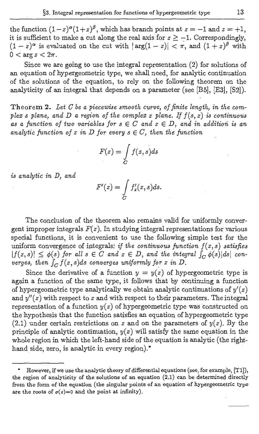
§3. Integral representation for functions of hypergeometric type 13
the function (1 -^)^(1+^)^, which has branch points at z — — 1 and z = +1,
it is sufficient to make a cut along the real axis for z > —1. Correspondingly,
(1 — z)a is evaluated on the cut with | arg(l — z)\ < 7T, and (1 + z)^ with
0 <args < 2tt.
Since we are going to use the integral representation (2) for solutions of
an equation of hypergeometric type, we shall need, for analytic continuation
of the solutions of the equation, to rely on the following theorem on the
analyticity of an integral that depends on a parameter (see [B5], [E3], [S2]).
Theorem 2. Let C be a pieceinise smooth curve, of finite length, in the
complex s plane, and D a region of the complex z plane. If f(s,z) is continuous
as a function of two variables for s 6 C and z £ D, and in addition i3 an
analytic function of z in D for every s £ C, then the function
F(z) = Jf(z,s)ds
c
is analytic in D, and
F'(z) = Jf>(z,s)ds.
c
The conclusion of the theorem also remains valid for uniformly
convergent improper integrals F(z). In studying integral representations for various
special functions, it is convenient to use the following simple test for the
uniform convergence of integrals: if the continuous function f(z, s) satisfies
1/(-^,-5)1 % <K-s) for °-U ^ £ C and z 6 £), and the integral jc <f>{s)\ds\
converges, then jc f(z, s)ds converges uniformly for z in D.
Since the derivative of a function y = y[z) of hypergeometric type is
again a function of the same type, it follows that by continuing a function
of hypergeometric type analytically we obtain analytic continuations of y'(s)
and y"(z) with respect to z and with respect to their parameters. The integral
representation of a function y(z) of hypergeometric type was constructed on
the hypothesis that the function satisfies an equation of hypergeometric type
(2.1) under certain restrictions on z and on the parameters of y(z). By the
principle of analytic continuation, y{z) will satisfy the same equation in the
whole region in which the left-hand side of the equation is analytic (the right-
hand side, zero, is analytic in every region).*
* However, if we use the analytic theory of differential equations (see, for example, [Tl]),
the region of analyticity of the solutions of an equation (2.1) can be determined directly
from the form of the equation (the singular points of an equation of hypergeometric type
are the roots of <r(z)=o and the point at infinity).
14 Chapter I. Foundations of the Theory of Special Functions
In the following discussion we shall study the solutions of particular
equations of hypergeometric type by using the integral representation (2),
and the results wiH be extended to a wider domain by means of the principle
of analytic continuation.
§4 Recursion relations and differentiation formulas
Let us consider a general method of obtaining various relationships for
functions yu{z) defined by the integral representation (3.2). We begin by
establishing relationships among functions of the form
c
which appear in the definitions of the yu{z) and their derivatives.
Lemma. Any three functions 4>Vifii{z) are connected by a linear relation
X>iM^fWM = o
i=i
with •polynomial coefficients Ai(z), provided that the differences V{ ~ Vj and
fij — /i-j are integers and that.
crU0+1(s)p(s)
(s - z)^
sm
a2
= 0 (m=0,l,2,...),
31
where si and $2 are the endpoints of the contour C; Vq is the i/,- with the
smallest real part; ^o> ihe ^,- with the largest real part.
Proof. Consider the sum £^=1-^^^((^)- We show that the coefficients
Ai = Ai(z) can be chosen so that this linear combination is zero. For any
fixed z we have
1 0
where y.% and uq are defined in the statement of the lemma, and
P(s) = J2 Aitr"-""^ - z)"0'^.
§4. Recursion relations and differentiation formulas
15
Since the differences Vi — Vq and fio ~ P-% are nonnegative integers, P{s) is a
polynomial in s. We choose the .A,- so that
GM
(1)
where Q(s) is a polynomial (we show below that such a choice of the
coefficients is possible). We obtain
i
If we require that the condition
(s - zY
32
«1
(T"o+l(s)p(s)
(s - zY»
32
31
0 (m-0,1,2,...),
which is similar to (3.4), holds at the endpoints of C, then the endpoint
terms become zero, and with the Ai determined in this way we have the
linear relation
Let us show that it is always possible to choose the coefficients of Q{s) and
the coefficients Ai so that (l) in fact holds. To do this, we rewrite (l) in
a more convenient form, using the differential equation (077,,)7
p„{s) = crl/(s)p(s), where rv(s) = r(s) + vry'{s). We obtain
TuP i
for
P{*) = Q(s) [0 - «kW - Wis)] + 0"«(* - z)Q'{s).
(3)
If we compare the left-hand and the right-hand sides of this equation, it is
easy to see that the degree of Q{s) is two less than the degree of P(s).
If we equate coefficients of powers of s on the two sides of (3), we obtain
a system of homogeneous linear equations in the coefficients of Q(s) .and the
coefficients A{(i — 1,2,3) that appear in the expression for P(s). The number
of equations is two more than the number of unknown coefficients of Q(s).
Hence the number of unknowns is at least one more than the number of
equations, and consequently one of the unknown coefficients can be assigned
arbitrarily. In the case when P(s) is at most of degree 1, the relation we are
considering remains valid if we take Q(s) = 0. In the resulting system of
equations, the coefficients of the unknowns are polynomials in z, so that in
this case after one coefficient is selected the remaining coefficients are rational
functions of z. After multiplying (2) by the common denominator of the Aj(z)
we obtain a linear relation with polynomial coefficients. This completes the
proof of the lemma.
16 Chapter I. Foundations of the Theory of Special Functions
In practical applications of the method the degree of P(s) can sometimes
be reduced by integrating by parts in some of the functions <j>V{tii (z). We have
c
(s - zy+i
l tr»(s)p(s) ** 1 [^(3)^(3)^3)
fi (s-zy
where r^^s) = r{s) + {y — l)cr'(s). Supposing, as usual, that the integrated
terms yield zero, we obtain
1 f r^1(3)a^(s)p(3)
M^~~j- (TT^ ds-
c
(4)
Example 1. Find a relation among ^„„1(2:), <f>vu(z) and <jS>„)(,+i(z).
In this case vq = u, fiQ = v + 1, P{s) = A^{s — z)2 + ^2(5 — z) + A3,
Q{s) ■=• 50 (a constant); the endpoint condition
<jVo+1{s)p{s)
Q(s)
"2
0,
51
(5-2:)^°
which arises in the proof of the lemma, is equivalent to
^(3)p(3) S2
(3 - z)^1
0.
hi
■ Equation (3) has the form
M* - zf + A2(s -2:) + ^3-50 [(* - z)t„(s) ~{v + 1)c(5)] .
Taking 50 = 1, expanding the right-hand side in powers of s ~ z, and
comparing coefficients, we obtain
v + l
v-l
-»
A2 - rv(z) ~{v + \)a'{z) = r(z) - ff'(z),
^3 = -(i/ + l)ff(z).
(5)
Therefore
4i(z)^„ „_i(z) + A2{z)(j>l/V{z) + Az{z)(j>^vjrl{z) = 0,
(6)
§4- Recursion relations and differentiation formulas
17
where the coefficients Ai(z) are defined by (5). It is convenient to rewrite the
last equation in a different form. Since
C 1
Hz)p(z)]' = r(z)p(z),
relation (6) yields a convenient integral representation for the derivatives of
functions of hypergeometric type:
c
where
cP = (r> + ^±Acv.
Generalization of the relation (7) deduced in Example 1 enables us to
obtain a convenient integral representation for the derivatives of any order of
functions of hypergeometric type.
In fact, (7) can be interpreted in the following way: an integral
representation for the first derivative of a function of hypergeometric type
C„ f ^(s)p(s) Cu
VAZ) = pV)J (s-z)^dS ~ -pjz)^(z) (8)
c
can be obtained from the original representation by replacing v by v — 1, p(z)
by Pi(z) — cr(z)p(z), and multiplying by the additional factor r'+|(i/ —l)cr".
It is then clear that
r(fc)
where
fc-1
I , U + S ~ l -»'
=n ,-+^^.- c.
.3=0
If we use (9) and the lemma proved above, we obtain the following theorem.
18 Chapter I. Foundations of the Theory of Special Functions
Theorem. Any three functions yii(z) are connected by a relation of the
form
with polynomial coefficients Ai(z), provided that the differences v\ — Vj are
integers and that
(s - 2)^+1
sm
a2
-0 (m^0,l,2,...).
Here 5j and s2 are the endpoints of C; Vq is the V{ of smallest real part; and
Ho is the V{ of largest real part.
We note that the equations that determine the coefficients A{(z) are
linear and homogeneous in the unknowns and independent of the contour C
used in defining 3/,,(2). Consequently two functions yu{z) of hypergeometric
type which differ only by factors independent ofv and by the choice of C will
satisfy relations of the kind under consideration with the same coefficients.
Example 2. Let us obtain a formula
Aiy'v(z) + A2y„+1(z) + A3yu{z) - 0, (10)
connecting y'v{z)%yu{z) and 3/,,+1(2). We shall refer to formulas that express
derivatives of functions of hypergeometric type in terms of the functions
themselves as differentiation formulas.
To obtain (10) we use the integral representations (7) and (8) for y'„{z)
and 1/1/(2), and a preliminary transformation of 3/,,+1(2), using (4). Then we
can write the left-hand side of (10) in the form
where
^1-^^(3-2) + ^2
a[z)
1 fa"
Cv+lT„(s)
v+l
{s)P{s)
-2)-+1
+ AZCV
k„ = t' + ?-^<t".
Since P(s) is a linear polynomial, Q(s) = 0 and consequently
cr{z) v + 1
§4. Recursion relations and differentiation formulas 19
In determining A\,A%^ and .A3 from this equation it is convenient to take
A\ = c(z)t expand the left-hand side in powers of s—2, and equate coefficients
of powers of s — z. We find
A2 = ~{v +1)-- , Az = «„—-A
As a result we obtain the differentiation formula
ffMl/U*) = ~f
C
0 „+1
(11)
In particular, for the polynomials
of hypergeometric type, we have v — n(n = 0,1,2,...) and Cn = n\Bnj{2iri)
(see formula (3.1)). Hence in this case the differentiation formula (11) can be
written in the form
/c.
*«*;« = ~
Bn
n L-^n+1
■yTi+iW-TnWynW
(12)
where
Tn W = r(z) + nff'(z), «n = r' +
n-1
<r".
Thus in Chapter 1 we have considered a method of constructing integral
representations for particular solutions of the generalized equation of
hypergeometric type and indicated ways of studying the properties of these
solutions. With this we complete our discussion of the general theory of special
functions; in the next chapter we turn to the study of the classical
orthogonal polynomials, which form an important subclass of the special functions
of mathematical physics.
21
Chapter II
The Classical
Orthogonal Polynomials
§5 Basic properties of polynomials of hypergeometric type.
1. Jacobi, laguerre and Hermite polynomials. In §2 we introduced the
polynomials yn(z) of hypergeometric type, which are solutions of
a(z)y"+r(z)y' + Xy = 0 (l)
with A = An = —nr'-~ |n(n—l)cr". They are given explicitly by the Rodrigues
formula *~ ~—
~^~ Vn(z)= ~^[^(z)p(z)]^\ (2)
where Bn is a normalizing constant and p(z) satisfies the differential equation
7 {^zJp&T=r(z)p(z). J""" --—- '(3)
Solving (3), we obtain, up to constant factors, the possible forms for p(z)
corresponding to the possible degrees of c(z):
J" (¾ - z)«(z - aY for <t(z) = (b- z)(z - a),
p(z) — { (z ~ o)a^z fc>r v{z) = z~ a,
[e<*z*+i3z for 0-(4 = 1.
Here a, i, a and /5 are constants (in general, complex). By linear changes of
variable, the expressions for a(z) and p(z) can be reduced (up to constant
multipliers) to the following canonical forms:
(1 - z)a(l + zY for <r(z) = 1 - z2,
p(z) = { zae~z for ry{z) = 2,
e~~ for o-(z) = 1.
22
Chapter II. The Classical Orthogonal Polynomials
. Under these transformations equations (1) and (3) become equations of the
same form, and the corresponding polynomials yn(z) of hypergeometric type
remain polynomials in the new variable and are, as before, defined by the
Rodrigues formula (2).
According to the form of t?{z) we obtain the following systems of
polynomials: „ _ -,-----
/f\ 1) Let a{z) = 1 - z\\p(z) = (1- z)a(l + zf. Then
"t{z) = -(a + 0 + 2)z + f3~a.
The corresponding polynomials yn(z) with* Bn = (—l)n/(2nn!) are
called the Jacobi polynomials and denoted by P„ \z):
Important special cases of the Jacobi polynomials are:
a) the Legendre •polynomials Pn(z) = P„ ' (z);
b) the Chebyshev polynomials of the first and second kinds:
Tn(z) = cosn<f>,
U (z) - _J_t' (z) - sin(n + 1)^
where <f> = cos_1(^). It will be shown later (§6, part 2) that
c) the Q^egenbauerpolynomials, also known as ultraspherical polynomials,
nK } (A+1/2),/n {Z)-
We have used the notation
where T(z) is the gamma function (see Appendix A).
* The values B„ are chosen for historical reasons but could be arbitrary. They agree
with the normalization in [E2].
§5. Basic properties of polynomials of hypergeometric type 23
/ W-/
"r{z) = — z + a + 1.
The polynomials* yn(z) with Bn := \jn\ are the Laguerre polynomials L%(z):
I . ^dn
P^PViS) Let a(z) = 1, p(z) = e~z\ Then r{z) = -2z. The polynomials yn(z)
■with f?n = (—1)" are the Hermite polynomials Hn(z)\
^) = (-1)-.^(.-1).
We have not considered the case when ff(z) has a double zero, i.e. a(z) =
{z ~ a)2. The polynomials of hypergeometric type corresponding to cr{z) =
[z ~ a)2 can be expressed in terms of the Laguerre polynomials. It was shown
in §1 that when a{z) = (z — a)2 the substitution s = l/(z — a) carries the
generalized equation of hypergeometric type
a t(z) , ff(z)
cr{z) & \z)
into an equation of the same type with a(s) — s. In particular, the equation
a(z)y" + r{z)y' + \ny = 0 fxn = -nr' - ~n(n - l)cr" J
for polynomials of hypergeometric type with cr(z) ■=■ (z — a)2 becomes, under
the substitution s = \}{z — a),
d?y | 2-~sr(a + l/s)dy ^ Xn =q
ds2 s ds s2
As we showed in §1, the substitution y = <f>(s)u carries this equation into an
equation of hypergeometric type if 4>(s) is chosen appropriately. A possible
form for (f>(s) is \jsn. Since
7-(2:) = T(a) + r'(z)(z - a),
we have r(a + 1/s) = r(a) + r'/s and we obtain the following equation for
u(s):
su" - [sr(a) + t' + 2(n - l)]u' + nr(a)u = 0.
24
Chapter II. The Classical Orthogonal Polynomials
Since u(s) = $ny and y is a polynomial of degree n in z ~ a + 1/s, the
function u(s) is a polynomial of degree n in s. Consequently u(s) is a polynomial
of hypergeometric type. Since, in the present case, the function p(s) that
determines the polynomials of hypergeometric type according to the Rodrigues
formula has the form
p(s) = s'r'~-2n+le-Tia>,
the polynomials u(s) = un(.s) are, if r{a) =£ 0, the same up to a normalizing
factor as the Laguerre polynomials L%(i), with a = —r' — 2n + 1, t = r(a)s.
Therefore the polynomials yn (z) are connected with the Laguerre polynomials
as follows:
This formula is still valid when r(a) = 0.
The best known polynomials of hypergeometric type in the case a{z) =
(z — a)2 are the Bessel polynomials, for which
o-(S) = z2, r(*) = 2(* + l), p{z) = e~2l\
Their Rodrigues formula is
The Bessel polynomials are normalized by yn(0) = 1. Their explicit form is
2. Consequences of the Rodrigues formula. We have shown that the
derivatives of all orders of polynomials yn(z) of hypergeometric type are also
polynomials of hypergeometric type (see section 2). The Rodrigues formula for
Vn{z) h^ the form
A B Jn — m
where
m-l
Amn~ (-1)™ JI ^*"> A°n = li ^kn = /i*(A)
A=0
= An — Aft.
§5. Basic properties of polynomials of hypergeometric type 25
Since fikn = —(n — k) (r' + |(n + k — l)ff"), we have
^- = ^^11^ + ^ + ^-1)
a
.n
(5)
Notice that the Rodrigues formula for Vn{z) can be obtained up to a
normalizing factor from the Rodrigues formula for yn(z) by replacing n by
n — m and p(z) by pm(z) = 0^(2)/9(2). Let us consider some corollaries of
equation (4).
1) From the Rodrigues formulas for yn(z) and y'n(z) we obtain the
following differentiation formulas for the Jacobi, Lagtierre and Hermite
polynomials:
dL<?\z) _ Tia+1)
dz
dHn{z)
dz
= 2nHn^{z).
(6)
2) By using the Rodrigues formula we can express the derivatives y'n{z)
in terms of the yn{z) themselves. In fact, since
yn+\{z) =
B
n+l
dn+l
-pfzfd^[Tniz)pniz)L
we have, by Leibniz's formula for differentiating a product,
!/n+i(z) =
jn~ 1
5
n
n
rn{z)yn{z)- T-r'nff{z)y'n{z)
Hence
v(z)y'n(z)
A
n
nr,
n L
Tn{z)yn{z)
Bn
B
n+l
■!/n+l00
(7)
in agreement with (4.12).
26
Chapter II. The Classical Orthogonal Polynomials
3) From (4) for m = n — 1 it is easy to find the coefficients an and bn of
the highest powers of z in the expansion
!/»M = anzn + bnzn~l + ....
Since
■y^~1)M=n\anz+(tn-l)lbni
j- [(Tn(z)p(z)] = — [cr(z)pn~i(z)] = rn-.i(2r>n_-l(»,
we have
An-.hnBnrn-.i(z) - n\anz + (n ~ l)lbn.
Hence
an = An~^fnT>n^ = Bn ff (V + i(n + k - l)A , a0 = B0;
n- a=o V y (8)
1" _ nrn-l(0)
4) By using the Rodrigues formula we can easily find the values of the
Laguerre and Jacobi polynomials for special values of z by applying Leibniz's
rule for the derivative of a product. For example,
Pl">®(l) = La(0) = Qn + a + x)
p(^)f-l) = (--1-)^ + ^ + 1)
n l J l l) nlTtf + l) ■
(9)
Hence we have, for the Legendre polynomials,
P„(l) = l, Pn(-l)-(-l)n. (9a)
3. Generating functions. A generating function for a system of polynomials
yn(z) of hypergeometric type is a function $(2, t) whose expansion in powers
of t has, for sufficiently small \t\i the form
S(M)=£^*n, (10)
n=0
§5. Basic properties of polynomials of hypergeometric type ' 27
where yn{z) is a polynomial of hypergeometric type for which the constant
Bn in the Rodrigues formula (2) is 1, i.e.
(evidently yn{z) = Bny{z)). By (3.1),
Vn{ } p{z)2iri] (s-z)^dSi
(11)
where C is a closed contour surrounding the point s = z (it assumed that
p(s) is analytic in the region inside C). We substitute the expression (11) for
yn(z) into (10) and interchange summation and integration:
$(*,<)
1 [ P(s)
2irip(z) J s — z
c
£
l»n=0 L
a(s)t
s — z
n.
ds.
The interchange of summation and integration can easily be justified for
sufficiently small \t\ and fixed z. The geometric series in the integrand can be
summed, and we obtain
*(*,*)
p(s)ds
2mp(z) J s — z — a(s)t'
c
The denominator of the integrand has, in general, two zeros. If t —*■ 0, one
of the zeros tends to s = z. At the same time, the second zero, if it exists,
tends to infinity. Therefore when \t\ is sufficiently small we may suppose
that there is just one zero s = £(#,0 of the denominator inside C, and the
integrand has a single pole inside C with residue
C-i
P(*)
1 - a'(s)t
Consequently we have the representation
*=*(*,*)
$(,,0 =
PM 1
p{z) 1 - cr'(s)t
*=*(*,*)
(12)
Here £(z,i) is the zero of the quadratic equation (in s) s — z ~~ a(s)t ~ 0
which is near s — z for small Itfl.
28
Chapter II, The Classical Orthogonal Polynomials
Formula (12) for the function $(•?,£) in (10) was established for
sufficiently small \i\. By the principle of analytic continuation, (10) remains valid
in the region of analyticity (with respect to i) of the two sides of (10), i.e.
in the disk \t\ < R, where R is the distance from the origin to the nearest
singular point of $(2, t) (for fixed z).
As an example we obtain the generating function for the Legendre
polynomials. In this case
and consequently, by (12),
$(M) =
1
3=^(_v) Vl + 4^ + 4***
1 + 2si
Since Bn = (—l)n/(2nn!) for the Legendre polynomials, we have
1
00
, = y pn(z)(-2t)n.
If we replace t by — i/2, we obtain the usual form of the generating function:
1
00
, = ypn(z)e.
(13)
The expansion (13) converges for |i| < 1 if — 1 < z < 1, since the singular
points of the generating function, which are at the roots of the equation
1 — 2iz + i2 = 0, are given by ii,2 = e^1* (cos^ = z) and He on \t\ = 1.
Formula (13) is often used in theoretical physics in the form
1 ^ rn
ri - r2
n=or>
(14)
where r< = min(ri,r2), f> = max^rj,^), and 6 is the angle between the
vectors r-j and r2. In fact,
*i - r2| = v^i+r2 ~ 2rir2cos^
.r2v1+te)2_2Scose (n<r2)-
§5. Basic properties of polynomials of hypergeometric type 29
Hence
and consequently *
rn
w^fe)'-^-* "=°r>
= E^rp»(cose)-
By using (10) and (12) we can obtain the following expansions for the
Laguerre and Hermite polynomials:
(1 - i)—* exp (-^) = f) i;(»)t", (15)
n=0
00
tn
exp^t-t2) = ^^)-. (16)
n=0
4. Orthogonality of polynomials of hypergeometric type. If p(z) is considered
on the real axis z — re, and satisfies some additional conditions, we can obtain
a number of special properties of the polynomials yn(z) of hypergeometric
type.
Theorem. Lei p(x) satisfy
a(x)P(x)xk\b = 0 (fc =0,1,...)- (17)
I £=:0,6
at the endpoints of an interval (a, 6). Then the polynomials yn(x) of
hypergeometric type corresponding to different An 's are orthogonal on (a, 6) with
■weight p(x), i.e.
b
/ yn(x)ym(x)p(x)dx = 0 (Am 7= An).
/'>V'" .■-..■■■-- '"^'
30
Chapter II. The Classical Orthogonal Polynomials
Proof. Consider the differential equations for yn(x) and ym(x):
[cr{x)p{x)y'J + XnP(x)yn = 0,
[<y{x)p{x)y'1J + Xmp(x)ym = 0.
Multiply the first equation by ym(x) and the second by yn{z)-, subtract the
second from the first, and integrate from a to b. Since
Vra{x) [(r(x)p(x)y'n(x)}' ~ yn(x) [a(x)p(x)y'm(x)]'
d
= -fa{<r(z)p(z)W[ym(x),yn(x)]},
where W(u,v) =
u v
u' v'
is the Wronskian, we obtain
6
(Am-An) < / ym{x)yn{x)p{x)dx = v(x)p(x)W[ym(x),yn(x)}\a.
a
Since W[ym(x),yn(x)} is a polynomial in x, the right-hand side is zero, by
(17). Hence "when Am ^ A n we have
6
J ym{x)yn{x)p{x)dx = 0, (18)
a
as was to be proved.
The polynomials yn{x) for which p{x) satisfies (17) are known as the
classical orthogonal polynomials. They are usually considered under the
auxiliary conditions that p(x) > 0 and cr(x) > 0 on (a, 6). These conditions are
satisfied by the Jacobi polynomials P%'^{x) for a = —1, b = 1, a > —15
/3 > —1; by the Laguerre polynomials L®{x) for a = 0, b = +oo, a > — 1; by
the Hermite polynomials Hn(x) for a = —oo, b = +oo. We observe that in
these cases the condition Am ^ An can be replaced by m =£ n.
Prom the properties of the derivatives of polynomials of hypergeometric
type (see part 2) it follows that the derivatives yn (x) of the classical
orthogonal polynomials are also classical polynomials, orthogonal with weight
ryk{x)p{x) on (a, 6):
6
[vikH*)yi!? (x)Pk(x)dx = 6mn4n, (18a)
§5. Basic properties of polynomials of hypergeometric type 31
where
c _ / 0 for m ^ n,
k 1 tor rn= n.
It is easy to express the squared norm d\n of yh, (re) in terms of the
squared norm d%?= d%n of yn(rc) by using the differential equation for y^ ^(rc):
£ [p*+i(z)yik+1)(x)} + ^nPk(x)yik\x) = 0. (19)
If we multiply (19) by yi *(x) and integrate over (a, 6), after integrating by
parts we obtain
Pk+i(x)yik+1\xyyik)(x)
n2
yik+1\x) Pk+1(x)dx
+ P-ka
i2
y{i\x) -pk(x)dx = 0.
The integrated terms are zero because of (17), and consequently
Hence, by induction, we obtain
m-l
dltn = dlYL ^n>
(20)
fc=0
We can calculate d\ for the Jacobi, Laguerre, and Hermite polynomials from
(20) with m = n, since
0
y^\x) = n\an, d*nn = {n\anf J an{x)p{x)dx.
(20a)
The integral Ja an(x)p(x)dx can be evaluated in terms of gamma functions
(see Appendix A, part 5):
( 2a+&+lT{n + a + l)r(n + /3 + 1)
n!(2n + a + j3 + l)T(n + a + /3 + 1)
dl=!> lr(n + a + l)
. n!
I. 2nn!^F
for Pi°"^(x),
for L%(x)t
for Hn(x).
32
Chapter II. The Classical Orthogonal Polynomials
The basic information about the Jacobi, Laguerre, and Hermite polynomials
is given in Table 1.
Table 1. Data for the classical orthogonal polynomials
Vn{x)
M)
p(x)
a{x)
t(x)
bn
<
p(">P)(x)(a>~l,f3>-l)
(-1,1)
(l-x)a().+x)p
l~x2
/3 - a - (a + 0 + 2)x
n(n + a + /3 + 1)
2nn\
T(2n + a + ,3 + 1)
2"n!r(n + a + 0 + 1)
(a - /3)r(2n + a + /3)
2n(n~l)lT(n+a + p + l)
2«+/Hir(n + a + Xjr(n + ^ + i)
n!(2n + a + /3 + l)r(n + a + /3 + 1)
■*£<*) <*>-!)
¢0,00)
1 + a- x
n
1
n!
(-1)" ■
n!
T(n + a + 1)
n!
-M*)
(—00,00)
1
-2x
2n
(-1)"
2"
0
2nn\y^
§6. Some general properties of orthogonal polynomials 33
§6 Some general properties of orthogonal polynomials
The classical orthogonal polynomials have many properties that follow
directly from their orthogonality. Similar properties are possessed by any
polynomials that are orthogonal on an interval (a, 6) with a weight p(x) > 0.
Let us consider some general properties of polynomials pn(x) that are
orthogonal on an interval (a, 6) with weight function p(x)> that is, that satisfy
Pn(x)pm(x)p(x)dx = 0 (m=£ n).
We shall suppose that the leading coefficient of pn(x) is real and different
from zero (n is the degree of the polynomial).
1. Expansion of an arbitrary polynomial in terms of the orthogonal
polynomials. Let us show that every ■polynomial qn(x) of degree n is a linear
combination of the orthogonal polynomials Pk(x)(k = 0,1,... ,n), i.e.
n
1n{x) = ^cfcTipfc(:r). (1)
ft=o
This is evident for n = 0. For general n > 0 we proceed by induction.
Suppose that every polynomial qn-i(x) has the representation
Ti-l
fc=0
Bbr qn{%) we determine the constant cnn so that the highest coefficient of
qn{x) — cnnpn(x) is zero, i.e. qn(x) - cnnpn(x) = qn-i(z). If we use (2), we
obtain (1) for qn(x).
The coefficients ckn in (l) are easily determined by the orthogonality
property
6
/ Pn(x)Pm(x)p(x)dx ~ 0 (m ^ n) (3)
a
which leads to the formula
b
Cfcn =-tf I Qn(x)pk(x)p(x)dx, (4)
a
34
Chapter II. The Classical Orthogonal Polynomials
where
0
4 = Pl(x)p(x)dx
is the square of the norm.
Let us show that the orthogonality condition (3) is equivalent to
/ pn{x)xmp{x)dx = 0 (m < n).
(5)
In fact, if we insert the expansion of pm(x) in powers of x into (3), with
m < n, then (3) follows from (5). Similarly, if we expand xm in terms of the
Pfc(rc), we obtain (5) from (3).
It follows from (5) that pn(x) is orthogonal to every •polynomial of lower
degree.
2. Uniqueness of the system of orthogonal polynomials corresponding to a
given weight. We can show that the interval (a, b) and the weight p(rc)
determine the polynomials pn(x) that satisfy the orthogonality condition (5), up to
a normalizing factor.
Suppose that there are two sets of polynomials pn(x) and pn(x) that
satisfy (5). We have
n
pn(x) = Y2CknPk(x).
fc=0
By (4) and (5), we have cfcn = 0 for k < n, so that pn(x) and pn(x) must be
proportional.
There is an explicit representation for pn(x) as a determinant:
pn(x) = An
Co
Ci
Cn-l
1
d -.
c2 ..
Cn
X
Cn
Cn+l
■ C%Tl-\
.■ xn
(6)
where An is a normalizing constant, and Ck = ja xkp(x)dx are the moments
of p(x). In fact, it can be verified that the polynomial (6) satisfies the
orthogonality condition (5).*
* The coefficient of xn in (6) is different from zero when A„/0, since it is proportional
tothe Gram determinant of the functions l,x,...,xn~1 (see [E2] and [Gl]).
§6. Some general properties of orthogonal polynomials 35
Example. It is known that the system of functions {cos ruf>} has the
orthogonality property:
7T
1 / cos n<f> cos m<f> d<f> = 0, ' m^n.
By using the relation
cos(n + l)<f> + cos(n — l)(f> = 2 cos (f> cos ruf)
and mathematical induction it is easy to show that cosn^ is a polynomial
of degree n in re = cos^ with leading coefficient an = 2n-1(a0 = 1). This
polynomial is the Chebyshev polynomial of the first kind, Tn(x). Making the
substitution x = cos ^, we obtain the following orthogonality relation for
Tn(x):
l
dx
-l
Tn(x)Tm(x)-^= = 0, m^n.
From this we see that the polynomials Tn(x) = cos n<f> in x = cos ¢, satisfy the
same orthogonality relation as the Jacobi polynomials P„ 5' 2 (re).
Therefore, by virtue of the uniqueness property of the orthogonal polynomials for
a given weight, we have
Tn(x) = cnPth~*\x).
Equating the coefficients of rcn, we obtain cn = n!/(l/2)n.
If we use the differentiation formula (5.6) for the Jacobi polynomials
then the Chebyshev polynomials of the second kind
= Mn + lU
sm<f>
(in
may be expressed in terms of the polynomials Pn2'2 (re) as
The polynomials T(rc) = 21-nTn(rc) are extensively used in problems of
approximation theory and in the general theory of iterative methods. The
reason for this is that they are the polynomials deviating least from zero on
36
Chapter II. The Classical Orthogonal Polynomials
[—1,1] among the polynomials qn(x) of degree n with, leading coefficient 1.
That is, the minimum of
max \qn(x)\
—i<i<i
is attained for
Tn(x) = 21_ncosn^, <f) = arccosrc.
In fact, at the points where Xk = cos(kTrfn) (k — 0,1,..., n), the polynomial
Tn(x) takes, with alternating signs, values of modulus
Hence if we suppose that there is a polynomial pn(x) with leading coefficient
1, for which
" - max |Tn(rc)l < pn{x) < max \fn(x)\,
-l<a:<l —1<2<1
for x £ [—1,1], then the polynomial Tn(x) — pn(x), of degree " — 1, would
alternate in sign at the points xq , x'-y,..., xn and would have to have n zeros,
which is impossible.
One can show in the same way that the polynomial
fn(x) = ^M ™th*o£[-i,i]
is the polynomial deviating least from zero on [—1,1] among polynomials
qn{x) of degree n that have qn(xo) = 1.
3. Recursion relations. All orthogonal polynomials satisfy recursion formulas
connecting three consecutive polynomials pn„i(x),p„(s),pn+i(rr):
xpn{x) = anPn+l{x) + /3nPn(z) + 7r*Pn~l(», (7)
where an,0n and "fn are constants.
Bbr the proof, we use the expansion
n+l
Xpn(x) = ^2cknpk(x). (8)
fc=0
By (4),
b
Ckn = -p j Pk(x)xpn(x)p(x)dx. (9)
a
§6. Some general properties of orthogonal polynomials 37
Since xpk(x) is a polynomial of degree k + 1, by the orthogonality properties
of pn(x) we have ckn = 0 when k + 1 < n. Hence (8) can be written in the
form
xpn = Otnpn+1 + 0npn + 7nPn-l,
where an = cn+1>n, /5n = cnn, 7n = cn_iin, as required.
The coefficients an, /5n, 7n can be expressed in terms of d\, i.e. the
square of the norm, and the coefficients an, bn of the highest terms in pn(x):
pn(x) = anxn + bnxn~l + ... (an £ 0).
It is clear from (9) that d\ckn = d2ncnk. Since an_i = cn,n_i, 7n = cn_1;Ti, if
we put & = n — 1 we obtain
7« = <*«-i<S/<fi-i- (10)
On the other hand, comparing the coefficients of the highest terms on the left-
hand and right-hand sides of (8), we have an = anan+i, bn = an6n+i +/5nan.
Hence
an a K K+i .^ an-i dn -
<3n+l an an+l an an-i
Therefore if we know the coefficients an and bn and the squared norms d\ of
any orthogonal polynomials pn(x), we can successively determine the
polynomials.
The coefficients an)/5nj7n obtained from (11) for the Jacobi, Laguerre
and Hermite polynomials are presented in Table 2. In addition, Table 2 (p. 38)
shows the coefficients Oin,^njjn that appear in the differentiation formula
v(x)y'n(x) = (anx + &n)yn{x) + 7nyn_i(:r).
This formula is obtained by substituting the expression for yn+i(x) from the
recursion relation (7) into formula (5.7).
Consider a recursion relation of the form (7),
zun(z) = anun+1(z) + &nun(z) +^^^) (7a)
for arbitrary complex values of z. One solution of this recursion is the set of
polynomials pn{z) that are orthogonal on (a, 6) with weight p(z). Another
set of solutions for z $ [a, b] is the set of functions
JbW= jpnism. ds.
J s — z
a
38
Chapter II. The Classical Orthogonal Polynomials
Table 2. Coefficients of recursion relations for the Jacobi, La-
guerre, and Hermite polynomials
y»(z)
7»
P^\x)
2(n+l)(n +a+ ,3+1)
(2n + a + /3 + l)(2n + a + 0 + 2)
at ">
p- — a-
(2n + a + /3)(2n + a + /3 + 2)
2(n+a)(n + /3)
(2n + a + /3)(2n + a + /3+ 1)
—n
(a-p)n
(2n + a + /3)
2(n+a)(n+/3)
2n + a + /3
■*£<*)
-(n+1)
2n + a+ 1
-(n + a)
0
n
-(n + a)
#»(*)
1
2
0
n
0
0
2n
Bbr the proof, it is sufficient to integrate the recursion relation for the
polynomials pn(s) on (a, 6) after multiplying by p(s)/(s — z) and use the equation
a a
b b
= J Pn{s)p(s)ds + z J Pn^s) ds = zqn(z) (n > 1).
The function
0
Pn(*) -Pn(z)
s — z
p(s)ds
is closely related to qn(z). It is easily seen to be a polynomial of degree n — 1,
and is called a polynomial of the second kind. Since
6 . 6
( x fPn(s)p(s) , [ p{s)ds , 1 .
J s- z J s- z ao
§6.j3ome general properties of orthogonal polynomials 39
when z $ [a, 6], and both pn(z) and qn(z) satisfy the same recursion (7a) for
z $ [a, 6], the polynomials rn{z) satisfy the same recursion. By continuity,
they still satisfy (7a) for z £ [a, 6].
4. Darboux-Chris toff el formula. From the recursion formula (7) there
immediately follows a formula that plays an important role in the theory of
orthogonal polynomials, namely the Darboux-Ghristoff'el formula
^Pk(x)Pk(y) _ I an Pn+l(x)Pn(y) ~ Pn(x)Pn+l(y) ,^
^ 4 d2nan+1 x-y
To derive this we use (7) and (10):
4
xpk(x) = akpk+1(x) +/3fcpfc(:r)+a!fc_i~-pfc~i(:r),
dfc-i
ypk(y) = &kPk+i(y) + &kPk(y) +ak-i~#i^Pk-i(y)-
ak-i
These recursions also hold for k = 0 if we put a—i/<P,1 ~ 0, p-^x) = 0.
Multiply the first equation by Pk(y)t the second by Pk(%), divide each
equation by d|, and subtract. This yields
( ^Pk{x)Pk(y) a / \ a r \
(x - y)—j2— = Aw>v) - Ah-ifa y),
where
Ak(x,y) = -£ \pk+i(x)pk(y) - Pk(x)pk+i(y)].
ak
Summing over k from 0 to n, we obtain
k=0 "*
This formula is evidently equivalent to (12) since an = an/an+1.
5. Properties of the zeros. Let us show that all zeros xj of pn(x) are simple
and on the interval [a, b). Let pn{x) have k changes of sign on (a, 6). Evidently
0 < k < n. The property in question will certainly be valid if we show that
k = n. Put
( 1 for k = 0,
qk(x)= I f[(x-Xj) for0<fc<n.
40
Chapter II. The Classical Orthogonal Polynomials
Here Xj are the points where pn(x) changes sign. The product pn(x)qk(x)
evidently does not change sign for x £ (a, 6). Therefore
b
Pn(x)qk(x)p(x)dx ^0.
a
It follows that k = n, since if it < n
b
/ Pn{x)qk{x)p(x)dx = 0
a
by (5).
We can show that the zeros of pn(x) and pn+i(x) are interlaced. For
the proof we consider the special case of the Darboux-Christoffel formula
obtained from (12) for y -+ re:
2%1 = 4— [14+iOOpnM -rf.(*K+iM] ■ (13)
Let xj(j — 1,2,..., n + 1) be the zeros of pn+i(x). By (13), the sign
of the product p'n+i{x)pn(x) at the zeros xj of pn.fi(rc) is independent of j.
However, the first factor p'n+i changes sign between Xj and xj+i. Therefore
the second factor pn(x) must also change sign. Consequently pn(x) has at
least one zero in the interval (rcj, sj+1). Since there are n intervals (xj, xy+i)
and each one contains at least one of the n zeros of pn(x)> it is clear that
between two successive zeros of pn+i(x) there is exactly one zero of pn(x).
6. Parity of polynomials from the parity of the weight function. Let {pn{x)}
be the polynomials orthogonal on (—a, a) with an even weight function p{x).
Then if we substitute — x for x in (3), we obtain
a
/ pn{-x)pTa{-x)p{x)dx = 0 (m ^ n).
— a
Since p(x) defines the polynomials uniquely up to a normalizing factor, we
have pn{—x) = cnpn(x). By comparing the coefficients of the leading terms
we obtain cn = (—1)". Hence we have, in particular, the following parity
properties of the Hermite and Legendre polynomials:
Hn(-x)=(-l)nHn(x),
Pn(-x)=(-l)nPn(x).
§6. Some general properties of orthogonal polynomials 41
The second equation is a special case of
which follows frpm the Rodrigues formula for the Jacobi polynomials.
We have shown that the polynomials that are orthogonal on (—a, a) with
an even weight function p{x) have the property
Pn(-X) = (-l)nPn(x).
Equating the coefficients of powers of re, we can easily see that when n is odd,
pn(x) contains only odd powers, and when n is even, only even powers, i.e.
P2n(x) = sn(x2), p2n+i(x) = xtn(x2).
Here sn(x) and tn(x) are polynomials of degree n. By using the orthogonality
of the polynomials {p2n(%)}, we'find that when m=£n
a a
/ P2n{x)p2m{x)p{x)dx = j Sn(x2)sm(x2)p(x)dx
— a —a
a2
= 2JSn(x2)sm(x2)p(x)dx - Jsn(asm(0^-d^ = 0.
0 0
Therefore the -polynomials sn(x) = P2n(\/x) are orthogonal on (0,a2)
with weight pi(x) = p(\/x)/^/x. Similarly,
a a
/ P2n+l(x)p2m+l(x)p(x)dx - / X2tn(x2)tm(x2)p(x)dx =
—a
,2
Jo
Consequently the ■polynomials tn(x) — P2n+i(V%)J'V% are orthogonal on
(0,a2) with weight p2{x) = ^/xp{^/x). Hence, in particular,
H2n{x) - CnL-^2{x2\ H2n+1(x) = AnxL^ix2).
The constants Cn and An can be found by equating the coefficients of the
highest terms in the respective formulas, and we obtain
H2n{x) = {-lY22-n\L-^2{x2\ (14)
ffan+iW = {-lY22n+1n\xL)!2{x2). (15)
42
Chapter II. The Classical Orthogonal Polynomials
Formulas (14) and (15) let us find, by using (5.9), the values of the Hermite
polynomials at x = 0:
*2n(0) = (~l}"(2n)!' H2n+1(0) = 0.
n!
7. Relation between two systems of orthogonal polynomials for which the
ratio of the weights is a rational function. The evaluation of the orthogonal
polynomials by (6), using the moments Ck-> is rather tedious when n is large.
It is more convenient to calculate the Pn(x) from the recursion relation (7)
if the coefficients of the recursion relation are known. These coefficients are
easily calculated only for a narrow class of orthogonal polynomials. Hence
it would be of great practical value to have simple formulas connecting two
systems of polynomials that are orthogonal with respect'to different weights.
Such formulas can be obtained, for example, when the ratio of the weights is
a rational function [Ul],
Let {pn(x)} and {pn(x)} be the polynomials orthogonal on (a, 6) with
respective weights p{x) and p(rc), and let p{x) = R(x)p(x)> where R(x) is a
rational function:
h I I
R(x)=Y[(x -aj) H(x-ft).
3=1 I J'=l
We first determine the connection between pn(re) andpn(rc) when k = 1,/ = 0,
i.e. p{x) = (re — aj)p(x). We expand pn(x) in terms of the pm(rc):
Pn(x) = ^2cmpm(x).
m=0
Here
0
Cm = "jjj- / Pn(x)pm(x)p(x)dx -
a
b 6
[ Pn(xfmix) ~ Pmiai)p(x)dx + Pm{ai) tpn{x)p{x)dx
I X-OLi J
Since (jpm(x) - pm(a1))/(rc - a2) is a polynomial of degree m - 1 < n, the
first integral is zero by the orthogonality of the polynomials pn(x). Hence
Cm= AnPraioc^jd2^
§6. Some general properties of orthogonal polynomials 43
where An is a constant. Consequently
If we now use the Darboux-Christoffel formula, we arrive at the following
expression:
- / n n Pn+l(x)Pn(<Xl) ~ Pn+l{<Xl)Pn(x) ,-„,
pn{x) = JJn (_lb)
X — Oil
(Dn are constants).
Now consider the case k = 0, 1 = 1, i.e. p(x) = p(x)/(x — ft). We again
use the expansion oipn{x) in terms of thepn(rc):
n
Pn = Y2 C™Prn{x)>
m=0
where
Cm= IT I Pn(.x)Pm(x)p(x)dx
a
b
= -jr / Pn(x)(x - &l)pm(x)p(x)dx.
a
Since the function (re — ft)pm(rc) is a polynomial of degree m + 1, the
coefficients cm are zero for m < n — 1 by the orthogonality of the pn($)> i-e.
Pn(x) = cn^1pn_1(x) +cnpn(x).
To determine cn_! and c„, we integrate this equation over (a, b) after
multiplying by p{x) = p(x)/(x - ft), i.e.
Cn-lffn-l(ft) + C„5n(ft) = 0,
where
/ n fPra{x)p{x)
qm{z)= / - dx.
J x - z
a
Hence
Cn = D^-jfft), Cn_! = -Dn5n(ft)
(Dn are constants).
44 Chapter II. The Classical Orthogonal Polynomials
Therefore for p(x) = p(x)/(x — /5i) we have
pn(x) = Dn [p„(aOsr„_i(#L) - Pn-i(x)qn(0i)] ■
(17)
We now consider the general case, where
p(x) = ^y p(x).
Ill*-to) •
If we use formulas of the form (16) and (17), we can show inductively,
increasing either k or I by 1 at each step, that
Pn(*) = -r
D
n
II (x - as)
Mi
Pn-l{<*l)
Pn-l{<*k)
Pn~l(x)
1n+k(0l)
1n+k(/3l)
Pn+k(&l)
Pn+k(&k)
Pn+k(x)
(Dn are normalizing constants).
We recall that the functions qm(z) and the polynomials pm(z) satisfy
the same recursion relations (see part 3).
§7. Qualitative behavior and asymptotic properties ,..
45
§7 Qualitative behavior and asymptotic properties
of the Jacobi, Laguerre and Hermite polynomials.
1. Qualitative behavior. In studying the qualitative behavior of solutions of
a differential equation of the form
[k(z)y']'+r(x)y = 0 (1)
on an interval where k(x) > 0 and R(x) > 0, it is convenient to use, not the
oscillating function y{x)i but the function
v{x) = y2{x)+a{x)[k{x)y'{x)]\ (2)
where the multiplier a{x) is chosen so that we know where v(x) is monotonia
For this purpose we calculate v'(x) by using (1):
v'{x) - 2yy'+a'{x)[k(x)yf + 2a{x)k(x)[k(x)y1}1
= a1 {x)[k{x)y']2 + 2yy'{l - a(x)k(x)r(x)}.
If we take a{x) — l/(ifc(rc)r(rc)) then
Ax) = LJEsfc) J ^x)yf]2-
(3)
Since [k(x)y'}2 > 0, if we choose a(x) in this way the intervals where u(rc)
is increasing or decreasing are the same as those for a{x) = \J{k{x)r{x)).
Notice that the values of v{x) and y2{x) are equal at the maxima of y2{x).
This lets us find the intervals where the successive maxima of |y(rc)| increase
or decrease.
Let us apply this transformation to describe the qualitative behavior of
the classical orthogonal polynomials on the interval (a, b) of orthogonality,
when cr{x) > 0. In this case the polynomials y = yn{x) satisfy the differential
equation (1), where
k(x) = a(x)p(x), r(x) = Ap(rr), A = Xn (n ^ 0). (4)
Accordingly, we put
v(x) = y2(x) + \-ia(x)[y>(x)]2. (5)
Using the differential equation for y(z), we find
»'w = g'w;2rWM*r. (6)
46
Chapter II. The Classical Orthogonal Polynomials
-ID "0.8 ~0S -DM -02 0 02 DM D£ OS ID
Figure 1.
It is clear from this formula that the sign of v'(x) is the same as the
sign of the linear polynomial (l/X)[cr'(x) - 2r(x)}. The values of v(x) and
y2(x) agree at the points where a(x) = 0, and also at the maxima of y2(x)
at which y'(x) = 0. Hence, in an interval where v'(x) < 0, the successive
values of \y(x)\ at such points will decrease, whereas when v'(x) > 0 they
will increase.
Examples. 1) For the Jacobz polynomials,
a(x) = 0 for x = ±1, a'(x) - 2r(x) = 2{a-0 + (a +0 + l)x}. (7)
Let a + 1/2 > 0, 0 + 1/2 > 0; then An > 1. When
0-a
— l<x<x =
a+0 + l
we have a'(x) - 2r(x) < 0 and \Pt'0)(x)\ < |P^^}(-1)|, and the'heights of
the maxima of \Pia'^(x)\ decrease as x increases. Similarly, when x < x < 1
the heights of the successive maxima of \Pia'^(x)\ will increase.
Therefore when a + 1/2 > 0 and 0 + l"/2 > 0, -1 < x < 1, we have
\P^\x)\ <max [|P^(-1)|,|P«>(1)|] . (8)
In particular, for the Legendre polynomials, we have (see Figure 1)
|P„(a0| <lfor -1<x<1. (9)
§7. Qualitative behavior and asymptotic properties ... 47
Figure 2.
2) For the Laguerre polynomials with a. + 1/2 > 0 and 0 < x < x =
a+ 1/2, we have |££(x)| < |I£(0)|, and the heights of the successive maxima
of JL*(a;)| decrease. If, however, x > x, the heights of successive maxima of
|££(rr)| increase (see Figure 2 for £*(&), a = 0).
3) For the Hetmite polynomials <j'(x)—2t(x) = 4x. Therefore the heights
of the successive maxima of JJJn(a;)| increase with increasing |rc|.
2. Asyraptotic properties and some inequalities. The preceding inequalities
describe the qualitative behavior of y = yn(x) on the interval of orthogonality.
We are now going to obtain some simple quantitative inequalities for the
Jacobi and Laguerre polynomials. These describe more precisely how the
values of the polynomials depend on n at interior points of (a, 6), under the
restrictions on the parameters given in part 1. Corresponding inequalities for
Hermite polynomials can be obtained by using the connection between the
Herniate and Laguerre polynomials, (6.14) and (6.15).*
* The estimates to be obtained in part 2 may be derived more easily (but less rigorously)
by means of a quasi classical approximation (see §19, part 2).
48
Chapter II. The Classical Orthogonal Polynomials
We start from the generalized equation of hyper geometric type
r(x) , , o-(rr)
«" +
v{x) c2(rc)
(10)
which the transformation u = <f>{x)y discussed in §1 transforms into the
equation
<r(x)y" + t(x )y' + Ay = 0. ¢11)
We recall the connection between the coefficients of (10) and (11);
f(re) = r{x) — 2tt(x), a(x) = Xcr(x) — g(x),
g(x) = 7r2(rc) + 7r(rc)[f(rc) - a'(x)] + Tr'(x)cr(x).
Here tt(x) is the polynomial, at most of degree 1, in the differential equation
4>'{x)j4>{x) = tt(x)/o-(x)
that determines <f>(x). It is convenient to write (10) in the form
q(x)
a{x)u" + f{x)u' +
A
cr(x)_
u-0.
(12)
In order to estimate u(x) we consider the function
w(x)=u2(x)-^X~1a(x)[u'(x))\
which is similar to v(x). It is evident that on the interval (a, 6) we have, for
either Jacobi or Laguerre polynomials,
\u(x)\ < *Jw{x).
(13)
By using (12), we obtain
w'{x)
a'{x)-2r{x) , ,l2 , 2q(x) .,,..
[u (x)\ + ^ J, \u(x)u (x).
A
Aff(x)'
The simplest expression for w'(x) is obtained when ir(x) is chosen so that
a'{x) — 2f(rc) = 0, which leads to
In this case
Tr(x) = ~[2r(x)-a'(x)}.
w'(x) = P&\u(x)u'(x).
Xa(x)
(14)
§7. Qualitative behavior and asymptotic properties ... 49
It follows from the evident inequality 2ab < a2 + 62 (a and 6 any real numbers)
that
2 (^)1/2 uu- < „» + ^ [«'(*)]' - «(*).
i
Consequently by (14)
id'Of) < J?^, ,w(x).
V\(T3/2(x)
Hence when x > rco we have
it; (a;) = ^(rco)exp
u/(s)
w(s)
ds
L^o
< iw(rro) exp
IffWI
L^o
VXo3/2^)
ds
(15)
and consequently by (13)
\u(x)\ < \/w(a;o) exp
IffWI
Ho
2v^^/2(5)
^3
(16)
Let us apply (16) to the Jacobi polynomials. By the symmetry relation
P^>(-s)«(-l)»P^>0r),
it is enough to estimate the Jacobi polynomials Pn*(x) for — 1 < x < 0.
For these values we have
a(x)^ l-x2 > 1+x,
whence
|ff(*)l
<
A,
2VXo3/2(x) _2v^(l + x)3/2'
where A\
max \q(x)\. For — 1 < xq < x < 0 we then find from (16) that
\u(x)\ < \/w(xQ)exp
A,
7A(l+x0)
-It is evident that we cannot take xq = —1 here. Let us determine xq from
the equation \/A(l + xq) = C, where C is a constant independent of n (since
50
Chapter II, The Classical Orthogonal Polynomials
A = An does depend on n, the number rc0 also depends on n). Now we have
Hx)\ <A2y/w(xQ) (17)
(^4.2 is independent of n).
To estimate w(xq) we use the connection between w(x) and the Jacobi
polynomial y{x) = P^a^\x). We have u(x) = 4>(x)y(x), where ^(rc) is a
solution of
Since
Tr(rc) _ 1 r(x) 1 o-'(x) _ 1 (ap)' 1 <r'
o-(x) 2 cr(x) 4 o-(x) 2 o-p 4 o-'
we have
<f>(x) = Kx)P2(s)]1/4 , u(x) = {a{x)p2{x)]ll"y{x),
whence
w(x) = u2{x)+^[ul{x)f
A
<s/<r(x)p2{x)
V
-^¾¾^^
(18)
In estimating i«(a;) we shall depend on the inequalities already established
for -1 < x < x = (/3 - a) J {a + 0 + 1),
v(x)<v(-l) = y2(-l),
0 < 2t(x) - a'{x) < 2r{-l) - ff'(-l),
and the evident inequalities (see (5))
\y(x)\ < V<X): V^toWtol < \M*)-
If we use these inequalities and the inequality ■y^Acfrco) > -\/A(l + so) — c,
we can deduce from (18) that
for xq < 5, where
™(s0) < A3^/(t(xo)p2(xq) i/2(-1)
*_1+(*-£^ + 1)\
§7. Qualitative behavior and asymptotic properties ...
51
The condition xo < x will be satisfied automatically for n > 1 if we take
C < y/l + 5, since A = An > 1 for n > 1.
Using the relation
Km ^0- ,= 1, |arg*|<,r-£ (18a)
s
(see Appendix A, formula (26)), formula (5.9), and the equation
which, determines rco, we can easily see that the numbers
are bounded, uniformly in n. Hence it follows from the inequality for w(xo)
and from (17) that when a + 1/2 > 0 and /3 + 1/2 > 0,
(1 _ JC)(«/S)+(i/4)(1 + ^)(0/2)+(1/4) pO*,/*)^) < _£ (19)
,4_
n
where the number A is independent of n.
Inequality (19) has been established for x > xq. However, it is
immediately clear from the behavior of the polynomials y(x) for —1 < x < x that
(19) remains valid for x < rco, since in this interval
Hx)p2{x)]l%{x)\ < W(xo)p2(xo))1/4\y(-l)\,
and the numbers ■y/n[a(xa)p2(iX(i)]1^\y(~-01 are bounded, uniformly in n.
Consequently (19) holds for — 1 < x < 0. From the equation
p(n«>p)(-x)~(~irpi^(x),
it is easily seen that (19) is also valid for 0 < x < 1.
For the Jacobi polynomials, since
d2 2tt+^+1r(n + q+l)r(n + ^ + l)
n n!(2n+a + /3 + l)r(n + a+/3 + l)'
we find, by again using (18a), that the numbers nd\ are bounded.
Consequently the inequality (19) for the Jacobi polynomials can be rewritten in
the form
(1 _ x)(«/2)+(V4)(l + ^/2)+(1/4)^-1 \P^\x)\ < Cx (20)
(the constant Cj is independent of n).
52
Chapter II. The Classical Orthogonal Polynomials
By the same method as for the Jacobi polyn'ji&ials, using (15) and
putting y/Xxo = C, we can obtain the following inequality £§*■ the Laguerre
polynomials L«(x) for 0 < x < 1, a + 1/2 > 0:
iw(x) C2
(21)
x
«/»)+(V4)e-»/2d-ijI«(jc)| < {W(x)/dlf2 < 03/"1/4 (22)
(the constant C2 is independent of n).
Inequality (16) is quite poor for the Laguerre polynomials as re —»■ +00,
since the right-hand side of (15) grows exponentially as cc ---+ +00, whereas
the left-hand side decreases exponentially. The inequality can be improved
by using (14) in the following way. Since
^/\-1<T(x)\u,(x)\<^/^),
we have
^7¾¾^^¾
i.e.
A r~T\< IgO^M^)! ^ \Q(x)\yp(xJ\y(x)\
Hence, for x > 1,
(23)
\/w('x) = \fw(l) + / ™ ^/w(7j
ds ■
ds
^J^fs,.
Applying Schwarz's inequality,* we obtain
VHX) £ Vw(l) + "7
f q2(s)ds ,
J 0-5/2(,) J
1 0
y2(s)p(s)ds,
* In Russian, the Cauchy-Bunyakovsky inequality, Although Bunyakovsky'a priority
is unquestioned, Western readers are likely to recognize the inequality more easily as
Schwarz's inequality.-Translator
§7. Qualitative behavior and asymptotic properties ...
53
■WJlCKC?
KxyCx)]i/^^M^<J%)
dl
<
'«;(!) + 1
dl
q2(s)ds
ff5/2(5)'
¢24)
By (21), we have
iw{l) < C2
4
n
1/4
(25)
Since g(re) is a quadratic polynomial, and cr(re)
independent of n, such that
re, there is a constant C3,
\
52(s)ds
o-V2(5)
< C3X5/4.
(26)
Combining (24), (25) and (26), we obtain, for re > 1 and a + 1/2 > 0,
x(a/2)+(l/4)e-«/2i^WL < J^L..L ^3^
n
1/4
n
1/2 "
(27)
It is easily verified that this inequality holds for all re > 0 (see (22)).
It is interesting to observe that (27) is also valid for a + 1/2 = 0, since
the Laguerre polynomials have
*c*)-^2-(*+£)z+i(*2-£)
■ «=-1/2
= 4*
in this case. Consequently the point re = 0 is not singular in (23), and in
integrating (23) we may take the lower limit at' re ~. 0 and immediately
obtain (27). .'
An inequality for Hermite polynomials can be obtained from (27) with
a = ±1/2 by using formulas (6.14) and (6.15):
.-g72 l-ffnQc)! < _5k_ + i£
dn
n
1/4
C3x^
1/2 •
n
(28)
54 Chapter II. The Classical Orthogonal Polynomials
Remark. If x £ [^1,^2], where a < xi < X2 < &, the following simpler
inequalities are consequences of (20), (27) and (28):
ip^mi <Ci f +1 o-0 +1 0\ (20a)
]i-(x)|/^ < CS/«V4 (a + I > 0) , (27a)
\Hn{x)\jdn<Czjnll* (28a)
(the constants C\,C2,Cz evidently depend on x\,X2 and the parameters
a,/3).
We can show that (20a) and (27a) remain valid for arbitrary real values
of a and /5. Let us show, for example, that (20a) is valid, or (what amounts
to the same thing) that
V^|P^(x)|<c, .(19a)
where c is a constant.
The proof is by induction. We assume that (19a) holds for P„ (x)
and Pn (x). From the differential equation of the Jacobi polynomials
and the differentiation formulas (5.6), we have
An
dx n v ' v ' dx2
_ ff ~ <* ~ (<* + ff + 2)s (tt+WQ , ,
_ iz_£l (x + 2±A±2) v^e?'"+2)M.
Since (19a) holds for P^+''"+1)(i) and P^'^M. we obtail1 (19a) for
Similarly we can prove (27a) for all real values of a.
§8. Expansion of functions in series of the classical orthogonal polynomials 55
§8 Expansion of functions in series
of the classical orthogonal polynomials
1. General considerations. In applications it is important to be able to find
numbers ani corresponding to a function /(re), that minimize the "mean
square deviation"
b r
mN
N
f(x) ~ X^^w
rc=0
p(x)dx,
where yn{%) are functions that are orthogonal on (a, 6) with weight p(x) > 0,
and /(re) satisfies
b
/ f2(x)p(x)dx < oo.
a
Since the yn{%) are orthogonal, we have
mN~ / /2(rc)/?(rc)^rc-2^an / f{x)yn{x)p{x)dx
rc=0
N
+ XX* jvl^p^)^-
n=0
Putting
dl
yl(x)p(x)dx, Cn==-j2 f(x)yn(x)p(x)dx,
we obtain
{ n=0 rt=0
It is then clear that the minimum of m^ is attained for an = c«, i.e.
Ajv^minmjv^ / f2{x)p{x)dx -^)4^-
56
Chapter II. The Classical Orthogonal Polynomials
Since the constants cn are independent of JV, the sequence {Ajv} is monotone
non-increasing and bounded below (Ajv > 0)- Consequently there is a non-
negative limit limjv-+oo Ajv, and therefore the series ^ ^n q cj^d^ converges^
moreover,
b
oo
J2&1< \ f{*)p{x)dx.
n=0
This is BesseVs inequality.
If limjv-+oo Ajv — 0, then
¢1)
Kx) - "Ylcnyn(x)j
n=0
where
Cn~ dl
f{x)yn{x)p(x)dx,
(2)
¢3)
and the series on the right-hand side of (2) converges in the mean with weight
p(x) on (a, 6), i.e.
b r
lim
JV-t-oo
N
-i 2
/M~ YlCnyn^
rt=0
/?(rr)drr = 0.
(4)
In this case (l) becomes
E«= f2(x)p(x)dx.
n=0 „
This is Parseval's equation. The series on the right of (2) is the Fourier series
of /(re) in terms of the functions yn(x), and the numbers cn are its Fourier
coefficients.
If (4) holds for all /(re) that satisfy the condition of square-integrability,
0
J f2{x)p{x)dx<co,
¢5)
the system {yn(x)} is called complete. A necessary condition for the
completeness of {yn(x)} is, as is easily verified, the property of being closed, that
§8. Expansion of functions in series of the classical orthogonal polynomials 57
is, that the equations
b
■ [ f{x)yn{x)P{x)dx - 0 ¢72-0,1,...) ¢6)
imply that /(re) = 0 for almost all re £ (a, 6), for every f(x) satisfying (5).
Consequently a basic question concerning the possibility of expanding /(re)
in a series (2) of orthogonal polynomials is whether the system is closed.
2. Closure of systems of orthogonal polynomials. We are going to show that
the system {pn(x)} '1S closed with respect to continuous functions /(re) if p(x)
is continuous on (a, 6) and there is a constant c0 > 0 such, that
6
[ec°Wp(x)dx<oo, (7)
To prove this, we consider a function /(re), continuous on (a, 6), for which
(5) and (6) are satisfied. We also consider the function
b
F{z)^ je^f(x)P(x)dx (8)
a
of a complex variable in a strip ]Imz| < C with C < Cq/2. Let us first show
that F(z) is analytic in this strip. It is enough to show that the integral (8)
converges uniformly. Since
\eixxf(x)P(x)\ < e^\f(x)\p(x) < ec^2\f(x)\p(x)
irx the strip in question, the integral for F(z) converges uniformly in the strip
if the integral
b
[ ec°W2\f(x)\p(x)dx
converges. The convergence of the latter integral follows from Schwarz's
inequality:
b
fec^2\f(x)\P(x)dx<
\
b b
/ ec^x\p(x)dx / f2(x)p(x)dx < oo.
58
Chapter II. The Classical Orthogonal Polynomials
By the theorem on the analyticity of integrals that depend on a parameter,
F(z) will be analytic in \Jmz\ < C, and in particular analytic in \z\ < C.
Hence it can be expanded in a Taylor series,
00 _n
*■—* n
n=0
(9)
By means of similar estimates it is easy to establish the uniform
convergence, in the same domain, of the integrals obtained by differentiating
the integrand with respect to z. Consequently the derivatives F^n\0) can be
evaluated by differentiation under the integral sign, whence
i?(")(0) = I\ix)n f(x)p(x)dx {n = 0,1,...).
Expanding (ix)n in terms of the polynomials Pk(x)(k = 0,1,... ,n) and using
(6), we obtain
jrt">(0)= (ix)nf{x)p{x)dx
b r
n
y^CknPk(x)
U-=0
f{x)p{x)dx
b
J2ckn / f(x)pk(x)p(x)dx = 0.
fc-0 „
Since F<n\0) = 0, it follows from (9) that F(z) is zero in the disk \z\ < C.
By the principle of analytic continuation, F(z) — 0 for all z in the domain of
analyticity of F(z). In particular, F(z) = 0 for all real z.
Formula (8) for f(z) can also be written in the form
F{z)= / eixzf(x)p{x)dx
(10)
if we take f(x)p(x) = 0 for x < a and x > b.
§8.Expansion of functions in series of the classical orthogonal polynomials 59
Bbr real 2, formula (10) for F(z) is the coefficient in the expansion of
f(x)p(x) in a Fourier integral. By Parseval's equation for Fourier integrals,
00 00
, J [f{x)P{x)fdx = i J \F{z)fdz - 0.
Since /(re) is continuous and p(x) is positive for x £ (a, 6), it follows that
/(re) = 0on (a, 6), i.e. the system of orthogonal polynomials pn(x) is indeed
closed on (a, 6).
If we use the explicit forms of p(x) for the classical orthogonal
polynomials, we can easily verify that the hypotheses imposed on p(x) are satisfied
for the classical orthogonal polynomials. For the Laguerre polynomials we
can take Cq < 1, and for the Jacobi and Hermite polynomials condition (7) is
satisfied for any co > 0. Hence the systems of classical orthogonal
polynomials are closed on the corresponding intervals (a, 6) with respect to continuous
/(re) that satisfy (5).
3. Expansion theorems. By using the closure of the systems of classical
orthogonal polynomials and the estimates obtained in §7, we can find rather
simple conditions that guarantee the validity of the expansion (2) of a given
/(re). We shall prove the following expansion theorem.
Theorem 1. Let f(x) be continuous on a < re < 6 and have a piecewise
continuous derivative in this interval; let p{x) be the weight function of one
of the classical systems of orthogonal polynomials yn(x). If the integrals
b b
/ f2(x)p(x)dx and / [f'(re)] a{x)p{x)dx
a a
converge, the expansion (2) of /(re) in terms of yn{x) is valid, and moreover
(2) converges uniformly on every interval [2:1,2:2] C {0.,0).
Proof. We begin by estimating the Fourier coefficients cn. The derivative
of the classical orthogonal polynomials are, as we proved in §5, orthogona
on (a, b) with weight cr(x)p(x). Therefore by Bessel's inequality (l) for th<
coefficients cn of the expansion of /'(2:) in terms of the y'n{x), we have
00
E5n<%< /[/'Ml <x)p{x)dx < 00,
rc=0
60
Chapter II. The Classical Orthogonal Polynomials
where
On=j]j\x)y'n{x)i{x)p{x)d,
a
Let us find the connection between cn and cn. By using the equation
(<Wn)' + KpVn ~ 0
and integration by parts, we obtain
(11)
3=2
Xi
%2
f{x)y'n{x)a{x)p{x)\xx\ - / f {x) [a{x)P{x)y'n{x)Ux
Xi
(12)
*2
f(x)y'n(x)<j(x)p(x)\£ +An / /(x)yn(aO/>(«)<&
X!
(a < rci < rc2 < &) -
By the hypotheses of the theorem and Schwarz's inequality, the integrals in
(12) have finite limits as x\ —*■ a and x% —*■ i. Hence the limits
Urn f{x)y'n(x)a(x)p(x) - An,
Urn. f(x)y'n(x)(?(x)p(x) = Bn
exist and are finite. Let us show that Bn = 0. Suppose that Bn =£ 0 for some
n. Then as x —> 6,
'« w <(^M=)' (13)
It follows from the explicit form of p(x) and from (13) that if Bn =£ 0 the
function f{x) cannot have
f{x)P{x)dx
§8. Expansion of functions in series of the classical orthogonal polynomials 61
finite. In fact, if, for example, 6 is finite, then as x —*■ b (see §5, Part l),
cr(x) ~ 6 - rr, p{x) ~ (6 - x)a (a > -1),
whence
It is clear from this that the integral j f2(x)p(x)dx diverges when a > —1.
A similar analysis can be given for the behavior of f2(x)p(x) as x -t+ 6
when b ~ +oo. Hence we have shown that Bn ~ 0 for all n. A similar analysis
of the behavior of f2(x)p(x) as x —*■ a shows that An = 0.
Consequently if we take limits in (12) as x\ —*■ a and X2 —*■ &j we obtain
/ f'{^)y'n{x)(T{x)p{x)dx = Xn f{x)yn{x)p{x)dx.
In particular, when /(re) = yn(rc) we have d\ = Anc^, whence cn = cn. Since
the series Y^Lo ^¾ converges, the series Y^Lo c^d^Xn must also converge.
Let us now show that our series Y^n=o cnVn(^) converges uniformly for
a < x\ < x < X2 < 6, for arbitrary x\ and rc2 in (a, 6). Using Schwarz's
inequality, we have
hfa(a:)l
vKtdn
N2
Y^ cnVn(x)
n=Nx
N2
^E
n=JV!
CjtCEjt V Ajt
<
<
iV2
JV2
* E «4«a„ e f^
(14)
oo
JV2
i/£0)
By the Cauchy criterion for the uniform convergence of series and inequality
(14), it' is easy to show that the series Y^Lo cnVn{x) will converge uniformly
for a < re i < x <X2 < 6 if the series
oo
E
vli*)
tk A»d»
converges uniformly in this domain.
62
Chapter II. The Classical Orthogonal Polynomials
In estimating y^l(x)/(Xn(^l) it is convenient to make a linear change of
variable so that the weight function p(x) and the polynomials yn(x)
are reduced to a canonical form (see §5). Under this change of variable,
Vn{x)I'(^n^n) 1S changed only by a constant multiple independent of n. Hence
in studying the convergence of
oo
■ y^ 3/%(s)
it is enough to consider only the cases when yn(x) are the Jacobi, Laguerre
or Hermite polynomials. Using the rough estimates from Part 2 of §7, we can
establish the uniform convergence of
oo
v^ yil(s)
kx^
for a < xi < x <X2 <b.
Let us do the calculations for the Laguerre polynomials yn(x) = L%(x)*
In this case a = 0, 6 ■=■ oo, p(_x) ~ xae~x. Fbr 0 < x\ < x < x-z < oo we have,
by (27a) of §7,
1 c
— \L°(x)\ < —fj- (c: a positive constant),
V »&1 < v -£- (15)
This inequality immediately implies the uniform convergence of
00 2 r \
.¾ x-<
in the interval 0 < x\ < x < X2 < X2 < oo when yn{x) ~ L%(x). The proof
is similar in the other cases.
Consequently we see that in virtue of (14) the series ][^
=o ^nlJn\X)
converges uniformly for a < x\ < x < X2 < & and therefore represents a
continuous function on (a, 6), since x\ and X2 are arbitrary.
Let us now show that this series converges to f{x). Consider the function
oo
J(x)-f(x)- YlCkVk^-
§8. Expansion of functions in series of the classical orthogonal polynomials 63
Let us find the Fourier coefficients of its expansion in a series of yn(x). Wc
have
b b
/ J{^)Vn{x)p{x)dx - / yn(x)p(x)
a
b
A.-0
dx
Cndn ~ E c* / Vn{x)yk{x)p{x)dx - IN,
where
In =/ yn{x)p(x)
OO
E c*v*w
Lk=N
dx
Since
yn(x)yk(x)p(x)dx — 0 for & ^ n,
we obtain
(16
/ f&)yn(x)p(x)dx = -In
a
for JV > n. We can estimate ijv by (14), taking Ni = N and JV2 = oo:
(1'
oo
oo
Un\
\ feo i \ k=N A*d*
By using an estimate of the same kind as (15), we can show that In —*■ 0
JV —*■ oo. Taking limits in (17), we obtain
f{x)yn{x)p{x)dx - 0.
Since this equation holds for every n, and /(re) is continuous for a < x <
the closure of the classical system of orthogonal polynomials implies tt
f(x) = 0 for a < x < 6, which, establishes the validity of the expansion
oo
f(x) - E^™^)-
n=0
64
Chapter II, The Classical Orthogonal Polynomials
Remark 1. We have established an expansion theorem for functions /(re)
that satisfy some not very restrictive conditions. A more general expansion
theorem can be established by means of a more complicated proof. For this
purpose it is desirable to transform the differential equation of the classical
orthogonal polynomials into a simpler form (see §19, Part 1):
u"(s) + [A - q(s)]u(s) = 0 (0<s< s0). (18)
The eigenfunctions of the original differential equation become eigenfunctions
u = un(s) of (IS). Then the expansion theorem for the classical orthogonal
polynomials can be replaced by the following expansion theorem for the
function un(s) (see [L5]).
Theorem 2. (Equiconvergence theorem). If J ° f2(s)ds is finite, then the
expansion of f(s). in terms of the eigenfunctions of (IS) on 0 .< s < so
converges or diverges simultaneously with its trigonometric Fourier expansion
on this interval (if sq = oo, the expansion is a Fourier integral rather than a
Fourier series).
Remark 2. If the expansion of /(#) in a series of classical orthogonal
polynomials yn(x) is needed only in the sense of convergence in the mean, then,
as is shown in courses on mathematical analysis, convergence for a function
/(re) that satisfies (5) follows immediately from the closure of the system
{Vn(x)} if all integrals are taken as Lebesgue integrals.
§9. Eigenvalue problems solved by orthogonal polynomials 65
§9 Eigenvalue problems that can be solved by
means of the classical orthogonal polynomials
1. Statement of the problem. Consider the solution of the equation
a(x)y" + r(x)y' + \y = 0 (l)
of hypergeometric type for various values of A, when p(x) satisfies the
equation (ffp)' = rp, is bounded on an interval (a, 6), and satisfies the conditions
imposed on p(x) for the classical orthogonal polynomials.
As we have seen, the simplest solutions of (l) are the classical orthogonal
polynomials yn(x), which, correspond to
A = Xn = ~nr' - ~n(n ~ 1>" (jj» = 0,1,...).
It turns out that the classical orthogonal polynomials are distinguished
among the solutions of (1) corresponding to various values of A not only by
their simplicity, but also because they are the only nontrivial solutions of (l)
for which. y{x)yfp{x) is both bounded and of integrable square on (a, 6).
This property is extensively used in quantum mechanics for solving
problems about the energy levels and wave functions of a particle in a potential
field. If external forces restrict the particle to a bounded part of space, so
that it cannot move off to infinity, one says that the particle is in a bound
state. To find the wave functions i/>(r) that describe these states, and the
corresponding energy levels E, one solves the time-independent Schxodinger
equation
+ 2
where % is Planck's constant, p. is the mass of the particle, U = U(r) is the
potential and r is the radius-vector.
Here the wave function tj>(r) must be bounded for all finite |r| and be
normalized by
y^(r)|2dV = l. (2)
v
Bbr many problems of quantum mechanics that can be solved analytically
by the method of separation of variables, the SchrSdinger equation reduces
to a generalized equation of hypergeometric type (§1):
«" + ~^' + 4t\u = 0 (a<x<b). (3)
o-(rc) (r(x)
66
Chapter II, The Classical Orthogonal Polynomials
The energy E appears as a parameter in the coefficients of equation (3). We
assume that cr(x) > 0 for re e (a, 6) and thatcrfrc) = 0 at the endpoints of
(a, 6), if the endpoints are not at infinity. Since (3) has no singular points
at any x £ (a, 6), the function u(x) is continuously differentiable on (a, 6).
Therefore it can have singular points only as x —*■ a or x —*■ 6. In order to state
the additional restrictions that should be imposed on u(x) at the endpoints
of (a, b), we rewrite (3) in self-adjoint form:
(crpu')' + (d-/a)pu = 0. (4)
Here p(x) > 0 and p(x) satisfies
(<rp)'-f/>. (5)
The function ip{v) will automatically be bounded and satisfy the
normalization condition (2) if the problem is formulated in terms of (4) in the
following way: Find all values of E for which (4) has a nontrivial solution on
(a, b) such that ^(^{^(rr)}1'2 is bounded and of integrable square on (a, 6),
i.e. \u{x)\{_p{x)~}1'2 <C (some constant) and
(if a and b are finite, the last condition can be omitted).
As we showed in §1, equation (3) can be transformed by the substitution
u = <f>{x)y into an equation of hypergeometric type
d
dx
dy_
dx
+ \py=0, (6)
where p{x) satisfies (cp)' = rp and r(x) is connected with f(rc) and (f>(x) by
r=r+ 2(^)0-.
It follows from this and (5) that p(x) = p{x)<f>2{x). Hence the requirements
on u{x){p{x)y-!2 become the requirements listed above on y(x)y/p(x). The
values of A for which, our problem has nontrivial solutions are the eigenvalues
and the corresponding functions j/(rc,A) are the eigenfunctions.
As we showed in §1, equation (3) can be transformed to the form (6) in
various ways. For the majority of the problems of quantum mechanics that
admit explicit solutions, this can be done by using a p(x) that is bounded on
(a, b) and satisfies the conditions imposed on p(x) for the classical orthogonal
polynomials.
§9. Eigenvalue problems solved by orthogonal polynomials 67
Remark. In order to satisfy the conditions imposed on p(x) for the classical
orthogonal polynomials, r{x) has to vanish at some point of (a, 6) and have
a negative derivative, r' < 0.
In fact, as we see from the Rodrigues formula, y\{x) = B\t(x) and
therefore r (re) has a zero on (a, 6). Moreover, by (5.20),
Since p{x) > 0 and cr(rc) > 0 for re £ (a, 6), we have d^ > 0, ^ > 0, whence
r' < 0.
This remark lets us simplify the selection of a transformation of (3) into
(6). We are led to a choice of the constant h and of the sign in formula (1.11)
for Tr(rc) that will make the function
t(x) = t(x) + 27r(rc)
satisfy the necessary conditions.
2. Classical orthogonal polynomials as eigenfunctions of some eigenvalue
problems. Let us consider the eigenvalue problem stated in Part 1.
Theorem. Lety = y(x) be a solution of the equation
1 <j{x)y" + r(x)y' + Xy = 0
of hyper geometric type, and let p(x), a solution of (crp)1 — rp, be bounded on
(a, b) and satisfy the conditions imposed on p(x) for the classical orthogonal
polynomials. Then nontrivial solutions of the equation of hypergeometric type
for which y{x)\Jp(x) is bounded and of integraUe square on (a, 6) exist only
when
'. A = An = -nr' - ~n(n - \)a" (n-0,1,...) (7)
and they have the form
y{x,Xn) = yn(x) - ^I^WK*)], (S)
i.e. they are the classical polynomials that are orthogonal with weight p{x)
on (a, b) (if a and 6 are finite, the condition of quadratic integrability can be
omitted).
68
Chapter II. The Classical Orthogonal Polynomials
Proof. That the classical orthogonal polynomials. y„(x) with A — An are
nontrivial solutions can be verified immediately.
Let us show that the problem has no other solutions. Suppose the
contrary, i.e. that for some A there is a nontrivial solution y = 3/(2:, A) which, is
not a classical orthogonal polynomial. We have
(apy')' + Xpy = 0, (vpy'n)' + Xnpyn = 0.
Multiply the first equation by yn(x) and the second by y(rc,A); subtract the
second equation from the first and integrate Over (2:1,2:2),0 < 2:1 < 2:2 < &
(note that the equations for 1/(2:, A) and yn(%) have no singular points on
[2:1,2:2]). We obtain
X2
(X-Xn) / y{x,X)yn{x)p{x)dx + v(x)p(x)W(yn,y)
XI
X2
= 0,
(9)
Xl
where
W(yn,y)==yn(x)y'(x,X)-~y'n(x)y(xiX)
is the Wronskian. When A ^- Xn (n = 0,1,...) it follows from (9) that
lim <y{x)p{x)W(yn,y) = cu
x—'a
\\ma(x)p{x)W(yn,y) = c2
x~b
(10)
(11)
(c3 and C2 are constants).
Bbr the proof, it is enough to take the limit in (9) as x\ —*■ a (or 2:2 —*■ &)
and use the convergence of the integral
b
I y{x,X)xjn{x)p{x)dx.
a
The convergence follows from the Schwarz inequality
X-2
y(x>X)y„(x)p(x)dx
X\
{ X2 Xl
< \ / y2(x,X)p(x)dx / yl(x)p(x)dx
Ul Xl
1/2
and the convergence of the integrals
y2(x, X)p(x)dx, / yl(x)p(x)dx.
§9. Eigenvalue problems solved by orthogonal polynomials 69
Equations (10) and (11) also hold for A = Xn if we put ci — c2 = c, since it
is clear from (9) that when A — A n we have
cr(x)p(x)W[yn(x)iy(x,\)] = const.
Let us show that the constant oi in (11) must be zero. Since
d_
dx
. Vn{x) .
W[yn{x\y{*A)]
we have
y{x,\) = yn(x)
y(*o,A) , [ W[yn{sly{s,\)]
yn(xo)
+
x0
j£«
d$
(12)
In (12) we choose the point xq < 6 so that it lies to the right of all the zeros of
yn(x). To discuss the behavior of y(x, A) as x —*■ 6, we use the explicit forms
of p(x) (see §5, Part 1). There are three cases:
1) b is finite and
ry{x) ~ b — re, p(x) ~ (b —x)a (a > 0)
as x —*■ 6;
2) 6 - +oo and
ff(rr) - x, />(rr) - a; V* (a > 0, /3 < 0)
as re —j- +oo;
3) 6 = +oo and
a(x) = l, p(x) ~ e01*^^ (a < 0)
as re —*■ +oo.
As follows from (11) with (¾ =£ 0, in the first case the integrand in (12)
has the following behavior as s —*■ 6:
W[yn{sly{s,\)]
C2
^MsM(s)"
70
Chapter II. The Classical Orthogonal Polynomials
Hence as x —*■ 6, in the first case we have
V y£(j) ~ I *(* - *) (a = 0),
so
/7TT / n f(6-x)-a/2 if a>0,
i.e. the function \/p(x)y(x, A) is unbounded. Hence, in the first case, we must
have c2 = 0.
In the other two cases we use the asymptotic behavior of the functions
in (12) as s --*■ +oo:
yn(s) ~ sn;
„r«W«WM f^+2n+1^ Xp(s)=s°ef>< (/3<0),
If we use L'HospitaTs rule, we obtain, as x —> --00,¾ 7^ 0,
i y£M ^U-^De-"8-"*;
ATT. n rI-((o«/2)+»+i)e-^/2
In either case, yp{x)y{x, A) is not of integrable square on (a, 6). Consequently
oi — 0 in these cases also. A similar study of \//?(rr)y(rc, A) as re —*■ a shows
that cj = 0.
Hence we have shown that
lim ff(x)p(x)W(yniy) = 0,
x—'a
lim <j{x)p(x)W(yn,y) - 0,
x—b
for all n. These equations are possible only if y(rc,A) = 0. In fact, if A 7^
An(n = 0,1,...), then from relation (9) we obtain
b
J y(x,\)yn(x)p(x)dx = 0 (n = 0,1,...)
a
as x% —*■ a and as rc2 —*■ 6. Because of the closure of the classical orthogonal
polynomials, this equation is possible only when y(rc, A) = 0 for re £ (a, 6).
§9. Eigenvalue problems solved by orthogonal polynomials 71
On the other hand, if A = An then (10) implies that W[yn(x), y(x, A)] =
0, i.e. the solutions yn{x) and y(rr,A) are linearly dependent, contrary to
hypothesis. This completes the proof of the theorem.
3. Quantum mechanics problems that lead to classical orthogonal
polynomials. We illustrate the applicability of the theorem of Part 2 by means of some
quantum, mechanics problems in which the SchrSdinger equation reduces to
a generalized equation of hypergeometric type.
Example 1. We consider the problem of finding the eigenvalues and eigen-
functions for the linear harmonic oscillator, i.e. for a particle in a field with
potential U — mto2x2/2 (ra is the mass, x the displacement from equilibrium,
to the angular frequency). The problem of the harmonic oscillator plays an
important role in the foundations of quantum electrodynamics, and has
applications to various types of oscillations in crystals and molecules.
The SchrSdinger equation for the wave function i}>(x) °f the harmonic
oscillator has the form
fi2 (ftj> 1 2 2" „ , ,
-j- -raw x ip = Eip (—oo < x < oo).
2m dx2
Here ij>(x) must be bounded and satisfy the normalization condition
oo
I i}>2(x)dx = l.
In solving the problem, it is convenient to replace x and E by dimen
sionless variables £ and e:
x = £y ^- ~ a£, E = Tioje.
Then we obtain the equation
r + (2e- £2)V> = 0
(primes denote differentiation with respect to £). This is a generalized equa
tion of hypergeometric type for which
*«) = !, r(£)«0, *(£) = 2€-£2.
We now have a problem of a kind that we have solved before. In the preser
case /5(£) = 1. Hence the requirement that v/5(£)0(£) is of integrable squai
72
Chapter II. The Classical Orthogonal Polynomials
follows from the normalization condition. Following the method used above,
we transform the equation for ^ to an equation of hypergeometric type,
by putting -0(£) = <K£)KO> where ¢(£) satisfies the equation
tit - <o/<a
In the present case the polynomial tt(£) is
7r(e) = ±^/k-2e+?.
The constant k can be determined from the condition that the function under
the square root sign has a double zero, i.e. k = 2e. There are two possible
polynomials tt(£) = ±£; we select the one for which.
has a negative derivative. The conditions on r(£) are satisfied if we take
r(£) = —2£, in which case
A = 2e-1, &) = e-t\
The energy eigenvalues are determined by
, n(n — I)..
A + nr'+-^—V' = 0,
which yields
e=en-n+-, i.e. E - En = Aw f n + - j (n = 0,1,...)-
We obtain the eigenfunctions in the form
These are, up to numerical factors, the Hermite polynomials fTn(£). The wave
functions ij>(x) 3xe
§9. Eigenvalue problems solved by orthogonal polynomials 73
The constants Cn can be found from the normalization condition
oo
Example 2. Consider the problem of finding the eigenvalues and eigenfunc-
tions for the one-dimensional Schrodinger equation
%2
2m
for a particle in the field
ij>" + U(x)ij> = Ei}> (-co < x < oo)
V,
U(x) = 1 , where U0 > 0
cosh ax
(the Poschl-Teller potential; see [19], problems 38, 39.) Here ^¢^) is to be
bounded, and normalized by
oo
/ $2(x)dx = 1. '
Since U(x) < 0, only values of E < 0 are admissible. To simplify the form of
the equation we make the change of independent variable s = tanharr.*
We then obtain the generalized equation of hypergeometric type
for which a = —1,6 = 1,
\<r(s) = l-s2y ?«--&, ^)=-.^ + ^(1-^),
'■■ -o 2mE 2 2mU0 ,_ „N
n, or n oll
* In many quantum mechanics problems that can be solved explicitly, the Schrodinger
equation can be reduced to an equation with rational coefficients by a natural change of
variable suggested by the form of t7(x), where the transformation must be one-to-one. In
the present case the potential has a simple expression in terms of hyperbolic functions, so it
is natural to try sinh ax, tanh ax, or exp(±aa:) as a new variable. We chose the substitution
3=ta,nh ax.
74
Chapter II. The Classical Orthogonal Polynomials
This is again a problem of the kind we have discussed. Here p(s) — 1. Hence
the integrability of the square of ^p(s)$>(s) follows from the normalization
condition Jf° ip2(x)dx — 1. In fact,
[§2(s)d$^a f ^ ^ dx < a j\j>2(x)dx = a.
J J . cosh ax J
— 1 ~oo -co
The solution is obtained by the previous method. We transform the equation
for $(s) to the equation of hypergeometric type
<T(s)y"+r(s)y' + \y = 0
by putting $(s) = 4>(s)y($), where <f>(s) satisfies
The polynomial ir(s) is now given by
■k
M - ±^^~^{l^s2)+k{l~s2).
The constant k is determined by the condition that the expression under the
square root sign has a double zero, that is, that & = 72 or h = 72 — 02. In
the first case tt(s) — ±/5; in the second, tt(s) = ±/5s. We choose the one for
which. r(s) = r(s) + 2tt(s) has a negative derivative and a zero on (-1,+1).
These conditions are satisfied by
r(S)=-2(l + /S)S,
which corresponds to
^) = -/5., ^) = (1-Sy/2,
A^t2-/?2-/?, ,(5) = (l-5y.
The energy eigenvalues are determined by
A + nr'+ -n(n-l)<r" = 0 (71 = 0,1,...),
which reduces to
72 - f _ /3 =, 2n(l + /3) + n(n - l).
§9. Eigenvalue problems solved by orthogonal polynomials 71
Hence the eigenvalues are
Bn = -^-02n where /3n = ~n~~ + \jl2 + \ (/¾. > 0).
»
The condition /3n > 0 can be satisfied only for
n < \12 +~~
1 1
i.e. there are only finitely many eigenvalues. In this case the eigenfunctioi
yn(s) have the form yn(s) = Pi^\s) with /3 - /3n. The wave functioi
ij>n{x) are
with /5 = /5n, s — tanh ax. Here Cn is a normalizing constant determined I
oo
J i>2n{x)dx = 1.
Other examples of the process of solving quantum mechanics probler
are discussed in §26.
76
Chapter II. The Classical Orthogonal Polynomials
§10 Spherical harmonics
1. Solution of Laplace's equation in spherical coordinates. Spherical
harmonics are an important class of special functions that are closely related to the
classical orthogonal polynomials. They arise, for example, when Laplace's
equation is solved in spherical coordinates. Since continuous solutions of
Laplace's equation are harmonic functions, these solutions are called spherical
harmonics; the term spherical functions is also used.
Let us find the bounded solutions of Laplace's equation Au = 0 in
spherical coordinates r,$,<f>. We have
Au = Aru + -^Aq^u,
where
1 S/. >\ 1 d2u
A^u = ^ede{smede) + ^eW
We look for particular solutions by assuming u — R(r)Y(6,<f). Substituting
this, into Laplace's equation, we obtain
r2ATR(r) _ A^YjO^)
R(r) Y (9,4) '
Since the left-hand side is independent of 6 and <f>, and the right-hand side is
independent of r, we have
r2ArR ^ A$^Y($,4,) =
R Y (9,$ *
where y. is a constant. Hence we have the equations
(r2R>)> = pR, ¢1)
A6f4tY + pY = 0. ¢2)
We can also solve (2) by separating variables, by putting
r(M) = e(0)$W).
§10. Spherical harmonics
77
This yields
6(6»)
= V,
where v is a constant. Therefore we obtain the following equations for ¢(^)
and 0(0):
$" + i/$ = 0, (3)
sin^rSmfl^+(/i sin2 ¢-1/)6 = 0. (4)
The requirement that $(^) is single-valued yields the periodicity $(^+2tt) =
¢(^). Under this condition, (3) can be solved only when v = m2 with m an
integer. Thus we obtain the linearly independent solutions of (3):
$-m(*)-C_me-™*
(Cm is a,normalizing constant).
The functions $m(<j0 = Cme.im^ (m = 0,±1,...) satisfy the
orthogonality condition
2k-
*m(^wW)^ = ^m^m', '
where
a n \n i2 c jl, m'=m,
It is convenient to take ^m = 1, so that Cm = l/V^r, i.e.
1
v2tt
im^
(m=0,±l,±2,...).
Now let us solve equation (4) with v = m2. If we put cos 9 = x, equation
(4) becomes the generalized equation of hypergeometric type (see §1)
d_
dx
n 2\dQ
+ [p-
m
6 = 0.
with a(x) = 1 - x2, t(x) = -2a;, ff(a;) = /i(l ~ ^2) t(%^ .^'V^
1 — z2 y ^.^:^¾.^.
(5)
78 Chapter II. The Classical Orthogonal Polynomials
The problem of finding bounded solutions of (5) on (—1, l) leads to the
saxae kind of eigenvalue problem as the one discussed in §9, since in the
present case c(rc)|i=±i = 0 and p(x) = 1. We shall therefore use the method
of §9.
We transform (5) to an equation of hyper geometric type by putting
Q(x) = 4>(x)y(x), where (f>(x) is a solution of $ j§ — ^{x)jry(x) (w(x) is a
polynomial of degree at most l). In the present case
7r(rr) = ±*s/k(\~x2) + m2-ii{l-x2),
where it is to be determined by the condition that the expression under the
square root sign has a double zero. We obtain the following possibilities for
7r(rc):
, \ T ±m for h = ft,
^ \ ±mx iork=fi — m2.
We must choose the form of tt(x) for which.
r(x) = r(x) + 27r(x)
has a negative derivative and a zero on (—1, l). Fbr m > 0 these conditions
are satisfied by
r(x) = -2(m+l)x,
which corresponds to
7r(x) = -mrc, #r) = (l-JF2)m/2,
A = /i - m{m + 1), p(x) = (1 - x2)m.
The eigenvalues y, are determined by
, n(n — 1) „
A + nr' + -L__—V = 0,
which yields fi= p.n = 1(1 + 1), where I = m + n (n = 0,1,...). The functions
yn(x) have the form
and are, up to constant factors, the Jacobi polynomials P„ ' (re). Since
n= 1 — m, where I is an integer such that I > m, we have, for m > 0,
0(x) = Glm(x) = Clm(l - x2)m/2P^m\x). (6)
§10. Spherical harmonics
79
Here Cim are normalizing constants. The functions ©im(rc) evidently satisfy
an orthogonality condition which follows from the orthogonality of the Jacobi
polynomials:
l
* / &lm(x)Ql-m(x)dx = AlmSll',
-1
where
l
' Alm = Cfm J [P^m} (*)]* (1 - x2)mdx.
-1
It is convenient to take* A ;m = 1, which yields
^=2^^^-^ + ^1
A different expression for the functions ®im(x), m > 0, follows from the
properties of the Jacob: polynomials. From the differentiation formula (5.6)
for Jacob: polynomials it follows that
jm
>(o,o),
where Pi(x) = -Pj ' (x) are the Legendre polynomials.
Hence for m > 0
where
p"v/ i _ n 2W2" -n(^)
P, (rcj-(l-rc J ^m
are the associated Leger^dre functions of the first kind.
This choice of the sign of Ctm is not always used. We follow the notation of [B3],
so
Chapter II. The Classical Orthogonal Polynomials
We can obtain explicit expressions for the ©im(x) by using the Rodrigues
formulas for Pi(x) and -P; ™m (z):
-m
We define €>im(x) for m < 0 by using (7) and (8). This yields
0i,-m(rr)-(-l)m6im(rr). (9)
It is then clear that, when m < 0, ©im(x) is again a solution of (5). Therefore
when ft — 1(1 + l) equation (2) has the bounded single-valued solutions
Ylm(e, ¢) = -Le^eim(cos 6) {-l<m< I). (10)
v2tt
The functions Yim($, <f>) are the spherical harmonics of order 1.
We give the spherical harmonics explicitly for the simplest cases:
YM*)=yj^^Pt(<xx9), (11)
YioiO,¢)= Jocose,
V ** (12)
Yll±1(9^)=±yj^Sm9e±it
It is easily verified that the Yim(9, <f) satisfy the orthogonality condition
fYtm(e14,)Yl7m,(e^)dn = Sii,smm,. (13)
a
The integration in (13) is with respect to solid angle,
dQ, = sin 6 d6d<f> (0 <$ <tt,0 < <j> < 2ir).
It is clear from (9) and (10) that
Y?m{B, <j>) = 6im(cos 9)*-m(<f>) = (-l)my;,-m(<?, ¢). (14)
§10. Spherical harmonics
81
Hence we have explicitly obtained the functions Y(6,<f>) that give the angle
dependence of the bounded solutions u = R(r)Y(9, <f>) of Laplace's equation.
To determine the functions R(r) we reduce (l) to the Euler equation
r2R"+2rR'-l(l + l)R=0,
whose general solution is
R(r)^C1rl+C2r~1~1
(Cj and C2 are constants). Hence the functions rlYim(9, <f) and r~l~1Y\m(6 :<f)
are particular solutions of Laplace's equation; the former are used in solving
interior boundary value problems for spherical regions, and the latter, for
exterior problems. They are known as solid spherical harmonics.
Remark. A different approach, to spherical harmonics, based on the
representations of the rotation group, is discussed, for example, in [G2], This
approach, is useful in the general theory of angular momentum in quantum
mechanics.
2. Properties of spherical harmonics. We now obtain the basic properties of
the spherical harmonics Yim(6,(f).
1) From the recursion relation for the Jacobi polynomials and the
connection of ©im(x) with P[Tm(%), it is easy to derive the recursion relation
(on I) for Yim(0, 4,)1
cose'Ylm^[j(i+iy-i) y^+{jp^t) y<-i.~
This formula remains valid for m < 0, as is easily seen by using (14).
2) Differentiating (7), we obtain the differentiation formula
dSim mx Q , (1(1+1)-m(m+l)
dx ~ l~x^lm+\ 1-rr2
Replacing m by — m and using (9), we can obtain another differentiation
formula
d&im mx /1(1 + 1) — m(m — l)
~dx~ = ~l^x*&!m~ \ T^
In these formulas we take ©im(x) = 0 for m = +.(1 + l).
a/*
e
l,m+l-
j/*
©I,m-1.
82
Chapter II- The Classical Orthogonal Polynomials
By eliminating d<dimjdx from the differentiation formulas, we obtain a
recursion on m for 0im(rc):
2mx
VT^x2
Qlm= \A(2+l)~m(m + l)6;,m+1
By using (10), we can obtain a differentiation formula for spherical
harmonics. Since
d6 ~ Sm V2^ dx
the differentiation formulas for 0jm(rc) can be written in the form
e±it f±^L + mCQt^Yi\ = v'^ + l)-m(m±l)yi,m±J. (15)
Here we are to put Yim(6, <f>) = 0 if m — ±(l + l).
The following differentiation formula can be derived from the explicit
form of the spherical harmonics:
— = zmYtm(V, <p).
(16)
3. Integral representation. Let us obtain an integral representation for the
Yim(9,<f>). Starting from the expression (7) for 0im(rc), let us represent
(d1+m/dx1+m) (1 ~x2)1 by Cauchy's integral formula:
dl+
m
dx1+>
'Zin J (s - re)
l+m+l
■ds
(C is a contour surrounding the point s — x). Let us take C to be a
circumference with center at 5 = re and radius \/l — x2. Then, putting
5 = x + \A — :r2em, we obtain
2\I
-(i-*2)
= (~2)l2 + m)!a - *2rm/2 /" e-im°(x + tVT^sina)'^.
2tt J
§10. Spherical harmonics
S3
Substituting this into (7) and using (10), we obtain the integral representation
for Ylm(9, ¢,):
2tt
Yim(0,4>) = Blm f e~im^~^(cos$ + isin$sma)lda
o
27T-0
;7T — q>
f e~im0![cos9 + ism9sm(a + 4>)]!da.
where
B—4^(^-raW + ra)!)1/S
Since the integral of a periodic function is the saxae over any interval whose
length is a period, we have
2tt
Yim(9,<j>) = Btm f e~im0![cos9 + ism9sm(a + 4>)]!da. (17)
o
4. Connection between homogeneous harmonic polynomials and spherical
harmonics. When we solved Laplace's equation Au = 0 in spherical
coordinates, we found the solutions that are bounded as r —> 0:
uim(r,e,<£) = rlYlm{e,<f).
We can write the integral representation (17) for uim(r,9,<f>) in Cartesian
coordinates x = r sin 9 cos 4>, y = r sin 9 sin (f>, z — r cos 9:
2tt
u!m(r, 9, ¢) = Bim j e~ima[r cos 9 + ir sinfl sin(a + <j>)]lda
o
2tt
— B[m / e ~tm0!(z + ix sin a+ iy cos a)!da.
o
It is then clear that the functions ujm(r,0, <f>) are the homogeneous
polynomials of degree I in re, y, z.
84
Chapter II. The Classical Orthogonal Polynomials
Recall that a homogeneous polynomial of degree 1 has the form
h,h,h
where the summation is over all nonnegative indices h > 0,22 > 0,¾ > 0
whose sum is 1. For example, r2 — x2 + y2 + z2 is a homogeneous polynomial.
Let us find the number of linearly independent homogeneous polynomials
of degree 1. It is enough to find all combinations of l± and 22, since for a given
1 the value of h is then determined: 1^ = 1 — 1\ — 22. For a given h the value
of h varies from 22 = 0 to 22 = 2 — 2j, i.e. it takes l — h + \ values. Hence the
number of linearly independent homogeneous polynomials of degree 2 is
A homogeneous polynomial that satisfies Laplace's equation is a
homogeneous harmonic polynomial. The function r'Y;m(#, ¢,) is an example.
From the homogeneous polynomials r2 and r'~2™Yj_2„im(#, <j>) we can
construct homogeneous polynomials of degree 1,
uimn(x,y, z) = (r2)nrl~2nY^2nim(e, ¢) = r'y,„2Bim(0, <f>).
Here the indices m and n can take integral values satisfying
0 < 2n < 1, -(1 - 2n) < m < 1 - 2ra.
Since the spherical harmonics Yi^2n,m(0,<j>) are linearly independent (as
follows from their orthogonality), the homogeneous polynomials uimn(x,y,z)
are linearly independent. For a given 1 — In there are 2(2 — In) + 1 possible
values of m. Hence the total number of these homogeneous polynomials is
£[2(2-2^+11 = ^^^.
n
Since we have constructed as many homogeneous polynomials as the total
number of linearly independent homogeneous polynomials of degree 1, every
homogeneous polynomial of degree 1 can be represented as a linear
combination of r!Yt^2n,m(0, ¢), i.e.
ui(x,y,z) « r1 5^ Cm„yi„a„im(tf, ^). (IS)
10. Spherical harmonics
85
We have thus obtained an expansion of an arbitrary homogeneous polynomial
in terms of spherical harmonics. It is easy to show by using (IS) that every
homogeneous harmonic ■polynomial of degree I is a linear combination of the
homogeneous harmonic polynomials rlYim{9, (f>).
In fact, let ui(x, y, z) be a homogeneous harmonic polynomial, Auj = 0.
If we apply the Laplacian Ar + (l/r2)A$^ to (IS), we obtain
A«, - r'-2 Y,[K* + l)~(l~ 2n)(2 - 2n + l)]Cmny,-2n,m(0, ¢)
m,rt
= T'~2 Y, 2n(?1 - 2U + ^)CmnYl~2n,m{e, ¢) = 0.
m,rc
Since the spherical harmonics Yi-2n,m{®i4>) are linearly independent, we
obtain
2n(22-2n+l)Cmn = 0,
that is, Cmn — 0 for n > 0, as required.
5. Generalized spherical harmonics. Under rotations of the coordinate
system, a homogeneous polynomial becomes a homogeneous polynomial of the
same degree. On the other hand, the Laplacian is invariant under rotations,
&xyz = Ar'j,'-'. Therefore every homogeneous harmonic polynomial becomes
a homogeneous harmonic polynomial of the same degree under a rotation.
Hence
ulm(x,y,z)= Y^Dlmm>uim>ix'iy',z'\
m'
where
Consequently
tfm(M)=£Swtfm*(6>V). (19)
m'
Thus the linear combinations of the YJm(0, <f>) with a given I form a (22 + 1)-
dimensional space that is invariant under rotation.
The coefficients Dlmm, evidently depend on the parameters that
determine the rotation. Every rotation of the coordinate system about the origin is
completely determined by three real parameters. In fact, every rotation can
be described by giving the direction of the rotation axis (two parameters)
and the angle of rotation (one parameter). A more commonly used set of
parameters that determine the rotation are the Euler angles ¢1,/3,7. Every
rotation can be realized by three successive rotations about the coordinate
axes:
86 Chapter II. The Classical Orthogonal Polynomials
a) a rotation about the z axis through the angle a;
b) a rotation about the new y axis through the angle /3;
c) a rotation about the new z axis through the angle* 7.
Consequently
■Dmm'=-Dmm'(<*,&7).
We shall denote the matrix with elements Dlmml{o.^0^) by £)(0:,/5,7) ajl(^
call it a finite rotation matrix.
Every rotation is uniquely specified by the Euler angles if they are taken
so that 0 < 0 < 2tt,0 < 0 < tt,0 < 7 < 2tt. If the Euler angles are
not in these intervals, one must keep in mind that a rotation with angles
(a+2fl-n1,/3+2fl-n2,7+2fl-ri3) coincides with the rotation (0:,,5,7) if ^1,^2,^3
are integers. Therefore
£)(o + 2*711,0 + 27rn2,7 + 27m3) = £)(0,/3,7).
Moreover, we observe that the rotation (o, /3,7) is equivalent to the rotation
(7r + o,-/3,7r+7).
The inverse rotation is described by the angles
<*i = -7, 0i = -0, 7i = ~a.
and is equivalent to the rotation
(?r + ai,-/5i,?r + 7i)-(7r-7, 0, tt-o).
Consequently the matrix of the inverse rotation is the matrix of the rotation
(tt-7,/3, tt-o), i.e.
£^(0,/3,7) = 1^-7,/3,^-0).
The functions Dmm,{a,0^) are known as generalized spherical harmonics,
since in many special cases they coincide with ordinary spherical harmonics.
They are also known as Wigner's D-functions. They are extensively used in
quantum mechanics. (See, for example, [B2], [Dl], [El], [Fl], [R2], [Vl]. Note
that in [B2] the functions ^,(2,^,7) are denoted by £)^,^(0,/3,7).)
* Sometimes the rotation through the angle /3 is taken about the new x axis instead of
about the new y axis. The Euler angles a-', /3\ 7' defined in this way are connected with
o-, /?, 1 by a'^a+it/2, p'^p, t'=t~n/2.
10. Spherical harmonics
87
We shall present a number of basic properties of generalized spherical
harmonics. Since the element of solid angle is invariant under a rotation of
coordinates, i.e. dQ, = dQJ, the orthogonality conditions
■t JYlm(e^)Y;mi(e^)da = smm„
JYlm^m^e^^dQ.' = tfm,m, '
(the superscript * means "complex conjugate") imply the formula
m'
i.e. the matrix £)^(0,/3,7), the transpose conjugate of £)(0:,/3,7), '1S equal
to £)^(0:,/3,7). This means that £)(0:,/3,7) *s a unitary matrix (see [Gl] or
[S6]). From (19) we obtain
yim-(0'^') = ^[5^(^,/3,7)1-^(61^). (20)
m
If we use the equations D~l(0,/3,7) — -0(71" —7,/3, tt —a) and £)^.(0,/3,7) —
£)T(o:,/3,7) we obtain the following formula:
^ w(*" 7, &*-<*) = [Dlm,m{«, /3,7)]*. (21)
Another elementary property of the generalized spherical harmonics is
easily obtained from property (14) of the Yim{9■> <£)'•
- Dlrt&M) = (-l)m-m>Lm.-m<(M,7)r. (22)
6. Addition theorem. We present a useful relation for spherical harmonics,
which, is known as the addition theorem. To obtain it, we consider two
arbitrary vectors ri and r2 whose directions are specified by the spherical
coordinates (0i,<f>i) and (02, ^2)- Let the angle between the vectors be u>. According
to (20) and (19) we have
*i«'(*i,*i) = B^r^^i,^), (23)
m
Ylm{e2^2) = Y,Dlmm,Ylm,{6'2^2). (24)
As the result of a rotation of the coordinate system let the direction of the
z' axis coincide with, that of the radius vector r2. Then 9[ = to, 6'2 = 0.
88
Chapter II. The Classical Orthogonal Polynomials
We set m' = 0 in (23). Since by virtue of (11)
*io(*i,*i)= y^^P;(cosW),
we have
2Z + 1P;(cosW) = X;(-C»Ur^(^^i)- (23a)
4tt
According to (7), at 02 = 0 we have Yjm*(0, <f>'2) = 0 if m' =£ 0. Therefore, by
(11) and (5.12), formula (24) takes the form
Ylm(92, <j>2) = -D^o(0, <h) = D'mo\f^^- (24a)
Comparing (23a) and (24a) yields
4 i
P/(cosw)=2Tfl ^ YUBiMYL{h,<h)- (25)
Relation (25) is known as the addition theorem for spherical harmonics.
It has numerous applications, for example in the theory of atomic spectra.
Formula (25) is very often applied in order to expand 1/jri — r2| in a series
of the spherical harmonics Ytm(9i,<f>x) and Y\m{92, <fn). Since (see (5.14))
OO J
we find from the addition theorem that
00 ' ,i
^1 = LE 2^^^-(^11^)^(^1^). (26)
l^-^l J^m—j" ' *'>
Here r< = min(r1,r2) and r> = max(r1,r2).
Example 1. Consider the potential
V
of a distribution of electric charge of density p(r) inside a volume V. To
calculate the potential u(v) at great distances from V we need its expansion
10. Spherical harmonics
89
in powers of 1/r, taking the origin inside V. Using (26) with v1 = r, r2 = r'
and r > r', we can represent (24) in the form
oo i
«w=EE^wa
1=0 m-^-l
where
Qlm = 2Th /(OWW^V)^'.
v
(28)
(29)
Formula (28) is known as the multipole expansion of the potential.
If V is a sphere 0 < r' < a and p(r') = p(r'), the integral (29) is easily
evaluated: Qim ~ v^irQSioSmo, where Q is the total charge. In this case, as
one would expect, u(r) = Qjr.
Example 2. Let us use (25) to solve the first interior boundary value problem
(Dirichlet problem) for Laplace's equation in a spherical region:
Au = 0, «(r, ¢,^)1^.=/(^,^).
We look for a solution by separation of variables in the form of a series
of spherical harmonics rlYim($, if):
Lm
(30)
The coefficients Cjm are obtained from the boundary conditions on. r = a
and the orthogonality of the functions Yjm(#, f). Then
clm^Jf(e'j')Yrm(e'^')da'.
The solution (30) can also be represented as an integral. To obtain this,
we substitute the expression for C;m into (30), interchange summation and
integration, and then carry out the summation on m by means of the addition
formula:
u(r,e,4) = J da'fce',41)
= Jda'f(e',4>']
E^H
(*',*')
•
90
Chapter II. The Classical Orthogonal Polynomials
Here p. is the cosine of the angle between the directions (¢9, <f) and (#', $');
ft = cos (9 cos $' + sin 9 sin 9' cos(^ — <f>').
To carry out the summation on I, we use the generating function of the
Legendre polynomials:
oo
7=0 V1 -Si/i + i2
Since
2v^
= 2^-
r
v^
1-f
we have
,+ (r/a)2]3/2
and consequently the solution of the first boundary value problem for
Laplace's equation in a spherical region can be represented in the form
1
"('.MHt- dn>f(9>,t>]
1 - (r/af
47T
[l-2^r/a + (r/a)2]3/2-
7. Explicit expressions for generalized spherical harnionics.We now obtain
explicit expressions for the functions Dlmm<{ot., /3,7). Let us perform two
successive rotations determined by the parameters ai,/3i,7i and ^2,^2,72; let
the equivalent single rotation be determined by the parameters ¢1,/3,7.
Furthermore let the first rotation transform the coordinates of some given vector
from ((9, <f>) to (^i, <f>i), and let the second rotation transform these coordinates
to(t9',</). Then
■ *W*1, ^) = ^^-(^,^,72)^(^,^)-
10. Spherical harmonics
91
On the other hand,
If we combine these expansions, we obtain, by the linear independence
of the spherical harmonics,
mi
i.e.
so that when two rotations are performed successively their matrices are
multiplied in inverse order. There is a similar result for the effect of several
rotations of the coordinate system. It follows from the definition of the Euler
angles and the preceding considerations that in order to calculate the
generalized spherical functions Dlmm,(a,f3,j) we need only obtain expressions
for them when the rotations are about the z and y axes. Let Clmm,(a) and
dlmm, (/5) be the generalized spherical harmonics corresponding to a rotation
through the angle a about the z axis and a rotation through the angle /3
about the y axis. Then we have
Dlmm,(a,0^)= Y, C«»,(flC'(7).
We now look for explicit expressions for the functions C!mm,(a). Under
a rotation through the angle a around the z axis, the spherical coordinates
of a given vector become 6' — 6, <f>' = (f> — a. Therefore
yim(M) = Yim(0',<f>' +a) = eimaYlm(6'\<f>').
On the other hand,
yim(M)= E clmm.(a)Ylm.(e'^').
m'
Hence
and consequently
£>w(",/S,7) = e'Cma+m'7)<&m'(fl. (31)
92
Chapter II. The Classical Orthogonal Polynomials
We now find the generalized spherical harmonics dlmm,(0) corresponding
to a rotation of the coordinate system through the angle 0 about the y axis.
In this case
*i«(M) = Ydlmm,{0)Ylm.{6',(!>'). (32)
The new coordinates (x',y',z') are connected with the old coordinates
(z, y, z) by
x = x' cos 0 + z' sin 0,
y = y\
z = z' cos 0 — x' sin 0.
Changing to spherical coordinates, we find the connection between (0, (f) and
sin 0 cos <f> = sin 0' cos <f>' cos 0 + cos $' sin 0,
sin 0 sin ^ = sin 0' sin <ji', (33)
cos 0 = cos $' cos /3 — sin 0' cos <ji' sin /3.
To determine dlmm,{0) we find a differential relation between these functions.
Since it is simplest to differentiate with respect to 0 and <f>' on the right-
hand side of (32), we consider this equation for a fixed $', taking 0 and (f> as
functions of 0 and <f>'. Consequently
dYtm(e,<j>) = 8YtmdO 3Ylm3(f>
80 80 80 + 8(j> 80'
8Ylm(0,(f>) ^3Ylm 30 8Ylm3(f>
d(j>' 30, 3(j>' 3(j> dfi'
The derivatives 80/80,80/8^,8^/80, and 8$/8$ are calculated by using
(33). Differentiating the last of these equations yields
qq=cos4>> q7; = -sin/3 sin ^.
The derivatives 8(j>/80 and d(f>/d(f> are easily found by differentiating the
second and first equations in (33):
-£ = - cot 0 sin ^,
7-y- = — sin 0 cot 0 cos <f> + COS 0.
d(p'
10. Spherical harmonics
93
Hence
d/3
dYlm(6,4>)
d<j>< *
,dYim(9,(f>) ,
cos ^ ^-—- - im cot 9 sm ^ Yim(0, ^),
sin^ '"£ + im cot$ cos 4, Yim($,<f>)
— sin /3
+ »mcos^yim(fl,^).
To calculate dyjm(#, ^)/^0 we use the differentiation formula (15). Since (15)
involves e±l^dYim/d$, and the expressions for 8Yim/df3 and dYim/d<f>' involve
cos (f> ■ dYim/d$ and sin^ • dYim/d6, in order to use (15) we must first form
the corresponding linear combinations of dYim/d/3 and dYjm/d<j>'. We have
30 T sin/3 d<j>'
'dYt
= e±'>
as
=F m cot 0 Yjr
± m cot /3 yj,
= ^l(l + l)-m(m±l)Yl,m±1(0,4,)±mcot/3Ylm(e,4,y
If we use the expansion (32) for Yim($^ ¢) and Y^m±i(9, <f) and equate the
coefficients of Yjm'ffl',^') on the left-hand and right-hand sides of the equation,
we obtain the required differential relation for dlmm,(/3):
±d>mm, ± m'~™p°Sl3d>mm, = TW + l)-m(m±l) <C±1,m„ (34)
Here we are to take ^±(j+i),m<(/3) = 0- By using (34) and the condition
dlnm'i®) = smm<, which follows from (32) for /3 = 0, we can determine the
functions dlmm,{0).
Let us rewrite (34) in a more compact form. If we multiply it by
exp (± fm'-mc/S/3df3) = (1 -cos/3)^--^(1 + cos/3)^'+~)/2,
V J sin/3 j
we obtain
d_
■d/3
(1 - cos /3)±{m' "m)/2 (1 + cos /3)T(m'+m)/2d/mm, (/3)
= T0(2 + 1)- m(m ± 1)(1- cos /3)±(™'-™)/2
x(l + cos/3)*m'+m)/2^±1,m,(/3).
(35)
94
Chapter II, The Classical Orthogonal Polynomials
If we use the upper signs and take m = 2, we find
(l-cos0m'-lV2(l+cosP)-(m'+lV2d\m,(/3) = const.
Hence
d\m,(0) = C,m,(l - cos /S)«—'>/2(l + cos /S)«+~')/2
(C;m' are constants). When m < I the functions dlmm,(ft) can be expressed
recursively in terms of d\m,(f3) by taking the lower signs in (35). After the
change of variable
x = cos/3, iwM = (1 " x)(»-»')/2(l + xfm+m'V2dlmml{jl),
we obtain
«m-»,m' =
dvmm<
^/2(2+ l)-m(m-l) dx '
whence
^ = ^ JL^ + l)-*-!)^'"'
i.e.
(-iy—(i-x)^-)/2(i + x)-(-'+-)/2
dmm'iP) = &lm' J 11^
n v^+i)-*(*-i)
x£^[(i-^-ma+-)i+m
(36)
To determine Cjm< we use the equation dlm,ml(0) = 1. Carrying out the
differentiations in (36) by Leibniz's rule, we obtain
, 2-*'2'+"'(J-m')!
dm'm'W = Wm' J —
- = 1.
II ^1(1 + 1)-8(3-1)
This yields
n vv+i)-^-i;
°ta'~ 2<(2-m')!
10. Spherical harmonics
95
Since
i
n [/(2+1)-^-1)1= n v+w-'+v- 1*7'
(22)1(2 - m)!
^ -r -a a* —-5 i- ■<■; ^
s
we finally obtain
S rm = (-i)'-" /(2 + m)i(2-m)i
mm'lP) 2<(2 - m)! V (2 + m')!(2 - m')I (37)
X (1 - rr)<m -m)/2(l + rr)-^m +-)/2-- [(1 - x)l~m' (1 + x)!+m' .
Observe that the dlmm,(f3) are real. They can be expressed in terms of Jacobi
polynomials-.
, , 1 /(2 + m)!(2-m)!
mm'lW 2^7(2 + 77^01(2-77¾^
X (! _ x)(m-m')/2(1 + x)(m+m')/2p(m-m',m+m')(x^
where re = cos/5. The dlmm<(/3) can be written in a different form by using
the symmetry relations that follow from (21), (22), (31), and the fact that
dL„, is real:
mm'
dlmm- = {~l)m~m'4,m, dlmml = (-l)m-mV m,_m,- (38)
By using (38) we can always ensure that
m-m' > 0, m + m' > 0.
Comparing (37) for m' = 0 with (8), we have
1/2
whence
^0(0)=(3277) 0i^)'
4.T ^/2
^LoK^T) = (^^yJ *im0?,a), (3q;
By using (21) we can obtain a similar equation
1/2
SL(M,7) = ("l)m (aTfl) ^(/5,7)-
96
Chapter II, The Classical Orthogonal Polynomials
§11 Functions of the second kind
1. Integral representations. As we showed in §3, the differential equation of
the classical orthogonal polynomials has solutions of the form
t \ C" f *"(*)/>(*) j
c
(1)
where the contour C is chosen so that
a
n+l
MpW
(*
- *V»+2
"2
= 0
(2)
«i
(si and 52 are the endpoints of the contour). A closed contour
surrounding the point s = z, with Cn = Bnn\/(2iri), yields the classical orthogonal
polynomials yn(z) that are orthogonal on (a, 6). When z £ [a,b], another
possibility is to take C to be the line segment joining s\ = a and 52 = b.
In this case (2) is satisfied, by (5.17). With Cn = Bnn\, the corresponding
solution is a function of the second kind, and is denoted by Qn(z):
Qn{z) =
Bnn\ f crn(s)p(s)
p{z) J (s-z
— zWl
ds.
(3)
It is easy to see from the explicit form of p(z) (see §5) that this function
can have branch points at z = a and z = b. In order to have a single-valued
function Qn(z) it is necessary to introduce a cut in the complex plane, for
example along (a, +00), that is, from z = a to the right along the real axis.
Then we may suppose that p{x + i0) = p(x) for x £ (a, b).
If we integrate by parts n times in (3), we obtain an integral
representation that connects Qn(z) with the polynomials yn(z):
Qn{z) =
Bn(n-1)\ I <Tn(s)p(s)
P«
(5 - zy
j d/ds[a"(s)p(s))
J {s-zY
Bn ndn/dsn)[anp(S))
p{z) J s~ z
ds.
Here the integrated terms are zero by (5.17), since
[<rn(z)p(z)]t»-«* = -J~-a™(z)p(z)yirHz).
11. Functions of the second kind
97
By using the Rodrigues formula for the yn{z), we can write the preceding
equation in the form
Qn{z)^w)!
1 fyn(s)p(s)
ds.
s — z
(4)
It is sometimes convenient to write (4) in the form
1
Qn(z) =
/>(*!
s - z J s — z
,a
The first integral on the right is a polynomial rn(z) of the second kind (see
§6, Part 3); the second integral can be expressed in terms of Qq(z). We obtain
0sW = _^.ri.W+^0oW.
(5)
Consequently the singularities of Qn(z) are determined by the behavior of
QoM and l/p(z).
2. Asyraptotic formula. By using (4), we can obtain an asymptotic formula
for Qn(z) for large \z\. We use the equation
s—z
1 1 __1
z\ — sjz z
V
= - E
E
«M-1
f\*+(f/£)^l
2V 1 — 5/2
+
fc=0 V ;
If we multiply by yn{s)p(s) and integrate from a to 6, we obtain
0
(6)
where
J 5-2
Here we used the orthogonality property (6.5).
98
Chapter II. The Classical Orthogonal Polynomials
If z —*■ oo and the shortest distance from z to (a, 6) is bounded away from
0, |.Rp(z)j is bounded and (6) provides an asymptotic formula for Qn{z). In
particular, when p = n + 1 we see from (6) that
Qn{z) = -^ l
1 + 0
CO
an p(z)zn+l
Here (and later) we use the notation f\{z) = 0[f2(z)] as z -+ zQ to mean
|/lMI<C|/2(*)|
in some neighborhood of z = zQ, where C is a constant.
It is clear from (7) that Qn{z) and yn(z) have different asymptotic
behavior and therefore are linearly independent solutions of the differential equation
of the classical orthogonal polynomials (except in the case n = 0, 0:+/5+1 = 0
for the Jacobi polynomials Pn \z)).
3. Recursion relations and differentiation formulas. Since the integral
representation (3) for Qn(z) differs from the integral representation of yn(z) only
by the constant factor l/(2?n) and the choice of contour, Qn(z) and yn(z)
must satisfy the same recursion relations and differentiation formulas (see
§§5 and 6):
zQn{z) = anQn+x(z) + 0nQn(z) +jnQn-i(z) (" > 1), (8)
*«<&« = h
nr.
n l '
Tn(z)Qn(z)--^Qn+l(z
Bn
+i
(9)
For the derivative of the function of the second kind we can use (4.7) to
obtain the integral representation
G'nM =
XnBnnl [<?n{S)p{S)d
v(z)p(z)J (s-z)« 5'
where Xn ~ r' + (n —l)ff"/2. When n = 0, this leads to a differential equation
for Qq(z):
'MpMQiM = c, (10)
where
0
C = XqBq / p(s)ds =
Xq4
:11. Functions of the second kind
99
We have used the fact that, by the Rodrigues formula, yo = Ba = cq.
From (10), it is easy to obtain a convenient formula for Qq(z):
. OoW = 0.(».)-c/^^. (u)
It is convenient to take zQ to be a value of z for which. Qq(zq) = 0. It is
clear from the asymptotic formula (7) that for the Laguerre function of the
second kind, Qq(z), we may take zq = -co, and for the Hermite function of
the second kind we may take zq = ±ioo. For the Jacobi function Qq (z)
we may take zq = oo if a + /5 > —1.
It follows from (11) that when z —*■ re, x £ (a, 6), the limits Qq(x ± iO)
exist, and therefore by (5) both of the limits Qn(x±i0) necessarily exist. Since
p{z)Qn{z) = p{z)Qn{z) by (4) (the bar denotes the complex conjugate),
for z = x the second solution of the equation for the classical orthogonal
polynomials can be taken to be, instead of Qn{x ± «0), the real combination
p(x)Qn(x) = -[p(x + iO)Qn(x + »0) + p(x - iO)Qn(x - »0)]
(recall that p(x + iO) = p(x)).
It can be shown that, with this definition, Qn{x) will satisfy the same
equations as yn(x) for x £ (a, b). The integral representation (4) will also
remain valid if the integral is interpreted as a principal value, since the integral
in (4) is an integral of Cauchy type (see, for example, [L3]).
4. Some special functions related to Qq(z): Incomplete beta and gamma
functions, exponential integrals, exponential integral function, integral sine
and cosine, error function, Fresnel integrals.
It follows from (11) that Qo(z) for the Jacobi polynomials reduces to
the incomplete beta function Bz{p,q) by the substitution t = 2/(1 + 5); for
the Laguerre polynomials, to the incomplete gamma function F(a, z) by the
substitution.t = —s; and for the Hermite polynomials, to the error function
erf(2) by the substitution t = ±is. These functions are defined as follows:
T(a, z)
= !t?-\\-ty-ldt,
= / e-H^'dt,
100
Chapter II. The Classical Orthogonal Polynomials
*2
z
9 r
erf(z) = -^= / e_t <ft.
v fl"«/
0
To make F(a, 2) single-valued, we need to introduce a cut from z = 0 to
2 = —00 along the real axis. Accordingly, in the formula for F(a, 2), we should
take I argi| < tt in ta~x. Similarly, in the formula for Bz{p,q) we should take
0 < argz <2tt, 0 < argi < 2tt, |arg(l —i)| < tt.
As an illustration we consider (11) for the Laguerre and Hermite
functions of the second kind.
l) For the Laguerre function of the second kind, if we put zq = —00 in
(11) we obtain
Q0(z) = Q%(z) = T(a + l) J
00
ds
z
—00
ff{s)p(s)
(12)
ea
= T(a + l) / ds^T{a + l)e-™T(-a,-z).
sa+
To make Qn(z) single-valued we introduced a cut from z = 0 to z = +00
along the real axis. Correspondingly, in evaluating sa+l in (12) we must
suppose that 0 < args < 2tt.
For integral values a. = m (m = 0,1,2,...) the function Q°(z) can be
expressed in terms of the functions
+00 00
£„(,) = »»-' J^ds=jt^dt, (13)
2 1
which, have many applications to problems of the transmission of radiation
through matter, in the theory of nuclear reactors. The functions Em(z) are
exponential integrals. If we put a. = mm (12) for z > 0, we obtain
f—-\ \mm^
Qt(-*)={ L 'flm+iM (*>o). (14)
By using (7), it is easy to obtain from (14) an asymptotic representation
for Em(z):
Em{z) = z-le-~L ~fl
1 + 0
\ z
(15)
11. Functions of the second kind
101
Differentiating (13), we obtain the differentiation formula
which leads to the following recursion relation:
Em(z) = ~J-r[e-2 - zEm„x(z)}. ¢16)
77* J_
Let us now investigate the behavior of Em(z) as z —*■ 0. By (16) it is
enough to study Ex(z), which has a singular point at z = 0. We isolate it by
using the identity
oo oo 1 1
z 1 s z
= C — ln# — / ds,
J s
0
where
oo 1
C = / ds+ / ds.
l o
If we expand e~a in powers of 5 and integrate term by term, we obtain an
expansion of Ex(z):
Bl(z) = c_ln2 + £L^_^. (17)
We evaluate C by integration by parts:
00 1
C = e~s In s| f + J e~3 In 5 ds + (e~a - 1) In s\J + /" e~3 In 5 ds
1 0
00
= /Valnsds = r'(l) = -7
(7 is Euler's constant; see Appendix A).
102 . Chapter II. The Classical Orthogonal Polynomials
In practice, the related exponential integral function Ei(«) is often used
instead of Ei(z)* these are connected by
Ei(z) = -Ei(-z).
Other related functions are
SiW= ^±ds, QW= /^¾
the integral sine and integral cosine. When z > 0 we can use Jordan's lemma
(see [L3] or [W3]) to obtain
oo
+100
-It
Ei(iz)= \—ds= / — ds = I ^—dt
•s J s
is is
oo oo
t
/cost , . f smt , f „,, . .1*1 „ ,11
—d* - % J —dt = - |Ci(z) +*\^K- Si(*)J |,
since
Hence, for z > 0,
sin 2 ,, 7T
dt = —,
t 2
a(z) = -±[El(iz)+E1(-iz)]1
(IS)
By the principle of analytic continuation, (IS) remains valid in a larger set
in the z plane.
From (15), (17) and (IS) we can easily obtain asymptotic representations
and expansions in powers of z for %\{z) and Ci(^). For example
._-\\kv2k+l
(-1)**
Sl^)-zJ(2fc+i)(2fc + l)!'
00 ' — -\\k+lz2k
Ci(z)=7 + ]nz-f2L^l
i-=i v '
Since these power series converge in the whole complex plane, Si(#) is analytic
in the whole plane, and Ql{z) is analytic in the plane cut along (— oo, 0).
11. Functions of the second kind
103
2) For the Eermite function of the second kind, if we take zQ
(the sign is the sign of Imz), we obtain
= ±£oo
±ioo
Qo(*) = V^ / e*2ds.
For z > 0 we have
IOO oo
Qo(iz) = 2^ f e*2ds = 2^i f e'^ds = *•»[! - erf (a)],
1Z
where
erffz) = —?= e 3 ds
(19)
is the error function.
From the asymptotic formula (7) for Qq(z) it is easy to obtain an
asymptotic formula for the error function:
erf (a) = 1 -
1 e"
.2 r
v^ •*
1 + 0
We can obtain an expansion of erf(^) m powers o/# by expanding e"
in (19) in powers of z and integrating term by term:
The Fresnel integrals
^fci fc!(2fc + l)
f irt2 r irt2
S(z) = / sin ^-<ft, C(z) = / cos ^-di
0 0
are closely related to the error function. In fact, when z > 0 we have
CM - iS(») = [ *-**>** = ^erf ^ z] .
This connection lets one obtain the asymptotic behavior and series expansions
for the Fresnel integrals.
Graphs of Ei(x), Si(rc), Ci(rc), erf(rc), S(x) and C(x) are given in Figures
3-5.
104
Chapter II. The Classical Orthogonal Polynomials
2.0
f.O
0
-f.O
-?n
£
— V~*
/
/
,
/
/
,
/
/
1
(x
/
/
•
S
'
'Si(x)
**•
—^
Ci(x
—i_
0 f
3
5
7 ec
Figure 3.
0 0.5 1 15 2 2.5 3 CO
Figure 4.
§11. Functions of the second kind
Figure 5. S(x) and C(x)
106 Chapter II. The Classical Orthogonal Polynomials
§12 Classical Orthogonal Polynomials of a Discrete Variable
1. The difference equation of hypergeoraetric type. The theory that we have
developed of polynomial solutions of the differential equation of hypergeo-
metric type,
&(x)y" + r(x)y' + \y = 0i (l)
where c{x) and r(x) are polynomials of at most second and first degree*,
and A is a constant, admits a natural generalization to the case when the
differential equation is replaced by a difference equation. Let us consider the
simplest case, when (1) is replaced by the difference equation
y(x 4- ft) - y(x) y(x) - y(x - ft)
ft
ft
4-
r(x)
y{x 4- ft) - y(x) y(x) - y{x - ft)
ft + ft
4- Ay(rr) = 0,
(2)
which, approximates (1) on a lattice with the constant mesh Arc = ft up to
second order in ft.**
By the linear change of variable x —*■ ftrc, which preserves the type of
the equation, we can always arrange that the mesh in (2) is equal to unity:
Arc ~ ft = 1. We then have
c{x)[y{x 4-1)- 2y(rc) 4- y{% - 1)] 4- -r(x){[y(rc 4-1)- y{x)\
4-[y(z)-y(x-l)]}4-Ay(rc) = 0.
This equation can be written in the form
a(rc)AVy(rc) 4- ^(^(A 4- V)y(rc) 4- Ay(rc) = 0,
(2a)
where
A/(rc) = /(re 4-1)- /(*), V/(rr) = /(re) - f(x - 1).
Since V/(x) — Af(x) — AV/(rc) , equation (2a) is equivalent to
a(x)AVy(x) 4- r(x)Ay(x) 4- Ay(rc) = 0,
(3)
* It will be convenient to denote the coefficients in (1) by 5(x) and r(x) instead of cr(x)
and r(x) as in Chapter 1.
"" We say that a difference Operator Lh approximates the differential operator L at the
§12. Classical Orthogonal Polynomials of a Discrete Variable 107
where
, o-(rc) = a(x) - -f(rr), f(x) = r(x).
Evidently a(x) is a polynomial of at most degree 2.
Before we turn to studying the solutions of (3), we consider a number of
properties of the operators A and V. We have
A/(:r) =V/(x 4-1), (4)
AV/(;f) - VA/(rr) = f(x 4-1)- 2f(x) 4- f(x - 1), (5)
A[/(<fM<f)] = f(x)Ag(x) 4- g{x 4- l)A/(rr). (6)
From (6) we obtain the formula for summation by parts:
b
Y2f{xi)Ag{xi) = f{xi)g{xi)
£^-+0^/(^). (7)
Here Xi+i — Xi 4- 1, and the summation is over indices i for which a < x{ <
b — 1. We observe that for a polynomial qm{x) of degree m the expressions
A5m(rc) and Vqm{x) are polynomials of degree m — 1; and that /S.mqm{x) =
Vmqra{x)=^q^\x).
We can establish a number of properties of the solutions of (3) that are
analogous to those of solutions of (1).
Let us show that the function vx{x) = Ay(rc) satisfies a difference
equation of the form (3). For the proof, we apply the operator A to both sides of
equation (3):
A[o-(rc)Vu1(x)] 4- A[r(x)u1(x)] 4- Xvi(x) = 0.
By using (6) and (4), we can write this equation in the form
cr(rc)AVui 4- ri(rc)Aui 4- ^i^i = 0, (8)
where Ti(x) — r{rc 4-1) 4-Acr(rc), ^ — A 4- Ar(rc). Since ri(rc) is a polynomial
of at most the first degree, and ^i is independent of re, equation (8) for vj(x)
is of the same form as (3).
It is also, easy to verify the converse: every solution of (8) with A ^ 0
can be represented in the form Vj(x) = Ay(rc), where y(x) is a solution of (3)
that can be expressed in terms of vi(x) by
y{x) = -(l/A)[o-(rr)Vu1 4- rfrr)^].
108
Chapter II. The Classical Orthogonal Polynomials
In a similar way we can obtain a difference equation of hypergeometric
type,
a{x)AVvn 4- rn{x)Avn 4- finvn = 0, (9)
for vn{x) = Any(rr). Here
rn(x) = Tn-jfa: 4-1) 4- Ao-(rc), TQ{x) - r{x), (10)
fin = ftn~i 4- Arn-ifrc), fia = A. (11)
The converse is also valid: every solution of (9) with ptk i=- 0 (& =
0,1,..., n — 1) can be represented asun(rc) = Any(rc), where y(x) is a solution
of (3).
If we rewrite (10) in the form
rn{x) 4- o-(rc) = rn-i{x 4-1) 4- <r{x 4-1), (10a)
we easily obtain an explicit expression for rn(x):
rn(x) — r(x 4- n) 4- cr(x 4- n) — (r(x).
To obtain an explicit formula for y.n we have only to observe that Arn(rc)
and A2cr(z) are independent of x. Therefore
Arn = Arn_! 4- A2a = ... = Ar 4- nA2ff,
and consequently /j-n = fJ-n—i 4- Ar 4- (n ~ l)A2o\ Hence
n 1
^n-^o + ^2{fJ-k ~ fik-i) = A 4- nAr 4- -n(n - l)A2cr
*=> " (12)
= A4-nr'4-in(n-l)o-".
2. Finite difference analogs of polynomials of hypergeometric type and of
their derivatives. A Rodrignes formula. The properties of the higher
differences Any(rc) established in part 1 allow us to construct a theory of classical
orthogonal polynomials of a discrete variable along the same lines as the
discussion in the preceding chapter. It is clear that vn(x) — const is a solution
of (9) for /j.n = 0. Since vn(x) — Any(x), this means that if
A = An — —nr' — -n(n — l)cr"
§12. Classical Orthogonal Polynomials of a Discrete Variable 109
there is a particular solution y = yn(x) of (3) which is a polynomial of degree
n, provided that fik =£ 0 for k = 0,1,..., n — 1. In fact, the equation
o-(rc)AVui 4- rk(x)Avk 4- fikVk = 0
for Vk(x) can be rewritten in the form
It is clear from this that if Vk+i(x) is a polynomial, then Vk(x) is also a
polynomial if ^ ^ 0.
To obtain an explicit expression for yn(x), we write (3) and (9) in self-
adjoint form:
A(o7>Vy)4-A/>y = 0, (13)
A((TpnVvn) 4- finPnVn = 0. (14)
Here p(x) and pn{x) satisfy difference equations,
A(<rp) = rPl (15)
A(o-pn) ~ rnpn. (16)
We can determine the connection between pn{x) and p(x) by writing
(16) in the form
It is now clear that (10a) is equivalent to
a{x 4- l)pn{x 4-1) ^ a{x-\-2)pn-1{x-\-2)
Pn{x) pn-l{x 4" 1)
i.e.
Pn{x 4-1) _ Pn{x) -_C ( \
a{x 4- 2)pn-l{x 4- 2) o-(rr 4- l)pn~i(x 4-1) "l h
where Cn{x) is any function of period 1. We only need to find a particular
solution of (16), so we may take Cn{x) = 1. We then obtain
pn(x) - (?(x 4- l)pn~i(x 4-1)-
Since po(x) — p{x), we have
n
Pn(x) = p{x 4- n) JJ ff(a: 4- A). (17)
110
Chapter II. The Classical Orthogonal Polynomials
By using the connection between pn{x) and pn+i{x) we can present (14)
as a simple relation between vn(x) and vn+i(x). In fact,
pn{x)vn{x) = -{I/ fJ.n)^W{x)pn{x)^Vn(x)}
= -CV^n)V[o-(x 4- l)pn{x 4- l)Avn(x)},
i.e.
pn{x)vn{x) - ~{l/{J.n)V[pn+l{x)vn+1(x)].
For m < n we now obtain successively
PraVm = V(/?m+iUm+i)
1 \ ( 1
(18)
n-1
where
^ = (-^11^ ^ = ^ t19^
We now proceed to obtain an explicit form for the polynomials of degree
n, i.e. y = yn{x).
If y — yn(x) we have vn(x) — yn{x) = const, and by using (18) we arrive
at the following expression for vmn{x) = Amyn(x):
vmn(x) = Amyn(x) = ^V-»Wi)], (20)
where
m-l
^-=^(^)1^ = (^11^ +
n— U
ion = 1 (^ < n),
"I1IJ -"-7171
/ , n+k-1 c„'
(21)
Hence, in particular, for m = 0 we obtain an explicit expression for yn{x):
yn(x) = ^Vn[Pn(x)}. (22)
p{x)
§12. Classical Orthogonal Polynomials of a Discrete Variable 111
Thus the polynomial solutions of (3) are determined by (22) up to the
normalizing factors Bn. These solutions correspond to the values
\ = \n = —nr' — —n(n — l)a".
By using (4) and (17), we can also write (22) in the form
n-l
p{x)J[cr{a:-k)
y„W=^A»W,-n)]=^A"
k=Q
(22a)
Equation (20) is the finite-difference analog of the Rodrigues formula for
the classical orthogonal polynomials and their derivatives (compare formula
(2.10)). The Rodrigues formula for the polynomials yn{x) and their differences
Ayn{x) leads to a relation between Ayn(x) and the polynomials themselves.
To find it, it is enough to observe that if m = 1 in (20) we have Ain = —Xn
and according to (17) we have [pi(x)]n-i = Pn{%)- In fact,
n—l n
[pi{x))n~i = p\{x'+n — \) JJtr(a;4- k) = p{x 4- n) JJ a{x 4- k) — pn{x).
k-i ■ fc=a
Hence
Ayn(x)=-\n^-Vn~1[pn(x)}
P1{X) - (23)
tin-1 Pl{x) tin
1
Here yn(x) is the polynomial obtained by replacing p(x) by pi{x) in the
formula for yn{x), a^d Bn is the normalizing constant in the Rodrigues formula
for yn{x).
By using (20) with m = n — 1 we can easily calculate the coefficients an
and bn of the highest powers of x in the expansion
yn{x) = anxn 4- bnxn~l 4- ....
For this purpose we first calculate the (n — l)th difference An"~1(xn), which
is a polynomial of the first degree. We have
An~\xn)^an(x + 0n),
112
Chapter II. The Classical Orthogonal Polynomials
where an and /5n are constants. To determine an and /5n, we observe that
A"(sB) = A[a„(jF+ &)]=«„.
Hence
an+1(x 4- /W) = A"(rrn+1) = A»-l(Aa:»+1) = A""l[(a: 4- 1)"+1 - xn+1]
A
n-l
1
(n 4- l)xn 4- -n(n 4-l)^"1 4-.-.
— (n 4- l)otn(a; 4- £») 4- xnCn + l)a»-i.
Equating coefficients of the powers of x on the two sides of this equation, we
obtain
<*»+i = (n4- l)a„,
<*»+i/0»+i - (n 4- l)an^n 4- ^n(n 4- l)a»-i.
Since aj = 1, the first equation yields an = nl, whence /5n+i = /3„ 4- j. Since
/3i = 0, we have /3n - (n - 1)/2. Therefore
A"-1(rr")-n!('rr4-
n-l
Consequently
A"~VW = A"-l(a„iFB 4- fcnx""1 4-...)
= ^^ + ^) + ^-1 -n\an U 4--(n-l) J 4-(n-l)lfcn,
On the other hand,
Vpn{x) = Apn{x-l) = A[(r(x)pn-i(x)] = Tn_i (x>n-l {x).
Consequently if we take m — n — 1 in (20) we obtain
An-i>nBnrn~i{x) -n\an fa; 4- -(n - 1) J 4- (n-l)! fcn,
whence
n-l
On
K
a„
An~\nBn , „ rr ( i . "■ 4- & — 1 „\ „ ,-.v
^ rn_x = £n _[_[ f r 4- a"\ , a0 - £0; (24)
fc=0
^~i(0) _ n(n-l) ^ nf(0) 4- (n - l)cr'(O)
n-l
r' 4-("-1)5-" '
(25)
§12. Classical Orthogonal Polynomials of a Discrete Variable 113
3. The orthogonality property. We now discuss the orthogonality of the
polynomial solutions of (3). To do this, we write the equations for yn{x) and
ym(rc) in self-adjoint form,
A[(r{z)p{x)Vyn{x)} 4- XnP(x)yn(x) = 0,
* &W{x)p{x)Vym{x)} 4- \mp(x)ym(x) - 0.
Multiply the first equation by ym and the second by yn, and subtract the
second from the first. We obtain
(Am - ^n)p{x)ym{x)yn{x) = A {cr{x)p{x)[ym{x)Vyn{x) - yn{x)Vym(x)]} .
If we now put x — xi and xi+\ — xi 4-1, and sum over the indices i for which
a < Xi < b — 1, we obtain
(Am - A„) ^ym{^i)Vn{xi)p{xi)
i
- cr{x)p{x) [ym{x)Vyn{x) - yn{x)Vym(x)]\ha .
The expression i/mVyn —ynVym is a polynomial in re. Hence under the
boundary conditions
a(x)p(x)xk\x^aib = 0 (fe = 0,l,...) (26)
the polynomial solutions of (3) are orthogonal on [a, b — l] with weight p(x):
6-1
5^ ymfxiKC^OpC^O = Wl (27)
We call the polynomials yn(x) classical orthogonal ■polynomials of a
discrete variable provided that (a, b) is an interval on the real axis and p(x)
satisfies (15) and (26). They are usually considered under the additional
condition p(x{) > 0 for a < Xi < b — 1.
The polynomials Ayn(rc) satisfy the equation obtained from the equation
for yn{x) by replacing p{x) by pi(x) = cr{x 4- l)p(x 4-1)- [r(x) 4- a-{x)]p{x)
and A by ^ = A 4- r\ The function pi(x) evidently satisfies a condition
similar to (26):
^(x)p1(x)xk\^aib__l = 0 (fc-0,1,...).
. Hence the polynomials Ayn(x) have the orthogonality property
6-2
Y2 Aym(rci)Ayn(rci)/?i(rci) = 5mnd\n.
114
Chapter II. The Classical Orthogonal Polynomials
Proceeding similarly, we can easily show that the polynomials Akyn(x)
satisfy
]£ Akym(xi)Akyn(xi)pk(xi) = 6mn4n. (28)
If we take p(a) > 0, and
a{xi) > 0 for a 4- 1 < Z{ < b - 1,
o-(rci) 4- r{xi) > 0 for a < Xi < b - 2,
it follows from (15), written in the form
p{x 4-1) = g(x) 4-r(rc)
p{x) <rc4-l) '
and the explicit form of pk(x) that
pk{xi) > 0 for a < x < b - k - 1 (& = 0,1,.. .)•
We now discuss the choice of a and fc to satisfy the boundary conditions
(26), and the positivity condition on p(xi) on the interval [a, b — 1] of
orthogonality. If a is finite, then by hypothesis p{a) > 0, i.e. a is a root of cr(rc).
Since a linear change of variable x —> re 4- & does not change the type of the
equation, it is always possible, if cr(x) ^ const, to take cr(0) = 0. That is, we
may suppose that a = 0. If b is finite, we have by (15)
a(b)p(b) = W(b-l)+r(b-l)]p(b~l).
Since p(b — 1) > 0 we have
a{b - 1) 4- r{b -1) = 0. (30)
When b = 4-co the boundary condition (26) will be satified if
lim xkp(x) = 0 (k = 0,1,...).
x—1-1-OO
A similar remark applies when a — -co.
§12. Classical Orthogonal Polynomials of a Discrete Variable 115
To calculate the squared norms d\ we first establish the connection
between the squared norms d\n and d\+l^ where
b-k-i
dln=* £ vln(zi)pk{zi), d2Qn = d2n, vkn{x) =^ Akyn{x).
1,'cs a
To do this, we write the difference equation for Vkn{x),
A[a{x)pk{x)Vvkn{x)} + fJ.knPk{x)vkn{x) = 0.
where fikn = Vk{^)\\^\n - An - Afc, multiply by vkn(x), and sum over the
values re — re; for which a<Xi<b~k~l:
Y2vkn{xi)A[(T(xi)pk{xi)Vvkn(xi)} + fikn^kn = 0'
i
.We use summation by parts (7) and the equations
Avkn{x) = Vk+l,n{x), <j{x + l)pk{x + l) = Pk+l{x),
to find that
^2vkn{x.i)A[cr{xi)pk{xi)Vvkn{xi)}
i
= <y{x)pk{x)VVkn{x)Vkn{x)\b~k - 4+J,n-
Since the first part of the right-hand side is zero because of the boundary
conditions (26), we have
J2 - — J1
fJ-kn
Hence we obtain successively
1^ -J_A
"in ~
fJ-Qn fJ-Qn fJ-ln
J2 = J2 „ _±J2 _ _i t~.fft — — nn
Ft Vkn
k=a
__ vnn\X) r, ___ / *\n a nSc
II P-kn
k=a
(31)
where
6-n-l
Sn^ Ys P»M- (32)
x:=a
116
Chapter II. The Classical Orthogonal Polynomials
For n = b — a — 1 (in the case when b — a = JV is finite) the sum Sn contains
only one term and hence is easily calculated:
SN-i — pN_j(a).
(33)
To calculate Sn for n < JV — 1 it is enough to be able to calculate the
ratio Sn-.i/Sn. To do this, we transform the expression (32) for Sn by using
the connection between pn{x) and pn~i{x):
i i i
We expand cr(rc) in powers of the first-degree polynomial rn-.i(x):
tr(x) - Ar^x) 4- Brn^(x) 4- C.
Then, by using the equation for pn-.i(x) and summing by parts, we obtain
5" ~ ^2iArn~iM + ^n-ifziK-if^) 4- CSn-X
i
= Y^Arn-ibi) 4- B}A[a{xi)Pn-.1{xi)} 4- CSn^
i
= -J2a^ + l)P»-i&i + l)^[Arn^{xi) 4- B) 4- CSn-.x
i
— —ATn^jSn 4- CSn-.i.
Hence
5n_x 1+^ 1+^/(2^)
Sn
c
°bl)
(34)
where re* is the root of the equation rn~i(x) = 0. We use the equations
«) = C and a" = 2A{r'n„J)2. With the aid of formulas (31)-(34), we
finally obtain
N-l
#=(-1)^2^^(0) n
1 +^7(M-i)
(31a)
where N = b— a, rj^j = r' 4- (& — l)c", and rc£ is the root of the equation
1
r{x) + (Jfe - l)tr'{x) + (Jfe - l)r; 4- ^{k - 1)V = 0.
§12. Classical Orthogonal Polynomials of a Discrete Variable 117
4. The Hahn, Chebyshev, Meixner, Kravchuk, and Charlier polynomials. Let
us find explicit expressions for the weight functions p(x) with respect to which
the classical orthogonal polynomials of a discrete variable are orthogonal. For
this purpose we rewrite the difference equation (15) in the form
P{x + 1) _ ff(aQ 4- t{x)
P(x) ffOr + 1) • W
It is easily verified that the solution of a difference equation
p{x + 1)
p{x)
= /w,
whose right-hand side is expressible as a product or quotient of two functions,
has the following simple property:
If pi(x) and P2{x) are solutions of the equations
px(re 4-1) _ ; (^ P2{x + l) _ ^
pi{x) P2{x)
then the solution of the equation
p{x 4-1)
p{x)
=.m
with /(re) = /i(rc)/2(rc) is p(x) = Pi{x)p2{x), and with /(re) = /1(2:)//2(2:) it
is p(x) = p1{x)/p2{x).
Since the right-hand side of (35) is a rational function, its solution can
be expressed in terms of the solutions of the difference equations
p{x +1)//)(1)=7 + 11, (36)
p{x + l)/p{x) = 7-x, (37)
p{x + l)/P{x) = % (38)
where 7 is a constant. Since
7 + a:^r(7 + a: + l)/r(7 + a:),
aparticular solution of (36) has the form p(x) ~ F(7 + rc). Similarly, by using
the equation
T(7 - x + 1) _ 1 1
7 X~ r(7-rr) r[(7+l)-(rr+l)] T(7+l-2:)'
118
Chapter II. The Classical Orthogonal Polynomials
we obtain a particular solution of (37):
Xrr)-l/r(74-l-rr).
It is easily verified that a particular solution of (38) is p(x) = yx.
Let us now find solutions of (35) corresponding to the different possible
degrees of cr(rc).
1) Let o-(x) = x(ji — re), cr(rr) 4- r(x) = (re 4- 72)(73 ~ ^)-
Here 71,72 and 73 are constants. With a — 0, b — JV, conditions (29) and
(30), namely
a{xi) > 0 for 1 <rct <N- 1,
cr{xi) + r(xi) > Ofor 0 < re; <N-2, (39)
ff(N - 1) 4- r{N - 1) = 0
will be satisfied if we take
7i=iV4-a, 72 = /34-1 (a > -1, /3 > -1), 73=^-1.
In this case (35) assumes the form
/>(rr+l) (rr + /3 + l)(JV-l-~rr)
p{x) (rr + l)(JV+a-l-rr)'
A solution of this equation is
(40)
, , r(JV + a-rr)r(rr+ /3+1) ; , 0 „ ,„,
p{x)= r(x + inN-x) C->-1^ >-D- (41)
Let us discuss the reasons for choosing 71 and 72 in the forms 71 —
N 4- ct, 72 = 0 4- 1. It is natural to expect that a polynomial solution yn(rc),
after the linear change of variable x = ^N(l 4- s), which carries the interval
(0,JV) to (-1,1), will tend to the Jacobi polynomial Pia'^(s) when N -> 00
(that is, when As = k = 2/JV —*■ 0), and that the weight function p(x) will
tend, except for a constant multiple, to the weight function (l — s)a(l 4- -s)^
for the Jacobi polynomials. A solution of (35) for
o-(rc) = rc(7i - re), ct(x) 4- r{x) = (re 4- 72)(-^ - 1 - re)
is given by
_ T(7l - x)T(x 4- 72) r [\N{1 - s) 4- 71 " #] T [JAT(1 4- s) 4- 72
p[x) r(x 4- i)r(iv - x) r [ajv(i - s)] r [ajv(i + 5) + 1]
§12. Classical Orthogonal Polynomials of a Discrete Variable 119
Since
we have
r r(g 4- a) 1
Hm -37^—- - 1,
T{z)za
(42)
p{x)
-JV(l-s)
-\1l~N r
1
JV(1 4- s)
172-1
as JV —*■ oo. Consequently it is natural to take 71 — JV — a, y2 — 1 — /5-
The polynomials yn(aO obtained by the Rodrjgues formula (22) when
Bn = (~l)"/nl, with weight function p(x) defined by (41), are called the
Eakn polynomials and denoted by hn (a;, JV). We shall also use the notation
kn {%) when JV is fixed in the corresponding formulas.
An important special case of the Hahn polynomials, called the Ckebyskev
polynomials of a discrete variable, denoted by
arises when p(x) = 1.
The Hahn polynomials hna {x,N) and their differences are orthogonal
on [0, JV - 1] when a > -1 and /5 > -1.
It is interesting that a simple relation was recently discovered connecting
the Hahn polynomials with the Clebsch-Gordan coefficients, which are
extensively used in quantum mechanics and in the theory of group representations.
This has stimulated further study of the properties of these coefficients. The
connection will be discussed in §26, part 5.
2) Let a(x) = x(x+ 71), ir(x) 4- r(x) = (72 ~ x)(y3 ~x). Condition (39)
will be satisfied if
7i>-l, 72>JV-2, 73^JV-1.
In this case a solution of (35) is
1
p{x) =
T(x 4- l)T{x 4- /1 4- l)r(JV 4-1/- x)V{N - x)
(/i>-1, i/>-1).
(43)
Here p. = 71, v = 72 — JV 4- 1.
The polynomials yn(x) obtained by the Rodrigues formula with Bn =
l/nl, when p(x) is defined by (43), are also called Hahn polynomials; they
are denoted by l(rt'v\x,N).
There is a simple connection between the polynomials hrt {%) and
hn^{x). If we formally set p. — — JV — a and v = — JV — /5, the expressions
120
Chapter II. The Classical Orthogonal Polynomials
for a(x) and a(x) 4-r(rr) corresponding to hit (x) and kna ' {%) differ only
in sign. Consequently the polynomials hi~N~cl>'~N~P\x) and hit {x) satisfy
the same difference equation. It is easily verified that, with our
normalization, these polynomials are the same. In fact, by using the gamma-function
formula
rwra-^) = ^-,
SW1TZ
we can show that the expressions (41) and (43) for p(x) differ, when y, =
—N — a, v = —JV — /5, only by the periodic factor
^ ~ sin7r(JV 4- a - x) sin7r(/3 4- 1 4- z)'
which does not affect the explicit formulas obtained by using the Rodrigu.es
formula. Hence the formulas for hn a> ■ {x) and hit (x) agree if the
normalizing constants Bn differ by the factor (—1)", since the corresponding
expressions for a(x) differ in sign.
Consequently the polynomials hn ~a> (x) provide analytic
continuations of hn {%) with respect to the parameters a and /3 from the
domain a > —1, /3 > — 1 into the domain a < 1- — JV, /3 < 1 — N.
Remark 1. When cr(rc) is a polynomial of degree 2, the solution of (35)
for p(x) behaves like a power as x —*■ ±oo, as we can see by using (42).
Therefore the choice a = —oo or b — 4-co has the effect that the moments
Z)i XiP{xi) ¢£ = 0,1,.. ■) of the weight function will not exist from some k
onward, i.e. in this case there is only a finite set of orthogonal polynomials
{yn{x)}, although the number of points over which we sum in the
orthogonality relation is infinite.
Remark 2. The polynomials h(/,I,}{x,N) and h(na,0\x,N) can be expressed
in terms of the polynomials pn{x, /5,7, 5), discussed in [E2], for which
Bn=± *(*) = x(fi - 1 + a), ,00 - (/?)*(7)s
nl x
Ks)>
where (a)x = T(a 4- x)/T(a). Since the functions cr(x) for.the polynomials
hn{x,N) and pn(x, /5,7, 6) coincide for fi = 6 ~ 1, 1/=7- /5, and N = 1— 7,
and the weight functions p(x) differ only by a constant factor, we have
hn^\x, N) = pn(x, 1 - JV - 1/, 1 - JV, 1 4- p).
By the relation
A^(x,iV)«Af-w-»'-w-«(x,iV)
§12. Classical Orthogonal Polynomials of a Discrete Variable 121
that we had above, we also obtain
lia'®{x, N) = pn(x, 0 4-1,1 - Nt 1 - N - a).
3) Let 'ff(x) — re. We consider the three cases
<r(x) + r{x) = < /1(7-«),
It*-'
Here y. and 7 are constants. Then (35) has the following solutions:
p(x) =
f /i*r(7+x)
c
c
V-
r{x 4- i)r(7 +1 - x)'
I ror + ir
In the first case we can satisfy the boundary conditions (26) and the
positivity of the weight function Pk{^i) by taking
a=0, 6 - 4-00, 0 < fi < 1, 7 > 0.
It is convenient to take C to be 1/1/(7). We then obtain the Pascal distribution
from probability theory,
With i?„ — fi~n, the corresponding polynomials are the Meixner polynomials
m^\x).
Arguing similarly in the second case, we take
a=0ib = N+l,<y = Ni p = P/q (p>0, 5>0, p+ff-l), C = 5NJV!.
The numbers /?(£;) become the familiar binomial distribution from
probability theory,
foi) - C^ff"-*, C*N = ,„,fl,,t. (45)
*i(^-»)r
With i?n = (—l)n5n/n! the corresponding polynomials are the Kravckuk
polynomials fc„ (rr,JV).
122
Chapter II. The Classical Orthogonal Polynomials
In the third case, with a = 0, b = -foo, C = e ^, we have the Poisson
distribution
P(*i) = -/-. (46)
The corresponding orthogonal polynomials of a discrete variable, with Bn =
fj.~n, are the Ckarlier polynomials Cn (x).
4) The case 0(x) = 1 is not of interest, since it does not lead to any new
polynomials.
From (23) we obtain the following difference formulas for the Hahn,
Meixner, Kravch.uk, and Charlier polynomials:
Ahl">®(x,N) « (a + /S + ^ + 1^^(1,^- 1); (47)
AA0*'">(jr, N) = ~(fi + v + 2JV - n --1)¾¾^ N - 1); (48)
AfcW(x,iV) = ^21(x,iV--l); (49)
Amj7"0W = „!l(klii)m(^^)(x); (50)
AcM{x) = -¾ (*). (51)
P-
Let us consider the symmetry properties of the orthogonal polynomials
of a discrete, variable that follow from the symmetry of p(x). For the Hahn
polynomials 7*4 (z,-A0, the weight function p(x) has the following
symmetries:
p{x) = p{x,aj) = p{N ~l~xj,a).
Hence by replacing i by N — 1 — i we can rewrite the orthogonality relation
J2 h^ix^h^ixMxi^aJ) = 0, n^m,
its a
in the form
N~l
£ Ai°'0(JV - 1 - Xi)h<£>®(N ~ 1 - Xi)P(xiJ, a) = 0, n ^ m.
Since the weight function and the interval of orthogonality determine the
polynomials uniquely, up to a constant multiple, we have
hi">V(N~l~-x) = Cnhl^\x),
§12. Classical Orthogonal Polynomials of a Discrete Variable 123
where Cn is a constant. Equating the coefficients of xn on both sides by using
(24), we obtain Cn = (-1)", i.e.
k(na>P\N -I ~x) = (~lTki^(x). (52a)
t
Similarly, the Kravch.uk polynomials satisfy
*£°to = (-l)"*i8)(* " *), P + q = 1. (52b)
The relation (52a) remains valid for all complex values of rc,a,5,iV.
Bbr the proof it is sufficient to use the difference equation for the Hahn
polynomials yn(x) = ki?^\x,N):
x{N 4- a - x)AVyn(x) 4- [(/3 4- l)(N - l) - (a 4- /3 4- 2>]A^(x)
■ 4-n(n 4-a 4-/3 4-l)lM(:r) = 0.
It is easy to verify that if we replace x by N — 1 — re, a by /3, and /3 by a, this
equation retains its form. Since, under this replacement, the polynomial yn{x)
remains a polynomial of the same degree, then because of the uniqueness of
polynomial solutions of difference equations of hypergeometric type we obtain
the relation
kl?>to(ztN) = Cnhi^(N - 1 - rr, JV),
where Cn is a constant which may be found by equating the coefficients
of xn. The resulting relation is obviously equivalent to (52a). Similarly we
may obtain (52b) for any complex values of x,p,N as well as the following
relations:
h^&\x,N) = h^N>a+^+N\x -a-N,-a), (52c)
k(nr\x,N)~^m(~K>~^\x). (52e)
By using the Rodrigues formula, it is easy to find ike values of ike Eakn,
Meixner, Kravckuk, and Ckarlier polynomials ai ike endpoints of ike interval
of orthogonality. Let us, as an example, find kn (0). We use the formula
which can be proved by induction. Since the function pn(x) for the Hahn
polynomials h^^\x) is zero at x = -1,-2,..., we have Vnpn(0) - pn(0)
124
Chapter II. The Classical Orthogonal Polynomials
and by the Rodrigues formula (22)
K {U) { l) n!(JV-n-l)! r(/3 + l) *
Similarly, for the Meixner, Kravch.uk, and Charlier polynomials we obtain
c«(0) = l.
By using their symmetry properties, we can easily find expressions for
hia>0\N~l)B.ndkip)(N):
" l } n!(JV-n-l)! r(a + l)
^^-^(]¾ ^
Finally we observe that /or any polynomials pn{%) that satisfy an
orthogonality relation of the form
N~l
i^ a
there is another orthogonality relation. In fact, if we consider the matrix C
whose elements are
Pn{Xi)vfp~i
C„_i
d
n
the orthogonality property for the polynomials pn(x) is equivalent to the
unitary property of the matrix C:
N-l
y j C-ni ' cmi — Omn*
I'raQ
Hence C also satisfies
/J Cnk 'Cnl = Ski,
§12. Classical Orthogonal Polynomials of a Discrete Variable 125
which, is equivalent to the "dual" orthogonality relation for the pn{x):
N~i x
y\ Pn(xk) -Pn(xi)pn = 4(,
.j n~U
where pn = l/d£.
Let us show that the dual orthogonality relation for the Hahn
polynomials hn '^ (re) leads to a new system of orthogonal polynomials. We need to
know the dependence on n of the values of hn (#) at re — i (i — 0,1,...).
For this purpose we rewrite the difference equation for the Hahn
polynomials in the form
yi+1 = {~Ai\n + Bi)yi + Cm^ (Ca = 0),
where
v.-imi,i .,, ( ir w-mn+p+D
^ = ^^ = ^--1)(. + ^1)1-
Bi and C{ are constants independent of n.
Hence by induction we find that yi/yo is a polynomial of degree i in An
with leading coefficient equal to
Since
An=in-~(a + /3)(a + /3 + 2),
where tn = sn(sn 4- l), sn = n 4- {<x 4- 0)/2, we obtain
( +iH(N~i~i)i r(n-+/3 + i) <„,,)
~l iJ n!(jV-n-l)! r(i+ /3 + 1) { lM'
where ^#¢) is a polynomial of degree i in t, with leading coefficient 1/iL
Hence the dual orthogonality relation for the'Hahn polynomials An (re)
126
Chapter II. The Classical Orthogonal Polynomials
leads to the following orthogonality relation for the polynomials w\a'^(t),
which, we naturally call the dual Hahn polynomials:
jV-l
E»i"-»«,>j"'»wft.=^&,
n=0
where
- - Q + /? 4- 2n 4-1 T(q 4-^4-^4- l)T{/3 4- n 4- 1)
Pn ~ nl{N ~ n - l)! T{a 4- /3 4- n 4- N 4- l)T(a 4- n 4- 1)
and
r'*~ &!(JV-&~l)!r(JV4-a-£j
^2= r(/?+fc + i)
(/5„ and Df. are obtained by taking c^ for the Hahn polynomials — see part 5,
Table 3.)
Consequently the dual orthogonality relation for the Hahn polynomials
i« (¢) leads to the dual Hahn polynomials, which are orthogonal on a
nonuniform lattice. The theory of these polynomials will be discussed in the
next section. We note that the dual orthogonality relation for the Kravchuk
polynomials does not lead to a new system of orthogonal polynomials, i.e.
the Kravchuk polynomials are self-dual,
5, Calculation of leading coefficients and squared norms. Tables of data. Let
us obtain the fundamental constants for the Hahn, Meixner, Kravchuk, and
Charlier polynomials. We first find the leading coefficients an and bn in the
expansions
yn{x) = anxn 4- bnxn-1 4-..-.
Here will be sufficient to use (24) and (25).
The squared norm d* can be found from (31). Its calculation leads to
the evaluation of the sums
b-n-1
The calculation of Sn is especially simple for the Meixner, Kravchuk, and
Charlier polynomials. For these polynomials
PnW = P{x + n) f[ <,{* + *) = P(x 4- ")-(pft' + "}-
§12. Classical Orthogonal Polynomials of a Discrete Variable 127
For the Meixner polynomials
Vb0c°~^ md *
j. *=o w;
For \fj.\ < 1 we have the Maclaurin expansion
and so, for the polynomials mi^fx), we obtain.
4 - ':7)\,- (53a)
For the Kravch.uk polynomials,
i=0
- (iv^gr £^ °N~nP q - (iv^i'
whence
dl = C%(pqT- (53b)
For the Charlier polynomials,
00 —/*„*+"
5>«M ^ S—i\— = v
i'=0
whence
d% =nl/fin. (53c)
For the Hahn polynomials the squared norms can be found from (31a),
since in this case the sum Sn reduces to a single term. We then find the
128
Chapter II- The Classical Orthogonal Polynomials
following expressions for d^:
' r(a 4- n 4- l)r(/3 4- n 4- l)(a 4- 0 4- n 4- l)jy
(a 4- /3 4- 2n 4- l)n!(JV - n - l)!
. = I (forA^(x,iV)),
" | (fi 4- v 4- iV - n)jy
0 4- ^ 4- 2JV - 2n - l)n!r(/i 4- N - n)r(i/ 4- N - n){N -n~l)\
(for &*'">(*)).
(53d)
Since the orthogonality property (27) of the classical orthogonal
polynomials of a discrete variable is obtained from the general orthogonality
property of orthogonal polynomials by replacing integration by summation, it
follows that, with the corresponding scalar product {yn,ym) for the Hahn,
Meixner, Kravch.uk and Charlier polynomials, all the general properties of
orthogonal polynomials are preserved. In particular, we have the recursion
relation
xyn{x) = anyn+1(x) 4- &nyn{x) 4- ynyn-i{x), (54)
whose coefficients can be found from the known values of a„, 6„, and d\ by
the formulas
_ ^71 n _ K_ bn+l _ fln-l <%
The basic information about the Hahn, Chebyshev, Meixner, Kravchuk,
and Charlier polynomials is displayed in Tables 3, 4, and 5.
§12. Classical Orthogonal Polynomials of a Discrete Variable 129
Table 3. Data for the Hahn polynomials hi? {x,N) and the
* Chebyshev polynomials tn{x)
h^\x,N)
tn(x)
(0,N)
(O.JV)
T(N + a - x)r(j3 + 1 + x)
T(x + l)T(N~x)
(a>-l,/3>-l)
1
x{N + a— x)
0S+l)(JV-l)-(a + /S+2)*
n(a + p + n + 1)
x(N ~x)
N-l~2x
n(n + 1)
(~l)ft
n!
(~l)f
n!
r(7^ + a - x)T(n + /3 + 1 + x)
T(x + 1)T(N - n - x)
r(JV~;e)r(n+l + ;e)
r(jv - n - x)r(x -i-1)
—;(a+/3+« + 1),
nl
n-1
(n-1)! L(/3+l)(^-l)+^-(^-/3 + 27^-2)
x(a + 0+n+1),^
r(a + n + l)r(j3 + n + l)(<* + /3 + n + 1)N
(a+13+ 2n+l)n!(JV~n~l)!
->+l)n
nl
N-1
(n-l)t
(JV +n)!
(")»
(2n+1)(/^-n-1)!
/a*
7n
(n+l)(a+j3+n+l)
(a+ j3+2n+l)(a+{3+2n+2)
a- {3+2N -2
+
(t32-a2)(a+0 + 2N)
4(a + /3 + 2n)(a + /3 + 2n + 2)
(a+n)Gg + w)(o: + ,g+JV+n)(JV-n)
(a + /3 + 2n)(a+/3 + 2n+l)
n+ 1
2(2n+l)
2
n(N2 - n2)
2(2n+l)
130
Chapter II. The Classical Orthogonal Polynomials
Table 4. Data for the Hahn polynomials h^,v{x^ N)
Vn{x)
(0,6)
p(x)
<r(x)
r(x)
K(x)
Bn
P»(z)
7«
U?lVX*,N)
(0,N)
(,. • i ,■ - -i\
T(x + l)T(x + ti + 1)T(N + v- x)V{N - x) [h " ' " J
x(x + /i)
(N + v+l)(N-l)-(2N + ix + v-2)x
n(2N + /i + v - n- 1)
1
n!
1
T{x + l)r(x + ii+ 1)T(N + v~n- x)r(N -n-x)
f-lV
nl
-?~.(2N + u - ii - 2)] (2N + p. + u - 2n + l)„_x
(N + ji + v- u)n
(2N + /i+v-2n- l)n\T(N + /x - n)T(N + u - n)(N - n - 1)!
(n+ 1)(2N+ ji+v-n- 1)
(2N + ji + v - 2n - 1)(2JV + p. + u - 2n - 2)
2(^-1) + 1/-^ (/i2 - u2){2N + n + v)
4 + 4(2JV + ji + v - 2^)(2^ + /^ + ;/ - 2n - 2)
(AT - n)(N ~n + fi)(N - n + u)(N ~n+ ji + u)
(2N + ii + v-2n)(2N + ii+v-2n-l) •
§12. Classical Orthogonal Polynomials of a Discrete Variable 131
Table 5. Data for the Meixner, Kravchuk and Charlier
polynomials
Vn(x)
(a,b)
K*)
<r(x)
r(x)
Bn
Pn(x)
an
bn
/3«
7n
m^(x)
(O.oo)
r(i + x)r(7)
(7>0,0</i<l)
X
IP ~ ar(l ~ p)
n{\-(i)
1
/iw+rvr(n + 7 + x)
r(7)r(x +1)
(*"T
n!(7)n
^( 1 - /1)7
P
H-l
n + /i(n + 7)
n(n ~ 1 + 7)
/,-1
#>(«)
(O.JV+1)
^tpr^JV-,:
^1 + ^(^ + 1-x)
0> 0,g>0,p + g= 1)
n
2
(_l)«g»
n!
Wj.pZ+ngJV~n~*
^ + 1)^+i-n-x)
1
n!
^p + (n-l)(§-p)
(n-1)!
n\(N~nyyq)
n + 1
n + p(AT - 2n)
pg(7^ - n + 1)
<&0(«)
(0,00)
e-»ii*
T(l + x)
X
jl — X
n
1
e-pfjx+n.
r(ar + 1)
1
n!
M"
n + fi
—n
132
Chapter II. The Classical Orthogonal Polynomials
6, Connection with the Jacobi, Laguerre and Hermite polynomials. It is
natural to expect that when k —*■ 0 the polynomial solutions of (2), properly
normalized, will converge to the polynomial solutions of (l), i.e. to the
Jacobi, Laguerre, and Hermite polynomials. The validity of this proposition is
most easily established by induction by using the corresponding convergence
of the recursion relations (54) for the respective polynomials. As an example,
we cany out the limiting process for the Hahn and Jacobi polynomials.
To begin with, the linear change of variable x — JV(l 4- s)/2 carries the
interval (0, JV) of orthogonality for the Hahn polynomials to (—1,1). Then
the difference equation (3) for the polynomials hn '^ (re) = u(s) takes the
form
-Ka + ff + 2)3 + a-ff+(ff+l)>]"(i + ^""M (55)
4- n(n 4- a 4- /3 4- l)w(s) = 0,
with h = 2/JV.
As h —*■ 0, equation (55) goes over formally to the differential equation
for the Jacobi polynomials Pn'"(s). Hence we expect the limit relation
Jim Cn(N)h^ fiiV(l 4- s)] - P<?>#(s). (56)
N->oo
2
where Cn(N) is a normalizing factor.
To establish the validity of (56) and find Cn{N) we compare the recursion
relations for Pia'®(s) and vn(s\N) = Cn(iV)fe^J[|iV(l 4- s)]:
,p(*.0f s^ 2(n+l)(n+tt+/3+l) r(«>A(A
Srn {S) ~(2n+ a+ 0 + l)(2n + a + 0 + 2yn+1 l J
, /32-a2 P^^(s)
(2n 4- ot 4- /3)(2n 4- a 4- /3 4- 2) "
2(n+a)(n+/3) n(^)f y
+ (2n 4-a 4-^)(2n4-a 4-^4-1) n~x y h
2(n+l)(n+a + j3+l) C„
SU" (272 4- a 4- /3 4- l)(2n 4- <* + /3 + 2) JVCn+1 U"+1
/32 - a2 4- (2/JV)[n(72 4- a 4- /3 4- l)(a -/3-2)-(/3+ !)(<* 4- /3)] ^
(2t2 4- a 4- /3)(272 4- a 4- /3 + 2)
2(72 4- a){n 4- 0) ( __ n\ f n+a+0\ NCn .
+ (272 4- a4- /3)(272 4- a4- /3 + l) V1 ivJ \l+ N ) C^^1'
§12. Classical Orthogonal Polynomials of a Discrete Variable 133
If we compare these recursion relations, it is clear that (56) will hold for
all n if it is satisfied for n — 0 and n = 1, and if Cn/Cn+J = JV. This yields
C-jv-\
Hence we obtain the following limit relation:
N-nk(«,0)
iV(l + s)
Pt'®(s) + 0(l/N).
(57)
In particular, for t n (x), the Chebyshev polynomials of a discrete variable,
(57) takes the form
N~ntn
2
iV(l + s)
Pn(s)+0(l/JV),
(58)
where Pn(s) are the Legendre polynomials.
By the same method we can obtain the following more precise asymptotic
formula for the Hahn polynomials kn ;(a:, N):
N-'hi"'®
\N{l + s)-\(fi + l),N
Pt>®(s) + 0(N-2), . (57a)
where N ~ N + %{a + /3) {N -> oo).
In just the same way, if we put y(x) ~ u(s), x = sk, y, = 1 — k in the
equation for the Meixner polynomials we obtain a difference equation which
for A —i- 0 goes over to the differential equation
su" 4-(7- s)u' 4- nu = 0.
Polynomial solutions of this equation have the form L'^~1(s). Hence we expect
a limit relation
limc^-^A) = 1^(3).
ft—*G
. Equating coefficients for terms of higher degree, we obtain c„ = l/nl. By the
recursion relations for the Meixner and Laguerre polynomials we obtain
^+^-^(1)=1^). + 0(¾.
(59)
We now find the limit relation for the Kravchuk polynomials kn(x).
Here it is convenient to appeal to a well known theorem on the binomial
distribution from probability theory, namely that as JV —*■ 00 we have
P(xi) = c>v_i
y/2irN'pq
exp
{i - Npf
2Npq
134
Chapter II. The Classical Orthogonal Polynomials
i.e. the weight function p(x) for the Kravch.uk polynomials, with x ~ xi = i,
tends, except for a normalizing factor, to the weight function for the Hermite
polynomials,
f \ -s2 -iv Z ~ Np
p(s) — e with s = —1====.
Corresponding to this, we put
1
x ~Np + \/'2Npqs, y(x)=u(s), k
V2Np~q
in the equation for the Kravch.uk polynomials. Then this equation takes the
form
[l + V N~P ) A5 ~ h +2n"W ~ °-
As JV —*■ oo this equation goes over formally to the differential equation
u" ~ 2su' 4- 2nu = 0,
whose polynomial solutions are the Hermite polynomials Hn(s). Repeating
the arguments used for (57)-(59), we obtain
jfe, (iv|^f nlfc(»'W+ V2iV^5) - JT„(S). (60)
1- Relation between generalized spherical harmonics and Kravchuk
polynomials. Let us show that there is a relation between the generalized spherical
harmonics and the Kravchuk polynomials, a relation that immediately
implies the unitary property of the spherical harmonics. For this purpose we
use formula (10.37) and the explicit expression of the generalized spherical
harmonics in terms of the Jacobi polynomials. We have
£ CWC^W^m, (61)
where
«L,M l /</ + raW-*0
2m]j {I + m')l{l - m')l (62)
x (1 - cos/5)^-^(1 4- cos/S)<™+™'>/2 P^-m,'m+m'\coS0).
§12. Classical Orthogonal Polynomials of a Discrete Variable 135
To determine the nature of the dependence of dlmm,{0) on m', with Z, m
and /5 fixed, we use the Rodrigues formula for the Jacobi polynomials (see
§5). By applying Leibniz's rule for differentiating a product, it is easy to see
that for fixed n and x the Jacobi polynomial P„ (re) is a polynomial in a
and /5 and that the sum of the highest powers of a and /5 is n. In our case a
and /5 depend linearly on m'. Consequently
where gn(x) is a polynomial of degree n in re. Hence we can write (61) in the
form
21
Y2<li-m{x)qi-mi{x)u{x) ~ 6mmi, (64)
where
w(rc)
1 A-cosff'
rr!(2/-rr)! Vl4-cos/3_
Formula (64) shows that the polynomials qn{x) are orthogonal on the
discrete set x = 0,1,..., 2/ with weight function w(ic). It is easy to see that
w(rc) coincides, up to a constant factor, with the weight function p(x) with
respect to which, the Kravch.uk polynomials &„p (re, JV) are orthogonal over
the same set of points re, if we take
p. . l~cos/5
l~p 14-cos/5'
Therefore, by the uniqueness of the system of orthogonal polynomials
with a given weight function, gn(x) coincides, up to a multiple independent
of x, with the Kravchuk polynomials &Jr(rc, JV) with p — sin2(/5/2), JV = 2/.
Thus (63) implies
dlmm,(0)=C^/rtx~)k(?\x,N) (65)
with x = I ~-m',n — l—m. The normalizing constant C ~ C(l, m>/3) can be
found, except for sign, from (6l) with m ~ m1:
C2<% = 1,
where d"^ is the squared'norm of the Kravchuk polynomial. To determine
the sign of C it is enough to find the sign of the coefficient of the term of
highest degree m' on the left-hand and right-hand sides of (65). If we use the
expression (62) for dl ,{0), we obtain C > 0.
136
Chapter II. The Classical Orthogonal Polynomials
Finally, we have the following connection between generalized spherical
harmonics and the Kravch.uk polynomials [K2]:-
^Ofl-^V^^O*,*), (66)
where
x ~ l~m',n = I ~ m, N = 2l,p ~ sin2(/3/2),
8, Particular solutions for the difference equation of hypergeometric type. It
was shown in §3 how we can obtain particular solutions for the equation of
hypergeometric type (2.1) by generalizing the Rodrigues formula for classical
orthogonal polynomials. There is a similar theorem for difference equations
of hypergeometric type.
Theorem, The difference equation of hypergeometric type
v{z)AVy 4- r{z)Ay 4- Ay = 0 (67)
has particular solutions of the form
y=y,w^g^*w (68)
if the condition
*®P"W '=0, (69)
(s-Z ~l)v+2
is satisfied, and has solutions of the form
, v Cv f pv{s)ds
V = y»{z) = -r^ / -, v (70)
p{z) J (s-z)v+1
c
if the condition
[<r{&+l)p{s+\),_ f <r{s)p{s)
J {s~z)„+2 J (s*~Z—l)»+2
C C
ds (71)
is satisfied. Here (&)„ — F(w 4- v)/T{u>)f C is a contour in the complex
s-plane, Cv is a constant, the functions p{z) and pv{z) are solutions of
the equations
&(ffp) = Tp, A{crPv) = T„pv, (72)
§12. Classical Orthogonal Polynomials of a Discrete Variable 137
where
r„ — 1-,,(2) = <r(z 4-1/)- <r(z) 4- r{z 4- v\
(73)
and v is a root of the equation
A + i/T' + ii/(v-l)ff" = 0.
(74)
Proof, We multiply the both sides of the equation
A[cr(s)pv(s)] = T»(s)pv(s)
by 1/(3 — 2),,+2 and transform the left-hand side of the resulting equality,
with a given 2, using the formula
A[/WffM] = f{s)Ag(s) 4- 9(s 4- l)A/(s).
Setting
5(34-1) =
(3 -2),,+2
, /($)=<r($K(s)
we obtain
A<7(3)
(1/4-2)
[5-(2 4-l)],+3
, Af{s) = r„($)/>„($),
whence
A
<r(s)pv(s)
4-(1/4-2)
<r(s)/v(s) ?■„($)/>,,($)
(3 -2-l)„+2J " [3-(24- l)]u+z (3-2),,+2 *
(75)
Let us consider the first case, i.e. when the solution is represented as the
sum (68). Putting s = a, a 4-1,..., b — 1 in (75) and summing from 3 = a to
3 = 6 — 1, we obtain
<r(s)pu(s)
(3-2-1),
+2
6 4-(, 4-2) y *w'"«
^ [3 - (2 4- l)]v+3 ^ (3 ~ 2),+2
£
7v(s)/>„(s)
The result of substituting a and 6 is zero if (69) is satisfied. Therefore
.-^ cr{s)p„(s) __ ^ Ty{s)p„{s)
C" + "° ^ ['- (* + UW -^(3-2),+2-
(76)
138
Chapter II. The Classical Orthogonal Polynomials
Using the expansions
<r{s) = <r(z 4- l) 4- {s - z - l)A<r(z) 4 (s ~ z)(s - z - l)<r" A
Tt,(s) = rw(ar)4- {s~z)t'u,
we can rewrite (76) in the form
1 a(z 4- l)AVu(z) 4- ^^A^V^z) 4- ^^<r"u(* - l)
1/4. l 1/4. l
where
Taking account of (73) and (74), we obtain
<r(z 4 l)u{z 4 1) 4 [A - r{z) - 2<r(z)]u{z) 4 [<r{z - l) 4 r(z - l)]u(z - 1) = 0.
The relation obtained for the function u(z) is equivalent to the difference
equation (67), as can easily be verified if one replaces u(z) by {l/C!/)p(z)y(z)
and then uses equation (72) for p(z). The proof in the second case is similar
except that we use integration instead of summation and (71) instead of (69).
This completes the proof.
Remark. Let us discuss conditions (69) and (71). The first condition will be
valid if
<r(s)p„(s)
(s~z~l)u
+2
= 0. , (69a)
s~a,b
In some cases this condition is satisfied if cr(a) ~ 0, b — 00.
Condition (71) can be rewritten as
r WW) A,g J *{*)pM (71a)
c> c
where C is the contour obtained from C by the shift s' = 341. The condition
(71a) is satisfied if, for example, C and C are closed and surround all the
singularities of the integrand.
§12. Classical Orthogonal Polynomials of a Discrete Variable 139
Examples. By using the theorem just proved, we construct some particular
solutions of equation (67) corresponding to various choices of the form of the
solution, the parameters a, 6, i/, and the contour C.
1°. The classical orthogonal polynomials of a discrete variable. Let us
consider equation (67) with A = A„ = ~nr' — \n{n — l)cr" (n — 0,1,...). We
choose the particular solution in the form (70):
y»(*0
>»0)
Bnnl f
2irip{z) J (s - z)n+1
c
ds,
(77)
where Bn is a constant, and C is a closed contour in the complex s-plane
surrounding the points s = z,z~l,... ,2—n, i.e., the zeros of the denominator
in the integrand, (s — z)n+j — (s — z)(s — z-f1) ...(3 — z-\- n). We shall also
assume that the integrand has no other singularities inside C and that C"
has the same properties as C.
Let us show that the solution (77) determines the classical orthogonal
polynomials of a discrete variable. By induction, it can easily be verified that
V"
n!
(s~z)
n+l
Hence
Vn{z)
Bn
27rip(z)
Pn{s)Vnz
s~ z
c
ds
B
n wn
pW
vi
1
Pn{s)
2tt{ J s — z
c
ds
Using the Cauchy integral formula
pn{z) ~ ^-- I ds
2-rri J s~z
c
we obtain the Rodrigues formula for the classical orthogonal polynomials of
a discrete variable:
Vn(z) ^= ^Vn[Pn(z)]- (78)
/>W
Hence (77) is the integral representation for the classical orthogonal
polynomials of a discrete variable.
140
Chapter II. The Classical Orthogonal Polynomials
2°. The functions of the second kind of a discrete variable. As the second
linearly independent solution of equation (67) for A = An we take a function
of the form (68):
{z ^ a, a 4- 1,...,6- l),
(79)
where Bn is the constant in the Rodrigues formula (78). The constants a and
b are to be subject to the condition
'WpM^L^-O (n =0,1,...),
(80)
which, holds for the classical orthogonal polynomials of a discrete variable. It
can be shown that in this case the conditions of the theorem are satisfied.
The function Qn{z) determined by (79) will be called the function of the
second kind of a discrete variable. Let us find the connection between the
functions Qn{z) and the polynomials yn{z). We have
A,
1
n
.0 -z)n\ (s -*0»+i*
Therefore it follows from (79) that
Q^) = -M^£p^)a
p(z)
s~a
.{s~z)n.
(81)
Using the formula for summation by parts, namely
b
6-1
Y2f(s)^9(s) = f(s-l)9(s)
6-1
-$>«v/M
for f{s) = pn(-s), g(s) = l/(s - z)„, we obtain from (81)
Qn{z) =
Bn(n-1)1 pn(s-l)
6 6-1
2-^ (a _
0 - z)n f *
p{z) } {s~z)n
The result of substituting a and b is zero by (80). Therefore
BB(n-l)lS Vpn{s)
Qn{z) -
/>(*)
{*-z)n
§12. Classical Orthogonal Polynomials of a Discrete Variable 141
Similarly we find that
Bn(n-2)1^ V2Pn(s) _ Bn b^VnPn(s)
i
From this we obtain, by using (78),
n (\ - l v^y»W^)
(z ^ a, a 4-1,...,6 -1).
By setting yn(s) ~ [yn{s) - yn{z)] 4- Vn{z), we can rewrite formula (82)
in the form
where
(z ^ a, a 4-1,...,6-1),
0(2:) ^-^ 3 — Z
a=a
and
d.—/ e — t
a=a
is a polynomial of degree n — 1 in z. From (83) it follows that all the
singularities of the second solution Qn{z) in the complex z plane are determined
by the behavior of the functions Qq{z) and l/p(z).
The values of the function Qn{z) were not determined on the set of
points z = rcfc — a, a 4- 1,..., b — 1. At these points we put
p{zh)Qn(zk) = ~[p{xk 4- iO)Qn{xk 4- *0) 4- p{xk -iO)Qn{xk -»0)].
= Km-\p(xi, + ie)Qn(xk + ie) + p(xk -^)Qn{xk - »e)],
which, according to (82) yields
CMs*) = -7-^: > — — \% t «)•
p{xk) ^ 5i -ret
Si —a.
142
Chapter II. The Classical Orthogonal Polynomials
§13 Classical orthogonal polynomials of a
discrete variable on nonuniform lattices
1, The difference equation of hyp ergeometric type on a nonuniform lattice.
In section 12 we considered the theory of solutions of the differential equation
of hypergeometric type
&{x)y" + r{x)y' 4- Ay - 0,
generalized to the difference equation
CD
9(x)\
f{x)
y{x + A) - y{x) y{x) - y{x - A)
A
A
4-
4-
2
y(x+h)-y(x) y{x) -y{x -A)
4-
A
A
(2)
4- Ay(rr) = 0,
which, approximates (l) on a lattice of constant mesh Arc = A. After the
change of independent variable x = x(s), we can obtain a further
generalization to the case when (l) is replaced by a difference equation on a class of
lattices with variable mesh Arc = x(s + A) — x{s):
&[x{s)]
rr(s+A/2)-rr(s-A/2)
y(s + K)- y{s) _ y{s) - y{s - A)
_rc(s + A) — x(s) x(s) — x{s — A)
Us)]
(3)
y{s + h)~ y{s) y{s) - y(s - A)
2 [x(s + A) — x(s) x(s) — x(s — A)
+ Ay($) = 0.
Equation (3) approximates (1) to second order in A, as is easily seen by
expanding x(s ± A), x(s ± A/2) and y(s ± A) by Taylor's formula.
1°. Let us show that under certain requirements for the function x(s) the
difference equation (3) has a property similar to the fundamental property of
the differential equation (l): the difference derivative
vi is) =
y{s + h)- y{s)
x{s 4- A) — rc(s)'
which is approximately equal to the derivative dy/dx at the point x(s + A/2),
satisfies an equation of the form (3) with xis) replaced by rci(s) = x[s + ^/2),
i.e. the equation
0\ [xi{s)]
v\ (s + A) — v\ (s) v\ (s) — i>i (s — h)
rci(s + hj2) -xi{s~~ A/2) \_xi{s + h) - x\{s) Xi(s) — rca(s - A)
fi[xi{s)]
+
vi (s + A) — i>i (s) v-x (s) — v\ (s — A)
rci(3 4- A) — re 1(3) X\(s) — x\(s ~ A)
(4)
4-^iui(5) = Q.
§13. Classical orthogonal polynomials on nonuniform lattices 143
Here fi(rci) and 5-i(rci) are polynomials of respective degrees at most 1 and
2 in x\\ fJ-i is a constant.
For the proof of this statement it is convenient to replace s by hs in (3)
and (4); as a result equations (3) and (4) become analogous equations with
h = 1:
a[x(s)]
A
Vy(5)
+
'[*W]
Ax{s - 1/2) [Vx{s)\ ^ 2 [Ax{s) ^ Vx{s)
Ay{s) Vy{s)
+ \y(s) - 0,
^i Ms)]
A
Vvijs)
Axi(s-l/2) [Vxi{s)
+
ri[xi(s)]
Av^s) Vui(5)_
2 [Axi(s) ^ Vxi(s).
+ fiivi(s) = 0,
where
(5)
(6)
¢1 (s) = x(s + 1/2), A/0) - /0 + 1)- /0), V/0) = /0) - /0 - 1),
A
Ax {s - 1/2)
/M-t^4_ iM-*""
Ax(s-l/2):
Ax{s)'
Let us apply the operator A/Ax{s) to equation (5). It is convenient to
use the relation
am-* w] = *±^±£W A/w+fk±})±mA9{s).
m
which, follows from (12.6). Since
a[x{s)]
A
Ax{s -1/2) [Vx{s)_
= Z[z{s)]
Vrn 0)'
applying the operator A/Ax(s) to the first summand in (5) yields
A
Ax{s)
a[x(s)]
Vvi{s)
Aui(s) Vvi{s)
Vxi(s) j 2 [Axi{s) Vxi(s)\ Ax{s)
Aa[x(s)]
+ ?{*[*(*+1)]+ *[*W]}
A
Ax^s-1/2) [Vxi{s)m '
Vui($)
The expression obtained will have a form analogous to the left-hand side of
(6) if we require that the functions
144
Chapter II. The Classical Orthogonal Polynomials
are, respectively, polynomials of degrees at most 1 and 2 in x\ (s) ~ rc(3+l/2).
Since
-rx2{s) =x{s + l) + x{s),
Arc(s)
these requirements are satisfied if the functions
1) x(s + l) + x(s), 2) re2 (3+ 1)+re2 (3)
are polynomials of degrees 1 and 2 in x\{s).
Let us show that if these two requirements for the function x{s) are
satisfied then applying the operator A/Ax(s) to equation (5) actually leads to
an equation of the form (6). Applying the operator A/Ax{s) to the remaining
terms of equation (5), we obtain
A
Arc (3)
[\y(s)] = Xv^s),
A) {«■«' [IS + IS]} " K^J <'["«][» W + *C
= 0 tui (^ + 1)+ 2ui (3) + Vl (5 - 1)]
Arc (3)
+
r[x{s + 1)] + f[x{s)] Am (3) + Vm (3)
2 Arc (3)
1)]}
Now we express the functions
lr r , \ „ / \ / , ^ Avi(s) 4-VvAs)
-^(3 + 1)+2^(3) + ^(3-1^, - 1W^ 1W
Arc(3)
in terms of the difference derivatives
A
Vvi (3)
Arci(3-l/2) LVrCi(3)J ' 2 |_Arci(3) ^ Vxi(s).
AVl{s) Vua(s)
which, appear in equation (6). For this purpose we use the easily verified
relations:
1
9
Am(s) Vui(s)
4-
2 LArd(3) ^ Vrci.(3)J 2 l_Vrci(3)J Arci(3)
Vui(5)
Av^s)
or
Vui(3)
Vx:(3)
§13. Classical orthogonal polynomials on nonuniform lattices 145
As a result we have
Aui($) =
Aua(s) Vui($)
Axi(s)l2 LAxiW ' Vx!(5)J
+
AiclV) A I" Vui(£)
2 Axi($-l/2) Lvzi(5).
Vui (3) =
VxiWU
Aui (3) Vui (3)
Ai(i)
A
Vui(5)
2 [Axi{s) ^ Vxi(5)J 2 Am(3 - 1/2) |_Vxi(s).
ui (5 + 1) + 2u: (3) + ui (5 - 1) = Au: (3) - Vux (5) + 4¾ (3).
Thus we obtain the equation
?i($>
A
Vui(5)
+
ri(s)
Ax1(3-l/2) LVxi(3)J 2 [Ax^s) Vxi(3).
Aui(3) Vui(3)
+ ^1(5) = 0»
(6a)
where
5-[rg(3 + l)] + 5-[rr(3)] 1 AffcQQ] Aj^a) + Vx1(3) 2
+
2 ' 4 Ax(s) 2Ax(3)
f[rc(5 + 1)] + f[3:(5)] Ax^s) - Vxi(s)
- M - Ag"[x(3)] Af[a:(3)] Aai(j) - Vrci(3)
TlW" Ajf(s) + Ai(s) 4
f[rc(5 + 1)] + t[x{s)] Ax^s) + Vxiis)
+
2 Ax (3)
(3)
(9)
/ii = A +
Af[x(3)]
Aa;($)
(10)
Since
Ar[a;(s)]
Ax(3)
= const ,
and since [Arc(3)]2 = 2[x2{s + l) +x2(s)] - [rc(3+ 1) +0:(3)]2 is a polynomial
of degree at most 2 in xi (s), and |{r[a;(s + 1)] + ^[3:(5)]} is a polynomial of
degree at most 1 in 0:1(3), equation (6a) for v1(s) will have the form (6) if
Arc1(3) + V3:i(3)
2Ax (3) '
= const ,
and T[Aa;i(s) — V 0^(3)] is a polynomial of degree at most 1 in X!(s).
146
Chapter II. The Classical Orthogonal Polynomials
According to the first requirement for x(s) we have
where a and /5 are constants. Hence
Ax^ + Vx^s) _ A[x{s + 1/2) + x{s - 1/2)] _ A [ax js) +/?] _
2Ax{s) ~ 2Ax{s) ~ Ax{s)
Axjjs) ~ Vxijs) ___ 1
Xl{s+ l) + xi(s) Xi{s) + X!JS ~ l)
9 "•" 9
(12)
-zi(s)
= 0^1(5) + ^ + 0-^(5).
From this we see that fi(s) — ^[£1(5)] and <?i{s) = 5'i[xi(5)]] where f^a^)
and <5"i(ici) are polynomials of respective degrees at most 1 and 2 in x\.
Therefore equation (5) may be called the difference equation of hyper-
geometric type because it has a property, analogous to the property of the
differential equation of hypergeometric type, of retaining its form after
differentiation. Let us recall that for the difference equation this property is
satisfied only on lattices x(s) that satisfy certain requirements (the form of
these lattices will be found in part 4).
Thus we come to an important theorem by means of which, we can now
construct a theory of classical orthogonal polynomials of a discrete variable
on nonuniform lattices.
Theorem 1. Lei the lattice function x(s) satisfy the following conditions: the
functions x(s + l) +x{s) and x2(s + 1) + x2(s) are, respectively, polynomials
of degrees 1 and 2 in x\(s) = x(s + 1/2). Then the difference derivative
vi{s) — Ay(s)/Ax(s) of the solution y{s) of equation (5) satisfies a difference
equation of the form (6), where ^(xi) and ri(rci) are polynomials of at most
second and first degrees in xi(s), respectively, and pti — const*.
The converse is also valid: every solution of equation (6) with A ^ 0 can
be represented in the form 1^1(5) = Ay(s)/Ax{s), where y(s) is a solution of
equation (5). For the proof, in accordance with (5), we assume
* In part 4, below, we classify the forms of lattices x(s) and show that in cases of
practical interest the second condition foe the function r(s) is a consequence of the first.
§13. Classical orthogonal polynomials on nonuniform lattices 147
We apply the operator A/Ax(s) to both sides of this equality and repeat
the transformations considered above. We then use equation (6) for v\ (s) with
y-i = A +
Af[s(s)]
Ax{s)
, ffiMs)] = ffa($), fj[a;i(5)] = ra(s)
(^1(3) and r^s) are determined by formulas (8) and (9)). As a result, we
obtain ui(s) ~ Ay{s)jAx{s). Substitution of this relation into expression
(14) yields equation (5) for the function y{s), which, was to be proved.
2°. We may show by induction that when the above requirements for
x(s) are satisfied, the functions vk(s) connected with the solution y = y(s)
of equation (5) by the relations
vk{s) =
Avk-i{s)
k'
satisfy the equations
^0
W = y(s), Xk(s) = x(s + -) (fc = 1,2,...)
o-k
*[*M]
A
Vvk{s)
n
fefrftOO]
Axk{s-%) [Vxk{s)y 2 [Axk{s)^Vxk{s)
Avk{s) Vvk{s)
(16)
where S>(xfc) and rk(xk) are polynomials of at most second and first degrees
in xki respectively; fik = const; and
VkW\$j\ = 5
1 Ark„i[xk-i(s)] Axk{s) + Vxk{s)
+ 4 Arr*_i(s)
2A^ (,) ^-^
h-i[xk~i{s + 1)] + rfc-i[xk-i{&)] Axkjs) - Vxk{s)
+ 2 4 '
cr0 {xo) ~ar{x)\ - (17)
_r ,,, Afffc^ [3:^1(5)] Afjt_i[a:jt_i(5)] Axft(s) - Vxk{s)
T>MS)] = A,W(,) + Ax^(s) 4
h-i[xk-i{s + l)j + ?ft-i[gfc-i<»] Arcfc(3) + Vrcfc(3)
2 2Arrft_a (3) '
r0(rro)-r(rr); (18)
Axjfc_i[xjfc_i(3)]
+
/i* = /Ijfc_i +
^0 = A.
(19)
'Aa;ft_i(5)
The converse is also valid: every solution of equation (16) with fik~i =£■ 0
can be represented in the form
Avk-iis)
vk{s) =
Ast-iOO1
148
Chapter II. The Classical Orthogonal Polynomials
where Vk-i(s) is a solution of the equation obtained from (16) by replacing
k by k - 1.
3°. lb study additional properties of solutions of (5) it is convenient to
use the equation
'Ay(s) Vy{s)
2 [Ax{s) + Vx{s)_
1
9
Ay{s)
-~A
Ax{s) ~ 2 [Vz{s)m
Vy{s)
and to rewrite equation (5) in the form
*«
A
Ax(s-l/2) LVx(3).
+-«£8+*«-<•■
w
here
cr(s) = &[x(s)] - ~t[x{s)]Ax ( s - - j ,
t{s) =t[x{s)].
An analogous form for equation (16) is
<rk(s)
A
Axk{s~l/2) [Vxkis).
Axk{s)
(20)
(21)
(22)
+ ^WXT7?T + ^*W=0, (23)
(24)
(25)
(26)
<rk{s) = &k[xk(s)] - -fk[xk{s)]Axk Is - - j ,
n{s) = r[xk{s)].
From (17) and (18) it follows that crk(s) — ct-it-s), i-e.
In addition, from (17) and (18) we can also obtain the relation
<r{s) + Tk{s)Axkh--) =<r($ + l) + rjt_i($ + l)Aa;fc_i (5+^)> (27)
which enables us, by using the functions tr(s),r(s) and x(s), to find rk(s) in
the form
Tk(s) =
o-js + k)- o-js) + r(s + k)Ax{s + k- 1/2)
Ax(s + (k -1)/2)
(28)
§13. Classical orthogonal polynomials on nonuniform lattices 149
An expression for fik may be obtained directly from (19) as
2. The Rodrigues formula. 1°. Theorem 1 enables us to construct a family
of polynomial solutions corresponding to certain values of A in the same way
as in the case of the differential equation. Proceeding from the conditions for
x{s) formulated above and using the relations
Axn(s) x(s + l)+x(s) Ax""1 js) xn-*(s + l)+xn-*(s)
Ax{s) 2 Ax{s) + 2 » { }
x^(s + 1)+ xn{s) x{s +1) + x{s) re""1 (s + l) + re""1 js) '
2 ~ 2 2
[Axjs)? Ax^(s)
+ 4 Ax(s) [60)
as well as the obvious equality
[Ax(s)]2 x2(s + l) + x2(s)
x{s + 1) + x{s)
(31)
it is easy to prove, by induction, general properties of the lattice function
x(s). Let pn{x) be an arbitrary polynomial of degree n; then
APn[xis)]-qn-^(s)), (32)
Ax{s)
Pn[x{s + 1)] + pn[x{s
= rBkW], (33)
where gn_i(a^i), rn(xi) are polynomials of the appropriate degrees in rca. It
is obvious that equalities (32) and (33) remain valid under replacement of
x(s) and x\{s) by Xk{s) and Xk+i{s).
Note that relations (29) and (30) may be obtained from (7) by putting
f[s) = xn~1(s)i g(s) = x(s) and f(s) = etvaxn~1(s), g(s) = x(s),
respectively.
To find a particular solution of equation (5) we observe that, equation
(16) with k = n, fin = 0 has the particular solution vn{s) = const. Let us
show that when k < n the functions Vk{s) connected by the relations
, . Avk{s)
150
Chapter II. The Classical Orthogonal Polynomials
will be polynomials of degree n — k in Xk{s) if vn(s) = const, provided that
fik y£ 0 for k = 0,1,..., n — 1. We shall prove this by induction, assuming
that the function Vk+i {s) is a polynomial of degree n — k — 1 in Xk+i (-s). From
equation (16) we have
vk{s) = ~
Tk Yk[xk{s)]v^U) + ~^~[vk+l{s) + Vh+l{s" 1)]i'
By virtue of (32) and (33) the functions
Vxk+i{s) - Axk+i{t)
t=«-l
and
9 K+l (5) + u*.-+l (5 - 1)] ^ « [Vfc+l (^ + 1)+ Ufc+1
t=a-l
are, respectively, polynomials of degrees n~~ k — 2 and n — fc — 1 in Xk+2 {s — l).
Since Xk+2{s — 1) = 2:1,.(5), the function u^fs) is obviously a polynomial of
degree n — k in £fc(s).
By applying this argument successively for k = n — l,n — 2, etc. we find
that there exists a solution y(s) = vq (s) of (5) which, is a polynomial of degree
n in x(s) for those A = An for which ptn = 0. We see from (19a) that
n-1
71-1
(19b)
m=^0
2°. To obtain an explicit expression for the polynomial y(s) = yn [x(s)] we
rewrite equations (5) and (16) in the form of (20) and (23) by taking account
of (26). Multiplying equations (20) and (23) by appropriate functions p(s)
and pk{s)i and using (12.6), we reduce these equations to self-adjoint form:
A
v{s)p{s)
Vy(s)
+ Xp{s)y{s)=0i
Ax{s~l/2) [ K "^ Va:(s).
Ax,(5A-l/2) hsK(5)lS)] + "*"W*W = 0-
Here p(s) and pk{s) satisfy the difference equations
A
(34)
(35)
Ax{s - 1/2)
A
Aa:fc(s-l/2)
[<r(s)p(s)] =r{s)p{s),
[<r{$)pk(s)] =n{s)pk{s).
(36)
(37)
§13. Classical orthogonal polynomials on nonuniform lattices 151
By using (37) and (27) we can determine the connection between pk{s) and
<r(s + l)pk{s +1) , v , ,.. , . /0v
-i i-r-i L =or(5) + rjt(5)Aa;jfc(s-l/2;
l\ ^(3+2)/^(3+2)
<r($ + 1*) + r^a (3 + l)Aa:fc_1 (s + - j
Pk-i{s+l)
From this we obtain
<r{s + l)pfc_i (3 + 1) <r(s + 2)pfc_a {s + 2)
/>fc(s) />*($+!)
= C(s),
where C(s) is an arbitrary function of period 1. By assuming C(s) = 1, we
obtain
Pk(s) = <x{s + l)/>fc_a (3 + 1). (38)
Hence
k
Pk{s) =p{s + h)Y[cr{s+i). (39)
i=i
By means of (38), equation (35) can be rewritten as a recurrent relation
between the functions Vk{s) and Ufc+i(5)- In fact,
Pk{s)vk(s) = — 7?;[pk+i(s)vk+1(s)]. (40)
From this we obtain
Pk(s)vk(s) = ^rk)\fin(s)vn(3)], (41)
where
fc-i
^-=(-1^11^ ^=^ (42)
Vim)[/(^)] = Vn_m+1... Vn-aVn[/(3)], V, = ^^y. (43)
Let us recall that, by definition,
Avk-i{s)
Axfc_i(3/)
154
Chapter II. The Classical Orthogonal Polynomials
will be called classical orthogonal polynomials of a discrete variable on
nonuniform lattices.
Since, by the Rodrigues formula (46),
yt{x) = B1f[rr(s)] = B^s),
for classical orthogonal polynomials, the function r(s) is a polynomial of the
first degree in x = x(s) with a nonzero coefficient for x(s).
If a and 6 are finite, the boundary conditions (49) can be presented in
the simpler form
<x{a)p(a) = 0, v(b)p(b) = 0, (49a)
because x(s — 1/2) is bounded. If we take p(si) ^- 0 for a < .s{ < b — 1, the
boundary condition at s = a is satisfied, provided that
tr(a) = 0. (49b)
On the other hand, by virtue of the equality
a{s + l)p(s + 1) = p{s)[ff{s) + r{s)Ax{s - 1/2)]
the boundary condition a(b)p(b) = 0 is satisfied if
o-(s) + r(s)Ax (s--
= 0. (49c)
2°. Proceeding similarly for equation (35) with h = 1 we can show that
for the functions vln(s) the orthogonality relation
&i-i
( 1\
Y2 ulm(3j)uln(3i)p1(3i)Aa;1 f 5,- — — J = Smnd2ln (51)
is valid if the boundary conditions
ff(s)/>i(s>? (s- 2)
= 0 (fc = 0,l,...) (52)
n=aub1
are satisfied. For finite a and 6, because of the relations
<j{a) = 0, <?{b)p(b) = 0,
ff(5Vi(5) = <r(s)<r(s +1V(3 +1)
§13. Classical orthogonal polynomials on nonuniform lattices
155
the boundary conditions (52) are satisfied for aa = a and &i = b - 1. In a
similar way, by induction, we find that the polynomials vkn{s) satisfy the
orthogonality relations
b~k~x / -j\
]►£ vkm(Si)vkn{Si)pk(Si)AXk ( Si ~ -J =^m«4n) (53)
3i=a ^ '
where d?kn is the squared norm of the polynomial vkn(s).
We shall also assume that the polynomials vkn(s), which, satisfy the
orthogonality relation (53), also satisfy the conditions
PkMAxk{si - 1/2) > 0 (a < si < b - k ~ 1), (53a)
similar to (50a), which were considered above for k = 0.
4. Classification of lattices. Let us determine the possible forms of the
functions x(s) for which equation (5) is a difference equation of hypergeometric
type. In accordance with the conditions of Theorem 1 in part 1, the
function x(s) may be determined by solving equation (ll) under the additional
condition that the function x2(s + 1) + x2{s) is a quadratic polynomial in
x\(s) = x(s + 1/2). Here it is convenient to use the fact that the form of
equation (ll) is preserved under the linear transformations
x(s) —+ Ax(s) + &, S —*■ ±3 +30)
where .A, B, and s0 are constants.
When (1^1, the transformation
x(s) —» x(s) +
l-a
carries (ll) to the form
x{s +1) + x{s) = 2ax{s + 1/2). (54)
The general solution of this equation is
<s) = cxq\3 +c2q\\
where 51 and q2 are the roots of the equation
q2 -2aq+ 1-=0, . (55)
156
Chapter II. The Classical Orthogonal Polynomials
and Ci and C2 are arbitrary functions of period 1/2. Let us show that the
additional condition on x(s) will be satisfied if ci and C2 are constants. Since
x2{s + 1) + x2{s) = [x{s + 1) + rr(s)]2 - 2x{s)x{s + 1),
it is sufficient to show that the product x{s)x(s +1) is a polynomial in x\(s).
By virtue of (55), 5^2 — 1- Hence
x(s)x(s + 1) = (clff?- + c2522a)(ci5?a+2 + C2522s+2)
= (ca52s+1 + c2522h+I)2 + c,C2(«!J^+2 + ff?'ff?*+2 - 2^-+^1-+1)
= [x{s + 1/2)]2 +C1C2{q1-q^)2,
i.e. x(s)x(s + 1) is a quadratic polynomial in x(s + 1/2). When a = 1, the
general solution of (11) has the form
x(s) = as2 + bs + c,
where a = 4/5, b and c are arbitrary functions of period 1/2. It is easy to verify
that the additional condition on x(s) is satisfied if a, 6 and c are constants.
By using the linear transformations x(s) —> Ax(s) + B, s —*■ s + so,
indicated above, where A, B, and so are constants, we can reduce the expressions
for the functions x(s) to simpler forms.
1) Let
x{s)=Ciq23 + C2ql\
where q\, q2 are the roots of the equation
52-2a5 + l=0,
and C\ and C2 are constants. If a > 1, we have 51 = ew, qi = e~w, with
uj > 0. If C\ ■ Ci > 0 the function x(s) can be represented in the form
x(s) = cosh2w5 by using the transformation s —> s + s0, ^(-s) —* Ax{s),
provided that the constants sq and A are chosen to satisfy the conditions
Cic2w*° = C2e~2wa° =A/2.
If, however, C\ • C2 < 0, the function x{s) can be represented, in a similar
way, in the form x(s) = sinh2ws. Now suppose that Ci = 0. Then if so = 0
and A = C, the function x(s) can be represented in the form x(s) = e2wa. If
Ci = 0, by making the transformation x(s) —>■ C2x(s), s —*■ —s, we can again
represent x(s) in the form x{s) = e2ua.
If a < 1, then qx = eiw, q2 = e~iu, C2 = Cx = \Cx\ei& (the bar denotes
the complex conjugate), and x(s) has the form x(s) = 1Ci|cos(2ws — <?). The
transformation x(s) —> \Ci\x(s), s —> s + so, s0 = S/(2uj) carries x{s) to the
form x(s) = cos2ws.
§13. Classical orthogonal polynomials on nonuniform lattices 157
2) Now let a = 1. Then x(s) ■= as2+&5+c, where a, 6, and c are constants.
If a = 0, the transformation x(s) —*■ Ax(s) + B, with A = 6, B = C, carries
re(s) to the form x(s) = s. On the other hand, if a =£■ 0, the transformation
x(s) —> Ax{s), s -+ s + 50, with .A = 6 + 2os0 = a, B = asl + 6so + c, will
carry x{s) to the form re(s) = 3(3 + l).
In the last case, x(s) was expressed in the form x(s) = s(s +1), rather
than x(s) = s2, since the polynomials in a discrete variable on the lattice
x{s) = 3(3 + l) are connected in a simple way with the Racah coefficients,
which, are extensively used in atomic physics. In this way we arrive at the
following canonical forms of the functions x(s):
I. x{s)=s (a = 1,0 = 0); (56)
II. x{s) =5(5+1) (a = 1,/3 = 1/4); (56a)
III. x{s) = e2wa (a > I,a = coshw,/3 = 0); (57)
IV. x{s) = sinh2cjs (a > l,a = coshw, /5 = 0); (57a)
V. x{s) .= cosh2cjs (a > l,a = coshw,/5 = 0); (57b)
VI. x{s) = cos2ws (0 <a <l,a = cosw,/3 =0). (58)
The case a < 0 is usually not of interest. The form of the lattices for
x{s) is chosen so that the function x(s) will be real at real 5.
5. Classification of polynomial systems on linear and quadratic lattices. Let us
consider the basic systems of classical orthogonal polynomials on nonuniform
lattices x(s) = s and x{s) = s(s + l). In order to find explicit expressions for
the weight functions p(s) for which the polynomials (46) are orthogonal, we
rewrite (36) in the form
. p(s + 1) _ g(5)+r(3)Arr(5-l/2)
P(s) ~ <r(i + l) .' ^
So that a one-to-one correspondence will exist between x = x(s) and 5 we
shall assume that x(s) is monotonic on the interval a <s <b.
1°. The lattice x(s) = s. The case of a linear lattice re(s) = s was
discussed in detail in §12. Depending on the degrees of the polynomials cr(s) and
¢1-(5) + t(s)Ax(s — 1/2) = tr(s) + 7-(5), by solving (59) we obtain the Hahn
polynomials &£a'^ (re, JV) and Vt^ (re, N), the Meixner polynomial ml7'^ (re),
the Kravchuk polynomial kn (re, JV), and the Charlier polynomial c„ (re), the
basic data for which are given in Table 3, 4 and 5.
2°. The lattice x{s) = s{s + l). For re(5) = s{s + l) (5 > -1/2) equation
(59) can be transformed into a more convenient form. Under the
transformation s —*■ —5 — 1 we have
re(5) = x(~s - I), Ax(s - 1/2) = -Are(t - l/2)|t=„a_i;
158
Chapter II. The Classical Orthogonal Polynomials
then according to (21) and (22) we obtain
<r(s) + t{s)Ax{s - 1/2) = <r(-s - l), (60)
The equation for p(s) has the form
p(s + l) <r(-$-l)
/>(s) 0-(5 + 1) '
(62)
By virtue of (21) and (22), <r(s) is a polynomial of the fourth or third degree
in s in this case. Let
4
^) = ^11^-^)- (63)
Then (62) for p{s) has the form
^=^—■ . ^
*' n (s+1-3,)
Since a (a) = 0, ff(—6) — 0 according to (49b), (49c), and (60), we may take
S\ = a and 52 = —b.
a) Let
0-(3) = (s-a){s + b){s -c){d-s) (65)
(in (63) we put A = —1, 33 = c, 34 = d). Then
r ^ _ r(3 + a + i)r(5 + c + i)r(3 + d + i)r{d-s)
p{s) ~ r(s - a + i)r(* - c + i)r(5 + 6 + i)r(& - s)' l }
Since Ax{s ~-1/2) = 25 +1 > 0 for s > -1/2, condition (50a) will be satisfied
when
-1/2 < a < b < 1 + d, |c| < 1 + a.
§13. Classical orthogonal polynomials on nonuniform lattices 159
b) Let
a{s) ={s- a){s + b){s - c)(s + d)
(67)
{A = 1, 33 =C, 34 =~d).
Then
p(s) =
r(5 + a + i)r(3 + c + i)
T(s - a + l)r(s - c + l)r(s + 6 + l)r(6 - s)T{s + d + l)Y(d - s)
(68)
(-1/2 <a<b< 1+d, |c|<l+a).
We denote by Un (re) and u£' ' (re), respectively, the polynomials yn (re),
with Bn = (—l)n/n! and Bn = 1/n!, corresponding to the weight functions
in (66) and (68). We call these the Racah polynomials, because they are
connected, by a simple relation, with the Racah coefficients which are widely
used in atomic physics.
c) For x(s) = s(s + 1) it may occur that <?(s) is a cubic polynomial, i.e.
o-(s) = (s - a){s + b)(s - c). (69)
Then
p(s + l) _ (s + l+a){b-s-l){s+l + c)
p{s) {s + 1 - a){s + 1 + b){s + 1 - c)'
(70)
whence
M r(s+a + i)r(s + c + i)
^ r(5-a + i)r(5+6 + i)r(6-5)r(5-c + i) y l)
(-l/2<a<6, |c|<l + a).
We denote by u4 (re) the orthogonal polynomials with Bn = (—l)n/n!.
Comparing the corresponding orthogonality relations and the coefficients of the
leading terms of the polynomials Wn (^) = Wn {x, a, b) with those of the dual
Hahn polynomials Wn {x) (see §12), we see that they coincide if
a = {a + 0)/2, b = a + N, c - (/3 - a)/2,
160
Chapter II. The Classical Orthogonal Polynomials
i.e. the Hahn polynomials and the w£* {x, a, b) are connected by*
~{ l) n\{N-n-l)ir{0 + i + l)Wi \ni 2 ' 2 + ,
(72)
tn =sn{sn + 1), sn = ~-^-+ n) .
3°. We obtained the difference equation (3) from the differential equation
(l) for the classical orthogonal polynomials. Consequently it is natural to
expect that the polynomial solutions of (3) and the weight functions will, in
the limit h —+ 0, become (with appropriate normalization) the polynomial
solutions of (l) and the corresponding weight functions.
Let us consider this limiting process for the Racah polynomials. Setting
k —» 0 in (3) corresponds toJV = 6 — a—+oo for the Racah polynomials.
It is easy to show that the weight function p(s) for the Racah polynomials
u« [x (-s)] becomes, in the limit JV -+ oot the weight function (1 — t)a (1 + i)0
for the Jacobi polynomials Ph" (t), where
x(b)~x(a)
For the proof it is sufficient to use the relation
n>+7)
27 s as z —» co.
r(* + s)
In fact, for a fixed t £ (—1, l) and JV —» co we have
6 = N + a&N,
(s+1/2)2-(a+ 1/2)2^ 2
1+1 "(6+ 1/2)2-(a+ 1/2)2 JV2 '
* The Racah polynomials and dual Hahn polynomials, with a different normalization,
were originally introduced m [A5] by means of the apparatus of generalized hypergeometric
functions.
§13. Classical orthogonal polynomials on nonuniform lattices 161
r(s+a + i)r(s + c + i) ws2{a+c) = ^y
r{s -a + i)r(5-c + i)
r{s+d + i)r{d-s)
iv2
■d+t)
r{s+b + i)r{b-s)
&{s+b)d-b{b-s)
\d~b
= (6
2-s2)a*t
JV2
(1-*)
Consequently
J2L (^)^^-)-& "'H^^
(73)
an
A similar limit relation must connect the Racah polynomials u« [x(s)]
d the Jacobi polynomials P,r'W(t):
Jim Cn(N)uif-a^)[x(s)] = P^(i).
N—i-oo
(74)
The constants Cn{N) are easily determined by equating the coefficients
of the leading terms on the two sides of (74):
Cn(N)=N-2n.
Because of the limit relation (74) we shall now refer to the Racah
polynomials ulc'^(re) as vr" (re), taking a = d — 6, /5 = a + c.
6. Construction of 5-analogs of polynomials that are orthogonal on linear and
quadratic lattices. We shall consider polynomials that are orthogonal on the
lattices x(s) = s (Hahn, Meixner, Kravch.uk and Charlier polynomials) and
x(s) = 3(3+1) (Racah and dual Hahn polynomials). In constructing a theory
of classical orthogonal polynomials of a discrete variable, we use difference
equations of hypergeometric type which'retain this form after difference
differentiation. It is possible to introduce difference equations of this kind only
for certain types of lattices x(s). Beyond the linear and quadratic lattices, the
requirements are satisfied (as we showed in part 5) by the lattice functions
x{s) =
qs = e2us
(5
sinh 2u>s (q
cosh 2ujs (q
cos 2ujs (q
= e2i»).
162
Chapter II. The Classical Orthogonal Polynomials
When q —*■ 1 (w —*■ 0) we have
e2wa » 1 + 2ujs, sinh2ws » 2w5;
cosh2ws w 1 + 2w2s2, cos2ws « 1 — 2u2s2,
i.e. the lattices become either linear or quadratic in s. The polynomials whose
limits as q —» 1 are polynomials which are orthogonal on linear or quadratic
lattices x(s) = s or 0:(3) = 3(3 + 1) are called 5-analogs of the corresponding
polynomials. We shall discuss methods for constructing weight functions for
the 5-analogs of the Hahn, Meixner, Kravch.uk and Charlier polynomials on
the lattices x(s) = e2wa and x(s) = sinh 2ujs, as well as for the 5-analogs of
the Racah and dual Hahn polynomials on the lattices x(s) = cosh2cj3 and
x(s) = cos2w3. In constructing the weight functions p(s), we shall start from
equation (59).
1°. Construction of 5-analogs of the Hahn, Meixner, Kravchuk and
Charlier polynomials on the lattices x(s) = exp(2w3) and x(s) = sinb.2w3.
a) The lattice x(s) = q3 {q = e2w). Replacing s by s — a does not
change the form of (5) with x(s) = q", and consequently, when considering
the orthogonality property, we may take a = 0, as in the case x(s) — s. Since
<r{s) = &[x{s)] - ~r[x{s)]Ax (s - ~j , Ax (s-~) = ^7fx(s)
where <?{x) and r(x) are polynomials of at most the second and first degrees,
respectively, the functions tr(s) and <x(s) + r(s)Ax{s — 1/2) are polynomials
of degree 2 at most in x = 0:(3), and the right-hand side of (59) is a rational
function in x(s). We are now going to decompose the functions <x(s + l) and
<r(s) + t(s)Ax{s — 1/2) into simple factors, linear in x = q3y and use the
property of the solutions of the equation
r mi\ n/iW
eV+M=FM with F(s) = =:-^,
p{&) LL9W
which was considered in §12, part 4. Then the solutions of (59) for the lattice
x = q3 can always be determined if we know particular solutions of the
equations
( q*+l - 1 ql~3 - 1,
Co-Li"* q~l q~l
P[S + l) = { ff-+7 + i ffr--+i (75)
PM
5+1 ' 5+1
§13. Classical orthogonal polynomials on nonuniform lattices 163
where a,/3 and 7 are constants. These solutions are
-1
*M =
r9(* + 7),
n9(s + 7),
r8(7-* + i)'
1
{a
n9(7-5+i)'
s(*-l)/2 ^a_
(76)
The function Tq(s) is called the 5-gatnma function; it is a generalization of
Euler's gamma-function T(s) [J2]. It is defined by
nd-«t+1)
(1 - oV~*i=2
lffl<i;
M>i.
For the function Tq(s) we have the relations
r8(5 + i) = ^r8w,
5-1
Kmr8w = rw.
The functions II5(s) and Tq(s) are connected by the relation
n8W
From (78) and (79) we have
limll5(s)=*l.
(77)
.(^8)
(79)
(80)
(81)
(82)
We shall also use, instead of Tq(s) and 115(5), the related functions tq(s)
and flq{s) satisfying the equations
65(5 + 1)
^5(5), v9(5)
^5(5), ^5(5)
qs/2_q-s/2
„1/2 _ „-1/2
5^/2 + g-
,/2
sinhw5
sinW '
coshu;5
q1/2 + q-1/2 coshw
(78a)
'(SI)
164
Chapter II. The Classical Orthogonal Polynomials
The functions Tq(s) and n?($) are connected with the functions Tq(s) and
II?(s) by the relations
nffW -
(83)
r,W
These functions have more symmetry than Tq(s) and Hq(s). For example,
from the relation ipq{~s) = —t}>q{s) it follows that
r«(* + D
r8(0
t=~ ^
which, corresponds to a similar relation for Euler's gamma-function:
r(t +1)
r(t)
t=-a
rQ +1)
For the function r„(s) the analogous equality has a more complicated form:
r«(t + i)
-5
(=—3
Furthermore, the relation
becomes the more symmetric relation:
Tq(s)=fl/g(s).
This relation allows a natural generalization of the definition of Tq(s) and
fiq{s) to the case when g — e2iw(w > 0), i.e. to the case \q\ = I:
f9{s) = \imfgl(s), (lff'1^1)
5'-*-g
fl,W= Kmfi,,W, (li/Mi)
(83a)
g'—q
Note that for the function fg(s) we have
Urn fVfs) = Hm f „/(«).
§13. Classical orthogonal polynomials on nonuniform lattices 165
We shall also use the following asymptotic properties of Tq(s) when
s —> +00, 0 < q < 1:
f8(5+l)wff-^"1)/4(l-ffr'e"Cg,
tTg(s + a) ^ 5„a(tt+23„3)/4^ _ ffy-ft#
r5(s)
Here C9 = — £ ln(l - 5fc+1). For the function fl9(s) when s —> +00, and
0 < 5 < 1, by using the preceding properties and (83) we obtain
ng(s +1) * ff-c-1)/4(1 +-ff)- exp[_(c92 - c8)],
5^+a) w 5„a(tt+2a„3)/4(1 + 5)„a_
The analogous relations for g > 1 can easily be obtained by using the
connections between the fimctions T1/q(s) and fi^fs), and between the functions
f9(s) and n9(5):
ri/90) = f90), n1/9(5) = n9(5).
By means of the simple relation
lim ^5(5)=5 (84)
we can construct systems of orthogonal polynomials which when q —* \
become the polynomials on the lattice x(s) = s considered above. In
accordance with (84), we shall choose the form of the functions <r(s) and
cr(s)-\-r(s)Ax(s— 1/2) so that the weight functions p(s) and the polynomials
Vn [^(5)] (with a specific choice of the constant Bn in the Rodrigues formula)
become, when 5 —*■ 1, the weight fimctions and polynomials on the lattice
x{s) = s. The polynomials on the lattice x{s) = q3 corresponding to the Hahn
polynomials Ana' {s) and hn {&), the Meixner polynomials nvQ(s), the
Kravch.uk polynomials &nP (-s)> and the Chaxlier polynomials c\?>{$) will be
denoted by h^\x,q) and Ut'v\x,q\ m^\x, q); k(np\x, 5); and c^(rr, q).
In order to guess the form of the functions cr(s) and tr(s) + r(s)Ax{s — 1/2)
in (59) for these polynomials, we replace the factors of the form ±(s + 7)
in the corresponding expressions on the lattice x{s) = s by the function
q(a+f)/2tf>q [±(s + 7)], which is a polynomial of first degree in x{s) = q".
Under this substitution the functions cr(s) and <r(s) + r(s)Ax{s — 1/2) will be
polynomials of at most second degree in 53.
166
Chapter II. The Classical Orthogonal Polynomials
In addition, in the process of choosing the form of the polynomials a(s)
and cr(s) + r(s)Ax(s — 1/2) it should be kept in mind that their constant
terms must obviously coincide, since the product
r(s)Ax(s - 1/2) = f [xWlKffV* - <T1/2>«]
is a polynomial of second degree in x = x(s) with constant term zero. In order
to satisfy this condition in the case when the functions cr(s) and cr(s) + r(s)
on the lattice x(s) = s are polynomials of at most first degree, we multiply
the assumed expressions for a-(s +1) and o-(s) + r(s)Ax(s — 1/2) in (59) by 53
(the introduction of this multiplier does not change equation (59) for p(s)).
But if a(s) is a polynomial of second degree on the lattice x(s) = s, under
the preceding transformations the constant terms in the polynomials cr(s)
and cr(s) + r(s)Ax(s — 1/2) coincide, as can easily be verified.
In order to express the function p(s) in terms of functions of the form
f 9 [±(5-7)3 and fi5 [±(5—7)], we shall use, instead of (75) and (76), particular
solutions of the equations
( +n 1 ^ + ^ ^(-y~s)]
which have the form
a", 0
f9(s + 7), l/f9(7-s + l);
/»W= "(6,(3+7), l/n9(7-5 + l); (76a)
Let us consider some specific cases of applying these methods.
1) The Sakn polynomials kh (re, g) and hn {x,q).
For the Hahn polynomials hr" (s) we have
<r(s) = s(N+a~ s), tr(s) + r(s) = (s + /? + l)(iV - 1 - s).
Therefore on the lattice x(s) = q" we take
a(s) « q*/2i>g(s)q(s-N-aV2i>q(N + a~s),
a(s) + r(s)Ax (s - ~\ = ql'+P+W^s + /? + \)q<--N+Wj>q{N ~\~s),
Equation (59) for p(s) takes the form
P(*+1) = (a+tonM* + I + l)^g(iy ~ 1 ~ 3)
Ks) • V>«0* + 1)^9(-^ + a - 1 - s)'
§13. Classical orthogonal polynomials on nonuniform lattices 167
By using (75a) and (76a) we obtain
P(s) = g(^wA(* + /? + l)r\(N + «~s)
nJ q Vq(s + l)V(N-s) ^ J
Since, when q —* 1, the function p(s) takes in the limit the form of the
weight function for the Hahn polynomials hn (s), it can be seen from the
Rodrigues formula that the limiting relation
will be satisfied if in the Rodrigues formula for An (%($)■> ¢) we take Bn —
(i-«)BM
In a similar way, for the Hahn polynomials h£ {x(s)^q) we obtain:
a(s) + r(s)Ax (s-lj
„-(N+(w-e)/2)*
p(s) = - ~ ; (86)
Vg(N + v- s)Vq(N - s)Tq(s + l)Vg(s + /* + 1)'
lim h^(x(s)tq) - A</^(S), 5„ = (q~ ir/nl
2) TAe Meixner, Kravchuk and Charlier q-polynomials. For the Meixner
■polynomials we have
ff(s) = s, a(s) + r(s) = ^(s + 7) (0 < p < 1,7 > 0).
Hence, for the polynomials m^'^(x, 5), by assuming
o-(s) + r(s)Arr (5 ~ ^) = ^(3+7)/V9(* + 7)ff*,
we obtain
/>(* + 1) = u0(7-i)/2 3^f±l)
168
Chapter II. The Classical Orthogonal Polynomials
A solution of this equation has the form
^)=^^14¾ (87)
r9(s + i)
where C is a constant. In order for the function p(s), when g —+ 1, to take the
form of the weight function for the polynomials mJC,fi (s), we suppose that
C = 1/f 5(7). The limit relation
EmmW (x(s)]5) = m^Vs)
is satisfied for Bn = ((5 — l)/^)n.
3) .For tAe Kravckuk polynomials
tr(s) = s, a(s) + r(s) = ^-(iV - s).
Therefore, for the polynomials fck (s, 5) we take
from which.
p(s) 1-/ W* + l)'
and hence
pf3) = C -2— ) ~~ q—^ (88)
where C is a constant. The limit relations will be satisfied if
Similarly, /or iAe ■polynomials c^ (re, 5) we obtain
<r(s) +^^3:(3-1/2)=,^,
P{s)==e^^—a~<^y\ (89)
r9(s + i)
'5-1
?-i v fi
§13. Classical orthogonal polynomials on nonuniform lattices 169
All the ^-polynomials considered on the lattice x(s) = q3 are orthogonal
(in s) for the same values of a and b as for the corresponding polynomials on
the lattice x(s) = s (under the additional restriction q < 1 for m„ (x,q),
which, follows directly from the asymptotic behavior of the function p(s) when
s —> +oo).
In addition to the polynomials that we have considered on the lattice
x(s) = q3 we can also construct polynomial systems for which, there are no
analogs on the lattice x(s) = s. For example, for
a(s) = q^q(s)q^-N-ay^q(N + a-s)t
a(s) + r(s)Ax fs - ~\ = ^¢(-^+0/2^ - 1 - s)
1-
1
(a > 0, 0 < q < 1)
we obtain
_ ^1-.)/« f,(jy + «-«)
M~ (!-«)* f,{s+ l)f,{N-sY (90)
The corresponding polynomials are orthogonal for a = 0, b = JV. In this
case these polynomials have no analogs on the lattice x(s) = s, since, when
<? —» 1, the function cr(s) has a limit; however, o-(s) + r(s)Ax(s — 1/2) —> oo,
p(s) —> OO.
4) The lattice x(s) = smh.2ws. Let q = e2w; then
x(s) = l-(q< - <T ), Ax (* - 0 = |(^1/2 ~ 5"1/2)(5a + <T).
It is also convenient to use the symmetry property of the lattice x(s):
x(s) = rc(t), Ax(s - 1/2) = - Ax(t - 1/2),
where t — — s — ZTr/ln^.
In accordance with (21) and (22)
0-(5) + r(s)Arr f s - 0 = a [~s - ~^, (91)
from which
*K«)3 = 2
ff(s) + ffrs_^L
(92)
wi - g("5A;^g(5)- 0»)
170
Chapter II. The Classical Orthogonal Polynomials
We note that by virtue of (21)
a(s) = <T2W<7H), (94)
where p4 (q3) is a polynomial of fourth degree in g". By using (92) and (93) it
can be easily verified by means of (94) that the functions r[rc(s)] and crfrrfs)]
are polynomials of at most first and second degrees in x(s) = (q* — 5-a)/2,
respectively, for an arbitrary form of ^4(5^). Let us construct the systems of
orthogonal polynomials which, when ¢-+1, i.e. uj —* 0, take the form of the
Hahn,. Meixner, Kravchuk and Charlier polynomials on the lattice x(s) — s.
To do this we use the limit relations
Urn ij>Js)=s, lim<jL(s)=l, (95)
where the functions ^5(5) aiic^ ^5(5) ^6 determined by (78a) and (81a). In
order to guess the form of the functions cr(s) and cr(s) + r(s)Ax(s — 1/2)
for these polynomials'we shall observe the following rule: if on the lattice
x(s) = s the expression for ct(s) has the factor 5—7 and the expression for
ff(,s) _j_ r(s) has the factor 5—71, then on the lattice x(s) — sinh2ws we shall
take the factor tl>q(s -7)^5(^ +71) in cr(s). Then, in accordance with (91),
the factor 4>q(s + 7)^(5 —7) will appear in o-(s) + r(s)Ax(s — 1/2). This is
because under the transformation s —> —s — iirj In g we have
1/2 + ff-l/2
i>g(s - 7) -» ~i 1/2-1/2^ +t)>
gi/2_ 5-i/2
^5(5-7)^5^+71) ^^5^+7)^5(^-71)-
In addition, by virtue of (95)
HmV»5(s -7)^5(5 +7i) =s -7,
5-1-1
Hm^9(.s +7)^5(^-71) =s-7i-
5—1
In our further discussion, when the cases cannot be reduced to the one
considered, we shall choose the form of the factors in a(s) specifically in each
case.
§13. Classical orthogonal polynomials on nonuniform lattices 171
5) Analogs of the Eahn polynomials h» (s — a) and h„' (s—a) on the
lattice a;(s^) — smh.2u>s (a < s < b—V). "Pot ib.e Tlk&m. polyaomials Hv' '(sr— a)
we have
cr(s) = (s — a)(6 + a — s),
ff(s) + r(s)- (s -a + /? + l)(6-l-s).
*
Consequently on the lattice x(s) = smh2ujs we suppose that
o-(s) = ^?(5 - a)4>q(s + a - /? ~ 1)^(6 + a - s)<f>g(b - 1 + s),
cr(s)+r(s)Ax(s-l/2) = <f>q(s + a)ij>q(s-a + 0 + l)4>g(b + a + s)i}>q(b-l-s).
It is evident that the expression for.ff(s) has the form (94), and that the
functions &(x) and r(x) will be polynomials of at most second and first
degrees in re, respectively.
Equation (59) takes the form
p(s + 1) = <f>q(s+ a)ij>q(s - a + /? + 1)^(6 + a + s)^q(b - I - s)
p(s) ij>q(s + l-a)4>q(s + a~i3)ij>q(b + a-l-s)4,g(s + by
By using (75a) and (76a), we obtain
(s) = Pg(* + a)fV(s - 0 + j3 + l)fig(6 + a + s)f q(b + a-s)
P{ fg(s + 1 - a)f 9 (6 - s)ng(s + a - /?)f[? (s + b)
By the same argument, for analogs of the polynomials h„ (s — a) we
obtain
0-(5) = ^5(-3- a)^9(s + 6+ v— l)ipq(s — a + p)<j>g(s + b — l),
<r(s) + r(s)ArrL-ij
= <j>q(s + a)ipq(b + v - l-s)<f>q(s + a-{i)t}>g(b-l-s), (97)
= ng(s+a)ng(s+q-^)
f?(s+l-a)f9(6-s)f9(6+t/-s)f9(s-a+^+l)n?(s+6)n9(s+6+^)'
172
Chapter II. The Classical Orthogonal Polynomials
2) Analogs of the Meixner polynomials on the lattice x(s) = sinh2u;s,
with s > a. For the Meixner polynomials rrin (s — a) we have
a(s) = 3-a, cr(s) + r(s) = fi(s + 7 - q) (0 < y. < l).
The factors s — a and 5 + 7 — a in the expression for c(-s) on the lattice
x(s) = sinh2cjs correspond to the factor i>g(s — a)<f>q(s— 7 + a). Furthermore,
in the expression for a(s) we have to choose a factor which is a polynomial
of first degree in g3 and such, that, in the limit g —> 1, it will be equal to
unity and, under the transformation s —* —s — i-rr/lng, to fi. The factor can
be taken in the form
qW + 5-I/2
It corresponds to the factor
(i + /0-(i-/Qg-(j-a)
¢1/2 + 5-l/2
in the expression for a(s) + r(s)Ax(s — 1/2). As a result we obtain
(i + /0+(i-/0ff'+o
0-(3) = V>?($ - a)^9(s-7 + a)'
¢1/2 + 5-l/2
g(3) + r(3)Ax (s-\)= *,(« + a)fr (« + 7 - a) (1 + "^ ffi'' '*
By assuming
i -/* _ „-«
1 + /1
we obtain an equation for /?(s) in the form
p(s + I) = g - 1 -(«+1/2i ^(3 + q)V»g(s + 7 - q)V>g(s + £ ~ q)
/>(s) 5 + 1 V>«(5 + 1 - a)<f>q(s - 7 + q + 1)^(3 + q + 1 - S)'
Using (75a) and (76a) yields
, s /g -1V -,»/2 fi?(3 + o)r^(3 + 7 - q)f ,(s + a - q)
PlS; \5 + ly f?(s + l-q)n9(s-7 + a + l)n?(s + q + l-5)'
(98)
3) Analogs of ike Kravchuk •polynomials on the lattice x(s) = sinh2ws
(a < s <b~ 1, b— q = JV + 1). For the Kravch.uk polynomials fc» (s —a) we
have
0-(3) = 3-q, 0-(3)+ r(s) =/1(6-1-.3), /1= —
§13. Classical orthogonal polynomials on nonuniform lattices 173
By using the same argument as for the analogs of the Meixner polynomials,
we can choose the functions a(s) and a(s) + t(s)Ax(s — 1/2) in the form
cr(s) = ij>q(s - a)<f>q(s + b - l).Fi(s, fi, g),
a(s) + r(s)Ax(s - 1/2) - <f>q(s + a)^q(b - 1 - s)F2(s, /i, g);
( (1-^) + (1-+^-+^
^l(s,fi,q)= •
gl/2 _|_ 5-l/2
(^+1)^--(^-1)
(0 < /i < 1, i.e. 0 <p< ~),
(p = 1, i.e. p=\)
(fi> I, i.e. \ <p<l);
qif2 + 5-1/2
(-(1 + /0^--(1-/0 (0<*<1)
-^2(3,^,5)= •
¢1/2 + 5-l/2
5"3 (/* = 1),
(/* + l)<T('+a) + (/* - 1)
¢1/2 + 5-l/2
By solving equation (59) we obtain
(/* > 1)-
/>M=
a)
•g-i\3 g-a/2ng(s+a)
,q + l) Vq(b-s)Vq(b-s + S)fq(s-a + l)fLq(s+b)nq(s + b + Sy
(99a)
(° — ^¾^)
b)
/>M - ~
<r*2n9(s + a)
f9(6-s)f9(s-a+l)n9(s + 6)
(/* = «
(99b)
/>M =
c)
'g + 1V • g"a^2fl9(3 + a)fi(s + a - £)
,g-ly f9(&-s)f9(s-a+l)n9(5 + &)f9(s-a + 5 + l)
(99c)
V>i, *' = * + 1
174
Chapter II. The Classical Orthogonal Polynomials
4) Analogs of the Ckarlier polynomials on ike lattice x(s) = sinh2ws
(s > a). For the Charlier polynomials Cn(s — a) we have
ff(s) = s— a, cr(s) + r(s) = fi.
We shall choose the functions ct(s) and a(s) + t(s)Ax(s — 1/2) in the form
a(s) = g^~a^g(s~a)F1(s,^g),
<r(s) + t(s)Ax (s - £) = g~{s+a)/%(s + a)F2(s, ^ g),
q3 + q~*+2+ 2fi(g-l)g~*
F1(s,fi,g) =
(5i/2+5-i/2)2
s g1/2+g~1/2 ( »*• \
^*«) = -,v2-,-i/2^ {-*~il?**)
_ g+lg*+g-a-2+2Kg~-l)ga
5-1 (5l/2+5-l/2)2
In order to rewrite (59) in a simpler form, we transform the expression for
Fi(s,fi,q) into
. g-/2 + (1 + »V2Kg - i))g-^2 g3/2 + (i- V2Kg - i))g~3/2
^¾/*,«- ffl/2+ff-l/2 ffi/2+ff-i/2
= ff<a+W2^(5 -a- iPh^'^Us -a + i/3) = ga\4>q(s - a + i/?)|2,
where
By using the connection between the functions i^C-s, ^, g) and .Fi(s, ^, g) we
obtain
F2(s:fi:g) = ^ga\i>q(s + a + i0)\2.
Solving equation (59) yields
,W = fi^Vr^. ^ + a)|fg(3+Q+^)|2
'w U + V r9(s-a + l)|n9(s + l-a+^)P
In order for the polynomials corresponding to these forms of p(s) to
become the analogous polynomials on the lattice x(s) = s when g —* 1, it is
enough to use the same values of the constants Bn as on the lattice x(s) = g3
in the Rodrigues formula.
2°. Construction of g-analogs for the Racah and dual Hahn polynomials
on the lattices x(s) — cosh 2ujs and x(s) = cos 2ujs.
§13. Classical orthogonal polynomials on nonuniform lattices 175
a) The lattice x(s) = cosh2ws. We suppose that g = e2w; then
w = \w+1-'), ax (s -1) = \^ - j-i/»)(„- - „-•)•
X
Since
x(-s) = x(s), Ax [t- -
tt=~3
= -Ax(,-i),
then according to (21) and (22), we have
a(s) + t(s)Ax (s - i j - ct(-s).
From this
By virtue of (21)
*[*«] = ^±^, (10!)
o-(5) = q~*°p4(q»\ (103)
where £4(5*) is a polynomial of fourth degree in qs. By using (101) and
(102), we can easily verify by means of (103) that the functions r[rc(s)] and
cr[a;(s)] are polynomials of at most first and second degrees, respectively, in
x($) — (q3 + 5-3)/2, for an arbitrary form of the polynomial £4(5^).
Since
then on the lattice x(s) = cash 2u>s we may obtain analogs of the polynomials
on the square lattice x(s) = s(s +1) if, starting from the expressions for cr(s)
and ct(s) + t(s)Ax(s — 1/2) on the lattice s(s + l), we replace s by s - 1/2,
a by a - 1/2, and b by b - 1/2.
l) Analogs of the Racah ■polynomials uit {x) on the lattice with x(s) =
cosh 2ujs. For the Racah polynomials under the transformation s —> s — 1/2
we have
a(s) = (s- a)(s + b - l)(s + a - /? ~ 1)(6 + a - s).
176
Chapter II. The Classical Orthogonal Polynomials
For their analogs we choose the functions a(s) and a(s) + r(s)Ax(s — 1/2)
in the form:
ff(s) = Ms ~ a)i>q(s + h ~ 1)-0^(3 + a - /? - 1)V>«(6 + a - s),
ct(s) + t(s)Ax (S-2J =v(s)
= t}>g(s + a)ij>g(b - 5 - l)V>5(s - a + /? + 1)V>5 (6 + a + s).
Solving equation (59) yields
(s) = rg(3 + a)f,(3-a+^ + l)fg(5 + & + a)f,(& + a~3)
f9(s-a+l)f?(6-S)f9(s+6)f9(s+a-^)
2) Analogs of the dual Sakn polynomials on the lattice x{s) = cosh2u;s.
For the dual Hahn polynomials we obtain, after the transformation s —*
5-1/2,
a(s) = (s- a)(s + b - l)(s - c - 1/2).
For their analogs we choose the functions a{s) and a(s) + r(s)Ax(s — 1/2)
in the form
0-(3) = t}>q(s - a)V>9(s + 6 - 1)V>«(« - c - l/2)4q(s - a),
o-(s) + r(s)Ax(s - 1/2) = V9Cs + a)t}>q(b - s ~ l)V>5(s + c + l/2)^(s + a).
Solving equation (59) yields
(s) = f,(3 + q)ng(s+q)f,(a + c + l/2)
f ?(s - a + l)fi9(s - a + l)f ?(s + 6)f g(b - s)Vq(s - c + 1/2)'
Since
Ax(s-l/Z)
which coincides with |Arc(s — 1/2) on the lattice
x(s) = [i(t + 1)- 1/4] |(=a_1/2,
in the both cases we should take
(-1)71
^ = ^-^-(.-1)-
2'-n\
§13. Classical orthogonal polynomials on nonuniform lattices 177
b) The lattice x(s) = cos2us. In order to obtain expressions for the
weight fimction with which the analogs of the Racah polynomials and the dual
Halm polynomials are orthogonal on the lattice x(s) = cos2us, it is natural
to replace, in the formulas for the lattice x(s) = cosh 2us, the parameter u
by «w,
smhus
by
*w = S <'-'■">
. . s anus , ■ 2iu!\
^ = 1^ (5 = e >■
, , , cosh us
4>g(s) = —z—
* coshu
by
, . , cos us
y cosu
and then to use the definitions of the functions f9(s), II9(s) for g = e2,w, i.e.
for \g\ = 1:
f9(s) = lim f9-(s), ft9(s) = lim flg,(3) (\g'\ ^ l).
q>—>q q' —>q
1) Analogs of the Racah •polynomials Un (re) on ike lattice x(s) =
cos 2us.
cr(s) = ij>q(s - a)t}>q(s + b - l)V>?(s + a-/?~l)V>9(> + a-s),
<t(s)+t(s)Ax (s-lj -=<?(-&)
= ij>q($ + a)V>5(6 - s - l)V>5(s - a + /? + l)V>?(& + a + s),
(A = rg(3 + a)f9(s - a + /? + l)f(s + & + a)f(b + a - s)
'W f 9(s - a + l)f 9{& - *)f 9{s + 6)f (s + a - /?)
2) Analogs of the dual ffakn •polynomials on the lattice x(s) = cos2us.
o-(s) = t}>q(s - a)i}>q(s + b- 1)V>?0 - c - l/2)if>g(s - a),
<r(s) + r(s)Ax fs--J
= V>9(s +a)V>«(&-5-l)V>? (s + c+- j <f>g(s + a),
178
Chapter II. The Classical Orthogonal Polynomials
(s) = f9(s + a)f> + C + 1/2)6,(3 + q)
f9(5-a + l)f9(6-5)f9(s + 6)n9(s-a + l)f9(s-c + l/2)'
In the both cases we should set Bn = 2nm2n /n\.
Remark. For the lattice x(s) = cos 2l-js, condition (50a) may fail to be
satisfied with certain values of a, b and uj. If, for example, p(s)Ax(s —1/2) < 0
with a < s < b — 1, then we must replace p(si)Ax(si — 1/2) by the absolute
value \p(si)Ax(si — 1/2) | in the orthogonality condition (50), so that the
squared norms d^ of the polynomials will be positive.
3°. Tables of basic data for 5-analogs. In conclusion we give tables
(pp. 180-186) which contain the basic data about the polynomials which
are analogs of the Hahn, Meixner, Kravch.uk, Charlier, Racah and dual Hahn
polynomials. We use the following notations: first we give the lattice number
(I-VI) and then the conditional notation of the polynomial analog. The
notations Bi,ff2,^d correspond to the Halm polynomials hn 00, &' W
and the dual Hahn polynomials Wn (re). The notations M, !<", C, Ri, .¾
correspond to the Meixner, Kravchuk, Charlier and Racah polynomials: mi7' (re),
k„ J(rc), c\t (x), u}?'ff)(x) and u» (re). For example, the systems of
polynomials defined by the weight functions (85)-(89) will be denoted by III-JJi,
III-tf2,ilI-M, lll-K, III-C.
7. Calculation of the leading coefficients and squared norms. Tables of data.
We obtain the basic data for the classical orthogonal polynomials of a
discrete variable on nonuniform lattices, supposing that the functions cr(s), r(s)
and p(s) are given for each form of the lattices.
1°. For calculating the coefficients an,bn in the expansion
yn(x) = anxn + fc^rr71"1 + ...
we use the Rodrigues formula (45) with k = n — 1. In accordance with (38)
and (37) we have
= ^^^ + 1^^
= *>■- >n n 77^k(s)/?»-i(5)] = An-lnB„r„-i[xn-i(s)].
pn,~l{S) /\Xn~l{S— 1/2)
§13. Classical orthogonal polynomials on nonuniform lattices 179
By formula (28) the first-degree polynomial r„-i[a:n~-i(s)] can be expressed
in terms of r(s) and ff(s). On the other hand, by virtue of -(44) we have
t;„-i,„W = A^sUsM] = anA^VM] + bnA^[xn-\s)}.
The operator A^ carries every polynomial of degree n in 3:(5) to a
polynomial of degree n — k in 2:/,.(5). Consequently
A^VOO] =an[zn~i(s) + ^„] (n=2,3,...). (108)
Hence, equating coefficients for different powers of xn~i (s) in the
following equality
^"^[x'W] + bnA^~%n~\S)} = U^-iIviW],
which, yields
^71^71- 1 — -^-71-1,71-^71^71-1
we can find an and bn in the form
„ - A»~l,nB»zl &71 _ Qn ^Ti-l(O) „ \ ,-.
Oin an ^71-1 \ Tn-1 /
Let us determine the coefficients an and /3n. We have
aB+i[a:„W + /?„+i] = A<">[;r»+1M]
= _* * '.._^_/_A_-r^iW1\
Al^WAi^W AixW \A3:(5)lX lS;j/
= A^"^^W] = A<"'1)^
where
* = * + £,/(*) = ~£)[*B+1M] = ^+1^)+^+1^^(0 + -- (no)
(Cn and Dn evidently depend on the form of the lattice). From this it follows
that
OinJrl[Xn~l(t) + /?»+l] = Cn+lOtn[xn-l{t) + 0n]
+ ^"+17 7I\ {<Xn~l[Xn~2(t) + /?n-lj} ,
Arrn_2(t)
Table 6. Lattice I, x(s) — s. Basic Data for the Hahn, Meixner,
Kravdauk and Charlier polynomials
No.
I-tf!
I -H 2
I-AT
l-K
l-C
y»(x)
hi^(s)
WHs)
«#■*>(•)
#>(*)
4°(»)
(fl.6)
(O.AA)
(O.Ar)
(0,-foo)
(0,Ar+l)
(0,-foo)
/<»)
r(n + a - «)r(0 + 1 + s)
r(s+i)r(AA-s)
(<*>-l,/?>-l)
1
r(s + i)r(s+/i + i)r(Ar + v- s)r(Ar - s)
(p > -l,y > -1)
p'T(s + y)
r(*+i)r(7)
(7>0,0</i<l)
A1pE(l - P)N~S
T(s+l)T(N+l-s)
(0<p<l)
a(s)
s(N + a - s)
s(s + /i)
s
s
s
a(s) + t(s)Ax(s - 1/2)
(s + 0+l)(Ar-l-s)
(Ar + v - 1 - s)(Ar - 1 - s)
fi(y+s)
i-,<*->
V-
Bn
(-1)"
1
nJ
1
(-!)«(!-p)«
1
Table 7. Lattice II, x(s) = s(s+1). Basic Data for the Racah and
dual Hahn polynomials
hr0.
11-¾
11-¾
n~Hd
&(*)
«(M)(at)
«<*">(*)
v$(z)
(M)
(a,b)
M)
M)
M
T(s+ a+ l)T(e-a + p+ l)T(b+ a- s)T(b+ a+ s+1)
T(e+a-p+l)T(8-a+l)T(b-8)r(b+8+l)
(-1/2 < a <b, a>-l, ~1 <0<2a+l, b = a + N)
r(s+a+l)r(s+c+l)
r(s-a+i)r(s-c+i)r(s+d+i)r(s+6+i)r(6-s)r(rf-s)
(-1/2 <a< b< 1 + d, |c|< 1+a, 6 = a + Ar)
r(s+a + i)r(s+c+i)
r(s - a + i)r(s- c+ i)r(6 - *)r(6 +«+1)
f-l/2<a< 6. |cl< a+ 1, 6 = a + Ar)
a(s)
(s-a)(s+6)
x(s+a-£)(&+a-s)
(s-a)(s+6)
x(s-c)(s+rf)
(s— a)(s-f b)(s — c)
o-(s)+r(s)Ai(s-l/2)
(s+a+l)(s+l-a + £)
x(6-s-l)(6+a+s+l)
(s+a+l)(s+c+l)
x(6-s-l)(rf-s-l)
(s+a+l)(s+c+l)(6-s-l)
sn
(-1)"
nl
1
(-1)"
n!
182 Chapter II. The Classical Orthogonal Polynomials
Table 8. Lattice III, x(s) = gs, q = e2w. Basic Data for the q-
analogs of the Hahn, Meixner, Kravchuk and Charlier
polynomials
No.
m-ifi
ni-ifo
III-M
III - K
111-C
yn(x)
A^(*,ff)
hM(x,i)
m<?>»\x,q)
#>(*,«)
C^(x,q)
Ca,6)-
(0,N)
(0,N)
(0,+oo)
(0,N + 1)
(0,+00)
P(s)
f«+al./2f,(* + /3 + l)f,(N + a ~ s)
(a>-l, /3>-l)
g-£JV+(^+i-)/2>
F«(JV + ^- s)f t(N - s)fj(s + l)f j(s +^ + 1)
J-r-lW3 /**r,(s + 7)
Tg(s-hl)Tg(7)
(D<J<1, 0</*< 1)
fq(N+l)pa(l~p)u-aq'-(N+1^2
Tg(s+l)Tg(N~s+l)
(Q<p<\)
_-.f.+iV4 e~V
f^ + 1)
\ 5>1, /*>0 j
§13. Classical orthogonal polynomials on nonuniform lattices
Table 8. (cont).
cr(s)
f^M')*-1
<f'21>Mi'~X
f^W1
a(s) + t(s)Ax(s - 1/2)
3(a_JV_„+l)/2
^+T)/2^(fi + T)g.
jf^-^'St* - %s
/zga
5„
n!
(3 - 1)"
(?)'
(l-p)n(l-5)n
' n!
(^y
184
Chapter II. The Classical Orthogonal Polynomials
Table 9. Lattice IV, x(s) = sinh(2ws) = (q* -q~3)/2,q = e2w.
Basic Data for the ^-analogs of the Hahn, Meixner,
Kravch.uk and Charlier polynomials
No.
M)
/>W
IV-iTi
M)
flgjs + a)f „(s ~ a + /3 + 1)5,(¾ + a + s)fq(b + a ~ s)
f s(s - a + l)f q(b ~ s)flq(s + a- 0)Tlf(s + b) ■
(a>-l, P>-l,b = a + N)
lV~H2
M)
n?(s+q)n?(s+q-^)
Tq(s+l~a)Vq(b~s)Tq(b+y-s)Tq(s~a+{i+l)Uq(s+b)IlQ(s+b+y)
(ji>-l, v> -1, 6 = 0 + 7^)
IV-M
(a, +oo)
g - * V n-c3/2 5? (g + ")r,(s + 7 - g)r,(* + 5 ~ a)
5 + V ' fq(s + l~a)Jlq(s + a + l~j)Uq(s + a + l~ 6)
(0 </*<!, 7>0, r'= ¢1-/*)/(! +/*))
iv~/<:
(a, 6)
n,(«+ 0)^1^,5)
r,(s - a + i)r,(6 - s + i)n?(s + 6 + 1)
(b = a + n +1),
Ji(«,ff) = -
3-1
g + V r?(6-5 + 5 + l)ns(s + 6 + 5 + l)
.(0<p<1/2y=_^_);
r,a(p = V2);
U-V f?(S-a + 5+l)
(l/2<p<l,g' = ^L_)
IV -c
(a,+00)
g - 1V -,»/2 ^(s + ")$*(* +a + W
g + V * f,(«-o+l)lfi,(« + l-a + */3)la
§13. Classical orthogonal polynomials on nonuniform lattices 185
Table 9. (cont).
*(*)
a(s) + r(s)Ax(s - 1/2)
Bn
xtf>q(b + a~s^q(b~l + s)
^(* + a)tf,(s-0+0 + 1)
x^(6 + a- + s)^?(6-l~s)
(1 - ?)"
n!
i/i,(s - a)^,(s + b + f - 1)
¢¢(8 + a)$q(b + v - 1 -s)
x¢q(& + a~fi)4>q(b~ 1-s)
(i ~ 1)"
n
^,(s-0)^(3-7 +a)
(1+/0 + (1-/0^
gl/2 + g-l/2
(l + /i)-(l-^)rt-a)
gl/2 + g-1/2
(3 - l)B
/i"
^,(«-a)^j(« + 6)-F2C«,5)
f (1-/0 + (1 + fi)q'+b
gi/2 + ri/2
^2(5,3)=-) 3B(p = l/2);
(/^ + 1)^)-(/^1)
¢1/2 +g-1/2
-<p<l,/. = -^-
2. 1 — p
^ + 0)^,(6-^3(^5)
f(l + /iV-'-(l-/i)
gl/2 + g-1/2
*s(m) =
(l-p)"(l-g)"
n!
g-(p = l/2);
(^+1)5-^ + (^-1)
gl/2 +g-1/2
1 , P
-<P<l,/i-T£-
^ 1 —p
X
g"="^j(s-a)
g°+g~B+2+2/x(g-l)g-
(gl/2 + rl/2)2
g-m,l(..+ «)(|±I)
5-M
x
5B + 5~fl - 2 + 2/i(g - l)gB
(gl/2 + ^1/2)2
Table 10. Lattice V, x(s) = cosh(2ws), q = e2w and lattice VI,
x(s) = cos 2tos, q — e2iw. Basic Data for the ^-analogs of
the Racah and dual Hahn polynomials
CO
CO
No.
V-iJi
V-Hd
VI-¾
VI ~Hd
(a,b)
(a, b)
(a,b)
(a,b)
(a, b)
A*)
T,(s+ a)Tq(s ~a+f3+ l)fq(s+ b+ a)ff(6+ a - s)
fq(s - a + l)f q(b - s)fq(s+ &)f „(s + a - /3)
(a> -1, /? > -1, a > 0, b- a+ N)
ft(*+ a)nq(s+ a)f ,(s + c + 1/2)
f,(s-a+l)n,(s-a+l)f,(s+6)ff(s-c+l/2)
(a>0, [c[<a+1/2, 6 = a+Ar)
f ,(s + a)f ,(* - a + (3+ l)fff(*+ &+ a)f,(¾ + or - s)
f, (s - a + l)f q(b - s)f,(s + b)T,(s + a - /3)
(a> -1, -!<£< 2a, 6-a+Ar, a> 0)
f,(«+a)n,(5+a)f,(5+c+l/2)
f , («-o+1)33 s (s-a-f l)f, («+6)f g (b -«) f , (s-c+1/2)
(a>0, jcj < a+ 1/2, 6- a + N)
a(s)
x^f(s+a-/?-l)^(6+a-s)
x^5(s - c - l/2)<£?(s — a)
xtff(s+a-0-l)#f(H-a-s)
^(«-a)^f(s+6-l)
x^5(s - c - l/2)^j(«— a)
ff(s) + r(s)Az(s - 1/2)
xtPf(s-a+0+l)#,(H(H-s)
!*,(«+a)tff(6-s-l)
xt^(s-fc-f l/2)#,(*+o)
tff(s+a)^(6-*-l)
xii,(s-(i+^l)ii,(Ha+s)
x^(s+c+l/2)#f(s+a)
Sn
(-1)"
2"n!
x(9-l)2n
(-1)"
2nni
x(9-l)2n
2"w2n
n!
2"w2n
nJ
§13. Classical orthogonal polynomials on nonuniform lattices 187
which for the given Cn and Dn yields a system of equations for an and /5n:
(111)
■ Ctn-i-l == Cn+lOin,
System (111) may be1 represented in the form of separate equations for each
value of interest:
CnCn+l
(Ilia)
(111b)
It is not difficult to solve equations (ilia) and (111b).
In order to find the coefficients Cn and Dn it is convenient to use the
relations (29) and (30).
a) In the case of the quadratic lattice x(s) = s(s + 1), i.e. lattice II,
relations (29) and (30) have the form
Axn(s)
Ax(s)
. xn(s + l)+xn(s)
9
X(S+\) + \
Axn~l(s) xn~l(s + l) + xn~l'(s)
Ax(s) + 2
,(29a)
W(S+\)+\
■g»-i(J + l) + g^M+Ax^W|
Ax (s)
By supposing in accordance with (HO) that
5+o +
s+o +
and equating the coefficients of the same powers of x in the relations (29a)
and (30a), we obtain
On = On~ 1 T" "-n~li
Dn = -Dn-1 + 7^n-l + Bn-1,
An == An—1)
.Bn = —An-i + Bn-l + Cn-i
4
(^-1,^-1/4,^-1,^1-0).
188
Chapter II. The Classical Orthogonal Polynomials
From this it is easy to find that
A -I C -n B -2&±H D "("-1)(2"-1)
By means of (Ilia) and (lllb) we obtain
an+1=n + l, 0n+1 _ & « *L±I (ai = l,/3i*0),
a,
12
whence
.an=nl, /5n
n2-l
12 '
b) In the remaining cases, i.e. for lattices III-VI, we have x(s) = Aq3 +
Bq~"\ A and B are constants;
x(s + 1) + x(s) = 2ax(s + 1/2) (a ^ 0);
rr(S)rr(5 + 1) = (A^ + £¢^)(^+1 + £^3+1))
= (A^1/2 + B<TC"+1/2))2 + const ^ ^ A + 1\+ const 5
[Arr(s)]2 = [rr(s + 1) + rr(s)]2 - 4x(s + l)rr(s)
2ax s + -
4rc I 5 + - j + const .
As a result the relations (29) and (30) take the'form
Axn(s) _ f l\ As"~i(3) ^-^^+1) + ^-1^)
Ax(s) -ax{s+ 2) Ax{s) + 2
^ + 1) + ^) / l\x^M+^
+
1'
(a2 — l)rc2 5+-+ const
Axn~l(s)
Ax(s)
(29b)
(30b)
From these relations we can obtain, by induction, that
Axn(s)
Ax(s)
xn(s + l) + xn(s)
9
9
CnXn~l S + ~\+EnXn~S[s+~} +
9
1
Anxn M+-J + JU
n-2
*+« +
(112)
(113)
§13. Classical orthogonal polynomials on nonuniform lattices 189
where An,Cn,Bn and Fn axe constants. Substituting the expansions (112)
and (113) into (29b) and (30b) yields a linear homogeneous system of first-
order difference equations with constant coefficients for An and Cn:
Cn ~ aCn~i + An~i,
1 An = aAn^1+(a2~l)Cn-1,
or
As usual in solving a system of the form Xn = AXn~i, where Xn is a
column vector and A is a matrix, we seek for particular solutions in the form
Xn = XnXQ. After substituting Xn = XnXo into the equation we obtain
AXq — XXq, From this it is seen that A is an eigenvalue of the secular
equation det(A — XB) ~ 0, where B is a unit matrix and Xq is an eigenvector.
In our case
det(A - XB)
a-X 1 •
a2 — 1 a — A
= A2-2aA + l = 0, (115)
whence Ai^ = a± t/o;2 — lj while A1A2 — 1, and Xx + A2 = 2a. We note that
equation (115) coincides with (55), i.e. Xi = qx, A2 — Q2-
The general solution of system (114) is a linear combination of particular
solutions. Since Ci = 1 and Ai = a, the solution of the difference equations
for Cn and An has the form
qi — Q2 sinhw
An — ^(«" + «2) — ct4>q(n)~ coshnw,
where
qi = ew ^ QV2] ^ _ 6-« ^ Q-i/2] a = coghw_
In this case we have Dn = 0 in (110), whence by means of (Ilia) and (111b)
we obtain
Qn+1
$q{n+ 1), /5„+l = fin
(«1« 1,/31=0).
From this, an = C(q)fq(n + 1), /3n = 0. Since f g(2) = 1, ax = 1, we have
C(q)~l i.e., an=fs(n + l).
190
Chapter II. The Classical Orthogonal Polynomials
2°. To determine the squared norm d\ ~ c^n in (53) we first need to
know the connection between c^n and dj.+1 n. By multiplying the both sides
of equation (35), where we put v'k(s) = u,tn(s),s = s^, A = An, by the product
vkn(si)&-x(si ~1 /2) and using the formula for summation by parts, we obtain
6~A-i
£ f(si)Ag(3i) ~ /(*)*(*)
si=a
b~k
6-A—i
~ £ 9(si+i)&f(si),
tii=a
and hence
Pkndkn = - 22 vkn(si)A
a-(si)pk(si)
Vufen(-Sj)
Vxk(si).
VuA„ (5.-)
6-A
Avkn(si)
Axk(si)
. Axk(si) _
' = £ uiJU,n(^)W-+l(si)Aa;A+l (5* - 2 ) = ^+1^
The terms evaluated at the limits are zero by virtue of the boundary
conditions (53a) imposed on the function Pk(s)- From this we successively obtain
1
1 1 ,2
where
/ft ~ A1 _ "^ j2
"n = "On — „ "In — "2n
II /*An
A=0
6-n-i
(f2
n-1
II P-kn
A=0
(116)
3(=a \ "-
If a and b are finite, the squared norm is calculated very simply. In this case
we have, in iact, b—a = N, where N is a positive integer. For n = N — 1 the
sum Sn contains only one summand:
Sn~i ~ pN-i(a)AxN-i(a ~ 1/2).
(117)
§13. Classical orthogonal polynomials on nonuniform lattices 191
To determine Sn, when n < N~ 1, it is sufficient to know how to calculate
the ratio Sn~i/Sn. For this purpose we transform the expression for S m using
the connection between pn(s) and /?n_i(s):
pn(s) - a(s + l)p^i(s + 1) = pn-i(s)[(r(s) + rn-1(s)Aa:n-1(S - 1/2)].
From this, on the one hand
= £ o-(s.-K-i(-Si)^n f s{ - - j .
On the other hand,
£„ = ^/>„_iM o-(-Si) + rn-i(-Si)Aa:n-i Ui- -J Axnfsi--J.
We take half the sum of these expressions and by appealing to (26), (24) and
(25) we obtain
Sn== ^Y^, Pn~l(Si)&Xn~l(si ~ 2)
X \ 0-n~l[xn~l(Si)}
Axn~i(si-l/2)
+ f„.l[ln_lM ^-1/2)^.(,,--3/2)}
Using the relations (12) and (13), we obtain an expression for 5n in the form
Sn - Y Pn~l(Si) Ax n^i I Si - -J Qn[xn_i(si)],
where
+ ^-^^(5)]^2 - 1)^-^) + (a + 1)/3]
(118)
is a polynomial of at most second degree in xn~i(s). We decompose the
polynomial Qn(xn~i) into powers of the first-degree polynomial f„_i(a:n_i):
) = AnTl_x(xn-x) + 5„fn_i(a;n-i) + Cn. (119)
Then Sn = Snl) + CnSn~i, where
S^ = ~^2{Anrn~i[xn^i{3i)] + Bn}rn~i[xn~i(si)]pn~i(si)Axn~i(si - |)
i
- ^2{Anrn~l[Xn~l(si)} + £„}A[ff(st-)/>n_i(Si)].
By using summation by parts, since the terms evaluated at the limits are
zero and
Afn_i[:rn_iO)]
-7^= const,
Arcn-i(s)
we obtain
Thus 5„ — —Anf'n~iSn + CnSn~u whence
Sn~1 1 + Anrn^_ 1
Sn On
To calculate the constant An it is sufficient to compare the coefficients
of xn-i(s) in equations (118) and (119):
For calculating Cn we set xn~i = £n-i in 0-^) ^^ (H9)» where re*.! is a
root of the equation
.vi(^n-i) == 0;
this yields Cn = a^n-i(^n-i)- ^-s a resu^i we obtain
5 , a+^
»->n—1 **':
rr"
n-l
(120)
Sn O-n-l(^n-l)"
3°. By using the values of an, 6n, c^ we can construct i&e recursion
relation
xyn(x) = anyn+1(x) + &nyn{x) + 7„y„_i(a:), (121)
;ju. ^liiKSiciti oi'inogoua,! polynomials on nonunitorm lattices
193
where
a.
a
n — j
an an+l
a" <%-!
4°. We obtain i&e 6a,sic tfoia for the classical orthogonal polynomials
of a discrete variable on nonuniform lattices for the examples of the Racah
•polynomials Un (x) and the dual Hahn polynomials wn'{x).
For the Racah polynomials, a(s) = (s — a)(s + 6)(s + a — /5)(6 + a — s).
In accordance with (61)
t(s)=t[x(s)}
0-(-5- 1) — cr(s)
2s+ 1
= (a + l)(a - /3)a + (/3+ 1)(6 - 1)(6 + a + 1>(S + l).
Similarly, by using formulas (28) and (45) for fn-i(x) and An_ljn we can
calculate the constants Q>n and bn from (109).
To determine the squared norm d^ we first need to find the value x*n^x =
—?n-i(0)/?n-i f°r which Tn~i(xn~i) — 0, and then use (116), (117), and
(120). Similarly we can calculate the leading coefficients and squared norms
of the dual Hahn polynomials. The results for the Racah and dual Hahn
polynomials are presented in Tables 11 and 12 (pp. 195-196), where we also
give the coefficients of the recursion relations (121).
Finally, we discuss the difference derivatives of the Racah and dual
Hahn polynomials. Using (45), we obtain the following formulas for the
Racah polynomials Un (x) = Un (re, a, 6) and the dual Hahn polynomials
wi?\x) ~ wn\x,a,b):
A4r'fl[s(s),q,6]
Ax(s)
Aw^{x(s),a,b]
Ax(s)
= (a + 0 + n+l)j£*>W
_ ,>-l/2)
W
n-1
x[s+i)'a+hh~5
x \s+ 2;,a+2'6
l
8. Asymptotic properties. The classical orthogonal polynomials of a discrete
variable, which are solutions of the difference equation (3), tend, as we have
seen, to the polynomial solutions of (1) as h —+ 0. This property was
established in Part 5 for the Racah polynomials (see (74)).
' It turns out that the Racah and Jacobi polynomials, Un (x) and
Pn 00, are connected by an asymptotic formula of higher precision than
(74). Let us choose a function connecting the arguments of these polynomials
in the form
rr=s(s+l) = --+fa-|j -+(6+-^
(122)
and consider the polynomials pn(t) = cnUn (x), where cn = N~2n,N2 =
(6 + a/2)2 - (a - ,5/2)2. It can be shown that when b - a = N -+ oo the
relation
Pn(i) = P^)(i)+0(l/iV2) (123)
is valid. We use the identity
]{a2 + b2+(a-/3)2 + (b+a)2-2}-~(a + /3)(a+0 + 2)
1
I1
1 1
'-?)+(*+r
-j(«+ 1)(/3 + 1).
(124)
Then recurrence relations for the polynomials Pn' (t) and pn(i) may be
presented in the form
tP^\t) - anP$l\t) + 0nP^\t) + 7»i£f (0, (125)
(a + 1)(0+ 1) + 2n(a + /3 + n + l)"
ipn(i) = anpn+x(t) +
+ 7»
1-
' n+ 0¾+ /3)/2 '
6 + a+(a-/3)/2,
■ / n+(a+/?)/2 \21
(126)
The coefficients CKn,/5n and 7n are given in Table 2.
When b — a = iV —► oo the coefficients in the relation (126) are different
from those in (125) by values of the order 0(N~2). Since
PQ(t) = P0ta-«(o, pi« = p^O) + o(iv-2),
we obtain by induction the desired asymptotic formula
u^\x,a,b) = N2n{P^\t) + 0(N~% b - a = N -* oo,
where
1 / ^\2 1 - i /, a\'
a^2 i + i
*< Kf. V_'liU?^l^_ <T-l L>l I'lll/llLJlKll | fl_*k JM IVU I U.Li;% <Jl I 11VI t Iti I t 1 *\.M I J I la^MM.^
Table 11. Data for the Racah polynomials u^{x)
&0O
u^[x(s)}, *(*) = ,(, + !)
M)
(a, 6)
r(a + s + l)r(s - a + /3 + l)r(6 + a - s)T(b + a + s + 1)
r(a - /3 + 5 + l)r(s ~ a + l)r(6 - s)'V(b + s+l)
(-1/2 < a < 6 - 1, a > -1, -1 < /3 < 2a + 1)
t(s)
An
(s - a)(s + 6)(s + a - /3)(6 + a - 5)
(a + l)o(o -/3) + (/3 + 1)6(6 + a) - (a + 1)(/3 +1) - (a + /3 + 2)*(«)
n(a + /3 + n + 1)
5„
£n(s)
(-1)"
n!
r(o + s + n + l)r(s ~g+ 0 + n + l)f(6 + a - s)r(6 + a + s + n + l)
T(a - /3 + 5 + l)r(s - a + i)r(6 - s - n)r(6 + s + 1)
n!
t(a + /3 + n + l)n
(a + /3+tt + l)n-i
(n -1)!
[-a6(6 -a + a + /3+n) + (a- /3)(6 + a)(6 -a-n)
-(6 - a)(6 - a + a + /3)n + -(2n2 + l)(a +/3)+ |n(n2 + 2)]
dl
r(or + n + l)r(/3 + n + l)r(6 -g + g + /3 + n + j)T(a + 6 + a + n + l)
(a + /3 + In + l)n!r(a + /3 + n + 1)(6 -a-n- l)!r(o + 6 - /3 - n)
aT
A,
7n
(n + l)(a + /3+n+ 1)
(a + /3 + 2n + l)(a + /3 + 2n + 2)
i[o2 + 63 + (a-/3)3+(6 + a)2-2]-|(a + /3 + 2n)
x(a + /3+2n + 2) +
(a + n)CS + n)
(a + /3 + 2n)(a + /3 + In + 1)
a + /3
(^-^(6 + ^/2)3-(^-/3/2)3]
2(a + /3 + 2n)(a + /3 + 2n + 2)
a+H"^l\2-U"-±£*
6-a+-
a+/3
vjimpn.*!- ii. j. lie kjirtShiCiii vyrj,riogon;ti roiyuomiais
Table 12. Data for the dual Halm polynomials Wn (¢)
yn(z)
(0,6)
r(s)
Pr.(s)
an
bn
dl
. /a*
7«
«£%(*)], «(*)=*<* + l)
(a, 6)
r(a + « + i)r(c + * + i)
r(s - a + i)r(6 - s)r(6 + 5 + i)r(s - c +1)
(-l/2<a< 6-1, \e\ <a + l)
(s — a)(s -f 6)(s — c)
afc — ac-f^c — a 4. 6 — c— 1— x(s)
n
(-1)*
nt
r(a 4- 5 4- n 4- l)T(c 4- s 4- n 4- 1)
r(s - a 4- l)r(6 - s - n)T(b 4- s + l)r(s - c+ 1)
1
n!
r.fi ., i h, i ^i i ^h ,, ,"in "11'■ ^ii
(n - l;l
T(a 4-c 4-n 4-1)
n!(6 ~a-n- l)lT(b -c-n)
n+1
afi - ac 4- 6c + (b - a - c - l)(2n 4-1)- 2n2
(a 4. c 4- n)(b — a — n)(6 -c-n)
glJ. Classical orinogonal polynomials on nonumiorin lamct'S iui
Under the same conditions, by means of the asymptotic representation
r(* + a + i)__2c+lri ,
T(s - a)
we obtain formulas for p(s) and the squared norms of u^ (x):
In a similar way we can obtain an asymptotic formula for the dual Hahn
polynomials as 6 —*■ oo;
(.^6-^-^) = La{t) + 0(l/6)) (128)
where x = a(a —a) + (6 — l)i.
9. Construction of some classes of nonuniform lattices by means of the Dar-
boux-Christoffel formula. We have considered a class of lattices for which it
is possible to construct a rather simple theory of orthogonal polynomials of
a discrete variable by using a generalized theory of the classical orthogonal
polynomials.
We now consider another method of constructing lattices for orthogonal
polynomials of a discrete variable by using the Darboux-Christoffel formula.
Let {pn{x)} be any system of orthogonal polynomials for which orthogonality
is defined either by the integral of the product of the polynomials and a weight
function /?(rc), or by the corresponding sums. For such polynomials we already
have the Darboux-Christoffel formula
n=0 G" aJV N-l X V
Here d\ are the squared norms and an are the coefficients of the leading terms
of the polynomials.
Let us show that by using this formula we can easily determine a lattice
{xi} and weights p(xi) for which the polynomials pn(x) are orthogonal in the
following sense:
JV-l
^2 Pm(xi)pn{Xi)p{xi) = <%Smn- (130)
j=0
198 Chapter II. The Classical Orthogonal Polynomials
In fact, let {a;,-} be the zeros of Pw(x)} i.e.pN(xi) ~ 0. Then if we take re =xi
and y = xj in (129), we obtain
Y^P»(?»)p»(sj-) n2f /1Q1%
n=0
where
It is convenient to write (131) in the form
JV-l
^2 c»«c«i = &j> (132)
with
__ Pnfai)
dnDi
It follows from (132) that the matrix C with elements cni (n,i = 0,1,...,
N — 1) is unitary, and hence there is another orthogonality relation for C:
jv-i
^2 CmiCni~Smn (m, n = 0,1,..., N - l). (133)
It is evident that (133) is equivalent to the orthogonality relation (130) for
the polynomials pn(x) if p(xi) — 1/-D?.
We have discussed the method of constructing an orthogonality relation
of the form (130) for the polynomials pn(x) in the case when the lattice {x{}
is determined by using the equations p^(xi) = 0. The entire discussion can
be carried over if {re;} is determined by using the more general equation
ocpN(xi) + /3pw-i{xi) = 0, where a and /5 are real coefficients, not both zero.
As an example we consider an orthogonality relation of the form (130)
for the Chebyshev polynomials of the first kind, Tn(x) — cos(narccosrc). In
this case
_ 1 ,2 _ /"" for n — 0,
an~ 2»-i' n~\ir/2 for n ^ 0;
Tn(xi) = 0 for
^(i+1/2) (i-0,l,...,JV-l),
re,- = cos
7T
LJV
13. Classical orthogonal polynomials on nonuniform lattices 199
whence
Hence we can write (130) in the form
JV-l
Ujv
Y, Tm[x(Si)}Tn[x(si)}^ = <fnSmn) (134)
i=0
where x{s) = cos(tcs/N), -S; = i + ~ (i — 0,1,..., JV — 1). The lattice xi —
cos(irSj/N) is a special case of the lattice (58) with uj =: ?r/(2JV). Consequently
it is natural to expect that the Chebyshev polynomials Tn(x) coincide, up to a
normalizing factor, with the 5-analogs of the Racah polynomials uh [x(s)}:
which, are orthogonal on the lattice with x(s) — cos2ojs, lJ — ?r/(2JV), a =
1/2, 6 — JV + |, and some values of a and /5.
By comparing (134) and (50), we see that our expectation is fulfilled if
p(si)Ax f s,- — - J — const. , (135)
where p(s) is defined by (106).
Let us verify that (135) is satisfied with a = 1/2, 6 = JV+|, a = /3 = -f.
In fact, (135) will be satisfied if
(135a)
p{si) Ax{s{ + l/2)'
Since (see Table 10)
Axjsj -1/2) sin^/JV)
Ax{Si + 1/2) ~ sin(7r(Si + l)/JV)>
p(sj + 1) _ ajsj) + r^QAsfo - 1/2)
p(si) cr(si + 1)
ij>g(N - § - Sj)Msi)MN +sj)
~ M^ + 2 + ^-K(s* +1)^(-^ -1 - s0
sin(?r(JV - 1/2 - Sj)) sm(irSj/2N) sin(7r(JV + Sj))/2N
~ sin(7r(JV + 1/2 + s;))/2JV sin(7r(s; + 1))/2JV sin(7r(JV - 1 - s,-))/2JV
sin(TOi/2JV) cos(7rsI-/2JV) _ sin(?r ,s,-/JV)
~ sin(7r(Si + 1))/2JV 005(7^(^ + 1))/2JV ~ sin(7r(si + l)/JV)
200
Chapter II. The Classical Orthogonal Polynomials
the validity of (135) is established.
Consequently
Tn{x) = Anuf^W{x{s),q] (150)
forz(.s) = cos 2ujs,uj = 7r/(2N),a - 1/2, b - JV+ 1/2. The constants An can
be determined by comparing coefficients of the leading terms in (150).
By using (150), one can show that the Chebyshev polynomials of the
second kind
__ , . sin(n + 1)4> ,, v
Un{x) = . , (4> = arccosrc),
/ simp
coincide, up to a constant multiple, with the 5-analogs uj,' ' ' (re, q) of the
Racah polynomials on the lattice x(s) = cos 2ujs, with uj — 7r/(2JV), for
a — 1, b — N. This follows from the easily verified relation
g.M«)] = ATZif)] (»>W = »(' + V2))
and the orthogonality of the polynomials
Ax{s)
on the lattice.
201
Chapter III
Bessel Functions
§14 Bessel's differential equation and its solutions
1. Solving the Hehnholtz equation in cylindrical coordinates- Bessel functions
are perhaps the most frequently used special functions. Typical problems that
lead to Bessel functions arise in solving the Selmkoltz equation
Av + Xv - 0
in cylindrical coordinates. We consider the simplest case, when v is
independent of the distance along the axis of the cylinder. Then v ~ u(r, <f>) and
1 d ( dv\ 1 d2v ,
So that v will be single-valued, we require that it satisfies the periodicity
condition v(r, <f> + 2tt) — v(r, <f>). Let us expand v in a Fourier series:
where
«■
vn{r)^~Jv{r^)e-in*d^. (2)
— ?r
It is easy to obtain a differential equation for v„(r) by integrating (1) on
(-7)-,71-) with weight e~tnf and simplifying the terms containing d2v/d(j>2 by
202
Chapter III. Bessel Functions
integrating twice by parts. Since v(r, <f>) is periodic in <f>, the integrated terms
vanish, and we obtain a differential equation for u(z) — vn{r) with z — VXr:
z2u" + zu' + (z2 - n2)u - 0.
We are going to study an equation of somewhat more general form,
z2u" + zu' + {z2-v2)u = Q, (3)
where z is a complex variable, and the parameter v can have any real or
complex values.
The solutions of (3) are Bessel functions of order v, or cylinder functions,
and (3) is Bessel's equation.
Many other differential equations can be obtained from Bessel's equation
by changes of variable. An example is Lommel's equation
„ 1 - 2a ,
v" + —j—vf +
{W?^2-^
v - 0, (4)
e.
which, is extensively used in applications; its solutions are
Here u„(z) is a Bessel function of order v] a, /3,-y are constants.
2. Definition of Bessel functions of the first kind and Hankel functions.
Bessel's equation (3) is the special case of the generalized equation of hy-
pergeometric type (l.l) for which. cr(z) = 2, r(z) = 1, a(z) = z2 — v2. In
reducing (3) to an equation of hyp ergeo metric type, the possible forms of
4>{z) are, as was shown in §1 (see the example given there) <f>{z) — z±u e±TZ,
corresponding to different choices of signs in formula (l.ll) for tt(z) and
different values of k. Let us consider, for example, <f>(z) = z^e'3. Putting
u(z) ■=■ <f>(z)y(z), we obtain an equation of hypergeometric type,
fftoy" + r(*V + Ay = 0, (3a)
where
a(z) = z, r(z) = 2iz + 2v + 1, A = z(2i/ + 1).
By Theorem 1 of §3 a particular solution of (3a) is
cM f <r»(s)p(s) J
y(z) = —~ / 7— \ Vi cU,
c
§14. BesseVs differential equation and its solutions
203
where cM is a normalizing constant, p{z) is a solution of the differential
equation
W(z)p(z)Y = r(z)p(z\
and ^ is a root of the equation
A+ /ir'+1,1(,1-l)<r" = 0
(we have used formulas (3.2) and (3.3), where in order to avoid confusion
we have replaced v by y. since v has already been used in the original Bessel
equation). The contour C is chosen so that
a
p+i
(s)P(s)
(s - zy+2
= o.
3lj32
In the present case,
/* = -*~ I P(z) = *">£»*.
Hence a particular solution of Bessel's equation can be written in the form
uu{z) = <j>{z)y{z) = avz-ve-ix f [s(z - s)]"-*e2isds, (5)
Jc
where a„ is a normalizing constant and C is chosen so that
^+1/2(^^-3/2^
= 0.
«1, S3
Let z > 0, Re v > 3/2. Then the ends of the contour can be taken at
si = 0,S2 = -2- Alternatively, C might go to infinity with Ims -+ +oo. Then
C can be one of the contours indicated in Figure 6.
e9
Co
0 z
Figure 6.
2U4
Chapter 111. Bessel Functions
We thus obtain the following three solutions of Bessel's equation:
40)0) - avz-ve-ix f{s(z-s)Y-y2e2i3dSl (6)
u^\z) = a^z-'e-™ f[s(z - s)Y^2e2iads, (7)
Ci
«<?>(*) = a^-'e-" f[s(z - s)Y^2e2i3ds. (8)
c2
In order to have a single-valued branch, of the function [s(z — s)]1'""1'2, we
take | args(z — s)| < tc. The contours Co, C\, C<i can be parametrized by
s = z{l+t)j2 (-1<*<1),
s = z(l + it/2) (0 < * < oo),
s = zzi/2 (0 < * < oo).
Then (6)-(8) become
l l
4°»W = fp*'/(l -^)-^.^^ = ^"Jil-Sy-^coszt dt, (9)
-1 -1
' (1) „ °F / -+\ ""V2
«(«W = -^- (£) e*(—/2-/4) j e-*H»-U2 ^ + | j dty (10)
anc
„(«(*) = ^1 ^'fi-i|*-W2-T/4) /*fi-***—1/2 (l-fY X 'dt- (11)
In accordance with the condition | argsfz —s)| < aythe values of arg(l±iii)
in (10) and (ll) are taken with the smallest possible absolute values.
If we take the normalizing constants real, and a\, = —a\, , we see from
(10) and (11) that when z and v are real, the functions ui (z) and u„ (z)
are complex conjugates. It is convenient to introduce a function that is real
for real z,
^M-^M + ^MJ. (12)
Let us show that this function is equal to u„ (z) if we take
a<?> «-<#> = 2a„. (13)
To prove this it is enough to apply Cauchy's theorem to the contour C which
is the union of C0,Ci and C2 (see Fig. 6). If we close the contour at 00,
Cauchy's theorem yields
c c2
+ !{s(z~s)Y-1l2e2i3ds+ !{s(z-s))v~1l2e2Uds^^
Co CL
(the integral over the part of the contour "at infinity" reduces to zero). Taking
account of (13) and using (6)-(8), we obtain
as required.
The function u\, {z)> with an appropriate choice of a„, is the Bessel
function of the first kind, Jv(z); the functions u\, '(z) and u), '(z) with the
normalization (13) are the1 ffankel functions of the first and second kind,
Hi, (z) and HJ> (z). By (14), these functions are connected by the equation
Uz) = \[H^(z)^H^{z)). (15)
The integral representations (9)-(11) are useful for investigating the
properties of Bessel functions: in particular, the integral representation for
J„(z) lets one obtain the power series for Jv(z); the integral representations
of the Hankel functions are used in obtaining the asymptotic expansions of
these functions as z —*■ 00.
To obtain the power series for Jv(z), we replace coszt in (9) by its
expansion in powers of zt and interchange summation and integration. We
obtain
,=o (2fc)> A
vjiia-jHei m. ots&ti ruijcuons
We can evaluate the coefficients in the series:
l l
J (I _ t2y-il2t2kdt = 2 /(1 - t2y^H2kdi
-1 0
1
J V T(v + k + l) .
o
_r(^ + ^)y^(2fc)!
22U-!r(z/ + ^ + i)- ■
Here we used the evenness of the integrand, the relation between the beta
and gamma functions, and the duplication formula for the gamma function
(see Appendix A). Hence we have
The series will have a simpler form if we choose a„ so that
l^(*+0=i. (16)
Finally we obtain
"w ^iMnu+h+i)- (17)
k=0
Using the value of av given by (16), we can rewrite (9)-(11) as
(*/2)"_
l/2;
-1
J^=7#fe)/(1:<2rl/2co"<d<- (18)
*^H~ r(, + 1/2) /e-V-^(1 + f) *, (19)
and
^W^V + 1/2) /e-^(l-f) ,, (20)
0
These are known as Poisson's integrals for the Bessel functions.
§15. Basic properties of Bessel functions
207
Other useful representations for the Hankel functions are obtained from
(19) and (20) by replacing t 'by t/z:
*<»« = {I
9 -,v.t(z-W2-7r/4)
1 z"e
V{v + 1/2)
7 / it \ p~1/2
/e~V-^(l + |y &, (19a)
m*)=V£
9 ^fe-i(s-7r^/2-7r/4)
r(i/ + i/2)
.-V-^Ml-^j <fc.(20a)
§15 Basic properties of Bessel functions
1. Recursion relations and differentiation formulas. Recursion relations and
differentiation formulas for Bessel functions can be found by the method of
§4 from the original integral representation of the functions:
uv(z) = avz-veTix f[s(z - s)Y-V2e2iads.
As an example, let us find a relation of the form
M{z)u'v{z) + A2{z)uu{z) + A3(z)u„_i(z) = 0,
where Ai(z) are rational functions of z. We have
Ai{z)u'„(z) + A2(z)uu(z) + Az{z)uv-X{z)
= e-"*-*-1 I'p(s)[s(z-s)]"-V2e2i3ds,
(1)
where
P(s) = A\av
(—v — iz)s{z — s) + { v ~ - j zs
-\-A2CLJ/zs(z — s)+Azz2al/^\.
For (1) to be satisfied, A\{z\ A%(z) and A$(z) are to be determined by the
condition
P(s)ls(z - ,)]'-»/V" = £{««[«(* - i)]-1***"},
208
Chapter III. Bessel Functions
where Q($) is a polynomial. As shown in §4, one coefficient of Q(s) can be
chosen arbitrarily. In the present case, Q(s) is a constant and we can take
Q(s) = av. Using the condition on P(s) and Q(s), we obtain the equation
A1 [(-i/ - iz)s(z -5)+(1/- 1/2)25] + ^225(2: - 5)
+ M^*»-\l*v ~ 2^(2 -5)+(:/- 1/2)(2 - 25).
If we use the values of av that correspond to 3„{z) and Hi ' (z), we obtain
dv^i/civ = (1/— 1/2)/2. The equation that determines A{ is valid for all s.
Hence we can find A{ by taking s to have any convenient value. Taking, for
example, s = 0, we obtain A3 = 2/2. The value s ~ z yields A\ = ~2/z.
The coefficient A2 is easily found by comparing the coefficients of the highest
power of s: A% = —2v/z2. Letting uv{z) stand for either 3v{z) or Hi ' \z),
we obtain the relation
-^(2) + ^(2) = ^^(2). (2)
By the same method, we can obtain a recursion involving uv(z), uv^i{z) and
uv-i{z). However, it is easier to differentiate (2) and eliminate u"(z),u'u(z)
and u'u_i{z) by using Bessel's equation and (2). We find
u„(z) - ^y~1Kv~i{z) + uu.2{z) = 0. (3)
Equations (2) and (3) can be transformed into the equivalent forms
--j-[zvuv(z) = 2J/_1uv_1(2),
2 dz
~--f[z-"uP(z)} = z-^ul/+1(z).
z dz
Hence
(4)
2. Analytic continuation and asymptotic formulas. We have defined 3u(z),
nll\z) and H?\z) only for 2 > 0 and Re v > 3/2. Now let 2 be a point
of the complex plane cut along (—00, 0), i.e. with |arg2| < it. This
restriction makes zv single-valued when v is not an integer. By using the integral
§15- Basic properties of Bessel functions
209
representations (14.18)-(14.20) we can continue Jv{z) and H\?"2\z) to larger
domains for both z and v.
The integral for J„(z) converges uniformly in z and v for Re v > ~~ -\-6,
\z\ < R (6 and R are arbitrary positive numbers), because
( \(l-t2)"-1/2 cos zt\ <e*(l-*2)*~a
and the integral /^(1 — t2)s~ldt converges. Hence, by Theorem 2, §3, the
function J„(z) is an analytic function of z and of v for |arg2:| < 7r, and
Re i/ > -1/2.
The integrals for H{„'2\z),
,/1 \"~1/2
are the Laplace integrals
CX>
f (2) = J e-*f(t)dtt
with /(<) = ii""1/2(l ± jti)1""1/2. The analytic continuation and asymptotic
representation of Laplace integrals of the form
CX)
F(z,p,q)= I e-*V(l + atydt
are discussed in detail in the example for Theorem 1 in Appendix B. In the
present case, p= q = v — \-,& = ±*/2, and the results of this example show
that the Hankel functions Hi, ' (z) are analytic in each variable for z =£ 0,
|arg2:| < 7r, Re v > —1/2. These functions have asymptotic representations
as z —► oo when Re z/ > —1/2 and | arg2:| < 7r ~ e:
£-(1,2)^) _ fjL\ e±i(-—(W2)-t/4)
1
'n—1 / . v k
,fc=o v '
. (5)
Here
Ck =
2*&!r(i/+|-&)'
210
Chapter III. Bessel Functions
and the upper signs apply to Hi (z), the lower signs to Hi" (z). If we use
the functional equation Y(z + 1) = zY(z), we can simplify the formula for CV
We have
/ l \ rQ/+i)
Hence
Ck = ]J
k ^1^- {21-if
(=1 u
8/
, C0=l.
Using the equation
J^)=\[Hl1\z)+Hi2\z)}
we obtain an asymptotic formula for Ju{z):
'*>-£f.{22~
+ o
,|Imz|
(6)
We have considered the analytic continuation of Bessel functions for
z ^ 0,|arg2:| < 7r and Re , > -1/2. The condition Re v > -1/2 is not
essential, since when Re , < —1/2 the analytic continuation can be obtained
from the recursion relation (3) with v decreased by 1. By the differentiation
formula (2) the derivatives of J„(z) and Hi ' (z) are analytic in z and in
, in the same region as the Bessel functions themselves. By the principle of
analytic continuation, the analytic continuations of the Bessel functions still
satisfy Bessel's equation.
3. Functional equations- The Bessel equation is not changed by replacing
v by —*/.'Therefore it not only has Hi \z) and Hi (z) as solutions, but
also H{ll(z) and H^j(z). In finding the formulas that connect H$'2)(z) with
H^f\z), we shall suppose for the time being that |Re,| < 1/2. Then the
Hankel functions H^ (z) have the asymptotic representations (5). It is clear
from these representations that the functions Hi ' \z) have different
asymptotic behavior as z ~► oo and therefore are linearly independent solutions of
Bessel's equation. Consequently
H(_%) ^AuHll\Z) + BuH?\z),
(7)
§15. Basic properties of Bessel functions
211
where A„ and Bv are constants. If we compare the asymptotic behavior, as
z —► oo, of the left-hand and right-hand sides of (7), we find that Au ~ e*nu
and Bv ~ 0, i-e.
H™(z) = e^H^iz). (8)
Similarly,
H^l(z) = e'^HfXz). (9)
It is easily verified by using (8) and (9) that (5), and therefore also (6), are
valid for all values of v.
We now find the connection between Hi, (z), Hi, (z) and J„(z), J-„(z).
Since
: (10)
we have
H(1) = J-P(z)-e-^J„(z)
ism-Kv , ..,
i sin "Kv
by (8) and (9).
4- Power series expansions- We have already obtained the power series
for real z > 0 and Re i/ > 3/2. To establish this expansion for arbitrary
values of v and z we investigate the region of analyticity of (12) by using a
theorem of Weierstrass (see [D2], [L3] or [S8]).
Theorem 1- Let fk(z) be analytic in a region D and let the series
oo
Saw
converge uniformly on every compact subset of D to f(z). Then in D:
1) f(z) is analytic;
8) Y^kLo fk(z) converges uniformly on every compact subset of D.
212
Chapter III. Bessel Functions
Remark. The series X^o fk(z) will converge uniformly in D if there is an
m such that for every z 6 D and i>mwe have
fk(z)
/t-iW
<ff<l,
where 5 is independent of z and l/mt2)! <C for z S D (C, a constant). This
test for the uniform convergence of a series is known as D'Alembert's test.
Let us show that (12) converges uniformly for z and v in the regions
0 < 6 < \z\ < R, \v\ < N, where R and N are arbitrarily large fixed numbers.
It will be sufficient to use the following estimate of the ratio of two successive
terms of the series:
uk{z)
Uk
-iW
4fc|fc +
_< R2 <i
v\ ~ 4k(k~N) ~4
where k > max(R2,N+l). Since the terms of the series are analytic functions
of z and z/for 6 < \z\ < R, \ &Tgz\ < 7r, and \v\ < N, the series (12) represents
an analytic function of z and v for all v and | arg^l < 7v.
Consequently both sides of (12) are analytic functions of each, of z and
v for all v and | arg^l < 7r. By the principle of analytic continuation, (12) is
valid in the specified domain of z and v.
If v ^- 0,1,2,..., the functions Jv(z) and J-U(z) are linearly
independent, since they behave differently as z —► 0:
Jv(z) a
r(* + i)'
J-,M
(*/2)
— V
r(-v + iy
It follows that when v ^ n(n = 0,1,2,...) the general solution of Bessel's
equation can be written
u{z) = CiJv{z) + C2J-v(z).
From (12) and (11) we can obtain the power series for Hi, ' \z). This
presents no difficulty for v ^ n; therefore we consider only the case v = n.
The points v = n are removable singular points on the right-hand sides of
(11), since the left-hand sides are analytic functions of v and consequently
approach limits as v —► n. The denominators in (11) vanish at v = n; hence
if the limits are to exist, the numerators must vanish at v = n, i.e.
j_„W=(-i)vbw.
§15. Basic properties of Bessel functions
213
It follows that when v = n the solutions Jn(z) and J-n(z) are linearly
dependent. Taking limits asi/-*n and using L'Hospital's rale, we find
H^2\z) = Jn(z) ± -[«„(*) + {-lfa-n{z)l
(13)
where au{z) = dJv{z)/dv (the plus sign corresponds to Hn (z))-
Since the series for Ju(z) converges uniformly in the region we are
considering, and its terms axe analytic functions of i/, we may, by the theorem of
Weierstrass, differentiate the series termwise in order to evaluate au{z). We
obtain
where ijs(z) is the logaxithmic derivative of the gamma function (see Appendix
A). Since
~g-(-l)°+1"!, «—»
(see formula (27) in Appendix A), we have
(-l)na-n(z) = (-l)nJ-n(z)ki(z/2)
^BM^^^^,,
k. k=0
k\
+E
fc=n
(-l)k(z/2)-n+2k*l>(k-n + l)
k\T(k~n + l)
= Jn(z) ln(*/2) - ^ ^ {-)
n-l
k=0
_^BM^!!^+1,
*=o
k\(n + k)\
Therefore
■ b£*\z) = Jn{z) ± i ^
7T
2JB(*)ln--^ {- J.
fc=o
(-l)*(«/2)"+2*
ftr—U
(14)
>.
214
Chapter III. Bessel Functions
When n ~ 0 the first sum is to be taken as zero. The values of i/>(x) for
integral x can be found from formula (16), Appendix A.
It follows from (11) and (14) that Hi, ' \z) have algebraic singular points
of type z±v at z — 0 when Re v ^ 0, and logarithmic singular points when
1/ = 0.
§16 Sommerfeld's integral representations
1. Sommerfeld's integral representation for Bessel functions. The Poisson
integral representations of Jv{z) and Hi, ' (z) are useful in discussing
properties of the solutions of Bessel's equation. There is a different integral
representation which is useful, for example, in diffraction problems. It is obtained
in the following way. As we showed in §14, the function
—rt
with z = V\r, is a Bessel function of order n if v satisfies the equation
Ay + Xv = 0. The simplest solution of Au + Xv = 0 when X = k2 > 0 is a,
plane wave v = elk"r, where k is the wave vector. If the y axis is taken in the
direction of k, then
y(r,^) = e'fcrsi11*.
Hence we obtain the following integral representation for the Bessel function
un(z):
Un(z)=^ /e*™ *-"*<#. (1)
27V J
—rt
There is a similar representation for Bessel functions of arbitrary order
v. To obtain it, it is natural to look for a solution of Bessel's equation for
arbitrary v in the form
uJz)= I eia^^-iv^d(f>.
We shall show that uu{z) is a solution of Bessel's equation if the contour C
is properly chosen. We start, as in the derivation of (1), from the fact that
is a solution of the Helmholtz equation
Idv ( dv\ 1 d2v t2
-rTr{TTr) + ^W+kV^°- (2)
§16. Sommerfeld's integral representation
215
It is easily verified that (2) remains valid for arbitrary complex values of r
and <f>.
We can obtain an equation for v„(r) — jcv{r^tf)e~w^dtf> by starting
from (2), integrating over C with weight e-1*1*, and simplifying the term
in d2v/d<f>2 by integrating by parts twice. If we require that the integrated
terms, namely *
e~w(£+^
= eikr3'm *-*"*(& cos <f> + v)
(where <f>i a^d <f>2 axe the endpoints of C), are zero, we obtain Bessel's
equation for uv{z). = v„{r) with z = kr.
We have therefore shown that the function
uv(z) - I e
c
j izsin<t>—iu
(3)
is actually a solution of Bessel's equation provided that
,iz s'm <j>—iv<j>
(ZCOS^+1/)|0*:=O.
(4)
Since cos<£ = (el* + e~"l*)/2, condition (4) will evidently be satisfied if
,,1¾ sin <j>—iv<j>\
10=01,02
= 0.
(5)
for every v.
A representation of the form (3) is known as a Sommerfeld
representation.
2. Sommerfeld's integral representations for Hankel functions and Bessel
functions of the first kind. The contour C in the integral representation for
u„(z) can, for example, be chosen as a contour that extends to infinity in
such a way that
"Re(iz sin<£ — iv<f) = He
1
j:\z\e1* (e
ie(J4> __ P-ilt>\ —
) — iv<$>
■—* —oo
(6)
as <f> —► oo, where & = arg^.
216
Chapter III. Bessel Functions
T
a
a
0
«*.
$
X
. Figure 7.
Let us consider the contour C indicated in Figure 7, where <f> = x + #■
We need to see what conditions on a and ft will make the contour have the
required properties.
Let x = a> i> —*■ +°°- IQ *his case the terms in ^ and el* in (6) can be
neglected in comparison with e~'*. The condition on the contour becomes
Re e'(f?-*} -»• +co, t/> -+ +co-
It is satisfied if cos(0 — a) > 0. We may therefore suppose that
6-7v/2<a<e + 7v/2. (7)
Now let x — ft-, V* ~~*" —oo. We find similarly that it is enough to
require that cos(0 + ft) < 0. This is satisfied if ft = —a ± 7r. We denote the
corresponding contours by C+ and C_.
There is a certain amount of freedom in the choice of the contours. Let
C" be determined by numbers a' and ft' that satisfy
cos(0 - a') > 0, cos(0 + ft') < 0.
We can easily show by Cauchy's theorem that C can be replaced by any other
contour C" determined by numbers a" and ft" provided that the inequalities
cos(0-a) > 0, cos{6 + ft) < 0 are satisfied for all a e [a', a"} and ft 6 [ft', ft"}.
Consequently it is clear, in particular, that the contour C in the Sommerfeld
representation can be replaced by a contour that has been shifted by an
amount less than 7r, without affecting the value of the Sommerfeld integral.
Since Uf,(z) satisfies Bessel's equation, it can be represented in the form
uv{z) = CvHW{z)+DvH?\z).
(8)
We can find Cv and Du by using the asymptotic behavior of Hi, ' \z). Let
us first consider the case when C is taken to be C+. Let |^:] —► oo and
§16. Sommerfeld's integral representation
217
arg2 — 7r/2. Then we can take a = /3 = 7r/2; that is, take <j> — -k/2 + ii/>,
where —oo < i/> < oo, in the formula for uu{z). This yields
oo
„(«) = fe"*'"/2 /e-^'^^V^
—OO
OO
= 2^-^/2 f e-M™"**coshvil>dil>.
0
To find the asymptotic behavior of u„{z) as 2 -* co we can use Watson's
lemma (see Appendix B), after first making the change of variable coshi/> =
1 + t. In fact, after this substitution we obtain
' uu(z) = 2iexp(-ixv/2 - \z\) f e~z^f(t)dt,
where
/M =
cosh[vln(l + t + V<(2+ *))]•
V*(2 + <)
Since /(i) = (2i)-a/2[l + 0(i)] as t -* 0, Watson's lemma yields
uu(z) = 2iew(-wv/2-\z\)-^l^ 1 + 0 (-
(2|*|)a/2 I
= i(27v/\z\)1/2 exp(-tKu/2 - \z\)
1+0U
as z —► oo. Comparing the leading terms on the two sides of (8), we find
Dv = 0, Cv - -TV. Therefore
(9)
In a similar way we obtain
t J
131110-1^0
d<j>
(10)
C-
by using the contour C_. Hence
J»{z)=\[H?\z)+H<?\z)]~ ^ J e^^d^ (11)
218
Chapter III. Bessel Functions
where C\ is indicated in Figure 8. When v = n, the integral over C\ reduces
to an integral over (—a — 7v, ~a + 7r) since the integrand is periodic.
-CC-Tt -CC+7T
^
?1
Figure 8.
Since the integral of a periodic function over an interval of length equal
to a period is independent of the location of the interval, we have
■K
(Ha)
i.e. the functions Jn(%) a^e
the Fourier coefficients of eir8ln*. Therefore
eusin<t>= J2 Jn(z)ein*. (12)
n=— oo
By the principle of analytic continuation, (12) is valid for all complex <f>.
We can simplify (Ha) by using the formula
eiz sin 4>-in4> = cos(z sin ^ _ n^) + i sm{z sin <f> - n<f>)
and the evenness or oddness (in <f) °f cos(2 sin 4> ~ n<f>) and sin(z sin <f> — n<f>).
Hence we obtain BesseVs integral
JJz) — — l cos(z sin <f> — n<f>)d<f>.
t J
§17. Special classes of Bessel functions
219
§17 Special classes of Bessel functions
1. Bessel functions of the second kind. In practice we often deal with solutions
of Bessel's equation for real v and positive z. It is not always convenient to
use the Hankel functions since they take complex values. However, Hi (z) ~
Hi (z) in the present case (the bar denotes the complex conjugate), and
U*) = \[H^\z)+H?\z)] = ReH^iz).
This suggests taking the second linearly independent solution of Bessel's
equation to be Im Hi (z), i.e.
^W-^I^W-^Wl-
(1)
The functions Yv{z) are known as Bessel functions of the second kind*
We can consider Yv{z) as defined by (l) for arbitrary complex values of
v and z. It is analytic in v except for v = n(n = 0, ±1, ±2,...) and analytic
in z for z ^ 0, |arg2:| < it.
We list the basic properties o£Yu(z), which follow from the corresponding
properties of the Hankel functions.
a) Yu(z) expressed in terms of J„(z) and J_„(z)'.
= co.^J,(«)-J-,(«) _, n)_
Sin7TI/
b) Series expansion ofYu{z) for v = n:
n-l
7V
2Jn(z)lnZ--J2
Z fc=0
(n-k-1)1 /£^2fc-«
jfe! U,
- E I: L w*+k+D+i>{k +1)]
fc=0
kl(n + k)\
> .
c) Asymptotic formula for Yu(z) as z —> oo:
^{z----)^0 —
* They are also called Weber functions or Neumann functions, and denoted by Nu(z).
We note that the Hankel functions are also called Bessel functions of the third kind.
220
Chapter III. Bessel Functions
d) Recursion relation and differentiation formula:
. yv-x{z) + y„+iM - (2i//*)nM,
Yv-l{z)-Yv+l{z)^2Y'{z).
Graphs of Jv(x) and Y„(x) for some integral values of v and x > 0 are
given in Figures 9 and 10.
2. Bessel functions whose order is half an odd integer. Bessel polynomials.
The Bessel functions of order half an odd integer* form a distinct class. They
are remarkable for being expressible in terms of elementary functions. To
establish this, we first use (19a) and (20a) of §14 to show that
1/2
cos z.
whence
/ 2 n i/2 , 2 v 1/2
3^z)^\Vz) sin*' Y^z) = -\TZ)
Moreover, according to (15.8) and (15.9),
Hence
/ 9 N 1/2 , 9 v 1/2
J-1/2W - (^-J cos z, Y-l/a(z) = \^-zj sinz.
Taking v = —1/2 in formulas (15.4), we obtain
2V2 .( i</\- ^,,
^)=(¾ ."(-^)">. (¾
* These functions include, for example, the solutions of the Helmholtn equation that
are obtained by separating variables in spherical coordinates.
§17. Special classes of Bessel functions
221
I.U
07
OS
03
Of
0
-02
-0M
-06
-08
-10
\
\
1
1
/
/
I
V
\
X
'\
V
\
A
/
■>
>
/ '\
f
\J
\
\
\
\
\
\
\
,
/A
\2
\
\
j
M
\h
\
/
/
'
/
/
c
..,.
\
/
/
/
y
/~-
V
X
Kf
\
\
/^
V
\
■
^
I
\
A
)'
'v_
V
*x
/
-/
A
/.
V
r
,^
ftP/
~^
2
2^
Figure 9.
** 2-^ ~
_/ z v%
% ^ VA
yt T 2 \
D y°r n A ^
* ] Kt n \
I I, V V
I 7/2 V
I LK2' K:P
pt i i /
//
! /
J L^Z
■ I /
,<n l / '
'■i.U ^
_ _ / . _*_ .^. _^_ .. ... ...
--I4
tl
^LLL
k- ^^^^-^^-^
V Z 2\ £\
S^ / X \
X ^ /\ *
\/^y /- ^
z^*^
-■' .. ■?-!-
A , -1 ^ '
*
<?
# //,■■'#?r.
Figure 10.
;'' ■■'■
222
Chapter III. Bessel Functions
W(*)=g)1/2*" (-;|)"—, (3)
It was shown by Liouville that halves of odd integers are the only indices for
which Bessel functions axe elementaxy.
It follows by induction from (2) that
&/>(•>- Sf^K
where pn(s) is a polynomial in s of degree n. From the asymptotic behavior
of H l,i2(z) as ^ —* oo it follows that pn(0) = (~i)n+1. Let us show that
pn(s) is a polynomial of hypergeometric type and can be expressed in terms
of Bessel polynomials (see §5, Part 1):
ynt2) = 2-V/^(22ne-2/,}>
In fact, from the differential equation for the Hankel functions S^L,2(z) we
can obtain a differential equation for pn(s):
s2ti(s) + 2(s + l)p'n(s) - n(n + l)Pn(s) *= 0.
This is an equation of hypergeometric type, and so the polynomials pn(s)
are polynomials of hypergeometric type. If we express pn(s) by using the
Rodrigues formula, we obtain
It is then clear that the polynomials pn(s) are, up to a normalizing factor,
the Bessel polynomials yn(s). Since pn(0) ~ (—i)n+1, yn(0) = 1, we finally
obtain the following formula connecting the Hankel functions H^Li^z) with
the Bessel polynomials:
^1/2W = (-0"+1g)1/2e^(i).
Similarly,
^lu^)-^l(i:)1/2^yn(-7.
§17. Special classes of Bessel functions
223
3. Modified Bessel functions. We have discussed the Bessel equation
z2u"+zu' + (z2~v2)u = 0
for complex z. In the most important applications, z is positive. However, in
many problems we are* also interested in solutions of the equation
z2u"+zu'~(z2+v2)u = 0 (5)
for z > 0. This equation is the Bessel equation with z replaced by iz, and
hence its solutions are known as Bessel functions with imaginary argument,
or modified Bessel functions. Evidently Ju(iz) and Hi (iz) are linearly
independent solutions of (5). The first solution is bounded as z —* 0 if v > 0,
and the second, as z —* oo.
It is customary to use
■iM^e-^J^iz), (6)
and
Kv(z) = ^6^^/2 H^(iz) (7)
instead of Ju(iz) and Hi (iz). These functions are real when z > 0 and u is
real, as follows from the formulas (see (14.7) and (14.19a))
(z/2)
v+2k
2 sinTri/
These are corollaries of the power series expansion of Ju(iz) and the equation
(15.11) that connects Hi, '(iz) with Jv(iz) and J-U(iz). The function Kv(z)
is known as Macdonald's function.
We list the basic properties of Iu(z) and Ku(z)\ these follow from their
relationship to Ju(iz) and H\, (iz).
1. Poisson integral re-presentations. It follows from (18) and (19a), §14,
that
l
^=^0^1)1^-12^1^°^^1
A'W=i5J e fl^W) ■
224
Chapter III. Bessel Functions
2) Series expansions:
fM,f (*/2)"+2t
S*T(* + " + !)'
*.«=(-1^/.(.)^/¾+ig(=¾^ (£)"- (8)
fc=0
(when n = 0 the first sum is to be taken to be zero).
It is evident from the expansion of Iu{z) that when z > 0 and v > 0
the function /1/(2) is positive and monotone increasing as z increases (see
Figure 11).
3) Connections between Kv(z) and K—V{z)> In{z) and I-n(z):
i_„00 = i„oo,
#-,,00 = #,(*).
4) Asymptotic behavior as z —* +00:
!,« = ^[1 + 0(1/*)],
(9)
5) Recursion relations and differentiation formulas:
Iv-\{z) - h+l{z) = —Iv(z),
z
Iw_loo + I*+lM = 2I;oo,
Kv-X{z) - Kv+l{z) = -—KM,
K^1(z)+Ku+1(z) = ~2K'l/(z)i
in particular
!{(*)« jiM, #;(*)«-tfiM.
§17. Special classes of Bessel functions
225
Figure 11.
u-v
03
0.2
0.1
0
1
L \
\ \
t/V.
r\
>
\ *
L
V
\\
1
1
\
s
* *
\
\
""NJ
i*
\
—>
7
V
SJ
k
^^
I
5
$
Figure 12.
226 Chapter III. Bessel Functions
6) Iv(z) and Ku(z) expressed as elementary functions when v is half an
odd integer:
^ov-feT'' (iff c°shz ^=^--^
^W = (5)1/S'"(-I5)"8" (» = 0,1,...).
7) Sommerfeld integral for K„(z) for z > 0:
oo oo
Kv(z) = ^ f e'zcosh^^d^= fe-zCosh*coshviJ>di>. ■ (10)
—oo 0
To derive (10) we took a = -k/2, <f> = -k/2 + iip, —oo < if) < oo, in (16.9).
It is evident from (10) that when z > 0 and v is real, Kv{z) is positive and
monotone decreasing as z increases (see Figure 12, p. 225).
If we make the substitution \z€~^ = t in (10) for z > 0, we obtain the
Sommerfeld integral:
oo
*»« = i(f)7«p(-»-J)i~>*. (ii)
0
Remark. It follows from the properties of Iv(z) and Kv{z) that when v > 0
and z > 0, the general solution of (5) has the form
u{z) = Ah{z)+BK„{z),
where B = 0 if u{z) is bounded at z = 0; if u(z) is bounded as z —* +oo then
A =:0.
We have considered several useful special classes of Bessel functions.
There axe other classes of functions that axe related to Bessel functions and
axe convenient in special problems. They include the real and imaginary paxts
of u„(z) for Im v = 0, axgz = :br/4, ±37r/4; and the Airy function
n=/(kl/^^i/sdW3/2) f°r*<0,
UHI/2 [/-i/. (P/2)+ ^1/3 (|-3/2)] fe*>0.
The Airy function is a solution of
U" + 2U = 0
(see (14.4)).
§18. Addition theorems
227
§18 Addition theorems
The addition formulas for Bessel functions have the form
K(R) = F(r>pJ)Y,fn(r)gn(P)hn(9\
(D
Tl=0
where r, /?, R axe the lengths of the sides of a triangle, 9 is the angle between
r and p (Figure 13), and F(r, p, 9) is an elementary function of simple form.
Figure 13.
These formulas provide series expansions of Bessel functions uv{K) of order i/,
with terms that axe products of the function F(r, p, 9), which is independent
of the summation index, by factors each of which depends on only one of
r, p and 9. Formulas of this kind axe important in mathematical physics and
other applications of Bessel functions.
1. Graf's addition theorem. Let u„(z) be one of Ju(z): H„(z), H„ (z). For
the simplest addition theorem we use Sommerfeld's integral for uu{R);
u„(R) = A I exp{iiJsin <f>— iv<f>}d<f>
(2)
(A is a normalizing constant, which is independent of v in the present case.)
Consider the triangle in Figure 13. Projecting the vector equation
R — p — r on the y axis, we have
Rsin(<f> + i/>) = /?sin</> — r sin(<£ — 9).
It is clear, by the principle of analytic continuation, that this equation remains
valid for complex <f>.
228
Chapter III. Bessel Functions
The contour C can, as we showed in §16, be chosen so that a shift by
i/> < 7r does not affect the value of the integral. If we replace <£in (2) by ^ + ^,
we obtain
uv{R)eiv^ = A f exp{iRsin(<f> + t/>) - ivcftty
c
= A exp {ip sin 4> + irsin(8 — ¢) ~ iv<f>}d<f>.
Since
oo
n=—oo
by (16.12), we have
oo .
n=-oo c
oo
= ]T Jn(r)uu+n(p)eind.
71= —OO
We can interchange summation and integration when r < p. Hence we obtain
oo
uv(R)eiv+ = ]T Jn{r)uv+n{p)ein8.
n=—oo
Since the substitutions R —* kR, r —* kr, p —* hp do not change # and
■0, we can write the formula as
oo
uu{kR)eiu^= J2 Jn{kr)uv±n{kp)ein8. (3)
71= — OO
This is Graf's addition theorem.
2. Gegenbauer's addition theorem. There is a different addition formula when
F(r,py8) = R". To obtain it, we consider the function
R~uu,(R) = v(;R).
Suppose for definiteness that r < p. In this case R ^ 0 and v(R) is
bounded as r —*■ 0.
§18. Addition theorems
229
The function v(R) satisfies the equation
Rv" + (2v+l)v' + Rv = 0
(4)
(see Lommel's equation, (14.4)). It is easy to deduce a partial differential
equation in r and /x — cos8 for fixed p. Since R — (r2 + p2 — 2rpp)1/2, we
have
dv dv r — pp. dv dv rp
dr dR R ! dp, dR R'
d2v d*v fr—pp\ ( dv
dr2 ~ dR? \ R J + dR
fl (r-pp)2
R R3
d2v $v frp\2 dv (rp)2
dp2 ~ dR2\RJ dR R? '
If we eliminate p, we obtain
1 dv ldv p
dv
RdR r dr r2 dp'
Since R? = (r — pp)2 + p2(l — p2), we have
<Pv d2v l~p2d2v
dR2 dr2
+
r2 5p2'
Substituting the formulas for dvjdR and d?v/dR2 into (4), we obtain the
partial differential equation
■>d2v .„ . dv 9 .„ 9. 52u .„ _. dv
-^ + (2-+1^+^ + (1-^^(2, + 1),^ = 0.
In the present case the addition formula (1) has the form
oo
V(R) = ^/n(0Sn(p)^n(^) (^ = COS ^)-
(5)
(6)
71=0
We can determine the forms of /n(r), <?n(p) and hn(p) by the requirement
that each term of (6) satisfies (5). For this purpose we look for particular
bounded solutions of (5) by the method of separation of variables, taking
v = f(r)h(p).
Substituting (7) into (5), we obtain
r2f" + (2v + l)r/'+r2/ _ -(1 - p2)h" + (2i/+ 1)^'
(7)
/
h
-A,
(5a)
230
Chapter III. Bessel Functions
where A is a constant. Hence we obtain an equation of hypergeometric type
for h(p\
(1 - fj,2)h" - (2v+l)pti + Xh = 0.
Its solutions for A = n(n + 2v) are the Jacobi polynomials P„ "~ ' '""" ' \fj,).
Hence it is reasonable to take
in (6). Then (6) becomes the expansion of v(R) in a series of Jacobi
polynomials:
v{R) = ^n^P)Pir-1^-1^).
(8)
n=0
Since v{R) satisfies the hypotheses of the theorem on expansions in series
of the Jacobi polynomials Pn '""" (/^) for v > —1/2 (see §8), we have
X
*n(r,p) = ^- Jv(R)(l - ^"V^C-i/^-i/^)^
l
= i / ^(1 ~ fY-lft?{n-lft--imW^
where ($^ is the squared norm of the Jacobi polynomial.
It remains to show that the coefficients an{r^p) can be represented in
the form
an(r,p) = fn(r)gn(p).
To establish this, we integrate (5) over (—1,1) after first multiplying by
(1 - ^-1^i^-i/2'"-!/2)^), and eliminate the terms in d2vjdy2 and
dv/dfj. by integration by parts. Since
d2
v
(1-^)^--(2:/+1)^
dv
(1-,')-"» = £
(1-,^1¾
§18. Addition theorems
231
we have
l
/
(1-^)--(2,, + 1),-
(l-^r-i/2p(,~i/2>,-i/2)w^
= (1 _^+l/2 ^p^-1/2,-1/2)^)
1
~ J%{1~ ^)t,+V2^^"l/2,""l/2)^)^
-1
= (1 - ^)^/2 l^'-V^-i/^) - „^M/V-1^)
[v—
J l'dp .
<i.
(1-^r+i/2^p^~i/2,,-i/2)(^
<fyj.
Since i/ + ^- > 0, the integrated terms vanish. Moreover, it follows from the
equation of the Jacobi polynomials that
A.
dpL
(1 _ ^),+1/2 ^pO-l/^-l/^)
\Ai Lb
Hence we obtain a differential equation for an(r,p):
d2an 2v+ldan
qti
dr
1 -
n(n + 2i/)
an = 0.
As we would expect, this agrees with (5a) when A = n(n + 2v).
The last equation is a special case of Lommel's equation (14.4). The only
solution that is bounded as r —► 0 is, up to a factor independent of r, the
function r~" J„+n(r)y i.e.
an0v) = r~u Jy+n(r)gn(p).
Consequently
an(r,p) = r-vJ„+n(r)gn(p)
l
(9)
232
Chapter III. Bessel Functions
where d\ is the squared norm of the Jacobi polynomial. To find gn{p) we
calculate the integral on the right-hand side of (9) by using the Rodrigues
formula for the Jacobi polynomials,
and integrating by parts n times:
i.
The integrated terms vanish at ±1 since the factor (l —fj,2) enters with positive
exponents.
On the other hand,
5,, Tp dv
T»V{R) = - RdR
for every function v(R), whence
Qn
dpin I R»
u.
m
= (rpr -~
LA.Y
Rdr)
u„(R)
R»
By the differentiation formula (4) of §15 we have
1JS
RdR.
n r
u„(R)
R»
u
u+n{R)
Rv+n
We therefore obtain
Rrvuv(R)(i - fy-^pir-ws'-wXiiytii
-i
§18. Addition theorems
233
Hence, by (9),
l
*
Let r —► 0. Then R~-> p and consequently
l
9n(p) U»+n(p) 1 /",.. _ ,,2\n+»-l/2j„
2"+"I\z/ + n + l) /?" 2nnl(%Jy ^} *'
Since (see §5,Table 1)
^2^1^ + ,, + 1/2)
n!(n + „)r(n+2,,) '
and
/(i - ^Y^-^dfx = 2/(1- fy+'-Wdp
-1
1
_ /, ,,n+„-i/2 1/2 , _ r(n + i/+l/2)r(l/2) *
"V^"^ * *~ r(n + z, + l) '
0
we finally obtain
( \ - ft (n + i/)T(n + 2v)uu+n(p)
9n{p)~ 2„_x r(n + i/'+l/2)/3" *
Then (8) takes the form
uv{R) -A ^ (n + t/)r(n + 2,/) Jy+B(r) u^.n(p) p(y~i/2^-1/2), -,
i2* S""1^ r(n + „+l/2) r" pv n W'
(11)
If we use the Gegetibauer polynomials
CM = r^-i>(-1/v-1/,>M
(l/+ l/2)n
* The integrand is even; the substitution t=:fi2 and the connection between the beta
and gamma functions (Appendix A) yield the value of the integral.
234
Chapter III. Bessel Functions
instead of the Jacobi polynomials, the expansion (11) takes the simpler form
-ft*
n=0
We recall that the formula was obtained for v > —1/2, r < p.
Evidently (12) remains valid if we make the substitutions R -+ kR,
r —► kr, p ■—* fcp, i.e.
*$>-«■(,) f>+»)^^W (1¾
Formula (13) is Gegenbauer's addition formula.
The Graf and Gegenbauer formulas were obtained under certain
restrictions on the parameters. However, (3) and (13) can be extended to a wider
range of parameters by the principle of analytic continuation.
3. Expansion of spherical and plane waves in series of Legendre polynomials.
Let us consider some corollaries of Gegenbauer's addition formula. These
are often applied, for example in quantum-mechanical scattering theory, for
solving diffraction problems.
1) In (13) put v =■ 1/2, u„(z) = Hi, \z), and use the explicit expression
for H^2(z). We obtain
— - «r J^(n + 1/2) ^ -^ Pn(jt).
1 /2
We have used the identity Cn (f) = Pn(f), where Pn(fi) is the Legendre
polynomial.
2) An interesting limiting form of the addition theorem is obtained from
(13) with u„(z) — Hi, (z) by letting p ~> oo. We have
R = p(l
2rp
r2Y/2
+ ~2 J =p~rv + 0{l/p),
lim K!%M= lim'W^^V^M^v^.
P^™(hR)~»H?\kR) />-°°
Hence we find from (13) that
«*' = 2T(„) f) i"(v + »)^CM.
n=0
(Ar)<
§19. Semiclassical approximation (WKB method) 235
When v ~ 1/2, it is then easy to obtain the expansion of a plane wave e*1*'1
in Legendre polynomials:
£ in U + I) Jn+1/2(kr)Pn(v)- (14)
Here k is the wave vector, pL — cos 6, and 0 is the angle between k and r.
§19 Semiclassical approximation (WKB method)
The transition from the classical physics of the late nineteenth century to
the quantum mechanics of the early twentieth century is exemplified by the
problem of finding uniformly asymptotic solutions of differential equations of
the form
[K*)yT + Ar(x)y = 0 (1)
as A —► +oo. We describe such approximate solutions as semiclassical
approximations [LI]. The initial investigations of Wentzel, Kramers and Brillouin
were subsequently extended by Langer and many others. Semiclassical
approximations are useful in many problems of mathematical physics.
1. Semiclassical approximation for the solutions of equations of second order.
Let us study the behavior of the solutions of an equation of the form
[Ks)y']' + Ar(*)y = 0 (1)
as A —► +oo. We see from simple examples with k(x) = const, or r(x) =
const, that the behavior of the solutions depends in an essential way on the
signs of k(x) and r(x). Consequently we are.going to discuss (1) in regions
where k(x) and r(x) have constant signs. We first consider the case when k(x)
and r(x) have the same sign, say k(x) > 0 and r(x) > 0, and we suppose
that these functions have continuous first and second derivatives.
1°. Let us try to reduce (1) to a simpler form by the substitutions
y{x) = 4>(x)u(.s), s=?s(x) (2)
If we substitute (2) into (1), we see that (1) becomes
u" + /(5)«' + \\g{s) - q{s)]u = 0, (la)
236
Chapter III. Bessel Functions
where
2k(x)s'(x)4>'(x) + [k(x)s'(x)n(x)
*(*)«K*)[*'(*)F
It will be convenient to choose the functions s(x) and tf>(x) so that g(s) —*■ 1
and /(3) —*■ 0 as A —► +00, i.e.
t5'^)]2 = 17¾.
r(s)
fc(x)
^(s) l[k(x)s'(x)}' _^l[k(x)r(x)]'
4>{x) ~ 2 fcO)s'0) ~ i fc(»r{» '
Then equation (l) assumes the standard form
u"+[\-q(s)]u=>0.
Here
¢¢.) =
r(x)(f>(x)
If we use (3) for ^>(x), we can write
ffW-
4r
'Jfe' r'V
'3 jfe' 1 r'
+ {lk lr \k + r .
(3)
(4)
(5)
If k(x) and r(x) have different signs on (a,6), (2) takes (l) to a form
similar to (4), namely
«"W - [A + ffW]«W - 0.
(6)
Since the behavior of the solutions of (6) as A —► +00 can be studied by the
same methods as for (4), we shall consider only the case when (1) has been
carried into (4) by the substitutions (2).
In (3) we have
X
s(x)= f[r(t)/k(t)]l/*dt (a<xQ<b), ^(¢) = [fc^M*)]"1'4.
XQ
§19. Semiclassical approximation (WKB method) 237
Let s(a) = c (c < 0) and 3(6) = d (d > 0). Then s(x) is continuous and
monotone increasing on (a, 6). Hence it has an inverse x = x(s) -which is
monotone increasing and continuous on (c, d), and q(s) is continuous on (c,d).
2°. It is natural to expect that as A —*■ +00 the solutions of (4) will agree
in the limit with the solutions of the simplified equation
u" + \u = 0,
i.e. that as A —► +00 we will have the approximate equation
v>(s) «s A cos pis -j- B sin pis,
where p = vA and A and B are constants.
We can verify this conjecture by a method that was proposed by Steklov
[S5]. We solve the equation
u
" + pi2u~ q{s)u (3a)
by variation of parameters, treating the right-hand side as known. We obtain
u{s) = u{s) + R,{s\ (7)
where
u{s) = Acqs pis -j- B sin fis,
3
R^s) = — / sin ^(3 — s')q(s')u(s')ds'.
V- J
0
Let us show that when c < c\ < s < d\ < d (¾ < 0, di > 0) we can
neglect R^s) in (7) as \i —► 00, i.e.
where M(ji) = max Ju(s)J. It is clear from the formula for R^s) that
\Rpis) < -LM(v), (9)
where
L= f\q(s')\ds', M(v)= max |«(*)|.
J Ci<a<rfi
ci
238
Chapter III. Bessel Functions
We estimate M(y) as y. —► oo. From (7) and (9) we have
|«(5)|<M(ri+ ^2^00,
whence
M(y) < M(y) + y^LMifi).
If we solve this inequality for M(/x) and use (9) for y > L, we obtain
^(*1 < ^
M(p) ~ y - i'
which establishes (8).
Returning to the original variables, we see that when k(x) > 0 and
r(x) > 0 on (a, 6) the solutions of (l) have the representation
y(x) « ^--[Acos g(s) + B sin g(s)), (10)
as A —*■ +oo, on every interval [eti, &i] C (a, 6); here
zo
The semiclassical method of solving (l) consists of replacing the solution of
(l) by the approximate solution (10).
When k(x) > 0 and r(x) < 0, we find similarly that
y(x) « \ [Ae*& + Be~t(% (10a)
where
pW=(AISI)1/2' ^ = /^-
Z0
In replacing the exact solution by an approximate solution, what is
significant is only the inequality \q{s)\ -C /x in (4). Consequently the approximate
solutions (10) and (10a) can be used not only in cases when A is large, but
also when A ~ 1 provided that \q{s)\ -C 1. As we see from (5), this is the case
when k{x) and r(x) have small derivatives, i.e. when the coefficients of (1)
§19. Semiclassical approximation (WKB method)
239
vary slowly and smoothly. We note that logarithmic derivatives of the
functions k(x) and r(x), as well as derivatives of the corresponding logarithmic
derivatives, enter into the right-hand side of formula (5). Here the summand
3fc'
'k'
1 W \ / fz- r_
4 & 4ri U r
will seem to dominate. Hence the smallness condition
'3ife' lr'\ fh'
<1
(5a)
must first be fulfilled. Condition (5a) is somewhat cruder than the condition
\q($)\ -C 1. However, if we consider the Schrodinger equation in the form
0+P2<s)^O, P\x) = 2[E-U(x)},
then the condition (5a) for this equation will coincide with that for
applicability of the semiclassical approximation \p'(x)/p2(x)\ -C 1, which .is widely
used in quantum mechanics. For this it is sufficient to set k(x) = 1 and
r(x) — p2(x) in (5a) provided that A ~ 1.
3°. It is also of practical interest to find an approximate solution of (l)
that is valid up to the endpoints of (a, 6) as A —► +00. Consider, for example,
the problem of an approximate representation of (1) for a < x < 6. If k(a) > 0
and r(a) > 0, all the reasoning that led to (10) remains valid. Hence we need
to consider the case when at least one of the functions k(x) and r(x) is zero
at x ~ a. Let, for example,
k(x) = (x — a)m ko(x)} r(x) = (x — a)'r0(x),
where ko(a) > 0, r<>(a) > 0 and kQ(x) and r'o(x) have continuous second
derivatives for a < x < 6. We assume that (I — m)/2 > —1 so that s(a) will
be finite. In this case the expressions for s(x) and q(s) are
'W-/^)1^*-^^-
(11)
q(s) = (x - a)
w-.l-2 *o0O ((1 + 171)(3771-1-4)
+
x — a,
4rQ(x) { 4
«0 ^0
+ (x - a)'
h ■ rQJ V4&0 4r0
'fr'
6 Kq
(12)
>.
240
Chapter III. Bessel Functions
If x p» a, we have
s(x)
(r0(a)\ 1/2 Q~-a)('-™+2>/2
and consequently we can represent q(s) in the form
where
2 „ Im-l|
7 = 7—ITT^ > °, " =
Z-m + 2 Z-m-j-2'
and /(3) is continuous for 0 < s < 3(6). We see that in the present case q(s)
has a singular point at s = 0. Hence in order to apply Steklov's method we
have to separate out the singularity of q(s)y i.e. we write (3) in the form
«''+(,'-^
^«=:aT-VW« C^ = \/A) (13)
and solve this equation by variation of parameters, treating the right-hand
side of (13) as known. Since the equation
«» + (^-^i)« = o
is a Lommel equation (14.4) with solution
u = Avv{\ls) + Bv_.„(/j.s),
where v„(z) = yfzju(z) and A and B are constants, we obtain a solution of
(13) in the form
u(s) = Avv(ps) + Bv-V(ps) + i^(s), (14)
where
30
7V
Kpfas') = -—: [vv(ps)v~„({is') - vv{ixs')v~v{ixs)].
ZtfJr sm tvj/
§19. Semiclassical approximation (WKB method)
241
It can be shown that Rfi(s) can be neglected in (14) as pL —► +oo. In estimating
Rp{&) it is convenient to take sq > 0 when B ^ 0 and so = 0 when B ~ 0.
The estimates can be carried out along the same lines as before, but they
are rather more complicated technically because to estimate the functions
v±t/(jis)i which appear in place of cos pis and sin ^3, it is necessary to consider
small and large values of fis separately:
\v±v(jas)\ <
C(ps)±v+1/2 for ps < 1,
C for fis > 1
(where C is a constant).
Returning to the original variables, we find that, in the case when k(x) =
(x — a)mk0(x) and r(x) — (x — a)lr0(x), with I ~ m + 2 > 0, and k0(x) and
ro(x) are positive and have continuous second derivatives for a < x < 6, the
solutions of (l) can be approximately represented, as A —► +oo, a < x < &i <
6, in the form
y0*0
&)
1/2
Jc(x)p(x)
{AJv[£(x)]+BJ-v[t(x)]h
K*) = (A^y , ^x) = jp{t)dt. „^ (,,1,...
(15)
When y is an integer we have to replace J~t,{£) in (15) by Y"„(£). We may
observe that when £(x) 3> 1, replacing the Bessel functions in (15) by the
first terms of their asymptotic expansions leads to a formula equivalent to
(10). If k{x) > 0 and r(x) > 0, (15) is replaced by
y(x)
ttx)
1/2
k(x)p(x)_
{AI„[t(x)] + BKM*)]h
*x) = (XWj\f ' ax^Jp{t)dt-
(16)
Similar formulas can be obtained for a < x < 6 if k(x) and r(x) have the
forms
k(x) = (6 - x)mk0(x), r(x) = (6- x)lr0(x),
k0(x) > 0, r0(x) > 0.
We have described a method of obtaining an asymptotic formula for the
solutions of (l) as A —*■ +oo. We now turn to applications of this formula to
the problems with which we are directly concerned.
242
Chapter III. Bessel Functions
2. Asymptotic formulas for classical orthogonal polynomials for large
values of n. Let us obtain an approximate formula for the Jacobi polynomials
Pna,®(x) far large n when a > 0 J > 0 md i £ [-1=1]- The function
y(x) = in (x) satisfies the differential equation (l) with
k(x) =(1- *)«+l(l + xy+\ r(x) = (1 - x)«(l + xf,
A = n(n+a+fi+ l).
In the present case m = /3 + 1, f — /?> ^ = /5. If n —► oo, we have A -+ +oo.
When — 1<x<1 — £, we have
where
X
£ = £0) = W , = A* arccos(-x), p = y/\.
Since the limit
Hm y{x) = P<«>«(-1) = (-If^iM
rQ? + l)i
exists, we have
£ = 0,
_ (1 , a.)(«ffl + (l/4)(1 + ^WWV^gfr)
= 2(2^+1)/4^^)(-,^ 2^r^ + ^ Hm
•yi^N *>/>
X
By L'Hospital's rule,
r Vl + x 1 1
hm —-^^- = hm
*—i £0) *—*2vT+~x £'(x) %/2'
Therefore
§19. Semiclassical approximation (WKB method)
%
Putting x = ~ cos 0, we have
for 0 < 6 < 7v - S.
From (17) we can easily deduce an approximate formula for the Jaa
polynomials P^\x) for -1< x < 1 if we use the equation
P^(x)=(-l)"P^)(-x).
If x 6 [—1 + £,1 — £]5 an approximate formula for Pn (x) can be fou
by using the asymptotic representation of Jp(fJ-B) as \iB —► +oo and 1
asymptotic representation of T(z) as z —► oo (see Appendix A):
pK^cos^ - cos{[n + (a + ^ + l)/2]g-(2a+l)7r/4}
" { } ~ ^¢^¢6/2))^/2((^(0/2))^/2 (-
(o < ^ < e < 7v - s).
When a = /5 = 0, this becomes an asymptotic formula for the Legen<
polynomials:
Similarly we can obtain an approximate formula for the Laguerre polynomi
L"(x) for x > 0 and large n. In particular, we have
.-1/3 _*/2T-or/2-I/4_a/2-l/4 ^, ,- ., 7T
£«(i) faT-^e'^x-^-^n^-^cos [2^nx - (2a + 1)~\ (l
for 0 < £ < x < N < co. If a = ±1/2, formula (19) is valid down to x =
since in this case v = ±1/2 and (13) does not have a singular point at s =
A corresponding formula for the Hermite polynomials Hn(x) can be c
tained from (19) by using formulas (6.14) and (6.15), which express the H<
mite polynomials in terms of Laguerre polynomials:
Hn{x)^y/2^j\ e**/2 cos f V^ x - ~7m) (|x| < iV < co). (S
Remark 1. Inequalities (20a), (27a) and (28a) of §7 (p. 54), which w(
obtained there by rather complicated calculations, are easily deducible frc
the estimates (18)-(20).
unapter Hi. Bessel Junctions
Remark 2. We derived (18) for a > 0 and /3 > 0. However, it remains valid
for all a and /?. We can prove this by induction. Suppose that (18) holds for
PiQ+M+1)(cos0) and Pia+2,/J+2)(cos0). Applying the differential equation
of the Jacobi polynomials and the differentiation formula (5.6), we obtain
An
T(x)n + a^+1p£V^l\z)
■Ms) (" + ° + I + 1)(" + ° + I + 2)p(y^>(,)
where
An = (n + a + /3 + l), r(x) = £--«-(a+£ + 2)x, <t(x) = 1-¾5
Hence
P^fcostf)
p - q - (a + $ + 2) cos gp(a+M+l)^ g^
2n
.«£« (: + 2+£±E) p^f.W2)(cos#)'
Substitute the asymptotic representations for -P„"t J(cos0) and
-^n-t + (cos#)> as obtained from (18), into the right-hand side, retaining
only the principal terms, and we find
p{«,0)feMcs „ _ *"* ° «*{[" ' 2 + (a + ^ + 5)/2]g - (2a + 5)tt/4}
71 l 0) ~ 4 v^r(sin(e/2))«+5/2(cos(e/2))^+5/2
cos{[n + (a + £ + l)/2]0 - (2a + 1)tt/4}
™{sm{6!2)y+U\cos{6!2)y+V> '
This agrees with (18). Similarly we can establish the validity of (19) for all
real a.
3. Semiclasszcal approximation for equations with singular points. The central
field. In discussing the motion of a particle in a central field it is useful to
obtain a semi classical approximation for an equation of the form
u" + r(x)u = 0,
(21)
§19. Semiclassical approximation (WKB method)
245
where x2r{x) is continuous together with its first and second derivatives for
0 < x < b. The previous approximation cannot be used for (21) in a
neighborhood of x = 0. However, the change of variables x = e=,u — ezl2v{z)
transforms the equation into
v"(z) +r1(z)v = 0,
(22)
where
ri(z) = ~~ + x2r(x)
x = ez
As z —► —oo (which corresponds to x —► 0), r\{z) differs little from a constant,
namely — i+lim-e-^o x2r(x). Moreover, lim^-.^ r\ '{z) = 0 (k = 1,2). Hence
T\{z) and its derivatives vary slowly for negative z of large modulus, and
we can apply the semiclassical approximation to (22). If the conditions of
applicability of. this method are satisfied for all required values of z, we can
return to the original variables and obtain an approximate solution of (2l)
of the previous form, but with r(x) replaced by r(x) ~ l/(4x2).
For example, consider the solution of the Schrodinger equation in
spherical coordinates for the radial part of the wave function -R(r),
> +
U(r) +
'(' + 1)
2r2
It = ER,
where r is distance from the origin, U(r) is the potential energy, E is the total
energy of the particle, and I — 0,1,2,... are the orbital quantum numbers.
In the semiclassical approximation we obtain
R(r) =
' (e/p)1/2[AJ1/3(0 + BJ-i/j(0] ¢^ > ^),
, (t/py/2[CI1/z(0 + DK1/3(0) (r < r0),
where
P = p(r) =
2[E - U(r)} -
(1 + 1/2)5
£ - £(r) =
p(r')dr'
ro
1/2
and ro is a root (supposed simple) of the equation p(r) = 0.
246
Chapter III. Bessel Functions
Since R(r) must be bounded as r —► 0, i.e. as ^ —*■ oo, we have C = 0.
Since R(r) and R'(r) must agree at r = ro, we can express A and B in
terms of D. If we expand the function under the square root sign in the
formula for p(r) in powers of (r — ro), we easily see that p(r)/\r — tq \1/2 and
£(r)/lr ~~ ro|3^2 and their first derivatives are continuous at r = ro. Hence
the joining conditions for R(r) and R'(r) at r = ro imply similar joining
conditions for
¢¢7-) = my/z(j>/ol/2R(r)
and its derivative. We have
A(£/2)2/3 B _r, ,31
$(r) =
T(4/3) T(2/3)
■kD
_1 (e/2)2/3
l2sin(7r/3) Lr(2/3) I\4/3) .
(r > ro),
+ O[(r-r0)3] (r<r0).
Since £2'3/|?" — ro I is continuous at r =: ro, comparing coefficients of powers
of (r — ro) yields
A^B =
■K
Vs
D.
4. Asymptotic formulas for Bessel functions of large order. danger's formulas.
The method explained above can be used to obtain asymptotic formulas for
Bessel functions whose order v is large. Let us transform the Bessel equation
x2y" + xy'+ (x2 - u2)y = 0
into the form (21) by the substitution u{x) ~ y/xy(vx) (see the Lommel
equation (14.4)). Then u(x) satsifies
n / s „ / v 1 v2 —1/4
u" + r{x)u ~ 0, r(x) ~ v2 ^~.
Here we may use the reasoning of Part 3, putting x = e*, u = ezI2v{z). Then
we obtain
v" + rj (z)v = 0, n (z) = v\e2z ~ l). (23)
Since v 3> 1, we can apply a semiclassical approximation to (23). In the
original variables the approximation for u{x) is
-w-sr
\Ah,%{i)^BKll%{i) (x<l),
CH^liO + DH^) (x>l).
(24)
§19, Semiclassical approximation (WKB method)
247
Here
p = p(x) = vs/x, s~\l~ x2!1''2,
£ = £<*) =
p(t)dt
_ ( Ktanh-1 s - s) (x < 1),
I v{s -tan-1 s) 0 > 1).
For example, put u(x) ~ \/xHl {yx). To determine C and D we compare
the principal terms of the asymptotic formulas (for x ■—* oo) for the two sides
of (24). Since
s(x) = x + 0(l/x), £(x) = v{x - tt/2) + 0(l/x),
as x —*■ oo for fixed v, we have
/ 2 \ 1/2
^/¾1^) w f — J exp[^x - 7ri//2 - tt/4)]
= fJL^ |ce'^(«-V2)-T/6-^r/4]+ _De-^(x-7r/2)-^/6-V)]| ^
from which it follows that
£ = 0, C=ei,r/6.
We determine A and f? by the joining conditions for u(x) and u'{x) at x = 1,
as in the previous example. We find
A = -2i, B = (2/^)6-^^,
i.e. in the semiclassical approximation, for large ^,
HP(vx) =
/tanh * 3
2V , :
/ tan-1 5 -^.
Iv1——e '
r e~iK/z 1
-^1/3(0 + -^1/3½)
' 7V '
,6s[fM
(x < 1),
(x > 1).
(25)
248
Chapter III. Bessel Functions
If we compare real parts in (25), we obtain the semiclassical approxima-
tion for Jt,{vx) for large v.
1 li^^~lK^) (*<1),
Jv(m) = I * V ^ (26)
Formulas (25) and (26) are langer's formulas [L2], More precise estimates
show that they provide uniform approximations to the Bessel functions with
error 0(v~~Afz) [L2]. It is interesting that (26) gives the behavior of J„(yx)
correctly as x —► 0, even though it was derived by using the asymptotic
formulas for Bessel functions as x —► oo.
5. Finding the energy eigenvalues for the Schrodinger equation in the semi-
classical approximation. The Bohr-Sommerfeld formula. The solution of the
Schrodinger equation
-^"0) + U(x)ip(x) = Eip(x) (-co < x < oo) (27)
describing the motion of a particle in a field with potential U(x) can be found
explicitly for only a few special forms of U(x) (E is the total energy of the
particle; we use a system of units in which the mass m and Planck's constant
h are both 1). This can be done, for example, when (27) can be reduced to a
generalized equation of hypergeometric type (see the theorem of §9, part 2)'.
However, it is more useful to have methods for solving (27) approximately
for any potential U(x).
Let us find the energy eigenvalues of (27) in the semiclassical
approximation. We are to find the values of E for which E — U(x) < 0 as x —► ±oo,
and tp(x) satisfies the normalizing condition
I \i>(x)\2dx = \. (28)
—oo
Let
E - U(x) > 0 for xi < x < x2
(this is the interval of classical motion) and let
E — U(x) < 0 for x < %i and x > x2,
where x± and x2 are simple roots of the equation E = U(x) (called turning
points in quantum mechanics).
§19. Semiclassical approximation (WKB method) 249
In solving the problem, we suppose that the integrals
n
p(x)dxy
p(x)dx
X2
diverge (p(x) = (2\E—U(x)\y/2) and that J*2 p(x)dx is sufficiently large. L
the semiclassical approximation we have, for —oo < x < x2,
^00 =
tt/p)1/2[AiJi/»(0+fiiifi/8(0] ' forx<xl5
(e/p)I/2[A2J_1/3(0 + ¾ J1/8(0] for x, < x < x2,
£ - £0*0 =
pC5)^5
*i
(29
We put Ai = 0 so that f \tj}(x)\2dx will converge. We can express A2 and B-
—oo
in terms of B\ by using the joining conditions for ip(x) and ^'(x) at x = x-_
(see the example in Part 3). This yields A2 = f?2 = -kB^J-Jz. Consequently
^)=A2(C/p)1/2{J-i/z^)+'Ji/3(0)
(30
for Xi < x < x2.
We are considering values of x which make £(x) sufficiently large. Fo
such values of x we can use the asymptotic formula for J±\jz{z):
j±i/3W»y~
2 / 7T
COS I 2 =F —
7T2
-V
We obtain
^(x) =
Cl
Vp0*0
cos
X
/ pOM5 - \
D=l
(31
(cl5 a constant).
.In a similar way we can obtain an expression for ^(x) for Xi < x < x2
by starting from the behavior of the function as x —► oo. If we conside
250
Chapter III. Bessel Functions
values of x for which JX2 p(s)ds is sufficiently large, we obtain
^00 =
C2
VpO*0
cos
x2
7V
p(s)ds - -
.*
(32)
(c2, a constant).
Let us consider an x for which both fx p(s)ds and fx 2 p(s)ds are large.
In this case we have the two expressions (31) and (32) for ip(x). These
expressions and their derivatives coincide at x only if
fp(s)ds + Jp(s)ds = J p(s)ds = 7v(n+~Y (33)
II X X\
where n =; 0,1,2, — It is easy to see that n is the number of zeros of tp{x)
(which can have zeros only for x\ < x < xt). Moreover, c2 = (—l)"c1.
Therefore, in the semiclassical approximation, the energy values E ~ En
(n = 0,1,2,...) in the discrete spectrum must be subject to (33). This is the
Bohr-Sommerfeld condition in quantum mechanics.
We can also obtain the Bohr-Sommerfeld condition for a particle in a
central field U(r), Repeating the preceding reasoning and using the results of
Part 3, we obtain the Bohr-Sommerfeld condition for the energy eigenvalues
Eni of the discrete spectrum in the form
ME)
I
ME)
/ p(r)dr = tv I n + - J ,
p(r) = {<
E - U(r) -
a+ 1/2)1
2r'
11/2
j , P(r)\r~ri>r2 = 0.
(34)
Example 1. Find, in the semiclassical approximation, the energy levels of
a particle in the field u(x) = |^w2x2 (the linear harmonic oscillator).
We obtained the exact solution in §9. If we use the same units as in §9,
the Schrodinger equation (27) becomes
In the present case
p(x) = ^2S-x2, Xl = -V2S, x2 =- V2S.
§19. Semiclassical approximation (WKB method)
251
The energy levels are found from the Bohr-Sommerfeld condition
y/2S -x^dx = TV (n + ^ ) .
(35)
-V2£
Since
we have
[ y/ax* + /3dx = ^x^/ax* +/3 + -/3 f—-,
dx
ax2+/?'
f ^2£~x2dx = £ f
From (35) we find
dx
V2S-
= £ arcsin
x
X'
X2
= 7v£.
Xl
£ = £n=n + ~
which agrees with the exact solution even when the condition fx* p(x)dx 3> 1
is not satisfied.
Example 2. Find, in the semiclassical approximation, the energy levels in
the field U(r) = —Z/r (we are using atomic units).
In the present case we put U(r) = ~Z/r in (34). After integrating by
parts, we find that
T-2
p(r)dr = rp(r)
n
T% T-i.
n n
r{{-.Zlr2) + {l+\YlrZ}
{2{E + {Zlr)-\{l+\yir*}}Vi
dr
T2
dr
= z
{2{Er-> + Zr - \{l + \y)}Ui
{l + \fdx
J {2[E + zx-\(i + \yz*\yt*
xx
Substituting this expression for the integral in (34), we obtain
Z2
which agrees with the exact value for all n and 1.
253
Chapter IV
Hypergeometric functions
In Chapters II and III we discussed properties of the classical orthogonal
polynomials and of Bessel functions. Those functions satisfy differential equations
which are special cases of the generalized equation of hypergeometric type
u..+M.+m o. - (1)
a{z) <72{z) '
Here cr(z) and a(z) are polynomials of degree at most 2, and r(z) is a
polynomial of degree at most 1.
By using the results of Chapter I, we can investigate the properties
of the solutions of any generalized equation of hypergeometric type. By the
substitution u = <j>(z)y with a suitable chosen <f>(z) we can reduce an equation
of the form (1) to the equation of hypergeometric type
a(z)y" + r(z)y' + Xy = 0, (2)
where r{z) is a polynomial of degree at most 1, and A is a constant (see §1).
In §3 we gave a method for constructing particular solutions of (2). In the
present chapter we apply this method to make a more detailed study of the
particular solutions.
§20 The equations of hypergeometric type and their solutions
1. Reduction to canonical form. We are going to transform (2) to a
canonical form by a linear change of independent variable. There are three cases,
according to the degree of a(z).
254
Chapter IV. Hypergeometric functions
1) Let a{z) be of degree 2: a(z) = [z — a)(b ~ z\a ^- b.* Under the
substitution z = a + (b — a)s, we obtain
1
^(1 - s)y" + ^^r[a + (6- 0)3)5,7 + Ay = 0.
It is always possible to choose the parameters a, /3 and 7 so that this
equation can be written in the form
s(l - s)y" + [7 - (a + /3 + l)s]y' - a£y = 0.
This is the hypergeometric equation^ also often called Gauss's equation.
2) Let a(z) be of degree l:cr{z)=^z~a. Putting z = a+bs, we transform
(2) to
sy" + r(a + bs)y' + A&y = 0. (3)
If r'(z) = 0, then (3) is the Lommel equation (14.4) for any b, and its solutions
can be expressed in terms of Bessel functions. If r'(z) ^ 0, then, with b =
-1/r'M,
r{a + bs) = r{a) + r'(a)bs ~ rip) — $■
Set 7 = r(a)y a = — A6. Then (3) reduces to
$y" + {1 - s)y' - &y = 0.
This is the confluent hypergeometric equation.
3) If 0-(2:) is independent of 2, we may take a(z) — 1. When r'(z) = 0,
equation (2) is a homogeneous linear equation with constant coefficients. If
r'{z) ^ 0, we can write (2) in the form
y" + bT(a + bs)y' + A62y = 0
after the substitution z — a-\-bs. By choosing a, b and v in this equation we
can put it in the form
y" - 2sy' + 2vy = 0,
which is the Sermite equation (when v — n it is the equation for the Hermite
polynomials).
* If a{z) has a double zeroj (2) can be reduced to an equation of hypergeometric type
for which <r(z) is of degree l(see §1).
§20. The equations of hypergeometric type and their solutions 255
2. Construction of particular solutions. Particular solutions of the
hypergeometric and confluent hypergeometric equations, and of the Hermite equation,
can be found by the method explained in §3. The number of such solutions
can be increased by using the transformation of the original equation into
another equation of the same form by the process suggested in §3. Let us
consider the corresponding transformations.
The equation of hypergeometric type (2) is the special case of (1) with
r(z) = 7-(2), a(z) = Xa(z). Therefore it can be transformed into an equation
of the same type by the substitution u = <j>(z)y (see §1), provided that <j>(z)
satisfies
where
f/ '_ \2 11/2
<Z) = ^YZ±{[^YZ) -™\ («-A-fc)
is a polynomial of degree 1 at most. The constant k is determined by the
condition that the discriminant of the quadratic under the square root sign
is zero.
1°. For the hypergeometric equation
z{\ - z)u" + [7 - (a + /3 + l)z]u' - a/3u = 0 (4)
we have
'l-7+(a + /?-iy
/ x 2 r* . / . rt «\ i2
a — r
—-— 1 — kct =
— Kz{\ — z).
Setting the discriminant of this quadratic equal to zero, we obtain two
possible values for k:
■ Kx =(l_7)(a + £_7), K2=0.
When KX = (1 — 7)(0: + /? — 7), there are the following possibilities for 71-(2)
and <j>(z)\
a) tt(*) = (1-7)(1-*), <j>{z)=zl~^
b) 7r(2) = (a + /?-7)2, <j>{z) = (1 - zy-a-?.
Substituting u = <j>{z)y with <f>(z) = z1""1 we arrive at the following equation
for y{z):
z{\ - z)y" + [2 - 7 - (a + p - 27 + S)z]y' - (a - 7 + 1)(/3 - 7 + l)y = 0.
256
Chapter IV. Hypergeometric functions
This can be written in the canonical form
z(l - z)y" + [V -(a' + ft + \)z\y' - a'fty = 0, • (4a)
by taking o' = a — 7 + 1, ft = ft — 7 + 1, 7' = 2 — 7. Similarly, when
<j>(z) = (1— zyt-<*-& the substitution u = <f>(z)y leads to (4a) with a' = 7 — 0,
ft=7-ftj' = 7-
Let u(z) = /(0,,5,7,¾) be a particular solution of (4). Then y(z) =
u(z)/<f>(z) satisfies the hypergeometric .equation with parameters a/,/?', 7'.
Hence u(z) = <j>(z)f(a'Jft,'y'}z) is also a solution of (4). Hence we have the
following particular solutions of (4):
«iM = /(<*»£» 7»*).
u2(z) = zl~tf(a - 7 + 1, ft - 7 + 1,2 - 7, *), (5)
«sW =(1-^-^/(7 -a,7-/5,7,^)-
We have considered transformations of (4) into an equation (4a) of the same
type for the case when k = (l — 7)(0: + ft — 7). Similar transformations
corresponding to k = 0 are not of interest, since they can be obtained by
applying two successive transformations of the preceding types.
Equation (4) is unchanged if 0 and ft are interchanged. Hence there are
also solutions obtainable from (5) by this operation: u^z) = /(,2,0,7,¾).
For the confluent hypergeometric equation
zu" + (7 - z)u -au = 0 (6)
a solution ux(z) = /(0,7,¾) leads to the solutions
u2(z) = zl"<f(a ~ 7 + 1,2 - 7, *),
wsU) = e /(7-^,7,--0-
For the Hermite equation,
u"-2zu' + 2z/u = 0, (8)
a solution ^(¾) = /(-(¾) generates the solution
u2(z) =e~~ /_„_j(w).
Since (8) is also invariant under replacement of 2 by —¾, we also have
the solutions
us(-z) = fu{-z), ua(z) - t~z /_„_x(~-«).
§20. The equations of hypergeometric type and their solutions 257
2°. We now construct the solutions of (4), (6) and (8) explicitly. As we
showed in §3, the equation
a(z)u" + r(z)u' + Xu = 0
of hypergeometric type has particular solutions of the form
U{z)-p{z)j {s-z)^dS- (9)
c
Here p(z) is a solution of (<jp)' = rpt where v is a root of the equation
A + vt' + \v{y - \)a" = 0, and C satisfies
e"+1(s)M
(s - z)v+2
= 0 (10)
31,32
(si and -s2 axe th.e endpoints of C).
We shall first construct solutions when z > 0. In addition, for (4) we
suppose that z < 1.
For ¢4),
a(z) = z{\ - z)t p(z) = zi-\\ - zy+P-i, v=-a (or v = -/?);
for (6),
a(z) = z, p(z) = z-7 xe ~, v = — a;
and for (8),
2
°(z) = 1, p(z) = «~2 -
For (4), condition (10) takes the form
3-y-«(l _ sY-f+\s - z)a-2\3li32 = 0.
Under certain restrictions on a, /3 and 7, this condition can be satisfied if the
endpoints of C are taken at s = 0,1,2 or 00. To construct solutions that have
simple behavior in neighborhoods of z = 0,1, or 00, we can conveniently take
C to be a straight line connecting s — 0,1 or 00 with s = z. Assuming that
0 < t < 1, we may take parametric equations of these lines in the forms
s = ztt Re 7 > Re a > 2;
s=l-(l-z)ti Re 7 < Re ^ + 1, Re a > 2;
5 - 2/*, Re £ > 1, Re a > 2.
Similarly we are led to the following contours for solutions of (6) and (8):
258
Chapter IV. Hypergeometric functions
a) for the confluent hypergeometric equation (6):
s = zt, Re7>Rea>2 (0<i<l),
s = z(l + t), Re a > 2 (0 < t < co);
b) for the Hermite equation (8):
s = z + t (0 < t < co).
3°. Jbr (4) and (6), the contour .s = zt leads to the following solutions:
ul(z) = F(aij3,y,z)
l
= C(a, /?,7)(1 -*)■*-«-* Jp-«~\\ - ty-\\ -zt)~Pdt, (11)
o
i
Ul(z) = F(a,7yz) = C(a,7y Jf-^il-tr-h-^dt. (12)
o
The functions F(aij3,j,z) and F(ayjiz) are the hypergeometric and cow-
fluent hypergeometric functions, respectively. The corresponding normalizing
constants C(a^,j) and C(a,j) are chosen so that
^,^,7,0)=^,7,0) = ^
we then have
da, fi, 7) = C(a, 7) = —L_ = r(g)rrg_ o). (13)
Here r(.z) is the gamma function, and B(u,v), the beta function (see
Appendix A).
For F(a,fi,y,z) and F(a,j, z), condition (10) is satisfied only under
certain restrictions on the parameters. It will be shown in the next part that
(11) and (12) allow F(a,^,j,z) and F(a,y,z) to be continued analytically
in z and each parameter into the region Re 7 > Re a > 0. An analytic
continuation of F(a,fi,j,z) or F(a,j,z) must, in the first place, satisfy (4)
or (6), respectively. In order to have F(a,ft,j,z) single-valued in (11), we
must require that | arg(l — zt)\ < 7r; to ensure this, we make a cut in the z
plane along the real axis for z>\.
§20. The equations of hypergeometric type and their solutions 259
We also obtain solutions of (4) by taking f(a, ft, 7, z) = F(a,ft, 7, z) in (5):
u2{z)^z1-'1F{a-7+\,ft-7+l,2-7,z),
uz{z) =,{\ - z)^-a^F{7 -a,7 - ft,7,z).
There are also the solutions obtained by interchanging a and ft. In particular,
uA{z) = F{ft,a,7,Z)
is a solution of the hypergeometric equation. The integral representations
defining these four solutions exist simultaneously provided that 0 < Re a < 1
and 0 < Re (7 — a) < 1. Since the hypergeometric equation has only two
linearly independent solutions, there must be a linear relation among the
v<i(z). For 7 / 1 the functions ui(z) and u2(z) are linearly independent,
since they behave differently as z —*■ 0. Hence for 7 ^ 1 both us(z) and u±(z)
must be linear combinations of ux(z) and u2(z). By comparing the behavior
of these functions as z —*■ 0, we find that
uz(z)=ux(z), u^(z) = ui(z) (Re7>l),
i.e., for Re 7 > 1,
F(a}ft,<yiz)~(l-zy-°<~-PF(7-a,7-ft,7izl (14)
F(a,ft,7,z)^F(ft,a,7iz). (15)
By using the principle of analytic continuation, we can drop the restriction
on 7. In (14) we may take (1 — zy~a~P to be the branch that is 1 at z = 0,
i.e. |arg(l — z)\ <-k.
In a similar way we obtain the two linearly independent solutions
u1(z)=F(a,7,z),
(16)
u2(z) = z1~'<F(a-7+1,2-7yz)
of the confluent hypergeometric equation} and the functional equation
F{a,7>z) = ezF{7-a,7,-z). (17)
By using (14) and (17) we can replace (11)-(13) by the simpler integral
representations
1
0
■. j |^i f-^-vin^iji i\ I iuit,MUJ J£»
^?■ *> = r(a)r(7-tt) /^(1 -0—'«-*■ («)
0
Other contours for the hypergeometric equation lead to the following
pairs of linearly independent solutions:
1) the contour s = 1-(1 -z)t (0 < i < 1):
u2(z) = (1 - zy-a-e'F(7 - 0,,7-0,7- cl -/? + 1,1 -a); (20)
2) the contour s = 2/2 (0 < * < 1):
u1(z)=z-aF(a,a -7 + l,a -0 + 1,1/^),
«2(«) =z-?F(j3J -7 + 1,/5 -a + 1,1/*).
(21)
For the confluent hypergeometric equation the contour 5 = z(\ + 2) leads
to the solution
u1(z) = G(a,7,z) = C(a,7) Je-'H^il + ty-^dt.
The function G(a, 7,2) is the confluent hypergeometric function of the second
kind. The integral defining G(a,j,z) is a Laplace integral and therefore by
Watson's lemma (see Appendix B)
lim zaG(a,j,z) = C(a,j)T(a).
z—* 00
It is convenient to take C(a,j) = l/r(a) so that the limit will be 1. Then
0
(Re a > 0,|arg2:| < 7r).
By using uj(2) = (£(0:,7,2:) as/(0,7,2:) in (7), we can construct a second
linearly independent solution
u2{z) = e"G(j-a,j,-z)
§20. The equations of hypergeometric type and their solutions 261
and obtain the functional equation
GO, 7, z) = z^Gia - 7 + 1,2 - 7, ~z). (23)
For (8), we can obtain similarly
oo
ux{z) - Hu(z) = Cv J e
o
-f-2^-,-1^
u2{z) = e'^H^-1{iz\ <24)
ui{z) = Hv(-z),
2
Ui(z) = e~" if™,,-! (-^)-
With CV = l/r(—i/), the functions Hv(z) are the Sermite functions*
4°. We collect some of the simplest properties of functions of
hypergeometric type, those that follow immediately from the integral representations
(18), (19), (22) and (24). It was shown in §2 that all derivatives of functions
of hypergeometric type are also functions of hypergeometric type. We can use
the integral representations of ^(0:,^,7,2), F(a)7iz), G(a,7,z) and Hu{z)
to make these general statements specific:
£F(a^y7,z)=:^-F(a + lJ + l}7 + l,z),
dz 7
—F(a, 7j z) = -F(a + 1,7 + l,z),
dz 7
— G(a,7,z) =-aG(a+1,7+ 1,2),
(25)
Combining the differentiation formulas (25) with (4), (6) and (8), we
obtain recursion relations:
<t>(a}/3}7,z) = (a+l)(j3 + l)z(l-z)<f>(a + 2,j3 + 2,7+2>z)
+ [7-0+/m)2]<Ka + l,/? + l;7 + l,2); (26)
<^(a,7,z)^(a + l)z<f>(a + 2}7 + 2,z) + (7-z)<l>(a + l}7 + l>z); (27)
* The constant C„ is chosen so that analytic continuation of H„{z) with respect to v
leads to the Hermite polynomial Hn{z) for v=n (see §22).
262
Chapter IV. Hypergeometric functions
G(a}7,z) = (a+l)zG(a + 2,7+2}z)-(7~-z)G(a + l77+l}z); (28)
Hv{z) = 2zHv„1{z)-{2v-2)Hv-2{z). (29)
Here
<t>(a,P>%z) = pT-T-^K^T,^),
1
^(aj7j2) = _ F(a,7,z).
If we replace a and ft in (26) by 7 — a and 7 — ft and use (14), we obtain the
recursion relation
<^(a}ft,7,z) = (7~a + l)(7-ft + l)-^-<f>(a,fti7+2,z)
X ~~~ A*
+[7~ (27 -a - /? + 1)*]-J_<^(a,/?, 7 + 1,2). (30)
Similarly we can obtain another recursion relation for the confluent
hypergeometric function:
<j>(a,77z)=:~(7~-a + l)z<f>(a}7 + 2,z) + (7 + z)<f>(ai7+ l,z). (31)
The recursion relations (26)-(31) are useful for obtaining analytic
continuations of functions of hypergeometric type. The general problem of finding
recursion relations is discussed in the next section.
3. Analytic continuation. Let us consider analytic continuations of the
functions F(a>fti7>z), F(a,7>z), G(a,7>z) and Hu{z). In the first place, we shall
determine the largest domains of z and of the parameters into which these
functions can be continued by using their integral representations and the
theorem on the analyticity of functions defined by integrals that depend on
parameters (Theorem 2, §3).
We shall show that the hypergeometric function F(a,ft,7,z) defined by
equation (18)
l
0
is analytic in each of a,ft,7, and z for Re 7 > Re a > 0, j arg(l — z)\ < -k.
To find the domain of analyticity we need to find the domain in which (18)
converges uniformly with respect to z and the corresponding parameters. We
have
§20. The equations of hypergeometric type and their solutions 263
where
ij>(t) = ta-6(l - t)t-a-s(l - zt)"p.
For each $ > 0 the function ifi(i) is continuous in all the variables collectively
in the dosed region 0 < i < 1, 6 < Re a < N, $ < Re (7 - a) < N, \/3\ < N}
\z\ < iV, J axg(l — 8 ~ z)\ < ft ~ S, and hence is bounded there:
\ta-\i- iy~a-s(\ - Zi)-P\ < c
(C, some constant). The restriction J arg(l — 6 — z)\ < tt — 6 is imposed so
that the region under consideration will not contain the singular points of
(1 — zt)~&, i.e. the points z = t~l (0 < t < 1). Consequently
j^-^l - i)f~a-\\ - zt)-P\ < Ct6~>{\ - t)S~x
in the region under consideration. Since the integral /0 t6~l{\ — t)6-1^
converges, the integral (18) that defines F(a,j3,j,z) converges uniformly in
the same region and is therefore an analytic function of each argument.
Since $ and N are arbitrary, the function F(a, /3,7, z) is analytic in each
argument for Re 7 > Re a > 0, J arg(l — z)\ < -k. The last condition means
that there is a cut in the z plane along the real axis for z>\.
Similarly we can show that F(a>yyz) is analytic in each argument for
Re 7 > Re a > 0 and all z.
The integral defining G(a,j,z) is a Laplace integral, which is discussed
in the example for Theorem 1 in Appendix B. It follows from this discussion
that G(a,j,z) is analytic in each variable for j arg^j < 37r/2, z ^ 0, Re a > 0.
It has the following asymptotic representation for z —*■ 00 with Re a > 0 and
jarg^j < (3?r/2) - e (e > 0):
L^ kirer ~ <* ~ *) ** U\
(32)
To make G(a,j,z) single-valued, it is enough to introduce a cut along the
real axis for z < 0 and suppose that —-k < arg z < tt. The asymptotic formula
(32) will be valid in this region.
To determine the region of analyticity of
0
we need to find a region in which the integral converges uniformly in z
and v. This takes place in a region Re 2 > —A7", $ ~ 1 < — Rei' — 1 < N
264
Chapter IV. Hypergeometric functions
(N > 0,<5 > 0) because
le-*2-2^—1! < e-ti+2Nt{ts~1+tN)
and the integral
fe-tZ+2Nt(ts"+tN)dt
converges. Since JV and $ are arbitrary, Hv{z) will be analytic in each variable
for Re v < 0.
We can continue F(a,ft,y,z), F(a,j,z), G(a,j,z) and Hv(z)
analytically under certain restrictions on the parameters. These restrictions can be
removed by using the recursion relations (26)-(31). Since (26) and (27)
involve functions <j>(a,/5,7,^) and ^(0,7,2) for which the difference 7 -- 0 is
the same, if we then decrease a by 1 in (26) and (27) we can continue the
functions
<f>(a,j3,y,Z) = ^rF(aJ,<y,z)}
and
^(0,7,2) = :^:-^(0,7,2)
to arbitrary values of 0 under the additional condition Re (7 — 0) > 0. The
analytic continuation of <f>(a,fi,y,z) and ^(0,7,2) for Re (7 — 0) < 0 can be
obtained by repeatedly decreasing 7 by 1 in (30) and (31). In a similar way,
we can continue G(a,j,z) and Hv(z) by using (28) and (29).
Because of the differentiation formula
which follows from (25), the derivative of ^(0:,/2,7,2) will be analytic in z
and the parameters a,/?, and 7 in the same region as ^(0,,2,7,2) itself. By
the principle of analytic continuation, <f>(a,j3^y, 2) will therefore satisfy the
hypergeometric equation (4) in the same region. Similar considerations apply
to ^(0,7,2), G(a,y,z) and Hv(z).
§21. Basic properties of functions of hypergeometric type 26
§21 Basic properties of functions of hypergeometric type
Our integral representations of functions of hypergeometric type make it poi
sible to obtain the basic properties of these functions: recursion relation
power series expansions, functional equations, asymptotic formulas. We sha
make extensive use of the results of Chapter I.
1. Recursion relations. We can show by the method of §4 that any thrc
hypergeometric functions F(ai,^i,ji}z)(i — 1,2,3),-for which the difference
ai ~ afc, /¾ — /?*, and 7j — 7^ are integers, are connected by a linear relatio
3
Y,Ci(z)F(ai,/3i}7i,z) = 0}
.■=1
where Ci(z) are polynomials. To prove this, we consider the expression
i
Let us show that the coefficients C{ — Ci(z) can be chosen so that thi
combination is zero. For a given 2, if we use the integral representation (20.18
we have
1
Y,CiF{*upuli,z)= jt^-\\-tya-^-\\~zt)-^p{t)dt.
i 0
Here #0,70 — ao, ^d -/¾ axe the numbers a;,7; — a,-, and -/¾ with tfo
smallest real parts; P(t) is a polynomial. The coefficients C( = Ci{z) ar>
determined by the condition
d (1
= -[tao(i-tyQ'ao0--^)1~^Q(i)},
where Q(t) is a polynomial. We obtain
Y/CiF(aiJi}7hz)~ta>(l-ty°-"\l~zty-P°Q(t)\l.
i
Since Re (70 — a0) — minRe (7; — a,-) > 0 and Re a0 = minRe a; > 0, tht
integrated terms reduce to zero. By selecting the coefficients C\ = Ci(z) ir
this way, we shall have the linear equation
Y/CiF(aiJu7hz) = 0.
i
It is easy to see, by the same reasoning as in §4, that the C{(i = 1, 2, 3)
are polynomials, determined up to a constant multiple. In a similar way we
can deduce a recursion relation for the confluent hypergeonietric functions
F{a,f,z) by using (20.19),
l
o
where P{i) is a polynomial. Here the C{{z) satisfy
*«o-'(l - t)^-°"-leztP{t) = ^-[tao0- - ty°~aoeztQ(t)}} (2)
at
where Q(t) is a polynomial. Since
Y^CiF{ail7itz) - <«•(!-<)-»-°"e**Q(0U = 0
for Re ji > Re a,- > 0, we obtain the required relation.
If we replace i by —i in the integral representation (20.22), we obtain an
analog of the representation (20.19) for -F(a, 7, z):
0
<?(<*, 7,*) = f^ ](-t)a-\l-ty-a-1e**dt.
—00
This differs from the integral representation of F(a, 7, z) only by a numerical
factor and the limits of integration. Repeating the preceding discussion, we
can easily see that the functions
G(a,7,z) and e**"^^ F(a, 7,z)
satisfy the same recursion relations.
As examples, we deduce the recursion relations that connect F(a,j,z)
and F(a ± 1,7, z). In this case
a j = a — 1, »2 = a, »3 = a + 1, ao = a: — 1,
70 — #0 = 7— a — 1.
Up to factors independent of t, the polynomial P(t) has the form.
P(t) = C1a(a-l)0—t)2 + C2a(7-a)tO—t) + C3(7-a)(7-a-l)t2. (3)
1--- -- -- --j 1-- - e>~- ">••"■" ■•- VK
The degree of Q(t) is zero; hence we may take Q(t) = 1. Then (2) becomes
Hence
P(t) = zt{\ -t) + (a- 1)(1 - i) - (7 - a - l)i.
Substituting this into (3) and comparing coefficients on the two sides of the
equation, we obtain
1 2a-<y + z _ 1
t^i = —, °2 = —7 r-, ^3 —
a' a(7 — a) ' 7— a
Finally we have
(7 - 0)^(0 - 1,7,2) + (2a - 7 + ^K 7,2) - aF(a + 1,7, 2) = 0.
2. Power series. We can obtain series for F(a, /?, 7,2) and -F(a, 7,2) by using
(20.18) and (20.19) and expanding (1 — zi)~& and &zt in their power series:
00
Orf)»
( = E
(4)
n=0
(1_zir, = Ew^L, w<1>
n=0
where
r(/? + n)
C/5)o = l, </?)„ = /?</? + l)---(/? + n-l) =
r(/?) '
If \z\ < 1, the series (4) converges uniformly for 0 < i < 1, and therefore
we can interchange summation and integration in the integral representation.
For Re 7 > Re a > 0 we obtain
"~° ° (5)
00 f \ f rtS
= E "
rc=0
(7)»«I
268
Chapter IV. Hypergeometric functions
Similarly we obtain
n«,7,.) = E^ («)
for all z.
Series (6) differs from (5) only by the omission of the factor (ft)n from
each term. Series (5) is the hypergeometric series and (6) is the confluent
hypergeometric series.
By D'Alembert's test (see §15, p. 212), the series (5) and (6) converge
uniformly in all parameters in every compact subset of their domain, not
containing negative integral or zero values of 7, where in (5) we must also
require in addition that \z\ < q < 1. Hence, by Weierstrass's theorem (§15,
part 4) these series represent analytic functions in all variables for 7 ^ — k
(k — 0,1,2,...), and (for (5)) under the additional restriction \z\ < 1. By
the principle of analytic continuation, equations (5) and (6) remain valid
throughout the specified domains.
If a — — m (m = 0,1,...), the hypergeometric series (5) terminates
and F(a7 ft, 7, z) becomes a polynomial of degree m in z. This polynomial is
well-defined for 7 = --k if m < k, since (7)^ =. (—k)n ^ 0 for n < m. Since
F(a, ft, 7, z) — F(ft, a, 7, z), this is evidently true also when ft — —m. Similar
remarks can also be made about (6).
Series expansions of the confluent hypergeometric function G(a,7, z) of
the second kind and of the Hermite function Hv{z) can be obtained from
the formulas that express these functions in terms of F(a,j,z) (see part 3,
below).
In solving special problems, one sometimes needs the generalized
hypergeometric function J,i^(a1,a2,. ..,ap]fti,ft2,.. .,ftq;z), whose power series is
a generalization of (5) and (6) [L6]:
^.('•i.^.-.^.A.A.-.A.*)-!,^).^)....^).^-
The series for these functions can converge only for p < q -j- 1; for p = q + 1
the series converges only for \z\ < 1. In the present notation
F(a,ft,7,z)=2F1(a,ft;r,z),
.F(a,7,z) -^ (a; 7; 2).
§21. Basic properties of functions of hypergeometric type 269
3. Functional equations and asymptotic formulas. The equations
F(aJ,7}z) = (l-zya^F(7-a}7~^7,z), (7)
F(aJy7,z) = F(^a}7,z) (8)
that we obtained above are examples of functional equations that connect
hypergeometric functions of the same argument z. Hypergeometric functions
also possess a whole series of functional equations that connect functions
with different arguments. In part 2, §20, we obtained some pairs of linearly
independent solutions of the hypergeometric equation, containing functions
of arguments z,\ — z, and \/z. Since the hypergeometric equation has only
two linearly independent solutions, every solution u(z) must be representable
as a linear combination of any two linearly independent solutions uy(z) and
u2(z):
u(z) = Cyuy(z)+C2u2(z). (9)
Let us notice a simple property of the coefficients Cy and C2: if u(z)y
Uy(z) andu2(z) and their z-derivatives are analytic functions ofa,/3,7, and z
in some domain, then the coefficients Cy = Cy(a,ft,7) and C2 = C2(a>ft>7)
are also analytic in each parameter, in the same domain.
This follows from the explicit form of Cy and C2\
Cy=W(u,U2)/W(uyiU2), C2 = W(uuu)/W(uUU2). (10)
Here
W(f,g)~f(z)g'(z)-f'(z)g(z)
is the Wronskian, which is different from zero if the functions are linearly
independent. Hence in finding Cy and C2, it is sufficient to find them
under restrictions on the parameters, and then apply the principle of analytic
continuation.
1°. Let u(z) = F(a,fi, 7,2). To determine the coefficients Cy and C2 in
(9), we shall use (7) and (8), and the values of u(z) at 0, 1 and 00. When
Re 7 > Re a > 0 and Re ft < 0, we have, from the representation (20.18),
1
jJS^.A**) = r(tt)r(7L)/r'(1-tr^'Jt
0
_ r(7)r(7 - <* - fl
T(7-a)T(7-py
270
Chapter IV. Hypergeometric functions
f(«j7Z) = r(7) r„_,_1( )7_„_x
2^oo (~s)-0 T(a)r(7-a) J '
o
_ r(7)r(q - /?)
r(a)r(7-/5)-
Here j arg(—^)[ < 7r. Moreover,
^,^,7,0)=1.
We obtain expansions of F(a,f37y,z) in terms of hypergeometric
functions of 1 — z and l/z:
F(a,j3,y,z) = ^(0^,7)^(0^, a + /5~7 + 1,1-*)
+ C2<a,/?,7)(1-2)^-^(7 -0:,7-/5,7 - «-/5 + 1,1-*), (11)
*W,7,*)
= ^a,/?,7)(-2)~a^(a,a-7 +1,^-/5+1,1/^) (12)
+ D2(aJ,7)(-z)~PF(pJ~7+l,p~a + l,l/z).
If Re 7 > Re a > 0 and Re /5 < 0, we can take limits in (11) as z —► 1, and
in (12) as 2 —► 00, and find
run ,\- r(7)r(7-^-/5) D( „, r(7)r(a - /?)
C,(a»A7)-r(7-a)r(7-fl' ^(a^,7)-r(a)r(7_^}.
To determine C2(a,/5,7) and £1(0:,,5,7), we can use (7) in (11) and (8) in
(12). We obtain
^,7)^(7-^^,7) = ¾^.
^^) = ^^) = ¾¾¾
Therefore
(13)
§21. Basic properties of functions of hypergeometric type 27
f(«, 0,7,,) = ggg I g (-,)-*■ (a,a-7+ l,a-^+ 1,¾
(14
+ r%IS^"'f(ft I - 7 + M - « +1,;) (l^)l<4
By the principle of analytic continuation, (13) and (14) are valid for all a,,
and 7.
By using (13) and (14) it is easy to find the behavior of F(a,f3,y, z) a
z —► 1 or as z —► oo, by using the expansions of the functions in terms c
1 — z or 1/^. By combining (13), (14) and (7) we can evidently obtain sti.'
more functional equations which make it possible to express F(a,j3,y,z) i:
terms of hypergeometric functions of
1/(1 -z), 1 - 1/z, and 1/(1 - \jz) = z/(z ~ 1)
(see the section on Basic ^Formulas, p. 410).
2°. Similarly we can obtain functional equations for confluent hypergeo
metric functions. We have
G(an,z)=Cx(a,7)F(an,z) + C2(ay7)z1~''F(a-7+l,2~7,z). (15;
To find C2(a, 7) we suppose temporarily that Re 7 — 1 > Re a > 0 and thai
z > 0, and take limits in (15) and in (22) of §20 as z —► 0. This yields
C2(a,7) = Km z'y~1G(a,j,z)
z-—«-0
„1 °°
. = lim ~ fe-*i0. + ty-a-idt
2-0 T(a) J J
0
= lim-~^r I e~*sa~\z + sy~a~lds= -i- f e~^~2ds = ^~ l\
,-0 T(a) J J T(a) J T(a)
We can determine Ci(a,j) by using (23) of §20:
G(a,j,z) = z1~^G(a -7+ 1,2-7,2).
This yields
Ci(a,7) = C,(a-7 + l,2-7)= v_ 3^
272
Chapter IV. Hypergeometric functions
Therefore
C(«,7,,)= ^-^
(16)
This makes it possible to expand ¢7(0:,7,2) in powers of z (see formula (6)).
By using (16), and (17) of §20, we can obtain a representation of F(a,jyz)
as a linear combination of G(a^jyz) and e*G(y — 0,7,-2). We have
esG(7 -a, 7,~z)^~7W7 ~ ", 7, -*)
1 (1 - a)
+ L(7~1}s (-zf-iffFO. - a,2 - 7, -2) (16a)
1 (7 - a)
= ^1^^^ + ¾¾^1-7^ -7+1,2-7,*).
Here 0 < arg(—2) < 7r, from which it follows that
(_2)1~7 = zi—ttffinii—t) = _zi—te±i*-t
for —7r < args < 7r (the plus sign corresponds to 0 < argz < 7r).
If we eliminate the function zl""fF(a — 7 + 1,2 — 7,2) from (16) and
(l6a) and use the addition formula for the gamma function, we obtain the
functional equation
F(a,j,z) =
r(7) ±ivaG^^
r(7 - a)
+ ^ffl±iA^)ezG(rf^a^_z)
1(a)
(17)
(the plus sign corresponds to 0 < argz < 7r; the minus, to —7r < argz < 0).
From (17) we can obtain an asymptotic formula for F(ayy,z) as z —*■ do (see
(33), §20):
*■(<*, 7,*)-r(7)(-*)-
+ r(7)e22a-^
£
U=0
n~-l
(<*)*
fc!r(7~a- fc)z*
Uofi
,n
Ete^i+^4
£jMr(7-*)*
(18)
Here (~z) a and 2:" 7 are to be interpreted with — -k < arg(—z) < -k and
—7v < arg-z < 7r, respectively.
§21. Basic properties of functions of hypergeometric type 273
3°. We now establish equations that connect the various solutions of the
Hermite equation, Hv(±z) and e~z H~-v~-\{±iz). These depend on (9) and
(10). The Wronskians that appear in (10) are easily evaluated at z = 0 by
using the values of H„(0) and ifj,(0). These values are easily calculated for
Re v < 0 by using (24), §20, and the duplication formula for-the gamma
function:
^(0) - m^Wy HM-~w^y (19)
We are led to the following equations for the Hermite functions:
Hu{z) = e^Hvi-z) + ^ly^e^+^+^/^H^^i-iz),
1(-1/)
Hv{z) = e^'H^-z) + 2^5e^--(^)/2if_„1(^).
By the principle of analytic continuation, these formulas are still valid foi
arbitrary v.
4°. There is also a class of functional equations connected with the
symmetry of the differential equation under replacement of z by —z. Suppose
that an equation
a{z)u" + r{z)u' + \u = 0 (20]
of hypergeometric type is invariant under replacement of z by —z, i.e.
a{-z) =v(z\ t(-z) = -r{z).
In this case
a{z)=a1{z2), t(z)={iz.
Here ai(s) is a polynomial of degree at most 1 in s, and y, is a constant
Under the substitutions s — z2\u(z) = v(s), equation (20) becomes
4sai(s)v" + 2[(tj(s) + fis]v' + Xv = 0. (21
Equation (21) is again an equation of hypergeometric type. Therefore ever;
solution u(z) of (20) can be represented as a linear combination of any twe
linearly independent solutions vi(s) and i^fs) of (21). Hence we arrive a
functional equations that connect functions of hypergeometric type in z witl
functions of hypergeometric type in -s = z2.
Let us consider some typical examples.
/
274
Chapter IV. Hypergeonietric functions
Example 1. Let u(s) satisfy
(1 - z2)u" -(a+ /3 + \)zv! ~ a/3u = 0,
which is not changed by replacing z by -2. If we carry this equation into
canonical form by the substitution i = (1 + ^)/2, one solution will be
u1(z) = F(a^il~(a + ^ + l)i~(l + z)Y
On the other hand, the substitutions s = z2>u(z) =■ v(s) lead to
s(\~s)v" + (~-~(a + $ + 2)3^ ^-^=0,
whose solutions can be expressed in terms of hypergeonietric functions of
s,l — 5,1/5, etc. Since the hypergeonietric function F(a^^j^z) has simple
behavior as z —*■ 0, it is natural to represent uy(z) as a linear combination
of functions of 1 — 5 = 1 — z2 and determine the coefficients by using the
behavior of ux(z) as z —*■ —1. Using (20), §20, we have
= C^Qa,I/?,|<a + /? + l),l-/)
+ C2(1-^—W^^(l-a),i(l-^),|(3-a-^),l-^.
If a + /3 > 1, letting z -► -1 yields C2 = 0, Cx = 1, i.e.
F^^\(a+ft+1),-(1+ z)^j =^^,^,^ + ^ + 1),1-^,
which is equivalent to
F ^a^^a + ^+^^-^^^a + ^+i,^!-^.
By the principle of analytic continuation, this equation remains valid for
arbitrary a and ft.
§21. Basic properties of functions of hypergeometric type 275
Example 2. Consider the equation for the Hermite function u = Hv{z),
u" - 2zu' + 2vu = 0.
This equation is not changed by replacing z by —z. Putting s = z2,u{z) =
u(s), we obtain
* *»" + Q - *) »'+ 5™ = °»
whose solutions can be expressed in terms of confluent hypergeometric
functions:
v(s) = CXF \-\v, |,*J + C2*V*F (j(l " *), §,*) ■
Hence
Hv{z) = C^F (-|"» |.*2) + ^2^ (|(1 - ")»|,*2) ■
It is easily seen that
Therefore, using (19), we arrive at the equation
*"w = r((i- ,)/2)f[~2^rz) ~ r&MxFU" 2*'2'* J"
(22)
By using (22) and (6), we can obtain the power series expansion of the
Hermite function H„(z).
If —7r/2 < axgz < tt/2, we can use (16) to put (22) into the form
Hv{z)^TG(-\v\z*y
(23)
Equations (22) and (23) make it possible to obtain an asymptotic formula
for the Hermite functions by using the asymptotic formulas (derived above)
for the confluent hypergeometric functions F{oc^,z) and (7(a, 7, z). In
particular, for —7r/2 < arg2 < tt/2, we have
H„(z)^(2zy[l + 0(yz2)}. (24)
All of our functional equations may become meaningless for parameter
values that lead to -Ffa, ,#,7,2) or F(aijiz) with 7 = — n (n — 0,1,...). In
zvb
(JhapLcr IV. ilypergconu:Lric luiiclmns
such singular cases we must replace F(a,j3,y,z) and .^(0,7,2) by
and
^(0,7,2) = ^(0,7,2)/^7)
and remove the in determination by L'Hospital's rule in the same way as for
the Bessel functions Hi, ' (2).when v — n (see §15, part 4).
Example 3. As an example of a singular case consider (16) with j = n
(n — 1,2,...). Here we replace F(aiyiz) by ¢6(0,7,2) and use the addition
formula for the gamma function (see Appendix A):
G( 0,7,2) = -7
7V
sin ^7
1
<t>(a,7>z)
|_r(o-7 + i) r(o)
2^(0-7 + 1,2-7,2)
(25)
The point 7 — n on the right-hand side of (25) is a removable singular point.
We take the limit in (25) as 7 —► n, calculating it by L'Hospital's rule, and
obtain
G(o,n,2)=(-ir
d
[r(o-7 + l)J
r(
-n
If we use the expansion of ¢6(0,7,2) in powers of z, we can now deduce the
corresponding expansion for G(a, n, 2):
G(a,n,z)
(&)kzk
+ (-1)" E 1" mw„,~M + ^(a - n + 1 + fc)
(26)
£-( fc!r(2 - n + fc)r(o)
- 1/.(0 - n + 1) - t/>(2 - n + k)].
Here ij>(z) is the logarithmic derivative of r(^) (see Appendix A). If 2—n+k =
—s (s = 0,1,...) in the last sum in (26), we must use the formulas
1 =0, £=^(-1)-+^.
T(-s)
n-s)
$21. Biisic propertied of functions of hypergeometric type 277
Then the last sum in (26) will fall into two parts, the first containing the
terms with 0 < k < n — 2, and the second, the terms with k > n — 1. If we
replace k in the first part by n — 1 — &, and by n — 1 + fe in the second part,
we finally obtain
z~k
(27)
^<*>n>*) (n-l)\T(a ~ n + 1) \£j (a - k)k(n - k)k
(when n — 1 the first sura has to be taken to be zero).
4. Special cases. Let us consider the problem of finding linearly
independent solutions of the hypergeometric equation for arbitrary a, /3 and 7. If
7 ^ n (n = 0, ±1, ±2,...) the functions
ux{z) ~F(a,fi,y,z)
and
^2(2)^--^-7 + 1,,3-7 + 1,2-7,2)
are linearly independent solutions. However, when 7 ~ n, one of these
functions becomes undefined and we have the problem of finding linearly
independent solutions.
Let us consider this problem first when 7 = n (n ~ 1,2,3,...) and
neither a,/5 nor a+/5 is an integer. In this case the functions F(a, /?, n, z) and
-Ffa,^, a+/3—n+1,1—2) are a pair of linearly independent solutions. To prove
this we consider their behavior as z —* 0. We know that F(a, fi, n, 0) = 1. To
study F(a, /3, a + ft — n + 1,1 — z) as z —»■ 0 we use the functional equation
obtained by replacing j by a+fi — 7+I and z by 1 — z in (13):
F(aJ,a+j3-7+ 1,1 ~z)
r rf 1 - -yI
=r(a+^-7+i)[r(a_7;1)r(^7+l)F(a,M,.) (28)
To remove the indeterminacy when 7 = n in (28) we need to replace the
hypergeometric functions by
<6(a,/?,7,2) = ^-F(aJ,j,z).
278
Chapter IV. Hypergeometric functions
By using the formula V(s)T(l — z) = -k /'sin^, we can rewrite (28) in the
form
F(aJ,a + l3-j + l,l~z)
#(<*>& 7.-¾)
r(a-7 + l)rO?-7+l) (29)
7T
sm7T7
1
V{cl)V{P)
^1-^(a~7+l,^-7+l,2-7^)
On the right-hand side, 7 = n is a removable singular point. Taking limits in
(29) as 7 —► n, by L'Hospital's rule, we find
.F(a,/?,a + /?-n + l,l-z)
= (-l)nT(a +/3 - n + I)
id
tf>{a,ptf,z)
[57 [r(a-7 + l)r(^-7 + l).
r(a)r(/?)
-(-l)nr(a + ^-n+l)
1 5
7=n
/A
^(0^,7,¾)
'r(a)r(^57L
157 |r(a~7 + i)rO?-7 + i)r(7).
zl~iF{a - 7 + IJ -7 + 1,2 - 7,»)
r(2 - 7)
7^=n
Hence
F(a,j3,a +/3-n+1,1 ~z)
(-l)nT(a +/3-~ n + I)
•{[^(a-n + 1)
r(a - n + l)T(j3 -n + l)(n - 1)!
+ *l>(j3-n + l)-iJ>(n))F(a,j3,n,z)+$(aJ,n,z)},
(30)
where
*t<*, # 7, *) ^ t<*. p, 7,2) r(a)r(/?)
X
57
l^F{a-1 + \J-1 + \,2-1,z)
r(2 - 7)
(31)
§21. Basic properties of functions of hypergeometric type 279
We can find the power series of §(a, ft, n, z) by using the corresponding
expansions for the hypergeometric functions. For \z\ < 1 we have
$(a,ft,7,z) = £i^p^(7) -^(7 +*)]
A=0
*K7)a
*oo
r(7) v- r(tt-7 + i + fe)r(ff-7 + i+.fe).*+1.
-7
(<0*0?)*_*r
•o
^r(a)r(/?)^ fc!r(2-7 + fc)
x [In a: + t/>(<* - 7 + 1 + fc) - t/>(<* - 7 + 1) +t/>0? - 7+ 1 + *0
-,/>(/?-7 +1)-,/,(2-7 +fc)]-
Making the same transformation for 7 = n as we did in going from (26) to
(27), we obtain
+y)^¥^^M+^+Q-^-n+i)+^+fc) (32)
-,/>(/?- n + 1) +t/>(«) - */>(" + *) - t/>(fc + 1)1-
This is still valid for n = 1 if we take the first sum in (32) to be zero.
We see from (30) and (32) that when a, ft and a +ft are not integers, the
functions F(a,ft,n,z) a,nd F(a, ft, a+ft~n+l, I—2) are linearly independent,
since they behave differently as z —► 0. Hence in this case we may take
F(a,ft,n>z) and i^(a,/5, a+ft—n+1,1—z) as linearly independent solutions of
the hypergeometric equation. Rather than taking F(a,ft, a + ft — n+1,1 — z)
as the second solution, it is convenient to use $(a,/?, n,s), since then we
can weaken the restrictions on a and ft. In fact, it follows from (30) that
$(a, ft,7, z) is a solution of the hypergeometric equation for 7 ~ n if a, ft
and a + ft are not integers, since it is a linear combination of two solutions
of this equation: F(a, ft, n, z) and F(a> ft, a + ft — n + 1,1 — 2). On the other
hand, <&(a, ft, n, 2) and its derivatives with respect to z are analytic functions
of each variable for |argj?| < -k, as follows from (31), for all values of the
parameters except the case when the factor
r(q-n + l)r(^-n + l)
r(a)r(/?)
(a-l)(a-2)...(a-n+l)0?-l)0?-2)...0?-n + l)
280
Chapter IV. Hypergeometric functions
becomes infinite, that is, when a — 1,2,... , n — 1 or ft ~ 1,2,..., n — 1.
Therefore for 7 — n (n — 1, 2,...) and
r(q~-n+l)r(/?-n + l) ,
the functions F(a,fi,n,z) and ^(a^,n,z) are linearly independent solutions
of the hypergeometric equation. If 7 — n (n ~ 1,2,...) and
T(a-n+l)T(l3~n + l) _
r(a)r(/?)
then two linearly independent solutions, just as for 7 ^ 0, ±1,..., are given
by F(a,ft,y,z) and zi~"fF(a -7 + 1,,5-7 + 1,2-7,2:), since the latter
function is well defined for 7 = n and integral values of a — 1,2,..., n — 1 or
/5 = 1,2,.. . ,n — 1. For these values of a,/5, and 7 this function is a polynomial
since a — 7 +1 or /3 — 7 + I will take negative integral values larger than 2 — 7
(see part 2).
Formula (32) for $(a, /3, n, z) becomes indeterminate when a or fi takes
one of the values 0, —1, —2, If we use the addition formulas for T(z) and
ij){z) for z < 0, then when a = —T7i (771 — 0,1,...) we can eliminate the
indeterminacy in the following way:
-m
(a)A[i/.(a + k) - t/>(a - n + 1)]|„B
(-rr(fc-m-l)! (a+fc>0),
771'
(-l)A(mJfe),[^(m+l-fc)-^(m + n)] (a + k<0).
Similarly we can eliminate the indeterminacy in the product
M*W0+*)-V<0-n + l)] for 0 = 0,-1,-2,....
It remains to consider the case when 7 = — n (n = 0,1,2,...) in the
hypergeometric equation. This case can be reduced to the preceding one if
we recall that the substitution u ~ z1 ~~>y leads to a hypergeometric equation
for y(z) with parameters a' — a—7+I, 0' = /5—7+1,7' = 2—7 (see §20, part
2). Hence when 7 — — n, linearly independent solutions of the hypergeometric
equation are
ux{z) = zn+1F(a + n + 1,0 + n + l,n + 2,2),
(a)
u2(z) = zn+l$(a + n + 1,0 + n+l,n +2,z),
§21. Basic properties of functions of hypergeometric type 2Sl
if
r(q)r(/?)
^oo;
(b)
if
ui(z) = F(a,j3,-n>z),
u2(z) = zn+1F(a + n + IJ + n + l,n + 2, z),
r(a)r(/?)
r(a+n + l)r(^ + n + l)
= oo.
Thus we have constructed a complete set of the linearly independent
solutions of the hypergeometric and confluent hyper geometric equations, for
all possible values of the parameters.
In conclusion, we present a table of the two linearly independent solutions
ui(z) and u2(z) as functions of a, /5, and 7. Here(a)fc = 01(0:+1) .. .(a+k—1),
(a)0 - 1, a1 = a - 7 + 1, /?' = p - 7 + 1, 7' = 2 - 7.
Table 13. Linearly independent solutions of the hypergeometric
equation
"'7
7#0,±1,...
7 w 1 + m,
msO.l,...
7 — 1 — m
171=1,,..
aj
a,P arbitrary
(*%(/?'),„ = G>
OAnOs'Wo
(a)mCS)m - 0
(a)mC^)m # 0
ux(z)
F(<x>P,7,*)
»
»
»
z^<&(a',/?',7',~")
«2(*)
^i-TF^^.y.*)
i)
¢(0,0,7,¾)
^FO^y,*)
ji
282
Chapter IV. Hypergeometric functions
§22 Representation of various functions in
terms of functions of hypergeometric type
Many special functions that arise in the solution of problems of
mathematical and theoretical physics can be expressed in terms of functions of
hypergeometric type: the hypergeometric functions F(a,^)j)z), the confluent
hypergeometric functions i^a, 7,2:) and G(a, 7,2:), and the Hermite
functions Hv{z). Such, representations let us read off the properties of functions
from the results previously obtained for functions of hypergeometric type:
power series expansions, asymptotic formulas, recursion relations, and
differentiation formulas. Let us consider some representative examples.
1. Some elementary functions. The functions F(a,0,7,a), F(0,j,z) and
¢¢0,7,z) &re particularly simple. By using power series arid ¢21.16), we
obtain
F(a,0,7}z) = F(0,7,z) = G(0,7,*) - 1.
Applying the functional equations ¢20.14), ¢20.17), and ¢20.23), we now
obtain
F(a,{3J,z) = ¢1- z)~aF(p - a,0,/M) - ¢1 - z)~a,
F(a, a, z) - e*F(0} a, -z) = ez,
G(a, a + l,z) = z~aG(0,1 - a, z) = z~a.
2. Jacobi, Laguerre, and Hermite polynomials. As we showed in §2, the
polynomial solutions of the differential equation
a(z)y" + T(z)y' + \y^0 ¢1)
of hypergeometric type are uniquely determined up to constant factors. Hence
to find polynomials of hypergeometric type, we have only to find the
polynomial solutions of ¢1). On the other hand, the solutions of ¢1) can be expressed
in terms of hypergeometric, confluent hypergeometric, or Hermite functions
according to the degree of a(z). This lets us connect the Jacobi, Laguerre and
Hermite polynomials with the functions F(a,ft,y,z), F(a,'j,z), G(a,7,2:),
and Hv{z).
1) Jacobi polynomials. The differential equation ¢1) for Pn (z) is
¢1 - z2)y" + [j3-a-(a + j3+ 2)z]y' + n(n + a + j3 + l)y = 0.
22. Representation of various functions in terms of functions ... , 283
After the substitution z — 1 ~2s this becomes the hypergeometric equation
s(l - s)y" + [7l - (ax + ft + l)s]y' - aafty ^ 0,
with aj = —n, ft — n + a + /5 + 1, 7! — /5 + 1. The polynomial solutions of
this equation are
y(z)^F(a1J1,y1,s)^F(-n,n + a + !3 + l,a + l,(l~z)/2).
Therefore
P<a>%) = Cn.F(-n,n + a + /? + l,a + 1,(1 -*)/2).
The constants Cn are easily found, for example by taking z — 1 (see §5, part
2). We find
By using the equation (see §6, part 6)
we can obtain an equivalent form of (2):
Putting a = /5 = 0 in (2) and (3), we obtain two equivalent representations
of the Legendre polynomials as hypergeometric functions:
P^) = ^^n,n + l,l,^^=(-l)^^-n,n + l,l,i|
2) Laguerre polynomials. The differential equation
zy" + (l + a-z)y' + ny^0
for the Laguerre polynomials L^(z) has the particular solution
y(*) = -F(-n,l + a,2),
which is a polynomial. Therefore
Ll{z) = CnF{-n,\-Va,z).
284
Chapter IV. Hypergeometric functions
The constant Cn can be found by putting z — 0 (§5, part 2). We obtain
rat ^ T(n + a + l) ,
By using (21.17), L"(z) can also be expressed in terms of the confluent
hypergeometric function G(a,j>z) of the second kind:
Lan(z)={-^f-G(-nA + a}z).
3) Btrmite polynomials. The differential equation
y"-2zy'+2ny = 0
for the Hermite polynomials has, as particular solutions, the Hermite
functions Hn{z), which are polynomials of degree n. Indeed, the functional
equation (21.22) yields
*3"W~r(l/2-n)*(fn'2'*J'
^+i(,)--r(_1/2_n)^^-n,-,,j.
Comparing the coefficients of the leading terms of the Hermite functions
H„(z) for v ~ n and for the Hermite polynomials shows that when v ~ n the
Hv{z) are the same as Hn(z).
3. Classical orthogonal polynomials of a discrete variable. Now let us consider
the connection between the classical orthogonal polynomials of a discrete
variable, and hypergeometric functions. We can obtain it from the Rodrigues
formula (12.22):
We can show by induction that for any f(x)
Therefore
v (x\ = B ffc^^tS
22. Representation of various functions in terms of functions ... 285
In particular, for the Meixner polynomials nvn'>1\x)1
- x.J^ + Hn)
pn(x) = p(x + n) II <* + *) = ^^¾¾^
Hence
P(x) * r(x»fc + i)r(7 + x)
w.fcr(7 + s + n) r(x + i) r(7 + x + n~*Q
^ r(7 + x) r(x + 1 - k) T(7 + x+ n)
n-*/ ,^ x(x-l)---(x-fc + l)
-A* ^ + xJ-(7 + ;c + n_i)(7 + ;c + n_2)...(7 + x + n-A:)
(-7 - x - n + Ijfc
Therefore
mj^x) = (7 + x)nF(-n, -x,-7 - x - n + 1,1/^).
Similarly we can obtain, for the Kravchuk polynomials kn (x) and the Char-
lier polynomials c£r(x),
fc^(x) - (-N +x)J^F{-n,~x,N ~n - x + l,-q/p),
4p(z) = (rz)nirnF(-ntx-n + ltp).
The Hahn polynomials h" ix) can conveniently be expressed in terms of
generalized hypergeometric functions (see §21, part 2):
x3.F2(~n,-x,JV + a- x;JV- x-n,-,3- x~n;l).
Remark. If we compare the formulas that express the Jacobi and Meixner
polynomials in terms of hypergeometric functions, we can find a connection
between these polynomials:
286
Chapter IV. Hypergeometric functions
Similarly, we can find a connection between the Laguerre and Charlier
polynomials:
4rtM = (ZJJF«-"M-
4. Functions of the second kind. The connection between the functions Qn(z)
for the classical orthogonal polynomials and functions of hypergeometric type
is most easily found if we start directly from the integral representations for
Qn(z) (see §11, part 1).
1) Jacobi functions of the second kind. The integral representation for
the Jacobi functions Qn (z) of the second kind has the form
q(«.0W« tm m~ .)-+-(1 + ^
-1
Putting s ~ 2i — 1, we obtain
0
If we compare this formula with the integral representation (20.18) for the
hypergeometric functions, we find the following representation for Qn {&)■
C(^(A _ 2"+^+' r(n + a + l)r(n + /? + !)
V" K~} (1 - ^"(1 + zY+0+* T(2n + a + /3 + 2)
xi^(n + l,n + /? + l,2n + a + /? + 2,2/(1 + -0).
Similarly, if we take s = 1 — 2t in (4), we obtain
(_1)»2n+oH-/>+1 r(n + a + l)r(n + /? + !)
<*» ^ (! _ ,)«-+cm-i(i + *)/J r(2n + a + p + 2)
x .F(n + 1, n + a + 1,2n + a + £ + 2,2/(1 - 0)-
2) Laguerre functions of the second kind. The integral representation for
the Laguerre functions Q%(z) of the second kind has the form
oo
l r e~3<-n+a
22. Representation of various functions in terms of functions ... 287
Let z < 0. Putting 5 = — zt, we obtain
oo
Q%(z) = e*z~a{-z)a I'e*Hn+a{\+tyn~ldt.
o
Comparing this with tfhe integral representation (20.22) for the confluent
hyper geometric function of the second kind, we obtain
Qan(z) = e*z~a(-z)°T(n + a + l)G(n + a + 1, a + \,-z). (5)
Since the definition of Q%(z) involves the factor za, we must introduce a
cut along the real axis for z > 0 in order to have Q"(z) single-valued, i.e.
we must suppose 0 < argz < 2-k. Therefore when z < 0 we must take
z'a = e'iira(-z)'a. We obtain
Q«(z) = e'inaT(n + a + l)ezG(n + a + 1, a + 1, -*).
This equation was obtained for z < 0, but by the principle of analytic
continuation it remains valid for all z.
3) Hermite functions of the second kind. The integral representation for
the Hermite functions of the second kind is
oo
Qn(z) - (-l)«n!c*a J e~?{£,-zyn~"di.
—oo
In order to represent Qn{z) in terms of Hermite functions we use the fact that
Qn(z) satisfies the same equation as the Hermite polynomials. Hence it can
be represented as a linear combination of two linearly independent solutions
of this equation:
Qn(z) = AnHn(z) + BBc*siT„n„1(-w), (6)
or
Qn(z) = CnHn(z) + Dne*2 H~n-i(iz). (7)
To determine the coefficients in these expressions we use the asymptotic
formulas for Qn{z) a^d the Hermite functions as z —► oo. Let z ~ z-j-iy, y —► oo.
Then by (11.7),
e~v2 r-
'♦«g:
288
Chapter IV. Hypergeometric functions
On the other hand, by (21.24) we have
Hn(z)^(2iyT[l + 0(l/y%
H^(~iz) = (2j,)-»-*[l + 0(l/y2)].
Hence An - 0, Bn = 2n+1nl^e~in(-n~xy2. We finally obtain
Qn(z) = 2^^6^-^-^^^(-^) (ko 0).
Similarly, we find from the equation Qn{z) ~ Qn(z) (the bar denotes the
complex conjugate) that
Qn(z) - 2^^6^+^-1^^.^)
when Im z < 0.
5. Bessel functions. The connection between Bessel functions and the
confluent hypergeometric functions of the first and second kinds is easily deduced
from the integral representations of these functions. For example (see §17,
part 3) we have
i
If we replace t by zt the integral representation of Ky{z) turns out to involve
the integral representation for G{v + 1/2,2z/ + 1,22:):
#„(2) = >^F(22:)i'e-*G(i/ + l/2,2i/ + 1,2¾).
To establish the connection of J„(z) with a confluent hypergeometric
function, we observe that we may replace cosh^i by ezt in the integrand for
/1,(2:), since
ezt — cosh zt + sinh 2i,
and the integral of an odd function is zero over a symmetric interval. After
replacing t by 2i — 1 in the resulting integral representation we arrive at the
22. Representation of various functions in terms of functions ... 289
following integral:
o
Hence
By the duplication formula for the gamma function we have
v^r(2^ +1) - 23t ^ + 1") r(i/ +1).
Hence we finally have
6. Elliptic integrals. The complete elliptic integrals of the first and the second
kinds axe
*/2
K(z)= j{\-z2$m24>Tind4>>
o
r/2
£(*)« j{\-z2sm24>yi2d<j>.
Putting sin2 ^ — t, we have the following integral representations:
i
K(z) = i /*-J/2(l-*)"J/2(l~*2*)"1/s^
o
i
^W« i jt~^2{l-~t)~^2{l-zH)^2dt.
290
Chapter IV. Hypergeometric functions
Comparing these integrals with the integral representations of the
hypergeometric functions, we obtain
The connection between the elliptic integrals and the hypergeometric
functions makes it possible to study K(z) and E(z) for complex values of z.
7. Whittaker functions. One of the special cases of the generalized equation
of hypergeometric type is Whittaker's equation
^+(4+- + ^^-0, (8)
where k and y are constants. Equation (8) is transformed into
zy" +(2^ + 1- z)y' + (k~y~ l/2)y = 0,
by the substitution u — z^+1^2e~z^2y; the solutions of that equation axe
Hence the Whittaker equation has solutions
ux{z) = Mkli(z) = **+We-*f*F (~-k + y,2y + l,z\
u2(z) - Wk,(z) = zV+^e-'ftG Q - k + y,2y + 1,^ ,
which axe known as Whittaker functions.
The function Mkp(z) has simple behavior as z —► 0, and Wkp(z) behaves
simply as z —► oo.
Since the Whittaker equation is unchanged if y is replaced by — y or
if k is replaced by — k and z by —2, it is also satisfied by Mk,-y,{z) and
M~k,±ii{—z), Wk,~-n(z) and W~k,±n(—z). These functions axe connected by
23. Definite integrals containing functions of hypergeometric type 291
many functional equations for confluent hypergeometric functions. We have,
for example,
M-kA-z) = (-zy+^e^F (| + fc + ^ + 1,-*)
= (~zy+^e-*/>F Q - *+^ + 1,*) ,
i.e., Mkn(z) and M~-kn(~"z) are linearly dependent. It follows from (20.23)
that
Wki^(z)~Wkli(z).
§23 Definite integrals containing
functions of hypergeometric type
The definite integrals that arise in applications and contain functions of
hypergeometric type can usually be evaluated either by using integral
representations for those functions or by using their expansions in series. We confine
ourselves to a few examples.
1) To evaluate the integral
oo
J e~Xxxl'F(a,j, hx)dx (Re A > Re k, Re v > -1)
o
it is convenient to use (20.19), supposing temporarily that Re 7 > Re a > 0
and A > k > 0:
00
[e~XxxuF{a^,kx)dx
0
1 00
_ ^7) Ita~l('-. _fy~o:~l Jt f -Xx+kxt vj
T(a)T(7-a)Jt U t} ** J 6 X dX
0
r(* +1) r(7) /^-^ ,v,~K~iA k
r(a)r(7-a)7* (1 t] . I1 aV
The integral representation (20.18) yields
00
^-^^(^7,^)^-3^^^(^^ + 1,7,^).
0
The resulting formula can be extended to arbitrary values of a, 7, A, and k
by means of the principle of analytic continuation.
292
Chapter IV. Hypergeometric functions
2) The integral
oo
fe~a2x* J„(bx)xpdx
is easily evaluated by using the series expansion of Ju(bx). We have
[e-aa*9J„(bx)xpdx** f e~a
„2 ,.2
.— a x
j^j *ir(fc + i/ + i) _
xpdx
On the other hand
oo oo
J e X ax 2a"+P+2fc+J J
0 0
;L-_r((i/ + p +1)/2 + ¾)
Hence
0
J„{bx)x dx - 2flp+1 ^( 1) ^j klT{l/+l + k} ■
If we use (21.6) for the confluent hypergeometric function and (20.17), our
integral is expressed as a confluent hypergeometric function:
oo
J e~a2x*J„(bx)xpdx
(1)
3) Let us consider the Sonine~Gegenbauer integral
o
K^X\tjP J^hx)xl,+ydx (a > °'6 > 0>^ > 0,Re „ > -1).
(x2 + y^jP/-*
;23. Definite integrals containing functions of hypergeometric type 293
To evaluate this integral we use Sommerfeld's integral for Macdonald's
function and formula (1) with p — v -f 1. We have
iM^Mlj (bx]x^dx
0 0
OO oo
2^+
oo
2/„2v_ .2..2 ,/A*\ dt
- b" ( v^+^"
~ a* \ V
Therefore
J tll-u
0
oo
2u~nu ^ y tt_,2(a3+63)/(4tt)_du_
o
AV,-i(yVV+^).
oo
0
^11 v^ + ^
^-1/—i
^-,-i(yvW&2).
Let us mention some corollaries of (2).
a) Let y, — 1/2. Since
(\ \1/2'
-^1/2(-2)- ( T^lA e
we have
Jv(bx)x'^1dx
V^T
y<
0
(2/(tt6))j/2 (;^=p) ^+1/2(yv^+^).
(2)
(3)
294
Chapter IV. Hypergeometric functions
In particular, when v ~ 0 we obtain
Jo(bx)xdx ~ —===-, (4)
When y —► 0 and v + 1/2 > 0, formula (3) yields
J.-UW* = -^=1== (^)'r (, + I) . (5)
In obtaining (5) we used the fact that
K"W~2sin7ri/r(-i/+l)~ 2 V2
for i/ > 0 and 2-+0.
b) Let 1/ < 2^i - 3/2 and a -► 0 in (2). Since then
r(/x) /a2\-^
A^(a^)
2 V 2 J _ '
we obtain
0
Taking /j = 3/2 here, and v = 0, we obtain
00
y (x2+^/^ y ■ ^
0
Formulas (2)-(7) were derived under various restrictions on the parameters.
The principle of analytic continuation lets us extend them to wider domains
of parameter values. In particular, (6) is valid for
-1 < Rei/< 2Re^~ -.
Taking p = 1/2, v — 0, we obtain
00
/" xJ0(M T e~by
■■ax —
\A2 + y2 h
295
Chapter V
Solution of some problems of
Mathematical Physics, Quantum
Mechanics, and Numerical Analysis
The theory of special functions is a branch of mathematics whose roots
penetrate deeply into analysis, the theory of functions of a complex variable, the
theory of group representations, and theoretical and mathematical physics.
Thanks to these connections, special functions have a wide domain of
applicability. In the present chapter we discuss a number of examples of the
application of special functions to the solution of some significant problems
in mathematical physics, quantum mechanics, and numerical analysis.
§24 Reduction of partial differential equations
to ordinary differential equations by the
method of separation of variables
1. General outline of the method of separation of variables. Generalized
equations of hyp erg eome trie type arise, as a rule, when the equations of
mathematical physics and quantum mechanics are solved by the method of separation
of variables. This is a method of obtaining particular solutions of equations
of the form
Lu = 0, (1)
where L is representable in the form
L = LlL2+MlM2- (2)
Here the operators Li and Mi act only on a subset of the variables, and L2
and M2 act oh the others; a product of operators means the result of applying
them successively. It is assumed that the operators Lj and Mj (i = 1,2) are
296 Chapter V. Solution of some problems of Mathematical Physics,. ...
linear, i.e. that
U{Ciu + C2v) = CiLiU + C2LiV,
Mi(du + C2v) = CiMiu + C2M{v
[C\%Ci constants).
Example. Let Lu = uxx +uyy. Then
L1 - d2/dx2, L2 = E, Mx~ Et M2 = d2/dy2,
where E is the identity.
For operators of the form (2) we can look for solutions of (1) of the form
u = uiu2, where u\ involves only the first set of variables and u2 involves the
others. Since
£^2(^1^2) = £it*i • L2u2,
MtM2(uiu2) = M1u1 • M2u2,
the equation Lu — 0 can be rewritten in the form
LjUj M2u%
-fl^i^i L2u2
Since L1ui/(MiUi) is independent of the second group of variables and
M2u2/(L2u2) is independent of the first group, we must have
L\ui __ M2u2 _
M\Ui L2u\
where A is a constant. Hence we obtain equations each containing functions
of only some of the variables:
L\ui = XMxul} M2u2 — ~XL2u2. (3)
Since L is linear, a linear combination of solutions,
u — 2_\ CiuUu2i (Cj, constants ),
i
corresponding to the various admissible values A = A*, will be a solution of
(1). Under certain conditions having to do with the completeness of the set
of particular solutions, every solution of Lu = 0 can be represented in the
form ^iCmuu2i-
We have reduced the solution of the original equation to the solution
of equations with fewer variables. In the most interesting case the resulting
equations can be reduced, by the same method, to a collection of ordinary
differential equations.
24. Reduction of partial differential equations ...
297
2. Application of curvilinear coordinate systems. We have given a general
description of the method of separation of variables for equations Lu = 0, where
L is a linear operator of a certain structure. In specific problems, when one
is to solve an equation Lu = 0 subject to boundary conditions, the method is
applicable only when the variables can be separated in the boundary
conditions as well as in the equations. Here one often introduces new independent
variables that reflect the symmetry of the problem. A system of curvilinear
coordinates should be chosen so that:
1) the boundaries of the domain where the problem is to be solved are
coordinate surfaces;
2) transformation to curvilinear coordinates leads to an equation that
can be separated.
Example. Let us consider the Helmholtz equation Au + k2u = 0 (A =
d2/dx2 -j- d2/dy2 + d2/dz2 is the Laplacian). There are eleven systems of
curvilinear coordinates in which the variables separate. These lead, as a rule,
to generalized equations of hypergeometric type.
As examples we shall discuss the Helmholtz equation in parabolic
cylinder coordinates and in rotational paraboloidal coordinates.* Parabolic
cylinder coordinates £, 77, £ are related to Cartesian coordinates by the formulas
and rotational paraboloidal coordinates £,77,^, by the formulas
x = £77 cos <f>, y = £77 sin <f>, z =-{£? ~ if).
In the first case the Helmholtz equation Au -\-k2u = 0 becomes
1 fd2u d2u\ d2u ,2
ew{-de + w)+W+ku = % (4)
and in the second,
1
+ikw+*u=*' (5)
Let us find particular solutions of (4) by separation of variables, by taking
u = U(t)V(ri)W(0- (6)
* In quantum mechanics textbooks rotational paraboloidal coordinates are often called
parabolic coordinates.
298 Chapter V. Solution of some problems of Mathematical Physics, ...
Substituting (6) into equation (4), we obtain
u"U) + v"0?)
e+V2 [U(0 V(v)\ [W(0
w"(0
+fc5
The left-hand side of this equation is independent of £, and the right-hand
side is independent of £ and 77. Hence
g"(fl . v"(v)
&+v2 [u($ + v(v)\
-A,
w"(Q
w(0
+ fc2--A,
(7)
(8)
where A is a constant.
Writing (7) in the form
V"(t)
we find similarly that
u"(0
xe =
u(0
- xe - a*,
v"(v)
v(v)
W
xrf = -^,
where ^ is a constant.
Hence we obtain the following equations for U(£), V(j?), and W(C):
^" + (fc2+A)^=-0.
In a similar way, if we seek a solution of (5) in the form.
we obtain the equations
u" + hi' + (k2e~xr2 +^ = 0,
y« + ly'+ (jfeV „ A»?-2 - a*)V = 0,
7]
(9)
(10)
(11)
(12)
(13)
(14)
:25. Boundary value problems of mathematical physics 299
for U(£),V(tj) and W(tf>). Equations (11) and (14) can be solved in terms
of elementary functions. Equations (10) and (13) lead to (9) and (12) if we
substitute ~pL for pL. Hence we need only solve (9) and (12).
Equation (9) is a generalized equation of hypergeometric type. For (12),
it is natural to make the preliminary substitution £2 = t, which transforms
(12) into a generalized equation of hypergeometric type,
Equations (9) and (15) can be carried respectively into the Hermite equation
and the confluent hypergeometric equation (see §20) by the method described
in 81.
§25 Boundary value problems of mathematical physics
When partial differential equations are solved by the method of separation
of variables, as described in §24, the problem reduces to the solution of
ordinary differential equations. The solutions of these equations can, in many
interesting problems of mathematical physics, be expressed in terms of
special functions. In order to obtain such solutions of the partial differential
equations in specific cases, we have to impose additional conditions on the
solutions so that the problems will have unique solutions. These conditions in
turn lead to conditions on the solutions of the ordinary differential equations
and thus to boundary value problems. Finally, the study of the properties of
the solutions of boundary value problems as applied to the differential
equations of special functions allows one to obtain interesting properties of special
functions. Let us consider, in greater detail, the solution of boundary value
problems by the method of separation of variables.
1. Sturm-LIouville problems. The method of separation of variables, as
discussed in §24, is extensively used in mathematical physics for solving partial
differential equations of the form
p(s>y»*)
**>£+**>£
= Lu, (1)
where ,,^>^i-~™>
Lu = div[fc(x, y, 2)grad u] — $(x, y, z)u. ^4^': *'' *"
If A{t) — l,B(i) = 0, equation (1) describesthe propagation fiJpf^ a /Krbfa-.
tion, for example of electromagnetic or acoustic waves; wheni';i^(i)V/~ ■ 0-,
■ ■"- "• -■
300 Chapter V. Solution of some problems of Mathematical Physics, ...
B(t) = 1, it describes transfer processes, for example heat transfer or the
diffusion of particles in a medium; when A{i) = 0 and B(t) = 0, it describes
the corresponding time-independent processes.
The solutions of partial differential equations usually involve arbitrary
functions. For example, the general solution of d2u/dxdy = 0 is u(x,y) =
f(x) + 9(y)i where / and g are arbitrary differentiate functions.
Consequently if we are to have a unique solution of a partial differential equation
corresponding to an actual physical problem, we must impose some
supplementary conditions. The most typical conditions are initial or boundary
conditions. For equation (1), initial conditions are the values of u(x,y,z}t)
and du(x,y}z}t)/dt (if A{t) = 0, it is enough to give only u(x,y,z}t)\t=,o)-
The simplest boundary conditions have the form
= 0. (2)
s
Here a(x,y,z) and fi(x,y,z) are given functions; S is the surface bounding
the domain where (1) is to be solved; du/dn is the derivative in the direction
of the outward normal to S.
Let us outline the solution of equation (1), with initial and boundary
conditions of the kind discussed above, by the method of separation of
variables. Particular solutions of (l) under the boundary conditions (2) can be
found by the method of separation of variables if we look for a solution of
the form
uO,y,2,i) = T(t)v(x,y,z).
We obtain the equations
A{i)T" + B{t)T' + AT - 0, (3)
Lv + Xpv = 0, (4)
where A is a constant. Equation (3) is an ordinary differential equation which,
for typical problems in mathematical physics, can easily be solved explicitly.
To solve (4) we are to use the boundary condition that follows from (2),
namely
= 0. (5)
s
Consequently we have arrived at the following boundary value problem:
to find a nontrivial solution of (4) under condition (5). A value of A for which
this problem has a nontrivial solution (v(xyy,z) ^ 0) is an eigenvalue, and
the corresponding v(x,y,z) is an eigenfunction.
Qu
a(x,y,z)u + @(x}y,z)—
dv
a(x,y,z)v + fi(x,y,z)—
§25. Boundary value problems of mathematical physics 301
In typical problems of mathematical physics, the eigenfunctions and the
eigenvalues A can be enumerated. Let vn(x,y,z) be the eigenfunction
corresponding to the eigenvalue A = An(n = 0,1,...). We then look for a solution
of (1) under the boundary condition (2) and the corresponding initial
conditions in the form
u(x,y,z,i) = y^Tn(t)vn(x,y,z),
n=0
where Tn(t) is the solution of (3) for A = An. For the initial conditions to be
satisfied, the values of Tn(t) and T^t) at t = 0 must be chosen so that
u(x,y,z,t)\t=o = ^Tn(0)un(>,y,2:),
d_
dt
u(x,y,z,t)
t=0
= Y,Z(0)vn(x,y,z).
n=0
Consequently in order to solve the problem for equation (1) we need to
require that arbitrary functions of x,y, and z (in the present case, u\t=o and
du/di\t=o) can be expanded in series of the eigenfunctions vn(x> y, 2), i.e.
that the system of eigenfunctions vn(%, y,z) is complete."
The problem is much simpler if the boundary value problem (4)-(5) that
we obtain by separation of variables reduces to a one-dimensional problem,
i.e. to an equation of the form
£y + A,oy = 0,
(6)
wi
ith
r d
Ly = Tx
*>i
-sO)y, k(x) > 0, p(x) >0.
* The representation of a solution in the form Y^™ „ Tn(t)vn(x,y,z) is useful not only
for equations of the form (1), but also for the more general nonhomogeneous equations
?0,y,2)
4*>£+*Mi
= Lu+F(x}y}z}t)
(see, for example, [V3]).
302 Chapter V. Solution of some problems of Mathematical Physics, ...
Equation (6) is considered on an interval (a,b) with boundary conditions of
the form
<*Ly(«)+Ay'to = 0,
a2y(b) + p2y'(b) = Q
(&j,/3j, given constants).
This is a Sturm-Liouville problem. The functions k(x), fc'(x), q(x) and
p(x) will be assumed continuous for x £ [o, b].
2. Basic properties of the eigenvalues and eigenfunctions. Let us consider the
basic properties of the solutions of a Sturm-Liouville problem. The simplest
properties are obtained from the identity
x2
(fLg-gLf)dx = k(x)W(f,g)
¢1
X2
xx
(8)
where
W(f,g) =
f 9
f 9'
is the Wronskian. Let y±(x) and y2{x) be two solutions of the Sturm-Liouville
problem corresponding to different eigenvalues Ai and A2. By (7), we have
<*iyi(<0+ftyi(a) = 0,
0^2(^+^(0) = 0.
If we consider these equations as homogeneous linear equations in the
constants ttj and j3j, we see that there can be a nontrivial solution only when
the determinant of the system, namely the Wronskian W(s/i,3/2), is zero for
x = a. Similarly, W(yi,y2)\x=b = 0. With x1 = a, x2 = b, f(x) = yi(x),
g{x) = 02(^), we find from (8) that
(yiLy2 - y2Lyi)dx = 0.
Because of (6), and because Ai i=- A2, we can rewrite this in the form
0
/ yi(x)y2(x)p(x)dx = 0 (Ai ¢. A2).
(9)
25. Boundary value problems of mathematical physics 303
Consequently two eigenfunctions of the Sturm-Liouville problem (6)-(7),
corresponding to different eigenvalues, are orthogonal on (a, b) with weight
function p(x).
It is easily shown by using this property that the eigenvalues of a Sturm-
Liouville problem are realii the coefficients in (6) and the constants a; and /¾
in (7) are real. In fact, suppose that y(x) is an eigenfunction corresponding
to a complex eigenvalue A. Taking complex conjugates in (6) and (7), we see
that the conjugate function y*(x) is an eigenfunction corresponding to the
eigenvalue A*. If we suppose that A ^ A*, equation (9) yields
\y(x)\2 p(x)dx = 0,
which is impossible since p{x) > 0 and y(x) =£ 0.
In problems of physical interest we are often required to determine
eigenfunctions and eigenvalues of boundary value problems in cases'when the
coefficients in (6) have singularities asi-ta (for example, when k(x) —► 0 or
q(x) —► oo, etc.). All the properties that we have discussed for the
eigenfunctions and eigenvalues of Sturm-Liouville problems remain valid under rather
general conditions on the coefficients of (6) as x —* a. In such cases the first
boundary condition (7) is often replaced by the requirement that the solution
of the problem should be bounded asi-ta.
For the Sturm-Liouville problem for equations without singular points,
the eigenfunctions axe determined by homogeneous boundary conditions of
the form (7) at both x = a and x = b. Here the properties of orthogonality of
the eigenfunctions and the reality of the eigenvalues depend on the property
of self-adjointness of L for the class of functions that have continuous second
derivatives on (a, b):
By (8), we have
[(fLg-gLf)dx^O.
\ b
(fLg-gLf)dx = k(x)W(f,g)
If / and g satisfy homogeneous boundary conditions at both x — a and x — &,
then L is self-adjoint since
wiM^ifg'-gf)
= o.
304 Chapter V. Solution of some problems of Mathematical Physics, ...
Now let x = a be a singular point of the equation. Then the properties of the
eigenf unctions and eigenvalues of the Sturm-Liouville problem for equations
without singularities are evidently preserved for equations with singularities
provided that the boundedness condition at x = a implies
k(x)(fg'-gf)
= 0.
x=a
A classification of the eigenfunctions and eigenvalues of Sturm-Liouville
problems can be based on the oscillatory properties of the solutions of the
equation.
3. Oscillation properties of the solutions of a Sturm-Liouville problem.
Oscillation properties of the solutions of
[Kx)v'Y + 9(*)v = 0 (10)
with k(x) > 0 can be studied by means of the substitutions
y = r(x) sin <f>(x), hy = r(x) cos <f>(x). (11)
We obtain the following equations for the unknown functions r(x) and 4>{x):
k{x)y' = k(x)(r' sin <$> + r<f>' cos <£) = r cos <£,
g(x)y = —[k(x)y]' — — r' cos(f> -\-r<f> sin<£ = gr sin<£.
Hence
T
r' sin tf> + T(f> cos ^ = — cos <£,
—r' cos <f> -\-T<t> sin <f> = gr sin <f>.
Solving for <f> and r'7 we obtain the following differential equations:
1
4>' =
k{x)
' 1 (l
T — -7" —
2 \k
From the second equation we obtain
cos2 <f> +g(x) sin <£,
(12)
— g sin 2^.
r(x) =r(x0)exp I - j
[k{i)
~9(i)
sm2<t>(i)di ) ,
xo
25. Boundary value problems of mathematical physics 30E
from which it follows that r(x) has a fixed sign. Therefore any variations c
sign of y(x) and y'(x) must result from variations of the signs of sin ^(x) an>
cos tf>{x)t i-e- w^ can study .the oscillations of the solutions of (10) just b
studying the behavior of the solution of the first equation in (12).
Xheoreni 1 (Comparison theorem). Let tf>(x) and 4>{x) he solutions oj
4>' = -n-r cos2 <f> + g{x) sin2 <f>,
K{X)
4*' = TTT cos2 $ + 9(x) sin2 ¢,
k(x)
with 4>{xq) = 4>{xq). If l/k(x) > ljk{x) and g{x) >'g(x), then
4>(x)> 4>{x) for x > xo,
4>{x) < (f>{x) for x < xo.
Proof. Put
+ ^
kv{x) k{x) ^ [k{x) k{x)\ '
9v(x) = g(x) + v{gix) ~ 9{x%
where the parameter v takes values between 0 and 1: 0 < v < 1. Consid
the equation
4>v = T~T\ cos2 $» + 9u{x) sin2 <$>„ (1
with the initial condition 4>v(xq) = 4>{xq). Since ko(x) = k(x), kj(x) = fc(a
9o(x) = g(x)-> a^d gi(x) = g{x), we have <$>o{x) = (f>{x) and <$>i{x) = 4>(x). I
ii>u{x) — d(f>v{x)jdv. By (13), we have
where
av — {gu — l/fcj,)sin2^„,
hu = (1/fc — 1/k) cos2 <f>„ + (g — g) sin2 tf>v.
Evidently hv{x) > 0. The solution of the linear inhomogeneous equation :
i\>v{x) has the form
X
tyv{x) - hu(t)exp
a„(s)ds
di.
.t
.j..■j v_.,ici|jl.i:i v . ..iuiiiuciii <_>i .sour- pri)i)K>iuK oi Jvt;iliutii;il.real J'liysi<\s', ...
It is clear from this expression that ij>v(x) > 0 for x > xq and ij>v(x) < 0 for
x < xq. The conclusion of the theorem follows from the evident equation
1 X
—^ dv= hj>v(x)du.
d<t>„{x)
o
This completes the proof of the theorem.
Remark. If we have strict inequality in one of the hypotheses of the theorem,
on part of the interval (xq,x), then we also have strict inequality in the
corresponding conclusion. This happens because bu(t) > 0 on the subinterval
under consideration.
We also notice the following property of <f>(x). Since 4>'{x) > 0 at the
points where <f>(x) = 7rn(n = 0, ±1,...) it follows that if 4>{x0) > nn we
have ($>{x) > 7tn for x > xq. For, in the contrary case there would be a point
x\ > xq such that 4>{x\) = ^, ^'(^i) ^ 0, which is impossible. In particular,
if 4>(xq) > 0 we have <f>(x) > 0 for x > x0.
The number of zeros of y{x) on (a, h) is (because y = r sin <£), equal to
the number of points in this interval where 4>{x) = 7tn. It therefore follows
that the number of zeros of y(x) is equal to the number of integers between
<f>(a)/ft and #(&)/ff.
We next consider the oscillations of the solutions of the Sturm-Liouville
problem
[KxW}' + 9(x, X)y = 0, g(xt A) = \p(z) - q{x\
aiy(a)+l3iy'(a)=0, (14)
«2y(&)+/52y'(&) = 0,
k(x) > 0 and p{x) > 0 for x G [a, b}.
After the substitutions (11) we obtained the following equation for 4>{x):
<t>' = Yf-r cos2 <$> + g(x, A) sin2 tf>.
The boundary conditions (14) can be rewritten, by means of (11), in the form
cot (f>{a) = — a.\k{a)jfix,
cot 4>{b) = -a2k{h)l^.
§25, Boundary value problems of mathematical physics 307
The first condition will be satisfied if we put
<f>(a) = cot'1 (-a^a)/ fo)
(when /¾ = 0 we take <f>(a) — 0). Then 0 < <f>(a) < -k and consequently
4>(b) > 0.
The second boundary condition serves to determine the eigenvalues A:
<f>(b) ~ #&,A) = cot'1 (~a2k(b)/j32) +7vn,
where n is a nonnegative integer (if /¾ = 0 we take cot*1 (—a2k(b)/ fi2) = "*).
Theorem 2 (Oscillation theorem). The Sturm-Liouville problem has an
infinite set of eigenvalues Xq < Xj < X2 < The eigenfunction
corresponding to X = An has n zeros on (a, b).
Proof. Let A = An be the roots of the equation
rtM) = eot->(-2sg*l)+™, (15)
where n is a nonnegative integer. Since 0 < <f>(o) < tt, and 7m < 4>(b,X) <
7v(n + 1), there are n integers between ¢(0.)/77 and <f>(b, An)/7r. As we saw
above, this means that the function y(x) = r(x)sin<f>(x) corresponding to
the eigenvalue A = An has n zeros on (a, b).
Let us now show that (15) has exactly one root for each given n =
0,1, Since the function g(x, X) = Xp(x) — q(x) increases with A, and <f>(o)
is independent of A, it follows from the comparison theorem (proved above)
that <f>(x) = <f>(x, X) is a monotonic increasing function of A for a given x > a.
Therefore, for a given n, equation (15) can have only one root A = A„, and
A„+1 > An. Consequently the eigenvalues can be indexed by the integers
n = 0,l,2,....
To show that (15) has a zero for each n = 0,1,..., it is enough to show
that
lim ^(&,A) = 0, Urn <£(&,A) = +co. (16)
A—►—00 A—»-f-oo
We use the comparison theorem. In the Sturm-Liouville problem, let us
replace k(x) and g(x, X) by constants k,g(X) or by k,g(X), where
i<7^r<7, j(A)<j(xfA)<ff(A).
k k(x) k
308 Chapter V. Solution of some problems of Mathematical Physics, ...
Then the corresponding functions 4>(x\ <f>(x) and <f>{x) will satisfy
4>' = tt^. cos2 <f> + g(x, A) sin2 <f>,
. <£'= -cos2 4>+ g{X)sin2 <£,
$' = ^ cos2 j> + <?(A) sin2 <j>.
k
If we replace the constants 0:1,/¾ in the boundary conditions (14) by 0:1,/¾
or #1,/31, respectively, chosen* so that <f>(a) — $(a) = <£(a), we shall then
have by the comparison theorem
^(x,A)<^r,A)<<£(x,A)
for x > a, and, in particular,
&M)<#M)<&M).
Therefore the limit relations (16) follow from the corresponding relations for
^(b,A) and^(&,A).
To determine ^(x,A) and ^(x,A), we solve the following equations for
y(x,X) and y(x,A):
5» + ^½ = 0, (17)
y" + ?By = 0. (18)
A-
Since g(x, A) = Xp(x) — q(x), we therefore see that lim g(x7 A) = —00 and
A—►— 00
lim g(x, A) = +00; we may then suppose that the corresponding conditions
A—'-f-oo _
are also satisfied by g(X) and §(X). Let us show that lim <f>(b, A) = 0 and
A—»— 00
lim <£(&,A) = 0. The solution of (17) that satisfies any (a) +$iy'(a) = 0
A—►—00
has the form
-( \\ — 1 A- l(«i/w) sinho;(x - a) — /3i coshw(a; - a)] for g(X) < 0,
V{X> J" lAsin[u;(x-a)+^o] for g(X) > 0,
* This condition will be satisfied if
§25. Boundary value problems of mathematical physics 309
where
lo = l^/fcl1/2, a-i sin tf>o +£iwco8#0 =0.
When x > a the function y(x, A) has no zeros if g(X) —► —oo, since in that
case
, ., f — Afix coshu;(x — a) for Bx ± 0,
y(x, A) ~ \ _ .
I A(ai/Lo)sinh.Lo(x — a) for /3i = 0.
This means that 0 < <j£(x, A) < 7v for x > a if A —► —oo. Moreover, it is easy
to see that
cot <^(x, A) = k _■. -^- —► -j-oo, A —► —oo.
y(x, A)
This means that lim ^(x, A) = 0.
A—►—oo
Now let A —► -j-oo. Then it is clear from the explicit form of y(x, A) that
this function can have arbitrarily many zeros on (a, b), i.e. <£(6, A) > 7m for
n > 0 provided that A is sufficiently large. Consequently lim <j>(b. A) — -j-oo.
A—'-f-oo
We have established the asymptotic behavior of <j£(x, A), and
corresponding results for <£(x, A) can be established in a similar way. Since
^(x,A)<^(x,A)<<£(x,A),
we have lim <£(b, A) = 0, lim <ji>(b, A) = -j-oo. This completes the proof of
A—' —oo A—'-f-oo
the theorem.
By a similar discussion we can obtain simple inequalities for the
eigenvalues. Let An and An correspond to Ai(x), #(x, A) and to fc(x), (?(x, A),
respectively, where
m -W)'Wr ^)^-^^^ •
aik{a)/!3i = aifcfa)/^ = axk(a) j $^
a2k(b)/p2 = a2k{b)/p2 - a2k(b)/p2,
and #,-,^,6^,^,5,-,,¾ are the corresponding constants in boundary
conditions of the form (14).
Since <j>{a) = <f>(a) = $(a), we have <£(b, A) < 4>(b,X) < <£(b, A), by the
comparison'theorem. On the other hand,
4>{b, An) = taJi-\-a2k(b)/j32) + 7rn,
^(b,An) = tan_1(-a2fc(b)/&) + 7m,
fe An) = tan-1(-32fc(&)/&) +™,
310 Chapter V. Solution of some problems of Mathematical Physics, ...
whence _^(&, An) — <£(&, A„) = <£(&, An). Consequently An < An < A„ because
<£(&, A), <f>(by A) and ^(&, A) increase with A.
We also discuss a useful method of obtaining lower bounds for the
eigenvalues when a:i/?i < 0 and 0:2/¾ > 0, a case that is important in applications.
We multiply the equation
[*toyT + [M*)-sto]y=o
by y{x) and integrate from x = a to b. We have
JyLydx }ydx-}y±{kf^dx
A =
fy2pdx
fy2pdx
On the other hand.
_ [*(&
ydx-[kdx~)dX~-kyy'
a
To estimate the integrated terms, we use the boundary conditions (14),
multiplying the first by (aiyf +piy)\x=a and the second by {a2y' +foy)\x=b. We
obtain
yy'U- = -7#^2(y2+y'2)U=a>o,
yy \x=b =
Therefore
-/¾½)4^
from which it follows that
b , b
A> I qy2dx I fy2pdx.
Since p{x) > 0, we have, by the mean value theorem,
qy dx = ( -
0
/ y2pdx, x* e (a, b).
25. Boundary value problems of mathematical physics 311
Therefore
A> min 44- (19)
There will be strict inequality when y{x) =£ const:, since
/*ey*>°-
4. Expansion of functions in eigenfunctions of a Sturm-Liouville problem.
Many boundary value problems of mathematical physics can be solved by
using the expansions of functions in terms of the eigenfunctions of a Sturm.'
Liouville problem,
OQ
f(x)=J2anyn(x). (20)
Here yn(x) is the eigenfunction corresponding to the eigenvalue A = A„; the
coefficients an are found by using the orthogonality of the eigenfunctions:
b , b
o-n = I f{x)yn{x)p{x)dx / [yl(x)p(x)dx. (21)
In the special case when k(x) = 1,,0(2) = 1,<7(X) = 0 and /¾ = /¾ ~ 0, the
eigenfunctions yn{x) have the form
. 7m, . hm
yn(x) = An sin —{x -a), A = W —
and when ai = ai = 0,
7T71 / 7VTI
yn{x) =Bncos—(x-a), Xn=J— (l = b-a).
In these special cases (20) becomes the Fourier sine or cosine expansion.
In the general case, conditions for the validity of (20) can be obtained
from conditions for expanding a function in Fourier series, as was done in §8
for the classical orthogonal polynomials (see the equiconvergence theorem).
O-L^, ^napter v. .^oiuuon Oi some promeins 01 jvia,uu;uiaucai riiyriics, ...
5. Boundary value problems for Bessel's equation. As an example of the
solution of a physical problem by separation of variables we consider the
solution of the heat flow equation
du/dt = a2Au
in the infinite cylinder r < tq with boundary condition
(au + pdu/dr)\r=rQ=0 (22)
and with arbitrary initial conditions, independent of distance along the
cylinder (a and /3 are constants).
Using cylindrical coordinates, we naturally suppose that u = u(r, <f>,t).
We look for particular solutions by separation of variables, taking
u = T(t)R(r)$(<f>).
Substituting this into the heat flow equation,
a2~dt~ r \dr) +r2d<t>2>
we obtain
a1, 1 rii r1- <±>
Here A is a constant since the left-hand side of the equation is independent
of r and <£, and the right-hand side is independent of t. The equation for T(t)
yields
T(t) = e"Aa\
We also have
r „ &"
~(rRf)' +Xr2 = -— =fi (fi= const ).
Solving for $(<£), we obtain
$(<£) = Acosy/]I<f> + £ sin v7(<£.
Since, for physical reasons, u(r, <f>,i) must be single-valued, $ must be
periodic,
¢(^ + 2^) = ^(^),
3¾. Hountlary value problems ot mutlicmnLicai physics
010
whence pL = n2, n = 0,1, Therefore R(r) must satisfy
#'+ !# + (A - £) H « 0, (23)
which is a special case of the Lommel equation (14.4). For physical reasons,
u(r, <£,i) should be bounded for r < ro, and in particular as r —* 0. Hence,
up to a constant factor,
R(r) = Jn(V\r).
By (22), R(r) must satisfy the boundary condition
[aii(r)+^'(r)]Uro=0, (24)
whence we obtain an equation for determining the possible values of A:
aJn(z)+<yzJ'n(z) = 0. (25)
Here
z = VAr0, 7 = /3/r0.
The general solution of our problem can be represented as a superposition of
the particular solutions:
oo oo
u(r,«£,i) = ^ Yl e"Anmtt ((Anm cosn<f> + Bnm sinn<f>)Jn(^/\^r)
n=0m=0
(summation over all different eigenvalues A).
The constants Anm and Bnm are determined from the initial conditions
by using the orthogonality of the eigenfunctions.
A natural generalization of (23)-(24) is the problem of finding the
eigenvalues and eigenfunctions for
= ('£) + (*-t>-° <"*"> ^
with the boundary condition [ay(x) + fiy'(x)]\x=i = 0 and a boundedness
condition as x —*■ 0. For a given A and v > 0 the condition at x — 0 is
satisfied by only one of the two linearly independent solutions of (26):
yx(x) = J„(kx) (fc = VA).
314 Chapter V. Solution of some problems of Mathematical Physics, ...
Equation (26) has a singular point at x = 0. Consequently we cannot know
that the basic properties of the eigenvalues and eigenfunctions of a Sturm-
Liouville system are still available until we know that
K*)W[yxM>Vx*(*)]—>V'
Using the power series of Ju{kx) and setting k{x) — x, we obtain
4y^(x)yL(x) - y^)y'xi(x)]
= x
Jv(kiX)—Ju(k2x)-J1/(k2x) — Ju(klx)
= X
{(hxyuhihxy-1 ~ (hxyvhikjx)
v-l)
+ 0(z2v+1)\ = 0{x2v+2) -+0, ¢-+0.
We obtain the following propositions.
1) The eigenfunctions for our problem are
yun{x)-= Jv{knx) (kn = vAn, n = 0,1,...),
and-the eigenvalues A = An are determined by the equation
<xJ„(z)+>yzJ'u(z) = 0,
(27)
where z — kl, k = VX, 7 = /5//.
If a/7 -\-v < 0, equation (27) will have a single root corresponding to an
eigenvalue A < 0. For this Value of A we have to replace y/\ and Jv{yf\x) by
i\f—\ and et1cv^2Iv(y/^Xx)) respectively.
2) The eigenfunctions Ju(knx) are orthogonal with weight function
p(x) = x on (0,1), i.e.
/ Jv{knx)Jv(kmx)x dx = 0 (m ^ n).
§25. Boundary value problems of mathematical physics 315
The squared norms N2n of the eigenfunctions Jv{knx) are easily calculated
by integration by parts:
i fc„i
NL = Jjl(fcnx)x dx = ~ J Jl(z)z dz
= hhn*)4=h
fcn
kl
\m
kni
- / z2Jv(z)J'v(z)dz
z=knl
(28)
Since according to the Bessel equation
J z2Ju{z)J'u{z)dz = J J>u(z)[v2Uz) - zJ'u(z) - z2J'J(z)]dz
= \{v2Jl{Z)-[ZJ'v{z)]2}
z=Ki
we finally obtain
NL = {^Jliz) + 2^[(*J1(«))J - "JJJMl}
x=knl
(29)
Equation (26) has a singular point at x = 0. However, it can be shown
that the oscillation theorem still holds, so that (27) has an infinite number
of roots Aq < Ai < A2 < ..., and the eigenfunctions y\(x) corresponding to
the eigenvalues A = An have n zeros in (0,1). By the comparison theorem,
A = An increases with v.
6, Dim and Iburier-Bessel expansions, Iburier-Bessel integral. An expansion
f(X) = "YlanJu(knx)^
(30)
n=0
where
N2
xf(x)J„(knx)dx,
(31)
316 Chapter V. Solution of some problems of Mathematical Physics, ...
is a Dini expansion of f(x). Here An are the roots of (27) and the square of
the norm is given by (29). If (27) reduces to Jv{z) ~ 0, that is, if 7 = 0, then
(30) is a Fourier-Bessel expansion. We have the following theorem.
Theorem 3. Let *Jxf{x) be absolutely iniegrable on [0,1} and lei v > —1/2.
Then, for 0 < x < I, the expansion (30) is equiconvergent with the ordinary
Fourier series.
The theory of Fourier-Bessel and Dini expansions is described in detail
in [W2].
In mathematical physics one often needs a limiting form of the Fourier-
Bessel expansion that is obtained from (30) by letting I -+ 00. We shall give
only a heuristic derivation. By (29)-(31),
l
00
fxf(x)Ju(knx)dx
where kn are determined from
Ju(hnl)^0. (33)
The first few terms of (32) do not contribute very much because of the factor
I2 in the denominator. Hence we may use the asymptotic value of kn for large
n. Using (33), we obtain
cos Usnl~ — - 7] w 0,
whence
hnl ss im + const.
Calculating .7£(£nZ) by the differentiation formula, we have
VKKl)? = (WW)]* ■» ^ **> (W - f - I) ~ ^
(wetooksin2(fcnZ — 7rz//2 — 7r/4) » 1, since cos(fcn/ — 7rz//2 — 7r/4) w 0). Since
Akn = kn+i — knzz 7T/7, the expansion (32) can be put in the form
/00 ~ 2 knJu(knx)Akn / xf{x)Ju{knx)dx.
kn=o {
§26. Solution of some basic problems in quantum mechanics 317
Since Akn -+ 0 as I -+ oo, if we replace summation over kn by integration,
we obtain
f(x) = / kF(k)Jv(kx)dk, (34)
o
oo
F(k) = j xf{x)Ju{kx)dx. (35)
The expansion (34) is a Fourier-Bessel integral
Conditions for a function f{x) to be expandable in a Fourier-Bessel
integral are discussed in [W2]. We have the following theorem.
Theorem 4. Lei y/xf(x) be absolutely iniegrable on (0,oo) and let v >
— 1/2. Then, for x > 0, the expansions (34) and (35) are equiconvergent with
the corresponding Fourier integral expansions.
We may observe that when v. = ±1/2 the expansions (30) and (34)
reduce to the series and integral expansions of -^Jxf{x) in terms of cosines
(y - -1/2) or sines [v = 1/2).
§26 Solution of some basic problems in quantum mechanics
In §9 we discussed a general method of solving quantum mechanics problems
for a state with a discrete energy spectrum, when these problems can be
reduced by the method of separation of yariables to differential equations of
the form
„«+m.+^i =0, (1)
<t(x) az{x)
Here cr(x) and &(x) are polynomials of degree at most 2, and f(x) is of
degree at most 1. In the present section we shall discuss the solution of some
basic quantum mechanics problems by the method of §9. Observe that the
differential equation (1) governs such fundamental problems as the motion
of a particle in a central field, the harmonic oscillator, the solution of the
Schrodinger, Dirac and Klein-Gordon equations for the Coulomb field, and
the motion of a charged particle in a homogeneous electric or magnetic field.
In addition, (1) governs models of many problems in atomic, molecular and
nuclear physics connected with the study of scattering, interactions of
neutrons with attracting nuclei, and analysis of the rotation-vibration spectra
318 Chapter V. Solution of some problems of Mathematical Physics, ...
of molecules (for example, the solution of the Schrodinger equation with the
Morse, Kratzer, Wood-Saxon, and Poschl-Teller potentials) (see [F2]).
To find the energy eigenvalues and the eigenfunctions for the
Schrodinger, Dirac or Klein-Gordon equation, we use the method of separation of
variables on some interval (a, b). The energy E appears as a parameter in the
coefficients of (l). Supplementary requirements have to be imposed,
depending on the problem. These are usually equivalent to the following conditions
on the solutions of (l): u(x)^/p(x) is to be bounded and of integrable square
on (a,i). Here p(x) is a solution of (crp)' = rp, where p(x) appears when (1)
is put into self-adjoint form:
(crpu')'+p(x)^\u = 0.
a(x)
As we showed in §9, this problem can be solved in the following way.
First we transform (l) into the equation
a(x)y" + r(x)y' + Xy = 0
of hypergeometric type by the substitution u = <f>{x)y. We choose the method
of reduction so that the function
t(x)=t(x)+2tv(x)
has a negative derivative and a zero on (a, b). We also suppose that cr(x) > 0
for x 6 (a, b). The eigenvalues are determined by
X+nr' + -n(n~l)cr" = 0 (n = 0,1,...),
and the eigenfunctions yn(^) are the polynomials
of degree n; they are orthogonal on (a, b) with weight p(x) satisfying the
equation (crp)' = rp (Bn is a normalizing constant).
Let us consider some typical quantum mechanics problems that can be
studied by this method.
1. Solution of the Schrodinger equation for a central field. A basic problem in
the quantum theory of the atom is the problem of the motion of an electron
in a central attractive force field. This is partly because a description of the
™^±;,vo ^f Joz-trmo in on n+nm Kv m^aTtR nf t.hfi mnira.l force aDDroximation is
§26. Solution of some basic problems in quantum mechanics 319
the basis for calculating various aspects of atomic structure (see [Hi]). Such
a description makes it easier to understand the behavior of atoms and to find
their energy states without having to solve the extremely difficult quantum
mechanical many-body problem.
To find the wave function i/>(r) of a particle in a central force field with
potential U(r), we have to solve the Schrodinger equation
2M.
A^ + -^-[E-U(r)}^ = 0
(2)
(% is Planck's constant, M is the mass of the particle, and U(r) is the potential
energy).
We shall try to find a solution of (2) by separating variables in spherical
coordinates, putting
</>(r) =F{r)Y{6,4>).
Proceeding as for Laplace's equation (see §10), we obtain the equations
A^y+Ay = o,
LA. ( 2^£\
r2 dr \ dr J
2M /T1 TT. ,, A
-^{E - U{r)) - -2
F{r) = 0,
(3)
(4)
iov'Y($, <f>) and F{r). As we showed before, equation (3) has solutions that are
bounded and single-valued for 0 < 6 < tt, 0 < tf> < 27r, only when A = 1(1 +1);
in this case Y($, <f>) ~ Yim(B, <f) is a spherical harmonic. Since
r2 dr \ dr J r dr2
the substitution R(r) — rF{r) takes (4) into the equation
R" +
f(,-,W)-S±i)
R~0.
(5)
For a state with a discrete spectrum the wave function i/>(r) should satisfy
the normalization condition
[\il>(r)\2r2drdn = l.
Since
j\Yim{6,4>)\2dtt = \,
320 Chapter V. Solution of some problems of Mathematical Physics, ...
the normalization condition for R(r) is
oo
f R2(r)dr = l. (6)
o
Here we assume that F(r) = (l/r)R(r) is bounded as r -+ 0.
2. Solution of the Schrodinger equation for the Coulomb field. The only atom
for which the Schrodinger equation can be solved exactly is the simplest atom
— that of hydrogen. This, however, does not diminish, but rather increases,
the importance of the exact solution for hydrogen, since an explicit analytical
solution can often be useful as the starting point in approximate calculations
for more complicated quantum-mechanical systems.
For a quantum-mechanical description of the hydrogen atom we need
to discuss the relative motion of the electron (mass m, charge —e) and the
nucleus (mass M, charge e). We can, in fact, solve the more general problem
in which the charge of the nucleus is Ze. This problem is of direct physical
interest, since except for relativistic effects the calculated energy eigenvalues
correspond to the observable energy levels of the hydrogen atom (Z = l), or
of a singly ionized helium atom (Z = 2), etc. In addition, this model of a
hydrogen-like atom is useful, for example, in investigating the spectra of the
alkali elements, as well as the x-ray spectra of atoms with large Z.
Our problem of the motion of an electron is easily reduced to the problem
of the motion of a single object, namely a particle with the reduced mass (see,
for example, [Jl])
rnM
in the Coulomb field U(r) = —Ze2/r, i.e. to the solution of the Schrodinger
equation
Since the potential energy U(r) is negative and tends to zero at infinity,
it follows from physical considerations that there is a discrete spectrum only
when E < 0 [Si].
Changing to spherical coordinates, we obtain the equation
R" +
2ft
n
3[e +
Ze'
1(1 + 1)
R = 0
(7)
§26. Solution of some basic problems in quantum mechanics 3
for the radial function R(r). It is convenient to transform (7) to dimensionl
form, using the atomic system of units in which the units of charge, leng
and energy are the charge e of the electron (e > 0), and
a0 = %2/(fie2), E0 -e2/a0.
>
Equation (7) now becomes
Z\ 1(1 + 1)
R" +
2{E +
R = 0.
The requirement that i/>(r) is bounded and of integrable square now redu
to the boundedness of R(r)jr as r -+ 0 and the normalization condition (
Equation (8) is a generalized equation of hypergeometric type, with
a(r) - r, f(r) = 0, a(r) = 2Er2 + 2Zr - 1(1 + 1).
We have the same kind of problem for equation (8) that was discussed
§9. In fact, p(r) — Ijr in the present case. Therefore the requirements t!
*Jp(r)R(r) is of integrable square on (0, oo) and is bounded as r -+ 0 fol
from (6) and the boundedness of R(r)jr as r -+ 0. Hence we can follow
method used above. We reduce (8) to the equation
a(r)y" +r(r)y' +Ay = 0
of hypergeometric type by setting R(r) = <f>(r)y(r), where <f>(r) is a solut
of
4>'I4>^-K(r)la(r).
In the present case the polynomial 7r(r) is
7V
(r) = i ± Ji - 2£r2 - 2Zr +1(1 + 1)+ kr.
The constant k is to be determined by making the expression under
square root sign have a double zero. We thus obtain the possible form;
7v(r):
?r(r) = - ±
' V^2Er +l + \ for k = 2Z + (21 + 1)7=2¾
_ yf^Er -l-\ for k = 2Z ~ (21 + 1)V=2E.
We must now choose 7v(r) so that the function
r(r) — r(r) + 2-k(t)
322 Chapter V. Solution of some problems of Mathematical PhysicSj ...
will have a negative derivative, and a zero on (0, +00). This condition is
satisfied by
T(r) = 2(1+1 -V^2Er),
which corresponds to
7r(r) = 1+1- V~2Er, <f>{r) = rl+1 exp{-V-2Er],
X = 2[Z-(1 + 1)^/^, p{r) = r2l+l exv{^/^2Er}.
The energy eigenvalues E axe determined by the equation
A + nr' + ~n(n - l)a" - 0 (n « 0,1,...),
which yields
E—WTT^f (9)
The values of E axe determined by the number n +1 + 1, which is known as
the principal quantum number.
In the present case the eigenfunctions y(r) = yni{r) axe
( x Bra _£_ f »+«+1 ( ZZr s
■ VnW) ^+1^(-2^/^+1 + 1)) Jr" L eX?\ n+/ + 1,
and axe, except for a numerical factor, the Laguerre polynomials L^+1(x)
with* x = 2Zr/(n + 1 +1). Hence the radial function R(r) = Rni(r) is
Rm(r) = Cnie-/V+1£i1+1(a0. (10)
It is easily verified that Rni(r) satisfies the original requirement
op
J' R2nl{r)dr < 00.
The constant Cni is determined by making this integral equal 1, i.e.
00
n+t + 1
2Z
~Cllje-*x*+\LV+\xfdx=\. (11)
* In quantum mechanics textbooks it is customary to denote the number of zeros of
R(r) by nrj and the principal quantum number by n. With this notation n should be
replaced by n—l—l in all formulas.
§26. Solution of some basic problems in quantum mechanics 323
The integral in (11) can be evaluated by using the recursion relation for
Laguerre polynomials (see §6). We have
XL**1 =2(n+l + l)Lll+> - (n +1)1¾1 - (n +2/ + 1)2¾1. (12)
Hence, by the orthogonality of the Laguerre polynomials, we obtain
oo
fe-xx2l+2{L2nl+l(x)]2dx
o
oo
= j e-*x2l^L2*\x)[2{n + I + l)L*+\x) + .. .]dx
o
oo
= 2(n + I + 1) f e-'xil^[L^1{x)fds - 2(n + I + 1)4,
where d\ is the square of the norm of L^i+1(x). Therefore
c2 - z - Znl as)
The simplest radial function occurs for n = 0:
^-^(^)^^^-
The most complicated radial function occurs for I = 0: it has the largest
possible number of zeros for a given energy. However, the dependence of the
wave function on $ and <f> is very simple in this case: for I — 0 the wave
function has spherical symmetry, since
n0(^)-l/V4ff.
Example 1- Knowing the radial functions Rnl{r), we can calculate various
properties of hydrogen-like atoms, in particular, the average potential energy
Uni for the electrostatic interaction between the electron and the nucleus,
and the average distance fni between the electron and the nucleus.
324 Chapter V. Solution of some problems of Mathematical PhysicSj ...
Using (10) and (13), we obtain
oo
Um = - J ~Rli(r)dr
0
oo
o
(n+1 + 1)2
Therefore the total energy E of the electron (see (9)) is equal to half the
average potential energy.
Moreover,
2 °°
rm= 1^11^-^(^^-) I'e--x*+\[xL«+\x))*dx.
To evaluate the integral it is enough to apply the recursion relation (12) and
use the orthogonality of the Laguerre polynomials:
fni = Ch (^±l)2[(n + l)Vn+1 +4(n + I + If <%+(21 + 1)¾..]
2
= CZt[" '2Z 'j ^^2[3(n+1+1)2-1(1+ 1)}
ca fn+l + lV (21 + 1)1,
= ±[3(n+l + lf -1(1 + 1)}.
Example 2. To find the electrostatic potential at a given point in a
hydrogen-like atom, by using the hydrogen-like wave functions.
Let the electron, which is in the Coulomb field of the nucleus of charge
Ze, be in the stationary state specified by the quantum numbers n, I, m. Since
the mass of the electron is small in comparison with the mass of the nucleus,
it will be sufficiently accurate to suppose that the nucleus is at rest at the
origin, r = 0. Let us find the average potential V(r) at the point r, due to
the electron and the nucleus.
Since the potential of the nucleus, in the units we are using, is Z/r, we
have
t J |r —r'
§26, Solution of some basic problems in quantum mechanics
In calculating the integral, it is convenient to use the generating functior
the Legendre polynomials and the addition theorem for spherical harmo
(see §10, part 5):
<
r-r'| "tv
1 3=0 >
3+1
A7T"
Since
^nim(r')=-Rni(r')Yim(0',4>'),
we have
|r—r'|
47T
x /V,m(0',4>')Yrm(0'4>')Y;ml(6',<f>')d£l'.
If we introduce the explicit forms of the spherical harmonics, the <f>' i
gration shows that the sum over m' reduces to the single term correspon'
to m' = 0. We finally obtain
Z ^ 47T
v{v) - 7 - £ 2JTTy'o(*' *> / ^Rl^dr'
a=0
. x / Y[m(8'} 4>')Yrm{0', 4>')y;0(8', 4>')dn.
The integral
< d2 /J\j.I
,«+i
i&(r>'
can be written in the form
,«+i
■Rn^')*' = ^ J(r>yRUr')dr> + fj f$*>.
.J-iu (.Jlrapter V, Solution of some problems of Muilroiua-Lical l'liysics, ...
The integral of the product of three spherical harmonics reduces to the
integral of a product of three functions 0/m(cos $):
l
JYim(B'} 4>')Yrm(e'} 4>')y;0(6'} 4>')d£i =^;J e?m(«)e,oM<fe.
-i
The last integral can be expressed in terms of Clebsch-Gordan
coefficients or Wigner coefficients; tables of these are available. See, for example,
[Dl], [El], [R2] and [VI]. Because of the orthogonality of the 0/m(x), the
integral is different from zero only for s = 0,2..., 2/, i.e. the sum in (14) has
only finitely many terms.
When the electron is in the ground state (n = 0,1 = 0), all the integrals
are easily evaluated. We obtain
V(r) =
For small r, V(r) w Z/r (as one would expect), and as r -+ oo we have
V(r) ~{Z ~ l)/r (potential of the nucleus screened by an electron).
3. Solution of the Klein-Gordon equation for the Coulomb field. We have
considered the solution of the Schrodinger equation for a charged particle
in a Coulomb field. If the energy of the particle.is comparable with its rest
mass energy Mc2 (M is the mass of the particle, c the speed of light), the
Schrodinger equation is no longer applicable and we have to use a relatjvistic
generalization of the Schrodinger equation, i.e. depending on the value of
the internal angular momentum of the particle (spin) we must use either the
Klein-Gordon or the Dirac equation.(See [Dl], [SI].)
Let us first consider the Klein-Gordon equation, which describes the
motion of a particle with charge —e (e > 0) with integral spin and mass M in
a Coulomb field of potential energy u(r) ~ —Ze2/r. This problem arises, for
example, in the study of pions in the field of an atomic nucleus. If we use a
system of units in which the mass M, Planck's constant ft, and c (the speed
of light) are all 1, the Klein-Gordon equation becomes
A</> +
(E +
^2
*=0 „«:£-«-£-. (15)
For bound states, 0 < E < 1.
§26. Solut ion of some basic problems in quantum mechanics 327
We look for particular solutions of (15) by separating variables in
spherical coordinates, setting i/>(r) = F(r)Y(9,<f>). Carrying out the same
operations as for Laplace's equation (see §10), we obtain the equations
A^y + Ay-o,
(16)
r2 dr \ dr J
W-1-
A
F(r) = 0.
(17)
As we showed above, (16) has solutions that are bounded and single-valued
for 0 < 8 < 7r and C) < <$> < 27r, only when A = 1(1 + 1); in that case
Y(0, <f>) ~ Yim(6, 4>)> the spherical harmonics. The substitution R(r) ~ rF(r)
transforms (17) into the equation
R" +
E +
V*
-1
*a+i)
R~0.
This is a generalized equation of hypergeometric type with
a(r) = r, r(r) = 0, a(r) = (Er + ^)2 - r2 - 1(1 + 1).
The function R(r) is to satisfy the normalization condition
(18)
oo
IR2(r)dr^\
(19)
and is to be bounded as r -+ 0. We note that for the solution of the
corresponding Schrodinger equation we used the stronger requirement that R(r)/r
was bounded as r -+ 0.
Equation (18) has a singular point at r = 0. Let us investigate the
behavior of R(r) for r ~ 0. Since
E +
V-
_1_
1(1 + 1) a*2-J(J+1)
as r -+ 0, the behavior of R(r) near r ~ 0 is approximately described by the
Euler equation
R" +
r2
whose solutions are
S{r) ^ drv+1 + C2r-V,
328 Chapter V. Solution of some problems of Mathematical Physics, ...
where
v = -1/2+ y/(l+ 1/2)* ~ y?
(we shall suppose that y. < I + 1/2). The requirement that R(r) is bounded
as r -+ 0 requires Ci ~ 0, i.e. R(r) ss Ciru+1 as r -+ 0.
Our problem for (18) is a problem, of the type that we considered in §9.
In fact, in this case p{r) ~ 1/r and the boundedness of \/p(r)R(r) as r -+ 0
and the integrabiUty of the square of this function on (0, oo) follow from the
behavior of R{r) as r -+ 0 and from (19). Hence we can apply the method
that we used in §9.
We transform (18) into an equation of hyper geometric type,
a(r)y"+r(r)y'+Ay = 0,
by putting R{r) ~ <f>(r)y(r), where <£(r) satisfies
^ = 7r(r)/a(r).
In the present case
1
v(r) = - ± ^/(1 + 1/2)2 _ ^2 _ 2pEr + (1- E2)r2 + kr.
The constant k is to be chosen so that the expression under the square root
sign has a double zero. We obtain the following possible forms for 7r(r):
?r(r) = -±
' y/\-E2r+v+\ for k^2yE + (2i/ + 1)-/1 - E2,
_ Vl~E2r~ v-\ for k = 2y,E - (2i/ + 1)-/1 - £2.
We must select 5r(r) so that the function
r(r) = f(r) ,+ 27r(r)
has a negative derivative, and a zero on (0, +oo). The function
r{r) ~ 2{y + 1 — ar)\ where a — \/l — E2,
satisfies these requirements, and correspondingly we have
7r(r) = v + 1 - or, ^(r) - r"+1e~ar,
A - 2 [^ - (!/ + 1) a], p{r) = r2"+1 e"2-,
1
*--« +
.+jy-^
.1/2
§26. Solution of some basic problems in quantum mechanics 329
The energy eigenvalues are determined from the equation
A+nr' + -n(n-iy = 0,
which yields *
-1/2
(n = 0,1,...)- (20)
The corresponding eigenfunctions are
„ (T\ = Bnl ^ rrn+2y+1c"2arV
up to a numerical factor they are the Laguerre polynomials i2,""*"1 (x), where
x ~ 2ar. The eigenfunctions R(r) ~ Rni(r) are
Rm(r)^Cnix"+1e-x/2Lll'+l(x).
It is easily verified that Rni(r) satisfy the restriction /0°° R*i(r)dr < oo. The
constants Cni are determined from (19) by the method used in solving the
corresponding Schrodinger equation.
Let us consider passing to the nonrelativistic limit. In this case, /x is
small. We estimate everything else as /x -+ 0:
*«*' ^wl-2(„+^+l)^ ^^
Rnl{r)^Cnlxl^e~^L^\x\ x
These agree with the formulas obtained in part 2 for the solution of the
Schrodinger equation, if we remember that in our system of units fir goes
over into Zr for the atomic system of units, and the energy
2(n + l + \y
contains the rest mass energy Eq = 1 of the particle.
E~En =
1 +
A*
n+v + l
n+l + V
2fi
-r.
n + J + 1
330 Chapter V. Solution of some problems of Mathematical Physics, ...
4. Solution of the Dirac equation for the Coulomb field. Now let us consider
the Dirac equation for a charged particle with half-integral spin in the field
U(r) =
Ze<
1°. In the present case the wave function of the particle has four
components i/>fc(r) (k = 1,..., 4). If we use the system of units in which the mass
M of the particle, Planck's constant 'h, and the speed of light are all equal to
1, the Dirac equation will have the form (see [B3])
dip4 _ i<t£±= o
V r ) dz dx dy
,^+-+lj^-_ + _ +
dy
0,
dx dy '
dtp2 , Qi>i , .d$\
. / u \ di>2 dip!
,^ + --1^--+- +
dy
0.
(21)
Here E and pL are the same as for the Klein-Gordon equation, and 0 < E < 1.
In spherical coordinates (r, 0, <£) the variables in (21) can be separated
by looking for a solution that has the form
= /(r)JWM),
= <~l)(/-''+1)/V)%^<M)-
(22)
Here j is a quantum number specifiying the total angular momentum of the
particle (j = 1/2,3/2,...); I and V are orbital angular momentum quantum
numbers, which, for a given j, can have the values j — 1/2 and j + 1/2, with
I' = 2j — I; the quantum number m takes half-integral values between the
numbers — j and j.
The functions Cljim(8, ¢) and Clji'm(6, ¢) contain the dependence of the
wave function on the angular variables and are called spherical spinors. They
can be expressed in terms of spherical harmonics and Clebsch-Gordan
coefficients, which arise in the addition of orbital and spin moments of electrons.
Spherical spinors are connected with the spherical harmonics Yim($,4>) as
§26. Solution of some basic problems in quantum mechanics 331
follows ([A2], [B3]):
Qjlm =
13 - ™
\ V 21 + I
Yiim+ii2{0,4>) j
for 1 = 3-1/2,
Cljlm =
for I = j + 1/2.
By substituting (22) into (21) we obtain a system of equations for /(r)
and g(r):
■ / ^ ^ (23)
where
/c =
-(1 + 1) for i = j-l/2,
/ for / = j + 1/2.
We remark that, as will be shown later, in the nonrelativistic approximation
I /(0 l»l g(r)\.
The conditions that determine /(0 and <?(0 for states with discrete
spectra lead to the following requirements: rf(r) and rg(r) must be bounded
as r —> 0 and satisfy
oo
Jr2[f(r)+g2(r)]dr.~l.
(24)
2°. Let us write the system (23) in matrix form. Let
/uA = ff(r)\
u =
U2
Then
where
A =
an a-i2
K9(r)J'
u' ~ Au,
( _1+K
\
u' = [ j
\u2
l~E~*
1+E + ^
r
1-K
(25)
;;^fu,:;
fa -'/
p. w
To find ^(r), we eliminate ^(r) from (25), obtaining a second order
differential equation
wi'-fflll + «22 +— J l4 + («ll«22 -«i2«2i ~a'n + —«n J ui ~ 0. (26)
Similarly, eliminating ^i(r), we obtain an equation for U2{r):
y-2~\ «11 + «22 + ~ U2 + («U«22 ~«12«21 ~ «22 H ~a22 ^2 — 0. (27)
\ ^21/ V «21 /
The components of A have the form
o-ik ~ kk + <Wri
where 6^ and Cj^ are constants. Equations (26) and (27) are not generalized
equations of hypergeometric type. This is connected with the fact that
«12 C12
«12 cl2r+6i2r2'
from which we can see that the coefficients of u'^r) and ux(r) in (26) have
the form
„ , , «12 Pl(0 c12
«11 + Q22 +
«12 r ci2r + 6i2r2'
, , a'i2 P2(r) cl2 cn + bnr
aii«22 - ai2«2i - a[x + —an = —^- —r ~
«12 rJ Ci2r + 612H r
(pi(r) and P2(0 are polynomials of degrees at most 1 and 2, respectively).
Equation (26) will become a generalized equation of hypergeometric type
with a(r) = r if either 612 °* C12 is zero. The following argument is useful.
By a linear transformation
\V2) ~ \U2j
with a nonsingulax- matrix C that is independent of r we obtain equations for
vi(r) and V2(r) of the same form as the original ones. In fact, (25) is replaced
by
v' = Av, (28)
where
v
y%} vfl2i «22
/Mn. ]jiuun;iiis iii nudin.mii nicc'uauics OOO
The coefficients aik are evidently linear combinations of the a,-*. Hence
they have the form
(bik and (¾¾ are constants).
The equations for vi(r) and V2(r) are similar to (26) and (27):
v"-( 5n +a22 + ~)v'l
V «12 J
( a' \
+ «11^22 ~ 112¾ ~ ^11-+ ^—^11 »1 = 0,
V a12 /
(29)
v'i~ Uu+aii + ^-jvii
X'
+ ( 5H022 - ^12^21 - 5'22 + ^«22 ) V2 ~ 0. (30)
\ fl2l /
Notice that the calculation of the coefficients in (29) and (30) is facilitated
by the similarity of A and A:
2n +^22 = all + a22, ^11^22 — ^12(221 = ^11^22 ~ ^12^21-
For (29) to be an equation of generalized hyper geometric type, it is
sufficient that either 612 = 0 or £12 — 0. Similarly for (30): either 631 = 0 or
C21 = 0. These conditions impose restrictions on the choice of C. Let
Then
A V a2l62 - a1272 + (an -022)7^ -011^7+01207-321^ + 022^/
The condition bl2 ~ 0 yields (1 + E) a2 - (1 - E)fi2 = 0,
ci2 = 0 " 2/^ + ^(^+^) = 0,
621 = 0 " (1 + E) 72 - (1 - E) 52 = 0,
C21-O " 2^ + ^(72+^2)-0.
We see that there are several possibilities for a, /3, 7, 5. All quantum
mechanics textbooks use the same one, namely 612 — 0, 621 ~ 0. We shall
.j.j'1 v_-iiti.|jL.t-r v . ..TOiuuori "i some proiik'rns ol ivia.t.ttt;iri'Lt-iCM.l riiysics, ...
instead determine a, /3, 7, 6 so that ci2 = 0,c2i = 0 (we will show later that
this is preferable to taking 612 = 0,621 = 0). This condition will be satisfied
if
C=( " "~*)t
where v = -\/k2 — fi2. We obtain the following system of equations for v\{r)
and V2(r):
If 1 + Ek/v 7^ 0, we can eliminate V2(r) from (31) and (32) and obtain a
differential equation for t?i(r):
v'i + -»; + ^ } ^ / K—^Vl = 0. 33
r r*
Now let 1 + Ek/v — 0, i.e. E = ~v/k, which is possible only if k < 0, since
v > 0 and E > 0. In this case a solution of (31) has the form
v1(r) = C1r-'/'1expf^rS\ .
This satisfies the conditions of the problem only if Cx — 0. Then we find from
(32) that
V2(r) = Cor"-1 exp(—Efj,r/v).
It is clear that this,V2(r), with C2 ^ 0, does satisfy the conditions of the
problem.
3°. Now let us consider the solution of (33). We need to know the
behavior of Vi(r) as r —> 0. Since
as r —► 0, the behavior of vi(r) in the neighborhood of r — 0 will be
approximately described by the Euler equation
r2v'l + 2rv[ - v {v + 1) vx = 0,
whose solution has the form
vl{r) = Clr" +^-^1.
!}2(i. Solution ol some ba^ic problems in quaiituru meclianics 335
From the requirements on v\(r) it follows that C2 = 0. Hence vi(r) fa C\rv
for r ~ 0.
Equation (33) is a generalized equation of hypergeometric type for which
a(r) = r, f (r) = 2, a(r) = (E2 - l) r2 + 2^r -1/(1/ + 1). Our problem for
(33) belongs to the class of problems that were studied in §9. In fact, in the
present case p(r) = r. The required integrability of the square of yjp(r)vi(r)
on (0,00) and bgundedness as r —► 0 follow from (24) and the behavior of
vi(r) as r —► 0. Hence we can use the method discussed in §9. We transform
(33) into an equation of hypergeometric type
<7(r)y" + r(r)y' + Ay = 0
by the substitution v\ — 4>{r)y, where <f>(r) satisfies
(tt(t*) is a polynomial of degree 1 at most). From the four possible forms
of 7r(r) we select the one for which the function r(r) = f (r) + 2w(r) has a
negative derivative, and a zero on (0, +00). The function r{r) = 2(i/ + l —ar)
satisfies these requirements, with a = \A ~ E2, v — \J k2 ~ /j?, and we have
jr(r)= -or + 1/, <f>(r)= r"e~ar,
A- 2 [^ - (1/ + 1) a], p(r)= r^e"2^.
The values E — En of the energy are determined by
A+nr' + |n(n-l)(j"«0 (n = 0,1,...),
whence
fiE-(n+v + l)a = 0, (34)
and the eigenfunctions axe found from the Rodrigues formula
y"« = W)^[°n{T)p{T)] = C"r_2"_Ie2°r|^ (r"^'*'*-2*') • (35)
The functions yn(r) axe, up to constant multiples, the Laguerre polynomials
£n"+1M. witha: = 2ar.
The eigenvalue E — —v/k. that we found above satisfies (34) with n = —1.
Consequently it is natural to replace n by n — 1 in (34) and (35) and define
the eigenvalues by
fiE-(n-\-u)a = 0 (n = 0,1...); a = y/l - E2. (36)
The eigenfunctions vi(r) will have the form
(A^e^lUl^i*) (n = 1,2...),
U } \0 (t* = 0).
(37)
It is easily verified that rvi(r) satisfies the original requirement of being of
integrable square.
4*. Brom (31). with E = En (n = 1,2,...), we have
v2(r)
I+Ek/v
»im + (^-^W)
v
If we again replace vi(r) by its value, we find
where y(x) is a polynomial of degree n. To determine y{x) we eliminate v\{r)
between (31) and (32):
+ 2v, + (^-1)^2^ + ,(1-^ = Q_
(38)
We obtain the following differential equation for y(x):
xy" +(2v-x)y' +ny = 0.
(39)
Equation (39) is an equation of hypergeometric type. Its only polynomial
solutions are Laguerre polynomials y(x) = BnL2"~'1(x)J whence
V2
{r) = Bnx»-le-*}2ll-l{x).
(40)
It is easily seen that our previous solution for E = — v/k. is included for n = 0.
To obtain the connection between the constants An and Bn in (37) and
(40) we compare the two sides of (31) as r —► 0, using the formula (see §5)
^(0)
T(n+a + l)
n\T(a + l) '
We have
2aVAnL2^+11 (0) = -2a („ + 1) ^1%%1 (0) + (l + ^f\ BnI%~1 (0),
whence
Since
we have
A„ = v +EK , Bn (n =1,2,...)-
an(n + 2i/)
n(n + 2v) = (n + vf - z/2 = —£ ^
a'
a'
An
a
£k
i/
"Bn-
Since we know vi(r) and ^(r), we can find /(r) and <?(r):
(!)
Therefore
j(r)
where
C
-l / f l
V ^2
Br
c-1-
^ « — V
2v{k — v) \ K — V /J,
x'-V2 [gixLl^ (x) + g2Ln»-i (x)} ,
a(« — i/)
2i/(«~
Bn
2i/(«~
a/j,
")
")
a = Vl - £2, £ = £n = •
1 +
^
2>
n + z/
-1/2
The formulas for /(r) and (?(r) remain valid for n — 0; in this case the terms
containing Lnv^{x) have to be taken to be zero.
5°. We can calculate Bn by using (24). We have
oo
j r2 [f2 (r) + g2 (r)] dr
o
Two types of integrals occur in the calculation:
oo
h= je-'x^imixtdx,
0
oo
o
The integral Jx can be evaluated in terms of the square of a norm,
oo
d£ = / e-*x* [LI {x)f dx = Ir(n + a + 1),
0
by using the recursion relation
xll(x) = ~(n + l)L%+1(x) + (2n + a+ l)L%(x) - (n + a)L^(x)
and the orthogonality property
oo
r
J e-*x«L«(x)L^(x)dx=0 (m # n).
o
We find
Ji - (2n + a + 1) / e"-x« [£« (x)]2 dx - l(2n + a + l)r(n + a + 1).
0
To calculate J2 it is enough to expand L«~2(x) in terms of the polynomials
La(x\
The coefficients ci and C2 are easily found by equating coefficients of xn and
xn~~l on the two sides of this equation:
ci = 1, c2 = -2.
This yields
j2=_2y e-»- [«_, (»)]»&=-2^2i.
Consequently
^--2° I, ^(n+2.) j •
Observe that this formula also applies when n = 0.
6°. We finally obtain
(41)
where
^
Ac '
a = \/l-£2, i/ - ^/k2 - y2,
a/J. a(tt — v)
i?/e — ^ Ek — v
When « — 0 the term xi^^1 has to be taken to be zero.
Let us consider the nonrelativistic limit. In that case ji fa 2/137 is small.
Let us estimate the other terms as /j, —► 0. We have
E « 1 - fi2/(2N2), N = n+v,
a = y/l- E2 ss /i/iV, i/- ] « |« -f.2/(2 \ k 1).
Now we estimate the order of /i, /2 and jj, 52 as functions of fi.
1) Let I = j - 1/2. Then « = -(/+1), « - v w 2«, £« - 1/ ft* 2«, and
consequently
340 Chapter V. Solution of some problems of Mathematical Physics, ...
2) Let I = j + 1/2. Then «=/,*-!/ = ^2/(21), Ek - v = (E - 1) « +
(« - i/) w ^2(iV2 - l2)/(2W2), whence
It is then clear that ] g(r) ]<j f(r) j in all cases, and
'M^y^^^^UM. (42)
The plus sign corresponds to t — j + 1/2; the minus, to t = j — 1/2. In
the nonrelativistic case, N = n + v is equal to n + "|/cj — n + \j + 1/2]; it
corresponds to the principal quantum number for the Schrodinger equation.
The formula (42) for f(r) agrees exactly with the corresponding solution of
the Schrodinger equation.
It is interesting to observe that the representation of f(r) and g(r) in
the form (41) is well adapted to the transition to the nonrelativistic case,
since one of the coefficients /i, /2, <h, 32 is much larger than the others
as y. —► 0. However, in the representation of f(r) and g(r) which usually
appears in the literature there is an overlap in the orders of the coefficients.
Hence to establish the identity of the nonrelativistic limit with the solution
of the Schrodinger equation one has to make another appeal to the recursion
relations for the hypergeometric functions.
7°. The Laguerre polynomials that appear in the formulas for f(r) and
g(r) can be expressed in terms of confluent hypergeometric functions, by
using the formula
Then (41) becomes
where
\9i 92 J \ F(-n,2v,x)
D 1 f(JSK -u)T(n+2u)\1/2
n vT(2v + 2)\ fi(K-u)nl J '
7X = ay,{EK + i/), /2 = 2va2{2v + 1)(« - v\
gl = cl(k - u)(Ek + 2/), 92 = 2jiva2(2v + 1).
§2f>. Solution of some basic problems in quantum mechanics 341
Our expressions for /(r) and g(r) remain valid, up to normalizing factors,
for states in the continous spectrum if we replace the integral values of n by
n = n(E), which is connected with a given E by (36), i.e.
n = /f -v, E>1.
WE2 -1 '
i
We have now discussed several basic problems in quantum mechanics.
Many other representative quantum mechanics problems can be solved by
the same methods.
5- Clebsch-Gordan coefficients and their connection with the Hahn
polynomials. We learn in courses in quantum mechanics that when the Hamiltonian
of a physical system is invariant under rotation of the coordinate axes, the
square of the angular momentum operator and its component in any given
direction (for instance, the z direction) commute with the Hamiltonian. This
means that there are states for which the wave functions are simultaneous
eigenfunctions of this pair of commuting operators. We shall consider the
properties of these operators in more detail.
Let us denote the angular momentum operator and its components along
the coordinate axes, in units of Planck's constant 'h, by J and JXi JVi JZi
respectively. The operators Jx, Jy, and Jz satisfy the following commutation
relations:
J X J V ' JyJx '— *«£) J
<iy<is "z"y == i^x, f I "J
It follows from these relations that the operators J2 — 3\ -j- J?j + J2 and Jz
commute and have a common system of eigenfunctions i/>ym which satisfy
J±^jm = [(J Tm)U±m + 1)]1/2 fem±1. (45)
Here J± = Jx ±iJy, the system {^m} is orthonormal, the quantum number
j can take only nonnegative integral or half-integral values, and the quantum
number m can take the values m — —j, —j + 1,..., j — 1, j.
H4:'Z Chapter V. Solution of some problems of Mathematical Physics, .,.
An important problem in quantum mechanics is the addition of angular
momenta, which may be described as follows. Let a physical system consist
of two subsystems whose angular momentum operators J^ and J2 commute,
and whose wave functions are ifijimi and tpj2m2. In this case the operator
J = J1 -j- J2 is the total angular momentum operator of the system and
satisfies the commutation relations (43). Hence there must be wave functions
$jm of the operators J2 and JZi satisfying (44) and (45). The problem is to
express <f>jm in terms of the known functions i/>jimi and il>j2m2-
V. This problem can be solved in the following way. The eigenfunction
of Jz = Ji~ + Jjjzj corresponding to the eigenvalue m — mi -j- 7712, is easily
seen to be the product i>jim.xi>j2m2- To construct the eigenfunction t^jm we
must find a linear combination of the products i/>jimi • il>j2m2 with a given
m = mi + ro2, which will be an eigenfunction of J2. Since J2 commutes with
Jj and J2■> the quantum numbers j\ and j2 must be considered fixed in this
linear combination, i.e.
4>jm= Yl 0'imU*2m2 \ jm)if>jimiif>j3m3. (46)
mx,m.2
The numbers (jimijimi \ jm) are the Clebsch-Gordan coefficients.
Since m = mi + m2 and, in addition,
~ji <mj< ju ~j2 <m2 < J2, ~j <m < j,
the quantum number j can have the values
]jl-J2]<j<jl+J2- (47)
Accordingly, we shall take Clebsch-Gordan coefficients to be zero if they do
not satisfy these conditions on mi, 1712, m, and j.
The orthonormality of the functions <f>jm, <f>3\mi and <f>j2m7 leads to the
following condition on the Clebsch-Gordan coefficients:
J2 1 0'imij2m2 I jm) f= 1. (48)
HI] ,1712
The Clebsch-Gordan coefficients play a fundamental role in quantum
mechanics. We can use them, for example, in constructing the wave functions for
complex systems (nuclei, atoms, molecules). Their theory is fully developed
in many sources (see, for example, [El], [R2],[Vl]). Without going into a
complete discussion, we shall give a simple derivation of their explicit form and
establish the connection between Clebsch-Gordan coefficients and classical
§2f>. Solution of some basic problems in quantum mechanics 343
orthogonal polynomials of a discrete variable". We start from the relations
(45) for ipjm, i>hmx and ^y2m2. If we apply the operator J± = Jl± + J2±
to both sides of (46), we obtain the following recurrence relations for the
Clebsch-Gordan coefficients:
am-i(iimU2"i2 I j,m - 1)
= a&O'i.r/ii +l,j2m2 \ jm) + a^2(Ji^iJ2,m2 + 1 \jm), (49)
Oi3mUimV2m2 \j,m + l)
= ami-i(h,mx -l,j2m2 \jm) + a3^2^(j1mij2,m2-l \ jm). (50)
Here a'm = [(j - m) (j + m + 1)]1/2.
2*. Let us put (49) and (50) into a simpler form. We have only to observe
that in (49) the change of any of the indices mi, m2, or m in (j\mij2m2 \ jm)
is accompanied by the appearance of a factor with the same index. Hence if
the values of j\, j2 and j are fixed, the transformation
(jimlj2m2 \jm) = A(mi) B (m2)C(m)um(m1,m2) (51)
lets us, by appropriate choice of the factors A,B, C, obtain an equation for
um ("ai,"^) w^h arbitrary constant coefficients:
cum-i (mi, m2) = aum (mi + 1, m2) + hum (mx, m2 + 1). (52)
Here we need to satisfy the conditions
ahMrn±±X)___ , B(m2 + 1) - C(m + 1)
a^ A(mi) ~a' a™* B(m2) ~ *' ^1 C(m) ~C* (53)
If we introduce the notation
/t = n <*« (&*=i)>
ass-j
particular solutions of (53) can be given in the form
Pm-i Rm.2 ^
* The analogy between the Clebsch-Gordan coefficients and the Jacobi polynomials
was first noticed in [G2j. See also [K2], [Nlj.
344 Chapter V. Solution of some problems of Mathematical Physics, ...
Since the numbers mi and m.2 in (?i ma ,72^2 I jm) are connected by mi +
rn% — m, we can denote um(mi,m2) — «m(mi,m-mi) by um{m\). With
this notation we can write (52) in the form
cwjn-itmj) = aum(mj +1) + bum(mi). (55)
It is convenient to take a = 1, b — —1, c = 1. Then. (55) becomes
um-i(mi)<= Aum(mi), (56)
where
A/(x) = /(:.+1)-/(*),
(7imiiama | jm) = (-l)A+ro» /^ «m(mi> (ms=m-mi). (57)
Pn»i /^»2
Similarly, (50) can be written in the form
vm+i(mi) - Vtfm(mi), (58)
where
72
{jimlj2m2 \jm) - (-1)^+^^S^Vm(mi) (m2 = m-m{). (59)
'm
3°. From (56) we have
Um(mi) = Aiwi("ii) = A8uro+2(mi) = ■ • • = A^u^r/n). (60)
We determine Uj(mi) from (58) with m = j. Since
{jimiJ2m2 1 j, j + 1) = 0,
we have vy+i(mi) = 0. Hence, by (58), Vj(mj) is independent of mi, i.e.
Vj(mi) — C, where C depends only on ji, ji-, and j. Hence we have, by (57)
and (59),
gh git
2
^-fmO = (-1)^- Hmif?rm±(jimij3ij - mi I jj)
Q3i $3.2
1)
(-1)31+33+3C [ VmiP3-m | _ ^)
26. Solution of some basic problems in quantum mechanics 345
Consequently, using (57) and (60), we obtain
{jimij2m2 \jm)
C_ Iy'l +h +3+32+™-2 Q
fr
m
/¾ P%J%*
-AJ'
fr
■h &n
n>ir3—mi
(62)
Since
0
m
(2y)l(j+m)"1/2
(J - m)! .
we can transform the formula (62) for the Clebsch-Gordan coefficients into
{hmiJ2m2\jm)={-l)^+^D
xAJ
Q'i - rni)\ (j2 - m2)! (j + m)lj1/2
,0'i + mi)!(y2-j-m2)!(y ~m)!_
'Q'i +mi)l(;'2 +j -mi)!'
.0'i — "ii)I (j2 — J + "ii)i J '
—m
(63)
where D is a constant depending only on ji, j2, and y. We can find ] D
from the normalization condition (48) for m — j:
(64)
mi
It is clear from (63) and (64) that a Clebsch-Gordan coefficient is determined
only up to a phase factor e'fi, which is usually found from the auxiliary
condition
(yim1y2m2 \jm) \mi=jltm=j> 0,
which is equivalent to requiring D = (~\y~3\+h j £) j.
4*. The sum in (64) can be evaluated by means of the formula
l
T(x)r(y) = V(x + y) /^(1 ~ ty^dt.
We have
0*i +mi)!)(y2+y -mi)!
1
- (ii +h +j +1)! Jth+mi{i - ty^-^dt.
0
346 Chapter V. Solution of some problems of Mathematical Physics, ...
Hence
y^Q'i +"*i)!(j2 +y-mi)!
tr10'i ~ mi)! 0'2 ~ 3 + mi)-'
(J1+J2+J+1)-'
O'l + 32 ~j
where
C*
nl
n ife!(n-*)!*■
On the other hand
m-i
_ +j'i +$~h(i __ ^y'z+j—j'i \~"q3i~™i (i _ ^y'i—"»1^*2— j'+
mi
= ^Ji+J-ian — i)J3+J—Jl.
—J + JTtl
Consequently
y^Qi +mi)!(j2 +j - mi)! _ fo +72+7 + l)!Q'i +7 -72))(72 +7 -7i)!
^0'i~m0!'0'2~y + "ii)! (ii+i2-j)!(2y + l)!
This yields
J3 = (_l)J-Ji+ia
(27+1)0^+72-^
-,1/2
.O'l +32 +j+ 1V-U +3i-32)H3 -7i +72)!.
• (65)
5*. If we expand the power of the difference operator in (63) by the
formula
A"/(mi) = E(-l)"+*-"l ,,,/("»! + *),
fc=0
fclfn - fc)!
we obtain a formula for the Clebsch-Gordan coefficients as a sum of a finite
number of terms of the form
(Jimi32m2 \jm)
, 1)ji-ml [ (^3+l)(h+h-3y\3^rn)\(j+m)\(jl^ml)\(J2-m2)\
[(h+h+3+iy-(J+3i ~32)\(j-h+32)Kh +mi)!02+m2)!.
11
-^ y. (-l)fcQi+mi+fc)!0'2+7-mi-fc)!
^A!0'-"i-A)!(7'i-mi~fc)!(72-7+"ii.+ A)!
(66)
26. Solution of some basic problems in quantum mechanics 347
(the derivation makes essential use of the fact that 2(j+j2—ji) is even). From
(66) we can obtain the following symmetry relations for the Clebsch-Gordan
coefficients:
(jimij2m2 \jm) = (-l)jl+j2 ■>(ji,-m,j2,-m2 |,-m);
■3 .
(jimij2m2 \jm) ~ (-l)Jl+J2_J(J2m2j1m1 \ jm);
(jimij2m,2 | jm)
(61)
(68)
/1,. . , 1,. . , 1,.
= < ^Ui +j2+m),-0i-;2+m1-m2),-0i +32-m),
gO'i ~ J2 - mi + "i2) | jji - j2 > (Regge symmetry) (69)
6°. By using (63) we can connect the Clebsch-Gordan coefficients with
the Hahn polynomials An (s), by using the Rodrigues formula (12.22) for
these polynomials (see Table 3):
where
Br
^(^¾^^
(-IT ,, _ (N+a-l-z)\(0 + z)\
nl ' P{)~ . x\(N-l~x)l
Pn(z)
_ (_N+a-l-x)!(j3 + n + x)l
(70)
To establish the connection we put x = j\ — mi in (63). Since
Am1/N=/{mi+l)~/{mi) = /{j1-i+l)~/(;,1-i) = -Vx/(ji-4
we have
0*imiJ2"i2 | ;m)
= (-If | J3 |
(;-+m)!]1/2 [ zlfa+ji-m-zy.
,0'-m)!j [(2ji -a:)!(j2-ii +m + x)!
x V
J—"m
(2j1-x)l(j~j1+j2+x)l
(71)
It is clear from comparing (70) and (71) that the Clebsch-Gordan coefficients
can be expressed in terms of the Hahn polynomials hi? (x) for
n=j-m> N = j1+j2-m+l, a = j1-j2+m, fi = j2~ji+m:
348 Chapter V. Solution of some problems of Mathematical Physics, ...
^p(x)h\?'p>(x) = —; -Y7j(iimij2m2 ] jm).
\D |[(;~m)!(;+m)!p2
It is easy to see that
where d^ are the squared norms of the Hahn polynomials.
Consequently we have a simple connection between the Clebsch-Gordan
coefficients and the Hahn polynomials:
(-iy*1-mi+i-w{;imu2m2 | jm) = j-y/p(x)h^ (x) (72)
with
x=ji~mi, n=j — m, N = j\ +32 — m + 1,
a = m + m', /3 = m~m! (mr — j\ — j2),
0(X) = 0'l+m0!0'2+m2)!
PK J (h -mi)Kh -m2)\'
We have established (72) under the restrictions a > —1, /5 > —1. These
inequalities will be satisfied if
Ji>j2, rn>ji~j2. (73)
This is possible for any Gebsch-Gordan coefficient if we use the symmetry
relations (67)-(69)-
The Clebsch-Gordan coefficients (iimij2m2 ] jm) can be different from
zero only under the selection rules given above,
\Ji—J2 \<j <ji +J2, m~mi +m2. (74)
Conditins (74) are necessary. If they are not satisfied, the Clebsch-Gordan
coefficients are zero. However, there are cases when the coefficients are zero
for special values of the angular momenta and components, even when (74)
is satisfied. The existence of such zeros leads to supplementary selection rules
which forbid quantum transitions whose amplitudes are proportional to the
vanishing Clebsch-Gordan coefficients.
The connection between the Clebsch-Gordan coefficients and the Hahn
polynomials provides an interpretation of the zeros of the coefficients. As we
noticed above, every Clebsch-Gordan coefficient can be carried by a symmetry
26. Solution of some basic problems in quantum mechanics 349
relation to a coefficient expressible in terms of a polynomial hi? (x) by
(72). All the zeros of the Clebsch-Gordan coefficients axe zeros of the Hahn
polynomial (72), and so are at points x = xi = 0,1,... ,N — 1.
Example. Let us consider the zeros of {3\mij2m2 \ j,j — 1), which
corresponds to the first-degree Hahn polynomial
h[a>®(x) = ~t(x) = (a + p + 2)x - (/3 + 1)(N - 1)
= 2jx ~ 0*2 ~ h + 3)(h + 32 ~ 3 + 1).
Under the selection rule (74) the coefficient {j\miJ2'^H 1 3,3 ~~ l) vanishes
when h\(x) has a zero at x = ji — mi. This leads to the condition
j(m1 -m2) = (ii ~y2)0*i +J2 + 1)-
For example, there will be such zeros for (1, 0,1,0[1,0) and (3,2,2,0)3,2).
8*. By using the connection between the Clebsch-Gordan coefficients and
the Hahn polynomials, given in (72), one can obtain many properties of the
coefficients which follow from corresponding properties of the polynomials.
As an example, we shall obtain an asymptotic representation of the Clebsch-
Gordan coefficient {jimij^JTVz \ jm) as j\ —► 00, 72 —► 00 for given m' «=
3\ —32, 3, and m, assuming that m' > 0 and m > m/. This corresponds for
the Hahn polynomials hi? (x) to having N —*• 00 with given a, /5, and n.
Since (z + a)\ ps zaz\ as 2 —► 00, we can obtain the following asymptotic
formula for the weight function p(x) of the Hahn polynomials as N —► 00:
p(x) « (N/2)a+?(l - s)a(l + sf, where a; = ijV(l + s).
Moreover, as was shown in §12, part 6, as N —► 00 we have
Therefore as j\ ■—* 00 with fixed j, m, and ji — y2) we have
(_1.)i1--1+i—(yi + J2 _ m +1)1/2{yimiJ-2m2 ! ;.m)
„ J_ r(2j+l)(i-m)!(j+m)l]1/2
~ 2m [ (j-m')l(j+m')l
x (1 - s)(m+m')/2(l _j_s)(m-m')/2p(m+m'>m-m')[-s\
r &;,-m,)-(»-m,)-i \
V 01-171^+02-1712) + 1 /
350 Chapter V. Solution of some problems of Mathematical Physics, ...
If also n = j — m is sufficiently large, we may use the asymptotic formula
(18) of §19 for the Jacobi polynomials Pw (x) as n —► oo, and obtain
(_l)ii-»u+;— (^ + j2 - m + 1)1/2 {j1mlj2m2 \ j.m)
•2(2y+l)(j-m-l)!(i+m)!l1/2 cos [(j + |) g - (m + m' + §) ar/2]
Vsinfl
tt(j -m')!0 + m')!
where
0i-m0 + 02-m2) + r
O<£<0<tt-£.
The properties of the Clebsch-Gordan coefficients {jim\j2rn2 I J^) when
j is varied can be obtained by using the connection between the Hahn
polynomials and the dual Hahn polynomials. As a result we obtain the following
relation between the Clebsch-Gordan coefficients and the dual Hahn
polynomials:
-(2j + i>QT1/2
dl
{jimij2m2 j jm)
w^(x,a,b),
where x = j(j + 1), a = m, b = jx + j2 + 1, c = j2 - j\, n = j\ - mlt and
m > j\ — j2 > 0. Here p(j) and d?n are the weight function and the squared
norm of the dual Hahn polynomial u>« (x, a, 6).
By using the symmetry properties
(jim1j2m2 \jm) = (j2-m2;ji,-mi \j—m)
_/ji+J2~m j2-ji-m2+m1 ji+j2 + m j2-ji +m2-m1,. . . \
"\ 2 2 ; 2 2 \3<l2~3iJ
we can obtain the analogous formula
■(2i + iva)ll/2
0'lmli2"l2 I J"l) -
dl
w^(x,a,b).
Here x = j(j + I), a = j2 - ju b - jx + j2 + 1, c = m, n = j'i -'mj,
J2 - Ji > "i > 0.
6. The Wigner 6j-synibols and the Racah polynomials. In the composition
of three angular momenta Ji, J 2 and J3 in quantum mechanics, there are
various possible connection schemes. For example,
Ji + J2 = Ji25 J12 + J3 = J
(75)
26. Solution of some basic problems in quantum mechanics 351
or
J2 + J 3 — J23, J23 + J]
J.
(76)
In the usual notation of quantum mechanics, we denote the eigenfunctions for
the total momentum J corresponding to (75) or (76) by ] 3123m) or J 3233m).
The transformation from j j 12jm) to ] 3233m) has the form
\j23jm) = J2
Jl2
3i 32 33
jl2 3 J23
\J12jm).
(77)
The transformation matrix
3i 32 3z
J12 3 323
is related to the Wigner 6j-symbols
3i 32 312
h 3 323
by
3i 32 33
312 j 323
^X)h+h+M [(2jl2 + 1)(2j23 + l)]1/2 n 32 3X2
I J3 3 323
(78)
Because the transformation matrix between two orthonormal systems of
functions [ 3123m) and ] 3233m) must be unitary, we obtain the following
orthogonality relation for the 6j-symbols:
X;c2^+i)(2i23+i)r.
■>•'
J23
31 32 312 Jl 32 3l2
33 3 323 J 133 j 323
= 6,
3i2,3i2-
(79)
Let us show that the 6j-symbols can be expressed in terms of the Racah
polynomials. It follows directly from (77) that the 6j-symbols can be expressed
in terms of the Clebsch-Gordan coefficients:
3i 32 33
312 3 323
(jim1J23m23 I jm)
= 5^0'i2"ii2i3,"i - m12 1 jm)(j1m1j2m2 | j'12^12)
(80)
mj
x {J2m2J3,m23 ~m2 | 723^23)-
352 Chapter V. Solution of some problems of Mathematical Physics, ...
Let us elucidate the dependence of the right-hand side of this equation on the
variable 7*23. For this purpose we use the relation between the Clebsch-Gordan
coefficients and the dual Hahn polynomials Wn (x, a, 6), x — x(s) = s(s -j-1),
which we established in part 4:
{J2m,2Jzmz j 72317123)
(2j23 +1)^023)
-,1/2
t
j2—ma
u4"l9& L7"23(i23 + 1),J3 -J2,J2 + J3 + 1] (81)
O's ~ h > m23 > 0),
where p(s) and an are the weight function and the squared norm of the
polynomials u>» (x,a, 6,) (see Table 12):
r(a + 5 + l)r(c-M + l)
^ r(5 - a + i)r(6 - 3)r(6 + s + i)v(s
-2 T(a + c+n + l)
n~ n!(6-a-n-l)!r(6-c-n)'
+ 1)'
It is easy to see by substituting (81) into (80) that the right-hand side of (80)
is, up to the factor [(2j23+1)^(723)]1^. a polynomial in x =723(723 + 1)- The
degree of this polynomial is max(j2 — m.2) — 712 + J^i +7*2- We choose this as
small as possible, i.e. we set mi = —71. Then if we substitute into (80) the
special values of the Clebsch-Gordan coefficients, we can calculate the weight
function and the leading coefficent of the polynomial, if we set 712 = ji ~ 32-
Then, by using the orthogonality property (79) of the 67-symbols, we obtain
71 32 712
/3 7 J23
(-1)
h +3+h$
PO'23)
-,1/2
¢2712 + 1)4
312—31+32 _
(82)
x u?i2-3i+j2~m ^23(723 + i);J3 -J2J3 +32 +1],
where m = 71 - 72, m' = 73 - j; 71 > J, h > J 2, h +7^ k + 73, and
73+7 > ji+h-
In (82), p(s) and c^ are the weight function and squared norm of the
Racah polynomials u^'^'(x, a, 6), x = s(s -j- l) (see Table 11).
27. Application of special functions to some problems of numerical analysis 353
§27 Application of special functions to
some problems of numerical analysis
1. Quadrature formulas of Gaussian type. In the approximate calculation of
definite integrals1 and of sums of a large number of terms, numerical analysis
makes extensive use of quadrature formulas of Gaussian type, which depend
on properties of orthogonal polynomials.
Quadrature formulas of Gaussian type for definite integrals are formulas
of the form
br
f(x)p(x)dx^Y/Xjf(xj), (l)
where p(x) > 0, and the coefficients Xj and abscissas Xj(j — 1,2,..., n) are
chosen so that (l) is exact for all polynomials of degree 2n — 1.
If the moments of the weight function,
b
Ck= fxkp(x)dx,
a
are known, the numbers Xj and Xj can be found from the system of equations
n
J2^j=Ck (4 = 0,1,..., 2n-l).
However, we generally use a different method. It turns out that the
Xj(j = 1, 2,..., n) are the zeros of a polynomial pn(x) that is orthogonal on
(a, b) with weight function p(x). For the proof, we consider the function
f(x) - xkpn(x),
where
n
pn(x) = (x-xi)(x - x2)...(x- xn) = JJOc-Xj')
is a polynomial of degree n whose zeros are the abscissas of the integration
formula. When k — 0,1,..., n — 1, f(x) is a polynomial of degree at most
2n — 1. Therefore if f(x) is substituted into (1), the integration formula
ought to produce the exact value of the integral for every k < n. Hence, for
354 Chapter V. Solution of some problems of Mathematical Physics, ...
k = 0,1,..., n — 1, we have
b b
I f(x)p(x)dx = / xkpn(x)p(x)dx
a
n
~ "Yl^jxk{x ~ X^XX ~ x^) • • -{x - xn)\x^Xi = 0.
Therefore the polynomial pn{x) is orthogonal to every power of order less
than n, and consequently must be the same, up to a constant factor, as the
polynomial pn(x) of degree n that is orthogonal with weight p(x) on (a, 6).
Hence we can conclude that to determine the abscissas Xj of the integration
formula it is enough to construct pn{x) and find its zeros.
To find the coefficients Xj, which are known as the Christoffd numbers,
it is convenient to take f(x) in (1) to be a polynomial of degree less than 2n
that is zero at all the abscissas except x — Xj. We obtain
b
Aj = Jua J f(x)p(x)dx.
a
If we take, for example, one of the functions f(x) = [(x — Xj)~1pn{x))2 or
f(x) — (x — Xj)~1pn(x)pn_i(x), we obtain the following expressions for the
coefficients Xj:
Xj =
Pn(x)
i2
_p'n(xj)(x~xj)_
p(x)dx, (2)
a.
It is clear from (2) that Xj > 0. The integral on the right of (3) is easily
evaluated. Since
Pn{x) an '
~f: = ~ Pn-i(«) + ^-2^),
where an is the leading coefficient of p„(x), and qn-2{x) is a polynomial of
degree n ~ 2, we obtain, by the properties of the orthogonal polynomials
where d\ = j p^(x)p(x)dx is the square of the. norm.
27. Application of special functions to some problems of numerical analysis 355
Notice that our whole discussion of Gaussian integration formulas is still
valid if the integral ja f(x)p(x)dx is replaced by a sura Y!/i f(xi)p(xi) (see
§12, part 3). In that case we obtain the abscissas and-the Christoffel numbers
by using the properties of orthogonal polynomials of a discrete variable. This
idea is often applied in evaluating sums that contain a function f(x) that is
not easily calculated, in order to use sums that have significantly fewer terms.
Let us look at some typical examples of the use of Gaussian integration
formulas.
Example 1. Since many special functions can be represented by definite
integrals, the use of Gaussian integration formulas for evaluating the integrals
can lead to convenient and reasonably accurate approximate formulas for the
special, functions.
The most frequently encountered Bessel functions are Jq{z) and Ji(z). In
many cases it is convenient to use simple approximate formulas (for example,
in machine calculations, where formulas are preferable to tables). We shall
use Poisson's integral to derive some approximate formulas for Jq{z) and
Ji(z). We have
The integral on the right can be evaluated for m = 0 by a Gaussian
integration formula:
} 1
Here the numbers Sj are the zeros of the Chebyshev polynomials of the first
kind, which are orthogonal on (-1,1) with weight (1 — s2)-1^2, and Ay are the
Christoffel numbers:
- 7T, Aj - ~.
2n n
Sj = cos — 7T, Aj
Taking f(s) — cos zs, we obtain the following approximate formula for Jo(z):
1 f cos zs , 1 ^, ( 2j — 1 \
dS PS ~ > COS Z COS — 7T .
JOW=i/
_i v 3=1
356 Chapter V. Solution of some problems of Mathematical Physics, ...
Table 14. Application of Gaussian integration formulas to the
calculation of Jq(z) and J\{z)
z
0.4
1.2
2.0
2.8
3.6
4.4
5.2
6.0
M*)
0.9604
0.6711
0.2239
-0.1850
-0.3918
-0.3423
-0.1103
0.1506
Mz)
0.9604
0.6711
0.2239
-0.1850
-0.3918
-0.3423
-0.1105
0.1496
M*)
0.1960
0.4983
0.5767
0.4097
0.09547
-0.2028
-0.3432
-0.2767
£(*)
0.1960
0.4983
0.5767
0.4097
0.09548
-0.2027
-0.3427
-0.2748
By using the formula Ji(z) = —Jq(z), we also obtain an approximate formula
for J\{z):
1 » 2j -1 .(
. 37-1 ^
Z COS 7T
2n
For even values of n, the set of abscissas Sj in the integration formula is
symmetric with respect to s — 0. Hence for an even f(s) there are only n/2
different terms in the integration formula. Taking, for example, n = 6, we
obtain
3
1- 3
J\{z) sy — yj xy sin .zxy.
Here
x* = cos
Z3
12
cos(tt/12) = 0.965926,
■7r= -¾ cos(tt/4) =0.707107,
cos(5tt/12) = 0.258819.
The accuracy of these formulas is indicated in Table 14, in which the
exact values of Jo(z) and J\(z) are compared with the values given by the
approximate formulas (denoted by Jo(z) and /1(2)).
Evidently the resulting formulas can also be used for complex z with not
too large values of \z\.
Example 2. Let us consider the application of Gaussian integration formulas
to the calculation of sums of the form
JV-l
Sjv = £ f(k).
27. Application of special functions to some problems of numerical analysis 357
Table 15. Application of Gaussian summation formulas to the
calculation of the sum X/fc=o VH-&
N-l
^A i
l
3
5
N
10
1
26.944
25.808
25.786
25.785
■10
42.603
42.360
42.360
42.360
1000
1
22405
21207
21148
21129
' 10
22606
21453
21405
- 21395
An integration formula lets us replace the sum by a sum of fewer terms:
n
i=i
In this case the abscissas Xj axe the zeros of polynomials Pn(%) that have th
orthogonality properties
JV-l
Yl Pn(k)pm(k) = 0 (m ^ n).
fc=0
The corresponding orthogonal polynomials axe the Chebyshev polynomials c
a discrete variable (see §12). As an illustration we give a compaxative table (
the results of calculating the sums Sjv for /(&) = (Z + fc)1'2 (with an integer ,
for different numbers of integration points (Table 15). Note that when n = I
the integration formula gives the exact value of the original sum.
Example 3. Calculating coefficients of absorption of light in spectral lin>
requires the evaluation of integrals of the form (see [S4])
OO _ 2
—OO
2
Because of the factor e~3 , only values with Js| < 1 axe significant in t"
integration. For these values the function l/[(x — .s)2 + y2] with a given
is quite smooth if y is compaxatively laxge. Consequently, when y > 1 ^
mav calculate K(x,y) by using a Gaussian formula based on the Hermi
358 Chapter V. Solution of some problems of Mathematical Physics, ...
polynomials:
*(,,,)„*(,,„) = IgA,_l_. (6)
However,'for small y the function y/[(x — s)2 + y2] will have a sharp maximum
at x = s and, for x of moderate size, the integration formula will not give
satisfactory results. To avoid this difficulty, we can first transform K(x, y)
into a form that is more suitable for the application of a Gaussian formula.
We have
K(x,y) - -Im / —ds.
■k J (x~s)-zy
—oo
If we use Cauchy's theorem to replace integration along the real axis by
integration along the line s = ai +i (a > 0, —oo < t < oo) parallel to the real
axis, we obtain the following expression for K(x, y):
1 f e~(ai+t)
K(x, y) = — Im / 7 -r rdt
—OO
e~* [(Q + 1/) CQS 2<^ — (x ~ t) sin 2at] ,,
(X~i)2+(a+y)2 ^ ^7)
—00
Thanks to the transformation, we have been able to replace the function
l/[(x — s)2 + y2] with its sharp maximum by an integrand involving the
much smoother function l/[(x — t)2 + (a + y)2], which can be replaced in the
essential part of the interval of integration by an approximating polynomial
of low degree. To be sure, the integrand also involves an additional oscillating
factor. However, if a sa 1, the function [(a + y) cos 2at — (x — i) sin 2at] is also
rather smooth in the essential part of the interval of integration. If we now
apply a Gaussian integration formula based on Hermite polynomials, and use
(7), we obtain
, ea vf^ (a+y)cos2aSj-(x— Sj)sin2asj ,
r(.,»)*%»)—Ev—(,-,.).+(,+^—'- (8)
This analysis shows that the application of Gaussian integration to the
integral (7) can give good results for all x and y if a « 1. As an illustration, we
give a comparative table of the results of calculating (5) and (7) by formulas
(6) and (8) for various numbers of abscissas when a — I and for various values
of x and y (Table 16, p.360).
:27. Application of special functions to some problems of numerical analysis 359
In conclusion we give tables (Tables 17, 18 and 19) of the Christoffel
numbers Xj and abscissas Xj for computing various types of integrals by
Gaussian formulas.* Here the Xj are the zeros of the Legendre, Laguerre or
Hermite polynomials. For the Legendre and Hermite polynomials, we tabulate
only the nonnegative Xj. It must be remembered that, for each positive Xj,
there is also an abscissa —Xj with the same Xj.
The formulas have the following forms:
}
1) f(x)dx = ^Ai/(xi)
-1 3=1
(xj the zeros of the Legendre polynomials Pn(x); see Table 17, p.360).
2) fe-*f(x)dx = J2Xjf(xj)
o 3=1-
(xj the zeros of the Laguerre polynomials ^(x); see Table 18, p.361).
3) f e-*2f(x)dx = J2Xjf(xj)
(xj the zeros of the Hermite polynomials Hn{x)\ see Table 19, p.362).
" When Aj-^i we use the convention that, for example, 0.(4)233699 means
0.0000233699.
ijfJU Chapter V. Solution of some problems of Mathematical Physics, ...
Table 16. Calculation of the Voigt integral
n
3
5
7
n
3
5
7
* = 0, y = 0.01
K(x,y) = 0.989
Ki{x,y)
37.6
30.1
25.8
Ki{x,y)
1.013
0.991
0.9895
3: = 0, y = l
K(x,y) = 0A28
Ki{x,y)
0.451
0.434
0.430
$2(9, v)
0.441
0.428
0.428
x=l, y=0.01
/<(x, 2/) = 0.369
Ki(xiV)
0.0225
0.693
"0.0434
Ka(*,!()
0.387
0.370
0,369
x= I, y=l
K(x,y) = 0.305
X:(x,y)
0.293
0.305
0.306
K2{x,y)
0.317
0.305
0.305
Table 17. Zeros xj of the Legendre polynomials P(x) and the Chri-
stoffel numbers A,-
n
2
3
4
5
6
7
*i
0.5773502692
0
0.7745966692
0.3399810436
0.8611363116
0
0.5384693101
0.9061798459
0.23S6191861
0.6612093865
0.9324695142
0
0.4058451514
0.7415311856
0.9491079123
V
1
0.8888888888
0.5555555555
0.6521451549
0.3478548451
0.5688888888
0.4786286705
0.2362688506
0.4679139346
0.3607615731
0.1713244924
0.4179591837
0.3818300505
0.2797053915
0.1294849662
n
8
9
10
*t
0.1834346422
0.5355324099
0.7966664774
0.9602898565
0
0.3242534234
0.6133714327
0.8360311073
0.9681602395
0.1488743390
0.4333953941
0.6794095683
0.8650633667
0.9739065285
h
0.3626837834
0.3137066459
0.222381035
0.1012285363
0.3302393550
0.3123470770
0.2606106964
0.1806481607
0.08127438836
0.2955242247
0.2692667193
0.2190863625
0.1494513491
0.06667134430
J27. Application of special functions to some problems of numerical analysis 361
Table 18. Zeros Xj of the Laguerre polynomials LQn(x) and the Chri-
stoffel numbers Xj
n
1
2
3
4
5
6
7
Xj
1
0.5857864376
3.4142135624
0.4157745567
2.2942803603
6.2899450829
0.3225476896
1.7457611011
4.5366202969
9.3950709123
0.2635603197
1.4134030591
3.5964257710
7.0858100059
12.6408008443
0.2228466042
1.1889321017
2.9927363261
5.7721435691
9.8374674184
15.9828739806
0.1930436766
1.0266648953
2.5678767450
4.90003530845
8.1821534446
12.7341802918
19.3957278623
Aj
1
0.8535533906
0.1464466094
0.7110930099
0.2785177336
0.0103892565
0.6031541043
0.3574186924
0.03888790851
0.(3)53929447056
0.5217556106
0.3986668111
0.07594244968
0.(2)3611758679
0.(4)2336997239
0.4589646740
0.4170008308
0.1133733821
0.01039919745
0.(3)2610172028
0.(6)8985479064
0.4093189517
0.4218312779
0.1471263487
0.02063351447
0.(2)1074010143
0.(4)1586546435
0.(7)3170315479
n
8
9
10
Xj
0.1702796323
0.9037017768
2.2210866299
4.2667001703
7.0429054024
10.7585160102
15.7406786413
22.8331317369
0.1523222277
0.8072200227
2.0051351556
3.7834739733■
6.2049567778
9.3729852517
13.4662369110
18.8335977889
26.3740718909
0.1377934705
0.7294545495
1.8083429017
3.4014336979
5.2224961400
8.3301527468
11.8437858379
16.2792578314
21.9965858120
29.9206970122
A,'
0.3691885893
0.4187867808
0.1757949866
0.03334349226
0.(2)2794536235
0.(4)9076508773
0.(6)8485746716
0.(8)1048001175
0.3361264218
0.4112139804
0.1992875254
0.04746056277
0.(2)5599626611
0.(3)3052497671
0.(5)6592123026
0.(7)4110769330
0.(10)3290874030
0.3084411158
0.4011199292
0.1180682876
0.06208745610
0.(2)9501516975
0.(3)7530083886
0.(4)2825923350
0.(6)4249313985
0.(8)1839564824
0.(12)9911827220
362 Chapter V. Solution of some problems of Mathematical Physics, ...
Table 19. Zeros of the Hermite polynomials Bn{x) and the Chri-
stoffel numbers A,-
n
1
2
3
4
5
6
7
*S
0
0.7071067812
0
1.2247448714
0.5246476233
1.6506801239
0
0.9585724646
2.0201828705
0.4360774119
1.3358490740
2.3506049737
0
0.8162878829
1.6735516288
2.6519613568
^
1.772453851
8.8862269255
1.181635901
0.2954089752
^.8049140900
0.08131283545
0.9453087205
0.3936193232
0.01995324206
0.7246295952
0.1570673203
0.(2)4530009906
0.8102646176
0.4256072526
0.05451558282
0.(3)9717812451
n
8
9
10
*j
0.3811869902
1.1571937124
1.9816567567
2.9306374203
0
0.7235510188
1.4685532892
2.2665805845
3.1909932018
0.3429013272
1.0366108298
1.7566836493
2.5327316742
3.4361591188
^
0.6611470126
0.2078023258
0.01707798301
0.(3)1996040722
0.7202352156
0.4326515590
0.08847452739
0.(2)4943624276
0.(4)3960697726
0.6108626337
0.2401386111
0.03387439446
0.(2)134364574?
0.(5)7640432855
§27. Application of special functions to some problems of numerical analysis 363
2. Compression of information by means of classical orthogonal polynomials
of a discrete variable.The problem of storing information is one of the
fundamental problems of science and technology. In this connection, an important
problem is the compression of information for signal processing, in particular,
in processing electrocardiograms, data obtained by satellites, etc.
At present, much use is being made of spectral methods of information
processing. Instead of recording a table of the values of the function f(t)
that describes a signal, we record the initial Fourier coefficients cn of the
expansion of f(t) in a series of functions yn(t) (^ = 0,1,...) that form a
complete orthogonal system:
/(*) - £ *»?»(<), cn=d-2(f(t%yn(t)),
n
where (/,<?) is the scalar product,
{yn,ym) = dndmn, omn — <
L 1 (m = n).
(9)
In the usual case, the scalar product of f(t) and g(t) is given by an
integral:
(1,9)= [/(<M*W<>«,
where p(t) > 0 is the weight function with respect to which yn(t) are
orthogonal (see, for example, §8). However, if f(t) is given by a table of values /(*,-)
(j = 0,1,..., N — l), it is more convenient to calculate the coefficients cn by
using a system of orthogonal functions yn(t) for which the scalar product is
a sum:
JV-l
(/,*)=£ fiuWihi- (10)
i'=0
Since the orthogonality condition (9) with the scalar product (10) is what
we have for the classical orthogonal polynomials of a discrete variable, these
polynomials can be used for compressing information.
As an example, we present the results of applying the Chebyshev
polynomials tn(x) to the processing of electrocardiograms. For reconstructing the
signal, the curve /(£) was broken into pieces and only the first three
coefficients of the Chebyshev polynomial expansion of f(t) were used for each
piece. The sizes of the pieces were chosen so that the mean square error was
at most 1%. Even such a simple algorithm proved to be very effective: the
364 Chapter V. Solution of some problems of Mathematical Physics, ...
coefficient of compression was between 6 and 12. Figure 14 shows part of an
original electrocardiogram and the reconstruction.
EKG
120.
100.
80.
60-
40.
m
A
^r1^
^ vj-
I/
1 1 1—
V
. . ,
/"""v
f ^tf^-V:
1
0 50 100 150 200 250 300 350 400
Time -+
Figure 14. Compressed EKG, Compression coefficient 8.6
3. Application of modified Bessel functions to problems of laser sounding.
In recent decades mathematics has penetrated extensively into very varied
branches of science. This penetration has arisen because of the construction of
mathematical models that provide quantitative descriptions in mathematical
language of the phenomena that arestudied. The role of mathematical models
is especially important in the first stages of formulating a problem, as the first
step in investigating a phenomenon that interests us. It is precisely at this
stage that there often arises, in various branches of science and technology,
the necessity of applying special functions. With their aid one may succeed
in obtaining the solution of a problem in an analytic form that is suitable for
study, and without much expenditure of time and effort (although possibly
also not without appeal to the computer), display the fundamental regularity
of the phenomenon, and estimate the influence of various factors. All this
applies particularly to Bessel functions, which appear to be perhaps the most
widely used of the special functions.
As an example, we discuss the application of the modified Bessel
functions In(z) to a problem in the laser sounding of the atmosphere, where we
can use information about the absorption of a laser pulse in a particular
spectral line of a substance that is of interest.
The study of the absorption of light in spectral lines can often provide
significant information about the physical properties of a substance. For
example, from the Doppler shift we can infer the velocity of an object; and from
the width of spectral lines, its temperature and density.
§27. Application of special functions to some problems of numerical analysis 365
At the present time, extensive use is being made of laser methods for
determining the chemical and aerosol content of the atmosphere, in particular
for discovering small unlocalized concentrations of gases. The most promising
method is apparently that of comparative absorption, based on the use of
laser lidar.* Laser pulses are sent into the atmosphere at two nearly equal
frequencies V\ and i^, one of which [y{) almost coincides with the center of
an absorption line va of the substance under investigation, whereas the other
lies outside this line, and the interval (Vj,^) does not overlap the other
absorption lines. The radiation reaches a receiver after being reflected from
some sort of reflector.
It can be shown that the ratio of the signal strengths received at
frequencies v\ and V2 can be determined from the absorption of the laser signal at
frequency V\ by the substance under investigation, provided that we suppose
that the effects of all other interactions of the signals with the substance are
effectively the same at frequencies vx and v2. In fact, let
k&(v) be the profile of the emitted line, i.e. the spectral intensity of the
laser pulse;
ka(v), the profile of the absorption line of the substance under
investigation, i.e. the mass absorption coefficient for light at the frequency v = va
of the line;
h{y)7 the absorption coefficient for all other interactions with the
substance.
Then the power of the laser signal registered at the receiver, assuming a
homogeneous atmosphere, will be
oo
o
where fia is the percentage (by mass) of the absorbing substance in the
atmosphere, and m is the mass of the absorbing substance in the path of the
laser pulse: m = LSpo (L = length of the path traversed by the pulse from
laser to receiver, S = area of the receiving antenna, and Pq = density of the
atmosphere).
For long-range sounding of the atmosphere one uses a narrow-band
signal, for which. kA(v) is appreciably different from zero only for a narrow range
of frequencies v :¾ v&. For v& = V\ or v^ = v2, the variation of the frequency
of the distorted function £a(V) in the corresponding interval can be neglected;
that is, in either case we may suppose k(y) = const. Moreover, when v^ = v2
we may suppose, because of the way v2 was chosen, that ka(y) is effectively
"Lidar" (Light Detection And Ranging) is to light as radar is to radio (Translator).
3GG Chapter V. Solution of some problems of Mathematical Physics, ...
zero over the range of integration. Hence the ratio of the signal intensities at
frequencies vx and V2 is given by
p, ■ /0~42)M^ '
(11)
In many cases that are important in practice, the actual line profile for
absorption is close to Lorentzian, namely
l ( \ — -fr 1*
(Jo is the intensity of the line, 7a the half-width).
The intensity k&{v) of the radiated line at frequency v is, as a rule,
described by a similar profile,
Pn
$>(*) = ^
7
t 72 + {v — Vi)2
(Po is the power of the emitted pulse; i — 1,2), In this case
7
T =
- Wo 72 + (^ ~ v\)'
exp
hm^-a
la
7T 72+(1/-1/3)^
dv
7
f Jo 72 + {y ~ v2)2
dv
Usually 7 -C ^ and then the integral over (0, 00) can be extended to (—00,00)
without changing T appreciably. Putting t = 2arctan((i/ — va)/7a) we have
T = T(z,a,6)
TV
ae
—z
-, — SCOS (
dt
(12)
■k J l+a2(l+£2) + [l-a2(l -£2)]cosi + 2a2£sint'
— TV
where
Jo"V*a 7a Vo.-V\
z = ———, a = —, S —
i7T7a
7
7«
In this expression for T, everything except pLa is easily determined. Hence
if T is measured experimentally, /ia can be found, for example from a graph
of T = T(fia) constructed by using (12).
§27. Application of special functions to some problems of numerical analysis 367
To evaluate the integral in (12) we first expand e zcoat in a Fourier
series. We find the coefficients by using (16.12) with z replaced by iz and <f>
by \ir -1:
oo
e-*cost= J2 (-l)nIn(z)e-int.
n=~oo
Since I-n{z) — In(z), we have
oo
e-scos* = /o(z) + 2 £(-l)»JB(z) cos nt.
Hence
n=l
T(z,a,6)~e
—z
lo W 5*o (a, tf) + 2 £ (-l)n JB (*) Sn (a, 6)
n=l
where
TV
„ , -. _ a f cos nt di
bn{a,6)- ^ J x + a2(i + 62^ + fi _ a2^ _ p^^ + 2a26sint ■
— TV
The substitution £ = eu transforms Sn(o;S) into a contour integral around
the unit circumference; this can be evaluated by residues:
where
P =
Sn(a,6)=(-l)npncosna,
f(q-l)2+a2<H1/2
(a + l)2+a2£2
(0 </><!),
l~a2(l-62) . . 2a26
cos a = , sin a = .
r = V[(s " I)2 + a2<P][(a + l)2 + a262].
We obtain
T{z7a,5)=c~'~
Since p < 1 and, as n —► oo,
/0(2) + 2 ^ pn cos nQ/n(2)
n=l
(13)
In(z) » («/2)"/n!,
the series (13) converges very rapidly, so that it is convenient for;-'cal'culation;
there are extensive tables of In(z).
368 Chapter V. Solution of some problems of Mathematical Pliysics, ...
Our formulas make it possible to calculate T for arbitrary values of 7a,
7, fJ-a, v\, vi a^d va, and to investigate various limiting cases.
For example, let vl = va, i.e. let the signal frequency be the center of
the absorption line. Then
6 = 0, p =
a-1
a =
a + 1
0 for 7a < 7 (a < 1),
7r for ja > 7 (a > 1).
Then (13) reduces to
T(z,a,0)=e-* 1^) + 2^(^) i»W -
In particular, if 7a = 7 (a = l), then
T(z,l,0) = e~*I0(z).
isuy
Appendices
A The Gamma Function
The gamma function is related to many quite simple, but at the same time
important, special functions. Familiarity with its properties is essential for
further study of special functions. Moreover, many integrals that are met
with in analysis can be evaluated in terms of gamma functions. In particular,
this is the case for the beta function integral.
1. Definition of Y{z) and B(u, v). The gamma function Y{z) and the beta
function B(u,v) are defined as follows:
oo
Y(z) = I e-H*~xdt, Rez>0; (1)
o
l
B(u,t;)= /V-*(l ~t)v-ldt, Reu>0, Re v > 0. (2)
o
By Theorem 2 (see §3), Y{z) is analytic where it is defined. In fact, (1)
converges uniformly in z in the domain 0 < 6 < Re z < A for arbitrary A
and S, since
,-t^it6-1 for0<i<l,
" I e~HA-1 for i > 1
and the integrals JQ ifi-1<ft and f™ e~HA~l dt converge.
It can be shown similarly that B(u7v) is analytic in both arguments
when Re u > 0 and Re v > 0.
370
Appendices
The beta function can be expressed in terms of gamma functions. To
show this it is enough to calculate the integral
in two ways; the integration is over £ > 0,7? > 0. On one hand
I(u,v) = I(u)I(v),
where
oo oo
J(«) = Je-?e*-*d£ = IJe-H^dt = |r(«).
0 0
On the other hand, if we transform I(u, v) to polar coordinates £ = r cos <£,
7} ~ r sin ^, we obtain
oo ir/2
I(u,v)= Je-r\2u+2v-ldr j cos2u~l <f> sm2v~l <$> d<$>
0 0
tt/2
= ~T(u + v) f cos2u-l<f> sm2v~l4>d4>.
With the substitution cos2 <f> = t, the ^-integral is expressible in terms of
tt/2
J cos2u~V sin2"-1 <f> d<f> = \b(u,v).
Substituting into I(u,v), we obtain
2. Functional equations. The function T(z) satisfies the following functional
equations:
r(* + i)«*r(*), (4)
T(z)T(l-z) = ^^, (5)
Sin7T2
22^r(.)r^ + i^r^r(2^). (6)
A. The Gamma Function
371
These play an important role in various transformations involving gamma
functions. Equation (5) is the addition formula^ and (6) is the duplication
formula.
To prove (4)-(6), it is convenient to write them, using (3), as functional
equations for the beta function:
B(z,l)^l/z, (7)
B(.z,l — z) = 7r/sin7T2:, (8)
2^B{z,z) = b(z,]^. (9)
Equations (7)-(9) can be derived by direct calculation of the beta integral
(2). We have
l
B(*,l)= ft^dt^^,
which is (7).
To prove (8), we put u ~ z, v = 1 — z in (2):
x-l
0
Now put s = t/(l - t). This yields
oo
z-l
B(z.l-z) = / ds.
The resulting integral can be evaluated by residue calculus. For this purpose
we replace integration along the real axis by integration around the closed
contour C shown in Figure 15. The function
s*-1
/W = T—" (0<args<27r)
+ s
has a pole at s — eITr and no other singular points in the domain bounded by
C. Hence when R > 1 (see Fig. 15, p.372)
[f(s)ds = 27vi Res f(s) == -2Trieiwz.
J 3=e'T
C
372
Appendices
Figure 15.
On the other hand, since 0 < Re z < 1, the integrals over the circumferences
of radii r and R tend to 0 as r —*■ 0 and R -+ oo, and the integral over the
lower side of the cut differs from the integral over the upper side by the factor
—e2mz, Hence when r —► 0 and R —► oo we obtain
B(z, 1 - z)(l ~ e27ciz) = -2irieiir*s
which is equivalent to (8) for 0 < Re z < 1.
To prove (9), we put u = v = z in (2):
B(z, z) = f[t(l -i)]*-1^, Re^ > 0.
Since the parabola y = i(l — t) is symmetric with respect to the line t
we have
1/2
= 1/2,
3{z,z)=2 J[i{l-t)Y-*di,
whence after substituting s — 42(1 — 2) we obtain
B(.,.) = ^/^(1-)-^ = %^
22*-l =
and this is equivalent to (9) when Re z > 0.
Consequently we have established the functional equations (4)-(6) for
the gamma function.
A. The Gamma Function
373
As an illustration, we calculate the values of T(z) for integral and half-
integral arguments. It follows from (4) that
T(n + l)=n\,
since T(l) = I. We see that the gamma function generalizes the factorial.
Also, if we put z = 1 /2 in (5), we obtain
r(i/2) = v^-
Consequently we can rewrite (6) in the form
22z-1Y{z)Y{z + 1/2) = yftT{2z). (6a)
Taking z = n + 1/2, we obtain
r(n + V2) " 2*»r(n + 1) " 2^^T- (10)
We can continue r(.z) analytically into the domain Re z > — (n + 1) by
using the formula
T(z) = r(*+n + D " (n)
K) z(z + l)...(z + n~l)(z+ny W
which follows from (4). Since n can be chosen arbitrarily, we obtain an
analytic continuation of T(z) for all z. We see from (11) that T(z) is analytic
except at z = —n (n = 0,1,2,...), where T(z) has simple poles with residues
(~l)n
Res r(*) = i-f~.
«=-« n!
By the principle of analytic continuation, (4)-(6) are valid for all values of
z for which they make sense. The analytic continuation of the beta function
can be obtained from (3).
It follows from (5) that T(z) has no zeros in the complex plane. In fact,
suppose T(zq) = 0. Evidently zQ ^ n + 1 (n = 0,1,2,...) since T(n + l) =
n! 7^ 0. Therefore T(l — z) would be analytic at zq. On the other hand
7V 1
lim T(l — z) = — lim —;—r = oo,
3-+30 sin T^o X-**q 1 [z)
which contradicts the analyticity of T(l — z) for z ^ n + 1. ,//¾^ ^'^
Figure 16 (p. 374) shows the graph of y = T(x). ,/.^ ,-.V?::f
$ * /-J / '
'6i-l
Appendices
-S~~^
-"^Y
I--r
15
\
/
/
/
-f
r
1
^
5
/-
H
T
J
n
z.
/-
0
\
\
\
\
\
1
i
1
o
t,
?
0
1
/
1
-5
1
-
?
3
/
—
4
.7
.^^_
^
Figure 16.
3. The logarithmic derivative of the gamma function. The function
also has many applications. This function is analytic in the complex plane
except for the points z = —n (n = 0,1,...), at which it has simple poles.
The following functional equations for 1/-(2) follow from the functional
equations (4)-(6) for the gamma function;
^ + 1) = 1/2+1/-(2),
l/)(2) = 1/-(1 — 2) — 7T COt 7YZ,
2ln2 + i>{z) + 1/- (z + ij = 21/-(2^).
We also note the formula
n 1
which is easily obtained from (12).
(12)
(13)
(14)
(15)
fc=i
A. The Gamma Function
375
Formulas (12)-(15) let us evaluate 1/-(2) for integral or half-integral values
of the argument. Let us write
1/.(1) =r'(i) = -7.
The number 7 is Euhr's constant (7 - 0.5772156649...). If we put z = 1/2
in (14), we find ^
For z = 1 and z = 1/2, (15) yields
i/.(n + l) = -7+X^, (16)
^("+i)=-7-21n2 + 2f:^I. (17)
N ' fc=l
The integral representation for the beta function leads to an integral
representation for 1/-(2). By definition,
,/ n r'00 r r(2) - T(z - Az) v
j/>(z) = v z= km , , - = km
1 Y{z - Az)
Y{z) a.-~.0 T(z)A(z) a^o [Az T(z)Az '
For sufficiently small Az > 0, the quotient Y{z — Az)/(T{z)Az) approximates
the beta function
B(2 - A2, A2) = —r ,
since
Km A2IYA2) = lim T(l + Az) = 1.
A*—0 Az—0
The factor I/A2 in the limit formula for 1/-(2) is easily eliminated by
considering the difference 1/-(2) — i/>(l). We have
i/}(z) — i/)(l) ~ 1/)(2) + 7 = lim
r(l-Ajy) IX2-A2)
A.-0 [ T(1)A2 T(2)A2
**-! /1 _-f\ Az
= lim /if^ifi^) *.
A2—0 j 1 — i \ t J
0
376
Appendices
After taking the limit under the integral sign, which is permissible since the
integral converges uniformly for small A2, we obtain an integral
representation for 1/-(2):
${z) = -7+/ 1~^t dt, Re z > 0. (18)
Replacing t by e * in (18), we obtain another frequently used integral
representation,
00
ij>(z) = ~7 + J & i ~J^~ dt, Re z > 0. (19)
0
From (18) we can obtain a simple series representation for ip(z) by
expanding 1/(1 — i) in powers of t and integrating term by term:
^) = -7+5(^-^)- (20)
O=0
4. Asymptotic formulas. We obtain asymptotic formulas for T(z) and 1/-(2)
by using the asymptotic properties of the Laplace integral (see Appendix B)
00
F(z)= Je~stf(t)dt.
0
We first transform the integral representation (19) of 1/-(2) as follows:
^) = -7+/ e~*V~**+/(e_t" e"2t) (t^f? " 7)dt-
00
Hence
1/.(2)=1/-0(2)-^),
A. The Gamraa Function
37
where
oo
F(z) = Je-=tf(t)dt,
oo
V*M = J &—=^—-dt - 7 + F(l).
0
We can express i/>q(z) in terms of elementaxy functions. In fact,
oo
so that il>tj(z) =\nz -\- C. The constant C is evaluated below.
The function f(t) satisfies the hypotheses of Appendix B for 0l = 02
7r/2, Hence for j axgjz] < 7v — e we have
^) = lnz + C-g^ + C/ :
zk+l ~ I zu+l J '
where a^ axe the coefficients of the expansion of f{i) in powers of t. Th
can be expressed in terms of the Bernoulli numbers Bk, which axe multip
of the Maclaurin coefficients of i/(V — l):
t °° tk
fc=0
In fact.
1 -1 °° +fe oo
fc-i
whence
fc=0 fc=l
a0 = 1 + Bi, afc = Bfc+1/(fc + l)! (k > l).
Since /(—t) = 1 — /(i), we have aQ = 1/2, a* = 0 for k — 2m (m = 1,2,..
Consequently
for ] argjzj < iv — e, where Rn{z) = 0(z~2n~2),
378
Appendices
Since
1/.(2) = -In 1¾
if we integrate the asymptotic formula for ifi(z) we obtain
In 1-(,) ■= fl + (C - 1), + (— 1/2)lnz + ± ^ *»>M^ + ii.(,).
Here D is a constant and
oo
£nt*) = - y\a)^
z
where the integration is over any contour that extends to infinity. If we
take this contour to be £ = zt (l < t < oo), we easily find that Rn(z) =
0(l/z2n+l).
To determine the constants C and D we use (4), (6), and estimates for
Inr(jz) that follow from the asymptotic formulas that we already have for
this function:
In T(z) = D + (C - 1> + (z - ~\ Inz + 0(1/z).
From
lnr(2 + l)-lnr(2)-ln2 = 0
it follows that
C - 1 + (z + 1) ln(l + 1/z) - 0(1/*).
Since
ln(l + 1/*) =1/* +0(1 A2),
we have C = 0. Similarly we obtain D = (In 27r)/2 from (6a).
Using the values of C and D, we now have the following asymptotic
formulas for } argjzj < 7v — e:
^)=^-^ + 0(^), (21)
lnr(z)= U-_jln2-2+-ln
2tt
A. The Gamma Function
379
We can obtain a recursion formula for the Bernoulli numbers from the
representation
00 j.k 00 00
* = (.«- i)5>tf = EE*m+
fc-0
m=l Jc=0
mlifel'
Put n = m + fc and sura the coefficients of in:
00 n—1
' = £'"£
Bfc ■
Comparing coefficients of £ on the two sides of the equation, we obtain a
recursion relation for calculating the Bn:
n-l
J2c*Bk=0 forn>l, BQ = 1, Ckn =
n\
fc^O
{n-k)\kV
Forn = 1, (22) yields
T{z+1) = y/2^z(z/eY
^ + °(?
If we take z = n, we obtain Stirling's formula
n\ » v27m(n/e)n.
We may observe that this formula is quite accurate even for small n. For
example, for n = 1 and n = 2 it yields 0.92 and 1.92 for l! and 2!, respectively.
5. Examples. 1) Integrals expressible in terms of gamma functions:
Jexp(-at^t^dt=^, p = 7/p
0
(Rea>0, Re/3>0, Re7>0);
b
J(t - a)°-\b - t)>-*dt = (6 - a)^-»IgW
a
(Rea>0, Re/5>0).
(23)
(24)
380
Appendices
Integral (23) can be evaluated by the substitution s = at@ when a >. 0,
/5 > 0, 7 > 0, and then generalized to a wider domain of a, /? and 7 by the
principle of analytic continuation. The substitution t = a + (b — a)s converts
the integral (24) into a beta function.
2) Some limits:
7 = lim
' n 1
Lfc=l
(25)
lim ^=(~l)n+1nl (27)
>-n r(z)
Here (25) is obtained by taking the limit as n —► 00 in
n 1
, jfe
and using (21) for i/>(n + l). To obtain (27) we need to know that the principal
term in the Laurent series of T(z) about z = — n is (—l)n/{n\(z + n)).
B Analytic properties and asymptotic
representations of Laplace integrals
A Laplace integral is an integral of the form
b
F(z)= [ ezSit) f(t)dt.
For our purposes it is enough to consider the case when S(t) = —i, a = 0,
b = +00, i.e.
F(z)= [e^fWt, (1)
Let us consider the analytic continuation of F{z) and describe the
behavior of F(z) as \z\ —► 00. To study F(z) as \z\ -+ 00, we shall need an
asymptotic formula, i.e. a representation
n-l
F{z) - Y, C*4>M + 0(4>n(z)l
B. Analytic properties and asymptotic representations of Laplace integrals 381
where <f>k(z) satisfies
|r|—oo <f>k\Z)
Here i/>(z) = 0{(f>n{z)) means that \4>{z)\ < C\<f>n(z)\, where C is a constant.
In many cases <f>k{z) is taken to be I/jz'** , where pLk is a constant.
1. An asymptotic formula for (l) can be obtained from the following
lemma.
Watson's lemma. Let f{i) satisfy the following hypotheses:
1) The integral f^ \f(t)\dt exists for c > 0, i.e. f(t) is locally absolutely
iniegrable on (0,oo);
2) as t —► 0, f(t) can be represented in the form
fc=0
wheTe —1 < Re A0 < Re Aj < ... < Re A„;
S) fit) = 0{evt) as t —*■ +oo, wheTe v > 0 is a constant. Then F(z),
defined by (1), has the following asymptotic representation for z —► oo, j arg^j <
^X>^ + <^). ■ (2)
Proof. Put
n-l
fc=0
Then
n-l °°
I._n •/
fe=0 0
where
Rn(z) = Je~ztrn(t)dt.
382
Appendices
Since (see Appendix A, part 5)
e-xttx"dt =
ZA*+1 '
argzj <tt/2=
thelemma will be established if we verify that Rn(z) = 0{z An 1) as z —► oo.
We have
o oo
Rn(*) = J e-*V„(*)<a + Je~ztrn{t)dt = R^(z) + i#>(*).
It follows from the hypotheses that rn(0 — 0(tXn) as i —*■ 0. Hence there axe
positive constants M and 6 such that \rn(i)\ < MtRe Xn for 0 < t < 6. For
such 6 and for Re z > 0, we have
6 0
l-fi^O)! < / |e-*'r„(<)|A < M Je
-tReztRe\ndt
oo
<M [e~tR^t^^dt = M^^n ^1] .
- J (Re z)Re a„ +i
If j arg^] < 7r/2 — e, we have Re z > \z\ sine and consequently
^'M = o (^putrr) = o (^).
To estimate Rh. \z) we put i — 5 + r;
oo oo
R%\z) = J e'ztrn(t)dt = e"'* J e~ZTrn(r + 5)dr.
The integral /0 e ZTrn{r + £)dr is uniformly bounded for Re z > v + e,
I a^g^l < t/2 — e. In fact, for such z7
oo oo
fe~zrrn(T + S)dr < !'e'^+t)r\rjj + 6)\dr.
B. Analytic properties and asymptotic representations of Laplace integrals 383
The integral on the right converges, since by hypothesis rn(t) is locally
absolutely integrable and rn(t) = 0{eui) as t —► oo. Therefore
R&\z) = 0(e~Sx) as z ~+ oo, \axgz\ <iv/2 - e.
Since 0{e~Sz) =10(z~s) as z —► oo for arbitrary positive s, we obtain the
required estimate for the remainder:
Rn(z) = b£\z) + Rg\z) = 0 (^~) <**-«>, | arg*| < | - e.
This completes the proof of the lemma.
Remark. Watson's lemma also holds for an integral of the form
a
F(z)= !' e~zif{i)dt, a>0.
Here hypothesis 3) can be omitted.
2. An analytic continuation of the Laplace integral
F(z) = Je~*f(t)dt,
and an asymptotic formula for the analytic continuation, can be obtained, in
the cases in which we are interested, by using the following theorem.
Theorem 1. Let f(t) be analytic in the sector where \t\ > 0, — 62 < axgi <
&\ {&i > 0, 62 > 0), and let f(t) be represented in the form
f(t) = Y^akiXk + 0(tXn), where - 1< Re A0 <ReA: < ... <ReAn,
fc=0
as t —► 0 in this sector, and in the form f(t) = 0{i^) as i ■—* oo, where
ft is a constant. Then the function F{z) defined by (l) for z > 0 can be
continued analytically into the sector \z\ > 0,—7r/2 — 9\ < zxgz < 7r/2 + 82.
For — 7r/2 — $1 + e < argz < 7r/2 + 62 — e(e > 0), the function F(z) has the
asymptotic representation
fe=:0 V 7
384
Appendices
Proof. Let us investigate the domain of analyticity of (l). Let z - re1*. By
the theorem on the analyticity of an integral that depends on a parameter
(see Theorem 2 of §3), F(z) is analytic in the sector \z\ > 0, \(f>\ < tt/2, since
the integral for F(z) converges uniformly for z in the domain \<f>\ < tt/2 - e,
\z\ > 6 > 0. In fact, in this domain
~xt
■—trcos0 <*■ ~t5sine
and the integral /0°°e tSaiXli\f(t)\dt converges by our hypotheses.
For the analytic continuation of F(z) into a larger domain, it is
convenient to transform (l) from integration with respect to a positive t to
integration along the ray t = pei8 (6 = const., p > 0) and consider the function
,■*
F8(z)= j <r*f(t)dt = j e~(-v>/Q>efV^ (4)
o o
(-e2<e<ex).
A study of the domain of analyticity of Fe{z), similar to that for F(z), shows
that Fff(z) is analytic in the domain j arg(^elff)] = |^ + #| < tt/2. Let us prove
that F$(z) is an analytic continuation of F(z) for \6\ < it. For the proof we
have only to appeal to the equality of these functions on some ray ^ = ^0
where F{z) and Fg(z) are analytic, for example when <£o = —8/2.
Figure 17.
By Cauchy's theorem, the integral Jce~ztf(t)dt is zero over the closed
contour of Figure 17. On the arc of radius R we have, with t = Re^, i/> G
[0,0], and2 = re~ifl/2,
f(t) = O(RP), \e~xt\ = e~rRcos(ir~9/2)t
Since jt/> - $/2\ < \$/2\ < tt/2, we have cos(^ - $/2) > cos(0/2) > 0. We
see from these estimates that the integral over the arc of radius R tends to
zero as R —► oo, i.e. F{z) = Fq{z) for <f> = -9/2, If the sector — $2 < & < &\
contains values with \$\ > 7v, we can show similarly that Fs(z) is an analytic
continuation of F$(z) if \$ — $\ < 7v.
B. Analytic properties and asymptotic representations of Laplace integrals 385
Consequently the functions F8(z) for all possible values of 6 provide
analytic continuations of F(z) to the union of the two sectors \<f> + 6\ < tt/2,
-62 < 8 < $i, i.e. in the sector -tt/2 - Bx < <f> < tt/2 + 62. This establishes
the first part of the theorem.
To obtain the asymptotic formula for F$(z) in the sector \<j>+Q\ < 7r/2-e
we apply Watson's lemma and formula (4) to F9(z). Since, by hypothesis,
f{peiS) = X; ak(peie)Xk + 0(/-) as p ~> 0 and f(pei9) = 0(/) as p ~+ + oo,
fc=o
then by Watson's lemma
£=0
This establishes the theorem.
Remark 1. If /(i) ~ txg(t) in a neighborhood of t = 0, where #(i) is
analytic, and Re A > —1, then we can take A& = A + k in the hypotheses of
the theorem; the constants a/, are the coefficients in the Maclauxin series of
oo
9(t)'- 9(f) = E ****•
£=0
Remark 2. If the function /(t) in Theorem 1 depends on parameters, is
an analytic function of each parameter in a domain D, and is continuous
in the parameters collectively in D for \t\ > 0, — 02 < &rgi < 8\, then the
analytic continuation of F(z) for z =£ 0 will also be an analytic function of
each parameter in the subset of D where the integral
oo
J' e-»'\f(pei8)\dp
o
converges uniformly in the parameters for each fixed y, > 0.
In fact, in this case F$(z), the analytic continuation of F(z)t converges
uniformly for \<$> + 8\ < tv/2 — e, \z\ > 8, since
oo
\FB(z)\ < J'e-^\f(peie)\dp (p = £sine),
o
sX„+l
in this domain.
386
Appendices
Example. Let us find the domain into which
oo
F(z,P,q) = j e-xti?{l + at)Ht
o
(z > 0, |arga| < 7r, | arg(l-j-ai)| < 7r, Re p > -1)
can be continued analytically in each variable, and find an asymptotic
representation for this function as z —► oo.
In this case /(i) = i*(l + aif, and g(t) = (1 + at)g has a singularity
(a branch point) for at = —1. This function is analytic in the sector where
j arg(ai)! < 7r, i.e. for —tt — arga < argi < 7r — arga. Hence the hypotheses
of Theorem 1 will be satisfied if $i = -k — arg a, 02 = -k + arg a, A& — p -j- fc,
/?=? + <?.
In order to find the domain over which F(z,p,q) can be continued
analytically in each variable, we find the domain where the integral
oo
J e-»o\f(peie)\dp = J e-»'\(pei9Y(l + aei9Py\dp,
o o
jarg(aeifl)j .< tt,
converges uniformly in p and q for each given y, > 0 (see Remark 2). This will
happen if Rep > 8-1, \p\ < iVandj^j < N. In fact, if t =peie,0 <p< 1, the
function j/(i)/^-11 ^^ De bounded, since it is continuous on a closed subset
of the variables collectively, i.e. |/(i)| < C^/-* (0 < p < 1). For p > 1 we
can give a similar argument with p replaced by 5 = 1/p (0 < s < 1). We find
that, when p.> 1, the function \t~2Nf(t)\ is bounded, i.e. |/(i)!.< C2p2N.
The constants Cx and C2 are evidently independent of p and q. Since the
integrals
1 oo
' I\~^p6-ldp and fe-^p2Ndp
o l
converge, the integral
J e-»?\f(peiS)\dp
converges uniformly in the specified domain. Hence F(z,p,q) is an analytic
continuation, in each variable, into the domain .
Re p > -1 + £, \p\< N, \q\ <N, 2^0,
3 3
— -7T-j- arga < arg2 < -7r + arga.
Basic formulas
387
Since 8 and N are arbitrary, we can transform this domain into
3 3
Rep > —1, z ^0, —-7r + axga < axgz < -7r + axga.
For j axg z\ <^ -k/2 the analytic continuation of F(z1 p, q) can be obtained from
the original integral
oo
fe-zttP(l + at)9dt (Re p > -l).
By Theorem 1, the function F(z,p^q) has the asymptotic representation
*■(*,?,«) =
r(g +1)
zp+i
n-l
EJ&±i+4^\0fi
£^ k\T(q + l-k) \Z.
, Ah" I
as 2 —► oo in the sector —(37r/2) + arga + e <axgz < (37r/2) +axga —e.
Basic formulas
I. Gamma function T(z)
Definition:
T(z)= I e-Hz-ldt, Re2>0.
Analytic continuation. The function T(z) can be continued analytically
over the whole complex plane except the points z = —n (n = 0,1,2,...) at
which it has simple poles with residues
Resr(.z)=(-l)7n!.
388
Appendices
Integrals involving the gamma function:
B(x,y) = Jt^a-ty-'dt = r(x + ly Rex>0> Re^>°;
oo
x + y)
o
Re a > 0, Re £ > 0, Re 7 > 0.
Functional equations:
T(z + 1) = -slX*), r(«)r(l - z) = tv/ sin tvz,
Special values:
r(n + l)=n!, r(l/2) = v^
Asymptotic formulas and their consequences:
]nr(z) ^ (z - l/2)lnz -z + -]xi2tv
n-1
B
2A
2fc(2fc -1>
-1U*
i3r + °(^rij» |arg»|<7r-^
where B& are the Bernoulli numbers defined by the recursion relations
n-l
£=0 v '
x\*
r(x + 1) = v^rx(-)
n-i+or^
12¾
XJ
(* > 0),
n! ?s v27vn f —) (Stirling's formula) ,
r(s + a)
r(*)
= 2
1 + 0 U
arg 2; j <7v — 8.
Appendix A contains a graph of y = T(x).
Basic formulas 389
II. ifi(z), the logarithmic derivative of the gamma function.
Definition:
i>{z) = T'(z)/r(z).
Functional equations:
1/-0+ 1) = l/z + 1p(z), ^(z) =1/-(1 -Z) -7rcot7T2,
2 In 2 + ij>{z) +1/>0 + 1/2) = 2t/>(2z).
Special values:
1/.(1) = T'(l) --7, 7 = 0.57721566...,
' ^)=-7-2In2, ^ + 1) = -7 + ^-,
fc^— J.
Integral representations and series expansion:
1 oo
/1 — i*-1 f e_t — e~zt
1_t dt = -7 + J \_&_t dt, Re z > 0,
o o
°° 1
Asymptotic formula:
| arg j?j < 7r — 5, Bjt the Bernoulli numbers (part I, above).
III. Generalized equation of hypergeometric type.
Differential equation:
„ t(z) , 5-( z)
O-(Z) (T2(Z)
<t{z) and 5(z)i polynomials of degree at most 2; r(z) a polynomial of degree
at most 1.
390
Appendices
Reduction of generalized equation of hypergeo metric type to one of hy-
pergeometric type. The substitution u ■=■ 4>{z)y carries the original equation
to one of the form
<?(z)y" + r(z)y' + \y^0,
where r{z) is a polynomial of degree at most 1, and A is a constant. Here
<f>{z) satisfies
where 71-(2) is a polynomial of degree at most 1:
and k is determined by the condition that the quadratic under the square
root sign has discriminant zero. Then r{z) and A are determined by
t(z)=t(z)+2-k(z), X = k+7v'(z).
Exceptions: 1) If 0-(2) has a double root, i.e. a-(z) = (2 — a)2, the original
equation can be carried into a generalized equation of hypergeometric type
with a-(s) = s, by the substitution s = l/(z — a).
2) If cr(z) = 1 and (t(z)/2)2 — a(z) is a polynomial of degree 1, it will
be impossible to reduce the original equation to an equation of hypergeo-
metric type by the method indicated previously. In this case the substitution
71-(2) = —f(z)/2 reduces the original equation to the form
y" + (az + b)y = 0.
The linear transformation s = az + b takes this into a Lommel equation (see
§16, part 1).
IV. Equation of hypergeometric type.
Differential equation:
^)y" + r(2)y' + Ay=0,
a(z) and 7-(2) are polynomials of respective degrees at most 2 and 1, and A
is a constant. Solutions of this equation are functions of hypergeo metric type.
Self-adjoint form:
(vpy')' + Xpy = 0,
Basic formulas
391
where p(z) satisfies
Hz)p(z)}' = r(z)p(z).
An equation of hypergeometric type can usually be carried by a linear
change of independent variable into one of the following canonical forms (see
§20, part 1):
hypergeometric equation (if a-(z) is a second-degree polynomial)
z(l - z)y" + [7 - (a + p + l)z]y' - a/3y = 0,
confluent hypergeometric equation (if er(z) is a first-degree polynomial)
zy" + (i - z)y' - ay = 0,
Hermite equation (if er(z) is a constant)
y" -2zy' + 2vy = 0.
Derivatives of functions y(z) of hypergeometric type. The derivatives
vn(z) = y^n\z) are functions of hypergeometric type and satisfy the equation
<?(z)v'n + Tn(z)v'n + flnVn = 0,
where rn{z) = r{z) + ncr'(z), y,n ~ A + nr' + n(n — l)c"/2.
Self-adjoint form of the equation for vn{z):
{(TpnV'n)' + flnpnVn = 0, pn{z) = (7n(z)p(z).
Integral representation for particular solutions y^(z):
y"{*> fa) J (s-iY""*-
C
Here C„ is a normalizing constant, p{z) satisfies [<y{z)p{z)]' = r(z)p(z), the
constant v is a root of A + vr' + v{y — l)o""/2 = 0, and the contour C is
chosen so that
— : J — 0 (si and s2 are the endpoints of C).
See §3 for possible choices of C.
/ippenclicca
Integral representations for yt, (2):
^(z)p(z) J (3- *y
M(z) = —^ / ° ^^ ds
Ci*> = Cv IX (V' +
8=0 ^
— 0
Recursion relations and differentiation formulas for particular solutions
y„(z). Any three functions yi,{ (z) are connected by a linear relation
;=i
with polynomial coefficients Ai(z), if Vi — Vj is an integer. For methods of
calculating the Ai(z), see §4.
V. Polynomials of hyp ergeometric type. Polynomials yn{z) of hypergeometric
type are polynomial solutions of the equation
<?(z)y"+r(z)y' + \y^0
corresponding to
A = An = —nr' ~ -n(n — 1)<t".
Rodrigues formula for polynomials of hypergeometric type:
(Bn is a normalizing constant).
Rodrigues formula for derivatives of polynomials yn{z) of hypergeometric
type:
tf"'<'>°,-w,w*— K(z)'(z)1-
Amn = -. tt j [T H <7 , A0n - 1.
(n - m)! ^ V 2 /
By linear changes of variable, we obtain the following canonical forms:
Basic formulas
393
l)'Jacobi polynomials
^) = 1-^, ^) = (1-^(1+^-
Important special cases of Jacobi polynomials are:
a) Legendre polynomials Pn{z) = Pn ' (2);
b) Chebyshev polynomials of the first and second kinds:
Tn(z) = tit--P,£~1/3*~i/2)(z) = cosn<£, where cos <f> = z;
tj (z) - (" + l)!pfi/2.:/2)M _ sin(n + l)4>
nC)~ (f)B n U" «M *
c) Gegenbauer polynomials
*^7rrrr^"1/2,A"I/2)^-
Notation: (a)n = a(a -f l) ... (a + n — 1), (a)o = 1.
2) Laguerre polynomials
yn{z)=L°{z)^^z~°^+°<e~-%
a(z)=z, p{z)=z°<e-*.
3) Sermiie polynomials
o-OO = l, K*) = e~z •
Differentiation formulas for Jacobi, Laguerre and Sermiie polynomials.
£piaJ0(*)=|(»+*+*+i)^-t^+1)(*).
^(x) ^ _£-i}(x), ^ifn(x) = 2n JB-!(x).
WL
Appendices.
If a-(z) has a double zero, i.e. 0-(2) — {z — a)2, the corresponding polynomials
yn(z) can be expressed in terms of Laguerre polynomials:
Vn(z) = Cn(z ~ a)nL-fl^-\ a = -r'-2n+l
(Cn is a normalizing constant).
VI. General properties of orthogonal polynomials. The polynomials pn(x)
axe orthogonal on (a, b) with weight p(x) if
6
I Pm(x)pn(x)p(x)dx =0 (m ^ n).
a
Explicit expression for pn(x):
pn(x) = An
Cn = fa xnp{x)dx axe the moments of the weight function, and An axe
normalizing constants.
Recursion relation:
{ \ an f \ , fbn bn+i \ , ^ , O-n-1 d~i f \
Xpn{x) = Pn+l(x) + pn(x) + -^-pn_X(x).
O-n+1 \0-n O-n+l/ 0-n an-l
Co
Ci
. . .
Cn~i
1
Ci •
c2 .
...
cn .
X
. cn
Cn+i
. . •
• C2n-1
. x"
Here
4 - / 2>n(z)/>(*)^
is the square of the norm; an and bn are the leading coefficients of pn(x):
Pn(x) = anxn + bnxn~l + ... (an ¢. 0).
Darboux- Chrisioffel formula:
•sr^ Pk{x)pk{y) _ 1 an Pn+i(x)pn(y) - pn(x)pn+1(y)
^ d\ dn an+i x-y
k=o
Bu-sic lorrnulas
ti'JO
VII. Classical orthogonal polynomials. The classical orthogonal polynomials
axe the polynomials yn(x) of hyper geometric type for which p(x) satisfies
v(x)p(x)xk\x=afi = 0
(a and b axe real; k =0,1,...), where p(x) > 0 on (a, 6). These polynomials
axe orthogonal with weight p(x) on (a, b), i.e.
o
/ ym(x)yn(x)p(x)dx = 0 (m ^ n).
The classical orthogonal polynomials can be caxried by lineax
transformations into the following canonical forms:
1) Jacobi polynomials Pn 0*0 if a > —1, /5 > —1;
2) Laguerre polynomials L%(x) if a > —1;
3) Hermite polynomials Hn(x).
Their basic properties axe summarized in Tables 1 and 2 (see §§5, 6).
Asymptotic formulas for n —► oo:
P(^(cos 9) ~ cos{{n+(a + P+l)/2}6-(2a+1)^/4} f
rn yCOS 0) ~ /~~,-,a loWa+intmta /o\\8+i/2 + U{^n >
7^(sin(e/2))^+i/2(cos(5/2))^+V2
(0 < 6 < 6 < 7v - 6\
7T
L%(x) - ^=e-/2x-«/2-i/4n«/2-i/4 ^3 ^2v/^~- (2a + 1)^J + 0(na/2"3/4)
(0 < 6 < x < N < oo),
'2n\
n/2
*„(*)« V§(^) e^/2
cos I x/2^x- ^+0^^/4)
2 J
(\x\<N<oo).
Generating functions:
(i-ir^exp (f^) = f>-oo*n.
i"
exp(2xi » i2) = ^ I„(i)-r.
n=0
iWU
Appendices
Legendre polynomials. The Legendre polynomials Pn(x) axe orthogonal
with, weight p(x) = 1 on (—1,1). They axe special cases of the Jacobi
polynomials PA 0*;) for a = ft = 0 and of the Gegenbauer polynomials C£(x)
for v = 1/2.
Differential equation:
(1 - x2)y" - 2xy' + n(n + l)y = 0, y = P„(x).
Rodrigues formula:
Integral representation:
P„(x) = — /(x + «Vl-a;2sin^)n^.
o
Generating function:
1 °°
Special values:
P«(l) = l, P„(-1)«(-1)B,
(-l)"(2n)!
*fe»+i(0) = 0, P2n(0) =
22»(nl)s
Square of the norm:
&= °
n 2n + l*
Recursion relations and differentiation formulas:
(1 - x2)P'n{x) = -(n + l)[Pa+1(x) - xPn(x%
(n + l)P„+i(x) - (2n + l>P„(x) + nPn^(x) » 0.
r>asic lormuias
ou I
Asymptotic formula:
p„(cos 6) = (1.)'" cos[(n +1/2)0-,/4] 0 ,
Graphs of the Legendre polynomials Pn(x) are shown for several values of n
in Figure 1 (§7).
VIIL Spherical harmonics.
Differential equation:
13/. „du\ 1 d2u ,,, .
sin 0 80 \ 80 ) sin 5 #<£
Explicit formulas:
Ylm(0, <£) = -==eim+elm(cos 6) {-l<m< I),
VZ7T
m*)=yfr
2Z+1 JZ-m)! 1 ^ _ 2 /2 d^ _
2 (l + m)\\ { } dzt+^1 }
2\l
(-1)
l-m r
■2ll\
2 (l-m)\\ [ } dx<~™[i XU
e,,-m(*) = (-i)™e/m(x), y;m(«, rt .= (-1)"«-m(0, *).
Orthogonality.
Yim{e,4>)Y^ml{e%4>)dn = 6w6mm,.
Recursion relation:
(cos 0)«m(0^) =
(Z+l)2-m2j1/8
4(/ + 1)2 - 1.
72-m2l1/2
+
4=12 -1
yi+i,in(0,#)
I.; 'I''
\v-
O'JCi
Appendices
Differentiation formulas:
d
-QjYim{9,4>) =irnYim{9,4>\
\J 89
,m±l
(when m = ±(l + 1) we must take Yim(6, <f) = 0).
Spherical harmonic expansion of an arbitrary homogeneous polynomial
of degree I:
Ul(x,y,z) =TlY^CmnYl-2n,m{0,4>)-
Spherical harmonic expansion of an arbitrary homogeneous harmonic
polynomial of degree I:
Mx*v,z) = rl Y, C^Ylrn{0,4>).
m=-l
Addition theorem:
47T
^(coso;) = ^-— Y, yim{0i,4>i)yL(82,4>2)
m=-l
(w is the angle between the vectors r^ and ra in the directions #i,<£i and
#2,^2),
00 i
r1
ri -r2
= E~ifrp<(cosa;)
/=o T>
i=o L
1 r:
r< = minfrijTa), r> = maxf^,^).
Generalized spherical harmonics. In the coordinate system defined by the
Euler angles a,/5,7, the spherical harmonics Yim{&,<f>) transform according
to
i
YUe,4>)= Y, DLmfafr-rWrnW**')-
m'=-l
utt£>n_ iui nii'l^
The coefficients Dlmm,(a, /^7) are the generalized spherical harmonics of
order I.
Explicit formula foT Dmm, (a, 0,^):
•(Z + m)!(Z-m)!l1/2
Xl+m')l(l-m!)\m
<Lm<P) = pr
where P„ (x) are Jacobi polynomials and x = cos/5.
Connections between spherical harmonics and generalized spherical
harmonics:
4:7V
-,1/2
Dl0m(a, /?,7) = (-1) ,2Z + 1
£<0(a,/?,7) = ^<cos/?).
%»(&<*),
47T
-,1/2
%»G?,7),
IX. Classical orthogonal polynomials of a discrete variable- These axe the
polynomials yn(x) that satisfy the difference equation
5-[x(s)]
A
'J Ax(S - 1/2)
Vx(s)m
+
r
>M]
AyQ) Vjfc)
Ai(s) Vx(s).
+ Ay(s)=0,
where y(s) = y«[x(s)]; 5-(x) and f(x) axe polynomials of at most second
and first degrees, respectively; A = A„ is a constant; x(s) is a solution of a
difference equation of the form [x(,s + 1) + x(s)]/2 = ax(s + 1/2) + /? (a and
j3 are constants); Af(s) = f(s + 1)- /(5), V/(>) = Af(s - l);
A
:/W =
Af(s)
Ax(s - 1/2)J v s Ax(s - 1/2)'
The polynomials y„(x) satisfy orthogonality relations of the form
Y^ ym[x(si)]ynlx(si)]p(si)Ax(3i - 1/2) = 6mnd2n
a<a;<b
(■Sf+i =-Sf + 1; 6 —a is an integer)
S\ ]>]KiHlH.IS
on the interval (a, 6), and p(s) satisfies the difference equation
a(s) = a[x(s)} - -r[x(s)]Ax(s -1/2),
and the boundary conditions
a(s)p(s)xk (s--
= 0 (£ = 0,1,...)•
a=a,6
The polynomials y(x) have an explicit expression in a form analogous to the
Rodrigues formula:
n
Here /?„(s) = p(s + A:) J] cr(s + j), xA(£) = x(s + fc/2).
The classical orthogonal polynomials are considered for the following
canonical forms of lattice functions x(s):
I. x(s) = 5 (linear lattice);
II. x(s) = s(s + 1) (quadratic lattice);
III. x(s) = q3 and x(s) = q~a, (q = e2w) (exponential lattices);
IV. x(s) = sinh2w£ = {q* - q~3)/2, (q = e2w);
V. x(s) = cosh2w6 = (q3 + q~3)/2;
VI. x(s) = cos 2los.
The basic data for the Hahn, Meixner, Kravchuk and Charlier
polynomials, hn (x), raW {x), fcn 0*0, c„ (x), which are orthogonal on a linear
lattice, are given in Tables 3-6. The basic data bot h for the Racah
polynomials t*n 0*0 and for the dual Hahn polynomials Wn(x) are given in Tables
7, 11, 12 for a quadratic lattice. In addition, analogs of the Hahn, Meixner,
Kravchuk and Charlier polynomials are considered in §13 on lattices III and
IV, which in the limit q —*■ l(w —*■ 0) take the form of the corresponding
polynomials on the uniform lattice x(s) = s (Tables 8, 9). Analogs of the
Racah polynomials and the dual Hahn polynomials on lattices V and VI are
discussed as well (Table 10).
For the classical orthogonal polynomials of a discrete variable all the
properties of the polynomials pn(x) that are orthogonal on (a, b) with weight
p(x) remain valid if we replace integration over (a, b) by summation over
discrete values of the independent variable.
music lorrnuias
'iUl
X. Special functions related to the functions Qo(z) of the second kind for the
classical orthogonal polynomials (see §ll).
a) Incomplete gamma function:
oo
T(a,x) = [ e'Ha-ldi.
After the substitution of i for x(l + s) the integral for T(a, x) reduces to
aa integral that represents a confluent hypergeometric function G(a,7,x) of
the second kind:
T(a,x) = e~xxaG(l,l + a,x).
Incomplete beta f-mciion:
X
After substituting i for xs the integral for Bx(p, q) becomes the integral
representation for a hypergeometric function F(a,^,jyix):
Bx(p,q) = -xPF(p,l-q,l+p,x).
P
b) Exponential integral:
-,—Z3
Em(z)= ——ds, Re*>0 (m= 1,2,...).
Recursion relation and differentiation formula: '
m— 1
E'm(*) = -Em-lW-
Series expansion for Ei{z):
~ f-l)*-1 zk
k=l
(7 is Euler's constant).
Asymptotic formula:
Em(z) =
U=o
n+l
- (m)fc =m(m+l)...(m + fc—1), (m)0
Connection between £1(2) and Ei(—z):
E1{z) = -Bi{-z).
c) Integral sine and cosine:
z z
Si(»= [~ds, Ci(z)= f
0 oo
Power series:
= 1.
coss
<£s.
^(2fc + l)(2fc + l)!'
fc=0
~ (_l)*+ia»*
c1(,)=7+in,-x;^^
(7 is Euler's constant).
Asymptotic formulas:
si(*) =
Ci(*) =
7T cos 2 . sinz - .
2-—P{z)-— Q{Z)>
where
w-t^^^
fc=0
w.j;fcM + ^
fc=0
d) Error function:
z
erf(jar) = —7= / e-s2da.
Power series:
2 ~ (-1)^^+1
£=0
Asymptotic formula:
erf(*) *= 1 -
ypK Z
i+E(-i)*1-3-^*~ 1}+o(^"-2)
Jc=l
(2,2)
7T
axg^l < -~£l •
e) Fresnel integrals:
z z
sin—ds, C(j?) = / cos— <fc.
Connection with the error function:
X
C{z) - iS{z) = J e~ilTt^2di = "i=erf
This lets one obtain asymptotic formulas and power series for the Fresj
integrals.
XI. Bessel functions.
a) Bessel functions in the strict sense.
Basel's equation:
z2u" + zu'+(z2~v2)u = 0;
u = Zv(z) is a Bessel function of order v.
Lommel's equation:
.. l-2a .
v" + v' +
ih^-1? +
a2 — v2^2
w = 0,
v(z) = *rzv{pz*).
^U^t
Appendices
Poisson's integral representations for the Bessel function J„(z) of the
first kind and the Hankel functions HJ>1,2\z):
l
Bl»(z) =
2 ei(z-*v/2-*/4)
7T2 T(U +
w- /•-"-" K)
i—1/2
<ft.
/ 9 „—i(z—7Ti//2—7r/4) /• / ,-4
j/-1/2
7T2 r(v + 1/2)
2^
<ft,
Re v> -2"
Sommerfeld integrals:
(the contours CltC+iC^ are shown in Figs. 7 and 8, §16),
—7T
OO
n=- oo
Asymptotic formulas:
j^=ar
cos ( z — J -j- CM - J sin 2 + O ( - J cos z
9 \ 1/2
_ 1 „-i(z-?rt//2-7r/4)
^=(¾ e
i + o -
1 + 0 -
\2.
music lormuiai.
Connections among Bessel functions:
H(H{z) = J*>H£\z\ jgf?l(z) = e-^Hf\z\
U*) = 5^W + 42)(*)], Yv{z) = ![!#>(*) - H?\z%
* % SID. 771/
%sin-KV
yyM=»"^W-J-W, J_W =(_!)-/„(,).
Sin7TI/
.Senes:
i-j fciro + fc + i)
*=0
n-l
ff»»(») = J»(*)±i 2J„(2)ln|-£
k=0
(n-fc-l)! (z\**-n
fc!
- El l,A , L W"+^-+1)+#*+1)]
*=0
fc!(n + fc)!
yn(,) = - 2Jn(,)ln--^ (-)
I fc=0
(for n = 0 the first sura is to be taken to be zero; ij>(z) is the logarithmic
derivative of the gamma function).
Graphs of Jn(x) and Yn(x) are given for a few values of n in Figs. 9 and
10 (§17).
Recursion relations and differentiation formulas:
Zi/-l(z)+Zl/+l(z) = —Zv{z),
z
Z^1{z)-Zv+l{z)^2Zl{z\
(±j^\z»Zv{z)]=z"-"Zv-n{z\ .
(Zv{z) stands for any of the functions Jv{z), Yv(z), H}1' (z)).
406
Appendices
Bess el functions of half-integral order.
<A/2<» =
^/2^) =
-,1/2
7VZ
'_2_
7VZ
_2_'
7VZ
JL
7VZ
2_
7tZ
sin 2, yi/2(» =-
-,1/2
7T2
COS Z
-,1/2
,±i(^-T/2)
-,1/2
-,1/2
Fourier-Bessel integrals:
oo
/(x)= f kF(k)J1/(kx)dk^
F(k) = / xf(x)Jl/(kx)dx.
o
Graf '.s addition formula:
oO
^(^)e^= J] J„(Ar)^+n(fcp)ciB* (r<p).
Gegenbauer's addition formula:
|^^"rME(^»)%^^W (r<rt.
(jfeiQ
n=0
(*r)" (fcp)'
Here r,p, i2 are the sides of an arbitrary triangle, i/> is the angle between the
sides R and p, /j = cos 6, 5 is the angle between the sides r and p, fc is an
arbitrary number, C£(/i) is a Gegenbauer polynomial, Zu(_z) is any of the
functions Jv{z\ Yv(z\ Hu'2\z), and r < p.
Basic formulas
407
Legendre polynomial expansion of a spherical wave (see the Gegenbauer
addition theorem):
eikR ~ , ^ Jn+l/2(kr) H(£l/2(kP)
_ = ^n+_j_ —P.W.
Legendre polynomial expansion of a plane wave:
(k is the wave vector, y, = cos 0, 0 is the angle between k and r).
b) Modified Bessel functions.
Differential equation:
z2u" + zv! - (z2 + v2)u = 0, u(z) = Zv{iz).
When z > 0, linearly independent solutions of this differential equation are
Poisson integral representation (Re v > —1/2):
l
/"W = ^f^j/(1-'2)"1/2eMh"<fa'
-1
oo
0
Sommerfeld integral representations for K„(z):
oo oo
#„(*) = ! /Vacosh^+^# = /V=cosh^cosh^#, Re^>0,
—oo
oo
/CW = 5 (!)" / c"*"*874'*"""1*, Re z > 0.
408
Appendices
Asymptotic behavior as z —+ -j-oo:
i*M =
(2-Kzy/2
1 + °[-z
, Kv{z) =
TV
11/2
I2zi
—z
1 + 0U
Connection between Iv{z) and K„{z) for different values of v:
TV I-V{z) - Iv{z)
Kv(z) =
SIXX7VV
Series:
x ,z) f (z/zr+2k
fc=0
*„M = (-1)-/,.(,) In § + I g (-!)'("-*-D' (|) "-
£=0
1 -^1^/2^+71
2 £^ + °)1
[t/>(n + fc + 1) + t/>(* + 1)]
(when n = 0 the first sura is to be taken to be zero).
Recursion and differentiation formulas:
h-i{z) -Iu+i(z) = —Iv(z\
^-1(2:) -Kv+l{z) = -~K„{z\
K^z) + K„+i(z) - -2K'„(z\ K'0(z) = -K^z).
I„{z) and Kv{z) of half-integral order:
2\1/2 /U\"
f 2 \ y /1 J \n
'»->/»« = (-J *"(;SJ «»h, (n = 0,1,...),
*-/»« = (£)'**" (-15)"«- (« = 0,!,...).
Graphs of J„(x) and Kn(x) for a few values of n are shown in Figs. 11 and
12 (see §17).
Basic formulas
409
XII. Hypergeometric functions ^(0:,/^,7,2).
Differential equation:
2(1 ~ z)y" + [7 - (a + /3 + l>]y' - apy = 0.
Particular solutions (7 ^ 0,±1,±2,...):
a) yi = ^(0,/^,7,2), y2=^"7-F,(«-7 + l^-7+l,2-7^);
b) Vl = .F(o,/?,o + /?-7 + l,l-2),
y2 =(1 -zy-^Fij -0,7 -/?,7 - a -/?+1,1 - 2);
c) yi =z-aF(a,a-i + l,a -/? + 1,1/2),
y2=^^^-7 + l)/5-a + l,l/^).
Integral representation:
1
F(a^,7,z) = r(a)rrg_a)/r-'(1-tr-°-'(i-rf)-^,
0
Re 7 > Re a > 0.'
Series:
«-.M..)-Efe)#<
r^ (7)» "I
1*1 < 1,
n=0
(a)„ = ^~^ = a(a + 1) ... (a + n - 1).
T(a)
Differentiation formula:
az 7
Recursion relations. Any three hypergeometric functions .F(oi,^1,71,2),
-^(^2,/52,72, 2) and -^(03, /53,73, z) having integral differences Oj-ofc, #-^,
7i — 7a are connected by a linear relation whose coefficients are polynomials
in z (for the method of finding recursion relations, see §21).
410
Appendices
Functional equations:
F(a,j3,1,z)^F(j3,a,1,z\
F(a, £,7,2:) -(1- zy-i-PFfr - a,7 - £,7,2),
^^^^^^^^ + ^-1 + ^--)
jarg(-z)j <tt.
These functional equations together with series expansions in terms of 1/z
lead to asymptotic formulas for the functions F(a,j3,'y,z) as 2 —t 00.
We can obtain many other functional equations by combining the
preceding three:
-F(<*,&7,*)
^-^SS'f- Ai-+^)
([ arg(-«)| < 7T, [ arg(l - z)\ < tt),
= ^r(7)r(7-a-^) / i+a+5-7 i^
r(7-a)r(7-^)^ Va,i + a ^'i + a + ^ 7, z J
7 w_a-gr(7)r(a + ^-7)
+ * { } r(a)T(0
/ 2~1\
x -F ( 7 — a, 1 — a, 1 + 7 — a — £, I
([ arg2J < tt, [ arg(l - 2:)( < tt),
^,^,7,2:) = (1-2:)-^(0,7-^7,2:/^-1)), [arg(l-2)|<7r,
F(aJt>rtz) = (1 -t^Ffr -aj^zftz -l))t |arg(l -*)| < tt.
For special cases see §21 and [Al],
Basic formulas
411
Various functions ex-pressed in terms of hyper geometric functions;
-F(<*,0,7,*) = 1,
= ^^^(-^^^-^)-
Pn{z) = F (~n,n + 1,1, ^p) = (-1)» J1 (-n,n + 1,1, ^) >
ic/2
K(z) -/(1--2 sin2 ^2^ = \F g, I I,,2) ,
o
7T/2
XIII. Confluent hypergeometric functions F(a,j,z) and G(a,7,2).
Differential equation:
zy" + (*/ ~z)y' ~ay-0.
Particular solutions:
a) yi = P(a,7,2), ya^^i^a-7 + 1,2-7,2);
b) yi=G(a,7,^), y2 = ezG(7 - a,7,-2).
Integral representations:
n-r) ___ *
-a)
0
1
n«,l,z) = r(a)r((^_ a) /^(1 -iV^-^di (Re 7 > Re a > 0),
00 _ _i
G(a,7,2) = iJLJe-H*--1 (l+ j)7 * (Rea >0),
0
00
^,7,.) = 1^/.-.-(1+.)-- (Re,>0,EeQ>0).
Appendices
Series:
^.7.-)-1:^
. n=Q
r^ (7)« n\
Differentiation formulas:
dz
TzF{a^z)
0
7
^(0 + 1,7 + 1,2),
-oG(o +1,7+ 1,2),
-7~°~Vg(<Vr
"M)]-
Recursion relations. Any three of the confluent hypergeometric
functions .^(01,71,2), F(a2i 72,2) and .^(03,73,2), that have integral differences
&i — &k-> 7» ~7fc) ^e connected by a lineax relation whose coefficients axe
polynomials in 2. The same is true for ¢7(0,7,2) (for the method of finding
the recursion relations see §21).
Functional equations:
F(a,7, z) = e=F(f - 0,7, -2),
G(a,7,*) - z^G{a -7 + 1,2-7,*),
G(a,7,*) =
F{a,i,z) =
r(i-7)
T(7-l) 1-
- -¾ -e±lV«G(o,7,2) + Etoie*±i'rCa-y)G(7 - 0,7, -*)
r(7 - 0)
r(o)
(the plus sign corresponds to Im z > 0).
For special cases see §21, part 4.
Asymptotic formulas as 2 —► 00:
^(0,7,2)
^(0,7,2)
*-"[! + 0(1/*)],
T(7)
r(7 - a)
(-,)-
1 + 0 -
+
r(o)e2
T
1+0U
(I arg2:| < 7T, J arg(-j?)| < tt).
Basic formulas
413
Various functions ex-pressed in terms of confluent hypergeometric
functions:
if(0,7,*)«<Z(0,7,*)=l, -
G(a,a + l,z) = z-a,
Kv{z) - yffi2z)"6-zG (v + i 2v + 1, 2z ) .
XIV- Hermite functions Hu^z).
Differential equation:
y" -2zy' + 2vy = 0.
Particular solutions:
a) 5¾ = Hv{z), y2 = H»{~z);
2 2
b) yi =cz jy_„_i(*z), yi =es #_„_!(-«).
Connection with confluent hypergeometric functions:
Hv{z) = 2^(-1//2,1/2,22) ([ arg^j < tt/2),
2<T(l/2) „/i/l 2\, 2T(-l/2) „/l-i/ 3
^^1^(1-1/)/2)^( 2'2,2yl+ W)lfV2 »2»
Integral representation:
00
0
2
2
Series:
00
-<.)=^i:<-.»t(^)S
'■i l-'-k
Appendices
Differentiation formula:
Hl(z) = toH^iz).
Recursion relation:
H„{z) - 2zH„-i{z) + 2{v - l)Hv-2{z) = 0.
Functional equations:
'e^^H-v-^iz) + e-ilT^2H-v^i(~iz)
Asymptotic formulas as z ■—* oo:
1 s
Hu{z) « (2*)*
1 + 0
l + O 75
7T
+
r(-iz)
(tt/2 < [ axg-zj < 7T, [ arg(-z)| < tt/2).
1 + 0
Parabolic cylinder functions:
Dv{z) -= 2""/2 exp(-^/4)^(^/V5).
i_/i^.i- ui itiyio
List of tables
1. Data for the classical orthogonal polynomials (p.32)
2. Coefficients of recursion relations for the Jacobi, Laguerre, and Hermite
polynomials (p.38)
3. Data for the Hahn polynomials kh" (xyN) and the Chebyshev
polynomials i„0) (p.129)
4. Data for the Hahn polynomials hif'^faN) (p.130)
5. Data for the Meixner, Kravchuk and Charlier polynomials (p.131)
.6. Lattice I, x(s) = s. Basic data for the Hahn, Meixner, Kravchuk and
Charlier polynomials (p.180)
7. Lattice II, x(s) = s(s -j- l). Basic data for the Racah and dual Hahn
polynomials (p.181)
8. Lattice III, x(s) ~ ga, q = exp(2u>). Basic data for the ^-analogs of the
Hahn, Meixner, Kravchuk and Charlier polynomials (pp.182/183)
9. Lattice IV, x(s) ~ sinh.2ws •=. ^{q9 — q~9\ q = exp(2o>). Basic data for
the ^-analogs of the Hahn, Meixner, Kravchuk and Charlier polynomials
(pp.184/185)
10. Lattice V, x(s) = cosh2u;s = l(q» + q~»)^ q = exp(2u;) and lattice VI,
x(s) = cos2o;s, q = e2,w. Basic data for the ^-analogs of the Racah and
dual Hahn polynomials (p.186)
11. Data for the Racah polynomials (p.195)
12. Data for the dual Hahn polynomials (p.196)
13. Linearly independent solutions of the hypergeometric equation (p.281)
14. Application of Gaussian integration formulas to the calculation of J0{z)
and J^z) (p.356)
15. Application of Gaussian summation formulas to the calculation of the
JV-l
sum £ y/l +k (p.357)
16. Calculation of the Voight integral (p.360)
17. Zeros of the Legendre polynomials Pn(x) and the Christoffel numbers
(p.360)
18. Zeros of the Laguerre polynomials L^(x) and the Christoffel numbers
(p.361)
19. Zeros of the Hermite polynomials Hn(x) and the Christoffel numbers
(p.362)
416
Appendices
References
[Al] M. Abramowitz and LA. Stegun, Editors, Handbook of
Mathematical Functions, National Bureau of Standards, Applied Mathematics
Series, 55, U.S. Government, Washington, D.C., 1964.
[A2] N.I. Ahiezer and V.B. Berestetsky, Quantum Electrodynamics, In-
terscience, New York, 1965; Moscow, 1969.
[A3] E.L. Ains, Ordinary differential equations, Harkov, 1939.
[A4] G. Arfken, Mathematical Methods for Physicists, 2nd ed., Academic
Press, New York and London, 1970.
[A5] R. Askey and J. Wilson, A set of orthogonal polynomials that
generalize the Racah coefficients or 6;-symbols, SIAM J. Math. Anal.
10:5 (1979), 1008-1016. ,
[A6] R. Askey, The 5-gamma and g-beta functions, Applicable Anal. 8
(1978), 125-141.
[Bl] P. Beckmann, Orthogonal Polynomials, Golem Press, Boulder, CO,
1973.
[B2] V.B.Berestetsky, E.M. Lifshits, and L.P. Pitayevsky, Relativistic
Quantum Theory, vol. 1, Pergamon, Oxford and New York, 1971;
Moscow, 1968.
[B3] H. Bethe and E. Salpeter, Quantum Mechanics of One- and Two-
Electron Atoms, Springer, Berlin, 1957; Fizmatgiz, Moscow, 1960.
[B4] D.M. Brink and G.R. Satchler, Angular Momentum, 2nd ed.,
Oxford, 1968.
[B5] R.C. Buck and E.F. Buck, Advanced Calculus, 3rd ed., McGraw-
Hill, New York (etc.), 1978.
[CI] G.F. Carrier, M. Krook, and C.E. Pearson, Functions of a Complex
Variable, McGraw-Hill, New York (etc.), 1966.
[Dl] A.S. Davydov, Quantum Mechanics, Pergamon, Oxford and New
York, 1965; Moscow, 1973.
[D2] J.W. Dettman, Mathematical Methods in Physics and Engineering,
2nd ed., McGraw-Hill, New York (etc.), 1969.
[El] A.R. Edmonds, Angular Momentum in Quantum Mechanics,
Princeton, 1953.
[E2] A. Erdelyi, editor, Higher Transcendental Functions, volumes I, II,
III, McGraw-Hill, New York (etc.), 1953
[E3] M.A. Evgrafov, Analytic Functions, Nauka, Moscow, 1968.
[Fl] U. Fano and G. Racah, Irreducible Tentorial Sets, Academic Press,
New York, 1959.
References
417
[F2] S. Fliigge, Practical Quantum Mechanics, Springer, Berlin and New-
York, 1971 (two volumes in one).
[Gl] I.M. Gelfand, Lectures on Linear Algebra, Moscow, 1971; Inter-
science, New York-London, 1961.
[G2] I.M.j Gelfand, R.A. Minlos, and Z.Ya. Shapiro, Representations of
the Rotation Group and the Lorentz Group, Macmillan, New York,
1963; Fizmatgiz, Moscow, 1958.
[G3] I.M. Gelfand, G.E. Shilov, and others, Generalized Functions, 5
vols., various languages and various publishers, 1964 and later.
[G4] V.V. Golubev, Lectures on the Analytic Theory of Ordinary
Differential Equations, Moscow, 1941.
[HI] D.R. Hartree, The Calculation of Atomic Structure, Wiley, New
York, 1967; Moscow, 1960.
[H2] W. Heitler, The Quantum Theory of Radiation, 2nd ed., Oxford,
1944.
[H3] E.W. Hobson, The Theory of Spherical and Ellipsoidal Harmonics,
Cambridge University Press, 1931.
[H4] H. Hochstadt, Special Functions of Mathematical Physics, Holt,
Rinehart and Winston, New York, 1961.
[Jl] F.H. Jackson, On ^-definite integrals, Quart. J. Pure Appl. Math.
10 (1910), 193-203.
[J2] E. Jahnke, F. Emde, and F. Losch, Tafeln hoherer Funktionen /
Tables of Higher Functions, Teubner, Stuttgart, 1966; Russian edition,
entitled Special Functions, Nauka, Moscow, 1977.
[Kl] S. Karlin and J.L. McGregor, The Hahn polynomials, formulas and
applications, Scripta Math. 26 (1961), 33-46.
[K2] T.H. Koomwinder, Krawtchouk polynomials, a unification of two
different group theoretic interpretations, SIAM J. Math. Anal. 13
(1982), 1011-1023.
[K3] T.H. Koomwinder, Clebsch-Gordan coefficients for SU(2) and Hahn
polynomials, Nieuw Arch. Wisk. 29 (1981), 140-155.
[LI] L.D. Landau and E.M. Lifshits, Quantum Mechanics (Nonrelativis-
tic Theory), Pergamon, Oxford and New York, 1977; Moscow, 1963.
[L2] R.E. Langer, On the asymptotic solutions of ordinary differential
equations with an application to Bessel functions of large order,
Trans. Amer. Math. Soc. 33 (1931), 23-64.
[L3] M.A. Lavryentyev and B.V. Shabat, Methods of the theory of
functions of a complex variable, Nauka, Moscow, 1973.
[L4] N.N. Lebedev, Special Functions and their Applications, Fizmatgiz,,",.:":,
Moscow, 1963. 'fVr/-''' "
418
Appendices
[L5] B.M. Levitan and I.S. Sargsyan, Introduction to Spectral Theory:
Selfadjoint Ordinary Differential Operators, American
Mathematical Society, Providence, 1973; Nauka, Moscow, 1970.
[L6] Y.L. Luke, The Special Functions and their Applications, Academic
Press, New York and London, 1969.
[Ml] T.M. MacRobert, Spherical Harmonics, 3rd ed., Pergamon, Oxford
and New York, 1967.
[M2] V.L. Makarov, Difference schemes with exact and explicit
spectra, preprints IM-72-12, IM 74-13, Mathematical Institute of The
Academy of Sciences of the Ukrainian SSR, Kiev, 1974.
[M3] W. Miller, Symmetry Groups and Their Applications, Academic
Press, New York, 1972.
[M4] P.M. Morse and H. Feshbach, Methods of Theoretical Physics,
McGraw-Hill, New York, Toronto, London, 1953.
[Nl] A.F. Nikiforov, S.K. Suslov and V.B. Uvarov, Classical orthogonal
polynomials of a discrete variable, Nauka, Moscow, 1985.
[N2] A.F. Nikiforov and V.B. Ouvarov, Fonctions speciales de la physique
mathematique, Mir, Moscow, 1983.
[01] F.W.J. Olver, Asymptotics and Special Functions, Academic Press,
New York and London, 1974.
[PI] J.L. Powell and B. Crasemann, Quantum Mechanics, Addison-Wes-
ley, Reading, MA, 1961.
[Rl] E.D. Rainville, Special Functions, Macmillan, New York, 1960.
[R2] M.E. Rose, Elementary Theory of Angular Momentum, Wiley, New
York, 1957.
[SI] L.I. Schiff, Quantum Mechanics, 3rd ed., McGraw-Hill, New York
(etc.), 1968.
[S2] Yu.V. Sidorov, M.V. Fedoryuk, and M.I. Shabunin, Lectures on the
Theory of Functions of a Complex Variable, Nauka, Moscow, 1976.
[S3] I.N. Sneddon, Special Functions of Mathematical Physics and
Chemistry, Interscience, New York, 1956.
[S4] I.I. Sobelman, Atomic Structure and Radiative Transitions,
Springer, Berlin and New York, 1979; Introduction to the .Theory of
Atomic Spectra, Moscow, 1963.
[S5] V.A. Steklov, On the Asymptotic Behavior of Solutions of Linear
Differential Equations, Harkov University Press, 1956.
[S6] G. Strang, Linear Algebra and its Applications, Academic Press,
New York (etc.), 1976.
[S7] P.K. Suetin, Classical Orthogonal Polynomials. Nauka, Moscow,
1976.
References
419
[S8] A.G. Sveshnikov and A.N. Tihonov, Theory of functions of a
complex variable, Nauka, Moscow, 1973.
[S9] G. Szego, Orthogonal Polynomials, 4th ed., American Mathematical
Society, Providence, 1975; Fizmatgiz, Moscow, 1963.
[Tl] F.G. Tricomi, Differential Equations, Hafner, New York, 1961; IL,
Moscow, 1962.
[Ul] V.B. Uvarov, The connection between systems of polynomials that
are orthogonal with respect to different distribution functions, Zh.
• Vychisl. Mat. i Mat. Fiz. 9 (1969), 1253-1262.
[VI] D.A. Varshalovich, A.N. Moskalev, and V.K. Hersonsky, Quantum
Theory of Angular Momentum, Nauka, Moscow, 1975.
[V2] N.Ya. Vilenkin, Special Functions and the Theory of Group
Representations, American Mathematical Society, Providence, 1968;
Nauka, Moscow, 1965.
[V3] V.S. Vladimirov, The Equations of Mathematical Physics, Nauka,
Moscow, 1976.
[Wl] P.R. Wallace, Mathematical Analysis of Physics Problems, Holt,
Rinehart, Winston, New York, 1972.
[W2] G.N. Watson, A Treatise on Bessel Functions, 2nd ed., Cambridge
University Press, 1944.
[W3] E.T. Whittaker and G.N. Watson, A Course of Modern Analysis,
4th ed., Cambridge University Press, 1927.
[W4] E.P. Wigner, The Application of Group Theory to the Special
Functions of Mathematical Physics, Princeton University Press, 1955.
[W5] J.A. Wilson, Some hypergeometric orthogonal polynomials, SIAM
J. Math. Analysis 11:4 (1980), 690-701.
420
Appendices
Index of Notations
a.
D
Ci(»
ci(x)
<(x)
mm'(a»&7)
<S
Em(z)
erf[z)
F(a>Mtz)
F(atftz)
G(aifiz)
hi^\x)
Hn(x)
Hu{x)
j&Hx)
H?\z)
Iv(z)
Jv{z)
tCji [ X j
K„{z)
£SM
m^\x)
Pn(x)
P?(x)
P^\x)
Qn{z)
Si(z)
in(x)
Tn(x)
ui^\x)
Un(x)
Wn '(X)
leading coefficient of the polynomial pn{x)
integral cosine
Gegenbauer polynomials
Charlier polynomials
generalized spherical harmonic of order I
squared norm of an orthogonal polynomial
exponential integral
error function
hypergeometric function
confluent hypergeometric function of first kind
confluent hypergeometric function of second kind
Hahn polynomials
Hermite polynomials
Hermit e function
Hank-el function of first kind, order v
Hankel function of second kind, order v
modified Bessel function of first kind, order v
Bessel function of first kind, order v
Kravchuk polynomials
Macdonald's function
Laguerre polynomials
Meixner polynomials
Legendre polynomials
associated Legendre functions
Jacobi polynomials
function of second kind for classical orthogonal
polynomials
integral sine
Chebyshev polynomials of a discrete variable
Chebyshev polynomials of first kind
Racah polynomials
Chebyshev polynomials of second kind
dual Hahn polynomials
List of figures
421
Yim{8, 4>)'- spherical harmonic of order I
Yu(z): Bessel function of second kind, order v
(a)n: a(a + l) -•- (a + n-1)
B(z, y): beta function
B*(a:, y): incomplete beta function
V(z): gamma function
r(a, z): incomplete gamma function
Vq{z): g-gamma function
7: Euler's constant
§(z); erf (z)
ip(z); logarithmic derivative of gamma function
List of figures
No. page
1. 46 Legendre polynomials
2. 47 Laguerre polynomials
3. 104 E^x), Si(x\ Ci(x)
4. 104 erf(z)
5. 105 S(x)i C(x) (Fresnel integrals)
6. 203 contour for Bessel functions
7. 216 contour for Bessel functions
8. 218 contour for Bessel functions
9. 221 Bessel functions
10. 221 Hankel functions
11. 225 modified Bessel functions
12. 225 Macdonald's functions
13. 227 Graf's addition theorem
14. 364 Compressed EKG
15. 372 contour for beta function
16. 374 gamma function
17. 384 contour
422
Index
absorption of light
acoustic waves
addition theorems
Airy function
analytic continuation
of Bessel functions
hypergeometric functions
of Laplace integrals
angular momentum
addition
applications of special functions
357
xv,29 9
87,371
226
12
268ff
262ff
383
xiii,81
342ff
295ff (Chap.V)
approximations
Arsenin, V.Ya.
associated Legendre functions
asymptotic formulas
for Bessel functions
for classical
orthogonal polynomials
for gamma function
for Laplace integrals
asymptotic properties
atomic
spectra
units
basic formulas
Bateman project
355ff
xvii
79
97ff
208ff
242ff
376
380
47
xiii
251
3S7-414
xvii
Bernoulli numbers 377
Bessel functions
201ff (Chap.Ill),403ff
addition theorems 227ff,234
as hypergeometric functions 288ff
asymptotics
first kind
functional equations
graphs
half-odd-integer order
modified
numerical calculation
Poisson integrals
power series
relations for
second kind
208ff,246ff
205
210ff
221
220ff
223,364,407
355
206
205-20 6,21 Iff
207ff
219
Sommerfeld representations 214ff
third kind
219
with imaginary argument 223
Bessel polynomials
Bessel's
equation,
boundary problems
inequality
integral
beta function
incomplete
binomial distribution
24,222
3,202
for 312
56
218
258,369-370
99
121
Index
423
Boas, ML.
Bohr-Sommerfeld condition
boundary value problems
for Bessel's equation
bound state
.j
canonical form
central field
Charlier polynomials
analogs
tables
Chebyshev, P.L.
Chebyshev polynomials .
zeros of
Christoffel numbers
xviii
250
299ff
312ff
65
253,395
244ff,318ff
117
167ff,174ff
180,182-185
xvi
22,35,393
355
354,359-362
classical orthogonal polynomials
xiii,xvi,30,395
as eigenfunctions 67ff
as hypergeometric functions 282ff
asymptotic formulas 242ff
data (table) 32
inequalities 47ff
of discrete variable
108,113,139,399
on a lattice 142ff
on nonuniform lattices 146ff
qualitative properties 45ff
recursion formulas 38
series of 55ff
solving eigenvalue problems 65ff
classification
of lattices 155
of polynomial systems 157
Clebsch-Gordan coefficients xvi,341ff
closed 56
closure 57
comparison theorems 305ff
complete systems 56
of eigenfunctions 301
compression of information 363
confluent hypergeometric equation
254ff,299
confluent hypergeometric functions
258,411
functional equations
second kind
convergence, uniform
Coulomb, C.A. de
field
potential
curvilinear coordinates
cylinder functions
271
260
61,212
317,320,326,330
xiii
297ff
xviii,202
D'Alembert's test 212
Darboux-Christoffel formula 39,197
derivatives
difference 142
of polynomials of
hypergeometric type 6
difference
derivative, 142
equations 107
of hypergeometric type 136ff
formulas 122
operators 107
differential equation xv
fundamental Iff
differentiation formulas
18ff,25,98ff,393
Dirac equation xiii,l,5,318
for Coulomb field 330ff
Dini expansions 315ff
Dirichlet problem 89
duplication formula 371
eigenfunctions 66
of Sturm-Liouville problem 303,307
infinity of 307
eigenvalue problems 65ff,302ff
eigenvalues 66,300
of Sturm-Liouville problem 303,307
EKG (electrocardiogram) 363-364
electromagnetic waves xv,299
elementary functions as
hypergeometric functions 282ff
elliptic integrals 289ff
energy levels 65
424
Index
equation
Bessel 3,202
Dirac x'rii,l,5,318
for Coulomb field 330ff
generalized, of
hypergeometric type 253ff
Lommel 4,202,231,254,403
of hypergeometric type 3,253ff
Parseval's 56
equiconvergence ■ 64
error function 99,103,402-403
Euler angles 85-86
Euler's constant 101,375
expansions
Dini, Fourier-Bessel 315ff
in eigenfunctions 311
of functions 55ff,59ff
of plane and spherical waves
234,407
of polynomials 33
exponential integrals 101ff,401
finite-difference analogs
Fourier-Bessel
expansions
integral
Fourier integral
Fourier coefficients, series
Fresnel integrals
functional equations
functions
expansions in series
integral representations
of hypergeometric type
9,21ff
in definite integrals
of second kind
as hypergeometric functi*
I08ff
315ff
315ff,406
64
56
103,403
37 Off
55ff
9ff
(Chap.II)
291ff
96ff
mis 286ff
logarithmic derivative
poles
Gaussian quadratures
Gauss's equation
Gegenbauer polynomials
374
373
353ff
254
393
gamma function
22,258,369-380,387-389
graph 374
incomplete 99
Gegenbauer's addition theorem
228-234,406
generalized equation, of
hypergeometric type 253ff,389ff
canonical form 253ff
generating functions 26ff
Hermite polynomials 29
Laguerre polynomials 29
Legendre polynomials 28
polynomials of
hypergeometric type 26ff
Graf's addition formula 227,406
Gram determinant 34
Hahn polynomials xvii,117
analogs 167,171,174
and Clebsch-Gordan coefficients
341ff
tables, 180-186,196
Hankel functions 202
first and second kind 205
graphs 221
Sommerfeld representations 215ff
harmonic oscillator 71,250,317
harmonic polynomials 83
harmonics, spherical 76fT
heat conduction xv
Helmholtz equation " l,201ff,220v297
Hermite equation 254,256,299
Hermite functions 26l,273ff,413-414
second kind 100,103
Hermite polynomials 21ff,72,393
Also see classical
orthogonal polynomials
generating function 29
maxima 47
hydrogen-like atoms 320ff
hyperbolic functions 73
Index
425
hypergeometric equation
table of solutions
hypergeometric functions
254
281
xii,253ff (Chap.IV),409ff
functional equations
recursions
hypergeometric type
equation of
functions of
difference equations
269ff
261
xvi
xvi,390ff
xvi,265ff
108,137ff,146
power series
polynomials of
incomplete beta and
gamma functions
inequalities
Bessel's
Cauchy- Bunyakovsky
for classical
orthogonal polynomials
Schwarz
infinity of solutions
information, compression of
integrals
analytic
containing functions of
hypergeometric type
Fourier
Fourier-Bessel
Fresnel
Sonine-Gegenbauer
integral cosine, sine
integral representations for
derivatives
functions of
hypergeometric type
functions of second kind
orthogonal polynomials of
a discrete variable
integration formulas
267
6ff
99,401
56
52
47ff
52
307
363
13
291ff
64
315ff,406
103,403
292
102,402
17ff
9ff
96ff
139
353ff
Jacobi polynomials
Also see classical
orthogonal polynomials
Klein-Gordon equation
central field
Kravclmk polynomials
analogs
tables
21ff,393
xiii, 1,318
326ff
117,134ff
167ff,172ff
180-185
Laguerre function, second kind 100
Laguerre polynomials
Also see classical
orthogonal polynomials
generating function
graphs
in Dirac equation
maxima
Langer, R-E.
Laplace equation
Laplacian
Laplace integral
laser sounding
lattices
classification
construction
quadratic
21ff,393
28,29
47
335-340
47
235ff,246ff
l,76ff,89
297
3S0ff
364ff
155ff
197
157,161
Legendre functions, associated 79
Legendre polynomials
associated
graphs, maxima
Leibniz's rule
L'Hospital's rule
lidar
light, absorption of
Liouville, J.
22,28,46,393,396
99
46
25,94
■70,213,278
365
357
elementary Bessel functions 222
logarithmic derivative
Lommel equation
Macdonald's function
graph
mean square deviation
276,374,389
4,202,231,254,403
223,293
225
55
426
Index
Meixner polynomials
analogs
tables
modified Bessel functions
graphs
application
molecular spectra
moments
multipole expansion
neutrons
nonhomogeneous
differential equation
nonuniform lattices
Neumann functions
nuclear reactors
numerical analysis
integration
summation
orthogonality
of eigenfunctions
of polynomials of
a discrete variable
on nonuniform lattice
orthogonal polynomials
117
167ff,172ff
180-185
223,407
225
364ff
317-318
34
89
317
301
142ff
219
xiii,xv
353ff, (§27)
353ff,353
357
29ff
303,313
113ff,124
152ff,157ff
29ff,394
Darboux-Christoffel formula 39
moments
parity
zeros
orthogonal polynomials,
34
40ff
39ff
classical xiii,xvi,30,32,395
Darboux-Christoffel formula 39
derivatives of
of discrete variable
30
xi,xv,xvi,103ff,l28ff
as hypergeometric functions 284ff
in summation
limit properties
q~ analogs ,
second kind
general properties
Oscillation
356ff
132ff
161ff
140
33ff
304
parabolic coordinates
parabolic cylinder
coordinates
functions
Parseval's equation
Pascal distribution
297
297
414
56
121
Poisson's integrals 206,223ff,355,404,407
poles of T(z)
polynomials
Bessel
Charlier
Chebyshev
classical orthogonal
deviating least from 0
dual
Gegenbauer
Hahn
Her mite
hypergeometric type
generating functions
orthogonal
Jacobi
Kravchuk
Laguerre
Meixner
of discrete variable
on lattices
Racah
ultraspherical
Poschl-Teller potential
potential field
potentials
multipole expansion
special
q~ analogs
g-garnma functions
quadrature formulas
qualitative behavior
quantum mechanics
373
24
117ff
22,117
21ff (Chap.II)
35-36
126ff
22
117ff
21
6ff
26ff
29ff
21
117ff
21
117ff
108ff
167ff
159
22
73
65
89
318
161ff
163ff
xiii,353ff
45 ff
xiii,xvi,l,65,71ff,234
solution of problems
§26,317ff
quasiclassical approximation
47,§19,235ff
Index
427
Racah
coefficients
polynomials
analogs
tables
radiation
*
recursion
functions of
hypergeometric type
functions of second kind
orthogonal polynomials
Regge symmetry
regular function
Rodrigues, B.O.
Rodrigues formula
consequences of
difference analogs
for polynomials of
hypergeometric type
xvii,159
159,350
174ff
181,186,195
XV
14ff,261
98ff
36
347
12
9
xiii,xvi,9
24
lll,139,149ff
6,9,392
rotational paraboloidal coordinates 297
rotation group
rotations
Rozhdestvenskii, B.L.
SamarskiJ, A.A.
satellites
scattering
x-iii,81
85ff
xvii
xiv
363
xiii,234,317
Schrodinger equation
xiii,l ,65,71,239,245,248,318
central field 318ff
Coulomb field 320ff
second kind 96ff,140
selection rules 348
self-adjoint form 7,109
semiclassical approximation
235ff,244ff,248
separation of variables 295ff
series
Fourier 56
of eigenfunctions 311
solid spherical harmonics 81
Sommerfeld integrals 215ff,293,404,407
special functions of
mathematical physics xii,l
spherical harmonics xvi,76ff,397-39 9
addition theorem 87
generalized 83ff,90ff,134ff,398
solid 81
spherical spinors 330
Steklov, V.A. xiii,237
stellar structure xv
Stirling's formula 379,388
Sturm-Liouville problems 299ff
comparison theorem 305
eigenvalues and eigenfunctions 302ff
oscillation of solutions 304-307
summation by parts 107,140
summation, numerical 355
Suslov, S.K. xvii
symmetry 122ff
transfer process
Tsirulis, T.T.
turning points
ultraspherical polynomials
uniform convergence
uniqueness of system
vibrations
Voigt integral
Watson's lemma
wave functions
expansions of
hydrogen-like
Weber function
weight functions
Whittaker functions
Wigner's
D-functions
6j-symbols
WKB method (Wentzel-
Kramers-Brill ouin)
Wronskian
300
xvii
248
22
61,212
34ff
299
357-358,360
217,381
65
234,407
324
219
29,353
290
86
350ff
xiii,235ff
r 30,302
zeros of orthogonal _, r
polynomials (if§ 39,^3.59-361
(■■ i ■•':■