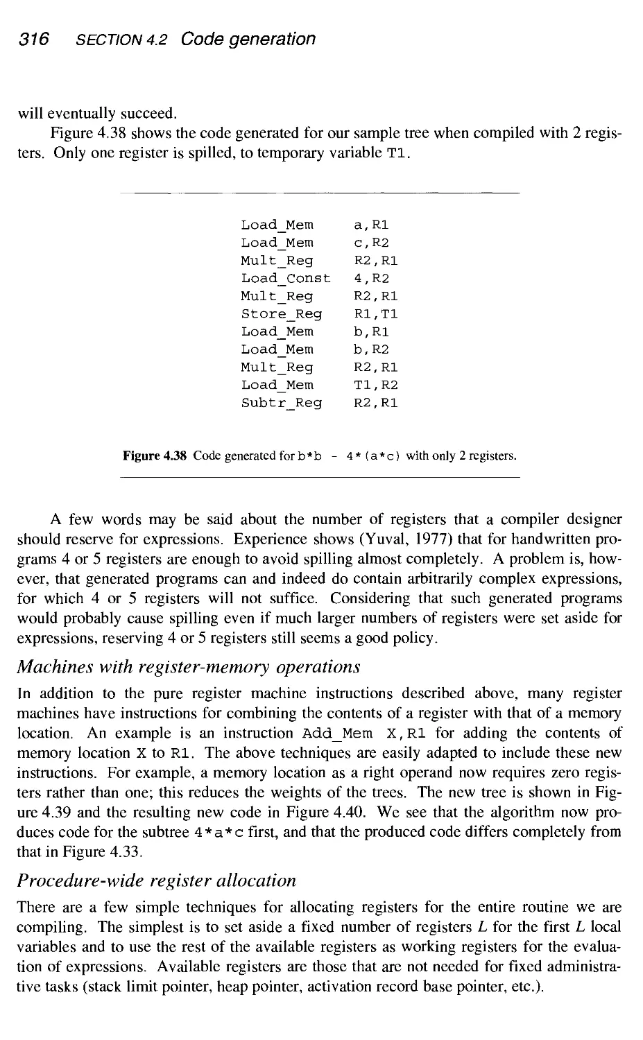
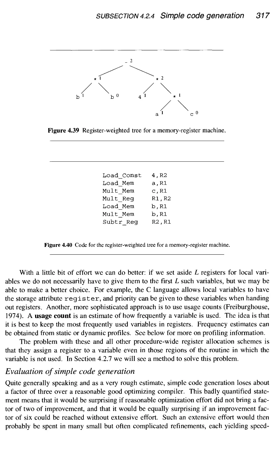
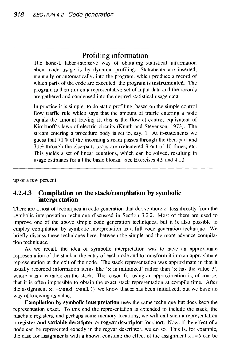
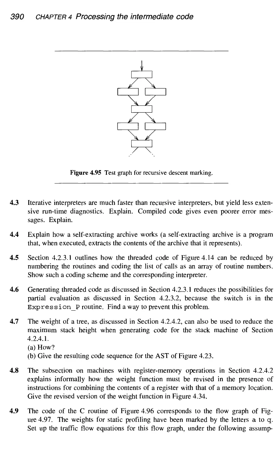
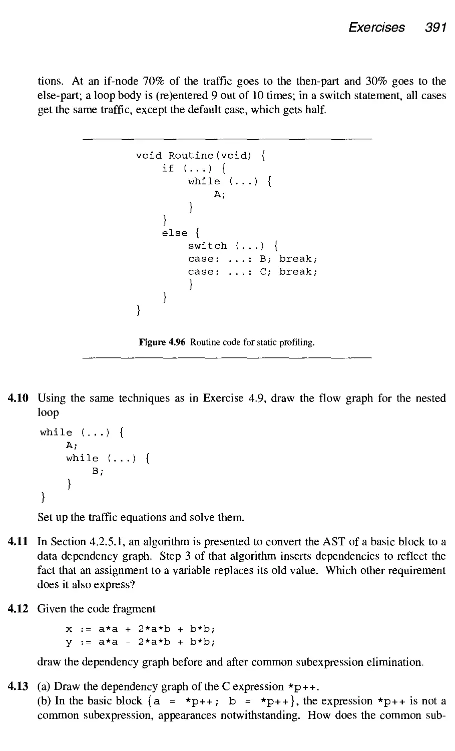
/


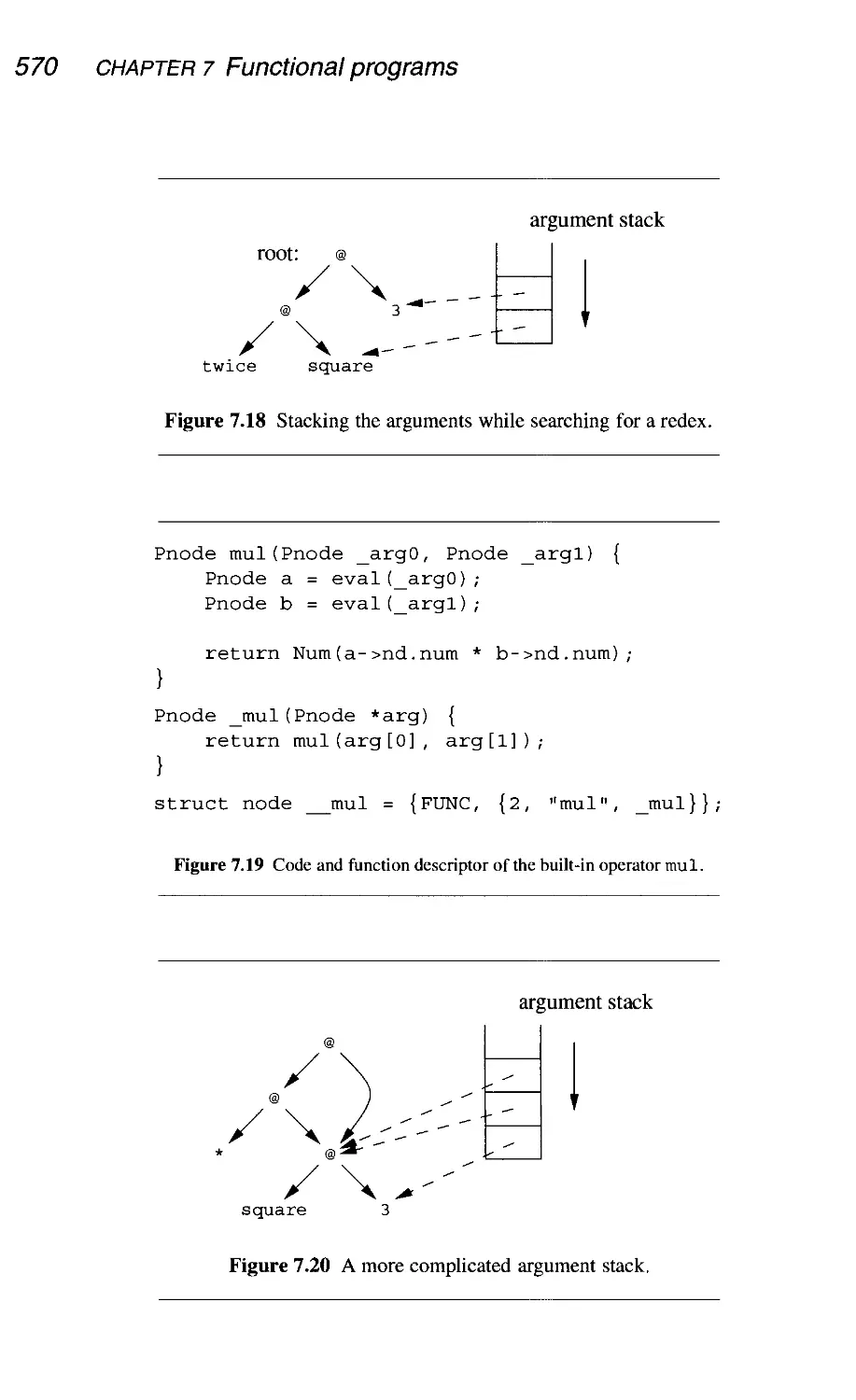
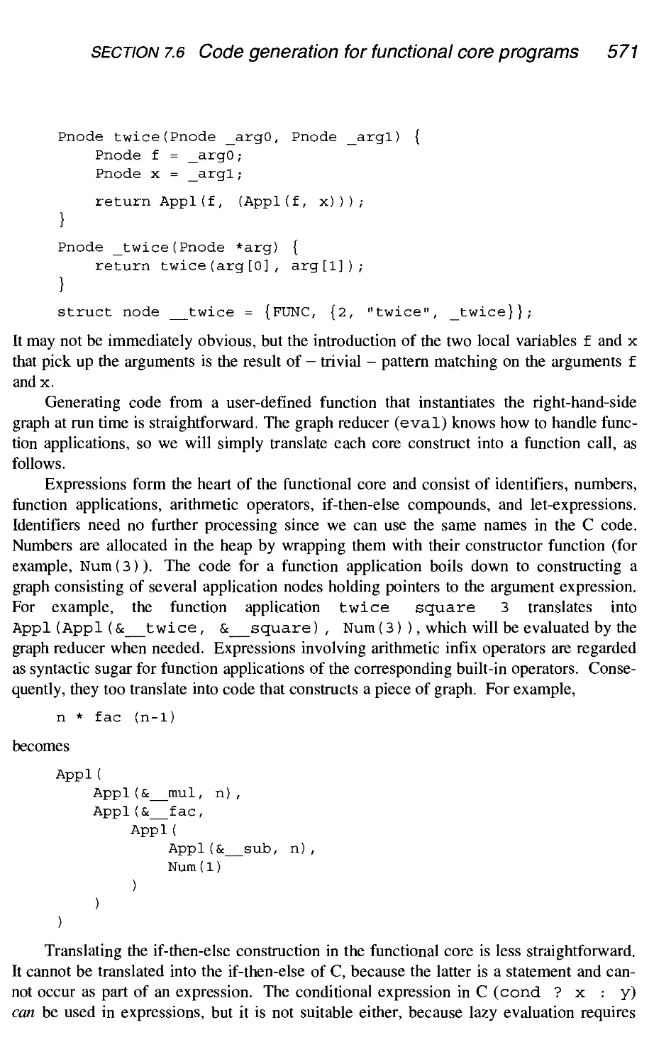


Tags: computer science computer technology computer engineering modern compiler design
ISBN: 0-471-97697-0


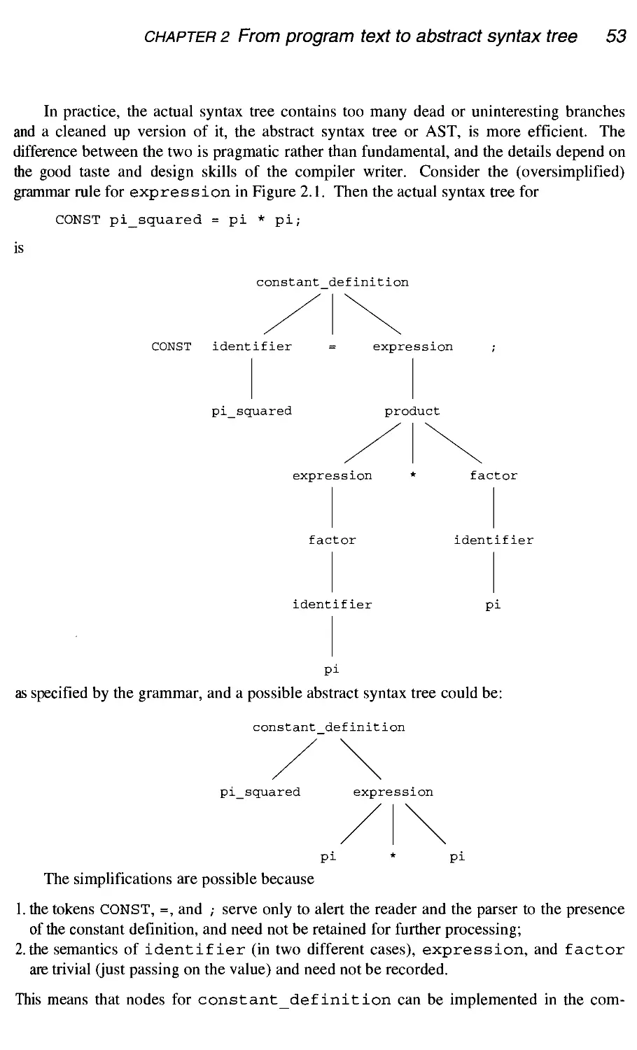
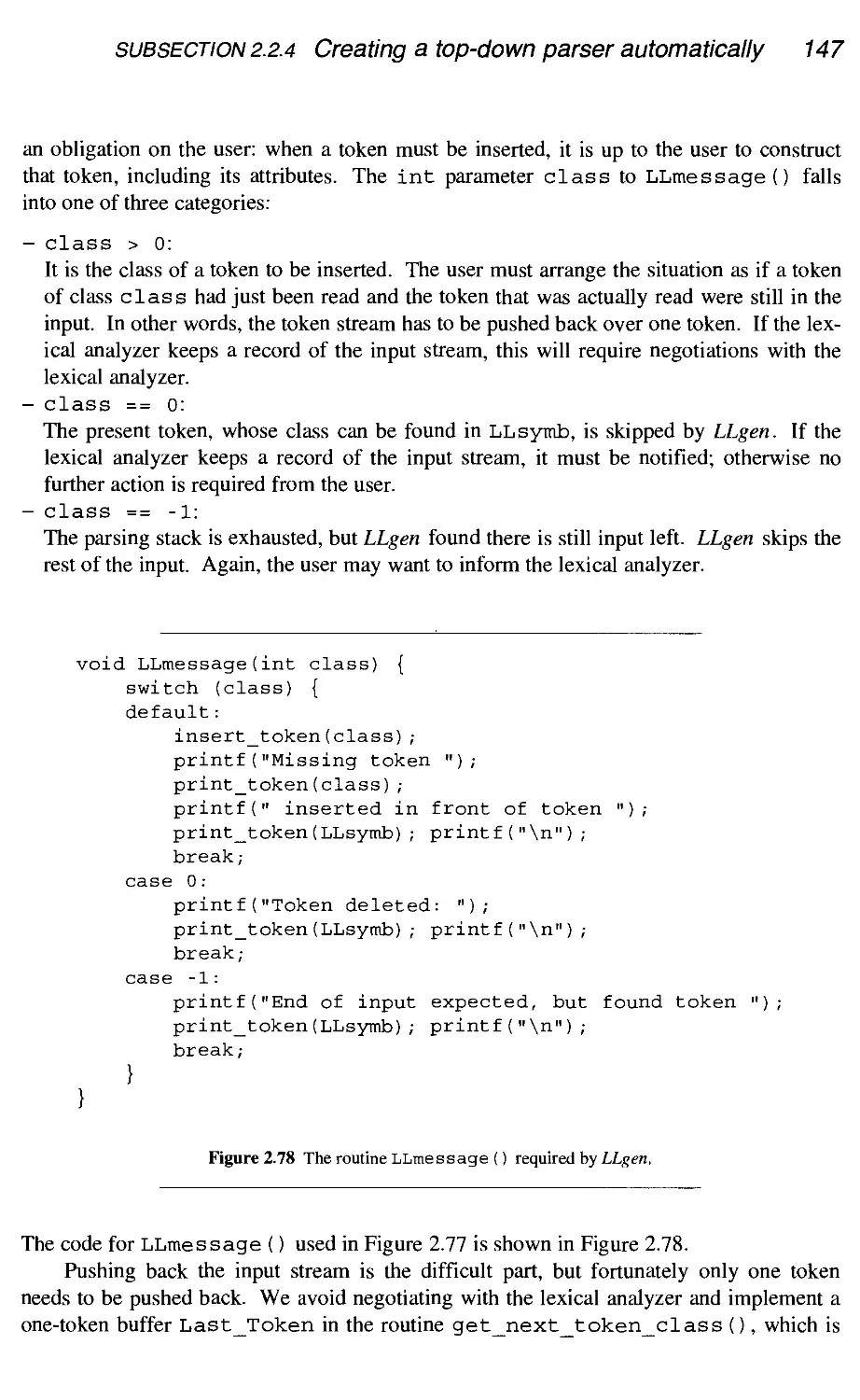
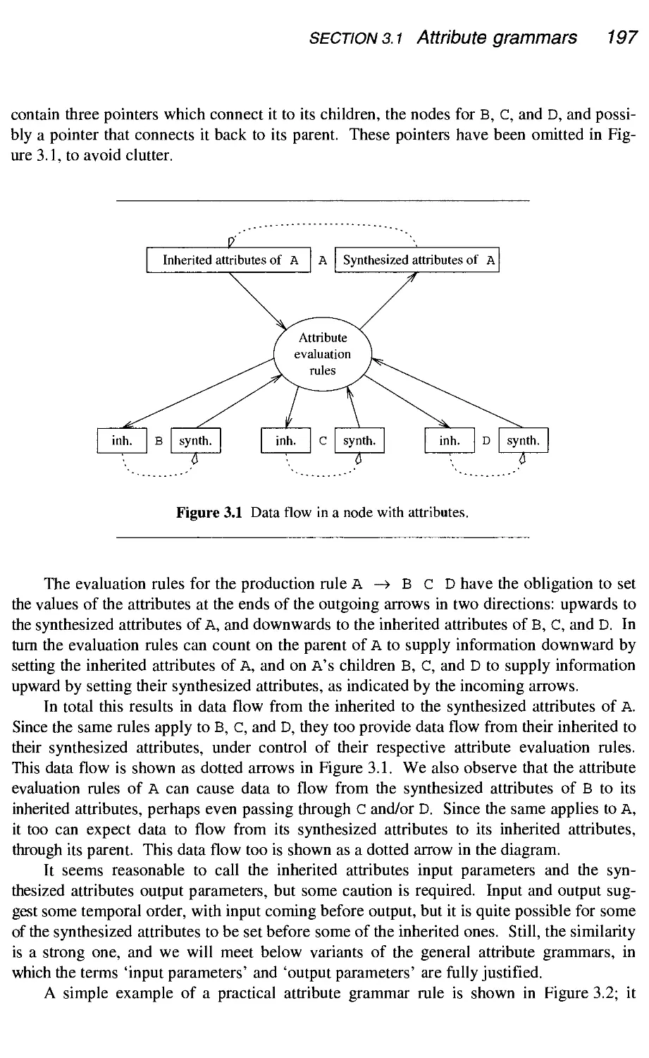
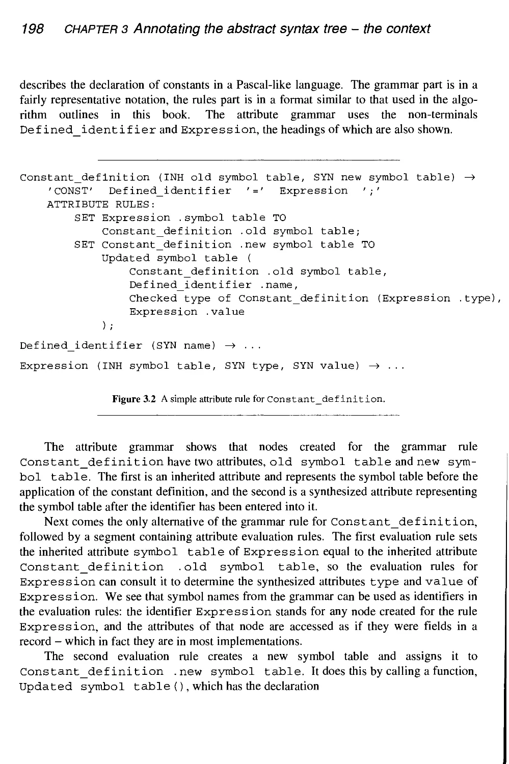
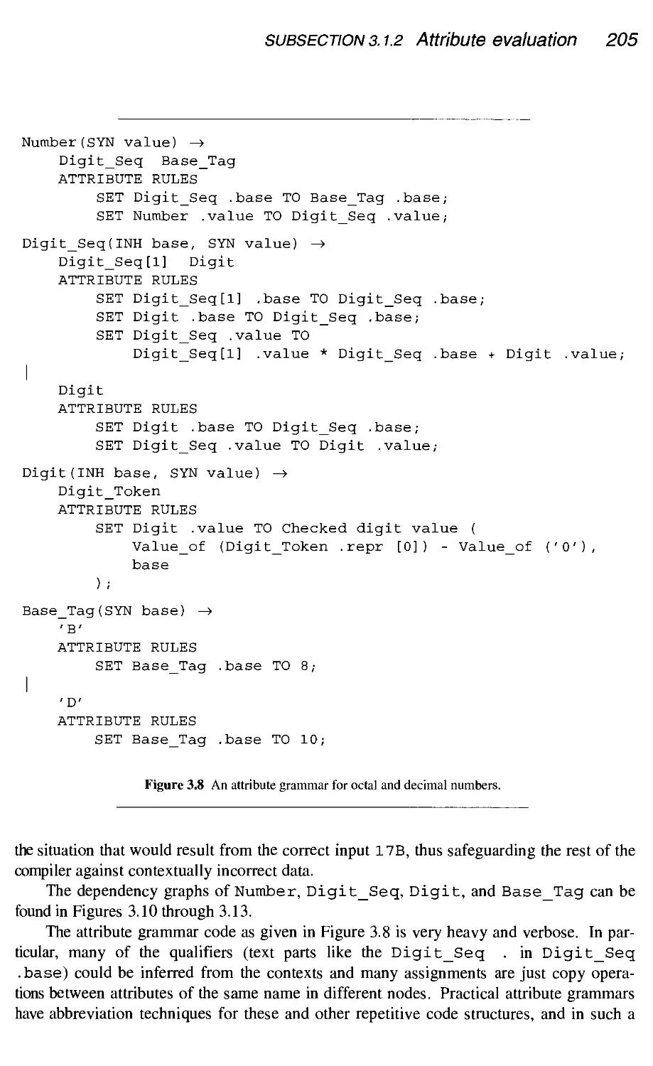
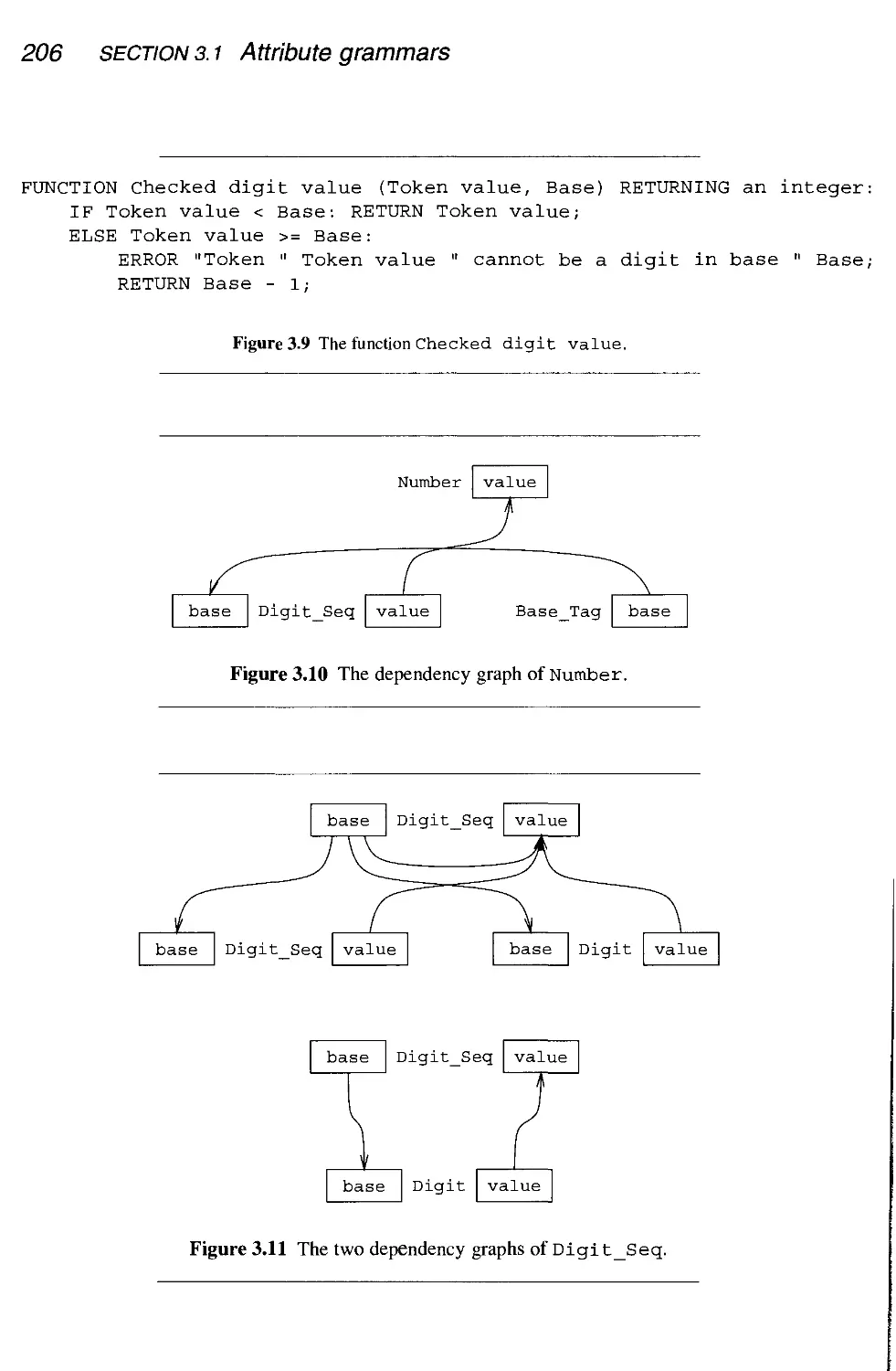
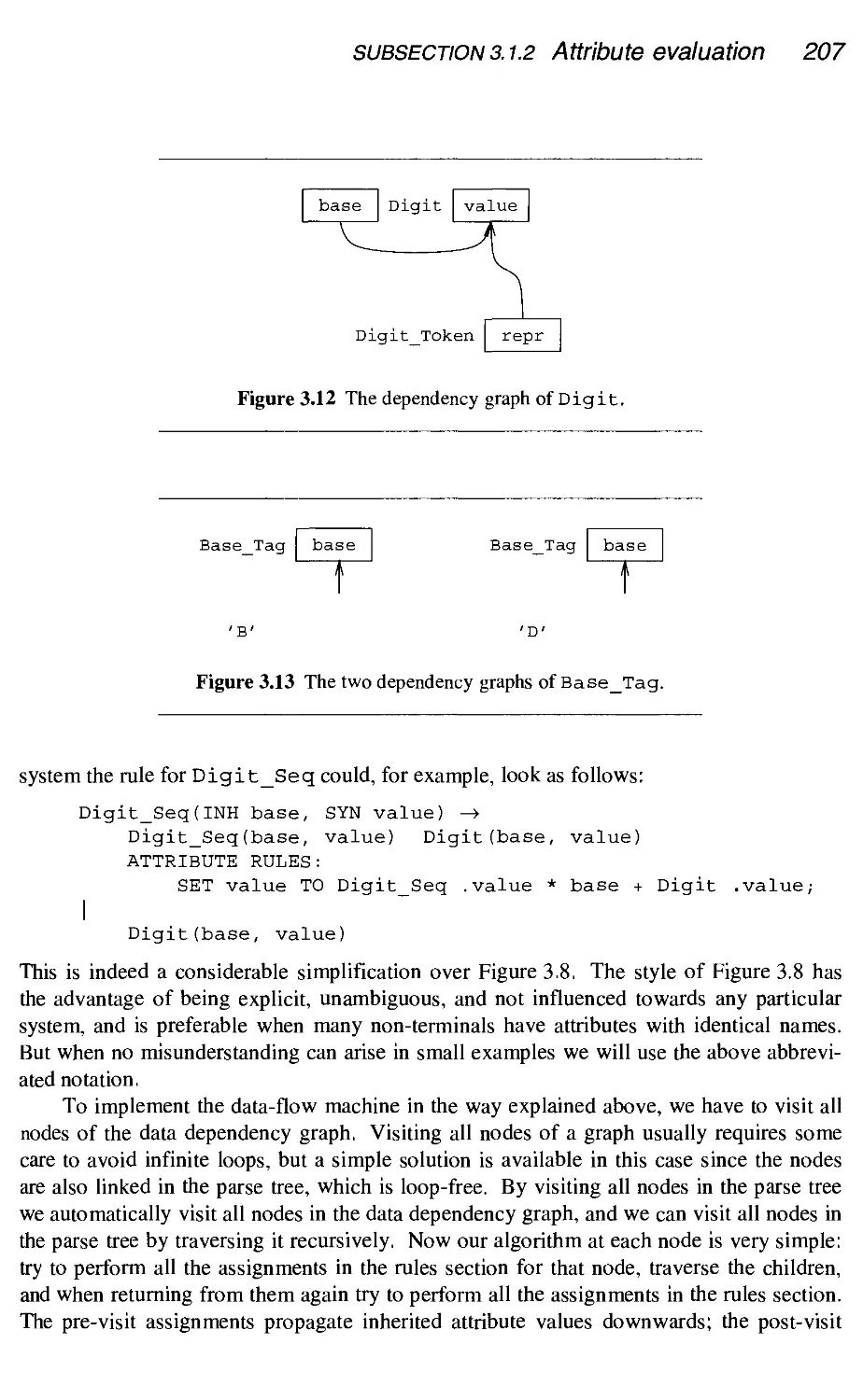
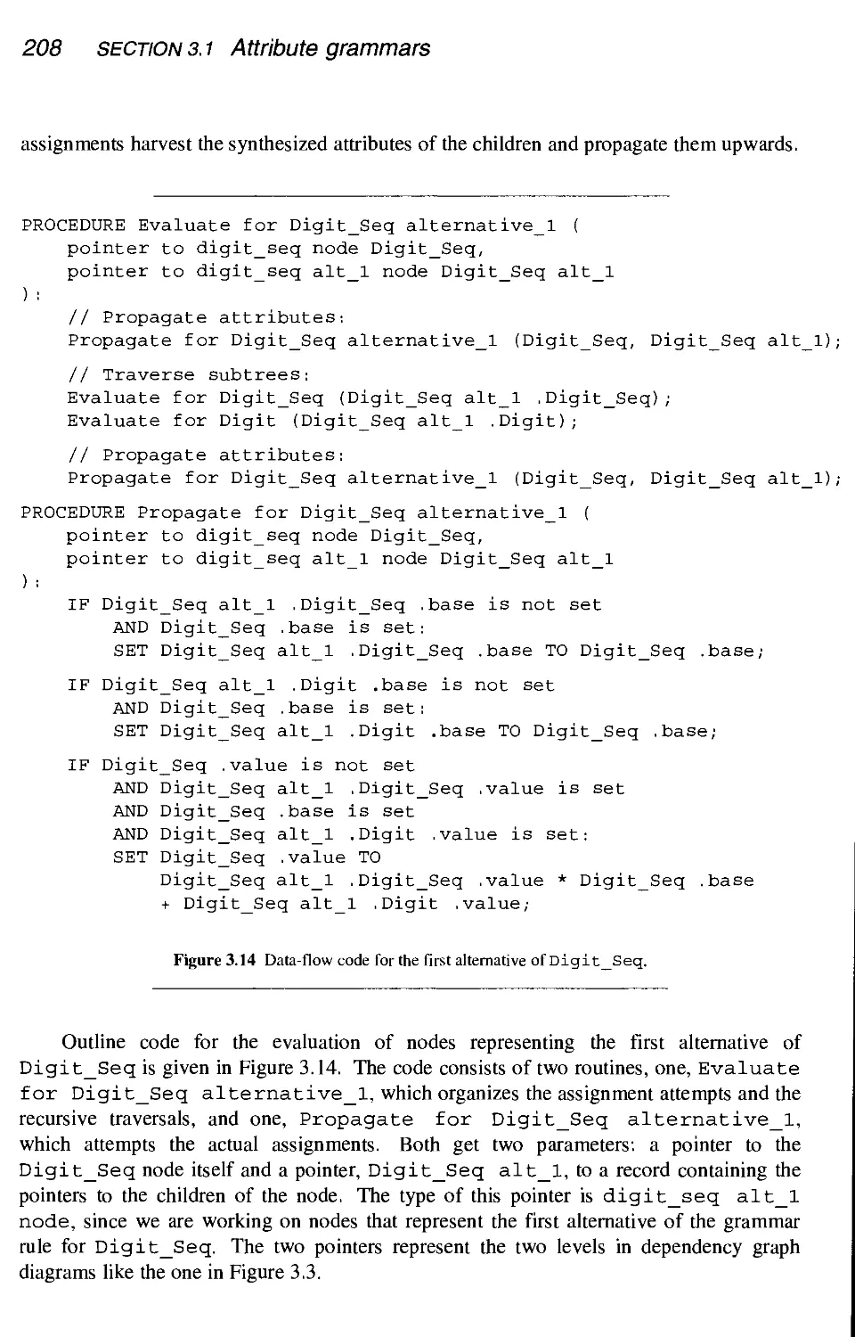
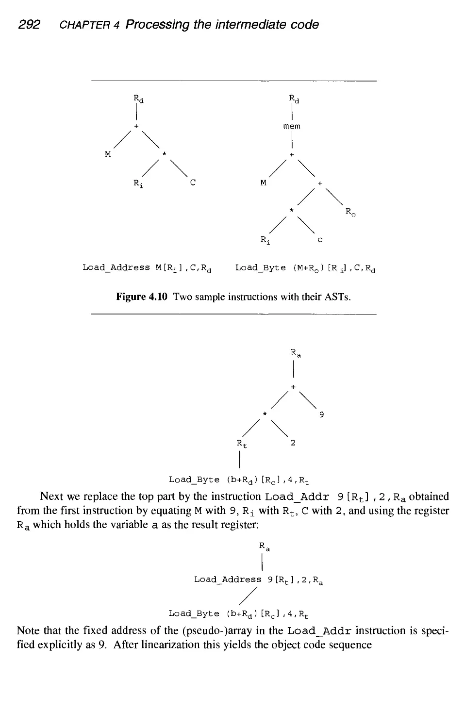
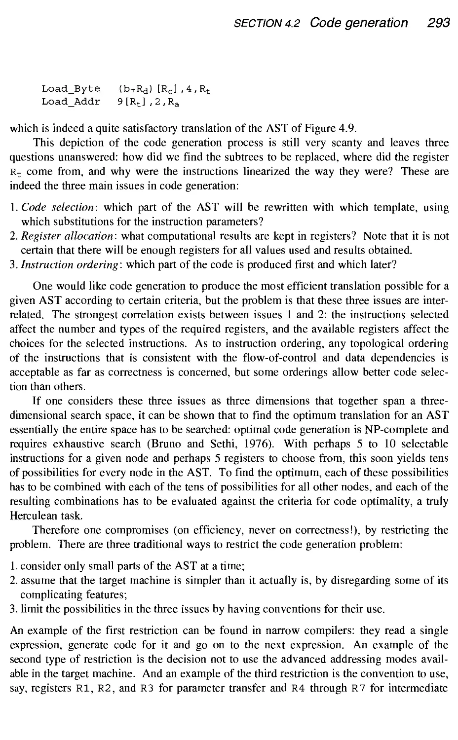
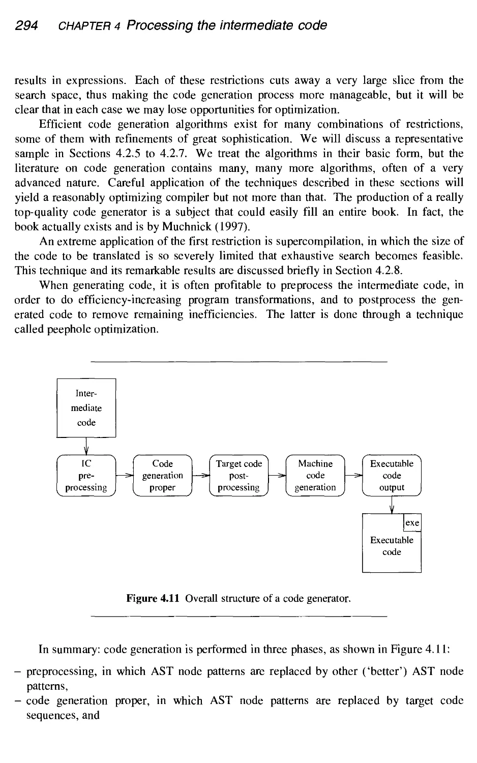
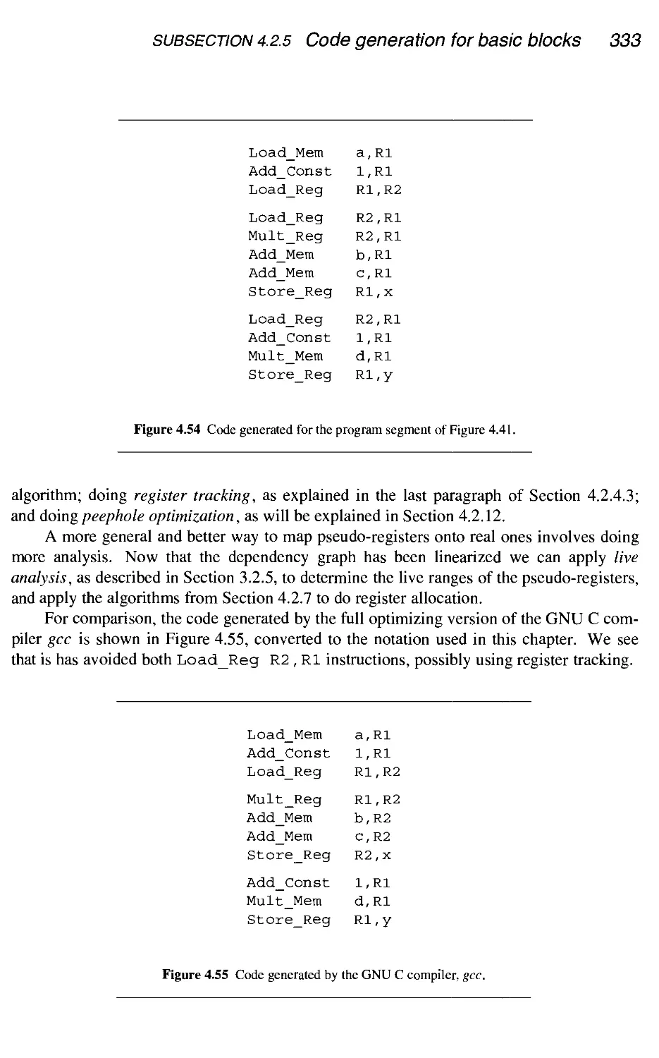
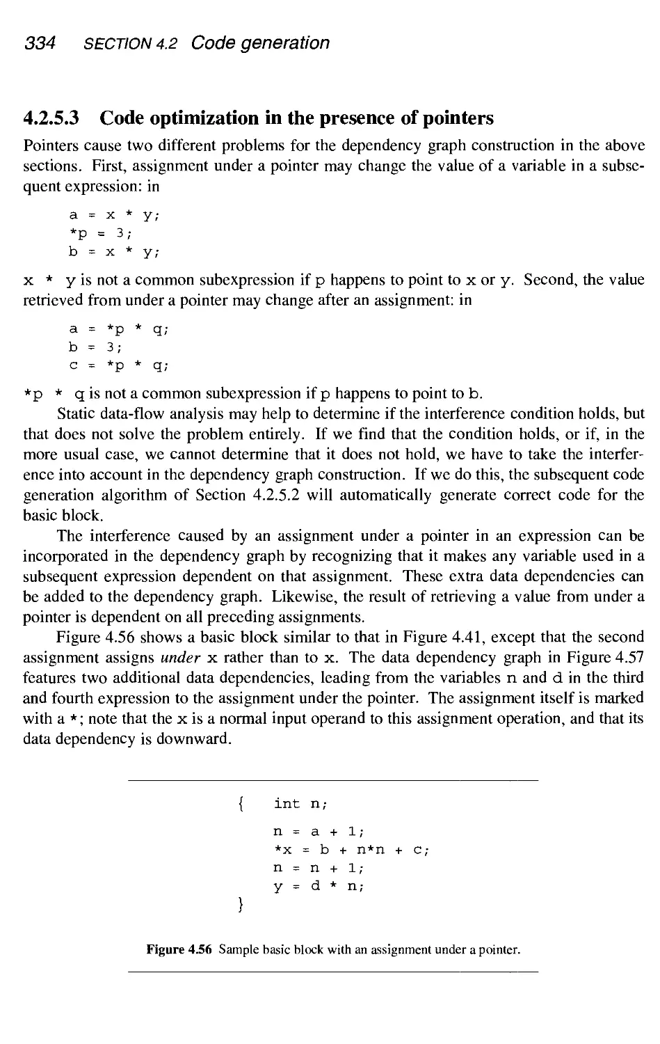
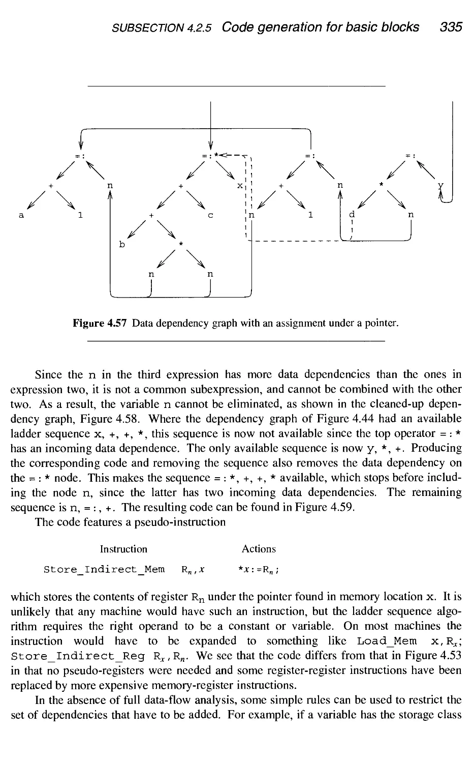
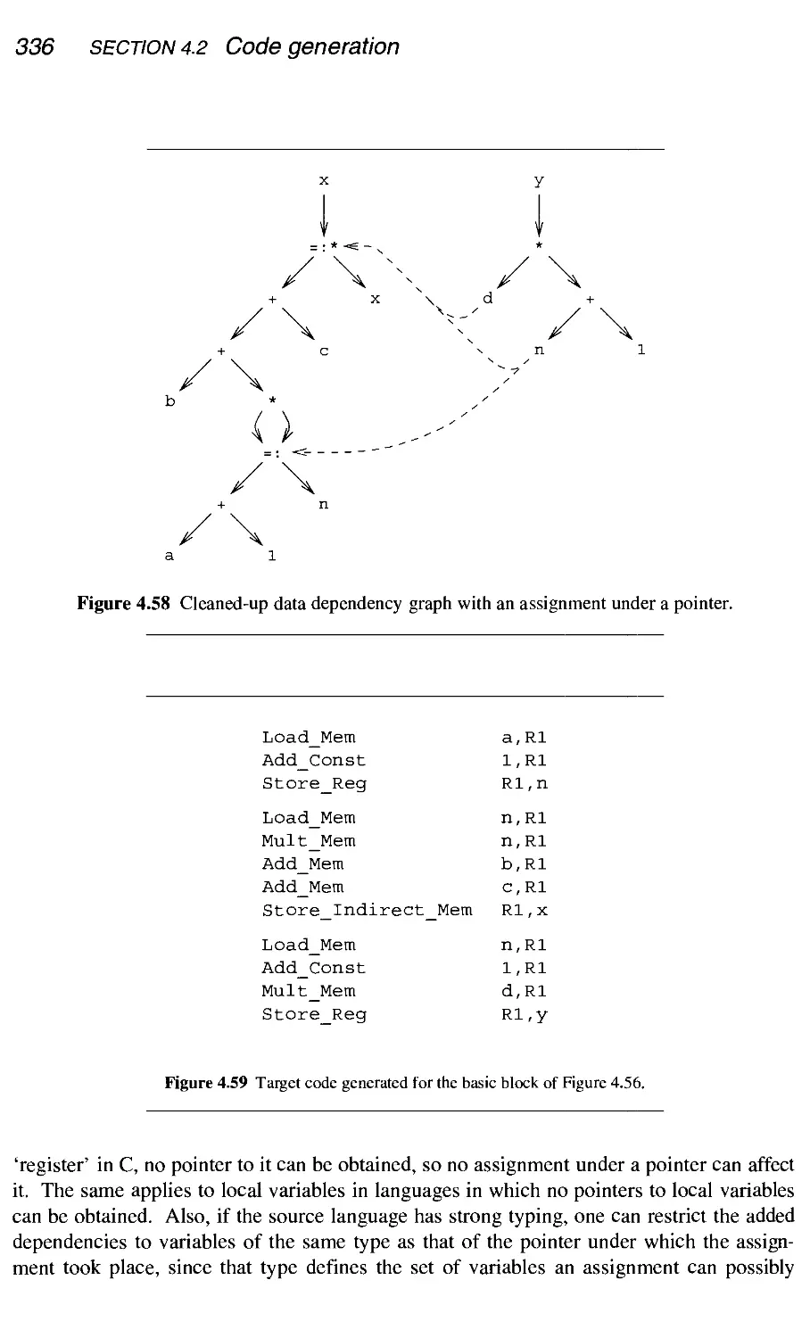
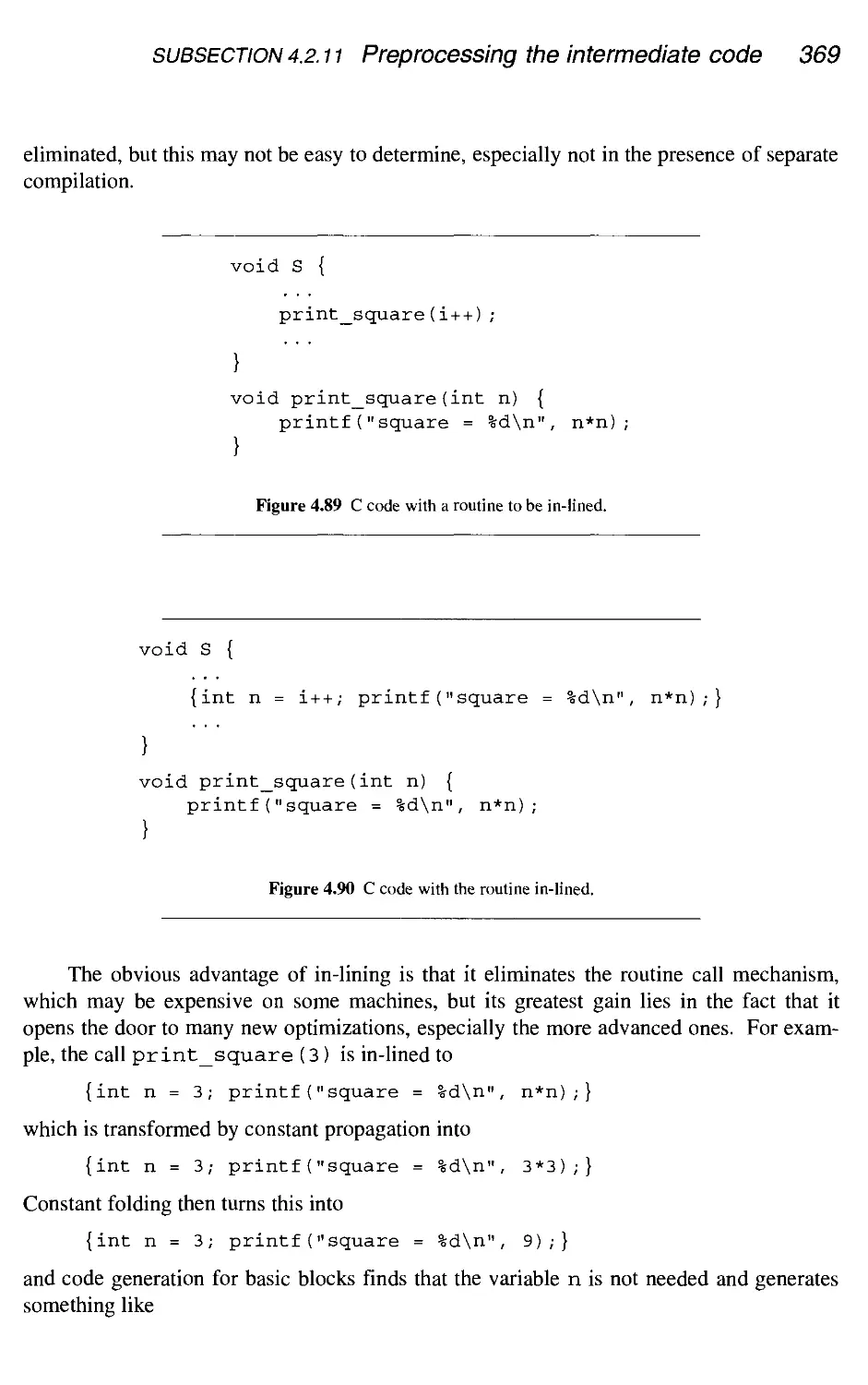
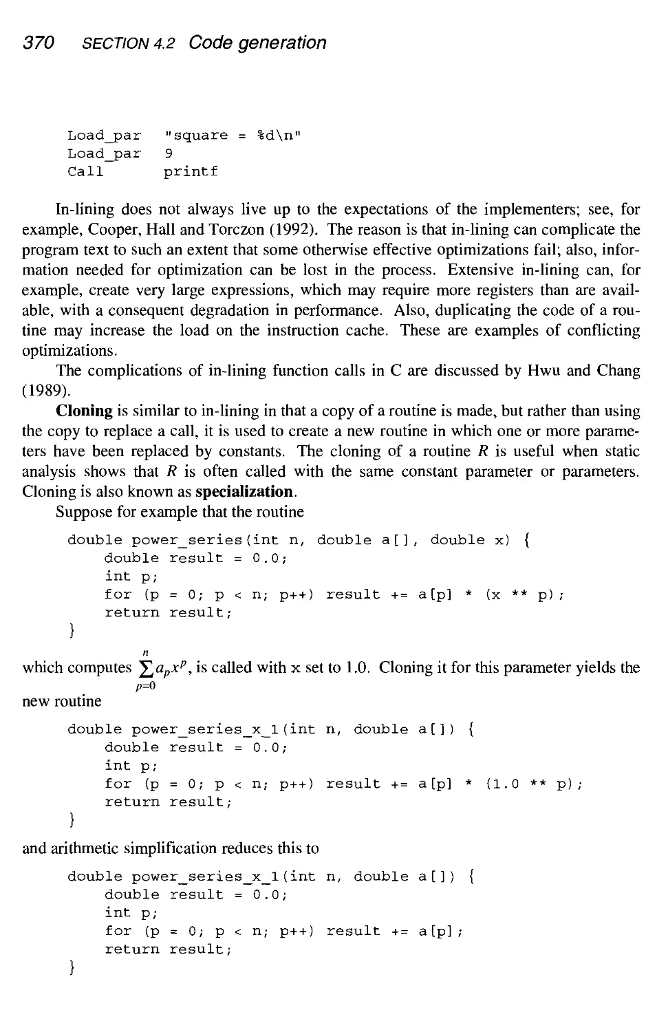
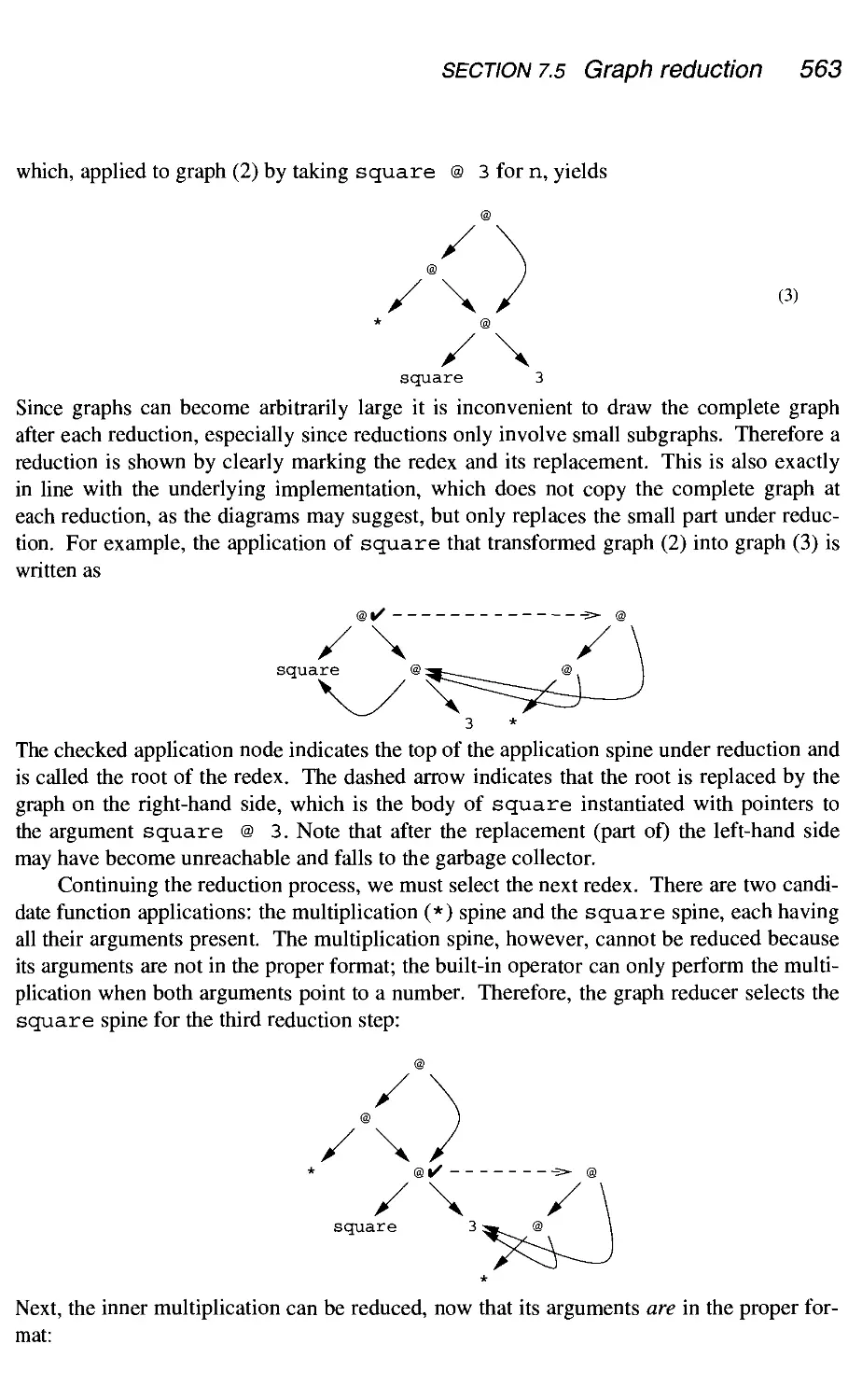
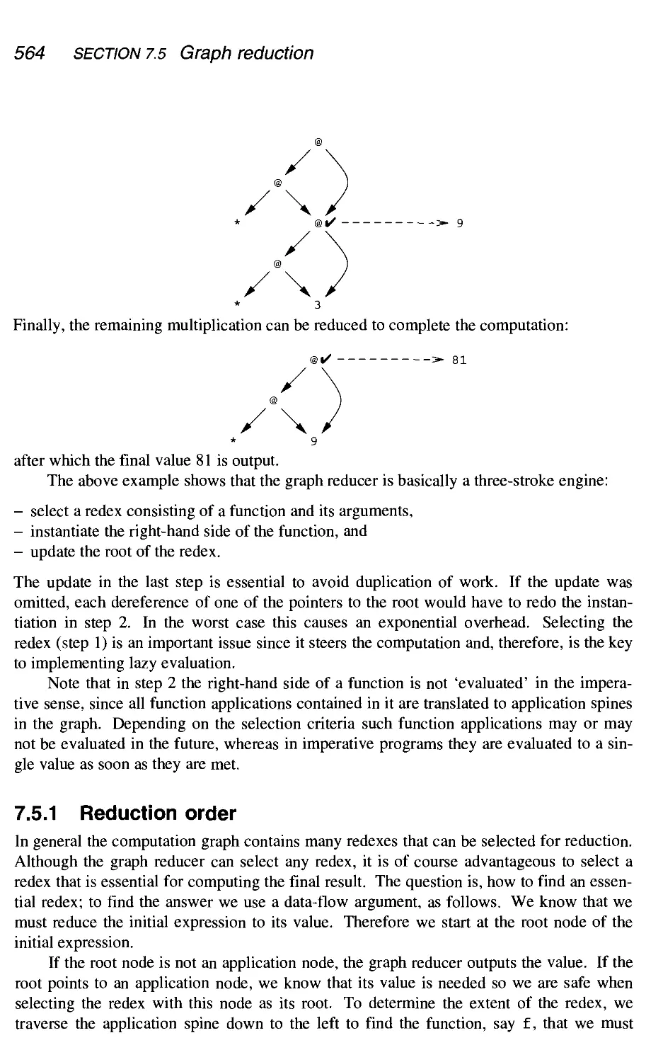
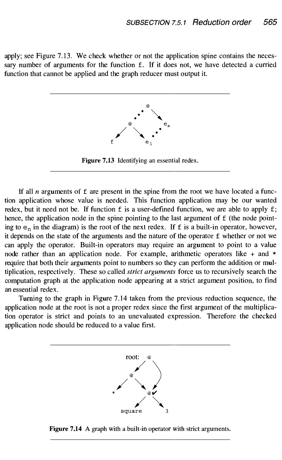
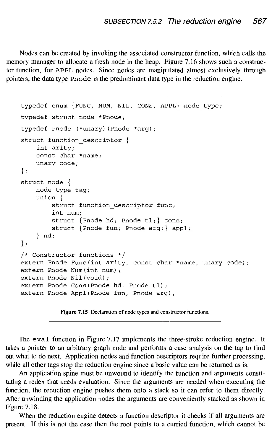
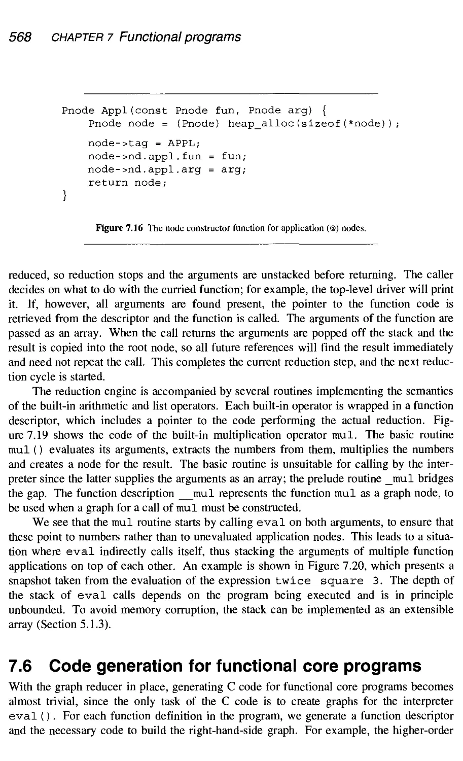
Text
WORLDWIDE
SERIES IN
COMPUTER
SCIENCE
Series Editors Professor David Barron, Southampton University, UK
Professor Peter Wegner, Brown University, USA
The Worldwide series in Computer Science has been created to publish textbooks which
both address and anticipate the needs of an ever evolving curriculum thereby shaping its
future. It is designed for undergraduates majoring in Computer Science and practitioners
who need to reskill. Its philosophy derives from the conviction that the discipline of
computing needs to produce technically skilled engineers who will inevitably face, and
possibly invent, radically new technologies throughout their future careers. New media
will be used innovatively to support high quality texts written by leaders in the field.
Books in Series
Ammeraal, Computer Graphics for Java Programmers
Ammeraal, C++ for Programmers 3rd Edition
Barron, The World of Scripting Languages
Ben-Ari, Ada for Software Engineers
Chapman & Chapman, Digital Multimedia
Gollmann, Computer Security
Goodrich & Tamassia, Data Structures and Algorithms in Java
Kotonya & Sommerville, Requirements Engineering: Processes and Techniques
Lowe & Hall, Hypermedia & the Web: An Engineering Approach
Magee & Kramer, Concurrency: State Models and Java Programs
Peters, Software Engineering: An Engineering Approach
Preiss, Data Structures and Algorithms with Object-Oriented Design Patterns in C++
Preiss, Data Structures and Algorithms with Object-Oriented Design Patterns in Java
Reiss, A Practical Introduction to Software Design with C++
Schneider, Concurrent and Real-time Systems
Winder & Roberts, Developing Java Software 2nd Edition
modern
compiler
design
Dick Grune
Mrye Universiteit, Amsterdam
u
|| Henri E. Bal
!l: Vrije Universiteit, Amsterdam
&:'■
3i»~:
Ceriel J. H. Jacobs
n)e Universiteit, Amsterdam
Koen G. Langendoen
De//t University
E JOHN WILEY & SONS, LTD
Chichester • New York • Weinheim • Brisbane • Singapore • Toronto
Copyright © 2000 by John Wiley & Sons, Ltd, The Atrium,
Southern Gate, Chichester
West Sussex PO19 8SQ, England
Telephone (+44) 1243 779777
Email (for orders and customer service enquiries): cs-books@wiley.co.uk
Visit our Home Page www.wileyeurope.com or www.wiley.com
Reprinted March 2001, October 2002, December 2003
All Rights Reserved. No part of this publication may be reproduced, stored in a retrieval
system or transmitted in any form or by any means, electronic, mechanical, photocopying, recording,
scanning or otherwise, except under the terms of the Copyright, Designs and Patents Act 1988 or
under the terms of a licence issued by the Copyright Licensing Agency Ltd, 90 Tottenham Court
Road, London WIT 4LP, UK, without the permission in writing of the Publisher. Requests to the
Publisher should be addressed to the Permissions Department, John Wiley & Sons Ltd, The Atrium,
Southern Gate, Chichester, West Sussex PO19 8SQ, England, or emailed to permreq@wiley.co.uk, or
faxed to (+44) 1243 770571.
This publication is designed to provide accurate and authoritative information in regard to the subject
matter covered. It is sold on the understanding that the Publisher is not engaged in rendering profes-
professional services. If professional advice or other expert assistance is required, the services of a compe-
competent professional should be sought.
Other Wiley Editorial Offices
John Wiley & Sons Inc., 111 River Street, Hoboken, NJ 07030, USA
Jossey-Bass, 989 Market Street, San Francisco, CA 94103-1741, USA
Wiley-VCH Verlag GmbH, Boschstr. 12, D-69469 Weinheim, Germany
John Wiley & Sons Australia Ltd, 33 Park Road, Milton, Queensland 4064, Australia
John Wiley & Sons (Asia) Pte Ltd, 2 Clementi Loop #02-01, Jin Xing Distripark, Singapore 129809
John Wiley & Sons (Canada) Ltd, 22 Worcester Road, Etobicoke, Ontario M9W 1L1
Wiley also publishes its books in a variety of electronic formats. Some content that appears
in print may not be available in electronic books.
British Library Cataloguing in Publication Data
A catalogue record for this book is available from the British Library.
ISBN 0-471-97697-0
Printed and bound, from authors' own electronic files, in Great Britain
by Biddies Ltd, King's Lynn, Norfolk
This book is printed on acid-free paper responsibly manufactured from sustainable
forestry, for which at least two trees are planted for each one used for paper production.
Contents
Preface
Xlll
1 Introduction
1.1 Why study compiler construction?
.1.1 Compiler construction is very successful
.1.2 Compiler construction has a wide applicability
.1.3 Compilers contain generally useful algorithms
1.2 A simple traditional modular compiler/interpreter
.2.1 The abstract syntax tree
.2.2 Structure of the demo compiler
.2.3 The language for the demo compiler
.2.4 Lexical analysis for the demo compiler
.2.5 Syntax analysis for the demo compiler
.2.6 Context handling for the demo compiler
.2.7 Code generation for the demo compiler
1.2.8 Interpretation for the demo compiler
1.3 The structure of a more realistic compiler
1.3.1 The structure
1.3.2 Run-time systems
1.3.3 Short-cuts
1.4 Compiler architectures
1.4.1 The width of the compiler
1.4.2 Who's the boss?
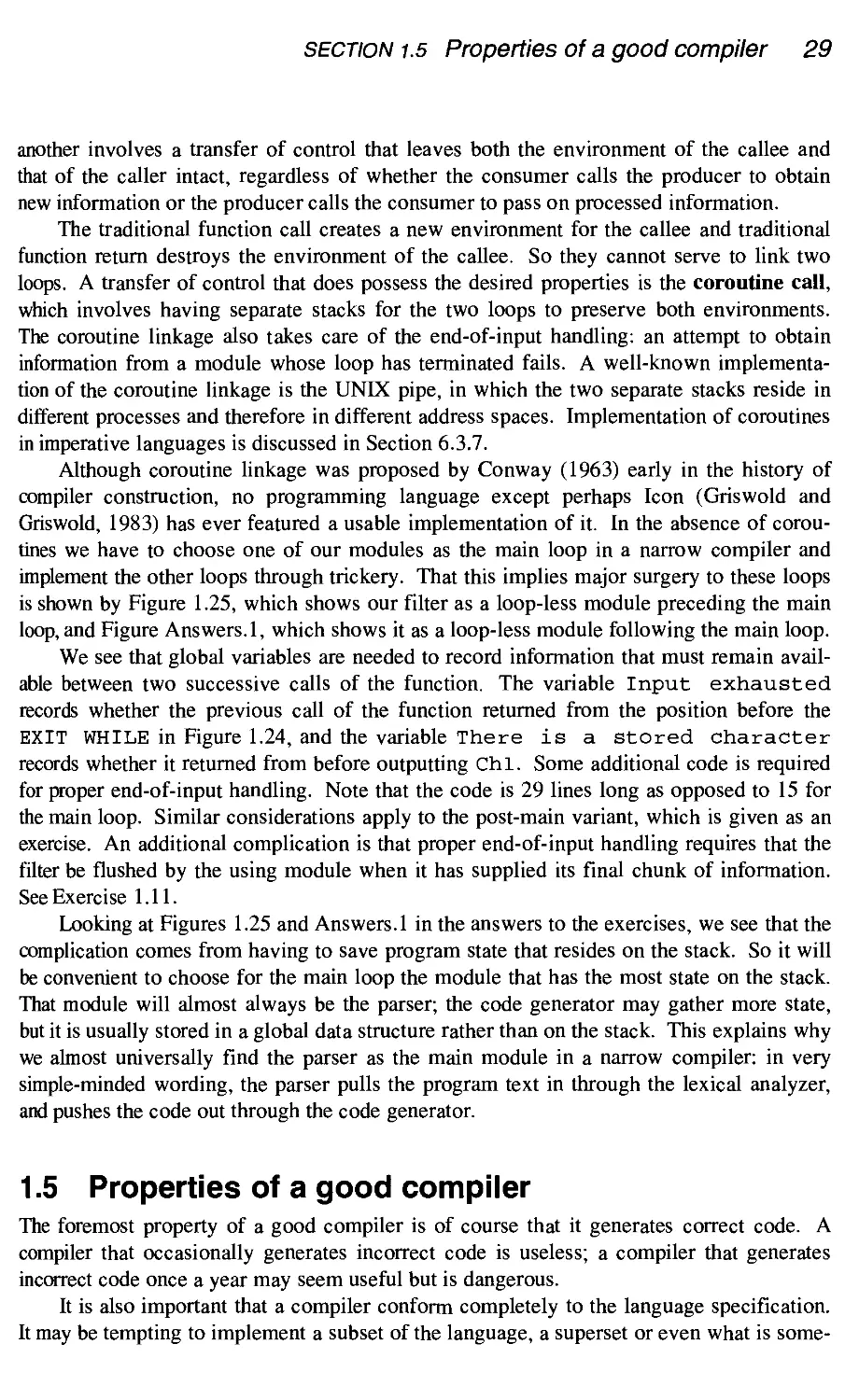
1.5 Properties of a good compiler
1
4
6
9
9
11
12
13
14
19
19
21
22
22
24
25
25
26
27
29
vi Contents
1.6 Portability and retargetability
1.7 Place and usefulness of optimizations
1.8 A short history of compiler construction
1.8.1 1945-1960: code generation
1.8.2 1960-1975: parsing
1.8.3 1975-present: code generation and code optimization;
paradigms
1.9 Grammars
1.9.1 The form of a grammar
1.9.2 The production process
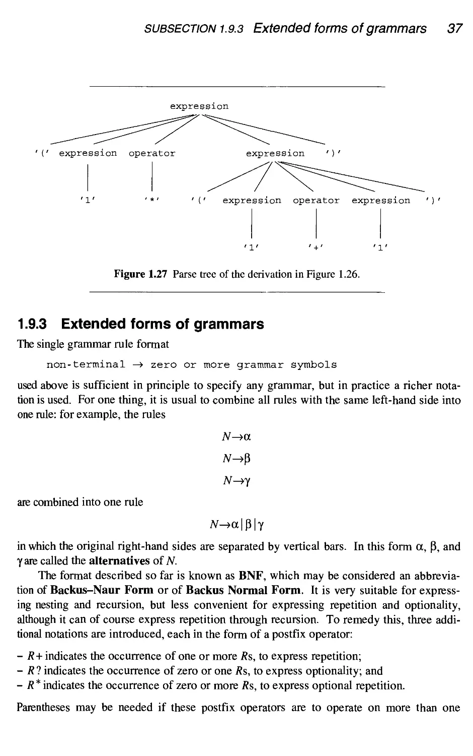
1.9.3 Extended forms of grammars
1.9.4 Properties of grammars
1.9.5 The grammar formalism
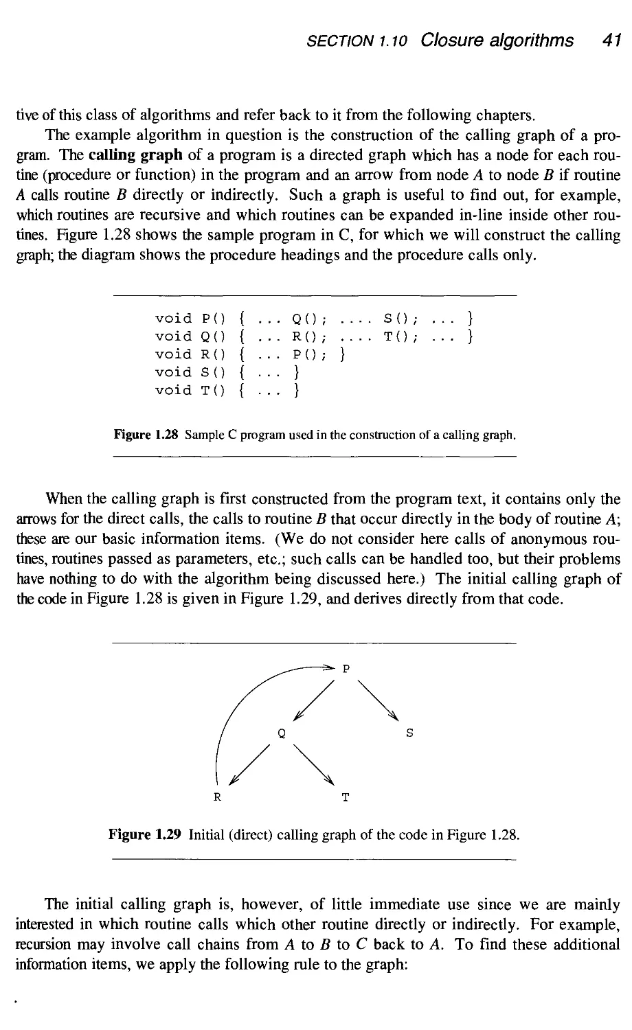
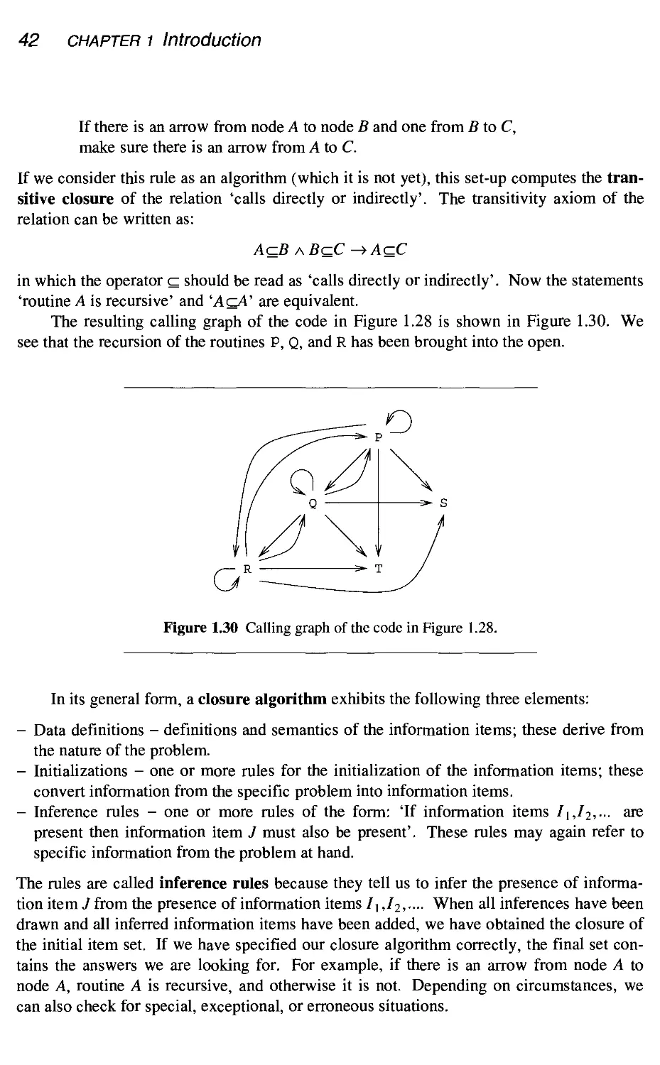
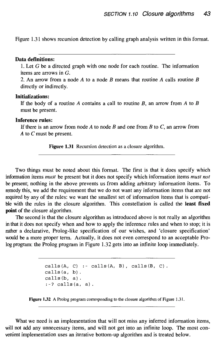
1.10 Closure algorithms
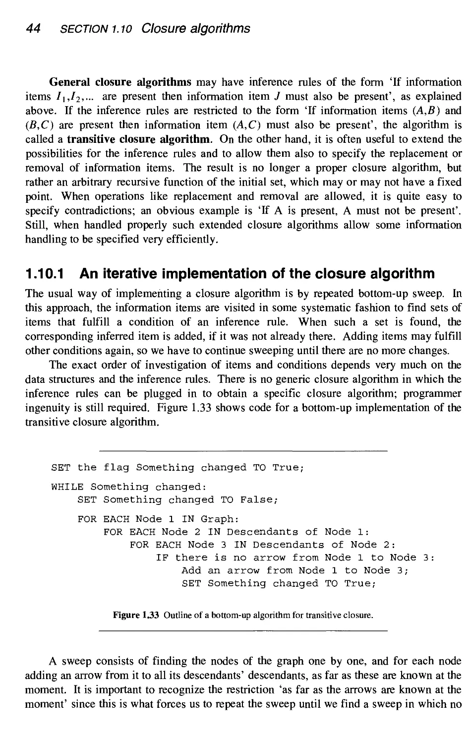
1.10.1 An iterative implementation of the closure algorithm
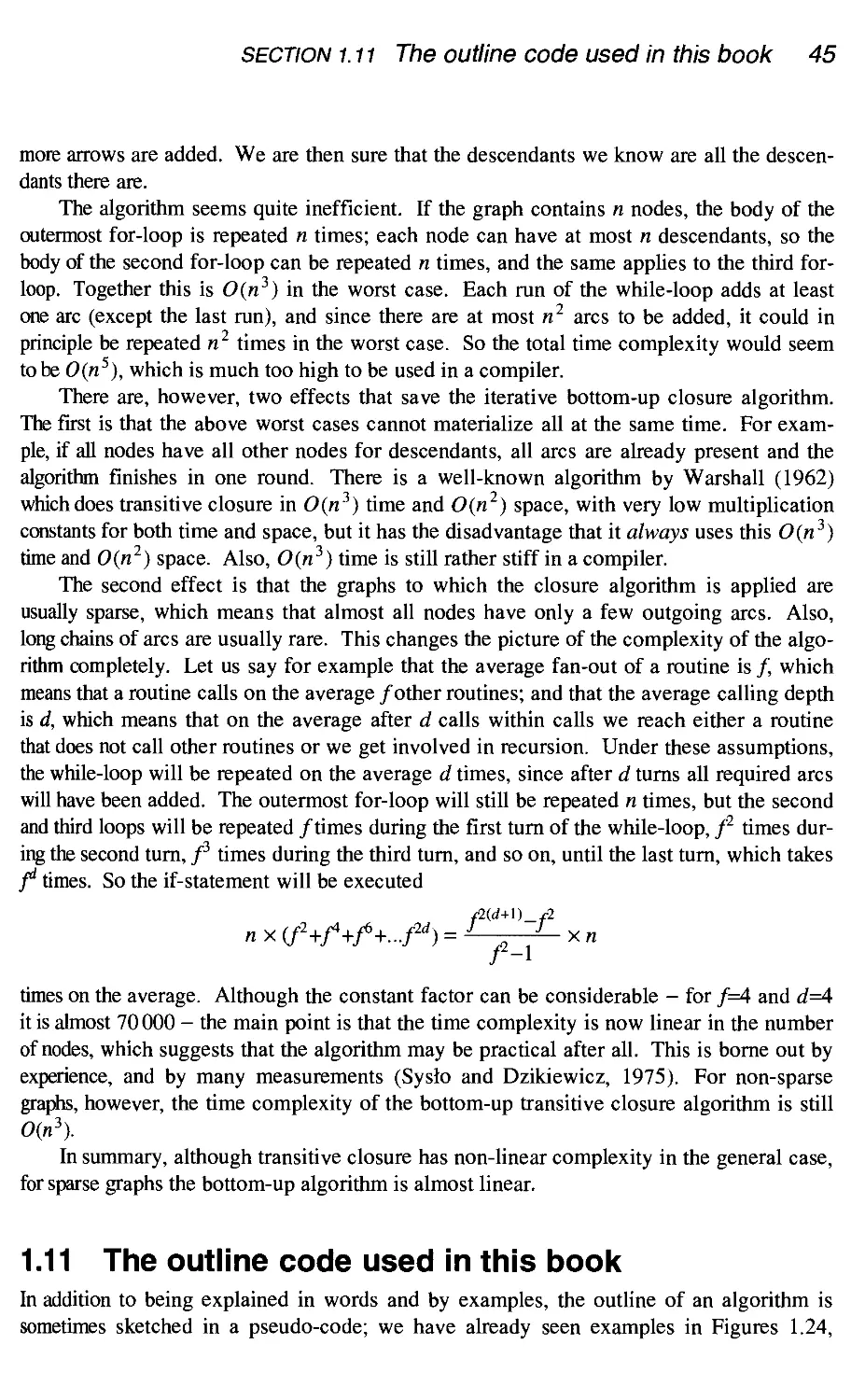
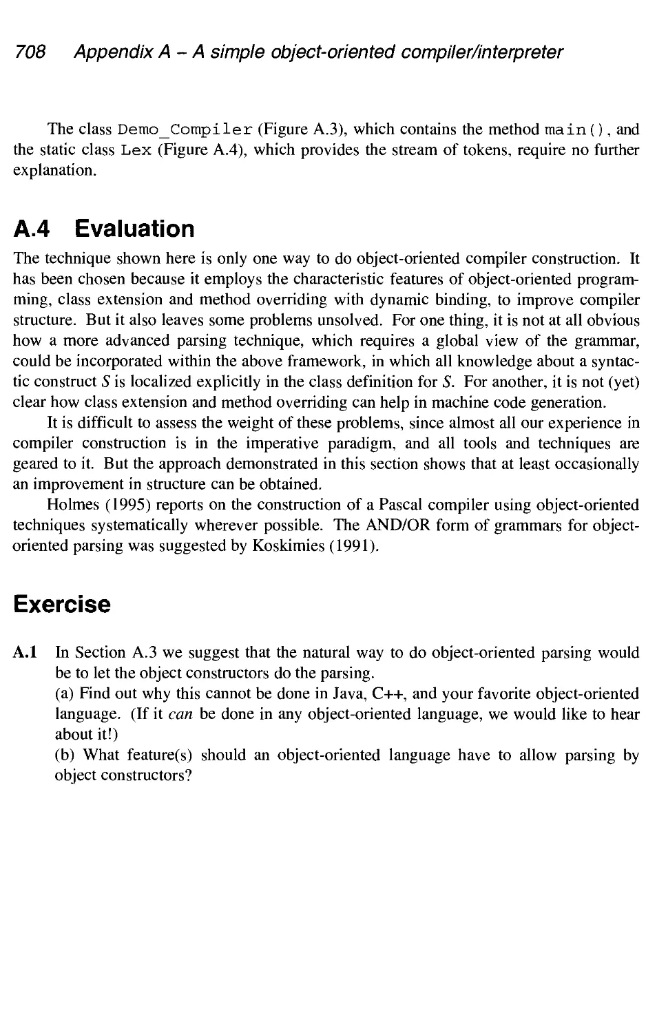
1.11 The outline code used in this book
1.12 Conclusion
Summary
Further reading
Exercises
32
32
33
33
33
34
34
35
35
37
38
38
40
44
45
47
47
48
49
2 From program text to abstract syntax tree
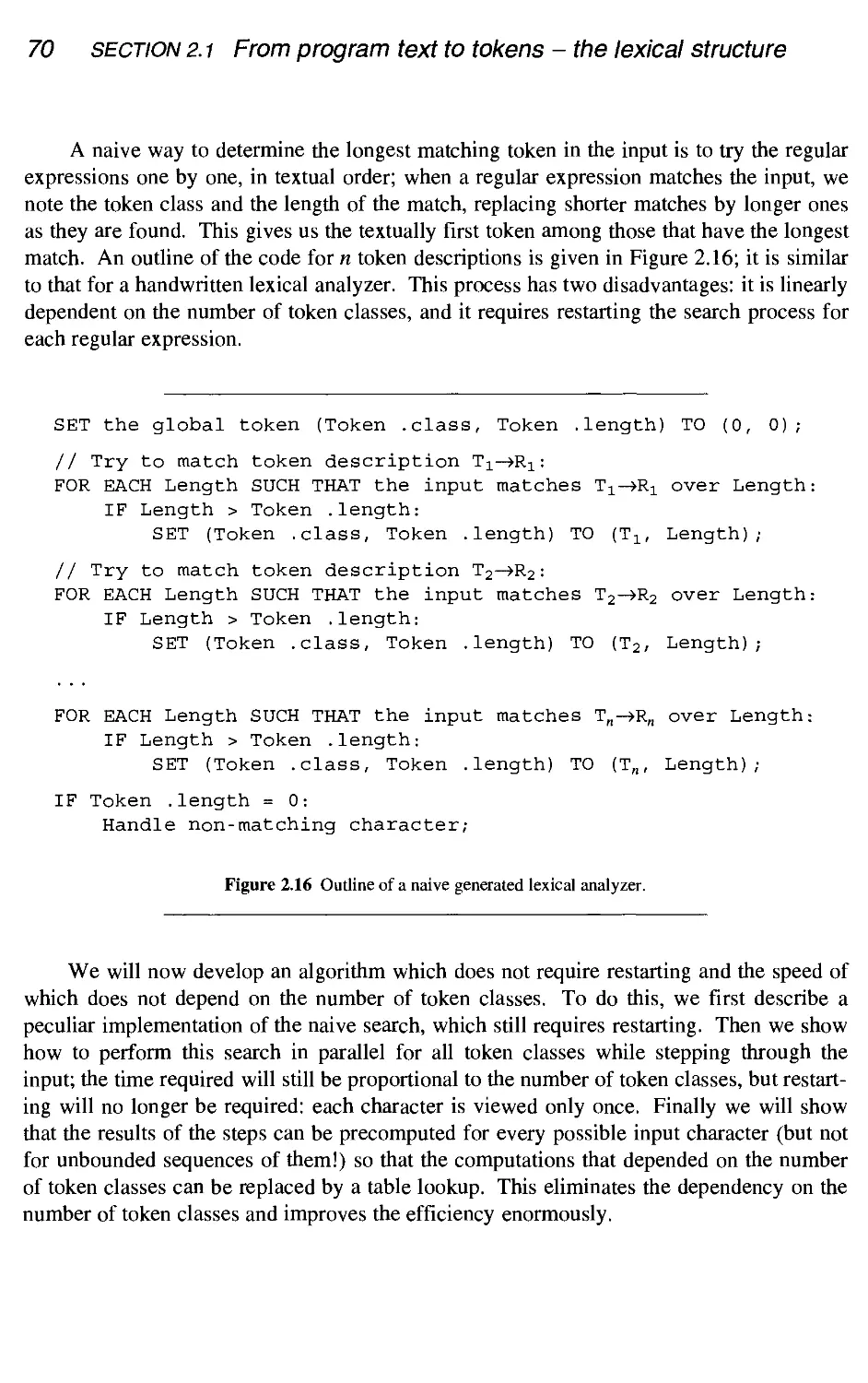
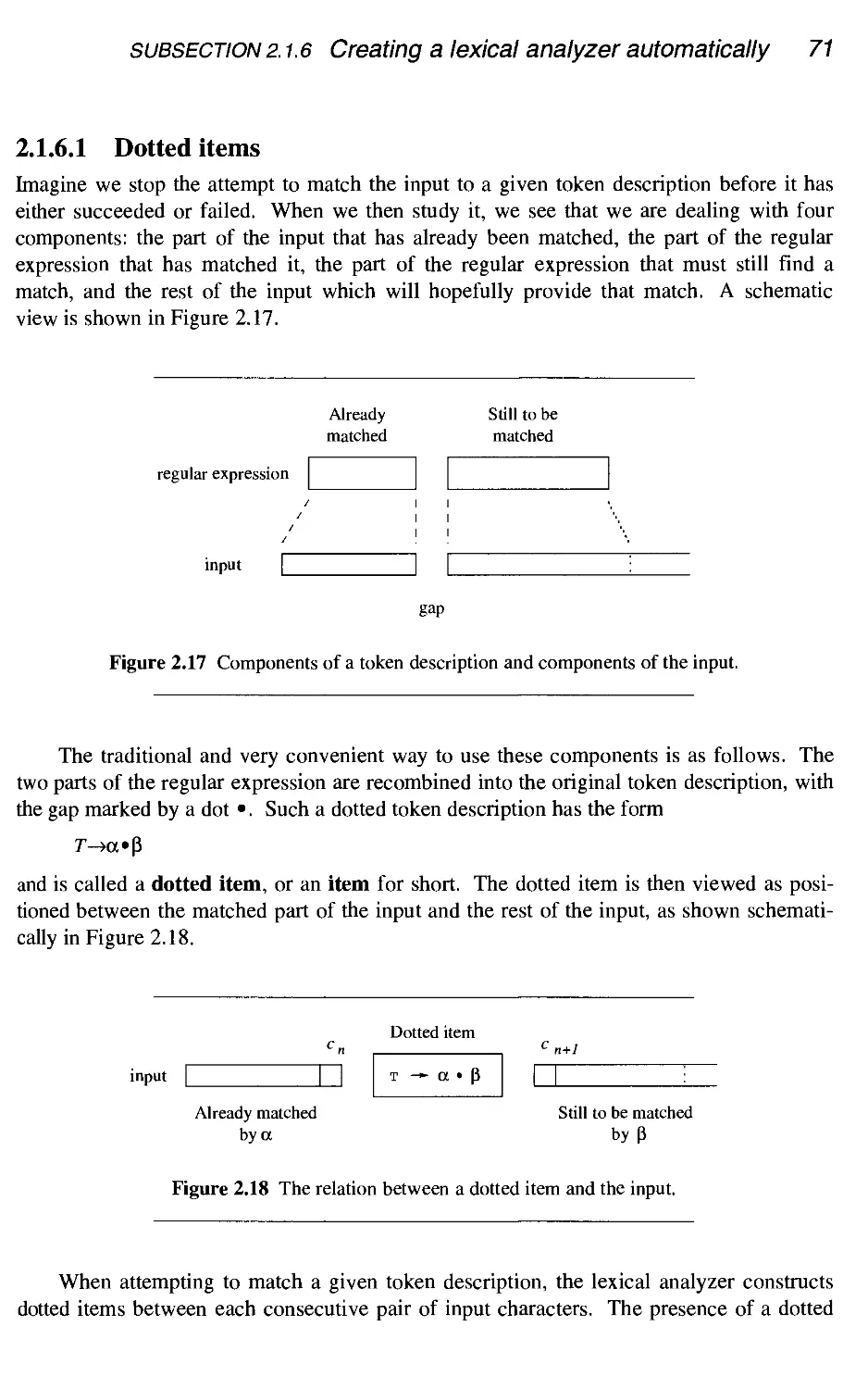
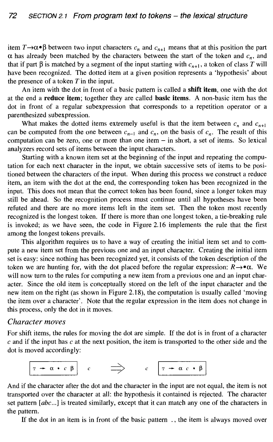
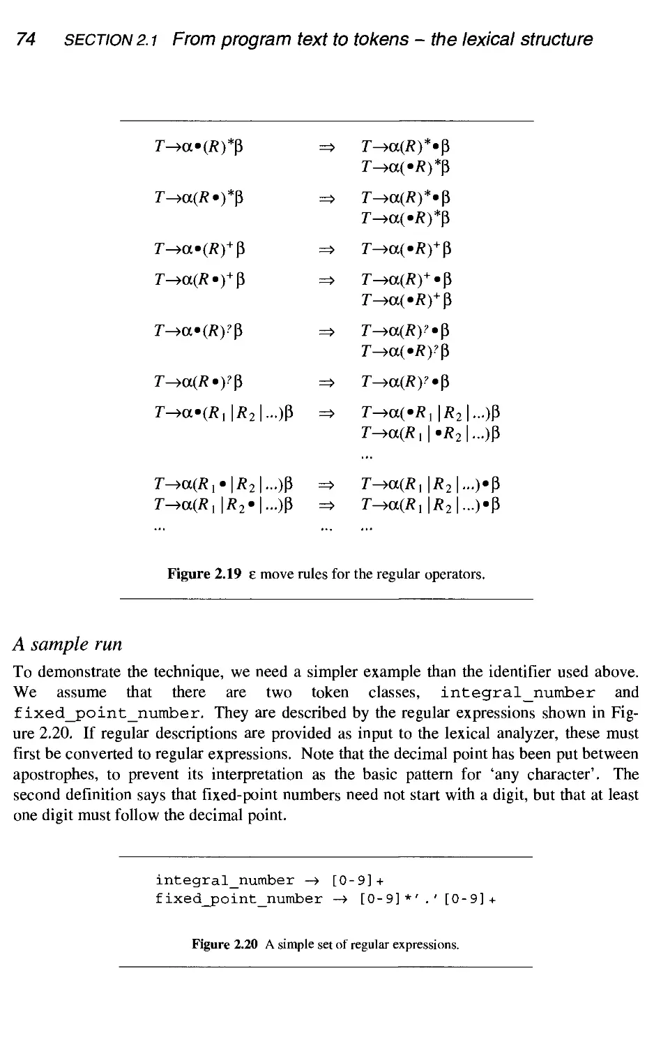
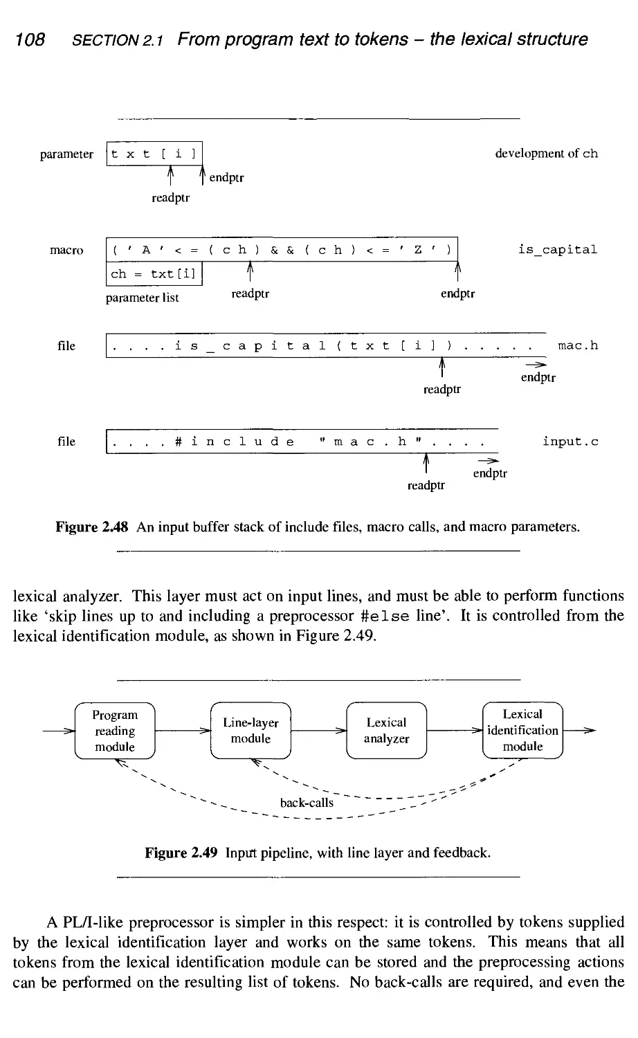
2.1 From program text to tokens - the lexical structure
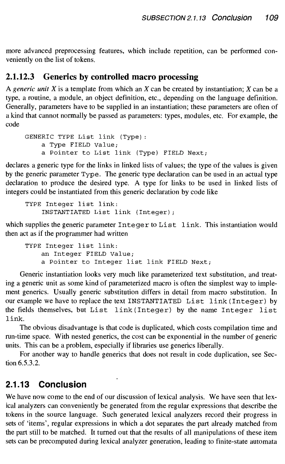
Reading the program text
Lexical versus syntactic analysis
Regular expressions and regular descriptions
Lexical analysis
Creating a lexical analyzer by hand
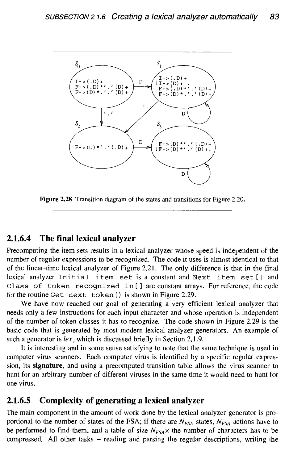
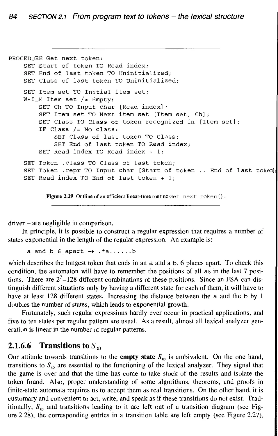
Creating a lexical analyzer automatically
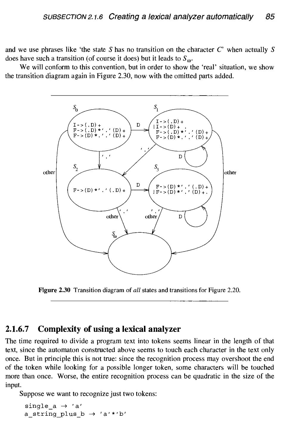
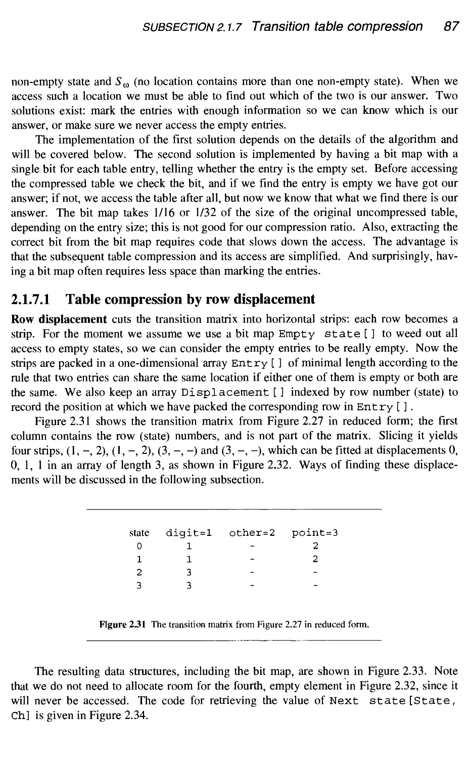
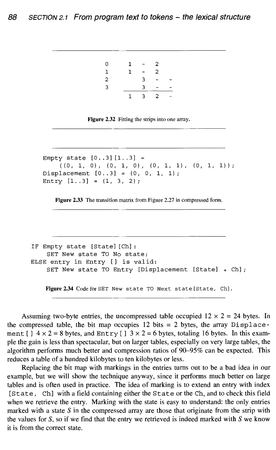
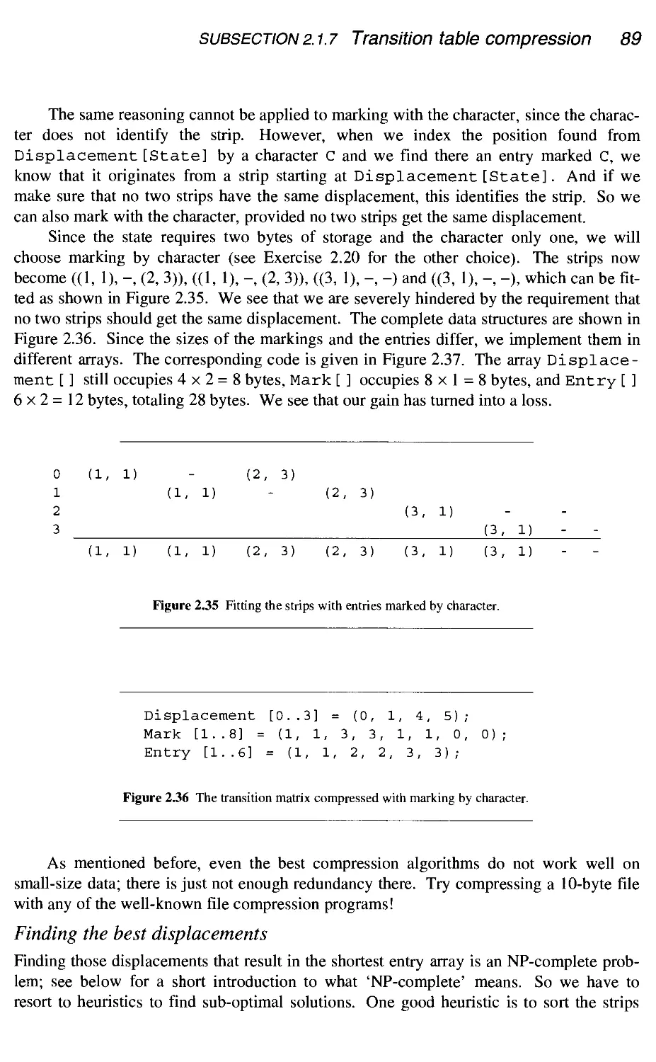
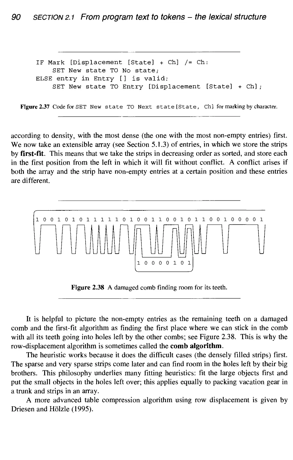
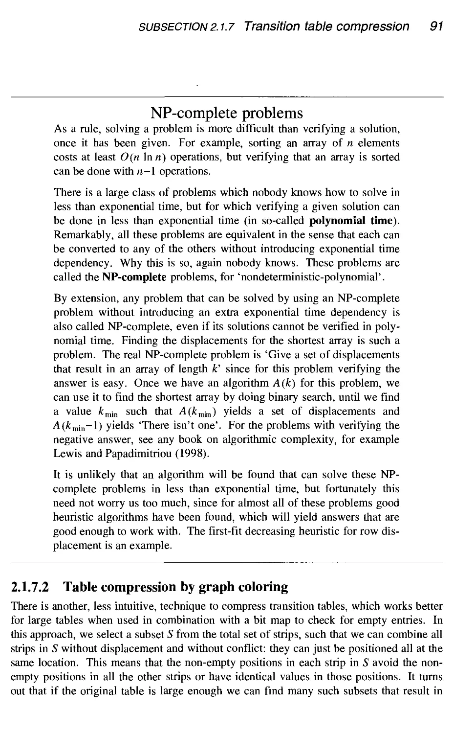
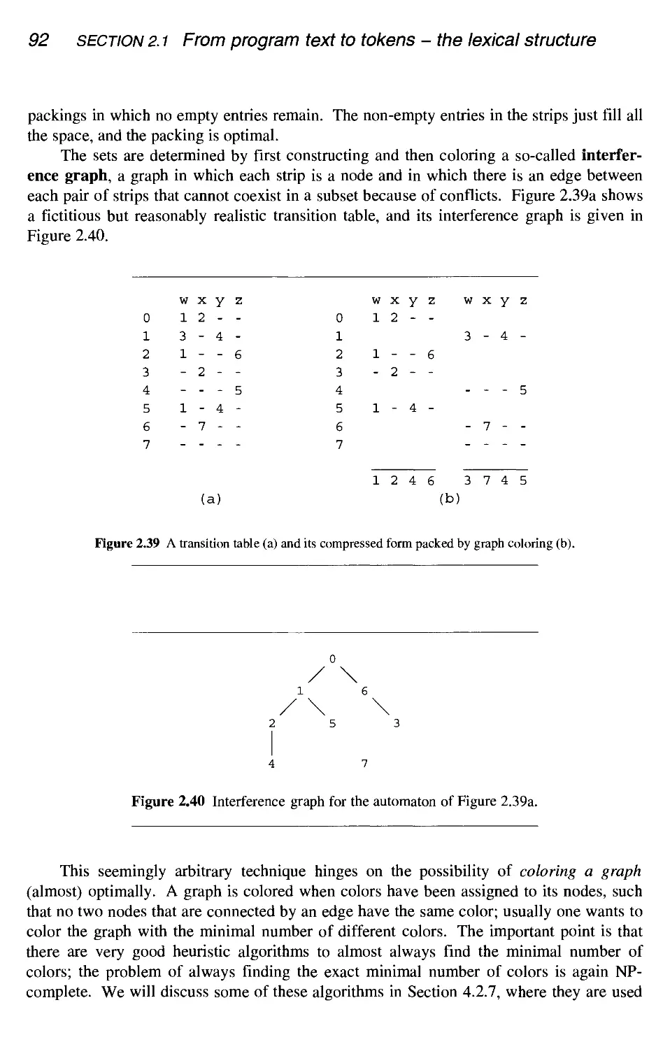
Transition table compression
Error handling in lexical analyzers
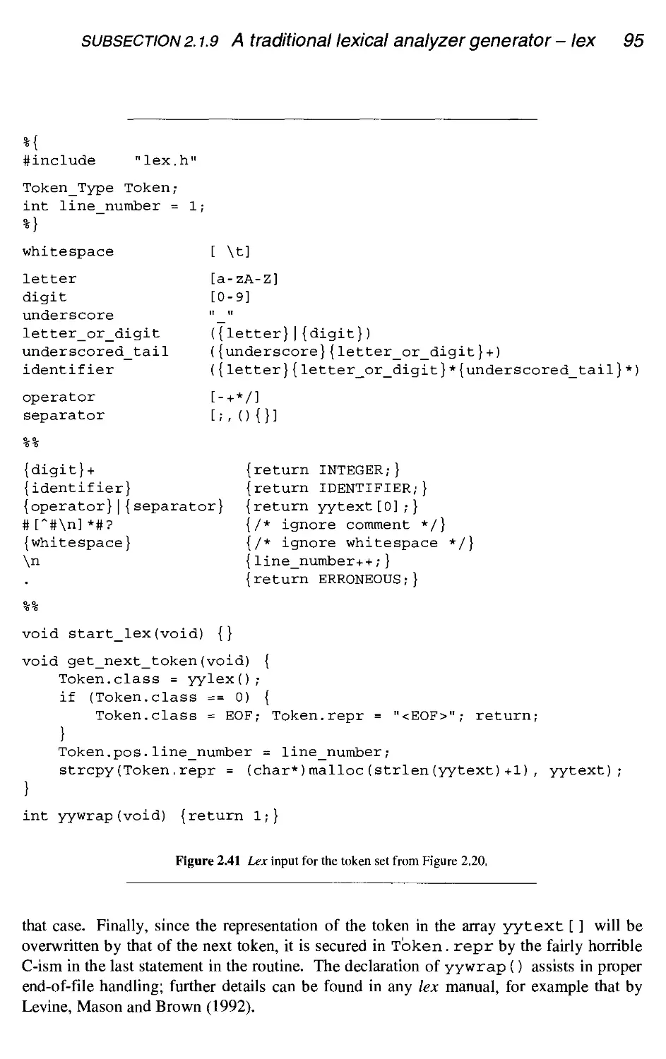
A traditional lexical analyzer generator - lex
Lexical identification of tokens
Symbol tables
Macro processing and file inclusion
Conclusion
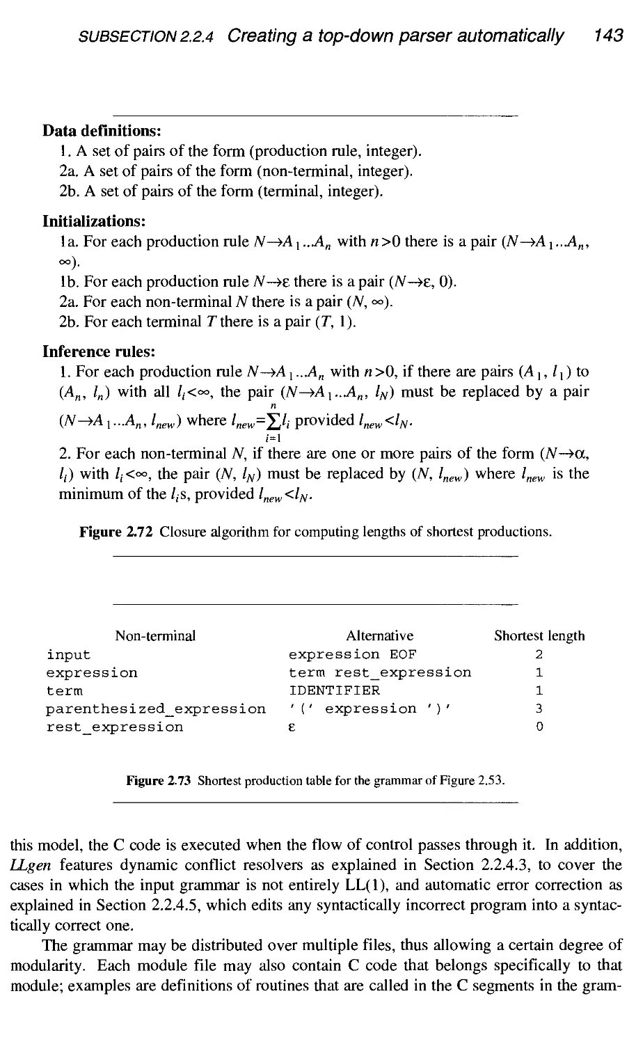
2.2 From tokens to syntax tree - the syntax
2.2.1 Two classes of parsing methods
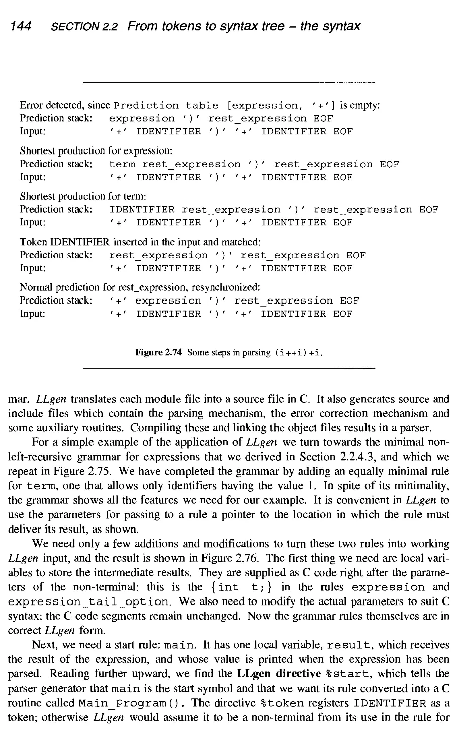
2.2.2 Error detection and error recovery
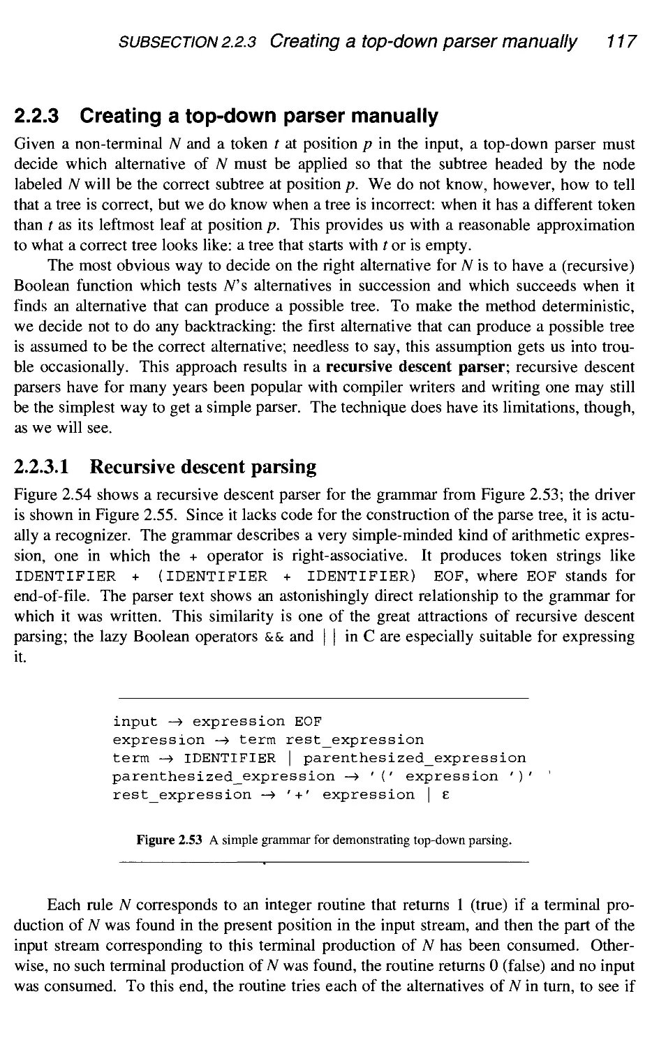
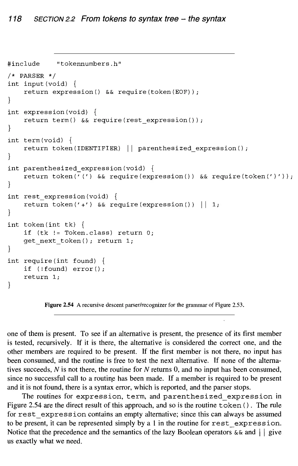
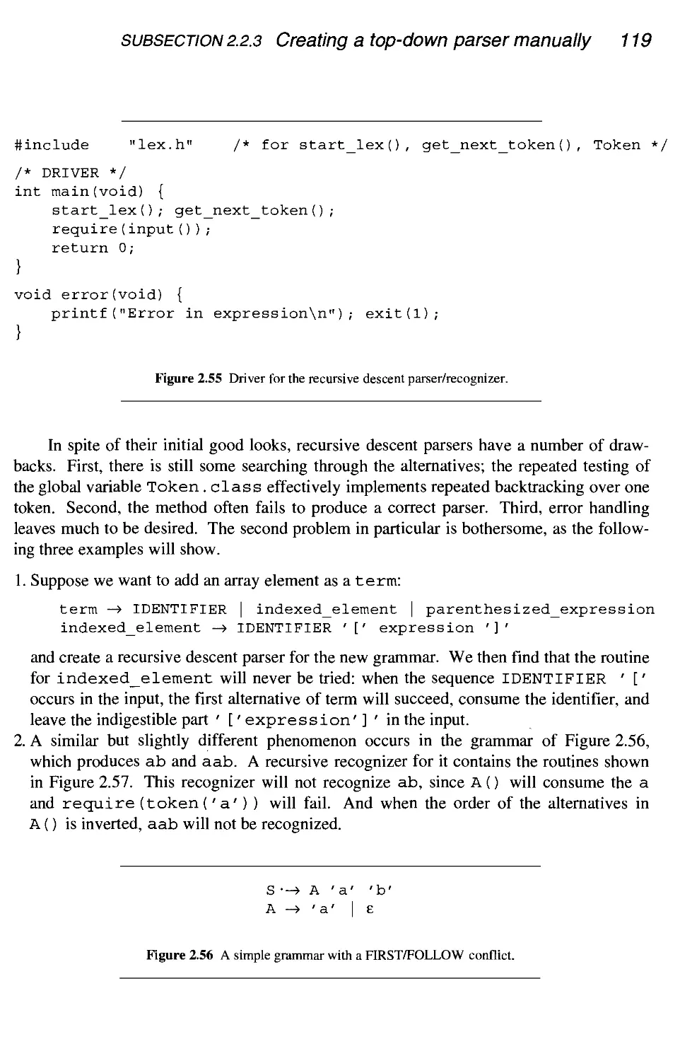
2.2.3 Creating a top-down parser manually
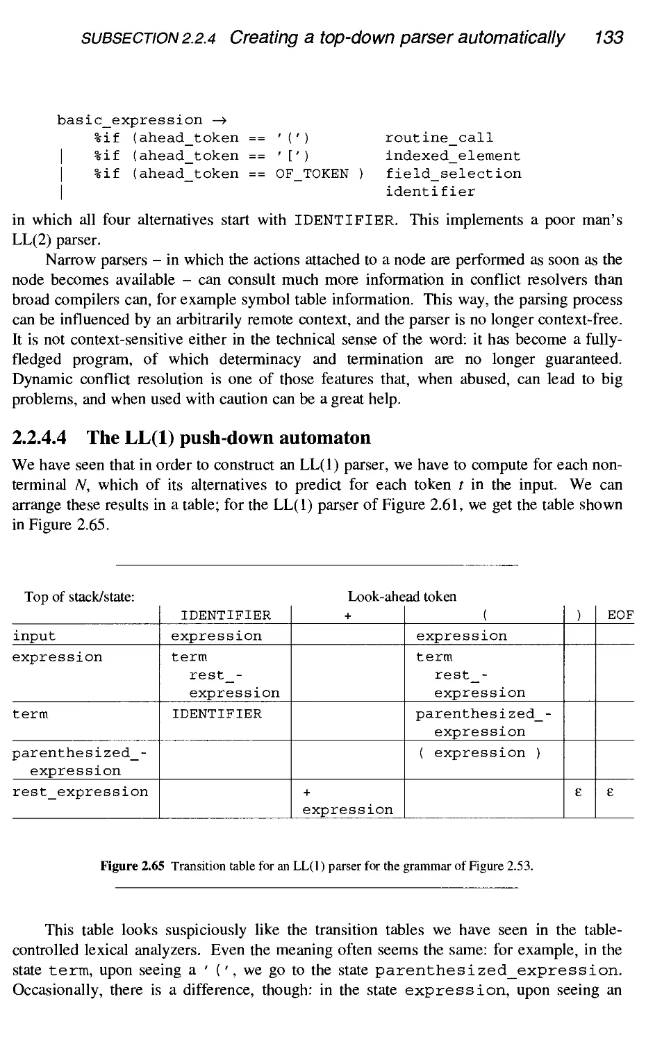
2.2.4 Creating a top-down parser automatically
2.
L.I
2.1.2
2.
2.
2.
2.
2.
2.
2.
1.3
1.4
.5
.6
1.7
1.8
1.9
2.1.10
2.1.11
2.1.12
2.
L.13
52
56
56
57
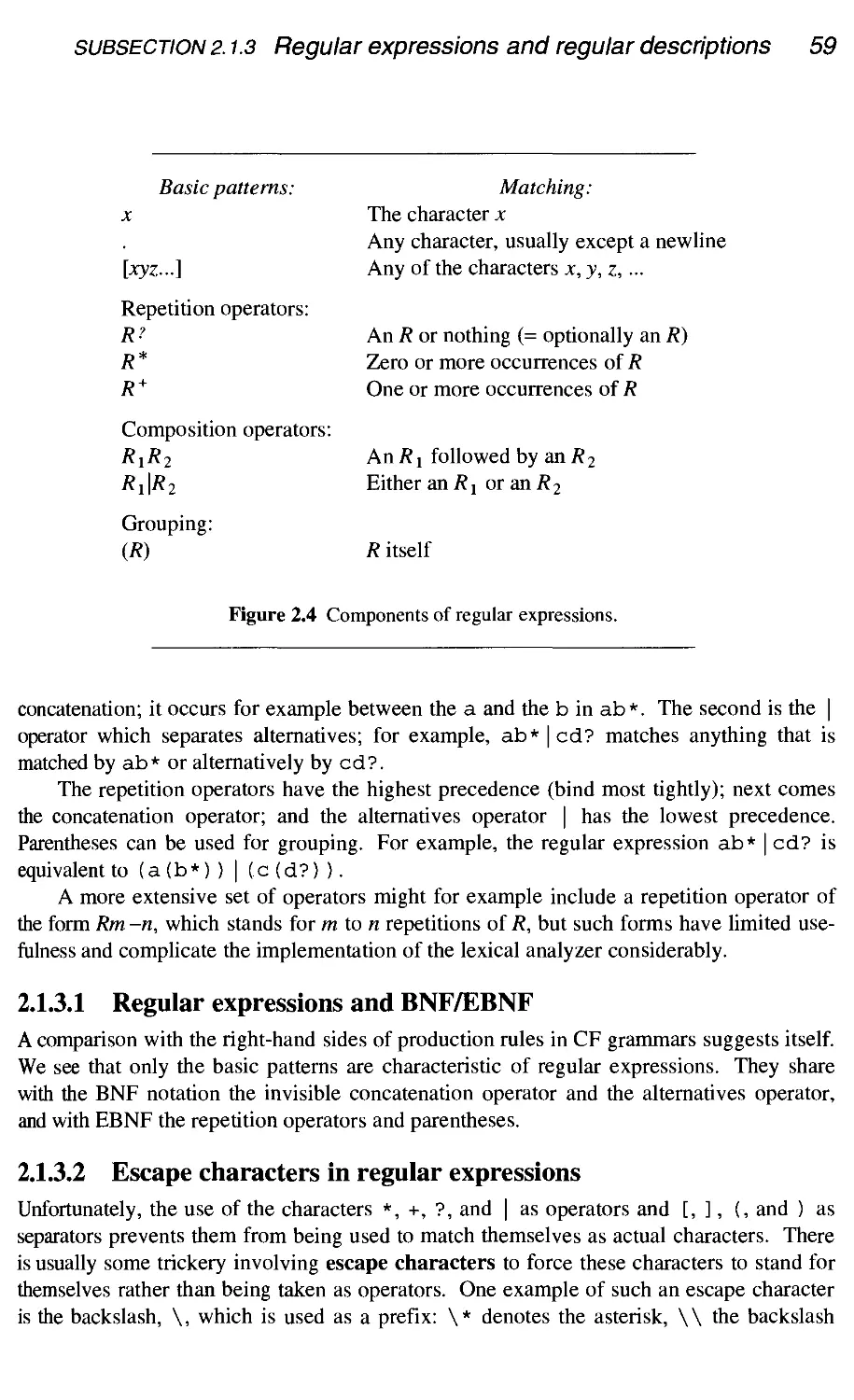
58
60
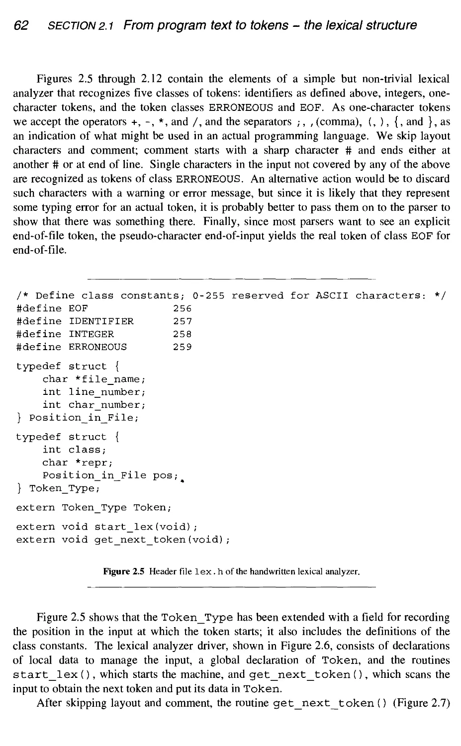
61
68
86
93
94
96
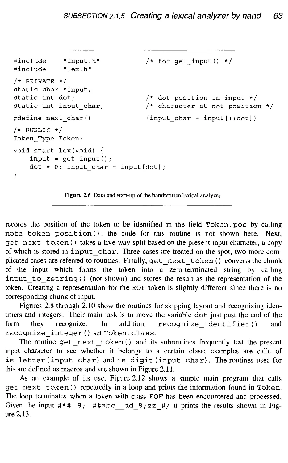
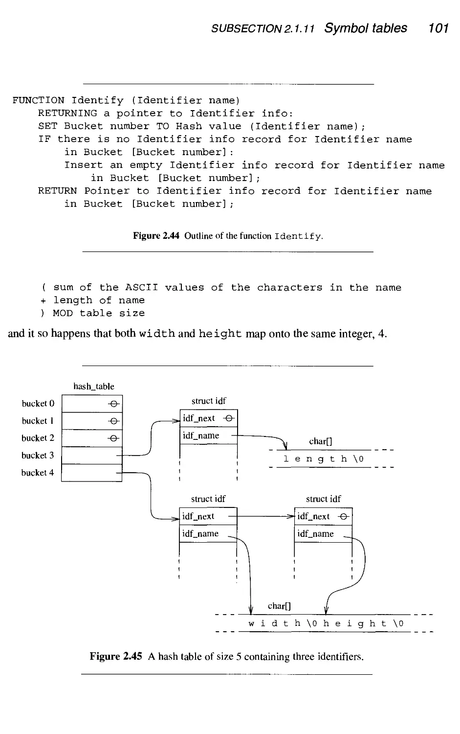
98
103
109
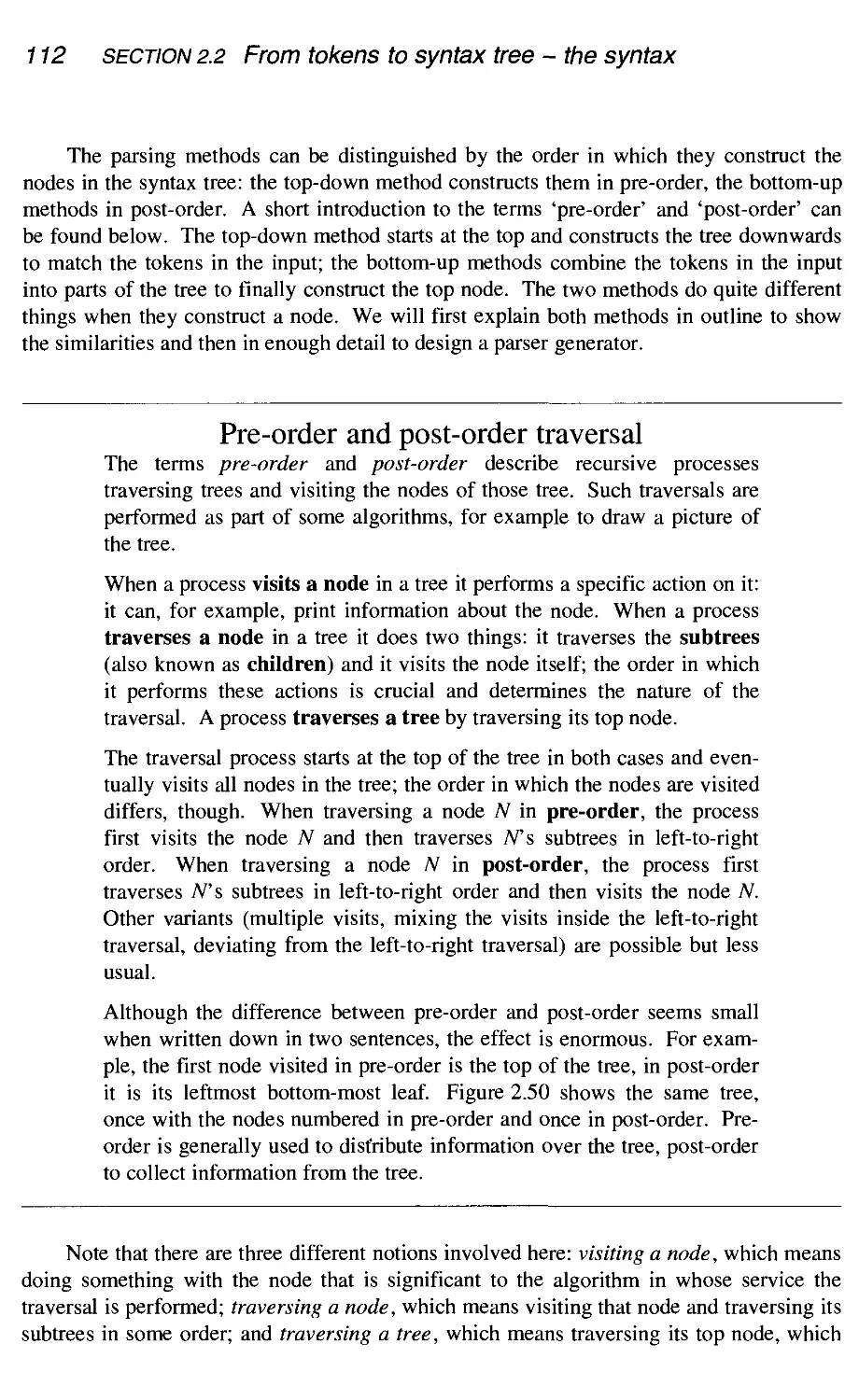
110
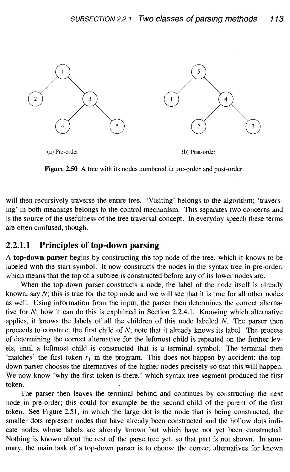
111
115
117
120
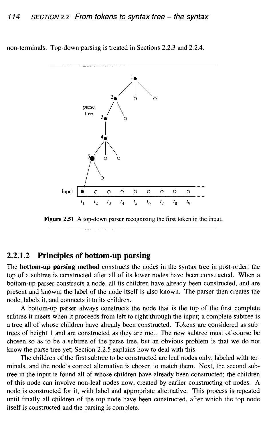
2.3
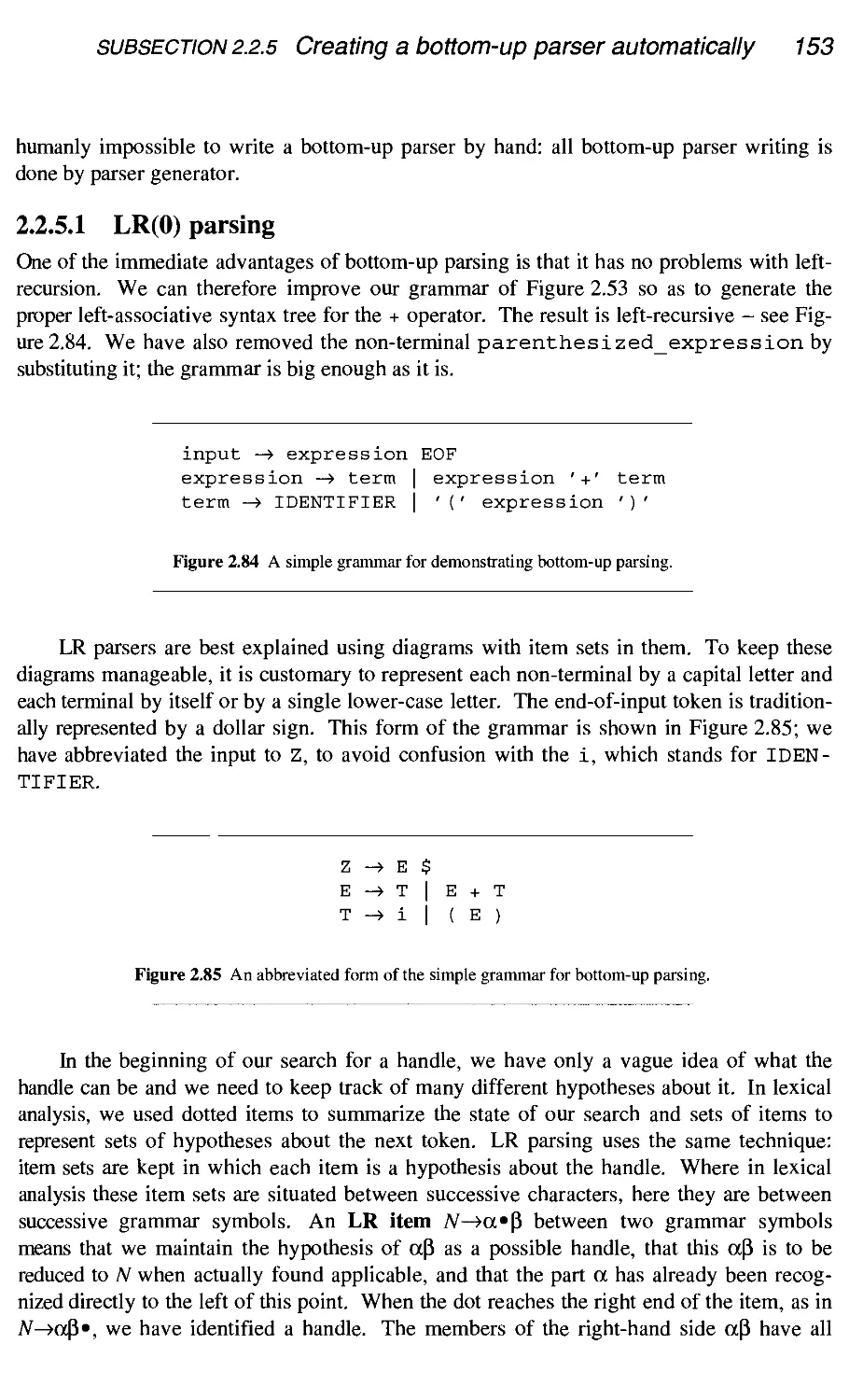
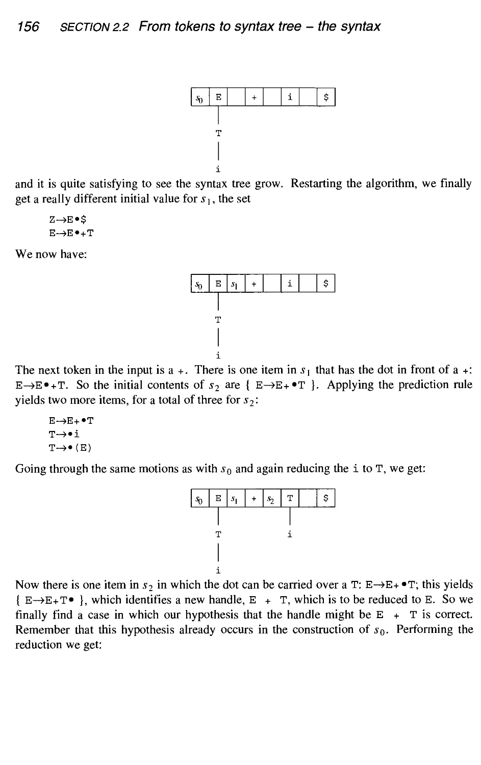
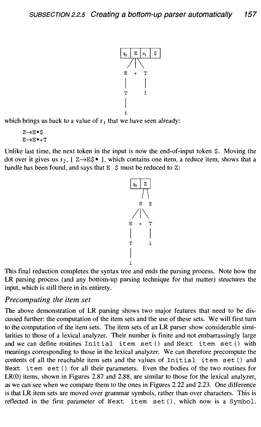
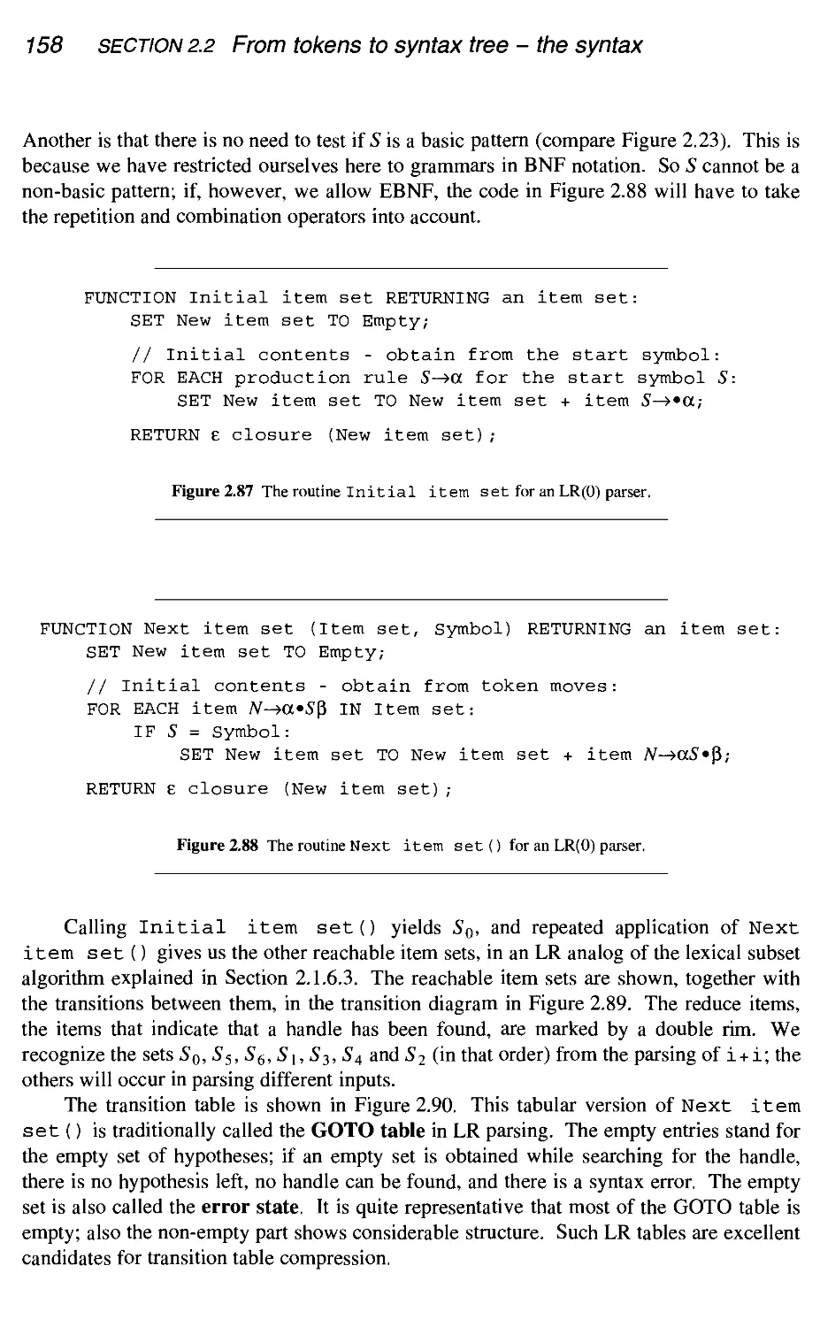
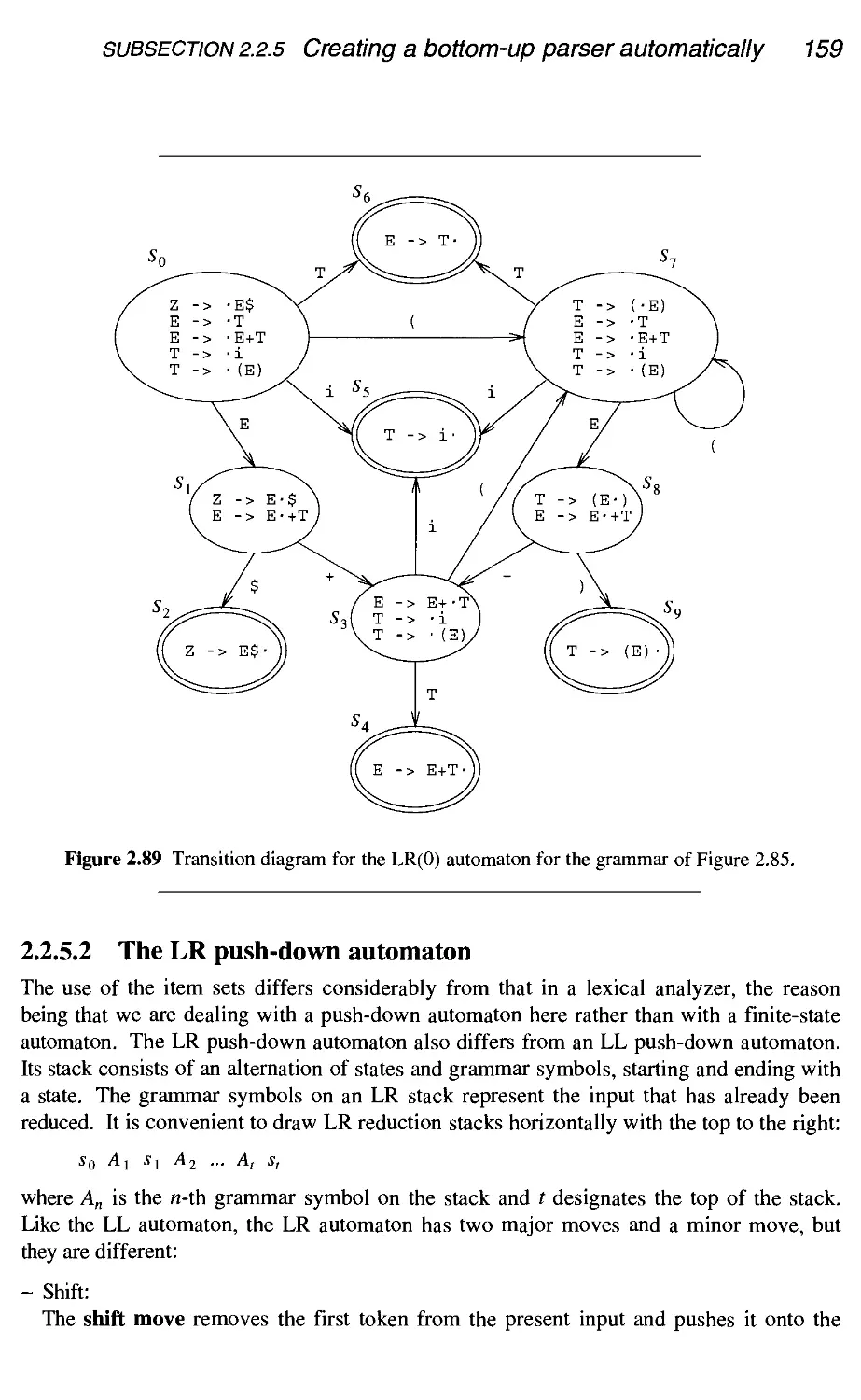
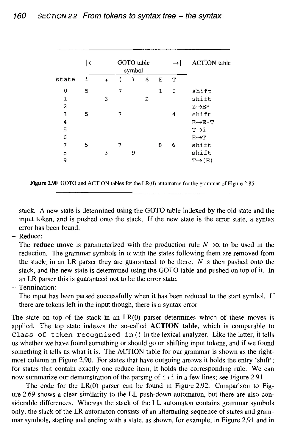
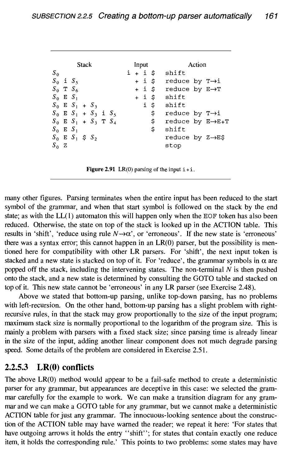
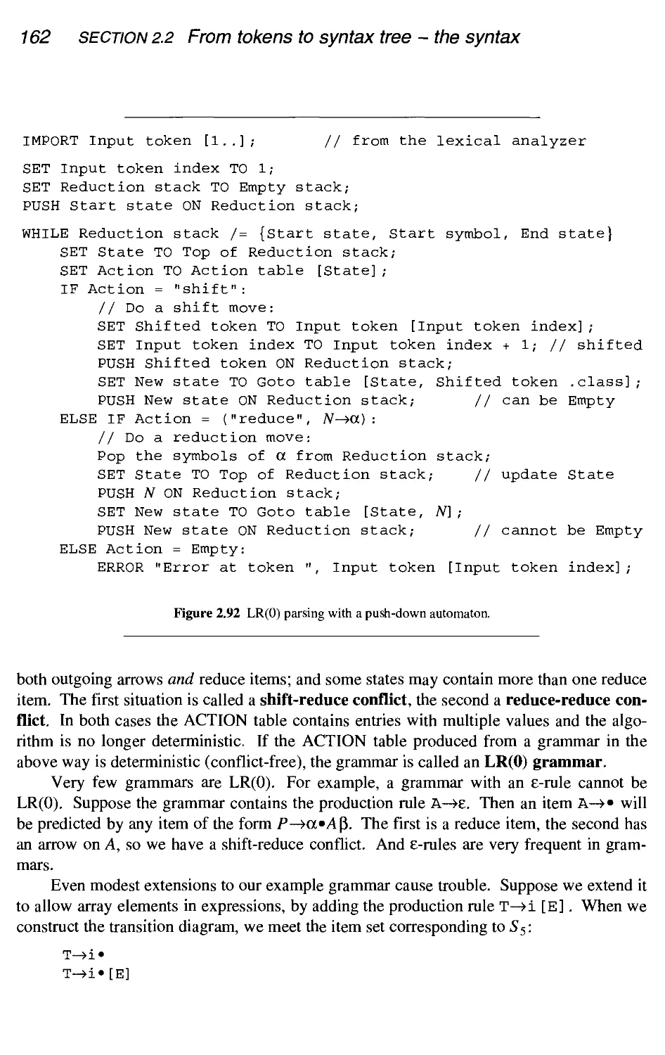
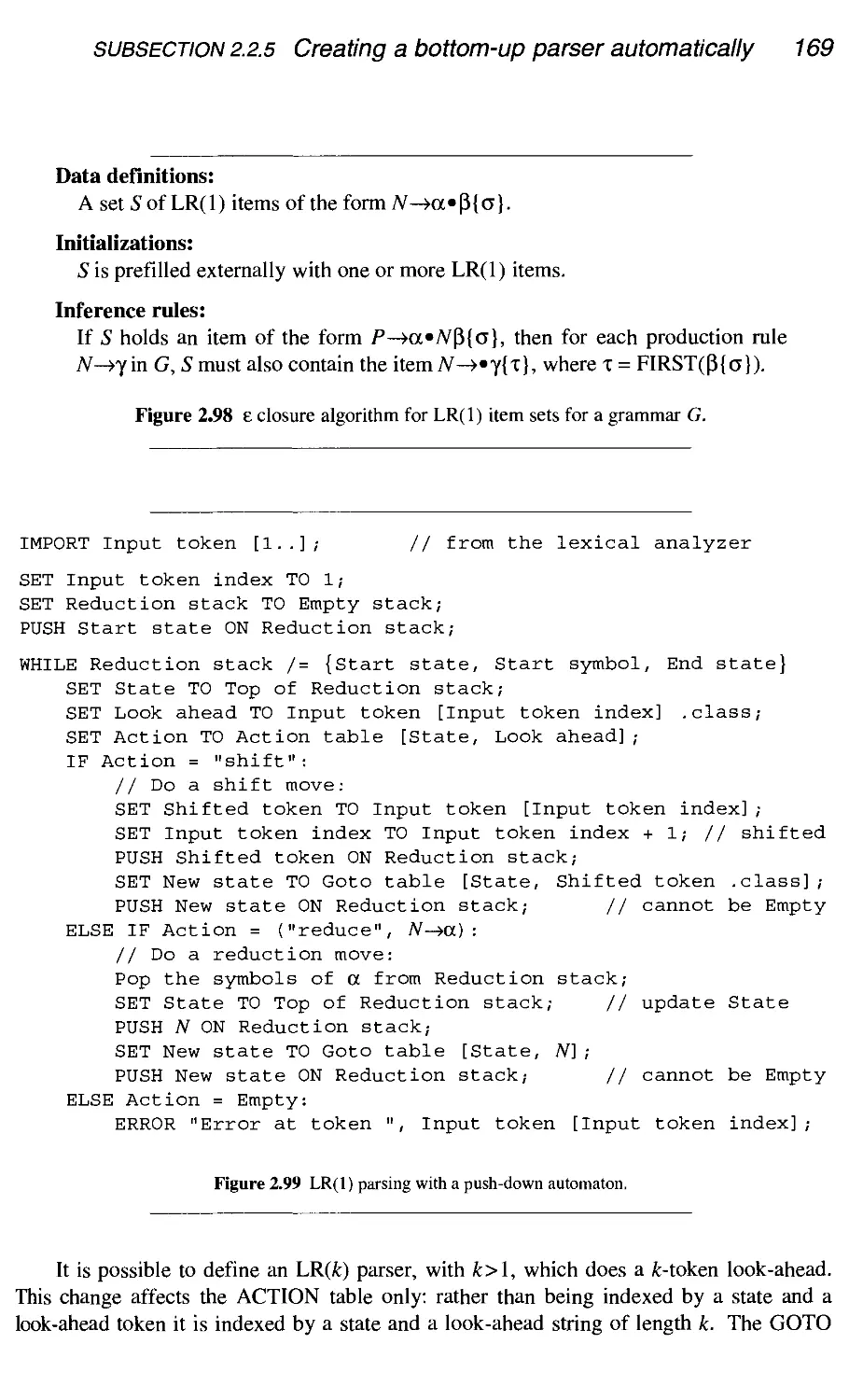
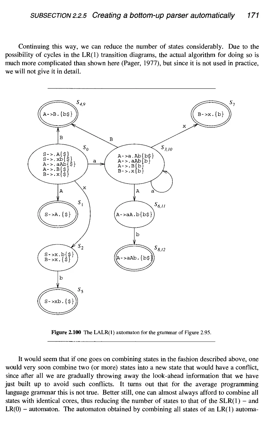
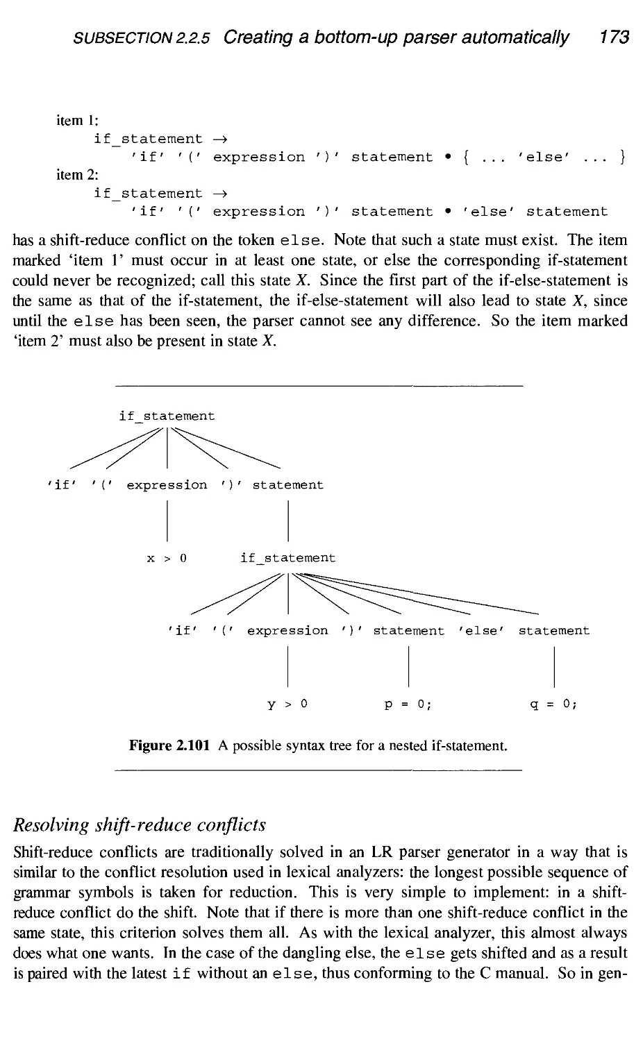
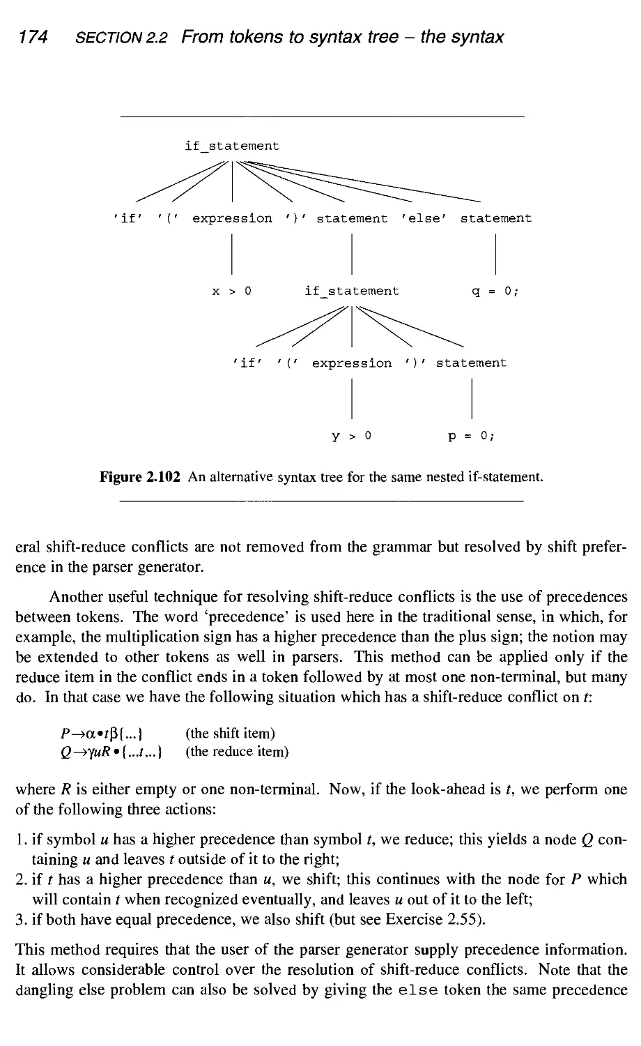
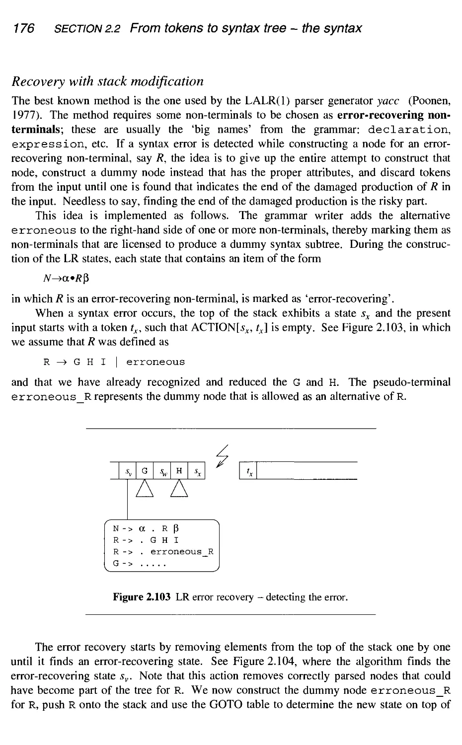
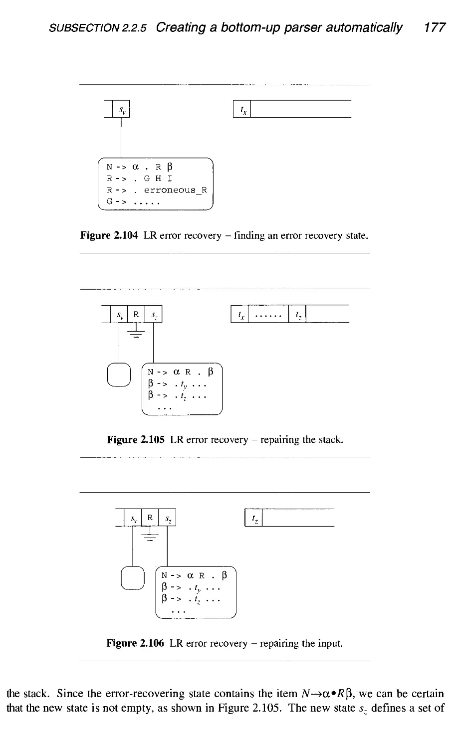
2.2.5 Creating a bottom-up parser automatically
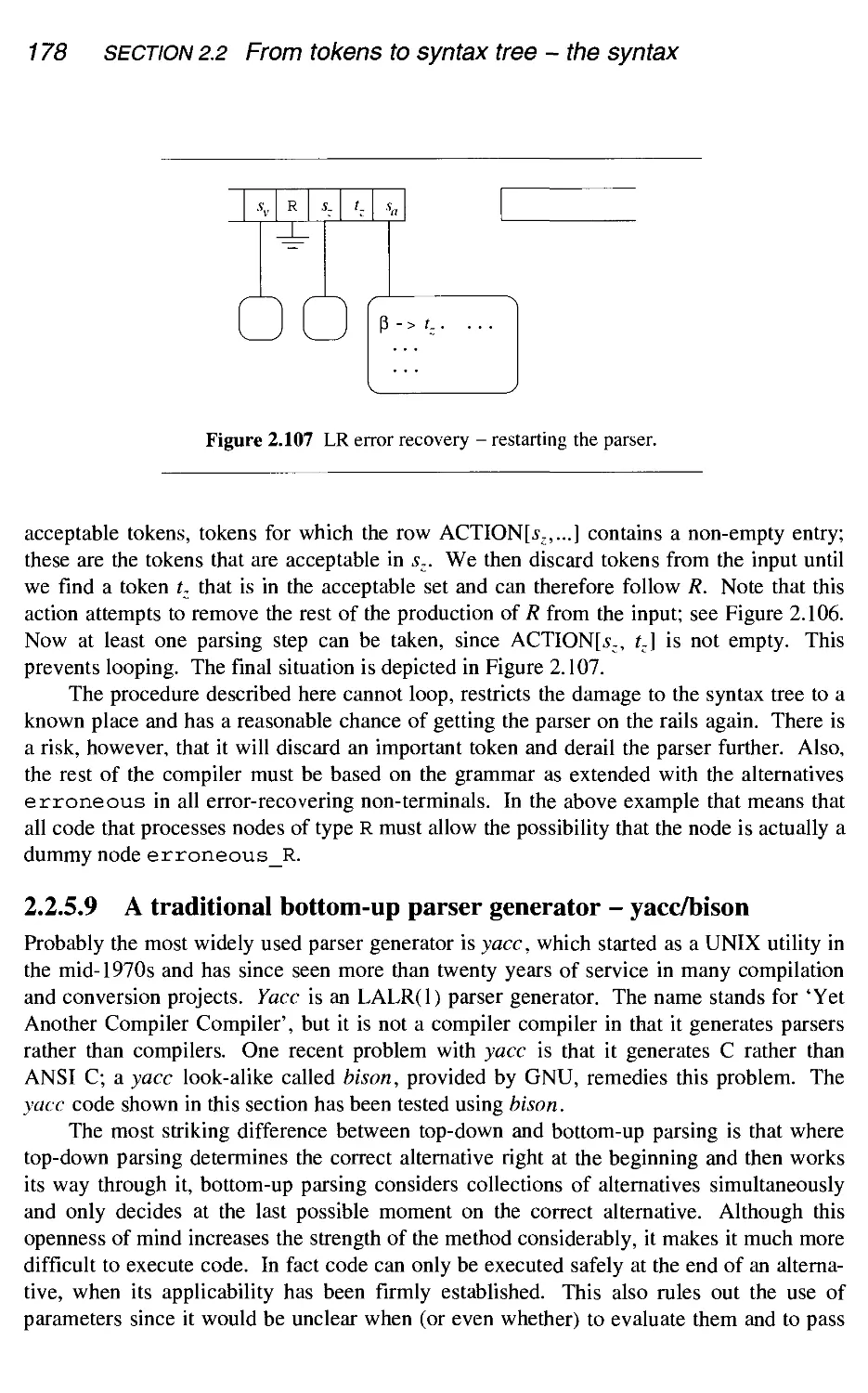
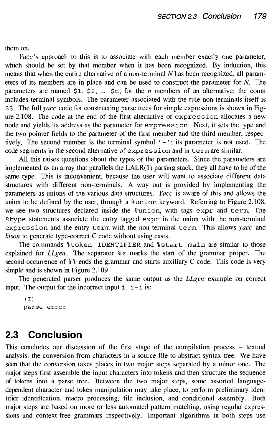
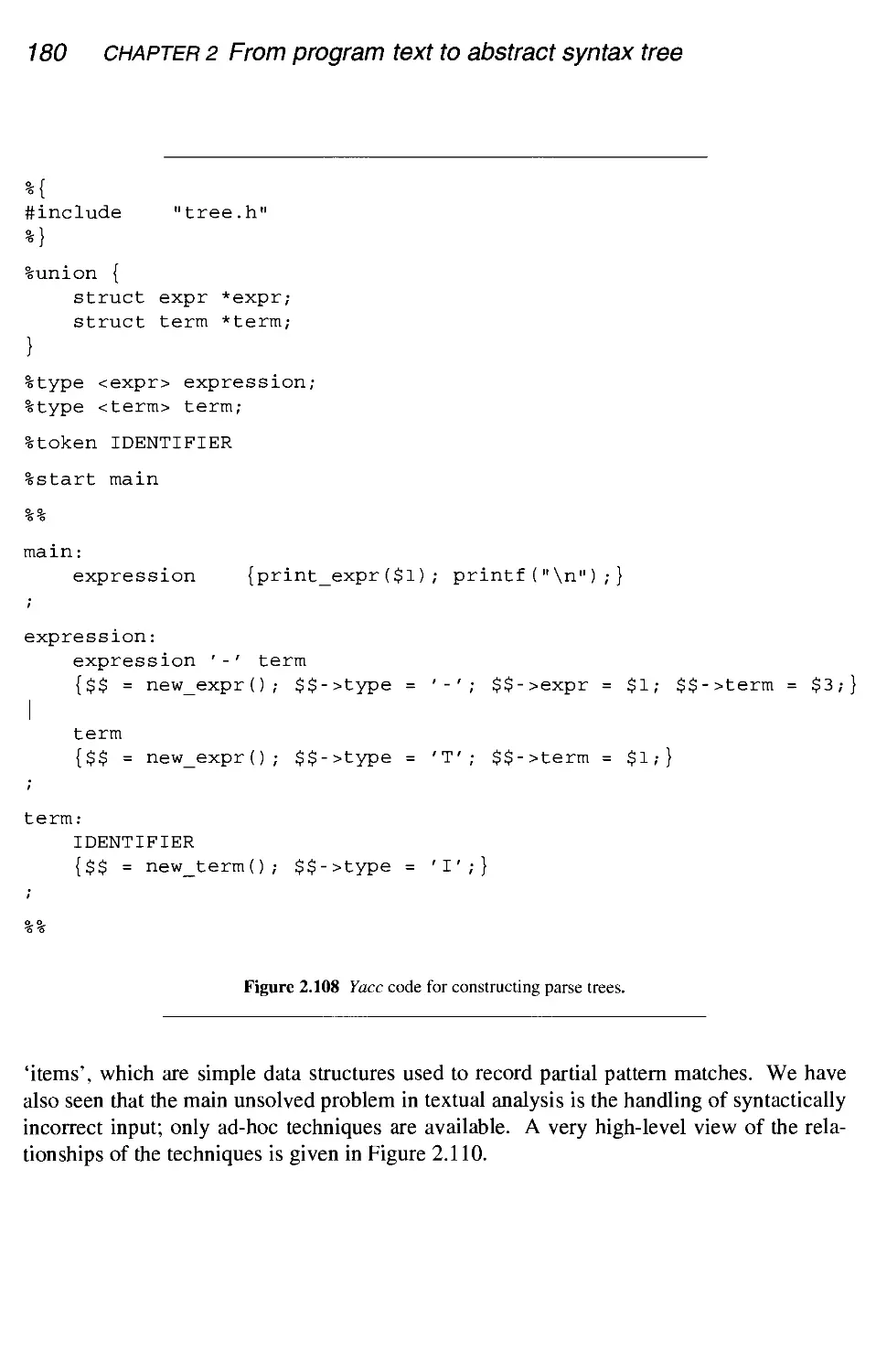
Conclusion
Summary
Further reading
Exercises
Contents vii
150
179
181
184
185
3 Annotating the abstract syntax tree - the context
3.1 Attribute grammars
3.2
.1 Dependency graphs
.2 Attribute evaluation
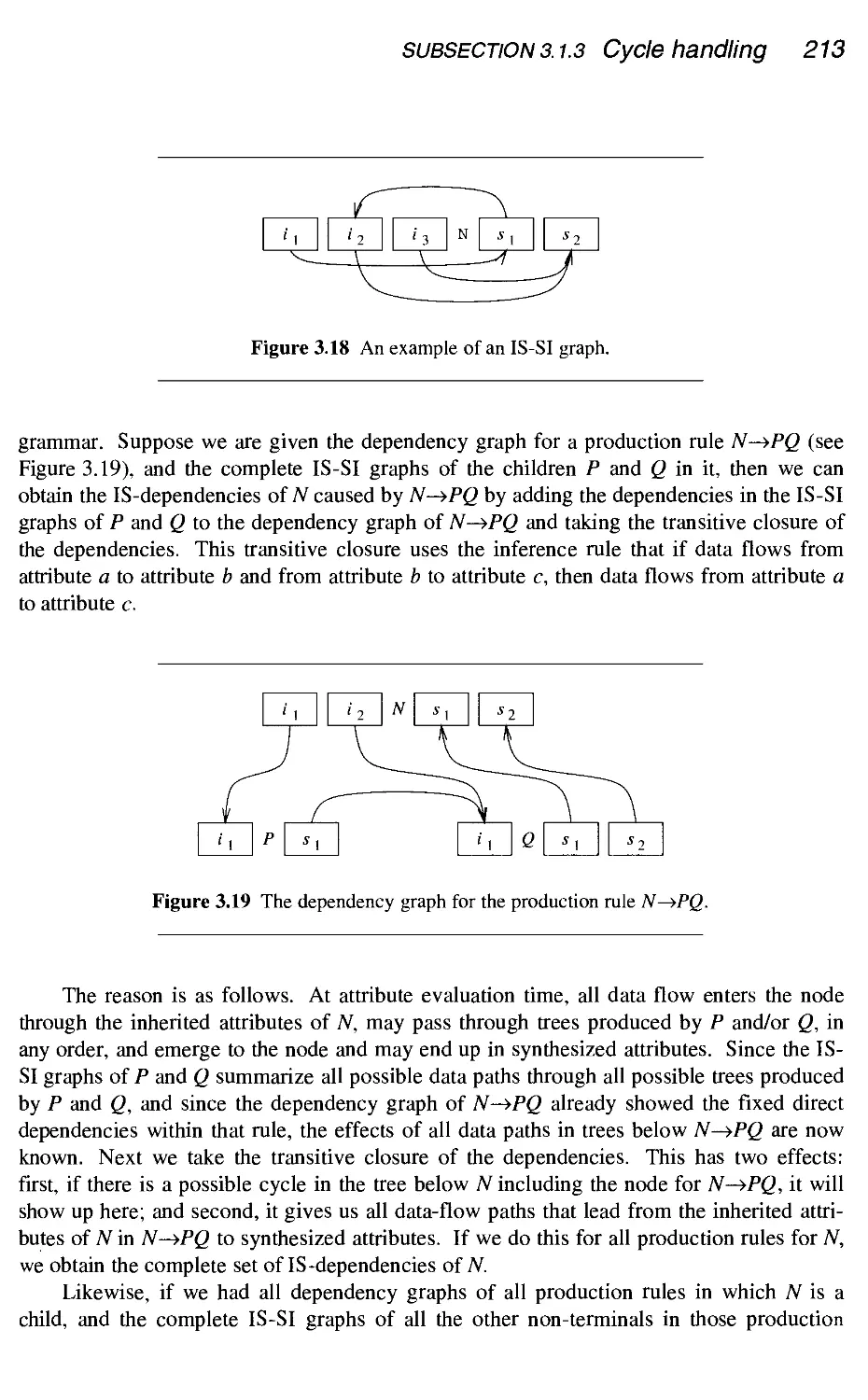
.3 Cycle handling
.4 Attribute allocation
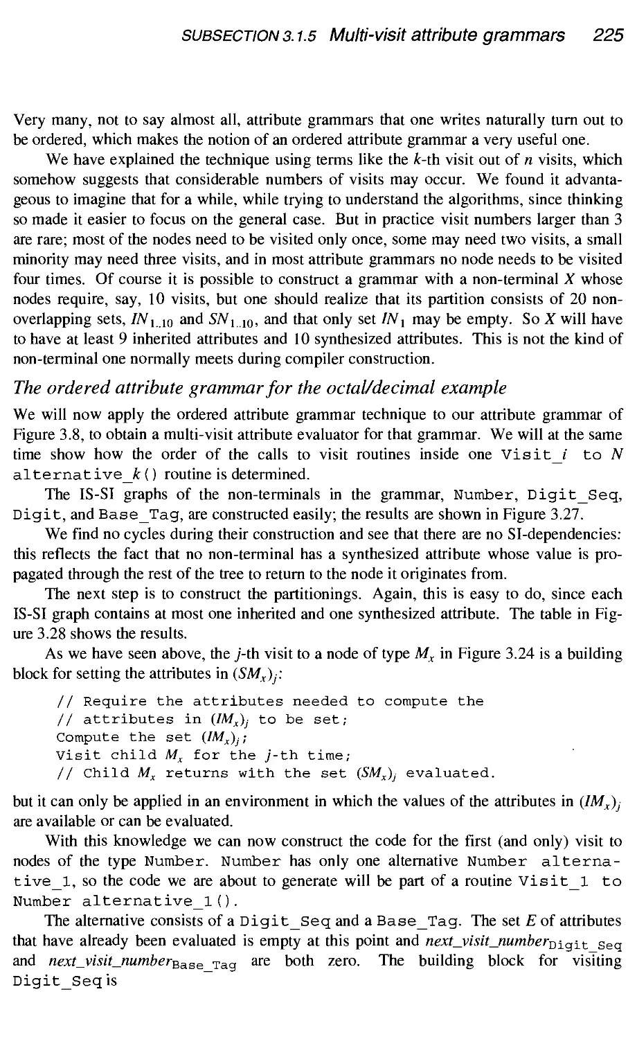
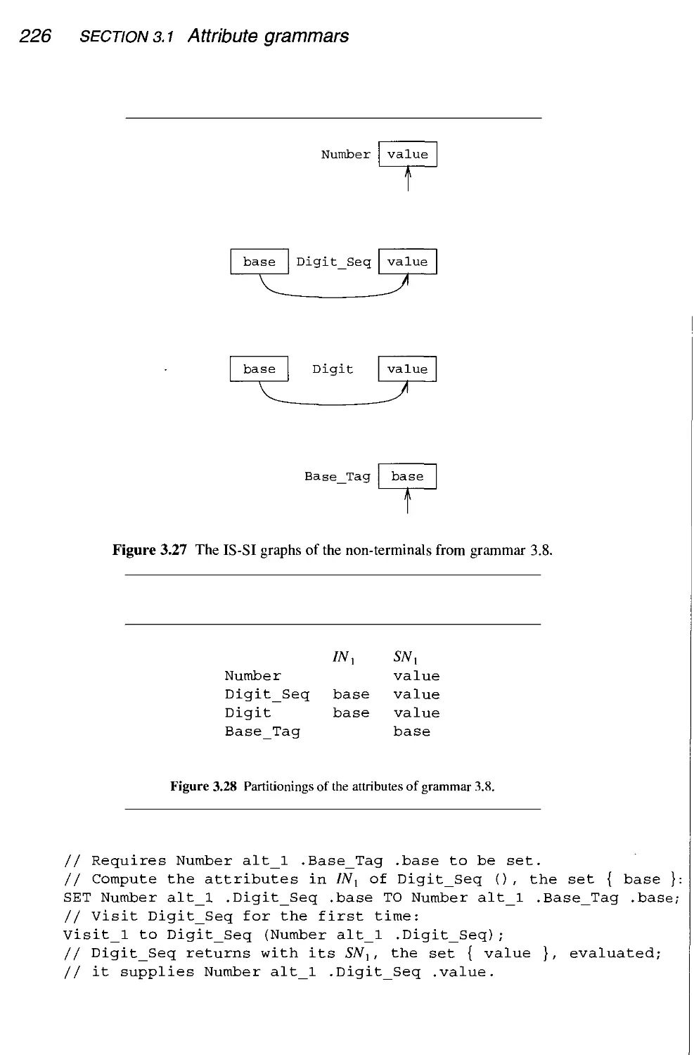
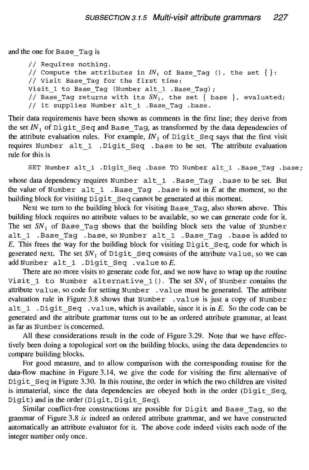
.5 Multi-visit attribute grammars
.6 Summary of the types of attribute grammars
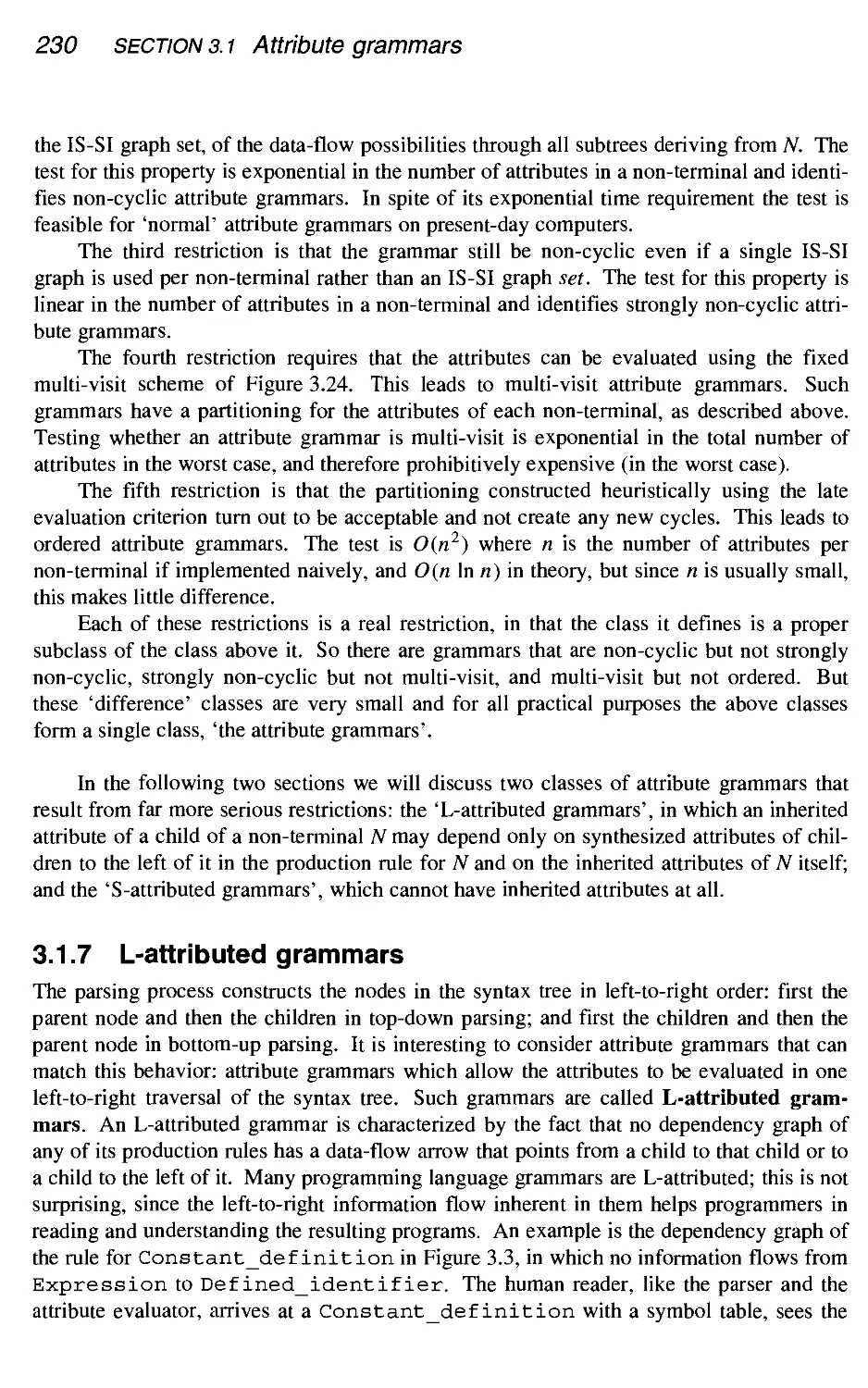
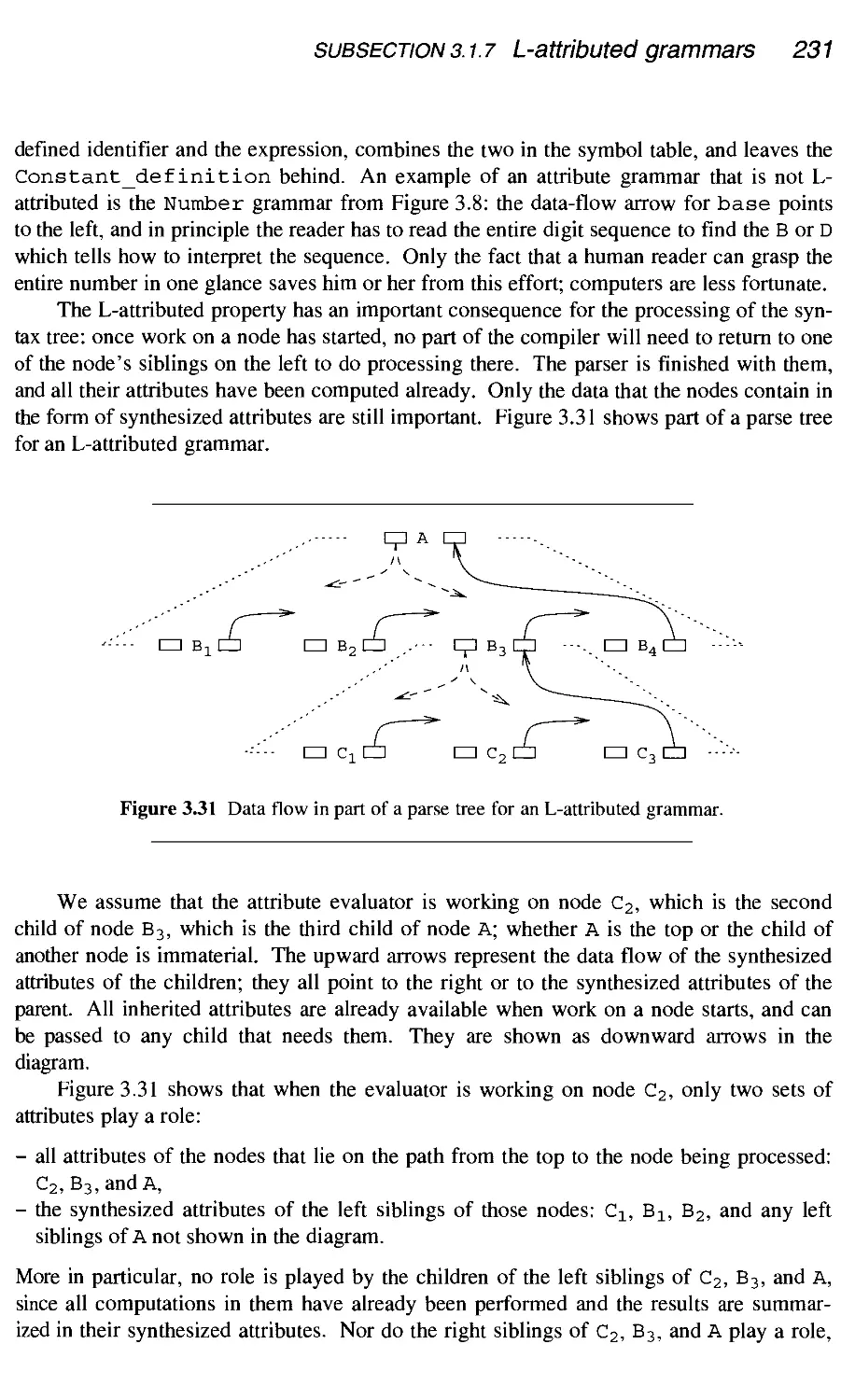
3.1.7 L-attributed grammars
3.1.8 S-attributed grammars
3.1.9 Equivalence of L-attributed and S-attributed grammars
3.1.10 Extended grammar notations and attribute grammars
3.1.11 Conclusion
Manual methods
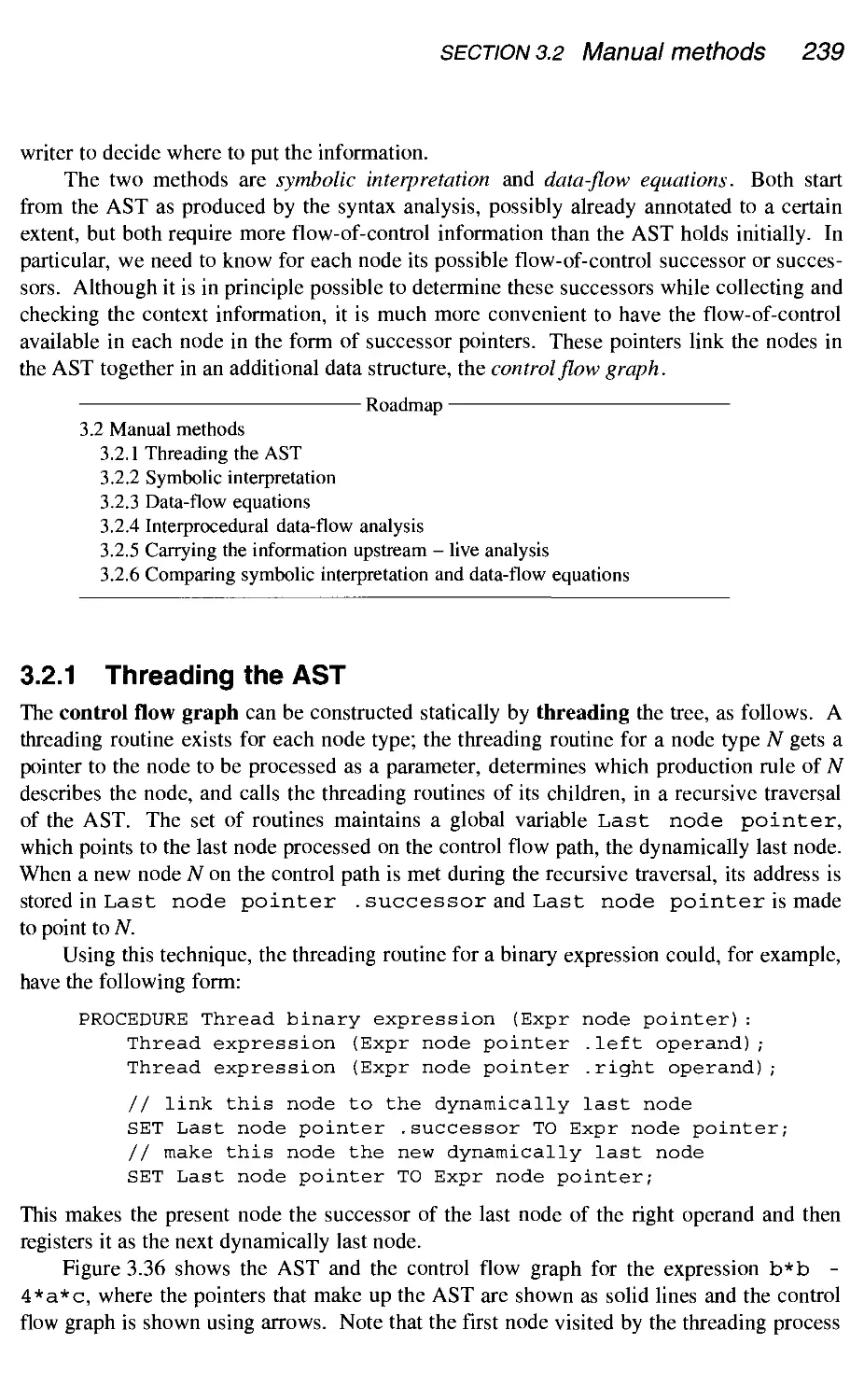
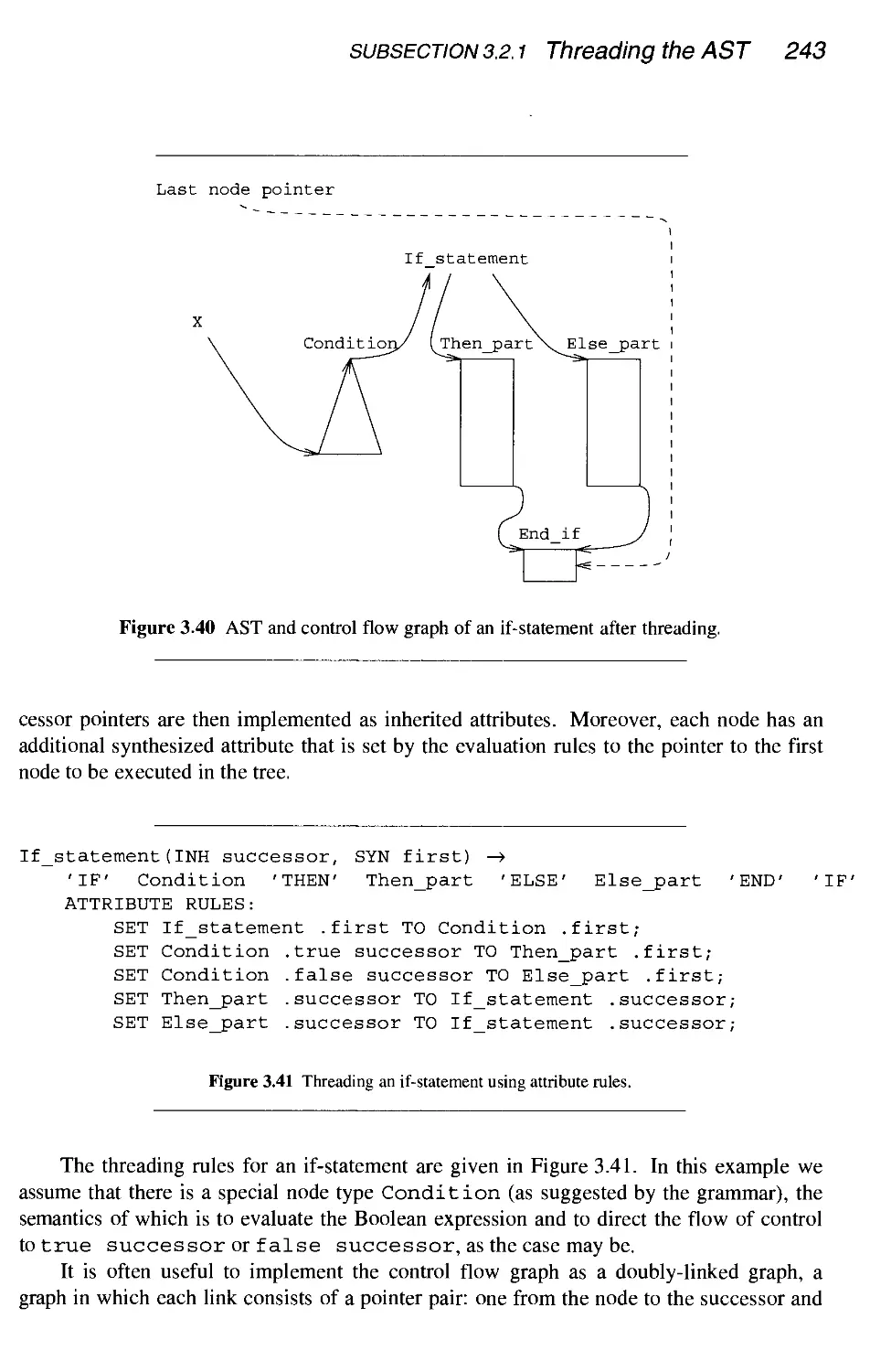
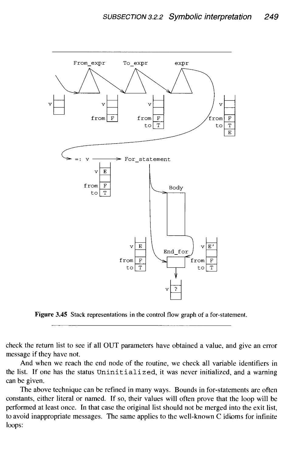
3.2.1 Threading the AST
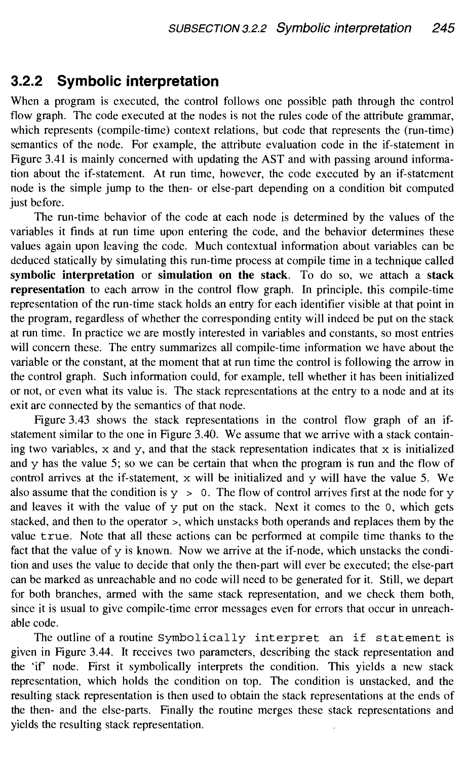
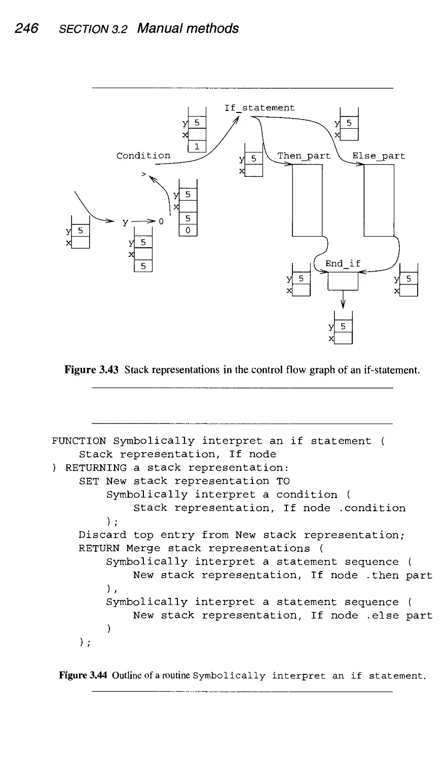
3.2.2 Symbolic interpretation
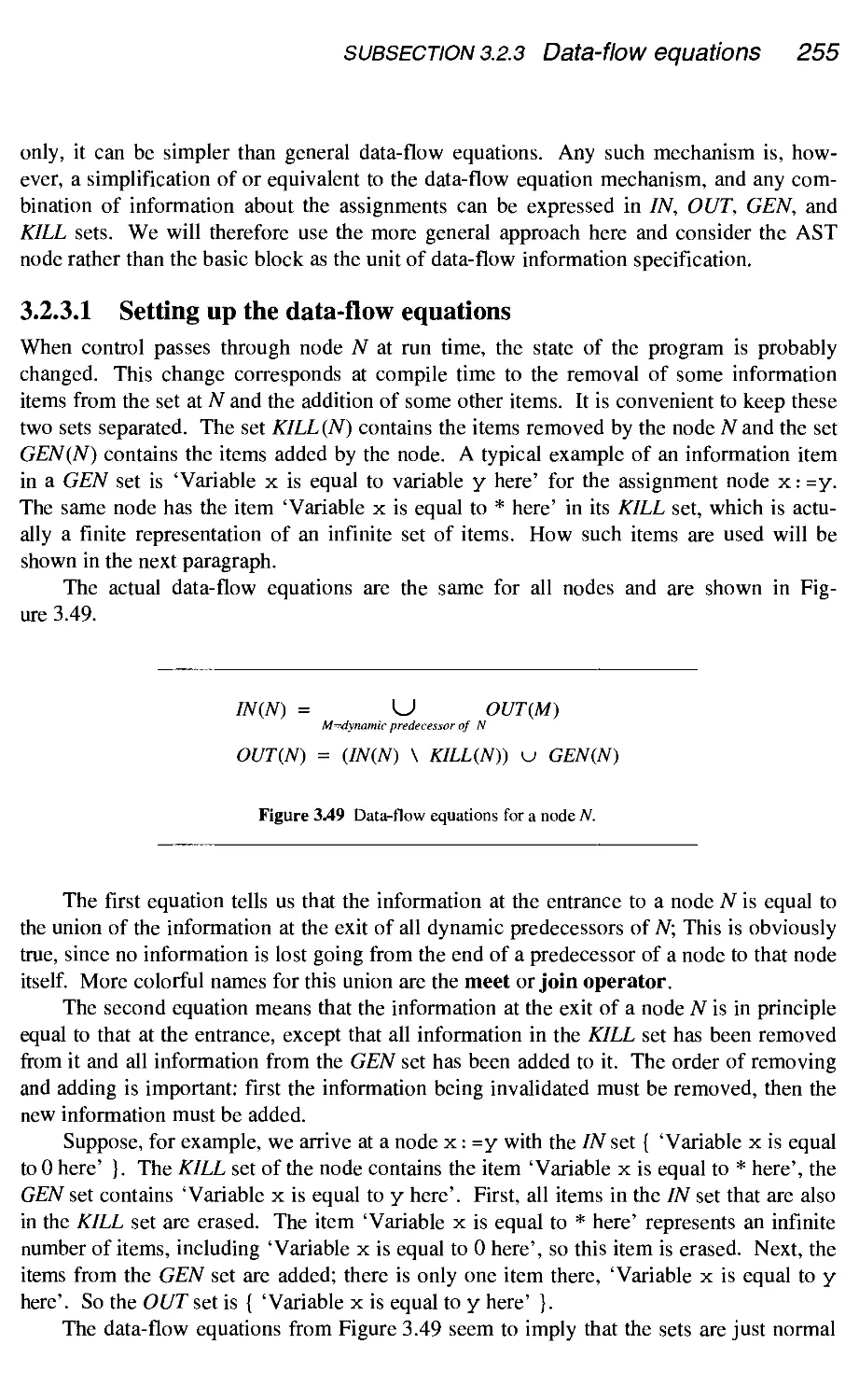
3.2.3 Data-flow equations
3.2.4 Interprocedural data-flow analysis
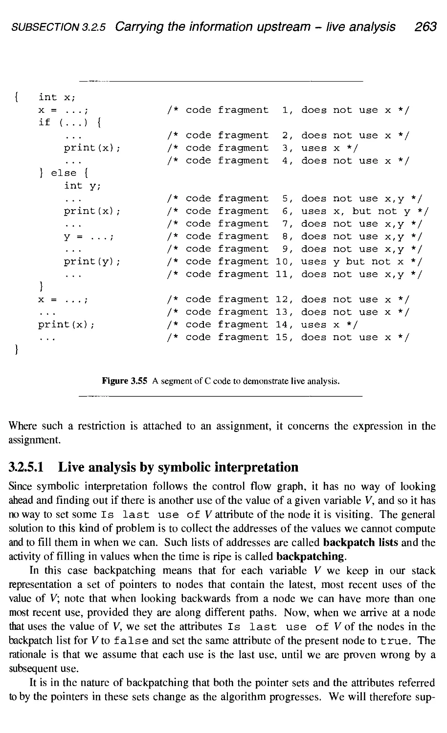
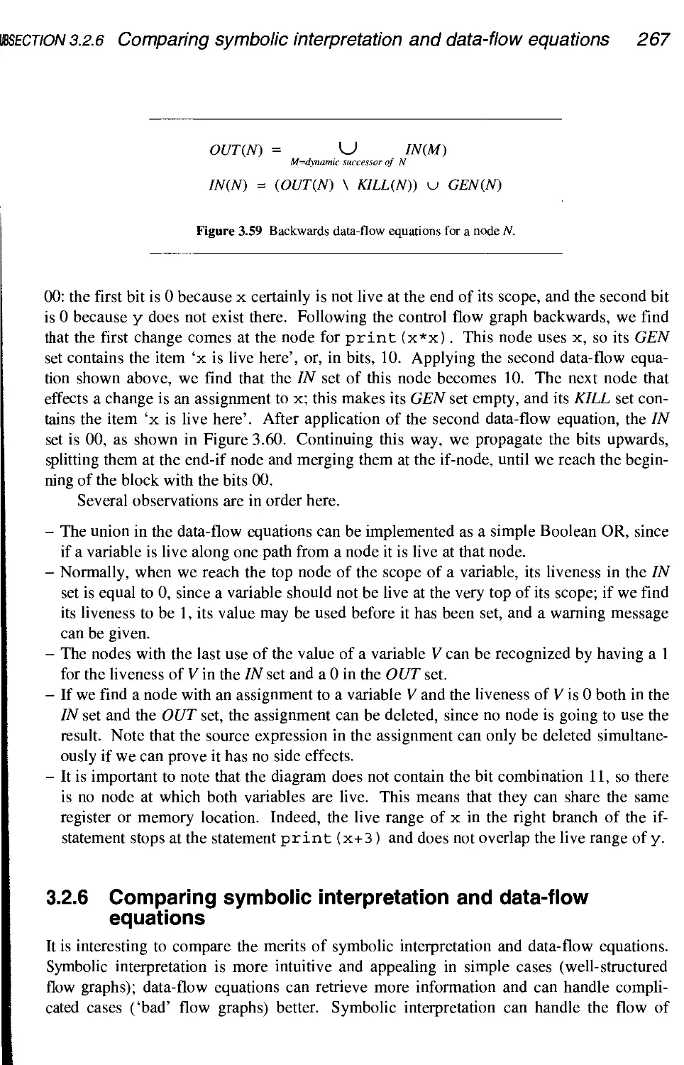
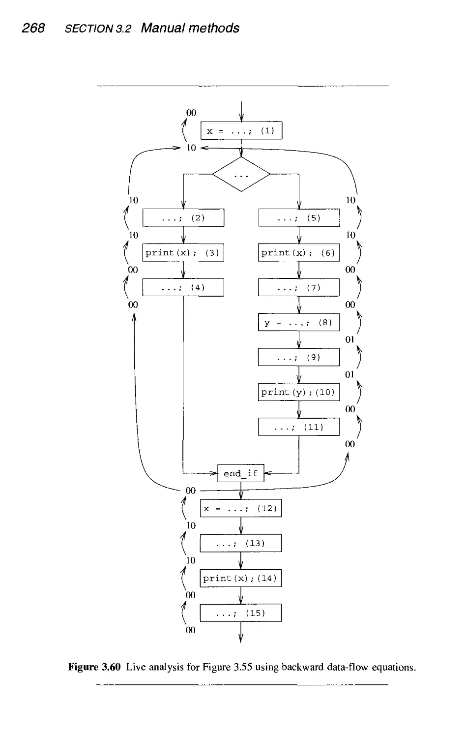
3.2.5 Carrying the information upstream - live analysis
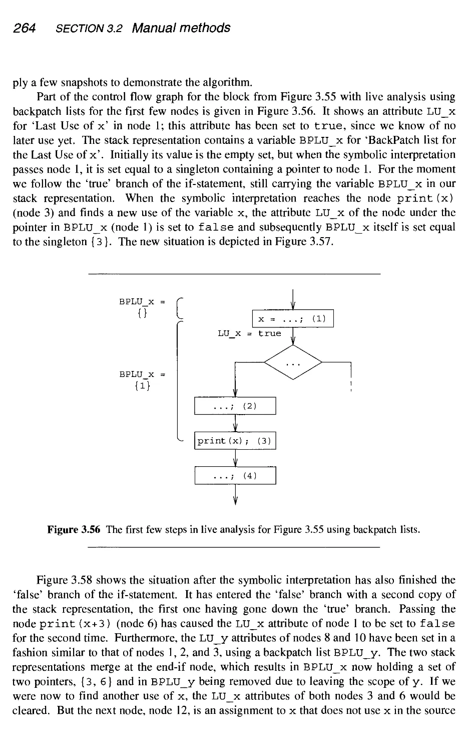
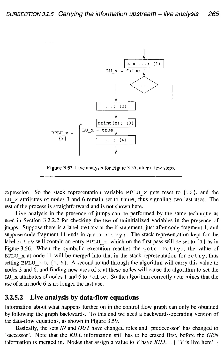
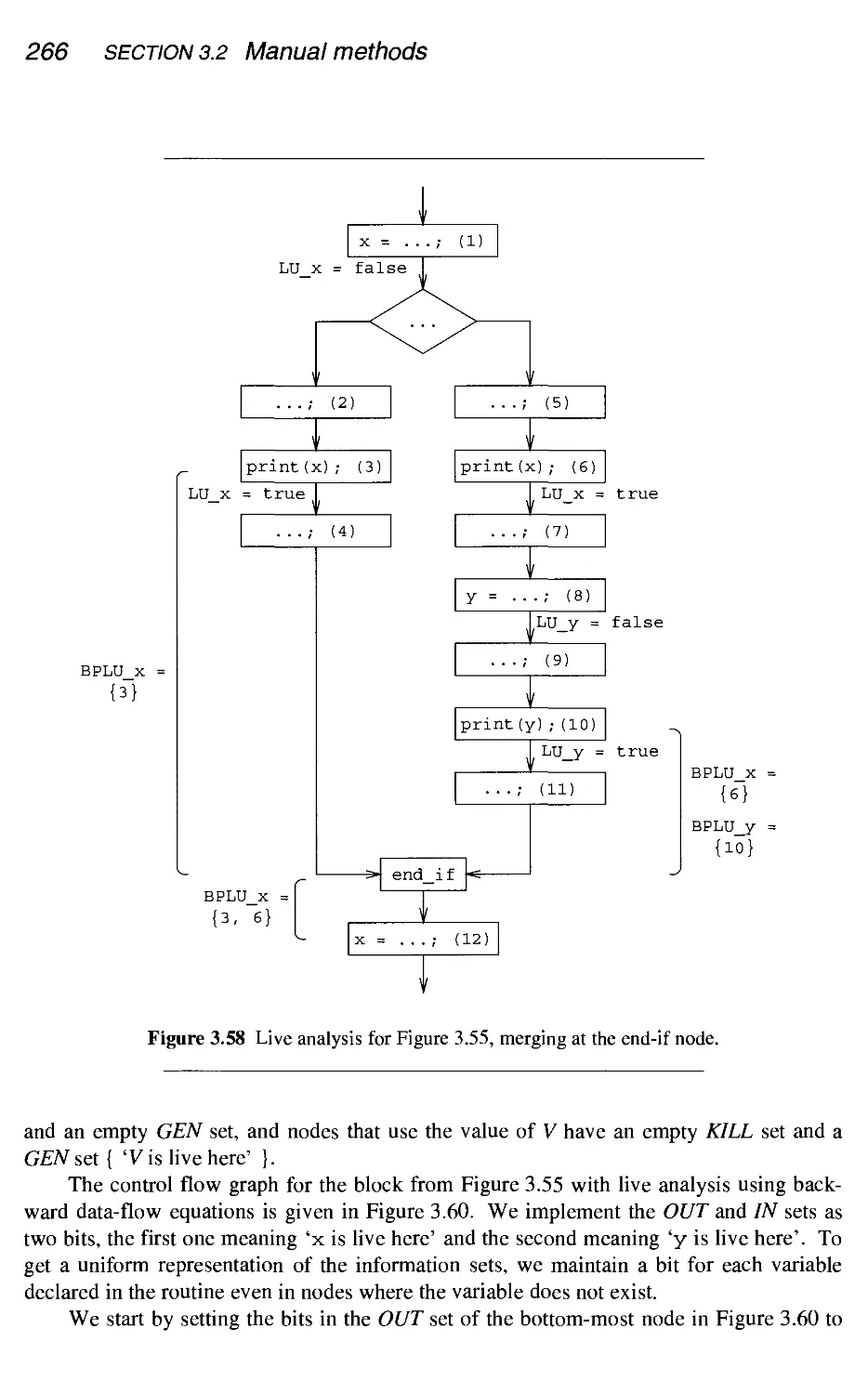
3.2.6 Comparing symbolic interpretation and data-flow equations
3.3 Conclusion
Summary
Further reading
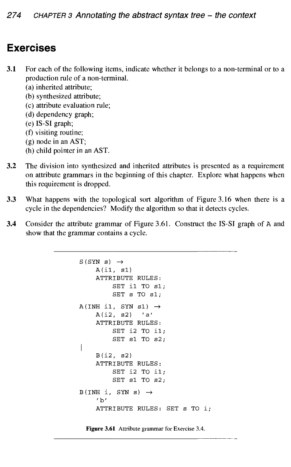
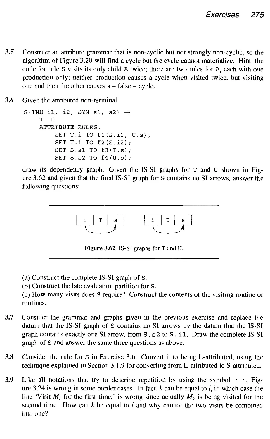
Exercises
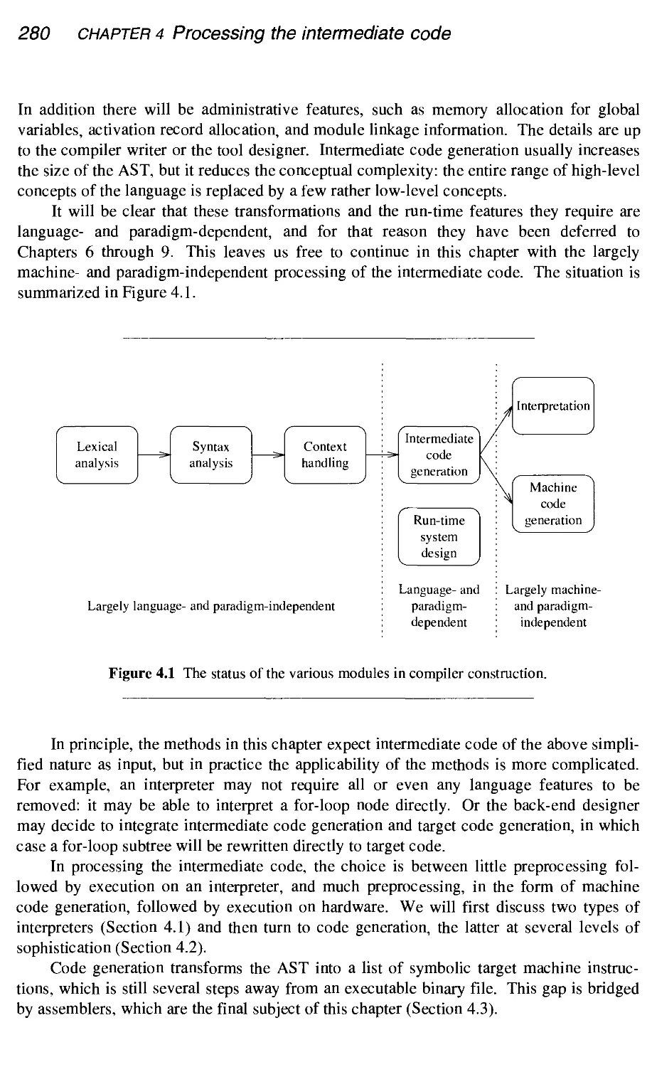
4 Processing the intermediate code
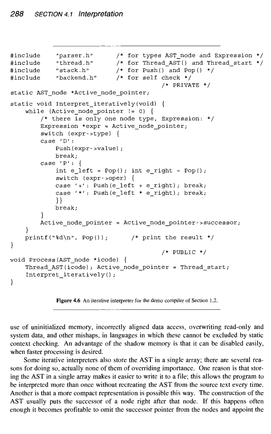
4.1 Interpretation
4.1.1 Recursive interpretation
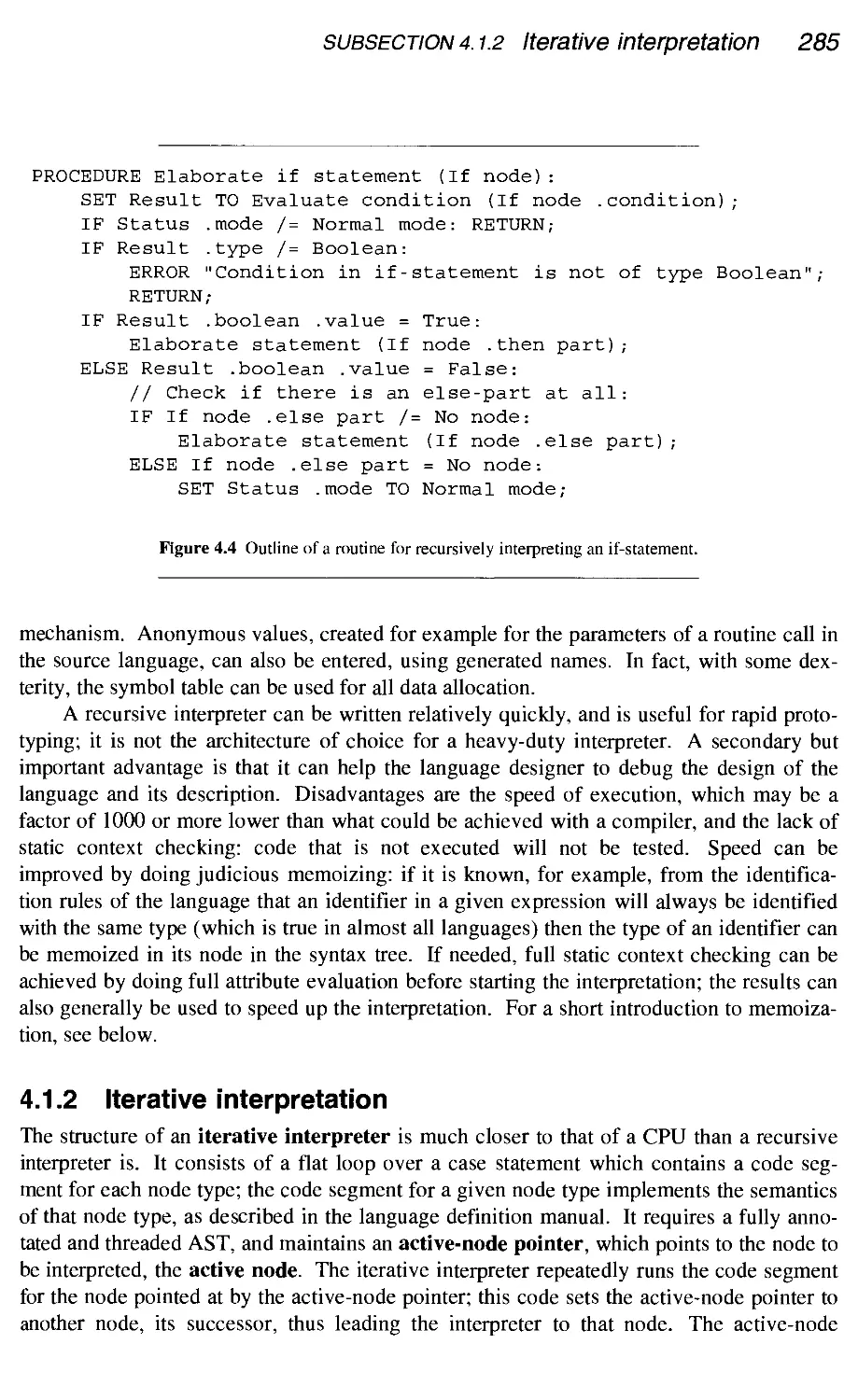
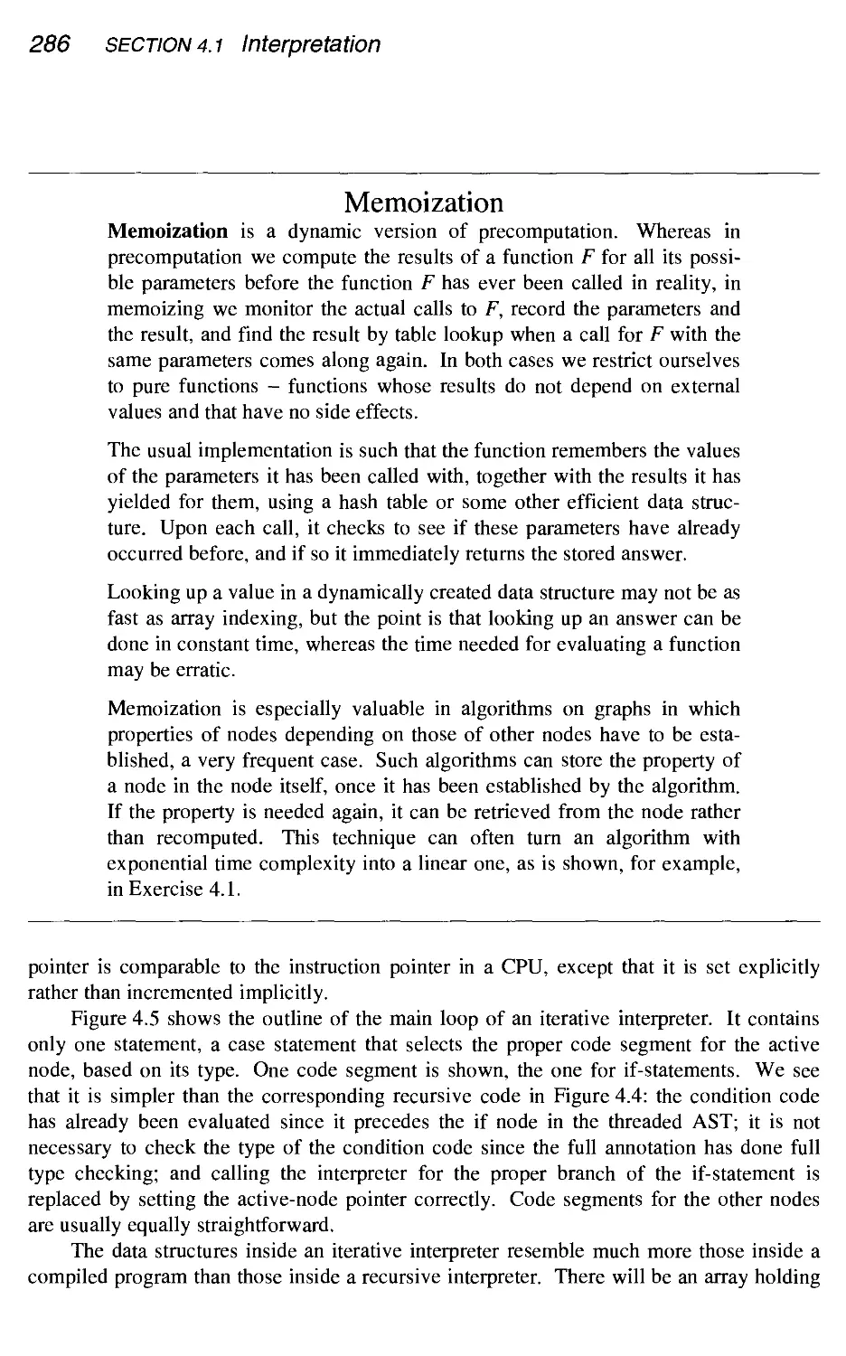
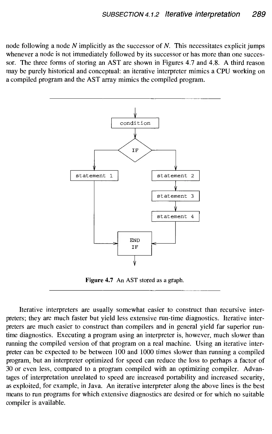
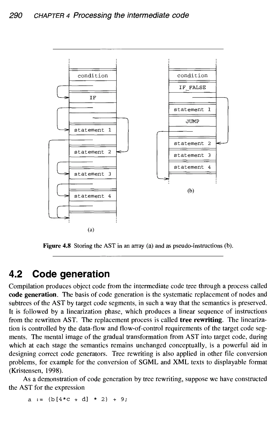
4.1.2 Iterative interpretation
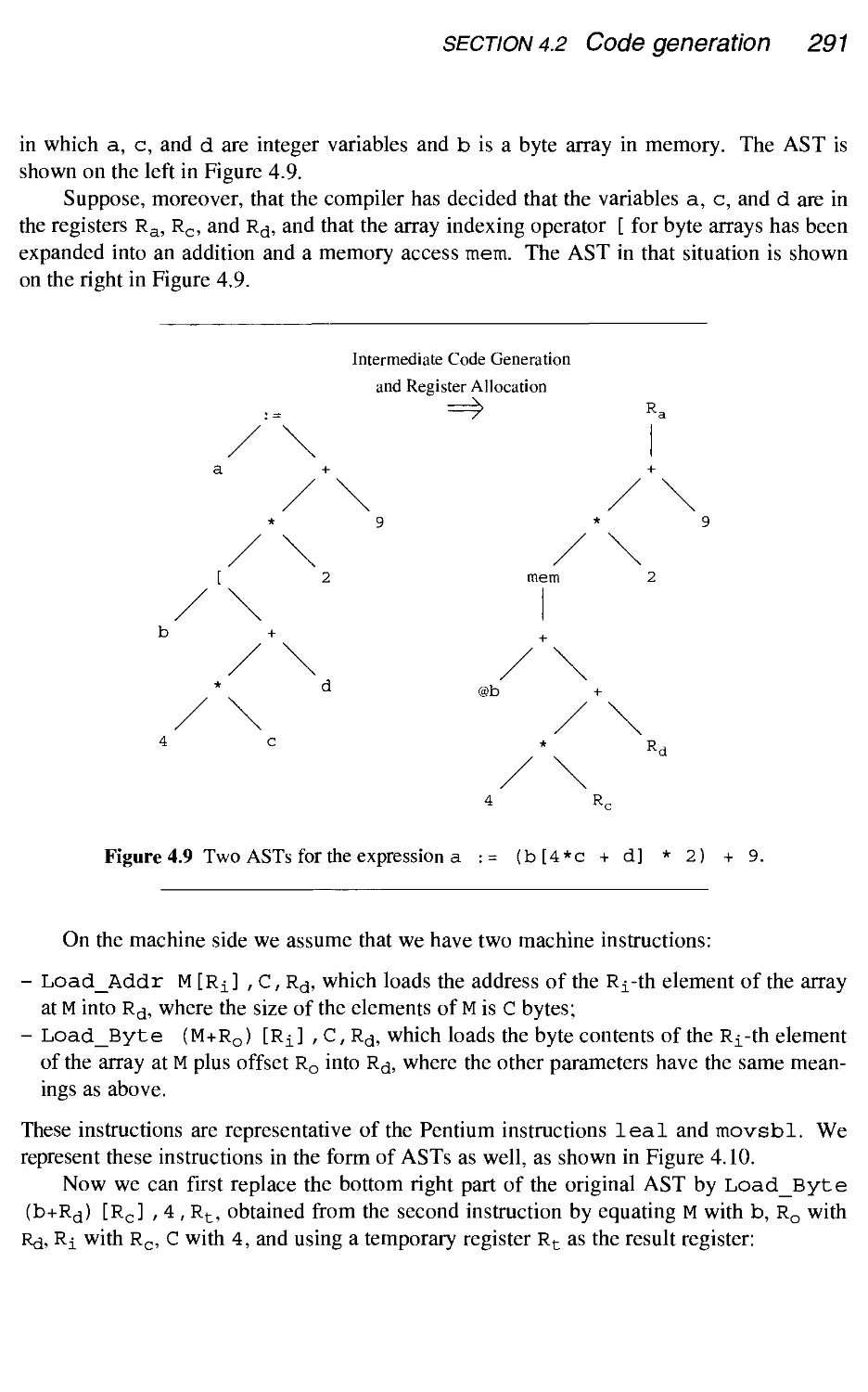
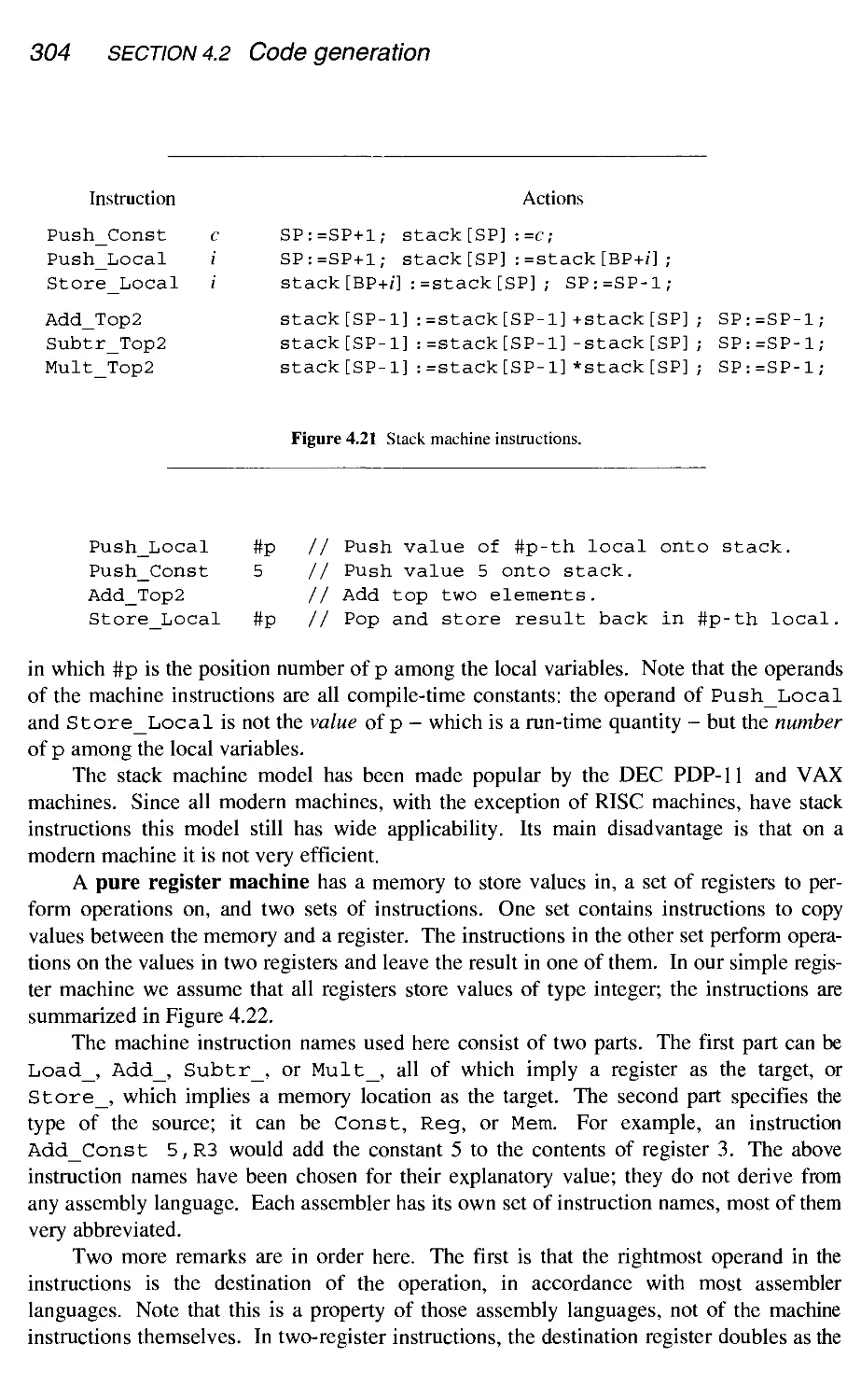
4.2 Code generation
4.2.1 Avoiding code generation altogether
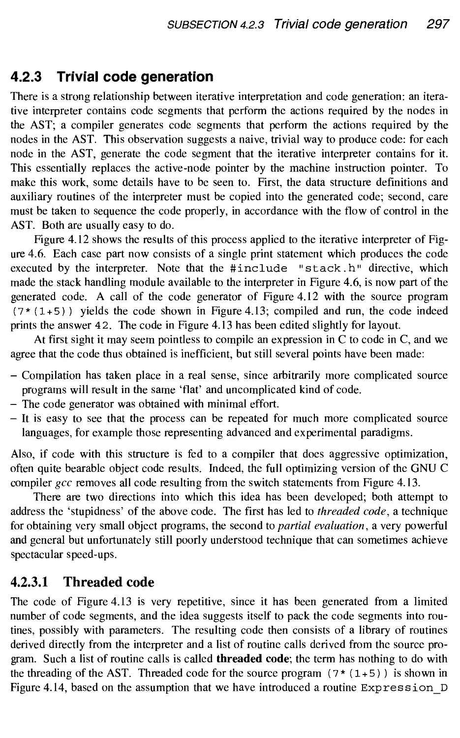
4.2.2 The starting point
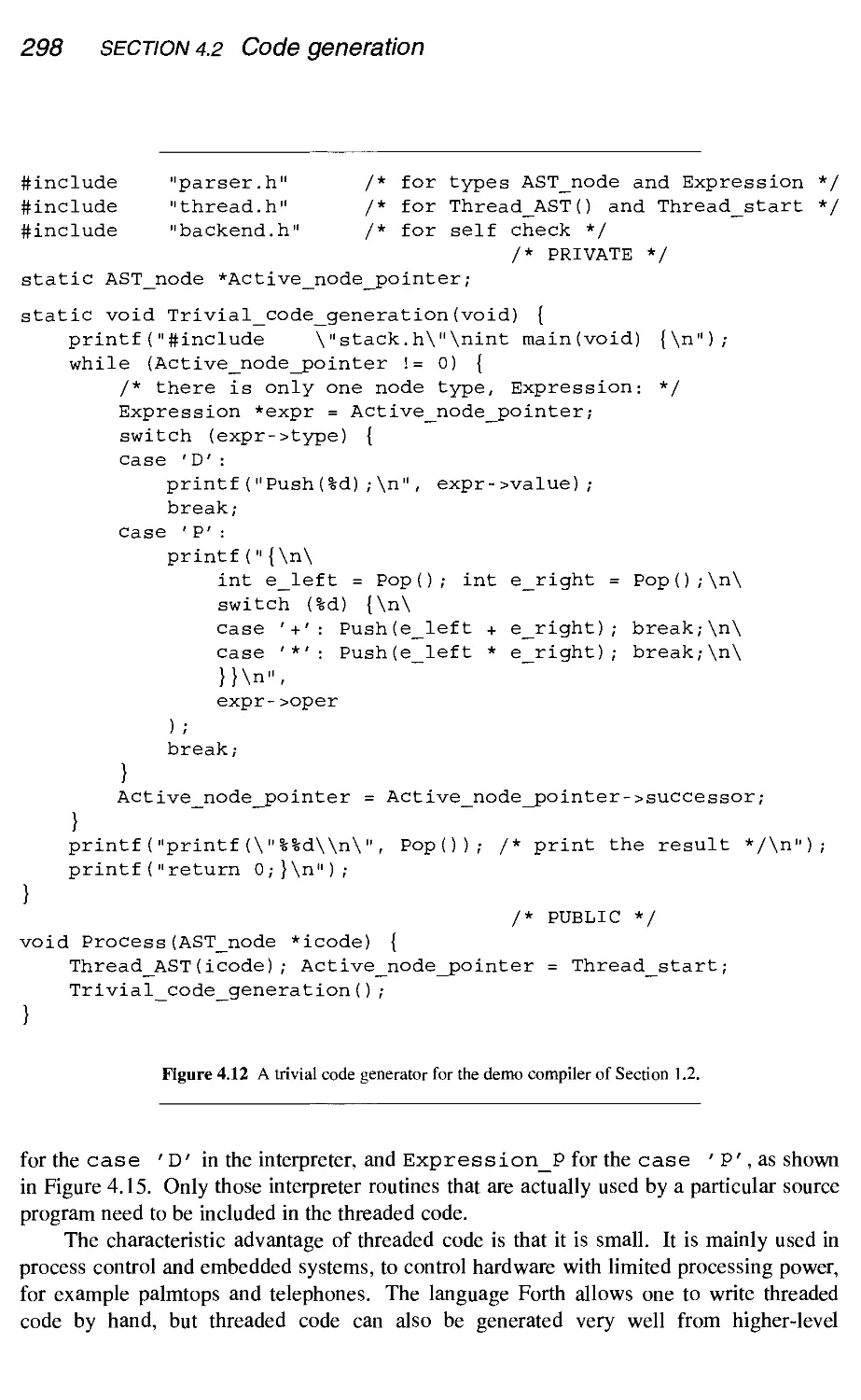
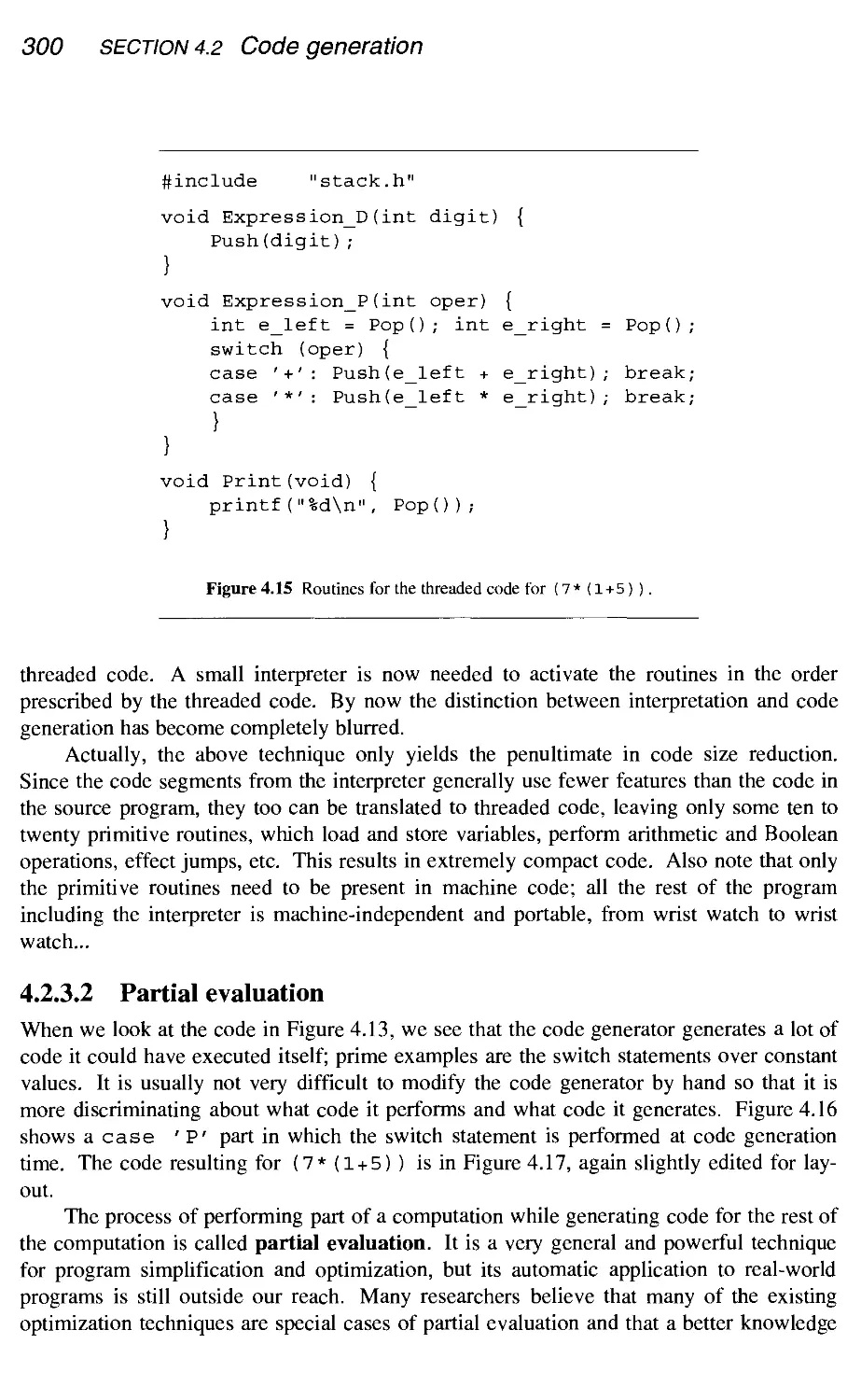
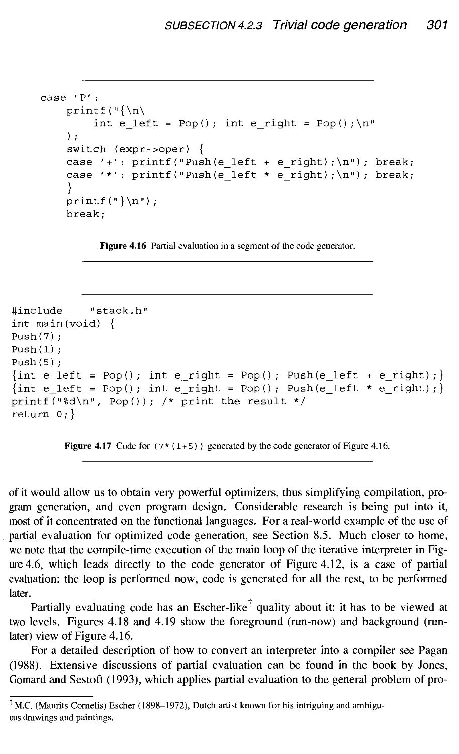
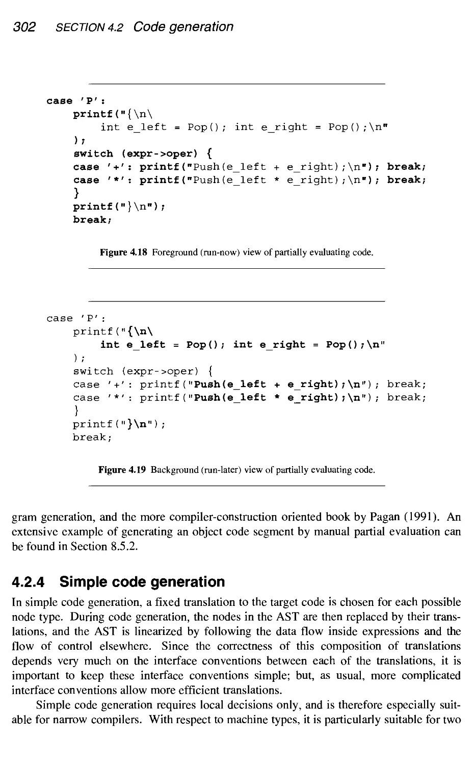
4.2.3 Trivial code generation
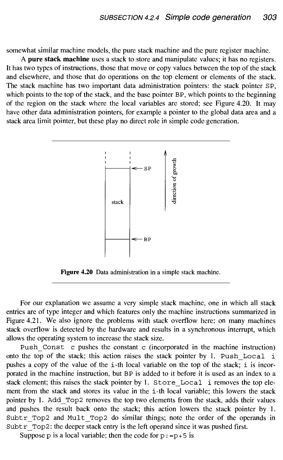
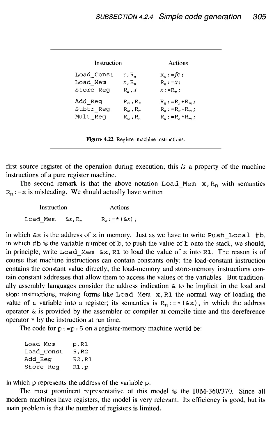
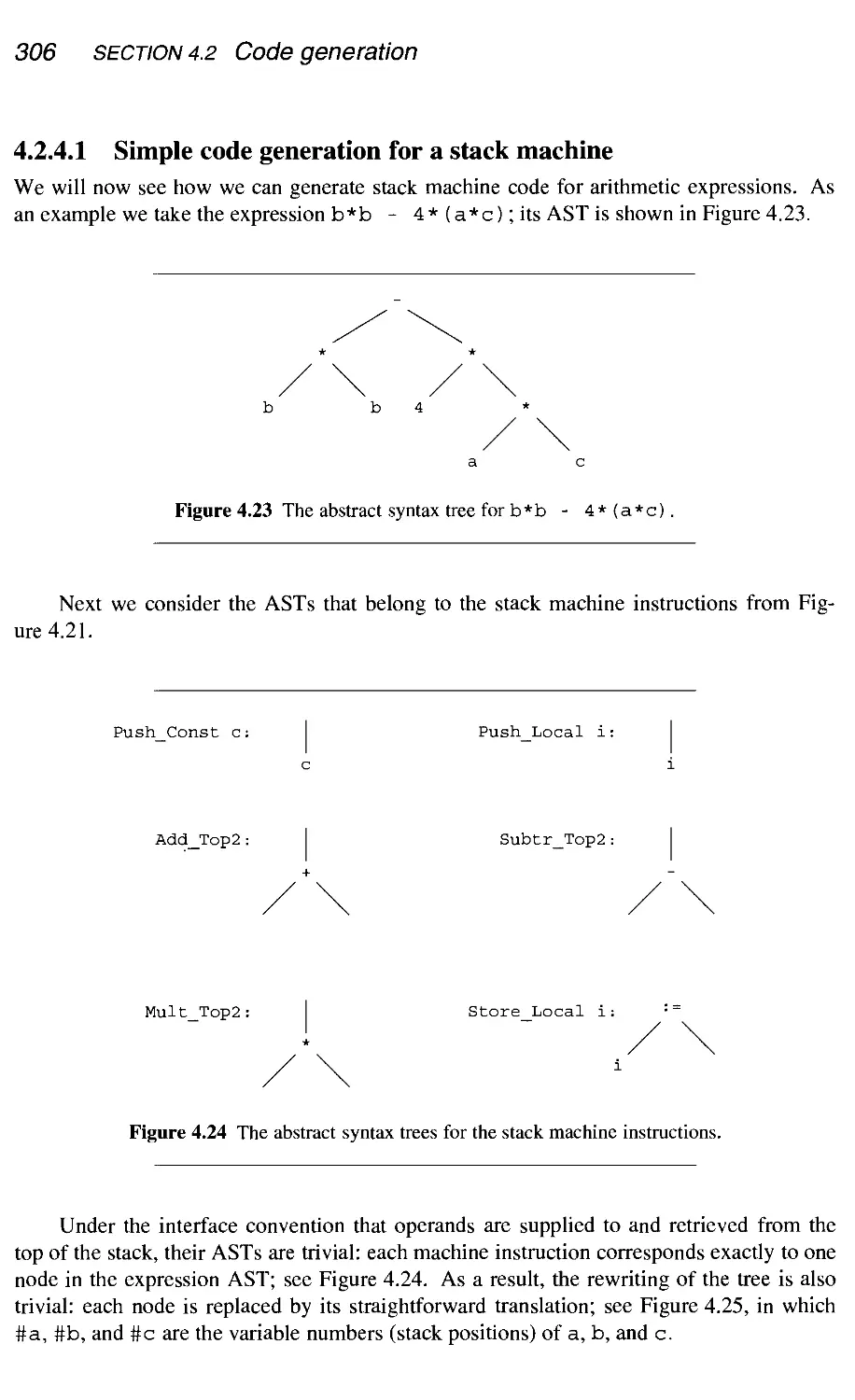
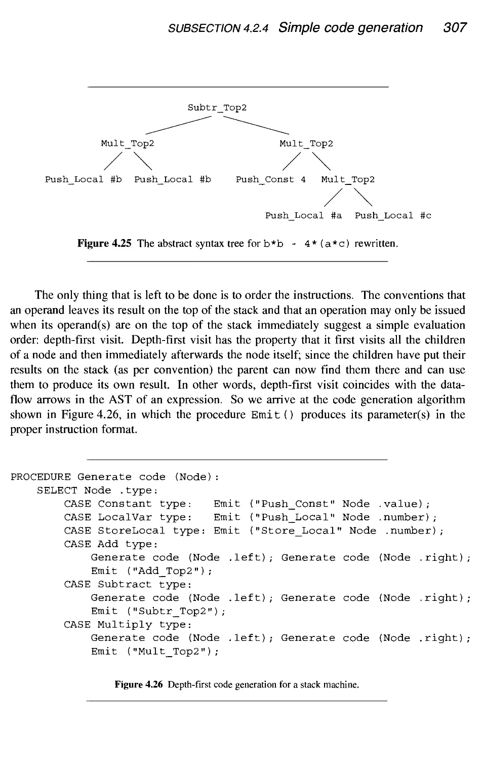
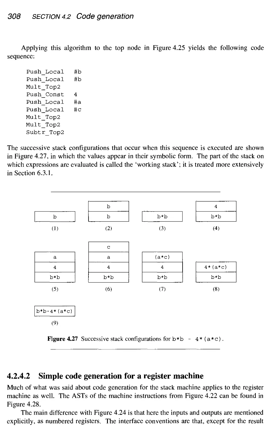
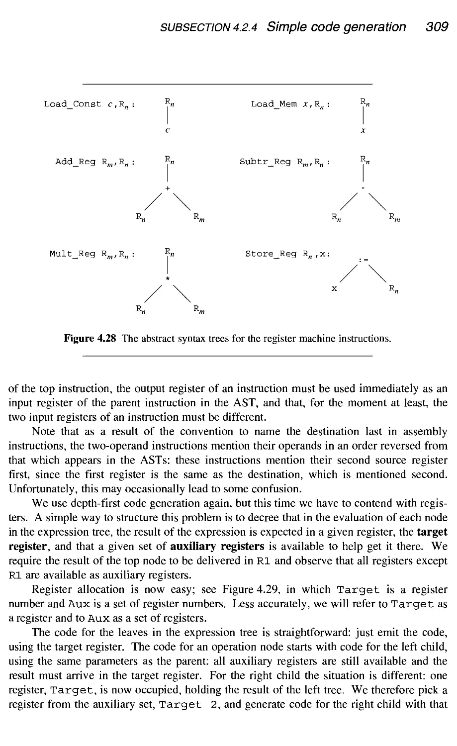
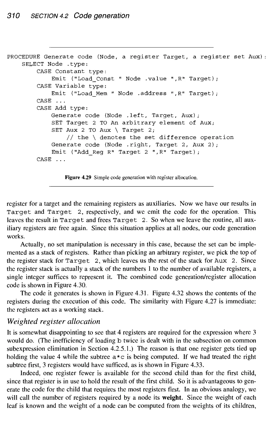
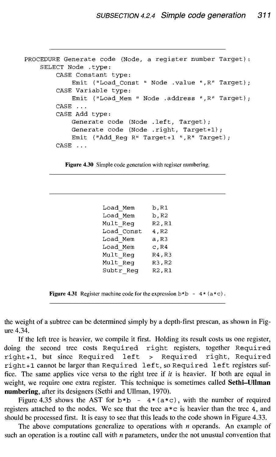
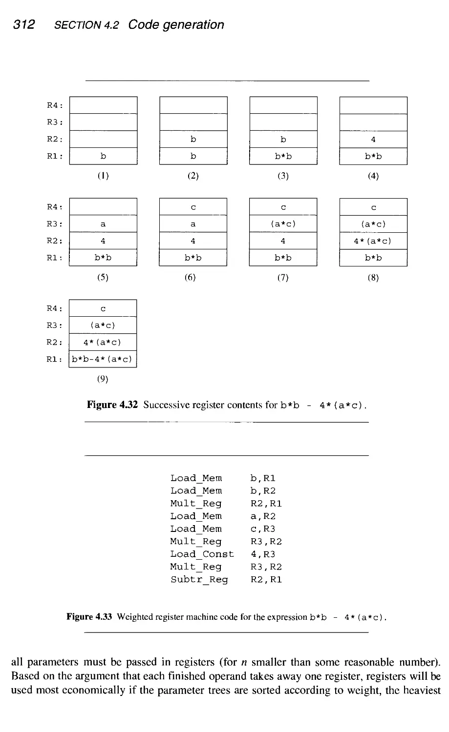
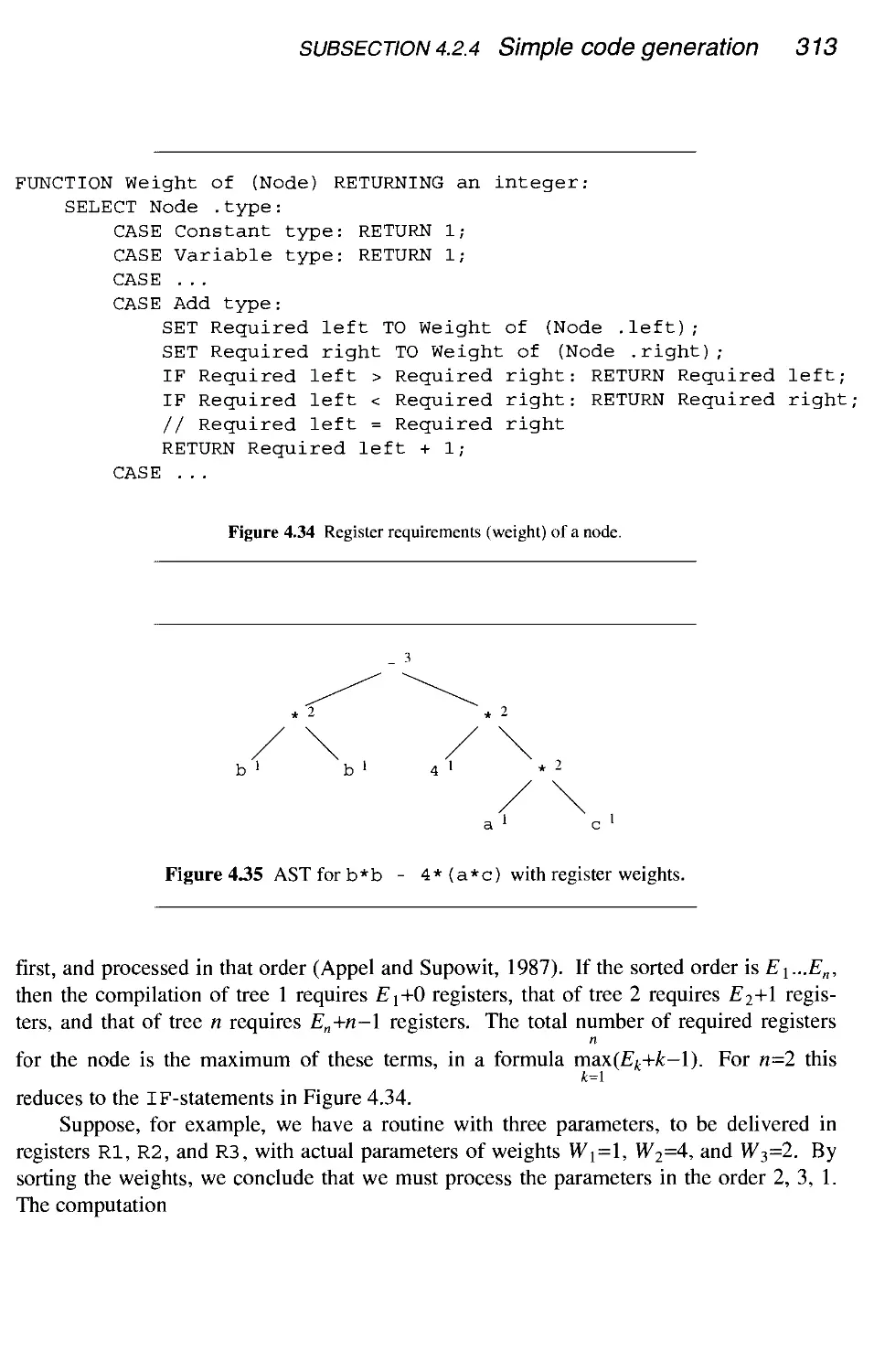
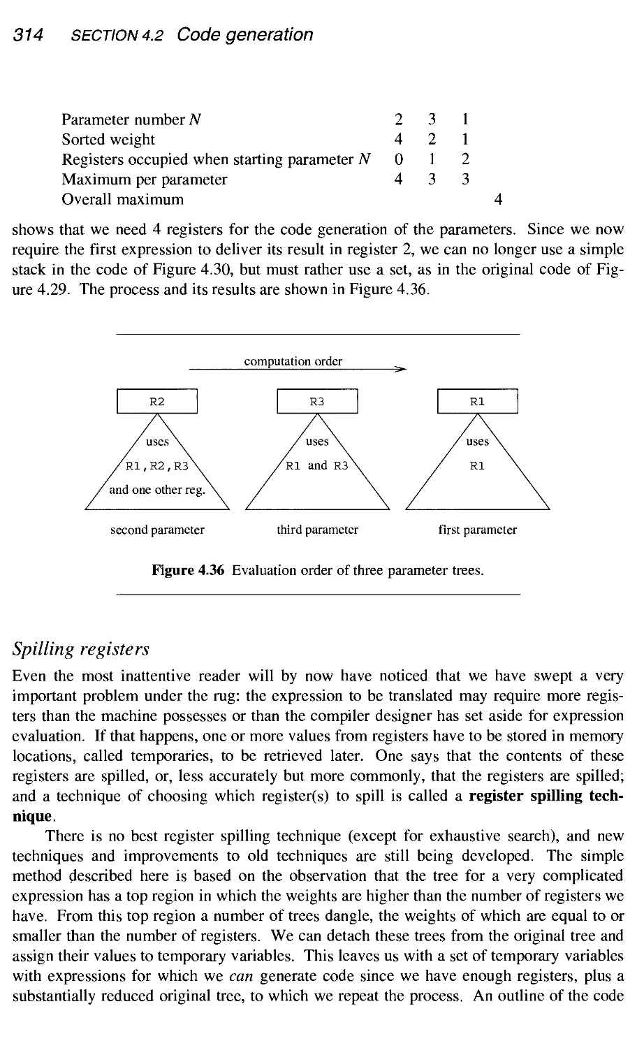
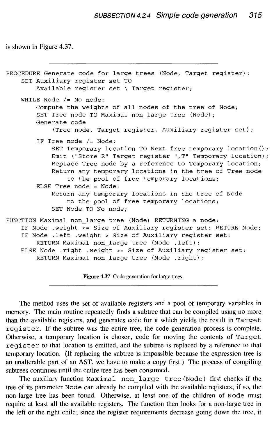
4.2.4 Simple code generation
194
195
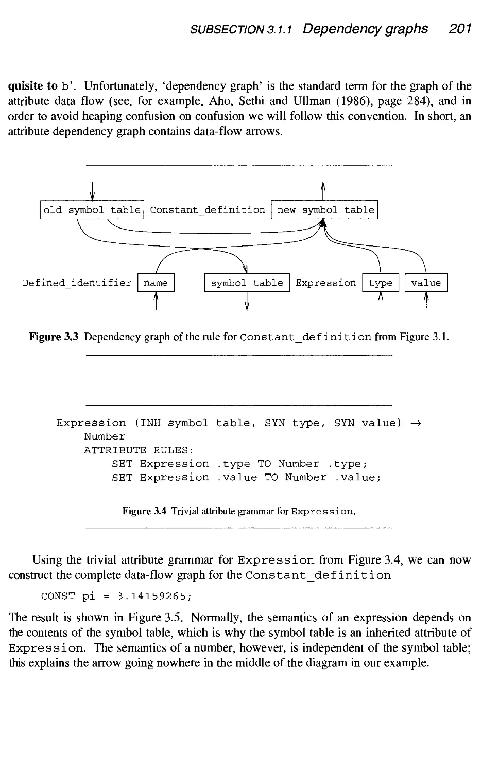
200
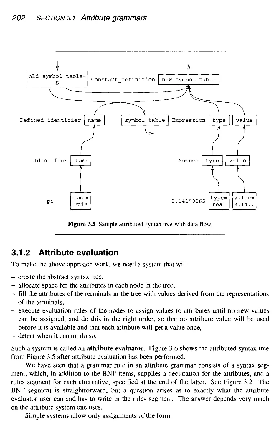
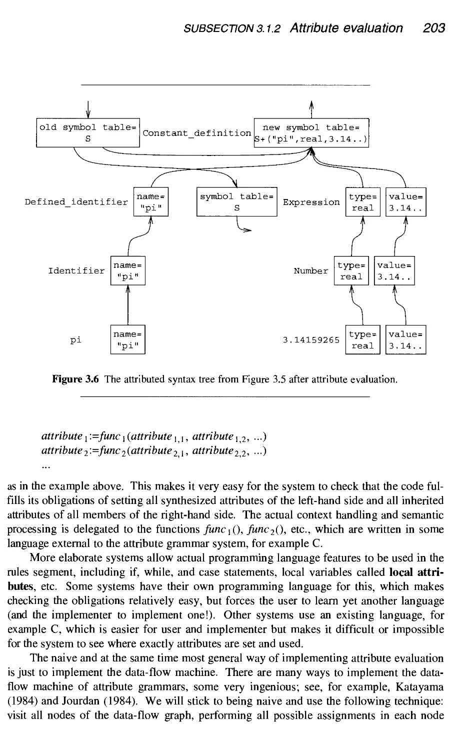
202
210
217
218
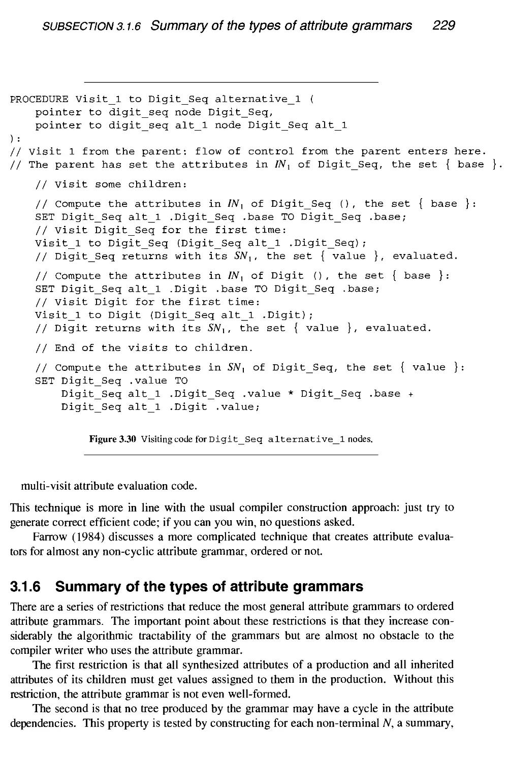
229
230
235
235
237
238
238
239
245
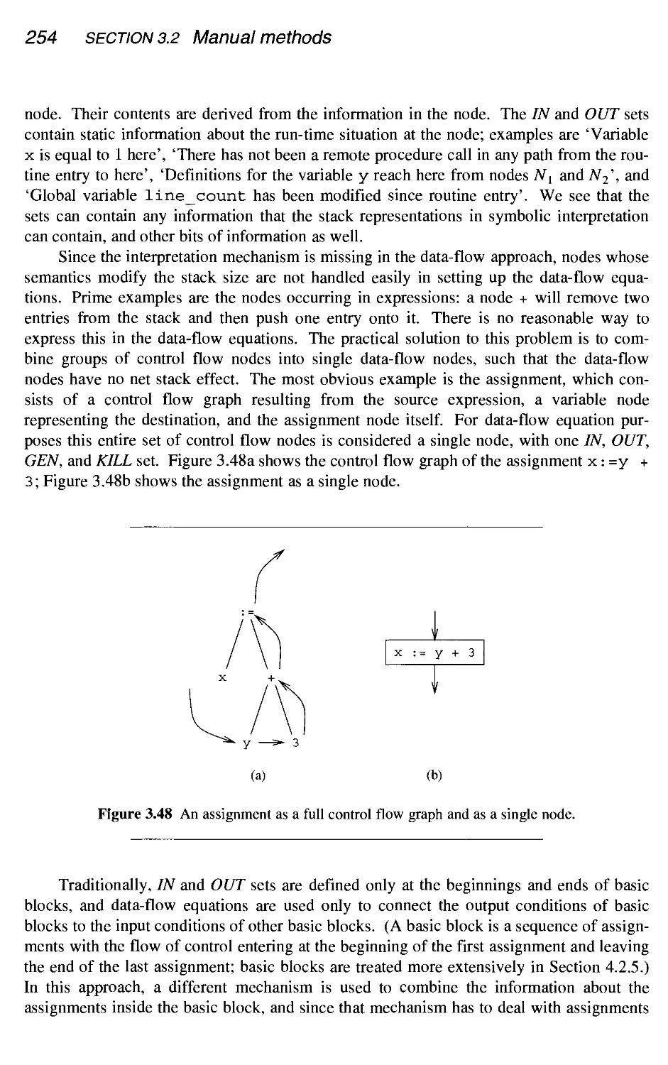
253
260
262
267
269
269
273
274
279
281
281
285
290
295
296
297
302
viii Contents
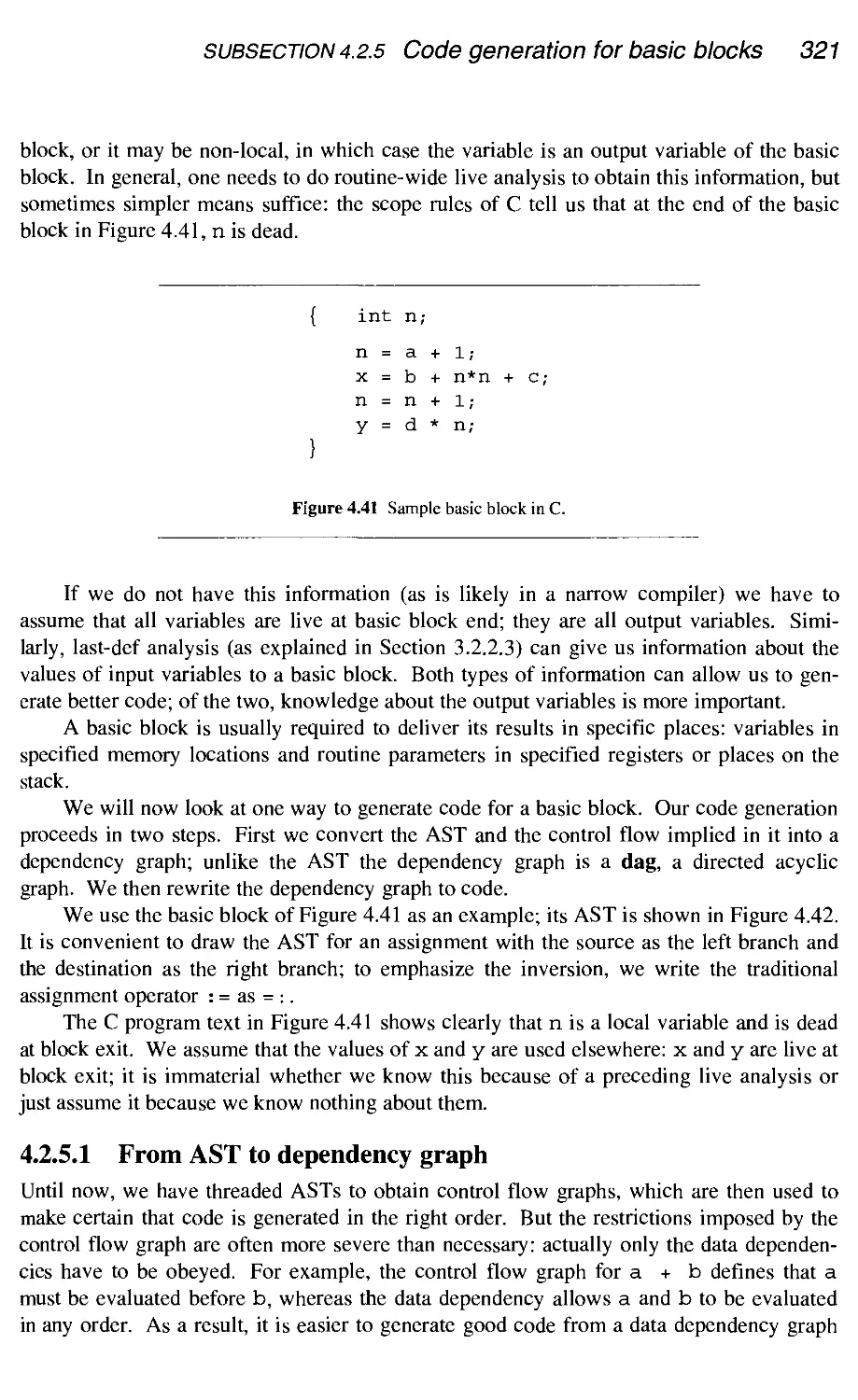
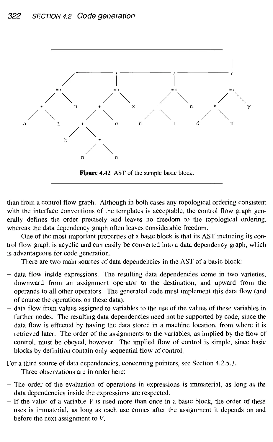
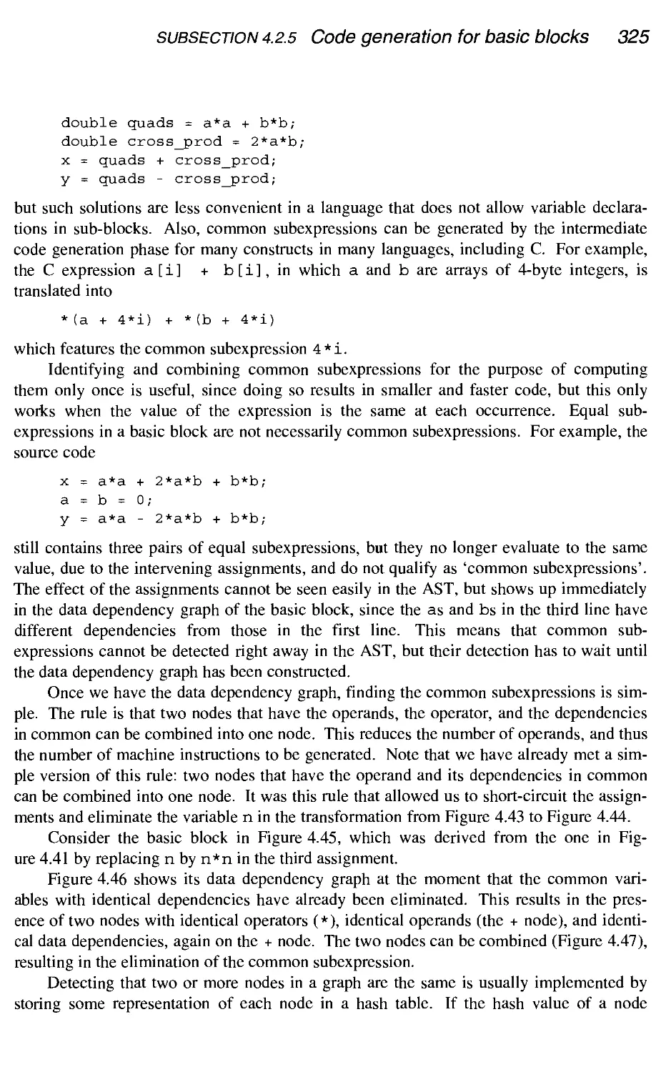
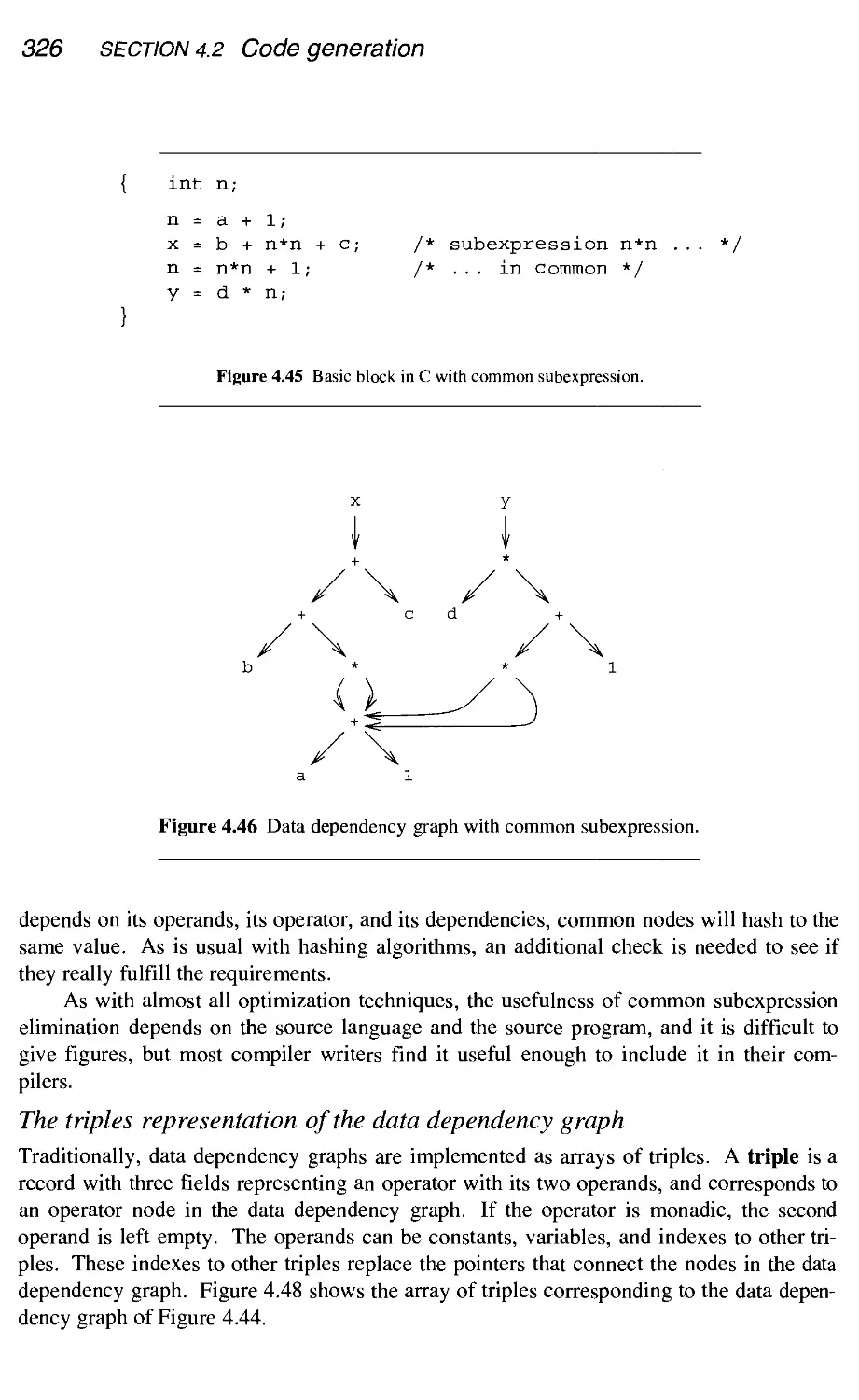
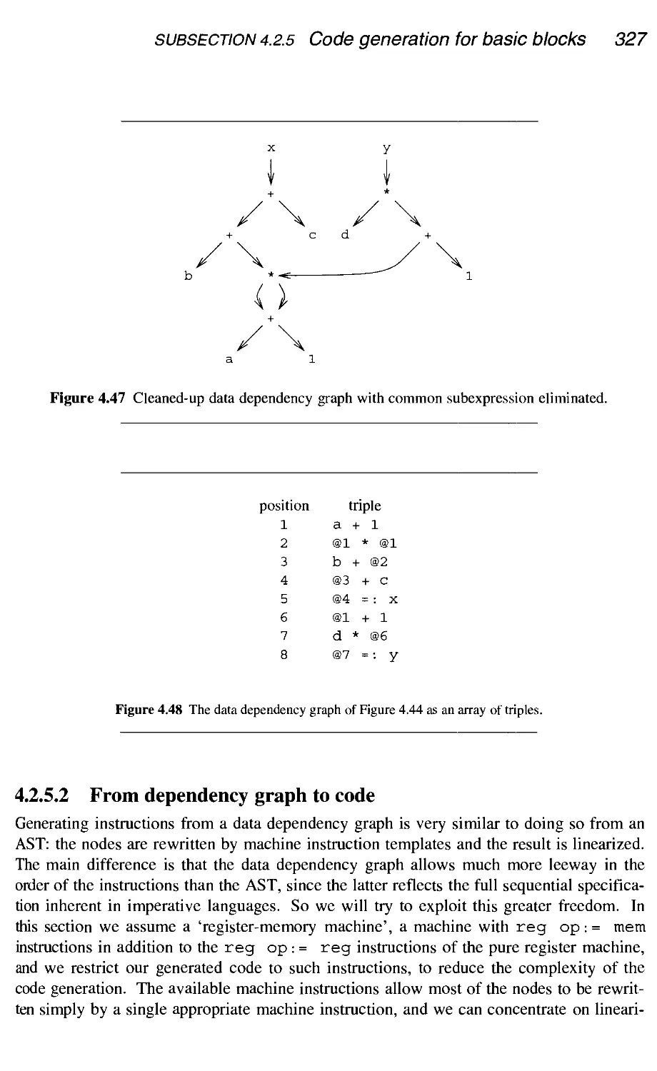
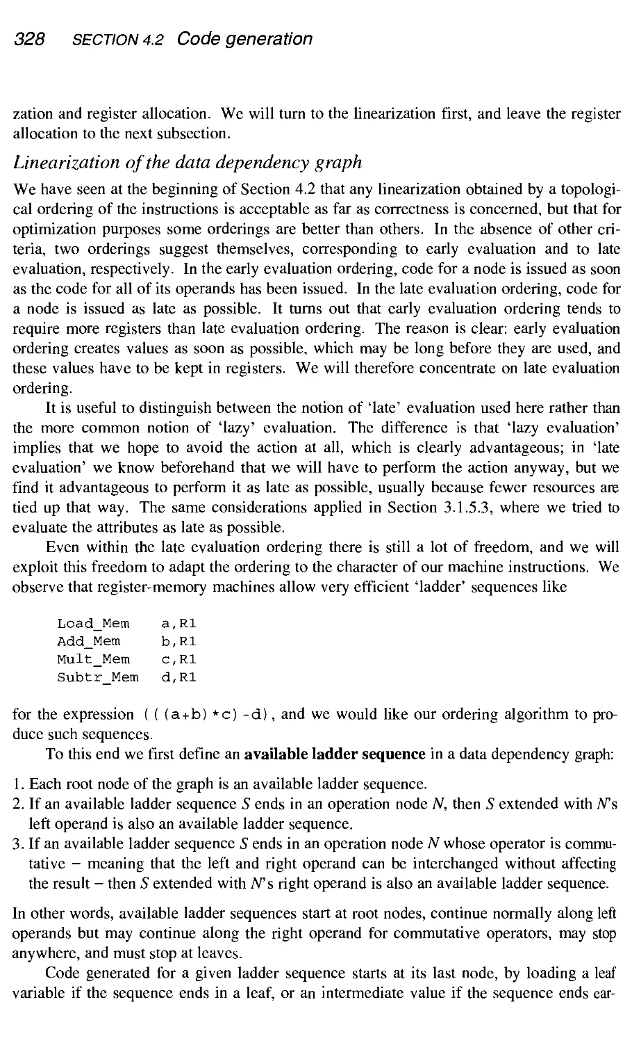
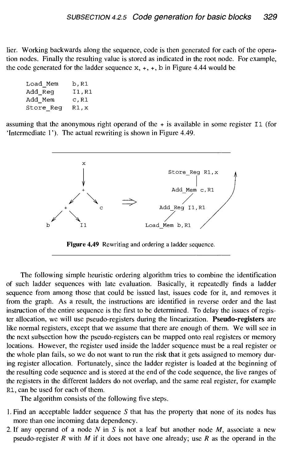
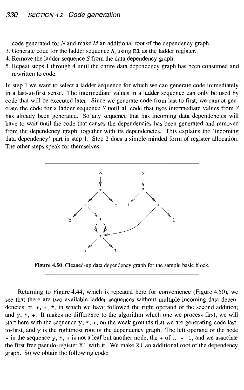
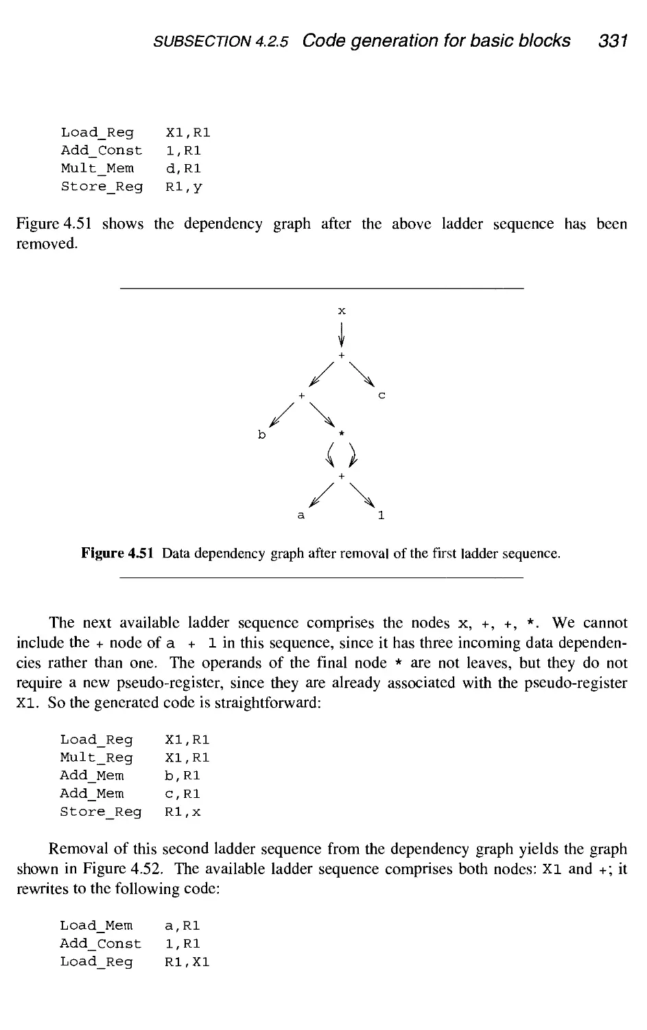
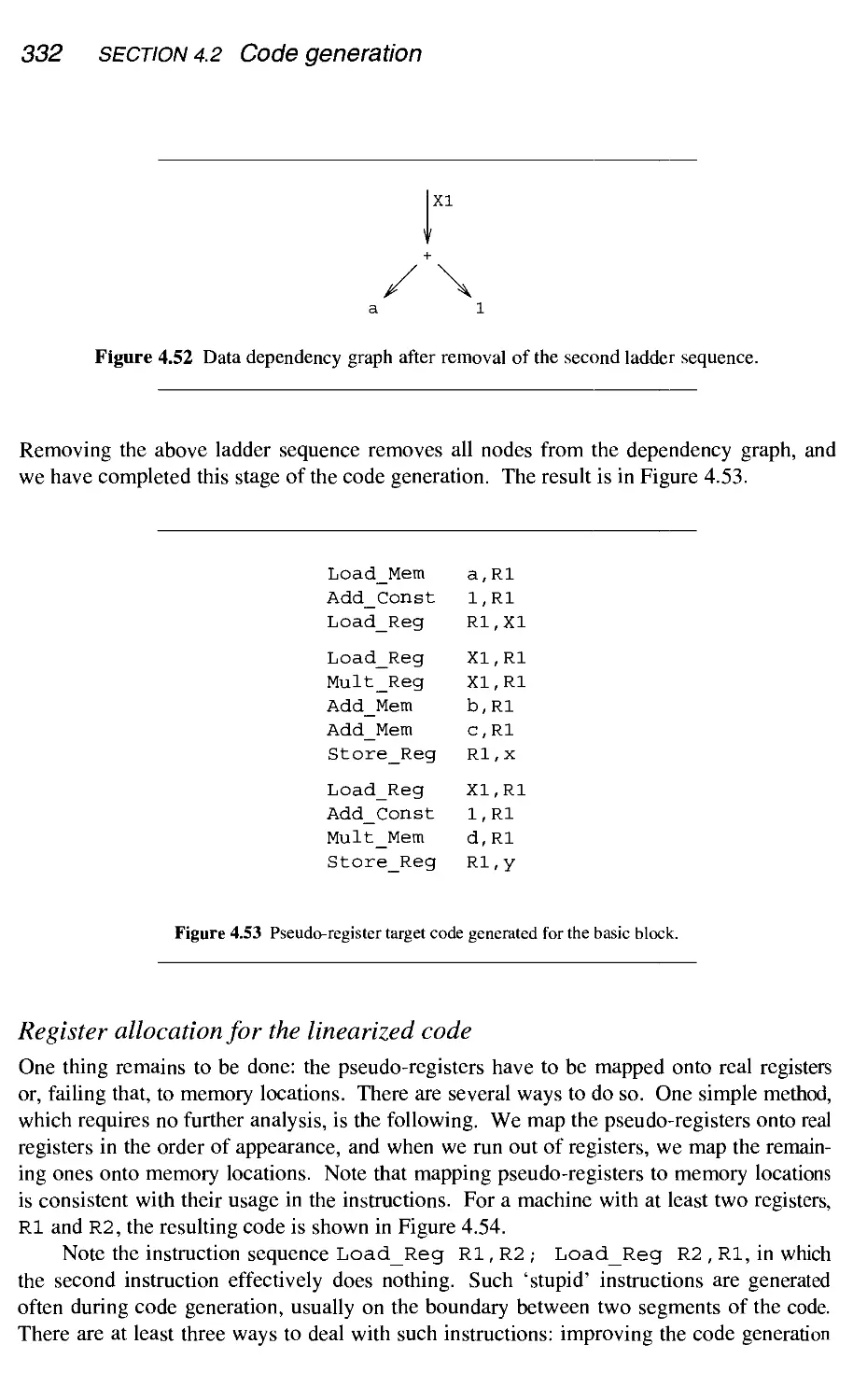
4.2.5 Code generation for basic blocks 320
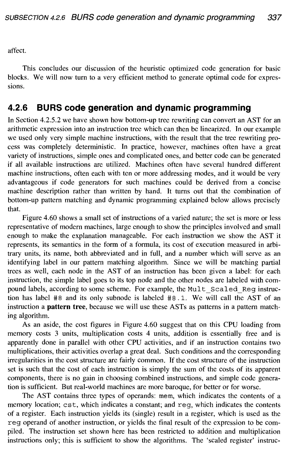
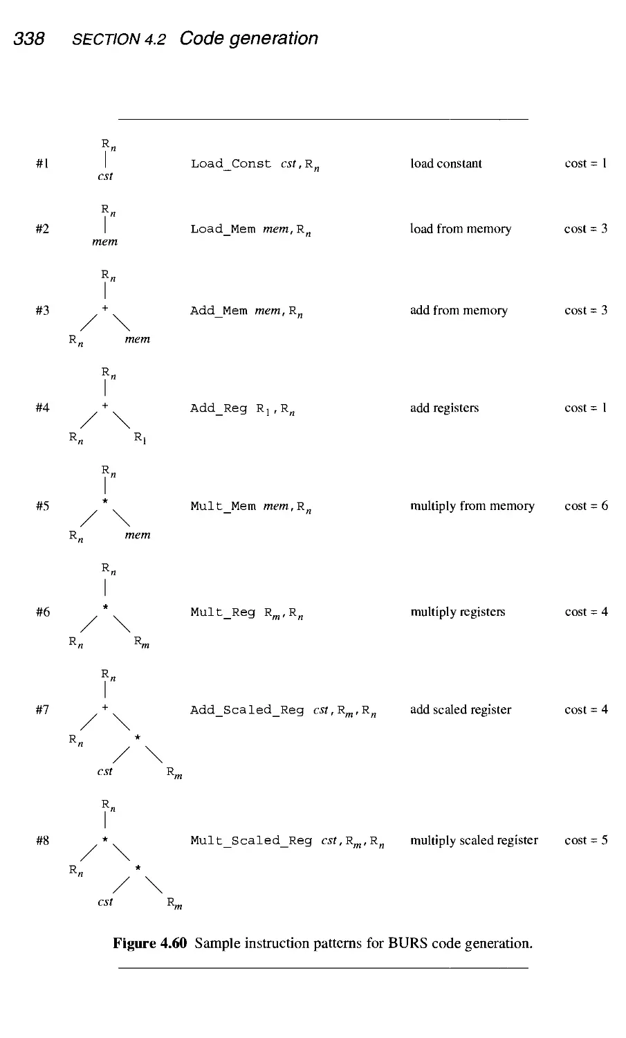
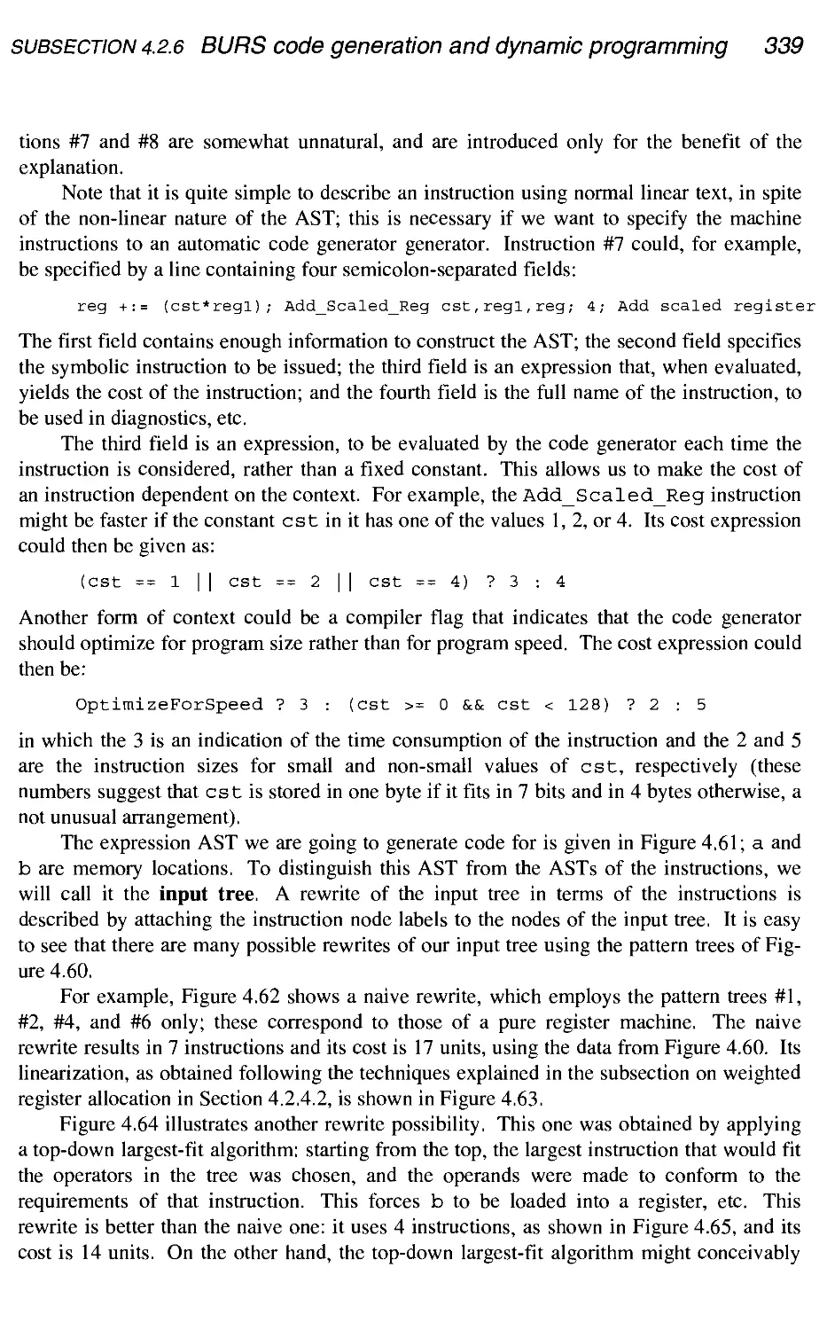
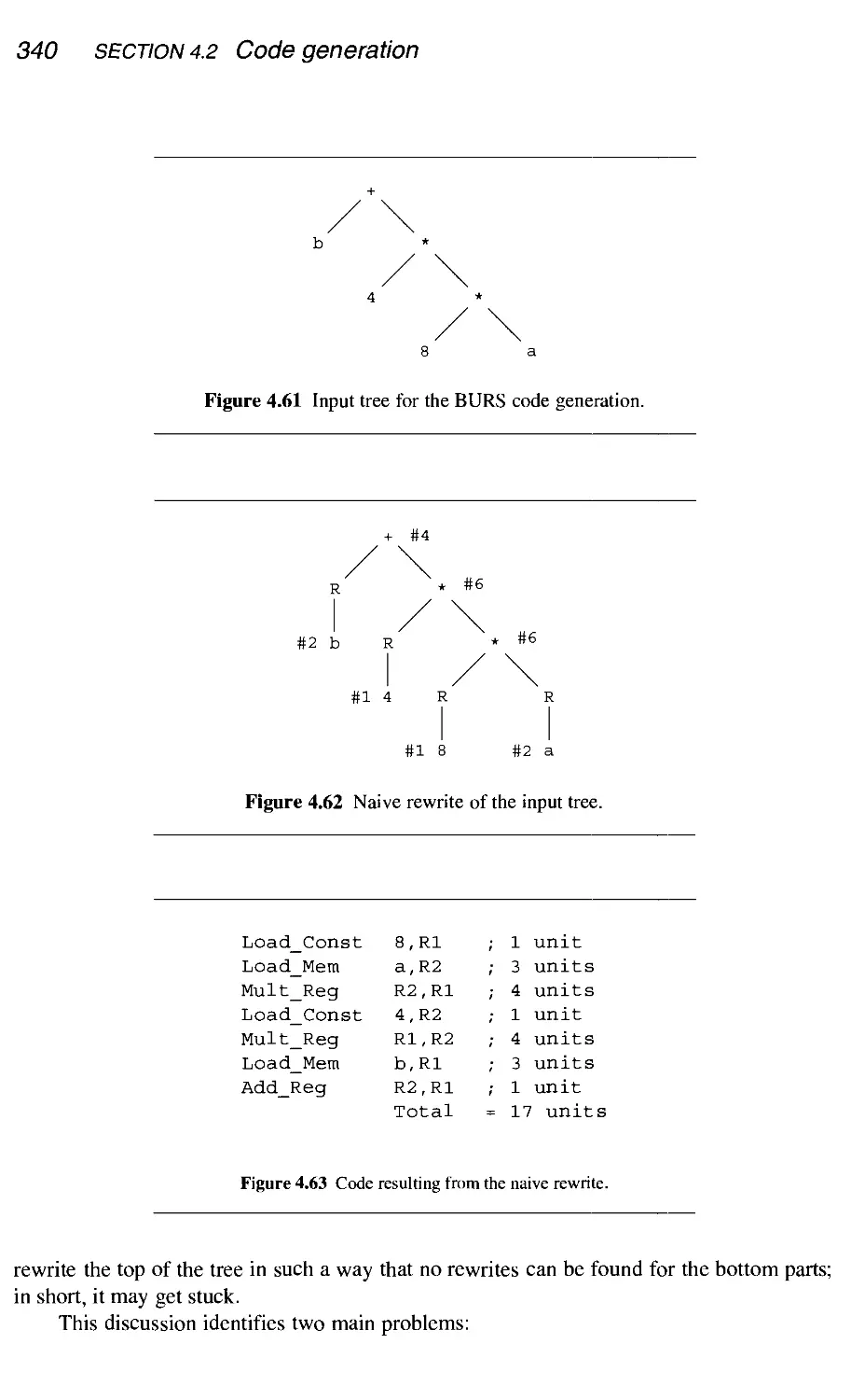
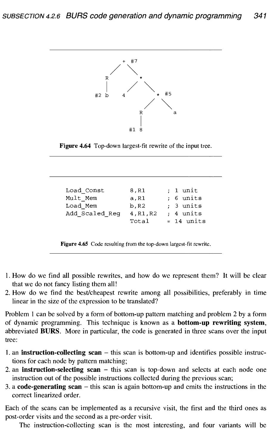
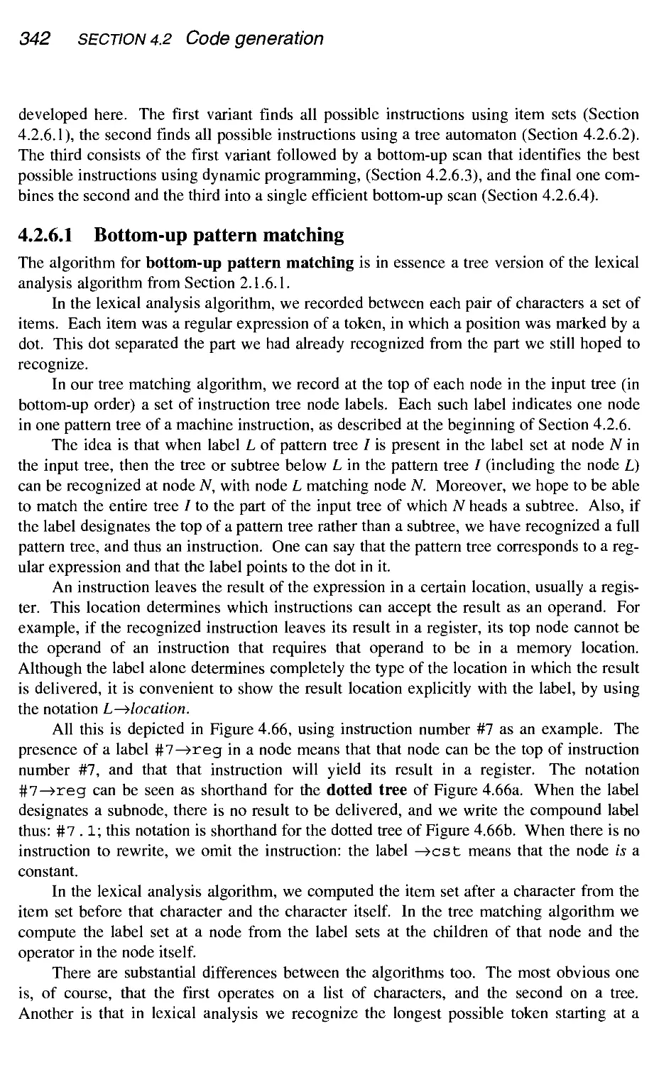
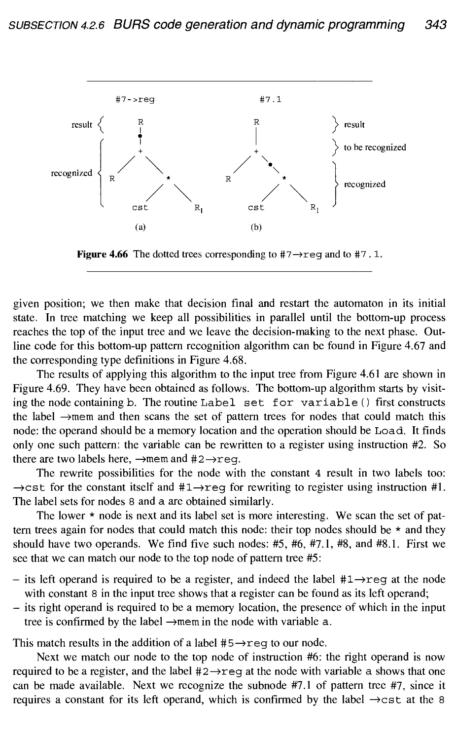
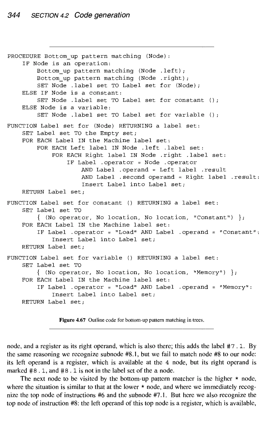
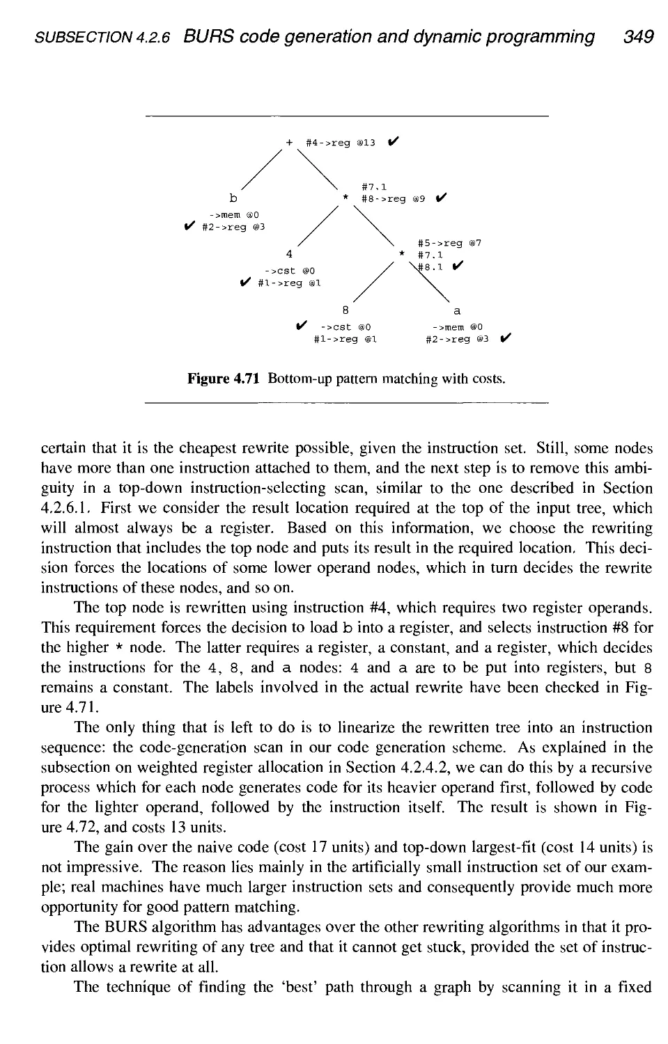
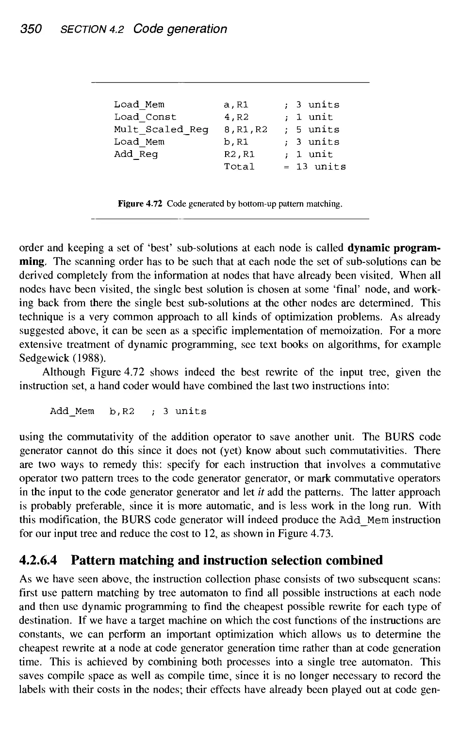
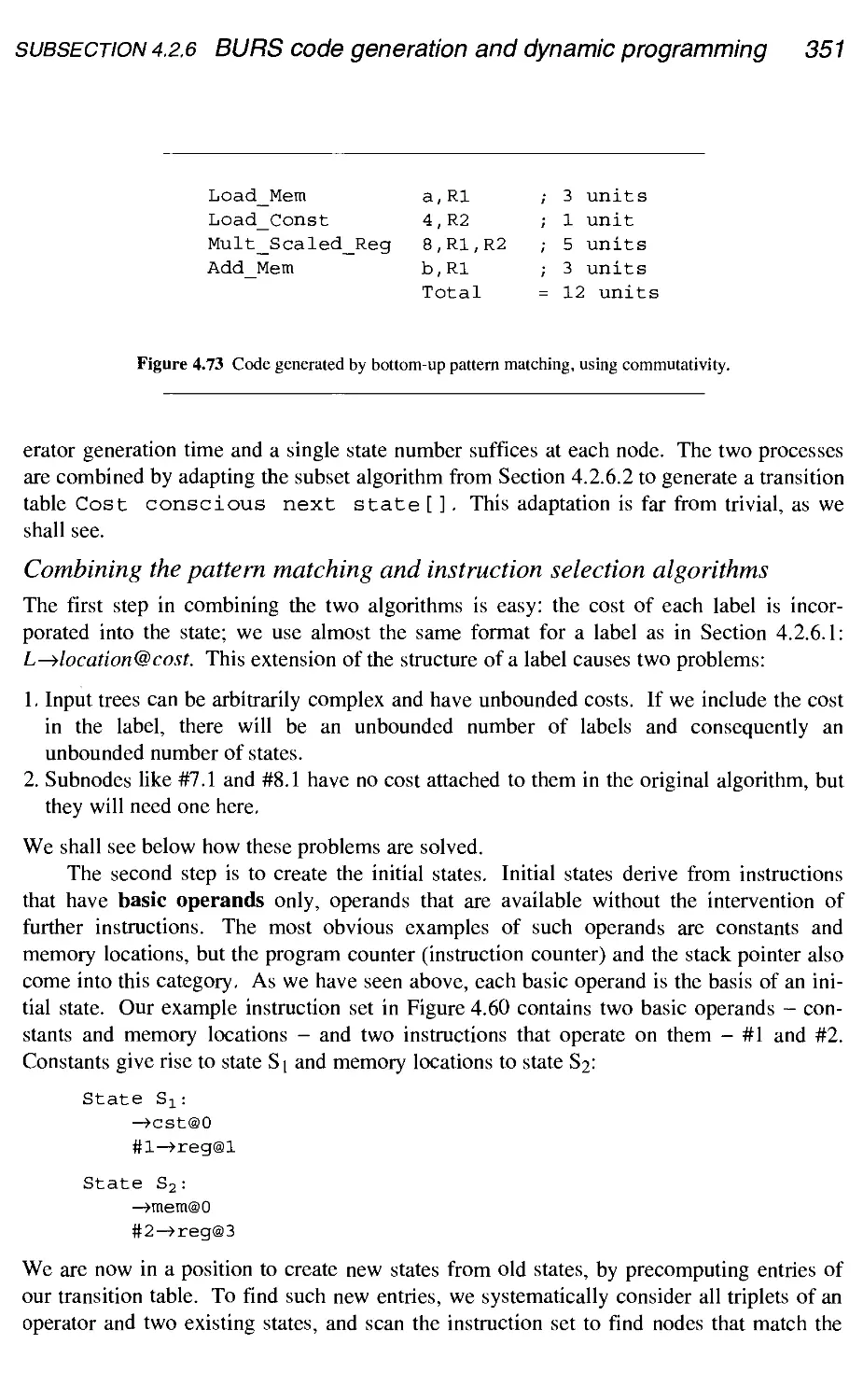
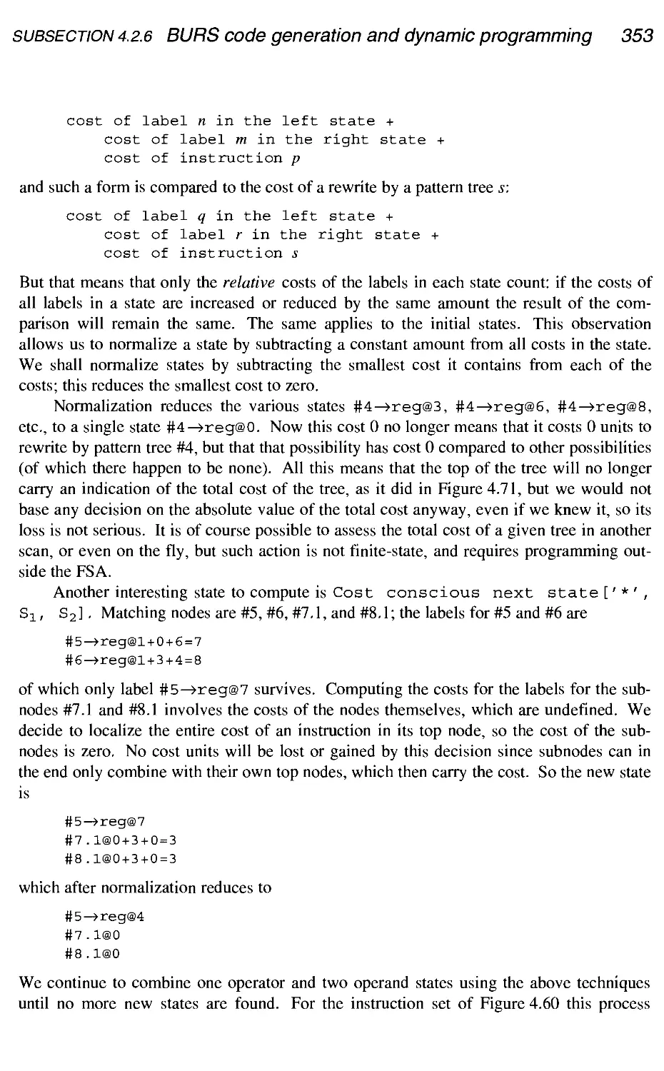
4.2.6 BURS code generation and dynamic programming 337
4.2.7 Register allocation by graph coloring 357
4.2.8 Supercompilation 363
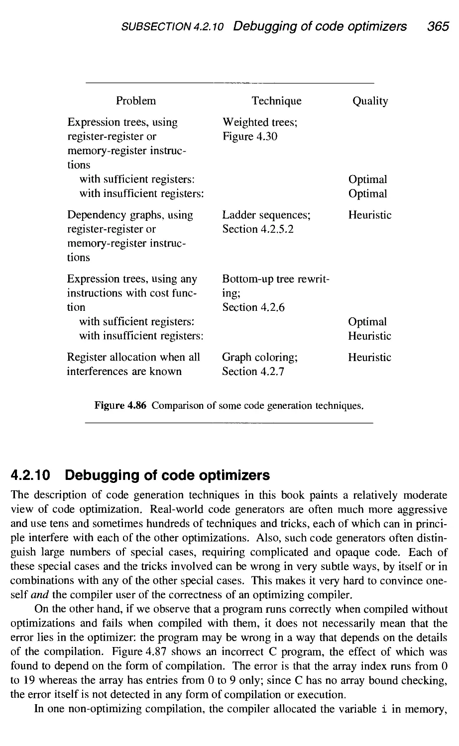
4.2.9 Evaluation of code generation techniques 364
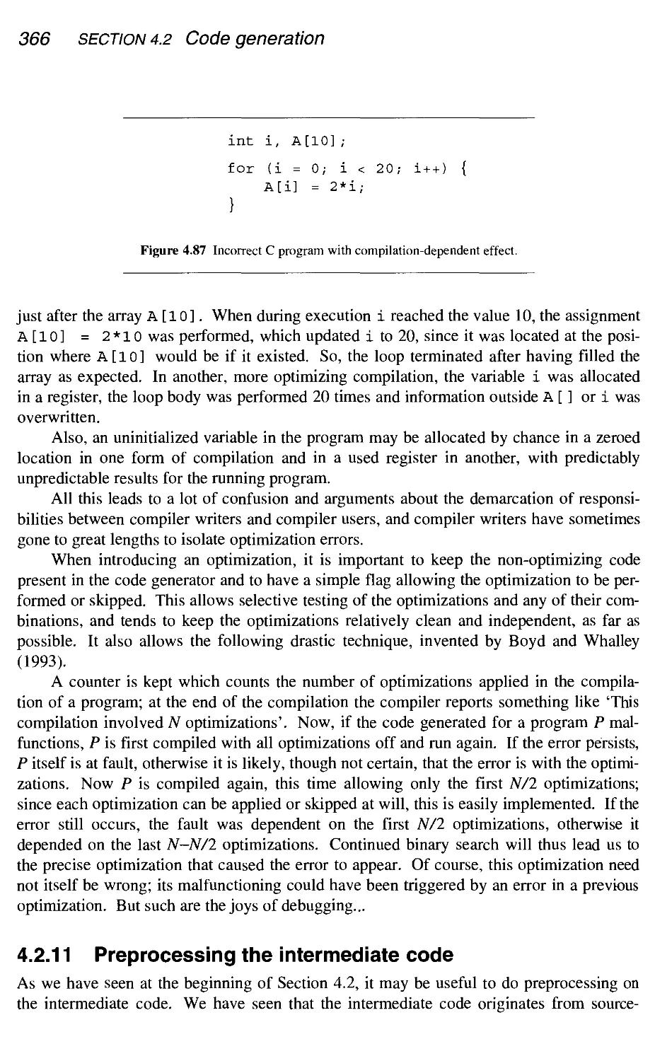
4.2.10 Debugging of code optimizers 365
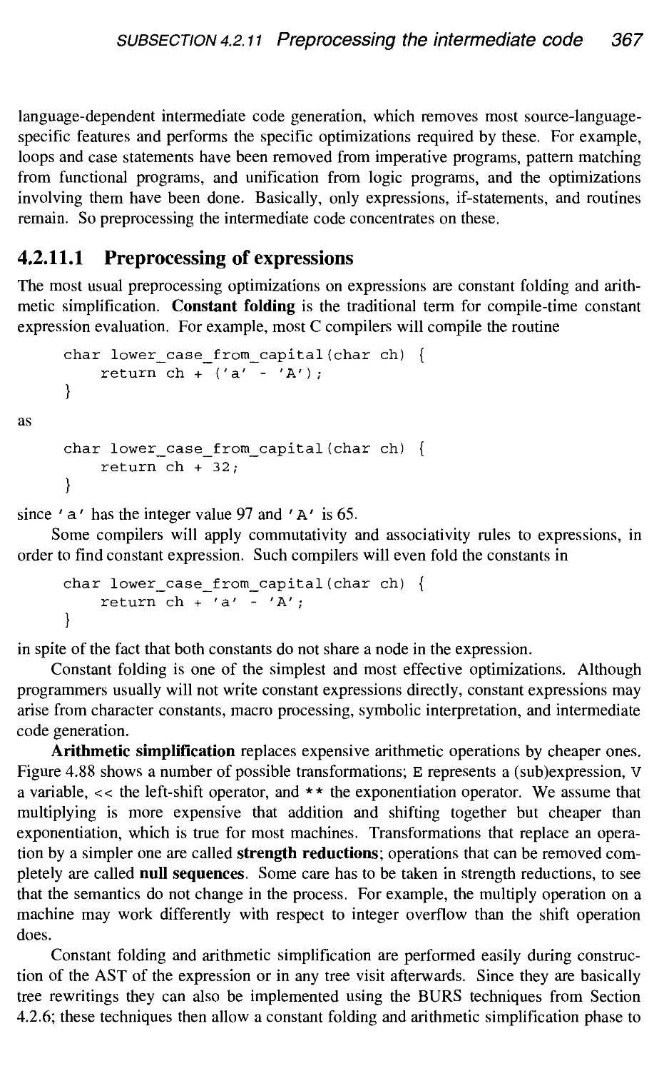
4.2.11 Preprocessing the intermediate code 366
4.2.12 Postprocessing the target code 371
4.2.13 Machine code generation 374
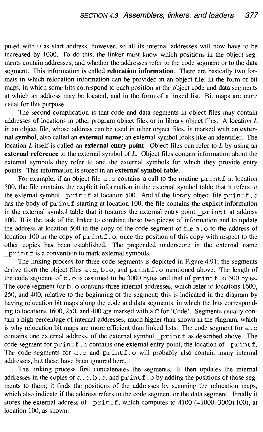
4.3 Assemblers, linkers, and loaders 375
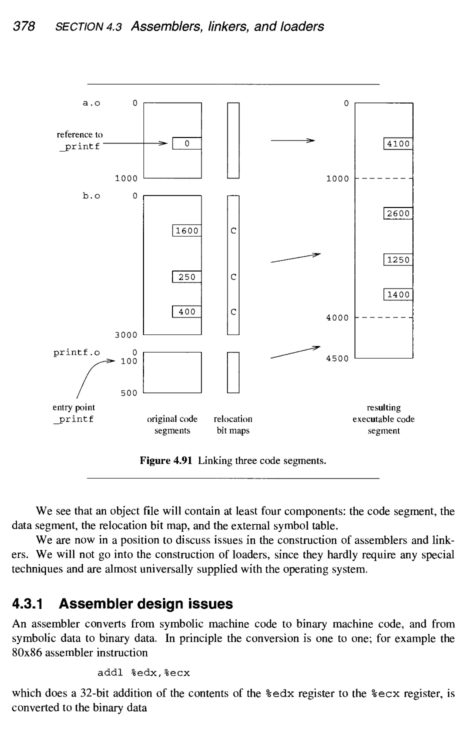
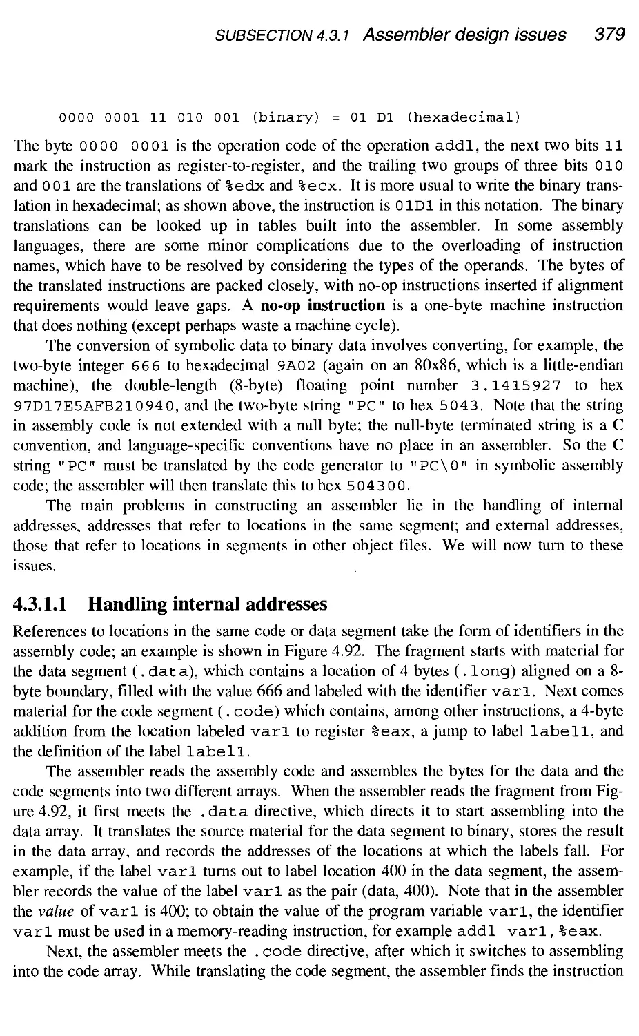
4.3.1 Assembler design issues 378
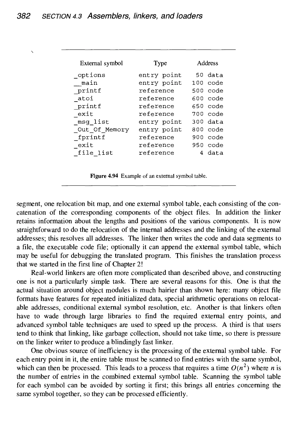
4.3.2 Linker design issues 381
4.4 Conclusion 383
Summary 383
Further reading 389
Exercises 389
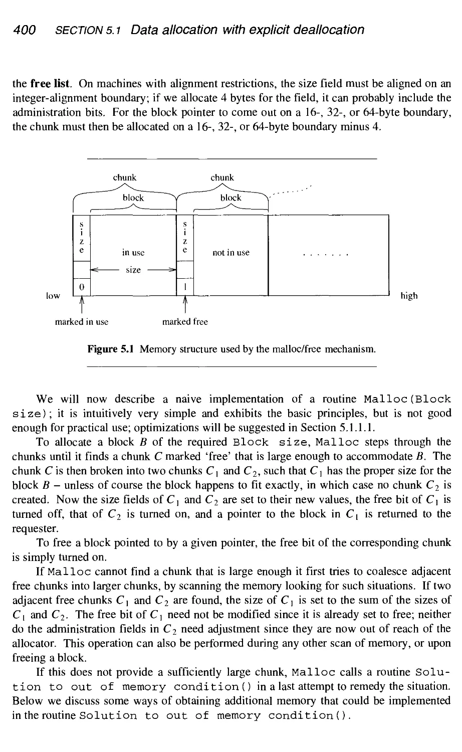
Memory management 396
5.1 Data allocation with explicit deallocation 398
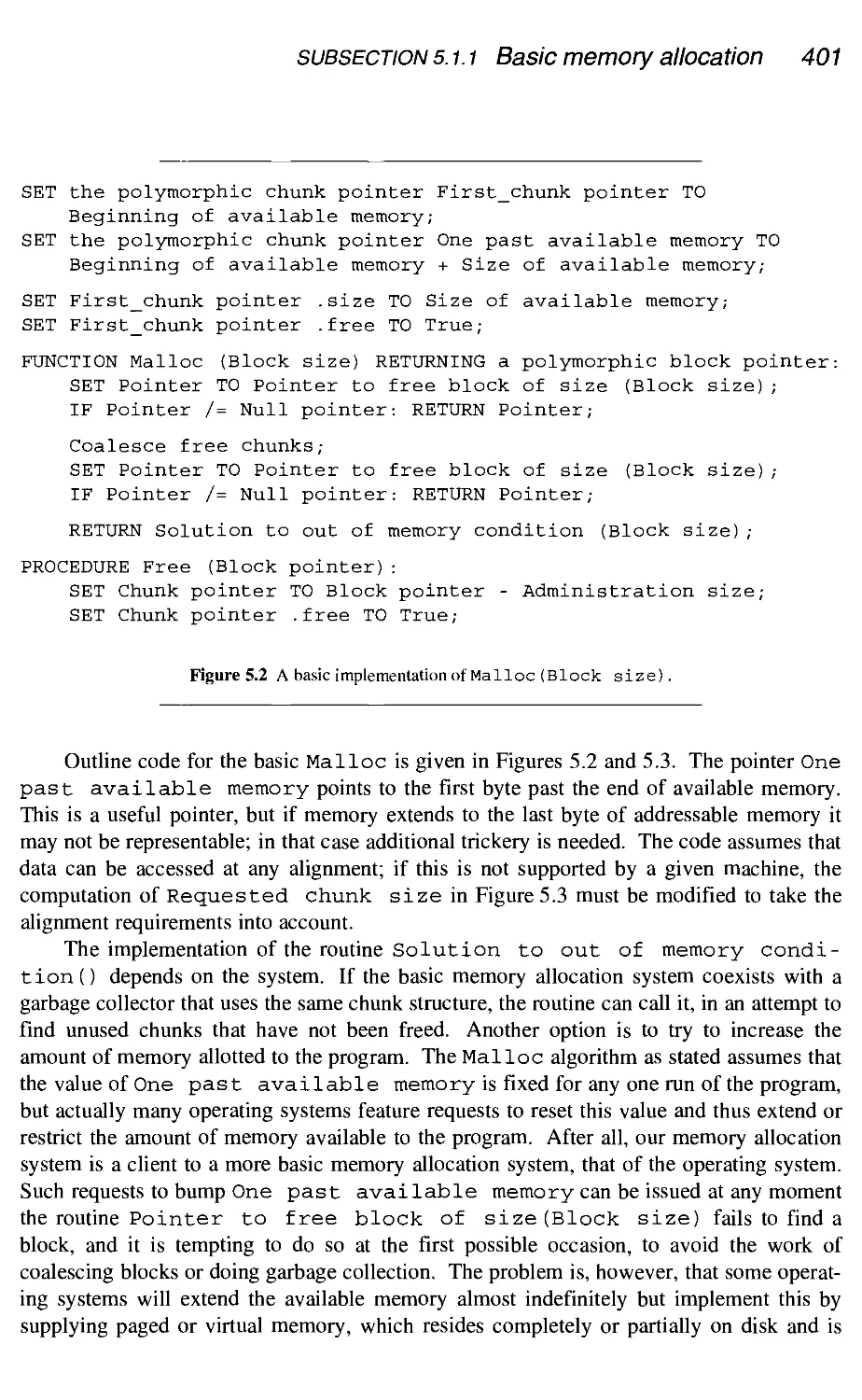
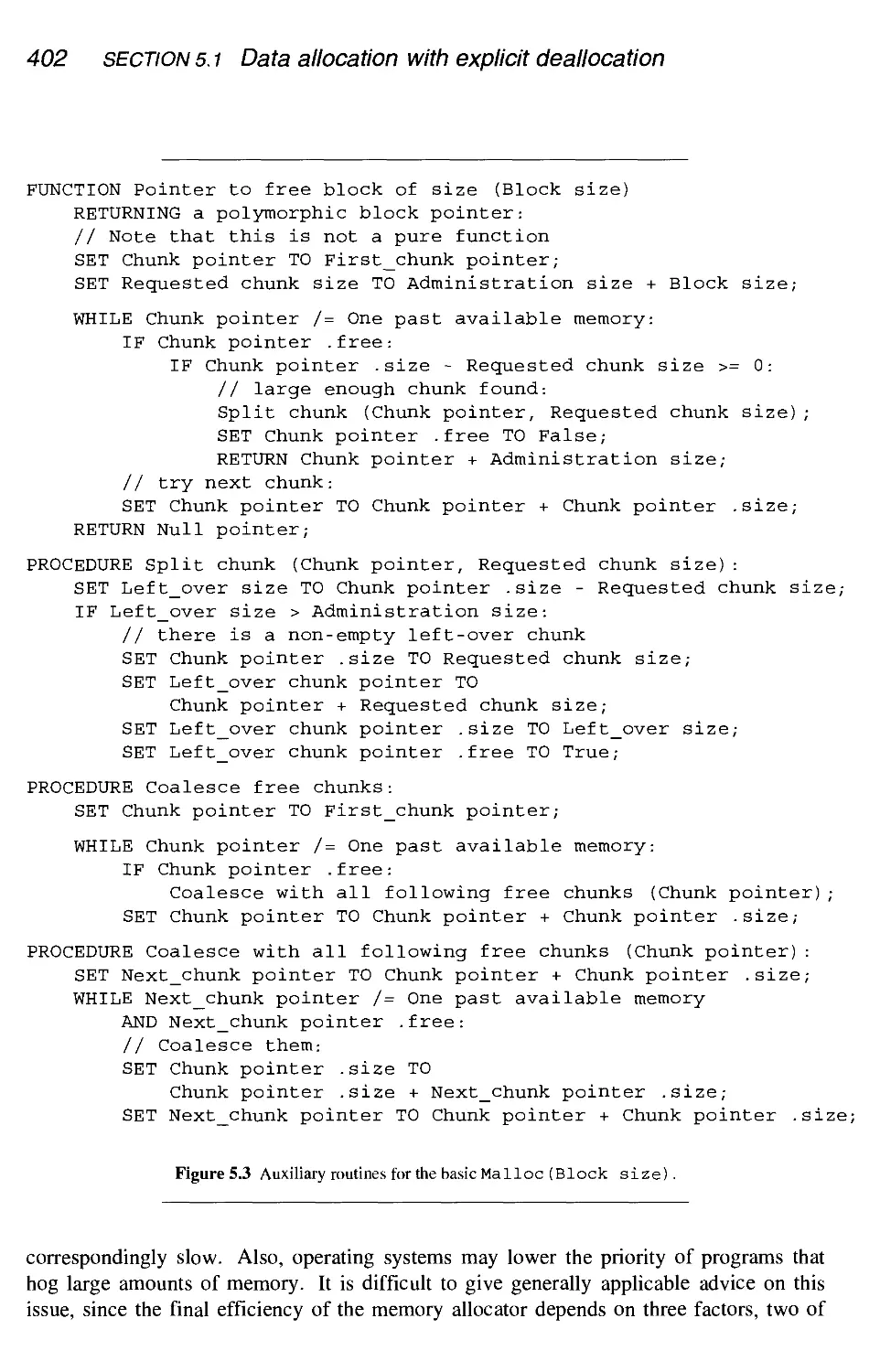
5.1.1 Basic memory allocation 399
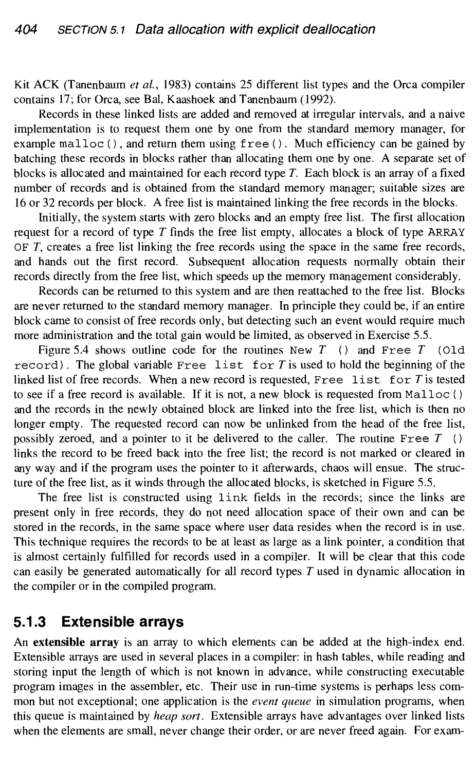
5.1.2 Linked lists 403
5.1.3 Extensible arrays 404
5.2 Data allocation with implicit deallocation 407
5.2.1 Basic garbage collection algorithms 407
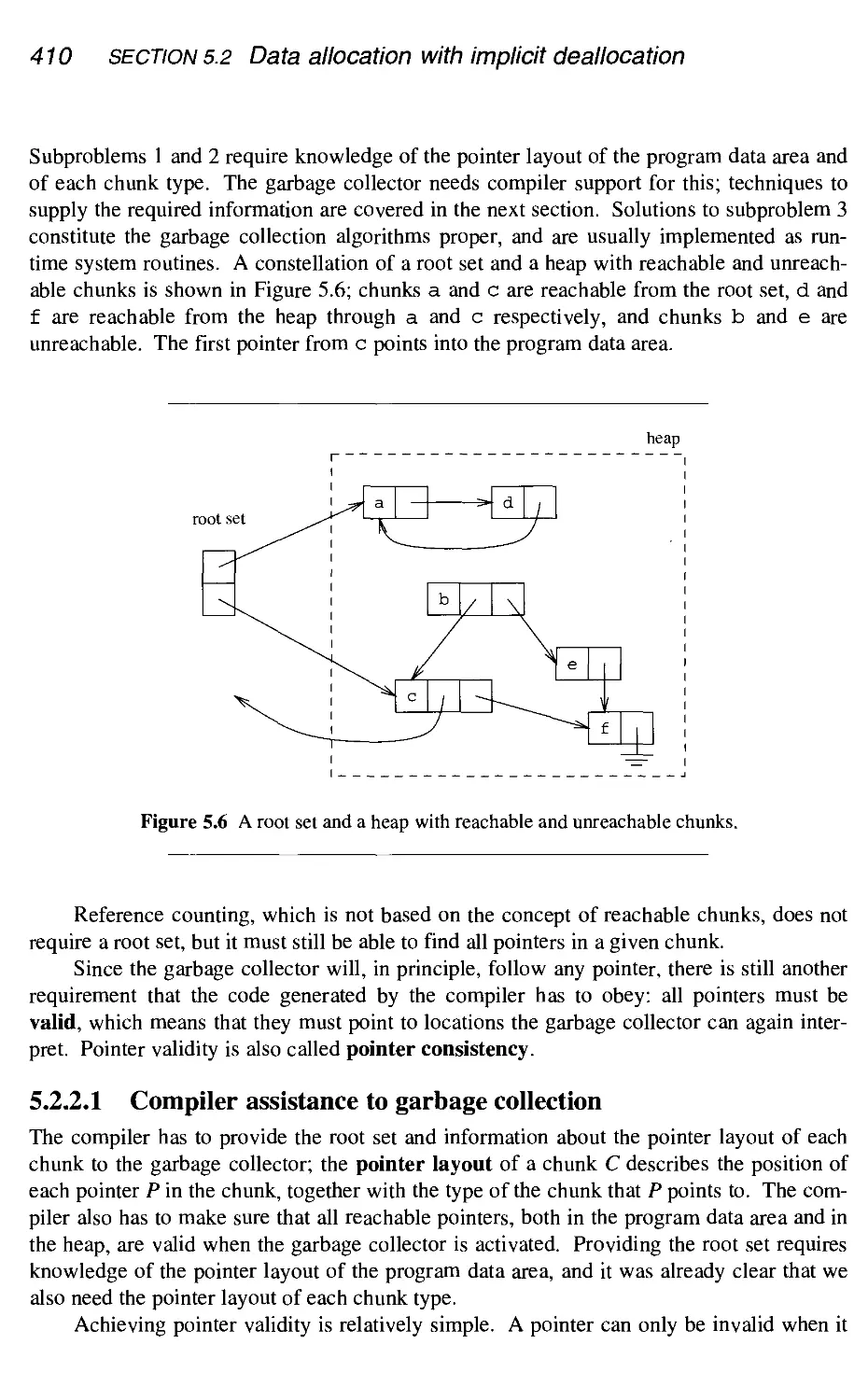
5.2.2 Preparing the ground 409
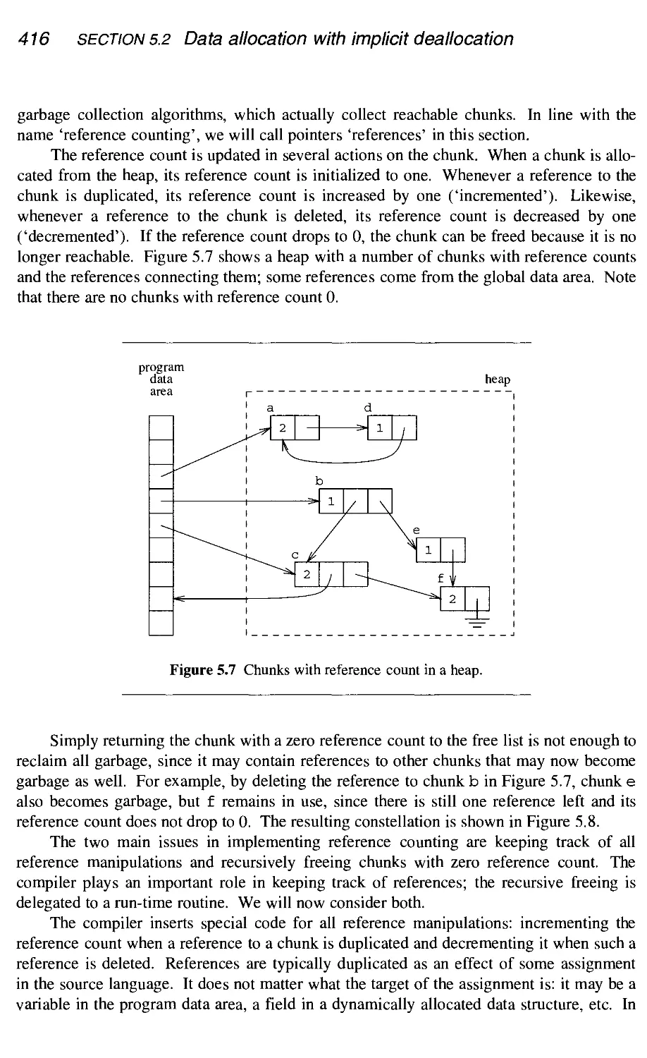
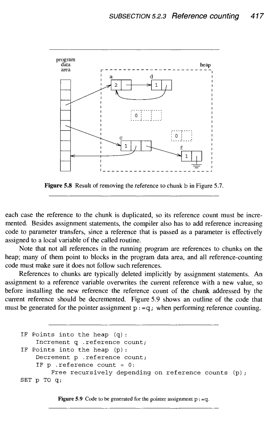
5.2.3 Reference counting 415
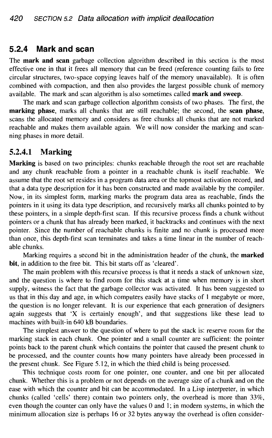
5.2.4 Mark and scan 420
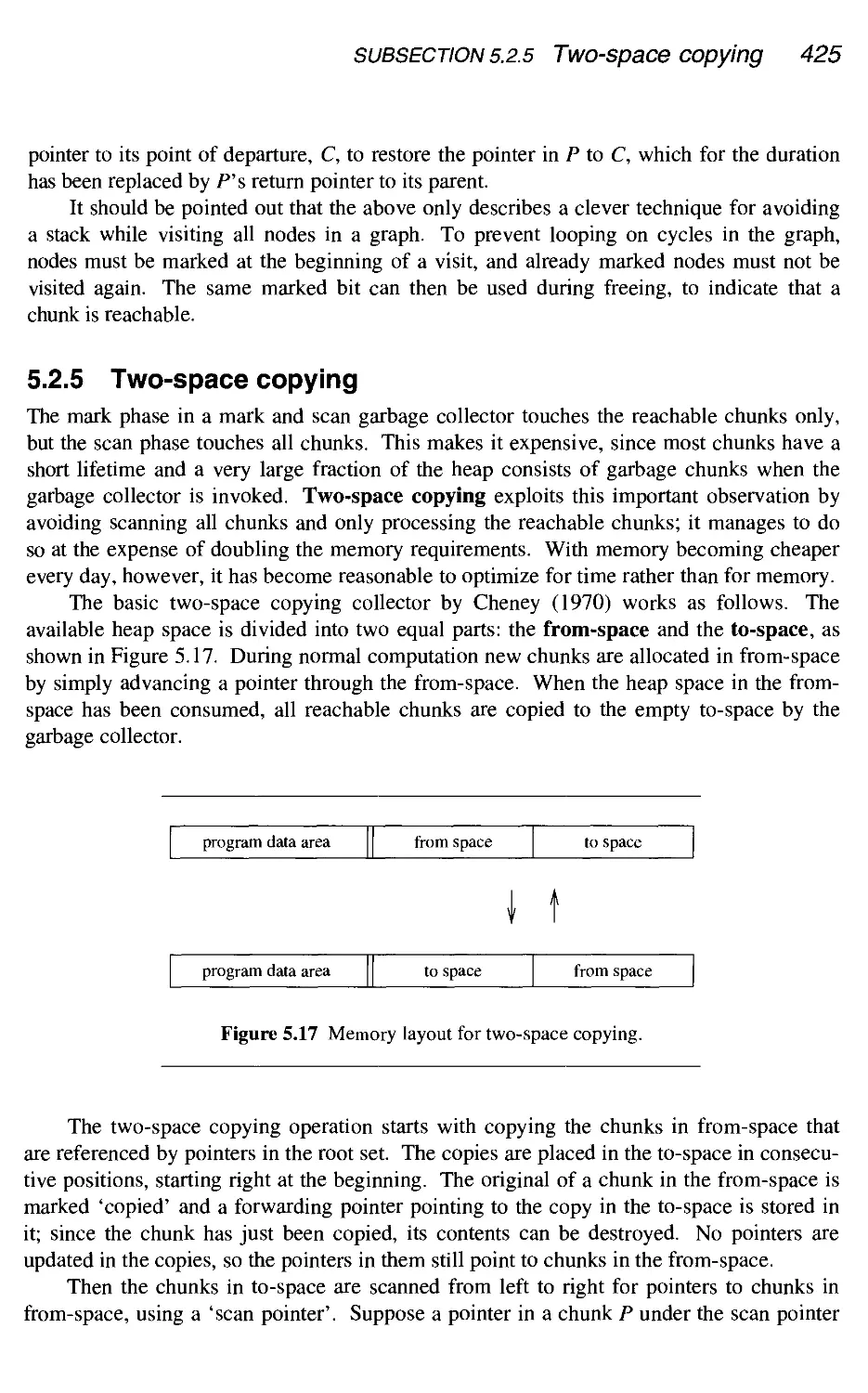
5.2.5 Two-space copying 425
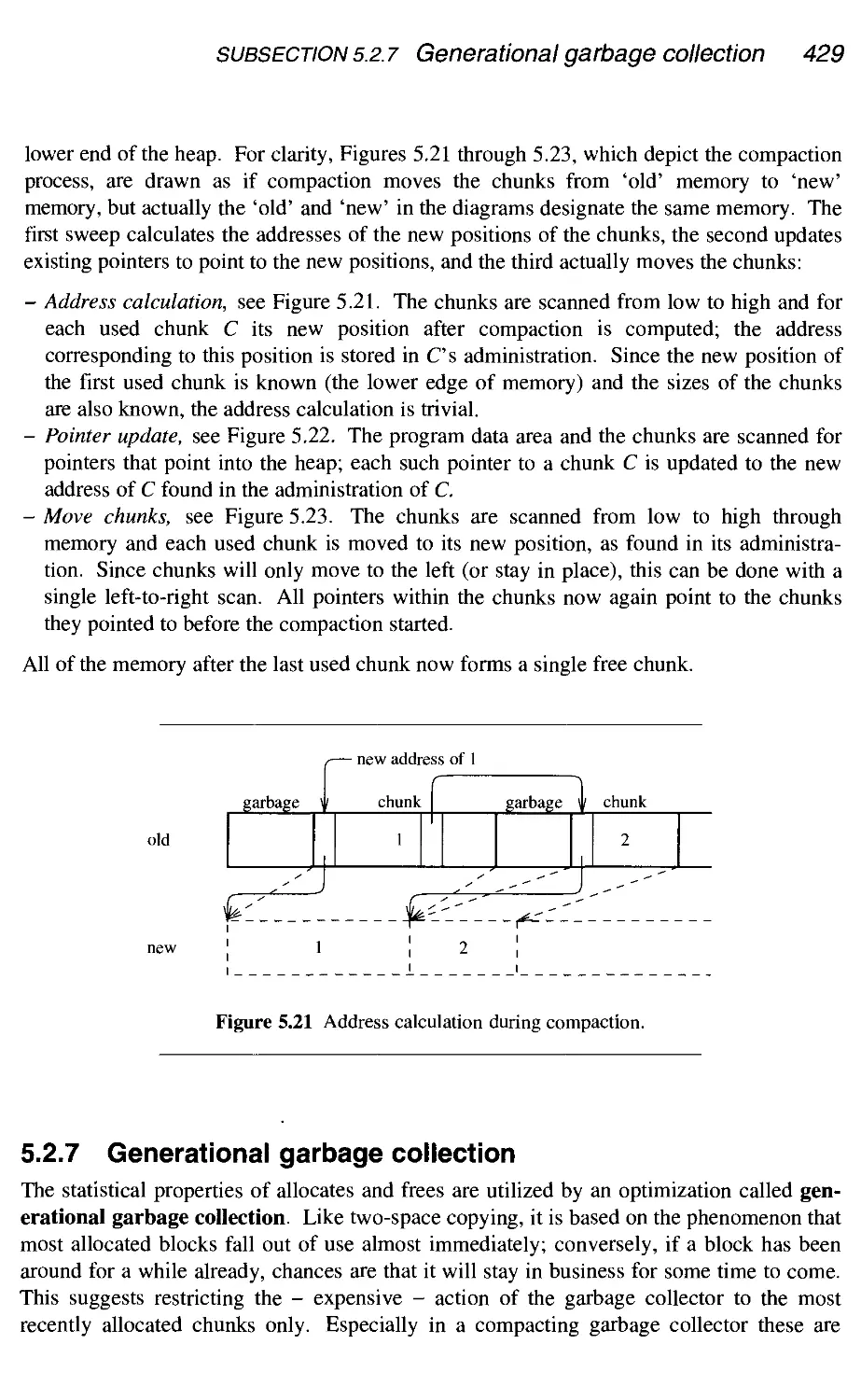
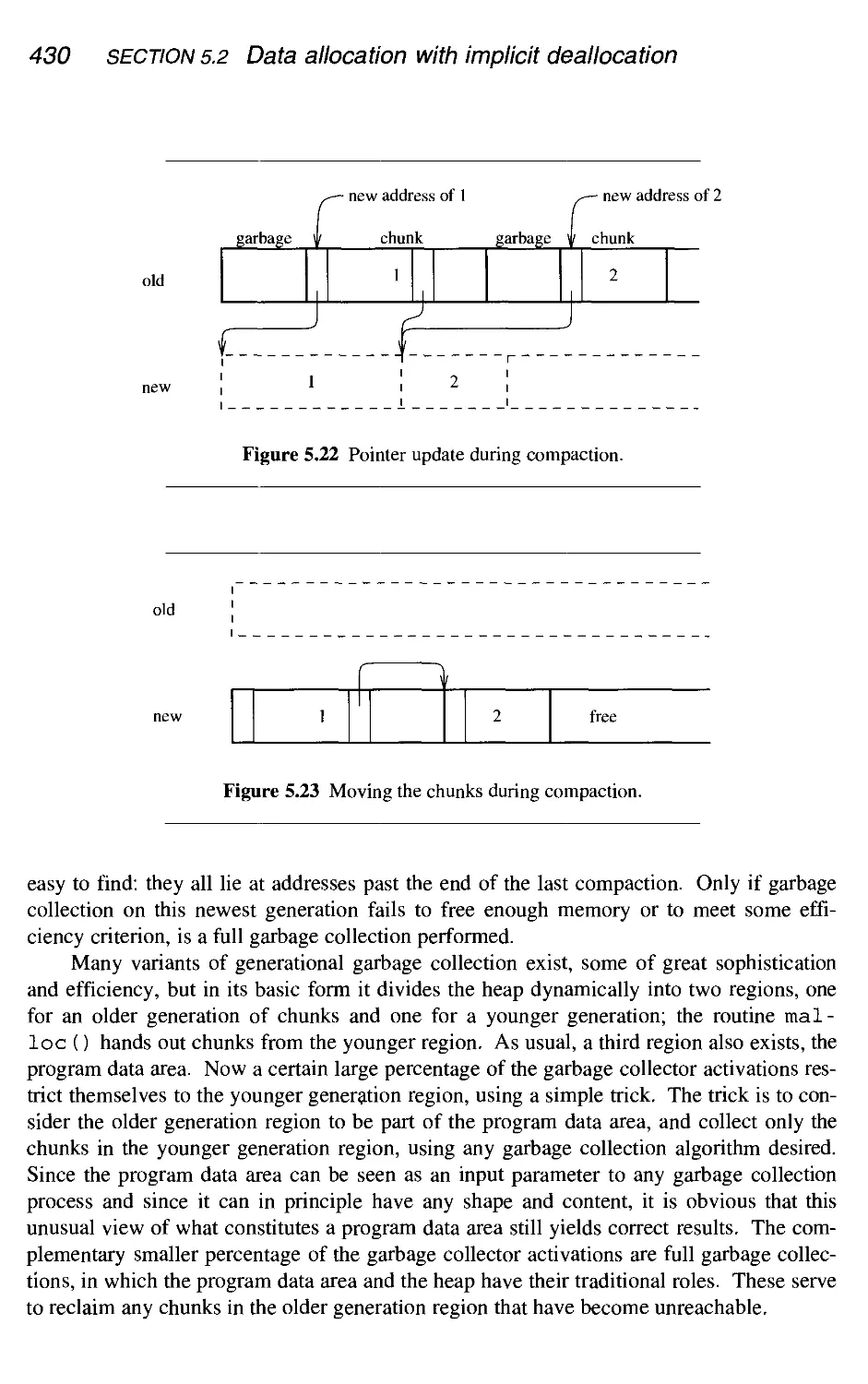
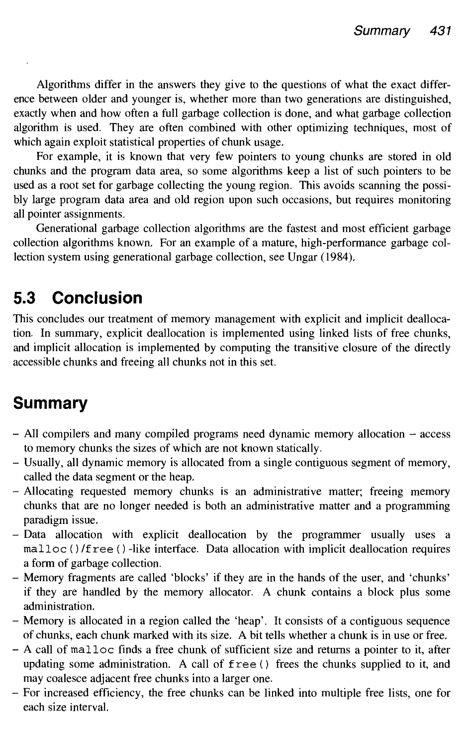
5.2.6 Compaction 428
5.2.7 Generational garbage collection 429
5.3 Conclusion 431
Summary 431
Further reading 434
Exercises 435
Imperative and object-oriented programs 438
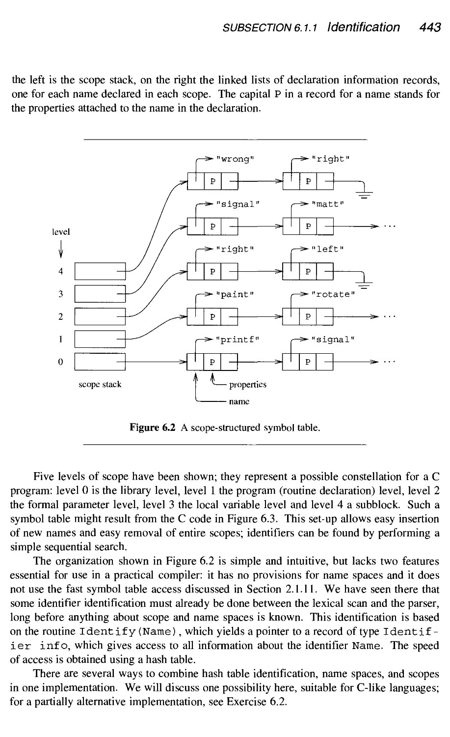
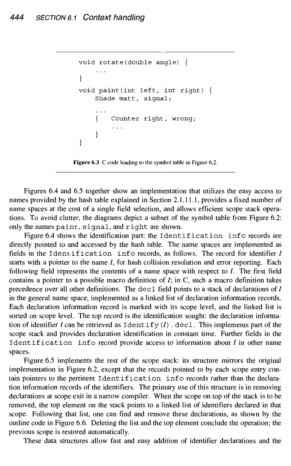
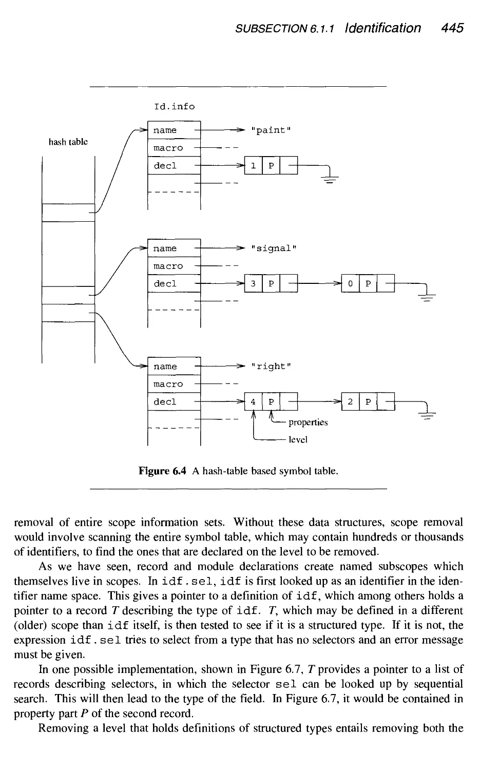
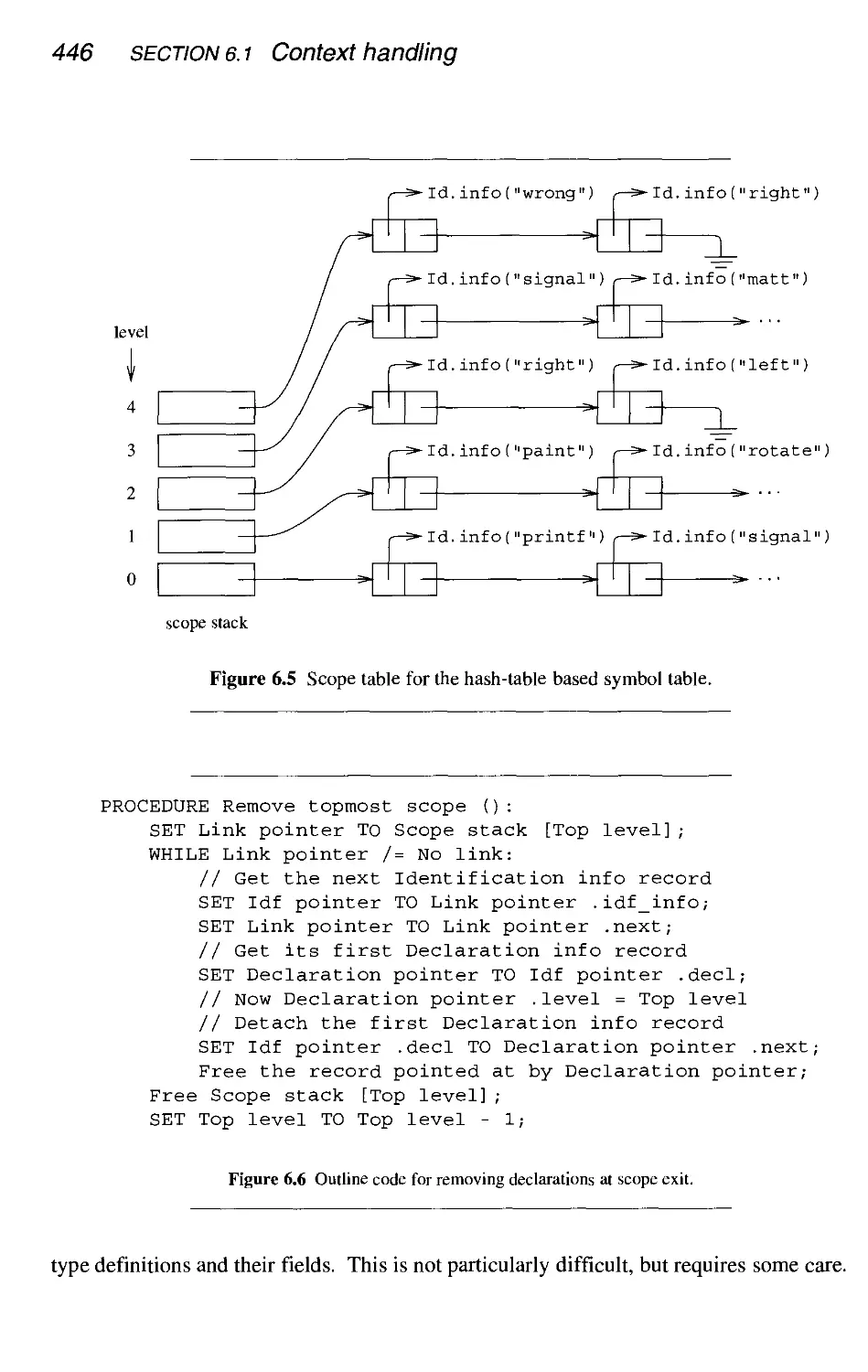
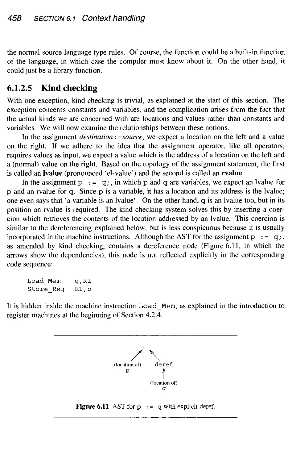
6.1 Context handling 440
6.1.1 Identification 441
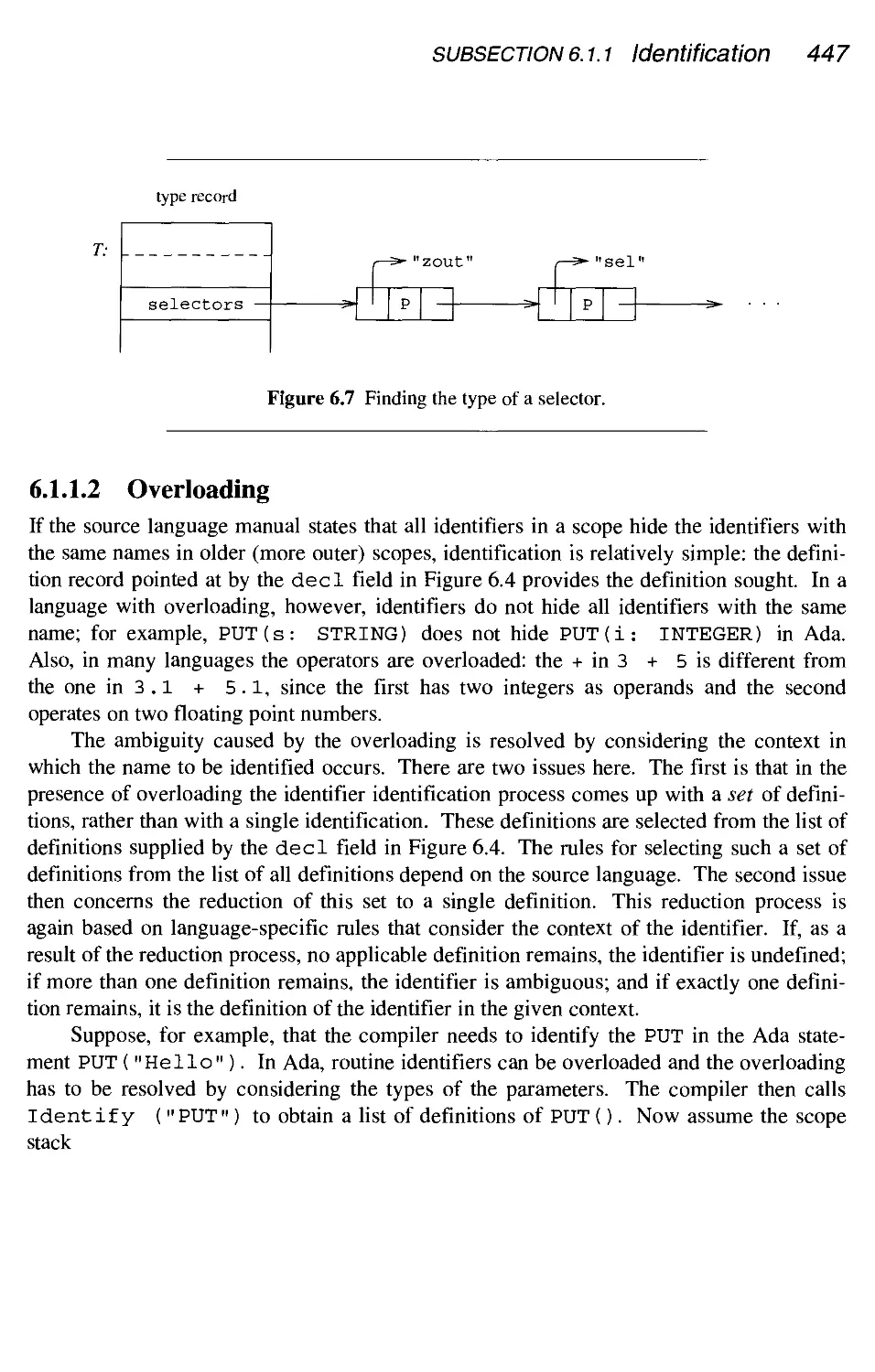
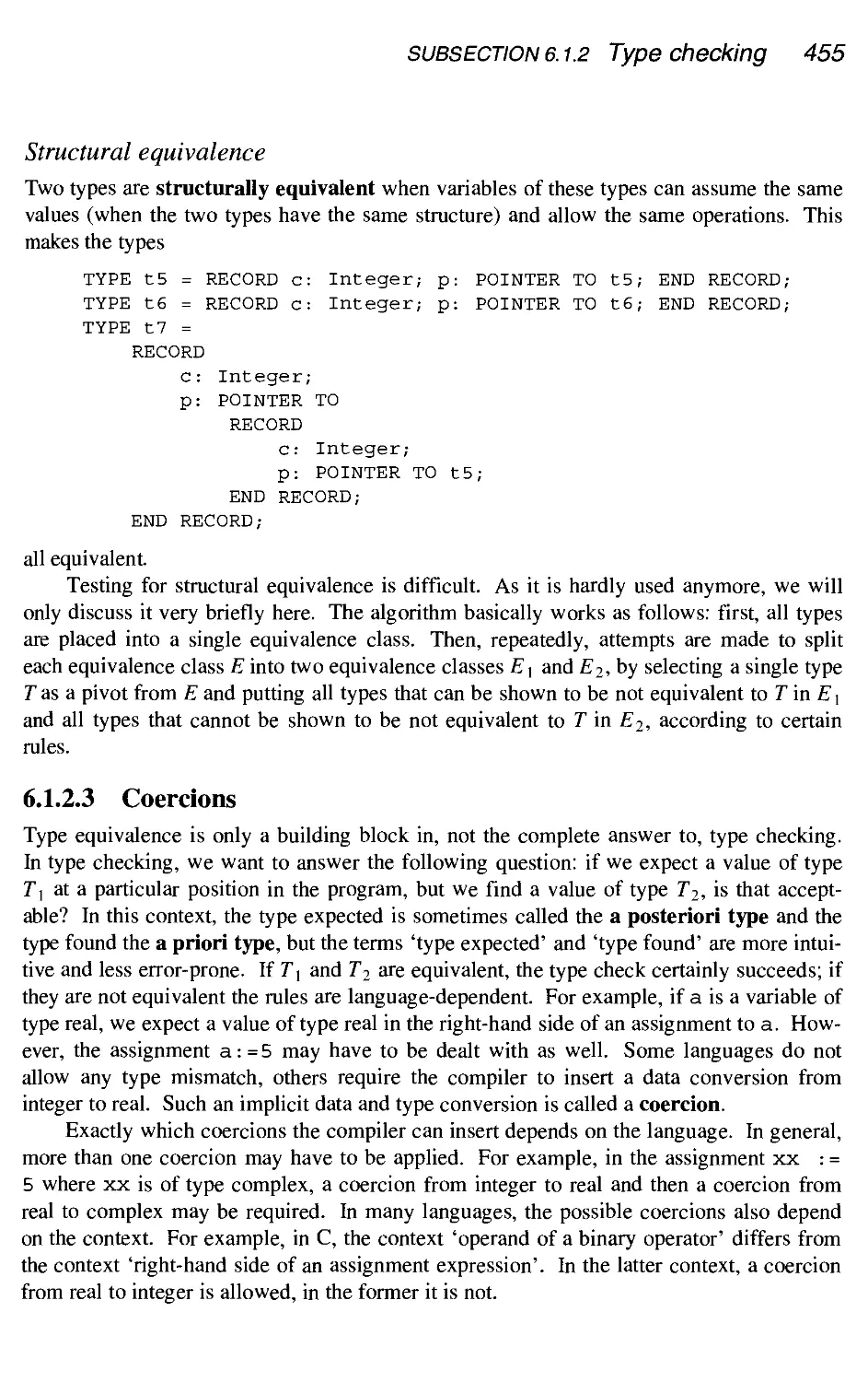
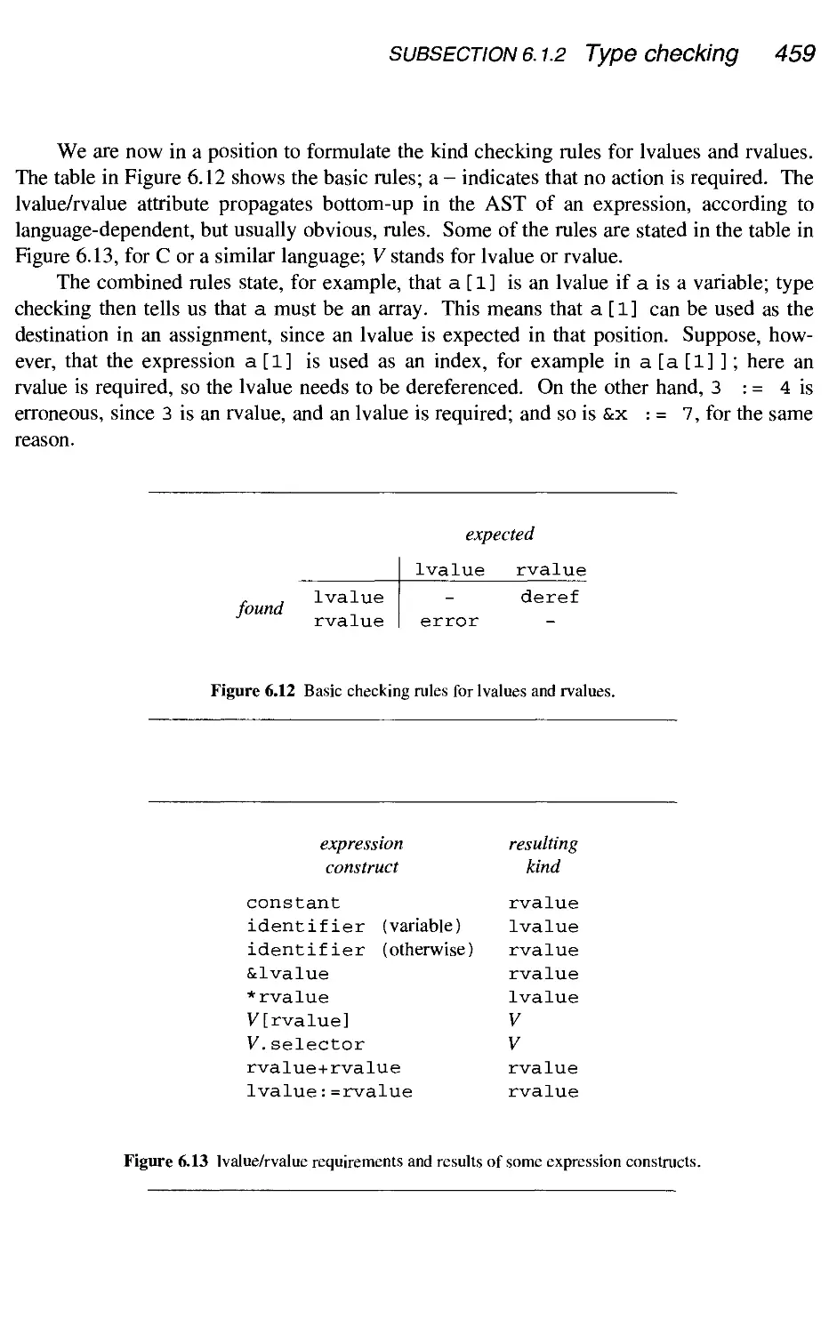
6.1.2 Type checking 449
6.1.3 Conclusion 460
6.2
6.3
6.4
6.5
6.6
Source
6.2.1
6.2.2
6.2.3
6.2.4
6.2.5
6.2.6
6.2.7
6.2.8
6.2.9
6.2.10
language data representation and handling
Basic types
Enumeration types
Pointer types
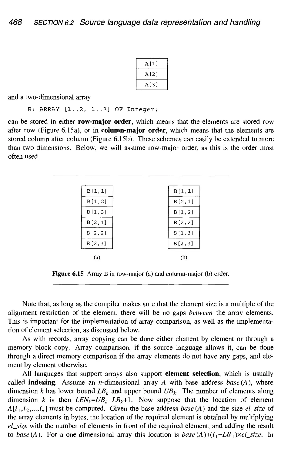
Record types
Union types
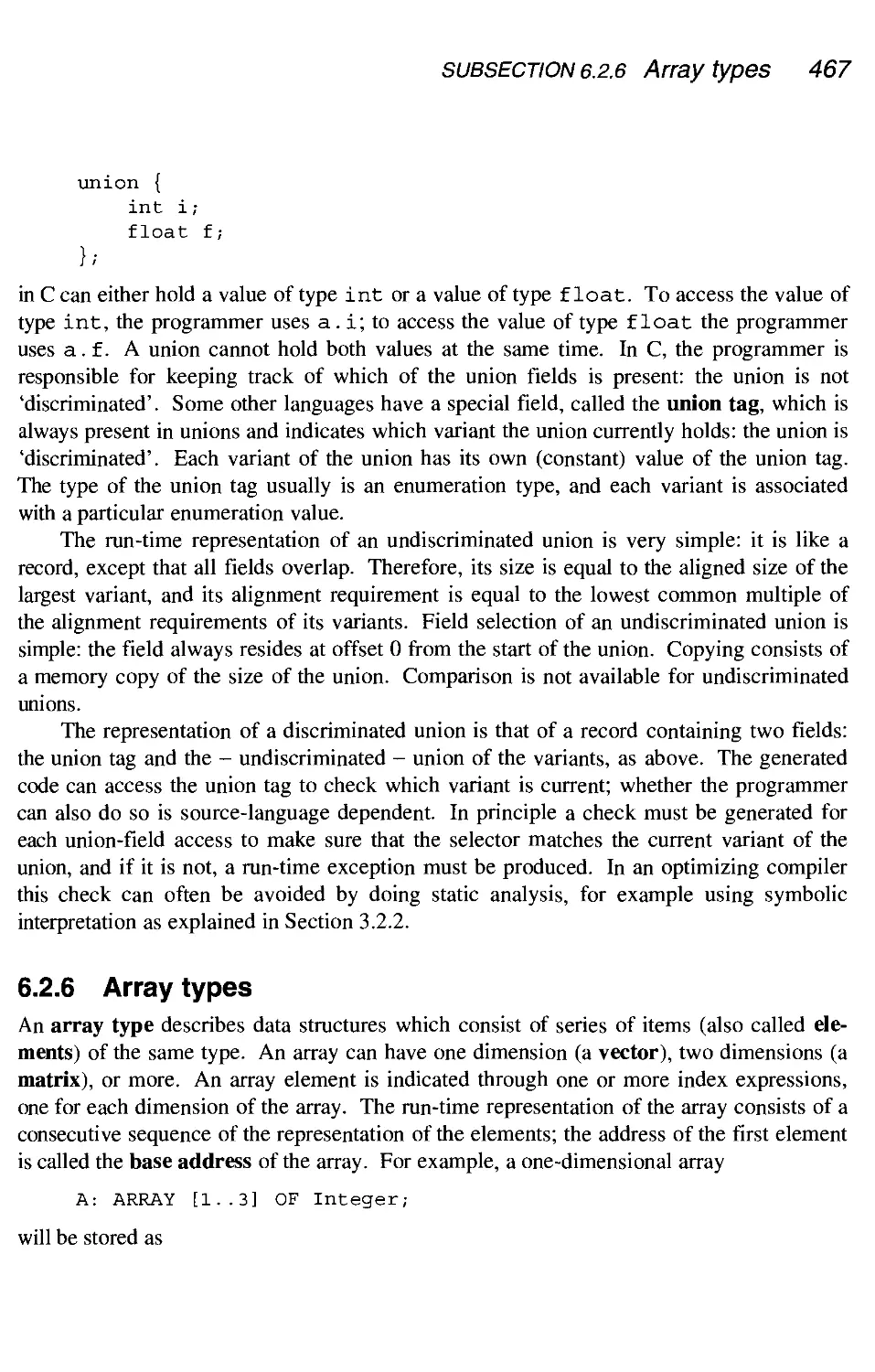
Array types
Set types
Routine types
Object types
Interface types
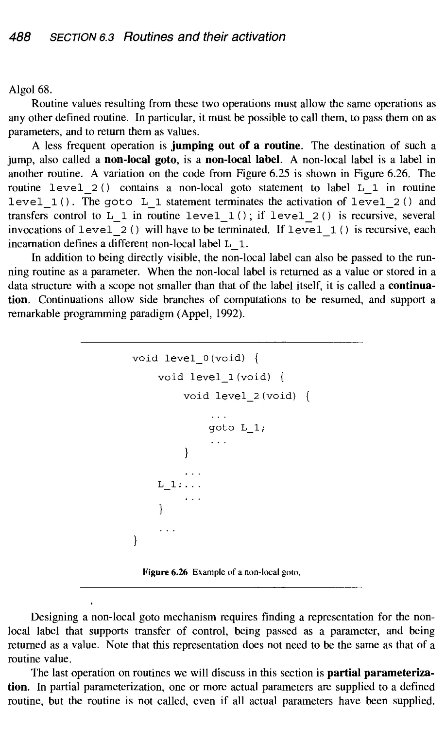
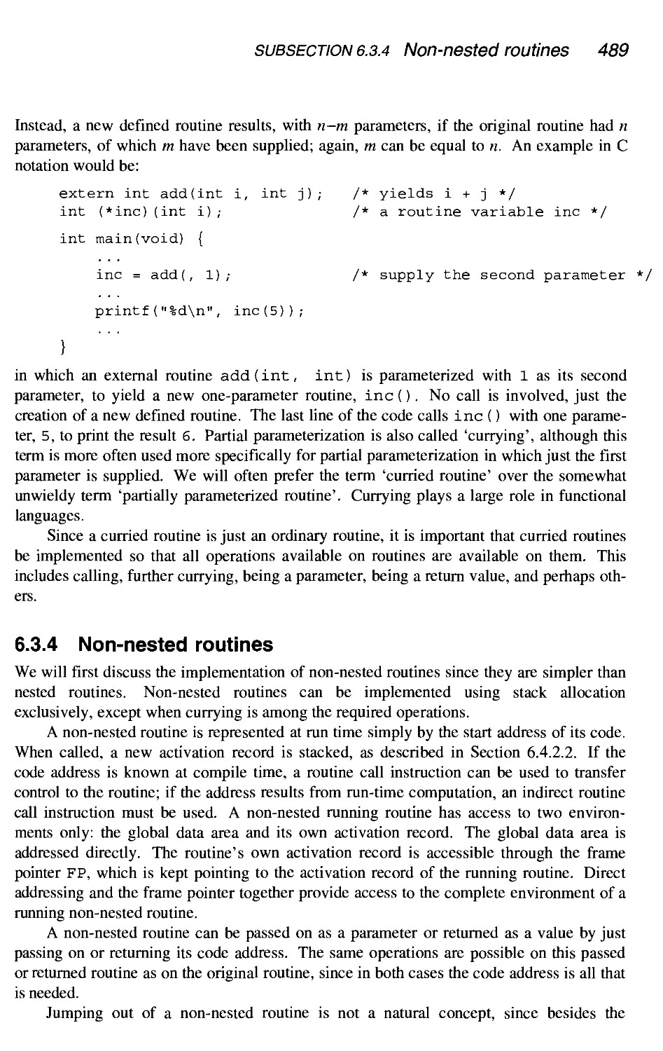
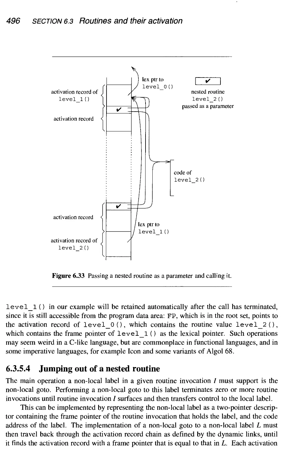
Routines and their activation
6.3.1
6.3.2
6.3.3
6.3.4
6.3.5
6.3.6
6.3.7
Activation records
Routines
Operations on routines
Non-nested routines
Nested routines
Lambda lifting
Iterators and coroutines
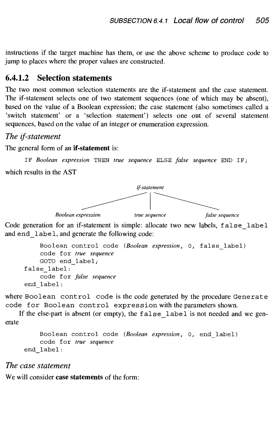
Code generation for control flow statements
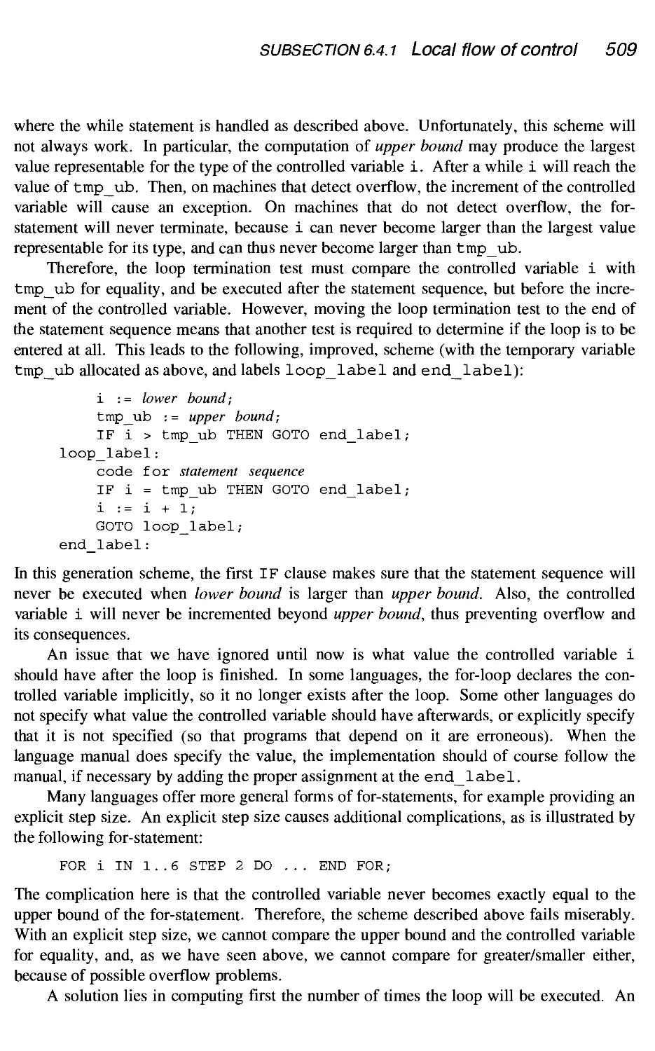
6.4.1
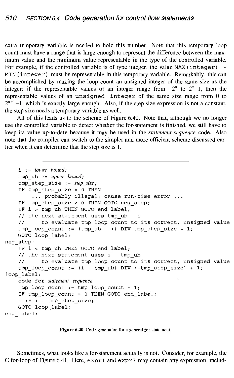
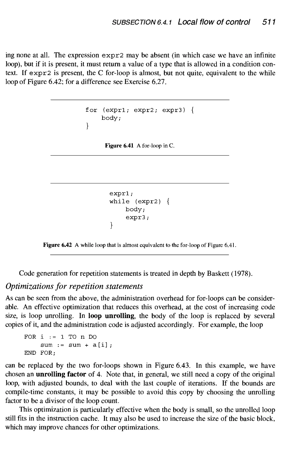
6.4.2
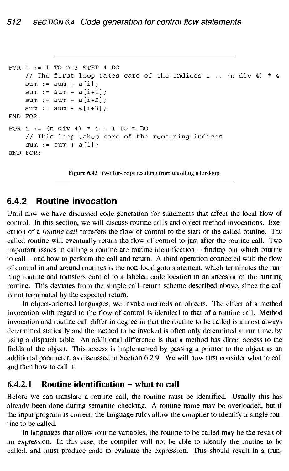
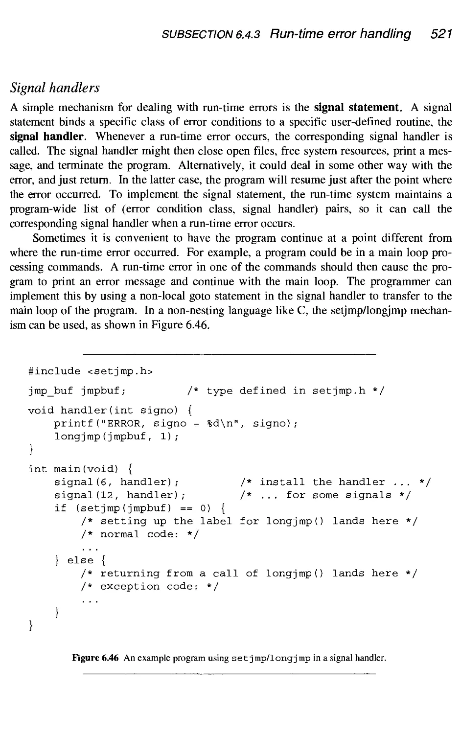
6.4.3
Local flow of control
Routine invocation
Run-time error handling
Code generation for modules
6.5.1
6.5.2
6.5.3
Name generation
Module initialization
Code generation for generics
Conclusion
Summary
Further
reading
Exercises
Contents ix
460
460
461
461
465
466
467
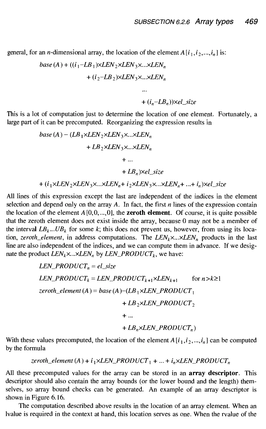
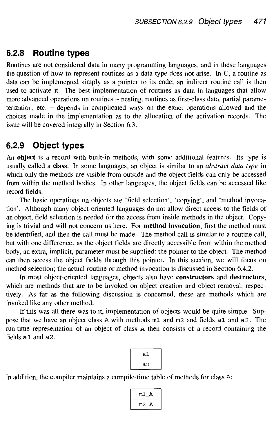
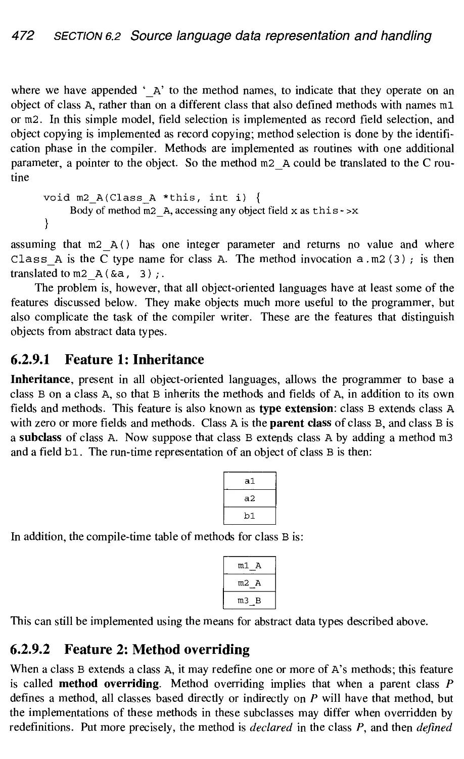
470
471
471
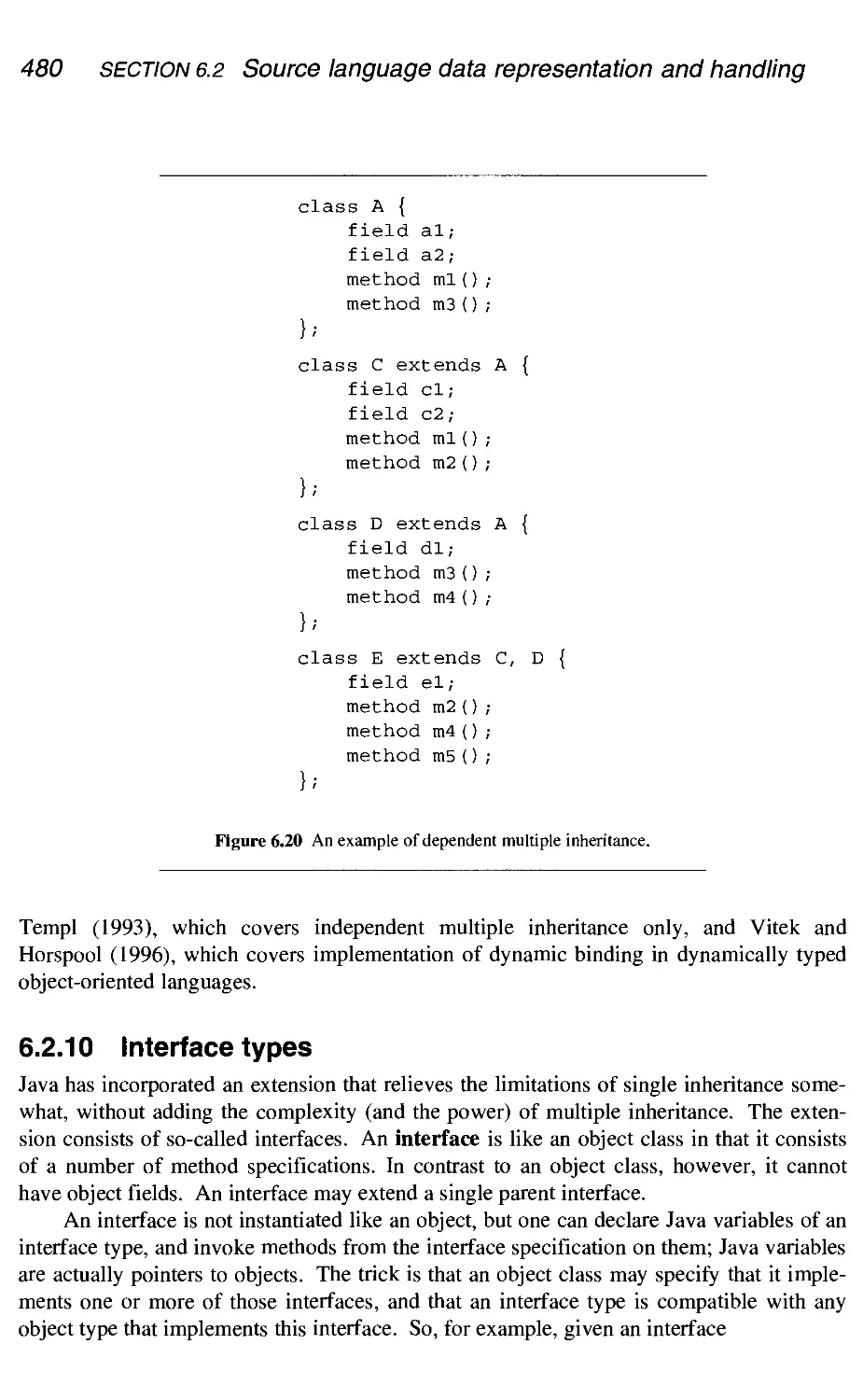
480
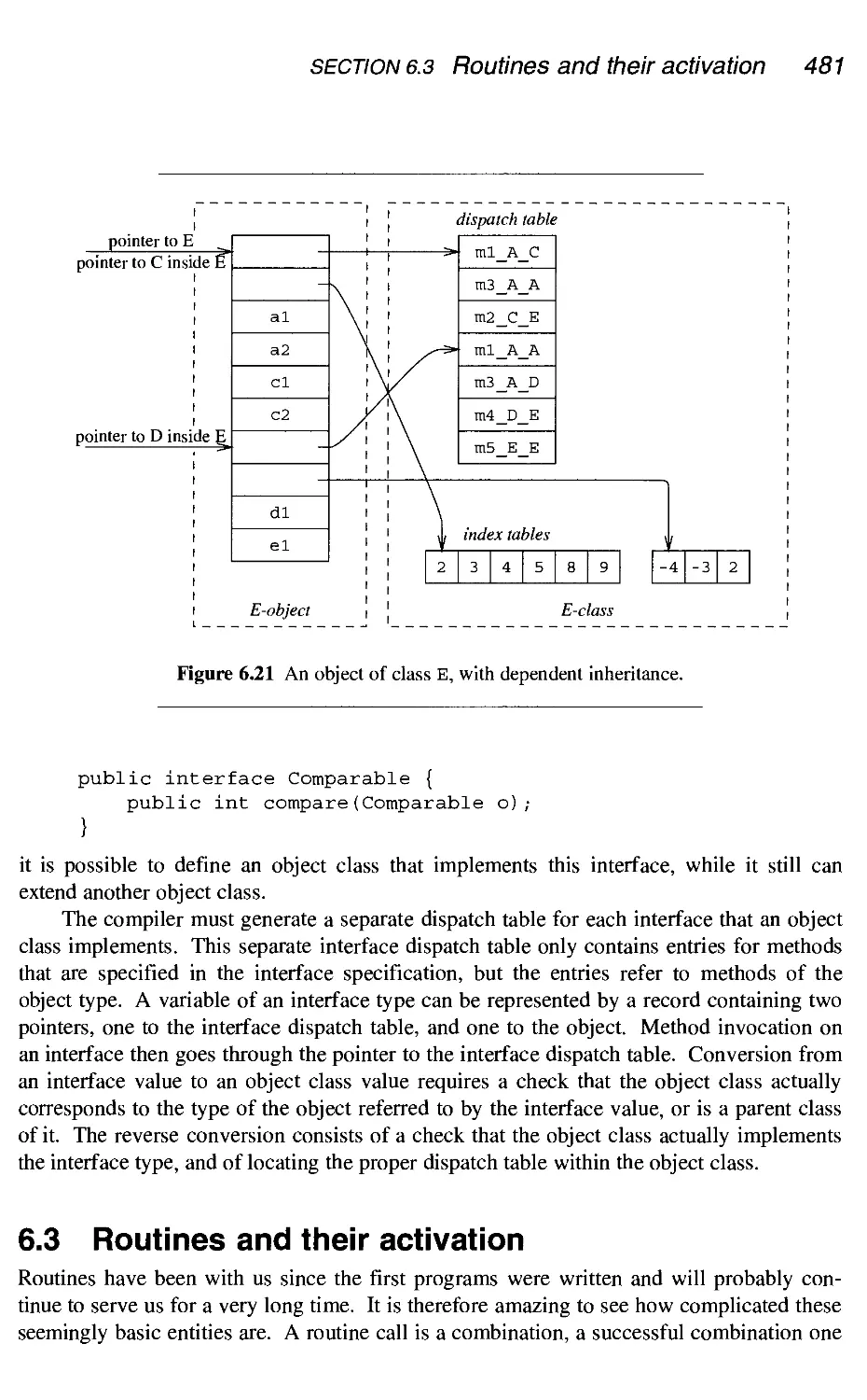
481
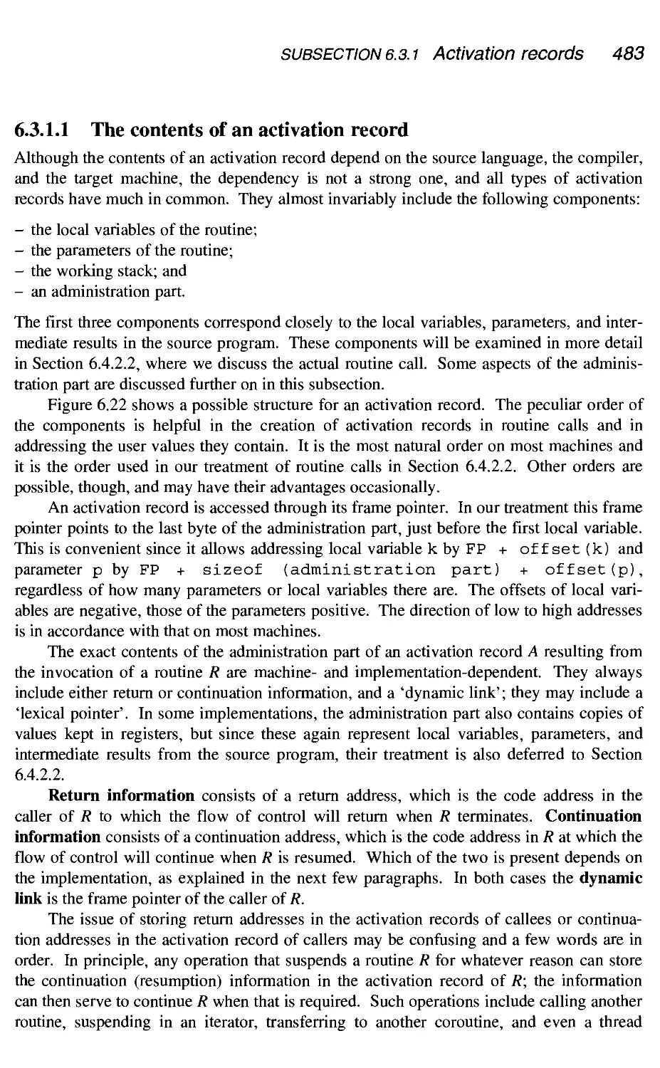
482
485
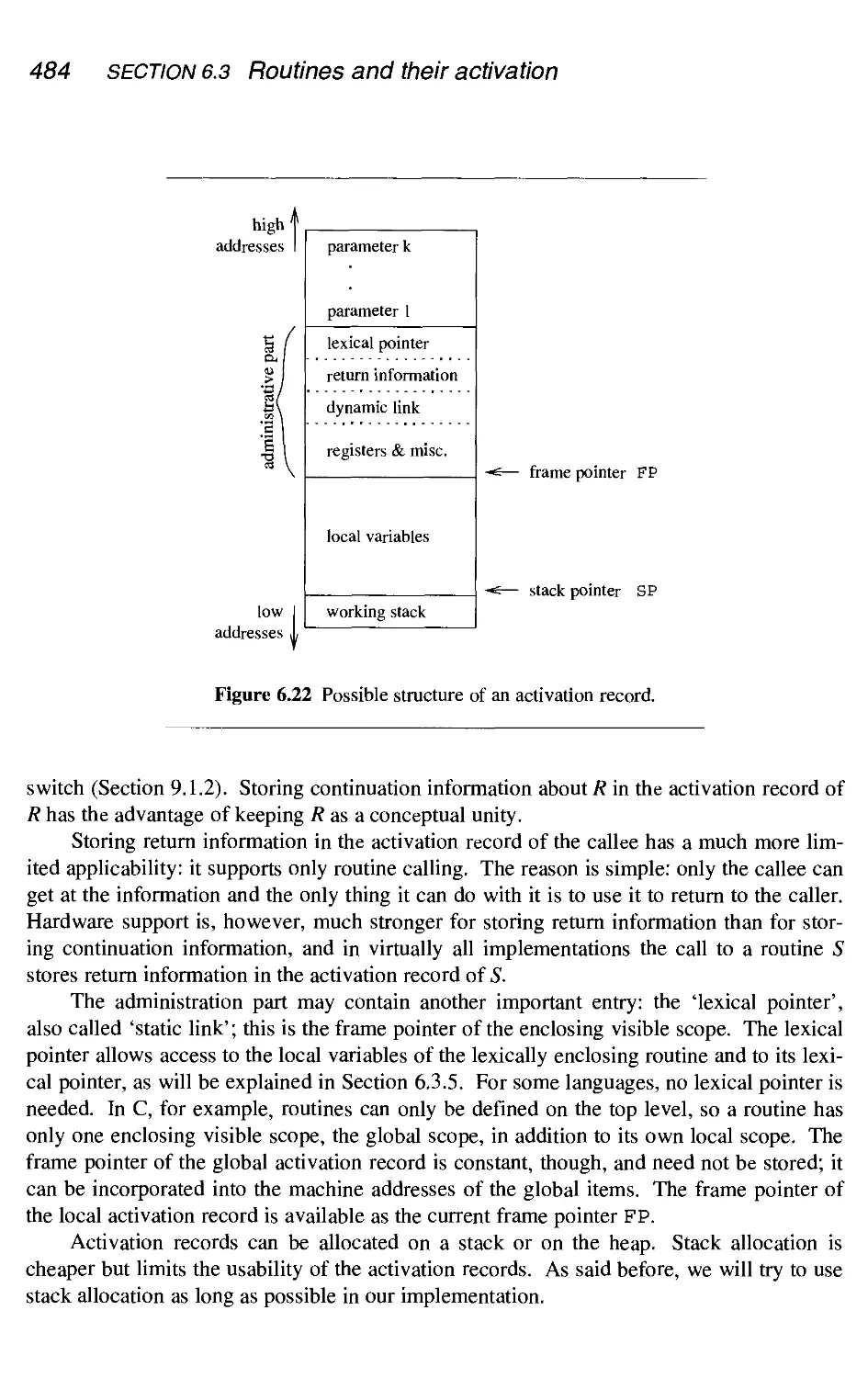
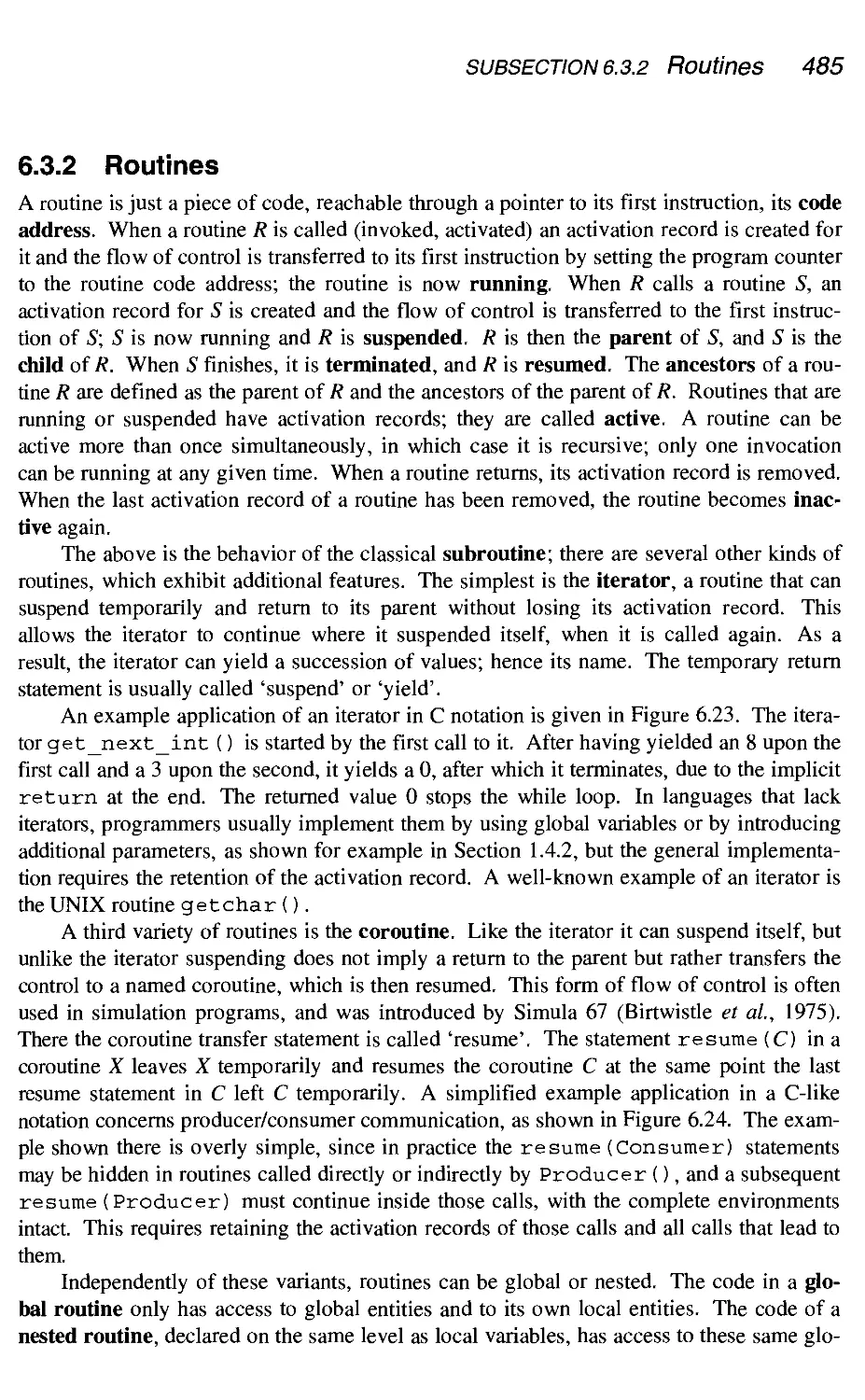
486
489
491
499
500
501
502
512
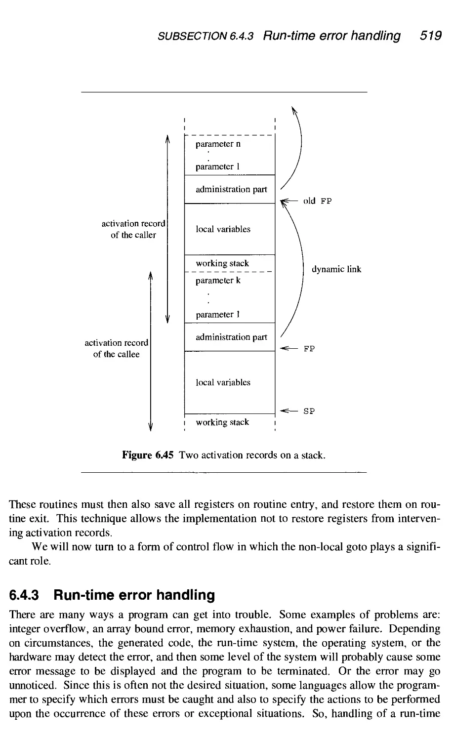
519
523
524
524
525
527
528
531
532
7 Functional programs 538
7.1 A short tour of Haskell 540
540
541
542
543
543
544
545
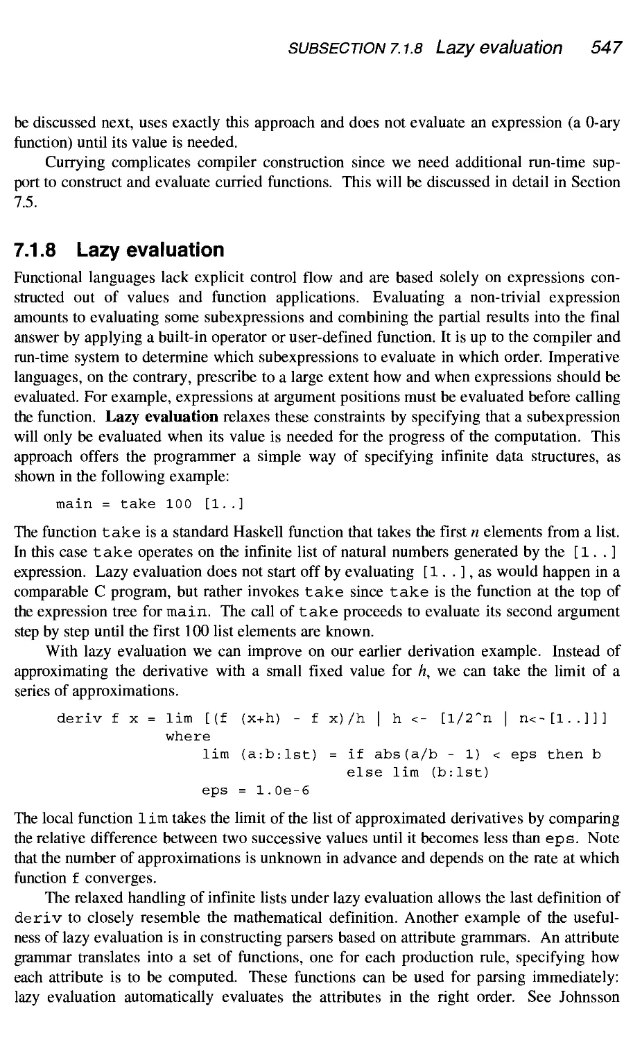
547
A short
7.1.1
7.1.2
7.1.3
7.1.4
7.1.5
7.1.6
7.1.7
7.1.8
tour of Haskell
Offside rule
Lists
List comprehension
Pattern matching
Polymorphic typing
Referential transparency
Higher-order functions
Lazy evaluation
x Contents
7.2
7.3
7.4
7.5
7.6
7.7
7.8
7.9
Compiling functional languages
7.2.1 The functional core
Polymorphic type checking
7.3.1 Polymorphic function application
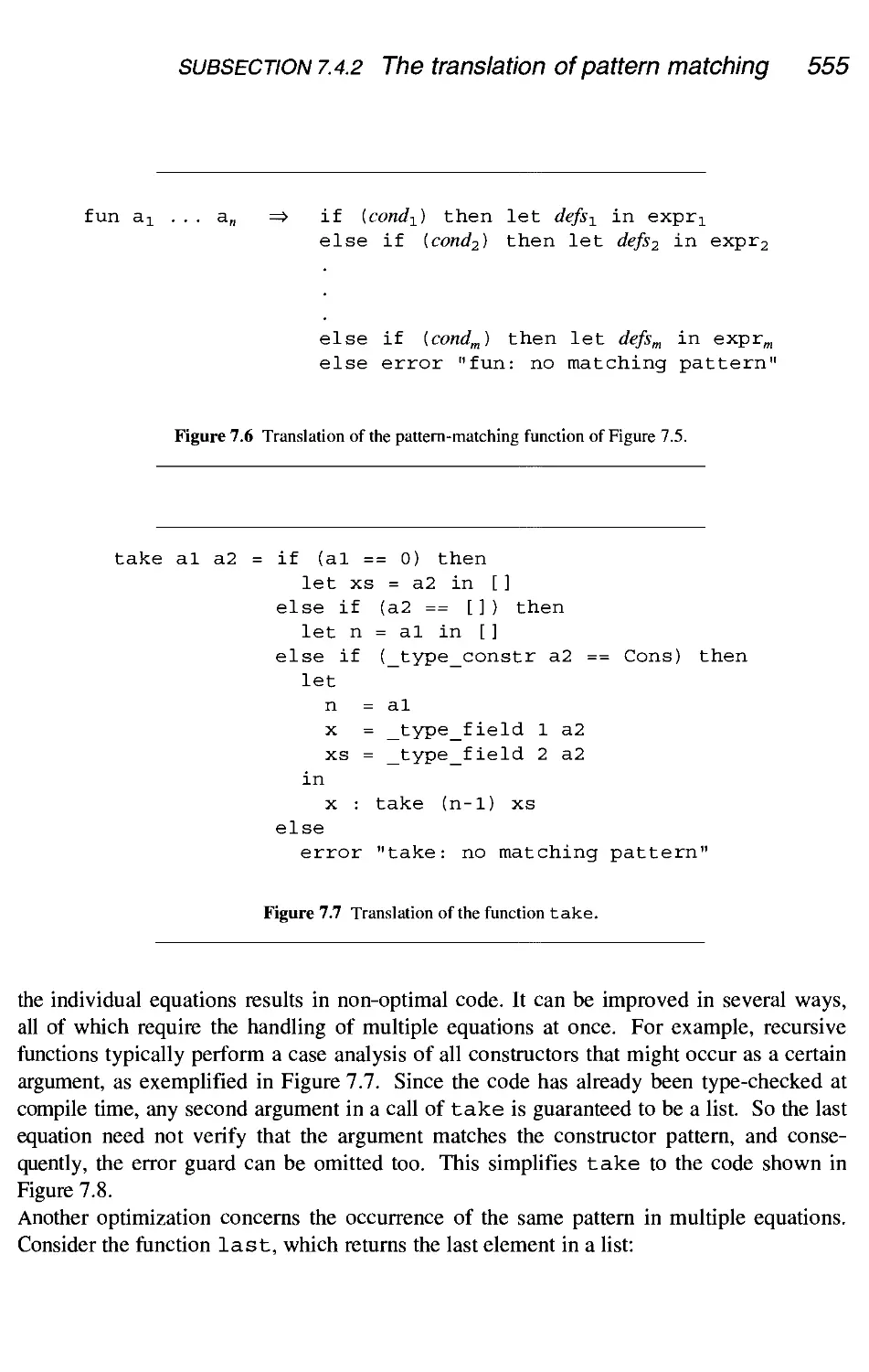
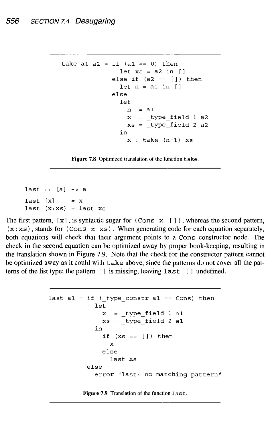
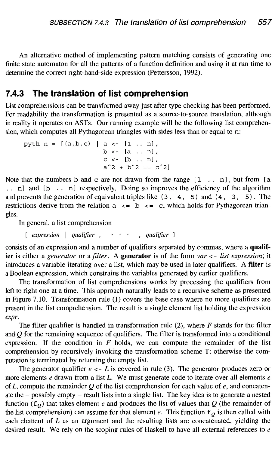
Desugaring
7.4.1 The translation of lists
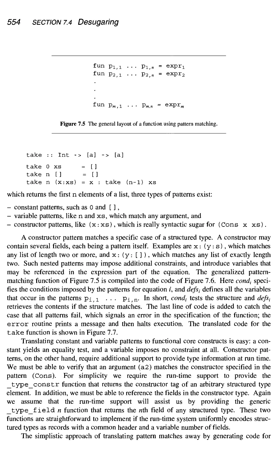
7.4.2 The translation of pattern matching
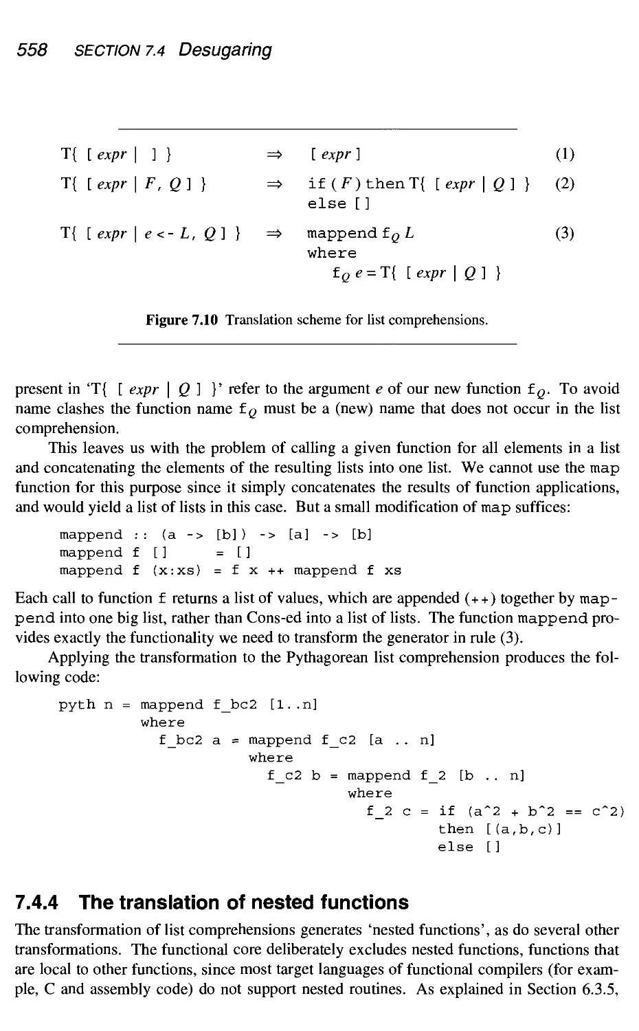
7.4.3 The translation of list comprehension
7.4.4 The translation of nested functions
Graph reduction
7.5.1 Reduction order
7.5.2 The reduction engine
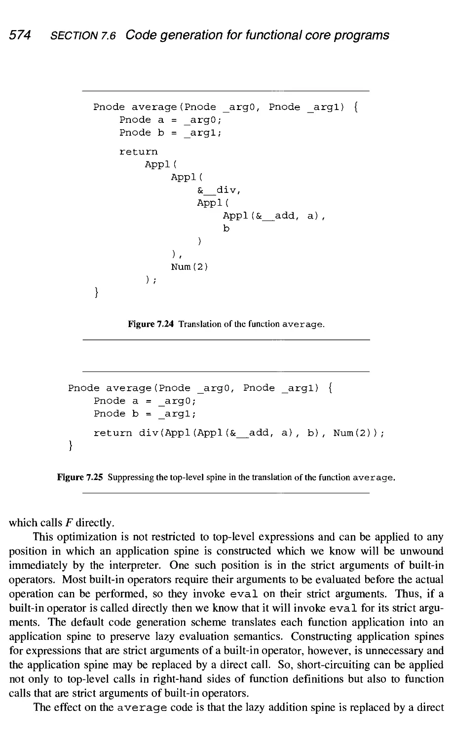
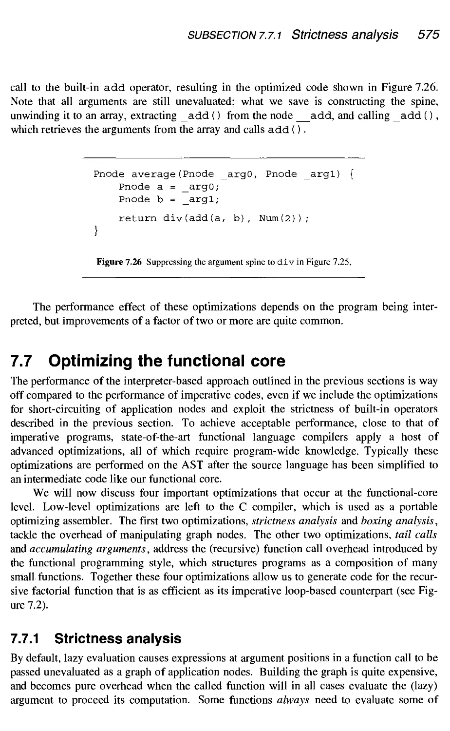
Code generation for functional core programs
7.6.1 Avoiding the construction of some application spines
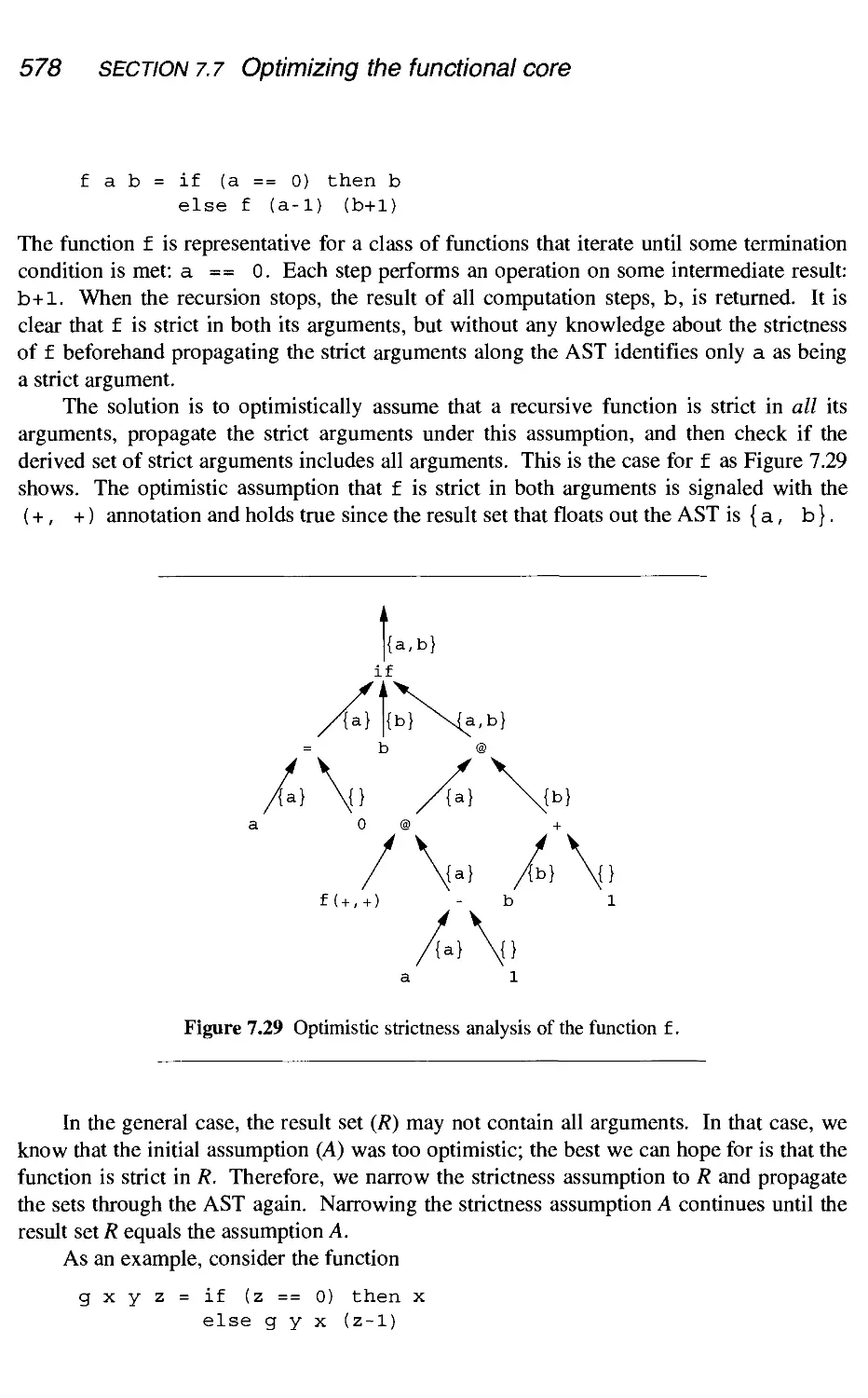
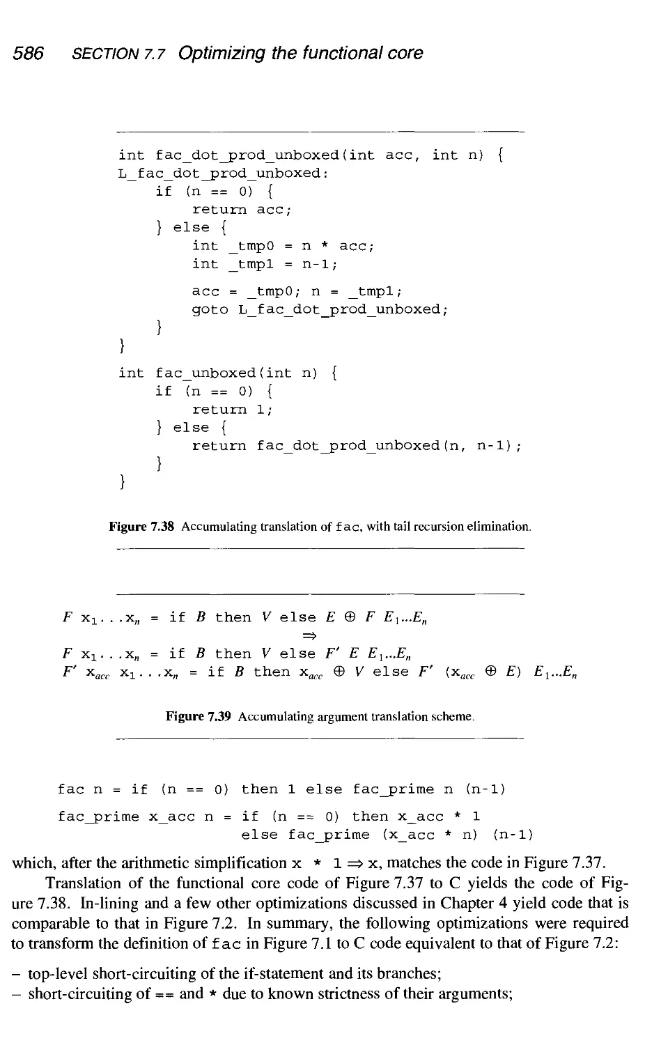
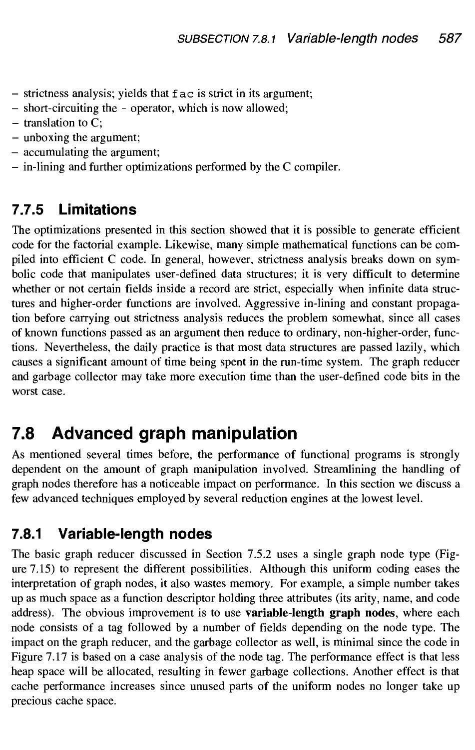
Optimizing the functional core
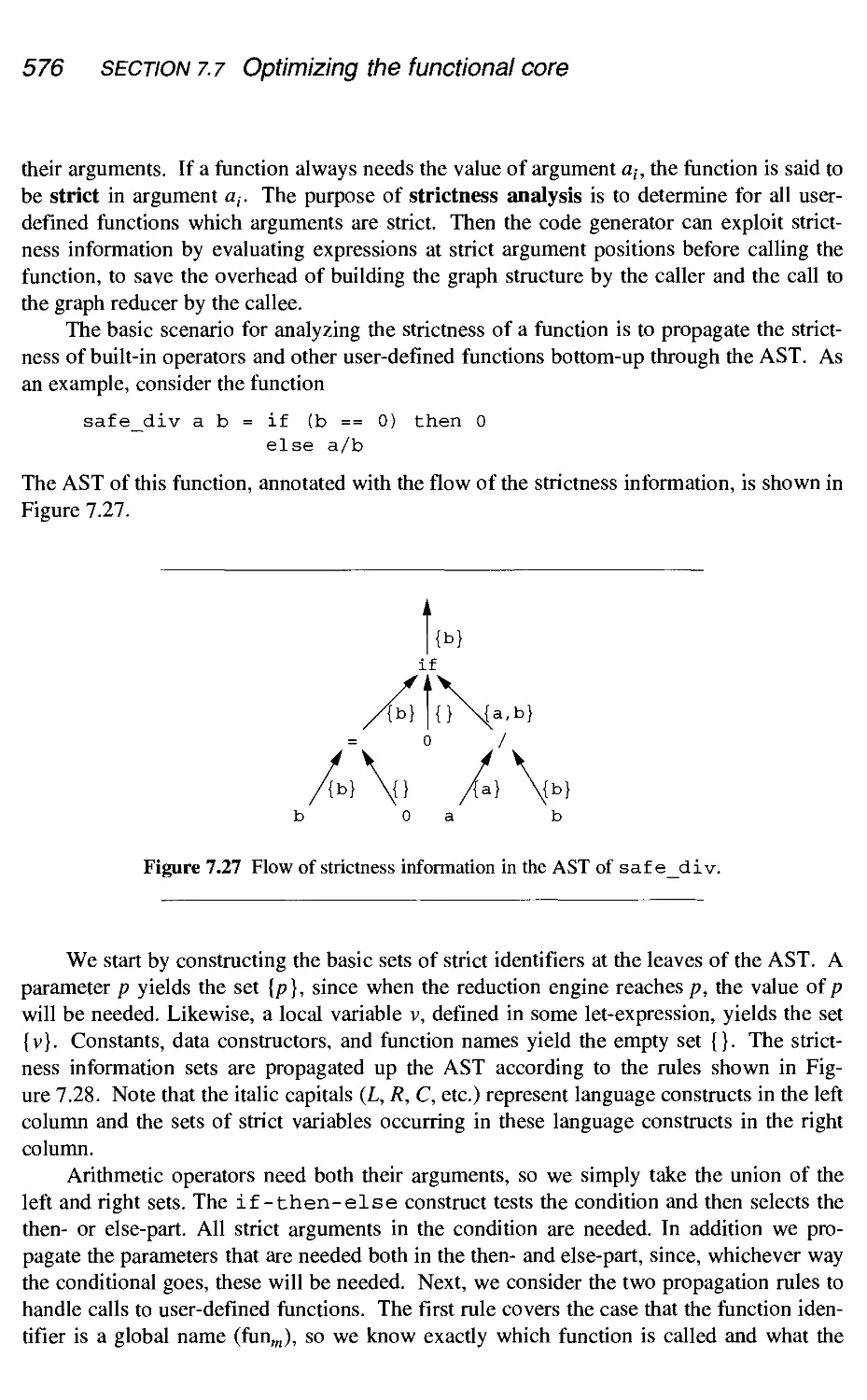
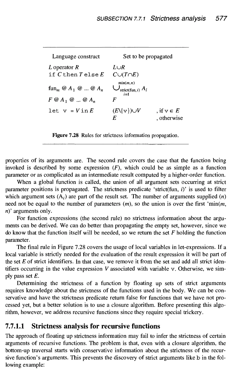
7.7.1 Strictness analysis
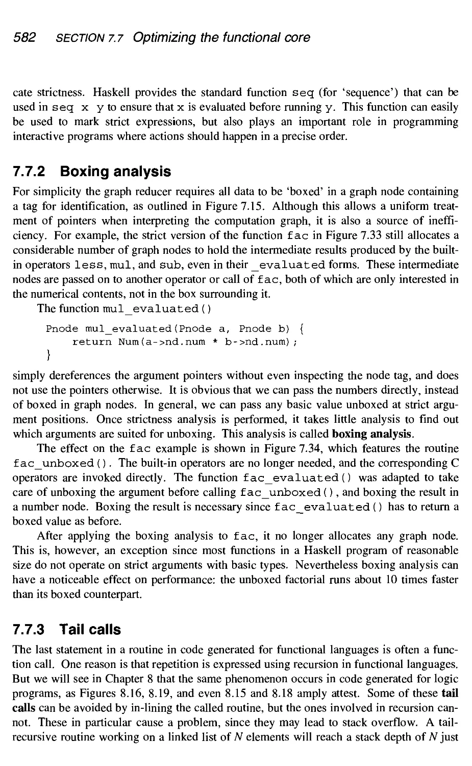
7.7.2 Boxing analysis
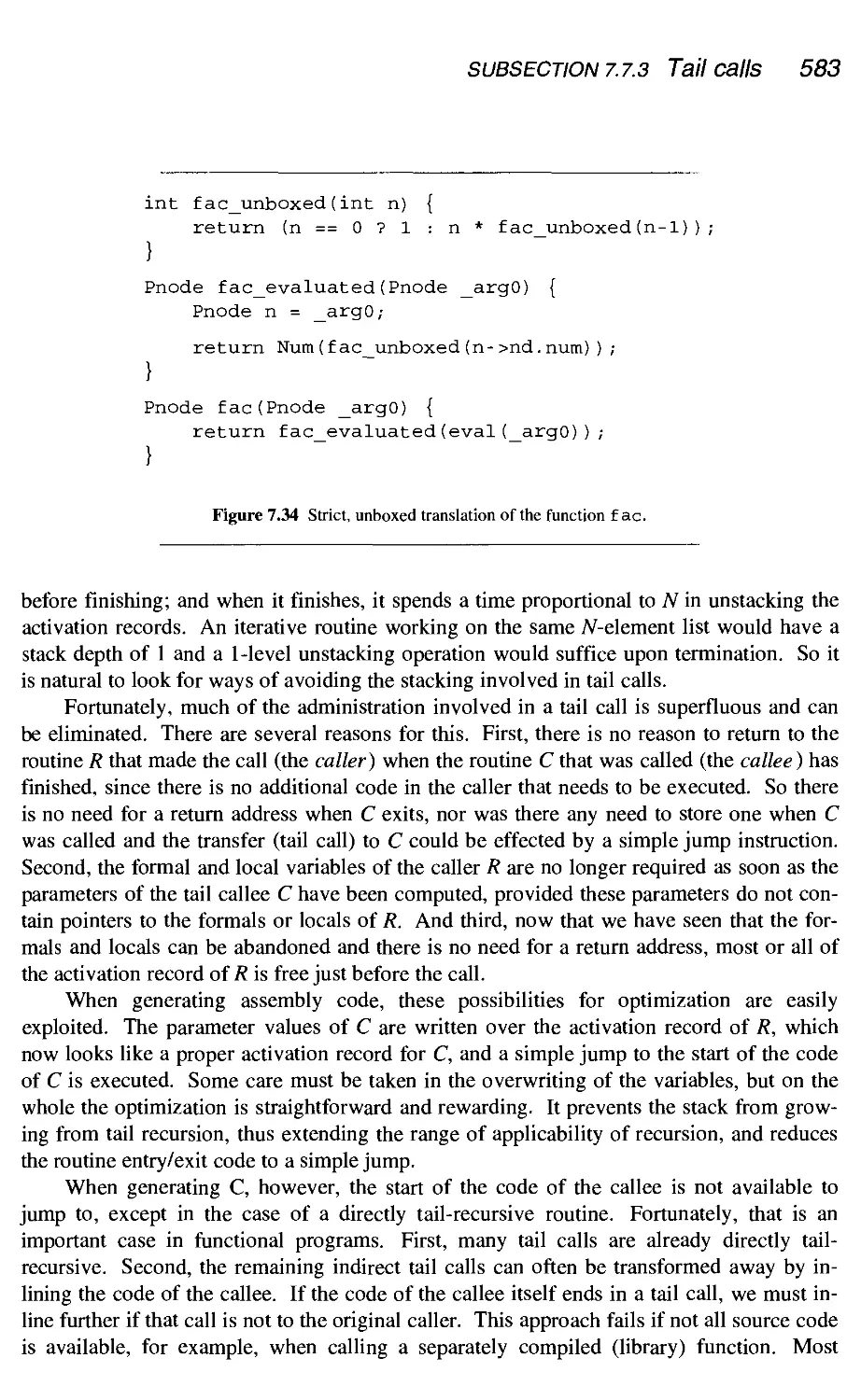
7.7.3 Tail calls
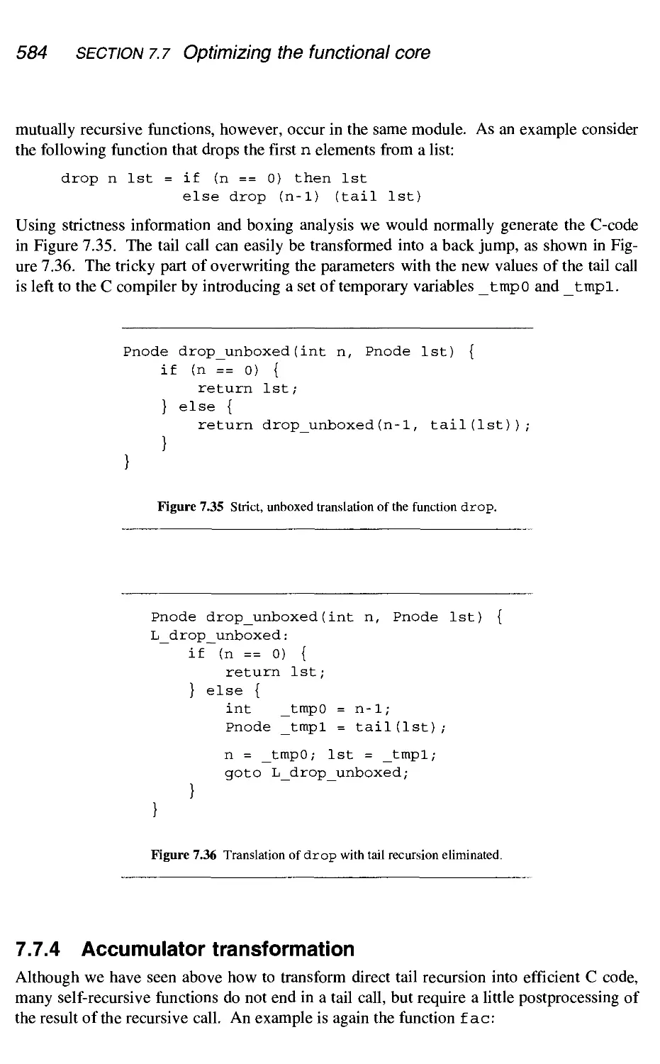
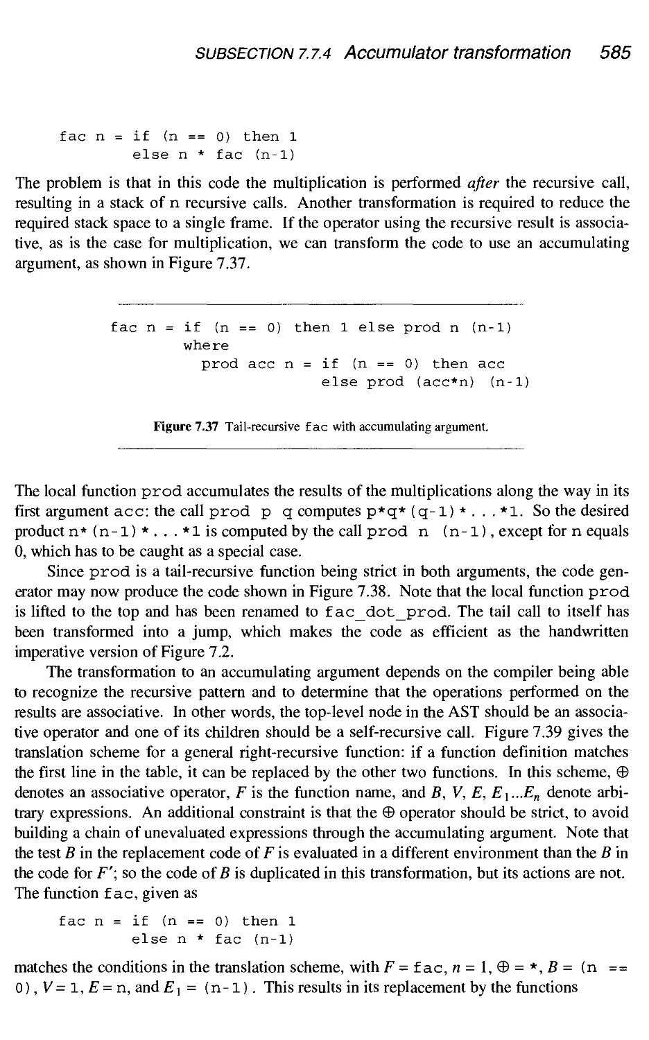
7.7.4 Accumulator transformation
7.7.5 Limitations
Advanced graph manipulation
7.8.1 Variable-length nodes
7.8.2 Pointer tagging
7.8.3 Aggregate node allocation
7.8.4 Vector apply nodes
Conclusion
Summary
Further reading
Exercises
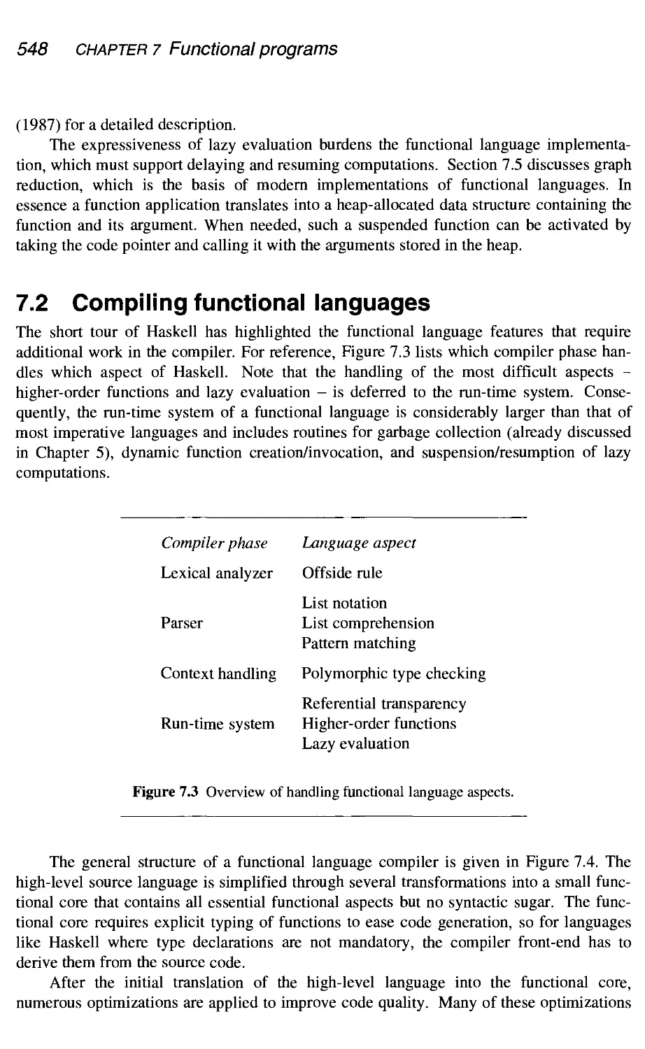
548
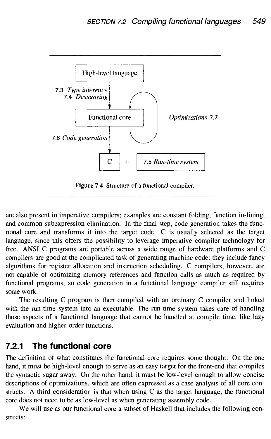
549
551
551
553
553
553
557
558
560
564
566
568
573
575
575
582
582
584
587
587
587
588
588
588
589
589
592
593
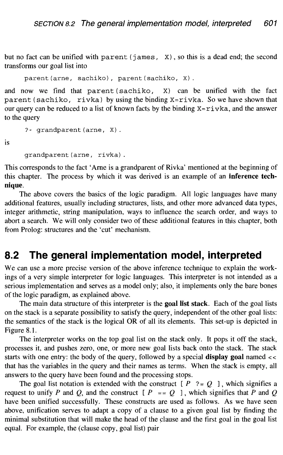
8 Logic programs 596
8.1 The logic programming model 598
8.1.1 The building blocks 598
8.1.2 The inference mechanism 600
8.2 The general implementation model, interpreted 601
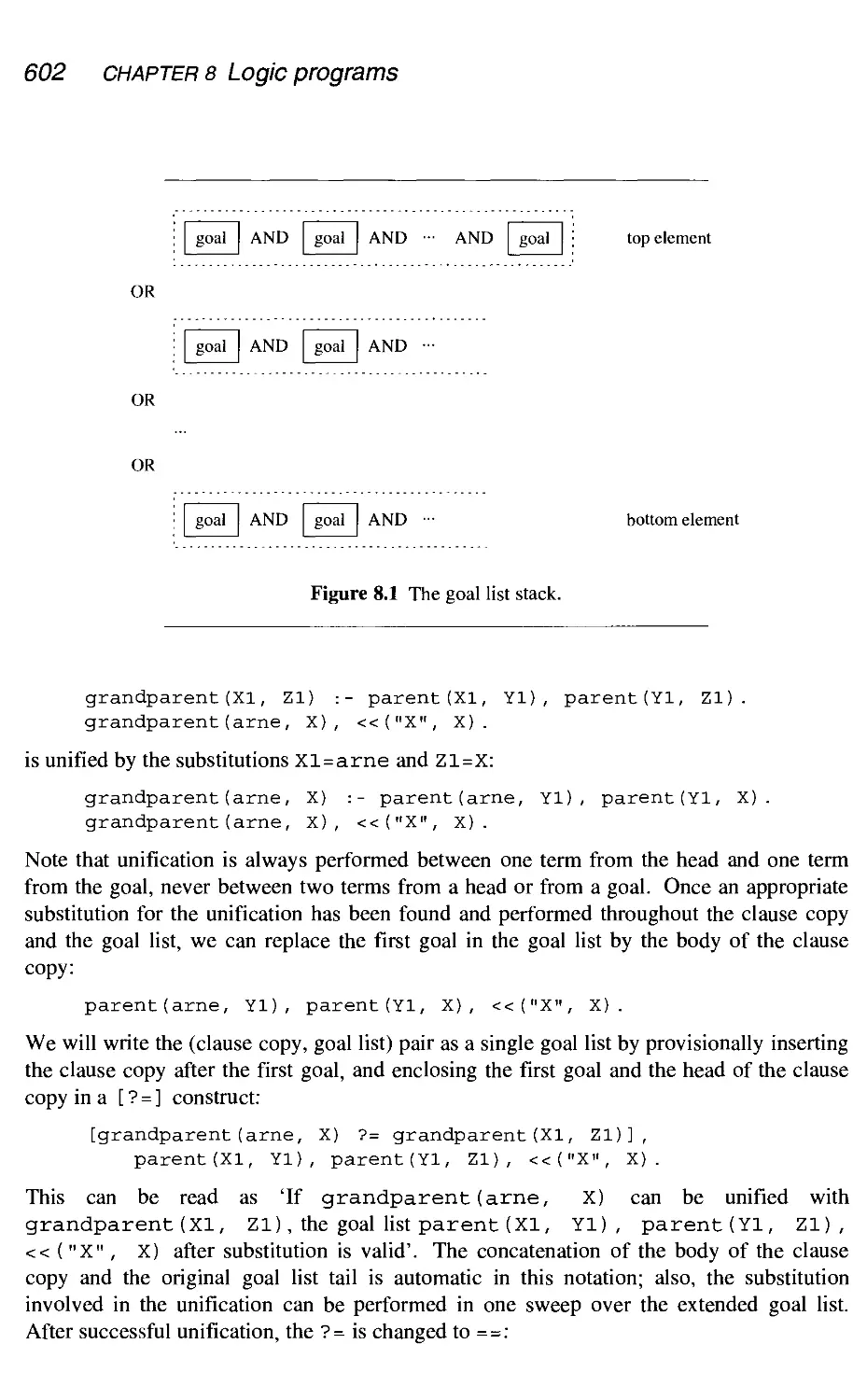
8.2.1 The interpreter instructions 603
8.2.2 Avoiding redundant goal lists 606
8.2.3 Avoiding copying goal list tails 606
8.3 Unification 607
8.3.1 Unification of structures, lists, and sets 607
Contents xi
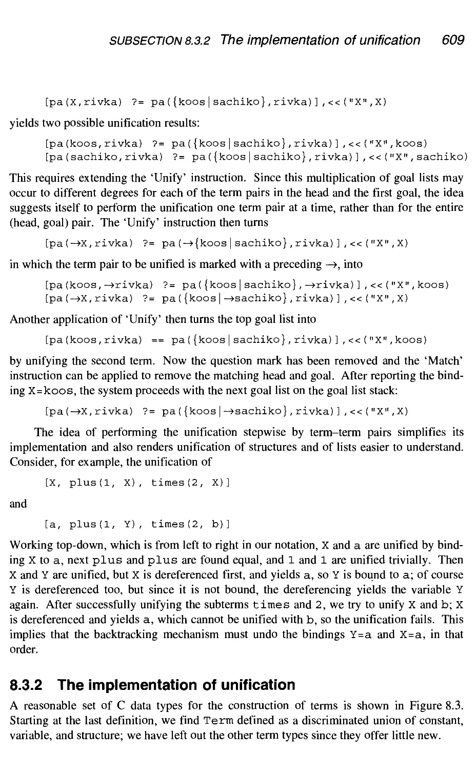
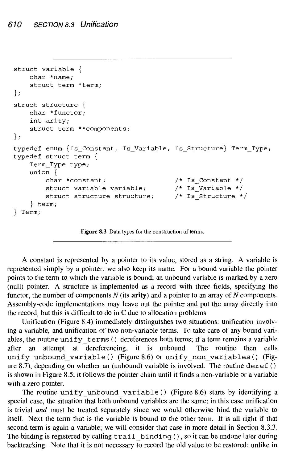
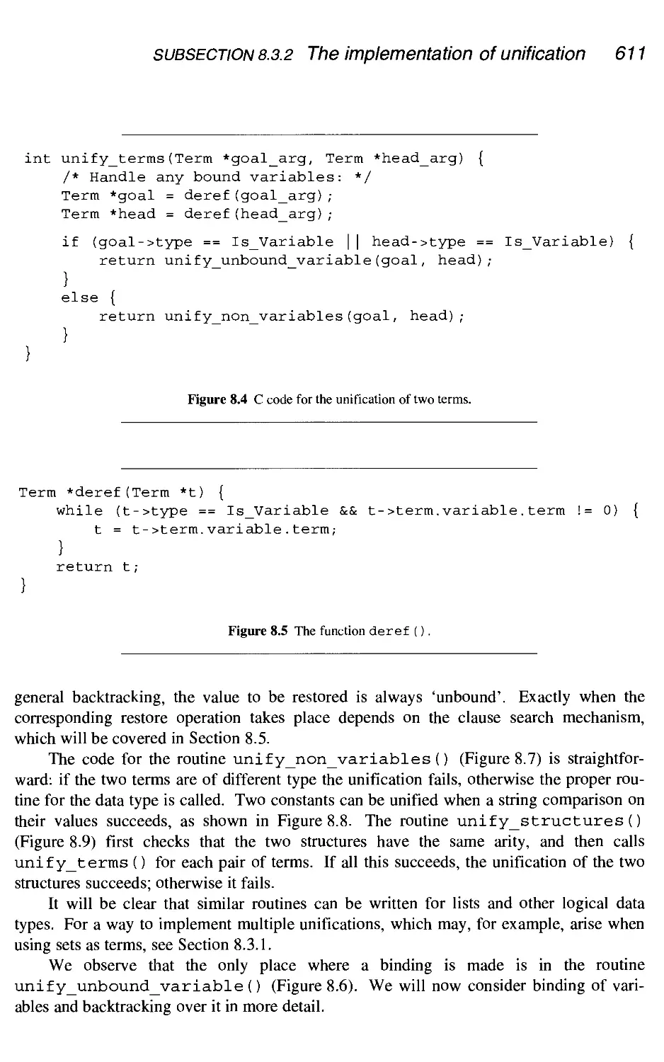
8.3.2 The implementation of unification 609
8.3.3 Unification of two unbound variables 612
8.3.4 Conclusion 614
8.4 The general implementation model, compiled 615
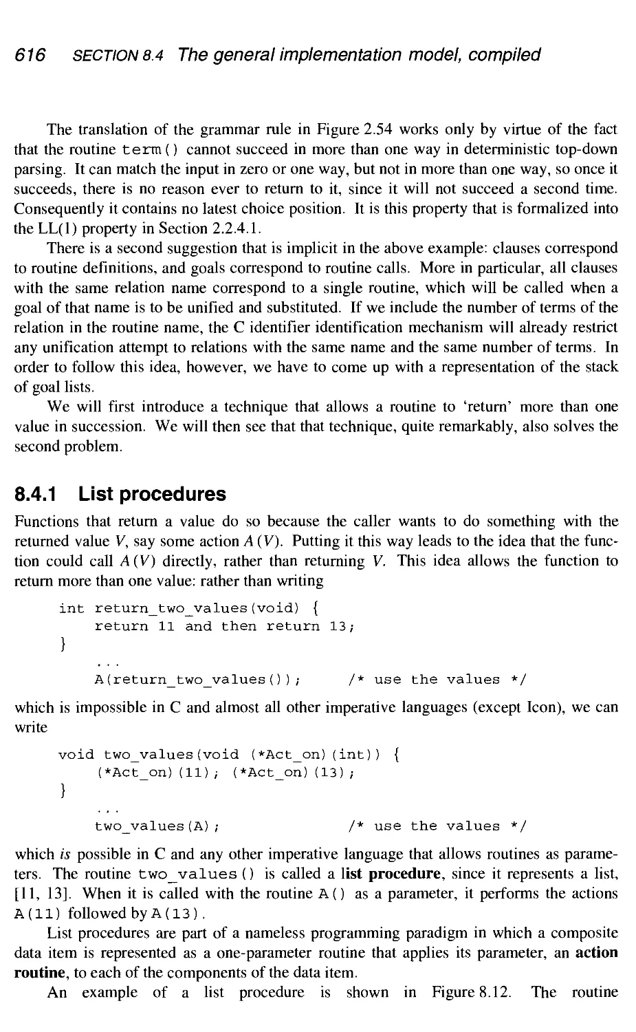
8.4.1 List procedures 616
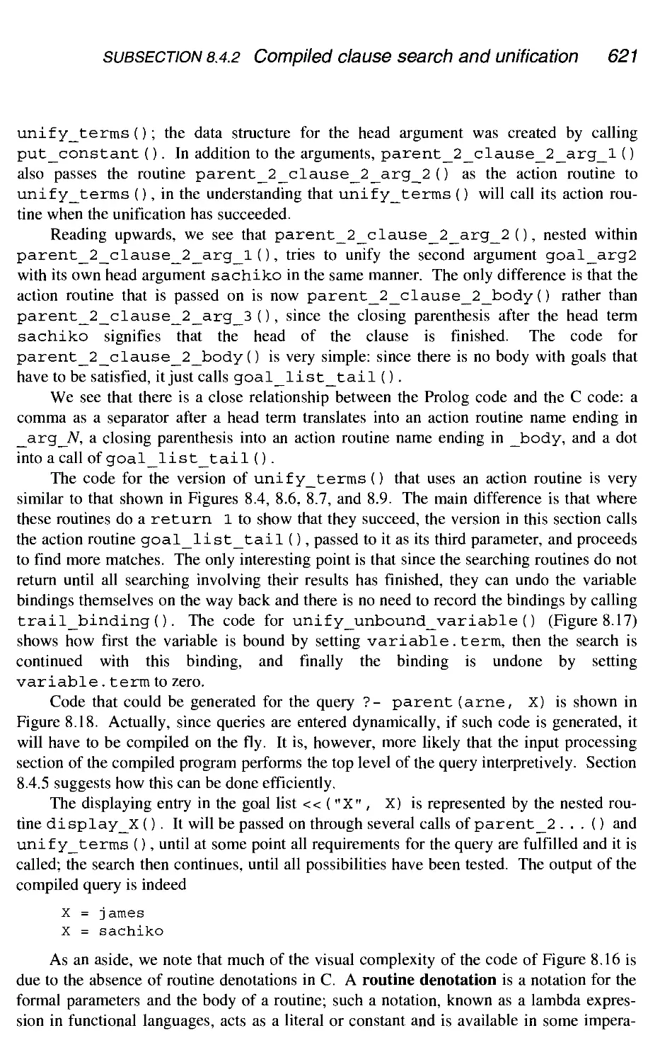
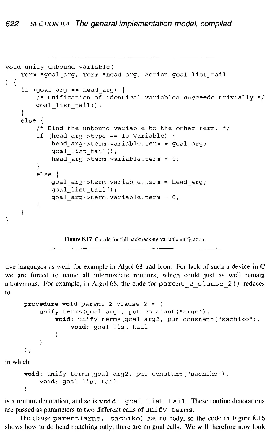
8.4.2 Compiled clause search and unification 619
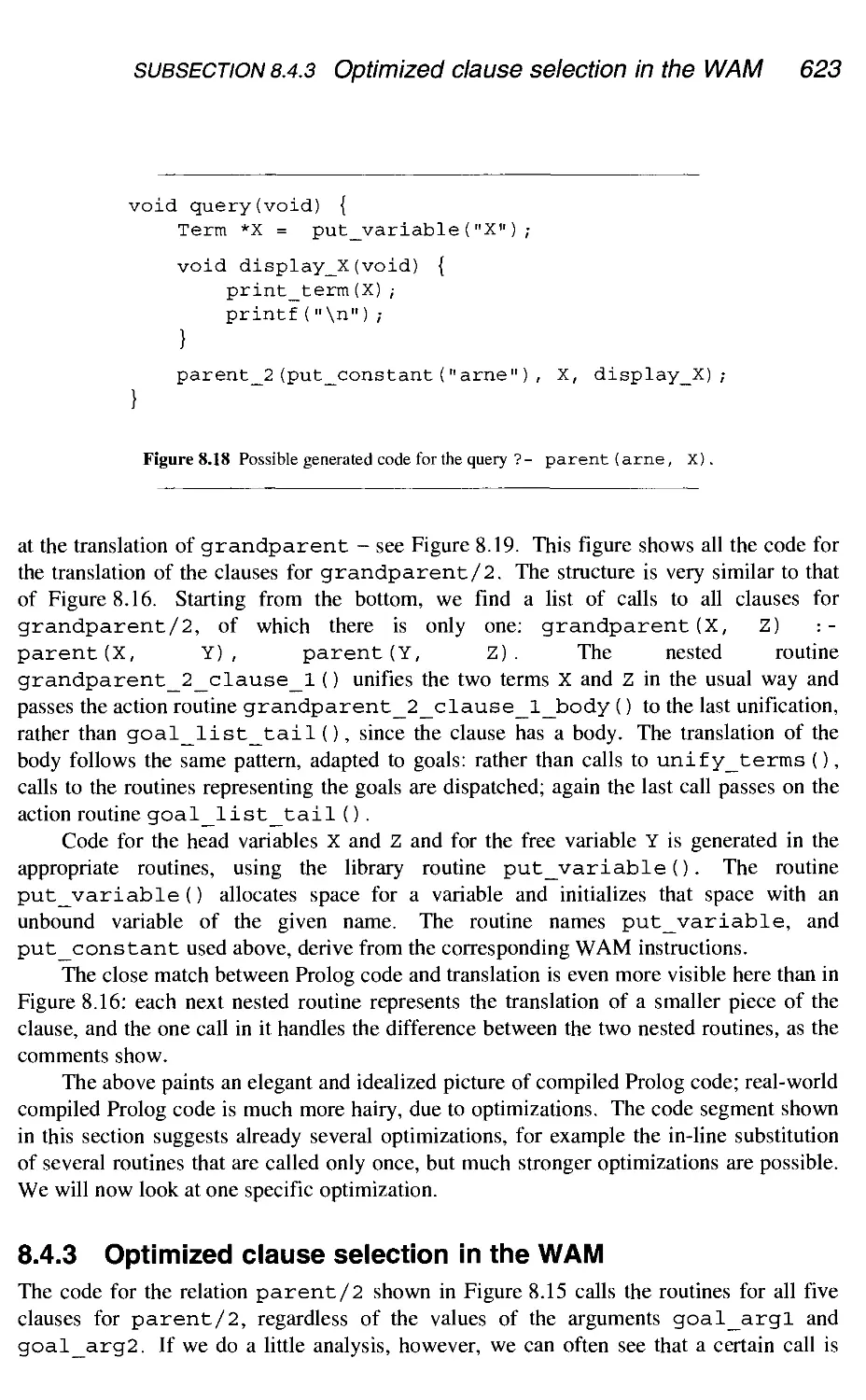
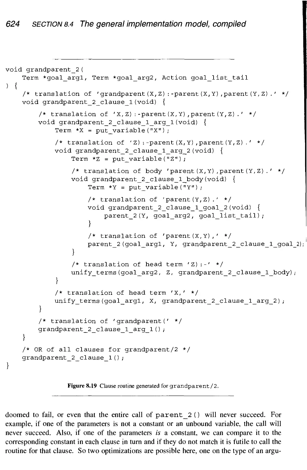
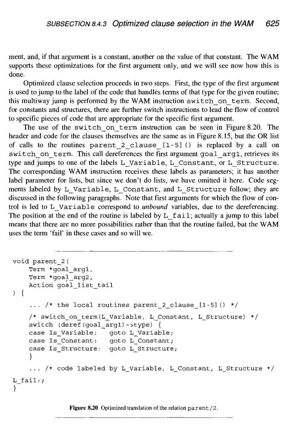
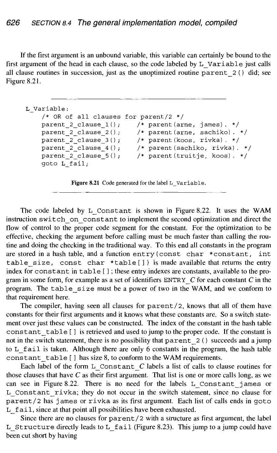
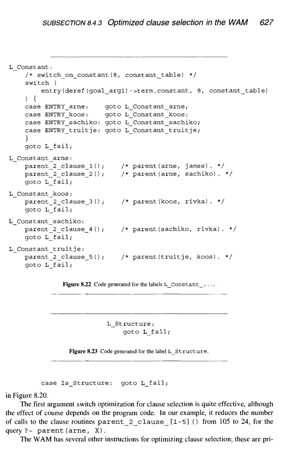
8.4.3 Optimized clause selection in the WAM 623
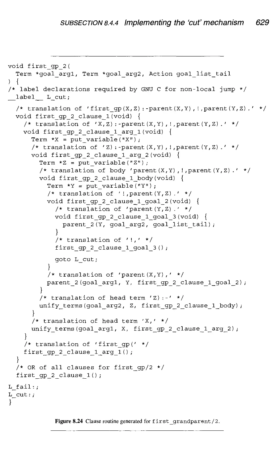
8.4.4 Implementing the 'cut' mechanism 628
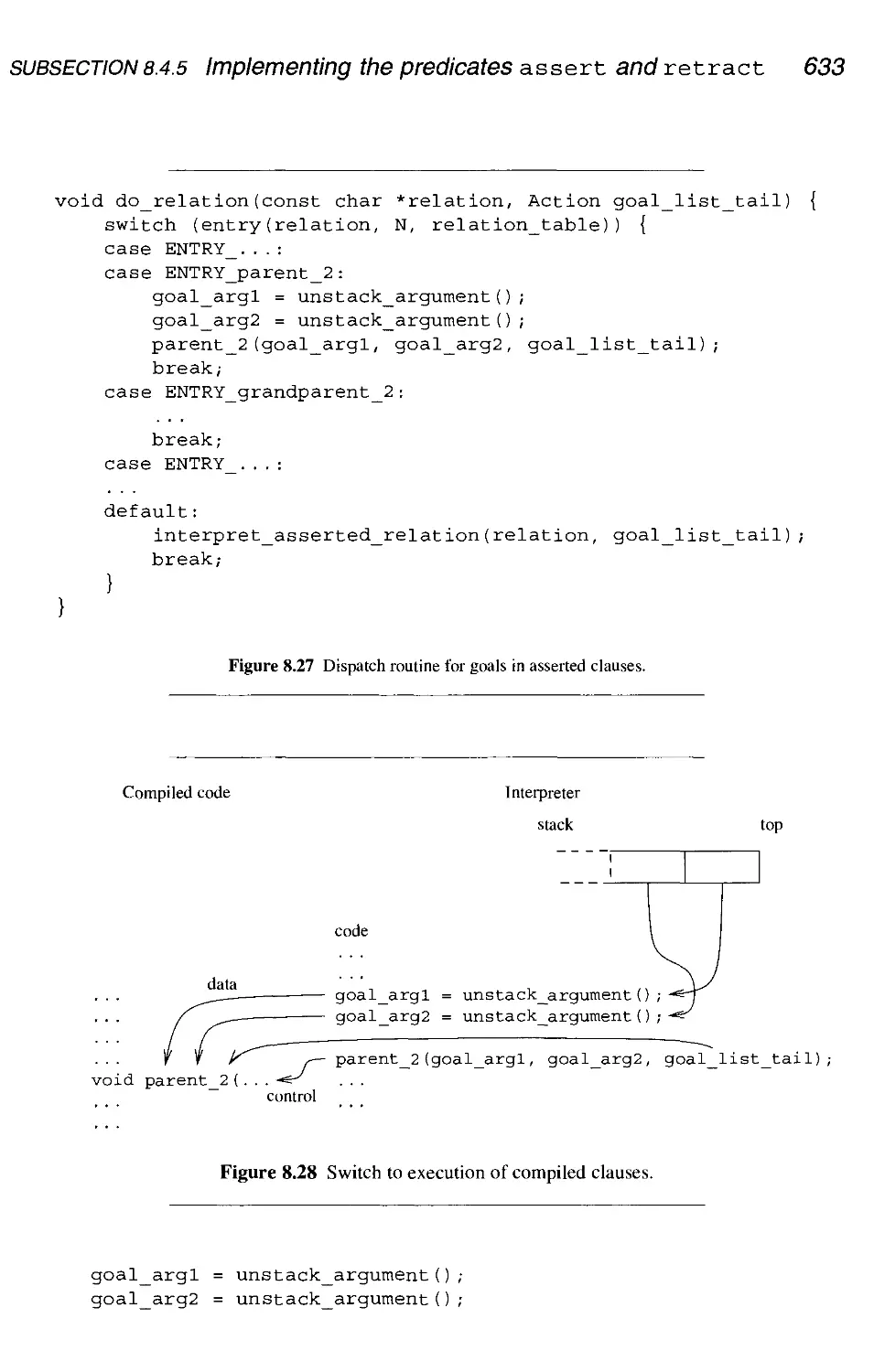
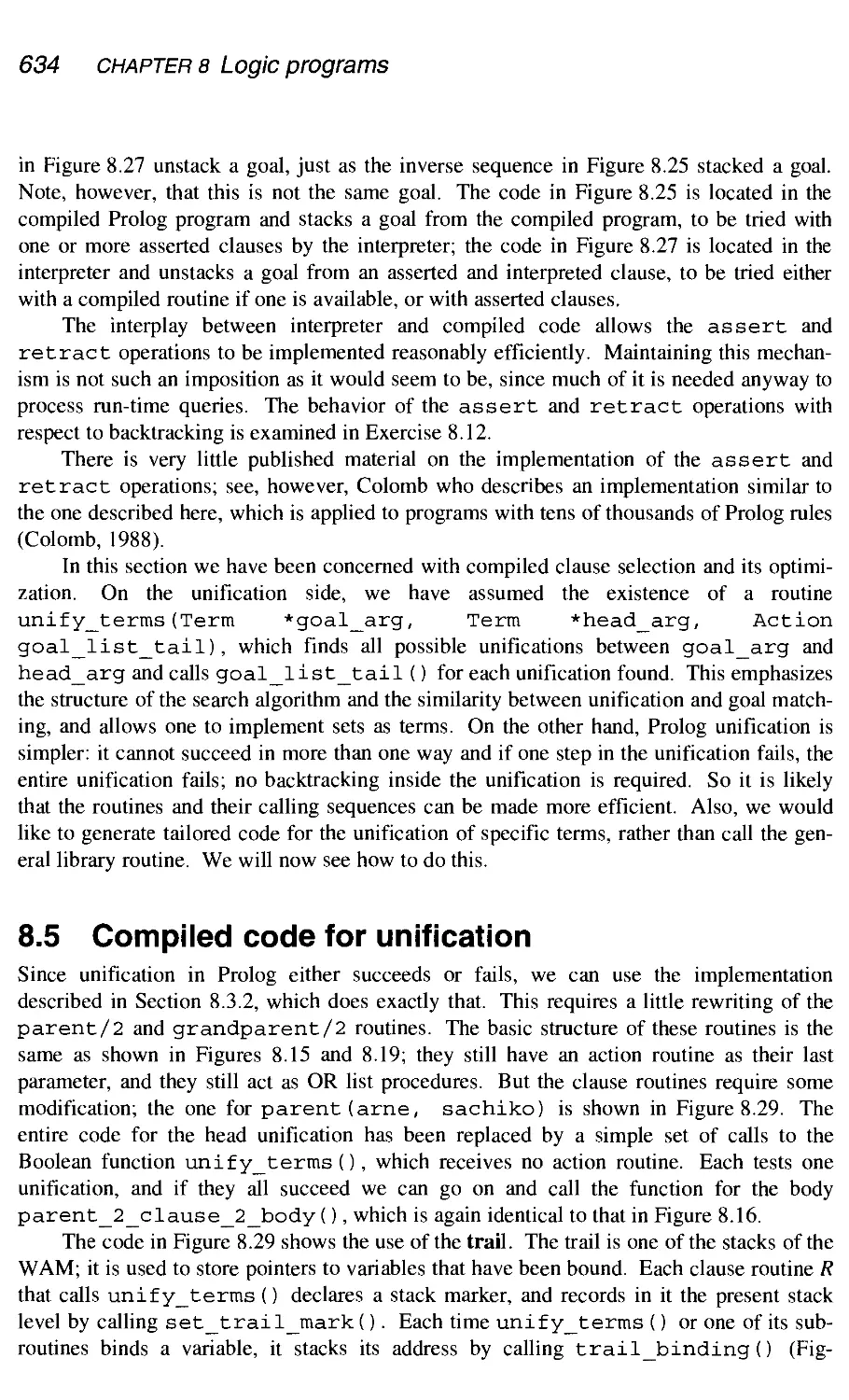
8.4.5 Implementing the predicates assert and retract 630
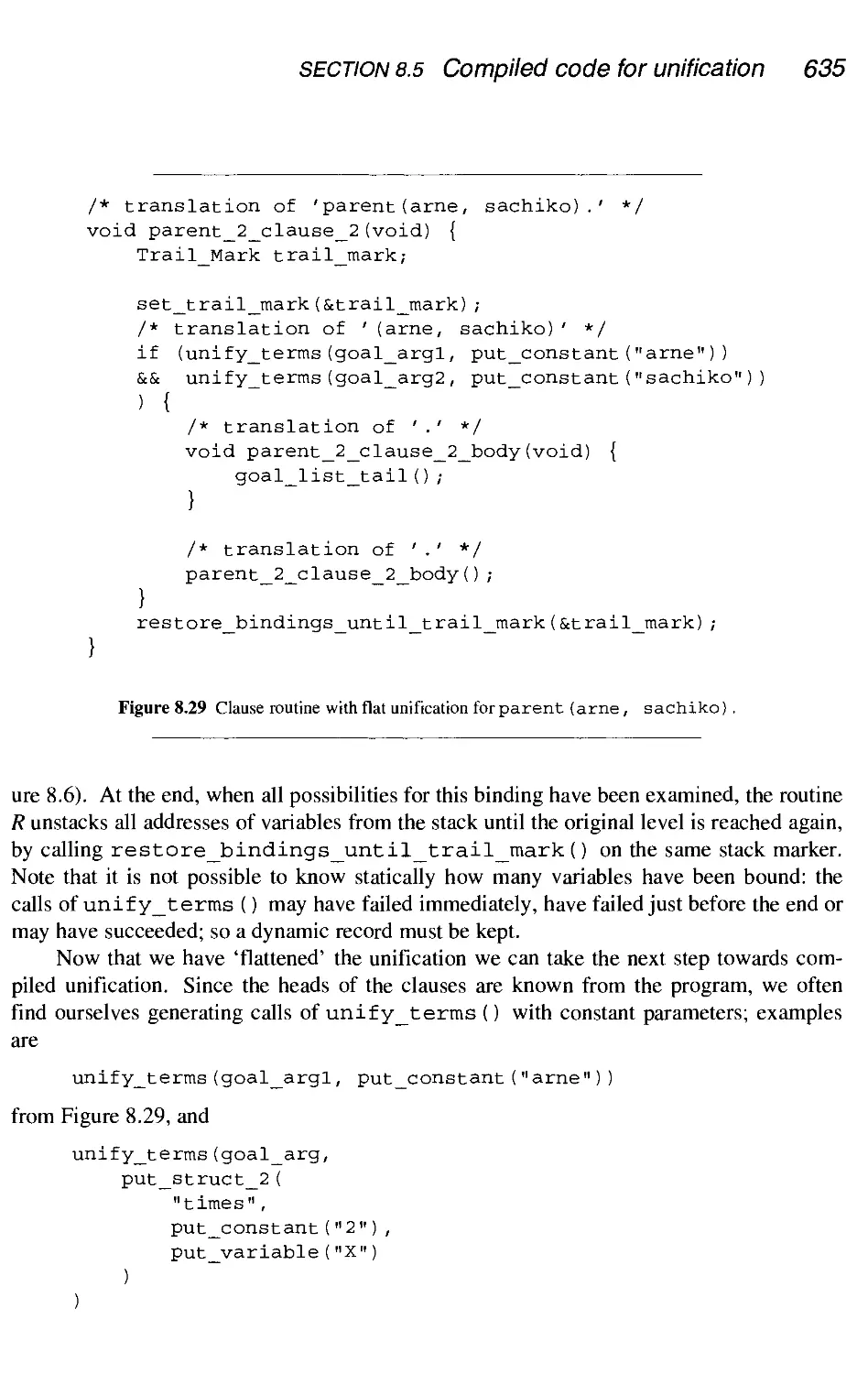
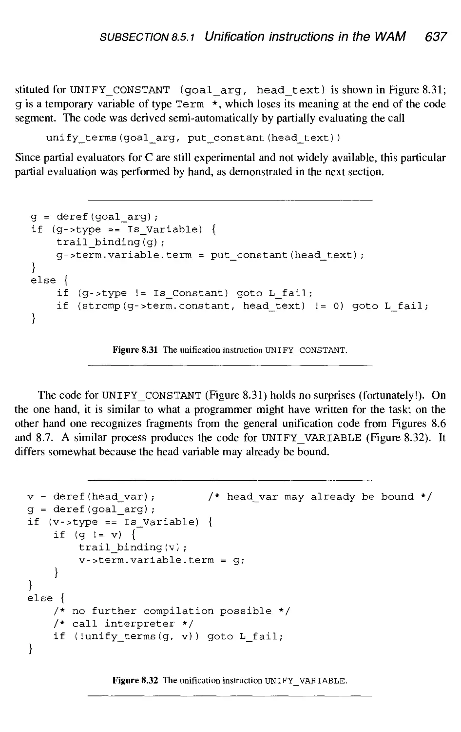
8.5 Compiled code for unification 634
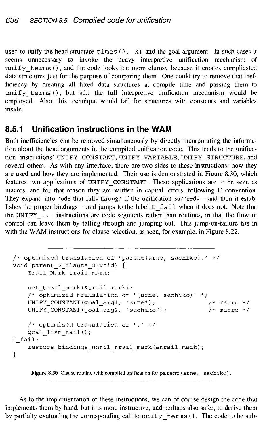
8.5.1 Unification instructions in the WAM 636
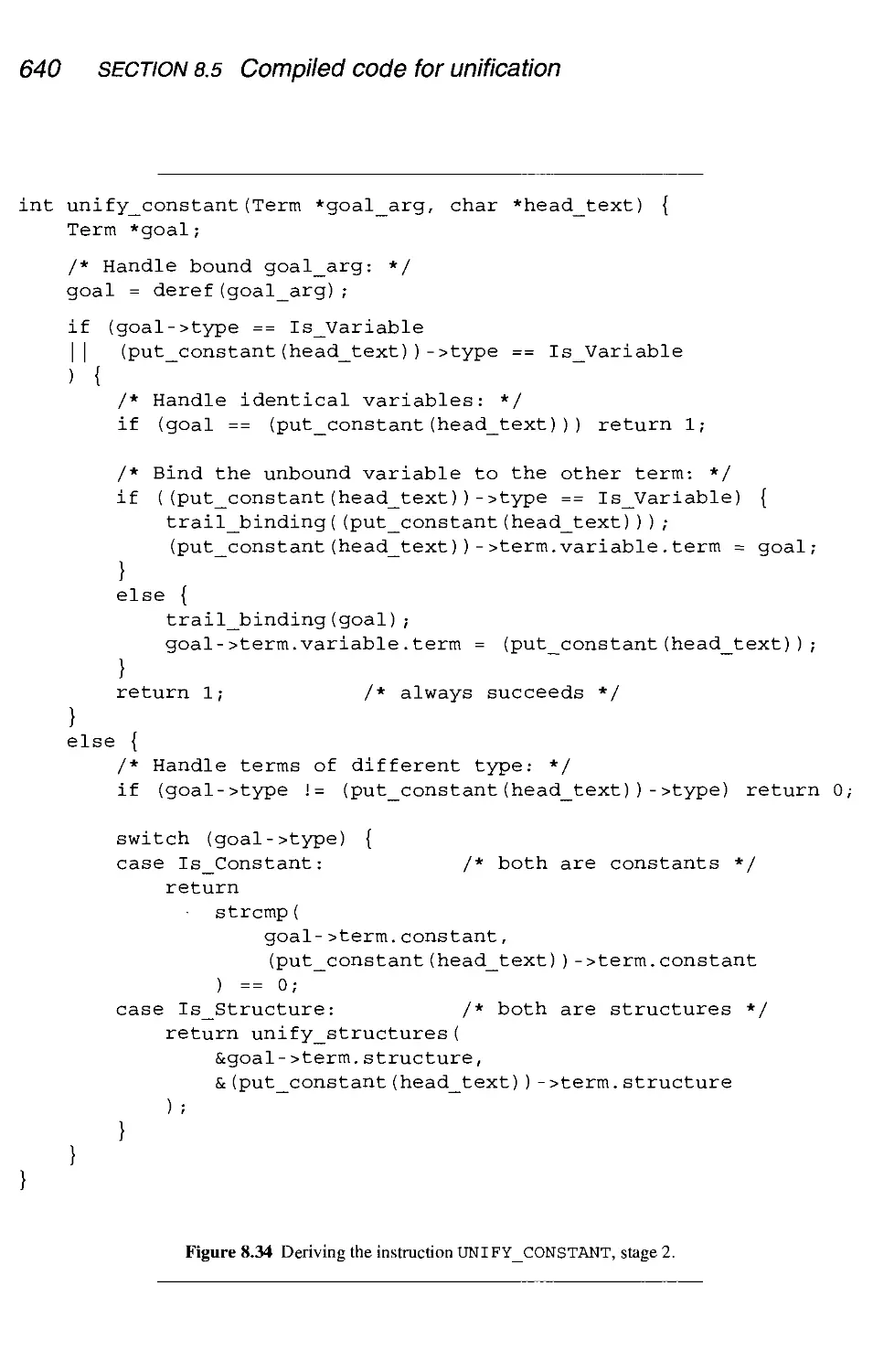
8.5.2 Deriving a unification instruction by manual partial
evaluation 638
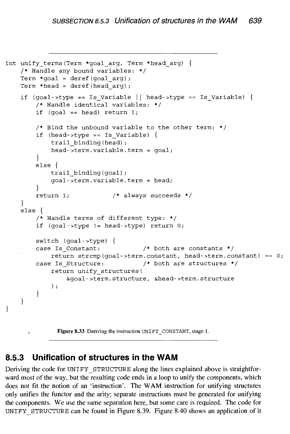
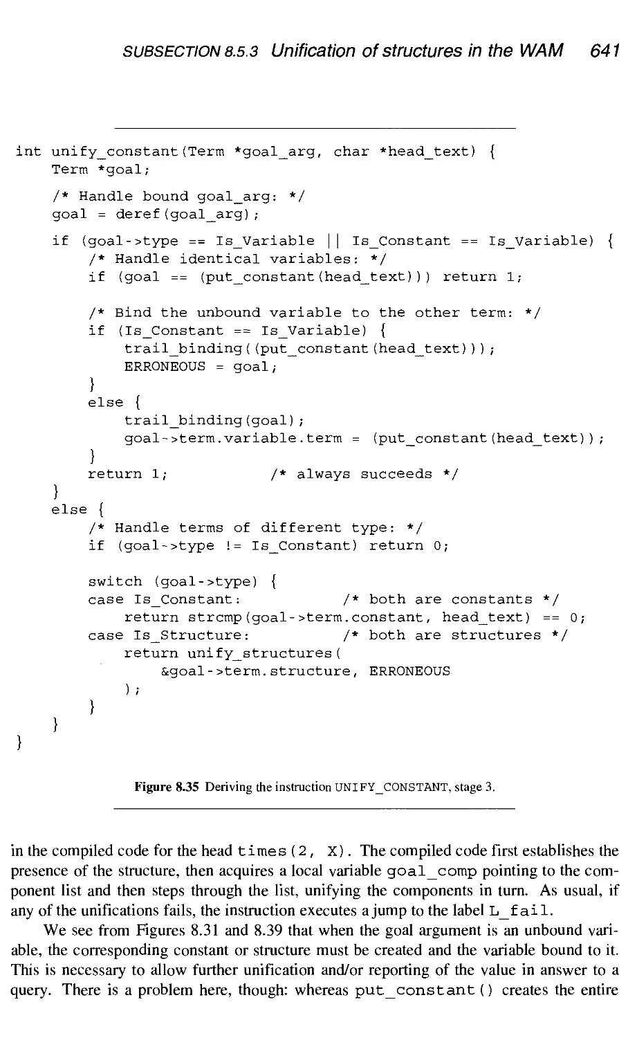
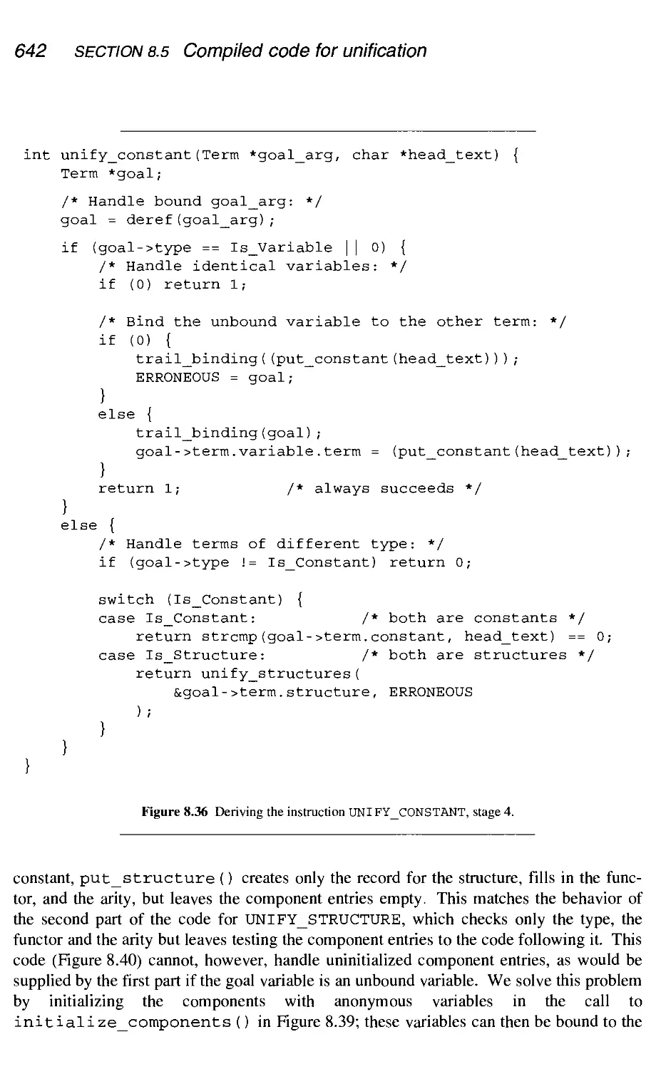
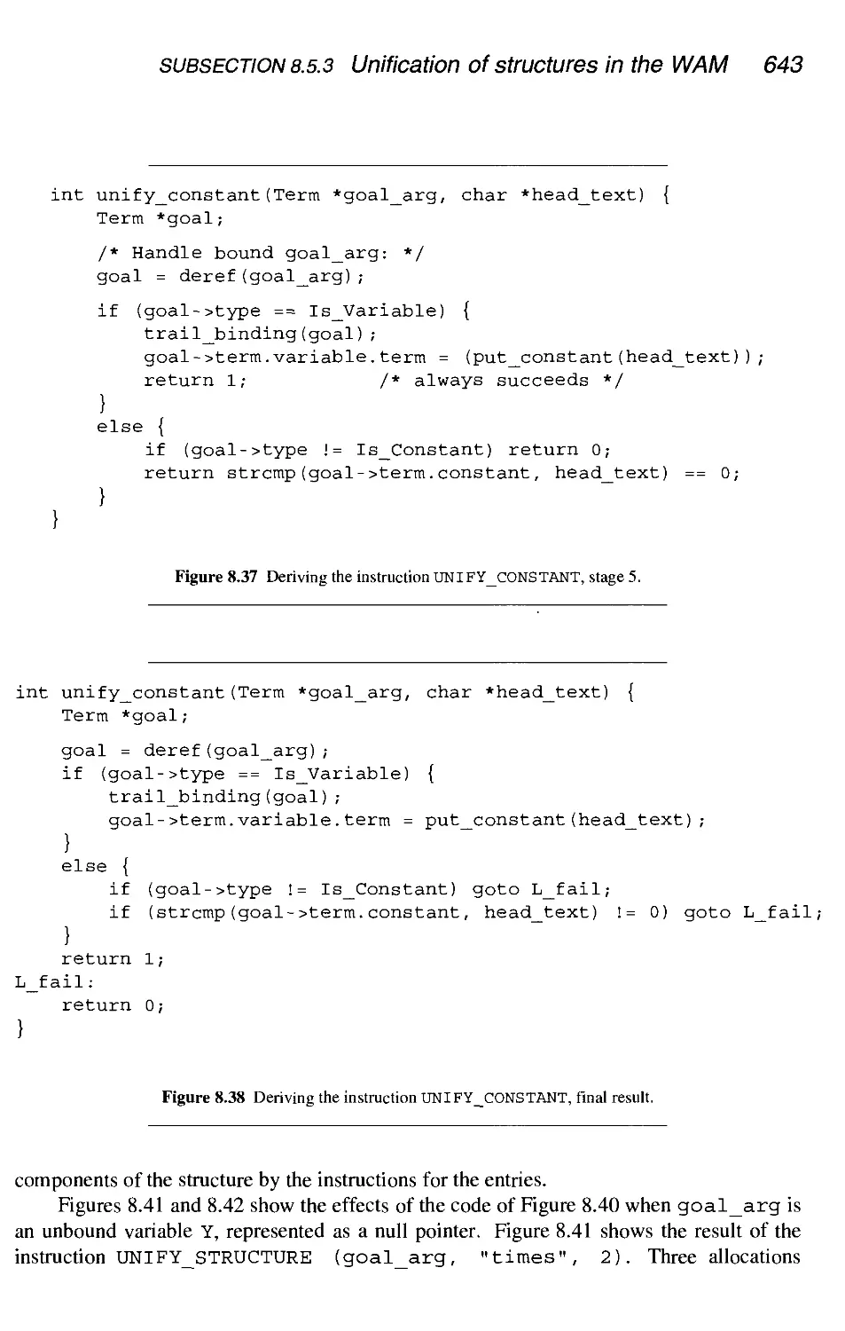
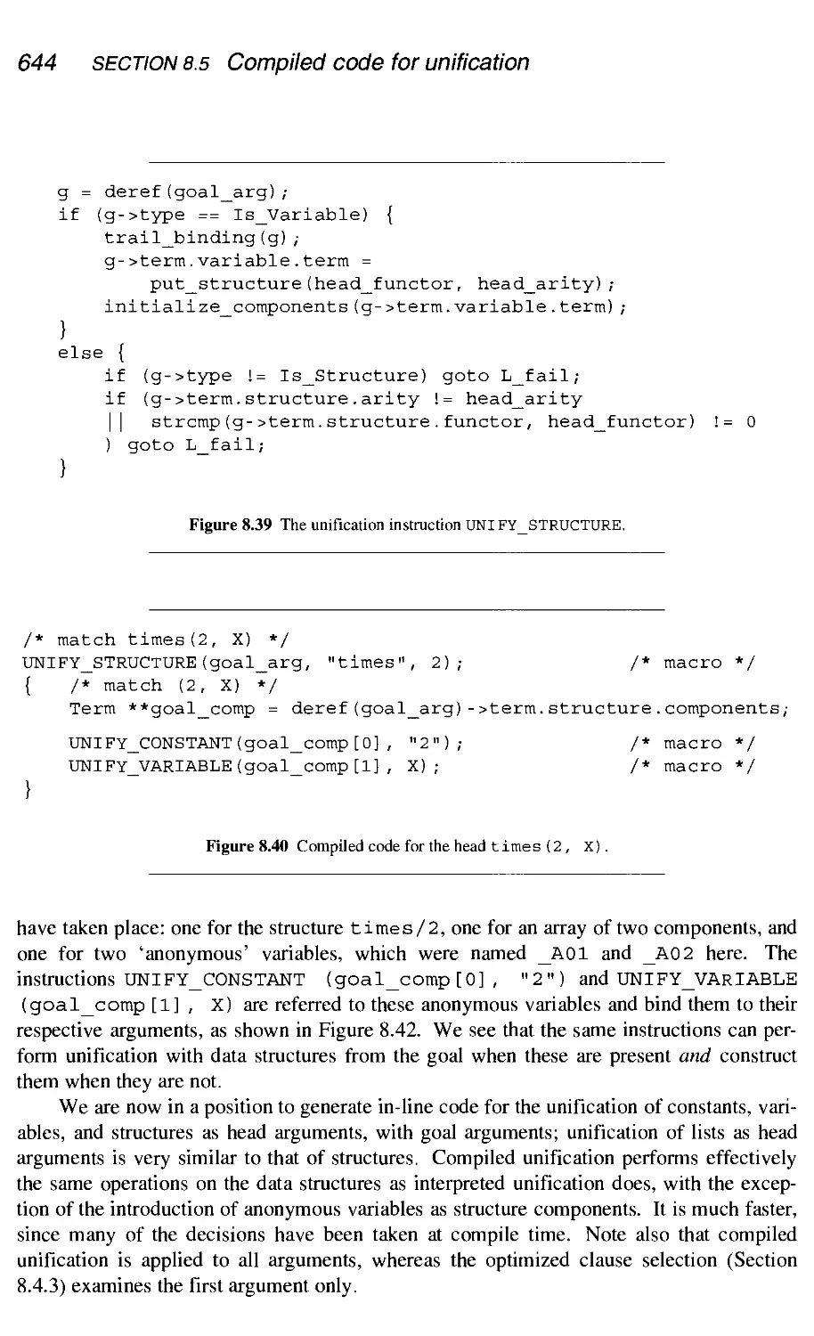
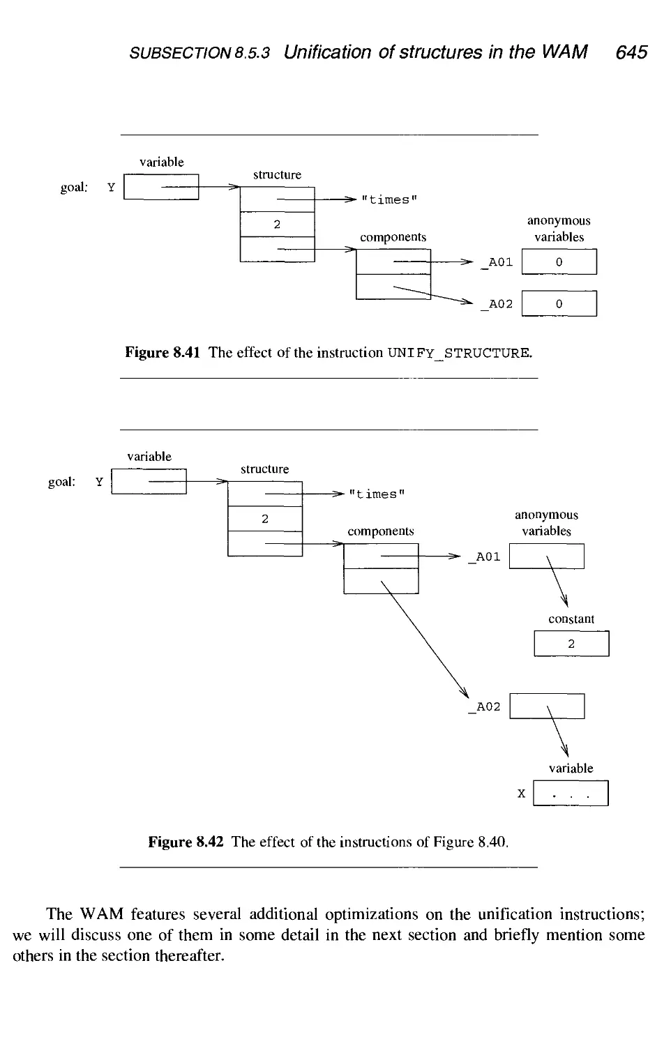
8.5.3 Unification of structures in the WAM 639
8.5.4 An optimization: read/write mode 646
8.5.5 Further unification optimizations in the WAM 648
8.5.6 Conclusion 650
Summary 650
Further reading 653
Exercises 653
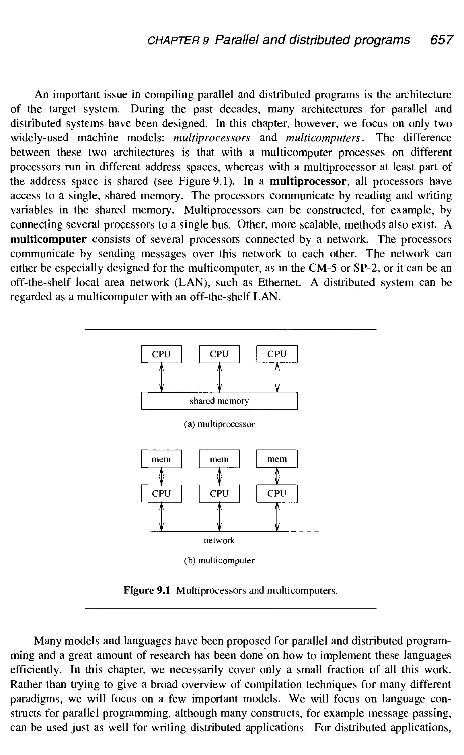
Parallel and distributed programs 656
9.1 Parallel programming models 659
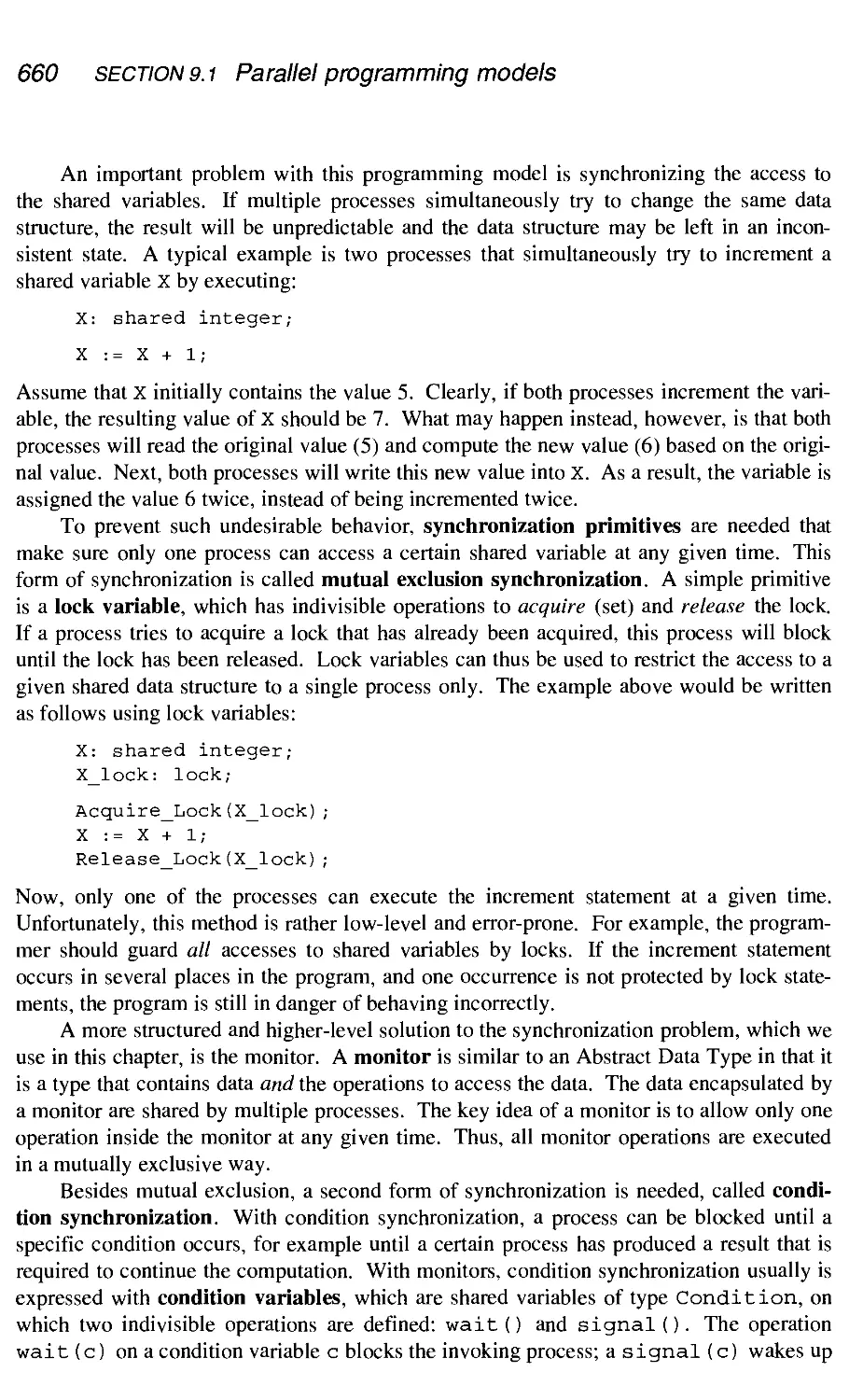
9.1.1 Shared variables and monitors 659
9.1.2 Message passing models 661
9.1.3 Object-oriented languages 663
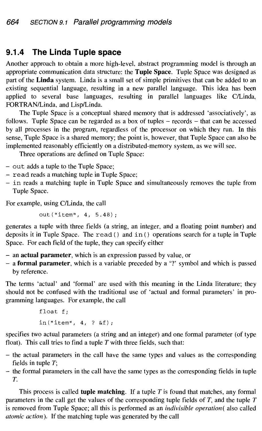
9.1.4 The Linda Tuple space 664
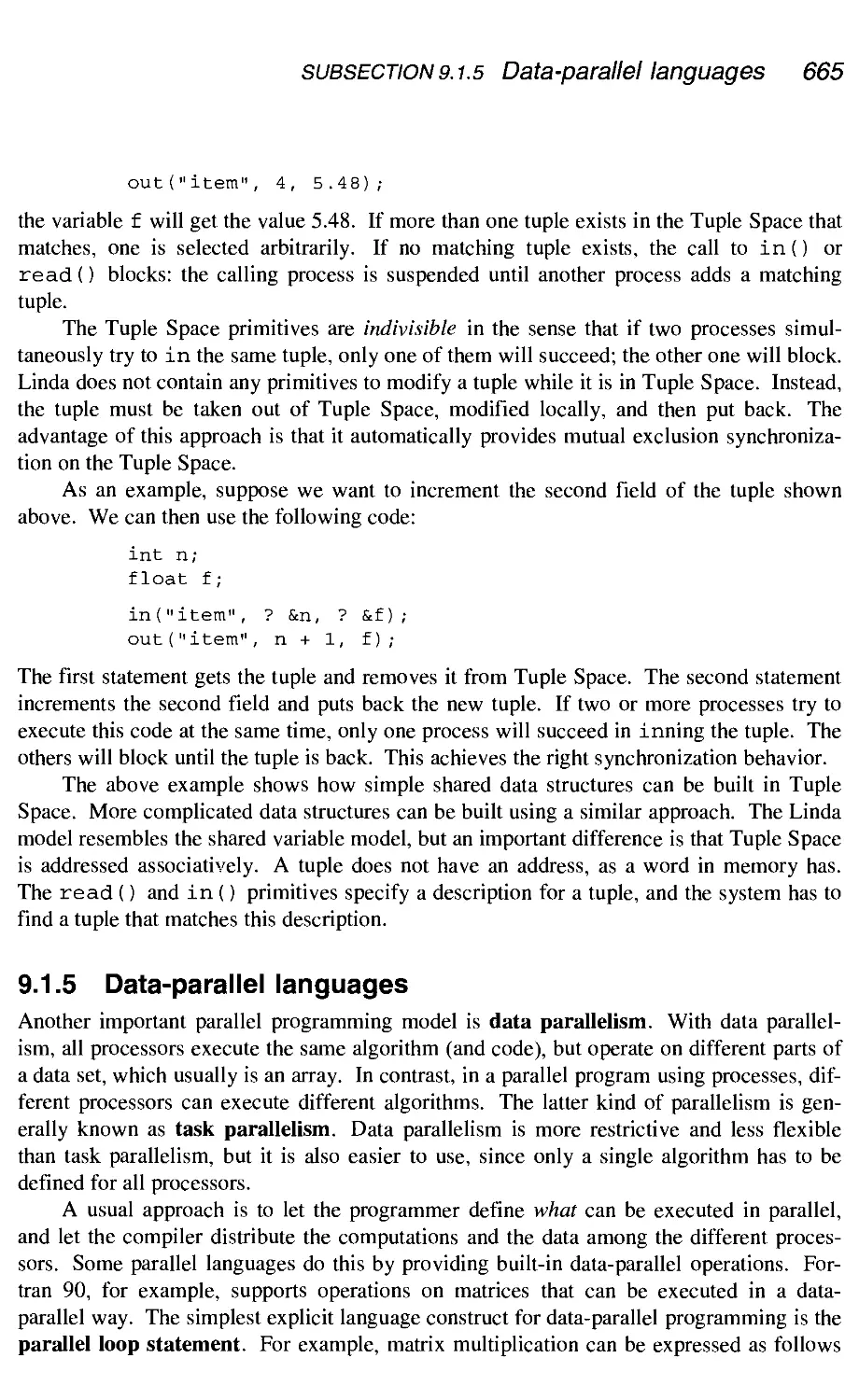
9.1.5 Data-parallel languages 665
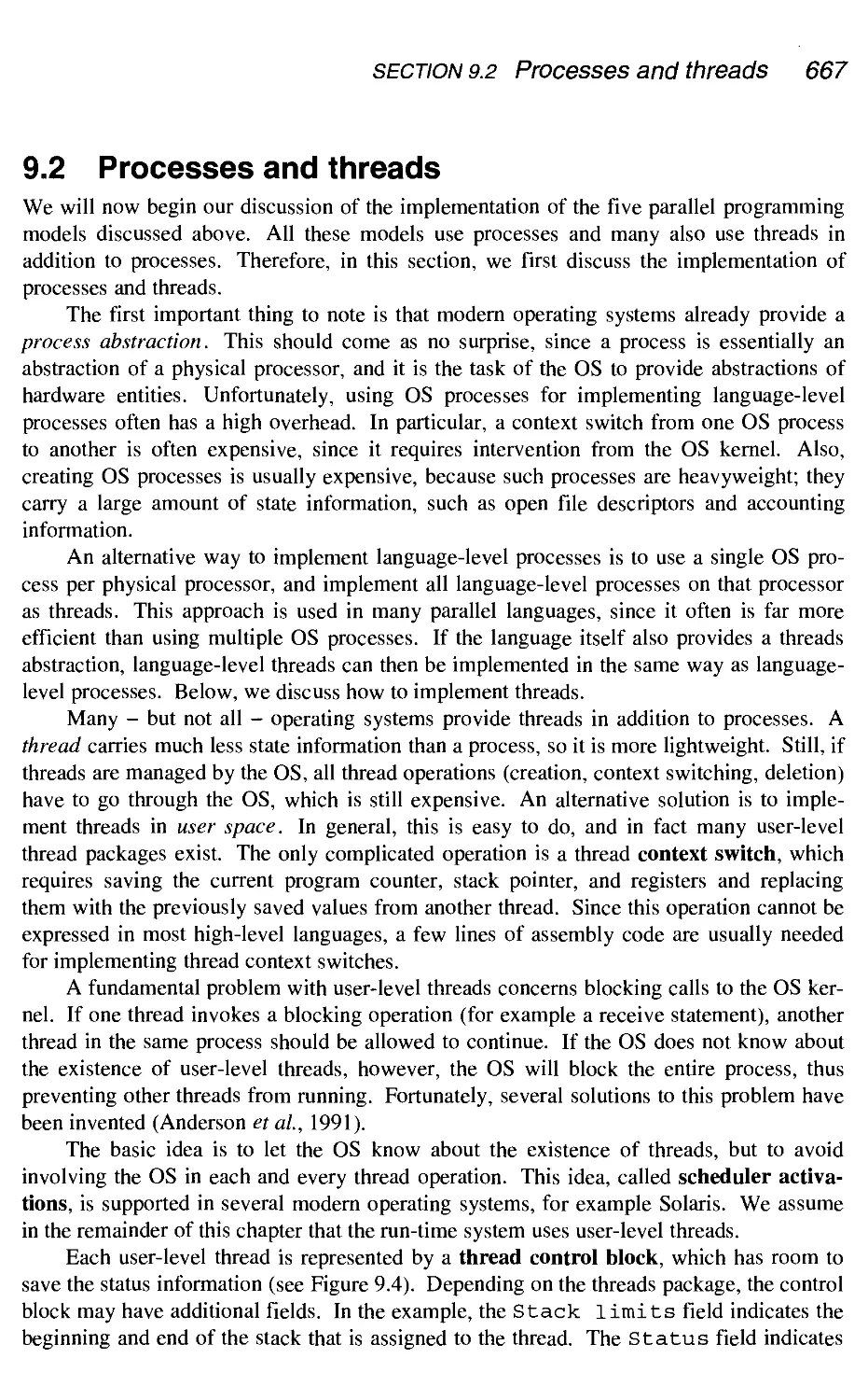
9.2 Processes and threads 667
9.3 Shared variables 668
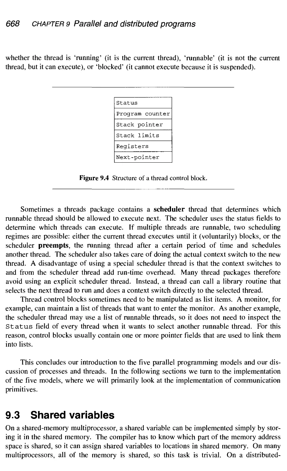
9.3.1 Locks 669
9.3.2 Monitors 669
9.4 Message passing 671
9.4.1 Locating the receiver 672
9.4.2 Marshaling 672
9.4.3 Type checking of messages 673
9.4.4 Message selection 674
9.5 Parallel object-oriented languages 674
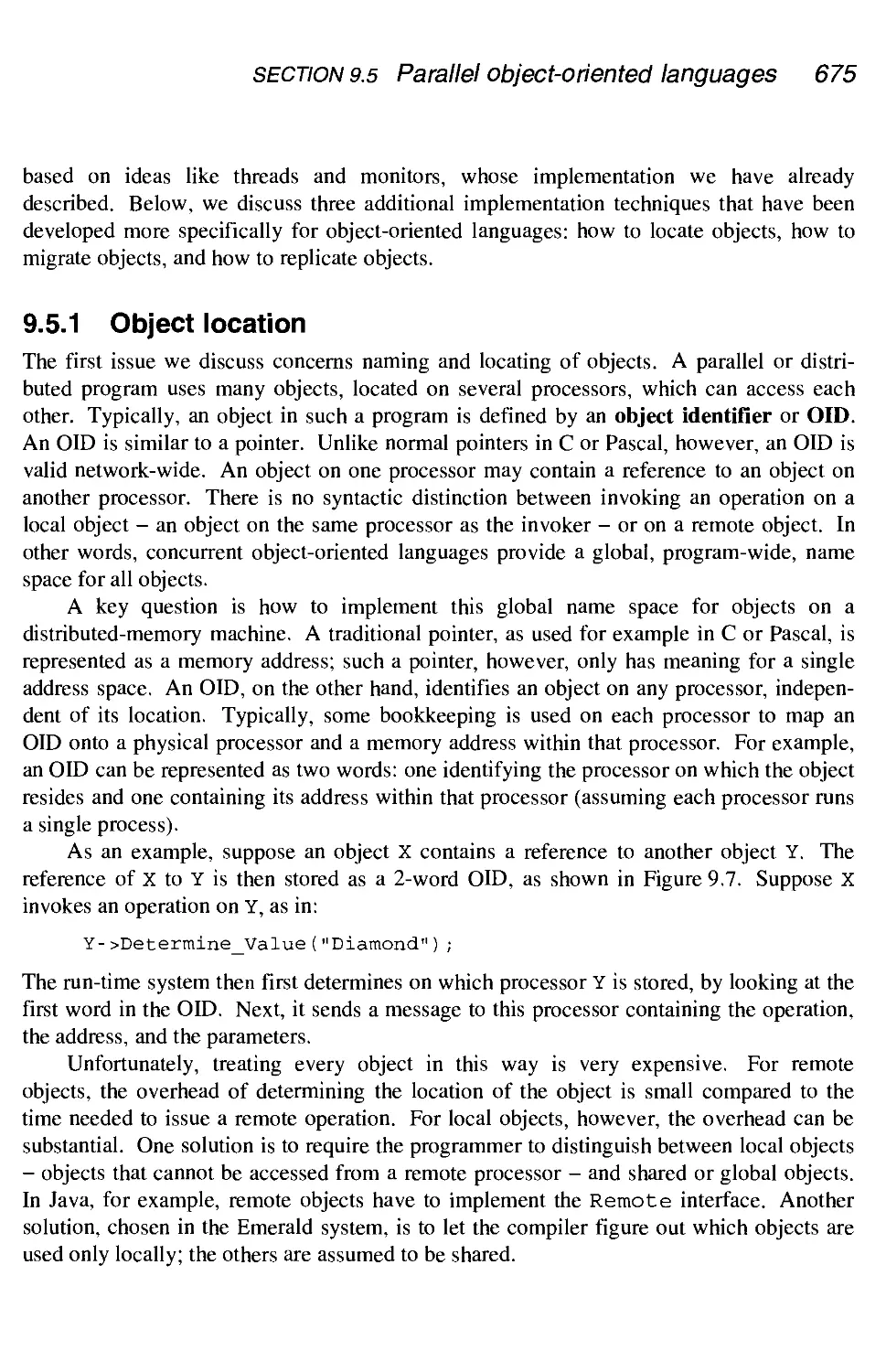
9.5.1 Object location 675
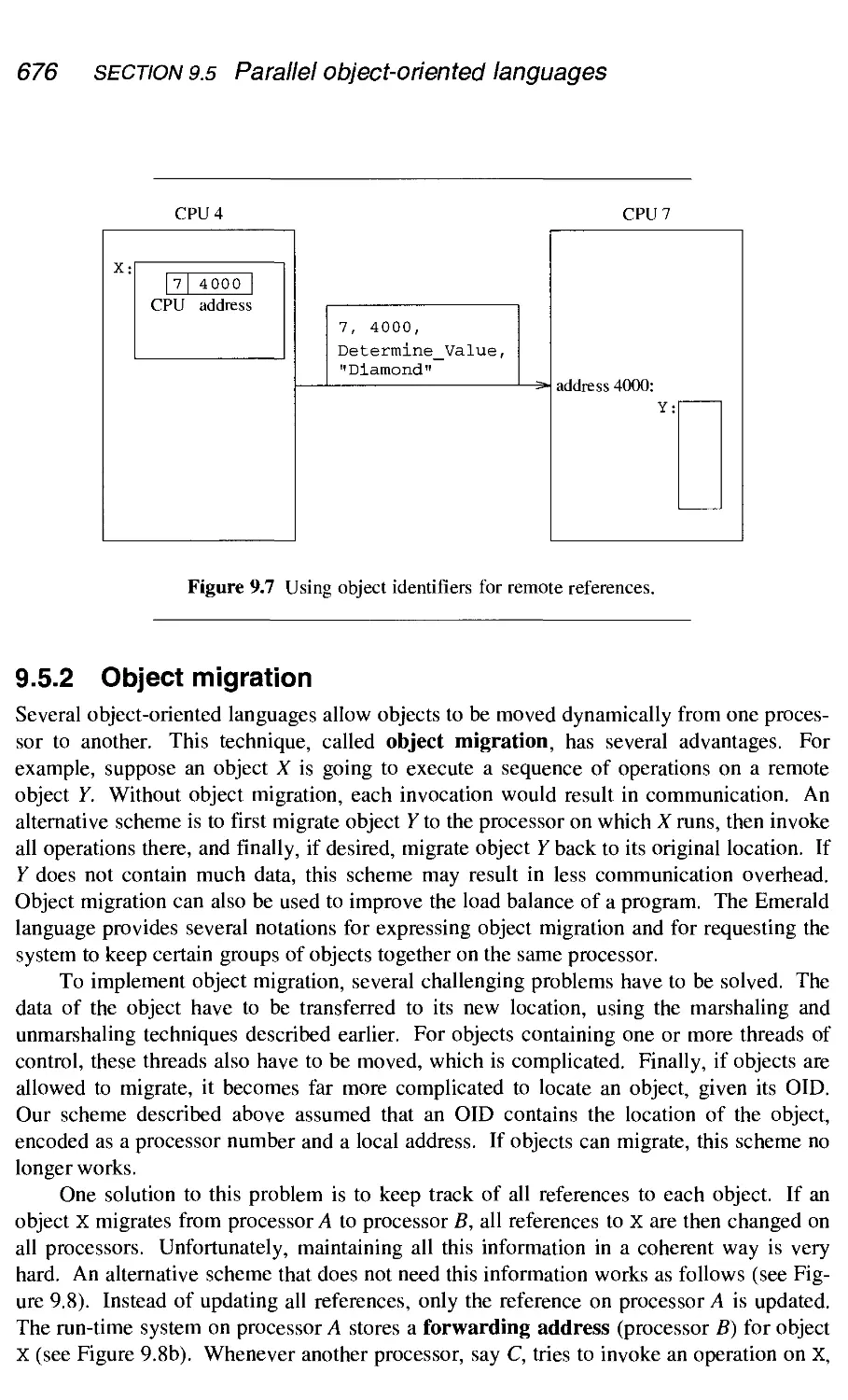
9.5.2 Object migration 676
9.5.3 Object replication 677
xii Contents
9.6 Tuple space 678
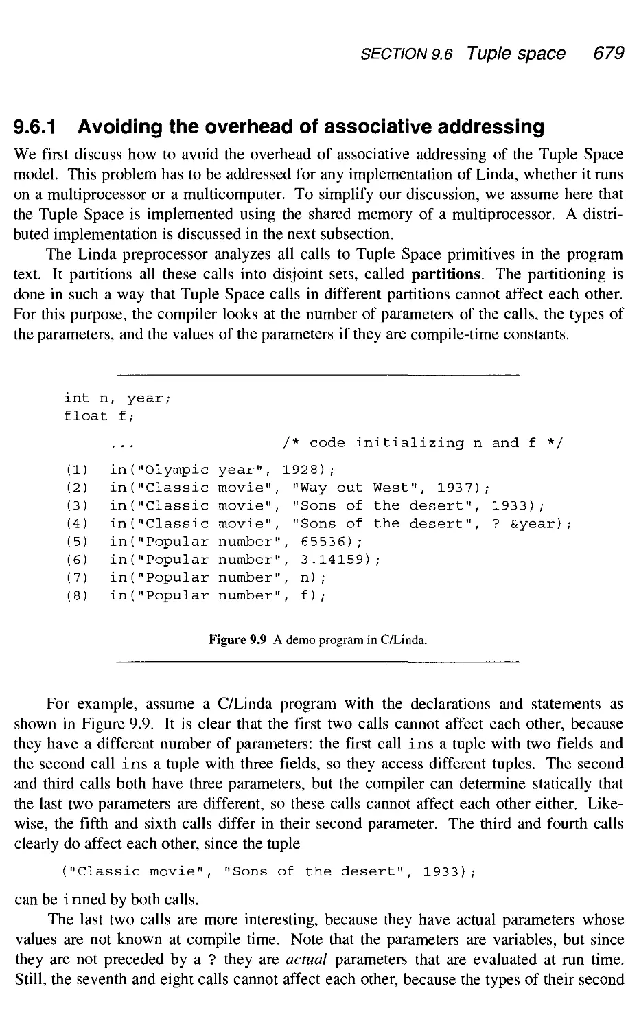
9.6.1 Avoiding the overhead of associative addressing 679
9.6.2 Distributed implementations of the tuple space 682
9.7 Automatic parallelization 684
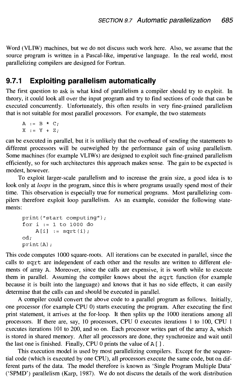
9.7.1 Exploiting parallelism automatically 685
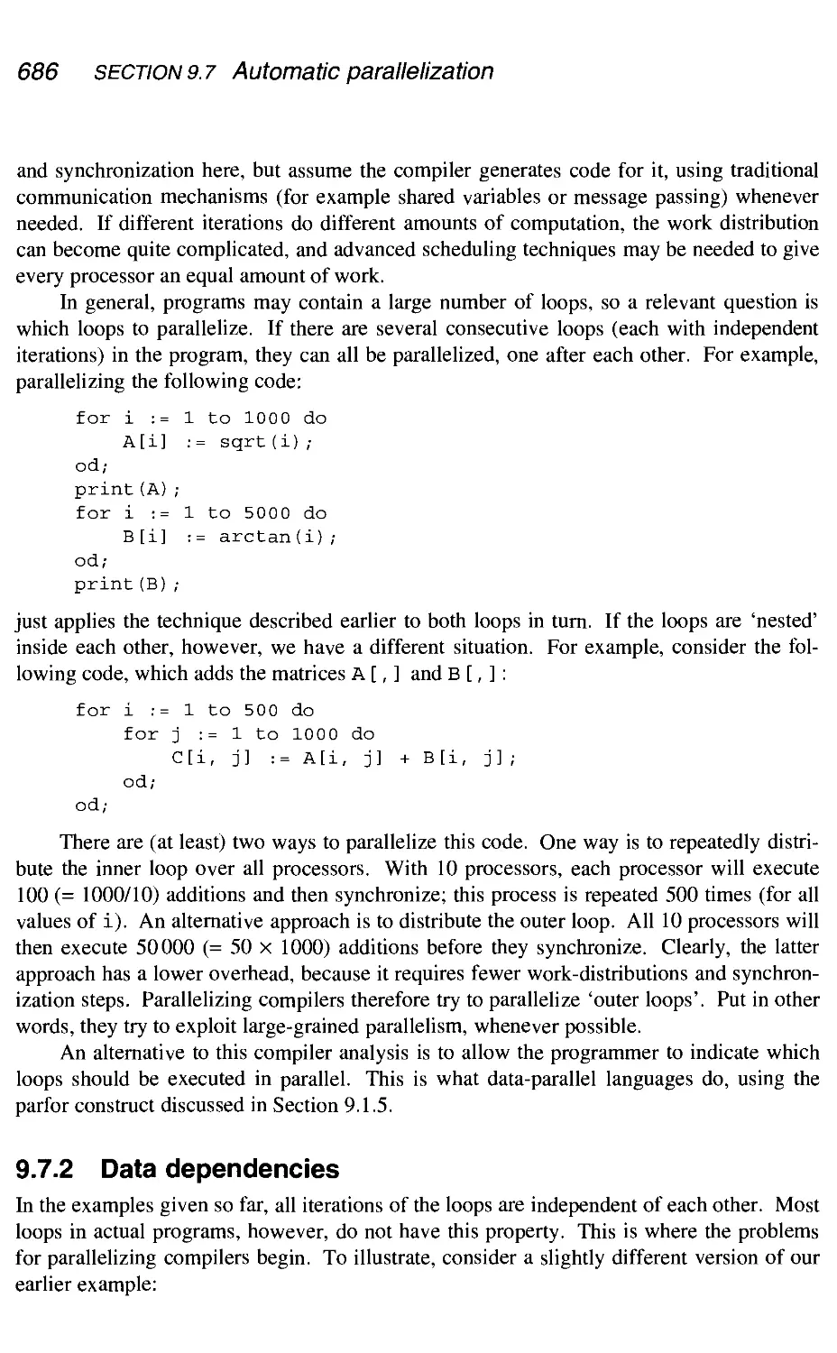
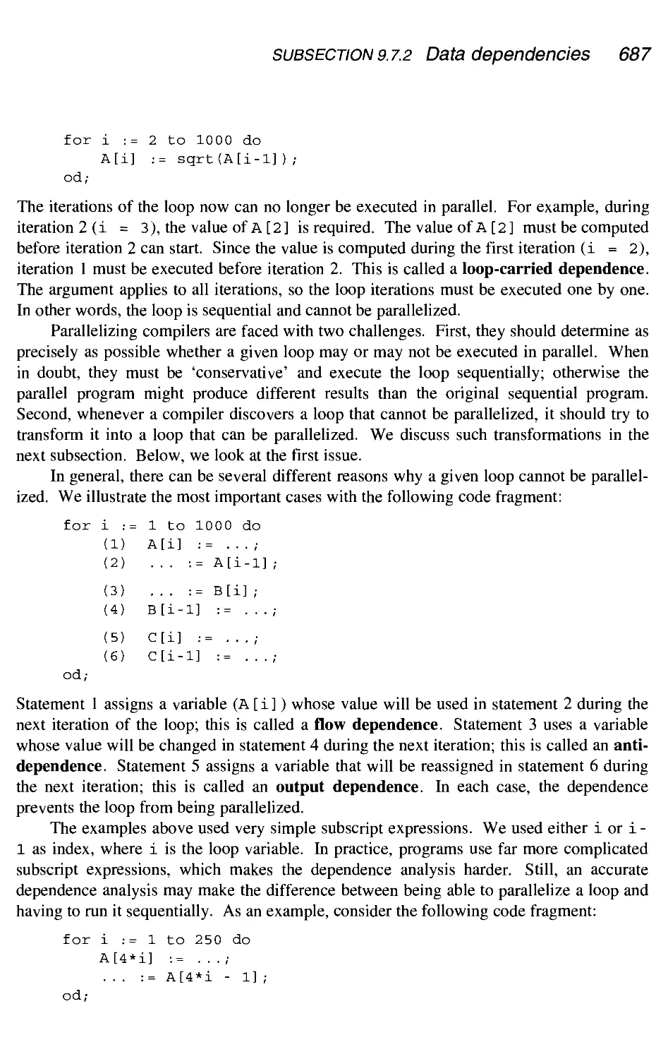
9.7.2 Data dependencies 686
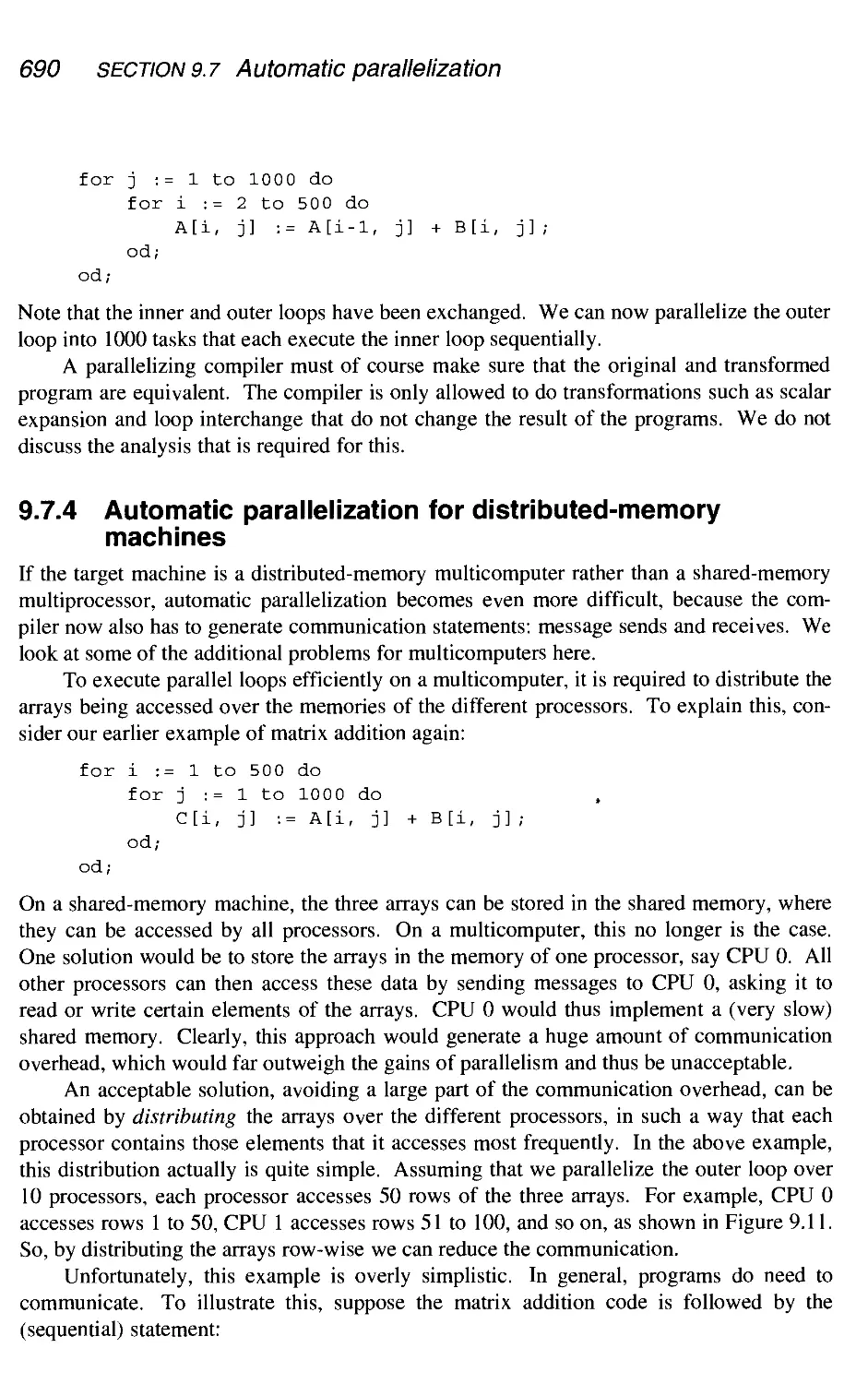
9.7.3 Loop transformations 688
9.7.4 Automatic parallelization for distributed-memory machines 690
9.8 Conclusion 693
Summary 693
Further reading 695
Exercises 695
Appendix A - A simple object-oriented
compiler/interpreter 699
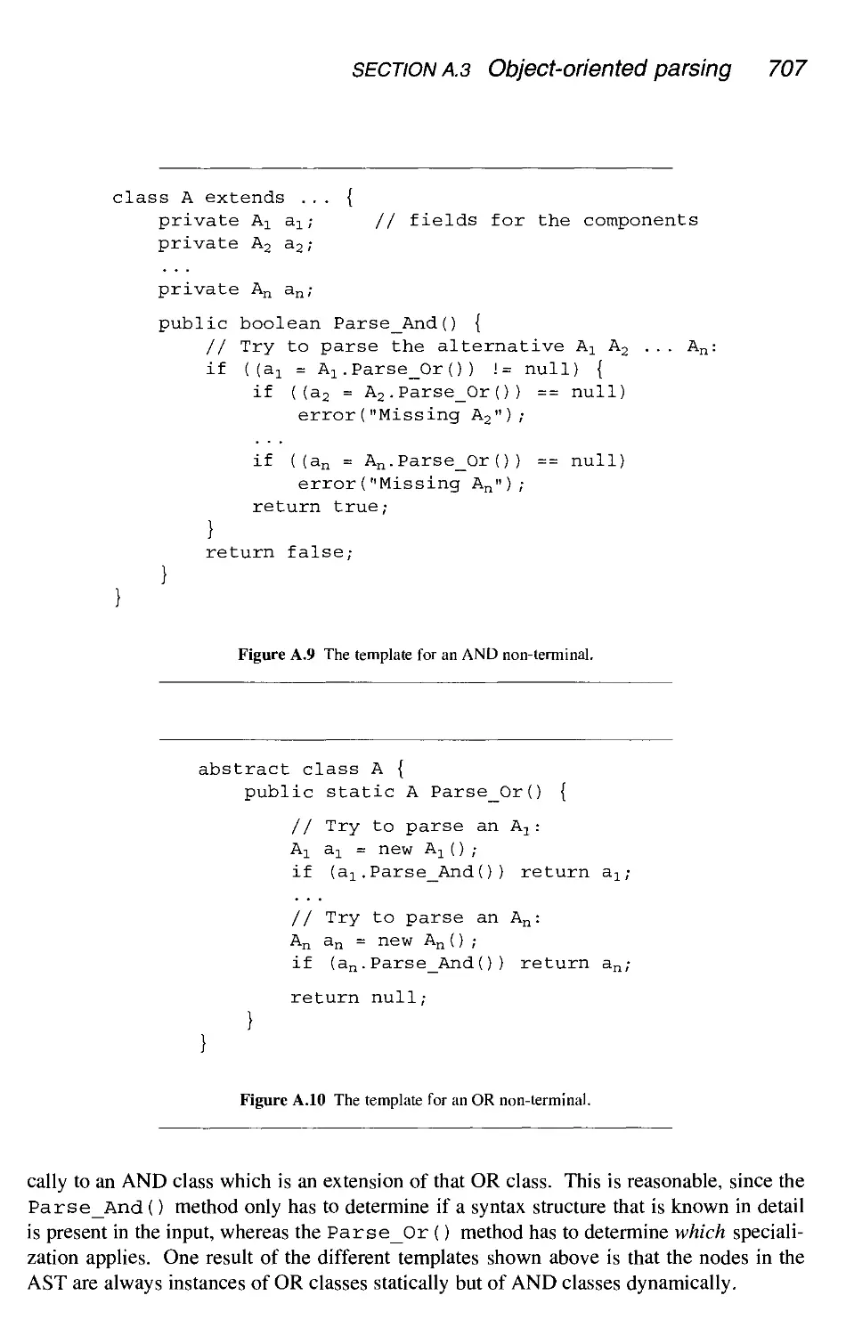
A. 1 Syntax-determined classes and semantics-determining methods 699
A.2 The simple object-oriented compiler 701
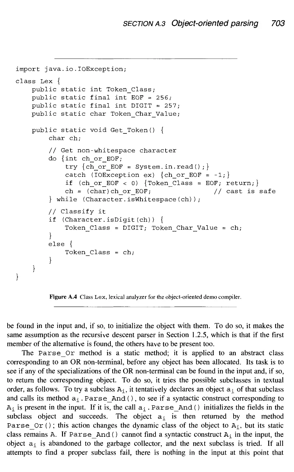
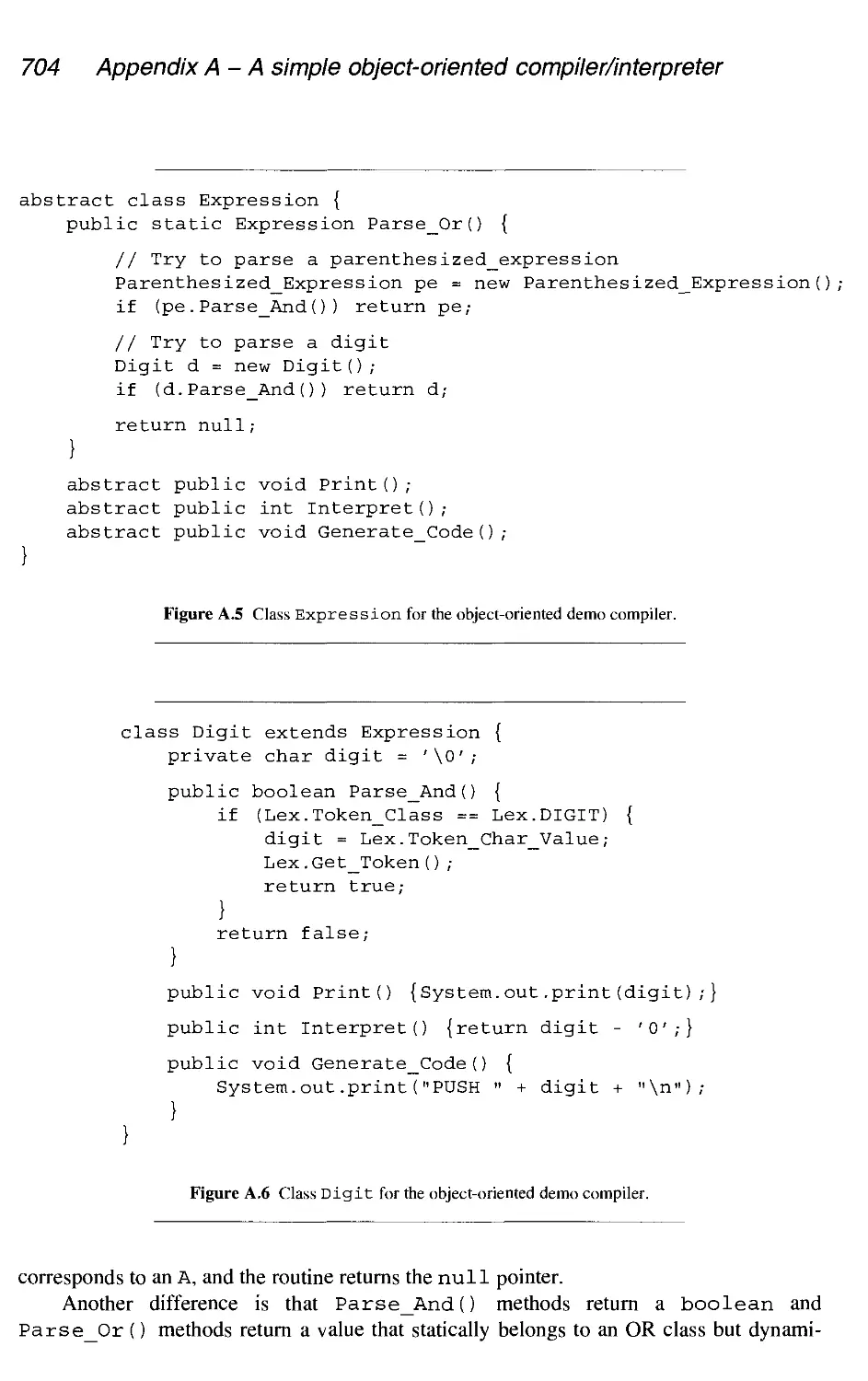
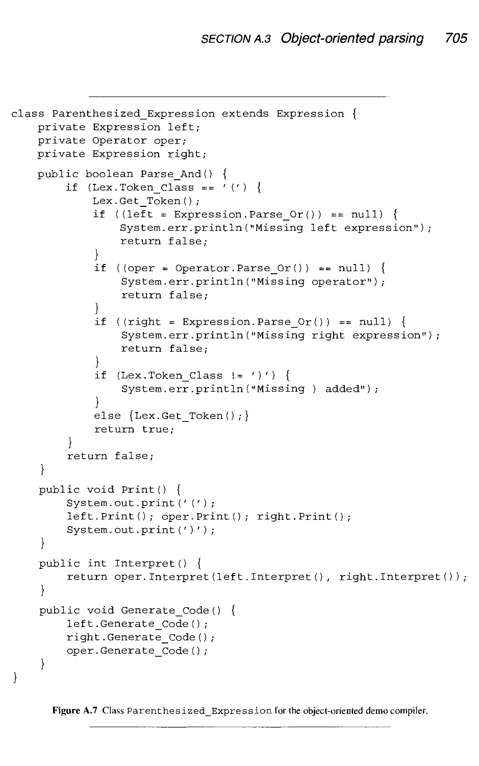
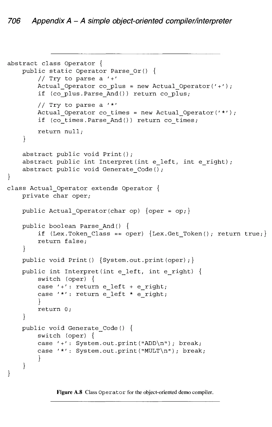
A.3 Object-oriented parsing 702
A.4 Evaluation 708
Exercise 708
Answers to exercises 709
References 720
Index 728
Preface
In the 1980s and 1990s, while the world was witnessing the rise of the PC and the Internet
on the front pages of the daily newspapers, compiler design methods developed with less
fanfare, developments seen mainly in the technical journals, and - more importantly - in
the compilers that are used to process today's software. These developments were driven
partly by the advent of new programming paradigms, partly by a better understanding of
code generation techniques, and partly by the introduction of faster machines with large
amounts of memory.
The field of programming languages has grown to include, besides the traditional
imperative paradigm, the object-oriented, functional, logical, and parallel/distributed
paradigms, which inspire novel compilation techniques and which often require more
extensive run-time systems than do imperative languages. BURS techniques (Bottom-Up
Rewriting Systems) have evolved into very powerful code generation techniques which
cope superbly with the complex machine instruction sets of present-day machines. And
the speed and memory size of modern machines allow compilation techniques and
programming language features that were unthinkable before. Modern compiler design
methods meet these challenges head-on.
The audience
Our audience are mature students in one of their final years, who have at least used a com-
compiler occasionally and given some thought to the concept of compilation. When these stu-
students leave the university, they will have to be familiar with language processors for each
of the modern paradigms, using modern techniques. Although curriculum requirements in
many universities may have been lagging behind in this respect, graduates entering the job
market cannot afford to ignore these developments.
Experience has shown us that a considerable number of techniques traditionally taught
XIII
xiv Preface
in compiler construction are special cases of more fundamental techniques. Often these
special techniques work for imperative languages only; the fundamental techniques have a
much wider application. An example is the stack as an optimized representation for activa-
activation records in strictly last-in-first-out languages. Therefore, this book
- focuses on principles and techniques of wide application, carefully distinguishing
between the essential (= material that has a high chance of being useful to the student)
and the incidental (= material that will benefit the student only in exceptional cases);
- provides a first level of implementation details and optimizations;
- augments the explanations by pointers for further study.
The student, after having finished the book, can expect to:
- have obtained a thorough understanding of the concepts of modern compiler design and
construction, and some familiarity with their practical application;
- be able to start participating in the construction of a language processor for each of the
modern paradigms with a minimal training period;
- be able to read the literature.
The first two provide a firm basis; the third provides potential for growth.
The structure of the book
This book is conceptually divided into two parts. The first, comprising Chapters 1 through
5, is concerned with techniques for program processing in general; it includes a chapter on
memory management, both in the compiler and in the generated code. The second part,
Chapters 6 through 9, covers the specific techniques required by the various programming
paradigms. The interactions between the parts of the book are outlined in the table on the
next page.
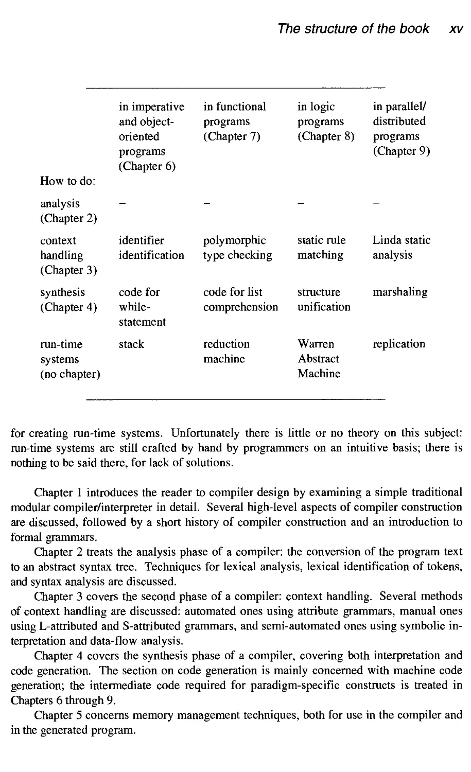
The leftmost column shows the four phases of compiler construction: analysis, con-
context handling, synthesis, and run-time systems. Chapters in this column cover both the
manual and the automatic creation of the pertinent software but tend to emphasize au-
automatic generation. The other columns show the four paradigms covered in this book; for
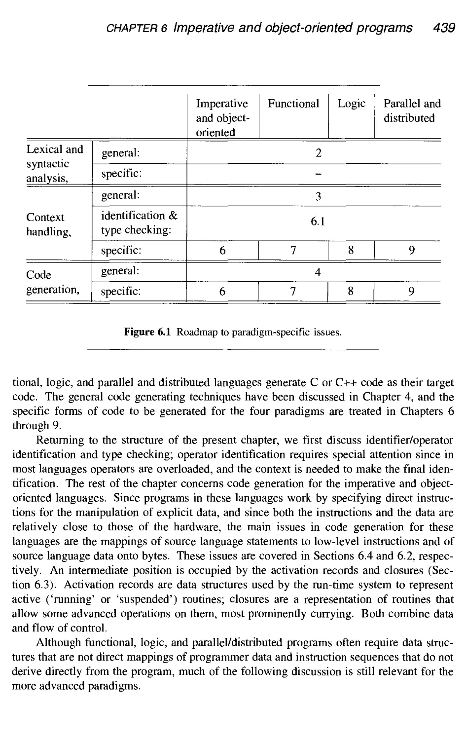
each paradigm an example of a subject treated by each of the phases is shown. These
chapters tend to contain manual techniques only, all automatic techniques having been
delegated to Chapters 2 through 4.
The scientific mind would like the table to be nice and square, with all boxes filled -
in short 'orthogonal' - but we see that the top right entries are missing and that there is no
chapter for 'run-time systems' in the leftmost column. The top right entries would cover
such things as the special subjects in the text analysis of logic languages, but present text
analysis techniques are powerful and flexible enough - and languages similar enough - to
handle all language paradigms: there is nothing to be said there, for lack of problems. The
chapter missing from the leftmost column would discuss manual and automatic techniques
The structure of the book xv
How to do:
analysis
(Chapter 2)
context
handling
(Chapter 3)
synthesis
(Chapter 4)
run-time
systems
(no chapter)
in imperative
and object-
oriented
programs
(Chapter 6)
—
identifier
identification
code for
while-
statement
stack
in functional
programs
(Chapter 7)
polymorphic
type checking
code for list
comprehension
reduction
machine
in logic
programs
(Chapter 8)
—
static rule
matching
structure
unification
Warren
Abstract
Machine
in parallel/
distributed
programs
(Chapter 9)
—
Linda static
analysis
marshaling
replication
for creating run-time systems. Unfortunately there is little or no theory on this subject:
run-time systems are still crafted by hand by programmers on an intuitive basis; there is
nothing to be said there, for lack of solutions.
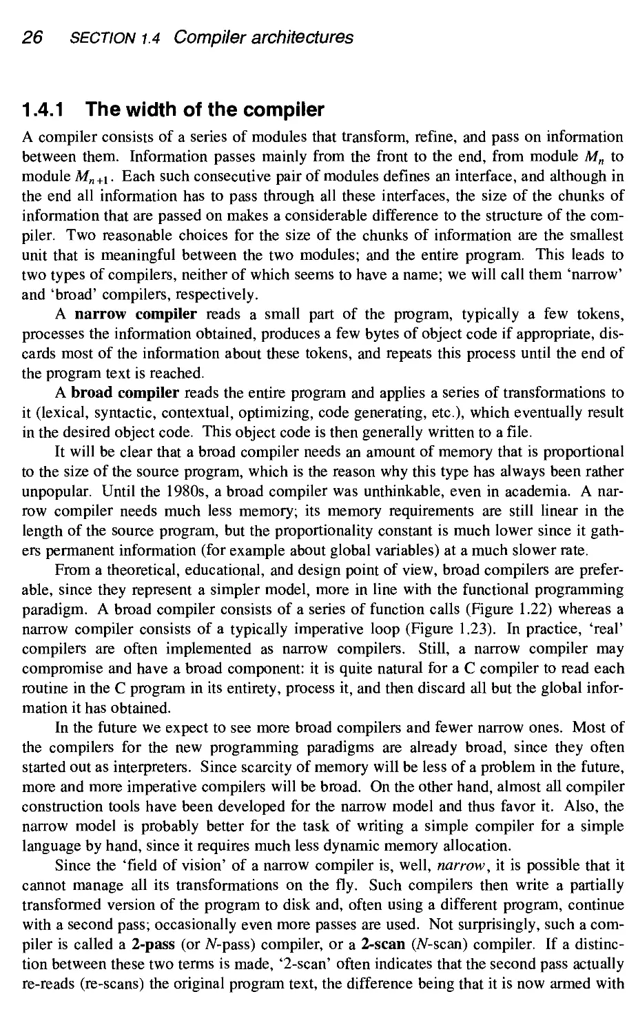
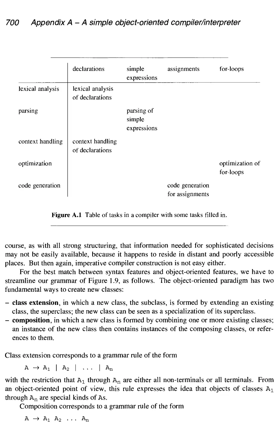
Chapter 1 introduces the reader to compiler design by examining a simple traditional
modular compiler/interpreter in detail. Several high-level aspects of compiler construction
are discussed, followed by a short history of compiler construction and an introduction to
formal grammars.
Chapter 2 treats the analysis phase of a compiler: the conversion of the program text
to an abstract syntax tree. Techniques for lexical analysis, lexical identification of tokens,
and syntax analysis are discussed.
Chapter 3 covers the second phase of a compiler: context handling. Several methods
of context handling are discussed: automated ones using attribute grammars, manual ones
using L-attributed and S-attributed grammars, and semi-automated ones using symbolic in-
interpretation and data-flow analysis.
Chapter 4 covers the synthesis phase of a compiler, covering both interpretation and
code generation. The section on code generation is mainly concerned with machine code
generation; the intermediate code required for paradigm-specific constructs is treated in
Chapters 6 through 9.
Chapter 5 concerns memory management techniques, both for use in the compiler and
in the generated program.
xvi Preface
Chapters 6 through 9 address the special problems in compiling for the various para-
paradigms - imperative, object-oriented, functional, logic, and parallel/distributed. Compilers
for imperative and object-oriented programs are similar enough to be treated together in
one chapter, Chapter 6.
Appendix A discusses a possible but experimental method of object-oriented compiler
construction, in which an attempt is made to exploit object-oriented concepts to simplify
compiler design.
Several subjects in this book are treated in a non-traditional way, and some words of
justification may be in order.
Lexical analysis is based on the same dotted items that are traditionally reserved for
bottom-up syntax analysis, rather than on Thompson's NFA construction. We see the dot-
dotted item as the essential tool in bottom-up pattern matching, unifying lexical analysis, LR
syntax analysis, and bottom-up code generation. The traditional lexical algorithms are just
low-level implementations of item manipulation. We consider the different treatment of
lexical and syntax analysis to be a historical artifact. Also, the difference between the lexi-
lexical and the syntax levels tends to disappear in modern software.
Considerable attention is being paid to attribute grammars, in spite of the fact that
their impact on compiler design has been limited. Still, they are the only known way of au-
automating context handling, and we hope that the present treatment will help to lower the
threshold of their application.
Functions as first-class data are covered in much greater depth in this book than is
usual in compiler design books. After a good start in Algol 60, functions lost much status
as manipulatable data in languages like C, Pascal, and Ada, although Ada 95 rehabilitated
them somewhat. The implementation of some modern concepts, for example functional
and logic languages, iterators, and continuations, however, requires functions to be mani-
manipulated as normal data. The fundamental aspects of the implementation are covered in the
chapter on imperative and object-oriented languages; specifics are given in the chapters on
the various other paradigms.
An attempt at justifying the outline code used in this book to specify algorithms can
be found in Section 1.11.
Additional material, including more answers to exercises, and all diagrams and all
code from the book, are available through John Wiley's Web page.
Use as a course book
The book contains far too much material for a compiler design course of 13 lectures of two
hours each, as given at our university, so a selection has to be made. Depending on the
maturity of the audience, an introductory, more traditional course can be obtained by
including, for example,
Acknowledgments xvii
Chapter 1;
Chapter 2 up to 2.1.7; 2.1.10; 2.1.11; 2.2 up to 2.2.4.5; 2.2.5 up to 2.2.5.7;
Chapter 3 up to 3.1.2; 3.1.7 up to 3.1.10; 3.2 up to 3.2.2.2; 3.2.3;
Chapter 4 up to 4.1; 4.2 up to 4.2.4.3; 4.2.6 up to 4.2.6.4; 4.2.11;
Chapter 5 up to 5.1.1.1; 5.2 up to 5.2.4;
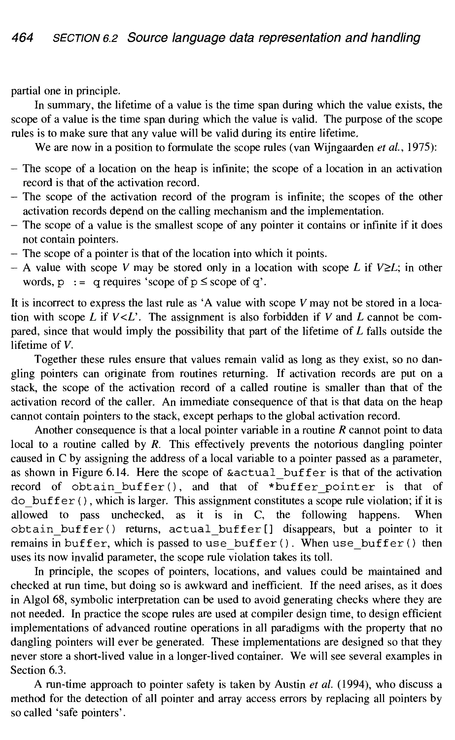
Chapter 6 up to 6.2.3.2; 6.2.4 up to 6.2.10; 6.4 up to 6.4.2.3.
A more advanced course would include all of Chapters 1 to 6, excluding Section 3.1.
This could be augmented by one of Chapters 7 to 9 and perhaps Appendix A.
An advanced course would skip much of the introductory material and concentrate on
the parts omitted in the introductory course: Section 3.1 and all of Chapters 5 to 9, plus
Appendix A.
Acknowledgments
We owe many thanks to the following people, who were willing to spend time and effort
on reading drafts of our book and to supply us with many useful and sometimes very
detailed comments: Mirjam Bakker, Raoul Bhoedjang, Wilfred Dittmer, Thomer M. Gil,
Ben N. Hasnai, Bert Huijben, Jaco A. Imthorn, John Romein, Tim Riihl, and the
anonymous reviewers. We thank Ronald Veldema for the Pentium code segments.
We are grateful to Simon Plumtree, Gaynor Redvers-Mutton, Dawn Booth, and Jane
Kerr of John Wiley & Sons Ltd, for their help and encouragement in writing this book.
Lambert Meertens kindly provided information on an older ABC compiler, and Ralph
Griswold on an Icon compiler.
We thank the Faculteit Wiskunde en Informatica (now part of the Faculteit der Exacte
Wetenschappen) of the Vrije Universiteit for their support and the use of their equipment.
Dick Grune dickecs.vu.nl, http://www.cs.vu.nl/~dick
Henri E. Bal bal@cs.vu.nl, http://www.cs.vu.nl/~bal
Ceriel J.H. Jacobs ceriel@cs.vu.nl, http://www.cs.vu.nl/~ceriel
Koen G. Langendoen koeniapds . twi . tudelf t. nl, http: //pds . twi . tudelft.nl/~koen
Amsterdam, May 2000
Trademark notice
Java™ is a trademark of Sun Microsystems
Miranda™ is a trademark of Research Software Ltd
MS-DOS™ is a trademark of Microsoft Corporation
Pentium™ is a trademark of Intel
PostScript™ is a trademark of Adobe Systems Inc
Smalltalk™ is a trademark of Xerox Corporation
UNIX™ is a trademark of AT&T
XVIII
1
Introduction
In its most general form, a compiler is a program that accepts as input a program text in a
certain language and produces as output a program text in another language, while
preserving the meaning of that text. This process is called translation, as it would be if the
texts were in natural languages. Almost all compilers translate from one input language,
the source language, to one output language, the target language, only. One normally
expects the source and target language to differ greatly: the source language could be C
and the target language might be machine code for the Pentium processor series. The
language the compiler itself is written in is called the implementation language.
The main reason why one wants such a translation is that one has hardware on which
one can 'run' the translated program, or more precisely: have the hardware perform the
actions described by the semantics of the program. After all, hardware is the only real
source of computing power. Running a translated program often involves feeding it input
data in some format, and will probably result in some output data in some other format.
The input data can derive from a variety of sources; examples are files, keystrokes, and
network packages. Likewise, the output can go to a variety of places; examples are files,
monitor screens, and printers.
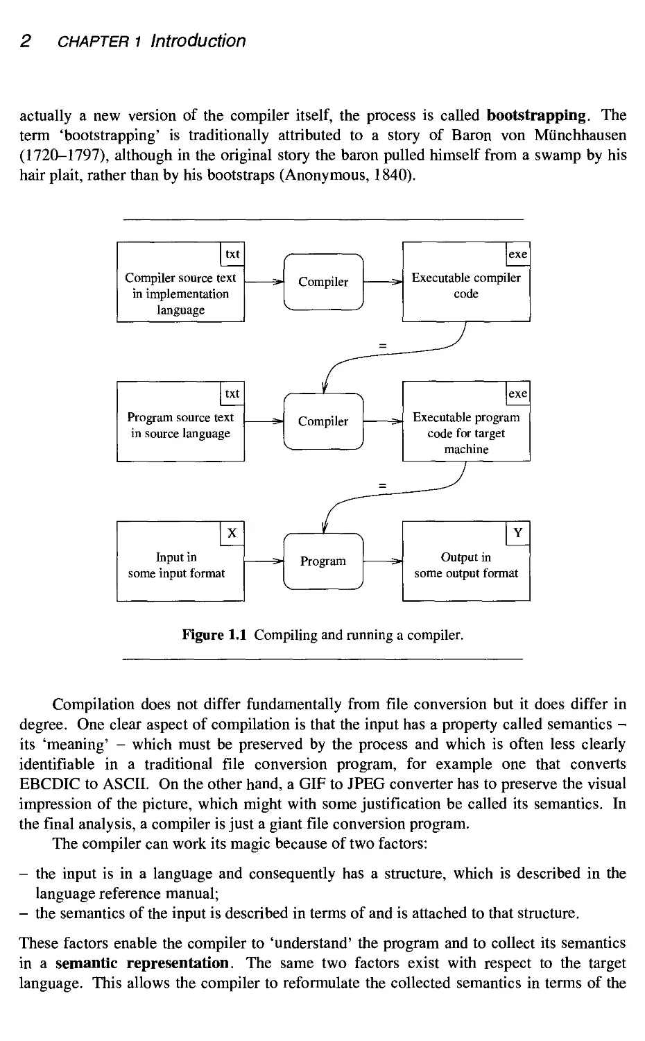
To obtain the translated program, we run a compiler, which is just another program
whose input data is a file with the format of a program source text and whose output data is
a file with the format of executable code. A subtle point here is that the file containing the
executable code is (almost) tacitly converted to a runnable program; on some operating
systems this requires some action, for example setting the 'execute' attribute.
To obtain the compiler, we run another compiler whose input consists of compiler
source text and which will produce executable code for it, as it would for any program
source text. This process of compiling and running a compiler is depicted in Figure 1.1;
that compilers can and do compile compilers sounds more confusing than it is. When the
source language is also the implementation language and the source text to be compiled is
chapter 1 Introduction
actually a new version of the compiler itself, the process is called bootstrapping. The
term 'bootstrapping' is traditionally attributed to a story of Baron von Miinchhausen
A720-1797), although in the original story the baron pulled himself from a swamp by his
hair plait, rather than by his bootstraps (Anonymous, 1840).
txt
Compiler source text
in implementation
language
Executable compiler
code
txt
Program source text
in source language
Compiler
Executable program
code for target
machine
X
Input in
some input format
Program
Output in
some output format
Figure 1.1 Compiling and running a compiler.
Compilation does not differ fundamentally from file conversion but it does differ in
degree. One clear aspect of compilation is that the input has a property called semantics -
its 'meaning' - which must be preserved by the process and which is often less clearly
identifiable in a traditional file conversion program, for example one that converts
EBCDIC to ASCII. On the other hand, a GIF to JPEG converter has to preserve the visual
impression of the picture, which might with some justification be called its semantics. In
the final analysis, a compiler is just a giant file conversion program.
The compiler can work its magic because of two factors:
- the input is in a language and consequently has a structure, which is described in the
language reference manual;
- the semantics of the input is described in terms of and is attached to that structure.
These factors enable the compiler to 'understand' the program and to collect its semantics
in a semantic representation. The same two factors exist with respect to the target
language. This allows the compiler to reformulate the collected semantics in terms of the
chapter 1 Introduction 3
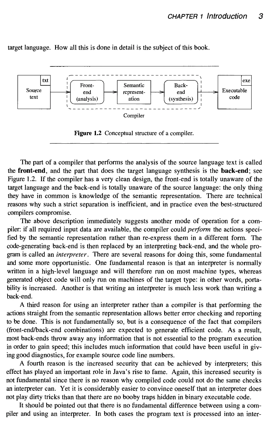
target language. How all this is done in detail is the subject of this book.
Source
text
txt
Front-
end
(analysis)
Semantic
represent-
representation
Back-
Backend
(synthesis)
Executal
code
exe
lie
Compiler
Figure 1.2 Conceptual structure of a compiler.
The part of a compiler that performs the analysis of the source language text is called
the front-end, and the part that does the target language synthesis is the back-end; see
Figure 1.2. If the compiler has a very clean design, the front-end is totally unaware of the
target language and the back-end is totally unaware of the source language: the only thing
they have in common is knowledge of the semantic representation. There are technical
reasons why such a strict separation is inefficient, and in practice even the best-structured
compilers compromise.
The above description immediately suggests another mode of operation for a com-
compiler: if all required input data are available, the compiler could perform the actions speci-
specified by the semantic representation rather than re-express them in a different form. The
code-generating back-end is then replaced by an interpreting back-end, and the whole pro-
program is called an interpreter. There are several reasons for doing this, some fundamental
and some more opportunistic. One fundamental reason is that an interpreter is normally
written in a high-level language and will therefore run on most machine types, whereas
generated object code will only run on machines of the target type: in other words, porta-
portability is increased. Another is that writing an interpreter is much less work than writing a
back-end.
A third reason for using an interpreter rather than a compiler is that performing the
actions straight from the semantic representation allows better error checking and reporting
to be done. This is not fundamentally so, but is a consequence of the fact that compilers
(front-end/back-end combinations) are expected to generate efficient code. As a result,
most back-ends throw away any information that is not essential to the program execution
in order to gain speed; this includes much information that could have been useful in giv-
giving good diagnostics, for example source code line numbers.
A fourth reason is the increased security that can be achieved by interpreters; this
effect has played an important role in Java's rise to fame. Again, this increased security is
not fundamental since there is no reason why compiled code could not do the same checks
an interpreter can. Yet it is considerably easier to convince oneself that an interpreter does
not play dirty tricks than that there are no booby traps hidden in binary executable code.
It should be pointed out that there is no fundamental difference between using a com-
compiler and using an interpreter. In both cases the program text is processed into an inter-
4 chapter 1 Introduction
Why is a compiler called a compiler?
The original meaning of 'to compile' is 'to select representative material
and add it to a collection'; present-day makers of compilation compact
discs use the term in its proper meaning. In its early days programming
language translation was viewed in the same way: when the input con-
contained for example 'a + b', a prefabricated code fragment 'load a in
register; add b to register' was selected and added to the output. A com-
compiler compiled a list of code fragments to be added to the translated pro-
program. Today's compilers, especially those for the non-imperative pro-
programming paradigms, often perform much more radical transformations
on the input program.
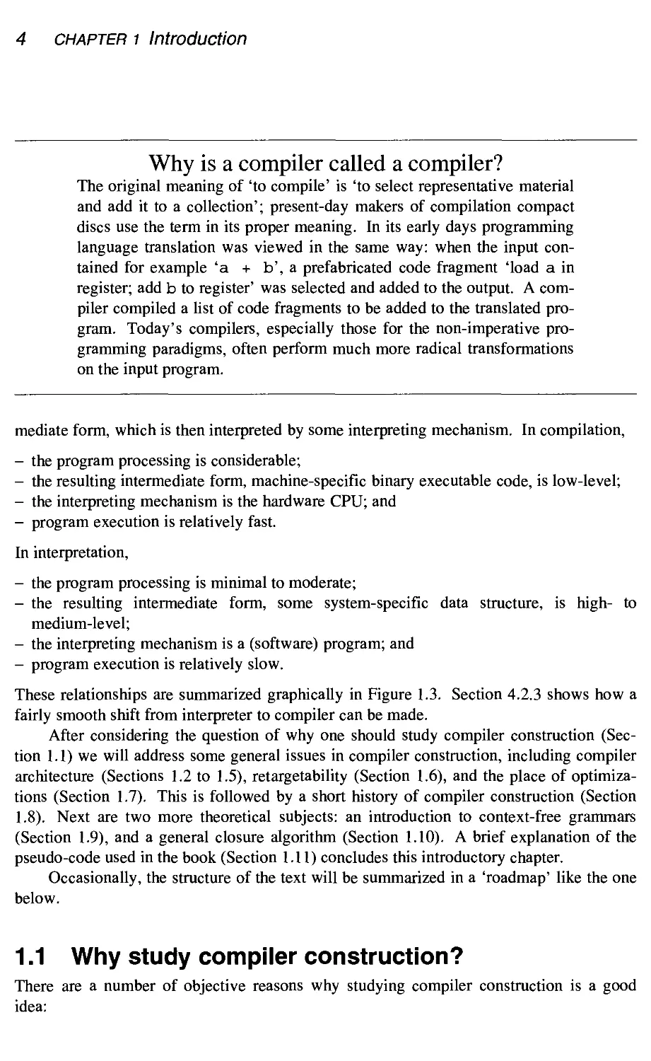
mediate form, which is then interpreted by some interpreting mechanism. In compilation,
- the program processing is considerable;
- the resulting intermediate form, machine-specific binary executable code, is low-level;
- the interpreting mechanism is the hardware CPU; and
- program execution is relatively fast.
In interpretation,
- the program processing is minimal to moderate;
- the resulting intermediate form, some system-specific data structure, is high- to
medium-level;
- the interpreting mechanism is a (software) program; and
- program execution is relatively slow.
These relationships are summarized graphically in Figure 1.3. Section 4.2.3 shows how a
fairly smooth shift from interpreter to compiler can be made.
After considering the question of why one should study compiler construction (Sec-
(Section 1.1) we will address some general issues in compiler construction, including compiler
architecture (Sections 1.2 to 1.5), retargetability (Section 1.6), and the place of optimiza-
optimizations (Section 1.7). This is followed by a short history of compiler construction (Section
1.8). Next are two more theoretical subjects: an introduction to context-free grammars
(Section 1.9), and a general closure algorithm (Section 1.10). A brief explanation of the
pseudo-code used in the book (Section 1.11) concludes this introductory chapter.
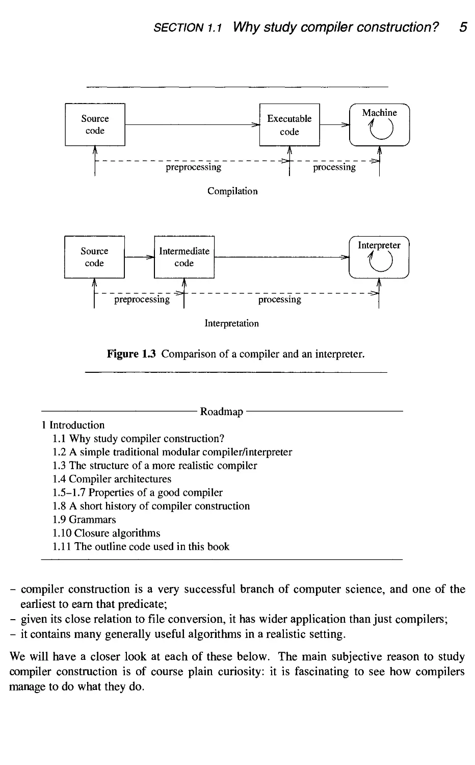
Occasionally, the structure of the text will be summarized in a 'roadmap' like the one
below.
1.1 Why study compiler construction?
There are a number of objective reasons why studying compiler construction is a good
idea:
section 1.1 Why study compiler construction? 5
Sou
CO
I
rce
de
preprocessing
Executable
code
I
Machine
u
processing "|
Compilation
Source
code
Intermediate
code
preprocessing processing
Interpretation
Figure 1.3 Comparison of a compiler and an interpreter.
Roadmap
1 Introduction
1.1 Why study compiler construction?
1.2 A simple traditional modular compiler/interpreter
1.3 The structure of a more realistic compiler
1.4 Compiler architectures
1.5-1.7 Properties of a good compiler
1.8 A short history of compiler construction
1.9 Grammars
1.10 Closure algorithms
1.11 The outline code used in this book
- compiler construction is a very successful branch of computer science, and one of the
earliest to earn that predicate;
- given its close relation to file conversion, it has wider application than just compilers;
- it contains many generally useful algorithms in a realistic setting.
We will have a closer look at each of these below. The main subjective reason to study
compiler construction is of course plain curiosity: it is fascinating to see how compilers
manage to do what they do.
6 section 1.1 Why study compiler construction?
1.1.1 Compiler construction is very successful
Compiler construction is a very successful branch of computer science. Some of the rea-
reasons for this are the proper structuring of the problem, the judicious use of formalisms, and
the use of tools wherever possible.
1.1.1.1 Proper structuring of the problem
Compilers analyze'their input, construct a semantic representation, and synthesize their
output from it. This analysis-synthesis paradigm is very powerful and widely applicable.
A program for tallying word lengths in a text could for example consist of a front-end
which analyzes the text and constructs internally a table of (length, frequency) pairs, and a
back-end which then prints this table. Extending this program, one could replace the text-
analyzing front-end by a module that collects file sizes in a file system; alternatively, or
additionally, one could replace the back-end by a module that produces a bar graph rather
than a printed table; we use the word 'module' here to emphasize the exchangeability of
the parts. In total, four programs have already resulted, all centered around the semantic
representation and each reusing lots of code from the others.
Likewise, without the strict separation of analysis and synthesis phases, programming
languages and compiler construction would not be where they are today. Without it, each
new language would require a completely new set of compilers for all interesting machines
- or die for lack of support. With it, a new front-end for that language suffices, to be com-
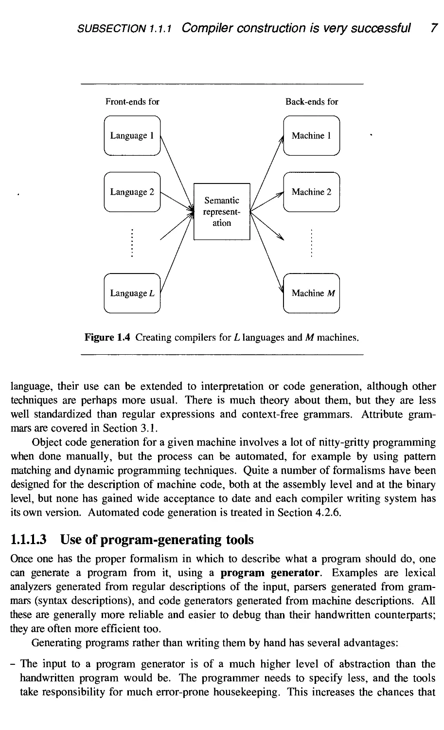
combined with the existing back-ends for the current machines: for L languages and M
machines, L front-ends and M back-ends are needed, requiring L+M modules, rather than
LxM programs. See Figure 1.4.
It should be noted immediately, however, that this strict separation is not completely
free of charge. If, for example, a front-end knows it is analyzing for a machine with spe-
special machine instructions for multi-way jumps, it can probably analyze case/switch state-
statements so that they can benefit from these machine instructions. Similarly, if a back-end
knows it is generating code for a language which has no nested routine declarations, it can
generate simpler code for routine calls. Many professional compilers are integrated com-
compilers, for one programming language and one machine architecture, using a semantic
representation which derives from the source language and which may already contain ele-
elements of the target machine. Still, the structuring has played and still plays a large role in
tiie rapid introduction of new languages and new machines.
1.1.1.2 Judicious use of formalisms
For some parts of compiler construction excellent standardized formalisms have been
developed, which greatly reduce the effort to produce these parts. The best examples are
regular expressions and context-free grammars, used in lexical and syntactic analysis.
Enough theory about these has been developed from the 1960s onwards to fill an entire
course, but the practical aspects can be taught and understood without going too deeply
into the theory. We will consider these formalisms and their applications in Chapter 2.
Attribute grammars are a formalism that can be used for handling the context, the
long-distance relations in a program that link, for example, the use of a variable to its
declaration. Since attribute grammars are capable of describing the full semantics of a
subsection 1.1.1 Compiler construction is very successful
Front-ends for
Back-ends for
Language 1
Language 2
Machine 1
Language L
Semantic
represent-
representation
Machine 2
Machine M
Figure 1.4 Creating compilers for L languages and M machines.
language, their use can be extended to interpretation or code generation, although other
techniques are perhaps more usual. There is much theory about them, but they are less
well standardized than regular expressions and context-free grammars. Attribute gram-
grammars are covered in Section 3.1.
Object code generation for a given machine involves a lot of nitty-gritty programming
when done manually, but the process can be automated, for example by using pattern
matching and dynamic programming techniques. Quite a number of formalisms have been
designed for the description of machine code, both at the assembly level and at the binary
level, but none has gained wide acceptance to date and each compiler writing system has
its own version. Automated code generation is treated in Section 4.2.6.
1.1.1.3 Use of program-generating tools
Once one has the proper formalism in which to describe what a program should do, one
can generate a program from it, using a program generator. Examples are lexical
analyzers generated from regular descriptions of the input, parsers generated from gram-
grammars (syntax descriptions), and code generators generated from machine descriptions. All
these are generally more reliable and easier to debug than their handwritten counterparts;
they are often more efficient too.
Generating programs rather than writing them by hand has several advantages:
- The input to a program generator is of a much higher level of abstraction than the
handwritten program would be. The programmer needs to specify less, and the tools
take responsibility for much error-prone housekeeping. This increases the chances that
8 section 1.1 Why study compiler construction?
the program will be correct. For example, it would be cumbersome to write parse tables
by hand.
- The use of program-generating tools allows increased flexibility and modifiability. For
example, if during the design phase of a language a small change in the syntax is con-
considered, a handwritten parser would be a major stumbling block to any such change.
With a generated parser, one would just change the syntax description and generate a
new parser.
- Pre-canned or tailored code can be added to the generated program, enhancing its power
at hardly any cost. For example, input error handling is usually a difficult affair in
handwritten parsers; a generated parser can include tailored error correction code with
no effort on the part of the programmer.
- A formal description can sometimes be used to generate more than one type of program.
For example, once we have written a grammar for a language with the purpose of gen-
generating a parser from it, we may use it to generate a syntax-directed editor, a special-
purpose program text editor that guides and supports the user in editing programs in that
language.
In summary, generated programs may be slightly more or slightly less efficient than
handwritten ones, but generating them is so much more efficient than writing them by hand
that whenever the possibility exists, generating a program is almost always to be preferred.
The technique of creating compilers by program-generating tools was pioneered by
Brooker et al. A963), and its importance has continually risen since. Programs that gen-
generate parts of a compiler are sometimes called compiler compilers, although this is clearly
a misnomer. Yet, the term lingers on.
1.1.2 Compiler construction has a wide applicability
Compiler construction techniques can be and are applied outside compiler construction in
its strictest sense. Alternatively, more programming can be considered compiler construc-
construction than one would traditionally assume. Examples are reading structured data, rapid
introduction of new formats, and general file conversion problems.
If data has a clear structure it is generally possible to write a grammar for it. Using a
parser generator, a parser can then be generated automatically. Such techniques can, for
example, be applied to rapidly create 'read' routines for HTML files, PostScript files, etc.
This also facilitates the rapid introduction of new formats. Examples of file conversion
systems that have profited considerably from compiler construction techniques are TeX
text formatters, which convert TeX text to dvi format, and PostScript interpreters, which
convert PostScript text to instructions for a specific printer.
1.1.3 Compilers contain generally useful algorithms
A third reason to study compiler construction lies in the generally useful data structures
and algorithms compilers contain. Examples are hashing, precomputed tables, the stack
mechanism, garbage collection, dynamic programming, and graph algorithms. Although
each of these can be studied in isolation, it is educationally more valuable and satisfying to
do so in a meaningful context.
subsection 1.2.1 The abstract syntax tree 9
1.2 A simple traditional modular compiler/interpreter
In this section we will show and discuss a simple demo compiler and interpreter, to intro-
introduce the concepts involved and to set the framework for the rest of the book. Turning to
Figure 1.2, we see that the heart of a compiler is the semantic representation of the pro-
program being compiled. This semantic representation takes the form of a data structure,
called the 'intermediate code' of the compiler. There are many possibilities for the form of
the intermediate code; two usual choices are linked lists of pseudo-instructions and anno-
annotated abstract syntax trees. We will concentrate here on the latter, since the semantics is
primarily attached to the syntax tree.
1.2.1 The abstract syntax tree
The syntax tree of a program text is a data structure which shows precisely how the vari-
various segments of the program text are to be viewed in terms of the grammar. The syntax
tree can be obtained through a process called 'parsing'; in other words, parsing is the pro-
process of structuring a text according to a given grammar. For this reason, syntax trees are
also called parse trees; we will use the terms interchangeably, with a slight preference for
'parse tree' when the emphasis is on the actual parsing. Conversely, parsing is also called
syntax analysis, but this has the problem that there is no corresponding verb 'to syntax-
analyze'. The parser can be written by hand if the grammar is very small and simple; for
larger and/or more complicated grammars it can be generated by a parser generator. Parser
generators are discussed in Chapter 2.
The exact form of the parse tree as required by the grammar is often not the most con-
convenient one for further processing, so usually a modified form of it is used, called an
abstract syntax tree, or AST. Detailed information about the semantics can be attached
to the nodes in this tree through annotations, which are stored in additional data fields in
the nodes; hence the term annotated abstract syntax tree. Since unannotated ASTs are
of limited use, ASTs are always more or less annotated in practice, and the abbreviation
'AST' is used also for annotated ASTs.
Examples of annotations are type information ('this assignment node concerns a
Boolean array assignment') and optimization information ('this expression does not con-
contain a function call'). The first kind is related to the semantics as described in the manual,
and is used, among other things, for context error checking. The second kind is not related
to anything in the manual but may be important for the code generation phase. The annota-
annotations in a node are also called the attributes of that node and since a node represents a
grammar symbol, one also says that the grammar symbol has the corresponding attributes.
It is the task of the context handling module to determine and place the annotations or attri-
attributes.
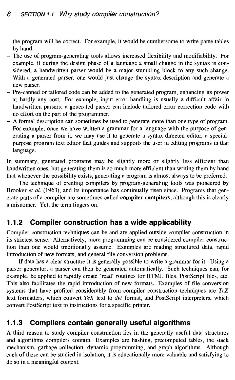
Figure 1.5 shows the expression b*b - 4*a*casa parse tree; the grammar used
for expression is similar to those found in the Pascal, Modula-2, or C manuals:
In linguistic and educational contexts, the verb 'to parse' is also used for the determination of
word classes: determining that in 'to go by' the word 'by' is an adverb and in 'by the way' it is a
preposition. In computer science the word is used exclusively to refer to syntax analysis.
10 section 1.2 A simple traditional modular compiler/interpreter
expression
expression
term
term
factor
term '*' factor term '*' factor identifier
factor identifier factor identifier
' c'
identifier
'b' identifier
' a'
Figure 1.5 The expression b*b - 4 *a*c as a parse tree.
expression —> expression '+' term
term —> term '*' factor | term '/'
factor —> identifier I constant I
| expression '-' term | term
factor | factor
1 (' expression ')'
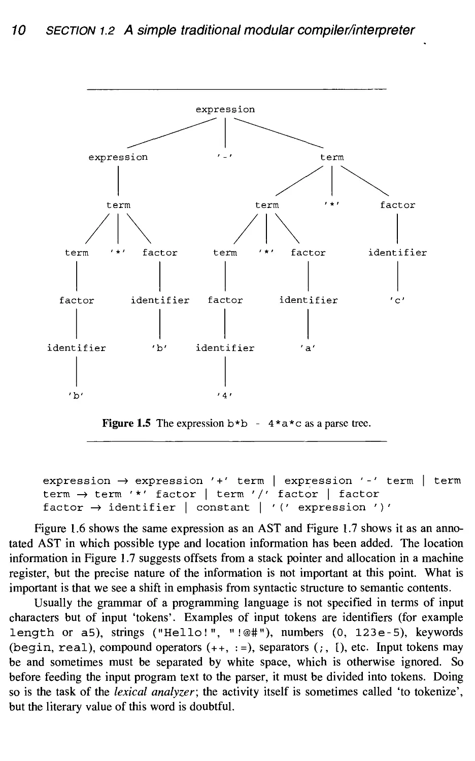
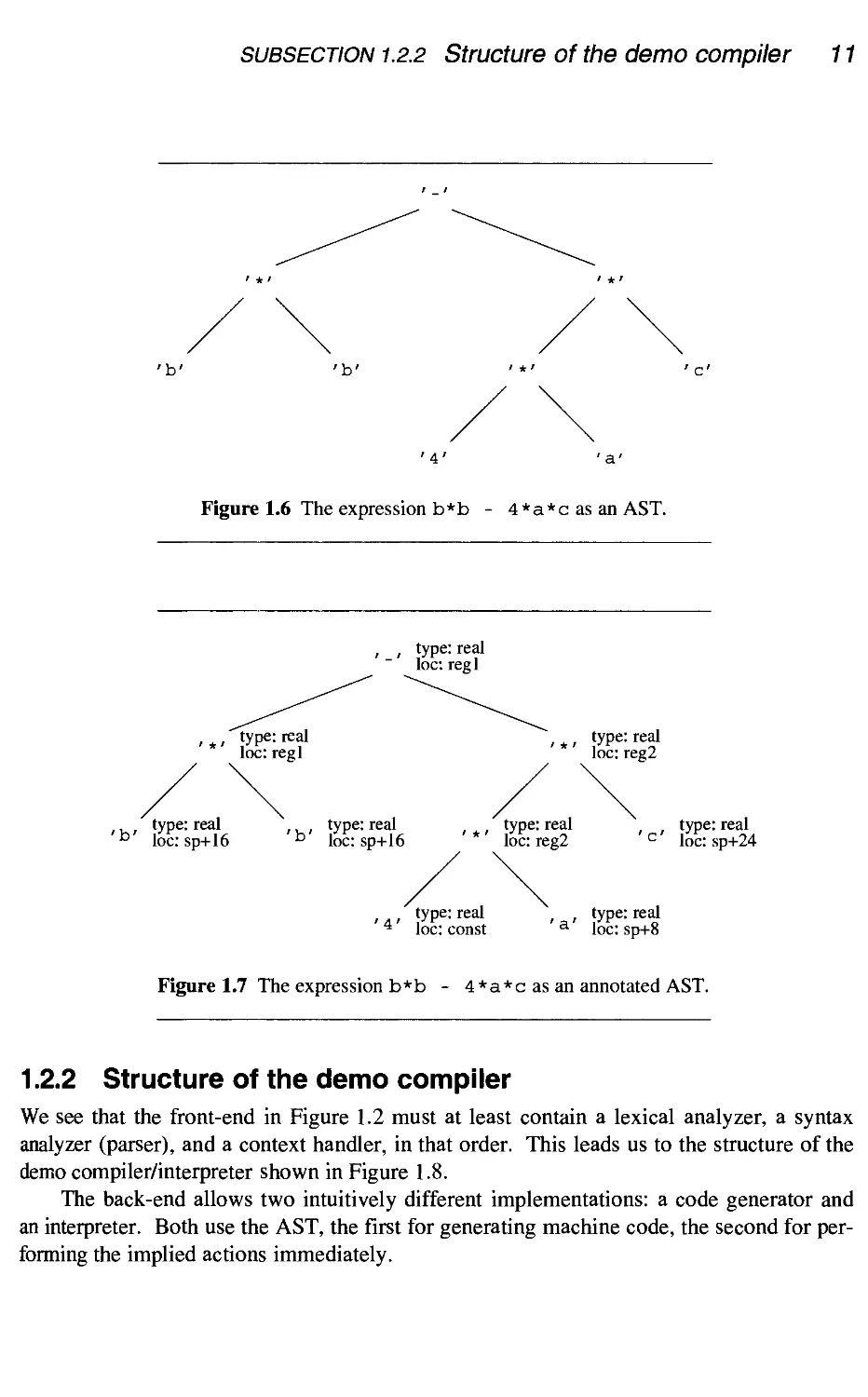
Figure 1.6 shows the same expression as an AST and Figure 1.7 shows it as an anno-
annotated AST in which possible type and location information has been added. The location
information in Figure 1.7 suggests offsets from a stack pointer and allocation in a machine
register, but the precise nature of the information is not important at this point. What is
important is that we see a shift in emphasis from syntactic structure to semantic contents.
Usually the grammar of a programming language is not specified in terms of input
characters but of input 'tokens'. Examples of input tokens are identifiers (for example
length or a5), strings ("Hello!", "!@#"), numbers @, 123e-5), keywords
(begin, real), compound operators (++, :=), separators (;, [), etc. Input tokens may
be and sometimes must be separated by white space, which is otherwise ignored. So
before feeding the input program text to the parser, it must be divided into tokens. Doing
so is the task of the lexical analyzer; the activity itself is sometimes called 'to tokenize',
but the literary value of this word is doubtful.
subsection 1.2.2 Structure of the demo compiler 11
'4'
Figure 1.6 The expression b*b - 4*a*c as an AST.
type: real
loc: regl
tyPe: rea'
loc: sp+16
type: real
loc: regl
type: real
'b' loc: sp+16
type: real
loc: reg2
type: real
loc: reg2
type: real
' c' loc: sp+24
type: real , , type: real
* loc: const a loc: sp+8
Figure 1.7 The expression b*b - 4 *a*c as an annotated AST.
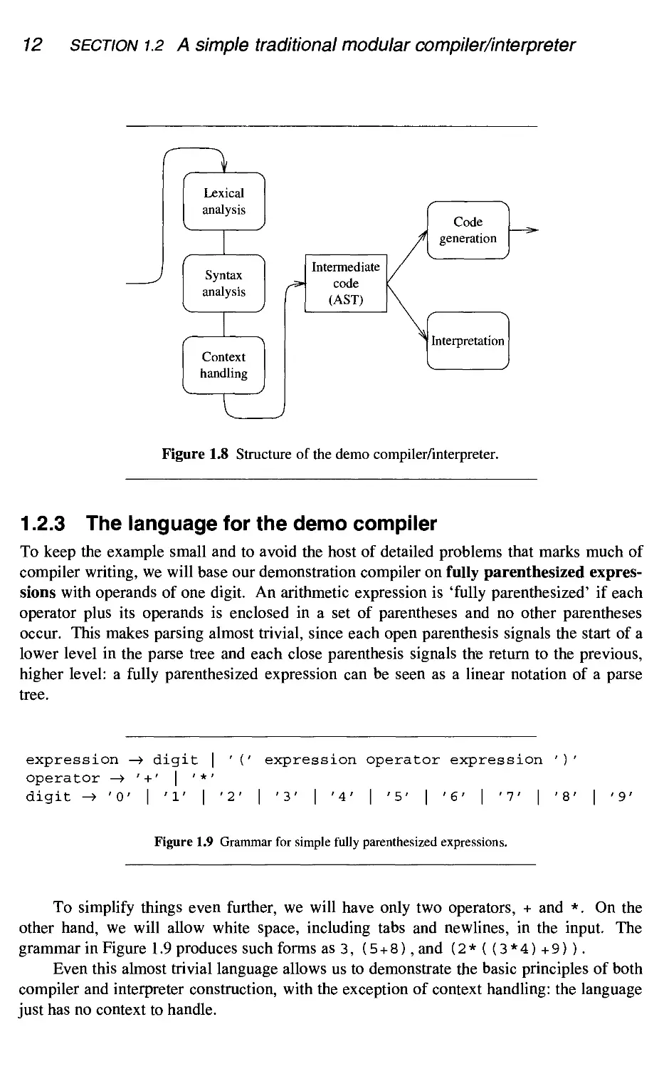
1.2.2 Structure of the demo compiler
We see that the front-end in Figure 1.2 must at least contain a lexical analyzer, a syntax
analyzer (parser), and a context handler, in that order. This leads us to the structure of the
demo compiler/interpreter shown in Figure 1.8.
The back-end allows two intuitively different implementations: a code generator and
an interpreter. Both use the AST, the first for generating machine code, the second for per-
performing the implied actions immediately.
12 section 1.2 A simple traditional modular compiler/interpreter
Lexical
analysis
Syntax
analysis
Context
handling
Intermediate
code
(AST)
Code
generation
Interpretation
Figure 1.8 Structure of the demo compiler/interpreter.
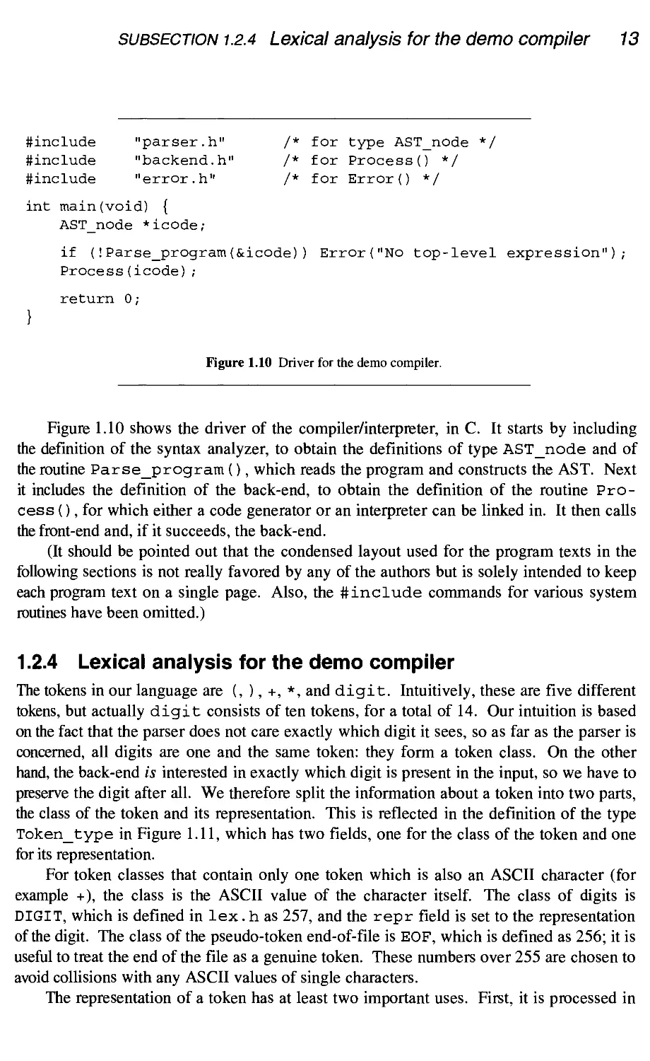
1.2.3 The language for the demo compiler
To keep the example small and to avoid the host of detailed problems that marks much of
compiler writing, we will base our demonstration compiler on fully parenthesized expres-
expressions with operands of one digit. An arithmetic expression is 'fully parenthesized' if each
operator plus its operands is enclosed in a set of parentheses and no other parentheses
occur. This makes parsing almost trivial, since each open parenthesis signals the start of a
lower level in the parse tree and each close parenthesis signals the return to the previous,
higher level: a fully parenthesized expression can be seen as a linear notation of a parse
tree.
expression —> digit | ' (' expression operator expression ')'
operator —» ' +' | ' *'
digit ->'O' | '1' | '2' | '3' | '4' | '5' | '6' | '7' | '8' | '9'
Figure 1.9 Grammar for simple fully parenthesized expressions.
To simplify things even further, we will have only two operators, + and *. On the
other hand, we will allow white space, including tabs and newlines, in the input. The
grammar in Figure 1.9 produces such forms as 3, E + 8), and B*(C*4)+9)).
Even this almost trivial language allows us to demonstrate the basic principles of both
compiler and interpreter construction, with the exception of context handling: the language
just has no context to handle.
subsection 1.2.4 Lexical analysis for the demo compiler 13
#include "parser.h" /* for type AST_node */
#include "backend.h" /* for Process 0 */
#include "error.h" /* for Error() */
int main(void) {
AST_node *icode;
if (!Parse_program(&icode)) Error("No top-level expression"
Process(icode);
return 0;
Figure 1.10 Driver for the demo compiler.
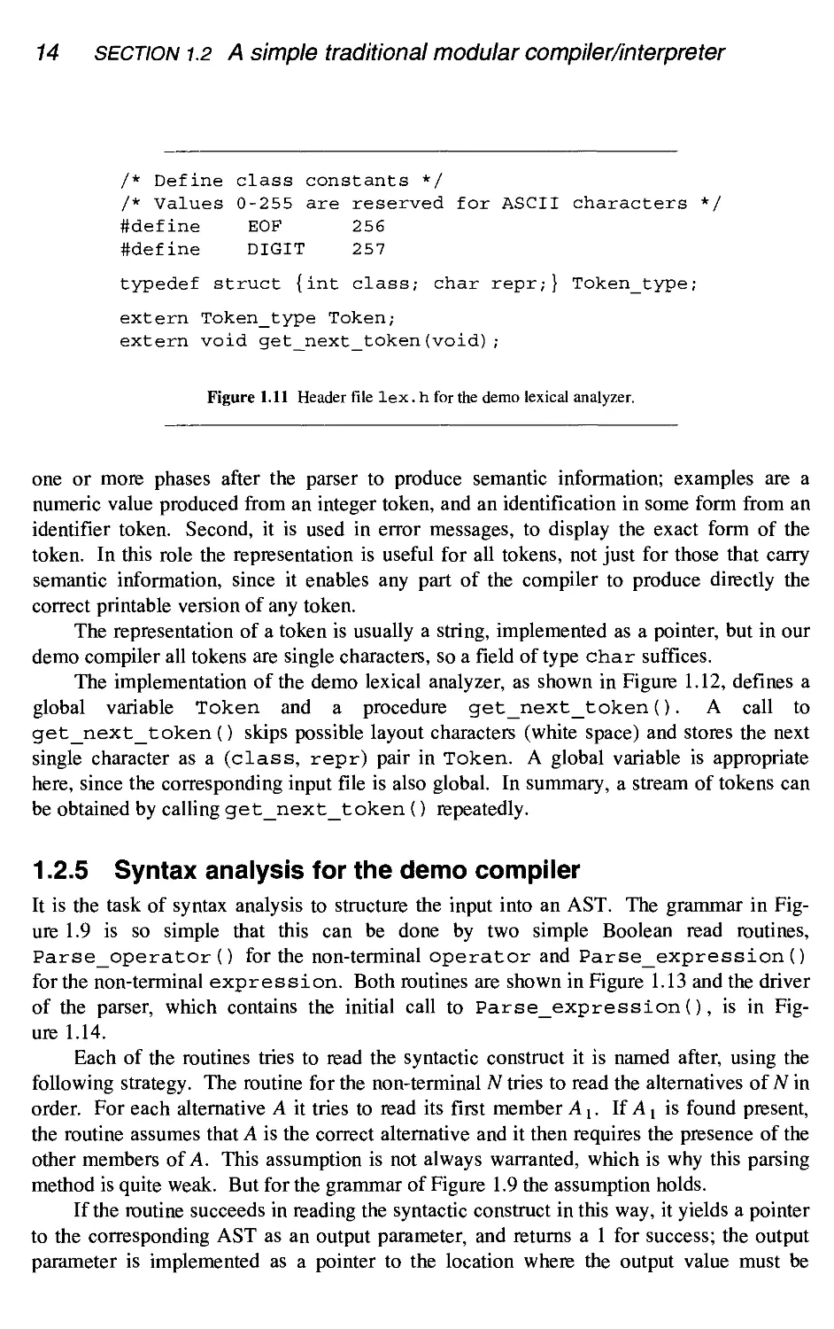
Figure 1.10 shows the driver of the compiler/interpreter, in C. It starts by including
the definition of the syntax analyzer, to obtain the definitions of type AST_node and of
the routine Parse_program (), which reads the program and constructs the AST. Next
it includes the definition of the back-end, to obtain the definition of the routine Pro-
Process (), for which either a code generator or an interpreter can be linked in. It then calls
the front-end and, if it succeeds, the back-end.
(It should be pointed out that the condensed layout used for the program texts in the
following sections is not really favored by any of the authors but is solely intended to keep
each program text on a single page. Also, the #include commands for various system
routines have been omitted.)
1.2.4 Lexical analysis for the demo compiler
The tokens in our language are (,),+,*, and digit. Intuitively, these are five different
tokens, but actually digit consists of ten tokens, for a total of 14. Our intuition is based
on the fact that the parser does not care exactly which digit it sees, so as far as the parser is
concerned, all digits are one and the same token: they form a token class. On the other
hand, the back-end is interested in exactly which digit is present in the input, so we have to
preserve the digit after all. We therefore split the information about a token into two parts,
the class of the token and its representation. This is reflected in the definition of the type
Token_type in Figure 1.11, which has two fields, one for the class of the token and one
for its representation.
For token classes that contain only one token which is also an ASCII character (for
example +), the class is the ASCII value of the character itself. The class of digits is
DIGIT, which is defined in lex. h as 257, and the repr field is set to the representation
of the digit. The class of the pseudo-token end-of-file is EOF, which is defined as 256; it is
useful to treat the end of the file as a genuine token. These numbers over 255 are chosen to
avoid collisions with any ASCII values of single characters.
The representation of a token has at least two important uses. First, it is processed in
14 section 1.2 A simple traditional modular compiler/interpreter
/* Define class constants */
/* Values 0-255 are reserved for ASCII characters */
#define EOF 256
ttdefine DIGIT 257
typedef struct {int class; char repr;} Token_type;
extern Token_type Token;
extern void get_next_token(void);
Figure 1.11 Header file lex. h for the demo lexical analyzer.
one or more phases after the parser to produce semantic information; examples are a
numeric value produced from an integer token, and an identification in some form from an
identifier token. Second, it is used in error messages, to display the exact form of the
token. In this role the representation is useful for all tokens, not just for those that carry
semantic information, since it enables any part of the compiler to produce directly the
correct printable version of any token.
The representation of a token is usually a string, implemented as a pointer, but in our
demo compiler all tokens are single characters, so a field of type char suffices.
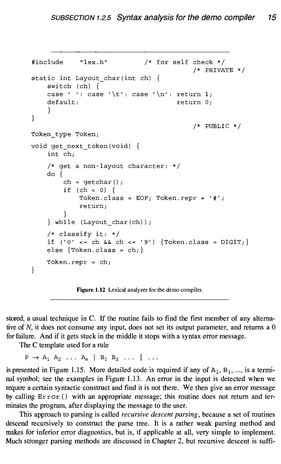
The implementation of the demo lexical analyzer, as shown in Figure 1.12, defines a
global variable Token and a procedure get_next_token (). A call to
get_next_token () skips possible layout characters (white space) and stores the next
single character as a (class, repr) pair in Token. A global variable is appropriate
here, since the corresponding input file is also global. In summary, a stream of tokens can
be obtained by calling get_next_token () repeatedly.
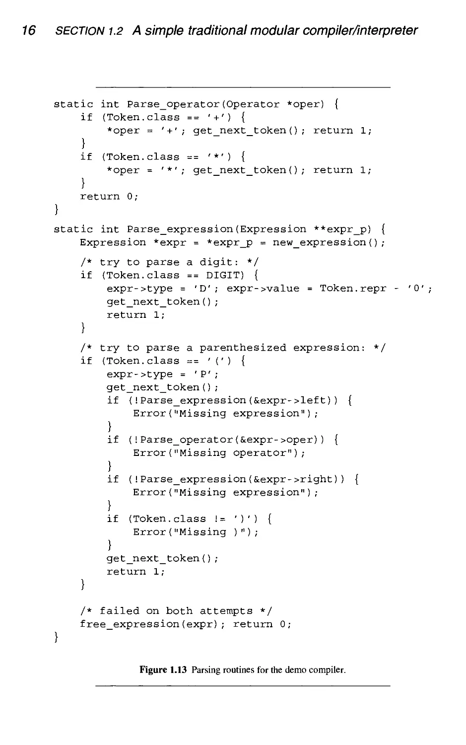
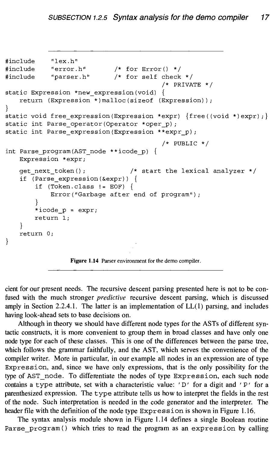
1.2.5 Syntax analysis for the demo compiler
It is the task of syntax analysis to structure the input into an AST. The grammar in Fig-
Figure 1.9 is so simple that this can be done by two simple Boolean read routines,
Parse_operator () for the non-terminal operator and Parse_expression ()
for the non-terminal expression. Both routines are shown in Figure 1.13 and the driver
of the parser, which contains the initial call to Parse_expression(), is in Fig-
Figure 1.14.
Each of the routines tries to read the syntactic construct it is named after, using the
following strategy. The routine for the non-terminal N tries to read the alternatives of N in
order. For each alternative A it tries to read its first member A i. If A [ is found present,
the routine assumes that A is the correct alternative and it then requires the presence of the
other members of A. This assumption is not always warranted, which is why this parsing
method is quite weak. But for the grammar of Figure 1.9 the assumption holds.
If the routine succeeds in reading the syntactic construct in this way, it yields a pointer
to the corresponding AST as an output parameter, and returns a 1 for success; the output
parameter is implemented as a pointer to the location where the output value must be
subsection 1.2.5 Syntax analysis for the demo compiler 15
#include "lex.h" /* for self check */
/* PRIVATE */
static int Layout_char(int ch) {
switch (ch) {
case ' ': case '\t': case '\n': return 1;
default: return 0;
/* PUBLIC */
Token_type Token;
void get_next_token(void) {
int ch;
/* get a non-layout character: */
do {
ch = getchar();
if (ch < 0) {
Token.class = EOF; Token.repr = '#';
return;
}
} while (Layout_char(ch));
/* classify it: */
if CO' <= ch && ch <= '9') {Token.class = DIGIT;}
else {Token.class = ch;}
Token.repr = ch;
Figure 1.12 Lexical analyzer for the demo compiler.
stored, a usual technique in C. If the routine fails to find the first member of any alterna-
alternative of N, it does not consume any input, does not set its output parameter, and returns a 0
for failure. And if it gets stuck in the middle it stops with a syntax error message.
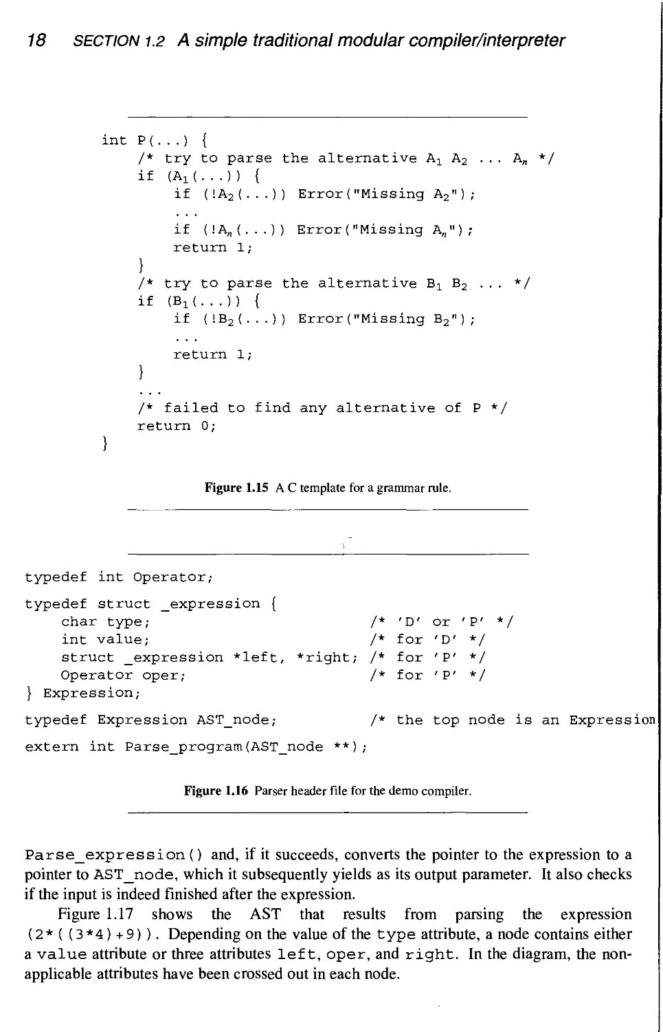
The C template used for a rule
P->AiA2 ... S, | BiBj ... | ...
is presented in Figure 1.15. More detailed code is required if any of Ai? Bi,..., is a termi-
terminal symbol; see the examples in Figure 1.13. An error in the input is detected when we
require a certain syntactic construct and find it is not there. We then give an error message
by calling Error () with an appropriate message; this routine does not return and ter-
terminates the program, after displaying the message to the user.
This approach to parsing is called recursive descent parsing, because a set of routines
descend recursively to construct the parse tree. It is a rather weak parsing method and
makes for inferior error diagnostics, but is, if applicable at all, very simple to implement.
Much stronger parsing methods are discussed in Chapter 2, but recursive descent is suffi-
16 section 1.2 A simple traditional modular compiler/interpreter
static int Parse_operator(Operator *oper) {
if (Token.class == '+') {
*oper = '+'; get_next_token(); return 1;
}
if (Token.class == '*') {
*oper = '*'; get_next_token(); return 1;
}
return 0;
}
static int Parse_expression(Expression **expr_p) {
Expression *expr = *expr_p = new_expression();
/* try to parse a digit: */
if (Token.class == DIGIT) {
expr->type = 'D'; expr->value = Token.repr - '0'
get_next_token();
return 1;
}
/* try to parse a parenthesized expression: */
if (Token.class =='(') {
expr->type = 'P';
get_next_token();
if (!Parse_expression(&expr->left)) {
Error("Missing expression");
}
if (!Parse_operator(&expr->oper)) {
Error("Missing operator");
}
if (!Parse_expression(&expr->right)) {
Error("Missing expression");
}
if (Token.class !=')') {
Error ("Missing )");
}
get_next_token();
return 1;
/* failed on both attempts */
free_expression(expr); return 0;
}
Figure 1.13 Parsing routines for the demo compiler.
subsection 1.2.5 Syntax analysis for the demo compiler 17
#include "lex.h"
#include "error.h" /* for Error() */
#include "parser.h" /* for self check */
/* PRIVATE */
static Expression *new_expression(void) {
return (Expression *)malloc(sizeof (Expression));
}
static void free_expression(Expression *expr) {free((void *)expr);}
static int Parse_operator(Operator *oper_p);
static int Parse_expression(Expression **expr_p);
/* PUBLIC */
int Parse_program(AST_node **icode_p) {
Expression *expr;
get_next_token(); /* start the lexical analyzer */
if (Parse_expression(&expr)) {
if (Token.class != EOF) {
Error("Garbage after end of program");
}
*icode_p = expr;
return 1;
}
return 0;
Figure 1.14 Parser environment for the demo compiler.
cient for our present needs. The recursive descent parsing presented here is not to be con-
confused with the much stronger predictive recursive descent parsing, which is discussed
amply in Section 2.2.4.1. The latter is an implementation of LLA) parsing, and includes
having look-ahead sets to base decisions on.
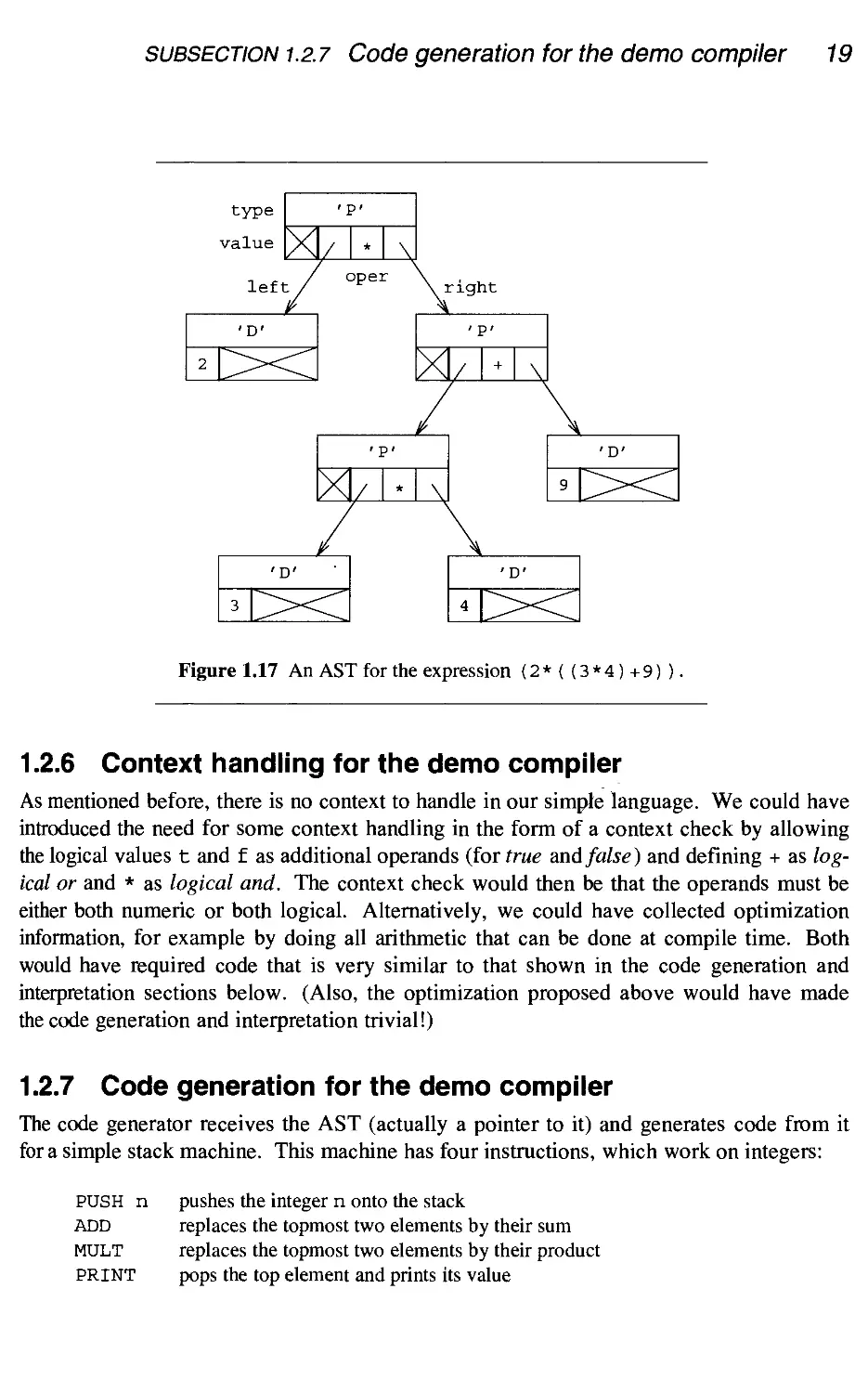
Although in theory we should have different node types for the ASTs of different syn-
syntactic constructs, it is more convenient to group them in broad classes and have only one
node type for each of these classes. This is one of the differences between the parse tree,
which follows the grammar faithfully, and the AST, which serves the convenience of the
compiler writer. More in particular, in our example all nodes in an expression are of type
Expression, and, since we have only expressions, that is the only possibility for the
type of AST_node. To differentiate the nodes of type Expression, each such node
contains a type attribute, set with a characteristic value: ' D' for a digit and ' P' for a
parenthesized expression. The type attribute tells us how to interpret the fields in the rest
of the node. Such interpretation is needed in the code generator and the interpreter. The
header file with the definition of the node type Expression is shown in Figure 1.16.
The syntax analysis module shown in Figure 1.14 defines a single Boolean routine
Parse_program () which tries to read the program as an expression by calling
18 section 1.2 A simple traditional modular compiler/interpreter
int P (...) {
/* try to parse the alternative A1 A2 ... An */
if (Ax(...)) {
if (!A2(...)) Error("Missing A2") ;
if (!An (...)) Error("Missing An") ;
return 1;
/* try to parse the alternative Bx B2 ... */
if {B1(...)) {
if (!B2(...)) Error("Missing B2");
return 1;
/* failed to find any alternative of P */
return 0;
}
Figure 1.15 A C template for a grammar rule.
typedef int Operator;
typedef struct _expression {
char type;
int value;
struct _expression *left, *right;
Operator oper;
} Expression;
typedef Expression AST_node; /* the top node is an Expression
extern int Parse_program(AST_node **);
Figure 1.16 Parser header file for the demo compiler.
/*
/*
/*
/*
'D'
for
for
for
or
'D'
'P'
' P'
'P'
*/
*/
*/
Parse_expression () and, if it succeeds, converts the pointer to the expression to a
pointer to AST_node, which it subsequently yields as its output parameter. It also checks
if the input is indeed finished after the expression.
Figure 1.17 shows the AST that results from parsing the expression
B*(C*4)+9)). Depending on the value of the type attribute, a node contains either
a value attribute or three attributes left, oper, and right. In the diagram, the non-
applicable attributes have been crossed out in each node.
subsection 1.2.7 Code generation for the demo compiler 19
type
value
J/ I * I \
left/ °per \ right
X
J/ I * I \
IX
Figure 1.17 An AST for the expression B*(C*4)+9)).
1.2.6 Context handling for the demo compiler
As mentioned before, there is no context to handle in our simple language. We could have
introduced the need for some context handling in the form of a context check by allowing
the logical values t and f as additional operands (for true and false) and defining + as log-
logical or and * as logical and. The context check would then be that the operands must be
either both numeric or both logical. Alternatively, we could have collected optimization
information, for example by doing all arithmetic that can be done at compile time. Both
would have required code that is very similar to that shown in the code generation and
interpretation sections below. (Also, the optimization proposed above would have made
the code generation and interpretation trivial!)
1.2.7 Code generation for the demo compiler
The code generator receives the AST (actually a pointer to it) and generates code from it
for a simple stack machine. This machine has four instructions, which work on integers:
PUSH n pushes the integer n onto the stack
ADD replaces the topmost two elements by their sum
MULT replaces the topmost two elements by their product
PRINT pops the top element and prints its value
20 section 1.2 A simple traditional modular compiler/interpreter
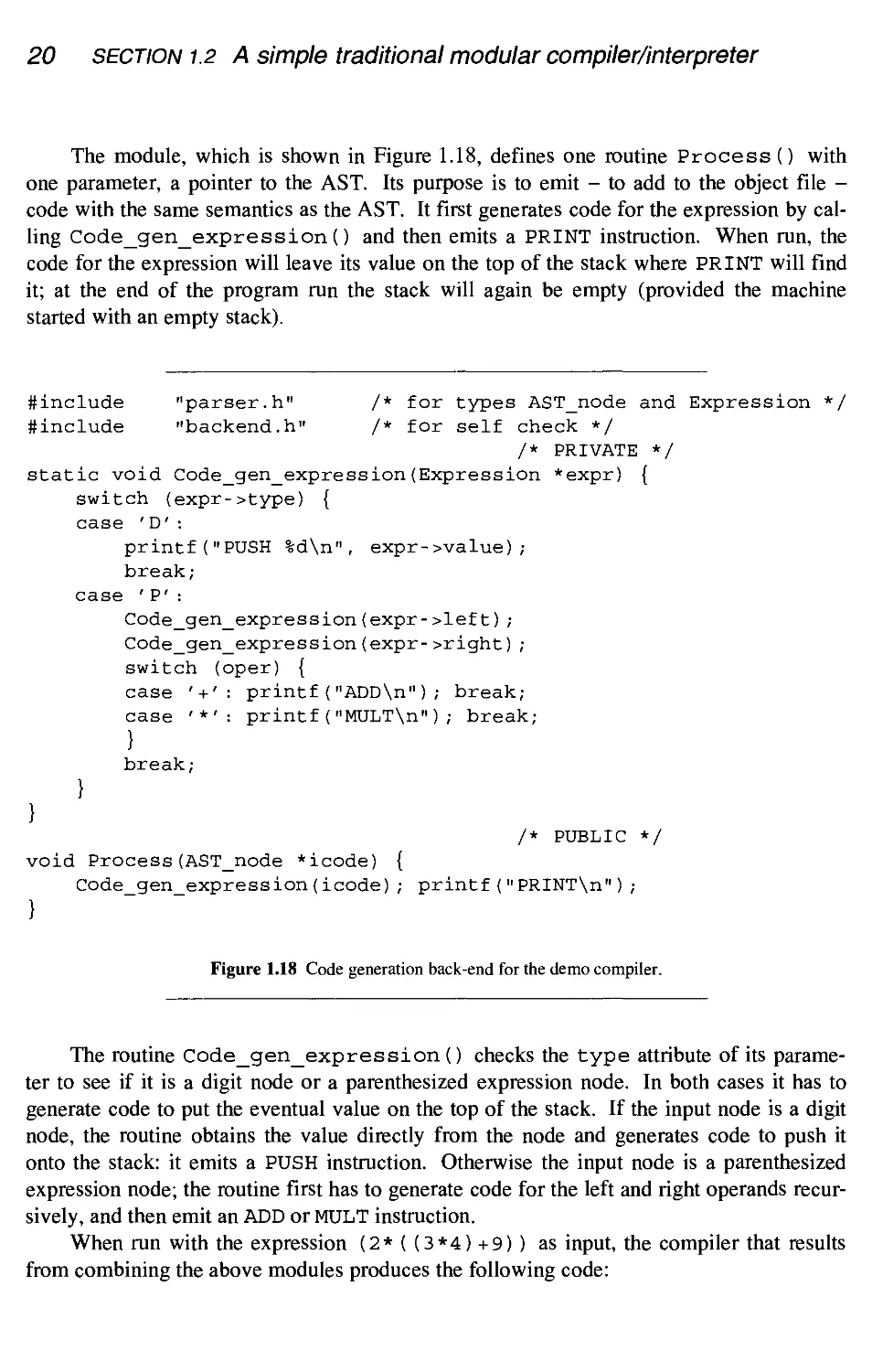
The module, which is shown in Figure 1.18, defines one routine Process () with
one parameter, a pointer to the AST. Its purpose is to emit - to add to the object file -
code with the same semantics as the AST. It first generates code for the expression by cal-
calling Code_gen_expression() and then emits a PRINT instruction. When run, the
code for the expression will leave its value on the top of the stack where PRINT will find
it; at the end of the program run the stack will again be empty (provided the machine
started with an empty stack).
#include "parser.h" /* for types AST_node and Expression */
ttinclude "backend.h" /* for self check */
/* PRIVATE */
static void Code_gen_expression(Expression *expr) {
switch (expr->type) {
case 'D':
printfC'PUSH %d\n" , expr->value);
break;
case ' P' :
Code_gen_expression(expr->left);
Code_gen_expression(expr->right);
switch (oper) {
case '+': printf("ADD\n"); break;
case '*': printf("MULT\n"); break;
}
break;
}
}
/* PUBLIC */
void Process(AST_node *icode) {
Code_gen_expression(icode); printf("PRINT\n");
Figure 1.18 Code generation back-end for the demo compiler.
The routine Code_gen_expression () checks the type attribute of its parame-
parameter to see if it is a digit node or a parenthesized expression node. In both cases it has to
generate code to put the eventual value on the top of the stack. If the input node is a digit
node, the routine obtains the value directly from the node and generates code to push it
onto the stack: it emits a PUSH instruction. Otherwise the input node is a parenthesized
expression node; the routine first has to generate code for the left and right operands recur-
recursively, and then emit an ADD or MULT instruction.
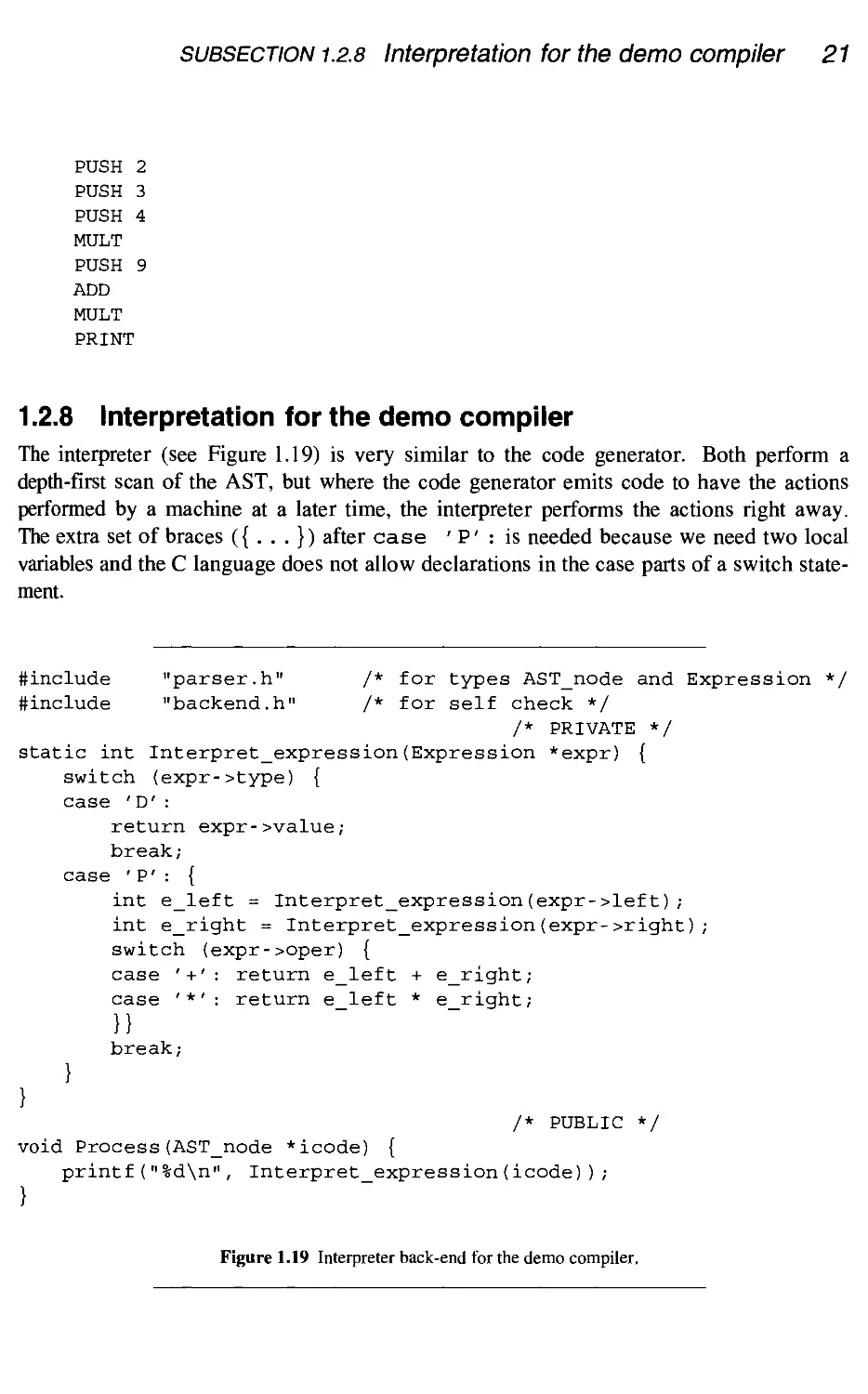
When run with the expression B*(C*4)+9)) as input, the compiler that results
from combining the above modules produces the following code:
subsection 1.2.8 Interpretation for the demo compiler 21
PUSH 2
PUSH 3
PUSH 4
MULT
PUSH 9
ADD
MULT
PRINT
1.2.8 Interpretation for the demo compiler
The interpreter (see Figure 1.19) is very similar to the code generator. Both perform a
depth-first scan of the AST, but where the code generator emits code to have the actions
performed by a machine at a later time, the interpreter performs the actions right away.
The extra set of braces ({...}) after case ' P' : is needed because we need two local
variables and the C language does not allow declarations in the case parts of a switch state-
statement.
#include "parser.h" /* for types AST_node and Expression */
#include "backend.h" /* for self check */
/* PRIVATE */
static int Interpret_expression(Expression *expr) {
switch (expr->type) {
case 'D':
return expr->value;
break;
case 'P' : {
int e_left = Interpret_expression(expr->left);
int e_right = Interpret_expression(expr->right);
switch (expr->oper) {
case '+': return e_left + e_right;
case '*': return e_left * e_right;
}}
break;
}
}
/* PUBLIC */
void Process(AST_node *icode) {
printf("%d\n", Interpret_expression(icode));
Figure 1.19 Interpreter back-end for the demo compiler.
22 section 1.3 The structure of a more realistic compiler
Note that the code generator code (Figure 1.18) and the interpreter code (Figure 1.19)
share the same module definition file (called a 'header file' in C), backend. h, shown in
Figure 1.20. This is possible because they both implement the same interface: a single rou-
routine Process (AST_node *). In Chapter 4 we will see an example of a different type
of interpreter (Section 4.1.2) and two other code generators (Sections 4.2.3 and 4.2.3.2),
each using this same interface. Another module that implements the back-end interface
meaningfully might be a module that displays the AST graphically. Each of these can be
combined with the lexical and syntax modules, to produce a program processor.
extern void Process(AST_node *);
Figure 1.20 Common back-end header for code generator and interpreter.
1.3 The structure of a more realistic compiler
Figure 1.8 showed that in order to describe the demo compiler we had to decompose the
front-end into three modules and that the back-end could stay as a single module. It will be
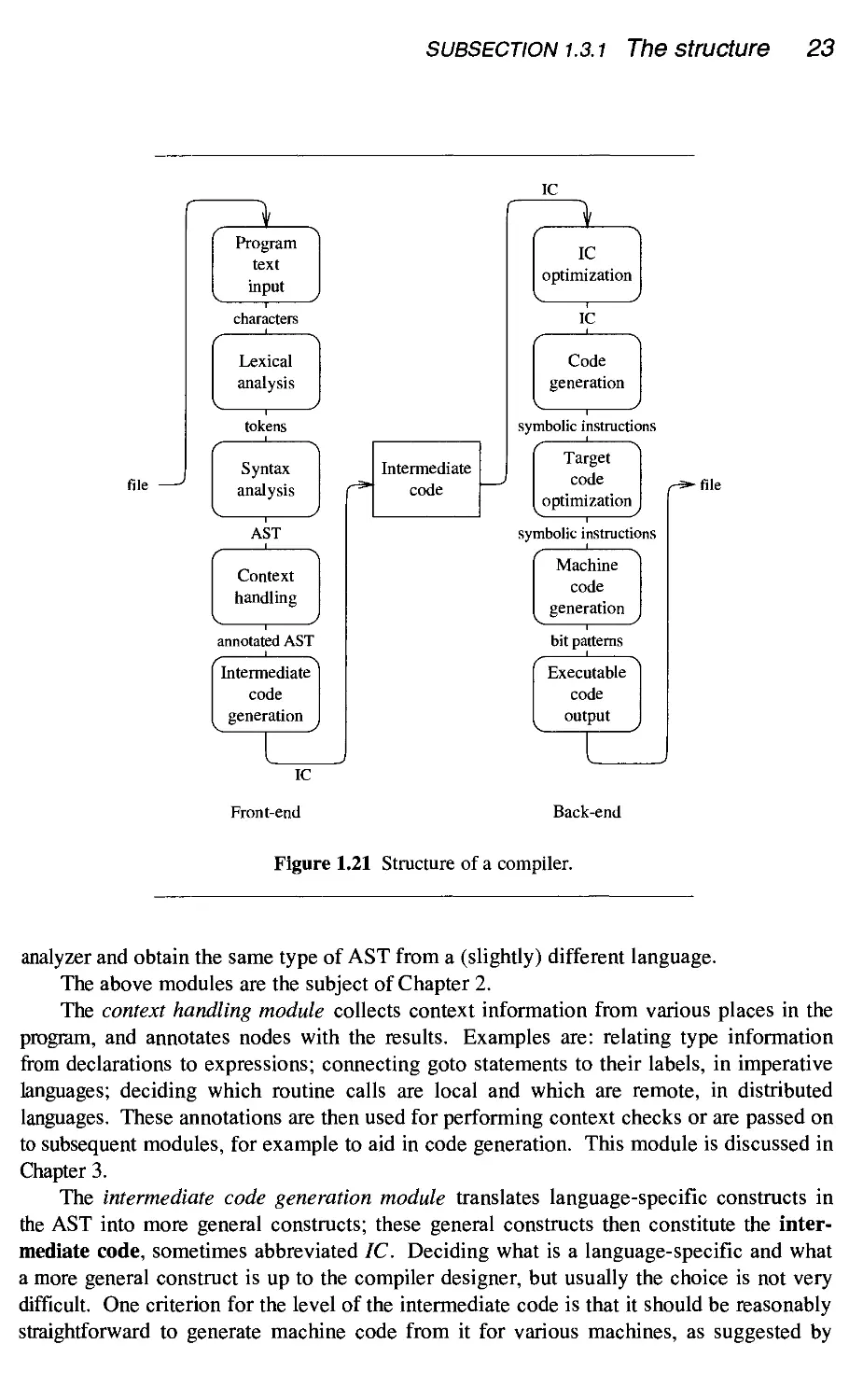
clear that this is not sufficient for a real-world compiler. A more realistic picture is shown
in Figure 1.21, in which front-end and back-end each consists of five modules. In addition
to these, the compiler will contain modules for symbol table handling and error reporting;
these modules will be called upon by almost all other modules.
1.3.1 The structure
A short description of each of the modules follows, together with an indication of where
the material is discussed in detail.
The program text input module finds the program text file, reads it efficiently, and
turns it into a stream of characters, allowing for different kinds of newlines, escape codes,
etc. It may also switch to other files, when these are to be included. This function may
require cooperation with the operating system on the one hand and with the lexical
analyzer on the other.
The lexical analysis module isolates tokens in the input stream and determines their
class and representation. It can be written by hand or generated from a description of the
tokens. Additionally, it may do some limited interpretation on some of the tokens, for
example to see if an identifier is perhaps actually a macro or a keyword (reserved word).
The syntax analysis module converts the stream of tokens into an abstract syntax tree
(AST). Some syntax analyzers consist of two modules. The first one reads the token
stream and calls a function from the second module for each syntax construct it recognizes;
the functions in the second module then construct the nodes of the AST and link them.
This has the advantage that one can replace the AST generation module to obtain a dif-
different AST from the same syntax analyzer, or, alternatively, one can replace the syntax
subsection 1.3.1 The structure 23
file
*
| Program |
text
1 input 1
characters
Lexical
analysis
tokens
Syntax
analysis
AST
Context
handling
annotated AST
| Intermediate |
code
I generation I
IC
Front-end
Figure 1
.21
Intermediate
code
■—'
IC
( .-.I
optimization
IC
Code
generation
symbolic instructions
( Target "]
code
1 optimizationl
symbolic instructions
Machine
code
generation I
bit patterns
Executable
code
output I
Back-end
Structure of a compiler.
file
analyzer and obtain the same type of AST from a (slightly) different language.
The above modules are the subject of Chapter 2.
The context handling module collects context information from various places in the
program, and annotates nodes with the results. Examples are: relating type information
from declarations to expressions; connecting goto statements to their labels, in imperative
languages; deciding which routine calls are local and which are remote, in distributed
languages. These annotations are then used for performing context checks or are passed on
to subsequent modules, for example to aid in code generation. This module is discussed in
Chapter 3.
The intermediate code generation module translates language-specific constructs in
the AST into more general constructs; these general constructs then constitute the inter-
intermediate code, sometimes abbreviated IC. Deciding what is a language-specific and what
a more general construct is up to the compiler designer, but usually the choice is not very
difficult. One criterion for the level of the intermediate code is that it should be reasonably
straightforward to generate machine code from it for various machines, as suggested by
24 section 1.3 The structure of a more realistic compiler
Figure 1.4. Usually the intermediate code consists almost exclusively of expressions and
flow-of-control instructions.
Examples of the translations done by the intermediate code generation module are:
replacing a while statement by tests, labels, and jumps in imperative languages; inserting
code for determining which method to call for an object in languages with dynamic bind-
binding; replacing a Prolog rule by a routine that does the appropriate backtracking search. In
each of these cases an alternative translation would be a call to a routine in the run-time
system, with the appropriate parameters: the Prolog rule could stay in symbolic form and
be interpreted by a run-time routine, a run-time routine could dynamically find the method
to be called, and even the while statement could be performed by a run-time routine if the
test and the body were converted to anonymous subroutines. The intermediate code gen-
generation module is the place where the division of labor between in-line code and the run-
runtime system is decided. This module is treated in Chapters 6 through 9, for the imperative,
object-oriented, functional, logic, and parallel and distributed programming paradigms.
The intermediate code optimization module performs preprocessing on the intermedi-
intermediate code, with the intention of improving the effectiveness of the code generation module.
An example of straightforward preprocessing is constant folding, in which all operations in
expressions with known simple operands are performed. A more sophisticated example is
in-lining, in which carefully chosen calls to some routines are replaced by the bodies of
those routines, while at the same time substituting the parameters.
The code generation module rewrites the AST into a linear list of target machine
instructions, in more or less symbolic form. To this end, it selects instructions for seg-
segments of the AST, allocates registers to hold data and arranges the instructions in the
proper order.
The target code optimization module considers the list of symbolic machine instruc-
instructions and tries to optimize it by replacing sequences of machine instructions by faster or
shorter sequences. It uses target-machine-specific properties.
The precise boundaries between intermediate code optimization, code generation, and
target code optimization are floating: if the code generation is particularly good, little tar-
target code optimization may be needed or even possible, and constant folding can be done
during code generation or even on the target code. Still, some optimizations fit better in
one module than in another, and it is useful to distinguish the above three levels.
The machine code generation module converts the symbolic machine instructions into
the corresponding bit patterns. It determines machine addresses of program code and data
and produces tables of constants and relocation tables.
The executable code output module combines the encoded machine instructions, the
constant tables, the relocation tables, and the headers, trailers, and other material required
by the operating system into an executable code file.
The back-end modules are discussed in Chapter 4.
1.3.2 Run-time systems
There is one important component of a compiler that is traditionally left outside compiler
structure pictures: the run-time system of the compiled programs. Some of the actions
required by a running program will be of a general, language-dependent and/or machine-
section 1.4 Compiler architectures 25
dependent housekeeping nature; examples are code for allocating arrays, manipulating
stack frames, and finding the proper method during method invocation in an object-
oriented language. Although it is quite possible to generate code fragments for these
actions wherever they are needed, these fragments are usually very repetitive and it is often
more convenient to compile them once and store the result in library modules. These
library modules together form the run-time system. Some imperative languages need
only a minimal run-time system; others, especially the logic and distributed languages, may
require run-time systems of considerable size, containing code for parameter unification,
remote procedure call, task scheduling, etc. The parts of the run-time system needed by a
specific program can be linked in by the linker when the complete object program is con-
constructed, or even be linked in dynamically when the compiled program is called; object
programs and linkers are explained in Section 4.3. If the back-end is an interpreter, the
run-time system must be incorporated in it.
As an aside it should be pointed out that run-time systems are not only traditionally
left out of compiler overview pictures like those in Figure 1.8 and Figure 1.21, they are
also sometimes overlooked or underestimated in compiler construction planning. Given
the fact that they may contain such beauties as printf (), malloc (), and concurrent
task management, overlooking them is definitely inadvisable.
1.3.3 Short-cuts
It is by no means always necessary to implement all modules of the back-end:
- Writing the modules for generating machine code and executable code can be avoided
by using the local assembler, which is almost always available.
- Writing the entire back-end can often be avoided by generating C code from the inter-
intermediate code. This exploits the fact that good C compilers are available on virtually any
platform, which is why C is sometimes called, half jokingly, 'The Machine-Independent
Assembler'. This is the usual approach taken by compilers for the more advanced para-
paradigms, but it is certainly also recommendable for first implementations of compilers for
new imperative and object-oriented languages.
The object code produced by the above 'short-cuts' is often of good to excellent quality,
but the increased compilation time may be a disadvantage. Most C compilers are quite
substantial programs and calling them may well cost noticeable time; their availability
may, however, make them worth it.
1.4 Compiler architectures
Compilers can differ considerably with regard to their architecture; unfortunately, termi-
terminology to describe the different types is lacking or confusing. Two architectural questions
dominate the scene. One is concerned with the granularity of the data that is passed
between the compiler modules: is it bits and pieces or is it the entire program? In other
words, how wide is the compiler? The second concerns the flow of control between the
compiler modules: which of the modules is the boss?
26 section 1.4 Compiler architectures
1.4.1 The width of the compiler
A compiler consists of a series of modules that transform, refine, and pass on information
between them. Information passes mainly from the front to the end, from module Mn to
module Mn+1. Each such consecutive pair of modules defines an interface, and although in
the end all information has to pass through all these interfaces, the size of the chunks of
information that are passed on makes a considerable difference to the structure of the com-
compiler. Two reasonable choices for the size of the chunks of information are the smallest
unit that is meaningful between the two modules; and the entire program. This leads to
two types of compilers, neither of which seems to have a name; we will call them 'narrow'
and 'broad' compilers, respectively.
A narrow compiler reads a small part of the program, typically a few tokens,
processes the information obtained, produces a few bytes of object code if appropriate, dis-
discards most of the information about these tokens, and repeats this process until the end of
the program text is reached.
A broad compiler reads the entire program and applies a series of transformations to
it (lexical, syntactic, contextual, optimizing, code generating, etc.), which eventually result
in the desired object code. This object code is then generally written to a file.
It will be clear that a broad compiler needs an amount of memory that is proportional
to the size of the source program, which is the reason why this type has always been rather
unpopular. Until the 1980s, a broad compiler was unthinkable, even in academia. A nar-
narrow compiler needs much less memory; its memory requirements are still linear in the
length of the source program, but the proportionality constant is much lower since it gath-
gathers permanent information (for example about global variables) at a much slower rate.
From a theoretical, educational, and design point of view, broad compilers are prefer-
preferable, since they represent a simpler model, more in line with the functional programming
paradigm. A broad compiler consists of a series of function calls (Figure 1.22) whereas a
narrow compiler consists of a typically imperative loop (Figure 1.23). In practice, 'real'
compilers are often implemented as narrow compilers. Still, a narrow compiler may
compromise and have a broad component: it is quite natural for a C compiler to read each
routine in the C program in its entirety, process it, and then discard all but the global infor-
information it has obtained.
In the future we expect to see more broad compilers and fewer narrow ones. Most of
the compilers for the new programming paradigms are already broad, since they often
started out as interpreters. Since scarcity of memory will be less of a problem in the future,
more and more imperative compilers will be broad. On the other hand, almost all compiler
construction tools have been developed for the narrow model and thus favor it. Also, the
narrow model is probably better for the task of writing a simple compiler for a simple
language by hand, since it requires much less dynamic memory allocation.
Since the 'field of vision' of a narrow compiler is, well, narrow, it is possible that it
cannot manage all its transformations on the fly. Such compilers then write a partially
transformed version of the program to disk and, often using a different program, continue
with a second pass; occasionally even more passes are used. Not surprisingly, such a com-
compiler is called a 2-pass (or N-pass) compiler, or a 2-scan (TV-scan) compiler. If a distinc-
distinction between these two terms is made, '2-scan' often indicates that the second pass actually
re-reads (re-scans) the original program text, the difference being that it is now armed with
subsection 1.4.2 Who's the boss? 27
SET Object code TO
Assembly(
Code generation(
Context check(
Parse(
Tokenize(
Source code
Figure 1.22 Flow-of-control structure of a broad compiler.
WHILE NOT Finished:
Read some data D from the source code;
Process D and produce the corresponding object code, if any;
Figure 1.23 Flow-of-control structure of a narrow compiler.
information extracted during the first scan.
The major transformations performed by a compiler and shown in Figure 1.21 are
sometimes called phases, giving rise to the term N-phase compiler, which is of course not
the same as an ,/V-pass compiler. Since on a very small machine each phase could very
well correspond to one pass, these notions are sometimes confused.
With larger machines, better syntax analysis techniques and simpler programming
language grammars, Af-pass compilers with N> 1 are going out of fashion. It turns out that
not only compilers but also people like to read their programs in one scan. This observa-
observation has led to syntactically stronger programming languages, which are correspondingly
easier to process.
Many algorithms in a compiler use only local information; for these it makes little
difference whether the compiler is broad or narrow. Where it does make a difference, we
will show the broad method first and then explain the narrow method as an optimization, if
appropriate.
1.4.2 Who's the boss?
In a broad compiler, control is not a problem: the modules run in sequence and each
module has full control when it runs, both over the processor and over the data. A simple
driver can activate the modules in the right order, as already shown in Figure 1.22. In a
28 section 1.4 Compiler architectures
narrow compiler, things are more complicated. While pieces of data are moving forward
from module to module, control has to shuttle forward and backward, to activate the proper
module at the proper time. We will now examine the flow of control in narrow compilers
in more detail.
The modules in a compiler are essentially 'filters', reading chunks of information,
processing them, and writing the result. Such filters are most easily programmed as loops
which execute function calls to obtain chunks of information from the previous module and
routine calls to write chunks of information to the next module. An example of a filter as a
main loop is shown in Figure 1.24.
WHILE Obtained input character Ch from previous module:
IF Ch = 'a':
// See if there is another 'a':
IF Obtained input character Chi from previous module:
IF Chi = 'a':
//We have 'aa':
Output character 'b' to next module;
ELSE Chi /= 'a':
Output character 'a' to next module;
Output character Chi to next module;
ELSE Chi not obtained:
Output character 'a' to next module;
EXIT WHILE;
ELSE Ch /= 'a':
Output character Ch to next module;
Figure 1.24 The filter aa -> b as a main loop.
It describes a simple filter which copies input characters to the output while replacing
the sequence aa by b; the filter is representative of, but of course much simpler than, the
kind of transformations performed by an actual compiler module. The reader may
nevertheless be surprised at the complexity of the code, which is due to the requirements
for the proper termination of the previous, the present, and the next module. The need for
proper handling of end of input is, however, very much a fact of life in compiler construc-
construction and we cannot afford to sweep its complexities under the rug.
The filter obtains its input characters by calling upon its predecessor in the module
sequence; such a call may succeed and yield a character, or it may fail. The transformed
characters are passed on to the next module. Except for routine calls to the previous and
the next module, control remains inside the while loop all the time, and no global variables
are needed.
Although main loops are efficient, easy to program and easy to understand, they have
one serious flaw which prevents them from being used as the universal programming
model for compiler modules: a main loop does not interface well with another main loop in
traditional programming languages. Linking the output of one main loop to the input of
section 1.5 Properties of a good compiler 29
another involves a transfer of control that leaves both the environment of the callee and
that of the caller intact, regardless of whether the consumer calls the producer to obtain
new information or the producer calls the consumer to pass on processed information.
The traditional function call creates a new environment for the callee and traditional
function return destroys the environment of the callee. So they cannot serve to link two
loops. A transfer of control that does possess the desired properties is the coroutine call,
which involves having separate stacks for the two loops to preserve both environments.
The coroutine linkage also takes care of the end-of-input handling: an attempt to obtain
information from a module whose loop has terminated fails. A well-known implementa-
implementation of the coroutine linkage is the UNIX pipe, in which the two separate stacks reside in
different processes and therefore in different address spaces. Implementation of coroutines
in imperative languages is discussed in Section 6.3.7.
Although coroutine linkage was proposed by Conway A963) early in the history of
compiler construction, no programming language except perhaps Icon (Griswold and
Griswold, 1983) has ever featured a usable implementation of it. In the absence of corou-
coroutines we have to choose one of our modules as the main loop in a narrow compiler and
implement the other loops through trickery. That this implies major surgery to these loops
is shown by Figure 1.25, which shows our filter as a loop-less module preceding the main
loop, and Figure Answers. 1, which shows it as a loop-less module following the main loop.
We see that global variables are needed to record information that must remain avail-
available between two successive calls of the function. The variable Input exhausted
records whether the previous call of the function returned from the position before the
EXIT WHILE in Figure 1.24, and the variable There is a stored character
records whether it returned from before outputting Chi. Some additional code is required
for proper end-of-input handling. Note that the code is 29 lines long as opposed to 15 for
the main loop. Similar considerations apply to the post-main variant, which is given as an
exercise. An additional complication is that proper end-of-input handling requires that the
filter be flushed by the using module when it has supplied its final chunk of information.
See Exercise 1.11.
Looking at Figures 1.25 and Answers. 1 in the answers to the exercises, we see that the
complication comes from having to save program state that resides on the stack. So it will
be convenient to choose for the main loop the module that has the most state on the stack.
That module will almost always be the parser; the code generator may gather more state,
but it is usually stored in a global data structure rather than on the stack. This explains why
we almost universally find the parser as the main module in a narrow compiler: in very
simple-minded wording, the parser pulls the program text in through the lexical analyzer,
and pushes the code out through the code generator.
1.5 Properties of a good compiler
The foremost property of a good compiler is of course that it generates correct code. A
compiler that occasionally generates incorrect code is useless; a compiler that generates
incorrect code once a year may seem useful but is dangerous.
It is also important that a compiler conform completely to the language specification.
It may be tempting to implement a subset of the language, a superset or even what is some-
30 chapter 1 Introduction
SET the flag Input exhausted TO False;
SET the flag There is a stored character TO False;
SET Stored character TO Undefined; // can never be an 'a'
FUNCTION Filtered character RETURNING a Boolean, a character:
IF Input Exhausted: RETURN False, No character;
ELSE IF There is a stored character:
// It cannot be an ' a' -.
SET There is a stored character TO False;
RETURN True, Stored character;
ELSE Input not exhausted AND There is no stored character:
IF Obtained input character Ch from previous module:
IF Ch = 'a':
// See if there is another 'a':
IF Obtained input character Chi from previous module:
IF Chi = 'a':
//We have 'aa':
RETURN True, 'b';
ELSE Chi /= 'a':
SET Stored character TO Chi;
SET There is a stored character TO True;
RETURN True, 'a';
ELSE Chi not obtained:
SET Input exhausted TO True;
RETURN True, 'a';
ELSE Ch /= 'a':
RETURN True, Ch;
ELSE Ch not obtained:
SET Input exhausted TO True;
RETURN False, No character;
Figure 1.25 The filter aa -> b as a pre-main module.
times sarcastically called an 'extended subset', and users may even be grateful, but those
same users will soon find that programs developed with such a compiler are much less
portable than those written using a fully conforming compiler. (For more about the notion
of 'extended subset', see Exercise 1.13.)
Another property of a good compiler, one that is often overlooked, is that it should be
able to handle programs of essentially arbitrary size, as far as available memory permits. It
seems very reasonable to say that no sane programmer uses more than 32 parameters in a
routine or more than 128 declarations in a block and that one may therefore allocate a fixed
amount of space for each in the compiler. One should, however, keep in mind that pro-
programmers are not the only ones who write programs. More and more software is generated
by other programs, and such generated software may easily contain more than 128 declara-
declarations in one block - although more than 32 parameters to a routine seems excessive, even
section 1.5 Properties of a good compiler 31
for a generated program; famous last words ... Especially any assumptions about limits on
the number of cases in a case/switch statement are unwarranted: very large case statements
are often used in the implementation of automatically generated parsers and code genera-
generators. Section 5.1.3 shows how the flexible memory allocation needed for handling pro-
programs of essentially arbitrary size can be achieved at an almost negligible increase in cost.
Compilation speed is an issue but not a major one. Small programs can be expected
to compile in under a second on modern machines. Larger programming projects are
usually organized in many relatively small subprograms, modules, library routines, etc.,
together called compilation units. Each of these compilation units can be compiled
separately, and recompilation after program modification is usually restricted to the modi-
modified compilation units only. Also, compiler writers have traditionally been careful to keep
their compilers 'linear in the input', which means that the compilation time is a linear func-
function of the length of the input file. This is even more important when generated programs
are being compiled, since these can be of considerable length.
There are several possible sources of non-linearity in compilers. First, all linear-time
parsing techniques are rather inconvenient, and the worry-free parsing techniques can be
cubic in the size of the input in the worst case. Second, many code optimizations are
potentially exponential in the size of the input, since often the best code can only be found
by considering all possible combinations of machine instructions. Third, naive memory
management can result in quadratic time consumption. Fortunately, good linear-time solu-
solutions or heuristics are available for all these problems.
Compiler size is hardly an issue anymore, with most computers having many mega-
megabytes of primary memory nowadays.
The user-friendliness of a compiler shows mainly in the quality of its error reporting.
At the least, the user should be presented with a clear error message which includes the
perceived cause of the error, the name of the input file, and the position in it. Giving a
really good error cause description is often hard or impossible, due to the limited insight
compilers have into incorrect programs. Pinpointing the error is aided by recording the file
name and line number with every token and every node in the AST. More fancy reporting
mechanisms, including showing parts of the syntax tree, may not have the beneficial effect
the compiler writer may expect from them, but it may be useful to provide some visual
display mechanism, for example opening a text editor at the point of the error.
The importance of the speed and the size of the generated code depends totally on the
purpose of the compiler. Normally one can expect that the user is more interested in high
speed than in small size (code for embedded applications, such as washing machines, port-
portable telephones, etc., is an exception). Moderately advanced optimization techniques will
perhaps provide a factor of three improvement over very naive code generation; imple-
implementing such optimizations may take about the same amount of time as the entire compiler
writing project. Gaining another factor of two or even three over this may be possible
through extensive and aggressive optimization; one can expect to spend many times the
original effort on an optimization phase of this nature.
32 chapter 1 Introduction
1.6 Portability and retargetability
A program is considered portable if it takes a limited and reasonable effort to make it run
on different machine types. What constitutes 'a limited and reasonable effort' is, of
course, a matter of opinion, but today many programs can be ported by just editing the
'makefile' to reflect the local situation and recompiling.
With compilers, machine dependence not only resides in the program itself, it resides
also - perhaps even mainly - in the output. Therefore, with compilers one has to distin-
distinguish two forms of portability: the ease with which the compiler itself can be made to run
on another machine, and the ease with which it can be made to generate code for another
machine. The first is called the portability of the compiler and the second is called its
retargetability. If the compiler is written in a reasonably good style in a modern high-
level language, good portability can be expected. Retargeting is achieved by replacing the
entire back-end; the retargetability is thus inversely related to the effort to create a new
back-end.
In this context it is important to note that creating a new back-end does not necessarily
mean writing one from scratch. Some of the code in a back-end is of course machine-
dependent, but much of it is not. If structured properly, some parts can be reused from
other back-ends and other parts can perhaps be generated from formalized machine-
descriptions. This approach can reduce creating a back-end from a major enterprise to a
reasonable effort. Given the proper tools, creating a back-end for a new machine may cost
between one and four programmer-months for an experienced compiler writer. Machine
descriptions range in size between a few hundred lines and many thousands of lines.
1.7 Place and usefulness of optimizations
Optimizations are attractive: much research in compiler construction is concerned with
them, and compiler writers regularly see all kinds of opportunities for optimizations. It
should, however, be kept in mind that implementing optimizations is the last phase in com-
compiler construction: unlike correctness, optimizations are an add-on feature. In program-
programming, it is easier to make a correct program fast than a fast program correct; likewise it is
easier to make correct generated object code fast than to make fast generated object code
correct.
There is another reason besides correctness why we tend to focus on the unoptimized
algorithm in this book: some traditional algorithms are actually optimized versions of more
basic algorithms. Sometimes the basic algorithm has wider applicability than the optim-
optimized version and in any case the basic version will provide us with more insight and free-
freedom of design than the optimized version.
A good example is the stack in implementations of imperative languages. At any
moment the stack holds the pertinent data - administration, parameters, and local data -
for each active routine, a routine that has been called and has not yet terminated. This set
of data is called the 'activation record' of this activation of the routine. Traditionally,
activation records are found only on the stack, and only the one on the top of the stack
represents a running routine; we consider the stack as the primary mechanism of which
activation records are just parts. It is, however, profitable to recognize the activation
section 1.8 A short history of compiler construction 33
record as the primary item: it arises naturally when a routine is called ('activated') since it
is obvious that its pertinent data has to be stored somewhere. Its allocation on a stack is
just an optimization that happens to be possible in many - but not all - imperative and
object-oriented languages. From this point of view it is easier to understand the implemen-
implementation of those languages for which stack allocation is not a good optimization: imperative
languages with coroutines or Ada-like tasks, object-oriented languages with active
Smalltalk-like objects, functional languages, Icon, etc.
Probably the best attitude towards optimization is to first understand and implement
the basic structure and algorithm, then see which optimizations the actual situation allows,
and only implement them if they are considered worthwhile (considering their cost). In
situations in which the need for optimization is obvious from the start, as for example in
code generators, the basic structure would include a framework for these optimizations.
This framework can then be filled in as the project progresses.
This concludes our introductory part on actually constructing a compiler. In the
remainder of this chapter we consider three further issues: the history of compiler construc-
construction, formal grammars, and closure algorithms.
1.8 A short history of compiler construction
Three periods can be distinguished in the history of compiler construction: 1945-1960,
1960-1975, and 1975-present. Of course, the years are approximate.
1.8.1 1945-1960: code generation
During this period languages developed relatively slowly and machines were idiosyncratic.
The primary problem was how to generate code for a given machine. The problem was
exacerbated by the fact that assembly programming was held in high esteem, and high--
high-level languages and compilers were looked at with a mixture of suspicion and awe: using a
compiler was often called 'automatic programming'. Proponents of high-level languages
feared, not without reason, that the idea of high-level programming would never catch on if
compilers produced code that was less efficient than what assembly programmers pro-
produced by hand. The first FORTRAN compiler (Sheridan, 1959) optimized heavily and was
far ahead of its time in that respect.
1.8.2 1960-1975: parsing
The 1960s and 1970s saw a proliferation of new programming languages, and language
designers began to believe that having a compiler for a new language quickly was more
important than having one that generated very efficient code. This shifted the emphasis in
compiler construction from back-ends to front-ends. At the same time, studies in formal
languages revealed a number of powerful techniques that could be applied profitably in
front-end construction, notably in parser generation.
34 chapter 1 Introduction
1.8.3 1975-present: code generation and code optimization;
paradigms
From 1975 to the present, both the number of new languages proposed and the number of
different machine types in regular use decreased, which reduced the need for quick-and-
simple/quick-and-dirty compilers for new languages and/or machines. The greatest tur-
turmoil in language and machine design being over, people began to demand professional
compilers that were reliable, efficient, both in use and in generated code, and preferably
with pleasant user interfaces. This called for more attention to the quality of the generated
code, which was easier now, since with the slower change in machines the expected life-
lifetime of a code generator increased.
Also, at the same time new paradigms in programming were developed, with func-
functional, logic, and distributed programming as the most prominent examples. Almost
invariably, the run-time requirements of the corresponding languages far exceeded those of
the imperative languages: automatic data allocation and deallocation, list comprehensions,
unification, remote procedure call, and many others, are features which require much run-
runtime effort that corresponds to hardly any code in the program text. More and more, the
emphasis shifts from 'how to compile' to 'what to compile to'.
1.9 Grammars
Grammars, or more precisely context-free grammars, are the essential formalism for
describing the structure of programs in a programming language. In principle, the gram-
grammar of a language describes the syntactic structure only, but since the semantics of a
language is defined in terms of the syntax, the grammar is also instrumental in the defini-
definition of the semantics.
There are other grammar types besides context-free grammars, but we will be mainly
concerned with context-free grammars. We will also meet regular grammars, which more
often go by the name of 'regular expressions' and which result from a severe restriction on
the context-free grammars; and attribute grammars, which are context-free grammars
extended with parameters and code. Other types of grammars play no more than a margi-
marginal role in compiler construction. The term 'context-free' is often abbreviated to CF. We
will give here a brief summary of the features of CF grammars.
A grammar is a recipe for constructing elements of a set of strings of symbols. When
applied to programming languages, the symbols are the tokens in the language, the strings
of symbols are program texts, and the set of strings of symbols is the programming
language. The string
BEGIN print ( "Hi!" ) END
consists of 6 symbols (tokens) and could be an element of the set of strings of symbols
generated by a programming language grammar, or in more normal words, be a program in
some programming language. This cut-and-dried view of a programming language would
be useless but for the fact that the strings are constructed in a structured fashion; and to this
structure semantics can be attached.
section 1.9 Grammars 35
1.9.1 The form of a grammar
A grammar consists of a set of production rules and a start symbol. Each production rule
defines a named syntactic construct. A production rule consists of two parts, a left-hand
side and a right-hand side, separated by a left-to-right arrow. The left-hand side is the
name of the syntactic construct; the right-hand side shows a possible form of the syntactic
construct. An example of a production rule is
expression —> ' (' expression operator expression ')'
The right-hand side of a production rule can contain two kinds of symbols, terminal sym-
symbols and non-terminal symbols. As the word says, a terminal symbol (or terminal for
short) is an end point of the production process, and can be part of the strings produced by
the grammar. A non-terminal symbol (or non-terminal for short) must occur as the left-
hand side (the name) of one or more production rules, and cannot be part of the strings pro-
produced by the grammar. Terminals are also called tokens, especially when they are part of
an input to be analyzed. Non-terminals and terminals together are called grammar sym-
symbols. The grammar symbols in the right-hand side of a rule are collectively called its
members; when they occur as nodes in a syntax tree they are more often called its 'chil-
'children'.
In discussing grammars, it is customary to use some conventions that allow the class
of a symbol to be deduced from its typographical form.
- Non-terminals are denoted by capital letters, mostly A, B, C, and N.
- Terminals are denoted by lower-case letters' near the end of the alphabet, mostly jc, v, and
z.
- Sequences of grammar symbols are denoted by Greek letters near the beginning of the
alphabet, mostly a (alpha), C (beta), and y (gamma).
- Lower-case letters near the beginning of the alphabet (a, b, c, etc.) stand for themselves,
as terminals.
- The empty sequence is denoted by £ (epsilon).
1.9.2 The production process
The central data structure in the production process is the sentential form. It is usually
described as a string of grammar symbols, and can then be thought of as representing a par-
partially produced program text. For our purposes, however, we want to represent the syntac-
syntactic structure of the program too. The syntactic structure can be added to the flat interpreta-
interpretation of a sentential form as a tree positioned above the sentential form so that the leaves of
the tree are the grammar symbols. This combination is also called a production tree.
A string of terminals can be produced from a grammar by applying so-called produc-
production steps to a sentential form, as follows. The sentential form is initialized to a copy of the
start symbol. Each production step finds a non-terminal N in the leaves of the sentential
form, finds a production rule N—m with N as its left-hand side, and replaces the TV in the
sentential form with a tree having TV as the root and the right-hand side of the production
rule, a, as the leaf or leaves. When no more non-terminals can be found in the leaves of
36 section 1.9 Grammars
the sentential form, the production process is finished, and the leaves form a string of ter-
terminals in accordance with the grammar.
Using the conventions described above, we can write that the production process
replaces the sentential form pWy by Pay.
The steps in the production process leading from the start symbol to a string of termi-
terminals are called the derivation of that string. Suppose our grammar consists of the four
numbered production rules:
[1] expression —> ' (' expression operator expression ')'
[2] expression —> '1'
[3] operator —> '+'
[4] operator —> '*'
in which the terminal symbols are surrounded by apostrophes and the non-terminals are
identifiers, and suppose the start symbol is expression. Then the sequence of senten-
sentential forms shown in Figure 1.26 forms the derivation of the string A* A + 1) ). More in
particular, it forms a leftmost derivation, a derivation in which it is always the leftmost
non-terminal in the sentential form that is rewritten. An indication R@P in the left margin
in Figure 1.26 shows that grammar rule R is used to rewrite the non-terminal at position P.
The resulting parse tree (in which the derivation order is no longer visible) is shown in Fig-
Figure 1.27.
expression
1@1 '(' expression operator expression ')'
2@2 ' (' '1' operator expression ')'
4@3 '(' '1' '*' expression ')'
1@4 '(' '1' '*' '(' expression operator expression
2@5 '(' '1' '*' '(' ' 1' operator expression ')' ')'
3@6 '(' '1' '*' '(' '1' '+' expression ')' ')'
2@7 '(' ' 1' '*' '(' '1' '+' '1' ')' ')'
Figure 1.26 Leftmost derivation of the string A * A +1) ).
We see that recursion - the ability of a production rule to refer directly or indirectly to
itself - is essential to the production process; without recursion, a grammar would produce
only a finite set of strings.
The production process is kind enough to produce the program text together with the
production tree, but then the program text is committed to a linear medium (paper, com-
computer file) and the production tree gets stripped off in the process. Since we need the tree
to find out the semantics of the program, we use a special program, called a 'parser', to
retrieve it. The systematic construction of parsers is treated in Section 2.2.
subsection 1.9.3 Extended forms of grammars 37
expression
'(' expression operator
expression operator expression
Figure 1.27 Parse tree of the derivation in Figure 1.26.
1.9.3 Extended forms of grammars
The single grammar rule format
non-terminal —> zero or more grammar symbols
used above is sufficient in principle to specify any grammar, but in practice a richer nota-
notation is used. For one thing, it is usual to combine all rules with the same left-hand side into
one rule: for example, the rules
are combined into one rule
in which the original right-hand sides are separated by vertical bars. In this form a, C, and
y are called the alternatives of N.
The format described so far is known as BNF, which may be considered an abbrevia-
abbreviation of Backus-Naur Form or of Backus Normal Form. It is very suitable for express-
expressing nesting and recursion, but less convenient for expressing repetition and optionality,
although it can of course express repetition through recursion. To remedy this, three addi-
additional notations are introduced, each in the form of a postfix operator:
- R + indicates the occurrence of one or more Rs, to express repetition;
- R ? indicates the occurrence of zero or one Rs, to express optionality; and
- R* indicates the occurrence of zero or more Rs, to express optional repetition.
Parentheses may be needed if these postfix operators are to operate on more than one
38 section 1.9 Grammars
grammar symbol. The grammar notation that allows the above forms is called EBNF, for
Extended BNF. An example is the grammar rule
parameter_list —> ('IN' | 'OUT')? identifier (',' identifier)*
which produces program fragments like
a, b
IN year, month, day
OUT left, right
1.9.4 Properties of grammars
There are a number of properties of grammars and its components that are used in discuss-
discussing grammars. A non-terminal N is left-recursive if, starting with a sentential form N, we
can produce another sentential form starting with N. An example of direct left-recursion is
expression —> expression '+' factor | factor
but we will meet other forms of left-recursion in Section 2.2.4.3. By extension, a grammar
that contains one or more left-recursive rules is itself called left-recursive. Right-
recursion also exists, but is less important.
A non-terminal N is nullable if, starting with a sentential form N, we can produce an
empty sentential form.
A non-terminal N is useless if it can never produce a string of terminal symbols: any
attempt to do so inevitably leads to a sentential that again contains N. A simple example is
expression —> '+' expression | '-' expression
but less obvious examples can easily be constructed. Theoretically, useless non-terminals
can just be ignored, but in real-world specifications they almost certainly signal a mistake
on the part of the user; in the above example, it is likely that a third alternative, perhaps |
factor, has been omitted. Grammar-processing software should check for useless non-
nonterminals, and reject the grammar if they are present.
A grammar is ambiguous if it can produce two different production trees with the
same leaves in the same order. That means that when we lose the production tree due to
linearization of the program text we cannot recover it unambiguously; and since the seman-
semantics derives from the production tree, we lose the semantics as well. So ambiguous gram-
grammars are to be avoided in the specification of programming languages, where attached
semantics plays an important role.
1.9.5 The grammar formalism
Thoughts, ideas, definitions, and theorems about grammars are often expressed in a
mathematical formalism. Some familiarity with this formalism is indispensable in reading
books and articles about compiler construction, which is why we will briefly introduce it
here. Much, much more can be found in any book on formal languages, for which see the
Further Reading section of this chapter.
subsection 1.9.5 The grammar formalism 39
1.9.5.1 The definition of a grammar
The basic unit in formal grammars is the symbol. The only property of these symbols is
that we can take two of them and compare them to see if they are the same. In this they are
comparable to the values of an enumeration type. Like these, symbols are written as iden-
identifiers, or, in mathematical texts, as single letters, possibly with subscripts. Examples of
symbols are N, x, procedure_body, assignment_symbol, tk.
The next building unit of formal grammars is the production rule. Given two sets of
symbols V\ and V2, a production rule is a pair
(N, a) such that Ne V x, ocg V2 *
in which X * means a sequence of zero or more elements of the set X. This means that a
production rule is a pair consisting of an N which is an element of Vj and a sequence a of
elements of V2. We call N the left-hand side and a the right-hand side. We do not nor-
normally write this as a pair (TV, a) but rather as N—hx; but technically it is a pair. The Vin Vj
and V2 stands for vocabulary.
Now we have the building units needed to define a grammar. A context-free gram-
grammar G is a 4-tuple
G=(VN,VT,S,P)
in which VN and Vj- are sets of symbols, S is a symbol, and P is a set of production rules.
The elements of VN are called the non-terminal symbols, those of VT the terminal sym-
symbols, and S is called the start symbol. In programmer's terminology this means that a
grammar is a record with four fields: the non-terminals, the terminals, the start symbol, and
the production rules.
The previous paragraph defines only the context-free form of a grammar. To make it
a real, acceptable grammar, it has to fulfill three context conditions:
VNnVT=0 A)
in which 0 denotes the empty set and which means that VN and VT are not allowed to have
symbols in common: we must be able to tell terminals and non-terminals apart;
SeVN B)
which means that the start symbol must be a non-terminal; and
Pc{(N,a)\NeVN,ae(VNvVT)*} C)
which means that the left-hand side of each production rule must be a non-terminal and
that the right-hand side may consist of both terminals and non-terminals but is not allowed
to include any other symbols.
1.9.5.2 Definition of the language generated by a grammar
Sequences of symbols are called strings. A string may be derivable from another string in
a grammar; more in particular, a string P is directly derivable from a string a, written as
a=>p, if and only if there exist strings y, 5j, 52, and a non-terminal Ne VN, such that
40 chapter 1 Introduction
, P = 81y82, (N,y)eP
This means that if we have a string and we replace a non-terminal N in it by its right-hand
side y in a production rule, we get a string that is directly derivable from it. This replace-
replacement is called a production step. Of course, 'replacement' is an imperative notion
whereas the above definition is purely functional.
A string (i is derivable from a string a, written as oc=>*p\ if and only if oc=C or there
exists a string y such that a=>*y and y=>p. This means that a string is derivable from
another string if we can reach the second string from the first through zero or more produc-
production steps.
A sentential form of a grammar G is defined as
a|S=>*oc
which is any string that is derivable from the start symbol S of G. Note that a may be the
empty string.
A terminal production of a grammar G is defined as a sentential form that does not
contain non-terminals:
which denotes a string derivable from S which is in VT*, the set of all strings that consist of
terminal symbols only. Again, a may be the empty string.
The language L generated by a grammar G is defined as
which is the set of all terminal productions of G. These terminal productions are called
sentences in the language X(G). Terminal productions are the main raison d'etre of gram-
grammars: if G is a grammar for a programming language, then £(G) is the set of all programs
in that language that are correct in a context-free sense. This is because terminal symbols
have another property in addition to their identity: they have a representation that can be
typed, printed, etc. For example the representation of the assignment_symbol could
be : = or =, that of integer_type_symbol could be int, etc. By replacing all termi-
terminal symbols in a sentence by their representations and possibly mixing in some blank space
and comments, we obtain a program. It is usually considered unsociable to have a terminal
symbol that has an empty representation; it is only slightly less objectionable to have two
different terminal symbols that share the same representation.
Since we are, in this book, more concerned with an intuitive understanding than with
formal proofs, we will use this formalism sparingly or not at all.
1.10 Closure algorithms
Quite a number of algorithms in compiler construction start off by collecting some basic
information items and then apply a set of rules to extend the information and/or draw con-
conclusions from them. These 'information-improving' algorithms share a common structure
which does not show up well when the algorithms are treated in isolation; this makes them
look more different than they really are. We will therefore treat here a simple representa-
section 1.10 Closure algorithms 41
tive of this class of algorithms and refer back to it from the following chapters.
The example algorithm in question is the construction of the calling graph of a pro-
program. The calling graph of a program is a directed graph which has a node for each rou-
routine (procedure or function) in the program and an arrow from node A to node B if routine
A calls routine B directly or indirectly. Such a graph is useful to find out, for example,
which routines are recursive and which routines can be expanded in-line inside other rou-
routines. Figure 1.28 shows the sample program in C, for which we will construct the calling
graph; the diagram shows the procedure headings and the procedure calls only.
void P () { ... Q () ; SO; ... }
void Q() { ... R(); TO; ... }
void RO { ... P () ; }
void SO { ... }
void TO { ... }
Figure 1.28 Sample C program used in the construction of a calling graph.
When the calling graph is first constructed from the program text, it contains only the
arrows for the direct calls, the calls to routine B that occur directly in the body of routine A;
these are our basic information items. (We do not consider here calls of anonymous rou-
routines, routines passed as parameters, etc.; such calls can be handled too, but their problems
have nothing to do with the algorithm being discussed here.) The initial calling graph of
the code in Figure 1.28 is given in Figure 1.29, and derives directly from that code.
R T
Figure 1.29 Initial (direct) calling graph of the code in Figure 1.28.
The initial calling graph is, however, of little immediate use since we are mainly
interested in which routine calls which other routine directly or indirectly. For example,
recursion may involve call chains from A to B to C back to A. To find these additional
information items, we apply the following rule to the graph:
42 chapter 1 Introduction
If there is an arrow from node A to node B and one from B to C,
make sure there is an arrow from A to C.
If we consider this rule as an algorithm (which it is not yet), this set-up computes the tran-
transitive closure of the relation 'calls directly or indirectly'. The transitivity axiom of the
relation can be written as:
in which the operator c should be read as 'calls directly or indirectly'. Now the statements
'routine A is recursive' and 'Ao4' are equivalent.
The resulting calling graph of the code in Figure 1.28 is shown in Figure 1.30. We
see that the recursion of the routines P, Q, and R has been brought into the open.
»- s
Figure 1.30 Calling graph of the code in Figure 1.28.
In its general form, a closure algorithm exhibits the following three elements:
- Data definitions - definitions and semantics of the information items; these derive from
the nature of the problem.
- Initializations - one or more rules for the initialization of the information items; these
convert information from the specific problem into information items.
- Inference rules - one or more rules of the form: 'If information items 7],/2,... are
present then information item J must also be present'. These rules may again refer to
specific information from the problem at hand.
The rules are called inference rules because they tell us to infer the presence of informa-
information item J from the presence of information items 7 ],/ 2,.... When all inferences have been
drawn and all inferred information items have been added, we have obtained the closure of
the initial item set. If we have specified our closure algorithm correctly, the final set con-
contains the answers we are looking for. For example, if there is an arrow from node A to
node A, routine A is recursive, and otherwise it is not. Depending on circumstances, we
can also check for special, exceptional, or erroneous situations.
section 1.10 Closure algorithms 43
Figure 1.31 shows recursion detection by calling graph analysis written in this format.
Data definitions:
1. Let G be a directed graph with one node for each routine. The information
items are arrows in G.
2. An arrow from a node A to a node B means that routine A calls routine B
directly or indirectly.
Initializations:
If the body of a routine A contains a call to routine B, an arrow from A to B
must be present.
Inference rules:
If there is an arrow from node A to node B and one from B to C, an arrow from
A to C must be present.
Figure 1.31 Recursion detection as a closure algorithm.
Two things must be noted about this format. The first is that it does specify which
information items must be present but it does not specify which information items must not
be present; nothing in the above prevents us from adding arbitrary information items. To
remedy this, we add the requirement that we do not want any information items that are not
required by any of the rules: we want the smallest set of information items that is compati-
compatible with the rules in the closure algorithm. This constellation is called the least fixed
point of the closure algorithm.
The second is that the closure algorithm as introduced above is not really an algorithm
in that it does not specify when and how to apply the inference rules and when to stop; it is
rather a declarative, Prolog-like specification of our wishes, and 'closure specification'
would be a more proper term. Actually, it does not even correspond to an acceptable Pro-
Prolog program: the Prolog program in Figure 1.32 gets into an infinite loop immediately.
calls(A, C) :- calls(A, B), calls (B, C) .
calls(a, b).
calls(b, a).
:-? calls(a, a).
Figure 1.32 A Prolog program corresponding to the closure algorithm of Figure 1.31.
What we need is an implementation that will not miss any inferred information items,
will not add any unnecessary items, and will not get into an infinite loop. The most con-
convenient implementation uses an iterative bottom-up algorithm and is treated below.
44 section 1.10 Closure algorithms
General closure algorithms may have inference rules of the form 'If information
items /i,/2,... are present then information item J must also be present', as explained
above. If the inference rules are restricted to the form 'If information items (A,B) and
(B,C) are present then information item (A,C) must also be present', the algorithm is
called a transitive closure algorithm. On the other hand, it is often useful to extend the
possibilities for the inference rules and to allow them also to specify the replacement or
removal of information items. The result is no longer a proper closure algorithm, but
rather an arbitrary recursive function of the initial set, which may or may not have a fixed
point. When operations like replacement and removal are allowed, it is quite easy to
specify contradictions; an obvious example is 'If A is present, A must not be present'.
Still, when handled properly such extended closure algorithms allow some information
handling to be specified very efficiently.
1.10.1 An iterative implementation of the closure algorithm
The usual way of implementing a closure algorithm is by repeated bottom-up sweep. In
this approach, the information items are visited in some systematic fashion to find sets of
items that fulfill a condition of an inference rule. When such a set is found, the
corresponding inferred item is added, if it was not already there. Adding items may fulfill
other conditions again, so we have to continue sweeping until there are no more changes.
The exact order of investigation of items and conditions depends very much on the
data structures and the inference rules. There is no generic closure algorithm in which the
inference rules can be plugged in to obtain a specific closure algorithm; programmer
ingenuity is still required. Figure 1.33 shows code for a bottom-up implementation of the
transitive closure algorithm.
SET the flag Something changed TO True;
WHILE Something changed:
SET Something changed TO False;
FOR EACH Node 1 IN Graph:
FOR EACH Node 2 IN Descendants of Node 1:
FOR EACH Node 3 IN Descendants of Node 2:
IF there is no arrow from Node 1 to Node 3:
Add an arrow from Node 1 to Node 3;
SET Something changed TO True;
Figure 1.33 Outline of a bottom-up algorithm for transitive closure.
A sweep consists of finding the nodes of the graph one by one, and for each node
adding an arrow from it to all its descendants' descendants, as far as these are known at the
moment. It is important to recognize the restriction 'as far as the arrows are known at the
moment' since this is what forces us to repeat the sweep until we find a sweep in which no
section 1.11 The outline code used in this book 45
more arrows are added. We are then sure that the descendants we know are all the descen-
descendants there are.
The algorithm seems quite inefficient. If the graph contains n nodes, the body of the
outermost for-loop is repeated n times; each node can have at most n descendants, so the
body of the second for-loop can be repeated n times, and the same applies to the third for-
loop. Together this is O(n3) in the worst case. Each run of the while-loop adds at least
one arc (except the last run), and since there are at most n2 arcs to be added, it could in
principle be repeated n2 times in the worst case. So the total time complexity would seem
to be O(n5), which is much too high to be used in a compiler.
There are, however, two effects that save the iterative bottom-up closure algorithm.
The first is that the above worst cases cannot materialize all at the same time. For exam-
example, if all nodes have all other nodes for descendants, all arcs are already present and the
algorithm finishes in one round. There is a well-known algorithm by Warshall A962)
which does transitive closure in O(n3) time and O(n2) space, with very low multiplication
constants for both time and space, but it has the disadvantage that it always uses this O(n3)
time and O(n2) space. Also, O(n3) time is still rather stiff in a compiler.
The second effect is that the graphs to which the closure algorithm is applied are
usually sparse, which means that almost all nodes have only a few outgoing arcs. Also,
long chains of arcs are usually rare. This changes the picture of the complexity of the algo-
algorithm completely. Let us say for example that the average fan-out of a routine is /, which
means that a routine calls on the average /other routines; and that the average calling depth
is d, which means that on the average after d calls within calls we reach either a routine
that does not call other routines or we get involved in recursion. Under these assumptions,
the while-loop will be repeated on the average d times, since after d turns all required arcs
will have been added. The outermost for-loop will still be repeated n times, but the second
and third loops will be repeated /times during the first turn of the while-loop, f2 times dur-
during the second turn, f3 times during the third turn, and so on, until the last turn, which takes
f times. So the if-statement will be executed
n x (J2+f+f+...f2d) = J 2 J x n
times on the average. Although the constant factor can be considerable - for /=4 and d=A
it is almost 70 000 - the main point is that the time complexity is now linear in the number
of nodes, which suggests that the algorithm may be practical after all. This is borne out by
experience, and by many measurements (Syslo and Dzikiewicz, 1975). For non-sparse
graphs, however, the time complexity of the bottom-up transitive closure algorithm is still
O(n3).
In summary, although transitive closure has non-linear complexity in the general case,
for sparse graphs the bottom-up algorithm is almost linear.
1.11 The outline code used in this book
In addition to being explained in words and by examples, the outline of an algorithm is
sometimes sketched in a pseudo-code; we have already seen examples in Figures 1.24,
46 chapter 1 Introduction
1.25, and 1.33. The outline code ignores much of the problematic details that beset many
real-world programming languages, including memory allocation and deallocation, type
conversion, and declaration before use. It is an informal, reasonably high-level language,
based loosely on the programming language ABC (Geurts et al, 1989). We have chosen
not to use an existing programming language, for several reasons:
- We emphasize the ideas behind the algorithms rather than their specific implementation,
since we believe the ideas will serve for a longer period and will allow the compiler
designer to make modifications more readily than a specific implementation would.
This is not a cookbook for compiler construction, and supplying specific code might
suggest that compilers can be constructed by copying code fragments from books.
- We do not want to be drawn into a C versus C++ versus Java discussion. We emphasize
ideas and principles, and we find each of these languages pretty unsuitable for high-level
idea expression.
- Real-world code is much less intuitively readable, mainly due to historical syntax and
memory allocation problems.
The rules of the outline code are not very fixed, but the following notes may help in
reading the code.
Lines can end in a semicolon (;), which signals a command, or in a colon (:), which
signals a control structure heading. The body of a control structure is indented by 4 spaces
with respect to its heading. The end of a control structure is evident from a return to a pre-
previous indentation level or from the end of the code segment; so there is no explicit END
line.
Keywords are all-capital; they are self-evident - we hope.
Identifiers can contain spaces in addition to letters, digits, and underscores; this is
unusual in programming languages, but is helpful in constructing meaningful identifiers
that print well both in program code and in running text.
Type identifiers and field selectors of records start with a lower-case letter, because
they denote a class ('a dog'); the other identifiers start with an upper-case letter, because
they denote individual items ('Fido').
Field selectors are marked by a dot: Node .left. The selector is separated from
the identifier by a space, to avoid constructs like Top node .left being misread as Top
(node. lef t). It also emphasizes the fact that the selector is actually a postfix operator
acting on the record.
A command can, among other things, be an English-language command starting with
a verb, with individual items embedded as arguments. Such commands can be viewed as
procedure calls. An example from Figure 1.33 is
Add an arrow from Node 1 to Node 3;
which can be viewed as a call to a procedure with two formal parameters Add an
arrow from ... to ..., in addition to being a command in English.
Long lines may be broken for reasons of page width; the continuation line or lines are
indented by another 4 spaces. Broken lines can be recognized by the fact that they do not
end in a colon or semicolon.
Comments start at / / and run to the end of the line.
Summary 47
1.12 Conclusion
This concludes our introduction to compiler writing. We have seen a toy interpreter and
compiler that already show many of the features of a real compiler. A discussion of the
general properties of compilers was followed by an introduction to context-free grammars
and closure algorithms. Finally, the outline code used in this book was introduced. As in
the other chapters, a summary, suggestions for further reading, and exercises follow.
Summary
- A compiler is a big file conversion program. The input format is called the source
language, the output format is called the target language, and the language it is written in
is the implementation language.
- One wants this file conversion because the result is in some sense more useful, like in
any other conversion. Usually the target code can be run efficiently, on hardware.
- Target code need not be low-level, as in assembly code. Many compilers for high- and
very high-level languages generate target code in C or C++.
- Target code need not be run on hardware, it can also be interpreted by an interpreter; in
that case the conversion from source to target can be much simpler.
- Compilers can compile newer versions of themselves; this is called bootstrapping.
- Compiling works by first analyzing the source text to construct a semantic representa-
representation, and then synthesizing target code from this semantic representation. This
analysis/synthesis paradigm is very powerful, and is also useful outside compiler con-
construction.
- The usual form of the semantic representation is the AST, abstract syntax tree, which is
the syntax tree of the input, with useful context and semantic annotations at the nodes.
- Large parts of compilers are generated automatically, using program generators based on
formalisms, which is another word for special-purpose programming languages. Impor-
Important formalisms are regular and context-free grammars (for program text analysis), attri-
attribute grammars (for context handling), and bottom-up tree rewriting (for code genera-
generation).
- The source code input consists of characters. Lexical analysis constructs tokens from
the characters. Syntax analysis constructs a syntax tree from the tokens. Context han-
handling checks and annotates the syntax tree. Code generation constructs target code from
the annotated syntax tree. Usually the target code needs the support of a run-time sys-
system.
- Broad compilers have the entire AST at their disposal all the time; narrow compilers
make do with the path from the node under consideration upwards to the top of the AST,
plus information collected about the branches on the left of that path.
- The driving loop of a narrow compiler is usually inside the parser: it pulls tokens out of
the lexical analyzer and pushes parse tree nodes to the code generator.
- A good compiler generates correct, truthful code, conforms exactly to the source
language standard, is able to handle programs of virtually arbitrary size, and contains no
quadratic or worse algorithms.
48 chapter 1 Introduction
- A compiler that can easily be run on different platforms is portable; a compiler that can
easily produce target code for different platforms is retargetable.
- Target code optimizations are attractive and useful, but dangerous. First make it correct,
then make it fast.
- Over the years, emphasis in compiler construction has shifted from how to compile it to
what to compile it into. Most of the how-to problems have been solved by automatic
generation from formalisms.
- Context-free grammars and parsing allow us to recover the structure of the source pro-
program; this structure was lost when its text was linearized in the process of committing it
to paper or text file.
- Many important algorithms in compiler construction are closure algorithms: information
is pumped around in a graph to collect more information, until no more new information
can be obtained at any node. The algorithms differ in what information is collected and
how.
Further reading
The most famous compiler construction book ever is doubtlessly Compilers: Principles,
Techniques and Tools, better known as 'The Red Dragon Book', by Aho, Sethi and Ullman
A986); unfortunately, no modern edition of it is to be expected. Few books treat compilers
for other paradigms besides the imperative; we mention Appel A997) for a code-oriented
and Wilhelm and Maurer A995) for a more formal treatment of the subjects. An accessi-
accessible and friendly introduction to compilers can be found in Terry A997).
New developments in compiler construction are reported in journals, for example
ACM Transactions on Programming Languages and Systems, Software - Practice and
Experience, ACM SIGPLAN Notices, Computer Languages, and the more theoretical Acta
Informatica; in the proceedings of conferences, for example ACM SIGPLAN Conference
on Programming Language Design and Implementation - PLDI, Conference on Object-
Oriented Programming Systems, Languages and Applications - OOPSLA, and IEEE
International Conference on Computer Languages - ICCL; and in some editions of 'Lec-
'Lecture Notes in Computer Science', more in particular the Compiler Construction Interna-
International Conference Vol. 1383 A998), Vol. 1060 A996), Vol. 786, A994), Vol. 641 A992),
and Vol. 1268: Implementation of Functional Languages: 8th International Workshop.
Interpreters are the second-class citizens of the compiler construction world: every-
everybody employs them, but hardly any author pays serious attention to them. There are a few
exceptions, though. Griswold and Griswold A986) is the only textbook dedicated solely to
interpreter construction, and a good one at that. Pagan A988) shows how thin the line
between interpreters and compilers is.
The standard work on grammars and formal languages is still Hopcroft and Ullman
A979). A relatively easy introduction to the subject is provided by Linz A997); a modern
book with more scope and more mathematical rigor is by Sudkamp A997). The most read-
readable book on the subject is probably that by Revesz A985).
Much has been written about transitive closure algorithms. Some interesting papers
are by Feijs and van Ommering A997), Nuutila A994), Schnorr A978), Purdom Jr. A970),
Exercises 49
and Warshall A962). Schnorr presents a sophisticated but still reasonably simple version
of the iterative bottom-up algorithm shown in Section 1.10.1 and proves that its expected
time requirement is linear in the sum of the number of nodes and the final number of
edges. Warshall's algorithm is very famous and is treated in any text book on algorithms,
for example Sedgewick A988).
Exercises
1.1 Compilers are often written in the language they implement. Identify advantages
and disadvantages of this technique.
1.2 Referring to Section 1.1.1.1, give additional examples of why a language front-end
would need information about the target machine and why a back-end would need
information about the source language.
1.3 Redo the demo compiler from Section 1.2 in your favorite programming language.
Compare it to the version in this book.
1.4 Given the following incomplete grammar for a very simple segment of English:
Sentence —> Subject Verb Object
Subject —> Noun_Phrase
Object —> Noun_Phrase
Noun_Phrase —» Noun_Compound | Personal_Name | Personal_Pronoun
Noun_Compound —> Article? Adjective_Sequence? Noun
(a) What is the parse tree for the sentence I see you, in which I and you are ter-
terminal productions of Personal_Pronoun and see is a terminal production of
Verb?
(b) What would be a sensible AST for this parse tree?
1.5 Consider the demo compiler from Section 1.2. One property of a good compiler is
that it is able to give good error messages, and good error messages require, at least,
knowledge of the name of the input file and the line number in this file where an
error occurred. Adapt the lexical analyzer from Section 1.2.4 to record these data in
the nodes and use them to improve the quality of the error reporting.
1.6 Implement the constant folding optimization discussed in Section 1.2.6: do all arith-
arithmetic at compile time.
1.7 One module that is missing from Figure 1.21 is the error reporting module. Which
of the modules shown would use the error reporting module and why?
1.8 Modify the code generator of Figure 1.18 to generate C code rather than PUSH, ADD,
MULT and PRINT instruction, and compile and run that code.
50 chapter 1 Introduction
1.9 Where is the context that must be remembered between each cycle of the while loop
in Figure 1.23 and the next?
1.10 Is the compiler implemented in Section 1.2 a narrow or a broad compiler?
1.11 Construct the post-main version of the main-loop module in Figure 1.24.
1.12 For those who already know what a finite-state automaton (FSA) is: rewrite the pre-
main and post-main versions of the aa -> b filter using an FSA. You will notice
that now the code is simpler: an FSA is a more efficient but less structured device for
the storage of state than a set of global variables.
1.13 What is an 'extended subset' of a language? Why is the term usually used in a
pejorative sense?
1.14 The grammar for expression in Section 1.2.1 has:
expression —> expression ' + ' term | expression '-' term | term
If we replaced this by
expression —>
expression '+' expression | expression '-' expression | term
the grammar would still produce the same language, but the replacement is not
correct. What is wrong?
1.15 Rewrite the EBNF rule
parameter_list -> ('IN' | 'OUT')? identifier (',' identifier)*
from Section 1.9.3 to BNF.
1.16 Given the grammar:
S -> A B | C
A —> B E
B —> x C y
C -> B C S
in which S is the start symbol.
(a) Name the non-terminals that are left-recursive, right-recursive, nullable, or use-
useless, if any.
(b) What language does the grammar produce?
(c) Is the grammar ambiguous?
1.17 Why could one want two or more terminal symbols with the same representation?
Give an example.
1.18 Why would it be considered bad design to have a terminal symbol with an empty
representation?
Exercises 51
1.19 Refer to Section 1.9.5.1 on the definition of a grammar, condition A). Why do we
have to be able to tell terminals and non-terminals apart?
1.20 Argue that there is only one 'smallest set of information items' that fulfills the
requirements of a closure specification.
1.21 History of compiler construction: Study Conway's paper A963) on the coroutine-
based modularization of compilers, and write a summary of it.
2
From program text to
abstract syntax tree
The front-end of a compiler starts with a stream of characters which constitute the program
text, and is expected to create from it intermediate code that allows context handling and
translation into target code. It does this by first recovering the syntactic structure of the
program by parsing the program text according to the grammar of the language. Since the
meaning of the program is defined in terms of its syntactic structure, possessing this
structure allows the front-end to generate the corresponding intermediate code.
For example, suppose a language has constant definitions of the form
CONST pi = 3.14159265;
CONST pi_squared = pi * pi;
and that the grammar for such constant definitions is:
constant_definition —> 'CONST' identifier '=' expression ';'
Here the apostrophes (' ') demarcate terminal symbols that appear as is in the program,
and identifier and expression are non-terminals which refer to grammar rules
supplied elsewhere.
The semantics of the constant definition could then be: 'The occurrence of the con-
constant definition in a block means that the expression in it is evaluated to give a value V and
that the identifier in it will represent that value V in the rest of the block.' (The actual
wording will depend on the context of the given language.)
The syntactic analysis of the program text results in a syntax tree, which contains
nodes representing the syntactic structures. Since the desired semantics is defined based
on those nodes, it is reasonable to choose some form of the syntax tree as the intermediate
code.
52
chapter 2 From program text to abstract syntax tree 53
In practice, the actual syntax tree contains too many dead or uninteresting branches
and a cleaned up version of it, the abstract syntax tree or AST, is more efficient. The
difference between the two is pragmatic rather than fundamental, and the details depend on
the good taste and design skills of the compiler writer. Consider the (oversimplified)
grammar rule for expression in Figure 2.1. Then the actual syntax tree for
CONST pi_squared = pi * pi;
constant definition
CONST identifier
pi_squared
expression
product
expression * factor
factor identifier
identifier
as specified by the grammar, and a possible abstract syntax tree could be:
constant definition
pi_squared
The simplifications are possible because
1. the tokens CONST, =, and ; serve only to alert the reader and the parser to the presence
of the constant definition, and need not be retained for further processing;
2. the semantics of identifier (in two different cases), expression, and factor
are trivial (just passing on the value) and need not be recorded.
This means that nodes for constant_def inition can be implemented in the com-
54 chapter 2 From program text to abstract syntax tree
expression -> product | factor
product —> expression '*' factor
factor —> number | identifier
Figure 2.1 A very simple grammar for expression.
piler as records with two fields:
struct constant_definition
Identifier *CD_idf;
Expression *CD_expr;
(in addition to some standard fields recording in which file and at what line the constant
definition was found).
Another example of a useful difference between parse tree and AST is the combina-
combination of the node types for if-then-else and if-then into one node type if-then-else. An if-
then node is represented by an if-then-else node, in which the else part has been supple-
supplemented as an empty statement, as shown in Figure 2.2.
if statement
IF
condition
THEN
statement
if statement
condition statement statement
(a) (b)
Figure 2.2 Syntax tree (a) and abstract syntax tree (b) of an if-then statement.
The context handling module gathers information about the nodes and combines it
with that of other nodes. This information serves to perform contextual checking and to
assist in code generation. The abstract syntax tree adorned with these bits of information is
called the annotated abstract syntax tree. Actually the abstract syntax tree passes through
many stages of 'annotatedness' during compilation. The degree of annotatedness starts out
at almost zero, straight from parsing, and continues to grow even through code generation,
in which, for example, actual memory addresses may be attached as annotations to nodes.
At the end of the context handling phase our AST might have the form
chapter 2 From program text to abstract syntax tree 55
constant definition
pi_squared
TYPE: real
expression
TYPE: real
Pi
TYPE: real
VAL: 3.14159265
Pi
TYPE: real
VAL: 3.14159265
and after constant folding - the process of evaluating constant expressions in the compiler
rather than at run time - it might be
constant definition
pi_squared
TYPE: real
expression
TYPE: real
VAL: 9.86960437
Having established the annotated abstract syntax tree as the ultimate goal of the
front-end, we can now work our way back through the design. To get an abstract syntax
tree we need a parse tree; to get a parse tree we need a parser, which needs a stream of
tokens; to get the tokens we need a lexical analyzer, which needs a stream of characters,
and to get these characters we need to read them. See Figure 2.3.
Input
text
|cha
i
i
rs^ | Lexical
" 1 analysis
Figure 2.3
J
tokens
Syntax
analysis
^ J
Pipeline from input to
AST
annotatec
Context 1
handling |
syntax tree
i
AST i
i
Annotated
AST
Some compiler systems come with a so-called structure editor and a program manage-
management system which stores the programs in parsed form. It would seem that such systems
can do without much of the machinery described in this chapter, but if they allow unstruc-
unstructured program text to be imported or allow such modifications to the existing text that parts
of it have to be reanalyzed from the character level on, they still need the full apparatus.
Noonan A985) gives a set of heuristic rules for deriving a good AST structure from a
grammar. For an even more compact internal representation of the program than ASTs see
Waddle A990).
56 section 2.1 From program text to tokens - the lexical structure
2.1 From program text to tokens - the lexical
structure
The form of the tokens to be recognized by lexical analyzers is almost always specified by
regular expressions or regular descriptions; these are discussed in Section 2.1.3. Taking
these regular expressions as input, the lexical analyzers themselves can be written by hand,
or, often more conveniently, generated automatically, as explained in Sections 2.1.5
through 2.1.9. The applicability of lexical analyzers can be increased considerably by
allowing them to do a limited amount of symbol handling, as shown in Sections 2.1.10
through 2.1.12.3.
The program reading module and the lexical analyzer are the only components of a
compiler that get to see the entire program text. As a result, they do a lot of work in spite
of their simplicity, and it is not unusual for 30% of the time spent in the front-end to be
actually spent in the reading module and lexical analyzer. This is less surprising when we
realize that the average line in a program may be some 30 to 50 characters long and may
contain perhaps no more than 3 to 5 tokens. It is not uncommon for the number of items to
be handled to be reduced by a factor of 10 between the input to the reading module and the
input to the parser. We will therefore start by paying some attention to the reading process;
we shall also focus on efficiency more in the lexical analyzer than elsewhere in the com-
compiler.
Roadmap
2.1 From program text to tokens - the lexical structure
2.1.1 Reading the program text
2.1.2 Lexical versus syntactic analysis
2.1.3 Regular expressions and regular descriptions
2.1.4 Lexical analysis
2.1.5-2.1.9 Creating lexical analyzers
2.1.10-2.1.12.3 Symbol handling and its applications
2.1.1 Reading the program text
Program text consists of characters, but the use of the standard character-reading routines
provided by the implementation language is often inadvisable: since these routines are
intended for general purposes, it is likely that they are slower than necessary, and on some
systems they may not even produce an exact copy of the characters the file contains. Older
compilers featured buffering techniques, to speed up reading of the program file and to
conserve memory at the same time. On modern machines the recommended method is to
read the entire file with one system call. This is usually the fastest input method and
obtaining the required amount of memory should not be a problem: modern machines have
at least several megabytes of memory and even generated program files are seldom that
large. Also, most operating systems allow the user to obtain the size of a file, so memory
can be allocated completely before reading the file.
In addition to speed, there is a second advantage to having the entire input file in
memory: it makes it easier to manage tokens of variable size. Examples of such tokens are
identifiers, strings, numbers, and perhaps comments. Many of these need to be stored for
subsection 2.1.2 Lexical versus syntactic analysis 57
further use by the compiler and allocating space for them is much easier if their sizes are
known in advance. Suppose, for example, that a string is read using a routine that yields
characters one by one. In this set-up, the incoming characters have to be stored in some
temporary buffer until the end of the string is found; the size of this buffer is not known in
advance. Only after the end of the string has been read can the final allocation of space for
the string take place; and once we have the final destination we still have to copy the char-
characters there. This may lead to complicated allocation techniques, or alternatively the com-
compiler writer is tempted to impose arbitrary limits on the largest allowable string length; it
also costs processing time for the copying operation.
With the entire file in memory, however, one can just note the position of the first
string character, find the end, calculate the size, allocate space, and copy it. Or, if the input
file stays in memory throughout the entire compilation, one could represent the string by a
pointer to the first character and its length, thus avoiding all allocation and copying. Keep-
Keeping the entire program text in memory has the additional advantage that error messages can
easily show the precise code around the place of the problem.
2.1.1.1 The troublesome newline
There is some disagreement as to whether 'newline' is a character or not, and if it is, what
it looks like. Trivial as the question may seem, it can be a continuous source of back-
background bother in writing and using the compiler. Several facts add to the confusion. First,
each operating system implements its own convention. In UNIX, the newline is a charac-
character, with the value of octal 12. In MS-DOS the newline is a combination of two characters,
with values octal 15 and 12, in that order; the meaning of the reverse order and that of the
characters in isolation is undefined. And in OS-370 the newline is not a character at all: a
text file consists of lines called 'logical records' and reading it produces a series of data
structures, each containing a single line. Second, in those systems that seem to have a
newline character, it is actually rather an end-of-line character, in that it does not occur at
the beginning of the first line, but does occur at the end of the last line. Again, what hap-
happens when the last line is not terminated properly by a 'newline character' is undefined.
And last but not least, some people have strong opinions on the question, not all of them in
agreement with the actual or the desired situation.
Probably the sanest attitude to this confusion is to convert the input to a fixed internal
format as soon as possible. This keeps the operating-system-dependent part of the com-
compiler to a minimum; some implementation languages already provide library routines for
doing this. The internal format must allow easy lexical analysis, for normal processing,
and easy reproduction of the original program text, for error reporting. A convenient for-
format is a single character array in which the lines are stored consecutively, each terminated
by a newline character. But when the text file format supplied by the operating system
differs too much from this, such an array may not be cheap to construct.
2.1.2 Lexical versus syntactic analysis
Having both a lexical and a syntax analysis requires one to decide where the border
between the two lies. Lexical analysis produces tokens and syntax analysis consumes
them, but what exactly is a token? Part of the answer comes from the language definition
58 section 2.1 From program text to tokens - the lexical structure
and part of it is design. A good guideline is 'If it can be separated from its left and right
neighbors by white space without changing the meaning, it's a token; otherwise it isn't.' If
white space is allowed between the colon and the equals sign in : =, it is two tokens, and
each has to appear as a separate token in the grammar. If they have to stand next to each
other, with nothing intervening, it is one token, and only one token occurs in the grammar.
This does not mean that tokens cannot include white space: strings can, and they are tokens
by the above rule, since adding white space in a string changes its meaning. Note that the
quotes that demarcate the string are not tokens, since they cannot be separated from their
neighboring characters by white space without changing the meaning.
Comments and white space are not tokens in that the syntax analyzer does not con-
consume them. They are generally discarded by the lexical analyzer, but it is often useful to
preserve them, to be able to show some program text surrounding an error.
From a pure need-to-know point of view, all the lexical analyzer has to supply in the
struct Token are the class and repr fields as shown in Figure 1.11, but in practice it is
very much worthwhile to also record the name of the file, line number, and character posi-
position in which the token was found (or actually where it started). Such information is
invaluable for giving user-friendly error messages, which may surface much later on in the
compiler, when the actual program text may be long discarded from memory.
2.1.3 Regular expressions and regular descriptions
The shapes of the tokens of a language may be described informally in the language
manual, for example: 'An identifier is a sequence of letters, digits, and underscores that
starts with a letter; no two consecutive underscores are allowed in it, nor can it have a trail-
trailing underscore.' Such a description is quite satisfactory for the user of the language, but
for compiler construction purposes the shapes of the tokens are more usefully expressed in
what are called 'regular expressions'. Regular expressions are well known from their use
as search expressions in text editors, where for example the search expression ab* is used
to find a text segment that consists of an a followed by zero or more bs.
A regular expression is a formula that describes a possibly infinite set of strings.
Like a grammar, it can be viewed both as a recipe for generating these strings and as a pat-
pattern to match these strings. The above regular expression ab*, for example, generates the
infinite set { a ab abb abbb ... }. When we have a string that can be generated by a
given regular expression, we say that the regular expression matches the string.
The most basic regular expression is a pattern that matches just one character, and the
simplest of these is the one that specifies that character explicitly; an example is the pattern
a which matches the character a. There are two more basic patterns, one for matching a
set of characters and one for matching all characters (usually with the exception of the
end-of-line character, if it exists). These three basic patterns appear at the top of Fig-
Figure 2.4. In this figure, x, y, z,... stand for any character and R, R^, Rj, •■• stand for any reg-
regular expression.
A basic pattern can optionally be followed by a repetition operator; examples are b?
for an optional b; b* for a possibly empty sequence of bs; and b+ for a non-empty
sequence of bs.
There are two composition operators. One is the invisible operator, which indicates
subsection 2.1.3 Regular expressions and regular descriptions 59
Basic patterns:
[xyz...]
Repetition operators:
R?
R*
R +
Composition operators:
Grouping:
(R)
Matching:
The character x
Any character, usually except a newline
Any of the characters x,y,z,...
An R or nothing (= optionally an R)
Zero or more occurrences of R
One or more occurrences of R
An R i followed by an R2
Either an R i or an R2
R itself
Figure 2.4 Components of regular expressions.
concatenation; it occurs for example between the a and the b in ab*. The second is the |
operator which separates alternatives; for example, ab* | cd? matches anything that is
matched by ab* or alternatively by cd?.
The repetition operators have the highest precedence (bind most tightly); next comes
the concatenation operator; and the alternatives operator | has the lowest precedence.
Parentheses can be used for grouping. For example, the regular expression ab* | cd? is
equivalent to (a (b*) ) | (c (d?) ).
A more extensive set of operators might for example include a repetition operator of
the form Rm -n, which stands for m to n repetitions of R, but such forms have limited use-
usefulness and complicate the implementation of the lexical analyzer considerably.
2.1.3.1 Regular expressions and BNF/EBNF
A comparison with the right-hand sides of production rules in CF grammars suggests itself.
We see that only the basic patterns are characteristic of regular expressions. They share
with the BNF notation the invisible concatenation operator and the alternatives operator,
and with EBNF the repetition operators and parentheses.
2.1.3.2 Escape characters in regular expressions
Unfortunately, the use of the characters *, +, ?, and | as operators and [, ], (, and ) as
separators prevents them from being used to match themselves as actual characters. There
is usually some trickery involving escape characters to force these characters to stand for
themselves rather than being taken as operators. One example of such an escape character
is the backslash, \, which is used as a prefix: \* denotes the asterisk, \\ the backslash
60 section 2.1 From program text to tokens - the lexical structure
character itself, etc. Another is the quote, ", which is used to surround the escaped part:
" *" denotes the asterisk, " + ?" denotes a plus followed by a question mark, """" denotes
the quote character itself, etc. As we can see, additional trickery is needed to represent the
escape character itself.
It might have been more esthetically satisfying if the escape characters had been used
to endow the normal characters *, +, ?, etc., with a special meaning rather than vice versa,
but this is not the path that history has taken and the present situation presents no serious
problems.
2.1.3.3 Regular descriptions
Regular expressions can easily become complicated and hard to understand; a more con-
convenient alternative is the so-called regular description. A regular description is like a
context-free grammar in EBNF, with the restriction that no non-terminal can be used
before it has been fully defined.
As a result of this restriction, we can substitute the right-hand side of the first rule
(which obviously cannot contain non-terminals) in the second and further rules, adding
pairs of parentheses where needed to obey the precedences of the repetition operators.
Now the right-hand side of the second rule will no longer contain non-terminals and can be
substituted in the third and further rules, and so on. The last rule combines all the informa-
information of the previous rules and its right-hand side corresponds to the desired regular expres-
expression.
The regular description for the identifier defined at the beginning of this section is:
letter -> [a-zA-Z]
digit -> [0-9]
underscore —> _
letter_or_digit —» letter | digit
underscored_tail —¥ underscore letter_or_digit+
identifier —> letter letter_or_digit* underscored_tail*
It is relatively easy to see that this implements the restrictions about the use of the under-
underscore: no two consecutive underscores and no trailing underscore.
The substitution process described above combines this into
identifier -> [a-zA-Z] ([a-zA-Z] | [0-9])* (_ ([a-zA-Z] | [0-9])+)
which, after some simplification, reduces to:
identifier -> [a-zA-Z] [a-zA-ZO-9]*(_ [a-zA-ZO-9]+)*
The right-hand side is the regular expression for identifier. This is a clear case of
conciseness versus readability.
2.1.4 Lexical analysis
Each token class of the source language is specified by a regular expression or regular
description. Some tokens have a fixed shape and correspond to a simple regular expres-
expression; examples are :, : =, and =/ = . Keywords also fall in this class, but are usually han-
handled by a later lexical identification phase; this phase is discussed in Section 2.1.10. Other
subsection 2.1.5 Creating a lexical analyzer by hand 61
tokens can occur in many shapes and correspond to more complicated regular expressions;
examples are identifiers and numbers. Strings and comments also fall in this class, but
again they often require special treatment. The combination of token class name and regu-
regular expression is called a token description. An example is
assignment_symbol —> :=
The basic task of a lexical analyzer is, given a set S of token descriptions and a posi-
position P in the input stream, to determine which of the regular expressions in S will match a
segment of the input starting at P and what that segment is.
If there is more than one such segment, the lexical analyzer must have a disambiguat-
ing rule; normally the longest segment is the one we want. This is reasonable: if S contains
the regular expressions =, =/, and =/=, and the input is =/=, we want the full =/ =
matched. If the longest segment is matched by more than one regular expression in S,
again tie-breaking is needed and we must assign priorities to the token descriptions in S.
Since S is a set, this is somewhat awkward, and it is usual to rely on the textual order in
which the token descriptions are supplied: the token that has been defined textually first in
the token description file wins. To use this facility, the compiler writer has to specify the
more specific token descriptions before the less specific ones: if any letter sequence is an
identifier except xyzzy, then the following will do the job:
magic_symbol —> xyzzy
identifier —» [a-z]+
- Roadmap -
Creating lexical analyzers:
2.1.5 Creating a lexical analyzer by hand
2.1.6 Creating a lexical analyzer automatically
2.1.7 Transition table compression
2.1.8 Error handling in lexical analyzers
2.1.9 A traditional lexical analyzer generator - lex
2.1.5 Creating a lexical analyzer by hand
Lexical analyzers can be written by hand or generated automatically, in both cases based
on the specification of the tokens through regular expressions; the required techniques are
treated in this and the following section, respectively. Generated lexical analyzers in par-
particular require large tables and it is profitable to consider methods to compress these tables
(Section 2.1.7). Next, we discuss input error handling in lexical analyzers. An example of
the use of a traditional lexical analyzer generator concludes the sections on the creation of
lexical analyzers.
It is relatively easy to write a lexical analyzer by hand. Probably the best way is to
start it with a case statement over the first character of the input. The first characters of the
different tokens are often different, and such a case statement will split the analysis prob-
problem into many smaller problems, each of which can be solved with a few lines of ad hoc
code. Such lexical analyzers can be quite efficient, but still require a lot of work, and may
be difficult to modify.
62 section 2.1 From program text to tokens - the lexical structure
Figures 2.5 through 2.12 contain the elements of a simple but non-trivial lexical
analyzer that recognizes five classes of tokens: identifiers as defined above, integers, one-
character tokens, and the token classes ERRONEOUS and EOF. As one-character tokens
we accept the operators +, -, *, and /, and the separators ;, , (comma), (, ), {, and }, as
an indication of what might be used in an actual programming language. We skip layout
characters and comment; comment starts with a sharp character # and ends either at
another # or at end of line. Single characters in the input not covered by any of the above
are recognized as tokens of class ERRONEOUS. An alternative action would be to discard
such characters with a warning or error message, but since it is likely that they represent
some typing error for an actual token, it is probably better to pass them on to the parser to
show that there was something there. Finally, since most parsers want to see an explicit
end-of-file token, the pseudo-character end-of-input yields the real token of class EOF for
end-of-file.
/* Define class constants; 0-255 reserved for ASCII characters: */
#define EOF 256
#define IDENTIFIER 257
#define INTEGER 258
#define ERRONEOUS 259
typedef struct {
char *file_name;
int line_number;
int char_number;
} Position_in_File;
typedef struct {
int class;
char *repr;
Position_in_File pos^
} Token_Type;
extern Token_Type Token;
extern void start_lex(void) ;
extern void get_next_token(void);
Figure 2.5 Header file lex. h of the handwritten lexical analyzer.
Figure 2.5 shows that the Token_Type has been extended with a field for recording
the position in the input at which the token starts; it also includes the definitions of the
class constants. The lexical analyzer driver, shown in Figure 2.6, consists of declarations
of local data to manage the input, a global declaration of Token, and the routines
start_lex (), which starts the machine, and get_next_token (), which scans the
input to obtain the next token and put its data in Token.
After skipping layout and comment, the routine get_next_token () (Figure 2.7)
subsection 2.1.5 Creating a lexical analyzer by hand 63
ttinclude "input.h" /* for get_input() */
#include "lex.h"
/* PRIVATE */
static char *input;
static int dot; /* dot position in input */
static int input_char; /* character at dot position */
#define next_char() (input_char = input[++dot])
/* PUBLIC */
Token_Type Token;
void start_lex(void) {
input = get_input();
dot = 0; input_char = input[dot];
Figure 2.6 Data and start-up of the handwritten lexical analyzer.
records the position of the token to be identified in the field Token. pos by calling
note_token_position (); the code for this routine is not shown here. Next,
get_next_token () takes a five-way split based on the present input character, a copy
of which is stored in input_char. Three cases are treated on the spot; two more com-
complicated cases are referred to routines. Finally, get_next_token () converts the chunk
of the input which forms the token into a zero-terminated string by calling
input_to_zstring () (not shown) and stores the result as the representation of the
token. Creating a representation for the EOF token is slightly different since there is no
corresponding chunk of input.
Figures 2.8 through 2.10 show the routines for skipping layout and recognizing iden-
identifiers and integers. Their main task is to move the variable dot just past the end of the
form they recognize. In addition, recognize_identif ier () and
recognize_integer () set Token. class.
The routine get_next_token () and its subroutines frequently test the present
input character to see whether it belongs to a certain class; examples are calls of
is_letter (input_char) and is_digit (input_char). The routines used for
this are defined as macros and are shown in Figure 2.11.
As an example of its use, Figure 2.12 shows a simple main program that calls
get_next_token () repeatedly in a loop and prints the information found in Token.
The loop terminates when a token with class EOF has been encountered and processed.
Given the input #*# 8; ##abc dd_8;zz_#/ it prints the results shown in Fig-
Figure 2.13.
64 section 2.1 From program text to tokens - the lexical structure
void get_next_token(void) {
int start_dot;
skip_layout_and_comment();
/* now we are at the start of a token or at end-of-file, so: */
note_token_position();
/* split on first character of the token */
start_dot = dot;
if (is_end_of_input(input_char)) {
Token.class = EOF; Token.repr = "<EOF>"; return;
}
if (is_letter(input_char)) {recognize_identifier();}
else
if (is_digit(input_char)) {recognize_integer();}
else
if (is_operator(input_char) || is_separator(input_char)) {
Token.class = input_char; next_char();
}
else {Token.class = ERRONEOUS; next_char();}
Token.repr = input_to_zstring(start_dot, dot-start_dot);
Figure 2.7 Main reading routine of the handwritten lexical analyzer.
void skip_layout_and_comment(void) {
while (is_layout(input_char)) {next_char();}
while (is_comment_starter(input_char)) {
next_char();
while (!is_comment_stopper(input_char)) {
if (is_end_of_input(input_char)) return;
next_char();
}
next_char();
while (is_layout(input_char)) {next_char();}
Figure 2.8 Skipping layout and comment in the handwritten lexical analyzer.
2.1.5.1 Optimization by precomputation
We see that often questions of the type is_letter (ch) are asked. These questions
have the property that their input parameters are from a finite set and their result depends
subsection 2.1.5 Creating a lexical analyzer by hand 65
void recognize_identifier(void) {
Token.class = IDENTIFIER; next_char();
while (is_letter_or_digit(input_char)) {next_char();}
while (is_underscore(input_char)
&& is_letter_or_digit(input[dot+1] )
) {
next_char();
while (is_letter_or_digit(input_char)) {next_char();}
Figure 2.9 Recognizing an identifier in the handwritten lexical analyzer.
void recognize_integer(void) {
Token.class = INTEGER; next_char();
while (is_digit(input_char)) {next_char();}
Figure 2.10 Recognizing an integer in the handwritten lexical analyzer.
#define is_end_of_input(ch)
#define is_layout(ch)
#define is_comment_starter(ch)
#define is_comment_stopper(ch)
#define is_uc_letter(ch)
#define is_lc_letter(ch)
#define is_letter(ch)
#define is_digit(ch)
#define is_letter_or_digit(ch)
#define is_underscore(ch)
#define is_operator(ch)
#define is_separator(ch)
((ch) == '\0')
(!is_end_of_input(ch) && (ch) <= ' ')
((ch) == '#')
((ch) == '#' || (ch) == '\n')
('A' <= (ch) && (ch) <= 'Z')
('a' <= (ch) && (ch) <= 'z')
(is_uc_letter(ch) || is_lc_letter(ch)
CO' <= (ch) && (ch) <= '9')
(is_letter(ch) || is_digit(ch))
((ch) == '_')
(strchr("+-*/", (ch)) != 0)
(strchr(";, (){}", (ch)) != 0)
Figure 2.11 Character classification in the handwritten lexical analyzer.
on the parameters only. This means that for given input parameters the answer will be the
same every time. If the finite set defined by the parameters is small enough, we can com-
66 section 2.1 From program text to tokens - the lexical structure
#include "lex.h" /* for start_lex(), get_next_token() */
int main(void) {
start_lex();
do {
get_next_token();
switch (Token.class) {
case IDENTIFIER: printf("Identifier"); break;
case INTEGER: printf("Integer"); break;
case ERRONEOUS: printf("Erroneous token"); break;
case EOF: printf("End-of-file pseudo-token"); break;
default: printf("Operator or separator"); break;
}
printf(": %s\n", Token.repr);
} while (Token.class != EOF);
return 0;
Figure 2.12 Driver for the handwritten lexical analyzer.
Integer: 8
Operator or separator: ;
Identifier: abc
Erroneous token: _
Erroneous token: _
Identifier: dd_8
Operator or separator: ;
Identifier: zz
Erroneous token: _
End-of-file pseudo-token: <EOF>
Figure 2.13 Sample results of the hand-written lexical analyzer.
pute all the answers in advance, store them in an array and replace the routine and macro
calls by simple array indexing. This technique is called precomputation and the gains in
speed achieved with it can be considerable. Often a special tool (program) is used which
performs the precomputation and creates a new program containing the array and the
replacements for the routine calls. Precomputation is closely linked to the use of program
generation tools.
Precomputation can be applied not only in handwritten lexical analyzers but every-
everywhere the conditions for its use are fulfilled. We will see several other examples in this
book. It is especially appropriate here, in one of the places in a compiler where speed
subsection 2.1.5 Creating a lexical analyzer by hand 67
matters: roughly estimated, a program line contains perhaps 30 to 50 characters, and each
of them has to be classified by the lexical analyzer.
Precomputation for character classification is almost trivial; most programmers do not
even think of it as precomputation. Yet it exhibits some properties that are representative
of the more serious applications of precomputation used elsewhere in compilers. One
characteristic is that naive precomputation yields very large tables, which can then be
compressed either by exploiting their structure or by more general means. We will see
examples of both.
Naive precomputation
The input parameter to each of the macros of Figure 2.11 is an 8-bit character, which can
have at most 256 values, and the outcome of the macro is one bit. This suggests represent-
representing the table of answers as an array A of 256 1-bit elements, in which element A [ch] con-
contains the result for parameter ch. However, few languages offer 1-bit arrays, and if they
do, accessing the elements on a byte-oriented machine is slow. So we decide to sacrifice 7
x 256 bits and allocate an array of 256 bytes for the answers. Figure 2.14 shows the
relevant part of a naive table implementation of is_operator (), assuming that the
ASCII character set is used. The answers are collected in the table
is_operator_bit [ ]; the first 42 positions contain zeroes, then we get some ones in
the proper ASCII positions and 208 more zeroes fill up the array to the full 256 positions.
We could have relied on the C compiler to fill out the rest of the array, but it is neater to
have them there explicitly, in case the language designer decides that ~ (position 126) or >
(position 242 in some character codes) is an operator too. Similar arrays exist for the other
11 character classifying macros.
#define is_operator(ch) (is_operator_bit[(ch)&0377]
static const char is_operator_bit[256] = {
o,
o,
1,
1,
o,
1,
o.
1,
o.
0, . .
0, . .
/*
/*
/*
/*
/*
/*
/*
position 0 */
another 41 zeroes */
' * *
' -'
' /' i
208
, position 42 */
*/
*/
, position 47 */
more zeroes */
Figure 2.14 A naive table implementation of is_operator ().
Another small complication arises from the fact that the ANSI C standard leaves it
undefined whether the range of a char is 0 to 255 (unsigned char) or -128 to 127
(signed char). Since we want to use the input characters as indexes into arrays, we
68 section 2.1 From program text to tokens - the lexical structure
have to make sure the range is 0 to 255. Forcibly extracting the rightmost 8 bits by AND-
ing with the octal number 0377 - which reads 11111111 in binary - solves the problem, at
the expense of one more operation, as shown in Figure 2.14.
This technique is usually called table lookup, which is somewhat misleading since
the term seems to suggest a process of looking through a table that may cost an amount of
time linear in the size of the table. But since the table lookup is implemented by array
indexing, its cost is constant, like that of the latter.
In C, the ctype package provides similar functions for the most usual subsets of the
characters, but one cannot expect it to provide tests for sets like { '+' '-' '*' '/' }•
One will have to create one's own, to match the requirements of the source language.
There are 12 character classifying macros in Figure 2.11, each occupying 256 bytes,
totaling 3072 bytes. Now 3 kilobytes is not a problem in a compiler, but in other compiler
construction applications naive tables are closer to 3 megabytes, 3 gigabytes or even 3 tera-
terabytes (DuJardin et ai, 1998), and table compression is usually essential. We will show
that even in this simple case we can easily reduce the size of the tables by more than a fac-
factor of ten.
Compressing the tables
We notice that the leftmost 7 bits of each byte in the arrays are always zero, and the idea
suggests itself to use these bits to store outcomes of some of the other functions. The
proper bit for a function can then be extracted by ANDing with a mask in which one bit is
set to 1 at the proper bit position. Since there are 12 functions, we need 12 bit positions,
or, rounded upwards, 2 bytes for each parameter value. This reduces the memory require-
requirements to 512 bytes, a gain of a factor of 6, at the expense of one bitwise AND instruction.
If we go through the macros in Figure 2.14, however, we also notice that three macros
test for one character only: is_end_of_input (), is_comment_starter (), and
is_underscore (). Replacing the simple comparison performed by these macros by a
table lookup would not bring in any gain, so these three macros are better left unchanged.
This means they do not need a bit position in the table entries. Two macros define their
classes as combinations of existing character classes: is_letter() and
is_letter_or_digit (). These can be implemented by combining the masks for
these existing classes, so we do not need separate bits for them either. In total we need
only 7 bits per entry, which fits comfortably in one byte. A representative part of the
implementation is shown in Figure 2.15. The memory requirements are now a single array
of 256 bytes, charbits [ ].
This technique exploits the particular structure of the arrays and their use; in Section
2.1.7 we will see a general compression technique. They both reduce the memory require-
requirements enormously at the expense of a small loss in speed.
2.1.6 Creating a lexical analyzer automatically
The previous sections discussed techniques for writing a lexical analyzer by hand. An
alternative method to obtain a lexical analyzer is to have it generated automatically from
regular descriptions of the tokens. This approach creates lexical analyzers that are fast and
easy to modify. We will consider the pertinent techniques in detail, first because automati-
subsection 2.1.6 Creating a lexical analyzer automatically 69
#define UC_LETTER_MASK A<<1) /* a 1 bit, shifted left 1 pos. */
#define LC_LETTER_MASK A<<2) /* a 1 bit, shifted left 2 pos. */
#define OPERATORMASK
#define LETTER_MASK (UC_LETTER_MASK | LC_LETTER_MASK)
#define bits_of(ch) (charbits[(ch)&0377])
#define is_end_of_input(ch) ((ch) == '\0')
#define is_uc_letter(ch) (bits_of(ch) & UC_LETTER_MASK)
#define is_lc_letter(ch) (bits_of(ch) & LC_LETTER_MASK)
#define is_letter(ch) (bits_of(ch) & LETTER_MASK)
#define is_operator(ch) (bits_of(ch) & OPERATOR_MASK)
static const char charbits [256] = {
0000, /* position 0 */
0040,
0040,
0000,
0002,
0002,
0000,
0004,
0004,
/*
/*
/*
/*
/*
/*
/*
/*
'*', position 42
'+' */
position 64 */
'A' */
<B' */
position 96 */
'a' */
'b' */
0000 /* position 255 */
Figure 2.15 Efficient classification of characters (excerpt).
cally generated lexical analyzers are interesting and important in themselves and second
because the techniques involved will be used again in syntax analysis and code generation.
Roadmap
2.1.6 Creating a lexical analyzer automatically
2.1.6.1 Dotted items
2.1.6.2 Concurrent search
2.1.6.3 Precomputing the item sets
2.1.6.4 The final lexical analyzer
2.1.6.5 Complexity of generating a lexical analyzer
2.1.6.6 Transitions to Sm
2.1.6.7 Complexity of using a lexical analyzer
70 section 2.1 From program text to tokens - the lexical structure
A naive way to determine the longest matching token in the input is to try the regular
expressions one by one, in textual order; when a regular expression matches the input, we
note the token class and the length of the match, replacing shorter matches by longer ones
as they are found. This gives us the textually first token among those that have the longest
match. An outline of the code for n token descriptions is given in Figure 2.16; it is similar
to that for a handwritten lexical analyzer. This process has two disadvantages: it is linearly
dependent on the number of token classes, and it requires restarting the search process for
each regular expression.
SET the global token (Token .class, Token .length) TO @, 0) ;
// Try to match token description Ti—^Rj :
FOR EACH Length SUCH THAT the input matches T1—>RX over Length:
IF Length > Token .length:
SET (Token .class, Token .length) TO (T1# Length);
// Try to match token description T2—»R2:
FOR EACH Length SUCH THAT the input matches T2->R2 over Length:
IF Length > Token .length:
SET (Token .class, Token .length) TO (T2, Length);
FOR EACH Length SUCH THAT the input matches Tn—>Rn over Length:
IF Length > Token .length:
SET (Token .class, Token .length) TO (Tn, Length);
IF Token .length = 0:
Handle non-matching character;
Figure 2.16 Outline of a naive generated lexical analyzer.
We will now develop an algorithm which does not require restarting and the speed of
which does not depend on the number of token classes. To do this, we first describe a
peculiar implementation of the naive search, which still requires restarting. Then we show
how to perform this search in parallel for all token classes while stepping through the
input; the time required will still be proportional to the number of token classes, but restart-
restarting will no longer be required: each character is viewed only once. Finally we will show
that the results of the steps can be precomputed for every possible input character (but not
for unbounded sequences of them!) so that the computations that depended on the number
of token classes can be replaced by a table lookup. This eliminates the dependency on the
number of token classes and improves the efficiency enormously.
subsection 2.1.6 Creating a lexical analyzer automatically 71
2.1.6.1 Dotted items
Imagine we stop the attempt to match the input to a given token description before it has
either succeeded or failed. When we then study it, we see that we are dealing with four
components: the part of the input that has already been matched, the part of the regular
expression that has matched it, the part of the regular expression that must still find a
match, and the rest of the input which will hopefully provide that match. A schematic
view is shown in Figure 2.17.
regular expression
/
/
/
/
input |
Already
matched
Still to be
matched
\
:
gap
Figure 2.17 Components of a token description and components of the input.
The traditional and very convenient way to use these components is as follows. The
two parts of the regular expression are recombined into the original token description, with
the gap marked by a dot •. Such a dotted token description has the form
and is called a dotted item, or an item for short. The dotted item is then viewed as posi-
positioned between the matched part of the input and the rest of the input, as shown schemati-
schematically in Figure 2.18.
input
Dotted item
cn+l
Already matched Still to be matched
by a by p
Figure 2.18 The relation between a dotted item and the input.
When attempting to match a given token description, the lexical analyzer constructs
dotted items between each consecutive pair of input characters. The presence of a dotted
72 section 2.1 From program text to tokens - the lexical structure
item T—»a»|3 between two input characters cn and cn+\ means that at this position the part
a has already been matched by the characters between the start of the token and cn, and
that if part p is matched by a segment of the input starting with cn+\, a token of class T will
have been recognized. The dotted item at a given position represents a 'hypothesis' about
the presence of a token T in the input.
An item with the dot in front of a basic pattern is called a shift item, one with the dot
at the end a reduce item; together they are called basic items. A non-basic item has the
dot in front of a regular subexpression that corresponds to a repetition operator or a
parenthesized subexpression.
What makes the dotted items extremely useful is that the item between cn and cn+\
can be computed from the one between cn_x and cn, on the basis of cn. The result of this
computation can be zero, one or more than one item - in short, a set of items. So lexical
analyzers record sets of items between the input characters.
Starting with a known item set at the beginning of the input and repeating the compu-
computation for each next character in the input, we obtain successive sets of items to be posi-
positioned between the characters of the input. When during this process we construct a reduce
item, an item with the dot at the end, the corresponding token has been recognized in the
input. This does not mean that the correct token has been found, since a longer token may
still be ahead. So the recognition process must continue until all hypotheses have been
refuted and there are no more items left in the item set. Then the token most recently
recognized is the longest token. If there is more than one longest token, a tie-breaking rule
is invoked; as we have seen, the code in Figure 2.16 implements the rule that the first
among the longest tokens prevails.
This algorithm requires us to have a way of creating the initial item set and to com-
compute a new item set from the previous one and an input character. Creating the initial item
set is easy: since nothing has been recognized yet, it consists of the token description of the
token we are hunting for, with the dot placed before the regular expression: i?—»»a. We
will now turn to the rules for computing a new item from a previous one and an input char-
character. Since the old item is conceptually stored on the left of the input character and the
new item on the right (as shown in Figure 2.18), the computation is usually called 'moving
the item over a character'. Note that the regular expression in the item does not change in
this process, only the dot in it moves.
Character moves
For shift items, the rules for moving the dot are simple. If the dot is in front of a character
c and if the input has c at the next position, the item is transported to the other side and the
dot is moved accordingly:
t -»• a c
And if the character after the dot and the character in the input are not equal, the item is not
transported over the character at all: the hypothesis it contained is rejected. The character
set pattern [abc...] is treated similarly, except that it can match any one of the characters in
the pattern.
If the dot in an item is in front of the basic pattern ., the item is always moved over
subsection 2.1.6 Creating a lexical analyzer automatically 73
the next character and the dot is moved accordingly, since the pattern . matches any char-
character.
Since these rules involve moving items over characters, they are called character
moves. Note that for example in the item T—>»a*, the dot is not in front of a basic pattern.
It seems to be in front of the a, but that is an illusion: the a is enclosed in the scope of the
repetition operator * and the item is actually T—>• (a*).
£ moves
A non-basic item cannot be moved directly over a character since there is no character set
to test the input character against. The item must first be processed ('developed') until
only basic items remain. The rules for this processing require us to indicate very precisely
where the dot is located, and it becomes necessary to put parentheses around each part of
the regular expression that is controlled by an operator.
An item in which the dot is in front of an operator-controlled pattern has to be
replaced by one or more other items that express the meaning of the operator. The rules
for this replacement are easy to determine. Suppose the dot is in front of an expression R
followed by a star:
r-MX»(/?)*P A)
The star means that R may occur zero or more times in the input. So the item actually
represents two items, one in which R is not present in the input, and one in which there is at
least one R. The first has the form
p B)
and the second one:
|3 C)
Note that the parentheses are essential to express the difference between item A) and item
C). Note also that the regular expression itself is not changed, only the position of the dot
in it is.
When the dot in item C) has finally moved to the end of R, there are again two possi-
possibilities: either this was the last occurrence of R or there is another one coming; therefore,
the item
r-*x(/?«)*p D)
must be replaced by two items, B) and C).
When the dot has been moved to another place, it may of course end up in front of
another non-basic pattern, in which case the process has to be repeated until there are only
basic items left.
Figure 2.19 shows the rules for the operators from Figure 2.4. In analogy to the char-
character moves which move items over characters, these rules can be viewed as moving items
over the empty string. Since the empty string is represented as e (epsilon), they are called 8
moves.
74 section 2.1 From program text to tokens - the lexical structure
r-Kx •(/?)*(}
Figure 2.19 e move rules for the regular operators.
A sample run
To demonstrate the technique, we need a simpler example than the identifier used above.
We assume that there are two token classes, integral_number and
f ixed_point_number. They are described by the regular expressions shown in Fig-
Figure 2.20. If regular descriptions are provided as input to the lexical analyzer, these must
first be converted to regular expressions. Note that the decimal point has been put between
apostrophes, to prevent its interpretation as the basic pattern for 'any character'. The
second definition says that fixed-point numbers need not start with a digit, but that at least
one digit must follow the decimal point.
integral_number -» [0-9]+
fixed_point_number —> [0-9]*' . ' [0-9] +
Figure 2.20 A simple set of regular expressions.
subsection 2.1.6 Creating a lexical analyzer automatically 75
We now try to recognize the input 3.1; using the regular expression
fixed_point_number —> ([0-9])* '.' ([0-9]) +
We then observe the following chain of events. The initial item set is
fixed_point_number -> • ([0-9])* '.' ([0-9])+
Since this is a non-basic pattern, it has to be developed using e moves; this yields two
items:
fixed_point_number —» (• [0-9])* '.' ([0-9]) +
fixed_point_number -> ([0-9])* • '.' ([0-9])+
The first item can be moved over the 3, resulting in
fixed_point_number —> ([0-9] •)* '.' ([0-9]) +
but the second item is discarded. The new item develops into
fixed_point_number -> (• [0-9])* '.' ([0-9])+
fixed_point_number -> ([0-9])* • '.' ([0-9])+
Moving this set over the character ' . ' leaves only one item:
fixed_point_number -> ([0-9])* '.' • ([0-9])+
which develops into
fixed_point_number -> ([0-9])* '.' (• [0-9])+
This item can be moved over the 1, which results in
fixed_point_number —> ([0-9])* '.' ([0-9] •) +
This in turn develops into
fixed_point_number -> ([0-9])* '.' (• [0-9])+
fixed_point_number —» ([0-9])* '.' ([0-9])+ • <<<< recognized
We note that the last item is a reduce item, so we have recognized a token; the token class
is f ixed_point_number. We record the token class and the end point, and continue
the algorithm, to look for a longer matching sequence. We find, however, that neither of
the items can be moved over the semicolon that follows the 3 .1 in the input, so the pro-
process stops.
When a token is recognized, its class and its end point are recorded, and when a
longer token is recognized later, this record is updated. Then, when the item set is
exhausted and the process stops, this record is used to isolate and return the token found,
and the input position is moved to the first character after the recognized token. So we
return a token with token class f ixed_point_number and representation 3 .1, and the
input position is moved to point at the semicolon.
2.1.6.2 Concurrent search
The above algorithm searches for one token class only, but it is trivial to modify it to
search for all the token classes in the language simultaneously: just put all initial items for
76 section 2.1 From program text to tokens - the lexical structure
them in the initial item set. The input 3.1; will now be processed as follows. The initial
item set
integral_number —» • ([0-9]) +
fixed_point_number —> • ([0-9])*
develops into
integral_number —» (• [0-9]) +
fixed_point_number —> (• [0-9])*
fixed_point_number —> ([0-9])* •
Processing the 3 results in
integral_number —> ([0-9] •) +
fixed_point_number —> ([0-9] •)*
which develops into
integral_number —> (• [0-9]) +
integral_number —> ([0-9])+ •
fixed_point_number -> (• [0-9])*
fixed_point_number —> ([0-9])* •
Processing the . results in
fixed_point_number -» ([0-9])* ' .
which develops into
fixed_point_number —> ( [0-9])* ' .
Processing the 1 results in
fixed_point_number —> ( [0-9])* ' .
which develops into
fixed_point_number —> ( [0-9])* ' .
fixed_point_number —> ([0-9])* '.
([0-9] ) +
( [0-9]) +
( [0-9]) +
[0-9])+
([0-9])+
( [0-9] ) +
[0-9]
[0-9]
([0-9]
(• [0-9])+
( [0-9] )+ •
<<<< recognized
<<<< recognized
Processing the semicolon results in the empty set, and the process stops. Note that no
integral_number items survive after the decimal point has been processed.
The need to record the latest recognized token is illustrated by the input 1. g, which
may for example occur legally in FORTRAN, where . ge. is a possible form of the
greater-than-or-equal operator. The scenario is then as follows. The initial item set
integral_number —> • ([0-9]) +
fixed_point_number —* • ( [0-9])*
develops into
integral_number —> (• [0-9]) +
fixed_point_number —» (• [0-9])*
fixed_point_number —> ([0-9])* •
([0-9])+
( [0-9] ) +
([0-9])+
subsection 2.1.6 Creating a lexical analyzer automatically 77
Processing the 1 results in
integral_number —> ([0-9] •) +
fixed_point_number -> ([0-9] •)* '.' ([0-9])+
which develops into
integral_number —» (• [0-9]) +
integral_number —> ([0-9])+ • <<<< recognized
fixed_point_number -» (• [0-9])* '.' ([0-9])+
fixed_point_number -» ([0-9])* • '.' ([0-9])+
Processing the . results in
fixed_point_number -» ([0-9])* '.' • ([0-9])+
which develops into
fixed_point_number -» ([0-9])* '.' (• [0-9])+
Processing the letter g results in the empty set, and the process stops. In this run, two char-
characters have already been processed after the most recent token was recognized. So the
read pointer has to be reset to the position of the point character, which turned out not to be
a decimal point after all.
In principle, the lexical analyzer must be able to reset the input over an arbitrarily
long distance, but in practice it only has to back up over a few characters. Note that this
backtracking is much easier if the entire input is in a single array in memory.
We now have a lexical analysis algorithm that processes each character once, except
for those that the analyzer backed up over. An outline of the algorithm is given in Fig-
Figure 2.21. The function Get next token () uses three functions that derive from the
token descriptions of the language:
-Initial item set () (Figure 2.22), which supplies the initial item set;
-Next item set (Item set, Ch) (Figure 2.23), which yields the item set result-
resulting from moving Item set over Ch;
- Class of token recognized in(Item set), which checks to see if any
item in Item set is a reduce item, and if so, returns its token class. If there are
several such items, it applies the appropriate tie-breaking rules. If there is none, it
returns the value No class.
The functions Initial item set () and Next item set () are similar in struc-
structure. Both start by determining which items are to be part of the new item set for external
reasons. Initial item set () does this by deriving them from the language specifi-
specification, Next item set () by moving the previous items over the character Ch. Next,
both functions determine which other items must be present due to the rules from Fig-
Figure 2.19, by calling the function e closure (). This function, which is shown in Fig-
Figure 2.24, starts by applying a closure algorithm from Figure 2.25 to the Item set being
processed. The inference rule of the closure algorithm adds items reachable from other
items by e moves, until all such items have been found. For example, from the input item
set
78 section 2.1 From program text to tokens - the lexical structure
IMPORT Input char [1..]; // as from the previous module
SET Read index TO 1; // the read index into Input char []
PROCEDURE Get next token:
SET Start of token TO Read index;
SET End of last token TO Uninitialized;
SET Class of last token TO Uninitialized;
SET Item set TO Initial item set ();
WHILE Item set /= Empty:
SET Ch TO Input char [Read index];
SET Item set TO Next item set (Item set, Ch) ;
SET Class TO Class of token recognized in (Item set);
IF Class /= No class:
SET Class of last token TO Class;
SET End of last token TO Read index;
SET Read index TO Read index + 1;
SET Token .class TO Class of last token;
SET Token . repr TO Input char [Start of token .. End of last token];
SET Read index TO End of last token + 1;
Figure 2.21 Outline of a linear-time lexical analyzer.
FUNCTION Initial item set RETURNING an item set:
SET New item set TO Empty;
// Initial contents - obtain from the language specification:
FOR EACH token description T—»/? IN the language specification:
SET New item set TO New item set + item T—>»R;
RETURN e closure (New item set);
Figure 2.22 The function Initial item set for a lexical analyzer.
integral_number —» • ([0-9]) +
fixed_point_number -> • ([0-9])* '.' ([0-9])+
it produces the item set
integral_number —> (• [0-9]) +
fixed_point_number -> (• [0-9])* '.' ([0-9])+
fixed_point_number —» ([0-9])* • '.' ([0-9]) +
subsection 2.1.6 Creating a lexical analyzer automatically 79
FUNCTION Next item set (Item set, Ch) RETURNING an item set:
SET New item set TO Empty;
// Initial contents - obtain from character moves:
FOR EACH item 7"-XX»Bp" IN Item set :
IF B is a basic pattern AND B matches Ch:
SET New item set TO New item set + item T—kxB»P;
RETURN e closure (New item set);
Figure 2.23 The function Next item set() for a lexical analyzer.
FUNCTION e closure (Item set) RETURNING an item set:
SET Closure set TO the Closure set produced by the
closure algorithm 2.25, passing the Item set to it;
// Filter out the interesting items:
SET New item set TO Empty set;
FOR EACH item I IN Closure set:
IF I is a basic item:
Insert I in New item set;
RETURN New item set;
Figure 2.24 The function e closure () for a lexical analyzer.
Data definitions:
Let Closure set be a set of dotted items.
Initializations:
Put each item in Item set in Closure set.
Inference rules:
If an item in Closure set matches the left-hand side of one of the e moves
in Figure 2.19, the corresponding right-hand side must be present in Closure
set.
Figure 2.25 Closure algorithm for dotted items.
We recognize the item sets from the example at the beginning of this section. The function
e closure () then removes all non-basic items from the result and returns the
cleaned-up e closure.
80 section 2.1 From program text to tokens - the lexical structure
2.1.6.3 Precomputing the item sets
We have now constructed a lexical analyzer that will work in linear time, but considerable
work is still being done for each character. In Section 2.1.5.1 we saw the beneficial effect
of precomputing the values yielded by functions, and the question arises whether we can
do the same here. Intuitively, the answer seems to be negative; although characters are a
finite domain, we seem to know nothing about the domain of Item set. (The value of
Initial item set () can obviously be precomputed, since it depends on the token
descriptions only, but it is called only once for every token, and the gain would be very
limited.) We know, however, that the domain is finite: there is a finite number of token
descriptions in the language specification, there is a finite number of places where a dot
can be put in a regular expression, so there is a finite number of dotted items. Conse-
Consequently, there is a finite number of sets of items, which means that, at least in principle, we
can precompute and tabulate the values of the functions Next item set (Item set,
Ch) and Class of token recognized in(Item set).
There is a problem here, however: the domain not only needs to be finite, it has to be
reasonably small too. Suppose there are 50 regular expressions (a reasonable number),
with 4 places for the dot to go in each. So we have 200 different items, which can be com-
combined into 2200 or about 1.6 x 1060 different sets. This seriously darkens the prospect of
tabulating them all. We are, however, concerned only with item sets that can be reached
by repeated applications of Next item set () to the initial item set: no other sets will
occur in the lexical analyzer. Fortunately, most items cannot coexist with most other items
in such an item set. The reason is that for two items to coexist in the same item set, their
portions before the dots must be able to match the same string, the input recognized until
that point. As an example, the items
some_token_l —> a • x
some_token_2 —> b • x
cannot coexist in the same item set, since the first item claims that the analyzer has just
seen an a and the second claims that it has just seen a b, which is contradictory. Also, the
item sets can contain basic items only. Both restrictions limit the number of items so
severely, that for the above situation of 50 regular expressions, one can expect perhaps a
few hundreds to a few thousands of item sets to be reachable, and experience has shown
that tabulation is quite feasible.
The item set considered by the lexical analyzer at a given moment is called its state.
The function Initial item set () provides its initial state, and the function Next
item set (Item set, Ch) describes its state transitions; the function Next item
set () is called a transition function. The algorithm itself is called a finite-state auto-
automaton, or FSA. Since there are only a finite number of states, it is customary to number
them, starting from So for the initial state.
The question remains how to determine the set of reachable item sets. The answer is
very simple: by just constructing them, starting from the initial item set; that item set is cer-
certainly reachable. For each character Ch in the character set we then compute the item set
Next item set (Item set, Ch). This process yields a number of new reachable
item sets (and perhaps some old ones we have already met). We repeat the process for
each of the new item sets, until no new item sets are generated anymore. Since the set of
subsection 2.1.6 Creating a lexical analyzer automatically 81
item sets is finite, this will eventually happen. This procedure is called the subset algo-
algorithm; it finds the reachable subsets of the set of all possible items, plus the transitions
between them. It is depicted as a closure algorithm in Figure 2.26.
Data definitions:
la. A 'state' is a set of items.
lb. Let States be a set of states.
2a. A 'state transition' is a triple (start state, character, end state).
2b. Let Transitions be a set of state transitions.
Initializations:
1. Set States to contain a single state, Initial item set ().
2. Set Transitions to the empty set.
Inference rules:
If States contains a state S, States must contain the state E and Transi-
Transitions must contain the state transition (S, Ch, E) for each character Ch in
the input character set, where E = Next item set (S, Ch).
Figure 2.26 The subset algorithm for lexical analyzers.
For the two token descriptions above, we find the initial state Initial item
set():
integral_number —» (• [0-9])+
fixed_point_number —» (• [0-9])* '.' ([0-9]) +
fixed_point_number -» ([0-9])* • '.' ([0-9])+
We call this state So- For this example we consider only three character classes: digits, the
decimal points and others - semicolons, parentheses, etc. We first compute Next item
set (Sq, digit), which yields
integral_number —> (• [0-9]) +
integral_number —> ([0-9])+ • <<<< recognized
fixed_point_number -» (• [0-9])* '.' ([0-9])+
fixed_point_number -> ([0-9])* • '.' ([0-9])+
and which we call state Si; the corresponding transition is (So, digit, Si). Next we
compute Next item set (So, ' . ' ), which yields state S2:
fixed_point_number —» ([0-9])* '.' (• [0-9])+
with the transition (So, ' .', Si)- The third possibility, Next item set (So,
other) yields the empty set, which we call Sm; this supplies transition (So, other, Sro).
We have thus introduced three new sets, Si, S2, and Sm, and we now have to apply
the inference rule to each of them. Next item set (S,, digit) yields
82 section 2.1 From program text to tokens - the lexical structure
integral_number —> (• [0-9]) +
integral_number —> ([0-9])+ • <<<< recognized
fixed_point_number —» (• [0-9])* '.' ([0-9]) +
fixed_point_number —> ([0-9])* • '.' ([0-9]) +
which we recognize as the state 5] we have already met. Next item setEi, '.')
yields
fixed_point_number —> ([0-9])* '.' (• [0-9]) +
which is our familiar state S2. Next item set (Si, other) yields the empty set
Sm, as does every move over the character class other.
We now turn to state S2. Next item setE2, digit) yields
fixed_point_number —> ([0-9])* '.' (• [0-9]) +
fixed_point_number —> ([0-9])* '.' ([0-9])+ • <<<< recognized
which is new and which we call S3. And Next item set (S2, ' • ' ) yields Sm.
It is easy to see that state S3 allows a non-empty transition only on the digits, and then
yields state S3 again. No new states are generated, and our closure algorithm terminates
after having generated five sets, out of a possible 64 {see Exercise 2.18).
The resulting transition table Next state [State, Ch] is given in Figure 2.27;
note that we speak of Next state now rather than Next item set since the item
sets are gone. The empty set Sa is shown as a dash. As is usual, the states index the rows
and the characters the columns. This figure also shows the token recognition table Class
of token recognized in [State], which indicates which token is recognized in
a given state, if any. It can be computed easily by examining the items in each state; it also
applies tie-breaking rules if more than one token is recognized in a state.
Next state [] Class of token recognized in[]
State Ch
digit point other
50 Si S2 - -
51 Si S2 - integral_number
S3 S3 - - fixed_point_number
Figure 2.27 Transition table and recognition table for the regular expressions from Figure 2.20.
It is customary to depict the states with their contents and their transitions in a transi-
transition diagram, as shown in Figure 2.28. Each bubble represents a state and shows the item
set it contains. Transitions are shown as arrows labeled with the character that causes the
transition. Recognized regular expressions are marked with an exclamation mark. To fit
the items into the bubbles, some abbreviations have been used: D for [ 0 - 9 ], I for
integral_number, and F for f ixed_point_number.
subsection 2.1.6 Creating a lexical analyzer automatically 83
Figure 2.28 Transition diagram of the states and transitions for Figure 2.20.
2.1.6.4 The final lexical analyzer
Precomputing the item sets results in a lexical analyzer whose speed is independent of the
number of regular expressions to be recognized. The code it uses is almost identical to that
of the linear-time lexical analyzer of Figure 2.21. The only difference is that in the final
lexical analyzer Initial item set is a constant and Next item set [ ] and
Class of token recognized in [ ] are constant arrays. For reference, the code
for the routine Get next token () is shown in Figure 2.29.
We have now reached our goal of generating a very efficient lexical analyzer that
needs only a few instructions for each input character and whose operation is independent
of the number of token classes it has to recognize. The code shown in Figure 2.29 is the
basic code that is generated by most modern lexical analyzer generators. An example of
such a generator is lex, which is discussed briefly in Section 2.1.9.
It is interesting and in some sense satisfying to note that the same technique is used in
computer virus scanners. Each computer virus is identified by a specific regular expres-
expression, its signature, and using a precomputed transition table allows the virus scanner to
hunt for an arbitrary number of different viruses in the same time it would need to hunt for
one virus.
2.1.6.5 Complexity of generating a lexical analyzer
The main component in the amount of work done by the lexical analyzer generator is pro-
proportional to the number of states of the FSA; if there are NFSA states, NFSA actions have to
be performed to find them, and a table of size NFSAx the number of characters has to be
compressed. All other tasks - reading and parsing the regular descriptions, writing the
84 section 2.1 From program text to tokens - the lexical structure
PROCEDURE Get next token:
SET Start of token TO Read index;
SET End of last token TO Uninitialized;
SET Class of last token TO Uninitialized;
SET Item set TO Initial item set;
WHILE Item set /= Empty:
SET Ch TO Input char [Read index];
SET Item set TO Next item set [Item set, Ch] ;
SET Class TO Class of token recognized in [Item set];
IF Class /= No class:
SET Class of last token TO Class;
SET End of last token TO Read index;
SET Read index TO Read index + 1;
SET Token .class TO Class of last token;
SET Token . repr TO Input char [Start of token .. End of last token];
SET Read index TO End of last token + 1;
Figure 2.29 Outline of an efficient linear-time routine Get next token ().
driver - are negligible in comparison.
In principle, it is possible to construct a regular expression that requires a number of
states exponential in the length of the regular expression. An example is:
a_and_b_6_apart —> . *a b
which describes the longest token that ends in an a and a b, 6 places apart. To check this
condition, the automaton will have to remember the positions of all as in the last 7 posi-
positions. There are 27=128 different combinations of these positions. Since an FSA can dis-
distinguish different situations only by having a different state for each of them, it will have to
have at least 128 different states. Increasing the distance between the a and the b by 1
doubles the number of states, which leads to exponential growth.
Fortunately, such regular expressions hardly ever occur in practical applications, and
five to ten states per regular pattern are usual. As a result, almost all lexical analyzer gen-
generation is linear in the number of regular patterns.
2.1.6.6 Transitions to S M
Our attitude towards transitions to the empty state Sw is ambivalent. On the one hand,
transitions to Sm are essential to the functioning of the lexical analyzer. They signal that
the game is over and that the time has come to take stock of the results and isolate the
token found. Also, proper understanding of some algorithms, theorems, and proofs in
finite-state automata requires us to accept them as real transitions. On the other hand, it is
customary and convenient to act, write, and speak as if these transitions do not exist. Trad-
Traditionally, Sa and transitions leading to it are left out of a transition diagram (see Fig-
Figure 2.28), the corresponding entries in a transition table are left empty (see Figure 2.27),
subsection 2.1.6 Creating a lexical analyzer automatically 85
and we use phrases like 'the state S has no transition on the character C when actually S
does have such a transition (of course it does) but it leads to S^.
We will conform to this convention, but in order to show the 'real' situation, we show
the transition diagram again in Figure 2.30, now with the omitted parts added.
other
other
Figure 2.30 Transition diagram of all states and transitions for Figure 2.20.
2.1.6.7 Complexity of using a lexical analyzer
The time required to divide a program text into tokens seems linear in the length of that
text, since the automaton constructed above seems to touch each character in the text only
once. But in principle this is not true: since the recognition process may overshoot the end
of the token while looking for a possible longer token, some characters will be touched
more than once. Worse, the entire recognition process can be quadratic in the size of the
input.
Suppose we want to recognize just two tokens:
single_a —> 'a'
a_string_plus_b —>
'a'*'b'
86 section 2.1 From program text to tokens - the lexical structure
and suppose the input is a sequence of n as, with no b anywhere. Then the input must be
divided into n tokens single_a, but before recognizing each single_a, the lexical
analyzer must hunt down the entire input to convince itself that there is no b. When it
finds out so, it yields the token single_a and resets the Read index back to End of
last token + 1, which is actually Start of token + 1 in this case. So recog-
recognizing the first single_a touches n characters, the second hunt touches n-1 characters,
the third n—2 characters, etc., resulting in quadratic behavior of the lexical analyzer.
Fortunately, as in the previous section, such cases do not occur in programming
languages. If the lexical analyzer has to scan right to the end of the text to find out what
token it should recognize, then so will the human reader, and a programming language
designed with two tokens as defined above would definitely have a less than average
chance of survival. Also, Reps A998) describes a more complicated lexical analyzer that
will divide the input stream into tokens in linear time.
2.1.7 Transition table compression
Transition tables are not arbitrary matrices; they exhibit a lot of structure. For one thing,
when a token is being recognized, only very few characters will at any point continue that
token; so most transitions lead to the empty set, and most entries in the table are empty.
Such low-density transition tables are called sparse. Densities (fill ratios) of 5% or less
are not unusual. For another, the states resulting from a move over a character Ch all con-
contain exclusively items that indicate that a Ch has just been recognized, and there are not too
many of these. So columns tend to contain only a few different values which, in addition,
do not normally occur in other columns. The idea suggests itself to exploit this redundancy
to compress the transition table. Now with a few hundred states, perhaps a hundred dif-
different characters, and say two or four bytes per entry, the average uncompressed lexical
analysis transition table occupies perhaps a hundred kilobytes. On modern computers this
is bearable, but parsing and code generation tables may be ten or a hundred times larger,
and compressing them is still essential, so we will explain the techniques here.
The first idea that may occur to the reader is to apply compression algorithms of the
Huffman or Lempel-Ziv variety to the transition table, in the same way they are used in
well-known file compression programs. No doubt they would do an excellent job on the
table, but they miss the point: the compressed table must still allow cheap access to Next
state [State, Ch], and digging up that value from a Lempel-Ziv compressed table
would be most uncomfortable!
There is a rich collection of algorithms for compressing tables while leaving the
accessibility intact, but none is optimal and each strikes a different compromise. As a
result, it is an attractive field for the inventive mind. Most of the algorithms exist in
several variants, and almost every one of them can be improved with some ingenuity. We
will show here the simplest versions of the two most commonly used algorithms, row dis-
displacement and graph coloring.
All algorithms exploit the fact that a large percentage of the entries are empty by put-
putting non-empty entries in those locations. How they do this differs from algorithm to algo-
algorithm. A problem is, however, that the so-called empty locations are not really empty but
contain the number of the empty set Sm. So we end up with locations containing both a
subsection 2.1.7 Transition table compression 87
non-empty state and Sm (no location contains more than one non-empty state). When we
access such a location we must be able to find out which of the two is our answer. Two
solutions exist: mark the entries with enough information so we can know which is our
answer, or make sure we never access the empty entries.
The implementation of the first solution depends on the details of the algorithm and
will be covered below. The second solution is implemented by having a bit map with a
single bit for each table entry, telling whether the entry is the empty set. Before accessing
the compressed table we check the bit, and if we find the entry is empty we have got our
answer; if not, we access the table after all, but now we know that what we find there is our
answer. The bit map takes 1/16 or 1/32 of the size of the original uncompressed table,
depending on the entry size; this is not good for our compression ratio. Also, extracting the
correct bit from the bit map requires code that slows down the access. The advantage is
that the subsequent table compression and its access are simplified. And surprisingly, hav-
having a bit map often requires less space than marking the entries.
2.1.7.1 Table compression by row displacement
Row displacement cuts the transition matrix into horizontal strips: each row becomes a
strip. For the moment we assume we use a bit map Empty state [ ] to weed out all
access to empty states, so we can consider the empty entries to be really empty. Now the
strips are packed in a one-dimensional array Entry [ ] of minimal length according to the
rule that two entries can share the same location if either one of them is empty or both are
the same. We also keep an array Displacement [ ] indexed by row number (state) to
record the position at which we have packed the corresponding row in Entry [ ].
Figure 2.31 shows the transition matrix from Figure 2.27 in reduced form; the first
column contains the row (state) numbers, and is not part of the matrix. Slicing it yields
four strips, A, -, 2), A, -, 2), C, -, -) and C, -, -), which can be fitted at displacements 0,
0, 1, 1 in an array of length 3, as shown in Figure 2.32. Ways of finding these displace-
displacements will be discussed in the following subsection.
state
0
1
2
3
digit=l
1
1
3
3
other=2
-
-
-
_
point=3
2
2
-
_
Figure 2.31 The transition matrix from Figure 2.27 in reduced form.
The resulting data structures, including the bit map, are shown in Figure 2.33. Note
that we do not need to allocate room for the fourth, empty element in Figure 2.32, since it
will never be accessed. The code for retrieving the value of Next state [State,
Ch] is given in Figure 2.34.
88 section 2.1 From program text to tokens - the lexical structure
0 1-2
1 1-2
2 3 -
3 3 -
Figure 2.32 Fitting the strips into one array.
Empty state [0..3][1..3] =
(@, 1, 0), @, 1, 0), @, 1, 1), @, 1, 1)
Displacement [0..3] = @, 0, 1, 1) ;
Entry [1. .3] = A, 3, 2) ;
Figure 2.33 The transition matrix from Figure 2.27 in compressed form.
IF Empty state [State][Ch]:
SET New state TO No state;
ELSE entry in Entry [] is valid:
SET New state TO Entry [Displacement [State] + Ch];
Figure 2.34 Code for SET New state TO Next state[State, Ch].
Assuming two-byte entries, the uncompressed table occupied 12 x 2 = 24 bytes. In
the compressed table, the bit map occupies 12 bits = 2 bytes, the array Displace-
Displacement [ ] 4x2 = 8 bytes, and Entry [ ] 3x2 = 6 bytes, totaling 16 bytes. In this exam-
example the gain is less than spectacular, but on larger tables, especially on very large tables, the
algorithm performs much better and compression ratios of 90-95% can be expected. This
reduces a table of a hundred kilobytes to ten kilobytes or less.
Replacing the bit map with markings in the entries turns out to be a bad idea in our
example, but we will show the technique anyway, since it performs much better on large
tables and is often used in practice. The idea of marking is to extend an entry with index
[State, Ch] with a field containing either the State or the Ch, and to check this field
when we retrieve the entry. Marking with the state is easy to understand: the only entries
marked with a state S in the compressed array are those that originate from the strip with
the values for S, so if we find that the entry we retrieved is indeed marked with S we know
it is from the correct state.
subsection 2.1.7 Transition table compression 89
The same reasoning cannot be applied to marking with the character, since the charac-
character does not identify the strip. However, when we index the position found from
Displacement [State] by a character C and we find there an entry marked C, we
know that it originates from a strip starting at Displacement [State]. And if we
make sure that no two strips have the same displacement, this identifies the strip. So we
can also mark with the character, provided no two strips get the same displacement.
Since the state requires two bytes of storage and the character only one, we will
choose marking by character (see Exercise 2.20 for the other choice). The strips now
become (A, 1), -, B, 3)), (A, 1), -, B, 3)), (C, 1), -, -) and (C, 1), -, -), which can be fit-
fitted as shown in Figure 2.35. We see that we are severely hindered by the requirement that
no two strips should get the same displacement. The complete data structures are shown in
Figure 2.36. Since the sizes of the markings and the entries differ, we implement them in
different arrays. The corresponding code is given in Figure 2.37. The array Displace-
Displacement [ ] still occupies 4x2 = 8 bytes, Mark [ ] occupies 8x1=8 bytes, and Entry [ ]
6x2=12 bytes, totaling 28 bytes. We see that our gain has turned into a loss.
0 A, 1) - B, 3)
1 A, 1) - B, 3)
2 C, 1)
3 C, 1)
A, 1) A, 1) B, 3) B, 3) C, 1) C, 1)
Figure 2.35 Fitting the strips with entries marked by character.
Displacement [0..3] = @, 1, 4, 5);
Mark [1..8] = A, 1, 3, 3, 1, 1, 0, 0);
Entry [1..6] = A, 1, 2, 2, 3, 3);
Figure 2.36 The transition matrix compressed with marking by character.
As mentioned before, even the best compression algorithms do not work well on
small-size data; there is just not enough redundancy there. Try compressing a 10-byte file
with any of the well-known file compression programs!
Finding the best displacements
Finding those displacements that result in the shortest entry array is an NP-complete prob-
problem; see below for a short introduction to what 'NP-complete' means. So we have to
resort to heuristics to find sub-optimal solutions. One good heuristic is to sort the strips
90 section 2.1 From program text to tokens - the lexical structure
Ch] /= Ch:
IF Mark [Displacement [State] +
SET New state TO No state;
ELSE entry in Entry [] is valid:
SET New state TO Entry [Displacement
[State] + Ch]
Figure 2.37 Code for SET New state TO Next state [State, Ch] for marking by character.
according to density, with the most dense (the one with the most non-empty entries) first.
We now take an extensible array (see Section 5.1.3) of entries, in which we store the strips
by first-fit. This means that we take the strips in decreasing order as sorted, and store each
in the first position from the left in which it will fit without conflict. A conflict arises if
both the array and the strip have non-empty entries at a certain position and these entries
are different.
Figure 2.38 A damaged comb finding room for its teeth.
It is helpful to picture the non-empty entries as the remaining teeth on a damaged
comb and the first-fit algorithm as finding the first place where we can stick in the comb
with all its teeth going into holes left by the other combs; see Figure 2.38. This is why the
row-displacement algorithm is sometimes called the comb algorithm.
The heuristic works because it does the difficult cases (the densely filled strips) first.
The sparse and very sparse strips come later and can find room in the holes left by their big
brothers. This philosophy underlies many fitting heuristics: fit the large objects first and
put the small objects in the holes left over; this applies equally to packing vacation gear in
a trunk and strips in an array.
A more advanced table compression algorithm using row displacement is given by
Driesen and Holzle A995).
subsection 2.1.7 Transition table compression 91
NP-complete problems
As a rule, solving a problem is more difficult than verifying a solution,
once it has been given. For example, sorting an array of n elements
costs at least O(n Inn) operations, but verifying that an array is sorted
can be done with n—\ operations.
There is a large class of problems which nobody knows how to solve in
less than exponential time, but for which verifying a given solution can
be done in less than exponential time (in so-called polynomial time).
Remarkably, all these problems are equivalent in the sense that each can
be converted to any of the others without introducing exponential time
dependency. Why this is so, again nobody knows. These problems are
called the NP-complete problems, for 'nondeterministic-polynomial'.
By extension, any problem that can be solved by using an NP-complete
problem without introducing an extra exponential time dependency is
also called NP-complete, even if its solutions cannot be verified in poly-
polynomial time. Finding the displacements for the shortest array is such a
problem. The real NP-complete problem is 'Give a set of displacements
that result in an array of length )C since for this problem verifying the
answer is easy. Once we have an algorithm A (k) for this problem, we
can use it to find the shortest array by doing binary search, until we find
a value kmin such that A(kmin) yields a set of displacements and
A(kmin—1) yields 'There isn't one'. For the problems with verifying the
negative answer, see any book on algorithmic complexity, for example
Lewis and Papadimitriou A998).
It is unlikely that an algorithm will be found that can solve these NP-
complete problems in less than exponential time, but fortunately this
need not worry us too much, since for almost all of these problems good
heuristic algorithms have been found, which will yield answers that are
good enough to work with. The first-fit decreasing heuristic for row dis-
displacement is an example.
2.1.7.2 Table compression by graph coloring
There is another, less intuitive, technique to compress transition tables, which works better
for large tables when used in combination with a bit map to check for empty entries. In
this approach, we select a subset S from the total set of strips, such that we can combine all
strips in S without displacement and without conflict: they can just be positioned all at the
same location. This means that the non-empty positions in each strip in S avoid the non-
nonempty positions in all the other strips or have identical values in those positions. It turns
out that if the original table is large enough we can find many such subsets that result in
92 section 2.1 From program text to tokens - the lexical structure
packings in which no empty entries remain. The non-empty entries in the strips just fill all
the space, and the packing is optimal.
The sets are determined by first constructing and then coloring a so-called interfer-
interference graph, a graph in which each strip is a node and in which there is an edge between
each pair of strips that cannot coexist in a subset because of conflicts. Figure 2.39a shows
a fictitious but reasonably realistic transition table, and its interference graph is given in
Figure 2.40.
0
1
2
3
4
5
6
7
w
1
3
1
-
-
1
-
-
X
2
-
-
2
-
-
7
-
y
-
4
-
-
-
4
-
-
z
-
-
6
-
5
-
-
-
0
1
2
3
4
5
6
7
w
1
1
-
1
X
2
-
2
-
y z
- -
- 6
- -
4 -
w x y z
3 - 4 -
- - - 5
- 7 - -
- - - -
1246 3745
(a) (b)
Figure 2.39 A transition table (a) and its compressed form packed by graph coloring (b).
0
/ \
1 6
/ \ \
2 5 3
Figure 2.40 Interference graph for the automaton of Figure 2.39a.
This seemingly arbitrary technique hinges on the possibility of coloring a graph
(almost) optimally. A graph is colored when colors have been assigned to its nodes, such
that no two nodes that are connected by an edge have the same color; usually one wants to
color the graph with the minimal number of different colors. The important point is that
there are very good heuristic algorithms to almost always find the minimal number of
colors; the problem of always finding the exact minimal number of colors is again NP-
complete. We will discuss some of these algorithms in Section 4.2.7, where they are used
subsection 2.1.8 Error handling in lexical analyzers 93
for register allocation.
The relation of graph coloring to our subset selection problem is obvious: the strips
correspond to nodes, the colors correspond to the subsets, and the edges prevent conflicting
strips from ending up in the same subset. Without resorting to the more sophisticated
heuristics explained in Section 4.2.7, we can easily see that the interference graph in Fig-
Figure 2.40 can be colored with two colors. It happens to be a tree, and any tree can be
colored with two colors, one for the even levels and one for the odd levels. This yields the
packing as shown in Figure 2.39b. The cost is 8 x 2 = 16 bytes for the entries, plus 32 bits
= 4 bytes for the bit map, plus 8x2=16 bytes for the mapping from state to strip, totaling
36 bytes, against 32 x 2 = 64 bytes for the uncompressed matrix.
2.1.8 Error handling in lexical analyzers
The only error that can occur in the scheme described in Section 2.1.6.4 is that no regular
expression matches the current input. This is easily remedied by specifying at the very end
of the list of regular expressions a regular expression ., which matches any single charac-
character, and have it return a token Unknown character. If no further action is taken, this
token is then passed to the parser, which will reject it and enter its error recovery.
Depending on the quality of the error recovery of the parser this may or may not be a
good idea, but it is likely that the resulting error message will not be very informative.
Since the lexical analyzer usually includes an identification layer (see Section 2.1.10), the
same layer can be used to catch and remove the Unknown character token and give a
more sensible error message.
If one wants to be more charitable towards the compiler user, one can add special reg-
regular expressions that match erroneous tokens that are likely to occur in the input. An
example is a regular expression for a fixed-point number along the above lines that has no
digits after the point; this is explicitly forbidden by the regular expressions in Figure 2.20,
but it is the kind of error people make. If the grammar of the language does not allow an
integral_number to be followed by a point in any position, we can adopt the specifi-
specification
integral_number —> [0-9] +
fixed_point_number —» [0-9]*' .' [0-9] +
bad_fixed_point_number —> [0-9]*'.'
This specification will produce the token bad_f ixed_point_number on such errone-
erroneous input. The lexical identification layer can then give a warning or error message,
append a character 0 to the end of Token . repr to turn it into a correct representation,
and change Token . class to fixed_point_number.
Correcting the representation by appending a 0 is important, since it allows routines
further on in the compiler to blindly accept token representations knowing that they are
correct. This avoids inefficient checks in semantic routines or alternatively obscure
crashes on incorrect compiler input.
It is in general imperative that phases that check incoming data for certain properties
do not pass on any data that does not conform to those properties, even if that means patch-
patching the data and even if that patching is algorithmically inconvenient. The only alternative
94 section 2.1 From program text to tokens - the lexical structure
is to give up further processing altogether. Experience has shown that if the phases of a
compiler do not adhere strictly to this rule, avoiding compiler crashes on incorrect pro-
programs is very difficult. Following this rule does not prevent all compiler crashes, but at
least implies that for each incorrect program that causes a compiler crash, there is also a
correct program that causes the same compiler crash.
2.1.9 A traditional lexical analyzer generator - lex
The best-known interface for a lexical analyzer generator is that of the UNIX program lex.
In addition to the official UNIX implementation, there are several freely available imple-
implementations that are for all practical purposes compatible with UNIX lex. Some of these
use highly optimized versions of the algorithm explained above and are very efficient.
Figure 2.41 shows a lexical analyzer description in lex format for the same token set
as in Figure 2.20. Lex input consists of three sections: one for regular definitions, one for
pairs of regular expressions and code segments, and one for auxiliary C code. The pro-
program lex generates from it a file in C, which contains the declaration of a single routine,
int yylex (void). The semantics of this routine is somewhat surprising, since it con-
contains a built-in loop. When called, it starts isolating tokens from the input file according to
the regular expressions in the second section, and for each token found it executes the C
code associated with it. This code can find the representation of the token in the array
char yytext [ ]. When the code executes a return statement with some value, the rou-
routine yylex () returns with that value; otherwise, yylex () proceeds to isolate the next
token. This set-up is convenient for both retrieving and skipping tokens.
The three sections in the lexical analyzer description are separated by lines that con-
contain the characters %% only. The first section contains regular definitions which correspond
to those in Figure 2.20; only a little editing was required to conform to the lex format. The
most prominent difference is the presence of braces ({...}) around the names of regular
expressions when they are applied rather than defined. The section also includes the file
lex. h to introduce definitions for the token classes; the presence of the C code is signaled
to lex by the markers % { and %}.
The second section contains the regular expressions for the token classes to be recog-
recognized together with their associated C code; again the regular expression names are
enclosed in braces. We see that the code segments for integer, identifier,
operator/separator, and unrecognized character stop the loop inside yylex () by returning
with the token class as the return value. For the operator/separator class this is the first
(and only) character in yytext [ ]. Comment and layout is skipped automatically by
associating empty C code with them. The regular expression for the comment means: a #
followed by anything except (") the character # and end of line (\n), occurring zero or
more times (*), and if that stops at a #, include the # as well.
To keep the interface clean, the only calls to yylex () occur in the third section.
This section is written to fit in with the driver for the handwritten lexical analyzer from
Figure 2.12. The routine startlex () is empty since lex generated analyzers do not
need to be started. The routine get_next_token () starts by calling yylex (). This
call will skip layout and comments until it has recognized a real token, the class value of
which is then returned. It also detects end of input, since yylex () returns the value 0 in
subsection 2.1.9 A traditional lexical analyzer generator - lex 95
%{
#include
'lex.h"
Token_Type Token;
int linenumber = 1;
whitespace
letter
digit
underscore
letter_or_digit
underscored_tail
identifier
operator
separator
[ \t]
[a-zA-Z]
[0-9]
II II
(Jletter}|{digit})
({underscore}{letter_or_digit}+)
({letter}{letter_or_digit}*{underscored_tail}*)
[-+*/]
{digit}+
{identifier}
{operator}|{separator}
#r#\n]*#?
{whitespace}
\n
{return INTEGER;}
{return IDENTIFIER;}
{return yytext [0] ;}
{/* ignore comment */}
{/* ignore whitespace */}
{line_number++;}
{return ERRONEOUS;}
void start_lex(void) {}
void get_next_token(void) {
Token.class = yylex();
if (Token.class == 0) {
Token.class = EOF; Token.repr = "<EOF>"; return;
Token.pos.line_number = line_number;
strcpy(Token.repr = (char*)malloc(strlen(yytext)+1), yytext);
}
int yywrap(void) {return 1;}
Figure 2.41 Lex input for the token set from Figure 2.20.
that case. Finally, since the representation of the token in the array yytext [ ] will be
overwritten by that of the next token, it is secured in Token. repr by the fairly horrible
C-ism in the last statement in the routine. The declaration of yywrap () assists in proper
end-of-file handling; further details can be found in any lex manual, for example that by
Levine, Mason and Brown A992).
96 section 2.1 From program text to tokens - the lexical structure
The handwritten lexical analyzer of Section 2.1.5 recorded the position in the input
file of the token delivered by tracking that position inside the routine next_char ().
Unfortunately, we cannot do this in a reliable way in lex, for two reasons. First, some vari-
variants of lex read ahead arbitrary amounts of input before producing the first token; and
second, some use the UNIX input routine f read () rather than getc () to obtain input.
In both cases, the relation between the characters read and the token recognized is lost. We
solve half the problem by explicitly counting lines in the lex code. To solve the entire
problem and record also the character positions inside a line, we need to add code to meas-
measure and tally the lengths of all patterns recognized. We have not shown this in our code to
avoid clutter.
This concludes our discussion of lexical analyzers proper. The basic purpose of the
stream of tokens generated by a lexical analyzer in a compiler is to be passed on to a syn-
syntax analyzer. For purely practical reasons it is, however, convenient, to introduce addi-
additional layers between lexical and syntax analysis. These layers may assist in further iden-
identification of tokens (Section 2.1.10), macro processing and file inclusion (Section 2.1.12.1),
conditional text inclusion (Section 2.1.12.2), and possibly generics (Section 2.1.12.3). We
will now first turn to these intermediate layers.
2.1.10 Lexical identification of tokens
In a clean design, the only task of a lexical analyzer is isolating the text of the token and
identifying its token class. The lexical analyzer then yields a stream of (token class, token
representation) pairs. The token representation is carried through the syntax analyzer to
the rest of the compiler, where it can be inspected to yield the appropriate semantic infor-
information. An example is the conversion of the representation 3 77#8 (octal 377 in Ada) to
the integer value 255. In a broad compiler, a good place for this conversion would be in
the initialization phase of the annotation of the syntax tree, where the annotations that
derive from the tokens form the basis of further attributes.
In a narrow compiler, however, the best place to do computations on the token text is
in the lexical analyzer. Such computations include simple conversions, as shown above,
but also more elaborate actions, for example identifier identification. Traditionally, almost
all compilers were narrow for lack of memory and did considerable semantic processing in
the lexical analyzer: the integer value 255 stored in two bytes takes less space than the
string representation " 3 7 7 # 8". With modern machines the memory considerations have
for the most part gone away, but language properties can force even a modern lexical
analyzer to do some semantic processing. Three such properties concern identifiers that
influence subsequent parsing, macro processing, and keywords.
In C and C++, typedef and class declarations introduce identifiers that influence the
parsing of the subsequent text. In particular, in the scope of the declaration
typedef int T;
the code fragment
subsection 2.1.10 Lexical identification of tokens 97
(T *)
is a cast which converts the subsequent expression to 'pointer to T", and in the scope of the
variable declaration
int T;
it is an incorrect expression with a missing right operand to the multiplication sign. In C
and C++ parsing can only continue when all previous identifiers have been identified suffi-
sufficiently to decide if they are type identifiers or not.
We said 'identified sufficiently' since in many languages we cannot do full identifier
identification at this stage. Given the Ada declarations
type Planet = (Mercury, Venus, Earth, Mars);
type Goddess = (Juno, Venus, Minerva, Diana);
then in the code fragment
for P in Mercury .. Venus loop
the identifier Venus denotes a planet, and in
for G in Juno .. Venus loop
it denotes a goddess. This requires overloading resolution and the algorithm for this
belongs in the context handling module rather than in the lexical analyzer. (Identification
and overloading resolution are covered in Section 6.1.1.)
A second reason to have at least some identifier identification done by the lexical
analyzer is related to macro processing. Many languages, including C, have a macro facil-
facility, which allows chunks of program text to be represented in the program by identifiers.
Examples of parameterless macros are
#define EOF 256
#define DIGIT 257
from the lexical analyzer in Figure 1.11; a macro with parameters occurred in
#define is_digit(c) ('0' <= (c) && (c) <= '9')
The straightforward approach is to do the macro processing as a separate phase between
reading the program and lexical analysis, but that means that each and every character in
the program will be processed several times; also the intermediate result may be very large.
See Exercise 2.26 for additional considerations. Section 2.1.12 shows that macro process-
processing can be conveniently integrated into the reading module of the lexical analyzer, pro-
provided the lexical analyzer checks each identifier to see if it has been defined as a macro.
A third reason to do some identifier identification in the lexical analyzer stems from
the existence of keywords. Most languages have a special set of tokens that look like iden-
identifiers but serve syntactic purposes: the keywords or reserved words. Examples are if,
switch, case, etc. from Java and C, and begin, end, task, etc. from Ada. There is
again a straightforward approach to deal with the problems that are caused by this, which is
specifying each keyword as a separate regular expression to the lexical analyzer, textually
before the regular expression for identifier. Doing so increases the size of the transition
table considerably, however, which may not be acceptable.
98 section 2.1 From program text to tokens - the lexical structure
These three problems can be solved by doing a limited amount of identifier identifica-
identification in the lexical analyzer, just enough to serve the needs of the lexical analyzer and
parser. Since identifier identification has many more links with the rest of the compiler
than the lexical analyzer itself has, the process is best delegated to a separate module, the
symbol table module. In practical terms this means that the routine Get next
token (), which is our version of the routine get_next_token () described exten-
extensively above, is renamed to something like Get next simple token (), and that the
real Get next token () takes on the structure shown in Figure 2.42. The procedure
Switch to macro () does the fancy footwork needed to redirect further input to the
macro body; see Section 2.1.12.1 for details.
FUNCTION Get next token () RETURNING a token:
SET Simple token TO Get next simple token ();
IF Class of Simple token = Identifier:
SET Simple token TO Identify in symbol table (Simple token)
// See if this has reset Class of Simple token:
IF Class of Simple token = Macro:
Switch to macro (Simple token);
RETURN Get next token ();
ELSE Class of Simple token /= Macro:
// Identifier or Type identifier or Keyword:
RETURN Simple token;
ELSE Class of Simple token /= Identifier:
RETURN Simple token;
Figure 2.42 A Get next token () that does lexical identification.
Effectively this introduces a separate phase between the lexical analyzer proper and
the parser, the lexical identification phase, as shown in Figure 2.43. Lexical identifica-
identification is also called screening (DeRemer, 1974). Once we have this mechanism in place, it
can also render services in the implementation of generic declarations; this aspect is
covered in Section 2.1.12.3. We will first consider implementation techniques for symbol
tables, and then see how to do macro processing and file inclusion; the section on lexical
analysis closes by examining the use of macro processing in implementing generic declara-
declarations.
2.1.11 Symbol tables
In its basic form a symbol table (or name list) can be thought of as an extensible array of
records that can be indexed by a string rather than by an integer. The string is the identifier
and the associated record contains collected information about the identifier. The basic
interface of a symbol table module consists of one single function:
Program
reading
module
subsection 2.1.11 Symbol tables 99
Lexical
analyzer
( ■ *\
Lexical
identification =»-
module I
Figure 2.43 Pipeline from input to lexical identification.
FUNCTION Identify (Identifier name)
RETURNING a pointer to Identifier info;
When called with an arbitrary string Identifier name it returns a pointer to a record
of type Identifier info; when it is later called with that same string, it returns the
same pointer, regardless of how often this is done and how many other calls of Iden-
Identify () intervene. The compiler writer chooses the record type Identifier info so
that all pertinent information that will ever need to be collected for an identifier can be
stored in it.
It is important that the function Identify () returns a pointer to the record rather
than a copy of the record, since we want to be able to update the record to collect informa-
information in it. In this respect Identify () acts just like an array of records in C. If C
allowed arrays to be indexed by strings, we could declare an array
struct Identif ier_inf o Sym_table [""],-
and use &Sym_table [Identifier_name] instead of Identify (Identif-
(Identifier name).
When used in a symbol table module for a C compiler, Identifier info could,
for example, contain pointers to the following pieces of information:
1. the actual string (for error messages and for verification in hashing; see below);
2. a macro definition (see Section 2.1.12);
3. a keyword definition;
4. a list of type, variable and function definitions (see Section 6.1.1);
5. a list of struct and union name definitions (see Section 6.1.1);
6. a list of struct and union field selector definitions (see Section 6.1.1);
In practice, many of these pointers would be null for most of the identifiers.
This approach splits the problem of building a symbol table module into two prob-
problems: how to obtain an access mechanism which emulates an extensible string-indexable
array, and how to design and maintain the data attached to the string (which in our case is
the identifier). The latter problem is actually a set of problems, since many pieces of infor-
information about identifiers have to be collected and maintained, for a variety of reasons and
often stemming from different parts of the compiler. We will treat these where they occur;
here we will turn to the implementation of the access mechanism.
100 section 2.1 From program text to tokens - the lexical structure
2.1.11.1 Implementing an extensible string-indexable array
It would be nice if implementation languages provided extensible string-indexable arrays
as a built-in type constructor, but with the exception of awk, Perl, and a few others, they
don't. There are several ways to implement such a mechanism. The most obvious one is
simple to implement but very inefficient: use a linked list of (string, data) pairs. The
access time is linear in the number of entries, which makes the cost of entering n identifiers
into the symbol table a quadratic function of n: the cost is O(n2). To get to the desired
string more easily, a tree structure - binary or more advanced - might be used. The access
time is now logarithmic in the number of entries, which makes the total cost O(n Inn),
which is better. The best approach is to use a hash table, which has almost constant, or,
with some care, totally constant access time. This makes the total cost linear.
There are many variants in hash algorithm design; we will present here what is called
closed hashing with chaining. The basic building block of hashing is the hash function.
The hash function accepts a string as a parameter and maps it onto an integer in the range
of 0 to N-\, for some N. Reasonable values of N range from a few hundreds to a few tens
of thousands, but in principle any number will work. These integers are to be used as
indexes into an array of N elements, the hash table. Each element in the hash table is a
container for a set of (string, data) pairs. These containers are often unceremoniously
called buckets. The idea is that a string S, which is mapped onto the integer M by the hash
function, will be stored in bucket number M, together with its data. Since the buckets are
elements of an array, finding the right bucket can be done in constant time, by indexing the
hash table.
A call of Identify (Identifier name) starts by computing the hash value of
Identifier name, to find the number of the bucket that is the proper place for Iden-
Identifier name and its associated data. It finds the bucket B by indexing, and examines it
to see if it contains the record (Identifier name, data). If it is indeed found, Iden-
Identify () returns the address of the record. If it is not found, Identifier name has
never been seen before: it certainly cannot be in any of the other buckets. The call to
Identify () then creates an empty record for it in the bucket B, stores the data of
Identifier name in it, and returns the address of the record. An outline of the code
for the function Identify is given in Figure 2.44.
Inevitably, sometimes two different strings will hash to the same integer and end up in
the same bucket, in what is called a collision. If we choose N much larger than the largest
expected number of different identifiers in a program (a not too well-defined concept!),
most buckets will be empty, many will contain one string, and a few will contain more than
one string. We can therefore use the simplest data structure to implement the buckets:
linked lists. Since the Identifier info records in the linked lists still contain their
strings we can easily find the corresponding record by stepping through the linked list. If
we do not find a corresponding record, we have to add an empty one. So we arrive at the
data layout shown in Figure 2.45, in which three identifiers, length, width, and
height have been introduced into a hash table of size 5 (actual sizes are more likely to be
between 1000 and 10000). The hash function used was
subsection 2.1.11 Symbol tables 101
FUNCTION Identify (Identifier name)
RETURNING a pointer to Identifier info:
SET Bucket number TO Hash value (Identifier name);
IF there is no Identifier info record for Identifier name
in Bucket [Bucket number]:
Insert an empty Identifier info record for Identifier name
in Bucket [Bucket number];
RETURN Pointer to Identifier info record for Identifier name
in Bucket [Bucket number];
Figure 2.44 Outline of the function Identify.
( sum of the ASCII values of the characters in the name
+ length of name
) MOD table size
and it so happens that both width and height map onto the same integer, 4.
hash_table
struct idf
width \0 height \0
Figure 2.45 A hash table of size 5 containing three identifiers.
102 section 2.1 From program text to tokens - the lexical structure
We can now see what the function Identify in symbol table (Token) in
Figure 2.46 must do. It calls the function Identify (Token) from Figure 2.44, exam-
examines the record obtained, and resets the class of the token accordingly, if needed. A possi-
possible structure for Identify in symbol table (Token) based on the data proposed
above for C is shown in Figure 2.46. To accommodate the new information in the token
we have extended it with a field Identifier info pointer; this is one of the
extensions discussed in Section 2.1.5. Since the extensions are usually very class-specific,
they can be allocated in a union, so their space requirements are not a problem.
FUNCTION Identify in symbol table (Token) RETURNING a token:
SET Identifier info pointer TO Identify (Representation of Token)
IF Identifier info indicates macro:
SET Class of Token TO Macro;
ELSE IF Identifier info indicates keyword:
SET Class of Token TO Keyword;
ELSE IF Identifier info indicates type identifier:
SET Class of Token TO Type identifier;
ELSE Identifier info indicates
variable, struct, union, etc. identifier:
// Do not change Class of Token;
Append Identifier info pointer to Token;
RETURN Token;
Figure 2.46 A possible Identify in symbol table (Token) forC.
Note that if the token represents an identifier, it now has two references to the identif-
identifier in it: one as the representation that any token has, and one in the identifier info. And
what is more, the two do not have to be the same. For example, in a language that allows
but does not differentiate lower-case and upper-case letters in identifiers (as does Ada) the
representation will be the actual representation of that token, for example PostScript
in one place and Postscript in another, and the string in the identifier info will always
be the same canonical representation, for example POSTSCRIPT.
2.1.11.2 A Simple optimization
Using linked lists for the buckets introduces a linear time component in the access mechan-
mechanism and a quadratic one in the entire algorithm. This can easily be seen by considering
what happens when we use a hash table of size 1: all strings will be mapped onto the same
integer, 0, and a single linked list will result. In fact, the hash table does nothing funda-
fundamental to the quadratic nature of the algorithm; it just replaces one list of length n by N
lists of average length n/N.
A simple but effective way to improve efficiency is by making the lists self-
organizing. The easiest way to effect this is by moving the record that is accessed to the
head of the linked list. The rationale is that when an identifier is used at a certain position
subsection 2.1.12 Macro processing and file inclusion 103
in the program, it is likely that it will again be referenced soon. So the next access will
find the most recently used identifier at the beginning of the list. This simple trick avoids
almost all list searching.
2.1.11.3 Hash functions
An important determinant of the quality of a hash table mechanism is the hash function. A
good hash function should be fast and should map the identifiers evenly over the integers,
with no obvious relationship between the identifiers that map onto the same integer.
Related identifiers like a, b, ab, ba, AB, BA, Ab, etc. should map onto different integers;
the hash value should depend on the value of each character in the string and also on their
order.
It is surprisingly easy to spend considerable effort on designing a hash function and
still come up with a bad one. McKenzie, Harries and Bell A990) have analyzed the perfor-
performance of several widely used hash functions and have concluded that the following simple
iterative algorithm performs very well, provided that 'good' combinations of the hash table
size N and the multiplication constant k are chosen.
ho=O
ht = kxht_i + Cj for 1 < i < n
H = BITS(/!n,30)MOD N
Here, n indicates the length of the identifier, c, is the ASCII value of the i-th character in
the identifier, and BITS(ft,m) yields the least significant (rightmost) m bits of the integer h.
Excellent values for k and N appear to be 613 and 1008. A faster algorithm can be
obtained for k=4 and TV=1403, since the multiplication by 4 can be implemented by a very
efficient left-shift, but the small value of k causes sets of similar identifiers to cluster.
Obviously, larger values for N result in a better performance, because there will be fewer
collisions, but raising N will also cost more memory. With k =613 and A^=1008, we obtain
the integers 610, 812, and 1005 for the hash values of length, width, and height,
respectively.
2.1.12 Macro processing and file inclusion
A macro definition defines an identifier as being a macro and having a certain string as a
value; when the identifier occurs in the program text, its string value is to be substituted in
its place. A macro definition can specify formal parameters, which have to be substituted
by the actual parameters. An example in C is
#define is_capital(ch) ('A' <= (ch) && (ch) <= 'Z')
which states that is_capital (ch) must be substituted by ('A' <= (ch) &&
(ch) <= 'Z') with the proper substitution for ch. The parentheses around the expres-
expression and the parameters serve to avoid precedence conflicts with operators outside the
expression or inside the parameters. A call (also called application) of this macro
is_capital(txt[i] )
104 section 2.1 From program text to tokens - the lexical structure
which supplies the actual parameter txt [i], is to be replaced by
('A' <= (txt[i]) && (txt[i]> <= 'Z')
The string value of the macro is kept in the macro field of the record associated with
the identifier. We assume here that there is only one level of macro definition, in that each
macro definition of an identifier / overwrites a previous definition of /, regardless of
scopes. If macro definitions are governed by scope in the source language, the macro field
will have to point to a stack (linked list) of definitions.
Many macro processors, including that of C, define a third substitution mechanism in
addition to macro substitution and parameter substitution: file inclusion. A file inclusion
directive contains a file name, and possibly formal parameters; the corresponding file is
retrieved from the file system and its contents are substituted for the file inclusion direc-
directive, possibly after parameter substitution. In C, file inclusions can nest to arbitrary depth.
Another text manipulation feature, related to the ones mentioned above, is condi-
conditional compilation. Actually, conditional text inclusion would be a better name, but the
feature is traditionally called conditional compilation. The text inclusion is controlled by
some form of if-statement recognizable to the macro processor and the condition in it must
be such that the macro processor can evaluate it. It may, for example, test if a certain
macro has been defined or compare two constants. If the condition evaluates to true, the
text up to the following macro processor ELSE or END IF is included; nesting macro pro-
processor IF statements should be honored as they are met in this process. And if the condi-
condition evaluates to false, the text up to the following macro ELSE or END IF is skipped, but
if an ELSE is present, the text between it and the matching END IF is included instead.
An example from C is
#ifdef UNIX
char *file_name_separator = '/';
ttelse
#ifdef MSDOS
char *file_name_separator = '\\';
#endif
ttendif
Here the #if def UNIX tests if the macro UNIX has been defined. If so, the line char
*f ile_name_separator = ' /' ; is processed as program text, otherwise a test for
the presence of a macro MSDOS is done. If both tests fail, no program code results from
the above example. The conditional compilation in C is line-oriented; only complete lines
can be included or skipped and each syntax fragment involved in conditional compilation
occupies a line of its own. All conditional compilation markers start with a # character at
the beginning of a line, which makes them easy to spot.
Some macro processors allow even more elaborate text manipulation. The PL/I
preprocessor features for-statements and procedures that will select and produce program
text, in addition to if-statements. For example, the PL/I code
subsection 2.1.12 Macro processing and file inclusion 105
%DECLARE I FIXED;
%D0 I := 1 TO 4; A (I)
%DEACTIVATE I;
:= I * (I - 1); %END;
in which the % sign marks macro keywords, produces the code
A(l) :
AB) :
AC) :
AD) :
= 1 *
= 2 *
= 3 *
= 4 *
A
B
C
D
- 1)
- 1)
- 1)
- 1)
In fact, the PL/I preprocessor acts on segments of the parse tree rather than on sequences of
characters, as the C preprocessor does. Similar techniques are used to generate structured
document text, in for example SGML or XML, from templates.
2.1.12.1 The input buffer stack
All the above substitution and inclusion features can be implemented conveniently by a
single mechanism: a stack of input buffers. Each stack element consists at least of a read
pointer and an end-of-text pointer. If the text has been read in from a file, these pointers
point into the corresponding buffer; this is the case for the initial input file and for included
files. If the text is already present in memory, the pointers point there; this is the case for
macros and parameters. The initial input file is at the bottom of the stack, and subsequent
file inclusions, macro calls, and parameter substitutions are stacked on top of it. The actual
input for the lexical analyzer is taken from the top input buffer, until it becomes exhausted;
we know this has happened when the read pointer becomes equal to the end pointer. Then
the input buffer is unstacked and reading continues on what is now the top buffer.
Back-calls
The input buffer stack is incorporated in the module for reading the input. It is controlled
by information obtained in the lexical identification module, which is at least two steps
further on in the pipeline. So, unfortunately we need up-calls, or rather back-calls, to sig-
signal macro substitution, which is recognized in the lexical identification module, back to the
input module. See Figure 2.47.
Program
reading
module
Lexical
analyzer
Lexical
identification
module
back-calls
Figure 2.47 Pipeline from input to lexical identification, with feedback.
106 section 2.1 From program text to tokens - the lexical structure
It is easy to see that in a clean modularized system these back-calls cannot be written.
We have seen that a lexical analyzer can overshoot the end of the token by some charac-
characters, and these characters have already been obtained from the input module when the sig-
signal to do macro expansion arrives. This signal in fact requests the input module to insert
text before characters it has already delivered. More in particular, if a macro mac has been
defined as dona Id and the input reads mac;, the lexical analyzer requires to see the char-
characters m, a, c, and ; before it can recognize the identifier mac and pass it on. The lexical
identification module then identifies mac as a macro and signals to the input module to
insert the text dona Id right after the end of the characters m, a, and c. The input module
cannot do this since it has already sent off the semicolon following these characters.
Fighting fire with fire, the problem is solved by introducing yet another back-call, one
from the lexical analyzer to the input module, signaling that the lexical analyzer has back-
backtracked over the semicolon. This is something the input module can implement, by just
resetting a read pointer, since the characters are in a buffer in memory. This is another
advantage of maintaining the entire program text in a single buffer. If a more complicated
buffering scheme is used, caution must be exercised if the semicolon is the last character in
an input buffer: exhausted buffers cannot be released until it is certain that no more back-
backtracking back-calls for their contents will be issued. Depending on the nature of the tokens
and the lexical analyzer, this may be difficult to ascertain.
All in all, the three modules have to be aware of each other's problems and internal
functions; actually they form one integrated module. Still, the structure shown in Fig-
Figure 2.47 is helpful in programming the module(s).
Parameters of macros
Handling the parameters requires some special care, on two counts. The first one is that
one has to be careful to determine the extent of an actual parameter before any substitution
has been applied to it. Otherwise the sequence
#define A a,b
ftdefine B(p) p
B(A)
would cause B (A) to be replaced by B (a, b) which gives B two parameters instead of
the required one.
The second concerns the substitution itself. It requires the formal parameters to be
replaced by the actual parameters, which can in principle be done by using the normal
macro substitution mechanism. In doing so, one has to take into account, however, that the
scope of the formal parameter is just the macro itself, unlike the scopes of real macros,
which are global. So, when we try to implement the macro call
is_capital(txt[i])
by simply defining its formal parameter and substituting its body:
#define ch txt [i]
('A' <= (ch) && (ch) <= 'Z')
subsection 2.1.12 Macro processing and file inclusion 107
we may find that we have just redefined an existing macro ch. Also, the call
is_capital (ch + 1) would produce
#define ch ch + 1
('A' <= (ch) && (ch) <= •Z')
with disastrous results.
One simple way to implement this is to generate a new name for each actual (not for-
formal!) parameter. So the macro call
is_capital(txt [i])
may be implemented as
#define arg_00393 txt [i]
('A' <= (arg_00393) && (arg_00393) <= 'Z')
assuming that txt [i] happens to be the 393rd actual parameter in this run of the macro
processor. Normal processing then turns this into
('A' <= (txt[i]) && (txt[i]) <= ' Z')
which is correct. A more efficient implementation that causes less clutter in the symbol
table keeps a set of 'local' macros with each buffer in the input buffer stack. These local
macros then apply to that buffer only; their values are set from the actual parameters.
Figure 2.48 shows the situation in which the above macro call occurs in an included
file mac . h; the lexical analyzer has just read the [ in the first substitution of the parame-
parameter.
Depending on the language definition, it may or may not be an error for a macro to be
recursive or for a file to include itself; if the macro system also features conditional text
inclusion, such recursion may be meaningful. A check for recursion can be made simply
by stepping down the input buffer stack and comparing identifiers.
2.1.12.2 Conditional text inclusion
The actual logic of conditional text inclusion is usually simple to implement; the difficult
question is where it fits in the character to token pipeline of Figure 2.47, or the input buffer
stack of Figure 2.48. The answer varies considerably with the details of the mechanism.
Conditional text inclusion as described in the language manual is controlled by certain
items in the text and acts on certain items in the text. The C preprocessor is controlled by
tokens that are matched by the regular expression \n# [\n\t ]*[a-z]+ (which
describes tokens like #if def starting right after a newline). These tokens must be recog-
recognized by the tokenizing process, to prevent them from being recognized inside other
tokens, for example inside comments. Also, the C preprocessor works on entire lines. The
PL/I preprocessor is controlled by tokens of the form % [A-Z] * and works on tokens
recognized in the usual way by the lexical analyzer.
The main point is that the place in the input pipeline where the control originates may
differ from the place where the control is exerted, as was also the case in macro substitu-
substitution. To make the interaction possible, interfaces must be present in both places.
So, in the C preprocessor, a layer must be inserted between the input module and the
108 section 2.1 From program text to tokens - the lexical structure
parameter t x t [ i ]
development of ch
endptr
readptr
('A'<=(ch)&&(ch)<='Z')
ch = txt[i]
is_capital
parameter list readptr
endptr
file . . . .is_capital (txt [i] )
mac .h
readptr
endptr
file
. . . .#include "mac.h
input.c
readptr
endptr
Figure 2.48 An input buffer stack of include files, macro calls, and macro parameters.
lexical analyzer. This layer must act on input lines, and must be able to perform functions
like 'skip lines up to and including a preprocessor #else line'. It is controlled from the
lexical identification module, as shown in Figure 2.49.
Program
reading
module
Line-layer
module
Lexical
analyzer
Lexical
identification [
module
back-calls
Figure 2.49 Input pipeline, with line layer and feedback.
A PL/I-like preprocessor is simpler in this respect: it is controlled by tokens supplied
by the lexical identification layer and works on the same tokens. This means that all
tokens from the lexical identification module can be stored and the preprocessing actions
can be performed on the resulting list of tokens. No back-calls are required, and even the
subsection 2.1.13 Conclusion 109
more advanced preprocessing features, which include repetition, can be performed con-
conveniently on the list of tokens.
2.1.12.3 Generics by controlled macro processing
A generic unit X is a template from which an X can be created by instantiation; X can be a
type, a routine, a module, an object definition, etc., depending on the language definition.
Generally, parameters have to be supplied in an instantiation; these parameters are often of
a kind that cannot normally be passed as parameters: types, modules, etc. For example, the
code
GENERIC TYPE List link (Type):
a Type FIELD Value;
a Pointer to List link (Type) FIELD Next;
declares a generic type for the links in linked lists of values; the type of the values is given
by the generic parameter Type. The generic type declaration can be used in an actual type
declaration to produce the desired type. A type for links to be used in linked lists of
integers could be instantiated from this generic declaration by code like
TYPE Integer list link:
INSTANTIATED List link (Integer);
which supplies the generic parameter Integer to List link. This instantiation would
then act as if the programmer had written
TYPE Integer list link:
an Integer FIELD Value;
a Pointer to Integer list link FIELD Next;
Generic instantiation looks very much like parameterized text substitution, and treat-
treating a generic unit as some kind of parameterized macro is often the simplest way to imple-
implement generics. Usually generic substitution differs in detail from macro substitution. In
our example we have to replace the text INSTANTIATED List link (Integer) by
the fields themselves, but List link (Integer) by the name Integer list
link.
The obvious disadvantage is that code is duplicated, which costs compilation time and
run-time space. With nested generics, the cost can be exponential in the number of generic
units. This can be a problem, especially if libraries use generics liberally.
For another way to handle generics that does not result in code duplication, see Sec-
Section 6.5.3.2.
2.1.13 Conclusion
We have now come to the end of our discussion of lexical analysis. We have seen that lex-
lexical analyzers can conveniently be generated from the regular expressions that describe the
tokens in the source language. Such generated lexical analyzers record their progress in
sets of 'items', regular expressions in which a dot separates the part already matched from
the part still to be matched. It turned out that the results of all manipulations of these item
sets can be precomputed during lexical analyzer generation, leading to finite-state automata
110 chapter 2 From program text to abstract syntax tree
or FSAs. Their implementation results in very efficient lexical analyzers, both in space,
provided the transition tables are compressed, and in time.
Traditionally, lexical analysis and lexical analyzers are explained and implemented
directly from the FSA or transition diagrams of the regular expressions (Thompson, 1968),
without introducing dotted items (Earley, 1970). Dotted items, however, unify lexical and
syntactic analysis and play an important role in tree-rewriting code generation, so we have
based our explanation of lexical analysis on them.
We have seen that the output of a lexical analyzer is a sequence of tokens, (token
class, token representation) pairs. The identifiers in this sequence often need some identif-
identification and further processing for the benefit of macro processing and subsequent syntax
analysis. This processing is conveniently done in a lexical identification phase. We will
now proceed to consider syntax analysis, also known as parsing.
2.2 From tokens to syntax tree - the syntax
There are two ways of doing parsing: top-down and bottom-up. For top-down parsers, one
has the choice of writing them by hand or having them generated automatically, but
bottom-up parsers can only be generated. In all three cases, the syntax structure to be
recognized is specified using a context-free grammar; grammars were discussed in Section
1.9. Section 2.2.2 details considerations concerning error detection and error recovery in
syntax analysis.
Roadmap
2.2 From tokens to syntax tree - the syntax
2.2.1 Two classes of parsing methods
2.2.2 Error detection and error recovery
2.2.3 Creating a top-down parser manually
2.2.4 Creating a top-down parser automatically
2.2.5 Creating a bottom-up parser automatically
Grammars are an essential tool in language specification; they have several important
aspects. First, a grammar serves to impose a structure on the linear sequence of tokens
which is the program. This structure is all-important since the semantics of the program is
specified in terms of the nodes in this structure. The process of finding the structure in the
flat stream of tokens is called parsing, and a module that performs this task is a parser.
Second, using techniques from the field of formal languages, a grammar can be
employed to construct a parser for it automatically. This is a great help in compiler con-
construction.
Third, grammars aid programmers to write syntactically correct programs and provide
answers to detailed questions about the syntax. They do the same for compiler writers.
There are two well-known and well-researched ways to do parsing: deterministic
left-to-right top-down (the LL method) and deterministic left-to-right bottom-up (the LR
and LALR methods). Left-to-right means that the program text, or more precisely the
sequence of tokens, is processed from left to right, one token at the time. Intuitively speak-
speaking, deterministic means that no searching is involved: each token brings the parser one
section 2.2 From tokens to syntax tree - the syntax 111
step closer to the goal of constructing the syntax tree. The theory of formal languages pro-
provides a more rigorous definition. The terms top-down and bottom-up will be explained
below.
The deterministic parsing methods require an amount of time that is a linear function
of the length of the input: they are linear-time methods. Unfortunately, they do not solve
all parsing problems: they work for restricted classes of grammars only. A grammar
copied 'as is' from a language manual has a very small chance of leading to a deterministic
method, unless of course the language designer has taken pains to make the grammar
match such a method. Dropping the property of being deterministic - allowing some
searching to take place - results in algorithms that can handle all grammars, but these
algorithms are no longer linear-time and their time and space requirements vary, some-
sometimes erratically. Since these methods do not (yet) play a significant role in compiler con-
construction, we will not discuss them here.
Besides parsing speed there is another reason to require determinacy: a grammar for
which a deterministic parser can be generated is guaranteed to be non-ambiguous, which is
of course a very important property of a programming language grammar. Being non-
ambiguous and allowing deterministic parsing are not exactly the same (the second implies
the first but not vice versa), but requiring determinacy is technically the best non-
ambiguity test we have.
Since an arbitrary grammar will often fail to match one of the standard parsing
methods, it is important to have techniques to transform the grammar so that it will.
Methods to do so are explained in Sections 2.2.4.3 and 2.2.5.7. The transformed grammar
will assign syntax trees to at least some programs that differ from the original trees. This
unavoidably causes some problems, since the semantics is described in terms of the origi-
original syntax trees. So grammar transformation methods must also create transformed seman-
semantic rules.
We will assume that the grammar of the programming language is non-ambiguous.
This implies that to each input program there belongs either one syntax tree, and then the
program is syntactically correct, or no syntax tree, and then the program contains one or
more syntax errors.
2.2.1 Two classes of parsing methods
A parsing method constructs the syntax tree for a given sequence of tokens. Constructing
the syntax tree means that a tree of nodes must be created and that these nodes must be
labeled with grammar symbols, in such a way that:
- leaf nodes are labeled with terminals and inner nodes are labeled with non-terminals;
- the top node is labeled with the start symbol of the grammar;
- the children of an inner node labeled N correspond to the members of an alternative of
N, in the same order as they occur in that alternative;
- the terminals labeling the leaf nodes correspond to the sequence of tokens, in the same
order as they occur in the input.
Left-to-right parsing starts with the first few tokens of the input and a syntax tree, which
initially consists of the top node only. The top node is labeled with the start symbol.
112 section 2.2 From tokens to syntax tree - the syntax
The parsing methods can be distinguished by the order in which they construct the
nodes in the syntax tree: the top-down method constructs them in pre-order, the bottom-up
methods in post-order. A short introduction to the terms 'pre-order' and 'post-order' can
be found below. The top-down method starts at the top and constructs the tree downwards
to match the tokens in the input; the bottom-up methods combine the tokens in the input
into parts of the tree to finally construct the top node. The two methods do quite different
things when they construct a node. We will first explain both methods in outline to show
the similarities and then in enough detail to design a parser generator.
Pre-order and post-order traversal
The terms pre-order and post-order describe recursive processes
traversing trees and visiting the nodes of those tree. Such traversals are
performed as part of some algorithms, for example to draw a picture of
the tree.
When a process visits a node in a tree it performs a specific action on it:
it can, for example, print information about the node. When a process
traverses a node in a tree it does two things: it traverses the subtrees
(also known as children) and it visits the node itself; the order in which
it performs these actions is crucial and determines the nature of the
traversal. A process traverses a tree by traversing its top node.
The traversal process starts at the top of the tree in both cases and even-
eventually visits all nodes in the tree; the order in which the nodes are visited
differs, though. When traversing a node N in pre-order, the process
first visits the node TV and then traverses Ws subtrees in left-to-right
order. When traversing a node N in post-order, the process first
traverses N's subtrees in left-to-right order and then visits the node N.
Other variants (multiple visits, mixing the visits inside the left-to-right
traversal, deviating from the left-to-right traversal) are possible but less
usual.
Although the difference between pre-order and post-order seems small
when written down in two sentences, the effect is enormous. For exam-
example, the first node visited in pre-order is the top of the tree, in post-order
it is its leftmost bottom-most leaf. Figure 2.50 shows the same tree,
once with the nodes numbered in pre-order and once in post-order. Pre-
order is generally used to distribute information over the tree, post-order
to collect information from the tree.
Note that there are three different notions involved here: visiting a node, which means
doing something with the node that is significant to the algorithm in whose service the
traversal is performed; traversing a node, which means visiting that node and traversing its
subtrees in some order; and traversing a tree, which means traversing its top node, which
subsection 2.2.1 Two classes of parsing methods 113
(a) Pre-order (b) Post-order
Figure 2.50 A tree with its nodes numbered in pre-order and post-order.
will then recursively traverse the entire tree. 'Visiting' belongs to the algorithm; 'travers-
'traversing' in both meanings belongs to the control mechanism. This separates two concerns and
is the source of the usefulness of the tree traversal concept. In everyday speech these terms
are often confused, though.
2.2.1.1 Principles of top-down parsing
A top-down parser begins by constructing the top node of the tree, which it knows to be
labeled with the start symbol. It now constructs the nodes in the syntax tree in pre-order,
which means that the top of a subtree is constructed before any of its lower nodes are.
When the top-down parser constructs a node, the label of the node itself is already
known, say TV; this is true for the top node and we will see that it is true for all other nodes
as well. Using information from the input, the parser then determines the correct alterna-
alternative for N; how it can do this is explained in Section 2.2.4.1. Knowing which alternative
applies, it knows the labels of all the children of this node labeled N. The parser then
proceeds to construct the first child of N; note that it already knows its label. The process
of determining the correct alternative for the leftmost child is repeated on the further lev-
levels, until a leftmost child is constructed that is a terminal symbol. The terminal then
'matches' the first token ?, in the program. This does not happen by accident: the top-
down parser chooses the alternatives of the higher nodes precisely so that this will happen.
We now know 'why the first token is there,' which syntax tree segment produced the first
token.
The parser then leaves the terminal behind and continues by constructing the next
node in pre-order; this could for example be the second child of the parent of the first
token. See Figure 2.51, in which the large dot is the node that is being constructed, the
smaller dots represent nodes that have already been constructed and the hollow dots indi-
indicate nodes whose labels are already known but which have not yet been constructed.
Nothing is known about the rest of the parse tree yet, so that part is not shown. In sum-
summary, the main task of a top-down parser is to choose the correct alternatives for known
114 section 2.2 From tokens to syntax tree - the syntax
non-terminals. Top-down parsing is treated in Sections 2.2.3 and 2.2.4.
parse
tree
input
OOOOOOOO
h h h h h >(, h h h
Figure 2.51 A top-down parser recognizing the first token in the input.
2.2.1.2 Principles of bottom-up parsing
The bottom-up parsing method constructs the nodes in the syntax tree in post-order: the
top of a subtree is constructed after all of its lower nodes have been constructed. When a
bottom-up parser constructs a node, all its children have already been constructed, and are
present and known; the label of the node itself is also known. The parser then creates the
node, labels it, and connects it to its children.
A bottom-up parser always constructs the node that is the top of the first complete
subtree it meets when it proceeds from left to right through the input; a complete subtree is
a tree all of whose children have already been constructed. Tokens are considered as sub-
subtrees of height 1 and are constructed as they are met. The new subtree must of course be
chosen so as to be a subtree of the parse tree, but an obvious problem is that we do not
know the parse tree yet; Section 2.2.5 .explains how to deal with this.
The children of the first subtree to be constructed are leaf nodes only, labeled with ter-
terminals, and the node's correct alternative is chosen to match them. Next, the second sub-
subtree in the input is found all of whose children have already been constructed; the children
of this node can involve non-leaf nodes now, created by earlier constructing of nodes. A
node is constructed for it, with label and appropriate alternative. This process is repeated
until finally all children of the top node have been constructed, after which the top node
itself is constructed and the parsing is complete.
subsection 2.2.2 Error detection and error recovery 115
Figure 2.52 shows the parser after it has constructed (recognized) its first, second, and
third nodes. The large dot indicates again the node being constructed, the smaller ones
those that have already been constructed. The first node spans tokens f3, tA, and t5; the
second spans t7 and ?8; and the third node spans the first node, token t6, and the second
node. Nothing is known yet about the existence of other nodes, but branches have been
drawn upward from tokens 11 and t2, since we know that they cannot be part of a smaller
subtree than the one spanning tokens ?3 through i8; otherwise that subtree would have been
the first to be constructed. In summary, the main task of a bottom-up parser is to repeat-
repeatedly find the first node all of whose children have already been constructed. Bottom-up
parsing is treated in Section 2.2.5.
I '2 '3 '4 '5 '6 *7 '8 '9
input
Figure 2.52 A bottom-up parser constructing its first, second, and third nodes.
2.2.2 Error detection and error recovery
An error is detected when the construction of the syntax tree fails; since both top-down and
bottom-up parsing methods read the tokens from left to right, this occurs when processing
a specific token. Then two questions arise: what error message to give to the user, and
whether and how to proceed after the error.
The position at which the error is detected may be unrelated to the position of the
actual error the user made. In the C fragment
x = a(p+q( - b(r-s);
the error is most probably the opening parenthesis after the q, which should have been a
closing parenthesis, but almost all parsers will report two missing closing parentheses
before the semicolon. It will be clear that it is next to impossible to spot this error at the
right moment, since the segment x = a(p+q(-b(r-s) is correct with q a function and
- a monadic minus. Some advanced error handling methods consider the entire program
when producing error messages, but after 25 years these are still experimental, and are
hardly ever found in compilers. The best one can expect from the efficient methods in use
116 section 2.2 From tokens to syntax tree - the syntax
today is that they do not derail the parser any further. Sections 2.2.4.5 and 2.2.5.8 discuss
such methods.
It has been suggested that with today's fast interactive systems, there is no point in
continuing program processing after the first error has been detected, since the user can
easily correct the error and then recompile in less time than it would take to read the next
error message. But users like to have some idea of how many syntax errors there are left in
their program; recompiling several times, each time expecting it to be the last time, is
demoralizing. We therefore like to continue the parsing and give as many error messages
as there are syntax errors. This means that we have to do error recovery.
There are two strategies for error recovery. One, called error correction modifies
the input token stream and/or the parser's internal state so that parsing can continue; we
will discuss below the question of whether the resulting parse tree will still be consistent.
There is an almost infinite number of techniques to do this; some are simple to implement,
others complicated, but all of them have a significant chance of derailing the parser and
producing an avalanche of spurious error messages. The other, called non-correcling
error recovery, does not modify the input stream, but rather discards all parser informa-
information and continues parsing the rest of the program with a grammar for 'rest of program'
(Richter, 1985). If the parse succeeds, there were no more errors; if it fails it has certainly
found another error. It may miss errors, though. It does not produce a parse tree for syn-
syntactically incorrect programs.
The grammar for 'rest of program' for a language L is called the suffix grammar of
L, since it generates all suffixes (tail ends) of all programs in L. Although the suffix gram-
grammar of a language L can be derived easily from the original grammar of L, suffix grammars
can generally not be handled by any of the deterministic parsing techniques. They need
stronger but slower parsing methods, which requires the presence of two parsers in the
compiler. Non-correcting error recovery yields very reliable error detection and recovery,
but is relatively difficult to implement. It is not often found in parser generators.
It is important that the parser never allows an inconsistent parse tree to be constructed,
when given syntactically incorrect input. All error recovery should be either error-
correcting and always produce parse trees that conform to the syntax, or be non-correcting
and produce no parse trees for incorrect input.
As already explained in Section 2.1.8 where we were concerned with token represen-
representations, allowing inconsistent data to find their way into later phases in a compiler is asking
for trouble, the more so when this data is the parse tree. Any subsequent phase working on
an inconsistent parse tree may easily access absent nodes, apply algorithms to the wrong
data structures, follow non-existent pointers, and get itself in all kinds of trouble, all of
which happens far away from the place where the error occurred. Any error recovery tech-
technique should be designed and implerriented so that it will under no circumstances produce
an inconsistent parse tree; if it cannot avoid doing so for technical reasons, the implementa-
implementation should stop further processing after the parsing phase. Non-correcting error recovery
has to do this anyway, since it does not produce a parse tree at all for an incorrect program.
Most parser generators come with a built-in error detection and recovery mechanism,
so the compiler writer has little say in the matter. Knowing how the error handling works
may allow the compiler writer to make it behave in a more user-friendly way, however.
subsection 2.2.3 Creating a top-down parser manually 117
2.2.3 Creating a top-down parser manually
Given a non-terminal N and a token t at position p in the input, a top-down parser must
decide which alternative of N must be applied so that the subtree headed by the node
labeled N will be the correct subtree at position p. We do not know, however, how to tell
that a tree is correct, but we do know when a tree is incorrect: when it has a different token
than t as its leftmost leaf at position p. This provides us with a reasonable approximation
to what a correct tree looks like: a tree that starts with t or is empty.
The most obvious way to decide on the right alternative for N is to have a (recursive)
Boolean function which tests Ws alternatives in succession and which succeeds when it
finds an alternative that can produce a possible tree. To make the method deterministic,
we decide not to do any backtracking: the first alternative that can produce a possible tree
is assumed to be the correct alternative; needless to say, this assumption gets us into trou-
trouble occasionally. This approach results in a recursive descent parser; recursive descent
parsers have for many years been popular with compiler writers and writing one may still
be the simplest way to get a simple parser. The technique does have its limitations, though,
as we will see.
2.2.3.1 Recursive descent parsing
Figure 2.54 shows a recursive descent parser for the grammar from Figure 2.53; the driver
is shown in Figure 2.55. Since it lacks code for the construction of the parse tree, it is actu-
actually a recognizer. The grammar describes a very simple-minded kind of arithmetic expres-
expression, one in which the + operator is right-associative. It produces token strings like
IDENTIFIER + (IDENTIFIER + IDENTIFIER) EOF, where EOF Stands for
end-of-file. The parser text shows an astonishingly direct relationship to the grammar for
which it was written. This similarity is one of the great attractions of recursive descent
parsing; the lazy Boolean operators && and | | in C are especially suitable for expressing
it.
input —> expression EOF
expression —> term rest_expression
term —> IDENTIFIER | parenthesized_expression
parenthesized_expression —» ' (' expression ')'
rest_expression —♦ '+' expression | e
Figure 2.53 A simple grammar for demonstrating top-down parsing.
Each rule N corresponds to an integer routine that returns 1 (true) if a terminal pro-
production of N was found in the present position in the input stream, and then the part of the
input stream corresponding to this terminal production of N has been consumed. Other-
Otherwise, no such terminal production of N was found, the routine returns 0 (false) and no input
was consumed. To this end, the routine tries each of the alternatives of N in turn, to see if
118 section 2.2 From tokens to syntax tree - the syntax
ttinclude "tokennumbers.h"
/* PARSER */
int input(void) {
return expression() && require(token(EOF));
}
int expression(void) {
return term() && require(rest_expression());
}
int term(void) {
return token(IDENTIFIER) || parenthesized_expression();
}
int parenthesized_expression(void) {
return token('(') && require(expression()) && require(token(')'));
}
int rest_expression(void) {
return token('+') && require(expression()) || 1;
}
int token(int tk) {
if (tk ! = Token.class) return 0;
get_next_token(); return 1;
}
int require(int found) {
if (!found) error();
return 1;
Figure 2.54 A recursive descent parser/recognizer for the grammar of Figure 2.53.
one of them is present. To see if an alternative is present, the presence of its first member
is tested, recursively. If it is there, the alternative is considered the correct one, and the
other members are required to be present. If the first member is not there, no input has
been consumed, and the routine is free to test the next alternative. If none of the alterna-
alternatives succeeds, N is not there, the routine for A' returns 0, and no input has been consumed,
since no successful call to a routine has been made. If a member is required to be present
and it is not found, there is a syntax error, which is reported, and the parser stops.
The routines for expression, term, and parenthesized_expression in
Figure 2.54 are the direct result of this approach, and so is the routine token (). The rule
for rest_expression contains an empty alternative; since this can always be assumed
to be present, it can be represented simply by a 1 in the routine for rest_expression.
Notice that the precedence and the semantics of the lazy Boolean operators && and | | give
us exactly what we need.
subsection 2.2.3 Creating a top-down parser manually 119
#include "lex.h" /* for start_lex(), get_next_token(), Token */
/* DRIVER */
int main(void) {
start_lex(); get_next_token();
require(input());
return 0;
}
void error(void) {
printf("Error in expression\n"); exit(l);
Figure 2.55 Driver for the recursive descent parser/recognizer.
In spite of their initial good looks, recursive descent parsers have a number of draw-
drawbacks. First, there is still some searching through the alternatives; the repeated testing of
the global variable Token .class effectively implements repeated backtracking over one
token. Second, the method often fails to produce a correct parser. Third, error handling
leaves much to be desired. The second problem in particular is bothersome, as the follow-
following three examples will show.
1. Suppose we want to add an array element as a term:
term -> IDENTIFIER | indexed_element | parenthesized_expression
indexed_element —> IDENTIFIER '[' expression ']'
and create a recursive descent parser for the new grammar. We then find that the routine
for indexed_element will never be tried: when the sequence IDENTIFIER ' ['
occurs in the input, the first alternative of term will succeed, consume the identifier, and
leave the indigestible part ' [' expression' ] ' in the input.
2. A similar but slightly different phenomenon occurs in the grammar of Figure 2.56,
which produces ab and aab. A recursive recognizer for it contains the routines shown
in Figure 2.57. This recognizer will not recognize ab, since A () will consume the a
and require (token (' a' ) ) will fail. And when the order of the alternatives in
A () is inverted, aab will not be recognized.
S —> A 'a' 'b'
A -> 'a' | £
Figure 2.56 A simple grammar with a FIRST/FOLLOW conflict.
120 section 2.2 From tokens to syntax tree - the syntax
int S(void) {
return A() && require(token('a')) && require(token('b'))
}
int A(void) {
return token('a') || 1;
Figure 2.57 A faulty recursive recognizer for grammar of Figure 2.56.
3. Suppose we want to replace the + for addition by a - for subtraction. Then the right
associativity expressed in the grammar from Figure 2.53 is no longer acceptable. This
means that the rule for expression will now have to read:
expression —> expression '-' term | ...
If we construct the recursive descent routine for this, we get
int expression(void) {
return expression() && require(token('-')) &&
require(term()) || . ..;
but a call to this routine is guaranteed to loop. Recursive descent parsers cannot handle
left-recursive grammars, which is a serious disadvantage, since most programming
language grammars are left-recursive in places.
2.2.4 Creating a top-down parser automatically
The principles of constructing a top-down parser automatically derive from those of writ-
writing one by hand, by applying precomputation. Grammars which allow this construction of
a top-down parser to be performed are called LLA) grammars, those that do not exhibit
LLA) conflicts. The LLA) parsing mechanism represents a push-down automaton, as
described in Section 2.2.4.4. An important aspect of a parser is its error recovery capabil-
capability; manual and automatic techniques are discussed in Section 2.2.4.5. An example of the
use of a traditional top-down parser generator concludes this section on the creation of
top-down parsers.
In previous sections we have obtained considerable gains by using precomputation,
and we can do the same here. When we look at the recursive descent parsing process in
more detail, we see that each time a routine for N is called with the same token t as first
token of the input, the same sequence of routines gets called and the same alternative of N
is chosen. So we can precompute for each rule N the alternative that applies for each token
t in the input. Once we have this information, we can use it in the routine for N to decide
right away which alternative applies on the basis of the input token. One advantage is that
this way we will no longer need to call other routines to find the answer, thus avoiding the
search overhead. Another advantage is that, unexpectedly, it also provides a solution of
subsection 2.2.4 Creating a top-down parser automatically 121
Roadmap
2.2.4 Creating a top-down parser automatically
2.2.4.1 LL(l) parsing
2.2.4.2 LLA) conflicts as an asset
2.2.4.3 LLA) conflicts as a liability
2.2 A A The LLA) push-down automaton
2.2.4.5 Error handling in LL parsers
2.2.4.6 A traditional top-down parser generator - LLgen
sorts to the problems with the three examples above.
2.2.4.1 LLA) parsing
When we examine the routines in Figure 2.54 closely, we observe that the final decision on
the success or failure of, for example, the routine term () is made by comparing the input
token to the first token produced by the alternatives of terraf): IDENTIFIER and
parenthesized_expression (). So we have to precompute the sets of first tokens
produced by all alternatives in the grammar, their so-called FIRST sets. It is easy to see
that in order to do so, we will also have to precompute the FIRST sets of all non-terminals;
the FIRST sets of the terminals are obvious.
The FIRST set of an alternative a, FIRST(a), contains all terminals a can start with;
if a can produce the empty string £, this e is included in the set FIRST(a). Finding
FIRST(a) is trivial when a starts with a terminal, as it does for example in
parenthesized_expression —> ' (' expression ')'
but when a starts with a non-terminal, say N, we have to find FIRST(A0- FIRST(^V), how-
however, is the union of the FIRST sets of its alternatives. So we have to determine the FIRST
sets of the rules and the alternatives simultaneously in one algorithm.
The FIRST sets can be computed by the closure algorithm shown in Figure 2.58. The
initializations set the FIRST sets of the terminals to contain the terminals as singletons, and
set the FIRST set of the empty alternative to e; all other FIRST sets start off empty. Notice
the difference between the empty set { } and the singleton containing e: {e}. The first
inference rule says that if a is an alternative of N, N can start with any token a can start
with. The second inference rule says that an alternative a can start with any token its first
member can start with, except e. The case that the first member of a is nullable (in which
case its FIRST set contains e) is covered by the third rule. The third rule says that if the
first member of a is nullable, a can start with any token the rest of the alternative after the
first member (p) can start with. If a contains only one member, the rest of the alternative
is the empty alternative and FIRST(or) contains e, as per initialization 4.
The closure algorithm terminates since the FIRST sets can only grow in each applica-
application of an inference rule, and their largest possible contents is the set of all terminals and e.
In practice it terminates very quickly. The initial and final FIRST sets for our simple
grammar are shown in Figures 2.59 and 2.60, respectively.
The FIRST sets can now be used in the construction of a predictive parser, as shown
in Figure 2.61. It is called a predictive recursive descent parser (or predictive parser
for short) because it predicts the presence of a given alternative without trying to find out
122 section 2.2 From tokens to syntax tree - the syntax
Data definitions:
1. Token sets called FIRST sets for all terminals, non-terminals and alterna-
alternatives of non-terminals in G.
2. A token set called FIRST for each alternative tail in G; an alternative tail is
a sequence of zero or more grammar symbols a if A a is an alternative or alter-
alternative tail in G.
Initializations:
1. For all terminals T, set FIRSTG) to {T}.
2. For all non-terminals N, set FIRST(A0 to the empty set.
3. For all non-empty alternatives and alternative tails a, set FIRST(a) to the
empty set.
4. Set the FIRST set of all empty alternatives and alternative tails to {e}.
Inference rules:
1. For each rule N^>a in G, FIRST(A0 must contain all tokens in FTRST(a),
including e if FIRST(a) contains it.
2. For each alternative or alternative tail a of the form A p\ FIRST(a) must
contain all tokens in FIRST(A), excluding e, should FIRST(A) contain it.
3. For each alternative or alternative tail a of the form A C and FIRST(A) con-
contains e, FIRST(a) must contain all tokens in FIRST(C), including e if
FIRST(P) contains it.
Figure 2.58 Closure algorithm for computing the FIRST sets in a grammar G.
explicitly if it is there. Actually the term 'predictive' is somewhat misleading: the parser
does not predict, it knows for sure. Its 'prediction' can only be wrong when there is a syn-
syntax error in the input.
We see that the code for each alternative is preceded by a case label based on its
FIRST set: all testing is done on tokens only, using switch statements in C. The routine for
a grammar rule will now only be called when it is certain that a terminal production of that
rule starts at this point in the input (barring syntactically incorrect input), so it will always
succeed and is represented by a procedure rather than by a Boolean function. This also
applies to the routine token (), which now only has to match the input token or give an
error message; the routine require () has disappeared.
LLA) parsing with nullable alternatives
A complication arises with the case label for the empty alternative in
rest_expression. Since it does not itself start with any token, how can we decide
whether it is the correct alternative? We base our decision on the following consideration:
when a non-terminal N produces a non-empty string we see a token that N can start with;
when N produces an empty string we see a token that can follow N. So we choose the null-
able alternative of N when we find ourselves looking at a token that can follow N.
This requires us to determine the set of tokens that can immediately follow a given
subsection 2.2.4 Creating a top-down parser automatically 123
Rule/alternative (tail)
input
expression EOF
EOF
expression
term rest_expression
res t_exp re s s i on
term
IDENTIFIER
I
parenthesized_expression
parenthesized_expression
' (' expression ') '
expression ' ) '
FIRST set
EOF }
J
IDENTIFIER }
{ }
{ ' (' }
{ }
rest_expression
'+' expression
expression
| e
{ }
{ '+'
{ }
{ e }
Figure 2.59 The initial FIRST sets.
non-terminal N; this set is called the FOLLOW set of N: FOLLOW(AT). This
FOLLOW(A0 can be computed using an algorithm similar to that for FIRST(A0; in this
case we do not need FOLLOW sets of the separate alternatives, though. The closure algo-
algorithm for computing FOLLOW sets is given in Figure 2.62.
The algorithm starts by setting the FOLLOW sets of all non-terminals to the empty
set, and uses the FIRST sets as obtained before. The first inference rule says that if a non-
nonterminal N is followed by some alternative tail C, N can be followed by any token that C
can start with. The second rule is more subtle: if {$ can produce the empty string, any token
that can follow M can also follow N.
Figure 2.63 shows the result of this algorithm on the grammar of Figure 2.53. We see
that FOLLOW(restexpression) = { EOF ) }, which supplies the case labels for the
nullable alternative in the routine for rest_expression in Figure 2.61. The parser
construction procedure described here is called LLA) parser generation: 'LL' because
the parser works from Left to right identifying the nodes in what is called Leftmost deriva-
derivation order, and 'A)' because all choices are based on a one-token look-ahead. A grammar
that can be handled by this process is called an LLA) grammar (but see the remark at the
end of this section).
The above process describes only the bare bones of LLA) parser generation: real-
world LLA) parser generators also have to worry about such things as
124 section 2.2 From tokens to syntax tree - the syntax
Rule/alternative (tail)
input
expression EOF
EOF
expression
term rest_expression
rest_expression
term
IDENTIFIER
parenthesized_expression
' (' expression ') '
expression ' ) '
FIRST set
{ IDENTIFIER '(' }
{ IDENTIFIER '(' }
{ EOF }
{ IDENTIFIER '(' }
{ IDENTIFIER '(' }
{ '+' e }
{ IDENTIFIER '(' }
{ IDENTIFIER }
parenthesized_expression { ' (' }
{ }
{ IDENTIFIER '(' }
rest_expression
'+' expression
expression
{'+'£}
{ '+' }
{ IDENTIFIER '(' }
Figure 2.60 The final FIRST sets.
repetition operators in the grammar; these allow, for example, expression and
rest_expression to be combined into
term
'+' term )*
expression
and complicate the algorithms for the computation of the FIRST and FOLLOW sets;
- detecting and reporting parsing conflicts (see below);
- including code for the creation of the syntax tree;
- including code and tables for syntax error recovery;
- optimizations; for example, the routine parenthesized_expression () in Fig-
Figure 2.61 is only called when it has already been established that Token .class is (, so
the test in the routine itself is superfluous.
Actually, technically speaking, the above grammar is strongly LLA) and the parser
generation process discussed yields strong-LL(l) parsers. There exists a more compli-
complicated fulI-LL(l) parser generation process, which is more powerful in theory, but it turns
out that there are no full-LL(l) grammars that are not also strongly-LL(l), so the differ-
difference has no direct practical consequences and everybody calls 'strong-LL(l) parsers'
'LL(l) parsers'. There is an indirect difference, though: since the full-LL(l) parser gen-
generation process collects more information, it allows better error recovery. But even this
subsection 2.2.4 Creating a top-down parser automatically 125
void input(void) {
switch (Token.class) {
case IDENTIFIER: case '(':
expression(); token(EOF); break;
default: error();
void expression(void) {
switch (Token.class) {
case IDENTIFIER: case '(':
termO; rest_expression(); break;
default: error();
void term(void) {
switch (Token.class) {
case IDENTIFIER: token(IDENTIFIER); break;
case '(': parenthesized_expression(); break;
default: error();
void parenthesized_expression(void) {
switch (Token.class) {
case '(': token('('); expression(); token(')'); break;
default: error();
void rest_expression(void) {
switch (Token.class) {
case '+': token('+'); expression(); break;
case EOF: case ')': break;
default: error();
void token(int tk) {
if (tk != Token.class) error();
get_next_token();
Figure 2.61 A predictive parser for the grammar of Figure 2.53.
property is not usually exploited in compilers. Further details are given in Exercise 2.42.
126 section 2.2 From tokens to syntax tree - the syntax
Data definitions:
1. Token sets called FOLLOW sets for all non-terminals in G.
2. Token sets called FIRST sets for all alternatives and alternative tails in G.
Initializations:
1. For all non-terminals N, set FOLLOWGV) to the empty set.
2. Set all FIRST sets to the values determined by the algorithm for FIRST sets.
Inference rules:
1. For each rule of the form M-MxNp in G, FOLLOW(A0 must contain all
tokens in FIRST(P), excluding e, should FIRST(p) contain it.
2. For each rule of the form M—HxNp in G where FIRST(p) contains e,
FOLLOW(A0 must contain all tokens in FOLLOW(M).
Figure 2.62 Closure algorithm for computing the FOLLOW sets in grammar G.
Rule
input
expression
term
parenthesized_expression
rest_expression
FIRST set
{ IDENTIFIER
{ IDENTIFIER
{ IDENTIFIER
{ '+< £ }
FOLLOW set
{ EOF ')' }
{ '+' EOF ')'
{ '+' EOF ')'
{ EOF ')' }
Figure 2.63 The FIRST and FOLLOW sets for the grammar from Figure 2.53.
2.2.4.2 LLA) conflicts as an asset
We now return to the first of our three problems described at the end of Section 2.2.3.1: the
addition of indexed_element to term. When we generate code for the new gram-
grammar, we find that FIRST(indexed_element) is { IDENTIFIER }, and the code for
term becomes:
void term(void) {
switch (Token.class) {
case IDENTIFIER:
case IDENTIFIER:
case ' (' :
default:
token(IDENTIFIER); break;
indexed_element(); break;
parenthesized_expression(); break;
error();
subsection 2.2.4 Creating a top-down parser automatically 127
Two different cases are marked with the same case label, which clearly shows the internal
conflict the grammar suffers from: the C code will not even compile. Such a conflict is
called an LLA) conflict, and grammars that are free from them are called 'LL(l) gram-
grammars'. It is the task of the parser generator to check for such conflicts, report them and
refrain from generating a parser if any are found. The grammar in Figure 2.53 is LLA),
but the grammar extended with the rule for indexed_element is not: it contains an
LLA) conflict, more in particular a FIRST/FIRST conflict. For this conflict, the parser
generator could for example report: 'Alternatives 1 and 2 of term have a FIRST/FIRST
conflict on token IDENTIFIER'.
For the non-terminals in the grammar of Figure 2.56 we find the following FIRST and
FOLLOW sets:
Rule FIRST set FOLLOW set
S -> A 'a' 'b' { 'a' } { }
A -> 'a' | e { 'a' e } { ' a' }
This yields the parser shown in Figure 2.64. This parser is not LLA) due to the conflict in
the routine for A. Here the first alternative of A is selected on input a, since a is in
FIRST(A), but the second alternative of A is also selected on input a, since a is in
FOLLOW(A): we have a FIRST/FOLLOW conflict.
void S(void) {
switch (Token.class) {
case 'a': A(); token('a'); token('b'); break;
default: error();
void A(void) {
switch (Token.class) {
case 'a': token('a'); break;
case 'a': break;
default: error();
Figure 2.64 A predictive parser for the grammar of Figure 2.56.
Our third example concerned a left-recursive grammar:
expression —> expression '-' term | ... .
This will certainly cause an LLA) conflict, for the following reason: the FIRST set of
expression will contain the FIRST sets of its non-recursive alternatives (indicated here
by . . .), but the recursive alternative starts with expression, so its FIRST set will con-
128 section 2.2 From tokens to syntax tree - the syntax
tain the FIRST sets of all the other alternatives: the left-recursive alternative will have a
FIRST/FIRST conflict with all the other alternatives.
We see that the LLA) method predicts the alternative Ak for a non-terminal N when
the look-ahead token is in the set
FIRSTS) u (if Ak is nullable then FOLLOW(iV))
This information must allow the alternative to predict to be identified uniquely, so the
above sets for A\...An must all be disjunct.
This leads to the following three requirements for a grammar to be LLA):
- No FIRST/FIRST conflicts:
For each non-terminal N, the FIRST sets of all its alternatives must be disjunct.
- No FIRST/FOLLOW conflicts:
For each non-terminal N that has a nullable alternative, FOLLOW(A') must be disjunct
from the FIRST sets of all alternatives of TV.
- No multiple nullable alternatives:
No non-terminal can have more than one nullable alternative.
Rather than creating a parser that does not work, as the recursive descent method
would, LLA) parser generation detects the LLA) conflict(s) and generates no parser at all.
This is safer than the more cavalier approach of the recursive descent method, but has a
new disadvantage: it leaves the compiler writer to deal with LLA) conflicts.
2.2.4.3 LLA) conflicts as a liability
When a grammar is not LLA) - and most are not - there are basically two options: use a
stronger parsing method or make the grammar LL( 1). Using a stronger parsing method is
in principle preferable, since it allows us to leave the grammar intact. Two kinds of
stronger parsing methods are available: enhanced LLA) parsers, which are still top-down,
and the bottom-up methods LALR(l) and LRA). The problem with these is that they may
not help: the grammar may not be amenable to any deterministic parsing method. Also,
top-down parsers are more convenient to use than bottom-up parsers when context han-
handling is involved, as we will see in Section 3.1.7. So there may be reason to resort to the
second alternative: making the grammar LLA). LLA) parsers enhanced by dynamic con-
conflict resolvers are treated in a subsection below.
Making a grammar LLA)
Making a grammar LLA) means creating a new grammar which generates the same
language as the original non-LL(l) grammar and which is LLA). The advantage of the
new grammar is that it can be used for automatic parser generation; the disadvantage is that
it does not construct exactly the right syntax trees, so some semantic patching up will have
to be done.
There is no hard and fast recipe for making a grammar LLA); if there were, the parser
generator could apply it and the problem would go away. In this section we present some
tricks and guidelines. Applying them so that the damage to the resulting syntax tree is
minimal requires judgment and ingenuity.
There are three main ways to remove LLA) conflicts: left-factoring, substitution, and
subsection 2.2.4 Creating a top-down parser automatically 129
left-recursion removal.
Left-factoring can be applied when two alternatives start directly with the same
grammar symbol, as in:
term -> IDENTIFIER | IDENTIFIER '[' expression ']' | ...
Here the common left factor IDENTIFIER is factored out, in the same way as for exam-
example the x can be factored out in x*y+x*z, leaving x* (y+z). The resulting grammar
fragment is now LLA), unless of course term itself can be followed by a [ elsewhere in
the grammar:
term -» IDENTIFIER after_identifier | ...
after_identifier —> ' [' expression ']' | £
or more concisely with a repetition operator:
term -> IDENTIFIER ( '[' expression ']' )? | ...
Substitution involves replacing a non-terminal Af in a right-hand side a of a produc-
production rule by the alternatives of N. If Af has n alternatives, the right-hand side a is replicated
n times, and in each copy N is replaced by a different alternative. For example, the result
of substituting the rule
A —> a | B c | E
in
S —> p A q
is:
S->paq|pBcq|pq
In a sense, substitution is the opposite of factoring. It is used when the conflicting entities
are not directly visible; this occurs in indirect conflicts and FIRST/FOLLOW conflicts.
The grammar fragment
term —> IDENTIFIER | indexed_element | parenthesized_expression
indexed_element —> IDENTIFIER ' [' expression '] '
exhibits an indirect FIRST/FIRST conflict on the token IDENTIFIER. Substitution of
indexed_element in term turns it into a direct conflict, which can then be handled by
left-factoring.
Something similar occurs in the grammar of Figure 2.56, which has a
FIRST/FOLLOW conflict. Substitution of A in S yields:
S —> ' a' ' a' ' b' | ' a' '.b'
which can again be made LLA) by left-factoring.
Left-recursion removal can in principle be performed automatically. The algorithm
removes all left-recursion from any grammar, but the problem is that it mangles the gram-
grammar beyond recognition. Careful application of the manual technique explained below will
also work in most cases, and leave the grammar largely intact.
Three types of left-recursion must be distinguished:
130 section 2.2 From tokens to syntax tree - the syntax
- direct left-recursion, in which an alternative of N starts with N;
- indirect left-recursion, in which an alternative of N starts with A, an alternative of A
starts with B, and so on, until finally an alternative in this chain brings us back to N\
- hidden left-recursion, in which an alternative of N starts with aN and a can produce e.
Indirect and hidden left-recursion (and hidden indirect left-recursion!) can usually be
turned into direct left-recursion by substitution. We will now see how to remove direct
left-recursion.
We assume that only one alternative of the left-recursive rule N starts with N; if there
are more, left-factoring will reduce them to one. Schematically, N has the form
in which a represents whatever comes after the N in the left-recursive alternative and
represents the other alternatives. This rule produces the set of strings
P
Pa
Pact
Paaa
Paaaoc
which immediately suggests the two non-left-recursive rules
in which N' produces the repeating tail of N, the set {a" |w>0}. It is easy to verify that
these two rules generate the same pattern as shown above.
This transformation gives us a technique to remove direct left-recursion. When we
apply it to the traditional left-recursive definition of an arithmetic expression
expression —> expression '-' term | term
we find that
N = expression
a = ' - ' term
P = term
So the non-left-recursive equivalent is:
expression —> term expression_tail_option
expression_tail_option. —> ' -' term expression_tail_option | e
There is no guarantee that repeated application of the above techniques will result in
an LLA) grammar. A not unusual vicious circle is that removal of FIRST/FIRST conflicts
through left-factoring results in nullable alternatives, which cause FIRST/FOLLOW con-
conflicts. Removing these through substitution causes new FIRST/FIRST conflicts, and so on.
But for many grammars LL(l)-ness can be achieved relatively easily.
subsection 2.2.4 Creating a top-down parser automatically 131
Undoing the semantic effects of grammar transformations
While it is often possible to transform our grammar into a new grammar that is acceptable
by a parser generator and that generates the same language, the new grammar usually
assigns a different structure to strings in the language than our original grammar did. For-
Fortunately, in many cases we are not really interested in the structure but rather in the seman-
semantics implied by it. In those cases, it is often possible to move the semantics to so-called
marker rules, syntax rules that always produce the empty string and whose only task con-
consists of making sure that the right actions are executed at the right time. The trick is then to
carry these marker rules along in the grammar transformations as if they were normal syn-
syntax rules.
It is convenient to collect all the semantics at the end of an alternative: it is the first
place in which we are certain we have all the information. Following this technique, we
can express the semantics of our traditional definition of arithmetic expressions as follows
inC:
expression(int *e) —>
expression(int *e) '-' term(int *t) {*e -= *t;}
| term(int *t) {*e = *t;}
We handle the semantics of the expressions as pointers to integers for our demonstration.
The C fragments {*e -= *t;} and {*e = *t;} are the marker rules; the first adds
the value obtained from term to that obtained from expression, the second just copies
the value obtained from term to the left-hand side. Note that the pointer to the result is
shared between expression on the left and expression on the right; the initial appli-
application of the rule expression somewhere else in the grammar will have to supply a
pointer to an integer variable.
Now we find that
N = expression(int *e)
a = '-' term(int *t) {*e -= *t;}
C = term (int *t) {*e = *t;}
So the semantically corrected non-left-recursive equivalent is
ression(int *e) —>
term(int *t) {*e = *t;} expression_tail_option(int *e)
expression_tail_option(int *e) —>
expression(int *e)
terra(int *t) {
ession_tail_option(int *e) —>
'-' term(int *t) {*e -= *t;} expression_tail_option(int *e)
£
This makes sense: the C fragment .{*e = *t;} now copies the value obtained from
term to a location shared with expression_tail_option; the code {*e - =
* t;} does effectively the same.
If the reader feels that all this is less than elegant patchwork, we agree. Still, the
transformations can be performed almost mechanically and few errors are usually intro-
introduced. A somewhat less objectionable approach is to rig the markers so that the correct
syntax tree is constructed in spite of the transformations, and to leave all semantic process-
132 section 2.2 From tokens to syntax tree - the syntax
ing to the next phase, which can then proceed as if nothing out of the ordinary had hap-
happened. In a subsection of Section 2.2.4.6 we show how this can be done in a traditional
top-down parser generator.
Automatic conflict resolution
There are two ways in which LL parsers can be strengthened: by increasing the look-ahead
and by allowing dynamic conflict resolvers. Distinguishing alternatives not by their first
token but by their first two tokens is called LLB). It helps, for example, to differentiate
between IDENTIFIER ' (' (routine call), IDENTIFIER ' [' (array element), IDEN-
IDENTIFIER 'of (field selection), IDENTIFIER '+' (expression) and perhaps others.
A disadvantage of LLB) is that the parser code can get much bigger. On the other hand,
only a few rules need the full power of the two-token look-ahead, so the problem can often
be limited. The ANTLR parser generator (Parr and Quong, 1995) computes the required
look-ahead for each rule separately: it is LL(fc), for varying k. But no amount of look-
ahead can resolve left-recursion.
Dynamic conflict resolvers are conditions expressed in some programming language
that are attached to alternatives that would otherwise conflict. When the conflict arises
during parsing, some of the conditions are evaluated to resolve it. The details depend on
the parser generator.
The parser generator LLgen (which will be discussed in Section 2.2.4.6) requires a
conflict resolver to be placed on the first of two conflicting alternatives. When the parser
has to decide between the two, the condition is evaluated and if it yields true, the first alter-
alternative is considered to apply. If it yields false, the parser continues with the second alter-
alternative, which, of course, may be the first of another pair of conflicting alternatives.
An important question is: what information can be accessed by the dynamic conflict
resolvers? After all, this information must be available dynamically during parsing, which
may be a problem. The simplest information one can offer is no information. Remarkably,
this already helps to solve, for example, the LLA) conflict in the if-then-else statement in
many languages. After left-factoring, the if-else statement in C may have the following
form:
if_else_statement —>
'if '(' expression ')' statement else_tail_option
else_tail_option —> 'else' statement | e
statement —> . . . | if_else_statement | ...
in which the rule for else_tail_option has a FIRST/FOLLOW conflict. The reason
for this conflict is that the rule has an alternative that produces e, and both its FIRST set
and its FOLLOW set contain the token ' else'. The ensuing LLA) conflict is solved by
attaching to the first alternative a conflict resolver that always returns true:
else_tail_option —> %if A) 'else' statement | £
The static conflict resolver %if A) can be expressed more appropriately as %prefer
in LLgen.
A more informative type of information that can be made available easily is one or
more look-ahead tokens. Even one token can be very useful: supposing the lexical
analyzer maintains a global variable ahead_token, we can write:
subsection 2.2.4 Creating a top-down parser automatically 133
basic_expression —>
(ahead_token == '(')
(ahead_token == '[')
%if (ahead token == OF TOKEN )
routine_call
indexed_element
field_selection
identifier
in which all four alternatives start with IDENTIFIER. This implements a poor man's
LLB) parser.
Narrow parsers - in which the actions attached to a node are performed as soon as the
node becomes available - can consult much more information in conflict resolvers than
broad compilers can, for example symbol table information. This way, the parsing process
can be influenced by an arbitrarily remote context, and the parser is no longer context-free.
It is not context-sensitive either in the technical sense of the word: it has become a fully-
fledged program, of which determinacy and termination are no longer guaranteed.
Dynamic conflict resolution is one of those features that, when abused, can lead to big
problems, and when used with caution can be a great help.
2.2.4.4 The LLA) push-down automaton
We have seen that in order to construct an LLA) parser, we have to compute for each non-
nonterminal N, which of its alternatives to predict for each token t in the input. We can
arrange these results in a table; for the LLA) parser of Figure 2.61, we get the table shown
in Figure 2.65.
Top of stack/state:
Look-ahead token
input
expression
term
parenthesized -
expression
rest expression
IDENTIFIER
expression
term
rest -
expression
IDENTIFIER
+
expression
(
expression
term
rest -
expression
parenthesized -
expression
( expression )
)
e
EOF
e
Figure 2.65 Transition table for an LLA) parser for the grammar of Figure 2.53.
This table looks suspiciously like the transition tables we have seen in the table-
controlled lexical analyzers. Even the meaning often seems the same: for example, in the
state term, upon seeing a ' (', we go to the state parenthesized_expression.
Occasionally, there is a difference, though: in the state expression, upon seeing an
134 section 2.2 From tokens to syntax tree - the syntax
IDENTIFIER, we go to a series of states, term and rest_expression. There is no
provision for this in the original finite-state automaton, but we can keep very close to its
original flavor by going to the state term and pushing the state rest_expression
onto a stack for later treatment. If we consider the state term as the top of the stack, we
have replaced the single state of the FSA by a stack of states. Such an automaton is called
a push-down automaton or PDA. A push-down automaton as derived from LLA) gram-
grammars by the above procedure is deterministic, which means that each entry in the transition
table contains only one value: it does not have to try more than one alternative. The stack
of states contains both non-terminals and terminals; together they form the prediction to
which the present input must conform (or it contains a syntax error). This correspondence
is depicted most clearly by showing the prediction stack horizontally above the present
input, with the top of the stack at the left. Figure 2.66 shows such an arrangement; in it,
the input was (i + i) +i where i is the character representation of the token IDENTIF-
IDENTIFIER, and the ' (' has just been processed. It is easy to see how the elements on the pred-
prediction stack are going to match the input.
Prediction stack: expression ' ) ' rest_expression EOF
Present input: IDENTIFIER ' + ' IDENTIFIER ')' '+' IDENTIFIER EOF
Figure 2.66 Prediction stack and present input in a push-down automaton.
A push-down automaton uses and modifies a push-down prediction stack and the
input stream, and consults a transition table Prediction table [Nonterminal,
Token]. Only the top of the stack and the first token in the input stream are consulted by
and affected by the algorithm. The table is two-dimensional and is indexed with non-
nonterminals in one dimension and tokens in the other; the entry indexed with a non-terminal
N and a token t either contains the alternative of N that must be predicted when the present
input starts with t, or is empty.
The automaton starts with the start symbol of the grammar as the only element on the
prediction stack, and the token stream as the input. It knows two major and one minor
types of moves; which one is applied depends on the top of the prediction stack:
- Prediction:
The prediction move applies when the top of the prediction stack is a non-terminal N.
N is removed (popped) from the stack, and the transition table entry Prediction
table [N, t] is looked up. If it contains no alternatives, we have found a syntax error
in the input. If it contains one alternative of N, then this alternative is pushed onto the
prediction stack. The LLA) property guarantees that the entry will not contain more
than one alternative. See Figure 2.67.
- Match:
The match move applies when the top of the prediction stack is a terminal. It must be
equal to the first token of the present input. If it is not, there is a syntax error; if it is,
subsection 2.2.4 Creating a top-down parser automatically 135
prediction stack A (- A j_j
input
' k+1
transition table
prediction stack A \ A i-1
input
Figure 2.67 Prediction move in an LLA) push-down automaton.
both tokens are removed. See Figure 2.68.
- Termination:
Parsing terminates when the prediction stack is exhausted. If the input stream is also
exhausted, the input has been parsed successfully; if it is not, there is a syntax error.
The push-down automaton repeats the above moves until it either finds a syntax error or
terminates successfully. Note that the algorithm as described above does not construct a
syntax tree; it is a recognizer only. If we want a syntax tree, we have to use the prediction
move to construct nodes for the members of the alternative and connect them to the node
that is being expanded. In the match move we have to attach the attributes of the input
token to the syntax tree.
Unlike the code for the recursive descent parser and the recursive predictive parser,
the code for the non-recursive predictive parser is independent of the language; all
language dependence is concentrated in the Prediction table [ ]. Outline code for
the LLA) push-down automaton is given in Figure 2.69. It assumes that the input tokens
reside in an array Input token [1. . ]; if the tokens are actually obtained by calling a
function like Next input token (), care has to be taken not to read beyond end-of-
136 section 2.2 From tokens to syntax tree - the syntax
prediction stack
input
prediction stack
input
*i-i
<k
A ,-_;
Figure 2.68 Match move in an LLA) push-down automaton.
file. The algorithm terminates successfully when the prediction stack is empty; since the
prediction stack can only become empty by matching the EOF token, we know that the
input is empty as well. When the stack is not empty, the prediction on the top of it is
examined. It is either a terminal, which then has to match the input token, or it is a non-
nonterminal, which then has to lead to a prediction, taking the input token into account. If
either of these requirements is not fulfilled, an error message follows; an error recovery
algorithm may then be activated. Such algorithms are described in Section 2.2.4.5.
It is instructive to see how the automaton arrived at the state of Figure 2.66. Fig-
Figure 2.70 shows all the moves.
Whether to use an LLA) predictive parser or an LLA) push-down automaton is
mainly decided by the compiler writer's preference, the general structure of the compiler,
and the available software. A predictive parser is more usable in a narrow compiler since
it makes combining semantic actions with parsing much easier. The push-down automaton
is more important theoretically and much more is known about it; little of this, however,
has found its way into compiler writing. Error handling may be easier in a push-down
automaton: all available information lies on the stack, and since the stack is actually an
array, the information can be inspected and modified directly; in predictive parsers it is
hidden in the flow of control.
2.2.4.5 Error handling in LL parsers
We have two major concerns in syntactic error recovery: to avoid infinite loops and to
avoid producing corrupt syntax trees. Neither of these dangers is imaginary. Many com-
compiler writers, including the authors, have written ad-hoc error correction methods only to
find that they looped on the very first error. The grammar
a c
b S
subsection 2.2.4 Creating a top-down parser automatically 137
IMPORT Input token [1..];
// from lexical analyzer
SET Input token index TO 1;
SET Prediction stack TO Empty stack;
PUSH Start symbol ON Prediction stack;
WHILE Prediction stack /= Empty stack:
Pop top of Prediction stack into Predicted;
IF Predicted is a Token class:
// Try a match move:
IF Predicted = Input token [Input token index] .class:
SET Input token index TO Input token index +1; // matched
ELSE Predicted /= Input token:
ERROR "Expected token not found: ", Predicted;
ELSE Predicted is a Non-terminal:
// Try a prediction move, using the input token as look-ahead:
SET Prediction TO
Prediction table [Predicted, Input token [Input token index]];
IF Prediction = Empty:
ERROR "Token not expected: ", Input token [Input token index]]
ELSE Prediction /= Empty:
PUSH The symbols of Prediction ON Prediction stack;
Figure 2.69 Predictive parsing with an LLA) push-down automaton.
Initial situation:
Prediction stack:
Input:
Prediction moves:
Prediction stack:
Prediction stack:
Prediction stack:
Prediction stack:
Input:
Match move on '
Prediction stack:
Input:
input
'(' IDENTIFIER '+' IDENTIFIER ')' '+' IDENTIFIER EOF
expression EOF
term rest_expression EOF
parenthesized_expression rest_expression EOF
'(' expression ')' rest_expression EOF
'(' IDENTIFIER '+' IDENTIFIER ')' '+' IDENTIFIER EOF
expression ')' rest_expression EOF
IDENTIFIER '+' IDENTIFIER ')' '+' IDENTIFIER EOF
Figure 2.70 The first few parsing moves for (i + i) +i.
138 section 2.2 From tokens to syntax tree - the syntax
provides a simple demonstration of the effect; it generates the language b*ac. Now sup-
suppose the actual input is c. The prediction is S, which, being a non-terminal, must be
replaced by one of its alternatives, in a prediction move. The first alternative, ac, is
rejected since the input does not start with a. The alternative bS fails too, since the input
does not start with b either. To the naive mind this suggests a way out: predict bS
anyhow, insert a b in front of the input, and give an error message 'Token b inserted in
line ...'. The inserted b then gets matched to the predicted b, which seems to advance the
parsing but in effect brings us back to the original situation. Needless to say, in practice
such infinite loops originate from much less obvious interplay of grammar rules.
Faced with the impossibility of choosing a prediction, one can also decide to discard
the non-terminal. This, however, will cause the parser to produce a corrupt syntax tree. To
see why this is so, return to Figure 2.51 and imagine what would happen if we tried to
'improve' the situation by deleting one of the nodes indicated by hollow dots.
A third possibility is to discard tokens from the input until a matching token is found:
if you need a b, skip other tokens until you find a b. Although this is guaranteed not to
loop, it has two severe problems. Indiscriminate skipping will often skip important struc-
structuring tokens like procedure or ), after which our chances for a successful recovery are
reduced to nil. Also, when the required token does not occur in the rest of the input at all,
we are left with a non-empty prediction and an empty input, and it is not clear how to
proceed from there.
A fourth possibility is inserting a non-terminal at the front of the prediction, to force a
match, but this would again lead to a corrupt syntax tree.
So we need a better strategy, one that guarantees that at least one input token will be
consumed to prevent looping and that nothing will be discarded from or inserted into the
prediction stack, to prevent corrupting the syntax tree. We will now discuss such a stra-
strategy, the acceptable-set method.
The acceptable-set method
The acceptable-set method is actually a framework for systematically constructing a safe
error recovery method (Stirling, 1985). It centers on an 'acceptable set' of tokens, and
consists of three steps, all of which are performed after the error has been detected. The
three steps are:
- Step 1: construct the acceptable set A from the state of the parser, using some suitable
algorithm C; it is required that A contain the end-of-file token;
- Step 2: discard tokens from the input stream until a token tA from the set A is found;
- Step 3: resynchronize the parser by advancing it until it arrives in a state in which it con-
consumes the token tA from the input, using some suitable algorithm R; this prevents loop-
looping.
Algorithm C is a parameter to the method, and in principle it can be determined freely.
The second step is fixed. Algorithm R, which is used in Step 3 to resynchronize the parser,
must fit in with algorithm C used to construct the acceptable set. In practice this means
that the algorithms C and R have to be designed together. The acceptable set is sometimes
called the follow set and the technique follow-set error recovery, but to avoid confusion
with the FOLLOW set described in Section 2.2A.I and the FOLLOW-set error recovery
subsection 2.2.4 Creating a top-down parser automatically 139
described below, we will not use these terms.
A wide range of algorithms presents itself for Step 1, but the two simplest possibili-
possibilities, those that yield the singleton {end-of-file} or the set of all tokens, are unsuitable: all
input and no input will be discarded, respectively, and in both cases it is difficult to see
how to advance the parser to accept the token tA. The next possibility is to take the empty
algorithm for R. This means that the state of the parser must be corrected by Step 2 alone
and so equates the acceptable set with the set of tokens that is correct at the moment the
error is detected. Step 2 skips all tokens until a correct token is found, and parsing can
continue immediately. The disadvantage is that this method has the tendency again to
throw away important structuring tokens like procedure or ), after which the situation
is beyond redemption. The term panic-mode for this technique is quite appropriate.
Another option is to have the compiler writer determine the acceptable set by hand.
If, for example, expressions in a language are always followed by ), ;, or ,, we can store
this set in a global variable Acceptable set whenever we start parsing an expression.
Then, when we detect an error, we skip the input until we find a token that is in Accept-
Acceptable set (Step 2), discard the fragment of the expression we have already parsed and
insert a dummy expression in the parse tree (Step 3) and continue the parser. This is some-
sometimes called the 'acceptable-set method' in a more narrow sense.
Although it is not unusual in recursive descent parsers to have the acceptable sets
chosen by hand, the choice can also be automated: use the FOLLOW sets of the non-
nonterminals. This approach is called FOLLOW-set error recovery (Hartmann, 1977;
Pemberton, 1980).
Both methods are relatively easy to implement but have the disadvantage that there is
no guarantee that the parser can indeed consume the input token in Step 3. For example, if
we are parsing a program in the language C and the input contains a (b + int; c), a
syntax error is detected upon seeing the int, which is a keyword, not an identifier, in C.
Since we are at that moment parsing an expression, the FOLLOW set does not contain
a token int but it does contain a semicolon. So the int is skipped in Step 2 but the semi-
semicolon is not. Then a dummy expression is inserted in Step 3 to replace b +, This leaves us
with a( _dummy_expression_ ; c) in which the semicolon still cannot be con-
consumed. The reason is that, although in general expressions may indeed be followed by
semicolons, which is why the semicolon is in the FOLLOW set, expressions in parameter
lists may not, since a closing parenthesis must intervene according to C syntax.
Another problem with FOLLOW sets is that they are often quite small; this results in
skipping large chunks of text. So the FOLLOW set is both too large and not large enough
to serve as the acceptable set. Both problems can be remedied to a large extent by basing
the acceptable set on continuations, as explained in the next section.
A fully automatic acceptable-set method based on continuations
The push-down automaton implementation of an LLA) parser shows clearly what material
we have to work with when we encounter a syntax error: the prediction stack and the first
few tokens of the rest of the input. More in detail, the situation looks as follows:
140 section 2.2 From tokens to syntax tree - the syntax
Prediction stack: ABC EOF
Input: i ...
in which we assume for the moment that the prediction starts with a non-terminal, A. Since
there is a syntax error, we know that A has no predicted alternative on the input token i,
but to guarantee a correct parse tree, we have to make sure that the prediction on the stack
comes true. Something similar applies if the prediction starts with a terminal.
Now suppose for a moment that the error occurred because the end of input has been
reached; this simplifies our problem temporarily by reducing one of the participants, the
rest of the input, to a single token, EOF. In this case we have no option but to construct the
rest of the parse tree out of thin air, by coming up with predictions for the required non-
nonterminals and by inserting the required terminals. Such a sequence of terminals that will
completely fulfill the predictions on the stack is called a continuation of that stack
(Rohrich, 1980).
A continuation can be constructed for a given stack by replacing each of the non-
nonterminals on the stack by a terminal production of it. So there are almost always infinitely
many continuations of a given stack, and any of them leads to an acceptable set in the way
explained below. For convenience and to minimize the number of terminals we have to
insert we prefer the shortest continuation: we want the shortest way out. This shortest con-
continuation can be obtained by predicting for each non-terminal on the stack the alternative
that produces the shortest string. How we find the alternative that produces the shortest
string is explained in the next subsection.
We now imagine feeding the chosen continuation to the parser. This will cause a
number of parser moves, leading to a sequence of stack configurations, the last of which
terminates the parsing process and completes the parse tree. The above situation could, for
example, develop as follows:
(say A —> pQ is the shortest alternative of A)
(inserted p is matched)
(say Q —» q is the shortest alternative of Q)
(inserted q is matched)
(always-present EOF is matched)
(the parsing process ends)
Each of these stack configurations has a FIRST set, which contains the tokens that would
be correct if that stack configuration were met. We take the union of all these sets as the
acceptable set of the original stack configuration ABC EOF. The acceptable set con-
contains all tokens in the shortest continuation plus the first tokens of all side paths of that con-
continuation. It is important to note that such acceptable sets always include the EOF token;
see Exercise 2.45.
We now return to our original problem, in which the rest of the input is still present
and starts with i. After having determined the acceptable set (Step 1), we do the follow-
following:
A
P
Q
q
B
B
Q
B
B
C
EOF
e
C
B
C
C
EOF
C EOF
EOF
EOF
EOF
subsection 2.2.4 Creating a top-down parser automatically 141
II Step 1: construct acceptable set:
SET Acceptable set TO Acceptable set of (Prediction stack);
// Step 2: skip unacceptable tokens:
WHILE Input token [Input token index] IS NOT IN Acceptable set:
MESSAGE "Token skipped: ", Input token [Input token index];
SET Input token index TO Input token index + 1;
// Step 3: resynchronize the parser:
SET the flag Resynchronized TO False;
WHILE NOT Resynchronized:
Pop top of Prediction stack into Predicted;
IF Predicted is a Token class:
// Try a match move:
IF Predicted = Input token [Input token index] .class:
SET Input token index TO Input token index +1; // matched
SET Resynchronized TO True; // resynchronized!
ELSE Predicted /= Input token:
Insert a token of class Predicted, including representation;
MESSAGE "Token inserted of class ", Predicted;
ELSE Predicted is a Non-terminal:
// Do a prediction move:
SET Prediction TO
Prediction table [Predicted, Input token [Input token index]]
IF Prediction = Empty:
SET Prediction TO Shortest production table [Predicted];
// Now Prediction /= Empty:
PUSH The symbols of Prediction ON Prediction stack;
Figure 2.71 Acceptable-set error recovery in a predictive parser.
- Step 2: skip unacceptable tokens:
Zero or more tokens from the input are discarded in order, until we meet a token that is
in the acceptable set. Since the token EOF is always acceptable, this step terminates.
Note that we may not need to discard any tokens at all: the present input token may be
acceptable in one of the other stack configurations.
- Step 3: resynchronize the parser:
We continue parsing with a modified parser. This modified parser first tries the usual
predict or match move. If this succeeds the parser is on the rails again and parsing can
continue normally, but if the move fails, the modified parser proceeds as follows. For a
non-terminal on the top of the prediction stack, it predicts the shortest alternative, and
for a terminal it inserts the predicted token. Step 3 is repeated until a move succeeds and
the parser is resynchronized.
Since the input token was in the 'acceptable set', it is in the FIRST set of one of the stack
configurations constructed by the repeated Steps 3, so resynchronization is guaranteed.
142 section 2.2 From tokens to syntax tree - the syntax
The code can be found in Figure 2.71.
The parser has now accepted one token, and the parse tree is still correct, provided we
produced the proper nodes for the non-terminals to be expanded and the tokens to be
inserted. We see that this approach requires the user to supply a routine that will create the
tokens to be inserted, with their representations, but such a routine is usually easy to write.
Finding the alternative with the shortest production
Each alternative of each non-terminal in a grammar defines in itself a language, a set of
strings. We are interested here in the length of the shortest string in each of these
languages. Once we have computed these, we know for each non-terminal which of its
alternatives produces the shortest string; if two alternatives produce shortest strings of the
same length, we simply choose one of them. We then use this information to fill the array
Shortest production table[ ].
The lengths of the shortest productions of all alternatives of all non-terminals can be
computed by the closure algorithm in Figure 2.72. It is based on the fact that the length of
shortest productions of an alternative N-^AB... is the sum of the lengths of the shortest
productions of A, B, etc. The initializations lb and 2b set the minimum lengths of empty
alternatives to 0 and those of terminal symbols to 1. All other lengths are set to °°, so any
actual length found will be smaller. The first inference rule says that the shortest length of
an alternative is the sum of the shortest lengths of its components; more complicated but
fairly obvious rules apply if the alternative includes repetition operators. The second infer-
inference rule says that the shortest length of a non-terminal is the minimum of the shortest
lengths of its alternatives. Note that we have implemented variables as (name, value)
pairs.
Figure 2.73 shows the table Shortest production table [] for the gram-
grammar of Figure 2.53. The error recovery steps on parsing (i + + i) +i are given in Fig-
Figure 2.74. The figure starts at the point at which the error is discovered and continues until
the parser is on the rails again. Upon detecting the error, we determine the acceptable set
of the stack expression ')' rest_expression EOF to be { IDENTIFIER ( +
) EOF }. So, we see that we do not need to skip any tokens, since the + in the input is in
the acceptable set: it is unacceptable to normal parsing but is acceptable to the error
recovery. Replacing expression and term with their shortest productions brings the
terminal IDENTIFIER to the top of the stack. Since it does not match the +, it has to be
inserted. It will be matched instantaneously, which brings the non-terminal
rest_expression to the top of the stack. Since that non-terminal has a normal predic-
prediction for the + symbol, the parser is on the rails again. We see that it has inserted an identif-
identifier between the two pluses.
2.2.4.6 A traditional top-down parser generator - LLgen
LLgen is the parser generator of the Amsterdam Compiler Kit (Tanenbaum et al, 1983). It
accepts as input a grammar that is more or less LLA), interspersed with segments of C
code. The non-terminals in the grammar can have parameters, and rules can have local
variables, both again expressed in C. Formally, the segments of C code correspond to
anonymous e-producing rules and are treated as such, but in practice an LLA) grammar
reads like a program with a flow of control that always chooses the right alternative. In
subsection 2.2.4 Creating a top-down parser automatically 143
Data definitions:
1. A set of pairs of the form (production rule, integer).
2a. A set of pairs of the form (non-terminal, integer).
2b. A set of pairs of the form (terminal, integer).
Initializations:
la. For each production rule A?—»A,..An with n>0 there is a pair (N^>A \..An,
~).
lb. For each production rule N—>e there is a pair (jV—»£, 0).
2a. For each non-terminal N there is a pair (N, °o).
2b. For each terminal T there is a pair (T, 1).
Inference rules:
1. For each production rule N—>A\..An with n>0, if there are pairs (A1; /]) to
(An, /„) with all li<°°, the pair (N—>A\..An, lN) must be replaced by a pair
n
(N^>A, ...An, lnew) where lnew=^Ji provided lnew<lN.
2. For each non-terminal N, if there are one or more pairs of the form (N—»a,
/,) with /,<°°, the pair (^V, lN) must be replaced by (TV, lnew) where lnew is the
minimum of the Z,s, provided lnew<lN-
Figure 2.72 Closure algorithm for computing lengths of shortest productions.
Non-terminal Alternative Shortest length
input expression EOF 2
expression term rest_expression 1
term IDENTIFIER 1
parenthesized_expression ' (' expression ')' 3
rest_expression e 0
Figure 2.73 Shortest production table for the grammar of Figure 2.53.
this model, the C code is executed when the flow of control passes through it. In addition,
LLgen features dynamic conflict resolvers as explained in Section 2.2.4.3, to cover the
cases in which the input grammar is not entirely LLA), and automatic error correction as
explained in Section 2.2.4.5, which edits any syntactically incorrect program into a syntac-
syntactically correct one.
The grammar may be distributed over multiple files, thus allowing a certain degree of
modularity. Each module file may also contain C code that belongs specifically to that
module; examples are definitions of routines that are called in the C segments in the gram-
144 section 2.2 From tokens to syntax tree - the syntax
Error detected, since Prediction table [expression, '+'] is empty:
Prediction stack: expression ' ) ' rest_expression EOF
Input: ' + ' IDENTIFIER ')' '+' IDENTIFIER EOF
Shortest production for expression:
Prediction stack: term rest_expression ' ) ' rest_expression EOF
Input: '+' IDENTIFIER ')' '+' IDENTIFIER EOF
Shortest production for term:
Prediction stack: IDENTIFIER rest_expression ')' rest_expression EOF
Input: '+' IDENTIFIER ')' '+' IDENTIFIER EOF
Token IDENTIFIER inserted in the input and matched:
Prediction stack: rest_expression ' ) ' rest_expression EOF
Input: ' + ' IDENTIFIER ')' '+' IDENTIFIER EOF
Normal prediction for rest_expression, resynchronized:
Prediction stack: '+' expression ')' rest_expression EOF
Input: '+' IDENTIFIER ')' '+' IDENTIFIER EOF
Figure 2.74 Some steps in parsing (i + + i) +i.
mar. LLgen translates each module file into a source file in C. It also generates source and
include files which contain the parsing mechanism, the error correction mechanism and
some auxiliary routines. Compiling these and linking the object files results in a parser.
For a simple example of the application of LLgen we turn towards the minimal non-
left-recursive grammar for expressions that we derived in Section 2.2.4.3, and which we
repeat in Figure 2.75. We have completed the grammar by adding an equally minimal rule
for term, one that allows only identifiers having the value 1. In spite of its minimality,
the grammar shows all the features we need for our example. It is convenient in LLgen to
use the parameters for passing to a rule a pointer to the location in which the rule must
deliver its result, as shown.
We need only a few additions and modifications to turn these two rules into working
LLgen input, and the result is shown in Figure 2.76. The first thing we need are local vari-
variables to store the intermediate results. They are supplied as C code right after the parame-
parameters of the non-terminal: this is the {int t;} in the rules expression and
expression_tail_option. We also need to modify the actual parameters to suit C
syntax; the C code segments remain unchanged. Now the grammar rules themselves are in
correct LLgen form.
Next, we need a start rule: main. It has one local variable, result, which receives
the result of the expression, and whose value is printed when the expression has been
parsed. Reading further upward, we find the LLgen directive %start, which tells the
parser generator that main is the start symbol and that we want its rule converted into a C
routine called Main_Program(). The directive %token registers IDENTIFIER as a
token; otherwise LLgen would assume it to be a non-terminal from its use in the rule for
subsection 2.2.4 Creating a top-down parser automatically 145
expression(int *e) —>
term(int *t) {*e = *t;}
expression_tail_option(int *e)
expression_tail_option(int *e) —>
'-' term(int *t) {*e -= *t;}
expression_tail_option(int *e)
I e
term(int *t) -» IDENTIFIER {*t = 1; } ;
Figure 2.75 Minimal non-left-recursive grammar for expressions.
%lexical get_next_token_class;
%token IDENTIFIER;
%start Main_Program, main;
main {int result;}:
expression(&result) {printf("result = %d\n", result);}
expression(int *e) {int t; } :
term(st) {*e = t;}
expression_tail_option(e)
expression_tail_option(int *e) {int t;}:
'-' term(&t) {*e -= t; }
expression_tail_option(e)
term(int *t):
IDENTIFIER {*t = 1;}
Figure 2.76 LLgen code for a parser for simple expressions.
term. And finally, the directive %lexical identifies the C routine int
get_next_token_class () as the entry point in the lexical analyzer from where to
obtain the stream of tokens, or actually token classes. The code from Figure 2.76 resides in
a file called parser. g. LLgen converts this file to one called parser. c, which con-
contains a recursive descent parser. The code is essentially similar to that in Figure 2.61, com-
146 section 2.2 From tokens to syntax tree - the syntax
plicated slightly by the error recovery code. When compiled, it yields the desired parser.
The file parser, g also contains some auxiliary code, shown in Figure 2.77. The
extra set of braces identifies the enclosed part as C code. The first item in the code is the
mandatory C routine main (); it starts the lexical engine and then the generated parser,
using the name specified in the %start directive. The rest of the code is dedicated
almost exclusively to error recovery support.
ttinclude "lex.h"
int main(void) {
start_lex(); Main_Program(); return 0;
}
Token_Type Last_Token; /* error recovery support */
int Reissue_Last_Token =0; /* idem */
int get_next_token_class(void) {
if (Reissue_Last_Token) {
Token = Last_Token;
Reissue_Last_Token = 0;
}
else get_next_token();
return Token.class;
}
void insert_token(int token_class) {
Last_Token = Token; Reissue_Last_Token = 1;
Token.class = token_class;
/* and set the attributes of Token, if any */
}
void print_token(int token_class) {
switch (token_class) {
case IDENTIFIER: printf("IDENTIFIER"); break;
case EOFILE : printf("<EOF>"); break;
default : printf("%c", token_class); break;
#include "LLmessage.i"
Figure 2.77 Auxiliary C code for a parser for simple expressions.
LLgen requires the user to supply a routine, LLmessage (int) to assist in the error
correction process. The routine LLmessage (int) is called by LLgen when an error has
been detected. On the one hand, it allows the user to report the error, on the other it places
subsection2.2.4 Creating a top-down parser automatically 147
an obligation on the user: when a token must be inserted, it is up to the user to construct
that token, including its attributes. The int parameter class to LLmessage () falls
into one of three categories:
- class > 0:
It is the class of a token to be inserted. The user must arrange the situation as if a token
of class class had just been read and the token that was actually read were still in the
input. In other words, the token stream has to be pushed back over one token. If the lex-
lexical analyzer keeps a record of the input stream, this will require negotiations with the
lexical analyzer.
- class == 0:
The present token, whose class can be found in LLsymb, is skipped by LLgen. If the
lexical analyzer keeps a record of the input stream, it must be notified; otherwise no
further action is required from the user.
- class == -1:
The parsing stack is exhausted, but LLgen found there is still input left. LLgen skips the
rest of the input. Again, the user may want to inform the lexical analyzer.
void LLmessage(int class) {
switch (class) {
default:
insert_token(class);
printf("Missing token ");
print_token(class);
printf(" inserted in front of token ");
print_token(LLsymb); printf("\n");
break;
case 0:
printf("Token deleted: ");
print_token(LLsymb); printf("\n");
break;
case -1:
printf("End of input expected, but found token ")
print_token(LLsymb); printf("\n");
break;
Figure 2.78 The routine LLmessage () required
The code for LLmessage () used in Figure 2.77 is shown in Figure 2.78.
Pushing back the input stream is the difficult part, but fortunately only one token
needs to be pushed back. We avoid negotiating with the lexical analyzer and implement a
one-token buffer Last_Token in the routine get_next_token_class (), which is
148 section 2.2 From tokens to syntax tree - the syntax
the usual packaging of the lexical analyzer routine yielding the class of the token. The use
of this buffer is controlled by a flag Reissue_Last_Token, which is switched on in
the routine inserttoken () when the token must be pushed back. When the subse-
subsequent call of get_next_token_class () finds the flag on, it reissues the token and
switches the flag off.
A sample run with the syntactically correct input i - i - i gives the output
result = -1
and a run with the incorrect input i i - i gives the messages
Token deleted: IDENTIFIER
result = 0
Constructing a correct parse tree with a transformed grammar
In a subsection of Section 2.2.4.3 we suggested that it is possible to construct a correct
parse tree even with a transformed grammar. Using techniques similar to the ones used
above, we will now indicate how to do this. The original grammar for simple expressions
with code for constructing parse trees can be found in Figure 2.79; the definitions of the
node types of the parse tree are given in Figure 2.80. Each rule creates the node
corresponding to its non-terminal, and has one parameter, a pointer to a location in which
to store the pointer to that node. This allows the node for a non-terminal N to be allocated
by the rule for N, but it also means that there is one level of indirection more here than
meets the eye: the node itself inside expression is represented by the C expression
(*ep) rather than by just ep. Memory for the node is allocated at the beginning of each
alternative using calls of new_expr (); this routine is defined in Figure 2.80. Next the
node type is set. The early allocation of the node allows the further members of an alterna-
alternative to write the pointers to their nodes in it. All this hinges on the facility of C to manipu-
manipulate addresses of fields inside records as separate entities.
expression(struct expr **ep):
{(*ep) = new_expr(); (*ep)->type = '-';}
expression(&(*ep)->expr) '-' term(&(*ep)->term)
| {(*ep) = new_expr(); (*ep)->type = 'T';}
term(&(*ep)->term)
term(struct term **tp):
{(*tp) = new_term(); (*tp)->type = 'I';}
IDENTIFIER
Figure 2.79 Original grammar with code for constructing a parse tree.
subsection 2.2.4 Creating a top-down parser automatically 149
struct expr {
int type; /* '-' or "I" */
struct expr *expr; /* for '-' */
struct term *term; /* for '-' and "I" */
};
#define new_expr() ((struct expr *)malloc(sizeof(struct expr))
struct term {
int type; /* 'I' only */
};
ttdefine new_term() ((struct term *)malloc(sizeof(struct term))
extern void print_expr(struct expr *e);
extern void print_term(struct term *t);
Figure 2.80 Data structures for the parse tree.
The code in Figure 2.79 has a serious LLA) problem: it exhibits hidden left-recursion.
The left-recursion of the rule expression is hidden by the C code { (*ep)
new_expr () ; (*ep) - >type = '-';}, which is a pseudo-rule producing e. This
hidden left-recursion prevents us from applying the left-recursion removal technique from
Section 2.2.4.3. To turn the hidden left-recursion into visible left-recursion, we move the
C code to after expression; this requires storing the result of expression tem-
temporarily in an auxiliary variable, eaux. See Figure 2.81, which shows only the new rule
for expression; the one for term remains unchanged.
expression(struct expr **ep):
expression(ep)
{ struct expr *e_aux = (*ep);
(*ep) = new_expr(); (*ep)->type = '-'; (*ep)->expr = e_aux;
}
'-' term(&(*ep)->term)
| { (*ep) = new_expr(); (*ep)->type = "I";}
term(&(*ep)->term)
Figure 2.81 Visibly left-recursive grammar with code for constructing a parse tree.
Now that we have turned the hidden left-recursion into direct left-recursion we can
apply the technique from Section 2.2.4.3. We find that
150 section 2.2 From tokens to syntax tree - the syntax
N = expression(struct expr **ep)
a =
{ struct expr *e_aux = (*ep);
(*ep) = new_expr(); (*ep)->type = '-'; (*ep)->expr = e_aux;
'-' term(&(*ep)->term)
P =
{ (*ep) = new_expr () ; (*ep)->type = "I";}
term(&(*ep)->term)
which results in the code shown in Figure 2.82. Figure 2.83 shows what the new code
does. The rule expression_tail_option is called with the address (ep) of a
pointer (*ep) to the top node collected thus far as a parameter (a). When another term is
found in the input, the pointer to the node is held in the auxiliary variable e_aux (b), a
new node is inserted above it (c), and the old node and the new term are connected to the
new node, which is accessible through ep as the top of the new tree. This technique con-
constructs proper parse trees in spite of the grammar transformation required for LLA) pars-
parsing.
expression(struct expr **ep):
{ (*ep) = new_expr(); (*ep)->type = "I";}
term(&(*ep)->term)
expression_tail_option(ep)
expression_tail_option(struct expr **ep):
{ struct expr *e_aux = (*ep);
(*ep) = new_expr(); (*ep)->type = '-'; (*ep)->expr = e_aux;
}
'-' term(&(*ep)->term)
expression_tail_option(ep)
Figure 2.82 Adapted LLgen grammar with code for constructing a parse tree.
A sample run with the input i - i - i yields (((I)-I)-I); here i is just an identif-
identifier and I is the printed representation of a token of the class IDENTIFIER.
2.2.5 Creating a bottom-up parser automatically
Unlike top-down parsing, for which only one practical technique is available - LLA) -
there are many bottom-up techniques. We will explain the principles using the fundamen-
fundamentally important but impractical LR@) technique and consider the practically important
LRA) and LALR(l) techniques in some depth. Not all grammars allow the LRA) or
subsection 2.2.5 Creating a bottom-up parser automatically 151
ep:
*ep:
(a)
new_expr
ep:
*ep:
/
ep:
ep:
A
(b)
I
l
\
e
aux:
ep:
*ep:
type:'-'
expr:
term:
Figure 2.83 Tree transformation performed by expression_tail_option.
LALR(l) parser construction technique to result in a parser; those that do not are said to
exhibit LRA) or LALR(l) conflicts, and measures to deal with them are discussed in Sec-
Section 2.2.5.7. Techniques to incorporate error handling in LR parsers are treated in Section
752 section 2.2 From tokens to syntax tree - the syntax
2.2.5.8. An example of the use of a traditional bottom-up parser generator concludes this
section on the creation of bottom-up parsers.
Roadmap
2.2.5 Creating a bottom-up parser automatically
2.2.5.1 LR@) parsing
2.2.5.3 LR@) conflicts
2.2.5.4 SLR(l) parsing
2.2.5.5 LRA) parsing
2.2.5.6 LALR(l) parsing
2.2.5.7 Making a grammar LRA) - or not
2.2.5.8 Error handling in LR parsers
2.2.5.9 A traditional bottom-up parser generator - yacc/bison
The main task of a bottom-up parser is to find the leftmost node that has not yet been
constructed but all of whose children have been constructed. This sequence of children is
called the handle, because this is where we get hold of the next node to be constructed.
Creating a node for a parent TV and connecting the children in the handle to that node is
called reducing the handle to N. In Figure 2.52, node 1, terminal ?6, and node 2 together
form the handle, which has just been reduced to node 3 at the moment the picture was
taken.
To construct that node we have to find the handle and we have to know to which
right-hand side of which non-terminal it corresponds: its reduction rule. It will be clear
that finding the handle involves searching both the syntax tree as constructed so far and the
input. Once we have found the handle and its reduction rule, our troubles are over: we
reduce the handle to the non-terminal of the reduction rule, and restart the parser to find the
next handle.
Although there is effectively only one deterministic top-down parsing algorithm,
LL(k), there are several different bottom-up parsing algorithms. All these algorithms differ
only in the way they find a handle; the last phase, reduction of the handle to a non-
nonterminal, is the same for each of them.
We mention the following bottom-up algorithms here:
- precedence parsing: pretty weak, but still used in simple parsers for anything that looks
like an arithmetic expression;
- BC(k,m): bounded-context with k tokens left context and m tokens right context; reason-
reasonably strong, very popular in the 1970s, especially BCB,1), but now out of fashion;
- LR@): theoretically important but too weak to be useful;
- SLR(l): an upgraded version of LR@), but still fairly weak;
- LR(]): like LR@) but both very powerful and very memory-consuming; and
- LALR(l): a slightly watered-down version of LRA), which is both powerful and usable:
the workhorse of present-day bottom-up parsing.
We will first concentrate on LR@), since it shows all the principles in a nutshell. The steps
to LRA) and from there to LALR(l) are then simple.
It turns out that finding a handle is not a simple thing to do, and all the above algo-
algorithms, with the possible exception of precedence parsing, require so much detail that it is
subsection 2.2.5 Creating a bottom-up parser automatically 153
humanly impossible to write a bottom-up parser by hand: all bottom-up parser writing is
done by parser generator.
2.2.5.1 LR@) parsing
One of the immediate advantages of bottom-up parsing is that it has no problems with left-
recursion. We can therefore improve our grammar of Figure 2.53 so as to generate the
proper left-associative syntax tree for the + operator. The result is left-recursive - see Fig-
Figure 2.84. We have also removed the non-terminal parenthesized_expression by
substituting it; the grammar is big enough as it is.
input —> expression EOF
expression —> term | expression '+' term
term —> IDENTIFIER | ' (' expression ')'
Figure 2.84 A simple grammar for demonstrating bottom-up parsing.
LR parsers are best explained using diagrams with item sets in them. To keep these
diagrams manageable, it is customary to represent each non-terminal by a capital letter and
each terminal by itself or by a single lower-case letter. The end-of-input token is tradition-
traditionally represented by a dollar sign. This form of the grammar is shown in Figure 2.85; we
have abbreviated the input to Z, to avoid confusion with the i, which stands for IDEN-
IDENTIFIER.
Z -> E $
E -> T | E + T
T -» i | ( E )
Figure 2.85 An abbreviated form of the simple grammar for bottom-up parsing.
In the beginning of our search for a handle, we have only a vague idea of what the
handle can be and we need to keep track of many different hypotheses about it. In lexical
analysis, we used dotted items to summarize the state of our search and sets of items to
represent sets of hypotheses about the next token. LR parsing uses the same technique:
item sets are kept in which each item is a hypothesis about the handle. Where in lexical
analysis these item sets are situated between successive characters, here they are between
successive grammar symbols. An LR item N—mx»P between two grammar symbols
means that we maintain the hypothesis of ocp as a possible handle, that this ap is to be
reduced to N when actually found applicable, and that the part a has already been recog-
recognized directly to the left of this point. When the dot reaches the right end of the item, as in
iV-MxP«, we have identified a handle. The members of the right-hand side aP have all
154 section 2.2 From tokens to syntax tree - the syntax
been recognized, since the item has been obtained by moving the dot successively over
each member of them. These members can now be collected as the children of a new node
N. As with lexical analyzers, an item with the dot at the end is called a reduce item; the
others are called shift items.
The various LR parsing methods differ in the exact form of their LR items, but not in
their methods of using them. So there are LR@) items, SLR(l) items, LRA) items and
LALR(l) items, and the methods of their construction differ, but there is essentially only
one LR parsing algorithm.
We will now demonstrate how LR items are used to do bottom-up parsing. Assume
the input is i + i$. First we are interested in the initial item set, the set of hypotheses about
the handle we have before the first token. Initially, we know only one node of the tree: the
top. This gives us the first possibility for the handle: Z—»"E$, which means that if we
manage to recognize an E followed by end-of-input, we have found a handle which we can
reduce to Z, the top of the syntax tree. But since the dot is still at the beginning of the
right-hand side, it also means that we have not seen any of these grammar symbols yet.
The first we need to see is an E. The dot in front of the non-terminal E suggests that we
may be looking for the wrong symbol at the moment and that the actual handle may derive
from E. This adds two new items to the initial item set, one for each alternative of E:
E—»»T and E—»»E+T, which describe two other hypotheses about the handle. Now we
have a dot in front of another non-terminal T, which suggests that perhaps the handle
derives from T. This adds two more items to the initial item set: T—»»i and T—>• (E).
The item E—>»E+T suggests also that the handle could derive from E, but we knew that
already and that item introduces no new hypotheses. So our initial item set, s0, contains
five hypotheses about the handle:
Z->«E$
E—>»T
E—>»E+T
T—>»i
T-»» (E)
As with a lexical analyzer, the initial item set is positioned before the first input symbol:
i
+
i
$
where we have left open spaces between the symbols to accommodate the future item sets.
Note that the four additional items in the item set s0 are the result of e moves, moves
made by the handle-searching automaton without consuming input. As before, the e moves
are performed because the dot is in front of something that cannot be matched directly.
The construction of the complete LR item is also very similar to that of a lexical item set:
the initial contents of the item set are brought in from outside and the set is completed by
applying an e closure algorithm. An e closure algorithm for LR item sets is given in Fig-
Figure 2.86. To be more precise, it is the e closure algorithm for LR@) item sets and s0 is an
LR@) item set. Other e closure algorithms will be shown below.
The e closure algorithm expects the initial contents to be brought in from elsewhere.
For the initial item set s0 this consists of the item Z—>»S$, where S is the start symbol of
the grammar and $ represents the end-of-input. The important part is the inference rule: it
subsection 2.2.5 Creating a bottom-up parser automatically 155
Data definitions:
A set S of LR@) items.
Initializations:
S is prefilled externally with one or more LR@) items.
Inference rules:
If S holds an item of the form P—MX»Afp\ then for each production rule N—>y
in G, S must also contain the item
Figure 2.86 e closure algorithm for LR@) item sets for a grammar G.
predicts new handle hypotheses from the hypothesis that we are looking for a certain non-
nonterminal, and is sometimes called the prediction rule; it corresponds to an e move, in that
it allows the automaton to move to another state without consuming input.
Note that the dotted items plus the prediction rule represent a top-down component in
our bottom-up algorithm. The items in an item set form one or more sets of top-down
predictions about the handle, ultimately deriving from the start symbol. Since the predic-
predictions are kept here as hypotheses in a set rather than being transformed immediately into
syntax tree nodes as they are in the LLA) algorithm, left-recursion does not bother us here.
Using the same technique as with the lexical analyzer, we can now compute the con-
contents of the next item set s i, the one between the i and the +. There is only one item in s0
in which the dot can be moved over an i: T—¥ • i. Doing so gives us the initial contents of
the new item set ^^ { T—>i» }. Applying the prediction rule does not add anything, so
this is the new item set. Since it has the dot at the end, it is a reduce item and indicates that
we have found a handle. More precisely, it identifies i as the handle, to be reduced to T
using the rule T—>i. When we perform this reduction and construct the corresponding part
of the syntax tree, the input looks schematically as follows:
T
+
i
$
Having done one reduction, we restart the algorithm, which of course comes up with
the same value for s0, but now we are looking at the non-terminal T rather than at the unre-
unreduced i. There is only one item in s0 in which the dot can be moved over a T: E—»»T.
Doing so gives us the initial contents of a new value for s,: ( E—»T» }. Again, applying
the prediction rule does not add anything, so this is the new item set; it contains one reduce
item. After reduction by E-VT, the input looks as follows:
156 section 2.2 From tokens to syntax tree - the syntax
E
+
i
$
and it is quite satisfying to see the syntax tree grow. Restarting the algorithm, we finally
get a really different initial value for s i, the set
Z->E»$
E—»E»+T
We now have:
E
sl
+
i
$
The next token in the input is a +. There is one item in sx that has the dot in front of a +:
E—»E»+T. So the initial contents of s2 are { E—»E+»T }. Applying the prediction rule
yields two more items, for a total of three for s2'-
T—>»i
T->» (E)
Going through the same motions as with s0 and again reducing the i to T, we get:
E
+
T
$
Now there is one item in s2 in which the dot can be carried over a T: E—»E+ »T; this yields
{ E—»E+T» }, which identifies a new handle, E + T, which is to be reduced to E. So we
finally find a case in which our hypothesis that the handle might be E + T is correct.
Remember that this hypothesis already occurs in the construction of sq. Performing the
reduction we get:
subsection 2.2.5 Creating a bottom-up parser automatically 157
E
$
7I\
E + T
which brings us back to a value of s! that we have seen already:
Z->E»$
E->E«+T
Unlike last time, the next token in the input is now the end-of-input token $. Moving the
dot over it gives us s2, { Z->E$» }, which contains one item, a reduce item, shows that a
handle has been found, and says that E $ must be reduced to Z:
z
This final reduction completes the syntax tree and ends the parsing process. Note how the
LR parsing process (and any bottom-up parsing technique for that matter) structures the
input, which is still there in its entirety.
Precomputing the item set
The above demonstration of LR parsing shows two major features that need to be dis-
discussed further: the computation of the item sets and the use of these sets. We will first turn
to the computation of the item sets. The item sets of an LR parser show considerable simi-
similarities to those of a lexical analyzer. Their number is finite and not embarrassingly large
and we can define routines Initial item set () and Next item set () with
meanings corresponding to those in the lexical analyzer. We can therefore precompute the
contents of all the reachable item sets and the values of Initial item set () and
Next item set () for all their parameters. Even the bodies of the two routines for
LR@) items, shown in Figures 2.87 and 2.88, are similar to those for the lexical analyzer,
as we can see when we compare them to the ones in Figures 2.22 and 2.23. One difference
is that LR item sets are moved over grammar symbols, rather than over characters. This is
reflected in the first parameter of Next item set (), which now is a Symbol.
158 section 2.2 From tokens to syntax tree - the syntax
Another is that there is no need to test if S is a basic pattern (compare Figure 2.23). This is
because we have restricted ourselves here to grammars in BNF notation. So S cannot be a
non-basic pattern; if, however, we allow EBNF, the code in Figure 2.88 will have to take
the repetition and combination operators into account.
FUNCTION Initial item set RETURNING an item set:
SET New item set TO Empty;
// Initial contents - obtain from the start symbol:
FOR EACH production rule S—»a for the start symbol 5:
SET New item set TO New item set + item S—»«CC;
RETURN e closure (New item set);
Figure 2.87 The routine Initial item set for an LR@) parser.
FUNCTION Next item set (Item set, Symbol) RETURNING an item set:
SET New item set TO Empty;
// Initial contents - obtain from token moves:
FOR EACH item iV-MX»SP IN Item set:
IF S = Symbol:
SET New item set TO New item set + item
RETURN e closure (New item set);
Figure 2.88 The routine Next item set () for an LR@) parser.
Calling Initial item set () yields So, and repeated application of Next
item set () gives us the other reachable item sets, in an LR analog of the lexical subset
algorithm explained in Section 2.1.6.3. The reachable item sets are shown, together with
the transitions between them, in the transition diagram in Figure 2.89. The reduce items,
the items that indicate that a handle has been found, are marked by a double rim. We
recognize the sets So, S5, S$, S\, S^, S4 and S2 (in that order) from the parsing of i + i; the
others will occur in parsing different inputs.
The transition table is shown in Figure 2.90. This tabular version of Next item
set () is traditionally called the GOTO table in LR parsing. The empty entries stand for
the empty set of hypotheses; if an empty set is obtained while searching for the handle,
there is no hypothesis left, no handle can be found, and there is a syntax error. The empty
set is also called the error state. It is quite representative that most of the GOTO table is
empty; also the non-empty part shows considerable structure. Such LR tables are excellent
candidates for transition table compression.
subsection 2.2.5 Creating a bottom-up parser automatically 159
Figure 2.89 Transition diagram for the LR@) automaton for the grammar of Figure 2.85.
2.2.5.2 The LR push-down automaton
The use of the item sets differs considerably from that in a lexical analyzer, the reason
being that we are dealing with a push-down automaton here rather than with a finite-state
automaton. The LR push-down automaton also differs from an LL push-down automaton.
Its stack consists of an alternation of states and grammar symbols, starting and ending with
a state. The grammar symbols on an LR stack represent the input that has already been
reduced. It is convenient to draw LR reduction stacks horizontally with the top to the right:
s0 A{ s{ A2 ... A, s,
where An is the n-th grammar symbol on the stack and t designates the top of the stack.
Like the LL automaton, the LR automaton has two major moves and a minor move, but
they are different:
- Shift:
The shift move removes the first token from the present input and pushes it onto the
160 section 2.2 From tokens to syntax tree - the syntax
GOTO table
symbol
( )
7
7
7
9
$
2
E
1
8
—>
T
6
4
6
ACTION table
shift
shift
shift
E->E+T
E->T
shift
shift
state l
0 5
1
2
3 5
4
5
6
7 5
8
9
Figure 2.90 GOTO and ACTION tables for the LR@) automaton for the grammar of Figure 2.85.
stack. A new state is determined using the GOTO table indexed by the old state and the
input token, and is pushed onto the stack. If the new state is the error state, a syntax
error has been found.
- Reduce:
The reduce move is parameterized with the production rule N—>a to be used in the
reduction. The grammar symbols in a with the states following them are removed from
the stack; in an LR parser they are guaranteed to be there. TV is then pushed onto the
stack, and the new state is determined using the GOTO table and pushed on top of it. In
an LR parser this is guaranteed not to be the error state.
- Termination:
The input has been parsed successfully when it has been reduced to the start symbol. If
there are tokens left in the input though, there is a syntax error.
The state on top of the stack in an LR@) parser determines which of these moves is
applied. The top state indexes the so-called ACTION table, which is comparable to
Class of token recognized in () in the lexical analyzer. Like the latter, it tells
us whether we have found something or should go on shifting input tokens, and if we found
something it tells us what it is. The ACTION table for our grammar is shown as the right-
rightmost column in Figure 2.90. For states that have outgoing arrows it holds the entry 'shift';
for states that contain exactly one reduce item, it holds the corresponding rule. We can
now summarize our demonstration of the parsing of i + i in a few lines; see Figure 2.91.
The code for the LR@) parser can be found in Figure 2.92. Comparison to Fig-
Figure 2.69 shows a clear similarity to the LL push-down automaton, but there are also con-
considerable differences. Whereas the stack of the LL automaton contains grammar symbols
only, the stack of the LR automaton consists of an alternating sequence of states and gram-
grammar symbols, starting and ending with a state, as shown, for example, in Figure 2.91 and in
subsection 2.2.5 Creating a bottom-up parser automatically 161
So
So
So
So
So
So
So
So
So
i
T
E
E
E
E
E
E
Stack
S5
s6
Si
Si
Si
Si
Si
Si
+ s3
t S, i S,
+ S3 T 54
$ s2
Input
i + i
+ i
+ i
+ i
i
$
$
$
$
$
$
$
$
Action
shift
reduce
reduce
shift
shift
reduce
reduce
shift
reduce
by
by
by
by
by
T—>i
E->T
T-»i
E->E+T
Z->E$
So Z stop
Figure 2.91 LR@) parsing of the input i + i.
many other figures. Parsing terminates when the entire input has been reduced to the start
symbol of the grammar, and when that start symbol is followed on the stack by the end
state; as with the LLA) automaton this will happen only when the EOF token has also been
reduced. Otherwise, the state on top of the stack is looked up in the ACTION table. This
results in 'shift', 'reduce using rule TV—»oc\ or 'erroneous'. If the new state is 'erroneous'
there was a syntax error; this cannot happen in an LR@) parser, but the possibility is men-
mentioned here for compatibility with other LR parsers. For 'shift', the next input token is
stacked and a new state is stacked on top of it. For 'reduce', the grammar symbols in a are
popped off the stack, including the intervening states. The non-terminal N is then pushed
onto the stack, and a new state is determined by consulting the GOTO table and stacked on
top of it. This new state cannot be 'erroneous' in any LR parser (see Exercise 2.48).
Above we stated that bottom-up parsing, unlike top-down parsing, has no problems
with left-recursion. On the other hand, bottom-up parsing has a slight problem with right-
recursive rules, in that the stack may grow proportionally to the size of the input program;
maximum stack size is normally proportional to the logarithm of the program size. This is
mainly a problem with parsers with a fixed stack size; since parsing time is already linear
in the size of the input, adding another linear component does not much degrade parsing
speed. Some details of the problem are considered in Exercise 2.51.
2.2.5.3 LR@) conflicts
The above LR@) method would appear to be a fail-safe method to create a deterministic
parser for any grammar, but appearances are deceptive in this case: we selected the gram-
grammar carefully for the example to work. We can make a transition diagram for any gram-
grammar and we can make a GOTO table for any grammar, but we cannot make a deterministic
ACTION table for just any grammar. The innocuous-looking sentence about the construc-
construction of the ACTION table may have warned the reader; we repeat it here: 'For states that
have outgoing arrows it holds the entry "shift"; for states that contain exactly one reduce
item, it holds the corresponding rule.' This points to two problems: some states may have
162 section 2.2 From tokens to syntax tree - the syntax
IMPORT Input token [1..]; // from the lexical analyzer
SET Input token index TO 1;
SET Reduction stack TO Empty stack;
PUSH Start state ON Reduction stack;
WHILE Reduction stack /= {Start state. Start symbol, End state}
SET State TO Top of Reduction stack;
SET Action TO Action table [State] ;
IF Action = "shift":
// Do a shift move:
SET Shifted token TO Input token [Input token index];
SET Input token index TO Input token index + 1; // shifted
PUSH Shifted token ON Reduction stack;
SET New state TO Goto table [State, Shifted token .class];
PUSH New state ON Reduction stack; // can be Empty
ELSE IF Action = ("reduce", W-HX) :
// Do a reduction move:
Pop the symbols of a from Reduction stack;
SET State TO Top of Reduction stack; // update State
PUSH N ON Reduction stack;
SET New state TO Goto table [State, N] ;
PUSH New state ON Reduction stack; // cannot be Empty
ELSE Action = Empty:
ERROR "Error at token ", Input token [Input token index];
Figure 2.92 LR@) parsing with a push-down automaton.
both outgoing arrows and reduce items; and some states may contain more than one reduce
item. The first situation is called a shift-reduce conflict, the second a reduce-reduce con-
conflict. In both cases the ACTION table contains entries with multiple values and the algo-
algorithm is no longer deterministic. If the ACTION table produced from a grammar in the
above way is deterministic (conflict-free), the grammar is called an LR@) grammar.
Very few grammars are LR@). For example, a grammar with an e-rule cannot be
LR@). Suppose the grammar contains the production rule A—»e. Then an item A—>• will
be predicted by any item of the form P—>a»A p. The first is a reduce item, the second has
an arrow on A, so we have a shift-reduce conflict. And e-rules are very frequent in gram-
grammars.
Even modest extensions to our example grammar cause trouble. Suppose we extend it
to allow array elements in expressions, by adding the production rule T—>i [E]. When we
construct the transition diagram, we meet the item set corresponding to S5:
T—>i»
T->i» [E]
subsection 2.2.5 Creating a bottom-up parser automatically 163
and we have a shift-reduce conflict on our hands: the ACTION table requires both a shift
and a reduce, and the grammar is no longer LR@).
Or suppose we want to allow assignments in the input by adding the rules Z—>V: =E$
and V-»i, where V stands for variable; we want a separate rule for V, since its seman-
semantics differs from that of T—>i. Now we find the item set corresponding to S5 to be
T—>i»
and we have a reduce-reduce conflict. These are very common cases.
Note that states that do not contain reduce items cannot cause conflicts: reduce items
are needed both for shift-reduce and for reduce-reduce conflicts. For more about the non-
existence of shift-shift conflicts see Exercise 2.49.
For a run-of-the-mill programming language grammar, one can expect the LR@)
automaton to have some thousands of states. With, say, 50 tokens in the language and 2 or
4 bytes to represent an entry, the ACTION/GOTO table will require some hundreds of
kilobytes. Table compression will reduce this to some tens of kilobytes. So the good news
is that LR@) tables claim only a moderate amount of memory; the bad news is that LR@)
tables are almost certainly full of conflicts.
The above examples show that the LR@) method is just too weak to be useful. This is
caused by the fact that we try to decide from the transition diagram alone what action to
perform, and that we ignore the input: the ACTION table construction uses a zero-token
look-ahead, hence the name LR@). There are basically three ways to use a one-token
look-ahead, SLR(l), LRA), and LALR(l). All three methods use a two-dimensional
ACTION table, indexed by the state on the top of the stack and the first token of the
present input. The construction of the states and the table differ, though.
2.2.5.4 SLR(l) parsing
The SLR(l) (for Simple LRA) (DeRemer, 1971)) parsing method has little practical signi-
significance these days, but we treat it here because we can explain it in a few lines at this stage
and because it provides a good stepping stone to the far more important LRA) method.
For one thing it allows us to show a two-dimensional ACTION table of manageable pro-
proportions.
The SLR(l) method is based on the consideration that a handle should not be reduced
to a non-terminal N if the look-ahead is a token that cannot follow N: a reduce item N—»oc»
is applicable only if the look-ahead is in FOLLOW(A0- Consequently, SLR(l) has the
same transition diagram as LR@) for a given grammar, the same GOTO table, but a dif-
different ACTION table.
Based on this rule and on the FOLLOW sets
FOLLOW(Z) = { $ }
FOLLOW(E) ={)+$}
FOLLOW(T) ={)+$}
we can construct the SLR(l) ACTION table for the grammar of Figure 2.85. The result is
shown in Figure 2.93, in which a reduction to a non-terminal N is indicated only for look-
ahead tokens in FOLLOW(A0-
164 section 2.2 From tokens to syntax tree - the syntax
state
0
1
2
3
4
5
6
7
8
9
i
shift
shift
shift
look-ahead
+ (
shift
shift
E->E+T
T—>i
E-VT
shift
shift
T-ME)
token
)
E->E+T
T—»i
E-»T
shift
T—> (E)
$
shift
Z->E$
E—>E+T
T->i
E^T
T_> (e)
Figure 2.93 ACTION table for the SLR(l) automaton for the grammar of Figure 2.85.
When we compare the ACTION table in Figure 2.93 to the GOTO table from Fig-
Figure 2.90, we see that the columns marked with non-terminals are missing; non-terminals do
not occur in the input and they do not figure in look-aheads. Where the ACTION table has
'shift', the GOTO table has a state number; where the ACTION table has a reduction, the
GOTO table is empty. It is customary to superimpose the ACTION and GOTO tables in
the implementation. The combined ACTION/GOTO table has shift entries of the form sN,
which mean 'shift to state AT; reduce entries vN, which mean 'reduce using rule number
AT; and of course empty entries which mean syntax errors. The ACTION/GOTO table is
also called the parse table. It is shown in Figure 2.94, in which the following numbering
of the grammar rules is used:
1: Z -> E $
2: E -> T
3: E -> E + T
4: T -> i
5: T -> ( E )
Note that each alternative counts as a separate rule. Also note that there is a lot of structure
in the ACTION/GOTO table, which can be exploited by a compression algorithm.
It should be emphasized that in spite of their visual similarity the GOTO and
ACTION tables are fundamentally different. The GOTO table is indexed by a state and
one grammar symbol that resides on the stack, whereas the ACTION table is indexed by a
state and a look-ahead token that resides in the input. That they can be superimposed in the
case of a one-token look-ahead is more or less accidental, and the trick is not available for
look-ahead lengths other than 1.
When we now introduce a grammar rule T—>i [E], we find that the shift-reduce con-
conflict has gone away. The reduce item T—>i» applies only when the look-ahead is one of
subsection 2.2.5 Creating a bottom-up parser automatically 165
0
1
2
3
4
5
6
7
8
9
s5
s5
s5
S3
r3
r4
r2
S3
r5
s7
s7
r3
r4
r2
s9
r5
s2
rl
r3
r4
r2
r5
stack symbol/look-ahead token
state i + ( ) $ E T
si s6
s4
s8 s6
Figure 2.94 ACTION/GOTO table for the SLR(l) automaton for the grammar of Figure 2.85.
')','+', and ' $', so the ACTION table can freely specify a shift for ' ['. The SLR(l)
table will now contain the line
state i + ( ) [ ] $
5 T—>i T—>i shift T—>i T—>i
Note the reduction on ], since ] is in the new FOLLOW(T). The ACTION table is deter-
deterministic and the grammar is SLR(l).
It will be clear that the SLR(l) automaton has the same number of states as the LR@)
automaton for the same grammar. Also, the ACTION/GOTO table of the SLR(l) automa-
automaton has the same size as the GOTO table of the LR@) automaton, but it has fewer empty
entries.
Experience has shown that SLR(l) is a considerable improvement over LR@), but is
still far inferior to LRA) or LALR(l). It was a popular method for some years in the early
1970s, mainly because its parsing tables are the same size as those of LR@). It has now
been almost completely superseded by LALR(l).
2.2.5.5 LRA) parsing
The reason why conflict resolution by FOLLOW set does not work nearly as well as one
might wish is that it replaces the look-ahead of a single item of a rule N in a given LR state
by FOLLOW set of N, which is the union of all the look-aheads of all alternatives of N in
all states. LRA) item sets are more discriminating: a look-ahead set is kept with each
separate item, to be used to resolve conflicts when a reduce item has been reached. This
greatly increases the strength of the parser, but also the size of its parse tables.
The LRA) technique will be demonstrated using the rather artificial grammar shown
in Figure 2.95. The grammar has been chosen because, first, it is not LLA) or SLR(l), so
166 section 2.2 From tokens to syntax tree - the syntax
these simpler techniques are ruled out, and second, it is both LRA) and LALR(l), but the
two automata differ.
S -» A | xb
A -> aAb | B
B -> x
Figure 2.95 Grammar for demonstrating the LR( 1) technique.
The grammar produces the language { xb, a"xb" | n>0}. This language can of
course be parsed by much simpler means, but that is beside the point: if semantics is
attached to the rules of the grammar of Figure 2.95, we want a structuring of the input in
terms of that grammar and of no other.
It is easy to see that the grammar is not LLA): x is in FIRST(B), so it is in FIRST(A),
and S exhibits a FIRST/FIRST conflict on x.
The grammar is not SLR(l) either, which we can see from the SLR(l) automaton
shown in Figure 2.96. Since the SLR(l) technique bases its decision to reduce using an
item N-hx* on the FOLLOW set of N, these FOLLOW sets have been added to each item
in set braces. We see that state S2 contains both a shift item, on b, and a reduce item,
B—>x» {b$}. The SLR(l) technique tries to solve this conflict by restricting the reduction
to those look-aheads that are in FOLLOW(B). Unfortunately, however, b is in
FOLLOW(A), so it is also in FOLLOW(B), resulting in an SLR(l) shift-reduce conflict.
The LRA) technique does not rely on FOLLOW sets, but rather keeps the specific
look-ahead with each item. We will write an LRA) item thus: N—>a»fi{o}, in which a is
the set of tokens that can follow this specific item. When the dot has reached the end of
the item, as in N—»aP»{a}, the item is an acceptable reduce item only if the look-ahead at
that moment is in o; otherwise the item is ignored.
The rules for determining the look-ahead sets are simple. The look-ahead sets of
existing items do not change; only when a new item is created, a new look-ahead set must
be determined. There are two situations in which this happens.
- When creating the initial item set:
The look-ahead set of the initial items in the initial item set So contains only one token,
the end-of-file token (denoted by $), since that is the only token that can follow the start
symbol of the grammar.
- When doing e moves:
The prediction rule creates new items for the alternatives of N in the presence of items
of the form P-^a»N$[o}; the look-ahead set of each of these items is FIRST(P(a}),
since that is what can follow this specific item in this specific position.
Creating new look-ahead sets requires us to extend our definition of FIRST sets to include
such look-ahead sets. The extension is simple: if FIRST(P) does not contain e,
FIRST(P(C}) is just equal to FIRST(p); if P can produce e, FIRST(P(o}) contains all the
tokens in FIRST(P), excluding e, plus the tokens in o. The e closure algorithm for LRA)
subsection 2.2.5 Creating a bottom-up parser automatically 167
i
. xb
.aAbfb$}
■Bfb$}
.x b$
Figure 2.96 The SLR(l) automaton for the grammar of Figure 2.95.
items is given in Figure 2.98.
Supplying the look-ahead of $ to the start symbol yields the items S—>»A{$} and
S—>»xb {$}, as shown in So, Figure 2.97. Predicting items for the A in the first item gives
us A—»«aAb {$} and A—>»B {$}, both of which carry $ as a look-ahead, since that is what
can follow the A in the first item. The same applies to the last item in So: B—»»x{$}.
The first time we see a different look-ahead is in S 3, in which the prediction rule for A
in the first item yields A—»»aAb{b} and A—>»B{b}. Both have a look-ahead b, since
FIRST(b {$}) = { b }. The rest of the look-ahead sets in Figure 2.97 do not contain any
surprises.
We are pleased to see that the shift-reduce conflict has gone: state 52 now has a shift
on b and a reduce on $. The other states were all right already and have of course not been
spoiled by shrinking the look-ahead set. So the grammar of Figure 2.95 is LRA).
168 section 2.2 From tokens to syntax tree - the syntax
Figure 2.97 The LRA) automaton for the grammar of Figure 2.95.
The code for the LRA) automaton is shown in Figure 2.99. The only difference with
the LR@) automaton in Figure 2.92 is that the Action table is now indexed by the
state and the look-ahead symbol. The pattern of Figure 2.99 can also be used in a straight-
straightforward fashion for LR(£) parsers for it>l, by simply indexing the ACTION table with
more look-ahead symbols. Of course, the ACTION table must have been constructed
accordingly.
We see that the LRA) automaton is more discriminating than the SLR(l) automaton.
In fact, it is so strong that any language that can be parsed from left to right with a one-
token look-ahead in linear time can be parsed using the LRA) method: LRA) is the strong-
strongest possible linear left-to-right parsing method. The reason for this is that it can be shown
(Knuth, 1965) that the set of LR items implements the best possible breadth-first search for
handles.
subsection 2.2.5 Creating a bottom-up parser automatically 169
Data definitions:
A set S of LRA) items of the form JV-MX»p{a).
Initializations:
5 is prefilled externally with one or more LRA) items.
Inference rules:
If S holds an item of the form P->a»iVp{G}, then for each production rule
G, 5 must also contain the item N-^»j{t}, where x = FIRST(|3{o}).
Figure 2.98 e closure algorithm for LRA) item sets for a grammar G.
IMPORT Input token [1..]; // from the lexical analyzer
SET Input token index TO 1;
SET Reduction stack TO Empty stack;
PUSH Start state ON Reduction stack;
WHILE Reduction stack /= {Start state, Start symbol, End state}
SET State TO Top of Reduction stack;
SET Look ahead TO Input token [Input token index] .class;
SET Action TO Action table [State, Look ahead];
IF Action = "shift":
// Do a shift move:
SET Shifted token TO Input token [Input token index];
SET Input token index TO Input token index +1; // shifted
PUSH Shifted token ON Reduction stack;
SET New state TO Goto table [State, Shifted token .class];
PUSH New state ON Reduction stack; // cannot be Empty
ELSE IF Action = ("reduce", N-MX) :
// Do a reduction move:
Pop the symbols of a from Reduction stack;
SET State TO Top of Reduction stack; // update State
PUSH N ON Reduction stack;
SET New state TO Goto table [State, N] ;
PUSH New state ON Reduction stack; // cannot be Empty
ELSE Action = Empty:
ERROR "Error at token ", Input token [Input token index];
Figure 2.99 LRA) parsing with a push-down automaton.
It is possible to define an LR(£) parser, with k>\, which does a k-token look-ahead.
This change affects the ACTION table only: rather than being indexed by a state and a
look-ahead token it is indexed by a state and a look-ahead string of length k. The GOTO
170 section 2.2 From tokens to syntax tree - the syntax
table remains unchanged. It is still indexed by a state and one stack symbol, since the sym-
symbol in the GOTO table is not a look-ahead; it already resides on the stack. LR(fc>l)
parsers are stronger than LRA) parsers, but only marginally so. If a grammar is not LRA),
chances are slim that it is LRB). Also, it can be proved that any language that can be
expressed by an LR(£>1) grammar can be expressed by an LRA) grammar. LR(/c>l)
parsing has some theoretical significance but has never become popular.
The increased parsing power of the LRA) technique does not come entirely free of
charge: LRA) parsing tables are one or two orders of magnitude larger than SLR(l) pars-
parsing tables. Whereas the average compressed SLR(l) automaton for a programming
language will require some tens of kilobytes of memory, LRA) tables may require some
megabytes of memory, with perhaps ten times that amount required during the construction
of the table. This may present little problem in present-day computers, but traditionally
compiler writers have been unable or unwilling to use that much memory just for parsing,
and ways to reduce the LRA) memory requirements have been sought. This has resulted
in the discovery of LALR(l) parsing. Needless to say, memory requirements for LR(&)
ACTION tables with k>l are again orders of magnitude larger.
A different implementation of LRA) that reduces the table sizes somewhat has been
presented by Fortes Galvez A992).
2.2.5.6 LALR(l) parsing
When we look carefully at the states in the LRA) automaton in Figure 2.97, we see that
some of the item sets are very similar to some other sets. More in particular, 53 and Sw
are similar in that they are equal if one ignores the look-ahead sets, and so are S4 and S9,
S6 and Sn, and S8 and S12. What remains of the item set of an LRA) state when one
ignores the look-ahead sets is called the core of the LRA) state. For example, the core of
state S 2 in Figure 2.97 is
S —¥ x»b
B —> x»
All cores of LRA) states correspond to LR@) states. The reason for this is that the con-
contents of the cores are determined only by the results of shifts allowed from other states.
These shifts are determined by the GOTO table and are not influenced by the look-aheads.
So, given an LRA) state whose core is an LR@) state, shifts from the item set in it will
produce new LRA) states whose cores are again LR@) states, regardless of look-aheads.
We see that the LRA) states are split-up versions of LR@) states.
Of course this fine split is the source of the power of the LRA) automaton, but this
power is not needed in each and every state. For example, we could easily combine states
Sg and 512 into one new state S812 holding one item A—»aAb» {b$}, without in the least
compromising the discriminatory power of the LRA) automaton. Note that we combine
states with the same cores only, and we do this by adding the look-ahead sets of the
corresponding items they contain.
Next we lead the transitions away from the old states and to the new state. In our
example, the transitions on b in S6 and Sn leading to Ss and Sl2 respectively, are moved
to lead to 5g 12- The states 58 and S12 can then be removed, reducing the number of states
by 1.
subsection 2.2.5 Creating a bottom-up parser automatically 171
Continuing this way, we can reduce the number of states considerably. Due to the
possibility of cycles in the LRA) transition diagrams, the actual algorithm for doing so is
much more complicated than shown here (Pager, 1977), but since it is not used in practice,
we will not give it in detail.
Figure 2.100 The LALR(l) automaton for the grammar of Figure 2.95.
It would seem that if one goes on combining states in the fashion described above, one
would very soon combine two (or more) states into a new state that would have a conflict,
since after all we are gradually throwing away the look-ahead information that we have
just built up to avoid such conflicts. It turns out that for the average programming
language grammar this is not true. Better still, one can almost always afford to combine all
states with identical cores, thus reducing the number of states to that of the SLR(l) - and
LR@) - automaton. The automaton obtained by combining all states of an LR(l) automa-
772 section 2.2 From tokens to syntax tree - the syntax
ton that have the same cores is the LALR(l) automaton.
The LALR(l) automaton for the grammar of Figure 2.95 is shown in Figure 2.100.
We see that our wholesale combining of states has done no damage: the automaton is still
conflict-free, and the grammar is LALR(l), as promised. The item B—»<:•{$} in 52 has
retained its look-ahead $, which distinguishes it from the shift on b. The item for B that
does have a look-ahead of b (since b is in FOLLOW(B), such an item must exist) sits
safely in state 57. The contexts in which these two reductions take place differ so much
that the LALR(l) method can keep them apart.
It is surprising how well the LALR(l) method works. It is probably the most popular
parsing method today, and has been so for at least twenty years. It combines power - it is
only marginally weaker than LRA) - with efficiency - it has the same memory require-
requirements as LR@). Its disadvantages, which it shares with the other bottom-up methods, will
become clear in the chapter on context handling, especially Section 3.1.7. Still, one
wonders if the LALR method would ever have been discovered (LaLonde et al., 1971) if
computers in the late 1960s had not been so starved of memory.
One reason why the LALR method works so well is that state combination cannot
cause shift-reduce conflicts. Suppose the LALR(l) automaton has a state 5 with a shift-
reduce conflict on the token t. Then S contains at least two items, a shift item
A->anP{c} and a reduce item B—>Y#{o1m2}. The shift item is present in all the LRA)
states that have been combined into 5, perhaps with different look-aheads. A reduce item
B—>Y»{O3?a4} with a look-ahead that includes t must be present in at least one of these
LRA) states, or / would not be in the LALR reduce item look-ahead set of 5. But that
implies that this LRA) state already had a shift-reduce conflict, so the conflict was not
caused by combining.
2.2.5.7 Making a grammar LRA) - or not
Although the chances for a grammar to be LRA) are much larger than those of being
SLR(l) or LLA), one often encounters a grammar that still is not LRA). The reason is
generally that the grammar is ambiguous, which implies that no deterministic method
would work. And the reason that one wants to use ambiguous grammars is that they often
allow the properties of die language to be stated more simply. An example is the grammar
fragment for conditional statement in C:
if_statement —» 'if ' (' expression ')' statement
| 'if '(' expression ')' statement 'else' statement
statement —> . . . | if_statement | ...
which exhibits the dangling else problem. Now the statement
if (x > 0) if (y > 0) p = 0; else q = 0;
is ambiguous, since it has two syntax trees, as shown in Figures 2.101 and 2.102. The C
manual states that the tree in Figure 2.101 is the correct parsing. In the LRA) automaton,
we notice the problem by observing that the state that contains the two items
subsection 2.2.5 Creating a bottom-up parser automatically 173
item 1:
if_statement —>
'if '(' expression ')' statement • { ... 'else' ... }
item 2:
if_statement —>
'if '(' expression ')' statement • 'else' statement
has a shift-reduce conflict on the token else. Note that such a state must exist. The item
marked 'item 1' must occur in at least one state, or else the corresponding if-statement
could never be recognized; call this state X. Since the first part of the if-else-statement is
the same as that of the if-statement, the if-else-statement will also lead to state X, since
until the else has been seen, the parser cannot see any difference. So the item marked
'item 2' must also be present in state X.
if statement
'if ' (' expression ')' statement
x > 0 if statement
'if '(' expression ')' statement 'else' statement
y>0 p = 0; q = 0;
Figure 2.101 A possible syntax tree for a nested if-statement.
Resolving shift-reduce conflicts
Shift-reduce conflicts are traditionally solved in an LR parser generator in a way that is
similar to the conflict resolution used in lexical analyzers: the longest possible sequence of
grammar symbols is taken for reduction. This is very simple to implement: in a shift-
reduce conflict do the shift. Note that if there is more than one shift-reduce conflict in the
same state, this criterion solves them all. As with the lexical analyzer, this almost always
does what one wants. In the case of the dangling else, the else gets shifted and as a result
is paired with the latest if without an else, thus conforming to the C manual. So in gen-
174 section 2.2 From tokens to syntax tree - the syntax
if statement
'if '(' expression ')' statement 'else' statement
x > 0 if_statement q = 0;
'if ' (' expression ')' statement
y > 0 p = 0;
Figure 2.102 An alternative syntax tree for the same nested if-statement.
eral shift-reduce conflicts are not removed from the grammar but resolved by shift prefer-
preference in the parser generator.
Another useful technique for resolving shift-reduce conflicts is the use of precedences
between tokens. The word 'precedence' is used here in the traditional sense, in which, for
example, the multiplication sign has a higher precedence than the plus sign; the notion may
be extended to other tokens as well in parsers. This method can be applied only if the
reduce item in the conflict ends in a token followed by at most one non-terminal, but many
do. In that case we have the following situation which has a shift-reduce conflict on t:
P-xx»?P{...) (the shift item)
Q—>Yk/?•{...;...} (the reduce item)
where R is either empty or one non-terminal. Now, if the look-ahead is t, we perform one
of the following three actions:
1. if symbol u has a higher precedence than symbol t, we reduce; this yields a node Q con-
containing u and leaves t outside of it to the right;
2. if t has a higher precedence than u, we shift; this continues with the node for P which
will contain t when recognized eventually, and leaves u out of it to the left;
3. if both have equal precedence, we also shift (but see Exercise 2.55).
This method requires that the user of the parser generator supply precedence information.
It allows considerable control over the resolution of shift-reduce conflicts. Note that the
dangling else problem can also be solved by giving the else token the same precedence
subsection 2.2.5 Creating a bottom-up parser automatically 175
as the ) token; then we do not have to rely on a built-in preference for shifting in a shift-
reduce conflict.
Resolving reduce-reduce conflicts
Reduce-reduce conflicts correspond to the situation in a lexical analyzer in which the long-
longest token still matches more than one pattern. The most common built-in resolution rule is
the same as in a lexical analyzer: the textually first grammar rule in the parser generator
input wins. This is easy to implement and is usually satisfactory.
2.2.5.8 Error handling in LR parsers
When an LR parser finds a syntax error, it has a reduction stack and an input token, such
that the ACTION table entry for the top of the stack s, and the input token tx is empty:
s0AlslA2...A,s, tx
To recover from the error we need to reach a situation in which this is no longer true.
Since two parties are involved, the stack and the input, we can consider modifying either or
both, but just as in Section 2.2.4.5, modifying the stack endangers our chances of obtaining
a correct syntax tree. Actually, things are even worse in an LR parser, since removing
states and grammar symbols from the reduction stack implies throwing away parts of the
syntax tree that have already been found to be correct.
There are many proposed techniques to do repairs, almost all of them moderately suc-
successful at best. Some even search the states on the stack and the next few input tokens
combinatorially to find the most promising match (McKenzie et al, 1995; Bertsch and
Nederhof, 1999).
Recovery without modifying the stack
One would prefer not to modify the stack, but this is difficult. Several techniques have
been proposed.
If the top state st allows a shift or reduction on a token, say tn one can insert this tr,
and perform the shift or reduction. Unfortunately, this has a good chance of bringing us
back to a situation with the same top state st, and since the rest of the input has not
changed, history will repeat itself.
We have seen that the acceptable-set techniques from Section 2.2.4.5 avoid modifying
the stack, so they suggest themselves for LR parsers too, but they are less successful there.
A naive approach is to take the set of correct tokens as the acceptable set. This causes the
parser to discard tokens from the input one by one until a token is found that does have an
entry in the ACTION/GOTO table, so parsing can continue, but this panic-mode error
recovery tends to throw away important tokens, and yields bad results. An approach simi-
similar to the one based on continuations, described for LL parsers in Section 2.2.4.5, is possi-
possible, but the corresponding algorithm is much more complicated for LR parsers (Rohrich,
1980).
All in all, practical error recovery techniques in LR parsers tend to modify the stack.
176 section 2.2 From tokens to syntax tree - the syntax
Recovery with stack modification
The best known method is the one used by the LALR(l) parser generator yacc (Poonen,
1977). The method requires some non-terminals to be chosen as error-recovering non-
nonterminals; these are usually the 'big names' from the grammar: declaration,
expression, etc. If a syntax error is detected while constructing a node for an error-
recovering non-terminal, say R, the idea is to give up the entire attempt to construct that
node, construct a dummy node instead that has the proper attributes, and discard tokens
from the input until one is found that indicates the end of the damaged production of R in
the input. Needless to say, finding the end of the damaged production is the risky part.
This idea is implemented as follows. The grammar writer adds the alternative
erroneous to the right-hand side of one or more non-terminals, thereby marking them as
non-terminals that are licensed to produce a dummy syntax subtree. During the construc-
construction of the LR states, each state that contains an item of the form
in which R is an error-recovering non-terminal, is marked as 'error-recovering'.
When a syntax error occurs, the top of the stack exhibits a state sx and the present
input starts with a token tx, such that ACTION^, tx] is empty. See Figure 2.103, in which
we assume that R was defined as
R -> G H I
erroneous
and that we have already recognized and reduced the G and H. The pseudo-terminal
erroneous_R represents the dummy node that is allowed as an alternative of R.
G
A
n -> a
R -> . C
R
; h
H
sx
A
p
I
R-> . erroneous R
G -> . .
Figure 2.103 LR error recovery - detecting the error.
The error recovery starts by removing elements from the top of the stack one by one
until it finds an error-recovering state. See Figure 2.104, where the algorithm finds the
error-recovering state sv. Note that this action removes correctly parsed nodes that could
have become part of the tree for R. We now construct the dummy node erroneous_R
for R, push R onto the stack and use the GOTO table to determine the new state on top of
subsection 2.2.5 Creating a bottom-up parser automatically 177
N -> a . R p
R -> . G H I
R-> . erroneous_R
G ->
Figure 2.104 LR error recovery - finding an error recovery state.
s,, R s.
tr t,
n-> a R .
p-> .fv...
p-> . r. ...
Figure 2.105 LR error recovery - repairing the stack.
sv R s
N-> a R . p
P-> .fv ...
Figure 2.106 LR error recovery - repairing the input.
the stack. Since the error-recovering state contains the item TV—»a«/?P, we can be certain
that the new state is not empty, as shown in Figure 2.105. The new state s. defines a set of
178 section 2.2 From tokens to syntax tree - the syntax
Figure 2.107 LR error recovery - restarting the parser.
acceptable tokens, tokens for which the row ACTION[5,,...] contains a non-empty entry;
these are the tokens that are acceptable in sz. We then discard tokens from the input until
we find a token /, that is in the acceptable set and can therefore follow R. Note that this
action attempts to remove the rest of the production of R from the input; see Figure 2.106.
Now at least one parsing step can be taken, since ACTION^, t,] is not empty. This
prevents looping. The final situation is depicted in Figure 2.107.
The procedure described here cannot loop, restricts the damage to the syntax tree to a
known place and has a reasonable chance of getting the parser on the rails again. There is
a risk, however, that it will discard an important token and derail the parser further. Also,
the rest of the compiler must be based on the grammar as extended with the alternatives
erroneous in all error-recovering non-terminals. In the above example that means that
all code that processes nodes of type R must allow the possibility that the node is actually a
dummy node erroneous_R.
2.2.5.9 A traditional bottom-up parser generator - yacc/bison
Probably the most widely used parser generator is yacc, which started as a UNIX utility in
the mid-1970s and has since seen more than twenty years of service in many compilation
and conversion projects. Yacc is an LALR(l) parser generator. The name stands for 'Yet
Another Compiler Compiler', but it is not a compiler compiler in that it generates parsers
rather than compilers. One recent problem with yacc is that it generates C rather than
ANSI C; a yacc look-alike called bison, provided by GNU, remedies this problem. The
yacc code shown in this section has been tested using bison.
The most striking difference between top-down and bottom-up parsing is that where
top-down parsing determines the correct alternative right at the beginning and then works
its way through it, bottom-up parsing considers collections of alternatives simultaneously
and only decides at the last possible moment on the correct alternative. Although this
openness of mind increases the strength of the method considerably, it makes it much more
difficult to execute code. In fact code can only be executed safely at the end of an alterna-
alternative, when its applicability has been firmly established. This also rules out the use of
parameters since it would be unclear when (or even whether) to evaluate them and to pass
section 2.3 Conclusion 179
them on.
Yacc's approach to this is to associate with each member exactly one parameter,
which should be set by that member when it has been recognized. By induction, this
means that when the entire alternative of a non-terminal N has been recognized, all param-
parameters of its members are in place and can be used to construct the parameter for N. The
parameters are named $1, $2, ... $n, for the n members of an alternative; the count
includes terminal symbols. The parameter associated with the rule non-terminals itself is
$$. The full yacc code for constructing parse trees for simple expressions is shown in Fig-
Figure 2.108. The code at the end of the first alternative of expression allocates a new
node and yields its address as the parameter for expression. Next, it sets the type and
the two pointer fields to the parameter of the first member and the third member, respec-
respectively. The second member is the terminal symbol ' -'; its parameter is not used. The
code segments in the second alternative of expression and in term are similar.
All this raises questions about the types of the parameters. Since the parameters are
implemented as an array that parallels the LALR(l) parsing stack, they all have to be of the
same type. This is inconvenient, because the user will want to associate different data
structures with different non-terminals. A way out is provided by implementing the
parameters as unions of the various data structures. Yacc is aware of this and allows the
union to be defined by the user, through a %union keyword. Referring to Figure 2.108,
we see two structures declared inside the %union, with tags expr and term. The
%type statements associate the entry tagged expr in the union with the non-terminal
expression and the entry term with the non-terminal term. This allows yacc and
bison to generate type-correct C code without using casts.
The commands %token IDENTIFIER and %start main are similar to those
explained for LLgen. The separator %% marks the start of the grammar proper. The
second occurrence of %% ends the grammar and starts auxiliary C code. This code is very
simple and is shown in Figure 2.109
The generated parser produces the same output as the LLgen example on correct
input. The output for the incorrect input i i - i is:
(I)
parse error
2.3 Conclusion
This concludes our discussion of the first stage of the compilation process - textual
analysis: the conversion from characters in a source file to abstract syntax tree. We have
seen that the conversion takes places in two major steps separated by a minor one. The
major steps first assemble the input characters into tokens and then structure the sequence
of tokens into a parse tree. Between the two major steps, some assorted language-
dependent character and token manipulation may take place, to perform preliminary iden-
identifier identification, macro processing, file inclusion, and conditional assembly. Both
major steps are based on more or less automated pattern matching, using regular expres-
expressions and context-free grammars respectively. Important algorithms in both steps use
180 chapter 2 From program text to abstract syntax tree
#include
tree.h"
%union {
struct expr *expr;
struct term *term;
}
%type <expr> expression;
%type <term> term;
%token IDENTIFIER
%start main
main:
expression {print_expr($1); printf("\n");}
expression:
expression '-' term
{$$ = new_expr(); $$->type = '-'; $$->expr = $1; $$->term = $3,
I
term
{$$ = new_expr(); $$->type = "I"; $$->term = $1;}
term:
IDENTIFIER
{$$ = new_term(); $$->type = 'I';}
Figure 2.108 Yacc code for constructing parse trees.
'items', which are simple data structures used to record partial pattern matches. We have
also seen that the main unsolved problem in textual analysis is the handling of syntactically
incorrect input; only ad-hoc techniques are available. A very high-level view of the rela-
relationships of the techniques is given in Figure 2.110.
Summary 181
#include
"lex.h"
int main(void) {
start_lex();
yyparse();
return 0;
/* routine generated by yacc */
int yylex(void) {
get_next_token();
return Token.class;
Figure 2.109 Auxiliary code for the yacc parser for simple expressions.
Top-down
Bottom-up
Lexical analysis
Decision on first char-
character: manual method
Decision on reduce
items: finite-state
automata
Syntax analysis
Decision on first
token: LLA) method
Decision on reduce
items: LR techniques
Figure 2.110 A very high-level view of text analysis techniques.
Summary
Summary - Lexical analysis
- Lexical analysis turns a stream of characters into a stream of tokens; syntax analysis
turns a stream of tokens into a parse tree, or, more probably, an abstract syntax tree.
Together they undo the linearization the program suffered in being written out sequen-
sequentially.
- An abstract syntax tree is a version of the syntax tree in which only the semantically
important nodes are retained. What is 'semantically important' is up to the compiler
writer.
- Source program processing starts by reading the entire program into a character buffer.
This simplifies memory management, token isolation, file position tracking, and error
reporting.
182 Summary
- Standardize newline characters as soon as you see them.
- A token consists of a number (its class), and a string (its representation); it should also
include position-tracking information.
- The form of the tokens in a source language is described by patterns in a special formal-
formalism; the patterns are called regular expressions. Complicated regular expressions can be
simplified by naming parts of them and reusing the parts; a set of named regular expres-
expressions is called a regular description.
- A lexical analyzer is a repeating pattern matcher that will cut up the input stream into
tokens matching the token patterns of the source language.
- Ambiguous patterns are resolved by accepting the longest match. If that fails, the order
of the patterns is used to break the tie.
- Lexical analyzers can be written by hand or generated automatically, in both cases based
on the specification of the tokens through regular expressions.
- Handwritten lexical analyzers make a first decision based on the first character of the
token, and use ad-hoc code thereafter.
- The lexical analyzer is the only part of the compiler that sees each character of the
source program; as a result, it performs an order of magnitude more actions that the rest
of the compiler phases.
- Much computation in a lexical analyzer is done by side-effect-free functions on a finite
domain. The results of such computations can be determined statically by precomputa-
tion and stored in a table. The computation can then be replaced by table lookup, greatly
increasing the efficiency.
- The resulting tables require and allow table compression.
- Generated lexical analyzers represent their knowledge as a set of items. An item is a
named fully parenthesized regular expression with a dot somewhere in it. The part
before the dot matches the last part of the input scanned; the part after the dot must
match the first part of the rest of the input for the item to succeed.
- Scanning one character results in an item being transformed into zero, one, or more new
items. This transition is called a shift. The set of items kept by the lexical analyzer is
transformed into another set of items by a shift over a character.
- The item sets are called states and the transformations are called state transitions.
- An item with the dot at the end, called a reduce item, signals a possible token found, but
the end of a longer token may still be ahead. When the item set becomes empty, there
are no more tokens to be expected, and the most recent reduce item identifies the token
to be matched and reduced.
- All this item manipulation can be avoided by precomputing the states and their transi-
transitions. This is possible since there are a finite number of characters and a finite number
of item sets; it becomes feasible when we limit the precomputation to those item sets
that can occur in practice: the states.
- The states, the transition table, and the transition mechanism together are called a finite-
state automaton, FSA.
- Generated lexical analyzers based on FSAs are very efficient, and are standard, although
handwritten lexical analyzers can come close.
- Transition tables consist mainly of empty entries. They can be compressed by cutting
them into strips, row-wise or column-wise, and fitting the values in one strip into the
Summary - Parsing 183
holes in other strips, by shifting one with respect to the other; the starting positions of
the shifted strips are recorded and used to retrieve entries. Some trick must be applied to
resolve the value/hole ambiguity.
- In another compression scheme, the strips are grouped into clusters, the members of
which do not interfere with each other, using graph coloring techniques. All members of
a cluster can then be superimposed.
- Often, identifiers recognized by the lexical analysis have to be identified further before
being passed to the syntax analyzer. They are looked up in the symbol table. This iden-
identification can serve type identifier identification, keyword identification, macro process-
processing, conditional compilation, and file inclusion.
- A symbol table is an extensible array of records indexed by strings. The string is the
identifier and the corresponding record holds all information about the identifier.
- String-indexable arrays can be implemented using hashing.
- Macro substitution, macro parameter expansion, conditional compilation, and file inclu-
inclusion can be implemented simultaneously using a single stack of input buffers.
- Often, generics can be implemented using file inclusion and macro processing. This
makes generics a form of token insertion, between the lexical and the syntax analyzer.
Summary - Parsing
- There are two ways of doing parsing: top-down and bottom-up. Top-down parsing tries
to mimic the program production process; bottom-up parsing tries to roll back the pro-
program production process.
- Top-down parsers can be written manually or be generated automatically from a
context-free grammar.
- A handwritten top-down parser consists of a set of recursive routines, each routine
corresponding closely to a rule in the grammar. Such a parser is called a recursive des-
descent parser. This technique works for a restricted set of grammars only; the restrictions
are not easily checked by hand.
- Generated top-down parsers use precomputation of the decisions that predictive recur-
recursive descent parsers take dynamically. Unambiguous transition tables are obtained for
LLA) grammars only.
- Construction of the table is based on the FIRST and FOLLOW sets of the non-terminals.
FIRST(A0 contains all tokens any production of N can start with, and eif N produces the
empty string. FOLLOW(TV) contains all tokens that can follow any production of N.
- The transition table can be incorporated in a recursive descent parser to yield a predic-
predictive parser, in which the parsing stack coincides with the routine calling stack; or be
used in an LLA) push-down automaton, in which the stack is an explicit array.
- LLA) conflicts can be removed by left-factoring, substitution, and left-recursion remo-
removal in the grammar, and can be resolved by having dynamic conflict resolvers in the
LLA) parser generator.
- LLA) parsers can recover from syntax errors by plotting a shortest path out, deleting
tokens from the rest of the input until one is found that is acceptable on that path, and
184 chapter 2 From program text to abstract syntax tree
then following that path until that token can be accepted. This is called acceptable-set
error recovery.
- Bottom-up parsers work by repeatedly identifying a handle. The handle is the list of
children of the last node that was expanded in producing the program. Once found, the
bottom-up parser reduces it to the parent node and repeats the process.
- Finding the handle is the problem; there are many approximative techniques.
- The LR parsing techniques use item sets of proposed handles. Their behavior with
respect to shift (over a token) is similar, their reduction decision criteria differ.
- In LR@) parsing any reduce item (= item with the dot at the end) causes a reduction. In
SLR(l) parsing a reduce item N—hx» causes a reduction only if the look-ahead token is
in the FOLLOW set of N. In LRA) parsing a reduce item N—>a« {a} causes a reduction
only if the look-ahead token is in o, a small set of tokens computed especially for that
occurrence of the item.
- Like the generated lexical analyzer, the LR parser can perform a shift over the next
token or a reduce by a given grammar rule. The decision is found by consulting the
ACTION table, which can be produced by precomputation on the item sets. If a shift is
prescribed, the new state can be found by consulting the GOTO table, which can be
precomputed in the same way. For LR parsers with a one-token look-ahead, the
ACTION and GOTO tables can be superimposed.
- The LALR(l) item sets and tables are obtained by combining those LRA) item sets that
differ in look-ahead sets only. This reduces the table sizes to those of LR@) parsers,
but, remarkably, keeps almost all parsing power.
- An LR item set has a shift/reduce conflict if one item in it orders a shift and another a
reduce, taking look-ahead into account. An LR item set has a reduce/reduce conflict if
two items in it order two different reduces, taking look-ahead into account.
- LR shift/reduce conflicts can be resolved by always preferring shift over reduce; LR
reduce/reduce conflicts can be resolved by accepting the longest sequence of tokens for
the reduce action. The precedence of operators can also help.
- Error recovery in an LR parser is difficult, since much of the information it gathers is of
a tentative nature. In one approach, some non-terminals are declared error-recovering
by the compiler writer. When an error occurs, states are removed from the stack until a
state is uncovered that allows a shift on an error-recovering non-terminal R; next, a
dummy node R is inserted; finally, input tokens are skipped until one is found that is
acceptable in the new state. This attempts to remove all traces of the production of R
and replaces it with a dummy R.
Further reading
The use of finite-state automata for lexical analysis was first described by Johnson et al.
A968) and the use of LLA) was first described by Lewis and Stearns (Lewis II and
Stearns, 1968), although in both cases the ideas were older. LR(fc) parsing was invented by
Knuth A965).
Lexical analysis and parsing are covered to varying degrees in all compiler design
books, but few books are dedicated solely to them. We mention here a practice-oriented
Exercises 185
book by Grune and Jacobs A990) and two theoretical books, one by Sippu and Soisalon-
Soininen A990) and the other by Aho and Ullman A973), both in two volumes. A book by
Chapman A987) gives a detailed treatment of LR parsing.
There are a number of good to excellent commercial and public domain lexical
analyzer generators and parser generators. Information about them can be found in the
postings in the comp. compilers newsgroup, which are much more up to date than any
printed text can be.
Exercises
2.1 Section 2.1.1 advises to read the program text with a single system call. Actually,
you usually need three: one to find out the size of the input file, one to allocate space
for it, and one to read it. Write a program for your favorite operating system that
reads a file into memory, and counts the number of occurrences of the character
sequence abc+abc. Try to make it as fast as possible. Note: the sequences may
overlap.
2.2 On your favorite system and programming language, time the process of reading a
large file using the language-supplied character read routine. Compare this time to
asking the system for the size of the file, allocating the space, and reading the file
using one call of the language-supplied mass read routine.
2.3 Using your favorite system and programming language, create a file of size 256
which contains all 256 different 8-bit characters. Read it character by character, and
as a block. What do you get?
2.4 Somebody in a compiler construction project suggests solving the newline problem
by systematically replacing all newlines by spaces, since they mean the same any-
anyway. Why is this almost certainly wrong?
2.5 Give a regular expression for all sequences of 0s and Is that
(a) contain exactly 2 Is.
(b) contain no consecutive Is.
(c) contain an even number of Is.
2.6 Why would the dot pattern (.) usually exclude the newline (Figure 2.4)?
2.7 What does the regular expression a?* mean? And a**? Are these expressions
erroneous? Are they ambiguous?
2.8 (from Stuart Broad) The following is a highly simplified grammar for URLs, assum-
assuming proper definitions for letter and digit.
186 chapter 2 From program text to abstract syntax tree
URL -> label | URL "." label
label —» letter ( letgit_hyphen_string? letgit )?
letgit_hyphen_string —>
letgit_hyphen | letgit_hyphen letgit_hyphen_string
letgit_hyphen —> letgit | "-"
letgit —> letter | digit
(a) Turn this grammar into a regular description.
(b) Turn this regular description into a regular expression.
2.9 Rewrite the skip_layout_and_comment routine of Figure 2.8 to allow for
nested comments.
2.10 The comment skipping scheme of Figure 2.8 suffices for single-character comment-
delimiters. However, multi-character comment-delimiters require some more atten-
attention. Write a skip_layout_and_comment routine for C, where comments are
delimited by '/ *' and '*/', and don't nest.
2.11 The end of the subsection on table compression in Section 2.1.5.1 leaves us with a
single array of 256 bytes, charbits [ ]. Since programs contain only ASCII char-
characters in the range 32 through 126, plus newline and perhaps tab, somebody proposes
to gain another factor of 2 and reduce the array to a length of 128. What is your
reaction?
2.12 Explain why is there a FOR EACH statement in Figure 2.16 rather than just:
IF the input matches Tx—>RX over Length:
2.13 The text distinguishes 'shift items' with the dot in front of a basic pattern, 'reduce
items' with the dot at the end, and 'non-basic items' with the dot in front of a regular
subexpression. What about items with the dot just before the closing parenthesis of a
parenthesized subexpression?
2.14 Suppose you are to extend an existing lexical analyzer generator with a basic pattern
=, which matches two consecutive occurrences of the same characters, for example
aa, ==, or , ,. How would you implement this (not so) basic pattern?
2.15 Argue the correctness of some of the dot motion rules of Figure 2.19.
2.16 Some systems that use regular expressions, for example SGML, add a third composi-
composition operator, &, with R l &R2 meaning that both R \ and R2 must occur but that they
may occur in any order; so Ri&R2 is equivalent to R\R2 |/?2-^i- Show the e move
rules for this composition operator in a fashion similar to those in Figure 2.19, start-
starting from the item T->a»(R]&R2&...&Rn)fi.
2.17 Show that the closure algorithm for dotted items (Figure 2.25) terminates.
Exercises 187
2.18 In Section 2.1.6.3, we claim that 'our closure algorithm terminates after having gen-
generated five sets, out of a possible 64'. Explain the 64.
2.19 The task is to isolate keywords in a file. A keyword is any sequence of letters del-
delineated by apostrophes: 'begin' is the keyword begin.
(a) Construct by hand the FSA to do this. (Beware of non-letters between apos-
apostrophes.)
(b) Write regular expressions for the process, and construct the FSA. Compare it to
the hand version.
2.20 Pack the transition table of Figure 2.31 using marking by state (rather than by char-
character, as shown in Figure 2.36). Tables to be compressed often contain many rows
that are similar. Examples are rows 0, 3, and 7 of Figure 2.90:
state i + ( ) $ E T
0 5 16 shift
3 5 7 4 shift
7 5 7 8 6 shift
More empty entries - and thus more compressibility - can be obtained by assigning
to one of the rows in such a group the role of 'principal' and reducing the others to
the difference with the principal. Taking row 7 for the principal, we can simplify the
table to:
state principal i + ( ) $ E T
0 7 1
3 7 4
7 5 7 8 6 shift
If, upon retrieval, an empty entry is obtained from a row that has a principal, the
actual answer can be obtained from that principal. Fill in the detail to turn this idea
into an algorithm.
2.21 Compress the SLR(l) table of Figure 2.94 in two ways: using row displacement with
marking by state, and using column displacement with marking by state.
2.22 Use lex, flex, or a similar lexical analyzer generator to generate a filter that removes
comment from C program files. One problem is that the comment starter /* may
occur inside strings. Another is that comments may be arbitrarily long and most
generated lexical analyzers store a token even if it is subsequently discarded, so
removing comments requires arbitrarily large buffers, which are not supplied by all
generated lexical analyzers. Hint: use the start condition feature of lex or flex to
consume the comment line by line.
2.23 Some programming languages, for example Algol 68, feature a token class similar to
strings - the format. It is largely similar to the formats used in C printf () calls.
188 chapter 2 From program text to abstract syntax tree
For example, $3d$ described the formatting of an integer value in 3 digits. Addi-
Additionally, numbers in formats may be dynamic expressions: integers formatted under
$n B*a) d$ will have 2*a digits. Design a lexical analyzer that will handle this.
Hint 1: the dynamic expressions can, of course, contain function calls that have for-
formats as parameters, recursively. Hint 2: this is not trivial.
2.24 Will the function Identify () in Figure 2.44 still work if the hash function maps
all identifiers onto the same number? Why?
2.25 Suppose your symbol table has to accommodate between 10 and 1000 identifiers as a
rule, but is also required occasionally to handle 10 million identifiers reasonably effi-
efficiently. Always allocating a hash table of size 10 million is out of the question.
Design an appropriate hash table algorithm.
2.26 An adviser to a compiler construction project insists that the programmatically
correct way to do macro processing is in a separate phase between reading the pro-
program and lexical analysis. Show this person the errors of his or her ways.
2.27 In the subsection on back-calls in Section 2.1.12.1, we need a back-call because the
process of recognizing the identifier mac overruns the end of the identifier by one
character. The handwritten lexical analyzer in Section 2.1.5 also overruns the end of
an identifier. Why do we not need a back-call there?
2.28 Give a code segment (in some ad hoc notation) that uses N generic items and that
will cause a piece of code to be generated 2N~X times under generics by macro
expansion.
2.29 Constructing a suffix grammar is easy. For example, the suffix rule for the non-
nonterminal A -> B C Dis:
A_suffix —» B_suffix C D | C D | C_suffix D | D | D_suffix
Using this technique, construct the suffix grammar for the grammar of Figure 2.84.
Try to make the resulting suffix grammar LALR(l) and check this property using an
LALR(l) parser generator. Use the resulting parser to recognize tails of productions
of the grammar of Figure 2.84.
2.30 Add parse tree constructing code to the recursive descent recognizer of Figure 2.54.
2.31 (a) Construct a (non-predictive) recursive descent parser for the grammar
S -> ' (' S ') ' I ' ) '
Will it parse correctly?
(b) Repeat for S^' (' S' ) ' | e.
(c) Repeat for S-»' (' S' ) ' | ' ) ' | e.
2.32 Why is the correct associativity of the addition operator + (in the grammar of Fig-
Figure 2.53) less important than that of the subtraction operator - ?
Exercises 189
2.33 Naive recursive descent parsing of expressions with n levels of precedence requires
n routines in the generated parser. Devise a technique to combine the n routines into
one routine, which gets the precedence as a parameter. Modify this code to replace
recursive calls to the same precedence level by repetition, so that only calls to parse
expressions of higher precedence remain.
2.34 Add parse tree constructing code to the predictive recognizer in Figure 2.61.
2.35 Naively generated predictive parsers often contain useless code. For example, the
entire switch mechanism in the routine parenthesized_expression() in
Figure 2.61 is superfluous, and so is the default: error () ; case in the routine
term (). Design rules to eliminate these inefficiencies.
2.36 Answer the questions of Exercise 2.31 for a predictive recursive descent parser.
2.37 (a) Devise the criteria for a grammar to allow parsing with a non-predictive recursive
descent parser. Call such a grammar NPRD.
(b) Would you create a predictive or non-predictive recursive descent parser for an
NPRD grammar?
2.38 The grammar in Figure 2.111 describes a simplified version of declarations in C.
declaration: decl_specifiers init_declarator? ';'
decl_specifiers: type_specifier decl_specifiers?
type_specifier: 'int' | 'long'
init_declarator: declarator initializer?
declarator: IDENTIFIER | declarator '(' ')' | declarator '[' ']'
initializer:
'=' expression
'=' '{' initializer_list '}' | '=' '{' initializer_list ',' '
initializer_list:
expression
initializer_list ',' initializer_list | '{' initializer_list
Figure 2.111 A simplified grammar for declarations in C.
(a) Show how this grammar produces the declaration long int i = {1, 2 } ;
(b) Make this grammar LLA) under the - unrealistic - assumption that expres-
expression is a single token.
(c) Retrieve the full grammar of the variable declaration in C from the manual and
make it LLA). (Much more difficult.)
2.39 (a) Construct the transition table of the LL( 1) push-down automaton for the grammar
190 chapter 2 From program text to abstract syntax tree
S -> A B C
A -> a A | C
B -> b
C -> c
(b) Repeat, but with the above definition of B replaced by
B -> b | e
2.40 Complete the parsing started in Figure 2.70.
2.41 Determine where exactly the prediction stack is located in a predictive parser.
2.42 Full-LLA), advanced parsing topic:
(a) The LLA) method described in this book uses the FOLLOW set of a non-
nonterminal TV to decide when to predict a nullable production of N. As in the SLR(l)
method, the FOLLOW set is too coarse an approximation since it includes any token
that can ever follow TV, whereas we are interested in the set of tokens that can follow
N on the actual prediction stack during parsing. Give a simple grammar in which
this makes a difference.
(b) We can easily find the exact token set that can actually follow the top non-
nonterminal T on the prediction stack [ T, a ]: it is FIRST(a). How can we use this
exact token set to improve our prediction?
(c) We can incorporate the exact follow set of each prediction stack entry into the
LLA) push-down automaton by expanding the prediction stack entries to (grammar
symbol, token set) pairs. In analogy to the LRA) automaton, these token sets are
called 'look-ahead sets'. Design rules for computing the look-ahead sets in the pred-
predictions for the stack element (N, a) for production rules N—>C.
(d) The LLA) method that uses the look-aheads described here rather than the FOL-
FOLLOW set is called 'full-LL(l)'. Show that full-LL(l) provides better error detection
than strong-LL(l), in the sense that it will not incorrectly predict a nullable alterna-
alternative. Give an example using the grammar from part (a).
(e) Show that there is no full-LL(l) grammar that is not also strong-LL(l). Hint: try
to construct a grammar that has a FIRST/FOLLOW conflict when using the FOL-
FOLLOW set, such that the conflict goes away in all situations when using the full-LL( 1)
look-ahead set.
(f) Show that there are full-LLB) grammars that are not strong-LLB). Hint: con-
consider a non-terminal with two alternatives, one producing the empty string and one
producing one token.
2.43 Using the grammar of Figure 2.53 and some tables provided in the text, determine
the acceptable set of the LLA) parsing stack parenthesized_expression
rest_expression EOF.
2.44 Consider the automatic computation of the acceptable set based on continuations, as
explained in Section 2.2.4.5. The text suggests that upon finding an error, the parser
goes through all the motions it would go through if the input were exhausted. This
Exercises 191
sounds cumbersome and it is. Devise a simpler method to compute the acceptable
set. Hint 1: use precomputation. Hint 2: note that the order in which the symbols sit
on the stack is immaterial for the value of the acceptable set.
2.45 Explain why the acceptable set of a prediction stack configuration a will always
contain the EOF token.
2.46 Project: Find rules for the conversion described in the subsection on constructing
correct parse trees with transformed grammars in Section 2.2.4.6, that allow the
conversion to be automated, or show that this cannot be done.
2.47 Compute the LR@) item sets and their transitions for the grammar
S-»' (' S' ) ' | ' ('. (Note: ' (', not ' ) ' in the second alternative.)
2.48 (a) Show that when the ACTION table in an LR parser calls for a 'reduce using rule
N->a', the top of the stack does indeed contain the members of a in the correct
order.
(b) Show that when the reduce move has been performed by replacing a by N, the
new state to be stacked on top of it cannot be 'erroneous' in an LR parser.
2.49 Explain why there cannot be shift-shift conflicts in an LR automaton.
2.50 Construct the LR@), SLR(l), LR(l), and LALR(l) automata for the grammar
S —> x S x | x
2.51 At the end of Section 2.2.5.2 we note in passing that right-recursion causes linear
stack size in bottom-up parsers. Explain why this is so. More in particular, show
that when parsing the string x" using the grammar S—»xS | x the stack will grow at
least to n elements. Also, is there a difference in behavior in this respect between
LR@), SLR(l), LR(l), and LALR(l) parsing?
2.52 Which of the following pairs of items can coexist in an LR item set?
(a) A -» P • Q and B -> Q P •
(b) A -» P • Q and B -> P Q •
(c) A —> • x and B —» x •
(d) A -» P • Q and B -» P • Q
(e) A -> P • Q and A -» • Q
2.53 (a) Can
A -> P • Q
P —> • p
Q -> • P
be an item set in an LR automaton?
(b) Repeat for the item set
192 chapter 2 From program text to abstract syntax tree
A -> P • P
A -> P • Q
P —» • p
Q -> * P
(c) Show that no look-ahead can make the item set in part (b) conflict-free.
2.54 Construct an unambiguous grammar fragment that implements the C interpretation
of the dangling else. Hint: since the ambiguity occurs when the then-part of an if-
statement contains an if-statement without an else-part, introduce two new non-
nonterminals, short_if_statement for an if-statement without an else-part, and
statement_but_not_short_if with the obvious meaning; additional new
non-terminals may be needed.
2.55 Refer to the subsection on resolving shift-reduce conflicts in Section 2.2.5.7 on mak-
making a grammar LRA), where precedence information about operators is used to help
resolve shift-reduce conflicts. In addition to having precedences, operators can be
left- or right-associative. For example, the expression a+b+c must be grouped as
(a+b) +c, but a**b**c, in which the ** represents the exponentiation operator,
must be grouped as a**(b**c), a convention arising from the fact that
(a**b) **c would simply be equal to a** (b*c). So, addition is left-associative
and exponentiation is right-associative. Incorporate associativity into the shift-
reduce conflict-resolving rules stated in the text.
2.56 (a) Show that the grammar for type in some programming language, shown in Fig-
Figure 2.112, exhibits a reduce/reduce conflict.
type —> actual_type | virtual_type
actual_type —> actual_basic_type actual_size
virtual_type —> virtual_basic_type virtual_size
actual_basic_type —> 'int' | 'char'
actual_size -> ' [' NUMBER ']'
virtual_basic_type —» 'int' | 'char' | 'void'
virtual_size —> ' [' ' ] '
Figure 2.112 Sample grammar for type.
(b) Make the grammar LALR(l); check your answer using an LALR(l) parser gen-
generator.
(c) Add code that constructs the proper parse tree in spite of the transformation.
2.57 Consider a variant of the grammar from Figure 2.95 in which A is error-recovering:
Exercises 193
S -> A | xb
A —> aAb | B | erroneous
B —» x
How will the LRA) parser for this grammar react to empty input? What will the
resulting parse tree be?
2.58 LR error recovery with stack modification throws away trees that have already been
constructed. What happens to pointers that already point into these trees from else-
elsewhere?
2.59 History of parsing: Study Samelson and Bauer's paper A960), which introduces the
use of a stack in parsing, and write a summary of it.
3
Annotating the abstract
syntax tree - the context
The lexical analysis and parsing described in Chapter 2, applied to a program text, result in
an abstract syntax tree with a minimal but important degree of annotation: the
Token, class and Token, repr attributes supplied by the lexical analyzer as the
initial attributes of the terminals in the leaf nodes of the AST. For example, a token
representing an integer has the class 'integer' and its value derives from the token
representation; a token representing an identifier has the class 'identifier', but completion
of further attributes may have to wait until the identification mechanism has done its work.
Lexical analysis and parsing together perform the context-free processing of the
source program, which means that they analyze and check features that can be analyzed
and checked either locally or in a nesting fashion. Other features, for example checking
the number of parameters in a call to a routine against the number of parameters in its
declaration, do not fall into this category. They require establishing and checking long-
range relationships, which is the domain of context handling.
Context handling is required for two different purposes: to check context conditions
imposed by the language specification and to collect information for semantic processing.
In an extremely clean compiler, two different phases would be assigned to this: first all
language-required context checking would be done, then the input program would be
declared contextually correct, and only then would the collection of other information start.
The techniques used are, however, exactly the same, and it would be artificial to
distinguish the two aspects on a technical level. After all, when we try to find out if a
given array parameter A to a routine has more than one dimension, it makes no difference
whether we do so because the language forbids multi-dimensional array parameters and we
have to give an error message if A has more than one dimension, or because we can
194
section 3.1 Attribute grammars 195
generate simpler code if we find that A has only one dimension.
The data needed for these analyses and checks is stored as attributes in the nodes of
the AST. Whether they are physically stored there or actually reside elsewhere, for
example in a symbol table or even in the local variables of an analyzing routine, is more or
less immaterial for the basic concepts, although convenience and efficiency considerations
may of course dictate one implementation or another. Since our prime focus in this book is
on understanding the algorithms involved rather than on their implementation, we will treat
the attributes as residing in the corresponding node.
The context-handling phase performs its task by computing all attributes and checking
all context conditions. As was the case with parsers, one can write the code for the
context-handling phase by hand or have it generated from a more high-level specification.
The most usual higher-level specification form is the attribute grammar. However, the use
of attribute grammars for context handling is much less widespread than that of context-
free grammars for syntax handling: context-handling modules are still often written by
hand. Two possible reasons why this is so come to mind. The first is that attribute
grammars are based on the 'data-flow paradigm' of programming, a paradigm in which
values can be computed in essentially arbitrary order, provided that the input values needed
for their computations have already been computed. This paradigm, although not really
weird, is somewhat unusual, and may be perceived as an obstacle. A second reason might
be that the gap between what can be achieved automatically and what can be achieved
manually is smaller with attribute grammars than with context-free grammars, so the gain
is less.
Still, attribute grammars allow one to stay much closer to the context conditions as
stated in a programming language manual than ad-hoc programming does. This is very
important in the construction of compilers for many modern programming languages, for
example C++, Ada, and Java, since these languages have large and often repetitive sets of
context conditions, which have to be checked rigorously. Any reduction in the required
manual conversion of the text of these context conditions will simplify the construction of
the compiler and increase the reliability of the result; attribute grammars can provide such
a reduction.
We will first discuss attribute grammars in Section 3.1, and then some manual
methods in Section 3.2. We have chosen this order because the manual methods can often
be viewed as simplified forms of attribute grammar methods, even though, historically,
they were invented earlier.
3.1 Attribute grammars
The computations required by context handling can be specified inside the context-free
grammar that is already being used for parsing; this results in an attribute grammar. To
express these computations, the context-free grammar is extended with two features, one
for data and one for computing:
- For each grammar symbol S, terminal or non-terminal, zero or more attributes are speci-
specified, each with a name and a type, like the fields in a record; these are formal attri-
attributes, since, like formal parameters, they consist of a name and a type only. Room for
196 chapter 3 Annotating the abstract syntax tree - the context
the actual attributes is allocated automatically in each node that is created for S in the
abstract syntax tree. The attributes are used to hold information about the semantics
attached to that specific node. So, all nodes in the AST that correspond to the same
grammar symbol S have the same formal attributes, but their values - the actual attri-
attributes - may differ.
- With each production rule N-^M]...Mn, a set of computation rules are associated - the
attribute evaluation rules- which express some of the attribute values of the left-hand
side N and the members of the right-hand side M, in terms of other attributes values of
these. These evaluation rules also check the context conditions and issue warning and
error messages. Note that evaluation rules are associated with production rules rather
than with non-terminals. This is reasonable since the evaluation rules are concerned
with the attributes of the members Mh which are production-rule-specific.
In addition, the attributes have to fulfill the following requirement:
- The attributes of each grammar symbol N are divided into two groups, called syn-
synthesized attributes and inherited attributes; the evaluation rules for all production
rules of N can count on the values of the inherited attributes of N to be set by the parent
node, and have themselves the obligation to set the synthesized attributes of N. Note
that the requirement concerns grammar symbols rather than production rules. This is
again reasonable, since in any position in the AST in which an N node produced by one
production rule for N occurs, a node produced by any other production rule of N may
occur and they should all have the same attribute structure.
The requirements apply to all alternatives of all grammar symbols, and more in particular
to all M,s in the production rule iV—>Mi...Afn. As a result, the evaluation rules for a pro-
production rule N—>Ml...Mn can count on the values of the synthesized attributes of M, to be
set by M{, and have the obligation to set the inherited attributes of M,, for all \<i<n. The
division of attributes into synthesized and inherited is not a logical necessity (see Exercise
3.2), but it is very useful and is an integral part of all theory about attribute grammars.
It is the task of an attribute evaluator to activate the evaluation rules in such an order
as to set all attribute values in a given AST, without using a value before it has been com-
computed. The paradigm of the attribute evaluator is that of a data-flow machine: a computa-
computation is performed only when all the values it depends on have been determined. Initially,
the only attributes that have values belong to terminal symbols; these are synthesized attri-
attributes and their values derive directly from the program text. These synthesized attributes
then become accessible to the evaluation rules of their parent nodes, where they allow
further computations, both for the synthesized attributes of the parent and for the inherited
attributes of the children of the parent. The attribute evaluator continues to propagate the
values until all attributes have obtained their values. This will happen eventually, provided
there is no cycle in the computations.
The attribute evaluation process within a node is summarized in Figure 3.1. It depicts
the four nodes that originate from a production rule A —> B C D. The inherited and syn-
synthesized attributes for each node have been indicated schematically to the left and the right
of the symbol name. The arrows symbolize the data flow, as explained in the next para-
paragraph. The picture is a simplification: in addition to the attributes, the node for A will also
section 3.1 Attribute grammars 197
contain three pointers which connect it to its children, the nodes for B, C, and D, and possi-
possibly a pointer that connects it back to its parent. These pointers have been omitted in Fig-
Figure 3.1, to avoid clutter.
p''
Inherited attributes of A
A
Synthesized attributes of A
/ Attribute \
I evaluation 1
^^^^ \^ rules / ^^-^^
inh.
B
synth.
Figure
inh.
C
synth.
inh.
0
3.1 Data flow in a node with attributes.
D
synth.
The evaluation rules for the production rule A —» B C D have the obligation to set
the values of the attributes at the ends of the outgoing arrows in two directions: upwards to
the synthesized attributes of A, and downwards to the inherited attributes of B, C, and D. In
turn the evaluation rules can count on the parent of A to supply information downward by
setting the inherited attributes of A, and on A's children B, C, and D to supply information
upward by setting their synthesized attributes, as indicated by the incoming arrows.
In total this results in data flow from the inherited to the synthesized attributes of A.
Since the same rules apply to B, C, and D, they too provide data flow from their inherited to
their synthesized attributes, under control of their respective attribute evaluation rules.
This data flow is shown as dotted arrows in Figure 3.1. We also observe that the attribute
evaluation rules of A can cause data to flow from the synthesized attributes of B to its
inherited attributes, perhaps even passing through C and/or D. Since the same applies to A,
it too can expect data to flow from its synthesized attributes to its inherited attributes,
through its parent. This data flow too is shown as a dotted arrow in the diagram.
It seems reasonable to call the inherited attributes input parameters and the syn-
synthesized attributes output parameters, but some caution is required. Input and output sug-
suggest some temporal order, with input coming before output, but it is quite possible for some
of the synthesized attributes to be set before some of the inherited ones. Still, the similarity
is a strong one, and we will meet below variants of the general attribute grammars, in
which the terms 'input parameters' and 'output parameters' are fully justified.
A simple example of a practical attribute grammar rule is shown in Figure 3.2; it
198 chapter 3 Annotating the abstract syntax tree - the context
describes the declaration of constants in a Pascal-like language. The grammar part is in a
fairly representative notation, the rules part is in a format similar to that used in the algo-
algorithm outlines in this book. The attribute grammar uses the non-terminals
Def ined_identif ier and Expression, the headings of which are also shown.
Constant_definition (INH old symbol table, SYN new symbol table) —>
'CONST' Defined_identifier '=' Expression ';'
ATTRIBUTE RULES:
SET Expression .symbol table TO
Constant_definition .old symbol table;
SET Constant_definition .new symbol table TO
Updated symbol table (
Constant_definition .old symbol table,
Defined_identifier .name,
Checked type of Constant_definition (Expression .type),
Expression .value
) ;
Defined_identifier (SYN name) —> . . .
Expression (INH symbol table, SYN type, SYN value) —> . . .
Figure 3.2 A simple attribute rule for Constant_def inition.
The attribute grammar shows that nodes created for the grammar rule
Constant_def inition have two attributes, old symbol table and new sym-
symbol table. The first is an inherited attribute and represents the symbol table before the
application of the constant definition, and the second is a synthesized attribute representing
the symbol table after the identifier has been entered into it.
Next comes the only alternative of the grammar rule for Constant_def inition,
followed by a segment containing attribute evaluation rules. The first evaluation rule sets
the inherited attribute symbol table of Expression equal to the inherited attribute
Constant_definition .old symbol table, so the evaluation rules for
Expression can consult it to determine the synthesized attributes type and value of
Expression. We see that symbol names from the grammar can be used as identifiers in
the evaluation rules: the identifier Expression stands for any node created for the rule
Expression, and the attributes of that node are accessed as if they were fields in a
record - which in fact they are in most implementations.
The second evaluation rule creates a new symbol table and assigns it to
Constant_def inition .new symbol table. It does this by calling a function,
Updated symbol table (), which has the declaration
section 3.1 Attribute grammars 199
FUNCTION Updated symbol table (
Symbol table, Name, Type, Value
) RETURNING a symbol table;
It takes the Symbol table and adds to it a constant identifier with the given Name,
Type, and Value, if that is possible; it then returns the new symbol table. If the constant
identifier cannot be added to the symbol table because of context conditions - there may be
another identifier there already with the same name and the same scope - the routine gives
an error message and returns the unmodified symbol table.
A number of details require more explanation. First, note that, although the order of
the two evaluation rules in Figure 3.2 seems very natural, it is in fact immaterial: the exe-
execution order of the evaluation rules is not determined by their textual position but rather by
the availability of their operands.
Second, the non-terminal Def ined_identif ier is used rather than just Iden-
Identifier. The reason is that there is actually a great difference between the two: a defin-
defining occurrence of an identifier has only one thing to contribute: its name; an applied
occurrence of an identifier, on the other hand, brings in a wealth of information in addition
to its name: scope information, type, kind (whether it is a constant, variable, parameter,
field selector, etc.), possibly a value, allocation information, etc.
The third remark concerns the use of Checked type of
Constant_definition (Expression .type) rather than just Expression
. type. A function call rather than the direct value is used, in order to perform a context
check on the type of the constant definition. Such a check is needed in a language that for-
forbids constant definitions of certain classes of types, for example unions. If the check
succeeds, the original Expression . type is returned; if it fails, an error message is
given and the routine returns a special value, Erroneous_Type. This filtering of values
is done to prevent inappropriate attribute values from getting into the system and causing
trouble later on in the compiler. Similar considerations prompted us to return the old sym-
symbol table rather than a corrupted one in the case of a duplicate identifier in the call of
Updated symbol table () above.
There is some disagreement on whether the start symbol and terminal symbols are dif-
different from other symbols with respect to attributes. In the original theory as published by
Knuth A968), the start symbol has no inherited attributes, and terminal symbols have no
attributes at all. The idea was that the AST has a certain semantics, which would emerge
as the synthesized attribute of the start symbol; and since this semantics was independent
of the environment, there was nothing to inherit. Also, terminal symbols serve syntactic
purposes most of the time and then have no semantics. Where they do have semantics, as
for example digits do, each terminal symbol is supposed to identify a separate alternative
and different attribute rules are associated with each of them.
In practice, however, there are good reasons besides orthogonality to allow both types
of attributes to both the start symbol and terminal symbols. The start symbol may need
inherited attributes to supply, for example, definitions from standard libraries, or details
about the machine for which to generate code; and terminals symbols already have syn-
synthesized attributes in the form of their representations. The conversion from representation
200 section 3.1 Attribute grammars
to synthesized attribute could be controlled by an inherited attribute, so it is reasonable for
terminal symbols to have inherited attributes.
We will now look into means of evaluating the attributes. One problem with this is
the possibility of an infinite loop in the computations. Normally it is the responsibility of
the programmer - in this case the compiler writer - not to write infinite loops, but when
one provides a high-level mechanism, one hopes to be able to give a bit more support. And
this is indeed possible: there is an algorithm for loop detection in attribute grammars. We
will have a look at it in Section 3.1.3.2; remarkably, it also leads to a more effective way of
attribute evaluation. Our main tool in understanding these algorithms is the dependency
graph, which we will discuss in the following section.
Roadmap
3.1 Attribute grammars
3.1.1 Dependency graphs
3.1.2 Attribute evaluation
3.1.3 Cycle handling
3.1.4 Attribute allocation
3.1.5 Multi-visit attribute grammars
3.1.6 Summary of the types of attribute grammars
3.1.7 L-attributed grammars
3.1.8 S-attributed grammars
3.1.9 Equivalence of L-attributed and S-attributed grammars
3.1.10 Extended grammar notations and attribute grammars
3.1.1 Dependency graphs
Each node in a syntax tree corresponds to a production rule N—>M, ...Mn; it is labeled with
the symbol N and contains the attributes of N and n pointers to nodes, labeled with Mx
through Mn. It is useful and customary to depict the data flow in a node for a given pro-
production rule by a simple diagram, called a dependency graph. The inherited attributes of
N are represented by named boxes on the left of the label and synthesized attributes by
named boxes on the right. The diagram for an alternative consists of two levels, the top
depicting the left-hand side of the grammar rule and the bottom the right-hand side. The
top level shows one non-terminal with attributes, the bottom level zero or more grammar
symbols, also with attributes. Data flow is indicated by arrows leading from the source
attributes to the destination attributes.
Figure 3.3 shows the dependency graph for the only production rule for
Constant_def inition; note that the dependency graph is based on the abstract syn-
syntax tree. The short incoming and outgoing arrows are not part of the dependency graph but
indicate the communication of this node with the surrounding nodes. Actually, the use of
the term 'dependency graph' for diagrams like the one in Figure 3.3 is misleading: the
arrows show the data flow, not the dependency, since the latter points in the other direc-
direction. If data flows from variable a to variable b, then b is dependent on a. Also, data
dependencies are sometimes given in the form of pairs; a pair (a, b) means 'b depends
on a', but it is often more useful to read it as 'data flows from a to b' or as 'a is prere-
subsection 3.1.1 Dependency graphs 201
quisite to b'. Unfortunately, 'dependency graph' is the standard term for the graph of the
attribute data flow (see, for example, Aho, Sethi and Ullman A986), page 284), and in
order to avoid heaping confusion on confusion we will follow this convention. In short, an
attribute dependency graph contains data-flow arrows.
Defined identifier
type
value
Figure 3.3 Dependency graph of the rule for Constantdef inition from Figure 3.1.
Expression (INH symbol table, SYN type, SYN value)
Number
ATTRIBUTE RULES:
SET Expression .type TO Number .type;
SET Expression .value TO Number .value;
Figure 3.4 Trivial attribute grammar for Expression.
Using the trivial attribute grammar for Expression from Figure 3.4, we can now
construct the complete data-flow graph for the Constant_def inition
CONST pi = 3.14159265;
The result is shown in Figure 3.5. Normally, the semantics of an expression depends on
the contents of the symbol table, which is why the symbol table is an inherited attribute of
Expression. The semantics of a number, however, is independent of the symbol table;
this explains the arrow going nowhere in the middle of the diagram in our example.
202 section 3.1 Attribute grammars
Defined identifier name
symbol table Expression type value
Number type value
Identifier
pi
name
1
name=
"pi"
3 .14159265
type=
real
value=
3.14. .
Figure 3.5 Sample attributed syntax tree with data flow.
3.1.2 Attribute evaluation
To make the above approach work, we need a system that will
- create the abstract syntax tree,
- allocate space for the attributes in each node in the tree,
- fill the attributes of the terminals in the tree with values derived from the representations
of the terminals,
- execute evaluation rules of the nodes to assign values to attributes until no new values
can be assigned, and do this in the right order, so that no attribute value will be used
before it is available and that each attribute will get a value once,
- detect when it cannot do so.
Such a system is called an attribute evaluator. Figure 3.6 shows the attributed syntax tree
from Figure 3.5 after attribute evaluation has been performed.
We have seen that a grammar rule in an attribute grammar consists of a syntax seg-
segment, which, in addition to the BNF items, supplies a declaration for the attributes, and a
rules segment for each alternative, specified at the end of the latter. See Figure 3.2. The
BNF segment is straightforward, but a question arises as to exactly what the attribute
evaluator user can and has to write in the rules segment. The answer depends very much
on the attribute system one uses.
Simple systems allow only assignments of the form
subsection 3.1.2 Attribute evaluation 203
Defined identifier
name=
"pi"
symbol table=
S
Expression
type=
real
value=
3.14. .
Identifier
Pi
name=
"pi"
name=
"pi"
Number
type=
real
value=
3 .14 . .
3.14159265
type=
real
value=
3.14..
Figure 3.6 The attributed syntax tree from Figure 3.5 after attribute evaluation.
attributex:=func{{attributeu, attribute 1>2, ...)
attribute2:=func2(attribute2l, attribute2>2, •••)
as in the example above. This makes it very easy for the system to check that the code ful-
fulfills its obligations of setting all synthesized attributes of the left-hand side and all inherited
attributes of all members of the right-hand side. The actual context handling and semantic
processing is delegated to the functions funcl(), func2(), etc., which are written in some
language external to the attribute grammar system, for example C.
More elaborate systems allow actual programming language features to be used in the
rules segment, including if, while, and case statements, local variables called local attri-
attributes, etc. Some systems have their own programming language for this, which makes
checking the obligations relatively easy, but forces the user to learn yet another language
(and the implementer to implement one!). Other systems use an existing language, for
example C, which is easier for user and implementer but makes it difficult or impossible
for the system to see where exactly attributes are set and used.
The naive and at the same time most general way of implementing attribute evaluation
is just to implement the data-flow machine. There are many ways to implement the data-
dataflow machine of attribute grammars, some very ingenious; see, for example, Katayama
A984) and Jourdan A984). We will stick to being naive and use the following technique:
visit all nodes of the data-flow graph, performing all possible assignments in each node
204 section 3.1 Attribute grammars
when we visit it, and repeat this process until all synthesized attributes of the root have
been given a value. An assignment is possible when all attributes needed for the assign-
assignment have already been given a value. It will be clear that this algorithm is wasteful of
computer time, but for educational purposes it has several advantages. First, it shows con-
convincingly that general attribute evaluation is indeed algorithmically possible; second, it is
relatively easy to implement; and third, it provides a good stepping stone to more realistic
attribute evaluation. The method is an example of dynamic attribute evaluation, since
the order in which the attributes are evaluated is determined dynamically, at run time of the
compiler; this is opposed to static attribute evaluation, where the order in which the attri-
attributes are evaluated is fixed in advance during compiler generation. (The term 'static attri-
attribute evaluation order' would actually be more appropriate, since it is the evaluation order
that is static rather than the evaluation.)
Number —> Digit_Seq Base_Tag
Digit_Seq —> Digit_Seq Digit | Digit
Digit -> DigitJToken // 0123456789
Base_Tag -> 'B' | 'D'
Figure 3.7 A context-free grammar for octal and decimal numbers.
3.1.2.1 A dynamic attribute evaluator
The strength of attribute grammars lies in the fact that they can transport information from
anywhere in the parse tree to anywhere else, in a controlled way. To demonstrate the attri-
attribute evaluation method, we use a simple attribute grammar that exploits this possibility. It
is shown in Figure 3.8 and calculates the value of integral numbers, in octal or decimal
notation; the context-free version is given in Figure 3.7. If the number, which consists of a
sequence of Digits, is followed by a Base_Tag ' B' it is to be interpreted as octal; if
followed by a ' D' it is decimal. So 17B has the value 15, 17D has the value 17 and 18B
is an error. Each Digit and the BaseTag are all considered separate tokens for this
example. The point is that the processing of the Digits depends on a token (B or D) else-
elsewhere, which means that the information of the BaseTag must be distributed over all
the digits. This models the distribution of information from any node in the AST to any
other node.
The multiplication and addition in the rules section of the first alternative of
Digit_Seq in Figure 3.8 do the real work. The index [1] in Digit_Seq[l] is
needed to distinguish this Digit_Seq from the Digit_Seq in the header. A context
check is done in the attribute rules for Digit to make sure that the digit found lies within
the range of the base indicated. Contextually improper input is detected and corrected by
passing the value of the digit through a testing function Checked digit value, the
code of which is shown in Figure 3.9. For example, the input 18B draws the error message
Token 8 cannot be a digit in base 8, and the attributes are reset to show
subsection 3.1.2 Attribute evaluation 205
Number(SYN value) —>
Digit_Seq Base_Tag
ATTRIBUTE RULES
SET Digit_Seq .base TO Base_Tag .base;
SET Number .value TO Digit_Seq .value;
Digit_Seq(INH base, SYN value) -»
Digit_Seq[l] Digit
ATTRIBUTE RULES
SET Digit_Seq[l] .base TO Digit_Seq .base;
SET Digit .base TO Digit_Seq .base;
SET Digit_Seq .value TO
Digit_Seq[l] .value * Digit_Seq .base + Digit .value;
I
Digit
ATTRIBUTE RULES
SET Digit .base TO Digit_Seq .base;
SET Digit_Seq .value TO Digit .value;
Digit(INH base, SYN value) ->
Digit_Token
ATTRIBUTE RULES
SET Digit .value TO Checked digit value (
Value_of (Digit_Token .repr [0]) - Value_of ('0'),
base
) ;
Base_Tag(SYN base) —>
'B'
ATTRIBUTE RULES
SET Base_Tag .base TO 8;
I
'D'
ATTRIBUTE RULES
SET BaseJTag .base TO 10;
Figure 3.8 An attribute grammar for octal and decimal numbers.
the situation that would result from the correct input 17B, thus safeguarding the rest of the
compiler against contextually incorrect data.
The dependency graphs of Number, Digit_Seq, Digit, and Base_Tag can be
found in Figures 3.10 through 3.13.
The attribute grammar code as given in Figure 3.8 is very heavy and verbose. In par-
particular, many of the qualifiers (text parts like the Digit_Seq . in Digit_Seq
.base) could be inferred from the contexts and many assignments are just copy opera-
operations between attributes of the same name in different nodes. Practical attribute grammars
have abbreviation techniques for these and other repetitive code structures, and in such a
206 section 3.1 Attribute grammars
FUNCTION Checked digit value (Token value, Base) RETURNING an integer:
IF Token value < Base: RETURN Token value;
ELSE Token value >= Base:
ERROR "Token " Token value " cannot be a digit in base " Base;
RETURN Base - 1;
Figure 3.9 The function Checked digit value.
Number value
base Digit_Seq value
Base_Tag base
Figure 3.10 The dependency graph of Number.
base Digit_Seq value
base Digit Seq value
base Digit_Seq value
base
Digit
value
Figure 3.11 The two dependency graphs of DigitSeq.
subsection 3.1.2 Attribute evaluation 207
base
Digit
value
Digit_Token repr
Figure 3.12 The dependency graph of Digit.
Base_Tag base Base_Tag base
'B' 'D'
Figure 3.13 The two dependency graphs of Base_Tag.
system the rule for Digit_Seq could, for example, look as follows:
Digit_Seq(INH base, SYN value) ->
Digit_Seq(base, value) Digit (base, value)
ATTRIBUTE RULES:
SET value TO Digit_Seq .value * base + Digit .value;
I
Digit(base, value)
This is indeed a considerable simplification over Figure 3.8. The style of Figure 3.8 has
the advantage of being explicit, unambiguous, and not influenced towards any particular
system, and is preferable when many non-terminals have attributes with identical names.
But when no misunderstanding can arise in small examples we will use the above abbrevi-
abbreviated notation.
To implement the data-flow machine in the way explained above, we have to visit all
nodes of the data dependency graph. Visiting all nodes of a graph usually requires some
care to avoid infinite loops, but a simple solution is available in this case since the nodes
are also linked in the parse tree, which is loop-free. By visiting all nodes in the parse tree
we automatically visit all nodes in the data dependency graph, and we can visit all nodes in
the parse tree by traversing it recursively. Now our algorithm at each node is very simple:
try to perform all the assignments in the rules section for that node, traverse the children,
and when returning from them again try to perform all the assignments in the rules section.
The pre-visit assignments propagate inherited attribute values downwards; the post-visit
208 section 3.1 Attribute grammars
assignments harvest the synthesized attributes of the children and propagate them upwards.
PROCEDURE Evaluate for Digit_Seq alternative_l (
pointer to digit_seq node Digit_Seq,
pointer to digit_seq alt_l node Digit_Seq alt_l
) :
// Propagate attributes:
Propagate for Digit_Seq alternative_l (Digit_Seq, Digit_Seq alt_l)
// Traverse subtrees:
Evaluate for Digit_Seq (Digit_Seq alt_l .Digit_Seq);
Evaluate for Digit (Digit_Seq alt_l .Digit);
// Propagate attributes:
Propagate for Digit_Seq alternative_l (Digit_Seq, Digit_Seq alt_l)
PROCEDURE Propagate for Digit_Seq alternative_l (
pointer to digit_seq node Digit_Seq,
pointer to digit_seq alt_l node Digit_Seq alt_l
) :
IF Digit_Seq alt_l .Digit_Seq .base is not set
AND Digit_Seq .base is set:
SET Digit_Seq alt_l .Digit_Seq .base TO Digit_Seq .base;
IF Digit_Seq alt_l .Digit .base is not set
AND Digit_Seq .base is set:
SET Digit_Seq alt_l .Digit .base TO Digit_Seq .base;
IF Digit_Seq .value is not set
AND Digit_Seq alt_l .Digit_Seq .value is set
AND Digit_Seq .base is set
AND Digit_Seq alt_l .Digit .value is set:
SET Digit_Seq .value TO
Digit_Seq alt_l .Digit_Seq .value * Digit_Seq .base
+ Digit_Seq alt_l .Digit .value;
Figure 3.14 Data-flow code for the first alternative of Digit_Seq.
Outline code for the evaluation of nodes representing the first alternative of
Digit_Seq is given in Figure 3.14. The code consists of two routines, one, Evaluate
for Digit_Seq alternative_l, which organizes the assignment attempts and the
recursive traversals, and one, Propagate for Digit_Seq alternative_l,
which attempts the actual assignments. Both get two parameters: a pointer to the
Digit_Seq node itself and a pointer, Digit_Seq alt_l, to a record containing the
pointers to the children of the node. The type of this pointer is digit_seq alt_l
node, since we are working on nodes that represent the first alternative of the grammar
rule for Digit_Seq. The two pointers represent the two levels in dependency graph
diagrams like the one in Figure 3.3.
subsection 3.1.2 Attribute evaluation 209
The routine Evaluate for Digit_Seq alternative_l is called by a rou-
routine Evaluate for Digit_Seq when this routine finds that the Digit_Seq node it
is called for derives its first alternative. The code in Evaluate for Digit_Seq
alternative_l is straightforward. The first IF statement in Propagate for
Digit_Seq alternative_l corresponds to the assignment
SET Digit_Seq[l] .base TO Digit_Seq .base;
in the rules section of Digit_Seq in Figure 3.8. It shows the same assignment, now
expressed as
SET Digit_Seq alt_l .Digit_Seq .base TO Digit_Seq .base;
but preceded by a test for appropriateness. The assignment is appropriate only if the desti-
destination value has not yet been set and the source value(s) are available. A more elaborate
version of the same principle can be seen in the third IF statement. All this means, of
course, that attributes have to be implemented in such a way that one can test if their values
have been set.
The overall driver, shown in Figure 3.15, calls the routine Evaluate for
Number repeatedly, until the attribute Number .value is set. Each such call will
cause a complete recursive traversal of the syntax tree, transporting values down and up as
available. For a 'normal' attribute grammar, this process converges in a few rounds. Actu-
Actually, for the present example it always stops after two rounds, since the traversals work
from left to right and the grammar describes a two-pass process. A call of the resulting
program with input 567B prints
Evaluate for Number called
Evaluate for Number called
Number .value = 375
The above data-flow implementation, charming as it is, has a number of drawbacks.
First, if there is a cycle in the computations, the attribute evaluator will loop. Second, the
produced code may not be large, but it does a lot of work; with some restrictions on the
attribute grammar, much simpler evaluation techniques become possible. There is much
theory about both problems, and we will discuss the essentials of them in Sections 3.1.3.2
and 3.1.5.
PROCEDURE Run the data-flow attribute evaluator on node Number:
WHILE Number .value is not set:
PRINT "Evaluate for Number called"; // report progress
Evaluate for Number (Number);
// Print one attribute:
PRINT "Number .value = ", Number .value;
Figure 3.15 Driver for the data-flow code.
270 section 3.1 Attribute grammars
There is another, almost equally naive, method of dynamic attribute evaluation, which
we want to mention here, since it shows an upper bound for the time required to do
dynamic attribute evaluation. In this method, we link all attributes in the parse tree into a
linked list, sort this linked list topologically according to the data dependencies, and per-
perform the assignments in the sorted order. If there are n attributes and d data dependencies,
sorting them topologically costs O(n+d); the subsequent assignments cost O(n). The topo-
logical sort will also reveal any (dynamic) cycles. For more about topological sort, see
below.
Topological sort
The difference between normal sorting and topological sorting is that the
normal sort works with a comparison operator that yields the values
'smaller', 'equal', and 'larger', whereas the comparison operator of the
topological sort can also yield the value 'don't care': normal sorting uses
a total ordering, topological sorting a partial ordering. Element that
compare as 'don't care' may occur in any order in the ordered result.
The topological sort is especially useful when the comparison represents
a dependency of some kind: the ordered result will be such that no ele-
element in it is dependent on a later element and each element will be pre-
preceded by all its prerequisites. This means that the elements can be pro-
produced, computed, assigned, or whatever, in their topological order.
Topological sort can be performed recursively in time proportional to
O(n+d), where n is the number of elements and d the number of depen-
dependencies, as follows. Take an arbitrary element not yet in the ordered
result, recursively find all elements it is dependent on, and put these in
the ordered result in the proper order. Now we can append the element
we started with, since all elements it depends on precede it. Repeat until
all elements are in the ordered result. For an outline algorithm see Fig-
Figure 3.16. It assumes that the set of nodes that a given node is dependent
on can be found in a time proportional to the size of that set.
3.1.3 Cycle handling
To prevent the attribute evaluator from looping, cycles in the evaluation computations must
be detected. We must distinguish between static and dynamic cycle detection. In dynamic
cycle detection, the cycle is detected during the evaluation of the attributes in an actual
syntax tree; it shows that there is a cycle in a particular tree. Static cycle detection looks at
the attribute grammar and from it deduces whether any tree that it produces can ever exhi-
exhibit a cycle: it covers all trees. In other words: if dynamic cycle detection finds that there is
no cycle in a particular tree, then all we know is that that particular tree has no cycle; if
static cycle detection finds that there is no cycle in an attribute grammar, then we know
subsection 3.1.3 Cycle handling 211
FUNCTION Topological sort of (a set Set) RETURNING a list:
SET List TO Empty list;
WHILE there is a Node in Set but not in List:
Append Node and its predecessors to List;
RETURN List;
PROCEDURE Append Node and its predecessors to List:
// First append the predecessors of Node:
FOR EACH Node_l IN the Set of nodes that Node is dependent on:
IF Node_l is not in List:
Append Node_l and its predecessors to List;
Append Node to List;
Figure 3.16 Outline code for a simple implementation of topological sort.
that no tree produced by that grammar will ever exhibit a cycle. Clearly static cycle detec-
detection is much more valuable than dynamic cycle detection; unsurprisingly, it is also much
more difficult.
3.1.3.1 Dynamic cycle detection
There is a simple way to dynamically detect a cycle in the above data-flow implementa-
implementation, but it is inelegant: if the syntax tree has N attributes and more than N rounds are found
to be required for obtaining an answer, there must be a cycle. The reasoning is simple: if
there is no cycle, each round will compute at least one attribute value, so the process will
terminate after at most N rounds; if it does not, there is a cycle. Even though this brute-
force approach works, the general problem with dynamic cycle detection remains: in the
end we have to give an error message saying something like 'Compiler failure due to a data
dependency cycle in the attribute grammar', which is embarrassing. It is far preferable to
do static cycle checking; if we reject during compiler construction any attribute grammar
that can ever produce a cycle, we will not be caught in the above situation.
3.1.3.2 Static cycle checking
As a first step in designing an algorithm to detect the possibility of an attribute dependency
cycle in any tree produced by a given attribute grammar, we ask ourselves how such a
cycle can exist at all. A cycle cannot originate directly from a dependency graph of a pro-
production rule P, for the following reason. The attribute evaluation rules assign values to one
set of attributes, the inherited attributes of the children of P and the synthesized attributes
of P, while using another set of attributes, the values of the synthesized attributes of the
children of P and the inherited attributes of P. And these two sets are disjoint, have no ele-
element in common, so no cycle can exist.
For an attribute dependency cycle to exist, the data flow has to leave the node, pass
through some part of the tree and return to the node, perhaps repeat this process several
times to different parts of the tree and then return to the attribute it started from. It can
212 section 3.1 Attribute grammars
leave downward through an inherited attribute of a child, into the tree that hangs from this
node and then it must return from that tree through a synthesized attribute of that child, or
it can leave towards the parent through one of its synthesized attributes, into the rest of the
tree, after which it must return from the parent through one of its inherited attributes. Or it
can do both in succession, repeatedly, in any combination.
Figure 3.17 shows a long, possibly circular, data-flow path. It starts from an inherited
attribute of node N, descends into the tree below N, passes twice through one of the sub-
subtrees at the bottom and once through the other, climbs back to a synthesized attribute of N,
continues to climb into the rest of the tree, where it first passes through a sibling tree of N
at the left and then through one at the right, after which it returns to node N, where it lands
at an inherited attribute. If this is the same inherited attribute the data flow started from,
there is a dependency cycle in this particular tree. The main point is that to form a depen-
dependency cycle the data flow has to leave the node, sneak its way through the tree and return
to the same attribute. It is this behavior that we want to catch at compiler construction
time.
Figure 3.17 A fairly long, possibly circular, data-flow path.
Figure 3.17 shows that there are two kinds of dependencies between the attributes of a
non-terminal N: from inherited to synthesized and from synthesized to inherited. The first
is called an IS-dependency and stems from all the subtrees that can be found under N;
there are infinitely many of these, so we need a summary of the dependencies they can
generate. The second is called an Si-dependency and originates from all the trees of
which N can be a node; there are again infinitely many of these. The summary of the
dependencies between the attributes of a non-terminal can be collected in an IS-SI graph,
an example of which is shown in Figure 3.18. Since IS-dependencies stem from things that
happen below nodes for N and Si-dependencies from things that happen above nodes for N,
it is convenient to draw the dependencies (in data-flow direction!) in those same positions.
The IS-SI graphs are used as follows to find cycles in the attribute dependencies of a
subsection 3.1.3 Cycle handling 213
<2
'3
*1
Figure 3.18 An example of an IS-SI graph.
grammar. Suppose we are given the dependency graph for a production rule N—>PQ (see
Figure 3.19), and the complete IS-SI graphs of the children P and Q in it, then we can
obtain the IS-dependencies of TV caused by N^>PQ by adding the dependencies in the IS-SI
graphs of P and Q to the dependency graph of N^PQ and taking the transitive closure of
the dependencies. This transitive closure uses the inference rule that if data flows from
attribute a to attribute b and from attribute b to attribute c, then data flows from attribute a
to attribute c.
'1
>2
N
s\
S2
'1
P
'1
Q
S2
Figure 3.19 The dependency graph for the production rule N-^PQ.
The reason is as follows. At attribute evaluation time, all data flow enters the node
through the inherited attributes of N, may pass through trees produced by P and/or Q, in
any order, and emerge to the node and may end up in synthesized attributes. Since the IS-
SI graphs of P and Q summarize all possible data paths through all possible trees produced
by P and Q, and since the dependency graph of N^PQ already showed the fixed direct
dependencies within that rule, the effects of all data paths in trees below N—>PQ are now
known. Next we take the transitive closure of the dependencies. This has two effects:
first, if there is a possible cycle in the tree below N including the node for N^>PQ, it will
show up here; and second, it gives us all data-flow paths that lead from the inherited attri-
attributes of N in N->PQ to synthesized attributes. If we do this for all production rules for N,
we obtain the complete set of IS-dependencies of N.
Likewise, if we had all dependency graphs of all production rules in which N is a
child, and the complete IS-SI graphs of all the other non-terminals in those production
214 section 3.1 Attribute grammars
rules, we could in the same manner detect any cycle that runs through a tree of which N is
a child, and obtain all Si-dependencies of N. Together this leads to the IS-SI graph of N
and the detection of all cycles involving N.
Initially, however, we do not have any complete IS-SI graphs. So we start with empty
IS-SI graphs and perform the transitive closure algorithm on each production rule in turn
and repeat this process until no more changes occur to the IS-SI graphs. The first sweep
through the production rules will find all IS- and Si-dependencies that follow directly from
the dependency graphs, and each following sweep will collect more dependencies, until all
have been found. Then, if no IS-SI graph exhibits a cycle, the attribute grammar is non-
cyclic and is incapable of producing an AST with a circular attribute dependency path. We
will examine the algorithm more in detail and then see why it cannot miss any dependen-
dependencies.
SET the flag Something was changed TO True;
// Initialization step:
FOR EACH terminal T IN Attribute grammar:
SET the IS-SI graph of T TO T s dependency graph;
FOR EACH non-terminal N IN Attribute grammar:
SET the IS-SI graph of N TO the empty set;
WHILE Something was changed:
SET Something was changed TO False;
FOR EACH production rule P = MQ^>M\...Mn IN Attribute grammar:
// Construct the dependency graph copy D:
SET the dependency graph D TO a copy of the dependency graph of P
II Add the dependencies already found for MIM) n:
FOR EACH M IN M0...Mn :
FOR EACH dependency d IN the IS-SI graph of M:
Insert d in D;
II Use the dependency graph D:
Compute all induced dependencies in D by transitive closure;
IF D contains a cycle: ERROR "Cycle found in production", P
II Propagate the newly discovered dependencies:
FOR EACH M IN M0...Mn:
FOR EACH dependency d IN D
SUCH THAT the attributes in d are attributes of M:
IF there is no dependency d in the IS-SI graph of M:
Enter a dependency d into the IS-SI graph of M;
SET Something was changed TO True;
Figure 3.20 Outline of the strong-cyclicity test for an attribute grammar.
subsection 3.1.3 Cycle handling 215
An outline of the algorithm is given in Figure 3.20. It examines each production rule
in turn, takes a copy of its dependency graph, merges in the dependencies already known
through the IS-SI graphs of the non-terminal and its children, and takes the transitive clo-
closure of the dependencies. If a cycle is discovered, an error message is given. Then the
algorithm updates the IS-SI graphs of the non-terminal and its children with any newly
discovered dependencies. If any IS-SI graph changes as a result of this, the process is
repeated, since still more dependencies might be discovered.
Figures 3.19 through 3.23 show the actions of one such step. The dependencies in
Figure 3.19 derive directly from the attribute evaluation rules given for N-^PQ in the attri-
attribute grammar. These dependencies are immutable, so we make a working copy of them in
D. The IS-SI graphs of N, P, and Q collected so far are shown in Figure 3.21. The
diagrams contain three IS-dependencies, in N, P, and Q; these may originate directly from
the dependency graphs of rules of these non-terminals, or they may have been found by
previous rounds of the algorithm. The diagrams also contain one Si-dependency, from
N.sx to N.i2; it must originate from a previous round of the algorithm, since the depen-
dependency graphs of rules for a non-terminal do not contain assignments to the inherited attri-
attributes of that non-terminal. The value of the synthesized attribute Q.s, does not depend on
any input to Q, so it is either generated inside Q or derives from a terminal symbol in Q;
this is shown as an arrow starting from nowhere.
'■ 1
'2
N
s2
«'l
p
Q
*1
s2
Figure 3.21 The IS-SI graphs of N, P, and Q collected so far.
The dotted lines in Figure 3.22 show the result of merging the IS-SI graphs of N, P,
and Q into the copy D. Taking the transitive closure adds many more dependencies, but to
avoid clutter, we have drawn only those that connect two attributes of the same non-
nonterminal. There are two of these, one IS-dependency from N.ix to N.s2 (because of the
path N.ii->P.ii—>P.sx^>Q.ix^>Q.s2^>N.s2), and one Si-dependency from Q.sx to Q.i\
(because of the path Q.S\—^N.sl^>N.i2—>Q.i\). These are added to the IS-SI graphs of N
and Q, respectively, resulting in the IS-SI graphs shown in Figure 3.23.
We now want to show that the algorithm of Figure 3.20 cannot miss cycles that might
occur; the algorithm may, however, sometimes detect cycles that cannot occur in actual
216 section 3.1 Attribute grammars
'1
<2
N
sl
S2
V
'1
P
sl
sl
S2
IS C
Figure 3.22 Transitive closure over the dependencies of N, P, Q and D.
i2
S2
Figure 3.23 The new IS-SI graphs of W, P, and g.
trees, as we will see below. Suppose the algorithm has declared the attribute grammar to
be cycle-free, and we still find a tree T with a cyclic attribute dependency path P in it. We
shall now show that this leads to a contradiction. We first take an arbitrary node N on the
path, and consider the parts of the path inside N. If the path does not leave N anywhere, it
just follows the dependencies of the dependency graph of N; since the path is circular, the
dependency graph of N itself must contain a cycle, which is impossible. So the path has to
leave the node somewhere. It does so through an attribute of the parent or a child node,
and then returns through another attribute of that same node; there may be more than one
node with that property. Now for at least one of these nodes, the attributes connected by
the path leaving and returning to N are not connected by a dependency arc in the IS-SI
graph of N: if all were connected they would form a cycle in the IS-SI graph, which would
have been detected. Call the node G, and the attributes A { and A 2 ■
Next we shift our attention to node G. A l and A 2 cannot be connected in the IS-SI
graph of G, since if they were the dependency would have been copied to the IS-SI graph
of N. So it is obvious that the dependency between A ( and A 2 cannot be a direct depen-
subsection 3.1.4 Attribute allocation 217
dency in the dependency graph of G. We are forced to conclude that the path continues
and that G too must have at least one parent or child node H, different from N, through
which the circular path leaves G and returns to it, through attributes that are not connected
by a dependency arc in the IS-SI graph of G: if they were all connected the transitive clo-
closure step would have added the dependency between A, and A2.
The same reasoning applies to H, and so on. This procedure crosses off all nodes as
possible sources of circularity, so the hypothetical circular path P cannot exist, which leads
to our claim that the algorithm of Figure 3.20 cannot miss cycles.
An attribute grammar in which no cycles are detected by the algorithm of Figure 3.20
is called strongly non-cyclic. The algorithm presented here is actually too pessimistic
about cyclicity and may detect cycles where none can materialize. The reason is that the
algorithm assumes that when the data flow from an attribute of node N passes through TV's
child Mk more than once, it can find a different subtree there on each occasion. This is the
result of merging into D in Figure 3.20 the IS-SI graph of Mk, which represents the data
flow through all possible subtrees for Mk. This assumption is clearly incorrect, and it occa-
occasionally allows dependencies to be detected that cannot occur in an actual tree, leading to
false cyclicity messages.
A correct algorithm exists, and uses a set of IS-SI graphs for each non-terminal, rather
than a single IS-SI graph. Each IS-SI graph in the set describes a combination of depen-
dependencies that can actually occur in a tree; the union of the IS-SI graphs in the set of IS-SI
graphs for N yields the single IS-SI graph used for N in the algorithm of Figure 3.20, much
in the same way as the union of the look-ahead sets of the items for N in an LR( 1) parser
yields the FOLLOW set of N. In principle, the correct algorithm is exponential in the max-
maximum number of members in any grammar rule, but tests (Raiha and Saarinen, 1982) have
shown that cyclicity testing for practical attribute grammars is quite feasible. A grammar
that shows no cycles under the correct algorithm is called non-cyclic. Almost all gram-
grammars that are non-cyclic are also strongly non-cyclic, so in practice the simpler, heuristic,
algorithm of Figure 3.20 is completely satisfactory. Still, it is not difficult to construct a
non-cyclic but not strongly non-cyclic attribute grammar, as is shown in Exercise 3.5.
The data-flow technique from Section 3.1.2 enables us to create very general attribute
evaluators easily, and the circularity test shown here allows us to make sure that they will
not loop. It is, however, felt that this full generality is not always necessary and that there
is room for less general but much more efficient attribute evaluation methods. We will
cover three levels of simplification: multi-visit attribute grammars (Section 3.1.5), L-
attributed grammars (Section 3.1.7), and S-attributed grammars (Section 3.1.8). The latter
two are specially important since they do not need the full syntax tree to be stored, and are
therefore suitable for narrow compilers.
3.1.4 Attribute allocation
So far we have assumed that the attributes of a node are allocated in that node, like fields
in a record. For simple attributes - integers, pointers to types, etc. - this is satisfactory, but
for large values, for example the environment, this is clearly undesirable. The easiest solu-
solution is to implement the routine that updates the environment such that it delivers a pointer
218 section 3.1 Attribute grammars
to the new environment. This pointer can then point to a pair containing the update and the
pointer to the old environment; this pair would be stored in global memory, hidden from
the attribute grammar. The implementation suggested here requires a lookup time linear in
the size of the environment, but better solutions are available.
Another problem is that many attributes are just copies of other attributes on a higher
or lower level in the syntax tree, and that much information is replicated many times,
requiring time for the copying and using up memory. Choosing a good form for the
abstract syntax tree already alleviates the problem considerably. Many attributes are used
in a stack-like fashion only and can be allocated very profitably on a stack (Jazayeri and
Pozefsky, 1981). Also, there is extensive literature on techniques for reducing the memory
requirements further (op den Akker and Sluiman, 1991; Engelfriet and deJong, 1990;
Kastens, 1987; Farrow and Yellin, 1986).
Simpler attribute allocation mechanisms are possible for the more restricted attribute
grammar types discussed below.
3.1.5 Multi-visit attribute grammars
Now that we have seen a solution to the cyclicity problem for attribute grammars, we turn
to their efficiency problems. The dynamic evaluation of attributes exhibits some serious
inefficiencies: values must repeatedly be tested for availability; the complicated flow of
control causes much overhead; and repeated traversals over the syntax tree may be needed
to obtain all desired attribute values.
3.1.5.1 Multi-visits
The above problems can be avoided by having a fixed evaluation sequence, implemented
as program code, for each production rule of each non-terminal N; this implements a form
of static attribute evaluation. The task of such a code sequence is to evaluate the attributes
of a node P, which represents production rule N-*MlM2.... The attribute values needed to
do so can be obtained in two ways:
- The code can visit a child C of P to obtain the values of some of C's synthesized attri-
attributes while supplying some of C's inherited attribute values to enable C to compute
those synthesized attributes.
- It can leave for the parent of P to obtain the values of some of P's own inherited attri-
attributes while supplying some of P's own synthesized attributes to enable the parent to
compute those inherited attributes.
Since there is no point in computing an attribute before it is needed, the computation of the
required attributes can be placed just before the point at which the flow of control leaves
the node for the parent or for a child. So there are basically two kinds of visits:
Supply a set of inherited attribute values to a child Mi
Visit child M,
Harvest a set of synthesized attribute values supplied by M,
subsection 3.1.5 Multi-visit attribute grammars 219
and
Supply a set of synthesized attribute values to the parent
Visit the parent
Harvest a set of inherited attribute values supplied by the parent
This reduces the possibilities for the visiting code of a production rule N^>Ml...Mn to the
outline shown in Figure 3.24.
// Visit 1 from the parent: flow of control from parent enters here.
// The parent has set some inherited attributes, the set INt.
1/ Visit some children Mk, M;, ...:
Compute some inherited attributes of Mkl the set (IMk)l;
Visit Mk for the first time;
// Mk returns with some of its synthesized attributes evaluated.
Compute some inherited attributes of M(, the set {lMt)x;
Visit M( for the first time;
// Mt returns with some of its synthesized attributes evaluated.
... // Perhaps visit some more children, including possibly Mk or
// Mt again, while supplying the proper inherited attributes
// and obtaining synthesized attributes in return.
// End of the visits to children.
Compute some of N' s synthesized attributes, the set SNX ;
Leave to the parent;
// End of visit 1 from the parent.
// Visit 2 from the parent: flow of control re-enters here.
// The parent has set some inherited attributes, the set IN2-
... // Again visit some children while supplying inherited
// attributes and obtaining synthesized attributes in return.
Compute some of N' s synthesized attributes, the set SN2 ;
Leave to the parent;
// End of visit 2 from the parent.
... // Perhaps code for some more visits 3..n from the parent,
// supplying sets W3 to INn and yielding
// sets SN3 to SNn.
Figure 3.24 Outline code for multi-visit attribute evaluation.
This scheme is called multi-visit attribute evaluation: the flow of control pays mul-
multiple visits to each node, according to a scheme fixed at compiler generation time. It can be
implemented as a tree-walker, which executes the code sequentially and moves the flow of
220 section 3.1 Attribute grammars
control to the children or the parent as indicated; it will need a stack to leave to the correct
position in the parent. Alternatively, and more usually, multi-visit attribute evaluation is
implemented by recursive descent. Each visit from the parent is then implemented as a
separate routine, a visiting routine, which evaluates the appropriate attribute rules and
calls the appropriate visit routines of the children. In this implementation, the 'leave to
parent' at the end of each visit is implemented as a return statement and the leave stack is
accommodated in the return stack.
®
©
i -th visit to N
provides IN,
yields SN. -=
IN.
V v v
en
m[ en en
i ... ^i
en m en en en
®
r% A
4 *-® i
<SM,).
I |
(IMk)
P
i performs j-th visit to M,.'
G) 'i providing (IMt).
yielding
®
i; performs /j-th visit to Mk
-] 1^-- providing (IMk)h
! yielding (SMk)^--~
Figure 3.25 The /-th visit to a node N, visiting two children, Mk and M;.
Figure 3.25 shows a diagram of the i-th visit to a node for the production rule
N^>MXM2—, during which the routine for that node visits two of its children, Mk and Mt.
The flow of control is indicated by the numbered dotted arrows, the data flow by the solid
arrows. In analogy to the notation IN, for the set of inherited attributes to be supplied to N
on the i-th visit, the notation (IMk)j indicates the set of inherited attributes to be supplied to
Mk on the /-th visit. The parent of the node has prepared for the visit by computing the
inherited attributes in the set INh and these are supplied to the node for N A). Assuming
subsection 3.1.5 Multi-visit attribute grammars 221
that the first thing the i-th visit to a node of that type has to do is to perform the h-th visit to
Mk B), the routine computes the inherited attributes (IMk)h C), using the data dependen-
dependencies from the dependency graph for the production rule N—>M\M2.... These are passed to
the node of type Mk, and its h-th visiting routine is called D). This call returns with the
synthesized attributes (SMk)h set E). One of these is combined with an attribute value
from IN, to produce the inherited attributes (IMt)j G) for the y'-th visit to M; F). This visit
(8) supplies back the values of the attributes in (SMi)j (9). Finally the synthesized attri-
attributes in SN[ are computed A0), and the routine returns A1). Note that during the visits to
Mk and Mt the flow of control (D) and (8)) and the data flow (solid arrows) coincide; this
is because we cannot see what happens inside these visits.
An important observation about the sets IN] n and SN\ n is in order here. INt is asso-
associated with the start of the i-th visit by the parent and SNj with the i-th leave to the parent.
The parent of the node for TV must of course adhere to this interface, but the parent does not
know which production rule for N has produced the child it is about to visit. So the sets
IN \ n and SN \ „ must be the same for all production rules for N: they are a property of the
non-terminal N rather than of each separate production rule for N.
Similarly, all visiting routines for production rules in the grammar that contain the
non-terminal N in the right-hand side must call the visiting routines of N in the same order
1..M. If N occurs more than once in one production rule, each occurrence must get its own
visiting sequence, which must consist of routine calls in that same order \..n.
It should also be pointed out that there is no reason why one single visiting routine
could not visit a child more than once. The visits can even be consecutive, if dependencies
in other production rules require more than one visit in general.
To obtain a multi-visit attribute evaluator, we will first show that once we know
acceptable IN and SN sets for all non-terminals we can construct a multi-visit attribute
evaluator, and we will then see how to obtain such sets.
3.1.5.2 Attribute partitionings
The above outline of the multiple visits to a node for a production rule N—>MlM2... parti-
partitions the attributes of N into a list of pairs of sets of attributes:
(INl,SN{),(IN2,SN2),...,(INn,SNn) for what is called an w-visit. Visit i uses the attributes
in INj, which were set by the parent, visits some children some number of times in some
order, and returns after having set the attributes in SVV,-. The sets IN] „ must contain all
inherited attributes of N, and SNt „ all its synthesized attributes, since each attribute must
in the end receive a value some way or another.
None of the IN, and SN{ can be empty, except IN i and perhaps SNn. We can see this
as follows. If an INj were empty, the visit from the parent it is associated with would not
supply any new information, and the visit could be combined with the previous visit. The
only exception is the first visit from the parent, since that one has no previous visit. If an
SNt were empty, the leave to the parent it is associated with would not supply any new
information to the parent, and the leave would be useless. An exception might be the last
visit to a child, if the only purpose of that visit is an action that does not influence the attri-
attributes, for example producing an error message. But actually that is an improper use of
attribute grammars, since in theory even error messages should be collected in an attribute
and produced as a synthesized attribute of the start symbol.
222 section 3.1 Attribute grammars
Given an acceptable partitioning (/Af,-,SAf).=1 n, it is relatively simple to generate the
corresponding multi-visit attribute evaluator. We will now consider how this can be done
and will at the same time see what the properties of an 'acceptable' partitioning are.
The evaluator we are about to construct consists of a set of recursive routines. There
are n routines for each production rule P Af—»M]... for non-terminal N, one for each of the
n visits, with n determined by N. So if there are p production rules for N, there will be a
total of pxn visit routines for N. Assuming that P is the k-th alternative of N, a possible
name for the routine for the j-th visit to that alternative might be Visit_i to N
alternative^. During this i-th visit, it calls the visit routines of some of the M\... in
P.
When a routine calls the /-th visit routine of a node N, it knows statically that it is
called for a node of type N, but it still has to find out dynamically which alternative of N is
represented by this particular node. Only then can the routine for the /-the visit to the k-th
alternative of Nbe called. So the routine Visit_i to N() contains calls to the routines
Visit_/ to N alternative^ (), as shown in Figure 3.26, for all required values
of/fc.
PROCEDURE Visit_i to N (pointer to an N node Node) :
SELECT Node .type:
CASE alternative_l:
Visit_i to N alternative_l (Node);
CASE alternative^:
Visit i to N alternative k (Node);
Figure 3.26 Structure of an i-th visit routine for N.
We will now discuss how we can determine which visit routines to call in which order
inside a visiting routine Visit_/ to N alternative^ (), based on information
gathered during the generation of the routines Visit_/? to N{) for \<h<i, and
knowledge of IN,..
When we are about to generate the routine Visit_/ to N alternative^ (),
we have already generated the corresponding visit routines for visits <i. From these we
know the numbers of the last visits generated to any of the children M\... of this alternative
of N, so for each Mx we have a next_visit_numberMx, which tells us the number of the next
required visit to Mx.
We also know what attribute values of N and its children have already been evaluated
as a result of previous visits; we call this set E, for 'evaluated'. And last but not least we
know INj. We add INt to E, since the attributes in it were evaluated by the parent of N.
We now check -to see if there is any child Mx whose next required visit routine can be
called; we designate the visit number of this routine by j and its value is given by
next_visit_numberM . Whether the routine can be called can be determined as follows.
subsection 3.1.5 Multi-visit attribute grammars 223
The j-th visit to Mx requires the inherited attributes in (IMx)j to be available. Part of them
may be in E, part of them must still be computed using the attribute evaluation rules of P.
These rules may require the values of other attributes, and so on. If all these attributes are
in E or can be computed from attributes that are in E, the routine Visit_/ to Mx () can
be called. If so, we generate code for the evaluation of the required attributes and for the
call to Visits/ toMj(). The routine Visit^/ toM^O itself has a form similar to
that in Figure 3.26, and has to be generated too.
When the code we are now generating is run and the call to the visit routine returns, it
will have set the values of the attributes in (SMx)j. We can therefore add these to E, and
repeat the process with the enlarged E.
When no more code for visits to children can be generated, we are about to end the
generation of the routine Visit_i to N alternative_A; (), but before doing so we
have to generate code to evaluate the attributes in S7V, to return them to the parent. But
here we meet a problem: we can do so only if those evaluations are allowed by the depen-
dependencies in P between the attributes; otherwise the code generation for the multi-visit attri-
attribute evaluator gets stuck. And there is no a priori reason why all the previous evaluations
would allow the attributes in SNt to be computed at precisely this moment.
This leads us to the definition of acceptable partitioning: a partitioning is acceptable
if the attribute evaluator generation process based on it can be completed without getting
stuck. So we have shown what we claimed above: having an acceptable partitioning
allows us to generate a multi-visit attribute evaluator.
Unfortunately, this only solves half the problem: it is not at all obvious how to obtain
an acceptable partitioning for an attribute grammar. To solve the other half of the problem,
we start by observing that the heart of the problem is the interaction between the attribute
dependencies and the order imposed by the given partitioning. The partitioning forces the
attributes to be evaluated in a particular order, and as such constitutes an additional set of
data dependencies. More in particular, all attributes of TV in INt must be evaluated before
all those in SNt, and all attributes in SNj must be evaluated before all those in INi+i. So, by
using the given partitioning, we effectively introduce the corresponding data dependencies.
To test the acceptability of the given partitioning, we add the data dependencies from
the partitioning to the data dependency graphs of the productions of N, for all non-
nonterminals N, and then run the cycle-testing algorithm of Figure 3.20 again, to see if the
overall attribute system is still cycle-free. If the algorithm finds a cycle, the set of parti-
tionings is not acceptable, but if there are no cycles, the corresponding code adheres both
to the visit sequence requirements and to the data dependencies in the attribute evaluation
rules. And this is the kind of code we are after.
Most attribute grammars have at least one acceptable set of partitionings. This is not
surprising since a grammar symbol N usually represents some kind of semantic unit, con-
connecting some input concept to some output concept, and it is to be expected that in each
production rule for N the information flows roughly in the same way.
Now we know what an acceptable partitioning is and how to recognize one; the ques-
question is how to get one, since it is fairly clear that a random partitioning will almost cer-
certainly cause cycles. Going through all possible partitionings is possible in theory, since all
sets are finite and non-empty, but the algorithm would take many times the lifetime of the
universe even for a simple grammar; it only shows that the problem is solvable. For-
224 section 3.1 Attribute grammars
tunately, there is a heuristic that will in the large majority of cases find an acceptable parti-
partitioning and that runs in linear time: the construction algorithm for ordered attribute
evaluators. This construction is based on late evaluation ordering of the attributes in the
IS-SI graphs we have already computed above in our test for non-cyclicity.
3.1.5.3 Ordered attribute grammars
Since the IS-SI graph of N contains only arrows from inherited to synthesized attributes
and vice versa, it is already close to a partitioning for N. Any partitioning for N must of
course conform to the IS-SI graph, but the IS-SI graph does not generally determine a par-
partitioning completely. For example, the IS-SI graph of Figure 3.18 allows two partitionings:
({/i,/3}, {5,}), ({/2}, {S2}) and ({/,}, {S^l ({/2,/3}, {S2}). Now the idea behind
ordered attribute grammars is that the later an attribute is evaluated, the smaller the chance
that its evaluation will cause a cycle. This suggests that the second partitioning is prefer-
preferable.
This late evaluation idea is used as follows to derive a partitioning from an IS-SI
graph. We want attributes to be evaluated as late as possible; the attribute evaluated last
cannot have any other attribute being dependent on it, so its node in the IS-SI graph cannot
have outgoing data-flow arrows. This observation can be used to find the synthesized attri-
attributes in SNfaH; note that we cannot write SNn since we do not know yet the value of n, the
number of visits required. SNiast contains all synthesized attributes in the IS-SI graph on
which no other attributes depend; these are exactly those that have no outgoing arrows.
Next, we remove the attributes in SNtast from the IS-SI graph. This exposes a layer of
inherited attributes that have no outgoing data-flow arrows; these make up IN!ast, and are
removed from the IS-SI graph. This process is repeated for the pair (INiast_\,SNiast_\), and
so on, until the IS-SI graph has been consumed completely. Note that this makes all the
sets in the partitioning non-empty except perhaps for IN], the last set to be created: it may
find the IS-SI graph empty already. We observe that this algorithm indeed produces the
partitioning ({/,}, [S{}), ([I2,h 1. [S2)) for the IS-SI graph of Figure 3.18.
The above algorithms can be performed without problems for any strongly cycle-free
attribute grammar, and will provide us with attribute partitionings for all symbols in the
grammar. Moreover, the partitioning for each non-terminal TV conforms to the IS-SI graph
for N since it was derived from it. So, adding the data dependencies arising from the parti-
partition to the IS-SI graph of N will not cause any direct cycle inside that IS-SI graph to be
created. But still the fact remains that dependencies are added, and these may cause larger
cycles, cycles involving more than one non-terminal to arise. So, before we can start gen-
generating code, we have to run our cycle-testing algorithm again. If the test does not find any
cycles, the grammar is an ordered attribute grammar and the partitionings can be used to
generate attribute evaluation code. This code will
- not loop on any parse tree, since the final set of IS-SI graphs was shown to be cycle-free;
- never use an attribute whose value has not yet been set, since the moment an attribute is
used is determined by the partitionings and the partitionings conform to the IS-SI graphs
and so to the dependencies;
- evaluate the correct values before each visit to a node and before each return from it,
since the code scheme in Figure 3.24 obeys the partitioning.
subsection 3.1.5 Multi-visit attribute grammars 225
Very many, not to say almost all, attribute grammars that one writes naturally turn out to
be ordered, which makes the notion of an ordered attribute grammar a very useful one.
We have explained the technique using terms like the k-th visit out of n visits, which
somehow suggests that considerable numbers of visits may occur. We found it advanta-
advantageous to imagine that for a while, while trying to understand the algorithms, since thinking
so made it easier to focus on the general case. But in practice visit numbers larger than 3
are rare; most of the nodes need to be visited only once, some may need two visits, a small
minority may need three visits, and in most attribute grammars no node needs to be visited
four times. Of course it is possible to construct a grammar with a non-terminal X whose
nodes require, say, 10 visits, but one should realize that its partition consists of 20 non-
overlapping sets, INi__w and SNt 10, and that only set IN{ may be empty. So X will have
to have at least 9 inherited attributes and 10 synthesized attributes. This is not the kind of
non-terminal one normally meets during compiler construction.
The ordered attribute grammar for the octal/decimal example
We will now apply the ordered attribute grammar technique to our attribute grammar of
Figure 3.8, to obtain a multi-visit attribute evaluator for that grammar. We will at the same
time show how the order of the calls to visit routines inside one Visit_j to N
alternative^ () routine is determined.
The IS-SI graphs of the non-terminals in the grammar, Number, Digit_Seq,
Digit, and Base_Tag, are constructed easily; the results are shown in Figure 3.27.
We find no cycles during their construction and see that there are no Si-dependencies:
this reflects the fact that no non-terminal has a synthesized attribute whose value is pro-
propagated through the rest of the tree to return to the node it originates from.
The next step is to construct the partitionings. Again, this is easy to do, since each
IS-SI graph contains at most one inherited and one synthesized attribute. The table in Fig-
Figure 3.28 shows the results.
As we have seen above, the j-th visit to a node of type Mx in Figure 3.24 is a building
block for setting the attributes in (SMx)f.
II Require the attributes needed to compute the
// attributes in (IMx)j to be set;
Compute the set (IMx)j;
Visit child Mx for the y'-th time;
// Child Mx returns with the set (SMx)j evaluated.
but it can only be applied in an environment in which the values of the attributes in (IMx)j
are available or can be evaluated.
With this knowledge we can now construct the code for the first (and only) visit to
nodes of the type Number. Number has only one alternative Number alterna-
alternative^, so the code we are about to generate will be part of a routine Visit_l to
Number alternative_l().
The alternative consists of a DigitSeq and a Base_Tag. The set E of attributes
that have already been evaluated is empty at this point and next_visit_numberDigit Seq
and next_visit_numberBase Tag are both zero. The building block for visiting
Digit_Seqis
226 section 3.1 Attribute grammars
Number value
base Digit_Seq value
base
Digit
value
Base_Tag base
Figure 3.27 The IS-SI graphs of the non-terminals from grammar 3.8.
/JV, SNX
Number value
Digit_Seq base value
Digit
Base_Tag
base value
base
Figure 3.28 Partitionings of the attributes of grammar 3.8.
// Requires Number alt_l .Base_Tag .base to be set.
// Compute the attributes in IN{ of Digit_Seq (), the set { base }
SET Number alt_l .Digit_Seq .base TO Number alt_l .Base_Tag .base;
// Visit Digit_Seq for the first time:
Visit_l to Digit_Seq (Number alt_l .Digit_Seq);
// Digit_Seq returns with its SNlf the set { value }, evaluated;
// it supplies Number alt_l .Digit_Seq .value.
subsection 3.1.5 Multi-visit attribute grammars 227
and the one for Base_Tag is
// Requires nothing.
// Compute the attributes in /iV, of Base_Tag (), the set { }:
// Visit Base_Tag for the first time:
Visit_l to Base_Tag (Number alt_l .Base_Tag);
// Base_Tag returns with its SNt, the set { base }, evaluated;
// it supplies Number alt_l .Base_Tag .base.
Their data requirements have been shown as comments in the first line; they derive from
the set IN{ of Digit_Seq and Base_Tag, as transformed by the data dependencies of
the attribute evaluation rules. For example, IN\ of Digit_Seq says that the first visit
requires Number alt_l .Digit_Seq .base to be set. The attribute evaluation
rule for this is
SET Number alt_l .Digit_Seq .base TO Number alt_l .Base_Tag .base;
whose data dependency requires Number alt_l .Base_Tag .base to be set. But
the value of Number alt_l . Base_Tag . base is not in E at the moment, so the
building block for visiting Digit_Seq cannot be generated at this moment.
Next we turn to the building block for visiting Base_Tag, also shown above. This
building block requires no attribute values to be available, so we can generate code for it.
The set SNX of Base_Tag shows that the building block sets the value of Number
alt_l .Base_Tag .base, so Number alt_l .Base_Tag .base is added to
E. This frees the way for the building block for visiting Digit_Seq, code for which is
generated next. The set SNi of Digit_Seq consists of the attribute value, so we can
add Number alt_l .Digit_Seq .value to E.
There are no more visits to generate code for, and we now have to wrap up the routine
Visit_l to Number alternative_l (). The set SNx of Number contains the
attribute value, so code for setting Number .value must be generated. The attribute
evaluation rule in Figure 3.8 shows that Number .value is just a copy of Number
alt_l . Digit_Seq . value, which is available, since it is in E. So the code can be
generated and the attribute grammar turns out to be an ordered attribute grammar, at least
as far as Number is concerned.
All these considerations result in the code of Figure 3.29. Note that we have effec-
effectively been doing a topological sort on the building blocks, using the data dependencies to
compare building blocks.
For good measure, and to allow comparison with the corresponding routine for the
data-flow machine in Figure 3.14, we give the code for visiting the first alternative of
Digit_Seq in Figure 3.30. In this routine, the order in which the two children are visited
is immaterial, since the data dependencies are obeyed both in the order (Digit_Seq,
Digit) and in the order (Digit, Digit_Seq).
Similar conflict-free constructions are possible for Digit and Base_Tag, so the
grammar of Figure 3.8 is indeed an ordered attribute grammar, and we have constructed
automatically an attribute evaluator for it. The above code indeed visits each node of the
integer number only once.
228 section 3.1 Attribute grammars
PROCEDURE Visit_l to Number alternative_l (
pointer to number node Number,
pointer to number alt_l node Number alt_l
) :
// Visit 1 from the parent: flow of control from the parent enters here.
// The parent has set the attributes in IN\ of Number, the set { } .
// Visit some children:
// Compute the attributes in 1NX of Base_Tag () , the set { }:
// Visit Base_Tag for the first time:
Visit_l to Base_Tag (Number alt_l .Base_Tag);
// Base_Tag returns with its SNX, the set { base }, evaluated.
// Compute the attributes in IN{ of Digit_Seq (), the set { base }:
SET Number alt_l .Digit_Seq .base TO Number alt_l .Base_Tag .base;
// Visit Digit_Seq for the first time:
Visit_l to Digit_Seq (Number alt_l .Digit_Seq);
// Digit_Seq returns with its SNX, the set { value }, evaluated.
// End of the visits to children.
// Compute the attributes in SN\ of Number, the set { value }:
SET Number .value TO Number alt_l .Digit_Seq .value;
Figure 3.29 Visiting code for Number nodes.
Of course, numbers of the form [0-9] + [BD] can be and normally are handled by
the lexical analyzer, but that is beside the point. The point is, however, that
- the grammar for Number is representative of those language constructs in which infor-
information from further on in the text must be used,
- the algorithms for ordered attribute evaluation have found out automatically that no node
needs to be visited more than once in this case, provided they are visited in the right
order.
See Exercises 3.6 and 3.7 for situations in which more than one visit is necessary.
The above construction was driven by the contents of the partitioning sets and the data
dependencies of the attribute evaluation rules. This suggests a somewhat simpler way of
constructing the evaluator while avoiding testing the partitionings for being appropriate:
- Construct the IS-SI graphs while testing for circularities.
- Construct from the IS-SI graphs the partitionings using late evaluation.
- Construct the code for the visiting routines, starting from the obligation to set the attri-
attributes in SNk and working backwards from there, using the data dependencies and the IN
and SN sets of the building blocks supplied by the other visit routines as our guideline.
If we can construct all visit routine bodies without violating the data dependencies, we
have proved that the grammar was ordered and have at the same time obtained the
subsection 3.1.6 Summary of the types of attribute grammars 229
PROCEDURE Visit_l to Digit_Seq alternative_l (
pointer to digit_seq node Digit_Seq,
pointer to digit_seq alt_l node Digit_Seq alt_l
) :
// Visit 1 from the parent: flow of control from the parent enters here.
// The parent has set the attributes in INl of Digit_Seq, the set { base
// Visit some children:
// Compute the attributes in IN{ of Digit_Seq (), the set { base }:
SET Digit_Seq alt_l .Digit_Seq .base TO Digit_Seq .base;
// Visit Digit_Seq for the first time:
Visit_l to Digit_Seq (Digit_Seq alt_l .Digit_Seq);
// Digit_Seq returns with its SNl, the set { value }, evaluated.
// Compute the attributes in INt of Digit (), the set { base }:
SET Digit_Seq alt_l .Digit .base TO Digit_Seq .base;
// Visit Digit for the first time:
Visit_l to Digit (Digit_Seq alt_l .Digit);
// Digit returns with its SNt, the set { value }, evaluated.
// End of the visits to children.
// Compute the attributes in SA^ of Digit_Seq, the set { value }:
SET Digit_Seq .value TO
Digit_Seq alt_l .Digit_Seq .value * Digit_Seq .base +
Digit_Seq alt_l .Digit .value;
Figure 3.30 Visiting code for Digit_Seq alternative_l nodes.
multi-visit attribute evaluation code.
This technique is more in line with the usual compiler construction approach: just try to
generate correct efficient code; if you can you win, no questions asked.
Farrow A984) discusses a more complicated technique that creates attribute evalua-
tors for almost any non-cyclic attribute grammar, ordered or not.
3.1.6 Summary of the types of attribute grammars
There are a series of restrictions that reduce the most general attribute grammars to ordered
attribute grammars. The important point about these restrictions is that they increase con-
considerably the algorithmic tractability of the grammars but are almost no obstacle to the
compiler writer who uses the attribute grammar.
The first restriction is that all synthesized attributes of a production and all inherited
attributes of its children must get values assigned to them in the production. Without this
restriction, the attribute grammar is not even well-formed.
The second is that no tree produced by the grammar may have a cycle in the attribute
dependencies. This property is tested by constructing for each non-terminal N, a summary,
230 section 3.1 Attribute grammars
the IS-SI graph set, of the data-flow possibilities through all subtrees deriving from N. The
test for this property is exponential in the number of attributes in a non-terminal and identi-
identifies non-cyclic attribute grammars. In spite of its exponential time requirement the test is
feasible for 'normal' attribute grammars on present-day computers.
The third restriction is that the grammar still be non-cyclic even if a single IS-SI
graph is used per non-terminal rather than an IS-SI graph set. The test for this property is
linear in the number of attributes in a non-terminal and identifies strongly non-cyclic attri-
attribute grammars.
The fourth restriction requires that the attributes can be evaluated using the fixed
multi-visit scheme of Figure 3.24. This leads to multi-visit attribute grammars. Such
grammars have a partitioning for the attributes of each non-terminal, as described above.
Testing whether an attribute grammar is multi-visit is exponential in the total number of
attributes in the worst case, and therefore prohibitively expensive (in the worst case).
The fifth restriction is that the partitioning constructed heuristically using the late
evaluation criterion turn out to be acceptable and not create any new cycles. This leads to
ordered attribute grammars. The test is O(n2) where n is the number of attributes per
non-terminal if implemented naively, and O(n In n) in theory, but since n is usually small,
this makes little difference.
Each of these restrictions is a real restriction, in that the class it defines is a proper
subclass of the class above it. So there are grammars that are non-cyclic but not strongly
non-cyclic, strongly non-cyclic but not multi-visit, and multi-visit but not ordered. But
these 'difference' classes are very small and for all practical purposes the above classes
form a single class, 'the attribute grammars'.
In the following two sections we will discuss two classes of attribute grammars that
result from far more serious restrictions: the 'L-attributed grammars', in which an inherited
attribute of a child of a non-terminal N may depend only on synthesized attributes of chil-
children to the left of it in the production rule for N and on the inherited attributes of N itself;
and the 'S-attributed grammars', which cannot have inherited attributes at all.
3.1.7 L-attributed grammars
The parsing process constructs the nodes in the syntax tree in left-to-right order: first the
parent node and then the children in top-down parsing; and first the children and then the
parent node in bottom-up parsing. It is interesting to consider attribute grammars that can
match this behavior: attribute grammars which allow the attributes to be evaluated in one
left-to-right traversal of the syntax tree. Such grammars are called L-attributed gram-
grammars. An L-attributed grammar is characterized by the fact that no dependency graph of
any of its production rules has a data-flow arrow that points from a child to that child or to
a child to the left of it. Many programming language grammars are L-attributed; this is not
surprising, since the left-to-right information flow inherent in them helps programmers in
reading and understanding the resulting programs. An example is the dependency graph of
the rule for Constant_def inition in Figure 3.3, in which no information flows from
Expression to Def ined_identif ier. The human reader, like the parser and the
attribute evaluator, arrives at a Constant_def inition with a symbol table, sees the
subsection 3.1.7 L-attributed grammars 231
defined identifier and the expression, combines the two in the symbol table, and leaves the
Constantdef inition behind. An example of an attribute grammar that is not L-
attributed is the Number grammar from Figure 3.8: the data-flow arrow for base points
to the left, and in principle the reader has to read the entire digit sequence to find the B or D
which tells how to interpret the sequence. Only the fact that a human reader can grasp the
entire number in one glance saves him or her from this effort; computers are less fortunate.
The L-attributed property has an important consequence for the processing of the syn-
syntax tree: once work on a node has started, no part of the compiler will need to return to one
of the node's siblings on the left to do processing there. The parser is finished with them,
and all their attributes have been computed already. Only the data that the nodes contain in
the form of synthesized attributes are still important. Figure 3.31 shows part of a parse tree
for an L-attributed grammar.
□ B-,
en c
Figure 3.31 Data flow in part of a parse tree for an L-attributed grammar.
We assume that the attribute evaluator is working on node C2, which is the second
child of node B3, which is the third child of node A; whether A is the top or the child of
another node is immaterial. The upward arrows represent the data flow of the synthesized
attributes of the children; they all point to the right or to the synthesized attributes of the
parent. All inherited attributes are already available when work on a node starts, and can
be passed to any child that needs them. They are shown as downward arrows in the
diagram.
Figure 3.31 shows that when the evaluator is working on node C2, only two sets of
attributes play a role:
- all attributes of the nodes that lie on the path from the top to the node being processed:
C2, B3, and A,
- the synthesized attributes of the left siblings of those nodes: C1; Bl5 B2, and any left
siblings of A not shown in the diagram.
More in particular, no role is played by the children of the left siblings of C2, B3, and A,
since all computations in them have already been performed and the results are summar-
summarized in their synthesized attributes. Nor do the right siblings of C2, B3, and A play a role,
232 section 3.1 Attribute grammars
since their synthesized attributes have no influence yet.
The attributes of C2, B3, and A reside in the corresponding nodes; work on these
nodes has already started but has not yet finished. The same is not true for the left siblings
of C2, B3, and A, since the work on them is finished; all that is left of them are their syn-
synthesized attributes. Now, if we could find a place to store the data synthesized by these left
siblings, we could discard each node in left-to-right order, after the parser has created it
and the attribute evaluator has computed its attributes. That would mean that we do not
need to construct the entire syntax tree but can restrict ourselves at all times to the nodes
that lie on the path from the top to the node being processed. Everything to the left of that
path has been processed and, except for the synthesized attributes of the left siblings, dis-
discarded; everything to the right of it has not been touched yet.
A place to store the synthesized attributes of left siblings is easily found: we store
them in the parent node. The inherited attributes remain in the nodes they belong to and
their values are transported down along the path from the top to the node being processed.
This structure is exactly what top-down parsing provides. This correspondence allows us
to write the attribute processing code between the various members, to be performed when
parsing passes through.
3.1.7.1 L-attributed grammars and top-down parsers
An example of a system for handling L-attributed grammars is LLgen; LLgen was
explained in Section 2.2.4.6, but the sample code in Figure 2.76 featured synthesized attri-
attributes only, representing the values of the expression and its subexpressions. Figure 3.32
includes an inherited attribute as well: a symbol table which contains the representations of
some identifiers, together with the integer values associated with these identifiers.
This symbol table is produced as a synthesized attribute by the non-terminal
declarations in the rule main, which processes one or more identifier declarations.
The symbol table is then passed as an inherited attribute down through expression and
expression_tail_option, to be used finally in term to look up the value of the
identifier found. This results in the synthesized attribute *t, which is then passed on
upwards. For example, the input b = 9, c = 5; b-c, passed to the program pro-
produced by LLgen from the grammar in Figure 3.32, yields the output result = 4. Note
that synthesized attributes in LLgen are implemented as pointers passed as inherited attri-
attributes, but this is purely an implementation trick of LLgen to accommodate the C language,
which does not feature output parameters.
The coordination of parsing and attribute evaluation is a great simplification com-
compared to multi-visit attribute evaluation, but is of course applicable to a much smaller class
of attribute grammars. Many attribute grammars can be doctored to become L-attributed
grammars, and it is up to the compiler constructor to decide whether to leave the grammar
intact and use an ordered attribute evaluator generator or to modify the grammar to adapt it
to a system like LLgen. In earlier days much of compiler design consisted of finding ways
to allow the - implicit - attribute grammar to be handled by a handwritten left-to-right
evaluator, to avoid handwritten multi-visit processing.
The L-attributed technique allows a more technical definition of a narrow compiler
than the one given in Section 1.4.1. A narrow compiler is a compiler, based formally or
informally on some form of L-attributed grammar, that does not save substantially more
subsection 3.1.7 L-attributed grammars 233
#include "symbol_table.h"
}
%lexical get_next_token_class;
%token IDENTIFIER;
%token DIGIT;
%start Main_Program, main;
main {symbol_table sym_tab; int result;}:
{init_symbol_table(&sym_tab);}
declarations(sym_tab)
expression(sym_tab, kresult)
{printf("result = %d\n", result);}
declarations(symbol_table sym_tab):
declaration(sym_tab) [ ',' declaration(sym_tab) ]* ';'
;
declaration(symbol_table sym_tab) {symbol_entry *sym_ent;}:
IDENTIFIER {sym_ent = look_up(sym_tab, Token.repr);}
'=' DIGIT {sym_ent->value = Token.repr - '0';}
expression(symbol_table sym_tab; int *e) {int t;}:
term(sym_tab, &t) {*e = t;}
expression_tail_option(sym_tab, e)
expression_tail_option(symbol_table sym_tab; int *e) {int t;}
'-' term(sym_tab, &t) {*e -= t;}
expression_tail_option(sym_tab, e)
term(symbol_table sym_tab; int *t):
IDENTIFIER {*t = look_up(sym_tab, Token.repr)->value;}
Figure 3.32 LLgen code for an L-attributed grammar for simple expressions.
information than that which is present on the path from the top to the node being pro-
processed. In most cases, the length of that path is proportional to In n, where n is the length
of the program, whereas the size of the entire AST is proportional to n. This, and the intui-
intuitive appeal of L-attributed grammars, explains the popularity of narrow compilers.
234 section 3.1 Attribute grammars
3.1.7.2 L-attributed grammars and bottom-up parsers
We have seen that the attribute evaluation in L-attributed grammars can be incorporated
conveniently in top-down parsing, but its implementation using bottom-up parsing is less
obvious. In fact, it seems impossible. The problem lies in the inherited attributes, which
must be passed down from parent nodes to children nodes. The problem is that in bottom-
up parsing the parent nodes are identified and created only after all of their children have
been processed, so there is just no place from where to pass down any inherited attributes
when they are needed. Yet the most famous LALR(l) parser generator yacc does it any-
anyway, and it is interesting to see how it accomplishes this feat.
As explained in Section 2.2.5.2, a bottom-up parser has a stack of shifted terminals
and reduced non-terminals; we parallel this stack with an attribute stack which contains the
attributes of each stack element in that same order. The problem is to fill the inherited
attributes, since code has to be executed for it. Code in a bottom-up parser can only be
executed at the end of an alternative, when the corresponding item has been fully recog-
recognized and is being reduced. But now we want to execute code in the middle:
A -> B {C.inh_attr := f(B.syn_attr);} C
where B.syn_attr is a synthesized attribute of B and C.inh_attr is an inherited
attribute of C. The trick is to attach the code to an e rule introduced for the purpose, say
A_actionl:
A —> B A_actionl C
A_actionl —> e {C.inh_attr := f(B.syn_attr);}
Yacc does this automatically and also remembers the context of A_actionl, so
B. syn_attrl and C. inh_attrl can be identified in spite of them having been lifted
out of their scopes by the above transformation.
Now the code in A_actionl is at the end of an alternative and can be executed
when the item Aactionl —> e • is reduced. This works, but the problem is that after
this transformation the grammar may no longer be LALR(l): introducing e rules is bad for
bottom-up parsers. The parser will work only if the item
is the only one in the set of hypotheses at that point. Only then can the parser be confident
that this is the item and that the code can be executed. This also ensures that the parent
node is A, so the parser knows already it is going to construct a parent node A. These are
severe requirements. Fortunately, there are many grammars with only a small number of
inherited attributes, so the method is still useful.
There are a number of additional tricks to get cooperation between attribute evalua-
evaluation and bottom-up parsing. One is to lay out the attribute stack so that the one and only
synthesized attribute of one node is in the same position as the one and only inherited attri-
attribute of the next node. This way no code needs to be executed in between and the problem
of executing code in the middle of a grammar rule is avoided. See the yacc or bison
manual for details and notation.
subsection 3.1.9 Equivalence of L-attributed and S-attributed grammars 235
3.1.8 S-attributed grammars
If inherited attributes are a problem, let's get rid of them. This gives S-attributed gram-
grammars, which are characterized by having no inherited attributes at all. It is remarkable
how much can still be done within this restriction. In fact, anything that can be done in an
L-attributed grammar can be done in an S-attributed grammar, as we will show in Section
3.1.9.
Now life is easy for bottom-up parsers. Each child node stacks its synthesized attri-
attributes, and the code at the end of an alternative of the parent scoops them all up, processes
them, and replaces them by the resulting synthesized attributes of the parent. A typical
example of an S-attributed grammar can be found in the yacc code in Figure 2.108. The
code at the end of the first alternative of expression:
{$$ = new_expr(); $$->type = '-'; $$->expr = $1; $$->term = $3;}
picks up the synthesized attributes of the children, $ 1 and $ 3, and combines them into the
synthesized attribute of the parent, $$. For historical reasons, yacc grammar rules each
have exactly one synthesized attribute; if more than one synthesized attribute has to be
returned, they have to be combined into a record, which then forms the only attribute. This
is comparable to functions allowing only one return value in most programming languages.
3.1.9 Equivalence of L-attributed and S-attributed grammars
It is relatively easy to convert an L-attributed grammar into an S-attributed grammar, but,
as is usual with grammar transformations, this conversion does not improve its looks. The
basic trick is to delay any computation that cannot be done now to a later moment when it
can be done. More in particular, any computation that would need inherited attributes is
replaced by the creation of a data structure specifying that computation and all its syn-
synthesized attributes. This data structure (or a pointer to it) is passed on as a synthesized
attribute up to the level where the missing inherited attributes are available, either as con-
constants or as synthesized attributes of nodes at that level. Then we do the computation.
The traditional example of this technique is the processing of variable declaration in a
C-like language; an example of such a declaration is int i, j ;. When inherited attri-
attributes are available, this processing can be described easily by the L-attributed grammar in
Figure 3.33. Here the rule Type_Declarator produces a synthesized attribute type,
which is then passed on as an inherited attribute to Declared_Idf_Sequence and
Declared_Idf. It is combined in the latter with the representation provided by Idf,
and the combination is added to the symbol table.
In the absence of inherited attributes, Declared_Idf can do only one thing: yield
repr as a synthesized attribute, as shown in Figure 3.34. The various reprs resulting
from the occurrences of Declared_Idf in Declared_Idf_Sequence are collected
into a data structure, which is yielded as the synthesized attribute repr list. Finally
this list reaches the level on which the type is known and where the delayed computations
can be performed.
It will be clear that this technique can in principle be used to eliminate all inherited
attributes at the expense of introducing more synthesized attributes and moving more code
236 section 3.1 Attribute grammars
Declaration —>
Type_Declarator(type) Declared_Idf_Sequence(type)
Declared_Idf_Sequence(INH type) —>
Declared_Idf(type)
I
Declared_Idf_Sequence(type) ',' Declared_Idf(type)
Declared_Idf(INH type) ->
Idf(repr)
ATTRIBUTE RULES:
Add to symbol table (repr, type);
Figure 3.33 Sketch of an L-attributed grammar for Declaration.
Declaration —>
Type_Declarator(type) Declared_Idf_Sequence(repr list) ';'
ATTRIBUTE RULES:
FOR EACH repr IN repr list:
Add to symbol table(repr, type);
Declared_Idf_Sequence(SYN repr list) —»
Declared_Idf(repr)
ATTRIBUTE RULES:
SET repr list TO Convert to list (repr);
I
Declared_Idf_Sequence(old repr list) ',' Declared_Idf(repr)
ATTRIBUTE RULES:
SET repr list TO Append to list (old repr list, repr);
Declared_Idf(SYN repr) -»
Idf(repr)
Figure 3.34 Sketch of an S-attributed grammar for Declaration.
up the tree. In this way, any L-attributed grammar can be converted into an S-attributed
one. Of course, in some cases, some of the attribute code will have to be moved right to
the top of the tree, in which case the conversion automatically creates a separate postpro-
postprocessing phase. This shows that in principle one scan over the input is enough.
subsection 3.1.10 Extended grammar notations and attribute grammars 237
The transformation from L-attributed to S-attributed grammar seems attractive: it
allows stronger, bottom-up, parsing methods to be used for the more convenient L-
attributed grammars. Unfortunately, the transformation is practically feasible for small
problems only, and serious problems soon arise. For example, attempts to eliminate the
entire symbol table as an inherited attribute (as used in Figure 3.2) lead to a scheme in
which at the end of each visibility range the identifiers used in it are compared to those
declared in it, and any identifiers not accounted for are passed on upwards to surrounding
visibility ranges. Also, much information has to be carried around to provide relevant error
messages. See Exercise 3.12 for a possibility to automate the process. Note that the code
in Figures 3.33 and 3.34 dodges the problem by having the symbol table as a hidden vari-
variable, outside the domain of attribute grammars.
3.1.10 Extended grammar notations and attribute grammars
Notations like E. attr for an attribute deriving from grammar symbol E break down if
there is more than one E in the grammar rule. A possible solution is to use E [ 1 ], E [ 2 ],
etc., for the children and E for the non-terminal itself, as we did for Digit_Seq in Fig-
Figure 3.8. More serious problems arise when the right-hand side is allowed to contain regu-
regular expressions over the grammar symbols, as in EBNF notation. Given an attribute gram-
grammar rule
Declaration_Sequence(SYN symbol table) —»
Declaration*
ATTRIBUTE RULES:
it is less than clear how the attribute evaluation code could access the symbol tables pro-
produced by the individual Declarations, to combine them into a single symbol table.
Actually, it is not even clear exactly what kind of node must be generated for a rule with a
variable number of children. As a result, most general attribute grammar systems do not
allow EBNF-like notations. If the system has its own attribute rule language, another
option is to extend this language with data access operations to match the EBNF exten-
extensions.
L-attributed and S-attributed grammars have fewer problems here, since one can just
write the pertinent code inside the repeated part. This is the approach taken in LLgen and a
possible form of the above rale for Declaration_Sequence in LLgen would be
Declaration_Sequence(struct Symbol_Table *Symbol_Table)
{struct Symbol_Table st;}:
{Clear_Symbol_Table(Symbol_Table);}
[ Declaration(&st)
{Merge_Symbol_Tables(Symbol_Table, &st);}
]*
given proper declarations of the routines Clear_Symbol_Table () and
Merge_Symbol_Tables (). Note that LLgen uses square brackets [ ] for the group-
238 chapter 3 Annotating the abstract syntax tree - the context
ing of grammatical constructs, to avoid confusion with the parentheses () used for passing
attributes to rules.
3.1.11 Conclusion
This concludes our discussion of grammar-based context handling. In this approach, the
context is stored in attributes, and the grammatical basis allows the processing to be com-
completely automatic (for attribute grammars) or largely automatic (for L- and S-attributed
grammars). Figure 3.35 summarizes the possible attribute value flow through the AST for
ordered attribute grammars, L-attributed grammars, and S-attributed grammars. Values
may flow along branches from anywhere to anywhere in ordered attribute grammars, up
one branch and then down the next in L-attributed grammars, and upward only in S-
attributed grammars.
Ordered L-attributed S-attributed
Figure 3.35 Pictorial comparison of three types of attribute grammars.
We will now discuss some manual methods, in which the context is stored in ad-hoc
data structures, not intimately connected with the grammar rules. Of course most of the
data structures are still associated with nodes of the AST, since the AST is the only
representation of the program that we have.
3.2 Manual methods
Although attribute grammars are the only means we have at the moment for generating
context processing programs automatically, the more advanced attribute evaluation tech-
techniques for them are still in their infancy, and much context processing programming is still
done at a lower level, by writing code in a traditional language like C or C++. We will
give here two methods to collect context information from the AST; one is completely
manual and the other uses some reusable software. Whether this collected information is
then stored in the nodes (as with an attribute grammar), stored in compiler tables, or con-
consumed immediately is immaterial here: since it is all handy-work, it is up to the compiler
section 3.2 Manual methods 239
writer to decide where to put the information.
The two methods are symbolic interpretation and data-flow equations. Both start
from the AST as produced by the syntax analysis, possibly already annotated to a certain
extent, but both require more flow-of-control information than the AST holds initially. In
particular, we need to know for each node its possible flow-of-control successor or succes-
successors. Although it is in principle possible to determine these successors while collecting and
checking the context information, it is much more convenient to have the flow-of-control
available in each node in the form of successor pointers. These pointers link the nodes in
the AST together in an additional data structure, the control flow graph.
Roadmap
3.2 Manual methods
3.2.1 Threading the AST
3.2.2 Symbolic interpretation
3.2.3 Data-flow equations
3.2.4 Interprocedural data-flow analysis
3.2.5 Carrying the information upstream - live analysis
3.2.6 Comparing symbolic interpretation and data-flow equations
3.2.1 Threading the AST
The control flow graph can be constructed statically by threading the tree, as follows. A
threading routine exists for each node type; the threading routine for a node type N gets a
pointer to the node to be processed as a parameter, determines which production rule of N
describes the node, and calls the threading routines of its children, in a recursive traversal
of the AST. The set of routines maintains a global variable Last node pointer,
which points to the last node processed on the control flow path, the dynamically last node.
When a new node N on the control path is met during the recursive traversal, its address is
stored in Last node pointer . successor and Last node pointer is made
to point to N.
Using this technique, the threading routine for a binary expression could, for example,
have the following form:
PROCEDURE Thread binary expression (Expr node pointer):
Thread expression (Expr node pointer .left operand);
Thread expression (Expr node pointer .right operand);
// link this node to the dynamically last node
SET Last node pointer .successor TO Expr node pointer;
// make this node the new dynamically last node
SET Last node pointer TO Expr node pointer;
This makes the present node the successor of the last node of the right operand and then
registers it as the next dynamically last node.
Figure 3.36 shows the AST and the control flow graph for the expression b*b -
4*a*c, where the pointers that make up the AST are shown as solid lines and the control
flow graph is shown using arrows. Note that the first node visited by the threading process
240 section 3.2 Manual methods
Last node pointer
Last node pointer
initial situation final situation
Figure 3.36 Control flow graph for the expression b*b - 4*a*c.
is the - node at the top but that the first node in the control flow graph is the leftmost b, as
it should be. Statically, the - node is the first node, but dynamically, at run time, the left-
leftmost b is the first node.
Threading code in C for the demo compiler from Section 1.2 is shown in Figure 3.37.
The threading code for a node representing a digit is trivial, that for a binary expression
node derives directly from the code for Thread binary expression given above.
Since there is no first dynamically last node, a dummy node is used to play that role tem-
temporarily. At the end of the threading, the thread is terminated properly; its start is retrieved
from the dummy node and stored in the global variable Thread_start, to be used by a
subsequent interpreter or code generator.
A complication arises if the flow of control exits in more than one place from the tree
below a node. This happens, for example, with the if-statement. Actually, there are two
problems here. The first is that the node that corresponds to the run-time then/else decision
has two successors rather than one, and the second is that when we reach the node dynami-
dynamically following the entire if-statement, its address must be recorded in the dynamically last
nodes of both the then-part and the else-part. So a single variable Last node
pointer is no longer sufficient.
The first problem can only be solved by just storing two successor pointers in the if-
node; this makes the if-node different from the other nodes, but in any graph that is more
complicated than a linked list, some node will have to store more than one pointer. One
way to solve the second problem is to replace Last node pointer by a set of last
nodes, each of which will be filled in when the dynamically next node in the control flow
path is found. But it is often more convenient to construct a special join node to merge the
diverging flow of control. Such a node is then part of the control flow graph without being
part of the AST; we will see in Section 3.2.2 that it can play a useful role in context check-
checking.
subsection 3.2.1 Threading the AST 241
#include "parser.h" /* for types AST_node and Expression */
#include "thread.h" /* for self check */
/* PRIVATE */
static AST_node *Last_node;
static void Thread_expression(Expression *expr) {
switch (expr->type) {
case ' D' :
Last_node->successor = expr; Last_node = expr;
break;
case 'P':
Thread_expression(expr->left);
Thread_expression(expr->right);
Last_node->successor = expr; Last_node = expr;
break;
/* PUBLIC */
AST_node *Thread_start;
void Thread_AST(AST_node *icode) {
AST_node Dummy_node;
Last_node = &Dummy_node; Thread_expression(icode)
Last_node->successor = (AST_node *H;
Thread_start = Dummy_node.successor;
Figure 3.37 Threading code for the demo compiler from Section 1.2.
The threading routine for an if-statement could then have the form shown in Fig-
Figure 3.38. The if-node passed as a parameter has two successor pointers, true succes-
successor and false successor. Note that these differ from the then part and else
part pointers; the part pointers point to the tops of the corresponding syntax subtrees, the
successor pointers point to the dynamically first nodes in these subtrees. The code starts
by threading the expression which is the condition in the if-statement; next, the if-node
itself is linked in as the dynamically next node, Last node pointer having been set
by Thread expression to point to the dynamically last node in the expression. To
prepare for processing the then- and else-parts, an End_i f node is created, to be used to
combine the control flows from both branches of the if-statement and to serve as a link to
the node that dynamically follows the if-statement.
Since the if-node does not have a single successor field, it cannot be used as a last
node, so we use a local auxiliary node Aux last node to catch the pointers to the
dynamically first nodes in the then- and else-parts. The call of Thread block (If
node . then part) will put the pointer to its dynamically first node in Aux last
node, from where it is picked up and assigned to If node . true successor by
242 section 3.2 Manual methods
the next statement. Finally, the end of the then-part will have the end-if-join node set as its
successor.
PROCEDURE Thread if statement (If node pointer):
Thread expression (If node pointer .condition);
SET Last node pointer .successor TO If node pointer;
SET End if join node TO Generate join node ();
SET Last node pointer TO address of a local node Aux last node;
Thread block (If node pointer .then part);
SET If node pointer .true successor TO Aux last node .successor;
SET Last node pointer .successor TO address of End if join node;
SET Last node pointer TO address of Aux last node;
Thread block (If node pointer .else part);
SET If node pointer .false successor TO Aux last node .successor;
SET Last node pointer .successor TO address of End if join node;
SET Last node pointer TO address of End if join node;
Figure 3.38 Sample threading routine for if-statements.
Last node pointer
If statement
Condition
Then_part Else_part
Figure 3.39 AST of an if-statement before threading.
Given the AST from Figure 3.39, the routine will thread it as shown in Figure 3.40.
Note that the Last node pointer pointer has been moved to point to the end-if-
join node.
Threading the AST can also be expressed by means of an attribute grammar. The sue-
subsection 3.2.1 Threading the AST 243
Last node pointer
If statement
Then_part \ Else_part
End if
«6
Figure 3.40 AST and control flow graph of an if-statement after threading.
cessor pointers are then implemented as inherited attributes. Moreover, each node has an
additional synthesized attribute that is set by the evaluation rules to the pointer to the first
node to be executed in the tree.
If_statement(INH successor, SYN first) ->
'IF' Condition 'THEN' Then_part 'ELSE' Else_part 'END'
ATTRIBUTE RULES:
SET If_statement .first TO Condition .first;
SET Condition .true successor TO Then_part .first;
SET Condition .false successor TO Else_part .first;
SET Then_part .successor TO If_statement .successor;
SET Else_part .successor TO If_statement .successor;
' IF'
Figure 3.41 Threading an if-statement using attribute rules.
The threading rules for an if-statement are given in Figure 3.41. In this example we
assume that there is a special node type Condition (as suggested by the grammar), the
semantics of which is to evaluate the Boolean expression and to direct the flow of control
to true successor or false successor, as the case may be.
It is often useful to implement the control flow graph as a doubly-linked graph, a
graph in which each link consists of a pointer pair: one from the node to the successor and
244 section 3.2 Manual methods
one from the successor to the node. This way, each node contains a set of pointers to its
dynamic successor(s) and a set of pointers to its dynamic predecessor(s). This arrangement
gives the algorithms working on the control graph great freedom of movement, which will
prove especially useful when processing data-flow equations. The doubly-linked control
flow graph of an if-statement is shown in Figure 3.42.
Last node pointer
If statement
Condition/ I Then part \ Else part
Figure 3.42 AST and doubly-linked control flow graph of an if-statement.
No threading is possible in a narrow compiler, for the simple reason that there is no
AST to thread. Correspondingly less context handling can be done than in a broad com-
compiler. Still, since parsing of programs in imperative languages tends to follow the flow of
control, some checking can be done. Also, context handling that cannot be avoided, for
example strong type checking, is usually based on information collected in the symbol
table.
Now that we have seen means to construct the complete control flow graph of a pro-
program, we are in a position to discuss two manual methods of context handling: symbolic
interpretation, which tries to mimic the behavior of the program at run time in order to col-
collect context information, and data-flow equations, which is a semi-automated restricted
form of symbolic interpretation. Other methods are possible. An unusual approach to
data-flow analysis, based on a grammatical paradigm different from that of the attribute
grammars, is given by Uhl and Horspool A994), in which the kinds of information to be
gathered by data-flow analysis must be specified and the processing is automatic.
subsection 3.2.2 Symbolic interpretation 245
3.2.2 Symbolic interpretation
When a program is executed, the control follows one possible path through the control
flow graph. The code executed at the nodes is not the rules code of the attribute grammar,
which represents (compile-time) context relations, but code that represents the (run-time)
semantics of the node. For example, the attribute evaluation code in the if-statement in
Figure 3.41 is mainly concerned with updating the AST and with passing around informa-
information about the if-statement. At run time, however, the code executed by an if-statement
node is the simple jump to the then- or else-part depending on a condition bit computed
just before.
The run-time behavior of the code at each node is determined by the values of the
variables it finds at run time upon entering the code, and the behavior determines these
values again upon leaving the code. Much contextual information about variables can be
deduced statically by simulating this run-time process at compile time in a technique called
symbolic interpretation or simulation on the stack. To do so, we attach a stack
representation to each arrow in the control flow graph. In principle, this compile-time
representation of the run-time stack holds an entry for each identifier visible at that point in
the program, regardless of whether the corresponding entity will indeed be put on the stack
at run time. In practice we are mostly interested in variables and constants, so most entries
will concern these. The entry summarizes all compile-time information we have about the
variable or the constant, at the moment that at run time the control is following the arrow in
the control graph. Such information could, for example, tell whether it has been initialized
or not, or even what its value is. The stack representations at the entry to a node and at its
exit are connected by the semantics of that node.
Figure 3.43 shows the stack representations in the control flow graph of an if-
statement similar to the one in Figure 3.40. We assume that we arrive with a stack contain-
containing two variables, x and y, and that the stack representation indicates that x is initialized
and y has the value 5; so we can be certain that when the program is run and the flow of
control arrives at the if-statement, x will be initialized and y will have the value 5. We
also assume that the condition is y > 0. The flow of control arrives first at the node for y
and leaves it with the value of y put on the stack. Next it comes to the 0, which gets
stacked, and then to the operator >, which unstacks both operands and replaces them by the
value true. Note that all these actions can be performed at compile time thanks to the
fact that the value of y is known. Now we arrive at the if-node, which unstacks the condi-
condition and uses the value to decide that only the then-part will ever be executed; the else-part
can be marked as unreachable and no code will need to be generated for it. Still, we depart
for both branches, armed with the same stack representation, and we check them both,
since it is usual to give compile-time error messages even for errors that occur in unreach-
unreachable code.
The outline of a routine Symbolically interpret an if statement is
given in Figure 3.44. It receives two parameters, describing the stack representation and
the 'if node. First it symbolically interprets the condition. This yields a new stack
representation, which holds the condition on top. The condition is unstacked, and the
resulting stack representation is then used to obtain the stack representations at the ends of
the then- and the else-parts. Finally the routine merges these stack representations and
yields the resulting stack representation.
246 section 3.2 Manual methods
Condition
\
5
^-3" y-
y
X
=»
5
5
-0
5
5
0
If statement
Then_part V Else_part
End if
y
X
1
in
y
X
5
Figure 3.43 Stack representations in the control flow graph of an if-statement.
FUNCTION Symbolically interpret an if statement (
Stack representation, If node
) RETURNING a stack representation:
SET New stack representation TO
Symbolically interpret a condition (
Stack representation, If node .condition
) ;
Discard top entry from New stack representation;
RETURN Merge stack representations (
Symbolically interpret a statement sequence (
New stack representation, If node .then part
),
Symbolically interpret a statement sequence (
New stack representation, If node .else part
Figure 3.44 Outline of a routine Symbolically interpret an if statement.
subsection 3.2.2 Symbolic interpretation 247
The actual code will contain more details. For example, it will have to check for the
presence of the else-part, since the original if-statement may have been if-then only. Also,
depending on how the stack representation is implemented it may need to be copied to pass
one copy to each branch of the if-statement.
It will be clear that many properties can be propagated in this way through the control
flow graph, and that the information obtained can be very useful both for doing context
checks and for doing optimizations. In fact, this is how some implementations of the C
context checking program lint operate.
Symbolic interpretation in one form or another was already used in the 1960s (for
example, Naur A965) used symbolic interpretation to do type checking in ALGOL 60) but
was not described in the mainstream literature until the mid-1970s (King, 1976); it was just
one of those things one did.
We will now consider the check for uninitialized variables in more detail, using two
variants of symbolic interpretation. The first, simple symbolic interpretation, works in one
scan from routine entrance to routine exit and applies to structured programs and specific
properties only; a program is structured when it consists of flow-of-control structures with
one entry point and one exit point only. The second variant, full symbolic interpretation,
works in the presence of any kind of flow of control and for a wider range of properties.
The fundamental difference between the two is that simple symbolic interpretation
follows the AST closely: for each node it analyzes its children once, in the order in which
they occur in the syntax, and the stack representations are processed as L-attributes. This
restricts the method to structured programs only, and to simple properties, but allows it to
be applied in a narrow compiler. Full symbolic interpretation, on the other hand, follows
the threading of the AST as computed in Section 3.2.1. This obviously requires the entire
AST and since the threading of the AST may and usually will contain cycles, a closure
algorithm is needed to compute the full required information. In short, the difference
between full and simple symbolic interpretation is the same as that between general attri-
attribute grammars and L-attributed grammars.
3.2.2.1 Simple symbolic interpretation
To check for the use of uninitialized variables using simple symbolic interpretation, we
make a compile-time representation of the local stack of a routine (and possibly of its
parameter stack) and follow this representation through the entire routine. Such a
representation can be implemented conveniently as a linked list of names and properties
pairs, a 'property list'.
The list starts off as empty, or, if there are parameters, as initialized with the parame-
parameters with their properties: Initialized for IN and INOUT parameters and Unini-
Uninitialized for OUT parameters. We also maintain a return list, in which we combine
the stack representations as found at return statements and routine exit.
We then follow the arrows in the control flow graph, all the while updating our list.
The precise actions required at each node type depend of course on the semantics of the
source language, but are usually fairly obvious. We will therefore indicate them only
briefly here.
When a declaration is met, the declared name is added to the list, with the appropriate
248 section 3.2 Manual methods
status: Initialized if there was an initialization in the declaration, and Uninitial-
Uninitialized otherwise.
When the flow of control splits, for example in an if-statement node, a copy is made
of the original list; one copy is followed on its route through the then-part, the other
through the else-part; and at the end-if node the two lists are merged. Merging is trivial
except in the case in which a variable obtained a value in one branch but not in the other.
In that case the status of the variable is set to May be initialized. The status May
be initialized is equal to Uninitialized for most purposes since one cannot
rely on the value being present at run time, but a different error message can be given for
its use. Note that the status should actually be called May be initialized and
also may not be initialized. The same technique applies to case statements.
When an assignment is met, the status of the destination variable is set to Initial-
Initialized, after processing the source expression first, since it may contain the same variable.
When the value of a variable is used, usually in an expression, its status is checked,
and if it is not Initialized, a message is given: an error message if the status is Unin-
Uninitialized, since the error is certain to happen when the code is executed and a warning
for May be initialized, since the code may actually still be all right. An example
of C code with this property is
/* y is still uninitialized here */
if (x >= 0) {y = 0; }
if (x > 0) {z = y; }
Here the status of y after the first statement is May be initialized. This causes a
warning concerning the use of y in the second statement, but the error cannot materialize,
since the controlled part of the second statement will only be executed if x > 0. In that
case the controlled part of the first statement will also have been executed, initializing y.
When we meet a node describing a routine call, we need not do anything at all in prin-
principle: we are considering information on the run-time stack only, and the called routine
cannot touch our run-time stack. If, however, the routine has IN and/or INOUT parame-
parameters, these have to be treated as if they were used in an expression, and any INOUT and
OUT parameters have to be treated as destinations in an assignment.
When we meet a for-statement, we pass through the computations of the bounds and
the initialization of the controlled variable. We then make a copy of the list, which we call
the loop-exit list. This list collects the information in force at the exit of the loop. We
pass the original list through the body of the for-statement, and combine the result with the
loop-exit list, as shown in Figure 3.45. The combination with the loop-exit list represents
the possibility that the loop body was executed zero times. Note that we ignore here the
back jump to the beginning of the for-statement - the possibility that the loop body was
executed more than once. We will see below why this is allowed.
When we find an exit-loop statement inside a loop, we merge the list we have col-
collected at that moment into the loop-exit list. We then continue with the empty list. When
we find an exit-loop statement outside any loop, we give an error message.
When we find a return statement, we merge the present list into the return list, and
continue with the empty list. We do the same when we reach the end of the routine, since a
return statement is implied there. When all stack representations have been computed, we
subsection 3.2.2 Symbolic interpretation 249
From_expr To_expr
expr
V
from
F
V
from
to
F
T
I
V
/from
/ to
F
T
E
-=»■ For statement
V
from
to
E
F
T
V
from
to
E
F
T
V
J
from
to
E'
F
T
Figure 3.45 Stack representations in the control flow graph of a for-statement.
check the return list to see if all OUT parameters have obtained a value, and give an error
message if they have not.
And when we reach the end node of the routine, we check all variable identifiers in
the list. If one has the status Uninitialized, it was never initialized, and a warning
can be given.
The above technique can be refined in many ways. Bounds in for-statements are often
constants, either literal or named. If so, their values will often prove that the loop will be
performed at least once. In that case the original list should not be merged into the exit list,
to avoid inappropriate messages. The same applies to the well-known C idioms for infinite
loops:
250 section 3.2 Manual methods
for (;;) ...
while A) ...
Once we have a system of symbolic interpretation in place in our compiler, we can
easily extend it to fit special requirements of and possibilities offered by the source
language. One possibility is to do similar accounting to see if a variable, constant, field
selector, etc. is used at all. A second possibility is to replace the status Initialized by
the value, the range, or even the set of values the variable may hold, a technique called
constant propagation. This information can be used for at least two purposes: to identify
variables that are actually used as constants in languages that do not have constant declara-
declarations, and to get a tighter grip on the tests in for- and while-loops. Both may improve the
code that can be generated. Yet another, more substantial, possibility is to do last-def
analysis, as discussed in Section 3.2.2.3.
When we try to implement constant propagation using the above technique, however,
we run into problems. Consider the segment of a C program in Figure 3.46. Applying the
above simple symbolic interpretation technique yields that i has the value 0 at the if-
statement, so the test i > 0 can be evaluated at compile time and yields 0 (false). Conse-
Consequently, an optimizer might conclude that the body of the if-statement, the call to
printf (), can be removed since it will not be executed. This is patently wrong.
int i = 0;
while (some condition) {
if (i > 0) printf("Loop reentered: i = %d\n", i);
Figure 3.46 Value set analysis in the presence of a loop statement.
It is therefore interesting to examine the situations in which, and the kind of properties
for which, simple symbolic interpretation as explained above will work. Basically, there
are four requirements for simple symbolic interpretation to work; motivation for these
requirements will be given below.
1. The program must consist of flow-of-control structures with one entry point and one exit
point only.
2. The values of the property must form a lattice, which means that the values can be
ordered in a sequence vi..vn such that there is no operation that will transform vj into v,
with i<j; we will write V/<vy for all i<j.
3. The result of merging two values must be at least as large as the smaller of the two.
4. An action taken on v, in a given situation must make any action taken on v,- in that same
situation superfluous, for v,<v;.
The first requirement allows each control structure to be treated in isolation, with the pro-
property being analyzed well-defined at the entry point of the structure and at its exit. The
subsection 3.2.2 Symbolic interpretation 251
other three requirements allow us to ignore the jump back to the beginning of looping con-
control structures, as we can see as follows. We call the value of the property at the entrance
of the loop body vin and that at the exit is vout. Requirement 2 guarantees that vin<vout.
Requirement 3 guarantees that when we merge the vout from the end of the first round
through the loop back into vin to obtain a value vnew at the start of a second round, then
vnew>vin. If we were now to scan the loop body for the second time, we would undertake
actions based on vnew. But it follows from requirement 4 that all these actions are superflu-
superfluous because of the actions already performed during the first round, since vnew>vin. So
there is no point in performing a second scan through the loop body, nor is there a need to
consider the jump back to the beginning of the loop construct.
The initialization property with values v| = Uninitialized, v2 = May be ini-
initialized, and v3 = Initialized fulfills these requirements, since the initialization
status can only progress from left to right over these values and the actions on Unini-
Uninitialized (error messages) render those on May be initialized superfluous
(warning messages), which again supersede those on Initialized (none).
If these four requirements are not fulfilled, it is necessary to perform full symbolic
interpretation, which avoids the above short-cuts. We will now discuss this technique,
using the presence of jumps as an example.
3.2.2.2 Full symbolic interpretation
Goto statements cannot be handled by simple symbolic interpretation, since they violate
requirement 1 in the previous section. To handle goto statements, we need full symbolic
interpretation. Full symbolic interpretation consists of performing the simple symbolic
interpretation algorithm repeatedly until no more changes in the values of the properties
occur, in closure algorithm fashion. We will now consider the details of our example.
We need an additional separate list for each label in the routine; these lists start off
empty. We perform the simple symbolic interpretation algorithm as usual, taking into
account the special actions needed at jumps and labels. Each time we meet a jump to a
label L, we merge our present list into L's list and continue with the empty list. When we
meet the label L itself, we merge in our present list, and continue with the merged list.
This assembles in the list for L the merger of the situations at all positions from where L
can be reached; this is what we can count on in terms of statuses of variables at label L -
but not quite!
If we first meet the label L and then a jump to it, the list at L was not complete, since
it may be going to be modified by that jump. So when we are at the end of the routine, we
have to run the simple symbolic interpretation algorithm again, using the lists we have
already assembled for the labels. We have to repeat this, until nothing changes any more.
Only then can we be certain that we have found all paths by which a variable can be unini-
uninitialized at a given label.
There are several things to note here. The first is that full symbolic interpretation is a
closure algorithm, an outline of which is shown in Figure 3.47; actually it is a family of
closure algorithms, the details of which depend on the node types, source language rules,
etc. Note that the inference rules allow information to be inferred backwards, from outgo-
outgoing arrow to incoming arrow; an example is 'there is no function call on any path from here
to the end of the routine.' Implemented naively, such inference rules lead to considerable
252 section 3.2 Manual methods
Data definitions:
Stack representations, with entries for every item we are interested in.
Initializations:
1. Empty stack representations are attached to all arrows in the control flow
graph residing in the threaded AST.
2. Some stack representations at strategic points are initialized in accordance
with properties of the source language; for example, the stack representations
of input parameters are initialized to Initialized.
Inference rules:
For each node type, source language dependent rules allow inferences to be
made, adding information to the stack representation on the outgoing arrows
based on those on the incoming arrows and the node itself, and vice versa.
Figure 3.47 Full symbolic interpretation as a closure algorithm.
inefficiency, and the situation is re-examined in Section 3.2.5.
The second is that in full symbolic interpretation we have to postpone the actions on
the initialization status until all information has been obtained, unlike the case of simple
symbolic interpretation, where requirement 4 allowed us to act immediately. A separate
traversal at the end of the algorithm is needed to perform the actions.
Next we note that the simple symbolic interpretation algorithm without jumps can be
run in one scan, simultaneously with the rest of the processing in a narrow compiler and
that the full algorithm with the jumps cannot: the tree for the routine has to be visited
repeatedly. So, checking initialization in the presence of jumps is fundamentally more dif-
difficult than in their absence.
But the most important thing to note is that although full symbolic interpretation
removes almost all the requirements listed in the previous section, it does not solve all
problems. We want the algorithm to terminate, but it is not at all certain it does. When
trying naively to establish the set of values possible for i in Figure 3.46, we first find the
set { 0 }. The statement i + + then turns this into the set { 0, 1 }. Merging this with the { 0
} at the loop entrance yields { 0, 1 }. The statement i + + now turns this into the set { 0, 1,
2 }, and so on, and the process never terminates.
The formal requirements to be imposed on the property examined have been analyzed
by Wegbreit A975); the precise requirements are fairly complicated, but in practice it is
usually not difficult to see if a certain property can be determined. It is evident that the
property 'the complete set of possible values' of a variable cannot be determined at com-
compile time in all cases. A good approximation is 'a set of at most two values, or any value'.
The set of two values allows a source language variable that is used as a Boolean to be
recognized in a language that does not feature Booleans. If we use this property in the
analysis of the code in Figure 3.46, we find the property values { 0 }, { 0, 1 }, and 'any
value' for i. This last property value does not change any more, and the process ter-
subsection 3.2.3 Data-flow equations 253
minates.
A sophisticated treatment of generalized constant propagation, both intraprocedural
and interprocedural, is given by Verbrugge, Co and Hendren A996), with special attention
to convergence. See Exercise 3.21 for an analysis of constant propagation by symbolic
interpretation and by data-flow equations.
3.2.2.3 Last-def analysis
Last-def analysis attaches to each use of a variable V pointers to all the places where the
present value of V could have come from; these are the last places where the value of V has
been defined before arriving at this use of V along any path in the control flow graph.
Hence the term 'last def, short for 'last definition'. It is also called reaching-definitions
analysis. The word 'definition' is used here rather than 'assignment' because there are
other language constructs besides assignments that cause the value of a variable to be
changed: a variable can be passed as an OUT parameter to a routine, it can occur in a read
statement in some languages, its address can have been taken, turned into a pointer and a
definition of the value under that or a similar pointer can take place, etc. All these rank as
'definitions'.
A definition of a variable V in a node n is said to reach a node p where V is used, if
there is a path through the control flow graph on which the value of V is not redefined.
This explains the name 'reaching definitions analysis': the definitions reaching each node
are determined.
Last-def information is useful for code generation, in particular for register allocation.
The information can be obtained by full symbolic interpretation, as follows. A set of last
defs is kept for each variable V in the stack representation. If an assignment to V is
encountered at a node n, the set is replaced by the singleton {«}; if two stack representa-
representations are merged, for example in an end-if node, the union of the sets is formed, and pro-
propagated as the new last-def information of V. Similar rules apply for loops and other
flow-of-control constructs.
Full symbolic interpretation is required since last-def information violates require-
requirement 4 above: going through a loop body for the first time, we may not have seen all last-
defs yet, since an assignment to a variable V at the end of a loop body may be part of the
last-def set in the use of V at the beginning of the loop body, and actions taken on insuffi-
insufficient information do not make later actions superfluous.
3.2.3 Data-flow equations
Data-flow equations are a half-way automation of full symbolic interpretation, in which the
stack representation is replaced by a collection of sets, the semantics of a node is described
more formally, and the interpretation is replaced by a built-in and fixed propagation
mechanism.
Two set variables are associated with each node N in the control flow graph, the input
set IN(N) and the output set OUT(N). Together they replace the stack representations;
both start off empty and are computed by the propagation mechanism. For each node N
two constant sets GEN(N) and KILL(N) are defined, which describe the semantics of the
254 section 3.2 Manual methods
node. Their contents are derived from the information in the node. The IN and OUT sets
contain static information about the run-time situation at the node; examples are 'Variable
x is equal to 1 here', 'There has not been a remote procedure call in any path from the rou-
routine entry to here', 'Definitions for the variable y reach here from nodes N\ and ./VV, and
'Global variable line_count has been modified since routine entry'. We see that the
sets can contain any information that the stack representations in symbolic interpretation
can contain, and other bits of information as well.
Since die interpretation mechanism is missing in the data-flow approach, nodes whose
semantics modify the stack size are not handled easily in setting up the data-flow equa-
equations. Prime examples are the nodes occurring in expressions: a node + will remove two
entries from the stack and then push one entry onto it. There is no reasonable way to
express this in the data-flow equations. The practical solution to this problem is to com-
combine groups of control flow nodes into single data-flow nodes, such that the data-flow
nodes have no net stack effect. The most obvious example is the assignment, which con-
consists of a control flow graph resulting from the source expression, a variable node
representing the destination, and the assignment node itself. For data-flow equation pur-
purposes this entire set of control flow nodes is considered a single node, with one IN, OUT,
GEN, and KILL set. Figure 3.48a shows the control flow graph of the assignment x: =y +
3; Figure 3.48b shows the assignment as a single node.
x := y + 3
(b)
Figure 3.48 An assignment as a full control flow graph and as a single node.
Traditionally, IN and OUT sets are defined only at the beginnings and ends of basic
blocks, and data-flow equations are used only to connect the output conditions of basic
blocks to the input conditions of other basic blocks. (A basic block is a sequence of assign-
assignments with the flow of control entering at the beginning of the first assignment and leaving
the end of the last assignment; basic blocks are treated more extensively in Section 4.2.5.)
In this approach, a different mechanism is used to combine the information about the
assignments inside the basic block, and since that mechanism has to deal with assignments
subsection 3.2.3 Data-flow equations 255
only, it can be simpler than general data-flow equations. Any such mechanism is, how-
however, a simplification of or equivalent to the data-flow equation mechanism, and any com-
combination of information about the assignments can be expressed in IN, OUT, GEN, and
KILL sets. We will therefore use the more general approach here and consider the AST
node rather than the basic block as the unit of data-flow information specification.
3.2.3.1 Setting up the data-flow equations
When control passes through node N at run time, the state of the program is probably
changed. This change corresponds at compile time to the removal of some information
items from the set at N and the addition of some other items. It is convenient to keep these
two sets separated. The set KILL(N) contains the items removed by the node A7 and the set
GEN(N) contains the items added by the node. A typical example of an information item
in a GEN set is 'Variable x is equal to variable y here' for the assignment node x: =y.
The same node has the item 'Variable x is equal to * here' in its KILL set, which is actu-
actually a finite representation of an infinite set of items. How such items are used will be
shown in the next paragraph.
The actual data-flow equations are the same for all nodes and are shown in Fig-
Figure 3.49.
IN(N) = U OUT(M)
M=dynamic predecessor of N
OUT(N) = (IN(N) \ K1LL{N)) u GEN{N)
Figure 3.49 Data-flow equations for a node N.
The first equation tells us that the information at the entrance to a node N is equal to
the union of the information at the exit of all dynamic predecessors of N; This is obviously
true, since no information is lost going from the end of a predecessor of a node to that node
itself. More colorful names for this union are the meet or join operator.
The second equation means that the information at the exit of a node N is in principle
equal to that at the entrance, except that all information in the KILL set has been removed
from it and all information from the GEN set has been added to it. The order of removing
and adding is important: first the information being invalidated must be removed, then the
new information must be added.
Suppose, for example, we arrive at a node x: =y with the IN set { 'Variable x is equal
to 0 here' }. The KILL set of the node contains the item 'Variable x is equal to * here', the
GEN set contains 'Variable x is equal to y here'. First, all items in the IN set that are also
in the KILL set are erased. The item 'Variable x is equal to * here' represents an infinite
number of items, including 'Variable x is equal to 0 here', so this item is erased. Next, the
items from the GEN set are added; there is only one item there, 'Variable x is equal to y
here'. So the OUT set is { 'Variable x is equal to y here' }.
The data-flow equations from Figure 3.49 seem to imply that the sets are just normal
256 section 3.2 Manual methods
sets and that the u symbol and the \ symbol represent the usual set union and set difference
operations, but the above explanation already suggests otherwise. Indeed the u and \ sym-
symbols should be read more properly as information union and information difference opera-
operators, and their exact workings depend very much on the kind of information they process.
For example, if the information items are of the form 'Variable V may be uninitialized
here', the u in the first data-flow equation can be interpreted as a set union, since Vcan be
uninitialized at a given node N if it can be uninitialized at the exit of even one of Af's prede-
predecessors. But if the information items say 'Variable V is guaranteed to have a value here',
the u operator must be interpreted as set intersection, since for the value of V to be
guaranteed at node N it must be guaranteed at the exits of all its predecessors. And merg-
merging information items of the type 'The value of variable x lies between i and / requires
special code that has little to do with set unions. Still, it is often possible to choose the
semantics of the information items so that u can be implemented as set union and \ as set
difference, as shown below. We shall therefore stick to the traditional notation of Fig-
Figure 3.49. For a more liberal interpretation see Morel A984), who incorporates the different
meanings of information union and information difference in a single theory, extends it to
global optimization, and applies it to suppress some run-time checks in Ada.
There is a third data-flow equation in addition to the two shown in Figure 3.49 -
although the term 'zeroth data-flow equation' would probably be more appropriate. It
defines the IN set of the first node of the routine as the set of information items established
by the parameters of the routine. More in particular, each IN and INOUT parameter gives
rise to an item 'Parameter Pt has a value here'. It is convenient to add control flow arrows
from all return statements in the routine to the end node of the routine, and to make the
OUT sets of the return statements, which are normally empty, equal to their IN sets. The
KILL set of the end node contains any item concerned with variables local to the routine.
This way the routine has one entry point and one exit point, and all information valid at
routine exit is collected in the OUT set of the end node; see Figure 3.50.
This streamlining of the external aspects of the data flow of a routine is helpful in
interprocedural data-flow analysis, as we will see below.
The combining, sifting, and adding of information items described above may look
cumbersome, but techniques exist to create very efficient implementations. In practice,
most of the information items are Boolean in nature: 'Variable x has been given a value
here' is an example. Such items can be stored in one bit each, packed efficiently in
machine words, and manipulated using Boolean instructions. This approach leads to an
extremely efficient implementation, an example of which we will see below.
More complicated items are manipulated using ad-hoc code. If it is, for example,
decided that information items of the type 'Variable x has a value in the range M to N
here' are required, data representations for such items in the sets and for the ranges they
refer to must be designed, and data-flow code must be written that knows how to create,
merge, and examine such ranges. So, usually the IN, OUT, KILL, and GEN sets contain bit
sets that are manipulated by Boolean machine instructions, and, in addition to these,
perhaps some ad-hoc items that are manipulated by ad-hoc code.
subsection 3.2.3 Data-flow equations 257
I IN := all value parameters have values
exit node KILL = all local information
Figure 3.50 Data-flow details at routine entry and exit.
3.2.3.2 Solving the data-flow equations
The first data-flow equation tells us how to obtain the IN set of all nodes when we know
the OUT sets of all nodes, and the second data-flow equation tells us how to obtain the
OUT set of a node if we know its IN set (and its GEN and KILL sets, but they are con-
constants). This suggests the almost trivial closure algorithm for establishing the values of all
IN and OUT sets shown in Figure 3.51.
The closure algorithm can be implemented by traversing the control graph repeatedly
and computing the IN and OUT sets of the nodes visited. Once we have performed a com-
complete traversal of the control flow graph in which no IN or OUT set changed, we have
found the solution to the set of equations. We then know the values of the IN sets of all
nodes and can use this information for context checking and code generation. Note that the
predecessors of a node are easy to find if the control graph is doubly-linked, as described in
Section 3.2.1 and shown in Figure 3.42.
Figures 3.52 through Figure 3.54 show data-flow propagation through an if-statement,
using bit patterns to represent the information. The meanings of the bits shown in Fig-
Figure 3.52 have been chosen so that the information union in the data-flow equations can be
implemented as a Boolean OR, and the information difference as a set difference; the set
difference is in turn implemented as a Boolean AND NOT. The initialization status of a
variable is coded in two bits; the first means 'may be uninitialized', the second means 'may
be initialized'. Figure 3.53 gives examples of their application. For example, if the first
bit is on and the second is off, the possibility of being uninitialized is left open but the pos-
possibility of being initialized is excluded; so the variable is guaranteed to be uninitialized.
258 section 3.2 Manual methods
Data definitions:
1. Constant KILL and GEN sets for each node.
2. Variable IN and OUT sets for each node.
Initializations:
1. The IN set of the top node is initialized with information established exter-
externally.
2. For all other nodes N, IN(N) and OUT(N) are set to empty.
Inference rules:
1. For any node N, IN(N) should contain
U OUT(M).
M=dynamic predecessor of N
2. For any node N, OUT(N) should contain
(IN(N)\KILL(N)) u GEN(N).
Figure 3.51 Closure algorithm for solving the data-flow equations.
This corresponds to the status Uninitialized in Section 3.2.2.1. Note that the nega-
negation of 'may be initialized' is not 'may be uninitialized' nor 'may not be initialized' - it is
'cannot be initialized'; trivalent logic is not easily expressed in natural language. If both
bits are on, both possibilities are present; this corresponds to the status May be ini-
initialized in Section 3.2.2.1. Both bits cannot be off at the same time: it cannot be that it
is impossible for the variable to be uninitialized and also impossible to be initialized at the
same time; or put more simply, there is no fourth possibility in trivalent logic.
y may be initialized
y may be uninitialized
x may be initialized
x may be uninitialized
Figure 3.52 Bit patterns for properties of the variables x and y.
Figure 3.54 shows how the bits and the information they carry are propagated through
both branches of the if-statement
subsection 3.2.3 Data-flow equations 259
0
1
1
1
1
0
0
0
x is guaranteed to have a value
y may or may not have a value
x is guaranteed not to have a value
the combination 00 for y is an error
Figure 3.53 Examples of bit patterns for properties of the variables x and y.
if y > 0 then x := y else y := 0 end if
Admittedly it is hard to think of a program in which this statement would occur, since it
does not have any reasonable effect, but examples that are both illustrative and reasonable
are much larger. We assume that x is uninitialized at the entry to this statement and that y
is initialized. So the bit pattern at entry is 1001. Since the decision node does not affect
either variable, this pattern is still the same at the exit. When the first data-flow equation is
used to construct the IN set of x: =y, it combines the sets from all the predecessors of this
node, of which there is only one, the decision node. So the IN set of x: =y is again 1001.
Its KILL and GEN sets reflect the fact that the node represents an assignment to x; it also
uses y, but that usage does not affect the bits for y. So its KILL set is 10 0 0, which tells us
to remove the possibility that x is uninitialized, and does not affect y; and its GEN set is
010 0, which tells us to add the possibility that x is initialized. Using the second data-flow
equation, they yield the new OUT set of the node, 0101, in which both x and y are
guaranteed to be initialized.
Similar but slightly different things happen in the right branch, since there the assign-
assignment is to y. The first data-flow equation for the end-if node requires us to combine the bit
patterns at all its predecessors. The final result is the bit pattern 1101, which says that x
may or may not be initialized and that y is initialized.
The above description assumes that we visit all the nodes by traversing the control
flow graph, much in the same way as we did in symbolic interpretation, but it is important
to note that this is in no way necessary and is useful for efficiency only. Since all actions
are purely local, we can visit the nodes in any permutation we like, as long as we stick to
the rule that we repeat our visits until nothing changes any more. Still, since the data-flow
equations transport information in the direction of the control flow, it is convenient to fol-
follow the latter.
Note that the data-flow algorithm in itself collects information only. It does no check-
checking and gives no error messages or warnings. A subsequent traversal, or more likely
several subsequent traversals are needed to utilize the information. One such traversal can
check for the use of uninitialized variables. Suppose the if-statement in Figure 3.54 is fol-
followed by a node z : =x; the traversal visiting this node will then find the IN set to be the bit
pattern 1101, the first two bits of which mean that x may or may not be initialized. Since
260 section 3.2 Manual methods
KILL
\ -
GEN
U -
1
1
0
0
0|0
0
0
1
1
0
0
o
0
ll
0
ll
o|
1
1
0
0
1
ll
|o
h
1°
ll
|0|0|l
| 0 | 1 | 0
1 0 | 0 | 1
JjFo l
1 o | o 11
] KILL
- \
GEN
- U
1
1
0
0
1
1
1
0
1
Figure 3.54 Data-flow propagation through an if-statement.
the node uses the value of x, a message saying something like 'Variable x may not have a
value in assignment z: =x' can be issued.
3.2.4 Interprocedural data-flow analysis
Interprocedural data-flow is the data-flow between routines, as opposed to that inside
routines. Such data flows in two directions, from the caller to the callee in a routine call,
and from callee to caller in a return statement. The resulting information seldom serves
context checking and is mostly useful for optimization purposes.
Symbolic interpretation can handle both kinds of information. One can collect infor-
information about the parameters of all calls to a given routine R by extracting it from the stack
representations at the calls. This information can then be used to set the stack representa-
representations of the IN and INOUT parameters of R, and carried into the routine by symbolic
interpretation of 7?. A useful piece of information uncovered by combining the stack
representations at all calls to R could, for example, be that its second parameter always has
subsection 3.2.4 Interprocedural data-flow analysis 261
the value 0. It is almost certain that this information can be used in the symbolic interpre-
interpretation of R, to simplify the code generated for R. In fact, R can be instantiated for the case
that its second parameter is 0.
Now one might wonder why a programmer would endow a routine with a parameter
and then always supply the same value for it, and whether it is reasonable for the compiler
writer to spend effort to detect such cases. Actually, there are two good reasons why such
a situation might arise. First, the routine may have been written for a more general appli-
application and be reused in the present source code in a more restricted context. The second is
that the routine may have served abstraction only and is called only once.
About the only information that can be passed backwards from the called routine to
the caller by symbolic interpretation is that an INOUT or OUT parameter is always set to a
given value, but this is less probable.
The same techniques can be applied when processing data-flow equations. Routines
usually have a unique entry node, and the set-up shown in Figure 3.50 provides each rou-
routine with a unique exit node. Collected information from the IN sets of all calls can be
entered as the IN set of the entry node, and the OUT set of the exit node can be returned as
the OUT set of the calls.
Information about global variables is especially interesting in this case. If, for exam-
example, an information item 'No global variable has been read or written' is entered in the IN
set of the entry node of a routine R and it survives until its exit node, we seem to have
shown that R has no side effects and that its result depends exclusively on its parameters.
But our conclusion is only correct if the same analysis is also done for all routines called
directly or indirectly by R and the results are fed back to R. If one of the routines does
access a global variable, the information item will not show up in its OUT set of the exit
node, and if we feed back the results to the caller and repeat this process, eventually it will
disappear from the OUT sets of the exit nodes of all routines that directly or indirectly
access a global variable.
One problem with interprocedural data-flow analysis is that we may not know which
routine is being called in a given call. For example, the call may invoke a routine under a
pointer, or a virtual function in an object-oriented language; the first type of call is also
known as an 'indirect routine call'. In both cases, the call can invoke any of a set of rou-
routines, rather than one specific routine. We will call this set the 'candidate set'; the smaller
the candidate set, the better the quality of the data-flow analysis will be. In the case of an
indirect call to a routine of type T, it is a safe approach to assume the candidate set to con-
contain the set of all routines of type T, but often we can do better: if we can obtain a list of all
routines of type T whose addresses are ever taken by the program, we can restrict the can-
candidate set to these. The candidate set for a call to a virtual function V is the set of all func-
functions that override V. In both cases, symbolic execution may be able to restrict the candi-
candidate set even further.
A second problem with interprocedural data-flow analysis is that it works best when
we have all control flow graphs of all routines in the entire program at our disposal; only
then are we certain that we see all calls to a given routine. Having all control flow graphs
available at the same moment, however, conflicts with separate compilation of modules or
packages. After all, the point in separate compilation is that only a small part of the pro-
program needs to be available. Also, the control flow graphs of libraries are usually not avail-
262 section 3.2 Manual methods
able. Both problems can be solved to a certain extent by having the compiler produce files
with control flow graph information in addition to the usual compiler output. Most
libraries do not contain calls to user programs, which reduces the problem, but some do: a
memory allocation package might, for example, call a user routine Report insuffi-
insufficient memory when it runs irreparably out of memory.
3.2.5 Carrying the information upstream - live analysis
Both symbolic interpretation and data-flow equations follow information as it flows 'for-
'forward' through the control flow graph; they collect information from the preceding nodes
and can deposit it at the present node. Mathematically speaking, this statement is non-
nonsense, since there is no concept of 'forward' in a graph: one can easily run in circles. Still,
control flow graphs are a special kind of graph in that they have one specific entry node
and one specific exit node; this does give them a general notion of direction.
There are some items of interest that can be determined best (or only) by following
the control flow backwards. One prominent example of such information is the liveness of
variables. A variable is live at a given node N in the control flow graph if the value it holds
is used on at least one path further through the control flow graph from N; otherwise it is
dead. Note that we are concerned with the use of a particular value of V, not with the use
of the variable V itself. As a result, a variable can have more than one live range, each
starting at an assignment of a value to the variable and ending at a node at which the value
is used for the last time.
During code generation it is important to know if a variable is live or dead at a given
node in the code, since if it is dead, the memory allocated to it can be reused. This is espe-
especially important if the variable resides in a register, since from that given node on, the
register can be used for other purposes. For another application, suppose that the variable
contains a pointer and that the compiled program uses garbage collection in its memory
management. It is then advantageous to generate code that assigns a null pointer to the
variable as soon as it becomes dead, since this may allow the garbage collector to free the
memory the original pointer pointed to.
The start of the live range of a variable V is marked by a node that contains a defini-
definition of V, where 'definition' is used in the sense of defining Vs value, as in Section
3.2.2.3. The end of the live range is marked by a node that contains the last use of the
value of V, in the sense that on no path from that node will the value be used again. The
problem is that this node is hard to recognize, since there is nothing special about it. We
only know that a node contains the last use of the value of V if on all paths from that node
we either reach the end of the scope of V or meet the start of another live range.
Information about the future use of variable values cannot be obtained in a straightfor-
straightforward way using the above methods of symbolic interpretation or data-flow equations. For-
Fortunately, the methods can be modified so they can solve this and other 'backward flow'
problems and we will discuss these modifications in the following two sections. We
demonstrate the techniques using the C code segment from Figure 3.55.
The assignments x = ... and y = ... define the values of x and y; the print
statements use the values of the variables shown. Code fragments indicated by ... do not
define any values and are subject to the restrictions shown in the accompanying comments.
subsection 3.2.5 Carrying the information upstream - live analysis 263
{ int x;
x = . . . ;
if (...) {
print(x);
} else {
int y;
print(x);
Y =
print(y);
print(x)
/* code fragment 1, does not use x */
/* code fragment 2, does not use x */
/* code fragment 3, uses x */
/* code fragment 4, does not use x */
does not use x,y */
uses x, but not y */
does not use x,y */
does not use x,y */
does not use x,y */
uses y but not x */
/* code fragment 11, does not use x,y */
/* code fragment 12, does not use x */
/* code fragment 13, does not use x */
/* code fragment 14, uses x */
/* code fragment 15, does not use x */
/*
/*
/*
/*
/*
/*
code
code
code
code
code
code
fragment
fragment
fragment
fragment
fragment
fragment
5
6
7
8
9
10
Figure 3.55 A segment of C code to demonstrate live analysis.
Where such a restriction is attached to an assignment, it concerns the expression in the
assignment.
3.2.5.1 Live analysis by symbolic interpretation
Since symbolic interpretation follows the control flow graph, it has no way of looking
ahead and finding out if there is another use of the value of a given variable V, and so it has
no way to set some Is last use of V attribute of the node it is visiting. The general
solution to this kind of problem is to collect the addresses of the values we cannot compute
and to fill them in when we can. Such lists of addresses are called backpatch lists and the
activity of filling in values when the time is ripe is called backpatching.
In this case backpatching means that for each variable V we keep in our stack
representation a set of pointers to nodes that contain the latest, most recent uses of the
value of V; note that when looking backwards from a node we can have more than one
most recent use, provided they are along different paths. Now, when we arrive at a node
that uses the value of V, we set the attributes Is last use of Vof the nodes in the
backpatch list for V to false and set the same attribute of the present node to true. The
rationale is that we assume that each use is the last use, until we are proven wrong by a
subsequent use.
It is in the nature of backpatching that both the pointer sets and the attributes referred
to by the pointers in these sets change as the algorithm progresses. We will therefore sup-
264 section 3.2 Manual methods
ply a few snapshots to demonstrate the algorithm.
Part of the control flow graph for the block from Figure 3.55 with live analysis using
backpatch lists for the first few nodes is given in Figure 3.56. It shows an attribute LU_x
for 'Last Use of x' in node 1; this attribute has been set to true, since we know of no
later use yet. The stack representation contains a variable BPLU_x for 'BackPatch list for
the Last Use of x'. Initially its value is the empty set, but when the symbolic interpretation
passes node 1, it is set equal to a singleton containing a pointer to node 1. For the moment
we follow the 'true' branch of the if-statement, still carrying the variable BPLU_x in our
stack representation. When the symbolic interpretation reaches the node print (x)
(node 3) and finds a new use of the variable x, the attribute LU_x of the node under the
pointer in BPLU_x (node 1) is set to false and subsequently BPLU_x itself is set equal
to the singleton {3}. The new situation is depicted in Figure 3.57.
BPLU x = f I
u L
BPLU X =
{1}
LU_
\
X = . . . ; A)
x = true
...; B)
print(x); C)
\
...; D)
Figure 3.56 The first few steps in live analysis for Figure 3.55 using backpatch lists.
Figure 3.58 shows the situation after the symbolic interpretation has also finished the
'false' branch of the if-statement. It has entered the 'false' branch with a second copy of
the stack representation, the first one having gone down the 'true' branch. Passing the
node print (x+3) (node 6) has caused the LU_x attribute of node 1 to be set to false
for the second time. Furthermore, the LU_y attributes of nodes 8 and 10 have been set in a
fashion similar to that of nodes 1, 2, and 3, using a backpatch list BPLU_y. The two stack
representations merge at the end-if node, which results in BPLUx now holding a set of
two pointers, {3,6} and in BPLU_y being removed due to leaving the scope of y. If we
were now to find another use of x, the LU_x attributes of both nodes 3 and 6 would be
cleared. But the next node, node 12, is an assignment to x that does not use x in the source
subsection 3.2.5 Carrying the information upstream - live analysis 265
BPLU_x =
{3}
LU x = true
Figure 3.57 Live analysis for Figure 3.55, after a few steps.
expression. So the stack representation variable BPLU_x gets reset to {12}, and the
LU_x attributes of nodes 3 and 6 remain set to true, thus signaling two last uses. The
rest of the process is straightforward and is not shown here.
Live analysis in the presence of jumps can be performed by the same technique as
used in Section 3.2.2.2 for checking the use of uninitialized variables in the presence of
jumps. Suppose there is a label retry at the if-statement, just after code fragment 1, and
suppose code fragment 11 ends in goto retry;. The stack representation kept for the
label retry will contain an entry BPLU_x, which on the first pass will be set to {1} as in
Figure 3.56. When the symbolic execution reaches the goto retry;, the value of
BPLU_x at node 11 will be merged into that in the stack representation for retry, thus
setting BPLU_x to {1, 6}. A second round through the algorithm will carry this value to
nodes 3 and 6, and finding new uses of x at these nodes will cause the algorithm to set the
LU_x attributes of nodes 1 and 6 to false. So the algorithm correctly determines that the
use of x in node 6 is no longer the last use.
3.2.5.2 Live analysis by data-flow equations
Information about what happens further on in the control flow graph can only be obtained
by following the graph backwards. To this end we need a backwards-operating version of
the data-flow equations, as shown in Figure 3.59.
Basically, the sets IN and OUT have changed roles and 'predecessor' has changed to
'successor'. Note that the KILL information still has to be erased first, before the GEN
information is merged in. Nodes that assign a value to V have KILL - { 'V is live here' }
266 section 3.2 Manual methods
BPLU_x =
C)
LU x = true
LU x = true
LU_y = false
LU_y = true
BPLU_x
{6}
BPLU_y
{10}
BPLU x =
{3, 6}
Figure 3.58 Live analysis for Figure 3.55, merging at the end-if node.
and an empty GEN set, and nodes that use the value of V have an empty KILL set and a
GEN set { 'V is live here' }.
The control flow graph for the block from Figure 3.55 with live analysis using back-
backward data-flow equations is given in Figure 3.60. We implement the OUT and IN sets as
two bits, the first one meaning 'x is live here' and the second meaning 'y is live here'. To
get a uniform representation of the information sets, we maintain a bit for each variable
declared in the routine even in nodes where the variable does not exist.
We start by setting the bits in the OUT set of the bottom-most node in Figure 3.60 to
^section 3.2.6 Comparing symbolic interpretation and data-flow equations 267
OUT(N) = *U IN(M)
M=dynamic successor of N
IN(N) = (OUT(N) \ K1LL{N)) u GEN(N)
Figure 3.59 Backwards data-flow equations for a node N.
00: the first bit is 0 because x certainly is not live at the end of its scope, and the second bit
is 0 because y does not exist there. Following the control flow graph backwards, we find
that the first change comes at the node for print (x*x). This node uses x, so its GEN
set contains the item 'x is live here', or, in bits, 10. Applying the second data-flow equa-
equation shown above, we find that the IN set of this node becomes 10. The next node that
effects a change is an assignment to x; this makes its GEN set empty, and its KILL set con-
contains the item 'x is live here'. After application of the second data-flow equation, the IN
set is 00, as shown in Figure 3.60. Continuing this way, we propagate the bits upwards,
splitting them at the end-if node and merging them at the if-node, until we reach the begin-
beginning of the block with the bits 00.
Several observations are in order here.
- The union in the data-flow equations can be implemented as a simple Boolean OR, since
if a variable is live along one path from a node it is live at that node.
- Normally, when we reach the top node of the scope of a variable, its liveness in the IN
set is equal to 0, since a variable should not be live at the very top of its scope; if we find
its liveness to be 1, its value may be used before it has been set, and a warning message
can be given.
- The nodes with the last use of the value of a variable V can be recognized by having a 1
for the liveness of V in the IN set and a 0 in the OUT set.
- If we find a node with an assignment to a variable V and the liveness of V is 0 both in the
IN set and the OUT set, the assignment can be deleted, since no node is going to use the
result. Note that the source expression in the assignment can only be deleted simultane-
simultaneously if we can prove it has no side effects.
- It is important to note that the diagram does not contain the bit combination 11, so there
is no node at which both variables are live. This means that they can share the same
register or memory location. Indeed, the live range of x in the right branch of the if-
statement stops at the statement print (x+3) and does not overlap the live range of y.
3.2.6 Comparing symbolic interpretation and data-flow
equations
It is interesting to compare the merits of symbolic interpretation and data-flow equations.
Symbolic interpretation is more intuitive and appealing in simple cases (well-structured
flow graphs); data-flow equations can retrieve more information and can handle compli-
complicated cases ('bad' flow graphs) better. Symbolic interpretation can handle the flow of
268 section 3.2 Manual methods
(
10
i
10
(
00
i
00
/
oo I
i
X = ...; A)
■=- 10 -= ,1,
1 \
. . . ; B)
•••; E)
1 \
print(x); C)
I
print(x); F)
1 \
...; D)
\
\
• • • ; G)
\
l
y = ...; (8)
\
I
...; (9)
\
1
print(y);A0)
\
...; A1)
end if
00 ;
X = . . . ; A2)
10 ,
{
...; A3)
10
{
print(x);A4)
00 ,
9
\
...; A5)
10
V
)
10
)
00
)
00
)
01
)
01
)
00
)
00
/
/
00
Figure 3.60 Live analysis for Figure 3.55 using backward data-flow equations.
Summary - Attribute grammars 269
information inside expressions more easily than data-flow equations can. Symbolic
interpretation fits in nicely with narrow compilers and L-attributed grammars, since only
slightly more is needed than what is already available in the nodes from the top to the node
where the processing is going on. Data-flow equations require the entire flow graph to be
in memory (which is why it can handle complicated cases) and require all attributes to be
present in all nodes (which is why it collects more information). Although symbolic
interpretation can handle arbitrary flow graphs, the algorithm begins to approach that of
data-flow equations and loses much of its attraction.
3.3 Conclusion
This concludes our discussion of context-handling methods. We have seen that they serve
to annotate the AST of the source program with information that can be obtained by com-
combining bits of information from arbitrarily far away in the AST, in short, from the context.
These annotations are required for checking the contextual correctness of the source pro-
program and for the intermediate and low-level code generation processes that must follow.
The automated context-handling methods are based on attribute grammars, which
come mainly in three flavors: multi-visit ordered, L-attributed, and S-attributed. The
manual context-handling methods are based on abstract symbolic interpretation, and come
mainly in three variants: full symbolic interpretation on the stack, simple symbolic
interpretation, and data-flow equations.
Summary
Summary - Attribute grammars
- Lexical analysis establishes local relationships between characters, syntax analysis
establishes nesting relationships between tokens, and context handling establishes long-
range relationships between AST nodes.
- Conceptually, the data about these long-range relationships is stored in the attributes of
the nodes; implementation-wise, part of it may be stored in symbol tables and other
tables.
- All context handling is based on a data-flow machine and all context-handling tech-
techniques are ways to implement that data-flow machine.
- The starting information for context handling is the AST and the classes and representa-
representations of the tokens that are its leaves.
- Context handlers can be written by hand or generated automatically from attribute gram-
grammars.
- Each non-terminal and terminal in an attribute grammar has its own specific set of for-
formal attributes.
- A formal attribute is a named property. An (actual) attribute is a named property and its
value; it is a (name, value) pair.
270 Summary
- Each node for a non-terminal and terminal S in an AST has the formal attributes of S;
their values may and usually will differ.
- With each production rule for S, a set of attribute evaluation rules is associated, which
set the synthesized attributes of 5 and the inherited attributes of 5" s children, while using
the inherited attributes of S and the synthesized attributes of 5"s children.
- The attribute evaluation rules of a production rule P for S determine data dependencies
between the attributes of S and those of the children of P. These data dependencies can
be represented in a dependency graph for P.
- The inherited attributes correspond to input parameters and the synthesized attributes to
output parameters - but they need not be computed in that order.
- Given an AST, the attribute rules allow us to compute more and more attributes, starting
from the attributes of the tokens, until all attributes have been computed or a loop in the
attribute dependencies has been detected.
- A naive way of implementing the attribute evaluation process is to visit all nodes repeat-
repeatedly and execute at each visit the attribute rules that have the property that the attribute
values they use are available and the attribute values they set are not yet available. This
is dynamic attribute evaluation.
- Dynamic attribute evaluation is inefficient and its naive implementation does not ter-
terminate if there is a cycle in the attribute dependencies.
- Static attribute evaluation determines the attribute evaluation order of any AST at com-
compiler construction time, rather than at compiler run time. It is efficient and detects cycles
at compiler generation time, but is more complicated.
- Static attribute evaluation order determination is based on IS-SI graphs and late evalua-
evaluation by topological sort. All these properties of the attribute grammar can be determined
at compiler construction time.
- The nodes in the IS-SI graph of a non-terminal N are the attributes of N, and the arrows
in it represent the summarized data dependencies between them. The arrows are sum-
summaries of all data dependencies that can result from any tree in which a node for N
occurs. The important point is that this summary can be determined at compiler con-
construction time, long before any AST is actually constructed.
- The IS-SI graph of TV depends on the dependency graphs of the production rules in
which N occurs and the IS-SI graphs of the other non-terminals in these production
rules. This defines recurrency relations between all IS-SI graphs in the grammar. The
recurrency relations are solved by transitive closure to determine all IS-SI graphs.
- If there is an evaluation cycle in the attribute grammar, an attribute will depend on itself,
and at least one of the IS-SI graphs will exhibit a cycle. This provides cycle detection at
compiler construction time; it allows avoiding constructing compilers that will loop on
some programs.
- A multi-visit attribute evaluator visits a node for non-terminal N one or more times; the
number is fixed at compiler construction time. At the start of the j'-th visit, some inher-
inherited attributes have been freshly set, the set /TV,-; at the end some synthesized attributes
have been freshly set, the set 57V,. This defines an attribute partitioning (/TV,-,57V,).=|
for each non-terminal N, leading to an n-visit. The INj together comprise all inherited
attributes of N, the 57V, all synthesized attributes.
Summary - L- and S-attributed grammars 271
- Given an acceptable partitioning, multi-visit code can be generated for the k-th alterna-
alternative of non-terminal N, as follows. Given the already evaluated attributes, we try to find
a child whose IN set allows the next visit to it. If there is one, we generate code for it.
Its SN set now enlarges our set of already evaluated attributes, and we repeat the pro-
process. When done, we try to generate evaluation code for SN of this visit to this alterna-
alternative of N. If the partitioning is acceptable, we can do so without violating data depen-
dependencies.
- Partitionings can be seen as additional data dependencies, which have to be merged with
the original data dependencies. If the result is still cycle-free, the partitioning is accept-
acceptable.
- Any partitioning of the IS-SI graph of a non-terminal N will allow all routines for N to
be generated, and could therefore be part of the required acceptable partitioning. Using
a specific one, however, creates additional dependencies for other non-terminals, which
may cause cycles in any of their dependency graphs. So we have to choose the partition-
partitioning of the IS-SI graph carefully.
- In an ordered attribute grammar, late partitioning of all IS-SI graphs yields an acceptable
partitioning.
- In late partitioning, all synthesized attributes on which no other attributes depend are
evaluated last. They are immediately preceded by all inherited attributes on which only
attributes depend that will be evaluated later, and so on.
- Once we have obtained our late partitioning, the cycle-testing algorithm can test it for
us, or we can generate code and see if the process gets stuck. If it does get stuck, the
attribute grammar was not an ordered attribute grammar.
Summary - L- and S-attributed grammars
- An L-attributed grammar is an attribute grammar in which no dependency graph of any
of its production rules has a data-flow arrow that points from an attribute to an attribute
to the left of it. L-attributed grammars allow the attributes to be evaluated in one left-
to-right traversal of the syntax tree.
- Many programming language grammars are L-attributed.
- L-attributed ASTs can be processed with only the information on the path from the
present node to the top, plus information collected about the nodes on the left of this
path. This is exactly what a narrow compiler provides.
- L-attributed grammar processing can be incorporated conveniently in top-down parsing.
L-attributed processing during bottom-up parsing requires assorted trickery, since there
is no path to the top in such parsers.
- S-attributed grammars have no inherited attributes at all.
- In an S-attributed grammar, attributes need to be retained only for non-terminal nodes
that have not yet been reduced to other non-terminals. These are exactly the non-
nonterminals on the stack of a bottom-up parser.
- Everything that can be done in an L-attributed grammar can be done in an S-attribute
272 Summary
grammar: just package any computation you cannot do for lack of an inherited attribute
into a data structure, pass it as a synthesized attribute, and do it when you can.
Summary - Manual methods
- The two major manual methods for context handling are symbolic interpretation (simu-
(simulation on the stack) and data-flow equations. Both need the control flow graph rather
than the AST.
- The control flow graph can be obtained by threading the AST; the thread is an additional
pointer in each node that points to the dynamic successor of that node. Some trickery is
needed if a node has more than one dynamic successor.
- The AST can be threaded by a recursive visit which keeps a pointer to the dynamically
last node. When reaching a new node the thread in the dynamically last node is updated
and the new node becomes the dynamically last node.
- Symbolic interpretation works by simulating the dynamic behavior of the global data of
the program and the local data of each of the routines at compile time. The possibilities
for such a simulation are limited, but still useful information can be obtained.
- In symbolic interpretation, a symbolic version of the activation record of the routine to
be analyzed is constructed, the stack representation. A similar representation of the glo-
global data may be used.
- Where the run-time global and stack representations contain the actual values of the
variables in them, the symbolic representations contain properties of those variables, for
example initialization status.
- Symbolic interpretation follows the control flow graph from routine entrance to routine
exit and records the changes in the properties of the variables.
- Simple symbolic interpretation follows the control flow graph in one top-to-bottom left-
to-right scan; this works for structured programs and a very restricted set of properties
only. Full symbolic interpretation keeps following the control flow graph until the pro-
properties in the symbolic representations converge; this works for any control structure and
a wider - but still limited - set of properties.
- The difference between full and simple symbolic interpretation is the same as that
between general attribute grammars and L-attributed grammars.
- Last-def analysis attaches to each node N representing a variable V, the set of pointers to
the nodes of those assignments that result in setting the value of V at N. Last-def
analysis can be done by full symbolic interpretation.
- A variable is 'live' at a given node if its value is used on at least one path through the
control flow graph starting from that node.
- Live analysis requires information to be propagated backwards along the flow of control,
from an assignment to a variable to its last preceding use: the variable is dead in the area
in between.
- Information can be passed backwards during symbolic interpretation by propagating for-
forwards a pointer to the node that needs the information and filling in the information
when it is found, using that pointer. This is called backpatching.
Further reading 273
- The other manual context-handling method, data-flow equations, is actually semi-
semiautomatic: data-flow equations are set up using handwritten code, the equations are then
solved automatically, and the results are interpreted by handwritten code.
- In data-flow equations, two sets of properties are attached to each node, its IN set and its
OUT set.
- The IN set of a node / is determined as the union of the OUT sets of the dynamic prede-
predecessors of / - all nodes whose outgoing flow of control leads to /.
- The OUT set of a node / is determined by its IN set, transformed by the actions inside
the node. These transformations are formalized as the removal of the node's KILL set
from its IN set, followed by the addition of its GEN set. In principle, the KILL and GEN
sets are constants of the node under consideration.
- If the properties in the IN, OUT, KILL, and GEN sets are implemented as bits, the set
union and set difference operations in the data-flow equations can be implemented very
efficiently as bit array manipulations.
- Given the IN set at the entrance to the routine and the KILL and GEN sets of all nodes,
all other IN sets and the OUT set can be computed by a simple closure algorithm: the
information is propagated until nothing changes any more.
- In another variant of data-flow equations, information is propagated backwards. Here
the OUT set of a node / is determined as the union of the IN sets of the dynamic succes-
successors of /, and the IN set of a node / is determined by its OUT set, transformed by the
actions inside the node.
- Live analysis can be done naturally using backwards data-flow equations.
- Interprocedural data-flow is the data-flow between routines, as opposed to that inside
routines.
- Interprocedural data-flow analysis can obtain information about the IN and INOUT
parameters of a routine R by collecting their states in all stack representations at calls to
R in all routines. Transitive closure over the complete program must be done to obtain
the full information.
Further reading
Synthesized attributes have probably been used since the day grammars were invented, but
the usefulness and manageability of inherited attributes was first shown by Knuth A968,
1971).
Whereas there are many parser generators, attribute evaluator generators are much
rarer. The first practical one for ordered attribute grammars was constructed by Kastens et
al. A982). Several more modern ones can be found on the Internet. For an overview of
possible attribute evaluation methods see Engelfriet A984).
Extensive information about many aspects of data-flow analysis can be found in
Muchnick and Jones A981).
274 chapter 3 Annotating the abstract syntax tree - the context
Exercises
3.1 For each of the following items, indicate whether it belongs to a non-terminal or to a
production rule of a non-terminal.
(a) inherited attribute;
(b) synthesized attribute;
(c) attribute evaluation rule;
(d) dependency graph;
(e) IS-SI graph;
(f) visiting routine;
(g) node in an AST;
(h) child pointer in an AST.
3.2 The division into synthesized and inherited attributes is presented as a requirement
on attribute grammars in the beginning of this chapter. Explore what happens when
this requirement is dropped.
3.3 What happens with the topological sort algorithm of Figure 3.16 when there is a
cycle in the dependencies? Modify the algorithm so that it detects cycles.
3.4 Consider the attribute grammar of Figure 3.61. Construct the IS-SI graph of A and
show that the grammar contains a cycle.
S (SYN s) ->
A(il, si)
ATTRIBUTE RULES:
SET il TO si;
SET s TO Si;
A(INH il, SYN si) -»
A(i2, s2) 'a'
ATTRIBUTE RULES:
SET i2 TO il;
SET si TO S2 ;
B(i2, S2)
ATTRIBUTE RULES:
SET i2 TO il;
SET si TO S2;
B(INH i, SYN S) ->
'b'
ATTRIBUTE RULES: SET S TO i;
Figure 3.61 Attribute grammar for Exercise 3.4.
Exercises 275
3.5 Construct an attribute grammar that is non-cyclic but not strongly non-cyclic, so the
algorithm of Figure 3.20 will find a cycle but the cycle cannot materialize. Hint: the
code for rule S visits its only child A twice; there are two rules for A, each with one
production only; neither production causes a cycle when visited twice, but visiting
one and then the other causes a - false - cycle.
3.6 Given the attributed non-terminal
S(INH il, i2, SYN si, s2) ->
T U
ATTRIBUTE RULES:
SET T.i TO fl(S.il, U.s);
SET U.i TO f2 (S.i2) ;
SET S.sl TO f3 (T.s) ;
SET S.S2 TO f4(U.S);
draw its dependency graph. Given the IS-SI graphs for T and U shown in Fig-
Figure 3.62 and given that the final IS-SI graph for S contains no SI arrows, answer the
following questions:
i
T
s
i
U
s
Figure 3.62 IS-SI graphs for T and U.
(a) Construct the complete IS-SI graph of S.
(b) Construct the late evaluation partition for S.
(c) How many visits does S require? Construct the contents of the visiting routine or
routines.
Consider the grammar and graphs given in the previous exercise and replace the
datum that the IS-SI graph of S contains no SI arrows by the datum that the IS-SI
graph contains exactly one SI arrow, from S . s2 to S . il. Draw the complete IS-SI
graph of S and answer the same three questions as above.
Consider the rule for S in Exercise 3.6. Convert it to being L-attributed, using the
technique explained in Section 3.1.9 for converting from L-attributed to S-attributed.
Like all notations that try to describe repetition by using the symbol • • •, Fig-
Figure 3.24 is wrong in some border cases. In fact, k can be equal to /, in which case the
line 'Visit M; for the first time;' is wrong since actually Mk is being visited for the
second time. How can k be equal to / and why cannot the two visits be combined
into one?
chapter 3 Annotating the abstract syntax tree - the context
3.10 Give an L-attributed grammar for Number, similar to the attribute grammar of Fig-
Figure 3.8.
3.11 Implement the effect of the LLgen code from Figure 3.32 in yacc.
3.12 Project. As shown in Section 3.1.9, L-attributed grammars can be converted by
hand to S-attributed, thereby allowing stronger parsing methods in narrow compilers.
The conversion requires delayed computations of synthesized attributes to be
returned instead of their values, which is very troublesome. A language in which
routines are first-class values would alleviate that problem.
Choose a language T with routines as first-class values. Design a simple language L
for L-attributed grammars in which the evaluation rules are expressed in T. L-
attributed grammars in L will be the input to your software. Design, and possibly
write, a converter from L to a version of L in which there are no more inherited attri-
attributes. These S-attributed grammars are the output of your software, and can be pro-
processed by a T speaking version of Bison or another LALR(l) parser generator, if one
exists. For hints see the Answer section.
3.13 Give the AST after threading of the while statement with syntax
while_statement —»
WHILE condition DO statements ;
as shown in Figure 3.40 for the if-statement.
3.14 Give the AST after threading of the repeat statement with syntax
repeat_statement —>
REPEAT statements UNTIL condition ;
as shown in Figure 3.40 for the if-statement.
3.15 The global variable Last node can be eliminated from the threading mechanism
described in Section 3.2.1 by using the technique from Figure 3.41: pass one or more
successor pointers to each threading routine and let each threading routine return a
pointer to its dynamically first node. Implement threading for the demo compiler of
Section 1.2 using this technique.
3.16 Describe the simple symbolic interpretation of a while statement.
3.17 Describe the simple symbolic interpretation of a repeat-until statement.
3.18 Some source language constructs require temporary variables to be allocated, for
example to keep bounds and counters in for-loops, for temporary results in compli-
complicated arithmetic expressions, etc. The temporary variables from code segments that
cannot be active simultaneously can overlap: if, for example, the then-part of an if-
statement requires one temporary variable and the else-part requires one temporary
variable too, we can allocate them in the same location and need only one temporary
variable.
Exercises 277
What variable(s) should be used in the stack representation to determine the max-
maximum number of temporary variables in a routine by symbolic interpretation? Can
the computation be performed by simple symbolic interpretation?
3.19 Section 3.2.2.2 states that each time we meet a jump to a label L, we merge our
present stack representation list into L's list and continue with the empty list. Some-
Somebody argues that this is wrong when we are symbolically interpreting the then-part of
an if-statement and the then-part ends in a jump. We would then continue to process
the else-part starting with an empty list, which is clearly wrong. Where is the error
in this reasoning?
3.20 Can simple symbolic interpretation be done in a time linear in the size of the source
program? Can full symbolic interpretation? Can the data-flow equations be solved
in linear time?
3.21 Why is full symbolic interpretation required to determine the property 'X is constant
with value V ? Why is simple symbolic interpretation using a 3-point lattice with v \
= 'X is uninitialized', v2 = 'X is constant with value V, and v3 = 'X is variable' not
enough?
3.22 Why cannot the data-flow equations be used to determine the property 'X is constant
with value V?
3.23 The text in Section 3.2.3.1 treats the assignment statement only, but consider the rou-
routine call. Given the declaration of the routine in terms of IN and OUT parameters,
what KILL and GEN sets should be used for a routine call node?
3.24 What is the status of x in the assignment x : = y in Figure 3.54 in the event that y
is uninitialized? Is this reasonable? Discuss the pros and cons of the present situa-
situation.
3.25 An optimization technique called code hoisting moves expressions to the earliest
point beyond which they would always be evaluated. An expression that is always
evaluated beyond a given point is called very busy at that point. Once it is known at
which points an expression is very busy, the evaluation of that expression can be
moved to the earliest of those points. Determining these points is a backwards data-
dataflow problem.
(a) Give the general data-flow equations to determine the points at which an expres-
expression is very busy.
(b) Consider the example in Figure 3.63. Give the KILL and GEN sets for the
expression x*x.
(c) Solve the data-flow equations for the expression x*x. What optimization
becomes possible?
3.26 Show that live analysis cannot be implemented by the forwards-operating data-flow
equations mechanism of Section 3.2.3.1.
278 chapter 3 Annotating the abstract syntax tree - the context
X = .
y : =
z := x*x
print
y : =
1;
]
- y
]
(X) ;
y+i;
(l)
B)
*y; C)
D)
E)
Figure 3.63 Example program for a very busy expression.
3.27 History of attribute grammars: Study Knuth's paper A968), which introduces inher-
inherited attributes, and summarize its main points.
4
Processing the
intermediate code
The previous chapter has provided us with an annotated syntax tree, either explicitly
available as a data structure in memory in a broad compiler or implicitly available during
parsing in a narrow compiler. This annotated syntax tree still bears very much the traces of
the source language and the programming paradigm it belongs to: higher-level constructs
like for-loops, method calls, list comprehensions, logic variables, and parallel select
statements are all still directly represented by nodes and subtrees. Yet we have seen that
the methods used to obtain the annotated syntax tree are largely language- and paradigm-
independent.
The next step in processing the AST is its transformation to intermediate code, as
suggested in Figure 1.21 and repeated in Figure 4.1. The AST as supplied by the context
handling module is full of nodes that reflect the specific semantic concepts of the source
language. As explained in Section 1.3, the intermediate code generation serves to reduce
the set of these specific node types to a small set of general concepts that can be
implemented easily on actual machines. Intermediate code generation finds the language-
characteristic nodes and subtrees in the AST and rewrites them into (replaces them by)
subtrees that employ only a small number of features, each of which corresponds rather
closely to a set of machine instructions. The resulting tree should probably be called an
intermediate code tree, but it is usual to still call it an AST when no confusion can arise.
The standard intermediate code tree features are
- expressions, including assignments,
- routine calls, procedure headings, and return statements, and
- conditional and unconditional jumps.
279
280 chapter 4 Processing the intermediate code
In addition there will be administrative features, such as memory allocation for global
variables, activation record allocation, and module linkage information. The details are up
to the compiler writer or the tool designer. Intermediate code generation usually increases
the size of the AST, but it reduces the conceptual complexity: the entire range of high-level
concepts of the language is replaced by a few rather low-level concepts.
It will be clear that these transformations and the run-time features they require are
language- and paradigm-dependent, and for that reason they have been deferred to
Chapters 6 through 9. This leaves us free to continue in this chapter with the largely
machine- and paradigm-independent processing of the intermediate code. The situation is
summarized in Figure 4.1.
Lexical
analysis
Syntax
analysis
Context
handling
Largely language- and paradigm-independent
Intermediate
code
generation
I Run-time I
system
^ design j
Language- and
paradigm-
dependent
Interpretation
Machine
code
generation
Largely machine-
and paradigm-
independent
Figure 4.1 The status of the various modules in compiler construction.
In principle, the methods in this chapter expect intermediate code of the above simpli-
simplified nature as input, but in practice the applicability of the methods is more complicated.
For example, an interpreter may not require all or even any language features to be
removed: it may be able to interpret a for-loop node directly. Or the back-end designer
may decide to integrate intermediate code generation and target code generation, in which
case a for-loop subtree will be rewritten directly to target code.
In processing the intermediate code, the choice is between little preprocessing fol-
followed by execution on an interpreter, and much preprocessing, in the form of machine
code generation, followed by execution on hardware. We will first discuss two types of
interpreters (Section 4.1) and then turn to code generation, the latter at several levels of
sophistication (Section 4.2).
Code generation transforms the AST into a list of symbolic target machine instruc-
instructions, which is still several steps away from an executable binary file. This gap is bridged
by assemblers, which are the final subject of this chapter (Section 4.3).
section 4.1 Interpretation 281
Roadmap ■
4 Processing the intermediate code
4.1 Interpretation
4.2 Code generation
4.3 Assemblers, linkers, and loaders
A sobering thought: whatever the processing method, writing the run-time system and
library routines used by the programs will be a substantial part of the work. Little advice
can be given on this; most of it is just coding, and usually there is much of it. It is surpris-
surprising how much semantics programming language designers manage to stash away in
innocently-looking library routines, especially formatting print routines.
4.1 Interpretation
The simplest way to have the actions expressed by the source program performed is to pro-
process the AST using an 'interpreter'. An interpreter is a program that considers the nodes
of the AST in the correct order and performs the actions prescribed for those nodes by the
semantics of the language. Note that unlike compilation, this requires the presence of the
input data needed for the program. Note also that an interpreter performs essentially the
same actions as the CPU of the computer, except that it works on AST nodes rather than on
machine instructions: a CPU considers the instructions of the machine program in the
correct order and performs the actions prescribed for those instructions by the semantics of
the machine.
Interpreters come in two varieties: recursive and iterative. A recursive interpreter
works directly on the AST and requires less preprocessing than an iterative interpreter,
which works on a linearized version of the AST.
4.1.1 Recursive interpretation
A recursive interpreter has an interpreting routine for each node type in the AST. Such
an interpreting routine calls other similar routines, depending on its children; it essentially
does what it says in the language definition manual. This architecture is possible because
the meaning of a given language construct is defined as a function of the meanings of its
components. For example, the meaning of an if-statement is defined by the meanings of
the condition, the then-part, and the else-part it contains, plus a short paragraph in the
manual that ties them together. This structure is reflected faithfully in a recursive inter-
interpreter, as can be seen in the routine in Figure 4.4, which first interprets the condition and
then, depending on the outcome, interprets the then-part or the else-part; since the then and
else-parts can again contain if-statements, the interpreter routine for if-statements will be
recursive, as will many other interpreter routines. The interpretation of the entire program
starts by calling the interpretation routine for Program with the top node of the AST as a
parameter. We have already seen a very simple recursive interpreter in Section 1.2.8; its
code was shown in Figure 1.19.
An important ingredient in a recursive interpreter is the uniform self-identifying
282 section 4.1 Interpretation
data representation. The interpreter has to manipulate data values defined in the program
being interpreted, but the types and sizes of these values are not known at the time the
interpreter is written. This makes it necessary to implement these values in the interpreter
as variable-size records that specify the type of the run-time value, its size, and the run-
runtime value itself. A pointer to such a record can then serve as 'the value' during interpreta-
interpretation.
As an example, Figure 4.2 shows a value of type Complex_Number as the pro-
programmer sees it; Figure 4.3 shows a possible representation of the same value in a recur-
recursive interpreter. The fields that correspond to run-time values are marked with a V in the
top left corner; each of them is self-identifying through its type field. The data representa-
representation consists of two parts, the value-specific part and the part that is common to all values
of the type Complex_Number. The first part provides the actual values, which vary
from entity to entity, the second part describes the type of the value, which is the same for
all values of type Complex_Number. These data structures will contain additional infor-
information in an actual interpreter, specifying for example source program file names and line
numbers at which the value or the type originated.
re:
im:
3.0
4.0
Figure 4.2 A value of type Complex_Number as the programmer sees it.
The pointer is part of the value and should never be copied separately: if a copy is
required, the entire record must be copied, and the pointer to the result is the new value. If
the record contains other values, these must also be copied. In a recursive interpreter,
which is slow anyway, it is probably worthwhile to stick to this representation even for the
most basic values, as for example integers and Booleans. Doing so makes processing and
reporting much more easy and uniform.
Another important feature is the status indicator; it is used to direct the flow of con-
control. Its primary component is the mode of operation of the interpreter. This is an
enumeration value; its normal value is something like Normal mode, indicating sequen-
sequential flow of control, but other values are available, to indicate jumps, exceptions, function
returns, and possibly other forms of flow of control. Its second component is a value in the
wider sense of the word, to supply more information about the non-sequential flow of con-
control. This may be a value for the mode Return mode, an exception name plus possible
values for the mode Exception mode, and a label for the mode Jump mode. The
status indicator should also contain the file name and the line number of the text in which
the status indicator was created, and possibly other debugging information.
Each interpreting routine checks the status indicator after each call to another routine,
to see how to carry on. If the status indicator is Normal mode, the routine carries on
normally. Otherwise, it checks to see if the mode is one that it should handle; if it is, it
subsection 4.1.1 Recursive interpretation 283
value:
type:
size:
values:
name:
class:
field:
"complex_number"
_f
RECORD
type:
value:
3.0
type:
value:
4.0
type:
next:
name:
-=»- "re"
type:
next:
"im"
name:
class:
type number:
BASIC
-s»- "real"
Specific to the given value of type
complex_number
Common to all values of type
complex_number
Figure 4.3 A representation of the value of Figure 4.2 in a recursive interpreter.
does so, but if it is not, the routine returns immediately, to let one of the parent routines
handle the mode.
For example, the interpreting routine for the C return-with-expression statement will
evaluate the expression in it and combine it with the mode value Return mode into a
status indicator, provided the status returned by the evaluation of the expression is Nor-
Normal mode (Rwe stands for Return with expression):
284 section 4.1 Interpretation
PROCEDURE Elaborate return with expression statement (Rwe node)
SET Result TO Evaluate expression (Rwe node .expression);
IF Status .mode /= Normal mode: RETURN;
SET Status .mode TO Return mode;
SET Status .value TO Result;
There are no special modes that a return statement must handle, so if the expression returns
with a special mode (a jump out of an expression, an arithmetic error, etc.) the routine
returns immediately, to let one of its ancestors handle the mode.
The above code follows the convention to refer to processing that results in a value as
'evaluating' and processing which does not result in a value as 'elaborating'. In an object-
oriented approach the nodes will be objects which have either an operation 'evaluate' or
'elaborate'. In an imperative approach we need many different function names, one for
each node type.
Figure 4.4 shows an outline for a routine for handling if-statements. It requires more
complex manipulation of the status indicator. First, the evaluation of the condition can ter-
terminate abnormally; this causes Elaborate if statement to return immediately.
Next, the result may be of the wrong type, in which case the routine has to take action: it
issues an error message and returns. We assume that the error routine either terminates the
interpretation process with the given error message or composes a new status indicator, for
example Erroneous mode, with the proper attributes. If we have, however, a correct
Boolean value in our hands, we interpret the then-part or the else-part and leave the status
indicator as that code leaves it. If we have to interpret the absent else-part of an if-then
statement, we just set the status indicator to Normal mode, since the interpretation of an
absent statement always succeeds. In fact, this assignment is superfluous, since the status
indicator is already Normal mode, but the presented code seems more uniform and
robust.
Variables, named constants, and other named entities are handled by entering them
into the symbol table, in the way they are described in the manual. Generally it is useful to
attach additional data to the entry. For example, if the manual entry for 'declaration of a
variable V of type T states that room should be allocated for it on the stack, we allocate the
required room on the heap and enter into the symbol table under the name V a record of a
type called something like Declarable, with the following fields:
- a pointer to the name V,
- the file name and line number of its declaration,
- an indication of the kind of the declarable (variable, constant, field selector, etc.),
- a pointer to the type T,
- a pointer to newly allocated room for the value of V,
- a bit telling whether or not V has been initialized, if known,
- one or more scope- and stack-related pointers, depending on the language,
- perhaps other data, depending on the language.
The variable V is then accessed by looking up the name V in the symbol table; effectively,
the name V is the address of the variable V.
If the language specifies so, a stack can be kept by the interpreter, but a symbol table
organization like the one shown in Figure 6.2 allows us to use the symbol table as a stack
subsection 4.1.2 Iterative interpretation 285
PROCEDURE Elaborate if statement (If node):
SET Result TO Evaluate condition (If node .condition);
IF Status .mode /= Normal mode: RETURN;
IF Result .type /= Boolean:
ERROR "Condition in if-statement is not of type Boolean";
RETURN;
IF Result .boolean .value = True:
Elaborate statement (If node .then part);
ELSE Result .boolean .value = False:
// Check if there is an else-part at all:
IF If node .else part /= No node:
Elaborate statement (If node .else part);
ELSE If node .else part = No node:
SET Status .mode TO Normal mode;
Figure 4.4 Outline of a routine for recursively interpreting an if-statement.
mechanism. Anonymous values, created for example for the parameters of a routine call in
the source language, can also be entered, using generated names. In fact, with some dex-
dexterity, the symbol table can be used for all data allocation.
A recursive interpreter can be written relatively quickly, and is useful for rapid proto-
prototyping; it is not the architecture of choice for a heavy-duty interpreter. A secondary but
important advantage is that it can help the language designer to debug the design of the
language and its description. Disadvantages are the speed of execution, which may be a
factor of 1000 or more lower than what could be achieved with a compiler, and the lack of
static context checking: code that is not executed will not be tested. Speed can be
improved by doing judicious memoizing: if it is known, for example, from the identifica-
identification rules of the language that an identifier in a given expression will always be identified
with the same type (which is true in almost all languages) then the type of an identifier can
be memoized in its node in the syntax tree. If needed, full static context checking can be
achieved by doing full attribute evaluation before starting the interpretation; the results can
also generally be used to speed up the interpretation. For a short introduction to memoiza-
tion, see below.
4.1.2 Iterative interpretation
The structure of an iterative interpreter is much closer to that of a CPU than a recursive
interpreter is. It consists of a flat loop over a case statement which contains a code seg-
segment for each node type; the code segment for a given node type implements the semantics
of that node type, as described in the language definition manual. It requires a fully anno-
annotated and threaded AST, and maintains an active-node pointer, which points to the node to
be interpreted, the active node. The iterative interpreter repeatedly runs the code segment
for the node pointed at by the active-node pointer; this code sets the active-node pointer to
another node, its successor, thus leading the interpreter to that node. The active-node
286 section 4.1 Interpretation
Memoization
Memoization is a dynamic version of precomputation. Whereas in
precomputation we compute the results of a function F for all its possi-
possible parameters before the function F has ever been called in reality, in
memoizing we monitor the actual calls to F, record the parameters and
the result, and find the result by table lookup when a call for F with the
same parameters comes along again. In both cases we restrict ourselves
to pure functions - functions whose results do not depend on external
values and that have no side effects.
The usual implementation is such that the function remembers the values
of the parameters it has been called with, together with the results it has
yielded for them, using a hash table or some other efficient data struc-
structure. Upon each call, it checks to see if these parameters have already
occurred before, and if so it immediately returns the stored answer.
Looking up a value in a dynamically created data structure may not be as
fast as array indexing, but the point is that looking up an answer can be
done in constant time, whereas the time needed for evaluating a function
may be erratic.
Memoization is especially valuable in algorithms on graphs in which
properties of nodes depending on those of other nodes have to be esta-
established, a very frequent case. Such algorithms can store the property of
a node in the node itself, once it has been established by the algorithm.
If the property is needed again, it can be retrieved from the node rather
than recomputed. This technique can often turn an algorithm with
exponential time complexity into a linear one, as is shown, for example,
in Exercise 4.1.
pointer is comparable to the instruction pointer in a CPU, except that it is set explicitly
rather than incremented implicitly.
Figure 4.5 shows the outline of the main loop of an iterative interpreter. It contains
only one statement, a case statement that selects the proper code segment for the active
node, based on its type. One code segment is shown, the one for if-statements. We see
that it is simpler than the corresponding recursive code in Figure 4.4: the condition code
has already been evaluated since it precedes the if node in the threaded AST; it is not
necessary to check the type of the condition code since the full annotation has done full
type checking; and calling the interpreter for the proper branch of the if-statement is
replaced by setting the active-node pointer correctly. Code segments for the other nodes
are usually equally straightforward.
The data structures inside an iterative interpreter resemble much more those inside a
compiled program than those inside a recursive interpreter. There will be an array holding
subsection 4.1.2 Iterative interpretation 287
WHILE Active node .type /= End of program type:
SELECT Active node .type:
CASE ...
CASE If type:
// We arrive here after the condition has been evaluated;
// the Boolean result is on the working stack.
SET Value TO Pop working stack ();
IF Value .boolean .value = True:
SET Active node TO Active node .true successor;
ELSE Value .boolean .value = False:
IF Active node .false successor /= No node:
SET Active node TO Active node .false successor;
ELSE Active node .false successor = No node:
SET Active node TO Active node .successor;
CASE ...
Figure 4.5 Sketch of the main loop of an iterative interpreter, showing the code for an if-statement.
the global data of the source program, if the source language allows these. If the source
language is stack-oriented, the iterative interpreter will maintain a stack, on which local
variables are allocated. Variables and other entities have addresses, which are offsets in
these memory arrays. Stacking and scope information, if applicable, is placed on the stack.
The symbol table is no longer relevant, but it is useful to keep it along, since with it better
error messages can be given. The stack can be conveniently implemented as an extensible
array, as explained in Section 5.1.3.
Figure 4.6 shows an iterative interpreter for the demo compiler of Section 1.2. Its
structure is based on Figure 4.5, and consists of one 'large' loop controlled by the active-
node pointer. Since there is only one node type in our demo compiler, Expression, the
body of the loop is simple. It is very similar to the code in Figure 1.19, except that the
values are retrieved from and delivered onto the stack, using Pop () and Push (), rather
than being yielded and returned by function calls. Note that the interpreter starts by thread-
threading the tree, in the routine Process ().
The iterative interpreter possesses much more information about the run-time events
inside a program than a compiled program does, but less than a recursive interpreter. A
recursive interpreter can maintain an arbitrary amount of information for a variable by stor-
storing it in the symbol table, whereas an iterative interpreter only has a value at a given
address. This can be remedied to a large extent by having shadow memory in the form of
arrays, parallel to the memory arrays maintained by the interpreter. Each byte in the sha-
shadow array holds properties of the corresponding byte in the memory array. Examples of
such properties are: 'This byte is uninitialized', 'This byte is a non-first byte of a pointer',
'This byte belongs to a read-only array', 'This byte is part of the routine call linkage', etc.
The 256 different values provided by one byte for this are usually enough but not ample,
and some clever packing may be required.
The shadow data can be used for interpreter-time checking, for example to detect the
288 section 4.1 Interpretation
#include "parser.h" /* for types AST_node and Expression */
ftinclude "thread.h" /* for Thread_AST() and Thread_start */
#include "stack.h" /* for Push() and Pop() */
#include "backend.h" /* for self check */
/* PRIVATE */
static AST_node *Active_node_pointer;
static void Interpret_iteratively(void) {
while (Active_node_pointer != 0) {
/* there is only one node type, Expression: */
Expression *expr = Active_node_pointer;
switch (expr->type) {
case 'D':
Push(expr->value);
break;
case 'P' : {
int e_left = Pop () ; int e_right = Pop () ;
switch (expr->oper) {
case '+': Push(e_left + e_right); break;
case '*': Push(e_left * e_right); break;
break;
Active_node_pointer = Active_node_pointer->successor;
printf("%d\n", Pop()); /* print the result */
/* PUBLIC */
void Process(AST_node *icode) {
Thread_AST(icode); Active_node_pointer = Thread_start;
Interpret_iteratively0 ;
Figure 4.6 An iterative interpreter for the demo compiler of Section 1.2.
use of uninitialized memory, incorrectly aligned data access, overwriting read-only and
system data, and other mishaps, in languages in which these cannot be excluded by static
context checking. An advantage of the shadow memory is that it can be disabled easily,
when faster processing is desired.
Some iterative interpreters also store the AST in a single array; there are several rea-
reasons for doing so, actually none of them of overriding importance. One reason is that stor-
storing the AST in a single array makes it easier to write it to a file; this allows the program to
be interpreted more than once without recreating the AST from the source text every time.
Another is that a more compact representation is possible this way. The construction of the
AST usually puts the successor of a node right after that node. If this happens often
enough it becomes profitable to omit the successor pointer from the nodes and appoint the
subsection 4.1.2 Iterative interpretation 289
node following a node N implicitly as the successor of N. This necessitates explicit jumps
whenever a node is not immediately followed by its successor or has more than one succes-
successor. The three forms of storing an AST are shown in Figures 4.7 and 4.8. A third reason
may be purely historical and conceptual: an iterative interpreter mimics a CPU working on
a compiled program and the AST array mimics the compiled program.
condition
statement 1
END
IF
1
statement 2
\
statement 3
statement 4
Figure 4.7 An AST stored as a graph.
Iterative interpreters are usually somewhat easier to construct than recursive inter-
interpreters; they are much faster but yield less extensive run-time diagnostics. Iterative inter-
interpreters are much easier to construct than compilers and in general yield far superior run-
runtime diagnostics. Executing a program using an interpreter is, however, much slower than
running the compiled version of that program on a real machine. Using an iterative inter-
interpreter can be expected to be between 100 and 1000 times slower than running a compiled
program, but an interpreter optimized for speed can reduce the loss to perhaps a factor of
30 or even less, compared to a program compiled with an optimizing compiler. Advan-
Advantages of interpretation unrelated to speed are increased portability and increased security,
as exploited, for example, in Java. An iterative interpreter along the above lines is the best
means to run programs for which extensive diagnostics are desired or for which no suitable
compiler is available.
290 chapter 4 Processing the intermediate code
1
u
1
condition
IF
statement 1
statement 2
statement 3
statement 4
condition
IF FALSE
statement 1
JUMP
statement 2
statement 3
statement 4
(b)
(a)
Figure 4.8 Storing the AST in an array (a) and as pseudo-instructions (b).
4.2 Code generation
Compilation produces object code from the intermediate code tree through a process called
code generation. The basis of code generation is the systematic replacement of nodes and
subtrees of the AST by target code segments, in such a way that the semantics is preserved.
It is followed by a linearization phase, which produces a linear sequence of instructions
from the rewritten AST. The replacement process is called tree rewriting. The lineariza-
linearization is controlled by the data-flow and flow-of-control requirements of the target code seg-
segments. The mental image of the gradual transformation from AST into target code, during
which at each stage the semantics remains unchanged conceptually, is a powerful aid in
designing correct code generators. Tree rewriting is also applied in other file conversion
problems, for example for the conversion of SGML and XML texts to displayable format
(Kristensen, 1998).
As a demonstration of code generation by tree rewriting, suppose we have constructed
the AST for the expression
a := (b[4*C + d] * 2) + 9;
section 4.2 Code generation 291
in which a, c, and d are integer variables and b is a byte array in memory. The AST is
shown on the left in Figure 4.9.
Suppose, moreover, that the compiler has decided that the variables a, c, and d are in
the registers Ra, Rc, and Rd, and that the array indexing operator [ for byte arrays has been
expanded into an addition and a memory access mem. The AST in that situation is shown
on the right in Figure 4.9.
Intermediate Code Generation
and Register Allocation
Figure 4.9 Two ASTs for the expression a := (b[4*c + d] * 2) + 9.
On the machine side we assume that we have two machine instructions:
- Load_Addr M [Ri ] , C, Rd, which loads the address of the Ri-th element of the array
at M into Rd, where the size of the elements of M is C bytes;
- Load_Byte (M+Ro) [Ri] , C, Rd, which loads the byte contents of the Ri-th element
of the array at M plus offset Ro into Rd, where the other parameters have the same mean-
meanings as above.
These instructions are representative of the Pentium instructions leal and movsbl. We
represent these instructions in the form of ASTs as well, as shown in Figure 4.10.
Now we can first replace the bottom right part of the original AST by Load_Byte
(b+Rd) [Rc] , 4 , Rt, obtained from the second instruction by equating M with b, Ro with
Rd, Ri with Rc, C with 4, and using a temporary register Rt as the result register:
292 chapter 4 Processing the intermediate code
Load_Address MlRjJ.C,!^ Load_Byte (M+Ro) [R J , C,Rd
Figure 4.10 Two sample instructions with their ASTs.
Load_Byte (b+Rd)[Rc],4,Rt
Next we replace the top part by the instruction Load_Addr 9 [Rt] , 2 , Ra obtained
from the first instruction by equating M with 9, R^ with Rt, C with 2, and using the register
Ra which holds the variable a as the result register:
Load_Address 9[Rt],2,Ra
Load_Byte (b+Rd)[Rc],4,Rt
Note that the fixed address of the (pseudo-)array in the Load_Addr instruction is speci-
specified explicitly as 9. After linearization this yields the object code sequence
section 4.2 Code generation 293
Load_Byte (b+Rd) [Rc] , 4 ,Rt
Load_Addr 9 [Rt] , 2 , Ra
which is indeed a quite satisfactory translation of the AST of Figure 4.9.
This depiction of the code generation process is still very scanty and leaves three
questions unanswered: how did we find the subtrees to be replaced, where did the register
Rt come from, and why were the instructions linearized the way they were? These are
indeed the three main issues in code generation:
1. Code selection: which part of the AST will be rewritten with which template, using
which substitutions for the instruction parameters?
2. Register allocation: what computational results are kept in registers? Note that it is not
certain that there will be enough registers for all values used and results obtained.
3. Instruction ordering: which part of the code is produced first and which later?
One would like code generation to produce the most efficient translation possible for a
given AST according to certain criteria, but the problem is that these three issues are inter-
interrelated. The strongest correlation exists between issues 1 and 2: the instructions selected
affect the number and types of the required registers, and the available registers affect the
choices for the selected instructions. As to instruction ordering, any topological ordering
of the instructions that is consistent with the flow-of-control and data dependencies is
acceptable as far as correctness is concerned, but some orderings allow better code selec-
selection than others.
If one considers these three issues as three dimensions that together span a three-
dimensional search space, it can be shown that to find the optimum translation for an AST
essentially the entire space has to be searched: optimal code generation is NP-complete and
requires exhaustive search (Bruno and Sethi, 1976). With perhaps 5 to 10 selectable
instructions for a given node and perhaps 5 registers to choose from, this soon yields tens
of possibilities for every node in the AST. To find the optimum, each of these possibilities
has to be combined with each of the tens of possibilities for all other nodes, and each of the
resulting combinations has to be evaluated against the criteria for code optimality, a truly
Herculean task.
Therefore one compromises (on efficiency, never on correctness!), by restricting the
problem. There are three traditional ways to restrict the code generation problem:
1. consider only small parts of the AST at a time;
2. assume that the target machine is simpler than it actually is, by disregarding some of its
complicating features;
3. limit the possibilities in the three issues by having conventions for their use.
An example of the first restriction can be found in narrow compilers: they read a single
expression, generate code for it and go on to the next expression. An example of the
second type of restriction is the decision not to use the advanced addressing modes avail-
available in the target machine. And an example of the third restriction is the convention to use,
say, registers Rl, R2, and R3 for parameter transfer and R4 through R7 for intermediate
294 chapter 4 Processing the intermediate code
results in expressions. Each of these restrictions cuts away a very large slice from the
search space, thus making the code generation process more manageable, but it will be
clear that in each case we may lose opportunities for optimization.
Efficient code generation algorithms exist for many combinations of restrictions,
some of them with refinements of great sophistication. We will discuss a representative
sample in Sections 4.2.5 to 4.2.7. We treat the algorithms in their basic form, but the
literature on code generation contains many, many more algorithms, often of a very
advanced nature. Careful application of the techniques described in these sections will
yield a reasonably optimizing compiler but not more than that. The production of a really
top-quality code generator is a subject that could easily fill an entire book. In fact, the
book actually exists and is by Muchnick A997).
An extreme application of the first restriction is supercompilation, in which the size of
the code to be translated is so severely limited that exhaustive search becomes feasible.
This technique and its remarkable results are discussed briefly in Section 4.2.8.
When generating code, it is often profitable to preprocess the intermediate code, in
order to do efficiency-increasing program transformations, and to postprocess the gen-
generated code to remove remaining inefficiencies. The latter is done through a technique
called peephole optimization.
Inter-
Intermediate
code
\
ic 1
pre-
preprocessing
Code
generation
proper
Target code
post-
postprocessing
Machine
code
generation
Executable
code
output
\
exe
Executable
code
Figure 4.11 Overall structure of a code generator.
In summary: code generation is performed in three phases, as shown in Figure 4.11:
preprocessing, in which AST node patterns are replaced by other ('better') AST node
patterns,
code generation proper, in which AST node patterns are replaced by target code
sequences, and
section 4.2 Code generation 295
- postprocessing, in which target code sequences are replaced by other ('better') target
code sequences, using peephole optimization.
Both pre- and postprocessing have a tendency to create new opportunities for themselves to
be applied, so in some compilers these processes are performed more than once.
Writing a code generator is a fascinating enterprise, but it is also far from trivial, and
it is good to examine options -on how to avoid it; suggestions are given in Section 4.2.1.
The code generation proper is then covered in Sections 4.2.2 to 4.2.10; preprocessing is
treated in Section 4.2.11, postprocessing in 4.2.12. The section on code generation closes
with a discussion of machine code generation, Section 4.2.13.
Roadmap
4.2 Code generation
4.2.1 Avoiding code generation altogether
4.2.2 The starting point
4.2.3 Trivial code generation
4.2.4 Simple code generation
Four optimizing code generation techniques:
4.2.5 Code generation for basic blocks
4.2.6 BURS code generation and dynamic programming
4.2.7 Register allocation by graph coloring
4.2.8 Supercompilation
4.2.9 Evaluation of code generation techniques
4.2.10 Debugging of code optimizers
Around code generation:
4.2.11 Preprocessing the intermediate code
4.2.12 Postprocessing the target code
4.2.13 Machine code generation
4.2.1 Avoiding code generation altogether
Before going into 'real' code generation we want to point out that we can avoid code gen-
generation entirely and still please our customers to a certain degree, provided we have an
interpreter for the source language. The trick is to incorporate the AST of the source pro-
program P and the interpreter into one executable program file, E. This can be achieved by
'freezing' the interpreter just before it begins its task of interpreting the AST, if the operat-
operating system allows doing so, or by copying and combining code segments and data struc-
structures. Calling the executable E starts the interpreter exactly at the point it was frozen, so
the interpreter starts interpreting the AST of P. The result is that the frozen interpreter plus
AST acts precisely as a compiled program.
This admittedly bizarre scheme allows a compiler to be constructed almost overnight
if an interpreter is available, which makes it a good way to do rapid prototyping. Also, it
makes the change from interpreter to compiler transparent to the users. In the introduction
of a new language, it is very important that the users have access to the full standard com-
296 section 4.2 Code generation
piler interface, right from day one. First working with an interpreter and then having to
update all the 'makefiles' when the real compiler arrives, because of changes in the com-
command line calling convention, generates very little goodwill. Occasionally, faking a com-
compiler is a valid option.
4.2.2 The starting point
As we have seen at the beginning of this chapter, the nodes in an intermediate code tree fall
mainly in one of three classes: administration, expressions, and flow-of-control. The
administration nodes correspond, for example, to declarations, module structure indica-
indications, etc. Normally, little or no code corresponds to them in the object code, although they
may contain expressions that have to be evaluated. Also, in some cases module linkage
may require code at run time to call the initialization parts of the modules in the right order
(see Section 6.5.2). Still, the code needed for administration nodes is minimal and almost
always trivial.
Flow-of-control nodes describe a variety of features: simple skipping deriving from
if-then statements, multi-way choice deriving from case statements, computed gotos, func-
function calls, exception handling, method application, Prolog rule selection, RPC (remote pro-
procedure calls), etc. If we are translating to real hardware rather than into a language that
will undergo further processing, the corresponding target instructions are usually restricted
to variants of the unconditional and conditional jump and the stacking routine call and
return. For traditional languages, the semantics given by the language manual for each of
the flow-of-control features can often be expressed easily in terms of the target machine,
perhaps with the exception of non-local gotos - jumps that leave a routine. The more
modern paradigms often require forms of flow of control that are more easily implemented
in library routines than mapped directly onto the hardware. An example is determining the
next Prolog clause the head of which matches a given goal. It is often profitable to expand
these library routines in-line by substituting their ASTs in the program AST; this results in
a much larger AST without the advanced flow-of-control features. This simplified AST is
then subjected to more traditional processing. In any case, the nature of the code required
for the flow-of-control nodes depends very much on the paradigm to which the source
language belongs. We will therefore cover this subject again in each of the chapters on
paradigm-specific compilation.
Expressions occur in all paradigms. They can occur explicitly in the code in all but
the logic languages, but they can also be inserted as the translation of higher-level language
constructs, for example array indexing. Many of the nodes for which code is to be gen-
generated belong to expressions, and in this section we will be mainly concerned with these.
We will now turn to techniques for code generation. Not surprisingly, generating effi-
efficient code is more difficult and requires more sophistication than generating inefficient
code. In the following sections we present expression code generation techniques of three
levels of sophistication: trivial (Section 4.2.3), simple (Section 4.2.4) and advanced (Sec-
(Sections 4.2.5 through 4.2.7); the division between these levels is more or less arbitrary, but
each higher level requires substantially more work from the compiler writer and produces
substantially better code.
subsection 4.2.3 Trivial code generation 297
4.2.3 Trivial code generation
There is a strong relationship between iterative interpretation and code generation: an itera-
iterative interpreter contains code segments that perform the actions required by the nodes in
the AST; a compiler generates code segments that perform the actions required by the
nodes in the AST. This observation suggests a naive, trivial way to produce code: for each
node in the AST, generate the code segment that the iterative interpreter contains for it.
This essentially replaces the active-node pointer by the machine instruction pointer. To
make this work, some details have to be seen to. First, the data structure definitions and
auxiliary routines of the interpreter must be copied into the generated code; second, care
must be taken to sequence the code properly, in accordance with the flow of control in the
AST. Both are usually easy to do.
Figure 4.12 shows the results of this process applied to the iterative interpreter of Fig-
Figure 4.6. Each case part now consists of a single print statement which produces the code
executed by the interpreter. Note that the #include "stack.h" directive, which
made the stack handling module available to the interpreter in Figure 4.6, is now part of the
generated code. A call of the code generator of Figure 4.12 with the source program
G* A + 5) ) yields the code shown in Figure 4.13; compiled and run, the code indeed
prints the answer 42. The code in Figure 4.13 has been edited slightly for layout.
At first sight it may seem pointless to compile an expression in C to code in C, and we
agree that the code thus obtained is inefficient, but still several points have been made:
- Compilation has taken place in a real sense, since arbitrarily more complicated source
programs will result in the same 'flat' and uncomplicated kind of code.
- The code generator was obtained with minimal effort.
- It is easy to see that the process can be repeated for much more complicated source
languages, for example those representing advanced and experimental paradigms.
Also, if code with this structure is fed to a compiler that does aggressive optimization,
often quite bearable object code results. Indeed, the full optimizing version of the GNU C
compiler gcc removes all code resulting from the switch statements from Figure 4.13.
There are two directions into which this idea has been developed; both attempt to
address the 'stupidness' of the above code. The first has led to threaded code, a technique
for obtaining very small object programs, the second to partial evaluation, a very powerful
and general but unfortunately still poorly understood technique that can sometimes achieve
spectacular speed-ups.
4.2.3.1 Threaded code
The code of Figure 4.13 is very repetitive, since it has been generated from a limited
number of code segments, and the idea suggests itself to pack the code segments into rou-
routines, possibly with parameters. The resulting code then consists of a library of routines
derived directly from the interpreter and a list of routine calls derived from the source pro-
program. Such a list of routine calls is called threaded code; the term has nothing to do with
the threading of the AST. Threaded code for the source program G * A + 5) ) is shown in
Figure 4.14, based on the assumption that we have introduced a routine Expression_D
298 section 4.2 Code generation
#include "parser.h" /* for types AST_node and Expression */
#include "thread.h" /* for Thread_AST() and Thread_start */
#include "backend.h" /* for self check */
/* PRIVATE */
static AST_node *Active_node_pointer;
static void Trivial_code_generation(void) {
printf("#include \"stack.h\"\nint main(void) {\n");
while (Active_node_pointer != 0) {
/* there is only one node type, Expression: */
Expression *expr = Active_node_pointer;
switch (expr->type) {
case 'D':
printf("Push(%d);\n", expr->value);
break;
case 'P':
printf("{\n\
int e_left = Pop () ; int e_right = Pop () ; \n\
switch (%d) {\n\
case '+': Push(e_left + e_right); break;\n\
case '*': Push(e_left * e_right); break;\n\
}}\n",
expr->oper
) ;
break;
}
Active_node_pointer = Active_node_pointer->successor;
}
printf("printf(\"%%d\\n\", Pop()); /* print the result */\n");
printf("return 0;}\n");
}
/* PUBLIC */
void Process(AST_node *icode) {
Thread_AST(icode); Active_node_pointer = Thread_start;
Trivial_code_generation();
Figure 4.12 A trivial code generator for the demo compiler of Section 1.2.
for the case ' D' in the interpreter, and Expression_P for the case ' P', as shown
in Figure 4.15. Only those interpreter routines that are actually used by a particular source
program need to be included in the threaded code.
The characteristic advantage of threaded code is that it is small. It is mainly used in
process control and embedded systems, to control hardware with limited processing power,
for example palmtops and telephones. The language Forth allows one to write threaded
code by hand, but threaded code can also be generated very well from higher-level
subsection 4.2.3 Trivial code generation 299
ttinclude "stack.h"
int main(void) {
PushG);
Push(l);
PushE);
{
int e_left = Pop(); int e_right = Pop();
switch D3) {
case '+': Push(e_left + e_right); break;
case '*': Push(e_left * e_right); break;
int e_left = Pop(); int e_right = Pop();
switch D2) {
case '+' : Push(e_left + e_right) ; break;
case '*': Push(e_left * e_right); break;
}}
printf("%d\n", Pop ()) ; /* print the result */
return 0;}
Figure 4.13 Code for G* A + 5) ) generated by the code generator of Figure 4.12.
int main(void) {
Expression_DG);
Expression_DA);
Expression_DE);
Expression_PD3);
Expression_PD2);
Print () ,-
return 0;
/* 43 = ASCII value of '+' */
/* 42 = ASCII value of '*' */
Figure 4.14 Possible threaded code for G * A + 5) ).
languages. Threaded code was first researched by Bell for the PDP-11 A973) and has
since been applied in a variety of contexts (Dewar, 1975; Ritter and Walker, 1980; Nguyen
and Raschner, 1982).
If the ultimate in code size reduction is desired, the routines can be numbered and the
list of calls can be replaced by an array of routine numbers; if there are no more than 256
different routines, one byte per call suffices (see Exercise 4.5). Since each routine has a
known number of parameters and since all parameters derive from fields in the AST and
are thus constants known to the code generator, the parameters can be incorporated into the
300 section 4.2 Code generation
#include "stack.h"
void Expression_D(int digit) {
Push(digit);
void Expression_P(int oper) {
int e_left = Pop () ; int e_right = Pop () ;
switch (oper) {
case '+': Push(e_left + e_right); break;
case '*': Push(e_left * e_right); break;
}
void Print(void) {
printf("%d\n", Pop());
Figure 4.15 Routines for the threaded code for G * A + 5) ).
threaded code. A small interpreter is now needed to activate the routines in the order
prescribed by the threaded code. By now the distinction between interpretation and code
generation has become completely blurred.
Actually, the above technique only yields the penultimate in code size reduction.
Since the code segments from the interpreter generally use fewer features than the code in
the source program, they too can be translated to threaded code, leaving only some ten to
twenty primitive routines, which load and store variables, perform arithmetic and Boolean
operations, effect jumps, etc. This results in extremely compact code. Also note that only
the primitive routines need to be present in machine code; all the rest of the program
including the interpreter is machine-independent and portable, from wrist watch to wrist
watch...
4.2.3.2 Partial evaluation
When we look at the code in Figure 4.13, we see that the code generator generates a lot of
code it could have executed itself; prime examples are the switch statements over constant
values. It is usually not very difficult to modify the code generator by hand so that it is
more discriminating about what code it performs and what code it generates. Figure 4.16
shows a case ' P' part in which the switch statement is performed at code generation
time. The code resulting for G* A + 5) ) is in Figure 4.17, again slightly edited for lay-
layout.
The process of performing part of a computation while generating code for the rest of
the computation is called partial evaluation. It is a very general and powerful technique
for program simplification and optimization, but its automatic application to real-world
programs is still outside our reach. Many researchers believe that many of the existing
optimization techniques are special cases of partial evaluation and that a better knowledge
subsection 4.2.3 Trivial code generation 301
case 'P':
printf("{\n\
int e_left = Pop () ; int e_right = Pop();\n"
) ;
switch (expr->oper) {
case '+': printf("Push(e_left + e_right);\n"); break;
case '*': printf("Push(e_left * e_right);\n"); break;
}
printf("}\n");
break;
Figure 4.16 Partial evaluation in a segment of the code generator.
#include "stack.h"
int main(void) {
PushG) ;
Push(l);
PushE);
{int e_left = Pop(); int e_right = Pop(); Push(e_left + e_right);}
{int e_left = Pop () ,- int e_right = Pop () ; Push(e_left * e_right);}
printf("%d\n", Pop ()) ; /* print the result */
return 0;}
Figure 4.17 Code for G* A + 5) ) generated by the code generator of Figure 4.16.
of it would allow us to obtain very powerful optimizers, thus simplifying compilation, pro-
program generation, and even program design. Considerable research is being put into it,
most of it concentrated on the functional languages. For a real-world example of the use of
partial evaluation for optimized code generation, see Section 8.5. Much closer to home,
we note that the compile-time execution of the main loop of the iterative interpreter in Fig-
Figure 4.6, which leads directly to the code generator of Figure 4.12, is a case of partial
evaluation: the loop is performed now, code is generated for all the rest, to be performed
later.
Partially evaluating code has an Escher-like quality about it: it has to be viewed at
two levels. Figures 4.18 and 4.19 show the foreground (run-now) and background (run-
later) view of Figure 4.16.
For a detailed description of how to convert an interpreter into a compiler see Pagan
A988). Extensive discussions of partial evaluation can be found in the book by Jones,
Gomard and Sestoft A993), which applies partial evaluation to the general problem of pro-
M.C. (Maurits Cornells) Escher A898-1972), Dutch artist known for his intriguing and ambigu-
ambiguous drawings and paintings.
302 section 4.2 Code generation
case 'P':
printf(»{\n\
int e_left = Pop () ,- int e_right = Pop();\n"
);
switch (expr->oper) {
case '+': printf("Push(e_left + e_right);\n"); break;
case '*': printf("Push(e_left * e_right);\n"); break;
}
printf("}\n");
break;
Figure 4.18 Foreground (run-now) view of partially evaluating code.
case 'P':
printf("{\n\
int eleft = Pop(); int eright = Pop();\n"
) ;
switch (expr->oper) {
case '+': printf("Push(e_left + e_right);\n"); break;
case '*': printf("Push(e_left * eright);\n"); break;
}
printf("}\n");
break;
Figure 4.19 Background (run-later) view of partially evaluating code.
gram generation, and the more compiler-construction oriented book by Pagan A991). An
extensive example of generating an object code segment by manual partial evaluation can
be found in Section 8.5.2.
4.2.4 Simple code generation
In simple code generation, a fixed translation to the target code is chosen for each possible
node type. During code generation, the nodes in the AST are then replaced by their trans-
translations, and the AST is linearized by following the data flow inside expressions and the
flow of control elsewhere. Since the correctness of this composition of translations
depends very much on the interface conventions between each of the translations, it is
important to keep these interface conventions simple; but, as usual, more complicated
interface conventions allow more efficient translations.
Simple code generation requires local decisions only, and is therefore especially suit-
suitable for narrow compilers. With respect to machine types, it is particularly suitable for two
subsection 4.2.4 Simple code generation 303
somewhat similar machine models, the pure stack machine and the pure register machine.
A pure stack machine uses a stack to store and manipulate values; it has no registers.
It has two types of instructions, those that move or copy values between the top of the stack
and elsewhere, and those that do operations on the top element or elements of the stack.
The stack machine has two important data administration pointers: the stack pointer SP,
which points to the top of the stack, and the base pointer BP, which points to the beginning
of the region on the stack where the local variables are stored; see Figure 4.20. It may
have other data administration pointers, for example a pointer to the global data area and a
stack area limit pointer, but these play no direct role in simple code generation.
stack
-SP
-£— BP
Figure 4.20 Data administration in a simple stack machine.
For our explanation we assume a very simple stack machine, one in which all stack
entries are of type integer and which features only the machine instructions summarized in
Figure 4.21. We also ignore the problems with stack overflow here; on many machines
stack overflow is detected by the hardware and results in a synchronous interrupt, which
allows the operating system to increase the stack size.
PushConst c pushes the constant c (incorporated in the machine instruction)
onto the top of the stack; this action raises the stack pointer by 1. Push_Local i
pushes a copy of the value of the i-th local variable on the top of the stack; i is incor-
incorporated in the machine instruction, but BP is added to it before it is used as an index to a
stack element; this raises the stack pointer by 1. Store_Local i removes the top ele-
element from the stack and stores its value in the i-th local variable; this lowers the stack
pointer by 1. Add_Top2 removes the top two elements from the stack, adds their values
and pushes the result back onto the stack; this action lowers the stack pointer by 1.
Subtr_Top2 and Mult_Top2 do similar things; note the order of the operands in
Subtr_Top2: the deeper stack entry is the left operand since it was pushed first.
Suppose p is a local variable; then the code for p: =p+5 is
304 section 4.2 Code generation
Instruction Actions
Push_Const c SP:=SP+1; stack [SP] :=C;
Push_Local i SP:=SP+1; stack [SP] :=stack[BP+(] ;
Store_Local i stack [BP+/] : =stack [SP] ; SP:=SP-1;
Add_Top2 stack[SP-l]:=stack[SP-1]+stack[SP]; SP:=SP-1;
Subtr_Top2 stack [SP-1] :=stack[SP-1]-stack[SP] ; SP:=SP-1;
Mult_Top2 stack[SP-l]:=stack[SP-1]*stack[SP]; SP:=SP-1;
Figure 4.21 Stack machine instructions.
Push_Local #p // Push value of #p-th local onto stack.
Push_Const 5 // Push value 5 onto stack.
Add_Top2 // Add top two elements.
Store_Local #p // Pop and store result back in #p-th local.
in which #p is the position number of p among the local variables. Note that the operands
of the machine instructions are all compile-time constants: the operand of Push_Local
and Store_Local is not the value of p - which is a run-time quantity - but the number
of p among the local variables.
The stack machine model has been made popular by the DEC PDP-11 and VAX
machines. Since all modern machines, with the exception of RISC machines, have stack
instructions this model still has wide applicability. Its main disadvantage is that on a
modern machine it is not very efficient.
A pure register machine has a memory to store values in, a set of registers to per-
perform operations on, and two sets of instructions. One set contains instructions to copy
values between the memory and a register. The instructions in the other set perform opera-
operations on the values in two registers and leave the result in one of them. In our simple regis-
register machine we assume that all registers store values of type integer; the instructions are
summarized in Figure 4.22.
The machine instruction names used here consist of two parts. The first part can be
Load_, Add_, Subtr_, or Mult_, all of which imply a register as the target, or
Store_, which implies a memory location as the target. The second part specifies the
type of the source; it can be Const, Reg, or Mem. For example, an instruction
Add_Const 5, R3 would add the constant 5 to the contents of register 3. The above
instruction names have been chosen for their explanatory value; they do not derive from
any assembly language. Each assembler has its own set of instruction names, most of them
very abbreviated.
Two more remarks are in order here. The first is that the rightmost operand in the
instructions is the destination of the operation, in accordance with most assembler
languages. Note that this is a property of those assembly languages, not of the machine
instructions themselves. In two-register instructions, the destination register doubles as the
subsection 4.2.4 Simple code generation 305
Instruction
Load Const c,
Load Mem x,
Store Reg Rn
Add Reg Rn
Subtr Reg Rn
Mult Reg Rn
Rn
,,Rn
.-RB
R
Actions
Rn : =/c ;
Rn : =X ;
X:=Rn;
R« : =R|1+Rm i
R : =R *R ;
Figure 4.22 Register machine instructions.
first source register of the operation during execution; this is a property of the machine
instructions of a pure register machine.
The second remark is that the above notation LoadMem x, Rn with semantics
Rn: =x is misleading. We should actually have written
Instruction Actions
Load_Mem &Jt,Rn Rn:=*(&jc);
in which &x is the address of x in memory. Just as we have to write Push_Local #b,
in which #b is the variable number of b, to push the value of b onto the stack, we should,
in principle, write Load_Mem &x, Rl to load the value of x into Rl. The reason is of
course that machine instructions can contain constants only: the load-constant instruction
contains the constant value directly, the load-memory and store-memory instructions con-
contain constant addresses that allow them to access the values of the variables. But tradition-
traditionally assembly languages consider the address indication & to be implicit in the load and
store instructions, making forms like LoadMem x,Rl the normal way of loading the
value of a variable into a register; its semantics is Rn: = * (&x), in which the address
operator & is provided by the assembler or compiler at compile time and the dereference
operator * by the instruction at run time.
The code for p: =p+5 on a register-memory machine would be:
Load_Mem p,Rl
Load_Const 5, R2
Add_Reg R2, Rl
Store_Reg Rl,p
in which p represents the address of the variable p.
The most prominent representative of this model is the IBM-360/370. Since all
modern machines have registers, the model is very relevant. Its efficiency is good, but its
main problem is that the number of registers is limited.
306 section 4.2 Code generation
4.2.4.1 Simple code generation for a stack machine
We will now see how we can generate stack machine code for arithmetic expressions. As
an example we take the expression b*b - 4* (a*c); its AST is shown in Figure 4.23.
b 4
Figure 4.23 The abstract syntax tree for b*b - 4*(a*c).
Next we consider the ASTs that belong to the stack machine instructions from Fig-
Figure 4.21.
Push Const c:
Push Local i:
Add_Top2:
Subtr_Top2:
Mult_Top2:
Store Local i:
Figure 4.24 The abstract syntax trees for the stack machine instructions.
Under the interface convention that operands are supplied to and retrieved from the
top of the stack, their ASTs are trivial: each machine instruction corresponds exactly to one
node in the expression AST; see Figure 4.24. As a result, the rewriting of the tree is also
trivial: each node is replaced by its straightforward translation; see Figure 4.25, in which
#a, #b, and #c are the variable numbers (stack positions) of a, b, and c.
subsection 4.2.4 Simple code generation 307
Subtr_Top2
Mult_Top2
Mult_Top2
Push_Local #b Push_Local #b Push_Const 4 Mult_Top2
Push_Local #a Push_Local #c
Figure 4.25 The abstract syntax tree for b*b - 4* (a*c) rewritten.
The only thing that is left to be done is to order the instructions. The conventions that
an operand leaves its result on the top of the stack and that an operation may only be issued
when its operand(s) are on the top of the stack immediately suggest a simple evaluation
order: depth-first visit. Depth-first visit has the property that it first visits all the children
of a node and then immediately afterwards the node itself; since the children have put their
results on the stack (as per convention) the parent can now find them there and can use
them to produce its own result. In other words, depth-first visit coincides with the data-
dataflow arrows in the AST of an expression. So we arrive at the code generation algorithm
shown in Figure 4.26, in which the procedure Emit () produces its parameter(s) in the
proper instruction format.
"Push_Const"
"Push_Local"
"Store Local1
Node .value);
Node .number);
Node .number);
PROCEDURE Generate code (Node):
SELECT Node .type:
CASE Constant type: Emit
CASE LocalVar type: Emit
CASE StoreLocal type: Emit
CASE Add type:
Generate code (Node .left); Generate code (Node .right);
Emit ("Add_Top2");
CASE Subtract type:
Generate code (Node
Emit ("Subtr_Top2");
CASE Multiply type:
Generate code (Node
Emit ("Mult_Top2");
.left) ; Generate code (Node .right) ,-
.left); Generate code (Node .right);
Figure 4.26 Depth-first code generation for a stack machine.
308 section 4.2 Code generation
Applying this algorithm to the top node in Figure 4.25 yields the following code
sequence:
Push
Push
Mult_
Push
Push
Push
Mult_
Mult
Subtr
Local
Local
Top2
Const
Local
Local
Top2
Top 2
Top2
#b
#b
4
#a
#c
The successive stack configurations that occur when this sequence is executed are shown
in Figure 4.27, in which the values appear in their symbolic form. The part of the stack on
which expressions are evaluated is called the 'working stack'; it is treated more extensively
in Section 6.3.1.
(D
b*b
E)
B)
b*b
F)
b*b
C)
(a*c)
b*b
G)
b*b
D)
4*(a*c)
b*b
(8)
b*b-4*{a*c)
(9)
Figure 4.27 Successive stack configurations for b*b - 4*(a*c).
4.2.4.2 Simple code generation for a register machine
Much of what was said about code generation for the stack machine applies to the register
machine as well. The ASTs of the machine instructions from Figure 4.22 can be found in
Figure 4.28.
The main difference with Figure 4.24 is that here the inputs and outputs are mentioned
explicitly, as numbered registers. The interface conventions are that, except for the result
subsection 4.2.4 Simple code generation 309
Load_Const c,Rn :
Load Mem x,
Add_Reg Rm,Rn :
Subtr_Reg Rm,Rn:
Mult_Reg Rm,R,, :
Store_Reg Rn ,x:
Figure 4.28 The abstract syntax trees for the register machine instructions.
of the top instruction, the output register of an instruction must be used immediately as an
input register of the parent instruction in the AST, and that, for the moment at least, the
two input registers of an instruction must be different.
Note that as a result of the convention to name the destination last in assembly
instructions, the two-operand instructions mention their operands in an order reversed from
that which appears in the ASTs: these instructions mention their second source register
first, since the first register is the same as the destination, which is mentioned second.
Unfortunately, this may occasionally lead to some confusion.
We use depth-first code generation again, but this time we have to contend with regis-
registers. A simple way to structure this problem is to decree that in the evaluation of each node
in the expression tree, the result of the expression is expected in a given register, the target
register, and that a given set of auxiliary registers is available to help get it there. We
require the result of the top node to be delivered in Rl and observe that all registers except
Rl are available as auxiliary registers.
Register allocation is now easy; see Figure 4.29, in which Target is a register
number and Aux is a set of register numbers. Less accurately, we will refer to Target as
a register and to Aux as a set of registers.
The code for the leaves in the expression tree is straightforward: just emit the code,
using the target register. The code for an operation node starts with code for the left child,
using the same parameters as the parent: all auxiliary registers are still available and the
result must arrive in the target register. For the right child the situation is different: one
register, Target, is now occupied, holding the result of the left tree. We therefore pick a
register from the auxiliary set, Target 2, and generate code for the right child with that
310 section 4.2 Code generation
PROCEDURE Generate code (Node, a register Target, a register set Aux)
SELECT Node .type:
CASE Constant type:
Emit ("Load_Const " Node .value ",R" Target);
CASE Variable type:
Emit ("Load_Mem " Node .address ",R" Target);
CASE ...
CASE Add type:
Generate code (Node .left, Target, Aux);
SET Target 2 TO An arbitrary element of Aux;
SET Aux 2 TO Aux \ Target 2;
// the \ denotes the set difference operation
Generate code (Node .right, Target 2, Aux 2);
Emit ("Add_Reg R" Target 2 ",R" Target);
CASE ...
Figure 4.29 Simple code generation with register allocation.
register for a target and the remaining registers as auxiliaries. Now we have our results in
Target and Target 2, respectively, and we emit the code for the operation. This
leaves the result in Target and frees Target 2. So when we leave the routine, all aux-
auxiliary registers are free again. Since this situation applies at all nodes, our code generation
works.
Actually, no set manipulation is necessary in this case, because the set can be imple-
implemented as a stack of registers. Rather than picking an arbitrary register, we pick the top of
the register stack for Target 2, which leaves us the rest of the stack for Aux 2. Since
the register stack is actually a stack of the numbers 1 to the number of available registers, a
single integer suffices to represent it. The combined code generation/register allocation
code is shown in Figure 4.30.
The code it generates is shown in Figure 4.31. Figure 4.32 shows the contents of the
registers during the execution of this code. The similarity with Figure 4.27 is immediate:
the registers act as a working stack.
Weighted register allocation
It is somewhat disappointing to see that 4 registers are required for the expression where 3
would do. (The inefficiency of loading b twice is dealt with in the subsection on common
subexpression elimination in Section 4.2.5.1.) The reason is that one register gets tied up
holding the value 4 while the subtree a*c is being computed. If we had treated the right
subtree first, 3 registers would have sufficed, as is shown in Figure 4.33.
Indeed, one register fewer is available for the second child than for the first child,
since that register is in use to hold the result of the first child. So it is advantageous to gen-
generate the code for the child that requires the most registers first. In an obvious analogy, we
will call the number of registers required by a node its weight. Since the weight of each
leaf is known and the weight of a node can be computed from the weights of its children,
subsection 4.2.4 Simple code generation 311
PROCEDURE Generate code (Node, a register number Target)
SELECT Node .type:
CASE Constant type:
Emit ("Load_Const " Node .value ",R" Target)
CASE Variable type:
Emit ("Load_Mem " Node .address ",R" Target)
CASE ...
CASE Add type:
Generate code (Node .left, Target);
Generate code (Node .right, Target+1);
Emit ("Add_Reg R" Target+1 ",R" Target);
CASE ...
Figure 4.30 Simple code generation with register numbering.
Load Mem
Load_Mem
Mult_Reg
Load_Const
Load Mem
Load_Mem
Mult_Reg
Mult_Reg
Subtr Reg
b,Rl
b,R2
R2.R1
4,R2
a,R3
C,R4
R4,R3
R3,R2
R2,R1
Figure 4.31 Register machine code for the expression b*b - 4*(a*c).
the weight of a subtree can be determined simply by a depth-first prescan, as shown in Fig-
Figure 4.34.
If the left tree is heavier, we compile it first. Holding its result costs us one register,
doing the second tree costs Required right registers, together Required
right + 1, but since Required left > Required right, Required
right + 1 cannot be larger than Required left, so Required left registers suf-
suffice. The same applies vice versa to the right tree if it is heavier. If both are equal in
weight, we require one extra register. This technique is sometimes called Sethi-Ullman
numbering, after its designers (Sethi and Ullman, 1970).
Figure 4.35 shows the AST for b*b - 4*(a*c), with the number of required
registers attached to the nodes. We see that the tree a*c is heavier than the tree 4, and
should be processed first. It is easy to see that this leads to the code shown in Figure 4.33.
The above computations generalize to operations with n operands. An example of
such an operation is a routine call with n parameters, under the not unusual convention that
312 section 4.2 Code generation
R4:
R3:
R2:
Rl:
R4 :
R3:
R2:
Rl:
R4 :
R3 :
R2 :
Rl:
b
A)
a
4
b*b
E)
c
(a*c)
4*(a*c)
b*b-4*(a*c)
b*b
B)
C)
b*b
(a*c)
b*b
F)
G)
Load
Load
Mem
Mem
Mult_Reg
Load_
Load
Mult_
Load
Mult_
Mem
Mem
Reg
Const
Reg
Subtr Reg
b,Rl
b,R2
R2,R1
a,R2
c,R3
R3,R2
4,R3
R3,R2
R2,R1
b*b
D)
4
c
(a*c)
*(a*c)
b*b
(8)
(9)
Figure 4.32 Successive register contents for b*b - 4*(a*c).
Figure4.33 Weighted register machine code for the expression b*b - 4*(a*c).
all parameters must be passed in registers (for n smaller than some reasonable number).
Based on the argument that each finished operand takes away one register, registers will be
used most economically if the parameter trees are sorted according to weight, the heaviest
subsection 4.2.4 Simple code generation 313
FUNCTION Weight of (Node) RETURNING an integer:
SELECT Node .type:
CASE Constant type: RETURN 1;
CASE Variable type: RETURN 1;
CASE ...
CASE Add type:
SET Required left TO Weight of (Node .left);
SET Required right TO Weight of (Node .right);
IF Required left > Required right: RETURN Required left;
IF Required left < Required right: RETURN Required right;
// Required left = Required right
RETURN Required left + 1;
CASE ...
Figure 4.34 Register requirements (weight) of a node.
Figure 4.35 AST for b*b - 4* (a*c) with register weights.
first, and processed in that order (Appel and Supowit, 1987). If the sorted order is Ex...En,
then the compilation of tree 1 requires Ei+0 registers, that of tree 2 requires £2+l regis-
registers, and that of tree n requires En+n—\ registers. The total number of required registers
n
for the node is the maximum of these terms, in a formula max(Ek+k-l). For n=2 this
reduces to the I F-statements in Figure 4.34.
Suppose, for example, we have a routine with three parameters, to be delivered in
registers Rl, R2, and R3, with actual parameters of weights W\=\, W2=4, and W3=2. By
sorting the weights, we conclude that we must process the parameters in the order 2, 3, 1.
The computation
314 section 4.2 Code generation
Parameter number N 2 3 1
Sorted weight 4 2 1
Registers occupied when starting parameter N 0 1 2
Maximum per parameter 4 3 3
Overall maximum 4
shows that we need 4 registers for the code generation of the parameters. Since we now
require the first expression to deliver its result in register 2, we can no longer use a simple
stack in the code of Figure 4.30, but must rather use a set, as in the original code of Fig-
Figure 4.29. The process and its results are shown in Figure 4.36.
R2
/uses \
/Rl, R2 , R3\
/and one other reg.\
computation order
R3
/uses \
/Rl and R3\
Rl
/uses\
/ Rl \
second parameter third parameter first parameter
Figure 4.36 Evaluation order of three parameter trees.
Spilling registers
Even the most inattentive reader will by now have noticed that we have swept a very
important problem under the rug: the expression to be translated may require more regis-
registers than the machine possesses or than the compiler designer has set aside for expression
evaluation. If that happens, one or more values from registers have to be stored in memory
locations, called temporaries, to be retrieved later. One says that the contents of these
registers are spilled, or, less accurately but more commonly, that the registers are spilled;
and a technique of choosing which register(s) to spill is called a register spilling tech-
technique.
There is no best register spilling technique (except for exhaustive search), and new
techniques and improvements to old techniques are still being developed. The simple
method described here is based on the observation that the tree for a very complicated
expression has a top region in which the weights are higher than the number of registers we
have. From this top region a number of trees dangle, the weights of which are equal to or
smaller than the number of registers. We can detach these trees from the original tree and
assign their values to temporary variables. This leaves us with a set of temporary variables
with expressions for which we can generate code since we have enough registers, plus a
substantially reduced original tree, to which we repeat the process. An outline of the code
subsection 4.2.4 Simple code generation 315
is shown in Figure 4.37.
PROCEDURE Generate code for large trees (Node, Target register):
SET Auxiliary register set TO
Available register set \ Target register;
WHILE Node /= No node:
Compute the weights of all nodes of the tree of Node;
SET Tree node TO Maximal non_large tree (Node);
Generate code
(Tree node. Target register, Auxiliary register set);
IF Tree node /= Node:
SET Temporary location TO Next free temporary location()
Emit ("Store R" Target register ",T" Temporary location)
Replace Tree node by a reference to Temporary location;
Return any temporary locations in the tree of Tree node
to the pool of free temporary locations;
ELSE Tree node = Node:
Return any temporary locations in the tree of Node
to the pool of free temporary locations;
SET Node TO No node;
FUNCTION Maximal non_large tree (Node) RETURNING a node:
IF Node .weight <= Size of Auxiliary register set: RETURN Node;
IF Node .left .weight > Size of Auxiliary register set:
RETURN Maximal non_large tree (Node .left);
ELSE Node .right .weight >= Size of Auxiliary register set:
RETURN Maximal non_large tree (Node .right);
Figure 4.37 Code generation for large trees.
The method uses the set of available registers and a pool of temporary variables in
memory. The main routine repeatedly finds a subtree that can be compiled using no more
than the available registers, and generates code for it which yields the result in Target
register. If the subtree was the entire tree, the code generation process is complete.
Otherwise, a temporary location is chosen, code for moving the contents of Target
register to that location is emitted, and the subtree is replaced by a reference to that
temporary location. (If replacing the subtree is impossible because the expression tree is
an unalterable part of an AST, we have to make a copy first.) The process of compiling
subtrees continues until the entire tree has been consumed.
The auxiliary function Maximal non_large tree (Node) first checks if the
tree of its parameter Node can already be compiled with the available registers; if so, the
non-large tree has been found. Otherwise, at least one of the children of Node must
require at least all the available registers. The function then looks for a non-large tree in
the left or the right child; since the register requirements decrease going down the tree, it
316 section 4.2 Code generation
will eventually succeed.
Figure 4.38 shows the code generated for our sample tree when compiled with 2 regis-
registers. Only one register is spilled, to temporary variable Tl.
Load_Mem
Load Mem
Mult_Reg
Load Const
Mult_Reg
Store Reg
Load Mem
Load Mem
Mult_Reg
Load Mem
Subtr Reg
a,Rl
c,R2
R2.R1
4,R2
R2,R1
R1,T1
b,Rl
b,R2
R2,R1
T1,R2
R2,R1
Figure 4.38 Code generated for b*b - 4* (a*c) with only 2 registers.
A few words may be said about the number of registers that a compiler designer
should reserve for expressions. Experience shows (Yuval, 1977) that for handwritten pro-
programs 4 or 5 registers are enough to avoid spilling almost completely. A problem is, how-
however, that generated programs can and indeed do contain arbitrarily complex expressions,
for which 4 or 5 registers will not suffice. Considering that such generated programs
would probably cause spilling even if much larger numbers of registers were set aside for
expressions, reserving 4 or 5 registers still seems a good policy.
Machines with register-memory operations
In addition to the pure register machine instructions described above, many register
machines have instructions for combining the contents of a register with that of a memory
location. An example is an instruction Add_Mem x,Rl for adding the contents of
memory location X to Rl. The above techniques are easily adapted to include these new
instructions. For example, a memory location as a right operand now requires zero regis-
registers rather than one; this reduces the weights of the trees. The new tree is shown in Fig-
Figure 4.39 and the resulting new code in Figure 4.40. We see that the algorithm now pro-
produces code for the subtree 4 *a*c first, and that the produced code differs completely from
that in Figure 4.33.
Procedure-wide register allocation
There are a few simple techniques for allocating registers for the entire routine we are
compiling. The simplest is to set aside a fixed number of registers L for the first L local
variables and to use the rest of the available registers as working registers for the evalua-
evaluation of expressions. Available registers are those that are not needed for fixed administra-
administrative tasks (stack limit pointer, heap pointer, activation record base pointer, etc.).
subsection 4.2.4 Simple code generation 317
Figure 4.39 Register-weighted tree for a memory-register machine.
Load Const
Load_Mem
Mult_Mem
Mult_Reg
Load Mem
Mult_Mem
Subtr Reg
4,R2
a,Rl
c,Rl
R1,R2
b,Rl
b,Rl
R2,R1
Figure 4.40 Code for the register-weighted tree for a memory-register machine.
With a little bit of effort we can do better: if we set aside L registers for local vari-
variables we do not necessarily have to give them to the first L such variables, but we may be
able to make a better choice. For example, the C language allows local variables to have
the storage attribute register, and priority can be given to these variables when handing
out registers. Another, more sophisticated approach is to use usage counts (Freiburghouse,
1974). A usage count is an estimate of how frequently a variable is used. The idea is that
it is best to keep the most frequently used variables in registers. Frequency estimates can
be obtained from static or dynamic profiles. See below for more on profiling information.
The problem with these and all other procedure-wide register allocation schemes is
that they assign a register to a variable even in those regions of the routine in which the
variable is not used. In Section 4.2.7 we will see a method to solve this problem.
Evaluation of simple code generation
Quite generally speaking and as a very rough estimate, simple code generation loses about
a factor of three over a reasonable good optimizing compiler. This badly quantified state-
statement means that it would be surprising if reasonable optimization effort did not bring a fac-
factor of two of improvement, and that it would be equally surprising if an improvement fac-
factor of six could be reached without extensive effort. Such an extensive effort would then
probably be spent in many small but often complicated refinements, each yielding speed-
318 section 4.2 Code generation
Profiling information
The honest, labor-intensive way of obtaining statistical information
about code usage is by dynamic profiling. Statements are inserted,
manually or automatically, into the program, which produce a record of
which parts of the code are executed: the program is instrumented. The
program is then run on a representative set of input data and the records
are gathered and condensed into the desired statistical usage data.
In practice it is simpler to do static profiling, based on the simple control
flow traffic rule which says that the amount of traffic entering a node
equals the amount leaving it; this is the flow-of-control equivalent of
Kirchhoffs laws of electric circuits (Knuth and Stevenson, 1973). The
stream entering a procedure body is set to, say, 1. At if-statements we
guess that 70% of the incoming stream passes through the then-part and
30% through the else-part; loops are (re)entered 9 out of 10 times; etc.
This yields a set of linear equations, which can be solved, resulting in
usage estimates for all the basic blocks. See Exercises 4.9 and 4.10.
up of a few percent.
4.2.4.3 Compilation on the stack/compilation by symbolic
interpretation
There are a host of techniques in code generation that derive more or less directly from the
symbolic interpretation technique discussed in Section 3.2.2. Most of them are used to
improve one of the above simple code generation techniques, but it is also possible to
employ compilation by symbolic interpretation as a full code generation technique. We
briefly discuss these techniques here, between the simple and the more advance compila-
compilation techniques.
As we recall, the idea of symbolic interpretation was to have an approximate
representation of the stack at the entry of each node and to transform it into an approximate
representation at the exit of the node. The stack representation was approximate in that it
usually recorded information items like 'x is initialized' rather than 'x has the value 3',
where x is a variable on the stack. The reason for using an approximation is, of course,
that it is often impossible to obtain the exact stack representation at compile time. After
the assignment x: =read_real () we know that x has been initialized, but we have no
way of knowing its value.
Compilation by symbolic interpretation uses the same technique but does keep the
representation exact. To this end the representation is extended to include the stack, the
machine registers, and perhaps some memory locations; we will call such a representation
a register and variable descriptor or regvar descriptor for short. Now, if the effect of a
node can be represented exactly in the regvar descriptor, we do so. This is, for example,
the case for assignments with a known constant: the effect of the assignment x: = 3 can be
subsection 4.2.4 Simple code generation 319
recorded exactly in the regvar descriptor as 'x = 3'. If, however, we cannot, for some
reason, record the effect of a node exactly in the regvar descriptor, we solve the problem
by generating code for the node and record its effect in the regvar descriptor. When con-
confronted with an assignment x:=read_real () we are forced to generate code for it.
Suppose in our compiler we call a function by using a Call_Routine instruction and
suppose further that we have decided that a function returns its result in register Rl. We
then generate the code Cal l_Rout ine read_real and record in the regvar descriptor
'The value of x is in Rl'. Together they implement the effect of the node
x: =read_real () exactly.
In this way, the regvar descriptor gets to contain detailed information about which
registers are free, what each of the other registers contains, where the present values of the
local and temporary variables can be found, etc. These data can then be used to produce
better code for the next node. Consider, for example, the code segment
x: =read_real () ; y:=x * x. At entry to the second assignment, the regvar
descriptor contains 'The value of x is in Rl'. Suppose register R4 is free. Now the second
assignment can be translated simply as Load_Reg R1,R4; Mult_Reg R1,R4,
which enters a second item into the regvar descriptor, "The value of y is in R4'. Note that
the resulting code
Call_Routine read_real
Load_Reg Rl, R4
Mult_Reg R1,R4
does not access the memory locations of x and y at all. If we have sufficient registers, the
values of x and y will never have to be stored in memory. This technique combines very
well with live analysis: when we leave the live range of a variable, we can delete all infor-
information about it from the regvar description, which will probably free a register.
Note that a register can contain the value of more than one variable: after
a: =b: =<expression>, the register that received the value of the expression contains
the present values of both a and b. Likewise the value of a variable can sometimes be
found in more than one place: after the generated code Load_Mem x, R3, the value of x
can be found both in the location x and in register R3.
The regvar descriptor can be implemented as a set of information items as suggested
above, but it is more usual to base its implementation on the fact that the regvar descriptor
has to answer three questions:
- where can the value of a variable V be found?
- what does register R contain?
- which registers are free?
It is traditionally implemented as a set of three data structures:
- a table of register descriptors, addressed by register numbers, whose n-th entry con-
contains information on what register n contains;
- a table of variable descriptors (also known as address descriptors), addressed by vari-
variable names, whose entry V contains information indicating where the value of variable V
can be found; and
320 section 4.2 Code generation
— a set of free registers.
The advantage is that answers to questions are available directly, the disadvantage is that
inserting and removing information may require updating three data structures.
When this technique concentrates mainly on the registers, it is called register track-
tracking.
4.2.5 Code generation for basic blocks
As explained at the beginning of Section 4.2, instruction selection, register allocation, and
instruction ordering are intertwined, and finding the optimal rewriting of the AST with
available instruction templates is NP-complete (Aho et ah, 1977; Bruno and Sethi, 1976).
We present here three techniques that each addresses a part of the problem. The first, basic
blocks, is mainly concerned with optimization, instruction selection, and instruction order-
ordering in limited parts of the AST. The second, bottom-up tree rewriting, discussed in Sec-
Section 4.2.6, shows how a very good instruction selector can be generated automatically for
very general instruction sets and cost functions, under the assumption that enough registers
are available. The third, register allocation by graph coloring, discussed in Section 4.2.7,
explains a good and very general heuristic for register allocation. In an actual compiler
some of these techniques would be combined with each other and/or with ad-hoc
approaches. We will turn first to the use of basic blocks.
Goto statements, routine calls, and other breaks in the flow of control are complicat-
complicating factors in code generation. This is certainly so in narrow compilers, in which neither
the code from which a jump to the present code may have originated nor the code to which
control is transferred is available, so no analysis can be done. But it is also true in a broad
compiler: the required code may be available (or in the case of a routine it may not), but
information about contents of registers and memory locations will still have to be merged
at the join nodes in the flow of control, and, as explained in Section 3.2.2.1, this merge
may have to be performed iteratively. Such join nodes occur in many places even in well-
structured programs and in the absence of user-written jumps: the join node of the flow of
control from the then-part and the else-part at the end of an if-else statement is an example.
The desire to do code generation in more 'quiet' parts of the AST has led to the idea
of basic blocks. A basic block is a part of the control graph that contains no splits Gumps)
or combines (labels). It is usual to consider only maximal basic blocks, basic blocks
which cannot be extended by including adjacent nodes without violating the definition of a
basic block. A maximal basic block starts at a label or at the beginning of the routine and
ends just before a jump or jump-like node or label or the end of the routine. A routine call
terminates a basic block, after the parameters have been evaluated and stored in their
required locations. Since jumps have been excluded, the control flow inside a basic block
cannot contain cycles.
In the imperative languages, basic blocks consist exclusively of expressions and
assignments, which follow each other sequentially. In practice this is also true for func-
functional and logic languages, since when they are compiled, imperative code is generated for
them.
The effect of an assignment in a basic block may be local to that block, in which case
the resulting value is not used anywhere else and the variable is dead at the end of the basic
subsection 4.2.5 Code generation for basic blocks 321
block, or it may be non-local, in which case the variable is an output variable of the basic
block. In general, one needs to do routine-wide live analysis to obtain this information, but
sometimes simpler means suffice: the scope rules of C tell us that at the end of the basic
block in Figure 4.41, n is dead.
{ int n;
n = a + 1 ,-
x = b + n*n + c;
n = n + 1 ;
y = d * n;
Figure 4.41 Sample basic block in C.
If we do not have this information (as is likely in a narrow compiler) we have to
assume that all variables are live at basic block end; they are all output variables. Simi-
Similarly, last-def analysis (as explained in Section 3.2.2.3) can give us information about the
values of input variables to a basic block. Both types of information can allow us to gen-
generate better code; of the two, knowledge about the output variables is more important.
A basic block is usually required to deliver its results in specific places: variables in
specified memory locations and routine parameters in specified registers or places on the
stack.
We will now look at one way to generate code for a basic block. Our code generation
proceeds in two steps. First we convert the AST and the control flow implied in it into a
dependency graph; unlike the AST the dependency graph is a dag, a directed acyclic
graph. We then rewrite the dependency graph to code.
We use the basic block of Figure 4.41 as an example; its AST is shown in Figure 4.42.
It is convenient to draw the AST for an assignment with the source as the left branch and
the destination as the right branch; to emphasize the inversion, we write the traditional
assignment operator : = as = :.
The C program text in Figure 4.41 shows clearly that n is a local variable and is dead
at block exit. We assume that the values of x and y are used elsewhere: x and y are live at
block exit; it is immaterial whether we know this because of a preceding live analysis or
just assume it because we know nothing about them.
4.2.5.1 From AST to dependency graph
Until now, we have threaded ASTs to obtain control flow graphs, which are then used to
make certain that code is generated in the right order. But the restrictions imposed by the
control flow graph are often more severe than necessary: actually only the data dependen-
dependencies have to be obeyed. For example, the control flow graph for a + b defines that a
must be evaluated before b, whereas the data dependency allows a and b to be evaluated
in any order. As a result, it is easier to generate good code from a data dependency graph
322 section 4.2 Code generation
n + x +
1 + en Id
Figure 4.42 AST of the sample basic block.
than from a control flow graph. Although in both cases any topological ordering consistent
with the interface conventions of the templates is acceptable, the control flow graph gen-
generally defines the order precisely and leaves no freedom to the topological ordering,
whereas the data dependency graph often leaves considerable freedom.
One of the most important properties of a basic block is that its AST including its con-
control flow graph is acyclic and can easily be converted into a data dependency graph, which
is advantageous for code generation.
There are two main sources of data dependencies in the AST of a basic block:
- data flow inside expressions. The resulting data dependencies come in two varieties,
downward from an assignment operator to the destination, and upward from the
operands to all other operators. The generated code must implement this data flow (and
of course the operations on these data).
- data flow from values assigned to variables to the use of the values of these variables in
further nodes. The resulting data dependencies need not be supported by code, since the
data flow is effected by having the data stored in a machine location, from where it is
retrieved later. The order of the assignments to the variables, as implied by the flow of
control, must be obeyed, however. The implied flow of control is simple, since basic
blocks by definition contain only sequential flow of control.
For a third source of data dependencies, concerning pointers, see Section 4.2.5.3.
Three observations are in order here:
- The order of the evaluation of operations in expressions is immaterial, as long as the
data dependencies inside the expressions are respected.
- If the value of a variable V is used more than once in a basic block, the order of these
uses is immaterial, as long as each use comes after the assignment it depends on and
before the next assignment to V.
subsection 4.2.5 Code generation for basic blocks 323
- The order in which the assignments to variables are executed is immaterial, as long as all
assignments to a specific variable V are executed in sequential, left-to-right, order.
These considerations give us a simple algorithm to convert the AST of a basic block
to a data dependency graph.
1. Replace the arcs that connect the nodes in the AST of the basic block by data depen-
dependency arrows. The arrows between assignment nodes and their destinations in the
expressions in the AST point from destination node to assignment node; the other arrows
point from the parent nodes downward.
2. Insert a data dependency arrow from each variable V used as an operand to the assign-
assignment that set its value, or to the beginning of the basic block if V was an input variable.
This dependency reflects the fact that a value stays in a variable until replaced.
3. Insert a data dependency arrow from each assignment to a variable V to the previous
assignment to V, if present. This dependency reflects the fact that an assignment to a
variable replaces the old value of that variable.
4. Designate the nodes that describe the output values as roots of the graph. From a data
dependency point of view, they are the primary interesting results from which all other
interesting results derive.
5. Remove the ; -nodes and their arrows. The effects of the flow of control specified by
them have been taken over by the data dependencies added in steps 2 and 3.
Figure 4.43 shows the resulting data dependency graph.
n
i {
M
b
+
/ \
n
J
+
c
X
*
/ \
\
n
j
\
X
u
n
u
Figure 4.43 Data dependency graph for the sample basic block.
Next, we realize that an assignment in the data dependency graph just passes on the
value and can be short-circuited. Also, we can eliminate from the graph all nodes not
reachable through at least one of the roots. These simplifications yield the final data
324 section 4.2 Code generation
dependency graph redrawn in Figure 4.44.
Figure 4.44 Cleaned-up data dependency graph for the sample basic block.
Note that the only roots to the graph are the external dependencies for x and y. Note
also that if we happened to know that x and y were dead at block exit too, the entire data
dependency graph would disappear automatically.
Figure 4.44 has the pleasant property that it specifies the semantics of the basic block
precisely: all required nodes and data dependencies are present and no node or data depen-
dependency is superfluous.
Before going into techniques of converting the dependency graph into efficient
machine instructions, however, we have to discuss two further issues concerning basic
blocks and dependency graphs. The first is an important optimization, common sub-
subexpression elimination, and the second is the traditional representation of basic blocks and
dependency graphs as triples.
Common subexpression elimination
Experience has shown that many basic blocks contain common subexpressions, sub-
subexpressions that occur more than once in the basic block and evaluate to the same value at
each occurrence. Common subexpressions originate from repeated subexpressions in the
source code, for example
x = a*a + 2*a*b + b*b;
y = a*a - 2*a*b + b*b;
which contains three common subexpressions. This may come as a surprise to C or Java
programmers, who are used to factoring out common subexpressions almost without think-
thinking:
subsection 4.2.5 Code generation for basic blocks 325
double quads = a*a + b*b;
double cross_prod = 2*a*b;
x = quads + cross_prod;
y = quads - cross_prod;
but such solutions are less convenient in a language that does not allow variable declara-
declarations in sub-blocks. Also, common subexpressions can be generated by the intermediate
code generation phase for many constructs in many languages, including C. For example,
the C expression a [ i ] + b [ i ], in which a and b are arrays of 4-byte integers, is
translated into
*(a + 4*i) + *(b + 4*i)
which features the common subexpression 4*i.
Identifying and combining common subexpressions for the purpose of computing
them only once is useful, since doing so results in smaller and faster code, but this only
works when the value of the expression is the same at each occurrence. Equal sub-
subexpressions in a basic block are not necessarily common subexpressions. For example, the
source code
x = a*a + 2*a*b + b*b;
a = b = 0;
y = a*a - 2*a*b + b*b;
still contains three pairs of equal subexpressions, but they no longer evaluate to the same
value, due to the intervening assignments, and do not qualify as 'common subexpressions'.
The effect of the assignments cannot be seen easily in the AST, but shows up immediately
in the data dependency graph of the basic block, since the as and bs in the third line have
different dependencies from those in the first line. This means that common sub-
subexpressions cannot be detected right away in the AST, but their detection has to wait until
the data dependency graph has been constructed.
Once we have the data dependency graph, finding the common subexpressions is sim-
simple. The rule is that two nodes that have the operands, the operator, and the dependencies
in common can be combined into one node. This reduces the number of operands, and thus
the number of machine instructions to be generated. Note that we have already met a sim-
simple version of this rule: two nodes that have the operand and its dependencies in common
can be combined into one node. It was this rule that allowed us to short-circuit the assign-
assignments and eliminate the variable n in the transformation from Figure 4.43 to Figure 4.44.
Consider the basic block in Figure 4.45, which was derived from the one in Fig-
Figure 4.41 by replacing n by n*n in the third assignment.
Figure 4.46 shows its data dependency graph at the moment that the common vari-
variables with identical dependencies have already been eliminated. This results in the pres-
presence of two nodes with identical operators (*), identical operands (the + node), and identi-
identical data dependencies, again on the + node. The two nodes can be combined (Figure 4.47),
resulting in the elimination of the common subexpression.
Detecting that two or more nodes in a graph are the same is usually implemented by
storing some representation of each node in a hash table. If the hash value of a node
326 section 4.2 Code generation
{ int n;
n = a + 1;
x = b + n*n + c; /* subexpression n*n
n = n*n +1; /* ... in common */
y = d * n;
}
Figure 4.45 Basic block in C with common subexpression.
c d
Figure 4.46 Data dependency graph with common subexpression.
depends on its operands, its operator, and its dependencies, common nodes will hash to the
same value. As is usual with hashing algorithms, an additional check is needed to see if
they really fulfill the requirements.
As with almost all optimization techniques, the usefulness of common subexpression
elimination depends on the source language and the source program, and it is difficult to
give figures, but most compiler writers find it useful enough to include it in their com-
compilers.
The triples representation of the data dependency graph
Traditionally, data dependency graphs are implemented as arrays of triples. A triple is a
record with three fields representing an operator with its two operands, and corresponds to
an operator node in the data dependency graph. If the operator is monadic, the second
operand is left empty. The operands can be constants, variables, and indexes to other tri-
triples. These indexes to other triples replace the pointers that connect the nodes in the data
dependency graph. Figure 4.48 shows the array of triples corresponding to the data depen-
dependency graph of Figure 4.44.
subsection 4.2.5 Code generation for basic blocks 327
a 1
Figure 4.47 Cleaned-up data dependency graph with common subexpression eliminated.
position
1
2
3
4
5
6
7
8
triple
a +
©1
b +
@3
@4
©1
d *
@7
1
* ®1
®2
+ c
= : X
+ 1
@6
= : y
Figure 4.48 The data dependency graph of Figure 4.44 as an array of triples.
4.2.5.2 From dependency graph to code
Generating instructions from a data dependency graph is very similar to doing so from an
AST: the nodes are rewritten by machine instruction templates and the result is linearized.
The main difference is that the data dependency graph allows much more leeway in the
order of the instructions than the AST, since the latter reflects the full sequential specifica-
specification inherent in imperative languages. So we will try to exploit this greater freedom. In
this section we assume a 'register-memory machine', a machine with reg op:= mem
instructions in addition to the reg op: = reg instructions of the pure register machine,
and we restrict our generated code to such instructions, to reduce the complexity of the
code generation. The available machine instructions allow most of the nodes to be rewrit-
rewritten simply by a single appropriate machine instruction, and we can concentrate on lineari-
328 section 4.2 Code generation
zation and register allocation. We will turn to the linearization first, and leave the register
allocation to the next subsection.
Linearization of the data dependency graph
We have seen at the beginning of Section 4.2 that any linearization obtained by a topologi-
cal ordering of the instructions is acceptable as far as correctness is concerned, but that for
optimization purposes some orderings are better than others. In the absence of other cri-
criteria, two orderings suggest themselves, corresponding to early evaluation and to late
evaluation, respectively. In the early evaluation ordering, code for a node is issued as soon
as the code for all of its operands has been issued. In the late evaluation ordering, code for
a node is issued as late as possible. It turns out that early evaluation ordering tends to
require more registers than late evaluation ordering. The reason is clear: early evaluation
ordering creates values as soon as possible, which may be long before they are used, and
these values have to be kept in registers. We will therefore concentrate on late evaluation
ordering.
It is useful to distinguish between the notion of iate' evaluation used here rather than
the more common notion of 'lazy' evaluation. The difference is that iazy evaluation'
implies that we hope to avoid the action at all, which is clearly advantageous; in iate
evaluation' we know beforehand that we will have to perform the action anyway, but we
find it advantageous to perform it as late as possible, usually because fewer resources are
tied up that way. The same considerations applied in Section 3.1.5.3, where we tried to
evaluate the attributes as late as possible.
Even within the late evaluation ordering there is still a lot of freedom, and we will
exploit this freedom to adapt the ordering to the character of our machine instructions. We
observe that register-memory machines allow very efficient 'ladder' sequences like
Load_Mem a, Rl
Add_Mem b,Rl
Mult_Mem c,Rl
Subtr_Metn d,Rl
for the expression ( ( (a+b) *c) -d), and we would like our ordering algorithm to pro-
produce such sequences.
To this end we first define an available ladder sequence in a data dependency graph:
1. Each root node of the graph is an available ladder sequence.
2. If an available ladder sequence S ends in an operation node TV, then S extended with N's
left operand is also an available ladder sequence.
3. If an available ladder sequence S ends in an operation node TV whose operator is commu-
commutative - meaning that the left and right operand can be interchanged without affecting
the result - then S extended with N's right operand is also an available ladder sequence.
In other words, available ladder sequences start at root nodes, continue normally along left
operands but may continue along the right operand for commutative operators, may stop
anywhere, and must stop at leaves.
Code generated for a given ladder sequence starts at its last node, by loading a leaf
variable if the sequence ends in a leaf, or an intermediate value if the sequence ends ear-
subsection 4.2.5 Code generation for basic blocks 329
Her. Working backwards along the sequence, code is then generated for each of the opera-
operation nodes. Finally the resulting value is stored as indicated in the root node. For example,
the code generated for the ladder sequence x, +, +, b in Figure 4.44 would be
Load_Mem b,Rl
Add_Reg II, Rl
Add_Mem c, Rl
Store_Reg Rl,x
assuming that the anonymous right operand of the + is available in some register 11 (for
'Intermediate 1'). The actual rewriting is shown in Figure 4.49.
Store_Reg Rl,x
Add_Mem c,Rl
+ c Add_Reg II, Rl
\ 7
II Load_Mem b,Rl
Figure 4.49 Rewriting and ordering a ladder sequence.
The following simple heuristic ordering algorithm tries to combine the identification
of such ladder sequences with late evaluation. Basically, it repeatedly finds a ladder
sequence from among those that could be issued last, issues code for it, and removes it
from the graph. As a result, the instructions are identified in reverse order and the last
instruction of the entire sequence is the first to be determined. To delay the issues of regis-
register allocation, we will use pseudo-registers during the linearization. Pseudo-registers are
like normal registers, except that we assume that there are enough of them. We will see in
the next subsection how the pseudo-registers can be mapped onto real registers or memory
locations. However, the register used inside the ladder sequence must be a real register or
the whole plan fails, so we do not want to run the risk that it gets assigned to memory dur-
during register allocation. Fortunately, since the ladder register is loaded at the beginning of
the resulting code sequence and is stored at the end of the code sequence, the live ranges of
the registers in the different ladders do not overlap, and the same real register, for example
Rl, can be used for each of them.
The algorithm consists of the following five steps.
1. Find an acceptable ladder sequence S that has the property that none of its nodes has
more than one incoming data dependency.
2. If any operand of a node N in S is not a leaf but another node M, associate a new
pseudo-register R with M if it does not have one already; use R as the operand in the
330 section 4.2 Code generation
code generated for N and make M an additional root of the dependency graph.
3. Generate code for the ladder sequence S, using Rl as the ladder register.
4. Remove the ladder sequence S from the data dependency graph.
5. Repeat steps 1 through 4 until the entire data dependency graph has been consumed and
rewritten to code.
In step 1 we want to select a ladder sequence for which we can generate code immediately
in a last-to-first sense. The intermediate values in a ladder sequence can only be used by
code that will be executed later. Since we generate code from last to first, we cannot gen-
generate the code for a ladder sequence S until all code that uses intermediate values from S
has already been generated. So any sequence that has incoming data dependencies will
have to wait until the code that causes the dependencies has been generated and removed
from the dependency graph, together with its dependencies. This explains the 'incoming
data dependency' part in step 1. Step 2 does a simple-minded form of register allocation.
The other steps speak for themselves.
Figure 4.50 Cleaned-up data dependency graph for the sample basic block.
Returning to Figure 4.44, which is repeated here for convenience (Figure 4.50), we
see that there are two available ladder sequences without multiple incoming data depen-
dependencies: x, +, +, *, in which we have followed the right operand of the second addition;
and y, *, +. It makes no difference to the algorithm which one we process first; we will
start here with the sequence y, *, +, on the weak grounds that we are generating code last-
to-first, and y is the rightmost root of the dependency graph. The left operand of the node
+ in the sequence y, *, + is not a leaf but another node, the + of a + 1, and we associate
the first free pseudo-register XI with it. We make XI an additional root of the dependency
graph. So we obtain the following code:
subsection 4.2.5 Code generation for basic blocks 331
Load_Reg XI,Rl
Add_Const 1,R1
Mult_Mem d,Rl
Store_Reg Rl,y
Figure 4.51 shows the dependency graph after the above ladder sequence has been
removed.
Figure 4.51 Data dependency graph after removal of the first ladder sequence.
The next available ladder sequence comprises the nodes x, +, +, *. We cannot
include the + node of a + 1 in this sequence, since it has three incoming data dependen-
dependencies rather than one. The operands of the final node * are not leaves, but they do not
require a new pseudo-register, since they are already associated with the pseudo-register
XI. So the generated code is straightforward:
Load_Reg XI, Rl
Mult_Reg XI, Rl
Add_Mem b,Rl
Add_Mem c, Rl
Store_Reg Rl,x
Removal of this second ladder sequence from the dependency graph yields the graph
shown in Figure 4.52. The available ladder sequence comprises both nodes: XI and +; it
rewrites to the following code:
Load_Mem a,Rl
Add_Const 1,R1
Load_Reg Rl, XI
332 section 4.2 Code generation
XI
Figure 4.52 Data dependency graph after removal of the second ladder sequence.
Removing the above ladder sequence removes all nodes from the dependency graph, and
we have completed this stage of the code generation. The result is in Figure 4.53.
Load Mem
Add Const
Load Reg
Load_Reg
Mult_Reg
Add_Mem
Add Mem
Store_Reg
Load Reg
Add Const
Mult Mem
Store Reg
a,Rl
1,R1
R1,X1
XI, Rl
XI, Rl
b,Rl
c,Rl
Rl,x
XI, Rl
1,R1
d,Rl
Ri,y
Figure 4.53 Pseudo-register target code generated for the basic block.
Register allocation for the linearized code
One thing remains to be done: the pseudo-registers have to be mapped onto real registers
or, failing that, to memory locations. There are several ways to do so. One simple method,
which requires no further analysis, is the following. We map the pseudo-registers onto real
registers in the order of appearance, and when we run out of registers, we map the remain-
remaining ones onto memory locations. Note that mapping pseudo-registers to memory locations
is consistent with their usage in the instructions. For a machine with at least two registers,
Rl and R2, the resulting code is shown in Figure 4.54.
Note the instruction sequence Load_Reg Rl, R2 ; Load_Reg R2 , Rl, in which
the second instruction effectively does nothing. Such 'stupid' instructions are generated
often during code generation, usually on the boundary between two segments of the code.
There are at least three ways to deal with such instructions: improving the code generation
subsection 4.2.5 Code generation for basic blocks 333
Load_Mem a,Rl
Add_Const 1, Rl
Load_Reg Rl, R2
Load_Reg R2, Rl
Mult_Reg R2,R1
Add_Mem b,Rl
Add_Mem c, Rl
Store_Reg Rl,x
Load_Reg R2 , Rl
Add_Const 1, Rl
Mult_Mem d,Rl
Store_Reg Rl, y
Figure 4.54 Code generated for the program segment of Figure 4.41.
algorithm; doing register tracking, as explained in the last paragraph of Section 4.2.4.3;
and doing peephole optimization, as will be explained in Section 4.2.12.
A more general and better way to map pseudo-registers onto real ones involves doing
more analysis. Now that the dependency graph has been linearized we can apply live
analysis, as described in Section 3.2.5, to determine the live ranges of the pseudo-registers,
and apply the algorithms from Section 4.2.7 to do register allocation.
For comparison, the code generated by the full optimizing version of the GNU C com-
compiler gcc is shown in Figure 4.55, converted to the notation used in this chapter. We see
that is has avoided both Load_Reg R2 , Rl instructions, possibly using register tracking.
Load_Mem a,Rl
Add_Const 1, Rl
Load_Reg Rl, R2
Mult_Reg R1,R2
Add_Mem b, R2
Add_Mem c, R2
Store_Reg R2,x
Add_Const 1,R1
Mult_Mem d,Rl
Store_Reg Rl, y
Figure 4.55 Code generated by the GNU C compiler, gcc.
334 section 4.2 Code generation
4.2.5.3 Code optimization in the presence of pointers
Pointers cause two different problems for the dependency graph construction in the above
sections. First, assignment under a pointer may change the value of a variable in a subse-
subsequent expression: in
a = x * y;
*P = 3;
b = x * y;
x * y is not a common subexpression if p happens to point to x or y. Second, the value
retrieved from under a pointer may change after an assignment: in
a = *p * q;
b = 3;
c = *p * q;
*p * q is not a common subexpression if p happens to point to b.
Static data-flow analysis may help to determine if the interference condition holds, but
that does not solve the problem entirely. If we find that the condition holds, or if, in the
more usual case, we cannot determine that it does not hold, we have to take the interfer-
interference into account in the dependency graph construction. If we do this, the subsequent code
generation algorithm of Section 4.2.5.2 will automatically generate correct code for the
basic block.
The interference caused by an assignment under a pointer in an expression can be
incorporated in the dependency graph by recognizing that it makes any variable used in a
subsequent expression dependent on that assignment. These extra data dependencies can
be added to the dependency graph. Likewise, the result of retrieving a value from under a
pointer is dependent on all preceding assignments.
Figure 4.56 shows a basic block similar to that in Figure 4.41, except that the second
assignment assigns under x rather than to x. The data dependency graph in Figure 4.57
features two additional data dependencies, leading from the variables n and d in the third
and fourth expression to the assignment under the pointer. The assignment itself is marked
with a *; note that the x is a normal input operand to this assignment operation, and that its
data dependency is downward.
int n;
n = a + 1 ;
*x = b + n*n + c;
n = n + 1;
y = d * n;
Figure 4.56 Sample basic block with an assignment under a pointer.
subsection 4.2.5 Code generation for basic blocks 335
= : *■<- - -v
U
Figure 4.57 Data dependency graph with an assignment under a pointer.
Since the n in the third expression has more data dependencies than the ones in
expression two, it is not a common subexpression, and cannot be combined with the other
two. As a result, the variable n cannot be eliminated, as shown in the cleaned-up depen-
dependency graph, Figure 4.58. Where the dependency graph of Figure 4.44 had an available
ladder sequence x, +, +, *, this sequence is now not available since the top operator = : *
has an incoming data dependence. The only available sequence is now y, *, +. Producing
the corresponding code and removing the sequence also removes the data dependency on
the = : * node. This makes the sequence = : *, +, +, * available, which stops before includ-
including the node n, since the latter has two incoming data dependencies. The remaining
sequence is n, = :, +. The resulting code can be found in Figure 4.59.
The code features a pseudo-instruction
Instruction Actions
Store_Indirect_Mem Rn,x *x:=Rn;
which stores the contents of register Rn under the pointer found in memory location x. It is
unlikely that any machine would have such an instruction, but the ladder sequence algo-
algorithm requires the right operand to be a constant or variable. On most machines the
instruction would have to be expanded to something like Load_Mem x,R,.;
Store_Indirect_Reg R^, Rn. We see that the code differs from that in Figure 4.53
in that no pseudo-registers were needed and some register-register instructions have been
replaced by more expensive memory-register instructions.
In the absence of full data-flow analysis, some simple rules can be used to restrict the
set of dependencies that have to be added. For example, if a variable has the storage class
336 section 4.2 Code generation
= ■ * «e - .
x V
a 1
Figure 4.58 Cleaned-up data dependency graph with an assignment under a pointer.
Load Mem
Add Const
Store Reg
Load Mem
Mult Mem
Add Mem
Add Mem
Store Indirect Mem
Load Mem
Add Const
Mult Mem
Store Reg
a,Rl
1,R1
Rl,n
n,Rl
n,Rl
b,Rl
c,Rl
Rl,x
n,Rl
1,R1
d,Rl
Rl,y
Figure 4.59 Target code generated for the basic block of Figure 4.56.
'register' in C, no pointer to it can be obtained, so no assignment under a pointer can affect
it. The same applies to local variables in languages in which no pointers to local variables
can be obtained. Also, if the source language has strong typing, one can restrict the added
dependencies to variables of the same type as that of the pointer under which the assign-
assignment took place, since that type defines the set of variables an assignment can possibly
subsection 4.2.6 BURS code generation and dynamic programming 337
affect.
This concludes our discussion of the heuristic optimized code generation for basic
blocks. We will now turn to a very efficient method to generate optimal code for expres-
expressions.
4.2.6 BURS code generation and dynamic programming
In Section 4.2.5.2 we have shown how bottom-up tree rewriting can convert an AST for an
arithmetic expression into an instruction tree which can then be linearized. In our example
we used only very simple machine instructions, with the result that the tree rewriting pro-
process was completely deterministic. In practice, however, machines often have a great
variety of instructions, simple ones and complicated ones, and better code can be generated
if all available instructions are utilized. Machines often have several hundred different
machine instructions, often each with ten or more addressing modes, and it would be very
advantageous if code generators for such machines could be derived from a concise
machine description rather than written by hand. It turns out that the combination of
bottom-up pattern matching and dynamic programming explained below allows precisely
that.
Figure 4.60 shows a small set of instructions of a varied nature; the set is more or less
representative of modern machines, large enough to show the principles involved and small
enough to make the explanation manageable. For each instruction we show the AST it
represents, its semantics in the form of a formula, its cost of execution measured in arbi-
arbitrary units, its name, both abbreviated and in full, and a number which will serve as an
identifying label in our pattern matching algorithm. Since we will be matching partial
trees as well, each node in the AST of an instruction has been given a label: for each
instruction, the simple label goes to its top node and the other nodes are labeled with com-
compound labels, according to some scheme. For example, the Mult_Scaled_Reg instruc-
instruction has label #8 and its only subnode is labeled #8.1. We will call the AST of an
instruction a pattern tree, because we will use these ASTs as patterns in a pattern match-
matching algorithm.
As an aside, the cost figures in Figure 4.60 suggest that on this CPU loading from
memory costs 3 units, multiplication costs 4 units, addition is essentially free and is
apparently done in parallel with other CPU activities, and if an instruction contains two
multiplications, their activities overlap a great deal. Such conditions and the corresponding
irregularities in the cost structure are fairly common. If the cost structure of the instruction
set is such that the cost of each instruction is simply the sum of the costs of its apparent
components, there is no gain in choosing combined instructions, and simple code genera-
generation is sufficient. But real-world machines are more baroque, for better or for worse.
The AST contains three types of operands: mem, which indicates the contents of a
memory location; cst, which indicates a constant; and reg, which indicates the contents
of a register. Each instruction yields its (single) result in a register, which is used as the
reg operand of another instruction, or yields the final result of the expression to be com-
compiled. The instruction set shown here has been restricted to addition and multiplication
instructions only; this is sufficient to show the algorithms. The 'scaled register' instruc-
338 section 4.2 Code generation
#1
#2
R«
cst
mem
Rn mem
#4
Load Const cst,R
Load_Mem mem,Rn
Add_Mem mem,Rn
Add_Reg Rl,Rn
load constant
cost = 1
load from memory cost = 3
add from memory cost = 3
add registers
cost = 1
#5 Mult_Mem mem,Rn
Rn mem
multiply from memory cost = 6
#6
Mult_Reg Rm,Rn
multiply registers cost = 4
R*
#7 + Add_Scaled_Reg «f,Rm,Rn add scaled register cost = 4
crt Rm
f"
#8 * Mult_Scaled_Reg c^,Rm,Rn multiply scaled register cost = 5
Figure 4.60 Sample instruction patterns for BURS code generation.
subsection 4.2.6 BURS code generation and dynamic programming 339
tions #7 and #8 are somewhat unnatural, and are introduced only for the benefit of the
explanation.
Note that it is quite simple to describe an instruction using normal linear text, in spite
of the non-linear nature of the AST; this is necessary if we want to specify the machine
instructions to an automatic code generator generator. Instruction #7 could, for example,
be specified by a line containing four semicolon-separated fields:
reg +:= (cst*regl); Add_Scaled_Reg cst,regl,reg; 4; Add scaled register
The first field contains enough information to construct the AST; the second field specifies
the symbolic instruction to be issued; the third field is an expression that, when evaluated,
yields the cost of the instruction; and the fourth field is the full name of the instruction, to
be used in diagnostics, etc.
The third field is an expression, to be evaluated by the code generator each time the
instruction is considered, rather than a fixed constant. This allows us to make the cost of
an instruction dependent on the context. For example, the Add_Scaled_Reg instruction
might be faster if the constant cst in it has one of the values 1, 2, or 4. Its cost expression
could then be given as:
(cst == 1 I I cst == 2 | | cst == 4) ? 3 : 4
Another form of context could be a compiler flag that indicates that the code generator
should optimize for program size rather than for program speed. The cost expression could
then be:
OptimizeForSpeed ? 3 : (cst >= 0 && cst < 128) ? 2 : 5
in which the 3 is an indication of the time consumption of the instruction and the 2 and 5
are the instruction sizes for small and non-small values of cst, respectively (these
numbers suggest that cst is stored in one byte if it fits in 7 bits and in 4 bytes otherwise, a
not unusual arrangement).
The expression AST we are going to generate code for is given in Figure 4.61; a and
b are memory locations. To distinguish this AST from the ASTs of the instructions, we
will call it the input tree. A rewrite of the input tree in terms of the instructions is
described by attaching the instruction node labels to the nodes of the input tree. It is easy
to see that there are many possible rewrites of our input tree using the pattern trees of Fig-
Figure 4.60.
For example, Figure 4.62 shows a naive rewrite, which employs the pattern trees #1,
#2, #4, and #6 only; these correspond to those of a pure register machine. The naive
rewrite results in 7 instructions and its cost is 17 units, using the data from Figure 4.60. Its
linearization, as obtained following the techniques explained in the subsection on weighted
register allocation in Section 4.2.4.2, is shown in Figure 4.63.
Figure 4.64 illustrates another rewrite possibility. This one was obtained by applying
a top-down largest-fit algorithm: starting from the top, the largest instruction that would fit
the operators in the tree was chosen, and the operands were made to conform to the
requirements of that instruction. This forces b to be loaded into a register, etc. This
rewrite is better than the naive one: it uses 4 instructions, as shown in Figure 4.65, and its
cost is 14 units. On the other hand, the top-down largest-fit algorithm might conceivably
340 section 4.2 Code generation
Figure 4.61 Input tree for the BURS code generation.
#4
#6
#2 b R
#6
#14 R
#18 #2 a
Figure 4.62 Naive rewrite of the input tree.
Load
Load
Mult
Load
Mult
Load
Add_
Const
Mem
Reg
Const
Reg
Mem
Reg
8,R1
a,R2
R2,R1
4,R2
R1,R2
b,Rl
R2,R1
Total
; 1
; 3
; 4
; 1
; 4
; 3
; 1
= 17
unit
units
units
unit
units
units
unit
units
Figure 4.63 Code resulting from the naive rewrite.
rewrite the top of the tree in such a way that no rewrites can be found for the bottom parts;
in short, it may get stuck.
This discussion identifies two main problems:
subsection 4.2.6 BURS code generation and dynamic programming 341
#7
#2 b 4
#5
#1 8
Figure 4.64 Top-down largest-fit rewrite of the input tree.
Load_Const 8,R1 ; 1 unit
Mult_Mem a,Rl ; 6 units
Load_Mem b,R2 ; 3 units
Add_Scaled_Reg 4,Rl,R2 ; 4 units
Total = 14 units
Figure 4.65 Code resulting from the top-down largest-fit rewrite.
1. How do we find all possible rewrites, and how do we represent them? It will be clear
that we do not fancy listing them all!
2. How do we find the best/cheapest rewrite among all possibilities, preferably in time
linear in the size of the expression to be translated?
Problem 1 can be solved by a form of bottom-up pattern matching and problem 2 by a form
of dynamic programming. This technique is known as a bottom-up rewriting system,
abbreviated BURS. More in particular, the code is generated in three scans over the input
tree:
1. an instruction-collecting scan - this scan is bottom-up and identifies possible instruc-
instructions for each node by pattern matching;
2. an instruction-selecting scan - this scan is top-down and selects at each node one
instruction out of the possible instructions collected during the previous scan;
3. a code-generating scan - this scan is again bottom-up and emits the instructions in the
correct linearized order.
Each of the scans can be implemented as a recursive visit, the first and the third ones as
post-order visits and the second as a pre-order visit.
The instruction-collecting scan is the most interesting, and four variants will be
342 section 4.2 Code generation
developed here. The first variant finds all possible instructions using item sets (Section
4.2.6.1), the second finds all possible instructions using a tree automaton (Section 4.2.6.2).
The third consists of the first variant followed by a bottom-up scan that identifies the best
possible instructions using dynamic programming, (Section 4.2.6.3), and the final one com-
combines the second and the third into a single efficient bottom-up scan (Section 4.2.6.4).
4.2.6.1 Bottom-up pattern matching
The algorithm for bottom-up pattern matching is in essence a tree version of the lexical
analysis algorithm from Section 2.1.6.1.
In the lexical analysis algorithm, we recorded between each pair of characters a set of
items. Each item was a regular expression of a token, in which a position was marked by a
dot. This dot separated the part we had already recognized from the part we still hoped to
recognize.
In our tree matching algorithm, we record at the top of each node in the input tree (in
bottom-up order) a set of instruction tree node labels. Each such label indicates one node
in one pattern tree of a machine instruction, as described at the beginning of Section 4.2.6.
The idea is that when label L of pattern tree / is present in the label set at node N in
the input tree, then the tree or subtree below L in the pattern tree / (including the node L)
can be recognized at node TV, with node L matching node N. Moreover, we hope to be able
to match the entire tree / to the part of the input tree of which N heads a subtree. Also, if
the label designates the top of a pattern tree rather than a subtree, we have recognized a full
pattern tree, and thus an instruction. One can say that the pattern tree corresponds to a reg-
regular expression and that the label points to the dot in it.
An instruction leaves the result of the expression in a certain location, usually a regis-
register. This location determines which instructions can accept the result as an operand. For
example, if the recognized instruction leaves its result in a register, its top node cannot be
the operand of an instruction that requires that operand to be in a memory location.
Although the label alone determines completely the type of the location in which the result
is delivered, it is convenient to show the result location explicitly with the label, by using
the notation L^tlocation.
All this is depicted in Figure 4.66, using instruction number #7 as an example. The
presence of a label #7—»reg in a node means that that node can be the top of instruction
number #7, and that that instruction will yield its result in a register. The notation
#7—>reg can be seen as shorthand for the dotted tree of Figure 4.66a. When the label
designates a subnode, there is no result to be delivered, and we write the compound label
thus: #7.1; this notation is shorthand for the dotted tree of Figure 4.66b. When there is no
instruction to rewrite, we omit the instruction: the label —>cst means that the node is a
constant.
In the lexical analysis algorithm, we computed the item set after a character from the
item set before that character and the character itself. In the tree matching algorithm we
compute the label set at a node from the label sets at the children of that node and the
operator in the node itself.
There are substantial differences between the algorithms too. The most obvious one
is, of course, that the first operates on a list of characters, and the second on a tree.
Another is that in lexical analysis we recognize the longest possible token starting at a
subsection 4.2.6 BURS code generation and dynamic programming 343
result
recognized <
#7->reg
R
I
#7.1
result
cst
(a)
cst
(b)
Figure 4.66 The dotted trees corresponding to #7—>reg and to #7 .1.
given position; we then make that decision final and restart the automaton in its initial
state. In tree matching we keep all possibilities in parallel until the bottom-up process
reaches the top of the input tree and we leave the decision-making to the next phase. Out-
Outline code for this bottom-up pattern recognition algorithm can be found in Figure 4.67 and
the corresponding type definitions in Figure 4.68.
The results of applying this algorithm to the input tree from Figure 4.61 are shown in
Figure 4.69. They have been obtained as follows. The bottom-up algorithm starts by visit-
visiting the node containing b. The routine Label set for variable () first constructs
the label —»mem and then scans the set of pattern trees for nodes that could match this
node: the operand should be a memory location and the operation should be Load. It finds
only one such pattern: the variable can be rewritten to a register using instruction #2. So
there are two labels here, ->mem and #2 —»reg.
The rewrite possibilities for the node with the constant 4 result in two labels too:
—»cst for the constant itself and #1—»reg for rewriting to register using instruction #1.
The label sets for nodes 8 and a are obtained similarly.
The lower * node is next and its label set is more interesting. We scan the set of pat-
pattern trees again for nodes that could match this node: their top nodes should be * and they
should have two operands. We find five such nodes: #5, #6, #7.1, #8, and #8.1. First we
see that we can match our node to the top node of pattern tree #5:
- its left operand is required to be a register, and indeed the label #l->reg at the node
with constant 8 in the input tree shows that a register can be found as its left operand;
- its right operand is required to be a memory location, the presence of which in the input
tree is confirmed by the label ->mem in the node with variable a.
This match results in the addition of a label #5—>reg to our node.
Next we match our node to the top node of instruction #6: the right operand is now
required to be a register, and the label #2—>reg at the node with variable a shows that one
can be made available. Next we recognize the subnode #7.1 of pattern tree #7, since it
requires a constant for its left operand, which is confirmed by the label —»cst at the 8
344 section 4.2 Code generation
PROCEDURE Bottom_up pattern matching (Node):
IF Node is an operation:
Bottom_up pattern matching (Node .left);
Bottom_up pattern matching (Node .right);
SET Node .label set TO Label set for (Node);
ELSE IF Node is a constant:
SET Node .label set TO Label set for constant 0;
ELSE Node is a variable:
SET Node .label set TO Label set for variable ();
FUNCTION Label set for (Node) RETURNING a label set:
SET Label set TO the Empty set;
FOR EACH Label IN the Machine label set:
FOR EACH Left label IN Node .left .label set:
FOR EACH Right label IN Node .right .label set:
IF Label .operator = Node .operator
AND Label .operand = Left label .result
AND Label .second operand = Right label .result:
Insert Label into Label set;
RETURN Label set;
FUNCTION Label set for constant () RETURNING a label set:
SET Label set TO
{ (No operator, No location, No location, "Constant") };
FOR EACH Label IN the Machine label set:
IF Label .operator = "Load" AND Label .operand = "Constant":
Insert Label into Label set;
RETURN Label set;
FUNCTION Label set for variable () RETURNING a label set:
SET Label set TO
{ (No operator, No location, No location, "Memory") };
FOR EACH Label IN the Machine label set:
IF Label .operator = "Load" AND Label .operand = "Memory":
Insert Label into Label set;
RETURN Label set;
Figure 4.67 Outline code for bottom-up pattern matching in trees.
node, and a register as its right operand, which is also there; this adds the label #7.1. By
the same reasoning we recognize subnode #8.1, but we fail to match node #8 to our node:
its left operand is a register, which is available at the 4 node, but its right operand is
marked #8.1, and #8 .1 is not in the label set of the a node.
The next node to be visited by the bottom-up pattern matcher is the higher * node,
where the situation is similar to that at the lower * node, and where we immediately recog-
recognize the top node of instructions #6 and the subnode #7.1. But here we also recognize the
top node of instruction #8: the left operand of this top node is a register, which is available,
subsection 4.2.6 BURS code generation and dynamic programming 345
TYPE operator: "Load", '+', '*';
TYPE location: "Constant", "Memory", "Register", a label;
TYPE label: // a node in a pattern tree
an operator FIELD operator;
a location FIELD operand;
a location FIELD second operand;
a location FIELD result;
Figure 4.68 Types for bottom-up pattern recognition in trees.
and its right operand is #8.1, which is indeed in the label set of the right operand of the
lower * node. Since the left operand allows a constant and the right operand allows a
register, we also include subnode #8.1.
Recognizing the top nodes of instructions #4 and #7 for the top node of the input tree
is now easy.
#4->reg
#7->reg
Figure 4.69 Label sets resulting from bottom-up pattern matching.
What we have obtained in the above instruction-collecting scan is an annotation of the
nodes of the input tree with sets of possible rewriting instructions (Figure 4.69). This
annotation can serve as a concise recipe for constructing tree rewrites using a subsequent
top-down scan. The top node of the input tree gives us the choice of rewriting it by
instruction #4 or by instruction #7. We could, for example, decide to rewrite by #7. This
forces the b node and the lower * node to be rewritten to registers and the higher * node
and the 4 node to remain in place. The label set at the b node supplies only one rewriting
to register: by instruction #2, but that at the lower * node allows two possibilities: instruc-
instruction #5 or instruction #6. Choosing instruction #5 results in the rewrite shown in Fig-
346 section 4.2 Code generation
ure 4.64; choosing instruction #6 causes an additional rewrite of the a node using instruc-
instruction #2. We have thus succeeded in obtaining a succinct representation of all possible
rewrites of the input tree.
Theoretically, it is possible for the pattern set to be insufficient to match a given input
tree. This then leads to an empty set of rewrite labels at some node, in which case the
matching process will get stuck. In practice, however, this is a non-problem since all real
machines have so many 'small' instructions that they alone will suffice to rewrite any
expression tree completely. Note, for example, that the instructions #1, #2, #4, and #6
alone are already capable of rewriting any expression tree consisting of constants, vari-
variables, additions, and multiplications. Also, the BURS automaton construction algorithm
discussed in Section 4.2.6.4 allows us to detect this situation statically, at compiler con-
construction time.
4.2.6.2 Bottom-up pattern matching, efficiently
It is important to note that the algorithm sketched above performs at each node an amount
of work that is independent of the size of the input tree. Also, the amount of space used to
store the label set is limited by the number of possible labels and is also independent of the
size of the input tree. Consequently, the algorithm is linear in the size of the input tree,
both in time and in space.
On the other hand, both the work done and the space required are proportional to the
size of the instruction set, which can be considerable, and we would like to remove this
dependency. Techniques from the lexical analysis scene prove again valuable; more in
particular we can precompute all possible matches at code generator generation time,
essentially using the same techniques as in the generation of lexical analyzers.
Since there is only a finite number of nodes in the set of pattern trees (which is sup-
supplied by the compiler writer in the form of a machine description), there is only a finite
number of label sets. So, given the operator of Node in Labe 1 set for (Node) and
the two label sets of its operands, we can precompute the resulting label set, in a fashion
similar to that of the subset algorithm for lexical analyzers in Section 2.1.6.3 and Fig-
Figure 2.26.
The initial label sets are supplied by the functions Label set for constant
() and Label set for variable (), which yield constant results. (Real-world
machines might add sets for the stack pointer serving as an operand, etc.) Using the loca-
locations in these label sets as operands, we check all nodes in the pattern trees to see if they
could work with zero or more of these operands. If they can, we note the relation and add
the resulting label set to our set of label sets. We then repeat the process with our enlarged
set of label sets, and continue until the process converges and no changes occur any more.
Only a very small fraction of the theoretically possible label sets are realized in this pro-
process.
The label sets are then replaced by numbers, the states. Rather than storing a label set
at each node of the input tree we store a state; this reduces the space needed in each node
for storing operand label set information to a constant and quite small amount. The result
is a three-dimensional table, indexed by operator, left operand state, and right operand
state; the indexed element contains the state of the possible matches at the operator.
This reduces the time needed for pattern matching at each node to that of simple table
subsection 4.2.6 BURS code generation and dynamic programming 347
indexing in a transition table; the simplified code is shown in Figure 4.70. As with lexical
analysis, the table algorithm uses constant and small amounts of time and space per node.
In analogy to the finite-state automaton (FSA) used in lexical analysis, which goes through
the character list and computes new states from old states and input characters using a table
lookup, a program that goes through a tree and computes new states from old states and
operators at the nodes using table indexing, is called a finite-state tree automaton.
PROCEDURE Bottom_up pattern matching (Node):
IF Node is an operation:
Bottom_up pattern matching (Node .left);
Bottom_up pattern matching (Node .right);
SET Node .state TO Next state
[Node .operand, Node .left .state, Node .right .state]
ELSE IF Node is a constant:
SET Node .state TO State for constant;
ELSE Node is a variable:
SET Node .state TO State for variable;
Figure 4.70 Outline code for efficient bottom-up pattern matching in trees.
With, say, a hundred operators and some thousand states, the three-dimensional table
would have some hundred million entries. Fortunately almost all of these are empty, and
the table can be compressed considerably. If the pattern matching algorithm ever retrieves
an empty entry, the original set of patterns was insufficient to rewrite the given input tree.
The above description applies only to pattern trees and input trees that are strictly
binary, but this restriction can easily be circumvented. Unary operators can be accommo-
accommodated by using the non-existing state 0 as the second operand, and nodes with more than
two children can be split into spines of binary nodes. This simplifies the algorithms
without slowing them down seriously.
4.2.6.3 Instruction selection by dynamic programming
Now that we have an efficient representation for all possible rewrites, as developed in Sec-
Section 4.2.6.1, we can turn our attention to the problem of selecting the 'best' one from this
set. Our final goal is to get the value of the input expression into a register at minimal cost.
A naive approach would be to examine the top node of the input tree to see by which
instructions it can be rewritten, and to take each one in turn, construct the rest of the
rewrite, calculate its cost, and take the minimum. Constructing the rest of the rewrite after
the first instruction has been chosen involves repeating this process for subnodes recur-
recursively. When we are, for example, calculating the cost of rewrite starting with instruction
#7, we are among other things interested in the cheapest way to get the value of the expres-
expression at the higher * node into a register, to supply the second operand to instruction #7.
This naive algorithm effectively forces us to enumerate all possible trees, an activity
we would like to avoid since there can be exponentially many of them. When we follow
348 section 4.2 Code generation
the steps of the algorithm on larger trees, we see that we often recompute the optimal
rewrites of the lower nodes in the tree. We could prevent this by doing memoization on
the results obtained for the nodes, but it is easier to just precompute these results in a
bottom-up scan, as follows.
For each node in our bottom-up scan, we examine the possible rewrites as determined
by the instruction-collecting scan, and for each rewriting instruction we establish its cost
by adding the cost of the instruction to the minimal costs of getting the operands in the
places in which the instruction requires them to be. We then record the best rewrite in the
node, with its cost, in the form of a label with cost indication. For example, we will write
the rewrite label #5—»reg with cost 7 units as #5—»reg@7. The minimal costs of the
operands are known because they were precomputed by the same algorithm, which visited
the corresponding nodes earlier, due to the bottom-up nature of the scan. The only thing
still needed to get the process started is knowing the minimal costs of the leaf nodes, but
since a leaf node has no operands, its cost is equal to the cost of the instruction, if one is
required to load the value, and zero otherwise.
As with the original instruction-collecting scan (as shown in Figure 4.69), this
bottom-up scan starts at the b node; refer to Figure 4.71. There is only one way to get the
value in a register, by using instruction #2, and the cost is 3; leaving it in memory costs 0.
The situation at the 4 and 8 nodes is also simple (load to register by instruction #1, cost =
1, or leave as constant), and that at the a node is equal to that at the b node. But the lower
* node carries four entries, #5—>reg, #6->reg, #7 .1, and #8 .1, resulting in the fol-
following possibilities:
- A rewrite with pattern tree #5 (= instruction #5) requires the left operand to be placed in
a register, which costs 1 unit; it requires its right operand to be in memory, where it
already resides; and it costs 6 units itself: together 7 units. This results in the label
#5->reg@7.
- A rewrite with pattern tree #6 again requires the left operand to be placed in a register, at
cost 1; it requires its right operand to be placed in a register too, which costs 3 units; and
it costs 4 units itself: together 8 units. This results in the label #6—»reg@8.
- The labels #7.1 and #8.1 do not correspond with top nodes of expression trees and
cannot get a value into a register, so no cost is attached to them.
We see that there are two ways to get the value of the subtree at the lower * node into a
register, one costing 7 units and the other 8. We keep only the cheaper possibility, the one
with instruction #5, and we record its rewrite pattern and its cost in the node. We do not
have to keep the rewrite possibility with instruction #6, since it can never be part of a
minimal cost rewrite of the input tree.
A similar situation obtains at the higher * node: it can be rewritten by instruction #6 at
cost 1 (left operand) + 7 (right operand) + 4 (instruction) = 12, or by instruction #8 at cost
1 (left operand) + 3 (right operand) + 5 (instruction) = 9. The choice is obvious: we keep
instruction #8 and reject instruction #6. At the top node we get again two possibilities:
instruction #4 at cost 3 (left operand) + 9 (right operand) + 1 (instruction) = 13, or by
instruction #7 at cost 3 (left operand) + 7 (right operand) + 4 (instruction) = 14. The
choice is again clear: we keep instruction #4 and reject instruction #7.
Now we have only one rewrite possibility for each location at each node, and we are
subsection 4.2.6 BURS code generation and dynamic programming 349
/
b
->mem @0
• #2->reg @3
+ #4->reg @13
\ #7.
* #8-
/\
/
4
->cst @0
f' #l->reg @1 /
Figure 4.71
/
8
t^ ->cst @0
#l->reg ®1
Bottom-up pattern
<
1
>reg @9 •/
\ #5->reg (
* #7.1
/ ^8 .1 •
a
- >mem
#2->reg
matching with
S7
@0
@3 •
costs.
certain that it is the cheapest rewrite possible, given the instruction set. Still, some nodes
have more than one instruction attached to them, and the next step is to remove this ambi-
ambiguity in a top-down instruction-selecting scan, similar to the one described in Section
4.2.6.1. First we consider the result location required at the top of the input tree, which
will almost always be a register. Based on this information, we choose the rewriting
instruction that includes the top node and puts its result in the required location. This deci-
decision forces the locations of some lower operand nodes, which in turn decides the rewrite
instructions of these nodes, and so on.
The top node is rewritten using instruction #4, which requires two register operands.
This requirement forces the decision to load b into a register, and selects instruction #8 for
the higher * node. The latter requires a register, a constant, and a register, which decides
the instructions for the 4, 8, and a nodes: 4 and a are to be put into registers, but 8
remains a constant. The labels involved in the actual rewrite have been checked in Fig-
Figure 4.71.
The only thing that is left to do is to linearize the rewritten tree into an instruction
sequence: the code-generation scan in our code generation scheme. As explained in the
subsection on weighted register allocation in Section 4.2.4.2, we can do this by a recursive
process which for each node generates code for its heavier operand first, followed by code
for the lighter operand, followed by the instruction itself. The result is shown in Fig-
Figure 4.72, and costs 13 units.
The gain over the naive code (cost 17 units) and top-down largest-fit (cost 14 units) is
not impressive. The reason lies mainly in the artificially small instruction set of our exam-
example; real machines have much larger instruction sets and consequently provide much more
opportunity for good pattern matching.
The BURS algorithm has advantages over the other rewriting algorithms in that it pro-
provides optimal rewriting of any tree and that it cannot get stuck, provided the set of instruc-
instruction allows a rewrite at all.
The technique of finding the 'best' path through a graph by scanning it in a fixed
350 section 4.2 Code generation
Load Mem
Load Const
Mult Scaled Reg
Load Mem
Add Reg
a,Rl
4,R2
8,R1,R2
b,Rl
R2,R1
Total
; 3
; 1
; 5
; 3
; 1
= 13
units
unit
units
units
unit
units
Figure 4.72 Code generated by bottom-up pattern matching.
order and keeping a set of 'best' sub-solutions at each node is called dynamic program-
programming. The scanning order has to be such that at each node the set of sub-solutions can be
derived completely from the information at nodes that have already been visited. When all
nodes have been visited, the single best solution is chosen at some 'final' node, and work-
working back from there the single best sub-solutions at the other nodes are determined. This
technique is a very common approach to all kinds of optimization problems. As already
suggested above, it can be seen as a specific implementation of memoization. For a more
extensive treatment of dynamic programming, see text books on algorithms, for example
Sedgewick A988).
Although Figure 4.72 shows indeed the best rewrite of the input tree, given the
instruction set, a hand coder would have combined the last two instructions into:
Add_Mem b,R2 ; 3 units
using the commutativity of the addition operator to save another unit. The BURS code
generator cannot do this since it does not (yet) know about such commutativities. There
are two ways to remedy this: specify for each instruction that involves a commutative
operator two pattern trees to the code generator generator, or mark commutative operators
in the input to the code generator generator and let it add the patterns. The latter approach
is probably preferable, since it is more automatic, and is less work in the long run. With
this modification, the BURS code generator will indeed produce the Add_Mem instruction
for our input tree and reduce the cost to 12, as shown in Figure 4.73.
4.2.6.4 Pattern matching and instruction selection combined
As we have seen above, the instruction collection phase consists of two subsequent scans:
first use pattern matching by tree automaton to find all possible instructions at each node
and then use dynamic programming to find the cheapest possible rewrite for each type of
destination. If we have a target machine on which the cost functions of the instructions are
constants, we can perform an important optimization which allows us to determine the
cheapest rewrite at a node at code generator generation time rather than at code generation
time. This is achieved by combining both processes into a single tree automaton. This
saves compile space as well as compile time, since it is no longer necessary to record the
labels with their costs in the nodes; their effects have already been played out at code gen-
subsection 4.2.6 BURS code generation and dynamic programming 351
Load Mem
Load Const
Mult_Scaled_Reg
Add Mem
a,Rl
4,R2
8,R1,R2
b,Rl
Total
; 3
; 1
; 5
; 3
= 12
units
unit
units
units
units
Figure 4.73 Code generated by bottom-up pattern matching, using commutativity.
erator generation time and a single state number suffices at each node. The two processes
are combined by adapting the subset algorithm from Section 4.2.6.2 to generate a transition
table Cost conscious next state [ ]. This adaptation is far from trivial, as we
shall see.
Combining the pattern matching and instruction selection algorithms
The first step in combining the two algorithms is easy: the cost of each label is incor-
incorporated into the state; we use almost the same format for a label as in Section 4.2.6.1:
L^>location@cost. This extension of the structure of a label causes two problems:
1. Input trees can be arbitrarily complex and have unbounded costs. If we include the cost
in the label, there will be an unbounded number of labels and consequently an
unbounded number of states.
2. Subnodes like #7.1 and #8.1 have no cost attached to them in the original algorithm, but
they will need one here.
We shall see below how these problems are solved.
The second step is to create the initial states. Initial states derive from instructions
that have basic operands only, operands that are available without the intervention of
further instructions. The most obvious examples of such operands are constants and
memory locations, but the program counter (instruction counter) and the stack pointer also
come into this category. As we have seen above, each basic operand is the basis of an ini-
initial state. Our example instruction set in Figure 4.60 contains two basic operands - con-
constants and memory locations - and two instructions that operate on them - #1 and #2.
Constants give rise to state Si and memory locations to state S2:
State S1:
—>cst@0
#1—>reg@l
State S2:
—>mem@0
#2->reg@3
We are now in a position to create new states from old states, by precomputing entries of
our transition table. To find such new entries, we systematically consider all triplets of an
operator and two existing states, and scan the instruction set to find nodes that match the
352 section 4.2 Code generation
triplet; that is, the operators of the instruction and the triplet are the same and the two
operands can be supplied by the two states.
Creating the cost-conscious next-state table
The only states we have initially are state Si and state S2. Suppose we start with the triplet
{' +', S1, S1}, in which the first S1 corresponds to the left operand in the input tree of the
instruction to be matched and the second Sj to the right operand. Note that this triplet
corresponds to a funny subtree: the addition of two constants; normally such a node would
have been removed by constant folding during preprocessing, for which see Section 4.2.11,
but the subset algorithm will consider all combinations regardless of their realizability.
There are three nodes in our instruction set that match the + in the above triplet: #3,
#4, and #7. Node #3 does not match completely, since it requires a memory location as its
second operand, which cannot be supplied by state S\, but node #4 does. The cost of the
subtree is composed of 1 for the left operand, 1 for its right operand, and 1 for the instruc-
instruction itself: together 3; notation: #4—»reg@l + l + l = 3. So this match enters the label
#4—»reg@3 into the label set. The operand requirements of node #7 are not met by state
Si, since it requires the right operand to be #7 .1, which is not in state Si; it is disregarded.
So the new state S3 contains the label #4—»reg@3 only, and Cost conscious next
state ['+' , Slr Sx] = S3.
More interesting things happen when we start calculating the transition table entry
Cost conscious next state ['+', Sx, S2]. The nodes matching the opera-
operator are again #3, #4, and #7, and again #3 and #4 match in the operands. Each node yields
a label to the new state number S4:
#4—>reg@l + 3 + l = 5
and we see that we can already at this moment (at code generator generation time) decide
that there is no point in using rewrite by #4 when the operands are state Si and state S2,
since rewriting by #3 will always be cheaper. So state S4 reduces to {#3—>reg@4}.
But when we try to compute Cost conscious next state [' + ' , S1,
S4], problem 1 noted above rears its head. Only one pattern tree matches: #4; its cost is
1+4+1=6 and it creates the single-label state S5 {#4->reg@6}. Repeating the process for
Cost conscious next state ['+', S1( S5] yields a state Sg {#4—>reg@8},
etc. It seems that we will have to create an infinite number of states of the form
{#4—»reg@C} for ever increasing Cs, which ruins our plan of creating a finite-state auto-
automaton. Still, we feel that somehow all these states are essentially the same, and that we
should be able to collapse them all; it turns out we can.
When we consider carefully how we are using the cost values, we find only two
usages:
1. in composing the costs of rewrites and then comparing the results to other such composi-
compositions;
2. as initial cost values in initial states.
The general form of the cost of a rewrite by a pattern tree p is
subsection 4.2.6 BURS code generation and dynamic programming 353
cost of label n in the left state +
cost of label m in the right state +
cost of instruction p
and such a form is compared to the cost of a rewrite by a pattern tree s:
cost of label q in the left state +
cost of label r in the right state +
cost of instruction i
But that means that only the relative costs of the labels in each state count: if the costs of
all labels in a state are increased or reduced by the same amount the result of the com-
comparison will remain the same. The same applies to the initial states. This observation
allows us to normalize a state by subtracting a constant amount from all costs in the state.
We shall normalize states by subtracting the smallest cost it contains from each of the
costs; this reduces the smallest cost to zero.
Normalization reduces the various states #4—>reg@3, #4—>reg@6, #4—>reg@8,
etc., to a single state #4->reg@0. Now this cost 0 no longer means that it costs 0 units to
rewrite by pattern tree #4, but that that possibility has cost 0 compared to other possibilities
(of which there happen to be none). All this means that the top of the tree will no longer
carry an indication of the total cost of the tree, as it did in Figure 4.71, but we would not
base any decision on the absolute value of the total cost anyway, even if we knew it, so its
loss is not serious. It is of course possible to assess the total cost of a given tree in another
scan, or even on the fly, but such action is not finite-state, and requires programming out-
outside the FSA.
Another interesting state to compute is Cost conscious next state [' * ' ,
S±, S2 ]. Matching nodes are #5, #6, #7.1, and #8.1; the labels for #5 and #6 are
#5—>reg@l + 0 + 6 = 7
#6—>reg@l + 3 + 4 = 8
of which only label #5—»reg@7 survives. Computing the costs for the labels for the sub-
nodes #7.1 and #8.1 involves the costs of the nodes themselves, which are undefined. We
decide to localize the entire cost of an instruction in its top node, so the cost of the sub-
nodes is zero. No cost units will be lost or gained by this decision since subnodes can in
the end only combine with their own top nodes, which then carry the cost. So the new state
is
#5—>reg@7
#7 . 1(80 + 3 + 0 = 3
#8.100+3+0=3
which after normalization reduces to
#5—>reg@4
#7.1@0
#8.1@0
We continue to combine one operator and two operand states using the above techniques
until no more new states are found. For the instruction set of Figure 4.60 this process
354 section 4.2 Code generation
yields 13 states, the contents of which are shown in Figure 4.74. The states Si, S2, S3, and
S4 in our explanation correspond to Sqi, Sq2> S03, and S05, respectively, in the table.
The state SOo is the empty state. Its presence as the value of an entry Cost cons-
conscious next state [op, Sx, Sy] means that no rewrite is possible for a node with
operator op and whose operands carry the states Sx and Sy. If the input tree contains such
a node, the code generation process will get stuck, and to avoid that situation any transition
table with entries Soo must be rejected at compiler generation time.
A second table (Figure 4.75) displays the initial states for the basic locations sup-
supported by the instruction set.
Soo
Soi
S03
So4
S05
S06
So7
S08
s09
S1O
Sn
Sl2
Sl3
= O
= {—>cst@0, #1—»reg©l}
= {—>mem@0, #2—»reg@3}
= {#4-»reg©0}
= {#6->reg@5,
= {#3-»reg©0}
= {#5—>reg@4,
= {#6->reg@0}
= {#5->reg@0}
= {#7->reg@0}
= {#8->reg@l,
= {#8->reg@0}
= {#8->reg@2,
= {#8—>reg@4,
#7.1@0,
#7.1@0,
#7.1@0,
#7.1@0,
#7.1@0,
#8
#8
#8
#8
#8
.i@o}
. l@0}
.l@0}
.l@0}
.100}
Figure 4.74 States of the BURS automaton for Figure 4.60.
cst:
mem:
Figure 4.75 Initial states
Soi
S02
; for the basic operands.
The transition table Cost conscious next state [] is shown in Figure 4.76;
we see that it does not contain the empty state SOo. To print the three-dimensional table on
two-dimensional paper, the tables for the operators + and * are displayed separately.
Almost all rows in the tables are identical and have already been combined in the printout,
compressing the table vertically. Further possibilities for horizontal compression are clear,
even in this small table. This redundancy is characteristic of BURS transition tables, and,
using the proper techniques, such tables can be compressed to an amazing degree (Proebst-
ing, 1995).
subsection 4.2.6 BURS code generation and dynamic programming 355
The last table, Figure 4.77, contains the actual rewrite information. It specifies, based
on the state of a node, which instruction can be used to obtain the result of the expression
in a given location. Empty entries mean that no instruction is required, entries with --
mean that no instruction is available and that the result cannot be obtained in the required
location. For example, if a node is labeled with the state S02 and its result is to be
delivered in a register, the node should be rewritten using instruction #2, and if its result is
required in memory, no instruction is needed; it is not possible to obtain the result as a con-
constant.
' + '
S01
Sl3
Soi
S03
s02
S05
S03
S03
S04
S09
S03
S09
s07
S03
s08
S03
S09 S
o c
fc>03 t>
lo Sn
33 S03
S12
S03
Sl3
S09
' * '
Soi
-
S13
S01
S04
S07
s02
S06
S08
S03
S04
S07
^04
S10
Sn
S05
S04
S07
S06
Sl2
Sn
s07
^04
S07
S08
S04
S07
S09
S04
s07
S10
S04
S07
Sn
S04
^07
Sl2
Sl3
Sn
Sl3
S12
Sn
Figure 4.76 The transition table Cost conscious next state!].
cst
mem
reg
S05 S06 S07
#1 #2 #4 #6 #3 #5
#6
S12 S13
#5 #7 #8 #8 #8 #8
Figure 4.77 The code generation table.
Code generation using the cost-conscious next-state table
The process of generating code from an input tree now proceeds as follows. First all
leaves are labeled with their corresponding initial states: those that contain constants with
Sqi and those that contain variables in memory with Sq2» as specified in the table in Fig-
Figure 4.75; see Figure 4.78. Next, the bottom-up scan assigns states to the inner nodes of the
tree, using the tables in Figure 4.76. Starting at the bottom-most node which has operator
356 section 4.2 Code generation
* and working our way upward, we learn from the table that Cost conscious next
state ['*', SOi, S02] is S06> Cost conscious next state ['*', SOi/
S06] is S12, and Cost conscious next state ['+', S02, S12] is S03. This
completes the assignment of states to all nodes of the tree. In practice, labeling the leaves
and the inner nodes can be combined in one bottom-up scan; after all, the leaves can be
considered operators with zero operands. In the same way, the process can easily be
extended for monadic operators.
Now that all nodes have been labeled with a state, we can perform the top-down scan
to select the appropriate instructions. The procedure is the same as in Section 4.2.6.3,
except that all decisions have already been taken, and the results are summarized in the
table in Figure 4.77. The top node is labeled with state S03 and the table tells us that the
only possibility is to obtain the result in a register and that we need instruction #4 to do so.
So both node b and the first * have to be put in a register. The table indicates instruction
#2 for b (state S02) and instruction #8 for the * node (state S12). The rewrite by instruc-
instruction #8 sets the required locations for the nodes 4, 8, and a: reg, cst, and reg, respec-
respectively. This, together with their states SOi, SOi, and S02, leads to the instructions #1, none
and #2, respectively. We see that the resulting code is identical to that of Figure 4.72, as it
should be.
#2
#4
/ \ #8
b sno * s,
= 01 #2 d ^02
Figure 4.78 States and instructions used in BURS code generation.
Experience shows that one can expect a speed-up (of the code generation process, not
of the generated code!) of a factor of ten to hundred from combining the scans of the
BURS into one single automaton. It should, however, be pointed out that only the speed of
the code generation part is improved by such a factor, not that of the entire compiler.
The combined BURS automaton is probably the fastest algorithm for good quality
code generation known at the moment; it is certainly one of the most advanced and
integrated automatic code generation techniques we have. However, full combination of
the scans is only possible when all costs are constants. This means, unfortunately, that the
technique is not very applicable today, since most modern machines do not have constant
instruction costs.
subsection 4.2.7 Register allocation by graph coloring 357
4.2.6.5 Adaptation of the BURS algorithm to different circumstances
One of the most pleasant properties of the BURS algorithm is its adaptability to different
circumstances. We will give some examples. As presented here, it is only concerned with
getting the value of the expression in a register, under the assumption that all registers are
essentially the same and can be used interchangeably. Suppose, however, that a machine
has two kinds of registers, A- and B-registers, which figure differently in the instruction
set; suppose, for example, that A-registers can be used as operands in address calculations
and B-registers cannot. The machine description will show for each register in each
instruction whether it is an A-register or a B-register. This is easily handled by the BURS
automaton by introducing labels like #65—>regA, #73—>regB, etc. A state (label set)
{#65—>regA@4, #73->regB@3} would then mean that the result could be delivered into
an A-register at cost 4 by rewriting with instruction #65 and into a B-register at cost 3 by
rewriting with instruction #73.
As a different example, suppose we want to use the size of the code as a tie breaker
when two rewrites have the same run-time cost (which happens often). To do so we use a
cost pair rather than a single cost value: (run-time cost, code size). Now, when comparing
costs, we first compare the run-time cost fields and if they turn out to be equal, we com-
compare the code sizes. If these are equal too, the two sequences are equivalent as to cost, and
we can choose either.
Another advantage of this method is that if we want to optimize for code size, we just
compare them as ordered integer pairs with the first and the second element exchanged.
The run-time cost will then be used as a tie breaker when two rewrites require the same
amount of code.
An adaptation in a completely different direction again is to include all machine
instructions - flow of control, fast move and copy, conversion, etc. - in the instruction set
and take the complete AST of a routine (or even the entire compilation unit) as the input
tree. Instruction selection and linearization would then be completely automatic. Such
applications of BURS technology are still experimental.
An accessible treatment of the theory behind bottom-up tree rewriting is given by
Hemerik and Katoen A990); for the full theory see Aho and Johnson A976). A more
recent publication on the application of dynamic programming to tree rewriting is by
Proebsting A995). An interesting variation on the BURS algorithm is described by Aho,
Ganapathi, and Tjiang A989).
In this section we have assumed that enough registers are available for any rewrite we
choose. For a way to include register allocation into the BURS automaton, see Exercise
4.25.
This concludes our discussion of code generation by combining bottom-up pattern
matching and dynamic programming. We have seen that it yields optimal code generation
when applicable, but that it is applicable to pure trees only.
4.2.7 Register allocation by graph coloring
In the subsection on procedure-wide register allocation in Section 4.2.4.2, we have seen
358 section 4.2 Code generation
that naive register allocation for the entire routine ignores the fact that variables only need
registers when they are live. On the other hand, when two variables are live at the same
position in the routine, they need two different registers. We can therefore say that two
variables that are both live at a given position in the program 'interfere' with each other
when register allocation is concerned. It will turn out that this interference information is
important for doing high-quality register allocation.
Without live analysis, we can only conclude that all variables have values at all posi-
positions in the program and they all interfere with each other. So it is essential for good regis-
register allocation to have done live analysis on the variables. We will demonstrate the tech-
technique of register allocation by graph coloring, using the program segment of Figure 4.79.
a := read();
b := read();
c := read();
a : = a + b + c;
if (a < 10) {
d := C + 8;
print(c) ;
} else if (a < 20) {
e := 10;
d : = e + a;
print(e);
} else {
f := 12;
d := f + a;
print(f) ;
}
print(d);
Figure 4.79 A program segment for live analysis.
This program segment contains 6 variables, a through f; the read () calls symbolize
unoptimizable expressions and the print () calls unoptimizable variable use. Its flow
graph is shown in Figure 4.80.
In addition, the diagram shows the live ranges of the six variables as heavy lines along
the code. A small but important detail is that the live range of a variable starts 'half-way'
through its first assignment, and stops 'half-way' through the assignment in which it is last
used. This is of course because an assignment computes the value of the source expression
completely before assigning it to the destination variable. In other words, in y: =x*x the
live ranges of x and y do not overlap if this is the end of the live range of x and the start of
the live range of y.
subsection 4.2.7 Register allocation by graph coloring 359
e := 10;
d := e+a;
print(e);
print(d);
Figure 4.80 Live ranges of the variables from Figure 4.79.
4.2.7.1 The register interference graph
The live ranges map of Figure 4.80 shows us exactly which variables are live simultane-
simultaneously at any point in the code, and thus which variables interfere with each other. This
allows us to construct a register interference graph of the variables, as shown in Fig-
Figure 4.81.
Figure 4.81 Register interference graph for the variables of Figure 4.79.
The nodes of this (non-directed) graph are labeled with the variables, and arcs are
drawn between each pair of variables that interfere with each other. Note that this interfer-
360 section 4.2 Code generation
ence graph may consist of a number of unconnected parts; this will happen, for example, in
routines in which the entire data flow from one part of the code to another goes through
global variables. Since variables that interfere with each other cannot be allocated the
same register, any actual register allocation must be subject to the restriction that the vari-
variables at the ends of an arc must be allocated different registers. This maps the register
allocation problem on the well-known graph coloring problem from graph theory: how to
color the nodes of a graph with the lowest possible number of colors, such that for each arc
the nodes at its ends have different colors.
Much work has been done on this problem, both theoretical and practical, and the idea
is to cash in on it here. That idea is not without problems, however. The bad news is that
the problem is NP-complete: even the best known algorithm needs an amount of time
exponential in the size of the graph to find the optimal coloring in the general case. The
good news is that there are heuristic algorithms that solve the problem in almost linear time
and usually do a good to very good job. We will now discuss one such algorithm.
4.2.7.2 Heuristic graph coloring
The basic idea of this heuristic algorithm is to color the nodes one by one and to do the
easiest node last. The nodes that are easiest to color are the ones that have the smallest
number of connections to other nodes. The number of connections of a node is called its
degree, so these are the nodes with the lowest degree. Now if the graph is not empty, there
must be a node N of degree k such that k is minimal, meaning that there are no nodes of
degree k—\ or lower; note that k can be 0. Call the k nodes to which N is connected M} to
Mk. We leave node N to be colored last, since its color is restricted only by the colors of k
nodes, and there is no node to which fewer restrictions apply. Also, not all of the k nodes
need to have different colors, so the restriction may even be less severe than it would seem.
We disconnect N from the graph while recording the nodes to which it should be recon-
reconnected. This leaves us with a smaller graph, which we color recursively using the same
process.
When we return from the recursion, we first determine the set C of colors that have
been used to color the smaller graph. We now reconnect node N to the graph, and try to
find a color in C that is different from each of the colors of the nodes M \ to Mk to which N
is reconnected. This is always possible when k< \ C |, where | C | is the number of colors
in the set C; and may still be possible if k> \ C \. If we find one, we use it to color node N;
if we do not, we create a new color and use it to color N. The original graph has now been
colored completely.
Outline code for this recursive implementation of the heuristic graph coloring algo-
algorithm is given in Figure 4.82. The graph is represented as a pair Graph .nodes,
Graph . arcs; the arcs are sets of two nodes each, the end points. This is a convenient
high-level implementation of an undirected graph. The algorithm as described above is
simple but very inefficient. Figure 4.82 already implements one optimization: the set of
colors used in coloring the graph is returned as part of the coloring process; this saves it
from being recomputed for each reattachment of a node.
Figure 4.83 shows the graph coloring process for the variables from Figure 4.79. The
top half shows the graph as it is recursively dismantled while the removed nodes are placed
on the recursion stack; the bottom half shows how it is reconstructed by the function
subsection 4.2.7 Register allocation by graph coloring 361
FUNCTION Color graph (Graph) RETURNING the Colors used set:
IF Graph = the Empty graph: RETURN the Empty set;
// Find the Least connected node:
SET Least connected node TO No node;
FOR EACH Node IN Graph .nodes:
SET Degree TO 0;
FOR EACH Arc IN Graph .arcs:
IF Arc contains Node:
Increment Degree;
IF Least connected node = No node OR
Degree < Minimum degree:
SET Least connected node TO Node;
SET Minimum degree TO Degree;
// Remove Least connected node from Graph:
SET Least connected node arc set TO the Empty set;
FOR EACH Arc IN Graph .arcs:
IF Arc contains Least connected node:
Remove Arc from Graph .arcs;
Insert Arc in Least connected node arc set;
Remove Least connected node from Graph .nodes;
// Color the reduced Graph recursively:
SET Colors used set TO Color graph (Graph);
// Color the Least connected node:
SET Left over colors set TO Colors used set;
FOR EACH Arc IN Least connected node arc set:
FOR EACH End point IN Arc:
IF End point /= Least connected node:
Remove End point .color from Left over colors set;
IF Left over colors set = Empty:
SET Color TO New color;
Insert Color in Colors used set;
Insert Color in Left over colors set;
SET Least connected node .color TO
Arbitrary choice from Left over colors set;
// Reattach the Least connected node:
Insert Least connected node in Graph .nodes;
FOR EACH Arc IN Least connected node arc set:
Insert Arc in Graph .arcs;
RETURN Colors used set;
Figure 4.82 Outline of a graph coloring algorithm.
362 section 4.2 Code generation
returning from the recursion. There are two places in which the algorithm is non-
deterministic: in choosing which of several nodes of lowest degree to detach and in choos-
choosing a free color from C when k< \ C |-1. In principle, the exact choice may influence the
further path of the process and affect the total number of registers used, but it usually does
not. Figure 4.83 was constructed using the assumption that the alphabetically first among
the nodes of lowest degree is chosen at each disconnection step and that the free color with
the lowest number is chosen at each reconnection step. We see that the algorithm can allo-
allocate the six variables in three registers; two registers will not suffice since the values of a,
b and c have to be kept separately, so this is optimal.
Graph:
f a b
Stack:
c b
a c b
e a c b
deacb fdeacb deacb
ei d2 ei ci d2 el
eacb acb cb b
Figure 4.83 Coloring the interference graph for the variables of Figure 4.79.
The above algorithm will find the heuristically minimal number of colors required for
any graph, plus the way to use them, but gives no hint about what to do when we do not
have that many registers.
An easy approach is to let the algorithm run to completion and view the colors as
pseudo-registers (of which there are an infinite number). These pseudo-registers are then
sorted according to the usage counts of the variables they hold, and real registers are
assigned to them in that order, highest usage count first; the remaining pseudo-registers are
allocated in memory locations. If our code had to be compiled with two registers, we
would find that pseudo-register 3 has the lowest usage count, and consequently b would
not get a register and its value would be stored in memory.
subsection 4.2.8 Supercompilation 363
In this section we have described only the simplest forms of register allocation
through graph coloring and register spilling. Much more sophisticated algorithms have
been designed, for example, by Briggs et al. A989), who describe an algorithm that is
linear in the number of variables to be allocated in registers. Extensive descriptions can be
found in the books of Morgan A998) and Muchnick A997).
The idea of using graph coloring in memory allocation problems was first published
by Yershov A971), who applied it to the superposition of global variables in a machine
with very little memory. Its application to register allocation was pioneered by Chaitin et
al. A981).
4.2.8 Supercompilation
The compilation methods of Sections 4.2.5 to 4.2.7 are applied at code generation time and
are concerned with rewriting the AST using appropriate templates. Supercompilation, on
the other hand, is applied at compiler writing time and is concerned with obtaining better
templates. It is still an experimental technique at the moment, and it is treated here briefly
because it is an example of original thinking and because it yields surprising results.
At the beginning of Section 4.2, we explained that optimal code generation requires
exhaustive search in the general case, although linear-time optimal code generation tech-
techniques are available for expression trees. One way to make exhaustive search feasible is to
reduce the size of the problem, and this is exactly what supercompilation does: optimal
code sequences for some very simple but useful functions are found off-line, during com-
compiler construction, by doing exhaustive search.
The idea is to focus on a very simple arithmetic or Boolean function F, for which
optimal code is to be obtained. A suitable set S of machine instructions is then selected by
hand; S is restricted to those instructions that do arithmetic and logical operations on regis-
registers; jumps and memory access are explicitly excluded. Next, all combinations of two
instructions from S are tried to see if they perform the required function F. If no combina-
combination works, all combinations of three instructions are tried, and so on, until we find a com-
combination that works or run out of patience.
Each prospective solution is tested by writing the Af-instruction sequence to memory
on the proper machine and trying the resulting small program with a list of say 1000 well-
chosen test cases. Almost all proposed solutions fail on one of the first few test cases, so
testing is very efficient. If the solution survives these tests, it is checked manually; in prac-
practice the solution is then always found to be correct. To speed up the process, the search
tree can be pruned by recognizing repeating or zero-result instruction combinations.
Optimal code sequences consisting of a few instructions can be found in a few hours; with
some luck, optimal code sequences consisting of a dozen or so instructions can be found in
a few weeks.
A good example is the function sign (n), which yields +1 for n > 0,0forn = 0,
and -1 for n < 0. Figure 4.84 shows the optimal code sequence found by supercompila-
supercompilation on the Intel 80x86; the sequence is surprising, to say the least.
The cwd instruction extends the sign bit of the %ax register, which is assumed to con-
contain the value of n, into the %dx register. Negw negates its register and sets the carry flag
cf to 0 if the register is 0 and to 1 otherwise. Adcw adds the second register plus the carry
364 section 4.2 Code generation
n in register %ax
cwd ; convert to double word:
; (%dx,%ax) = (extend_sign(%ax), %ax)
negw %ax ; negate: (%ax,cf) := (-%ax, %ax /= 0)
adcw %dx,%dx ; add with carry: %dx := %dx + %dx + cf
sign(n) in %dx
Figure 4.84 Optimal code for the function sign (n).
flag to the first. The actions for n > 0, n = 0, and n < 0 are shown in Figure 4.85;
dashes indicate values that do not matter to the code. Note how the correct answer is
obtained for n < 0: adcw %dx, %dx sets %dx to %dx+%dx+cf = -lH—1+1 =-1.
initially:
cwd
negw %ax
adcw %dx,%dx
Case
%dx
-
0
0
1
n >
%ax
n
n
-n
-n
0
cf
-
-
1
1
Case
%dx
-
0
0
0
n =
%ax
0
0
0
0
0
cf
-
-
0
0
Case
%dx
-
-1
-1
-1
n <
%ax
n
n
-n
-n
0
cf
-
-
1
1
Figure 4.85 Actions of the 80x86 code from Figure 4.84.
Supercompilation was pioneered by Massalin A987), who found many astounding
and very 'clever' code sequences for the 68000 and 80x86 machines. Using more
advanced search techniques, Granlund and Kenner A992) have determined surprising
sequences for the IBM RS/6000, which have found their way into the GNU C compiler.
4.2.9 Evaluation of code generation techniques
Figure 4.86 summarizes the most important code generation techniques we have covered.
The bottom line is that we can only generate optimal code for all simple expression trees
and for complicated trees when there are sufficient registers. Also, it can be proved that
code generation for dependency graphs is NP-complete under a wide range of conditions,
so there is little hope that we will find an efficient optimal algorithm for that problem. On
the other hand, quite good heuristic algorithms for dependency graphs and some of the
other code generation problems are available.
subsection 4.2.10 Debugging of code optimizers 365
Problem
Expression trees, using
register-register or
memory-register instruc-
instructions
with sufficient registers:
with insufficient registers:
Dependency graphs, using
register-register or
memory-register instruc-
instructions
Expression trees, using any
instructions with cost func-
function
with sufficient registers:
with insufficient registers:
Register allocation when all
interferences are known
Technique
Weighted trees;
Figure 4.30
Ladder sequences;
Section 4.2.5.2
Bottom-up tree rewrit-
rewriting;
Section 4.2.6
Graph coloring;
Section 4.2.7
Quality
Optimal
Optimal
Heuristic
Optimal
Heuristic
Heuristic
Figure 4.86 Comparison of some code generation techniques.
4.2.10 Debugging of code optimizers
The description of code generation techniques in this book paints a relatively moderate
view of code optimization. Real-world code generators are often much more aggressive
and use tens and sometimes hundreds of techniques and tricks, each of which can in princi-
principle interfere with each of the other optimizations. Also, such code generators often distin-
distinguish large numbers of special cases, requiring complicated and opaque code. Each of
these special cases and the tricks involved can be wrong in very subtle ways, by itself or in
combinations with any of the other special cases. This makes it very hard to convince one-
oneself and the compiler user of the correctness of an optimizing compiler.
On the other hand, if we observe that a program runs correctly when compiled without
optimizations and fails when compiled with them, it does not necessarily mean that the
error lies in the optimizer: the program may be wrong in a way that depends on the details
of the compilation. Figure 4.87 shows an incorrect C program, the effect of which was
found to depend on the form of compilation. The error is that the array index runs from 0
to 19 whereas the array has entries from 0 to 9 only; since C has no array bound checking,
the error itself is not detected in any form of compilation or execution.
In one non-optimizing compilation, the compiler allocated the variable i in memory,
366 section 4.2 Code generation
int i, A[10];
for (i = 0; i < 20; i++) {
= 2*i;
Figure 4.87 Incorrect C program with compilation-dependent effect.
just after the array A [10]. When during execution i reached the value 10, the assignment
A[10] = 2*10 was performed, which updated i to 20, since it was located at the posi-
position where A [ 10 ] would be if it existed. So, the loop terminated after having filled the
array as expected. In another, more optimizing compilation, the variable i was allocated
in a register, the loop body was performed 20 times and information outside A [ ] or i was
overwritten.
Also, an uninitialized variable in the program may be allocated by chance in a zeroed
location in one form of compilation and in a used register in another, with predictably
unpredictable results for the running program.
All this leads to a lot of confusion and arguments about the demarcation of responsi-
responsibilities between compiler writers and compiler users, and compiler writers have sometimes
gone to great lengths to isolate optimization errors.
When introducing an optimization, it is important to keep the non-optimizing code
present in the code generator and to have a simple flag allowing the optimization to be per-
performed or skipped. This allows selective testing of the optimizations and any of their com-
combinations, and tends to keep the optimizations relatively clean and independent, as far as
possible. It also allows the following drastic technique, invented by Boyd and Whalley
A993).
A counter is kept which counts the number of optimizations applied in the compila-
compilation of a program; at the end of the compilation the compiler reports something like 'This
compilation involved N optimizations'. Now, if the code generated for a program P mal-
malfunctions, P is first compiled with all optimizations off and run again. If the error persists,
P itself is at fault, otherwise it is likely, though not certain, that the error is with the optimi-
optimizations. Now P is compiled again, this time allowing only the first N/2 optimizations;
since each optimization can be applied or skipped at will, this is easily implemented. If the
error still occurs, the fault was dependent on the first N/2 optimizations, otherwise it
depended on the last N-N/2 optimizations. Continued binary search will thus lead us to
the precise optimization that caused the error to appear. Of course, this optimization need
not itself be wrong; its malfunctioning could have been triggered by an error in a previous
optimization. But such are the joys of debugging...
4.2.11 Preprocessing the intermediate code
As we have seen at the beginning of Section 4.2, it may be useful to do preprocessing on
the intermediate code. We have seen that the intermediate code originates from source-
subsection 4.2.11 Preprocessing the intermediate code 367
language-dependent intermediate code generation, which removes most source-language-
specific features and performs the specific optimizations required by these. For example,
loops and case statements have been removed from imperative programs, pattern matching
from functional programs, and unification from logic programs, and the optimizations
involving them have been done. Basically, only expressions, if-statements, and routines
remain. So preprocessing the intermediate code concentrates on these.
4.2.11.1 Preprocessing of expressions
The most usual preprocessing optimizations on expressions are constant folding and arith-
arithmetic simplification. Constant folding is the traditional term for compile-time constant
expression evaluation. For example, most C compilers will compile the routine
char lower_case_from_capital(char ch) {
return ch + ('a' - 'A');
as
char lower_case_from_capital(char ch) {
return ch + 32;
}
since ' a' has the integer value 97 and 'A' is 65.
Some compilers will apply commutativity and associativity rules to expressions, in
order to find constant expression. Such compilers will even fold the constants in
char lower_case_from_capital(char ch) {
return ch + 'a' - 'A';
}
in spite of the fact that both constants do not share a node in the expression.
Constant folding is one of the simplest and most effective optimizations. Although
programmers usually will not write constant expressions directly, constant expressions may
arise from character constants, macro processing, symbolic interpretation, and intermediate
code generation.
Arithmetic simplification replaces expensive arithmetic operations by cheaper ones.
Figure 4.88 shows a number of possible transformations; E represents a (sub)expression, V
a variable, < < the left-shift operator, and * * the exponentiation operator. We assume that
multiplying is more expensive that addition and shifting together but cheaper than
exponentiation, which is true for most machines. Transformations that replace an opera-
operation by a simpler one are called strength reductions; operations that can be removed com-
completely are called null sequences. Some care has to be taken in strength reductions, to see
that the semantics do not change in the process. For example, the multiply operation on a
machine may work differently with respect to integer overflow than the shift operation
does.
Constant folding and arithmetic simplification are performed easily during construc-
construction of the AST of the expression or in any tree visit afterwards. Since they are basically
tree rewritings they can also be implemented using the BURS techniques from Section
4.2.6; these techniques then allow a constant folding and arithmetic simplification phase to
368 section 4.2 Code generation
be generated from specifications. In principle, constant folding can be viewed as an
extreme case of arithmetic simplification.
E
2
3
V
E
E
E
1
operation
* 2 ** n
* V
* V
** 2
+ 0
* 1
** x
** E
=>
=>
=>
=>
=>
=>
=>
E
V
replacement
<< n
+ V
(V << 1) + V
V
E
E
E
1
* V
Figure 4.88 Some transformations for arithmetic simplification.
Detailed algorithms for the reduction of multiplication to addition are supplied by
Cocke and Kennedy A977); generalized operator strength reduction is discussed in depth
by Paige and Koenig A982).
4.2.11.2 Preprocessing of if-statements and goto statements
When the condition in an if-then-else statement turns out to be a constant, we can delete
the code of the branch that will never be executed. This process is called dead code elimi-
elimination. Also, if a goto or return statement is followed by code that has no incoming data
flow (for example because it does not carry a label), that code is dead and can be elim-
eliminated.
4.2.11.3 Preprocessing of routines
The major preprocessing actions that can be applied to routines are in-lining and cloning.
The idea of in-lining is to replace a call to a routine R in the AST of a routine 5 by the
body of R. To this end, a copy is made of the AST of R and this copy is attached to the
AST of S in the place of the call. Somewhat surprisingly, routines R and S may be the
same, since only one call is replaced by each in-lining step. One might be inclined to also
replace the parameters in-line, in macro substitution fashion, but this is usually wrong; it is
necessary to implement the parameter transfer in the way it is defined in the source
language. So the call node in S is replaced by some nodes which do the parameter transfer
properly, a block that results from copying the block inside routine R, and some nodes that
handle the return value, if applicable.
As an example, the C routine print_square () in Figure 4.89 has been in-lined in
Figure 4.90. Note that the naive macro substitution printf ("square = %d\n",
i + + *i + +) would be incorrect, since it would increase i twice. If static analysis has
shown that there are no other calls to print_square (), the code of the routine can be
subsection 4.2.11 Preprocessing the intermediate code 369
eliminated, but this may not be easy to determine, especially not in the presence of separate
compilation.
void S {
print_square
void print_square(int n) {
printf("square = %d\n", n*n);
Figure 4.89 C code with a routine to be in-lined.
void S {
{int n = i++; printf("square = %d\n", n*n);}
void print_square(int n) {
printf("square = %d\n", n*n) ;
Figure 4.90 C code with the routine in-lined.
The obvious advantage of in-lining is that it eliminates the routine call mechanism,
which may be expensive on some machines, but its greatest gain lies in the fact that it
opens the door to many new optimizations, especially the more advanced ones. For exam-
example, the call print_square C) is in-lined to
{int n = 3; printf("square = %d\n", n*n);}
which is transformed by constant propagation into
{int n = 3; printf("square = %d\n", 3*3);}
Constant folding then turns this into
{int n = 3; printf("square = %d\n", 9);}
and code generation for basic blocks finds that the variable n is not needed and generates
something like
370 section 4.2 Code generation
Load_par "square = %d\n"
Load_par 9
Call printf
In-lining does not always live up to the expectations of the implementers; see, for
example, Cooper, Hall and Torczon A992). The reason is that in-lining can complicate the
program text to such an extent that some otherwise effective optimizations fail; also, infor-
information needed for optimization can be lost in the process. Extensive in-lining can, for
example, create very large expressions, which may require more registers than are avail-
available, with a consequent degradation in performance. Also, duplicating the code of a rou-
routine may increase the load on the instruction cache. These are examples of conflicting
optimizations.
The complications of in-lining function calls in C are discussed by Hwu and Chang
A989).
Cloning is similar to in-lining in that a copy of a routine is made, but rather than using
the copy to replace a call, it is used to create a new routine in which one or more parame-
parameters have been replaced by constants. The cloning of a routine R is useful when static
analysis shows that R is often called with the same constant parameter or parameters.
Cloning is also known as specialization.
Suppose for example that the routine
double power_series(int n, double a[], double x) {
double result = 0.0;
int p ;
for (p = 0; p < n; p++) result += a [p] * (x ** p) ;
return result;
which computes ^apxp, is called with x set to 1.0. Cloning it for this parameter yields the
new routine
double power_series_x_l(int n, double a[]) {
double result = 0.0;
int p;
for (p = 0; p < n; p++) result += a [p] * A.0 ** p) ;
return result;
}
and arithmetic simplification reduces this to
double power_series_x_l(int n, double a[]) {
double result = 0.0;
int p;
for (p = 0; p < n; p++) result += a [p] ;
return result;
subsection 4.2.12 Postprocessing the target code 371
Each call of the form power_series (n, a, 1.0) is then replaced by a call
power_series_x_l (n, a), and a more efficient program results. Note that the
transformation is useful even if there is only one such call. Note also that in cloning the
constant parameter can be substituted in macro fashion, since it is constant and cannot
have side effects.
A large proportion of the calls with constant parameters concerns calls to library rou-
routines, and cloning is most effective when the complete program is being optimized, includ-
including the library routines.
4.2.12 Postprocessing the target code
As we have seen above (Figures 4.54 and 4.59), even moderately sophisticated code gen-
generation techniques can produce stupid instruction sequences like
Load_Reg Rl,R2
Load_Reg R2,Rl
or
Store_Reg Rl,n
Load_Mem n,Rl
One way of remedying this situation is to do postprocessing in the form of peephole optim-
optimization. Peephole optimization replaces sequences of symbolic machine instructions in its
input by more efficient sequences. This raises two questions: what instruction sequences
are we going to replace, and by what other instruction sequences; and how do we find the
instructions to be replaced? The two questions can be answered independently.
4.2.12.1 Creating replacement patterns
The instruction sequence to be replaced and its replacements can be specified in a replace-
replacement pattern. A replacement pattern consists of three components: a pattern instruction
list with parameters, the left-hand side; conditions on those parameters; and a replacement
instruction list with parameters, the right-hand side. A replacement pattern is applicable if
the instructions in the pattern list match an instruction sequence in the input, with parame-
parameters that fulfill the conditions. Its application consists of replacing the matched instructions
by the instructions in the replacement list, with the parameters substituted. Usual lengths
for patterns lists are one, two, three, or perhaps even more instructions; the replacement list
will normally be shorter.
An example in some ad-hoc notation is
Load_Reg Ra,Rb; Load_Reg RC/R-d I Ra=Rd/ Rb=Rc => LoadJReg Ra,Rb
which says that if we find the first two LoadReg instructions in the input such that (|)
they refer to the same but reversed register pair, we should replace them (=>) by the third
instruction.
It is tempting to construct a full set of replacement patterns for a given machine,
372 section 4.2 Code generation
which can be applied to any sequence of symbolic machine instructions to obtain a more
efficient sequence, but there are several problems with this idea.
The first is that instruction sequences that do exactly the same as other instruction
sequences are rarer than one might think. For example, suppose a machine has an integer
increment instruction Increment Rn, which increments the contents of register Rn by 1.
Before accepting it as a replacement for Add_Const l, Rn we have to verify that both
instructions affect the condition registers of the machine in the same way and react to
integer overflow in the same way. If there is any difference, the replacement cannot be
accepted in a general-purpose peephole optimizer. If, however, the peephole optimizer is
special-purpose and is used after a code generator that is known not to use condition regis-
registers and is used for a language that declares the effect of integer overflow undefined, the
replacement can be accepted without problems.
The second is that we would often like to accept replacements that patently do not do
the same thing as the original. For example, we would like to replace the sequence
Load_Const l,Rm; Add_Reg Rm,Rn by Increment Rn, but this is incorrect
since the first instruction sequence leaves Rm set to 1 and the second does not affect that
register. If, however, the code generator is kind enough to indicate that the second use of
Rm is its last use, the replacement is correct. This could be expressed in the replacement
pattern
Load_Const l,Ra; Add_Reg Rb,Rc I Ra = Rt>< is_last_use (Rb) =>
Increment Rc
Last-use information may be readily obtained when the code is being generated, but will
not be available to a general-purpose peephole optimizer.
The third is that code generators usually have a very limited repertoire of instruction
sequences, and a general-purpose peephole optimizer contains many patterns that will just
never match anything that is generated.
Replacement patterns can be created by hand or generated by a program. For simple
postprocessing, a handwritten replacement pattern set suffices. Such a set can be con-
constructed by somebody with a good knowledge of the machine in question, by just reading
pages of generated code. Good replacement patterns then easily suggest themselves.
Experience shows (Tanenbaum et al., 1982) that about a hundred patterns are sufficient to
take care of almost all correctable inefficiencies left by a relatively simple code generator.
Experience has also shown (Davidson and Whalley, 1989) that searching for clever
peephole optimizations is entertaining but of doubtful use: the most useful optimizations
are generally obvious.
Replacement patterns can also be derived automatically from machine descriptions, in
a process similar to code generation by bottom-up tree rewriting. Two, three, or more
instruction trees are combined into one tree, and the best possible rewrite for it is obtained.
If this rewrite has a lower total cost than the original instructions, we have found a replace-
replacement pattern. The process is described by Davidson and Fraser A984a).
This automatic process is especially useful for the more outlandish applications of
peephole optimization. An example is the use of peephole optimization to subsume the
entire code generation phase from intermediate code to machine instructions (Wendt,
1990). In this process, the instructions of the intermediate code and the target machine
subsection 4.2.12 Postprocessing the target code 373
instructions together are considered instructions of a single imaginary machine, with the
proviso that any intermediate code instruction is more expensive than any sequence of
machine instructions. A peephole optimizer is then used to optimize the intermediate code
instructions away. The peephole optimizer is generated automatically from descriptions of
both the intermediate and the machine instructions. This combines code generation and
peephole optimization and works because any rewrite of any intermediate instructions to
machine instructions is already an improvement. It also shows the interchangeability of
some compiler construction techniques.
4.2.12.2 Locating and replacing instructions
We will now turn to techniques for locating instruction sequences in the target instruction
list that match any of a list of replacement patterns; once found, the sequence must be
replaced by the indicated replacement. A point of consideration is that this replacement
may cause a new pattern to appear that starts somewhat earlier in the target instruction list,
and the algorithm must be capable of catching this new pattern as well.
Some peephole optimizers allow labels and jumps inside replacement patterns:
GOTO La; Lb: | La = Lb => Lb:
but most peephole optimizers restrict the left-hand side of a replacement pattern to a
sequence of instructions with the property that the flow of control is guaranteed to enter at
the first instruction and to leave at the end of the last instruction. These are exactly the
requirements for a basic block, and most peephole optimization is done on the code pro-
produced for basic blocks.
The linearized code from the basic block is scanned to find left-hand sides of patterns.
When a left-hand side is found, its applicability is checked using the conditions attached to
the replacement pattern, and if it applies, the matched instructions are replaced by those in
the right-hand side. The process is then repeated to see if more left-hand sides of patterns
can be found.
The total result of all replacements depends on the order in which left-hand sides are
identified, but as usual, finding the least-cost result is an NP-complete problem. A simple
heuristic ordering is to find the first place in a left-to-right scan at which a matching left-
hand side is found and then replace the longest possible match. The scanner must then
back up a few instructions, to allow for the possibility that the replacement together with
the preceding instructions match another left-hand side.
We have already met a technique that will do multiple pattern matching efficiently,
choose the longest match, and avoid backing up - using an FSA; and that is what most
peephole optimizers do. Since we have already discussed several pattern matching algo-
algorithms, we will describe this one only briefly here.
The dotted items involved in the matching operation consist of the pattern instruction
lists of the replacement patterns, without the attached parameters; the dot may be posi-
positioned between two pattern instructions or at the end. We denote an item by Pi...»...Pk,
with Pt for the i-th instruction in the pattern, and the input by /] ...IN. The set of items kept
between the two input instructions /„ and In+l contains all dotted items Pl...Pk*Pk+l... for
which P\...Pk matches /nHt+i ■••4• To move this set over the instruction In+l, we keep only
the items for which Pk+i matches /n+], and we add all new items Pi*... for which P\
374 section 4.2 Code generation
matches /n+1. When we find an item with the dot at the end, we have found a matching
pattern and only then are we going to check the condition attached to it. If more than one
pattern matches, including conditions, we choose the longest.
After having replaced the pattern instructions by the replacement instructions, we can
start our scan at the first replacing instruction, since the item set just before it summarizes
all partly matching patterns at that point. No backing up over previous instructions is
required.
4.2.12.3 Evaluation of peephole optimization
The importance of a peephole optimizer is inversely proportional to the quality of the code
yielded by the code generation phase. A good code generator requires little peephole
optimization, but a naive code generator can benefit greatly from a good peephole optim-
optimizer. Some compiler writers (Davidson and Whalley, 1989; Davidson and Fraser, 1984b)
report good quality compilers from naive code generation followed by aggressive peephole
optimization.
4.2.13 Machine code generation
The result of the above compilation efforts is that our source program has been
transformed into a linearized list of target machine instructions in some symbolic format.
A usual representation is an array or a linked list of records, each describing a machine
instruction in a format that was decided by the compiler writer; this format has nothing to
do with the actual bit patterns of the real machine instructions. The purpose of compilation
is, however, to obtain an executable object file with semantics corresponding to that of the
source program. Such an object file contains the bit patterns of the machine instructions
described by the output of the code generation process, embedded in binary-encoded infor-
information that is partly program-dependent and partly operating-system-dependent. For
example, the headers and trailers are OS-dependent, information about calls to library rou-
routines are program-dependent, and the format in which this information is specified is again
OS-dependent.
So the task of target machine code generation is the conversion of the machine code in
compiler-internal format into an object file. Since code selection, register allocation, and
instruction ordering have already been done, this conversion is straightforward in principle.
But writing code for it is a lot of work, and since it involves specifying hundreds of bit pat-
patterns, error-prone work at that. In short, it should be avoided; fortunately that is easy to do,
and highly recommended.
Almost all systems feature at least one assembler, a program that accepts lists of
machine code instructions and surrounding information in character code format and gen-
generates objects files from them. These human-readable lists of symbolic machine instruc-
instructions are called assembly code; the machine instructions we have seen above were in some
imaginary assembly code. So by generating assembly code as the last stage of our code
generation process we can avoid writing the target machine code generation part of the
compiler and capitalize on the work of the people who wrote the assembler. In addition to
reducing the amount of work involved in the construction of our compiler we also gain a
useful interface for checking and debugging the generated code: its output in readable
section 4.3 Assemblers, linkers, and loaders 375
assembly code.
It is true that writing the assembly output to file and calling another program to finish
the job slows down the compilation process, but the costs are often far outweighed by the
software-engineering benefits. Even if no assembler is available, as may be the case for an
experimental machine, it is probably worth while to first write the assembler and then use
it as the final step in the compilation process. Doing so partitions the work, provides an
interface useful in constructing the compiler, and yields an assembler, which is a useful
program in its own right and which can also be used for other compilers.
If a C or C++ compiler is available on the target platform, it is possible and often
attractive to take this idea a step further, by changing to existing software earlier in the
compiling process: rather than generating intermediate code from the annotated AST we
generate C or C++ code from it, which we then feed to the existing C or C++ compiler.
The latter does all optimization and target machine code generation, and usually does it
very well. We name C and C++ here, since these are probably the languages with the best,
the most optimizing, and the most widely available compilers at this moment. This is
where C has earned its name as the platform-independent assembler language.
Code generation into a higher-level language than assembly language is especially
attractive for compilers for non-imperative languages, and many compilers for functional,
logical, distributed, and special-purpose languages produce C code in their final step. But
the approach can also be useful for imperative and object-oriented languages: one of the
first C++ compilers produced C code and even a heavily checking and profiling compiler
for C itself could generate C code in which all checking and profiling has been made expli-
explicit. In each of these situations the savings in effort and gains in platform-independence are
enormous. On the down side, using C as the target language produces compiled programs
that may be up to a factor of two slower than those generated directly in assembler or
machine code.
Lemkin A988) gives a case study of C as a target language for a compiler for the
functional language SAIL, and Tarditi, Lee and Acharya A992) discuss the use of C for
translating Standard ML.
If, for some reason, the compiler should do its own object file generation, the same
techniques can be applied as those used in an assembler. The construction of assemblers is
discussed below.
4.3 Assemblers, linkers, and loaders
An assembler, like a compiler, is a converter from source code to target code, so many of
the usual compiler construction techniques are applicable in assembler construction; they
include lexical analysis, symbol table management, and backpatching. There are differ-
differences too, though, resulting from the relative simplicity of the source format and the rela-
relative complexity of the target format. Assemblers are best understood by realizing that even
the output of an assembler is still several steps away from the target program at the
moment it begins executing. We will start from this situation and work our way back-
backwards, to understand the tasks of an assembler.
A running program consists of four components: a code segment, a stack segment, a
data segment, and a set of registers. The contents of the code segment derive from the
376 chapter 4 Processing the intermediate code
source code and are usually immutable; the code segment itself is often extendible to allow
dynamic linking. The contents of the stack segment are mutable and start off empty.
Those of the data segment are also mutable and are prefilled from the literals and strings
from the source program. The contents of the registers usually start off uninitialized or
zeroed.
The code and the data relate to each other through addresses of locations in the seg-
segments. These addresses are stored in the machine instructions and in the prefilled part of
the data segment. Most operating systems will set the registers of the hardware memory
manager unit of the machine in such a way that the address spaces of the code and data
segments start at zero for each running program, regardless of where these segments are
located in real memory.
A run of a program is initiated by loading the contents of an executable code file into
memory, using a loader. The loader is usually an integrated part of the operating system,
which makes it next to invisible, and its activation is implicit in calling a program, but we
should not forget that it is there. As part of the operating system, it has special privileges.
All initialized parts of the program derive from the executable code file, in which all
addresses should be based on segments starting at zero. The loader reads these segments
from the executable code file and copies them to suitable memory segments; it then creates
a stack segment, and jumps to a predetermined location in the code segment, to start the
program. So the executable code file must contain a code segment and a data segment; it
may also contain other indications, for example the initial stack size and the execution start
address.
The executable code file derives from combining one or more program object files
and probably some library object files, and is constructed by a linker. The linker is a nor-
normal user program, without any privileges. All operating systems provide at least one, and
most traditional compilers use this standard linker, but an increasing number of compiling
systems come with their own linker. The reason is that a specialized linker can check that
the proper versions of various object modules are used, something the standard linker,
usually designed for FORTRAN and COBOL, cannot do.
Each object file carries its own code and data segment contents, and it is the task of
the linker to combine these into the one code segment and one data segment of the execut-
executable code file. The linker does this in the obvious way, by making copies of the segments,
concatenating them, and writing them to the executable code file, but there are two compli-
complications here. (Needless to say, the object file generator and the linker have to agree on the
format of the object files.)
The first complication concerns the addresses inside code and data segments. The
code and data in the object files relate to each other through addresses, the same way those
in the executable code file do, but since the object files were created without knowing how
they will be linked into an executable code file, the address space of each code or data seg-
segment of each object file starts at zero. This means that all addresses inside the copies of all
object files except the first one have to be adjusted to their actual positions when code and
data segments from different object files are linked together.
Suppose, for example, that the length of the code segment in the first object file a. o
is 1000 bytes. Then the second code segment, deriving from object file b. o, will start at
the location with machine address 1000. All its internal addresses were originally com-
section 4.3 Assemblers, linkers, and loaders 377
puted with 0 as start address, however, so all its internal addresses will now have to be
increased by 1000. To do this, the linker must know which positions in the object seg-
segments contain addresses, and whether the addresses refer to the code segment or to the data
segment. This information is called relocation information. There are basically two for-
formats in which relocation information can be provided in an object file: in the form of bit
maps, in which some bits correspond to each position in the object code and data segments
at which an address may be located, and in the form of a linked list. Bit maps are more
usual for this purpose.
The second complication is that code and data segments in object files may contain
addresses of locations in other program object files or in library object files. A location L
in an object file, whose address can be used in other object files, is marked with an exter-
external symbol, also called an external name; an external symbol looks like an identifier. The
location L itself is called an external entry point. Object files can refer to L by using an
external reference to the external symbol of L. Object files contain information about the
external symbols they refer to and the external symbols for which they provide entry
points. This information is stored in an external symbol table.
For example, if an object file a. o contains a call to the routine printf at location
500, the file contains the explicit information in the external symbol table that it refers to
the external symbol _printf at location 500. And if the library object file printf . o
has the body of printf starting at location 100, the file contains the explicit information
in the external symbol table that it features the external entry point _printf at address
100. It is the task of the linker to combine these two pieces of information and to update
the address at location 500 in the copy of the code segment of file a. o to the address of
location 100 in the copy of printf . o, once the position of this copy with respect to the
other copies has been established. The prepended underscore in the external name
_printf is a convention to mark external symbols.
The linking process for three code segments is depicted in Figure 4.91; the segments
derive from the object files a. o, b. o, and printf . o mentioned above. The length of
the code segment of b. o is assumed to be 3000 bytes and that of printf . o 500 bytes.
The code segment for b. o contains three internal addresses, which refer to locations 1600,
250, and 400, relative to the beginning of the segment; this is indicated in the diagram by
having relocation bit maps along the code and data segments, in which the bits correspond-
corresponding to locations 1600, 250, and 400 are marked with a C for 'Code'. Segments usually con-
contain a high percentage of internal addresses, much higher than shown in the diagram, which
is why relocation bit maps are more efficient than linked lists. The code segment for a. o
contains one external address, of the external symbol _printf as described above. The
code segment for printf . o contains one external entry point, the location of _printf.
The code segments for a.o and printf .o will probably also contain many internal
addresses, but these have been ignored here.
The linking process first concatenates the segments. It then updates the internal
addresses in the copies of a. o, b. o, and printf . o by adding the positions of those seg-
segments to them; it finds the positions of the addresses by scanning the relocation maps,
which also indicate if the address refers to the code segment or the data segment. Finally it
stores the external address of printf, which computes to 4100 (=1000+3000+100), at
location 100, as shown.
378 section 4.3 Assemblers, linkers, and loaders
reference to
_printf
1000
3000
printf.o 0
100
500
4000
4500
entry point
_printf
original code relocation
segments bit maps
Figure 4.91 Linking three code segments.
resulting
executable code
segment
We see that an object file will contain at least four components: the code segment, the
data segment, the relocation bit map, and the external symbol table.
We are now in a position to discuss issues in the construction of assemblers and link-
linkers. We will not go into the construction of loaders, since they hardly require any special
techniques and are almost universally supplied with the operating system.
4.3.1 Assembler design issues
An assembler converts from symbolic machine code to binary machine code, and from
symbolic data to binary data. In principle the conversion is one to one; for example the
80x86 assembler instruction
addl %edx,%ecx
which does a 32-bit addition of the contents of the %edx register to the %ecx register, is
converted to the binary data
subsection 4.3.1 Assembler design issues 379
0000 0001 11 010 001 (binary) = 01 Dl (hexadecimal)
The byte 0000 0001 is the operation code of the operation addl, the next two bits 11
mark the instruction as register-to-register, and the trailing two groups of three bits 010
and 001 are the translations of %edx and %ecx. It is more usual to write the binary trans-
translation in hexadecimal; as shown above, the instruction is 01D1 in this notation. The binary
translations can be looked up in tables built into the assembler. In some assembly
languages, there are some minor complications due to the overloading of instruction
names, which have to be resolved by considering the types of the operands. The bytes of
the translated instructions are packed closely, with no-op instructions inserted if alignment
requirements would leave gaps. A no-op instruction is a one-byte machine instruction
that does nothing (except perhaps waste a machine cycle).
The conversion of symbolic data to binary data involves converting, for example, the
two-byte integer 666 to hexadecimal 9A02 (again on an 80x86, which is a little-endian
machine), the double-length (8-byte) floating point number 3.1415927 to hex
97D17E5AFB210940, and the two-byte string "PC" to hex 5043. Note that the string
in assembly code is not extended with a null byte; the null-byte terminated string is a C
convention, and language-specific conventions have no place in an assembler. So the C
string "PC" must be translated by the code generator to "PC\0" in symbolic assembly
code; the assembler will then translate this to hex 5 04300.
The main problems in constructing an assembler lie in the handling of internal
addresses, addresses that refer to locations in the same segment; and external addresses,
those that refer to locations in segments in other object files. We will now turn to these
issues.
4.3.1.1 Handling internal addresses
References to locations in the same code or data segment take the form of identifiers in the
assembly code; an example is shown in Figure 4.92. The fragment starts with material for
the data segment (. data), which contains a location of 4 bytes (. long) aligned on a 8-
byte boundary, filled with the value 666 and labeled with the identifier varl. Next comes
material for the code segment (. code) which contains, among other instructions, a 4-byte
addition from the location labeled varl to register %eax, a jump to label labell, and
the definition of the label labell.
The assembler reads the assembly code and assembles the bytes for the data and the
code segments into two different arrays. When the assembler reads the fragment from Fig-
Figure 4.92, it first meets the .data directive, which directs it to start assembling into the
data array. It translates the source material for the data segment to binary, stores the result
in the data array, and records the addresses of the locations at which the labels fall. For
example, if the label varl turns out to label location 400 in the data segment, the assem-
assembler records the value of the label varl as the pair (data, 400). Note that in the assembler
the value of varl is 400; to obtain the value of the program variable varl, the identifier
varl must be used in a memory-reading instruction, for example addl varl, %eax.
Next, the assembler meets the . code directive, after which it switches to assembling
into the code array. While translating the code segment, the assembler finds the instruction
380 section 4.3 Assemblers, linkers, and loaders
.data
varl:
. code
labell:
.align 8
.long 666
addl varl,%eax
jmp labell
Figure 4.92 Assembly code fragment with internal symbols.
addl varl, %eax, for which it assembles the proper binary pattern and register indica-
indication, plus the value of the data segment label varl, 400. It stores the result in the array in
which the code segment is being assembled. In addition, it marks the location of this
instruction as 'relocatable to the data segment' in the relocation bit map. When the assem-
assembler encounters the instruction jmp labell, however, it cannot do something similar,
since the value of labell is not yet known.
There are two solutions to this problem: backpatching and two-scans assembly. When
using backpatching, the assembler keeps a backpatch list for each label whose value is not
yet known. The backpatch list for a label L contains the addresses Ai...An of the locations
in the code and data segments being assembled, into which the value of L must be stored
when the value of L becomes available. When an applied occurrence of the label L is
encountered and the assembler decides that the value of L must be assembled into a loca-
location Ah the address A, is inserted in the backpatch list for L and the location at A, is zeroed.
The resulting arrangement is shown in Figure 4.93, which depicts the assembly code, the
assembled binary code, and one backpatch list, for the label labell. When finally the
defining occurrence of L is found, the address of the position it labels is determined and
assigned to L as its value. Next the backpatch list is processed, and for each entry Ak, the
value of L is stored in the location addressed by Ak.
In two-scans assembly, the assembler processes its input file twice. The purpose of
the first scan is to determine the values of all labels. To this end, the assembler goes
through the conversion process described above, but without actually assembling any code:
the assembler just keeps track of where everything would go. During this process it meets
the defining occurrences of all labels. For each label L, the assembler can record in its
symbol table the value of L, since that value derives from the position that L is found to
label. During the second scan, the values of all labels are known and the actual translation
can take place without problems.
subsection 4.3.2 Linker design issues 381
Assembly
code
jmp labell
Assembled
binary
Backpatch list
for labell
jmp labell
jmp labell
labell:
Figure 4.93 A backpatch list for labels.
Some additional complications may occur if the assembler language supports features
like macro processing, multiple segments, labels in expressions, etc., but these are mostly
of an administrative nature.
4.3.1.2 Handling external addresses
The external symbol and address information of an object file is summarized in its external
symbol table, an example of which is shown in Figure 4.94. The table specifies, among
other things, that the data segment has an entry point named _options at location 50, the
code segment has an entry point named main at location 100, the code segment refers
to an external entry point _printf at location 500, etc. Also there is a reference to an
external entry point named _f ile_list at location 4 in the data segment. Note that the
meaning of the numbers in the address column is completely different for entry points and
references. For entry points, the number is the value of the entry point symbol; for refer-
references, the number is the address where the value of the referred entry point must be stored.
The external symbol table can be constructed easily while the rest of the translation is
being done. The assembler then produces a binary version of it and places it in the proper
position in the object file, together with the code and data segments, the relocation bit
maps, and possibly further header and trailer material.
4.3.2 Linker design issues
The basic operation of a linker is simple: it reads each object file and appends each of the
four components to the proper one of four lists. This yields one code segment, one data
382 section 4.3 Assemblers, linkers, and loaders
External symbol Type Address
_options entry point 50 data
main entry point 100 code
_printf reference 500 code
_atoi reference 600 code
_printf reference 650 code
_exit reference 700 code
_msg_list entry point 300 data
_Out_Of_Memory entry point 800 code
_fprintf reference 900 code
_exit reference 950 code
file list reference 4 data
Figure 4.94 Example of an external symbol table.
segment, one relocation bit map, and one external symbol table, each consisting of the con-
concatenation of the corresponding components of the object files. In addition the linker
retains information about the lengths and positions of the various components. It is now
straightforward to do the relocation of the internal addresses and the linking of the external
addresses; this resolves all addresses. The linker then writes the code and data segments to
a file, the executable code file; optionally it can append the external symbol table, which
may be useful for debugging the translated program. This finishes the translation process
that we started in the first line of Chapter 2!
Real-world linkers are often more complicated than described above, and constructing
one is not a particularly simple task. There are several reasons for this. One is that the
actual situation around object modules is much hairier than shown here: many object file
formats have features for repeated initialized data, special arithmetic operations on relocat-
relocatable addresses, conditional external symbol resolution, etc. Another is that linkers often
have to wade through large libraries to find the required external entry points, and
advanced symbol table techniques are used to speed up the process. A third is that users
tend to think that linking, like garbage collection, should not take time, so there is pressure
on the linker writer to produce a blindingly fast linker.
One obvious source of inefficiency is the processing of the external symbol table. For
each entry point in it, the entire table must be scanned to find entries with the same symbol,
which can then be processed. This leads to a process that requires a time O(n2) where n is
the number of entries in the combined external symbol table. Scanning the symbol table
for each symbol can be avoided by sorting it first; this brings all entries concerning the
same symbol together, so they can be processed efficiently.
Summary - Interpretation 383
4.4 Conclusion
This concludes our discussion of the last step in compiler construction, the transformation
of the fully annotated AST to an executable binary file. The basic process is that of tree
rewriting: nodes or sets of nodes are replaced by nodes or sets of nodes that embody the
same semantics and that are closer to the hardware. The most powerful tree rewriting pro-
process, BURS, is based on a pattern matching technique that is a tree extension of that used
for textual analysis in the front-end of a compiler.
In an extremely high-level view of compiler construction, one can say that textual
analysis is done by pattern matching, context handling by data-flow machine, and object
code synthesis (code generation) again by pattern matching. Many of the algorithms used
both in compiler building and in compilation can conveniently be expressed as closure
algorithms.
Summary
- The annotated AST produced by context handling is converted to intermediate code in a
paradigm- and language-specific process. Next, the intermediate code is converted into
symbolic machine instructions by a paradigm-independent, language-independent, and
largely machine-independent process: code generation. The symbolic machine instruc-
instructions are then converted to some suitable low-level code: C code, assembly code,
machine code.
- Another option is to interpret the intermediate code.
- Intermediate code usually consist of expressions, routine administration and calls, and
jumps; it may include special-purpose language-specific operations, which can be in-
lined or hidden in a library routine.
Summary - Interpretation
- An interpreter is a program that considers the nodes of the AST in the correct order and
performs the actions prescribed for those nodes by the semantics of the language. An
interpreter performs essentially the same actions as the CPU of the computer, except that
it works on AST nodes rather than on machine instructions.
- Interpreters come in two varieties: recursive and iterative. A recursive interpreter has an
interpreting routine for each node type in the AST; it follows the control flow graph. An
iterative interpreter consists of a flat loop over a case statement which contains a code
segment for each node type; it keeps an active-node pointer similar to the instruction
pointer of a CPU.
- The routine in a recursive interpreter for the non-terminal N performs the semantics of
the non-terminal N. It normally follows the control flow graph, except when a status
indicator indicates otherwise.
- Unless the source language specifies the data allocation explicitly, run-time data in a
384 Summary
recursive interpreter is usually kept in an extensive symbol table. This allows ample
debugging information to be kept.
- A recursive interpreter can be written relatively quickly, and is useful for rapid proto-
prototyping; it is not the architecture of choice for a heavy-duty interpreter.
- The run-time data in an iterative interpreter are kept in arrays that represent the global
data area and the activation records of the routines, in a form that is close to that of a
compiled program.
- Additional information about the run-time data in an iterative interpreter can be kept in
shadow arrays that parallel the data arrays. These shadow arrays can be of assistance in
detecting the use of uninitialized data, the improper use of data, alignment errors,
attempts to overwrite protected or system area data, etc.
- Using an iterative interpreter can be expected to be between 30 and 100 times slower
than running a compiled program, but an interpreter optimized for speed can reduce the
loss to perhaps a factor 10.
Summary - Code generation
- The basis of code generation is the systematic replacement of nodes and subtrees of the
AST by target code segments, in such a way that the semantics is preserved. It is fol-
followed by a linearization phase, which produces a linear sequence of instructions from
the rewritten AST.
- The replacement process is called tree rewriting. The linearization is controlled by the
data-flow and flow-of-control requirements of the target code segments.
- The three main issues in code generation are code selection, register allocation, and
instruction ordering.
- Finding the optimal combination is NP-complete in the general case. There are three
ways to simplify the code generation problem: 1. consider only small parts of the AST at
a time; 2. simplify the target machine; 3. restrict the interfaces between code segments.
- Code generation is performed in three phases: 1. preprocessing, in which some AST
node patterns are replaced by other ('better') AST node patterns, using program
transformations; 2. code generation proper, in which all AST node patterns are replaced
by target code sequences, using tree rewriting; 3. postprocessing, in which some target
code sequences are replaced by other ('better') target code sequences, using peephole
optimization.
- Pre- and postprocessing may be performed repeatedly.
- The simplest way to obtain code is to generate for each node of the AST the code seg-
segment an iterative interpreter would execute for it. If the target code is C or C++, all
optimizations can be left to the C or C++ compiler. This process turns an interpreter
into a compiler with a minimum of investment.
- Rather than repeating a code segment many times, routine calls to a single copy in a
library can be generated, reducing the size of the object code considerably. This tech-
technique is called threaded code. The object size reduction may be important for embedded
systems.
Summary - Code generation 385
An even larger reduction in object size can be achieved by numbering the library rou-
routines and storing the program as a list of these numbers. All target machine dependency
is now concentrated in the library routines.
Going in the other direction, the repeated code segments may each be partially evaluated
in their contexts, leading to more efficient code.
In simple code generation, a fixed translation to the target code is chosen for each possi-
possible node type. These translations are based on mutual interface conventions.
Simple code generation requires local decisions only, and is therefore especially suitable
for narrow compilers.
Simple code generation for a register machine rewrites each expression node by a single
machine instruction; this takes care of code selection. The interface convention is that
the output register of one instruction must be used immediately as an input register of
the parent instruction.
Code for expressions on a register machine can be generated by a depth-first recursive
visit; this takes care of instruction ordering. The recursive routines carry two additional
parameters: the register in which the result must be delivered and the set of free regis-
registers; this takes care of register allocation.
Since each operand that is not processed immediately ties up one register, it is advanta-
advantageous to compile code first for the operand that needs the most registers. This need,
called the weight of the node, or its Sethi-Ullman number, can be computed in a depth-
first visit.
When an expression needs more registers than available, we need to spill one or more
registers to memory. There is no best register spilling technique, except for exhaustive
search, which is usually not feasible. So we resort to heuristics.
In one heuristic, we isolate maximal subexpressions that can be compiled with the avail-
available registers, compile them and store the results in temporary variables. This reduces
the original tree, to which we repeat the process.
The machine registers are divided into four groups by the compiler designer: those
needed for administration purposes, those reserved for parameter transfer, those reserved
for expression evaluation, and those used to store local variables. Usually, the size of
each set is fixed, and some of these sets may be empty.
Often, the set of registers reserved for local variables is smaller than the set of candi-
candidates. Heuristics include first come first served, register hints from the programmer, and
usage counts obtained by static or dynamic profiling. A more advanced heuristic uses
graph coloring.
Compilation on the stack/compilation by symbolic interpretation is somewhat similar to
symbolic interpretation. As in the latter, we keep a symbolic representation, but now we
include both the stack and the registers; more importantly, this time the information in
the representation must be exact. The representation is called a regvar descriptor.
If the effect of a node can be stored exactly in the regvar descriptor, we do so. No code
is generated for the node, but its semantics is preserved in the regvar descriptor: old
regvar + node = new regvar.
If the effect of a node is such that we cannot keep the information in the regvar descrip-
descriptor exact, we generate code to achieve the effect, and record the result in the regvar. So
386 Summary
the semantics is preserved in the rewriting of the node: old regvar + node = code + new
regvar.
- If we have the information from live analysis available, we can delete all information
about a variable from the regvar description the moment we leave its live range.
- A basic block is a maximal part of the control graph that contains no splits (jumps) or
combines (labels). A basic block starts at a label or at the beginning of the routine and
ends just before a jump or jump-like node or label or the end of the routine. It contains
expressions and assignments only.
- The concept of a basic block separates the concerns of code generation for straight
sequences of expressions and assignments from those of flow of control. The separation
is especially useful for narrow compilers, since it allows them to do optimized code gen-
generation for expression sequences.
- Code generation for basic blocks proceeds in two steps. First the control flow graph is
converted into a dependency graph, which is a 'dag', a directed acyclic graph. We then
rewrite the dependency graph to code. The gain lies in the fact that the dependency
graph is much less restrictive to instruction ordering than the control flow graph.
- The dependency graph of a basic block is formed by two kinds of dependencies: data
dependencies inside expressions through operands, and data dependencies through vari-
variables that obtain their value in an assignment and whose value is used in an expression
further on. The ultimate data dependencies are the values that are still needed after the
basic block; these are called the roots of the basic block.
- Emphasizing these data dependencies and removing other flow-of-control dependencies
yields a rough data dependency graph that can be simplified by shunting out the assign-
assignments and keeping only those nodes that are reachable from the roots. The graph is a
dag, a directed acyclic graph.
- The dag of a basic block can be reduced further by recognizing common subexpressions.
The reduction takes place by merging nodes that have the same operands, operator, and
dependencies, repeatedly.
- Traditionally, dags of basic blocks are implemented as arrays of triples.
- The nodes in the dag of a basic block are rewritten to the corresponding machine instruc-
instructions. The dag is then linearized based on late evaluation of the operands.
- The specific form of late evaluation used for linearizing dags identifies ladder
sequences; such ladder sequences match sequences of register-memory instructions that
all have the register in common. Such sequences are very efficient.
- To find the linearization, first available ladder sequences are isolated and then code from
them is generated in last-to-first order, starting with a ladder on which no data from
other ladders depend. The ladder is then removed from the dag and the process is
repeated.
- Pointers in expressions in basic blocks can be handled by two simple rules: 1. an assign-
assignment under a pointer makes any variable used in a subsequent expression dependent on
that assignment; 2. retrieving a value from under a pointer is dependent on all preceding
assignments. Extended analysis may allow some of these dependencies to be canceled.
- Optimal rewriting of expression trees (but not of dags!) can be obtained through BURS
code generation; BURS stands for Bottom-Up Rewriting System.
Summary - Code generation 387
The BURS technique allows one to decompose a given input tree of arbitrary complexity
into a number of subtrees, each of which is a member of a given set of trees, the pattern
trees. The pattern trees may again be of arbitrary complexity.
To apply BURS to code generation, we equate the input tree with the expression AST
and the pattern trees with the ASTs of the machine instructions.
BURS operates in two scans over the input tree, one bottom-up and one top-down. The
bottom-up scan annotates each node of the input tree with references to nodes in the pat-
pattern trees. The presence of a reference to a node TV with an node / in the input tree
means that the tree with / at the top can be rewritten by rewriting its top section by the
subtree that has N as its top. This implies that after the rewrite of the top section, all
other parts of the tree below / can also be rewritten. The top-down scan can then rewrite
the entire tree.
The bottom-up scan combines sets of fragments of pattern trees that are applicable at a
certain node in the input tree much in the same way as a lexical analyzer combines sets
of items of regular expressions that are applicable in a certain position in the input
stream.
Like the lexical analyzer, the speed of the BURS pattern matcher can be improved by
implementing it as an FSA, a tree automaton in this case, rather than interpretatively.
Unlike the case of the lexical analyzer, the various patterns have different costs, and we
want a minimum-cost rewrite. In the interpreting implementation, cost-based decisions
can be handled by using a dynamic programming technique: at each node, only the
cheapest way to get the result in a given register type is retained. In the tree automaton
implementation, constant costs can be incorporated into the automaton. The resulting
transition table are often huge but can be compressed considerably.
BURS code generation is adapted relatively easily to additional requirements. Examples
are code generation for machines with several types of registers and the extension of the
method to flow-of-control instructions.
Two variables which are both live at a given position in the program 'interfere' with
each other when register allocation is concerned. If we know the live ranges of all vari-
variables, we can construct the register interference graph of the variables, in which each
node represents a variable and each arc between two node Af t and N2 represents overlap
of the live ranges of the variables represented by the nodes N ] and N2 ■
We can find a possible assignment of registers to variables by coloring the graph such
that no two nodes of the same color are connected by an arc; each color then represents a
register. The optimal register assignment corresponds to a graph coloring with the
lowest possible number of colors.
The problem of optimal graph coloring is NP-complete, but good heuristics exist; for
example, temporarily remove a node of minimal degree from the graph, color the
remaining graph recursively using the same algorithm, reconnect the removed node and
color it.
In supercompilation, a small but frequently used intermediate code fragment is taken and
the best possible code for it is generated using exhaustive search. The resulting code is
then used as a template in a compiler. Surprising code sequences have been found in
this way.
388 Summary
Summary - Further processing
- Before converting the intermediate code to target code it may be preprocessed to
improve efficiency. Examples of simple preprocessing are constant folding and arith-
arithmetic simplification. Care has to be taken that arithmetic overflow conditions are
translated faithfully by preprocessing, if the source language semantics requires so.
- More extensive preprocessing can be done on routines: they can be in-lined or cloned.
- In in-lining a call to a routine is replaced by the body of the routine called. This saves
the calling and return sequences and opens the way for further optimizations. Care has
to be taken to preserve the semantics of the parameter transfer.
- In cloning, a copy C of a routine 7? is made, in which the value of a parameter P is fixed
to the value V; all calls to R in which the parameter P has the value V are replaced by
calls to the copy C. Often a much better translation can be produced for the copy C than
for the original routine R.
- Some sub-optimal symbolic machine code sequences produced by the code generation
process can be removed by peephole optimization, in which fixed parameterized
sequences are replaced by other, better, fixed parameterized sequences. About a hun-
hundred replacement patterns are sufficient to take care of almost all correctable inefficien-
inefficiencies left by a relatively simple code generator.
- Replaceable sequences in the instruction stream are recognized using an FSA based on
the replacement patterns in the peephole optimizer. The FSA recognizer identifies the
longest possible sequence, as it does in a lexical analyzer. The sequence is then replaced
and scanning resumes.
- Code generation yields a list of symbolic machine instructions, which is still several
steps away from a executable binary program. In most compilers, these steps are
delegated to the local assembler.
- The assembler translates the symbolic instructions generated for a source code module
to a relocatable binary object file. The linker combines some relocatable binary files
and probably some library object files into an executable binary program file. The
loader loads the contents of the executable binary program file into memory and starts
the execution of the program.
- The code and data segments of a relocatable object file consist of binary code derived
directly from the symbolic instructions. Since some machine instruction require special
alignment, it may be necessary to insert no-ops in the relocatable object code.
- Relocatable binary object files contain code segments, data segments, relocation infor-
information, and external linkage information.
- The memory addresses in a relocatable binary object file are computed as if the file were
loaded at position 0 in memory. The relocation information lists the positions of the
addresses that have to be updated when the file is loaded in a different position, as it
usually will be.
- Obtaining the relocation information is in principle a two-scan process. The second scan
can be avoided by backpatching the relocatable addresses as soon as their values are
determined. The relocation information is usually implemented as a bit map.
- An external entry point marks a given location in a relocatable binary file as available
from other relocatable binary files. An external entry point in one module can be
Exercises 389
accessed by an external reference in a different, or even the same, module.
- The external linkage information is usually implemented as an array of records.
- The linker combines the code segments and the data segments of its input files, converts
relative addresses to absolute addresses using the relocation and external linkage infor-
information, and links in library modules to satisfy left-over external references.
- Linking results in an executable code file, consisting of one code segment and one data
segment. The relocation bit maps and external symbol tables are gone, having served
their purpose. This finishes the translation process.
- In an extremely high-level view of compiler construction, one can say that textual
analysis is done by pattern matching, context handling by data-flow machine, and object
code synthesis (code generation) again by pattern matching.
Further reading
Books on and general discussions about interpreter design are rare, unfortunately. The
most prominent examples are by Griswold and Griswold A986), who describe an Icon
interpreter in detail, and by Klint A981), who describes a variety of interpreter types.
Much valuable information can still be found in the Proceedings of the SIGPLAN '87 Sym-
Symposium on Interpreters and Interpretive Techniques A987).
The most important recent books on code generation are by Muchnick A997), and
Morgan A998). A continuous source of information can be found in the annual ACM SIG-
SIGPLAN Conferences on Programming Language Design and Implementation, PLDI. For a
survey of data-flow analysis techniques see Kennedy A981). A complete compiler, the
retargetable C compiler Ice, is described by Fraser and Hanson A995).
As with interpreters, reading material on assembler design is not abundant; we men-
mention Saloman A992) as one of the few books.
Linkers and loaders have long lived in the undergrowth of compilers and operating
systems; yet they are getting more important with each new programming language and
more complicated with each new operating system. Levine's book A999) is the first book
in 20 years to give serious attention to them and the first ever to be dedicated exclusively to
them.
Exercises
4.1 This is an exercise in memoization, which is not properly a compiler construction
subject, but the exercise is still instructive. Given a directed acyclic graph G and a
node TV* in it, design and implement an algorithm for finding the shortest distance
from N to a leaf of G by recursive descent, where a leaf is a node with no outgoing
arcs. Test your implementation on a large graph of the structure shown in Fig-
Figure 4.95.
4.2 Extend the iterative interpreter in Figure 4.5 with code for operators.
390 chapter 4 Processing the intermediate code
Figure 4.95 Test graph for recursive descent marking.
4.3 Iterative interpreters are much faster than recursive interpreters, but yield less exten-
extensive run-time diagnostics. Explain. Compiled code gives even poorer error mes-
messages. Explain.
4.4 Explain how a self-extracting archive works (a self-extracting archive is a program
that, when executed, extracts the contents of the archive that it represents).
4.5 Section 4.2.3.1 outlines how the threaded code of Figure 4.14 can be reduced by
numbering the routines and coding the list of calls as an array of routine numbers.
Show such a coding scheme and the corresponding interpreter.
4.6 Generating threaded code as discussed in Section 4.2.3.1 reduces the possibilities for
partial evaluation as discussed in Section 4.2.3.2, because the switch is in the
Expression_P routine. Find a way to prevent this problem.
4.7 The weight of a tree, as discussed in Section 4.2.4.2, can also be used to reduce the
maximum stack height when generating code for the stack machine of Section
4.2.4.1.
(a) How?
(b) Give the resulting code sequence for the AST of Figure 4.23.
4.8 The subsection on machines with register-memory operations in Section 4.2.4.2
explains informally how the weight function must be revised in the presence of
instructions for combining the contents of a register with that of a memory location.
Give the revised version of the weight function in Figure 4.34.
4.9 The code of the C routine of Figure 4.96 corresponds to the flow graph of Fig-
Figure 4.97. The weights for static profiling have been marked by the letters a to q.
Set up the traffic flow equations for this flow graph, under the following assump-
Exercises 391
tions. At an if-node 70% of the traffic goes to the then-part and 30% goes to the
else-part; a loop body is (re)entered 9 out of 10 times; in a switch statement, all cases
get the same traffic, except the default case, which gets half.
void Routine(void) {
if (...) {
while (...) {
A;
else {
switch (...) {
case: ...: B; break;
case: ...: C; break;
Figure 4.96 Routine code for static profiling.
4.10 Using the same techniques as in Exercise 4.9, draw the flow graph for the nested
loop
while (...) {
A;
while (...) {
B;
Set up the traffic equations and solve them.
4.11 In Section 4.2.5.1, an algorithm is presented to convert the AST of a basic block to a
data dependency graph. Step 3 of that algorithm inserts dependencies to reflect the
fact that an assignment to a variable replaces its old value. Which other requirement
does it also express?
4.12 Given the code fragment
x := a*a + 2*a*b + b*b;
y := a*a - 2*a*b + b*b;
draw the dependency graph before and after common subexpression elimination.
4.13 (a) Draw the dependency graph of the C expression *p+ + .
(b) In the basic block {a = *p++; b = *p++}, the expression *p++ is not a
common subexpression, appearances notwithstanding. How does the common sub-
392 chapter 4 Processing the intermediate code
Figure 4.97 Flow graph for static profiling of Figure 4.96.
expression elimination technique described in Section 4.2.5.1 discover that *p++ is
not a common subexpression?
4.14 In Section 1.2 we chose ASTs over lists of instructions for the intermediate code
representation. Redo the demo compiler from that section with triples rather than
ASTs as intermediate code.
4.15 Give the data dependency graph after common subexpression elimination of Exer-
Exercise 4.12 in triple representation.
4.16 Step 2 of the algorithm in the subsection on the linearization of the data dependency
graph in Section 4.2.5.2 features two nodes, S and N. Is the algorithm still correct
when S and N happen to be the same node?
4.17 Show that there is always at least one available ladder sequence when linearizing the
data dependency graph.
4.18 Refer to Figure 4.49 concerning the rewriting and ordering of a ladder sequence.
Given the commutativity of the + operator, it is tempting to add the value of b
Exercises 393
directly to II without loading it into register Rl first, thus saving one register and
one instruction. Explain why this is not allowed.
4.19 Use the ladder-sequence algorithm on page 329 to generate code for the dependency
graph of Figure Answers.8. Draw the updated dependency graph after each coded
ladder sequence.
4.20 The ladder-sequence algorithm on page 329 always uses Rl as the ladder register in
step 3. Better code can be obtained by using the 'appropriate' register and so avoid-
avoiding register-to-register transfers. Discuss ways to choose an 'appropriate' register.
4.21 Given a machine with 3 machine instructions:
A) Rx := mem
B) Rx := Rx + R2
C) Ri : = Rx + mem
where mem denotes the contents of a memory location.
(a) Show the sets that the BURS code generator builds at the nodes of the input tree
corresponding to the expression a + b, and explain why it does so.
(b) Show the tree or trees that result from the rewriting process.
4.22 Refer to Section 4.2.6.3 on instruction selection by dynamic programming. Suppose
we indicate associativity of operators to the code generator generator, in addition to
commutativity. Would this be useful? Would this cause the code generator genera-
generator to add more patterns? Which ones?
4.23 Redesign the lexical analysis algorithm to yield the largest number of tokens for a
given input string, rather than the longest matches, using dynamic programming in a
way similar to the tree pattern matching algorithm. Why is it not good enough to just
yield the shortest token all the time?
4.24 Redesign the lexical analysis algorithm to yield the smallest number of matches,
rather than the longest matches.
4.25 The dynamic programming algorithm sketched in Section 4.2.6.3 assigns cost zero to
the label mem, since the label means 'value already resides in memory' rather than
'value can be brought to memory at cost C". Add an instruction Store_Reg R,x
with cost 3 units to the instruction set of Figure 4.60. This instruction allows any
operand that resides in a register to be yielded in memory, at a price. Also, in addi-
addition to the cost of a rewrite in a label, we can record the maximum number of regis-
registers used.
Redo the computations that led to Figure 4.71, while including the possibility of stor-
storing operands in memory and recording the maximum number of registers used. Use
the resulting tree to derive an instruction sequence when only one register is avail-
available. What happens when two registers are available?
chapter 4 Processing the intermediate code
4.26 Given the register interference graph for the five variables a, b, c, d, and e:
d e
show the steps the graph coloring algorithm goes through when coloring this graph,
and produce the resulting register allocation.
4.27 Given the code sequence
{ int tmp_2ab = 2*a*b;
int tmp_aa = a*a;
int tmp_bb = b*b;
x = tmp_aa + tmp_2ab +tmp_bb;
y = tmp_aa - tmp_2ab +tmp_bb;
}
and given that a and b are live on entry and dead on exit, and that x and y are live
on exit:
(a) Construct the register interference graph.
(b) Color the graph. How many registers do we need?
4.28 Refer to Section 4.2.8 on supercompilation. Suppose we have a modest set of 20
machine instructions, each operating on 2 registers, and 3 machine registers. We
want to find a pattern for a given function by trying all combinations of at most N
instructions. Under the assumptions that trying a single combination takes ten
microseconds, that all but one or two combinations are rejected, and that rejecting
takes place on the average after two tests, what would be a reasonable value of N for
the search to take a weekend?
4.29 On some processors, multiplication is extremely expensive, and it is worthwhile to
replace all multiplications with a constant by a combination of left-shifts, additions,
and/or subtractions. Assume that our register machine of Figure 4.22 has an addi-
additional instruction:
Instruction Actions
Shift_Left_Reg c,Rn Rn:=Rn«c;
which shifts the contents of Rn over | c | bits, to the right if c < 0, and to the left
otherwise. Write a routine that generates code for this machine to multiply RO with
a positive value multiplicator given as a parameter, without using the
Mult_Reg instruction. The routine should leave the result in Rl.
Hint: scoop up sequences of all Is, then all 0s, in the binary representation of mul-
multiplicator, starting from the right.
Exercises 395
4.30 What is the result of in-lining the call P @) to the C routine
void P(int i) {
if (i < 1) return; else Q();
}
(a) immediately after the substitution?
(b) after constant propagation?
(c) after constant folding?
(d) after dead code elimination?
(e) What other optimization (not covered in the book) would be needed to eliminate
the sequence entirely? How could the required information be obtained?
4.31 For a processor of your choice, find out the exact semantics of the Add_Const
1, Rn and Increment Rn instructions, find out where they differ and write a com-
complete replacement pattern in the style shown in Section 4.2.12.1 for Increment
Rc.
4.32 Given a simple, one-register processor, with, among others, an instruction
Add_Constant c, which adds a constant c to the only, implicit, register. Two
obvious peephole optimization patterns are
Add_Constant c; Add_Constant d => Add_Constant c+d
Add_Constant 0 =>
Show how the FSA recognizer and replacer described in Section 4.2.12.2 completely
removes the instruction sequence Add_Constant 1; Add_Constant 2 ;
Add_Constant - 3. Show all states of the recognizer during the transformation.
4.33 Learn to use the local assembler, for example by writing, assembling and running a
program that prints the tables of multiplication from 1 to 10.
4.34 Many processors have program-counter relative addressing modes and/or instruc-
instructions. They may, for example, have a jump instruction that adds a constant to the
program counter. What is the advantage of such instructions and addressing modes?
4.35 Many processors have conditional jump instructions only for conditional jumps with
a limited range. For example, the target of the jump may not be further than 128
bytes away from the current program counter. Sometimes, an assembler for such a
processor still allows unlimited conditional jumps. How can such an unlimited con-
conditional jump be implemented?
4.36 Find and study documentation on the object file format of a compiler system that you
use regularly. In particular, read the sections on the symbol table format and the
relocation information.
4.37 History of code generation: Study Anderson's two-page paper A964), which intro-
introduces a rudimentary form of bottom-up tree-rewriting for code generation, and iden-
identify and summarize the techniques used. Hint: the summary will be much longer
than the paper.
5
Memory management
All compilers and many run-time systems use dynamically sized data. The size of such
data is not known in advance and room for it must be found at run time. Examples inside
the compiler are symbol tables, strings from the source program, ASTs, register
interference graphs for graph coloring, and many others. The examples in run-time
systems derive from the nature of the source language: strings, dynamically sized arrays in
imperative languages, closures in functional languages, tentative unifications in logic
languages, and incoming messages in distributed languages are a few that come to mind.
There was a time when compiler writers could afford to allocate fixed amounts of
memory for such data, for example 32 bytes for an identifier, and give an error message or
even truncate the data, with or without warning, when the limit was exceeded. With the
sometimes awkward memory structures and the limited memory management techniques
of those days, such restrictions helped to simplify compiler writing. Also, available
memories were so small that nobody expected to be able to use long identifiers or to
compile large programs. With present memory sizes and better programming languages,
techniques, and algorithms, both arguments have become void, and dynamic memory
management is an integral part of both compilers and run-time systems.
When a program is started, most operating systems allocate at least the following
three memory segments for it:
- the 'code segment', which contains the program code and which is usually read-only or
execute-only; it is addressed by the program counter and is next to invisible to the
program code itself;
- the 'stack segment', which contains the stack and which may come with an overflow and
underflow detection mechanism; it is addressed by one or more stack pointers, which are
most of the time manipulated automatically by machine instructions;
- the 'data segment', which is a single contiguous stretch of memory locations, totally at
the disposition of the program for the purpose of storing data; its start location and size
396
chapter 5 Memory management 397
are accessible to the program in some way and its contents are addressable by machine
instructions; its use is up to the programmer. When the emphasis is on memory
management, the data segment is also called the heap.
Some operating systems allow more complicated and sometimes baroque
architectures, but we will restrict ourselves to the simple case. Our main interest is in the
data segment; we will use it for all our memory management. Usually there is an operating
system command or system call to resize the data segment; if the segment has to be moved
as a result of this, the operating system makes sure this move is transparent to the program.
It is the task of memory management to hand out and collect subsegments of the data
segment such that all subsegments fit inside the data segment and no memory location is
ever part of more than one subsegment. These subsegments are usually called 'blocks' or
'chunks'; for a more precise definition of blocks and chunks see Section 5.1.1. Additional
important objectives are that a request for memory should not be refused when there is still
a possibility to fulfill it and that the amortized cost of obtaining and freeing memory should
be constant or almost constant. See below for an explanation of the notion of 'amortized
cost'. Memory allocation methods in the 1960s and 70s used to require a time proportional
to the number of blocks handed out; this resulted in quadratic time requirements and
limited the methods to some several thousands of blocks. This was no problem with the
limited computer memories in those days but is unacceptable now, and more efficient
methods are required.
Amortized costs
The amortized cost of steps in a sequence is the average cost of one
step, averaged over a long enough period. If, for example, each step
normally costs 1 unit but one in five costs 10 units, the amortized cost is
2.8 units, since that is the average per step in the long run.
This way of measuring costs is useful for situations in which we cannot
prevent occasional steps from being much more expensive than usual.
This is the case in algorithms that require occasional reorganization of
their data; it also applies to buying a house.
Allocating memory in the heap is easy enough: we keep a pointer to the first free
location in the heap, allocate the requested block from there, and bump the pointer to the
next free location. The problem with this scheme is that sooner or later, we run out of heap
space; if memory blocks are requested continually and no blocks are released, even the
largest memory will fill up eventually. If we decide we want blocks to be released, a new
question arises: who is responsible for the release? The naive answer is 'the programmer,
of course', but that answer underestimates the complexity of the task; also, run-time
systems often allocate data which have unpredictable lifetimes and of whose existence the
programmer is not even aware. Efforts to solve these problems have resulted in techniques
for automatically releasing unused data.
398 chapter 5 Memory management
In the following sections we will discuss techniques for data allocation with explicit
deallocation by the programmer, and for data allocation with implicit deallocation.
Implicit deallocation is usually called 'garbage collection'. Generally speaking, most
compilers deallocate their internal data explicitly (or not at all) and most run-time systems
leave the deallocation of user-allocated data to the user or the garbage collector, and that of
their own data to the garbage collector. More in particular, almost all run-time systems for
programs in the functional, logical, and more advanced paradigms feature garbage
collectors. Garbage collectors are also used in many applications outside compiler
construction. Examples are text editors, word processors, photo editors, and web browsers.
We will therefore discuss the techniques with explicit deallocation in a general and
compiler setting and those with implicit deallocation in a run-time system setting.
Roadmap
5 Memory management
5.1 Data allocation with explicit deallocation
5.1.1 Basic memory allocation
5.1.2 Linked lists
5.1.3 Extensible arrays
5.2 Data allocation with implicit deallocation
5.2.1 Basic garbage collection algorithms
5.2.2 Preparing the ground
5.2.3 Reference counting
5.2.4 Mark and scan
5.2.5 Two-space copying
5.2.6 Compaction
5.2.7 Generational garbage collection
5.1 Data allocation with explicit deallocation
In most systems, basic memory allocation comes in the form of a routine that finds a block
of unused memory of the requested size, marks it as used, and returns a pointer to the
block. If no such block is available, the result varies: a null pointer may be returned, an
error routine may be called, or the program may be aborted. The requested size is given as
a parameter to the routine; the marking prevents the block from being handed out more
than once. A second routine can be used to return the block to the system. This routine
simply marks the block as not in use. The implementation of this marking varies; a bit map
with one marking bit for each byte suggests itself, but other implementations are possible
and perhaps equally usual.
This basic mechanism is available in C as the routines void *malloc (size__t
size) and free (void *ptr). The void * construction is a trick to fake
polymorphic pointers in C, and need not worry us here. We will discuss the workings of
malloc () and free () below.
Although compilers are essentially just normal programs, they have enough in com-
common to consider the allocation and deallocation problems of two classes of data types that
are in great demand in compilers. These data types are linked lists and extensible arrays;
section 5.1 Data allocation with explicit deallocation 399
both are used to implement sorted or unsorted sets or bags. It would be nice if the imple-
implementation language had type constructors for them built in, but hardly any language does.
A correct and efficient implementation of these data structures is of the utmost importance
for the correctness and the efficiency of the compiler, which is why we will pay attention
to them here.
It is true that some modern languages (notably the functional and logic languages, and
Java) have automatic data allocation and deallocation mechanisms, but in practice almost
all compilers are still written in a traditional language, for example C or C++. Data alloca-
allocation and deallocation in these languages requires considerable care, and experience has
shown that it is very advantageous in compiler writing to organize memory management
properly and systematically.
5.1.1 Basic memory allocation
A memory allocation request of N bytes supplies the user with a pointer to the first byte of
a block of N free bytes. The memory allocation process requires the block to be embedded
in a more complicated data structure since some additional administration is necessary for
each block. Memory fragments are called blocks if they are in the hands of the user, and
chunks if they are handled by the memory allocator. A chunk contains a block plus some
administration; this administration includes at least the length of the chunk and is usually
located just before the block. A user-held pointer to a block points to the first byte avail-
available to the user; a chunk pointer points to the beginning of the chunk; in most implementa-
implementations, there is a small constant difference between the two. Block pointers can occur in
many places, including program variables, machine registers, and blocks on the heap.
Chunk pointers occur only in chunk administrations, if at all.
The offset between chunk pointer and block pointer needs some attention on machines
with alignment requirements. On such machines, data items of a given type can only be
stored at addresses that obey certain restrictions depending on the type. A usual restriction
is that the address must be a multiple of 2N, with N depending on the type. On many
machines, for example, integers can only be stored in and retrieved from locations with
addresses divisible by 4.
A user who calls malloc () expects to obtain a pointer that is aligned properly for
storing any data type in the language. This restricts the pointer to be divisible by the least
common multiple of all data alignment requirements in the language. In practice this
means that the numerical value of the block pointer returned by malloc () must be a
multiple of 8 or 16, and chunk addresses must be at least 8 or 16 bytes apart.
We will now consider the relation between chunks and the heap. The heap is carved
up into a contiguous sequence of chunks, each chunk marked with its size. The last byte of
one chunk is followed immediately by the first byte of the next chunk. Since the length of
a chunk is known, one can find its end and thus the start of the next chunk. Pointers that
reside inside a block are under user control and will point to the start of blocks or be null;
pointers inside the allocation administration, if any, are under the control of the allocator
and will point to chunks. A possible layout of chunks is shown in Figure 5.1. In addition
to the chunk size field, we need a few bits in each chunk for administration purposes. One
of the bits is a free bit, which indicates if a chunk is free. Together, the free chunks form
400 section 5.1 Data allocation with explicit deallocation
the free list. On machines with alignment restrictions, the size field must be aligned on an
integer-alignment boundary; if we allocate 4 bytes for the field, it can probably include the
administration bits. For the block pointer to come out on a 16-, 32-, or 64-byte boundary,
the chunk must then be allocated on a 16-, 32-, or 64-byte boundary minus 4.
chunk
block
low
s
1
z
e
0
in use
^ size ^
s
l
z
e
1
not in use
high
marked in use marked free
Figure 5.1 Memory structure used by the malloc/free mechanism.
We will now describe a naive implementation of a routine Malloc (Block
size); it is intuitively very simple and exhibits the basic principles, but is not good
enough for practical use; optimizations will be suggested in Section 5.1.1.1.
To allocate a block B of the required Block size, Malloc steps through the
chunks until it finds a chunk C marked 'free' that is large enough to accommodate B. The
chunk C is then broken into two chunks C] and C2, such that C, has the proper size for the
block B - unless of course the block happens to fit exactly, in which case no chunk C2 is
created. Now the size fields of C\ and C2 are set to their new values, the free bit of C\ is
turned off, that of C2 is turned on, and a pointer to the block in C\ is returned to the
requester.
To free a block pointed to by a given pointer, the free bit of the corresponding chunk
is simply turned on.
If Malloc cannot find a chunk that is large enough it first tries to coalesce adjacent
free chunks into larger chunks, by scanning the memory looking for such situations. If two
adjacent free chunks C] and C2 are found, the size of C, is set to the sum of the sizes of
C] and C2. The free bit of C\ need not be modified since it is already set to free; neither
do the administration fields in C2 need adjustment since they are now out of reach of the
allocator. This operation can also be performed during any other scan of memory, or upon
freeing a block.
If this does not provide a sufficiently large chunk, Malloc calls a routine Solu-
Solution to out of memory condition () in a last attempt to remedy the situation.
Below we discuss some ways of obtaining additional memory that could be implemented
in the routine Solution to out of memory condition ().
subsection 5.1.1 Basic memory allocation 401
SET
SET the polymorphic chunk pointer First_chunk pointer TO
Beginning of available memory;
the polymorphic chunk pointer One past available memory TO
Beginning of available memory + Size of available memory;
SET First_chunk pointer .size TO Size of available memory;
SET First_chunk pointer .free TO True;
FUNCTION Malloc (Block size) RETURNING a polymorphic block pointer:
SET Pointer TO Pointer to free block of size (Block size);
IF Pointer /= Null pointer: RETURN Pointer;
Coalesce free chunks;
SET Pointer TO Pointer to free block of size (Block size);
IF Pointer /= Null pointer: RETURN Pointer;
RETURN Solution to out of memory condition (Block size);
PROCEDURE Free (Block pointer):
SET Chunk pointer TO Block pointer - Administration size;
SET Chunk pointer .free TO True;
Figure 5.2 A basic implementation of Malloc (Block size).
Outline code for the basic Malloc is given in Figures 5.2 and 5.3. The pointer One
past available memory points to the first byte past the end of available memory.
This is a useful pointer, but if memory extends to the last byte of addressable memory it
may not be representable; in that case additional trickery is needed. The code assumes that
data can be accessed at any alignment; if this is not supported by a given machine, the
computation of Requested chunk size in Figure 5.3 must be modified to take the
alignment requirements into account.
The implementation of the routine Solution to out of memory condi-
condition () depends on the system. If the basic memory allocation system coexists with a
garbage collector that uses the same chunk structure, the routine can call it, in an attempt to
find unused chunks that have not been freed. Another option is to try to increase the
amount of memory allotted to the program. The Malloc algorithm as stated assumes that
the value of One past available memory is fixed for any one run of the program,
but actually many operating systems feature requests to reset this value and thus extend or
restrict the amount of memory available to the program. After all, our memory allocation
system is a client to a more basic memory allocation system, that of the operating system.
Such requests to bump One past available memory can be issued at any moment
the routine Pointer to free block of size (Block size) fails to find a
block, and it is tempting to do so at the first possible occasion, to avoid the work of
coalescing blocks or doing garbage collection. The problem is, however, that some operat-
operating systems will extend the available memory almost indefinitely but implement this by
supplying paged or virtual memory, which resides completely or partially on disk and is
402 section 5.1 Data allocation with explicit deallocation
FUNCTION Pointer to free block of size (Block size)
RETURNING a polymorphic block pointer:
// Note that this is not a pure function
SET Chunk pointer TO First_chunk pointer;
SET Requested chunk size TO Administration size + Block size;
WHILE Chunk pointer /= One past available memory:
IF Chunk pointer .free:
IF Chunk pointer .size - Requested chunk size >= 0:
// large enough chunk found:
Split chunk (Chunk pointer, Requested chunk size);
SET Chunk pointer .free TO False;
RETURN Chunk pointer + Administration size;
// try next chunk:
SET Chunk pointer TO Chunk pointer + Chunk pointer .size;
RETURN Null pointer;
PROCEDURE Split chunk (Chunk pointer, Requested chunk size):
SET Left_over size TO Chunk pointer .size - Requested chunk size;
IF Left_over size > Administration size:
// there is a non-empty left-over chunk
SET Chunk pointer .size TO Requested chunk size;
SET Left_over chunk pointer TO
Chunk pointer + Requested chunk size;
SET Left_over chunk pointer .size TO Left_over size;
SET Left__over chunk pointer .free TO True;
PROCEDURE Coalesce free chunks:
SET Chunk pointer TO First_chunk pointer;
WHILE Chunk pointer /= One past available memory:
IF Chunk pointer .free:
Coalesce with all following free chunks (Chunk pointer);
SET Chunk pointer TO Chunk pointer + Chunk pointer .size;
PROCEDURE Coalesce with all following free chunks (Chunk pointer):
SET Next_chunk pointer TO Chunk pointer + Chunk pointer .size;
WHILE Next_chunk pointer /= One past available memory
AND Next_chunk pointer .free:
// Coalesce them:
SET Chunk pointer .size TO
Chunk pointer .size + Next_chunk pointer .size;
SET Next_chunk pointer TO Chunk pointer + Chunk pointer .size;
Figure 5.3 Auxiliary routines for the basic Malloc (Block size) .
correspondingly slow. Also, operating systems may lower the priority of programs that
hog large amounts of memory. It is difficult to give generally applicable advice on this
issue, since the final efficiency of the memory allocator depends on three factors, two of
subsection 5.1.2 Linked lists 403
which are unknown: the memory allocator itself, the way the program uses it, and the
operating system. One important rule is of course that the memory allocator should not
give up as long as there is one possibility left to continue.
5.1.1.1 Optimizations for basic memory allocation
There are two efficiency problems with the above implementation; both lie with the free
list. First, finding a suitable chunk in the free list requires linear search through the entire
memory, which is unacceptable. Second, coalescing is done in a separate phase, performed
only when the usual linear search fails; this makes the performance of the algorithm irregu-
irregular.
The simplest approach to the first problem is to chain the free chunks in a linked list;
the link pointers can be accommodated in the unused space following the administration
area. Chunks can still be split as explained above; chunks that are freed can be prepended
to the list. We have thus replaced linear search through all chunks by linear search through
the free chunks. This is some improvement, but is likely not to be enough.
A more sophisticated implementation classifies the free chunks according to size and
keeps a free list for each interval. Intervals could for example be defined by the powers of
2, and separate linked lists could be kept for all free chunks with sizes between 2" and
2"+1-l, for a sensible set of values of n. Now, when a block is requested of size s, we
determine a k such that 2k~l<s<2k. We now find the linked list for chunks of sizes 2k
through 2*+l-l; if that list is empty, we try the list for 2k+l through 2*+2-l, and so on, until
we find one that is not empty. The first block in that list is guaranteed to have enough
room, so allocation takes place in (almost) constant time. The chunk left over in the allo-
allocation must of course be linked into the free list of its interval; this can be done in constant
time too. The interval boundaries do not need to be powers of 2; depending on the applica-
application, a different increasing sequence can be more useful.
Coalescing can be done on the fly, during each call of Free if we have easy access to
the chunk preceding the one being freed; the one following it is already within easy reach,
using the size of the chunk being freed. This access can be obtained simply by copying the
size information of each chunk at its end, where it can be found by the Free operation. Of
course, this duplicate size information costs additional space and must be maintained by all
other operations on the chunks.
By combining these two optimizations, a very efficient memory allocator can be con-
constructed. The combination of the two optimizations is not entirely trivial since a chunk
being freed may be merged with the preceding and/or following chunks, depending on
which of them is free. The surrounding free chunk or chunks must then be detached from
their respective free lists, and the chunk resulting from the merge must be inserted in its
proper free list.
We will now turn to two special applications of memory allocation in a compiler,
linked lists and extensible arrays.
5.1.2 Linked lists
Linked lists are used for many purposes in a compiler: identifier lists, symbol tables, string
storage, syntax trees, code fragments, etc. The C compiler from the Amsterdam Compiler
404 section 5.1 Data allocation with explicit deallocation
Kit ACK (Tanenbaum et ai, 1983) contains 25 different list types and the Orca compiler
contains 17; for Orca, see Bal, Kaashoek and Tanenbaum A992).
Records in these linked lists are added and removed at irregular intervals, and a naive
implementation is to request them one by one from the standard memory manager, for
example malloc (), and return them using free (). Much efficiency can be gained by
batching these records in blocks rather than allocating them one by one. A separate set of
blocks is allocated and maintained for each record type T. Each block is an array of a fixed
number of records and is obtained from the standard memory manager; suitable sizes are
16 or 32 records per block. A free list is maintained linking the free records in the blocks.
Initially, the system starts with zero blocks and an empty free list. The first allocation
request for a record of type T finds the free list empty, allocates a block of type ARRAY
OF T, creates a free list linking the free records using the space in the same free records,
and hands out the first record. Subsequent allocation requests normally obtain their
records directly from the free list, which speeds up the memory management considerably.
Records can be returned to this system and are then reattached to the free list. Blocks
are never returned to the standard memory manager. In principle they could be, if an entire
block came to consist of free records only, but detecting such an event would require much
more administration and the total gain would be limited, as observed in Exercise 5.5.
Figure 5.4 shows outline code for the routines New T () and Free T (Old
record). The global variable Free list for T is used to hold the beginning of the
linked list of free records. When a new record is requested, Free list for Tis tested
to see if a free record is available. If it is not, a new block is requested from Malloc ()
and the records in the newly obtained block are linked into the free list, which is then no
longer empty. The requested record can now be unlinked from the head of the free list,
possibly zeroed, and a pointer to it be delivered to the caller. The routine Free T ()
links the record to be freed back into the free list; the record is not marked or cleared in
any way and if the program uses the pointer to it afterwards, chaos will ensue. The struc-
structure of the free list, as it winds through the allocated blocks, is sketched in Figure 5.5.
The free list is constructed using link fields in the records; since the links are
present only in free records, they do not need allocation space of their own and can be
stored in the records, in the same space where user data resides when the record is in use.
This technique requires the records to be at least as large as a link pointer, a condition that
is almost certainly fulfilled for records used in a compiler. It will be clear that this code
can easily be generated automatically for all record types T used in dynamic allocation in
the compiler or in the compiled program.
5.1.3 Extensible arrays
An extensible array is an array to which elements can be added at the high-index end.
Extensible arrays are used in several places in a compiler: in hash tables, while reading and
storing input the length of which is not known in advance, while constructing executable
program images in the assembler, etc. Their use in run-time systems is perhaps less com-
common but not exceptional; one application is the event queue in simulation programs, when
this queue is maintained by heap sort. Extensible arrays have advantages over linked lists
when the elements are small, never change their order, or are never freed again. For exam-
subsection 5.1.3 Extensible arrays 405
SET Free list for T TO No T;
FUNCTION New T () RETURNING a pointer to an T:
IF Free list for T = No T:
II Acquire a new block of records:
SET New block [1 .. Block factor for T] TO
Malloc (Size of T * Block factor for D;
// Construct a free list in New block:
SET Free list for T TO address of New block [1];
FOR Record count IN [1 .. Block factor for T - 1]
SET New block [Record count] .link TO
address of New block [Record count + 1];
SET New block [Block factor for T] .link TO No T;
II Extract a new record from the free list:
SET New record TO Free list for T;
SET Free list for T TO New record .link;
// Zero the New record here, if required;
RETURN New record;
PROCEDURE Free T (Old record):
// Prepend Old record to free list:
SET Old record .link TO Free list for T;
SET Free list for T TO address of Old record;
Figure 5.4 Outline code for blockwise allocation of records of type T.
pie, storing the characters of a string in an extensible array is much more attractive than
storing them in a linked list.
The simple-minded approach to extensible arrays would be to first allocate an array of
reasonable size, and then, when the array turns out to be too small, to extend it with a rea-
reasonable increment, and to repeat this process as needed. Doing so, however, yields a qua-
quadratic algorithm, as can be seen as follows. We write the cost of allocating an array of size
n as C(n). When we try to increase the size of the array, say with \i bytes, we will find that
there is not always room for this at the end of the array. In that case we will have to allo-
allocate a new array, at a cost a, which we suppose is independent of n. We then have to copy
the contents of the old array; this will have a cost proportional to n, say yn. In C, the func-
function realloc () does all this for us; other systems usually have similar facilities. This
leads us to the following recurrence relation for the cost of obtaining a new array of length
n+\i:
C (n +|i)=C (n )+a+yn
The recurrence relation is solved by
406 section 5.1 Data allocation with explicit deallocation
free list Elem
block 1
block k
Figure 5.5 List of free records in allocated blocks.
which can easily be verified by substitution, and which shows that the process is quadratic
in n.
Fortunately, it is possible to extend arrays in linear time. The trick is to increase the
size of the array by a constant factor rather than by a constant amount. When the array
needs to be extended, we allocate a new array that is P times as big, with C> 1. Again, this
allocation has constant cost a. We then copy the contents of the old array into the new
array, at cost yn. This yields the recurrence relation
C($n)=C(n)+a+yn
which has the solution
C(n)=
a
P-l ln(P)
ln(n)
This can again be verified by substitution, and shows that the process indeed requires time
linear in n; the logarithmic term is negligible. Intuitively speaking, each reallocation step
takes P times as much time as the previous one, but the results last P times as long.
A disadvantage of almost any scheme for extensible arrays is that sooner or later the
array has to be moved. Consequently, no pointers can be kept to entries in the array, and
accessing elements of the array using an index involves loading the address of the array
first rather than using a fixed starting location. Fortunately, the C syntax allows the same
construction for both situations: it is 'referentially transparent' in this case since the index-
subsection 5.2.1 Basic garbage collection algorithms 407
ing construct A [ i ] will work both if A is a fixed allocated array of type T and if A is a
pointer to a dynamically allocated array of type T.
The basic allocation scheme embodied by malloc () and free (), the linked list
allocation, and the extensible array technique all have one thing in common: deallocation is
explicitly indicated by the user. Explicit deallocation is a problem, though, for program-
programmer and compiler alike. We will now turn to automatic methods that remove the need for
explicit deallocation.
5.2 Data allocation with implicit deallocation
Implicit deallocation, or garbage collection as it is usually called, is the automatic recla-
reclamation of memory that is no longer in use by the application program. Programming sys-
systems that offer garbage collection relieve the programmer from the error-prone task of
reclaiming memory manually by using an explicit free() primitive. Correctly freeing
blocks in handwritten code requires a considerable insight into the dynamics of the pro-
program. Correctly freeing blocks in generated code is often not feasible, due to the
unpredictable lifetimes of the allocated data structures.
Many programmers have experienced the consequences of freeing memory too early
by mistake and, later on, dereferencing a so-called 'dangling pointer' to the freed - and
possibly reused - data. This kind of error is hard to find and correct, for several reasons:
- the dangling pointer may not be dereferenced until long after the memory has been freed
erroneously;
- after dereferencing the dangling pointer, the program may proceed with the incorrect
data for some time before an inconsistency is observed;
- the error may be hard to reproduce, because the exact same sequence of memory alloca-
allocations and deallocations may be required to cause the observed error; this is especially a
problem in interactive systems.
Therefore, garbage collection is considered to be an important feature of modern program-
programming systems that reduces programming efforts considerably.
Examples of programming systems that offer garbage collection are object-oriented
languages like Java and Smalltalk, functional languages like ML and Haskell, logic
languages like Prolog, and scripting languages like awk and Perl.
5.2.1 Basic garbage collection algorithms
In principle, the objective of garbage collection is to reclaim automatically the set of
memory chunks that will no longer be used by the program, the garbage set. Since, how-
however, no automatic method can determine what the program is going to do, this ideal is
unattainable. Two practical approximations for the garbage set are 'the set of all chunks to
which there are no pointers', and 'the set of all chunks that are not reachable from the
non-heap-allocated program data'. It will be clear that no chunk in either of these sets can
be in use in the program, so these approximations are safe. The 'no-pointers' criterion
leads to a technique called reference counting, and the 'not-reachable' criterion is exempli-
408 section 5.2 Data allocation with implicit deallocation
fied in this chapter by two techniques, mark and scan and two-space copying. The three
techniques are all very different:
- Reference counting directly identifies garbage chunks. It is simple and reasonably effi-
efficient but requires all pointer actions to be monitored during program execution and may
not recover all garbage chunks.
- Mark and scan identifies reachable chunks and concludes that the rest is garbage. It is
reasonably efficient and does not require pointer monitoring, but is quite complicated. It
is the only algorithm that will recover all available memory.
- Two-space copying is not concerned with garbage. It copies the reachable chunks from
a memory region called 'from-space' to a memory region called 'to-space'; the remain-
remaining space in to-space is a single free chunk. It is very efficient, does not require pointer
monitoring and is moderately complicated but wastes half of the memory.
Once garbage chunks have been identified by these techniques they must be turned
into free memory space to be useful. Garbage chunks found by reference counting or mark
and scan must be returned to the free list by the algorithm. Two-space copying automati-
automatically creates a fresh free list consisting of a single large chunk that includes all of free
memory.
Locating all free chunks and adding them to the free list is not always enough: it
allows us to get more chunks in the free list, and we may even succeed in coalescing adja-
adjacent free chunks, but it leaves the free memory fragmented in a number of free chunks
separated by chunks in use. This phenomenon is called memory fragmentation. If the
user requests a chunk with a size that is larger than the largest chunk in the free list, the
memory allocator is unable to supply that chunk, even though the total size of free memory
may be larger or even much larger than the request. To obtain the free memory in its most
valuable form, a single free chunk, we need to do compaction. Compaction moves the
reachable chunks to one side, thereby moving the free chunks to the other side; the latter
can then easily be coalesced into a single free chunk; it is more complicated and time-
consuming than just freeing the garbage chunks, but it avoids fragmentation and is the best
way to recover all unused memory.
The main problem with compaction is that it involves moving reachable chunks,
which may contain pointers to other chunks which are also moved. Needless to say, this
has to be orchestrated carefully; a technique for doing so is explained in Section 5.2.6.
Reference counting and mark and scan can optionally be followed by a compaction phase;
two-space copying does compaction automatically.
Garbage collection algorithms come in three varieties:
- One-shot: the garbage collector is started, runs to completion while in full control of all
chunks, and then returns, leaving behind a hopefully improved situation. Since the gar-
garbage collector is in full control when it runs, it can be fairly simple, but its unexpected
activation can be disruptive. This is not much of a problem inside compilers, but it may
be so inside application programs.
- On-the-fly (also called incremental): some garbage collector actions are performed at
each call of Malloc and/or Free. These actions make some local modifications to the
chunk structure to increase the probability of finding a free chunk when needed. On-
subsection 5.2.2 Preparing the ground 409
the-fly garbage collectors are usually much more difficult to construct than one-shot gar-
garbage collectors, but are smoother and less disruptive in their operation. Also, they may
still need a one-shot garbage collector as back-up for situations in which they cannot
cope with the demand.
- Concurrent: the garbage collector runs on a second processor, different from the one
that runs the program. It runs continuously and concurrently, and tries to keep memory
garbage-free. Unfortunately, concurrent garbage collection is sometimes also called
on-the-fly, in spite of the fact that this term suggest one agent rather than two.
Reference counting garbage collection is an on-the-fly algorithm. On-the-fly and con-
concurrent variants of mark and scan garbage collection have been known since the late 1970s
(Dijkstra and Lamport, 1978; Ben-Ari, 1984), but have not seen wide application. We will
restrict ourselves here to reference counting and the one-shot variants of mark and scan and
two-space copying.
Garbage collection needs considerable preparation and support in the compiler, which
will be treated in the next section. We will then discuss the three garbage collection tech-
techniques mentioned above: reference counting, mark and scan, and two-space copying (Sec-
(Sections 5.2.3 to 5.2.5), followed by an explanation of compaction (Section 5.2.6). It has been
found advantageous to restrict most of the garbage collection activations to the most
recently allocated set of chunks, the newest generation. A discussion of this optimizing
approach, called 'generational garbage collection' (Section 5.2.7), concludes this section
and this chapter.
5.2.2 Preparing the ground
A chunk is only reachable by the program if the program directly has a pointer to it or can
use a pointer to reach the chunk indirectly. The pointers that are directly available to the
program can be located in various places, depending on the implementation. These places
may include the global variables, local variables, routine parameters, registers, and perhaps
others. We will use the term program data area for the non-heap memory that is directly
accessible to the program code. The set of pointers in the program data area will be
referred to as the root set. It should be noted that the root set is a conceptual notion rather
than a data structure; it is the set of all pointers in the program data area, not a list of their
values. The root set is usually not implemented directly but is conceptually present in the
program code of the garbage collector.
The pointers in the root set may point to chunks in the heap, which is under control of
the garbage collector; such chunks are then reachable. Reachable chunks in the heap can,
of course, contain pointers that point to other chunks in the heap, which are then reachable
as well.
This decomposes the problem of finding all reachable chucks - and so the problem of
garbage collection - into three subproblems:
1. determining the root set by finding all pointers in the program data area, with their types;
2. finding all pointers in a given chunk, with their types;
3. finding all reachable chunks using the information of 1 and 2.
410 section 5.2 Data allocation with implicit deallocation
Subproblems 1 and 2 require knowledge of the pointer layout of the program data area and
of each chunk type. The garbage collector needs compiler support for this; techniques to
supply the required information are covered in the next section. Solutions to subproblem 3
constitute the garbage collection algorithms proper, and are usually implemented as run-
runtime system routines. A constellation of a root set and a heap with reachable and unreach-
able chunks is shown in Figure 5.6; chunks a and c are reachable from the root set, d and
f are reachable from the heap through a and c respectively, and chunks b and e are
unreachable. The first pointer from c points into the program data area.
heap
root set
a
d
/
b
/
\
c
/
e
1
f
1
Figure 5.6 A root set and a heap with reachable and unreachable chunks.
Reference counting, which is not based on the concept of reachable chunks, does not
require a root set, but it must still be able to find all pointers in a given chunk.
Since the garbage collector will, in principle, follow any pointer, there is still another
requirement that the code generated by the compiler has to obey: all pointers must be
valid, which means that they must point to locations the garbage collector can again inter-
interpret. Pointer validity is also called pointer consistency.
5.2.2.1 Compiler assistance to garbage collection
The compiler has to provide the root set and information about the pointer layout of each
chunk to the garbage collector; the pointer layout of a chunk C describes the position of
each pointer P in the chunk, together with the type of the chunk that P points to. The com-
compiler also has to make sure that all reachable pointers, both in the program data area and in
the heap, are valid when the garbage collector is activated. Providing the root set requires
knowledge of the pointer layout of the program data area, and it was already clear that we
also need the pointer layout of each chunk type.
Achieving pointer validity is relatively simple. A pointer can only be invalid when it
subsection 5.2.2 Preparing the ground 411
is uninitialized or when it has been ruined by assigning a bad pointer value to it. If the
compiler makes sure that each newly allocated pointer of type pointer to T is initialized
correctly, no bad pointer values of the type pointer to T can arise. If the source language is
type-secure, no values of other types can be assigned to a pointer to type T, and pointer
validity is assured. If the source language is not type-secure, pointer validity cannot be
achieved and garbage collection can only be based on the pessimistic assumptions of con-
conservative garbage collection; conservative garbage collection is briefly described below in
this section.
Determining the layout of chunks is very simple and several techniques are available
for specifying the layout to the garbage collector. Determining and maintaining the pointer
layout of the program data area can be troublesome, however. Both subjects are covered in
the next two sections.
Specifying pointer layout of chunks
The compiler is in full control of the layout of chunks, so the only problem is how to
transfer the knowledge of the pointer layout to the garbage collector. The method
employed depends on the answer to an important question: are chunks 'self-descriptive'?
A chunk is self-descriptive if having a pointer to it is sufficient to obtain the pointer layout
of the chunk pointed to. There are two ways for chunks to be self-descriptive: they can
carry their pointer layout information in each copy, either directly or in the form of a
pointer to a shared descriptor, or they can all have the same layout. The latter situation
arises for example in Lisp interpreters, in which each chunk consists of exactly two
pointers, one to the car field and one to the cdr field of the Lisp cell.
There are several ways to make the pointer layout of chunks available to the garbage
collector.
- The compiler can generate a bit map for each chunk type, specifying which words inside
a chunk of that type are pointers to other chunks. With this method, chunks must be
self-descriptive, since just having the pointer must be sufficient for the garbage collector
to continue. So each chunk must either contain its bit map or a pointer to its bit map.
This method requires the collector to interpret the bit map, which might be too expen-
expensive.
- The compiler can generate a specific routine for each chunk type, which calls a garbage
collector routine passed as a parameter for each pointer inside the chunk. This method
avoids the run-time interpretation of bit maps and the need for self-description, since the
code can pass the type of the chunk together with the pointer to the garbage collector
routine. It also makes handling any chunk of a type that does not contain pointers a null
operation, probably a useful optimization. A problem with this method is that such rou-
routines tend to be recursive, in which case they require an undetermined amount of stack
space, which may or may not be available when the garbage collector is activated. This
is one of the rare cases where a significant portion of the run-time system can be gen-
generated automatically.
- The compiler can organize the chunks to start off with an array containing all pointers,
followed by the other data types. With this organization, the collector only has to know
the location of the pointer array and the total number of pointers inside the chunk. If the
pointer array is the first field and the total number of pointers is stored in the chunk's
412 section 5.2 Data allocation with implicit deallocation
administration, the chunk is self-descriptive at low cost.
Collecting the pointers inside a consecutive region is the most efficient method since it
requires the fewest cross calls between compiled code and collector. The language defini-
definition may, however, not allow the reorganization of the data items inside a chunk.
In addition to the pointer layout, the collector has to know the size of each chunk.
Similar considerations as with the pointer layout apply.
The technique of specifying the pointer layout by routine is described extensively by
Goldberg A991), for a strongly typed source language.
Specifying the pointer layout of the program data area
The root set is usually supplied by running a library routine that scans the program data
area and calls a specific garbage collection routine for each pointer the program data area
contains. It is then up to the specific garbage collection routine to see if the pointer is
interesting and perform the proper actions. To perform its task, the library routine must be
able to find all pointers in the program data area, with their types, and be sure each pointer
is valid; in short, it needs the pointer layout of the program data area. The problem is that
the pointer layout of the program data area, unlike that of chunks, is complicated and
dynamically variable.
The program data area usually consists of the global data area and a stack holding one
or more stack frames or activation records. The pointer layout of the global data area is
known and constant, although it may be distributed over several source program modules.
To know the pointer layout of the stack, the garbage collector has to know which activation
records it contains, and what the pointer layout of each activation record is. Both pieces of
information are dynamic, so activation records must be self-describing. This is, however,
easier said than done: the contents of the activation records change dynamically.
The main obstacles to a pointer-valid program data area of known layout are the
working stacks and parameter lists under construction which may occur in the activation
records. Working stacks may contain pointers in dynamically differing places and of
dynamically differing types depending on the progress of the program, and parameter lists
do not correspond to a data type in the language. Also, parameters lists are sometimes con-
constructed on the working stack, which combines the problems.
In both cases the solution lies in defining anonymous data types for all structures that
can occur, and keeping track of which one is current. For example, the parameter list of a
routine with three formal parameters
PROCEDURE Three parameters (
an integer I,
a tree pointer Tp,
a graph pointer Gp
)
can be described by a record type
subsection 5.2.2 Preparing the ground 413
TYPE _anonymous_0 0 01:
an integer I;
a tree pointer Tp;
a graph pointer Gp;
To get guaranteed pointer validity, the record must be allocated in its entirety before the
actual parameters are evaluated, and the pointers in it must be set to null; they are then
updated as the actual parameters are obtained. Adding this feature to an existing compiler
may require considerable work.
The same technique must be used for the working stack but there the situation is
worse: whereas parameter lists are fixed and appear in the program in the form of formal
parameter lists, the data structures that appear on the working stack are the results of
pushes and pops generated by the code generator, after it has optimized the target code.
One source of relief in this awkward situation is that pointer validity is only required at
points where the garbage collector can indeed be activated; this is at an explicit use of an
allocator and at a routine call. Fortunately, these are exactly the points at which a code
generator tends to make sure that all values from registers are stored safely in memory. So
we only have to define anonymous data types for the working stack configurations at these
points. Still, for a large routine with many expressions that manipulate pointers, this can
amount to a considerable number of anonymous data types. Also, the actual data type of
the working stack has to be updated at run time.
Similar techniques can be used for data structures with dynamically changing types,
for example unions.
Another approach to pointers in the working stack can be followed in implementations
in which the working stack is used only to implement expressions. The technique is sim-
simple: make sure the working stack is always empty when a garbage collector activation can
occur. In fact, it has to be empty when any call occurs, since any call might in the end
cause a call to the garbage collector to be made. To achieve this situation, all calls, and all
other actions that can have side effects are moved to positions before the expression, using
temporary variables. For example, an expression
a := (b := cC)) + d(new Tree);
in which the assignment (: =) inside the expression yields the value assigned and new is
the record allocator, is transformed into
b := CC) ;
tl := new Tree;
t2 := d(tl);
a := (b) + t2;
In effect, the 'difficult' part of the working stack has been moved to the local variable
stack. Since the data type of the local variable stack is constant for a given routine, only
one anonymous data type needs to be generated.
Some languages and compilers just cannot supply the pointer layout information and
consistency required by garbage collection. An example of such a language is C, in which
in principle any piece of data can be stored in any type of variable by using the proper cast.
414 section 5.2 Data allocation with implicit deallocation
To accommodate such languages and such compilers, another approach to the pointer lay-
layout and consistency problem has been devised. In this approach any sequence of bytes in
the program data area and the heap that contains a value that could represent a valid pointer
is taken to be a valid pointer.
Once this drastic idea has sunk in, two things will become clear. The first is that some
recognized pointers may actually be fake. This has two consequences: we have to be very
careful in following pointers; and we may occasionally reach a chunk by accident that
could not have been reached by following correct pointers. This may cause subsequent
algorithms to retain chunks that could be freed. The second is that if all pointers to non-
free chunks indeed reside in the program data area and the heap, we will find all non-free
chunks. This prevents the algorithm from freeing chunks that should be retained.
The approach described here is known as conservative garbage collection, since it
conserves at least as many chunks as it should and probably more; the idea was introduced
by Boehm and Weiser A988). Its implementation requires considerable care; pitfalls are
discussed by Wentworth A990) and Boehm A993). Although it has been applied success-
successfully in some systems, it is still regarded as experimental, and we will not discuss it any
further here.
5.2.2.2 Some simplifying assumptions
Garbage collection is an old and mature subject and many techniques, ranging from
straightforward to ingenious to downright sneaky, have been invented in the course of
time. A full treatment of garbage collectors could easily fill a book (at least one such book
exists, Jones and Lins A996)), so we will make a number of simplifying assumptions for
the benefit of the following discussion.
We assume that the garbage collector operates on the same memory structure as and
in cooperation with the simple malloc/free mechanism described in Section 5.1.1. We also
assume that it is possible both to free blocks explicitly and to have them freed automati-
automatically by a garbage collector. This is useful in implementations in which the run-time sys-
system itself uses allocated blocks and knows when to free them safely; it also allows the gar-
garbage collector to free blocks through this mechanism, thus decreasing the complexity of
the garbage collector.
Even with our simplified malloc/free model, the following constitutes an outline only;
several issues are swept under the rug. For one thing we assume that all pointers point to
the beginning of chunks - or at least to a fixed position inside of them. In some languages
the programmer can construct a pointer to a field inside a record; it must then be possible
to reconstruct from such a pointer the pointer to the allocated chunk into which it points.
Actual garbage collectors are full of details required by the peculiarities of the data
types of the implemented language, including arrays, unions, and sets of types that may
contain pointers. And last, and in this case probably least, in addition to data pointers the
administrative pointers that connect activation records must be followed. These pointers
are essential especially in functional languages and in imperative languages that feature
coroutines, functions as first-class citizens, or tasks.
We also assume that all chunks are self-descriptive, either because they have enough
information in them to retrieve the pointer layout, or because they all have the same struc-
structure. The algorithms below can usually be reworked easily to operate on non-self-
subsection 5.2.3 Reference counting 415
descriptive data, but some benefits of the algorithm may be lost in the process.
As said before, the discussion below is concerned with the basic algorithms only,
which are relatively simple; actual garbage collectors tend to be complicated and hairy,
and, which is worse, error prone. The reasons for this additional complexity are twofold.
The first is that the basic algorithms assume the user data to consist of chunks of
known size and type, with all pointers initialized. Worse, many memory management pub-
publications in the computer science literature use a model in which chunks are all of the same
type and in which the heap and the program data area have the same uniform structure.
Reality is different. Actual languages have uninitialized pointers, arrays of dynamically
alterable size, unions which have dynamic types some of which may contain pointers,
exception handlers which may invalidate assumptions about what is on the working stack,
tasks that may update data structures concurrently and other surprises. Also the structures
of the program data area and the heap are usually vastly different. There is no fundamental
reason why all these complications could not be incorporated correctly in an existing gar-
garbage collection algorithm, but doing so requires considerable care and increases the com-
complexity of the code.
The second reason is that garbage collection is intuitively considered a waste of valu-
valuable computer cycles by many users, and there is pressure on the compiler writer to optim-
optimize the garbage collector heavily. Given the baroque structure of the data types in most
languages, there is indeed often room for spectacular optimization; for example, knowing
that an array consists of elements that do not contain pointers and so does not need to be
scanned will improve the speed of the garbage collector.
Also, the target code optimizer may optimize away code that is essential for the gar-
garbage collector. It may, for example, decide in a late stage that it can hold a variable in a
register all the time and delete all memory accesses to the location reserved for it. This
leaves an uninitialized pointer location, which will derail the garbage collector, unless the
pointer layout is also updated. Again, this can all be programmed correctly, but tends to
heap complication on complication. Each optimization, both of the garbage collector and
of the generated code, is a threat to garbage collection correctness, and has to be designed
and implemented with the utmost care.
Garbage collectors are notoriously difficult to debug, since they are doing surgery on
the nervous system of the running program - the pointers in the activation records and in
user data structures in the heap. For the same reason, a bug in the garbage collector will
cause unpredictable and incomprehensible failure of the user program. Conversely, once a
compiler has a name of having a buggy garbage collector, any failure of any user program
using the compiler will first be blamed on the garbage collector, before any other source of
error is considered. Even more than is the case with other parts of a compiler, it is impor-
important to get a garbage collector right before making it fast.
We will now turn to the actual garbage collection algorithms.
5.2.3 Reference counting
Reference counting is an intuitive garbage collection algorithm that records in each chunk
the number of pointers that point to it; when the number drops to zero the chunk can be
declared garbage; in a literal sense, reference counting collects garbage, unlike the other
416 section 5.2 Data allocation with implicit deallocation
garbage collection algorithms, which actually collect reachable chunks. In line with the
name 'reference counting', we will call pointers 'references' in this section.
The reference count is updated in several actions on the chunk. When a chunk is allo-
allocated from the heap, its reference count is initialized to one. Whenever a reference to the
chunk is duplicated, its reference count is increased by one ('incremented'). Likewise,
whenever a reference to the chunk is deleted, its reference count is decreased by one
('decremented'). If the reference count drops to 0, the chunk can be freed because it is no
longer reachable. Figure 5.7 shows a heap with a number of chunks with reference counts
and the references connecting them; some references come from the global data area. Note
that there are no chunks with reference count 0.
program
data
area
2
1
/
heap
2
/
1
i
—=a>
1
"I
2
1
Figure 5.7 Chunks with reference count in a heap.
Simply returning the chunk with a zero reference count to the free list is not enough to
reclaim all garbage, since it may contain references to other chunks that may now become
garbage as well. For example, by deleting the reference to chunk b in Figure 5.7, chunk e
also becomes garbage, but f remains in use, since there is still one reference left and its
reference count does not drop to 0. The resulting constellation is shown in Figure 5.8.
The two main issues in implementing reference counting are keeping track of all
reference manipulations and recursively freeing chunks with zero reference count. The
compiler plays an important role in keeping track of references; the recursive freeing is
delegated to a run-time routine. We will now consider both.
The compiler inserts special code for all reference manipulations: incrementing the
reference count when a reference to a chunk is duplicated and decrementing it when such a
reference is deleted. References are typically duplicated as an effect of some assignment
in the source language. It does not matter what the target of the assignment is: it may be a
variable in the program data area, a field in a dynamically allocated data structure, etc. In
subsection 5.2.3 Reference counting 417
program
data
Figure 5.8 Result of removing the reference to chunk b in Figure 5.7.
each case the reference to the chunk is duplicated, so its reference count must be incre-
incremented. Besides assignment statements, the compiler also has to add reference increasing
code to parameter transfers, since a reference that is passed as a parameter is effectively
assigned to a local variable of the called routine.
Note that not all references in the running program are references to chunks on the
heap; many of them point to blocks in the program data area, and all reference-counting
code must make sure it does not follow such references.
References to chunks are typically deleted implicitly by assignment statements. An
assignment to a reference variable overwrites the current reference with a new value, so
before installing the new reference the reference count of the chunk addressed by the
current reference should be decremented. Figure 5.9 shows an outline of the code that
must be generated for the pointer assignment p: =q; when performing reference counting.
IF Points into the heap (q):
Increment q .reference count;
IF Points into the heap (p):
Decrement p .reference count;
IF p .reference count = 0:
Free recursively depending on reference counts (p)
SET p TO q;
Figure 5.9 Code to be generated for the pointer assignment p : =q.
418 section 5.2 Data allocation with implicit deallocation
The other source of reference deletions is returning from a routine call. When a rou-
routine returns, all its local variables are deleted. A local variable holding a reference to a
chunk should be processed to decrement the associated reference count, and the same
applies to parameters that hold references.
We have seen that the proper way to reclaim the memory allocated to a chunk is to
first decrement recursively the reference counts of all references contained in the chunk,
and then return it to the free list. Recursion, however, is an unwelcome feature in a gar-
garbage collector since it requires an unpredictable amount of stack space. Depending on the
run-time system and the operating system, this stack space may be part of the program data
area, part of the heap, or a separate memory segment; in any case, its size is limited and
may not suffice for the operation of the garbage collector. Having a garbage collector fail
for lack of memory is kind of embarrassing, though, and several techniques have been
invented to avoid the problem. The best solution is using pointer reversal, which will be
explained in Section 5.2.4.3. A simpler but still adequate solution is suggested in Exercise
5.10(c). We will discuss here briefly a very simple trick that does not solve the problem
completely, but usually alleviates it sufficiently: tail recursion elimination.
The trick is to use repetition rather than recursion for the last pointer in the chunk to
be freed. This avoids using the stack for freeing chunks that form a linear list. An outline
of the code is given in Figure 5.10, in which Pointer references the chunk to be freed
recursively.
PROCEDURE Free recursively depending on reference counts(Pointer);
WHILE Pointer /= No chunk:
IF NOT Points into the heap (Pointer): RETURN;
IF NOT Pointer .reference count = 0: RETURN;
FOR EACH Index IN 1 .. Pointer .number of pointers - 1:
Free recursively depending on reference counts
(Pointer .pointer [Index]);
SET Aux pointer TO Pointer;
IF Pointer .number of pointers = 0:
SET Pointer TO No chunk;
ELSE Pointer .number of pointers > 0:
SET Pointer TO
Pointer .pointer [Pointer .number of pointers];
Free chunk(Aux pointer); // the actual freeing operation
Figure 5.10 Recursively freeing chunks while avoiding tail recursion.
Reference counting is a simple technique that can be implemented easily by modify-
modifying the compiler to perform reference manipulation as outlined above. Unfortunately,
reference counting has some serious drawbacks that limit its applicability. First, and
foremost, reference counting cannot reclaim cyclic data structures. Consider the example
in Figure 5.8, in which the reference count of chunk a is 2. If the reference from the root
subsection 5.2.3 Reference counting 419
set to chunk a is deleted, the reference count drops to 1 so the chunk is not reclaimed, as
shown in Figure 5.11. By definition, however, chunk a has become garbage since it is no
longer reachable from the root set. Reference counting cannot reclaim chunk a because
chunk d, which has also become garbage, holds a reference to it.
Figure 5.11 Reference counting fails to identify circular garbage.
The problem with reference counting is that it takes its decisions by considering only
one node in the graph at a time, and in order to reclaim a cyclic data structure all nodes in
the data structure should be considered as garbage together. Once reference counting has
failed to reclaim a cyclic data structure, the chunks involved will never be reclaimed. This
has the unfortunate effect that free space leaks away, which might even cause the program
to run out of free space when other garbage collectors would be able to reclaim the cyclic
structures and allow the program to continue.
The second problem with reference counting is efficiency. The compiled code has to
monitor all reference manipulations, and each and every reference manipulation requires
the adjustment of the associated reference counts. This is a considerable overhead in com-
comparison to other garbage collection techniques that do not monitor any pointer action and
reclaim garbage chunks only when needed (see Sections 5.2.4 and 5.2.5).
The final problem with reference counting is memory fragmentation. The free list is
augmented with the reclaimed chunks, but it remains fragmented. In principle, doing a
compaction phase during a reference counting allocation request is possible, but few refer-
reference counting garbage collectors go to such lengths.
Despite its problems, reference counting is a popular technique for managing rela-
relatively small numbers of dynamically allocated data structures, usually in handwritten
software. For example, a UNIX kernel typically uses reference counts to handle the
recovery of file descriptors. Its use in generated code is less widespread.
420 section 5.2 Data allocation with implicit deallocation
5.2.4 Mark and scan
The mark and scan garbage collection algorithm described in this section is the most
effective one in that it frees all memory that can be freed (reference counting fails to free
circular structures, two-space copying leaves half of the memory unavailable). It is often
combined with compaction, and then also provides the largest possible chunk of memory
available. The mark and scan algorithm is also sometimes called mark and sweep.
The mark and scan garbage collection algorithm consists of two phases. The first, the
marking phase, marks all chunks that are still reachable; the second, the scan phase,
scans the allocated memory and considers as free chunks all chunks that are not marked
reachable and makes them available again. We will now consider the marking and scan-
scanning phases in more detail.
5.2.4.1 Marking
Marking is based on two principles: chunks reachable through the root set are reachable
and any chunk reachable from a pointer in a reachable chunk is itself reachable. We
assume that the root set resides in a program data area or the topmost activation record, and
that a data type description for it has been constructed and made available by the compiler.
Now, in its simplest form, marking marks the program data area as reachable, finds the
pointers in it using its data type description, and recursively marks all chunks pointed to by
these pointers, in a simple depth-first scan. If this recursive process finds a chunk without
pointers or a chunk that has already been marked, it backtracks and continues with the next
pointer. Since the number of reachable chunks is finite and no chunk is processed more
than once, this depth-first scan terminates and takes a time linear in the number of reach-
reachable chunks.
Marking requires a second bit in the administration header of the chunk, the marked
bit, in addition to the free bit. This bit starts off as 'cleared'.
The main problem with this recursive process is that it needs a stack of unknown size,
and the question is where to find room for this stack at a time when memory is in short
supply, witness the fact that the garbage collector was activated. It has been suggested to
us that in this day and age, in which computers easily have stacks of 1 megabyte or more,
the question is no longer relevant. It is our experience that each generation of designers
again suggests that 'X is certainly enough', and that suggestions like these lead to
machines with built-in 640 kB boundaries.
The simplest answer to the question of where to put the stack is: reserve room for the
marking stack in each chunk. One pointer and a small counter are sufficient: the pointer
points back to the parent chunk which contains the pointer that caused the present chunk to
be processed, and the counter counts how many pointers have already been processed in
the present chunk. See Figure 5.12, in which the third child is being processed.
This technique costs room for one pointer, one counter, and one bit per allocated
chunk. Whether this is a problem or not depends on the average size of a chunk and on the
ease with which the counter and bit can be accommodated. In a Lisp interpreter, in which
chunks (called 'cells' there) contain two pointers only, the overhead is more than 33%,
even though the counter can only have the values 0 and 1; in modern systems, in which the
minimum allocation size is perhaps 16 or 32 bytes anyway the overhead is often consider-
to parent
subsection 5.2.4 Mark and scan 421
to parent
3rd child
Figure 5.12 Marking the third child of a chunk.
ably less. For a way to mark the directed graph of all reachable chunks without using
space for the extra pointer, see Section 5.2.4.3.
5.2.4.2 Scanning and freeing
Just freeing the unreachable chunks is now easy: using the lengths noted in the chunks we
step through memory, from chunk to chunk. For each chunk C we check if it has been
marked reachable; if so, we clear the marked bit of C, and if not, we turn on the free bit of
C.
We can also exploit this left-to-right scan to combine adjacent free chunks. To this
end, we keep a pointer F to the first free chunk we find and note its size. As long as we
keep on meeting free blocks, we just add up their sizes until we run into a chunk in use or
into end of memory. We then update the administration of the chunk pointed to by F to the
total size of the free chunks, thus creating a single larger free chunk, and continue our scan.
We repeat this process as soon as we meet another free chunk, and so on.
The result of a mark and scan operation is a heap in which all chunks marked in use
are reachable and each pair of free chunks is separated by chunks in use. This is the best
one can achieve without moving the chunks. A subsequent compaction phase can combine
all the free chunks into one large free chunk, thereby improving the performance even
further.
422 section 5.2 Data allocation with implicit deallocation
5.2.4.3 Pointer reversal - marking without using stack space
The above marking technique requires an overhead of one pointer plus a few bits in each
chunk at all times, even when the garbage collector is not running. This overhead can be
avoided almost completely by pointer reversal. This ingenious technique has applications
outside of the field of garbage collection, since it allows one to visit all nodes of a directed
graph without using additional space for a stack. The garbage collection algorithm based
on pointer reversal is also called the Schorr and Waite algorithm after its inventors
(Schorr and Waite, 1967).
The marking algorithm described above kept a pointer in each chunk C being visited.
This pointer pointed to C's parent P in the visiting process and would be followed when
the marking algorithm was finished with chunk C. Now, when the marking algorithm is
working on chunk C, it finds the pointers in C, which point to children of C and visits them
one by one. Imagine that the marking algorithm has gone off visiting the «-th child of C,
say D; then after a while it will return from this visit. Upon returning from D to C, the
marking algorithm can retain a pointer to D, the chunk it just left. But this pointer also
resides in C in the n-th pointer field! This leads to the observation that while visiting the
«-th child of C the contents of the n-th pointer field in C are redundant.
Parent
pointer
Figure 5.13 The Schorr and Waite algorithm, arriving at C.
The 'Schorr and Waite graph marking algorithm' utilizes this redundancy to store the
parent pointer which would otherwise go on the stack, as follows. Figure 5.13 depicts the
situation when processing the chunk C starts. The algorithm maintains two auxiliary
pointers, Parent pointer and Chunk pointer; Chunk pointer points to the
chunk being processed, Parent pointer to its parent. Moreover, each chunk contains
a counter field which records the number of the pointer in the chunk that is being followed;
the counter starts off at 0 and when it has reached the total number of pointers in the chunk,
the chunk has been visited completely.
We assume that the processing of pointers in C proceeds until we reach the «-th
pointer, which points to child D. In order to move to D, we shift the contents of Parent
subsection 5.2.4 Mark and scan 423
n-th pointer
Parent
pointer
Chunk
pointer
Figure 5.14 Moving to D.
n-th pointer
Parent
pointer
Number of pointers in D
Figure 5.15 About to return from D.
pointer, Chunk pointer, and the n-th pointer field in C circularly, using a tem-
temporary variable Old parent pointer. Some care is required, since the pointer that
addresses C changes in the middle of the code:
424 section 5.2 Data allocation with implicit deallocation
Parent
pointer
Chunk
pointer
Number of pointers in C
Figure 5.16 About to return from C.
// C is pointed to by Chunk pointer.
SET Old parent pointer TO Parent pointer;
SET Parent pointer TO Chunk pointer;
// C is pointed to by Parent pointer.
SET Chunk pointer TO n-th pointer field in C;
SET n-th pointer field in C TO Old parent pointer;
This results in the return pointer to the parent P of C being stored in the n-th pointer field
in C, which normally points to D, as shown in Figure 5.14. As far as Parent pointer
and Chunk pointer are concerned, the situation is now equivalent to that in Fig-
Figure 5.13, when we first arrived at C, except that C is now the parent and D is the chunk
going to be processed.
Figure 5.15 shows the situation when we are about to return from visiting D; the only
difference with Figure 5.14 is that the counter in D has now reached the total number of
pointers in D. In order to return from D to C, we circularly shift back the pointers:
// C is pointed to by Parent pointer.
SET Old parent pointer TO Parent pointer;
// C is pointed to by Old parent pointer.
SET Parent pointer TO n-th pointer field in C;
SET n-th pointer field in C TO Chunk pointer;
SET Chunk pointer TO Old parent pointer;
// C is pointed to by Chunk pointer.
and increment the counter in C.
The whole fancy footwork is then repeated for the n+l-th pointer in C, and so on,
until all children of C have been visited. We are then ready to return from C, as shown in
Figure 5.16. Note that the return pointer to P has by now been stored in and subsequently
retrieved from each pointer position in C.
Returning to P from C, the marking algorithm is in a position similar to where it was
when returning from D to C. Again, the marking algorithm makes sure it brings along the
subsection 5.2.5 Two-space copying 425
pointer to its point of departure, C, to restore the pointer in P to C, which for the duration
has been replaced by P' s return pointer to its parent.
It should be pointed out that the above only describes a clever technique for avoiding
a stack while visiting all nodes in a graph. To prevent looping on cycles in the graph,
nodes must be marked at the beginning of a visit, and already marked nodes must not be
visited again. The same marked bit can then be used during freeing, to indicate that a
chunk is reachable.
5.2.5 Two-space copying
The mark phase in a mark and scan garbage collector touches the reachable chunks only,
but the scan phase touches all chunks. This makes it expensive, since most chunks have a
short lifetime and a very large fraction of the heap consists of garbage chunks when the
garbage collector is invoked. Two-space copying exploits this important observation by
avoiding scanning all chunks and only processing the reachable chunks; it manages to do
so at the expense of doubling the memory requirements. With memory becoming cheaper
every day, however, it has become reasonable to optimize for time rather than for memory.
The basic two-space copying collector by Cheney A970) works as follows. The
available heap space is divided into two equal parts: the from-space and the to-space, as
shown in Figure 5.17. During normal computation new chunks are allocated in from-space
by simply advancing a pointer through the from-space. When the heap space in the from-
space has been consumed, all reachable chunks are copied to the empty to-space by the
garbage collector.
program data area
program data area
Figure 5.17 Memory
from space
* t
to space
layout for two-space
to space
from space
copying.
The two-space copying operation starts with copying the chunks in from-space that
are referenced by pointers in the root set. The copies are placed in the to-space in consecu-
consecutive positions, starting right at the beginning. The original of a chunk in the from-space is
marked 'copied' and a forwarding pointer pointing to the copy in the to-space is stored in
it; since the chunk has just been copied, its contents can be destroyed. No pointers are
updated in the copies, so the pointers in them still point to chunks in the from-space.
Then the chunks in to-space are scanned from left to right for pointers to chunks in
from-space, using a 'scan pointer'. Suppose a pointer in a chunk P under the scan pointer
426 section 5.2 Data allocation with implicit deallocation
points to a chunk Q in from-space. Now there are two possibilities: Q is marked 'copied',
in which case it contains a forwarding pointer which is used to update the pointer in P; or
Q is not marked 'copied', in which case it must be copied now. After the copy has been
made, the original Q is marked 'copied' and its contents are replaced by a forwarding
pointer to the copy. This process is repeated until the to-space contains no more pointers to
chunks in from-space. Then all reachable chunks in the from-space have been copied to
to-space and all pointers have been updated to point into to-space. Next, the roles of the
two semi-spaces are 'flipped', and ordinary computation is resumed.
When scanning, we may also find that the pointer in a chunk P points to the program
data area; such pointers need no attention and are ignored. The strict separation of pro-
program data and the heap allows the garbage collector to detect efficiently with one compare
instruction whether the pointer refers to a chunk in from-space or in program data. The
pointer cannot point to a chunk in to-space, since P has just been copied from from-space,
which contains no pointers to to-space, and no pointers in it have been updated yet.
from-space
root set
Figure 5.18 Initial situation in two-space copying.
This algorithm does not need a stack to keep track of which chunks contain pointers
that still must be traced. Instead it uses a simple scan pointer in the to-space that shows
which of the copied chunks have been scanned and which have not. Figure 5.18 shows the
from- and to-spaces at the start of a garbage collection operation, Figure 5.19 shows a
subsection 5.2.5 Two-space copying 427
from-space
root set
scan pointer
Figure 5.19 Snapshot after copying the first level.
snapshot after the three chunks directly accessible from the root set have been copied and
scanning started, and Figure 5.20 shows the situation after four chunks have been copied
and one has been scanned. The forwarding pointers have been shown as dotted lines with
hollow arrow heads, to distinguish them from the 'real' pointers; in an implementation, the
'copied' marker, not shown in the diagrams, serves to distinguish between the two.
We see that the collector copies the graph in breadth-first order, and compacts the
chunks automatically (inevitably it also compacts the arrows in the diagram!). It is also
easy to see that after all chunks have been copied and scanned, the from-space contains no
interesting data any more and can be considered empty.
A copying garbage collector addresses the fragmentation overhead and time complex-
complexity of the mark and scan garbage collector. The key insight is to move chunks so free
space will always be consecutive, which makes memory allocation very cheap, since it can
be performed by advancing a global pointer. The main problems with two-space copying
garbage collection are that it wastes half of the heap and that its performance is poor if the
heap is nearly full. Two-space copying is a very effective but also very demanding gar-
garbage collection algorithm. It is a good choice when run-time speed is important and
memory is not scarce. This is frequently the case with advanced programming paradigms
428 section 5.2 Data allocation with implicit deallocation
from-space
root set
scan pointer
Figure 5.20 Snapshot after having scanned one chunk.
on modern machines, which is where we find two-space copying most often.
5.2.6 Compaction
Since the size of the largest free chunk may be considerably smaller than the sum of the
sizes of all free chunks, it is useful to move all used chunks together. Doing so moves all
free chunks together also, so they can be combined into one maximum-size free chunk.
The compaction algorithm described below can be performed in any situation in which
there are only two kinds of chunks, chunks marked in use and chunks marked free, and the
pointers in the chunks marked in use are all consistent. Since this is true even if some of
the chunks marked in use are actually unreachable, compaction can, technically speaking,
be done at almost any moment: it is largely independent of garbage collection and is just a
free-list improving technique. Needless to say, it is most effective just after the garbage
collector has run, and in practice it is often integrated with the garbage collector. It is use-
useless after two-space copying, though.
Compaction is most simply done in three left-to-right sweeps through memory, using
one additional pointer per chunk. We assume that the used chunks will be moved to the
subsection 5.2.7 Generational garbage collection 429
lower end of the heap. For clarity, Figures 5.21 through 5.23, which depict the compaction
process, are drawn as if compaction moves the chunks from 'old' memory to 'new'
memory, but actually the 'old' and 'new' in the diagrams designate the same memory. The
first sweep calculates the addresses of the new positions of the chunks, the second updates
existing pointers to point to the new positions, and the third actually moves the chunks:
- Address calculation, see Figure 5.21. The chunks are scanned from low to high and for
each used chunk C its new position after compaction is computed; the address
corresponding to this position is stored in C's administration. Since the new position of
the first used chunk is known (the lower edge of memory) and the sizes of the chunks
are also known, the address calculation is trivial.
- Pointer update, see Figure 5.22. The program data area and the chunks are scanned for
pointers that point into the heap; each such pointer to a chunk C is updated to the new
address of C found in the administration of C.
- Move chunks, see Figure 5.23. The chunks are scanned from low to high through
memory and each used chunk is moved to its new position, as found in its administra-
administration. Since chunks will only move to the left (or stay in place), this can be done with a
single left-to-right scan. All pointers within the chunks now again point to the chunks
they pointed to before the compaction started.
All of the memory after the last used chunk now forms a single free chunk.
garbage
- new address of 1
chunk
old
1
garbage y chunk
Figure 5.21 Address calculation during compaction.
5.2.7 Generational garbage collection
The statistical properties of allocates and frees are utilized by an optimization called gen-
generational garbage collection. Like two-space copying, it is based on the phenomenon that
most allocated blocks fall out of use almost immediately; conversely, if a block has been
around for a while already, chances are that it will stay in business for some time to come.
This suggests restricting the - expensive - action of the garbage collector to the most
recently allocated chunks only. Especially in a compacting garbage collector these are
430 section 5.2 Data allocation with implicit deallocation
old
rnew address of 1 ,— new address of 2
chunk garbage y chunk
Figure 5.22 Pointer update during compaction.
old
free
Figure 5.23 Moving the chunks during compaction.
easy to find: they all lie at addresses past the end of the last compaction. Only if garbage
collection on this newest generation fails to free enough memory or to meet some effi-
efficiency criterion, is a full garbage collection performed.
Many variants of generational garbage collection exist, some of great sophistication
and efficiency, but in its basic form it divides the heap dynamically into two regions, one
for an older generation of chunks and one for a younger generation; the routine mal-
loc () hands out chunks from the younger region. As usual, a third region also exists, the
program data area. Now a certain large percentage of the garbage collector activations res-
restrict themselves to the younger generation region, using a simple trick. The trick is to con-
consider the older generation region to be part of the program data area, and collect only the
chunks in the younger generation region, using any garbage collection algorithm desired.
Since the program data area can be seen as an input parameter to any garbage collection
process and since it can in principle have any shape and content, it is obvious that this
unusual view of what constitutes a program data area still yields correct results. The com-
complementary smaller percentage of the garbage collector activations are full garbage collec-
collections, in which the program data area and the heap have their traditional roles. These serve
to reclaim any chunks in the older generation region that have become unreachable.
Summary 431
Algorithms differ in the answers they give to the questions of what the exact differ-
difference between older and younger is, whether more than two generations are distinguished,
exactly when and how often a full garbage collection is done, and what garbage collection
algorithm is used. They are often combined with other optimizing techniques, most of
which again exploit statistical properties of chunk usage.
For example, it is known that very few pointers to young chunks are stored in old
chunks and the program data area, so some algorithms keep a list of such pointers to be
used as a root set for garbage collecting the young region. This avoids scanning the possi-
possibly large program data area and old region upon such occasions, but requires monitoring
all pointer assignments.
Generational garbage collection algorithms are the fastest and most efficient garbage
collection algorithms known. For an example of a mature, high-performance garbage col-
collection system using generational garbage collection, see Ungar A984).
5.3 Conclusion
This concludes our treatment of memory management with explicit and implicit dealloca-
deallocation. In summary, explicit deallocation is implemented using linked lists of free chunks,
and implicit allocation is implemented by computing the transitive closure of the directly
accessible chunks and freeing all chunks not in this set.
Summary
- All compilers and many compiled programs need dynamic memory allocation - access
to memory chunks the sizes of which are not known statically.
- Usually, all dynamic memory is allocated from a single contiguous segment of memory,
called the data segment or the heap.
- Allocating requested memory chunks is an administrative matter; freeing memory
chunks that are no longer needed is both an administrative matter and a programming
paradigm issue.
- Data allocation with explicit deallocation by the programmer usually uses a
malloc () /free () -like interface. Data allocation with implicit deallocation requires
a form of garbage collection.
- Memory fragments are called 'blocks' if they are in the hands of the user, and 'chunks'
if they are handled by the memory allocator. A chunk contains a block plus some
administration.
- Memory is allocated in a region called the 'heap'. It consists of a contiguous sequence
of chunks, each chunk marked with its size. A bit tells whether a chunk is in use or free.
- A call of malloc finds a free chunk of sufficient size and returns a pointer to it, after
updating some administration. A call of free () frees the chunks supplied to it, and
may coalesce adjacent free chunks into a larger one.
- For increased efficiency, the free chunks can be linked into multiple free lists, one for
each size interval.
432 chapter 5 Memory management
- Compiler data structures that require dynamic allocation are linked lists and extensible
arrays. Linked lists of records of a given size can be implemented efficiently by batch-
batching the records in larger blocks and maintaining a free list of them. Extensible arrays
can be implemented efficiently by increasing the array size by a constant factor.
- Data allocation with implicit deallocation is very useful since explicit deallocation is
very difficult for the programmer to do; explicit deallocation in generated code is often
so difficult as to be infeasible. Also, memory allocation errors are hard to find and
correct.
- Garbage collection should free all chunks that the program will not use any more, but
settles for the chunks that are unreachable from the program data area.
- Reference counting garbage collection detects garbage chunks by seeing their reference
counts drop to zero. Mark and scan garbage collection identifies all reachable chunks by
transitive closure and frees all unreachable chunks. Two-space copying garbage collec-
collection copies all reachable chunks to a different space, to-space; the remaining space in
to-space is a single free chunk.
- Just returning identified garbage chunks to the free list leaves free memory fragmented;
compaction is needed to upgrade the fragmented free list into a single free chunk.
- Garbage collection algorithms can be one-shot, on-the-fly, or concurrent.
- To operate, the garbage collector needs a root set and the pointer layout of all reachable
chunks. Also, all reachable pointers must be valid, point to something sensible or be
null. Compiler support is needed for all three of these features.
- The root set is extracted from the program data area; pointer layout follows from the
chunk data types. The compiler must provide both to the garbage collector in the com-
compiled program.
- Pointer validity can be achieved in a type-secure language by properly initializing all
pointers.
- The pointer layout of chunks is known to the compiler; it can be supplied to the garbage
collector in the form of a bit map, in the form of a routine, or it can be fixed.
- Chunks can be self-descriptive, in which case the pointer layout can be obtained from
each chunk itself. Otherwise the pointer layout must be supplied by the context.
- The pointer layout of the program data area is complicated and dynamically variable.
The main villains are the stack with arbitrary activation records and the working stacks
and parameter lists under construction in these activation records.
- Pointer layouts must be created by the compiler for every possible activation record that
can occur during program execution, and code must be generated that keeps track of
which one is current.
- The number of required pointer layouts for activation records may be reduced by using
the working stack only for simple expressions. It is then empty when the garbage col-
collector is activated.
- If the language does not allow the root set and/or the pointer layout to be provided or
pointer consistency to be achieved, a conservative estimate can be made of the root set
and the pointers in each chunk: any value that looks like a pointer is a pointer. If imple-
implemented carefully, this works correctly; it may still leave some garbage undetected,
though.
Summary 433
Actual garbage collectors are complicated by baroque language features such as arrays
of dynamically alterable size, unions with dynamic types which contain pointers, and
exception handlers. The effects of aggressive code optimization can also be a compli-
complicating factor.
Reference counting garbage collection records in each chunk the number of pointers that
point to it; when the number drops to zero the chunk is garbage and can be freed.
To keep the reference count of a chunk current, it must be incremented when a reference
to the chunk is copied and decremented when such a reference is destroyed.
When reference counting frees a chunk, the reference counts of all chunks it refers to
must be decremented, and so on, recursively. A recursive implementation can be
achieved using pointer reversal.
Reference counting cannot free unreachable circular data structures. Also, monitoring
all pointer manipulation may be expensive.
Mark and scan garbage collection is the only algorithm that frees all memory that can be
freed. It is often combined with compaction, and then also provides the largest possible
chunk of memory available.
The marking phase marks all chunks that are still reachable; the scan phase scans the
allocated memory and frees all chunks that are not marked reachable.
Marking needs a stack of unknown size. This stack can be distributed over the chunks,
with each chunk having room for a parent pointer in the marking process. The scan
phase can combine adjacent chunks to improve the quality of the free list.
The overhead of the room for the parent pointer can be eliminated by using pointer
reversal, also called the Schorr and Waite algorithm. In pointer reversal, while visiting a
child D of a chunk C, the parent pointer of C is stored in the location in C which held the
pointer to D. The visit to D returns a pointer to D, which is used to restore the pointer in
C by swapping it with the parent pointer. This restores the parent pointer, which can
then be swapped with the location of the next pointer in C.
In two-space copying, the available heap space is divided into two equal parts: the
from-space and the to-space. New chunks are allocated in from-space by advancing a
pointer. Upon garbage collection, all reachable chunks are copied from the from-space
to the empty to-space, while updating all pointers, including those in the program data
area.
Two-space copying copies the graph of reachable chunks in breadth-first fashion: first
the chunks that are reachable directly from the program data area, then those reachable
in two steps from the program data area, then those reachable in three steps, and so on.
When a chunk is reached for the first time, through a pointer P, the chunk is copied to
the first free position in the to-space, and a forwarding pointer is left in the original,
pointing to the copy; the pointer to the copy replaces P. When a chunk is reached again,
through a pointer Q, no copying takes place and the forwarding pointer is used to replace
Q-
When all reachable chunks in the from-space have been copied to to-space and all
pointers have been updated, the roles of from-space and to-space are flipped, and ordi-
ordinary computation is resumed.
Two-space copying does not need a stack; it avoids the fragmentation overhead and time
434 chapter 5 Memory management
complexity of the mark and scan garbage collector. Its main problem is that it wastes
half of the heap. It is a good choice when run-time speed is important and memory is
not scarce.
- The size of the largest free chunk may be considerably smaller than the sum of the sizes
of all free chunks; this is called fragmentation. Compaction moves all used chunks
together; this moves all free chunks together also, so they can be combined into one
maximum-size free chunk.
- Compaction is a free-list improving technique rather than a garbage collection technique
and is largely independent of garbage collection. It can, technically speaking, be done at
almost any moment, but is most effective right after a garbage collection.
- Compaction is done in three left-to-right sweeps through memory: the first sweep calcu-
calculates the addresses of the new positions of the chunks in the heap; the second updates
existing pointers in the program data area and the heap chunks to point to the new posi-
positions; and the third actually moves the chunks.
- Generational garbage collection restricts the expensive action of the garbage collector to
the most recently allocated chunks only, since these are the most short-lived.
- In its basic form, generational garbage collection divides the heap dynamically into one
region for an older generation of chunks and one for a younger generation. Generational
garbage collector activations restrict themselves to the younger generation region by
considering the older generation region to be part of the program data area. The algo-
algorithm then automatically collects only the chunks in the younger generation region.
- Generational garbage collection algorithms are the fastest and most efficient garbage
collection algorithms known.
- In summary, explicit deallocation is implemented using linked lists of free chunks, and
implicit allocation is implemented by computing the transitive closure of the directly
accessible chunks and freeing all chunks not in this set.
Further reading
Detailed information about the garbage collection algorithms described here and many oth-
others can be found in the book Garbage Collection - Algorithms for Automatic Dynamic
Memory Management by Jones and Lins A996). An extensive bibliography on garbage
collection and related topics is supplied by Sankaran A994), and an interesting survey is
given by Cohen A981). Journals to consult are, for example, ACM SIGPLAN Notices,
ACM Transactions on Programming Languages and Systems, and Software — Practice and
Experience.
Garbage collection has a long history starting in the 1960s with the development of
LISP. The original paper on LISP (McCarthy, 1960) describes mark and scan garbage col-
collection, called 'reclamation' there. The early garbage collection algorithms, such as refer-
reference counting, imposed a considerable overhead on the execution time of an application,
which led to the (mis)conception that garbage collection is more expensive than manual
memory management. Recent studies, however, have shown that advanced algorithms
such as generational copying garbage collection perform roughly as well as, and sometimes
even better than, manual memory management (Appel, 1987; Barrett and Zorn, 1995).
Exercises 435
Recent advances have been reported in the Conference Proceedings of the ACM SIG-
PLAN International Symposium on Memory Management ISMM '98, ACM S1GPLAN
Notices, Vol. 34, No. 3, March 1999, and in the more algorithmically oriented computer
science journals. Much material can also be found in the Proceedings of the International
Workshop on Memory Management 1992, published as Springer's Lecture Notes in Com-
Computer Science No. 637.
Exercises
5.1 Modify the outline code for the basic Malloc given in Figures 5.2 and 5.3 for the
situation that the least common multiple of the alignment restrictions of the machine
is 32 and the Administration size is 4.
5.2 In Section 5.1.1 we suggest calling the garbage collector, if there is one, whenever
Malloc () runs out of space, hoping that it will free some unused chunks the user
has forgotten to free. It would seem, however, that this is incorrect, since the user
could free some of these chunks later on in the program, and these chunks would
then be freed twice. Why is this not a problem?
5.3 In languages with explicit memory deallocation, memory leaks can be a major prob-
problem. Memory leaks occur when the programmer forgets to deallocate a block of
memory that is no longer used. What can be done to address this problem, apart
from using a garbage collector? Answers are supplied by Hastings and Joyce
A992), Barach, Taenzer and Wells A982) and in the answers section of this book.
5.4 (a) Using a loop of calls to malloc (), each requesting say 1 Mb, find out how
much memory one can obtain on your system.
(b) By timing the access times of random bytes in the chunks thus obtained, find out
if the access times of the chunks are all equal. If they are not, what could be the
cause?
5.5 In Section 5.1.2 it is claimed that returning blocks to the standard memory manager
would require much administration. Why is it not enough to have a single counter
per block, which holds the number of busy records for that block, and to return the
block when it reaches 0?
5.6 Where, in the construction of assemblers as explained in Section 4.3, can one make
good use of extensible arrays?
5.8
Name some properties of garbage collection algorithms that make concurrent gar-
garbage collection very hard.
A C programmer (hacker) decides to exploit the fact that addresses on the target
machine are always less than 2**31, and uses the most significant C2nd) bit of some
pointer variables as a flag bit, to store some useful information, using code like:
436 chapter 5 Memory management ~
int x, *p;
/* set flag bit thus: */
p = (int *) ( (int) p | 0x8 0000000);
/* dereference the pointer thus: */
x = * (int *) ((int) p & 0x7fffffff);
What will this do to the garbage collection algorithms? Will conservative garbage
collection still work?
5.9 In Figure 5.9, the reference count of the chunk under p is incremented before that of
the chunk under q is decremented. What could conceivably go wrong if the order
were reversed? Hint: consider the assignment p : =p.
5.10 (a) Implement recursive descent marking. Test your implementation on a large
graph of the structure shown in Figure 4.95. What is the complexity of the algo-
algorithm? What is the complexity of your implementation? How about memoization?
(b) Implement the Schorr and Waite marking algorithm. Answer the same questions
as in part (a).
(c) There is another algorithm for marking a graph without using an unbounded
stack: use a bounded stack as explained by Knuth A973) in his Art of Computer Pro-
Programming, Algorithm C on page 415. It works as follows. Say, the stack is limited
to 100 entries. When the stack overflows, the oldest entry is discarded, leaving the
100 most recent return addresses. When the stack becomes exhausted (underflows)
the algorithm stops. We call this Algorithm A. The marking algorithm now consists
of repeated calls of A, until a call finds no more nodes to mark.
(i) Argue that this works.
(ii) What part of the graph will be marked by a single run of the algorithm A?
(iii) Implement, test, and time the algorithm; hint: you need one more marking bit
than for the unbounded stack implementation. What is its complexity?
5.11 One possibility to limit the stop-and-go behavior of the mark and scan algorithm is to
perform the scan phase incrementally. After the mark phase, we no longer perform a
scan of the complete memory, but rather modify the Malloc () code in Figures 5.2
and 5.3 to scan until it finds a free chunk of suitable size. Give outline code that
implements this incremental scheme.
5.12 Consider the pointer reversal algorithm of Section 5.2.4.3 for binary trees in read-
readonly memory, for example on a CD-ROM. The algorithm requires us to store the
parent pointer in a node, to be able to find the parent upon having finished with the
node, but we cannot write that pointer in read-only memory. Suppose now that the
tree stores the 'exclusive or' (®) of the left and right pointers and the parent pointer,
rather than the left and right pointers themselves. When returning for the last time to
a node, we can then find the parent pointer as follows. The right pointer entry holds
right pointer ® parent pointer, and since we know right
pointer (we just came from there!), we can compute the parent pointer:
Exercises 437
right pointer ® parent pointer ® right pointer
= parent pointer
using the equalities A®5<&4 = A®A®B = 0®B = B. Turn this idea into a complete
algorithm.
5.13 Compaction has occasionally been characterized as 'one-space copying', in analogy
to two-space copying. Describe the similarities and differences.
5.14 History of memory management: Study Collins' paper A960), which introduces
reference counting, and write a summary of it in modern terminology.
6
Imperative and object-
oriented programs
In the previous chapters we have discussed general methods for performing lexical and
syntax analysis, context handling, code generation, and memory management, while
disregarding the programming paradigm from which the source program originated. In
doing so, we have exploited the fact that much of compiler construction is independent of
the source code paradigm. Still, a Java compiler differs considerably from a Prolog
compiler: both require paradigm-specific techniques, in addition to general compiler
construction techniques. We will explore these paradigm-specific techniques in the next
four chapters. Figure 6.1 shows the numbers of the chapters and sections that contain
material on the subjects of lexical and syntactic analysis, context handling, and code
generation for programs in the four paradigms covered in this book. For each of the three
subjects we have already considered the general methods; the paradigm-specific methods
are covered as shown in the table.
There are hardly any paradigm-specific lexical and syntactic issues, so the general
treatment in Chapter 2 suffices. One exception is the 'offside rule' in some functional
languages, in which the text layout plays a role in parsing; it is described in Section 7.1.1.
Two aspects of context handling are almost universal: identification and type checking;
rather than dedicating a separate chapter to these, we cover them at the beginning of the
present chapter, in Section 6.1. The paradigm-specific context manipulations are described
where needed in Chapters 6 through 9.
The main differences in compilers for different paradigms lie in the kind of code they
generate, and this is the primary reason for having a separate chapter for each of them.
Most (but not all) compilers for imperative and object-oriented languages produce code at
the level of an assembler or lower, whereas many (but by no means all) compilers for func-
438
chapter 6 Imperative and object-oriented programs 439
Lexical and
syntactic
analysis,
Context
handling,
Code
generation,
general:
specific:
general:
identification &
type checking:
specific:
general:
specific:
Imperative
and object-
oriented
Functional
Logic
Parallel and
distributed
2
-
3
6.1
6
7
8
9
4
6
7
8
9
Figure 6.1 Roadmap to paradigm-specific issues.
tional, logic, and parallel and distributed languages generate C or C++ code as their target
code. The general code generating techniques have been discussed in Chapter 4, and the
specific forms of code to be generated for the four paradigms are treated in Chapters 6
through 9.
Returning to the structure of the present chapter, we first discuss identifier/operator
identification and type checking; operator identification requires special attention since in
most languages operators are overloaded, and the context is needed to make the final iden-
identification. The rest of the chapter concerns code generation for the imperative and object-
oriented languages. Since programs in these languages work by specifying direct instruc-
instructions for the manipulation of explicit data, and since both the instructions and the data are
relatively close to those of the hardware, the main issues in code generation for these
languages are the mappings of source language statements to low-level instructions and of
source language data onto bytes. These issues are covered in Sections 6.4 and 6.2, respec-
respectively. An intermediate position is occupied by the activation records and closures (Sec-
(Section 6.3). Activation records are data structures used by the run-time system to represent
active ('running' or 'suspended') routines; closures are a representation of routines that
allow some advanced operations on them, most prominently currying. Both combine data
and flow of control.
Although functional, logic, and parallel/distributed programs often require data struc-
structures that are not direct mappings of programmer data and instruction sequences that do not
derive directly from the program, much of the following discussion is still relevant for the
more advanced paradigms.
440 chapter 6 Imperative and object-oriented programs
Roadmap
6 Imperative and object-oriented programs
6.1 Context handling
6.1.1 Identification
6.1.2 Type checking
6.2 Source language data representation and handling
6.2.1 Basic types to 6.2.9 Object types
6.3 Routines and their activation
6.3.1 Activation records
6.3.2 Routines
6.3.3 Operations on routines
6.3.4 Non-nested routines
6.3.5 Nested routines
6.3.6 Lambda lifting
6.3.7 Iterators and coroutines
6.4 Code generation for control flow statements
6.4.1 Local flow of control
6.4.2 Routine invocation
6.4.3 Run-time error handling
6.5 Code generation for modules
6.5.1 Name generation
6.5.2 Module initialization
6.5.3 Code generation for generics
6.1 Context handling
The context handling phase follows the lexical and syntactic phases. The latter are con-
concerned with local phenomena and relate each item to its immediate neighbors only: for
example, lexical analysis combines letters with adjacent letters and digits into identifiers,
and syntax analysis combines adjacent identifiers and operators into expressions. Context
handling, on the other hand, is concerned with long-distance relations: for example, it
relates the type of a variable in a declaration to its use in an expression and relates the posi-
position of a label to its use in a goto statement. The connectors in these long-range relations
are the identifiers: all applied occurrences of an identifier i in an expression are plugs
which fit in one socket, the declaration for i, and from that socket they obtain information
about type, lifetime, and so on.
The first task of the context phase is to take the annotated syntax tree and to find the
defining occurrence of each applied occurrence of an identifier or operator in the program.
That done, the context phase can turn to its second task, performing the context check-
checking on each node of the tree, as specified by the rules in the language definition. Most of
the context rules in language manuals are concerned with type checking, and will, for
example, specify that the condition expression in an if-statement must have type Boolean.
Other rules may, for example, forbid a jump to a label inside a for-statement from a goto
statement outside that for-statement.
Additionally, context handling may be used to perform the final steps in syntax check-
checking. For example, the syntax of a language as given in the manual may forbid records
(structs) with no fields, but it is probably more user-friendly to allow such records in the
section 6.1 Context handling 441
parser and to issue the error message 'No fields found in record type declaration' during
context handling than to exclude them syntactically and issue the message 'Unexpected
closing parenthesis', or something similar, during parsing.
Context handling is also sometimes called semantic checking, which emphasizes the
checking for correct meaning more than that for correct context use. Of course, correct
meaning cannot be checked in any formal sense of the word, but often useful warnings
about dubious meanings can be given. Examples are the detection of unused variables and
routines, infinite loops, non-trivial expressions that have a trivial result (for example EXPR
>= 0, where EXPR is an expression of type unsigned integer), and many others. The
problem with this is that much of this information becomes available more or less automat-
automatically during code optimization. Issuing the warnings in that phase, however, has the awk-
awkward property that the messages fail to appear when the program is compiled without
optimizations, but duplicating part of the code optimization effort in the context handler
just to give the proper messages is not attractive either. The reasonable compromise -
doing the analysis and issuing the messages in the context phase and saving the results for
the code generator - complicates the interfaces of all the phases between the context phase
and the consumer of the information. Such are the worries of the compiler designer.
We will now first turn to two context handling issues that play a direct role in static
correctness checking in most languages: identification and type checking.
6.1.1 Identification
At a conceptual level, identification is the process of finding the defining occurrence of a
given applied occurrence of an identifier or operator. The defining occurrence of an iden-
identifier is the place of its main, and usually only, introduction. This introduction supplies
information about the identifier: its kind (whether it is a constant, a variable, a module,
etc.), its type, possibly an initial or fixed value, possible allocation properties, etc. The
other occurrences of an identifier are its applied occurrences and are the consumers of
this information. For example, in
month: integer RANGE [1..12];
month := 1;
WHILE month <= 12 DO
print_string(month_name[month]);
month := month + 1;
DONE ;
the month in the first line is the defining occurrence, the others are applied occurrences.
This formulation of the problem does not cover all cases. Some languages allow for-
forward declarations, which result in identifiers having more than one introduction. Other
languages do not require identifiers to be introduced or declared at all; those languages
have the information about the identifiers built in or the information is distributed over all
the applied occurrences: type and other properties of an identifier follow from its form
and/or use.
At the compiler construction level, these differences disappear: there is an information
entry for each named item in the program, in which all information about this item is col-
442 section 6.1 Context handling
lected. It is the task of the identification process to connect all occurrences of an identifier
to its proper entry. Information can then be inserted in and retrieved from this entry as
desired. As explained in Section 2.1.11, the information base in which all the entries are
kept is called the symbol table or name list.
Not all identifiers must be looked up in the same set of entries: for example, variables
must be looked up among the local and global identifiers, field selectors must be looked up
among the field selectors of a given type, etc. Each of these sets of entries defines a name
space, and the syntactic position of an identifier in the program determines which name
space it belongs in. The precise rules follow from the language manual, but usually iden-
identifiers in the syntactic positions of variable names, routine names, and some others live in
one name space, the general name space, and field selectors live in special name spaces
belonging to record types.
This implies that one can have a variable name i next to a field name i, without the
two getting in each other's way, as shown in the C code fragment
struct one_int {
int i;
} i;
i . i = 3 ;
The first i in i . i is looked up in the general name space, leading to its identification as a
variable of type struct one_int. The second i is then looked up in the special name
space of the field selectors of the type struct one_int.
Specific questions about the name spaces in a particular language must be answered
by the language manual. Examples of such questions are whether labels live in the general
name space or in a special label name space, and whether module names have a name
space of their own. In principle any position that can be distinguished syntactically or con-
textually can have its own name space. C has three main name spaces, one containing the
names of enums, structs, and unions, one containing the labels, and one containing all the
rest; the latter includes variable identifiers, routine identifiers, type identifiers, and
enumeration value identifiers. In addition, C has a name space for each struct and each
union; these name spaces contain only the field selectors of the corresponding structs and
unions.
6.1.1.1 Scopes
Some name spaces, especially those in block-structured languages, are scope-structured.
These scopes work in stack fashion: there is a stack of scope elements, one for each scope
entered, and all actions are performed on the top element(s). The rules are simple:
- a new empty scope element is stacked upon scope entry;
- declared identifiers are entered in the top scope element;
- applied identifiers are looked up in the scope elements from top to bottom; and
- the top element is removed upon scope exit, thus removing all declarations from that
scope.
A naive implementation of a scope-structured name space is shown in Figure 6.2; on
subsection 6.1.1 Identification 443
the left is the scope stack, on the right the linked lists of declaration information records,
one for each name declared in each scope. The capital P in a record for a name stands for
the properties attached to the name in the declaration.
"right"
level
r
I
i»- "
P
paint"
r
i
3»- "
P
rotate"
"printf"
"signal"
scope stack
- properties
■ name
Figure 6.2 A scope-structured symbol table.
Five levels of scope have been shown; they represent a possible constellation for a C
program: level 0 is the library level, level 1 the program (routine declaration) level, level 2
the formal parameter level, level 3 the local variable level and level 4 a subblock. Such a
symbol table might result from the C code in Figure 6.3. This set-up allows easy insertion
of new names and easy removal of entire scopes; identifiers can be found by performing a
simple sequential search.
The organization shown in Figure 6.2 is simple and intuitive, but lacks two features
essential for use in a practical compiler: it has no provisions for name spaces and it does
not use the fast symbol table access discussed in Section 2.1.11. We have seen there that
some identifier identification must already be done between the lexical scan and the parser,
long before anything about scope and name spaces is known. This identification is based
on the routine Identify (Name), which yields a pointer to a record of type Identif-
Identifier info, which gives access to all information about the identifier Name. The speed
of access is obtained using a hash table.
There are several ways to combine hash table identification, name spaces, and scopes
in one implementation. We will discuss one possibility here, suitable for C-like languages;
for a partially alternative implementation, see Exercise 6.2.
444 section 6.1 Context handling
void rotate(double angle) {
void paint(int left, int right) {
Shade matt, signal;
{ Counter right, wrong;
Figure 6.3 C code leading to the symbol table in Figure 6.2.
Figures 6.4 and 6.5 together show an implementation that utilizes the easy access to
names provided by the hash table explained in Section 2.1.11.1, provides a fixed number of
name spaces at the cost of a single field selection, and allows efficient scope stack opera-
operations. To avoid clutter, the diagrams depict a subset of the symbol table from Figure 6.2:
only the names paint, signal, and right are shown.
Figure 6.4 shows the identification part: the Identification info records are
directly pointed to and accessed by the hash table. The name spaces are implemented as
fields in the Identification info records, as follows. The record for identifier /
starts with a pointer to the name /, for hash collision resolution and error reporting. Each
following field represents the contents of a name space with respect to /. The first field
contains a pointer to a possible macro definition of /; in C, such a macro definition takes
precedence over all other definitions. The decl field points to a stack of declarations of/
in the general name space, implemented as a linked list of declaration information records.
Each declaration information record is marked with its scope level, and the linked list is
sorted on scope level. The top record is the identification sought: the declaration informa-
information of identifier / can be retrieved as Identify (/) . decl. This implements part of the
scope stack and provides declaration identification in constant time. Further fields in the
Identification info record provide access to information about / in other name
spaces.
Figure 6.5 implements the rest of the scope stack: its structure mirrors the original
implementation in Figure 6.2, except that the records pointed to by each scope entry con-
contain pointers to the pertinent Identification info records rather than the declara-
declaration information records of the identifiers. The primary use of this structure is in removing
declarations at scope exit in a narrow compiler. When the scope on top of the stack is to be
removed, the top element on the stack points to a linked list of identifiers declared in that
scope. Following that list, one can find and remove these declarations, as shown by the
outline code in Figure 6.6. Deleting the list and the top element conclude the operation; the
previous scope is restored automatically.
These data structures allow fast and easy addition of identifier declarations and the
subsection 6.1.1 Identification 445
Id.info
paint"
hash table
name -
macro -
decl
right"
4
1
P
\ A
— properties
- level
2
P
Figure 6.4 A hash-table based symbol table.
removal of entire scope information sets. Without these data structures, scope removal
would involve scanning the entire symbol table, which may contain hundreds or thousands
of identifiers, to find the ones that are declared on the level to be removed.
As we have seen, record and module declarations create named subscopes which
themselves live in scopes. In idf . sel, idf is first looked up as an identifier in the iden-
identifier name space. This gives a pointer to a definition of idf, which among others holds a
pointer to a record T describing the type of idf. T, which may be defined in a different
(older) scope than idf itself, is then tested to see if it is a structured type. If it is not, the
expression idf . sel tries to select from a type that has no selectors and an error message
must be given.
In one possible implementation, shown in Figure 6.7, T provides a pointer to a list of
records describing selectors, in which the selector sel can be looked up by sequential
search. This will then lead to the type of the field. In Figure 6.7, it would be contained in
property part P of the second record.
Removing a level that holds definitions of structured types entails removing both the
446 section 6.1 Context handling
level
Id. info ( "wrong" ) ,—=»- Id. info ("right")
Id. info ( "signal") <—=*- Id. info ("matt" )
Id. info (" right") p-s- Id. info ( " lef t")
Id. info ("paint") pH>- Id. info (" rotate")
Id.info("printf") ,—*■ Id.info("signal"
scope stack
Figure 6.5 Scope table for the hash-table based symbol table.
PROCEDURE Remove topmost scope ():
SET Link pointer TO Scope stack [Top level];
WHILE Link pointer /= No link:
// Get the next Identification info record
SET Idf pointer TO Link pointer .idf_info;
SET Link pointer TO Link pointer .next;
// Get its first Declaration info record
SET Declaration pointer TO Idf pointer .decl;
// Now Declaration pointer .level = Top level
// Detach the first Declaration info record
SET Idf pointer .decl TO Declaration pointer .next;
Free the record pointed at by Declaration pointer;
Free Scope stack [Top level] ,-
SET Top level TO Top level - 1;
Figure 6.6 Outline code for removing declarations at scope exit.
type definitions and their fields. This is not particularly difficult, but requires some care.
subsection 6.1.1 Identification 447
type record
r
i
5*- "
P
zout"
r
i
^"
p
sel
»
Figure 6.7 Finding the type of a selector.
6.1.1.2 Overloading
If the source language manual states that all identifiers in a scope hide the identifiers with
the same names in older (more outer) scopes, identification is relatively simple: the defini-
definition record pointed at by the decl field in Figure 6.4 provides the definition sought. In a
language with overloading, however, identifiers do not hide all identifiers with the same
name; for example, PUT(s: STRING) does not hide PUT(i: INTEGER) in Ada.
Also, in many languages the operators are overloaded: the + in 3 + 5 is different from
the one in 3 .1 + 5.1, since the first has two integers as operands and the second
operates on two floating point numbers.
The ambiguity caused by the overloading is resolved by considering the context in
which the name to be identified occurs. There are two issues here. The first is that in the
presence of overloading the identifier identification process comes up with a set of defini-
definitions, rather than with a single identification. These definitions are selected from the list of
definitions supplied by the decl field in Figure 6.4. The rules for selecting such a set of
definitions from the list of all definitions depend on the source language. The second issue
then concerns the reduction of this set to a single definition. This reduction process is
again based on language-specific rules that consider the context of the identifier. If, as a
result of the reduction process, no applicable definition remains, the identifier is undefined;
if more than one definition remains, the identifier is ambiguous; and if exactly one defini-
definition remains, it is the definition of the identifier in the given context.
Suppose, for example, that the compiler needs to identify the PUT in the Ada state-
statement PUT ("Hello"). In Ada, routine identifiers can be overloaded and the overloading
has to be resolved by considering the types of the parameters. The compiler then calls
Identify ("PUT") to obtain a list of definitions of PUT (). Now assume the scope
stack
448 section 6.1 Context handling
level 1:
procedure PUT(STRING) = P64;
procedure PUT(MATRIX) = P57;
level 0:
procedure PUT(INTEGER) = P4 8;
procedure PUT(STRING) = P33;
procedure PUT(FILE_TYPE, INTEGER) = P27;
procedure PUT(FILE_TYPE, STRING) = P14 ;
Here PN, with N a number, represents the properties of the declaration in the symbol table;
also, the other identifiers in the scope stack are not shown. The call Identify
(" PUT") will then return the list
procedure PUT(STRING) = P64;
procedure PUT(MATRIX) = P57;
procedure PUT(INTEGER) = P48;
procedure PUT(FILE_TYPE, INTEGER) = P27;
procedure PUT(FILE_TYPE, STRING) = P14 ;
Note that the definition procedure PUT (STRING) = P3 3 is not included: it is hid-
hidden by the definition procedure PUT (STRING) = P64, since the routine name and
the parameter types are identical. Going through this list with the parameter of type
STRING of the call, the compiler rejects the last four entries because of differences in
number and types of parameters, but keeps the first entry, P64. So only one definition
remains and the call is correct. A call PUT (MY_0UTPUT, 3) will identify P27, and the
PUT in a third call PUT (MY_OUTPUT, 3.14) would fail to be identified.
A considerable additional complication is that the types of the actual parameters that
help determine the definition of a routine name can themselves be the result of overload
resolution. The problem is even more severe when identification is combined with coer-
coercions; that situation is discussed in Section 6.1.2.3.
Now that we have seen how we can still identify names in the presence of overload-
overloading, we consider its consequences for removing the top scope upon block exit. The main
change is that there can now be more than one definition with the same level in the defini-
definition record chains in Figure 6.4. It is easy to remove them all rather than just the first one,
when visiting the Identifier info record in the code in Figure 6.6.
6.1.1.3 Imported scopes
Some programming languages feature constructs that introduce copies of scopes from other
places. Examples are the scope resolution operator in C++, the with-statement in Pascal
and Modula-2, and the import declaration in Modula-2, Ada, and other languages with
modules or packages. The details of these scope importers differ from language to
language. In C++, a scope resolution operator x: : preceding a function definition intro-
introduces the field selectors of the class x in a scope around that function definition. The Pas-
Pascal and Modula-2 construct WITH x DO ... END is similar: it starts a new scope in
which the field selectors of the record x are available as identifiers in the general name
space. The FROM module IMPORT declaration of Modula-2 and the use declaration
of Ada, however, do not introduce a new scope but rather merge the new names into the
subsection 6.1.2 Type checking 449
present scope. Name clashes must be prevented in Modula-2 by explicitly selecting the
imported names, and are avoided automatically in Ada by the overloading mechanism and
the visibility rules associated with the use declaration. In all cases the result is that, with
some identifiers, the programmer can just write sel, instead of idf . sel, or more impor-
importantly PUT (" Text") instead of TEXT_IO. PUT (" Text").
The obvious implementation of this feature is of course to retrieve the scope S to be
imported, and to collect all names in it. Next, this collection is filtered as required, and a
new scope is created and stacked if the semantics of the importing construct prescribes so.
Each name N is then defined in the top-level scope in the usual fashion, with its properties
derived from its entry in S. The time required by this technique is proportional to the
number of names imported.
6.1.2 Type checking
The previous section has shown us that looking up an identifier leads to a declaration infor-
information record - a container for the properties of the object that the identifier identifies.
The most basic and obvious, but therefore somewhat inconspicuous, property is the kind of
the object - whether it is a constant, a variable, a routine, a type, a module, etc.; and the
first step in checking the proper use of the identifier is checking this kind. Kind checking
in itself is almost - but not entirely - trivial: for example, when the context requires a
module identifier, it is simple to test if a module identifier has been supplied, using the
declaration information. Some of the kinds, however, specify objects that involve values,
for example constants, variables, and routines. These values belong to types - sets of
values and operations - and their use is subject to often complicated and intricate rules,
and has to be checked: type checking is not at all trivial. We will therefore first concen-
concentrate on type checking, and address one issue in kind checking at the end of this section.
Type checking is involved in large parts of the annotated syntax tree. For example,
the language rules usually specify which types can be combined with a certain operator;
there are rules for formal and actual parameter types in a routine call; and assigning an
expression value to a variable restricts the allowed types for the expression. Type informa-
information in a compiler has to be implemented in such a way that all these and many other
checks can be performed conveniently.
Types are usually introduced by name through type declarations, as in
TYPE Int_Array = ARRAY [Integer 1..10] OF Integer;
which defines the type IntArray, but they may also be introduced anonymously, as in
the following variable declaration:
VAR a: ARRAY [Integer 1..10] OF Real;
When a type is introduced anonymously, it does not have a name in the source program,
but for uniformity it needs one. Therefore, the compiler must use its imagination to invent
a unique name, for example producing such internal names as #type01_in_line_35.
So the above declaration of a is seen as an abbreviation of
450 section 6.1 Context handling
TYPE #type01_in_line_3 5 = ARRAY [Integer 1..10] OF Integer;
VAR a: #type01_in_line_3 5;
Type declarations often refer to other type identifiers. In some languages they are
allowed to refer to identifiers that have not been declared yet; such references are called
forward references. Forward references enable the user to define mutually recursive
types, for example:
TYPE Ptr_List_Entry = POINTER TO List_Entry;
TYPE List_Entry =
RECORD
Element: Integer;
Next: Ptr_List_Entry;
END RECORD;
However, forward references also add some complications to the work of the compiler
writer:
- The forward references must be resolved. When, during processing, a forward reference
is met, it is added to the symbol table, marked as a forward reference. Next, when a type
declaration for this forward reference is met, its symbol table entry is modified to
represent the actual type instead of a forward reference.
- A check must be added for loose ends. At the end of a scope in which forward refer-
references occur, the forward references all must have been resolved if the language manual
says so (and it usually does). This check can be implemented by checking all symbol
table entries of the scope for forward references. If a forward reference is met, it is a
loose end, and must be reported.
- A check must be added for circularity. The consequence of allowing forward references
is that the user can now write a circular type definition:
TYPE x = y;
TYPE y = x;
which probably is illegal. We will see below how to deal with this problem.
6.1.2.1 The type table
All types in a compilation unit are collected in a type table, with a single entry for each
type. For each type, the type table entry might, among others, contain the following:
- its type constructor ('basic', 'record', 'array', 'pointer', and others);
- the size and alignment requirements of a variable of the type;
- the types of the components, if applicable.
Various information is being recorded for types:
- for a basic type: its precise type (integer, real, etc.);
- for a record type: the list of the record fields, with their names and types;
- for an array type: the number of dimensions, the index type(s), and the element type;
subsection 6.1.2 Type checking 451
- for a pointer type: the referenced type;
- for other type constructors: the appropriate information.
The type table entry must contain all the type information required to perform the type
checking and code generation. The exact content therefore depends on the source language
at hand. The representation in the compiler, on the other hand, depends on the implemen-
implementation language, the language in which the compiler is written. In an imperative implemen-
implementation language, the representation of a type usually is a record with a variant part (or a
union) for those items that depend on the type constructor. In an object-oriented imple-
implementation language, a type would be an object class with all fields and methods that all
type constructors share, and each type constructor would have its own subclass, with exten-
extensions specific for the type constructor at hand.
To demonstrate how the type table is built, let us now consider a simple language with
record and pointer as the only type constructors, and one built-in type: integer.
Also, for the sake of simplicity, let us assume that there is only one, global, scope for type
identifiers. In this language, the built-in type integer is a predefined identifier indicat-
indicating an integer type. The compiler places the identifier in the symbol table and its type in
the type table, before it starts processing the input. This results in
type table: symbol table:
TYPE 0: INTEGER "integer": TYPE 0
where the type table is indexed by values of the form TYPE n (implemented as integers or
pointers) and the symbol table is indexed by strings, as explained in Section 2.1.11.1.
Because of possible forward references, it is not possible to just build the type table as
input is processed. One possible solution is to add identifier references to the type table,
which must be resolved when all input has been processed. For example, let us process the
following type declarations:
TYPE a = b;
TYPE b = POINTER TO a;
TYPE c = d;
type d = co-
coprocessing the first type declaration, TYPE a = b;, might result in the following type
table and symbol table:
type table: symbol table:
TYPE 0: INTEGER "integer": TYPE 0
TYPE 1: ID_REF "b" "a": TYPE 1
"b": UNDEFINED_TYPE
Then, processing TYPE b = POINTER TO a; results in another type table entry for a
(because references to identifiers have not been resolved yet). So, we add TYPE 2:
ID_REF "a" to the type table and process TYPE b = POINTER TO TYPE 2. The
UNDEFINED_TYPE symbol table entry for b is now resolved, and we obtain:
452 section 6.1 Context handling
type table:
TYPE 0: INTEGER
TYPE 1: ID_REF "b"
TYPE 2: ID_REF "a"
TYPE 3: POINTER TO TYPE
symbol table:
"integer": TYPE 0
"a": TYPE 1
"b": TYPE 3
The last two lines of the input are processed in the same way, and our type table and sym-
symbol table now look as follows:
type table
TYPE
TYPE
TYPE
TYPE
TYPE
TYPE
0
1
2
3
4
5
INTEGER
ID_REF
ID_REF
POINTER
ID REF
ID REF
"b"
"a"
TO TYPE 2
"d"
M £ ii
symbol table:
"integer" :
"a"
"b"
"c"
"d"
TYPE
TYPE
TYPE
TYPE
TYPE 0
1
3
4
5
Now that the input has been processed, all identifier references must be resolved.
There are two reasons for doing this, the more important one being cycle detection. The
other reason is that it is convenient to have each type referred to by a single, unique, index
in the type table.
The first step in resolving the identifier references is to replace the identifier refer-
references in the type table by type references: a reference to an entry in the symbol table which
refers to an entry in the type table is replaced by a direct reference to this type table entry.
Our modified type table now has the following contents:
type table
TO TYPE 2
Now, cycles can be detected by the closure algorithm presented in Figure 6.8. The
algorithm also resolves type references to type references: when it has finished, a type
table entry can still be a TYPE, but the entry it then refers to is no longer a TYPE - unless
it is a cyclic definition. The algorithm constructs a set Cyclic containing all type table
entries describing a type with a cycle. After executing this algorithm, our type table looks
as follows:
TYPE
TYPE
TYPE
TYPE
TYPE
TYPE
0
1
2
3
4
5
INTEGER
TYPE 3
TYPE 1
POINTER
TYPE 5
TYPE 4
subsection 6.1.2 Type checking 453
type table
TYPE
TYPE
TYPE
TYPE
TYPE
TYPE
0
1
2
3
4
5
INTEGER
TYPE
TYPE
3
3
POINTER TO TYPE 2
TYPE
TYPE
4
4
and the Cyclic set contains both TYPE 4 and TYPE 5. For all members in the Cyclic set,
an error message must be produced. Also, these type table entries can be replaced with a
special ERRONEOUSJTYPE entry.
Data definitions:
1. Let T be a type table that has entries containing either a type description or a
reference (TYPE) to a type table entry.
2. Let Cyclic be a set of type table entries.
Initializations:
Initialize the Cyclic set to empty.
Inference rules:
If there exists a TYPE type table entry tl in T and t\ is not a member of
Cyclic, let t2 be the type table entry referred to by tx.
1. If tz is t j then add tx to Cyclic.
2. If 12 is a member of Cyclic then add ?i to Cyclic.
3. If ?2 is again a TYPE type table entry, replace, in t\, the reference to t2 with
the reference referred to by t2.
Figure 6.8 Closure algorithm for detecting cycles in type definitions.
A good next step is to replace any type table reference TYPE n, where the correspond-
corresponding type table entry n contains TYPE m, with a type table reference TYPE m. Note that
there may be many of these references, in the symbol table, in the type table itself, as well
as in other data structures in the compiler. This action converts our type table and symbol
table to
type table
TYPE
TYPE
TYPE
TYPE
TYPE
TYPE
0
1
2
3
4
5
INTEGER
TYPE 3
TYPE 3
POINTER TO
ERRONEOUS_
ERRONEOUS
TYPE 3
TYPE
TYPE
symbol table:
"integer"
"a": TYPE
"b": TYPE
"C": TYPE
"d": TYPE
3
3
4
5
TYPE 0
454 section 6.1 Context handling
and may make similar changes to other data structures in the compiler.
Another option is to have a function Actual type () in the compiler, which is
used whenever a type table reference is required and which resolves a TYPE, for example:
FUNCTION Actual type (Type index) RETURNING a type index:
IF Type table [Type index] is a TYPE reference:
RETURN Type table [Type index] .referred index;
ELSE Type table [Type index] is a direct type:
RETURN Type index;
The first approach is less error prone, but requires an extra pass over the internal compiler
data structures.
For a different approach to scope table management see Assmann A992).
6.1.2.2 Type equivalence
When type checking an expression or the formal and actual parameters of a routine call,
often two types must be compared to see if they match in the given context. For example,
a routine may be declared to have a parameter of a floating point type, and a call to this
routine may have an integer parameter. The compiler has to detect this situation, and pro-
produce an error message if the language rules do not allow this. Which combinations are
allowed in which context is specified by the language manual. For example, the routine
call of the example above is allowed in (ANSI) C, but not in Modula-2.
An important part of comparing two types concerns the notion of type equivalence.
When two types are equivalent, values of these types have the same representations: one
can be used where the other is required, and vice versa. The language manual, again,
specifies when two types are equivalent. There are two kinds of type equivalence, struc-
structural equivalence and name equivalence. Virtually all modern imperative and object-
oriented languages use name equivalence.
Name equivalence
Two types are name-equivalent when they have the same name. Note that this requires
every type to have a name (either user-declared or anonymously assigned by the compiler).
In a language with name equivalence, the two types tl and t2 in
TYPE tl = ARRAY [Integer] OF Integer;
TYPE t2 = ARRAY [Integer] OF Integer;
are not equivalent since they have different generated names, but the following two types
are:
TYPE t3 = ARRAY [Integer] OF Integer;
TYPE t4 = t3;
Implementing a name equivalence check is easy: name-equivalent types have the same
index in the type table, once the ID_REF entries as described above have been resolved.
subsection 6.1.2 Type checking 455
Structural equivalence
Two types are structurally equivalent when variables of these types can assume the same
values (when the two types have the same structure) and allow the same operations. This
makes the types
TYPE t5 =
TYPE t6 =
TYPE t7 =
RECORD c
RECORD c
RECORD
C :
p:
: Integer
: POINTER
RECORD
C :
p:
: Integer; j
: Integer; j
;
TO
Integer;
POINTER TO
END RECORD;
END RECORD;
D: POINTER
D: POINTER
t5;
TO
TO
t5;
t6;
END
END
RECORD;
RECORD;
all equivalent.
Testing for structural equivalence is difficult. As it is hardly used anymore, we will
only discuss it very briefly here. The algorithm basically works as follows: first, all types
are placed into a single equivalence class. Then, repeatedly, attempts are made to split
each equivalence class E into two equivalence classes E\ and E2, by selecting a single type
T as a pivot from E and putting all types that can be shown to be not equivalent to T in E i
and all types that cannot be shown to be not equivalent to T in E2, according to certain
rules.
6.1.2.3 Coercions
Type equivalence is only a building block in, not the complete answer to, type checking.
In type checking, we want to answer the following question: if we expect a value of type
T] at a particular position in the program, but we find a value of type T2, is that accept-
acceptable? In this context, the type expected is sometimes called the a posteriori type and the
type found the a priori type, but the terms 'type expected' and 'type found' are more intui-
intuitive and less error-prone. If T\ and T2 are equivalent, the type check certainly succeeds; if
they are not equivalent the rules are language-dependent. For example, if a is a variable of
type real, we expect a value of type real in the right-hand side of an assignment to a. How-
However, the assignment a: = 5 may have to be dealt with as well. Some languages do not
allow any type mismatch, others require the compiler to insert a data conversion from
integer to real. Such an implicit data and type conversion is called a coercion.
Exactly which coercions the compiler can insert depends on the language. In general,
more than one coercion may have to be applied. For example, in the assignment xx : =
5 where xx is of type complex, a coercion from integer to real and then a coercion from
real to complex may be required. In many languages, the possible coercions also depend
on the context. For example, in C, the context 'operand of a binary operator' differs from
the context 'right-hand side of an assignment expression'. In the latter context, a coercion
from real to integer is allowed, in the former it is not.
456 section 6.1 Context handling
The presence of coercions complicates operator and routine identification, because
operand and result types may need to be coerced to another type, before a matching identif-
identification can be found. Also, unrestricted application of coercions may lead to ambiguities.
For example, the + in the expression 2 + 3 indicates integer addition, but, allowing a coer-
coercion from integer to floating point for both operands, could also indicate floating point
addition.
Finding the proper coercions in an AST, for a language with arbitrary sets of types,
contexts, and coercions, is a very difficult problem, for which no solution has yet been
found. The approach presented here is similar to the one used in Section 6.1.1.2 to handle
overloading of identifiers, and works for moderately complicated coercion rules. It is
based on two closure algorithms, to be applied in succession. The first finds all types in
each node that might play a role, the second crosses out all inapplicable types; the details
depend on the source language rules. If in the end any type set in a node is empty, no iden-
identification could be made, and if any of the type sets contains more than one element, an
ambiguity has been detected.
The closure algorithms are given in Figures 6.9 and 6.10. The sets with which the
type sets of the nodes are initialized can be built in (as for a leaf 3 .14) or supplied by the
identification mechanism. Note that even the leaf nodes get type sets, since they too may
be overloaded (for example enumeration values in Ada), and/or coerced. The inference
rule in Figure 6.9 adds all types reachable by coercions; usually there are very few of these.
The inference rules in Figure 6.10 then remove all types that are upward or downward
incompatible. Note that the algorithm only determines the types; we have to record the
coercions used separately.
Data definitions:
Let each node in the expression have a variable type set S attached to it. Also,
each node is associated with a non-variable context C.
Initializations:
The type set S of each operator node contains the result types of all identifica-
identifications of the operator in it; the type set S of each leaf node contains the types of
all identifications of the node. The context C of a node derives from the
language manual.
Inference rules:
For each node N with context C, if its type set S contains a type T{ which the
context C allows to be coerced to a type T2, T2 must also be present in S.
Figure 6.9 The closure algorithm for identification in the presence of overloading and coercions,
phase 1.
As said before, the algorithm presented here is not the answer to all identification
problems in the presence of overloading and coercions. In fact, as it stands, it is not even
capable of handling operator identification in C. The basic problem is mainly one of
subsection 6.1.2 Type checking 457
Data definitions:
Let each node in the expression have a type set S attached to it.
Initializations:
Let the type set S of each node be filled by the algorithm of Figure 6.9.
Inference rules:
1. For each operator node N with type set S, if S contains a type T such that
there is no operator identified in N that results in T and has operands Tx and
7*2 such that T\ is in the type set of the left operand of jV and T2 is in the type
set of the right operand of TV, T is removed from S.
2. For each operand node A' with type set S, if S contains a type T that is not
compatible with at least one type of the operator that works on N, T is removed
from S.
Figure 6.10 The closure algorithm for identification in the presence of overloading and coercions,
phase 2.
language design and can be sketched as follows. Suppose a language has two types, int
and real, and two +-operators, with types (int, int) —» int and (real,
real) —> real. To accommodate expressions like 3 .14 + 5 the language has to
allow a coercion from int to real in operand context, to reach the expression 3.14 +
(real) 5, which identifies the second +. But having such a coercion in operand context
makes the expression 3 + 5 ambiguous, since it allows both 3 + 5 to identify the first +
and (real) 3 + (real) 5 to identify the second +. This problem in language design is
solved by having rules like 'In operand context, a value can only be coerced to real if the
other operand is real without using a coercion'. Such rules make the coercions allowed
in one syntactic position dependent on what is found in another syntactic position. This
kind of longer-range relationship is not supported by the algorithm presented here and has
to be coded separately, either as a third scan over the expression or as ad-hoc code in the
inference rule in Figure 6.10.
Another potential problem with the algorithm is that phase 1 will not terminate for
certain coercion rules. This happens, for example, with the coercion rules of Algol 68,
where the inference rule in Figure 6.9 will continue forever to require new types. For-
Fortunately very few programming languages have such a complicated coercion mechanism as
Algol 68, so this phenomenon is usually not a problem.
6.1.2.4 Casts and conversions
Some languages allow the use of casts. A cast specifies the required type explicitly. For
the compiler, it just introduces a different context, with usually different and stronger coer-
coercion rules. A cast differs from an explicit conversion in that it still uses the coercion sys-
system of the language. In contrast, an explicit conversion is a function which transforms data
of one type to that of another type, and the types of its operands and result are subject to
458 section 6.1 Context handling
the normal source language type rules. Of course, the function could be a built-in function
of the language, in which case the compiler must know about it. On the other hand, it
could just be a library function.
6.1.2.5 Kind checking
With one exception, kind checking is trivial, as explained at the start of this section. The
exception concerns constants and variables, and the complication arises from the fact that
the actual kinds we are concerned with are locations and values rather than constants and
variables. We will now examine the relationships between these notions.
In the assignment destination -. =source, we expect a location on the left and a value
on the right. If we adhere to the idea that the assignment operator, like all operators,
requires values as input, we expect a value which is the address of a location on the left and
a (normal) value on the right. Based on the topology of the assignment statement, the first
is called an lvalue (pronounced 'el-value') and the second is called an rvalue.
In the assignment p : = q;, in which p and q are variables, we expect an lvalue for
p and an rvalue for q. Since p is a variable, it has a location and its address is the lvalue;
one even says that 'a variable is an lvalue'. On the other hand, q is an lvalue too, but in its
position an rvalue is required. The kind checking system solves this by inserting a coer-
coercion which retrieves the contents of the location addressed by an lvalue. This coercion is
similar to the dereferencing explained below, but is less conspicuous because it is usually
incorporated in the machine instructions. Although the AST for the assignment p : = q;,
as amended by kind checking, contains a dereference node (Figure 6.11, in which the
arrows show the dependencies), this node is not reflected explicitly in the corresponding
code sequence:
Load_Mem q,Rl
Store_Reg Rl, p
It is hidden inside the machine instruction Load_Mem, as explained in the introduction to
register machines at the beginning of Section 4.2.4.
(location of) deref
(location of)
q
Figure 6.11 AST for p : = q with explicit deref.
subsection 6.1.2 Type checking 459
We are now in a position to formulate the kind checking rules for lvalues and rvalues.
The table in Figure 6.12 shows the basic rules; a - indicates that no action is required. The
lvalue/rvalue attribute propagates bottom-up in the AST of an expression, according to
language-dependent, but usually obvious, rules. Some of the rules are stated in the table in
Figure 6.13, for C or a similar language; V stands for lvalue or rvalue.
The combined rules state, for example, that a [1] is an lvalue if a is a variable; type
checking then tells us that a must be an array. This means that a [ 1 ] can be used as the
destination in an assignment, since an lvalue is expected in that position. Suppose, how-
however, that the expression a [1] is used as an index, for example in a [a [1] ]; here an
rvalue is required, so the lvalue needs to be dereferenced. On the other hand, 3 : = 4 is
erroneous, since 3 is an rvalue, and an lvalue is required; and so is &x : = 7, for the same
reason.
found
lvalue
rvalue
expected
lvalue rvalue
deref
error
Figure 6.12 Basic checking rules for lvalues and rvalues.
expression
construct
constant
identifier (variable)
identifier (otherwise)
&lvalue
♦rvalue
V[rvalue]
V. selector
rvalue+rvalue
lvalue:=rvalue
resulting
kind
rvalue
lvalue
rvalue
rvalue
lvalue
V
V
rvalue
rvalue
Figure 6.13 lvalue/rvalue requirements and results of some expression constructs.
460 section 6.2 Source language data representation and handling
6.1.3 Conclusion
This concludes our discussion of context handling for imperative and object-oriented
languages. The main problem is the identification of types, operators and identifiers. The
problem is complicated by forward references, type equivalence rules, routine and operator
identification rules, overloading of identifiers and operators, and context-dependent coer-
coercions. No hard-and-fast general algorithm is available, but for almost all practical
languages the problem can be solved by some form of inference rules working on type sets
in the nodes of the expressions, and for many languages much simpler approaches involv-
involving only one type per node are possible.
6.2 Source language data representation and
handling
In this section we discuss some of the data structures that represent source language data at
run time, and the run-time manipulation needed to deal with the source language opera-
operations on these data. In the source language, a data item has a type, which may be a basic,
built-in type of the language, or a constructed type, built using one of the type constructors
in the language. The target language data types are usually limited to single bytes, integers
of various sizes, address representations, and floating point numbers of several sizes.
Every source language data type is mapped to a particular combination of target
language data types, and the run-time representation of a source language data item is the
result of the application of this mapping. It is the task of the compiler writer to create such
a mapping. We assume here that the target language has the common arithmetic, com-
comparison, and copy operations, and has a byte-addressable memory; this assumption is
almost universally justified.
6.2.1 Basic types
The usual basic types in a source language are characters, integers of several sizes, and
floating point numbers of several sizes. The source language operations on these typically
are arithmetic operations, assignment and comparison. The arithmetic operations include
addition, subtraction, multiplication, division, and remainder. All these can be mapped
directly to the target language data types and operations. Often, the same arithmetic opera-
operations can be used for unsigned arithmetic, except for comparison. For these, special
instructions usually exist. Characters usually are mapped to single bytes, although some
modern source languages require two or four bytes to represent all possible character
values.
Some source languages also have a void type, corresponding to no value at all. In
some other languages a void type is present, but only implicitly. A target language
representation for a void type is not needed.
subsection 6.2.3 Pointer types 461
6.2.2 Enumeration types
An enumeration type defines a set of names to be the values of the new data type. The
run-time representation is an integer, with values usually ranging from 0 to the number of
enumeration values minus 1, although some languages allow the programmer to specify the
integer values corresponding to the names of the enumeration type. In any case, the range
of values is known at compile time, so an integer type of suitable size can be chosen to
represent the values.
Operations allowed on enumerations usually are limited to copying, comparison for
equality, comparison for greater/smaller, and sometimes increment/decrement, all of which
are readily available in the target language for the integer representation chosen.
An enumeration type which is available in many languages, including some that do
not have explicit enumeration types, is the Boolean type, with false and true as
enumeration literals. An implementation with 0 for false and 1 for true suggests
itself, but in many cases representing the Boolean value can be avoided, as shown in Sec-
Section 6.4.1.1.
6.2.3 Pointer types
Most imperative and object-oriented languages support a pointer type of some kind.
Pointers represent the addresses of source language data structures. The run-time represen-
representation of a pointer is an unsigned integer of a size large enough to represent an address.
The integer operations for copying, assignment, comparison, etc. are available for pointers
as well, and some target machines have special instructions or addressing modes for deal-
dealing with pointers.
The one operation that is particular to pointers is dereferencing, which consists of
obtaining the value of the data structure that the pointer refers to. If the value to be
obtained is small enough to fit in a register, dereferencing can usually be implemented as a
single machine instruction. If the value is larger, though, as in dereferencing a pointer to a
record or array, the situation is more complicated. Theoretically, dereferencing delivers
the value on top of the working stack, but it is more efficient to find out what the final des-
destination of the value is and to copy it to that place directly. For example, the assignment
q = *P;
in which q is the name of a record variable of type T and p is a pointer to a record of the
same type, may be translated to a call of a library routine byte_copy ():
byte_copy(&q, p, sizeof {T) ) ;
or the loop inside byte_copy may be in-lined.
An obvious optimization is available when the record obtained by dereferencing is
used only for field selection. The language C has a special notation for this situation,
ptr->field, but other languages require the programmer to use the formally correct
notation (*ptr) . field. Literal implementation of the latter would indeed dereference
the record under the pointer ptr to the top of the working stack and then replace the top of
the working stack by the selected field. But when the compiler recognizes the situation it
462 section 6.2 Source language data representation and handling
can first compute the pointer to the field and then dereference that pointer:
(*ptr) .field is translated as * (& (ptr->f ield) ).
The above applies when the context requires an rvalue. When the context requires an
lvalue for a field selection, for instance in an assignment to ptr->f ield, the required
address can be obtained by adding the offset of field within the record to the pointer
ptr.
Most languages that support pointers actually support typed pointers, for example
POINTER TO INTEGER. In addition, there is often a generic pointer type, one that can
be coerced to any other pointer type. For example, C has a 'pointer to void' type,
Modula-2 has a 'pointer to byte' type. Coercing such a generic pointer type to another
pointer type is a compile-time action, for which no run-time code is required.
6.2.3.1 Bad pointers
In the above we have assumed that a pointer indeed points to a valid value present in
memory. In an incorrect program this need not be the case. Although the compiler can
usually make sure that if the pointer refers to a value, that value will be of the right type,
there are a number of situations in which the pointer does not refer to a value:
1. the pointer was never initialized;
2. the pointer is a null pointer, normally used to indicate the absence of a value, but the
programmer forgot to check;
3. the pointer once referred to a value, but that value was located on the heap and has been
removed since by a free () operation, leaving the pointer dangling;
4. the pointer once referred to a value, but that value was located in the activation record of
a routine that has since been terminated, leaving the pointer dangling.
These dangers make pointers hard to use, as anyone with programming experience in C can
confirm.
Languages differ in their approach to bad pointers. In C, the actions of an incorrect
program are undefined, and the best one can hope of any of the above errors is that the pro-
program crashes before it produces incorrect results. The memory management units
(MMUs) of most processors will generate an exception or trap if the pointer to be derefer-
dereferenced is null, thus catching error 2 above, but their behavior on uninitialized pointers (error
1) will be erratic, and since errors 3 and 4 involve perfectly good pointers whose referents
have gone away, no MMU assistance can be expected for them.
Languages designers sometimes take measures to tame the pointer. Several
approaches suggest themselves. Avoiding pointers at all is a good way to solve pointer
problems (as done, for example, in Java and in functional and logic languages) but requires
a lot of alternative programming support.
Automatic initialization of pointers eliminates uninitialized pointers (error 1). The
dereferencing of null pointers (error 2) can be eliminated in the language design by having
two kinds of pointer-like type constructors, 'pointers', which may point to a value or be
null, and 'references', which are guaranteed to point to a value. References can be derefer-
dereferenced safely. Pointers cannot be dereferenced and can only be used in a test for null; if the
pointer is not null, a reference is obtained, which can then, of course, be dereferenced
safely. Having a garbage collector and disallowing calls to f ree () eliminates dangling
subsection 6.2.3 Pointer types 463
pointers to the heap (error 3). And disallowing pointers to local variables eliminates other
dangling pointers (error 4).
Although these possibilities are language design issues rather than compiler design
issues, they are still relevant to compiler design. Implementing automatic initialization of
pointers is easy, and symbolic interpretation can often establish that a pointer cannot be
null. This is especially important in translating generated code, in which care has already
been taken never to dereference null pointers. Also, there is a technique that avoids dan-
dangling pointer errors due to returning routines without disallowing pointers to local vari-
variables. Aspects of this technique are important for the run-time systems of some imperative
and many functional and logic languages, which is why we will discuss these aspects here.
6.2.3.2 Pointer scope rules
Of the four types of errors, error 4 is the most problematic, since a good pointer turns into a
dangling pointer through a routine exit, an action that is only remotely associated with the
pointer. Following the saying that an ounce of prevention is worth a pound of cure, a set of
rules has been developed to prevent dangling pointers from arising in the first place, the
so-called 'scope rules'. Although no language except Algol 68 has put these rules in the
hands of the programmer, they play a considerable role in the more advanced forms of rou-
routine construction and calling, and in the implementation of functional and logic languages.
Because the possibilities and restrictions of passing routines as parameters and returning
them as values are difficult to understand without these scope rules, it seems advisable to
treat them here, in their more easily understandable data structure version.
Values located in activation records have limited 'lifetimes', where the lifetime of an
entity is the time in the run of the program during which the entity exists. The lifetime of a
value is the same as that of the activation record in which it resides. Therefore, pointers to
local values have limited 'validity spans'; the validity span of a pointer is equal to the life-
lifetime of the value it points to. For historic reasons, the validity span of a pointer is called its
scope, and the rules for avoiding dangling pointers are called the scope rules. This termi-
terminology is unfortunate , since it inevitably causes confusion with the terms 'scope of an
identifier' and 'scope rules', as discussed in Section 6.1.1, but we will conform to it to
keep in line with the literature. Where necessary, a distinction can be made by using the
terms 'identifier scope' and 'pointer scope'.
The values that pointers refer to can be located in activation records or on the heap;
for the purpose of this discussion, the global data area can be considered as the oldest
activation record.
The lifetime of a value is equal to that of the container it is located in. For values on
the heap, the lifetime is infinite; this does not mean that the data will be kept infinitely
long, but rather that it is impossible to ever find out that its lifetime may not be infinite.
The lifetime of an activation record is governed by the routine calling mechanism; if
the call is a simple subroutine call, the lifetime of the resulting activation record is
enclosed in the lifetime of the activation record of the caller. If we call the lifetime of an
activation record its 'scope', as we did before with pointers, we see that one scope can lie
completely inside another scope. We will call a scope P smaller than a scope Q (P<Q) if
P lies entirely inside Q. This imposes an ordering on scopes, but we will see that some
scopes, for example those in different threads, are incommensurable, so the ordering is a
464 section 6.2 Source language data representation and handling
partial one in principle.
In summary, the lifetime of a value is the time span during which the value exists, the
scope of a value is the time span during which the value is valid. The purpose of the scope
rules is to make sure that any value will be valid during its entire lifetime.
We are now in a position to formulate the scope rules (van Wijngaarden et al., 1975):
- The scope of a location on the heap is infinite; the scope of a location in an activation
record is that of the activation record.
- The scope of the activation record of the program is infinite; the scopes of the other
activation records depend on the calling mechanism and the implementation.
- The scope of a value is the smallest scope of any pointer it contains or infinite if it does
not contain pointers.
- The scope of a pointer is that of the location into which it points.
- A value with scope V may be stored only in a location with scope L if V>L; in other
words, p : = q requires 'scope of p < scope of q'.
It is incorrect to express the last rule as 'A value with scope V may not be stored in a loca-
location with scope L if V<L'. The assignment is also forbidden if V and L cannot be com-
compared, since that would imply the possibility that part of the lifetime of L falls outside the
lifetime of V.
Together these rules ensure that values remain valid as long as they exist, so no dan-
dangling pointers can originate from routines returning. If activation records are put on a
stack, the scope of the activation record of a called routine is smaller than that of the
activation record of the caller. An immediate consequence of that is that data on the heap
cannot contain pointers to the stack, except perhaps to the global activation record.
Another consequence is that a local pointer variable in a routine R cannot point to data
local to a routine called by R. This effectively prevents the notorious dangling pointer
caused in C by assigning the address of a local variable to a pointer passed as a parameter,
as shown in Figure 6.14. Here the scope of &actual_buf f er is that of the activation
record of obtain_buf fer (), and that of *buf fer_pointer is that of
do_buf f er (), which is larger. This assignment constitutes a scope rule violation; if it is
allowed to pass unchecked, as it is in C, the following happens. When
obtain_buf f er () returns, actual_buf f er [] disappears, but a pointer to it
remains in buffer, which is passed to use_buf f er (). When use_buf f er () then
uses its now invalid parameter, the scope rule violation takes its toll.
In principle, the scopes of pointers, locations, and values could be maintained and
checked at run time, but doing so is awkward and inefficient. If the need arises, as it does
in Algol 68, symbolic interpretation can be used to avoid generating checks where they are
not needed. In practice the scope rules are used at compiler design time, to design efficient
implementations of advanced routine operations in all paradigms with the property that no
dangling pointers will ever be generated. These implementations are designed so that they
never store a short-lived value in a longer-lived container. We will see several examples in
Section 6.3.
A run-time approach to pointer safety is taken by Austin et al. A994), who discuss a
method for the detection of all pointer and array access errors by replacing all pointers by
so called 'safe pointers'.
subsection 6.2.4 Record types 465
void do_buffer(void) {
char *buffer;
obtain_buffer(&buffer);
use_buffer(buffer);
}
void obtain_buffer(char **buffer_pointer) {
char actual_buffer[256];
*buffer_pointer = &actual_buffer;
/* this is a scope-violating assignment: */
/* scope of *buffer_pointer > scope of &actual_buffer */
Figure 6.14 Example of a scope violation in C.
6.2.4 Record types
A record, also called a structure, is a data item in which a fixed number of members of
possibly different types are grouped together. In the target language, these members are
represented consecutively in a memory area that is large enough to contain all members.
For example, a variable of the C structure
struct example {
int memberl;
double member2;
};
is - in principle - represented as follows:
memberl
member2
However, some processors impose address alignment requirements on certain data
accesses. For example, the SPARC processor requires an int (a 4-byte quantity) to have
an address that is a multiple of 4 (is 4-byte aligned), and a double (an 8-byte quantity) to
be 8-byte aligned. Memberl of the example above thus must be 4-byte aligned, which is
easily accomplished if the structure itself is 4-byte aligned, but member2 must be 8-byte
aligned, and this can be accomplished by first making sure that it is 8-byte aligned within
the structure by inserting a gap of 4 bytes between memberl and member2, and then
making sure that the structure itself is 8-byte aligned. This way, member2 will also
always be 8-byte aligned.
In general, gaps must be inserted between the structure members to make sure that
each member is aligned properly within the structure, and then the size and the alignment
requirement for the structure itself must be computed. This alignment requirement is the
lowest common multiple (LCM) of the member alignment requirements. Often this is just
466 section 6.2 Source language data representation and handling
the largest member alignment requirement, because alignment requirements usually are
small powers of 2 (and thus one is either a multiple or a divisor of the other). Also, a gap
can be inserted at the end of the structure to make sure that the size of the structure is a
multiple of its alignment requirement. This is convenient when the structure is used to
build other data types, such as an array of these structures.
To get back to our example structure, on a SPARC it will be represented as follows:
member 1 gap
member2
and it must be aligned on 8-byte boundaries. If x is a variable of this type, it has size 16,
x. memberl lies at offset 0 from the start of x, and x. member2 lies at offset 8 from the
start of x.
The mandatory operations on record types are field selection and copying; com-
comparison for equality is not always required. The selection of a field from a record is
accomplished in the target language by computing the address of the field, and then access-
accessing the field through that address. This is done by adding the offset of the field within the
record, which is known to the compiler, to the address of the record. The resulting address
is the lvalue of the field (if it has one in the context at hand). To obtain the rvalue of the
field, the address must be dereferenced. Record copying can be accomplished by either
copying all fields individually or by copying the whole record, including the contents of
any gaps. The latter may be more efficient if there is an efficient memory block copy
instruction or routine available in the target language.
The possible presence of gaps makes record comparison more complicated than
record copying. The contents of a gap usually are undefined, so they must be disregarded
when comparing records. Therefore, record comparison has to be done field by field. For
the example record type above, the compiler could generate a routine, returning 1 if the
records are equal, and 0 if they are not, according to the following C scheme:
int compare_example(struct example *sl, struct example *s2) {
if (sl->memberl != s2->memberl) return 0;
if (sl->member2 != s2->member2) return 0;
return 1;
}
and then generate code that calls this routine whenever two records of this type must be
compared. It could also generate in-line code to perform the comparison.
6.2.5 Union types
A union type is a data type of which the values are of one of a set of types. For example, a
variable a of type
subsection 6.2.6 Array types 467
union {
int i ;
float f;
};
in C can either hold a value of type int or a value of type float. To access the value of
type int, the programmer uses a. i; to access the value of type float the programmer
uses a. f. A union cannot hold both values at the same time. In C, the programmer is
responsible for keeping track of which of the union fields is present: the union is not
'discriminated'. Some other languages have a special field, called the union tag, which is
always present in unions and indicates which variant the union currently holds: the union is
'discriminated'. Each variant of the union has its own (constant) value of the union tag.
The type of the union tag usually is an enumeration type, and each variant is associated
with a particular enumeration value.
The run-time representation of an undiscriminated union is very simple: it is like a
record, except that all fields overlap. Therefore, its size is equal to the aligned size of the
largest variant, and its alignment requirement is equal to the lowest common multiple of
the alignment requirements of its variants. Field selection of an undiscriminated union is
simple: the field always resides at offset 0 from the start of the union. Copying consists of
a memory copy of the size of the union. Comparison is not available for undiscriminated
unions.
The representation of a discriminated union is that of a record containing two fields:
the union tag and the - undiscriminated - union of the variants, as above. The generated
code can access the union tag to check which variant is current; whether the programmer
can also do so is source-language dependent. In principle a check must be generated for
each union-field access to make sure that the selector matches the current variant of the
union, and if it is not, a run-time exception must be produced. In an optimizing compiler
this check can often be avoided by doing static analysis, for example using symbolic
interpretation as explained in Section 3.2.2.
6.2.6 Array types
An array type describes data structures which consist of series of items (also called ele-
elements) of the same type. An array can have one dimension (a vector), two dimensions (a
matrix), or more. An array element is indicated through one or more index expressions,
one for each dimension of the array. The run-time representation of the array consists of a
consecutive sequence of the representation of the elements; the address of the first element
is called the base address of the array. For example, a one-dimensional array
A: ARRAY [1..3] OF Integer;
will be stored as
468 section 6.2 Source language data representation and handling
A[2]
A[3]
and a two-dimensional array
B: ARRAY [1..2, 1..3] OF Integer;
can be stored in either row-major order, which means that the elements are stored row
after row (Figure 6.15a), or in column-major order, which means that the elements are
stored column after column (Figure 6.15b). These schemes can easily be extended to more
than two dimensions. Below, we will assume row-major order, as this is the order most
often used.
B[l
B[l
B[l
B[2
B[2
B[2
,11
,2]
,3]
,1]
,2]
,3]
B[2,2]
B[2,3]
(a) (b)
Figure 6.15 Array B in row-major (a) and column-major (b) order.
Note that, as long as the compiler makes sure that the element size is a multiple of the
alignment restriction of the element, there will be no gaps between the array elements.
This is important for the implementation of array comparison, as well as the implementa-
implementation of element selection, as discussed below.
As with records, array copying can be done either element by element or through a
memory block copy. Array comparison, if the source language allows it, can be done
through a direct memory comparison if the array elements do not have any gaps, and ele-
element by element otherwise.
All languages that support arrays also support element selection, which is usually
called indexing. Assume an n-dimensional array A with base address base (A), where
dimension k has lower bound LBk and upper bound UBk. The number of elements along
dimension k is then LENk=UBk-LBk+l. Now suppose that the location of element
A[ii,i2<•••>'«] must be computed. Given the base address base(A) and the size el_size of
the array elements in bytes, the location of the required element is obtained by multiplying
el_size with the number of elements in front of the required element, and adding the result
to base {A). For a one-dimensional array this location is base (A)+(i t-LB \)xel_size. In
subsection 6.2.6 Array types 469
general, for an n-dimensional array, the location of the element A [il,i2,...,in] is:
base (A) + ((ix-LB {)xLEN2xLENj,x...xLENn
+ {i2-LB2)xLEN3x...xLENn
+ {in-LBn))xel_size
This is a lot of computation just to determine the location of one element. Fortunately, a
large part of it can be precomputed. Reorganizing the expression results in
base(A) - (LBlxLEN2xLEN3x...xLENn
+ LB2xLEN3x...xLENn
+ ...
+ LBn)xel_size
+ (ilxLEN2xLEN3x...xLENn+ i2xLEN3x...xLENn+ ...+ in)xel_size
All lines of this expression except the last are independent of the indices in the element
selection and depend only on the array A. In fact, the first n lines of the expression contain
the location of the element A [0,0, ...,0], the zeroth element. Of course, it is quite possible
that the zeroth element does not exist inside the array, because 0 may not be a member of
the interval LBk...UBk for some k; this does not prevent us, however, from using its loca-
location, zeroth_element, in address computations. The LENkx...xLENn products in the last
line are also independent of the indices, and we can compute them in advance. If we desig-
designate the product LENkx...xLENn by LEN_PRODUCTk, we have:
LEN_PRODUCTn = el_size
LEN_PRODUCTk = LEN_PRODUCTk+i xLENk+l for n >k>\
zeroth_element (A) = base (A )-{LB, xLEN_PRODUCTl
+ LB2xLEN_PRODUCT2
+...
+ LBnxLEN_PRODUCTn)
With these values precomputed, the location of the element A[il,i2, ...,/„] can be computed
by the formula
zeroth_element{A) + ixxLEN_PRODUCTx + ... + inxLEN_PRODUCTn
All these precomputed values for the array can be stored in an array descriptor. This
descriptor should also contain the array bounds (or the lower bound and the length) them-
themselves, so array bound checks can be generated. An example of an array descriptor is
shown in Figure 6.16.
The computation described above results in the location of an array element. When an
lvalue is required in the context at hand, this location serves as one. When the rvalue of the
470 section 6.2 Source language data representation and handling
zeroth_element
LB,
LEN,
LEN_PRODUCT,
LENn
LEN_PRODUCTn
Figure 6.16 An array descriptor.
array element is required, the location (a pointer) must be dereferenced. Again, this
dereferencing may be implicit in the selected machine instructions.
When the array does not change size during its lifetime, and the bounds are known at
compile time, it is called a static array. In contrast, when the array may change size dur-
during its lifetime, or its bounds are determined at run time, it is called a dynamic array. For
static arrays the array descriptor does not actually have to exist at run time. Instead, the
compiler can compute all the values the array descriptor would contain and use them as
constants in index expressions, with the exception of zeroth_element. The compiler can,
however, compute the offset of zeroth_element from the first element of the array itself,
and use that to compute the value of zeroth_element when needed.
6.2.7 Set types
Some languages have set types, which are usually limited to sets of a small subrange of
integers. These are probably best implemented as bitsets. In a bitset, each value in the
subrange is represented by a single bit: if the bit is set, the value is a member of the set; if
the bit is not set, the value is not a member of the set. Bitsets can be stored conveniently in
target machine words. For example, the set of the integers ranging from 0 to 31 can be
represented by a single 32-bit word.
The usual set operations are implemented by means of bit operations: set union is
implemented with a bitwise OR, set intersection is implemented with a bitwise AND, sym-
symmetric set difference is implemented with a bitwise EXCLUSIVE OR, and set difference is
implemented with a bitwise NOT followed by a bitwise AND.
Some languages allow sets of any type for which comparison for equality exists.
Some possible representations of such sets are linked lists (Tarjan, 1975), trees, and hash
tables (Sassa and Goto, 1976).
subsection 6.2.9 Object types 471
6.2.8 Routine types
Routines are not considered data in many programming languages, and in these languages
the question of how to represent routines as a data type does not arise. In C, a routine as
data can be implemented simply as a pointer to its code; an indirect routine call is then
used to activate it. The best implementation of routines as data in languages that allow
more advanced operations on routines - nesting, routines as first-class data, partial parame-
parameterization, etc. - depends in complicated ways on the exact operations allowed and the
choices made in the implementation as to the allocation of the activation records. The
issue will be covered integrally in Section 6.3.
6.2.9 Object types
An object is a record with built-in methods, with some additional features. Its type is
usually called a class. In some languages, an object is similar to an abstract data type in
which only the methods are visible from outside and the object fields can only be accessed
from within the method bodies. In other languages, the object fields can be accessed like
record fields.
The basic operations on objects are 'field selection', 'copying', and 'method invoca-
invocation'. Although many object-oriented languages do not allow direct access to the fields of
an object, field selection is needed for the access from inside methods in the object. Copy-
Copying is trivial and will not concern us here. For method invocation, first the method must
be identified, and then the call must be made. The method call is similar to a routine call,
but with one difference: as the object fields are directly accessible from within the method
body, an extra, implicit, parameter must be supplied: the pointer to the object. The method
can then access the object fields through this pointer. In this section, we will focus on
method selection; the actual routine or method invocation is discussed in Section 6.4.2.
In most object-oriented languages, objects also have constructors and destructors,
which are methods that are to be invoked on object creation and object removal, respec-
respectively. As far as the following discussion is concerned, these are methods which are
invoked like any other method.
If this was all there was to it, implementation of objects would be quite simple. Sup-
Suppose that we have an object class A with methods ml and m2 and fields al and a2. The
run-time representation of an object of class A then consists of a record containing the
fields al and a2:
al
a2
In addition, the compiler maintains a compile-time table of methods for class A:
ml_A
m2 A
472 section 6.2 Source language data representation and handling
where we have appended '_A' to the method names, to indicate that they operate on an
object of class A, rather than on a different class that also defined methods with names ml
or m2. In this simple model, field selection is implemented as record field selection, and
object copying is implemented as record copying; method selection is done by the identifi-
identification phase in the compiler. Methods are implemented as routines with one additional
parameter, a pointer to the object. So the method m2_A could be translated to the C rou-
routine
void m2_A(Class_A *this, int i) {
Body of method m2_A, accessing any object field x as this- >x
assuming that m2_A () has one integer parameter and returns no value and where
Class_A is the C type name for class A. The method invocation a.m2 C) ; is then
translated to m2_A (&a, 3) ;.
The problem is, however, that all object-oriented languages have at least some of the
features discussed below. They make objects much more useful to the programmer, but
also complicate the task of the compiler writer. These are the features that distinguish
objects from abstract data types.
6.2.9.1 Feature 1: Inheritance
Inheritance, present in all object-oriented languages, allows the programmer to base a
class B on a class A, so that B inherits the methods and fields of A, in addition to its own
fields and methods. This feature is also known as type extension: class B extends class A
with zero or more fields and methods. Class A is the parent class of class B, and class B is
a subclass of class A. Now suppose that class B extends class A by adding a method m3
and a field bl. The run-time representation of an object of class B is then:
al
a2
bl
In addition, the compile-time table of methods for class B is:
ml
m2
m3
A
A
_B
This can still be implemented using the means for abstract data types described above.
6.2.9.2 Feature 2: Method overriding
When a class B extends a class A, it may redefine one or more of A's methods; this feature
is called method overriding. Method overriding implies that when a parent class P
defines a method, all classes based directly or indirectly on P will have that method, but
the implementations of these methods in these subclasses may differ when overridden by
redefinitions. Put more precisely, the method is declared in the class P, and then defined
subsection 6.2.9 Object types 473
in class P and possibly redefined in any of its subclasses. We use the phrase 'the declara-
declaration of X' here as a statement saying that X exists, and 'the definition of X' as a statement
telling exactly what X is; this usage is in accordance with but somewhat stricter than the
traditional usage in programming languages, where one speaks for example of 'forward
declarations' rather than of 'forward definitions'.
Now assume that class B in the example above redefines method m2, which was
already defined for objects of class A. Then the definition of method m2 in A is both its
only declaration and its first definition; that in class B is a redefinition. Some languages,
for example C++ and Java, allow the method declaration to occur without a definition; the
method is then virtual, and a class in which at least one virtual method occurs, is an
abstract class. The actual methods must then be defined in classes that extend the abstract
class.
We will rename the methods so that the name reflects both the class in which it is
declared and the class in which it is defined. The names consist of three parts, the method
name, the class it is declared in, and the class it is defined in; the parts are separated by
underscores (_). So a name m2_A_B is used to designate a method m2 declared in class A
and defined in class B.
Method overriding affects the compile-time table of methods. Under the above
assumption that class B redefines method m2, which was already declared and defined in
class A, the method table of class A now becomes:
and the method table of class B becomes:
ml
m2
ml
m2
m3
A
A
_A_
_A_
_B_
A
A
A
_B
_B
Now suppose a is an object of class A, and b is an object of class B. A method call
a. m2 (. . .) will then be translated with a call to m2_A_A, whereas a method call
b. m2 (...) will be translated to a call to m2_A_B. This differentiates clearly between
m2_A_A, which was declared in class A and defined in class A, and m2_A_B which was
also declared in class A but defined in class B.
If inheritance is the only other object-oriented feature in the language, the type of the
translation of m2_A_A is
void m2_A_A(Class_A *this, int i);
and that of m2_A_B is
void m2_A_B(Class_B *this, int i);
474 section 6.2 Source language data representation and handling
6.2.9.3 Feature 3: Polymorphism
When a class B extends a class A and the language allows a pointer of type 'pointer to class
B' to be assigned to a variable of type 'pointer to class A', the language supports polymor-
polymorphism: a variable of type 'pointer to class A' may actually refer to an object of class A or
any of its extensions. The implementation of this feature requires a new operation, pointer
supertyping: converting a pointer to an object of subclass B to a pointer to an object of a
parent class A. This operation is used in assignments, for example:
class B *b = . . . ;
class A *a = b;
in which the second line is translated into
class A *a = convert_ptr_to_B_to_ptr_to_A(b);
For now, the routine convert_ptr_to_B_to_ptr_to_A () is a compile-time type
operation. Because an object of class B starts with the fields of class A, the value of the
pointer need not be changed and the only effect consists of changing the type of the
pointer:
pointer to B
pointer to A inside B
al
a2
bl
But note that we now have identical pointers to objects of different classes.
6.2.9'.4 Feature 4: Dynamic binding
Now that a pointer p of type class A * can actually refer to an object of class B, a
question arises about the methods that apply. If the source program applies method m2 to
the object referred to by p, should the translation invoke m2_A_A or m2_A_B? There are
two possible answers to this question: static binding, which maintains that statically p
refers to an object of class A, so m2_A_A should be called; and dynamic binding, which
maintains that if the object is actually of class B we should apply m2_A_B, and if the
object is actually of class A, we should apply m2_A_A. Static binding is trivial to imple-
implement, but most object-oriented languages use dynamic binding, for various important pro-
programming language design reasons. Dynamic binding has two significant consequences:
- There are two kinds of As out there, 'genuine' As which use m2_A_A and As 'embed-
'embedded' in Bs, which use m2_A_B, and the two cannot be distinguished statically. It fol-
follows that from now on, the object representation must include dynamic type information,
telling if it is an A or a B.
- B's methods require a pointer to a B to obtain access to all of B's fields. As m2 may,
however, be called through a pointer of type 'pointer to A' that dynamically points to an
object of class B, we need yet another operation, pointer (re)subtyping, which recon-
reconstructs a pointer to B from the pointer to A. The method invocation p - >m2 C), where
p is statically a pointer to an object of class A, could then be translated to
subsection 6.2.9 Object types 475
switch (dynamic_type_of(p)) {
case Dynamic_class_A: m2_A_A(p, 3); break;
case Dynamic_class_B:
m2_A_B(convert_ptr_to_A_to_ptr_to_B(p), 3); break;
}
where the dynamic type information is an enumeration type with the values
Dynamic_Class_A and Dynamic_Class_B. When p is statically a pointer to B,
we could translate the invocation p - >m2 C) immediately to
m2_A_B(p, 3) ;
Note that this code is consistent with the declarations void m2_A_A(Class_A
*this, int i) and void m2_A_B (Class_B *this, int i). We will see,
however, that a better translation is possible. For now, pointer subtyping is again a
compile-time operation.
The switch statement used to find out which method routine to call is a function that
works on a small domain, and lends itself to precomputation. To this end we incorporate
the pointer conversion from A to B in the routine for m2_A_B, which now accepts a
pointer to A:
void m2_A_B(Class_A *this_A, int i) {
Class_B *this = convert_ptr_to_A_to_ptr_to_B(this_A);
Body of method m2_A_B, accessing any object field x as thi s - >x
}
More in general, every method translation m_X_Y gets as its first parameter a pointer to
Class_X, which is then immediately converted to a pointer to Class_y by applying
convert_ptr_to_X_to_ptr_to_F(). If X and Y are the same, the conversion can
be omitted.
With this modification to m2_A_B (), the method invocation p- >m2 C), where p is
statically a pointer to an object of class A, can be translated as
(dynamic_type_of(p) == Dynamic_class_A ? m2_A_A : m2_A_B)(p, 3)
which features a computed function which is called with the parameter list (p, 3).
Rather than computing the function from the dynamic type information of p each time an
operation on p is performed, we can incorporate the resulting function address in the
dynamic type information. The type information for an object of class B is then a record
with three selectors, ml_A, m2_A, and m3_B, containing the addresses of the routines to
be called for methods ml, m2, and m3. These are ml_A_A(), m2_A_B(), and
m3_B_B (); each of these routines has as its first parameter a pointer to an object of class
A. Such a record with addresses of method routines is called a dispatch table and the type
information in each object is implemented as a pointer to its dispatch table, as shown in
Figure 6.17.
The type information for an object of class A is a two-field dispatch table containing
the addresses of the routines rnlAA () and m2_A_A (), both of which have a pointer to
an object of class A as their first parameter. So in both dispatch tables the selector ml_A
476 section 6.2 Source language data representation and handling
pointer to B __
pointer to A i
al
a2
bl
B-object
r
-.
dispatch table
ml A A
m2 A B
13 BB
B-class
Figure 6.17 The representation of an object of class B.
selects routines of the same type; the same applies to m2_A. This in turn means that the
selection p->dispatch_table->m2_A, where p is of type class A *, yields the
proper routine with the proper type, regardless of whether p points to an object of class A
or one of class B. The method invocation p->m2 C) can now be translated very effi-
efficiently as
(p->dispatch_table->m2_A)(p, 3);
As we have modified the routine m2_A_B (), the translation given above for the
invocation p- >m2 C), when p is statically a pointer to B, is no longer correct. The rou-
routine now expects a pointer to A, and must be given one:
m2_A_B(convert_ptr_to_B_to_ptr_to_A(p), 3);
Until now, the effect of the conversion routines has been that of type conversion only;
no actual code was involved. We will now turn to another object-oriented feature that
requires the conversion routines to have substance.
6.2.9.5 Feature 5: Multiple inheritance
So far, we have only discussed single inheritance, in which an object class may only
inherit from a single parent class. In this section, we will discuss the consequences of
allowing objects to extend more than one parent class. This feature is called multiple
inheritance, and is supported by several important object-oriented programming
languages. Suppose, for example, that we have an object class C with fields cl and c2
and methods ml and m2, an object class D with field dl and methods m3 and m4, and an
object class E which extends both C and D, adds a field el, redefines methods m2 and m4,
and adds a method m5, as shown in Figure 6.18.
Unlike the situation with single inheritance, it is no longer possible to represent an
object as a pointer to a dispatch table followed by all object fields. In particular, the 'D
inside E' object must start with a pointer to its dispatch table, followed by its object fields.
It is still possible to combine the dispatch tables for E, 'C inside E', and 'D inside E'.
However, they are no longer all indicated by the same pointer. The dispatch table for E
becomes:
subsection 6.2.9 Object types 477
class C {
field cl;
field c2;
method ml();
method m2();
};
class D {
field dl;
method m3 () ;
method m4();
};
class E extends C, D {
field el;
method m2();
method m4();
method m5();
Figure 6.18 An example of multiple inheritance.
ml_C_C
m2_C_E
m3_D_D
m4_D_E
m5_E_E
so the dispatch tables for E and 'C inside E' still have the same address. The dispatch table
for 'D inside E' starts right behind the dispatch table for 'C inside E'. The representation is
summarized in Figure 6.19.
Note that the pointer supertyping and pointer subtyping operations, which up to this
point did not require code, now in some instances get substance:
supertyping:
convert_ptr_to_E_to_ptr_to_C(e) = e
convert_ptr_to_E_to_ptr_to_D(e) = e + sizeof (class C)
subtyping:
convert_ptr_to_C_to_ptr_to_E(c) = c
convert_ptr_to_D_to_ptr_to_E(d) = d - sizeof (class C)
When an object class E inherits from both class C and class D, an ambiguity may
arise. For example, C and D may both contain a method with the same name. Class E
inherits both these methods, but when applying a method with this name to an object of
class E, only one method can be applied, and it may not be clear which version is intended.
The language rules should indicate when a conflict or ambiguity arises, and the compiler
has to detect these situations. Often the compiler task is complicated enough to warrant
478 section 6.2 Source language data representation and handling
pointer to E __
pointer to C inside E~
pointer to D insi
deE
cl
c2
dl
el
E-object
r
dispatch table
m2 C E
m3_D_D
m4_D_E
m5_E_E
E-class
Figure 6.19 A representation of an object of class E.
specific publications, for example Ramalingam and Srinivasan A997) or Boyland and Cas-
tagna A997). These are very language-specific problems, however, and we will not dis-
discuss them here.
6.2.9.6 Feature 6: Dependent multiple inheritance
An important issue that arises with multiple inheritance, one which we have ignored in the
discussion above, is repeated inheritance. For example, if both class C and D of the
example above are extensions of a class A, then what does 'A inside E' mean? Depending
on the language, this can mean one of two things: either an object of class E contains two
objects of class A, or it contains one object of class A. In the former case we speak of
independent inheritance, in the latter we speak of dependent inheritance. Some
languages allow both, or even a mixture of the two: some fields may be inherited depen-
dently, others independently.
Independent multiple inheritance is implemented exactly as described above. The
only complication is in the identification, and the language rules should prescribe when and
how the programmer should use qualification, exactly as if the fields and/or methods of
class A resulted from different classes, but with the same names.
Now let us turn to dependent inheritance. The added complexity here is not in the
method selection, but in the representation of the object data. We can no longer use the
'parent objects first' scheme, because, in the example above, we would get two copies of
the data of A. So, we will have to arrange the object data so that it only has one copy of the
A data. We can accomplish that by placing the components of the object data in the object
in the following order: the first entry is the pointer to dispatch table of E (and of 'C inside
E'); the next entries are the fields of A; then follow all fields of C not inherited from A; the
entry after that is the pointer to dispatch table of 'D inside E' (which points to within E's
dispatch table); next are all fields of D not inherited from A; and, finally, all fields of E not
inherited from C or D.
This order is correct for the E object and the 'C inside E' object, but what about the 'D
subsection 6.2.9 Object types 479
inside E' object? The compiler has to decide what a D object looks like when compiling
the D object class, at a time when it does not know about either C or E. Assuming that a D
consists of a pointer to its dispatch table followed by its fields will not work, since when a
D resides inside an object of type E, the fields it inherits from A are some distance ahead of
the dispatch table pointer and D's own fields follow it. So when producing code to access
the object fields, the compiler has no idea where they are. As usual, the answer to this kind
of problem is a run-time descriptor. This descriptor should allow a method to find the
object fields, given a pointer to the object itself. For each field, the descriptor must contain
the offset of the field from the object pointer. We enumerate the object fields, so that we
can use the enumeration index as an index in an offset table. In addition to a pointer to the
dispatch table, the object representation now must also contain a pointer to the offset table.
Since we do not know beforehand which object classes will be involved in multiple inheri-
inheritance, we must follow this two-pointer scheme for all objects.
Now let us return to our example of Figure 6.18, and extend it by assuming that both
object class C and object class D extend an object class A, which has fields al and a2 and
methods ml and m3. So, object class C redefines method ml, and object class D redefines
method m3; see Figure 6.20.
An object of class E has the representation depicted in Figure 6.21. Assuming that all
pointers and fields have size 1, field al has offset 2 from the E pointer, field a2 has offset
3, etc., and the index table of class E contains
2 3 4 5 8 9
The index table of the 'D inside E' class contains
-4 -3 2
Note that for an object of class E, there is an ambiguity on ml as well as m3. The language
rules or the programmer will have to specify which ml and m3 are intended when applying
it to an object of class E.
By now it may be clear why some languages (notably Java) do not allow multiple
inheritance: it causes many complications and adds some method invocation overhead. On
the other hand, the benefit is added flexibility.
6.2.9.7 Optimizations for method invocation
All the manipulations discussed above make a method invocation more expensive than a
routine call: the method is called through a dispatch table, and the method itself may have
to adjust the object pointer that is passed to it. Therefore, some languages have a mechan-
mechanism for indicating that a method may not be redefined by a subclass. Such an indication
allows the compiler to identify the method directly, as it would identify any routine; the
compiler can then use the routine call mechanism instead of the dispatch table. In Java, a
method can be marked 'final', indicating that it may not be redefined. In C++, methods
that may be redefined must be marked 'virtual'.
Static analysis can also be of assistance in allowing the compiler to find out exactly to
which subclass a method is applied. It may also be able to determine the method called,
and generate a direct routine call.
More information about the implementation of inheritance can be found in papers by
480 section 6.2 Source language data representation and handling
class A {
field al;
field a2;
method ml();
method m3();
};
class C extends A {
field cl;
field c2;
method ml();
method m2();
};
class D extends A {
field dl;
method m3();
method m4();
};
class E extends C, D {
field el;
method m2();
method m4();
method m5();
Figure 6.20 An example of dependent multiple inheritance.
Tempi A993), which covers independent multiple inheritance only, and Vitek and
Horspool A996), which covers implementation of dynamic binding in dynamically typed
object-oriented languages.
6.2.10 I nterface types
Java has incorporated an extension that relieves the limitations of single inheritance some-
somewhat, without adding the complexity (and the power) of multiple inheritance. The exten-
extension consists of so-called interfaces. An interface is like an object class in that it consists
of a number of method specifications. In contrast to an object class, however, it cannot
have object fields. An interface may extend a single parent interface.
An interface is not instantiated like an object, but one can declare Java variables of an
interface type, and invoke methods from the interface specification on them; Java variables
are actually pointers to objects. The trick is that an object class may specify that it imple-
implements one or more of those interfaces, and that an interface type is compatible with any
object type that implements this interface. So, for example, given an interface
section 6.3 Routines and their activation 481
dispatch table
ml
m3
m2
ml
m3
m4
m5
A
A
_C_
_A_
_A_
_D_
E
_C
A
_E
A
_D
_E
E
index tables
2
3
4
5
8
9
-4
-3
2
E-class
Figure 6.21 An object of class E, with dependent inheritance.
public interface Comparable {
public int compare(Comparable o);
}
it is possible to define an object class that implements this interface, while it still can
extend another object class.
The compiler must generate a separate dispatch table for each interface that an object
class implements. This separate interface dispatch table only contains entries for methods
that are specified in the interface specification, but the entries refer to methods of the
object type. A variable of an interface type can be represented by a record containing two
pointers, one to the interface dispatch table, and one to the object. Method invocation on
an interface then goes through the pointer to the interface dispatch table. Conversion from
an interface value to an object class value requires a check that the object class actually
corresponds to the type of the object referred to by the interface value, or is a parent class
of it. The reverse conversion consists of a check that the object class actually implements
the interface type, and of locating the proper dispatch table within the object class.
6.3 Routines and their activation
Routines have been with us since the first programs were written and will probably con-
continue to serve us for a very long time. It is therefore amazing to see how complicated these
seemingly basic entities are. A routine call is a combination, a successful combination one
482 section 6.3 Routines and their activation
must admit, of at least four loosely related features:
1. supplying a new computing environment containing at least some temporary memory,
the local variables;
2. passing information to the new environment, the parameters;
3. transfer of the flow of control to the new environment, with - in principle - guaranteed
return;
4. returning information from the new environment, the return value(s).
Some of these features are available in isolation in some languages. Creating a new
environment A) is available in C and many other languages as block entrance. Code that
can be transferred to with guaranteed return C) without creating a new environment is
known as a 'refinement' (Bal and Grune, 1994). But the package deal of the routine call
has been far more influential.
6.3.1 Activation records
The list of the four features above shows that the basic ingredient of a routine activation is
the new environment. The data structure supporting the new environment is the activation
record, also called frame. An activation record holds the data pertinent to an invocation
of a routine or object method; it represents an activated and not yet terminated routine. In
particular, it contains user data - local variables, parameters, return values, register con-
contents - and administration data - code addresses, pointers to other activation records.
Managing the user data is discussed in Section 6.4.2.2.
In non-concurrent code, only one of the activation records represents a running rou-
routine; all the others are suspended: no instructions of those routine activations are being exe-
executed. The instruction being executed is located in the code of the running routine and the
program counter, PC, points at it, or - more usually - just after it, depending on hardware
conventions. The activation record of the running routine is indicated by a frame pointer,
FP. The frame pointer, which usually resides in a dedicated register, is used at run time to
access the contents of the activation record of the running routine; its use is explained in
more detail in Section 6.4.2.2.
In this section we concern ourselves with allocating, deallocating, and otherwise
organizing the activation records in efficient ways. In many languages, routines are
activated in a strictly last-in-first-out order: when a routine A invokes a routine B, A cannot
continue until B has finished. For such languages a stack is the preferred allocation
scheme for activation records. In other languages complications exist, due to features like
nested routines, iterators, coroutines, routines passed as parameters, routines returned as
routine results, partially parameterized calls, non-local gotos, and continuations. Such
features complicate the use of a stack for the activation records. In our implementations,
we will try to use stack allocation as long as possible, for efficiency reasons.
We will first discuss the contents of activation records. Next, we consider several
forms of routines and make an inventory of the operations available on routines. Finally
we consider implementations of these operations on the various forms of routines.
subsection 6.3.1 Activation records 483
6.3.1.1 The contents of an activation record
Although the contents of an activation record depend on the source language, the compiler,
and the target machine, the dependency is not a strong one, and all types of activation
records have much in common. They almost invariably include the following components:
- the local variables of the routine;
- the parameters of the routine;
- the working stack; and
- an administration part.
The first three components correspond closely to the local variables, parameters, and inter-
intermediate results in the source program. These components will be examined in more detail
in Section 6.4.2.2, where we discuss the actual routine call. Some aspects of the adminis-
administration part are discussed further on in this subsection.
Figure 6.22 shows a possible structure for an activation record. The peculiar order of
the components is helpful in the creation of activation records in routine calls and in
addressing the user values they contain. It is the most natural order on most machines and
it is the order used in our treatment of routine calls in Section 6.4.2.2. Other orders are
possible, though, and may have their advantages occasionally.
An activation record is accessed through its frame pointer. In our treatment this frame
pointer points to the last byte of the administration part, just before the first local variable.
This is convenient since it allows addressing local variable k by FP + offset (k) and
parameter p by FP + sizeof (administration part) + offset (p),
regardless of how many parameters or local variables there are. The offsets of local vari-
variables are negative, those of the parameters positive. The direction of low to high addresses
is in accordance with that on most machines.
The exact contents of the administration part of an activation record A resulting from
the invocation of a routine R are machine- and implementation-dependent. They always
include either return or continuation information, and a 'dynamic link'; they may include a
'lexical pointer'. In some implementations, the administration part also contains copies of
values kept in registers, but since these again represent local variables, parameters, and
intermediate results from the source program, their treatment is also deferred to Section
6.4.2.2.
Return information consists of a return address, which is the code address in the
caller of R to which the flow of control will return when R terminates. Continuation
information consists of a continuation address, which is the code address in R at which the
flow of control will continue when R is resumed. Which of the two is present depends on
the implementation, as explained in the next few paragraphs. In both cases the dynamic
link is the frame pointer of the caller of R.
The issue of storing return addresses in the activation records of callees or continua-
continuation addresses in the activation record of callers may be confusing and a few words are in
order. In principle, any operation that suspends a routine R for whatever reason can store
the continuation (resumption) information in the activation record of R; the information
can then serve to continue R when that is required. Such operations include calling another
routine, suspending in an iterator, transferring to another coroutine, and even a thread
484 section 6.3 Routines and their activation
high
addresses
low
addresses
parameter k
parameter 1
lexical pointer
return information
dynamic link
registers & misc.
local variables
working stack
frame pointer FP
stack pointer SP
Figure 6.22 Possible structure of an activation record.
switch (Section 9.1.2). Storing continuation information about R in the activation record of
R has the advantage of keeping R as a conceptual unity.
Storing return information in the activation record of the callee has a much more lim-
limited applicability: it supports only routine calling. The reason is simple: only the callee can
get at the information and the only thing it can do with it is to use it to return to the caller.
Hardware support is, however, much stronger for storing return information than for stor-
storing continuation information, and in virtually all implementations the call to a routine S
stores return information in the activation record of S.
The administration part may contain another important entry: the 'lexical pointer',
also called 'static link'; this is the frame pointer of the enclosing visible scope. The lexical
pointer allows access to the local variables of the lexically enclosing routine and to its lexi-
lexical pointer, as will be explained in Section 6.3.5. For some languages, no lexical pointer is
needed. In C, for example, routines can only be defined on the top level, so a routine has
only one enclosing visible scope, the global scope, in addition to its own local scope. The
frame pointer of the global activation record is constant, though, and need not be stored; it
can be incorporated into the machine addresses of the global items. The frame pointer of
the local activation record is available as the current frame pointer FP.
Activation records can be allocated on a stack or on the heap. Stack allocation is
cheaper but limits the usability of the activation records. As said before, we will try to use
stack allocation as long as possible in our implementation.
subsection 6.3.2 Routines 485
6.3.2 Routines
A routine is just a piece of code, reachable through a pointer to its first instruction, its code
address. When a routine R is called (invoked, activated) an activation record is created for
it and the flow of control is transferred to its first instruction by setting the program counter
to the routine code address; the routine is now running. When R calls a routine S, an
activation record for S is created and the flow of control is transferred to the first instruc-
instruction of S; S is now running and R is suspended. R is then the parent of S, and S is the
child of R. When 5 finishes, it is terminated, and R is resumed. The ancestors of a rou-
routine R are defined as the parent of R and the ancestors of the parent of R. Routines that are
running or suspended have activation records; they are called active. A routine can be
active more than once simultaneously, in which case it is recursive; only one invocation
can be running at any given time. When a routine returns, its activation record is removed.
When the last activation record of a routine has been removed, the routine becomes inac-
inactive again.
The above is the behavior of the classical subroutine; there are several other kinds of
routines, which exhibit additional features. The simplest is the iterator, a routine that can
suspend temporarily and return to its parent without losing its activation record. This
allows the iterator to continue where it suspended itself, when it is called again. As a
result, the iterator can yield a succession of values; hence its name. The temporary return
statement is usually called 'suspend' or 'yield'.
An example application of an iterator in C notation is given in Figure 6.23. The itera-
iterator get_next_int () is started by the first call to it. After having yielded an 8 upon the
first call and a 3 upon the second, it yields a 0, after which it terminates, due to the implicit
return at the end. The returned value 0 stops the while loop. In languages that lack
iterators, programmers usually implement them by using global variables or by introducing
additional parameters, as shown for example in Section 1.4.2, but the general implementa-
implementation requires the retention of the activation record. A well-known example of an iterator is
the UNIX routine getchar ().
A third variety of routines is the coroutine. Like the iterator it can suspend itself, but
unlike the iterator suspending does not imply a return to the parent but rather transfers the
control to a named coroutine, which is then resumed. This form of flow of control is often
used in simulation programs, and was introduced by Simula 67 (Birtwistle et ah, 1975).
There the coroutine transfer statement is called 'resume'. The statement resume (C) in a
coroutine X leaves X temporarily and resumes the coroutine C at the same point the last
resume statement in C left C temporarily. A simplified example application in a C-like
notation concerns producer/consumer communication, as shown in Figure 6.24. The exam-
example shown there is overly simple, since in practice the resume (Consumer) statements
may be hidden in routines called directly or indirectly by Producer (), and a subsequent
resume (Producer) must continue inside those calls, with the complete environments
intact. This requires retaining the activation records of those calls and all calls that lead to
them.
Independently of these variants, routines can be global or nested. The code in a glo-
global routine only has access to global entities and to its own local entities. The code of a
nested routine, declared on the same level as local variables, has access to these same glo-
486 section 6.3 Routines and their activation
void use_iterator(void) {
int i;
while ((i = get_next_int()) > 0) {
printf("%d\n", i);
int get_next_int(void)
yield 8;
yield 3;
yield 0;
Figure 6.23 An example application of an iterator in C notation.
char buffer [100];
void Producer(void) {
while (produce_buffer()) {
resume(Consumer);
}
empty_buffer(); /* signal end of stream */
resume(Consumer);
}
void Consumer(void) {
resume(Producer);
while (!empty_buffer_received()) {
consume_buffer();
resume(Producer);
Figure 6.24 Simplified producer/consumer communication using coroutines.
bal and strictly local environments, but also to entities declared in lexically intervening
routines, as shown in Figure 6.25. Since j, k, and 1 reside in different activation records,
providing access to them requires some thought.
6.3.3 Operations on routines
In addition to declaring a routine, which specifies its name, parameter types, and return
type and which is a compile-time action, several operations of increasing complexity can
subsection 6.3.3 Operations on routines 487
int i ;
void level_0(void) {
int j ;
void level_l(void) {
int k;
void level_2(void) {
int 1;
... /* code has access to i, j, k, 1 */
k = 1;
j = 1;
}
... /* code has access to i, j, k */
j = k;
}
... /* code has access to i, j */
Figure 6.25 Nested routines in C notation.
be performed on routines.
First of all, a routine can be defined. This differs from declaring a routine in that
defining it supplies the code of the routine. Also, defining may be a run-time action: when
the routine level_l () in Figure 6.25 is recursive, each recursive invocation defines a
different routine level_2 (), each having access to a different incarnation of variable k.
A routine definition results in a defined routine, possibly represented at run time as a rou-
routine value.
No doubt the most important operation on a defined routine is calling it. Calling a
defined routine creates an activation record for it and transfers control to its code. Details
of routine calling, which include parameter passing, passing back a return value and return-
returning from the routine, are covered in Section 6.4.2.2.
Once a defined routine is seen as a value, two more operations on it become possible:
passing it as a parameter to a routine in a call, and returning it as a value from a routine
call. An important difference between these two operations is that passing a routine value
as a parameter introduces the value into a smaller pointer scope, whereas returning a rou-
routine as a value introduces the value into a larger scope. (Pointer scopes were treated in
Section 6.2.3.2.) Consequently, returning routines as values is fundamentally more diffi-
difficult to implement than passing them as parameters. It turns out that once we have imple-
implemented returning routines as values, we can also store them in arbitrary data structures,
more in particular in global variables. Routines passed as parameters are important in the
implementation of logic languages, routines stored in data structures are essential for func-
functional languages. Both occur in some imperative languages, for example Icon and
488 section 6.3 Routines and their activation
Algol 68.
Routine values resulting from these two operations must allow the same operations as
any other defined routine. In particular, it must be possible to call them, to pass them on as
parameters, and to return them as values.
A less frequent operation is jumping out of a routine. The destination of such a
jump, also called a non-local goto, is a non-local label. A non-local label is a label in
another routine. A variation on the code from Figure 6.25 is shown in Figure 6.26. The
routine level_2() contains a non-local goto statement to label L_l in routine
level_l (). The goto L_l statement terminates the activation of level_2 () and
transfers control to L_l in routine level_l(); if level_2 () is recursive, several
invocations of level_2 () will have to be terminated. If level_l () is recursive, each
incarnation defines a different non-local label L_l.
In addition to being directly visible, the non-local label can also be passed to the run-
running routine as a parameter. When the non-local label is returned as a value or stored in a
data structure with a scope not smaller than that of the label itself, it is called a continua-
continuation. Continuations allow side branches of computations to be resumed, and support a
remarkable programming paradigm (Appel, 1992).
void level_0(void) {
void level_l(void) {
void level_2(void) {
goto L_l;
Figure 6.26 Example of a non-local goto.
Designing a non-local goto mechanism requires finding a representation for the non-
nonlocal label that supports transfer of control, being passed as a parameter, and being
returned as a value. Note that this representation does not need to be the same as that of a
routine value.
The last operation on routines we will discuss in this section is partial parameteriza-
parameterization. In partial parameterization, one or more actual parameters are supplied to a defined
routine, but the routine is not called, even if all actual parameters have been supplied.
subsection 6.3.4 Non-nested routines 489
Instead, a new defined routine results, with n-m parameters, if the original routine had n
parameters, of which m have been supplied; again, m can be equal to n. An example in C
notation would be:
extern int add(int i, int j)
int (*inc)(int i);
int main(void) {
inc = add(, 1);
printf("%d\n", inc E));
/* yields i + j */
/* a routine variable inc */
/* supply the second parameter */
in which an external routine add (int, int) is parameterized with 1 as its second
parameter, to yield a new one-parameter routine, inc (). No call is involved, just the
creation of a new defined routine. The last line of the code calls inc () with one parame-
parameter, 5, to print the result 6. Partial parameterization is also called 'currying', although this
term is more often used more specifically for partial parameterization in which just the first
parameter is supplied. We will often prefer the term 'curried routine' over the somewhat
unwieldy term 'partially parameterized routine'. Currying plays a large role in functional
languages.
Since a curried routine is just an ordinary routine, it is important that curried routines
be implemented so that all operations available on routines are available on them. This
includes calling, further currying, being a parameter, being a return value, and perhaps oth-
others.
6.3.4 Non-nested routines
We will first discuss the implementation of non-nested routines since they are simpler than
nested routines. Non-nested routines can be implemented using stack allocation
exclusively, except when currying is among the required operations.
A non-nested routine is represented at run time simply by the start address of its code.
When called, a new activation record is stacked, as described in Section 6.4.2.2. If the
code address is known at compile time, a routine call instruction can be used to transfer
control to the routine; if the address results from run-time computation, an indirect routine
call instruction must be used. A non-nested running routine has access to two environ-
environments only: the global data area and its own activation record. The global data area is
addressed directly. The routine's own activation record is accessible through the frame
pointer FP, which is kept pointing to the activation record of the running routine. Direct
addressing and the frame pointer together provide access to the complete environment of a
running non-nested routine.
A non-nested routine can be passed on as a parameter or returned as a value by just
passing on or returning its code address. The same operations are possible on this passed
or returned routine as on the original routine, since in both cases the code address is all that
is needed.
Jumping out of a non-nested routine is not a natural concept, since besides the
490 section 6.3 Routines and their activation
routine's own code there is no other syntactically visible code to jump to. Still, it is occa-
occasionally useful to terminate a running routine and transfer control to a marked code loca-
location in an ancestor routine. Two possible applications are: stopping a recursive search
when an answer has been found; and handling exceptions (Section 6.4.3.2). The C pro-
programming language has the setjmp/longjmp mechanism for this. A call to the built-in
routine set jtnp (env) saves information about its code position and stack environment
in a 'jump buffer' pointed to by the parameter env, and returns 0; it marks a possible place
in the execution of the program to which control may be transferred by performing the
non-local goto. A later call to the built-in routine longjmp (env, val) restores the
environment saved by the last call of set jmp (env), and returns from the call to
set jmp () as if it returned val. This effectively implements a non-local goto, with the
jump buffer representing the non-local label. A condition for the proper functioning of this
mechanism is that the routine that called set jmp must still be active at the time the
corresponding longjmp is called.
The mechanism is demonstrated in Figure 6.27. The routine find_div_7 () imple-
implements a recursive search for a number divisible by 7, and is symbolic for any such search
process. When a number divisible by 7 has been found, a longjmp is performed to the
label (*jmpbuf_ptr) passed as a parameter, otherwise the search continues with the
next higher number. Without the longjmp call, the search recurses into infinity.
#include <setjmp.h>
void find_div_7(int n, jmp_buf *jmpbuf_ptr) {
if (n % 7 == 0) longjmp(*jmpbuf_ptr, n);
find_div_7(n + 1, jmpbuf_ptr);
}
int main(void) {
jmp_buf jmpbuf; /* type defined in setjmp.h */
int return_value;
if ((return_value = setjmp(jmpbuf)) == 0) {
/* setting up the label for longjmp() lands here */
find_div_7A, &jmpbuf);
}
else {
/* returning from a call of longjmp() lands here */
printf("Answer = %d\n", return_value);
}
return 0;
Figure 6.27 Demonstration of the setjmp/longjmp mechanism.
subsection 6.3.5 Nested routines 491
The driver establishes the 'non-local label' by calling set jmp (); the actual label is
not textually visible and is located after the else. The driver then initiates the search,
starting at 1; the non-local label is passed as a parameter. When the solution is found,
f ind_div_7 performs the non-local goto, which lands at the else branch.
Note that the traditional C programming technique of allocating the jmp_buf data
structure among the global variables constitutes a violation of the pointer scope rules. The
jump buffer will contain pointers to the activation record of the routine that fills it, so its
scope is smaller than that of the global data area. If the jump buffer is filled in the routine
main () in C the problem disappears, since there is no code on a global level that could
access the jump buffer, but if the jump buffer is filled in a subroutine, a pointer scope vio-
violation can easily occur, resulting in a jump to a routine that has already been terminated.
Passing the jump buffer address as a parameter to all interested routines as in Figure 6.27
solves the problem and is safe, but annoying.
Now that we have seen the feature and its use, we turn to its implementation. The
implementation of set jmp (env) must at least save the frame pointer of its caller and its
own return address in the jump buffer env. The implementation of long jmp (env,
val) retrieves the destination activation record frame pointer and the return address from
the jump buffer env. It then unstacks activation records until it finds the destination
activation record and transfers to the return address. The implementation must also deliver
val in the function result register.
Currying of non-nested routines cannot be implemented substantially more simply
than that of nested ones. We will therefore postpone its discussion to the next section.
6.3.5 Nested routines
Not all operations on nested routines can be implemented using stack allocation for the
activation record, but much can still be done to preserve the stack regime.
In addition to the usual code address, the routine descriptor used to represent a defined
nested routine R must contain enough information to provide access to the data that are
visible from the point of its definition. These are the constants, variables, parameters, rou-
routines, etc., of the lexically enclosing routines of R and reside in activation records of these
routines. The straightforward way to provide this access is to include the frame pointer of
the invocation of the routine in which R is defined (another solution, using 'closures' is
discussed below, in Section 6.3.5.5). This pointer is called the lexical pointer or static
link. Referring to Figure 6.25, the descriptor of the routine level_2 () consists of the
code address of level_2 () and a lexical pointer, the frame pointer of the enclosing rou-
routine level_l (). Figure 6.28 shows such a two-pointer routine descriptor.
Several points are worth noting here. The first is that it is conceptually convenient to
imagine the definition of a routine to correspond to run-time code, which produces a
correctly filled local routine descriptor in the activation record, just as the definition int
i = 5; produces a correctly filled local integer variable. Figure 6.29 shows possible
code for the construction of a routine descriptor for the routine level_2 () from Fig-
Figure 6.25. Further optimization may of course render the explicit construction of the routine
descriptor superfluous, just as constant propagation can remove the allocation of i from
492 section 6.3 Routines and their activation
lexical pointer
routine address
Figure 6.28 A routine descriptor for a language that requires lexical pointers.
the program if i turns out not to be modified anywhere. Also, the value
level_2_as_a_value could be constructed on the fly when calling routine A() in
Figure 6.29.
void level_l(void) {
int k;
void level_2(void) {
int 1;
routine_descriptor level_2_as_a_value = {
FP_of_this_activation_record(), /* FP of level_l() */
level_2 /* code address of level_2()*/
};
A(level_2_as_a_value); /* level_2() as a parameter */
Figure 6.29 Possible code for the construction of a routine descriptor.
A second point is that if 1 eve 11 () is recursive, each incarnation has a different
activation record with a different address, so the routine descriptors for the different
level_2 () s in them differ, as they should.
Another point is that when nested routines have a two-pointer descriptor, then so must
the non-nested ones, for reasons of uniformity. The top-level routine descriptors can get a
null lexical pointer, since all data visible from outside a top-level routine is accessible by
direct addressing and the lexical pointer will never be consulted.
Since the code of routine level_2() has access not only to the data of
levell () but also to those of level_0 (), it would seem that supplying a lexical
pointer to just the activation record of 1 eve 11 () is not enough. We will see now, how-
however, that it is.
subsection 6.3.5 Nested routines 493
6.3.5.1 Calling a nested routine
When a routine R defined by a two-pointer routine descriptor D is called, a new activation
record is created; the present program counter PC, the frame pointer FP and the lexical
pointer from D are stored in the administration area of the new activation record; FP is
made to point to the new activation record; and control is transferred to the code address
from D. See Figure 6.30.
Activation record of
lexical parent of R
Adm. part
Activation record of
the caller Q of R
FP —2*
(
\
Adm. part
lexical ptr ■
routine addr -
J
■>,
Activation record of
lexical parent of R
Adm. part
-^—-
Activation record of
the caller Q of R
code of Q
PC-
code of R
a. Before calling R. b. After calling R.
Figure 6.30 Calling a routine defined by the two-pointer routine descriptor D.
494 section 6.3 Routines and their activation
As said, the point of having a lexical pointer is the access it allows to all lexically
enclosing environments. We will now first see how the access to 1 and k in the statement
k = 1 in Figure 6.25 can be obtained. The variable 1 is located in the activation record
of the running routine, so it can be reached through the frame pointer: 1 is * (FP +
offset A) ), where offset (X) is the offset of entry X from the frame pointer of the
activation record. The variable k is located in the activation record of the immediately
enclosing routine, which can be reached through the lexical pointer, which in turn can be
found through the frame pointer: k is *(* (FP + of f set (lexical_pointer) ) +
offset (k) ) in routine 1 eve 1_2 (). (Of course, k is * (FP + of f set (k) ) in rou-
routine level_l ().) So the assignment k = 1 is translated to intermediate code as shown
in Figure 6.31. The translation of the statement j = 1 is similar, except that j must be
found by following the lexical pointer twice (Figure 6.31). These translations may look
imposing, but BURS techniques can often find good code for such forms, by exploiting
advanced addressing modes.
*(
*(
FP
+
offset(lexical_pointer)
)
+
offset(k)
) =
*(FP + offset A))
Figure 6.31 Intermediate code for the non-local assignment k = 1.
We see that storing the lexical pointer to the activation record of the lexically enclos-
enclosing routine in the activation record of the running routine builds a linked list of those
activation records that hold the data visible from the running routine. The length of the list
is equal to the lexical nesting depth of the running routine.
The number of times the lexical pointer must be followed to reach an entry in a rou-
routine R from a routine S is equal to the difference in lexical nesting depth between S and R.
It is therefore convenient to represent local addresses in the compiler as pairs of nesting
difference and offset; since the nesting difference cannot be negative, a value of -1 can be
used to code direct addressing. So, inside routine level_2 (), 1 is represented as [0,
offset A) ], k as [1, of f set (k) ], j as [2, offset (j) ], and i as [-1,
offset (i) ]. Note that the nesting difference is a compile-time constant.
subsection 6.3.5 Nested routines 495
*(
*(
* ( FP
offset(lexical_pointer)
offset(lexical_pointer)
offset (j)
) =
*(FP + offsetA))
Figure 6.32 Intermediate code for the non-local assignment j = 1.
6.3.5.2 Passing a nested routine as a parameter
Passing a nested routine as a parameter is simple now: just pass the two-pointer descriptor.
No matter to what static or dynamic depth the routine level_2 () is passed on, when it is
finally called the above calling scheme constructs an activation record with a lexical
pointer that indicates the activation record of level_l () and thus restores the proper
environment for a call of level_2 (); see Figure 6.33.
Since the two-pointer routine descriptor contains a pointer of possibly limited scope,
the lexical pointer, we have to consider the pointer scope rules. The scope of the routine
descriptor is the same as that of the activation record in which the routine was declared.
When passing the routine descriptor to a child routine, it is passed into an environment of
smaller scope, so no scope violation can occur, regardless of whether we use a heap or a
stack for the activation records.
6.3.5.3 Returning a nested routine as a value
Returning a nested routine as a value is equally simple: just return the two-pointer descrip-
descriptor. Now, however, the two-pointer descriptor is passed to an environment of potentially
larger scope, so there is the danger of a pointer scope violation. The violation will indeed
occur under a stack regime: when routine level_l () returns routine level_2 () as a
value to its parent level_0 (), and this parent calls the returned routine, the call will
construct an activation record for level_2 () whose lexical pointer refers to the activa-
activation record of level_l (), which is long gone! We see that returning a nested routine as
a value is incompatible with the stack regime; it requires the activation records to be allo-
allocated on the heap.
Heap allocation indeed solves the problem. Since all environments have the same
infinite scope, no data is introduced into environments of larger scope, and no pointer
scope violation can occur. More in detail, the activation record of the call of routine
496 section 6.3 Routines and their activation
activation record of
level_l0
activation record
lex ptr to
level 0()
activation record
activation record of
level 2()
nested routine
level_2 ()
passed as a parameter
code of
level 2 ()
Figure 6.33 Passing a nested routine as a parameter and calling it.
level_l () in our example will be retained automatically after the call has terminated,
since it is still accessible from the program data area: FP, which is in the root set, points to
the activation record of level_0 (), which contains the routine value level_2 (),
which contains the frame pointer of level_l () as the lexical pointer. Such operations
may seem weird in a C-like language, but are commonplace in functional languages, and in
some imperative languages, for example Icon and some variants of Algol 68.
6.3.5.4 Jumping out of a nested routine
The main operation a non-local label in a given routine invocation / must support is the
non-local goto. Performing a non-local goto to this label terminates zero or more routine
invocations until routine invocation / surfaces and then transfers control to the local label.
This can be implemented by representing the non-local label as a two-pointer descrip-
descriptor containing the frame pointer of the routine invocation that holds the label, and the code
address of the label. The implementation of a non-local goto to a non-local label L must
then travel back through the activation record chain as defined by the dynamic links, until
it finds the activation record with a frame pointer that is equal to that in L. Each activation
subsection 6.3.5 Nested routines 497
record met on the way must be released, since the activation of the corresponding routine is
terminated implicitly by the non-local goto. Once the proper activation record has been
found, FP is made to point to it and execution proceeds at the code address indicated in L.
If routine level_l () in Figure 6.26 is recursive, each invocation defines a different
label L_l. Their representations differ by pointing to different activation records; per-
performing non-local gotos on them will terminate different numbers of active routines.
The two-pointer non-local label descriptor can be passed as a parameter or returned as
a value in the same way as a routine descriptor can, and the same pointer scope considera-
considerations hold. The two are, however, fundamentally different: a routine descriptor holds a
pointer to an activation record that will be the parent of a new running routine and a code
address to be jumped to by a routine call instruction, a non-local label descriptor holds a
pointer to an activation record that will itself be running again and a code address to be
jumped to by a jump instruction.
As with routine definitions, it is often convenient to allocate the non-local label
descriptor as a constant entry in the activation record, as shown in Figure 6.34. Again,
however, values like L_l_as_a_value may be constructed on the fly.
void level_l(void) {
non_local_label_descriptor L_l_as_a_value = {
FP_of_this_activation_record(), /* FP of level_l() */
L_l /* code address of L_l */
};
void level_2(void) {
non_local_goto(L_l_as_a_value); /* goto L_l; */
L 1:
Figure 6.34 Possible code for the construction of a label descriptor.
6.3.5.5 Currying a routine
The data structure representing a curried routine must be capable of holding an indeter-
indeterminate number of actual parameters, so the above two-pointer descriptor does not suffice
and will have to be extended. The extension consists of space for all its parameters, plus a
mask indicating which parameters have already been filled in. Figure 6.35 shows the result
of partially parameterizing a 5-parameter routine with its second and fourth parameter
values.
498 section 6.3 Routines and their activation
high ^
addresses 1
Figure 6.35 A closure
value of param. 4
value of param. 2
lexical pointer
routine address
01010
for a partially parameterized routine.
This representation of a partially parameterized routine is called a closure; unfor-
unfortunately it is the same term as used in 'transitive closure' and 'closure algorithm', with
which it has nothing to do. The closure can be allocated on the stack or on the heap, with
different consequences for the pointer scope rules.
Once we have this representation, implementing the desired operations on it is simple.
Currying a closure further is implemented by scanning the mask to find the locations of the
free parameters and filling them in. The required type checking has already been done
since the curried routine just has a new routine type with a subset of the original parame-
parameters. If currying in the stricter sense of supplying only the first actual parameter is used,
the mask can be replaced by a counter and finding the location of the first free parameter is
trivial.
Calling a curried routine implies completing the closure by supplying the last of the
parameters and then invoking it. The invocation of a completely curried routine can be
done remarkably efficiently: allocate room for the activation record and block copy the
closure into it. If the layout is chosen properly, the parameters and the lexical pointer are
already in place, and the mask can be overwritten by the dynamic link; such a layout is
already shown in Figure 6.35.
Note that it is possible to have a closure that represents a fully parameterized routine,
which has nevertheless not been invoked. Such a routine/closure acts as a parameterless
routine, and can be treated as such.
Passing a curried routine as a parameter or returning it as a value can be implemented
in the obvious way: pass a copy of the closure. Since the closure contains the required lex-
lexical pointer, it can be invoked in the same way as described above. This implementation
requires that all routines must be treated as curried and closures must be used instead of
two-pointer routine descriptors everywhere.
subsection 6.3.6 Lambda lifting 499
6.3.5.6 Conclusion
In this subsection we have considered representations for nested routines and implementa-
implementations for the operations on them. Some of these operations, notably passing them as
parameters and returning them as values, give rise to new routines and we have been care-
careful to ensure that our implementations of the operations also work on them.
Most operations on routines and non-local labels are compatible with a stack regime,
except returning them as values, which requires heap-allocated activation records. Since
heap allocation of the activation records slows down the calling mechanism, it is important
to seek ways to avoid it and maintain a stack regime. We will now discuss such a way.
6.3.6 Lambda lifting
The problem with two-pointer routine descriptors is that they contain a lexical pointer,
which points into the stack and which reduces its pointer scope. As a result, two-pointer
routine descriptors cannot be moved around freely, which in turn limits their usability.
One simple solution was given above: allocate all activation records on the heap. We will
now consider another simple solution: do away with lexical pointers and make all routines
global. This immediately reintroduces the original problem: how to gain access to the
non-local data; but we now give a new answer: pass pointers to them as parameters.
Figure 6.36 shows the result of this transformation on the routines of Figure 6.25. At
the top we see the innermost routine 1 eve 12 (), which used to have access to two non-
nonlocal non-global variables, j and k, and which now has two pointer parameters. When
called (in level_l ()), the actual parameters are supplied from j, which level_l ()
has received as a parameter, and the address of k. A similar explanation applies to the call
of level_l () in level_0 (). It is clear that the two assignments *k = 1 and * j =
1 assign the value of 1 to the proper locations.
The transformation shown here is called lambda lifting. The name derives from the
lambda expressions in Lisp and other functional languages that are lifted to global level by
it, but the technique has been in use with C programmers for ages.
Lambda lifting has effectively rid us of two-pointer routine descriptors with their lim-
limited scopes, but the moment we try to pass a lifted routine as a parameter, we run into a
new problem: how do we pass on the extra parameters that result from the lambda lifting?
When passing level_2 () as a parameter, how do we pass the j and &k that go with it?
There is a stunning answer to this question: use partial parameterization! Rather than pass-
passing the code address of 1 eve 12 (), we pass a closure C containing the code address, j,
and &k. Note that these closures, unlike the earlier closures, do not contain lexical
pointers. When the routine parameter corresponding to C is finally called, the run-time
system recognizes it as a closure and performs a closure invocation.
The scope of closure C is determined by the scope of & j, which, unfortunately is
again that of the activation record of the lexically enclosing routine, level_l (). This
still prevents the closure from being returned as a value, due to pointer scope problems.
This problem is solved by another drastic measure: all local data that is used non-locally is
allocated on the heap and the corresponding local entries are replaced by pointers. Fig-
Figure 6.37 shows the final result. In particular, the closure passed in the call of A () has
500 section 6.3 Routines and their activation
int i ;
void level_2(int * j , int *k)
int 1;
*k = 1;
*j = 1;
/* code has access to i, *j , *k, 1 */
void level_l(int *j) {
int k;
level_2(j, &k);
A(level 2) ;
/* code has access to i, *j, k */
/* was: level_2(); */
/* level_2() as a parameter: */
/* this is a problem */
void level_0(void) {
int j ;
level_l(&j);
/* code has access to i, j */
/* was: level 10; */
Figure 6.36 Lambda-lifted routines in C notation.
infinite scope: it contains a code address and two heap pointers. Thus, the closure can be
moved to any environment and called wherever needed. The activation record of
level_l () may long have disappeared; the required 'locals' in it still exist on the heap.
We have now achieved an implementation in which the stack mechanism is used for
the routine invocation administration and the strictly local variables, and in which variables
that are used non-locally are allocated on the heap. Such an implementation is advanta-
advantageous for languages in which efficient routine calling and free movement of routine vari-
variables are very important. The implementation is especially profitable for languages that
require currying anyway; in short, for implementing functional languages and advanced
imperative languages. The main property of the implementation is that routines are
represented by closures that do not carry lexical pointers; this gives them the opportunity to
acquire infinite scope.
6.3.7 Iterators and coroutines
The above techniques give us enough material to implement both iterators and coroutines
in a simple way. The two implementations are almost identical. The invocation of an
iterator or coroutine creates an activation record in the usual way, and its address is stored
in a variable, allocated for the purpose; the activation record will have to be allocated on
the heap, unless the functionality of the iterator or coroutine is restricted severely. When
section 6.4 Code generation for control flow statements 501
int i ;
void level_2(int * j , int *k) {
int 1;
... /* code has access to i, *j, *k, 1 */
*k = 1;
*j = 1;
}
void level_l(int *j) {
int *k = (int *)malloc(sizeof (int));
... /* code has access to i, *j, *k */
level_2(j, k) ,- /* was: level_2(); */
A(closure(level_2, j, k)); /* was: A(level_2); */
}
void level_0(void) {
int *j = (int *)malloc (sizeof (int));
... /* code has access to i, *j */
level_l(j); /* was: level_l(); */
Figure 6.37 Lambda-lifted routines with additional heap allocation in C notation.
either is suspended, continuation information is stored in that activation record. The itera-
iterator returns temporarily to its caller, whose activation record can be found by following the
dynamic link; the coroutine transfers to another coroutine, whose activation record can be
found in its coroutine variable. When the iterator or coroutine is resumed the continuation
information is retrieved and acted upon. When the iterator or coroutine terminates, its
activation record is deleted, and the iterator or coroutine variable zeroed.
This concludes our discussion of non-nested and nested routines and the implementa-
implementation of several operations applicable to them. The basic data structures in all the imple-
implementations are the activation record and the routine representation. The latter exists in two
variants, the two-pointer routine descriptor and the closure. The detailed allocation design
decisions are based on the pointer scope rules explained in Section 6.2.3.2.
6.4 Code generation for control flow statements
In Section 4.2, we discussed code generation for expressions and basic blocks. In this sec-
section, we will concentrate on code generation for statements that affect the flow of control,
and thus demarcate the basic blocks. Three levels of flow of control can be distinguished:
502 section 6.4 Code generation for control flow statements
- local flow of control, which determines the statement inside a routine or method to be
executed next (Section 6.4.1);
- routine calls and method invocations, which perform the parameter transfer and flow-
of-control manipulation needed to activate a new routine (Section 6.4.2);
- non-local jumps, which transfer the flow of control out of the currently running routine
into an ancestor routine (Section 6.4.2.3).
We assume that all source code expressions, with one exception, have already been
evaluated and that the results have been stored in an appropriate place, usually a register.
The exception is formed by Boolean expressions used for flow control, for example the
control expressions in if-statements; they are treated separately in Section 6.4.1.1. In addi-
addition, we assume the existence of a mechanism in the compiler for allocating temporary
variables and labels. This description is intentionally not very precise; details always
depend on the source and target languages.
To describe the code generation for the flow of control, we will use the four statement
types below, written in a Pascal-like notation. Each has a straightforward equivalent on
virtually all processors.
- a simple goto statement: GOTO label;
- an indirect goto statement: GOTO label register,
- a conditional goto statement, in two forms:
IF condition register THEN GOTO label
and
IF NOT condition register THEN GOTO label;
- an assignment statement: destination : = source.
We will sometimes write simple expressions where registers appear in the above
statements, especially when these expressions derive from the code generation mechanism
itself rather than from the source code; this increases the readability of the code samples.
6.4.1 Local flow of control
The two main mechanisms for influencing the local flow of control in imperative and
object-oriented languages are 'selection' and 'repetition'. Selection causes a piece of code
to be selected for execution, based on the value of some expression. Repetition causes a
piece of code to be executed zero or more times, based on the value of some expression or
expressions. More often than not these expressions are Boolean expressions, and in many
cases it is useful to translate them in special ways. We will therefore first consider code
generation for Boolean expressions used in controlling program execution, and then turn to
code for selection and repetition statements.
6.4.1.1 Boolean expressions in flow of control
Fundamentally, Boolean expressions are no different than other expressions: evaluating
one yields a Boolean value, on the stack or in a register. Most Boolean expressions are,
however, used to affect the flow of control rather than to produce a value; we will call
Boolean expressions used in that way Boolean control expressions. There are two rea-
subsection 6.4.1 Local flow of control 503
sons to treat Boolean control expressions specially.
The first reason has to do with two properties of machine instructions. Boolean
expressions often consist of comparisons and the comparison instructions of most
machines produce their results in special condition registers in a special format rather than
as 0/1 integer values; so an additional conversion is required to obtain a genuine Boolean.
And the most usual way of affecting the flow of control is by using a conditional jump, and
the machine instructions for conditional jumps base their decisions on condition registers
rather than on 0/1 integer values; so jumping on a Boolean value requires an additional
conversion of the Boolean value to a value in a condition register. It will, however, be
clear that the naive code sequence for Boolean control expressions
/* code for the Boolean expression: */
comparison code, yielding a condition value
conversion from condition value to Boolean
/* code for the conditional jump: */
conversion from Boolean to condition value
jump on condition value
is to be avoided.
The second reason is related to a property of some programming languages. Several
programming languages (for example C, Ada, Java) feature lazy Boolean operators, opera-
operators that evaluate operands only when their value is needed. Examples are the && and | |
operators in C. Such operators do not fit the translation model discussed in Sections
4.2.4.1 and 4.2.4.2: expr^ && expr2 cannot be translated as
code to compute exprx in
code to compute expr2 in loc2
code for the && operator on locx and loc2
since that would result in the unconditional evaluation of both expressions. Instead, code
intermingled with conditional jumps must be generated; again these conditional jumps
react to values in condition registers. In short, Boolean control expressions are tightly
interrelated with conditional jumping.
This relationship can be exploited conveniently when we know the labels to which
control must be transferred when the Boolean expression yields true or false, before we
generate the code. We can then use a code generation technique like the one shown in Fig-
Figure 6.38. The procedure Generate code for Boolean control expres-
expression gets two parameters, True label and False label, in addition to the usual
Node pointer. A special value No label is available for these parameters, to indicate
that control must continue at the end of the expression: the control must 'fall through' to
the end. We assume a single condition register here, although most machines have several
of them, with assorted semantics.
If the node represents a (numeric) comparison operator, we generate code for this
operator; this leaves the result in the condition register. Then, depending on the presence
or absence of the true and false labels, we generated zero, one or two jump instructions.
The use of the value No label is shown in the entry for the lazy && operator. First
we generate code for the expression before the && operator, such that when the expression
fails control is transferred to the False label and when the expression succeeds, the
504 section 6.4 Code generation for control flow statements
PROCEDURE Generate code for Boolean control expression (
Node, True label, False label
) :
SELECT Node .type:
CASE Comparison type: // <, >, ==, etc. in C
Generate code for comparison expression (Node .expr);
// The comparison result is now in the condition register
IF True label /= No label:
Emit ("IF condition register THEN GOTO" True label);
IF False label /= No label:
Emit ("GOTO" False label);
ELSE True label = No label:
IF False label /= No label:
Emit ("IF NOT condition register THEN GOTO"
False label);
CASE Lazy and type: // the && in C
Generate code for Boolean control expression
(Node .left, No label, False label);
Generate code for Boolean control expression
(Node .right. True label, False label);
CASE ...
CASE Negation type: // the ! in C
Generate code for Boolean control expression
(Node, False label, True label);
Figure 6.38 Code generation for Boolean expressions.
control falls through, to reach the expression after the && operator. Similar entries can be
constructed for the | | and ? : operators of C. The last entry in Figure 6.38 shows that the
implementation of the negation operator comes free of charge: we just swap the true and
false labels.
As an example, the call
Generate code for Boolean control expression (
Parse ("i > 0 && j > 0"), No label, Else label
) :
in which we assume that Parse (string) produces the parse tree for string, yields
the code sequence
Compare_greater i, 0
IF NOT condition register THEN GOTO Else label
Compare_greater j, 0
IF NOT condition register THEN GOTO Else label
There are also occasions when we have to construct a genuine Boolean value, for
example to assign it to a variable or to pass it as a parameter. We can then use conversion
subsection 6.4.1 Local flow of control 505
instructions if the target machine has them, or use the above scheme to produce code to
jump to places where the proper values are constructed.
6.4.1.2 Selection statements
The two most common selection statements are the if-statement and the case statement.
The if-statement selects one of two statement sequences (one of which may be absent),
based on the value of a Boolean expression; the case statement (also sometimes called a
'switch statement' or a 'selection statement') selects one out of several statement
sequences, based on the value of an integer or enumeration expression.
The if-statement
The general form of an if-statement is:
IF Boolean expression THEN true sequence ELSE false sequence END IF;
which results in the AST
if-statement
Boolean expression true sequence false sequence
Code generation for an if-statement is simple: allocate two new labels, falselabel
and end_label, and generate the following code:
Boolean control code {Boolean expression, 0, false_label)
code for true sequence
GOTO end_label;
false_label:
code for false sequence
end_label:
where Boolean control code is the code generated by the procedure Generate
code for Boolean control expression with the parameters shown.
If the else-part is absent (or empty), the f alse_label is not needed and we gen-
generate
Boolean control code {Boolean expression, 0, end_label)
code for true sequence
end_label:
The case statement
We will consider case statements of the form:
506 section 6.4 Code generation for control flow statements
CASE case expression IN
/! : statement sequence j
/„ : statement sequence,,
ELSE else - statement sequence
END CASE;
where /, ... /„ are case labels - integer or enumeration values representing compile-time
constants. The expression case expression must be evaluated. If its value is equal to one
of the values /[, ..., /„, the corresponding statement sequence is executed. If not, the state-
statement sequence of the else-part is executed.
There are many code generation schemes for case statements and it is the task of the
compiler to select an efficient one for the statement at hand. The choice depends on the
number of case entries, the range (or reach) of the case labels, and on the density of the
case labels within the range.
The following is a simple scheme that works well when there are only a few case
entries (n being small, say 10 or less). First, n+2 labels are allocated: label_l through
label_«, label_else, and label_next. Also, a temporary variable is allocated for
the case expression. Then, the code of Figure 6.39 is generated. This scheme implements
a linear search through all the case labels. Note that we allocate a temporary variable for
the case expression. Usually, the language manual specifies that the case expression must
be evaluated only once, and, even if the language manual does not, it may still be more
efficient to do so.
tmp_case_value := case expression;
IF tmp_case_value = /, THEN GOTO label_l;
IF tmp_case_value = /„ THEN GOTO label_n;
GOTO label_else; // or insert the code at label_else
label_l:
code for statement sequence i
GOTO label_next;
label_n:
code for statement sequence,,
GOTO label_next;
label_else:
code for else-statement sequence
label next:
Figure 6.39 A simple translation scheme for case statements.
The execution time of the above scheme is linear in n, the number of cases in the case
statement. Case selection in constant time is possible using a jump table, as follows. First
subsection 6.4.1 Local flow of control 507
the compiler computes the lowest case label Ilow and the highest case label Ihigh. Then the
compiler generates a table of 4,^-/;ow+l entries, to be indexed with indices ranging from
0 to high-how The entries in this table are code labels: labelk for an entry with index
Ik-Iiow, for k ranging from 1 to n, and labelelse for all others. Finally the following
code is generated:
tmp_case_value : = case expression ;
IF tmp_case_value < Ilow THEN GOTO label_else;
IF tmp_case_value > Ihigh THEN GOTO label_else;
GOTO table [tmp_case_value - Ihw];
If Ihigi,-Ilow is much larger than n, many of the jump table entries contain label_else,
and the table may be deemed too space-inefficient. In that case, the case labels can be
organized into a balanced binary tree, in which each node of the tree represents one case
label /, the right branch indicates a subtree with case labels larger than /, and the left
branch indicates a subtree with case labels smaller than /. For each node node_fc in the
binary tree, the following code is generated:
labeljt:
IF tmp_case_value < Ik THEN
GOTO label of left branch of node_fc;
IF tmp_case_value > Ik THEN
GOTO label of right branch of node_£;
code for statement sequencek
GOTO label_next;
If the left branch and/or the right branch does not exist, the corresponding GOTO is
replaced by GOTO label_else.
Many more advanced translation schemes for case statements exist. Several transla-
translation schemes for the case statement were analyzed and compared by Sale A981). Very
sophisticated techniques for producing good code for the case statement are described by
Hennessy and Mendelsohn A982), Bernstein A985), and Kannan and Proebsting A994).
6.4.1.3 Repetition statements
The most common repetition statements are the while statement and the for-statement. The
while statement executes a statement sequence an indeterminate number of times (includ-
(including 0 times), as long as the while expression remains fulfilled. The for-statement executes
a statement sequence a fixed number of times.
The while statement
The while statement
WHILE Boolean expression DO statement sequence END WHILE;
can be processed by allocating two labels: end_label and test_label, and generat-
generating the following code:
508 section 6.4 Code generation for control flow statements
test__label:
Boolean control code {Boolean expression, 0, end_label);
code for statement sequence
GOTO test_label;
end_label:
In many cases, however, the following scheme results in more efficient code: allocate two
labels: sequence_label and test_label, and generate the following code:
GOTO test_label;
sequence_label:
code for statement sequence
test_label:
Boolean control code (Boolean expression, sequence_label, 0) ;
This scheme is usually more efficient when there are several iterations, because it only
executes a single conditional jump instruction per iteration, whereas the first scheme exe-
executes a conditional jump instruction and an unconditional jump instruction per iteration. If
Boolean expression evaluates to false the first time, there will be no iterations, and the
first scheme is more efficient.
Which scheme is more efficient also depends on the target processor. Note that the
branch in the conditional goto statement of the first scheme is actually taken only once. On
many processors, in particular processors that maintain an instruction look-ahead cache, a
conditional branch instruction is more expensive when the branch is taken than when it is
not, because when it is, the instruction look-ahead cache must be flushed. On the other
hand, some modern processors perform look-ahead at the target of the branch instruction as
well, and/or have a sophisticated branch prediction mechanism.
The for-statement
We will first consider the following type of for-statement:
FOR i IN lower bound, .upper bound DO
statement sequence
END FOR;
where i is the controlled variable of the for-statement, the implicit step size is 1, and
lower bound and upper bound are to be evaluated once upon starting the for-statement.
Code generation for a for-statement is quite tricky, because care must be taken that the
controlled variable of the for-statement does not cause overflow.
The intuitive approach is to allocate a temporary variable tmp_ub for the upper
bound, and generate the following code:
i := lower bound;
tmp_ub := upper bound;
WHILE i <= tmp_ub DO
code for statement sequence
i := i+1;
END WHILE;
subsection 6.4.1 Local flow of control 509
where the while statement is handled as described above. Unfortunately, this scheme will
not always work. In particular, the computation of upper bound may produce the largest
value representable for the type of the controlled variable i. After a while i will reach the
value of tmp_ub. Then, on machines that detect overflow, the increment of the controlled
variable will cause an exception. On machines that do not detect overflow, the for-
statement will never terminate, because i can never become larger than the largest value
representable for its type, and can thus never become larger than tmp_ub.
Therefore, the loop termination test must compare the controlled variable i with
tmp_ub for equality, and be executed after the statement sequence, but before the incre-
increment of the controlled variable. However, moving the loop termination test to the end of
the statement sequence means that another test is required to determine if the loop is to be
entered at all. This leads to the following, improved, scheme (with the temporary variable
tmp_ub allocated as above, and labels loop_label and end_label):
i := lower bound;
tmp_ub := upper bound;
IF i > tmp_ub THEN GOTO end_label;
loop_label:
code for statement sequence
IF i = tmp_ub THEN GOTO end_label;
i := i + 1;
GOTO loop_label;
end_label:
In this generation scheme, the first IF clause makes sure that the statement sequence will
never be executed when lower bound is larger than upper bound. Also, the controlled
variable i will never be incremented beyond upper bound, thus preventing overflow and
its consequences.
An issue that we have ignored until now is what value the controlled variable i
should have after the loop is finished. In some languages, the for-loop declares the con-
controlled variable implicitly, so it no longer exists after the loop. Some other languages do
not specify what value the controlled variable should have afterwards, or explicitly specify
that it is not specified (so that programs that depend on it are erroneous). When the
language manual does specify the value, the implementation should of course follow the
manual, if necessary by adding the proper assignment at the end_label.
Many languages offer more general forms of for-statements, for example providing an
explicit step size. An explicit step size causes additional complications, as is illustrated by
the following for-statement:
FOR i IN 1..6 STEP 2 DO ... END FOR;
The complication here is that the controlled variable never becomes exactly equal to the
upper bound of the for-statement. Therefore, the scheme described above fails miserably.
With an explicit step size, we cannot compare the upper bound and the controlled variable
for equality, and, as we have seen above, we cannot compare for greater/smaller either,
because of possible overflow problems.
A solution lies in computing first the number of times the loop will be executed. An
510 section 6.4 Code generation for control flow statements
extra temporary variable is needed to hold this number. Note that this temporary loop
count must have a range that is large enough to represent the difference between the max-
maximum value and the minimum value representable in the type of the controlled variable.
For example, if the controlled variable is of type integer, the value MAX (integer) -
MIN (integer) must be representable in this temporary variable. Remarkably, this can
be accomplished by making the loop count an unsigned integer of the same size as the
integer: if the representable values of an integer range from -2" to 2"-l, then the
representable values of an unsigned integer of the same size range from 0 to
2"+1-l, which is exactly large enough. Also, if the step size expression is not a constant,
the step size needs a temporary variable as well.
All of this leads us to the scheme of Figure 6.40. Note that, although we no longer
use the controlled variable to detect whether the for-statement is finished, we still have to
keep its value up-to-date because it may be used in the statement sequence code. Also
note that the compiler can switch to the simpler and more efficient scheme discussed ear-
earlier when it can determine that the step size is 1.
i : = lower bound ;
tmp_ub := upper bound;
tmp_step_size := step_size;
IF tmp_step_size = 0 THEN
... probably illegal; cause run-time error ...
IF tmp_step_size < 0 THEN GOTO neg_step;
IF i > tmp_ub THEN GOTO end_label;
// the next statement uses tmp_ub - i
// to evaluate tmp_loop_count to its correct, unsigned value
tmp_loop_count := (tmp_ub - i) DIV tmp_step_size + 1;
GOTO loop_label;
neg_step:
IF i < tmp_ub THEN GOTO end_label;
// the next statement uses i - tmp_ub
// to evaluate tmp_loop_count to its correct, unsigned value
tmp_loop_count := (i - tmp_ub) DIV (-tmp_step_size) + 1;
loop_label:
code for statement sequence
tmp_loop_count := tmp_loop_count - 1;
IF tmp_loop_count = 0 THEN GOTO end_label;
i := i + tmp_step_size;
GOTO loop_label;
end_label:
Figure 6.40 Code generation for a general for-statement.
Sometimes, what looks like a for-statement actually is not. Consider, for example, the
C for-loop of Figure 6.41. Here, exprl and expr3 may contain any expression, includ-
subsection 6.4.1 Local flow of control 511
ing none at all. The expression expr2 may be absent (in which case we have an infinite
loop), but if it is present, it must return a value of a type that is allowed in a condition con-
context. If expr2 is present, the C for-loop is almost, but not quite, equivalent to the while
loop of Figure 6.42; for a difference see Exercise 6.27.
for (exprl; expr2; expr3) {
body;
Figure 6.41 A for-loop in C.
exprl;
while (expr2) {
body ;
expr3;
Figure 6.42 A while loop that is almost equivalent to the for-loop of Figure 6.41.
Code generation for repetition statements is treated in depth by Baskett A978).
Optimizations for repetition statements
As can be seen from the above, the administration overhead for for-loops can be consider-
considerable. An effective optimization that reduces this overhead, at the cost of increasing code
size, is loop unrolling. In loop unrolling, the body of the loop is replaced by several
copies of it, and the administration code is adjusted accordingly. For example, the loop
FOR i := 1 TO n DO
sum := sum + a[i ] ;
END FOR;
can be replaced by the two for-loops shown in Figure 6.43. In this example, we have
chosen an unrolling factor of 4. Note that, in general, we still need a copy of the original
loop, with adjusted bounds, to deal with the last couple of iterations. If the bounds are
compile-time constants, it may be possible to avoid this copy by choosing the unrolling
factor to be a divisor of the loop count.
This optimization is particularly effective when the body is small, so the unrolled loop
still fits in the instruction cache. It may also be used to increase the size of the basic block,
which may improve chances for other optimizations.
512 section 6.4 Code generation for control flow statements
FOR i := 1 TO n-3 STEP 4 DO
// The first loop takes care of the indices 1 .. (n div 4) * 4
sum := sum + a[i];
sum := sum + a[i+l];
sum := sum + a[i+2];
sum := sum + a[i+3];
END FOR;
FOR i := (n div 4) * 4 + 1 TO n DO
// This loop takes care of the remaining indices
sum := sum + a[i];
END FOR;
Figure 6.43 Two for-loops resulting from unrolling a for-loop.
6.4.2 Routine invocation
Until now we have discussed code generation for statements that affect the local flow of
control. In this section, we will discuss routine calls and object method invocations. Exe-
Execution of a routine call transfers the flow of control to the start of the called routine. The
called routine will eventually return the flow of control to just after the routine call. Two
important issues in calling a routine are routine identification - finding out which routine
to call - and how to perform the call and return. A third operation connected with the flow
of control in and around routines is the non-local goto statement, which terminates the run-
running routine and transfers control to a labeled code location in an ancestor of the running
routine. This deviates from the simple call-return scheme described above, since the call
is not terminated by the expected return.
In object-oriented languages, we invoke methods on objects. The effect of a method
invocation with regard to the flow of control is identical to that of a routine call. Method
invocation and routine call differ in degree in that the routine to be called is almost always
determined statically and the method to be invoked is often only determined at run time, by
using a dispatch table. An additional difference is that a method has direct access to the
fields of the object. This access is implemented by passing a pointer to the object as an
additional parameter, as discussed in Section 6.2.9. We will now first consider what to call
and then how to call it.
6.4.2.1 Routine identification - what to call
Before we can translate a routine call, the routine must be identified. Usually this has
already been done during semantic checking. A routine name may be overloaded, but if
the input program is correct, the language rules allow the compiler to identify a single rou-
routine to be called.
In languages that allow routine variables, the routine to be called may be the result of
an expression. In this case, the compiler will not be able to identify the routine to be
called, and must produce code to evaluate the expression. This should result in a (run-
subsection 6.4.2 Routine invocation 513
time) routine value, as discussed in Section 6.2.8; the routine value can then be called
through an (indirect) routine call, for which an instruction is available on all reasonable tar-
target machines.
In object-oriented languages, method identification is not so simple. As we have seen
in Section 6.2.9.4, in many cases a dispatch table must be consulted at run time to find the
method to be invoked. The result of this consultation is again a routine value.
6.4.2.2 Routine calls - how to call it
Calling a routine is not just a transfer of control to the code of the routine; the calling
sequence must also create the components of an activation record, as described in Section
6.3.1.1. Part of the calling sequence is performed at the routine call site and part is per-
performed at the entry point of the called routine.
Before creating the components of the activation record, space for the activation
record itself must be allocated. If a stack is used to store activation records, the space is
allocated more or less automatically: the components are pushed onto the stack in the right
order. If the allocation is explicit, the caller must allocate a chunk of memory of a suitable
size, large enough to contain all components. This means that the required size must
somehow be made available to the caller, for example as a run-time constant.
In the following discussion we will assume that activation records are allocated on a
stack; this is the most usual situation. Heap allocation of activation records can be derived
easily from the discussion below; where special measures are required, these are described.
A stack is a memory area onto which items can be pushed and from which items can
be popped. Associated with a stack is a stack pointer, SP, which points to the 'top' of the
stack; the stack pointer resides in a dedicated register.
There is some confusion about which way stacks grow in memory. In abstract
descriptions of stack machines, the usual convention is that pushing an item onto the stack
raises the stack pointer; we used this convention in the pure stack machine of Section 4.2.4.
On almost all real-world machines, however, pushing an item onto the stack lowers the
stack pointer. This implies that the stack grows from high-numbered addresses to low-
numbered addresses. Since we are considering code for real machines here, we will follow
the hardware convention in this section.
There is an independent confusion about drawing stacks on paper: which way do they
grow on paper? Although the word 'stack' would suggest otherwise, stacks traditionally
grow downwards in drawings, and we will follow that convention. Together the two con-
conventions imply that memory addresses decrease from top to bottom in drawings, as was
already illustrated in Figure 6.22.
The major advantage of using a stack for the activation records is that they do not
have to be explicitly allocated and deallocated, thus saving considerably on allocation and
deallocation times. Another advantage is that the working stack of the caller and the
parameter area of the callee can be combined, which may save some time and space, as
parameter values no longer have to be copied.
We will now discuss the individual components of the activation record, in the order
in which they are usually created.
514 section 6.4 Code generation for control flow statements
The parameter area and parameter transfer
The parameters of the routine must be stored in or pushed to the location in which the cal-
lee expects them. The compiler must impose a rule for accomplishing this. An example of
such a rule is: when parameters are passed on the stack, the last parameter is pushed first.
Such a rule is suitable for languages that allow a variable number of parameters to be
passed in a routine call and results in the parameter area shown in Figure 6.22 when the
activation record is constructed on the stack. The compiler could also reserve a fixed
number of registers for parameter passing and push the rest of the parameters onto the
stack. Whatever scheme is chosen, it is essential that the caller stores the parameters in
locations where the callee can access them.
If the routine returns a result, the parameter area may also contain a pointer to the
location in which this result must be stored.
In some languages, a value can have a dynamic component, a component the size of
which can only be determined at run time; the prime example is a dynamic array. For a
parameter with a dynamic component, the dynamic component is allocated on the heap.
The parameter part of the activation record then contains a pointer to the component, or a
descriptor of known size with a pointer to the component.
Usually, the language manual specifies which parameter passing mechanism is to be
used. The simplest and most common parameter passing mechanism is call by value: the
rvalue of the actual parameter is used as the initial value of the corresponding formal
parameter.
Many languages also support some form of output parameters, allowing a routine to
change the values of some of its actual parameters by assigning to the corresponding for-
formal parameters. There are two common mechanisms for this: call by reference, in which
the change is effected immediately, and call by result, in which the change is effected
upon return from the call. Both call by reference and call by result can be implemented by
passing the lvalue of the actual parameter instead of its rvalue. The usual context condition
here is that the actual parameter has an lvalue. In call by reference, an assignment to the
formal parameter is implemented as an assignment to this lvalue. Call by result is imple-
implemented by allocating a local variable for the parameter, using this local variable throughout
the routine, and assigning this local variable through the corresponding lvalue parameter in
the return sequence.
Another common parameter passing mechanism is call by value-result, which is a
combination of call by value and call by result. It is implemented using the scheme of call
by result, with the addition that the local variable allocated for the parameter is initialized
with the value of the actual parameter.
The administration part
The administration part includes the frame pointer of the caller, which represents the
dynamic link, and the return or continuation address. In languages that require so, it may
also contain the frame pointer of the lexically enclosing routine, which represents the static
link. During the initialization of the administration part, control is transferred to the callee,
after saving the return address in the activation record of the callee or the continuation
address in the activation record of the caller. Sometime during this phase, the old frame
subsection 6.4.2 Routine invocation 515
pointer is stored in the administration part and FP is set to indicate the new activation
record.
The administration part also often contains space to save some machine registers. For
example, sometimes machine registers are used for local variables and temporaries. When
this is the case, these registers must be saved on routine call entry and restored on routine
exit. There are two frequently used schemes for register saving and restoring: 'caller
saves' and 'callee saves'. In the callee-saves scheme, the routine entry code of the callee
saves all registers that may be corrupted by the callee's code. In the caller-saves scheme,
the routine call code contains code which saves the registers that the caller requires to be
unharmed upon continuing after the call. In this scheme, the callee is free to use and cor-
corrupt all machine registers, since the caller has saved the ones it needs.
The caller-saves scheme usually requires fewer register saves and restores during run
time, but may require more instruction space, because every calling sequence also contains
code to save and restore registers. The callee-saves scheme only has code for this purpose
at the routine entry and routine exit. Note that in the caller-saves scheme, the registers are
saved in the caller's activation record, whereas in the callee-saves scheme, they are saved
in the callee's activation record.
The local variable area
Once control has been transferred to the callee, the callee can start building the local vari-
variable area, the part of the activation record in which local variables and compiler tem-
temporaries reside. Usually, the compiler can determine the size of this component by consid-
considering it as a record of which the local variables of the routine are the fields; given the sizes
and alignment requirements of the local variables, the size of the local variable area fol-
follows.
The compiler also knows what temporary variables are required for the code of the
routine, by keeping track of their number, size and alignment requirements during the code
generation phase for this routine. This information is very dependent on the details of the
code generation process, since optimizations may introduce or remove temporary vari-
variables. Space for the local variable area is allocated by decreasing the stack pointer by the
proper amount.
As with parameters, one or more of the local variables may have a dynamic com-
component; this dynamic component can be allocated on the heap, but for local variables there
is another option, allocating it in the dynamic allocation part of the activation record, as
explained below.
The working stack
The local variable area is followed by the working stack, which is used for anonymous
intermediate results from expressions. It may also be used for the bounds of for-
statements, although it is more common to put these in temporaries. Going through the
code of a routine, the compiler can easily keep track of the size of the working stack and
record its maximum size. At the end of the scan, the maximum size of the working stack
for the routine is known; it can then be incorporated as a fixed-size block in the activation
record.
The top of the working stack is indicated by the stack pointer as left by the allocation
516 section 6.4 Code generation for control flow statements
of the local variable area, and the working stack itself is the space below it. Machine
instructions with push and pop properties can be used to access the working stack.
The dynamic allocation part
If the target language allows activation records of dynamically extensible size, the activa-
activation record may also have a separate dynamic allocation part for local variables. These
dynamic parts are then stored in the dynamic allocation part instead of on the heap. Since
the dynamic allocation part is the only part the size of which cannot be determined stati-
statically, it has to come at the end of the activation record, as shown in Figure 6.44. In this
set-up, the stack pointer points to the 'top' of the dynamic allocation part.
high I
addresses I
low I
addresses i
parameter k
parameter 1
lexical pointer
return address
dynamic link
registers & misc.
local variables
working stack
dynamic allocation
part
-S FP
-«— SP
Figure 6.44 An activation record with a dynamic allocation part.
Some processors do not allow dynamic allocation parts, because they require the size
of the activation record to be specified when it is created, by the compiler. For example,
the SPARC processor has a save/restore mechanism for creating new activation records;
the save part of the mechanism requires the size as a parameter. If the target language
allows it, however, storing the dynamic part of local variables or parameters in the activa-
activation record has the advantage that it does not have to be deallocated explicitly on routine
exit. Instead, its deallocation is implicit in the deallocation of the activation record. Also,
allocation on the stack is much faster, since it only involves resetting the stack pointer.
subsection 6.4.2 Routine invocation 517
A disadvantage is that the stack pointer SP is now no longer available for manipulat-
manipulating the working stack: a working stack pointer must be implemented in software. But it is
still not necessary to check for stack overflow, since sufficient space is guaranteed to be
available.
Returning function results
If the callee returns a value, the result can be made available to the caller in several ways.
For a 'simple' result type, such as an integer, real, or pointer, the compiler usually uses a
machine register, called the function result register. The callee simply stores the result in
this register, and the caller accesses this register to obtain the result. This register may
serve other purposes as well, for example as a scratch register in the evaluation of expres-
expressions. For a 'compound' result type, which means any result that does not fit naturally
into a register, the situation is more complicated. There are three reasonable solutions:
- If the compiler knows the size of the result, it can allocate a temporary variable in the
data space of the caller, and pass its address as an extra parameter to the callee. The cal-
callee then stores the result through this address.
- Space for the result can be allocated dynamically by the callee, and a pointer to the allo-
allocated space is returned through the function result register.
- The result can be left on the working stack of the callee, in the dynamic allocation part
of its activation record, or in one of its local variables, with a pointer to it in the function
result register. Note that when activation records are allocated on the stack, the return
sequence must make sure that the memory area in which the result resides is not
overwritten. Also, the caller must then copy or use the result before it can use the stack
again. When activation records are allocated on the heap, the caller must copy or use the
result before releasing the activation record of the callee.
The calling and return sequences
To summarize, the calling sequence consists of the following steps:
- Create an activation record.
- Evaluate parameters and store them in the activation record.
- Fill the administration part of the activation record. Entries include the frame pointer of
the caller and the return address. They may also include the lexical pointer if required,
probably some machine registers, and possibly also the old stack pointer.
- Transfer control to the callee.
- Make the frame pointer FP point to the activation record of the callee.
- Update the stack pointer SP, allowing enough space for the local variable part.
The dynamic allocation part, if present, is filled as the values of the local variables are
computed.
The return sequence consists of the following steps:
^ Some data types, for example a record with just four character fields, fit unnaturally into a regis-
register. Most compilers will consider such result types 'compound'.
518 section 6.4 Code generation for control flow statements
- If the callee has a return value, store the result in the area designated for it. This is dis-
discussed below in more detail.
- Restore the machine registers that were saved in the administration part.
- Update the stack pointer SP so that it indicates the frame pointer FP.
- Restore the frame pointer FP from the administration part.
- Transfer control to the caller, using the saved return address. Note that the administra-
administration part can still be accessed, because SP now indicates the activation record.
- Release the activation record of the callee.
Activation records and stack layout
A typical layout of a stack with activation records is shown in Figure 6.45; the diagram
depicts two activation records, that of a caller and that of its callee. We see that the two
activation records overlap partially, as a result of the following technique. The caller
evaluates the actual parameters of the call one by one, in last-to-first order, using its work-
working stack. After evaluating a parameter, the result is left on the working stack, and the next
one is evaluated on top of it. In this way, when all parameters have been evaluated, their
values lie on the top of the caller's working stack. The working stack of the caller can now
be used as the parameter area of the callee, resulting in overlap between the two activation
records.
In this set-up, local variables are addressed through the frame pointer FP using nega-
negative offsets, parameters are addressed through FP using positive offsets, and the working
area is addressed through the stack pointer SP. The position of SP in Figure 6.45 indicates
an empty working stack.
If the implementation places activation records on the heap instead of on the stack,
some of the techniques described above are not possible. Since activation records on the
heap are separate entities, they cannot overlap and the working stack in one cannot serve as
the parameter area in the other. Since records on the heap cannot be extended, activation
records on the heap cannot have dynamic allocation parts.
Routine calling and parameter passing have received ample attention in the early
literature; some pertinent papers are by Wichmann A977) and Kowaltowski A981).
6.4.2.3 Non-local gotos
The flow-of-control aspects of non-local goto statements have already been covered in
Section 6.3.5.4. We will consider here the data handling aspects.
The main data issue of the implementation of a non-local goto statement is that the
registers that were saved in the intervening activation records must be restored when these
activation records are destroyed. In the absence of special measures there is no proper way
to do this, because there is no way to find out which registers to restore from a given
activation record. A special measure that can be taken to prevent this problem is to record
in each activation record which saved registers it contains. Restoring the registers then
becomes trivial, at the cost of some extra book-keeping at each routine call. For some tar-
target machines, it may be feasible to always, in each activation record, save and restore the
same set of registers, so that it is not required to record which registers are saved. Another
option is not to use register variables in routines that can be the target of a non-local goto.
subsection 6.4.3 Run-time error handling 519
activation record
of the caller
activation record
of the callee
parameter n
parameter 1
administration part
local variables
working stack
parameter k
parameter 1
administration part
local variables
i working stack
old FP
dynamic link
SP
Figure 6.45 Two activation records on a stack.
These routines must then also save all registers on routine entry, and restore them on rou-
routine exit. This technique allows the implementation not to restore registers from interven-
intervening activation records.
We will now turn to a form of control flow in which the non-local goto plays a signifi-
significant role.
6.4.3 Run-time error handling
There are many ways a program can get into trouble. Some examples of problems are:
integer overflow, an array bound error, memory exhaustion, and power failure. Depending
on circumstances, the generated code, the run-time system, the operating system, or the
hardware may detect the error, and then some level of the system will probably cause some
error message to be displayed and the program to be terminated. Or the error may go
unnoticed. Since this is often not the desired situation, some languages allow the program-
programmer to specify which errors must be caught and also to specify the actions to be performed
upon the occurrence of these errors or exceptional situations. So, handling of a run-time
520 section 6.4 Code generation for control flow statements
error consists of two parts: the error must be detected and the actions for the error must be
performed. Both have their problems: detecting the error may be difficult and some of the
required actions are very inconvenient.
6.4.3.1 Detecting a run-time error
A run-time error can be caused either by the program itself or by external circumstances.
Detecting a run-time error caused by external circumstances is very system-specific. For
example, a memory failure - the malfunction of a memory section - may or may not be
made available to the program. It is up to the run-time system to make errors caused by
external circumstances available if it can.
Often, the operating system makes exceptional external circumstances available to the
run-time system by causing an interrupt. For example, on the UNIX operating system, a
user can interrupt a running program by typing a control-C or similar keystroke. The
default action on an interrupt is to terminate the program, but UNIX includes a mechanism
for making the interrupt available to the program. The program is then able to detect that
an interrupt has occurred, and take appropriate action.
Examples of run-time errors caused by the program itself are: integer overflow, array
bound errors, division by zero, and dereferencing a null pointer. Some of these errors
cause the operating system to give an interrupt, but often, the compiler must generate
checks to detect these run-time errors. Several error conditions can be checked for by exa-
examining certain bits in the processor status word. For example, there is usually an overflow
bit, indicating that the last instruction performed caused an overflow.
Most processors lack special facilities for higher-level error conditions, for example
array or range bound errors. If such errors are to be detected, the compiler must generate
code to perform a check, testing that a certain integer falls within a range. Such a check
basically looks as follows:
IF (val < lowerbound) OR (val > upperbound) THEN
THROW range_error;
END IF;
where THROW is a basic statement to signal an error. These checks can be quite expensive,
which is why many compilers have a switch that disables the generation of these checks.
6.4.3.2 Handling a run-time error
When a programming language does not have facilities to allow the user to deal with run-
runtime errors, the story ends here. The run-time system can make sure that it produces an
intelligible error message, and then may terminate the program, producing some kind of
memory image, usually called a 'memory dump', which can then be examined using a
post-mortem debugger. Many languages, however, include a mechanism for dealing with
run-time errors. We will now discuss two such mechanisms, signal routines and excep-
exceptions.
subsection 6.4.3 Run-time error handling 521
Signal handlers
A simple mechanism for dealing with run-time errors is the signal statement. A signal
statement binds a specific class of error conditions to a specific user-defined routine, the
signal handler. Whenever a run-time error occurs, the corresponding signal handler is
called. The signal handler might then close open files, free system resources, print a mes-
message, and terminate the program. Alternatively, it could deal in some other way with the
error, and just return. In the latter case, the program will resume just after the point where
the error occurred. To implement the signal statement, the run-time system maintains a
program-wide list of (error condition class, signal handler) pairs, so it can call the
corresponding signal handler when a run-time error occurs.
Sometimes it is convenient to have the program continue at a point different from
where the run-time error occurred. For example, a program could be in a main loop pro-
processing commands. A run-time error in one of the commands should then cause the pro-
program to print an error message and continue with the main loop. The programmer can
implement this by using a non-local goto statement in the signal handler to transfer to the
main loop of the program. In a non-nesting language like C, the setjmp/longjmp mechan-
mechanism can be used, as shown in Figure 6.46.
#include <setjmp.h>
jmp_buf jmpbuf; /* type defined in setjmp.h */
void handler(int signo) {
printf("ERROR, signo = %d\n", signo);
longjmp(jmpbuf, 1);
int main(void) {
signalF, handler); /* install the handler ... */
signalA2, handler); /* ... for some signals */
if (setjmp(jmpbuf) == 0) {
/* setting up the label for longjmp() lands here */
/* normal code: */
} else {
/* returning from a call of longjmp() lands here */
/* exception code: */
Figure 6.46 An example program using setjmp/longjmp in a signal handler.
522 section 6.4 Code generation for control flow statements
Exception handlers
A more flexible feature, available in several programming languages, is the facility to
specify 'exception handlers'. An exception handler specifies a particular error condition
and a set of statements that will be executed should this error condition occur. This allows
an exception handler to access the local variables of the block or routine in which the error
condition occurred. The statements in the exception handler replace the rest of the state-
statements in the block or routine, should the corresponding error condition, or 'exception',
occur.
Usually, each block of statements or each routine can have its own exception handler.
It can even have several exception handlers, for different error conditions.
When an exception E occurs, the chain of activation records is followed, releasing
activation records on the way as in the implementation of a non-local goto, until one is
found that has a handler for the exception E. This handler is then executed, and execution
resumes at the end of the block or routine that the handler is associated with - unless the
exception handler terminates the program or causes another exception.
For each exception handler, the compiler generates the code corresponding to the
statements in the exception handler, terminating it with a jump to the end of the block asso-
associated with the handler, and labels this code with a unique handler label. Also, for each
block or routine with exception handlers it generates a table of (exception, handler label)
tuples, with one entry for each exception handler.
In addition, the administration part of each activation record must contain a pointer to
the table of exception handlers currently installed for its routine. If the exception handlers
are associated with a routine, this is a constant; if they are associated with a block, the
pointer must be updated as blocks with exception handlers are entered and left. Now,
when an exception E occurs, the chain of activation records is examined as follows, most
recent activation record first:
1 The pointer to the table of exception handlers is extracted from the currently examined
activation record.
2 The table referenced is searched for a handler for exception E. If such a handler H is
found, step 3 is performed. If not, step 1 is performed on the parent activation record
(the one of the caller). If there are no more activation records, the program is ter-
terminated, possibly after printing a message.
3 A non-local goto to the exception handler H is performed. This automatically releases
all examined activation records that turned out not to have a handler for exception E.
Note that the generated code for the exception handler takes care of the continuation of
the program execution, once the handler is finished.
The discussion above leads us to the important observation that routines with exception
handlers can be the target of a non-local goto. So, depending on the implementation of
non-local gotos, the compiler may or may not keep variables of routines with exception
handlers in registers, in accordance with the preceding discussion on non-local gotos.
A disadvantage of the method described above is that, depending on the implementa-
implementation of the non-local goto, activation records may be examined twice, once to find a
handler, and once to perform the non-local goto. An optimization to this approach is to
restore information from an examined activation record when it turns out not to have a
section 6.5 Code generation for modules 523
handler for the exception, and to then discard the activation record.
The exception handler mechanism is more flexible than the signal handler mechan-
mechanism. Its increased flexibility comes, however, at the cost of a slight increase in the number
of instructions required to perform a routine call or block entrance; these instructions are
necessary for the construction of the exception handler table. Other exception handler
implementations are feasible, of which we will discuss one example.
An alternative implementation replaces the (exception, handler label) pairs mentioned
above by a program-wide list of tuples (exception, handler label, start address, end
address). Here 'start address' indicates the beginning of the block protected by the
handler, and 'end address' indicates the end of that block. When an exception occurs, the
run-time system uses this list of tuples to determine which handler should be invoked, as
follows. First, the value of the program counter at the time' the exception occurred is com-
compared with the start and end addresses of blocks protected by a handler for the exception at
hand. If it falls within a start address-end address range, a handler is found, and a non-
nonlocal goto is performed, as discussed above. If not, the return address is extracted from the
activation record at hand. This return address represents the position in the code where the
caller currently is. This position may again be protected by a handler, so, again, it is com-
compared with the start and end addresses of blocks protected by a handler for the exception at
hand. Again, as above, if a handler is found, a non-local goto is performed. If not, the
return address of the caller is extracted, etc. Ultimately, either a return address (and an
activation record) with a handler is found, or execution terminates.
This scheme is more efficient as long as no exceptions occur. However, searching a
handler may be more expensive, depending on the exact implementation of the exception
handler table.
6.5 Code generation for modules
Modules (also called packages) are syntactic structures in which a number of related items
are grouped together. They often restrict access to their contents by providing an explicit
interface, which is then the only means of accessing the module. The related items in a
module could for example be variables and routines affecting these variables. Modules are
somewhat similar to objects, but there are also considerable differences. In some respects
they are simpler: they usually cannot be created dynamically, and lack all the object-
oriented features discussed in Section 6.2.9. On the other hand, modules are compilation
units and it must be possible to compile them separately; second, modules often require an
explicit initialization.
Regarding code generation, modules introduce two problems to the compiler writer:
- The target language usually has one, flat, name space. Therefore, the compiler must
make sure that if two different modules export an item of the same name, they have a
different name in the generated code.
- The compiler must generate code to perform the module initialization; a complication
here is that at module initialization modules may use items from other modules, so these
other modules must be initialized first.
524 section 6.5 Code generation for modules
6.5.1 Name generation
Usually, the rules that the characters in a name must obey are more strict in the source
language than in the target language. Often, there is a character c that is allowed in names
in the target language but not in names in the source language; examples are the . (dot)
and the $ sign. If so, tiiis feature can be used to create unique names for items in a
module: simply concatenate the item name to the module name, using c as a separator.
Note that this assumes that module names are unique, which they usually are.
If there is no such character, there may be some other rules in the source language that
can be exploited in the compiler to produce a unique name. If all else fails, the compilation
process could have a phase that analyzes the complete program and does name generation.
6.5.2 Module initialization
Most source languages allow modules to have explicit initialization code, for example for
global variables. Even if this is not the case, a language might require implicit initializa-
initialization of these variables. Note that a module, and more specifically the initialization code of
a module, could use items from other modules. This means that those modules should be
initialized earlier. This can be accomplished by having the initialization code of each
module call the initialization code of all the modules that it uses. Then, the whole initiali-
initialization phase can be started by calling the initialization phase of the module that contains
the main program.
When adopting this solution, there are two issues one should be aware of: avoiding
multiple initializations and detecting circular dependencies.
6.5.2.1 Avoiding multiple initializations
If module A uses module B and module C, and module B also uses module C, the initializa-
initialization code of module A calls that of module B and that of module C. The initialization code
of module B also calls that of module C, so C's initialization will get called twice. This
can be prevented by having a module-specific variable This module has been
initialized in each module, which is set to true once its initialization code is called.
The initialization of a module then becomes:
IF NOT This module has been initialized:
SET This module has been initialized TO true;
// call initialization of the modules used by this module
// code for this module's own initializations
6.5.2.2 Detecting circular dependencies
Circular dependencies between module specifications are usually detected by the compiler.
When compiling a module specification A that imports a module specification B, the com-
compiler usually demands that module specification B is present for examination or has already
been compiled. If module specification B then requires module specification A, the com-
compiler can easily detect that it already was compiling A, and deal with this according to what
the language manual prescribes (which is probably to disallow this).
For module implementations the situation is different. When compiling a module
subsection 6.5.3 Code generation for generics 525
implementation A, which uses module specification B, the compiler can see what module
specifications are used by the module specification for B, but it cannot know what module
specifications are used by B's implementation, since the latter need not even be available
yet. Now suppose the present or a future B implementation uses A's specification. Then
we have a circular dependency, which is not detected at compile time, because when com-
compiling B's implementation, the compiler only reads A's specification, which in our example
does not use B at all.
One way to detect circular dependencies is to postpone this check to run time, during
module initialization. Each module then has a module-wide Boolean variable This
module is being initialized, and the initialization code then becomes:
IF This module is being initialized:
// circular dependency; deal with it
IF NOT This module is initialized:
SET This module is initialized TO true;
SET This module is being initialized TO true;
// call initialization of the modules used by this module
SET This module is being initialized TO false;
// code for this module's own initializations
A disadvantage of this approach is that the error does not become apparent until the
compiled program is run. A more elegant solution to this problem is to have the compiler
produce a list of the modules that each module uses. A separate compilation phase, which
is invoked after all module implementations have been compiled, may then read these lists
and detect circular dependencies.
Such a phase could also be used to determine a global initialization order, by impos-
imposing a relation < on the modules, such that A <B means that the initialization of A must be
called before the initialization of B. In the absence of circular dependencies, a topological
sort then gives the global initialization order. The presence of such a phase allows the gen-
generation of an initialization routine, to be called at program startup, which calls the module
initializations in the right order. The module initializations themselves then only perform
the initialization of the module itself. It is, however, not always convenient or practical to
have such a phase.
6.5.3 Code generation for generics
Many languages offer generic units. A generic unit is a recipe for generating actual ver-
versions of the unit; it is parameterized with one or more generic parameters, usually types.
Generic units are usually limited to routines, modules, and object classes. A generic unit
must be instantiated by supplying the actual parameters to produce an instance of the gen-
generic unit, which can then be used like any other unit in the program. Section 2.1.12.3
presented the classic example of a generic list.
When generating code for a generic unit, we are faced with the question of how to
implement a generic parameter, especially when it is a type. There are two fundamental
ways to deal with this problem. The first way is to not produce code for the generic unit
itself, but rather to produce code for every instantiation. This can be viewed as expanding
the generic unit as if it were a macro, as already suggested in Section 2.1.12.3 in the con-
526 section 6.5 Code generation for modules
text of macro processing. Alternatively, the compiler writer can design run-time represen-
representations of the generic parameters whatever they are, and pass them as normal parameters
during run time. Given the unusual nature of generic parameters, they have unusual
representations, called 'dope vectors'.
6.5.3.1 Instantiation through expansion
In instantiation through expansion, no code is generated for the generic unit, which
remains available as an AST only. Suppose we have a generic unit G with a generic
parameter type T, and suppose the generic unit is instantiated with actual parameter type tp.
The instantiation then consists of the following steps:
- Create a copy of the AST of the generic unit G.
- In the copy of the AST, replace every occurrence of identifier T which is identified as
the generic parameter type T by the type indicated by the identifier tp at the instantiation
point.
- Process the resulting AST as if it were an ordinary AST, resulting from an ordinary unit.
An important issue that must be treated with care is name generation, also discussed
in Section 6.5.1. Usually, the target language has a single, flat, name space. Therefore, the
compiler must generate a unique name for each instantiation. We cannot just use the gen-
generic unit's name - which is supposed to be unique - since a generic unit may be instan-
instantiated more than once. However, the instantiation probably also has a name, and the unit in
which the instantiation takes place also has a name. A combination of all these names
allows the compiler to produce a unique name for the items in the instantiated unit.
Instantiation through expansion is relatively easy to implement and there is no run-
runtime overhead. It may, however, increase the size of the generated code significantly,
especially when a generic unit contains instantiations of its own. Of course, the compiler
could keep track of which instantiations it has already performed and reuse those when
possible, but this will not always help, because all instantiations may be with different
parameters.
6.5.3.2 Instantiation through dope vectors
In instantiation through dope vectors, the compiler actually produces code for the gen-
generic unit from the AST. The generated code will have to utilize run-time descriptors for
the instantiation parameters. The run-time descriptor of an instantiation parameter must
contain enough information to support all possible usages of a generic parameter of its
kind: for a constant, it should contain its value; for a routine, it should contain its address
and a lexical pointer, if applicable; and for a type, it should contain a so-called dope vec-
vector.
If a generic parameter is a type tp, the compiler will have to generate code to allocate,
initialize, and deallocate variables of type tp, and to perform operations that involve tp, for
example assignment, comparison, copying, and possibly arithmetic operations of various
lengths. Since these are operations that very much depend on the nature of the type tp, it is
convenient for the compiler to generate calls to routines which perform these operations.
The addresses of these routines can then be found in the run-time descriptor of the instan-
section 6.6 Conclusion 527
tiation parameter, the dope vector. This makes a dope vector very similar to a method
table with entries for a constructor, a destructor, a copy routine, etc.
So, the dope vector has an entry for each operation that is allowed on a value or vari-
variable of a generic parameter type, including allocation, deallocation, and copying. Each
entry indicates a routine implementing the specific operation, as depicted in Figure 6.47.
bool compare {tp *tpl, tp *tp2) {
void assignUp *dst, tp *src) { .
void deallocUp *arg) { ... }
tp *alloc(void) { ... }
void init (tp *dst) { • . . }
Figure 6.47 A dope vector for generic type tp.
The main advantage of the use of dope vectors is that the executable code of the gen-
generic unit is shared by all its instantiations. A disadvantage is the added overhead: often,
dynamic allocation schemes must be used for types for which simple static allocation
would be sufficient. Also, there is the routine call overhead for simple operations such as
assignment and comparison. Note that this overhead cannot be eliminated by in-lining the
call, since the routine to be called is not known until run time.
6.6 Conclusion
This brings us to the end of our discussion of the strongly interrelated issues of intermedi-
intermediate code generation and code generation for run-time systems, for imperative and object-
oriented languages. We have seen that the most important run-time data structure is the
activation record: it allows both data and the flow of control to move from routine to rou-
routine. Code for its manipulation can be generated in-line or be contained in run-time library
routines. The design of other run-time data structures, which derive from source language
type constructors, is fairly straightforward. We have seen that all source language flow of
control is expressed by simple unconditional and conditional jumps in the intermediate
code; the generation of code for expressions has already been covered in Section 4.2. Spe-
Special attention was paid to the selection of the proper method to call in an object-oriented
method invocation; dispatch tables of varying complexity are used to implement specific
object-oriented features. Another area in which intermediate code and run-time system are
interwoven is exception handling. Finally we have discussed issues in the implementation
of modules and of generics.
528 Summary
Summary
Summary - Context handling
- Static correctness checking during context handling consists mostly of two issues: iden-
identification and type checking.
- Identification matches an applied occurrence of an identifier or operator with its defining
occurrence, and with a symbol table entry, in which the information about the item is
collected.
- A scope stack allows fast and easy manipulation of scope information sets.
- Some languages allow identifiers or operators to have several different definitions
through overloading. Overload resolution is the process of reducing the set of possible
definitions of an operator or identifier to a single one.
- Type checking is the process that determines which type combinations in the source pro-
program are legal according to the rules of the source language. It does so by determining
which types are equivalent, and deciding which coercions are allowed in which context.
- Each node in the AST of an expression represents either an lvalue (a location) or an
rvalue (a value). These attributes propagate bottom-up, according to language-
dependent, but usually intuitive, rules.
Summary - Data representation and routines
- Characters, integers, floating point numbers, enumerations, and pointers all have an
obvious corresponding data type in virtually all target languages.
- The target representation of a record type consists of the consecutive target representa-
representations of its members, possibly separated by gaps to obey alignment requirements of the
target machine.
- The target representation of an array type consists of the consecutive target representa-
representations of its elements, either in row-major or column-major order. In addition, a run-time
array descriptor is required for dynamic arrays.
- The run-time representation of an object consists of two parts: A) a pointer to a table for
the present implementation of the object type, and B) a record holding the object fields.
The table is a dispatch table for the methods, and possibly an index table for the fields.
- Inheritance and polymorphism make it necessary to enumerate object methods, and use
the enumeration index of a method to obtain its address at run time from the dispatch
table. Dependent multiple inheritance requires a similar technique to find the offset of a
field within an object representation, using the field index table.
- An activation record holds the data pertinent to the invocation of a routine or object
method. It includes the parameters, an administration part, local variables, and a work-
working stack.
- If routines are activated in a strictly last-in-first-out order, a stack can be used to store
the activation records.
Summary - Code generation 529
- An activation record is accessed through a frame pointer, which usually resides in a
dedicated machine register.
- A routine is a piece of code, reachable through its code address. When a routine is
called, an activation record is created for it and flow of control is transferred to its first
instruction.
- The above actually is a subroutine. Other kinds of routines are iterators and coroutines.
- An iterator yields a succession of values.
- A coroutine can suspend itself, and does so by transferring control to another coroutine,
which then resumes at the point where it was last suspended.
- Routines can be global or nested. A global routine can only access global entities and its
own local entities. A nested routine can access those, and can in addition access entities
in lexically intervening routines.
- Operations on routines include declaring a routine (specifying its name, parameter types,
and return type), defining a routine (declaring it and supplying its code), calling a rou-
routine, passing a routine as parameter, returning a routine as a value, jumping out of a rou-
routine (a non-local goto), and partial parameterization (creating a new routine with some of
the parameters of the original routine already supplied).
- Nested routines require access to lexically intervening routines. This can be imple-
implemented by means of a lexical pointer, which is a copy of the frame pointer of the lexi-
lexically enclosing scope.
- Passing a nested routine as a parameter or returning it as a result requires a two-pointer
value: a lexical pointer and a routine address. Returning a nested routine as a result may
violate pointer scope rules.
- A closure is a representation of a partially parameterized routine, with space for all
parameters plus a mask indicating which parameters have been filled in.
- A nested routine can be lifted out of its parent by isolating the activation record of the
parent routine as a data structure and passing it to the lifted routine. This allows all the
access the nested routine had.
- Any place a lifted routine is called, the activation record of its parent must be passed to
it. In particular, if a lifted routine is passed around, the activation record of its parent
must be passed along with it; they form a (routine address, activation record address)
pair.
Summary - Code generation
- The two main mechanisms for local flow of control are selection (if- and case state-
statements) and repetition (for- and while statements). Code is generated for them by map-
mapping them to lower-level target language constructs, such as conditional jumps and
assignments.
- Code for if-statements is trivial, using true and false labels. The jump can be integrated
into the Boolean expression by passing the true and false labels to the routine that gen-
generates code for it.
- Case statements can be implemented as linear lists of tests, jump tables, balanced binary
trees, and others.
530 Summary
- Code for the while statements is similar to that for the if-statement, including the incor-
incorporation of the jump into the Boolean expression.
- The for-statement poses two problems: in a naive implementation the controlled variable
may overflow where it should not, and for non-unit step size, the upper bound may be
overstepped. Both problems are remedied by a careful implementation; the resulting
code is surprisingly complex.
- The code for repetition statements can be optimized by 'unrolling the loop', generating
the code for the loop body multiple times.
- The translation of a routine call or method invocation consists of two steps: identifying
the routine or method called, and performing the call.
- The routine to be called can be a named routine, a routine variable or a method. The
first two identify themselves, the third is looked up in the dispatch table.
- A routine is called in three steps: an activation record is allocated, it is partly filled with
information, and control is transferred to the start of the code of the routine; filling the
activation record may then continue. Many detailed decisions are required to design a
complete routine call protocol.
- The information stored in the activation record may include parameters, return or con-
continuation information, a lexical pointer, a dynamic link (old frame pointer), dumped
register values, local variables, working stack, dynamic allocation part, etc.
- Storing of register values may be done by the caller ('caller saves') or by the callee
('callee saves'), with subtly different effects. In both cases it is the register values of the
caller that get saved.
- A dynamic allocation part may be present to hold the dynamic parts of local variables
and perhaps parameters.
- In most languages activation records can be allocated on the stack. If routines can be
returned as values (functional languages), or if more than one thread is present (corou-
(coroutines) this is not possible and heap allocation must be used.
- A return value can be delivered in a function result register, on the top of the working
stack, or under a pointer passed as an input parameter.
- While performing a non-local goto, the registers stored in the activation records that are
removed must be restored. Special code is required for this.
- Run-time error handling (exception handling) consists of two parts, detecting the error
and processing the error.
- Detection of run-time errors depends in complicated ways on language properties, the
operating system, the run-time system, and compiler-generated checks. Two different
mechanisms for dealing with run-time errors are: signal handlers, and exception
handlers.
- A signal statement binds a specific class of error conditions to a specific user-defined
routine, the signal handler. Whenever a run-time error occurs, the corresponding signal
handler is called.
- To implement the signal statement, the run-time system maintains a program-wide list of
(error condition class, signal handler) pairs, so it can call the corresponding signal
handler when a run-time error occurs. Signal handlers often perform a non-local goto.
- An exception handler specifies a particular error condition and a set of statements that
will be executed should this error condition occur. The statements in the exception
Further reading 531
handler replace the rest of the statements in the block or routine, should the correspond-
corresponding error condition, or exception, occur.
- When an exception E occurs, the chain of activation records is followed, releasing
activation records as in the implementation of a non-local goto, until one is found that
has a handler for the exception E. This handler is then executed, and execution resumes
at the end of the block or routine that the handler is associated with.
- The administration part of each activation record contains a pointer to the table of excep-
exception handlers currently installed for its routine. If the exception handlers are associated
with a block, the pointer must be updated as blocks with exception handlers are entered
and left.
- The presence of modules in a source language forces the compiler to generate unique
names, because the target language usually has a flat name space.
- The initialization phase must make sure that modules are initialized in the proper order,
obeying module dependencies.
- The two common implementations for instantiation of generic units are expansion, in
which the compiler processes the generic unit at the instantiation point as if it were an
ordinary unit, and dope vectors, in which the compiler generates run-time descriptors,
the so-called dope vectors, for the generic parameters of the generic unit.
Further reading
For many years, the only programming languages in existence were imperative ones.
Examples of imperative programming languages are: FORTRAN, Algol 60, Pascal,
Algol 68, Modula-2, C, Ada, and many, many more. Some of these languages are still
quite popular. Consequently, there exist many compiler construction books that discuss the
implementation of imperative programming languages. Examples are the books by Louden
A997), Terry A997), Parsons A992), and of course Aho, Sethi and Ullman A986), but
there are many more.
The first object-oriented language was Simula. It introduced classes, inheritance, and
polymorphism. It was originally designed specifically for simulation problems (hence the
name), but was later developed into a complete programming language. Other, more
well-known, object-oriented languages are Smalltalk, C++, and Java. There are no books
that are specifically about the compilation of object-oriented languages, although both
Appel A997) and Wilhelm and Maurer A995) pay considerable attention to the subject.
Many advances in the compilation of imperative and object-oriented languages are
reported in the conference proceedings of the ACM SIGPLAN Conference on Program-
Programming Language Design and Implementation - PLDI, the Conference on Object-Oriented
Programming Systems, Languages and Applications - OOPSLA, the IEEE International
Conference on Computer Languages - ICCL, and the European Conference on Object-
Oriented Programming - ECOOP.
532 chapter 6 Imperative and object-oriented programs
Exercises
6.1 Why is the result of the expression EXPR >= 0 trivial, when EXPR is an expres-
expression of type unsigned integer?
6.2 In Section 6.1.1, Figure 6.4, we first follow the hash table and then split according to
the name space desired. Perhaps a more intuitive way of implementing name spaces
is to have a separate hash table for each name space, and pass a pointer to it as a
parameter to the routine Identify (). A call Identify (Name space,
Name) would then return a pointer to the proper Declaration info. Discuss
the pros and cons of this idea.
6.3 The following declarations are given for a language that uses name equivalence:
A, B: array [1..10] of int;
C: array [1..10] of int;
D: array [1..10] of int;
Explain which of these four variables have the same type and which have different
types.
6.4 Explain the transformations the type of a routine undergoes in partial parameteriza-
parameterization.
6.5 Determine which nodes carry lvalues, which carry rvalues and where dereference
operators have to be added, in the AST for the expression a[a[l]] : =
s [0] . sel; assume that a is an integer array variable and s is a variable array of
structures.
6.6 Design rules for the lvalue/rvalue checking of the C conditional expression
condition?expr 1: exprl. Compare your rules with the behavior of the GNU C com-
compiler, with and without -ansi and -pedantic flags.
6.7 One of the scope rules in Section 6.2.3.2 says 'The scope of a value is the smallest
scope of any pointer it contains or infinite if it does not contain pointers.' What if
the value contains pointers with incommensurable scopes?
6.8 In C, why is it that assignment (=) is defined for structs and equality (==) is not?
(Hint: this is a compiler construction question.)
6.9 Given the C structure
struct example2 {
int memberl;
double member2;
int member3;
Exercises 533
where an int is 4 bytes and a double is 8 bytes, and an int must be 4-byte
aligned, and a double must be 8-byte aligned.
(a) What is the size and alignment of s t rue t examp 1 e 2 ?
(b) What happens if fields member2 and member3 are interchanged?
(c) Could an optimizing compiler consider reorganizing record fields to achieve
minimal size?
6.10 Section 6.2.6 suggests that the compiler can compute the offset of zeroth_element
from the first element of the array itself. Let us call this offset zeroth_offset. Give
the formula for zeroth_offset(A) and the formula for the address of A[il,..., in] using
base (A) and zeroth_offset (A) instead of zeroth_element (A).
6.11 Refer to Section 6.2.7 on set types. Discuss the implementation of set union and set
intersection when implementing a set as a linked list.
6.12 Consider the following classes (presented in a Java-like syntax):
abstract class Shape {
boolean IsShapeO { return true; }
boolean IsRectangle() { return false; }
boolean IsSquareO { return false; }
abstract double SurfaceArea();
class Rectangle extends Shape {
double SurfaceArea() {
boolean IsRectangle() { return true; }
}
class Square extends Rectangle {
boolean IsSquareO { return true; }
}
Give the method tables of the classes Rectangle and Square.
6.13 When a language supports polymorphism, as described in Section 6.2.9.3, it is some-
sometimes necessary to examine the actual type of the object at hand. The example of
Exercise 6.12 has methods like IsSquare that enable the user to do this. Some
languages have a built-in operator for this. For instance, Java has the instanceof
operator. The expression A instanceof C is a Boolean expression yielding
true if A indicates an object that is an instance of class C. Design an implementa-
implementation for this operator.
6.14 Refer to Figures 6.18 and 6.19 concerning multiple inheritance. Given an object e
of class E, give the compiled code for the calls e. ml (), e. m3 (), and e. m4 ().
6.15 Refer to Figures 6.20 and 6.21 concerning dependent multiple inheritance. Suppose
534 chapter 6 Imperative and object-oriented programs
method m5 in class E is defined as
void m5() {
el = dl + al;
}
where all fields have type int. Give the compiled C code for m5.
6.16 Explain why the 'caller saves' scheme usually requires fewer register saves and
restores at run time than 'callee saves'.
6.17 Given the GNU C routine:
void A(int A_par) {
void B(void) {
printf("B called, A_par = %dO, A_par);
}
void C(int i) {
if (i == 0) B(); else C(i-l);
}
C ( 5 ) ;
}
(a) Draw the stack that results from the call A C).
(b) How does the final call of B () access the parameter A_par of A?
(c) Repeat parts (a) and (b) for the routine
void A(int A_par) {
void C(int i) {
void B(void) {
printf("B called, A_par = %d0, A_par) ,-
}
if (i == 0) B(); else C(i-l);
}
CE);
6.18 (F.E.J. Kruseman Aretz, mid-1960s) Write a program that reads an array of integers
terminated by a zero, and prints its middle element, without using an array, linked
list, or otherwise allocated data. Hint: Read the elements of the array recursively, on
each level of recursion prepare a routine element (int i), which returns the i-
th element, and pass this routine to the next level.
6.19 Why is it that the closure must be copied to the activation record in the invocation of
a curried routine? If the closure is allocated in an extensible array on the heap, it
could itself be turned into an activation record, could it not?
6.20 Study the coroutine mechanism of Simula 67 (Birtwistle et al., 1975), and design
intermediate code sequences for the new, detach and resume commands.
Exercises 535
6.21 Routine invocation implementation project.
(a) Study the routine call and routine exit instructions of a machine and assembler
available to you.
(b) Design an activation record layout, simple parameter passing and routine call and
routine exit sequences for recursive routines, and test your design by running the
translation (manual or otherwise) of, for example, the mutually recursive routines
shown in Figure 6.48. Here showSP () is an ad-hoc routine which allows you to
monitor the progress by showing the value of the stack pointer in some way; you will
probably have to improvise. Start by calling A A0).
void A(int i) {
showSP("A.SP.entry");
if (i > 0) {B(i-l);}
showSP("A.SP.exit");
}
void B(int i) {
showSP("B.SP.entry");
if (i > 0) {A(i-l);}
showSP("B.SP.exit");
Figure 6.48 Mutually recursive test routines.
(c) Design a format for routines as parameters and test your design with the code
from Figure 6.49; start by calling A A0 , B).
void A(int i, void C()) {
showSP("A.SP.entry");
if (i > 0) {C(i-1, A);}
showSP("A.SP.exit");
}
void B(int i, void CO) {
showSP("B.SP.entry");
if (i > 0) {C(i-1, B);}
showSP("B.SP.exit");
Figure 6.49 Routines for testing routines as parameters.
536 chapter 6 Imperative and object-oriented programs
(d) Design a format for labels as parameters and test your design with the code from
Figure 6.50.
void A(int i, label L) {
showSP("A.SP.entry");
if (i > 0) {B(i-1, exit); return;}
exit: showSP("A.SP.exit"); goto L;
}
void B(int i, label L) {
showSP("B.SP.entry");
if (i > 0) {A(i-1, exit); return;}
exit: showSP("B.SP.exit"); goto L;
Figure 6.50 Routines for testing labels as parameters.
6.22 What code should be generated for the Boolean assignment b : = x > y, in which
b is a Boolean variable with the representation 'true' = 1 and 'false' = 0, and x > y
translates to Compare_greater x, y, which leaves the result in the
condition register!
6.23 The discussion of case statements in Section 6.4.1.2 mentions using a balanced tree
for the case labels as a possible implementation for the case statement. Why does the
tree have to be balanced?
6.24 Discuss the translation of a case statement by means of a hash table.
6.25 A repeat statement allows the programmer to execute a sequence of statements an
indeterminate number of times, until a Boolean expression is fulfilled. Give a trans-
translation of the statement
REPEAT statement sequence UNTIL Boolean expression END REPEAT;
to intermediate code. Note that the statement sequence is executed at least once.
6.26 The C language has a break and a continue statement. The break statement ter-
terminates the closest enclosing loop, and the continue statement proceeds with the next
iteration. In fact, these are both jumps. In the code generation schemes of Section
6.4.1.3, where would these go to? In other words, where should the compiler place
the break_label, and where the continue_label?
6.27 Why is the C while loop of Figure 6.42 not exactly equivalent to the for-loop of Fig-
Figure 6.41? Hint: consider the effect of a continue statement inside the body.
Exercises 537
6.28 In Figure 6.40, what goes wrong if one generates
i := i + tmp_step_size; A)
IF tmp_loop_count = 0 THEN GOTO end_label; B)
GOTO loop_label;
end_label:
in which statements A) and B) are interchanged with respect to the original?
6.29 The optimization explained in the last subsection of Section 6.4.1.3 replaces a loop
with a step size of 1 by a loop with a step size of 4, thus apparently introducing all
the complexity of the code of Figure 6.40. Devise a simpler code scheme for such
loops. Make sure it is still overflow-resistant.
6.30 In Section 6.4.2.2 we claim that pushing the last parameter first onto a stack is a
technique suitable for languages that allow a variable number of parameters to be
passed in a routine call. Explain.
6.31 Refer to the subsection on signal handlers in Section 6.4.3.2 on handling run-time
errors. Consider the following code fragment in a language that allows a exception
handler to resume at the point where the error occurred:
X := A / B;
Y := A / B;
An optimizing compiler wants to transform this code into:
X := A / B;
Y := X;
Explain why, if an exception handler is defined for the code fragment, this optimiza-
optimization is incorrect.
6.32 A language designer is designing a programming language that features, among
other things, generic routines with generic type parameters. He/she considers adding
generic routines as generic parameters (non-generic routines can already be passed
as normal parameters in the language) and comes to you, a compiler designer, for
advice. Evaluate the proposed addition from a compiler construction point of view.
6.33 History of imperative language implementation: Study Sheridan's paper A959) on
the IBM FORTRAN compiler, and identify and summarize the techniques used.
7
Functional programs
Functional languages are based on the idea that a program is a function with one input
parameter, its input, and one result, its output. Running a program is seen as the
application of a function to the input, resulting in the output. This computational model of
function application, simple as it is, is very expressive and builds upon the results of
mathematical research into computable functions.
The mathematical world view of functional languages shows up in a number of
places. For example, syntactical constructs have been included in the language to ease the
specification of sets and recursive functions. More important, however, is the idea that a
programmer should not be bothered with implementation details of a certain function, but
should rather concentrate on specifying its input-output relation. In particular, a
programmer should specify what to compute, rather than how, where, and when.
Consequently, there are no ; -operators, for-loops, or other statements that specify how the
computation proceeds from one statement to the other; more specifically, there are no
statements at all. Also, there is no assignment operator specifying a variable or memory
location where a computation must be stored.
The difference in approach to computing is illustrated by the following example that
lists program sections for the factorial function f ac in the functional language Haskell
(Figure 7.1) and the imperative language C (Figure 7.2).
fac 0=1
fac n = n * fac (n-1)
Figure 7.1 Functional specification of factorial in Haskell.
538
chapter 7 Functional programs 539
int fac(int n) {
int product = 1;
while (n > 0) {
product *= n;
n- - ;
}
return product;
Figure 7.2 Imperative definition of factorial in C.
The functional specification of f ac is a good example of how recursion is used to
tackle problems. The function is defined by two equations. The first equation states that
0! = 1, while the second equation states that n ! = nx(n-l)!. Unfolding the recursion then
leads to n ! = «x(n-l)x(n-2)x...xl. This definition of factorial is also the basis for the C
code, but this is not directly visible because of the interleaving of control statements and
computation rules. The C code uses a while loop to avoid expensive recursive function
calls; the intermediate results produced by the loop are accumulated in the local variable
product.
Efficiency considerations often lead imperative language programmers to compromise
on the readability of their code. Functional language programmers, on the other hand, put
the burden of finding an efficient computation order on the compiler. Fortunately, com-
compiler technology for functional languages has matured enough to handle cases like fac-
factorial: the techniques discussed in the remainder of this chapter are capable of generating C
code from the Haskell specification that is equivalent in efficiency.
Functional languages raise the level of abstraction at which programmers should be
concerned about performance. Functional programmers must still be concerned about
O(n2) versus O(rclogn) algorithms, but need no longer worry about reducing the number
of function calls, managing memory efficiently, and other low-level programming aspects.
A consequence is that the interpreter or compiler must handle these issues and must handle
them efficiently. The first functional language compilers were not up to this task, and gen-
generated very slow code; a slow-down of a factor of 100 compared to C was no exception.
Fortunately, today's compilers are capable of generating code quality that matches, and
sometimes even exceeds, that of plain C for a considerable class of programs.
On the one hand, compilers for functional languages are more complicated than their
imperative counterparts. The front-end has to handle additional syntactic constructs captur-
capturing concise mathematical notations, whereas the back-end has to handle the higher level of
abstraction. On the other hand, functional languages compilers are simpler than their
imperative counterparts. The simple and regular syntax leads to a small and clean front-
end without the many exceptional cases typically found in imperative compilers, and the
functional paradigm eases many of the advanced analyses employed by an optimizing
back-end, since, for example, no memory aliasing can occur.
540 section 7.1 A short tour of Haskell
Before discussing the additional techniques employed in a functional language com-
compiler, we present a short tour of the programming language Haskell (Peyton Jones and
Hughes, 1999) to highlight the aspects of functional languages that require special care.
Haskell was defined by an international standard committee. It is representative of the
'purely functional lazy languages' and contains most features from the functional
languages developed so far.
7.1 A short tour of Haskell
The following sections emphasize the aspects of functional languages that raise the level of
abstraction above that of imperative languages. Some aspects, such as pattern matching,
have a modest impact on the compiler and are typically handled in the lexical analyzer and
parser. This so-called syntactic sugar includes: the offside rule, list notation, list
comprehension, and pattern matching. Other aspects of functional languages like lazy
evaluation cannot even be handled completely at compile time and require considerable
run-time support. The syntax of function application is explained below.
Function application
The syntax for function application is very concise, but possibly
misleading for the unwary. Applying a function f to the two arguments
11 and 13 is written in Haskell as:
f 11 13
Note that there are no brackets around the arguments to f, nor are the
arguments separated by a comma. The reason for simply juxtaposing
function and arguments is that it allows currying to be expressed natur-
naturally, as shown in Section 7.1.7.
Function application binds stronger than any operator, so g n+1 is
parsed as (g n) + 1 rather than g (n+1) as the layout may suggest.
Also, it is left-associative, so g g n is parsed as (g g) n, rather than
as g (g n), and parentheses are required to obtain the other interpreta-
interpretation.
7.1.1 Offside rule
The layout of a Haskell program matters to parsing. Consider the following definition of
divide, which handles divisions by zero:
divide x 0 = inf
divide x y = x/y
SUBSECTION 7.1.2 Lists 541
The definition consists of two equations. An equation consists of a left-hand side, fol-
followed by the = token, followed by the right-hand side. Note that there is no explicit token
to denote the end of each equation. In many languages a line break is treated as ordinary
white space, which would allow incorrect parses such as:
(divide x 0 = inf divide x)
(y = x/y)
On the other hand, treating every line break as a equation terminator is very inconvenient
since a long expression may need to span several lines for clarity. The offside rule con-
controls the bounding box of an expression. Everything below and to the right of the = token
is defined to be part of the expression that makes up the right-hand side of the equation.
The right-hand side terminates just before the first token that is 'offside' - to the left - of
the = position. The offside rule has to be applied recursively when handling nested equa-
equations, as in:
fac n = if (n == 0) then 1 else prod n (n-1)
where
prod ace n = if (n == 0) then ace
else prod (acc*n) (n-1)
The offside rule can be handled conveniently in the lexical analyzer by having it insert
explicit end-of-equation tokens (the ; in Haskell), as follows. The lexical analyzer main-
maintains a stack of offside markers. When the lexical analyzer detects a token with associated
offside semantics such as =, it pushes the current character position onto the marker stack.
Upon detecting a line break, the lexical analyzer skips all white space and records the char-
character position of the next token. It compares the position against the top of the marker
stack. If the new position is less than the marker, the lexical analyzer pops the marker and
returns the end-of-equation token. It continues popping markers and returning end-of-
equation tokens until the stack is empty or the position is greater than the top marker.
7.1.2 Lists
The list is a powerful data structure that has been part of functional languages from day
one with the introduction of the list processing language LISP (McCarthy, 1960). Since
lists are used so frequently, Haskell includes special notation for them. The empty list,
also known as 'Nil', is denoted by [ ]. Non-empty lists are written as an opening bracket
[, the elements separated by commas, and a closing bracket ], as shown in the examples
below:
[]
[l]
[1, 2, 3, 4]
[4, 3, 7, 7, 1]
["red", "yellow", "green"]
[1 .. 10]
Strings are actually just lists of characters, so "red" is a convenient notation for [" r",
" e", " d" ]. The last example shows a shorthand notation named arithmetic sequence
542 section 7.1 A short tour of Haskell
for the list [1, 2, 3, 4, 5, 6, 7, 8, 9, 10]. The elements of a list can be of
any type - integers, strings, user-defined types, etc. - but all elements of a given list must
be of the same type; the polymorphic typing of Haskell, discussed in Section 7.1.5, does
not allow lists to contain elements of different types.
Lists can also be constructed element by element using the : infix operator. This
operator combines an element and a list into a new list. For example, the list [ 1, 2, 3 ]
is equivalent to the expression
A : B : C : [])))
As a second example, consider the range function, which constructs the arithmetic
sequence [n . . m] dynamically:
range n m = if n>m then []
else (n : range (n+1) m)
7.1.3 List comprehension
List comprehension is syntax that closely matches mathematical set notation. For exam-
example, the set of squares of all odd numbers up to 100, defined mathematically by
S = {n2\ ne{l,...,100} a odd n)
can be expressed in Haskell as follows:
s = [n~2 | n <- [1..100], odd n]
where the < - symbolizes the element sign 'e' rather than an arrow. The list comprehen-
comprehension is read as 'n square, such that n is an element of 1 to 100 and n is odd'.
List comprehension is convenient for developing programs that can be expressed in
terms of sets. Note, however, that list comprehension, as the name suggests, generates lists
rather than sets: ordering is important and elements may occur multiple times in list
comprehensions. It is especially convenient to use when generating new lists from old
ones. For example, the quicksort algorithm can be specified concisely using list
comprehensions as follows:
qsort [] = [ ]
qsort (x:xs) = qsort [y | y <- xs, y < x]
+ + [x]
+ + qsort [y | y <- xs, y >= x]
Here the pivot of the quicksort is taken to be the head of the input list; it is isolated from
this list by using pattern matching on the infix operator : (see below). The list comprehen-
comprehension for all elements that go left of the pivot x iterates over the tail of the input list xs
filtering out all elements less than x. The second list comprehension filters out all ele-
elements greater or equal to x. Both are then sorted recursively and concatenated with the
pivot using the concatenating function + +.
List comprehension is considered syntactic sugar since it can be transformed rela-
relatively easily into a simpler expression. This transformation will be discussed in Section
7.4.3.
subsection 7.1.5 Polymorphic typing 543
7.1.4 Pattern matching
Pattern matching is a convenient way to express recursive functions. In fact, we have
already met a case of pattern matching, the factorial function in Figure 7.1 reproduced
here:
fac 0=1
fac n = n * fac (n-1)
The first equation defines the base case of the recursive specification, which matches the
argument with pattern 0; the match will only succeed if the actual parameter has the value
0. The second equation covers all arguments by matching against the pattern n; this match
will always succeed. Another example is the length function
length [] =0
length (x:xs) = 1 + length xs
which computes the length of a list by pattern matching on the empty list [ ] and on the
infix list constructor :.
In general a function is specified by several equations containing patterns at argument
positions in the left-hand side. A pattern can be a constant such as 0 and [ ], a variable
such as n or x, or a constructor whose elements are themselves patterns such as (x: xs).
Function equations are matched from top to bottom; the patterns in them are matched from
left to right.
Function definitions based on pattern matching can be translated easily into equivalent
definitions based on if-then-else constructs. For example, the fac function without pat-
pattern match can be defined as
fac n = if (n == 0) then 1
else n * fac (n-1)
The length function requires some more work since the pattern in the second equation
(x: xs) introduces two identifiers that are subsequently used in the right-hand side of the
equation. We use the let-expression of Haskell to introduce the local definitions we need:
length list = if (list == []) then 0
else let
x = head list
xs = tail list
in
1 + length xs
Further technical details of translating pattern matching will be presented in Section 7.4.2.
7.1.5 Polymorphic typing
Haskell, like most functional languages, is a strongly typed language. This means that for
each expression or definition we can check at compile time whether or not it obeys the typ-
typing rules of the language. Haskell supports the usual monomorphic types consisting of
basic types, for example Char and Int, and user-defined structured types, for example
records and unions. In addition, Haskell supports polymorphic types. An expression is
544 section 7.1 A short tour of Haskell
said to be polymorphic if it 'has many types'. For example, the empty list [ ] has many
types: list of characters, list of numbers, and an infinite number of others. The exact type
depends on the context in which [ ] is used. An important source of polymorphism is the
class of list handling functions that operate on any type of list. Consider the length
function again:
length [ ] =0
length (x:xs) = 1 + length xs
The function length can be applied to any type of list since the individual list elements
are not used; the element x pattern-matched in length's second equation does not appear
in the corresponding right-hand side. Type declarations, which are optional in Haskell,
consist of an identifier, a type declaration sign ': :' and a type specification. The type of
length is:
length :: [a] -> Int
where a is a type variable that stands for an arbitrary type. Thus, length takes an arbi-
arbitrary list ([a]) as input and returns (->) an integer (Int) as its output. We can derive
instances of a polymorphic type by replacing type variables with specific types. For exam-
example, by replacing a with Int or [Char] we see that
[Int] -> Int
[ [Char]] -> Int
are instances of the type [a] -> Int. These instances typically appear when length
is used in larger expressions and the context imposes additional constraints of the type of
length, as for example in
length [1, 2, 3] + length ["red", "yellow", "green"]
The main advantage of polymorphic typing is that functions and data structures can be
reused for any desired type instance. The same definition of length can be used to com-
compute the length of a list of integers and a list of strings. Languages without a polymorphic
type system would require the specification of two length functions: one that operates
on lists of integers and another that handles lists of strings. C allows the programmer to
resort to pointers and write a single length function that operates on generic lists, where
elements are present as void * pointers. The handling of pointers, however, is error-
prone and the use of the void * device discards valuable type information.
Type checking in polymorphic languages like Haskell is more difficult than in tradi-
traditional monomorphic type systems. In particular, the equality of types involving type vari-
variables is harder to determine and requires unification, as will be explained in Section 7.3.
7.1.6 Referential transparency
By definition, a function in Haskell defines a fixed relation between inputs and output:
whenever a function f is applied to the argument value arg it will produce the same out-
output no matter what the overall state of the computation is. Haskell, like any other pure
functional language, is said to be 'referentially transparent' or 'side-effect free.' This pro-
property does not hold for imperative languages, where assignments to global variables and
subsection 7.1.7 Higher-order functions 545
through pointers may cause two function calls f arg to yield different results, even when
the argument value arg is the same in both calls.
The good thing about referential transparency is that it simplifies program analysis
and transformation since a closed expression always denotes the same value independent
of the context, and may be moved around freely. A closed expression is an expression that
contains no references to external names other than global identifiers. The bad thing is that
it prevents the programmer from writing space-efficient programs that use in-place
updates. For example, adding 1 to all elements of a list in Haskell requires a complete new
list to be constructed:
add_one [] = []
add_one (x:xs) = x+1 : add_one xs
Each application of the list constructor ':' allocates a fresh node.
In an imperative language, we can update the input list in-place, in which case we
require the caller to create a copy of the input beforehand if the original is still needed
later. In simple cases the functional language compiler can determine that the input list is
indeed no longer needed after the call to add_one, so it can generate in-place updates too.
Unfortunately, whenever the input list is passed as part of a larger data structure the com-
compiler probably cannot infer the last-use requirement, and must conservatively allocate a
new list.
Functional programs are notorious for allocating huge amounts of memory. Therefore
garbage collection is a very important part of the run-time system. It allows the run-time
system to present the user with an unlimited amount of memory, but requires the compiler
to insert the necessary hooks in the code, as discussed in Section 5.2.2.1. Given the fast
rate at which functional programs typically allocate and, implicitly, deallocate memory,
garbage collection techniques that only examine the live data, like two-space copying (Sec-
(Section 5.2.5), perform best.
7.1.7 Higher-order functions
A fundamental concept of modern functional languages is that functions are 'first-class
citizens': functions may be passed as arguments, returned as results, and kept in data struc-
structures, just like ordinary data values such as integers. A function that takes a function as an
argument, or delivers one as a result, is referred to as a higher-order function. Imperative
languages barely support higher-order functions: functions may perhaps be passed as
parameters, but it is impossible to create 'new' functions at run time.
The ability to construct new functions out of existing ones provides great abstractive
power to the user, and is common in mathematics. The differential operator, for example,
is a higher-order function which takes a function as argument and returns another function,
its derivative, as the result:
D/ = / where f(x) = limhj{x+h)-f(x)
n
f_
where
f_ x =
h
(f
0.
(x+h) -
0001
546 section 7.1 A short tour of Haskell
This mathematical definition can be directly expressed in Haskell as follows:
diff f = _
where
f x) / h
Note that this definition of diff crudely approximates the true derivative since it takes the
limit by fixing h to a small constant; a better definition that employs a sequence of ever
decreasing values will be presented in Section 7.1.8.
The important aspect of the example is that diff returns as its result a 'new' function
that is composed out of already existing functions (f, +, -, and /). The expression diff
square approximates the function 2x and can be used in other expressions. For example,
the expression
(diff square) 0
yields an approximation to the derivative of square in point 0: 0 . 0001. Since diff
square yields a function, it can be differentiated again: the expression
(diff (diff square)) 0
yields 2 . 0 as an approximation to the second derivative of square in point 0.
Another way to create new functions is to partially apply an existing function to a
number of arguments that is less than the arity of the function. This technique is known as
currying, after the logician H.B. Curry, and can be used to specialize functions by fixing
some parameter values. As an example, we will look at the differential operator again.
Instead of constructing a new function that truly operates as the derivative, we can define a
function deriv that computes the derivative of f in point x:
deriv f x = (f (x+h) - f x) / h
where
h = 0.0001
It is important to note that there is no semantic difference between the definitions of the
unary function diff and the binary function deriv, since the equation
deriv f x == (diff f) x
holds for any function f and point x. Functional languages therefore consider a function
with n arguments as syntactic sugar for a chain of n unary functions processing the argu-
arguments one by one:
f e, e2 .. . en = (" f e,) e2) ... eB)
This view allows currying since function calls consisting of functions applied to too few
arguments like deriv square are not semantic errors, but can be usefully interpreted as
shorthand notation for some new function. In short, an n-ary function applied to m argu-
arguments denotes an (n—m)-ary function. In this view, applying an n-ary function to n argu-
arguments leads to a 0-ary function, which may be passed around like any other function. As a
consequence it is not necessary to compute the value of a 0-ary function when simply pass-
passing it on to another function: it may be passed unevaluated as long as the called function is
prepared to carry out the evaluation when needing the value. Lazy evaluation, which is to
subsection 7.1.8 Lazy evaluation 547
be discussed next, uses exactly this approach and does not evaluate an expression (a 0-ary
function) until its value is needed.
Currying complicates compiler construction since we need additional run-time sup-
support to construct and evaluate curried functions. This will be discussed in detail in Section
7.5.
7.1.8 Lazy evaluation
Functional languages lack explicit control flow and are based solely on expressions con-
constructed out of values and function applications. Evaluating a non-trivial expression
amounts to evaluating some subexpressions and combining the partial results into the final
answer by applying a built-in operator or user-defined function. It is up to the compiler and
run-time system to determine which subexpressions to evaluate in which order. Imperative
languages, on the contrary, prescribe to a large extent how and when expressions should be
evaluated. For example, expressions at argument positions must be evaluated before calling
the function. Lazy evaluation relaxes these constraints by specifying that a subexpression
will only be evaluated when its value is needed for the progress of the computation. This
approach offers the programmer a simple way of specifying infinite data structures, as
shown in the following example:
main = take 100 [1..]
The function take is a standard Haskell function that takes the first n elements from a list.
In this case take operates on the infinite list of natural numbers generated by the [1. . ]
expression. Lazy evaluation does not start off by evaluating [ 1. . ], as would happen in a
comparable C program, but rather invokes take since take is the function at the top of
the expression tree for main. The call of take proceeds to evaluate its second argument
step by step until the first 100 list elements are known.
With lazy evaluation we can improve on our earlier derivation example. Instead of
approximating the derivative with a small fixed value for h, we can take the limit of a
series of approximations.
deriv f x = lim [(f (x+h) - f x)/h | h <- [l/2"n | n<-[l..]]]
where
lim (a:b:lst) = if abs(a/b - 1) < eps then b
else lim (b:1st)
eps = 1.0e-6
The local function 1 im takes the limit of the list of approximated derivatives by comparing
the relative difference between two successive values until it becomes less than eps. Note
that the number of approximations is unknown in advance and depends on the rate at which
function f converges.
The relaxed handling of infinite lists under lazy evaluation allows the last definition of
deriv to closely resemble the mathematical definition. Another example of the useful-
usefulness of lazy evaluation is in constructing parsers based on attribute grammars. An attribute
grammar translates into a set of functions, one for each production rule, specifying how
each attribute is to be computed. These functions can be used for parsing immediately:
lazy evaluation automatically evaluates the attributes in the right order. See Johnsson
548 chapter 7 Functional programs
A987) for a detailed description.
The expressiveness of lazy evaluation burdens the functional language implementa-
implementation, which must support delaying and resuming computations. Section 7.5 discusses graph
reduction, which is the basis of modern implementations of functional languages. In
essence a function application translates into a heap-allocated data structure containing the
function and its argument. When needed, such a suspended function can be activated by
taking the code pointer and calling it with the arguments stored in the heap.
7.2 Compiling functional languages
The short tour of Haskell has highlighted the functional language features that require
additional work in the compiler. For reference, Figure 7.3 lists which compiler phase han-
handles which aspect of Haskell. Note that the handling of the most difficult aspects -
higher-order functions and lazy evaluation - is deferred to the run-time system. Conse-
Consequently, the run-time system of a functional language is considerably larger than that of
most imperative languages and includes routines for garbage collection (already discussed
in Chapter 5), dynamic function creation/invocation, and suspension/resumption of lazy
computations.
Compiler phase Language aspect
Lexical analyzer Offside rule
List notation
Parser List comprehension
Pattern matching
Context handling Polymorphic type checking
Referential transparency
Run-time system Higher-order functions
Lazy evaluation
Figure 7.3 Overview of handling functional language aspects.
The general structure of a functional language compiler is given in Figure 7.4. The
high-level source language is simplified through several transformations into a small func-
functional core that contains all essential functional aspects but no syntactic sugar. The func-
functional core requires explicit typing of functions to ease code generation, so for languages
like Haskell where type declarations are not mandatory, the compiler front-end has to
derive them from the source code.
After the initial translation of the high-level language into the functional core,
numerous optimizations are applied to improve code quality. Many of these optimizations
section 7.2 Compiling functional languages 549
High-level language
7.3 Type inference
7.4 Desugaring
Functional core
7.6 Code generation
Optimizations 7.7
7.5 Run-time system
Figure 7.4 Structure of a functional compiler.
are also present in imperative compilers; examples are constant folding, function in-lining,
and common subexpression elimination. In the final step, code generation takes the func-
functional core and transforms it into the target code. C is usually selected as the target
language, since this offers the possibility to leverage imperative compiler technology for
free. ANSI C programs are portable across a wide range of hardware platforms and C
compilers are good at the complicated task of generating machine code: they include fancy
algorithms for register allocation and instruction scheduling. C compilers, however, are
not capable of optimizing memory references and function calls as much as required by
functional programs, so code generation in a functional language compiler still requires
some work.
The resulting C program is then compiled with an ordinary C compiler and linked
with the run-time system into an executable. The run-time system takes care of handling
those aspects of a functional language that cannot be handled at compile time, like lazy
evaluation and higher-order functions.
7.2.1 The functional core
The definition of what constitutes the functional core requires some thought. On the one
hand, it must be high-level enough to serve as an easy target for the front-end that compiles
the syntactic sugar away. On the other hand, it must be low-level enough to allow concise
descriptions of optimizations, which are often expressed as a case analysis of all core con-
constructs. A third consideration is that when using C as the target language, the functional
core does not need to be as low-level as when generating assembly code.
We will use as our functional core a subset of Haskell that includes the following con-
constructs:
550 section 7.2 Compiling functional languages
- basic data types, including int, char, and bool;
- (user-defined) structured data types;
- typed non-nesting functions;
- local bindings as part of let-expressions;
- expressions consisting of identifiers, arithmetic operators, if-then-else compounds, and
function applications;
- higher-order functions;
- lazy evaluation semantics.
These constructs, except for the last two, can be easily mapped onto C constructs. For
example, the factorial function without pattern match
fac
fac
maps into:
int
n =
fac
int
if
- >
(n
else n
(int
return
n)
(n
int
= = 0)
* fac
{
= = 0 ?
then 1
(n-1)
1 : n
* fac(n-l));
}
Since most of the functional core can be mapped easily to C, code generation concentrates
on making higher-order functions and lazy evaluation explicit by generating calls to the
run-time system.
The remaining sections of this chapter discuss the various parts of a functional com-
compiler as outlined in Figure 7.4. First we briefly discuss type checking (Section 7.3), fol-
followed by the desugaring transformations that translate Haskell into the functional core
(Section 7.4). Next, we discuss the run-time system (Section 7.5), which takes care of han-
handling higher-order functions and lazy evaluation by means of an interpreter known as the
graph reducer. This graph reducer is the target of the code generator described next (Sec-
(Section 7.6); when generating C, difficult functional core constructs like higher-order func-
functions are translated into calls to the run-time system. The most important optimizations
performed on the functional core that reduce the number of calls to the run-time system by
performing part of the interpretation at compile time are covered in Section 7.7. Finally,
we discuss some advanced graph manipulation techniques aimed at reducing memory con-
consumption (Section 7.8). Such reduction also improves the speed of the compiled program,
due to better cache behavior and reduced garbage collector activity.
Roadmap
7.3 Polymorphic type checking
7.4 Desugaring
7.5 Graph reduction
7.6 Code generation for functional core programs
7.7 Optimizing the functional core
7.8 Advanced graph manipulation
subsection 7.3.1 Polymorphic function application 551
7.3 Polymorphic type checking
The polymorphic type system of Haskell makes type checking more difficult than for
imperative (monomorphic) languages as discussed in Chapter 6. The simple notion of type
equivalence needs to be redefined when polymorphic types like [a] and [b -> c] are
compared. Another complication is that type declarations in Haskell are optional.
Although good programming practice dictates that users explicitly provide the types of
their functions, the Haskell type checker must be capable of deriving type information
solely from the function definition. It is not immediately obvious how to do this, since it is
a property of a polymorphic function that it has many types. For example, consider the
higher-order function map, which applies a function f to all elements of a list:
map f [] = []
map f (x:xs) = f x : map f xs
From the [ ] pattern in the first equation we derive that the second argument of map is a
list. Likewise the result of map is a list too. Note that both list types are not related, so the
first equation constrains the type to
map :: a -> [b] -> [c]
The second equation contains the subexpression f x, which reveals that f is a function.
The general type of a function is a - > p\ We know, however, that x is an element of the
argument list with type [b] and that f x is part of map's result list with type [c].
Therefore, we conclude that the type of f is b - > c. The type of map is now constrained
to
map :: (b -> c) -> [b] -> [c]
The brackets around b - > c are necessary since the - > operator is right-associative,
which is consistent with currying. We cannot refine the type further without compromis-
compromising on the generality of map. For example, narrowing the type to (a -> a) -> [a]
- > [a] ) excludes the use of functions like ord that transform values from one type into
another (Char to Int). When inferring types, the type checker should derive from the
constraints the most general instance of the type, which represents the complete set of
types that the function covers.
7.3.1 Polymorphic function application
Type checking in Haskell boils down to handling function application, which is the essen-
essential building block of expressions, and may involve a polymorphic function as well as a
polymorphic argument. When encountering an anonymous function application like
fun expr
the type checker introduces type variables so it can express typing constraints:
fun :: a -> b
expr :: c
552 section 7.3 Polymorphic type checking
In imperative languages function application is dealt with by checking whether or not the
type of an expression at some argument position (c) is 'equal' to the type of the
corresponding formal parameter (a). In Haskell it is not required that types a and c are
equal in that they represent the same set of types, but only that they can be unified to a sub-
subset that is common to both. Consider, for example, the type declarations of functions map
and length:
map :: (a -> b) -> [a] -> [b]
length :: [c] -> Int
In the expression
map length
the type checker must unify the type of length, which is [c] -> Int, with the type of
map's first argument, a -> b. This results in a becoming the list [c] and b becoming
Int, which allows the type checker to conclude that the type instance of map in map
length is
map :: ( [c] -> Int) -> [ [c]] -> [Int]
and so the type of map length itself is
map length :: [[c] ] -> [Int]
This result can be used to determine that the expression
map length ["red", "yellow", "green"]
is well-typed: the types [ [c] ] and [ [Char] ] are unifiable, with c = Char. An expres-
expression like map length [1 .. 100], however, is invalid: the unification of [ [c] ]
and [Int] fails, because it would require [c] and Int to be unified, which is impossible
because Int is not a list.
The details of unification are deferred to Chapter 8, since unification is the basic
mechanism used to implement logic programming languages.
For our type-checking purpose it suffices to notice that the unification of two
polymorphic types essentially results in a substitution of the type variables involved. These
substitutions are easily accommodated in the type-table structure suggested in Section
6.1.2. When type checking an n-ary function f, n fresh types t^ are added, one for each
argument, and the type of f is set to
f :: t[ ->...-> tB -> tr
a, : : t;
A function definition may comprise multiple equations, which are to be type checked one
after the other. Each equation may contain some patterns at argument positions. A pattern
is handled by introducing fresh types for its components and unifying the top-level type
with the corresponding argument type ti. For example, the pattern (x:xs) requires two
additional entries in the type table, one for x, say tx, and another for xs, say txs. The
type of (x: xs) is then [tx], which must be unified with type t^.
Type checking then proceeds bottom up through the AST for the right-hand side of
the equation. Constants simply propagate their corresponding type, which may be
subsection 7.4.2 The translation of pattern matching 553
polymorphic. This is, for example, the case with the empty list [ ]. We create a fresh
entry in the type table to hold a new instance of the type [a]. It is important that each
occurrence of [ ] gets its own type so the type checker can handle cases like
length A:M) + length Ca':[])
where the first occurrence of [ ] has type [Int] and the second (unrelated) occurrence is
of type [Char]. Global identifiers like length must also be assigned a fresh type on
each occurrence, since they may be used in different contexts. In the example above
length has types [Int] -> Int and [Char] -> Int, respectively. For local
identifiers like parameter names, on the other hand, the type checker must use a single
entry in the type table to catch type errors like
f xs = length xs + xs
Type checking fails since the two types for xs - [a] and Int - cannot be unified. The
intermediate nodes in the AST are essentially all function applications, and require a unifi-
unification as outlined above.
7.4 Desugaring
The next step after type checking is to remove the syntactic sugar from a Haskell program
and transform it into its functional-core equivalent. In this section we focus on translating
lists, pattern matching, list comprehension, and nested functions to core constructs.
7.4.1 The translation of lists
List notations contain three forms of syntactic sugar: the :, , and . . infix operators. The
operator : constructs a node with three fields: a type tag Cons, an element, and a list. So
the form x : xs is transformed to (Cons x xs), and the list [1, 2, 3] is
transformed to
(Cons 1 (Cons 2 (Cons 3 [])))
Lists like [ 1. .10 0] and [ 1. . ] are usually translated to calls of library functions that
express these lists in terms of : and [ ]. An example of such a function is the function
range, already encountered in Section 7.1.2:
range n m = if n>m then []
else (n : range (n+1) m)
7.4.2 The translation of pattern matching
Pattern matching is a notational convenience for expressing recursive functions that con-
contain several cases distinguished by patterns occurring at parameter positions. The general
layout of such a function is shown in Figure 7.5. The n-ary function fun is specified as m
equations with patterns constraining the arguments. The equations are matched from top to
bottom; the patterns are matched from left to right.
As exemplified by the function take
554 section 7.4 Desugaring
fun p1#1 ... pljB = exprj
fun p2>1 ... p2iH = expr2
fun pm,! ... pmn = exprm
Figure 7.5 The general layout of a function using pattern matching.
take :: Int -> [a] -> [a]
take 0 xs = []
take n [] = []
take n (x:xs) = x : take (n-1) xs
which returns the first n elements of a list, three types of patterns exist:
- constant patterns, such as 0 and [ ],
- variable patterns, like n and xs, which match any argument, and
- constructor patterns, like (x:xs), which is really syntactic sugar for (Cons x xs).
A constructor pattern matches a specific case of a structured type. A constructor may
contain several fields, each being a pattern itself. Examples are x: (y: s), which matches
any list of length two or more, and x: (y: [ ] ), which matches any list of exactly length
two. Such nested patterns may impose additional constraints, and introduce variables that
may be referenced in the expression part of the equation. The generalized pattern-
matching function of Figure 7.5 is compiled into the code of Figure 7.6. Here condt speci-
specifies the conditions imposed by the patterns for equation i, and defst defines all the variables
that occur in the patterns Pifi ... Pi,n- In short, condt tests the structure and defsi
retrieves the contents if the structure matches. The last line of code is added to catch the
case that all patterns fail, which signals an error in the specification of the function; the
error routine prints a message and then halts execution. The translated code for the
take function is shown in Figure 7.7.
Translating constant and variable patterns to functional core constructs is easy: a con-
constant yields an equality test, and a variable imposes no constraint at all. Constructor pat-
patterns, on the other hand, require additional support to provide type information at run time.
We must be able to verify that an argument (a2) matches the constructor specified in the
pattern (Cons). For simplicity we require the run-time support to provide the
_type_constr function that returns the constructor tag of an arbitrary structured type
element. In addition, we must be able to reference the fields in the constructor type. Again
we assume that the run-time support will assist us by providing the generic
_type_f ield n function that returns the nth field of any structured type. These two
functions are straightforward to implement if the run-time system uniformly encodes struc-
structured types as records with a common header and a variable number of fields.
The simplistic approach of translating pattern matches away by generating code for
subsection 7.4.2 The translation of pattern matching 555
fun ax . . . an => if {cond-y) then let defsy in exprx
else if [cond2) then let defs2 in expr2
else if (condm) then let defsm in exprm
else error "fun: no matching pattern"
Figure 7.6 Translation of the pattern-matching function of Figure 7.5.
take al a2 = if (al == 0) then
let xs = a2 in [ ]
else if (a2 == []) then
let n = al in [ ]
else if (_type_constr a2 == Cons) then
let
n = al
x = _type_field 1 a2
xs = _type_field 2 a2
in
x : take (n-1) xs
else
error "take: no matching pattern"
Figure 7.7 Translation of the function take.
the individual equations results in non-optimal code. It can be improved in several ways,
all of which require the handling of multiple equations at once. For example, recursive
functions typically perform a case analysis of all constructors that might occur as a certain
argument, as exemplified in Figure 7.7. Since the code has already been type-checked at
compile time, any second argument in a call of take is guaranteed to be a list. So the last
equation need not verify that the argument matches the constructor pattern, and conse-
consequently, the error guard can be omitted too. This simplifies take to the code shown in
Figure 7.8.
Another optimization concerns the occurrence of the same pattern in multiple equations.
Consider the function last, which returns the last element in a list:
556 section 7.4 Desugaring
take al a2 = if (al == 0) then
let xs = a2 in [ ]
else if (a2 == []) then
let n = al in [ ]
else
let
n = al
x = _type_field 1 a2
xs = _type_field 2 a2
in
x : take (n-1) xs
Figure 7.8 Optimized translation of the function take.
last :: [a] -> a
last [x] = x
last (x:xs) = last xs
The first pattern, [x], is syntactic sugar for (Cons x [ ] ), whereas the second pattern,
(x: xs), stands for (Cons x xs). When generating code for each equation separately,
both equations will check that their argument points to a Cons constructor node. The
check in the second equation can be optimized away by proper book-keeping, resulting in
the translation shown in Figure 7.9. Note that the check for the constructor pattern cannot
be optimized away as it could with take above, since the patterns do not cover all the pat-
patterns of the list type; the pattern [ ] is missing, leaving last [ ] undefined.
last al = if (_type_constr al == Cons) then
let
x = _type_field 1 al
xs = _type_field 2 al
in
if (xs == []) then
x
else
last xs
else
error "last: no matching pattern"
Figure 7.9 Translation of the function last.
subsection 7.4.3 The translation of list comprehension 557
An alternative method of implementing pattern matching consists of generating one
finite state automaton for all the patterns of a function definition and using it at run time to
determine the correct right-hand-side expression (Pettersson, 1992).
7.4.3 The translation of list comprehension
List comprehensions can be transformed away just after type checking has been performed.
For readability the transformation is presented as a source-to-source translation, although
in reality it operates on ASTs. Our running example will be the following list comprehen-
comprehension, which computes all Pythagorean triangles with sides less than or equal to n:
pyth n = [(a,b,c) | a <- [1 .. n],
b <- [a . . n] ,
c <- [b . . n] ,
a + b~2 == c~2]
Note that the numbers b and c are not drawn from the range [1 . . n], but from [a
. . n] and [b . . n] respectively. Doing so improves the efficiency of the algorithm
and prevents the generation of equivalent triples like C , 4, 5) and D , 3 , 5). The
restrictions derive from the relation a <= b <= c, which holds for Pythagorean trian-
triangles.
In general, a list comprehension
t expression \ qualifier , • • • , qualifier ]
consists of an expression and a number of qualifiers separated by commas, where a qualif-
qualifier is either a generator or a filter. A generator is of the form var <- list expression; it
introduces a variable iterating over a list, which may be used in later qualifiers. A filter is
a Boolean expression, which constrains the variables generated by earlier qualifiers.
The transformation of list comprehensions works by processing the qualifiers from
left to right one at a time. This approach naturally leads to a recursive scheme as presented
in Figure 7.10. Transformation rule A) covers the base case where no more qualifiers are
present in the list comprehension. The result is a single element list holding the expression
expr.
The filter qualifier is handled in transformation rule B), where F stands for the filter
and Q for the remaining sequence of qualifiers. The filter is transformed into a conditional
expression. If the condition in F holds, we can compute the remainder of the list
comprehension by recursively invoking the transformation scheme T; otherwise the com-
computation is terminated by returning the empty list.
The generator qualifier e < - L is covered in rule C). The generator produces zero or
more elements e drawn from a list L. We must generate code to iterate over all elements e
of L, compute the remainder Q of the list comprehension for each value of e, and concaten-
concatenate the - possibly empty - result lists into a single list. The key idea is to generate a nested
function (f q) that takes element e and produces the list of values that Q (the remainder of
the list comprehension) can assume for that element e. This function f g is then called with
each element of L as an argument and the resulting lists are concatenated, yielding the
desired result. We rely on the scoping rules of Haskell to have all external references to e
558 section 7.4 Desugaring
T{ [ expr | ] } =» [ expr ] A)
T{ [expr | F, Q] } =» if (F) then T{ [ expr | Q ]} B)
else [ ]
T{ [ expr | e <- L, Q ] } => mappend fg L C)
where
f fi e = T{ [ expr | Q ] }
Figure 7.10 Translation scheme for list comprehensions.
present in T{ [ expr \ Q ] }' refer to the argument e of our new function f q. To avoid
name clashes the function name f g must be a (new) name that does not occur in the list
comprehension.
This leaves us with the problem of calling a given function for all elements in a list
and concatenating the elements of the resulting lists into one list. We cannot use the map
function for this purpose since it simply concatenates the results of function applications,
and would yield a list of lists in this case. But a small modification of map suffices:
mappend :: (a -> [b]) -> [a] -> [b]
mappend f [] = [ ]
mappend f (x:xs) =fx++ mappend f xs
Each call to function f returns a list of values, which are appended (++) together by map-
mappend into one big list, rather than Cons-ed into a list of lists. The function mappend pro-
provides exactly the functionality we need to transform the generator in rule C).
Applying the transformation to the Pythagorean list comprehension produces the fol-
following code:
pyth n = mappend f_bc2 [l..n]
where
f_bc2 a = mappend f_c2 [a .. n]
where
f_c2 b = mappend f_2 [b .. n]
where
f_2 c = if (a~2 + b == c~2)
then [(a,b,c)]
else []
7.4.4 The translation of nested functions
The transformation of list comprehensions generates 'nested functions', as do several other
transformations. The functional core deliberately excludes nested functions, functions that
are local to other functions, since most target languages of functional compilers (for exam-
example, C and assembly code) do not support nested routines. As explained in Section 6.3.5,
subsection 7.4.4 The translation of nested functions 559
the standard approach in non-functional compilers is to parameterize the nested routine
with a lexical pointer, the frame pointer of the lexically enclosing function. Through this
pointer, the generated code can access variables in outer scopes.
Using lexical pointers to activation records in combination with higher-order func-
functions and lazy evaluation causes dynamic scope violations, however, since a call to a
nested function may escape its lexical scope at run time, rendering its lexical pointer
invalid. For example, a nested function can be returned as the result of a higher-order
function; lazy evaluation can delay the execution of a call to the nested function until long
after the caller has returned its value, which contains a reference to the suspended call.
The latter case is exemplified by the function sv_mul shown in Figure 7.11.
sv_mul seal vec = let
s_mul x = seal * x
in
map s_mul vec
Figure 7.11 A function returning a function.
The sv_mul function defines the multiplication of a scalar and a vector, which is
represented by a list. It calls the higher-order function map to apply the nested function
smul to each element in the vector list. At run time, however, the interpreted code for
svmul returns a graph holding the unevaluated expression map s_mul vec. Since
this graph includes a pointer to smul, which is defined in the activation record of
svmul, its dynamic scope (pointer scope) is that of the activation record. Returning the
graph to an environment of larger scope constitutes a scope violation, as explained in Sec-
Section 6.2.3.2. If we return the routine value map s_mul vec, the activation record of
svjnul will be removed before the nested function s_mul is ever applied.
A potential solution is to allocate activation records from the heap instead of allocat-
allocating them on the stack. The obvious disadvantage, however, is the higher cost. Also, the
overhead of allocating and initializing activation records, passing and dereferencing lexical
pointers, is relatively large for most nested functions, which usually only reference one or
two non-local entries. Therefore, modern functional language compilers use lambda lifting
to unnest nested routines, as explained in Section 6.3.6. The functional core, however,
directly supports currying (partial parameterization), so we do not need to generate clo-
closures and take care of allocating (part of) the activation records in the heap as in the
imperative case. Translating a nested routine f to a global routine is just a matter of
extending it with additional parameters p! ... pa that capture the out-of-scope pointers;
each usage of the nested function f must be replaced with a curried call: f Pi ... pa.
Returning to our scalar-vector multiply example of Figure 7.11, we lift the nested
s_mul function into a global function named sv_mul_dot_s_mul as follows (we use
the identifier sv_mul_dot_s_mul rather than the intended svmul. s_mul since
Haskell does not allow dots in identifiers). We extend the function heading with an addi-
additional parameter named seal that captures the pointer to the seal parameter of the outer
560 chapter 7 Functional programs
sv_mul function. Next, all calls of s_mul in the body of sv_mul are replaced by the
expression sv_mul_dot_s_mul seal. The result is shown in Figure 7.12, in which
the function sv_mul now returns an expression in which names either refer to parameters
(passed by value) or to global names.
sv_mul_dot_s_mul seal x = seal * x
sv_mul seal vec = map (sv_mul_dot_s_mul seal) vec
Figure 7.12 The function of Figure 7.11, with s_mul lambda-lifted.
For nested functions with a single out-of-scope pointer, lambda lifting is definitely
cheaper than using heap-allocated activation records. Passing one additional parameter is
as expensive as passing a lexical pointer, while no activation record has to be allocated and
initialized. In most other cases lambda lifting outperforms activation records too. Activa-
Activation records are only beneficial when shared between multiple nested functions so the ini-
initialization overhead can be amortized; this case rarely occurs in practice.
Now that we have seen how the front-end can remove all syntactic sugar from the
source program and leave just program text in the functional core, we can turn to the prob-
problem of translating this functional core text to runnable code. The main issues are higher-
order functions and lazy evaluation. The usual translation of functional core code is a
hybrid one: the generated code creates data structures, graphs, that are handled further by
an interpreter. The next section introduces the graphs and treats the interpreter, the graph
reducer. The generation of the code that produces these graphs is explained in Section 7.6.
There are a multitude of possibilities to short-circuit this two-stage process of first creating
graphs and then reducing them, each leading to better code but a more complicated code
generator. The most prominent of these are covered in the last few sections of this chapter.
7.5 Graph reduction
The graph reducer is the heart of the run-time system and deals with higher-order func-
functions and lazy evaluation. It will be used extensively by the code generator, described in
the next section, to handle the applications of both standard and higher-order functions to
their arguments. The graph reducer is an interpreter which operates on heap-allocated data
structures representing expressions that are part of the functional program being executed.
Expressions may be simple basic values such as integers and Booleans, structured types
such as lists, and function applications. A function application can either represent a cur-
curried function consisting of a function and some of its arguments, or a lazy function applica-
application with all arguments present whose value may or may not be needed during the
remainder of the computation.
Recall that currying depends on the observation that
section 7.5 Graph reduction 561
f ex e2 ... en
is syntactic sugar for the chain of unary function applications written as
(" f ei) e2) ... ej
or, more explicitly, as
(" f @ ex) @ e2) ... ej
in which the function operator @ has been made visible. Graph reduction takes this obser-
observation literally, by representing a function application as a linked list of application nodes,
an application spine:
\
The ©-operator denotes an application node holding a function pointer and an argu-
argument pointer. With this explicit representation of function application, higher-order func-
functions can be passed around as ordinary pointers, and can be instantiated by allocating and
initializing the required application nodes.
The execution of a functional program starts with the construction of the graph
representing the initial expression whose value must be computed. Next, the graph reducer
repeatedly selects a part of the graph that represents an expression that can be simplified by
applying a function definition. Such an expression is called a reducible expression, or a
redex for short. The selected redex is then reduced and the process is repeated. The graph
reducer stops when it can no longer find a reducible expression. Finally, the resulting
graph is returned as the result of the initial expression.
Each step of the graph reducer is commonly referred to as a reduction, because an
expression is reduced to a simpler one. Note, however, that applying a function usually
enlarges the graph since the number of nodes representing the body usually exceeds the
number of nodes holding the application spine. Nevertheless, applying a function is con-
considered to yield a simpler expression since one level of abstraction - the function - is
peeled off.
The fully reduced expression resulting from a nested expression is just returned as its
result. The result of the top-level expression is printed by the driver, as the result of the
program. The driver prints the expression through a depth-first visit of all nodes, perform-
performing a case analysis on the type of each node. A basic value can be printed immediately; a
function node has an associated name; a structured value is handled by recursively invok-
invoking the graph reducer on each field; and a curried function is printed as first the function
name (f) and then recursively the arguments one by one. Note that finding a curried func-
function is not an error since functions are first-class citizens and may be the result of any
expression, even of the main program.
As an example of the operation of the graph reducer, consider the reduction of the fol-
following expression:
562 chapter 7 Functional programs
let
twice f x = f (f x)
square n = n*n
in
twice square 3
The higher-order function twice applies the function square passed as an argument
twice to the value 3. The graph reducer starts off with building the initial expression
twice square 3:
® 3 A)
/ \
twice square
The next step is to select a function application that can be reduced. The initial expression
contains just one redex, the application of twice to its two parameters, square and 3.
Now the declaration
twice f x = f (f x)
says that we can replace the subgraph
/ \
X. f @
twice f
for any substitution of f and x. By taking square for f and 3 for x, we can replace
graph A) by
@
/ \
square @ B)
Likewise, the declaration
square n = n*n
allows us to replace the subgraph
/ \
square
section 7.5 Graph reduction 563
which, applied to graph B) by taking square @ 3 for n, yields
C)
square
Since graphs can become arbitrarily large it is inconvenient to draw the complete graph
after each reduction, especially since reductions only involve small subgraphs. Therefore a
reduction is shown by clearly marking the redex and its replacement. This is also exactly
in line with the underlying implementation, which does not copy the complete graph at
each reduction, as the diagrams may suggest, but only replaces the small part under reduc-
reduction. For example, the application of square that transformed graph B) into graph C) is
written as
/ \
square
3
The checked application node indicates the top of the application spine under reduction and
is called the root of the redex. The dashed arrow indicates that the root is replaced by the
graph on the right-hand side, which is the body of square instantiated with pointers to
the argument square @ 3. Note that after the replacement (part of) the left-hand side
may have become unreachable and falls to the garbage collector.
Continuing the reduction process, we must select the next redex. There are two candi-
candidate function applications: the multiplication (*) spine and the square spine, each having
all their arguments present. The multiplication spine, however, cannot be reduced because
its arguments are not in the proper format; the built-in operator can only perform the multi-
multiplication when both arguments point to a number. Therefore, the graph reducer selects the
square spine for the third reduction step:
square
Next, the inner multiplication can be reduced, now that its arguments are in the proper for-
format:
564 section 7.5 Graph reduction
Finally, the remaining multiplication can be reduced to complete the computation:
©• 3- 81
\
* 9
after which the final value 81 is output.
The above example shows that the graph reducer is basically a three-stroke engine:
- select a redex consisting of a function and its arguments,
- instantiate the right-hand side of the function, and
- update the root of the redex.
The update in the last step is essential to avoid duplication of work. If the update was
omitted, each dereference of one of the pointers to the root would have to redo the instan-
instantiation in step 2. In the worst case this causes an exponential overhead. Selecting the
redex (step 1) is an important issue since it steers the computation and, therefore, is the key
to implementing lazy evaluation.
Note that in step 2 the right-hand side of a function is not 'evaluated' in the impera-
imperative sense, since all function applications contained in it are translated to application spines
in the graph. Depending on the selection criteria such function applications may or may
not be evaluated in the future, whereas in imperative programs they are evaluated to a sin-
single value as soon as they are met.
7.5.1 Reduction order
In general the computation graph contains many redexes that can be selected for reduction.
Although the graph reducer can select any redex, it is of course advantageous to select a
redex that is essential for computing the final result. The question is, how to find an essen-
essential redex; to find the answer we use a data-flow argument, as follows. We know that we
must reduce the initial expression to its value. Therefore we start at the root node of the
initial expression.
If the root node is not an application node, the graph reducer outputs the value. If the
root points to an application node, we know that its value is needed so we are safe when
selecting the redex with this node as its root. To determine the extent of the redex, we
traverse the application spine down to the left to find the function, say f, that we must
subsection 7.5.1 Reduction order 565
apply; see Figure 7.13. We check whether or not the application spine contains the neces-
necessary number of arguments for the function f. If it does not, we have detected a curried
function that cannot be applied and the graph reducer must output it.
Figure 7.13 Identifying an essential redex.
If all n arguments of f are present in the spine from the root we have located a func-
function application whose value is needed. This function application may be our wanted
redex, but it need not be. If function f is a user-defined function, we are able to apply f;
hence, the application node in the spine pointing to the last argument of f (the node point-
pointing to en in the diagram) is the root of the next redex. If f is a built-in operator, however,
it depends on the state of the arguments and the nature of the operator f whether or not we
can apply the operator. Built-in operators may require an argument to point to a value
node rather than an application node. For example, arithmetic operators like + and *
require that both their arguments point to numbers so they can perform the addition or mul-
multiplication, respectively. These so called strict arguments force us to recursively search the
computation graph at the application node appearing at a strict argument position, to find
an essential redex.
Turning to the graph in Figure 7.14 taken from the previous reduction sequence, the
application node at the root is not a proper redex since the first argument of the multiplica-
multiplication operator is strict and points to an unevaluated expression. Therefore the checked
application node should be reduced to a value first.
root:
square
Figure 7.14 A graph with a built-in operator with strict arguments.
566 section 7.5 Graph reduction
The process of developing the graph and finding the next redex to be evaluated in the
computation is called unwinding. The unwind procedure outlined above always selects
the 'leftmost outermost' redex. This reduction order is also known as normal-order
reduction. It is the underlying mechanism to implement lazy evaluation. Imperative
languages use a different strategy for evaluating expressions; they evaluate expressions at
argument positions before invoking the function. This applicative-order reduction policy
selects the 'leftmost innermost' redex. The following example illustrates the difference:
let
const c x = c
in
const 1 B+3)
The corresponding graph is:
/\
const
+ 2
Normal-order reduction selects the leftmost outermost redex, the root of which is the top
application node in our example. This application of const reduces to 1 immediately,
without ever touching the second argument of const. Applicative-order reduction, on the
other hand, selects the leftmost innermost redex, which is the addition that yields 5.
Another reduction is needed to reduce const 1 5 to the final result 1. This example
shows that applicative-order reduction may need more reduction steps to derive the same
result as normal-order reduction. In the worst case, however, applicative-order reduction
may start evaluating a non-terminating computation that is not needed and, consequently,
fail to produce the result obtained with normal-order reduction. Another consequence of
the difference in reduction order is that the expression const 1 A/0) will generate a
run-time 'division by zero' error under applicative-order reduction, while no error occurs
under normal-order reduction.
7.5.2 The reduction engine
This section provides the C code for a simple reduction engine based on the previous dis-
discussion. The reduction engine operates on four types of graph nodes: numbers, lists, func-
function applications, and function descriptors. Figure 7.15 shows the header file declaring the
structure of graph nodes: a tag and a union holding one of the four node types.
A function descriptor contains the arity of the function, its name for printing and
debugging purposes, and a pointer to the actual C code. An integer is represented directly
by its value. A list node holds one CONStructor consisting of pointers to the head and tail
of the list; the empty list contains no further information besides the NIL tag. And a
(binary) application node holds pointers to the function and argument. The function
pointer may point to a function descriptor or another application node.
subsection 7.5.2 The reduction engine 567
Nodes can be created by invoking the associated constructor function, which calls the
memory manager to allocate a fresh node in the heap. Figure 7.16 shows such a construc-
constructor function, for APPL nodes. Since nodes are manipulated almost exclusively through
pointers, the data type Pnode is the predominant data type in the reduction engine.
typedef enum {FUNC, NUM, NIL, CONS, APPL} node_type;
typedef struct node *Pnode;
typedef Pnode (*unary)(Pnode *arg);
struct function_descriptor {
int arity;
const char *name;
unary code;
};
struct node {
node_type tag;
union {
struct function_descriptor func;
int num;
struct {Pnode hd; Pnode tl;} cons;
struct {Pnode fun; Pnode arg;} appl;
} nd;
};
/* Constructor functions */
extern Pnode Func(int arity, const char *name, unary code)
extern Pnode Num(int num);
extern Pnode Nil(void);
extern Pnode Cons(Pnode hd, Pnode tl) ;
extern Pnode Appl(Pnode fun, Pnode arg);
Figure 7.15 Declaration of node types and constructor functions.
The eval function in Figure 7.17 implements the three-stroke reduction engine. It
takes a pointer to an arbitrary graph node and performs a case analysis on the tag to find
out what to do next. Application nodes and function descriptors require further processing,
while all other tags stop the reduction engine since a basic value can be returned as is.
An application spine must be unwound to identify the function and arguments consti-
constituting a redex that needs evaluation. Since the arguments are needed when executing the
function, the reduction engine pushes them onto a stack so it can refer to them directly.
After unwinding the application nodes the arguments are conveniently stacked as shown in
Figure 7.18.
When the reduction engine detects a function descriptor it checks if all arguments are
present. If this is not the case then the root points to a curried function, which cannot be
568 chapter 7 Functional programs
Pnode Appl(const Pnode fun, Pnode arg) {
Pnode node = (Pnode) heap_alloc(sizeof(*node)
node->tag = APPL;
node->nd.appl.fun = fun;
node->nd.appl.arg = arg;
return node;
Figure 7.16 The node constructor function for application (@) nodes.
reduced, so reduction stops and the arguments are unstacked before returning. The caller
decides on what to do with the curried function; for example, the top-level driver will print
it. If, however, all arguments are found present, the pointer to the function code is
retrieved from the descriptor and the function is called. The arguments of the function are
passed as an array. When the call returns the arguments are popped off the stack and the
result is copied into the root node, so all future references will find the result immediately
and need not repeat the call. This completes the current reduction step, and the next reduc-
reduction cycle is started.
The reduction engine is accompanied by several routines implementing the semantics
of the built-in arithmetic and list operators. Each built-in operator is wrapped in a function
descriptor, which includes a pointer to the code performing the actual reduction. Fig-
Figure?.^ shows the code of the built-in multiplication operator mul. The basic routine
mul () evaluates its arguments, extracts the numbers from them, multiplies the numbers
and creates a node for the result. The basic routine is unsuitable for calling by the inter-
interpreter since the latter supplies the arguments as an array; the prelude routine _mul bridges
the gap. The function description mul represents the function mul as a graph node, to
be used when a graph for a call of mul must be constructed.
We see that the mul routine starts by calling eval on both arguments, to ensure that
these point to numbers rather than to unevaluated application nodes. This leads to a situa-
situation where eval indirectly calls itself, thus stacking the arguments of multiple function
applications on top of each other. An example is shown in Figure 7.20, which presents a
snapshot taken from the evaluation of the expression twice square 3. The depth of
the stack of eval calls depends on the program being executed and is in principle
unbounded. To avoid memory corruption, the stack can be implemented as an extensible
array (Section 5.1.3).
7.6 Code generation for functional core programs
With the graph reducer in place, generating C code for functional core programs becomes
almost trivial, since the only task of the C code is to create graphs for the interpreter
eval (). For each function definition in the program, we generate a function descriptor
and the necessary code to build the right-hand-side graph. For example, the higher-order
section 7.6 Code generation for functional core programs 569
#include "node.h"
#include "eval.h"
#define STACK_DEPTH 10000
static Pnode arg[STACK_DEPTH];
static int top = STACK_DEPTH; /* grows down */
Pnode eval(Pnode root) {
Pnode node = root ;
int frame, arity;
frame = top;
for (;;) {
switch (node->tag) {
case APPL: /* unwind */
arg[--top] = node->nd.appl.arg; /* stack argument */
node = node->nd.appl.fun; /* application node */
break;
case FUNC:
arity = node->nd.func.arity;
if (frame-top < arity) { /* curried function */
top = frame;
return root;
}
node = node->nd.func.code(&arg [top]); /* reduce */
top += arity; /* unstack arguments */
*root = *node; /* update root pointer */
break;
default:
return node;
Figure 7.17 Reduction engine.
function
twice f x = f (f x)
can be easily transformed into the code
570 chapter 7 Functional programs
argument stack
root:
/ \ -----
twice square
Figure 7.18 Stacking the arguments while searching for a redex.
Pnode mul(Pnode _argO, Pnode _argl) {
Pnode a = eval(_argO);
Pnode b = eval(_argl);
return Nura(a->nd.num * b->nd.num);
Pnode _mul(Pnode *arg) {
return mul(arg[0] , arg [1]) ;
struct node mul = {FUNC, {2, "mul", _mul}};
Figure 7.19 Code and function descriptor of the built-in operator mul.
argument stack
/
\
square 3
Figure 7.20 A more complicated argument stack.
section 7.6 Code generation for functional core programs 571
Pnode twice(Pnode _argO, Pnode _argl) {
Pnode f = _argO;
Pnode x = _argl;
return Appl(f, (Appl(f, x) ) ) ;
}
Pnode _twice(Pnode *arg) {
return twice(arg[0], arg[l]);
}
struct node twice = {FUNC, {2, "twice", _twice}};
It may not be immediately obvious, but the introduction of the two local variables f and x
that pick up the arguments is the result of - trivial - pattern matching on the arguments f
andx.
Generating code from a user-defined function that instantiates the right-hand-side
graph at run time is straightforward. The graph reducer (eval) knows how to handle func-
function applications, so we will simply translate each core construct into a function call, as
follows.
Expressions form the heart of the functional core and consist of identifiers, numbers,
function applications, arithmetic operators, if-then-else compounds, and let-expressions.
Identifiers need no further processing since we can use the same names in the C code.
Numbers are allocated in the heap by wrapping them with their constructor function (for
example, Num C)). The code for a function application boils down to constructing a
graph consisting of several application nodes holding pointers to the argument expression.
For example, the function application twice square 3 translates into
Appl (Appl (& twice, & square) , Num C) ), which will be evaluated by the
graph reducer when needed. Expressions involving arithmetic infix operators are regarded
as syntactic sugar for function applications of the corresponding built-in operators. Conse-
Consequently, they too translate into code that constructs a piece of graph. For example,
n * fac (n-1)
becomes
AppK
Appl(& mul, n),
Appl(& fac,
AppK
Appl(& sub, n)
NumA)
Translating the if-then-else construction in the functional core is less straightforward.
It cannot be translated into the if-then-else of C, because the latter is a statement and can-
cannot occur as part of an expression. The conditional expression in C (cond ? x : y)
can be used in expressions, but it is not suitable either, because lazy evaluation requires
572 chapter 7 Functional programs
that nothing be evaluated before it is needed. Without further analysis we cannot be sure
that the condition tested in an (nested) if-then-else compound is needed. Therefore we
translate the if-then-else compound into a call to the built-in conditional primitive shown in
Figure 7.21. Note that Booleans are handled as numbers by the run-time system, just as in
C.
Pnode conditional(Pnode _argO, Pnode _argl, Pnode _arg2) {
Pnode cond = _argO;
Pnode _then = _argl;
Pnode _else = _arg2;
return eval(cond)->nd.num ? then : else;
Pnode _conditional(Pnode *arg) {
return conditional(arg[0], arg[l], arg[2]);
}
struct node conditional =
{FUNC, {3, "conditional", _conditional}};
Figure 7.21 Code and function descriptor of the built-in conditional operator.
The final construct that can be used to form an expression in the functional core is the
let-expression. An example of a let-expression is shown in Figure 7.22. The main pro-
property of let-expressions is that they introduce local bindings. These bindings are translated
into assignments to local variables in C. Such a local variable holds a pointer to the graph
node representing the named expression, which can even be a (curried) function. The
translation of the function f is shown in Figure 7.23; the usual definitions of _f and f
are not shown.
f a = let
b = fac a
c = b * b
in
c + c
Figure 7.22 Example of a let-expression.
Dependencies between local bindings are resolved by topologically sorting the bind-
bindings before emitting code; the case of bindings that mutually refer to each other is handled
in Exercise 7.13. Let-expressions may occur at the top level or nested inside other expres-
expressions. Since C does not allow local variables to be declared inside expressions, such nested
section 7.6 Code generation for functional core programs 573
Pnode f(Pnode _argO) {
Pnode a = _argO;
Pnode b = Appl(& fac, a);
Pnode c = Appl(Appl(& mul, b), b)
return Appl(Appl(& add, c), c);
Figure 7.23 Translation of the let-expression of Figure 7.22.
let-expressions require some more work. We can float the nested locals to the beginning of
the C function if we resolve name clashes caused by merging the nested scopes. This is
easily accomplished by renaming nested identifiers to unique names.
7.6.1 Avoiding the construction of some application spines
The performance of the interpreted core programs is rather poor. The construction and
interpretation of the graphs is the main source of overhead. For example, a simple multi-
multiplication already requires the allocation of two apply nodes making up the function call
and a number node to store the result. Fortunately, a simple optimization, short-circuiting
function applications, requires no further program analysis and can significantly reduce the
graph handling overhead. It can be applied to top-level expressions and to the arguments
of many built-in functions, as we will see. Section 7.7 covers optimizations that require
more extensive compile-time program analysis.
The code generation scheme discussed above treats all function calls equally and gen-
generates code to allocate a spine of application nodes. When such an application spine is
returned as the result of a function, the graph reducer immediately unwinds this spine to
locate the function and arguments, followed by a call to that function. As an example con-
consider the function average:
average a b = (a+b) / 2
the C translation of which is shown in Figure 7.24. When average () (or actually
_average ()) is invoked by the graph reducer we know that its value is needed under the
lazy evaluation mechanism. Therefore we can short-circuit the construction of the appli-
application spine for the top-level call and call the div () routine directly, as shown in Fig-
Figure 7.25. Note that the arguments to div () are still unevaluated.
More in general, if the top-level expression in a right-hand side is an application of a
function F with n arguments, the standard code segment for this application
Appl( AppK" &_F, Ay) , ... An )
which builds an application spine of length n, can be short-circuited to
F(Alt ... An)
574 section 7.6 Code generation for functional core programs
Pnode average(Pnode _argO, Pnode _argl)
Pnode a = _argO;
Pnode b = _argl;
return
Appl(
Appl(
& div,
AppK
Appl(& add, a),
b
NumB)
Figure 7.24 Translation of the function average.
Pnode average(Pnode _argO, Pnode _argl) {
Pnode a = _argO;
Pnode b = _argl;
return div(Appl(Appl(& add, a), b), NumB));
Figure 7.25 Suppressing the top-level spine in the translation of the function average.
which calls F directly.
This optimization is not restricted to top-level expressions and can be applied to any
position in which an application spine is constructed which we know will be unwound
immediately by the interpreter. One such position is in the strict arguments of built-in
operators. Most built-in operators require their arguments to be evaluated before the actual
operation can be performed, so they invoke eval on their strict arguments. Thus, if a
built-in operator is called directly then we know that it will invoke eval for its strict argu-
arguments. The default code generation scheme translates each function application into an
application spine to preserve lazy evaluation semantics. Constructing application spines
for expressions that are strict arguments of a built-in operator, however, is unnecessary and
the application spine may be replaced by a direct call. So, short-circuiting can be applied
not only to top-level calls in right-hand sides of function definitions but also to function
calls that are strict arguments of built-in operators.
The effect on the average code is that the lazy addition spine is replaced by a direct
subsection 7.7.1 Strictness analysis 575
call to the built-in add operator, resulting in the optimized code shown in Figure 7.26.
Note that all arguments are still unevaluated; what we save is constructing the spine,
unwinding it to an array, extracting add () from the node add, and calling add (),
which retrieves the arguments from the array and calls add ().
Pnode average(Pnode _argO, Pnode _argl) {
Pnode a = _argO;
Pnode b = _argl;
return div(add(a, b), NumB));
Figure 7.26 Suppressing the argument spine to div in Figure 7.25.
The performance effect of these optimizations depends on the program being inter-
interpreted, but improvements of a factor of two or more are quite common.
7.7 Optimizing the functional core
The performance of the interpreter-based approach outlined in the previous sections is way
off compared to the performance of imperative codes, even if we include the optimizations
for short-circuiting of application nodes and exploit the strictness of built-in operators
described in the previous section. To achieve acceptable performance, close to that of
imperative programs, state-of-the-art functional language compilers apply a host of
advanced optimizations, all of which require program-wide knowledge. Typically these
optimizations are performed on the AST after the source language has been simplified to
an intermediate code like our functional core.
We will now discuss four important optimizations that occur at the functional-core
level. Low-level optimizations are left to the C compiler, which is used as a portable
optimizing assembler. The first two optimizations, strictness analysis and boxing analysis,
tackle the overhead of manipulating graph nodes. The other two optimizations, tail calls
and accumulating arguments, address the (recursive) function call overhead introduced by
the functional programming style, which structures programs as a composition of many
small functions. Together these four optimizations allow us to generate code for the recur-
recursive factorial function that is as efficient as its imperative loop-based counterpart (see Fig-
Figure 7.2).
7.7.1 Strictness analysis
By default, lazy evaluation causes expressions at argument positions in a function call to be
passed unevaluated as a graph of application nodes. Building the graph is quite expensive,
and becomes pure overhead when the called function will in all cases evaluate the (lazy)
argument to proceed its computation. Some functions always need to evaluate some of
576 section 7.7 Optimizing the functional core
their arguments. If a function always needs the value of argument ah the function is said to
be strict in argument a,. The purpose of strictness analysis is to determine for all user-
defined functions which arguments are strict. Then the code generator can exploit strict-
strictness information by evaluating expressions at strict argument positions before calling the
function, to save the overhead of building the graph structure by the caller and the call to
the graph reducer by the callee.
The basic scenario for analyzing the strictness of a function is to propagate the strict-
strictness of built-in operators and other user-defined functions bottom-up through the AST. As
an example, consider the function
safe_div a b = if (b == 0) then 0
else a/b
The AST of this function, annotated with the flow of the strictness information, is shown in
Figure 7.27.
if
{b}
0 /
/{b} \{} /{a} \{b}
b 0 a b
Figure 7.27 Flow of strictness information in the AST of saf e_div.
We start by constructing the basic sets of strict identifiers at the leaves of the AST. A
parameter p yields the set [p], since when the reduction engine reaches p, the value of p
will be needed. Likewise, a local variable v, defined in some let-expression, yields the set
{v}. Constants, data constructors, and function names yield the empty set {}. The strict-
strictness information sets are propagated up the AST according to the rules shown in Fig-
Figure 7.28. Note that the italic capitals (L, R, C, etc.) represent language constructs in the left
column and the sets of strict variables occurring in these language constructs in the right
column.
Arithmetic operators need both their arguments, so we simply take the union of the
left and right sets. The if-then-else construct tests the condition and then selects the
then- or else-part. All strict arguments in the condition are needed. In addition we pro-
propagate the parameters that are needed both in the then- and else-part, since, whichever way
the conditional goes, these will be needed. Next, we consider the two propagation rules to
handle calls to user-defined functions. The first rule covers the case that the function iden-
identifier is a global name (funm), so we know exactly which function is called and what the
subsection 7.7.1 Strictness analysis 577
Language construct
L operator R
if CthenTelsef
funm @A{ @ ... @An
F@Ai@...@An
let v = VinE
Set to be
CWn£)
min(m,n)
^-'strictffun, i) A
F
(£\{v})uV
E
propagated
,ifve E
, otherwise
Figure 7.28 Rules for strictness information propagation.
properties of its arguments are. The second rule covers the case that the function being
invoked is described by some expression (F), which could be as simple as a function
parameter or as complicated as an intermediate result computed by a higher-order function.
When a global function is called, the union of all argument sets occurring at strict
parameter positions is propagated. The strictness predicate 'strict(fun, i)' is used to filter
which argument sets (A,) are part of the result set. The number of arguments supplied («)
need not be equal to the number of parameters (m), so the union is over the first 'min(m,
n)' arguments only.
For function expressions (the second rule) no strictness information about the argu-
arguments can be derived. We can do better than propagating the empty set, however, since we
do know that the function itself will be needed, so we return the set F holding the function
parameter.
The final rule in Figure 7.28 covers the usage of local variables in let-expressions. If a
local variable is strictly needed for the evaluation of the result expression it will be part of
the set E of strict identifiers. In that case, we remove it from the set and add all strict iden-
identifiers occurring in the value expression V associated with variable v. Otherwise, we sim-
simply pass set E.
Determining the strictness of a function by floating up sets of strict arguments
requires knowledge about the strictness of the functions used in the body. We can be con-
conservative and have the strictness predicate return false for functions that we have not pro-
processed yet, but a better solution is to use a closure algorithm. Before presenting this algo-
algorithm, however, we address recursive functions since they require special trickery.
7.7.1.1 Strictness analysis for recursive functions
The approach of floating up strictness information may fail to infer the strictness of certain
arguments of recursive functions. The problem is that, even with a closure algorithm, the
bottom-up traversal starts with conservative information about the strictness of the recur-
recursive function's arguments. This prevents the discovery of strict arguments like b in the fol-
following example:
578 section 7.7 Optimizing the functional core
f a b = if (a == 0) then b
else f (a-1) (b+1)
The function f is representative for a class of functions that iterate until some termination
condition is met: a == 0. Each step performs an operation on some intermediate result:
b+1. When the recursion stops, the result of all computation steps, b, is returned. It is
clear that f is strict in both its arguments, but without any knowledge about the strictness
of f beforehand propagating the strict arguments along the AST identifies only a as being
a strict argument.
The solution is to optimistically assume that a recursive function is strict in all its
arguments, propagate the strict arguments under this assumption, and then check if the
derived set of strict arguments includes all arguments. This is the case for f as Figure 7.29
shows. The optimistic assumption that f is strict in both arguments is signaled with the
(+, +) annotation and holds true since the result set that floats out the AST is {a, b}.
Figure 7.29 Optimistic strictness analysis of the function f.
In the general case, the result set (/?) may not contain all arguments. In that case, we
know that the initial assumption (A) was too optimistic; the best we can hope for is that the
function is strict in R. Therefore, we narrow the strictness assumption to R and propagate
the sets through the AST again. Narrowing the strictness assumption A continues until the
result set R equals the assumption A.
As an example, consider the function
g x y z = if (z == 0) then x
else g y x (z-1)
subsection 7.7.1 Strictness analysis 579
The optimistic approach in the case of g needs three steps:
step assumption result
1 {x, y, z} {x, z}
2 {x, z} {z}
3 {z} {z}
This is the correct result, since g returns either x or y depending on whether or not z is
even. In general, the optimistic approach is guaranteed to produce the correct set of strict
arguments for any recursive function f that terminates. Only for recursive functions that
deteriorate once invoked, the optimistic scheme may report arguments to be strict that are
not. An obvious but ugly example is the function
f X = f X
The optimistic approach derives that f is strict in x in one step. Although this is strictly
speaking incorrect, since the value will never be needed, the error has no serious conse-
consequences in practice. Evaluating an expression in a non-strict context has two potential
consequences: A) the evaluation may not terminate, or B) an invalid operation is being
performed. Since the call to f would not terminate anyway, the only difference is that in
case B) a run-time error is reported instead of looping indefinitely.
Now that we have shown how to handle self-recursive functions, it is easy to general-
generalize the optimistic approach to cover mutually recursive functions calling each other. The
closure algorithm in Figure 7.30 does exactly that. It starts off with a set of strictness
assumptions, one for each function involved, and iterates until the corresponding result sets
match their assumptions.
The algorithm of Figure 7.30 is capable of identifying any strict argument, but
requires all ASTs to be available at once. This is not very practical (separate compilation),
nor feasible (proprietary libraries). Some compilers therefore store strictness information in
associated info files, which will be consulted when a function is used in another program
module. Whenever an info file is updated, all modules depending on it must be recompiled
to identify as many strict arguments as possible. In the case of a library, recompiling to
update the info file is usually not an option and, consequently, strict arguments may be
missed. This, however, is only a problem for higher-order library functions that operate on
user functions; all other functions cannot call back the program module, and therefore do
not depend on external strictness information. Functional language compilers often
include a library file containing the source code of common higher-order functions like
map and mappend with each user file instead of linking them as a library. This results in
better analysis and, hence, better code.
7.7.1.2 Code generation for strict arguments
Expressions occurring at strict argument positions may be evaluated immediately without
constructing a graph. Section 7.6.1 already showed the advantage of exploiting the strict-
strictness of the arguments of built-in operators. Now we can also exploit strictness of user-
defined functions. For example, consider the factorial function f ac:
580 section 7.7 Optimizing the functional core
Data definitions:
1. Let Strict be an associative mapping from (identifier, int) pairs to Booleans,
where each pair describes a function name and argument index.
Initializations:
1. For each function / with arity m set Strict[f, i] to true for arguments i rang-
ranging from 1 to m.
Inference rules:
1. If propagation of strictness information through the AST of function /
shows that/is not strict in argument i, then Strict[f, i] must be false.
Figure 7.30 Closure algorithm for strictness predicate.
fac n = if (n == 0) then 1
else n * fac (n-1)
Without strictness information about itself fac compiles into the code shown in Fig-
Figure 7.31. Note that the strictness of the built-in multiplication mul is already used to call
fac directly. Also, the conditional has been expanded in-line, and the strictness of its first
argument has been used to call equal directly. The argument of fac, however, is passed
lazily as a graph. Using the fact that fac is strict in its argument n allows us to remove
the last spine construction, leading to the code of Figure 7.32.
Pnode fac(Pnode _argO) {
Pnode n = _argO;
return equal(n, Num@))->nd.num ? Num(l)
: mul(n, fac(Appl(Appl(& sub, n), Num(l))))
Figure 7.31 Lazy translation of the argument of fac.
Until now we have used the strictness information to avoid constructing applications
spines, but we can go one step further. In addition to generating a routine fac () which
expects one unevaluated argument in which it is strict, we can generate a second routine
fac_evaluated(), which expects an evaluated argument. We can then replace
fac (n) by
fac_evaluated(eval(n))
and, if we know that n has already been evaluated, leave out the call to eval (). We can
do the same for the built-in operators, leading to the introduction of add_evaluated (),
subsection 7.7.1 Strictness analysis 581
Pnode fac(Pnode _argO) {
Pnode n = _argO;
return equal(n, Num@))->nd.num ? Num(l)
: mul(n, fac(sub(n, Num(l))));
Figure 7.32 The first step in exploiting the strictness of the argument of fac.
equal_evaluated (), etc. The code for f ac that uses this optimization is shown in
Figure 7.33; note that the code for f ac () itself has been left in place, and now calls
f ac_evaluated () after evaluating the argument. Now, when generating a direct call
of fac, the code generation has a choice between two translations: calling
fac_evaluated () if fac is known to be strict and the argument is known to be
evaluated, and calling fac () otherwise. (The options of calling _fac () when argu-
arguments are in an array and of creating a node using fac are still open as well.) This
code uses at most one call of eval () for each call of f ac (n); this is a great improve-
improvement over the code from Figure 7.32, which called eval () 6n times.
Pnode fac_evaluated(Pnode _argO) {
Pnode n = _argO;
return equal_evaluated(n, Num@))->nd.num ? Num(l)
: mul_evaluated(n, fac_evaluated(sub_evaluated(n, Num(l))))
}
Pnode fac(Pnode _argO) {
return fac_evaluated(eval(_argO));
Figure 7.33 Exploiting the strictness of fac and the built-in operators.
With strictness analysis we avoid constructing and interpreting application spines at
strict positions. The overall effect on performance is strongly program dependent, since
the quality of the strictness analyzer and the laziness of the program determine which frac-
fraction of the application spines can be optimized away. The strictness analysis discussed so
far only considers arguments of functions, but many expressions are part of data structures.
Some progress has been made with analyzing the strictness of data structures like lists
(Burn, 1991), but in general it is a hard nut to crack, so most strictness analyzers simply do
not address the issue at all.
To alleviate the problem of strictness analysis failing to determine the strictness of
certain expressions compilers often have provisions for the programmer to manually indi-
582 section 7.7 Optimizing the functional core
cate strictness. Haskell provides the standard function seq (for 'sequence') that can be
used in seq x y to ensure that x is evaluated before running y. This function can easily
be used to mark strict expressions, but also plays an important role in programming
interactive programs where actions should happen in a precise order.
7.7.2 Boxing analysis
For simplicity the graph reducer requires all data to be 'boxed' in a graph node containing
a tag for identification, as outlined in Figure 7.15. Although this allows a uniform treat-
treatment of pointers when interpreting the computation graph, it is also a source of ineffi-
inefficiency. For example, the strict version of the function f ac in Figure 7.33 still allocates a
considerable number of graph nodes to hold the intermediate results produced by the built-
in operators less, mul, and sub, even in their _evaluated forms. These intermediate
nodes are passed on to another operator or call of f ac, both of which are only interested in
the numerical contents, not in the box surrounding it.
The function mul_evaluated ()
Pnode mul_evaluated(Pnode a, Pnode b) {
return Num(a->nd.num * b->nd.num);
}
simply dereferences the argument pointers without even inspecting the node tag, and does
not use the pointers otherwise. It is obvious that we can pass the numbers directly, instead
of boxed in graph nodes. In general, we can pass any basic value unboxed at strict argu-
argument positions. Once strictness analysis is performed, it takes little analysis to find out
which arguments are suited for unboxing. This analysis is called boxing analysis.
The effect on the f ac example is shown in Figure 7.34, which features the routine
f ac_unboxed (). The built-in operators are no longer needed, and the corresponding C
operators are invoked directly. The function f ac_evaluated () was adapted to take
care of unboxing the argument before calling f ac_unboxed (), and boxing the result in
a number node. Boxing the result is necessary since f ac_evaluated () has to return a
boxed value as before.
After applying the boxing analysis to f ac, it no longer allocates any graph node.
This is, however, an exception since most functions in a Haskell program of reasonable
size do not operate on strict arguments with basic types. Nevertheless boxing analysis can
have a noticeable effect on performance: the unboxed factorial runs about 10 times faster
than its boxed counterpart.
7.7.3 Tail calls
The last statement in a routine in code generated for functional languages is often a func-
function call. One reason is that repetition is expressed using recursion in functional languages.
But we will see in Chapter 8 that the same phenomenon occurs in code generated for logic
programs, as Figures 8.16, 8.19, and even 8.15 and 8.18 amply attest. Some of these tail
calls can be avoided by in-lining the called routine, but the ones involved in recursion can-
cannot. These in particular cause a problem, since they may lead to stack overflow. A tail-
recursive routine working on a linked list of N elements will reach a stack depth of N just
subsection 7.7.3 Tail calls 583
int fac_unboxed(int n) {
return (n == 0 ? 1 : n * fac_unboxed(n-1));
}
Pnode fac_evaluated(Pnode _argO) {
Pnode n = _argO;
return Num(fac_unboxed(n->nd.num));
Pnode fac(Pnode _argO) {
return fac_evaluated(eval(_argO));
Figure 7.34 Strict, unboxed translation of the function fac.
before finishing; and when it finishes, it spends a time proportional to N in unstacking the
activation records. An iterative routine working on the same TV-element list would have a
stack depth of 1 and a 1-level unstacking operation would suffice upon termination. So it
is natural to look for ways of avoiding the stacking involved in tail calls.
Fortunately, much of the administration involved in a tail call is superfluous and can
be eliminated. There are several reasons for this. First, there is no reason to return to the
routine R that made the call (the caller) when the routine C that was called (the callee) has
finished, since there is no additional code in the caller that needs to be executed. So there
is no need for a return address when C exits, nor was there any need to store one when C
was called and the transfer (tail call) to C could be effected by a simple jump instruction.
Second, the formal and local variables of the caller R are no longer required as soon as the
parameters of the tail callee C have been computed, provided these parameters do not con-
contain pointers to the formals or locals of R. And third, now that we have seen that the for-
mals and locals can be abandoned and there is no need for a return address, most or all of
the activation record of R is free just before the call.
When generating assembly code, these possibilities for optimization are easily
exploited. The parameter values of C are written over the activation record of R, which
now looks like a proper activation record for C, and a simple jump to the start of the code
of C is executed. Some care must be taken in the overwriting of the variables, but on the
whole the optimization is straightforward and rewarding. It prevents the stack from grow-
growing from tail recursion, thus extending the range of applicability of recursion, and reduces
the routine entry/exit code to a simple jump.
When generating C, however, the start of the code of the callee is not available to
jump to, except in the case of a directly tail-recursive routine. Fortunately, that is an
important case in functional programs. First, many tail calls are already directly tail-
recursive. Second, the remaining indirect tail calls can often be transformed away by in-
lining the code of the callee. If the code of the callee itself ends in a tail call, we must in-
inline further if that call is not to the original caller. This approach fails if not all source code
is available, for example, when calling a separately compiled (library) function. Most
584 section 7.7 Optimizing the functional core
mutually recursive functions, however, occur in the same module. As an example consider
the following function that drops the first n elements from a list:
drop n 1st = if (n == 0) then 1st
else drop (n-1) (tail 1st)
Using strictness information and boxing analysis we would normally generate the C-code
in Figure 7.35. The tail call can easily be transformed into a back jump, as shown in Fig-
Figure 7.36. The tricky part of overwriting the parameters with the new values of the tail call
is left to the C compiler by introducing a set of temporary variables _tmpO and _tmpl.
Pnode drop_unboxed(int n, Pnode 1st) {
if (n == 0) {
return 1st;
} else {
return drop_unboxed(n-1, tailAst)
Figure 7.35 Strict, unboxed translation of the function drop.
Pnode drop_unboxed(int n, Pnode 1st) {
L_drop_unboxed:
if (n == 0) {
return 1st;
} else {
int _tmpO = n-1;
Pnode _tmpl = tailAst);
n = _tmpO; 1st = _tmpl;
goto L_drop_unboxed;
Figure 7.36 Translation of drop with tail recursion eliminated.
7.7.4 Accumulator transformation
Although we have seen above how to transform direct tail recursion into efficient C code,
many self-recursive functions do not end in a tail call, but require a little postprocessing of
the result of the recursive call. An example is again the function f ac:
subsection 7.7.4 Accumulator transformation 585
fac n = if (n == 0) then 1
else n * fac (n-1)
The problem is that in this code the multiplication is performed after the recursive call,
resulting in a stack of n recursive calls. Another transformation is required to reduce the
required stack space to a single frame. If the operator using the recursive result is associa-
associative, as is the case for multiplication, we can transform the code to use an accumulating
argument, as shown in Figure 7.37.
fac n = if (n == 0) then 1 else prod n (n-1)
where
prod ace n = if (n == 0) then ace
else prod (acc*n) (n-1)
Figure 7.37 Tail-recursive fac with accumulating argument.
The local function prod accumulates the results of the multiplications along the way in its
first argument ace: the call prod p q computes p*q* (q-1) * ... *1. So the desired
product n*(n-l)*...*lis computed by the call prod n (n-1), except for n equals
0, which has to be caught as a special case.
Since prod is a tail-recursive function being strict in both arguments, the code gen-
generator may now produce the code shown in Figure 7.38. Note that the local function prod
is lifted to the top and has been renamed to f ac_dot_prod. The tail call to itself has
been transformed into a jump, which makes the code as efficient as the handwritten
imperative version of Figure 7.2.
The transformation to an accumulating argument depends on the compiler being able
to recognize the recursive pattern and to determine that the operations performed on the
results are associative. In other words, the top-level node in the AST should be an associa-
associative operator and one of its children should be a self-recursive call. Figure 7.39 gives the
translation scheme for a general right-recursive function: if a function definition matches
the first line in the table, it can be replaced by the other two functions. In this scheme, ©
denotes an associative operator, F is the function name, and B, V, E, E\...En denote arbi-
arbitrary expressions. An additional constraint is that the © operator should be strict, to avoid
building a chain of unevaluated expressions through the accumulating argument. Note that
the test B in the replacement code of F is evaluated in a different environment than the B in
the code for F'\ so the code of B is duplicated in this transformation, but its actions are not.
The function fac, given as
fac n = if (n == 0) then 1
else n * fac (n-1)
matches the conditions in the translation scheme, with F = fac, n = 1, © = *, B - (n = =
0), V = 1, E = n, and E ] = (n -1). This results in its replacement by the functions
586 section 7.7 Optimizing the functional core
int fac_dot_prod_unboxed(int ace, int n)
L_fac_dot_prod_unboxed:
if (n == 0) {
return ace;
} else {
int _tmpO = n * ace;
int _tmpl = n-1;
ace = _tmpO; n = _tmpl;
goto L_fac_dot_prod_unboxed;
int fac_unboxed(int n) {
if (n == 0) {
return 1;
} else {
return fac_dot_prod_unboxed(n, n-1)
Figure 7.38 Accumulating translation of f ac, with tail recursion elimination.
F Xj. . .xn = if B then V else E ® F £,...£„
F xx. . .xn = if B then V else F' E Ex...En
F' xacc xx. . .xn = if B then xacc © V else F' {xacc ffi E) El...En
Figure 7.39 Accumulating argument translation scheme.
fac n = if (n == 0) then 1 else fac_prime n (n-1)
fac_prime x_acc n = if (n == 0) then x_acc * 1
else fac_prime (x_acc * n) (n-1)
which, after the arithmetic simplification x * 1 => x, matches the code in Figure 7.37.
Translation of the functional core code of Figure 7.37 to C yields the code of Fig-
Figure 7.38. In-lining and a few other optimizations discussed in Chapter 4 yield code that is
comparable to that in Figure 7.2. In summary, the following optimizations were required
to transform the definition of fac in Figure 7.1 to C code equivalent to that of Figure 7.2:
- top-level short-circuiting of the if-statement and its branches;
- short-circuiting of == and * due to known strictness of their arguments;
subsection 7.8.1 Variable-length nodes 587
- strictness analysis; yields that f ac is strict in its argument;
- short-circuiting the - operator, which is now allowed;
- translation to C;
- unboxing the argument;
- accumulating the argument;
- in-lining and further optimizations performed by the C compiler.
7.7.5 Limitations
The optimizations presented in this section showed that it is possible to generate efficient
code for the factorial example. Likewise, many simple mathematical functions can be com-
compiled into efficient C code. In general, however, strictness analysis breaks down on sym-
symbolic code that manipulates user-defined data structures; it is very difficult to determine
whether or not certain fields inside a record are strict, especially when infinite data struc-
structures and higher-order functions are involved. Aggressive in-lining and constant propaga-
propagation before carrying out strictness analysis reduces the problem somewhat, since all cases
of known functions passed as an argument then reduce to ordinary, non-higher-order, func-
functions. Nevertheless, the daily practice is that most data structures are passed lazily, which
causes a significant amount of time being spent in the run-time system. The graph reducer
and garbage collector may take more execution time than the user-defined code bits in the
worst case.
7.8 Advanced graph manipulation
As mentioned several times before, the performance of functional programs is strongly
dependent on the amount of graph manipulation involved. Streamlining the handling of
graph nodes therefore has a noticeable impact on performance. In this section we discuss a
few advanced techniques employed by several reduction engines at the lowest level.
7.8.1 Variable-length nodes
The basic graph reducer discussed in Section 7.5.2 uses a single graph node type (Fig-
(Figure 7.15) to represent the different possibilities. Although this uniform coding eases the
interpretation of graph nodes, it also wastes memory. For example, a simple number takes
up as much space as a function descriptor holding three attributes (its arity, name, and code
address). The obvious improvement is to use variable-length graph nodes, where each
node consists of a tag followed by a number of fields depending on the node type. The
impact on the graph reducer, and the garbage collector as well, is minimal since the code in
Figure 7.17 is based on a case analysis of the node tag. The performance effect is that less
heap space will be allocated, resulting in fewer garbage collections. Another effect is that
cache performance increases since unused parts of the uniform nodes no longer take up
precious cache space.
588 section 7.8 Advanced graph manipulation
7.8.2 Pointer tagging
Graph nodes are quite small, so the node tag field consumes relatively much memory. Note
that a graph node is always identified through a pointer, or else it is garbage, so we can lift
the tag from the node and put it in the pointer itself. The least significant bits in a pointer
are 'free', because of alignment constraints for the nodes. Typically nodes are aligned on
word D bytes) boundaries, allowing 2 bits for tagging. Four tags is precisely what we need
to encode the node types used by the basic graph reducer; the node_type defined in Fig-
Figure 7.15 enumerates five values, but we can easily represent 'Nil' as a constant (null)
pointer. If more tags are needed the most significant bits in a pointer can be used for tag-
tagging too. This reduces the maximal addressable memory space, but, when using 32-bit
pointers, taking two bits off still leaves 1 Gbyte. In combination with the two least signifi-
significant bits, this provides 16 different tags, which is enough to represent the (most common)
node types in any graph reducer.
Pointer tagging saves one word per graph node, which reduces the pressure on the
cache and garbage collector. Another advantage is that inspecting the tag now consists of
selecting a few bits from the pointer instead of dereferencing it. The selection can be
accomplished with a simple binary AND operation, and is cheaper than the memory
lookup required before. Nothing comes for free, of course, but the price of pointer tagging
is small: before dereferencing a tagged pointer the tag bits must be zeroed to convert it into
a 'clean' pointer. It typically requires one binary AND operation to zero the tag bits, so the
benefits far outweigh the costs.
7.8.3 Aggregate node allocation
The basic code generation scheme from Section 7.6 translates a function into a sequence of
calls to constructor functions like Num () and Appl () to build the graph representing the
body of the function. This simplistic approach causes the nodes to be allocated one by one.
It is more efficient to allocate them all at once. Aggregate node allocation can be
arranged, but requires some analysis of the AST to compute the total amount of heap space
needed for the complete expression. Note that the compiler can no longer generate code
that calls the constructor functions of the run-time system, but must generate the proper
code for filling in the specific node type itself.
7.8.4 Vector apply nodes
The usage of binary application nodes supports the concepts of currying and higher-order
functions very well, but has the drawback of generating long application spines for func-
functions with many arguments. Calling an n-ary function in a lazy context requires n applica-
application nodes. Although aggregate allocation of the nodes at once reduces the costs of build-
building the spine somewhat, more can be gained by representing the spine as a single vector of
pointers to the arguments. A vector apply node is a variable-length graph node consisting
of a function pointer, a length field, and n argument pointers. The length field is needed by
both the graph reducer and the garbage collector to function properly. The vector apply
node is more space efficient than a spine of binary application nodes if the number of argu-
arguments exceeds two B+n versus 2«). Another advantage of using vector nodes is that
Summary 589
unwinding becomes cheaper, because the pointers in the application spine need not be
traversed.
Vector apply nodes frequently represent delayed function calls in which all function
arguments are present; the number of arguments matches the arity of the function. In this
case the vector apply node is in fact a self-contained closure. The graph reducer can
improve performance by discriminating closures from curried applications. Normally the
graph reducer unwinds an apply node by stacking the argument list before finally invoking
the function through its code address. The arguments are passed as an array of pointers.
Inside a closure the arguments already appear as an array, so the graph reducer can skip the
unwind phase and invoke the function directly. This saves processing as well as stack
space. It is an important optimization since most vector apply nodes hold closures and cur-
currying is used (relatively) sparingly in most functional programs.
7.9 Conclusion
This concludes the chapter on compiling functional programs. We saw that the increased
level of abstraction provided by functional languages over traditional imperative languages
puts a burden on the compiler writer. Some features, like pattern matching and list
comprehension, are considered syntactic sugar and can be handled quite easily in the
front-end. Fundamental features like currying, higher-order functions, and lazy evaluation,
however, require substantial effort from the compiler back-end even when C is used as the
target language. Lazy evaluation implies an execution order (normal order reduction) that
is different from the strict model offered by the target machine (applicative order reduction
inC).
Therefore the language run-time system centers around an interpreter, the graph
reducer, that repeatedly searches for the next computation step (reduction) in a graph of
unevaluated expressions. To increase performance, the functional language compiler
exploits several optimizations to minimize or even circumvent interpretation overhead (for
example, graph manipulation). Strictness analysis is the most important optimization since
it identifies which expressions must always be evaluated, so traditional code can be gen-
generated for them. Unfortunately, strictness analysis on symbolic code involving user-defined
data structures is notoriously difficult. As a consequence a large fraction of the computa-
computation goes through the interpreter. This also explains why the garbage collector, discussed in
Chapter 5, is another important component of the run-time system of a functional language.
Summary
- Functional languages promote a declarative style where programmers specify only what
to compute. It is up to the compiler and run-time system to decide how, where, and
when to compute (sub-)results.
- Functional languages include special syntax (for example, list comprehension) and pro-
programming constructs (for example, higher-order functions) to raise the level of abstrac-
abstraction. This complicates the compiler and the run-time system.
590 Summary
— Syntactic sugar is handled by the lexical analyzer and parser. This includes the offside
rule, list notation, list comprehension, and pattern matching.
- The more fundamental issues concern polymorphic typing, referential transparency,
higher-order functions, and lazy evaluation.
Summary - The front-end
- A functional language compiler is typically structured as a front-end that transforms the
complete source language to an intermediate language that contains only the essential
features: basic data types, structured data types (lists), non-nesting functions, local bind-
bindings (lets), expressions, higher-order functions, and lazy evaluation semantics.
- Numerous optimizations are performed on the intermediate code (or actually the AST),
before code is generated. Most compilers build on imperative compiler technology by
generating C; C is used as a portable optimizing assembler.
- Pattern matching is handled by generating a simpler function which includes a sequence
of if-then-else constructs to explicitly check whether or not actual arguments match a
specific constant or type constructor.
- List comprehension is handled by a translation scheme that transforms the
(semi-)mathematical notation into a set of higher-order functions that iterate over lists
and filter out the right elements.
- Nested functions are floated to the top by the lambda-lifting transformation. Pointers to
identifiers in outer scopes are translated into pointers to additional arguments that are
passed to the lifted functions explicitly.
- Type checking of functional languages is complicated by polymorphic types; functions
and expressions may have multiple types. Also, types need not be specified explicitly,
so the compiler must infer the type of arbitrary expressions using type inference tech-
techniques.
- Type inference first determines the constraints that are imposed by the body of the func-
function at hand. The set of constraints is then solved by unification, which results in the
most general instance of the type of the function.
Summary - Graph reduction
- Higher-order functions and lazy evaluation are tackled by an interpreter known as the
graph reducer, which explicitly manipulates application nodes representing (partial)
function calls. A function call with n argument expressions is represented as a spine of n
application nodes, each holding a function and argument pointer. An application spine
that holds a function and all its arguments is known as a 'redex' (for 'reducible expres-
expression').
- The graph reducer is a three-stroke engine that repeatedly selects a redex, instantiates
the right-hand side of the function, and updates the root of the redex. Instantiating the
right-hand side of the function builds the graph representing the body and replaces the
Summary - Graph reduction 591
formal parameters with pointers to the actual arguments.
The reduction order controls the selection of the next redex. Normal-order reduction
always selects the leftmost outermost redex and, consequently, only reduces what is
needed to progress the computation; this is lazy evaluation. Applicative-order reduction
is used by imperative languages and evaluates the leftmost innermost redex first; expres-
expressions at argument positions are evaluated before calling the function.
Normal-order reduction can handle a larger class of programs. It allows programmers to
specify infinite data structures as long as they only use a finite part of them.
The code generator emits C code, which will be invoked by the graph reducer, to instan-
instantiate the body of a user-defined function at run time.
Expressions are translated into a sequence of application nodes. The if-then-else con-
construct translates into a call to the conditional function supplied by the run-time sys-
system. Local bindings (let-expressions) translate into assignments to local variables in C.
If a function / directly calls another function g (with some arbitrary argument expres-
expressions) then control can be transferred directly to g without using application nodes. This
optimization short-circuits top-level function applications. Expressions occurring as
operands to a built-in strict operator may be evaluated immediately instead of being
transformed into a (lazy) piece of graph.
A broad compiler, which has access to the AST of all functions, is needed to achieve
acceptable performance. Strictness analysis and boxing analysis are program-wide ana-
analyses that avoid the manipulation of graphs in many cases.
Strictness analysis identifies for each function which arguments will always be
evaluated, so corresponding argument expressions need not be passed as a graph of func-
function applications, but may be evaluated safely before the call.
Determining the strict arguments of a function proceeds bottom-up through the AST.
Function application is handled by looking up the strict arguments of the called function
and passing the sets of strict arguments in the AST at the corresponding positions
upward. The strictness properties of a recursive function are optimistically set to true.
Then the strict arguments are determined by repeatedly propagating sets along the AST,
until a fixed point is reached.
Once strictness analysis is performed it is no longer necessary to pass strict arguments as
graph nodes. Boxing analysis determines which arguments may be passed by value and
takes care of changing between boxed and unboxed representations when switching
from interpreted to compiled code.
In assembly code, the tail call inside a routine R can be optimized into a stack adjust-
adjustment plus jump to the new routine, C.
In C we can only jump to the start of the current routine. This allows us to optimize the
important case of directly tail-recursive functions by overwriting the parameters with the
values of the tail call and jumping back to the start of function R.
Often recursive functions do not end in a tail call, but in an operator that processes the
result returned by the tail call. The accumulating transformation may be applied when
the operator is associative and the tail call is recursive. The body of the function is reor-
reorganized to take an additional argument that accumulates partial results in a strictly tail-
recursive manner; the operation is performed as input to the accumulating argument of
the tail call.
592 chapter 7 Functional programs
- The end result is that state-of-the-art compilers for functional languages can emit code
that is similar to traditional imperative counterparts for the class of numerical algo-
algorithms. Optimizing symbolic and inherently lazy programs is much more difficult,
though.
- The last drop of performance can be gained by streamlining the graph reducer itself. We
discussed four advanced graph-manipulation techniques: variable-length nodes, pointer
tagging, aggregate node allocation, and vector apply nodes (or closures).
Further reading
Functional programming differs considerably from imperative programming. The books
by Bird A998) and Thompson A999) provide a gentle introduction into the world of
higher-order functions, currying, and lazy evaluation. Both books use the Haskell
language, which is the de facto functional language with lazy semantics and which
succeeds early lazy languages like SASL, Miranda, and LML. Standard ML (Milner et ah,
1997) on the other hand, is the prominent functional language with strict, or non-lazy,
semantics. It is quite popular, and the book by Paulson A996) is a good place to start.
LISP, originating in the early sixties, is still alive, with Scheme (Dybvig, 1996) being the
prominent representative.
Detailed information about the implementation of functional languages can be found
in the proceedings of the annual International Conference on Functional Programming -
ICFP, which combines the former biennial Functional Programming and Computer Archi-
Architecture - FPCA and Lisp and Functional Programming - LFP conferences. The Imple-
Implementation of Functional Languages workshops are also a rich source of information. Jour-
Journals to consider are the Journal of Functional Programming, and Higher-Order and Sym-
Symbolic Computation (formerly: LISP and Symbolic Computation). A systematic study of
functional language implementations is given by Douence and Fradet A998).
This chapter discussed the modern approach of compiling functional languages using
C as the universal assembler. This approach is the most recent stage in the historical
development of implementing functional languages, which progressed from poorly per-
performing interpreters (SKI combinators (Turner, 1979)) through supercombinators (G-
machine (Johnsson, 1984)) to native code generation. The standard reference to the early
work is The Implementation of Functional Programming Languages (Peyton Jones, 1987).
The follow-up Implementing Functional Languages (Peyton Jones and Lester, 1992), is
especially useful for practitioners since it describes the spineless tagless G-machine that
forms the heart of the state-of-the-art Haskell compiler from Glasgow University.
The Glasgow Haskell Compiler (GHC) is available from the Internet
(http://www.haskell.org/ghc/), and comes with a complete set of sources. It is structured
such that 'others can plug in their own strictness analyzer, profiler, front-end, back-end, or
other special pass'. This open structure, and the availability of all source code, eases
experimentation with the compiler, although learning the GHC's internals is quoted to be
'a fairly substantial exercise'.
Exercises 593
Exercises
7.1 In Section 7.3, the type of map is described as map :: (b -> c) -> [b] ->
[c] 'since the -> operator is right-associative, which is consistent with currying'.
Explain why the right-associativity of the - > operator is consistent with currying and
what would be wrong if the type of map were specified as map : : b - > c - >
[b] -> [c].
7.2 Derive the type of the following function f oldr, which folds a right-associative
operator into a list of values:
foldr op val [] = val
foldr op val (x:xs) = op x (foldr op val xs)
7.3 Haskell uses the dot operator (.) to denote function composition (f . g). What is the
polymorphic type of this built-in composition operator?
7.4 Give equivalent functional-core expressions for the following lists:
"list"
[1..481]
7.5 Pattern matching is considered syntactic sugar that can easily be compiled away.
Transform the function
unique (a:b:cs) = if (a == b) then a : unique cs
else a : unique (b:cs)
unique cs = cs
which contains a nested pattern, into an equivalent functional-core routine.
7.6 The pattern translation in Figure 7.6 contains code to catch cases in which all pat-
patterns fail.
(a) Argue that the activation of this code signals an error in the specification of the
function.
(b) Argue that it signals an error in the use of the function.
7.7 Pattern matching by repeated variables; advanced topic: Some functional languages
(for example Miranda, but not Haskell) allow another form of pattern matching, pat-
pattern matching by repeated variables. This pattern allows an argument name to
occur more than once in the left-hand side of a function definition and requires these
occurrences to have the same value for the match to succeed. This allows, for exam-
example, definitions like
equal x x = 1
equal x y = 0
(a) Find out the precise semantics of this form of pattern matching in Miranda, with
an eye to, for example, f (x: (y: xs) ) (y: (x: ys) ).
594 chapter 7 Functional programs
(b) Design a translation technique for the translation of these patterns to the func-
functional core.
(c) Design the strictness computation rules for the code resulting from these patterns.
7.8 The definition of the quicksort function from Section 7.1.3 uses list comprehensions.
Use the translation scheme in Figure 7.10 to derive a version that uses higher-order
functions instead.
7.9 The transformed qsort function in Exercise 7.8 uses local functions. Use the
lambda-lifting transformation to float these functions out.
7.10 Applicative-order reduction may compute expressions that are not needed. Give an
example where applicative-order reduction even fails to terminate, while normal-
order reduction succeeds in returning a result (by being lazy).
7.11 The three-stroke reduction engine ends each reduction step by updating the root with
the result. Omitting the update may lead to exponential overhead. Give an example
program that demonstrates this.
7.12 The reduction engine in Figure 7.17 updates the root node by copying the value into
it. This approach does not work if we extend the reducer to handle user-defined data
structures, which can be of arbitrary size. The usual work-around is to introduce
indirection nodes that consist of a tag and a pointer to the true value. Discuss the
changes of the eval () code that are required to incorporate such indirection nodes.
7.13 Recursive definitions inside let-expressions can not be translated into assignments to
local C variables. Explain. A solution is to use a two-phase approach. First, generate
code for the recursive definition while using a blank entry for each forward refer-
reference. Second, generate code to backpatch the blank entries. Give the translation for
the function
rep n = let
1st = n : 1st
in
1st
which generates an infinite list of ns.
7.14 Explain the optimizations in Section 7.6.1 as examples of partial evaluation.
7.15 What are the strict arguments of the following function?
fxyzO=x+z
fxyzp=fy00 (p-1) + f z z 0 (p-l)
7.16 Explain the unboxing transformation of Figure 7.33 to Figure 7.34 as an example of
partial evaluation.
7.17 In the last few paragraphs of Section 7.7.3 we examined the problem of filling a
parameter record with values, some of which possibly derive from that same param-
Exercises 595
eter record. If, for simplicity, we assume that all values have the same size, we can
formalize the problem as follows. Given the set A of assignments
P_new[l] := fx(...);
P_new[2] := f2(...);
P_new [N] := fN (...);
in which P_new [ ] is an array, and the function arguments (...) may contain any
combination of the elements of an array P_old, give an algorithm for generating
code for the assignments in A that works correctly even if P_new and P_old are
actually the same array. These assignments do what is called in situ replacement.
7.18 The mappend function given in Section 7.4.3 looks like a suitable candidate for the
accumulating argument transformation, but it is not. Explain. Hint: consider the
performance consequences.
7.19 Discuss the benefits of using vector apply nodes when evaluating the following
expression:
take 100 (from 1)
where
take 0 xs = []
take n (x:xs) = x : take (n-1) xs
from n = n : from (n+1)
7.20 History of functional language implementation: Study Landin's paper A964) on the
mechanical evaluation of expressions, and identify and summarize the concepts and
techniques described.
8
Logic programs
In the previous chapter we have seen that the compilation of functional programs is
basically simple, once the idea of a closure is understood. The situation for logic programs
is different: even implementing the basic mechanisms already poses considerable
problems.
Logic programming is based on the specification of 'relations' between 'terms',
'facts' using these relations, and 'rules' for 'inferring' new facts from existing facts. Some
of the terms involved in these facts and rules may be or may contain logical variables.
Facts and rules together are called 'clauses'. A program in a logic language consists of a
'list of clauses'.
The point of logic programming is that it is possible to request specific inferred facts
by doing 'queries'. Such inferred facts are obtained by the program by searching through
the clauses, combining them in various ways and doing backtracking when the
combinations lead nowhere, and often even when they do lead to a desired fact. During
this search, the variables in the rules may be bound tentatively to various terms, and these
bindings will have to be undone during backtracking. The terms tried for variables may be
constants, but may also be other variables or structures; these structures may hold
constants, bound or unbound variables and/or further structures. Also, the variables are
themselves terms. For these reasons, the usual means of binding variables to values, the
assignment, is out of the question, and the binding is performed by a process called
'unification', to be explained further on in this chapter.
Note that 'a variable is bound to a value', whereas 'a value is assigned to a variable'.
The reason for using the verb 'to bind' in this way is that, unlike traditional variables, logic
variables can be unbound - have no binding - or bound - have a binding - and that if they
have a binding, that binding leads to a value (or another variable).
An example of a relation is 'is a parent of. Facts using this relation might be 'Arne is
a parent of Sachiko' and 'Sachiko is a parent of Rivka'. Another example of a relation is
596
chapter 8 Logic programs 597
'is a grandparent of, and the two relations might be linked in a rule 'X is a grandparent of
Z if there is a Y such that X is a parent of Y and Y is a parent of Z\ in which X, Y, and Z are
logical variables. The system should then be able to infer from the above facts the new
fact 'Arne is a grandparent of Rivka'.
The first logic language processors were interpreters, and in fact there has long been
serious doubt if logic language programs could be compiled profitably at all. Today, for
problems of a logic programming nature, logic programs compiled by high-end logic-
language compilers achieve speeds that approach those obtained for the corresponding
imperative implementations to within a factor of 2 of 3. Compilation of full backtracking
search over the clauses and of unification of the terms require substantial implementation
effort even in their non-optimized form, but modern Prolog compilers achieve the
remarkable speed of their object code by doing extensive optimizations. Fortunately, many
optimizations consist of specializations of more general code and can be understood easily
on the basis of that code.
We will first explain the full backtracking search mechanism by showing a very
simple and inefficient interpreter for it (Section 8.2). This is followed by a discussion of
the unification of two terms (Section 8.3). We then concentrate on a general compilation
technique for full recursive backtracking search over the clauses combined with full
recursive backtracking unification of the terms. Its main property is that it is a uniform
implementation of a logic programming model that is slightly more general than is required
by Prolog, and from which more specialized implementations can be derived (Section 8.4).
Often, some of the search code can be performed at compile time and part of the remainder
can be generated as chunks of in-line code. This often allows us to avoid calling upon the
general search mechanism. This optimization is discussed in Section 8.4.3.
Next, we restrict ourselves to unification as used in Prolog, which does not require
backtracking; this yields a more imperative implementation of unification (Section 8.5).
As with the search code, often some of the unification code can be performed at compile
time and some of the remainder can be generated as chunks of in-line code. Finally, we
apply one optimization to the unification code: 'Read'/'Write' mode (Section 8.5.4).
Some compilers for logic languages simplify life by generating C code rather than
assembly code, and so will we in this chapter. There is a problem with this approach,
however: the most natural expression of full backtracking search requires nested routine
declarations, which standard C does not allow. Fortunately, one of the most important C
implementations, the GNU C compiler, has an extension that allows exactly these nested
routines. Also, nested routines are available in a few other imperative languages. Some
compilers for advanced logic languages take the level of the target code another step higher
and generate Prolog code (Debray, 1994).
Whereas few intermediate codes for imperative languages have reached more than
local fame, there exists a more or less well-known intermediate code for Prolog: the
Warren Abstract Machine or WAM; this may reflect on the complexity of the task of
compiling Prolog. The WAM document defines 39 instructions that together allow an
efficient compiled implementation of Prolog, including the 'cut' operator but excluding
assert, retract, and the numeric operators (Warren, 1983). The instructions deal
with such things as selecting the proper clause to use in inferring a fact, unifying under
various circumstances, and backtracking. Each instruction corresponds reasonably closely
598 section 8.1 The logic programming model
to a node in the AST of a Prolog program; this makes intermediate code generation
relatively easy.
The WAM does all memory allocation, for which it uses five stacks; it can do its own
deallocation, but efficiency can be increased by using an internal compacting garbage
collector on some of the stacks. The machine incorporates quite a number of optimizations
to the basic Prolog execution model. Many of these optimizations interact with each other,
with the result that most WAM instructions cannot be understood in isolation: several
readings of the defining document are required to understand the purpose and applicability
of the instructions. The WAM report gives translations of the WAM instructions into an
abstract assembly code, which allows WAM to target code generation almost by macro
processing. Ait-Kaci has written a tutorial on the WAM (Ait-Kaci, 1991).
The WAM is too detailed for treatment in this book. We will first concentrate on the
basic execution model for logic languages and then derive a few WAM-like instructions
from it, with optimizations. This approach avoids the complications inherent in interacting
optimizations and may also be helpful in designing WAM-like instruction sets for other
logic languages. For another derivation of some WAM instructions see Kursawe A987).
Roadmap
8 Logic programs
8.1 The logic programming model
8.2 The general implementation model, interpreted
8.3 Unification
8.4 The general implementation model, compiled
8.5 Compiled code for unification
8.1 The logic programming model
We will recall here briefly the principle and some of the concepts of logic programming,
mainly to review the terminology and to introduce a simple working example.
8.1.1 The building blocks
Logic programming is based on named relations between terms, facts stating such rela-
relations, and rules for inferring new facts from established facts. A fact consists of the name
of the relation and its terms, in some syntactic notation; it is an instance of the named rela-
relation. An example of a relation is parent/2, which notation means that the relation is
named parent and governs 2 terms; in other words, it is a binary relation. The number
of terms may be important in a given logic language to identify the relation: a logic
language might allow another relation parent/I, which would then govern 1 term and
be a unary relation. A few examples of facts using the relation parent/2 are:
subsection 8.1.1 The building blocks 599
parent(arne, jaraes).
parent(arne, sachiko).
parent(koos, rivka).
parent(sachiko, rivka).
parent(truitje, koos).
It is more than likely that the first fact is intended to mean that Arne is a parent of James,
and that similar meanings should be attached to the other four facts, but of course such an
interpretation is in no way necessary for a logic program to function.
Given the above facts, a query could be
?- parent(X, rivka).
in which X is an unbound variable. Conventionally, names of variables begin with a capi-
capital letter, and names of constants begin with a small letter. The query ?- parent (X,
rivka) asks the system to scan the facts, to find those which match the query, and to
show the values of the variables for which the matches occur; note the plural 'matches',
since more than one match may occur. The body of the query, parent (X, rivka) is
our initial goal of the search. A fact matches a goal if there is a binding for the variables
in the goal and the fact that makes goal and fact equal. The above goal results in two suc-
successive bindings, X = sachiko and X = koos, since the first makes the goal equal to
the fact parent (sachiko, rivka) and the second to parent (koos, rivka).
Queries do not need to contain variables: the query ?- parent (koos, rivka)
results in yes and the query ?- parent (rivka, arne) results in no. On the other
hand, facts may contain variables: the fact parent (X, rivka) means that X is a parent
of Rivka for any value of X. The fact parent (X, rivka) can be considered as short-
shorthand for an infinite number of facts: parent (a, rivka), parent (b, rivka), ...
This feature is useful, for example to express the fact equal (X, X) which says that X
equals X for any value of X.
An example of a rule is
grandparent(X, Z) :- parent(X, Y), parent(Y, Z) .
which means that when we have established the facts parent (X, Y) and parent (Y,
Z) for some values of X, Y, and Z, we may infer the fact grandparent (X, Z).
Another interpretation of this rule is that we may replace the goal grandparent (X,
Z) by the goal list parent (X, Y) , parent (Y, Z), for any bindings of X, Y, and Z.
The part before the : - token is called the head of the rule, the part after the : - token is
called the body of the rule. We see that the comma in the body can be interpreted as a log-
logical AND.
Again the rule may be seen as a summary of infinitely many rules, obtained by infin-
infinitely many different bindings for X, Y, and Z:
600 section 8.1 The logic programming model
grandparent(a, c) :- parent (a, b) , parent(b, c) .
with X=a, Y=b, Z = c
grandparent(truitje, rivka) :-
parent(truitje, koos), parent(koos, rivka).
with X=truitje, Y=koos, Z = rivka
grandparent(arne, rivka) :-
parent(arne, koos), parent(koos, rivka).
with X=arne, Y=koos, Z = rivka
Note that the facts required by the second example have been established above and that
we may therefore infer the fact grandparent (truitje, rivka); this is not the
case in the first and the third example.
Actually, facts and rules are not as different in nature as it seems: rules establish facts
conditionally upon other facts, facts do so unconditionally. It is therefore convenient to
play down the difference and combine them in the notion clause.
8.1.2 The inference mechanism
Now suppose the system is presented with the query
?- grandparent(arne, X).
which asks for an X of which arne is a grandparent, and makes grandparent (arne,
X) our initial goal. The system then tries to find or infer the goal for some binding for X.
There are no grandparent facts directly, but there is a rule for inferring them, the
clause
grandparent(X, Z) :- parent(X, Y), parent(Y, Z).
To get an applicable instance of this clause, we make a copy of it with fresh variables in it:
grandparent(XI, Zl) :- parent(XI, Yl), parent(Yl, Zl).
and try to make the goal grandparent (arne, X) and the head of this clause equal by
binding the variables in them; this is the unification process we mentioned above. It is
easy to see that the bindings Xl=arne and Z1=X do the job; note that we can bind a vari-
variable (Zl) to a variable (X). This unification transforms the clause copy into
grandparent(arne, X) :- parent(arne, Yl), parent(Yl, X).
We can now replace our goal grandparent (arne , X) by a new goal list:
parent(arne, Yl), parent(Yl, X).
Next, we try to unify the first part, parent (arne, Yl) with a fact and find that there
are two possibilities, parent (arne, james) (with Yl = james) and
parent (arne, sachiko) (with Yl = sachiko). The first transforms our goal list
into
parent(arne, james), parent(james, X).
section 8.2 The general implementation model, interpreted 601
but no fact can be unified with parent (j ames, X), so this is a dead end; the second
transforms our goal list into
parent(arne, sachiko), parent(sachiko, X).
and now we find that parent (sachiko, X) can be unified with the fact
parent (sachiko, rivka) by using the binding X=rivka. So we have shown that
our query can be reduced to a list of known facts by the binding X=rivka, and the answer
to the query
?- grandparent(arne, X).
is
grandparent(arne, rivka).
This corresponds to the fact 'Arne is a grandparent of Rivka' mentioned at the beginning of
this chapter. The process by which it was derived is an example of an inference tech-
technique.
The above covers the basics of the logic paradigm. All logic languages have many
additional features, usually including structures, lists, and other more advanced data types,
integer arithmetic, string manipulation, ways to influence the search order, and ways to
abort a search. We will only consider two of these additional features in this chapter, both
from Prolog: structures and the 'cut' mechanism.
8.2 The general implementation model, interpreted
We can use a more precise version of the above inference technique to explain the work-
workings of a very simple interpreter for logic languages. This interpreter is not intended as a
serious implementation and serves as a model only; also, it implements only the bare bones
of the logic paradigm, as explained above.
The main data structure of this interpreter is the goal list stack. Each of the goal lists
on the stack is a separate possibility to satisfy the query, independent of the other goal lists:
the semantics of the stack is the logical OR of all its elements. This set-up is depicted in
Figure 8.1.
The interpreter works on the top goal list on the stack only. It pops it off the stack,
processes it, and pushes zero, one, or more new goal lists back onto the stack. The stack
starts with one entry: the body of the query, followed by a special display goal named <<
that has the variables in the query and their names as terms. When the stack is empty, all
answers to the query have been found and the processing stops.
The goal list notation is extended with the construct [ P ?= Q ], which signifies a
request to unify P and Q, and the construct [ P == Q ], which signifies that P and Q
have been unified successfully. These constructs are used as follows. As we have seen
above, unification serves to adapt a copy of a clause to a given goal list by finding the
minimal substitution that will make the head of the clause and the first goal in the goal list
equal. For example, the (clause copy, goal list) pair
602 chapter 8 Logic programs
OR
OR
OR
goal
goal
AND
AND
goal
goal
AND ■•■ AND
AND -
goal
top element
goal AND goal AND
bottom element
Figure 8.1 The goal list stack.
grandparent(XI, Zl) :- parent(Xl, Yl), parent(Yl, Zl).
grandparent(arne, X), <<{"X", X).
is unified by the substitutions Xl=arne and Z1=X:
grandparent(arne, X) :- parent(arne, Yl), parent(Yl, X).
grandparent(arne, X), <<("X", X).
Note that unification is always performed between one term from the head and one term
from the goal, never between two terms from a head or from a goal. Once an appropriate
substitution for the unification has been found and performed throughout the clause copy
and the goal list, we can replace the first goal in the goal list by the body of the clause
copy:
parent(arne, Yl), parent(Yl, X), <<("X", X).
We will write the (clause copy, goal list) pair as a single goal list by provisionally inserting
the clause copy after the first goal, and enclosing the first goal and the head of the clause
copy in a [ ? = ] construct:
[grandparent(arne, X) ?= grandparent(XI, Zl)],
parent(XI, Yl), parent(Yl, Zl), <<("X", X).
This can be read as 'If grandparent (arne, X) can be unified with
grandparent (XI, Zl), the goal list parent (XI, Yl), parent (Yl, Zl),
< < (" X", X) after substitution is valid'. The concatenation of the body of the clause
copy and the original goal list tail is automatic in this notation; also, the substitution
involved in the unification can be performed in one sweep over the extended goal list.
After successful unification, the ?= is changed to = = :
section 8.2 The general implementation model, interpreted 603
[grandparent(arne, X) == grandparent(arne, X)],
parent(arne, Yl), parent(Yl, X), <<("X", X).
The difference between ? = and = = serves to guide the interpreter.
8.2.1 The interpreter instructions
The interpreter is iterative and has four instructions:
- 'Attach clauses'. The top element T does not contain ?= or = = , nor is it the special
display goal; it is popped off the stack. For each clause C in the program, a copy Ti of T
is made, a copy C \ of C is made, all variables in C \ are replaced by fresh variables, C \
is attached to Tx using the [? = ] construct, and the result is pushed onto the stack. The
process is depicted in Figure 8.2.
- 'Unify'. The top element Tcontains ?= and is popped off the stack. An attempt is made
to unify the goal and the clause head in T in the [ ? = ] construct, resulting in zero or
more substitutions. For each substitution S a copy of T is made, and S is applied to all
elements in the copy. The zero or more resulting goal lists are stacked (in Prolog at
most one goal list results). If the unification is completed in any of them, the ? = separa-
separator is replaced by the == separator.
- 'Match'. The top element T contains == and is popped off the stack. The [ = = ] con-
construct, which contains the two unified goals, is removed from it and the result is pushed
back onto the stack.
- 'Succeed'. The top element T is the special display goal and is popped off the stack. Its
terms are displayed in answer to the query.
It is easy to see that in each situation only one interpreter instruction is applicable.
^clause head :- clause body.
[ first goal ?= clause head ], clause body, other goals.
first goal, other goals.
Figure 8.2 The action of 'Attach clauses' using one clause.
We will now show how this interpreter processes the query
?- grandparent (arne, X). To keep the example small, we reduce the program to
four clauses:
pa(arne, james)
pa(arne, sachiko)
pafsachiko, rivka)
gp(X, Z) :- pa(X, Y), pa(Y, Z)
604 section 8.2 The general implementation model, interpreted
in which we abbreviate parent and grandparent to pa and gp, respectively, and
leave out the (Prolog) dot at the end of each clause. We show the stack with one entry to a
line. The initial stack is
gp(arne,X),<<("X",X)
The applicable instruction is 'Attach clauses' and since there are four clauses, this results
in four entries:
[gp(arne,X) ?= pa(arne,james)],<<("X",X)
[gp(arne,X) ?= pa(arne,sachiko)],<<("X",X)
[gp(arne,X) ?= pa(sachiko,rivka)],<<("X",X)
[gp(arne,X) ?= gp(XI,Zl)],pa(XI,Yl),pa(Yl,Zl),<<("X",X)
A copy of each of the four clauses has been inserted after the first goal, using the [ ? = ]
construct. Note that the variables in the clause for gp have been renamed. Note also that
the entire goal list has been copied four times.
The instruction applicable to the top goal list is 'Unify', but it fails immediately since
not even the names of the relations to be unified (gp and pa) match; so this goal list is
rejected. The same happens to the next two goal lists. This leaves us with one goal list:
[gp(arne,X) ?= gp(XI,Zl)],pa(XI,Yl),pa(Yl,Zl),<<("X",X)
The unification attempt of gp (arne, X) and gp (XI, Zl) succeeds when we substitute
arne for XI and X for Zl:
[gp(arne,X) == gp(arne,X)],pa(arne,Yl),pa(Yl,X),<<("X",X)
The next applicable instruction is 'Match', which removes the two unified goals:
pa(arne,Yl),pa(Y1,X),<<("X",X)
Applying 'Attach clauses' results in
[pa(arne,Yl) ?= pa(arne,james)],pa(Yl,X),<<("X",X)
[pa(arne,Yl) ?= pa(arne,sachiko)],pa(Yl,X),<<("X",X)
[pa(arne,Yl) ?= pa(sachiko,rivka)],pa(Yl,X),<<("X",X)
[pa(arne,Yl) ?= gp(X2,Z2)],pa(X2,Y2),pa(Y2,Z2),pa(Yl,X),<<("X",X)
The top entry unifies by putting Yl equal to james; 'Match' then removes the unified
goals:
pa(james,X),<<("X",X)
[pa(arne,Yl) ?= pa(arne,sachiko)],pa(Yl,X),<<("X",X)
[pa(arne,Yl) ?= pa(sachiko,rivka)],pa(Yl,X),<<("X",X)
[pa(arne,Yl) ?= gp(X2,Z2)],pa(X2,Y2),pa(Y2,Z2),pa(Yl,X),<<("X",X)
It is important to note that the substitution of Yl takes place in the top entry only; this
keeps the entries completely independent. 'Attach clauses' yields
subsection 8.2.1 The interpreter instructions 605
[pa(james,X) ?= pa(arne,james)],<<("X",X)
[pa(james,X) ?= pa(arne,sachiko)],<<("X",X)
[pa(james,X) ?= pa(sachiko,rivka)],<<("X",X)
[pa(james,X) ?= gp(X,Z)],pa(X,Y),pa(Y,Z),<<("X",X)
[pa(arne,Yl) ?= pa(arne,sachiko)],pa(Yl,X),<<("X",X)
[pa(arne,Yl) ?= pa(sachiko,rivka)],pa(Yl,X),<<("X",X)
[pa(arne,Yl) ?= gp(X2,Z2)],pa(X2,Y2),pa(Y2,Z2),pa(Yl,X),<<("X",X)
Four unification attempts fail, leaving
[pa(arne,Yl) ?= pa(arne,sachiko)],pa(Y1,X),<<("X",X)
[pa(arne,Yl) ?= pa (sachiko,rivka)],pa(Yl,X),<<("X",X)
[pa(arne,Yl) ?= gp(X2,Z2)],pa(X2,Y2),pa(Y2,Z2),pa(Yl,X),<<("X",X)
Again, a unification attempt succeeds, with Yl = sachiko this time, and after matching
results in
pa(sachiko,X),<<("X",X)
[pa(arne,Yl) ?= pa(sachiko,rivka)],pa(Yl,X),<<("X",X)
[pa(arne,Yl) ?= gp(X2,Z2)],pa(X2,Y2),pa(Y2,Z2),pa(Yl,X),<<("X",X)
The top entry again requires an 'Attach clauses':
[pa(sachiko,X) ?= pa(arne,james)],<<("X",X)
[pa(sachiko,X) ?= pa(arne,sachiko)],<<("X",X)
[pa(sachiko,X) ?= pa(sachiko,rivka)],<<("X",X)
[pa(sachiko,X) ?= gp(X3,Z3)],pa(X3,Y3),pa(Y3,Z3),<<("X",X)
[pa(arne,Yl) ?= pa(sachiko,rivka)],pa(Yl,X),<<("X",X)
[pa(arne,Yl) ?= gp(X2,Z2)],pa(X2,Y2),pa(Y2,Z2),pa(Yl,X),<<("X",X)
The attempts at unification on the first two entries fail, removing the entries, but the third
succeeds with X=rivka:
[pa(sachiko,rivka) == pa(sachiko,rivka)],<<("X",rivka)
[pa(sachiko,X) ?= gp(X3,Z3)],pa(X3,Y3),pa(Y3,Z3),<< ("X", X)
[pa(arne,Yl) ?= pa(sachiko,rivka)],pa(Yl,X),<<("X",X)
[pa(arne,Yl) ?= gp(X2,Z2)],pa(X2,Y2),pa(Y2,Z2),pa(Yl,X),<<("X",X)
'Match' removes the unified goals, leaving us for the first time with a display goal:
<< ("X",rivka)
[pa(sachiko,X) ?= gp(X3,Z3)],pa(X3,Y3),pa(Y3,Z3),<<("X",X)
[pa(arne,Yl) ?= pa (sachiko,rivka)],pa(Yl,X) ,<<("X",X)
[pa(arne,Yl) ?= gp(X2,Z2)] ,pa(X2,Y2) ,pa(Y2,Z2) ,pa(Yl,X) ,<< ("X",
The interpreter instruction 'Succeed' now displays the binding X=rivka in answer to the
query, and removes the entry. The next three unifications fail, leaving an empty stack.
Reaching the bottom of the stack signals the end of our search for answers to the query.
It will be clear that an interpreter performing the four instructions 'Attach clauses',
'Unify', 'Match', and 'Succeed' can be written easily, but it will be equally clear that the
interpreter has two glaring inefficiencies: 'Attach clauses' generates large numbers of goal
lists that are obviously dead ends, and many goals in the goal lists are copied many times.
x)
606 section 8.2 The general implementation model, interpreted
Also, the treatment of unification has been rather vague. We will now turn to these prob-
problems, not with an eye to improving the interpreter, which is a cardboard model anyway, but
because any serious compiled code based on the above model will exhibit the same prob-
problems if we do not solve them here.
8.2.2 Avoiding redundant goal lists
The 'Attach clauses' instruction generates inordinate numbers of redundant goal lists
because it attaches any clause to the goal list being processed even if it is obvious that the
subsequent unification will fail. An example is
[gp(arne,X) ?= pa(arne,james)],<<("X",X)
in which an instance of the relation gp/2 can never match an instance of the relation
pa/2. A more subtle example is
[pa(arne,Yl) ?= pa(sachiko,rivka)],pa(Yl,X),<<("X",X)
in which the relation names match, but the first term differs. If the names of the relations
are known at compile time, the first redundancy can be diagnosed and avoided easily at
compile time. The second example is less straightforward: whereas the term sachiko is
known at compile time, the corresponding term arne is the result of a binding at run time.
So a run-time check is required, but the possibility of this check can be determined at com-
compile time. The C code we will generate uses the identification mechanism of C to avoid the
first redundancy (the beginning of Section 8.4) and some simple run-time code to avoid the
second (Section 8.4.3).
8.2.3 Avoiding copying goal list tails
A simple way to avoid copying the entire goal list TV times for N applicable clauses in
'Attach clauses' suggests itself: copy the first goal and the clause only, and represent the
rest of the goal list by a pointer to the original copy:
[pa {arne, YD ?= pa (arne, james) ], 1
[pa (arne, Yl) ?= pa (arne, sachiko) ], 1
[pa (arne, Yl) ?= pa (sachiko, rivka) ], T ' ,'
[pa(arne,YD ?= gp (X2 , Z2) ] ,pa (X2 , Y2) , pa (Y2 , Z2) ,-*
This solves the efficiency problem, but introduces a new problem, which becomes apparent
when we do the unification on the top element, binding the variable Yl to the constant
james:
[pa(arne,james) ?= pa(arne,james)],
[pa (arne, Yl) ?= pa (arne, sachiko) ], ■
[pa (arne, Yl) ?= pa (sachiko, rivka) ], 'n
[pa(arne,Yl) ?= gp(X2,Z2)] ,pa(X2,Y2) ,pa(Y2 , Z2)H
The data structure now suggests that pa (j ames, X) , < < (" X", X) will be the goal list
tail for the other three unifications as well. But we know from the above analysis that the
top goal list will eventually fail, and that the goal list tail that leads to success is actually
pa (sachiko, X) ,<<( "X", X). So by the time the unification [pa (arne, Yl) ? =
subsection 8.3.1 Unification of structures, lists, and sets 607
pa (arne, sachiko] ) is being done, the old goal list tail pa(Yl,X) , << ("X",X)
must have been restored. The problem is solved by recording the fact that the binding
Yl = james was performed tentatively and then undoing it - backtracking over it - when
the goal list is dropped. This is the first moment in our discussion of the execution of logic
programs that the idea of backtracking actually pops up: the need for backtracking ori-
originates from our wish to avoid copying the entire partial solution at each and any choice
point.
How exactly tentative bindings are recorded and undone depends on the implementa-
implementation details of the unification process. Also, we have left the unification process under-
specified in the above example of the processing of a logic query. It is therefore time now
to turn to unification in more detail.
8.3 Unification
Until now we have seen only the simplest form of unification, involving only constants and
variables. Even then there are already three possibilities:
- unification between two constants: the unification succeeds if the two constants are
equal and fails otherwise;
- unification between an (unbound) variable and a constant: the constant is bound to the
variable and the unification succeeds;
- unification between two (unbound) variables: the variable in the head is bound to that in
the goal and the unification succeeds.
We do not treat the case of a bound variable separately. A bound variable can be bound to
a constant, in which case it is treated as that constant, or it can be bound to an unbound or
bound variable, in which case it is treated as that unbound or bound variable. The inter-
interpreter or the generated code must contain code to find out what a variable is bound to; this
code is said to 'dereference' the variable. The unification of two variables requires some
thought and will be discussed in more detail in Section 8.3.3.
It is important to implement unification in such a way that it is possible to undo bind-
bindings, since this is required by backtracking. This is quite difficult in general, but we will
see that in the traditional implementation it is simple to undo the most recent binding; this
rule applies recursively, so bindings B\, B2, ■ ■ ■, Bn can be undone cheaply in the order
Bn,Bn_\, • • ■, B |. Fortunately, that is all that the usual backtrack techniques require. We
will return to this subject in Section 8.5.
8.3.1 Unification of structures, lists, and sets
Most logic languages allow other terms in addition to constants and variables. Examples
are structures, lists, and sets. Structures are named lists of a fixed number of components;
times B , X) is an example of a structure with the name times and the components 2
and X. The name of a structure is also called its functor; the above example explains why.
Note that structures look like facts, but they do not express a relation; they just represent
data structures and the structure times B, X) above could well represent the
mathematical formula 2x.
608 section 8.3 Unification
Structures can only be unified with variables or other structures. Two structures are
unified by the same rules as a (head, goal) pair is: their names must be equal, the number
of components contained in them must be equal, and these components must be unifiable
pairwise by finding the proper bindings, recursively if necessary, in top-down fashion. So
times B, X) and times B, times (Y, Z) ) can be unified by binding X to
times (Y, Z), since the substitution X=times(Y, Z) turns both structures into
timesB, times(Y, Z)).
There is a rather subtle difficulty here: suppose we try to unify the two structures
times B , X) and times B , times (Y, X) ). Straightforward unification binds X
to times (Y, X) ), but the corresponding substitution X=times (Y, X) turns the first
structure into times B, times (Y, X)) and the second into times B,
times(Y, times(Y, X)))! The reason is of course that we bound the variable X to
a structure in which that same variable X occurs, causing a circularity. In this case, the
unification is not possible, and the system should reject it. Diagnosing this situation is
called the occur check. The occur check is perceived as expensive, since it seems to
require scanning the structures involved, and many Prolog systems forgo it, accepting the
incorrect binding. Remarkably, this almost never leads to incorrect results; Plaisted A984)
has tried to find an explanation of this phenomenon. Martelli and Montanari A982) give
an efficient bottom-up implementation of unification, which performs the occur check free
of charge.
Many logic languages feature lists as terms. An example is the Prolog list
[X, plus(l, X), timesB, X)]
Actually, a list is just a nested set of binary structures with functor " | ", and the above list
denotation is shorthand for
11 | " (X, " | " (plus(l, X), "I "(times B, X), "[]")))
in which " [ ] " is the empty list. In principle, lists can be implemented as structures using
the " | " functor, but in practice systems use tailored code for them for efficiency reasons.
Unification of lists follows the same rules as that of structures; for example,
[X, plus(l, X), timesB, X)]
and
[a, plusd, Y) , times B, a)]
can by unified by X=a and Y=a.
Another type of term is the set, as occurring for example in the fact
pa({koos|sachiko},rivka).
which summarizes
pa(koos,rivka).
pa(sachiko,rivka).
This seems a harmless abbreviation, but now the goal list
subsection 8.3.2 The implementation of unification 609
[pa(X,rivka) ?= pa({koos|sachiko},rivka)],<<("X",X)
yields two possible unification results:
[pa(koos,rivka) ?= pa({koos|sachiko},rivka)],<<("X",koos)
[pa(sachiko,rivka) ?= pa({koos|sachiko},rivka)],<<("X",sachiko)
This requires extending the 'Unify' instruction. Since this multiplication of goal lists may
occur to different degrees for each of the term pairs in the head and the first goal, the idea
suggests itself to perform the unification one term pair at a time, rather than for the entire
(head, goal) pair. The 'Unify' instruction then turns
[pa (—>X, rivka) ?= pa (—>{koos | sachiko}, rivka) ],<<( "X", X)
in which the term pair to be unified is marked with a preceding —>, into
[pa (koos, —»rivka) ?= pa({koos|sachiko} , —>rivka) ],<<("X",koos)
[pa (—>X,rivka) ?= pa({koos|—>sachiko},rivka)],<<( "X", X)
Another application of 'Unify' then turns the top goal list into
[pa(koos,rivka) == pa({koos|sachiko},rivka)],<<("X",koos)
by unifying the second term. Now the question mark has been removed and the 'Match'
instruction can be applied to remove the matching head and goal. After reporting the bind-
binding X=koos, the system proceeds with the next goal list on the goal list stack:
[pa (—>X,rivka) ?= pa({koos| —>sachiko},rivka)],<<( "X" , X)
The idea of performing the unification stepwise by term-term pairs simplifies its
implementation and also renders unification of structures and of lists easier to understand.
Consider, for example, the unification of
[X, plus(l, X), timesB, X)]
and
[a, plusQ, Y) , timesB, b) ]
Working top-down, which is from left to right in our notation, X and a are unified by bind-
binding X to a, next plus and plus are found equal, and 1 and 1 are unified trivially. Then
X and Y are unified, but X is dereferenced first, and yields a, so Y is bound to a; of course
Y is dereferenced too, but since it is not bound, the dereferencing yields the variable Y
again. After successfully unifying the subterms times and 2, we try to unify X and b; X
is dereferenced and yields a, which cannot be unified with b, so the unification fails. This
implies that the backtracking mechanism must undo the bindings Y=a and X=a, in that
order.
8.3.2 The implementation of unification
A reasonable set of C data types for the construction of terms is shown in Figure 8.3.
Starting at the last definition, we find Term defined as a discriminated union of constant,
variable, and structure; we have left out the other term types since they offer little new.
610 section 8.3 Unification
struct variable {
char *name;
struct term *term;
};
struct structure {
char *functor;
int arity;
struct term **components;
};
typedef enum {Is_Constant, Is_Variable, Is_Structure} Term_Type;
typedef struct term {
Term_Type type;
union {
char *constant; /* Is_Constant */
struct variable variable; /* Is_Variable */
struct structure structure; /* Is_Structure */
} term;
} Term;
Figure 8.3 Data types for the construction of terms.
A constant is represented by a pointer to its value, stored as a string. A variable is
represented simply by a pointer; we also keep its name. For a bound variable the pointer
points to the term to which the variable is bound; an unbound variable is marked by a zero
(null) pointer. A structure is implemented as a record with three fields, specifying the
functor, the number of components N (its arity) and a pointer to an array of TV components.
Assembly-code implementations may leave out the pointer and put the array directly into
the record, but this is difficult to do in C due to allocation problems.
Unification (Figure 8.4) immediately distinguishes two situations: unification involv-
involving a variable, and unification of two non-variable terms. To take care of any bound vari-
variables, the routine unif y_terms () dereferences both terms; if a term remains a variable
after an attempt at dereferencing, it is unbound. The routine then calls
unify_unbound_variable () (Figure 8.6) or unify_non_variables () (Fig-
(Figure 8.7), depending on whether an (unbound) variable is involved. The routine deref ()
is shown in Figure 8.5; it follows the pointer chain until it finds a non-variable or a variable
with a zero pointer.
The routine unify_unbound_variable() (Figure 8.6) starts by identifying a
special case, the situation that both unbound variables are the same; in this case unification
is trivial and must be treated separately since we would otherwise bind the variable to
itself. Next the term that is the variable is bound to the other term. It is all right if that
second term is again a variable; we will consider that case in more detail in Section 8.3.3.
The binding is registered by calling trail_binding (), so it can be undone later during
backtracking. Note that it is not necessary to record the old value to be restored; unlike in
subsection 8.3.2 The implementation of unification 611
int unify_terms(Term *goal_arg, Term *head_arg) {
/* Handle any bound variables: */
Term *goal = deref(goal_arg);
Term *head = deref(head_arg);
if (goal->type == Is_Variable || head->type == Is_Variable)
return unify_unbound_variable(goal, head);
}
else {
return unify_non_variables(goal, head);
Figure 8.4 C code for the unification of two terms.
Term *deref(Term *t) {
while (t->type == Is_Variable && t->term.variable.term != 0) {
t = t->term.variable.term;
}
return t;
Figure 8.5 The function deref ().
general backtracking, the value to be restored is always 'unbound'. Exactly when the
corresponding restore operation takes place depends on the clause search mechanism,
which will be covered in Section 8.5.
The code for the routine unify_non_variables () (Figure 8.7) is straightfor-
straightforward: if the two terms are of different type the unification fails, otherwise the proper rou-
routine for the data type is called. Two constants can be unified when a string comparison on
their values succeeds, as shown in Figure 8.8. The routine unify_structures ()
(Figure 8.9) first checks that the two structures have the same arity, and then calls
unif y_terms () for each pair of terms. If all this succeeds, the unification of the two
structures succeeds; otherwise it fails.
It will be clear that similar routines can be written for lists and other logical data
types. For a way to implement multiple unifications, which may, for example, arise when
using sets as terms, see Section 8.3.1.
We observe that the only place where a binding is made is in the routine
unif y_unbound_variable () (Figure 8.6). We will now consider binding of vari-
variables and backtracking over it in more detail.
612 section 8.3 Unification
int unify_unbound_variable(Term *goal, Term *head) {
/* Handle identical variables: */
if (goal == head) {
/* Unification of identical variables is trivial */
}
else {
/* Bind the unbound variable to the other term: */
if (head->type == Is_Variable) {
trail_binding(head);
head->term.variable.term = goal;
}
else {
trail_binding(goal);
goal->term.variable.term = head;
return 1; /* variable unification always succeeds */
}
Figure 8.6 C code for unification involving at least one unbound variable.
int unify_non_variables(Term *goal, Term *head) {
/* Handle terms of different type: */
if (goal->type != head->type) return 0;
switch (goal->type) {
case Is_Constant: /* both are constants */
return unify_constants(goal, head);
case Is_Structure: /* both are structures */
return unify_structures(
&goal->term.structure, &head->term.structure
Figure 8.7 C code for the unification of two non-variables.
8.3.3 Unification of two unbound variables
Unification between two variables is unlike anything that happens to variables in impera-
imperative languages: the variables are associated with each other in such a way that both are still
unbound, and that when one of them is bound to a constant or a third variable, so is the
other. The usual implementation of this association is to bind one of the variables to the
subsection 8.3.3 Unification of two unbound variables 613
int unify_constants(Term *goal, Term *head) {
return strcmp(goal->term.constant, head->term.constant) == 0;
Figure 8.8 C code for the unification of two constants.
int unify_structures(
struct structure *s_goal, struct structure *s_head
int counter;
if (s_goal->arity != s_head->arity
| strcmp(s_goal->functor, s_head->functor) != 0
) return 0;
for (counter = 0; counter < s_head->arity; counter++) {
if (!unify_terms(
s_goal->components[counter], s_head->components[counter]
)) return 0;
return 1;
Figure 8.9 C code for the unification of two structures.
other, and to dereference any variable before use to find out what it is actually bound to.
There is a slight conceptual problem with this, though, since binding an unbound variable
B to an unbound variable A results in B still being unbound.
Figure 8.10b shows the result of a sequence of four variable-variable bindings: B to A,
C to B, D to B, and E to C. Although one would expect this sequence to produce the bind-
binding tree shown in Figure 8.10a, this is not what happens. Binding B to A results in a simple
binding of B to A, but binding C to B starts by dereferencing B (and C), only to find that B
is actually A. So, in the implementation, C is bound to A rather than to B. The same hap-
happens to the bindings D to B, and E to C.
As we have seen above, the binding of an unbound variable V to a term T is imple-
implemented as a pointer in V to T. Undoing the binding is easy if we know the position of this
pointer: store a zero pointer in it. It is important to note that only the most recent binding
can be undone easily this way, for the following reason. Since both variables are derefer-
dereferenced before binding, the decision of which pointer is stored into which variable can
depend on any of the previous bindings. In the above example, the binding of C to B
resulted actually in C being bound to A because B was already bound to A. If we were now
614 section 8.3 Unification
C D
1/
D B C E
I \\//
(a) (b)
Figure 8.10 Examples of variable-variable bindings.
to attempt to undo the binding of B to A, we would have to unbind C from A and bind it to
B, but the data structure in Figure 8.10b gives us no possibility to do so. The most recent
binding is the only binding that has the property that no other bindings depend on it, so it
can be removed without problems. Figure 8.10a contains enough information to undo any
binding at any moment, but is much less efficient. Most logic languages, including Prolog,
undo only the most recent binding and thus allow us to use the more efficient implementa-
implementation of Figure 8.10b.
More complicated trees of bindings can also occur. If, for example, C in Figure 8.10b
is bound to an unbound variable Z, a pointer to Z is written into A, and A is registered for
undoing purposes. This results in the tree of Figure 8.1 la. Now, when the binding of C to
Z is undone, the pointer in A is zeroed, restoring the situation to that of Figure 8.10b. Note
that neither of these actions affected C, the variable that was bound.
The tree shown in Figure 8.1 lb could result from binding W to A; the tree of which W
is part could have been created by binding V to W and then W to X. More in particular, a
binding of any variable in the tree V, W, X to any variable in the tree A-E, Z ends up as a
binding from X to Z. Undoing such a binding just zeroes the pointer in X.
8.3.4 Conclusion
This concludes our discussion of interpreted unification of logic terms; interpreted search
was explained already in Section 8.2. We will now look at compiled search and will return
to compiled unification in Section 8.5. Although it is possible to generate code for stati-
statically recognizable unification operations, compiled code will still have to do full unifica-
unification in the general case. So even compiled code will have to include the routine
unify_terms().
section 8.4 The general implementation model, compiled 615
DBCE DBCEV
\y/ \y/ \
A AW
\ \
Z Z-e X
(a) (b)
Figure 8.11 Examples of more complicated variable-variable bindings.
8.4 The general implementation model, compiled
It is tempting to generate the C code
int grandparent(Term *X, Term *Z) {
Term *Y = new_Term();
Y->type = Is_Variable;
return parent(X, &Y) && parent(&Y, Z);
}
for the inference rule
grandparent(X, Z) :- parent(X, Y), parent(Y, Z).
much the same way we generated the C code
int expression(void) {
return terra)) && rest_expression();
}
in Figure 2.54 for the grammar rule
expression —> term rest_expression
from Figure 2.53. That would be wrong, however, as the simple call
grandparent ( "arne" , &X) shows. The resulting call parent ( "arne" , &Y)
will successfully set Y to " james", but the subsequent call parent (" james", Z)
will fail; so the query grandparent ("arne", &X) will also fail, incorrectly. The
reason is that to function properly, the routine should backtrack upon failure to the position
where the latest choice was made. This position is inside the call of parent ("arne",
&Y), where another value (sachiko) can be assigned to Y. For the call
parent (" j ames", Z) to start in the body of the routine for grandparent (), the
call parent ("arne", &Y) must have finished, however. In C and most other impera-
imperative languages, no local information is preserved for routines after they have finished, so it
is impossible in these languages to backtrack to the indicated position inside the call
parent ("arne", &Y) after that call has finished. One imperative language in which
this is possible, is Icon.
616 section 8.4 The general implementation model, compiled
The translation of the grammar rule in Figure 2.54 works only by virtue of the fact
that the routine term () cannot succeed in more than one way in deterministic top-down
parsing. It can match the input in zero or one way, but not in more than one way, so once it
succeeds, there is no reason ever to return to it, since it will not succeed a second time.
Consequently it contains no latest choice position. It is this property that is formalized into
the LLA) property in Section 2.2.4.1.
There is a second suggestion that is implicit in the above example: clauses correspond
to routine definitions, and goals correspond to routine calls. More in particular, all clauses
with the same relation name correspond to a single routine, which will be called when a
goal of that name is to be unified and substituted. If we include the number of terms of the
relation in the routine name, the C identifier identification mechanism will already restrict
any unification attempt to relations with the same name and the same number of terms. In
order to follow this idea, however, we have to come up with a representation of the stack
of goal lists.
We will first introduce a technique that allows a routine to 'return' more than one
value in succession. We will then see that that technique, quite remarkably, also solves the
second problem.
8.4.1 List procedures
Functions that return a value do so because the caller wants to do something with the
returned value V, say some action A (V). Putting it this way leads to the idea that the func-
function could call A (V) directly, rather than returning V. This idea allows the function to
return more than one value: rather than writing
int return_two_values(void) {
return 11 and then return 13;
A(return_two_values()); /* use the values */
which is impossible in C and almost all other imperative languages (except Icon), we can
write
void two_values(void (*Act_on)(int)) {
(*Act_on)A1); (*Act_on)A3);
two_values(A); /* use the values */
which is possible in C and any other imperative language that allows routines as parame-
parameters. The routine two_values () is called a list procedure, since it represents a list,
[11, 13]. When it is called with the routine A() as a parameter, it performs the actions
A(ll) followed by A A3).
List procedures are part of a nameless programming paradigm in which a composite
data item is represented as a one-parameter routine that applies its parameter, an action
routine, to each of the components of the data item.
An example of a list procedure is shown in Figure 8.12. The routine
subsection 8.4.1 List procedures 617
number_pair_list () represents the list of integer pairs [A, 3), D, 6), G, 3)]; the type
'list of integer pairs' is already suggested by the type of the routine. Note that the routine
specifies the list of numbers only and gives no indication of the action(s) to be performed
on them. It is data only.
The routine number_pair_list 0 can be used to define another routine which
finds and prints all pairs in number_pair_list that sum up to a given parameter sum.
One way to do so is shown in Figure 8.13. To use the number list routine, an action routine
to be applied to each pair must be defined; this is f s_test_sum(), which gets the
values of the pair as parameters and does the checking. Neither
number_pair_list () nor f s_test_sum () can have additional parameters without
damaging the general applicability of number_pair_list () as a list procedure. So
the parameter of f ind_sum (int sum) must be passed by storing it in a global vari-
variable, fs_sum. A call f ind_sum A0) makes its parameter available globally and then
lets number_pair_list () call f s_test_sum () for each pair of integers that
number_pair_list () represents. Finally, fs_test_sum () tests the required pro-
property using the global variable f s_sum. The output is
Solution found: 4, 6
Solution found: 7, 3
void number_pair_list(void (*Action)(int vl, int v2)) {
(*Action)A, 3) ;
(*Action)D, 6);
(♦Action)G, 3);
Figure 8.12 An example of a list procedure.
The code in Figure 8.13 definitely lacks elegance; worse, the approach does not scale.
Any serious program using this technique will contain many action routines, each belong-
belonging to a f ind_sum-like routine. If we are not careful, their names will clash and we are
already trying to avoid such future name clashes by using the prefix f s_ on the global
names. This is not good enough, however, since the global variable f s_sum prevents the
routine f ind_sum () from being used recursively. Suppose in some problem the action
routine f s_test_sum() needs to call find_sumD2) to decide whether the pair of
integers it is called with constitute a solution. This cannot be programmed conveniently in
the style of Figure 8.13, since a call of f ind_sumD2) would overwrite the value of
f s_sum.
A good approach to program structure problems is often to keep the scope of names as
small as possible. In our case this means that both f s_test_sum() and fs_sum
should be local to find_sum(), as shown in Figure 8.14. This allows each
f ind_sum-like routine to have its own action routine named test_sum () without the
danger of name clashes; moreover, and more importantly, the global variable f s_sum has
618 section 8.4 The general implementation model, compiled
int fs_sum;
void fs_test_sum(int vl, int v2) {
if (vl + v2 == fs_sum) {
printf("Solution found: %d, %d\n", vl, v2)
void find_sum(int sum) {
fs_sum = sum;
number_pair_list(fs_test_sum);
Figure 8.13 An application of the list procedure.
disappeared completely, allowing full recursion. The problem with the code in Figure 8.14
is that it is not ANSI C: it uses a nested routine. Fortunately, one of the most important C
implementations, the GNU C compiler, has an extension that allows exactly these nested
routines. Also, nested routines are available in a few other imperative languages.
void find_sum(int sum) {
void test_sum(int vl, int v2) {
if (vl + v2 == sum) {
printf("Solution found: %d, %d\n", vl, v2)
number_pair_list(test_sum);
}
Figure 8.14 An application of the list procedure, using nested routines.
It should be noted that action routines differ from continuations as explained in Sec-
Section 6.3.3. Continuations represent the entire rest of the program, do not return to the
caller, and consequently are usually called at the end of a routine. Action routines do
return, and can be called freely at any place in a routine. They only represent that part of
the program that is dependent on the data the action routine is called with - although in
some programs that may of course include almost the entire rest of the program.
We now have enough techniques to tackle the compiled implementation of logic
languages.
subsection 8.4.2 Compiled clause search and unification 619
8.4.2 Compiled clause search and unification
We translate each clause for a given relation into a routine, and then create a single list pro-
procedure for that relation, which calls each of the clause routines in succession. Goals of the
relation are translated as calls to the corresponding list procedure. Both the list procedure
and the clause translations get a special action routine parameter in such a call. This action
routine is to be called for each successful unification of the goal and one of the clauses for
the relation. In fact, the action routine represents the goal list tail used in the interpreter in
Section 8.2. We see that using list procedures solves both the problem of routines return-
returning multiple values and the problem of the duplicated goal lists, as promised at the end of
the introduction to this section.
For example, the relation parent/2 in Section 8.1 translates into the list procedure
shown in Figure 8.15. This routine calls five clause routines to establish the logical OR of
the five clauses. The clause routines are local to and nested inside the routine
parent_2 (). They can therefore access its parameters as non-local variables. And
when they have met with success, they will call the action routine goal_list_tail ().
One of these clause routines, the one for parent (arne, sachiko), is shown in Fig-
Figure 8.16; it will be discussed in the next paragraph.
void parent_2(
Term *goal_argl.
Term *goal_arg2.
Action goal_list_tail
) {
... /* the local routines parent_2_clause_[1-5]() */
/* OR of all clauses for parent/2 */
parent_2_clause_l(); /* parent(arne, james). */
parent_2_clause_2
parent_2_clause_3
parent_2_clause_4
parent_2_clause_5
/* parent(arne, sachiko). */
/* parent(koos, rivka). */
/* parent(sachiko, rivka). */
/* parent(truitje, koos). */
Figure 8.15 Translation of the relation parent/2.
Suppose we have a query ?- parent (arne, X), resulting in the initial goal list
parent (arne, X), <<("X", X) as shown in the explanation of the interpreter. To
expand the first goal parent (arne, X) in this goal list, we issue the call
parent_2 ("arne", X, goal_list_tail), in which the action routine
goal_list_tail () corresponds to the goal list tail <<("X", X). Since
parent_2 () will call each clause for parent/2 and since each clause will call
goallisttail () whenever it succeeds, this results effectively in the same actions
as the interpreter performs on the stack of goal lists
620 section 8.4 The general implementation model, compiled
[parent(arne,X) ?= parent(arne,james)],
[parent(arne,X) ?= parent(arne,sachiko)]
[parent(arne,X) ?= parent(koos,rivka)],
[parent(arne,X) ?= parent(sachiko,rivka)],—
[parent(arne,X) ?= parent(truitje,koos)],
We see that the action routine provides a very convenient and effective way to avoid copy-
copying the goal list tail.
/* translation of 'parent(arne, sachiko).' */
void parent_2_clause_2(void) {
/* translation of 'arne, sachiko).' */
void parent_2_clause_2_arg_l(void) {
/* translation of 'sachiko).' */
void parent_2_clause_2_arg_2(void) {
/* translation of '.' */
void parent_2_clause_2_body(void) {
goal_list_tail();
/* translation of head term 'sachiko)' */
unify_terms(goal_arg2, put_constant("sachiko")
parent_2_clause_2_body
/* translation of head term 'arne, ' */
unify_terms(goal_argl, put_constant("arne"),
parent_2_clause_2_arg_2
/* translation of 'parent(' */
parent_2_clause_2_arg_l0;
Figure 8.16 Generated clause routine for parent (arne, sachiko).
The code generated for parent_2_clause_2 () and shown in Figure 8.16 goes
through the same motions as the interpreter. It is best read from the bottom upwards, due
to the 'declaration before use' rule of C. Parent_2_clause_2 () calls the nested rou-
routine parent_2_clause_2_arg_l () for the first argument. That routine attempts to
unify the first argument goal_argl with its own first head argument arne by calling
subsection 8.4.2 Compiled clause search and unification 621
unify_terms (); the data structure for the head argument was created by calling
put_constant (). In addition to the arguments, parent_2_clause_2_arg_l ()
also passes the routine parent_2_clause_2_arg_2() as the action routine to
unif y_terms (), in the understanding that unif y_terms () will call its action rou-
routine when the unification has succeeded.
Reading upwards, we see that parent_2_clause_2_arg_2 (), nested within
parent_2_clause_2_arg_l (), tries to unify the second argument goal_arg2
with its own head argument sachiko in the same manner. The only difference is that the
action routine that is passed on is now parent_2_clause_2_body() rather than
parent_2_clause_2_arg_3 (), since the closing parenthesis after the head term
sachiko signifies that the head of the clause is finished. The code for
parent_2_clause_2_body () is very simple: since there is no body with goals that
have to be satisfied, it just calls goal_list_tail ().
We see that there is a close relationship between the Prolog code and the C code: a
comma as a separator after a head term translates into an action routine name ending in
_arg_N, a closing parenthesis into an action routine name ending in _body, and a dot
into a call ofgoal_list_tail ().
The code for the version of unif y_terms () that uses an action routine is very
similar to that shown in Figures 8.4, 8.6, 8.7, and 8.9. The main difference is that where
these routines do a return 1 to show that they succeed, the version in this section calls
the action routine goal_list_tail (), passed to it as its third parameter, and proceeds
to find more matches. The only interesting point is that since the searching routines do not
return until all searching involving their results has finished, they can undo the variable
bindings themselves on the way back and there is no need to record the bindings by calling
trail_binding (). The code for unify_unbound_variable () (Figure 8.17)
shows how first the variable is bound by setting variable, term, then the search is
continued with this binding, and finally the binding is undone by setting
variable . term to zero.
Code that could be generated for the query ?- parent (arne, X) is shown in
Figure 8.18. Actually, since queries are entered dynamically, if such code is generated, it
will have to be compiled on the fly. It is, however, more likely that the input processing
section of the compiled program performs the top level of the query interpretively. Section
8.4.5 suggests how this can be done efficiently.
The displaying entry in the goal list << ("X", X) is represented by the nested rou-
routine display_X (). It will be passed on through several calls of parent_2 ... 0 and
unif y_terms (), until at some point all requirements for the query are fulfilled and it is
called; the search then continues, until all possibilities have been tested. The output of the
compiled query is indeed
X = james
X = sachiko
As an aside, we note that much of the visual complexity of the code of Figure 8.16 is
due to the absence of routine denotations in C. A routine denotation is a notation for the
formal parameters and the body of a routine; such a notation, known as a lambda expres-
expression in functional languages, acts as a literal or constant and is available in some impera-
622 section 8.4 The general implementation model, compiled
void unify_unbound_variable(
Term *goal_arg, Term *head_arg, Action goal_list_tail
) {
if (goal_arg == head_arg) {
/* Unification of identical variables succeeds trivially */
goal_list_tail();
}
else {
/* Bind the unbound variable to the other term: */
if (head_arg->type == Is_Variable) {
head_arg->term.variable.term = goal_arg;
goal_list_tail();
head_arg->term.variable.term = 0;
}
else {
goal_arg->term.variable.term = head_arg;
goal_list_tail();
goal_arg->term.variable.term = 0;
Figure 8.17 C code for full backtracking variable unification.
tive languages as well, for example in Algol 68 and Icon. For lack of such a device in C
we are forced to name all intermediate routines, which could just as well remain
anonymous. For example, in Algol 68, the code for parent_2_clause_2 () reduces
to
procedure void parent 2 clause 2 = (
unify terms(goal argl, put constant("arne"),
void: unify terms(goal arg2, put constant("sachiko"),
void: goal list tail
in which
void: unify terms(goal arg2, put constant("sachiko"),
void: goal list tail
)
is a routine denotation, and so is void: goal list tail. These routine denotations
are passed as parameters to two different calls of unify terms.
The clause parent (arne, sachiko) has no body, so the code in Figure 8.16
shows how to do head matching only; there are no goal calls. We will therefore now look
subsection 8.4.3 Optimized clause selection in the WAM 623
void query(void) {
Term *X = put_variable("X");
void display_X(void) {
print_term(X);
printf("\n");
parent_2(put_constant("arne"), X, display_X);
}
Figure 8.18 Possible generated code for the query ?- parent (arne, X).
at the translation of grandparent - see Figure 8.19. This figure shows all the code for
the translation of the clauses for grandparent/2. The structure is very similar to that
of Figure 8.16. Starting from the bottom, we find a list of calls to all clauses for
grandparent/2, of which there is only one: grandparent (X, Z) :-
parent (X, Y) , parent (Y, Z). The nested routine
grandparent_2_clause_l () unifies the two terms X and Z in the usual way and
passes the action routine grandparent_2_clause_l_body () to the last unification,
rather than goal_list_tail (), since the clause has a body. The translation of the
body follows the same pattern, adapted to goals: rather than calls to unif y_terms (),
calls to the routines representing the goals are dispatched; again the last call passes on the
action routine goal_list_tail ().
Code for the head variables X and Z and for the free variable Y is generated in the
appropriate routines, using the library routine put_variable (). The routine
put_variable () allocates space for a variable and initializes that space with an
unbound variable of the given name. The routine names put_variable, and
put_constant used above, derive from the corresponding WAM instructions.
The close match between Prolog code and translation is even more visible here than in
Figure 8.16: each next nested routine represents the translation of a smaller piece of the
clause, and the one call in it handles the difference between the two nested routines, as the
comments show.
The above paints an elegant and idealized picture of compiled Prolog code; real-world
compiled Prolog code is much more hairy, due to optimizations. The code segment shown
in this section suggests already several optimizations, for example the in-line substitution
of several routines that are called only once, but much stronger optimizations are possible.
We will now look at one specific optimization.
8.4.3 Optimized clause selection in the WAM
The code for the relation parent/2 shown in Figure 8.15 calls the routines for all five
clauses for parent/2, regardless of the values of the arguments goalargl and
goal_arg2. If we do a little analysis, however, we can often see that a certain call is
624 section 8.4 The general implementation model, compiled
void grandparent_2(
Term *goal_argl, Term *goal_arg2. Action goal_list_tail
/* translation of 'grandparent(X,Z) :-parent(X,Y) ,parent (Y,Z) .' */
void grandparent_2_clause_l(void) {
/* translation of 'X,Z):-parent(X,Y),parent(Y,Z).' */
void grandparent_2_clause_l_arg_l(void) {
Term *X = put_variable("X");
/* translation of 'Z) :-parent(X,Y) ,parent (Y,Z) .' */
void grandparent_2_clause_l_arg_2(void) {
Term *Z = put_variable("Z");
/* translation of body 'parent(X,Y),parent(Y,Z).' */
void grandparent_2_clause_l_body(void) {
Term *Y = put_variable("Y");
/* translation of 'parent(Y,Z).' */
void grandparent_2_clause_l_goal_2(void) {
parent_2(Y, goal_arg2, goal_list_tail);
/* translation of 'parent (X,Y) ,' */
parent_2(goal_argl, Y, grandparent_2_clause_l_goal_2);
/* translation of head term ' Z):-' */
unify_terms(goal_arg2, Z, grandparent_2_clause_l_body) ;
/* translation of head term 'X,' */
unify_terms(goal_argl, X, grandparent_2_clause_l_arg_2);
/* translation of 'grandparent(' */
grandparent_2_clause_l_arg_l();
/* OR of all clauses for grandparent/2 */
grandparent_2_clause_l();
}
Figure 8.19 Clause routine generated for grandparent/2.
doomed to fail, or even that the entire call of parent_2 () will never succeed. For
example, if one of the parameters is not a constant or an unbound variable, the call will
never succeed. Also, if one of the parameters is a constant, we can compare it to the
corresponding constant in each clause in turn and if they do not match it is futile to call the
routine for that clause. So two optimizations are possible here, one on the type of an argu-
subsection 8.4.3 Optimized clause selection in the WAM 625
ment, and, if that argument is a constant, another on the value of that constant. The WAM
supports these optimizations for the first argument only, and we will see now how this is
done.
Optimized clause selection proceeds in two steps. First, the type of the first argument
is used to jump to the label of the code that handles terms of that type for the given routine;
this multiway jump is performed by the WAM instruction switch_on_term. Second,
for constants and structures, there are further switch instructions to lead the flow of control
to specific pieces of code that are appropriate for the specific first argument.
The use of the switch_on_term instruction can be seen in Figure 8.20. The
header and code for the clauses themselves are the same as in Figure 8.15, but the OR list
of calls to the routines parent_2_clause_[1-5] () is replaced by a call on
switch_on_term. This call dereferences the first argument goal_argl, retrieves its
type and jumps to one of the labels L_Variable, L_Constant, or L_Structure.
The corresponding WAM instruction receives these labels as parameters; it has another
label parameter for lists, but since we don't do lists, we have omitted it here. Code seg-
segments labeled by L_Variable, L_Constant, and L_Structure follow; they are
discussed in the following paragraphs. Note that first arguments for which the flow of con-
control is led to L_Variable correspond to unbound variables, due to the dereferencing.
The position at the end of the routine is labeled by L_f ail; actually a jump to this label
means that there are no more possibilities rather than that the routine failed, but the WAM
uses the term 'fail' in these cases and so will we.
void parent_2(
Term *goal_argl,
Term *goal_arg2.
Action goal_list_tail
) {
... /* the local routines parent_2_clause_[1-5]() */
/* switch_on_term(L_Variable, L_Constant, L_Structure)
switch (deref(goal_argl)->type) {
case Is_Variable: goto L_Variable;
case Is_Constant: goto L_Constant;
case Is_Structure: goto L_Structure;
/* code labeled by L_Variable, L_Constant, L_Structure */
L_fail:;
}
Figure 8.20 Optimized translation of the relation parent / 2.
626 section 8.4 The general implementation model, compiled
If the first argument is an unbound variable, this variable can certainly be bound to the
first argument of the head in each clause, so the code labeled by L_Variable just calls
all clause routines in succession, just as the unoptimized routine parent_2 () did; see
Figure 8.21.
L_Variable:
/* OR of all clauses for parent/2 */
parent_2_clause_l(); /* parent(arne, james). */
parent_2_clause_2(); /* parent(arne, sachiko). */
parent_2_clause_3(); /* parent(koos, rivka). */
parent_2_clause_4(); /* parent(sachiko, rivka). */
parent_2_clause_5(); /* parent(truitje, koos). */
goto L_fail;
Figure 8.21 Code generated for the label Invariable.
The code labeled by L_Constant is shown in Figure 8.22. It uses the WAM
instruction switch_on_constant to implement the second optimization and direct the
flow of control to the proper code segment for the constant. For the optimization to be
effective, checking the argument before calling must be much faster than calling the rou-
routine and doing the checking in the traditional way. To this end all constants in the program
are stored in a hash table, and a function entry (const char *constant, int
table_size, const char *table [ ] ) is made available that returns the entry
index for constant in table [ ]; these entry indexes are constants, available to the pro-
program in some form, for example as a set of identifiers ENTRYC for each constant C in the
program. The table_size must be a power of two in the WAM, and we conform to
that requirement here.
The compiler, having seen all clauses for parent/2, knows that all of them have
constants for their first arguments and it knows what these constants are. So a switch state-
statement over just these values can be constructed. The index of the constant in the hash table
constanttable [ ] is retrieved and used to jump to the proper code. If the constant is
not in the switch statement, there is no possibility that parent_2 () succeeds and a jump
to L_f ail is taken. Although there are only 6 constants in the program, the hash table
constant_table [ ] has size 8, to conform to the WAM requirements.
Each label of the form L_Constant_C labels a list of calls to clause routines for
those clauses that have C as their first argument. That list is one or more calls long, as we
can see in Figure 8.22. There is no need for the labels L_Constant_james or
L_Constant_rivka; they do not occur in the switch statement, since no clause for
parent/2 has james or rivka as its first argument. Each list of calls ends in goto
L_f ail, since at that point all possibilities have been exhausted.
Since there are no clauses for parent/2 with a structure as first argument, the label
L_Structure directly leads to Lfail (Figure 8.23). This jump to a jump could have
been cut short by having
subsection 8.4.3 Optimized clause selection in the WAM 627
L_Constant:
/* switch_on_constant(8, constant_table) */
switch (
entry(deref(goal_argl)->term.constant, 8, constant_table)
) {
case ENTRY_arne: goto L_Constant_arne;
case ENTRY_koos: goto L_Constant_koos;
case ENTRY_sachiko: goto L_Constant_sachiko;
case ENTRY_truitje: goto L_Constant_truitje;
goto L_fail;
L_Constant_arne:
parent_2_clause_l()
parent_2_clause_2()
goto L_fail;
L_Constant_koos:
parent_2_clause_3()
goto L_fail;
L_Constant_sachiko:
parent_2_clause_4()
goto L_fail;
L_Constant_truitj e:
parent_2_clause_5()
goto L_fail;
/* parent(arne, james). */
/* parent(arne, sachiko). */
/* parent(koos, rivka). */
/* parent(sachiko, rivka). */
/* parent(truitje, koos). */
Figure 8.22 Code generated for the labels L_Constant_....
L_Structure:
goto L_fail;
Figure 8.23 Code generated for the label LStructure.
case Is_Structure: goto L_fail;
in Figure 8.20.
The first argument switch optimization for clause selection is quite effective, although
the effect of course depends on the program code. In our example, it reduces the number
of calls to the clause routines parent_2_clause_[l-5] () from 105 to 24, for the
query?- parent (arne, X).
The WAM has several other instructions for optimizing clause selection; these are pri-
628 section 8.4 The general implementation model, compiled
marily concerned with avoiding administrative and routine call overhead. There is a set of
three clause routine call instructions, try_me_else, retry_me_else, and
trust_me_else, which are used for the first call, the middle calls, and the last call,
respectively, of the clause routines in OR lists, both in top-level routines (Figure 8.15) and
after L_Variable and L_Constant_. . . labels. The first instruction incorporates the
routine call and entry administration of parent_2 (), the last the routine exit administra-
administration. There is a corresponding set try, retry, and trust, which are used for call lists
after L_Constant and L_Structure labels. These instructions call simplified ver-
versions of the clause routines that assume that the first argument already matches completely
(L_Constant) or partially (L_Structure). These combined optimizations compli-
complicate the WAM considerably, but do increase its efficiency.
8.4.4 Implementing the 'cut' mechanism
Prolog allows the search space to be reduced explicitly by using cuts. The cut operator is
an argumentless goal that always succeeds; it is written as an exclamation mark: !. Its
property is that if it succeeds in a clause C for a relation R, it commits the relation R to the
search space described by the part after the cut in clause C; the rest of the search space of
C and the search spaces of the other clauses for R are ignored. In other words, once the
search has passed a cut in a clause for a relation R, then backtracking over that cut causes
further processing of the goal R to be skipped.
The cut is surprisingly simple to implement: after having called the action routine for
the part of the clause after the cut, jump to the end of the routine for the relation. The tech-
technique is shown in Figure 8.24, which contains the translation of the clause
first_grandparent(X, Z) :- parent(X, Y), !, parent(Y, Z).
In this figure, the relation name f irst_grandparent was abbreviated to f irst_gp
to avoid overly long lines. The clause tries to say that X is a first-grandparent of Z if Z is a
child of the first child of X, assuming that the relation parent/2 mentions the children in
chronological order. It is actually an unfortunate way of expressing that idea, since it will
not solve queries like f irst_grandparent (X, rivka) except by accident, and
only serves here as an example of a clause with a cut.
The translation of the cut is in the middle of the text, and consists of a call to the
action routine first_gp_2_clause_l_goal_3() representing the rest of the
clause, followed by a jump to L_cut. This label is positioned entirely at the end of the
routine for f irst_gp_2, after the label L_f ail. The reason for having two separate
labels will become evident in the next section. Normal backtracking would backtrack into
f irst_gp_2_clause_l_body () when f irst_gp_2_clause_l_goal_3 () is
finished, to find other bindings for goal_argl and Y, but the jump to L_cut cuts this
attempt short, in accordance with the semantics of the cut mechanism. The label L_cut
has been declared at the beginning of its scope, as is required for non-local labels in GNU
C.
subsection 8.4.4 Implementing the 'cut' mechanism 629
void first_gp_2(
Term *goal_argl, Term *goal_arg2, Action goal_list_tail
) {
/* label declarations required by GNU C for non-local jump */
label L_cut;
/* translation of 'first_gp(X,Z):-parent(X,Y),!,parent(Y,Z).'
void first_gp_2_clause_l(void) {
/* translation of 'X,Z):-parent(X,Y),!,parent(Y,Z).' */
void first_gp_2_clause_l_arg_l(void) {
Term *X = put_variable("X");
/* translation of 'Z):-parent(X,Y),!,parent(Y,Z).' */
void first_gp_2_clause_l_arg_2(void) {
Term *Z = put_variable("Z");
/* translation of body 'parent (X,Y) ,!,parent(Y,Z) .' */
void first_gp_2_clause_l_body(void) {
Term *Y = put_variable("Y");
/* translation of '!,parent(Y,Z).' */
void first_gp_2_clause_l_goal_2(void) {
/* translation of 'parent(Y,Z).' */
void first_gp_2_clause_l_goal_3(void) {
parent_2(Y, goal_arg2, goal_list_tail);
}
/* translation of ' ! , ' */
first_gp_2_clause_l_goal_3();
goto L_cut;
}
/* translation of 'parent(X,Y),' */
parent_2(goal_argl, Y, first_gp_2_clause_l_goal_2);
}
/* translation of head term ' Z) :-' */
unify_terms(goal_arg2, Z, first_gp_2_clause_l_body);
}
/* translation of head term 'X,' */
unify_terms(goal_argl, X, first_gp_2_clause_l_arg_2);
}
/* translation of 'first_gp(' */
first_gp_2_clause_l_arg_l();
}
/* OR of all clauses for first_gp/2 */
first_gp_2_clause_l();
L_fail:;
L cut: ;
Figure 8.24 Clause routine generated for f irst_grandparent/2.
630 section 8.4 The general implementation model, compiled
8.4.5 Implementing the predicates assert and retract
Some logic languages (in particular Prolog) feature the possibility to add and remove
clauses during program execution, using extra-logical predicates, predicates that do not
express relations. The extra-logical predicate assert (Clause) dynamically adds the
term Clause as a clause to the program. There are no restrictions on the relation
expressed by this clause: it may be a program-defined relation, already occurring statically
in the program, it may be a relation that is known only from assert calls, or it may be a
brand new one. Conversely, the extra-logical predicate retract (Clause) dynami-
dynamically removes the clause Clause from the program. Again, there are no restrictions on
the kinds of clauses that may be retracted: in particular it is permitted to retract program-
defined clauses. The question is how to incorporate such additions and removals to com-
compiled code and how to activate the new clauses, preferably without compromising the effi-
efficiency of the program-defined clauses.
A brute-force solution immediately suggests itself: upon adding or removing a clause
for the relation R, recompile and relink the routine for R, and update the table of constants.
Apart from requiring a pretty heavy machinery, this may not be cost-effective: some Pro-
Prolog programs start by asserting large numbers of facts, each of which would cause a recom-
pilation. We will therefore discuss a more hybrid technique here, in which we switch to an
interpreter for the asserted clause but switch back to compiled routines as soon as possible.
In this approach, we keep the asserted clauses in symbolic form, possibly augmented
with some mechanism that allows fast access to the asserted clauses for a given relation.
This makes the assert and retract operations themselves simple, and the remaining
question is how to activate the newly added clauses. We first consider the case that the
asserted clause refers to a program-defined relation. We also assume that asserted clauses
are to be activated after the program-defined clauses; this corresponds to assertz () in
Prolog. The case for assertaO, which adds clauses to be activated before the
program-defined ones, is similar.
To absorb the asserted clause into the search process, we return to the routine gen-
generated for parent/2 (Figure 8.15) and add the code shown in Figure 8.25 to call the
interpreter. This code checks a global counter to see if any asserted clauses for
parent/2 are present at this moment that should be activated after the program-defined
clauses; such global counters must be maintained for all relations by assert and
retract, and serve to avoid calling the interpreter unnecessarily. If there is at least one
asserted clause for parent/2 to be activated now, the name of the relation and the two
arguments are stacked in inverse order on the interpreter stack; the name of the relation
must be stacked last since it is the first piece of information the interpreter will be
interested in. Then the interpreter is called, with the original action routine of
parent_2 () as its only parameter. The interpreter calls this action routine each time it
finds a way to satisfy the goal just stored on the interpreter stack; each such call implies a
return to compiled code. Note that the values "parent/2", goal_argl,
goal_arg2, and goal_list_tail together represent the goal list stack introduced in
the interpreter in Section 8.2. The process is depicted in Figure 8.26.
We now see the reason for having two separate labels L_f ail and L_cut: a jump to
subsection 8.4.5 Implementing the predicates assert and retract 631
void parent_2(
Term *goal_argl.
Term *goal_arg2,
Action goal_list_tail
) {
... /* the local routines parent_2_clause_[1-5]() */
/* guarded OR of all clauses for parent/2 */
if (!retracted_parent_2_clause_l)
parent_2_clause_l(); /* parent(arne, james). */
if (!retracted_parent_2_clause_2)
parent_2_clause_2(); /* parent(arne, Sachiko). */
if (!retracted_parent_2_clause_3)
parent_2_clause_3(); /* parent(koos, rivka). */
if (!retracted_parent_2_clause_4)
parent_2_clause_4(); /* parent(sachiko, rivka). */
if (!retracted_parent_2_clause_5)
parent_2_clause_5(); /* parent(truitje, koos). */
L_fail:
if (number_of_clauses_added_at_end_for_parent_2 > 0) {
stack_argument(goal_arg2);
stack_argument(goal_argl);
stack_argument(put_constant("parent/2"));
interpret(goal_list_tail) ;
}
L cut:;
Figure 8.25 Translation of parent/ 2 with code for controlling asserted and retracted clauses.
L_fail signals exhaustion of the program-defined clauses; a jump to Lcut signals
abandoning all further clauses for the relation, including those added byassertz.
The code in Figure 8.25 handles the assertion of clauses and the retraction of clauses
that have been asserted. The retraction of program-defined clauses is implemented by
preceding each call of a clause routine C by a test using a global Boolean retracted_C.
Many Prolog implementers decide that this causes so much useless overhead that the
implementation does not allow program-defined clauses to be retracted unless they are
specifically declared as retractable.
The goal lists in asserted clauses may contain goals with relations that occur only in
other asserted clauses, in which case the processing of these goals has to be left to the
interpreter, but they may also contain goals with program-defined relations. Since a rou-
routine has been compiled for such a goal, it is profitable to call that routine to process the
goal, rather than leaving it entirely to the interpreter. This requires the run-time conversion
of the name of a routine to a call to that routine. To effect this, we use the same entry ()
routine used in selecting code for unifying a constant shown in Figure 8.22, and apply it
632 section 8.4 The general implementation model, compiled
Compiled code Interpreter
stack top
stack_argument(goal_arg2);
stack_argument(goal_argl);
stack_argument(put_constant
interpret(goal_list_tail);
control
void interpret(.
Figure 8.26 Switch to interpretation of added clauses.
here to the name of the relation and a fixed table of names of program-defined clauses.
The dispatch routine do_relation () is shown in Figure 8.27 and uses the name of the
relation and the fixed table of relation names to select a code sequence for that relation.
The code sequence for parent/2 unstacks the goal arguments from the interpreter stack
and passes them and an action routine to the compiled routine parent_2 (); the other
code sequences are similar. If the requested relation is not program-defined, the flow of
control is directed to an interpreter routine interpret_asserted_relation (),
which searches relations that stem from asserted clauses only.
The action routine passed to do_relation() is an internal routine in the inter-
interpreter. It processes the goals still left on the interpreter stack and then calls the action rou-
routine originally passed to the interpreter in Figure 8.25. If we assume that the goal list stack
is maintained explicitly in the interpreter, the relation name to be passed to
do_relation () is found on the top of the stack and do_relation () is called as fol-
follows:
do_relation(unstack_argument()->name, internal_goal_list_tail);
The process is depicted in Figure 8.28.
The unstack_argument () call
unstack_argument()->name
in the above call of do relation () and those in
subsection 8.4.5 Implementing the predicates assert and retract 633
void do_relation(const char *relation, Action goal_list_tail) {
switch (entry(relation, N, relation_table)) {
case ENTRY_...:
case ENTRY_parent_2:
goal_argl = unstack_argument();
goal_arg2 = unstack_argument();
parent_2(goal_argl, goal_arg2, goal_list_tail);
break;
case ENTRY_grandparent_2:
break;
case ENTRY_...:
default:
interpret_asserted_relation(relation, goal_list_tail);
break;
Figure 8.27 Dispatch routine for goals in asserted clauses.
Compiled code
Interpreter
stack
data
code
goal_argl = unstack_argument0;
goal_arg2 = unstack_argument();
top
void parent_2(...
parent_2(goal_argl, goal_arg2, goal_list_tail);
control
Figure 8.28 Switch to execution of compiled clauses.
goal_argl = unstack_argument();
goal_arg2 = unstack_argument();
634 chapter 8 Logic programs
in Figure 8.27 unstack a goal, just as the inverse sequence in Figure 8.25 stacked a goal.
Note, however, that this is not the same goal. The code in Figure 8.25 is located in the
compiled Prolog program and stacks a goal from the compiled program, to be tried with
one or more asserted clauses by the interpreter; the code in Figure 8.27 is located in the
interpreter and unstacks a goal from an asserted and interpreted clause, to be tried either
with a compiled routine if one is available, or with asserted clauses.
The interplay between interpreter and compiled code allows the assert and
retract operations to be implemented reasonably efficiently. Maintaining this mechan-
mechanism is not such an imposition as it would seem to be, since much of it is needed anyway to
process run-time queries. The behavior of the assert and retract operations with
respect to backtracking is examined in Exercise 8.12.
There is very little published material on the implementation of the assert and
retract operations; see, however, Colomb who describes an implementation similar to
the one described here, which is applied to programs with tens of thousands of Prolog rules
(Colomb, 1988).
In this section we have been concerned with compiled clause selection and its optimi-
optimization. On the unification side, we have assumed the existence of a routine
unify_terms(Term *goal_arg, Term *head_arg. Action
goal_list_tail), which finds all possible unifications between goal_arg and
head_arg and calls goal_list_tail () for each unification found. This emphasizes
the structure of the search algorithm and the similarity between unification and goal match-
matching, and allows one to implement sets as terms. On the other hand, Prolog unification is
simpler: it cannot succeed in more than one way and if one step in the unification fails, the
entire unification fails; no backtracking inside the unification is required. So it is likely
that the routines and their calling sequences can be made more efficient. Also, we would
like to generate tailored code for the unification of specific terms, rather than call the gen-
general library routine. We will now see how to do this.
8.5 Compiled code for unification
Since unification in Prolog either succeeds or fails, we can use the implementation
described in Section 8.3.2, which does exactly that. This requires a little rewriting of the
parent/2 and grandparent/2 routines. The basic structure of these routines is the
same as shown in Figures 8.15 and 8.19; they still have an action routine as their last
parameter, and they still act as OR list procedures. But the clause routines require some
modification; the one for parent (arne, sachiko) is shown in Figure 8.29. The
entire code for the head unification has been replaced by a simple set of calls to the
Boolean function unify_terms (), which receives no action routine. Each tests one
unification, and if they all succeed we can go on and call the function for the body
parent_2_clause_2_body (), which is again identical to that in Figure 8.16.
The code in Figure 8.29 shows the use of the trail. The trail is one of the stacks of the
WAM; it is used to store pointers to variables that have been bound. Each clause routine R
that calls unify_terms () declares a stack marker, and records in it the present stack
level by calling set_trail_mark (). Each time unif y_terms () or one of its sub-
subroutines binds a variable, it stacks its address by calling trail_binding () (Fig-
section 8.5 Compiled code for unification 635
/* translation of 'parent(arne, sachiko).' */
void parent_2_clause_2(void) {
Trail_Mark trail_mark;
set_trail_tnark (&trail_mark) ;
/* translation of '(arne, sachiko)' */
if (unify_terms(goal_argl, put_constant("arne"))
&& unify_terms(goal_arg2, put_constant("sachiko")
) {
/* translation of '.' */
void parent_2_clause_2_body(void) {
goal_list_tail();
/* translation of '.' */
parent_2_clause_2_body();
}
restore_bindings_until_trail_mark(&trail_mark);
Figure 8.29 Clause routine with flat unification for parent (arne, sachiko).
ure 8.6). At the end, when all possibilities for this binding have been examined, the routine
R unstacks all addresses of variables from the stack until the original level is reached again,
by calling restore_bindings_until_trail_mark () on the same stack marker.
Note that it is not possible to know statically how many variables have been bound: the
calls of uni f y_terms () may have failed immediately, have failed just before the end or
may have succeeded; so a dynamic record must be kept.
Now that we have 'flattened' the unification we can take the next step towards com-
compiled unification. Since the heads of the clauses are known from the program, we often
find ourselves generating calls of unif yterms () with constant parameters; examples
are
unify_terms(goal_argl, put_constant("arne"))
from Figure 8.29, and
unify_terms(goal_arg,
put_struct_2(
"times",
put_constant( ") ,
put_variable("X")
636 section 8.5 Compiled code for unification
used to unify the head structure times B , X) and the goal argument. In such cases it
seems unnecessary to invoke the heavy interpretive unification mechanism of
unify_terms (), and the code looks the more clumsy because it creates complicated
data structures just for the purpose of comparing them. One could try to remove that inef-
inefficiency by creating all fixed data structures at compile time and passing them to
unify_terms (), but still the full interpretive unification mechanism would be
employed. Also, this technique would fail for structures with constants and variables
inside.
8.5.1 Unification instructions in the WAM
Both inefficiencies can be removed simultaneously by directly incorporating the informa-
information about the head arguments in the compiled unification code. This leads to the unifica-
unification 'instructions' UNIFY_CONSTANT, UNI FY_VARIABLE, UNIFY_STRUCTURE, and
several others. As with any interface, there are two sides to these instructions: how they
are used and how they are implemented. Their use is demonstrated in Figure 8.30, which
features two applications of UNIFY_CONSTANT. These applications are to be seen as
macros, and for that reason they are written in capital letters, following C convention.
They expand into code that falls through if the unification succeeds - and then it estab-
establishes the proper bindings - and jumps to the label L_f ail when it does not. Note that
the UNIFY_. . . instructions are code segments rather than routines, in that the flow of
control can leave them by falling through and jumping out. This jump-on-failure fits in
with the WAM instructions for clause selection, as seen, for example, in Figure 8.22.
/* optimized translation of 'parent(arne, sachiko).' */
void parent_2_clause_2(void) {
Trail_Mark trail_mark;
set_trail_mark(&trail_mark);
/* optimized translation of '(arne, sachiko)' */
UNIFY_CONSTANT(goal_argl, "arne"); /* macro */
UNIFY_C0NSTANT(goal_arg2, "sachiko"); /* macro */
/* optimized translation of '.' */
goal_list_tail();
L_fail:
restore_bindings_until_trail_mark(&trail_mark);
Figure 8.30 Clause routine with compiled unification for parent (arne, sachiko).
As to the implementation of these instructions, we can of course design the code that
implements them by hand, but it is more instructive, and perhaps also safer, to derive them
by partially evaluating the corresponding call to unif y_terms (). The code to be sub-
subsection 8.5.1 Unification instructions in the WAM 637
stituted for UNIFY_CONSTANT (goal_arg, head_text) is shown in Figure 8.31;
g is a temporary variable of type Term *, which loses its meaning at the end of the code
segment. The code was derived semi-automatically by partially evaluating the call
unify_terms(goal_arg, put_constant(head_text))
Since partial evaluators for C are still experimental and not widely available, this particular
partial evaluation was performed by hand, as demonstrated in the next section.
g = deref(goal_arg);
if (g->type == Is_Variable) {
trail_binding(g);
g->term.variable.term = put_constant(head_text);
}
else {
if (g->type != Is_Constant) goto L_fail;
if (strcmp(g->term.constant, head_text) != 0) goto L_fail,
}
Figure 8.31 The unification instruction UNIFY_CONSTANT.
The code for UNIFY_CONSTANT (Figure 8.31) holds no surprises (fortunately!). On
the one hand, it is similar to what a programmer might have written for the task; on the
other hand one recognizes fragments from the general unification code from Figures 8.6
and 8.7. A similar process produces the code for UNIFY_VARIABLE (Figure 8.32). It
differs somewhat because the head variable may already be bound.
v = deref(head_var); /* head_var may already be bound */
g = deref(goal_arg);
if (v->type == Is_Variable) {
if (g != v) {
trail_binding(v);
v->term.variable.term = g;
}
else {
/* no further compilation possible */
/* call interpreter */
if (!unify_terms(g, v)) goto L_fail;
Figure 8.32 The unification instruction UNIFY_VARIABLE.
638 section 8.5 Compiled code for unification
8.5.2 Deriving a unification instruction by manual partial
evaluation
As said above, the code for the unification instruction UNIFY_CONSTANT from Fig-
Figure 8.31 was derived by manual partial evaluation. We will now show how such optimized
instructions can be derived with only minor effort. In the case of UNIFY_CONSTANT, the
derivation basically consists of in-lining the subroutines of unif y_terms (), replacing
the parameter head_arg by put_constant (head_text) and then repeatedly
applying simplifications and deleting unreachable code. The process required the follow-
following six editing operations of an almost mechanical nature.
1. Code in-lining. Start from unify_terms () (Figure 8.4) and in-line
unify_non_variables () (Figure 8.7) and unif y_unbound_variable ()
(Figure 8.6). This is easy to do since they all have the same parameters; just inserting
the code suffices. The test for constants is already in-line; we do not in-line
unify_structures () since we foresee we will not need it. The result is still
correct running C; see Figure 8.33.
2. Specialization to 'constant' as head. Remove the useless head
deref (head_arg) statement, since head_arg is not a variable. Change the head-
heading to int unify_constant(Term *goal, char *head_text) and
replace head by (put_constant (head_text) ) throughout the body. See Fig-
Figure 8.34.
3. Property substitution. We replace (put_constant (head_text) ) ->type by
Is_Constant, (put_constant(head_text))->term.constant by
head_text, and then (put_constant (head_text) ) ->term. * by ERRONE-
ERRONEOUS. The code no longer compiles, due to the presence of ERRONEOUS. See Fig-
Figure 8.35.
4. Constant propagation. We replace Is_Constant == Is_Variable by 0, goal
= = (put_constant (head_text) ) by 0 since goal->type is Is_Variable
in that context, and goal->type by Is_Constant in the switch statement, since
that is its value in that context. The code again does not compile, due to the presence of
ERRONEOUS. See Figure 8.36.
5. Dead code elimination. Remove the ineffective operations (| | 0) and the unreachable
code (if @)) The code compiles again since all occurrences of ERRONEOUS were
located in unreachable code, as desired. See Figure 8.37.
6. Convert to WAM interface. Replace return 1 by fall-through and return 0 by
goto L_f ail, to match the WAM flow of control. Remove superfluous parentheses.
This is the final product. See Figure 8.38.
This process of partially evaluating a part of an interpreter to obtain an optimized
intermediate code instruction can be applied in many situations. More in particular, it pro-
provided the code segments for UNIFY_VARIABLE (Figure 8.32) and UNIFY_STRUCTURE
(see below).
subsection 8.5.3 Unification of structures in the WAM 639
int unify_terms(Term *goal_arg, Term *head_arg) {
/* Handle any bound variables: */
Term *goal = deref(goal_arg);
Term *head = deref(head_arg);
if (goal->type == Is_Variable || head->type == Is_Variable) {
/* Handle identical variables: */
if (goal == head) return 1;
/* Bind the unbound variable to the other term: */
if (head->type == Is_Variable) {
trail_binding(head);
head->term.variable.term = goal;
}
else {
trail_binding(goal);
goal->term.variable.term = head;
}
return 1; /* always succeeds */
}
else {
/* Handle terms of different type: */
if (goal->type != head->type) return 0;
switch (goal->type) {
case Is_Constant: /* both are constants */
return strcmp(goal->term.constant, head->term.constant) == 0;
case Is_Structure: /* both are structures */
return unify_structures(
&goal->term.structure, &head->term.structure
Figure 8.33 Deriving the instruction UNIFY_CONSTANT, stage 1.
8.5.3 Unification of structures in the WAM
Deriving the code for UNIFYSTRUCTURE along the lines explained above is straightfor-
straightforward most of the way, but the resulting code ends in a loop to unify the components, which
does not fit the notion of an 'instruction'. The WAM instruction for unifying structures
only unifies the functor and the arity; separate instructions must be generated for unifying
the components. We use the same separation here, but some care is required. The code for
UNIFY_STRUCTURE can be found in Figure 8.39. Figure 8.40 shows an application of it
640 section 8.5 Compiled code for unification
int unify_constant(Term *goal_arg, char *head_text) {
Term *goal;
/* Handle bound goal_arg: */
goal = deref(goal_arg);
if (goal->type == Is_Variable
|| (put_constant(head_text))->type == Is_Variable
) {
/* Handle identical variables: */
if (goal == (put_constant(head_text))) return 1;
/* Bind the unbound variable to the other term: */
if ((put_constant(head_text))->type == Is_Variable) {
trail_binding((put_constant(head_text)));
(put_constant(head_text))->term.variable.term = goal;
}
else {
trail_binding(goal);
goal->term.variable.term = (put_constant(head_text));
}
return 1; /* always succeeds */
}
else {
/* Handle terms of different type: */
if (goal->type != (put_constant(head_text))->type) return 0;
switch (goal->type) {
case Is_Constant: /* both are constants */
return
strcmp(
goal->term.constant,
(put_constant(head_text))->term.constant
) == 0;
case Is_Structure: /* both are structures */
return unify_structures(
&goal->term.structure,
&(put_constant(head_text))->term.structure
Figure 8.34 Deriving the instruction UNIFY_CONSTANT, stage 2.
subsection 8.5.3 Unification of structures in the WAM 641
int unify_constant(Term *goal_arg, char *head_text) {
Term *goal;
/* Handle bound goal_arg: */
goal = deref(goal_arg);
if (goal->type == Is_Variable || Is_Constant == Is_Variable)
/* Handle identical variables: */
if (goal == (put_constant(head_text))) return 1;
/* Bind the unbound variable to the other term: */
if (ls_Constant == Is_Variable) {
trail_binding((put_constant(head_text)));
ERRONEOUS = goal;
}
else {
trail_binding(goal);
goal->term.variable.term = (put_constant(head_text))
}
return 1; /* always succeeds */
}
else {
/* Handle terms of different type: */
if (goal->type != Is_Constant) return 0;
switch (goal->type) {
case Is_Constant: /* both are constants */
return strcmp(goal->term.constant, head_text) == 0;
case Is_Structure: /* both are structures */
return unify_structures(
&goal->term.structure, ERRONEOUS
Figure 8.35 Deriving the instruction UNIFY_CONSTANT, stage 3.
in the compiled code for the head times B , X). The compiled code first establishes the
presence of the structure, then acquires a local variable goalcomp pointing to the com-
component list and then steps through the list, unifying the components in turn. As usual, if
any of the unifications fails, the instruction executes a jump to the label L_f ail.
We see from Figures 8.31 and 8.39 that when the goal argument is an unbound vari-
variable, the corresponding constant or structure must be created and the variable bound to it.
This is necessary to allow further unification and/or reporting of the value in answer to a
query. There is a problem here, though: whereas put_constant () creates the entire
642 section 8.5 Compiled code for unification
int unify_constant(Term *goal_arg, char *head_text) {
Term *goal;
/* Handle bound goal_arg: */
goal = deref(goal_arg);
if (goal->type == Is_Variable || 0) {
/* Handle identical variables: */
if @) return 1;
/* Bind the unbound variable to the other term: */
if @) {
trail_binding((put_constant(head_text)));
ERRONEOUS = goal;
else {
trail_binding(goal);
goal->term.variable.term = (put_constant(head_text));
return 1; /* always succeeds */
else {
/* Handle terms of different type: */
if (goal->type != Is_Constant) return 0;
switch (Is_Constant) {
case Is_Constant: /* both are constants */
return strcmp(goal->term.constant, head_text) == 0;
case Is_Structure: /* both are structures */
return unify_structures(
&goal->term.structure, ERRONEOUS
Figure 8.36 Deriving the instruction UNIFY_CONSTANT, stage 4.
constant, put_structure () creates only the record for the structure, fills in the func-
functor, and the arity, but leaves the component entries empty. This matches the behavior of
the second part of the code for UNIFY_STRUCTURE, which checks only the type, the
functor and the arity but leaves testing the component entries to the code following it. This
code (Figure 8.40) cannot, however, handle uninitialized component entries, as would be
supplied by the first part if the goal variable is an unbound variable. We solve this problem
by initializing the components with anonymous variables in the call to
initializecomponents () in Figure 8.39; these variables can then be bound to the
subsection 8.5.3 Unification of structures in the WAM 643
int unify_constant(Term *goal_arg, char *head_text) {
Term *goal;
/* Handle bound goal_arg: */
goal = deref(goal_arg);
if (goal->type == Is_Variable) {
trail_binding(goal);
goal->term.variable.term = (put_constant(head_text)]
return 1; /* always succeeds */
}
else {
if (goal->type != Is_Constant) return 0;
return strcmp(goal->term.constant, head_text) == 0 ;
Figure 8.37 Deriving the instruction UNIFY_CONSTANT, stage 5.
int unify_constant(Term *goal_arg, char *head_text) {
Term *goal;
goal = deref(goal_arg);
if (goal->type == Is_Variable) {
trail_binding(goal) ;
goal->term.variable.term = put_constant(head_text);
}
else {
if (goal->type != Is_Constant) goto L_fail;
if (strcmp(goal->term.constant, head_text) != 0) goto L_fail;
}
return 1;
L_fail:
return 0;
Figure 8.38 Deriving the instruction UNIFY_CONSTANT, final result.
components of the structure by the instructions for the entries.
Figures 8.41 and 8.42 show the effects of the code of Figure 8.40 when goalarg is
an unbound variable Y, represented as a null pointer. Figure 8.41 shows the result of the
instruction UN IF Y_STRUCTURE (goal_arg, "times", 2). Three allocations
644 section 8.5 Compiled code for unification
g = deref(goal_arg);
if (g->type == Is_Variable) {
trail_binding(g);
g->term.variable.term =
put_structure(head_functor, head_arity);
initialize_components(g->term.variable.term);
}
else {
if (g->type != Is_Structure) goto L_fail;
if (g->term.structure.arity != head_arity
| strcmp(g->term.structure.functor, head_functor) != 0
goto L_fail;
Figure 8.39 The unification instruction UNIFY_STRUCTURE.
/* match timesB, X) */
UNIFY_STRUCTURE(goal_arg, "times", 2); /* macro */
{ /* match B, X) */
Term **goal_comp = deref(goal_arg)->term.structure.components;
UNIFY_CONSTANT(goal_comp[0], "); /* macro */
UNIFYJVARIABLE(goal_comp[1], X); /* macro */
Figure8.40 Compiled code for the head times B, X).
have taken place: one for the structure times/2, one for an array of two components, and
one for two 'anonymous' variables, which were named _A01 and _A02 here. The
instructions UN IF Y_CONSTANT (goal_comp [0] , ") and UNIFYJVARIABLE
(goal_comp [1] , X) are referred to these anonymous variables and bind them to their
respective arguments, as shown in Figure 8.42. We see that the same instructions can per-
perform unification with data structures from the goal when these are present and construct
them when they are not.
We are now in a position to generate in-line code for the unification of constants, vari-
variables, and structures as head arguments, with goal arguments; unification of lists as head
arguments is very similar to that of structures. Compiled unification performs effectively
the same operations on the data structures as interpreted unification does, with the excep-
exception of the introduction of anonymous variables as structure components. It is much faster,
since many of the decisions have been taken at compile time. Note also that compiled
unification is applied to all arguments, whereas the optimized clause selection (Section
8.4.3) examines the first argument only.
subsection 8.5.3 Unification of structures in the WAM 645
goal: Y
variable
structure
2
"times"
components
—
^ A02
anonymous
variables
0
0
Figure 8.41 The effect of the instruction UNIFY_STRUCTURE.
goal: Y
variable
1 1 structure
2
i *■ "times"
components
\
\
\
A02
anonymous
variables
\
\
constant
2
\
variable
Figure 8.42 The effect of the instructions of Figure 8.40.
The WAM features several additional optimizations on the unification instructions;
we will discuss one of them in some detail in the next section and briefly mention some
others in the section thereafter.
646 section 8.5 Compiled code for unification
8.5.4 An optimization: read/write mode
There is a second solution to the problem of the uninitialized component entries, already
suggested in the wording above: leave the entries uninitialized and modify the unification
instructions so they can handle that situation. This solution is especially attractive because
the anonymous variables are clearly an artifact of our implementation and continue to add
at least one level of indirection to all operations on the structure; avoiding them will result
in considerable speed-up, since many Prolog programs manipulate structures and lists
extensively.
The solution cannot be implemented as it stands, however, and requires two modifica-
modifications. The first is simple: the unification instructions on the components have to be noti-
notified that the component entries have not been initialized. This is done by introducing a
global state variable 'mode' with two values, 'Read' and 'Write'. In 'Read' mode, each
instruction works as described above. In 'Write' mode the instruction creates precisely the
data structure that it would unify with in 'Read' mode, and initializes the proper com-
component entry with a pointer to it. Unification starts in 'Read' mode, and a
UNIFY_STRUCTURE that needs to create the structure switches to 'Write' mode. Since
structures can be nested, the mode must be saved at the start of structure unification and
restored at the end of it.
The second modification is also simple but more far-reaching. The unification
instructions as described above get a pointer to the goal argument to work on, and unifica-
unification instructions for the components of structures get pointers to the components. As a
result, when we do not initialize the component entries, the instructions get uninitialized
pointers, and no amount of clever programming can make them do anything sensible with
them. To initialize a component entry with a pointer to a data structure, the instruction
needs the address of the component entry, rather than its - uninitialized - value. So the
unification instructions need pointers to pointers to data structures; as the saying goes,
there is no problem in computer science that cannot be solved by introducing another level
of indirection. Fortunately, this is easy to do, as shown in Figure 8.43, where we have just
added the address operator & to the goal arguments. The code saves the mode in mode_l
before calling the read/write version of UNIFY_STRUCTURE, since that instruction may
set the mode to 'Write', to warn the following instructions. The mode is restored when all
structure components have been unified. Nested structures will need more than one tem-
temporary mode_N to save nesting modes and more than one temporary goal_comp to
address the various component lists.
Now that we have seen how the new instructions are used, we can look into their
implementation. The read/write version of UNIFY_CONSTANT is shown in Figure 8.44
and is representative of the general approach. The code for 'Read' mode is the same as
that for the original UNIFY_CONSTANT (Figure 8.31), except that there is an extra
dereference operation on the pointer to the goal argument. The code for 'Write' mode
creates the constant and stores a pointer to it under the goal argument pointer, which in
'Write' mode will be an entry in a component list of a goal structure.
The code for UNIFY_STRUCTURE (Figure 8.45) follows this pattern with the excep-
exception that it sets the mode to 'Write' rather than initializing the components, when the goal
argument is an unbound variable.
Figures 8.46 and 8.47 show the effects of the code of Figure 8.40 with goal_arg an
subsection 8.5.4 An optimization: read/write mode 647
I* match timesB, X) */
mode_l = mode; /* save mode */
UNIFY_STRUCTURE(&goal_arg, "times", 2); /* macro */
/* saves read/write mode and may set it to Write_Mode */
{ /* match B, X) */
register Term **goal_comp =
deref(goal_arg)->term.structure.components;
UNIFY_CONSTANT(&goal_comp[0], "); /* macro */
UNIFY_VARIABLE(&goal_comp[1], X); /* macro */
}
mode = mode_l;
Figure 8.43 Compiled code with read/write mode for the head times B , X).
if (mode == Read_Mode) {
g = deref(*goal_ptr);
if (g->type == Is_Variable) {
trail_binding(g);
g->term.variable.term = put_constant(head_text);
}
else {
if (g->type != Is_Constant) goto L_fail;
if (strcmp(g->term.constant, head_text) != 0) goto L_fail;
else { /* mode == Write_Mode */
*goal_ptr = put_constant(head_text);
Figure 8.44 The instruction UNIFY_CONSTANT with read/write mode.
unbound variable Y, this time using read/write mode. Figure 8.46 shows that the instruc-
instruction UN IF Y_STRUCTURE (goal_arg, "times", 2) has now left the component
array entries uninitialized, avoiding the overhead of the construction of the anonymous
variables. The instructions UNIFY_CONSTANT (goal_comp [0] , ") and
UNIFY_VARIABLE (goal_comp [1] , X) recognize this situation and fill in the
component array entries with their respective arguments, as shown in Figure 8.47.
Compiled unification with read/write mode creates exactly the same data structure as
a set of calls to the put_. . . routines, except that only that part of the data structure is
created that is not already present in the goal argument.
648 section 8.5 Compiled code for unification
if (mode == Read_Mode) {
g = deref(*goal_ptr);
if (g->type == Is_Variable) {
trail_binding(g);
g->tertn. variable . term =
put_structure(head_functor, head_arity);
mode = Write_Mode; /* signal uninitialized goals */
}
else {
if (g->type != Is_Structure) goto L_fail;
if (g->term.structure.arity != head_arity
|| strcmp(g->term.structure.functor, head_functor) != 0
) goto L_fail;
else { /* mode == Write_Mode */
*goal_ptr = put_structure(head_functor, head_arity);
Figure 8.45 The instruction UNIFY_STRUCTURE with read/write mode.
goal: Y
variable
structure
2
"times"
components
???
???
Figure 8.46 The effect of the instruction UNIFY_STRUCT with read/write mode.
8.5.5 Further unification optimizations in the WAM
The above UNIFY_. . . instructions are simpler than the actual WAM instructions, which
feature several further optimizations. We will briefly discuss them here; for a full treat-
treatment see the tutorial by Ait-Kaci A991).
We saw that the unification of structures is somewhat complicated by the fact that
they can nest. This necessitates saving the mode as shown in Figure 8.43, and leads to the
use of several component pointers at the same time, each of which we would like to allo-
allocate in a machine register. The WAM avoids these complications in a drastic way: it for-
forbids nested structures. If the head argument consists of a nested structure, it must be uni-
subsection 8.5.5 Further unification optimizations in the WAM 649
variable
goal: Y
structure
-"times"
components constant
variable
Figure 8.47 The effect of the instructions of Figure 8.40 with read/write mode.
fied in top-down breadth-first fashion: the goal and head top-level structures are unified
first, skipping any substructures. Next, the second level of structures is unified, skipping
any subsubstructures, etc. Since deeply nested head arguments to clauses are rare, this res-
restriction is not much of a problem in practice. The restriction has several advantages: sav-
saving the mode has become superfluous; only one goal_comp pointer is needed, which can
easily be placed in a register; and the door is opened to other optimizations, which we will
describe now.
Since only the UNIFY_STRUCTURE instruction can set the mode to 'Write', the
mode is guaranteed to be 'Read' in any unification not inside a structure. Since simpler
code can be generated in 'Read' mode (for example the code of Figure 8.31) than when the
mode is unknown (Figure 8.44), the WAM has special instructions GET_... to be used
instead of UNIFY_. . . whenever 'Read' mode is guaranteed statically; so
GET_CONSTANT would be used instead of UNIFY_CONSTANT in Figure 8.30. Note that
since no structure unification is ever started inside a structure, there is no
UNIFY_STRUCTURE in the WAM, just a GET_STRUCTURE.
Since there is only one pointer to the component list, goal_comp, it can be implicit
in the machine and need not be passed explicitly to the instructions. And since the unifica-
unification instructions for structure components (the UNIFY_. . . instructions) are differentiated
from those used outside structures (the GET_. . . instructions), GET_STRUCTURE can set
the pointer goal_comp and the UNIFY_. . . instructions can use it and then increment
it, to reach the next component. This also removes the need for the extra indirection
described above. As a result, the compiled unification code of Figure 8.43 reduces to
GET_STRUCTURE(goal, "times", 2); /* macro */
UNIFY_CONSTANTB); /* macro */
UNIFY_VARIABLE(X); /* macro */
Note that UNIFY_CONSTANT and UNI FY_VARIABLE each have one parameter now,
the head argument known from the rule head; the goal argument is implicit.
A different optimization concerns the instructions GET_VARIABLE and
UNIFY_VARIABLE. The first use of a free variable X is guaranteed to be unbound, so the
650 chapter 8 Logic programs
instruction reduces to
v = head_var;
g = deref(goal);
trail_binding(v);
v->term.variable.term = g;
for GET_VARIABLE and to
v = head_var;
if (mode == Read_Mode) {
g = deref(*goal_comp++);
trail_binding(v);
v->term.variable.term = g;
}
else { /* mode == Write_Mode */
*goal_comp++ = v;
}
for UNIFY_VARIABLE; note the use of the goal component entry pointer goal_comp in
the latter, since it is used only during structure unification. The original GET_VARIABLE
and UNI FY_VARIABLE instructions are renamed to GET_VALUE and UNIFY_VALUE,
although these names are somewhat misleading. The second and further uses of a head
variable need not represent a value at all since it may have become bound to an unbound
variable.
8.5.6 Conclusion
This concludes our discussion of some optimizations of compiled unification in the WAM,
and of compiled unification in general. We have seen that the building blocks for compiled
unification can to a large extent be derived semi-automatically by the partial evaluation of
calls to the interpreter. This method was already applied to the imperative languages in
Section 4.2.3.2, but the gain was limited there. The difference is that here the method is
applied manually and to a relatively simple interpreter. Professional compilers for func-
functional and logic languages combine these or similar techniques and use them in combina-
combination with optimized clause selection (Section 8.4.3) and tail call elimination (Section
7.7.3), and such traditional optimization techniques as constant propagation, in-lining, and
cloning. The resulting code can come within a factor of two or three with respect to the
speed of a similar program in an imperative or object-oriented language.
Summary
- Logic programming is based on A) the specification of relations between terms, B) facts
using these relations, and C) rules for inferring new facts from existing facts. Specific
inferred facts can be requested by doing queries.
- Facts and rules together are called clauses; they can contain logic variables.
- A logic variable can be A) unbound; B) bound to a value, in which case it represents
that value; or C) bound to another variable, in which case it represents whatever that
Summary 651
variable represents. A binding of a variable in a clause gives a new clause; the new
clause is called an instantiation of the more general clause.
Clauses can be used to infer new facts, as follows. A clause consists of a head and a list
of goals; dependencies between the head and goals are expressed by logic variables. If
in an instantiation of a clause all goals are established facts, the head of the clause can be
inferred as a fact.
Answering a query means finding bindings for the variables in it that turn the query into
a known or inferred fact.
To infer a goal fact F, a clause is sought that might infer F, given proper variable bind-
bindings. Possible proper bindings are found by unifying F with the head of the clause. The
clause is then instantiated using these bindings; the instantiated goal list yields new
goals. Some of these may be known facts, others may need to be inferred. If all goals
are eventually reduced to known facts or empty, F is inferred.
The state of the search for clauses and bindings can be recorded in a stack of extended
goal lists. An extended goal list is a list of goals and unification requests.
The inference process considers the top stack entry only. If the top stack entry is empty,
we have found an answer to the query and report it, using the instruction 'Succeed'. If
the top stack entry contains unification requests, an attempt is made to satisfy these,
using the instructions 'Unify' and 'Match'; if this fails the top entry is removed. Other-
Otherwise, clauses are located that might infer the first goal in the top entry. The instruction
'Attach clauses' is used to make copies of the top entry and insert unification requests
with these clauses in them.
All Prolog interpreters and compiled Prolog programs work with this inference process
or optimizations of it.
The inference process acts only on the topmost entry and mainly on its first goal, except
for variable binding, which acts on the whole topmost entry. The non-first goals in the
non-topmost entries are almost exclusively copies of those in the topmost stack entry,
and it is an essential optimization to combine them. However, once combined, variable
binding in the topmost entry affects them all. To undo this effect when the topmost
entry is removed, all bindings are recorded when performed and undone when the top-
topmost entry is removed. This is called backtracking.
Unification is a top-down process on two terms, one from a head term and one from a
goal term. The terms are viewed as trees. For unification to succeed, the two top nodes
must be equal and have the same number of children, and the pairwise unification of the
children of both terms must succeed.
An unbound variable is unified with a value or variable by binding it to that value or
variable. The binding is recorded for backtracking purposes.
Structures, lists, and sets are unified by the same rules as terms. Variables in them are
unified by the rules for variable unification.
Most Prolog compilers generate either C code or WAM code. The Warren Abstract
Machine code is an assembly level macro code that allows convenient optimizing Prolog
compilation.
In a compiled Prolog program, each relation is implemented as a routine, and so is each
clause.
652 chapter 8 Logic programs
- The first goal in the routine for a clause C is processed by a call G to the routine com-
compiled for the relation in that first goal. This routine gets an action routine as a parameter
that will be called whenever G succeeds in finding a proper set of bindings. The action
routine is constructed to process the rest of the goals of C and then call C's action rou-
routine. This implements the AND component of inference. The technique requires nesting
routine declarations.
- The routine compiled for a relation R successively tries all clauses for R, passing to them
the action routine it obtained from its caller. Copying the goal list has been replaced by
copying the action routine. This implements the OR component of inference.
- Static and dynamic analysis can show that many of the calls to clauses for a relation can-
cannot succeed, and should be avoided. The WAM has special instructions for this.
- The WAM has an instruction for clause selection based on the nature of the first goal
argument: constant, variable, structure, or list; it effects a four-way jump. Next, for con-
constants and structures as goal arguments it has instructions which perform TV-way jumps,
based on the value of the constant or the functor of the structure. The code positions
reached through these jumps are occupied by calls to exactly the clauses that can have
first head arguments with the selected properties.
- Exhaustion of the search possibilities is implemented as a jump to a fail label in the
WAM.
- The Prolog 'cut' is implemented by jumping to the fail label when backtracking over it.
- Assert is implemented by conditionally calling the interpreter at the beginning and the
end of each routine for a relation. Retract is implemented by conditionally calling
the clause routines.
- If the interpreter finds in an asserted clause a goal for which a compiled routine exists, it
switches back to the compiled code.
- Naive compiled code for unification is inefficient because it often compares known con-
constants to known constants and because it often creates data structures just to compare
them.
- To avoid the inefficiencies, the WAM has special instructions for unification with head
arguments that are constants, variables, structures, and lists. These instructions are par-
partial evaluations of the general unification routine for head arguments, specialized for
constants, variables, structures, and lists. They apply to all head arguments, first or
otherwise.
- If a WAM unification instruction meets a goal value, it compares the value to its built-in
value. If the two match, the instruction continues; otherwise it jumps to the fail label.
- If a WAM unification instruction meets a goal variable, it creates a copy of its internal
value, binds the variable to it, and continues.
- The WAM unification instructions for structures and lists create the top nodes of the
structure or list only. The creation of the children is left to further unification instruc-
instructions, which are notified of this situation by turning from 'Read' mode to 'Write' mode.
- Using the above and many other optimizations, compiled logic programs can come
within a factor of two or three with respect to the speed of equivalent programs in
imperative and object-oriented languages.
Exercises 653
Further reading
Information about the implementation of logic languages can be found in journals like the
Journal of Logic Programming and ACM Transactions on Programming Languages and
Systems, and in the proceedings of, for example, the International Conference on Logic
Programming and the ACM SIGPLAN Conference on Programming Language Design and
Implementation - PLDI.
The original explanation of the Warren Abstract Machine is given by Warren A983).
Ai't-Kaci A991) has written a tutorial on the WAM.
The definitive survey of sequential Prolog implementation, both historically and
technically, was written by Van Roy A994); it contains an extensive literature list.
Exercises
8.1 Prolog tries the different subgoals in the body of a clause from left to right. In
theory, other evaluation orders are also possible, for example from right to left. For
each of the two queries
?- grandparent(arne, Z).
?- grandparent(X, rivka).
determine whether left-to-right or right-to-left order is more efficient (using the
grandparent relation of Section 8.1). What can we learn from this?
8.2 In Section 8.2.1 we showed how the interpreter processes the query ?- gp (arne,
X). Process this query again, but now using the optimizations discussed in Section
8.2.2.
8.3 Given the following relations:
author(grune, parsingTechniques).
author(Jacobs, parsingTechniques).
author(grune, programmingLanguageEssentials).
author(bal, programmingDistributedSystems).
author(bal, programmingLanguageEssentials).
coauthor(X,Y) :- author(X, Book), (Y, Book).
(a) Show how the interpreter described at the beginning of Section 8.2 processes the
query:
?- coauthor(bal, grune).
(b) Describe which code will be generated for these relations using the techniques of
Section 8.4.2.
(c) Describe which code will be generated for the relations using the optimized
clause selection technique described in Section 8.4.3.
8.4 Project: In Section 8.2 we presented an implementation model in which the goal lists
654 chapter 8 Logic programs
are kept in a queue which acts like a stack since the 'Attach clauses' instruction
manipulates it in a last-in-first-out fashion.
Explore the effects of changing the 'Attach clauses' instruction so as to manipulate
the queue entries in a first-in-first-out fashion: it removes the top element, but adds
the new clauses at the bottom. Which of the optimizations discussed here are still
applicable?
8.5 A language designer proposes to allow queries in which relation names can be vari-
variables as well. Discuss the consequences for the general interpreted implementation
model.
8.6 (a) Show how the interpreter processes unification ofp(X, [2, X, 4]) and
p C , [A, B, 4] ), using the techniques described in Section 8.3.
(b) Describe which code will be generated for this unification using the techniques
described in Section 8.5.
8.7 Write a unification routine unif y_lists () for lists as described in Section 8.3.1.
Why is this code an improvement over direct application of
unify_structures()?
8.8 In Section 8.3.3 we explain that the unification sequence B to A, C to B, D to B, E to
C, leads to the binding tree in Figure 8.10b rather than the one in Figure 8.10a. Is
there a binding sequence that would lead to the tree in Figure 8.10a, and if so, what is
it?
8.9 Refer to the example at the beginning of Section 8.4.1 on list procedures. The pro-
procedure return_two_values () could also return a list with both values it wants
to return, and let the caller consume the results one at a time. Why will this not work
in general?
8.10 Write a list procedure that accepts two list procedures specifying integer lists and
that implements the intersection of both lists.
8.11 Construct code for a clause with two cuts in it:
first_first_grandparent(X, Z) :- parent(X, Y), !, parent(Y, Z),
which tries to say that X is a first-first-grandparent of Z if Z is the first child of the
first child of X.
8.12 Find out from the Prolog manual how assert and retract should behave with
respect to backtracking, and verify if the approach from Section 8.4.5 supports this
behavior.
8.13 Design an implementation of optimized clause selection and retracted clause han-
handling in an integrated fashion using bit vectors. Hint: see Colomb A988).
8.14 (a) The meta-logical operator var(X) in Prolog is defined to succeed if X is
currently an unbound variable and to fail otherwise. How can this operator be imple-
Exercises 655
merited in compiled Prolog?
(b) The meta-logical arithmetical infix operator is in Prolog requires its right
operand to be a structure E that represents an arithmetic expression in some specific
format. All variables in E must be bound. If V is currently an unbound variable, the
operation succeeds and V is bound to the arithmetic value of E. If V is bound and its
value is equal to the arithmetic value of E, the operation succeeds. Otherwise it fails.
How can this operator be implemented in compiled Prolog? Assume the existence of
a routine Term *evaluate_expression () that evaluates an expression in the
specific format to a term of type Constant, or gives an error message if the
expression is in error. Also assume single-length integer arithmetic.
8.15 Suppose one introduces in Prolog an arithmetic operator between with the syntax
V between £, and E2
which evaluates E\ and E2 as in Exercise 8.14. If V is unbound, the operation
succeeds with V bound successively to all arithmetic values between E\ and E2
inclusive (of which there may be zero!). If V is bound and its value lies between E\
and E2 inclusive, the operation succeeds. Otherwise it fails. How can this operator
be implemented in compiled Prolog?
8.16 Derive a unification instruction UNIFY_LIST for unifying lists, similar to the one
in Figure 8.39.
8.17 History of logic language implementation: Study Robinson's paper A965), which
introduces unification as an essential part of theorem proving and logic programming
(requires considerable mathematical sophistication), or his later paper (Robinson,
1971) which concerns the implementation of unification, and write a summary of it.
9
Parallel and distributed
programs
Parallel and distributed systems consist of multiple processors that can communicate with
each other. Languages for programming such systems support constructs for expressing
concurrency and communication. In this chapter, we will study how such languages can be
implemented. As we will see, the presence of multiple processors introduces many new
problems for a language implementer.
We will first define what we mean by a parallel system and what by a distributed
system. In a parallel system, the goal is to solve a given problem as fast as possible, using
multiple processors. These processors cooperate to solve a single problem. Parallel
processing typically features in applications that would take a huge amount of compute
time, often weeks or months, on a single processor. So, the reason for using a parallel
system is to obtain performance improvements.
A distributed system also contains multiple processors, but now the processors work
on many different tasks from many users. There is normally no single problem involved.
A typical configuration is a system with one workstation per user, plus some additional
processors providing a file service or a time-shared compute service. The processors in a
distributed system are autonomous and are connected by a network. There are many
reasons for using a distributed system instead of a single, centralized machine: a distributed
system is more cost-effective, potentially more fault-tolerant, and it is easier to extend the
system incrementally.
Interestingly, it is possible to use a distributed system as a parallel one. In fact, many
research groups have studied how to use a collection of (idle) workstations for running
parallel programs. This approach is attractive, because many institutes already have the
workstations installed.
656
chapter 9 Parallel and distributed programs 657
An important issue in compiling parallel and distributed programs is the architecture
of the target system. During the past decades, many architectures for parallel and
distributed systems have been designed. In this chapter, however, we focus on only two
widely-used machine models: multiprocessors and multicomputers. The difference
between these two architectures is that with a multicomputer processes on different
processors run in different address spaces, whereas with a multiprocessor at least part of
the address space is shared (see Figure 9.1). In a multiprocessor, all processors have
access to a single, shared memory. The processors communicate by reading and writing
variables in the shared memory. Multiprocessors can be constructed, for example, by
connecting several processors to a single bus. Other, more scalable, methods also exist. A
multicomputer consists of several processors connected by a network. The processors
communicate by sending messages over this network to each other. The network can
either be especially designed for the multicomputer, as in the CM-5 or SP-2, or it can be an
off-the-shelf local area network (LAN), such as Ethernet. A distributed system can be
regarded as a multicomputer with an off-the-shelf LAN.
CPU
CPU
CPU
shared memory
(a) multiprocessor
mem
1
\
mem
\ 1
1 \
CPU
mem
\ 1
CPU
1 \
}
CPU
i \
network
(b) multicomputer
Figure 9.1 Multiprocessors and multicomputers.
Many models and languages have been proposed for parallel and distributed program-
programming and a great amount of research has been done on how to implement these languages
efficiently. In this chapter, we necessarily cover only a small fraction of all this work.
Rather than trying to give a broad overview of compilation techniques for many different
paradigms, we will focus on a few important models. We will focus on language con-
constructs for parallel programming, although many constructs, for example message passing,
can be used just as well for writing distributed applications. For distributed applications,
658 chapter 9 Parallel and distributed programs
additional language constructs exist, such as atomic transactions, but these will not be dis-
discussed here.
The parallel programming models we discuss are: shared variables, message passing,
objects, Tuple Space, and data-parallel programming. The first two models, shared vari-
variables and message passing, are low-level communication mechanisms that reflect the
underlying hardware. Objects, Tuple Space, and data parallelism are high-level constructs
that allow communication to be expressed at a higher level of abstraction. The models are
described in Section 9.1. Their implementation is based on processes and threads, which
are treated in Section 9.2. In Sections 9.3 to 9.6 we discuss implementation techniques for
shared variables, message passing, objects, and Tuple Space. In Section 9.7, we look at
automatic parallelization, which tries to generate data parallel programs from sequential
programs.
We should emphasize that much interesting research is done on other programming
paradigms too, in particular on functional and logic languages, and on other parallel pro-
programming models, for example collective communication. Also, we will restrict ourselves
to compilation techniques for multiprocessors and multicomputers built out of simple
microprocessors. Much research has also been done on alternative forms of parallel
hardware, for example vector computers, super-scalar machines, and data-flow machines.
We will not cover these in this book.
- Roadmap -
9 Parallel and distributed programs
9.1 Parallel programming models
9.2 Processes and threads
9.3 Shared variables
9.4 Message passing
9.5 Parallel object-oriented languages
9.6 Tuple space
9.7 Automatic parallelization
A few general remarks can be made about the implementation of parallel languages.
Even more than with logic and functional languages, much of the implementation comes in
the form of a large run-time system, rather than compiler support. Some of the more popu-
popular parallel programming systems (for example PVM and MPI) are even implemented
entirely as libraries that are linked with a program written in a traditional language, such as
C or FORTRAN. These programming systems need no direct compiler support whatso-
whatsoever. A problem with this approach is that the programmer is responsible for making the
correct library calls, since there is no compiler that checks the calls. Incorrect usage of the
library occurs, for example, when a process sends a message containing an integer value,
while the receiver expects a floating point value. The type error will not be caught, and
will result in incorrect and unpredictable program behavior. This approach is comparable
to programming in assembly, where the library calls are regarded as machine instructions
of the underlying system.
Many other programming systems are designed as relatively small extensions to exist-
existing languages. Often, they are implemented using compilers that do check for errors such
as the one described above. Compilers for such languages usually are fairly simple, how-
section 9.1 Parallel programming models 659
ever, and most of the language implementation consists of a complex run-time system.
An interesting area where compilers do play an important role concerns languages
with implicit parallelism. In most languages, the programmer is required to express paral-
parallelism explicitly, and to use statements to coordinate the parallel activities (for example by
using message passing). In languages with implicit parallelism, on the other hand, the
compiler tries to parallelize the program automatically. This also requires the compiler to
automatically generate communication code. Such compilers are very hard to build and
are sometimes even referred to as heroic compilers. We study such compilers in Section
9.7.
One problem in studying parallel run-time systems is that the boundary between the
Operating System (OS) and the run-time system is often fuzzy. Many primitives, such as
processes and communication, can be implemented either in the OS or in the run-time sys-
system. A recent trend is to move functionality from the OS to the run-time system. The
advantages are that it saves expensive interactions with the OS and that it gives the com-
compiler writer more control over the implementation of the functionality. An extreme form
used in some systems is to map devices, for example the network interface, in user space
and to let the run-time system control the device without any involvement from the OS. In
our discussions, we will always make clear which functionality we assume the OS to pro-
provide.
9.1 Parallel programming models
A parallel programming model provides support for expressing parallelism as well as com-
communication and synchronization between parallel tasks. Below we briefly describe the pro-
programming models used in this chapter.
9.1.1 Shared variables and monitors
Perhaps the simplest parallel programming model is that of a collection of processes com-
communicating through shared variables. A process is an abstraction of a physical processor.
Each process executes program code sequentially. Conceptually, a process may be thought
of as containing a virtual processor, which supplies the processing power, and an address
space, which stores data; so an address space is an abstraction of physical memory. The
concepts of process and address space are used in many other parallel programming
models (discussed later) as well.
A program can create multiple processes to obtain parallelism. A new process is
created with the fork statement, as in
fork sort(A, 1, 10) ;
which forks off a copy of sort () as a new process and passes three parameters to it.
With the shared-variable programming model, at least part of the address spaces of
the processes overlap, so multiple processes can access the same variables. Such variables
are called shared variables. A given shared variable can be read and written by some or
all processes, and can thus serve as a mechanism for communication between these
processes.
660 section 9.1 Parallel programming models
An important problem with this programming model is synchronizing the access to
the shared variables. If multiple processes simultaneously try to change the same data
structure, the result will be unpredictable and the data structure may be left in an incon-
inconsistent state. A typical example is two processes that simultaneously try to increment a
shared variable X by executing:
X: shared integer;
X := X + 1;
Assume that X initially contains the value 5. Clearly, if both processes increment the vari-
variable, the resulting value of X should be 7. What may happen instead, however, is that both
processes will read the original value E) and compute the new value F) based on the origi-
original value. Next, both processes will write this new value into X. As a result, the variable is
assigned the value 6 twice, instead of being incremented twice.
To prevent such undesirable behavior, synchronization primitives are needed that
make sure only one process can access a certain shared variable at any given time. This
form of synchronization is called mutual exclusion synchronization. A simple primitive
is a lock variable, which has indivisible operations to acquire (set) and release the lock.
If a process tries to acquire a lock that has already been acquired, this process will block
until the lock has been released. Lock variables can thus be used to restrict the access to a
given shared data structure to a single process only. The example above would be written
as follows using lock variables:
X: shared integer;
X_lock: lock;
Acquire_Lock(X_lock);
X := X + 1;
Release_Lock(X_lock) ;
Now, only one of the processes can execute the increment statement at a given time.
Unfortunately, this method is rather low-level and error-prone. For example, the program-
programmer should guard all accesses to shared variables by locks. If the increment statement
occurs in several places in the program, and one occurrence is not protected by lock state-
statements, the program is still in danger of behaving incorrectly.
A more structured and higher-level solution to the synchronization problem, which we
use in this chapter, is the monitor. A monitor is similar to an Abstract Data Type in that it
is a type that contains data and the operations to access the data. The data encapsulated by
a monitor are shared by multiple processes. The key idea of a monitor is to allow only one
operation inside the monitor at any given time. Thus, all monitor operations are executed
in a mutually exclusive way.
Besides mutual exclusion, a second form of synchronization is needed, called condi-
condition synchronization. With condition synchronization, a process can be blocked until a
specific condition occurs, for example until a certain process has produced a result that is
required to continue the computation. With monitors, condition synchronization usually is
expressed with condition variables, which are shared variables of type Condition, on
which two indivisible operations are defined: wait () and signal (). The operation
wait (c) on a condition variable c blocks the invoking process; a signal (c) wakes up
subsection 9.1.2 Message passing models 661
one process blocked in a wait on the same condition variable. The two primitives can only
be invoked from within a monitor operation. An important feature of the wait operation is
that a process that blocks in a wait operation is temporarily lifted out of the monitor, so
another process may enter the monitor.
A simple example of a monitor is given in Figure 9.2. The monitor contains a vari-
variable representing a 'bin' and operations to put data in the bin and take data out of it. The
put () operation blocks if the bin already contains data and the get () operation blocks
if the bin does not yet contain data. When the operations wake up after being blocked, they
recheck the status of the bin, because the status may have changed again since the signal
operation was issued.
monitor BinMonitor;
bin: integer;
occupied: Boolean := false;
full, empty: Condition;
operation put(x: integer);
begin
while occupied do # wait if the bin already is occupied
wait(empty);
od;
bin := x; # put the item in the bin
occupied := true;
signal(full); # wake up a process blocked in get
end;
operation get(x: out integer);
begin
while not occupied do # wait if the bin is empty
wait(full) ;
od;
x := bin; # get the item from the bin
occupied := false;
signal(empty); # wakeup a process blocked in put
end;
end;
Figure 9.2 An example monitor.
9.1.2 Message passing models
The shared variable programming model is primarily intended for programming shared
memory multiprocessors, machines with physical shared memory. The model is less suit-
suitable for multicomputers, since such machines do not have a shared memory for storing
shared variables. An alternative programming model, message passing, is suitable for both
662 section 9.1 Parallel programming models
multiprocessors and multicomputers.
With message passing, each process can access only its own local data. Processes can
exchange data by sending messages to each other. The basic model uses two primitives,
the send statement and the receive statement, as illustrated below:
processl:
send(process2, message);
process2:
receive(processl, message);
Here, the first process sends a message to the second process. The call to receive ()
blocks the second process until the message has arrived. The format of a message depends
on the programming system. In low-level systems a message usually is just an array of
bytes. In higher-level languages, a message can be a record-like structured value, with
fields of different types.
Many variations of this basic send/receive model exist. One issue is how the sender
and receiver address each other. In the basic model, the sender and receiver specify the
name of each other. A more flexible method is to let the receiver accept messages sent by
any process in the program. This method is useful if the receiver does not know in
advance who is going to send the next message. Another way of increasing flexibility is to
avoid specifying process names at all, by using indirect names. Many languages use port
names for this purpose. A message sent to a specific port is delivered at a process that
issues a receive statement on the corresponding port name. It is up to the system to match
senders and receivers.
Another important issue concerns the question of when exactly the sending process is
allowed to continue. With asynchronous message passing the sender continues immedi-
immediately. With synchronous message passing the sender waits until the receiver has accepted
the message. Synchronous message passing is more restrictive, but it has the advantage
that when the sender continues it knows that the message has been delivered.
In some languages, the receiver is given control over which messages to accept. For
example, the receiver may specify which kinds of messages it wants to accept, or in which
order to handle messages if multiple messages are available:
receive print(size, text) suchthat size < 4096;
# only accept print messages with a small size
or
receive print(size, text) by size;
# order the messages by increasing size
We have so far assumed that messages are received by an explicit receive statement.
An alternative method, called implicit receipt, is to create a new thread for each incoming
message. A thread is a lightweight subprocess, with its own program counter and stack.
A thread executes in the context of a process and can access the address space of this pro-
process: a thread does not have an address space of its own. This thread will execute a mes-
message handler, a routine that is defined by the programmer for each type of message. After
executing the handler, the thread terminates. With implicit receipt, multiple threads may
thus be executing within a single process. All these threads can access the global variables
subsection 9.1.3 Object-oriented languages 663
of that process.
Threads can also be used for other purposes. For example, if a process wants to send
a request to a remote process, it can create a separate thread to send a message and wait for
the result. In the mean time, the original thread (for example the main program) can con-
continue processing. Threads have become an important concept in many parallel program-
programming systems, and will be discussed in Section 9.2.
In this book we assume that the threads of a process execute in a pseudo-parallel way,
which means that each executes in turn on the (single) processor on which the process
runs; this is also called concurrent execution. Alternatively, multiple CPUs of a shared-
memory multiprocessor could be assigned to the process, in which case the threads can
execute physically in parallel. If the synchronization mechanisms described for shared
variables (for example locks and monitors) are used for synchronizing access to the global
variables of the process, the program will execute correctly in both cases.
9.1.3 Object-oriented languages
Shared variables and message passing are low-level models that directly reflect the
shared-memory and distributed-memory machine architectures. Many other parallel pro-
programming languages have been designed that are based on more abstract models. Exam-
Examples include parallel functional, logic, and object-oriented languages. In this chapter, we
will discuss the latter category, which contains a large number of languages (Wilson and
Lu, 1996).
The key idea of object-oriented programming is to 'encapsulate' the data in objects.
The data inside an object can only be accessed through operations (or methods) defined
on the object. Other important concepts are classes, inheritance, and polymorphism (Bal
and Grune, 1994), but we need not discuss these here. One of the greatest advantages
claimed for object-oriented programming is that it results in well-structured programs,
making the technique suitable for writing large programs and easing the reuse of software
components. These advantages are just as important for parallel programming as for
sequential programming, which explains the large interest in parallel object-oriented
languages.
Parallelism can be introduced by allowing several objects to execute at the same time,
possibly on different processors, by letting a process execute inside the object. Communi-
Communication between objects is expressed through operation invocations: an object can invoke an
operation on another object, possibly located on a remote processor. Operation invocation
is similar to message passing, but it is more cleanly integrated in the language semantics.
Just as with message passing, there are many alternatives for invoking and servicing an
operation. Synchronous invocations wait until the operation has been executed, while
asynchronous invocations continue immediately. The receiving object can accept invoca-
invocations explicitly or implicitly.
Many parallel object-oriented languages allow the process inside an object to consist
of multiple threads of control. A popular model is to have one thread for the main process
of the object and to create an additional thread on the fly for each operation invocation; this
implements implicit receipt. Synchronization of these threads can be expressed using a
monitor. Many parallel object-oriented languages are based on monitors.
664 section 9.1 Parallel programming models
9.1.4 The Linda Tuple space
Another approach to obtain a more high-level, abstract programming model is through an
appropriate communication data structure: the Tuple Space. Tuple Space was designed as
part of the Linda system. Linda is a small set of simple primitives that can be added to an
existing sequential language, resulting in a new parallel language. This idea has been
applied to several base languages, resulting in parallel languages like C/Linda,
FORTRAN/Linda, and Lisp/Linda.
The Tuple Space is a conceptual shared memory that is addressed 'associatively', as
follows. Tuple Space can be regarded as a box of tuples - records - that can be accessed
by all processes in the program, regardless of the processor on which they run. In this
sense, Tuple Space is a shared memory; the point is, however, that Tuple Space can also be
implemented reasonably efficiently on a distributed-memory system, as we will see.
Three operations are defined on Tuple Space:
- out adds a tuple to the Tuple Space;
- read reads a matching tuple in Tuple Space;
- in reads a matching tuple in Tuple Space and simultaneously removes the tuple from
Tuple Space.
For example, using C/Linda, the call
out("item", 4, 5.48);
generates a tuple with three fields (a string, an integer, and a floating point number) and
deposits it in Tuple Space. The read () and in () operations search for a tuple in Tuple
Space. For each field of the tuple, they can specify either
- an actual parameter, which is an expression passed by value, or
- a formal parameter, which is a variable preceded by a '?' symbol and which is passed
by reference.
The terms 'actual' and 'formal' are used with this meaning in the Linda literature; they
should not be confused with the traditional use of 'actual and formal parameters' in pro-
programming languages. For example, the call
float f;
in("item", 4, ? &f);
specifies two actual parameters (a string and an integer) and one formal parameter (of type
float). This call tries to find a tuple T with three fields, such that:
- the actual parameters in the call have the same types and values as the corresponding
fields in tuple T;
- the formal parameters in the call have the same types as the corresponding fields in tuple
T.
This process is called tuple matching. If a tuple T is found that matches, any formal
parameters in the call get the values of the corresponding tuple fields of T, and the tuple T
is removed from Tuple Space; all this is performed as an indivisible operation( also called
atomic action). If the matching tuple was generated by the call
subsection 9.1.5 Data-parallel languages 665
out("item", 4, 5.48);
the variable f will get the value 5.48. If more than one tuple exists in the Tuple Space that
matches, one is selected arbitrarily. If no matching tuple exists, the call to in () or
read () blocks: the calling process is suspended until another process adds a matching
tuple.
The Tuple Space primitives are indivisible in the sense that if two processes simul-
simultaneously try to in the same tuple, only one of them will succeed; the other one will block.
Linda does not contain any primitives to modify a tuple while it is in Tuple Space. Instead,
the tuple must be taken out of Tuple Space, modified locally, and then put back. The
advantage of this approach is that it automatically provides mutual exclusion synchroniza-
synchronization on the Tuple Space.
As an example, suppose we want to increment the second field of the tuple shown
above. We can then use the following code:
int
n;
float f;
in('
out
'item",
("item"
? &n, ?
, n + 1,
&f) ;
f) ;
The first statement gets the tuple and removes it from Tuple Space. The second statement
increments the second field and puts back the new tuple. If two or more processes try to
execute this code at the same time, only one process will succeed in inning the tuple. The
others will block until the tuple is back. This achieves the right synchronization behavior.
The above example shows how simple shared data structures can be built in Tuple
Space. More complicated data structures can be built using a similar approach. The Linda
model resembles the shared variable model, but an important difference is that Tuple Space
is addressed associatively. A tuple does not have an address, as a word in memory has.
The read () and in () primitives specify a description for a tuple, and the system has to
find a tuple that matches this description.
9.1.5 Data-parallel languages
Another important parallel programming model is data parallelism. With data parallel-
parallelism, all processors execute the same algorithm (and code), but operate on different parts of
a data set, which usually is an array. In contrast, in a parallel program using processes, dif-
different processors can execute different algorithms. The latter kind of parallelism is gen-
generally known as task parallelism. Data parallelism is more restrictive and less flexible
than task parallelism, but it is also easier to use, since only a single algorithm has to be
defined for all processors.
A usual approach is to let the programmer define what can be executed in parallel,
and let the compiler distribute the computations and the data among the different proces-
processors. Some parallel languages do this by providing built-in data-parallel operations. For-
Fortran 90, for example, supports operations on matrices that can be executed in a data-
parallel way. The simplest explicit language construct for data-parallel programming is the
parallel loop statement. For example, matrix multiplication can be expressed as follows
666 section 9.1 Parallel programming models
using data parallelism:
parfor i := 1 to N do
parfor j := 1 to N do
C[i, j] := 0;
for k := 1 to N do
C[i, j] := C[i, j] + A[i, j] * B[j, k] ;
od;
od;
Od;
This example specifies that the steps of the two outer loops can be executed in paral-
parallel, leaving it to the compiler to actually distribute the computations over the different pro-
processors. An important advantage of data parallelism is that, due to their simple structure,
data-parallel programs are easier to analyze by a compiler. We will discuss this in more
detail in Section 9.7, when we look at automatic parallelization. Figure 9.3 summarizes the
five parallel programming models.
process 1
read
,, write
shared variables
read ,
process 2
shared variables
process 1
send
msg
receive i
receive
msg
send
process 2
message passing
process 1 obj
obj.
process 2
parallel objects
process 1
IN
, OUT
Tuple Space
IN
1 OUT
process I
array, part 1
pr. 1
V
pr.2
array, part 2
Tuple Space data-parallel
Figure 9.3 Summary of the five parallel programming models.
section 9.2 Processes and threads 667
9.2 Processes and threads
We will now begin our discussion of the implementation of the five parallel programming
models discussed above. All these models use processes and many also use threads in
addition to processes. Therefore, in this section, we first discuss the implementation of
processes and threads.
The first important thing to note is that modern operating systems already provide a
process abstraction. This should come as no surprise, since a process is essentially an
abstraction of a physical processor, and it is the task of the OS to provide abstractions of
hardware entities. Unfortunately, using OS processes for implementing language-level
processes often has a high overhead. In particular, a context switch from one OS process
to another is often expensive, since it requires intervention from the OS kernel. Also,
creating OS processes is usually expensive, because such processes are heavyweight; they
carry a large amount of state information, such as open file descriptors and accounting
information.
An alternative way to implement language-level processes is to use a single OS pro-
process per physical processor, and implement all language-level processes on that processor
as threads. This approach is used in many parallel languages, since it often is far more
efficient than using multiple OS processes. If the language itself also provides a threads
abstraction, language-level threads can then be implemented in the same way as language-
level processes. Below, we discuss how to implement threads.
Many - but not all - operating systems provide threads in addition to processes. A
thread carries much less state information than a process, so it is more lightweight. Still, if
threads are managed by the OS, all thread operations (creation, context switching, deletion)
have to go through the OS, which is still expensive. An alternative solution is to imple-
implement threads in user space. In general, this is easy to do, and in fact many user-level
thread packages exist. The only complicated operation is a thread context switch, which
requires saving the current program counter, stack pointer, and registers and replacing
them with the previously saved values from another thread. Since this operation cannot be
expressed in most high-level languages, a few lines of assembly code are usually needed
for implementing thread context switches.
A fundamental problem with user-level threads concerns blocking calls to the OS ker-
kernel. If one thread invokes a blocking operation (for example a receive statement), another
thread in the same process should be allowed to continue. If the OS does not know about
the existence of user-level threads, however, the OS will block the entire process, thus
preventing other threads from running. Fortunately, several solutions to this problem have
been invented (Anderson et al, 1991).
The basic idea is to let the OS know about the existence of threads, but to avoid
involving the OS in each and every thread operation. This idea, called scheduler activa-
activations, is supported in several modern operating systems, for example Solaris. We assume
in the remainder of this chapter that the run-time system uses user-level threads.
Each user-level thread is represented by a thread control block, which has room to
save the status information (see Figure 9.4). Depending on the threads package, the control
block may have additional fields. In the example, the Stack limits field indicates the
beginning and end of the stack that is assigned to the thread. The Status field indicates
668 chapter 9 Parallel and distributed programs
whether the thread is 'running' (it is the current thread), 'runnable' (it is not the current
thread, but it can execute), or 'blocked' (it cannot execute because it is suspended).
Status
Program counter
Stack pointer
Stack limits
Registers
Next-pointer
Figure 9.4 Structure of a thread control block.
Sometimes a threads package contains a scheduler thread that determines which
runnable thread should be allowed to execute next. The scheduler uses the status fields to
determine which threads can execute. If multiple threads are runnable, two scheduling
regimes are possible: either the current thread executes until it (voluntarily) blocks, or the
scheduler preempts, the running thread after a certain period of time and schedules
another thread. The scheduler also takes care of doing the actual context switch to the new
thread. A disadvantage of using a special scheduler thread is that the context switches to
and from the scheduler thread add run-time overhead. Many thread packages therefore
avoid using an explicit scheduler thread. Instead, a thread can call a library routine that
selects the next thread to run and does a context switch directly to the selected thread.
Thread control blocks sometimes need to be manipulated as list items. A monitor, for
example, can maintain a list of threads that want to enter the monitor. As another example,
the scheduler thread may use a list of runnable threads, so it does not need to inspect the
Status field of every thread when it wants to select another runnable thread. For this
reason, control blocks usually contain one or more pointer fields that are used to link them
into lists.
This concludes our introduction to the five parallel programming models and our dis-
discussion of processes and threads. In the following sections we turn to the implementation
of the five models, where we will primarily look at the implementation of communication
primitives.
9.3 Shared variables
On a shared-memory multiprocessor, a shared variable can be implemented simply by stor-
storing it in the shared memory. The compiler has to know which part of the memory address
space is shared, so it can assign shared variables to locations in shared memory. On many
multiprocessors, all of the memory is shared, so this task is trivial. On a distributed-
section 9.3 Shared variables 669
memory multicomputer, shared variables are of course much more difficult to implement.
Techniques have been developed to simulate a virtual shared memory on top of a
distributed-memory system (Li and Hudak, 1989; Keleher et ah, 1994). Just as virtual
memory moves pages between main memory and the disk, virtual shared memory moves
pages between the memories of different processors. This technique is outside the scope of
this book, however.
9.3.1 Locks
The main difficulty with the shared-variable model is how to implement the synchroniza-
synchronization primitives. Let us first look at lock variables. A lock variable has two operations, to
acquire and release the lock, that look deceptively simple. The hard problem, however, is
implementing these operations indivisibly. If several threads try to execute an operation on
the same lock variable, only one of them should be allowed to execute at any one same
time. This problem has been studied extensively in the operating systems literature.
One solution for making the primitives indivisible is by implementing them in the OS,
but this has a high overhead. Fortunately, most processors have hardware instructions that
are intended to allow an efficient user-level implementation of locks. A frequently used
instruction is test-and-set. This instruction checks if a given variable is equal to zero, and
if so it sets the variable to one; either way, the original value of the variable is returned.
The hardware guarantees the instruction to be indivisible.
With such an instruction, it becomes possible to implement indivisible operations on a
lock. A lock variable holds a zero if it is free and a one if it is taken. To acquire the lock,
a test-and-set instruction on this variable is executed. If the result is zero, the lock was
free, and the variable is now set to one. If multiple threads try to acquire the lock simul-
simultaneously, only one of the test-and-set instructions will return zero, since the instruction is
indivisible; the others will see that the variable was already set to one. Thus, there can be
no confusion about which thread obtained the lock.
If a thread fails to acquire a lock, it should block until the lock becomes free; this hap-
happens when it is set to zero again by some other thread. A simple way to implement this
blocking is to repeatedly try acquiring the lock. This approach is called busy waiting (or
spinning). It wastes CPU time, however, which in general should be avoided. A better
solution is to maintain a list of blocked threads with each lock variable, as shown in Fig-
Figure 9.5. With this approach, when a thread needs to block on a lock, its control block is
added to this list, its status is set to 'not runnable', and another (runnable) thread is selected
by the scheduler (see Figure 9.5b). Whenever a thread releases a lock, it can make the first
thread on the list 'runnable' again, so the scheduler will eventually select it for execution
again (see Figure 9.5c). Note that releasing a lock now becomes more complicated than
just resetting the lock variable to zero; for further details see Exercise 9.4.
9.3.2 Monitors
Let us now look at the second synchronization primitive described in Section 9.1.1: the
monitor. A monitor is a higher-level mechanism than a lock. It is usually implemented
with some support from the compiler. In particular, the compiler helps in making all moni-
670 section 9.3 Shared variables
lock variable
(b)
\
— Thread control blocks
not runnable
not runnable
(c)
\
— Thread control blocks
not runnable
runnable
Figure 9.5 A lock variable containing a list of blocked threads.
tor operations mutually exclusive. First of all, it automatically generates a lock variable for
each monitor, called the monitor lock. Also, the compiler generates code at the start of
every monitor operation to acquire the monitor lock; likewise, it generates code at the end
of the operation to release the lock. These statements assure that only one thread can be in
the monitor at a time; if multiple threads try to execute an operation on the same monitor,
all but one will be blocked on the monitor lock.
The compiler also generates code to implement the wait and signal operations. For
this purpose, a separate list is used for each condition variable, containing the control
blocks of threads that are blocked in a wait operation on that condition variable. The wait
operation adds the control block of the current thread to this list, marks the current thread
as 'not runnable', releases the monitor lock, and finally allows the scheduler to resume
another thread. A signal operation makes one of the threads in the list runnable and
removes its control block from this list. Depending on the precise semantics of the moni-
monitor, a signal operation may or may not do a context switch to the signaled thread. If no
context switch is done, the signaled thread will eventually be selected by the scheduler.
section 9.4 Message passing 671
When that moment arrives, the thread will first obtain the monitor lock again, and then
continue executing its operation.
9.4 Message passing
We will now discuss how to implement message passing on a distributed-memory
machine. The implementation depends on which of the communication protocols provided
by the operating system is being used. Many languages are implemented on top of a reli-
reliable communication protocol, such as TCP/IP. For efficiency reasons, some language
implementers prefer a lighter-weight, unreliable protocol, such as UDP, or even use their
own communication protocols. An unreliable protocol usually is more efficient than a reli-
reliable one; this implies that it obtains a lower latency and higher throughput. The disadvan-
disadvantage is of course that the language run-time system then needs to implement its own proto-
protocol to make the language-level operations reliable. Since this protocol can be tailored to
what the run-time system needs, the overall performance may be better than that on top of
a reliable OS protocol (Bal et al., 1998).
In the extreme case, some languages are implemented by letting the OS map the net-
network device in user space, and running the entire network protocol as part of the run-time
system. This approach only uses the OS during program initialization (to map the network
device), but avoids using the OS for communication, so it has a low overhead (Bhoedjang
et ah, 1998). In general, the more functionality is implemented in user space, the more
flexibility the run-time system has. This often results in performance gains, but at the cost
of a more complicated run-time system. For our discussion, however, we assume that the
run-time system is built on top of a reliable communication protocol provided by the OS.
Even with this simplification, there still are many issues the run-time system has to
take care of. The issues we discuss are: locating the receiver, marshaling, type checking,
and message selection. For the purpose of our discussion, assume we have two processes,
Sender and Receiver, that are running on different processors and that want to com-
communicate with each other as follows:
Process Sender:
A, B: array [1. .100]
initialize A and B;
send multiply(A, B)
Process Receiver:
A, B: array[1..100]
receive multiply(A,
of
to
of
B)
float;
Receiver;
float;
•
multiply A and B, print result;
Process Sender thus sends a message multiply (A, B) with two arrays of 100 float-
floating point numbers to process Receiver; process Receiver waits for such a message to
arrive and then services it.
672 section 9.4 Message passing
9.4.1 Locating the receiver
The first question to answer is how the sender manages to get the message delivered at the
right destination process. At the language level, identifiers such as Sender and
Receiver are used to identify processes, but the OS communication protocol clearly
does not know anything at all about such identifiers. Typically, OS protocols only know
about processor names. Thus, the first task of a run-time system is to maintain an adminis-
administration of where each language process runs. In languages that implement language-level
processes as threads, an often-used approach is to have one communication daemon
thread per processor. A message intended for process Receiver is then first sent to the
daemon of the processor on which Receiver runs, using the OS communication proto-
protocol; the daemon then hands the message to the thread that implements the destination pro-
process (as described later).
9.4.2 Marshaling
Another issue is how to transmit the message over the network. In the example above, the
message is a structured value containing two arrays of floating point numbers. The OS
communication protocol, however, does not know about data types like arrays or floating
point numbers. A typical protocol merely provides a primitive to send and receive flat
message buffers, which are untyped arrays of bytes. Therefore, procedures are needed
that will convert a language-level message to a flat buffer at the sending side and to con-
convert such a buffer back at the receiving side. Such procedures are known as marshaling
and unmarshaling routines. The conversion process is also called (de)serialization.
An example of these conversions is shown in Figure 9.6. Here, a record has to be
marshaled that contains the string "John" and the integer 26. The message buffer con-
containing the marshaled data starts with a length field in a fixed format D bytes), denoting the
number of bytes to follow (9). Next, the string is stored in the buffer, in null-terminated
ASCII form. Finally the four bytes of the integer value are stored in the buffer, with the
least significant byte at the rightmost (highest) address, which also happens to be the for-
format used by the sending processor. At the receiving side, the string and integer value are
extracted from the buffer. Note that, in the example, the receiving processor uses a dif-
different data representation for integers than is used for the buffer, and stores the least signi-
significant byte at the leftmost address. An important advantage of marshaling is that such
differences in machine representations can be masked. All that is needed is that the sender
and receiver agree upon the format of the marshaled data in the buffer. As an optimization,
it is also possible to always store the data in the format of the sender, and include a descrip-
description of this format, for example specifying the byte order in the buffer. The receiver can
then check whether the format in the buffer is different from its own format. This scheme
avoids doing conversions when the sender and receiver have the same data format.
In a library-based programming system, the user often has to write the marshaling
routines by hand. With parallel languages, the routines are usually generated automatically
by the compiler from the type definitions of the values sent and received. The marshaling
routine for a message containing simple data structures, for example arrays, is easy to gen-
generate. The routine simply allocates a buffer of the right size and copies the arrays into the
buffer. For complicated, pointer-based data structures (such as lists, trees, and graphs),
subsection 9.4.3 Type checking of messages 673
name
age
0000001A
"John"
= 26
marshaling
00
00
00
09
J
o
h
n
\o
00
00
00
1A
4-byte length
unmarshaling
name age
1A000000
= 26
"John"
Figure 9.6 Marshaling.
however, automatic generation is not always possible, because the compiler cannot know
what constitutes the entire data structure or how to deal with cycles in data structures.
Many languages therefore restrict the data types that can be used in messages to scalars,
records, and arrays, and disallow data types that contain pointers.
An interesting approach to marshaling is taken by Java RMI, the Java Remote Method
Invocation. Any object can be marshaled automatically, provided its class implements the
Serializable interface. The Java library contains generic routines that can marshal
and unmarshal any serializable object. The routines are written in Java and check dynami-
dynamically what the types of the object parameters are, using an object-oriented feature called
reflection. This approach is highly flexible, but unfortunately the run-time inspection also
has a tremendous overhead. It has been shown (Maassen et al, 1999) that specialized
compiler-generated routines can be orders of magnitude faster.
9.4.3 Type checking of messages
Another important advantage of using a parallel language rather than a library is that the
compiler can type-check messages, in the same way it type-checks routine calls. In the
example above, the compiler can check that multiply messages always contain two
arrays of 100 floating point numbers each. Without such a compiler-check, the sender
could also send, say, one array of 400 integer numbers. The discrepancy would go unno-
unnoticed, but would clearly result in erroneous results, because the receiver will interpret the
incoming stream of bytes as floating point numbers.
674 chapter 9 Parallel and distributed programs
9.4.4 Message selection
After marshaling the message, the next step is to actually transfer it over the network. As
stated before, we assume that the operating system provides a reliable communication pro-
protocol to achieve this, so we do not discuss the details of such a protocol here.
Once a message has been delivered at the destination processor, typically using a
communication daemon thread, the next step is to hand the message to a local thread.
Depending on the language, this may be a complicated task, because programmers often
are given control over the order in which incoming messages are serviced. In the simplest
case (used in our example above), the receiver only indicates the type of message it wants
to receive (such as a multiply). In this case, the run-time system can store incoming
messages in separate lists, based on the message type. Each receive statement then blocks
until the list for the specified type is non-empty.
Some languages, however, give the user more flexibility about which messages to
accept, and in which order. In SR, for example, the receiver can specify a predicate on the
message:
receive msg(A, N) suchthat N < 50;
In this case, the run-time system has to traverse the list of incoming messages of type msg
and check if there is any message whose second field is smaller than 50. Whenever a new
message arrives, it also has to be checked in this way. Features like these make the
language more expressive, but they clearly also complicate the language implementation.
Our discussion so far has assumed that messages are accepted using an explicit
receive statement. An alternative form is implicit message receipt. Conceptually, this
approach creates a new thread of control within the receiving process that executes a mes-
message handler. To implement this, the run-time system may indeed create a new thread of
control for each message. Since message handlers generally take little execution time,
however, the overhead of creating and destroying these threads will be high.
To reduce the overhead, several techniques can be used. One idea is to have the com-
communication daemon thread execute the message handler for each incoming message,
without creating a new thread. Although this will work in most cases, sometimes a mes-
message handler routine may need to block. For example, it may want to acquire a lock that is
already taken. Clearly, the communication daemon thread should not block, since it would
prevent other incoming messages from being serviced. If message handlers are allowed to
block, it follows that they need to be executed by a separate thread.
A second and more general idea is to use a pool of message handling threads. When a
thread has finished executing a handler, it is returned to the pool instead of being des-
destroyed. When another message comes in, it can be handled by one of the threads in this
pool. If the pool is empty when a message arrives, a new thread is created. In this way,
many expensive thread creation and destruction operations can be avoided.
9.5 Parallel object-oriented languages
To a large extent, parallel object-oriented languages can use similar implementation tech-
techniques as imperative languages. As we have seen, many object-oriented languages are
section 9.5 Parallel object-oriented languages 675
based on ideas like threads and monitors, whose implementation we have already
described. Below, we discuss three additional implementation techniques that have been
developed more specifically for object-oriented languages: how to locate objects, how to
migrate objects, and how to replicate objects.
9.5.1 Object location
The first issue we discuss concerns naming and locating of objects. A parallel or distri-
distributed program uses many objects, located on several processors, which can access each
other. Typically, an object in such a program is defined by an object identifier or OID.
An OID is similar to a pointer. Unlike normal pointers in C or Pascal, however, an OID is
valid network-wide. An object on one processor may contain a reference to an object on
another processor. There is no syntactic distinction between invoking an operation on a
local object - an object on the same processor as the invoker - or on a remote object. In
other words, concurrent object-oriented languages provide a global, program-wide, name
space for all objects.
A key question is how to implement this global name space for objects on a
distributed-memory machine. A traditional pointer, as used for example in C or Pascal, is
represented as a memory address; such a pointer, however, only has meaning for a single
address space. An OID, on the other hand, identifies an object on any processor, indepen-
independent of its location. Typically, some bookkeeping is used on each processor to map an
OID onto a physical processor and a memory address within that processor. For example,
an OID can be represented as two words: one identifying the processor on which the object
resides and one containing its address within that processor (assuming each processor runs
a single process).
As an example, suppose an object X contains a reference to another object Y. The
reference of X to Y is then stored as a 2-word OID, as shown in Figure 9.7. Suppose X
invokes an operation on Y, as in:
Y->Determine_Value("Diamond");
The run-time system then first determines on which processor Y is stored, by looking at the
first word in the OID. Next, it sends a message to this processor containing the operation,
the address, and the parameters.
Unfortunately, treating every object in this way is very expensive. For remote
objects, the overhead of determining the location of the object is small compared to the
time needed to issue a remote operation. For local objects, however, the overhead can be
substantial. One solution is to require the programmer to distinguish between local objects
- objects that cannot be accessed from a remote processor - and shared or global objects.
In Java, for example, remote objects have to implement the Remote interface. Another
solution, chosen in the Emerald system, is to let the compiler figure out which objects are
used only locally; the others are assumed to be shared.
676 section 9.5 Parallel object-oriented languages
CPU 4
X-
7 4000
CPU address
7, 4000,
Determine Value,
"Diamond"
CPU 7
address 4000:
Y:
Figure 9.7 Using object identifiers for remote references.
9.5.2 Object migration
Several object-oriented languages allow objects to be moved dynamically from one proces-
processor to another. This technique, called object migration, has several advantages. For
example, suppose an object X is going to execute a sequence of operations on a remote
object Y. Without object migration, each invocation would result in communication. An
alternative scheme is to first migrate object Y to the processor on which X runs, then invoke
all operations there, and finally, if desired, migrate object Y back to its original location. If
Y does not contain much data, this scheme may result in less communication overhead.
Object migration can also be used to improve the load balance of a program. The Emerald
language provides several notations for expressing object migration and for requesting the
system to keep certain groups of objects together on the same processor.
To implement object migration, several challenging problems have to be solved. The
data of the object have to be transferred to its new location, using the marshaling and
unmarshaling techniques described earlier. For objects containing one or more threads of
control, these threads also have to be moved, which is complicated. Finally, if objects are
allowed to migrate, it becomes far more complicated to locate an object, given its OID.
Our scheme described above assumed that an OID contains the location of the object,
encoded as a processor number and a local address. If objects can migrate, this scheme no
longer works.
One solution to this problem is to keep track of all references to each object. If an
object X migrates from processor A to processor B, all references to X are then changed on
all processors. Unfortunately, maintaining all this information in a coherent way is very
hard. An alternative scheme that does not need this information works as follows (see Fig-
Figure 9.8). Instead of updating all references, only the reference on processor A is updated.
The run-time system on processor A stores a forwarding address (processor B) for object
X (see Figure 9.8b). Whenever another processor, say C, tries to invoke an operation on X,
subsection 9.5.3 Object replication 677
it will send a message to the run-time system on processor A, because processor C is not
yet aware of the new location of X. The run-time system of processor A will notice that X
has moved and use the forwarding address for X to determine its current location (proces-
(processor B); the message is then forwarded to this processor. The run-time system of processor
B will execute the operation, return the result to processor C, and also inform the run-time
system of processor C of the new location of X. All subsequent invocations from processor
C on object X will go straight to processor B, as shown in Figure 9.8c. In theory, an object
can move multiple times, so many forwarding addresses may have to be followed to find a
given object. For this reason, the technique is known as pointer chasing.
(a)
machine C machine A
reference to X
machine B
(b)
reference to X
"]_ forwarding
. i address
X:CH
i i
X:dl
reference to X
Figure 9.8 Pointer chasing.
9.5.3 Object replication
Besides object migration, some languages also support object replication. With this tech-
technique, copies of an object are stored in the local memories of several processors. The
advantage of object replication is that operations that read the state of the object but do not
modify it can be executed using the local copy, without doing any communication. Thus,
if an object is mainly read and seldom modified, object replication can substantially reduce
the communication overhead (Bal et al., 1998). Some languages also use replication to
make programs more fault-tolerant.
A key issue is what to do when an object is modified. Clearly, if the operation is
applied only on the local copy of the object, all other copies in the system will become
out-of-date. Two solutions to this problem are possible. One is to invalidate all other
copies, by asking each processor to delete its copy. The problem with this is that a proces-
processor whose copy has been invalidated needs to get a new copy of the object when it again
needs to invoke an operation on the object. If the object is large, this will have a high com-
678 chapter 9 Parallel and distributed programs
munication overhead. The alternative is to update all copies, for example by sending the
operation and its parameters and applying the operation to all copies of the object.
The most fundamental problem with object replication in general is how to guarantee
consistency of all copies. We illustrate this using the update protocol. Assume that
processes on two processors, M, and M2, simultaneously want to do an operation on an
object X that contains an integer with initial value 0. For example, M, wants to set the
integer to 10 and M2 wants to set it to 20, both using an operation assign ():
M\\ X->assignA0);
M2 : X->assignB0) ;
If M| and M2 both send their operation to all processors, there is a risk that these messages
may arrive in a different order at different processors. Some processors may receive the
message from Mt first and then the message from M2, so the final value of the integer
becomes 20. Other processors may receive the messages the other way round, resulting in
a final value of 10. As a result, the replicas of the object will become inconsistent. Many
solutions have been proposed for keeping the replicas of objects consistent. The solution
taken in the Orca system is to use totally-ordered group communication, which guaran-
guarantees that all messages arrive at all destination processors in the same order (Bal et ai,
1998). With this primitive, either all processors receive the message from Mx first, or all
processors receive the message from M2 first. Mixtures are guaranteed not to occur. This
communication primitive can be implemented either by the OS or by a user-space protocol.
9.6 Tuple space
The next programming model we discuss is the Linda Tuple Space. Tuple Space provides
a particularly interesting challenge for language implementers. Recall that the Tuple Space
is a kind of associative shared memory. We will discuss how the Tuple Space can be
implemented on a distributed-memory system.
A trivial way of implementing Tuple Space would be to store the entire Tuple Space
as a list on a single processor (the 'Tuple Space server'), and search this entire list when-
whenever a tuple is read. Obviously, this approach will be highly inefficient. First, it requires a
linear search of the entire Tuple Space. Second, every Tuple Space operation will com-
communicate with the Tuple Space server, making this processor a communication bottleneck.
Thus, an efficient Tuple Space implementation has to address two issues:
- how to avoid the overhead of associative addressing;
- how to implement the shared memory model on a system that does not provide shared
memory.
These problems can be solved using a combination of compile-time and run-time tech-
techniques. The Linda preprocessor translates Linda programs into the target language (for
example C) and also analyzes the usage of Tuple Space operations, as discussed below.
The Linda kernel is a run-time system that is linked with the compiled target language
code. The preprocessor and the kernel cooperate to address the two issues discussed
above.
section 9.6 Tuple space 679
9.6.1 Avoiding the overhead of associative addressing
We first discuss how to avoid the overhead of associative addressing of the Tuple Space
model. This problem has to be addressed for any implementation of Linda, whether it runs
on a multiprocessor or a multicomputer. To simplify our discussion, we assume here that
the Tuple Space is implemented using the shared memory of a multiprocessor. A distri-
distributed implementation is discussed in the next subsection.
The Linda preprocessor analyzes all calls to Tuple Space primitives in the program
text. It partitions all these calls into disjoint sets, called partitions. The partitioning is
done in such a way that Tuple Space calls in different partitions cannot affect each other.
For this purpose, the compiler looks at the number of parameters of the calls, the types of
the parameters, and the values of the parameters if they are compile-time constants.
int n,
float
A) i
B) i
C) i
D) i
E) i
F) i
G) i
(8) i
year;
f ;
n("Olympic
n("Classic
n("Classic
n("Classic
n("Popular
n("Popular
n("Popular
n("Popular
year",
movie",
movie",
movie",
number"
number"
number"
number"
Figure 9.9 A
/* code initializing n
1928) ;
"Way out West", 1937) ;
"Sons of the desert",
"Sons of the desert",
, 65536) ;
, 3.14159) ;
, n) ;
, f) ;
demo program in C/Linda.
and f */
1933);
? &year)
For example, assume a C/Linda program with the declarations and statements as
shown in Figure 9.9. It is clear that the first two calls cannot affect each other, because
they have a different number of parameters: the first call ins a tuple with two fields and
the second call ins a tuple with three fields, so they access different tuples. The second
and third calls both have three parameters, but the compiler can determine statically that
the last two parameters are different, so these calls cannot affect each other either. Like-
Likewise, the fifth and sixth calls differ in their second parameter. The third and fourth calls
clearly do affect each other, since the tuple
("Classic movie", "Sons of the desert", 1933);
can be inned by both calls.
The last two calls are more interesting, because they have actual parameters whose
values are not known at compile time. Note that the parameters are variables, but since
they are not preceded by a ? they are actual parameters that are evaluated at run time.
Still, the seventh and eight calls cannot affect each other, because the types of their second
680 section 9.6 Tuple space
parameter are different: the seventh call features an integer parameter and the eight call a
floating point parameter.
It is not clear at compile time whether the fifth and seventh calls will affect each
other, since that depends on the run-time value of the variable n. Likewise, the sixth and
eight calls may or may not affect each other, depending on the value of f. In such cases,
the compiler is conservative and puts both calls in the same partition.
The compiler performs the analysis that we informally described above and uses it to
generate the five partitions shown in Figure 9.10 for the demo C/Linda program of Fig-
Figure 9.9. In this example we have used in calls everywhere, but the analysis is the same if
out or read primitives (or some combination) are used.
Partition 1 :
A) inC'Olympic year", 1928);
Partition 2:
B) in("Classic movie", "Way out West", 1937);
Partition 3:
C) in("Classic movie", "Sons of the desert", 1933);
D) in("Classic movie", "Sons of the desert", ? &year)
Partition 4:
E) in("Popular number", 65536);
G) in("Popular number", n);
Partition 5:
F) in("Popular number", 3.14159);
(8) in("Popular number", f);
Figure 9.10 The partitions for the demo C/Linda program in Figure 9.9.
An immediate advantage of this analysis is that the entire Tuple Space can now be
split up into different sections, one for each partition. Since calls in two different partitions
cannot affect each other, a call need only search the section of the Tuple Space that is
reserved for its partition. So, instead of an exhaustive search of the entire Tuple Space, a
call need only search a small part of the Tuple Space.
The result of the Tuple Space analysis can be used for more advanced optimizations
as well. In particular, the Linda preprocessor analyzes all calls within a partition and then
determines a storage representation that is optimized for that partition. We illustrate this
idea with several examples.
Assume a given partition contains the three calls in the following fragment:
subsection 9.6.1 Avoiding the overhead of associative addressing 681
string title, SomeTitle;
int year, SomeYear;
out("Classic movie", "Sons of the desert", 1933);
out("Classic movie", SomeTitle, SomeYear);
in("Classic movie", ? &title, ? &year);
So, no other calls in the program produce or consume tuples of this form. The tuples of
this form will be stored in a separate section of Tuple Space. Since all tuples in this sec-
section of Tuple Space will always have the constant "Classic movie" as their first field,
there is no need to do run-time matching on this field. In other words, the compiler can
determine statically that the first field of the out operation and the in operation will
always match. Hence, this field need not be stored in the tuple at run-time, which saves
memory and the costs of a run-time string comparison. Also, the second and third parame-
parameters of the in call are formal parameters of the right type, so they will always match the
actual parameters.
In conclusion, there is no need to do any run-time matching at all for the in call. If
tuples of this form exist, resulting from one or more out calls, the run-time system can
just take such a tuple and return it. A simple way to implement this is to store the tuples of
this partition in a queue. The out call adds a tuple to this queue and the in call waits
until the queue is not empty and then returns the first element.
So, the following data structure is used for this partition:
Q: queue of record
string title;
int year;
A call like out ("Classic movie", title, year) is translated into:
enqueue(Q, [title, year]);
and a call like in ("Classic movie", ? &title, ? &year) is translated into:
[title, year] := dequeue(Q);
where dequeue blocks while the queue is empty. The result is that during run time the
Tuple Space need not be searched at all: it is sufficient to do an operation on a queue data
structure. The overhead of the associative memory model has thus been eliminated in this
case.
As another example, assume the programmer changes the in statement into
in("Classic movie", ? &title, 1940);
to search for classic movies produced in 1940. This small change has a major impact on
the representation scheme. Clearly, this call still belongs to the partition described above,
since it has the right number and types of elements. So, we now have a partition with these
calls:
out("Classic movie", "Sons of the desert", 1933);
out("Classic movie", SomeTitle, SomeYear);
in("Classic movie", ? fctitle, 1940);
682 section 9.6 Tuple space
The new in call cannot be translated into a simple dequeue statement, because it requires
that the third field contains the value 1940. One solution would be to search the entire
queue until a tuple is found whose last field contains 1940. Unfortunately, if the queue
contains many elements, as for example in a complete list of all classic movies, this search
may take a long time. The Linda preprocessor therefore switches to an alternative
representation scheme for partitions like these, based on a hash table. Each tuple that is
added by the out operation is inserted into a hash table, using the last field of the tuple as
a hash key. The in operation likewise uses the last field as a hash value, so a linear search
is avoided.
If both in calls are used in the same program, things become more complicated again.
Assume the program contains the following two statements;
in("Classic movie", ? &title, ? &year);
inC'Classic movie", ? &title, 1940);
The problem is that the first call does not have an actual parameter (a value) that can
be used for hashing. Instead, the first call must search the hash table. The hash table thus
must have an interface that allows this operation.
To summarize, the Linda preprocessor partitions all Tuple Space calls in a program
into disjoint sets and then selects a representation scheme for each set that is tailored to that
set. The result is that a Tuple Space call seldom needs to search the complete Tuple Space.
9.6.2 Distributed implementations of the tuple space
The second problem that a Linda implementation has to address is how to represent the
Tuple Space on a hardware system that does not have a shared memory. On a shared-
memory multiprocessor, the entire Tuple Space can simply be stored in this shared
memory. On a distributed-memory machine, however, other representations have to be
found.
Several approaches exist to represent Tuple Space on a distributed-memory machine.
One approach is based on hashing. As described above, many Tuple Space calls contain a
field that has a hash value associated with it. We have described how this hash field can be
used to avoid searching the Tuple Space. In a distributed implementation, the hash field
can also be used to determine on which processor to store the tuple. To continue our ear-
earlier example, a statement like
out("Classic movie", "The Music Box", 1932);
can use the last field A932) as a hash value. Assume we have a hash function h{) that
returns a value between 1 and P, where P is the number of processors in the system. The
above statement then sends a message to processor /?A932) and stores the tuple
("Classic movie", "The Music Box", 1932)
on that processor. (As described earlier, the first field can actually be optimized away, but
we will ignore this optimization for our current discussion.) In this way, all tuples in the
partition get randomly distributed among all processors, thus preventing one processor
from becoming a communication bottleneck.
When a statement like
subsection 9.6.2 Distributed implementations of the tuple space 683
in("Classic movie", ? ktitle, 1940);
is executed, a message is sent to processor /zA940) to ask it for a tuple that matches the in
call.
A problem occurs if the program contains in calls that do not have an actual parame-
parameter for the last field, as in
in("Classic movie", ? &title, ? &year);
In this case, the Linda preprocessor can determine that the last field is not suitable as a
hash value. The second field has the same problem. Instead, the preprocessor can use the
first field as hash value. Unfortunately, this means that all tuples that have "Classic
movie" as their first field will be stored on the same processor. If there are many such
tuples, this processor may become a bottleneck.
The hash-based solution thus tries to distribute all tuples randomly among all proces-
processors. The advantage is that it is less likely that any one processor becomes a bottleneck.
The disadvantage is that almost all Tuple Space calls result in communication. Also, if a
processor Pl wants to send data to another processor P2 (using a tuple), chances are that
the data go through another (random) processor P3, because the tuple containing the data is
hashed onto processor P3. In this case, two messages (instead of one) are required to get
the data from the source to the destination.
A completely different approach than hashing is to use a uniform distribution, which
comes in several variants. One option is to broadcast all out calls and store the new tuple
at all processors. The entire Tuple Space thus becomes replicated on all processors. The
advantage is that read calls can be executed locally, using the local copy of Tuple Space,
so they do not require any communication at all. In calls can first check the local Tuple
Space to see if a matching tuple is available, but they also need communication to inform
the other processors that they have to delete the tuple.
The second form of uniform distribution is the inverse of the above scheme: all out
calls are executed without doing communication and the new tuple is generated in the local
Tuple Space. The entire Tuple Space thus is partitioned among all processors. Whenever
a tuple needs to be found (using read or in operations), the run-time system first checks
if a matching tuple is available in the local partition. If not, it broadcasts a request to all
processors. Each processor then checks if a matching tuple is available in its partition. If
multiple processors have a matching tuple, further communication is needed to select one
of the tuples.
Yet another uniform distribution scheme organizes all processors in a two-
dimensional grid. If a processor P executes an out call, the call is sent to all processors in
the same row as P. A read or in call is sent to all processors in the same column of the
sender. Since a row and a column always intersect at exactly one point, a read or in call
will always find the tuple (at the processor at the intersection point) if it exists.
To summarize, many different representations of the Tuple Space on a distributed sys-
system are possible. The best scheme in general depends on the application. For example, if
an application frequently reads a given tuple (for example the global bound in a branch-
and-bound algorithm), the best performance is obtained if the tuple is replicated. Thus, the
first uniform distribution scheme, which replicates the Tuple Space, is most efficient. If
684 chapter 9 Parallel and distributed programs
tuples are read infrequently, however, this scheme is less efficient. The best scheme also
depends on the underlying hardware. For example, if the hardware supports multicast
(sending the same message to multiple processors), for example an Ethernet network, repli-
replicating the Tuple Space becomes more attractive.
A general problem with this variety of implementation techniques is that the perfor-
performance model is not clear to the programmer. For example, on some implementations
read operations may be cheap while in and out operations are expensive. On other
implementations, out operations are cheap and read and in operations are expensive.
In other words, the performance of a Linda program will be hard to predict without know-
knowing more about the underlying hardware and Linda implementation. This makes it hard to
write programs that are not only portable but also efficient on a wide range of systems.
In conclusion, Linda provides an abstract, high-level programming model. Imple-
Implementing Linda efficiently is a challenging task, and many novel techniques have been
developed to avoid the overhead of associative addressing and to implement the Tuple
Space on a distributed-memory system. The high level of abstraction also makes it more
difficult for the programmer to understand the performance behavior of the Linda primi-
primitives. Nonetheless, the Linda model has had quite some impact on parallel processing
research since its introduction in 1985, and is still being studied and used. For example,
JavaSpaces (Freeman et al., 1999) is based on a model somewhat similar to Tuple Space.
9.7 Automatic parallelization
The techniques described so far in this chapter are intended for implementing languages
with explicit constructs for expressing parallelism. An interesting question is whether we
need such languages at all. Parallel programming is more difficult than sequential pro-
programming, so for the programmer it would be much easier if the language implementation
would take care of the parallelization. The holy grail in parallel processing is to design a
compiler that takes as input any sequential program written in a given language and pro-
produces as output an efficient parallel program. In this way, programmers could write their
programs in sequential languages and would not be bothered with expressing parallelism,
communication, or synchronization. In addition, existing sequential programs could be run
on a parallel computer without any effort from the user.
The key issue is of course whether such an automatically parallelizing compiler can
be implemented. No such compiler exists yet, and it is hard to tell if one ever will. For
many applications, clever ideas are required to parallelize them efficiently. Many research
papers and Ph.D. theses have been devoted to describing such ideas for specific applica-
applications. It remains to be seen whether a compiler will ever be able to parallelize all these
applications automatically. On the other hand, substantial progress has been made with
automatic parallelization. Rather than trying to predict the future, we will describe the
technical problems of automatic parallelization and illustrate some of the techniques that
have been developed so far.
Most of the work on automatic parallelization is targeted for specific classes of paral-
parallel architectures. We initially assume that the target machine is a shared-memory multi-
multiprocessor. In Section 9.7.4 we shall look at distributed-memory multicomputers. Much
research has been done on compilers for vector computers and Very Long Instruction
section 9.7 Automatic parallelization 685
Word (VLIW) machines, but we do not discuss such work here. Also, we assume that the
source program is written in a Pascal-like, imperative language. In the real world, most
parallelizing compilers are designed for Fortran.
9.7.1 Exploiting parallelism automatically
The first question to ask is what kind of parallelism a compiler should try to exploit. In
theory, it could look all over the input program and try to find sections of code that can be
executed concurrently. Unfortunately, this often results in very fine-grained parallelism
that is not suitable for most parallel processors. For example, the two statements
A := B * C;
X := Y + Z;
can be executed in parallel, but it is unlikely that the overhead of sending the statements to
different processors will be outweighed by the performance gain of using parallelism.
Some machines (for example VLIWs) are designed to exploit such fine-grained parallelism
efficiently, so for such architectures this approach makes sense. The gain to be expected is
modest, however.
To exploit larger-scale parallelism and to increase the grain size, a good idea is to
look only at loops in the program, since this is where programs usually spend most of their
time. This observation is especially true for numerical programs. Most parallelizing com-
compilers therefore exploit loop parallelism. As an example, consider the following state-
statements:
print("start computing");
for i := 1 to 1000 do
A[i] := sqrt(i);
Off-
Offprint (A) ;
This code computes 1000 square-roots. All iterations can be executed in parallel, since the
calls to sqrt are independent of each other and the results are written to different ele-
elements of array A. Moreover, since the calls are expensive, it is worth while to execute
them in parallel. Assuming the compiler knows about the sqrt function (for example
because it is built into the language) and knows that it has no side effects, it can easily
determine that the calls can and should be executed in parallel.
A compiler could convert the above code to a parallel program as follows. Initially,
one processor (for example CPU 0) starts executing the program. After executing the first
print statement, it arrives at the for-loop. It then splits up the 1000 iterations among all
processors. If there are, say, 10 processors, CPU 0 executes iterations 1 to 100, CPU 1
executes iterations 101 to 200, and so on. Each processor writes part of the array A, which
is stored in shared memory. After all processors are done, they synchronize and wait until
the last one is finished. Finally, CPU 0 prints the value of A [ ].
This execution model is used by most parallelizing compilers. Except for the sequen-
sequential code (which is executed by one CPU), all processors execute the same code, but on dif-
different parts of the data. The model therefore is known as 'Single Program Multiple Data'
('SPMD') parallelism (Karp, 1987). We do not discuss the details of the work distribution
686 section9.7 Automatic parallelization
and synchronization here, but assume the compiler generates code for it, using traditional
communication mechanisms (for example shared variables or message passing) whenever
needed. If different iterations do different amounts of computation, the work distribution
can become quite complicated, and advanced scheduling techniques may be needed to give
every processor an equal amount of work.
In general, programs may contain a large number of loops, so a relevant question is
which loops to parallelize. If there are several consecutive loops (each with independent
iterations) in the program, they can all be parallelized, one after each other. For example,
parallelizing the following code:
for i := 1 to 1000 do
A[i] := sqrt(i);
od;
print(A);
for i := 1 to 5000 do
B[i] := arctan(i);
od;
print(B);
just applies the technique described earlier to both loops in turn. If the loops are 'nested'
inside each other, however, we have a different situation. For example, consider the fol-
following code, which adds the matrices A [, ] and B [, ]:
for i := 1 to 500 do
for j := 1 to 1000 do
C[i, j] := A[i, j] + B[i, j] ;
od;
Od;
There are (at least) two ways to parallelize this code. One way is to repeatedly distri-
distribute the inner loop over all processors. With 10 processors, each processor will execute
100 (= 1000/10) additions and then synchronize; this process is repeated 500 times (for all
values of i). An alternative approach is to distribute the outer loop. All 10 processors will
then execute 50000 (= 50 x 1000) additions before they synchronize. Clearly, the latter
approach has a lower overhead, because it requires fewer work-distributions and synchron-
synchronization steps. Parallelizing compilers therefore try to parallelize 'outer loops'. Put in other
words, they try to exploit large-grained parallelism, whenever possible.
An alternative to this compiler analysis is to allow the programmer to indicate which
loops should be executed in parallel. This is what data-parallel languages do, using the
parfor construct discussed in Section 9.1.5.
9.7.2 Data dependencies
In the examples given so far, all iterations of the loops are independent of each other. Most
loops in actual programs, however, do not have this property. This is where the problems
for parallelizing compilers begin. To illustrate, consider a slightly different version of our
earlier example:
subsection 9.7.2 Data dependencies 687
for i := 2 to 1000 do
A[i] := sqrt(A[i-1] ) ;
od;
The iterations of the loop now can no longer be executed in parallel. For example, during
iteration 2 (i = 3), the value of A [2] is required. The value of A [ 2 ] must be computed
before iteration 2 can start. Since the value is computed during the first iteration (i = 2),
iteration 1 must be executed before iteration 2. This is called a loop-carried dependence.
The argument applies to all iterations, so the loop iterations must be executed one by one.
In other words, the loop is sequential and cannot be parallelized.
Parallelizing compilers are faced with two challenges. First, they should determine as
precisely as possible whether a given loop may or may not be executed in parallel. When
in doubt, they must be 'conservative' and execute the loop sequentially; otherwise the
parallel program might produce different results than the original sequential program.
Second, whenever a compiler discovers a loop that cannot be parallelized, it should try to
transform it into a loop that can be parallelized. We discuss such transformations in the
next subsection. Below, we look at the first issue.
In general, there can be several different reasons why a given loop cannot be parallel-
parallelized. We illustrate the most important cases with the following code fragment:
for i := 1 to 1000 do
A) A[i] := ...;
B) ... := A[i-1];
C) ... := B[i];
D) B[i-1] := ...;
E) C[i] :=
F) C[i-1] := ...;
Od;
Statement 1 assigns a variable (A [ i ]) whose value will be used in statement 2 during the
next iteration of the loop; this is called a flow dependence. Statement 3 uses a variable
whose value will be changed in statement 4 during the next iteration; this is called an anti-
dependence. Statement 5 assigns a variable that will be reassigned in statement 6 during
the next iteration; this is called an output dependence. In each case, the dependence
prevents the loop from being parallelized.
The examples above used very simple subscript expressions. We used either i or i -
1 as index, where i is the loop variable. In practice, programs use far more complicated
subscript expressions, which makes the dependence analysis harder. Still, an accurate
dependence analysis may make the difference between being able to parallelize a loop and
having to run it sequentially. As an example, consider the following code fragment:
for i := 1 to 250 do
A[4*i] := . . . ;
... := A[4*i - 1] ;
Od;
688 section 9.7 Automatic parallelization
At first sight, one might say that the code looks similar to statements 1 and 2 of our previ-
previous example, so there is a flow dependence. More careful inspection of the code reveals
that this is not the case. The first statement will assign the array entries 4, 8, 12, and so on,
while the second statement will read the entries 3, 7, 11, and so on. Thus, there is no
dependence and the loop can be parallelized. On the other hand, the loop
for i := 1 to 200 do
A[5*i] := ...;
... := A[4*i - 1] ;
Od;
does have a dependence. For example, iteration 3 (i = 3) will assign to A [15] while
iteration 4 will read this element. Several techniques, often based on algebraic manipula-
manipulation, have been developed for testing whether a given loop contains any dependencies.
Several other problems exist that make loop analysis and parallelization even harder.
If a loop contains a routine call, this routine will have to be analyzed to determine its
effects on any variables that it can access. So, interprocedural analysis is required here.
Another hard problem concerns pointer variables. The code below, for example, contains
an indirect assignment through a pointer variable p:
for i := 1 to 250 do
*P : =
. . . := A[4*i] ;
Od;
If p points to an element of A [ ], this assignment may cause a loop-carried dependence.
Unfortunately, it is often difficult to determine during compile time whether p points into
A [ ], let alone determining to which specific element p points. Often, this depends on
run-time conditions, and cannot be determined during compile time. Still, several tech-
techniques have been developed that try to estimate the possible targets of pointer variables and
use this information to parallelize conservatively loops containing pointer-dereferences
(Hummel et al, 1994).
An alternative to this compiler analysis is to let the programmer indicate which loops
can safely be run in parallel. Data-parallel languages often use a construct like the parfor
statement for this purpose. This construct thus may indicate that it is both desirable and
legal to run a given loop in parallel. Of course, this also takes away an important advan-
advantage of automatic parallelization.
9.7.3 Loop transformations
The for-loops written by the programmer often have a form that make compiler optimiza-
optimization and parallelization difficult. Optimizing compilers for parallel machines therefore
exploit techniques to transform loops into other forms, that are either more efficient or
easier to parallelize. Dozens of such loop restructuring transformations have been
designed and each compiler typically uses a bag of such 'tricks.' Some transformations are
not related to parallelism, but try to increase sequential performance, for example by
improving the caching behavior of the program; they strive to increase the hit ratio for the
CPU cache. Rather than trying to give a complete overview of loop transformations, we
subsection9.7.3 Loop transformations 689
will illustrate the general idea by describing two transformations that are designed specifi-
specifically for parallel machines.
We start with a simple example, shown below:
for i := 1 to 250 do
A[4*i] := sqrt(i) ;
T := A[4*i - 1] ;
Od;
This code is similar to one of our earlier examples, but an important difference is that it
contains an assignment to a scalar variable T. The problem is that this assignment creates
an output dependence, since every iteration of the loop will do an assignment to that same
T. A compiler can easily transform this loop to an equivalent loop that does not have this
dependence. The idea is to let every iteration assign to a different (temporary) variable.
After the loop has been executed, the value of the last B50th) iteration is assigned to T.
We can implement this idea using an extra array, called Tmp [ ].
for i := 1 to 2 50 do
A[4*i] := sqrt(i);
Tmp[i] := A[4*i - 1] ;
Od;
T := Tmp[250];
This transformation is called scalar expansion. It eliminates the output dependence and
thus allows the transformed loop to be parallelized. On a distributed-memory machine, a
slightly different approach is to give every processor its own scalar variable, stored in its
local memory. The Tmp [ ] array then essentially is distributed over the local memories.
This transformation is known as privatization.
Another important transformation is loop interchange, which works on nested loops,
such as the loops shown below:
for i := 2 to 500 do
for j := 1 to 1000 do
A[i, j] := A[i-1, j] + B[i, j];
Od;
Od;
This code is similar to the matrix addition code shown earlier, but the left-hand side of the
assignment statement now is an element of A [, ]. This assignment statement causes a
loop-carried dependence. For example, iteration 2 (i = 3) of the outer loop uses the ele-
elements A [2, 1] to A [2, 1000], which are computed during iteration 1 (i = 2). We
could parallelize the inner loop, but, as we have discussed before, this generates fine-
finegrained parallelism, which is less efficient. We can solve this problem by transforming the
code as follows:
690 section 9.7 Automatic parallelization
for j := 1 to 1000 do
for i := 2 to 500 do
A[i, j] := A[i-1, j] + B[i, j] ;
od;
Od;
Note that the inner and outer loops have been exchanged. We can now parallelize the outer
loop into 1000 tasks that each execute the inner loop sequentially.
A parallelizing compiler must of course make sure that the original and transformed
program are equivalent. The compiler is only allowed to do transformations such as scalar
expansion and loop interchange that do not change the result of the programs. We do not
discuss the analysis that is required for this.
9.7.4 Automatic parallelization for distributed-memory
machines
If the target machine is a distributed-memory multicomputer rather than a shared-memory
multiprocessor, automatic parallelization becomes even more difficult, because the com-
compiler now also has to generate communication statements: message sends and receives. We
look at some of the additional problems for multicomputers here.
To execute parallel loops efficiently on a multicomputer, it is required to distribute the
arrays being accessed over the memories of the different processors. To explain this, con-
consider our earlier example of matrix addition again:
for i := 1 to 500 do
for j := 1 to 1000 do ,
C[i, j] := A[i, j] + B[i, j] ;
Od;
Od;
On a shared-memory machine, the three arrays can be stored in the shared memory, where
they can be accessed by all processors. On a multicomputer, this no longer is the case.
One solution would be to store the arrays in the memory of one processor, say CPU 0. All
other processors can then access these data by sending messages to CPU 0, asking it to
read or write certain elements of the arrays. CPU 0 would thus implement a (very slow)
shared memory. Clearly, this approach would generate a huge amount of communication
overhead, which would far outweigh the gains of parallelism and thus be unacceptable.
An acceptable solution, avoiding a large part of the communication overhead, can be
obtained by distributing the arrays over the different processors, in such a way that each
processor contains those elements that it accesses most frequently. In the above example,
this distribution actually is quite simple. Assuming that we parallelize the outer loop over
10 processors, each processor accesses 50 rows of the three arrays. For example, CPU 0
accesses rows 1 to 50, CPU 1 accesses rows 51 to 100, and so on, as shown in Figure 9.11.
So, by distributing the arrays row-wise we can reduce the communication.
Unfortunately, this example is overly simplistic. In general, programs do need to
communicate. To illustrate this, suppose the matrix addition code is followed by the
(sequential) statement:
section9.7.4 Automatic parallelization for distributed-memory machines 691
1
50
51
100
1
1000^
CPUO
CPU 1
451
CPU 10
500
Figure 9.11 An array distributed over 10 CPUs.
A[l, 1] := A[125, 1] + A[175, 1];
With the row-wise distribution described above, the two operands are stored on CPUs 2
and 3, respectively. If CPU 0, which contains A [1, 1], executes the statement, it thus
has to communicate with these two processors to get the current values of the two ele-
elements. A slightly more complicated example is the following code:
for i := 2 to 499 do
for j := 1 to 1000 do
A[i, j] := B[i-1, j] + B[i+1, j];
Od;
Od;
Most of the assignments can be executed without doing communication, using the distribu-
distribution described above. For example, processor 0 can assign B [ 1, 1] + B[3, 1] to
A [ 2 , 1 ], since it contains all these elements. For some assignments, however, data from
a remote processor are needed. For example, the assignment to A [ 5 0, 1 ] requires
B [ 51, 1 ], which is stored on CPU 1. In general, each processor requires the last row of
its left neighbor and the first row of its right neighbor (except for the leftmost and right-
rightmost processor).
The task of the compiler is to generate the communication statements needed to
implement these data transfers. In simple cases like the one above, the compiler can com-
compute precisely which elements each processor needs, so it can insert send and receive state-
statements in the code to transfer these elements. Figure 9.12 shows in a pseudo-notation what
the code generated by the compiler might look like. Each processor is assigned a number
of rows of the matrices, ranging from lower_bound to upper_bound. A processor
allocates space for these parts of the array, and some extra space to contain two additional
rows of B; the initialization of the arrays is not shown. At the start of the execution, each
processor checks to see if it should send its first and last rows to its neighbors; we use the
692 section 9.7 Automatic parallelization
notation B[i, *] to denote a row of B. Next, each processor checks if it should receive
rows from its neighbors. The send commands can be synchronous or asynchronous, the
receive commands are synchronous. Finally, each processor performs its share of the
work.
INPUT:
ID: number of this processor (ranging from 0 to P-l)
lower_bound: number of first row assigned to this processor
upper_bound: number of last row assigned to this processor
real A[lower_bound..upper_bound, 1000],
B[lower_bound-l .. upper_bound+l, 10 00];
if ID > 0 then send B[lower_bound, *] to processor ID-1;
if ID < P-l then send B[upper_bound, *] to processor ID+1;
if ID > 0 then receive B[lower_bound-l, *] from processor ID-1;
if ID < P-l then receive B[upper_bound+l, *] from processor ID+1;
for i := lower_bound to upper_bound do
for j := 1 to 1000 do
A[i, j] := B[i-1, j] + B[i + 1, j] ;
od;
od;
Figure 9.12 Generated (pseudo-)code.
In more complicated cases, the data to be transferred can only be computed at run
time. As an example, for the statement
A[l, 1] := B[X, 1] ;
it depends on the run-time value of X from which processor the element must be fetched.
In this case, the compiler generates code to determine this processor (at run time) and to
send a request message to it; the run-time system on this processor will then reply with the
requested value. Note that this exchange needs two messages over the network, a request
and a reply, so it is less efficient than the earlier example.
Finally, there are many important optimizations a compiler can apply to reduce the
communication overhead. For example, message combining (or message aggregation)
combines multiple small messages into a single large message, which is more efficient on
most systems. Another optimization is to exploit special hardware primitives, such as
broadcasting. We do not discuss such optimizations here. Suffice it to say that the task of
generating efficient message passing code makes the already very challenging task of
automatic parallelization even more difficult.
The data distribution has a huge impact on the performance of the parallel program,
since it determines to a large extent which data transfers will take place. The optimal dis-
distribution depends on how the arrays are used in the most time-consuming parts of the pro-
program. Since it is very difficult for a compiler to determine the optimal distribution,
Summary 693
languages like High Performance Fortran allow the programmer to help the compiler. HPF
defines a collection of compiler directives that programmers can use to specify distribu-
distributions of arrays. For example, the following HPF code fragment
!HPF$ PROCESSORS prD)
real AA00, 100)
!HPF$ DISTRIBUTE A(BLOCK,*) ONTO pr
declares a two-dimensional array A that is distributed row-wise over four processors.
Many other types of distributions, for example cyclic or column-wise, can also be
expressed in HPF. The compiler can use this information as hints about how to distribute
the data structures. The speed-ups achieved by supplying hints depend completely on the
nature of the problem and the quality of the hints; they can easily make the difference
between an infeasible computation and a readily doable one.
9.8 Conclusion
This concludes our discussion of compilation and processing techniques for parallel and
distributed programs. We have seen that such programs may express the parallelism expli-
explicitly or may rely on automatic parallelization by some language processor. Five models
for explicit parallelism have been introduced and their implementations discussed; the
Linda Tuple Space can profit more from compiler support than the other four. Automatic
parallelization still is a challenging problem, especially for distributed-memory machines.
Some languages therefore use a combination of compiler analysis and directives from the
user.
Summary
- The goal of parallel systems is to solve a given problem as fast as possible, using multi-
multiple processors. A distributed system contains multiple autonomous processors that are
connected by a network and that work on many different tasks from many users.
- A process is an abstraction of a physical processor. A process contains an address space
that stores data.
- Many models and languages exist for programming parallel and distributed systems.
The programming models discussed in this chapter are shared variables, message pass-
passing, shared objects, Tuple Space, and data-parallelism.
- Shared variables are variables that can be accessed by multiple processes. Mutual exclu-
exclusion synchronization mechanisms (for example locks) and condition synchronization
mechanisms (for example monitors) are used to synchronize access to the shared vari-
variables.
- Message passing uses two primitives, send and receive, to transfer data from one process
to another process. Languages differ in the way processes are addressed, and the way
messages are sent (synchronous or asynchronous) and received (explicitly or implicitly).
- Parallel object-oriented languages encapsulate shared data in objects.
694 chapter 9 Parallel and distributed programs
- Linda provides a globally shared data structure called the Tuple Space, which is
addressed associatively.
- With data-parallel programs, all processors execute the same algorithm, but operate on
different parts of the data set. Automatically parallelizing compilers usually try to gen-
generate data-parallel programs.
- Many parallel and distributed languages are implemented mainly using a run-time sys-
system rather than extensive compiler support.
- Language-level processes can be implemented using operating system processes, but a
more efficient approach is to use lightweight threads.
- The main problem in implementing shared variables on a shared-memory multiprocessor
is how to execute the synchronization primitives indivisibly, and without using busy
waiting. Indivisible operations usually are implemented on top of an indivisible
hardware instruction, such as test-and-set. Busy waiting is avoided by maintaining a list
of blocked threads.
- For message passing, there are many implementation issues. Many different communi-
communication protocols exist (for example, UDP, TCP/IP, and custom user-level protocols).
- The receiver of a message is located using an administration of where each language
process runs.
- Marshaling and unmarshaling are used to convert between data structures and a linear
buffer (an array of bytes) that can be sent over the network.
- One of the advantages of a parallel language over a library is that its implementation can
type-check messages.
- Languages that give the programmer control over the order in which messages are ser-
serviced need a more complicated run-time system, which maintains a list of incoming
messages that is inspected whenever the application wants to receive a message.
- For parallel object-oriented languages, one issue is how to locate objects; if objects can
migrate, pointer chasing techniques can be used.
- Languages that support object replication must use a protocol for keeping the replicas of
an object consistent. When an object is modified, such a protocol can either invalidate
the copies of the object or it can update all copies, for example using totally-ordered
group communication.
- The Linda Tuple Space is based on associative addressing; Linda compilers reduce the
associated overhead by selecting the right storage representation for each tuple.
- On a distributed-memory multicomputer, Tuple Space can use a hash-based partitioning
or a uniform distribution scheme (replicating or partitioning the Tuple Space). The most
efficient scheme depends on the application and the underlying hardware.
- Automatic parallelization is a challenging problem. Parallelizing compilers try to find
outer loops with iterations that are independent from each other. To eliminate loop
dependencies, they can apply loop restructuring transformations. For machines without
shared memory, the compiler also has to distribute the data structures over the different
processors and generate communication statements when processors need remote data.
Message combining is an important optimization to reduce the communication overhead.
High Performance Fortran (HPF) also uses information (hints) from the programmer to
improve performance.
Exercises 695
Further reading
There are several general introductions to parallel processing (Almasi and Gottlieb, 1994;
Quinn, 1994; Kumar et al, 1994; Wilson, 1995). Good books on distributed systems
include Tanenbaum A995) and Coulouris, Dollimore and Kindberg A994). Two survey
papers about parallel and distributed programming languages are by Bal, Steiner and
Tanenbaum A989) and Skillicorn and Talia A998).
A survey of distributed programming models is given by Andrews A991). The book
by Wilson and Lu A996) focuses on object-oriented parallel languages based on C++. An
extensive overview of distributed shared memory systems is included in Tanenbaum's
book A995). More concise survey papers are by Stumm and Zhou A990) and Nitzberg
and Lo A991). Object migration and replication are discussed extensively in papers by Jul
et al. A988) and Bal et al. A998) respectively. Linda is described in several research
papers (Ahuja et al, 1986; Carriero and Gelernter, 1989). A technical report describes
implementation issues of Linda (Bjornson et al, 1988).
The literature contains several overviews of compiler transformations for automatic
parallelization (Wolfe, 1996; Bacon et al, 1994). Examples of automatically parallelizing
compilers include Polaris (Blume et al, 1996) and SUIF (Hall et al, 1996). High Perfor-
Performance Fortran is described by Loveman A993).
Exercises
9.1 Message passing can be implemented on both shared-memory and distributed-
memory machines, whereas shared variables are difficult to implement on machines
without shared memory. Does this imply that shared variables and monitors are
superfluous?
9.2 The Linda Tuple Space can be used to simulate both message passing and shared
variables. Describe how both sending/receiving messages and reading/writing
shared variables can be simulated using Linda.
9.3 Explain why the costs of a thread switch depend very much on the CPU architecture.
9.4 As discussed in Section 9.3, busy waiting can be avoided by using an administration
(a list of control blocks) for blocked threads. This administration, however, also has
to be protected by locks, to make the operations on it indivisible. So, to implement a
lock without busy waiting, we need another lock. Will this result in an endless
implementation loop?
9.5 Some run-time systems acquire locks using a combination of busy waiting and
thread switching, to avoid wasting CPU cycles while still reducing the overhead of
thread switches. Can you think of a useful combination?
9.6 (a) Explain what happens if two processes simultaneously try to execute a monitor
operation that just reads and returns data protected by the monitor (but without modi-
modifying any data).
696 chapter 9 Parallel and distributed programs
(b) Design an - optimized - implementation of monitors that will allow multiple
readers, while preserving the original monitor semantics as perceived by the pro-
programmer.
9.7 Many message passing languages that use ports as explained in Section 9.1 allow
only a single process at a time to receive from any given port. Why would this res-
restriction be imposed?
9.8 Write marshaling and unmarshaling routines for the following procedure:
procedure f(x: float; y: integer; z: array[1..100] of integer);
9.9 Some message passing languages (for example Ada, SR) support a 'select state-
statement', with which a receiver can wait for different types of messages from different
senders, depending on which one arrives first. Very few languages support the
opposite: a statement with which a sender can wait until one of the receivers is wil-
willing to accept its message (is waiting in a receive statement). Can you think of a rea-
reason for this?
9.10 Section 9.4.4 explained that message handlers that may block should be executed by
a newly created thread rather than by a daemon thread. Someone suggests the fol-
following idea: let the daemon thread simply start executing the message handler. Only
if the handler actually needs to block, create a new thread dynamically, copy the
current stack of the daemon to the newly created thread, and let the new thread con-
continue the execution of the handler. Why is this hard to implement?
9.11 In Section 9.5.2 we discussed the possibility of migrating an object from one proces-
processor to another processor. Suppose an object X invokes an operation on an object Y
that is located on a different processor. Further suppose X contains a thread of con-
control, but Y does not. Two different options for object migration now exist: X could
be moved to the processor of Y, or Y could be moved to the processor of X. What are
the advantages and disadvantages of both options?
9.12 Someone suggests a new update protocol for implementing replicated objects that
does not need totally-ordered group communication. The scheme works as follows.
For each replicated object, one processor (containing a replica) is designated as the
primary copy. If a processor wants to do a write operation on a replicated object, it
sends the operation to the primary copy of the object. The primary copy broadcasts
the operation to all other processors that contain a copy. Why is this scheme
incorrect?
9.13 The operation Maximum is defined as follows. Each processor performs the follow-
following procedure call:
result = Maximum (value) ,-
where value may be different for each processor. Each processor waits (blocks)
until every processor has started this call. Next, every processor gets as result the
Exercises 697
maximum of all the value parameters.
Figure 9.13 shows how the operation can be implemented in C/Linda, for a fixed
number of processors P:
int Maximum(int value) {
if (mycpu ==1) {
/* the first CPU creates the tuple */
out("max", value, 1);
} else {
/* other CPUs wait their turn */
in("max", ? &max, mycpu);
if (value > max) max = value;
out("max", max, mycpu + 1);
}
/* wait until all CPUs are done */
read("max", ? &max, P);
return max;
Figure 9.13 C/Linda code for the operation Maximum.
(a) Analyze the performance of the operation for the three different distributed
implementations of Tuple Space described in Section 9.6.2.
(b) Design an optimized operation, using handwritten message passing. Compare
the optimized implementation with the Linda version.
9.14 Some implementations of Tuple Space support an extra primitive f etch_all (t),
with which all tuples that match t can be obtained in one indivisible operation.
Explain why this primitive is difficult to implement.
9.15 Does the following code contain a loop dependency? If so, what kind of dependency
is it?
for i := 2 to 9 do
A[7*i] := i*i;
A[9*i - 2] := i*i*i;
A[ll* (i-1)+7] := i*i*i*i*;
od;
9.16 Loop interchanges as described in Section 9.7.3 may also have performance disad-
disadvantages. Consider the following example:
698 chapter 9 Parallel and distributed programs
for i := 1 to 1000 do
for j := 1 to 1000 do
A[i, j] := A[i, j] + 1;
Od;
Od;
The sequential performance of this code may decrease substantially if the two loops
are interchanged. Explain.
9.17 History of parallel and distributed language implementation: Study Karp's paper
A987), which points out the difficulties of parallel programming and introduces the
concept of SPMD parallelism, and summarize its main points.
Appendix A - A simple object-
oriented compiler/interpreter
A compiler can be viewed as a set of algorithms for tasks that apply actions to data that
represent syntactic constructs. Examples are parsing (the text of) a function call,
optimizing (the AST of) an expression, generating code for (the AST of) a for-loop, etc.
Figure A. 1 shows some of these tasks in a table.
In Section 1.2 we have shown how this table can be sliced up into rows, each row
corresponding to a module or pass. Figures 1.12 through 1.19 showed four modules: lexi-
lexical analysis, parsing, code generation, and interpretation. This arrangement emphasizes
the actions performed on the data, and is representative of the imperative programming
paradigm (but see Section 1.4.1). It is also possible to slice this table along the columns.
This results in modules for syntactic data objects, with the actions attached to them, and
leads to an object-oriented approach to compiler construction.
A.1 Syntax-determined classes and semantics-
determining methods
In the object-oriented approach to compiler construction shown here, we have classes for
declarations, expressions, function calls, statements, for-loops, etc., each with methods
'Parse', 'Handle context', 'Interpret', 'Generate code', and a few others. This has the
advantage that all information about a syntactic construct is collected in one place in the
compiler, in the code for that syntactic construct. For example, each instance of the class
Function_Call knows how to create itself by parsing, how to handle its context, how
to optimize itself, how to generate code for itself, etc., in good object-oriented fashion.
More in particular, calling the method Generate_Code () of the top object of the AST
will set the machinery in motion and generate code for the entire tree. A disadvantage is of
699
700 Appendix A- A simple object-oriented compiler/interpreter
lexical analysis
parsing
context handling
optimization
code generation
declarations
lexical analysis
of declarations
context handling
of declarations
simple
expressions
parsing of
simple
expressions
assignments
code generation
for assignments
for-loops
optimization of
for-loops
Figure A.I Table of tasks in a compiler with some tasks filled in.
course, as with all strong structuring, that information needed for sophisticated decisions
may not be easily available, because it happens to reside in distant and poorly accessible
places. But then again, imperative compiler construction is not easy either.
For the best match between syntax features and object-oriented features, we have to
streamline our grammar of Figure 1.9, as follows. The object-oriented paradigm has two
fundamental ways to create new classes:
- class extension, in which a new class, the subclass, is formed by extending an existing
class, the superclass; the new class can be seen as a specialization of its superclass.
- composition, in which a new class is formed by combining one or more existing classes;
an instance of the new class then contains instances of the composing classes, or refer-
references to them.
Class extension corresponds to a grammar rule of the form
A —> Ai | A2 I ... I An
with the restriction that A± through An are either all non-terminals or all terminals. From
an object-oriented point of view, this rule expresses the idea that objects of classes A±
through An are special kinds of As.
Composition corresponds to a grammar rule of the form
A -> Ai A, ... An
section A.2 The simple object-oriented compiler 701
with the restriction that there are no other rules for A. From an object-oriented point of
view, this rule expresses the idea that objects of class A are composed of objects of classes
A± through An. The object-oriented view does not impose the proper order Ax ... An of
the components, however; this order must be insured separately by the code of the parsing
routines.
To find a natural assignment of the non-terminals in a grammar to extended and com-
composed classes, we have to restrict our grammar to rules of the above forms; such a grammar
is in AND/OR form. It is easy to bring a grammar into AND/OR form by introducing
some new non-terminals. A possible AND/OR form of our grammar for fully
parenthesized expressions is shown in Figure A.2. The non-terminals expression and
operator are OR non-terminals, digit and parenthesized_expression are
AND non-terminals. The rule for expression says that digit and
parenthesized_expression are both special kinds of expressions, which fits
our intuition. The classes Digit and Parenthesized_Expression will therefore
be extensions of the class Expression. Since each expression is either a digit or a
parenthesized expression, there will be no objects with dynamic class Expression, only
Digit and Parenthesized_Expression. The syntax tree itself will consist of
nodes of static types Expression and Operator only.
expression —> digit | parenthesized_expression
digit -> DIGIT
parenthesized_expression —> ' (' expression operator expression ')'
operator —> '+' \ '*'
Figure A.2 The grammar for simple fully parenthesized expressions in AND/OR form.
A.2 The simple object-oriented compiler
Figures A.3 through A.8 show the demo compiler in Java. The class Expression in
Figure A.5 has been declared abstract, and features the abstract methods Print (),
Interpret (), and Generate_Code (); this makes these methods obligatory for the
classes Digit (Figure A.6) and Parenthesized_Expression (Figure A.7).
Indeed, both Digit and Parenthesized_Expression contain non-abstract imple-
implementations of the methods. The same applies to the abstract class Operator. It is now
easy to verify that if the top node is the object Program of class Expression, the
method call Program. Print () will print the expression, Program. Interpret ()
will evaluate the expression, and Program.Generate_Code () will generate code for
the expression. Making the syntax tree create itself by parsing turns out to be more diffi-
difficult, however.
702 Appendix A-A simple object-oriented compiler/interpreter
class Demo_Compiler {
public static void main(String[] args) {
// Get the intermediate code
Lex.Get_Token(); // start the lexical analyser
Expression icode = Expression.Parse_Or();
if (Lex.Token_Class != Lex.EOF) {
System.err.println("Garbage at end of program ignored")
if (icode == null) {
System.err.println("No intermediate code produced");
return;
// Print it
System.out.print("Expression: ");
icode.Print();
System.out.println();
// Interpret it
System.out.print("Interpreted: ") ;
System.out.println(icode.Interpret());
// Generate code for it
System.out.println("Code:") ;
icode.Generate_Code();
System.out.println("PRINT");
Figure A.3 Class Demo_Compiler, driver for the object-oriented demo compiler.
A.3 Object-oriented parsing
It would be nice to rig the constructors that are called when an object is created so they
would do the parsing; then the simple declaration Expression Program = new
Expression () ; would create a new object Program of class Expression, initial-
initialized with the parse tree. Unfortunately, this seems impossible for technical reasons (see
Exercise A.I).
The next best thing is to have self-parsing methods for all nodes; this is the approach
shown in Figures A.5 through A.8. The parsing templates for AND and OR non-terminals
differ. The template for an AND non-terminal, shown in Figure A.9, is similar to that
shown for the recursive descent parser in Section 1.2.5, except that there is only one alter-
alternative to parse. The template for an OR non-terminal, shown in Figure A. 10, is less obvi-
obvious.
The differences between the AND and OR templates are considerable. The
Parse_And () method is applied to an already allocated object of an extended class
corresponding to an AND non-terminal. Its task is to see if the required components can
section A.3 Object-oriented parsing 703
import Java.io.IOException;
class Lex {
public static int Token_Class;
public static final int EOF = 256;
public static final int DIGIT = 257;
public static char Token_Char_Value;
public static void Get_Token() {
char ch;
// Get non-whitespace character
do {int ch_or_EOF;
try {ch_or_EOF = System.in.read();}
catch (IOException ex) {ch_or_EOF = -1;}
if (ch_or_EOF < 0) {Token_Class = EOF; return;}
ch = (char)ch_or_EOF; // cast is safe
} while (Character.isWhitespace(ch));
// Classify it
if (Character.isDigit(ch)) {
Token_Class = DIGIT; Token_Char_Value = ch;
}
else {
Token_Class = ch;
Figure A.4 Class Lex, lexical analyzer for the object-oriented demo compiler.
be found in the input and, if so, to initialize the object with them. To do so, it makes the
same assumption as the recursive descent parser in Section 1.2.5, which is that if the first
member of the alternative is found, the others have to be present too.
The Parse_0r method is a static method; it is applied to an abstract class
corresponding to an OR non-terminal, before any object has been allocated. Its task is to
see if any of the specializations of the OR non-terminal can be found in the input and, if so,
to return the corresponding object. To do so, it tries the possible subclasses in textual
order, as follows. To try a subclass A^, it tentatively declares an object a± of that subclass
and calls its method ai . Parse_And (), to see if a syntactic construct corresponding to
Ai is present in the input. If it is, the call a^ . Parse_And () initializes the fields in the
subclass object and succeeds. The object ai is then returned by the method
Parse_0r (); this action changes the dynamic class of the object to Ai, but its static
class remains A. If Parse_And () cannot find a syntactic construct Ai in the input, the
object ai is abandoned to the garbage collector, and the next subclass is tried. If all
attempts to find a proper subclass fail, there is nothing in the input at this point that
704 Appendix A-A simple object-oriented compiler/interpreter
abstract class Expression {
public static Expression Parse_Or() {
// Try to parse a parenthesized_expression
Parenthesized_Expression pe = new Parenthesized_Expression()
if (pe.Parse_And()) return pe;
// Try to parse a digit
Digit d = new Digit 0 ;
if (d.Parse_And()) return d;
return null;
}
abstract public void Print();
abstract public int Interpret();
abstract public void Generate_Code();
Figure A.5 Class Expression for the object-oriented demo compiler.
class Digit extends Expression {
private char digit = '\0';
public boolean Parse_And() {
if (Lex.Token_Class == Lex.DIGIT) {
digit = Lex.Token_Char_Value;
Lex.Get_Token();
return true;
}
return false;
}
public void Print() {System.out.print(digit);}
public int Interpret() {return digit - '0';}
public void Generate_Code() {
System.out.print("PUSH " + digit + "\n");
Figure A.6 Class Digit for the object-oriented demo compiler.
corresponds to an A, and the routine returns the null pointer.
Another difference is that Parse_And () methods return a boolean and
Parse_0r () methods return a value that statically belongs to an OR class but dynami-
section A.3 Object-oriented parsing 705
class Parenthesized_Expression extends Expression {
private Expression left;
private Operator oper;
private Expression right;
public boolean Parse_And() {
if (Lex.Token_Class =='(') {
Lex.Get_Token();
if ((left = Expression.Parse_Or()) == null) {
System.err.println("Missing left expression");
return false;
}
if ((oper = Operator.Parse_Or()) == null) {
System.err.println("Missing operator");
return false;
}
if ((right = Expression.Parse_Or()) == null) {
System.err.println("Missing right expression");
return false;
}
if (Lex.Token_Class != ')') {
System.err.println("Missing ) added");
}
else {Lex.Get_Token();}
return true;
}
return false;
}
public void Print() {
System.out.print('(' ) ;
left.Print(); oper.Print(); right.Print();
System.out.print(')');
}
public int Interpret() {
return oper.Interpret(left.Interpret(), right.Interpret()
}
public void Generate_Code() {
left.Generate_Code();
right.Generate_Code();
oper.Generate_Code();
Figure A.7 Class Parenthesized_Expression for the object-oriented demo compiler.
706 Appendix A- A simple object-oriented compiler/interpreter
abstract class Operator {
public static Operator Parse_Or() {
// Try to parse a '+'
Actual_Operator co_plus = new Actual_Operator('+')
if (co_plus.Parse_And()) return co_plus;
// Try to parse a '*'
Actual_Operator co_times = new Actual_Operator('*'
if (co_times.Parse_And()) return co_tiraes;
return null;
abstract public void Print();
abstract public int Interpret(int e_left, int e_right);
abstract public void Generate_Code();
}
class Actual_Operator extends Operator {
private char oper;
public Actual_Operator(char op) {oper = op;}
public boolean Parse_And() {
if (Lex.Token_Class == oper) {Lex.Get_Token(); return true;}
return false;
}
public void Print() {System.out.print(oper);}
public int Interpret(int e_left, int e_right) {
switch (oper) {
case '+': return e_left + e_right;
case '*': return e_left * e_right;
}
return 0;
}
public void Generate_Code() {
switch (oper) {
case '+': System.out.print("ADD\n"); break;
case '*': System.out.print("MULT\n"); break;
Figure A.8 Class Operator for the object-oriented demo compiler.
section A.3 Object-oriented parsing 707
class A extends ... {
private Ax ax; // fields for the components
private A2 a2;
private An an;
public boolean Parse_And() {
// Try to parse the alternative Ax A2 ... An:
if ( (ax = A1.Parse_Or()) != null) {
if ( (a2 = A2 .Parse_Or()) == null)
error("Missing A2");
if ( (an = An.Parse_Or()) == null)
error("Missing An");
return true;
}
return false;
Figure A.9 The template for an AND non-terminal.
abstract class A {
public static A Parse_Or() {
// Try to parse an Ax:
Ai ax = new A1{) ;
if (a1.Parse_And()) return ax;
// Try to parse an An:
An an = new An();
if (an. Parse_And ()) return an;
return null;
Figure A.10 The template for an OR non-terminal.
cally to an AND class which is an extension of that OR class. This is reasonable, since the
Parse_And () method only has to determine if a syntax structure that is known in detail
is present in the input, whereas the Parse_0r () method has to determine which speciali-
specialization applies. One result of the different templates shown above is that the nodes in the
AST are always instances of OR classes statically but of AND classes dynamically.
708 Appendix A- A simple object-oriented compiler/interpreter
The class Demo_Compiler (Figure A.3), which contains the method main (), and
the static class Lex (Figure A.4), which provides the stream of tokens, require no further
explanation.
A.4 Evaluation
The technique shown here is only one way to do object-oriented compiler construction. It
has been chosen because it employs the characteristic features of object-oriented program-
programming, class extension and method overriding with dynamic binding, to improve compiler
structure. But it also leaves some problems unsolved. For one thing, it is not at all obvious
how a more advanced parsing technique, which requires a global view of the grammar,
could be incorporated within the above framework, in which all knowledge about a syntac-
syntactic construct S is localized explicitly in the class definition for S. For another, it is not (yet)
clear how class extension and method overriding can help in machine code generation.
It is difficult to assess the weight of these problems, since almost all our experience in
compiler construction is in the imperative paradigm, and all tools and techniques are
geared to it. But the approach demonstrated in this section shows that at least occasionally
an improvement in structure can be obtained.
Holmes A995) reports on the construction of a Pascal compiler using object-oriented
techniques systematically wherever possible. The AND/OR form of grammars for object-
oriented parsing was suggested by Koskimies A991).
Exercise
A.I In Section A.3 we suggest that the natural way to do object-oriented parsing would
be to let the object constructors do the parsing.
(a) Find out why this cannot be done in Java, C++, and your favorite object-oriented
language. (If it can be done in any object-oriented language, we would like to hear
about it!)
(b) What feature(s) should an object-oriented language have to allow parsing by
object constructors?
Answers to exercises
Additional answers to exercises are available through John Wiley's Web page.
Answers for Chapter 1
1.1 Advantages: Assuming the language is still being designed, writing a major piece of software in it is an
excellent shake-down for the language design. Compiling the compiler may be a good way to debug the
compiler (but there is a problem here: how defensible is debugging by using not well debugged tools?) Any
improvement to the compiler benefits the compiler writers themselves, which gives them an incentive to
improve the compiler more.
Disadvantages: Bootstrapping problems: there is no compiler to compile the first version with. Any
changes to the language may necessitate many modifications to the compiler, as both the implementation
and the source language change. The compiler may inadvertently be tuned to constructions used specifi-
specifically in the compiler.
1.9 In data structures outside the while statement, as with any while statement.
1.11 See Figure Answers. 1.
1.13 First a subset is created by taking away some features; the language is then extended by adding new
features. An example would be a C compiler which does not implement floating point numbers but does
have built-in infinite-length integer arithmetic. The sarcasm comes from the fact that everything is an
extended subset of everything else, which makes the term meaningless.
1.19 The grammatical production process stops when the sentential form consists of terminals only; to test this
situation, we have to be able to tell terminals and non-terminals apart. Actually, this is not entirely true: we
can scan the grammar, declare all symbols in left-hand sides as non-terminals and all other symbols as ter-
terminals. So context condition A) actually provides redundancy that can be checked.
1.20 Suppose there were two different smallest sets of information items, 5, and S2. Then S, and S2 must have
the same size (or one would not be the smallest) and each must contain at least one item the other does not
contain (or they would not be different). Call one such differing item in S, X. Since both sets started with
709
710 Answers to exercises
SET the flag There is a character _a_ buffered TO False;
PROCEDURE Accept filtered character Ch from previous module:
IF There is a character _a_ buffered = True:
// See if this is a second 'a':
IF Ch = 'a':
//We have 'aa':
SET There is a character _a_ buffered TO False;
Output character 'b' to next module;
ELSE Ch /= 'a':
SET There is a character _a_ buffered TO False;
Output character 'a' to next module;
Output character Ch to next module;
ELSE IF Ch = 'a':
SET There is a character _a_ buffered TO True;
ELSE There is no character 'a' buffered AND Ch /= 'a':
Output character Ch to next module;
PROCEDURE Flush:
IF There is a character _a_ buffered:
SET There is a character _a_ buffered TO False;
Output character 'a' to next module;
Flush next module;
Figure Answers.l The filter aa —> b as a post-main module.
the same initial items, X cannot be an initial item but must have been added by some application of an infer-
inference rule. This rule clearly did not apply in 52, so there must be at least one other item Y that is present in
S, and absent from S2. By induction, all items in S, must differ from all items in 52, but this is impossible
since both started with the same initial items.
Answers for Chapter 2
2.7 They both mean the same as a*. They are not fundamentally erroneous but may draw a warning from a
processor, since they are probably not what the programmer intended. Ambiguity is not a concept in lexical
analysis, so they are not ambiguous.
2.11 Let him/her implement it and then feed an object file or jpeg picture as source file to the compiler; admire
the crash. Or, more charitably, explain this intention to the inventor.
2.17 Each round adds at least one dotted item to Closure set and there is only a finite number of dotted
items.
2.23 Close cooperation between lexical and syntax analyzer is required. As a kludge, preliminary skipping of the
dynamic expression based on counting nested parentheses could be considered. Error recovery is a night-
nightmare.
2.26 It isn't as simple as that. It depends on the amount of interaction of the macro processing with the lexical
analysis of larger units, for example strings and comments. In C the scheme is hare-brained since it would
require the macro processor to do almost full lexical analysis, to avoid substituting inside strings and com-
comments. But in a language in which macro names have an easily recognizable form (for example in PL/1, in
which macro names start with a %), there is no such interference, and a better structuring of the compiler is
obtained by a separate phase. But the loss in speed and the large memory requirements remain. Also, with
full macro processing preceding compilation, it is very difficult to reconstruct the source text as the com-
compiler user sees it.
Answers for Chapter 2 711
2.29 Figure Answers.2 shows an LALR(l) suffix grammar for the grammar of Figure 2.84.
%token IDENTIFIER
%token EOF
%%
input_suffix :
expression_suffix EOF | EOF ;
expression :
term | expression '+' term ;
expression_suffix :
term_suffix | expression_suffix '+' term | '+' term
term :
IDENTIFIER | '(' expression ')' ;
term_suffix :
expression ')' | expression_suffix ')' | ')' ;
Figure Answers.2 An LALR( I) suffix grammar for the grammar of Figure 2.84.
2.33 See Hanson A985).
2.37 (a)LL(l) and E-free. (b) Predictive is still more efficient.
2.41 The recursion stack consists of a list of activation records, each of which defines an active routine; only the
top one is running. Each activation record contains a continuation address (often called return address) tel-
telling where the routine should continue when it becomes the top node. The code from the continuation
address to the end of the routine consists of zero or more routine calls. These calls represent what is being
predicted and the corresponding grammar symbols are part of the prediction stack. Thus each activation
record represents part of the prediction stack; the total prediction stack is the concatenation of all these
parts, in the order of the activation records. Additional exercise: draw a picture that illustrates the above
explanation in a clear way.
2.44 The acceptable set of a non-terminal N is the union of FIRST(iV) and the acceptable set of the shortest alter-
alternative of N. So, the acceptable sets of all non-terminals can be precomputed using a closure algorithm.
Now, if the prediction stack is available directly (as an array or a linked list), we can traverse the stack and
compute the union of the acceptable sets of the symbols in it. In LLgen, however, the prediction stack is
just the C stack and is not available for traversal. LLgen keeps an integer array indexed by grammar sym-
symbols counting how many times a given symbol is present on the stack. This information is easily maintained
and suffices to compute the acceptable set.
2.48 (a) When the ACTION table calls for a 'reduce using rule N—>a', the item set corresponding to the state on
the top of the stack contains the item N—*am. The dot can only be at the end of a when it has just passed
over the last member of a, which must therefore be just below the top state on the stack. This reasoning
applies successively to all other members of a, which must therefore also be on the stack.
(b) The item set preceding a on the stack must contain the item N—>*a, or no a would be recognized and
no item N—>a» would eventually be found. The item N—>«ot must have originated from some item
P—»P»/vY The presence of this item guarantees that a transition on N is possible, leading to a state that
includes P—>$N*y.
2.49 A value 'shift' in an ACTION table entry does not conflict with another 'shift' value in that same entry, but
a 'shift' and a 'reduce' do. So do a 'reduce' and another 'reduce', since they are actually two different
'reduces': 'reduce to M' and 'reduce to N'.
2.51 The tree has the form [ (x ] n (x) )n~ and the last x is the first handle, in any bottom-up parser.
So all the [ (x ]n~ must be stacked.
712 Answers to exercises
2.55 After rule 2, add: 'If t and « are the same operator: if the operator is left-associative, reduce, otherwise
shift.'
2.58 In a pure bottom-up parser no such pointers exist: trees are constructed before their parents, and the only
pointer to a tree is the one on the stack that is used to discard the tree; the stack entry that contains it is
removed by the recovery process. If other pointers have been created outside the parsing mechanism, these
must be found and zeroed.
Answers for Chapter 3
3.2 For a non-terminal N, some of its production rules could set some attributes and other rules could set other
attributes. Then the attributes in a tree with a node for N ;n it could be evaluable for one production (tree)
of that N, and not for another. This destroys the composability of context-free grammars, which says that
anywhere an N is specified, any production of N is acceptable.
3.5 See Figures Answers.3 and Answers.4.
f
il
{
i2
A
si
1
s2
il
i2
A
si
s2
il
i2
A
si
s2
Figure Answers.3 Dependency graphs for S and A.
3.9 The fact that no intervening visits to other children are needed shows that the production rule already has all
the information for the second visit. This may, however, not be the case in all production rules that have
this type of child, so other production rules may require two non-consecutive visits.
3.15 See Figure Answers.5, and note that the code is a simplification over that from Figure 3.37.
3.18 We need two variables, the actual number needed here and a high-water mark. Simple symbolic interpreta-
interpretation suffices.
3.19 The successor of the then-part is the merge node at the end of the if-statement rather than its else-part, and it
is correct that we enter that node with an empty list during symbolic interpretation, since we will never
reach the end of the if-statement from the end of the then-part when the program is run, due to the interven-
intervening jump. Full symbolic interpretation works on the threaded AST rather than on the linear program text.
3.21 It violates requirement 4 in Section 3.2.2.1: the actions to be taken on constants do not subsume those taken
on variables. Quite to the contrary, any constant can be handled by code generated for variables but not the
other way around.
Answers for Chapter 3 713
IS-SI graph set of A:
f
il
f
i2
A
Si
s2
f
il
f '
i2
A
si
S2
merged IS-SI graph of A:
f
il
f
i2
A
si
s2
Figure Answers.4 IS-SI graph sets and IS-SI graph of A.
#include "parser.h" /* for types AST_node and Expression */
#include "thread.h" /* for self check */
/* PRIVATE */
static AST_node *Thread_expression(Expression *expr, AST__node *succ) {
switch (expr->type) {
case 'D':
expr->successor = succ; return expr;
break;
case 'P':
expr- >successor = succ ;
return
Thread_expression(expr->left,
Thread_expression(expr->right, expr)
) ;
break;
/* PUBLIC */
ASTnode *Thread_start;
void Thread_AST(AST^node *icode) {
Thread_start = Thread_expression(icode, 0);
Figure Answers.5 Alternative threading code for the demo compiler from Section 1.2.
3.24 x becomes initialized. Con: It sounds unreasonable and counterintuitive to get a variable initialized by
assigning the value of an uninitialized variable to it. Pro: The error in the program is probably the lack of
initialization of y; the further usage of x is independent of this error. Since a warning is already given on
the assignment, no further warnings on subsequent - probably correct - uses of x seem appropriate.
714 Answers to exercises
3.26 Consider any routine with a flow-of-control graph that is a linear list from routine entry to routine exit.
Whatever the contents of the KILL and GEN sets, the IN and OUT sets will be computed in one scan
through the list, and there is no way to transport the information about the routine exit back to the last use of
a variable.
Answers for Chapter 4
4.4 A self-extracting archive works exactly like the 'compiler' of Section 4.2.1: there, the executable file con-
contains both the AST and the interpreter. A self-extracting archive contains both the contents of the archive
and the extraction code. Often, the archive is compressed, and the extraction code also contains decompres-
decompression code.
4.5 The program:
int Program[] = {'D',7,'D',1,'D',5,'P','+','P','*','!',0};
The interpreter:
int main(void) {
int PC = 0;
int Instruction;
while ((Instruction = Program[PC++]) != 0) {
switch (Instruction) {
case 'D': Expression_D(Program[PC++]); break;
case 'P': Expression_P(Program[PC++]); break;
case '!': Print 0; break;
return 0;
4.9 See Figure Answers.6; the 'then' gets 0.7, the 'else' 0.3; loop skipping gets 0.1, loop entering 0.9; the cases
get 0.4, 0.4, 0.2. Traffic at routine entry is arbitrarily set to 1. The first column gives the 17 equations; all
can be solved by simple substitution, except those for e, f, and g, which need elimination. The results are
given in the second column. Note that we predict that for every time the routine is called, the loop body A
will be executed 6.3 times. Also note that the traffic out of the routine is again 1; what goes in must come
out.
4.11 These dependencies also express the requirement that all assignments to a variable are executed in sequen-
sequential, left-to-right order.
4.12 See Figures Answers.7 and Answers.8.
4.13 (a) See Figure Answers.9.
(b) The input p of the second *p++ is dependent on the output p of the first *p++ and so its dependencies
differ from those of the input p of the first *p++.
4.16 S and N cannot be the same node, since that would make the dependency graph contain a cycle because S
refers to N.
4.17 A ladder sequences starts at each graph root, except when that root has an incoming dependency. Not all
roots can have incoming dependencies, or the dependency graph would be cyclic.
4.23 Suppose the token set { a, bed, ab, c, d ) and the input abed. Immediately returning the a yields 2
tokens, whereas 3 can be achieved, obviously.
Assume the entire input is in memory. Record in each item its starting position and the number of tokens
recognized so far. At each reduce item that says that N tokens have been recognized, add the Initial
item set with token counter N+l and the present location as starting point. Having arrived at the end of
Answers for Chapter 4 715
a
b
c
d
e
f
g
h
i
j
k
1
m
n
o
P
q
Equation
= 1
= 0.7
= 0.3
= b
= 0.1
= g
= 0.9
= c
= 0.4
= 0.4
= 0.2
= i
= j
= k
= e
a
a
(d+f)
(d+f)
h
h
h
= 1+m+n
= o+p
Value
1.0
0.7
0.3
0.7
0.7
6.3
6.3
0.3
0.12
0.12
0.06
0.12
0.12
0.06
0.7
0.30
1.0
Figure Answers.6 Traffic equations and their solution for Figure 4.97.
* b b * * b
b
r X r X r X r X
2 a 2 a
Figure Answers.7 The dependency graph before common subexpression elimination.
the input, find the reduce item with the largest token counter and isolate the token it identifies. Work back-
backwards, identifying tokens.
4.28 For the first instruction in the sequence we have 20*2=40 combinations, using Rl, Rl and Rl, R2, or more
compactly {Rl} , {Rl, R2}. For the second instruction we have 20*2*3=120 combinations, using
{Rl, R2 } , {Rl, R2 , R3 }; for the further instructions we have 20*3*3=180 combinations each. In total
4800x180"^ combinations.
Estimating a weekend at 2.5 days, each of about 80000 seconds, we have about 2xl0"iiseconds, or 2xl010
tests. So we want the largest N for which 4800xl80/V~2 is smaller than 2x10'°. Now, 4800xl804~2=l .5xl08
and 4800xl805-2=2.7xl010, so N=4.
716 Answers to exercises
Figure Answers-8 The dependency graph after common subexpression elimination.
Figure Answers.9 The dependency graph of the expression *p+
4.34 Advantages of PC-relative addressing modes and instructions are:
- they require no relocation, thus reducing the work of the linker;
- they allow position-independent code, code that can be loaded anywhere in memory, without any modif-
modifications;
- they may allow shorter instructions: an offset may fit in a byte whereas a full address usually does not.
Even if it does, the assembler still has to reserve space for a full address, because the linker may modify it.
Answers for Chapter 5
5.2 The garbage collector will free chunks only when they are unreachable. If they are unreachable they cannot
be freed by the user since the user does not have a pointer to them any more. So it is safe to call the garbage
collector from Malloc ().
5.6 In the allocation of the arrays into which the code and data segments will be compiled; perhaps in the allo-
allocation of the external symbol table.
5.7 In general, the garbage collection algorithms inspect pointer values, which will be (simultaneously) changed
by the application. Some garbage collection algorithms (for example two-space copying and compaction)
Answers for Chapter 6 717
copy data, which is dangerous if the application can access the data in the meantime. Some algorithms
assume that the garbage collection only becomes active at specific points in the program (see Section 5.2.2),
which is difficult to guarantee with a concurrent garbage collection.
5.9 If the assignment p : =p is not optimized away, if p points to a chunk P with reference count 1, if P contains
a pointer to another chunk Q and if the reference count of Q is also 1, then first decreasing the reference
count of P causes P to be freed, which causes Q to be freed. Subsequently increasing the reference count of
P will not raise the reference count of Q again and the pointer to Q in P will be left dangling. Also, on some
systems freeing P might cause compaction to take place, after which the chunk P would be gone entirely
and incrementing its reference count would overwrite an arbitrary memory location.
5.12 See Siklossy A972).
5.14 The 'overlapping lists' in the paper are dags.
Answers for Chapter 6
6.2 In most languages we need to know if an identifier is a keyword or the name of a macro, long before its
name space is known. If we want to postpone the identification to the time that the proper name space is
known, we will need other mechanisms to solve the keyword and macro name questions.
6.6 We have rvalue?V:V —> rvalue. In principle, rvalue ? lvalue : lvalue could yield an lvalue, but ANSI C
defines it to yield an rvalue. In GNU C an lvalue results, but a warning is given under the -pedantic
flag.
6.7 Can't be. The last scope rule forbids the creation of such values.
6.13 At run time, a class may be represented by a class descriptor which contains, among others, the method
table of the class. Such a class descriptor could also contain a pointer to the class descriptor of its parent
class. An object then contains a reference to its class descriptor instead of a reference to the method table.
Then, the implementation of the instanceof operator becomes easy, see Figure Answers.10.
FUNCTION Instance of (Obj, Class) RETURNING a boolean;
SET Object Class TO Obj. Class;
WHILE Object Class /= No class:
IF Object Class = Class:
RETURN true;
ELSE Object Class /= Class:
SET Object Class TO Object Class .Parent;
RETURN false;
Figure Answers.10 Implementation of the instanceof operator.
6.14 The code for these calls is:
(*(e->dispatch_table[0]))(e);
(*(e->dispatch_table[2]))((class D *)((char *)e + sizeof(class C)));
(*(e->dispatch_table[3]))((class D *)((char *)e + sizeof(class C)));
Note that although m4 is redefined in class E, it still requires a pointer to an object of class D.
6.16 For example, when the caller calls several routines consecutively, the 'caller saves' scheme allows saving
and restoring only once, whereas the 'callee saves' scheme has no option but to do it for every call. Also, in
the 'callee saves' scheme the callee has to save and restore all registers that might be needed by any caller,
whereas the 'caller saves' scheme allows for saving and restoring only those registers that are needed for
718 Answers to exercises
this particular caller, at this particular call site.
6.28 This may cause overflow, because the controlled variable may then be incremented beyond the upper bound
(and thus possibly beyond the maximum representable value).
6.30 Pushing the last parameter first makes sure that the first parameter ends up on the top of the stack, regard-
regardless of the number of parameters. Unstacking the parameters will therefore yield them in textual order.
6.32 Two new operations must be supported: instantiation of a generic routine which is a parameter, and passing
a generic routine as a parameter to an instantiation. The consequences from a compiler construction point of
view are modest. When implementing instantiation through expansion, the first instantiation to be dealt
with resides within a non-generic unit. Therefore, a generic routine parameter is available as an AST, which
can be copied and processed just as the AST of an ordinary generic unit.
One issue that must be dealt with, weather the language has generic routine parameters or not, is cycle
detection: when one generic unit contains an instantiation of another generic unit, the result is a chain of
instantiations, which must be terminated by the instantiation of a generic unit which does not contain further
instantiations. If this is not the case, the implementation through expansion scheme will fail. Without gen-
generic routine parameters, detecting this situation is easy: when a generic unit occurs twice on the instantiation
chain, there is a cycle. With generic routine parameters, when an identical instantiation (same generic unit
and same instantiation parameters) occurs twice on the instantiation chain, there is a cycle.
When implementing instantiation through dope vectors, a generic routine has a code address, and can be
passed as a parameter, just like an ordinary routine.
Answers for Chapter 7
7.6 (a) One should not write functions that fail for some arguments (but sometimes one has to), (b) One should
not call a function with arguments for which it will fail (but that is sometimes hard to know).
7.11 The following program uses the value of the expression f ac 20 210 times:
tree 0 val = val
tree n val - let t = tree (n-1) val in t*t
main = print (tree 10 (fac 20))
7.18 Although the ++ (append) operator is associative, the amount of work differs for a ++ (b ++ c) and
(a ++ b) ++ c. This is a consequence of the append operator, which essentially creates a copy of its
first argument to'replace'the null pointer with a pointer to the second list. In (a ++ b) ++ c the list a
is copied twice, whereas only one copy is required for a ++ (b ++ c). Transforming mappend into
an accumulating argument function would cause the sublists to be copied many times (depending on their
position).
7.19 There is no reduction in heap space since all lazy expressions allocated in the heap consist of a (built-in)
function with two arguments, which is the break-even point. The benefit is in the graph reducer, which does
not need to unwind application spines, but can call the suspended function immediately.
Answers for Chapter 8
8.4 The new paradigm implements breadth-first search rather than depth-first search. This usually takes (much)
more time, but will find a solution if one exists, unlike depth-first search which may work itself in an infin-
infinite branch of the search tree. The discussed optimizations are all applicable to some degree.
8.9 The number of values returned in general is unbound, so an infinite list may have to be returned.
8.12 The asserts and retracts should not be undone by backtracking. Since the data structure in which the
asserted clauses are kept and the corresponding counters (for example,
number_of_clauses_added_at_end_f or_parent_2 in Figure 8.25) are global variables, no
Answers for Appendix A 719
backtracking will occur, as required.
Answers for Chapter 9
9.1 No; shared variables are easier to use than message passing. Also, on a shared-memory machine, shared-
variable programs often get better performance than message passing programs, because message passing
programs do more copying.
9.4 No; the lock that is used to protect the administration can use spinning, because the operations on the list are
very simple and will not block for a long time.
9.6 (a) The first operation that succeeds in acquiring the monitor lock will continue. The second operation,
however, will block on the monitor lock, and thus cannot continue until the first operation has released the
lock. Thus, although the two operations could in principle be executed simultaneously, the implementation
of a monitor runs them sequentially.
(b) 1. Use symbolic interpretation to find those operations that are read-only. 2. Use a multi-state lock to
protect the monitor: nobody inside, some readers inside, some readers inside and one or more writers wait-
waiting, and one writer inside.
9.10 It is difficult to copy the stack of a thread, because there may exist variables that point into the stack. In C,
for example, it is possible to take the address of a local variable (stored on the stack) and store this value in
a global variable. If the stack is copied to a new region in memory, the global variable will still point to the
location in the original stack. So, migrating a stack from one memory region to another is hard to imple-
implement transparently.
9.11 Since X contains a thread, it is harder to migrate, since threads always have a state that has to be migrated
(for example, a stack); moreover, thread migration has the same implementation difficulty as stack migra-
migration, as described in the answer to Exercise 9.10. Migrating object Y is easier and less expensive, since it
does not contain a thread. On the other hand, if multiple active objects (like X) located on different proces-
processors do operations on object Y, object Y will repeatedly be moving between these processors. In this case, it
may be more efficient to move the active objects to the processor of Y.
Answers for Appendix A
A.I (a) In Java, C++, and probably in most other object-oriented languages, the 'constructor' is not a constructor
at all but rather an initializer. The real constructor is the new, and when it has finished constructing the
object (building the house), the constructor is called to initialize it (move in the furniture). In Expres-
Expression Program = new Expression ();, the new allocates space for an Expression, which will
not be large enough to hold any of its extended subtypes, and the constructor cannot stretch this space after-
afterwards. Also, it is the new that returns the object (or a pointer to it), not the constructor,
(b) Its constructor should be a real constructor, in which the programmer can allocate the space, possibly for
a subtype, initialize its fields, and return the constructed object.
References
Aho, A. V., Ganapathi, M., and Tjiang, S. W. K. (Oct. 1989). Code generation using tree pattern matching and
dynamic programming. ACM Trans. Programming Languages and Systems, 11D), 491-516
Aho, A. V. and Johnson, S. C. (March 1976). Optimal code generation for expression trees. J. ACM, 23C),
488-501
Aho, A. V., Johnson, S. C, and Ullman, J. D. (Jan. 1977). Code generation for expressions with common
subexpressions. J. ACM, 24A), 146-160
Aho, A. V., Sethi, R., and Ullman, J. D. A986). Compilers: Principles, Techniques and Tools. Addison-Wesley
Aho, A. V. and Ullman, J. D. A973). The Theory of Parsing, Translation and Compiling, Vol. I: Parsing, Vol. II:
Compiling. Prentice Hall
Ahuja, S., Carriero, N., and Gelernter, D. (Aug. 1986). Linda and friends. IEEE Computer, 19(8), 26-34
Ait-Kaci, H. A991). Warren's Abstract Machine -A Tutorial Reconstruction. MIT Press
Almasi, G. S. and Gottlieb, A. A994). Highly Parallel Computing. 2nd Edn. Benjamin/Cummings
Anderson, J. P. (March 1964). A note on some compiling algorithms. Comm. ACM, 7C), 149-150
Anderson, T. E., Bershad, B. N., Lazowska, E. D., and Levy, H. M. (Oct. 1991). Scheduler activations: Effective
kernel support for the user-level management of parallelism. In 13th ACM Symposium on Operating Systems
Principles (Edward D. Lazowska, ed.), pp. 95-109. ACM
Andrews, G. R. (March 1991). Paradigms for process interaction in distributed programs. ACM Computing
Surveys, 23A), 49-90
Anonymous A840). Des Freiherrn von Munchhausen wunderbare Reisen und Abentheuer zu Wasser und zu
Lande. Dieterichsche Buchhandlung, Gottingen
Appel, A. W. A987). Garbage collection can be faster than stack allocation. Information Processing Letters, 25,
275-279
Appel, A. W. A992). Compiling with Continuations. Cambridge University Press
Appel, A. W. A997). Modern Compiler Implementation in C/MUJava. Cambridge University Press
Appel, A. W. and Supowit, K. J. (June 1987). Generalizations of the Sethi-Ullman algorithm for register
allocation. Software — Practice and Experience, 17F), 417-421
Assmann, W. (Oct. 1992). Another solution of scoping problems in symbol tables. In Compiler Construction, 4th
International Conference, CC'92 (U. Kastens and P. Pfahler, ed.), pp. 66-72. Springer-Verlag
Austin, T. M., Breach, S. E., and Sohi, G. S. (June 1994). Efficient detection of all pointer and array access errors.
ACM SIGPLAN Notices, 29F), 290-312
Bacon, D. F., Graham, S. L., and Sharp, O. J. (Dec. 1994). Compiler transformations for high-performance
computing. ACM Computing Surveys, 26D), 345-420
Bal, H. E., Bhoedjang, R., Hofman, R., Jacobs, C, Langendoen, K., Riihl, T., and Kaashoek, M. F. (Feb. 1998).
Performance evaluation of the Orca shared-object system. ACM Trans. Computer Systems, 16A), 1-40
720
References 721
Bal, H. E. and Grune, D. A994). Programming Language Essentials. Addison-Wesley
Bal, H. E., Kaashoek, M. F., and Tanenbaum, A. S. (March 1992). Orca: A language for parallel programming of
distributed systems. IEEE Trans. Software Engineering, 18C), 190-205
Bal, H. E., Steiner, J. G., and Tanenbaum, A. S. (Sept. 1989). Programming languages for distributed computing
systems. ACM Computing Surveys, 21C), 261-322
Barach, D. R., Taenzer, D. H., and Wells, R. E. (May 1982). A technique for finding storage allocation errors in
C-language programs. ACM SIGPLAN Notices, 17E), 16-23
Barrett, D. A. and Zorn, B. G. (June 1995). Garbage collection using a dynamic threatening boundary. ACM
SIGPLAN Notices, 30F), 301-314
Baskett, F. (April 1978). The best simple code generation technique for while, for, and do loops. ACM SIGPLAN
Notices, 13D), 31-32
Bell, J. R. (June 1973). Threaded code. Commun. ACM, 16F), 370-372
Ben-Ari, M. (July 1984). Algorithms for on-the-fly garbage collection. ACM Trans. Programming Languages and
Systems, 6C), 333-344
Bernstein, R. L. (Oct. 1985). Producing good code for the case statement. Software - Practice and Experience,
15A0), 1021-1024
Bertsch, E. and Nederhof, M.-J. (Jan. 1999). On failure of the pruning technique in 'Error repair in shift-reduce
parsers'. ACM Trans. Programming Languages and Systems, 21A), 1-10
Bhoedjang, R. A. F., Riihl, T., and Bal, H. E. (Nov. 1998). User-level network interface protocols. IEEE
Computer, 31A1), 53-60
Bird, R. J. A998). Introduction to Functional Programming using Haskell. 2nd Edn. Prentice-Hall Europe
Birtwistle, G. M., Dahl, O.-J., Myhrhaug, B., and Nygaard, K. A975). SIMULA begin. Petrocelli/Charter
Bjornson, R., Carriero, N., Gelernter, D., and Leichter, J. (Jan. 1988). Linda, the Portable Parallel. Technical
Report RR-520, Yale University
Blume, W., Doallo, R., Eigenmann, R., Grout, J., Hoeflinger, J., Lawrence, T., Lee, J., Padua, D., Paek, Y.,
Pottenger, B., Rauchwerger, L., and Tu, P. (Dec. 1996). Parallel programming with Polaris. IEEE Computer,
29A2), 78-83
Boehm, H.-J. (June 1993). Space-efficient conservative garbage collection. ACM SIGPLAN Notices, 28F),
197-206
Boehm, H.-J. and Weiser, M. (Sept. 1988). Garbage collection in an uncooperative environment. Software —
Practice and Experience, 18(9), 807-820
Boyd, M. R. and Whalley, D. B. (June 1993). Isolation and analysis of optimization errors. ACM SIGPLAN
Notices, 28F), 26-25
Boyland, J. and Castagna, G. (Oct. 1997). Parasitic methods - Implementation of multi-methods for Java. A CM
SIGPLAN Notices, 32( 10), 66-76
Briggs, P., Cooper, K. D., Kennedy, K., and Torczon, L. (July 1989). Coloring heuristics for register allocation.
ACM SIGPLAN Notices, 24G), 275-284
Brooker, R. A., MacCallum, I. R., Morris, D., and Rohl, J. S. A963). The compiler compiler. Annual Review
Automatic Programming, 3, 229-322
Bruno, J. and Sethi, R. (July 1976). Code generation for a one-register machine. J. ACM, 23C), 502-510
Burn, G. L. A991). Lazy Functional Languages: Abstract Interpretation and Compilation. Pitman
Carriero, N. and Gelernter, D. (Sept. 1989). How to write parallel programs: A guide to the perplexed. ACM
Computing Surveys, 21C), 323-357
Chaitin, G. J., Auslander, M. A., Chandra, A. K., Cocke, J., Hopkins, M. E., and Markstein, P. W. A981).
Register allocation via coloring. Computer Languages, 6( 1), 45-57
Chapman, N. P. A987). LR Parsing: Theory and Practice. Cambridge University Press
Cheney, C. J. (Nov. 1970). A non-recursive list compacting algorithm. Commun. ACM, 13A1), 677-678
Cocke, J. and Kennedy, K. (Nov. 1977). An algorithm for reduction of operator strength. Commun. ACM, 20( 11),
850-856
Cohen, J. A981). Garbage collection of linked data structures. ACM Computing Surveys, 13C), 341 -367
Collins, G. E. (Dec. 1960). A method for overlapping and erasure of lists. Commun. ACM, 3A2), 655-657
Colomb, R. M. (March 1988). Assert, retract and external processes in Prolog. Software - Practice and
Experience, 18C), 205-220
Conway, M. E. (July 1963). Design of a separable transition-diagram compiler. Commun. ACM, 6G), 396-408
722 References
Cooper, K. D., Hall, M. W., and Torczon, L. (March 1992). Unexpected side effects of inline substitution: A case
study. ACM Letters on Programming Languages and Systems, 1A), 22-32
Coulouris, G., Dollimore, J., and Kindberg, T. A994). Distributed Systems — Concepts and Design. 2nd Edn.
Addison-Wesley
Davidson, J. W. and Fraser, C. W. (June 1984a). Automatic generation of peephole optimizations. ACM SIGPLAN
Notices, 19F), 111-116
Davidson, J. W. and Fraser, C. W. (Oct. 1984b). Code selection through object code optimization. ACM Trans.
Programming Languages and Systems, 6D), 505-526
Davidson, J. W. and Whalley, D. B. (Jan. 1989). Quick compilers using peephole optimizations. Software -
Practice and Experience, 19A), 79-97
Debray, S. K. A994). Implementing logic programming systems - The quiche-eating approach. In
Implementations of Logic Programming Systems (E. Tick and G. Succi, ed.), pp. 65-88. Kluwer Academic
DeRemer, F. L. (July 1971). Simple LR(k) grammars. Commun. ACM, 14G), 453-460
DeRemer, F. L. A974). Lexical analysis. In Compiler Construction, An Advanced Course (F.L. Bauer and J.
Eickel, ed.), pp. 109-120. Springer-Verlag
Dewar, R. (June 1975). Indirect threaded code. Commun. ACM, 18F), 330-331
Dijkstra, E. W. and Lamport, L. (Nov. 1978). On-the-fly garbage collection: an exercise in cooperation. Commun.
ACM, 21A1), 966-975
Douence, R. and Fradet, P. (March 1998). A systematic study of functional language implementations. TOPLAS,
20B), 344-387
Driesen, K. and Holzle, U. (Oct. 1995). Minimizing row displacement dispatch tables. ACM SIGPLAN Notices,
30A0), 141-155
DuJardin, E., Amiel, E., and Simon, E. (Jan. 1998). Fast algorithms for compressed multimethod dispatch tables.
ACM Trans. Programming Languages and Systems, 20A), 116-165
Dybvig, R. K. A996). The Scheme Programming Language: ANSI Scheme. 2nd Edn. Prentice Hall
Earley, J. (Feb. 1970). An efficient context-free parsing algorithm. Commun. ACM, 13B), 94-102
Engelfriet, J. A984). Attribute grammars: attribute evaluation methods. In Methods and Tools for Compiler
Construction (B. Lorho, ed.), pp. 102-138. Cambridge University Press
Engelfriet, J. and De Jong, W. A990). Attribute storage optimization by stacks. Ada Informatica, 27, 567-581
Farrow, R. (June 1984). Sub-protocol-evaluators for attribute grammars. ACM SIGPLAN Notices, 19F), 70-80
Farrow, R. and Yellin, D. A986). A comparison of storage optimizations in automatically generated attribute
evaluators. Ada Informatica, 23, 393-427
Feijs, L. M. G. and Van Ommering, R. C. (Aug. 1997). Abstract derivation of transitive closure algorithms.
Information Processing Letters, 63C), 159-164
Fortes Galvez, J. (Oct. 1992). Generating LRA) parsers of small size. In Compiler Construction, 4th International
Conference, CC'92 (U. Kastens and P. Pfahler, ed.), pp. 16-29. Springer-Verlag
Fraser, C. W. and Hanson, D. R. A995). A Retargetable C Compiler — Design and Implementation.
Benjamin/Cummings, Redwood City, Ca.
Freeman, E., Hupfer, S., and Arnold, K. A999). JavaSpaces - Principles, Patterns, and Practice. Addison-
Wesley
Freiburghouse, R. A. (Nov. 1974). Register allocation via usage counts. Commun. ACM, 17A1), 638-642
Geurts, L., Meertens, L., and Pemberton, S. A989). The ABC Programmer's Handbook. Prentice Hall
Goldberg, B. (June 1991). Tag-free garbage collection for strongly typed programming languages. ACM
SIGPLAN Notices, 26F), 165-176
Granlund, T. and Kenner, R. (July 1992). Eliminating branches using a super-optimizer and the GNU C compiler.
ACM SIGPLAN Notices, 27, 341-352
Griswold, R. E. and Griswold, M. T. A983). The Icon Programming Language. Prentice Hall
Griswold, R. E. and Griswold, M. T. A986). The Implementation of the Icon Programming Language. Princeton
University Press
Grune, D. and Jacobs, C. J. H. A990). Parsing Techniques: a Practical Guide. Ellis Horwood
Hall, M. W., Anderson, J. M., Amarasinghe, S. P., Murphy, B. R., Liao, S.-W., Bugnion, E., and Lam, M. S. (Dec.
1996). Maximizing multiprocessor performance with the SUIF compiler. IEEE Computer, 29A2), 84-89
Hanson, D. R. (Dec. 1985). Compact recursive-descent parsing of expressions. Software - Practice and
Experience, 15A2), 1205-1212
References 723
Hartmann, A. C. A977). A Concurrent-Pascal compiler for minicomputers. Springer- Verlag
Hastings, R. and Joyce, B. A992). Purify - Fast detection of memory leaks and access errors. In Winter '92
USEN1X Conference (Eric Allman, ed.), pp. 125-136. USENIX Association
Hemerik, C. and Katoen, J. P. (Jan. 1990). Bottom-up tree acceptors. Science of Computer Programming, 13,
51-72
Hennessy, J. L. and Mendelsohn, N. (Sept. 1982). Compilation of the Pascal case statement. Software - Practice
and Experience, 12(9), 879-882
Holmes, J. A995). Object-Oriented Compiler Construction. Prentice-Hall International
Hopcroft, J. E. and Ullman, J. D. A979). Introduction to Automata Theory, Languages, and Computation.
Addison-Wesley
Hummel, J., Hendren, L. J., and Nicolau, A. (Aug. 1994). A framework for data dependence testing in the
presence of pointers. In 1994 International Conference on Parallel Processing (Vol. II) (K.C. Tai, ed.), pp.
216-224. CRC Press
Hwu, W.-M. and Chang, P. P. (July 1989). Inline function expansion for compiling C programs. ACM SIGPLAN
Notices, 24G), 246-257
Jazayeri, M. and Pozefsky, D. (Oct. 1981). Space efficient storage management for attribute grammars. ACM
Trans. Programming Languages and Systems, 3D), 388-404
Johnson, W. L., Porter, J. S., Ackley, S. I., and Ross, D. T. (Dec. 1968). Automatic generation of efficient lexical
processors using finite state techniques. Commun. ACM, 11A2), 805-813
Johnsson, T. (June 1984). Efficient compilation of lazy evaluation. ACM SIGPLAN Notices, 19F), 58-69
Johnsson, T. (Sept. 1987). Attribute grammars as a functional programming paradigm. In 3rd Functional
Programming Languages and Computer Architecture Conference (G. Kahn, ed.), pp. 154-173. Springer-
Verlag
Jones, N. D., Gomard, C. K., and Sestoft, P. (April 1993). Partial Evaluation and Program Generation. Prentice
Hall
Jones, R. and Lins, R. A996). Garbage Collection - Algorithms for Automatic Dynamic Memory Management.
John Wiley
Jourdan, M. (June 1984). Strongly non-circular attribute grammars and their recursive evaluation. ACM SIGPLAN
Notices, 19F), 81-93
Jul, E., Levy, H., Hutchinson, N., and Black, A. (Feb. 1988). Fine-grained mobility in the Emerald system. A CM
Trans. Computer Systems, 6A), 109-133
Kannan, S. and Proebsting, T. A. (Feb. 1994). Correction to 'Producing good code for the case statement'.
Software - Practice and Experience, 24B), 233
Karp, A. H. (May 1987). Programming for parallelism. IEEE Computer, 20E), 43-57
Kastens, U. A987). Lifetime analysis for attributes. Ada Informatica, 24, 633-652
Kastens, U., Hutt, B., and Zimmermann, E. A982). GAG: A Practical Compiler Generator. Springer-Verlag
Katayama, T. (July 1984). Translation of attribute grammars into procedures. ACM Trans. Programming
Languages and Systems, 6C), 345-369
Keleher, P., Cox, A. L., Dwarkadas, S., and Zwaenepoel, W. (Jan. 1994). TreadMarks: Distributed shared
memory on standard workstations and operating systems. In Winter 94 USENIX Conference (Jeffrey Mogul,
ed.), pp. 115-132. USENIX Association
Kennedy, K. A981). A survey of data flow analysis techniques. In Program Flow Analysis (Steven S. Muchnick
and Neil D. Jones, ed.), pp. 5-54. Prentice Hall
King, J. (July 1976). Symbolic execution and program testing. Commun. ACM, 19G), 385-394
Klint, P. (Sept. 1981). Interpretation techniques. Software - Practice and Experience, 11(9), 963-973
Knuth, D. E. A965). On the translation of languages from left to right. Inform. Control, 8, 607-639
Knuth, D. E. A968). Semantics of context-free languages. Math. Syst. Theory, 2B), 127-145
Knuth, D. E. A971). Semantics of context-free languages - correction. Math. Syst. Theory, 5A), 95-96
Knuth, D. E. A973). The Art of Computer Programming — Vol 1: Fundamental Algorithms. 2nd Edn. Addison-
Wesley
Knuth, D. E. and Stevenson, F. R. A973). Optimal measurement points for program frequency counts. BIT, 13,
313-322
Koskimies, K. (June 1991). Object-orientation in attribute grammars. In Attribute Grammars, Applications and
Systems (H. Alblas & B. Melichar, ed.), pp. 297-329. Springer-Verlag
724 References
Kowaltowski, T. A981). Parameter passing mechanisms and run-time data structures. Software - Practice and
Experience, 11G), 757-765
Kristensen, A. A998). Template resolution in XML/HTML. Computer Networks and ISDN Systems, 30A-7),
239-249
Kumar, V., Grama, A., Gupta, A., and Karypis, G. A994). Introduction to Parallel Computing - Design and
Analysis of Algorithms. Benjamin/Cummings
Kursawe, P. A987). How to invent a Prolog machine. New Generation Computing, 5, 97-114
LaLonde, W. R., Lee, E. S., and Horning, J. J. A971). An LALR(yt) parser generator. In IFIP Congress 71 (C.V.
Freiman, ed.), pp. 153-157. North-Holland
Landin, P. J. (April 1964). The mechanical evaluation of expressions. Computer J., 6D), 308-320
Lemkin, P. F. (Oct. 1988). PSAIL: a portable SAIL to C compiler - description and tutorial. ACM SIGPLAN
Notices, 23A0), 149-171
Levine, J. R. A999). Linkers and Loaders. Morgan-Kaufmann
Levine, J. R., Mason, T., and Brown, D. A992). Lex and Yacc. 2nd Edn. O'Reilly
Lewis, H. R. and Papadimitriou, C. H. A998). Elements of the Theory of Computation. Prentice Hall
Lewis II, P. M. and Stearns, R. E. A968). Syntax-directed transduction. J. ACM, 15C), 465-488
Li, K. and Hudak, P. (Nov. 1989). Memory coherence in shared virtual memory systems. ACM Trans. Computer
Systems, 7D), 321-359
Linz, P. A997). An Introduction to Formal Languages and Automata. 2nd Edn. Jones and Bartlett
Louden, K. C. A997). Compiler Construction - Principles and Practice. PWS Publishing
Loveman, D. B. (Feb. 1993). High performance Fortran. IEEE Parallel and Distributed Technology, 1A), 25-42
Maassen, J., Van Nieuwpoort, R., Veldema, R., Bal, H. E., and Plaat, A. (Aug. 1999). An efficient implementation
of Java's remote method invocation. ACM SIGPLAN Notices, 34(8), 173-182
Martelli, A. and Montanari, U. (April 1982). An efficient unification algorithm. ACM Trans. Programming
Languages and Systems, 4B), 258-282
Massalin, H. (Oct. 1987). Superoptimizer - A look at the smallest program. ACM SIGPLAN Notices, 22A0),
122-126
McCarthy, J. (April 1960). Recursive functions of symbolic expressions and their computation by machine.
Commun. ACM, 3D), 184-195
McKenzie, B. J., Harries, R., and Bell, T. C. (Feb. 1990). Selecting a hashing algorithm. Software - Practice and
Experience, 20B), 209-224
McKenzie, B. J., Yeatman, C, and De Vere, L. (July 1995). Error repair in shift-reduce parsers. ACM Trans.
Programming Languages and Systems, 17D), 672-689
Milner, R., Tofte, M., Harper, R., and MacQueen, D. A997). The Definition of Standard ML. revised Edn. MIT
Press
Morel, E. A984). Data flow analysis and global optimization. In Methods and Tools for Compiler Construction
(B. Lorho, ed.), pp. 289-315. Cambridge University Press
Morgan, R. A998). Building an Optimizing Compiler. Digital Press/Butterworth-Heinemann
Muchnick, S. A997). Advanced Compiler Design and Implementation. Morgan Kaufmann
Muchnick, S. S. and Jones, N. D. A981). Program Flow Analysis. Prentice Hall
Naur, P. A965). Checking of operand types in ALGOL compilers. BIT, 5, 151-163
Nguyen, T.-T. and Raschner, E. W. (May 1982). Indirect threaded code used to emulate a virtual machine. ACM
SIGPLAN Notices, 17E), 80-89
Nitzberg, B. and Lo, V. (Aug. 1991). Distributed shared memory - A survey of issues and algorithms. IEEE
Computer, 24(8), 52-60
Noonan, R. E. A985). An algorithm for generating abstract syntax trees. Computer Languages, 10C/4), 225-236
Nuutila, E. (Nov. 1994). An efficient transitive closure algorithm for cyclic digraphs. Information Processing
Utters, 52D), 207-213
Op den Akker, R. and Sluiman, E. (June 1991). Storage allocation for attribute evaluators using stacks and queues.
In Attribute Grammars, Applications and Systems (H. Alblas & B. Melichar, ed.), pp. 140-150. Springer-
Verlag
Pagan, F. G. (June 1988). Converting interpreters into compilers. Software - Practice and Experience, 18F),
509-527
Pagan, F. G. A991). Partial Computation and the Construction of Language Processors. Prentice Hall
References 725
Pager, D. A977). The lane-tracing algorithm for constructing LR(k) parsers and ways of enhancing its efficiency.
Inform. Set, 12, 19-42
Paige, R. and Koenig, S. (July 1982). Finite differencing of computable expressions. ACM Trans. Programming
Languages and Systems, 4C), 402-452
Parr, T. J. and Quong, R. W. A995). ANTLR: A predicated-LL(jt) parser generator. Software - Practice and
Experience, 25G), 789-810
Parsons, T. W. A992). Introduction to Compiler Construction. Computer Science Press
Paulson, L. C. A996). ML for the Working Programmer. 2nd Edn. Cambridge University Press
Pemberton, S. A980). Comments on an error-recovery scheme by Hartmann. Software - Practice and
Experience, 10C), 231-240
Pettersson, M. (Oct. 1992). A term pattern-match compiler inspired by finite automata theory. In Compiler
Construction, 4th International Conference, CC'92 (U. Kastens and P. Pfahler, ed.), pp. 258-270. Springer-
Verlag
Peyton Jones, S. L. A987). The Implementation of Functional Programming Languages. Prentice Hall
Peyton Jones, S. and Hughes, J. (Feb. 1999). Haskell 98: A non-strict, purely functional language. Technical
Report http://www.haskell.org/onlinereport, Internet
Peyton Jones, S. L. and Lester, D. R. A992). Implementing Functional Languages. Prentice Hall
Plaisted, D. A. A984). The occur-check problem in Prolog. New Generation Computing, 2, 309-322
Poonen, G. (Aug. 1977). Error recovery for LR(&) parsers. In Information Processing 77 (Bruce Gilchrist, ed.),
pp. 529-533. North Holland
Proebsting, T. A. (May 1995). BURS automata generation. ACM Trans. Programming Languages and Systems,
17C), 461-486
Purdom Jr., P. A970). A transitive closure algorithm. BIT, 10, 76-94
Quinn, M. J. A994). Parallel Computing - Theory and Practice. McGraw-Hill
Raiha, K.-J. and Saarinen, M. A982). Testing attribute grammars for circularity. Ada Informatica, 17, 185-192
Ramalingam, G. and Srinivasan, H. A997). A member lookup algorithm for C++. ACM SIGPLAN Notices, 32E),
18-30
Reps, T. (March 1998). Maximal-munch tokenization in linear time. ACM Trans. Programming Languages and
Systems, 20B), 259-273
Revesz, G. E. A985). Introduction to Formal Languages. McGraw-Hill
Richter, H. (July 1985). Noncorrecting syntax error recovery. ACM Trans. Programming Languages and Systems,
7C), 478-489
Ritter, T. and Walker, G. (Sept. 1980). Varieties of threaded code for language implementation. BYTE, 5(9),
206-227
Robinson, J. A (Jan. 1965). A machine-oriented logic based on the resolution principle. J. ACM, 12A), 23-41
Robinson, J. A. A971). Computational logic: The unification computation. Mach. Intell, 6, 63-72
Rohrich, J. (Feb. 1980). Methods for the automatic construction of error correcting parsers. Ada Informatica,
13B), 115-139
Sale, A. (Sept. 1981). The implementation of case statements in Pascal. Software — Practice and Experience,
11(9), 929-942
Saloman, D. A992). Assemblers and Loaders. Ellis Horwood
Samelson, K. and Bauer, F. L. (Feb. 1960). Sequential formula translation. Commun. ACM, 3B), 76-83
Sankaran, N. (Sept. 1994). A bibliography on garbage collection and related topics. ACM SIGPLAN Notices,
29(9), 149-158
Sassa, M. and Goto, E. A976). A hashing method for fast set operations. Information Processing Letters, 5B),
31-34
Schnorr, C. P. (May 1978). An algorithm for transitive closure with linear expected time. SIAM J. Comput., 7B),
127-133
Schorr, H. and Waite, W. M. (Aug. 1967). An efficient machine-independent procedure for garbage collection in
various list structures. Commun. ACM, 10(8), 501-506
Sedgewick, R. A988). Algorithms. Addison-Wesley
Sethi, R. and Ullman, J. D. (Oct. 1970). The generation of optimal code for arithmetic expressions. J. ACM, 17D),
715-728
Sheridan, P. B. (Feb. 1959). The arithmetic translator-compiler of the IBM FORTRAN automatic coding system.
Commun. ACM, 2B), 9-21
726 References
Siklossy, L. (June 1972). Fast and read-only algorithms for traversing trees without an auxiliary stack. Information
Processing Letters, 1D), 149-152
Sippu, S. and Soisalon-Soininen, E. A988/1990). Parsing Theory, Vol. I: Languages and Parsing; Vol. II: LL(k)
and LR(k) Parsing. Springer-Verlag
Skillicorn, D. B. and Talia, D. (June 1998). Models and languages for parallel computation. ACM Computing
Surveys, 30B), 123-169
Stirling, C. P. (March 1985). Follow set error recovery. Software - Practice and Experience, 15C), 239-257
Stumm, M. and Zhou, S. (May 1990). Algorithms implementing distributed shared memory. IEEE Computer,
23E), 54-64
Sudkamp, T. A. A997). Languages and Machines - An Introduction to the Theory of Computer Science. 2nd Edn.
Addison-Wesley
Systo, M. M. and Dzikiewicz, J. A975). Computational experiences with some transitive closure algorithms.
Computing, 15, 33-39
Tanenbaum, A. S. A995). Distributed Operating Systems. Prentice Hall
Tanenbaum, A. S., Van Staveren, H., Keizer, E. G., and Stevenson, J. W. (Sept. 1983). A practical toolkit for
making portable compilers. Commun. ACM, 26(9), 654-660
Tanenbaum, A. S., Van Staveren, H., and Stevenson, J. W. (Jan. 1982). Using peephole optimization on
intermediate code. ACM Trans. Programming Languages and Systems, 4A), 21-36
Tarditi, D. R., Lee, P., and Acharya, A. (June 1992). No assembly required: compiling Standard ML to C. ACM
Letters on Programming Languages and Systems, 1B), 161-177
Tarjan, R. E. (April 1975). Efficiency of a good but not linear set merging algorithm. J. ACM, 22B), 215-225
Tempi, J. (April 1993). A systematic approach to multiple inheritance. ACM S1GPLAN Notices, 28D), 61-66
Terry, P. D. A997). Compilers and Compiler Generators - An Introduction Using C++. International Thomson
Thompson, K. (June 1968). Regular expression search algorithm. Commun. ACM, 11F), 419-422
Thompson, S. A999). Haskell: The Craft of Functional Programming. 2nd Edn. Addison-Wesley
Turner, D. A. A979). A new implementation technique for applicative languages. Software - Practice and
Experience, 9, 31-49
Uhl, J. S. and Horspool, R. N. A994). Flow grammars - a flow analysis methodology. In Compiler Construction:
5th International Conference, CC '94 (Peter A. Fritzson, ed.), pp. 203-217. Springer-Verlag
Ungar, D. M. (May 1984). Generation scavenging: A non-disruptive high performance storage reclamation
algorithm. ACM SIGPLAN Notices, 19E), 157-167
Van Roy, P. A994). 1983-1993: The wonder years of sequential Prolog implementation. J. Logic Programming,
19-20, 385-441
Van Wijngaarden, A., Mailloux, B. J., Peck, J. E. L., Koster, C. H. A., Sintzoff, M., Lindsey, C. H., Meertens, L.
G. L. T., and Fisker, R. G. A975). Revised report on the algorithmic language Algol 68. Ada Informatica, 5,
1-236
Verbrugge, C, Co, P., and Hendren, L. A996). Generalized constant propagation - a study in C. In Compiler
Construction: 6th International Conference, CC'96 (Tibor Gyimothy, ed.), pp. 74-90. Springer-Verlag
Vitek, J. and Horspool, R. N. A996). Compact dispatch tables for dynamically typed object-oriented languages. In
Compiler Construction: 6th International Conference, CC'96 (Tibor Gyimothy, ed.), pp. 309-325. Springer-
Verlag
Waddle, V. E. (Jan. 1990). Production trees: a compact representation of parsed programs. ACM Trans.
Programming Languages and Systems, 12A), 61-83
Warren, D. H. D. (Oct. 1983). An Abstract Prolog Instruction Set. Technical Report Technical Note 309, Artificial
Intelligence Center, SRI
Warshall, S. A962). A theorem on Boolean matrices. J. ACM, 9, 11-12
Wegbreit, B. (Sept. 1975). Property extraction in well-founded property sets. IEEE Trans. Software Engineering,
SE-1C), 270-285
Wendt, A. L. (June 1990). Fast code generation using automatically generated decision trees. ACM SIGPLAN
Notices, 25F), 9-15
Wentworth, E. P. (July 1990). Pitfalls of conservative garbage collection. Software - Practice and Experience,
20G), 719-727
Wichmann, B. A. (May-June 1977). How to call procedures, or second thoughts on Ackermann's function.
Software - Practice and Experience, 7C), 317-329
References 727
Wilhelm, R. and Maurer, D. A995). Compiler Design. Addison-Wesley
Wilson, G. V. A995). Practical Parallel Programming. MIT Press
Wilson, G. V. and Lu, P. A996). Parallel Programming Using C++. MIT Press
Wolfe, M. J. A996). High Performance Compilers for Parallel Computing. Addison-Wesley
Yershov, A. P. A971). The Alpha Automatic Programming System. Academic Press
Yuval, G. (July-Aug. 1977). The utility of the CDC 6000 registers. Software - Practice and Experience, 7D),
535-536
Index
2-pass compiler 26
2-scan compiler 26
a posteriori type 455
a priori type 455
ABC 46
abstract class 473, 701, 703
abstract data type 471-472
abstract syntax tree 9, 22, 52, 55, 194
acceptable partitioning 222, 223-224
acceptable-set method 138-139
accumulating arguments 585, 595
acquiring a lock 660, 669-670, 674, 695
action routine 616
ACTION table 160, 170, 191
activation record 32,412,462,482
active node 285-286
active routine 32,485,497,711
active-node pointer 285-287, 297
actual parameter in Linda 664
Ada 447, 696
address descriptor 319
address space 29, 376, 657, 659, 662, 668, 675
administration part 483-484, 514, 522
aggregate node allocation 588
Algol 68 457, 463-464, 488, 496, 622
Algol 68 format 187
alignment requirements 379, 399, 435, 465, 467,
533
alternative 37, 113-114,702
ambiguous grammar 38, 111, 172, 192,457
amortized cost 397, 560
analysis-synthesis paradigm 6
ancestor routine 485, 490
AND/OR form 701, 708
annotated abstract syntax tree 9-10, 54, 279
annotation 9,96, 194
anonymous type declaration 449
anti-dependence 687
ANTLR 132
application spine 561,573,718
applicative-order reduction 566, 594
applied occurrence 199, 380, 440, 441
arithmetic sequence construct 541
arithmetic simplification 367, 370, 586
arity 546, 566, 587, 610, 639
array descriptor 469
array type 450, 467
array without array 534
assembly code 374, 379-380, 583, 667
assertaO 630
assertzO 630-631
assignment 248, 277, 321, 416, 458, 464, 532
assignment under a pointer 334, 688
associative addressing 664
AST 9
asynchronous message passing 662-663, 692
atomic action 664
Attach clauses instruction 603
attribute 9,96, 135,234,547
attribute evaluation rule 196-197, 211, 223, 227,
274
attribute evaluator 196, 202, 204, 231, 273
attribute grammar 7,195, 547
automatic parallelization 684, 695
automatic programming 33
728
Index 729
auxiliary register 309
available ladder sequence 328
back-end 3,6, 11,32
backpatch list 263, 380
backpatching 263, 380
backtracking 77, 117, 596, 607, 654
Backus Normal Form 37
Backus-Naur Form 37
backward data-flow 262, 277
bad pointer 462
bag 399
base address 467-468
basic block 254, 320, 322, 373
basic item 72-73, 80
basic operand 351
basic type 450, 460, 543, 582
BC(k,m) parsing 152
binary relation 598
binding a logical variable 596, 654
bison 178
bitset 470
block 397,399
blocked thread 668-670, 695-696
BNF 37,59, 158,202
body 599
Boolean control expression 502
Boolean type 461
bootstrapping 2, 709
bottom-up parser 114, 150, 178, 191, 230, 234-235,
712
bottom-up pattern matching 341, 342-343, 346
bottom-up rewriting system 341
bottom-up tree rewriting 320, 357, 365, 372
bounded stack 436
boxing analysis 582
broad compiler 26-27, 96. 244, 320
bucket 100, 102
BURS 337, 341, 349, 357, 494
busy waiting 669, 695
C 25, 117, 375, 442, 549, 558, 597
C preprocessor 107
caching behavior 688
call by reference 514
call by result 514
call by value 514
call by value-result 514
callee 29, 260, 513, 534, 576, 583
callee-saves scheme 515, 534
caller 260,518,576,583
caller-saves scheme 515, 534
calling graph 41, 43
calling sequence 513,515,517,634
candidate set 261
case label 506,536
case statement 505-507, 536
cast 457
cell 411,420
character move 73
child 112
child routine 485,495
chunk 397,399
class 471
class composition 700
class extension 700,708
clause 596,600
cloning 368,370-371
closed hashing with chaining 100
closure 439, 498, 589
closure algorithm 42, 498
closure specification 43,51
CM-5 657
coalesce 400,403,408
code address of a routine 483, 485, 491, 496, 499,
587
code generated for a query 621
code generation 19, 290, 295, 297, 302, 320, 337,
374,501,523,525,568
code generation module 24
code hoisting 277
code in-lining 24, 369-370, 395, 582, 623, 638
code segment 375, 396, 716
code selection 293
code-generating scan 341
coercion 448, 455
collision 100, 103, 444
column-major order 468
comb algorithm 90
comment starter 68, 187
common subexpression 324-325, 334-335,
391-392
common subexpression elimination 310, 324-326,
549
communication daemon thread 672, 674
compaction 408,421,428,437,717
comp.compilers newsgroup 185
compilation by symbolic interpretation 318
compilation unit 31, 357, 450, 523
compiler 1
compiler compiler 8, 178
composition operator 58, 186
compound result type 517
concurrent execution 663, 675, 685
concurrent garbage collection 409, 435
condition code 286
condition synchronization 660
condition variable 660, 670
730 Index
conditional compilation 104
conditional text inclusion 104, 107
conservative garbage collection 414
conservative parallelization 687
constant folding 24, 49, 55, 367, 395, 549
constant propagation 250, 253, 369, 395, 638
context condition 39, 195-196, 199,709
context handling 9, 19, 194, 244, 440
context handling module 23, 54, 97, 279
context (in coercions) 455
context switch 667-668, 670
context-free grammar 34, 39, 60, 133, 194, 712
context-handling module 195
continuation 482-483,488,618
continuation information 483—484, 501
continuation of a stack 139, 140, 175
control flow graph 239, 245, 253, 266, 321
conversion 457
core of an LR( 1) state 170-171
coroutine 29, 33, 414, 482, 484, 485, 500
coroutine call 29
ctype package 68
currying 489, 497, 540, 546, 551, 560, 592-593
cut operator 597,601,628,654
dag 321
dangerous compiler 29
dangling else 172-173, 175, 192
dangling pointer 407,463-464
data dependency 686
data parallelism 658, 665-666, 685
data segment 376,396,716
data-flow equations 253, 262, 265, 267, 277
data-flow paradigm 195
data-parallel programming 658, 665, 688
dead code elimination 368, 395, 638
dead variable 321
debugging of garbage collectors 415
declaration of a method 473
defining occurrence 199,380,440,441
definition of a method 473
degree of a node 360
dependency graph 200, 274, 321, 326-328
dependent inheritance 478
dependent on 200, 334
dereferencing 407, 461-462, 607, 609, 625
dereferencing a field selection 461
derivable from 40
derivation 36
deserialization 672
desugaring 553
deterministic 110, 117, 134, 172, 337
direct left-recursion 130
directed acyclic graph 321
directly derivable from 39
discriminated union 467
dispatch table 475-476, 478-479, 481, 512
display goal 601
distributed system 656, 695
distributing an array 690
dope vector 526
dotted item 71-72, 110, 153, 373
dotted tree 342
dvi format 8
dynamic allocation part 515,516
dynamic array 470,514
dynamic attribute evaluation 204, 210
dynamic binding 474, 480, 708
dynamic conflict resolver 132,143
dynamic cycle detection 211
dynamic link 483,501,514
dynamic programming 337, 347, 350, 357
e closure 77,79, 154, 166
emove 73, 154, 186
EBNF 38, 50, 59
elaborate a statement 284
element of an array 467
element selection 468
empty list 541
empty state 84, 88, 354
enumeration type 461, 467, 475
equation 541
error correction 116, 136, 144, 175
error detection 115-116,142,190
error handling in lexical analyzers 93
error state 158
error-recovering non-terminal 176
escape character 59
Escher, M.C. 301
Ethernet 657
evaluate an expression 284
event queue 404
exception handler 415, 522, 537
exclusive or 436
executable code output module 24
Extended BNF 38
extended subset 30, 50
extensible array 98, 287, 398, 404, 435
external entry point 377
external name 377
external reference 377
external symbol 377
external symbol table 377
extra-logical predicate 630
fact 596,598
failure in the WAM 625
Index 731
field selection 466
file inclusion 104
filter 557
final method 479
fine-grained parallelism 685
finite-state automaton 80
finite-state tree automaton 347
FIRST set 121
first-class citizens, functions as 545
FIRST/FIRST conflict 127
first-fit 90
FIRST/FOLLOW conflict 127
flex 187
flow dependence 687
FOLLOW set 123
follow set 138
FOLLOW-set error recovery 139
follow-set error recovery 138
fork statement 659
formal attribute 195
formal parameter in Linda 664
for-statement 508
forward declaration 441, 473
forward reference 450, 594
forwarding address 676
FP 482,515,517-518
frame 412,482,489,585
frame pointer 482, 489, 493, 559
free bit 399,420-421
free list 400,416
from-space 408,425
front-end 3,52,539
FSA 50, 80, 347, 373
full symbolic interpretation 247, 251, 277
full-LL(l) 124, 190
fully parenthesized expression 12, 701
function result register 517
functional core 549, 558-559, 568, 575, 594
functor 607, 639
garbage collection 262, 398, 407, 545, 598
garbage set 407
gcc 297,333
general closure algorithm 44
general name space 442
generational garbage collection 409, 429
generator 557
generic pointer type 462
generic unit 109, 525
global routine 485
GNU C compiler 297
goal 599
goal list stack 601
goto statement 251,368,502
GOTO table 158
grammar 34, 35
grammar symbol 35, 195
graph coloring 92
graph reducer 560
handle 152
hash function 100,682
hash table 100, 188, 325, 443, 470, 532, 626, 682
Haskell 540
head 599
header file in C 22
heap 397, 462, 484, 495, 498, 560
heap sort 404
heroic compiler 659
heuristic graph coloring 360
hidden left-recursion 130, 149
High Performance Fortran 693
higher-order function 545
HPF 693
Huffman compression 86
IC 23
Icon 29, 33, 389, 488, 496, 615, 622
if-statement 368, 505
implementation language 1, 100, 399, 451
implicit parallelism 659
implicit receipt 662
imported scope 448
in operation in Linda 664, 679
in situ replacement 595
inactive routine 485
incremental garbage collection 408, 436
independent inheritance 478
indexing 468
indirect left-recursion 130
indirect routine call 261,471,489
indivisible operation 660, 664-665, 669, 695, 697
inference rule 42
inference technique 601
inheritance 472
inherited attribute 196
initial state 80,343,351
in-lining 368
input tree 339
instantiation through dope vectors 526
instantiation through expansion 526
instruction ordering 293
instruction-collecting scan 341
instruction-selecting scan 341
instrumenting a program 317
interface 480
interference graph 92, 359
intermediate code 9, 23
732 Index
intermediate code generation module 23
intermediate code optimization module 24
intermediate code tree 279
interpreter 3, 281, 295, 560, 603, 630, 699
interprocedural data-flow analysis 260, 688
invalidate replicated copies 677
IS-dependency 212
IS-SI graph 212,274
item 71-72, 110, 153,373
iterative interpreter 285, 297, 389, 603
iterator 485, 500
JavaRMI 673
join operator 255
jump buffer 490
jump table 506
jumping out of a routine 488, 496
kind 449
ladder sequence 328
LALR(l) automaton 172
LALR(l) parsing 152, 170, 176, 191, 234
lambda lifting 499, 559, 594
language generated by a grammar 40
last-def analysis 253
late evaluation 224, 228, 328
latency 671
lattice 250,277
L-attributed grammar 230, 269, 275
lazy Boolean operator 117-118,503
lazy evaluation 328, 547, 560, 564, 566, 575
Ice 389
least fixed point 43
left-associative 153,540,712
left-factoring 129
left-hand side 35
leftmost derivation 36
leftmost innermost redex 566
leftmost outermost redex 566
left-recursion removal 129
left-recursive 38, 120, 127, 144
Lempel-Ziv compression 86
let-expression 543, 572, 594
lex 83,94, 187
lexical analysis module 22
lexical analyzer 10, 61, 68, 83, 93-94, 541
lexical identification phase 98
lexical pointer 483-484, 491, 493, 514, 559
library 25, 281, 297, 376, 658, 672
lifetime 463
Linda 664
Linda kernel 678
Linda preprocessor 678
Linda Tuple Space 678
linear-time 31, 86, 111, 168, 224, 277, 406
linked list 398,403
linker 25,376,381,389
lint 247
list 541
list comprehension 542, 557
list procedure 616, 654
live analysis 262-263, 265, 319, 333, 358
live variable 262
LLA) conflict 127-128
LLA) grammar 123, 127, 142
LLA) parser generation 123
LLA) parsing 121-122, 139
LLB) grammar 132, 190
LLgen 132, 142, 179, 232, 237, 711
LLgen directive 144
loader 376, 389
local attribute 203
local variable area 515
location 458
lock variable 660, 669
longjmpO 490
look-ahead set 165-166,190
loop interchange 689
loop restructuring transformation 688
loop unrolling 511
loop-carried dependence 687
loop-exit list 248
LR automaton 159
LRitem 153, 191
LR reduce item 154
LR shift item 154
LR@) grammar 162
LR@) parsing 152-153,191
LRA) parsing 152, 165, 191,217
lvalue 458,462,470,514
machine code generation 374
machine code generation module 24
macro application 103
macro call 103
macro definition 103, 444
makefile 32,296
mark and scan 408, 420
mark and sweep 420
marked bit 420
marker rule 131
marking 420
marking phase 420
marshaling 672
Match instruction 603, 609
match move 134
matching a goal 599
Index 733
matching in regular expressions 58
matrix 467
maximal basic block 320
meaning of 'to compile' 3
meet operator 255
member 35
memoization 285, 348, 350, 389, 436
memory dump 520
memory fragmentation 408,419,427
memory management unit 462
message aggregation 692
message buffer 672
message combining 692
message handler 662
message passing 658,671
message selection 674
method 663
method invocation 471,479,512,673
method overriding 472
Miranda 593
module 523
module initialization 524
monitor 660, 669, 695
monitor lock 670
most recent binding 607,613
MP1 658
multicomputer 657
multiple inheritance 476, 533
multiprocessor 657
multi-visit attribute evaluation 219, 230
mutual exclusion synchronization 660
name equivalence 454
name generation for modules 524
name list 98, 442
name space 442, 526, 532, 675
narrow compiler 26, 96, 232, 269, 302, 320-321,
444
nested routine 485, 558, 597, 618
newline 57, 185
non-correcting error recovery 116
non-cyclic attribute grammar 217, 275
non-deterministic 162, 362
nondeterministic-polynomial 90
non-local assignment 494
non-local goto 482,488,496,518
non-local label 488,491,496
non-terminal symbol 35, 39
no-op instruction 379
normal-order reduction 566
NP-complete 89, 90, 293, 320, 360, 373
N-phase compiler 27
NPRD grammar 189
null sequence 367
nullable non-terminal 38, 121-122, 190
object 471, 658
object constructor 471, 527, 702, 708
object destructor 471, 527
object identifier 675
object location 675
object migration 676
object replication 677
object-oriented compiler construction 699
object-oriented parsing 702
occur check 608
offset table 479
offside rule 438, 541
OID 675
one-shot garbage collection 408
one-space copying 437
on-the-fly garbage collection 408
operation on an object 663
optimization 32, 64, 102, 403, 479, 511, 646, 648
ordered attribute evaluator 224
ordered attribute grammar 224
out operation in Linda 664
outer loop 686
outline code 46
output dependence 687
overloading 447
package 523
panic-mode error correction 139
parallel loop statement 665
parallel system 656
parameter area 514
parameter passing mechanism 514
parent class 472, 476, 481
parent routine 485
parse table 164
parse tree 9, 148
parser 36,110,702
parsing 9,110,540,616
partial evaluation 297, 300, 390, 638
partial parameterization 488, 499
partition (Tuple Space) 679, 683
partitioning (of attributes) 222
passing a routine as a parameter 463, 487, 495, 617
pattern matching 543, 553, 593
pattern tree 337
PDA 134
peephole optimization 333, 371
phase of a compiler 27
PL/I preprocessor 104-105, 107-108,710
pointer chasing 677
pointer consistency 410
pointer layout 410
734 Index
pointer problems 334
pointer (re)subtyping 474
pointer reversal 422
pointer scope rules 463,559,717
pointer supertyping 474
pointer tagging 588
pointer type 461
pointer validity 410
polymorphic function application 551
polymorphic type 543
polymorphic type checking 551
polymorphism 474
polynomial time 90
pool of threads 674
port 662
portability 32
portability of a compiler 32
position-independent code 716
post-order visit 112
precedence 59, 174
precedence parsing 152
precomputation 66, 80, 120, 157, 191, 285, 346,
469, 475
prediction move 134
prediction rule 155
prediction stack 134
predictive parser 121
predictive recursive descent parser 17,121
pre-order visit 112
prerequisite to 200,210
privatization 689
process 658, 659
process abstraction 667
production rule 35, 39, 196, 547
production step 35, 40
production tree 35
program counter 351, 395, 482, 493, 662, 667
program data area 409, 496
program generator 7, 66, 301
program text input module 22, 56
program-counter relative addressing 395
Prolog 43, 296, 597, 628, 630, 654
property list 247
pseudo-register 329, 362
pure register machine 304
pure stack machine 303
push-down automaton 134, 159
PVM 658
qualifier 557
query 596,599
reaching-definitions analysis 253
read operation in Linda 664
read/write mode 646
receive statement 662
reclamation 434
record type 465
recursive descent parser 15, 117
recursive interpreter 281
redex 561
reduce item 72, 186, 714
reduce move 160
reduce-reduce conflict 162
reducible expression 561
reduction engine 566
reduction (graph) 561
reduction (in parsing) 152
reduction stack 159
reference counting 407, 415
referential transparency 406, 544
refinement 482
register allocation 293, 316, 332-333, 357
register allocation by graph coloring 320, 357
register and variable descriptor 318
register descriptor 319
register interference graph 359
register spilling technique 314
register storage class 336
register tracking 320, 333
register-memory machine 327
regular description 56, 60
regular expression 34, 56, 58, 237, 342
regular grammar 34
regvar descriptor 318
relation 596,598
releasing a lock 660
relocation 380
relocation information 377
repeated inheritance 478
repeated variables 593
repetition operator 58, 72, 124, 142
replacement pattern 371
replicated Tuple Space 683
rest of program, grammar for 116
resume statement 485
resuming a routine 483, 485
retargetability 32
return information 483
return list 247
returning a routine as a value 482, 487, 495, 559
right-associative 117, 192, 551, 593
right-hand side 35
right-recursion 38, 191
root set 409, 496
routine call 487,512-513,616
routine definition 487,616
routine denotation 621
Index 735
routine type 471
row displacement 87
row-major order 468
rule 596,599
runnable thread 668
running routine 32, 439, 482, 485
running thread 668
run-time error 519
run-time system 25, 281, 396, 499, 545, 560, 659,
667
rvalue 458,462,470,514
safe pointer 464
S-attributed grammar 230, 235, 275-276
scalar expansion 689
scan phase 420
scan pointer 425
scheduler 668, 686
scheduler activation 667
Schorr and Waite algorithm 422, 436
scope in block-structured languages 442
scope of a pointer 463, 491, 532, 559
screening 98
select statement 696
selection statement 505
self-descriptive chunk 411
self-organizing list 102
semantic checking 441
semantic representation 2
send statement 662
sentence 40
sentential form 35, 40
serialization 672
set type 470
Sethi-UUman numbering 311
setjmpO 491
setjmp/longjmp mechanism 490
shadow memory 287
shared variable 658, 659, 668
shift item 72, 166, 172, 186
shift move 159
shift-reduce conflict 162
shift-shift conflict 191
short-circuiting a function application 573, 586
Si-dependency 212
signal handler 521, 537
signal operation 660, 670
signal statement 521
signature of a computer virus 83
simple symbolic interpretation 247, 277, 712
simulation on the stack 245
single inheritance 476
Single Program Multiple Data parallelism 685
SLR(l) parsing 152, 163, 190-191
Smalltalk 33
sorted set 399
source language 1
SP 513
SP-2 657
sparse transition table 86
specialization 370
spineless tagless G-machine 592
spinning 669
SPMD parallelism 685
SR 674
stack 513
stack, direction of growth 513
stack of input buffers 105
stack pointer 513
stack representation 245
stack segment 376, 396
start symbol 35, 39, 136, 144, 199
state 80
state transition 80
static array 470
static attribute evaluation 204,218
static binding 474
static cycle checking 211
static link 484,491,514
status indicator 282
storage representation in Linda 680
strength reduction 367
strict argument 565, 574, 576, 579, 594
strictness analysis 576, 594
string 39
strong-LL( 1) parser 124
strongly LLA) 124
strongly non-cyclic 217, 275
structural equivalence 455
structure type 465
subclass 472
subroutine 485
subset algorithm 81, 158, 346, 352
substitution in grammars 129
subtree 112
Succeed instruction 603, 605
suffix grammar 116,188
supercompilation 363
suspend statement 485
suspended routine 439, 482, 485
switch statement 505
symbol 39
symbol table 98, 133, 188,284,442
symbolic interpretation 245
synchronization primitive 660
synchronous message passing 662
syntactic sugar 540, 553
syntax analysis 9, 57, 110, 440
736 Index
syntax analysis module 22
syntax tree 9, 110, 135,230
synthesized attribute 196
table compression 86
table lookup 68, 285, 347
tail call 582
target code optimization module 24
target language 1, 375, 523, 549
target register 309
task 33,656
task parallelism 665
TCP/IP 671
term 596
terminal 35
terminal production 40
terminal symbol 35, 39
terminated routine 32, 462, 485
test-and-set instruction 669
TeX 8
thread 658,662,667
thread control block 667
thread preemption 668
threaded code 297
threading (of an AST) 239, 247, 276, 287
throughput 671
token 10,35
token description 61, 70, 77
tokenize 10
top-down parser 113, 120, 142, 232
to-space 408, 425
totally-ordered group communication 678
trail 610,634
transition diagram 82, 158, 161, 163
transition function 80
transitive closure 42, 498
transitive closure algorithm 44
translation 1
traversing a node 112
traversing a tree 112
tree rewriting 290
triple 324,326
tuple matching 664
Tuple Space 658, 664, 678
Tuple Space server 678
two-scans assembly 380
two-space copying 408, 420, 425, 437, 545
type 449
type checking 449, 673
type declaration 449,544,551
type equivalence 454—455,551
type extension 472
type table 450, 552
type variable 544,551
typed pointer 462
UDP 671
unary relation 598
unbound variable 599,612,625
undiscriminated union 467
unification 544, 596, 607, 609, 612, 634, 654-655
uniform distribution in Linda 683
uniform self-identifying data representation 281
Unify instruction 603, 609
union tag 467
union type 466
unmarshaling 672
unrolling factor 511
unwinding 566,575,589,718
update replicated copies 678
URL syntax 185
usage count 317, 362
useless non-terminal 38
user space 667
validity span 463
value 458
value of a variable in an assembler 379
variable descriptor 319
variable-length graph node 587
vector 467
vector apply node 588, 595
very busy expression 277
virtual method 473, 479
visiting a node 112
visiting routine 220
vocabulary 39
void type 460
wait operation 660, 670
WAM 597, 623, 636, 638, 648, 653
Warren Abstract Machine 597, 653
weight of a subtree 310-311, 313-314, 316, 365,
390
weighted register allocation 310, 339, 349
while statement 276, 507, 509
working stack 308, 412, 461, 483, 513, 515, 517
yacc 176, 178,234
yield statement 485
zeroth element 469, 533