/


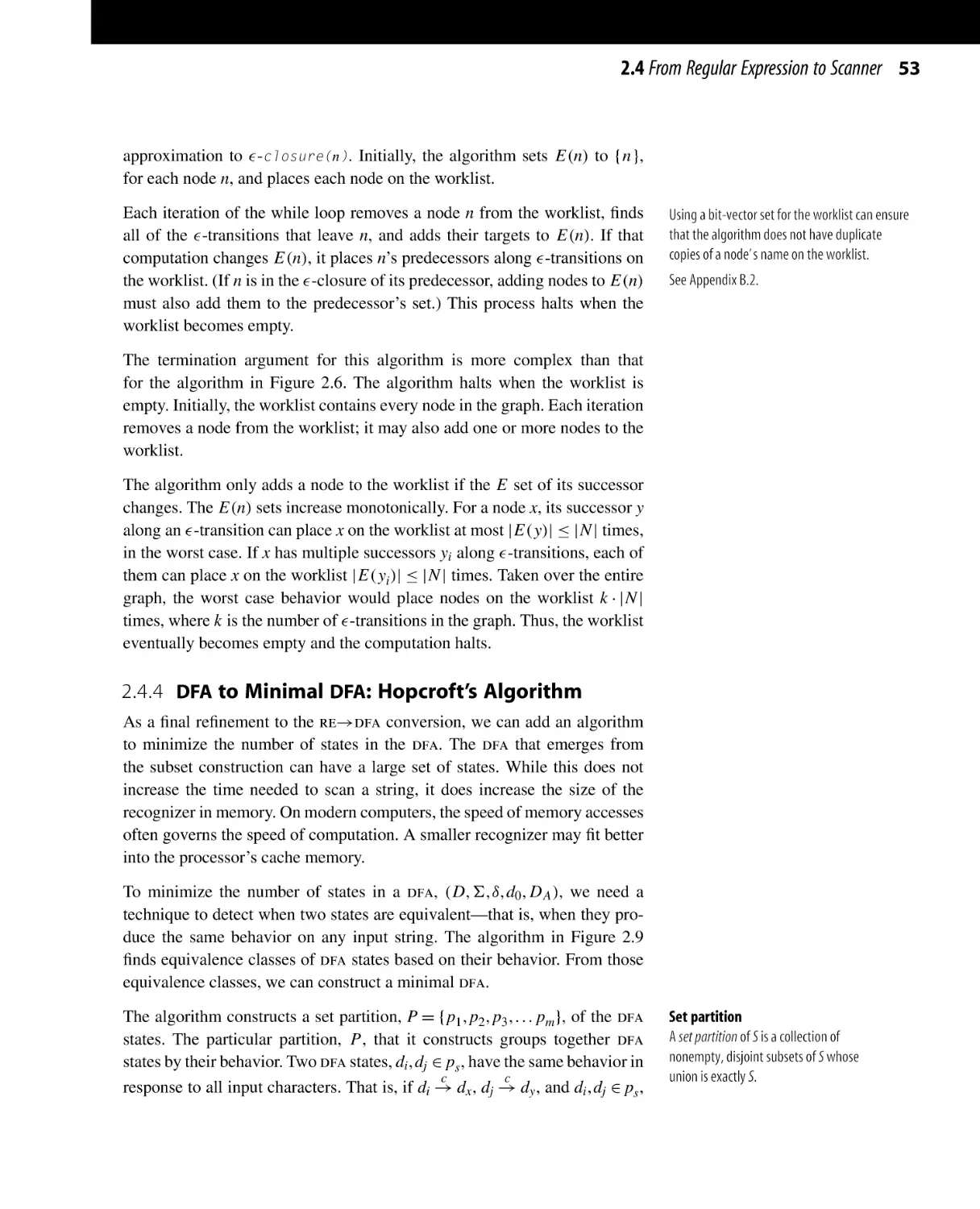


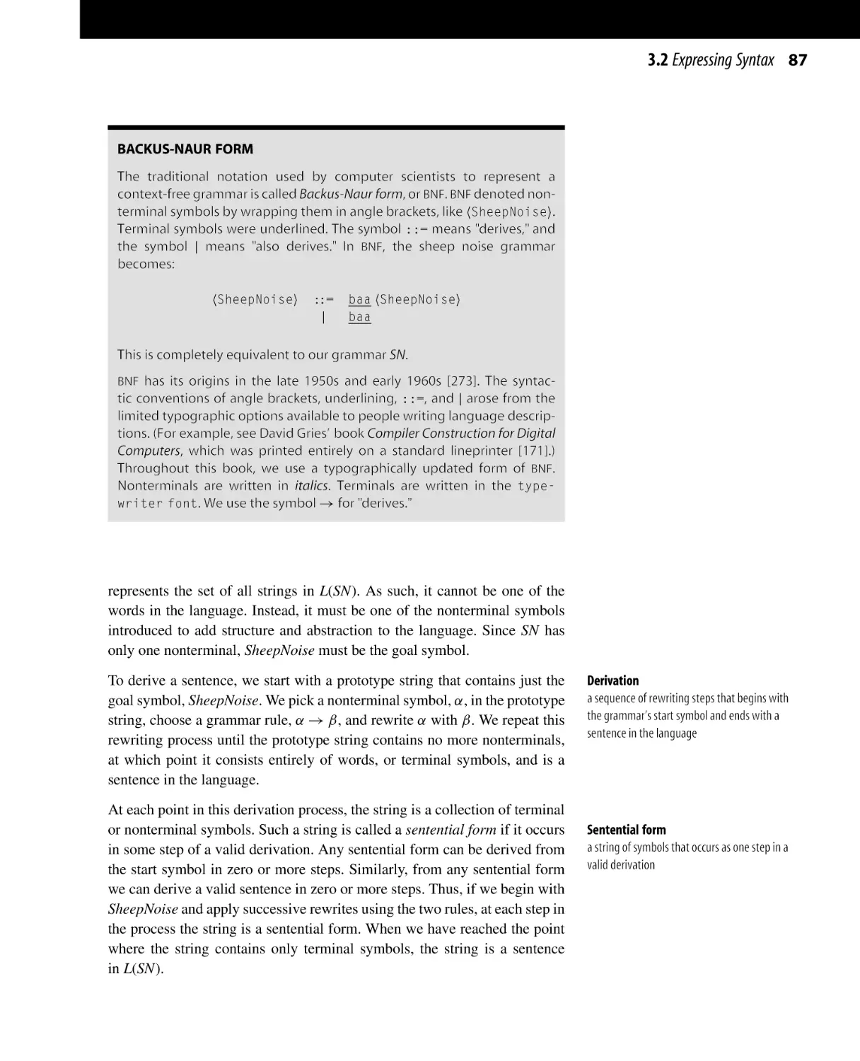


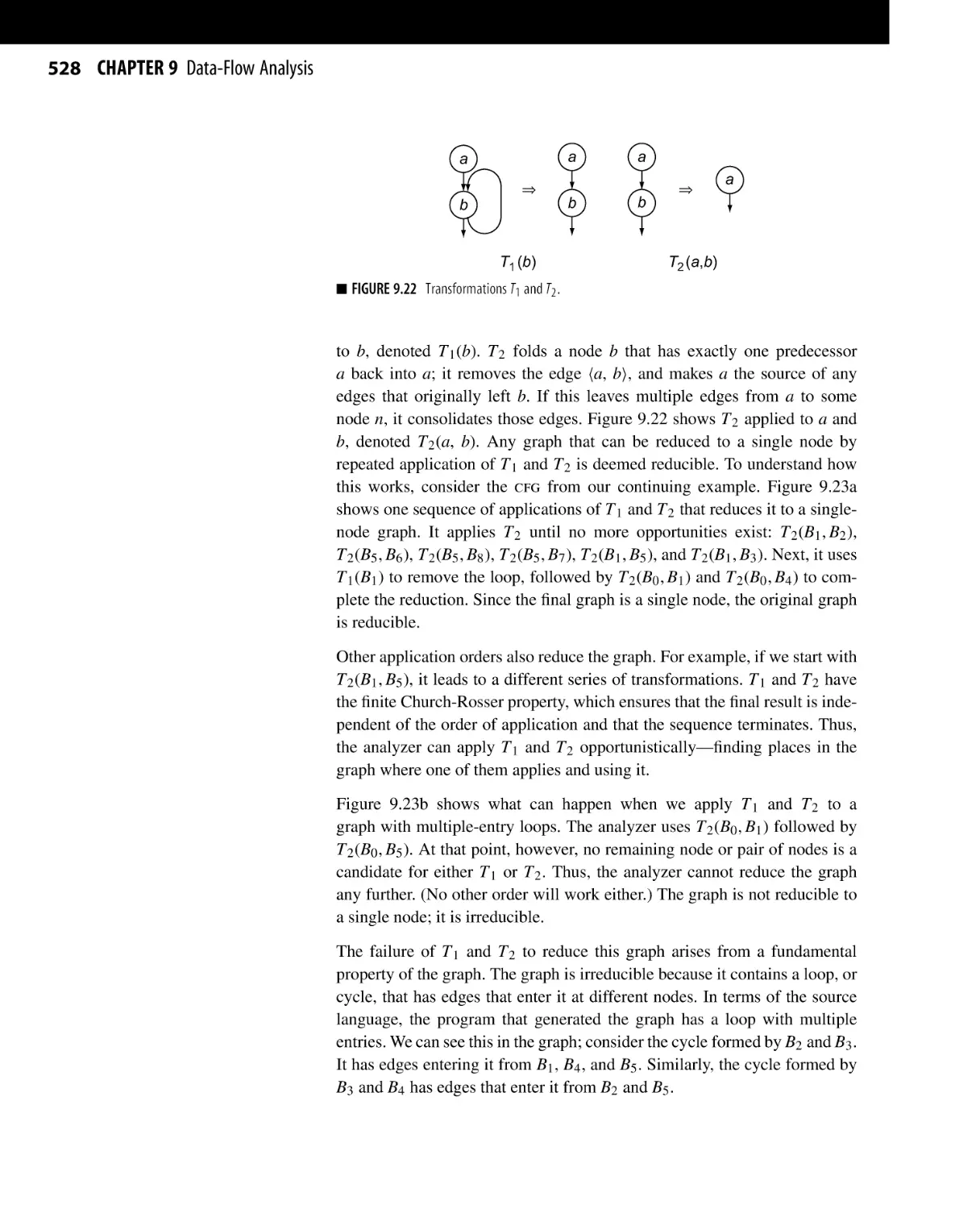


Text
In Praise of Engineering a Compiler Second Edition
Compilers are a rich area of study, drawing together the whole world of computer science in
one, elegant construction. Cooper and Torczon have succeeded in creating a welcoming guide to
these software systems, enhancing this new edition with clear lessons and the details you simply
must get right, all the while keeping the big picture firmly in view. Engineering a Compiler is an
invaluable companion for anyone new to the subject.
Michael D. Smith
Dean of the Faculty of Arts and Sciences
John H. Finley, Jr. Professor of Engineering and Applied Sciences, Harvard University
The Second Edition of Engineering a Compiler is an excellent introduction to the construction
of modern optimizing compilers. The authors draw from a wealth of experience in compiler
construction in order to help students grasp the big picture while at the same time guiding
them through many important but subtle details that must be addressed to construct an effective optimizing compiler. In particular, this book contains the best introduction to Static Single
Assignment Form that I’ve seen.
Jeffery von Ronne
Assistant Professor
Department of Computer Science
The University of Texas at San Antonio
Engineering a Compiler increases its value as a textbook with a more regular and consistent
structure, and with a host of instructional aids: review questions, extra examples, sidebars, and
marginal notes. It also includes a wealth of technical updates, including more on nontraditional
languages, real-world compilers, and nontraditional uses of compiler technology. The optimization material—already a signature strength—has become even more accessible and clear.
Michael L. Scott
Professor
Computer Science Department
University of Rochester
Author of Programming Language Pragmatics
Keith Cooper and Linda Torczon present an effective treatment of the history as well as a
practitioner’s perspective of how compilers are developed. Theory as well as practical real
world examples of existing compilers (i.e. LISP, FORTRAN, etc.) comprise a multitude of effective discussions and illustrations. Full circle discussion of introductory along with advanced
“allocation” and “optimization” concepts encompass an effective “life-cycle” of compiler
engineering. This text should be on every bookshelf of computer science students as well as
professionals involved with compiler engineering and development.
David Orleans
Nova Southeastern University
This page intentionally left blank
Engineering a Compiler
Second Edition
About the Authors
Keith D. Cooper is the Doerr Professor of Computational Engineering at Rice University. He
has worked on a broad collection of problems in optimization of compiled code, including interprocedural data-flow analysis and its applications, value numbering, algebraic reassociation,
register allocation, and instruction scheduling. His recent work has focused on a fundamental
reexamination of the structure and behavior of traditional compilers. He has taught a variety of
courses at the undergraduate level, from introductory programming through code optimization
at the graduate level. He is a Fellow of the ACM.
Linda Torczon, Senior Research Scientist, Department of Computer Science at Rice University, is a principal investigator on the Platform-Aware Compilation Environment project
(PACE), a DARPA-sponsored project that is developing an optimizing compiler environment
which automatically adjusts its optimizations and strategies to new platforms. From 1990 to
2000, Dr. Torczon served as executive director of the Center for Research on Parallel Computation (CRPC), a National Science Foundation Science and Technology Center. She also served
as the executive director of HiPerSoft, of the Los Alamos Computer Science Institute, and of
the Virtual Grid Application Development Software Project (VGrADS).
Engineering a Compiler
Second Edition
Keith D. Cooper
Linda Torczon
Rice University
Houston, Texas
AMSTERDAM • BOSTON • HEIDELBERG • LONDON
NEW YORK • OXFORD • PARIS • SAN DIEGO
SAN FRANCISCO • SINGAPORE • SYDNEY • TOKYO
Morgan Kaufmann Publishers is an imprint of Elsevier
Acquiring Editor: Todd Green
Development Editor: Nate McFadden
Project Manager: Andre Cuello
Designer: Alisa Andreola
Cover Image: “The Landing of the Ark,” a vaulted ceiling-design whose iconography was narrated, designed, and drawn by John
Outram of John Outram Associates, Architects and City Planners, London, England. To read more visit www.johnoutram.com/rice.html.
Morgan Kaufmann is an imprint of Elsevier.
30 Corporate Drive, Suite 400, Burlington, MA 01803, USA
Copyright © 2012 Elsevier, Inc. All rights reserved.
No part of this publication may be reproduced or transmitted in any form or by any means, electronic or mechanical, including
photocopying, recording, or any information storage and retrieval system, without permission in writing from the publisher. Details on
how to seek permission, further information about the Publisher’s permissions policies and our arrangements with organizations such as
the Copyright Clearance Center and the Copyright Licensing Agency, can be found at our website: www.elsevier.com/permissions.
This book and the individual contributions contained in it are protected under copyright by the Publisher (other than as may be noted
herein).
Notices
Knowledge and best practice in this field are constantly changing. As new research and experience broaden our understanding, changes
in research methods or professional practices may become necessary. Practitioners and researchers must always rely on their own
experience and knowledge in evaluating and using any information or methods described herein. In using such information or methods
they should be mindful of their own safety and the safety of others, including parties for whom they have a professional responsibility.
To the fullest extent of the law, neither the Publisher nor the authors, contributors, or editors, assume any liability for any injury and/or
damage to persons or property as a matter of products liability, negligence or otherwise, or from any use or operation of any methods,
products, instructions, or ideas contained in the material herein.
Library of Congress Cataloging-in-Publication Data
Application submitted
British Library Cataloguing-in-Publication Data
A catalogue record for this book is available from the British Library.
ISBN: 978-0-12-088478-0
For information on all Morgan Kaufmann publications
visit our website at www.mkp.com
Printed in the United States of America
11 12 13 14 10 9 8 7 6 5 4 3 2 1
We dedicate this volume to
n
n
n
our parents, who instilled in us the thirst for knowledge and supported
us as we developed the skills to follow our quest for knowledge;
our children, who have shown us again how wonderful the process of
learning and growing can be; and
our spouses, without whom this book would never have been written.
About the Cover
The cover of this book features a portion of the drawing, “The Landing of the Ark,” which
decorates the ceiling of Duncan Hall at Rice University. Both Duncan Hall and its ceiling were
designed by British architect John Outram. Duncan Hall is an outward expression of architectural, decorative, and philosophical themes developed over Outram’s career as an architect. The
decorated ceiling of the ceremonial hall plays a central role in the building’s decorative scheme.
Outram inscribed the ceiling with a set of significant ideas—a creation myth. By expressing
those ideas in an allegorical drawing of vast size and intense color, Outram created a signpost
that tells visitors who wander into the hall that, indeed, this building is not like other buildings.
By using the same signpost on the cover of Engineering a Compiler, the authors intend to signal
that this work contains significant ideas that are at the core of their discipline. Like Outram’s
building, this volume is the culmination of intellectual themes developed over the authors’
professional careers. Like Outram’s decorative scheme, this book is a device for communicating
ideas. Like Outram’s ceiling, it presents significant ideas in new ways.
By connecting the design and construction of compilers with the design and construction of
buildings, we intend to convey the many similarities in these two distinct activities. Our many
long discussions with Outram introduced us to the Vitruvian ideals for architecture: commodity,
firmness, and delight. These ideals apply to many kinds of construction. Their analogs for compiler construction are consistent themes of this text: function, structure, and elegance. Function
matters; a compiler that generates incorrect code is useless. Structure matters; engineering detail
determines a compiler’s efficiency and robustness. Elegance matters; a well-designed compiler,
in which the algorithms and data structures flow smoothly from one pass to another, can be a
thing of beauty.
We are delighted to have John Outram’s work grace the cover of this book.
Duncan Hall’s ceiling is an interesting technological artifact. Outram drew the original design
on one sheet of paper. It was photographed and scanned at 1200 dpi yielding roughly 750 mb
of data. The image was enlarged to form 234 distinct 2 × 8 foot panels, creating a 52 × 72 foot
image. The panels were printed onto oversize sheets of perforated vinyl using a 12 dpi acrylicink printer. These sheets were precision mounted onto 2 × 8 foot acoustic tiles and hung on the
vault’s aluminum frame.
viii
Contents
About the Authors . . . . . . . . . . . . . . . . . . . . . . . . . . . . . . . . . . . . . . . . . . . . . . . . . . . . . . . . . . . . . . . . . . . . . . . . iv
About the Cover . . . . . . . . . . . . . . . . . . . . . . . . . . . . . . . . . . . . . . . . . . . . . . . . . . . . . . . . . . . . . . . . . . . . . . . . . . viii
Preface . . . . . . . . . . . . . . . . . . . . . . . . . . . . . . . . . . . . . . . . . . . . . . . . . . . . . . . . . . . . . . . . . . . . . . . . . . . . . . . . . . . . . xix
CHAPTER 1 Overview of Compilation . . . . . . . . . . . . . . . . . . . . . . . . . . . . . . . . . . . . . . . . . . . . . . . . . . .
1.1
1.2
1.3
1.4
Introduction . . . . . . . . . . . . . . . . . . . . . . . . . . . . . . . . . . . . . . . . . . . . . . . . . . . . . . . . . .
Compiler Structure . . . . . . . . . . . . . . . . . . . . . . . . . . . . . . . . . . . . . . . . . . . . . . . . . . .
Overview of Translation . . . . . . . . . . . . . . . . . . . . . . . . . . . . . . . . . . . . . . . . . . . . .
1.3.1 The Front End . . . . . . . . . . . . . . . . . . . . . . . . . . . . . . . . . . . . . . . . . . . . . . . . .
1.3.2 The Optimizer . . . . . . . . . . . . . . . . . . . . . . . . . . . . . . . . . . . . . . . . . . . . . . . . .
1.3.3 The Back End . . . . . . . . . . . . . . . . . . . . . . . . . . . . . . . . . . . . . . . . . . . . . . . . .
Summary and Perspective . . . . . . . . . . . . . . . . . . . . . . . . . . . . . . . . . . . . . . . . . . .
Chapter Notes . . . . . . . . . . . . . . . . . . . . . . . . . . . . . . . . . . . . . . . . . . . . . . . . . . . . . . . .
Exercises . . . . . . . . . . . . . . . . . . . . . . . . . . . . . . . . . . . . . . . . . . . . . . . . . . . . . . . . . . . . .
1
1
6
9
10
14
15
21
22
23
CHAPTER 2 Scanners . . . . . . . . . . . . . . . . . . . . . . . . . . . . . . . . . . . . . . . . . . . . . . . . . . . . . . . . . . . . . . . . . . . . . . 25
2.1
2.2
2.3
2.4
2.5
Introduction . . . . . . . . . . . . . . . . . . . . . . . . . . . . . . . . . . . . . . . . . . . . . . . . . . . . . . . . . .
Recognizing Words . . . . . . . . . . . . . . . . . . . . . . . . . . . . . . . . . . . . . . . . . . . . . . . . . .
2.2.1 A Formalism for Recognizers . . . . . . . . . . . . . . . . . . . . . . . . . . . . . . . .
2.2.2 Recognizing More Complex Words . . . . . . . . . . . . . . . . . . . . . . . . . .
Regular Expressions . . . . . . . . . . . . . . . . . . . . . . . . . . . . . . . . . . . . . . . . . . . . . . . . .
2.3.1 Formalizing the Notation . . . . . . . . . . . . . . . . . . . . . . . . . . . . . . . . . . . . .
2.3.2 Examples . . . . . . . . . . . . . . . . . . . . . . . . . . . . . . . . . . . . . . . . . . . . . . . . . . . . . .
2.3.3 Closure Properties of REs . . . . . . . . . . . . . . . . . . . . . . . . . . . . . . . . . . . .
From Regular Expression to Scanner . . . . . . . . . . . . . . . . . . . . . . . . . . . . . . .
2.4.1 Nondeterministic Finite Automata . . . . . . . . . . . . . . . . . . . . . . . . . . .
2.4.2 Regular Expression to NFA: Thompson’s
Construction . . . . . . . . . . . . . . . . . . . . . . . . . . . . . . . . . . . . . . . . . . . . . . . . . . .
2.4.3 NFA to DFA: The Subset Construction . . . . . . . . . . . . . . . . . . . . . .
2.4.4 DFA to Minimal DFA: Hopcroft’s Algorithm . . . . . . . . . . . . . . .
2.4.5 Using a DFA as a Recognizer . . . . . . . . . . . . . . . . . . . . . . . . . . . . . . .
Implementing Scanners . . . . . . . . . . . . . . . . . . . . . . . . . . . . . . . . . . . . . . . . . . . . . .
2.5.1 Table-Driven Scanners . . . . . . . . . . . . . . . . . . . . . . . . . . . . . . . . . . . . . . . .
2.5.2 Direct-Coded Scanners . . . . . . . . . . . . . . . . . . . . . . . . . . . . . . . . . . . . . . .
2.5.3 Hand-Coded Scanners . . . . . . . . . . . . . . . . . . . . . . . . . . . . . . . . . . . . . . . .
2.5.4 Handling Keywords . . . . . . . . . . . . . . . . . . . . . . . . . . . . . . . . . . . . . . . . . . .
25
27
29
31
34
35
36
39
42
43
45
47
53
57
59
60
65
69
72
ix
x Contents
2.6
2.7
Advanced Topics . . . . . . . . . . . . . . . . . . . . . . . . . . . . . . . . . . . . . . . . . . . . . . . . . . . . .
2.6.1 DFA to Regular Expression . . . . . . . . . . . . . . . . . . . . . . . . . . . . . . . . . .
2.6.2 Another Approach to DFA Minimization:
Brzozowski’s Algorithm . . . . . . . . . . . . . . . . . . . . . . . . . . . . . . . . . . . . . .
2.6.3 Closure-Free Regular Expressions . . . . . . . . . . . . . . . . . . . . . . . . . . .
Chapter Summary and Perspective . . . . . . . . . . . . . . . . . . . . . . . . . . . . . . . . . .
Chapter Notes . . . . . . . . . . . . . . . . . . . . . . . . . . . . . . . . . . . . . . . . . . . . . . . . . . . . . . . .
Exercises . . . . . . . . . . . . . . . . . . . . . . . . . . . . . . . . . . . . . . . . . . . . . . . . . . . . . . . . . . . . .
74
74
75
77
78
78
80
CHAPTER 3 Parsers . . . . . . . . . . . . . . . . . . . . . . . . . . . . . . . . . . . . . . . . . . . . . . . . . . . . . . . . . . . . . . . . . . . . . . . . 83
3.1
3.2
3.3
3.4
3.5
3.6
3.7
Introduction . . . . . . . . . . . . . . . . . . . . . . . . . . . . . . . . . . . . . . . . . . . . . . . . . . . . . . . . . .
Expressing Syntax . . . . . . . . . . . . . . . . . . . . . . . . . . . . . . . . . . . . . . . . . . . . . . . . . . .
3.2.1 Why Not Regular Expressions? . . . . . . . . . . . . . . . . . . . . . . . . . . . . . .
3.2.2 Context-Free Grammars . . . . . . . . . . . . . . . . . . . . . . . . . . . . . . . . . . . . . .
3.2.3 More Complex Examples . . . . . . . . . . . . . . . . . . . . . . . . . . . . . . . . . . . . .
3.2.4 Encoding Meaning into Structure . . . . . . . . . . . . . . . . . . . . . . . . . . . .
3.2.5 Discovering a Derivation for an Input String . . . . . . . . . . . . . . . .
Top-Down Parsing . . . . . . . . . . . . . . . . . . . . . . . . . . . . . . . . . . . . . . . . . . . . . . . . . . .
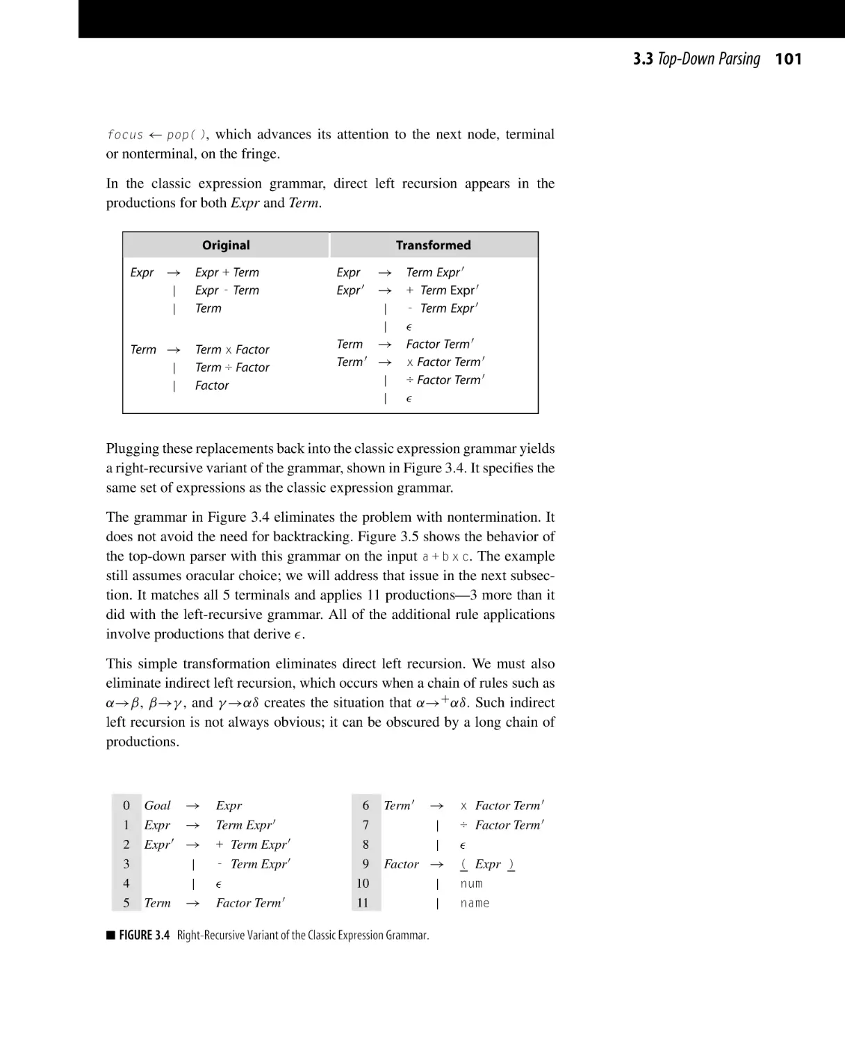
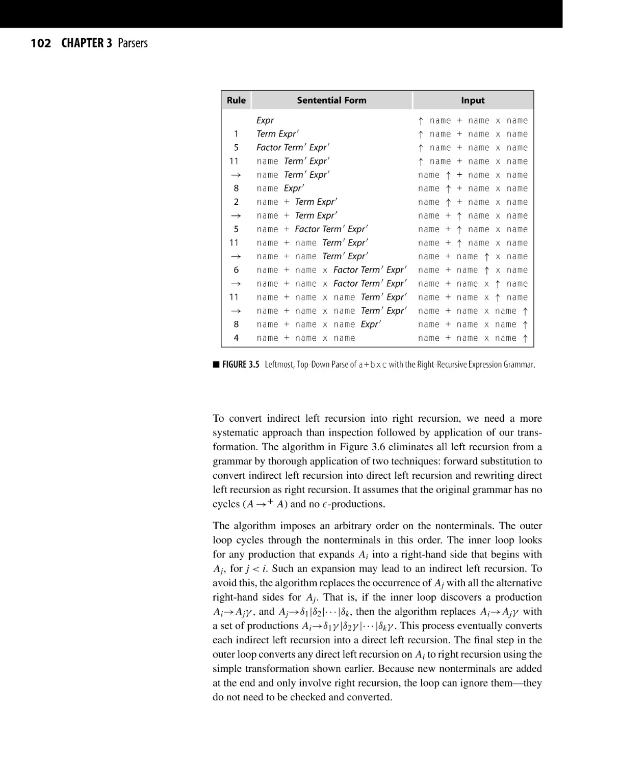
3.3.1 Transforming a Grammar for Top-Down Parsing . . . . . . . . . . .
3.3.2 Top-Down Recursive-Descent Parsers . . . . . . . . . . . . . . . . . . . . . . .
3.3.3 Table-Driven LL(1) Parsers . . . . . . . . . . . . . . . . . . . . . . . . . . . . . . . . . .
Bottom-Up Parsing . . . . . . . . . . . . . . . . . . . . . . . . . . . . . . . . . . . . . . . . . . . . . . . . . .
3.4.1 The LR(1) Parsing Algorithm . . . . . . . . . . . . . . . . . . . . . . . . . . . . . . . .
3.4.2 Building LR(1) Tables . . . . . . . . . . . . . . . . . . . . . . . . . . . . . . . . . . . . . . . .
3.4.3 Errors in the Table Construction . . . . . . . . . . . . . . . . . . . . . . . . . . . . .
Practical Issues . . . . . . . . . . . . . . . . . . . . . . . . . . . . . . . . . . . . . . . . . . . . . . . . . . . . . . .
3.5.1 Error Recovery . . . . . . . . . . . . . . . . . . . . . . . . . . . . . . . . . . . . . . . . . . . . . . . .
3.5.2 Unary Operators . . . . . . . . . . . . . . . . . . . . . . . . . . . . . . . . . . . . . . . . . . . . . .
3.5.3 Handling Context-Sensitive Ambiguity . . . . . . . . . . . . . . . . . . . . .
3.5.4 Left versus Right Recursion . . . . . . . . . . . . . . . . . . . . . . . . . . . . . . . . . .
Advanced Topics . . . . . . . . . . . . . . . . . . . . . . . . . . . . . . . . . . . . . . . . . . . . . . . . . . . . .
3.6.1 Optimizing a Grammar . . . . . . . . . . . . . . . . . . . . . . . . . . . . . . . . . . . . . . .
3.6.2 Reducing the Size of LR(1) Tables . . . . . . . . . . . . . . . . . . . . . . . . . .
Summary and Perspective . . . . . . . . . . . . . . . . . . . . . . . . . . . . . . . . . . . . . . . . . . .
Chapter Notes . . . . . . . . . . . . . . . . . . . . . . . . . . . . . . . . . . . . . . . . . . . . . . . . . . . . . . . .
Exercises . . . . . . . . . . . . . . . . . . . . . . . . . . . . . . . . . . . . . . . . . . . . . . . . . . . . . . . . . . . . .
83
85
85
86
89
92
95
96
98
108
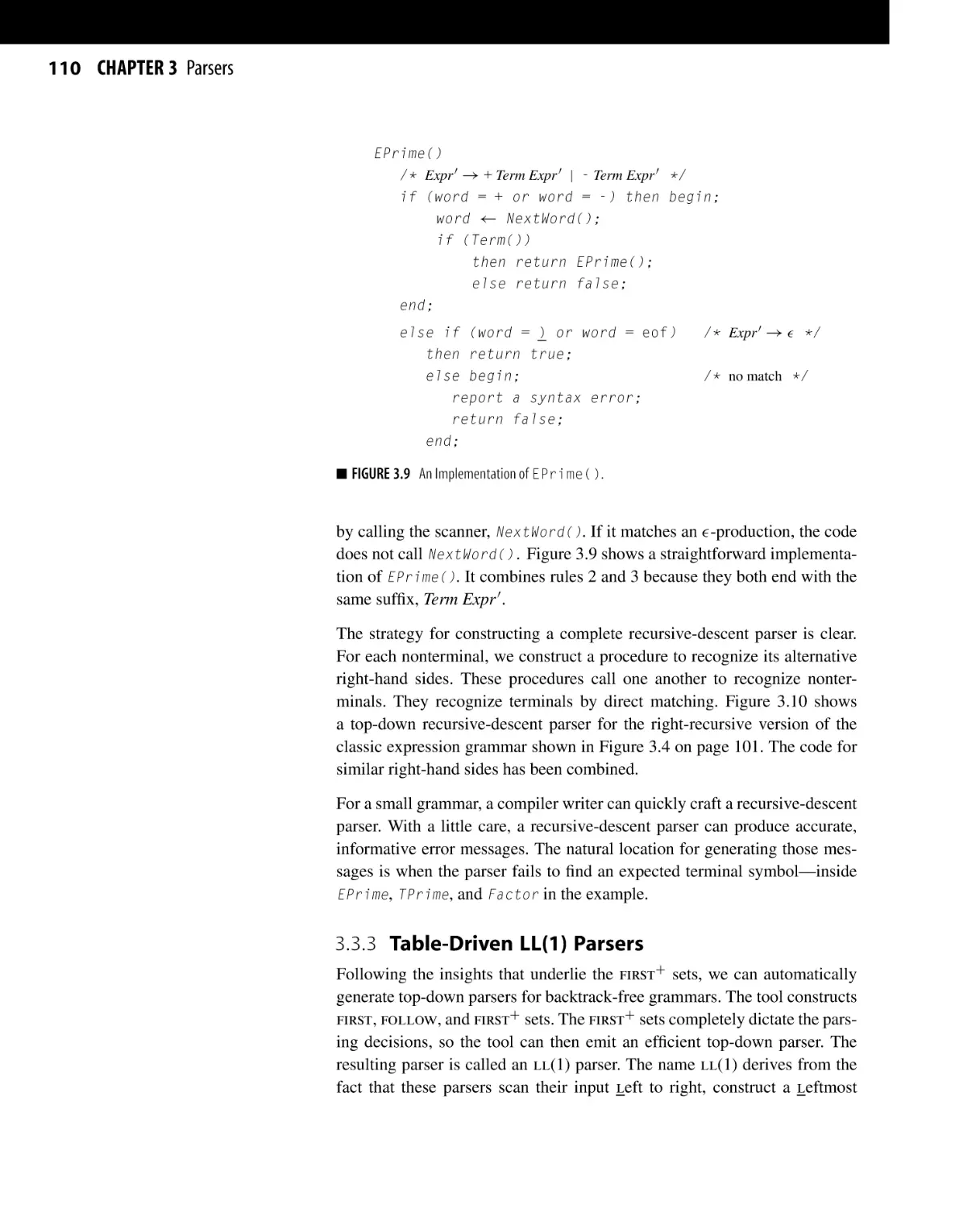
110
116
118
124
136
141
141
142
143
144
147
148
150
155
156
157
Contents xi
CHAPTER 4 Context-Sensitive Analysis . . . . . . . . . . . . . . . . . . . . . . . . . . . . . . . . . . . . . . . . . . . . . . . . . . 161
4.1
4.2
4.3
4.4
4.5
4.6
Introduction . . . . . . . . . . . . . . . . . . . . . . . . . . . . . . . . . . . . . . . . . . . . . . . . . . . . . . . . . .
An Introduction to Type Systems . . . . . . . . . . . . . . . . . . . . . . . . . . . . . . . . . . .
4.2.1 The Purpose of Type Systems . . . . . . . . . . . . . . . . . . . . . . . . . . . . . . . .
4.2.2 Components of a Type System . . . . . . . . . . . . . . . . . . . . . . . . . . . . . . .
The Attribute-Grammar Framework . . . . . . . . . . . . . . . . . . . . . . . . . . . . . . . .
4.3.1 Evaluation Methods . . . . . . . . . . . . . . . . . . . . . . . . . . . . . . . . . . . . . . . . . . .
4.3.2 Circularity . . . . . . . . . . . . . . . . . . . . . . . . . . . . . . . . . . . . . . . . . . . . . . . . . . . . .
4.3.3 Extended Examples . . . . . . . . . . . . . . . . . . . . . . . . . . . . . . . . . . . . . . . . . . .
4.3.4 Problems with the Attribute-Grammar Approach . . . . . . . . . . .
Ad Hoc Syntax-Directed Translation . . . . . . . . . . . . . . . . . . . . . . . . . . . . . . .
4.4.1 Implementing Ad Hoc Syntax-Directed Translation . . . . . . . .
4.4.2 Examples . . . . . . . . . . . . . . . . . . . . . . . . . . . . . . . . . . . . . . . . . . . . . . . . . . . . . .
Advanced Topics . . . . . . . . . . . . . . . . . . . . . . . . . . . . . . . . . . . . . . . . . . . . . . . . . . . . .
4.5.1 Harder Problems in Type Inference . . . . . . . . . . . . . . . . . . . . . . . . . .
4.5.2 Changing Associativity . . . . . . . . . . . . . . . . . . . . . . . . . . . . . . . . . . . . . . .
Summary and Perspective . . . . . . . . . . . . . . . . . . . . . . . . . . . . . . . . . . . . . . . . . . .
Chapter Notes . . . . . . . . . . . . . . . . . . . . . . . . . . . . . . . . . . . . . . . . . . . . . . . . . . . . . . . .
Exercises . . . . . . . . . . . . . . . . . . . . . . . . . . . . . . . . . . . . . . . . . . . . . . . . . . . . . . . . . . . . .
161
164
165
170
182
186
187
187
194
198
199
202
211
211
213
215
216
217
CHAPTER 5 Intermediate Representations . . . . . . . . . . . . . . . . . . . . . . . . . . . . . . . . . . . . . . . . . . . . . 221
5.1
5.2
5.3
5.4
Introduction . . . . . . . . . . . . . . . . . . . . . . . . . . . . . . . . . . . . . . . . . . . . . . . . . . . . . . . . . .
5.1.1 A Taxonomy of Intermediate Representations . . . . . . . . . . . . . .
Graphical IRs . . . . . . . . . . . . . . . . . . . . . . . . . . . . . . . . . . . . . . . . . . . . . . . . . . . . . . . . .
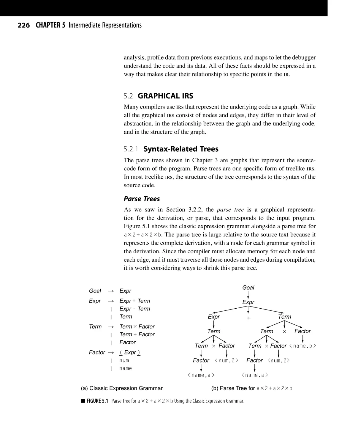
5.2.1 Syntax-Related Trees . . . . . . . . . . . . . . . . . . . . . . . . . . . . . . . . . . . . . . . . .
5.2.2 Graphs . . . . . . . . . . . . . . . . . . . . . . . . . . . . . . . . . . . . . . . . . . . . . . . . . . . . . . . . .
Linear IRs . . . . . . . . . . . . . . . . . . . . . . . . . . . . . . . . . . . . . . . . . . . . . . . . . . . . . . . . . . . .
5.3.1 Stack-Machine Code . . . . . . . . . . . . . . . . . . . . . . . . . . . . . . . . . . . . . . . . . .
5.3.2 Three-Address Code . . . . . . . . . . . . . . . . . . . . . . . . . . . . . . . . . . . . . . . . . .
5.3.3 Representing Linear Codes . . . . . . . . . . . . . . . . . . . . . . . . . . . . . . . . . . .
5.3.4 Building a Control-Flow Graph from a Linear Code . . . . . . . .
Mapping Values to Names . . . . . . . . . . . . . . . . . . . . . . . . . . . . . . . . . . . . . . . . . . .
5.4.1 Naming Temporary Values . . . . . . . . . . . . . . . . . . . . . . . . . . . . . . . . . . .
5.4.2 Static Single-Assignment Form . . . . . . . . . . . . . . . . . . . . . . . . . . . . . .
5.4.3 Memory Models . . . . . . . . . . . . . . . . . . . . . . . . . . . . . . . . . . . . . . . . . . . . . .
221
223
226
226
230
235
237
237
238
241
243
244
246
250
xii Contents
5.5
5.6
Symbol Tables . . . . . . . . . . . . . . . . . . . . . . . . . . . . . . . . . . . . . . . . . . . . . . . . . . . . . . . .
5.5.1 Hash Tables . . . . . . . . . . . . . . . . . . . . . . . . . . . . . . . . . . . . . . . . . . . . . . . . . . .
5.5.2 Building a Symbol Table . . . . . . . . . . . . . . . . . . . . . . . . . . . . . . . . . . . . .
5.5.3 Handling Nested Scopes . . . . . . . . . . . . . . . . . . . . . . . . . . . . . . . . . . . . . .
5.5.4 The Many Uses for Symbol Tables . . . . . . . . . . . . . . . . . . . . . . . . . .
5.5.5 Other Uses for Symbol Table Technology . . . . . . . . . . . . . . . . . . .
Summary and Perspective . . . . . . . . . . . . . . . . . . . . . . . . . . . . . . . . . . . . . . . . . . .
Chapter Notes . . . . . . . . . . . . . . . . . . . . . . . . . . . . . . . . . . . . . . . . . . . . . . . . . . . . . . . .
Exercises . . . . . . . . . . . . . . . . . . . . . . . . . . . . . . . . . . . . . . . . . . . . . . . . . . . . . . . . . . . . .
253
254
255
256
261
263
264
264
265
CHAPTER 6 The Procedure Abstraction . . . . . . . . . . . . . . . . . . . . . . . . . . . . . . . . . . . . . . . . . . . . . . . . . 269
6.1
6.2
6.3
6.4
6.5
6.6
6.7
Introduction . . . . . . . . . . . . . . . . . . . . . . . . . . . . . . . . . . . . . . . . . . . . . . . . . . . . . . . . . .
Procedure Calls . . . . . . . . . . . . . . . . . . . . . . . . . . . . . . . . . . . . . . . . . . . . . . . . . . . . . .
Name Spaces . . . . . . . . . . . . . . . . . . . . . . . . . . . . . . . . . . . . . . . . . . . . . . . . . . . . . . . . .
6.3.1 Name Spaces of Algol-like Languages . . . . . . . . . . . . . . . . . . . . . .
6.3.2 Runtime Structures to Support Algol-like
Languages . . . . . . . . . . . . . . . . . . . . . . . . . . . . . . . . . . . . . . . . . . . . . . . . . . . . .
6.3.3 Name Spaces of Object-Oriented Languages . . . . . . . . . . . . . . . .
6.3.4 Runtime Structures to Support Object-Oriented
Languages . . . . . . . . . . . . . . . . . . . . . . . . . . . . . . . . . . . . . . . . . . . . . . . . . . . . .
Communicating Values Between Procedures . . . . . . . . . . . . . . . . . . . . . . .
6.4.1 Passing Parameters . . . . . . . . . . . . . . . . . . . . . . . . . . . . . . . . . . . . . . . . . . . .
6.4.2 Returning Values . . . . . . . . . . . . . . . . . . . . . . . . . . . . . . . . . . . . . . . . . . . . . .
6.4.3 Establishing Addressability . . . . . . . . . . . . . . . . . . . . . . . . . . . . . . . . . .
Standardized Linkages . . . . . . . . . . . . . . . . . . . . . . . . . . . . . . . . . . . . . . . . . . . . . . .
Advanced Topics . . . . . . . . . . . . . . . . . . . . . . . . . . . . . . . . . . . . . . . . . . . . . . . . . . . . .
6.6.1 Explicit Heap Management . . . . . . . . . . . . . . . . . . . . . . . . . . . . . . . . . . .
6.6.2 Implicit Deallocation . . . . . . . . . . . . . . . . . . . . . . . . . . . . . . . . . . . . . . . . .
Summary and Perspective . . . . . . . . . . . . . . . . . . . . . . . . . . . . . . . . . . . . . . . . . . .
Chapter Notes . . . . . . . . . . . . . . . . . . . . . . . . . . . . . . . . . . . . . . . . . . . . . . . . . . . . . . . .
Exercises . . . . . . . . . . . . . . . . . . . . . . . . . . . . . . . . . . . . . . . . . . . . . . . . . . . . . . . . . . . . .
269
272
276
276
280
285
290
297
297
301
301
308
312
313
317
322
323
324
CHAPTER 7 Code Shape . . . . . . . . . . . . . . . . . . . . . . . . . . . . . . . . . . . . . . . . . . . . . . . . . . . . . . . . . . . . . . . . . . . 331
7.1
7.2
7.3
Introduction . . . . . . . . . . . . . . . . . . . . . . . . . . . . . . . . . . . . . . . . . . . . . . . . . . . . . . . . . .
Assigning Storage Locations . . . . . . . . . . . . . . . . . . . . . . . . . . . . . . . . . . . . . . . .
7.2.1 Placing Runtime Data Structures . . . . . . . . . . . . . . . . . . . . . . . . . . . . .
7.2.2 Layout for Data Areas . . . . . . . . . . . . . . . . . . . . . . . . . . . . . . . . . . . . . . . .
7.2.3 Keeping Values in Registers . . . . . . . . . . . . . . . . . . . . . . . . . . . . . . . . . .
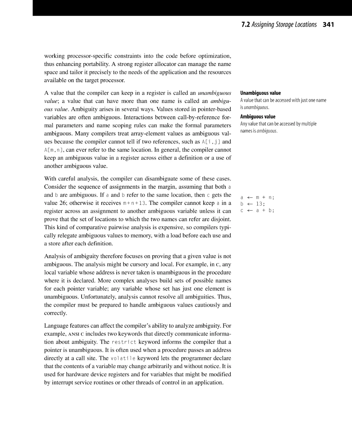
Arithmetic Operators . . . . . . . . . . . . . . . . . . . . . . . . . . . . . . . . . . . . . . . . . . . . . . . .
7.3.1 Reducing Demand for Registers . . . . . . . . . . . . . . . . . . . . . . . . . . . . .
331
334
335
336
340
342
344
Contents xiii
7.3.2 Accessing Parameter Values . . . . . . . . . . . . . . . . . . . . . . . . . . . . . . . . . .
7.3.3 Function Calls in an Expression . . . . . . . . . . . . . . . . . . . . . . . . . . . . . .
7.3.4 Other Arithmetic Operators . . . . . . . . . . . . . . . . . . . . . . . . . . . . . . . . . .
7.3.5 Mixed-Type Expressions . . . . . . . . . . . . . . . . . . . . . . . . . . . . . . . . . . . . .
7.3.6 Assignment as an Operator . . . . . . . . . . . . . . . . . . . . . . . . . . . . . . . . . . .
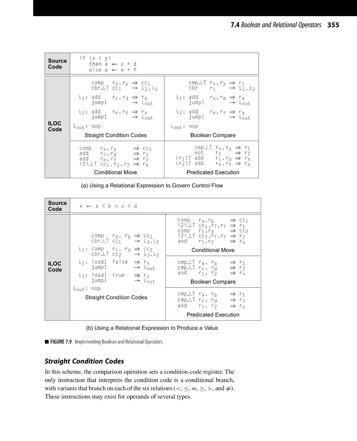
7.4 Boolean and Relational Operators . . . . . . . . . . . . . . . . . . . . . . . . . . . . . . . . . .
7.4.1 Representations . . . . . . . . . . . . . . . . . . . . . . . . . . . . . . . . . . . . . . . . . . . . . . .
7.4.2 Hardware Support for Relational Operations . . . . . . . . . . . . . . . .
7.5 Storing and Accessing Arrays . . . . . . . . . . . . . . . . . . . . . . . . . . . . . . . . . . . . . . .
7.5.1 Referencing a Vector Element . . . . . . . . . . . . . . . . . . . . . . . . . . . . . . . .
7.5.2 Array Storage Layout . . . . . . . . . . . . . . . . . . . . . . . . . . . . . . . . . . . . . . . . .
7.5.3 Referencing an Array Element . . . . . . . . . . . . . . . . . . . . . . . . . . . . . . .
7.5.4 Range Checking . . . . . . . . . . . . . . . . . . . . . . . . . . . . . . . . . . . . . . . . . . . . . . .
7.6 Character Strings . . . . . . . . . . . . . . . . . . . . . . . . . . . . . . . . . . . . . . . . . . . . . . . . . . . . .
7.6.1 String Representations . . . . . . . . . . . . . . . . . . . . . . . . . . . . . . . . . . . . . . . .
7.6.2 String Assignment . . . . . . . . . . . . . . . . . . . . . . . . . . . . . . . . . . . . . . . . . . . .
7.6.3 String Concatenation . . . . . . . . . . . . . . . . . . . . . . . . . . . . . . . . . . . . . . . . . .
7.6.4 String Length . . . . . . . . . . . . . . . . . . . . . . . . . . . . . . . . . . . . . . . . . . . . . . . . . .
7.7 Structure References . . . . . . . . . . . . . . . . . . . . . . . . . . . . . . . . . . . . . . . . . . . . . . . . .
7.7.1 Understanding Structure Layouts . . . . . . . . . . . . . . . . . . . . . . . . . . . .
7.7.2 Arrays of Structures . . . . . . . . . . . . . . . . . . . . . . . . . . . . . . . . . . . . . . . . . . .
7.7.3 Unions and Runtime Tags . . . . . . . . . . . . . . . . . . . . . . . . . . . . . . . . . . . .
7.7.4 Pointers and Anonymous Values . . . . . . . . . . . . . . . . . . . . . . . . . . . . .
7.8 Control-Flow Constructs . . . . . . . . . . . . . . . . . . . . . . . . . . . . . . . . . . . . . . . . . . . .
7.8.1 Conditional Execution . . . . . . . . . . . . . . . . . . . . . . . . . . . . . . . . . . . . . . . .
7.8.2 Loops and Iteration . . . . . . . . . . . . . . . . . . . . . . . . . . . . . . . . . . . . . . . . . . .
7.8.3 Case Statements . . . . . . . . . . . . . . . . . . . . . . . . . . . . . . . . . . . . . . . . . . . . . . .
7.9 Procedure Calls . . . . . . . . . . . . . . . . . . . . . . . . . . . . . . . . . . . . . . . . . . . . . . . . . . . . . .
7.9.1 Evaluating Actual Parameters . . . . . . . . . . . . . . . . . . . . . . . . . . . . . . . .
7.9.2 Saving and Restoring Registers . . . . . . . . . . . . . . . . . . . . . . . . . . . . . .
7.10 Summary and Perspective . . . . . . . . . . . . . . . . . . . . . . . . . . . . . . . . . . . . . . . . . . .
Chapter Notes . . . . . . . . . . . . . . . . . . . . . . . . . . . . . . . . . . . . . . . . . . . . . . . . . . . . . . . .
Exercises . . . . . . . . . . . . . . . . . . . . . . . . . . . . . . . . . . . . . . . . . . . . . . . . . . . . . . . . . . . . .
345
347
348
348
349
350
351
353
359
359
361
362
367
369
370
370
372
373
374
375
376
377
378
380
381
384
388
392
393
394
396
397
398
CHAPTER 8 Introduction to Optimization . . . . . . . . . . . . . . . . . . . . . . . . . . . . . . . . . . . . . . . . . . . . . . 405
8.1
8.2
Introduction . . . . . . . . . . . . . . . . . . . . . . . . . . . . . . . . . . . . . . . . . . . . . . . . . . . . . . . . . .
Background . . . . . . . . . . . . . . . . . . . . . . . . . . . . . . . . . . . . . . . . . . . . . . . . . . . . . . . . . . .
8.2.1 Examples . . . . . . . . . . . . . . . . . . . . . . . . . . . . . . . . . . . . . . . . . . . . . . . . . . . . . .
8.2.2 Considerations for Optimization . . . . . . . . . . . . . . . . . . . . . . . . . . . . .
8.2.3 Opportunities for Optimization . . . . . . . . . . . . . . . . . . . . . . . . . . . . . . .
405
407
408
412
415
xiv Contents
8.3
8.4
8.5
8.6
8.7
8.8
Scope of Optimization . . . . . . . . . . . . . . . . . . . . . . . . . . . . . . . . . . . . . . . . . . . . . . .
Local Optimization . . . . . . . . . . . . . . . . . . . . . . . . . . . . . . . . . . . . . . . . . . . . . . . . . .
8.4.1 Local Value Numbering . . . . . . . . . . . . . . . . . . . . . . . . . . . . . . . . . . . . . .
8.4.2 Tree-Height Balancing . . . . . . . . . . . . . . . . . . . . . . . . . . . . . . . . . . . . . . . .
Regional Optimization . . . . . . . . . . . . . . . . . . . . . . . . . . . . . . . . . . . . . . . . . . . . . . .
8.5.1 Superlocal Value Numbering . . . . . . . . . . . . . . . . . . . . . . . . . . . . . . . . .
8.5.2 Loop Unrolling . . . . . . . . . . . . . . . . . . . . . . . . . . . . . . . . . . . . . . . . . . . . . . . .
Global Optimization . . . . . . . . . . . . . . . . . . . . . . . . . . . . . . . . . . . . . . . . . . . . . . . . .
8.6.1 Finding Uninitialized Variables with Live
Information . . . . . . . . . . . . . . . . . . . . . . . . . . . . . . . . . . . . . . . . . . . . . . . . . . . .
8.6.2 Global Code Placement . . . . . . . . . . . . . . . . . . . . . . . . . . . . . . . . . . . . . . .
Interprocedural Optimization . . . . . . . . . . . . . . . . . . . . . . . . . . . . . . . . . . . . . . . .
8.7.1 Inline Substitution . . . . . . . . . . . . . . . . . . . . . . . . . . . . . . . . . . . . . . . . . . . .
8.7.2 Procedure Placement . . . . . . . . . . . . . . . . . . . . . . . . . . . . . . . . . . . . . . . . . .
8.7.3 Compiler Organization for Interprocedural
Optimization . . . . . . . . . . . . . . . . . . . . . . . . . . . . . . . . . . . . . . . . . . . . . . . . . .
Summary and Perspective . . . . . . . . . . . . . . . . . . . . . . . . . . . . . . . . . . . . . . . . . . .
Chapter Notes . . . . . . . . . . . . . . . . . . . . . . . . . . . . . . . . . . . . . . . . . . . . . . . . . . . . . . . .
Exercises . . . . . . . . . . . . . . . . . . . . . . . . . . . . . . . . . . . . . . . . . . . . . . . . . . . . . . . . . . . . .
417
420
420
428
437
437
441
445
445
451
457
458
462
467
469
470
471
CHAPTER 9 Data-Flow Analysis . . . . . . . . . . . . . . . . . . . . . . . . . . . . . . . . . . . . . . . . . . . . . . . . . . . . . . . . . . 475
9.1
9.2
9.3
9.4
9.5
Introduction . . . . . . . . . . . . . . . . . . . . . . . . . . . . . . . . . . . . . . . . . . . . . . . . . . . . . . . . . .
Iterative Data-Flow Analysis . . . . . . . . . . . . . . . . . . . . . . . . . . . . . . . . . . . . . . . .
9.2.1 Dominance . . . . . . . . . . . . . . . . . . . . . . . . . . . . . . . . . . . . . . . . . . . . . . . . . . . .
9.2.2 Live-Variable Analysis . . . . . . . . . . . . . . . . . . . . . . . . . . . . . . . . . . . . . . .
9.2.3 Limitations on Data-Flow Analysis . . . . . . . . . . . . . . . . . . . . . . . . . .
9.2.4 Other Data-Flow Problems . . . . . . . . . . . . . . . . . . . . . . . . . . . . . . . . . . .
Static Single-Assignment Form . . . . . . . . . . . . . . . . . . . . . . . . . . . . . . . . . . . . .
9.3.1 A Simple Method for Building SSA Form . . . . . . . . . . . . . . . . . .
9.3.2 Dominance Frontiers . . . . . . . . . . . . . . . . . . . . . . . . . . . . . . . . . . . . . . . . . .
9.3.3 Placing φ-Functions . . . . . . . . . . . . . . . . . . . . . . . . . . . . . . . . . . . . . . . . . .
9.3.4 Renaming . . . . . . . . . . . . . . . . . . . . . . . . . . . . . . . . . . . . . . . . . . . . . . . . . . . . . .
9.3.5 Translation Out of SSA Form . . . . . . . . . . . . . . . . . . . . . . . . . . . . . . . .
9.3.6 Using SSA Form . . . . . . . . . . . . . . . . . . . . . . . . . . . . . . . . . . . . . . . . . . . . . .
Interprocedural Analysis . . . . . . . . . . . . . . . . . . . . . . . . . . . . . . . . . . . . . . . . . . . . .
9.4.1 Call-Graph Construction . . . . . . . . . . . . . . . . . . . . . . . . . . . . . . . . . . . . . .
9.4.2 Interprocedural Constant Propagation . . . . . . . . . . . . . . . . . . . . . . .
Advanced Topics . . . . . . . . . . . . . . . . . . . . . . . . . . . . . . . . . . . . . . . . . . . . . . . . . . . . .
9.5.1 Structural Data-Flow Algorithms and Reducibility . . . . . . . . .
9.5.2 Speeding up the Iterative Dominance Framework . . . . . . . . . .
475
477
478
482
487
490
495
496
497
500
505
510
515
519
520
522
526
527
530
Contents xv
9.6 Summary and Perspective . . . . . . . . . . . . . . . . . . . . . . . . . . . . . . . . . . . . . . . . . . . 533
Chapter Notes . . . . . . . . . . . . . . . . . . . . . . . . . . . . . . . . . . . . . . . . . . . . . . . . . . . . . . . . 534
Exercises . . . . . . . . . . . . . . . . . . . . . . . . . . . . . . . . . . . . . . . . . . . . . . . . . . . . . . . . . . . . . 535
CHAPTER 10 Scalar Optimizations . . . . . . . . . . . . . . . . . . . . . . . . . . . . . . . . . . . . . . . . . . . . . . . . . . . . . . . . . . 539
10.1 Introduction . . . . . . . . . . . . . . . . . . . . . . . . . . . . . . . . . . . . . . . . . . . . . . . . . . . . . . . . . . . . .
10.2 Eliminating Useless and Unreachable Code . . . . . . . . . . . . . . . . . . . . . . . .
10.2.1 Eliminating Useless Code . . . . . . . . . . . . . . . . . . . . . . . . . . . . . . . . . . . .
10.2.2 Eliminating Useless Control Flow . . . . . . . . . . . . . . . . . . . . . . . . . .
10.2.3 Eliminating Unreachable Code . . . . . . . . . . . . . . . . . . . . . . . . . . . . . .
10.3 Code Motion . . . . . . . . . . . . . . . . . . . . . . . . . . . . . . . . . . . . . . . . . . . . . . . . . . . . . . . . . . .
10.3.1 Lazy Code Motion . . . . . . . . . . . . . . . . . . . . . . . . . . . . . . . . . . . . . . . . . . . .
10.3.2 Code Hoisting . . . . . . . . . . . . . . . . . . . . . . . . . . . . . . . . . . . . . . . . . . . . . . . . .
10.4 Specialization . . . . . . . . . . . . . . . . . . . . . . . . . . . . . . . . . . . . . . . . . . . . . . . . . . . . . . . . . .
10.4.1 Tail-Call Optimization . . . . . . . . . . . . . . . . . . . . . . . . . . . . . . . . . . . . . . . .
10.4.2 Leaf-Call Optimization . . . . . . . . . . . . . . . . . . . . . . . . . . . . . . . . . . . . . . .
10.4.3 Parameter Promotion . . . . . . . . . . . . . . . . . . . . . . . . . . . . . . . . . . . . . . . . .
10.5 Redundancy Elimination . . . . . . . . . . . . . . . . . . . . . . . . . . . . . . . . . . . . . . . . . . . . . .
10.5.1 Value Identity versus Name Identity . . . . . . . . . . . . . . . . . . . . . . . .
10.5.2 Dominator-based Value Numbering . . . . . . . . . . . . . . . . . . . . . . . . .
10.6 Enabling Other Transformations . . . . . . . . . . . . . . . . . . . . . . . . . . . . . . . . . . . . .
10.6.1 Superblock Cloning . . . . . . . . . . . . . . . . . . . . . . . . . . . . . . . . . . . . . . . . . . .
10.6.2 Procedure Cloning . . . . . . . . . . . . . . . . . . . . . . . . . . . . . . . . . . . . . . . . . . . .
10.6.3 Loop Unswitching . . . . . . . . . . . . . . . . . . . . . . . . . . . . . . . . . . . . . . . . . . . .
10.6.4 Renaming . . . . . . . . . . . . . . . . . . . . . . . . . . . . . . . . . . . . . . . . . . . . . . . . . . . . . .
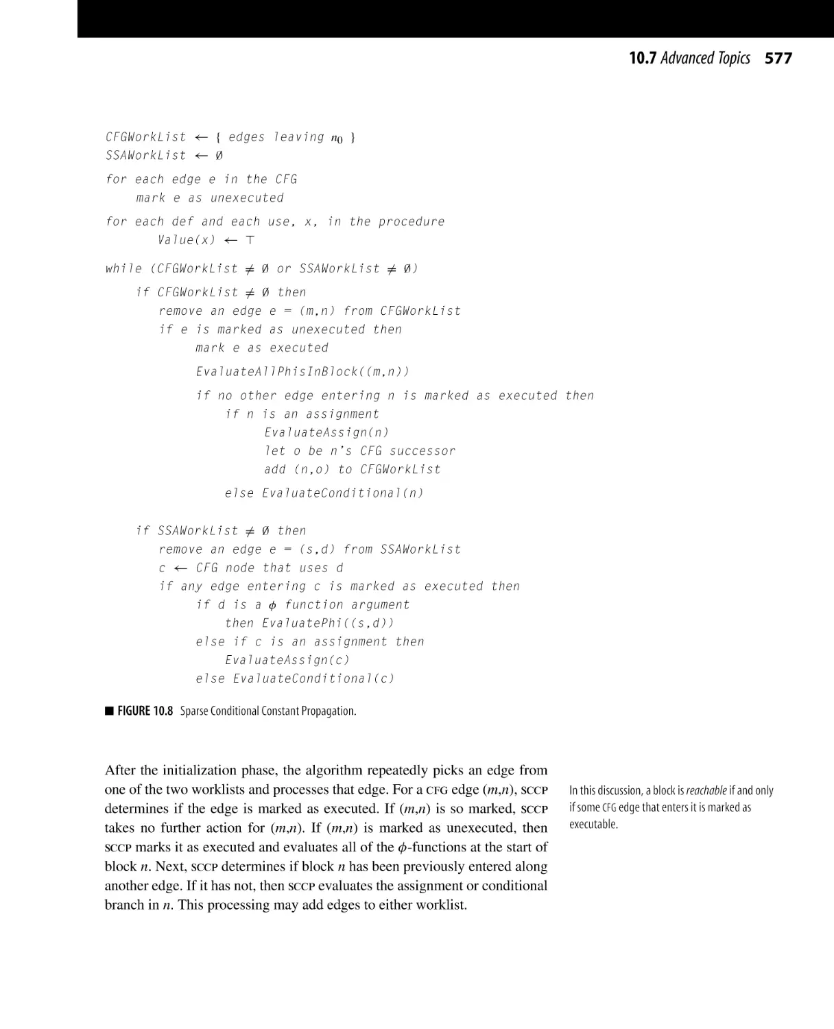
10.7 Advanced Topics . . . . . . . . . . . . . . . . . . . . . . . . . . . . . . . . . . . . . . . . . . . . . . . . . . . . . . .
10.7.1 Combining Optimizations . . . . . . . . . . . . . . . . . . . . . . . . . . . . . . . . . . . .
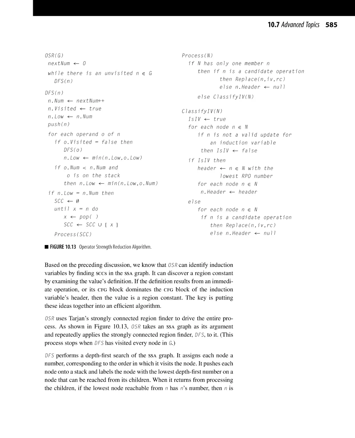
10.7.2 Strength Reduction . . . . . . . . . . . . . . . . . . . . . . . . . . . . . . . . . . . . . . . . . . . .
10.7.3 Choosing an Optimization Sequence . . . . . . . . . . . . . . . . . . . . . . . .
10.8 Summary and Perspective . . . . . . . . . . . . . . . . . . . . . . . . . . . . . . . . . . . . . . . . . . . .
Chapter Notes . . . . . . . . . . . . . . . . . . . . . . . . . . . . . . . . . . . . . . . . . . . . . . . . . . . . . . . . . .
Exercises . . . . . . . . . . . . . . . . . . . . . . . . . . . . . . . . . . . . . . . . . . . . . . . . . . . . . . . . . . . . . . . .
539
544
544
547
550
551
551
559
560
561
562
563
565
565
566
569
570
571
572
573
575
575
580
591
592
593
594
CHAPTER 11 Instruction Selection . . . . . . . . . . . . . . . . . . . . . . . . . . . . . . . . . . . . . . . . . . . . . . . . . . . . . . . . . 597
11.1
11.2
11.3
11.4
Introduction . . . . . . . . . . . . . . . . . . . . . . . . . . . . . . . . . . . . . . . . . . . . . . . . . . . . . . . . . . . . .
Code Generation . . . . . . . . . . . . . . . . . . . . . . . . . . . . . . . . . . . . . . . . . . . . . . . . . . . . . . .
Extending the Simple Treewalk Scheme . . . . . . . . . . . . . . . . . . . . . . . . . . . .
Instruction Selection via Tree-Pattern Matching . . . . . . . . . . . . . . . . . . .
11.4.1 Rewrite Rules . . . . . . . . . . . . . . . . . . . . . . . . . . . . . . . . . . . . . . . . . . . . . . . . . .
11.4.2 Finding a Tiling . . . . . . . . . . . . . . . . . . . . . . . . . . . . . . . . . . . . . . . . . . . . . . .
11.4.3 Tools . . . . . . . . . . . . . . . . . . . . . . . . . . . . . . . . . . . . . . . . . . . . . . . . . . . . . . . . . . . .
597
600
603
610
611
616
620
xvi Contents
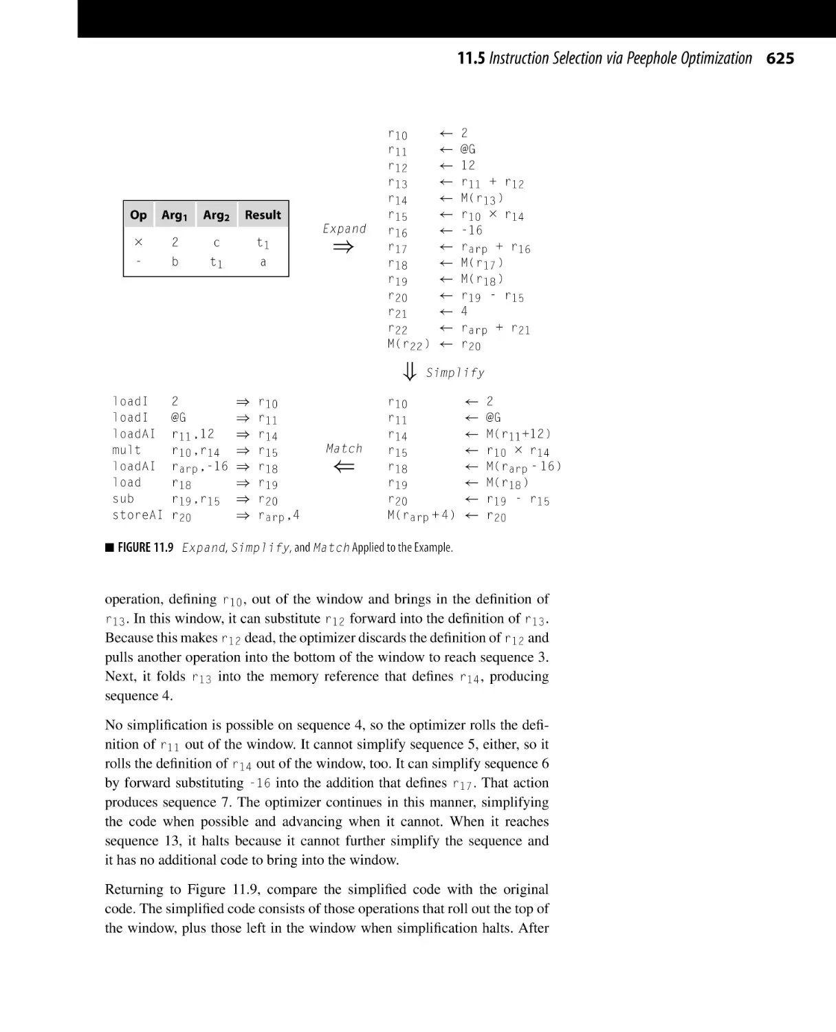
11.5 Instruction Selection via Peephole Optimization . . . . . . . . . . . . . . . . . . .
11.5.1 Peephole Optimization . . . . . . . . . . . . . . . . . . . . . . . . . . . . . . . . . . . . . . .
11.5.2 Peephole Transformers . . . . . . . . . . . . . . . . . . . . . . . . . . . . . . . . . . . . . . .
11.6 Advanced Topics . . . . . . . . . . . . . . . . . . . . . . . . . . . . . . . . . . . . . . . . . . . . . . . . . . . . . . .
11.6.1 Learning Peephole Patterns . . . . . . . . . . . . . . . . . . . . . . . . . . . . . . . . . .
11.6.2 Generating Instruction Sequences . . . . . . . . . . . . . . . . . . . . . . . . . . .
11.7 Summary and Perspective . . . . . . . . . . . . . . . . . . . . . . . . . . . . . . . . . . . . . . . . . . . .
Chapter Notes . . . . . . . . . . . . . . . . . . . . . . . . . . . . . . . . . . . . . . . . . . . . . . . . . . . . . . . . . .
Exercises . . . . . . . . . . . . . . . . . . . . . . . . . . . . . . . . . . . . . . . . . . . . . . . . . . . . . . . . . . . . . . . .
621
622
629
632
632
633
634
635
637
CHAPTER 12 Instruction Scheduling . . . . . . . . . . . . . . . . . . . . . . . . . . . . . . . . . . . . . . . . . . . . . . . . . . . . . . . 639
12.1 Introduction . . . . . . . . . . . . . . . . . . . . . . . . . . . . . . . . . . . . . . . . . . . . . . . . . . . . . . . . . . . . .
12.2 The Instruction-Scheduling Problem . . . . . . . . . . . . . . . . . . . . . . . . . . . . . . . .
12.2.1 Other Measures of Schedule Quality . . . . . . . . . . . . . . . . . . . . . . . .
12.2.2 What Makes Scheduling Hard? . . . . . . . . . . . . . . . . . . . . . . . . . . . . . .
12.3 Local List Scheduling . . . . . . . . . . . . . . . . . . . . . . . . . . . . . . . . . . . . . . . . . . . . . . . . .
12.3.1 The Algorithm . . . . . . . . . . . . . . . . . . . . . . . . . . . . . . . . . . . . . . . . . . . . . . . . .
12.3.2 Scheduling Operations with Variable Delays . . . . . . . . . . . . . .
12.3.3 Extending the Algorithm . . . . . . . . . . . . . . . . . . . . . . . . . . . . . . . . . . . . .
12.3.4 Tie Breaking in the List-Scheduling
Algorithm . . . . . . . . . . . . . . . . . . . . . . . . . . . . . . . . . . . . . . . . . . . . . . . . . . . . . .
12.3.5 Forward versus Backward List Scheduling . . . . . . . . . . . . . . . .
12.3.6 Improving the Efficiency of List Scheduling . . . . . . . . . . . . . .
12.4 Regional Scheduling . . . . . . . . . . . . . . . . . . . . . . . . . . . . . . . . . . . . . . . . . . . . . . . . . . .
12.4.1 Scheduling Extended Basic Blocks . . . . . . . . . . . . . . . . . . . . . . . . .
12.4.2 Trace Scheduling . . . . . . . . . . . . . . . . . . . . . . . . . . . . . . . . . . . . . . . . . . . . . .
12.4.3 Cloning for Context . . . . . . . . . . . . . . . . . . . . . . . . . . . . . . . . . . . . . . . . . . .
12.5 Advanced Topics . . . . . . . . . . . . . . . . . . . . . . . . . . . . . . . . . . . . . . . . . . . . . . . . . . . . . . .
12.5.1 The Strategy of Software Pipelining . . . . . . . . . . . . . . . . . . . . . . . .
12.5.2 An Algorithm for Software Pipelining . . . . . . . . . . . . . . . . . . . . . .
12.6 Summary and Perspective . . . . . . . . . . . . . . . . . . . . . . . . . . . . . . . . . . . . . . . . . . . .
Chapter Notes . . . . . . . . . . . . . . . . . . . . . . . . . . . . . . . . . . . . . . . . . . . . . . . . . . . . . . . . . .
Exercises . . . . . . . . . . . . . . . . . . . . . . . . . . . . . . . . . . . . . . . . . . . . . . . . . . . . . . . . . . . . . . . .
639
643
648
649
651
651
654
655
655
656
660
661
661
663
664
666
666
670
673
673
675
CHAPTER 13 Register Allocation . . . . . . . . . . . . . . . . . . . . . . . . . . . . . . . . . . . . . . . . . . . . . . . . . . . . . . . . . . . . 679
13.1 Introduction . . . . . . . . . . . . . . . . . . . . . . . . . . . . . . . . . . . . . . . . . . . . . . . . . . . . . . . . . . . . .
13.2 Background Issues . . . . . . . . . . . . . . . . . . . . . . . . . . . . . . . . . . . . . . . . . . . . . . . . . . . . .
13.2.1 Memory versus Registers . . . . . . . . . . . . . . . . . . . . . . . . . . . . . . . . . . . .
13.2.2 Allocation versus Assignment . . . . . . . . . . . . . . . . . . . . . . . . . . . . . . .
13.2.3 Register Classes . . . . . . . . . . . . . . . . . . . . . . . . . . . . . . . . . . . . . . . . . . . . . . .
13.3 Local Register Allocation and Assignment . . . . . . . . . . . . . . . . . . . . . . . . .
13.3.1 Top-Down Local Register Allocation . . . . . . . . . . . . . . . . . . . . . . .
679
681
681
682
683
684
685
Contents xvii
13.3.2 Bottom-Up Local Register Allocation . . . . . . . . . . . . . . . . . . . . . .
13.3.3 Moving Beyond Single Blocks . . . . . . . . . . . . . . . . . . . . . . . . . . . . . .
13.4 Global Register Allocation and Assignment . . . . . . . . . . . . . . . . . . . . . . . .
13.4.1 Discovering Global Live Ranges . . . . . . . . . . . . . . . . . . . . . . . . . . . .
13.4.2 Estimating Global Spill Costs . . . . . . . . . . . . . . . . . . . . . . . . . . . . . . .
13.4.3 Interferences and the Interference Graph . . . . . . . . . . . . . . . . . . .
13.4.4 Top-Down Coloring . . . . . . . . . . . . . . . . . . . . . . . . . . . . . . . . . . . . . . . . . .
13.4.5 Bottom-Up Coloring . . . . . . . . . . . . . . . . . . . . . . . . . . . . . . . . . . . . . . . . . .
13.4.6 Coalescing Copies to Reduce Degree . . . . . . . . . . . . . . . . . . . . . . .
13.4.7 Comparing Top-Down and Bottom-Up
Global Allocators . . . . . . . . . . . . . . . . . . . . . . . . . . . . . . . . . . . . . . . . . . . . .
13.4.8 Encoding Machine Constraints in the
Interference Graph . . . . . . . . . . . . . . . . . . . . . . . . . . . . . . . . . . . . . . . . . . . .
13.5 Advanced Topics . . . . . . . . . . . . . . . . . . . . . . . . . . . . . . . . . . . . . . . . . . . . . . . . . . . . . . .
13.5.1 Variations on Graph-Coloring Allocation . . . . . . . . . . . . . . . . . .
13.5.2 Global Register Allocation over SSA Form . . . . . . . . . . . . . . . .
13.6 Summary and Perspective . . . . . . . . . . . . . . . . . . . . . . . . . . . . . . . . . . . . . . . . . . . .
Chapter Notes . . . . . . . . . . . . . . . . . . . . . . . . . . . . . . . . . . . . . . . . . . . . . . . . . . . . . . . . . .
Exercises . . . . . . . . . . . . . . . . . . . . . . . . . . . . . . . . . . . . . . . . . . . . . . . . . . . . . . . . . . . . . . . .
686
689
693
696
697
699
702
704
706
708
711
713
713
717
718
719
720
APPENDIX A ILOC . . . . . . . . . . . . . . . . . . . . . . . . . . . . . . . . . . . . . . . . . . . . . . . . . . . . . . . . . . . . . . . . . . . . . . . . . . . . . . 725
A.1 Introduction . . . . . . . . . . . . . . . . . . . . . . . . . . . . . . . . . . . . . . . . . . . . . . . . . . . . . . . . . . . . .
A.2 Naming Conventions . . . . . . . . . . . . . . . . . . . . . . . . . . . . . . . . . . . . . . . . . . . . . . . . . . .
A.3 Individual Operations . . . . . . . . . . . . . . . . . . . . . . . . . . . . . . . . . . . . . . . . . . . . . . . . . .
A.3.1 Arithmetic . . . . . . . . . . . . . . . . . . . . . . . . . . . . . . . . . . . . . . . . . . . . . . . . . . . . . . .
A.3.2 Shifts . . . . . . . . . . . . . . . . . . . . . . . . . . . . . . . . . . . . . . . . . . . . . . . . . . . . . . . . . . . . .
A.3.3 Memory Operations . . . . . . . . . . . . . . . . . . . . . . . . . . . . . . . . . . . . . . . . . . . . .
A.3.4 Register-to-Register Copy Operations . . . . . . . . . . . . . . . . . . . . . . . .
A.4 Control-Flow Operations . . . . . . . . . . . . . . . . . . . . . . . . . . . . . . . . . . . . . . . . . . . . . .
A.4.1 Alternate Comparison and Branch Syntax . . . . . . . . . . . . . . . . . . .
A.4.2 Jumps . . . . . . . . . . . . . . . . . . . . . . . . . . . . . . . . . . . . . . . . . . . . . . . . . . . . . . . . . . . . .
A.5 Representing SSA Form . . . . . . . . . . . . . . . . . . . . . . . . . . . . . . . . . . . . . . . . . . . . . . .
725
727
728
728
729
729
730
731
732
732
733
APPENDIX B Data Structures . . . . . . . . . . . . . . . . . . . . . . . . . . . . . . . . . . . . . . . . . . . . . . . . . . . . . . . . . . . . . . . . 737
B.1 Introduction . . . . . . . . . . . . . . . . . . . . . . . . . . . . . . . . . . . . . . . . . . . . . . . . . . . . . . . . . . . . .
B.2 Representing Sets . . . . . . . . . . . . . . . . . . . . . . . . . . . . . . . . . . . . . . . . . . . . . . . . . . . . . . .
B.2.1 Representing Sets as Ordered Lists . . . . . . . . . . . . . . . . . . . . . . . . . . .
B.2.2 Representing Sets as Bit Vectors . . . . . . . . . . . . . . . . . . . . . . . . . . . . . .
B.2.3 Representing Sparse Sets . . . . . . . . . . . . . . . . . . . . . . . . . . . . . . . . . . . . . . .
B.3 Implementing Intermediate Representations . . . . . . . . . . . . . . . . . . . . . . . . .
B.3.1 Graphical Intermediate Representations . . . . . . . . . . . . . . . . . . . . . .
B.3.2 Linear Intermediate Forms . . . . . . . . . . . . . . . . . . . . . . . . . . . . . . . . . . . . .
737
738
739
741
741
743
743
748
xviii Contents
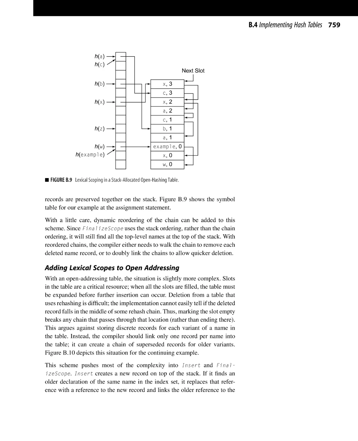
B.4 Implementing Hash Tables . . . . . . . . . . . . . . . . . . . . . . . . . . . . . . . . . . . . . . . . . . . .
B.4.1 Choosing a Hash Function . . . . . . . . . . . . . . . . . . . . . . . . . . . . . . . . . . . . .
B.4.2 Open Hashing . . . . . . . . . . . . . . . . . . . . . . . . . . . . . . . . . . . . . . . . . . . . . . . . . . .
B.4.3 Open Addressing . . . . . . . . . . . . . . . . . . . . . . . . . . . . . . . . . . . . . . . . . . . . . . . .
B.4.4 Storing Symbol Records . . . . . . . . . . . . . . . . . . . . . . . . . . . . . . . . . . . . . . .
B.4.5 Adding Nested Lexical Scopes . . . . . . . . . . . . . . . . . . . . . . . . . . . . . . . .
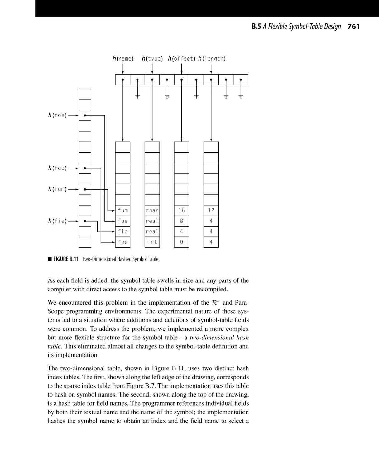
B.5 A Flexible Symbol-Table Design . . . . . . . . . . . . . . . . . . . . . . . . . . . . . . . . . . . . .
750
750
752
754
756
757
760
BIBLIOGRAPHY . . . . . . . . . . . . . . . . . . . . . . . . . . . . . . . . . . . . . . . . . . . . . . . . . . . . . . . . . . . . . . . . . . . . . . . . . . . . . . . . 765
INDEX . . . . . . . . . . . . . . . . . . . . . . . . . . . . . . . . . . . . . . . . . . . . . . . . . . . . . . . . . . . . . . . . . . . . . . . . . . . . . . . . . . . . . . . . . . . 787
Preface to the Second Edition
The practice of compiler construction changes continually, in part because the designs of
processors and systems change. For example, when we began to write Engineering a Compiler (eac) in 1998, some of our colleagues questioned the wisdom of including a chapter on
instruction scheduling because out-of-order execution threatened to make scheduling largely
irrelevant. Today, as the second edition goes to press, the rise of multicore processors and the
push for more cores has made in-order execution pipelines attractive again because their smaller
footprints allow the designer to place more cores on a chip. Instruction scheduling will remain
important for the near-term future.
At the same time, the compiler construction community continues to develop new insights and
algorithms, and to rediscover older techniques that were effective but largely forgotten. Recent
research has created excitement surrounding the use of chordal graphs in register allocation
(see Section 13.5.2). That work promises to simplify some aspects of graph-coloring allocators.
Brzozowski’s algorithm is a dfa minimization technique that dates to the early 1960s but has
not been taught in compiler courses for decades (see Section 2.6.2). It provides an easy path
from an implementation of the subset construction to one that minimizes dfas. A modern course
in compiler construction might include both of these ideas.
How, then, are we to structure a curriculum in compiler construction so that it prepares students
to enter this ever changing field? We believe that the course should provide each student with
the set of base skills that they will need to build new compiler components and to modify
existing ones. Students need to understand both sweeping concepts, such as the collaboration
between the compiler, linker, loader, and operating system embodied in a linkage convention,
and minute detail, such as how the compiler writer might reduce the aggregate code space used
by the register-save code at each procedure call.
n
CHANGES IN THE SECOND EDITION
The second edition of Engineering a Compiler (eac2e) presents both perspectives: big-picture
views of the problems in compiler construction and detailed discussions of algorithmic alternatives. In preparing eac2e, we focused on the usability of the book, both as a textbook and as a
reference for professionals. Specifically, we
n
n
Improved the flow of ideas to help the student who reads the book sequentially. Chapter
introductions explain the purpose of the chapter, lay out the major concepts, and provide a
high-level overview of the chapter’s subject matter. Examples have been reworked to
provide continuity across chapters. In addition, each chapter begins with a summary and a
set of keywords to aid the user who treats eac2e as a reference book.
Added section reviews and review questions at the end of each major section. The review
questions provide a quick check as to whether or not the reader has understood the major
points of the section.
xix
xx Preface to the Second Edition
n
n
Moved definitions of key terms into the margin adjacent to the paragraph where they are
first defined and discussed.
Revised the material on optimization extensively so that it provides broader coverage of
the possibilities for an optimizing compiler.
Compiler development today focuses on optimization and on code generation. A newly hired
compiler writer is far more likely to port a code generator to a new processor or modify an optimization pass than to write a scanner or parser. The successful compiler writer must be familiar
with current best-practice techniques in optimization, such as the construction of static singleassignment form, and in code generation, such as software pipelining. They must also have the
background and insight to understand new techniques as they appear during the coming years.
Finally, they must understand the techniques of scanning, parsing, and semantic elaboration
well enough to build or modify a front end.
Our goal for eac2e has been to create a text and a course that exposes students to the critical
issues in modern compilers and provides them with the background to tackle those problems.
We have retained, from the first edition, the basic balance of material. Front ends are commodity
components; they can be purchased from a reliable vendor or adapted from one of the many
open-source systems. At the same time, optimizers and code generators are custom-crafted
for particular processors and, sometimes, for individual models, because performance relies so
heavily on specific low-level details of the generated code. These facts affect the way that we
build compilers today; they should also affect the way that we teach compiler construction.
n
ORGANIZATION
eac2e divides the material into four roughly equal pieces:
n
n
n
n
n
The first major section, Chapters 2 through 4, covers both the design of a compiler front
end and the design and construction of tools to build front ends.
The second major section, Chapters 5 through 7, explores the mapping of source-code into
the compiler’s intermediate form—that is, these chapters examine the kind of code that the
front end generates for the optimizer and back end.
The third major section, Chapters 8 through 10, introduces the subject of code
optimization. Chapter 8 provides an overview of optimization. Chapters 9 and 10 contain
deeper treatments of analysis and transformation; these two chapters are often omitted
from an undergraduate course.
The final section, Chapters 11 through 13, focuses on algorithms used in the compiler’s
back end.
THE ART AND SCIENCE OF COMPILATION
The lore of compiler construction includes both amazing success stories about the application of
theory to practice and humbling stories about the limits of what we can do. On the success side,
modern scanners are built by applying the theory of regular languages to automatic construction
of recognizers. lr parsers use the same techniques to perform the handle-recognition that drives
Preface to the Second Edition xxi
a shift-reduce parser. Data-flow analysis applies lattice theory to the analysis of programs in
clever and useful ways. The approximation algorithms used in code generation produce good
solutions to many instances of truly hard problems.
On the other side, compiler construction exposes complex problems that defy good solutions.
The back end of a compiler for a modern processor approximates the solution to two or more
interacting np-complete problems (instruction scheduling, register allocation, and, perhaps,
instruction and data placement). These np-complete problems, however, look easy next to problems such as algebraic reassociation of expressions (see, for example, Figure 7.1). This problem
admits a huge number of solutions; to make matters worse, the desired solution depends on context in both the compiler and the application code. As the compiler approximates the solutions
to such problems, it faces constraints on compile time and available memory. A good compiler
artfully blends theory, practical knowledge, engineering, and experience.
Open up a modern optimizing compiler and you will find a wide variety of techniques. Compilers use greedy heuristic searches that explore large solution spaces and deterministic finite
automata that recognize words in the input. They employ fixed-point algorithms to reason
about program behavior and simple theorem provers and algebraic simplifiers to predict the
values of expressions. Compilers take advantage of fast pattern-matching algorithms to map
abstract computations to machine-level operations. They use linear diophantine equations
and Pressburger arithmetic to analyze array subscripts. Finally, compilers use a large set of
classic algorithms and data structures such as hash tables, graph algorithms, and sparse set
implementations.
In eac2e, we have tried to convey both the art and the science of compiler construction. The
book includes a sufficiently broad selection of material to show the reader that real tradeoffs
exist and that the impact of design decisions can be both subtle and far-reaching. At the same
time, eac2e omits some techniques that have long been part of an undergraduate compiler
construction course, but have been rendered less important by changes in the marketplace, in
the technology of languages and compilers, or in the availability of tools.
n
APPROACH
Compiler construction is an exercise in engineering design. The compiler writer must choose
a path through a design space that is filled with diverse alternatives, each with distinct costs,
advantages, and complexity. Each decision has an impact on the resulting compiler. The quality
of the end product depends on informed decisions at each step along the way.
Thus, there is no single right answer for many of the design decisions in a compiler. Even
within “well understood” and “solved” problems, nuances in design and implementation have
an impact on both the behavior of the compiler and the quality of the code that it produces.
Many considerations play into each decision. As an example, the choice of an intermediate
representation for the compiler has a profound impact on the rest of the compiler, from time
and space requirements through the ease with which different algorithms can be applied. The
decision, however, is often given short shrift. Chapter 5 examines the space of intermediate
xxii Preface to the Second Edition
representations and some of the issues that should be considered in selecting one. We raise the
issue again at several points in the book—both directly in the text and indirectly in the exercises.
eac2e explores the design space and conveys both the depth of the problems and the breadth
of the possible solutions. It shows some ways that those problems have been solved, along with
the constraints that made those solutions attractive. Compiler writers need to understand both
the problems and their solutions, as well as the impact of those decisions on other facets of the
compiler’s design. Only then can they make informed and intelligent choices.
n
PHILOSOPHY
This text exposes our philosophy for building compilers, developed during more than twentyfive years each of research, teaching, and practice. For example, intermediate representations
should expose those details that matter in the final code; this belief leads to a bias toward
low-level representations. Values should reside in registers until the allocator discovers that
it cannot keep them there; this practice produces examples that use virtual registers and store
values to memory only when it cannot be avoided. Every compiler should include optimization;
it simplifies the rest of the compiler. Our experiences over the years have informed the selection
of material and its presentation.
n
A WORD ABOUT PROGRAMMING EXERCISES
A class in compiler construction offers the opportunity to explore software design issues in
the context of a concrete application—one whose basic functions are well understood by any
student with the background for a compiler construction course. In most versions of this course,
the programming exercises play a large role.
We have taught this class in versions where the students build a simple compiler from start to
finish—beginning with a generated scanner and parser and ending with a code generator for
some simplified risc instruction set. We have taught this class in versions where the students
write programs that address well-contained individual problems, such as register allocation or
instruction scheduling. The choice of programming exercises depends heavily on the role that
the course plays in the surrounding curriculum.
In some schools, the compiler course serves as a capstone course for seniors, tying together
concepts from many other courses in a large, practical, design and implementation project.
Students in such a class might write a complete compiler for a simple language or modify an
open-source compiler to add support for a new language feature or a new architectural feature.
This class might present the material in a linear order that closely follows the text’s organization.
In other schools, that capstone experience occurs in other courses or in other ways. In such
a class, the teacher might focus the programming exercises more narrowly on algorithms and
their implementation, using labs such as a local register allocator or a tree-height rebalancing
pass. This course might skip around in the text and adjust the order of presentation to meet the
needs of the labs. For example, at Rice, we have often used a simple local register allocator
Preface to the Second Edition xxiii
as the first lab; any student with assembly-language programming experience understands the
basics of the problem. That strategy, however, exposes the students to material from Chapter 13
before they see Chapter 2.
In either scenario, the course should draw material from other classes. Obvious connections
exist to computer organization, assembly-language programming, operating systems, computer
architecture, algorithms, and formal languages. Although the connections from compiler construction to other courses may be less obvious, they are no less important. Character copying,
as discussed in Chapter 7, plays a critical role in the performance of applications that include
network protocols, file servers, and web servers. The techniques developed in Chapter 2 for
scanning have applications that range from text editing through url-filtering. The bottomup local register allocator in Chapter 13 is a cousin of the optimal offline page replacement
algorithm, min.
n
ADDITIONAL MATERIALS
Additional resources are available that can help you adapt the material presented in eac2e to
your course. These include a complete set of lectures from the authors’ version of the course at
Rice University and a set of solutions to the exercises. Your Elsevier representative can provide
you with access.
Acknowledgments
Many people were involved in the preparation of the first edition of eac. Their contributions
have carried forward into this second edition. Many people pointed out problems in the first
edition, including Amit Saha, Andrew Waters, Anna Youssefi, Ayal Zachs, Daniel Salce, David
Peixotto, Fengmei Zhao, Greg Malecha, Hwansoo Han, Jason Eckhardt, Jeffrey Sandoval, John
Elliot, Kamal Sharma, Kim Hazelwood, Max Hailperin, Peter Froehlich, Ryan Stinnett, Sachin
Rehki, Sağnak Taşırlar, Timothy Harvey, and Xipeng Shen. We also want to thank the reviewers
of the second edition, who were Jeffery von Ronne, Carl Offner, David Orleans, K. Stuart
Smith, John Mallozzi, Elizabeth White, and Paul C. Anagnostopoulos. The production team
at Elsevier, in particular, Alisa Andreola, Andre Cuello, and Megan Guiney, played a critical
role in converting the a rough manuscript into its final form. All of these people improved this
volume in significant ways with their insights and their help.
Finally, many people have provided us with intellectual and emotional support over the last
five years. First and foremost, our families and our colleagues at Rice have encouraged us at
every step of the way. Christine and Carolyn, in particular, tolerated myriad long discussions on
topics in compiler construction. Nate McFadden guided this edition from its inception through
its publication with patience and good humor. Penny Anderson provided administrative and
organizational support that was critical to finishing the second edition. To all these people go
our heartfelt thanks.
This page intentionally left blank
Chapter
1
Overview of Compilation
n
CHAPTER OVERVIEW
Compilers are computer programs that translate a program written in one
language into a program written in another language. At the same time, a
compiler is a large software system, with many internal components and
algorithms and complex interactions between them. Thus, the study of compiler construction is an introduction to techniques for the translation and
improvement of programs, and a practical exercise in software engineering.
This chapter provides a conceptual overview of all the major components of
a modern compiler.
Keywords: Compiler, Interpreter, Automatic Translation
1.1 INTRODUCTION
The role of the computer in daily life grows each year. With the rise of the
Internet, computers and the software that runs on them provide communications, news, entertainment, and security. Embedded computers have changed
the ways that we build automobiles, airplanes, telephones, televisions, and
radios. Computation has created entirely new categories of activity, from
video games to social networks. Supercomputers predict daily weather and
the course of violent storms. Embedded computers synchronize traffic lights
and deliver e-mail to your pocket.
All of these computer applications rely on software computer programs
that build virtual tools on top of the low-level abstractions provided by the
underlying hardware. Almost all of that software is translated by a tool
called a compiler. A compiler is simply a computer program that translates other computer programs to prepare them for execution. This book
presents the fundamental techniques of automatic translation that are used
Engineering a Compiler. DOI: 10.1016/B978-0-12-088478-0.00001-3
Copyright c 2012, Elsevier Inc. All rights reserved.
Compiler
a computer program that translates other
computer programs
1
2 CHAPTER 1 Overview of Compilation
to build compilers. It describes many of the challenges that arise in compiler
construction and the algorithms that compiler writers use to address them.
Conceptual Roadmap
A compiler is a tool that translates software written in one language into
another language. To translate text from one language to another, the tool
must understand both the form, or syntax, and content, or meaning, of the
input language. It needs to understand the rules that govern syntax and meaning in the output language. Finally, it needs a scheme for mapping content
from the source language to the target language.
The structure of a typical compiler derives from these simple observations.
The compiler has a front end to deal with the source language. It has a back
end to deal with the target language. Connecting the front end and the back
end, it has a formal structure for representing the program in an intermediate form whose meaning is largely independent of either language. To
improve the translation, a compiler often includes an optimizer that analyzes
and rewrites that intermediate form.
Overview
Computer programs are simply sequences of abstract operations written in
a programming language—a formal language designed for expressing computation. Programming languages have rigid properties and meanings—as
opposed to natural languages, such as Chinese or Portuguese. Programming
languages are designed for expressiveness, conciseness, and clarity. Natural
languages allow ambiguity. Programming languages are designed to avoid
ambiguity; an ambiguous program has no meaning. Programming languages
are designed to specify computations—to record the sequence of actions that
perform some task or produce some results.
Programming languages are, in general, designed to allow humans to express
computations as sequences of operations. Computer processors, hereafter
referred to as processors, microprocessors, or machines, are designed to execute sequences of operations. The operations that a processor implements
are, for the most part, at a much lower level of abstraction than those specified in a programming language. For example, a programming language typically includes a concise way to print some number to a file. That single
programming language statement must be translated into literally hundreds
of machine operations before it can execute.
The tool that performs such translations is called a compiler. The compiler
takes as input a program written in some language and produces as its output an equivalent program. In the classic notion of a compiler, the output
1.1 Introduction 3
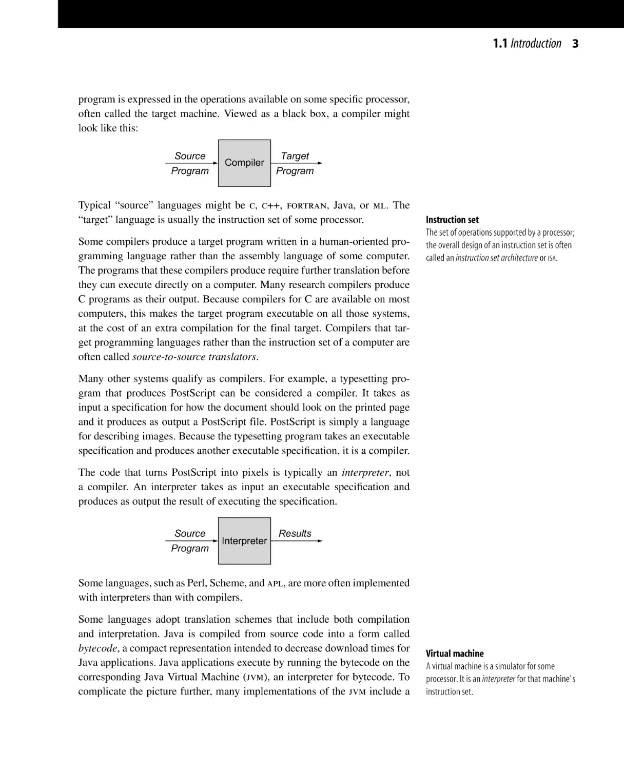
program is expressed in the operations available on some specific processor,
often called the target machine. Viewed as a black box, a compiler might
look like this:
Source
Program
Compiler
Target
Program
Typical “source” languages might be c, c++, fortran, Java, or ml. The
“target” language is usually the instruction set of some processor.
Some compilers produce a target program written in a human-oriented programming language rather than the assembly language of some computer.
The programs that these compilers produce require further translation before
they can execute directly on a computer. Many research compilers produce
C programs as their output. Because compilers for C are available on most
computers, this makes the target program executable on all those systems,
at the cost of an extra compilation for the final target. Compilers that target programming languages rather than the instruction set of a computer are
often called source-to-source translators.
Instruction set
The set of operations supported by a processor;
the overall design of an instruction set is often
called an instruction set architecture or ISA.
Many other systems qualify as compilers. For example, a typesetting program that produces PostScript can be considered a compiler. It takes as
input a specification for how the document should look on the printed page
and it produces as output a PostScript file. PostScript is simply a language
for describing images. Because the typesetting program takes an executable
specification and produces another executable specification, it is a compiler.
The code that turns PostScript into pixels is typically an interpreter, not
a compiler. An interpreter takes as input an executable specification and
produces as output the result of executing the specification.
Source
Program
Interpreter
Results
Some languages, such as Perl, Scheme, and apl, are more often implemented
with interpreters than with compilers.
Some languages adopt translation schemes that include both compilation
and interpretation. Java is compiled from source code into a form called
bytecode, a compact representation intended to decrease download times for
Java applications. Java applications execute by running the bytecode on the
corresponding Java Virtual Machine (jvm), an interpreter for bytecode. To
complicate the picture further, many implementations of the jvm include a
Virtual machine
A virtual machine is a simulator for some
processor. It is an interpreter for that machine’s
instruction set.
4 CHAPTER 1 Overview of Compilation
compiler that executes at runtime, sometimes called a just-in-time compiler,
or jit, that translates heavily used bytecode sequences into native code for
the underlying computer.
Interpreters and compilers have much in common. They perform many of the
same tasks. Both analyze the input program and determine whether or not it
is a valid program. Both build an internal model of the structure and meaning of the program. Both determine where to store values during execution.
However, interpreting the code to produce a result is quite different from
emitting a translated program that can be executed to produce the result. This
book focuses on the problems that arise in building compilers. However, an
implementor of interpreters may find much of the material relevant.
Why Study Compiler Construction?
A compiler is a large, complex program. Compilers often include hundreds
of thousands, if not millions, of lines of code, organized into multiple subsystems and components. The various parts of a compiler interact in complex
ways. Design decisions made for one part of the compiler have important ramifications for other parts. Thus, the design and implementation of
a compiler is a substantial exercise in software engineering.
A good compiler contains a microcosm of computer science. It makes practical use of greedy algorithms (register allocation), heuristic search techniques
(list scheduling), graph algorithms (dead-code elimination), dynamic programming (instruction selection), finite automata and push-down automata
(scanning and parsing), and fixed-point algorithms (data-flow analysis). It
deals with problems such as dynamic allocation, synchronization, naming, locality, memory hierarchy management, and pipeline scheduling. Few
software systems bring together as many complex and diverse components. Working inside a compiler provides practical experience in software
engineering that is hard to obtain with smaller, less intricate systems.
Compilers play a fundamental role in the central activity of computer
science: preparing problems for solution by computer. Most software is compiled, and the correctness of that process and the efficiency of the resulting
code have a direct impact on our ability to build large systems. Most students
are not satisfied with reading about these ideas; many of the ideas must be
implemented to be appreciated. Thus, the study of compiler construction is
an important component of a computer science education.
Compilers demonstrate the successful application of theory to practical
problems. The tools that automate the production of scanners and parsers
apply results from formal language theory. These same tools are used for
1.1 Introduction 5
text searching, website filtering, word processing, and command-language
interpreters. Type checking and static analysis apply results from lattice theory, number theory, and other branches of mathematics to understand and
improve programs. Code generators use algorithms for tree-pattern matching, parsing, dynamic programming, and text matching to automate the
selection of instructions.
Still, some problems that arise in compiler construction are open problems—
that is, the current best solutions have room for improvement. Attempts to
design high-level, universal, intermediate representations have foundered on
complexity. The dominant method for scheduling instructions is a greedy
algorithm with several layers of tie-breaking heuristics. While it is obvious
that compilers should use commutativity and associativity to improve the
code, most compilers that try to do so simply rearrange the expression into
some canonical order.
Building a successful compiler requires expertise in algorithms, engineering,
and planning. Good compilers approximate the solutions to hard problems.
They emphasize efficiency, in their own implementations and in the code
they generate. They have internal data structures and knowledge representations that expose the right level of detail—enough to allow strong
optimization, but not enough to force the compiler to wallow in detail.
Compiler construction brings together ideas and techniques from across the
breadth of computer science and applies them in a constrained setting to
solve some truly hard problems.
The Fundamental Principles of Compilation
Compilers are large, complex, carefully engineered objects. While many
issues in compiler design are amenable to multiple solutions and interpretations, there are two fundamental principles that a compiler writer must
keep in mind at all times. The first principle is inviolable:
The compiler must preserve the meaning of the program being compiled.
Correctness is a fundamental issue in programming. The compiler must
preserve correctness by faithfully implementing the “meaning” of its input
program. This principle lies at the heart of the social contract between the
compiler writer and compiler user. If the compiler can take liberties with
meaning, then why not simply generate a nop or a return? If an incorrect
translation is acceptable, why expend the effort to get it right?
The second principle that a compiler must observe is practical:
The compiler must improve the input program in some discernible way.
6 CHAPTER 1 Overview of Compilation
A traditional compiler improves the input program by making it directly
executable on some target machine. Other “compilers” improve their input
in different ways. For example, tpic is a program that takes the specification for a drawing written in the graphics language pic and converts it into
LATEX; the “improvement” lies in LATEX’s greater availability and generality.
A source-to-source translator for c must produce code that is, in some measure, better than the input program; if it is not, why would anyone invoke it?
1.2 COMPILER STRUCTURE
A compiler is a large, complex software system. The community has been
building compilers since 1955, and over the years, we have learned many
lessons about how to structure a compiler. Earlier, we depicted a compiler as
a simple box that translates a source program into a target program. Reality,
of course, is more complex than that simple picture.
As the single-box model suggests, a compiler must both understand the
source program that it takes as input and map its functionality to the target
machine. The distinct nature of these two tasks suggests a division of labor
and leads to a design that decomposes compilation into two major pieces: a
front end and a back end.
Source
Program
Front End
IR
Back End
Target
Program
Compiler
The front end focuses on understanding the source-language program. The
back end focuses on mapping programs to the target machine. This separation of concerns has several important implications for the design and
implementation of compilers.
IR
A compiler uses some set of data structures to
represent the code that it processes. That form is
called an intermediate representation, or IR.
The front end must encode its knowledge of the source program in some
structure for later use by the back end. This intermediate representation (ir)
becomes the compiler’s definitive representation for the code it is translating.
At each point in compilation, the compiler will have a definitive representation. It may, in fact, use several different irs as compilation progresses,
but at each point, one representation will be the definitive ir. We think of
the definitive ir as the version of the program passed between independent
phases of the compiler, like the ir passed from the front end to the back end
in the preceding drawing.
In a two-phase compiler, the front end must ensure that the source program
is well formed, and it must map that code into the ir. The back end must map
1.2 Compiler Structure 7
MAY YOU STUDY IN INTERESTING TIMES
This is an exciting era in the design and implementation of compilers. In
the 1980s, almost all compilers were large, monolithic systems. They took
as input one of a handful of languages and produced assembly code for
some particular computer. The assembly code was pasted together with
the code produced by other compilations—including system libraries and
application libraries—to form an executable. The executable was stored
on a disk, and at the appropriate time, the final code was moved from the
disk to main memory and executed.
Today, compiler technology is being applied in many different settings. As
computers find applications in diverse places, compilers must cope with
new and different constraints. Speed is no longer the sole criterion for
judging the compiled code. Today, code might be judged on how small
it is, on how much energy it consumes, on how well it compresses, or on
how many page faults it generates when it runs.
At the same time, compilation techniques have escaped from the monolithic systems of the 1980s. They are appearing in many new places. Java
compilers take partially compiled programs (in Java "bytecode" format)
and translate them into native code for the target machine. In this environment, success requires that the sum of compile time plus runtime must be
less than the cost of interpretation. Techniques to analyze whole programs
are moving from compile time to link time, where the linker can analyze
the assembly code for the entire application and use that knowledge to
improve the program. Finally, compilers are being invoked at runtime to
generate customized code that capitalizes on facts that cannot be known
any earlier. If the compilation time can be kept small and the benefits are
large, this strategy can produce noticeable improvements.
the ir program into the instruction set and the finite resources of the target
machine. Because the back end only processes ir created by the front end, it
can assume that the ir contains no syntactic or semantic errors.
The compiler can make multiple passes over the ir form of the code before
emitting the target program. This should lead to better code, as the compiler
can, in effect, study the code in one phase and record relevant details. Then,
in later phases, it can use these recorded facts to improve the quality of
translation. This strategy requires that knowledge derived in the first pass be
recorded in the ir, where later passes can find and use it.
Finally, the two-phase structure may simplify the process of retargeting
the compiler. We can easily envision constructing multiple back ends for a
single front end to produce compilers that accept the same language but target different machines. Similarly, we can envision front ends for different
Retargeting
The task of changing the compiler to generate
code for a new processor is often called
retargeting the compiler.
8 CHAPTER 1 Overview of Compilation
languages producing the same ir and using a common back end. Both
scenarios assume that one ir can serve for several combinations of source
and target; in practice, both language-specific and machine-specific details
usually find their way into the ir.
Optimizer
The middle section of a compiler, called an
optimizer, analyzes and transforms the IR to
improve it.
Introducing an ir makes it possible to add more phases to compilation. The
compiler writer can insert a third phase between the front end and the back
end. This middle section, or optimizer, takes an ir program as its input and
produces a semantically equivalent ir program as its output. By using the ir
as an interface, the compiler writer can insert this third phase with minimal
disruption to the front end and back end. This leads to the following compiler
structure, termed a three-phase compiler.
Source
Program
Front End
IR
Optimizer
IR
Back End
Target
Program
Compiler
The optimizer is an ir-to-ir transformer that tries to improve the ir program
in some way. (Notice that these transformers are, themselves, compilers
according to our definition in Section 1.1.) The optimizer can make one or
more passes over the ir, analyze the ir, and rewrite the ir. The optimizer
may rewrite the ir in a way that is likely to produce a faster target program
from the back end or a smaller target program from the back end. It may
have other objectives, such as a program that produces fewer page faults or
uses less energy.
Conceptually, the three-phase structure represents the classic optimizing
compiler. In practice, each phase is divided internally into a series of passes.
The front end consists of two or three passes that handle the details of
recognizing valid source-language programs and producing the initial ir
form of the program. The middle section contains passes that perform different optimizations. The number and purpose of these passes vary from
compiler to compiler. The back end consists of a series of passes, each of
which takes the ir program one step closer to the target machine’s instruction set. The three phases and their individual passes share a common
infrastructure. This structure is shown in Figure 1.1.
In practice, the conceptual division of a compiler into three phases, a front
end, a middle section or optimizer, and a back end, is useful. The problems
addressed by these phases are different. The front end is concerned with
understanding the source program and recording the results of its analysis into ir form. The optimizer section focuses on improving the ir form.
1.3 Overview of Translation 9
-
-
Reg Allocation
-
Inst Scheduling
...
Inst Selection
-
Optimization n
-
Optimization 2
-
Optimization 1
Optimizer
Back
End
Elaboration
-
Parser
-
Scanner
Front
End
-
6
6
6
6
6
6
6
6
6
?
?
?
?
?
?
?
?
?
Infrastructure
n FIGURE 1.1 Structure of a Typical Compiler.
The back end must map the transformed ir program onto the bounded
resources of the target machine in a way that leads to efficient use of those
resources.
Of these three phases, the optimizer has the murkiest description. The term
optimization implies that the compiler discovers an optimal solution to some
problem. The issues and problems that arise in optimization are so complex and so interrelated that they cannot, in practice, be solved optimally.
Furthermore, the actual behavior of the compiled code depends on interactions among all of the techniques applied in the optimizer and the back end.
Thus, even if a single technique can be proved optimal, its interactions with
other techniques may produce less than optimal results. As a result, a good
optimizing compiler can improve the quality of the code, relative to an unoptimized version. However, an optimizing compiler will almost always fail to
produce optimal code.
The middle section can be a single monolithic pass that applies one or more
optimizations to improve the code, or it can be structured as a series of
smaller passes with each pass reading and writing ir. The monolithic structure may be more efficient. The multipass structure may lend itself to a less
complex implementation and a simpler approach to debugging the compiler.
It also creates the flexibility to employ different sets of optimization in different situations. The choice between these two approaches depends on the
constraints under which the compiler is built and operates.
1.3 OVERVIEW OF TRANSLATION
To translate code written in a programming language into code suitable for
execution on some target machine, a compiler runs through many steps.
10 CHAPTER 1 Overview of Compilation
NOTATION
Compiler books are, in essence, about notation. After all, a compiler translates a program written in one notation into an equivalent program written
in another notation. A number of notational issues will arise in your
reading of this book. In some cases, these issues will directly affect your
understanding of the material.
Expressing Algorithms We have tried to keep the algorithms concise.
Algorithms are written at a relatively high level, assuming that the reader
can supply implementation details. They are written in a slanted, sansserif font. Indentation is both deliberate and significant; it matters most
in an if-then-else construct. Indented code after a then or an else
forms a block. In the following code fragment
if Action [s,word] = ‘‘shift si ’’ then
push word
push si
word ← NextWord()
else if · · ·
all the statements between the then and the else are part of the then
clause of the if-then-else construct. When a clause in an if-thenelse construct contains just one statement, we write the keyword then
or else on the same line as the statement.
Writing Code In some examples, we show actual program text written in
some language chosen to demonstrate a particular point. Actual program
text is written in a monospace font.
Arithmetic Operators Finally, we have forsaken the traditional use
of * for × and of / for ÷, except in actual program text. The meaning
should be clear to the reader.
To make this abstract process more concrete, consider the steps needed to
generate executable code for the following expression:
a ← a × 2 × b × c × d
where a, b, c, and d are variables, ← indicates an assignment, and × is the
operator for multiplication. In the following subsections, we will trace the
path that a compiler takes to turn this simple expression into executable code.
1.3.1 The Front End
Before the compiler can translate an expression into executable targetmachine code, it must understand both its form, or syntax, and its meaning,
1.3 Overview of Translation 11
or semantics. The front end determines if the input code is well formed, in
terms of both syntax and semantics. If it finds that the code is valid, it creates
a representation of the code in the compiler’s intermediate representation; if
not, it reports back to the user with diagnostic error messages to identify the
problems with the code.
Checking Syntax
To check the syntax of the input program, the compiler must compare the
program’s structure against a definition for the language. This requires an
appropriate formal definition, an efficient mechanism for testing whether or
not the input meets that definition, and a plan for how to proceed on an
illegal input.
Mathematically, the source language is a set, usually infinite, of strings
defined by some finite set of rules, called a grammar. Two separate passes
in the front end, called the scanner and the parser, determine whether or not
the input code is, in fact, a member of the set of valid programs defined by
the grammar.
Programming language grammars usually refer to words based on their parts
of speech, sometimes called syntactic categories. Basing the grammar rules
on parts of speech lets a single rule describe many sentences. For example,
in English, many sentences have the form
Sentence → Subject verb Object endmark
where verb and endmark are parts of speech, and Sentence, Subject, and
Object are syntactic variables. Sentence represents any string with the form
described by this rule. The symbol “→” reads “derives” and means that an
instance of the right-hand side can be abstracted to the syntactic variable on
the left-hand side.
Consider a sentence like “Compilers are engineered objects.” The first step
in understanding the syntax of this sentence is to identify distinct words
in the input program and to classify each word with a part of speech. In a
compiler, this task falls to a pass called the scanner. The scanner takes a
stream of characters and converts it to a stream of classified words—that
is, pairs of the form (p,s), where p is the word’s part of speech and s is its
spelling. A scanner would convert the example sentence into the following
stream of classified words:
(noun,“Compilers”), (verb,“are”), (adjective,“engineered”),
(noun,“objects”), (endmark,“.”)
Scanner
the compiler pass that converts a string of
characters into a stream of words
12 CHAPTER 1 Overview of Compilation
In practice, the actual spelling of the words might be stored in a hash table
and represented in the pairs with an integer index to simplify equality tests.
Chapter 2 explores the theory and practice of scanner construction.
In the next step, the compiler tries to match the stream of categorized words
against the rules that specify syntax for the input language. For example,
a working knowledge of English might include the following grammatical
rules:
1
2
3
4
5
6
Sentence
Subject
Subject
Object
Object
Modifier
...
→
→
→
→
→
→
Subject verb Object endmark
noun
Modifier noun
noun
Modifier noun
adjective
By inspection, we can discover the following derivation for our example
sentence:
Rule
—
1
2
5
6
Prototype Sentence
Sentence
Subject verb Object endmark
noun verb Object endmark
noun verb Modifier noun endmark
noun verb adjective noun endmark
The derivation starts with the syntactic variable Sentence. At each step, it
rewrites one term in the prototype sentence, replacing the term with a righthand side that can be derived from that rule. The first step uses Rule 1
to replace Sentence. The second uses Rule 2 to replace Subject. The third
replaces Object using Rule 5, while the final step rewrites Modifier with
adjective according to Rule 6. At this point, the prototype sentence generated by the derivation matches the stream of categorized words produced by
the scanner.
Parser
the compiler pass that determines if the input
stream is a sentence in the source language
The derivation proves that the sentence “Compilers are engineered objects.”
belongs to the language described by Rules 1 through 6. The sentence is
grammatically correct. The process of automatically finding derivations is
called parsing. Chapter 3 presents the techniques that compilers use to parse
the input program.
1.3 Overview of Translation 13
A grammatically correct sentence can be meaningless. For example, the
sentence “Rocks are green vegetables” has the same parts of speech in
the same order as “Compilers are engineered objects,” but has no rational
meaning. To understand the difference between these two sentences requires
contextual knowledge about software systems, rocks, and vegetables.
The semantic models that compilers use to reason about programming languages are simpler than the models needed to understand natural language.
A compiler builds mathematical models that detect specific kinds of inconsistency in a program. Compilers check for consistency of type; for example,
the expression
Type checking
the compiler pass that checks for type-consistent
uses of names in the input program
a ← a × 2 × b × c × d
might be syntactically well-formed, but if b and d are character strings, the
sentence might still be invalid. Compilers also check for consistency of number in specific situations; for example, an array reference should have the
same number of dimensions as the array’s declared rank and a procedure
call should specify the same number of arguments as the procedure’s definition. Chapter 4 explores some of the issues that arise in compiler-based type
checking and semantic elaboration.
Intermediate Representations
The final issue handled in the front end of a compiler is the generation of
an ir form of the code. Compilers use a variety of different kinds of ir,
depending on the source language, the target language, and the specific transformations that the compiler applies. Some irs represent the program as a
graph. Others resemble a sequential assembly code program. The code in
the margin shows how our example expression might look in a low-level,
sequential ir. Chapter 5 presents an overview of the variety of kinds of irs
that compilers use.
For every source-language construct, the compiler needs a strategy for how
it will implement that construct in the ir form of the code. Specific choices
affect the compiler’s ability to transform and improve the code. Thus, we
spend two chapters on the issues that arise in generation of ir for source-code
constructs. Procedure linkages are, at once, a source of inefficiency in the
final code and the fundamental glue that pieces together different source files
into an application. Thus, we devote Chapter 6 to the issues that surround
procedure calls. Chapter 7 presents implementation strategies for most other
programming language constructs.
t0
t1
t2
t3
a
←
←
←
←
←
a × 2
t0 × b
t1 × c
t2 × d
t3
14 CHAPTER 1 Overview of Compilation
TERMINOLOGY
A careful reader will notice that we use the word code in many places
where either program or procedure might naturally fit. Compilers can be
invoked to translate fragments of code that range from a single reference
through an entire system of programs. Rather than specify some scope of
compilation, we will continue to use the ambiguous, but more general,
term, code.
1.3.2 The Optimizer
When the front end emits ir for the input program, it handles the statements
one at a time, in the order that they are encountered. Thus, the initial ir
program contains general implementation strategies that will work in any
surrounding context that the compiler might generate. At runtime, the code
will execute in a more constrained and predictable context. The optimizer
analyzes the ir form of the code to discover facts about that context and uses
that contextual knowledge to rewrite the code so that it computes the same
answer in a more efficient way.
Efficiency can have many meanings. The classic notion of optimization is
to reduce the application’s running time. In other contexts, the optimizer
might try to reduce the size of the compiled code, or other properties such
as the energy that the processor consumes evaluating the code. All of these
strategies target efficiency.
Returning to our example, consider it in the context shown in Figure 1.2a.
The statement occurs inside a loop. Of the values that it uses, only a and
d change inside the loop. The values of 2, b, and c are invariant in the
loop. If the optimizer discovers this fact, it can rewrite the code as shown in
Figure 1.2b. In this version, the number of multiplications has been reduced
from 4·n to 2·n + 2. For n > 1, the rewritten loop should execute faster. This
kind of optimization is discussed in Chapters 8, 9, and 10.
Analysis
Data-flow analysis
a form of compile-time reasoning about the
runtime flow of values
Most optimizations consist of an analysis and a transformation. The analysis
determines where the compiler can safely and profitably apply the technique.
Compilers use several kinds of analysis to support transformations. Dataflow analysis reasons, at compile time, about the flow of values at runtime.
Data-flow analyzers typically solve a system of simultaneous set equations
that are derived from the structure of the code being translated. Dependence
analysis uses number-theoretic tests to reason about the values that can be
1.3 Overview of Translation 15
b ← ···
c ← ···
a ← 1
for i = 1 to n
read d
a ← a × 2 × b × c × d
end
b ← ···
c ← ···
a ← 1
t ← 2 × b × c
for i = 1 to n
read d
a ← a × d × t
end
(a) Original Code in Context
(b) Improved Code
n FIGURE 1.2 Context Makes a Difference.
assumed by subscript expressions. It is used to disambiguate references to
array elements. Chapter 9 presents a detailed look at data-flow analysis and
its application, along with the construction of static-single-assignment form,
an ir that encodes information about the flow of both values and control
directly in the ir.
Transformation
To improve the code, the compiler must go beyond analyzing it. The compiler must use the results of analysis to rewrite the code into a more
efficient form. Myriad transformations have been invented to improve the
time or space requirements of executable code. Some, such as discovering
loop-invariant computations and moving them to less frequently executed
locations, improve the running time of the program. Others make the code
more compact. Transformations vary in their effect, the scope over which
they operate, and the analysis required to support them. The literature on
transformations is rich; the subject is large enough and deep enough to
merit one or more separate books. Chapter 10 covers the subject of scalar
transformations—that is, transformations intended to improve the performance of code on a single processor. It presents a taxonomy for organizing
the subject and populates that taxonomy with examples.
1.3.3 The Back End
The compiler’s back end traverses the ir form of the code and emits code
for the target machine. It selects target-machine operations to implement
each ir operation. It chooses an order in which the operations will execute
efficiently. It decides which values will reside in registers and which values
will reside in memory and inserts code to enforce those decisions.
16 CHAPTER 1 Overview of Compilation
ABOUT ILOC
Throughout the book, low-level examples are written in a notation that
we call ILOC—an acronym derived from "intermediate language for an
optimizing compiler." Over the years, this notation has undergone many
changes. The version used in this book is described in detail in Appendix A.
Think of ILOC as the assembly language for a simple RISC machine. It has a
standard set of operations. Most operations take arguments that are registers. The memory operations, loads and stores, transfer values between
memory and the registers. To simplify the exposition in the text, most
examples assume that all data consists of integers.
Each operation has a set of operands and a target. The operation is written
in five parts: an operation name, a list of operands, a separator, a list of
targets, and an optional comment. Thus, to add registers 1 and 2, leaving
the result in register 3, the programmer would write
add r1 ,r2 ⇒ r3
// example instruction
The separator, ⇒, precedes the target list. It is a visual reminder that information flows from left to right. In particular, it disambiguates cases where
a person reading the assembly-level text can easily confuse operands and
targets. (See loadAI and storeAI in the following table.)
The example in Figure 1.3 only uses four ILOC operations:
ILOC Operation
loadAI
loadI
mult
storeAI
r1 ,c2 ⇒ r3
c1
⇒ r2
r1 ,r2 ⇒ r3
r1
⇒ r2 ,c3
Meaning
Memory(r1 +c2 ) → r3
c1 → r2
r1 × r2 → r3
r1 → Memory(r2 +c3 )
Appendix A contains a more detailed description of ILOC. The examples
consistently use rarp as a register that contains the start of data storage
for the current procedure, also known as the activation record pointer.
Instruction Selection
t0
t1
t2
t3
a
←
←
←
←
←
a × 2
t0 × b
t1 × c
t2 × d
t3
The first stage of code generation rewrites the ir operations into target
machine operations, a process called instruction selection. Instruction
selection maps each ir operation, in its context, into one or more
target machine operations. Consider rewriting our example expression,
a ← a × 2 × b × c × d, into code for the iloc virtual machine to
illustrate the process. (We will use iloc throughout the book.) The ir form
of the expression is repeated in the margin. The compiler might choose
the operations shown in Figure 1.3. This code assumes that a, b, c, and d
1.3 Overview of Translation 17
loadI
rarp , @a ⇒ ra
2
⇒ r2
loadAI
rarp , @b ⇒ rb
// constant 2 into r2
// load ‘b’
loadAI
rarp , @c ⇒ rc
// load ‘c’
loadAI
rarp , @d ⇒ rd
// load ‘d’
mult
ra , r2
mult
ra , rb
mult
ra , rc
ra , rd
loadAI
mult
storeAI ra
⇒
⇒
⇒
⇒
⇒
// load ‘a’
ra
// ra ← a × 2
ra
// ra ← (a × 2) × b
ra
ra
// ra ← (a × 2 × b) × c
// ra ← (a × 2 × b × c) × d
rarp , @a
// write ra back to ‘a’
n FIGURE 1.3 ILOC Code for a ← a × 2 × b × c × d.
are located at offsets @a, @b, @c, and @d from an address contained in the
register rarp .
The compiler has chosen a straightforward sequence of operations. It loads
all of the relevant values into registers, performs the multiplications in order,
and stores the result to the memory location for a. It assumes an unlimited
supply of registers and names them with symbolic names such as ra to hold
a and rarp to hold the address where the data storage for our named values
begins. Implicitly, the instruction selector relies on the register allocator to
map these symbolic register names, or virtual registers, to the actual registers
of the target machine.
The instruction selector can take advantage of special operations on
the target machine. For example, if an immediate-multiply operation
(multI) is available, it might replace the operation mult ra , r2 ⇒ ra with
multI ra , 2 ⇒ ra , eliminating the need for the operation loadI 2 ⇒ r2 and
reducing the demand for registers. If addition is faster than multiplication, it might replace mult ra , r2 ⇒ ra with add ra , ra ⇒ ra , avoiding both
the loadI and its use of r2 , as well as replacing the mult with a faster
add. Chapter 11 presents two different techniques for instruction selection that use pattern matching to choose efficient implementations for ir
operations.
Register Allocation
During instruction selection, the compiler deliberately ignored the fact
that the target machine has a limited set of registers. Instead, it used virtual registers and assumed that “enough” registers existed. In practice, the
earlier stages of compilation may create more demand for registers than the
hardware can support. The register allocator must map those virtual registers
Virtual register
a symbolic register name that the compiler uses
to indicate that a value can be stored in a register
18 CHAPTER 1 Overview of Compilation
onto actual target-machine registers. Thus, the register allocator decides, at
each point in the code, which values should reside in the target-machine registers. It then rewrites the code to reflect its decisions. For example, a register
allocator might minimize register use by rewriting the code from Figure 1.3
as follows:
loadAI
rarp , @a ⇒ r1
⇒
loadAI rarp , @b ⇒
mult
r1 , r2
⇒
loadAI rarp , @c ⇒
mult
r1 , r2
⇒
loadAI rarp , @d ⇒
mult
r1 , r2
⇒
storeAI r1
⇒
add
r1 , r1
// load ‘a’
r1
// r1 ← a × 2
r2
// load ‘b’
r1
r2
// r1 ← (a × 2) × b
// load ‘c’
r1
// r1 ← (a × 2 × b) × c
r2
// load ‘d’
r1
// r1 ← (a × 2 × b × c) × d
rarp , @a
// write ra back to ‘a’
This sequence uses three registers instead of six.
Minimizing register use may be counterproductive. If, for example, any of
the named values, a, b, c, or d, are already in registers, the code should
reference those registers directly. If all are in registers, the sequence could
be implemented so that it required no additional registers. Alternatively, if
some nearby expression also computed a × 2, it might be better to preserve
that value in a register than to recompute it later. This optimization would
increase demand for registers but eliminate a later instruction. Chapter 13
explores the problems that arise in register allocation and the techniques that
compiler writers use to solve them.
Instruction Scheduling
To produce code that executes quickly, the code generator may need to
reorder operations to reflect the target machine’s specific performance constraints. The execution time of the different operations can vary. Memory
access operations can take tens or hundreds of cycles, while some arithmetic operations, particularly division, take several cycles. The impact of
these longer latency operations on the performance of compiled code can be
dramatic.
Assume, for the moment, that a loadAI or storeAI operation requires three
cycles, a mult requires two cycles, and all other operations require one cycle.
The following table shows how the previous code fragment performs under
these assumptions. The Start column shows the cycle in which each operation begins execution and the End column shows the cycle in which it
completes.
1.3 Overview of Translation 19
Start
End
1
4
5
8
10
13
15
18
20
3
4
7
9
12
14
17
19
22
loadAI
rarp , @a ⇒ r1
add
r1 , r1
loadAI
mult
loadAI
mult
loadAI
mult
storeAI
⇒ r1
rarp , @b ⇒ r2
r1 , r2
⇒ r1
rarp , @c ⇒ r2
r1 , r2
⇒ r1
rarp , @d ⇒ r2
r1 , r2
⇒ r1
r1
⇒ rarp , @a
// load ‘a’
// r1 ← a × 2
// load ‘b’
// r1 ← (a × 2) × b
// load ‘c’
// r1 ← (a × 2 × b) × c
// load ‘d’
// r1 ← (a × 2 × b × c) × d
// write ra back to ‘a’
This nine-operation sequence takes 22 cycles to execute. Minimizing register use did not lead to rapid execution.
Many processors have a property by which they can initiate new operations
while a long-latency operation executes. As long as the results of a longlatency operation are not referenced until the operation completes, execution
proceeds normally. If, however, some intervening operation tries to read the
result of the long-latency operation prematurely, the processor delays the
operation that needs the value until the long-latency operation completes.
An operation cannot begin to execute until its operands are ready, and its
results are not ready until the operation terminates.
The instruction scheduler reorders the operations in the code. It attempts to
minimize the number of cycles wasted waiting for operands. Of course, the
scheduler must ensure that the new sequence produces the same result as the
original. In many cases, the scheduler can drastically improve the performance of “naive” code. For our example, a good scheduler might produce
the following sequence:
Start
End
1
2
3
4
5
6
7
9
11
3
4
5
4
6
8
8
10
13
loadAI
rarp , @a ⇒ r1
loadAI
loadAI
add
mult
loadAI
mult
rarp , @b ⇒ r2
rarp , @c ⇒ r3
r1 , r1 ⇒ r1
r1 , r2 ⇒ r1
rarp , @d ⇒ r2
r1 , r3 ⇒ r1
mult
storeAI
r1 , r 2
r1
⇒ r1
⇒ rarp , @a
// load ‘a’
// load ‘b’
// load ‘c’
// r1 ← a × 2
// r1 ← (a × 2) × b
// load ‘d’
// r1 ← (a × 2 × b) × c
// r1 ← (a × 2 × b × c) × d
// write ra back to ‘a’
20 CHAPTER 1 Overview of Compilation
COMPILER CONSTRUCTION IS ENGINEERING
A typical compiler has a series of passes that, together, translate code
from some source language into some target language. Along the way,
the compiler uses dozens of algorithms and data structures. The compiler
writer must select, for each step in the process, an appropriate solution.
A successful compiler executes an unimaginable number of times. Consider the total number of times that GCC compiler has run. Over GCC’s
lifetime, even small inefficiencies add up to a significant amount of time.
The savings from good design and implementation accumulate over time.
Thus, the compiler writer must pay attention to compile time costs, such
as the asymptotic complexity of algorithms, the actual running time of
the implementation, and the space used by data structures. The compiler
writer should have in mind a budget for how much time the compiler will
spend on its various tasks.
For example, scanning and parsing are two problems for which efficient
algorithms abound. Scanners recognize and classify words in time proportional to the number of characters in the input program. For a typical
programming language, a parser can build derivations in time proportional
to the length of the derivation. (The restricted structure of programming
languages makes efficient parsing possible.) Because efficient and effective techniques exist for scanning and parsing, the compiler writer should
expect to spend just a small fraction of compile time on these tasks.
By contrast, optimization and code generation contain several problems
that require more time. Many of the algorithms that we will examine for
program analysis and optimization will have complexities greater than
O(n). Thus, algorithm choice in the optimizer and code generator has a
larger impact on compile time than it does in the compiler’s front end. The
compiler writer may need to trade precision of analysis and effectiveness
of optimization against increases in compile time. He or she should make
such decisions consciously and carefully.
This version of the code requires just 13 cycles to execute. The code uses
one more register than the minimal number. It starts an operation in every
cycle except 8, 10, and 12. Other equivalent schedules are possible, as are
equal-length schedules that use more registers. Chapter 12 presents several
scheduling techniques that are in widespread use.
Interactions Among Code-Generation Components
Most of the truly hard problems that occur in compilation arise during code
generation. To make matters more complex, these problems interact. For
1.4 Summary and Perspective 21
example, instruction scheduling moves load operations away from the arithmetic operations that depend on them. This can increase the period over
which the values are needed and, correspondingly, increase the number of
registers needed during that period. Similarly, the assignment of particular
values to specific registers can constrain instruction scheduling by creating
a “false” dependence between two operations. (The second operation cannot be scheduled until the first completes, even though the values in the
common register are independent. Renaming the values can eliminate this
false dependence, at the cost of using more registers.)
1.4 SUMMARY AND PERSPECTIVE
Compiler construction is a complex task. A good compiler combines ideas
from formal language theory, from the study of algorithms, from artificial
intelligence, from systems design, from computer architecture, and from the
theory of programming languages and applies them to the problem of translating a program. A compiler brings together greedy algorithms, heuristic
techniques, graph algorithms, dynamic programming, dfas and nfas, fixedpoint algorithms, synchronization and locality, allocation and naming, and
pipeline management. Many of the problems that confront the compiler are
too hard for it to solve optimally; thus, compilers use approximations, heuristics, and rules of thumb. This produces complex interactions that can lead to
surprising results—both good and bad.
To place this activity in an orderly framework, most compilers are organized
into three major phases: a front end, an optimizer, and a back end. Each
phase has a different set of problems to tackle, and the approaches used to
solve those problems differ, too. The front end focuses on translating source
code into some ir. Front ends rely on results from formal language theory
and type theory, with a healthy dose of algorithms and data structures. The
middle section, or optimizer, translates one ir program into another, with
the goal of producing an ir program that executes efficiently. Optimizers
analyze programs to derive knowledge about their runtime behavior and then
use that knowledge to transform the code and improve its behavior. The back
end maps an ir program to the instruction set of a specific processor. A back
end approximates the answers to hard problems in allocation and scheduling,
and the quality of its approximation has a direct impact on the speed and size
of the compiled code.
This book explores each of these phases. Chapters 2 through 4 deal with
the algorithms used in a compiler’s front end. Chapters 5 through 7 describe
background material for the discussion of optimization and code generation.
Chapter 8 provides an introduction to code optimization. Chapters 9 and 10
22 CHAPTER 1 Overview of Compilation
provide more detailed treatment of analysis and optimization for the interested reader. Finally, Chapters 11 through 13 cover the techniques used by
back ends for instruction selection, scheduling, and register allocation.
n
CHAPTER NOTES
The first compilers appeared in the 1950s. These early systems showed
surprising sophistication. The original fortran compiler was a multipass
system that included a distinct scanner, parser, and register allocator, along
with some optimizations [26, 27]. The Alpha system, built by Ershov and
his colleagues, performed local optimization [139] and used graph coloring
to reduce the amount of memory needed for data items [140, 141].
Knuth provides some interesting recollections of compiler construction in
the early 1960s [227]. Randell and Russell describe early implementation efforts for Algol 60 [293]. Allen describes the history of compiler
development inside ibm with an emphasis on the interplay of theory and
practice [14].
Many influential compilers were built in the 1960s and 1970s. These include
the classic optimizing compiler fortran H [252, 307], the Bliss-11 and
Bliss-32 compilers [72, 356], and the portable bcpl compiler [300]. These
compilers produced high-quality code for a variety of cisc machines. Compilers for students, on the other hand, focused on rapid compilation, good
diagnostic messages, and error correction [97, 146].
The advent of risc architecture in the 1980s led to another generation of
compilers; these focused on strong optimization and code generation [24,
81, 89, 204]. These compilers featured full-blown optimizers structured as
shown in Figure 1.1. Modern risc compilers still follow this model.
During the 1990s, compiler-construction research focused on reacting to
the rapid changes taking place in microprocessor architecture. The decade
began with Intel’s i860 processor challenging compiler writers to manage
pipelines and memory latencies directly. At its end, compilers confronted
challenges that ranged from multiple functional units to long memory latencies to parallel code generation. The structure and organization of 1980s risc
compilers proved flexible enough for these new challenges, so researchers
built new passes to insert into the optimizers and code generators of their
compilers.
While Java systems use a mix of compilation and interpretation [63, 279],
Java is not the first language to employ such a mix. Lisp systems have long
included both native-code compilers and virtual-machine implementation
Exercises 23
schemes [266, 324]. The Smalltalk-80 system used a bytecode distribution
and a virtual machine [233]; several implementations added just-in-time
compilers [126].
n
EXERCISES
1. Consider a simple Web browser that takes as input a textual string in
html format and displays the specified graphics on the screen. Is the
display process one of compilation or interpretation?
2. In designing a compiler, you will face many tradeoffs. What are the
five qualities that you, as a user, consider most important in a compiler
that you purchase? Does that list change when you are the compiler
writer? What does your list tell you about a compiler that you would
implement?
3. Compilers are used in many different circumstances. What differences
might you expect in compilers designed for the following applications?
a. A just-in-time compiler used to translate user interface code
downloaded over a network
b. A compiler that targets the embedded processor used in a cellular
telephone
c. A compiler used in an introductory programming course at a high
school
d. A compiler used to build wind-tunnel simulations that run on a
massively parallel processor (where all processors are identical)
e. A compiler that targets numerically intensive programs to a large
number of diverse machines
This page intentionally left blank
Chapter
2
Scanners
n
CHAPTER OVERVIEW
The scanner’s task is to transform a stream of characters into a stream of
words in the input language. Each word must be classified into a syntactic
category, or “part of speech.” The scanner is the only pass in the compiler
to touch every character in the input program. Compiler writers place a premium on speed in scanning, in part because the scanner’s input is larger,
in some measure, than that of any other pass, and, in part, because highly
efficient techniques are easy to understand and to implement.
This chapter introduces regular expressions, a notation used to describe
the valid words in a programming language. It develops the formal mechanisms to generate scanners from regular expressions, either manually or
automatically.
Keywords: Scanner, Finite Automaton, Regular Expression, Fixed Point
2.1 INTRODUCTION
Scanning is the first stage of a three-part process that the compiler uses
to understand the input program. The scanner, or lexical analyzer, reads a
stream of characters and produces a stream of words. It aggregates characters to form words and applies a set of rules to determine whether or not each
word is legal in the source language. If the word is valid, the scanner assigns
it a syntactic category, or part of speech.
The scanner is the only pass in the compiler that manipulates every character of the input program. Because scanners perform a relatively simple task,
grouping characters together to form words and punctuation in the source
language, they lend themselves to fast implementations. Automatic tools
for scanner generation are common. These tools process a mathematical
Engineering a Compiler. DOI: 10.1016/B978-0-12-088478-0.00002-5
Copyright c 2012, Elsevier Inc. All rights reserved.
25
26 CHAPTER 2 Scanners
description of the language’s lexical syntax and produce a fast recognizer.
Alternatively, many compilers use hand-crafted scanners; because the task
is simple, such scanners can be fast and robust.
Conceptual Roadmap
Recognizer
a program that identifies specific words in a
stream of characters
This chapter describes the mathematical tools and programming techniques
that are commonly used to construct scanners—both generated scanners
and hand-crafted scanners. The chapter begins, in Section 2.2, by introducing a model for recognizers, programs that identify words in a stream of
characters. Section 2.3 describes regular expressions, a formal notation for
specifying syntax. In Section 2.4, we show a set of constructions to convert a
regular expression into a recognizer. Finally, in Section 2.5 we present three
different ways to implement a scanner: a table-driven scanner, a direct-coded
scanner, and a hand-coded approach.
Both generated and hand-crafted scanners rely on the same underlying techniques. While most textbooks and courses advocate the use of generated
scanners, most commercial compilers and open-source compilers use handcrafted scanners. A hand-crafted scanner can be faster than a generated
scanner because the implementation can optimize away a portion of the overhead that cannot be avoided in a generated scanner. Because scanners are
simple and they change infrequently, many compiler writers deem that the
performance gain from a hand-crafted scanner outweighs the convenience
of automated scanner generation. We will explore both alternatives.
Overview
Syntactic category
a classification of words according to their
grammatical usage
Microsyntax
the lexical structure of a language
A compiler’s scanner reads an input stream that consists of characters
and produces an output stream that contains words, each labelled with its
syntactic category—equivalent to a word’s part of speech in English. To
accomplish this aggregation and classification, the scanner applies a set of
rules that describe the lexical structure of the input programming language,
sometimes called its microsyntax. The microsyntax of a programming language specifies how to group characters into words and, conversely, how to
separate words that run together. (In the context of scanning, we consider
punctuation marks and other symbols as words.)
Western languages, such as English, have simple microsyntax. Adjacent
alphabetic letters are grouped together, left to right, to form a word.
A blank space terminates a word, as do most nonalphabetic symbols. (The
word-building algorithm can treat a hyphen in the midst of a word as
if it were an alphabetic character.) Once a group of characters has been
aggregated together to form a potential word, the word-building algorithm
can determine its validity with a dictionary lookup.
2.2 Recognizing Words 27
Most programming languages have equally simple microsyntax. Characters
are aggregated into words. In most languages, blanks and punctuation marks
terminate a word. For example, Algol and its descendants define an identifier
as a single alphabetic character followed by zero or more alphanumeric characters. The identifier ends with the first nonalphanumeric character. Thus,
fee and f1e are valid identifiers, but 12fum is not. Notice that the set of
valid words is specified by rules rather than by enumeration in a dictionary.
In a typical programming language, some words, called keywords or reserved words, match the rule for an identifier but have special meanings. Both
while and static are keywords in both C and Java. Keywords (and punctuation marks) form their own syntactic categories. Even though static
matches the rule for an identifier, the scanner in a C or Java compiler would
undoubtedly classify it into a category that has only one element, the keyword static. To recognize keywords, the scanner can either use dictionary
lookup or encode the keywords directly into its microsyntax rules.
The simple lexical structure of programming languages lends itself to efficient scanners. The compiler writer starts from a specification of the language’s microsyntax. She either encodes the microsyntax into a notation
accepted by a scanner generator, which then constructs an executable scanner, or she uses that specification to build a hand-crafted scanner. Both
generated and hand-crafted scanners can be implemented to require just
O(1) time per character, so they run in time proportional to the number of
characters in the input stream.
2.2 RECOGNIZING WORDS
The simplest explanation of an algorithm to recognize words is often a
character-by-character formulation. The structure of the code can provide
some insight into the underlying problem. Consider the problem of recognizing the keyword new. Assuming the presence of a routine NextChar that
returns the next character, the code might look like the fragment shown in
Figure 2.1. The code tests for n followed by e followed by w. At each step,
failure to match the appropriate character causes the code to reject the string
and “try something else.” If the sole purpose of the program was to recognize the word new, then it should print an error message or return failure.
Because scanners rarely recognize only one word, we will leave this “error
path” deliberately vague at this point.
The code fragment performs one test per character. We can represent the
code fragment using the simple transition diagram shown to the right of the
code. The transition diagram represents a recognizer. Each circle represents
an abstract state in the computation. Each state is labelled for convenience.
Keyword
a word that is reserved for a particular syntactic
purpose and, thus, cannot be used as an identifier
28 CHAPTER 2 Scanners
c ← NextChar();
if (c = ‘n’)
?
then begin;
s0
n
?
c ← NextChar();
if (c = ‘e’)
then begin;
s1
e
?
c ← NextChar();
if (c = ‘w’)
then report success;
s2
w
?
else try something else;
end;
s
else try something else;
3
end;
else try something else;
n FIGURE 2.1 Code Fragment to Recognize "new".
si
The initial state, or start state, is s0 . We will always label the start state as
s0 . State s3 is an accepting state; the recognizer reaches s3 only when the
input is new. Accepting states are drawn with double circles, as shown in
the margin. The arrows represent transitions from state to state based on the
input character. If the recognizer starts in s0 and reads the characters n, e,
and w, the transitions take us to s3 . What happens on any other input, such
as n, o, and t? The n takes the recognizer to s1 . The o does not match the
edge leaving s1 , so the input word is not new. In the code, cases that do not
match new try something else. In the recognizer, we can think of this action
as a transition to an error state. When we draw the transition diagram of a
recognizer, we usually omit transitions to the error state. Each state has a
transition to the error state on each unspecified input.
Using this same approach to build a recognizer for while would produce the
following transition diagram:
s0
w
s1
h
s2
i
s3
l
s4
e
s5
If it starts in s0 and reaches s5 , it has identified the word while. The
corresponding code fragment would involve five nested if-then-else
constructs.
To recognize multiple words, we can create multiple edges that leave a given
state. (In the code, we would begin to elaborate the do something else paths.)
2.2 Recognizing Words 29
One recognizer for both new and not might be
w s
s2 3
e
3
n
- s0 - s1
Q
oQ
s
t s
s4 5
The recognizer uses a common test for n that takes it from s0 to s1 ,
n
e
denoted s0 → s1 . If the next character is e, it takes the transition s1 → s2 .
o
If, instead, the next character is o, it makes the move s1 → s4 . Finally, a w
w
t
in s2 , causes the transition s2 → s3 , while a t in s4 produces s4 → s5 . State
s3 indicates that the input was new while s5 indicates that it was not. The
recognizer takes one transition per input character.
We can combine the recognizer for new or not with the one for while by
merging their initial states and relabeling all the states.
w s
s2 3
e
3
n s
- s0 1
Q
oQ
s
Jw
t s
s4 5
J
J
J
^
J
h s
i s
l s
e s
s6 7
8
9
10
State s0 has transitions for n and w. The recognizer has three accepting states,
s3 , s5 , and s10 . If any state encounters an input character that does not match
one of its transitions, the recognizer moves to an error state.
2.2.1 A Formalism for Recognizers
Transition diagrams serve as abstractions of the code that would be required
to implement them. They can also be viewed as formal mathematical objects, called finite automata, that specify recognizers. Formally, a finite
automaton (fa) is a five-tuple (S, 6, δ, s0 , S A ), where
n
n
S is the finite set of states in the recognizer, along with an error state se .
6 is the finite alphabet used by the recognizer. Typically, 6 is the union
of the edge labels in the transition diagram.
Finite automaton
a formalism for recognizers that has a finite set of
states, an alphabet, a transition function, a start
state, and one or more accepting states
30 CHAPTER 2 Scanners
n
n
n
δ(s, c) is the recognizer’s transition function. It maps each state s ∈ S
and each character c ∈ 6 into some next state. In state si with input
c
character c, the fa takes the transition si → δ(si , c).
s0 ∈ S is the designated start state.
S A is the set of accepting states, S A ⊆ S. Each state in S A appears as a
double circle in the transition diagram.
As an example, we can cast the fa for new or not or while in the formalism
as follows:
S = {s0 , s1 , s2 , s3 , s4 , s5 , s6 , s7 , s8 , s9 , s10 , se }
6 = {e, h, i, l, n, o, t, w}
( n
w
e
s0 → s1 , s0 → s6 , s1 → s2 ,
δ=
t
h
i
s4 → s5 , s6 → s7 , s7 → s8 ,
o
w
s1 → s4 ,
s2 → s3 ,
s8 → s9 ,
s9 → s10
l
)
e
s0 = s0
S A = {s3 , s5 , s10 }
For all other combinations of state si and input character c, we define
δ(si , c) = se , where se is the designated error state. This quintuple is equivalent to the transition diagram; given one, we can easily re-create the other.
The transition diagram is a picture of the corresponding fa.
An fa accepts a string x if and only if, starting in s0 , the sequence of characters in the string takes the fa through a series of transitions that leaves
it in an accepting state when the entire string has been consumed. This
corresponds to our intuition for the transition diagram. For the string new,
n
e
our example recognizer runs through the transitions s0 → s1 , s1 → s2 , and
w
s2 → s3 . Since s3 ∈ S A , and no input remains, the fa accepts new. For the
n
input string nut, the behavior is different. On n, the fa takes s0 → s1 . On u,
u
it takes s1 → se . Once the fa enters se , it stays in se until it exhausts the input
stream.
More formally, if the string x is composed of characters x1 x2 x3 . . . xn , then
the fa (S, 6, δ, s0 , S A ) accepts x if and only if
δ(δ(. . . δ(δ(δ(s0 , x1 ), x2 ), x3 ) . . . , xn−1 ), xn ) ∈ S A.
Intuitively, this definition corresponds to a repeated application of δ to a
pair composed of some state s ∈ S and an input symbol xi . The base case,
δ(s0 , x1 ), represents the fa’s initial transition, out of the start state, s0 , on
the character x1 . The state produced by δ(s0 , x1 ) is then used as input, along
with x2 , to δ to produce the next state, and so on, until all the input has been
2.2 Recognizing Words 31
consumed. The result of the final application of δ is, again, a state. If that
state is an accepting state, then the fa accepts x1 x2 x3 . . . xn .
Two other cases are possible. The fa might encounter an error while
processing the string—that is, some character x j might take it into the error
state se . This condition indicates a lexical error; the string x1 x2 x3 . . . x j is
not a valid prefix for any word in the language accepted by the fa. The
fa can also discover an error by exhausting its input and terminating in a
nonaccepting state other than se . In this case, the input string is a proper prefix of some word accepted by the fa. Again, this indicates an error. Either
kind of error should be reported to the end user.
In any case, notice that the fa takes one transition for each input character.
Assuming that we can implement the fa efficiently, we should expect the
recognizer to run in time proportional to the length of the input string.
2.2.2 Recognizing More Complex Words
The character-by-character model shown in the original recognizer for not
extends easily to handle arbitrary collections of fully specified words. How
could we recognize a number with such a recognizer? A specific number,
such as 113.4, is easy.
s0
1
s1
1
s2
3
4
s3 ‘.’ s4
s5
To be useful, however, we need a transition diagram (and the corresponding code fragment) that can recognize any number. For simplicity’s sake,
let’s limit the discussion to unsigned integers. In general, an integer is either
zero, or it is a series of one or more digits where the first digit is from one
to nine, and the subsequent digits are from zero to nine. (This definition
rules out leading zeros.) How would we draw a transition diagram for this
definition?
s2
1…9
s0
0…9
s3
0…9
s4
0…9
s5
0…9
…
0
s1
0
The transition s0 → s1 handles the case for zero. The other path, from s0 to
s2 , to s3 , and so on, handles the case for an integer greater than zero. This
path, however, presents several problems. First, it does not end, violating the
stipulation that S is finite. Second, all of the states on the path beginning with
s2 are equivalent, that is, they have the same labels on their output transitions
and they are all accepting states.
32 CHAPTER 2 Scanners
char ← NextChar( );
state ← s0 ;
S = {s0 , s1 , s2 , se }
while (char 6= eof and state 6= se ) do
6 = {0, 1, 2, 3, 4, 5, 6, 7, 8, 9}
state ← δ(state,char);
char ← NextChar( );
0
s0 →
s1 ,
end;
δ=
if (state ∈ SA )
then report acceptance;
else report failure;
SA = {s1 , s2 }
s 0-9
2 → s2 ,
1-9
s0 → s2
0-9
s1 → se
n FIGURE 2.2 A Recognizer for Unsigned Integers.
Lexeme
the actual text for a word recognized by an FA
This fa recognizes a class of strings with a common property: they are all
unsigned integers. It raises the distinction between the class of strings and
the text of any particular string. The class “unsigned integer” is a syntactic
category, or part of speech. The text of a specific unsigned integer, such as
113, is its lexeme.
We can simplify the fa significantly if we allow the transition diagram to
have cycles. We can replace the entire chain of states beginning at s2 with a
single transition from s2 back to itself:
1…9
s0
s2
0…9
0
s1
This cyclic transition diagram makes sense as an fa. From an implementation perspective, however, it is more complex than the acyclic transition
diagrams shown earlier. We cannot translate this directly into a set of nested
if-then-else constructs. The introduction of a cycle in the transition graph
creates the need for cyclic control flow. We can implement this with a while
loop, as shown in Figure 2.2. We can specify δ efficiently using a table:
δ
0
1
2
3
4
5
6
7
8
9
Other
s0
s1
s2
se
s1
se
s2
se
s2
se
s2
se
s2
se
s2
se
s2
se
s2
se
s2
se
s2
se
s2
se
s2
se
s2
se
s2
se
s2
se
s2
se
s2
se
s2
se
s2
se
s2
se
se
se
se
se
Changing the table allows the same basic code skeleton to implement other
recognizers. Notice that this table has ample opportunity for compression.
2.2 Recognizing Words 33
The columns for the digits 1 through 9 are identical, so they could be
represented once. This leaves a table with three columns: 0, 1 . . . 9, and other.
Close examination of the code skeleton shows that it reports failure as soon
as it enters se , so it never references that row of the table. The implementation can elide the entire row, leaving a table with just three rows and three
columns.
We can develop similar fas for signed integers, real numbers, and complex
numbers. A simplified version of the rule that governs identifier names in
Algol-like languages, such as C or Java, might be: an identifier consists of
an alphabetic character followed by zero or more alphanumeric characters.
This definition allows an infinite set of identifiers, but can be specified with
the simple two-state fa shown to the left. Many programming languages
extend the notion of “alphabetic character” to include designated special
characters, such as the underscore.
fas can be viewed as specifications for a recognizer. However, they are not
particularly concise specifications. To simplify scanner implementation, we
need a concise notation for specifying the lexical structure of words, and
a way of turning those specifications into an fa and into code that implements the fa. The remaining sections of this chapter develop precisely those
ideas.
SECTION REVIEW
A character-by-character approach to scanning leads to algorithmic clarity. We can represent character-by-character scanners with a transition
diagram; that diagram, in turn, corresponds to a finite automaton. Small
sets of words are easily encoded in acyclic transition diagrams. Infinite
sets, such as the set of integers or the set of identifiers in an Algol-like
language, require cyclic transition diagrams.
Review Questions
Construct an FA to accept each of the following languages:
1. A six-character identifier consisting of an alphabetic character followed by zero to five alphanumeric characters
2. A string of one or more pairs, where each pair consists of an open
parenthesis followed by a close parenthesis
3. A Pascal comment, which consists of an open brace, {, followed by
zero or more characters drawn from an alphabet, 6, followed by a
close brace, }
s0
a…z,
A…Z
s1
a…z,
A…Z,
0…9
34 CHAPTER 2 Scanners
2.3 REGULAR EXPRESSIONS
The set of words accepted by a finite automaton, F , forms a language,
denoted L(F ). The transition diagram of the fa specifies, in precise detail,
that language. It is not, however, a specification that humans find intuitive.
For any fa, we can also describe its language using a notation called a regular expression (re). The language described by an re is called a regular
language.
Regular expressions are equivalent to the fas described in the previous
section. (We will prove this with a construction in Section 2.4.) Simple
recognizers have simple re specifications.
n
n
n
The language consisting of the single word new can be described by an
re written as new. Writing two characters next to each other implies that
they are expected to appear in that order.
The language consisting of the two words new or while can be written
as new or while. To avoid possible misinterpretation of or, we write
this using the symbol | to mean or. Thus, we write the re as
new | while.
The language consisting of new or not can be written as new | not.
Other res are possible, such as n(ew | ot). Both res specify the same
pair of words. The re n(ew | ot) suggests the structure of the fa that we
drew earlier for these two words.
w s
s2 3
e
3
n s
- s0 1
Q
oQ
s
t s
s4 5
To make this discussion concrete, consider some examples that occur in most
programming languages. Punctuation marks, such as colons, semicolons,
commas, and various brackets, can be represented by their character representations. Their res have the same “spelling” as the punctuation marks
themselves. Thus, the following res might occur in the lexical specification
for a programming language:
: ; ? => ( ) { } [ ]
Similarly, keywords have simple res.
if while this integer instanceof
To model more complex constructs, such as integers or identifiers, we need
a notation that can capture the essence of the cyclic edge in an fa.
2.3 Regular Expressions 35
The fa for an unsigned integer, shown at the left, has three states: an initial
state s0 , an accepting state s1 for the unique integer zero, and another accepting state s2 for all other integers. The key to this fa’s power is the transition
from s2 back to itself that occurs on each additional digit. State s2 folds the
specification back on itself, creating a rule to derive a new unsigned integer
from an existing one: add another digit to the right end of the existing number. Another way of stating this rule is: an unsigned integer is either a zero,
or a nonzero digit followed by zero or more digits. To capture the essence
of this fa, we need a notation for this notion of “zero or more occurrences”
of an re. For the re x, we write this as x∗ , with the meaning “zero or more
occurrences of x.” We call the * operator Kleene closure, or closure for short.
Using the closure operator, we can write an re for this fa:
0…9
1…9
s0
s2
0
s1
0 | (1 | 2 | 3 | 4 | 5 | 6 | 7 | 8 | 9) (0 | 1 | 2 | 3 | 4 | 5 | 6 | 7 | 8 | 9)∗ .
2.3.1 Formalizing the Notation
To work with regular expressions in a rigorous way, we must define them
more formally. An re describes a set of strings over the characters contained
in some alphabet, 6, augmented with a character that represents the empty
string. We call the set of strings a language. For a given re, r, we denote
the language that it specifies as L(r). An re is built up from three basic
operations:
1. Alternation The alternation, or union, of two sets of strings, R and S,
denoted R | S, is {x | x ∈ R or x ∈ S}.
2. Concatenation The concatenation oftwo sets R and S, denoted RS,
contains all strings formed by prepending an element of R onto one
from S, or {x y | x ∈ R and y ∈ S}.
S∞ i
3. Closure The Kleene closure of a set R, denoted R ∗ , is i=
0 R . This is
just the union of the concatenations of R with itself, zero or more times.
For convenience, we sometimes use a notation for finite closure. The notation R i denotes from one to i occurrences of R. A finite closure can be
always be replaced with an enumeration of the possibilities; for example,
R 3 is just (R | R R | R R R). The positive closure, denoted R + , is just R R ∗
and consists of one or more occurrences of R. Since all these closures can
be rewritten with the three basic operations, we ignore them in the discussion
that follows.
Using the three basic operations, alternation, concatenation, and Kleene
closure, we can define the set of res over an alphabet 6 as follows:
1. If a ∈ 6, then a is also an re denoting the set containing only a.
2. If r and s are res, denoting sets L(r) and L(s), respectively, then
Finite closure
For any integer i, the RE Ri designates one to i
occurrences of R.
Positive closure
The RE R+ denotes one or more occurrences of R,
S
i
often written as ∞
i=1 R .
36 CHAPTER 2 Scanners
REGULAR EXPRESSIONS IN VIRTUAL LIFE
Regular expressions are used in many applications to specify patterns in
character strings. Some of the early work on translating REs into code was
done to provide a flexible way of specifying strings in the "find" command
of a text editor. From that early genesis, the notation has crept into many
different applications.
Unix and other operating systems use the asterisk as a wildcard to match
substrings against file names. Here, ∗ is a shorthand for the RE 6 ∗ , specifying zero or more characters drawn from the entire alphabet of legal
characters. (Since few keyboards have a 6 key, the shorthand has stayed
with us.) Many systems use ? as a wildcard that matches a single character.
The grep family of tools, and their kin in non-Unix systems, implement
regular expression pattern matching. (In fact, grep is an acronym for global
regular-expression pattern match and print.)
Regular expressions have found widespread use because they are easily
written and easily understood. They are one of the techniques of choice
when a program must recognize a fixed vocabulary. They work well for
languages that fit within their limited rules. They are easily translated into
an executable form, and the resulting recognizer is fast.
r | s is an re denoting the union, or alternation, of L(r) and L(s),
rs is an re denoting the concatenation of L(r) and L(s), respectively, and
r∗ is an re denoting the Kleene closure of L(r ).
3. is an re denoting the set containing only the empty string.
To eliminate any ambiguity, parentheses have highest precedence, followed
by closure, concatenation, and alternation, in that order.
As a convenient shorthand, we will specify ranges of characters with the
first and the last element connected by an ellipsis, “. . . ”. To make this
abbreviation stand out, we surround it with a pair of square brackets. Thus,
[0. . . 9] represents the set of decimal digits. It can always be rewritten as
(0 | 1 | 2 | 3 | 4 | 5 | 6 | 7 | 8 | 9).
2.3.2 Examples
The goal of this chapter is to show how we can use formal techniques to
automate the construction of high-quality scanners and how we can encode
the microsyntax of programming languages into that formalism. Before proceeding further, some examples from real programming languages are in
order.
2.3 Regular Expressions 37
1. The simplified rule given earlier for identifiers in Algol-like languages,
an alphabetic character followed by zero or more alphanumeric
characters, is just ([A. . . Z] | [a. . . z]) ([A. . . Z] | [a. . . z] | [0. . . 9])∗ . Most
languages also allow a few special characters, such as the underscore ( ),
the percent sign (%), or the ampersand (&), in identifiers.
If the language limits the maximum length of an identifier, we can use
the appropriate finite closure. Thus, identifiers limited to six characters
might be specified as ([A. . . Z] | [a. . . z]) ([A. . . Z] | [a. . . z] | [0. . . 9])5. If
we had to write out the full expansion of the finite closure, the re would
be much longer.
2. An unsigned integer can be described as either zero or a nonzero digit
followed by zero or more digits. The re 0 | [1. . . 9] [0. . . 9]∗ is more
concise. In practice, many implementations admit a larger class of
strings as integers, accepting the language [0. . . 9]+ .
3. Unsigned real numbers are more complex than integers. One possible re
might be (0 | [1. . . 9] [0. . . 9]∗ ) ( | . [0. . . 9]∗ ) The first part is just the re
for an integer. The rest generates either the empty string or a decimal
point followed by zero or more digits.
Programming languages often extend real numbers to scientific notation,
as in (0 | [1. . . 9] [0. . . 9]∗ ) ( | . [0. . . 9]∗ ) E ( | + | −)
(0 | [1. . . 9] [0. . . 9]∗ ).
This re describes a real number, followed by an E, followed by an
integer to specify the exponent.
4. Quoted character strings have their own complexity. In most languages,
any character can appear inside a string. While we can write an re for
strings using only the basic operators, it is our first example where a
complement operator simplifies the re. Using complement, a character
string in c or Java can be described as “ (ˆ”)∗ ”.
c and c++ do not allow a string to span multiple lines in the source
code—that is, if the scanner reaches the end of a line while inside a
string, it terminates the string and issues an error message. If we
represent newline with the escape sequence \n, in the c style, then the
re “ ( ˆ(” | \n) )∗ ” will recognize a correctly formed string and will take
an error transition on a string that includes a newline.
5. Comments appear in a number of forms. c++ and Java offer the
programmer two ways of writing a comment. The delimiter // indicates
a comment that runs to the end of the current input line. The re for this
style of comment is straightforward: // (ˆ\n)∗ \n, where \n represents the
newline character.
Multiline comments in c, c++, and Java begin with the delimiter /* and
end with */. If we could disallow * in a comment, the re would be
Complement operator
The notation ∧ c specifies the set {6 − c},
the complement of c with respect to 6.
Complement has higher precedence than
∗ , |, or + .
Escape sequence
Two or more characters that the scanner
translates into another character. Escape
sequences are used for characters that lack a
glyph, such as newline or tab, and for ones that
occur in the syntax, such as an open or close
quote.
38 CHAPTER 2 Scanners
simple: /* (ˆ*)∗ */. With *, the re is more complex: /* ( ˆ* | *+ ˆ/ )∗ */.
An fa to implement this re follows.
s0
/
s1 *
^*
*
s2 *
s3
/
s4
^(*|/)
The correspondence between the re and this fa is not as obvious as it
was in the examples earlier in the chapter. Section 2.4 presents
constructions that automate the construction of an fa from an re.
The complexity of the re and fa for multiline comments arises from the
use of multi-character delimiters. The transition from s2 to s3 encodes
the fact that the recognizer has seen a * so that it can handle either the
appearance of a / or the lack thereof in the correct manner. In contrast,
Pascal uses single-character comment delimiters: { and }, so a Pascal
comment is just { ˆ}∗ }.
Trying to be specific with an re can also lead to complex expressions. Consider, for example, that the register specifier in a typical assembly language
consists of the letter r followed immediately by a small integer. In iloc,
which admits an unlimited set of register names, the re might be r[0. . . 9]+ ,
with the following fa:
s0
r
s1
0…9
0…9
s2
This recognizer accepts r29, and rejects s29. It also accepts r99999, even
though no currently available computer has 100,000 registers.
On a real computer, however, the set of register names is severely limited—
say, to 32, 64, 128, or 256 registers. One way for a scanner to check validity
of a register name is to convert the digits into a number and test whether
or not it falls into the range of valid register numbers. The alternative is to
adopt a more precise re specification, such as:
r ( [0. . . 2] ([0. . . 9] | ) | [4. . . 9] | (3 (0 | 1 | )) )
This re specifies a much smaller language, limited to register numbers
0 to 31 with an optional leading 0 on single-digit register names. It accepts
2.3 Regular Expressions 39
r0, r00, r01, and r31, but rejects r001, r32, and r99999. The corresponding
fa looks like:
s2
0…2
s0
r
s1
4…9
3
s5
0…9
0,1
s3
s6
s4
Which fa is better? They both make a single transition on each input character. Thus, they have the same cost, even though the second fa checks a more
complex specification. The more complex fa has more states and transitions,
so its representation requires more space. However, their operating costs are
the same.
This point is critical: the cost of operating an fa is proportional to the length
of the input, not to the length or complexity of the re that generates the fa.
More complex res may produce fas with more states that, in turn, need more
space. The cost of generating an fa from an re may also rise with increased
complexity in the re. But, the cost of fa operation remains one transition
per input character.
Can we improve our description of the register specifier? The previous re is
both complex and counterintuitive. A simpler alternative might be:
r0 | r00 | r1 | r01 | r2 | r02 | r3 | r03 | r4 | r04 | r5 | r05 | r6 | r06 | r7 | r07 |
r8 | r08 | r9 | r09 | r10 | r11 | r12 | r13 | r14 | r15 | r16 | r17 | r18 | r19 | r20 |
r21 | r22 | r23 | r24 | r25 | r26 | r27 | r28 | r29 | r30 | r31
This re is conceptually simpler, but much longer than the previous version.
The resulting fa still requires one transition per input symbol. Thus, if we
can control the growth in the number of states, we might prefer this version of the re because it is clear and obvious. However, when our processor
suddenly has 256 or 384 registers, enumeration may become tedious, too.
2.3.3 Closure Properties of REs
Regular expressions and the languages that they generate have been the subject of extensive study. They have many interesting and useful properties.
Some of these properties play a critical role in the constructions that build
recognizers from res.
Regular languages
Any language that can be specified by a regular
expression is called a regular language.
40 CHAPTER 2 Scanners
PROGRAMMING LANGUAGES VERSUS NATURAL LANGUAGES
Lexical analysis highlights one of the subtle ways in which programming
languages differ from natural languages, such as English or Chinese. In
natural languages, the relationship between a word’s representation—its
spelling or its pictogram—and its meaning is not obvious. In English, are is
a verb while art is a noun, even though they differ only in the final character.
Furthermore, not all combinations of characters are legitimate words. For
example, arz differs minimally from are and art, but does not occur as a
word in normal English usage.
A scanner for English could use FA-based techniques to recognize potential
words, since all English words are drawn from a restricted alphabet. After
that, however, it must look up the prospective word in a dictionary to
determine if it is, in fact, a word. If the word has a unique part of speech,
dictionary lookup will also resolve that issue. However, many English words
can be classified with several parts of speech. Examples include buoy and
stress; both can be either a noun or a verb. For these words, the part of
speech depends on the surrounding context. In some cases, understanding
the grammatical context suffices to classify the word. In other cases, it
requires an understanding of meaning, for both the word and its context.
In contrast, the words in a programming language are almost always
specified lexically. Thus, any string in [1. . . 9][0. . . 9]∗ is a positive integer.
The RE [a. . . z]([a. . . z]|[0. . . 9])∗ defines a subset of the Algol identifiers;
arz, are and art are all identifiers, with no lookup needed to establish the
fact. To be sure, some identifiers may be reserved as keywords. However,
these exceptions can be specified lexically, as well. No context is required.
This property results from a deliberate decision in programming language design. The choice to make spelling imply a unique part of speech
simplifies scanning, simplifies parsing, and, apparently, gives up little in
the expressiveness of the language. Some languages have allowed words
with dual parts of speech—for example, PL/I has no reserved keywords.
The fact that more recent languages abandoned the idea suggests that
the complications outweighed the extra linguistic flexibility.
Regular expressions are closed under many operations—that is, if we apply
the operation to an re or a collection of res, the result is an re. Obvious
examples are concatenation, union, and closure. The concatenation of two
res x and y is just xy. Their union is x | y. The Kleene closure of x is just x∗ .
From the definition of an re, all of these expressions are also res.
These closure properties play a critical role in the use of res to build scanners. Assume that we have an re for each syntactic category in the source
language, a0 , a1 , a2 , . . . , an . Then, to construct an re for all the valid words
in the language, we can join them with alternation as a0 | a1 | a2 | . . . | an .
Since res are closed under union, the result is an re. Anything that we can
2.3 Regular Expressions 41
do to an re for a single syntactic category will be equally applicable to the
re for all the valid words in the language.
Closure under union implies that any finite language is a regular language.
We can construct an re for any finite collection of words by listing them
in a large alternation. Because the set of res is closed under union, that
alternation is an re and the corresponding language is regular.
Closure under concatenation allows us to build complex res from simpler ones by concatenating them. This property seems both obvious and
unimportant. However, it lets us piece together res in systematic ways. Closure ensures that ab is an re as long as both a and b are res. Thus, any
techniques that can be applied to either a or b can be applied to ab; this
includes constructions that automatically generate a recognizer from res.
Regular expressions are also closed under both Kleene closure and the
finite closures. This property lets us specify particular kinds of large, or even
infinite, sets with finite patterns. Kleene closure lets us specify infinite sets
with concise finite patterns; examples include the integers and unboundedlength identifiers. Finite closures let us specify large but finite sets with equal
ease.
The next section shows a sequence of constructions that build an fa to recognize the language specified by an re. Section 2.6 shows an algorithm
that goes the other way, from an fa to an re. Together, these constructions
establish the equivalence of res and fas. The fact that res are closed under
alternation, concatenation, and closure is critical to these constructions.
The equivalence between res and fas also suggests other closure properties.
For example, given a complete fa, we can construct an fa that recognizes all
words w that are not in L(fa), called the complement of L(fa). To build this
new fa for the complement, we can swap the designation of accepting and
nonaccepting states in the original fa. This result suggests that res are closed
under complement. Indeed, many systems that use res include a complement
operator, such as the ˆ operator in lex.
SECTION REVIEW
Regular expressions are a concise and powerful notation for specifying
the microsyntax of programming languages. REs build on three basic
operations over finite alphabets: alternation, concatenation, and Kleene
closure. Other convenient operators, such as finite closures, positive
closure, and complement, derive from the three basic operations. Regular
expressions and finite automata are related; any RE can be realized in an
FA and the language accepted by any FA can be described with RE. The
next section formalizes that relationship.
Complete FA
an FA that explicitly includes all error transitions
42 CHAPTER 2 Scanners
Review Questions
1. Recall the RE for a six-character identifier, written using a finite closure.
([A. . . Z] | [a. . . z]) ([A. . . Z] | [a. . . z] | [0. . . 9])5
Rewrite it in terms of the three basic RE operations: alternation,
concatenation, and closure.
2. In PL/I, the programmer can insert a quotation mark into a string by
writing two quotation marks in a row. Thus, the string
The quotation mark, ", should be typeset in italics
would be written in a PL/I program as
"The quotation mark, "", should be typeset in italics."
Design an RE and an FA to recognize PL/I strings. Assume that strings
begin and end with quotation marks and contain only symbols drawn
from an alphabet, designated as 6. Quotation marks are the only
special case.
2.4 FROM REGULAR EXPRESSION TO SCANNER
The goal of our work with finite automata is to automate the derivation
of executable scanners from a collection of res. This section develops the
constructions that transform an re into an fa that is suitable for direct implementation and an algorithm that derives an re for the language accepted by
an fa. Figure 2.3 shows the relationship between all of these constructions.
To present these constructions, we must distinguish between deterministic
fas, or dfas, and nondeterministic fas, or nfas, in Section 2.4.1. Next,
Kleene’s Construction
Code for
a scanner
RE
DFA Minimization
Thompson’s
Construction
DFA
Subset
Construction
NFA
n FIGURE 2.3 The Cycle of Constructions.
2.4 From Regular Expression to Scanner 43
we present the construction of a deterministic fa from an re in three steps.
Thompson’s construction, in Section 2.4.2, derives an nfa from an re. The
subset construction, in Section 2.4.3, builds a dfa that simulates an nfa.
Hopcroft’s algorithm, in Section 2.4.4, minimizes a dfa. To establish the
equivalence of res and dfas, we also need to show that any dfa is equivalent to an re; Kleene’s construction derives an re from a dfa. Because it
does not figure directly into scanner construction, we defer that algorithm
until Section 2.6.1.
2.4.1 Nondeterministic Finite Automata
Recall from the definition of an re that we designated the empty string, , as
an re. None of the fas that we built by hand included , but some of the res
did. What role does play in an fa? We can use transitions on to combine
fas and form fas for more complex res. For example, assume that we have
fas for the res m and n, called fam and fan , respectively.
s0
m
n
s0
s1
s1
We can build an fa for mn by adding a transition on from the accepting
state of fam to the initial state of fan , renumbering the states, and using fan ’s
accepting state as the accepting state for the new fa.
s0
m
s1
s2
n
s3
With an -transition, the definition of acceptance must change slightly to
allow one or more -transitions between any two characters in the input
string. For example, in s1 , the fa takes the transition s1 → s2 without consuming any input character. This is a minor change, but it seems intuitive.
Inspection shows that we can combine s1 and s2 to eliminate the -transition.
s0
m
n
s1
s2
Merging two fas with an -transition can complicate our model of how fas
work. Consider the fas for the languages a∗ and ab.
a
s0
s0
a
s1
b
s2
-transition
a transition on the empty string, , that does
not advance the input
44 CHAPTER 2 Scanners
We can combine them with an -transition to form an fa for a∗ ab.
a
s0
s1
a
s2
b
s3
The transition, in effect, gives the fa two distinct transitions out of s0
a
on the letter a. It can take the transition s0 → s0 , or the two transitions
a
s0 → s1 and s1 → s2 . Which transition is correct? Consider the strings aab
a
and ab. The dfa should accept both strings. For aab, it should move s0 → s0 ,
a
b
a
s0 → s1 , s1 → s2 , and s2 → s3 . For ab, it should move s0 → s1 , s1 → s2 , and
b
s2 → s3 .
Nondeterministic FA
an FA that allows transitions on the empty string,
, and states that have multiple transitions on
the same character
Deterministic FA
A DFA is an FA where the transition function is
single-valued. DFAs do not allow -transitions.
Configuration of an NFA
the set of concurrently active states of an NFA
As these two strings show, the correct transition out of s0 on a depends on
the characters that follow the a. At each step, an fa examines the current
character. Its state encodes the left context, that is, the characters that it has
already processed. Because the fa must make a transition before examining
the next character, a state such as s0 violates our notion of the behavior of a
sequential algorithm. An fa that includes states such as s0 that have multiple
transitions on a single character is called a nondeterministic finite automaton
(nfa). By contrast, an fa with unique character transitions in each state is
called a deterministic finite automaton (dfa).
To make sense of an nfa, we need a set of rules that describe its behavior.
Historically, two distinct models have been given for the behavior of
an nfa.
1. Each time the nfa must make a nondeterministic choice, it follows the
transition that leads to an accepting state for the input string, if such a
transition exists. This model, using an omniscient nfa, is appealing
because it maintains (on the surface) the well-defined accepting
mechanism of the DFA. In essence, the nfa guesses the correct
transition at each point.
2. Each time the nfa must make a nondeterministic choice, the nfa clones
itself to pursue each possible transition. Thus, for a given input
character, the nfa is in a specific set of states, taken across all of its
clones. In this model, the nfa pursues all paths concurrently.
At any point, we call the specific set of states in which the nfa is active
its configuration. When the nfa reaches a configuration in which it has
exhausted the input and one or more of the clones has reached an
accepting state, the nfa accepts the string.
In either model, the nfa (S, 6, δ, s0 , S A ) accepts an input string x1 x2 x3 . . . xk
if and only if there exists at least one path through the transition diagram that
starts in s0 and ends in some sk ∈ S A such that the edge labels along the path
2.4 From Regular Expression to Scanner 45
match the input string. (Edges labelled with are omitted.) In other words,
the ith edge label must be xi . This definition is consistent with either model
of the nfa’s behavior.
Equivalence of NFAs and DFAs
nfas and dfas are equivalent in their expressive power. Any dfa is a special
case of an nfa. Thus, an nfa is at least as powerful as a dfa. Any nfa
can be simulated by a dfa—a fact established by the subset construction in
Section 2.4.3. The intuition behind this idea is simple; the construction is a
little more complex.
Consider the state of an nfa when it has reached some point in the input
string. Under the second model of nfa behavior, the nfa has some finite
set of operating clones. The number of these configurations can be bounded;
for each state, the configuration either includes one or more clones in that
state or it does not. Thus, an nfa with n states produces at most |6|n
configurations.
To simulate the behavior of the nfa, we need a dfa with a state for each
configuration of the nfa. As a result, the dfa may have exponentially more
states than the nfa. While SDFA , the set of states in the dfa, might be large,
it is finite. Furthermore, the dfa still makes one transition per input symbol.
Thus, the dfa that simulates the nfa still runs in time proportional to the
length of the input string. The simulation of an nfa on a dfa has a potential
space problem, but not a time problem.
Since nfas and dfas are equivalent, we can construct a dfa for a∗ ab:
a
s0
a
s1
b
s2
It relies on the observation that a∗ ab specifies the same set of words as aa∗ b.
2.4.2 Regular Expression to NFA:
Thompson’s Construction
The first step in moving from an re to an implemented scanner must derive
an nfa from the re. Thompson’s construction accomplishes this goal in a
straightforward way. It has a template for building the nfa that corresponds
to a single-letter re, and a transformation on nfas that models the effect of
each basic re operator: concatenation, alternation, and closure. Figure 2.4
Powerset of N
the set of all subsets of N, denoted 2N
46 CHAPTER 2 Scanners
si
a
si
sj
sk
sl
(b) NFA for “b”
(a) NFA for “a”
a
b
sk
sj
b
a
sk
b
sj
sm
sl
sn
sl
(d) NFA for “a | b”
(c) NFA for “ab”
sp
si
si
a
sj
sq
(e) NFA for “a* ”
n FIGURE 2.4 Trivial NFAs for Regular Expression Operators.
shows the trivial nfas for the res a and b, as well as the transformations
to form nfas for the res ab, a|b, and a∗ from the nfas for a and b. The
transformations apply to arbitrary nfas.
The construction begins by building trivial nfas for each character in the
input re. Next, it applies the transformations for alternation, concatenation, and closure to the collection of trivial nfas in the order dictated by
precedence and parentheses. For the re a(b|c)∗ , the construction would first
build nfas for a, b, and c. Because parentheses have highest precedence,
it next builds the nfa for the expression enclosed in parentheses, b|c. Closure has higher precedence than concatenation, so it next builds the closure,
(b|c)∗ . Finally, it concatenates the nfa for a to the nfa for (b|c)∗ .
The nfas derived from Thompson’s construction have several specific properties that simplify an implementation. Each nfa has one start state and one
accepting state. No transition, other than the initial transition, enters the
start state. No transition leaves the accepting state. An -transition always
connects two states that were, earlier in the process, the start state and the
accepting state of nfas for some component res. Finally, each state has at
most two entering and two exiting -moves, and at most one entering and
one exiting move on a symbol in the alphabet. Together, these properties
simplify the representation and manipulation of the nfas. For example, the
construction only needs to deal with a single accepting state, rather than
iterating over a set of accepting states in the nfa.
2.4 From Regular Expression to Scanner 47
s0
a
s2
s1
b
s4
s3
c
s5
(a) NFAs for “a”, “b”, and “c”
s2
b
s3
s6
s7
s4
c
s5
(b) NFA for “b | c”
s2
s8
b
s3
s6
s7
s4
c
s9
s5
(c) NFA for “( b | c)ⴱ”
s2
s0
a
s1
s8
b
s3
s6
s7
s4
c
s9
s5
(d) NFA for “a(b | c)ⴱ”
n FIGURE 2.5 Applying Thompson’s Construction to a(b|c)∗ .
Figure 2.5 shows the nfa that Thompson’s construction builds for a(b|c)∗ .
It has many more states than the dfa that a human would likely produce,
shown at left. The nfa also contains many -moves that are obviously
unneeded. Later stages in the construction will eliminate them.
2.4.3 NFA to DFA: The Subset Construction
Thompson’s construction produces an nfa to recognize the language specified by an re. Because dfa execution is much easier to simulate than nfa
execution, the next step in the cycle of constructions converts the nfa built
b,c
s0
a
s1
48 CHAPTER 2 Scanners
REPRESENTING THE PRECEDENCE OF OPERATORS
Thompson’s construction must apply its three transformations in an order
that is consistent with the precedence of the operators in the regular
expression. To represent that order, an implementation of Thompson’s
construction can build a tree that represents the regular expression and its
internal precedence. The RE a(b|c)∗ produces the following tree:
+
a
*
|
b
c
where + represents concatenation, | represents alternation, and * represents closure. The parentheses are folded into the structure of the tree
and, thus, have no explicit representation.
The construction applies the individual transformations in a postorder walk
over the tree. Since transformations correspond to operations, the postorder walk builds the following sequence of NFAs: a, b, c, b|c, (b|c)∗ , and,
finally, a(b|c)∗ . Chapters 3 and 4 show how to build expression trees.
by Thompson’s construction into a dfa that recognizes the same language.
The resulting dfas have a simple execution model and several efficient
implementations. The algorithm that constructs a dfa from an nfa is called
the subset construction.
The subset construction takes as input an nfa, (N , 6, δ N , n0 , N A ). It produces
a dfa, (D, 6, δ D , d0 , D A ). The nfa and the dfa use the same alphabet, 6.
The dfa’s start state, d0 , and its accepting states, D A , will emerge from the
construction. The complex part of the construction is the derivation of the
set of dfa states D from the nfa states N , and the derivation of the dfa
transition function δ D .
Valid configuration
configuration of an NFA that can be
reached by some input string
The algorithm, shown in Figure 2.6, constructs a set Q whose elements, qi
are each a subset of N , that is, each qi ∈ 2 N . When the algorithm halts, each
qi ∈ Q corresponds to a state, di ∈ D, in the dfa. The construction builds the
elements of Q by following the transitions that the nfa can make on a given
input. Thus, each qi represents a valid configuration of the nfa.
The algorithm begins with an initial set, q0 , that contains n0 and any states
in the nfa that can be reached from n0 along paths that contain only
2.4 From Regular Expression to Scanner 49
q0 ← -closure({n0 });
Q ← q0 ;
WorkList ← {q0 };
while (WorkList 6= ∅ ) do
remove q from WorkList;
for each character c ∈ 6 do
t ← -closure(Delta(q, c));
T[q, c] ← t;
if t ∈
/ Q then
add t to Q and to WorkList;
end;
end;
n FIGURE 2.6 The Subset Construction.
-transitions. Those states are equivalent since they can be reached without
consuming input.
To construct q0 from n0 , the algorithm computes -closure(n0 ). It takes,
as input, a set S of nfa states. It returns a set of nfa states constructed
from S as follows: -closure examines each state si ∈ S and adds to S any
state reachable by following one or more -transitions from si . If S is the
set of states reachable from n0 by following paths labelled with abc, then
-closure(S) is the set of states reachable from n0 by following paths
labelled abc ∗ . Initially, Q has only one member, q0 and the WorkList
contains q0 .
The algorithm proceeds by removing a set q from the worklist. Each q represents a valid configuration of the original nfa. The algorithm constructs,
for each character c in the alphabet 6, the configuration that the nfa would
reach if it read c while in configuration q. This computation uses a function
Delta(q, c) that applies the nfa’s transition function to each element of q.
It returns ∪s∈qi δ N (s,c).
The while loop repeatedly removes a configuration q from the worklist and
uses Delta to compute its potential transitions. It augments this computed
configuration with any states reachable by following -transitions, and adds
any new configurations generated in this way to both Q and the worklist.
When it discovers a new configuration t reachable from q on character c, the
algorithm records that transition in the table T. The inner loop, which iterates
over the alphabet for each configuration, performs an exhaustive search.
Notice that Q grows monotonically. The while loop adds sets to Q but never
removes them. Since the number of configurations of the nfa is bounded and
50 CHAPTER 2 Scanners
each configuration only appears once on the worklist, the while loop must
halt. When it halts, Q contains all of the valid configurations of the nfa and
T holds all of the transitions between them.
Q can become large—as large as |2 N | distinct states. The amount of nonde-
terminism found in the nfa determines how much state expansion occurs.
Recall, however, that the result is a dfa that makes exactly one transition per
input character, independent of the number of states in the dfa. Thus, any
expansion introduced by the subset construction does not affect the running
time of the dfa.
From Q to D
When the subset construction halts, it has constructed a model of the desired
dfa, one that simulates the original nfa. Building the dfa from Q and T is
straightforward. Each qi ∈ Q needs a state di ∈ D to represent it. If qi contains an accepting state of the nfa, then di is an accepting state of the dfa.
We can construct the transition function, δ D , directly from T by observing
the mapping from qi to di . Finally, the state constructed from q0 becomes
d0 , the initial state of the dfa.
Example
Consider the nfa built for a(b|c)∗ in Section 2.4.2 and shown in Figure 2.7a,
with its states renumbered. The table in Figure 2.7b sketches the steps that
the subset construction follows. The first column shows the name of the
set in Q being processed in a given iteration of the while loop. The second
column shows the name of the corresponding state in the new dfa. The third
column shows the set of nfa states contained in the current set from Q. The
final three columns show results of computing the -closure of Delta on
the state for each character in 6.
The algorithm takes the following steps:
1. The initialization sets q0 to -closure({n0 }), which is just n0 . The first
iteration computes -closure(Delta(q0 ,a)), which contains six nfa
states, and -closure(Delta(q0 ,b)) and -closure(Delta(q0 ,c)),
which are empty.
2. The second iteration of the while loop examines q1 . It produces two
configurations and names them q2 and q3 .
3. The third iteration of the while loop examines q2 . It constructs two
configurations, which are identical to q2 and q3 .
4. The fourth iteration of the while loop examines q3 . Like the third
iteration, it reconstructs q2 and q3 .
Figure 2.7c shows the resulting dfa; the states correspond to the dfa states
from the table and the transitions are given by the Delta operations that
2.4 From Regular Expression to Scanner 51
b
n4
n0
a
n2
n1
n5
n3
n8
c
n6
n9
n7
(a) NFA for “a(b | c)* ” (With States Renumbered)
-closure(Delta(q,*))
Set
Name
DFA
States
NFA
States
a
q0
d0
q1
d1
q2
d2
q3
d3
n0
n1 , n2 , n3 ,
n4 , n6 , n9
n5 , n8 , n9 ,
n3 , n4 , n6
n7 , n8 , n9 ,
n3 , n4 , n6
n1 , n2 , n3 ,
n4 , n6 , n9
b
c
– none –
– none –
n 7 , n8 , n9 ,
n3 , n4 , n6
– none –
n5 , n8 , n9 ,
n3 , n4 , n6
– none –
q2
q3
– none –
q2
q3
(b) Iterations of the Subset Construction
d0
a
d2
b
c
d1
c
b
b
d3
c
(a) Resulting DFA
n FIGURE 2.7 Applying the Subset Construction to the NFA from Figure 2.5.
generate those states. Since the sets q1 , q2 and q3 all contain n9 (the
accepting state of the nfa), all three become accepting states in the dfa.
Fixed-Point Computations
The subset construction is an example of a fixed-point computation, a particular style of computation that arises regularly in computer science. These
52 CHAPTER 2 Scanners
Monotone function
a function f on domain D is monotone if,
∀ x, y∈ D, x ≤ y⇒f (x) ≤ f (y)
computations are characterized by the iterated application of a monotone
function to some collection of sets drawn from a domain whose structure is
known. These computations terminate when they reach a state where further
iteration produces the same answer—a “fixed point” in the space of successive iterates. Fixed-point computations play an important and recurring role
in compiler construction.
Termination arguments for fixed-point algorithms usually depend on known
N
properties of the domain. For the subset construction, the domain D is 22 ,
N
N
since Q = {q0 , q1 , q2 , . . . , qk } where each qi ∈ 2 . Since N is finite, 2 and
N
22 are also finite. The while loop adds elements to Q; it cannot remove
an element from Q. We can view the while loop as a monotone increasing
function f, which means that for a set x, f (x) ≥ x. (The comparison operator
≥ is ⊇.) Since Q can have at most |2 N | distinct elements, the while loop can
iterate at most |2 N | times. It may, of course, reach a fixed point and halt more
quickly than that.
Computing -closure Offline
An implementation of the subset construction could compute -closure()
by following paths in the transition graph of the nfa as needed. Figure 2.8
shows another approach: an offline algorithm that computes -closure( {n})
for each state n in the transition graph. The algorithm is another example of
a fixed-point computation.
For the purposes of this algorithm, consider the transition diagram of the
nfa as a graph, with nodes and edges. The algorithm begins by creating a
set E for each node in the graph. For a node n, E(n) will hold the current
for each state n ∈ N do
E(n) ← {n};
end;
WorkList ← N;
while (WorkList 6= ∅) do
remove n from WorkList;
S
t ← {n} ∪
E( p);
n→p ∈ δN
if t 6= E(n)
then begin;
E(n) ← t;
WorkList ← WorkList ∪ {m | m →n ∈ δN };
end;
end;
n FIGURE 2.8 An Offline Algorithm for -closure.
2.4 From Regular Expression to Scanner 53
approximation to -closure(n). Initially, the algorithm sets E(n) to { n },
for each node n, and places each node on the worklist.
Each iteration of the while loop removes a node n from the worklist, finds
all of the -transitions that leave n, and adds their targets to E(n). If that
computation changes E(n), it places n’s predecessors along -transitions on
the worklist. (If n is in the -closure of its predecessor, adding nodes to E(n)
must also add them to the predecessor’s set.) This process halts when the
worklist becomes empty.
Using a bit-vector set for the worklist can ensure
that the algorithm does not have duplicate
copies of a node’s name on the worklist.
See Appendix B.2.
The termination argument for this algorithm is more complex than that
for the algorithm in Figure 2.6. The algorithm halts when the worklist is
empty. Initially, the worklist contains every node in the graph. Each iteration
removes a node from the worklist; it may also add one or more nodes to the
worklist.
The algorithm only adds a node to the worklist if the E set of its successor
changes. The E(n) sets increase monotonically. For a node x, its successor y
along an -transition can place x on the worklist at most |E( y)| ≤ |N | times,
in the worst case. If x has multiple successors yi along -transitions, each of
them can place x on the worklist |E( yi )| ≤ |N | times. Taken over the entire
graph, the worst case behavior would place nodes on the worklist k · |N |
times, where k is the number of -transitions in the graph. Thus, the worklist
eventually becomes empty and the computation halts.
2.4.4 DFA to Minimal DFA: Hopcroft’s Algorithm
As a final refinement to the re→dfa conversion, we can add an algorithm
to minimize the number of states in the dfa. The dfa that emerges from
the subset construction can have a large set of states. While this does not
increase the time needed to scan a string, it does increase the size of the
recognizer in memory. On modern computers, the speed of memory accesses
often governs the speed of computation. A smaller recognizer may fit better
into the processor’s cache memory.
To minimize the number of states in a dfa, (D, 6, δ, d0 , D A ), we need a
technique to detect when two states are equivalent—that is, when they produce the same behavior on any input string. The algorithm in Figure 2.9
finds equivalence classes of dfa states based on their behavior. From those
equivalence classes, we can construct a minimal dfa.
The algorithm constructs a set partition, P = { p1 , p2 , p3 , . . . pm }, of the dfa
states. The particular partition, P, that it constructs groups together dfa
states by their behavior. Two dfa states, di , dj ∈ ps , have the same behavior in
c
c
response to all input characters. That is, if di → dx , dj → dy , and di , dj ∈ ps ,
Set partition
A set partition of S is a collection of
nonempty, disjoint subsets of S whose
union is exactly S.
54 CHAPTER 2 Scanners
T ← {DA ,
P ← ∅
{ D − DA } };
Split(S) {
for each c ∈ 6 do
if c splits S into s1 and s2
then return {s1 , s2 };
while (P 6= T) do
P ← T;
end;
T ← ∅;
for each set p ∈ P do
T ← T ∪ Split(p);
end;
return S;
}
end;
n FIGURE 2.9 DFA Minimization Algorithm.
then dx and dy must be in the same set pt . This property holds for every
set ps ∈ P, for every pair of states di , dj ∈ ps , and for every input character, c.
Thus, the states in ps have the same behavior with respect to input characters
and the remaining sets in P.
To minimize a dfa, each set ps ∈ P should be as large as possible, within
the constraint of behavioral equivalence. To construct such a partition, the
algorithm begins with an initial rough partition that obeys all the properties except behavioral equivalence. It then iteratively refines that partition
to enforce behavioral equivalence. The initial partition contains two sets,
p0 = D A and p1 = {D − D A }. This separation ensures that no set in the
final partition contains both accepting and nonaccepting states, since the
algorithm never combines two partitions.
The algorithm refines the initial partition by repeatedly examining each
ps ∈ P to look for states in ps that have different behavior for some input
string. Clearly, it cannot trace the behavior of the dfa on every string. It
can, however, simulate the behavior of a given state in response to a single
input character. It uses a simple condition for refining the partition: a symbol
c ∈ 6 must produce the same behavior for every state di ∈ ps . If it does not,
the algorithm splits ps around c.
This splitting action is the key to understanding the algorithm. For di and
dj to remain together in ps , they must take equivalent transitions on each
c
c
character c ∈ 6. That is, ∀ c ∈ 6, di → dx and dj → dy , where dx , dy ∈ pt . Any
c
state dk ∈ ps where dk → dz , dz ∈
/ pt , cannot remain in the same partition as di
and dj . Similarly, if di and dj have transitions on c and dk does not, it cannot
remain in the same partition as di and dj .
Figure 2.10 makes this concrete. The states in p1 = {di , dj , dk } are equivalent
if and only if their transitions, ∀ c ∈ 6, take them to states that are, themselves, in an equivalence class. As shown, each state has a transition on a:
a
a
a
di → dx , dj → dy , and dk → dz . If dx , dy , and dz are all in the same set in
2.4 From Regular Expression to Scanner 55
di
a
dx
di
a
di
dx
p4
p2
dj
dk
a
a
p1
dy
dj
dz
dk
p2
p1
(a) a Does Not Split p1
a
a
(b) a Splits p1
a
dx
p2
dy
dj
dz
dk
p3
p5
a
a
dy
dz
p3
(c) Partitions After Split On a
n FIGURE 2.10 Splitting a Partition around a.
the current partition, as shown on the left, then di , dj , and dk should remain
together and a does not split p1 .
On the other hand, if dx , dy , and dz are in two or more different sets, then
a splits p1 . As shown in the center drawing of Figure 2.10, dx ∈ p2 while
dy and dz ∈ p3 , so the algorithm must split p1 and construct two new sets
p4 = {di } and p5 = {dj , dk } to reflect the potential for different outcomes
with strings that begin with the symbol a. The result is shown on the
right side of Figure 2.10. The same split would result if state di had no
transition on a.
To refine a partition P, the algorithm examines each p ∈ P and each c ∈ 6.
If c splits p, the algorithm constructs two new sets from p and adds them
to T . (It could split p into more than two sets, all having internally consistent
behavior on c. However, creating one consistent state and lumping the rest
of p into another state will suffice. If the latter state is inconsistent in its
behavior on c, the algorithm will split it in a later iteration.) The algorithm
repeats this process until it finds a partition where it can split no sets.
To construct the new dfa from the final partition p, we can create a single
state to represent each set p ∈ P and add the appropriate transitions between
these new representative states. For the state representing pl , we add a transition to the state representing pm on c if some dj ∈ pl has a transition on
c to some dk ∈ pm . From the construction, we know that if dj has such a
transition, so does every other state in pl ; if this were not the case, the algorithm would have split pl around c. The resulting dfa is minimal; the proof
is beyond our scope.
Examples
Consider a dfa that recognizes the language fee | fie, shown in Figure 2.11a.
By inspection, we can see that states s3 and s5 serve the same purpose. Both
56 CHAPTER 2 Scanners
e
f
s0
s2
e
s3
s1
i
s4
e
s5
(a) DFA for “fee | fie”
Examines
Step
Current
Partition
Set
Char
Action
0
1
2
3
4
{ {s3 , s5 }, {s0 , s1, s2 , s4 } }
{ {s3 , s5 }, {s0 , s1, s2 , s4 } }
{ {s3 , s5 }, {s0 , s1, s2 , s4 } }
{ {s3 , s5 }, {s0 , s1 }, {s2 , s4 } }
{ {s3 , s5 }, {s0 }, {s1 }, {s2 , s4 } }
—
{s3 , s5 }
{s0 , s1, s2 , s4 }
{s0 , s1 }
all
—
all
—
none
split {s2 , s4 }
split {s1 }
none
e
f
all
(b) Critical Steps in Minimizing the DFA
s0
f
s1
i,e
s2
e
s3
(c) The Minimal DFA (States Renumbered)
n FIGURE 2.11 Applying the DFA Minimization Algorithm.
are accepting states entered only by a transition on the letter e. Neither has
a transition that leaves the state. We would expect the dfa minimization
algorithm to discover this fact and replace them with a single state.
Figure 2.11b shows the significant steps that occur in minimizing this
dfa. The initial partition, shown as step 0, separates accepting states from
nonaccepting states. Assuming that the while loop in the algorithm iterates
over the sets of P in order, and over the characters in 6 = {e, f, i} in order,
then it first examines the set {s3 , s5 }. Since neither state has an exiting transition, the state does not split on any character. In the second step, it examines
{s0 , s1 , s2 , s4 }; on the character e, it splits {s2 , s4 } out of the set. In the third
step, it examines {s0 , s1 } and splits it around the character f. At that point,
the partition is { {s3 , s5 }, {s0 }, {s1 }, {s2 , s4 } }. The algorithm makes one final
pass over the sets in the partition, splits none of them, and terminates.
To construct the new dfa, we must build a state to represent each set in
the final partition, add the appropriate transitions from the original dfa, and
designate initial and accepting state(s). Figure 2.11c shows the result for this
example.
2.4 From Regular Expression to Scanner 57
d0
a
d2
b
c
d1
c
b
d0
b
d3
c
p1
(a) Original DFA
a
d2
b
c
d1
c
p2
b
b
d3
c
(b) Initial Partition
n FIGURE 2.12 DFA for a(b|c ∗ ) .
As a second example, consider the dfa for a (b | c)∗ produced by Thompson’s construction and the subset construction, shown in Figure 2.12a.
The first step of the minimization algorithm constructs an initial partition
{ {d0 }, {d1 , d2 , d3 } }, as shown on the right. Since p1 has only one state, it
cannot be split. When the algorithm examines p2 , it finds no transitions on a
from any state in p2 . For both b and c, each state has a transition back into p2 .
Thus, no symbol in 6 splits p2 , and the final partition is { {d0 }, {d1 , d2 , d3 } }.
The resulting minimal dfa is shown in Figure 2.12b. Recall that this is
the dfa that we suggested a human would derive. After minimization, the
automatic techniques produce the same result.
This algorithm is another example of a fixed-point computation. P is finite;
at most, it can contain |D| elements. The while loop splits sets in P, but
never combines them. Thus, |P| grows monotonically. The loop halts when
some iteration splits no sets in P. The worst-case behavior occurs when
each state in the dfa has different behavior; in that case, the while loop halts
when P has a distinct set for each di ∈ D. This occurs when the algorithm is
applied to a minimal dfa.
2.4.5 Using a DFA as a Recognizer
Thus far, we have developed the mechanisms to construct a dfa implementation from a single re. To be useful, a compiler’s scanner must recognize
all the syntactic categories that appear in the grammar for the source language. What we need, then, is a recognizer that can handle all the res for the
language’s microsyntax. Given the res for the various syntactic categories,
r1 , r2 , r3 , . . . , rk , we can construct a single re for the entire collection by
forming (r1 | r2 | r3 | . . . | rk ).
If we run this re through the entire process, building an nfa, constructing
a dfa to simulate the nfa, minimizing it, and turning that minimal dfa into
executable code, the resulting scanner recognizes the next word that matches
one of the ri ’s. That is, when the compiler invokes it on some input, the
s0 a
b,c
s1
58 CHAPTER 2 Scanners
scanner will examine characters one at a time and accept the string if it is in
an accepting state when it exhausts the input. The scanner should return both
the text of the string and its syntactic category, or part of speech. Since most
real programs contain more than one word, we need to transform either the
language or the recognizer.
At the language level, we can insist that each word end with some easily recognizable delimiter, like a blank or a tab. This idea is deceptively
attractive. Taken literally, it requires delimiters surrounding all operators, as
+, -, (, ), and the comma.
At the recognizer level, we can change the implementation of the dfa and its
notion of acceptance. To find the longest word that matches one of the res,
the dfa should run until it reaches the point where the current state, s, has no
outgoing transition on the next character. At that point, the implementation
must decide which re it has matched. Two cases arise; the first is simple. If
s is an accepting state, then the dfa has found a word in the language and
should report the word and its syntactic category.
If s is not an accepting state, matters are more complex. Two cases occur. If
the dfa passed through one or more accepting states on its way to s, the recognizer should back up to the most recent such state. This strategy matches
the longest valid prefix in the input string. If it never reached an accepting
state, then no prefix of the input string is a valid word and the recognizer
should report an error. The scanners in Section 2.5.1 implement both these
notions.
As a final complication, an accepting state in the dfa may represent several
accepting states in the original nfa. For example, if the lexical specification includes res for keywords as well as an re for identifiers, then a
keyword such as new might match two res. The recognizer must decide
which syntactic category to return: identifier or the singleton category for
the keyword new.
Most scanner-generator tools allow the compiler writer to specify a priority
among patterns. When the recognizer matches multiple patterns, it returns
the syntactic category of the highest-priority pattern. This mechanism
resolves the problem in a simple way. The lex scanner generator, distributed
with many Unix systems, assigns priorities based on position in the list of
res. The first re has highest priority, while the last re has lowest priority.
As a practical matter, the compiler writer must also specify res for parts
of the input stream that do not form words in the program text. In most
programming languages, blank space is ignored, but every program contains
it. To handle blank space, the compiler writer typically includes an re that
matches blanks, tabs, and end-of-line characters; the action on accepting
2.5 Implementing Scanners 59
blank space is to invoke the scanner, recursively, and return its result. If
comments are discarded, they are handled in a similar fashion.
SECTION REVIEW
Given a regular expression, we can derive a minimal DFA to recognize
the language specified by the RE using the following steps: (1) apply
Thompson’s construction to build an NFA for the RE; (2) use the subset
construction to derive a DFA that simulates the behavior of the RE; and
(3) use Hopcroft’s algorithm to identify equivalent states in the DFA and
construct a minimal DFA. This trio of constructions produces an efficient
recognizer for any language that can be specified with an RE.
Both the subset construction and the DFA minimization algorithm are
fixed-point computations. They are characterized by repeated application of a monotone function to some set; the properties of the domain
play an important role in reasoning about the termination and complexity of these algorithms. We will see more fixed-point computations in
later chapters.
Review Questions
1. Consider the RE who | what | where. Use Thompson’s construction to
build an NFA from the RE. Use the subset construction to build a DFA
from the NFA. Minimize the DFA.
2. Minimize the following DFA:
t
s1
h
s2
e
s3
r
s4
s6
e
s7
r
s8
e
s9
e
s5
s0
h
2.5 IMPLEMENTING SCANNERS
Scanner construction is a problem where the theory of formal languages has
produced tools that can automate implementation. For most languages, the
compiler writer can produce an acceptably fast scanner directly from a set
of regular expressions. The compiler writer creates an re for each syntactic
category and gives the res as input to a scanner generator. The generator
constructs an nfa for each re, joins them with -transitions, creates a corresponding dfa, and minimizes the dfa. At that point, the scanner generator
must convert the dfa into executable code.
60 CHAPTER 2 Scanners
Lexical
Scanner
Patterns Generator
Tables
FA
Interpreter
n FIGURE 2.13 Generating a Table-Driven Scanner.
This section discusses three implementation strategies for converting a dfa
into executable code: a table-driven scanner, a direct-coded scanner, and a
hand-coded scanner. All of these scanners operate in the same manner, by
simulating the dfa. They repeatedly read the next character in the input and
simulate the dfa transition caused by that character. This process stops when
the dfa recognizes a word. As described in the previous section, that occurs
when the current state, s, has no outbound transition on the current input
character.
If s is an accepting state, the scanner recognizes the word and returns a lexeme and its syntactic category to the calling procedure. If s is a nonaccepting
state, the scanner must determine whether or not it passed through an accepting state on the way to s. If the scanner did encounter an accepting state, it
should roll back its internal state and its input stream to that point and report
success. If it did not, it should report the failure.
These three implementation strategies, table driven, direct coded, and hand
coded, differ in the details of their runtime costs. However, they all have
the same asymptotic complexity—constant cost per character, plus the cost
of roll back. The differences in the efficiency of well-implemented scanners
change the constant costs per character but not the asymptotic complexity of
scanning.
The next three subsections discuss implementation differences between
table-driven, direct-coded, and hand-coded scanners. The strategies differ
in how they model the dfa’s transition structure and how they simulate
its operation. Those differences, in turn, produce different runtime costs.
The final subsection examines two different strategies for handling reserved
keywords.
2.5.1 Table-Driven Scanners
The table-driven approach uses a skeleton scanner for control and a set
of generated tables that encode language-specific knowledge. As shown in
Figure 2.13, the compiler writer provides a set of lexical patterns, specified
2.5 Implementing Scanners 61
r
0, 1, 2, . . ., 9
EOF
Other
Register
Digit
Other
Other
NextWord()
state ← s0 ;
lexeme ← ‘‘ ’’;
clear stack;
The Classifier Table, CharCat
push(bad);
while (state 6= se ) do
NextChar(char);
lexeme ← lexeme + char;
if state ∈ SA
then clear stack;
push(state);
cat ← CharCat[char];
state ← δ[state,cat];
end;
while(state ∈
/ SA and
state 6= bad) do
state ← pop();
truncate lexeme;
Register
Digit
Other
s1
se
se
se
se
s2
s2
se
se
se
se
se
s0
s1
s2
se
The Transition Table, δ
s0
s1
s2
se
invalid invalid register invalid
The Token Type Table, Type
RollBack();
end;
if state ∈ SA
then return Type[state];
else return invalid;
s0
r
s1
0…9
0…9
s2
The Underlying DFA
n FIGURE 2.14 A Table-Driven Scanner for Register Names.
as regular expressions. The scanner generator then produces tables that drive
the skeleton scanner.
Figure 2.14 shows a table-driven scanner for the re r [0. . . 9]+ , which was
our first attempt at an re for iloc register names. The left side of the
figure shows the skeleton scanner, while the right side shows the tables for
r [0. . . 9]+ and the underlying dfa. Notice the similarity between the code
here and the recognizer shown in Figure 2.2 on page 32.
The skeleton scanner divides into four sections: initializations, a scanning
loop that models the dfa’s behavior, a roll back loop in case the dfa overshoots the end of the token, and a final section that interprets and reports the
results. The scanning loop repeats the two basic actions of a scanner: read
a character and simulate the dfa’s action. It halts when the dfa enters the
62 CHAPTER 2 Scanners
error state, se . Two tables, CharCat and δ, encode all knowledge about the
dfa. The roll back loop uses a stack of states to revert the scanner to its most
recent accepting state.
The skeleton scanner uses the variable state to hold the current state of
the simulated dfa. It updates state using a two-step, table-lookup process.
First, it classifies char into one of a small set of categories using the CharCat table. The scanner for r [0. . . 9]+ has three categories: Register, Digit, or
Other. Next, it uses the current state and the character category as indices
into the transition table, δ.
For small examples, such as r[0 . . . 9]+ , the
classifier table is larger than the complete
transition table. In a realistically sized example,
that relationship should be reversed.
This two-step translation, character to category, then state and category to
new state, lets the scanner use a compressed transition table. The tradeoff
between direct access into a larger table and indirect access into the compressed table is straightforward.A complete table would eliminate the mapping through CharCat, but would increase the memory footprint of the table.
The uncompressed transition table grows as the product of the number of
states in the dfa and the number of characters in 6; it can grow to the point
where it will not stay in cache.
With a small, compact character set, such as ascii, CharCat can be represented as a simple table lookup. The relevant portions of CharCat should
stay in the cache. In that case, table compression adds one cache reference
per input character. As the character set grows (e.g. Unicode), more complex
implementations of CharCat may be needed. The precise tradeoff between
the per-character costs of both compressed and uncompressed tables will
depend on properties of both the language and the computer that runs the
scanner.
To provide a character-by-character interface to the input stream, the skeleton scanner uses a macro, NextChar, which sets its sole parameter to contain
the next character in the input stream. A corresponding macro, RollBack,
moves the input stream back by one character. (Section 2.5.3 looks at
NextChar and RollBack.)
If the scanner reads too far, state will not contain an accepting state at
the end of the first while loop. In that case, the second while loop uses the
state trace from the stack to roll the state, lexeme, and input stream back
to the most recent accepting state. In most languages, the scanner’s overshoot will be limited. Pathological behavior, however, can cause the scanner
to examine individual characters many times, significantly increasing the
overall cost of scanning. In most programming languages, the amount of
roll back is small relative to the word lengths. In languages where significant amounts of roll back can occur, a more sophisticated approach to this
problem is warranted.
2.5 Implementing Scanners 63
Avoiding Excess Roll Back
Some regular expressions can produce quadratic calls to roll back in the
scanner shown in Figure 2.14. The problem arises from our desire to have
the scanner return the longest word that is a prefix of the input stream.
Consider the re ab | (ab)∗ c. The corresponding dfa, shown in the margin,
recognizes either ab or any number of occurrences of ab followed by a
final c. On the input string ababababc, a scanner built from the dfa will read
all the characters and return the entire string as a single word. If, however, the
input is abababab, it must scan all of the characters before it can determine
that the longest prefix is ab. On the next invocation, it will scan ababab
to return ab. The third call will scan abab to return ab, and the final call
will simply return ab without any roll back. In the worst, case, it can spend
quadratic time reading the input stream.
Figure 2.15 shows a modification to the scanner in Figure 2.14 that avoids
this problem. It differs from the earlier scanner in three important ways.
First, it has a global counter, InputPos, to record position in the input
stream. Second, it has a bit-array, Failed, to record dead-end transitions
as the scanner finds them. Failed has a row for each state and a column for
each position in the input stream. Third, it has an initialization routine that
NextWord()
state ← s0 ;
lexeme ← ‘‘ ’’;
clear stack;
push(hbad, badi);
while (state 6= se ) do
NextChar(char);
InputPos ← InputPos + 1;
lexeme ← lexeme + char;
hstate,InputPosi ← pop();
truncate lexeme;
RollBack();
end;
if state ∈ SA
then return TokenType[state];
else return bad;
then break;
push(hstate,InputPosi);
cat ← CharCat[char];
state ← δ[state,cat];
end;
n FIGURE 2.15 The Maximal Munch Scanner.
s0
a
?
InitializeScanner()
InputPos = 0;
for each state s in the DFA do
for i = 0 to |input stream| do
Failed[s,i] ← false;
end;
end;
s1
b
?
a
s3 s2
a
b
c
6?
?
c
s4
s5
while(state ∈
/ SA and state 6= bad ) do
Failed[state,InputPos] ← true;
if Failed[state,InputPos]
if state ∈ SA
then clear stack;
?
64 CHAPTER 2 Scanners
must be called before NextWord() is invoked. That routine sets InputPos
to zero and sets Failed uniformly to false.
This scanner, called the maximal munch scanner, avoids the pathological
behavior by marking dead-end transitions as they are popped from the stack.
Thus, over time, it records specific hstate,input positioni pairs that cannot
lead to an accepting state. Inside the scanning loop, the first while loop, the
code tests each hstate,input positioni pair and breaks out of the scanning loop
whenever a failed transition is attempted.
Optimizations can drastically reduce the space requirements of this scheme.
(See, for example, Exercise 16 on page 82.) Most programming languages
have simple enough microsyntax that this kind of quadratic roll back cannot
occur. If, however, you are building a scanner for a language that can exhibit
this behavior, the scanner can avoid it for a small additional overhead per
character.
Generating the Transition and Classifier Tables
Given a dfa, the scanner generator can generate the tables in a straightforward fashion. The initial table has one column for every character in the
input alphabet and one row for each state in the dfa. For each state, in order,
the generator examines the outbound transitions and fills the row with the
appropriate states. The generator can collapse identical columns into a single
instance; as it does so, it can construct the character classifier. (Two characters belong in the same class if and only if they have identical columns
in δ.) If the dfa has been minimized, no two rows can be identical, so row
compression is not an issue.
Changing Languages
To model another dfa, the compiler writer can simply supply new tables.
Earlier in the chapter, we worked with a second, more constrained specification for iloc register names, given by the re: r( [0. . . 2] ([0. . . 9] | ) |
[4. . . 9] | (3 (0 | 1 | )) ). That re gave rise to the following dfa:
s2
0…2
s0
r
s1
4…9
3
s5
0…9
0,1
s3
s6
s4
Because it has more states and transitions than the re for r [0. . . 9]+ , we
should expect a larger transition table.
2.5 Implementing Scanners 65
s0
s1
s2
s3
s4
s5
s6
se
r
0,1
2
3
4 ... 9
Other
s1
se
se
se
se
se
se
se
se
s2
s3
se
se
s6
se
se
se
s2
s3
se
se
se
se
se
se
s5
s3
se
se
se
se
se
se
s4
s3
se
se
se
se
se
se
se
se
se
se
se
se
se
As a final example, the minimal dfa for the re a (b|c)∗ has the following
table:
b,c
s0
a
s1
s0
s1
Minimal DFA
a
b,c
Other
s1
se
se
s1
se
se
Transition Table
The character classifier has three classes: a, b or c, and all other characters.
2.5.2 Direct-Coded Scanners
To improve the performance of a table-driven scanner, we must reduce the
cost of one or both of its basic actions: read a character and compute the
next dfa transition. Direct-coded scanners reduce the cost of computing
dfa transitions by replacing the explicit representation of the dfa’s state
and transition graph with an implicit one. The implicit representation simplifies the two-step, table-lookup computation. It eliminates the memory
references entailed in that computation and allows other specializations. The
resulting scanner has the same functionality as the table-driven scanner, but
with a lower overhead per character. A direct-coded scanner is no harder to
generate than the equivalent table-driven scanner.
The table-driven scanner spends most of its time inside the central while
loop; thus, the heart of a direct-coded scanner is an alternate implementation of that while loop. With some detail abstracted, that loop performs the
following actions:
while (state 6= se ) do
NextChar(char);
cat ← CharCat[char];
state ← δ [state,cat];
end;
66 CHAPTER 2 Scanners
REPRESENTING STRINGS
The scanner classifies words in the input program into a small set of
categories. From a functional perspective, each word in the input stream
becomes a pair hword,typei, where word is the actual text that forms the
word and type represents its syntactic category.
For many categories, having both word and type is redundant. The
words +, ×, and for have only one spelling. For identifiers, numbers,
and character strings, however, the compiler will repeatedly use the
word. Unfortunately, many compilers are written in languages that lack
an appropriate representation for the word part of the pair. We need
a representation that is compact and offers a fast equality test for two
words.
A common practice to address this problem has the scanner create a single hash table (see Appendix B.4) to hold all the distinct strings used in
the input program. The compiler then uses either the string’s index in this
"string table" or a pointer to its stored image in the string table as a proxy
for the string. Information derived from the string, such as the length of
a character constant or the value and type of a numerical constant, can
be computed once and referenced quickly through the table. Since most
computers have storage-efficient representations for integers and pointers, this reduces the amount of memory used internally in the compiler.
By using the hardware comparison mechanisms on the integer or pointer
proxies, it also simplifies the code used to compare them.
Notice the variable state that explicitly represents the dfa’s current state
and the tables CharCat and δ that represent the dfa’s transition diagram.
Overhead of Table Lookup
For each character, the table-driven scanner performs two table lookups,
one in CharCat and another in δ. While both lookups take O(1) time, the
table abstraction imposes constant-cost overheads that a direct-coded scanner can avoid. To access the ith element of CharCat, the code must compute
its address, given by
@CharCat0 + i × w
Detailed discussion of code for array addressing
starts on page 359 in Section 7.5.
where @CharCat0 is a constant related to the starting address of CharCat
in memory and w is the number of bytes in each element of CharCat. After
computing the address, the code must load the data found at that address in
memory.
2.5 Implementing Scanners 67
Because δ has two dimensions, the address calculation is more complex. For
the reference δ(state,cat), the code must compute
@δ0 + (state × number of columns in δ + cat) × w
where @δ0 is a constant related to the starting address of δ in memory and
w is the number of bytes per element of δ. Again, the scanner must issue a
load operation to retrieve the data stored at this address.
Thus, the table-driven scanner performs two address computations and two
load operations for each character that it processes. The speed improvements
in a direct-coded scanner come from reducing this overhead.
Replacing the Table-Driven Scanner’s While Loop
Rather than represent the current dfa state and the transition diagram explicitly, a direct-coded scanner has a specialized code fragment to implement
each state. It transfers control directly from state-fragment to state-fragment
to emulate the actions of the dfa. Figure 2.16 shows a direct-coded scanner
sinit : lexeme ← ‘‘ ’’;
clear stack;
s2 :
push(bad);
goto s0 ;
s0 :
if state ∈ SA
then clear stack;
push(state);
NextChar(char);
if ‘0’ ≤ char ≤ ‘9’
then goto s2 ;
lexeme ← lexeme + char;
if state ∈ SA
then clear stack;
push(state);
if (char = ‘r’)
then goto s1 ;
else goto sout ;
s1 :
NextChar(char);
lexeme ← lexeme + char;
if state ∈ SA
then clear stack;
push(state);
if (‘0’ ≤ char ≤ ’9’)
then goto s2 ;
else goto sout ;
n FIGURE 2.16 A Direct-Coded Scanner for r[0...9]+ .
NextChar(char);
lexeme ← lexeme + char;
else goto sout
sout :
while (state ∈
/ SA and
state 6= bad) do
state ← pop();
truncate lexeme;
RollBack();
end;
if state ∈ SA
then return Type[state];
else return invalid;
68 CHAPTER 2 Scanners
for r [0. . . 9]+ ; it is equivalent to the table-driven scanner shown earlier in
Figure 2.14.
Consider the code for state s1 . It reads a character, concatenates it onto the
current word, and advances the character counter. If char is a digit, it jumps
to state s2 . Otherwise, it jumps to state sout . The code requires no complicated address calculations. The code refers to a tiny set of values that can be
kept in registers. The other states have equally simple implementations.
The code in Figure 2.16 uses the same mechanism as the table-driven scanner to track accepting states and to roll back to them after an overrun.
Because the code represents a specific dfa, we could specialize it further. In
particular, since the dfa has just one accepting state, the stack is unneeded
and the transitions to sout from s0 and s1 can be replaced with report
failure. In a dfa where some transition leads from an accepting state to a
nonaccepting state, the more general mechanism is needed.
A scanner generator can directly emit code similar to that shown in
Figure 2.16. Each state has a couple of standard assignments, followed by
branching logic that implements the transitions out of the state. Unlike the
table-driven scanner, the code changes for each set of res. Since that code
is generated directly from the res, the difference should not matter to the
compiler writer.
Code in the style of Figure 2.16 is often called
spaghetti code in honor of its tangled control
flow.
Of course, the generated code violates many of the precepts of structured
programming. While small examples may be comprehensible, the code for
a complex set of regular expressions may be difficult for a human to follow. Again, since the code is generated, humans should not need to read
or debug it. The additional speed obtained from direct coding makes it an
attractive option, particularly since it entails no extra work for the compiler
writer. Any extra work is pushed into the implementation of the scanner
generator.
Classifying Characters
The continuing example, r [0. . . 9]+ , divides the alphabet of input characters
into just four classes. An r falls in class Register. The digits 0, 1, 2, 3, 4, 5, 6,
7, 8, and 9 fall in class Digit, the special character returned when NextChar
exhausts its input falls in class EndOfFile, and anything else falls in class
Other.
Collating sequence
the "sorting order" of the characters in an
alphabet, determined by the integers assigned
each character
The scanner can easily and efficiently classify a given character, as shown
in Figure 2.16. State s0 uses a direct test on ‘r’ to determine if char is
in Register. Because all the other classes have equivalent actions in the
dfa, the scanner need not perform further tests. States s1 and s2 classify
2.5 Implementing Scanners 69
char into either Digit or anything else. They capitalize on the fact that the
digits 0 through 9 occupy adjacent positions in the ascii collating sequence,
corresponding to the integers 48 to 57.
In a scanner where character classification is more involved, the translationtable approach used in the table-driven scanner may be less expensive than
directly testing characters. In particular, if a class contains multiple characters that do not occupy adjacent slots in the collating sequence, a table
lookup may be more efficient than direct testing. For example, a class that
contained the arithmetic operators +, -, *, \, and ˆ (43, 45, 42, 48, and
94 in the ascii sequence) would require a moderately long series of comparisons. Using a translation table, such as CharCat in the table-driven
example, might be faster than the comparisons if the translation table stays
in the processor’s primary cache.
2.5.3 Hand-Coded Scanners
Generated scanners, whether table-driven or direct-coded, use a small, constant amount of time per character. Despite this fact, many compilers use
hand-coded scanners. In an informal survey of commercial compiler groups,
we found that a surprisingly large fraction used hand-coded scanners.
Similarly, many of the popular open-source compilers rely on hand-coded
scanners. For example, the flex scanner generator was ostensibly built to
support the gcc project, but gcc 4.0 uses hand-coded scanners in several of
its front ends.
The direct-coded scanner reduced the overhead of simulating the dfa; the
hand-coded scanner can reduce the overhead of the interfaces between the
scanner and the rest of the system. In particular, a careful implementation
can improve the mechanisms used to read and manipulate characters on
input and the operations needed to produce a copy of the actual lexeme on
output.
Buffering the Input Stream
While character-by-character i/o leads to clean algorithmic formulations, the
overhead of a procedure call per character is significant relative to the cost
of simulating the dfa in either a table-driven or a direct-coded scanner. To
reduce the i/o cost per character, the compiler writer can use buffered i/o,
where each read operation returns a longer string of characters, or buffer,
and the scanner then indexes through the buffer. The scanner maintains a
pointer into the buffer. Responsibility for keeping the buffer filled and tracking the current location in the buffer falls to NextChar. These operations can
70 CHAPTER 2 Scanners
be performed inline; they are often encoded in a macro to avoid cluttering
the code with pointer dereferences and increments.
The cost of reading a full buffer of characters has two components, a large
fixed overhead and a small per-character cost. A buffer and pointer scheme
amortizes the fixed costs of the read over many single-character fetches.
Making the buffer larger reduces the number of times that the scanner incurs
this cost and reduces the per-character overhead.
Using a buffer and pointer also leads to a simple and efficient implementation of the RollBack operation that occurs at the end of both the generated
scanners. To roll the input back, the scanner can simply decrement the input
pointer. This scheme works as long as the scanner does not decrement the
pointer beyond the start of the buffer. At that point, however, the scanner
needs access to the prior contents of the buffer.
Double buffering
A scheme that uses two input buffers in a modulo
fashion to provide bounded roll back is often
called double buffering.
In practice, the compiler writer can bound the roll-back distance that a scanner will need. With bounded roll back, the scanner can simply use two
adjacent buffers and increment the pointer in a modulo fashion, as shown
below:
Buffer 0
0
Buffer 1
n-1 n
6
Input
Pointer
2n-1
To read a character, the scanner increments the pointer, modulo 2n and
returns the character at that location. To roll back a character, the program
decrements the input pointer, modulo 2n. It must also manage the contents
of the buffer, reading additional characters from the input stream as needed.
Both NextChar and RollBack have simple, efficient implementations, as
shown in Figure 2.17. Each execution of NextChar loads a character, increments the Input pointer, and tests whether or not to fill the buffer. Every n
characters, it fills the buffer. The code is small enough to be included inline,
perhaps generated from a macro. This scheme amortizes the cost of filling
the buffer over n characters. By choosing a reasonable size for n, such as
2048, 4096, or more, the compiler writer can keep the i/o overhead low.
Rollback is even less expensive. It performs a test to ensure that the
buffer contents are valid and then decrements the input pointer. Again, the
implementation is sufficiently simple to be expanded inline. (If we used
this implementation of NextChar and RollBack in the generated scanners,
RollBack would need to truncate the final character away from lexeme.)
2.5 Implementing Scanners 71
Char ← Buffer[Input];
Input ← 0;
Input ← (Input + 1) mod 2n;
Fence ← 0;
if (Input mod n = 0)
then begin;
fill Buffer[0 : n];
Initialization
fill Buffer[Input : Input + n - 1];
Fence ← (Input + n) mod 2n;
end;
return Char;
Implementing NextChar
if (Input = Fence)
then signal roll back error;
Input ← (Input - 1) mod 2n;
Implementing RollBack
n FIGURE 2.17 Implementing NextChar and RollBack.
As a natural consequence of using finite buffers, RollBack has a limited history in the input stream. To keep it from decrementing the pointer beyond the
start of that context, NextChar and RollBack cooperate. The pointer Fence
always indicates the start of the valid context. NextChar sets Fence each
time it fills a buffer. RollBack checks Fence each time it tries to decrement
the Input pointer.
After a long series of NextChar operations, say, more than n of them, RollBack can always back up at least n characters. However, a sequence of calls
to NextChar and RollBack that work forward and backward in the buffer
can create a situation where the distance between Input and Fence is less
than n. Larger values of n decrease the likelihood of this situation arising.
Expected backup distances should be a consideration in selecting the buffer
size, n.
Generating Lexemes
The code shown for the table-driven and direct-coded scanners accumulated
the input characters into a string lexeme. If the appropriate output for each
syntactic category is a textual copy of the lexeme, then those schemes are
efficient. In some common cases, however, the parser, which consumes the
scanner’s output, needs the information in another form.
For example, in many circumstances, the natural representation for a register number is an integer, rather than a character string consisting of an ‘r’
and a sequence of digits. If the scanner builds a character representation,
then somewhere in the interface, that string must be converted to an integer. A typical way to accomplish that conversion uses a library routine,
such as atoi in the standard C library, or a string-based i/o routine, such as
72 CHAPTER 2 Scanners
sscanf. A more efficient way to solve this problem would be to accumulate
the integer’s value one digit at a time.
In the continuing example, the scanner could initialize a variable, RegNum,
to zero in its initial state. Each time that it recognized a digit, it could
multiply RegNum by 10 and add the new digit. When it reached an accepting state, RegNum would contain the needed value. To modify the scanner
in Figure 2.16, we can delete all statements that refer to lexeme, add
RegNum ← 0; to sinit , and replace the occurrences of goto s2 in states
s1 and s2 with:
begin;
RegNum ← RegNum × 10 + (char - ‘0’);
goto s2 ;
end;
where both char and ‘0’ are treated as their ordinal values in the ascii
collating sequence. Accumulating the value this way likely has lower
overhead than building the string and converting it in the accepting state.
For other words, the lexeme is implicit and, therefore, redundant. With
singleton words, such as a punctuation mark or an operator, the syntactic
category is equivalent to the lexeme. Similarly, many scanners recognize
comments and white space and discard them. Again, the set of states that
recognize the comment need not accumulate the lexeme. While the individual savings are small, the aggregate effect is to create a faster, more compact
scanner.
This issue arises because many scanner generators let the compiler writer
specify actions to be performed in an accepting state, but do not allow
actions on each transition. The resulting scanners must accumulate a
character copy of the lexeme for each word, whether or not that copy is
needed. If compile time matters (and it should), then attention to such minor
algorithmic details leads to a faster compiler.
2.5.4 Handling Keywords
We have consistently assumed that keywords in the input language should
be recognized by including explicit res for them in the description that
generates the dfa and the recognizer. Many authors have proposed an alternative strategy: having the dfa classify them as identifiers and testing each
identifier to determine whether or not it is a keyword.
This strategy made sense in the context of a hand-implemented scanner.
The additional complexity added by checking explicitly for keywords causes
2.5 Implementing Scanners 73
a significant expansion in the number of dfa states. This added implementation burden matters in a hand-coded program. With a reasonable hash table
(see Appendix B.4), the expected cost of each lookup should be constant.
In fact, this scheme has been used as a classic application for perfect hashing. In perfect hashing, the implementor ensures, for a fixed set of keys, that
the hash function generates a compact set of integers with no collisions. This
lowers the cost of lookup on each keyword. If the table implementation takes
into account the perfect hash function, a single probe serves to distinguish
keywords from identifiers. If it retries on a miss, however, the behavior can
be much worse for nonkeywords than for keywords.
If the compiler writer uses a scanner generator to construct the recognizer,
then the added complexity of recognizing keywords in the dfa is handled by
the tools. The extra states that this adds consume memory, but not compile
time. Using the dfa mechanism to recognize keywords avoids a table lookup
on each identifier. It also avoids the overhead of implementing a keyword
table and its support functions. In most cases, folding keyword recognition
into the dfa makes more sense than using a separate lookup table.
SECTION REVIEW
Automatic construction of a working scanner from a minimal DFA is
straightforward. The scanner generator can adopt a table-driven
approach, wherein it uses a generic skeleton scanner and languagespecific tables, or it can generate a direct-coded scanner that threads
together a code fragment for each DFA state. In general, the direct-coded
approach produces a faster scanner because it has lower overhead per
character.
Despite the fact that all DFA-based scanners have small constant costs
per characters, many compiler writers choose to hand code a scanner.
This approach lends itself to careful implementation of the interfaces
between the scanner and the I/O system and between the scanner and
the parser.
a
Review Questions
1. Given the DFA shown to the left, complete the following:
a. Sketch the character classifier that you would use in a table-driven
implementation of this DFA.
b. Build the transition table, based on the transition diagram and
your character classifier.
c. Write an equivalent direct-coded scanner.
s1
b
s4
c
s7
s0
b
s2
c
s5
a
s8
c
s3
a
s6
b
s9
74 CHAPTER 2 Scanners
2. An alternative implementation might use a recognizer for
(a|b|c) (a|b|c) (a|b|c), followed by a lookup in a table that contains
the three words abc, bca, and cab.
a. Sketch the DFA for this language.
b. Show the direct-coded scanner, including the call needed to
perform keyword lookup.
c. Contrast the cost of this approach with those in question 1 above.
3. What impact would the addition of transition-by-transition actions
have on the DFA-minimization process? (Assume that we have a linguistic mechanism of attaching code fragments to the edges in the
transition graph.)
2.6 ADVANCED TOPICS
2.6.1 DFA to Regular Expression
The final step in the cycle of constructions, shown in Figure 2.3, is to
construct an re from a dfa. The combination of Thompson’s construction
and the subset construction provide a constructive proof that dfas are at
least as powerful as res. This section presents Kleene’s construction, which
builds an re to describe the set of strings accepted by an arbitrary dfa. This
algorithm establishes that res are at least as powerful as dfas. Together, they
show that res and dfas are equivalent.
Consider the transition diagram of a dfa as a graph with labelled edges.
The problem of deriving an re that describes the language accepted by the
dfa corresponds to a path problem over the dfa’s transition diagram. The
set of strings in L(dfa) consists of the set of edge labels for every path
from d0 to di , ∀ di ∈ D A . For any dfa with a cyclic transition graph, the set
of such paths is infinite. Fortunately, res have the Kleene closure operator
to handle this case and summarize the complete set of subpaths created by
a cycle.
Figure 2.18 shows one algorithm to compute this path expression. It assumes
that the dfa has states numbered from 0 to |D| − 1, with d0 as the start state.
It generates an expression that represents the labels along all paths between
two nodes, for each pair of nodes in the transition diagram. As a final step,
it combines the expressions for each path that leaves d0 and reaches some
accepting state, di ∈ D A . In this way, it systematically constructs the path
expressions for all paths.
The algorithm computes a set of expressions, denoted Rkij , for all the relevant
values of i, j, and k. Rkij is an expression that describes all paths through
the transition graph from state i to state j, without going through a state
2.6 Advanced Topics 75
for i = 0 to |D| − 1
for j = 0 to |D| − 1
1
R−
ij = { a | δ(d i , a) = d j }
if (i = j) then
1
−1
R−
ij = Rij | { }
for k = 0 to |D|−1
for i = 0 to |D |−1
for j = 0 to |D|−1
Rkij = Rkik−1 (Rkkk−1 )∗ Rkkj−1 | Rkij−1
L = |s ∈ D
j
A
|D|−1
R0j
n FIGURE 2.18 Deriving a Regular Expression from a DFA.
numbered higher than k. Here, through means both entering and leaving, so
that R21, 16 can be nonempty if an edge runs directly from 1 to 16.
Initially, the algorithm places all of the direct paths from i to j in Rij−1 , with
{} added to Rij−1 if i = j. Over successive iterations, it builds up longer paths
to produce Rijk by adding to Rkij−1 the paths that pass through k on their way
from i to j. Given Rkij−1 , the set of paths added by going from k − 1 to k is
exactly the set of paths that run from i to k using no state higher than k − 1,
concatenated with the paths from k to itself that pass through no state higher
than k − 1, followed by the paths from k to j that pass through no state higher
than k − 1. That is, each iteration of the loop on k adds the paths that pass
through k to each set Rkij−1 to produce Rijk .
When the k loop terminates, the various Rkij expressions account for all paths
through the graph. The final step computes the set of paths that start with
d0 and end in some accepting state, dj ∈ d A , as the alternation of the path
expressions.
2.6.2 Another Approach to DFA Minimization:
Brzozowski’s Algorithm
If we apply the subset construction to an nfa that has multiple paths from
the start state for some prefix, the construction will group the states involved
in those duplicate prefix paths together and will create a single path for that
prefix in the dfa. The subset construction always produces dfas that have
no duplicate prefix paths. Brzozowski used this observation to devise an
alternative dfa minimization algorithm that directly constructs the minimal
dfa from an nfa.
Traditional statements of this algorithm assume
that node names range from 1 to n, rather than
from 0 to n−1. Thus, they place the direct paths
in R0ij .
76 CHAPTER 2 Scanners
a
b
c
a
b
c
s4
s1 s2 s3 s1
s2
s3
s4
]
J
J
s b
c
s
b
c
s0
s7
s11
s0 s6 s6
s7
5
5
J
J
]
a s d s
a s
d s
J
^ s8
J s8
10
9
9
10
(a) NFA for abc | bc | ad
(b) Reverse the NFA in (a)
a
b
s1 s2
s3
k
Q
Qc
s11
a
+
s8 s7
d
a s b s
s
1
2
3
k
Q
*
Qc
s0
s11
X
XXX
a s
+
z
X
s
8
7
d
(c) Subset the NFA in (b)
(d) Reverse the DFA in (c)
s2
d
b
a
?
@@
R
b
c s
- s3 s0
11
(e) Subset the NFA in (d) to Produce the Minimal DFA
n FIGURE 2.19 Minimizing a DFA with Brzozowski’s Algorithm.
For an nfa n, let reverse(n) be the nfa obtained by reversing the direction
of all the transitions, making the initial state into a final state, adding a new
initial state, and connecting it to all of the states that were final states in n.
Further, let reachable(n) be a function that returns the set of states and transitions in n that are reachable from its initial state. Finally, let subset(n) be
the dfa produced by applying the subset construction to n.
Now, given an nfa n, the minimal equivalent dfa is just
reachable( subset( reverse( reachable( subset( reverse(n))) ))).
The inner application of subset and reverse eliminates duplicate suffixes in
the original nfa. Next, reachable discards any states and transitions that are
no longer interesting. Finally, the outer application of the triple, reachable,
subset, and reverse, eliminates any duplicate prefixes in the nfa. (Applying
reverse to a dfa can produce an nfa.)
The example in Figure 2.19 shows the steps of the algorithm on a simple
nfa for the re abc | bc | ad. The nfa in Figure 2.19a is similar to the
one that Thompson’s construction would produce; we have removed the
-transitions that “glue” together the nfas for individual letters. Figure 2.19b
2.6 Advanced Topics 77
shows the result of applying reverse to that nfa. Figure 2.19c depicts the dfa
that subset constructs from the reverse of the nfa. At this point, the algorithm applies reachable to remove any unreachable states; our example nfa
has none. Next, the algorithm applies reverse to the dfa, which produces
the nfa in Figure 2.19d. Applying subset to that nfa produces the dfa in
Figure 2.19e. Since it has no unreachable states, it is the minimal dfa for
abc | bc | cd.
This technique looks expensive, because it applies subset twice and we know
that subset can construct an exponentially large set of states. Studies of
the running times of various fa minimization techniques suggest, however,
that this algorithm performs reasonably well, perhaps because of specific
properties of the nfa produced by the first application of reachable (subset(
reverse(n))). From a software-engineering perspective, it may be that implementing reverse and reachable is easier than debugging the partitioning
algorithm.
2.6.3 Closure-Free Regular Expressions
One subclass of regular languages that has practical application beyond
scanning is the set of languages described by closure-free regular expressions. Such res have the form w1 | w2 | w3 | . . . | wn where the individual words, wi , are just concatenations of characters in the alphabet, 6.
These res have the property that they produce dfas with acyclic transition
graphs.
These simple regular languages are of interest for two reasons. First, many
pattern recognition problems can be described with a closure-free re. Examples include words in a dictionary, urls that should be filtered, and keys to a
hash table. Second, the dfa for a closure-free re can be built in a particularly
efficient way.
To build the dfa for a closure-free re, begin with a start state s0 . To add
a word to the existing dfa, the algorithm follows the path for the new
word until it either exhausts the pattern or finds a transition to se . In the
former case, it designates the final state for the new word as an accepting
state. In the latter, it adds a path for the new word’s remaining suffix. The
resulting dfa can be encoded in tabular form or in direct-coded form (see
Section 2.5.2). Either way, the recognizer uses constant time per character in
the input stream.
In this algorithm, the cost of adding a new word to an existing dfa is
proportional to the length of the new word. The algorithm also works
incrementally; an application can easily add new words to a dfa that is
in use. This property makes the acyclic dfa an interesting alternative for
78 CHAPTER 2 Scanners
s0
s
fQQ
?
+
s
d
s1
s5
s9
s2
s6
s10
e
e
e
?
?
?
e
e
e
?
?
?
s3
s7
s11
s4
s8
s12
d
d
d
?
?
?
implementing a perfect hash function. For a small set of keys, this technique
produces an efficient recognizer. As the number of states grows (in a directcoded recognizer) or as key length grows (in a table-driven recognizer),
the implementation may slow down due to cache-size constraints. At some
point, the impact of cache misses will make an efficient implementation of a
more traditional hash function more attractive than incremental construction
of the acyclic dfa.
The dfas produced in this way are not guaranteed to be minimal. Consider
the acyclic dfa that it would produce for the res deed, feed, and seed, shown
to the left. It has three distinct paths that each recognize the suffix eed.
Clearly, those paths can be combined to reduce the number of states and
transitions in the dfa. Minimization will combine states (s2 , s6 , s10 ), states
(s3 , s7 , s11 ), and states (s4 , s8 , s12 ) to produce a seven state dfa.
The algorithm builds dfas that are minimal with regard to prefixes of words
in the language. Any duplication takes the form of multiple paths for the
same suffix.
2.7 CHAPTER SUMMARY AND PERSPECTIVE
The widespread use of regular expressions for searching and scanning is
one of the success stories of modern computer science. These ideas were
developed as an early part of the theory of formal languages and automata.
They are routinely applied in tools ranging from text editors to web filtering
engines to compilers as a means of concisely specifying groups of strings
that happen to be regular languages. Whenever a finite collection of words
must be recognized, dfa-based recognizers deserve serious consideration.
The theory of regular expressions and finite automata has developed techniques that allow the recognition of regular languages in time proportional
to the length of the input stream. Techniques for automatic derivation of
dfas from res and for dfa minimization have allowed the construction of
robust tools that generate dfa-based recognizers. Both generated and handcrafted scanners are used in well-respected modern compilers. In either case,
a careful implementation should run in time proportional to the length of the
input stream, with a small overhead per character.
n
CHAPTER NOTES
Originally, the separation of lexical analysis, or scanning, from syntax analysis, or parsing, was justified with an efficiency argument. Since the cost
Chapter Notes 79
of scanning grows linearly with the number of characters, and the constant
costs are low, pushing lexical analysis from the parser into a separate
scanner lowered the cost of compiling. The advent of efficient parsing techniques weakened this argument, but the practice of building scanners persists
because it provides a clean separation of concerns between lexical structure
and syntactic structure.
Because scanner construction plays a small role in building an actual compiler, we have tried to keep this chapter brief. Thus, the chapter omits many
theorems on regular languages and finite automata that the ambitious reader
might enjoy. The many good texts on this subject can provide a much deeper
treatment of finite automata and regular expressions, and their many useful
properties [194, 232, 315].
Kleene [224] established the equivalence of res and fas. Both the Kleene
closure and the dfa to re algorithm bear his name. McNaughton and Yamada
showed one construction that relates res to nfas [262]. The construction
shown in this chapter is patterned after Thompson’s work [333], which
was motivated by the implementation of a textual search command for an
early text editor. Johnson describes the first application of this technology to
automate scanner construction [207]. The subset construction derives from
Rabin and Scott [292]. The dfa minimization algorithm in Section 2.4.4
is due to Hopcroft [193]. It has found application to many different problems, including detecting when two program variables always have the same
value [22].
The idea of generating code rather than tables, to produce a direct-coded
scanner, appears to originate in work by Waite [340] and Heuring [189].
They report a factor of five improvement over table-driven implementations.
Ngassam et al. describe experiments that characterize the speedups possible
in hand-coded scanners [274]. Several authors have examined tradeoffs in
scanner implementation. Jones [208] advocates direct coding but argues for
a structured approach to control flow rather than the spaghetti code shown
in Section 2.5.2. Brouwer et al. compare the speed of 12 different scanner implementations; they discovered a factor of 70 difference between the
fastest and slowest implementations [59].
The alternative dfa minimization technique presented in Section 2.6.2
was described by Brzozowski in 1962 [60]. Several authors have compared dfa minimization techniques and their performance [328, 344]. Many
authors have looked at the construction and minimization of acyclic dfas
[112, 343, 345].
80 CHAPTER 2 Scanners
n
Section 2.2
EXERCISES
1. Describe informally the languages accepted by the following fas:
a
a.
s0
a,b
s2
b
a
b
s1
0
b.
s1
0
1
0
s0
s2
1
s0
a
b
s1
0,1
a
a
1
b
c.
s3
a
s2
b
s3
b
b
s4
a
b
s5
a
s6
2. Construct an fa accepting each of the following languages:
a. {w ∈ {a, b}∗ | w starts with ‘a’ and contains ‘baba’ as a substring}
b. {w ∈ {0, 1}∗ | w contains ‘111’ as a substring and does not contain
‘00’ as a substring}
c. {w ∈ {a, b, c}∗ | in w the number of ‘a’s modulo 2 is equal to the
number of ‘b’s modulo 3}
3. Create fas to recognize (a) words that represent complex numbers and
(b) words that represent decimal numbers written in scientific
notation.
Section 2.3
Hint
Not all the specifications describe regular
languages.
4. Different programming languages use different notations to represent
integers. Construct a regular expression for each one of the following:
a. Nonnegative integers in c represented in bases 10 and 16.
b. Nonnegative integers in vhdl that may include underscores
(an underscore cannot occur as the first or last character).
c. Currency, in dollars, represented as a positive decimal number
rounded to the nearest one-hundredth. Such numbers begin with
the character $, have commas separating each group of three digits
to the left of the decimal point, and end with two digits to the right
of the decimal point, for example, $8,937.43 and $7,777,777.77.
5. Write a regular expression for each of the following languages:
a. Given an alphabet 6 = {0, 1}, L is the set of all strings of
alternating pairs of 0s and pairs of 1s.
a,b
Exercises 81
b. Given an alphabet 6 = {0, 1}, L is the set of all strings of 0s and 1s
that contain an even number of 0s or an even number of 1s.
c. Given the lowercase English alphabet, L is the set of all strings in
which the letters appear in ascending lexicographical order.
d. Given an alphabet 6 = {a, b, c, d}, L is the set of strings xyzwy,
where x and w are strings of one or more characters in 6, y is any
single character in 6, and z is the character z, taken from outside
the alphabet. (Each string xyzwy contains two words xy and wy
built from letters in 6. The words end in the same letter, y. They
are separated by z.)
e. Given an alphabet 6 = {+, −, ×, ÷, (, ), id}, L is the set of
algebraic expressions using addition, subtraction, multiplication,
division, and parentheses over ids.
6. Write a regular expression to describe each of the following
programming language constructs:
a. Any sequence of tabs and blanks (sometimes called white space)
b. Comments in the programming language c
c. String constants (without escape characters)
d. Floating-point numbers
7. Consider the three regular expressions:
(ab | ac)∗
(0 | 1)∗ 1100 1∗
(01 | 10 | 00)∗ 11
a. Use Thompson’s construction to construct an nfa for each re.
b. Convert the nfas to dfas.
c. Minimize the dfas.
8. One way of proving that two res are equivalent is to construct their
minimized dfas and then compare them. If they differ only by state
names, then the res are equivalent. Use this technique to check the
following pairs of res and state whether or not they are
equivalent.
a. (0 | 1)∗ and (0∗ | 10∗ )∗
b. (ba)+ (a∗ b∗ | a∗ ) and (ba)∗ ba+ (b∗ | )
9. In some cases, two states connected by an -move can be combined.
a. Under what set of conditions can two states connected by an
-move be combined?
b. Give an algorithm for eliminating -moves.
Section 2.4
82 CHAPTER 2 Scanners
c. How does your algorithm relate to the -closure function used to
implement the subset construction?
10. Show that the set of regular languages is closed under intersection.
11. The dfa minimization algorithm given in Figure 2.9 is formulated to
enumerate all the elements of P and all of the characters in 6 on each
iteration of the while loop.
a. Recast the algorithm so that it uses a worklist to hold the sets that
must still be examined.
b. Recast the Split function so that it partitions the set around all of
the characters in 6.
c. How does the expected case complexity of your modified
algorithms compare to the expected case complexity of the original
algorithm?
Section 2.5
12. Construct a dfa for each of the following c language constructs, and
then build the corresponding table for a table-driven implementation
for each of them:
a. Integer constants
b. Identifiers
c. Comments
13. For each of the dfas in the previous exercise, build a direct-coded
scanner.
14. This chapter describes several styles of dfa implementations. Another
alternative would use mutually recursive functions to implement a
scanner. Discuss the advantages and disadvantages of such an
implementation.
15. To reduce the size of the transition table, the scanner generator can use
a character classification scheme. Generating the classifier table,
however, seems expensive. The obvious algorithm would require
O(|6|2 · | states|) time. Derive an asymptotically faster algorithm for
finding identical columns in the transition table.
16. Figure 2.15 shows a scheme that avoids quadratic roll back behavior
in a scanner built by simulating a dfa. Unfortunately, that scheme
requires that the scanner know in advance the length of the input
stream and that it maintain a bit-matrix, Failed, of size
|states| × |input|. Devise a scheme that avoids the need to know the
size of the input stream in advance. Can you use the same scheme to
reduce the size of the Failed table in cases where the worst case input
does not occur?
Chapter
3
Parsers
n
CHAPTER OVERVIEW
The parser’s task is to determine if the input program, represented by the
stream of classified words produced by the scanner, is a valid sentence in the
programming language. To do so, the parser attempts to build a derivation
for the input program, using a grammar for the programming language.
This chapter introduces context-free grammars, a notation used to specify
the syntax of programming languages. It develops several techniques for
finding a derivation, given a grammar and an input program.
Keywords: Parsing, Grammar, ll(1), lr(1), Recursive Descent
3.1 INTRODUCTION
Parsing is the second stage of the compiler’s front end. The parser works
with the program as transformed by the scanner; it sees a stream of words
where each word is annotated with a syntactic category (analogous to its part
of speech). The parser derives a syntactic structure for the program, fitting
the words into a grammatical model of the source programming language.
If the parser determines that the input stream is a valid program, it builds a
concrete model of the program for use by the later phases of compilation. If
the input stream is not a valid program, the parser reports the problem and
appropriate diagnostic information to the user.
As a problem, parsing has many similarities to scanning. The formal problem has been studied extensively as part of formal language theory; that
work forms the theoretical basis for the practical parsing techniques used in
most compilers. Speed matters; all of the techniques that we will study take
time proportional to the size of the program and its representation. Lowlevel detail affects performance; the same implementation tradeoffs arise
Engineering a Compiler. DOI: 10.1016/B978-0-12-088478-0.00003-7
Copyright c 2012, Elsevier Inc. All rights reserved.
83
84 CHAPTER 3 Parsers
in parsing as in scanning. The techniques in this chapter are amenable to
implementation as table-driven parsers, direct-coded parsers, and handcoded parsers. Unlike scanners, where hand-coding is common, toolgenerated parsers are more common than hand-coded parsers.
Conceptual Roadmap
The primary task of the parser is to determine whether or not the input program is a syntactically valid sentence in the source language. Before we can
build parsers that answer this question, we need both a formal mechanism
for specifying the syntax of the source language and a systematic method of
determining membership in this formally specified language. By restricting
the form of the source language to a set of languages called context-free languages, we can ensure that the parser can efficiently answer the membership
question. Section 3.2 introduces context-free grammars (cfgs) as a notation
for specifying syntax.
Many algorithms have been proposed to answer the membership question
for cfgs. This chapter examines two different approaches to the problem.
Section 3.3 introduces top-down parsing in the form of recursive-descent
parsers and ll(1) parsers. Section 3.4 examines bottom-up parsing as
exemplified by lr(1) parsers. Section 3.4.2 presents the detailed algorithm
for generating canonical lr(1) parsers. The final section explores several
practical issues that arise in parser construction.
Overview
Parsing
given a stream s of words and a grammar G, find
a derivation in G that produces s
A compiler’s parser has the primary responsibility for recognizing syntax—
that is, for determining if the program being compiled is a valid sentence in
the syntactic model of the programming language. That model is expressed
as a formal grammar G; if some string of words s is in the language defined
by G we say that G derives s. For a stream of words s and a grammar G,
the parser tries to build a constructive proof that s can be derived in G—a
process called parsing.
Parsing algorithms fall into two general categories. Top-down parsers try
to match the input stream against the productions of the grammar by predicting the next word (at each point). For a limited class of grammars,
such prediction can be both accurate and efficient. Bottom-up parsers work
from low-level detail—the actual sequence of words—and accumulate context until the derivation is apparent. Again, there exists a restricted class of
grammars for which we can generate efficient bottom-up parsers. In practice, these restricted sets of grammars are large enough to encompass most
features of interest in programming languages.
3.2 Expressing Syntax 85
3.2 EXPRESSING SYNTAX
The task of the parser is to determine whether or not some stream of words
fits into the syntax of the parser’s intended source language. Implicit in this
description is the notion that we can describe syntax and check it; in practice,
we need a notation to describe the syntax of languages that people might use
to program computers. In Chapter 2, we worked with one such notation,
regular expressions. They provide a concise notation for describing syntax
and an efficient mechanism for testing the membership of a string in the
language described by an re. Unfortunately, res lack the power to describe
the full syntax of most programming languages.
For most programming languages, syntax is expressed in the form of a
context-free grammar. This section introduces and defines cfgs and explores
their use in syntax-checking. It shows how we can begin to encode meaning
into syntax and structure. Finally, it introduces the ideas that underlie the
efficient parsing techniques described in the following sections.
3.2.1 Why Not Regular Expressions?
To motivate the use of cfgs, consider the problem of recognizing algebraic
expressions over variables and the operators +, -, × , and ÷. We can define
“variable” as any string that matches the re [a. . . z] ([a. . . z] | [0. . . 9])∗ , a
simplified, lowercase version of an Algol identifier. Now, we can define an
expression as follows:
[a. . . z] ([a. . . z] | [0 . . . 9])∗ ( (+ | - | × | ÷) [a. . . z] ([a. . . z] | [0 . . . 9])∗ )∗
This re matches “a + b × c” and “fee ÷ fie × foe”. Nothing about the re
suggests a notion of operator precedence; in “a + b × c,” which operator executes first, the + or the × ? The standard rule from algebra suggests × and ÷
have precedence over + and -. To enforce other evaluation orders, normal
algebraic notation includes parentheses.
Adding parentheses to the re in the places where they need to appear is
somewhat tricky. An expression can start with a ‘(’, so we need the option
for an initial (. Similarly, we need the option for a final ).
( ( | ) [a. . . z] ([a. . . z] | [0. . . 9])∗
( (+ | - | × | ÷) [a. . . z] ([a. . . z] | [0. . . 9])∗ )∗ ( ) | )
This re can produce an expression enclosed in parentheses, but not one
with internal parentheses to denote precedence. The internal instances of
( all occur before a variable; similarly, the internal instances of ) all occur
We will underline ( and ) so that they are visually
distinct from the ( and ) used for grouping in REs.
86 CHAPTER 3 Parsers
after a variable. This observation suggests the following re:
( ( | ) [a. . . z] ([a. . . z] | [0. . . 9])∗
( (+ | - | × | ÷) [a. . . z] ([a. . . z] | [0. . . 9])∗ ( ) | ) )∗
Notice that we simply moved the final ) inside the closure.
This re matches both “a + b × c” and “( a + b ) × c.” It will match any correctly parenthesized expression over variables and the four operators in the
re. Unfortunately, it also matches many syntactically incorrect expressions,
such as “a + ( b × c” and “a + b ) × c ).” In fact, we cannot write an re that
will match all expressions with balanced parentheses. (Paired constructs,
such as begin and end or then and else, play an important role in most
programming languages.) This fact is a fundamental limitation of res; the
corresponding recognizers cannot count because they have only a finite set
of states. The language (m )n where m = n is not regular. In principle, dfas
cannot count. While they work well for microsyntax, they are not suitable to
describe some important programming language features.
3.2.2 Context-Free Grammars
Context-free grammar
For a language L, its CFG defines the sets of strings
of symbols that are valid sentences in L.
Sentence
a string of symbols that can be derived from the
rules of a grammar
To describe programming language syntax, we need a more powerful notation than regular expressions that still leads to efficient recognizers. The
traditional solution is to use a context-free grammar (cfg). Fortunately,
large subclasses of the cfgs have the property that they lead to efficient
recognizers.
A context-free grammar, G, is a set of rules that describe how to form sentences. The collection of sentences that can be derived from G is called the
language defined by G, denoted G. The set of languages defined by contextfree grammars is called the set of context-free languages. An example may
help. Consider the following grammar, which we call SN:
SheepNoise → baa SheepNoise
| baa
Production
Each rule in a CFG is called a production.
Nonterminal symbol
a syntactic variable used in a grammar’s
productions
Terminal symbol
a word that can occur in a sentence
A word consists of a lexeme and its syntactic
category. Words are represented in a grammar by
their syntactic category
The first rule, or production reads “SheepNoise can derive the word baa
followed by more SheepNoise.” Here SheepNoise is a syntactic variable
representing the set of strings that can be derived from the grammar. We
call such a syntactic variable a nonterminal symbol. Each word in the language defined by the grammar is a terminal symbol. The second rule reads
“SheepNoise can also derive the string baa.”
To understand the relationship between the SN grammar and L(SN), we need
to specify how to apply rules in SN to derive sentences in L(SN). To begin,
we must identify the goal symbol or start symbol of SN. The goal symbol
3.2 Expressing Syntax 87
BACKUS-NAUR FORM
The traditional notation used by computer scientists to represent a
context-free grammar is called Backus-Naur form, or BNF. BNF denoted nonterminal symbols by wrapping them in angle brackets, like hSheepNoisei.
Terminal symbols were underlined. The symbol ::= means "derives," and
the symbol | means "also derives." In BNF, the sheep noise grammar
becomes:
hSheepNoisei
::=
|
baa hSheepNoisei
baa
This is completely equivalent to our grammar SN.
BNF has its origins in the late 1950s and early 1960s [273]. The syntactic conventions of angle brackets, underlining, ::=, and | arose from the
limited typographic options available to people writing language descriptions. (For example, see David Gries’ book Compiler Construction for Digital
Computers, which was printed entirely on a standard lineprinter [171].)
Throughout this book, we use a typographically updated form of BNF.
Nonterminals are written in italics. Terminals are written in the typewriter font. We use the symbol → for "derives."
represents the set of all strings in L(SN). As such, it cannot be one of the
words in the language. Instead, it must be one of the nonterminal symbols
introduced to add structure and abstraction to the language. Since SN has
only one nonterminal, SheepNoise must be the goal symbol.
To derive a sentence, we start with a prototype string that contains just the
goal symbol, SheepNoise. We pick a nonterminal symbol, α, in the prototype
string, choose a grammar rule, α → β, and rewrite α with β. We repeat this
rewriting process until the prototype string contains no more nonterminals,
at which point it consists entirely of words, or terminal symbols, and is a
sentence in the language.
At each point in this derivation process, the string is a collection of terminal
or nonterminal symbols. Such a string is called a sentential form if it occurs
in some step of a valid derivation. Any sentential form can be derived from
the start symbol in zero or more steps. Similarly, from any sentential form
we can derive a valid sentence in zero or more steps. Thus, if we begin with
SheepNoise and apply successive rewrites using the two rules, at each step in
the process the string is a sentential form. When we have reached the point
where the string contains only terminal symbols, the string is a sentence
in L(SN).
Derivation
a sequence of rewriting steps that begins with
the grammar’s start symbol and ends with a
sentence in the language
Sentential form
a string of symbols that occurs as one step in a
valid derivation
88 CHAPTER 3 Parsers
CONTEXT-FREE GRAMMARS
Formally, a context-free grammar G is a quadruple (T, NT, S, P) where:
T
is the set of terminal symbols, or words, in the language L(G). Terminal symbols correspond to syntactic categories returned by the
scanner.
NT is the set of nonterminal symbols that appear in the productions
of G. Nonterminals are syntactic variables introduced to provide
abstraction and structure in the productions.
S is a nonterminal designated as the goal symbol or start symbol of
the grammar. S represents the set of sentences in L(G).
P is the set of productions or rewrite rules in G. Each rule in P has the
form NT → (T ∪ NT)+ ; that is, it replaces a single nonterminal with
a string of one or more grammar symbols.
The sets T and NT can be derived directly from the set of productions, P.
The start symbol may be unambiguous, as in the SheepNoise grammar, or
it may not be obvious, as in the following grammar:
Paren → ( Bracket )
| (
)
Bracket → [ Paren ]
| [
]
In this case, the choice of start symbol determines the shape of the outer
brackets. Using Paren as S ensures that every sentence has an outermost
pair of parentheses, while using Bracket forces an outermost pair of square
brackets. To allow either, we would need to introduce a new symbol Start
and the productions Start→Paren | Bracket.
Some tools that manipulate grammars require that S not appear on the
right-hand side of any production, which makes S easy to discover.
To derive a sentence in SN, we start with the string that consists of one symbol, SheepNoise. We can rewrite SheepNoise with either rule 1 or rule 2. If
we rewrite SheepNoise with rule 2, the string becomes baa and has no further
opportunities for rewriting. The rewrite shows that baa is a valid sentence
in L(SN). The other choice, rewriting the initial string with rule 1, leads to
a string with two symbols: baa SheepNoise. This string has one remaining
nonterminal; rewriting it with rule 2 leads to the string baa baa, which is a
sentence in L(SN). We can represent these derivations in tabular form:
Rule
Sentential Form
Rule
SheepNoise
2
baa
Rewrite with Rule 2
1
2
Sentential Form
SheepNoise
baa SheepNoise
baa baa
Rewrite with Rules 1 Then 2
3.2 Expressing Syntax 89
As a notational convenience, we will use →+ to mean “derives in one or
more steps.” Thus, SheepNoise →+ baa and SheepNoise →+ baa baa.
Rule 1 lengthens the string while rule 2 eliminates the nonterminal SheepNoise. (The string can never contain more than one instance of SheepNoise.)
All valid strings in SN are derived by zero or more applications of rule 1,
followed by rule 2. Applying rule 1 k times followed by rule 2 generates a
string with k + 1 baas.
3.2.3 More Complex Examples
The SheepNoise grammar is too simple to exhibit the power and complexity
of cfgs. Instead, let’s revisit the example that showed the shortcomings of
res: the language of expressions with parentheses.
1 Expr →
2
|
3
|
4 Op →
5
|
6
|
7
|
( Expr )
Expr Op name
name
+
×
÷
Beginning with the start symbol, Expr, we can generate two kinds of subterms: parenthesized subterms, with rule 1, or plain subterms, with rule 2.
To generate the sentence “(a + b) × c”, we can use the following rewrite
sequence (2,6,1,2,4,3), shown on the left. Remember that the grammar
deals with syntactic categories, such as name rather than lexemes such as
a, b, or c.
Expr
Rule
2
6
1
2
4
3
Sentential Form
Expr
Expr Op name
Expr × name
( Expr ) × name
( Expr Op name ) × name
( Expr + name ) × name
( name + name ) × name
Rightmost Derivation of ( a + b ) × c
Expr
(
Expr
-
Expr
Op
<name,a>
+
Op
)
-
<name,c>
×
<name,b>
Corresponding Parse Tree
The tree on the right, called a parse tree, represents the derivation as a
graph.
Parse tree or syntax tree
a graph that represents a derivation
90 CHAPTER 3 Parsers
This simple cfg for expressions cannot generate a sentence with unbalanced
or improperly nested parentheses. Only rule 1 can generate an open parenthesis; it also generates the matching close parenthesis. Thus, it cannot
generate strings such as “a + ( b × c” or “a + b ) × c),” and a parser built from
the grammar will not accept the such strings. (The best re in Section 3.2.1
matched both of these strings.) Clearly, cfgs provide us with the ability to
specify constructs that res do not.
The derivation of (a + b) × c rewrote, at each step, the rightmost remaining
nonterminal symbol. This systematic behavior was a choice; other choices
are possible. One obvious alternative is to rewrite the leftmost nonterminal
at each step. Using leftmost choices would produce a different derivation sequence for the same sentence. The leftmost derivation of (a + b) × c
would be:
Rightmost derivation
a derivation that rewrites, at each step, the
rightmost nonterminal
Leftmost derivation
a derivation that rewrites, at each step, the
leftmost nonterminal
Expr
Rule
2
1
2
3
4
6
Sentential Form
Expr
Expr Op name
( Expr ) Op name
( Expr Op name ) Op name
( name Op name ) Op name
( name + name ) Op name
( name + name ) × name
Leftmost Derivation of ( a + b ) x c
Expr
(
Expr
-
Expr
Op
<name,a>
+
Op
)
-
<name,c>
×
<name,b>
Corresponding Parse Tree
The leftmost and rightmost derivations use the same set of rules; they apply
those rules in a different order. Because a parse tree represents the rules
applied, but not the order of their application, the parse trees for the two
derivations are identical.
Ambiguity
A grammar G is ambiguous if some sentence in
L(G) has more than one rightmost (or leftmost)
derivation.
From the compiler’s perspective, it is important that each sentence in the
language defined by a cfg has a unique rightmost (or leftmost) derivation.
If multiple rightmost (or leftmost) derivations exist for some sentence, then,
at some point in the derivation, multiple distinct rewrites of the rightmost
(or leftmost) nonterminal lead to the same sentence. A grammar in which
multiple rightmost (or leftmost) derivations exist for a sentence is called an
ambiguous grammar. An ambiguous grammar can produce multiple derivations and multiple parse trees. Since later stages of translation will associate
meaning with the detailed shape of the parse tree, multiple parse trees imply
multiple possible meanings for a single program—a bad property for a programming language to have. If the compiler cannot be sure of the meaning
of a sentence, it cannot translate it into a definitive code sequence.
3.2 Expressing Syntax 91
The classic example of an ambiguous construct in the grammar for a programming language is the if-then-else construct of many Algol-like
languages. The straightforward grammar for if-then-else might be
1 Statement →
2
|
3
|
4
|
if Expr then Statement else Statement
if Expr then Statement
Assignment
. . . other statements . . .
This fragment shows that the else is optional. Unfortunately, the code
fragment
if Expr1 then if Expr2 then Assignment1 else Assignment2
has two distinct rightmost derivations. The difference between them is
simple. The first derivation has Assignment2 controlled by the inner
if, so Assignment2 executes when Expr1 is true and Expr2 is false:
Statement
if
Expr1
Statement
then
Expr2 then
if
Statement
else
Assignment1
Statement
Assignment2
The second derivation associates the else clause with the first if, so that
Assignment2 executes when Expr1 is false, independent of the value of
Expr2 :
Statement
if
Expr1
then
if
Statement
else
Statement
Expr2 then
Statement
Assignment2
Assignment1
Clearly, these two derivations produce different behaviors in the compiled
code.
92 CHAPTER 3 Parsers
To remove this ambiguity, the grammar must be modified to encode a
rule that determines which if controls an else. To fix the if-then-else
grammar, we can rewrite it as
1 Statement →
2
|
3
|
if Expr then Statement
4 WithElse
5
if Expr then WithElse else WithElse
→
|
if Expr then WithElse else Statement
Assignment
Assignment
The solution restricts the set of statements that can occur in the then part
of an if-then-else construct. It accepts the same set of sentences as the
original grammar, but ensures that each else has an unambiguous match to
a specific if. It encodes into the grammar a simple rule—bind each else
to the innermost unclosed if. It has only one rightmost derivation for the
example.
Rule
Sentential Form
1
2
3
5
Statement
if Expr then Statement
if Expr then if Expr then WithElse else Statement
if Expr then if Expr then WithElse else Assignment
if Expr then if Expr then Assignment else Assignment
The rewritten grammar eliminates the ambiguity.
The if-then-else ambiguity arises from a shortcoming in the original
grammar. The solution resolves the ambiguity in a way by imposing a
rule that is easy for the programmer to remember. (To avoid the ambiguity
entirely, some language designers have restructured the if-then-else construct by introducing elseif and endif.) In Section 3.5.3, we will look at
other kinds of ambiguity and systematic ways of handling them.
3.2.4 Encoding Meaning into Structure
The if-then-else ambiguity points out the relationship between meaning and grammatical structure. However, ambiguity is not the only situation
where meaning and grammatical structure interact. Consider the parse tree
that would be built from a rightmost derivation of the simple expression
a + b x c.
3.2 Expressing Syntax 93
Rule
2
6
2
4
3
Expr
Sentential Form
Expr
Expr
Expr
Expr
Expr
Op
Expr
Op name
x name
Expr
Op
<name,a>
+
Op name x name
+ name x name
name + name x name
Derivation of a + b x c
<name,b>
<name,c>
×
Corresponding Parse Tree
One natural way to evaluate the expression is with a simple postorder treewalk. It would first compute a + b and then multiply that result by c to
produce the result (a + b) x c. This evaluation order contradicts the classic
rules of algebraic precedence, which would evaluate it as a + (b x c). Since
the ultimate goal of parsing the expression is to produce code that will implement it, the expression grammar should have the property that it builds a tree
whose “natural” treewalk evaluation produces the correct result.
The real problem lies in the structure of the grammar. It treats all of the
arithmetic operators in the same way, without any regard for precedence. In
the parse tree for (a + b) x c, the fact that the parenthetic subexpression was
forced to go through an extra production in the grammar adds a level to the
parse tree. The extra level, in turn, forces a postorder treewalk to evaluate
the parenthetic subexpression before it evaluates the multiplication.
We can use this effect to encode operator precedence levels into the grammar. First, we must decide how many levels of precedence are required. In
the simple expression grammar, we have three levels of precedence: highest
precedence for ( ), medium precedence for x and ÷, and lowest precedence for + and -. Next, we group the operators at distinct levels and use
a nonterminal to isolate the corresponding part of the grammar. Figure 3.1
0
1
2
3
Goal
Expr
4
5
6
Term
7
Factor →
|
|
8
9
→
→
|
|
→
|
|
n FIGURE 3.1 The Classic Expression Grammar.
Expr
Expr + Term
Expr - Term
Term
Term x Factor
Term ÷ Factor
Factor
( Expr )
num
name
94 CHAPTER 3 Parsers
shows the resulting grammar; it includes a unique start symbol, Goal, and a
production for the terminal symbol num that we will use in later examples.
In the classic expression grammar, Expr, represents the level for + and -,
Term represents the level for × and ÷, and Factor represents the level for ( ).
In this form, the grammar derives a parse tree for a + b x c that is consistent
with standard algebraic precedence, as shown below.
Rule
1
4
6
9
9
3
6
9
Expr
Sentential Form
Expr
Expr + Term
Expr + Term x Factor
Expr + Term x name
Expr + Factor x name
Expr + name x name
Term + name x name
Factor + name x name
Expr
Term
+
Term
Term
Factor
Factor
<name,x>
<name,y>
×
Factor
<name,z>
name + name x name
Derivation of a + b x c
Corresponding Parse Tree
A postorder treewalk over this parse tree will first evaluate b x c and then
add the result to a. This implements the standard rules of arithmetic precedence. Notice that the addition of nonterminals to enforce precedence adds
interior nodes to the tree. Similarly, substituting the individual operators for
occurrences of Op removes interior nodes from the tree.
Other operations require high precedence. For example, array subscripts
should be applied before standard arithmetic operations. This ensures, for
example, that a + b[i] evaluates b[i] to a value before adding it to a,
as opposed to treating i as a subscript on some array whose location is
computed as a + b. Similarly, operations that change the type of a value,
known as type casts in languages such as C or Java, have higher precedence than arithmetic but lower precedence than parentheses or subscripting
operations.
If the language allows assignment inside expressions, the assignment operator should have low precedence. This ensures that the code completely
evaluates both the left-hand side and the right-hand side of the assignment before performing the assignment. If assignment (←) had the same
precedence as addition, for example, the expression a ← b + c would assign
b’s value to a before performing the addition, assuming a left-to-right
evaluation.
3.2 Expressing Syntax 95
CLASSES OF CONTEXT-FREE GRAMMARS AND THEIR PARSERS
We can partition the universe of context-free grammars into a hierarchy
based on the difficulty of parsing the grammars. This hierarchy has many
levels. This chapter mentions four of them, namely, arbitrary CFGs, LR(1)
grammars, LL(1) grammars, and regular grammars (RGs). These sets nest as
shown in the diagram.
Arbitrary CFGs require more time to
parse than the more restricted LR(1) or
LL(1) grammars. For example, Earley’s
algorithm parses arbitrary CFGs in O(n3 )
time, worst case, where n is the number
of words in the input stream. Of course,
the actual running time may be better. Historically, compiler writers have
shied away from "universal" techniques
because of their perceived inefficiency.
RG
LR(1)
LL(1)
Context-Free
Grammars
The LR(1) grammars include a large subset of the unambiguous CFGs. LR(1)
grammars can be parsed, bottom-up, in a linear scan from left to right, looking at most one word ahead of the current input symbol. The widespread
availability of tools that derive parsers from LR(1) grammars has made LR(1)
parsers "everyone’s favorite parsers."
The LL(1) grammars are an important subset of the LR(1) grammars. LL(1)
grammars can be parsed, top-down, in a linear scan from left to right,
with a one-word lookahead. LL(1) grammars can be parsed with either a
hand-coded recursive-descent parser or a generated LL(1) parser. Many
programming languages can be written in an LL(1) grammar.
Regular grammars (RGs) are CFGs that generate regular languages. A regular grammar is a CFG where productions are restricted to two forms, either
A→ a or A→ aB, where A, B ∈ NT and a ∈ T. Regular grammars are equivalent to regular expressions; they encode precisely those languages that can
be recognized by a DFA. The primary use for regular languages in compiler
construction is to specify scanners.
Almost all programming-language constructs can be expressed in LR(1)
form and, often, in LL(1) form. Thus, most compilers use a fast-parsing
algorithm based on one of these two restricted classes of CFG.
3.2.5 Discovering a Derivation for an Input String
We have seen how to use a cfg G as a rewriting system to generate sentences that are in L(G). In contrast, a compiler must infer a derivation for a
96 CHAPTER 3 Parsers
given input string, or determine that no such derivation exists. The process
of constructing a derivation from a specific input sentence is called parsing.
A parser takes, as input, an alleged program written in some source language.
The parser sees the program as it emerges from the scanner: a stream of
words annotated with their syntactic categories. Thus, the parser would see
a + b x c as hname,ai + hname,bi x hname,ci. As output, the parser needs to
produce either a derivation for the input program or an error message for an
invalid program. For an unambiguous language, a parse tree is equivalent to
a derivation; thus, we can think of the parser’s output as a parse tree.
It is useful to visualize the parser as building a syntax tree for the input
program. The parse tree’s root is known; it represents the grammar’s start
symbol. The leaves of the parse tree are known; they must match, in order
from left to right, the stream of words returned by the scanner. The hard part
of parsing lies in discovering the grammatical connection between the leaves
and the root. Two distinct and opposite approaches for constructing the tree
suggest themselves:
1. Top-down parsers begin with the root and grow the tree toward the
leaves. At each step, a top-down parser selects a node for some
nonterminal on the lower fringe of the tree and extends it with a subtree
that represents the right-hand side of a production that rewrites the
nonterminal.
2. Bottom-up parsers begin with the leaves and grow the tree toward the
root. At each step, a bottom-up parser identifies a contiguous substring
of the parse tree’s upper fringe that matches the right-hand side of some
production; it then builds a node for the rule’s left-hand side and
connects it into the tree.
In either scenario, the parser makes a series of choices about which productions to apply. Most of the intellectual complexity in parsing lies in
the mechanisms for making these choices. Section 3.3 explores the issues
and algorithms that arise in top-down parsing, while Section 3.4 examines
bottom-up parsing in depth.
3.3 TOP-DOWN PARSING
A top-down parser begins with the root of the parse tree and systematically extends the tree downward until its leaves match the classified words
returned by the scanner. At each point, the process considers a partially built
parse tree. It selects a nonterminal symbol on the lower fringe of the tree
and extends it by adding children that correspond to the right-hand side of
3.3 Top-Down Parsing 97
some production for that nonterminal. It cannot extend the frontier from a
terminal. This process continues until either
a. the fringe of the parse tree contains only terminal symbols, and the input
stream has been exhausted, or
b. a clear mismatch occurs between the fringe of the partially built parse
tree and the input stream.
In the first case, the parse succeeds. In the second case, two situations are
possible. The parser may have selected the wrong production at some earlier
step in the process, in which case it can backtrack, systematically reconsidering earlier decisions. For an input string that is a valid sentence, backtracking
will lead the parser to a correct sequence of choices and let it construct
a correct parse tree. Alternatively, if the input string is not a valid sentence, backtracking will fail and the parser should report the syntax error to
the user.
One key insight makes top-down parsing efficient: a large subset of the
context-free grammars can be parsed without backtracking. Section 3.3.1
shows transformations that can often convert an arbitrary grammar into
one suitable for backtrack-free top-down parsing. The two sections that follow it introduce two distinct techniques for constructing top-down parsers:
hand-coded recursive-descent parsers and generated ll(1) parsers.
Figure 3.2 shows a concrete algorithm for a top-down parser that constructs a leftmost derivation. It builds a parse tree, anchored at the variable
root. It uses a stack, with access functions push( ) and pop( ), to track the
unmatched portion of the fringe.
The main portion of the parser consists of a loop that focuses on the leftmost unmatched symbol on the partially-built parse tree’s lower fringe. If
the focus symbol is a nonterminal, it expands the parse tree downward; it
chooses a production, builds the corresponding part of the parse tree, and
moves the focus to the leftmost symbol on this new portion of the fringe. If
the focus symbol is a terminal, it compares the focus against the next word
in the input. A match moves both the focus to the next symbol on the fringe
and advances the input stream.
If the focus is a terminal symbol that does not match the input, the parser
must backtrack. First, it systematically considers alternatives for the most
recently chosen rule. If it exhausts those alternatives, it moves back up the
parse tree and reconsiders choices at a higher level in the parse tree. If this
process fails to match the input, the parser reports a syntax error. Backtracking increases the asymptotic cost of parsing; in practice, it is an expensive
way to discover syntax errors.
98 CHAPTER 3 Parsers
root ← node for the start symbol, S ;
focus ← root;
push(null);
word ← NextWord( );
while (true) do;
if (focus is a nonterminal) then begin;
pick next rule to expand focus (A → β1 , β2 , . . . , βn );
build nodes for β1 , β2 . . . βn as children of focus;
push(βn , βn−1 , . . . , β2 );
focus ← β1 ;
end;
else if (word matches focus) then begin;
word ← NextWord( );
focus ← pop( )
end;
else if (word = eof and focus = null)
then accept the input and return root;
else backtrack;
end;
n FIGURE 3.2 A Leftmost, Top-Down Parsing Algorithm.
To facilitate finding the "next" rule, the parser
can store the rule number in a nonterminal’s
node when it expands that node.
The implementation of “backtrack” is straightforward. It sets focus to its
parent in the partially-built parse tree and disconnects its children. If an
untried rule remains with focus on its left-hand side, the parser expands
focus by that rule. It builds children for each symbol on the right-hand side,
pushes those symbols onto the stack in right-to-left order, and sets focus
to point at the first child. If no untried rule remains, the parser moves up
another level and tries again. When it runs out of possibilities, it reports a
syntax error and quits.
When it backtracks, the parser must also rewind the input stream. Fortunately, the partial parse tree encodes enough information to make this action
efficient. The parser must place each matched terminal in the discarded
production back into the input stream, an action it can take as it disconnects them from the parse tree in a left-to-right traversal of the discarded
children.
3.3.1 Transforming a Grammar for Top-Down Parsing
The efficiency of a top-down parser depends critically on its ability to pick
the correct production each time that it expands a nonterminal. If the parser
always makes the right choice, top-down parsing is efficient. If it makes
poor choices, the cost of parsing rises. For some grammars, the worst case
3.3 Top-Down Parsing 99
behavior is that the parser does not terminate. This section examines two
structural issues with cfgs that lead to problems with top-down parsers and
presents transformations that the compiler writer can apply to the grammar
to avoid these problems.
A Top-Down Parser with Oracular Choice
As an initial exercise, consider the behavior of the parser from Figure 3.2
with the classic expression grammar in Figure 3.1 when applied to the string
a + b x c. For the moment, assume that the parser has an oracle that picks the
correct production at each point in the parse. With oracular choice, it might
proceed as shown in Figure 3.3. The right column shows the input string,
with a marker ↑ to indicate the parser’s current position in the string. The
symbol → in the rule column represents a step in which the parser matches
a terminal symbol against the input string and advances the input. At each
step, the sentential form represents the lower fringe of the partially-built
parse tree.
With oracular choice, the parser should take a number of steps proportional
to the length of the derivation plus the length of the input. For a + b x c the
parser applied eight rules and matched five words.
Notice, however, that oracular choice means inconsistent choice. In both
the first and second steps, the parser considered the nonterminal Expr. In the
first step, it applied rule 1, Expr → Expr + Term. In the second step, it applied
rule 3, Expr → Term. Similarly, when expanding Term in an attempt to match
a, it applied rule 6, Term → Factor, but when expanding Term to match b,
Rule
1
3
6
9
→
→
4
6
9
→
→
9
→
Sentential Form
Input
name + name x name
name + name x name
Expr
Expr + Term
Term + Term
Factor + Term
name + Term
name + Term
name + Term
name + Term x Factor
name + Factor x Factor
name + name x Factor
name + name x Factor
name + name x Factor
name
name
name
name
name
name + name x name
name + name x name
name + name x ↑ name
name + name x name ↑
↑
↑
↑
↑
↑
name + name x name
name + name x name
name + name x name
name ↑ + name x name
name +
+
+
+
+
+
↑
↑
↑
↑
name x
x
x
x
x
name
name
name
name ↑
name x
n FIGURE 3.3 Leftmost, Top-Down Parse of a+bxc with Oracular Choice.
name
name
name
name
name
↑ name
100 CHAPTER 3 Parsers
it applied rule 4, Term → Term x Factor. It would be difficult to make the
top-down parser work with consistent, algorithmic choice when using this
version of the expression grammar.
Eliminating Left Recursion
One problem with the combination of the classic expression grammar and a
leftmost, top-down parser arises from the structure of the grammar. To see
the difficulty, consider an implementation that always tries to apply the rules
in the order in which they appear in the grammar. Its first several actions
would be:
Rule
Sentential Form
1
1
1
Expr
Expr + Term
Expr + Term + Term
···
Input
↑
↑
↑
↑
name
name
name
name
+
+
+
+
name
name
name
name
×
×
×
×
name
name
name
name
It starts with Expr and tries to match a. It applies rule 1 to create the sentential form Expr + Term on the fringe. Now, it faces the nonterminal Expr and
the input word a, again. By consistent choice, it applies rule 1 to replace Expr
with Expr + Term. Of course, it still faces Expr and the input word a. With
this grammar and consistent choice, the parser will continue to expand the
fringe indefinitely because that expansion never generates a leading terminal
symbol.
Left recursion
A rule in a CFG is left recursive if the first symbol
on its right-hand side is the symbol on its
left-hand side or can derive that symbol.
The former case is called direct left recursion,
while the latter case is called indirect left
recursion.
This problem arises because the grammar uses left recursion in productions
1, 2, 4, and 5. With left-recursion, a top-down parser can loop indefinitely
without generating a leading terminal symbol that the parser can match (and
advance the input). Fortunately, we can reformulate a left-recursive grammar
so that it uses right recursion—any recursion involves the rightmost symbol
in a rule.
The translation from left recursion to right recursion is mechanical. For
direct left recursion, like the one shown below to the left, we can rewrite
the individual productions to use right recursion, shown on the right.
Fee →
|
Fee α
β
Fee
Fee0
→ β Fee0
→ α Fee0
|
The transformation introduces a new nonterminal, Fee0 , and transfers the
recursion onto Fee0 . It also adds the rule Fee0 →, where represents the
empty string. This -production requires careful interpretation in the parsing algorithm. To expand the production Fee0 →, the parser simply sets
3.3 Top-Down Parsing 101
focus ← pop( ), which advances its attention to the next node, terminal
or nonterminal, on the fringe.
In the classic expression grammar, direct left recursion appears in the
productions for both Expr and Term.
Original
Expr →
|
|
Term →
|
|
Transformed
Expr + Term
Expr - Term
Term
Expr
Expr 0
Term x Factor
Term ÷ Factor
Factor
Term →
Term 0 →
|
|
→ Term Expr 0
→ + Term Expr 0
|
|
- Term Expr 0
Factor Term 0
x Factor Term 0
÷ Factor Term 0
Plugging these replacements back into the classic expression grammar yields
a right-recursive variant of the grammar, shown in Figure 3.4. It specifies the
same set of expressions as the classic expression grammar.
The grammar in Figure 3.4 eliminates the problem with nontermination. It
does not avoid the need for backtracking. Figure 3.5 shows the behavior of
the top-down parser with this grammar on the input a + b x c. The example
still assumes oracular choice; we will address that issue in the next subsection. It matches all 5 terminals and applies 11 productions—3 more than it
did with the left-recursive grammar. All of the additional rule applications
involve productions that derive .
This simple transformation eliminates direct left recursion. We must also
eliminate indirect left recursion, which occurs when a chain of rules such as
α →β, β →γ , and γ →αδ creates the situation that α →+ αδ. Such indirect
left recursion is not always obvious; it can be obscured by a long chain of
productions.
0
1
2
3
4
5
Goal →
Expr →
Expr 0 →
|
|
Term →
Expr
Term Expr 0
+ Term Expr 0
- Term Expr 0
Factor Term 0
6
7
8
9
10
11
Term 0
→
x Factor Term 0
|
|
÷ Factor Term 0
Factor →
|
|
n FIGURE 3.4 Right-Recursive Variant of the Classic Expression Grammar.
( Expr )
num
name
102 CHAPTER 3 Parsers
Rule
1
5
11
→
8
2
→
5
11
→
6
→
11
→
8
4
Sentential Form
Expr
Term Expr 0
Factor Term 0 Expr 0
name Term 0 Expr 0
name Term 0 Expr 0
name Expr 0
name + Term Expr 0
name + Term Expr 0
name + Factor Term 0 Expr 0
name + name Term 0 Expr 0
name + name Term 0 Expr 0
name + name x Factor Term 0
name + name x Factor Term 0
name + name x name Term 0
name + name x name Term 0
name + name x name Expr 0
name + name x name
Input
name
name
name
name
name ↑
name ↑
name ↑
name +
name +
name +
name +
name +
name +
name +
name +
name +
name +
↑
↑
↑
↑
Expr 0
Expr 0
Expr 0
Expr 0
+
+
+
+
+
+
+
name
name
name
name
name
name
name
↑ name
↑ name
↑ name
name ↑
name ↑
name x
name x
name x
name x
name x
x
x
x
x
x
x
x
x
x
x
x
x
name
name
name
name
name
name
name
name
name
name
name
name
↑ name
↑ name
name ↑
name ↑
name ↑
n FIGURE 3.5 Leftmost, Top-Down Parse of a+bxc with the Right-Recursive Expression Grammar.
To convert indirect left recursion into right recursion, we need a more
systematic approach than inspection followed by application of our transformation. The algorithm in Figure 3.6 eliminates all left recursion from a
grammar by thorough application of two techniques: forward substitution to
convert indirect left recursion into direct left recursion and rewriting direct
left recursion as right recursion. It assumes that the original grammar has no
cycles (A →+ A) and no -productions.
The algorithm imposes an arbitrary order on the nonterminals. The outer
loop cycles through the nonterminals in this order. The inner loop looks
for any production that expands Ai into a right-hand side that begins with
Aj , for j < i. Such an expansion may lead to an indirect left recursion. To
avoid this, the algorithm replaces the occurrence of Aj with all the alternative
right-hand sides for Aj . That is, if the inner loop discovers a production
Ai → Aj γ , and Aj →δ1 |δ2 |· · · |δk , then the algorithm replaces Ai → Aj γ with
a set of productions Ai →δ1 γ |δ2 γ |· · · |δk γ . This process eventually converts
each indirect left recursion into a direct left recursion. The final step in the
outer loop converts any direct left recursion on Ai to right recursion using the
simple transformation shown earlier. Because new nonterminals are added
at the end and only involve right recursion, the loop can ignore them—they
do not need to be checked and converted.
3.3 Top-Down Parsing 103
impose an order on the nonterminals,A1 , A2 , . . . , An
for i ← 1 to n do;
for j ← 1 to i - 1 do;
if ∃ a production Ai → Aj γ
then replace Ai → Aj γ with one or more
productions that expand Aj
end;
rewrite the productions to eliminate
any direct left recursion on Ai
end;
n FIGURE 3.6 Removal of Indirect Left Recursion.
Considering the loop invariant for the outer loop may make this clearer. At
the start of the ith outer loop iteration
∀ k < i, no production expanding Ak has Al in its rhs, for l < k.
At the end of this process, (i = n), all indirect left recursion has been eliminated through the repetitive application of the inner loop, and all immediate
left recursion has been eliminated in the final step of each iteration.
Backtrack-Free Parsing
The major source of inefficiency in the leftmost, top-down parser arises from
its need to backtrack. If the parser expands the lower fringe with the wrong
production, it eventually encounters a mismatch between that fringe and the
parse tree’s leaves, which correspond to the words returned by the scanner.
When the parser discovers the mismatch, it must undo the actions that built
the wrong fringe and try other productions. The act of expanding, retracting,
and re-expanding the fringe wastes time and effort.
In the derivation of Figure 3.5, the parser chose the correct rule at each
step. With consistent choice, such as considering rules in order of appearance in the grammar, it would have backtracked on each name, first trying
Factor → ( Expr ) and then Factor → num before deriving name. Similarly,
the expansions by rules 4 and 8 would have considered the other alternatives
before expanding to .
For this grammar, the parser can avoid backtracking with a simple modification. When the parser goes to select the next rule, it can consider both
the focus symbol and the next input symbol, called the lookahead symbol. Using a one symbol lookahead, the parser can disambiguate all of the
choices that arise in parsing the right-recursive expression grammar. Thus,
we say that the grammar is backtrack free with a lookahead of one symbol.
A backtrack-free grammar is also called a predictive grammar.
Backtrack-free grammar
a CFG for which the leftmost, top-down parser can
always predict the correct rule with lookahead of
at most one word
104 CHAPTER 3 Parsers
for each α ∈ (T ∪ eof ∪ ) do;
FIRST(α)
← α;
end;
for each A ∈ N T do;
FIRST(A)
← ∅;
end;
while (FIRST sets are still changing) do;
for each p ∈ P, where p has the form A→β do;
if β is β1 β2 . . . βk , where βi ∈ T ∪ N T , then begin;
rhs ← FIRST(β1 ) − {};
i ← 1;
while ( ∈ FIRST(βi ) and i ≤ k-1) do;
rhs ← rhs ∪ (FIRST(βi+1 ) − {}) ;
i ← i + 1;
end;
end;
if i = k and ∈ FIRST(βk )
then rhs ← rhs ∪ {};
FIRST(A)
←
FIRST(A)
∪
rhs;
end;
end;
n FIGURE 3.7 Computing FIRST Sets for Symbols in a Grammar.
We can formalize the property that makes the right-recursive expression
grammar backtrack free. At each point in the parse, the choice of an expansion is obvious because each alternative for the leftmost nonterminal leads
to a distinct terminal symbol. Comparing the next word in the input stream
against those choices reveals the correct expansion.
FIRST set
For a grammar symbol α, FIRST(α) is the set of
terminals that can appear at the start of a
sentence derived from α.
eof occurs implicitly at the end of every
sentence in the grammar. Thus, it is in both the
domain and range of FIRST.
The intuition is clear, but formalizing it will require some notation. For each
grammar symbol α, define the set first(α) as the set of terminal symbols
that can appear as the first word in some string derived from α. The domain
of first is the set of grammar symbols, T ∪ N T ∪ {, eof} and its range is
T ∪ {, eof}. If α is either a terminal, , or eof, then first(α) has exactly
one member, α. For a nonterminal A, first(A) contains the complete set of
terminal symbols that can appear as the leading symbol in a sentential form
derived from A.
Figure 3.7 shows an algorithm that computes the first sets for each symbol in a grammar. As its initial step, the algorithm sets the first sets for the
3.3 Top-Down Parsing 105
simple cases, terminals, , and eof. For the right-recursive expression grammar shown in Figure 3.4 on page 101, that initial step produces the following
first sets:
FIRST
num
name
+
-
×
÷
(
)
eof
num
name
+
-
x
÷
(
)
eof
Next, the algorithm iterates over the productions, using the first sets for the
right-hand side of a production to derive the first set for the nonterminal on
its left-hand side. This process halts when it reaches a fixed point. For the
right-recursive expression grammar, the first sets of the nonterminals are:
FIRST
Expr
Expr’
Term
Term’
Factor
(, name, num
+, -,
(, name, num
x, ÷ ,
(, name, num
We defined first sets over single grammar symbols. It is convenient to
extend that definition to strings of symbols. For a string of symbols,
s = β1 β2 β3 . . . βk , we define first(s) as the union of the first sets for
β1 , β2 , . . . , βn , where βn is the first symbol whose first set does not contain
, and ∈ first(s) if and only if it is in the set for each of the βi , 1 ≤ i ≤ k.
The algorithm in Figure 3.7 computes this quantity into the variable rhs.
Conceptually, first sets simplify implementation of a top-down parser. Consider, for example, the rules for Expr 0 in the right-recursive expression
grammar:
2 Expr 0 →
3
|
4
|
+ Term Expr 0
- Term Expr 0
When the parser tries to expand an Expr 0 , it uses the lookahead symbol and
the first sets to choose between rules 2, 3, and 4. With a lookahead of +,
the parser expands by rule 2 because + is in first(+ Term Expr 0 ) and not in
first(- Term Expr 0 ) or first(). Similarly, a lookahead of - dictates a choice
of rule 3.
Rule 4, the -production, poses a slightly harder problem. first() is just
{}, which matches no word returned by the scanner. Intuitively, the parser
should apply the production when the lookahead symbol is not a member
of the first set of any other alternative. To differentiate between legal inputs
106 CHAPTER 3 Parsers
for each A ∈ N T do;
FOLLOW(A)
← ∅;
end;
FOLLOW(S)
← { eof } ;
while (FOLLOW sets are still changing) do;
for each p ∈ P of the form A → β1 β2 · · · βk do;
TRAILER ← FOLLOW(A);
for i ← k down to 1 do;
if βi ∈ N T then begin;
FOLLOW(βi )
←
FOLLOW(βi ) ∪
TRAILER;
if ∈ FIRST(βi )
then TRAILER ← TRAILER ∪ (FIRST(βi ) − );
else TRAILER ← FIRST(βi );
end;
else TRAILER ← FIRST(βi );
// is {βi }
end;
end;
end;
n FIGURE 3.8 Computing FOLLOW Sets for Non-Terminal Symbols.
and syntax errors, the parser needs to know which words can appear as the
leading symbol after a valid application of rule 4—the set of symbols that
can follow an Expr 0 .
FOLLOW set
For a nonterminal α, FOLLOW(α) contains the
set of words that can occur immediately after α
in a sentence.
To capture that knowledge, we define the set follow(Expr 0 ) to contain all
of the words that can occur to the immediate right of a string derived from
Expr 0 . Figure 3.8 presents an algorithm to compute the follow set for each
nonterminal in a grammar; it assumes the existence of first sets. The algorithm initializes each follow set to the empty set and then iterates over
the productions, computing the contribution of the partial suffixes to the
follow set of each symbol in each right-hand side. The algorithm halts
when it reaches a fixed point. For the right-recursive expression grammar,
the algorithm produces:
FOLLOW
Expr
Expr’
Term
Term’
Factor
eof, )
eof, )
eof, +, -, )
eof, +, -, )
eof, +, -, x, ÷, )
The parser can use follow(Expr 0 ) when it tries to expand an Expr 0 . If the
lookahead symbol is +, it applies rule 2. If the lookahead symbol is -, it
applies rule 3. If the lookahead symbol is in follow(Expr 0 ), which contains
eof and ), it applies rule 4. Any other symbol causes a syntax error.
3.3 Top-Down Parsing 107
Using first and follow, we can specify precisely the condition that makes
a grammar backtrack free for a top-down parser. For a production A → β,
define its augmented first set, first+ , as follows:
first(β)
if ∈/ first(β)
first+ (A→β) =
first(β) ∪ follow(A) otherwise
Now, a backtrack-free grammar has the property that, for any nonterminal A
with multiple right-hand sides, A→β1 | β2 | · · · | βn
first+ (A→βi ) ∩ first+ (A→βj ) = ∅, ∀ 1 ≤ i, j ≤ n, i 6= j.
Any grammar that has this property is backtrack free.
For the right-recursive expression grammar, only productions 4 and 8 have
first+ sets that differ from their first sets.
4
8
Production
FIRST set
FIRST+ set
Expr 0 →
Term 0 →
{ }
{ }
{ , eof, ) }
{ , eof, +, -, ) }
Applying the backtrack-free condition pairwise to each set of alternate righthand sides proves that the grammar is, indeed, backtrack free.
Left-Factoring to Eliminate Backtracking
Not all grammars are backtrack free. For an example of such a grammar, consider extending the expression grammar to include function calls,
denoted with parentheses, ( and ), and array-element references, denoted
with square brackets, [ and ]. To add these options, we replace production 11, Factor → name, with a set of three rules, plus a set of right-recursive
rules for argument lists.
11 Factor
→
12
|
13
|
15 ArgList
→
16 MoreArgs →
17
|
name
name [ ArgList ]
name ( ArgList )
Expr MoreArgs
, Expr MoreArgs
Because productions 11, 12, and 13 all begin with name, they have identical
first+ sets. When the parser tries to expand an instance of Factor with a
lookahead of name, it has no basis to choose among 11, 12, and 13. The
compiler writer can implement a parser that chooses one rule and backtracks
when it is wrong. As an alternative, we can transform these productions to
create disjoint first+ sets.
A two-word lookahead would handle this case.
However, for any finite lookahead we can devise
a grammar where that lookahead is insufficient.
108 CHAPTER 3 Parsers
The following rewrite of productions 11, 12, and 13 describes the same
language but produces disjoint first+ sets:
11 Factor
→
12 Arguments →
13
|
14
|
Left factoring
the process of extracting and isolating common
prefixes in a set of productions
name Arguments
[ ArgList ]
( ArgList )
The rewrite breaks the derivation of Factor into two steps. The first step
matches the common prefix of rules 11, 12, and 13. The second step recognizes the three distinct suffixes: [ Expr ] , ( Expr ) , and . The rewrite adds
a new nonterminal, Arguments, and pushes the alternate suffixes for Factor into right-hand sides for Arguments. We call this transformation left
factoring.
We can left factor any set of rules that has alternate right-hand sides with a
common prefix. The transformation takes a nonterminal and its productions:
A → αβ1 | αβ2 | · · · | αβn | γ1 | γ2 | · · · | γj
where α is the common prefix and the γi ’s represent right-hand sides that
do not begin with α. The transformation introduces a new nonterminal B to
represent the alternate suffixes for α and rewrites the original productions
according to the pattern:
A → α B | γ1 | γ2 | · · · | γj
B → β1 | β2 | · · · | βn
To left factor a complete grammar, we must inspect each nonterminal, discover common prefixes, and apply the transformation in a systematic way.
For example, in the pattern above, we must consider factoring the right-hand
sides of B, as two or more of the βi ’s could share a prefix. The process stops
when all common prefixes have been identified and rewritten.
Left-factoring can often eliminate the need to backtrack. However, some
context-free languages have no backtrack-free grammar. Given an arbitrary
cfg, the compiler writer can systematically eliminate left recursion and
use left-factoring to eliminate common prefixes. These transformations may
produce a backtrack-free grammar. In general, however, it is undecidable
whether or not a backtrack-free grammar exists for an arbitrary context-free
language.
3.3.2 Top-Down Recursive-Descent Parsers
Backtrack-free grammars lend themselves to simple and efficient parsing
with a paradigm called recursive descent. A recursive-descent parser is
3.3 Top-Down Parsing 109
PREDICTIVE PARSERS VERSUS DFAs
Predictive parsing is the natural extension of DFA-style reasoning to parsers.
A DFA transitions from state to state based solely on the next input
character. A predictive parser chooses an expansion based on the next
word in the input stream. Thus, for each nonterminal in the grammar, there
must be a unique mapping from the first word in any acceptable input
string to a specific production that leads to a derivation for that string. The
real difference in power between a DFA and a predictively parsable grammar derives from the fact that one prediction may lead to a right-hand
side with many symbols, whereas in a regular grammar, it predicts only a
single symbol. This lets predictive grammars include productions such as
p→ (p), which are beyond the power of a regular expression to describe.
(Recall that a regular expression can recognize (+ 6 ∗ )+ , but this does
not specify that the numbers of opening and closing parentheses must
match.)
Of course, a hand-coded, recursive-descent parser can use arbitrary tricks
to disambiguate production choices. For example, if a particular left-hand
side cannot be predicted with a single-symbol lookahead, the parser could
use two symbols. Done judiciously, this should not cause problems.
structured as a set of mutually recursive procedures, one for each nonterminal in the grammar. The procedure corresponding to nonterminal A
recognizes an instance of A in the input stream. To recognize a nonterminal
B on some right-hand side for A, the parser invokes the procedure corresponding to B. Thus, the grammar itself serves as a guide to the parser’s
implementation.
Consider the three rules for Expr 0 in the right-recursive expression grammar:
Production
2
3
4
Expr 0 → + Term Expr 0
| - Term Expr 0
|
FIRST+
{+}
{-}
{ ,eof,) }
To recognize instances of Expr 0 , we will create a routine EPrime(). It follows a simple scheme: choose among the three rules (or a syntax error) based
on the first+ sets of their right-hand sides. For each right-hand side, the
code tests directly for any further symbols.
To test for the presence of a nonterminal, say A, the code invokes the procedure that corresponds to A. To test for a terminal symbol, such as name, it
performs a direct comparison and, if successful, advances the input stream
110 CHAPTER 3 Parsers
EPrime()
/* Expr 0 → + Term Expr 0 | - Term Expr 0 */
if (word = + or word = -) then begin;
word ← NextWord();
if (Term())
then return EPrime();
else return false;
end;
else if (word = ) or word = eof)
then return true;
else begin;
report a syntax error;
return false;
/* Expr 0 → */
/* no match */
end;
n FIGURE 3.9 An Implementation of EPrime().
by calling the scanner, NextWord(). If it matches an -production, the code
does not call NextWord(). Figure 3.9 shows a straightforward implementation of EPrime(). It combines rules 2 and 3 because they both end with the
same suffix, Term Expr 0 .
The strategy for constructing a complete recursive-descent parser is clear.
For each nonterminal, we construct a procedure to recognize its alternative
right-hand sides. These procedures call one another to recognize nonterminals. They recognize terminals by direct matching. Figure 3.10 shows
a top-down recursive-descent parser for the right-recursive version of the
classic expression grammar shown in Figure 3.4 on page 101. The code for
similar right-hand sides has been combined.
For a small grammar, a compiler writer can quickly craft a recursive-descent
parser. With a little care, a recursive-descent parser can produce accurate,
informative error messages. The natural location for generating those messages is when the parser fails to find an expected terminal symbol—inside
EPrime, TPrime, and Factor in the example.
3.3.3 Table-Driven LL(1) Parsers
Following the insights that underlie the first+ sets, we can automatically
generate top-down parsers for backtrack-free grammars. The tool constructs
first, follow, and first+ sets. The first+ sets completely dictate the parsing decisions, so the tool can then emit an efficient top-down parser. The
resulting parser is called an ll(1) parser. The name ll(1) derives from the
fact that these parsers scan their input left to right, construct a leftmost
3.3 Top-Down Parsing 111
Main( )
TPrime( )
/* Goal → Expr */
word ← NextWord( );
/* Term 0 → x Factor Term 0 */
/* Term 0 → ÷ Factor Term 0 */
if (Expr( ))
if (word = x or word = ÷ )
then if (word = eof )
then begin;
word ← NextWord( );
if ( Factor( ) )
then return TPrime( );
else Fail();
then report success;
else Fail( );
Fail( )
report syntax error;
attempt error recovery or exit;
end;
else if (word = + or word = - or
word = ) or word = eof)
/* Term 0 → */
then return true;
else Fail();
Expr( )
/* Expr → Term Expr 0 */
if ( Term( ) )
then return EPrime( );
else Fail();
Factor( )
EPrime( )
/* Expr 0 → + Term Expr 0 */
/* Expr 0 → - Term Expr 0 */
if (word = + or word = - )
then begin;
word ← NextWord( );
if ( Term() )
then return EPrime( );
else Fail();
end;
else if (word = ) or word = eof)
/* Expr 0 → */
then return true;
else Fail();
/* Factor → ( Expr ) */
if (word = ( ) then begin;
word ← NextWord( );
if (not Expr( ) )
then Fail();
if (word 6= ) )
then Fail();
word ← NextWord( );
return true;
end;
/* Factor → num */
/* Factor → name */
else if (word = num or
word = name )
then begin;
Term( )
Term → Factor Term 0
/*
*/
if ( Factor( ) )
then return TPrime( );
else Fail();
n FIGURE 3.10 Recursive-Descent Parser for Expressions.
word ← NextWord( );
return true;
end;
else Fail();
112 CHAPTER 3 Parsers
word ← NextWord( );
push eof onto Stack;
push the start symbol, S, onto Stack;
focus ← top of Stack;
loop forever;
if (focus = eof and word = eof)
then report success and exit the loop;
else if (focus ∈ T or focus = eof) then begin;
if focus matches word then begin;
pop Stack;
word ← NextWord( );
end;
else report an error looking for symbol at top of stack;
end;
else begin; /* focus is a nonterminal */
if Table[focus,word] is A → B1 B2 · · · Bk then begin;
pop Stack;
for i ← k to 1 by -1 do;
if (Bi 6= )
then push Bi onto Stack;
end;
end;
else report an error expanding focus;
end;
focus ← top of Stack;
end;
(a) The Skeleton LL(1) Parser
Goal
Expr
Expr 0
Term
Term 0
Factor
eof
+
-
×
÷
(
)
name
num
—
—
4
—
8
—
—
—
2
—
8
—
—
—
3
—
8
—
—
—
—
—
6
—
—
—
—
—
7
—
0
1
—
5
—
9
—
—
4
—
8
—
0
1
—
5
—
11
0
1
—
5
—
10
(b) The LL(1) Parse Table for Right-Recursive Expression Grammar
n FIGURE 3.11 An LL(1) Parser for Expressions.
3.3 Top-Down Parsing 113
build FIRST, FOLLOW, and FIRST+ sets;
for each nonterminal A do;
for each terminal w do;
Table[A ,w] ← error;
end;
for each production p of the form A → β do;
for each terminal w ∈ FIRST+ (A → β) do;
Table[A ,w] ← p;
end;
if eof ∈ FIRST+ (A → β)
then Table[A ,eof] ← p;
end;
end;
n FIGURE 3.12 LL(1) Table-Construction Algorithm.
derivation, and use a lookahead of 1 symbol. Grammars that work in an ll(1)
scheme are often called ll(1) grammars. ll(1) grammars are, by definition,
backtrack free.
To build an ll(1) parser, the compiler writer provides a right-recursive,
backtrack-free grammar and a parser generator constructs the actual parser.
The most common implementation technique for an ll(1) parser generator uses a table-driven skeleton parser, such as the one shown at the top of
Figure 3.11. The parser generator constructs the table, Table, which codifies the parsing decisions and drives the skeleton parser. The bottom of
Figure 3.11 shows the ll(1) table for the right-recursive expression grammar
shown in Figure 3.4 on page 101.
In the skeleton parser, the variable focus holds the next grammar symbol
on the partially built parse tree’s lower fringe that must be matched. (focus
plays the same role in Figure 3.2.) The parse table, Table, maps pairs of
nonterminals and lookahead symbols (terminals or eof) into productions.
Given a nonterminal A and a lookahead symbol w, Table[A,w] specifies
the correct expansion.
The algorithm to build Table is straightforward. It assumes that first,
follow, and first+ sets are available for the grammar. It iterates over the
grammar symbols and fills in Table, as shown in Figure 3.12. If the grammar
meets the backtrack free condition (see page 107), the construction will produce a correct table in O(|P| × |T |) time, where P is the set of productions
and T is the set of terminals.
If the grammar is not backtrack free, the construction will assign more than
one production to some elements of Table. If the construction assigns to
Parser generator
a tool that builds a parser from specifications,
usually a grammar in a BNF-like notation
Parser generators are also called compiler
compilers.
114 CHAPTER 3 Parsers
Rule
—
0
1
5
11
→
8
2
→
5
11
→
6
→
11
→
8
4
Stack
eof
eof
eof
eof
eof
eof
eof
eof
eof
eof
eof
eof
eof
eof
eof
eof
eof
eof
Goal
Expr
Expr 0
Expr 0
Expr 0
Expr 0
Expr 0
Expr 0
Expr 0
Expr 0
Expr 0
Expr 0
Expr 0
Expr 0
Expr 0
Expr 0
Expr 0
Term
Term 0 Factor
Term 0 name
Term 0
Term +
Term
Term 0 Factor
Term 0 name
Term 0
Term 0 Factor x
Term 0 Factor
Term 0 name
Term 0
Input
name
name
name
name
name
name ↑
name ↑
name ↑
name +
name +
name +
name +
name +
name +
name +
name +
name +
name +
↑
↑
↑
↑
↑
+
+
+
+
+
+
+
+
name
name
name
name
name
name
name
name
↑ name
↑ name
↑ name
name ↑
name ↑
name x
name x
name x
name x
name x
x
x
x
x
x
x
x
x
x
x
x
x
x
name
name
name
name
name
name
name
name
name
name
name
name
name
↑ name
↑ name
name ↑
name ↑
name ↑
n FIGURE 3.13 Actions of the LL(1) Parser on a + b x c.
Table[A,w] multiple times, then two or more alternative right-hand sides
for A have w in their first+ sets, violating the backtrack-free condition.
The parser generator can detect this situation with a simple test on the two
assignments to Table.
The example in Figure 3.13 shows the actions of the ll(1) expression parser
for the input string a + b x c. The central column shows the contents of the
parser’s stack, which holds the partially completed lower fringe of the parse
tree. The parse concludes successfully when it pops Expr 0 from the stack,
leaving eof exposed on the stack and eof as the next symbol, implicitly, in
the input stream.
Now, consider the actions of the ll(1) parser on the illegal input string
x + ÷ y, shown in Figure 3.14 on page 115. It detects the syntax error when
it attempts to expand a Term with lookahead symbol ÷. Table[Term,÷]
contains “—”, indicating a syntax error.
Alternatively, an ll(1) parser generator could emit a direct-coded parser,
in the style of the direct-coded scanners discussed in Chapter 2. The
parser generator would build first, follow, and first+ sets. Next, it
would iterate through the grammar, following the same scheme used by
the table-construction algorithm in Figure 3.12. Rather than emitting table
entries, it would generate, for each nonterminal, a procedure to recognize
3.3 Top-Down Parsing 115
Rule
—
0
1
5
11
→
8
2
syntax error
at this point
→
Stack
eof
eof
eof
eof
eof
eof
eof
eof
Goal
Expr
Expr 0
Expr 0
Expr 0
Expr 0
Expr 0
Expr 0
eof Expr 0
Term
Term 0 Factor
Term 0 name
Term 0
Term +
Term
Input
name
name
name
name
name
name ↑
name ↑
name ↑
↑
↑
↑
↑
↑
+
+
+
+
+
+
+
+
÷
÷
÷
÷
÷
÷
÷
÷
name
name
name
name
name
name
name
name
name + ↑ ÷ name
n FIGURE 3.14 Actions of the LL(1) Parser on x + ÷ y.
each of the possible right-hand sides for that nonterminal. This process
would be guided by the first+ sets. It would have the same speed and locality advantages that accrue to direct-coded scanners and recursive-descent
parsers, while retaining the advantages of a grammar-generated system, such
as a concise, high-level specification and reduced implementation effort.
SECTION REVIEW
Predictive parsers are simple, compact, and efficient. They can be
implemented in a number of ways, including hand-coded, recursivedescent parsers and generated LL(1) parsers, either table driven or direct
coded. Because these parsers know, at each point in the parse, the set of
words that can occur as the next symbol in a valid input string, they can
produce accurate and useful error messages.
Most programming-language constructs can be expressed in a
backtrack-free grammar. Thus, these techniques have widespread
application. The restriction that alternate right-hand sides for a
nonterminal have disjoint FIRST+ sets does not seriously limit the
utility of LL(1) grammars. As we will see in Section 3.5.4, the primary
drawback of top-down, predictive parsers lies in their inability to handle
left recursion. Left-recursive grammars model the left-to-right associativity of expression operators in a more natural way than right-recursive
grammars.
Review Questions
1. To build an efficient top-down parser, the compiler writer must express
the source language in a somewhat constrained form. Explain the
restrictions on the source-language grammar that are required to
make it amenable to efficient top-down parsing.
116 CHAPTER 3 Parsers
2. Name two potential advantages of a hand-coded recursive-descent
parser over a generated, table-driven LL(1) parser, and two advantages
of the LL(1) parser over the recursive-descent implementation.
3.4 BOTTOM-UP PARSING
Bottom-up parsers build a parse tree starting from its leaves and working
toward its root. The parser constructs a leaf node in the tree for each word
returned by the scanner. These leaves form the lower fringe of the parse
tree. To build a derivation, the parser adds layers of nonterminals on top
of the leaves in a structure dictated by both the grammar and the partially
completed lower portion of the parse tree.
At any stage in the parse, the partially-completed parse tree represents the
state of the parse. Each word that the scanner has returned is represented by a
leaf. The nodes above the leaves encode all of the knowledge that the parser
has yet derived. The parser works along the upper frontier of this partiallycompleted parse tree; that frontier corresponds to the current sentential form
in the derivation being built by the parser.
Handle
a pair, hA→β,ki, such that β appears in the
frontier with its right end at position k and
replacing β with A is the next step in the parse
Reduction
reducing the frontier of a bottom-up parser by
A→β replaces β with A in the frontier
To extend the frontier upward, the parser looks in the current frontier for a
substring that matches the right-hand side of some production A → β. If it
finds β in the frontier, with its right end at k, it can replace β with A, to
create a new frontier. If replacing β with A at position k is the next step in
a valid derivation for the input string, then the pair hA → β,ki is a handle in
the current derivation and the parser should replace β with A. This replacement is called a reduction because it reduces the number of symbols on the
frontier, unless |β| = 1. If the parser is building a parse tree, it builds a node
for A, adds that node to the tree, and connects the nodes representing β as
A’s children.
Finding handles is the key issue that arises in bottom-up parsing. The
techniques presented in the following sections form a particularly efficient
handle-finding mechanism. We will return to this issue periodically throughout Section 3.4. First, however, we will finish our high-level description of
bottom-up parsers.
The bottom-up parser repeats a simple process. It finds a handle hA → β,ki
on the frontier. It replaces the occurrence of β at k with A. This process
continues until either: (1) it reduces the frontier to a single node that represents the grammar’s goal symbol, or (2) it cannot find a handle. In the first
case, the parser has found a derivation; if it has also consumed all the words
in the input stream (i.e. the next word is eof), then the parse succeeds. In the
3.4 Bottom-Up Parsing 117
second case, the parser cannot build a derivation for the input stream and it
should report that failure.
A successful parse runs through every step of the derivation. When a parse
fails, the parser should use the context accumulated in the partial derivation to produce a meaningful error message. In many cases, the parser can
recover from the error and continue parsing so that it discovers as many
syntactic errors as possible in a single parse (see Section 3.5.1).
The relationship between the derivation and the parse plays a critical role in
making bottom-up parsing both correct and efficient. The bottom-up parser
works from the final sentence toward the goal symbol, while a derivation
starts at the goal symbol and works toward the final sentence. The parser,
then, discovers the steps of the derivation in reverse order. For a derivation:
Goal = γ0 → γ1 → γ2 → · · · → γn−1 → γn = sentence,
the bottom-up parser discovers γi → γi+1 before it discovers γi−1 → γi . The
way that it builds the parse tree forces this order. The parser must add the
node for γi to the frontier before it can match γi .
The scanner returns classified words in left-to-right order. To reconcile the
left-to-right order of the scanner with the reverse derivation constructed by
the scanner, a bottom-up parser looks for a rightmost derivation. In a rightmost derivation, the leftmost leaf is considered last. Reversing that order
leads to the desired behavior: leftmost leaf first and rightmost leaf last.
At each point, the parser operates on the frontier of the partially constructed
parse tree; the current frontier is a prefix of the corresponding sentential form
in the derivation. Because each sentential form occurs in a rightmost derivation, the unexamined suffix consists entirely of terminal symbols. When the
parser needs more right context, it calls the scanner.
With an unambiguous grammar, the rightmost derivation is unique. For a
large class of unambiguous grammars, γi−1 can be determined directly from
γi (the parse tree’s upper frontier) and a limited amount of lookahead in the
input stream. In other words, given a frontier γi and a limited number of
additional classified words, the parser can find the handle that takes γi to
γi−1 . For such grammars, we can construct an efficient handle-finder, using
a technique called lr parsing. This section examines one particular flavor of
lr parser, called a table-driven lr(1) parser.
An lr(1) parser scans the input from left to right to build a rightmost derivation in reverse. At each step, it makes decisions based on the history of the
parse and a lookahead of, at most, one symbol. The name lr(1) derives
118 CHAPTER 3 Parsers
from these properties: left-to-right scan, reverse rightmost derivation, and
1 symbol of lookahead.
Informally, we will say that a language has the lr(1) property if it can be
parsed in a single left-to-right scan, to build a reverse-rightmost derivation,
using only one symbol of lookahead to determine parsing actions. In practice, the simplest test to determine if a grammar has the lr(1) property is to
let a parser generator attempt to build the lr(1) parser. If that process fails,
the grammar lacks the lr(1) property. The remainder of this section introduces lr(1) parsers and their operation. Section 3.4.2 presents an algorithm
to build the tables that encode an lr(1) parser.
3.4.1 The LR(1) Parsing Algorithm
The critical step in a bottom-up parser, such as a table-driven lr(1) parser, is
to find the next handle. Efficient handle finding is the key to efficient bottomup parsing. An lr(1) parser uses a handle-finding automaton, encoded into
two tables, called Action and Goto. Figure 3.15 shows a simple table-driven
lr(1) parser.
The skeleton lr(1) parser interprets the Action and Goto tables to find successive handles in the reverse rightmost derivation of the input string. When
it finds a handle hA →β,ki, it reduces β at k to A in the current sentential
form—the upper frontier of the partially completed parse tree. Rather than
build an explicit parse tree, the skeleton parser keeps the current upper frontier of the partially constructed tree on a stack, interleaved with states from
the handle-finding automaton that let it thread together the reductions into
a parse. At any point in the parse, the stack contains a prefix of the current
frontier. Beyond this prefix, the frontier consists of leaf nodes. The variable
word holds the first word in the suffix that lies beyond the stack’s contents;
it is the lookahead symbol.
Using a stack lets the LR(1) parser make the
position, k, in the handle be constant and
implicit.
To find the next handle, the lr(1) parser shifts symbols onto the stack until
the automaton finds the right end of a handle at the stack top. Once it has
a handle, the parser reduces by the production in the handle. To do so, it
pops the symbols in β from the stack and pushes the corresponding lefthand side, A, onto the stack. The Action and Goto tables thread together
shift and reduce actions in a grammar-driven sequence that finds a reverse
rightmost derivation, if one exists.
To make this concrete, consider the grammar shown in Figure 3.16a, which
describes the language of properly nested parentheses. Figure 3.16b shows
the Action and Goto tables for this grammar. When used with the skeleton
lr(1) parser, they create a parser for the parentheses language.
3.4 Bottom-Up Parsing 119
push $;
push start state, s0 ;
word ← NextWord( );
while (true) do;
state ← top of stack;
if Action[state,word] = ‘‘reduce A → β’’ then begin;
pop 2 × | β | symbols;
state ← top of stack;
push A;
push Goto[state, A];
end;
else if
push
push
word
end;
Action[state,word] = ‘‘shift si ’’ then begin;
word;
si ;
← NextWord( );
else if Action[state,word] = ‘‘accept’’
then break;
else Fail( );
end;
report success;
/* executed break on ‘‘accept’’ case */
n FIGURE 3.15 The Skeleton LR(1) Parser.
To understand the behavior of the skeleton lr(1) parser, consider the
sequence of actions that it takes on the input string “( )”.
Iteration
State
word
initial
1
2
3
4
5
—
0
3
7
2
1
(
(
)
eof
eof
eof
Stack
$
$
$
$
$
$
0
0
0
0
0
0
( 3
( 3 ) 7
Pair 2
List 1
Handle
Action
— none —
— none —
— none —
—
shift 3
shift 7
reduce 5
reduce 3
accept
()
Pair
List
The first line shows the parser’s initial state. Subsequent lines show its state
at the start of the while loop, along with the action that it takes. At the start
of the first iteration, the stack does not contain a handle, so the parser shifts
the lookahead symbol, (, onto the stack. From the Action table, it knows to
shift and move to state 3. At the start of the second iteration, the stack still
120 CHAPTER 3 Parsers
State
1
2
3
4
5
Goal → List
List → List Pair
| Pair
Pair → ( Pair )
| ( )
(a) Parentheses Grammar
0
1
2
3
4
5
6
7
8
9
10
11
Action Table
Goto Table
eof
List
Pair
1
2
4
(
r2
s3
s3
r3
s6
r2
r5
r4
s6
r5
r4
acc
r3
)
s7
5
s8
s 10
9
s 11
r5
r4
(b) Action and Goto Tables
n FIGURE 3.16 The Parentheses Grammar.
does not contain a handle, so the parser shifts ) onto the stack to build more
context. It moves to state 7.
In an LR parser, the handle is always positioned at
stacktop and the chain of handles produces a
reverse rightmost derivation.
In the third iteration, the situation has changed. The stack contains a handle, hPair → ( ) i,t, where t is the stack top. The Action table directs the
parser to reduce ( ) to Pair. Using the state beneath Pair on the stack, 0, and
Pair, the parser moves to state 2 (specified by Goto[0,Pair]). In state 2,
with Pair atop the stack and eof as its lookahead, the parser finds the handle hList → Pair,ti and reduces, which leaves the parser in state 1 (specified
by Goto[0,List]). Finally, in state 1, with List atop the stack and eof as
its lookahead, the parser discovers the handle hGoal → List,ti. The Action
table encodes this situation as an accept action, so the parse halts.
This parse required two shifts and three reduces. lr(1) parsers take time
proportional to the length of the input (one shift per word returned from
the scanner) and the length of the derivation (one reduce per step in the
derivation). In general, we cannot expect to discover the derivation for a
sentence in any fewer steps.
Figure 3.17 shows the parser’s behavior on the input string, “( ( ) ) ( ).”
The parser performs six shifts, five reduces, and one accept on this input.
Figure 3.18 shows the state of the partially-built parse tree at the start of
each iteration of the parser’s while loop. The top of each drawing shows an
iteration number and a gray bar that contains the partial parse tree’s upper
frontier. In the lr(1) parser, this frontier appears on the stack.
3.4 Bottom-Up Parsing 121
Iteration
State
word
initial
1
2
3
4
5
6
7
8
9
10
11
12
—
0
3
6
10
5
8
2
1
3
7
4
1
(
(
(
)
)
)
(
(
(
)
eof
eof
eof
Stack
$0
$ 0
$ 0
$ 0
$ 0
$ 0
$ 0
$ 0
$ 0
$ 0
$ 0
$ 0
$ 0
(
(
(
(
(
3
3
3
3
3
Pair
List
List
List
List
List
( 6
( 6 ) 10
Pair 5
Pair 5 ) 8
2
1
1 ( 3
1 ( 3 )7
1 Pair 4
1
Handle
Action
— none —
— none —
— none —
— none —
—
shift 3
shift 6
shift 10
reduce 5
shift 8
reduce 4
reduce 3
shift 3
shift 7
reduce 5
reduce 2
accept
()
— none —
( Pair )
Pair
— none —
— none —
()
List Pair
List
n FIGURE 3.17 States of the LR(1) Parser on ( ( ) ) ( ).
Handle Finding
The parser’s actions shed additional light on the process of finding handles.
Consider the parser’s actions on the string “( )”, as shown in the table on
page 119. The parser finds a handle in each of iterations 3, 4, and 5. In iteration 3, the frontier of ( ) clearly matches the right-hand side of production 5.
From the Action table, we see that a lookahead of either eof or ( implies
a reduce by production 5. Then, in iteration 4, the parser recognizes that
Pair, followed by a lookahead of either eof or ( constitutes a handle for the
reduction by List → Pair. The final handle of the parse, List with lookahead
of eof in state 1, triggers the accept action.
To understand how the states preserved on the stack change the parser’s
behavior, consider the parser’s actions on our second input string,
“( ( ) ) ( ),” as shown in Figure 3.17. Initially, the parser shifts (, (, and )
onto the stack, in iterations 1 to 3. In iteration 4, the parser reduces by
production 5; it replaces the top two symbols on the stack, ( and ), with
Pair and moves to state 5.
Between these two examples, the parser recognized the string ( ) at stacktop
as a handle three times. It behaved differently in each case, based on the prior
left context encoded in the stack. Comparing these three situations exposes
how the stacked states control the future direction of the parse.
With the first example, ( ), the parser was in s7 with a lookahead of
eof when it found the handle. The reduction reveals s0 beneath ( ), and
Goto[s0 ,Pair ] is s2 . In s2 , a lookahead of eof leads to another reduction
followed by an accept action. A lookahead of ) in s2 produces an error.
122 CHAPTER 3 Parsers
2.
List
10.
(
(
)
?
Pair
(
(
4.
(
(
5.
(
3.
(
UA
(
UA
)
Pair
?
Pair
)
Pair
(
AU
Pair
)
(
AU
Pair
(
)
)
List
List
)
Pair
?
Pair
)
(
List
8.
)
PPq
P
)
PP
?
)
q
P
A
U
AU
)
12.
(
(
PPP
?
)
q
Pair
7.
)
List
11.
(
6.
Pair
(
)
Pair
(
PPq
?
)
P
(
PPP
?
)
q
Pair
(
AU
AU
)
)
)
?
Pair
(
PP
?
)
q
P
Pair
(
A
U
Goal
13.
)
?
PPP
)
q
List
)
List
List
9.
(
Pair
?
Pair
(
PP
?
)
q
P
Pair
(
A
U
(
)
Pair
?
PPP
?
)
q
Pair
(
AU
)
n FIGURE 3.18 The Sequence of Partial Parse Trees Built for (( ))( ).
)
(
)
AU
)
3.4 Bottom-Up Parsing 123
The second example, ( ( ) ) ( ), encounters a handle for ( ) twice. The
first handle occurs in iteration 4. The parser is in s10 with a lookahead of ).
It has previously shifted (, (, and ) onto the stack. The Action table indicates “r 5,” so the parser reduces by Pair → ( ). The reduction reveals s3
beneath ( ) and Goto[s3 ,Pair] is s5 , a state in which further )’s are legal.
The second time it finds ( ) as a handle occurs in iteration 10. The reduction
reveals s1 beneath ( ) and takes the parser to s4 . In s4 , a lookahead of either
eof or ( triggers a reduction of List Pair to List, while a lookahead of ) is
an error.
The Action and Goto tables, along with the stack, cause the parser to track
prior left context and let it take different actions based on that context. Thus,
the parser handles correctly each of the three instances in which it found a
handle for ( ). We will revisit this issue when we examine the construction
of Action and Goto.
Parsing an Erroneous Input String
To see how an lr(1) parser discovers a syntax error, consider the sequence
of actions that it takes on the string “( ) )”, shown below:
Iteration
State
word
Stack
Handle
Action
initial
1
2
3
—
0
3
7
(
(
)
)
$0
$ 0
$ 0 ( 3
$ 0 ( 3 ) 7
— none —
— none —
— none —
— none —
—
shift 3
shift 7
error
The first two iterations of the parse proceed as in the first example, “( )”.
The parser shifts ( and ). In the third iteration of the while loop, it looks at
the Action table entry for state 7 and ). That entry contains neither shift,
reduce, nor accept, so the parser interprets it as an error.
The lr(1) parser detects syntax errors through a simple mechanism: the
corresponding table entry is invalid. The parser detects the error as soon
as possible, before reading any words beyond those needed to prove the
input erroneous. This property allows the parser to localize the error to a
specific point in the input. Using the available context and knowledge of
the grammar, we can build lr(1) parsers that provide good diagnostic error
messages.
Using LR Parsers
The key to lr parsing lies in the construction of the Action and Goto tables.
The tables encode all of the legal reduction sequences that can arise in a
124 CHAPTER 3 Parsers
reverse rightmost derivation for the given grammar. While the number of
such sequences is huge, the grammar itself constrains the order in which
reductions can occur.
The compiler writer can build Action and Goto tables by hand. However,
the table-construction algorithm requires scrupulous bookkeeping; it is a
prime example of the kind of task that should be automated and relegated
to a computer. Programs that automate this construction are widely available. The next section presents one algorithm that can be used to construct
lr(1) parse tables.
With an lr(1) parser generator, the compiler writer’s role is to define the
grammar and to ensure that the grammar has the lr(1) property. In practice,
the lr(1) table generator identifies those productions that are ambiguous or
that are expressed in a way that requires more than one word of lookahead
to distinguish between a shift action and a reduce action. As we study the
table-construction algorithm, we will see how those problems arise, how to
cure them, and how to understand the kinds of diagnostic information that
lr(1) parser generators produce.
Using More Lookahead
The ideas that underlie lr(1) parsers actually define a family of parsers that
vary in the amount of lookahead that they use. An lr(k) parser uses, at
most, k lookahead symbols. Additional lookahead allows an lr(2) parser
to recognize a larger set of grammars than an lr(1) parsing system. Almost
paradoxically, however, the added lookahead does not increase the set of
languages that these parsers can recognize. lr(1) parsers accept the same set
of languages as lr(k) parsers for k > 1. The lr(1) grammar for a language
may be more complex than an lr(k) grammar.
3.4.2 Building LR(1) Tables
To construct Action and Goto tables, an lr(1) parser generator builds a
model of the handle-recognizing automaton and uses that model to fill in
the tables. The model, called the canonical collection of sets of lr(1) items,
represents all of the possible states of the parser and the transitions between
those states. It is reminiscent of the subset construction from Section 2.4.3.
To illustrate the table-construction algorithm, we will use two examples.
The first is the parentheses grammar given in Figure 3.16a. It is small
enough to use as a running example, but large enough to exhibit some of
the complexities of the process.
3.4 Bottom-Up Parsing 125
1 Goal → List
2 List → List Pair
3
| Pair
4 Pair → ( Pair )
5
| ( )
Our second example, in Section 3.4.3, is an abstracted version of the classic if-then-else ambiguity. The table construction fails on this grammar
because of its ambiguity. The example highlights the situations that lead to
failures in the table-construction process.
LR(1) Items
In an lr(1) parser, the Action and Goto tables encode information about the
potential handles at each step in the parse. The table-construction algorithm,
therefore, needs a concrete representation for both handles and potential handles, and their associated lookahead symbols. We represent each potential
handle with an lr(1) item. An lr(1) item [A→β • γ , a] consists of a production A → βγ ; a placeholder, •, that indicates the position of the stacktop
in the production’s right-hand side; and a specific terminal symbol, a, as a
lookahead symbol.
The table-construction algorithm uses lr(1) items to build a model of the
sets of valid states for the parser, the canonical collection of sets of lr(1)
items. We designate the canonical collection CC = {cc0 , cc1 , cc2 , . . . , ccn }.
The algorithm builds CC by following possible derivations in the grammar;
in the final collection, each set cci in CC contains the set of potential handles in some possible parser configuration. Before we delve into the table
construction, further explanation of lr(1) items is needed.
For a production A→βγ and a lookahead symbol a, the placeholder can
generate three distinct items, each with its own interpretation. In each case,
the presence of the item in some set cci in the canonical collection indicates
input that the parser has seen is consistent with the occurrence of an A followed by an a in the grammar. The position of • in the item distinguishes
between the three cases.
1. [A→•βγ ,a] indicates that an A would be valid and that recognizing a β
next would be one step toward discovering an A. We call such an item a
possibility, because it represents a possible completion for the input
already seen.
2. [A→β • γ ,a] indicates that the parser has progressed from the state
[A→•βγ ,a] by recognizing β. The β is consistent with recognizing
LR(1) item
[A→β • γ , a] where A→βγ is a grammar
production, • represents the position of the
parser’s stacktop, and a is a terminal symbol in
the grammar
126 CHAPTER 3 Parsers
[Goal → • List,eof]
[Goal → List •,eof]
[List → • List Pair,eof] [List → • List Pair,( ]
[List → List • Pair,eof] [List → List • Pair,( ]
[List → List Pair •,eof] [List → List Pair •,( ]
[List → • Pair,eof ]
[List → Pair •,eof ]
[List → • Pair,( ]
[List → Pair •,( ]
[Pair → • ( Pair ),eof ]
[Pair → ( • Pair ),eof ]
[Pair → ( Pair • ),eof ]
[Pair → ( Pair ) •,eof ]
[Pair → • ( Pair ),)]
[Pair → ( • Pair ),)]
[Pair → ( Pair • ),)]
[Pair → ( Pair ) •,)]
[Pair → • ( Pair ),(]
[Pair → ( • Pair ),(]
[Pair → ( Pair • ),(]
[Pair → ( Pair ) •,(]
[Pair → • ( ),eof]
[Pair → ( • ),eof]
[Pair → ( ) •,eof]
[Pair → • ( ),(]
[Pair → ( • ),(]
[Pair → ( ) •,(]
[Pair → • ( ),)]
[Pair → ( • ),)]
[Pair → ( ) •,)]
n FIGURE 3.19 LR(1) Items for the Parentheses Grammar.
an A. One valid next step would be to recognize a γ . We call such an
item partially complete.
3. [A→βγ •,a] indicates that the parser has found βγ in a context where
an A followed by an a would be valid. If the lookahead symbol is a,
then the item is a handle and the parser can reduce βγ to A. Such an
item is complete.
In an lr(1) item, the • encodes some local left context—the portions of
the production already recognized. (Recall, from the earlier examples, that
the states pushed onto the stack encode a summary of the context to the
left of the current lr(1) item—in essence, the history of the parse so far.)
The lookahead symbol encodes one symbol of legal right context. When the
parser finds itself in a state that includes [A→βγ •,a] with a lookahead of a,
it has a handle and should reduce βγ to A.
Figure 3.19 shows the complete set of lr(1) items generated by the
parentheses grammar. Two items deserve particular notice. The first,
[Goal → • List,eof], represents the initial state of the parser—looking for
a string that reduces to Goal, followed by eof. Every parse begins in this
state. The second, [Goal → List •,eof], represents the desired final state of
the parser—finding a string that reduces to Goal, followed by eof. This
item represents every successful parse. All of the possible parses result from
stringing together parser states in a grammar-directed way, beginning with
[Goal → • List,eof] and ending with [Goal → List •,eof].
3.4 Bottom-Up Parsing 127
Constructing the Canonical Collection
To build the canonical collection of sets of lr(1) items, CC, a parser generator must start from the parser’s initial state, [Goal → • List,eof], and
construct a model of all the potential transitions that can occur. The algorithm represents each possible configuration, or state, of the parser as a set
of lr(1) items. The algorithm relies on two fundamental operations on these
sets of lr(1) items: taking a closure and computing a transition.
n
n
The closure operation completes a state; given some core set of lr(1)
items, it adds to that set any related lr(1) items that they imply. For
example, anywhere that Goal → List is legal, the productions that
derive a List are legal, too. Thus, the item [Goal → • List,eof] implies
both [List → • List Pair,eof] and [List → • Pair,eof]. The closure
procedure implements this function.
To model the transition that the parser would make from a given state
on some grammar symbol, x, the algorithm computes the set of items
that would result from recognizing an x. To do so, the algorithm selects
the subset of the current set of lr(1) items where • precedes x and
advances the • past the x in each of them. The goto procedure
implements this function.
To simplify the task of finding the goal symbol, we require that the grammar
have a unique goal symbol that does not appear on the right-hand side of any
production. In the parentheses grammar, that symbol is Goal.
The item [Goal → • List,eof] represents the parser’s initial state for the
parentheses grammar; every valid parse recognizes Goal followed by eof.
This item forms the core of the first state in CC, labelled cc0 . If the grammar
has multiple productions for the goal symbol, each of them generates an item
in the initial core of cc0 .
The closure Procedure
To compute the complete initial state of the parser, cc0 , from its core, the
algorithm must add to the core all of the items implied by the items in the
core. Figure 3.20 shows an algorithm for this computation. Closure iterates
over all the items in set s. If the placeholder • in an item immediately precedes some nonterminal C, then closure must add one or more items for
each production that can derive C. Closure places the • at the initial position
of each item that it builds this way.
The rationale for closure is clear. If [A→β • Cδ,a] ∈ s, then a string that
reduces to C, followed by δ a will complete the left context. Recognizing
a C followed by δ a should cause a reduction to A, since it completes the
128 CHAPTER 3 Parsers
closure(s)
while (s is still changing)
for each item [A→β • Cδ,a] ∈ s
for each production C →γ ∈ P
for each b ∈ FIRST(δa)
s ← s ∪ {[C →•γ ,b]}
return s
n FIGURE 3.20 The closure Procedure.
production’s right-hand side (Cδ) and follows it with a valid lookahead
symbol.
In our experience, this use of FIRST(δ a) is the
point in the process where a human is most to
likely make a mistake.
To build the items for a production C →γ , closure inserts the placeholder
before γ and adds the appropriate lookahead symbols—each terminal that
can appear as the initial symbol in δ a. This includes every terminal in
first(δ). If ∈ first(δ), it also includes a. The notation first(δ a) in the
algorithm represents this extension of the first set to a string in this way. If
δ is , this devolves into first(a) = { a }.
For the parentheses grammar, the initial item is [Goal → • List,eof]. Applying closure to that set adds the following items:
[List → • List Pair,eof], [List → • List Pair,( ], [List → • Pair,eof ],
[List → • Pair,( ], [Pair → • ( Pair ),eof ], [Pair → • ( Pair ),(],
[Pair → • ( ),eof] [Pair → • ( ),(]
These eight items, along with [Goal → • List,eof], constitute set cc0 in the
canonical collection. The order in which closure adds the items will depend
on how the set implementation manages the interaction between the “for
each item” iterator and the set union in the innermost loop.
Closure is another fixed-point computation. The triply-nested loop either
adds items to s or leaves s intact. It never removes an item from s. Since the
set of lr(1) items is finite, this loop must halt. The triply nested loop looks
expensive. However, close examination reveals that each item in s needs to
be processed only once. A worklist version of the algorithm could capitalize
on that fact.
The goto Procedure
The second fundamental operation that the construction uses is the goto
function. Goto takes as input a model of a parser state, represented as a set
cci in the canonical collection, and a grammar symbol x. It computes, from
cci and x, a model of the parser state that would result from recognizing an
x in state i.
3.4 Bottom-Up Parsing 129
goto(s, x)
moved ← ∅
for each item i ∈ s
if the form of i is [α →β • xδ, a] then
moved ← moved ∪ {[α →βx • δ, a]}
return closure(moved)
n FIGURE 3.21 The goto Function.
The goto function, shown in Figure 3.21, takes a set of lr(1) items s and
a grammar symbol x and returns a new set of lr(1) items. It iterates over
the items in s. When it finds an item in which the • immediately precedes
x, it creates a new item by moving the • rightward past x. This new item
represents the parser’s configuration after recognizing x. Goto places these
new items in a new set, takes its closure to complete the parser state, and
returns that new state.
Given the initial set for the parentheses grammar,
[Goal → • List, eof]
cc0 = [List → • Pair, eof]
[Pair → • ( Pair ),(]
[List → • List Pair, eof]
[List → • Pair, (]
[Pair → • ( ), eof]
[List → • List Pair, (]
[Pair → • ( Pair ), eof]
[Pair → • ( ),(]
we can derive the state of the parser after it recognizes an initial ( by computing goto(cc0 ,( ). The inner loop finds four items that have • before (.
Goto creates a new item for each, with the • advanced beyond (. Closure
adds two more items, generated from the items with • before Pair. These
items introduce the lookahead symbol ). Thus, goto(cc0 ,( ) returns
(
[Pair → ( • Pair ),eof]
[Pair → ( • ),(]
[Pair → ( • Pair ),(]
[Pair → • ( Pair ),)]
)
[Pair → ( • ),eof]
.
[Pair → • ( ),)]
To find the set of states that derive directly from some state such as cc0 , the
algorithm can compute goto(cc0 ,x) for each x that occurs after a • in an
item in cc0 . This produces all the sets that are one symbol away from cc0 .
To compute the complete canonical collection, we simply iterate this process
to a fixed point.
The Algorithm
To construct the canonical collection of sets of lr(1) items, the algorithm
computes the initial set, cc0 , and then systematically finds all of the sets of
lr(1) items that are reachable from cc0 . It repeatedly applies goto to the new
sets in CC; goto, in turn, uses closure. Figure 3.22 shows the algorithm.
For a grammar with the goal production S0 →S, the algorithm begins by
initializing CC to contain cc0 , as described earlier. Next, it systematically
130 CHAPTER 3 Parsers
cc0 ← closure({[S0 →• S, eof]})
CC ← { cc0 }
while (new sets are still being added to CC)
for each unmarked set cci ∈ CC
mark cci as processed
for each x following a • in an item in cci
temp ← goto(cci,x)
if temp ∈
/ CC
then CC ← CC ∪ {temp}
record transition from cci to temp on x
n FIGURE 3.22 The Algorithm to Build CC.
extends CC by looking for any transition from a state in CC to a state not
yet in CC. It does this constructively, by building each possible state, temp,
and testing temp for membership in CC. If temp is new, it adds temp to CC.
Whether or not temp is new, it records the transition from cci to temp for
later use in building the parser’s Goto table.
To ensure that the algorithm processes each set cci just once, it uses a simple
marking scheme. It creates each set in an unmarked condition and marks the
set as it is processed. This drastically reduces the number of times that it
invokes goto and closure.
This construction is a fixed-point computation. The canonical collection, CC,
is a subset of the powerset of the lr(1) items. The while loop is monotonic;
it adds new sets to CC and never removes them. If the set of lr(1) items has
n elements, then CC can grow no larger than 2n items, so the computation
must halt.
This upper bound on the size of CC is quite loose. For example, the parentheses grammar has 33 lr(1) items and produces just 12 sets in CC. The
upper bound would be 233 , a much larger number. For more complex grammars, |CC| is a concern, primarily because the Action and Goto tables grow
with |CC|. As described in Section 3.6, both the compiler writer and the
parser-generator writer can take steps to reduce the size of those tables.
The Canonical Collection for the Parentheses Grammar
As a first complete example, consider the problem of building CC
for the parentheses grammar. The initial set, cc0 , is computed as
closure([Goal → • List,eof]).
3.4 Bottom-Up Parsing 131
Iteration
Item
Goal
List
Pair
(
)
eof
0
cc0
∅
cc1
cc2
cc3
∅
∅
1
cc1
cc2
cc3
∅
∅
∅
∅
∅
∅
cc4
cc3
∅
∅
∅
∅
cc5
cc6
cc7
∅
∅
∅
cc4
cc5
cc6
cc7
∅
∅
∅
∅
∅
∅
∅
∅
∅
∅
∅
∅
cc9
cc6
cc8
cc10
∅
∅
∅
cc8
cc9
cc10
∅
∅
∅
∅
∅
∅
∅
∅
∅
∅
∅
∅
cc11
∅
∅
∅
∅
cc11
∅
∅
∅
∅
∅
∅
2
3
4
∅
∅
∅
∅
∅
∅
n FIGURE 3.23 Trace of the LR(1) Construction on the Parentheses Grammar.
[Goal → • List, eof]
cc0 = [List → • Pair, eof]
[Pair → • ( Pair ),(]
[List → • List Pair, eof]
[List → • Pair, (]
[Pair → • ( ), eof]
[List → • List Pair, (]
[Pair → • ( Pair ), eof]
[Pair → • ( ),(]
Since each item has the • at the start of its right-hand side, cc0 contains only
possibilities. This is appropriate, since it is the parser’s initial state. The first
iteration of the while loop produces three sets, cc1 , cc2 , and cc3 . All of the
other combinations in the first iteration produce empty sets, as indicated in
Figure 3.23, which traces the construction of CC.
goto(cc0 , List) is cc1 .
[Goal → List •, eof]
cc1 = [Pair → • ( Pair ), eof]
[List → List • Pair, eof]
[Pair → • ( Pair ), (]
[Pair → • ( ), (]
[List → List • Pair, (]
[Pair → • ( ), eof]
cc1 represents the parser configurations that result from recognizing a List.
All of the items are possibilities that lead to another pair of parentheses,
except for the item [Goal → List •, eof]. It represents the parser’s accept
state—a reduction by Goal → List, with a lookahead of eof.
goto(cc0 , Pair) is cc2 .
n
o
cc2 = [List → Pair •, eof] [List → Pair •, (]
cc2 represents the parser configurations after it has recognized an initial Pair.
Both items are handles for a reduction by List → Pair.
132 CHAPTER 3 Parsers
goto(cc0 ,() is cc3 .
(
cc3 =
[Pair → • ( Pair ), )]
[Pair → • ( ), )]
[Pair → ( • Pair ), eof]
[Pair → ( • ), eof]
)
[Pair → ( • Pair ), (]
[Pair → ( • ), (]
cc3 represents the parser’s configuration after it recognizes an initial (.
When the parser enters state 3, it must recognize a matching ) at some point
in the future.
The second iteration of the while loop tries to derive new sets from cc1 ,
cc2 , and cc3 . Five of the combinations produce nonempty sets, four of which
are new.
goto(cc1 , Pair) is cc4 .
n
cc4 = [List → List Pair •, eof] [List → List Pair •, (]
o
The left context for this set is cc1 , which represents a state where the parser
has recognized one or more occurrences of List. When it then recognizes a
Pair, it enters this state. Both items represent a reduction by List → List Pair.
goto(cc1 ,() is cc3 , which represents the future need to find a matching ).
goto(cc3 , Pair) is cc5 .
n
o
cc5 = [Pair → ( Pair • ), eof] [Pair → ( Pair • ), (]
cc5 consists of two partially complete items. The parser has recognized a (
followed by a Pair; it now must find a matching ). If the parser finds a ), it
will reduce by rule 4, Pair → ( Pair ).
goto(cc3 ,() is cc6 .
(
[Pair → • ( Pair ), )]
cc6 =
[Pair → • ( ), )]
[Pair → ( • Pair ), )]
[Pair → ( • ), )]
)
The parser arrives in cc6 when it encounters a ( and it already has at least
one ( on the stack. The items show that either a ( or a ) lead to valid states.
goto(cc3 ,)) is cc7 .
n
cc7 = [Pair → ( ) •, eof] [Pair → ( ) •, (]
o
If, in state 3, the parser finds a ), it takes the transition to cc7 . Both items
specify a reduction by Pair → ( ).
The third iteration of the while loop tries to derive new sets from cc4 ,
cc5 , cc6 , and cc7 . Three of the combinations produce new sets, while one
produces a transition to an existing state.
3.4 Bottom-Up Parsing 133
goto(cc5 ,)) is cc8 .
n
o
cc8 = [Pair → ( Pair ) •, eof] [Pair → ( Pair ) •, (]
When it arrives in state 8, the parser has recognized an instance of rule 4,
Pair → ( Pair ). Both items specify the corresponding reduction.
goto(cc6 , Pair) is cc9 .
n
cc9 = [Pair → ( Pair • ), )]
o
In cc9 , the parser needs to find a ) to complete rule 4.
goto(cc6 ,() is cc6 . In cc6 , another ( will cause the parser to stack another
state 6 to represent the need for a matching ).
goto(cc6 ,)) is cc10 .
n
cc10 = [Pair → ( ) •, )]
o
This set contains one item, which specifies a reduction to Pair.
The fourth iteration of the while loop tries to derive new sets from cc8 , cc9 ,
and cc10 . Only one combination creates a nonempty set.
goto(cc9 ,)) is cc11 .
n
cc11 = [Pair → ( Pair ) •, )]
o
State 11 calls for a reduction by Pair → ( Pair ).
The final iteration of the while loop tries to derive new sets from cc11 .
It finds only empty sets, so the construction halts with 12 sets, cc0
through cc11 .
Filling in the Tables
Given the canonical collection of sets of lr(1) items for a grammar, the
parser generator can fill in the Action and Goto tables by iterating through
CC and examining the items in each ccj ∈ CC. Each ccj becomes a parser
state. Its items generate the nonempty elements of one row of Action; the
corresponding transitions recorded during construction of CC specify the
nonempty elements of Goto. Three cases generate entries in the Action
table:
134 CHAPTER 3 Parsers
1. An item of the form [A→β•cγ ,a] indicates that encountering the
terminal symbol c would be a valid next step toward discovering the
nonterminal A. Thus, it generates a shift item on c in the current state.
The next state for the recognizer is the state generated by computing
goto on the current state with the terminal c. Either β or γ can be .
2. An item of the form [A→β•, a] indicates that the parser has recognized
a β, and if the lookahead is a, then the item is a handle. Thus, it
generates a reduce item for the production A→β on a in the current
state.
3. An item of the form [S 0 → S•, eof] where S 0 is the goal symbol indicates
the accepting state for the parser; the parser has recognized an input
stream that reduces to the goal symbol and the lookahead symbol is eof.
This item generates an accept action on eof in the current state.
Figure 3.24 makes this concrete. For an lr(1) grammar, it should uniquely
define the nonerror entries in the Action and Goto tables.
The table-filling actions can be integrated into
the construction of CC.
Notice that the table-filling algorithm essentially ignores items where the •
precedes a nonterminal symbol. Shift actions are generated when • precedes
a terminal. Reduce and accept actions are generated when • is at the right end
of the production. What if cci contains an item [A→β • γ δ, a], where γ ∈
N T ? While this item does not generate any table entries itself, its presence
in the set forces the closure procedure to include items that generate table
entries. When closure finds a • that immediately precedes a nonterminal
symbol γ , it adds productions that have γ as their left-hand side, with a •
preceding their right-hand sides. This process instantiates first(γ ) in cci .
The closure procedure will find each x ∈ first(γ ) and add the items into
cci to generate shift items for each x.
for each cci ∈ CC
for each item I ∈ cci
if I is [A→β • cγ ,a] and goto(cci ,c) = ccj then
Action[i ,c] ← ‘‘shift j’’
else if I is [A→β•, a] then
Action[i ,a] ← ‘‘reduce A→β’’
else if I is [S 0 → S•, eof] then
Action[i , eof ] ← ‘‘accept’’
for each n ∈ N T
if goto(cci ,n) = ccj then
Goto[i ,n] ← j
n FIGURE 3.24 LR(1) Table-Filling Algorithm.
3.4 Bottom-Up Parsing 135
For the parentheses grammar, the construction produces the Action and
Goto tables shown in Figure 3.16b on page 120. As we saw, combining the
tables with the skeleton parser in Figure 3.15 creates a functional parser for
the language.
In practice, an lr(1) parser generator must produce other tables needed by
the skeleton parser. For example, when the skeleton parser in Figure 3.15 on
page 119 reduces by A → β, it pops “2 × | β |” symbols from the stack and
pushes A onto the stack. The table generator must produce data structures
that map a production from the reduce entry in the Action table, say A → β,
into both | β | and A. Other tables, such as a map from the integer representing
a grammar symbol into its textual name, are needed for debugging and for
diagnostic messages.
Handle Finding, Revisited
lr(1) parsers derive their efficiency from a fast handle-finding mechanism
embedded in the Action and Goto tables. The canonical collection, CC, represents a handle-finding dfa for the grammar. Figure 3.25 shows the dfa for
our example, the parentheses grammar.
How can the lr(1) parser use a dfa to find the handles, when we know
that the language of parentheses is not a regular language? The lr(1) parser
relies on a simple observation: the set of handles is finite. The set of handles
is precisely the set of complete lr(1) items—those with the placeholder •
at the right end of the item’s production. Any language with a finite set of
sentences can be recognized by a dfa. Since the number of productions and
the number of lookahead symbols are both finite, the number of complete
items is finite, and the language of handles is a regular language.
When the lr(1) parser executes, it interleaves two kinds of actions: shifts
and reduces. The shift actions simulate steps in the handle-finding dfa. The
Pair
)
- cc4
- cc8
cc1
cc5
@ (
List
Pair
(
@
?
(
R
@
Pair
- cc3 (- cc6
- cc9 )- cc11
cc0
@
@
@
)@
)@
Pair @
R
@
R
@
R
@
cc2
cc7
cc10
n FIGURE 3.25 Handle-Finding DFA for the Parentheses Grammar.
The LR(1) parser makes the handle’s position
implicit, at stacktop. This design decision
drastically reduces the number of possible
handles.
136 CHAPTER 3 Parsers
parser performs one shift action per word in the input stream. When the
handle-finding dfa reaches a final state, the lr(1) parser performs a reduce
action. The reduce actions reset the state of the handle-finding dfa to reflect
the fact that the parser has recognized a handle and replaced it with a nonterminal. To accomplish this, the parser pops the handle and its state off
the stack, revealing an older state. The parser uses that older state, the lookahead symbol, and the Goto table to discover the state in the dfa from which
handle-finding should continue.
The reduce actions tie together successive handle-finding phases. The reduction uses left context—the state revealed by the reduction summarizes the
prior history of the parse—to restart the handle-finding dfa in a state that
reflects the nonterminal that the parser just recognized. For example, in the
parse of “( ( ) ) ( )”, the parser stacked an instance of state 3 for every
( that it encounters. These stacked states allow the algorithm to match up
the opening and closing parentheses.
Notice that the handle-finding dfa has transitions on both terminal and nonterminal symbols. The parser traverses the nonterminal edges only on a
reduce action. Each of these transitions, shown in gray in Figure 3.25, corresponds to a valid entry in the Goto table. The combined effect of the terminal
and nonterminal actions is to invoke the dfa recursively each time it must
recognize a nonterminal.
3.4.3 Errors in the Table Construction
As a second example of the lr(1) table construction, consider the ambiguous grammar for the classic if-then-else construct. Abstracting away
the details of the controlling expression and all other statements (by treating them as terminal symbols) produces the following four-production
grammar:
1 Goal
2 Stmt
3
4
→
→
|
|
Stmt
if expr then Stmt
if expr then Stmt else Stmt
assign
It has two nonterminal symbols, Goal and Stmt, and six terminal symbols,
if, expr, then, else, assign, and the implicit eof.
The construction begins by initializing cc0 to the item [Goal →
• Stmt, eof ] and taking its closure to produce the first set.
3.4 Bottom-Up Parsing 137
0
1
2
3
4
5
6
7
8
9
Item
Goal
Stmt
if
expr
then
else
assign
eof
cc0
cc1
cc2
cc3
cc4
cc5
cc6
cc7
cc8
cc9
cc10
cc11
cc12
cc13
cc14
cc15
∅
cc1
cc2
∅
∅
∅
cc3
∅
∅
∅
∅
∅
∅
∅
∅
∅
∅
∅
cc4
∅
∅
∅
∅
∅
∅
∅
∅
∅
∅
∅
∅
∅
∅
∅
∅
∅
cc5
∅
∅
∅
∅
cc6
cc7
∅
∅
∅
cc8
∅
∅
∅
∅
∅
∅
∅
∅
∅
∅
∅
cc9
∅
∅
∅
∅
∅
∅
∅
∅
∅
∅
∅
∅
cc11
cc2
cc12
∅
∅
cc3
∅
∅
∅
∅
∅
∅
∅
∅
∅
cc10
∅
∅
∅
∅
cc13
cc7
∅
∅
∅
∅
∅
∅
∅
cc8
∅
∅
∅
∅
∅
∅
∅
∅
∅
cc14
∅
∅
cc15
cc7
∅
∅
∅
cc8
∅
∅
∅
∅
∅
∅
∅
∅
∅
n FIGURE 3.26 Trace of the LR(1) Construction on the If-Then-Else Grammar.
(
cc0 =
[Goal → • Stmt, eof ]
[Stmt → • assign, eof ]
[Stmt → • if expr then Stmt, eof ]
[Stmt → • if expr then Stmt else Stmt, eof ]
From this set, the construction begins deriving the remaining members of
the canonical collection of sets of lr(1) items.
Figure 3.26 shows the progress of the construction. The first iteration examines the transitions out of cc0 for each grammar symbol. It produces three
new sets for the canonical collection from cc0 : cc1 for Stmt, cc2 for if, and
cc3 for assign. These sets are:
n
cc1 = [Goal → Stmt •, eof ]
o
(
[Stmt → if • expr then Stmt, eof ],
[Stmt → if • expr then Stmt else Stmt, eof ]
n
o
cc3 = [Stmt → assign •, eof ]
)
cc2 =
The second iteration examines transitions out of these three new sets.
Only one combination produces a new set, looking at cc2 with the symbol
expr.
(
cc4 =
[Stmt → if expr • then Stmt, eof],
[Stmt → if expr • then Stmt else Stmt, eof]
)
)
138 CHAPTER 3 Parsers
The next iteration computes transitions from cc4 ; it creates cc5 as
goto(cc4 ,then).
[Stmt → if expr then • Stmt, eof ],
[Stmt → if expr then • Stmt else Stmt, eof ],
cc5 = [Stmt → • if expr then Stmt, {eof, else}],
[Stmt → • assign, {eof, else}],
[Stmt → • if expr then Stmt else Stmt, {eof, else}]
The fourth iteration examines transitions out of cc5 . It creates new sets for
Stmt, for if, and for assign.
(
cc6 =
[Stmt → if expr then Stmt •, eof ],
[Stmt → if expr then Stmt • else Stmt, eof ]
)
(
[Stmt → if • expr then Stmt,{eof, else}],
cc7 =
[Stmt → if • expr then Stmt else Stmt, {eof, else}]
)
cc8 = {[Stmt → assign •, {eof, else}]}
The fifth iteration examines cc6 , cc7 , and cc8 . While most of the combinations produce the empty set, two combinations lead to new sets. The
transition on else from cc6 leads to cc9 , and the transition on expr from
cc7 creates cc10 .
[Stmt → if expr then Stmt else • Stmt, eof ],
[Stmt → • if expr then Stmt, eof ],
cc9 =
[Stmt → • if expr then Stmt else Stmt, eof ],
[Stmt → • assign, eof ]
(
)
[Stmt → if expr • then Stmt, {eof, else}],
cc10 =
[Stmt → if expr • then Stmt else Stmt, {eof, else}]
When the sixth iteration examines the sets produced in the fifth iteration, it
creates two new sets, cc11 from cc9 on Stmt and cc12 from cc10 on then. It
also creates duplicate sets for cc2 and cc3 from cc9 .
cc11 = {[Stmt → if expr then Stmt else Stmt •, eof ]}
cc12
[Stmt → if expr then • Stmt, {eof, else}],
[Stmt → if expr then • Stmt else Stmt, {eof, else}],
= [Stmt → • if expr then Stmt, {eof, else}],
[Stmt → • if expr then Stmt else Stmt, {eof, else}],
[Stmt → • assign, {eof, else}]
3.4 Bottom-Up Parsing 139
Iteration seven creates cc13 from cc12 on Stmt. It recreates cc7 and cc8 .
(
cc13 =
)
[Stmt → if expr then Stmt • , {eof, else}],
[Stmt → if expr then Stmt • else Stmt, {eof, else}]
Iteration eight finds one new set, cc14 from cc13 on the transition for else.
cc14
[Stmt → if expr then Stmt else • Stmt, {eof, else}],
[Stmt → • if expr then Stmt, {eof, else}],
=
[Stmt → • if expr then Stmt else Stmt, {eof, else}],
[Stmt → • assign, {eof, else}]
Iteration nine generates cc15 from cc14 on the transition for Stmt, along with
duplicates of cc7 and cc8 .
cc15 = {[Stmt → if expr then Stmt else Stmt •, {eof, else}]}
The final iteration looks at cc15 . Since the • lies at the end of every item
in cc15 , it can only generate empty sets. At this point, no additional sets of
items can be added to the canonical collection, so the algorithm has reached
a fixed point. It halts.
The ambiguity in the grammar becomes apparent during the table-filling
algorithm. The items in states cc0 through cc12 generate no conflicts. State
cc13 contains four items:
1.
2.
3.
4.
[Stmt → if
[Stmt → if
[Stmt → if
[Stmt → if
expr then Stmt • , else]
expr then Stmt • , eof ]
expr then Stmt • else Stmt, else]
expr then Stmt • else Stmt, eof ]
Item 1 generates a reduce entry for cc13 and the lookahead else. Item 3
generates a shift entry for the same location in the table. Clearly, the table
entry cannot hold both actions. This shift-reduce conflict indicates that the
grammar is ambiguous. Items 2 and 4 generate a similar shift-reduce conflict
with a lookahead of eof. When the table-filling algorithm encounters such
a conflict, the construction has failed. The table generator should report the
problem—a fundamental ambiguity between the productions in the specific
lr(1) items—to the compiler writer.
In this case, the conflict arises because production 2 in the grammar is a
prefix of production 3. The table generator could be designed to resolve this
conflict in favor of shifting; that forces the parser to recognize the longer
production and binds the else to the innermost if.
A typical error message from a parser generator
includes the LR(1) items that generate the
conflict; another reason to study the table
construction.
140 CHAPTER 3 Parsers
An ambiguous grammar can also produce a reduce-reduce conflict. Such
a conflict can occur if the grammar contains two productions A→γ δ and
B →γ δ, with the same right-hand side γ δ. If a state contains the items
[A→γ δ •,a] and [B →γ δ •,a], then it will generate two conflicting reduce
actions for the lookahead a—one for each production. Again, this conflict
reflects a fundamental ambiguity in the underlying grammar; the compiler
writer must reshape the grammar to eliminate it (see Section 3.5.3).
Since parser generators that automate this process are widely available, the
method of choice for determining whether a grammar has the lr(1) property
is to invoke an lr(1) parser generator on it. If the process succeeds, the
grammar has the lr(1) property.
Exercise 12 shows an LR(1) grammar that has no
equivalent LL(1) grammar.
As a final example, the LR tables for the classic
expression grammar appear in Figures 3.31
and 3.32 on pages 151 and 152.
SECTION REVIEW
LR(1) parsers are widely used in compilers built in both industry and
academia. These parsers accept a large class of languages. They use
time proportional to the size of the derivation that they construct. Tools
that generate an LR(1) parser are widely available in a broad variety of
implementation languages.
The LR(1) table-construction algorithm is an elegant application of theory
to practice. It systematically builds up a model of the handle-recognizing
DFA and then translates that model into a pair of tables that drive the
skeleton parser. The table construction is a complex undertaking that
requires painstaking attention to detail. It is precisely the kind of task that
should be automated—parser generators are better at following these
long chains of computations than are humans. That notwithstanding,
a skilled compiler writer should understand the table-construction
algorithms because they provide insight into how the parsers work, what
kinds of errors the parser generator can encounter, how those errors
arise, and how they can be remedied.
Review Questions
1. Show the steps that the skeleton LR(1) parser, with the tables for the
parentheses grammar, would take on the input string “( ( ) ( ) ) ( ) .”
2. Build the LR(1) tables for the SheepNoise grammar, given in
Section 3.2 2 on page 86, and show the skeleton parser’s actions on
the input “baa baa baa.”
3.5 Practical Issues 141
3.5 PRACTICAL ISSUES
Even with automatic parser generators, the compiler writer must manage
several issues to produce a robust, efficient parser for a real programming
language. This section addresses several issues that arise in practice.
3.5.1 Error Recovery
Programmers often compile code that contains syntax errors. In fact, compilers are widely accepted as the fastest way to discover such errors. In this
application, the compiler must find as many syntax errors as possible in a
single attempt at parsing the code. This requires attention to the parser’s
behavior in error states.
All of the parsers shown in this chapter have the same behavior when they
encounter a syntax error: they report the problem and halt. This behavior
prevents the compiler from wasting time trying to translate an incorrect program. However, it ensures that the compiler finds at most one syntax error
per compilation. Such a compiler would make finding all the syntax errors
in a file of program text a potentially long and painful process.
A parser should find as many syntax errors as possible in each compilation.
This requires a mechanism that lets the parser recover from an error by moving to a state where it can continue parsing. A common way of achieving this
is to select one or more words that the parser can use to synchronize the input
with its internal state. When the parser encounters an error, it discards input
symbols until it finds a synchronizing word and then resets its internal state
to one consistent with the synchronizing word.
In an Algol-like language, with semicolons as statement separators, the
semicolon is often used as a synchronizing word. When an error occurs,
the parser calls the scanner repeatedly until it finds a semicolon. It then
changes state to one that would have resulted from successful recognition
of a complete statement, rather than an error.
In a recursive-descent parser, the code can simply discard words until it finds
a semicolon. At that point, it can return control to the point where the routine
that parses statements reports success. This may involve manipulating the
runtime stack or using a nonlocal jump like C’s setjmp and longjmp.
In an lr(1) parser, this kind of resynchronization is more complex. The
parser discards input until it finds a semicolon. Next, it scans backward down
the parse stack until it finds a state s such that Goto[s, Statement] is a valid,
nonerror entry. The first such state on the stack represents the statement that
142 CHAPTER 3 Parsers
contains the error. The error recovery routine then discards entries on the
stack above that state, pushes the state Goto[s, Statement] onto the stack and
resumes normal parsing.
In a table-driven parser, either ll(1) or lr(1), the compiler needs a way
of telling the parser generator where to synchronize. This can be done
using error productions—a production whose right-hand side includes a
reserved word that indicates an error synchronization point and one or
more synchronizing tokens. With such a construct, the parser generator can
construct error-recovery routines that implement the desired behavior.
Of course, the error-recovery routines should take steps to ensure that the
compiler does not try to generate and optimize code for a syntactically
invalid program. This requires simple handshaking between the errorrecovery apparatus and the high-level driver that invokes the various parts
of the compiler.
3.5.2 Unary Operators
The classic expression grammar includes only binary operators. Algebraic
notation, however, includes unary operators, such as unary minus and absolute value. Other unary operators arise in programming languages, including
autoincrement, autodecrement, address-of, dereference, boolean complement, and typecasts. Adding such operators to the expression grammar
requires some care.
Consider adding a unary absolute-value operator, k, to the classic expression
grammar. Absolute value should have higher precedence than either x or ÷.
Goal
0
Goal → Expr
1
2
3
Expr
4
5
6
Term → Term x Value
| Term ÷ Value
| Value
7
8
Value → k Factor
| Factor
9
10
11
Factor → ( Expr )
| num
| name
Expr
→ Expr + Term
| Expr - Term
| Term
(a) The Grammar
-
Expr
||
Term
Term
Value
Value
Factor
Factor
<num,3>
<name,x>
(b) Parse Tree for kx - 3
n FIGURE 3.27 Adding Unary Absolute Value to the Classic Expression Grammar.
3.5 Practical Issues 143
However, it needs a lower precedence than Factor to force evaluation of parenthetic expressions before application of k. One way to write this grammar
is shown in Figure 3.27. With these additions, the grammar is still lr(1). It
lets the programmer form the absolute value of a number, an identifier, or a
parenthesized expression.
Figure 3.27b shows the parse tree for the string kx - 3. It correctly shows that
the code must evaluate kx before performing the subtraction. The grammar
does not allow the programmer to write kkx, as that makes little mathematical sense. It does, however, allow k(kx), which makes as little sense
as kkx.
The inability to write kkx hardly limits the expressiveness of the language.
With other unary operators, however, the issue seems more serious. For
example, a C programmer might need to write **p to dereference a variable declared as char **p;. We can add a dereference production for Value
as well: Value → * Value. The resulting grammar is still an lr(1) grammar,
even if we replace the x operator in Term → Term x Value with *, overloading the operator “*” in the way that C does. This same approach works for
unary minus.
3.5.3 Handling Context-Sensitive Ambiguity
Using one word to represent two different meanings can create a syntactic
ambiguity. One example of this problem arose in the definitions of several
early programming languages, including fortran, pl/i, and Ada. These languages used parentheses to enclose both the subscript expressions of an
array reference and the argument list of a subroutine or function. Given a
textual reference, such as fee(i,j), the compiler cannot tell if fee is a
two-dimensional array or a procedure that must be invoked. Differentiating
between these two cases requires knowledge of fee’s declared type. This
information is not syntactically obvious. The scanner undoubtedly classifies fee as a name in either case. A function call and an array reference can
appear in many of the same situations.
Neither of these constructs appears in the classic expression grammar. We
can add productions that derive them from Factor.
Factor
→ FunctionReference
|
|
|
|
ArrayReference
( Expr )
num
name
FunctionReference → name ( ArgList )
ArrayReference
→ name ( ArgList )
144 CHAPTER 3 Parsers
Since the last two productions have identical right-hand sides, this grammar
is ambiguous, which creates a reduce-reduce conflict in an lr(1) table
builder.
Resolving this ambiguity requires extra-syntactic knowledge. In a recursivedescent parser, the compiler writer can combine the code for FunctionReference and ArrayReference and add the extra code required to check the
name’s declared type. In a table-driven parser built with a parser generator,
the solution must work within the framework provided by the tools.
Two different approaches have been used to solve this problem. The compiler writer can rewrite the grammar to combine both the function invocation
and the array reference into a single production. In this scheme, the issue is
deferred until a later step in translation, when it can be resolved with information from the declarations. The parser must construct a representation that
preserves all the information needed by either resolution; the later step will
then rewrite the reference to its appropriate form as an array reference or as
a function invocation.
Alternatively, the scanner can classify identifiers based on their declared
types, rather than their microsyntactic properties. This classification requires
some hand-shaking between the scanner and the parser; the coordination is
not hard to arrange as long as the language has a define-before-use rule.
Since the declaration is parsed before the use occurs, the parser can make
its internal symbol table available to the scanner to resolve identifiers into
distinct classes, such as variable-name and function-name. The relevant
productions become:
FunctionReference → function-name ( ArgList )
ArrayReference
→ variable-name ( ArgList )
Rewritten in this way, the grammar is unambiguous. Since the scanner
returns a distinct syntactic category in each case, the parser can distinguish
the two cases.
3.5.4 Left versus Right Recursion
As we have seen, top-down parsers need right-recursive grammars rather
than left-recursive ones. Bottom-up parsers can accommodate either left or
right recursion. Thus, the compiler writer must choose between left and right
recursion in writing the grammar for a bottom-up parser. Several factors play
into this decision.
3.5 Practical Issues 145
Stack Depth
In general, left recursion can lead to smaller stack depths. Consider two alternate grammars for a simple list construct, shown in Figures 3.28a and 3.28b.
(Notice the similarity to the SheepNoise grammar.) Using these grammars to
produce a five-element list leads to the derivations shown in Figures 3.28c
and 3.28d, respectively. An lr(1) parser would construct these sequences in
reverse. Thus, if we read the derivation from the bottom line to the top line,
we can follow the parsers’s actions with each grammar.
1. Left-recursive grammar This grammar shifts elt1 onto its stack and
immediately reduces it to List. Next, it shifts elt2 onto the stack and
reduces it to List. It proceeds until it has shifted each of the five elti s
onto the stack and reduced them to List. Thus, the stack reaches a
2
maximum depth of two and an average depth of 10
6 = 13.
2. Right-recursive grammar This version shifts all five elti s onto its
stack. Next, it reduces elt5 to List using rule two, and the remaining
List → List elt
| elt
List → elt List
| elt
(a) Left-Recursive Grammar
(b) Right-Recursive Grammar
List
List
elt1 List
List elt5
elt1 elt2 List
List elt4 elt5
elt1 elt2 elt3 List
List elt3 elt4 elt5
elt1 elt2 elt3 elt4 List
List elt2 elt3 elt4 elt5
elt1 elt2 elt3 elt4 elt5
elt1 elt2 elt3 elt4
elt5 List
(c) Derivation with Left Recursion
(d) Derivation with Right Recursion
elt5
elt4
elt3
elt1 elt2
(e) AST with Left Recursion
n FIGURE 3.28 Left- and Right-Recursive List Grammars.
elt1
elt2
elt3
elt4
elt5
(f) AST with Right Recursion
146 CHAPTER 3 Parsers
elti s using rule one. Thus, its maximum stack depth will be five and its
average will be
20
6
= 3 13 .
The right-recursive grammar requires more stack space; its maximum stack
depth is bounded only by the length of the list. In contrast, the maximum
stack depth with the left-recursive grammar depends on the grammar rather
than the input stream.
For short lists, this is not a problem. If, however, the list represents the
statement list in a long run of straight-line code, it might have hundreds
of elements. In this case, the difference in space can be dramatic. If all other
issues are equal, the smaller stack height is an advantage.
Associativity
Abstract syntax tree
An AST is a contraction of the parse tree. See
Section 5.2.1 on page 227.
Left recursion naturally produces left associativity, and right recursion naturally produces right associativity. In some cases, the order of evaluation
makes a difference. Consider the abstract syntax trees (asts) for the two fiveelement lists, shown in Figures 3.28e and 3.28f. The left-recursive grammar
reduces elt1 to a List, then reduces List elt2 , and so on. This produces the
ast shown on the left. Similarly, the right-recursive grammar produces the
ast shown on the right.
For a list, neither of these orders is obviously incorrect, although the rightrecursive ast may seem more natural. Consider, however, the result if we
replace the list constructor with arithmetic operations, as in the grammars
Expr → Expr + Operand
| Expr - Operand
| Operand
Expr → Operand + Expr
| Operand - Expr
| Operand
For the string x1 + x2 + x3 + x4 + x5 the left-recursive grammar implies a leftto-right evaluation order, while the right-recursive grammar implies a rightto-left evaluation order. With some number systems, such as floating-point
arithmetic, these two evaluation orders can produce different results.
Since the mantissa of a floating-point number is small relative to the range of
the exponent, addition can become an identity operation with two numbers
that are far apart in magnitude. If, for example, x4 is much smaller than x5 ,
the processor may compute x4 + x5 = x5 With well-chosen values, this effect
can cascade and yield different answers from left-to-right and right-to-left
evaluations.
Similarly, if any of the terms in the expression is a function call, then the
order of evaluation may be important. If the function call changes the value
3.6 Advanced Topics 147
of a variable in the expression, then changing the evaluation order might
change the result.
In a string with subtractions, such as x1 -x2 +x3 , changing the evaluation
order can produce incorrect results. Left associativity evaluates, in a postorder tree walk, to (x1 - x2 ) + x3 , the expected result. Right associativity,
on the other hand, implies an evaluation order of x1 - (x2 + x3 ). The compiler must, of course, preserve the evaluation order dictated by the language
definition. The compiler writer can either write the expression grammar so
that it produces the desired order or take care to generate the intermediate
representation to reflect the correct order and associativity, as described in
Section 4.5.2.
SECTION REVIEW
Building a compiler involves more than just transcribing the grammar
from some language definition. In writing down the grammar, many
choices arise that have an impact on both the function and the utility of
the resulting compiler. This section dealt with a variety of issues, ranging
from how to perform error recovery through the tradeoff between left
recursion and right recursion.
Review Questions
1. The programming language C uses square brackets to indicate an
array subscript and parentheses to indicate a procedure or function
argument list. How does this simplify the construction of a parser
for C?
2. The grammar for unary absolute value introduced a new terminal
symbol as the unary operator. Consider adding a unary minus to
the classic expression grammar. Does the fact that the same terminal symbol occurs as either a unary minus or a binary minus introduce
complications? Justify your answer.
3.6 ADVANCED TOPICS
To build a satisfactory parser, the compiler writer must understand the basics
of engineering a grammar and a parser. Given a working parser, there are
often ways of improving its performance. This section looks at two specific
issues in parser construction. First, we examine transformations on the grammar that reduce the length of a derivation to produce a faster parse. These
148 CHAPTER 3 Parsers
Goal
0
1
2
3
4
5
6
7
8
9
Goal
Expr
→ Expr
→ Expr + Term
| Expr | Term
Term → Term x
| Term ÷
| Factor
Factor → ( Expr
| num
| name
Term
Factor
Factor
)
Expr
+
Expr
Term
Term
Term
Factor
Factor
<name,a>
<name,2>
(a) The Classic Expression Grammar
×
Factor
<name,b>
(b) Parse Tree for a + 2 x b
n FIGURE 3.29 The Classic Expression Grammar, Revisited.
ideas apply to both top-down and bottom-up parsers. Second, we discuss
transformations on the grammar and the Action and Goto tables that reduce
table size. These techniques apply only to lr parsers.
3.6.1 Optimizing a Grammar
While syntax analysis no longer consumes a major share of compile time,
the compiler should not waste undue time in parsing. The actual form of a
grammar has a direct effect on the amount of work required to parse it. Both
top-down and bottom-up parsers construct derivations. A top-down parser
performs an expansion for every production in the derivation. A bottomup parser performs a reduction for every production in the derivation. A
grammar that produces shorter derivations takes less time to parse.
The compiler writer can often rewrite the grammar to reduce the parse tree
height. This reduces the number of expansions in a top-down parser and the
number of reductions in a bottom-up parser. Optimizing the grammar cannot
change the parser’s asymptotic behavior; after all, the parse tree must have
a leaf node for each symbol in the input stream. Still, reducing the constants
in heavily used portions of the grammar, such as the expression grammar,
can make enough difference to justify the effort.
Consider, again, the classic expression grammar from Section 3.2.4. (The
lr(1) tables for the grammar appear in Figures 3.31 and 3.32.) To enforce
the desired precedence among operators, we added two nonterminals, Term
and Factor, and reshaped the grammar into the form shown in Figure 3.29a.
This grammar produces rather large parse trees, even for simple expressions.
For example, the expression a + 2 x b, the parse tree has 14 nodes, as shown
3.6 Advanced Topics 149
Goal
4
5
6
7
8
9
10
11
12
Term →
|
|
|
|
|
|
|
|
Term x ( Expr )
Term x name
Term x num
Term ÷ ( Expr )
Term ÷ name
Term ÷ num
( Expr )
name
num
(a) New Productions for Term
Expr
Expr
Term
+
Term
Term
<name,a>
<name,2>
×
<name,b>
(b) Parse Tree for a + 2 x b
n FIGURE 3.30 Replacement Productions for Term.
in Figure 3.29b. Five of these nodes are leaves that we cannot eliminate.
(Changing the grammar cannot shorten the input program.)
Any interior node that has only one child is a candidate for optimization. The
sequence of nodes Expr to Term to Factor to hname,ai uses four nodes for a
single word in the input stream. We can eliminate at least one layer, the layer
of Factor nodes, by folding the alternative expansions for Factor into Term,
as shown in Figure 3.30a. It multiplies by three the number of alternatives
for Term, but shrinks the parse tree by one layer, shown in Figure 3.30b.
In an lr(1) parser, this change eliminates three of nine reduce actions, and
leaves the five shifts intact. In a top-down recursive-descent parser for an
equivalent predictive grammar, it would eliminate 3 of 14 procedure calls.
In general, any production that has a single symbol on its right-hand side
can be folded away. These productions are sometimes called useless productions. Sometimes, useless productions serve a purpose—making the
grammar more compact and, perhaps, more readable, or forcing the derivation to assume a particular shape. (Recall that the simplest of our expression
grammars accepts a + 2 x b but does not encode any notion of precedence
into the parse tree.) As we shall see in Chapter 4, the compiler writer may
include a useless production simply to create a point in the derivation where
a particular action can be performed.
Folding away useless productions has its costs. In an lr(1) parser, it can
make the tables larger. In our example, eliminating Factor removes one column from the Goto table, but the extra productions for Term increase the size
of CC from 32 sets to 46 sets. Thus, the tables have one fewer column, but
an extra 14 rows. The resulting parser performs fewer reductions (and runs
faster), but has larger tables.
150 CHAPTER 3 Parsers
In a hand-coded, recursive-descent parser, the larger grammar may increase
the number of alternatives that must be compared before expanding some
left-hand side. The compiler writer can sometimes compensate for the
increased cost by combining cases. For example, the code for both nontrivial
expansions of Expr 0 in Figure 3.10 is identical. The compiler writer could
combine them with a test that matches word against either + or -. Alternatively, the compiler writer could assign both + and - to the same syntactic
category, have the parser inspect the syntactic category, and use the lexeme
to differentiate between the two when needed.
3.6.2 Reducing the Size of LR(1) Tables
Unfortunately, the lr(1) tables generated for relatively small grammars
can be large. Figures 3.31 and 3.32 show the canonical lr(1) tables for
the classic expression grammar. Many techniques exist for shrinking such
tables, including the three approaches to reducing table size described in
this section.
Combining Rows or Columns
If the table generator can find two rows, or two columns, that are identical,
it can combine them. In Figure 3.31, the rows for states 0 and 7 through 10
are identical, as are rows 4, 14, 21, 22, 24, and 25. The table generator can
implement each of these sets once, and remap the states accordingly. This
would remove nine rows from the table, reducing its size by 28 percent. To
use this table, the skeleton parser needs a mapping from a parser state to
a row index in the Action table. The table generator can combine identical columns in the analogous way. A separate inspection of the Goto table
will yield a different set of state combinations—in particular, all of the rows
containing only zeros should condense to a single row.
In some cases, the table generator can prove that two rows or two columns
differ only in cases where one of the two has an “error” entry (denoted by a
blank in our figures). In Figure 3.31, the columns for eof and for num differ
only where one or the other has a blank. Combining such columns produces
the same behavior on correct inputs. It does change the parser’s behavior on
erroneous inputs and may impede the parser’s ability to provide accurate and
helpful error messages.
Combining rows and columns produces a direct reduction in table size. If this
space reduction adds an extra indirection to every table access, the cost of
those memory operations must trade off directly against the savings in memory. The table generator could also use other techniques to represent sparse
matrices—again, the implementor must consider the tradeoff of memory size
against any increase in access costs.
3.6 Advanced Topics 151
Action Table
State
0
1
2
3
4
5
6
7
8
9
10
11
12
13
14
15
16
17
18
19
20
21
22
23
24
25
26
27
28
29
30
31
eof
+
−
acc
r4
r7
s7
r4
r7
s8
r4
r7
s9
r7
s 10
r7
r9
r 10
r9
r 10
r9
r 10
r9
r 10
r9
r 10
×
÷
s 21
r4
r7
s 22
r4
r7
s 24
r7
s 25
r7
r9
r 10
r2
r3
r5
r6
r9
r 10
r2
r3
r5
r6
r9
r 10
s9
s9
r5
r6
r9
r 10
s 10
s 10
r5
r6
(
)
num
name
s4
s5
s6
s 14
s 15
s 16
s4
s4
s4
s4
s5
s5
s5
s5
s6
s6
s6
s6
s 15
s 16
s 14
s 14
s 15
s 15
s 16
s 16
s 14
s 14
s 15
s 15
s 16
s 16
s 23
r4
r7
s 14
r2
r3
r5
r6
r8
r8
s 21
r2
r3
r5
r6
r8
r8
s 22
r2
r3
r5
r6
r8
r8
s 24
s 24
r5
r6
r8
r9
r 10
r8
s 25
s 25
r5
r6
r8
s 31
r2
r3
r5
r6
r8
n FIGURE 3.31 Action Table for the Classic Expression Grammar.
Shrinking the Grammar
In many cases, the compiler writer can recode the grammar to reduce the
number of productions it contains. This usually leads to smaller tables. For
example, in the classic expression grammar, the distinction between a number and an identifier is irrelevant to the productions for Goal, Expr, Term,
and Factor. Replacing the two productions Factor → num and Factor →
152 CHAPTER 3 Parsers
Goto Table
Goto Table
State
Expr
Term
Factor
State
0
1
2
3
4
5
6
7
8
9
10
11
12
13
14
15
1
2
3
11
12
13
16
17
18
19
20
21
22
23
24
25
26
27
28
29
30
31
26
17
18
3
3
19
20
12
13
Expr
Term
Factor
27
28
13
13
29
30
n FIGURE 3.32 Goto Table for the Classic Expression Grammar.
name with a single production Factor → val shrinks the grammar by a production. In the Action table, each terminal symbol has its own column.
Folding num and name into a single symbol, val, removes a column from
the Action table. To make this work, in practice, the scanner must return the
same syntactic category, or word, for both num and name.
Similar arguments can be made for combining x and ÷ into a single terminal muldiv, and for combining + and - into a single terminal addsub.
Each of these replacements removes a terminal symbol and a production.
These three changes produce the reduced expression grammar shown in
Figure 3.33a. This grammar produces a smaller CC, removing rows from the
table. Because it has fewer terminal symbols, it has fewer columns as well.
The resulting Action and Goto tables are shown in Figure 3.33b. The
Action table contains 132 entries and the Goto table contains 66 entries,
for a total of 198 entries. This compares favorably with the tables for the
original grammar, with their 384 entries. Changing the grammar produced a
48 percent reduction in table size. The tables still contain opportunities for
further reductions. For example, rows 0, 6, and 7 in the Action table are
identical, as are rows 4, 11, 15, and 17. Similarly, the Goto table has many
3.6 Advanced Topics 153
1
2
3
4
5
6
7
Goal
Expr
→ Expr
→ Expr addsub Term
Term
→ Term muldiv Factor
| Term
| Factor
Factor → ( Expr )
| val
(a) The Reduced Expression Grammar
Action Table
0
1
2
3
4
5
6
7
8
9
10
11
12
13
14
15
16
17
18
19
20
21
eof
addsub
muldiv
acc
r3
r5
s6
r3
r5
s7
r5
r7
r7
r7
s 15
r3
r5
s 17
r5
r2
r4
r7
r2
r4
r7
s7
r4
r6
r6
r6
Goto Table
(
)
val
Expr
Term
Factor
s4
s5
1
2
3
s 11
s 12
8
9
10
s4
s4
s5
s5
13
3
14
9
10
19
10
s 16
r3
r5
s 11
s 12
s 11
s 12
s 11
s 15
r2
r4
r6
s 17
r4
r6
18
r7
s 12
20
s 21
r2
r4
r6
(b) Action and Goto Tables for the Reduced Expression Grammar
n FIGURE 3.33 The Reduced Expression Grammar and its Tables.
rows that only contain the error entry. If table size is a serious concern, rows
and columns can be combined after shrinking the grammar.
Other considerations may limit the compiler writer’s ability to combine productions. For example, the x operator might have multiple uses that make
combining it with ÷ impractical. Similarly, the parser might use separate
154 CHAPTER 3 Parsers
productions to let the parser handle two syntactically similar constructs in
different ways.
Directly Encoding the Table
As a final improvement, the parser generator can abandon the tabledriven skeleton parser in favor of a hard-coded implementation. Each state
becomes a small case statement or a collection of if–then–else statements
that test the type of the next symbol and either shift, reduce, accept, or
report an error. The entire contents of the Action and Goto tables can be
encoded in this way. (A similar transformation for scanners is discussed in
Section 2.5.2.)
The resulting parser avoids directly representing all of the “don’t care” states
in the Action and Goto tables, shown as blanks in the figures. This space
savings may be offset by larger code size, since each state now includes
more code. The new parser, however, has no parse table, performs no table
lookups, and lacks the outer loop found in the skeleton parser. While its
structure makes it almost unreadable by humans, it should execute more
quickly than the corresponding table-driven parser. With appropriate codelayout techniques, the resulting parser can exhibit strong locality in both the
instruction cache and the paging system. For example, we should place all
the routines for the expression grammar together on a single page, where
they cannot conflict with one another.
Using Other Construction Algorithms
Several other algorithms to construct lr-style parsers exist. Among these
techniques are the slr(1) construction, for simple lr(1), and the lalr(1)
construction, for lookahead lr(1). Both of these constructions produce
smaller tables than the canonical lr(1) algorithm.
The slr(1) algorithm accepts a smaller class of grammars than the canonical lr(1) construction. These grammars are restricted so that the lookahead
symbols in the lr(1) items are not needed. The algorithm uses follow sets
to distinguish between cases in which the parser should shift and those in
which it should reduce. This mechanism is powerful enough to resolve many
grammars of practical interest. By using follow sets, the algorithm eliminates the need for lookahead symbols. This produces a smaller canonical
collection and a table with fewer rows.
The lalr(1) algorithm capitalizes on the observation that some items in the
set representing a state are critical and that the remaining ones can be derived
from the critical items. The lalr(1) table construction only represents the
3.7 Summary and Perspective 155
critical items; again, this produces a canonical collection that is equivalent
to the one produced by the slr(1) construction. The details differ, but the
table sizes are the same.
The canonical lr(1) construction presented earlier in the chapter is the most
general of these table-construction algorithms. It produces the largest tables,
but accepts the largest class of grammars. With appropriate table reduction
techniques, the lr(1) tables can approximate the size of those produced by
the more limited techniques. However, in a mildly counterintuitive result,
any language that has an lr(1) grammar also has an lalr(1) grammar and
an slr(1) grammar. The grammars for these more restrictive forms will
be shaped in a way that allows their respective construction algorithms to
resolve the situations in which the parser should shift and those in which it
should reduce.
3.7 SUMMARY AND PERSPECTIVE
Almost every compiler contains a parser. For many years, parsing was a
subject of intense interest. This led to the development of many different
techniques for building efficient parsers. The lr(1) family of grammars
includes all of the context-free grammars that can be parsed in a deterministic fashion. The tools produce efficient parsers with provably strong
error-detection properties. This combination of features, coupled with the
widespread availability of parser generators for lr(1), lalr(1), and slr(1)
grammars, has decreased interest in other automatic parsing techniques such
as operator precedence parsers.
Top-down, recursive-descent parsers have their own set of advantages. They
are, arguably, the easiest hand-coded parsers to construct. They provide
excellent opportunities to detect and repair syntax errors. They are efficient;
in fact, a well-constructed top-down, recursive-descent parser can be faster
than a table-driven lr(1) parser. (The direct encoding scheme for lr(1) may
overcome this speed advantage.) In a top-down, recursive-descent parser, the
compiler writer can more easily finesse ambiguities in the source language
that might trouble an lr(1) parser—such as a language in which keyword
names can appear as identifiers. A compiler writer who wants to construct a
hand-coded parser, for whatever reason, is well advised to use the top-down,
recursive-descent method.
In choosing between lr(1) and ll(1) grammars, the choice becomes one of
available tools. In practice, few, if any, programming-language constructs
fall in the gap between lr(1) grammars and ll(1) grammars. Thus, starting with an available parser generator is always better than implementing a
parser generator from scratch.
156 CHAPTER 3 Parsers
More general parsing algorithms are available. In practice, however, the
restrictions placed on context-free grammars by the lr(1) and ll(1) classes
do not cause problems for most programming languages.
n
CHAPTER NOTES
The earliest compilers used hand-coded parsers [27, 227, 314]. The syntactic richness of Algol 60 challenged early compiler writers. They tried a
variety of schemes to parse the language; Randell and Russell give a fascinating overview of the methods used in a variety of Algol 60 compilers [293,
Chapter 1].
Irons was one of the first to separate the notion of syntax from translation [202]. Lucas appears to have introduced the notion of recursive-descent
parsing [255]. Conway applies similar ideas to an efficient single-pass
compiler for cobol [96].
The ideas behind ll and lr parsing appeared in the 1960s. Lewis and Stearns
introduced ll(k) grammars [245]; Rosenkrantz and Stearns described their
properties in more depth [305]. Foster developed an algorithm to transform a
grammar into ll(1) form [151]. Wood formalized the notion of left-factoring
a grammar and explored the theoretical issues involved in transforming a
grammar to ll(1) form [353, 354, 355].
Knuth laid out the theory behind lr(1) parsing [228]. DeRemer and others developed techniques, the slr and lalr table-construction algorithms,
that made the use of lr parser generators practical on the limited-memory
computers of the day [121, 122]. Waite and Goos describe a technique
for automatically eliminating useless productions during the lr(1) tableconstruction algorithm [339]. Penello suggested direct encoding of the tables
into executable code [282]. Aho and Ullman [8] is a definitive reference
on both ll and lr parsing. Bill Waite provided the example grammar in
exercise 3.7.
Several algorithms for parsing arbitrary context-free grammars appeared
in the 1960s and early 1970s. Algorithms by Cocke and Schwartz [91],
Younger [358], Kasami [212], and Earley [135] all had similar computational complexity. Earley’s algorithm deserves particular note because of
its similarity to the lr(1) table-construction algorithm. Earley’s algorithm
derives the set of possible parse states at parse time, rather than at runtime,
where the lr(1) techniques precompute these in a parser generator. From a
high-level view, the lr(1) algorithms might appear as a natural optimization
of Earley’s algorithm.
Exercises 157
n
EXERCISES
1. Write a context-free grammar for the syntax of regular expressions.
Section 3.2
2. Write a context-free grammar for the Backus-Naur form (bnf)
notation for context-free grammars.
3. When asked about the definition of an unambiguous context-free
grammar on an exam, two students gave different answers. The first
defined it as “a grammar where each sentence has a unique syntax tree
by leftmost derivation.” The second defined it as “a grammar where
each sentence has a unique syntax tree by any derivation.” Which one
is correct?
4. The following grammar is not suitable for a top-down predictive
parser. Identify the problem and correct it by rewriting the grammar.
Show that your new grammar satisfies the ll(1) condition.
L →
|
Ra
Q ba
R →
|
|
aba
caba
Q →
|
bbc
bc
R bc
5. Consider the following grammar:
A → Ba
B → dab
| Cb
C → cB
| Ac
Does this grammar satisfy the ll(1) condition? Justify your answer. If
it does not, rewrite it as an ll(1) grammar for the same language.
6. Grammars that can be parsed top-down, in a linear scan from left to
right, with a k word lookahead are called ll(k) grammars. In the text,
the ll(1) condition is described in terms of first sets. How would
you define the first sets necessary to describe an ll(k) condition?
7. Suppose an elevator is controlled by two commands: ↑ to move the
elevator up one floor and ↓ to move the elevator down one floor.
Assume that the building is arbitrarily tall and that the elevator starts
at floor x.
Write an ll(1) grammar that generates arbitrary command sequences
that (1) never cause the elevator to go below floor x and (2) always
return the elevator to floor x at the end of the sequence. For example,
↑↑↓↓ and ↑↓↑↓ are valid command sequences, but ↑↓↓↑ and ↑↓↓
are not. For convenience, you may consider a null sequence as valid.
Prove that your grammar is ll(1).
Section 3.3
158 CHAPTER 3 Parsers
Section 3.4
8. Top-down and bottom-up parsers build syntax trees in different
orders. Write a pair of programs, TopDown and BottomUp, that take a
syntax tree and print out the nodes in order of construction. TopDown
should display the order for a top-down parser, while BottomUp
should show the order for a bottom-up parser.
9. The ClockNoise language (CN) is represented by the following
grammar:
Goal
→ ClockNoise
ClockNoise → ClockNoise tick tock
| tick tock
a.
b.
c.
d.
What are the lr(1) items of CN?
What are the first sets of CN?
Construct the Canonical Collection of Sets of lr(1) Items for CN.
Derive the Action and Goto tables.
10. Consider the following grammar:
Start →
S
→
A
→
|
B
→
C
→
S
Aa
BC
BCf
b
c
a. Construct the canonical collection of sets of lr(1) items for this
grammar.
b. Derive the Action and Goto tables.
c. Is the grammar lr(1)?
11. Consider a robot arm that accepts two commands: 5 puts an apple in
the bag and 4 takes an apple out of the bag. Assume the robot arm
starts with an empty bag.
A valid command sequence for the robot arm should have no prefix
that contains more 4 commands than 5 commands. As examples,
5544 and 545 are valid command sequences, but 5445 and
54544 are not.
a. Write an lr(1) grammar that represents all the value command
sequences for the robot arm.
b. Prove that the grammar is lr(1).
Exercises 159
12. The following grammar has no known ll(1) equivalent:
0 Start → A
1
| B
2 A
3
→ ( A )
4 B
5
→ ( B >
|
|
a
b
Show that the grammar is lr(1).
13. Write a grammar for expressions that can include binary operators (+
and x), unary minus (-), autoincrement (++), and autodecrement (- -)
with their customary precedence. Assume that repeated unary minuses
are not allowed, but that repeated autoincrement and autodecrement
operators are allowed.
Section 3.6
14. Consider the task of building a parser for the programming language
Scheme. Contrast the effort required for a top-down recursive-descent
parser with that needed for a table-driven lr(1) parser. (Assume that
you already have an lr(1) table generator.)
Section 3.7
15. The text describes a manual technique for eliminating useless
productions in a grammar.
a. Can you modify the lr(1) table-construction algorithm so that it
automatically eliminates the overhead from useless productions?
b. Even though a production is syntactically useless, it may serve a
practical purpose. For example, the compiler writer might associate
a syntax-directed action (see Chapter 4) with the useless
production. How should your modified table-construction
algorithm handle an action associated with a useless production?
This page intentionally left blank
Chapter
4
Context-Sensitive Analysis
n
CHAPTER OVERVIEW
An input program that is grammatically correct may still contain serious
errors that would prevent compilation. To detect such errors, a compiler performs a further level of checking that involves considering each statement
in its actual context. These checks find errors of type and of agreement.
This chapter introduces two techniques for context-sensitive checking.
Attribute grammars are a functional formalism for specifying contextsensitive computation. Ad hoc syntax-directed translation provides a simple
framework where the compiler writer can hang arbitrary code snippets to
perform these checks.
Keywords: Semantic Elaboration, Type Checking, Attribute Grammars,
Ad Hoc Syntax Directed Translation
4.1 INTRODUCTION
The compiler’s ultimate task is to translate the input program into a form that
can execute directly on the target machine. For this purpose, it needs knowledge about the input program that goes well beyond syntax. The compiler
must build up a large base of knowledge about the detailed computation
encoded in the input program. It must know what values are represented,
where they reside, and how they flow from name to name. It must understand the structure of the computation. It must analyze how the program
interacts with external files and devices. All of these facts can be derived
from the source code, using contextual knowledge. Thus, the compiler must
perform deeper analysis than is typical for a scanner or a parser.
These kinds of analysis are either performed alongside parsing or in a postpass that traverses the ir produced by the parser. We call this analysis either
Engineering a Compiler. DOI: 10.1016/B978-0-12-088478-0.00004-9
Copyright c 2012, Elsevier Inc. All rights reserved.
161
162 CHAPTER 4 Context-Sensitive Analysis
“context-sensitive analysis,” to differentiate it from parsing, or “semantic
elaboration,” since its elaborates the ir. This chapter explores two techniques
for organizing this kind of analysis in a compiler: an automated approach
based on attribute grammars and an ad hoc approach that relies on similar
concepts.
Conceptual Roadmap
To accumulate the contextual knowledge needed for further translation, the
compiler must develop ways of viewing the program other than syntax. It
uses abstractions that represent some aspect of the code, such as a type system, a storage map, or a control-flow graph. It must understand the program’s
name space: the kinds of data represented in the program, the kinds of data
that can be associated with each name and each expression, and the mapping from a name’s appearance in the code back to a specific instance of that
name. It must understand the flow of control, both within procedures and
across procedures. The compiler will have an abstraction for each of these
categories of knowledge.
This chapter focuses on mechanisms that compilers use to derive contextsensitive knowledge. It introduces one of the abstractions that the compiler
manipulates during semantic elaboration, the type system. (Others are introduced in later chapters.) Next, the chapter presents a principled automatic
approach to implementing these computations in the form of attribute
grammars. It then presents the most widely used technique, ad hoc syntaxdirected translation, and compares the strengths and weaknesses of these
two tools. The advanced topics section includes brief descriptions of situations that present harder problems in type inference, along with a final
example of ad hoc syntax-directed translation.
Overview
Consider a single name used in the program being compiled; let’s call it x.
Before the compiler can emit executable target-machine code for computations involving x, it must have answers to many questions.
n
n
What kind of value is stored in x? Modern programming languages use
a plethora of data types, including numbers, characters, boolean values,
pointers to other objects, sets (such as {red, yellow, green}), and
others. Most languages include compound objects that aggregate
individual values; these include arrays, structures, sets, and strings.
How big is x? Because the compiler must manipulate x, it needs to
know the length of x’s representation on the target machine. If x is a
number, it might be one word (an integer or floating-point number), two
4.1 Introduction 163
n
n
n
words (a double-precision floating-point number or a complex number),
or four words (a quad-precision floating-point number or a doubleprecision complex number). For arrays and strings, the number of
elements might be fixed at compile time or it might be determined at
runtime.
If x is a procedure, what arguments does it take? What kind of value, if
any, does it return? Before the compiler can generate code to invoke a
procedure, it must know how many arguments the code for the called
procedure expects, where it expects to find those arguments, and what
kind of value it expects in each argument. If the procedure returns a
value, where will the calling routine find that value, and what kind of
data will it be? (The compiler must ensure that the calling procedure
uses the value in a consistent and safe manner. If the calling procedure
assumes that the return value is a pointer that it can dereference, and the
called procedure returns an arbitrary character string, the results may
not be predictable, safe, or consistent.)
How long must x’s value be preserved? The compiler must ensure that
x’s value remains accessible for any part of the computation that can
legally reference it. If x is a local variable in Pascal, the compiler can
easily overestimate x’s interesting lifetime by preserving its value for
the duration of the procedure that declares x. If x is a global variable
that can be referenced anywhere, or if it is an element of a structure
explicitly allocated by the program, the compiler may have a harder
time determining its lifetime. The compiler can always preserve x’s
value for the entire computation; however, more precise information
about x’s lifetime might let the compiler reuse its space for other values
with nonconflicting lifetimes.
Who is responsible for allocating space for x (and initializing it)? Is
space allocated for x implicitly, or does the program explicitly allocate
space for it? If the allocation is explicit, then the compiler must assume
that x’s address cannot be known until the program runs. If, on the other
hand, the compiler allocates space for x in one of the runtime data
structures that it manages, then it knows more about x’s address. This
knowledge may let it generate more efficient code.
The compiler must derive the answers to these questions, and more, from
the source program and the rules of the source language. In an Algol-like
language, such as Pascal or c, most of these questions can be answered by
examining the declarations for x. If the language has no declarations, as in
apl, the compiler must either derive this kind of information by analyzing
the program, or it must generate code that can handle any case that might
arise.
164 CHAPTER 4 Context-Sensitive Analysis
Many, if not all, of these questions reach beyond the context-free syntax of
the source language. For example, the parse trees for x ← y and x ← z differ
only in the text of the name on the right-hand side of the assignment. If x and
y are integers while z is a character string, the compiler may need to emit
different code for x ← y than for x ← z. To distinguish between these cases,
the compiler must delve into the program’s meaning. Scanning and parsing
deal solely with the program’s form; the analysis of meaning is the realm of
context-sensitive analysis.
To see this difference between syntax and meaning more clearly, consider
the structure of a program in most Algol-like languages. These languages
require that every variable be declared before it is used and that each use of
a variable be consistent with its declaration. The compiler writer can structure the syntax to ensure that all declarations occur before any executable
statement. A production such as
ProcedureBody → Declarations Executables
To solve this particular problem, the compiler
typically creates a table of names. It inserts a
name on declaration; it looks up the name at
each reference. A lookup failure indicates a
missing declaration.
This ad hoc solution bolts onto the parser, but
uses mechanisms well outside the scope of
context-free languages.
where the nonterminals have the obvious meanings, ensures that all declarations occur before any executable statements. This syntactic constraint
does nothing to check the deeper rule—that the program actually declares
each variable before its first use in an executable statement. Neither does it
provide an obvious way to handle the rule in c++ that requires declaration
before use for some categories of variables, but lets the programmer intermix
declarations and executable statements.
Enforcing the “declare before use” rule requires a deeper level of knowledge
than can be encoded in the context-free grammar. The context-free grammar
deals with syntactic categories rather than specific words. Thus, the grammar
can specify the positions in an expression where a variable name may occur.
The parser can recognize that the grammar allows a variable name to occur,
and it can tell that one has occurred. However, the grammar has no way to
match one instance of a variable name with another; that would require the
grammar to specify a much deeper level of analysis—an analysis that can
account for context and that can examine and manipulate information at a
deeper level than context-free syntax.
4.2 AN INTRODUCTION TO TYPE SYSTEMS
Type
an abstract category that specifies properties
held in common by all its members
Common types include integer, list, and character.
Most programming languages associate a collection of properties with
each data value. We call this collection of properties the value’s type.
The type specifies a set of properties held in common by all values of
that type. Types can be specified by membership; for example, an integer might be any whole number i in the range −231 ≤ i < 231 , or red
4.2 An Introduction to Type Systems 165
might be a value in an enumerated type colors, defined as the set
{red, orange, yellow, green, blue, brown, black, white}. Types can
be specified by rules; for example, the declaration of a structure in c defines
a type. In this case, the type includes any object with the declared fields in
the declared order; the individual fields have types that specify the allowable ranges of values and their interpretation. (We represent the type of a
structure as the product of the types of its constituent fields, in order.) Some
types are predefined by a programming language; others are constructed by
the programmer. The set of types in a programming language, along with
the rules that use types to specify program behavior, are collectively called
a type system.
4.2.1 The Purpose of Type Systems
Programming-language designers introduce type systems so that they can
specify program behavior at a more precise level than is possible in a
context-free grammar. The type system creates a second vocabulary for
describing both the form and behavior of valid programs. Analyzing a
program from the perspective of its type system yields information that
cannot be obtained using the techniques of scanning and parsing. In a compiler, this information is typically used for three distinct purposes: safety,
expressiveness, and runtime efficiency.
Ensuring Runtime Safety
A well-designed type system helps the compiler detect and avoid runtime
errors. The type system should ensure that programs are well behaved—
that is, the compiler and runtime system can identify all ill-formed programs
before they execute an operation that causes a runtime error. In truth, the
type system cannot catch all ill-formed programs; the set of ill-formed programs is not computable. Some runtime errors, such as dereferencing an
out-of-bounds pointer, have obvious (and often catastrophic) effects. Others, such as mistakenly interpreting an integer as a floating-point number,
can have subtle and cumulative effects. The compiler should eliminate as
many runtime errors as it can using type-checking techniques.
To accomplish this, the compiler must first infer a type for each expression.
These inferred types expose situations in which a value is incorrectly interpreted, such as using a floating-point number in place of a boolean value.
Second, the compiler must check the types of the operands of each operator
against the rules that define what the language allows. In some cases, these
rules might require the compiler to convert values from one representation
to another. In other circumstances, they may forbid such a conversion and
simply declare that the program is ill formed and, therefore, not executable.
Type inference
the process of determining a type for each name
and each expression in the code
166 CHAPTER 4 Context-Sensitive Analysis
+
integer
integer
real
double
complex
integer
real
double
complex
real
real
real
double
complex
double
complex
double
double
double
complex
complex
illegal
complex
illegal
n FIGURE 4.1 Result Types for Addition in FORTRAN 77.
Implicit conversion
Many languages specify rules that allow an
operator to combine values of different type and
require that the compiler insert conversions as
needed.
The alternative is to require the programmer to
write an explicit conversion or cast.
In many languages, the compiler can infer a type for every expression. fortran 77 has a particularly simple type system with just a handful of types.
Figure 4.1 shows all the cases that can arise for the + operator. Given an
expression a + b and the types of a and b, the table specifies the type of a + b.
For an integer a and a double-precision b, a + b produces a double-precision
result. If, instead, a were complex, a + b would be illegal. The compiler
should detect this situation and report it before the program executes—a
simple example of type safety.
For some languages, the compiler cannot infer types for all expressions. apl,
for example, lacks declarations, allows a variable’s type to change at any
assignment, and lets the user enter arbitrary code at input prompts. While this
makes apl powerful and expressive, it ensures that the implementation must
do some amount of runtime type inference and checking. The alternative, of
course, is to assume that the program behaves well and ignore such checking.
In general, this leads to bad behavior when a program goes awry. In apl,
many of the advanced features rely heavily on the availability of type and
dimension information.
Safety is a strong reason for using typed languages. A language implementation that guarantees to catch most type-related errors before they execute can
simplify the design and implementation of programs. A language in which
every expression can be assigned an unambiguous type is called a strongly
typed language. If every expression can be typed at compile time, the language is statically typed; if some expressions can only be typed at runtime,
the language is dynamically typed. Two alternatives exist: an untyped language, such as assembly code or bcpl, and a weakly typed language—one
with a poor type system.
Improving Expressiveness
A well-constructed type system allows the language designer to specify
behavior more precisely than is possible with context-free rules. This capability lets the language designer include features that would be impossible
4.2 An Introduction to Type Systems 167
to specify in a context-free grammar. An excellent example is operator
overloading, which gives context-dependent meanings to an operator. Many
programming languages use + to signify several kinds of addition. The interpretation of + depends on the types of its operands. In typed languages,
many operators are overloaded. The alternative, in an untyped language, is
to provide lexically different operators for each case.
For example, in bcpl, the only type is a “cell.” A cell can hold any bit
pattern; the interpretation of that bit pattern is determined by the operator
applied to the cell. Because cells are essentially untyped, operators cannot be
overloaded. Thus, bcpl uses + for integer addition and #+ for floating-point
addition. Given two cells a and b, both a + b and a #+ b are valid expressions,
neither of which performs any conversion on its operands.
In contrast, even the oldest typed languages use overloading to specify complex behavior. As described in the previous section, fortran has a single
addition operator, +, and uses type information to determine how it should
be implemented. ansi c uses function prototypes—declarations of the number and type of a function’s parameters and the type of its returned value—to
convert arguments to the appropriate types. Type information determines the
effect of autoincrementing a pointer in c; the amount of the increment is
determined by the pointer’s type. Object-oriented languages use type information to select the appropriate implementation at each procedure call. For
example, Java selects between a default constructor and a specialized one by
examining the constructor’s argument list.
Generating Better Code
A well-designed type system provides the compiler with detailed information about every expression in the program—information that can often be
used to produce more efficient translations. Consider implementing addition in fortran 77. The compiler can completely determine the types of
all expressions, so it can consult a table similar to the one in Figure 4.2.
The code on the right shows the iloc operation for the addition, along
with the conversions specified in the fortran standard for each mixed-type
expression. The full table would include all the cases from Figure 4.1.
In a language with types that cannot be wholly determined at compile
time, some of this checking might be deferred until runtime. To accomplish
this, the compiler would need to emit code similar to the pseudo-code in
Figure 4.3. The figure only shows the code for two numeric types, integer
and real. An actual implementation would need to cover the entire set of
possibilities. While this approach ensures runtime safety, it adds significant
Operator overloading
An operator that has different meanings based
on the types of its arguments is "overloaded."
168 CHAPTER 4 Context-Sensitive Analysis
Type of
a
Code
b
a+b
integer
integer
integer
integer
real
real
integer
double
double
real
real
real
real
double
double
double
double
double
iADD ra , rb ⇒ ra+b
i2f fa ⇒ raf
fADD raf , rb ⇒ ra +b
f
i2d ra ⇒ rad
dADD rad , rb ⇒ ra +b
d
fADD ra , rb ⇒ ra+b
r2d ra ⇒ rad
dADD rad , rb ⇒ ra +b
d
dADD ra , rb ⇒ ra+b
n FIGURE 4.2 Implementing Addition in FORTRAN 77.
overhead to each operation. One goal of compile-time checking is to provide
such safety without the runtime cost.
The benefit of keeping a in a register comes from
speed of access. If a’s tag is in RAM, that benefit is
lost.
An alternative is to use part of the space in a to
store the tag and to reduce the range of values
that a can hold.
Notice that runtime type checking requires a runtime representation for type.
Thus, each variable has both a value field and a tag field. The code that performs runtime checking—the nested if-then-else structure in Figure 4.3—
relies on the tag fields, while the arithmetic uses the value fields. With tags,
each data item needs more space, that is, more bytes in memory. If a variable
is stored in a register, both its value and its tag will need registers. Finally,
tags must be initialized, read, compared, and written at runtime. All of those
activities add overhead to a simple addition operation.
Runtime type checking imposes a large overhead on simple arithmetic and
on other operations that manipulate data. Replacing a single addition, or a
conversion and an addition, with the nest of if-then-else code in Figure 4.3
has a significant performance impact. The size of the code in Figure 4.3
strongly suggests that operators such as addition be implemented as procedures and that each instance of an operator be treated as a procedure call. In a
language that requires runtime type checking, the costs of runtime checking
can easily overwhelm the costs of the actual operations.
Performing type inference and checking at compile time eliminates this
kind of overhead. It can replace the complex code of Figure 4.3 with the
fast, compact code of Figure 4.2. From a performance perspective, compiletime checking is always preferable. However, language design determines
whether or not that is possible.
4.2 An Introduction to Type Systems 169
// partial code for "a+b ⇒ c"
if (tag(a) = integer) then
if (tag(b) = integer) then
value(c) = value(a) + value(b);
tag(c) = integer;
else if (tag(b) = real) then
temp = ConvertToReal(a);
value(c) = temp + value(b);
tag(c) = real;
else if (tag(b) = . . . ) then
// handle all other types . . .
else
signal runtime type fault
else if (tag(a) = real) then
if (tag(b) = integer) then
temp = ConvertToReal(b);
value(c) = value(a) + temp;
tag(c) = real;
else if (tag(b) = real) then
value(c) = value(a) + value(b);
tag(c) = real;
else if (tag(b) = . . . ) then
// handle all other types . . .
else
signal runtime type fault
else if (tag(a) = . . . ) then
// handle all other types . . .
else
signal illegal tag value;
n FIGURE 4.3 Schema for Implementing Addition with Runtime Type Checking.
Type Checking
To avoid the overhead of runtime type checking, the compiler must analyze
the program and assign a type to each name and each expression. It must
check these types to ensure that they are used in contexts where they are
legal. Taken together, these activities are often called type checking. This is
an unfortunate misnomer, because it lumps together the separate activities of
type inference and identifying type-related errors.
170 CHAPTER 4 Context-Sensitive Analysis
The programmer should understand how type checking is performed in
a given language and compiler. A strongly typed, statically checkable
language might be implemented with runtime checking (or with no checking). An untyped language might be implemented in a way that catches
certain kinds of errors. Both ml and Modula-3 are good examples of strongly
typed languages that can be statically checked. Common Lisp has a strong
type system that must be checked dynamically. ansi c is a typed language,
but some implementations do a poor job of identifying type errors.
The theory underlying type systems encompasses a large and complex body
of knowledge. This section provides an overview of type systems and
introduces some simple problems in type checking. Subsequent sections
use simple problems of type inference as examples of context-sensitive
computations.
4.2.2 Components of a Type System
A type system for a typical modern language has four major components: a
set of base types, or built-in types; rules for constructing new types from the
existing types; a method for determining if two types are equivalent or compatible; and rules for inferring the type of each source-language expression.
Many languages also include rules for the implicit conversion of values from
one type to another based on context. This section describes each of these in
more detail, with examples from popular programming languages.
Base Types
Most programming languages include base types for some, if not all, of the
following kinds of data: numbers, characters, and booleans. These types are
directly supported by most processors. Numbers typically come in several
forms, such as integers and floating-point numbers. Individual languages add
other base types. Lisp includes both a rational number type and a recursive
type cons. Rational numbers are, essentially, pairs of integers interpreted as
ratios. A cons is defined as either the designated value nil or (cons first
rest) where first is an object, rest is a cons, and cons creates a list from
its arguments.
The precise definitions for base types, and the operators defined for them,
vary across languages. Some languages refine these base types to create
more; for example, many languages distinguish between several types of
numbers in their type systems. Other languages lack one or more of these
base types. For example, c has no string type, so c programmers use an array
of characters instead. Almost all languages include facilities to construct
more complex types from their base types.
4.2 An Introduction to Type Systems 171
Numbers
Almost all programming languages include one or more kinds of numbers as
base types. Typically, they support both limited-range integers and approximate real numbers, often called floating-point numbers. Many programming
languages expose the underlying hardware implementation by creating distinct types for different hardware implementations. For example, c, c++, and
Java distinguish between signed and unsigned integers.
fortran, pl/i, and c expose the size of numbers. Both c and fortran
specify the length of data items in relative terms. For example, a double
in fortran is twice the length of a real. Both languages, however, give
the compiler control over the length of the smallest category of number.
In contrast, pl/i declarations specify a length in bits. The compiler maps
this desired length onto one of the hardware representations. Thus, the
ibm 370 implementation of pl/i mapped both a fixed binary(12) and a
fixed binary(15) variable to a 16-bit integer, while a fixed binary(31)
became a 32-bit integer.
Some languages specify implementations in detail. For example, Java
defines distinct types for signed integers with lengths of 8, 16, 32, and 64
bits. Respectively, they are byte, short, int, and long. Similarly, Java’s
float type specifies a 32-bit ieee floating-point number, while its double
type specifies a 64-bit ieee floating-point number. This approach ensures
identical behavior on different architectures.
Scheme takes a different approach. The language defines a hierarchy of number types but lets the implementor select a subset to support. However, the
standard draws a careful distinction between exact and inexact numbers and
specifies a set of operations that should return an exact number when all of
its arguments are exact. This provides a degree of flexibility to the implementer, while allowing the programmer to reason about when and where
approximation can occur.
Characters
Many languages include a character type. In the abstract, a character is a single letter. For years, due to the limited size of the Western alphabets, this led
to a single-byte (8-bit) representation for characters, usually mapped into the
ascii character set. Recently, more implementations—both operating system and programming language—have begun to support larger character
sets expressed in the Unicode standard format, which requires 16 bits. Most
languages assume that the character set is ordered, so that standard comparison operators, such as <, =, and >, work intuitively, enforcing lexicographic
ordering. Conversion between a character and an integer appears in some
languages. Few other operations make sense on character data.
172 CHAPTER 4 Context-Sensitive Analysis
Booleans
Most programming languages include a boolean type that takes on two values: true and false. Standard operations provided for booleans include
and, or, xor, and not. Boolean values, or boolean-valued expressions, are
often used to determine the flow of control. c considers boolean values as a
subrange of the unsigned integers, restricted to the values zero (false) and
one (true).
Compound and Constructed Types
While the base types of a programming language usually provide an adequate abstraction of the actual kinds of data handled directly by the hardware, they are often inadequate to represent the information domain needed
by programs. Programs routinely deal with more complex data structures,
such as graphs, trees, tables, arrays, records, lists, and stacks. These structures consist of one or more objects, each with its own type. The ability to
construct new types for these compound or aggregate objects is an essential
feature of many programming languages. It lets the programmer organize
information in novel, program-specific ways. Tying these organizations to
the type system improves the compiler’s ability to detect ill-formed programs. It also lets the language express higher-level operations, such as a
whole-structure assignment.
Take, for example, Lisp, which provides extensive support for programming
with lists. Lisp’s list is a constructed type. A list is either the designated value
nil or (cons first rest) where first is an object, rest is a list, and
cons is a constructor that creates a list from its two arguments. A Lisp implementation can check each call to cons to ensure that its second argument is,
in fact, a list.
Arrays
Arrays are among the most widely used aggregate objects. An array groups
together multiple objects of the same type and gives each a distinct name—
albeit an implicit, computed name rather than an explicit, programmerdesignated, name. The c declaration int a[100][200]; sets aside space for
100 × 200 = 20,000 integers and ensures that they can be addressed using
the name a. The references a[1][17] and a[2][30] access distinct and
independent memory locations. The essential property of an array is that
the program can compute names for each of its elements by using numbers
(or some other ordered, discrete type) as subscripts.
Support for operations on arrays varies widely. fortran 90, pl/i, and apl
all support assignment of whole or partial arrays. These languages support element-by-element application of arithmetic operations to arrays. For
4.2 An Introduction to Type Systems 173
10 × 10 arrays x, y, and z, indexed from 1 to 10, the statement x = y + z would
overwrite each x[i,j] with y[i,j] + z[i,j] for all 1 ≤ i, j ≤ 10. apl takes
the notion of array operations further than most languages; it includes operators for inner product, outer product, and several kinds of reductions. For
example, the sum reduction of y, written x ← +/y, assigns x the scalar sum
of the elements of y.
An array can be viewed as a constructed type because we construct an array
by specifying the type of its elements. Thus, a 10 × 10 array of integers has
type two-dimensional array of integers. Some languages include the array’s
dimensions in its type; thus a 10 × 10 array of integers has a different type
than a 12 × 12 array of integers. This lets the compiler catch array operations
in which dimensions are incompatible as a type error. Most languages allow
arrays of any base type; some languages allow arrays of constructed types
as well.
Strings
Some programming languages treat strings as a constructed type. pl/i, for
example, has both bit strings and character strings. The properties, attributes,
and operations defined on both of these types are similar; they are properties
of a string. The range of values allowed in any position differs between a bit
string and a character string. Thus, viewing them as string of bit and string of
character is appropriate. (Most languages that support strings limit the builtin support to a single string type—the character string.) Other languages,
such as c, support character strings by handling them as arrays of characters.
A true string type differs from an array type in several important ways. Operations that make sense on strings, such as concatenation, translation, and
computing the length, may not have analogs for arrays. Conceptually, string
comparison should work from lexicographic order, so that "a" < "boo" and
"fee" < "fie". The standard comparison operators can be overloaded and
used in the natural way. Implementing comparison for an array of characters
suggests an equivalent comparison for an array of numbers or an array of
structures, where the analogy to strings may not hold. Similarly, the actual
length of a string may differ from its allocated size, while most uses of an
array use all the allocated elements.
Enumerated Types
Many languages allow the programmer to create a type that contains a specific set of constant values. An enumerated type, introduced in Pascal, lets
the programmer use self-documenting names for small sets of constants.
Classic examples include days of the week and months. In c syntax, these
might be
174 CHAPTER 4 Context-Sensitive Analysis
enum WeekDay {Monday, Tuesday, Wednesday,
Thursday, Friday, Saturday, Sunday};
enum Month {January, February, March, April,
May, June, July, August, September,
October, November, December};
The compiler maps each element of an enumerated type to a distinct value.
The elements of an enumerated type are ordered, so comparisons between
elements of the same type make sense. In the examples, Monday < Tuesday
and June < July. Operations that compare different enumerated types
make no sense—for example, Tuesday > September should produce a type
error, Pascal ensures that each enumerated type behaves as if it were a subrange of the integers. For example, the programmer can declare an array
indexed by the elements of an enumerated type.
Structures and Variants
Structures, or records, group together multiple objects of arbitrary type. The
elements, or members, of the structure are typically given explicit names.
For example, a programmer implementing a parse tree in c might need nodes
with both one and two children.
struct Node1 {
struct Node2 {
struct
Node2 *left;
Node2 *right;
unsigned Operator;
struct
Node1 *left;
unsigned Operator;
int
struct
Value
int
}
Value
}
The type of a structure is the ordered product of the types of the individual elements that it contains. Thus, we might describe the type of
a Node1 as (Node1 *) × unsigned × int, while a Node2 would be
(Node2 *) × (Node2 *) × unsigned × int. These new types should have
the same essential properties that a base type has. In c, autoincrementing
a pointer to a Node1 or casting a pointer into a Node1 * has the desired
effect—the behavior is analogous to what happens for a base type.
Many programming languages allow the creation of a type that is the union
of other types. For example, some variable x can have the type integer or
boolean or WeekDay. In Pascal, this is accomplished with variant records—
a record is the Pascal term for a structure. In c, this is accomplished with a
union. The type of a union is the alternation of its component types; thus
our variable x has type integer ∪ boolean ∪ WeekDay. Unions can also
4.2 An Introduction to Type Systems 175
AN ALTERNATIVE VIEW OF STRUCTURES
The classical view of structures treats each kind of structure as a distinct
type. This approach to structure types follows the treatment of other aggregates, such as arrays and strings. It seems natural. It makes distinctions that
are useful to the programmer. For example, a tree node with two children
probably should have a different type than a tree node with three children;
presumably, they are used in different situations. A program that assigns
a three-child node to a two-child node should generate a type error and a
warning message to the programmer.
From the perspective of the runtime system, however, treating each structure as a distinct type complicates the picture. With distinct structure types,
the heap contains an arbitrary set of objects drawn from an arbitrary set
of types. This makes it difficult to reason about programs that deal directly
with the objects on the heap, such as a garbage collector. To simplify such
programs, their authors sometimes take a different approach to structure
types.
This alternate model considers all structures in the program as a single
type. Individual structure declarations each create a variant form of the
type structure. The type structure, itself, is the union of all these variants.
This approach lets the program view the heap as a collection of objects of
a single type, rather than a collection of many types. This view makes code
that manipulates the heap much simpler to analyze and optimize.
include structures of distinct types, even when the individual structure types
have different lengths. The language must provide a mechanism to reference
each field unambiguously.
Pointers
Pointers are abstract memory addresses that let the programmer manipulate
arbitrary data structures. Many languages include a pointer type. Pointers
let a program save an address and later examine the object that it addresses.
Pointers are created when objects are created (new in Java or malloc in c).
Some languages provide an operator that returns the address of an object,
such as c’s & operator.
To protect programmers from using a pointer to type t to reference a structure
of type s, some languages restrict pointer assignment to “equivalent” types.
In these languages, the pointer on the left-hand side of an assignment must
have the same type as the expression on the right-hand side. A program can
legally assign a pointer to integer to a variable declared as pointer to integer
but not to one declared as pointer to pointer to integer or pointer to boolean.
The address operator, when applied to an object
of type t, returns a value of type pointer to t.
176 CHAPTER 4 Context-Sensitive Analysis
These latter assignments are either illegal or require an explicit conversion
by the programmer.
Polymorphism
A function that can operate on arguments of
different types is a polymorphic function.
If the set of types must be specified explicitly, the
function uses ad hoc polymorphism; if the
function body does not specify types, it uses
parametric polymorphism.
Of course, the mechanism for creating new objects should return an object
of the appropriate type. Thus, Java’s new explicitly creates a typed object;
other languages use a polymorphic routine that takes the return type as a
parameter. ansi c handles this in an unusual way: The standard allocation
routine malloc returns a pointer to void. This forces the programmer to
cast the value returned by each call to malloc.
Some languages allow direct manipulation of pointers. Arithmetic on pointers, including autoincrement and autodecrement, allow the program to
construct new pointers. c uses the type of a pointer to determine autoincrement and decrement magnitudes. The programmer can set a pointer to the
start of an array; autoincrementing advances the pointer from one element
in the array to the next element.
Type safety with pointers relies on an implicit assumption that addresses
correspond to typed objects. The ability to construct new pointers seriously reduces the ability of both the compiler and its runtime system to
reason about pointer-based computations and to optimize such code. (See,
for example, Section 8.4.1.)
Type Equivalence
struct Tree {
struct Tree *left;
struct Tree *right;
int value
}
struct STree {
struct STree *left;
struct STree *right;
int value
}
A critical component of any type system is the mechanism that it uses to
decide whether or not two different type declarations are equivalent. Consider the two declarations in c shown in the margin. Are Tree and STree the
same type? Are they equivalent? Any programming language with a nontrivial type system must include an unambiguous rule to answer this question for
arbitrary types.
Historically, two general approaches have been tried. The first, name equivalence, asserts that two types are equivalent if and only if they have the
same name. Philosophically, this rule assumes that the programmer can
select any name for a type; if the programmer chooses different names, the
language and its implementation should honor that deliberate act. Unfortunately, the difficulty of maintaining consistent names grows with the size of
the program, the number of authors, and the number of distinct files of code.
The second approach, structural equivalence, asserts that two types are
equivalent if and only if they have the same structure. Philosophically, this
rule asserts that two objects are interchangeable if they consist of the same
set of fields, in the same order, and those fields all have equivalent types.
Structural equivalence examines the essential properties that define the type.
4.2 An Introduction to Type Systems 177
REPRESENTING TYPES
As with most objects that a compiler must manipulate, types need an internal representation. Some languages, such as FORTRAN 77, have a small fixed
set of types. For these languages, a small integer tag is both efficient and
sufficient. However, many modern languages have open-ended type systems. For these languages, the compiler writer needs to design a structure
that can represent arbitrary types.
If the type system is based on name equivalence, any number of simple
representations will suffice, as long as the compiler can use the representation to trace back to a representation of the actual structure. If
the type system is based on structural equivalence, the representation of
the type must encode its structure. Most such systems build trees to represent types. They construct a tree for each type declaration and compare
tree structures to test for equivalence.
Each policy has strengths and weaknesses. Name equivalence assumes that
identical names occur as a deliberate act; in a large programming project,
this requires discipline to avoid unintentional clashes. Structural equivalence assumes that interchangeable objects can be used safely in place of
one another; if some of the values have “special” meanings, this can create problems. (Imagine two hypothetical, structurally identical types. The
first holds a system i/o control block, while the second holds the collection
of information about a bit-mapped image on the screen. Treating them as
distinct types would allow the compiler to detect a misuse—passing the i/o
control block to a screen refresh routine—while treating them as the same
type would not.)
Inference Rules
In general, type inference rules specify, for each operator, the mapping
between the operand types and the result type. For some cases, the mapping
is simple. An assignment, for example, has one operand and one result. The
result, or left-hand side, must have a type that is compatible with the type
of the operand, or right-hand side. (In Pascal, the subrange 1..100 is compatible with the integers since any element of the subrange can be assigned
safely to an integer.) This rule allows assignment of an integer value to an
integer variable. It forbids assignment of a structure to an integer variable,
without an explicit conversion that makes sense of the operation.
The relationship between operand types and result types is often specified
as a recursive function on the type of the expression tree. The function
computes the result type of an operation as a function of the types of its
178 CHAPTER 4 Context-Sensitive Analysis
operands. The functions might be specified in tabular form, similar to the
table in Figure 4.1. Sometimes, the relationship between operand types and
result types is specified by a simple rule. In Java, for example, adding two
integer types of different precision produces a result of the more precise
(longer) type.
The inference rules point out type errors. Mixed-type expressions may be
illegal. In fortran 77, a program cannot add a double and a complex.
In Java, a program cannot assign a number to a character. These combinations should produce a type error at compile time, along with a message
that indicates how the program is ill formed.
Some languages require the compiler to perform implicit conversions. The
compiler must recognize certain combinations of mixed-type expressions
and handle them by inserting the appropriate conversions. In fortran,
adding an integer and a floating-point number forces conversion of the
integer to floating-point form before the addition. Similarly, Java mandates
implicit conversions for integer addition of values with different precision.
The compiler must coerce the less precise value to the form of the more
precise value before addition. A similar situation arises in Java with integer
assignment. If the right-hand side is less precise, it is converted to the more
precise type of the left-hand side. If, however, the left-hand side is less precise than the right-hand side, the assignment produces a type error unless the
programmer inserts an explicit cast operation to change its type and coerce
its value.
Declarations and Inference
This scheme overloads 2 with different meanings
in different contexts. Experience suggests that
programmers are good at understanding this
kind of overloading.
As previously mentioned, many programming languages include a “declare
before use” rule. With mandatory declarations, each variable has a welldefined type. The compiler needs a way to assign types to constants. Two
approaches are common. Either a constant’s form implies a specific type—
for example, 2 is an integer and 2.0 is a floating-point number—or the
compiler infers a constant’s type from its usage—for example, sin(2)
implies that 2 is a floating-point number, while x ← 2, for integer x,
implies that 2 is an integer. With declared types for variables, implied types
for constants, and a complete set of type-inference rules, the compiler can
assign types to any expression over variables and constants. Function calls
complicate the picture, as we shall see.
Some languages absolve the programmer from writing any declarations. In
these languages, the problem of type inference becomes substantially more
intricate. Section 4.5 describes some of the problems that this creates and
some of the techniques that compilers use to address them.
4.2 An Introduction to Type Systems 179
CLASSIFYING TYPE SYSTEMS
Many terms are used to describe type systems. In the text, we have
introduced the terms strongly typed, untyped, and weakly typed languages.
Other distinctions between type systems and their implementations are
important.
Checked versus Unchecked Implementations The implementation of a programming language may elect to perform enough checking to detect
and to prevent all runtime errors that result from misuse of a type. (This
may actually exclude some value-specific errors, such as division by zero.)
Such an implementation is called strongly checked. The opposite of a
strongly checked implementation is an unchecked implementation—one
that assumes a well-formed program. Between these poles lies a spectrum
of weakly checked implementations that perform partial checking.
Compile Time versus Runtime Activity A strongly typed language may have
the property that all inference and all checking can be done at compile time. An implementation that actually does all this work at compile
time is called statically typed and statically checked. Some languages have
constructs that must be typed and checked at runtime. We term these
languages dynamically typed and dynamically checked. To confuse matters
further, of course, a compiler writer can implement a strongly typed, statically typed language with dynamic checking. Java is an example of a
language that could be statically typed and checked, except for an execution model that keeps the compiler from seeing all the source code at
once. This forces it to perform type inference as classes are loaded and to
perform some of the checking at runtime.
Inferring Types for Expressions
The goal of type inference is to assign a type to each expression that occurs
in a program. The simplest case for type inference occurs when the compiler
can assign a type to each base element in an expression—that is, to each
leaf in the parse tree for an expression. This requires declarations for all
variables, inferred types for all constants, and type information about all
functions.
Conceptually, the compiler can assign a type to each value in the expression
during a simple postorder tree walk. This should let the compiler detect every
violation of an inference rule, and report it at compile time. If the language
lacks one or more of the features that make this simple style of inference
possible, the compiler will need to use more sophisticated techniques. If
180 CHAPTER 4 Context-Sensitive Analysis
compile time type inference becomes too difficult, the compiler writer may
need to move some of the analysis and checking to runtime.
Type inference for expressions, in this simple case, directly follows the
expression’s structure. The inference rules describe the problem in terms
of the source language. The evaluation strategy operates bottom up on the
parse tree. For these reasons, type inference for expressions has become a
classic example problem to illustrate context-sensitive analysis.
Interprocedural Aspects of Type Inference
Type inference for expressions depends, inherently, on the other procedures
that form the executable program. Even in the simplest type systems, expressions contain function calls. The compiler must check each of those calls. It
must ensure that each actual parameter is type compatible with the corresponding formal parameter. It must determine the type of any returned value
for use in further inference.
Type signature
a specification of the types of the formal
parameters and return value(s) of a function
Function prototype
The C language includes a provision that lets the
programmer declare functions that are not
present. The programmer includes a skeleton
declaration, called a function prototype.
To analyze and understand procedure calls, the compiler needs a type signature for each function. For example, the strlen function in c’s standard
library takes an operand of type char * and returns an int that contains its
length in bytes, excluding the terminating character. In c, the programmer
can record this fact with a function prototype that looks like:
unsigned int strlen(const char *s);
This prototype asserts that strlen takes an argument of type char *, which
it does not modify, as indicated by the const attribute. The function returns
a nonnegative integer. Writing this in a more abstract notation, we might
say that
strlen : const char * → unsigned int
which we read as “strlen is a function that takes a constant-valued character string and returns an unsigned integer.” As a second example, the classic
Scheme function filter has the type signature
filter: (α →boolean) × list of α → list of α
That is, filter is a function that takes two arguments. The first should be
a function that maps some type α into a boolean, written (α →boolean), and
the second should be a list whose elements are of the same type α. Given
arguments of those types, filter returns a list whose elements have type α.
The function filter exhibits parametric polymorphism: its result type is a
function of its argument types.
4.2 An Introduction to Type Systems 181
To perform accurate type inference, the compiler needs a type signature for
every function. It can obtain that information in several ways. The compiler
can eliminate separate compilation, requiring that the entire program be presented for compilation as a unit. The compiler can require the programmer
to provide a type signature for each function; this usually takes the form of
mandatory function prototypes. The compiler can defer type checking until
either link time or runtime, when all such information is available. Finally,
the compiler writer can embed the compiler in a program-development system that gathers the requisite information and makes it available to the
compiler on demand. All of these approaches have been used in real systems.
SECTION REVIEW
A type system associates with each value in the program some textual
name, a type, that represents a set of common properties held by all
values of that type. The definition of a programming language specifies
interactions between objects of the same type, such as legal operations
on values of a type, and between objects of different type, such as mixedtype arithmetic operations. A well-designed type system can increase the
expressiveness of a programming language, allowing safe use of features
such as overloading. It can expose subtle errors in a program long before
they become puzzling runtime errors or wrong answers. It can let the
compiler avoid runtime checks that waste time and space.
A type system consists of a set of base types, rules for constructing
new types from existing ones, a method for determining equivalence
of two types, and rules for inferring the types of each expression in
a program. The notions of base types, constructed types, and type
equivalence should be familiar to anyone who has programmed in a
high-level language. Type inference plays a critical role in compiler
implementation.
Review Questions
1. For your favorite programming language, write down the base types
in its type system. What rules and constructs does the language allow
to build aggregate types? Does it provide a mechanism for creating a
procedure that takes a variable number of arguments, such as printf
in the C standard I/O library?
2. What kinds of information must the compiler have to ensure type
safety at procedure calls? Sketch a scheme based on the use of function prototypes. Sketch a scheme that can check the validity of those
function prototypes.
182 CHAPTER 4 Context-Sensitive Analysis
4.3 THE ATTRIBUTE-GRAMMAR FRAMEWORK
Attribute
a value attached to one or more of the nodes in a
parse tree
One formalism that has been proposed for performing context-sensitive
analysis is the attribute grammar, or attributed context-free grammar. An
attribute grammar consists of a context-free grammar augmented by a set
of rules that specify computations. Each rule defines one value, or attribute,
in terms of the values of other attributes. The rule associates the attribute
with a specific grammar symbol; each instance of the grammar symbol that
occurs in a parse tree has a corresponding instance of the attribute. The rules
are functional; they imply no specific evaluation order and they define each
attribute’s value uniquely.
To make these notions concrete, consider a context-free grammar for
signed binary numbers. Figure 4.4 defines the grammar SBN = (T,NT,S,P).
SBN generates all signed binary numbers, such as -101, +11, -01, and
+11111001100. It excludes unsigned binary numbers, such as 10.
From SBN, we can build an attribute grammar that annotates Number with
the value of the signed binary number that it represents. To build an attribute
grammar from a context-free grammar, we must decide what attributes each
node needs, and we must elaborate the productions with rules that define
values for these attributes. For our attributed version of SBN, the following
attributes are needed:
Symbol
Attributes
Number
Sign
List
Bit
value
negative
position, value
position, value
In this case, no attributes are needed for the terminal symbols.
Figure 4.5 shows the productions of SBN elaborated with attribution rules.
Subscripts are added to grammar symbols whenever a specific symbol
Number
Sign
P=
List
Bit
→
→
|
→
|
→
|
Sign List
+
−
List Bit
Bit
0
T
= { +, -, 0, 1 }
NT = { Number, Sign, List, Bit }
S
= { Number }
1
n FIGURE 4.4 An Attribute Grammar for Signed Binary Numbers.
4.3 The Attribute-Grammar Framework 183
Production
Attribution Rules
1
Number → Sign List
List.position ← 0
if Sign.negative
then Number.value← - List.value
else Number.value ← List.value
2
Sign → +
Sign.negative ← false
3
Sign → -
Sign.negative ← true
4
List → Bit
Bit.position ← List.position
List.value ← Bit.value
5
List0 → List1 Bit
List1 .position ← List0 .position + 1
Bit.position ← List0 .position
List0 .value ← List1 .value + Bit.value
6
Bit → 0
7
Bit → 1
Bit.value ← 0
Bit.value ← 2Bit.position
n FIGURE 4.5 Attribute Grammar for Signed Binary Numbers.
appears multiple times in a single production. This practice disambiguates
references to that symbol in the rules. Thus, the two occurrences of
List in production 5 have subscripts, both in the production and in the
corresponding rules.
The rules add attributes to the parse tree nodes by their names. An attribute
mentioned in a rule must be instantiated for every occurrence of that kind of
node.
Each rule specifies the value of one attribute in terms of literal constants
and the attributes of other symbols in the production. A rule can pass information from the production’s left-hand side to its right-hand side; a rule
can also pass information in the other direction. The rules for production
4 pass information in both directions. The first rule sets Bit.position to
List.position, while the second rule sets List.value to Bit.value. Simpler attribute grammars can solve this particular problem; we have chosen
this one to demonstrate particular features of attribute grammars.
Given a string in the SBN grammar, the attribution rules set Number.value
to the decimal value of the binary input string. For example, the string -101
causes the attribution shown in Figure 4.6a. (The names for value, number,
and position are truncated in the figure.) Notice that Number.value has
the value -5.
To evaluate an attributed parse tree for some sentence in L(S B N ), the
attributes specified in the various rules are instantiated for each node in
184 CHAPTER 4 Context-Sensitive Analysis
the parse tree. This creates, for example, an attribute instance for both
value and position in each List node. Each rule implicitly defines a set
of dependences; the attribute being defined depends on each argument to the
rule. Taken over the entire parse tree, these dependences form an attributedependence graph. Edges in the graph follow the flow of values in the
evaluation of a rule; an edge from nodei .field j to nodek .fieldl indicates that
the rule defining nodek .fieldl uses the value of nodei .field j as one of its
inputs. Figure 4.6b shows the attribute-dependence graph induced by the
parse tree for the string -101.
Synthesized attribute
an attribute defined wholly in terms of the
attributes of the node, its children, and constants
Inherited attribute
an attribute defined wholly in terms of the
node’s own attributes and those of its siblings or
its parent in the parse tree (plus constants)
The rule node.field←1 can be treated as either
synthesized or inherited.
The bidirectional flow of values that we noted earlier (in, for example, production 4) shows up in the dependence graph, where arrows indicate both
flow upward toward the root (Number) and flow downward toward the
leaves. The List nodes show this effect most clearly. We distinguish between
attributes based on the direction of value flow. Synthesized attributes are
defined by bottom-up information flow; a rule that defines an attribute for
the production’s left-hand side creates a synthesized attribute. A synthesized
attribute can draw values from the node itself, its descendants in the parse
tree, and constants. Inherited attributes are defined by top-down and lateral
information flow; a rule that defines an attribute for the production’s righthand side creates an inherited attribute. Since the attribution rule can name
any symbol used in the corresponding production, an inherited attribute can
draw values from the node itself, its parent and its siblings in the parse tree,
Numberval:-5
Numberval:-5
pos:0
Signneg:true
pos:0
pos:1
pos:2
pos:1
Bit val:1
List val:4
List val:4
pos:1
pos:2
Bit val:0
List val:4
Bit val:1
pos:1
Bit val:0
pos:2
pos:2
1
pos:0
List val:4
Bit val:4
Bit val:4
-
pos:0
List val:5
Signneg:true
List val:5
0
1
(a) Parse Tree for-101
n FIGURE 4.6 Attributed Tree for the Signed Binary Number −101.
-
1
0
(b) Dependence Graph for-101
1
4.3 The Attribute-Grammar Framework 185
and constants. Figure 4.6b shows that the value and negative attributes are
synthesized, while the position attribute is inherited.
Any scheme for evaluating attributes must respect the relationships encoded
implicitly in the attribute-dependence graph. Each attribute must be defined
by some rule. If that rule depends on the values of other attributes, it cannot
be evaluated until all those values have been defined. If the rule depends on
no other attribute values, then it must produce its value from a constant or
some external source. As long as no rule relies on its own value, the rules
should uniquely define each value.
Of course, the syntax of the attribution rules allows a rule to reference its
own result, either directly or indirectly. An attribute grammar containing
such rules is ill formed. We say that such rules are circular because they
can create a cycle in the dependence graph. For the moment, we will ignore
circularity; Section 4.3.2 addresses this issue.
The dependence graph captures the flow of values that an evaluator must
respect in evaluating an instance of an attributed tree. If the grammar is
noncircular, it imposes a partial order on the attributes. This partial order
determines when the rule defining each attribute can be evaluated. Evaluation order is unrelated to the order in which the rules appear in the
grammar.
Consider the evaluation order for the rules associated with the uppermost
List node—the right child of Number. The node results from applying production five, List → List Bit; applying that production adds three rules to
the evaluation. The two rules that set inherited attributes for the List node’s
children must execute first. They depend on the value of List.position and
set the position attributes for the node’s subtrees. The third rule, which
sets the List node’s value attribute, cannot execute until the two subtrees
both have defined value attributes. Since those subtrees cannot be evaluated
until the first two rules at the List node have been evaluated, the evaluation
sequence will include the first two rules early and the third rule much later.
To create and use an attribute grammar, the compiler writer determines a
set of attributes for each symbol in the grammar and designs a set of rules
to compute their values. These rules specify a computation for any valid
parse tree. To create an implementation, the compiler writer must create an
evaluator; this can be done with an ad hoc program or by using an evaluator generator—the more attractive option. The evaluator generator takes as
input the specification for the attribute grammar. It produces the code for an
evaluator as its output. This is the attraction of attribute grammars for the
compiler writer; the tools take a high-level, nonprocedural specification and
automatically produce an implementation.
Circularity
An attribute grammar is circular if it can, for some
inputs, create a cyclic dependence graph.
186 CHAPTER 4 Context-Sensitive Analysis
One critical insight behind the attribute-grammar formalism is the notion
that the attribution rules can be associated with productions in the contextfree grammar. Since the rules are functional, the values that they produce
are independent of evaluation order, for any order that respects the relationships embodied in the attribute-dependence graph. In practice, any order
that evaluates a rule only after all of its inputs have been defined respects the
dependences.
4.3.1 Evaluation Methods
The attribute-grammar model has practical use only if we can build evaluators that interpret the rules to evaluate an instance of the problem
automatically—a specific parse tree, for example. Many attribute evaluation techniques have been proposed in the literature. In general, they fall
into three major categories.
1. Dynamic Methods These techniques use the structure of a particular
attributed parse tree to determine the evaluation order. Knuth’s original
paper on attribute grammars proposed an evaluator that operated in a
manner similar to a dataflow computer architecture—each rule “fired”
as soon as all its operands were available. In practical terms, this might
be implemented using a queue of attributes that are ready for evaluation.
As each attribute is evaluated, its successors in the attribute dependence
graph are checked for “readiness” (see Section 12.3). A related scheme
would build the attribute dependence graph, topologically sort it, and
use the topological order to evaluate the attributes.
2. Oblivious Methods In these methods, the order of evaluation is
independent of both the attribute grammar and the particular attributed
parse tree. Presumably, the system’s designer selects a method deemed
appropriate for both the attribute grammar and the evaluation
environment. Examples of this evaluation style include repeated
left-to-right passes (until all attributes have values), repeated
right-to-left passes, and alternating left-to-right and right-to-left passes.
These methods have simple implementations and relatively small
runtime overheads. They lack, of course, any improvement that can be
derived from knowledge of the specific tree being attributed.
3. Rule-Based Methods Rule-based methods rely on a static analysis of the
attribute grammar to construct an evaluation order. In this framework,
the evaluator relies on grammatical structure; thus, the parse tree guides
the application of the rules. In the signed binary number example, the
evaluation order for production 4 should use the first rule to set
Bit.position, recurse downward to Bit, and, on return, use Bit.value to
set List.value. Similarly, for production 5, it should evaluate the first
4.3 The Attribute-Grammar Framework 187
two rules to define the position attributes on the right-hand side, then
recurse downward to each child. On return, it can evaluate the third rule
to set the List.value field of the parent List node. Tools that perform the
necessary static analysis offline can produce fast rule-based evaluators.
4.3.2 Circularity
Circular attribute grammars can give rise to cyclic attribute-dependence
graphs. Our models for evaluation fail when the dependence graph contains
a cycle. A failure of this kind in a compiler causes serious problems—for
example, the compiler might not be able to generate code for its input. The
catastrophic impact of cycles in the dependence graph suggests that this issue
deserves close attention.
If a compiler uses attribute grammars, it must handle circularity in an
appropriate way. Two approaches are possible.
1. Avoidance The compiler writer can restrict the attribute grammar to a
class that cannot give rise to circular dependence graphs. For example,
restricting the grammar to use only synthesized and constant attributes
eliminates any possibility of a circular dependence graph. More general
classes of noncircular attribute grammars exist; some, like strongly
noncircular attribute grammars, have polynomial-time tests for
membership.
2. Evaluation The compiler writer can use an evaluation method that
assigns a value to every attribute, even those involved in cycles. The
evaluator might iterate over the cycle and assign appropriate or default
values. Such an evaluator would avoid the problems associated with a
failure to fully attribute the tree.
In practice, most attribute-grammar systems restrict their attention to noncircular grammars. The rule-based evaluation methods may fail to construct
an evaluator if the attribute grammar is circular. The oblivious methods and
the dynamic methods will attempt to evaluate a circular dependence graph;
they will simply fail to define some of the attribute instances.
4.3.3 Extended Examples
To better understand the strengths and weaknesses of attribute grammars as
a tool, we will work through two more detailed examples that might arise
in a compiler: inferring types for expression trees in a simple, Algol-like
language, and estimating the execution time, in cycles, for a straight-line
sequence of code.
188 CHAPTER 4 Context-Sensitive Analysis
Inferring Expression Types
Any compiler that tries to generate efficient code for a typed language must
confront the problem of inferring types for every expression in the program.
This problem relies, inherently, on context-sensitive information; the type
associated with a name or num depends on its identity—its textual name—
rather than its syntactic category.
Consider a simplified version of the type inference problem for expressions
derived from the classic expression grammar given in Chapter 3. Assume
that the expressions are represented as parse trees, and that any node representing a name or num already has a type attribute. (We will return to the
problem of getting the type information into these type attributes later in
the chapter.) For each arithmetic operator in the grammar, we need a function that maps the two operand types to a result type. We will call these
functions F+ , F− , F× , and F÷ ; they encode the information found in tables
such as the one shown in Figure 4.1. With these assumptions, we can write
simple attribution rules that define a type attribute for each node in the tree.
Figure 4.7 shows the attribution rules.
If a has type integer (denoted I ) and c has type real (denoted R), then
this scheme generates the following attributed parse tree for the input string
a - 2 × c:
Exprtype:
Exprtype:
Termtype:
<name,a>type:
-
Termtype:
Termtype:
× <name,c>type:
<num,2>type:
The leaf nodes have their type attributes initialized appropriately. The
remainder of the attributes are defined by the rules from Figure 4.7, with
the assumption that F+ , F− , F× , and F÷ reflect the fortran 77 rules.
A close look at the attribution rules shows that all the attributes are synthesized attributes. Thus, all the dependences flow from a child to its parent
in the parse tree. Such grammars are sometimes called S-attributed grammars. This style of attribution has a simple, rule-based evaluation scheme.
It meshes well with bottom-up parsing; each rule can be evaluated when
the parser reduces by the corresponding right-hand side. The attributegrammar paradigm fits this problem well. The specification is short. It is
easily understood. It leads to an efficient evaluator.
Careful inspection of the attributed expression tree shows two cases in which
an operation has an operand whose type is different from the type of the
4.3 The Attribute-Grammar Framework 189
Production
Attribution Rules
Expr0 → Expr1 + Term
| Expr1 − Term
| Term
Expr0 .type ← F+ (Expr1 .type,Term.type)
Expr0 .type ← F− (Expr1 .type,Term.type)
Expr0 .type ← Term.type
Term0 → Term1 Factor
| Term1 Factor
| Factor
Term0 .type ← F× (Term1 .type,Factor.type)
Term0 .type ← F÷ (Term1 .type,Factor.type)
Term0 .type ← Factor.type
Factor → (Expr)
| num
| name
Factor.type ← Expr.type
num.type is already defined
name.type is already defined
n FIGURE 4.7 Attribute Grammar to Infer Expression Types.
operation’s result. In fortran 77, this requires the compiler to insert a conversion operation between the operand and the operator. For the Term node
that represents the multiplication of 2 and c, the compiler would convert 2
from an integer representation to a real representation. For the Expr node
at the root of the tree, the compiler would convert a from an integer to
a real. Unfortunately, changing the parse tree does not fit well into the
attribute-grammar paradigm.
To represent these conversions in the attributed tree, we could add an
attribute to each node that holds its converted type, along with rules to
set the attributes appropriately. Alternatively, we could rely on the process
that generates code from the tree to compare the two types—parent and
child—during the traversal and insert the necessary conversion. The former
approach adds some work during attribute evaluation, but localizes all of the
information needed for a conversion to a single parse-tree node. The latter
approach defers that work until code generation, but does so at the cost of
distributing the knowledge about types and conversions across two separate
parts of the compiler. Either approach will work; the difference is largely a
matter of taste.
A Simple Execution-Time Estimator
As a second example, consider the problem of estimating the execution
time of a sequence of assignment statements. We can generate a sequence
of assignments by adding three new productions to the classic expression
grammar:
Block
→
|
Block Assign
Assign
Assign → name = Expr;
190 CHAPTER 4 Context-Sensitive Analysis
Production
Attribution Rules
Block0 → Block1 Assign
|
{ Block0 .cost ← Block1 .cost + Assign.cost }
{ Block0 .cost ← Assign.cost }
Assign
Assign → name = Expr;
{ Assign.cost ← Cost(store) + Expr.cost }
Expr0
{ Expr0 .cost ← Expr1 .cost + Cost(add) + Term.cost }
{ Expr0 .cost ← Expr1 .cost + Cost(sub) + Term.cost }
{ Expr0 .cost ← Term.cost }
→ Expr1 + Term
|
|
Expr1 − Term
Term
Term0 → Term1 × Factor
| Term1 ÷ Factor
| Factor
{ Term0 .cost ← Term1 .cost + Cost(mult) + Factor.cost }
{ Term0 .cost ← Term1 .cost + Cost(div) + Factor.cost }
{ Term0 .cost ← Factor.cost }
Factor → (Expr)
| num
| name
{ Factor.cost ← Expr.cost }
{ Factor.cost ← Cost(loadI) }
{ Factor.cost ← Cost(load) }
n FIGURE 4.8 Simple Attribute Grammar to Estimate Execution Time.
where Expr is from the expression grammar. The resulting grammar is simplistic in that it allows only simple identifiers as variables and it contains no
function calls. Nonetheless, it is complex enough to convey the issues that
arise in estimating runtime behavior.
Figure 4.8 shows an attribute grammar that estimates the execution time of a
block of assignment statements. The attribution rules estimate the total cycle
count for the block, assuming a single processor that executes one operation
at a time. This grammar, like the one for inferring expression types, uses
only synthesized attributes. The estimate appears in the cost attribute of
the topmost Block node of the parse tree. The methodology is simple. Costs
are computed bottom up; to read the example, start with the productions for
Factor and work your way up to the productions for Block. The function
Cost returns the latency of a given iloc operation.
Improving the Execution-Cost Estimator
To make this example more realistic, we can improve its model for how
the compiler handles variables. The initial version of our cost-estimating
attribute grammar assumes that the compiler naively generates a separate
load operation for each reference to a variable. For the assignment x = y + y,
the model counts two load operations for y. Few compilers would generate
a redundant load for y. More likely, the compiler would generate a sequence
such as:
4.3 The Attribute-Grammar Framework 191
loadAI rarp , @y ⇒ ry
add
ry , ry
⇒ rx
storeAI rx
⇒ rarp , @x
that loads y once. To approximate the compiler’s behavior better, we can
modify the attribute grammar to charge only a single load for each variable
used in the block. This requires more complex attribution rules.
To account for loads more accurately, the rules must track references to each
variable by the variable’s name. These names are extra-grammatical, since
the grammar tracks the syntactic category name rather than individual names
such as x, y, and z. The rule for name should follow the general outline:
if ( name has not been loaded )
then Factor.cost ← Cost(load);
else Factor.cost ← 0;
The key to making this work is the test “name has not been loaded.”
To implement this test, the compiler writer can add an attribute that holds
the set of all variables already loaded. The production Block → Assign can
initialize the set. The rules must thread the expression trees to pass the set
through each assignment. This suggests augmenting each node with two sets,
Before and After. The Before set for a node contains the lexemes of all
names that occur earlier in the Block; each of these must have been loaded
already. A node’s After set contains all the names in its Before set, plus
any names that would be loaded in the subtree rooted at that node.
The expanded rules for Factor are shown in Figure 4.9. The code assumes
that it can obtain the textual name—the lexeme—of each name. The first
production, which derives ( Expr ), copies the Before set down into the
Expr subtree and copies the After set up to the Factor. The second production, which derives num, simply copies its parent’s Before set into its
parent’s After set. num must be a leaf in the tree; therefore, no further actions
are needed. The final production, which derives name, performs the critical
work. It tests the Before set to determine whether or not a load is needed
and updates the parent’s cost and After attributes accordingly.
To complete the specification, the compiler writer must add rules that copy
the Before and After sets around the parse tree. These rules, sometimes
called copy rules, connect the Before and After sets of the various Factor
nodes. Because the attribution rules can reference only local attributes—
defined as the attributes of a node’s parent, its siblings, and its children—
the attribute grammar must explicitly copy values around the parse tree to
192 CHAPTER 4 Context-Sensitive Analysis
Production
Factor → (Expr)
Attribution Rules
{ Factor.cost ← Expr.cost;
Expr.Before ← Factor.Before;
Factor.After ← Expr.After }
|
num
{ Factor.cost ← Cost(loadI);
Factor.After ← Factor.Before }
|
name
{ if (name.lexeme ∈
/ Factor.Before)
then
Factor.cost ← Cost(load);
Factor.After ← Factor.Before
∪ { name.lexeme }
else
Factor.cost ← 0;
Factor.After ← Factor.Before }
n FIGURE 4.9 Rules to Track Loads in Factor Productions.
ensure that they are local. Figure 4.10 shows the required rules for the other
productions in the grammar. One additional rule has been added; it initializes
the Before set of the first Assign statement to ∅.
This model is much more complex than the simple model. It has over three
times as many rules; each rule must be written, understood, and evaluated.
It uses both synthesized and inherited attributes, so the simple bottom-up
evaluation strategy will no longer work. Finally, the rules that manipulate
the Before and After sets require a fair amount of attention—the kind of
low-level detail that we would hope to avoid by using a system based on
high-level specifications.
Back to Inferring Expression Types
In the initial discussion about inferring expression types, we assumed that
the attributes name.type and num.type were already defined by some external mechanism. To fill in those values using an attribute grammar, the
compiler writer would need to develop a set of rules for the portion of the
grammar that handles declarations.
Those rules would need to record the type information for each variable
in the productions associated with the declaration syntax. The rules would
need to collect and aggregate that information so that a small set of attributes
contained the necessary information on all the declared variables. The rules
would need to propagate that information up the parse tree to a node that is
an ancestor of all the executable statements, and then to copy it downward
into each expression. Finally, at each leaf that is a name or num, the rules
would need to extract the appropriate facts from the aggregated information.
4.3 The Attribute-Grammar Framework 193
Production
Block0 → Block1 Assign
|
Assign
Attribution Rules
{ Block0 .cost ← Block1 .cost + Assign.cost;
Assign.Before ← Block1 .After;
Block0 .After ← Assign.After
{ Block0 .cost ← Assign.cost;
Assign.Before ← ∅;
Block0 .After ← Assign.After }
Assign → name = Expr;
{ Assign.cost ← Cost(store) + Expr.cost;
Expr.Before ← Assign.Before;
Assign.After ← Expr.After }
Expr0
{ Expr0 .cost ← Expr1 .cost + Cost(add) + Term.cost;
Expr1 .Before ← Expr0 .Before;
Term.Before ← Expr1 .After;
Expr0 .After ← Term . After }
→ Expr1 + Term
|
Expr1 − Term
{ Expr0 .cost ← Expr1 .cost + Cost(sub) + Term . cost;
Expr1 .Before ← Expr0 .Before;
Term.Before ← Expr1 .After;
Expr0 .After ← Term.After }
|
Term
{ Expr0 .cost ← Term . cost;
Term.Before ← Expr0 .Before;
Expr0 .After ← Term . After }
Term0 → Term1 × Factor
{ Term0 .cost ← Term1 .cost + Cost(mult) + Factor . cost;
Term1 .Before ← Term0 .Before;
Factor.Before ← Term1 .After;
Term0 .After ← Factor . After }
|
Term1 ÷ Factor
{ Term0 .cost ← Term1 .cost + Cost(div) + Factor.cost;
Term1 .Before ← Term0 .Before;
Factor.Before ← Term1 .After;
Term0 .After ← Factor . After }
|
Factor
{ Term0 .cost ← Factor . cost;
Factor.Before ← Term0 .Before;
Term0 .After ← Factor . After }
n FIGURE 4.10 Copy Rules to Track Loads.
The resulting set of rules would be similar to those that we developed for
tracking loads but would be more complex at the detailed level. These rules
also create large, complex attributes that must be copied around the parse
tree. In a naive implementation, each instance of a copy rule would create a
new copy. Some of these copies could be shared, but many of the versions
created by merging information from multiple children will differ (and, thus,
need to be distinct copies). The same problem arises with the Before and
After sets in the previous example.
194 CHAPTER 4 Context-Sensitive Analysis
A Final Improvement to the Execution-Cost Estimator
While tracking loads improved the fidelity of the estimated execution costs,
many further refinements are possible. Consider, for example, the impact of
finite register sets on the model. So far, our model has assumed that the target
computer provides an unlimited set of registers. In reality, computers provide
small register sets. To model the capacity of the register set, the estimator
could limit the number of values allowed in the Before and After sets.
As a first step, we must replace the implementation of Before and After.
They were implemented with arbitrarily sized sets; in this refined model,
the sets should hold exactly k values, where k is the number of registers
available to hold the values of variables. Next, we must rewrite the rules
for the production Factor → name to model register occupancy. If a value
has not been loaded, and a register is available, it charges for a simple load.
If a load is needed, but no register is available, it can evict a value from
some register and charge for the load. The choice of which value to evict
is complex; it is discussed in Chapter 13. Since the rule for Assign always
charges for a store, the value in memory will be current. Thus, no store is
needed when a value is evicted. Finally, if the value has already been loaded
and is still in a register, then no cost is charged.
This model complicates the rule set for Factor → name and requires a
slightly more complex initial condition (in the rule for Block → Assign).
It does not, however, complicate the copy rules for all the other productions.
Thus, the accuracy of the model does not add significantly to the complexity
of using an attribute grammar. All of the added complexity falls into the few
rules that directly manipulate the model.
4.3.4 Problems with the Attribute-Grammar Approach
The preceding examples illustrate many of the computational issues that
arise in using attribute grammars to perform context-sensitive computations
on parse trees. Some of these pose particular problems for the use of attribute
grammars in a compiler. In particular, most applications of attribute grammars in the front end of a compiler assume that the results of attribution
must be preserved, typically in the form of an attributed parse tree. This
section details the impact of the problems that we have seen in the preceding
examples.
Handling Nonlocal Information
Some problems map cleanly onto the attribute-grammar paradigm, particularly those problems in which all information flows in the same direction.
However, problems with a complex pattern of information flow can be
difficult to express as attribute grammars. An attribution rule can name only
4.3 The Attribute-Grammar Framework 195
values associated with a grammar symbol that appears in the same production; this constrains the rule to using only nearby, or local, information. If the
computation requires a nonlocal value, the attribute grammar must include
copy rules to move those values to the points where they are used.
Copy rules can swell the size of an attribute grammar; compare Figures 4.8,
4.9, and 4.10. The implementor must write each of those rules. In the evaluator, each of the rules must be executed, creating new attributes and additional
work. When information is aggregated, as in the declare-before-use rule or
the framework for estimating execution times, a new copy of the information must be made each time a rule changes an aggregate’s value. These
copy rules add another layer of work to the tasks of writing and evaluating
an attribute grammar.
Storage Management
For realistic examples, evaluation produces large numbers of attributes. The
use of copy rules to move information around the parse tree can multiply
the number of attribute instances that evaluation creates. If the grammar
aggregates information into complex structures—to pass declaration information around the parse tree, for example—the individual attributes can be
large. The evaluator must manage storage for attributes; a poor storagemanagement scheme can have a disproportionately large negative impact
on the resource requirements of the evaluator.
If the evaluator can determine which attribute values can be used after evaluation, it may be able to reuse some of the attribute storage by reclaiming
space for values that can never again be used. For example, an attribute
grammar that evaluated an expression tree to a single value might return
that value to the process that invoked it. In this scenario, the intermediate
values calculated at interior nodes might be dead—never used again—and,
thus, candidates for reclamation. On the other hand, if the tree resulting from
attribution is persistent and subject to later inspection—as might be the case
in an attribute grammar for type inference—then the evaluator must assume
that a later phase of the compiler can traverse the tree and inspect arbitrary
attributes. In this case, the evaluator cannot reclaim the storage for any of
the attribute instances.
This problem reflects a fundamental clash between the functional nature of
the attribute-grammar paradigm and the imperative use to which it might
be put in the compiler. The possible uses of an attribute in later phases
of the compiler have the effect of adding dependences from that attribute
to uses not specified in the attribute grammar. This bends the functional
paradigm and removes one of its strengths: the ability to automatically
manage attribute storage.
196 CHAPTER 4 Context-Sensitive Analysis
Instantiating the Parse Tree
An attribute grammar specifies a computation relative to the parse tree for a
valid sentence in the underlying grammar. The paradigm relies, inherently,
on the availability of the parse tree. The evaluator might simulate the parse
tree, but it must behave as if the parse tree exists. While the parse tree is
useful for discussions of parsing, few compilers actually build a parse tree.
Some compilers use an abstract syntax tree (ast) to represent the program
being compiled. The ast has the essential structure of the parse tree but
eliminates many of the internal nodes that represent nonterminal symbols
in the grammar (see the description starting on page 226 of Section 5.2.1).
If the compiler builds an ast, it could use an attribute grammar tied to a
grammar for the ast. However, if the compiler has no other use for the ast,
then the programming effort and compile-time cost associated with building
and maintaining the ast must be weighed against the benefits of using the
attribute-grammar formalism.
Locating the Answers
One final problem with attribute-grammar schemes for context-sensitive
analysis is more subtle. The result of attribute evaluation is an attributed
tree. The results of the analysis are distributed over that tree, in the form
of attribute values. To use these results in later passes, the compiler must
traverse the tree to locate the desired information.
The compiler can use carefully constructed traversals to locate a particular node, which requires walking from the root of the parse tree down to
the appropriate location—on each access. This makes the code both slower
and harder to write, because the compiler must execute each of these traversals and the compiler writer must construct each of them. The alternative is
to copy the important answers to a point in the tree where they are easily
found, typically the root. This introduces more copy rules, exacerbating that
problem.
Breakdown of the Functional Paradigm
One way to address all of these problems is to add a central repository for
attributes. In this scenario, an attribute rule can record information directly
into a global table, where other rules can read the information. This hybrid
approach can eliminate many of the problems that arise from nonlocal information. Since the table can be accessed from any attribution rule, it has the
effect of providing local access to any information already derived.
Adding a central repository for facts complicates matters in another way.
If two rules communicate through a mechanism other than an attribution
4.3 The Attribute-Grammar Framework 197
rule, the implicit dependence between them is removed from the attribute
dependence graph. The missing dependence should constrain the evaluator to ensure that the two rules are processed in the correct order; without
it, the evaluator may be able to construct an order that, while correct for
the grammar, has unintended behavior because of the removed constraint.
For example, passing information between the declaration syntax and an
executable expression through a table might allow the evaluator to process
declarations after some or all of the expressions that use the declared variables. If the grammar uses copy rules to propagate that same information,
those rules constrain the evaluator to orders that respect the dependences
embodied by those copy rules.
SECTION REVIEW
Attribute grammars provide a functional specification that can
be used to solve a variety of problems, including many of the
problems that arise in performing context-sensitive analysis. In
the attribute-grammar approach, the compiler writer produces
succinct rules to describe the computation; the attribute-grammar
evaluator then provides the mechanisms to perform the actual
computation. A high-quality attribute-grammar system would
simplify the construction of the semantic elaboration section of a
compiler.
The attribute-grammar approach has never achieved widespread
popularity for a number of mundane reasons. Large problems, such
as the difficulty of performing nonlocal computation and the need to
traverse the parse tree to discover answers to simple questions, have
discouraged the adoption of these ideas. Small problems, such as space
management for short-lived attributes, evaluator efficiency, and the lack
of widely-available, open-source attribute-grammar evaluators have also
made these tools and techniques less attractive.
Review Questions
1. From the “four function calculator” grammar given in the margin,
construct an attribute-grammar scheme that attributes each Calc
node with the specified computation, displaying the answer on each
reduction to Expr.
2. The “define-before-use” rule specifies that each variable used in a procedure must be declared before it appears in the text. Sketch an
attribute-grammar scheme for checking that a procedure conforms
with this rule. Is the problem easier if the language requires that all
declarations precede any executable statement?
Calc → Expr
Expr → Expr + Term
| Expr − Term
| Term
Term → Term × num
| Term ÷ num
| num
Four Function Calculator
198 CHAPTER 4 Context-Sensitive Analysis
4.4 AD HOC SYNTAX-DIRECTED TRANSLATION
The rule-based evaluators for attribute grammars introduce a powerful idea
that serves as the basis for the ad hoc techniques used for context-sensitive
analysis in many compilers. In the rule-based evaluators, the compiler writer
specifies a sequence of actions that are associated with productions in the
grammar. The underlying observation, that the actions required for contextsensitive analysis can be organized around the structure of the grammar,
leads to a powerful, albeit ad hoc, approach to incorporating this kind of
analysis into the process of parsing a context-free grammar. We refer to this
approach as ad hoc syntax-directed translation.
In this scheme, the compiler writer provides snippets of code that execute
at parse time. Each snippet, or action, is directly tied to a production in the
grammar. Each time the parser recognizes that it is at a particular place in the
grammar, the corresponding action is invoked to perform its task. To implement this in a top-down, recursive-descent parser, the compiler writer simply
adds the appropriate code to the parsing routines. The compiler writer has
complete control over when the actions execute. In a bottom-up, shift-reduce
parser, the actions are performed each time the parser performs a reduce
action. This is more restrictive, but still workable.
To make this concrete, consider reformulating the signed binary number
example in an ad hoc syntax-directed translation framework. Figure 4.11
shows one such framework. Each grammar symbol has a single value associated with it, denoted val in the code snippets. The code snippet for each
rule defines the value associated with the symbol on the rule’s left-hand side.
Rule 1 simply multiplies the value for Sign with the value for List. Rules 2
and 3 set the value for Sign appropriately, just as rules 6 and 7 set the value
for each instance of Bit. Rule 4 simply copies the value from Bit to List. The
real work occurs in rule 5, which multiplies the accumulated value of the
leading bits (in List.val) by two, and then adds in the next bit.
So far, this looks quite similar to an attribute grammar. However, it has two
key simplifications. Values flow in only one direction, from leaves to root.
It allows only a single value per grammar symbol. Even so, the scheme in
Figure 4.11 correctly computes the value of the signed binary number. It
leaves that value at the root of the tree, just like the attribute grammar for
signed binary numbers.
These two simplifications make possible an evaluation method that works
well with a bottom-up parser, such as the lr(1) parsers described in Chapter 3. Since each code snippet is associated with the right-hand side of a
specific production, the parser can invoke the action each time it reduces by
4.4 Ad Hoc Syntax-Directed Translation 199
Production
1
2
3
4
5
6
7
Number
Sign
Sign
List
List0
Bit
Bit
→
→
→
→
→
→
→
Sign List
+
-
Bit
List1 Bit
0
1
Code Snippet
Number . val ← Sign . val × List . val
Sign . val ← 1
Sign . val ← -1
List . val ← Bit . val
List0 .val ← 2 × List1 .val + Bit . val
Bit . val ← 0
Bit . val ← 1
n FIGURE 4.11 Ad Hoc Syntax-Directed Translation for Signed Binary Numbers.
that production. This requires minor modifications to the reduce action in
the skeleton lr(1) parser shown in Figure 3.15.
else if Action[s,word] = “reduce A→β” then
invoke the appropriate reduce action
pop 2 × |β| symbols
s ← top of stack
push A
push Goto[s, A]
The parser generator can gather the syntax-directed actions together, embed
them in a case statement that switches on the number of the production being
reduced, and place the case statement just before it pops the right-hand side
from the stack.
The translation scheme shown in Figure 4.11 is simpler than the scheme used
to explain attribute grammars. Of course, we can write an attribute grammar
that applies the same strategy. It would use only synthesized attributes. It
would have fewer attribution rules and fewer attributes than the one shown
in Figure 4.5. We chose the more complex attribution scheme to illustrate
the use of both synthesized and inherited attributes.
4.4.1 Implementing Ad Hoc Syntax-Directed
Translation
To make ad hoc syntax-directed translation work, the parser must include
mechanisms to pass values from their definitions in one action to their uses
in another, to provide convenient and consistent naming, and to allow for
actions that execute at other points in the parse. This section describes
mechanisms for handling these issues in a bottom-up, shift-reduce parser.
200 CHAPTER 4 Context-Sensitive Analysis
Analogous ideas will work for top-down parsers. We adopt a notation introduced in the Yacc system, an early and popular lalr(1) parser generator
distributed with the Unix operating system. The Yacc notation has been
adopted by many subsequent systems.
Communicating between Actions
To pass values between actions, the parser must have a methodology for
allocating space to hold the values produced by the various actions. The
mechanism must make it possible for an action that uses a value to find it.
An attribute grammar associates the values (attributes) with nodes in the
parse tree; tying the attribute storage to the tree nodes’ storage makes it possible to find attribute values in a systematic way. In ad hoc syntax-directed
translation, the parser may not construct the parse tree. Instead, the parser
can integrate the storage for values into its own mechanism for tracking the
state of the parse—its internal stack.
Recall that the skeleton lr(1) parser stored two values on the stack for each
grammar symbol: the symbol and a corresponding state. When it recognizes
a handle, such as a List Bit sequence to match the right-hand side of rule 5,
the first pair on the stack represents the Bit. Underneath that lies the pair
representing the List. We can replace these hsymbol, statei pairs with triples,
hvalue, symbol, statei. This provides a single value attribute per grammar
symbol—precisely what the simplified scheme needs. To manage the stack,
the parser pushes and pops more values. On a reduction by A→β, it pops
3 × |β| items from the stack, rather than 2 × |β| items. It pushes the value
along with the symbol and state.
This approach stores the values at easily computed locations relative to
the top of the stack. Each reduction pushes its result onto the stack as part of
the triple that represents the left-hand side. The action reads the values for
the right-hand side from their relative positions in the stack; the i th symbol
on the right-hand side has its value in the i th triple from the top of the stack.
Values are restricted to a fixed size; in practice, this limitation means that
more complex values are passed using pointers to structures.
To save storage, the parser could omit the actual grammar symbols from
the stack. The information necessary for parsing is encoded in the state.
This shrinks the stack and speeds up the parse by eliminating the operations that stack and unstack those symbols. On the other hand, the grammar
symbol can help in error reporting and in debugging the parser. This tradeoff is usually decided in favor of not modifying the parser that the tools
produce—such modifications must be reapplied each time the parser is
regenerated.
4.4 Ad Hoc Syntax-Directed Translation 201
Naming Values
To simplify the use of stack-based values, the compiler writer needs a notation for naming them. Yacc introduced a concise notation to address this
problem. The symbol $$ refers to the result location for the current production. Thus, the assignment $$ = 0; would push the integer value zero
as the result corresponding to the current reduction. This assignment could
implement the action for rule 6 in Figure 4.11. For the right-hand side, the
symbols $1, $2, . . . , $n refer to the locations for the first, second, through
nth symbols in the right-hand side, respectively.
Rewriting the example from Figure 4.11 in this notation produces the
following specification:
Production
1
2
3
4
5
6
7
Number
Sign
Sign
List
List0
Bit
Bit
→
→
→
→
→
→
→
Sign List
+
-
Bit
List1 Bit
0
1
Code Snippet
$$
$$
$$
$$
$$
$$
$$
←
←
←
←
←
←
←
$1 × $2
1
−1
$1
2 × $1 + $2
0
1
Notice how compact the code snippets are. This scheme has an efficient
implementation; the symbols translate directly into offsets from the top of
the stack. The notation $1 indicates a location 3 × |β| slots below the top of
the stack, while a reference to $i designates the location 3 × (|β| − i + 1)
slots from the top of the stack. Thus, the positional notation allows the action
snippets to read and write the stack locations directly.
Actions at Other Points in the Parse
Compiler writers might also need to perform an action in the middle of a
production or on a shift action. To accomplish this, compiler writers can
transform the grammar so that it performs a reduction at each point where an
action is needed. To reduce in the middle of a production, they can break the
production into two pieces around the point where the action should execute.
A higher-level production that sequences the first part, then the second part,
is added. When the first part reduces, the parser invokes the action. To force
actions on shifts, a compiler writer can either move them into the scanner
or add a production to hold the action. For example, to perform an action
202 CHAPTER 4 Context-Sensitive Analysis
whenever the parser shifts the terminal symbol Bit, a compiler writer can
add a production
ShiftedBit → Bit
and replace every occurrence of Bit with ShiftedBit. This adds an extra
reduction for every terminal symbol. Thus, the additional cost is directly
proportional to the number of terminal symbols in the program.
4.4.2 Examples
To understand how ad hoc syntax-directed translation works, consider
rewriting the execution-time estimator using this approach. The primary
drawback of the attribute-grammar solution lies in the proliferation of rules
to copy information around the tree. This creates many additional rules in
the specification and duplicates attribute values at many nodes.
To address these problems in an ad hoc syntax-directed translation scheme,
the compiler writer typically introduces a central repository for information
about variables, as suggested earlier. This eliminates the need to copy values
around the trees. It also simplifies the handling of inherited values. Since the
parser determines evaluation order, we do not need to worry about breaking
dependences between attributes.
Most compilers build and use such a repository, called a symbol table. The
symbol table maps a name into a variety of annotations such as a type, the
size of its runtime representation, and the information needed to generate
a runtime address. The table may also store a number of type-dependent
fields, such as the type signature of a function or the number of dimensions and their bounds for an array. Section 5.5 and Appendix B.4 delve
into symbol-table design more deeply.
Load Tracking, Revisited
Consider, again, the problem of tracking load operations that arose as part of
estimating execution costs. Most of the complexity in the attribute grammar
for this problem arose from the need to pass information around the tree.
In an ad hoc syntax-directed translation scheme that uses a symbol table,
the problem is easy to handle. The compiler writer can set aside a field in
the table to hold a boolean that indicates whether or not that identifier has
already been charged for a load. The field is initially set to false. The
critical code is associated with the production Factor → name. If the name’s
symbol table entry indicates that it has not been charged for a load, then
cost is updated and the field is set to true.
4.4 Ad Hoc Syntax-Directed Translation 203
Production
Syntax-Directed Actions
Block0 → Block1 Assign
|
Assign
Assign → name = Expr ;
{ cost = cost + Cost(store) }
Expr
→ Expr + Term
{ cost = cost + Cost(add) }
|
Expr − Term
{ cost = cost + Cost(sub) }
|
Term
Term
→ Term × Factor
|
Term ÷ Factor
|
Factor
{ cost = cost + Cost(mult) }
{ cost = cost + Cost(div) }
Factor → ( Expr )
|
num
{ cost = cost + Cost(loadI) }
|
name
{ if name’s symbol table field
indicates that it has not been loaded
then
cost = cost + Cost(load)
set the field to true }
n FIGURE 4.12 Tracking Loads with Ad Hoc Syntax-Directed Translation.
Figure 4.12 shows this case, along with all the other actions. Because the
actions can contain arbitrary code, the compiler can accumulate cost in a
single variable, rather than creating a cost attribute at each node in the parse
tree. This scheme requires fewer actions than the attribution rules for the
simplest execution model, even though it can provide the accuracy of the
more complex model.
Notice that several productions have no actions. The remaining actions are
simple, except for the action taken on a reduction by name. All of the complication introduced by tracking loads falls into that single action; contrast
that with the attribute-grammar version, where the task of passing around
the Before and After sets came to dominate the specification. The ad hoc
version is cleaner and simpler, in part because the problem fits nicely into
the evaluation order dictated by the reduce actions in a shift-reduce parser.
Of course, the compiler writer must implement the symbol table or import it
from some library of data-structure implementations.
Clearly, some of these strategies could also be applied in an attributegrammar framework. However, they violate the functional nature of the
attribute grammar. They force critical parts of the work out of the attributegrammar framework and into an ad hoc setting.
204 CHAPTER 4 Context-Sensitive Analysis
The scheme in Figure 4.12 ignores one critical issue: initializing cost. The
grammar, as written, contains no production that can appropriately initialize
cost to zero. The solution, as described earlier, is to modify the grammar in
a way that creates a place for the initialization. An initial production, such as
Start → CostInit Block, along with CostInit → , does this. The framework
can perform the assignment cost ← 0 on the reduction from to CostInit.
Type Inference for Expressions, Revisited
The problem of inferring types for expressions fit well into the attributegrammar framework, as long as we assumed that leaf nodes already had
type information. The simplicity of the solution shown in Figure 4.7 derives
from two principal facts. First, because expression types are defined recursively on the expression tree, the natural flow of information runs bottom up
from the leaves to the root. This biases the solution toward an S-attributed
grammar. Second, expression types are defined in terms of the syntax of the
source language. This fits well with the attribute-grammar framework, which
implicitly requires the presence of a parse tree. All the type information
can be tied to instances of grammar symbols, which correspond precisely
to nodes in the parse tree.
We can reformulate this problem in an ad hoc framework, as shown in
Figure 4.13. It uses the type inference functions introduced with Figure 4.7.
The resulting framework looks similar to the attribute grammar for the same
purpose from Figure 4.7. The ad hoc framework provides no real advantage
for this problem.
Production
Expr
Term
Syntax-Directed Actions
→ Expr − Term
{ $$ ← F+ ($1,$3) }
|
Expr − Term
{ $$ ← F− ($1,$3) }
|
Term
{ $$ ← $1 }
→ Term × Factor
{ $$ ← F× ($1,$3) }
|
Term ÷ Factor
{ $$ ← F÷ ($1,$3) }
|
Factor
{ $$ ← $1 }
Factor → ( Expr )
{ $$ ← $2 }
|
num
{ $$ ← type of the num }
|
name
{ $$ ← type of the name }
n FIGURE 4.13 Ad Hoc Framework for Inferring Expression Types.
4.4 Ad Hoc Syntax-Directed Translation 205
Production
Expr
Term
Syntax-Directed Actions
→ Expr + Term
{ $$ ← MakeNode2 (plus, $1, $3);
$$.type ← F+ ($1.type, $3.type) }
|
Expr − Term
{ $$ ← MakeNode2 (minus, $1, $3);
$$.type ← F− ($1.type,$3.type) }
|
Term
{ $$ ← $1 }
→ Term × Factor
{ $$ ← MakeNode2 (times, $1, $3);
$$.type ← F× ($1.type, $3.type) }
|
Term ÷ Factor
{ $$ ← MakeNode2 (divide, $1, $3);
$$.type ← F÷ ($1.type, $3.type) }
|
Factor
{ $$ ← $1 }
Factor → ( Expr )
{ $$ ← $2 }
|
num
{ $$ ← MakeNode0 (number);
$$.text ← scanned text;
$$.type ← type of the number }
|
name
{ $$ ← MakeNode0 (identifier);
$$.text ← scanned text;
$$.type ← type of the identifier }
n FIGURE 4.14 Building an Abstract Syntax Tree and Inferring Expression Types.
Building an Abstract Syntax Tree
Compiler front ends must build an intermediate representation of the program for use in the compiler’s middle part and its back end. Abstract syntax
trees are a common form of tree-structured ir. The task of building an ast
fits neatly into an ad hoc syntax-directed translation scheme.
Assume that the compiler has a series of routines named MakeNodei , for
0 ≤ i ≤ 3. The routine takes, as its first argument, a constant that uniquely
identifies the grammar symbol that the new node will represent. The remaining i arguments are the nodes that head each of the i subtrees. Thus,
MakeNode0 (number) constructs a leaf node and marks it as representing
a num. Similarly,
MakeNode2 (Plus,MakeNode0 (number,) MakeNode0 (number))
builds an ast rooted in a node for plus with two children, each of which is
a leaf node for num.
The MakeNode routines can implement the
tree in any appropriate way. For example, they
might map the structure onto a binary tree, as
discussed in Section B.3.1.
206 CHAPTER 4 Context-Sensitive Analysis
To build an abstract syntax tree, the ad hoc syntax-directed translation
scheme follows two general principles:
1. For an operator, it creates a node with a child for each operand. Thus,
2 + 3 creates a binary node for + with the nodes for 2 and 3 as children.
2. For a useless production, such as Term → Factor, it reuses the result
from the Factor action as its own result.
In this manner, it avoids building tree nodes that represent syntactic variables, such as Factor, Term, and Expr. Figure 4.14 shows a syntax-directed
translation scheme that incorporates these ideas.
Generating ILOC for Expressions
As a final example of manipulating expressions, consider an ad hoc
framework that generates iloc rather than an ast. We will make several
simplifying assumptions. The example limits its attention to integers;
handling other types adds complexity, but little insight. The example also
assumes that all values can be held in registers—both that the values fit in
registers and that the iloc implementation provides more registers than the
computation will use.
Code generation requires the compiler to track many small details. To
abstract away most of these bookkeeping details (and to defer some deeper
issues to following chapters), the example framework uses four supporting
routines.
1. Address takes a variable name as its argument. It returns the number of
a register that contains the value specified by name. If necessary, it
generates code to load that value.
2. Emit handles the details of creating a concrete representation for the
various iloc operations. It might format and print them to a file.
Alternatively, it might build an internal representation for later use.
3. NextRegister returns a new register number. A simple implementation
could increment a global counter.
4. Value takes a number as its argument and returns a register number. It
ensures that the register contains the number passed as its argument. If
necessary, it generates code to move that number into the register.
Figure 4.15 shows the syntax-directed framework for this problem. The
actions communicate by passing register names in the parsing stack. The
actions pass these names to Emit as needed, to create the operations that
implement the input expression.
4.4 Ad Hoc Syntax-Directed Translation 207
Production
Expr
Syntax-Directed Actions
→ Expr + Term
{ $$ ← NextRegister;
Emit(add, $1, $3, $$) }
| Expr − Term
{ $$ ← NextRegister;
Emit(sub, $1, $3, $$) }
| Term
{ $$ ← $1 }
Term → Term × Factor
{ $$ ← NextRegister;
Emit(mult, $1, $3, $$) }
| Term ÷ Factor
{ $$ ← NextRegister;
Emit(div, $1, $3,$$) }
| Factor
{ $$ ← $1 }
Factor → ( Expr )
{ $$ ← $2 }
| num
{ $$ ← Value(scanned text); }
| name
{ $$ ← Address(scanned text); }
n FIGURE 4.15 Emitting ILOC for Expressions.
Processing Declarations
Of course, the compiler writer can use syntax-directed actions to fill in much
of the information that resides in the symbol table. For example, the grammar fragment shown in Figure 4.16 describes a limited subset of the syntax
for declaring variables in c. (It omits typedefs, structs, unions, the type
qualifiers const, restrict, and volatile, as well as the details of the
initialization syntax. It also leaves several nonterminals unelaborated.) Consider the actions required to build symbol-table entries for each declared
variable. Each Declaration begins with a set of one or more qualifiers that
specify the variable’s type and storage class. These qualifiers are followed
by a list of one or more variable names; each variable name can include
specifications about indirection (one or more occurrences of *), about array
dimensions, and about initial values for the variable.
For example, the StorageClass production allows the programmer to specify
information about the lifetime of a variable’s value; an auto variable has a
lifetime that matches the lifetime of the block that declares it, while static
variables have lifetimes that span the program’s entire execution. The register specifier suggests to the compiler that the value should be kept in a
location that can be accessed quickly—historically, a hardware register. The
extern specifier tells the compiler that declarations of the same name in
different compilation units are to be linked as a single object.
208 CHAPTER 4 Context-Sensitive Analysis
DeclarationList
→
|
Declaration
SpecifierList
→
→
Specifier
→
StorageClass
→
|
|
|
|
|
TypeSpecifier
→
|
|
|
|
|
|
|
|
InitDeclaratorList
→
|
InitDeclarator
→
Declarator
→
Pointer
→
|
|
|
DirectDeclarator
→
|
|
|
|
|
|
DeclarationList Declaration
Declaration
SpecifierList InitDeclaratorList ;
Specifier SpecifierList
Specifier
StorageClass
TypeSpecifier
auto
static
extern
register
void
char
short
int
long
signed
unsigned
float
double
InitDeclaratorList , InitDeclarator
InitDeclarator
Declarator = Initializer
Declarator
Pointer DirectDeclarator
DirectDeclarator
*
* Pointer
ident
( Declarator )
DirectDeclarator ( )
DirectDeclarator ( ParameterTypeList )
DirectDeclarator ( IdentifierList )
DirectDeclarator [ ]
DirectDeclarator [ ConstantExpr ]
n FIGURE 4.16 A Subset of C’s Declaration Syntax.
While such restrictions can be encoded in the
grammar, the standard writers chose to leave it
for semantic elaboration to check, rather than
complicate an already large grammar.
The compiler must ensure that each declared name has at most one storage
class attribute. The grammar places the specifiers before a list of one or more
names. The compiler can record the specifiers as it processes them and apply
them to the names when it later encounters them. The grammar admits an
arbitrary number of StorageClass and TypeSpecifier keywords; the standard
limits the ways that the actual keywords can be combined. For example,
it allows only one StorageClass per declaration. The compiler must enforce
4.4 Ad Hoc Syntax-Directed Translation 209
WHAT ABOUT CONTEXT-SENSITIVE GRAMMARS?
Given the progression of ideas from the previous chapters, it might seem
natural to consider the use of context-sensitive languages to perform
context-sensitive checks, such as type inference. After all, we used regular languages to perform lexical analysis and context-free languages to
perform syntax analysis. A natural progression might suggest the study of
context-sensitive languages and their grammars. Context-sensitive grammars can express a larger family of languages than can context-free
grammars.
However, context-sensitive grammars are not the right answer for two distinct reasons. First, the problem of parsing a context-sensitive grammar
is P-Space complete. Thus, a compiler that used such a technique could
run very slowly. Second, many of the important questions are difficult,
if not impossible, to encode in a context-sensitive grammar. For example, consider the issue of declaration before use. To write this rule into
a context-sensitive grammar would require the grammar to encode each
distinct combination of declared variables. With a sufficiently small name
space (for example, Dartmouth BASIC limited the programmer to singleletter names, with an optional single digit), this might be manageable; in a
modern language with a large name space, the set of names is too large to
encode in a context-sensitive grammar.
this restriction through context-sensitive checking. Similar restrictions apply
to TypeSpecifiers. For example, short is legal with int but not with float.
To process declarations, the compiler must collect the attributes from the
qualifiers, add any indirection, dimension, or initialization attributes, and
enter the variable in the table. The compiler writer might set up a properties
structure whose fields correspond to the properties of a symbol-table entry.
At the end of a Declaration, it can initialize the values of each field in the
structure. As it reduces the various productions in the declaration syntax, it
can adjust the values in the structure accordingly.
n
n
n
On a reduction of auto to StorageClass, it can check that the field for
storage class has not already been set, and then set it to auto. Similar
actions for static, extern, and register complete the handling of
those properties of a name.
The type specifier productions will set other fields in the structure. They
must include checks to insure that only valid combinations occur.
Reduction from ident to DirectDeclarator should trigger an action that
creates a new symbol-table entry for the name and copies the current
settings from the properties structure into that entry.
210 CHAPTER 4 Context-Sensitive Analysis
n
Reducing by the production
InitDeclaratorList → InitDeclaratorList , InitDeclarator
can reset the properties fields that relate to the specific name, including
those set by the Pointer, Initializer, and DirectDeclarator productions.
By coordinating a series of actions across the productions in the declaration syntax, the compiler writer can arrange to have the properties structure
contain the appropriate settings each time a name is processed.
When the parser finishes building the DeclarationList, it has built a symboltable entry for each variable declared in the current scope. At that point, it
may need to perform some housekeeping chores, such as assigning storage
locations to declared variables. This can be done in an action for the production that reduces the DeclarationList. If necessary, that production can
be split to create a convenient point for the action.
SECTION REVIEW
The introduction of parser generators created the need for a
mechanism to tie context-sensitive actions to the parse-time
behavior of the compiler. Ad hoc syntax-directed translation, as
described in this section, evolved to fill that need. It uses some of the
same intuitions as the attribute-grammar approach. It allows only one
evaluation order. It has a limited name space for use in the code snippets
that form semantic actions.
Despite these limitations, the power of allowing arbitrary code in
semantic actions, coupled with support for this technique in widely used
parser generators, has led to widespread use of ad hoc syntax-directed
translation. It works well in conjunction with global data structures, such
as a symbol table, to perform nonlocal communication. It efficiently and
effectively solves a class of problems that arise in building a compiler’s
front end.
Calc → Expr
Expr → Expr + Term
| Expr − Term
| Term
Term → Term × num
| Term ÷ num
| num
Four function calculator
Hint: Recall that an attribute grammar does not
specify order of evaluation.
Review Questions
1. Consider the problem of adding ad hoc actions to an LL(1) parser generator. How would you modify the LL(1) skeleton parser to include
user-defined actions for each production?
2. In review question 1 for Section 4.3, you built an attribute-grammar
framework to compute values in the “four function calculator” grammar. Now, consider implementing a calculator widget for the desktop
on your personal computer. Contrast the utility of your attribute
grammar and your ad hoc syntax-directed translation scheme for the
calculator implementation.
4.5 Advanced Topics 211
4.5 ADVANCED TOPICS
This chapter has introduced the basic notions of type theory and used them
as one motivating example for both attribute-grammar frameworks and for
ad hoc syntax-directed translation. A deeper treatment of type theory and its
applications could easily fill an entire volume.
The first subsection lays out some language design issues that affect the
way that a compiler must perform type inference and type checking. The
second subsection looks at a problem that arises in practice: rearranging
a computation during the process of building the intermediate representation
for it.
4.5.1 Harder Problems in Type Inference
Strongly typed, statically checked languages can help the programmer produce valid programs by detecting large classes of erroneous programs. The
same features that expose errors can improve the compiler’s ability to generate efficient code for a program by eliminating runtime checks and exposing
where the compiler can specialize special case code for some construct to
eliminate cases that cannot occur at runtime. These facts account, in part,
for the growing role of type systems in modern programming languages.
Our examples, however, have made assumptions that do not hold in all
programming languages. For example, we assumed that variables and procedures are declared—the programmer writes down a concise and binding
specification for each name. Varying these assumptions can radically change
the nature of both the type-checking problem and the strategies that the
compiler can use to implement the language.
Some programming languages either omit declarations or treat them as
optional information. Scheme programs lack declarations for variables.
Smalltalk programs declare classes, but an object’s class is determined only
when the program instantiates that object. Languages that support separate
compilation—compiling procedures independently and combining them at
link time to form a program—may not require declarations for independently
compiled procedures.
In the absence of declarations, type checking is harder because the compiler
must rely on contextual clues to determine the appropriate type for each
name. For example, if i is used as an index for some array a, that might constrain i to have a numeric type. The language might allow only integer
subscripts; alternatively, it might allow any type that can be converted to
an integer.
Typing rules are specified by the language definition. The specific details
of those rules determine how difficult it is to infer a type for each variable.
212 CHAPTER 4 Context-Sensitive Analysis
This, in turn, has a direct effect on the strategies that a compiler can use to
implement the language.
Type-Consistent Uses and Constant Function Types
Consider a declaration-free language that requires consistent use of variables
and functions. In this case, the compiler can assign each name a general type
and narrow that type by examining each use of the name in context. For
example, a statement such as a ← b × 3.14159 provides evidence that a and
b are numbers and that a must have a type that allows it to hold a decimal
number. If b also appears in contexts where an integer is expected, such as an
array reference c(b), then the compiler must choose between a noninteger
number (for b × 3.14159) and an integer (for c(b)). With either choice, it
will need a conversion for one of the uses.
If functions have return types that are both known and constant—that is,
a function fee always returns the same type—then the compiler can solve
the type inference problem with an iterative fixed-point algorithm operating
over a lattice of types.
Type-Consistent Uses and Unknown Function Types
Map can also handle functions with multiple
arguments. To do so, it takes multiple argument
lists and treats them as lists of arguments, in
order.
If the type of a function varies with the function’s arguments, then the
problem of type inference becomes more complex. This situation arises in
Scheme, for example. Scheme’s library procedure map takes as arguments a
function and a list. It returns the result of applying the function argument to
each element of the list. That is, if the argument function takes type α to β,
then map takes a list of α to a list of β. We would write its type signature as
map: (α →β) × list of α → list of β
Since map’s return type depends on the types of its arguments, a property
known as parametric polymorphism, the inference rules must include equations over the space of types. (With known, constant return types, functions
return values in the space of types.) With this addition, a simple iterative
fixed-point approach to type inference is not sufficient.
The classic approach to checking these more complex systems relies on unification, although clever type-system design and type representations can
permit the use of simpler or more efficient techniques.
Dynamic Changes in Type
If a variable’s type can change during execution, other strategies may be
required to discover where type changes occur and to infer appropriate types.
4.5 Advanced Topics 213
In principle, a compiler can rename the variables so that each definition site
corresponds to a unique name. It can then infer types for those names based
on the context provided by the operation that defines each name.
To infer types successfully, such a system would need to handle points
in the code where distinct definitions must merge due to the convergence
of different control-flow paths, as with φ-functions in static single assignment form (see Sections 5.4.2 and 9.3). If the language includes parametric
polymorphism, the type-inference mechanism must handle it, as well.
The classic approach to implementing a language with dynamically changing types is to fall back on interpretation. Lisp, Scheme, Smalltalk, and apl
all have similar problems. The standard implementation practice for these
languages involves interpreting the operators, tagging the data with their
types, and checking for type errors at runtime.
In apl, the programmer can easily write a program where a × b multiplies
integers the first time it executes and multiplies multidimensional arrays of
floating-point numbers the next time. This led to a body of research on check
elimination and check motion. The best apl systems avoided most of the
checks that a naive interpreter would need.
4.5.2 Changing Associativity
As we saw in Section 3.5.4, associativity can make a difference in numerical
computation. Similarly, it can change the way that data structures are built.
We can use syntax-directed actions to build representations that reflect a
different associativity than the grammar would naturally produce.
In general, left-recursive grammars naturally produce left associativity,
while right-recursive grammars naturally produce right associativity. To
see this, consider the left-recursive and right-recursive list grammars, augmented with syntax-directed actions to build lists, shown at the top of
Figure 4.17. The actions associated with each production build a list representation. Assume that L(x,y) is a list constructor; it can be implemented
as MakeNode2 (cons,x,y). The lower part of the figure shows the result of
applying the two translation schemes to an input consisting of five elts.
The two trees are, in many ways, equivalent. An in-order traversal
of both trees visits the leaf nodes in the same order. If we add
parentheses to reflect the tree structure, the left-recursive tree is
((((elt1 ,elt2 ),elt3 ),elt4 ),elt5 ) while the right-recursive tree
is (elt1 ,(elt2 ,(elt3 ,(elt4 ,elt5 )))). The ordering produced by left
recursion corresponds to the classic left-to-right ordering for algebraic
operators. The ordering produced by right recursion corresponds to the
notion of a list found in Lisp and Scheme.
214 CHAPTER 4 Context-Sensitive Analysis
Production
Actions
List → List elt
| elt
{$$ ← L($1,$2)}
{$$ ← $1}
elt5
elt4
elt3
elt1
Production
Actions
List → elt List
| elt
{$$ ← L($1,$2)}
{$$ ← $1}
elt1
elt2
elt3
elt2
elt4 elt
5
Left Recursion
Right Recursion
n FIGURE 4.17 Recursion versus Associativity.
Sometimes, it is convenient to use different directions for recursion and associativity. To build the right-recursive tree from the left-recursive grammar,
we could use a constructor that adds successive elements to the end of the
list. A straightforward implementation of this idea would have to walk the
list on each reduction, making the constructor itself take O(n2 ) time, where
n is the length of the list. To avoid this overhead, the compiler can create a
list header node that contains pointers to both the first and last nodes in the
list. This introduces an extra node to the list. If the system constructs many
short lists, the overhead may be a problem.
A solution that we find particularly appealing is to use a list header node
during construction and discard it after the list has been built. Rewriting the
grammar to use an -production makes this particularly clean.
Grammar
List
→
|
List elt
Quux → List
Actions
{ $$ ← MakeListHeader ( ) }
{ $$ ← AddToEnd($1, $2) }
{ $$ ← RemoveListHeader($1) }
A reduction with the -production creates the temporary list header node;
with a shift-reduce parser, this reduction occurs first. The List → List elt
production invokes a constructor that relies on the presence of the temporary header node. When List is reduced on the right-hand side of any other
production, the corresponding action invokes a function that discards the
temporary header and returns the first element of the list.
This approach lets the parser reverse the associativity at the cost of a small
constant overhead in both space and time. It requires one more reduction per
list, for the -production. The revised grammar admits an empty list, while
4.6 Summary and Perspective 215
the original grammar did not. To remedy this problem, RemoveListHeader
can explicitly check for the empty case and report the error.
4.6 SUMMARY AND PERSPECTIVE
In Chapters 2 and 3, we saw that much of the work in a compiler’s front
end can be automated. Regular expressions work well for lexical analysis. Context-free grammars work well for syntax analysis. In this chapter,
we examined two ways to perform context-sensitive analysis: attributegrammar formalism and an ad hoc approach. For context-sensitive analysis, unlike scanning and parsing, formalism has not displaced the ad hoc
approach.
The formal approach, using attribute grammars, offers the hope of writing high-level specifications that produce reasonably efficient executables.
While attribute grammars are not the solution to every problem in contextsensitive analysis, they have found application in several domains, ranging
from theorem provers to program analysis. For problems in which the
attribute flow is mostly local, attribute grammars work well. Problems that
can be formulated entirely in terms of one kind of attribute, either inherited
or synthesized, often produce clean, intuitive solutions when cast as attribute
grammars. When the problem of directing the flow of attributes around the
tree with copy rules comes to dominate the grammar, it is probably time to
step outside the functional paradigm of attribute grammars and introduce a
central repository for facts.
The ad hoc technique, syntax-directed translation, integrates arbitrary snippets of code into the parser and lets the parser sequence the actions and pass
values between them. This approach has been widely embraced because of
its flexibility and its inclusion in most parser-generator systems. The ad hoc
approach sidesteps the practical problems that arise from nonlocal attribute
flow and from the need to manage attribute storage. Values flow in one direction alongside the parser’s internal representation of its state (synthesized
values for bottom-up parsers and inherited for top-down parsers). These
schemes use global data structures to pass information in the other direction
and to handle nonlocal attribute flow.
In practice, the compiler writer often tries to solve several problems at
once, such as building an intermediate representation, inferring types, and
assigning storage locations. This tends to create significant attribute flows
in both directions, pushing the implementor toward an ad hoc solution
that uses some central repository for facts, such as a symbol table. The
justification for solving many problems in one pass is usually compiletime efficiency. However, solving the problems in separate passes can
216 CHAPTER 4 Context-Sensitive Analysis
often produce solutions that are easier to understand, to implement, and to
maintain.
This chapter introduced the ideas behind type systems as an example of the
kind of context-sensitive analysis that a compiler must perform. The study
of type theory and type-system design is a significant scholarly activity with
a deep literature of its own. This chapter scratched the surface of type inference and type checking, but a deeper treatment of these issues is beyond the
scope of this text. In practice, the compiler writer needs to study the type system of the source language thoroughly and to engineer the implementation
of type inference and type checking carefully. The pointers in this chapter
are a start, but a realistic implementation requires more study.
n
CHAPTER NOTES
Type systems have been an integral part of programming languages since
the original fortran compiler. While the first type systems reflected the
resources of the underlying machine, deeper levels of abstraction soon
appeared in type systems for languages such as Algol 68 and Simula 67.
The theory of type systems has been actively studied for decades, producing a string of languages that embodied important principles. These include
Russell [45] (parametric polymorphism), clu [248] (abstract data types),
Smalltalk [162] (subtyping through inheritance), and ml [265] (thorough
and complete treatment of types as first-class objects). Cardelli has written
an excellent overview of type systems [69]. The apl community produced
a series of classic papers that dealt with techniques to eliminate runtime
checks [1, 35, 264, 349].
Attribute grammars, like many ideas in computer science, were first proposed by Knuth [229, 230]. The literature on attribute grammars has focused
on evaluators [203, 342], on circularity testing [342], and on applications
of attribute grammars [157, 298]. Attribute grammars have served as the
basis for several successful systems, including Intel’s Pascal compiler for the
80286 [142, 143], the Cornell Program Synthesizer [297] and the Synthesizer
Generator [198, 299].
Ad hoc syntax-directed translation has always been a part of the development
of real parsers. Irons described the basic ideas behind syntax-directed translation to separate a parser’s actions from the description of its syntax [202].
Undoubtedly, the same basic ideas were used in hand-coded precedence
parsers. The style of writing syntax-directed actions that we describe was
introduced by Johnson in Yacc [205]. The same notation has been carried
forward into more recent systems, including bison from the Gnu project.
Exercises 217
n
EXERCISES
1. In Scheme, the + operator is overloaded. Given that Scheme is
dynamically typed, describe a method to type check an operation of
the form (+ a b) where a and b may be of any type that is valid for
the + operator.
Section 4.2
2. Some languages, such as apl or php, neither require variable
declarations nor enforce consistency between assignments to the same
variable. (A program can assign the integer 10 to × and later assign the
string value “book” to × in the same scope.) This style of
programming is sometimes called type juggling.
Suppose that you have an existing implementation of a language
that has no declarations but requires type-consistent uses. How could
you modify it to allow type juggling?
3. Based on the following evaluation rules, draw an annotated parse tree
that shows how the syntax tree for a - (b + c) is constructed.
Production
E0
E0
E0
T
T
→
→
→
→
→
E1 + T
E1 − T
T
(E)
id
Evaluation Rules
{
{
{
{
{
E 0 .nptr ← mknode(+, E 1 .nptr, T.nptr) }
E 0 .nptr ← mknode(-, E 1 .nptr, T.nptr) }
E 0 .nptr ← T.nptr }
T.nptr ← E.nptr }
T.nptr ← mkleaf(id ,id .entry) }
4. Use the attribute-grammar paradigm to write an interpreter for the
classic expression grammar. Assume that each name has a value
attribute and a lexeme attribute. Assume that all attributes are already
defined and that all values will always have the same type.
5. Write a grammar to describe all binary numbers that are multiples of
four. Add attribution rules to the grammar that will annotate the start
symbol of a syntax tree with an attribute value that contains the
decimal value of the binary number.
6. Using the grammar defined in the previous exercise, build the syntax
tree for the binary number 11100.
a. Show all the attributes in the tree with their corresponding values.
b. Draw the attribute dependence graph for the syntax tree and
classify all attributes as being either synthesized or inherited.
Section 4.3
218 CHAPTER 4 Context-Sensitive Analysis
Section 4.4
7. A Pascal program can declare two integer variables a and b with the
syntax
var a, b: int
This declaration might be described with the following grammar:
VarDecl → var IDList : TypeID
IDList
→ IDList, ID
| ID
where IDList derives a comma-separated list of variable names and
TypeID derives a valid Pascal type. You may find it necessary to
rewrite the grammar.
a. Write an attribute grammar that assigns the correct data type to
each declared variable.
b. Write an ad hoc syntax-directed translation scheme that assigns the
correct data type to each declared variable.
c. Can either scheme operate in a single pass over the syntax tree?
8. Sometimes, the compiler writer can move an issue across the
boundary between context-free and context-sensitive analysis.
Consider, for example, the classic ambiguity that arises between
function invocation and array references in fortran 77 (and other
languages). These constructs might be added to the classic expression
grammar using the productions:
Factor
→ name ( ExprList )
ExprList → ExprList , Expr
| Expr
Here, the only difference between a function invocation and an array
reference lies in how the name is declared.
In previous chapters, we have discussed using cooperation between
the scanner and the parser to disambiguate these constructs. Can the
problem be solved during context-sensitive analysis? Which solution
is preferable?
9. Sometimes, a language specification uses context-sensitive
mechanisms to check properties that can be tested in a context-free
way. Consider the grammar fragment in Figure 4.16 on page 208. It
allows an arbitrary number of StorageClass specifiers when, in fact,
the standard restricts a declaration to a single StorageClass specifier.
a. Rewrite the grammar to enforce the restriction grammatically.
b. Similarly, the language allows only a limited set of combinations of
TypeSpecifier. long is allowed with either int or float; short is
allowed only with int. Either signed or unsigned can appear
Exercises 219
with any form of int. signed may also appear on char. Can these
restrictions be written into the grammar?
c. Propose an explanation for why the authors structured the grammar
as they did.
d. Do your revisions to the grammar change the overall speed of the
parser? In building a parser for c, would you use the grammar like
the one in Figure 4.16, or would you prefer your revised grammar?
Justify your answer.
10. Object-oriented languages allow operator and function overloading. In
these languages, the function name is not always a unique identifier,
since you can have multiple related definitions, as in
void Show(int);
void Show(char *);
void Show(float);
For lookup purposes, the compiler must construct a distinct identifier
for each function. Sometimes, such overloaded functions will have
different return types, as well. How would you create distinct
identifiers for such functions?
11. Inheritance can create problems for the implementation of
object-oriented languages. When object type A is a parent of object
type B, a program can assign a “pointer to B” to a “pointer to A,” with
syntax such as a ← b. This should not cause problems since
everything that A can do, B can also do. However, one cannot assign a
“pointer to A” to a “pointer to B,” since object class B can implement
methods that object class A does not.
Design a mechanism that can use ad hoc syntax-directed translation to
determine whether or not a pointer assignment of this kind is allowed.
Hint: The scanner returned a single token type for
any of the StorageClass values and another token
type for any of the TypeSpecifiers.
Section 4.5
This page intentionally left blank
Chapter
5
Intermediate Representations
n
CHAPTER OVERVIEW
The central data structure in a compiler is the intermediate form of the
program being compiled. Most passes in the compiler read and manipulate
the ir form of the code. Thus, decisions about what to represent and how
to represent it play a crucial role in both the cost of compilation and its
effectiveness. This chapter presents a survey of ir forms that compilers use,
including graphical ir, linear irs, and symbol tables.
Keywords: Intermediate Representation, Graphical ir, Linear ir, ssa Form,
Symbol Table
5.1 INTRODUCTION
Compilers are typically organized as a series of passes. As the compiler
derives knowledge about the code it compiles, it must convey that information from one pass to another. Thus, the compiler needs a representation
for all of the facts that it derives about the program. We call this representation an intermediate representation, or ir. A compiler may have a single ir,
or it may have a series of irs that it uses as it transforms the code from source
language into its target language. During translation, the ir form of the input
program is the definitive form of the program. The compiler does not refer
back to the source text; instead, it looks to the ir form of the code. The properties of a compiler’s ir or irs have a direct effect on what the compiler can
do to the code.
Almost every phase of the compiler manipulates the program in its ir form.
Thus, the properties of the ir, such as the mechanisms for reading and writing specific fields, for finding specific facts or annotations, and for navigating
around a program in ir form, have a direct impact on the ease of writing the
individual passes and on the cost of executing those passes.
Engineering a Compiler. DOI: 10.1016/B978-0-12-088478-0.00005-0
Copyright c 2012, Elsevier Inc. All rights reserved.
221
222 CHAPTER 5 Intermediate Representations
Conceptual Roadmap
This chapter focuses on the issues that surround the design and use of an
ir in compilation. Section 5.1.1 provides a taxonomic overview of irs and
their properties. Many compiler writers consider trees and graphs as the natural representation for programs; for example, parse trees easily capture the
derivations built by a parser. Section 5.2 describes several irs based on trees
and graphs. Of course, most processors that compilers target have linear
assembly languages as their native language. Accordingly, some compilers
use linear irs with the rationale that those irs expose properties of the target
machine’s code that the compiler should explicitly see. Section 5.3 examines
linear irs.
Appendix B.4 provides more material on symbol
table implementation.
The final sections of this chapter deal with issues that relate to irs but are not,
strictly speaking, ir design issues. Section 5.4 explores issues that relate to
naming: the choice of specific names for specific values. Naming can have a
strong impact on the kind of code generated by a compiler. That discussion
includes a detailed look at a specific, widely used ir called static singleassignment form, or ssa. Section 5.5 provides a high-level overview of how
the compiler builds, uses, and maintains symbol tables. Most compilers build
one or more symbol tables to hold information about names and values and
to provide efficient access to that information.
Overview
To convey information between its passes, a compiler needs a representation
for all of the knowledge that it derives about the program being compiled.
Thus, almost all compilers use some form of intermediate representation to
model the code being analyzed, translated, and optimized. Most passes in
the compiler consume ir; the scanner is an exception. Most passes in the
compiler produce ir; passes in the code generator can be exceptions. Many
modern compilers use multiple irs during the course of a single compilation.
In a pass-structured compiler, the ir serves as the primary and definitive
representation of the code.
A compiler’s ir must be expressive enough to record all of the useful facts
that the compiler might need to transmit between passes. Source code is
insufficient for this purpose; the compiler derives many facts that have no
representation in source code, such as the addresses of variables and constants or the register in which a given parameter is passed. To record all of
the detail that the compiler must encode, most compiler writers augment the
ir with tables and sets that record additional information. We consider these
tables part of the ir.
5.1 Introduction 223
Selecting an appropriate ir for a compiler project requires an understanding
of the source language, the target machine, and the properties of the applications that the compiler will translate. For example, a source-to-source
translator might use an ir that closely resembles the source code, while a
compiler that produces assembly code for a microcontroller might obtain
better results with an assembly-code-like ir. Similarly, a compiler for c
might need annotations about pointer values that are irrelevant in a compiler for Perl, and a Java compiler keeps records about the class hierarchy
that have no counterpart in a c compiler.
Implementing an ir forces the compiler writer to focus on practical issues.
The compiler needs inexpensive ways to perform the operations that it does
frequently. It needs concise ways to express the full range of constructs that
might arise during compilation. The compiler writer also needs mechanisms
that let humans examine the ir program easily and directly. Self-interest
should ensure that compiler writers pay heed to this last point. Finally, compilers that use an ir almost always make multiple passes over the ir for a
program. The ability to gather information in one pass and use it in another
improves the quality of code that a compiler can generate.
5.1.1 A Taxonomy of Intermediate Representations
Compilers have used many kinds of ir. We will organize our discussion of
irs along three axes: structural organization, level of abstraction, and naming
discipline. In general, these three attributes are independent; most combinations of organization, abstraction, and naming have been used in some
compiler.
Broadly speaking, irs fall into three structural categories:
n
n
n
Graphical IRs encode the compiler’s knowledge in a graph. The
algorithms are expressed in terms of graphical objects: nodes, edges,
lists, or trees. The parse trees used to depict derivations in Chapter 3
are a graphical ir.
Linear IRs resemble pseudo-code for some abstract machine. The
algorithms iterate over simple, linear sequences of operations. The iloc
code used in this book is a form of linear ir.
Hybrid IRs combine elements of both graphical and linear irs, in an
attempt to capture their strengths and avoid their weaknesses. A
common hybrid representation uses a low-level linear ir to represent
blocks of straight-line code and a graph to represent the flow of control
among those blocks.
The ⇒ symbol in ILOC serves no purpose except
to improve readability.
224 CHAPTER 5 Intermediate Representations
The structural organization of an ir has a strong impact on how the compiler
writer thinks about analysis, optimization, and code generation. For example, treelike irs lead naturally to passes structured as some form of treewalk.
Similarly, linear irs lead naturally to passes that iterate over the operations
in order.
The second axis of our ir taxonomy is the level of abstraction at which the
ir represents operations. The ir can range from a near-source representation
in which a single node might represent an array access or a procedure call to
a low-level representation in which several ir operations must be combined
to form a single target-machine operation.
To illustrate the possibilities, assume that A[1...10, 1...10] is an array of
four-byte elements stored in row-major order and consider how the compiler
might represent the array reference A[i,j] in a source-level tree and in iloc.
subI
ri , 1
⇒ r1
multI r1 , 10 ⇒ r2
subscript
A
i
j
Source-Level Tree
subI
rj , 1
⇒ r3
add
r2 , r3 ⇒ r4
multI r4 , 4
⇒ r5
loadI @A
⇒ r6
add
r5 , r6 ⇒ r7
load
r7
⇒ rAij
ILOC Code
In the source-level tree, the compiler can easily recognize the computation as
an array reference; the iloc code obscures that fact fairly well. In a compiler
that tries to determine when two different references can touch the same
memory location, the source-level tree makes it easy to find and compare
references. By contrast, the iloc code makes those tasks hard. Optimization
only makes the situation worse; in the iloc code, optimization might move
parts of the address computation elsewhere. The tree node will remain intact
under optimization.
On the other hand, if the goal is to optimize the target-machine code generated for the array access, the iloc code lets the compiler optimize details
that remain implicit in the source-level tree. For this purpose, a low-level ir
may prove better.
Not all tree-based irs use a near-source-level of abstraction. To be sure, parse
trees are implicitly related to the source code, but trees with other levels
5.1 Introduction 225
of abstraction have been used in many compilers. Many c compilers, for
example, have used low-level expression trees. Similarly, linear irs can have
relatively high-level constructs, such as a max or a min operator, or a stringcopy operation.
The third axis of our ir taxonomy deals with the name space used to represent values in the code. In translating source code to a lower-level form, the
compiler must choose names for a variety of distinct values. For example, to
evaluate a - 2 × b in a low-level ir, the compiler might generate a sequence
of operations such as those shown in the margin. Here, the compiler has
used four names, t1 through t4 . An equally valid scheme would replace
the occurrences of t2 and t4 with t1 , which cuts the number of names
in half.
The choice of a naming scheme has a strong effect on how optimization can
improve the code. If the subexpression 2 - b has a unique name, the compiler
might find other evaluations of 2 - b that it can replace with a reference to
the value produced here. If the name is reused, the current value may not be
available at the subsequent, redundant evaluation. The choice of a naming
scheme also has an impact on compile time, because it determines the sizes
of many compile-time data structures.
As a practical matter, the costs of generating and manipulating an ir should
concern the compiler writer, since they directly affect a compiler’s speed.
The data-space requirements of different irs vary over a wide range. Since
the compiler typically touches all of the space that it allocates, data space
usually has a direct relationship to running time. To make this discussion
concrete, consider the irs used in two different research systems that we
built at Rice University.
n
n
The Rn Programming Environment built an abstract syntax tree for
fortran. Nodes in the tree occupied 92 bytes each. The parser built an
average of eleven nodes per fortran source line, for a size of just over
1,000 bytes per source-code line.
The mscp research compiler used a full-scale implementation of iloc.
(The iloc in this book is a simple subset.) iloc operations occupy 23 to
25 bytes. The compiler generates an average of roughly fifteen iloc
operations per source-code line, or about 375 bytes per source-code
line. Optimization reduces the size to just over three operations per
source-code line, or fewer than 100 bytes per source-code line.
Finally, the compiler writer should consider the expressiveness of the ir—its
ability to accommodate all the facts that the compiler needs to record. The
ir for a procedure might include the code that defines it, the results of static
t1
t2
t3
t4
←
←
←
←
b
2 × t1
a
t3 - t2
226 CHAPTER 5 Intermediate Representations
analysis, profile data from previous executions, and maps to let the debugger
understand the code and its data. All of these facts should be expressed in a
way that makes clear their relationship to specific points in the ir.
5.2 GRAPHICAL IRS
Many compilers use irs that represent the underlying code as a graph. While
all the graphical irs consist of nodes and edges, they differ in their level of
abstraction, in the relationship between the graph and the underlying code,
and in the structure of the graph.
5.2.1 Syntax-Related Trees
The parse trees shown in Chapter 3 are graphs that represent the sourcecode form of the program. Parse trees are one specific form of treelike irs.
In most treelike irs, the structure of the tree corresponds to the syntax of the
source code.
Parse Trees
As we saw in Section 3.2.2, the parse tree is a graphical representation for the derivation, or parse, that corresponds to the input program.
Figure 5.1 shows the classic expression grammar alongside a parse tree for
a × 2 + a × 2 × b. The parse tree is large relative to the source text because it
represents the complete derivation, with a node for each grammar symbol in
the derivation. Since the compiler must allocate memory for each node and
each edge, and it must traverse all those nodes and edges during compilation,
it is worth considering ways to shrink this parse tree.
Goal
→ Expr
Expr
→ Expr + Term
|
|
Term
Expr - Term
Term
→ Term × Factor
|
|
Term ÷ Factor
Factor
Factor → ( Expr )
|
|
num
name
Goal
Expr
Expr
Term
Term
×
Factor
Term × Factor
Term × Factor < name,b >
Factor < num,2 >
Factor <num,2>
< name,a >
(a) Classic Expression Grammar
Term
+
< name,a >
(b) Parse Tree for a × 2 + a × 2 × b
n FIGURE 5.1 Parse Tree for a × 2 + a × 2 × b Using the Classic Expression Grammar.
5.2 Graphical IRs 227
Minor transformations on the grammar, as described in Section 3.6.1,
can eliminate some of the steps in the derivation and their corresponding
syntax-tree nodes. A more effective technique is to abstract away those
nodes that serve no real purpose in the rest of the compiler. This approach
leads to a simplified version of the parse tree, called an abstract syntax tree.
Parse trees are used primarily in discussions of parsing, and in attributegrammar systems, where they are the primary ir. In most other applications
in which a source-level tree is needed, compiler writers tend to use one of
the more concise alternatives, described in the remainder of this subsection.
Abstract Syntax Trees
The abstract syntax tree (ast) retains the essential structure of the parse tree
but eliminates the extraneous nodes. The precedence and meaning of the
expression remain, but extraneous nodes have disappeared. Here is the ast
for a × 2 + a × 2 × b:
Abstract syntax tree
An AST is a contraction of the parse tree that omits
most nodes for nonterminal symbols.
+
×
×
a
2
a
×
b
2
The ast is a near-source-level representation. Because of its rough correspondence to a parse tree, the parser can built an ast directly (see
Section 4.4.2).
asts have been used in many practical compiler systems. Source-to-source
systems, including syntax-directed editors and automatic parallelization
tools, often use an ast from which source code can easily be regenerated. The S-expressions found in Lisp and Scheme implementations are,
essentially, asts.
Even when the ast is used as a near-source-level representation, representation choices affect usability. For example, the ast in the Rn Programming
Environment used the subtree shown in the margin to represent a complex
constant in fortran, written (c1 ,c2 ). This choice worked well for the
syntax-directed editor, in which the programmer was able to change c1 and
c2 independently; the pair node corresponded to the parentheses and the
comma.
This pair format, however, proved problematic for the compiler. Each
part of the compiler that dealt with constants needed special-case code
for complex constants. All other constants were represented with a single
pair
c1
c2
AST Designed for Editing
constant
(c1,c2)
AST for Compiling
228 CHAPTER 5 Intermediate Representations
STORAGE EFFICIENCY AND GRAPHICAL REPRESENTATIONS
Many practical systems have used abstract syntax trees to represent the
source text being translated. A common problem encountered in these
systems is the size of the AST relative to the input text. Large data structures
can limit the size of programs that the tools can handle.
The AST nodes in the Rn Programming Environment were large enough
that they posed a problem for the limited memory systems of 1980s
workstations. The cost of disk I/O for the trees slowed down all the Rn
tools.
No single problem leads to this explosion in AST size. Rn had only one kind
of node, so that structure included all the fields needed by any node. This
simplified allocation but increased the node size. (Roughly half the nodes
were leaves, which need no pointers to children.) In other systems, the
nodes grow through the addition of myriad minor fields used by one pass
or another in the compiler. Sometimes, the node size increases over time,
as new features and passes are added.
Careful attention to the form and content of the AST can shrink its size.
In Rn , we built programs to analyze the contents of the AST and how the
AST was used. We combined some fields and eliminated others. (In some
cases, it was less expensive to recompute information than to write it and
read it.) In a few cases, we used hash linking to record unusual facts—using
one bit in the field that stores each node’s type to indicate the presence
of additional information stored in a hash table. (This scheme reduced the
space devoted to fields that were rarely used.) To record the AST on disk,
we converted it to a linear representation with a preorder treewalk; this
eliminated the need to record any internal pointers.
In Rn , these changes reduced the size of ASTs in memory by roughly 75
percent. On disk, after the pointers were removed, the files were about
half the size of their memory representation. These changes let Rn handle
larger programs and made the tools more responsive.
node that contained a pointer to the constant’s actual text. Using a similar format for complex constants would have complicated some operations,
such as editing the complex constants and loading them into registers. It
would have simplified others, such as comparing two constants. Taken over
the entire system, the simplifications would likely have outweighed the
complications.
Abstract syntax trees have found widespread use. Many compilers and interpreters use them; the level of abstraction that those systems need varies
widely. If the compiler generates source code as its output, the ast typically has source-level abstractions. If the compiler generates assembly code,
5.2 Graphical IRs 229
the final version of the ast is usually at or below the abstraction level of the
machine’s instruction set.
Directed Acyclic Graphs
While the ast is more concise than a syntax tree, it faithfully retains the
structure of the original source code. For example, the ast for a × 2 + a × 2 × b
contains two distinct copies of the expression a × 2. A directed acyclic graph
(dag) is a contraction of the ast that avoids this duplication. In a dag, nodes
can have multiple parents, and identical subtrees are reused. Such sharing
makes the dag more compact than the corresponding ast.
For expressions without assignment, textually identical expressions must
produce identical values. The dag for a × 2 + a × 2 × b , shown to the left,
reflects this fact by sharing a single copy of a × 2. The dag encodes an
explicit hint for evaluating the expression. If the value of a cannot change
between the two uses of a, then the compiler should generate code to
evaluate a × 2 once and use the result twice. This strategy can reduce the
cost of evaluation. However, the compiler must prove that a’s value cannot change. If the expression contains neither assignment nor calls to other
procedures, the proof is easy. Since an assignment or a procedure call can
change the value associated with a name, the dag construction algorithm
must invalidate subtrees as the values of their operands change.
dags are used in real systems for two reasons. If memory constraints limit
the size of programs that the compiler can handle, using a dag can help by
reducing the memory footprint. Other systems use dags to expose redundancies. Here, the benefit lies in better compiled code. These latter systems
tend to use the dag as a derivative ir—building the dag, transforming the
definitive ir to reflect the redundancies, and discarding the dag.
Level of Abstraction
All of our example trees so far have shown near-source irs. Compilers
also use low-level trees. Tree-based techniques for optimization and code
generation, in fact, may require such detail. As an example, consider the
statement w ← a - 2 × b. A source-level ast creates a concise form, as shown
in Figure 5.2a. However, the source-level tree lacks much of the detail
needed to translate the statement into assembly code. A low-level tree,
shown in Figure 5.2b, can make that detail explicit. This tree introduces four
new node types. A val node represents a value already in a register. A num
node represents a known constant. A lab node represents an assembly-level
label, typically a relocatable symbol. Finally, u is an operator that dereferences a value; it treats the value as a memory address and returns the contents
of the memory at that address.
Directed acyclic graph
A DAG is an AST with sharing. Identical subtrees are
instantiated once, with multiple parents.
+
×
×
a
b
2
230 CHAPTER 5 Intermediate Representations
←
+
-
←
val
rarp
-
w
num
4
×
num
2
×
a
2
+
b
val
rarp
(a) Source-Level AST
num
lab
@G
-16
(b) Low-Level AST
+
num
12
n FIGURE 5.2 Abstract Syntax Trees with Different Levels of Abstraction.
Data area
The compiler groups together storage for values
that have the same lifetime and visibility. We call
these blocks of storage data areas.
The low-level tree reveals the address calculations for the three variables.
w is stored at offset 4 from the pointer in rarp , which holds the pointer to the
data area for the current procedure. The double dereference of a shows that
it is a call-by-reference formal parameter accessed through a pointer stored
16 bytes before rarp . Finally, b is stored at offset 12 after the label @G.
The level of abstraction matters because the compiler can, in general, only
optimize details that are exposed in the ir. Properties that are implicit
in the ir are hard to change, in part because the compiler would need
to translate implicit facts in different, instance-specific ways. For example,
to customize the code generated for an array reference, the compiler must
rewrite the related ir expressions. In a real program, different array references are optimized in different ways, each according to the surrounding
context. For the compiler to tailor those references, it must be able to write
down the improvements in the ir.
As a final point, notice that the representations for the variable references
in the low-level tree reflect the different interpretations that occur on the
right and left side of the assignment. On the left-hand side, w evaluates to an
address, while both a and b evaluate to values because of the u operator.
5.2.2 Graphs
While trees provide a natural representation for the grammatical structure of
the source code discovered by parsing, their rigid structure makes them less
useful for representing other properties of programs. To model these aspects
of program behavior, compilers often use more general graphs as irs. The
dag introduced in the previous section is one example of a graph.
5.2 Graphical IRs 231
Control-Flow Graph
The simplest unit of control flow in a program is a basic block—a maximal
length sequence of straightline, or branch-free, code. A basic block is a
sequence of operations that always execute together, unless an operation
raises an exception. Control always enters a basic block at its first operation
and exits at its last operation.
Basic block
a maximal-length sequence of branch-free code
A control-flow graph (cfg) models the flow of control between the basic
blocks in a program. A cfg is a directed graph, G = (N , E). Each node
n ∈ N corresponds to a basic block. Each edge e = (ni , n j ) ∈ E corresponds
to a possible transfer of control from block ni to block n j .
Control-flow graph
A CFG has a node for every basic block and an edge
for each possible control transfer between blocks.
To simplify the discussion of program analysis in Chapters 8 and 9, we
assume that each cfg has a unique entry node, n0 , and a unique exit node,
n f . In the cfg for a procedure, n0 corresponds to the procedure’s entry point.
If a procedure has multiple entries, the compiler can insert a unique n0 and
add edges from n0 to each actual entry point. Similarly, n f corresponds to
the procedure’s exit. Multiple exits are more common than multiple entries,
but the compiler can easily add a unique n f and connect each of the actual
exits to it.
The cfg provides a graphical representation of the possible runtime controlflow paths. The cfg differs from the syntax-oriented irs, such as an ast, in
which the edges show grammatical structure. Consider the following cfg for
a while loop:
while(i < 100)
begin
while i < 100
stmt1
stmt2
stmt1
end
stmt2
The edge from stmt1 back to the loop header creates a cycle; the ast for this
fragment would be acyclic. For an if-then-else construct, the cfg is acyclic:
if (x = y)
then stmt1
else stmt2
stmt3
if (x = y)
stmt2
stmt1
stmt3
It shows that control always flows from stmt1 and stmt2 to stmt3 . In an ast,
that connection is implicit, rather than explicit.
Compilers typically use a cfg in conjunction with another ir. The cfg represents the relationships among blocks, while the operations inside a block
It begins with a labelled operation and ends with
a branch, jump, or predicated operation.
We use the acronym CFG for both context-free
grammar (see page 86) and control-flow graph.
The meaning should be clear from context.
232 CHAPTER 5 Intermediate Representations
1
2
3
4
5
6
7
8
9
10
loadAI
rarp , @a ⇒ ra
loadI
2
loadAI
rarp , @b ⇒ rb
rarp , @c ⇒ rc
loadAI
loadAI
⇒ r2
mult
rarp , @d ⇒ rd
ra , r2
⇒ ra
mult
ra , rb
mult
ra , rc
mult
ra , rd
storeAI ra
⇒
⇒
⇒
⇒
1
rarp
2
6
ra
ra
ra
rarp , @a
3
4
7
5
8
9
10
n FIGURE 5.3 An ILOC Basic Block and Its Dependence Graph.
are represented with another ir, such as an expression-level ast, a dag, or
one of the linear irs. The resulting combination is a hybrid ir.
Single-statement blocks
a block of code that corresponds to a single
source-level statement
Some authors recommend building cfgs in which each node represents a
shorter segment of code than a basic block. The most common alternative
block is a single-statement block. Using single-statement blocks can simplify
algorithms for analysis and optimization.
The tradeoff between a cfg built with single-statement blocks and one built
with basic blocks revolves around time and space. A cfg built on singlestatement blocks has more nodes and edges than a cfg built with basic
blocks. The single-statement version uses more memory and takes longer
to traverse than the basic-block version of a cfg. More important, as the
compiler annotates the nodes and edges in the cfg, the single-statement cfg
has many more sets than the basic-block cfg. The time and space spent in
constructing and using these annotations undoubtedly dwarfs the cost of cfg
construction.
Many parts of the compiler rely on a cfg, either explicitly or implicitly.
Analysis to support optimization generally begins with control-flow analysis and cfg construction (Chapter 9). Instruction scheduling needs a cfg
to understand how the scheduled code for individual blocks flows together
(Chapter 12). Global register allocation relies on a cfg to understand how
often each operation might execute and where to insert loads and stores for
spilled values (Chapter 13).
Dependence Graph
Data-dependence graph
a graph that models the flow of values from
definitions to uses in a code fragment
Compilers also use graphs to encode the flow of values from the point where
a value is created, a definition, to any point where it is used, a use. A datadependence graph embodies this relationship. Nodes in a data-dependence
5.2 Graphical IRs 233
1
2
x ← 0
3
4
5
6
while (i < 100)
7
print x
a
2
i ← 1
3
4
6
5
1
if (a[i] > 0)
then x ← x + a[i]
i ← i + 1
7
n FIGURE 5.4 Interaction between Control Flow and the Dependence Graph.
graph represent operations. Most operations contain both definitions and
uses. An edge in a data-dependence graph connects two nodes, one that
defines a value and another that uses it. We draw dependence graphs with
edges that run from definition to use.
To make this concrete, Figure 5.3 reproduces the example from Figure 1.3
and shows its data-dependence graph. The graph has a node for each statement in the block. Each edge shows the flow of a single value. For example,
the edge from 3 to 7 reflects the definition of rb in statement 3 and its subsequent use in statement 7. rarp contains the starting address of the local
data area. Uses of rarp refer to its implicit definition at the start of the
procedure; they are shown with dashed lines.
The edges in the graph represent real constraints on the sequencing of
operations—a value cannot be used until it has been defined. However,
the dependence graph does not fully capture the program’s control flow.
For example, the graph requires that 1 and 2 precede 6. Nothing, however, requires that 1 or 2 precedes 3. Many execution sequences preserve
the dependences shown in the code, including h1, 2, 3, 4, 5, 6, 7, 8, 9, 10i and
h2, 1, 6, 3, 7, 4, 8, 5, 9, 10i. The freedom in this partial order is precisely what
an “out-of-order” processor exploits.
At a higher level, consider the code fragment shown in Figure 5.4. References to a[i] are shown deriving their values from a node representing prior
definitions of a. This connects all uses of a together through a single node.
Without sophisticated analysis of the subscript expressions, the compiler
cannot differentiate between references to individual array elements.
This dependence graph is more complex than the previous example. Nodes
5 and 6 both depend on themselves; they use values that they may have
defined in a previous iteration. Node 6, for example, can take the value of
i from either 2 (in the initial iteration) or from itself (in any subsequent
iteration). Nodes 4 and 5 also have two distinct sources for the value of i:
nodes 2 and 6.
234 CHAPTER 5 Intermediate Representations
Data-dependence graphs are often used as a derivative ir—constructed from
the definitive ir for a specific task, used, and then discarded. They play a
central role in instruction scheduling (Chapter 12). They find application in
a variety of optimizations, particularly transformations that reorder loops to
expose parallelism and to improve memory behavior; these typically require
sophisticated analysis of array subscripts to determine more precisely the
patterns of access to arrays. In more sophisticated applications of the datadependence graph, the compiler may perform extensive analysis of array
subscript values to determine when references to the same array can overlap.
Call Graph
Interprocedural
Any technique that examines interactions across
multiple procedures is called interprocedural.
Intraprocedural
Any technique that limits its attention to a single
procedure is called intraprocedural.
Call graph
a graph that represents the calling relationships
among the procedures in a program
The call graph has a node for each procedure and
an edge for each call site.
To address inefficiencies that arise across procedure boundaries, some compilers perform interprocedural analysis and optimization. To represent the
runtime transfers of control between procedures, compilers use a call graph.
A call graph has a node for each procedure and an edge for each distinct
procedure call site. Thus, the code calls q from three textually distinct sites
in p; the call graph has three edges ( p, q), one for each call site.
Both software-engineering practice and language features complicate the
construction of a call graph.
n
n
n
Separate compilation, the practice of compiling small subsets of a
program independently, limits the compiler’s ability to build a call
graph and to perform interprocedural analysis and optimization. Some
compilers build partial call graphs for all of the procedures in a
compilation unit and perform analysis and optimization across that set.
To analyze and optimize the whole program in such a system, the
programmer must present it all to the compiler at once.
Procedure-valued parameters, both as input parameters and as return
values, complicate call-graph construction by introducing ambiguous
call sites. If fee takes a procedure-valued argument and invokes it, that
site has the potential to call a different procedure on each invocation of
fee. The compiler must perform an interprocedural analysis to limit the
set of edges that such a call induces in the call graph.
Object-oriented programs with inheritance routinely create ambiguous
procedure calls that can only be resolved with additional type
information. In some languages, interprocedural analysis of the class
hierarchy can provide the information needed to disambiguate these
calls. In other languages, that information cannot be known until
runtime. Runtime resolution of ambiguous calls poses a serious problem
for call graph construction; it also creates significant runtime overheads
on the execution of the ambiguous calls.
Section 9.4 discusses practical techniques for call graph construction.
5.3 Linear IRs 235
SECTION REVIEW
Graphical IRs present an abstract view of the code being compiled. They
differ in the meaning imputed to each node and each edge.
n
n
n
n
n
In a parse tree, nodes represent syntactic elements in the sourcelanguage grammar, while the edges tie those elements together into
a derivation.
In an abstract syntax tree or a dag, nodes represent concrete items
from the source-language program, and edges tie those together in a
way that indicates control-flow relationships and the flow of data.
In a control-flow graph, nodes represent blocks of code and edges
represent transfers of control between blocks. The definition of a
block may vary, from a single statement through a basic block.
In a dependence graph, the nodes represent computations and the
edges represent the flow of values from definitions to uses; as such,
edges also imply a partial order on the computations.
In a call graph, the nodes represent individual procedures and the
edges represent individual call sites. Each call site has a distinct edge
to provide a representation for call-site specific knowledge, such as
parameter bindings.
Graphical IRs encode relationships that may be difficult to represent in
a linear IR. A graphical IR can provide the compiler with an efficient way
to move between logically connected points in the program, such as the
definition of a variable and its use, or the source of a conditional branch
and its target.
Review Questions
1. Compare and contrast the difficulty of writing a prettyprinter for a
parse tree, an AST and a DAG. What additional information would be
needed to reproduce the original code’s format precisely?
2. How does the number of edges in a dependence graph grow as a
function of the input program’s size?
5.3 LINEAR IRS
The alternative to a graphical ir is a linear ir. An assembly-language program is a form of linear code. It consists of a sequence of instructions that
execute in their order of appearance (or in an order consistent with that
order). Instructions may contain more than one operation; if so, those operations execute in parallel. The linear irs used in compilers resemble the
assembly code for an abstract machine.
Prettyprinter
a program that walks a syntax tree and writes
out the original code
236 CHAPTER 5 Intermediate Representations
The logic behind using a linear form is simple. The source code that serves
as input to the compiler is a linear form, as is the target-machine code that
it emits. Several early compilers used linear irs; this was a natural notation for their authors, since they had previously programmed in assembly
code.
Linear irs impose a clear and useful ordering on the sequence of operations.
For example, in Figure 5.3, contrast the iloc code with the data-dependence
graph. The iloc code has an implicit order; the dependence graph imposes a
partial ordering that allows many different execution orders.
If a linear ir is used as the definitive representation in a compiler, it must
include a mechanism to encode transfers of control among points in the
program. Control flow in a linear ir usually models the implementation of
control flow on the target machine. Thus, linear codes usually include conditional branches and jumps. Control flow demarcates the basic blocks in a
linear ir; blocks end at branches, at jumps, or just before labelled operations.
Taken branch
In most ISAs, conditional branches use one label.
Control flows either to the label, called the taken
branch, or to the operation that follows the label,
called the not-taken or fall-through branch.
In the iloc used throughout this book, we include a branch or jump at the
end of every block. In iloc, the branch operations specify a label for both
the taken path and the not-taken path. This eliminates any fall-through paths
at the end of a block. Together, these stipulations make it easier to find basic
blocks and to reorder them.
Many kinds of linear irs have been used in compilers.
n
Destructive operation
an operation in which one of the operands is
always redefined with the result
n
n
One-address codes model the behavior of accumulator machines and
stack machines. These codes expose the machine’s use of implicit
names so that the compiler can tailor the code for it. The resulting code
is quite compact.
Two-address codes model a machine that has destructive operations.
These codes fell into disuse as memory constraints became less
important; a three-address code can model destructive operations
explicitly.
Three-address codes model a machine where most operations take two
operands and produce a result. The rise of risc architectures in the
1980s and 1990s made these codes popular, since they resemble a
simple risc machine.
The remainder of this section describes two linear irs that remain popular:
stack-machine code and three-address code. Stack-machine code offers a
compact, storage-efficient representation. In applications where ir size matters, such as a Java applet transmitted over a network before execution,
stack-machine code makes sense. Three-address code models the instruction
format of a modern risc machine; it has distinct names for two operands and
5.3 Linear IRs 237
a result. You are already familiar with one three-address code: the iloc used
in this book.
5.3.1 Stack-Machine Code
Stack-machine code, a form of one-address code, assumes the presence of
a stack of operands. Most operations take their operands from the stack
and push their results back onto the stack. For example, an integer subtract operation would remove the top two elements from the stack and push
their difference onto the stack. The stack discipline creates a need for some
new operations. Stack irs usually include a swap operation that interchanges
the top two elements of the stack. Several stack-based computers have been
built; this ir seems to have appeared in response to the demands of compiling for these machines. Stack-machine code for the expression a - 2 × b
appears in the margin.
push 2
push b
multiply
push a
subtract
Stack-Machine Code
Stack-machine code is compact. The stack creates an implicit name space
and eliminates many names from the ir. This shrinks the size of a program
in ir form. Using the stack, however, means that all results and arguments
are transitory, unless the code explicitly moves them to memory.
Stack-machine code is simple to generate and to execute. Smalltalk 80 and
Java both use bytecodes, a compact ir similar in concept to stack-machine
code. The bytecodes either run in an interpreter or are translated into targetmachine code just prior to execution. This creates a system with a compact
form of the program for distribution and a reasonably simple scheme for
porting the language to a new target machine (implementing the interpreter).
Bytecode
an IR designed specifically for its compact form;
typically code for an abstract stack machine
The name derives from its limited size; opcodes
are limited to one byte or less.
5.3.2 Three-Address Code
In three-address code most operations have the form i ← j op k, with an
operator (op), two operands (j and k) and one result (i). Some operators, such as an immediate load and a jump, will need fewer arguments.
Sometimes, an operation with more than three addresses is needed. Three
address code for a - 2 × b appears in the margin. iloc is another example of
a three-address code.
Three-address code is attractive for several reasons. First, three-address code
is reasonably compact. Most operations consist of four items: an operation and three names. Both the operation and the names are drawn from
limited sets. Operations typically require 1 or 2 bytes. Names are typically
represented by integers or table indices; in either case, 4 bytes is usually
enough. Second, separate names for the operands and the target give the
compiler freedom to control the reuse of names and values; three-address
code has no destructive operations. Three-address code introduces a new set
t1
t2
t3
t4
t5
←
←
←
←
←
2
b
t1 × t2
a
t4 - t3
Three-Address Code
238 CHAPTER 5 Intermediate Representations
of compiler-generated names—names that hold the results of the various
operations. A carefully chosen name space can reveal new opportunities
to improve the code. Finally, since many modern processors implement
three-address operations, a three-address code models their properties well.
Within three-address codes, the set of specific supported operators and their
level of abstraction can vary widely. Often, a three-address ir will contain
mostly low-level operations, such as jumps, branches, and simple memory operations, alongside more complex operations that encapsulate control
flow, such as max or min. Representing these complex operations directly
makes them easier to analyze and optimize.
For example, mvcl (move characters long) takes a source address, a destination address, and a character count. It copies the specified number of
characters from memory beginning at the source address to memory beginning at the destination address. Some machines, like the ibm 370, implement
this functionality in a single instruction (mvcl is a 370 opcode). On machines
that do not implement the operation in hardware, it may require many
operations to perform such a copy.
Adding mvcl to the three-address code lets the compiler use a compact representation for this complex operation. It allows the compiler to analyze,
optimize, and move the operation without concern for its internal workings.
If the hardware supports an mvcl-like operation, then code generation will
map the ir construct directly to the hardware operation. If the hardware does
not, then the compiler can translate mvcl into a sequence of lower-level ir
operations or a procedure call before final optimization and code generation.
5.3.3 Representing Linear Codes
Many data structures have been used to implement linear irs. The choices
that a compiler writer makes affect the costs of various operations on ir
code. Since a compiler spends most of its time manipulating the ir form of
the code, these costs deserve some attention. While this discussion focuses
on three-address codes, most of the points apply equally to stack-machine
code (or any other linear form).
t1
t2
t3
t4
t5
←
←
←
←
←
2
b
t1 × t2
a
t4 - t3
Three-Address Code
Three-address codes are often implemented as a set of quadruples. Each
quadruple is represented with four fields: an operator, two operands (or
sources), and a destination. To form blocks, the compiler needs a mechanism
to connect individual quadruples. Compilers implement quadruples in a
variety of ways.
Figure 5.5 shows three different schemes for implementing the threeaddress code for a - 2 × b, repeated in the margin. The simplest scheme, in
5.3 Linear IRs 239
Target
Op
Arg1
t1
t2
t3
t4
t5
←
←
2
b
t1
a
t4
×
←
-
Arg2
(a) Simple Array
t2
t3
t1 ← 2
t1 ← 2
t2 ← b
t2 ← b
t3 × t1 t2
t3 × t1 t2
t4 ← a
t4 ← a
t5 - t4 t3
t5 - t4 t3
(b) Array of Pointers
(c) Linked List
n FIGURE 5.5 Implementations of Three-Address Code for a - 2 × b.
Figure 5.5a, uses a short array to represent each basic block. Often, the compiler writer places the array inside a node in the cfg. (This may be the most
common form of hybrid ir.) The scheme in Figure 5.5b uses an array of
pointers to group quadruples into a block; the pointer array can be contained
in a cfg node. The final scheme, in Figure 5.5c, links the quadruples together
to form a list. It requires less storage in the cfg node, at the cost of restricting
accesses to sequential traversals.
Consider the costs incurred in rearranging the code in this block. The first
operation loads a constant into a register; on most machines this translates
directly into an immediate load operation. The second and fourth operations
load values from memory, which on most machines might incur a multicycle
delay unless the values are already in the primary cache. To hide some of the
delay, the instruction scheduler might move the loads of b and a in front of
the immediate load of 2.
In the simple array scheme, moving the load of b ahead of the immediate load requires saving the four fields of the first operation, copying the
corresponding fields from the second slot into the first slot, and overwriting the fields in the second slot with the saved values for the immediate
load. The array of pointers requires the same three-step approach, except
that only the pointer values must be changed. Thus, the compiler saves the
pointer to the immediate load, copies the pointer to the load of b into
the first slot in the array, and overwrites the second slot in the array with
the saved pointer to the immediate load. For the linked list, the operations
are similar, except that the complier must save enough state to let it traverse
the list.
Now, consider what happens in the front end when it generates the initial
round of ir. With the simple array form and the array of pointers, the compiler must select a size for the array—in effect, the number of quadruples
that it expects in a block. As it generates the quadruples, it fills in the array.
If the array is too large, it wastes space. If it is too small, the compiler must
240 CHAPTER 5 Intermediate Representations
INTERMEDIATE REPRESENTATIONS IN ACTUAL USE
In practice, compilers use a variety of IRs. Legendary FORTRAN compilers of
yore, such as IBM’s FORTRAN H compilers, used a combination of quadruples and control-flow graphs to represent the code for optimization. Since
FORTRAN H was written in FORTRAN, it held the IR in an array.
For a long time, GCC relied on a very low-level IR, called register transfer language (RTL). In recent years, GCC has moved to a series of IRs. The
parsers initially produce a near-source tree; these trees can be language
specific but are required to implement parts of a common interface. That
interface includes a facility for lowering the trees to the second IR, GIMPLE.
Conceptually, GIMPLE consists of a language-independent, tree-like structure for control-flow constructs, annotated with three-address code for
expressions and assignments. It is designed, in part, to simplify analysis.
Much of GCC’s new optimizer uses GIMPLE; for example, GCC builds static
single-assignment form on top of GIMPLE. Ultimately, GCC translates GIMPLE
into RTL for final optimization and code generation.
The LLVM compiler uses a single low-level IR; in fact, the name LLVM stands
for "low-level virtual machine." LLVM’s IR is a linear three-address code. The
IR is fully typed and has explicit support for array and structure addresses. It
provides support for vector or SIMD data and operations. Scalar values are
maintained in SSA form throughout the compiler. The LLVM environment
uses GCC front ends, so LLVM IR is produced by a pass that performs GIMPLEto-LLVM translation.
The Open64 compiler, an open-source compiler for the IA-64 architecture, uses a family of five related IRs, called WHIRL. The initial translation in
the parser produces a near-source-level WHIRL. Subsequent phases of the
compiler introduce more detail to the WHIRL program, lowering the level
of abstraction toward the actual machine code. This lets the compiler use a
source-level AST for dependence-based transformations on the source text
and a low-level IR for the late stages of optimization and code generation.
reallocate it to obtain a larger array, copy the contents of the “too small”
array into the new, larger array, and deallocate the small array. The linked
list, however, avoids these problems. Expanding the list just requires
allocating a new quadruple and setting the appropriate pointer in the
list.
A multipass compiler may use different implementations to represent the
ir at different points in the compilation process. In the front end, where the
focus is on generating the ir, a linked list might both simplify the implementation and reduce the overall cost. In an instruction scheduler, with its focus
on rearranging the operations, either of the array implementations might
make more sense.
5.3 Linear IRs 241
Notice that some information is missing from Figure 5.5. For example, no
labels are shown because labels are a property of the block rather than any
individual quadruple. Storing a list of labels with the block saves space in
each quadruple; it also makes explicit the property that labels occur only on
the first operation in a basic block. With labels attached to a block, the compiler can ignore them when reordering operations inside the block, avoiding
one more complication.
5.3.4 Building a Control-Flow Graph
from a Linear Code
Compilers often must convert between different irs, often different styles
of irs. One routine conversion is to build a cfg from a linear ir such as
iloc. The essential features of a cfg are that it identifies the beginning and
end of each basic block and connects the resulting blocks with edges that
describe the possible transfers of control among blocks. Often, the compiler
must build a cfg from a simple, linear ir that represents a procedure.
As a first step, the compiler must find the beginning and the end of each basic
block in the linear ir. We will call the initial operation of a block a leader.
An operation is a leader if it is the first operation in the procedure, or if it
has a label that is, potentially, the target of some branch. The compiler can
identify leaders in a single pass over the ir, shown in Figure 5.6a. It iterates
over the operations in the program, in order, finds the labelled statements,
and records them as leaders.
If the linear ir contains labels that are not used as branch targets, then treating labels as leaders may unnecessarily split blocks. The algorithm could
Ambiguous jump
a branch or jump whose target cannot be
determined at compile time; typically, a jump to
an address in a register
for i ← 1 to next - 1
j ← Leader[i] + 1
while ( j ≤ n and opj ∈
/ Leader)
j ← j + 1
j ← j - 1
Last[i] ← j
next ← 1
Leader[next++] ← 1
for i ← 1 to n
if opi has a label li then
Leader[next++] ← i
create a CFG node for li
(a) Finding Leaders
n FIGURE 5.6 Building a Control-Flow Graph.
if opj is "cbr rk → l1 , l2 " then
add edge from j to node for l1
add edge from j to node for l2
else if opj is "jumpI → l1 " then
add edge from j to node for l1
else if opj is "jump → r1 " then
add edges from j to all labelled statements
(b) Finding Last and Adding Edges
242 CHAPTER 5 Intermediate Representations
COMPLICATIONS IN CFG CONSTRUCTION
Features of the IR, the target machine, and the source language can
complicate CFG construction.
Ambiguous jumps may force the compiler to introduce edges that are
never feasible at runtime. The compiler writer can improve this situation by
including features in the IR that record potential jump targets. ILOC includes
the tbl pseudo-operation to let the compiler record the potential targets
of an ambiguous jump. Anytime the compiler generates a jump, it should
follow the jump with a set of tbl operations that record the possible
branch targets. CFG construction can use these hints to avoid spurious
edges.
If the compiler builds a CFG from target-machine code, features of the target architecture can complicate the process. The algorithm in Figure 5.6
assumes that all leaders, except the first, are labelled. If the target machine
has fall-through branches, the algorithm must be extended to recognize unlabeled statements that receive control on a fall-through path.
PC-relative branches cause a similar set of problems.
Branch delay slots introduce several problems. A labelled statement that
sits in a branch delay slot is a member of two distinct blocks. The compiler
can cure this problem by replication—creating new (unlabeled) copies of
the operations in the delay slots. Delay slots also complicate finding the
end of a block. The compiler must place operations located in delay slots
into the block that precedes the branch or jump.
If a branch or jump can occur in a branch delay slot, the CFG builder must
walk forward from the leader to find the block-ending branch—the first
branch it encounters. Branches in the delay slot of a block-ending branch
can, themselves, be pending on entry to the target block. They can split
the target block and force creation of new blocks and new edges. This kind
of behavior seriously complicates CFG construction.
Some languages allow jumps to labels outside the current procedure. In
the procedure containing the branch, the branch target can be modelled
with a new CFG node created for that purpose. The complication arises
on the other end of the branch. The compiler must know that the target
label is the target of a nonlocal branch, or else subsequent analysis may
produce misleading results. For this reason, languages such as Pascal or
Algol restricted nonlocal gotos to labels in visible outer lexical scopes. C
requires the use of the functions setjmp and longjmp to expose these
transfers.
track which labels are jump targets. However, if the code contains any ambiguous jumps, then it must treat all labelled statements as leaders anyway.
The second pass, shown in Figure 5.6b, finds every block-ending operation.
It assumes that every block ends with a branch or a jump and that branches
5.4 Mapping Values to Names 243
specify labels for both outcomes—a “branch taken” label and a “branch not
taken” label. This simplifies the handling of blocks and allows the compiler’s
back end to choose which path will be the “fall through” case of a branch.
(For the moment, assume branches have no delay slots.)
To find the end of each block, the algorithm iterates through the blocks, in
order of their appearance in the Leader array. It walks forward through the ir
until it finds the leader of the next block. The operation immediately before
that leader ends the current block. The algorithm records that operation’s
index in Last[i], so that the pair hLeader[i],Last[i]i describes block i.
It adds edges to the cfg as needed.
For a variety of reasons, the cfg should have a unique entry node n0 and a
unique exit node n f . The underlying code should have this shape. If it does
not, a simple postpass over the graph can create n0 and n f .
SECTION REVIEW
Linear IRs represent the code being compiled as an ordered sequence
of operations. Linear IRs can vary in their level of abstraction; the source
code for a program in a plain text file is a linear form, as is the assembly
code for that same program. Linear IRs lend themselves to compact,
human-readable representations.
Two widely used linear IRs are bytecodes, generally implemented as a
one-address code with implicit names on many operations, and threeaddress code, generally implemented as a set of binary operations that
have distinct name fields for two operands and one result.
Review Questions
1. Consider the expression a × 2 + a × 2 × b. Translate it into stack machine
code and into three address code. Compare and contrast the number
of operations and the number of operands in each form. How do they
compare against the trees in Figure 5.1?
2. Sketch an algorithm to build control-flow graphs from ILOC for
programs that include spurious labels and ambiguous jumps.
5.4 MAPPING VALUES TO NAMES
The choice of a specific ir and a level of abstraction helps determine what
operations the compiler can manipulate and optimize. For example, a sourcelevel ast makes it easy to find all the references to an array ×. At the same
244 CHAPTER 5 Intermediate Representations
time, it hides the details of the address calculations required to access an
element of ×. In contrast, a low-level, linear ir such as iloc exposes the
details of the address calculation, at the cost of obscuring the fact that a
specific reference relates to ×.
Similarly, the discipline that the compiler uses to assign internal names to
the various values computed during execution has an effect on the code that
it can generate. A naming scheme can expose opportunities for optimization
or it can obscure them. The compiler must invent names for many, if not
all, of the intermediate results that the program produces when it executes.
The choices that it makes with regard to names determines, to a large extent,
which computations can be analyzed and optimized.
5.4.1 Naming Temporary Values
The ir form of a program usually contains more detail than does the source
version. Some of those details are implicit in the source code; others result
from deliberate choices in the translation. To see this, consider the four-line
block of source code shown in Figure 5.7a. Assume that the names refer to
distinct values.
The block deals with just four names, { a, b, c, d }. It refers to more than
four values. Each of b, c, and d have a value before the first statement executes. The first statement computes a new value, b + c, as does the second,
which computes a - d. The expression b + c in the third statement computes
t1 ← b
t1 ← b
t2 ← c
t2 ← c
t3 ← t1 + t2
t3 ← t1 + t2
a
a
← t3
← t3
t4 ← d
t4 ← d
t1 ← t3 - t4
t5 ← t3 - t4
b
b
← t1
← t5
a ← b + c
t2 ← t1 + t2
t6 ← t5 + t2
b ← a - d
c
c
c ← b + c
t4 ← t3 - t4
t5 ← t3 - t4
d ← a - d
d
d
(a) Source Code
← t2
← t4
(b) Source Names
n FIGURE 5.7 Naming Leads to Different Translations.
← t6
← t5
(c) Value Names
5.4 Mapping Values to Names 245
a different value than the earlier b + c, unless c = d initially. Finally, the last
statement computes a - d; its result is always identical to that produced by
the second statement.
The source code names tell the compiler little about the values that they hold.
For example, the use of b in the first and third statements refer to distinct
values (unless c = d). The reuse of the name b conveys no information; in
fact, it might mislead a casual reader into thinking that the code sets a and c
to the same value.
When the compiler names each of these expressions, it can chose names in
ways that specifically encode useful information about their values. Consider, for example, the translations shown in Figures 5.7b and 5.7c. These
two variants were generated with different naming disciplines.
The code in Figure 5.7b uses fewer names than the code in 5.7c. It
follows the source code names, so that a reader can easily relate the code
back to the code in Figure 5.7a. The code in Figure 5.7c uses more names
than the code in 5.7b. Its naming discipline reflects the computed values and
ensures that textually identical expressions produce the same result. This
scheme makes it obvious that a and c may receive different values, while b
and d must receive the same value.
As another example of the impact of names, consider again the representation of an array reference, A[i,j]. Figure 5.8 shows two ir fragments that
represent the same computation at very different levels of abstraction. The
high-level ir, in Figure 5.8a, contains all the essential information and is
easy to identify as a subscript reference. The low-level ir, in Figure 5.8b,
load
1
sub
rj , r1 ⇒ r2
loadI 10
subscript
A
i
j
(a) Source-Level Abstract Syntax Tree
⇒ r1
⇒ r3
mult
r2 , r3 ⇒ r4
sub
ri , r1 ⇒ r5
add
r4 , r5 ⇒ r6
loadI @A
⇒ r7
add
r7 , r6 ⇒ r8
load
r8
⇒ rA
ij
(b) Low-Level Linear Code (ILOC)
n FIGURE 5.8 Different Levels of Abstraction for an Array Subscript Reference .
246 CHAPTER 5 Intermediate Representations
exposes many details to the compiler that are implicit in the high-level ast
fragment. All of the details in the low-level ir can be inferred from the
source-level ast.
In the low-level ir, each intermediate result has its own name. Using distinct
names exposes those results to analysis and transformation. In practice, most
of the improvement that compilers achieve in optimization arises from capitalizing on context. To make that improvement possible, the ir must expose
the context. Naming can hide context, as when it reuses one name for many
distinct values. It can also expose context, as when it creates a correspondence between names and values. This issue is not specifically a property
of linear codes; the compiler could use a lower-level ast that exposed the
entire address computation.
5.4.2 Static Single-Assignment Form
SSA form
an IR that has a value-based name system,
created by renaming and use of
pseudo-operations called φ-functions
SSA encodes both control and value flow. It is
used widely in optimization (see Section 9.3).
φ-function
A φ-function takes several names and merges
them, defining a new name.
Static single-assignment form (ssa) is a naming discipline that many modern
compilers use to encode information about both the flow of control and the
flow of data values in the program. In ssa form, names correspond uniquely
to specific definition points in the code; each name is defined by one operation, hence the name static single assignment. As a corollary, each use of
a name as an argument in some operation encodes information about where
the value originated; the textual name refers to a specific definition point. To
reconcile this single-assignment naming discipline with the effects of control flow, ssa form inserts special operations, called φ-functions, at points
where control-flow paths meet.
A program is in ssa form when it meets two constraints: (1) each definition
has a distinct name; and (2) each use refers to a single definition. To transform an ir program to ssa form, the compiler inserts φ-functions at points
where different control-flow paths merge and it then renames variables to
make the single-assignment property hold.
To clarify the impact of these rules, consider the small loop shown on the
left side of Figure 5.9. The right column shows the same code in ssa form.
Variable names include subscripts to create a distinct name for each definition. φ-functions have been inserted at points where multiple distinct values
can reach the start of a block. Finally, the while construct has been rewritten
with two distinct tests, to reflect the fact that the initial test refers to x0 while
the end-of-loop test refers to x2 .
The φ-function’s behavior depends on context. It defines its target ssa name
with the value of its argument that corresponds to the edge along which
5.4 Mapping Values to Names 247
x0 ← · · ·
y0 ← · · ·
x ← ···
y ← ···
while(x < 100)
x ← x + 1
y ← y + x
if (x0 ≥ 100) goto next
loop: x1 ← φ(x0 ,x2 )
y1 ← φ(y0 ,y2 )
x2 ← x1 + 1
y2 ← y1 + x2
if (x2 < 100) goto loop
next: x3 ← φ(x0 ,x2 )
y3 ← φ(y0 ,y2 )
(a) Original Code
(b) Code in SSA Form
n FIGURE 5.9 A Small Loop in SSA Form.
control entered the block. Thus, when control flows into the loop from the
block above the loop, the φ-functions at the top of the loop body copy the
values of x0 and y0 into x1 and y1 , respectively. When control flows into
the loop from the test at the loop’s bottom, the φ-functions select their other
arguments, x2 and y2 .
On entry to a basic block, all of its φ-functions execute concurrently, before
any other statement. First, they all read the values of the appropriate arguments, then they all define their target ssa names. Defining their behavior in
this way allows the algorithms that manipulate ssa form to ignore the ordering of φ-functions at the top of a block—an important simplification. It can
complicate the process of translating ssa form back into executable code, as
we shall see in Section 9.3.5.
ssa form was intended for code optimization. The placement of φ-functions
in ssa form encodes information about both the creation of values and their
uses. The single-assignment property of the name space allows the compiler to sidestep many issues related to the lifetimes of values; for example,
because names are never redefined or killed, the value of a name is available along any path that proceeds from that operation. These two properties
simplify and improve many optimization techniques.
The example exposes some oddities of ssa form that bear explanation. Consider the φ-function that defines x1 . Its first argument, x0 , is defined in the
block that precedes the loop. Its second argument, x2 , is defined later in the
block labelled loop. Thus, when the φ first executes, one of its arguments
is undefined. In many programming-language contexts, this would cause
problems. Since the φ-function reads only one argument, and that argument
248 CHAPTER 5 Intermediate Representations
THE IMPACT OF NAMING
In the late 1980s, we experimented with naming schemes in a FORTRAN
compiler. The first version generated a new temporary register for each
computation by bumping a simple counter. It produced large name spaces,
for example, 985 names for a 210-line implementation of the singular value
decomposition (SVD). The name space seemed large for the program size.
It caused speed and space problems in the register allocator, where the
size of the name space governs the size of many data structures. (Today,
we have better data structures and faster machines with more memory.)
The second version used an allocate/free protocol to manage names. The
front end allocated temporaries on demand and freed them when the
immediate uses were finished. This scheme used fewer names; for example,
SVD used roughly 60 names. It sped up allocation, reducing, for example,
the time to find live variables in SVD by 60 percent.
Unfortunately, associating multiple expressions with a single temporary
name obscured the flow of data and degraded the quality of optimization.
The decline in code quality overshadowed any compile-time benefits.
Further experimentation led to a short set of rules that yielded strong
optimization while mitigating growth in the name space.
1. Each textual expression received a unique name, determined by
entering the operator and operands into a hash table. Thus, each
occurrence of an expression, for example, r17 +r21 , targeted the
same register.
2. In hopi ri , rj ⇒ rk , k was chosen so that i,j < k.
3. Register copy operations (i2i ri ⇒ rj in ILOC) were allowed to have
i > j only if rj corresponded to a scalar program variable. The registers
for such variables were only defined by copy operations. Expressions
evaluated into their "natural" register and then were moved into the
register for the variable.
4. Each store operation (store ri ⇒ rj in ILOC) is followed by a copy
from ri into the variable’s named register. (Rule 1 ensures that loads
from that location always target the same register. Rule 4 ensures that
the virtual register and memory location contain the same value.)
This name-space scheme used about 90 names for SVD, but exposed all the
optimizations found with the first name-space scheme. The compiler used
these rules until we adopted SSA form, with its discipline for names.
corresponds to the most recently taken edge in the cfg, it can never read the
undefined value.
φ-functions do not conform to a three-address model. A φ-function takes
an arbitrary number of operands. To fit ssa form into a three-address ir, the
5.4 Mapping Values to Names 249
BUILDING SSA
Static single-assignment form is the only IR we describe that does not have
an obvious construction algorithm. Section 9.3 presents the algorithm in
detail. However, a sketch of the construction process will clarify some of
the issues. Assume that the input program is already in ILOC form. To
convert it to an equivalent linear form of SSA, the compiler must first insert
φ-functions and then rename the ILOC virtual registers.
The simplest way to insert φ-functions adds one for each ILOC virtual register at the start of each basic block that has more than one predecessor
in the control-flow graph. This inserts many unneeded φ-functions; most
of the complexity in the full algorithm is aimed at reducing the number of
extraneous φ-functions.
To rename the ILOC virtual registers, the compiler can process the blocks,
in a depth-first order. For each virtual register, it keeps a counter. When
the compiler encounters a definition of ri , it increments the counter for
ri , say to k, and rewrites the definition with the name ri . As the compiler
k
traverses the block, it rewrites each use of ri with rik until it encounters
another definition of ri . (That definition bumps the counter to k + 1.) At
the end of a block, the compiler looks down each control-flow edge and
rewrites the appropriate φ-function parameter for ri in each block that
has multiple predecessors.
After renaming, the code conforms to the two rules of SSA form. Each
definition creates a unique name. Each use refers to a single definition. Several better SSA construction algorithms exist; they insert fewer φ-functions
than this simple approach.
compiler writer must include a mechanism for representing operations with
longer operand lists. Consider the block at the end of a case statement as
shown in the margin.
The φ-function for x17 must have an argument for each case. A φ-operation
has one argument for each entering control-flow path; thus, it does not fit
into the fixed-arity, three-address scheme.
In a simple array representation for three-address code, the compiler writer
must either use multiple slots for each φ-operation or use a side data structure
to hold the φ-operations’ arguments. In the other two schemes for implementing three-address code shown in Figure 5.5, the compiler can insert
tuples of varying size. For example, the tuples for load and load immediate
might have space for just two names, while the tuple for a φ-operation could
be large enough to accommodate all its operands.
switch on y0
x1← ... x2 ← ...
x15 ← ... x16 ← ...
x17 ←φ (...)
250 CHAPTER 5 Intermediate Representations
5.4.3 Memory Models
Just as the mechanism for naming temporary values affects the information that can be represented in an ir version of a program, so, too, does the
compiler’s choice of a storage location for each value. The compiler must
determine, for each value computed in the code, where that value will reside.
For the code to execute, the compiler must assign a specific location, such as
register r13 or 16 bytes from the label L0089. Before the final stages of code
generation, however, the compiler may use symbolic addresses that encode
a level in the memory hierarchy, for example, registers or memory, but not
a specific location within that level.
Consider the iloc examples used throughout this book. A symbolic memory
address is denoted by prefixing it with the character @. Thus, @x is the offset
of × from the start of the storage area containing it. Since rarp holds the
activation record pointer, an operation that uses @x and rarp to compute an
address depends, implicitly, on the decision to store the variable x in the
memory reserved for the current procedure’s activation record.
In general, compilers work from one of two memory models.
1. Register-to-Register Model Under this model, the compiler keeps
values in registers aggressively, ignoring any limitations imposed by the
size of the machine’s physical register set. Any value that can legally be
kept in a register for most of its lifetime is kept in a register. Values are
stored to memory only when the semantics of the program require
it—for example, at a procedure call, any local variable whose address is
passed as a parameter to the called procedure must be stored back to
memory. A value that cannot be kept in a register for most of its lifetime
is stored in memory. The compiler generates code to store its value each
time it is computed and to load its value at each use.
2. Memory-to-Memory Model Under this model, the compiler assumes
that all values are kept in memory locations. Values move from memory
to a register just before they are used. Values move from a register to
memory just after they are defined. The number of registers named in
the ir version of the code can be small compared to the registerto-register model. In this model, the designer may find it worthwhile to
include memory-to-memory operations, such as a memory-to-memory
add, in the ir.
The choice of memory model is mostly orthogonal to the choice of ir. The
compiler writer can build a memory-to-memory ast or a memory-to-memory
version of iloc just as easily as register-to-register versions of either of these
5.4 Mapping Values to Names 251
THE HIERARCHY OF MEMORY OPERATIONS IN ILOC 9X
The ILOC used in this book is abstracted from an IR named ILOC 9X that was
used in a research compiler project at Rice University. ILOC 9X includes a
hierarchy of memory operations that the compiler uses to encode knowledge about values. At the bottom of the hierarchy, the compiler has little
or no knowledge about the value; at the top of the hierarchy, it knows the
actual value. These operations are as follows:
Operation
Meaning
Immediate load
Nonvarying load
Loads a known constant value into a register.
Loads a value that does not change during
execution. The compiler does not know the value,
but can prove that it is not defined by a program
operation.
Operate on a scalar value, not an array element,
a structure element, or a pointer-based value.
Operate on a value that may be an array element,
a structure element, or a pointer-based value. This
is the general-case operation.
Scalar load & store
General load & store
By using this hierarchy, the front end can encode knowledge about the target value directly into the ILOC 9X code. As other passes discover additional
information, they can rewrite operations to change a value from using a
general-purpose load to a more restricted form. If the compiler discovers
that some value is a known constant, it can replace a general load or a scalar
load of that value with an immediate load. If an analysis of definitions and
uses discovers that some location cannot be defined by any executable
store operation, loads of that value can be rewritten to use a non-varying
load.
Optimizations can capitalize on the knowledge encoded in this fashion. For
example, a comparison between the result of a non-varying load and a constant must itself be invariant—a fact that might be difficult or impossible
to prove with a scalar load or a general load.
irs. (Stack-machine code and code for an accumulator machine might be
exceptions; they contain their own unique memory models.)
The choice of memory model has an impact on the rest of the compiler.
With a register-to-register model, the compiler typically uses more registers
than the target machine provides. Thus, the register allocator must map the
set of virtual registers used in the ir program onto the physical registers provided by the target machine. This often requires insertion of extra load, store,
252 CHAPTER 5 Intermediate Representations
and copy operations, making the code slower and larger. With a memoryto-memory model, however, the ir version of the code typically uses fewer
registers than a modern processor provides. Here, the register allocator looks
for memory-based values that it can hold in registers for longer periods
of time. In this model, the allocator makes the code faster and smaller by
removing loads and stores.
Compilers for risc machines tend to use the register-to-register model for two
reasons. First, the register-to-register model more closely reflects the instruction sets of risc architectures. risc machines do not have a full complement
of memory-to-memory operations; instead, they implicitly assume that values can be kept in registers. Second, the register-to-register model allows the
compiler to encode directly in the ir some of the subtle facts that it derives.
The fact that a value is kept in a register means that the compiler, at some
earlier point, had proof that keeping it in a register is safe. Unless it encodes
that fact in the ir, the compiler will need to prove it, again and again.
To elaborate, if the compiler can prove that only one name provides access
to a value, it can keep that value in a register. If multiple names might exist,
the compiler must behave conservatively and keep the value in memory.
For example, a local variable x can be kept in a register, unless it can be
referenced in another scope. In a language that supports nested scopes, like
Pascal or Ada, this reference can occur in a nested procedure. In c, this can
occur if the program takes x’s address, &x, and accesses the value through
that address. In Algol or pl/i, the program can pass x as a call-by-reference
parameter to another procedure.
SECTION REVIEW
The schemes used to name values in a compiler’s IR have a direct effect
on the compiler’s ability to optimize the IR and to generate quality
assembly code from the IR. The compiler must generate internal names
for all values, from variables in the source language program to the
intermediate values computed as part of an address expression for a
subscripted array reference. Careful use of names can encode and expose
facts for late use in optimization; at the same time, proliferation of names
can slow the compiler by forcing it to use larger data structures.
The name space generated in SSA form has gained popularity because
it encodes useful properties; for example, each name corresponds to a
unique definition in the code. This precision can aid in optimization, as
we will see in Chapter 8.
The name space can also encode a memory model. A mismatch between
the memory model and the target machine’s instruction set can complicate subsequent optimization and code generation, while a close match
allows the compiler to tailor carefully to the target machine.
5.5 Symbol Tables 253
Review Questions
1. Consider the function fib shown in the margin. Write down the
ILOC that a compiler’s front end might generate for this code under
a register-to-register model and under a memory-to-memory model.
How do the two compare? Under what circumstances might each
memory be desirable?
2. Convert the register-to-register code that you generated in the previous question into SSA form. Are there φ-functions whose output value
can never be used?
int fib(int n) {
int x = 1;
int y = 1;
int z = 1;
while(n > 1)
z = x + y;
x = y;
y = z;
n = n - 1;
return z;
}
5.5 SYMBOL TABLES
As part of translation, a compiler derives information about the various entities manipulated by the program being translated. It must discover and store
many distinct kinds of information. It encounters a wide variety of names—
variables, defined constants, procedures, functions, labels, structures, and
files. As discussed in the previous section, the compiler also generates many
names. For a variable, it needs a data type, its storage class, the name and
lexical level of its declaring procedure, and a base address and offset in
memory. For an array, the compiler also needs the number of dimensions
and the upper and lower bounds for each dimension. For records or structures, it needs a list of the fields, along with the relevant information for
each field. For functions and procedures, it needs the number of parameters
and their types, as well as the types of any returned values; a more sophisticated translation might record information about what variables a procedure
can reference or modify.
The compiler must either record this information in the ir or re-derive it on
demand. For the sake of efficiency, most compilers record facts rather than
recompute them. These facts can be recorded directly in the ir. For example, a compiler that builds an ast might record information about variables
as annotations (or attributes) of the node representing each variable’s declaration. The advantage of this approach is that it uses a single representation
for the code being compiled. It provides a uniform access method and a
single implementation. The disadvantage of this approach is that the single
access method may be inefficient—navigating the ast to find the appropriate
declaration has its own costs. To eliminate this inefficiency, the compiler
can thread the ir so that each reference has a link back to the corresponding
declaration. This adds space to the ir and overhead to the ir builder.
The alternative, as we saw in Chapter 4, is to create a central repository for
these facts and provide efficient access to it. This central repository, called
When the compiler writes the IR to disk, it may be
cheaper to recompute facts than to write them
and then read them.
254 CHAPTER 5 Intermediate Representations
a symbol table, becomes an integral part of the compiler’s ir. The symbol table localizes information derived from potentially distant parts of the
source code. It makes such information easily and efficiently available, and it
simplifies the design and implementation of any code that must refer to information about variables derived earlier in compilation. It avoids the expense
of searching the ir to find the portion that represents a variable’s declaration;
using a symbol table often eliminates the need to represent the declarations
directly in the ir. (An exception occurs in source-to-source translation. The
compiler may build a symbol table for efficiency and preserve the declaration syntax in the ir so that it can produce an output program that closely
resembles the input program.) It eliminates the overhead of making each
reference contain a pointer to the declaration. It replaces both of these with
a computed mapping from the textual name to the stored information. Thus,
in some sense, the symbol table is simply an efficiency trick.
At many places in this text, we refer to “the symbol table.” As we shall see in
Section 5.5.4, the compiler may include several distinct, specialized symbol
tables. A careful implementation might use the same access methods for all
these tables.
b
Symbol-table implementation requires attention to detail. Because nearly
every aspect of translation refers to the symbol table, efficiency of access
is critical. Because the compiler cannot predict, before translation, the number of names that it will encounter, expanding the symbol table must be
both graceful and efficient. This section provides a high-level treatment of
the issues that arise in designing a symbol table. It presents the compilerspecific aspects of symbol-table design and use. For deeper implementation
details and design alternatives, see Section B.4 in Appendix B.
a
5.5.1 Hash Tables
0
1
2
h(d)
3
4
5
6
7
8
9
c
A compiler accesses its symbol table frequently. Thus, efficiency is a key
issue in the design of a symbol table. Because hash tables provide constanttime expected-case lookups, they are the method of choice for implementing
symbol tables. Hash tables are conceptually elegant. They use a hash function, h, to map names to small integers, and use the small integer to index
the table. With a hashed symbol table, the compiler stores all the information
that it derives about the name n in the table in slot h(n). The figure in the
margin shows a simple ten-slot hash table. It is a vector of records, each
record holding the compiler-generated description of a single name. The
names a, b, and c have already been inserted. The name d is being inserted,
at h(d) = 2.
5.5 Symbol Tables 255
The primary reason to use hash tables is to provide a constant-time expectedcase lookup keyed by a textual name. To achieve this, h must be inexpensive
to compute. Given an appropriate function h, accessing the record for n
requires computing h(n) and indexing into the table at h(n). If h maps two
or more symbols to the same small integer, a “collision” occurs. (In the
marginal figure, this would occur if h(d) = 3.) The implementation must
handle this situation gracefully, preserving both the information and the
lookup time. In this section, we assume that h is a perfect hash function, that
is, it never produces a collision. Furthermore, we assume that the compiler
knows, in advance, how large to make the table. Appendix B.4 describes
hash-table implementation in more detail, including hash functions, collision
handling, and schemes for expanding a hash table.
Hash tables can be used as an efficient representation for sparse graphs.
Given two nodes, x and y, an entry for the key xy indicates that an edge (x, y)
exists. (This scheme requires a hash function that generates a good distribution from a pair of small integers; both the multiplicative and universal hash
functions described in Appendix B.4.1 work well.) A well-implemented
hash table can provide fast insertion and a fast test for the presence of a
specific edge. Additional information is required to answer questions such
as “What nodes are adjacent to x?”
5.5.2 Building a Symbol Table
The symbol table defines two interface routines for the rest of the compiler.
1. LookUp(name) returns the record stored in the table at h(name) if one
exists. Otherwise, it returns a value indicating that name was not
found.
2. Insert(name,record) stores the information in record in the table at
h(name). It may expand the table to accommodate the record for name.
The compiler can use separate functions for LookUp and Insert, or they can
be combined by passing LookUp a flag that specifies whether or not to insert
the name. This ensures, for example, that a LookUp of an undeclared variable
will fail—a property useful for detecting a violation of the declare-beforeuse rule in syntax-directed translation schemes or for supporting nested
lexical scopes.
This simple interface fits directly into the ad hoc syntax-directed translation schemes described in Chapter 4. In processing declaration syntax, the
compiler builds up a set of attributes for each variable. When the parser recognizes a production that declares some variable, it can enter the name and
256 CHAPTER 5 Intermediate Representations
AN ALTERNATIVE TO HASHING
Hashing is the method most widely used to organize a compiler’s symbol
table. Multiset discrimination is an interesting alternative that eliminates
any possibility of worst-case behavior. The critical insight behind multiset
discrimination is that the index can be constructed offline in the scanner.
To use multiset discrimination, the compiler writer must take a different
approach to scanning. Instead of processing the input incrementally, the
compiler scans the entire program to find the complete set of identifiers. As
it discovers each identifier, it creates a tuple hname,positioni, where name
is the text of the identifier and position is its ordinal position in the list of
classified words, or tokens. It enters all the tuples into a large set.
The next step sorts the set lexicographically. In effect, this creates a set
of subsets, one per identifier. Each of these subsets holds the tuples for
all the occurrences of its identifier. Since each tuple refers to a specific
token, through its position value, the compiler can use the sorted set to
modify the token stream. The compiler makes a linear scan over the set,
processing each subset. It allocates a symbol-table index for the entire
subset, then rewrites the tokens to include that index. This augments the
identifier tokens with their symbol-table indices. If the compiler needs a
textual lookup function, the resulting table is ordered alphabetically for a
binary search.
The price for using this technique is an extra pass over the token stream,
along with the cost of the lexicographic sort. The advantages, from a complexity perspective, are that it avoids any possibility of hashing’s worst-case
behavior and that it makes the initial size of the symbol table obvious, even
before parsing. This technique can be used to replace a hash table in almost
any application in which an offline solution will work.
attributes into the symbol table using Insert. If a variable name can appear
in only one declaration, the parser can call LookUp first to detect a repeated
use of the name. When the parser encounters a variable name outside the
declaration syntax, it uses LookUp to obtain the appropriate information from
the symbol table. LookUp fails on any undeclared name. The compiler writer,
of course, may need to add functions to initialize the table, to store it to and
retrieve it from external media, and to finalize it. For a language with a single
name space, this interface suffices.
5.5.3 Handling Nested Scopes
Few programming languages provide a single unified name space. Most
languages allow a program to declare names at multiple levels. Each of these
5.5 Symbol Tables 257
levels has a scope, or a region in the program’s text where the name can be
used. Each of these levels has a lifetime, or a period at runtime where the
value is preserved.
If the source language allows scopes to be nested one inside another, then the
front end needs a mechanism to translate a reference, such as x, to the proper
scope and lifetime. The primary mechanism that compilers use to perform
this translation is a scoped symbol table.
For the purposes of this discussion, assume that a program can create an
arbitrary number of scopes nested one within another. We will defer an
in-depth discussion of lexical scoping until Section 6.3.1; however, most
programmers have enough experience with the concept for this discussion.
Figure 5.10 shows a c program that creates five distinct scopes. We will
label the scopes with numbers that indicate the nesting relationships among
them. The level 0 scope is the outermost scope, while the level 3 scope is the
innermost one.
The table on the right side of the figure shows the names declared in each
scope. The declaration of b at level 2a hides the level 1 declaration from
any code inside the block that creates level 2a. Inside level 2b, a reference
to b again refers to the level 1 parameter. In a similar way, the declarations
static int w;
int x;
/* level 0 */
void example(int a, int b) {
int c;
/* level 1 */
{
int b, z;
...
/* level 2a */
}
{
int a, x;
/* level 2b */
...
{
int c, x; /* level 3 */
b = a + b + c + w;
}
}
}
n FIGURE 5.10 Simple Lexical Scoping Example in C.
Level
Names
0
1
2a
2b
3
w, x, example
a, b, c
b, z
a, x
c, x
258 CHAPTER 5 Intermediate Representations
of a and × in level 2b hide their earlier declarations (at level 1 and level 0,
respectively).
This context creates the naming environment in which the assignment statement executes. Subscripting names to show their level, we find that the
assignment refers to
b1 = a2b + b1 + c3 + w0
Notice that the assignment cannot use the names declared in level 2a because
that block closes, along with its scope, before level 2b opens.
To compile a program that contains nested scopes, the compiler must map
each variable reference to its specific declaration. This process, called
name resolution, maps each reference to the lexical level at which it is
declared. The mechanism that compilers use to accomplish this name resolution is a lexically scoped symbol table. The remainder of this section
describes the design and implementation of lexically scoped symbol tables.
The corresponding runtime mechanisms, which translate the lexical level of
a reference to an address, are described in Section 6.4.3. Scoped symbol
tables also have direct application in code optimization. For example, the
superlocal value-numbering algorithm presented in Section 8.5.1 relies on a
scoped hash table for efficiency.
The Concept
To manage nested scopes, the parser must change, slightly, its approach to
symbol-table management. Each time the parser enters a new lexical scope,
it can create a new symbol table for that scope. This scheme creates a sheaf
of tables, linked together in an order that corresponds to the lexical nesting
levels. As it encounters declarations in the scope, it enters the information
into the current table. Insert operates on the current symbol table. When
it encounters a variable reference, LookUp must first check the table for the
current scope. If the current table does not hold a declaration for the name, it
checks the table for the surrounding scope. By working its way through the
symbol tables for successively lower-numbered lexical levels, it either finds
the most recent declaration for the name, or fails in the outermost scope,
indicating that the variable has no declaration visible in the current scope.
Figure 5.11 shows the symbol table built in this fashion for our example program, at the point where the parser has reached the assignment statement.
When the compiler invokes the modified LookUp function for the name b,
it will fail in level 3, fail in level 2, and find the name in level 1. This
corresponds exactly to our understanding of the program—the most recent
5.5 Symbol Tables 259
Level 3
Current
Level
Level 2b
Level 1
Level 0
b,...
x,...
x,...
x,...
c,...
c,...
a,...
a,...
exa ...
w,...
n FIGURE 5.11 Simple "Sheaf-of-Tables" Implementation.
declaration for b is as a parameter to example, at level 1. Since the first block
at level 2, block 2a, has already closed, its symbol table is not on the search
chain. The level where the symbol is found, 1 in this case, forms the first
part of an address for b. If the symbol-table record includes a storage offset for each variable, then the pair hlevel, offseti specifies where to find b in
memory—at offset from the start of storage for the level scope. We call this
pair b’s static coordinate.
The Details
To handle this scheme, two additional calls are required. The compiler needs
a call that initializes a new symbol table for a scope and one that finalizes
the table for a scope.
1. InitializeScope() increments the current level and creates a new
symbol table for that level. It links the new table to the enclosing level’s
table and updates the current level pointer used by LookUp and
Insert.
2. FinalizeScope() changes the current-level pointer so that it points to
the table for the scope surrounding the current level and then decrements
the current level. If the compiler needs to preserve the level-by-level
tables for later use, FinalizeScope can either leave the table intact in
memory or write the table to external media and reclaim its space.
To account for lexical scoping, the parser calls InitializeScope each time
it enters a new lexical scope and FinalizeScope each time it exits a lexical
Static coordinate
a pair, < l,o> , that records address information
about some variable x
l specifies the lexical level where x is declared; o
specifies the offset within the data area for that
level.
260 CHAPTER 5 Intermediate Representations
scope. This scheme produces the following sequence of calls for the program
in Figure 5.10:
1. InitializeScope
2. Insert(w)
3. Insert(×)
4. Insert(example)
5. InitializeScope
6. Insert(a)
7. Insert(b)
8. Insert(c)
9. InitializeScope
10. Insert(b)
11. Insert(z)
12. FinalizeScope
13. InitializeScope
14. Insert(a)
15. Insert(×)
16. InitializeScope
17. Insert(c)
18. Insert(×)
19. LookUp(b)
20. LookUp(a)
21. LookUp(b)
22. LookUp(c)
23. LookUp(w)
24. FinalizeScope
25. FinalizeScope
26. FinalizeScope
27. FinalizeScope
As it enters each scope, the compiler calls InitializeScope. It adds each
name to the table using Insert. When it leaves a given scope, it calls
FinalizeScope to discard the declarations for that scope. For the assignment statement, it looks up each of the names, as encountered. (The order
of the LookUp calls will vary, depending on how the assignment statement is
traversed.)
If FinalizeScope retains the symbol tables for finalized levels in memory,
the net result of these calls will be the symbol table shown in Figure 5.12.
The current level pointer is set to a null value. The tables for all levels are
left in memory and linked together to reflect lexical nesting. The compiler
can provide subsequent passes of the compiler with access to the relevant
symbol-table information by storing a pointer to the appropriate table in the
Level 3
Level 1
Level 2b
b,...
Level 2a
Current
Level
x,...
x,...
x,...
b,...
c,...
c,...
a,...
n FIGURE 5.12 Final Table for the Example.
Level 0
z,...
a,...
exa ...
w,...
5.5 Symbol Tables 261
ir at the start of each new level. Alternatively, identifiers in the ir can point
directly to their symbol-table entries.
5.5.4 The Many Uses for Symbol Tables
The preceding discussion focused on a central symbol table, albeit one that
might be composed of several tables. In reality, compilers build multiple
symbol tables that they use for different purposes.
Structure Table
The textual strings used to name fields in a structure or record exist in a distinct name space from the variables and procedures. The name size might
occur in several different structures in a single program. In many programming languages, such as c or Ada, using size as a field in a structure does
not preclude its use as a variable or function name.
For each field in a structure, the compiler needs to record its type, its size,
and its offset inside the record. It gleans this information from the declarations, using the same mechanisms that it uses for processing variable
declarations. It must also determine the overall size for the structure, usually
computed as the sum of the field sizes, plus any overhead space required by
the runtime system.
There are several approaches for managing the name space of field names:
1. Separate Tables The compiler can maintain a separate symbol table for
each record definition. This is the cleanest idea, conceptually. If the
overhead for using multiple tables is small, as in most object-oriented
implementations, then using a separate table and associating it with the
symbol table entry for the structure’s name makes sense.
2. Selector Table The compiler can maintain a separate table for field
names. To avoid clashes between fields with identical names in different
structures, it must use qualified names—concatenate either the name of
the structure or something that uniquely maps to the structure, such as
the structure name’s symbol-table index, to the field name. For this
approach, the compiler must somehow link together the individual fields
associated with each structure.
3. Unified Table The compiler can store field names in its principal
symbol table by using qualified names. This decreases the number of
tables, but it means that the principal symbol table must support all of
the fields required for variables and functions, as well as all of the fields
needed for each field-selector in a structure. Of the three options, this is
probably the least attractive.
262 CHAPTER 5 Intermediate Representations
The separate table approach has the advantage that any scoping issues—
such as reclaiming the symbol table associated with a structure—fit naturally
into the scope management framework for the principal symbol table. When
the structure can be seen, its internal symbol table is accessible through the
corresponding structure record.
In the latter two schemes, the compiler writer will need to pay careful attention to scoping issues. For example, if the current scope declares a structure
fee and an enclosing scope already has defined fee, then the scoping mechanism must correctly map fee to the structure (and its corresponding field
entries). This may also introduce complications into the creation of qualified
names. If the code contains two definitions of fee, each with a field named
size, then fee.size is not a unique key for either field entry. This problem can be solved by associating a unique integer, generated from a global
counter, with each structure name.
Linked Tables for Name Resolution in an Object-Oriented
Language
In an object-oriented language, the name scoping rules are governed by the
structure of the data as much as by the structure of the code. This creates
a more complicated set of rules; it also leads to a more complicated set of
symbol tables. Java, for example, needs tables for the code being compiled,
for any external classes that are both known and referenced in the code, and
for the inheritance hierarchy above the class containing the code.
A simple implementation attaches a symbol table to each class, with two
nesting hierarchies: one for lexical scoping inside individual methods and
the other following the inheritance hierarchy for each class. Since a single class can serve as superclass to several subclasses, this latter hierarchy
is more complicated than the simple sheaf-of-tables drawing suggests.
However, it is easily managed.
To resolve a name fee when compiling a method m in class C, the compiler
first consults the lexically scoped symbol table for m. If it does not find fee in
this table, it then searches the scopes for the various classes in the inheritance
hierarchy, starting with C and proceeding up the chain of superclasses from
C. If this lookup fails to find fee, the search then checks the global symbol
table for a class or symbol table of that name. The global table must contain
information on both the current package and any packages that have been
used.
Thus, the compiler needs a lexically scoped table for each method, built
while it compiles the methods. It needs a symbol table for each class, with
links upward through the inheritance hierarchy. It needs links to the other
5.5 Symbol Tables 263
classes in its package and to a symbol table for package-level variables. It
needs access to the symbol tables for each used class. The lookup process
is more complex, because it must follow these links in the correct order
and examine only names that are visible. However, the basic mechanisms
required to implement and manipulate the tables are already familiar.
5.5.5 Other Uses for Symbol Table Technology
The basic ideas that underlie symbol table implementation have widespread
application, both inside a compiler and in other domains. Hash tables are
used to implement sparse data structures; for example, a sparse array can
be implemented by constructing a hash key from the indices and only storing non-zero values. Runtime systems for lisp-like languages have reduced
their storage requirements by having the cons operator hash its arguments—
effectively enforcing a rule that textually identical objects share a single
instance in memory. Pure functions, those that always return the same values on the same input parameters, can use a hash table to produce an
implementation that behaves as a memo function.
SECTION REVIEW
Several tasks inside a compiler require efficient mappings from
noninteger data into a compact set of integers. Symbol table technology provides an efficient and effective way to implement many of these
mappings. The classic examples map a textual string, such as the name
of a variable or temporary, into an integer. Key considerations that arise
in symbol table implementation include scalability, space efficiency, and
cost of creation, insertion, deletion, and destruction, both for individual
entries and for new scopes.
This section presented a simple and intuitive approach to implementing
a symbol table: linked sheafs of hash tables. (Section B.4, in Appendix B,
presents several alternative implementation schemes.) In practice, this
simple scheme works well in many applications inside a compiler, ranging from the parser’s symbol table to tracking information for superlocal
value numbering (see Section 8.5.1).
Review Questions
1. Using the "sheaf-of-tables" scheme, what is the complexity of inserting
a new name into the table at the current scope? What is the complexity of looking up a name declared at an arbitrary scope? What
is, in your experience, the maximum lexical-scope nesting level for
programs that you write?
Memo function
a function that stores results in a hash table
under a key built from its arguments and uses the
hash table to avoid recomputation of prior results
264 CHAPTER 5 Intermediate Representations
2. When the compiler initializes a scope, it may need to provide an initial
symbol table size. How might you estimate that initial symbol table
size in the parser? How might you estimate it in subsequent passes of
the compiler?
5.6 SUMMARY AND PERSPECTIVE
The choice of an intermediate representation has a major impact on the
design, implementation, speed, and effectiveness of a compiler. None of
the intermediate forms described in this chapter are, definitively, the right
answer for all compilers or all tasks in a given compiler. The designer must
consider the overall goals of a compiler project when selecting an intermediate form, designing its implementation, and adding auxiliary data structures
such as symbol and label tables.
Contemporary compiler systems use all manner of intermediate representations, ranging from parse trees and abstract syntax trees (often used in
source-to-source systems) through lower-than-machine-level linear codes
(used, for example, in the Gnu compiler systems). Many compilers use
multiple irs—building a second or third one to perform a particular analysis
or transformation, then modifying the original, and definitive, one to reflect
the result.
n
CHAPTER NOTES
The literature on intermediate representations and experience with them is
sparse. This is somewhat surprising because of the major impact that decisions about irs have on the structure and behavior of a compiler. The classic
ir forms have been described in a number of textbooks [7, 33, 147, 171].
Newer forms like ssa [50, 110, 270] are described in the literature on analysis and optimization. Muchnick provides a modern treatment of the subject
and highlights the use of multiple levels of ir in a single compiler [270].
The idea of using a hash function to recognize textually identical operations
dates back to Ershov [139]. Its specific application in Lisp systems seems to
appear in the early 1970s [124, 164]; by 1980, it was common enough that
McCarthy mentions it without citation [259].
Cai and Paige introduced multiset discrimination as an alternative to hashing [65]. Their intent was to provide an efficient lookup mechanism with
guaranteed constant time behavior. Note that closure-free regular expressions, described in Section 2.6.3, can be applied to achieve a similar effect.
The work on shrinking the size of Rn ’s ast was done by David Schwartz
and Scott Warren.
Exercises 265
In practice, the design and implementation of an ir has an inordinately large
impact on the eventual characteristics of the completed compiler. Large,
complex irs seem to shape systems in their own image. For example, the
large asts used in early 1980s programming environments like Rn limited
the size of programs that could be analyzed. The rtl form used in gcc has
a low level of abstraction. Accordingly, the compiler does a fine job of managing details such as those needed for code generation, but has few, if any,
transformations that require source-like knowledge, such as loop blocking
to improve memory hierarchy behavior.
n
EXERCISES
1. A parse tree contains much more information than an abstract syntax
tree.
a. In what circumstances might you need information that is found in
the parse tree but not the abstract syntax tree?
b. What is the relationship between the size of the input program and
its parse tree? Its abstract syntax tree?
c. Propose an algorithm to recover a program’s parse tree from its
abstract syntax tree.
Section 5.2
2. Write an algorithm to convert an expression tree into a dag.
3. Show how the following code fragment
if (c[i] 6= 0)
Section 5.3
then a[i] ← b[i] ÷ c[i];
else a[i] ← b[i];
might be represented in an abstract syntax tree, in a control-flow
graph, and in quadruples. Discuss the advantages of each
representation. For what applications would one representation be
preferable to the others?
4. Examine the code fragment shown in Figure 5.13. Draw its cfg and
show its ssa form as a linear code.
5. Show how the expression x - 2 × y might be translated into an abstract
syntax tree, one-address code, two-address code, and three-address
code.
6. Given a linear list of iloc operations, develop an algorithm that finds
the basic blocks in the iloc code. Extend your algorithm to build a
control-flow graph to represent the connections between blocks.
7. For the code shown in Figure 5.14, find the basic blocks and construct
the cfg.
Section 5.4
266 CHAPTER 5 Intermediate Representations
···
x ← ···
y ← ···
a ← y + 2
b ← 0
while(x < a)
if (y < x)
x ← y + 1
y ← b × 2
else
x ← y + 2
y ← a ÷ 2;
w ← x + 2
z ← y × a
y ← y + 1
n FIGURE 5.13 Code Fragment for Exercise 4.
L01: add
ra ,rb
r1
L05: add
r9 ,rb
add
rc ,rd
r2
add
ra ,rb
r3
add
rc ,rd
r4
i2i
ra
r5
add
r13 ,rb
L02,L04
multI
r12 ,17
⇒
⇒
add
r1 ,r2
⇒
add
ra ,rb
⇒
cmp LT r1 ,r2
⇒
cbr
r5
→
L02: add
ra ,rb
⇒
multI r6 ,17
⇒
jumpI
→
L03: add
ra , rb ⇒
multI r22 ,17 ⇒
jumpI
→
L04: add
rc ,rd
⇒
i2i
ra
⇒
cmp LT r9 ,rd
⇒
cbr
r10
→
r6
r7
jumpI
L06: add
r1 ,r2
L03
i2i
r2
r22
i2i
r1
r23
add
r17 ,r18
L07
add
r18 ,r17
r8
multI
r1 ,17
r9
r10
jumpI
⇒
⇒
⇒
⇒
⇒
⇒
→
⇒
⇒
⇒
⇒
⇒
⇒
→
r11
r12
r13
r13
r14
r15
L03
r16
r17
r18
r19
r20
r21
L03
L07: nop
L05,L06
n FIGURE 5.14 Code Fragment for Exercise 7.
8. Consider the three c procedures shown in Figure 5.15.
a. Suppose a compiler uses a register-to-register memory model.
Which variables in procedures A, B, and C would the compiler be
forced to store in memory? Justify your answers.
b. Suppose a compiler uses a memory-to-memory model. Consider
the execution of the two statements that are in the if clause of the
Exercises 267
static int max = 0;
void A(int b, int e)
{
int B(int k)
{
int x, y;
int a, c, d, p;
x = pow(2, k);
a = B(b);
y = x * 5;
return y;
if (b > 100) {
c = a + b;
d = c * 5 + e;
}
else
c = a * b;
*p = c;
C(&p);
}
}
void C(int *p)
{
if (*p > max)
max = *p;
}
n FIGURE 5.15 Code for Exercise 8.
if-else construct. If the compiler has two registers available at
that point in the computation, how many loads and stores would the
compiler need to issue in order to load values in registers and store
them back to memory during execution of those two statements?
What if the compiler has three registers available?
9. In fortran, two variables can be forced to begin at the same storage
location with an equivalence statement. For example, the following
statement forces a and b to share storage:
equivalence (a,b)
Can the compiler keep a local variable in a register throughout the
procedure if that variable appears in an equivalence statement? Justify
your answer.
10. Some part of the compiler must be responsible for entering each
identifier into the symbol table.
a. Should the scanner or the parser enter identifiers into the symbol
table? Each has an opportunity to do so.
b. Is there an interaction between this issue, declare-before-use rules,
and disambiguation of subscripts from function calls in a language
with the FORTRAN 77 ambiguity?
11. The compiler must store information in the ir version of the program
that allows it to get back to the symbol table entry for each name.
Among the options open to the compiler writer are pointers to the
Section 5.5
268 CHAPTER 5 Intermediate Representations
1
2
3
4
5
6
7
8
9
10
11
12
13
14
15
16
17
procedure main
integer a, b, c;
procedure f1(w,x);
integer a,x,y;
call f2(w,x);
end;
procedure f2(y,z)
integer a,y,z;
procedure f3(m,n)
integer b, m, n;
c = a * b * m * n;
end;
call f3(c,z);
end;
...
call f1(a,b);
end;
n FIGURE 5.16 Program for Exercise 12.
original character strings and subscripts into the symbol table. Of
course, the clever implementor may discover other options.
What are the advantages and disadvantages of each of these
representations for a name? How would you represent the name?
12. You are writing a compiler for a simple lexically-scoped language.
Consider the example program shown in Figure 5.16.
a. Draw the symbol table and its contents at line 11.
b. What actions are required for symbol table management when the
parser enters a new procedure and when it exits a procedure?
13. The most common implementation technique for a symbol table uses
a hash table, where insertion and deletion are expected to have O(1)
cost.
a. What is the worst-case cost for insertion and for deletion in a hash
table?
b. Suggest an alternative implementation scheme that guarantees
O(1) insertion and deletion.
Chapter
6
The Procedure Abstraction
n
CHAPTER OVERVIEW
Procedures play a critical role in the development of software systems.
They provide abstractions for control flow and naming. They provide basic
information hiding. They are the building block on which systems provide
interfaces. They are one of the principal forms of abstraction in Algol-like
languages; object-oriented languages rely on procedures to implement their
methods or code members.
This chapter provides an in-depth look at the implementation of procedures
and procedure calls, from the perspective of a compiler writer. Along the
way, it highlights the implementation similarities and differences between
Algol-like languages and object-oriented languages.
Keywords: Procedure Calls, Parameter Binding, Linkage Conventions
6.1 INTRODUCTION
The procedure is one of the central abstractions in most modern programming languages. Procedures create a controlled execution environment;
each procedure has its own private named storage. Procedures help define
interfaces between system components; cross-component interactions are
typically structured through procedure calls. Finally, procedures are the basic
unit of work for most compilers. A typical compiler processes a collection of
procedures and produces code for them that will link and execute correctly
with other collections of compiled procedures.
This latter feature, often called separate compilation, allows us to build large
software systems. If the compiler needed the entire text of a program for each
compilation, large software systems would be untenable. Imagine recompiling a multimillion line application for each editing change made during
Engineering a Compiler. DOI: 10.1016/B978-0-12-088478-0.00006-2
Copyright c 2012, Elsevier Inc. All rights reserved.
269
270 CHAPTER 6 The Procedure Abstraction
development! Thus, procedures play as critical a role in system design and
engineering as they do in language design and compiler implementation.
This chapter focuses on how compilers implement the procedure abstraction.
Conceptual Roadmap
To translate a source-language program into executable code, the compiler
must map all of the source-language constructs that the program uses into
operations and data structures on the target processor. The compiler needs a
strategy for each of the abstractions supported by the source language. These
strategies include both algorithms and data structures that are embedded into
the executable code. These runtime algorithms and data structures combine
to implement the behavior dictated by the abstraction. These runtime strategies also require support at compile time in the form of algorithms and data
structures that run inside the compiler.
This chapter explains the techniques used to implement procedures and
procedure calls. Specifically, it examines the implementation of control,
of naming, and of the call interface. These abstractions encapsulate many
of the features that make programming languages usable and that enable
construction of large-scale systems.
Overview
Callee
In a procedure call, we refer to the procedure that
is invoked as the callee.
Caller
In a procedure call, we refer to the calling
procedure as the caller.
The procedure is one of the central abstractions that underlie most modern
programming languages. Procedures create a controlled execution environment. Each procedure has its own private named storage. Statements
executed inside the procedure can access the private, or local, variables in
that private storage. A procedure executes when it is invoked, or called, by
another procedure (or the operating system). The callee may return a value
to its caller, in which case the procedure is termed a function. This interface
between procedures lets programmers develop and test parts of a program
in isolation; the separation between procedures provides some insulation
against problems in other procedures.
Procedures play an important role in the way that programmers develop software and that compilers translate programs. Three critical abstractions that
procedures provide allow the construction of nontrivial programs.
1. Procedure Call Abstraction Procedural languages support an
abstraction for procedure calls. Each language has a standard
mechanism to invoke a procedure and map a set of arguments, or
parameters, from the caller’s name space to the callee’s name space.
This abstraction typically includes a mechanism to return control to the
6.1 Introduction 271
caller and continue execution at the pointimmediately after the call.
Most languages allow a procedure to return one or more values to the
caller. The use of standard linkage conventions, sometimes referred to
as calling sequences, lets the programmer invoke code written and
compiled by other people and at other times; it lets the application
invoke library routines and system services.
2. Name Space In most languages, each procedure creates a new and
protected name space. The programmer can declare new names, such as
variables and labels, without concern for the surrounding context. Inside
the procedure, those local declarations take precedence over any earlier
declarations for the same names. The programmer can create parameters
for the procedure that allow the caller to map values and variables in the
caller’s name space into formal parameters in the callee’s name space.
Because the procedure has a known and separate name space, it can
function correctly and consistently when called from different contexts.
Executing a call instantiates the callee’s name space. The call must
create storage for the objects declared by the callee. This allocation
must be both automatic and efficient—a consequence of calling the
procedure.
3. External Interface Procedures define the critical interfaces among the
parts of large software systems. The linkage convention defines rules
that map names to values and locations, that preserve the caller’s
runtime environment and create the callee’s environment, and that
transfer control from caller to callee and back. It creates a context in
which the programmer can safely invoke code written by other people.
The existence of uniform calling sequences allows the development and
use of libraries and system calls. Without a linkage convention, both the
programmer and the compiler would need detailed knowledge about the
implementation of the callee at each procedure call.
Thus, the procedure is, in many ways, the fundamental abstraction that
underlies Algol-like languages. It is an elaborate facade created collaboratively by the compiler and the underlying hardware, with assistance
from the operating system. Procedures create named variables and map
them to virtual addresses; the operating system maps virtual addresses to
physical addresses. Procedures establish rules for visibility of names and
addressability; the hardware typically provides several variants of load and
store operations. Procedures let us decompose large software systems into
components; linkers and loaders knit these together into an executable program that the hardware can execute by advancing its program counter and
following branches.
Linkage convention
an agreement between the compiler and
operating system that defines the actions taken
to call a procedure or function
Actual parameter
A value or variable passed as a parameter at a call
site is an actual parameter of the call.
Formal parameter
A name declared as a parameter of some
procedure p is a formal parameter of p.
272 CHAPTER 6 The Procedure Abstraction
A WORD ABOUT TIME
This chapter deals with both compile-time and runtime mechanisms. The
distinction between events that occur at compile time and those that
occur at runtime can be confusing. The compiler generates all the code
that executes at runtime. As part of the compilation process, the compiler
analyzes the source code and builds data structures that encode the results
of the analysis. (Recall the discussion of lexically scoped symbol tables in
Section 5 5.3.) The compiler determines much of the storage layout that
the program will use at runtime. It then generates the code needed to
create that layout, to maintain it during execution, and to access both data
objects and code in memory. When the compiled code runs, it accesses
data objects and calls procedures or methods. All of the code is generated
at compile time; all of the accesses occur at runtime.
A large part of the compiler’s task is putting in place the code needed to
realize the various pieces of the procedure abstraction. The compiler must
dictate the layout of memory and encode that layout in the generated program. Since it may compile the different components of the program at
different times, without knowing their relationships to one another, this
memory layout and all the conventions that it induces must be standardized
and uniformly applied. The compiler must also use the various interfaces
provided by the operating system, to handle input and output, manage
memory, and communicate with other processes.
This chapter focuses on the procedure as an abstraction and the mechanisms
that the compiler uses to establish its control abstraction, name space, and
interface to the outside world.
6.2 PROCEDURE CALLS
In Algol-like languages (alls), procedures have a simple and clear
call/return discipline. A procedure call transfers control from the call site
in the caller to the start of the callee; on exit from the callee, control
returns to the point in the caller that immediately follows its invocation.
If the callee invokes other procedures, they return control in the same way.
Figure 6.1a shows a Pascal program with several nested procedures, while
Figures 6.1b and 6.1c show the program’s call graph and its execution
history, respectively.
The call graph shows the set of potential calls among the procedures.
Executing Main can result in two calls to Fee: one from Foe and another
from Fum. The execution history shows that both calls occur at runtime. Each
6.2 Procedure Calls 273
program Main(input, output);
Main
var x,y,z: integer;
procedure Fee;
var x: integer;
Fie
begin { Fee }
x := 1;
Foe
y := x * 2 + 1
end;
Fum
procedure Fie;
var y: real;
procedure Foe;
Fee
var z: real;
procedure Fum;
(b) Call Graph
var y: real;
begin { Fum }
x := 1.25 * z;
Fee;
writeln(‘x = ’,x)
end;
begin { Foe }
z := 1;
Fee;
Fum
end;
begin { Fie }
Foe;
writeln(‘x = ’,x)
end;
begin { Main }
x := 0;
Fie
end.
(a) Example Pascal Program
1.
2.
3.
4.
5.
6.
7.
8.
9.
10.
Main calls Fie
Fie calls Foe
Foe calls Fee
Fee returns to Foe
Foe calls Fum
Fum calls Fee
Fee returns to Fum
Fum returns to Foe
Foe returns to Fie
Fie returns to Main
(c) Execution History
n FIGURE 6.1 Nonrecursive Pascal Program and Its Execution History.
of these calls creates a distinct instance, or activation, of Fee. By the time
that Fum is called, the first instance of Fee is no longer active. It was created
by the call from Foe (event 3 in the execution history), and destroyed after
it returned control back to Foe (event 4). When control returns to Fee, from
the call in Fum (event 6), it creates a new activation of Fee. The return from
Fee to Fum destroys that activation.
Activation
A call to a procedure activates it; thus, we call an
instance of its execution an activation.
274 CHAPTER 6 The Procedure Abstraction
(define (fact k)
(cond
[(<= k 1) 1]
[else (* (fact (sub1 k)) k)]
))
n FIGURE 6.2 Recursive Factorial Program in Scheme.
When the program executes the assignment x := 1 in the first invocation
of Fee, the active procedures are Fee, Foe, Fie, and Main. These all lie
on a path in the call graph from Main to Fee. Similarly, when it executes
the second invocation of Fee, the active procedures (Fee, Fum, Foe, Fie,
and Main) lie on a path from Main to Fee. Pascal’s call and return mechanism ensures that, at any point during execution, the procedure activations
instantiate some rooted path through the call graph.
Diverge
A computation that does not terminate normally
is said to diverge.
Return address
When p calls q, the address in p where execution
should continue after p’s return is called its
return address.
When the compiler generates code for calls and returns, that code must preserve enough information so that calls and returns operate correctly. Thus,
when Foe calls Fum, the code must record the address in Foe to which Fum
should return control. Fum may diverge, or not return, due to a runtime error,
an infinite loop, or a call to another procedure that does not return. Still,
the call mechanism must preserve enough information to allow execution to
resume in Foe if Fum returns.
The call and return behavior of alls can be modelled with a stack. As
Fie calls Foe, it pushes the return address in Fie onto the stack. When
Foe returns, it pops that address off the stack and jumps to the address.
If all procedures use the same stack, popping a return address exposes the
next one.
The stack mechanism handles recursion as well. The call mechanism, in
effect, unrolls the cyclic path through the call graph and creates a distinct
activation for each call to a procedure. As long as the recursion terminates,
this path will be finite and the stack of return addresses will correctly capture
the program’s behavior.
To make this concrete, consider the recursive factorial computation shown
in Figure 6.2. When invoked to compute (fact 5), it generates a series of
recursive calls: (fact 5) calls (fact 4) calls (fact 3) calls (fact 2)
calls (fact 1). At that point, the cond statement executes the clause for
(<= k 1), terminating the recursion. The recursion unwinds in the reverse
order, with the call to (fact 1) returning the value 1 to (fact 2). It, in
turn, returns the value 2 to (fact 3), which returns 6 to (fact 4). Finally,
(fact 4) returns 24 to (fact 5), which multiplies 24 times 5 to return the
answer 120. The recursive program exhibits last-in, first-out behavior, so the
stack mechanism correctly tracks all of the return addresses.
6.2 Procedure Calls 275
Control Flow in Object-Oriented Languages
From the perspective of procedure calls and returns, object-oriented languages (ools) are similar to alls. The primary differences between procedure calls in an ool and an all lie in the mechanism used to name the
callee and in the mechanisms used to locate the callee at runtime.
More Complex Control Flow
Following Scheme, many programming languages allow a program to
encapsulate a procedure and its runtime context into an object called a
closure. When the closure is invoked, the procedure executes in the encapsulated runtime context. A simple stack is inadequate to implement this control
abstraction. Instead, the control information must be saved in some more
general structure that can represent the more complex control-flow relationship. Similar problems arise if the language allows references to local
variables that outlast a procedure’s activation.
SECTION REVIEW
In Algol-like languages, procedures are invoked with a call and they
terminate in a return, unless the procedure diverges. To translate
calls and returns, the compiler must arrange for the code to record, at
each call, the appropriate return address and to use, at each return, the
return address that corresponds to the correct call. Using a stack to hold
return addresses correctly models the last-in, first-out behavior of return
addresses.
One key data structure used to analyze caller–callee relationships is the
call graph. It represents the set of calls between procedures, with an
edge from Foe to Fum for each call site in Foe that invokes Fum. Thus, it
captures the static relationship between callers and callees defined
by the source code. It does not capture the dynamic, or runtime,
relationship between procedures; for example, it cannot tell how many
times the recursive factorial program in Figure 6.2 calls itself.
Review Questions
1. Many programming languages include a direct transfer of control,
often called a goto. Compare and contrast a procedure call and a
goto.
2. Consider the factorial program shown in Figure 6 2. Write down the
execution history of a call to (fact 5). Explicitly match up the calls
and returns. Show the value of k and of the return value.
Closure
a procedure and the runtime context that defines
its free variables
276 CHAPTER 6 The Procedure Abstraction
6.3 NAME SPACES
Scope
In an Algol-like language, scope refers to a name
space. The term is often used in discussions of the
visibility of names.
In most procedural languages, a complete program will contain multiple
name spaces. Each name space, or scope, maps a set of names to a set of
values and procedures over some set of statements in the code. This range
might be the whole program, some collection of procedures, a single procedure, or a small set of statements. The scope may inherit some names from
other scopes. Inside a scope, the programmer can create names that are inaccessible outside the scope. Creating a name, fee, inside a scope can obscure
definitions of fee in surrounding scopes, in effect making them inaccessible
inside the scope. Thus, scope rules give the programmer control over access
to information.
6.3.1 Name Spaces of Algol-like Languages
Most programming languages inherit many of the conventions that were
defined for Algol 60. This is particularly true of the rules that govern the
visibility of names. This section explores the notion of naming that prevails
in alls, with particular emphasis on the hierarchical scope rules that apply
in such languages.
Nested Lexical Scopes
Lexical scope
Scopes that nest in the order that they are
encountered in the program are often called
lexical scopes.
In lexical scoping, a name refers to the definition
that is lexically closest to its use−−that is, the
definition in the closest surrounding scope.
Most alls allow the programmer to nest scopes inside one another. The
limits of a scope are marked by specific terminal symbols in the programming language. Typically, each new procedure defines a scope that covers
its entire definition. Pascal demarcated scopes with a begin at the start and
an end at the finish. c uses curly braces, { and }, to begin and end a block;
each block defines a new scope.
Pascal popularized nested procedures. Each procedure defines a new scope,
and the programmer can declare new variables and procedures in each scope.
It uses the most common scoping discipline, called lexical scoping. The
general principle behind lexical scoping is simple:
In a given scope, each name refers to its lexically closest
declaration.
Thus, if s is used in the current scope, it refers to the s declared in the current
scope, if one exists. If not, it refers to the declaration of s that occurs in the
closest enclosing scope. The outermost scope contains global variables.
To make lexical scoping concrete, consider the Pascal program shown in
Figure 6.3. It contains five distinct scopes, one corresponding to the program
Main and one for each of the procedures Fee, Fie, Foe, and Fum. Each procedure declares some set of variables drawn from the set of names x, y, and z.
6.3 Name Spaces 277
program Main0 (input, output);
var x1 ,y1 ,z1 : integer;
procedure Fee1 ;
var x2 : integer;
Scope
x
y
z
Main
h1, 0i
h2, 0i
h1, 0i
h1, 0i
h1, 0i
h1, 4i
h1, 4i
h2, 0i
h2, 0i
h4, 0i
h1, 8i
h1, 8i
h1, 8i
h3, 0i
h3, 0i
Fee
begin { Fee1 }
Fie
x2 := 1;
Foe
Fum
y1 := x2 * 2 + 1
end;
(b) Static Coordinates
procedure Fie1 ;
var y2 : real;
procedure Foe2 ;
Main
var z3 : real;
procedure Fum3
Fee
var y4 : real;
Fie
begin { Fum3 }
x1 := 1.25 * z3 ;
Fee1 ;
Foe
writeln(‘x = ’,x1 )
end;
Fum
begin { Foe2 }
z3 := 1;
(c) Nesting Relationships
Fee1 ;
Fum3
Main
end;
begin { Fie1 }
Foe2 ;
Fie
Fee
writeln(‘x = ’,x1 )
end;
Foe
begin { Main0 }
x1 := 0;
Fie1
Fum
end.
(a) Pascal Program
(d) Calling Relationships
n FIGURE 6.3 Nested Lexical Scopes in Pascal.
The figure shows each name with a subscript that indicates its level number.
Names declared in a procedure always have a level that is one more than
the level of the procedure name. Thus, if Main has level 0, as shown, names
declared directly in Main, such as x, y, z, Fee, and Fie all have level 1.
To represent names in a lexically scoped language, the compiler can use the
static coordinate for each name. The static coordinate is a pair hl,oi, where
Static coordinate
For a name x declared in scope s, its static
coordinate is a pair hl,oi where l is the lexical
nesting level of s and o is the offset where x is
stored in the scope’s data area.
278 CHAPTER 6 The Procedure Abstraction
DYNAMIC SCOPING
The alternative to lexical scoping is dynamic scoping. The distinction
between lexical and dynamic scoping only matters when a procedure
refers to a variable that is declared outside the procedure’s own scope,
often called a free variable.
With lexical scoping, the rule is simple and consistent: a free variable is
bound to the declaration for its name that is lexically closest to the use. If
the compiler starts in the scope containing the use, and checks successive
surrounding scopes, the variable is bound to the first declaration that
it finds. The declaration always comes from a scope that encloses the
reference.
With dynamic scoping, the rule is equally simple: a free variable is bound
to the variable by that name that was most recently created at runtime.
Thus, when execution encounters a free variable, it binds that free variable
to the most recent instance of that name. Early implementations created a
runtime stack of names, on which every name was pushed as its declaration
was encountered. To bind a free variable, the running code searched the
name stack from its top downward until a variable with the right name was
found. Later implementations are more efficient.
While many early Lisp systems used dynamic scoping, lexical scoping has
become the dominant choice. Dynamic scoping is easy to implement in an
interpreter and somewhat harder to implement efficiently in a compiler.
It can create bugs that are difficult to detect and hard to understand.
Dynamic scoping still appears in some languages; for example, Common
Lisp still allows the program to specify dynamic scoping.
l is the name’s lexical nesting level and o is the its offset in the data area
for level l. To obtain l, the front end uses a lexically scoped symbol table,
as described in Section 5.5.3. The offset, o, should be stored with the name
and its level in the symbol table. (Offsets can be assigned when declarations
are processed during context-sensitive analysis.) The table on the right side
of Figure 6.3 shows the static coordinate for each variable name in each
procedure.
The second part of name translation occurs during code generation. The
compiler must use the static coordinate to locate the value at runtime. Given
a coordinate hl,oi, the code generator must emit code that translates l into
the runtime address of the appropriate data area. Then, it can use the offset o
to compute the address for the variable corresponding to hl,oi. Section 6.4.3
describes two different ways to accomplish this task.
6.3 Name Spaces 279
Scope Rules across Various Languages
Programming language scope rules vary idiosyncratically from language to
language. The compiler writer must understand the specific rules of a source
language and must adapt the general translation schemes to work with these
specific rules. Most alls have similar scope rules. Consider the rules for the
languages fortran, c, and Scheme:
n
n
n
fortran has a simple name space. A fortran program creates a single
global scope, along with a local scope for each procedure or function.
Global variables are grouped together in a “common block”; each
common block consists of a name and a list of variables. The global
scope holds the names of procedures and common blocks. Global
names have lifetimes that match the lifetime of the program. A
procedure’s scope holds parameter names, local variables, and labels.
Local names obscure global names if they conflict. Names in the local
scope have, by default, lifetimes that match an invocation of the
procedure, The programmer can give a local variable the lifetime of a
global variable by listing it in a save statement.
c has more complex rules. A c program has a global scope for
procedure names and global variables. Each procedure has a local scope
for variables, parameters, and labels. The language definition does not
allow nested procedures, although some compilers have implemented
this feature as an extension. Procedures can contain blocks (set off with
left and right braces) that create separate local scopes; blocks can be
nested. Programmers often use a block-level scope to create temporary
storage for code generated by a preprocessor macro or to create a local
variable whose scope is the body of a loop.
c introduces another scope: the file-level scope. This scope includes
names declared as static that not enclosed in a procedure. Thus,
static procedures and functions are in the file-level scope, as are any
static variables declared at the outermost level in the file. Without
the static attribute, these names would be global variables. Names in
the file-level scope are visible to any procedure in the file, but are not
visible outside the file. Both variables and procedures can be declared
static.
Scheme has a simple set of scope rules. Almost all objects in Scheme
reside in a single global space. Objects can be data or executable
expressions. System-provided functions, such as cons, live alongside
user-written code and data items. Code, which consists of an executable
expression, can create private objects by using a let expression.
Nesting let expressions inside one another can create nested lexical
scopes of arbitrary depth.
Separate compilation makes it hard for FORTRAN
compilers to detect different declarations for a
common block in distinct files. Thus, the compiler
must translate common-block references into
hblock, offseti pairs to produce correct behavior.
Static name
A variable declared as static retains its value
across invocations of its defining procedure.
Variables that are not static are called automatic.
280 CHAPTER 6 The Procedure Abstraction
6.3.2 Runtime Structures to Support Algol-like
Languages
Activation record
a region of storage set aside to hold control
information and data storage associated with a
single instance of a single procedure
To implement the twin abstractions of procedure calls and scoped name
spaces, the translation must establish a set of runtime structures. The key
data structure involved in both control and naming is the activation record
(ar), a private block of memory associated with a specific invocation of a
specific procedure. In principle, every procedure call gives rise to a new ar.
n
n
n
n
The compiler must arrange for each call to store the return address
where the callee can find it. The return address goes into the ar.
The compiler must map the actual parameters at the call site into the
formal parameter names by which they are known in the callee. To do
so, it stores ordered parameter information in the ar.
The compiler must create storage space for variables declared in the
callee’s local scope. Since these values have lifetimes that match the
lifetime of the return address, it is convenient to store them in the ar.
The callee needs other information to connect it to the surrounding
program, and to allow it to interact safely with other procedures. The
compiler arranges to store that information in the callee’s ar.
Since each call creates a new ar, when multiple instances of a procedure
are active, each has its own ar. Thus, recursion gives rise to multiple ars,
each of which holds the local state for a different invocation of the recursive
procedure.
Activation record pointer
To locate the current AR the compiler arranges to
keep a pointer to the AR, the activation record
pointer, in a designated register.
Figure 6.4 shows how the contents of an ar might be laid out. The entire ar
is addressed through an activation record pointer (arp), with various fields
in the ar found at positive and negative offsets from the arp. The ars in
Figure 6.4 have a number of fields.
n
n
n
n
n
n
n
The parameter area holds actual parameters from the call site, in an
order that corresponds to their order of appearance at the call.
The register save area contains enough space to hold registers that the
procedure must preserve due to procedure calls.
The return-value slot provides space to communicate data from the
callee back to the caller, if needed.
The return-address slot holds the runtime address where execution
should resume when the callee terminates.
The “addressability” slot holds information used to allow the callee to
access variables in surrounding lexical scopes (not necessarily the
caller).
The slot at the callee’s arp stores the caller’s arp. The callee needs this
pointer so that it can restore the caller’s environment when it terminates.
The local data area holds variables declared in the callee’s local scope.
6.3 Name Spaces 281
Local-Data Area
ARP + n
ARP
Local-Data Area
Caller’s ARP
Addressability
Return Address
Caller’s ARP
Addressability
Return Address
Return Value
Return Value
Register-Save Area
Register-Save Area
Parameters
Parameters
Caller’s AR
ARP-m
…
Callee’s AR
n FIGURE 6.4 Typical Activation Records.
For the sake of efficiency, some of the information shown in Figure 6.4 may
be kept in dedicated registers.
Local Storage
The ar for an invocation of procedure q holds the local data and state information for that invocation. Each separate call to q generates a separate ar.
All data in the ar is accessed through the arp. Because procedures typically
access their ar frequently, most compilers dedicate a hardware register to
hold the arp of the current procedure. In iloc, we refer to this dedicated
register as rarp .
The arp always points to a designated location in the ar. The central part
of the ar has a static layout; all the fields have known fixed lengths. This
ensures that the compiled code can access those items at fixed offsets from
the arp. The ends of the ar are reserved for storage areas whose sizes
may change from one invocation to another; typically one holds parameter
storage while the other holds local data.
Reserving Space for Local Data
Each local data item may need space in the ar. The compiler should assign
each such item an appropriately sized area and record the current lexical
level and its offset from the arp in the symbol table. This pair, the lexical
level and offset, become the item’s static coordinate. Then, the variable can
be accessed using an operation like loadAO, with rarp and the offset as its
arguments, to provide efficient access to local variables.
282 CHAPTER 6 The Procedure Abstraction
The compiler may not know the sizes of some local variables at compile
time. For example, the program might read the size of an array from external
media or determine it from work done in an earlier phase of the computation.
For such variables, the compiler can leave space in the local data area for a
pointer to the actual data or to a descriptor for an array (see Section 7.5.3 on
page 362). The compiler arranges to allocate the actual storage elsewhere,
at runtime, and to fill the reserved slot with the address of the dynamically
allocated memory. In this case, the static coordinate leads the compiler to
the pointer’s location, and the actual access either uses the pointer directly
or uses the pointer to calculate an appropriate address in the variable-length
data area.
Initializing Variables
If the source language allows the program to specify an initial value for
a variable, the compiler must arrange for that initialization to occur. If the
variable is allocated statically—that is, it has a lifetime that is independent
of any procedure—and the initial value is known at compile time, the data
can be inserted directly into the appropriate locations by the loader. (Static
variables are usually stored outside all ars. Having one instance of such
a variable provides the needed semantics—a single value preserved across
all the calls. Using a separate static data area—either one per procedure or
one for the entire program—lets the compiler use the initialization features
commonly found in loaders.)
Local variables, on the other hand, must be initialized at runtime. Because
a procedure may be invoked multiple times, the only feasible way to set
initial values is to generate instructions that store the necessary values to
the appropriate locations. In effect, these initializations are assignments that
execute before the procedure’s first statement, each time it is invoked.
Space for Saved Register Values
When p calls q, one of them must save the register values that p needs
after the call. It may be necessary to save all the register values; on the
other hand, a subset may suffice. On return to p, these saved values must
be restored. Since each activation of p stores a distinct set of values, it
makes sense to store these saved registers in the ar of either p or q, or both.
If the callee saves a register, its value is stored in the callee’s register save
area. Similarly, if the caller saves a register, its value is stored in the caller’s
register save area. For a caller p, only one call inside p can be active at a
time. Thus, a single register save area in p’s ar suffices for all the calls that
p can make.
6.3 Name Spaces 283
Allocating Activation Records
When p calls q at runtime, the code that implements the call must allocate an
ar for q and initialize it with the appropriate values. If all the fields shown in
Figure 6.4 are stored in memory, then the ar must be available to the caller,
p, so that it can store the actual parameters, return address, caller’s arp, and
addressability information. This forces allocation of q’s ar into p, where
the size of its local data area may not be known. On the other hand, if these
values are passed in registers, actual allocation of the ar can be performed in
the callee, q. This lets q allocate the ar, including any space required for the
local data area. After allocation, it may store into its ar some of the values
passed in registers.
The compiler writer has several options for allocating activation records.
This choice affects both the cost of procedure calls and the cost of implementing advanced language features, such as building a closure. It also
affects the total amount of memory needed for activation records.
Stack Allocation of Activation Records
In many cases, the contents of an ar are only of interest during the lifetime of the procedure whose activation causes the ar’s creation. In short,
most variables cannot outlive the procedure that creates them, and most procedure activations cannot outlive their callers. With these restrictions, calls
and returns are balanced; they follow a last-in, first-out (lifo) discipline. A
call from p to q eventually returns, and any returns that occur between the
call from p to q and the return from q to p must result from calls made (either
directly or indirectly) by q. In this case, the activation records also follow the
lifo ordering; thus, they can be allocated on a stack. Pascal, c, and Java are
typically implemented with stack-allocated ars.
Keeping activation records on a stack has several advantages. Allocation
and deallocation are inexpensive; each requires one arithmetic operation
on the value that marks the stack’s top. The caller can begin the process
of setting up the callee’s ar. It can allocate all the space up to the local
data area. The callee can extend the ar to include the local data area by
incrementing the top-of-stack (tos) pointer. It can use the same mechanism to extend the current ar incrementally to hold variable-size objects,
as shown in Figure 6.5. Here, the callee has copied the tos pointer into
the local data area slot for A and then incremented the tos pointer by
the size of A. Finally, with stack-allocated ars, a debugger can walk the
stack from its top to its base to produce a snapshot of the currently active
procedures.
284 CHAPTER 6 The Procedure Abstraction
New
TOS
Space for A
Old
TOS
Local-Data Area
Pointer to A
ARP
Caller ARP
…
n FIGURE 6.5 Stack Allocation of a Dynamically Sized Array.
Heap Allocation of Activation Records
If a procedure can outlive its caller, the stack discipline for allocating ars
breaks down. Similarly, if a procedure can return an object, such as a closure,
that includes, explicitly or implicitly, references to its local variables, stack
allocation is inappropriate because it will leave behind dangling pointers.
In these situations, ars can be kept in heap storage (see Section 6.6).
Implementations of Scheme and ml typically use heap-allocated ars.
A modern memory allocator can keep the cost of heap allocation low. With
heap-allocated ars, variable-size objects can be allocated as separate objects
on the heap. If heap objects need explicit deallocation, then the code for procedure return must free the ar and its variable-size extensions. With implicit
deallocation (see Section 6.6.2), the garbage collector frees them when they
are no longer useful.
Static Allocation of Activation Records
Leaf procedure
a procedure that contains no calls
If a procedure q calls no other procedures, then q can never have multiple active invocations. We call q a leaf procedure since it terminates a path
through a graph of the possible procedure calls. The compiler can statically
allocate activation records for leaf procedures. This eliminates the runtime
costs of ar allocation. If the calling convention requires the caller to save its
own registers, then q’s ar needs no register save area.
If the language does not allow closures, the compiler can do better than
allocating a static ar for each leaf procedure. At any point during execution,
only one leaf procedure can be active. (To have two such procedures active,
the first one would need to call another procedure, so it would not be a leaf.)
Thus, the compiler can allocate a single static ar for use by all of the leaf
procedures. The static ar must be large enough to accommodate any of the
6.3 Name Spaces 285
program’s leaf procedures. The static variables declared in any of the leaf
procedures can be laid out together in that single ar. Using a single static
ar for leaf procedures reduces the space overhead of separate static ars for
each leaf procedure.
Coalescing Activation Records
If the compiler discovers a set of procedures that are always invoked in
a fixed sequence, it may be able to combine their activation records. For
example, if a call from p to q always results in calls to r and s, the compiler
may find it profitable to allocate the ars for q, r, and s at the same time.
Combining ars can save on the costs of allocation; the benefits will vary
directly with allocation costs. In practice, this optimization is limited by separate compilation and the use of function-valued parameters. Both limit the
compiler’s ability to determine the calling relationships that actually occur
at runtime.
6.3.3 Name Spaces of Object-Oriented Languages
Much has been written about object-oriented design, object-oriented programming, and object-oriented languages. Languages such as Simula,
Smalltalk, c++, and Java all support object-oriented programming. Many
other languages have extensions that provide them with features to support
object-oriented programming. Unfortunately, the term object-oriented has
been given so many different meanings and implementations that it has come
to signify a wide range of language features and programming paradigms.
As we shall see, not all ools can be compiled, in the traditional sense of
a translation that finalizes all of the details about the executable program.
Features of some ools create name spaces that cannot be understood until
runtime. Implementations of these languages rely on runtime mechanisms
that run from interpretation to runtime compilation (so-called just-in-time
compilers or jits). Because interpreters and jits use many of the same structures as a compiler, we describe the problem as it might be implemented in
a traditional compiler.
From the compiler’s perspective, ools reorganize the program’s name space.
Most ools retain the procedure-oriented lexical scoping conventions of
an all for use within procedural code. They augment this classic naming
scheme with a second set of conventions for naming, one organized around
the layout of data—specifically, the definitions of objects. This data-centric
naming discipline leads to a second hierarchy of scopes and a second mechanism for resolving names—that is, for mapping a source-language name into
a runtime address so that the compiled code can access the data associated
with that name.
Just-in-time compiler
Schemes that perform some of the tasks of a
traditional compiler at runtime are often called
just-in-time compilers or JITs.
In a JIT, compile time becomes part of runtime,
so JITs place an emphasis on compile-time
efficiency.
286 CHAPTER 6 The Procedure Abstraction
TERMINOLOGY FOR OBJECT-ORIENTED LANGUAGES
The diversity of object-oriented languages has led to some ambiguity in
the terms that we use to discuss them. To make the discussion in this
chapter concrete, we will use the following terms:
1. Object An object is an abstraction with one or more members. Those
members can be data items, code that manipulates those data items,
or other objects. An object with code members is a class. Each object
has internal state—data whose lifetimes match the object’s lifetime.
2. Class A class is a collection of objects with the same abstract structure
and characteristics. A class defines the set of data members in each
instance of the class and defines the code members (methods) that are
local to that class. Some methods are public, or externally visible,
others are private, or invisible outside the class.
3. Inheritance Inheritance refers to a relationship among classes that
defines a partial order on the name scopes of classes. Each class may
have a superclass from which it inherits both code and data members.
If a is the superclass of b, b is a subclass of a. Some languages allow a
class to have multiple superclasses.
4. Receiver Methods are invoked relative to some object, called the
method’s receiver. The receiver is known by a designated name, such
as this or self, inside the method.
The complexity and the power of an OOL arise, in large part, from the
organizational possibilities presented by its multiple name spaces.
The syntax and terminology used to specify
subclasses varies between languages. In Java,
a subclass extends its superclass, while in C++, a
subclass is derived from its superclass.
Inheritance imposes an ancestor relation on the classes in an application.
Each class has, by declaration, one or more parent classes, or superclasses.
Inheritance changes both the name space of the application and the mapping
of method names to implementations. If α is a superclass of β, then β is
a subclass of α and any method defined in α must operate correctly on an
object of class β, if it is visible in β. The converse is not true; a method
declared in class β cannot be applied to an object of its superclass α, as the
method from β may need fields present in an object of class β that are absent
from an object of class α.
Visibility
When a method runs, it can reference names defined in multiple scope hierarchies. The method is a procedure, with its own name space defined by the
set of lexical scopes in which it is declared; the method can access names in
those scopes using the familiar conventions defined for alls. The method
was invoked relative to some receiver; it can access that object’s own members. The method is defined in the receiver’s class. The method can access
6.3 Name Spaces 287
the members of that class and, by inheritance, of its superclasses. Finally,
the program creates some global name space and executes in it. The running
method can access any names that are contained in that global name space.
To make these issues concrete, consider the abstracted example shown in
Figure 6.6. It defines a class, Point, of objects with integer fields x and y
and methods draw and move. ColorPoint is a subclass of Point that extends
Point with an additional field c of type Color. It uses Point’s method for
move, overrides its method for draw and defines a new method test that
performs some computation and then invokes draw. Finally, class C defines
local fields and methods and uses ColorPoint.
Now, consider the names that are visible inside method m of class C. Method
m maps x and y to their declarations in C. It expressly references the class
names Point and ColorPoint. The assignment y = p.x takes its right-hand
side from the field x in the object p, which p has by inheritance from class
Point. The left-hand side refers to m’s local variable y. The call to draw
maps to the method defined in ColorPoint. Thus, m refers to definitions
from all three classes in the example.
class Point {
public int x, y;
public void draw() { ... };
public void move() { ... };
}
class ColorPoint extends Point {
// inherits x, y, & move()
Color c;
// local field of ColorPoint
public void draw() { ... };
// hide Point’s draw()
public void test() { ...; draw(); };
// local method
}
class C {
int x, y;
public void m() {
// local fields
// local method
int y;
// local variable of m
Point p = new ColorPoint();
// uses ColorPoint and, by
y = p.x
// inheritance, Point
p.draw()
}
}
n FIGURE 6.6 Definitions for Point and ColorPoint.
288 CHAPTER 6 The Procedure Abstraction
To translate this example, the compiler must track the hierarchy of names
and scopes established both by the scope rules inside methods and classes
and by the hierarchy of classes and superclasses established by extends.
Name resolution in this environment depends on both the details of the code
definitions and the class structure of the data definitions. To translate an ool,
the compiler needs to model both the name space of the code and the name
spaces associated with the class hierarchy. The complexity of that model
depends on details of the specific ool.
In Java, public makes a name visible
everywhere while private makes the name
visible only within its own class.
To add a final complication, some ools provide attributes for individual
names that change their visibility. For example, a Java name can have the
attributes public or private. Similarly, some ools provide a mechanism to
reference names obscured by nesting. In c++, the :: operator allows the code
to name a scope while in Java the programmer can use a fully qualified name.
Naming in the Class Hierarchy
The class hierarchy defines a set of nested name scopes, just as a set of nested
procedures and blocks does in an all. In an all, lexical position defines the
relationship between those name scopes—if procedure d is declared inside
procedure c, then d’s name space is nested inside c’s name space. In an ool,
the class declarations can be lexically disjoint and the subclass relation is
specified by explicit declarations.
Direct superclass
If class α extends β, then β is α’s direct
superclass. If β has a superclass γ , then γ is, by
transitivity, a superclass of α, but it is not α’s
direct superclass.
To find the declaration of a name, the compiler must search the lexical hierarchy, the class hierarchy, and the global name space. For a name x in a
method m, the compiler first searches the lexical scopes that surround the
reference in m. If that lookup fails, it searches the class hierarchy for the
class that contains m. Conceptually, it searches m’s declared class, then m’s
direct superclass, then that class’ direct superclass, and so on until it finds
the name or exhausts the class hierarchy. If the name is not found in either
the lexical hierarchy or the class hierarchy, the compiler searches the global
name space.
To support the more complex naming environment of an ool, the compiler
writer uses the same basic tools used with an all: a linked set of symbol
tables (see Section 5.5.3). In an ool, the compiler simply has more tables
than in an all and it must use those tables in a way that reflects the naming
environment. It can link the tables together in the appropriate order, or it can
keep the three kinds of tables separate and search them in the appropriate
order.
The major complication that arises with some ools derives not from the
presence of a class hierarchy, but rather from when that hierarchy is defined.
If the ool requires that class definitions be present at compile time and that
6.3 Name Spaces 289
TRANSLATING JAVA
The Java programming language was designed to be portable, to be
secure, and to have a compact representation for transmission over networks. These design goals led directly to a two-stage translation scheme
for Java that is followed in almost all Java implementations.
Java code is first compiled, in the traditional sense, from Java source into
an IR called Java bytecode. Java bytecode is compact. Java bytecode forms
the instruction set for the Java Virtual Machine (JVM). The JVM has been
implemented with an interpreter that can be compiled on almost any
target platform, providing portability. Because Java code executes inside
the JVM, the JVM can control interactions between the Java code and the
system, limiting the ability of a Java program to gain illicit access to system
resources—a strong security feature.
This design implies a specific translation scheme. Java code is first compiled
into Java bytecode. The bytecode is then interpreted by the JVM. Because
interpretation adds runtime overhead, many JVM implementations include
a just-in-time compiler that translates heavily used bytecode sequences
into native code for the underlying hardware. As a result, Java translation
is a combination of compilation and interpretation.
class definitions not change after compile time, then name resolution inside
methods can be performed at compile time. We say that such a language
has a closed class structure. On the other hand, if the language allows the
running program to change its class structure, either by importing classes as
in Java or by editing classes as in Smalltalk, then the language has an open
class structure.
Given a method m, the compiler can map a name that appears in m to either
a declaration in some nested scope of m, or to the class definition that contains m. If the name is declared in a superclass, the compiler’s ability to
determine which superclass declares the name depends on whether the class
structure is open or closed. With a closed class structure, the compiler has
the complete class hierarchy, so it can resolve all names back to their declarations and, with appropriate runtime structures to support naming, can
generate code to access any name. With an open class structure, the compiler may not know the class structure until runtime. Such languages require
runtime mechanisms to resolve names in the class hierarchy; that requirement, in turn, typically leads to implementations that rely on interpretation
or runtime compilation. Similar situations can arise from explicit or implicit
conversions in a language with a closed class structure; for example virtual
functions in c++ may require runtime support.
Closed class structure
If the class structure of an application is fixed at
compile time, the OOL has a closed hierarchy.
Open class structure
If an application can change its class structure at
runtime, it has an open hierarchy.
c++ has a closed class structure. Any functions,
other than virtual functions, can be resolved at
compile time. Virtual functions require runtime
resolution.
290 CHAPTER 6 The Procedure Abstraction
6.3.4 Runtime Structures to Support Object-Oriented
Languages
Just as Algol-like languages need runtime structures to support their lexical
name spaces, so too do object-oriented languages need runtime structures to
support both their lexical hierarchy and their class hierarchy. Some of those
structures are identical to the ones found in an all. For example, the control
information for methods, as well as storage for method-local names, is stored
in ars. Other structures are designed to address specific problems introduced
by the ool. For example, object lifetimes need not match the invocation of
any particular method, so their persistent state cannot be stored in some ar.
Thus, each object needs its own object record (or) to hold its state. The ors
of classes instantiate the inheritance hierarchy; they play a critical role in
translation and execution.
The amount of runtime support that an ool needs depends heavily on features of the ool. To explain the range of possibilities, we will begin with the
structures that might be generated for the definitions in Figure 6.6, assuming a language with single inheritance and an open class structure. From that
base case, we will explore the simplifications and optimizations that a closed
class structure allows.
Figure 6.7 shows the runtime structures that might result from instantiating three objects using the definitions from Figure 6.6. SimplePoint
instantiates Point, while both LeftCorner and RightCorner instantiate
ColorPoint. Each of object has its own or, as do the classes Point and
-
class
methods
superclass
class methods
•
•
•
•
- draw
methods
superclass
class methods
-
class
ColorPoint move
test
•
•
•
•
- draw
move
Point
•
class
•
methods
x 1022
y 14
- draw
move
•
class
•
methods
x 84
y 364
SimplePoint
- draw
c blue
LeftCorner
n FIGURE 6.7 Runtime Structures for the ColorPoint Example.
move
test
?
-?
class
methods
superclass
class methods
•
•
•
•
class
•
class
•
methods
x 278
y 16
- draw
c red
RightCorner
move
test
6.3 Name Spaces 291
ColorPoint. For completeness, the diagram shows an or for class class.
Depending on the language, an implementation may avoid representing
some of these fields, method vectors, and pointers.
The or for a simple object, such as LeftCorner, contains a pointer to the
class that defined LeftCorner, a pointer to the method vector for that class,
and space for its fields, x, y, and c, Notice that the inherited fields in a
ColorPoint and in its method vector have the same offset that they would
in the base class Point. The or for ColorPoint literally extends the or
for Point. The resulting consistency allows a superclass method such as
Point.move to operate correctly on a subclass object, such as LeftCorner.
The or for a class contains a pointer to its class, class, a pointer to the
method vector for class, and its local fields which include superclass
and class methods. In the figure, all method vectors are drawn as complete
method vectors—that is, they include all of the methods for the class, both
local and inherited. The superclass field records the inheritance hierarchy,
which may be necessary in an open class structure. The class methods field
points to the method vector used members of the class.
To avoid a confusing tangle of lines in the figure, we have simplified the
method vectors in several ways. The drawing shows separate method vectors
rather than pointers to a shared copy of the class methods vectors. The copies
are drawn in gray. Class class has null pointers for both its methods and
its class methods fields. In a real implementation, these would likely have
some methods, which would, in turn, cause non-null pointers in the methods
field of both Point and ColorPoint.
Method Invocation
How does the compiler generate code to invoke a method such as draw?
Methods are always invoked relative to an object, say RightCorner, as
receiver. For the invocation to be legal, RightCorner must be visible at
the point of the call, so the compiler can discover how to find RightCorner
with a symbol-table lookup. The compiler first looks in the method’s lexical
hierarchy, then in the class hierarchy, and, finally, in the global scope. That
lookup provides enough information to let the compiler emit code to obtain
a pointer to RightCorner’s or.
Once the compiler has emitted code to obtain the or pointer, it locates the
method vector pointer at offset 4 in the or pointer. It uses draw’s offset,
which is 0 relative to the method vector pointer, to obtain a pointer to the
desired implementation of draw. It uses that code pointer in a standard procedure call, with one twist—it passes RightCorner’s or pointer as the implicit
first parameter to draw. Because it located draw from RightCorner’s or,
292 CHAPTER 6 The Procedure Abstraction
which contains a pointer to ColorPoint’s class methods vector, the code
sequence locates the proper implementation of draw. If the invocation had
been SimplePoint.draw, the same process would have found Point’s
method vector pointer and called Point.draw.
The example assumes that each class has a complete method vector. Thus,
the slot for move in ColorPoint’s method vector points to Point.move
while the slot for draw points to ColorPoint.draw. This scheme produces the desired result—an object of class x invokes the implementation
of a method that is visible inside the definition for class x. The alternative
scheme would represent only ColorPoint’s locally defined methods in its
class method vector, and would locate an inherited method by chasing ors
up the superclass chain in a manner analogous to access links for lexical
scoping and ars.
Object-Record Layout
"Implementation" might be a compiler, an
interpreter, or a JIT. The layout problem is the
same.
One subtle point in the example is that an implementation must maintain
consistent offsets, by name, up and down the superclass hierarchy. Fields,
such as x and y, must appear at the same offset in an or of class Point and
ColorPoint for a method such as move to operate correctly on ors of either
its class or its superclasses. For the same reason, methods must appear at the
same offsets in the method vectors of related classes.
Without inheritance, the compiler can assign offsets in arbitrary order to the
class’ fields and methods. It compiles those offsets directly into the code.
The code uses the receiver’s pointer (e.g. this) and the offsets to locate any
desired field in the or or any method in the method vector.
With single inheritance, or layout is straightforward. Since each class has
only one direct superclass, the compiler appends the new fields to the end
of the superclass or layout, extending the or layout. This approach, called
prefixing, ensures consistent offsets up and down the superclass hierarchy.
When an object is cast to one of its superclasses, the fields in the or are in
their expected locations. The ors in Figure 6.7 follow this scheme.
In a language with a closed class structure, object-record layout can be done
at compile time, as soon as all the superclasses are known. In a language
with an open class structure, object-record layout must be done between the
time when the superclass structure is known and the time when ors are allocated. If the class structure is unknown at compile time but cannot change at
runtime, these issues can be resolved at linktime or at the start of execution.
If the class structure can change at runtime, as in either Java or Smalltalk,
then the runtime environment must be prepared to adjust object layouts and
the class hierarchy.
6.3 Name Spaces 293
n
n
If classes change infrequently, the overhead for adjusting object-record
layouts can be small. The runtime environment, either an interpreter or
a JIT and an interpreter, can compute object record layouts and build
method vectors for each affected class when the class structure changes.
If classes change often, the compiler must still compute object-record
layouts and adjust them. However, it may be more efficient for the
implementation to use incomplete method vectors and search rather
than rebuilding class method vectors at each change. (See the next
subsection.)
In Java, for example, classes only change when
the class loader runs. Thus, the class loader could
trigger the rebuilding process.
As a final issue, consider what happens if the language allows changes to the
structure of a class that has instantiated objects. Adding a field or a method to
a class with instantiated objects necessitates visiting those objects, building
them new ors, and connecting those ors back into the runtime environment
in a seamless way. (Typically, the latter requirement requires an extra level
of indirection on references to ors.) To avoid these complications, most
languages forbid changes to classes that already have instantiated objects.
Static versus Dynamic Dispatch
The runtime structures shown in Figure 6.7 suggest that every method call
requires one or more load operations to locate the method’s implementation. In a language with a closed class structure, the compiler can avoid this
overhead for most calls. In c++, for example, the compiler can resolve any
method to a concrete implementation at compile time, unless the method
is declared as a virtual method—meaning, essentially, that the programmer
wants to locate the implementation relative to the receiver’s class.
With a virtual method, dispatch is done through the appropriate method
vector. The compiler emits code to locate the method’s implementation at
runtime using the object’s method vector, a process called dynamic dispatch.
If, however, the c++ compiler can prove that some virtual method call has a
known invariant receiver class, it can generate a direct call, sometimes called
static dispatch.
Languages with open class structures may need to rely on dynamic dispatch.
If the class structure can change at runtime, the compiler cannot resolve
method names to implementations; instead, it must defer this process to
runtime. The techniques used to address this problem range from recomputing method vectors at each change in the class hierarchy to runtime name
resolution and search in the class hierarchy.
n
If the class hierarchy changes infrequently, the implementation may
simply rebuild method vectors for the affected classes after each
change. In this scheme, the runtime system must traverse the superclass
Dispatch
The process of calling a method is often called
dispatch, a term derived from the messagepassing model of OOLs such as Smalltalk.
294 CHAPTER 6 The Procedure Abstraction
METHOD CACHES
To support an open class hierarchy, the compiler may need to produce
a search key for each method name and retain a mapping of keys to
implementations that it can search at runtime. The map from method
name to search key can be simple—using the method name or a hash
index for that name—or it can be complex—assigning each method name
an integer from a compact set using some link-time mechanism. In either
case, the compiler must include tables that can be searched at runtime to
locate the implementation of a method in the most recent ancestor of the
receiver’s class.
To improve method lookup in this environment, the runtime system can
implement a method cache—a software analog of the hardware data cache
found in most processors. The method cache has a small number of entries,
say 1000. Each cache entry consists of a key, a class, and a pointer to a
method implementation. A dynamic dispatch begins with a lookup in the
method cache; if it finds an entry with the receiver’s class and method
key, it returns the cached method pointer. If the lookup fails, the dispatch
performs a complete search up the superclass chain, starting with the
receiver’s class. It caches the result that it finds and returns the method
pointer.
Of course, creating a new entry may force eviction of some other cache
entry. Standard cache replacement policies, such as least recently used
or round robin, can select the method to evict. Larger caches retain
more information, but require more memory and may take longer to
search. When the class structure changes, the implementation can clear
the method cache to prevent incorrect results on future lookups.
To capture type locality at individual calls, some implementations use an
inline method cache, a single entry cache located at the actual call site. The
cache stores the receiver’s class and the method pointer from the last
invocation at that site. If the current receiver class matches the previous
receiver class, the call uses the cached method pointer. A change to the
class hierarchy must invalidate the cache, either by changing the class’ tag
or by overwriting the class tags at each inline cache. If the current class
does not match the cached class, a full lookup is used, and that lookup
writes its results into the inline cache.
n
hierarchy to locate method implementations and build subclass method
vectors.
If the class hierarchy changes often, the implementor may choose to
keep incomplete method vectors in each class—record just the local
methods. In this scheme, a call to a superclass method triggers a
runtime search in the class hierarchy for the first method of that name.
6.3 Name Spaces 295
Either of these schemes requires that the language runtime retain lookup
tables of method names—either source level names or search keys derived
from those names. Each class needs a small dictionary in its or. Runtime
name resolution looks up the method name in the dictionaries through the
hierarchy, in a manner analogous to the chain of symbol tables described in
Section 5.5.3.
ool implementations try to reduce the cost of dynamic dispatch through one
of two general strategies. They can perform analysis to prove that a given
method invocation always uses a receiver of the same known class, in which
case they can replace dynamic dispatch with static dispatch. For calls where
they cannot discover the receiver’s class, or where the class varies at runtime,
the implementations can cache search results to improve performance. In
this scheme, the search consults a method cache before it searches the class
hierarchy. If the method cache contains the mapping for the receiver’s class
and the method name, the call uses the cached method pointer and avoids
the search.
Multiple Inheritance
Some ools allow multiple inheritance, meaning a new class may inherit
from several superclasses that have inconsistent object layouts. This situation poses a new problem: the compiled code for a superclass method
uses offsets based on the or layout for that superclass. Of course, different immediate superclasses may assign conflicting offsets to their fields.
To reconcile these competing offsets, the compiler must adopt a slightly
more complex scheme: it must use different or pointers with methods from
different superclasses.
Consider a class α that inherits from multiple superclasses, β, γ , and δ. To
lay out the or for an object of class α, the implementation must first impose
an order on α’s superclasses—say β, γ , δ. It lays out the or for class α as
the entire or, including class pointer and method vector, for β, followed by
the entire or for γ , followed by the entire or for δ. To this layout, it appends
any fields declared locally in the declaration of α. It constructs the method
vector for α by appending α’s methods to the method vector for the first
superclass.
The drawing in the margin shows the resulting or layout for class α, We
assume that α defines two local fields, α1 and α2 , and that the fields of
β, γ , and δ are named similarly. The or for α divides into four logical
sections: the or for β, the or for γ , the or for δ, and the space for fields
declared in α. Methods declared in α are appended to the method vector for
the first section. The “shadow” class pointers and method vectors, whose
296 CHAPTER 6 The Procedure Abstraction
class α
methods •
β1
β2
class α
methods •
- β methods
α methods
- γ methods
γ1
γ2
γ3
class α
methods •
δ1
-
δ methods
α1
α2
Object Record for α
labels appear in gray, exist to allow those superclass methods to receive
the environment that they expect—the or layout of the corresponding
superclass.
The remaining complication involved in multiple inheritance lies in the fact
that the or pointer must be adjusted when a superclass method is invoked
using one of the shadow class pointers and method vectors. The invocation
must adjust the pointer by the distance between the class pointer at the top of
the or and the shadow class pointer. The simplest mechanism to accomplish
this adjustment is to insert a trampoline function between the method vector
and the actual method. The trampoline adjusts the or pointer, invokes the
method with all of the parameters, and readjusts the or pointer on return.
SECTION REVIEW
Algol-like languages typically use lexical scoping, in which names
spaces are properly nested and new instances of a name obscure older
ones. To hold data associated with its local scope, a procedure has an
activation record for each invocation. In contrast, while object-oriented
languages may use lexical scopes for procedure-local names, they
also rely on a hierarchy of scopes defined by the data—by the
hierarchy of class definitions. This dual-hierarchy name space leads
to more complex interactions among names and to more complex
implementations.
Both styles of naming require runtime structures that both reflect and
implement the naming hierarchy. In an ALL, the activation records
can capture the structure of the name space, provide the necessary
storage for most values, and preserve the state necessary for correct
execution. In an OOL, the activation records of running code still
capture the lexically scoped portion of the name space and the state of
execution; however, the implementation also needs a hierarchy of object
records and class records to model the object-based portion of the
name space.
Review Questions
1. In C, setjmp and longjmp provide a mechanism for interprocedural
transfer of control. setjmp creates a data structure; invoking longjmp
on the data structure created by a setjmp causes execution to continue immediately after the setjmp, with the context present when
the setjmp executed. What information must setjmp preserve? How
does the implementation of setjmp change between stack-allocated
and heap-allocated ARs?
6.4 Communicating Values Between Procedures 297
2. Consider the example from Figure 6.7. If the compiler encounters a
reference to LeftCorner with a cast to class Point, which implementation of the method draw would that cast reference invoke? How
could the programmer refer to the other implementation of draw?
6.4 COMMUNICATING VALUES BETWEEN
PROCEDURES
The central notion underlying the concept of a procedure is abstraction. The
programmer abstracts common operations relative to a small set of names,
or formal parameters, and encapsulates those operations in a procedure. To
use the procedure, the programmer invokes it with an appropriate binding of values, or actual parameters, to those formal parameters. The callee
executes, using the formal parameter names to access the values passed as
actual parameters. If the programmer desires, the procedure can return a
result.
6.4.1 Passing Parameters
Parameter binding maps the actual parameters at a call site to the callee’s
formal parameters. It lets the programmer write a procedure without knowledge of the contexts in which it will be called. It lets the programmer invoke
the procedure from many distinct contexts without exposing details of the
procedure’s internal operation in each caller. Thus, parameter binding plays
a critical role in our ability to write abstract, modular code.
Most modern programming languages use one of two conventions for mapping actual parameters to formal parameters: call-by-value binding and
call-by-reference binding. These techniques differ in their behavior. The
distinction between them may be best explained by understanding their
implementations.
Call by Value
Consider the following procedure, written in c, and several call sites that
invoke it:
int fee(int x, int y) {
}
c = fee(2,3);
x = 2 * x;
y = x + y;
a = 2;
return y;
c = fee(a,b);
b = 3;
a = 2;
b = 3;
c = fee(a,a);
Call by value
a convention where the caller evaluates the
actual parameters and passes their values to the
callee
Any modification of a value parameter in the
callee is not visible in the caller.
298 CHAPTER 6 The Procedure Abstraction
CALL-BY-NAME PARAMETER BINDING
Algol introduced another parameter-binding mechanism, call by name. In
call-by-name binding, a reference to a formal parameter behaves exactly
as if the actual parameter had been textually substituted in its place, with
appropriate renaming. This simple rule can lead to complex behavior.
Consider the following artificial example in Algol 60:
begin comment Simple array example;
procedure zero(Arr,i,j,u1,u2);
integer Arr;
integer i,j,u1,u2;
begin;
for i := 1 step 1 until u1 do
for j := 1 step 1 until u2 do
Arr := 0;
end;
integer array Work[1:100,1:200];
integer p, q, x, y, z;
x := 100;
y := 200;
zero(Work[p,q],p,q,x,y);
end
The call to zero assigns zero to every element of the array Work. To see
this, rewrite zero with the text of the actual parameters.
While call-by-name binding was easy to define, it was difficult to implement and to understand. In general, the compiler must produce, for
each formal parameter, a function that evaluates the actual parameter
to return a pointer. These functions are called thunks. Generating competent thunks was complex; evaluating a thunk for each parameter access
was expensive. In the end, these disadvantages overcame any advantages
that call-by-name parameter binding offered.
The R programming language, a domain-specific tool for statistical analysis, implements a lazy form of call-by-value binding. The implementation
creates and passes thunks that are invoked the first time that the parameter value is actually referenced. The thunk, or promise, stores its result for
subsequent references.
With call-by-value parameter passing, as in c, the caller copies the value
of an actual parameter into the appropriate location for the corresponding
formal parameter—either a register or a parameter slot in the callee’s ar.
Only one name refers to that value—the name of the formal parameter. Its
value is an initial condition, determined by evaluating the actual parameter
6.4 Communicating Values Between Procedures 299
at the time of the call. If the callee changes its value, that change is visible
inside the callee, but not in the caller.
The three invocations produce the following results when invoked using
call-by-value parameter binding:
Call by
a
Return
b
Value
in
out
in
out
Value
fee(2,3)
fee(a,b)
fee(a,a)
2
2
2
2
3
3
3
3
7
7
6
With call by value, the binding is simple and intuitive.
One variation on call-by-value binding is call-by-value-result binding. In the
value-result scheme, the values of formal parameters are copied back into the
corresponding actual parameters as part of the process of returning control
from the callee to the caller. The programming language Ada includes valueresult parameters. The value-result mechanism also satisfies the rules of the
fortran 77 language definition.
Call by Reference
With call-by-reference parameter passing, the caller stores a pointer in the
ar slot for each parameter. If the actual parameter is a variable, it stores
the variable’s address in memory. If the actual parameter is an expression,
the caller evaluates the expression, stores the result in the local data area of
its own ar, and then stores a pointer to that result in the appropriate parameter slot in the callee’s ar. Constants should be treated as expressions to avoid
any possibility of the callee changing the value of a constant. Some languages forbid passing expressions as actual parameters to call-by-reference
formal parameters.
Inside the callee, each reference to a call-by-reference formal parameter
needs an extra level of indirection. Call by reference differs from call by
value in two critical ways. First, any redefinition of a reference formal
parameter is reflected in the corresponding actual parameter. Second, any
reference formal parameter might be bound to a variable that is accessible
by another name inside the callee. When this happens, we say that the names
are aliases, since they refer to the same storage location. Aliasing can create
counterintuitive behavior.
Call by reference
a convention where the compiler passes an
address for the formal parameter to the callee
If the actual parameter is a variable (rather than
an expression), then changing the formal’s value
also changes the actual’s value.
300 CHAPTER 6 The Procedure Abstraction
Consider the earlier example, rewritten in pl/i, which uses call-by-reference
parameter binding.
c = fee(2,3);
fee: procedure (x,y)
a = 2;
returns fixed binary;
Alias
When two names can refer to the same location,
they are said to be aliases.
In the example, the third call creates an alias
between x and y inside fee.
declare x, y fixed binary;
b = 3;
x = 2 * x;
y = x + y;
c = fee(a,b);
return y;
b = 3;
end fee;
c = fee(a,a);
a = 2;
With call-by-reference parameter binding, the example produces different
results. The first call is straightforward. The second call redefines both a
and b; those changes would be visible in the caller. The third call causes
x and y to refer to the same location, and thus, the same value. This alias
changes fee’s behavior. The first assignment gives a the value 4. The second
assignment then gives a the value 8, and fee returns 8, where fee(2,2)
would return 6.
Call by
a
Return
b
Reference
in
out
in
out
Value
fee(2,3)
fee(a,b)
2
2
4
8
3
3
7
3
7
7
8
fee(a,a)
Space for Parameters
The size of the representation for a parameter has an impact on the cost
of procedure calls. Scalar values, such as variables and pointers, are stored
in registers or in the parameter area of the callee’s ar. With call-by-value
parameters, the actual value is stored; with call-by-reference parameters, the
address of the parameter is stored. In either case, the cost per parameter is
small.
Large values, such as arrays, records, or structures, pose a problem for call
by value. If the language requires that large values be copied, the overhead
of copying them into the callee’s parameter area will add significant cost to
the procedure call. (In this case, the programmer may want to model call by
reference and pass a pointer to the object rather than the object.) Some languages allow the implementation to pass such objects by reference. Others
include provisions that let the programmer specify that passing a particular
6.4 Communicating Values Between Procedures 301
parameter by reference is acceptable; for example, the const attribute in c
assures the compiler that a parameter with the attribute is not modified.
6.4.2 Returning Values
To return a value from a function the compiler must set aside space for the
returned value. Because the return value, by definition, is used after the
callee terminates, it needs storage outside the callee’s ar. If the compiler
writer can ensure that the return value is of small fixed size, then it can store
the value either in the caller’s ar or in a designated register.
With call-by-value parameters, linkage
conventions often designate the register
reserved for the first parameter as the register to
hold the return value.
All of our pictures of the ar have included a slot for a returned value. To
use this slot, the caller allocates space for the returned value in its own ar,
and stores a pointer to that space in the return slot of its own ar. The callee
can load the pointer from the caller’s return-value slot (using the copy of the
caller’s arp that it has in the callee’s ar). It can use the pointer to access the
storage set aside in the caller’s ar for the returned value. As long as both
caller and callee agree about the size of the returned value, this works.
If the caller cannot know the size of the returned value, the callee may need
to allocate space for it, presumably on the heap. In this case, the callee allocates the space, stores the returned value there, and stores the pointer in the
return-value slot of the caller’s ar. On return, the caller can access the return
value using the pointer that it finds in its return-value slot. The caller must
free the space allocated by the callee.
If the return value is small—the size of the return-value slot or less—then the
compiler can eliminate the indirection. For a small return value, the callee
can store the value directly into the return value slot of the caller’s ar. The
caller can then use the value directly from its ar. This improvement requires,
of course, that the compiler handle the value in the same way in both the
caller and the callee. Fortunately, type signatures for procedures can ensure
that both compiles have the requisite information.
6.4.3 Establishing Addressability
As part of the linkage convention, the compiler must ensure that each procedure can generate an address for each variable that it needs to reference.
In an all, a procedure can refer to global variables, local variables, and any
variable declared in a surrounding lexical scope. In general, the address calculation consists of two portions: finding the base address of the appropriate
data area for the scope that contains the value, and finding the correct offset
within that data area. The problem of finding base addresses divides into two
Data area
The region in memory that holds the data for a
specific scope is called its data area.
Base address
The address of the start of a data area is often
called a base address.
302 CHAPTER 6 The Procedure Abstraction
cases: data areas with static base addresses and those whose address cannot
be known until runtime.
Variables with Static Base Addresses
Compilers typically arrange for global data areas and static data areas to have
static base addresses. The strategy to generate an address for such a variable
is simple: compute the data area’s base address into a register and add its
offset to the base address. The compiler’s ir will typically include address
modes to represent this calculation; for example, in iloc, loadAI represents
a “register + immediate offset” mode and loadAO represents a “register +
register” mode.
To generate the runtime address of a static base address, the compiler
attaches a symbolic, assembly-level label to the data area. Depending on
the target machine’s instruction set, that label might be used in a load immediate operation or it might be used to initialize a known location, in which
case it can be moved into a register with a standard load operation.
Name mangling
The process of constructing a unique string from a
source-language name is called name mangling.
If &fee. is too long for an immediate load, the
compiler may need to use multiple operations to
load the address.
The compiler constructs the label for a base address by mangling the name.
Typically, it adds a prefix, a suffix, or both to the original name, using characters that are legal in the assembly code but not in the source language. For
example, mangling the global variable name fee might produce the label
&fee.; the label is then attached to an assembly-language pseudo-operation
that reserves space for fee. To move the address into a register, the compiler
might emit an operation such as loadI &fee. ⇒ ri . Subsequent operations
can then use ri to access the memory location for fee. The label becomes a
relocatable symbol for the assembler and the loader, which convert it into a
runtime virtual address.
Global variables may be labelled individually or in larger groups. In
fortran, for example, the language collects global variables into common
blocks. A typical fortran compiler establishes one label for each common block. It assigns an offset to each variable in each common block and
generates load and store operations relative to the common block’s label.
If the data area is larger than the offset allowed in a “register + offset”
operation, it may be advantageous to have multiple labels for parts of the
data area.
Similarly, the compiler may combine all the static variables in a single scope
into one data area. This reduces the likelihood of an unexpected naming
conflict; such conflicts are discovered during linking or loading and can be
confusing to the programmer. To avoid such conflicts, the compiler can base
the label on a globally visible name associated with the scope. This strategy
decreases the number of base addresses in use at any time, reducing demand
6.4 Communicating Values Between Procedures 303
for registers. Using too many registers to hold base addresses may adversely
affect overall runtime performance.
Variables with Dynamic Base Addresses
As described in Section 6.3.2, local variables declared within a procedure
are typically stored in the procedure’s ar. Thus, they have dynamic base
addresses. To access these values, the compiler needs a mechanism to find
the addresses of various ars. Fortunately, lexical scoping rules limit the set
of ars that can be accessed from any point in the code to the current ar and
the ars of lexically enclosing procedures.
Local Variable of the Current Procedure
Accessing a local variable of the current procedure is trivial. Its base address
is simply the address of the current ar, which is stored in the arp. Thus, the
compiler can emit code that adds its offset to the arp and uses the result as
the value’s address. (This offset is the same value as the offset in the value’s
static coordinate.) In iloc the compiler might use a loadAI (an “address +
immediate offset” operation) or a loadAO (an “address + offset” operation).
Most processors provide efficient support for these common operations.
In some cases, a value is not stored at a constant offset from the arp. The
value might reside in a register, in which case loads and stores are not
needed. If the variable has an unpredictable or changing size, the compiler
will store it in an area reserved for variable-size objects, either at the end
of the ar or in the heap. In this case, the compiler can reserve space in the
ar for a pointer to the variable’s actual location and generate one additional
load to access the variable.
Local Variables of Other Procedures
To access a local variable of some enclosing lexical scope, the compiler
must arrange for the construction of runtime data structures that map a static
coordinate, produced using a lexically-scoped symbol table in the parser,
into a runtime address.
For example, assume that procedure fee, at lexical level m, references variable a from fee’s lexical ancestor fie, at level n. The parser converts this
reference into a static coordinate hn,oi, where o is a’s offset in the ar for fie.
The compiler can compute the number of lexical levels between fee and fie
as m−n. (The coordinate hm–n,oi is sometimes called the static-distance
coordinate of the reference.)
The compiler needs a mechanism to convert hn,oi into a runtime address.
In general, that scheme will use runtime data structures to find the arp of
304 CHAPTER 6 The Procedure Abstraction
the most recent level n procedure, and use that arp as the base address in
its computation. It adds the offset o to that base address to produce a runtime address for the value whose static coordinate is hn,oi. The complication
lies in building and traversing the runtime data structures to find the base
address. The following subsections examine two common methods: use of
access links and use of a global display.
Access Links
The intuition behind access links is simple. The compiler ensures that each
ar contains a pointer, called an access link or a static link, to the ar of
its immediate lexical ancestor. The access links form a chain that includes
all the lexical ancestors of the current procedure, as shown in Figure 6.8.
Thus, any local variable of another procedure that is visible to the current
procedure is stored in an ar on the chain of access links that begins in the
current procedure.
To access a value hn,oi from a level m procedure, the compiler emits code
to walk the chain of links and find the level n arp. Next, it emits a load
that uses the level n arp and o. To make this concrete, consider the program
represented by Figure 6.8. Assume that m is 2 and that the access link is
stored at an offset of −4 from the arp. The following table shows a set of
Level 0
Local-Data Area
Level 1
Local-Data Area
Level 2
ARP
Caller’s ARP
Local-Data Area
Access Link
Caller’s ARP
Return Address
Access Link
Return Value
Return Address
Register-Save Area
Parameters
n FIGURE 6.8 Using Access Links.
Access Link
Return Address
Return Value
Register-Save Area
Parameters
Return Value
Register-Save Area
Caller’s ARP
Parameters
6.4 Communicating Values Between Procedures 305
three different static coordinates alongside the iloc code that a compiler
might generate for them. Each sequence leaves the result in r2 .
Coordinate
Code
h2,24i
loadAI rarp , 24 ⇒ r2
h1,12i
loadAI rarp , -4 ⇒ r1
loadAI r1 , 12
⇒ r2
h0,16i
loadAI rarp , -4 ⇒ r1
loadAI r1 , -4
⇒ r1
loadAI r1 , 16
⇒ r2
Since the compiler has the static coordinate for each reference, it can
compute the static distance (m−n). The distance tells it how many chainfollowing loads to generate, so the compiler can emit the correct sequence
for each nonlocal reference. The cost of the address calculation is proportional to the static distance. If programs exhibit shallow lexical nesting, the
difference in cost between accessing two variables at different levels will be
fairly small.
To maintain access links, the compiler must add code to each procedure call
that finds the appropriate arp and stores it as the callee’s access link. For a
caller at level m and a callee at level n, three cases arise. If n = m + 1, the
callee is nested inside the caller, and the callee can use the caller’s arp as its
access link. If n = m, the callee’s access link is the same as the caller’s access
link. Finally, if n < m, the callee’s access link is the level n − 1 access link
for the caller. (If n is zero, the access link is null.) The compiler can generate
a sequence of m − n + 1 loads to find this arp and store that pointer as the
callee’s access link.
Global Display
In this scheme, the compiler allocates a single global array, called the
display, to hold the arp of the most recent activation of a procedure at
each lexical level. All references to local variables of other procedures
become indirect references through the display. To access a variable hn,oi,
the compiler uses the arp from element n of the display. It uses o as the
offset and generates the appropriate load operation. Figure 6.9 shows this
situation.
Returning to the static coordinates used in the discussion of access links, the
following table shows code that the compiler might emit for a display-based
306 CHAPTER 6 The Procedure Abstraction
Display
Level 0
Level 0
Local-Data Area
Level 1
Level 1
Level 2
Saved Pointer
Local-Data Area
Level 3
Level 2
Return Address
Caller’s ARP
Local-Data Area
ARP
Caller’s ARP
Caller’s ARP
Saved Pointer
Return Address
Return Value
Return Value
Saved Pointer
Register-Save Area
Return Address
Parameters
Return Value
Register-Save Area
Parameters
Register-Save Area
Parameters
n FIGURE 6.9 Using a Global Display.
implementation. Assume that the current procedure is at lexical level 2, and
that the label disp gives the address of the display.
Coordinate
Code
h2,24i
loadAI rarp , 24 ⇒ r2
h1,12i
loadI disp
loadAI r1 , 4
h0,16i
loadAI r1 , 12
⇒ r1
⇒ r1
⇒ r2
loadI disp
loadAI r1 , 16
⇒ r1
⇒ r2
With a display, the cost of nonlocal access is fixed. With access links, the
compiler generates a series of m−n loads; with a display, it uses n × l as
offset into the display, where l is the length of a pointer (4 in the example).
Local access is still cheaper than nonlocal access, but with a display, the
penalty for nonlocal access is constant, rather than variable.
Of course, the compiler must insert code where needed to maintain the display. Thus, when procedure p at level n calls some procedure q at level n+1,
p’s arp becomes the display entry for level n. (While p is executing, that
6.4 Communicating Values Between Procedures 307
entry is unused.) The simplest way to keep the display current is to have p
update the level n entry when control enters p and to restore it on exit from p.
On entry, p can copy the level n display entry to the reserved addressability
slot in its ar and store its own arp in the level n slot of the display.
Many of these display updates can be avoided. The only procedures that can
use the arp stored by a procedure p are procedures q that p calls (directly or
indirectly), where q is nested inside p’s scope. Thus, any p that does not call
a procedure nested inside itself need not update the display. This eliminates
all updates in leaf procedures, as well as many other updates.
SECTION REVIEW
If the fundamental purpose of a procedure is abstraction, then the
ability to communicate values between procedures is critical to their
utility. The flow of values between procedures occurs with two different
mechanisms: the use of parameters and the use of values that are
visible in multiple procedures. In each of these cases, the compiler writer
must arrange access conventions and runtime structures to support the
access. For parameter binding, two particular mechanisms have emerged
as the common cases: call by value and call by reference. For nonlocal
accesses, the compiler must emit code to compute the appropriate base
addresses. Two mechanisms have emerged as the common cases: access
links and a display.
The most confusing aspect of this material is the distinction between
actions that happen at compile time, such as the parser finding static
coordinates for a variable, and those that happen at runtime, such as
the executing program tracing up a chain of access links to find the ARP
of some surrounding scope. In the case of compile-time actions, the
compiler performs the action directly. In the case of runtime actions, the
compiler emits code that will perform the action at runtime.
Review Questions
1. An early FORTRAN implementation had an odd bug. The short program
in the margin would print, as its result, the value 16. What did the
compiler do that led to this result? What should it have done instead?
(FORTRAN uses call-by-reference parameter binding.)
2. Compare and contrast the costs involved in using access links versus global displays to establish addresses for references to variables
declared in surrounding scopes. Which would you choose? Do language features affect your choice?
subroutine change(n)
integer n
n = n * 2
end
program test
call change(2)
print *, 2 * 2
end
308 CHAPTER 6 The Procedure Abstraction
6.5 STANDARDIZED LINKAGES
The procedure linkage is a contract between the compiler, the operating system, and the target machine that clearly divides responsibility for naming,
allocation of resources, addressability, and protection. The procedure linkage
ensures interoperability of procedures between the user’s code, as translated
by the compiler, and code from other sources, including system libraries,
application libraries, and code written in other programming languages.
Typically, all of the compilers for a given combination of target machine
and operating system use the same linkage, to the extent possible.
The linkage convention isolates each procedure from the different environments found at call sites that invoke it. Assume that procedure p has an
integer parameter x. Different calls to p might bind x to a local variable stored
in the caller’s stack frame, to a global variable, to an element of some static
array, and to the result of evaluating an integer expression such as y + 2.
Because the linkage convention specifies how to evaluate the actual parameter and store its value, as well as how to access x in the callee, the compiler
can generate code for the callee that ignores the differences between the runtime environments at the different calls sites. As long as all the procedures
obey the linkage convention, the details will mesh to create the seamless
transfer of values promised by the source-language specification.
The linkage convention is, of necessity, machine dependent. For example, it
depends implicitly on information such as the number of registers available
on the target machine and the mechanisms for executing a call and a return.
Figure 6.10 shows how the pieces of a standard procedure linkage fit
together. Each procedure has a prologue sequence and an epilogue sequence.
Each call site includes both a precall sequence and a postreturn sequence.
Procedure p
Prologue
Procedure q
Precall
Postreturn
Epilogue
n FIGURE 6.10 A Standard Procedure Linkage.
ll
Prologue
Ca
Re
tur
n
Epilogue
6.5 Standardized Linkages 309
n
Precall Sequence The precall sequence begins the process of
constructing the callee’s environment. It evaluates the actual
parameters, determines the return address, and, if necessary, the address
of space reserved to hold a return value. If a call-by-reference parameter
is currently allocated to a register, the precall sequence needs to store it
into the caller’s ar so that it can pass that location’s address to the
callee.
Many of the values shown in the diagrams of the ar can be passed to
the callee in registers. The return address, an address for the return
value, and the caller’s arp are obvious candidates. The first k actual
parameters can be passed in registers as well—a typical value for k
might be 4. If the call has more than k parameters, the remaining
actual parameters must be stored in either the callee’s ar or the
caller’s ar.
n
Postreturn Sequence The postreturn sequence undoes the actions of the
precall sequence. It must restore any call-by-reference and
call-by-value-result parameters that need to be returned to registers. It
restores any caller-saved registers from the register save area. It may
need to deallocate all or part of the callee’s ar.
n
Prologue Sequence The prologue for a procedure completes the task of
creating the callee’s runtime environment. It may create space in the
callee’s ar to store some of the values passed by the caller in registers.
It must create space for local variables and initialize them, as necessary.
If the callee references a procedure-specific static data area, it may need
to load the label for that data area into a register.
n
Epilogue Sequence The epilogue for a procedure begins the process
of dismantling the callee’s environment and reconstructing the
caller’s environment. It may participate in deallocating the callee’s ar.
If the procedure returns a value, the epilogue may be responsible
for storing the value into the address specified by the caller.
(Alternatively, the code generated for a return statement may perform
this task.) Finally, it restores the caller’s arp and jumps to the return
address.
This framework provides general guidance for building a linkage convention. Many of the tasks can be shifted between caller and callee. In general,
moving work into the prologue and epilogue code produces more compact code. The precall and postreturn sequences are generated for each call,
while the prologue and epilogue occur once per procedure. If procedures
are called, on average, more than once, then there are fewer prologue and
epilogue sequences than precall and postreturn sequences.
310 CHAPTER 6 The Procedure Abstraction
MORE ABOUT TIME
In a typical system, the linkage convention is negotiated between the compiler implementors and the operating-system implementors at an early
stage of the system’s development. Thus, issues such as the distinction
between caller-saves and callee-saves registers are decided at design
time. When the compiler runs, it must emit procedure prologue and
epilogue sequences for each procedure, along with precall and postreturn sequences for each call site. This code executes at runtime. Thus, the
compiler cannot know the return address that it should store into a callee’s
AR. (Neither can it know, in general, the address of that AR.) It can, however,
include a mechanism that will generate the return address at link time
(using a relocatable assembly language label) or at runtime (using some
offset from the program counter) and store it into the appropriate location
in the callee’s AR.
Similarly, in a system that uses a display to provide addressability for
local variables of other procedures, the compiler cannot know the runtime
addresses of the display or the AR. Nonetheless, it emits code to maintain
the display. The mechanism that achieves this requires two pieces of information: the lexical nesting level of the current procedure and the address
of the global display. The former is known at compile time; the latter can
be determined at link time by using a relocatable assembly language label.
Thus, the prologue can simply load the current display entry for the procedure’s level (using a loadAO from the display address) and store it into
the AR (using a storeAO relative to the ARP). Finally, it stores the address
of the new AR into the display slot for the procedure’s lexical level.
Saving Registers
Caller-saves registers
The registers designated for the caller to save
are caller-saves registers.
Callee-saves registers
The registers designated for the callee to save
are callee-saves registers.
At some point in the call sequence, any register values that the caller expects
to survive across the call must be saved into memory.Either the caller or the
callee can perform the actual save; there is an advantage to either choice.
If the caller saves registers, it can avoid saving values that it knows are not
useful across the call; that knowledge might allow it to preserve fewer values.
Similarly, if the callee saves registers, it can avoid saving values of registers
that it does not use; again, that knowledge might result in fewer saved values.
In general, the compiler can use its knowledge of the procedure being compiled to optimize register save behavior. For any specific division of labor
between caller and callee, we can construct programs for which it works
well and programs for which it does not. Most modern systems take a middle
ground and designate a portion of the register set for caller-saves treatment
and a portion for callee-saves treatment. In practice, this seems to work well.
It encourages the compiler to put long-lived values in callee-saves registers,
where they will be stored only if the callee actually needs the register. It
6.5 Standardized Linkages 311
encourages the compiler to put short-lived values in caller-saves registers,
where it may avoid saving them at a call.
Allocating the Activation Record
In the most general case, both the caller and the callee need access to the
callee’s ar. Unfortunately, the caller cannot know, in general, how large the
callee’s ar must be (unless the compiler and linker can contrive to have
the linker paste the appropriate values into each call site).
With stack-allocated ars, a middle ground is possible. Since allocation consists of incrementing the stack-top pointer, the caller can begin the creation
of the callee’s ar by bumping the stack top and storing values into the
appropriate places. When control passes to the callee, it can extend the partially built ar by incrementing the stack top to create space for local data.
The postreturn sequence can then reset the stack-top pointer, performing the
entire deallocation in a single step.
With heap-allocated ars, it may not be possible to extend the callee’s ar
incrementally. In this situation, the compiler writer has two choices.
1. The compiler can pass the values that it must store in the callee’s ar in
registers; the prologue sequence can then allocate an appropriately sized
ar and store the passed values in it. In this scheme, the compiler writer
reduces the number of values that the caller passes to the callee by
arranging to store the parameter values in the caller’s ar. Access to
those parameters uses the copy of the caller’s arp that is stored in the
callee’s ar.
2. The compiler writer can split the ar into multiple distinct pieces, one to
hold the parameter and control information generated by the caller and
the others to hold space needed by the callee but unknown to the caller.
The caller cannot, in general, know how large to make the local data
area. The compiler can store this number for each callee using mangled
labels; the caller can then load the value and use it. Alternatively, the
callee can allocate its own local data area and keep its base address in a
register or in a slot in the ar created by the caller.
Heap-allocated ars add to the overhead cost of a procedure call. Care in the
implementation of the calling sequence and the allocator can reduce those
costs.
Managing Displays and Access Links
Either mechanism for managing nonlocal access requires some work in the
calling sequence. Using a display, the prologue sequence updates the display record for its own level and the epilogue sequence restores it. If the
312 CHAPTER 6 The Procedure Abstraction
procedure never calls a more deeply nested procedure, it can skip this step.
Using access links, the precall sequence must locate the appropriate first
access link for the callee. The amount of work varies with the difference
in lexical level between caller and callee. As long as the callee is known at
compile time, either scheme is reasonably efficient. If the callee is unknown
(if it is, for example, a function-valued parameter), the compiler may need
to emit special-case code to perform the appropriate steps.
SECTION REVIEW
The procedure linkage ties together procedures. The linkage convention
is a social contract between the compiler, the operating system, and
the underlying hardware. It governs the transfer of control between
procedures, the preservation of the caller’s state and the creation of the
callee’s state, and the rules for passing values between them.
Standard procedure linkages allow us to assemble executable programs
from procedures that have different authors, that are translated at
different times, and that are compiled with different compilers.
Procedure linkages allow each procedure to operate safely and correctly.
The same conventions allow application code to invoke system and
library calls. While the details of the linkage convention vary from system
to system, the basic concepts are similar across most combinations of
target machine, operating system, and compiler.
Review Questions
1. What role does the linkage convention play in the construction of large
programs? Of interlanguage programs? What facts would the compiler
need to know in order to generate code for an interlanguage call?
2. If the compiler knows, at a procedure call, that the callee does not,
itself, contain any procedure calls, what steps might it omit from the
calling sequence? Are there any fields in the AR that the callee would
never need?
6.6 ADVANCED TOPICS
The compiler must arrange for the allocation of space to hold the various runtime structures discussed in Section 6.3. For some languages, those
structures have lifetimes that do not fit well into the first-in first-out discipline of a stack. In such cases, the language implementation allocates space
in the runtime heap—a region of memory set aside for such objects and
managed by routines in a runtime support library. The compiler must also
arrange storage for other objects that have lifetimes unrelated to the flow of
6.6 Advanced Topics 313
control, such as many lists in a Scheme program or many objects in a Java
program.
We assume a simple interface to the heap, namely, a routine allocate(size) and a routine free(address). The allocate routine takes an
integer argument size and returns the address of a block of space in the
heap that contains at least size bytes. The free routine takes the address
of a block of previously allocated space in the heap and returns it to the
pool of free space. The critical issues that arise in designing algorithms for
explicitly managing the heap are the speeds of both allocate and free and
the extent to which the pool of free space becomes fragmented into small
blocks.
This section sketches the algorithms involved in allocation and reclamation of space in a runtime heap. Section 6.6.1 focuses on techniques for
explicit management of the heap. Along the way, it describes how to
implement free for each of the schemes. Section 6.6.2 examines implicit
deallocation—techniques that avoid the need for free.
6.6.1 Explicit Heap Management
Most language implementations include a runtime system that provides support functions for the code generated by the compiler. The runtime system
typically includes provision for management of a runtime heap. The actual
routines that implement the heap may be language specific, as in a Scheme
interpreter or a Java virtual machine, or they may be part of the underlying
operating system, as in the Posix implementations of malloc and free.
While many techniques have been proposed to implement allocate and
free, most of those implementations share common strategies and insights.
This section explores a simple strategy, first-fit allocation, that exposes most
of the issues, and then shows how a strategy such as first fit is used to
implement a modern allocator.
First-Fit Allocation
The goal of a first-fit allocator is to allocate and free space in the heap
quickly. First fit emphasizes speed over memory utilization. Every block
in the heap has a hidden field that holds its size. In general, the size field is
located in the word preceding the address returned by allocate, as shown
in Figure 6.11a. Blocks available for allocation reside on a list called the free
list. In addition to the mandatory size field, blocks on the free list have additional fields, as shown in Figure 6.11b. Each free block has a pointer to the
next block on the free list (set to null in the last block) and a pointer to the
block itself in the last word of the block. To initialize the heap, the allocator
creates a free list that contains a single large unallocated block.
314 CHAPTER 6 The Procedure Abstraction
size
size
next
(a) Allocated Block
(b) Free Block
n FIGURE 6.11 Blocks in a First-Fit Allocator.
A call allocate(k) causes the following sequence of events: The allocate routine walks the free list until it discovers a block with size greater
than or equal to k plus one word for the size field. Assume it finds an appropriate block, bi . It removes bi from the free list. If bi is larger than necessary,
allocate creates a new free block from the excess space at the end of bi
and places that block on the free list. The allocate routine returns a pointer
to the second word of bi .
If allocate fails to find a large enough block, it tries to extend the heap.
If it succeeds in extending the heap, it returns a block of appropriate size
from this newly allocated portion of the heap. If extending the heap fails,
allocate reports failure (typically by returning a null pointer).
To deallocate a block, the program calls free with the address of the block,
b j . The simplest implementation of free adds b j to the head of the free list
and returns. This produces a fast free routine. Unfortunately, it leads to an
allocator that, over time, fragments memory into small blocks.
To overcome this flaw, the allocator can use the pointer at the end of a freed
block to coalesce adjacent free blocks. The free routine loads the word preceding b j ’s size field, which is the end-of-block pointer for the block that
immediately precedes b j in memory. If that word contains a valid pointer,
and it points to a matching block header (one whose address plus size field
points to the start of b j ), then both b j and its predecessor are free. The free
routine can combine them by increasing the predecessor’s size field and storing the appropriate pointer at the end of bj . Combining these blocks lets free
avoid updating the free list.
To make this scheme work, allocate and free must maintain the end-ofblock pointers. Each time that free processes a block, it must update that
pointer with the address of the head of the block. The allocate routine
must invalidate either the next pointer or the end-of-block pointer to prevent
free from coalescing a freed block with an allocated block in which those
fields have not been overwritten.
The free routine can also try to combine bj with its successor in memory,
bk . It can use bj ’s size field to locate the start of bk . It can use bk ’s size field
and end-of-block pointer to determine if bk is free. If bk is free, then free
6.6 Advanced Topics 315
ARENA-BASED ALLOCATION
Inside the compiler itself, the compiler writer may find it profitable to use
a specialized allocator. Compilers have phase-oriented activity. This lends
itself well to an arena-based allocation scheme.
With an arena-based allocator, the program creates an arena at the beginning of an activity. It uses the arena to hold allocated objects that are
related in their use. Calls to allocate objects in the arena are satisfied in
a stacklike fashion; an allocation involves incrementing a pointer to the
arena’s high-water mark and returning a pointer to the newly allocated
block. No call is used to deallocate individual objects; they are freed when
the arena that contains them is deallocated.
The arena-based allocator is a compromise between traditional allocators
and garbage-collecting allocators. With an arena-based allocator, the calls
to allocate can be made lightweight (as in the modern allocator). No
freeing calls are needed; the program frees the entire arena in a single call
when it finishes the activity for which the arena was created.
can combine the two blocks, removing bk from the free list, adding bj to the
free list, and updating bj ’s size field and end-of-block pointer appropriately.
To make the free-list update efficient, the free list should be a doubly linked
list. Of course, the pointers are stored in unallocated blocks, so the space
overhead is irrelevant. Extra time required to update the doubly linked free
list is minimal.
As described, the coalescing scheme depends on the fact that the relationship
between the final pointer and the size field in a free block are absent in an
allocated block. While it is extremely unlikely that the allocator will identify
an allocated block as free, this can happen. To ensure against this unlikely
event, the implementor can make the end-of-block pointer a field that exists
in both allocated and free blocks. On allocation, the pointer is set to contain
an address outside the heap, such as zero. On freeing, the pointer is set to
the block’s own address. The cost of this added assurance is an extra field in
each allocated block and an extra store for each allocation.
Many variations on first-fit allocation have been tried. They trade off the
cost of allocate, the cost of free, the amount of fragmentation produced
by a long series of allocations, and the amount of space wasted by returning
blocks larger than requested.
Multipool Allocators
Modern allocators are derived from first-fit allocation but simplified by a
couple of observations about the behavior of programs. As memory sizes
316 CHAPTER 6 The Procedure Abstraction
grew in the early 1980s, it became reasonable to waste some space if doing
so led to faster allocation. At the same time, studies of program behavior
suggested that real programs allocate memory frequently in a few common
sizes and infrequently in large or unusual sizes.
Modern allocators use separate memory pools for several common sizes.
Typically, selected sizes are powers of two, starting with a small block size
(such as 16 bytes) and running up to the size of a virtual-memory page (typically 4096 or 8192 bytes). Each pool has only one size of block, so allocate
can return the first block on the appropriate free list, and free can simply
add the block to the head of the appropriate free list. For requests larger
than a page, a separate first-fit allocator is used. Allocators based on these
ideas are fast. They work particularly well for heap allocation of activation
records.
These changes simplify both allocate and free. The allocate routine
must check for an empty free list and adds a new page to the free list if it
is empty. The free routine inserts the freed block at the head of the free
list for its size. A careful implementation could determine the size of a freed
block by checking its address against the memory segments allocated for
each pool. Alternative schemes include using a size field as before, and, if
the allocator places all the storage on a page into a single pool, storing the
size of the blocks in a page in the first word of the page.
Debugging Help
Programs written with explicit allocation and deallocation are notoriously
difficult to debug. It appears that programmers have difficulty deciding
when to free heap-allocated objects. If the allocator can quickly distinguish between an allocated object and a free object, then the heapmanagement software can provide the programmer with some help in
debugging.
For example, to coalesce adjacent free blocks, the allocator needs a pointer
from the end of a block back to its head. If an allocated block has that pointer
set to an invalid value, then the deallocation routine can check that field
and report a runtime error when the program attempts to deallocate a free
block or an illegal address—a pointer to anything other than the start of an
allocated block.
For a modest additional overhead, heap-management software can provide
additional help. By linking together allocated blocks, the allocator can create
an environment for memory-allocation debugging tools. A snapshot tool can
walk the list of allocated blocks. Tagging blocks by the call site that created
them lets the tool expose memory leaks. Timestamping them allows the tool
6.6 Advanced Topics 317
to provide the programmer with detailed information about memory use.
Tools of this sort can provide invaluable help in locating blocks that are
never deallocated.
6.6.2 Implicit Deallocation
Many programming languages support implicit deallocation of heap objects.
The implementation deallocates memory objects automatically when they
are no longer in use. This requires some care in the implementation of
both the allocator and the compiled code. To perform implicit deallocation,
or garbage collection, the compiler and runtime system must include a
mechanism for determining when an object is no longer of interest, or dead,
and a mechanism for reclaiming and recycling the dead space.
The work associated with garbage collection can be performed incrementally, for individual statements, or it can be performed as a batch-oriented
task that runs on demand, when the free-space pool is exhausted. Reference counting is a classic way to perform incremental garbage collection.
Mark-sweep collection is a classic approach to performing batch-oriented
collection.
Reference Counting
This technique adds a counter to each heap-allocated object. The counter
tracks the number of outstanding pointers that refer to the object. When the
allocator creates the object, it sets the reference count to one. Each assignment to a pointer variable adjusts two reference counts. It decrements the
reference count of the pointer’s preassignment value and increments the
reference count of the pointer’s postassignment value. When an object’s reference count drops to zero, no pointer exists that can reach the object, so
the system may safely free the object. Freeing an object can, in turn, discard
pointers to other objects. This must decrement the reference counts of those
objects. Thus, discarding the last pointer to an abstract syntax tree should
free the entire tree. When the root node’s reference count drops to zero, it is
freed and its descendant’s reference counts are decremented. This, in turn,
should free the descendants, decrementing the counts of their children. This
process continues until the entire ast has been freed.
The presence of pointers in allocated objects creates problems for referencecounting schemes, as follows:
1. The running code needs a mechanism to distinguish pointers from other
data. It may either store extra information in the header field for each
object or limit the range of pointers to less than a full word and use the
Garbage collection
the implicit deallocation of objects that reside on
the runtime heap
318 CHAPTER 6 The Procedure Abstraction
remaining bits to “tag” the pointer. Batch collectors face the same
problem and use the same solutions.
2. The amount of work done for a single decrement can grow quite large.
If external constraints require bounded deallocation times, the runtime
system can adopt a more complex protocol that limits the number of
objects deallocated for each pointer assignment. By keeping a queue of
objects that must be freed and limiting the number handled on each
reference-count adjustment, the system can distribute the cost of
freeing objects over a larger set of operations. This amortizes the cost of
freeing over the set of all assignments to heap-allocated objects and
bounds the work done per assignment.
3. The program might form cyclic graphs with pointers. The reference
counts for a cyclic data structure cannot be decremented to zero. When
the last external pointer is discarded, the cycle becomes both
unreachable and nonrecyclable. To ensure that all such objects are freed,
the programmer must break the cycle before discarding the last pointer
to the cycle. (The alternative, to perform reachability analysis on the
pointers at runtime, would make reference counting prohibitively
expensive.) Many categories of heap-allocated objects, such as
variable-length strings and activation records, cannot be involved in
such cycles.
Reference counting incurs additional cost on every pointer assignment. The
amount of work done for a specific pointer assignment can be bounded; in
any well-designed scheme, the total cost can be limited to some constant
factor times the number of pointer assignments executed plus the number
of objects allocated. Proponents of reference counting argue that these overheads are small enough and that the pattern of reuse in reference-counting
systems produces good program locality. Opponents of reference counting argue that real programs do more pointer assignments than allocations,
so that garbage collection achieves equivalent functionality with less total
work.
Batch Collectors
If the collector cannot free any space, then it
must request additional space from the system.
If none is available, allocation fails.
Batch collectors consider deallocation only when the free-space pool has
been exhausted. When the allocator fails to find needed space, it invokes
the batch collector. The collector pauses the program’s execution, examines the pool of allocated memory to discover unused objects, and reclaims
their space. When the collector terminates, the free-space pool is usually
nonempty. The allocator can finish its original task and return a newly allocated object to the caller. (As with reference counting, schemes exist that
perform collection incrementally to amortize the cost over longer periods of
execution.)
6.6 Advanced Topics 319
Logically, batch collectors proceed in two phases. The first phase discovers the set of objects that can be reached from pointers stored in program
variables and compiler-generated temporaries. The collector conservatively
assumes that any object reachable in this manner is live and that the remainder are dead. The second phase deallocates and recycles dead objects.
Two commonly used techniques are mark-sweep collectors and copying
collectors. They differ in their implementation of the second phase of
collection—recycling.
Identifying Live Data
Collecting allocators discover live objects by using a marking algorithm.
The collector needs a bit for each object in the heap, called a mark bit. This
bit can be stored in the object’s header, alongside tag information used to
record pointer locations or object size. Alternatively, the collector can create
a dense bit map for the heap when needed. The initial step clears all the mark
bits and builds a worklist that contains all the pointers stored in registers and
in variables accessible to current or pending procedures. The second phase
of the algorithm walks forward from these pointers and marks every object
that is reachable from this set of visible pointers.
Figure 6.12 presents a high-level sketch of a marking algorithm. It is a simple
fixed-point computation that halts because the heap is finite and the marks
prevent a pointer contained in the heap from entering the Worklist more
than once. The cost of marking is, in the worst case, proportional to the
number of pointers contained in program variables and temporaries plus the
size of the heap.
The marking algorithm can be either precise or conservative. The difference
lies in how the algorithm determines that a specific data value is a pointer in
the final line of the while loop.
n
n
In a precise collector, the compiler and runtime system know the type
and layout of each object. This information can be recorded in object
headers, or it can be known implicitly from the type system. Either way,
the marking phase only follows real pointers.
In a conservative marking phase, the compiler and runtime system may
be unsure about the type and layout of some objects. Thus, when an
object is marked, the system considers each field that may be a possible
pointer. If its value might be a pointer, it is treated as a pointer. Any
value that does not represent a word-aligned address might be excluded,
as might values that fall outside the known boundaries of the heap.
Conservative collectors have limitations. They fail to reclaim some objects
that a precise collector would find. Nonetheless, conservative collectors have
320 CHAPTER 6 The Procedure Abstraction
Clear all marks
Worklist ← { pointer values from activation records & registers }
while (Worklist 6 = ∅)
remove p from the Worklist
if (p→object is unmarked)
mark p→object
add pointers from p→object to Worklist
n FIGURE 6.12 A Simple Marking Algorithm.
been successfully retrofitted into implementations for languages such as c
that do not normally support garbage collection.
When the marking algorithm halts, any unmarked object must be unreachable from the program. Thus, the second phase of the collector can treat that
object as dead. Some objects marked as live may also be dead. However, the
collector lets them survive because it cannot prove them dead. As the second
phase traverses the heap to collect the garbage, it can reset the mark fields to
“unmarked.” This lets the collector avoid the initial traversal of the heap in
the marking phase.
Mark-Sweep Collectors
Mark-sweep collectors reclaim and recycle objects by making a linear pass
over the heap. The collector adds each unmarked object to the free list (or
one of the free lists), where the allocator will find it and reuse it. With a
single free list, the same collection of techniques used to coalesce blocks
in the first-fit allocator applies. If compaction is desirable, it can be implemented by incrementally shuffling live objects downward during the sweep,
or with a postsweep compaction pass.
Copying Collectors
Copying collectors divide memory into two pools, an old pool and a new
pool. The allocator always operates from the old pool. The simplest type of
copying collector is called stop and copy. When an allocation fails, a stop
and copy collector copies all the live data from the old pool into the new pool
and swaps the identities of the old and new pools. The act of copying live
data compacts it; after collection, all the free space is in a single contiguous
block. Collection can be done in two passes, like mark sweep, or it can be
done incrementally, as live data is discovered. An incremental scheme can
mark objects in the old pool as it copies them to avoid copying the same
object multiple times.
An important family of copying collectors are the generational collectors.
These collectors capitalize on the observation that an object that survives
6.6 Advanced Topics 321
one collection is more likely to survive subsequent collections. To capitalize
on this observation, generational collectors periodically repartition their
“new” pool into a “new” and an “old” pool. In this way, successive collections examine only newly allocated objects. Generational schemes vary
in how often they declare a new generation, freezing the surviving objects
and exempting them from the next collection, and whether or not they
periodically re-examine the older generations.
Comparing the Techniques
Garbage collection frees the programmer from needing to worry about when
to release memory and from tracking down the inevitable storage leaks
that result from attempting to manage allocation and deallocation explicitly.
The individual schemes have their strengths and weaknesses. In practice,
the benefits of implicit deallocation outweigh the disadvantages of either
scheme for most applications.
Reference counting distributes the cost of deallocation more evenly across program execution than does batch collection. However, it increases the cost of
every assignment that involves a heap-allocated value—even if the program
never runs out of free space. In contrast, batch collectors incur no cost until the
allocator fails to find needed space. At that point, however, the program incurs
the full cost of collection. Thus, any allocation can provoke a collection.
Mark-sweep collectors examine the entire heap, while copying collectors
only examine the live data. Copying collectors actually move every live
object, while mark-sweep collectors leave them in place. The tradeoff
between these costs will vary with the application’s behavior and with the
actual costs of various memory references.
Reference-counting implementations and conservative batch collectors have
problems recognizing cyclic structures, because they cannot distinguish
between references from within the cycle and those from without. The marksweep collectors start from an external set of pointers, so they discover that
a dead cyclic structure is unreachable. The copying collectors, starting from
the same set of pointers, simply fail to copy the objects involved in the cycle.
Copying collectors compact memory as a natural part of the process. The
collector can either update all the stored pointers, or it can require use of
an indirection table for each object access. A precise mark-sweep collector
can compact memory, too. The collector would move objects from one end
of memory into free space at the other end. Again, the collector can either
rewrite the existing pointers or mandate use of an indirection table.
In general, a good implementor can make both mark sweep and copying work well enough that they are acceptable for most applications. In
322 CHAPTER 6 The Procedure Abstraction
applications that cannot tolerate unpredictable overhead, such as real-time
controllers, the runtime system must incrementalize the process, as the amortized reference-counting scheme does. Such collectors are called real-time
collectors.
6.7 SUMMARY AND PERSPECTIVE
The primary rationale for moving beyond assembly language is to provide a more abstract programming model and, thus, raise both programmer
productivity and the understandability of programs. Each abstraction that a
programming language supports needs a translation to the target machine’s
instruction set. This chapter has explored the techniques commonly used to
translate some of these abstractions.
Procedural programming was invented early in the history of programming.
Some of the first procedures were debugging routines written for early computers; the availability of these prewritten routines allowed programmers to
understand the runtime state of an errant program. Without such routines,
tasks that we now take for granted, such as examining the contents of a variable or asking for a trace of the call stack, required the programmer to enter
long machine-language sequences without error.
The introduction of lexical scoping in languages like Algol 60 influenced
language design for decades. Most modern programming languages carry
forward some of Algol’s philosophy toward naming and addressability.
Techniques developed to support lexical scoping, such as access links and
displays, reduced the runtime cost of this abstraction. These techniques are
still used today.
Object-oriented languages take the scoping concepts of alls and reorient
them in data-directed ways. The compiler for an object-oriented language
uses both compile-time and runtime structures invented for lexical scoping
to implement the naming discipline imposed by the inheritance hierarchy of
a specific program.
Modern languages have added some new twists. By making procedures
first-class objects, languages like Scheme have created new controlflow paradigms. These require variations on traditional implementation
techniques—for example, heap allocation of activation records. Similarly,
the growing acceptance of implicit deallocation requires occasional conservative treatment of a pointer. If the compiler can exercise a little more care
and free the programmer from ever deallocating storage again, that appears
to be a good tradeoff. (Generations of experience suggest that programmers
Chapter Notes 323
are not effective at freeing all the storage that they allocate. They also free
objects to which they retain pointers.)
As new programming paradigms emerge, they will introduce new abstractions that require careful thought and implementation. By studying the
successful techniques of the past and understanding the constraints and costs
involved in real implementations, compiler writers will develop strategies
that decrease the runtime penalty for using higher levels of abstraction.
n
CHAPTER NOTES
Much of the material in this chapter comes from the accumulated experience
of the compiler-construction community. The best way to learn more about
the name-space structures of various languages is to consult the language
definitions themselves. These documents are a necessary part of a compiler
writer’s library.
Procedures appeared in the earliest high-level languages—that is, languages that were more abstract than assembly language. fortran [27] and
Algol 60 [273] both had procedures with most of the features found in modern languages. Object-oriented languages appeared in the late 1960s with
simula 67 [278] followed by Smalltalk 72 [233].
Lexical scoping was introduced in Algol 60 and has persisted to the present
day. The early Algol compilers introduced most of the support mechanisms described in this chapter, including activation records, access links,
and parameter-passing techniques. Much of the material from Sections 6.3
through 6.5 was present in these early systems [293]. Optimizations quickly
appeared, like folding storage for a block-level scope into the containing
procedure’s activation record. The ibm 370 linkage conventions recognized
the difference between leaf procedures and others; they avoided allocating
a register save area for leaf routines. Murtagh took a more complete and
systematic approach to coalescing activation records [272].
The classic reference on memory allocation schemes is Knuth’s Art of Computer Programming [231, § 2.5]. Modern multipool allocators appeared in
the early 1980s. Reference counting dates to the early 1960s and has been
used in many systems [95, 125]. Cohen and later Wilson, provide broad surveys of the literature on garbage collection [92, 350]. Conservative collectors were introduced by Boehm and Weiser [44, 46, 120]. Copying collectors
appeared in response to virtual memory systems [79, 144]; they led, somewhat naturally, to the generational collectors in widespread use today [247,
337]. Hanson introduced the notion of arena-based allocation [179].
324 CHAPTER 6 The Procedure Abstraction
n
Section 6.2
EXERCISES
1. Show the call tree and execution history for the following c program:
int Sub(int i, int j) {
return i - j;
}
int Mul(int i, int j) {
return i * j;
}
int Delta(int a, int b, int c) {
return Sub(Mul(b,b), Mul(Mul(4,a),c));
}
void main() {
int a, b, c, delta;
scanf("%d %d %d", &a, &b, &c);
delta = Delta(a, b, c);
if (delta == 0)
puts("Two equal roots");
else if (delta > 0)
puts("Two different roots");
else
puts("No root");
}
2. Show the call tree and execution history for the following c program:
void Output(int n, int x) {
printf("The value of %d! is %s.\n", n, x);
}
int Fat(int n) {
int x;
if (n > 1)
x = n * Fat(n - 1);
else
x = 1;
Output(n, x);
return x;
}
void main() {
Fat(4);
}
Exercises 325
3. Consider the following Pascal program, in which only procedure calls
and variable declarations are shown:
1
2
3
4
5
6
7
8
9
10
11
12
13
14
15
16
17
18
19
20
21
22
23
24
25
26
27
28
29
30
31
32
33
34
35
program Main(input, output);
var a, b, c : integer;
procedure P4; forward;
procedure P1;
procedure P2;
begin
end;
var b, d, f : integer;
procedure P3;
var a, b : integer;
begin
P2;
end;
begin
P2;
P4;
P3;
end;
var d, e : integer;
procedure P4;
var a, c, g : integer;
procedure P5;
var c, d : integer;
begin
P1;
end;
var d : integer;
begin
P1;
P5;
end;
begin
P1;
P4;
end.
a. Construct a static coordinate table, similar to the one in Figure 6.3.
b. Construct a graph to show the nesting relationships in the program.
c. Construct a graph to show the calling relationships in the program.
Section 6.3
326 CHAPTER 6 The Procedure Abstraction
4. Some programming languages allow the programmer to use functions
in the initialization of local variables but not in the initialization of
global variables.
a. Is there an implementation rationale to explain this seeming quirk
of the language definition?
b. What mechanisms would be needed to allow initialization of a
global variable with the result of a function call?
5. The compiler writer can optimize the allocation of ars in several
ways. For example, the compiler might:
a. Allocate ars for leaf procedures statically.
b. Combine the ars for procedures that are always called together.
(When α is called, it always calls β.)
c. Use an arena-style allocator in place of heap allocation of ars.
For each scheme, consider the following questions:
a. What fraction of the calls might benefit? In the best case? In the
worst case?
b. What is the impact on runtime space utilization?
6. Draw the structures that the compiler would need to create to support
an object of type Dumbo, defined as follows:
class Elephant {
private int Length;
private int Weight;
static int type;
public int GetLen();
public int GetTyp();
}
class Dumbo extends Elephant {
private int EarSize;
private boolean Fly;
public boolean CanFly();
}
7. In a programming language with an open class structure, the number
of method invocations that need runtime name resolution, or dynamic
dispatch, can be large. A method cache, as described in Section 6.3.4,
can reduce the runtime cost of these lookups by short-circuiting them.
As an alternative to a global method cache, the implementation might
maintain a single entry method cache at each call site—an inline
Exercises 327
1
2
3
4
5
6
7
8
9
10
11
12
13
14
15
16
17
procedure main;
var a : array[1...3] of int;
i : int;
procedure p2(e : int);
begin
e := e + 3;
a[i] := 5;
i := 2;
e := e + 4;
end;
begin
a := [1, 10, 77];
i := 1;
p2(a[i]);
for i := 1 to 3 do
print(a[i]);
end.
n FIGURE 6.13 Program for Problem 8.
method cache that records record the address of the method most
recently dispatched from that site, along with its class.
Develop pseudocode to use and maintain such an inline method cache.
Explain the initialization of the inline method caches and any
modifications to the general method lookup routine required to
support inline method caches.
8. Consider the program written in Pascal-like pseudo code shown in
Figure 6.13. Simulate its execution under call-by-value,
call-by-reference, call-by-name, and call-by-value-result parameter
binding rules. Show the results of the print statements in each case.
9. The possibility that two distinct variables refer to the same object
(memory area) is considered undesirable in programming languages.
Consider the following Pascal procedure, with parameters passed by
reference:
procedure mystery(var x, y : integer);
begin
x := x + y;
y := x - y;
x := x - y;
end;
Section 6.4
328 CHAPTER 6 The Procedure Abstraction
1
2
3
4
5
6
7
8
9
10
11
12
13
14
15
16
17
18
19
20
21
22
23
24
25
26
program main(input, output);
procedure P1( function g(b: integer): integer);
var a: integer;
begin
a := 3;
writeln(g(2))
Local Variables
end;
Access Link
procedure P2;
var a: integer;
ARP
function F1(b: integer): integer;
Return Address
Argument 1
begin
F1 := a + b
···
end;
Argument n
procedure P3;
var a:integer;
(b) Activation Record Structure
begin
a := 7;
ARP
P1(F1)
end;
Access Link (0)
Return Address (0)
begin
a := 0;
(c) Initial Activation Record
P3
end;
begin
P2
end.
(a) Example Pascal Program
n FIGURE 6.14 Program for Problem 10.
If no overflow or underflow occurs during the arithmetic operations:
a. What result does mystery produce when it is called with two
distinct variables, a and b?
b. What would be the expected result if mystery is invoked with a
single variable a passed to both parameters? What is the actual
result in this case?
Section 6.5
10. Consider the Pascal program shown in Figure 6.14a. Suppose that the
implementation uses ars as shown in Figure 6.14b. (Some fields have
been omitted for simplicity.) The implementation stack allocates
the ars, with the stack growing toward the top of the page. The arp is
Exercises 329
the only pointer to the ar, so access links are previous values of the
arp. Finally, Figure 6.14c shows the initial ar for a computation.
For the example program in Figure 6.14a, draw the set of its ars just
prior to the return from function F1. Include all entries in the ars. Use
line numbers for return addresses. Draw directed arcs for access links.
Label the values of local variables and parameters. Label each ar with
its procedure name.
11. Assume that the compiler is capable of analyzing the code to
determine facts such as “from this point on, variable v is not used
again in this procedure” or “variable v has its next use in line 11 of
this procedure,” and that the compiler keeps all local variables in
registers for the following three procedures:
procedure main
integer a, b, c
b = a + c;
c = f1(a,b);
call print(c);
end;
procedure f1(integer x, y)
integer v;
v = x * y;
call print(v);
call f2(v);
return -x;
end;
procedure f2(integer q)
integer k, r;
···
k = q / r;
end;
a. Variable x in procedure f1 is live across two procedure calls. For
the fastest execution of the compiled code, should the compiler
keep it in a caller-saves or callee-saves register? Justify your
answer.
b. Consider variables a and c in procedure main. Should the compiler
keep them in caller-saves or callee-saves registers, again assuming
that the compiler is trying to maximize the speed of the compiled
code? Justify your answer.
330 CHAPTER 6 The Procedure Abstraction
12. Consider the following Pascal program. Assume that the ars follow
the same layout as in problem 10,with the same initial condition,
except that the implementation uses a global display rather than access
links.
1
2
3
4
5
6
7
8
9
10
11
12
13
14
15
16
17
18
19
20
21
program main(input, output);
var x : integer;
a : float;
procedure p1();
var g:character;
begin
···
end;
procedure p2();
var h:character;
procedure p3();
var h,i:integer;
begin
p1();
end;
begin
p3();
end;
begin
p2();
end
Draw the set of ars that are on the runtime stack when the program
reaches line 7 in procedure p1.
Chapter
7
Code Shape
n
CHAPTER OVERVIEW
To translate an application program, the compiler must map each sourcelanguage statement into a sequence of one or more operations in the target
machine’s instruction set. The compiler must chose among many alternative
ways to implement each construct. Those choices have a strong and direct
impact on the quality of the code that the compiler eventually produces.
This chapter explores some of the implementation strategies that the
compiler can employ for a variety of common programming-language
constructs.
Keywords: Code Generation, Control Structures, Expression Evaluation
7.1 INTRODUCTION
When the compiler translates application code into executable form, it faces
myriad choices about specific details, such as the organization of the computation and the location of data. Such decisions often affect the performance
of the resulting code. The compiler’s decisions are guided by information
that it derives over the course of translation. When information is discovered
in one pass and used in another, the compiler must record that information
for its own later use.
Often, compilers encode facts in the ir form of the program—facts that are
hard to re-derive unless they are encoded. For example, the compiler might
generate the ir so that every scalar variable that can safely reside in a register is stored in a virtual register. In this scheme, the register allocator’s job
is to decide which virtual registers it should demote to memory. The alternative, generating the ir with scalar variables stored in memory and having the
allocator promote them into registers, requires much more complex analysis.
Engineering a Compiler. DOI: 10.1016/B978-0-12-088478-0.00007-4
Copyright c 2012, Elsevier Inc. All rights reserved.
331
332 CHAPTER 7 Code Shape
Encoding knowledge into the ir name space in this way both simplifies the
later passes and improves the compiler’s effectiveness and efficiency.
Conceptual Roadmap
The translation of source code constructs into target-machine operations is
one of the fundamental acts of compilation. The compiler must produce target code for each source-language construct. Many of the same issues arise
when generating ir in the compiler’s front end and generating assembly code
for a real processor in its back end. The target processor may, due to finite
resources and idiosyncratic features, present a more difficult problem, but
the principles are the same.
This chapter focuses on ways to implement various source-language constructs. In many cases, specific details of the implementation affect the
compiler’s ability to analyze and to improve the code in later passes. The
concept of “code shape” encapsulates all of the decisions, large and small,
that the compiler writer makes about how to represent the computation in
both ir and assembly code. Careful attention to code shape can both simplify the task of analyzing and improving the code, and improve the quality
of the final code that the compiler produces.
Overview
In general, the compiler writer should focus on shaping the code so that the
various passes in the compiler can combine to produce outstanding code. In
practice, a compiler can implement most source-language constructs many
ways on a given processor. These variations use different operations and
different approaches. Some of these implementations are faster than others;
some use less memory; some use fewer registers; some might consume less
energy during execution. We consider these differences to be matters of code
shape.
Code shape has a strong impact both on the behavior of the compiled code
and on the ability of the optimizer and back end to improve it. Consider,
for example, the way that a c compiler might implement a switch statement that switched on a single-byte character value. The compiler might
use a cascaded series of if–then–else statements to implement the switch
statement. Depending on the layout of the tests, this could produce different results. If the first test is for zero, the second for one, and so on, then
this approach devolves to linear search over a field of 256 keys. If characters are uniformly distributed, the character searches will require an average
of 128 tests and branches per character—an expensive way to implement a
case statement. If, instead, the tests perform a binary search, the average case
would involve eight tests and branches, a more palatable number. To trade
7.1 Introduction 333
Source Code
Code
x+y+z
Low-Level, Three-Address Code
r1 ← rx + ry r1 ← rx + rz r1 ← ry + rz
r2 ← r1 + rz r2 ← r1 + ry r2 ← r1 + rx
+
Tree
x
y
+
z
+
+
rz
rx ry
+
rx rz
+
+
ry
ry
rx
rz
n FIGURE 7.1 Alternate Code Shapes for x + y + z.
data space for speed, the compiler can construct a table of 256 labels and
interpret the character by loading the corresponding table entry and jumping
to it—with a constant overhead per character.
All of these are legal implementations of the switch statement. Deciding
which one makes sense for a particular switch statement depends on many
factors. In particular, the number of cases and their relative execution frequencies are important, as is detailed knowledge of the cost structure for
branching on the processor. Even when the compiler cannot determine the
information that it needs to make the best choice, it must make a choice. The
differences among the possible implementations, and the compiler’s choice,
are matters of code shape.
As another example, consider the simple expression x + y + z, where x, y,
and z are integers. Figure 7.1 shows several ways of implementing this
expression. In source-code form, we may think of the operation as a ternary
add, shown on the left. However, mapping this idealized operation into a
sequence of binary additions exposes the impact of evaluation order. The
three versions on the right show three possible evaluation orders, both as
three-address code and as abstract syntax trees. (We assume that each variable is in an appropriately named register and that the source language does
not specify the evaluation order for such an expression.) Because integer
addition is both commutative and associative, all the orders are equivalent;
the compiler must choose one to implement.
Left associativity would produce the first binary tree. This tree seems “natural” in that left associativity corresponds to our left-to-right reading style.
Consider what happens if we replace y with the literal constant 2 and z with
3. Of course, x + 2 + 3 is equivalent to x + 5. The compiler should detect the
computation of 2 + 3, evaluate it, and fold the result directly into the code.
In the left-associative form, however, 2 + 3 never occurs. The order x + z + y
hides it, as well. The right-associative version exposes the opportunity for
334 CHAPTER 7 Code Shape
improvement. For each prospective tree, however, there is an assignment
of variables and constants to x, y, and z that does not expose the constant
expression for optimization.
As with the switch statement, the compiler cannot choose the best shape
for this expression without understanding the context in which it appears.
If, for example, the expression x + y has been computed recently and neither
the values of x nor y have changed, then using the leftmost shape would let
the compiler replace the first operation, r1 ← rx + ry , with a reference to
the previously computed value. Often, the best evaluation order depends on
context from the surrounding code.
This chapter explores the code-shape issues that arise in implementing
many common source-language constructs. It focuses on the code that
should be generated for specific constructs, while largely ignoring the algorithms required to pick specific assembly-language instructions. The issues
of instruction selection, register allocation, and instruction scheduling are
treated separately, in later chapters.
7.2 ASSIGNING STORAGE LOCATIONS
As part of translation, the compiler must assign a storage location to each
value produced by the code. The compiler must understand the value’s type,
its size, its visibility, and its lifetime. The compiler must take into account
the runtime layout of memory, any source-language constraints on the layout
of data areas and data structures, and any target-processor constraints on
placement or use of data. The compiler addresses these issues by defining
and following a set of conventions.
A typical procedure computes many values. Some of them, such as variables in an Algol-like language, have explicit names in the source code.
Other values have implicit names, such as the value i - 3 in the expression
A[i - 3, j + 2].
n
n
The lifetime of a named value is defined by source-language rules and
actual use in the code. For example, a static variable’s value must be
preserved across multiple invocations of its defining procedure, while a
local variable of the same procedure is only needed from its first
definition to its last use in each invocation.
In contrast, the compiler has more freedom in how it treats unnamed
values, such as i - 3. It must handle them in ways that are consistent
with the meaning of the program, but it has great leeway in determining
where these values reside and how long to retain them.
7.2 Assigning Storage Locations 335
Compilation options may also affect placement; for example, code compiled
to work with a debugger should preserve all values that the debugger can
name—typically named variables.
The compiler must also decide, for each value, whether to keep it in a register
or to keep it in memory. In general, compilers adopt a “memory model”—a
set of rules to guide it in choosing locations for values. Two common policies
are a memory-to-memory model and a register-to-register model. The choice
between them has a major impact on the code that the compiler produces.
With a memory-to-memory model, the compiler assumes that all values
reside in memory. Values are loaded into registers as needed, but the code
stores them back to memory after each definition. In a memory-to-memory
model, the ir typically uses physical register names. The compiler ensures
that demand for registers does not exceed supply at each statement.
In a register-to-register model, the compiler assumes that it has enough registers to express the computation. It invents a distinct name, a virtual register,
for each value that can legally reside in a register. The compiled code will
store a virtual register’s value to memory only when absolutely necessary,
such as when it is passed as a parameter or a return value, or when the
register allocator spills it.
Physical register
a named register in the target ISA
Virtual register
a symbolic name used in the IR in place of a
physical register name
Choice of memory model also affects the compiler’s structure. For example,
in a memory-to-memory model, the register allocator is an optimization that
improves the code. In a register-to-register memory model, the register allocator is a mandatory phase that reduces demand for registers and maps the
virtual register names onto physical register names.
7.2.1 Placing Runtime Data Structures
To perform storage assignment, the compiler must understand the systemwide conventions on memory allocation and use. The compiler, the operating
system, and the processor cooperate to ensure that multiple programs can
execute safely on an interleaved (time-sliced) basis. Thus, many of the decisions about how to lay out, manipulate, and manage a program’s address
space lie outside the purview of the compiler writer. However, the decisions have a strong impact on the code that the compiler generates. Thus,
the compiler writer must have a broad understanding of these issues.
Figure 7.2 shows a typical layout for the address space used by a single compiled program. The layout places fixed size regions of code and data at the
low end of the address space. Code sits at the bottom of the address space;
the adjacent region, labelled Static, holds both static and global data areas,
along with any fixed size data created by the compiler. The region above
The compiler may create additional static data
areas to hold constant values, jump tables, and
debugging information.
336 CHAPTER 7 Code Shape
2n
Free Memory
Stack
Heap
Static
Code
Low
n FIGURE 7.2 Logical Address-Space Layout.
these static data areas is devoted to data areas that expand and contract. If
the compiler can stack-allocate ars, it will need a runtime stack. In most languages, it will also need a heap for dynamically allocated data structures. To
allow for efficient space utilization, the heap and the stack should be placed
at opposite ends of the open space and grow towards each other. In the drawing, the heap grows toward higher addresses, while the stack grows toward
lower addresses. The opposite arrangement works equally well.
From the compiler’s perspective, this logical address space is the whole
picture. However, modern computer systems typically execute many programs in an interleaved fashion. The operating system maps multiple logical
address spaces into the single physical address space supported by the processor. Figure 7.3 shows this larger picture. Each program is isolated in its
own logical address space; each can behave as if it has its own machine.
Page
the unit of allocation in a virtual address space
The operating system maps virtual pages into
physical page frames.
A single logical address space can occupy disjoint pages in the physical
address space; thus, the addresses 100,000 and 200,000 in the program’s logical address space need not be 100,000 bytes apart in physical memory. In
fact, the physical address associated with the logical address 100,000 may be
larger than the physical address associated with the logical address 200,000.
The mapping from logical addresses to physical addresses is maintained
cooperatively by the hardware and the operating system. It is, in almost all
respects, beyond the compiler’s purview.
7.2.2 Layout for Data Areas
For convenience, the compiler groups together the storage for values with
the same lifetimes and visibility; it creates distinct data areas for them. The
placement of these data areas depends on language rules about lifetimes
and visibility of values. For example, the compiler can place procedurelocal automatic storage inside the procedure’s activation record, precisely
because the lifetimes of such variables matches the ar’s lifetime. In contrast,
it must place procedure-local static storage where it will exist across
invocations—in the “static” region of memory. Figure 7.4 shows a typical
7.2 Assigning Storage Locations 337
Compiler’s View
2n
…
…
large
0
Stack
Stack
2n
0
Code
Static
Heap
0
Code
Static
Heap
2n
Stack
Stack
Code
Static
Heap
0
Code
Static
Heap
2n
0
Physical
Addresses
Virtual
Addresses
Operating
System’s
View
Hardware’s View
n FIGURE 7.3 Different Views of the Address Space.
if x is declared locally in procedure p, and
its value is not preserved across distinct invocations of p
then assign it to procedure-local storage
if its value is preserved across invocations of p
then assign it to procedure-local static storage
if x is declared as globally visible
then assign it to global storage
if x is allocated under program control
then assign it to the runtime heap
n FIGURE 7.4 Assigning Names to Data Areas.
set of rules for assigning a variable to a specific data area. Object-oriented
languages follow different rules, but the problems are no more complex.
Placing local automatic variables in the ar leads to efficient access. Since
the code already needs the arp in a register, it can use arp-relative offsets
to access these values, with operations such as loadAI or loadAO. Frequent
access to the ar will likely keep it in the data cache. The compiler places
variables with either static lifetimes or global visibility into data areas in the
“static” region of memory. Access to these values takes slightly more work
at runtime; the compiler must ensure that it has an address for the data area
in a register.
Values stored in the heap have lifetimes that the compiler cannot easily
predict. A value can be placed in the heap by two distinct mechanisms.
To establish the address of a static or global data
area, the compiler typically loads a relocatable
assembly language label.
338 CHAPTER 7 Code Shape
A PRIMER ON CACHE MEMORIES
One way that architects try to bridge the gap between processor speed and
memory speed is through the use of cache memories. A cache is a small,
fast memory placed between the processor and main memory. The cache
is divided into a series of equal-sized frames. Each frame has an address
field, called its tag, that holds a main-memory address.
The hardware automatically maps memory locations to cache frames. The
simplest mapping, used in a direct-mapped cache, computes the cache
address as the main memory address modulo the size of the cache. This
partitions the memory into a linear set of blocks, each the size of a cache
frame. A line is a memory block that maps to a frame. At any point in time,
each cache frame holds a copy of the data from one of its blocks. Its tag
field holds the address in memory where that data normally resides.
On each read access to memory, the hardware checks to see if the
requested word is already in its cache frame. If so, the requested bytes
are returned to the processor. If not, the block currently in the frame is
evicted and the requested block is brought into the cache.
Some caches use more complex mappings. A set-associative cache uses
multiple frames for each cache line, typically two or four frames per line.
A fully associative cache can place any block in any frame. Both these
schemes use an associative search over the tags to determine if a block is
in the cache. Associative schemes use a policy to determine which block to
evict; common schemes are random replacement and least-recently-used
(LRU) replacement.
In practice, the effective memory speed is determined by memory bandwidth, cache block length, the ratio of cache speed to memory speed,
and the percentage of accesses that hit in the cache. From the compiler’s
perspective, the first three are fixed. Compiler-based efforts to improve
memory performance focus on increasing the ratio of cache hits to cache
misses, called the hit ratio.
Some architectures provide instructions that allow a program to give the
cache hints as to when specific blocks should be brought into memory
(prefetched) and when they are no longer needed (flushed).
The programmer can explicitly allocate storage from the heap; the compiler
should not override that decision. The compiler can place a value on the heap
when it detects that the value might outlive the procedure that created it. In
either case, a value in the heap is represented by a full address, rather than
an offset from some base address.
7.2 Assigning Storage Locations 339
Assigning Offsets
In the case of local, static, and global data areas, the compiler must assign
each name an offset inside the data area. Target isas constrain the placement of data items in memory. A typical set of constraints might specify
that 32-bit integers and 32-bit floating-point numbers begin on word (32-bit)
boundaries, that 64-bit integer and floating-point data begin on doubleword
(64-bit) boundaries, and that string data begin on halfword (16-bit) boundaries. We call these alignment rules.
Some processors provide operations to implement procedure calls beyond
a simple jump operation. Such support often adds further alignment constraints. For example, the isa might dictate the format of the ar and the
alignment of the start of each ar. The dec vax computers had a particularly
elaborate call instruction; it stored registers and other parts of the processor
state based on a call-specific bit mask that the compiler produced.
For each data area, the compiler must compute a layout that assigns each
variable in the data area its offset. That layout must comply with the isa’s
alignment rules. The compiler may need to insert padding between some
variables to obtain the proper alignments. To minimize wasted space, the
compiler should order the variables into groups, from those with the most
restrictive alignment rules to those with the least. (For example, doubleword alignment is more restrictive than word alignment.) The compiler then
assigns offsets to the variables in the most restricted category, followed by
the next most restricted class, and so on, until all variables have offsets.
Since alignment rules almost always specify a power of two, the end of each
category will naturally fit the restriction for the next category.
Relative Offsets and Cache Performance
The widespread use of cache memories in modern computer systems has
subtle implications for the layout of variables in memory. If two values are
used in proximity in the code, the compiler would like to ensure that they can
reside in the cache at the same time. This can be accomplished in two ways.
In the best situation, the two values would share a single cache block, which
guarantees that the values are fetched from memory to the cache together. If
they cannot share a cache block, the compiler would like to ensure that the
two variables map to different cache lines. The compiler can achieve this by
controlling the distance between their addresses.
If we consider just two variables, controlling the distance between them
seems manageable. When all the active variables are considered, however, the problem of optimal arrangement for a cache is np-complete. Most
Most assembly languages have directives to
specify the alignment of the start of a data area,
such as a doubleword boundary.
340 CHAPTER 7 Code Shape
variables have interactions with many other variables; this creates a web of
relationships that the compiler may not be able to satisfy concurrently. If
we consider a loop that uses several large arrays, the problem of arranging
mutual noninterference becomes even worse. If the compiler can discover
the relationship between the various array references in the loop, it can add
padding between the arrays to increase the likelihood that the references hit
different cache lines and, thus, do not interfere with each other.
As we saw previously, the mapping of the program’s logical address space
to the hardware’s physical address space need not preserve the distance
between specific variables. Carrying this thought to its logical conclusion,
the reader should ask how the compiler can ensure anything about relative
offsets that are larger than the size of a virtual-memory page. The processor’s cache may use either virtual addresses or physical addresses in its
tag fields. A virtually addressed cache preserves the spacing between values that the compiler creates; with such a cache, the compiler may be able
to plan noninterference between large objects. With a physically addressed
cache, the distance between two locations in different pages is determined
by the page mapping (unless cache size ≤ page size). Thus, the compiler’s
decisions about memory layout have little, if any, effect, except within a
single page. In this situation, the compiler should focus on getting objects
that are referenced together into the same page and, if possible, the same
cache line.
7.2.3 Keeping Values in Registers
Spill
When the register allocator cannot assign some
virtual register to a physical register, it spills the
value by storing it to RAM after each definition
and loading it into a temporary register before
each use.
In a register-to-register memory model, the compiler tries to assign as many
values as possible to virtual registers. In this approach, the compiler relies on
the register allocator to map virtual registers in the ir to physical registers
on the processor and to spill to memory any virtual register that it cannot
keep in a physical register. If the compiler keeps a static value in a register,
it must load the value before its first use in the procedure and store it back
to memory before leaving the procedure, either at the procedure’s exit or at
any call site within the procedure.
In most of the examples in this book, we follow a simple method for assigning virtual registers to values. Each value receives its own virtual register
with a distinct subscript. This discipline exposes the largest set of values to
subsequent analysis and optimization. It may, in fact, use too many names.
(See the digression, “The Impact of Naming” on page 248.) However, this
scheme has three principal advantages. It is simple. It can improve the
results of analysis and optimization. It prevents the compiler writer from
7.2 Assigning Storage Locations 341
working processor-specific constraints into the code before optimization,
thus enhancing portability. A strong register allocator can manage the name
space and tailor it precisely to the needs of the application and the resources
available on the target processor.
A value that the compiler can keep in a register is called an unambiguous
value; a value that can have more than one name is called an ambiguous value. Ambiguity arises in several ways. Values stored in pointer-based
variables are often ambiguous. Interactions between call-by-reference formal parameters and name scoping rules can make the formal parameters
ambiguous. Many compilers treat array-element values as ambiguous values because the compiler cannot tell if two references, such as A[i,j] and
A[m,n], can ever refer to the same location. In general, the compiler cannot
keep an ambiguous value in a register across either a definition or a use of
another ambiguous value.
With careful analysis, the compiler can disambiguate some of these cases.
Consider the sequence of assignments in the margin, assuming that both a
and b are ambiguous. If a and b refer to the same location, then c gets the
value 26; otherwise it receives m + n + 13. The compiler cannot keep a in a
register across an assignment to another ambiguous variable unless it can
prove that the set of locations to which the two names can refer are disjoint.
This kind of comparative pairwise analysis is expensive, so compilers typically relegate ambiguous values to memory, with a load before each use and
a store after each definition.
Analysis of ambiguity therefore focuses on proving that a given value is not
ambiguous. The analysis might be cursory and local. For example, in c, any
local variable whose address is never taken is unambiguous in the procedure
where it is declared. More complex analyses build sets of possible names
for each pointer variable; any variable whose set has just one element is
unambiguous. Unfortunately, analysis cannot resolve all ambiguities. Thus,
the compiler must be prepared to handle ambiguous values cautiously and
correctly.
Language features can affect the compiler’s ability to analyze ambiguity. For
example, ansi c includes two keywords that directly communicate information about ambiguity. The restrict keyword informs the compiler that a
pointer is unambiguous. It is often used when a procedure passes an address
directly at a call site. The volatile keyword lets the programmer declare
that the contents of a variable may change arbitrarily and without notice. It is
used for hardware device registers and for variables that might be modified
by interrupt service routines or other threads of control in an application.
Unambiguous value
A value that can be accessed with just one name
is unambiguous.
Ambiguous value
Any value that can be accessed by multiple
names is ambiguous.
a ← m + n;
b ← 13;
c ← a + b;
342 CHAPTER 7 Code Shape
SECTION REVIEW
The compiler must determine, for each value computed in the program,
where it must be stored: in memory or a register and, in either case, the
specific location. It must assign to each value a location that is consistent
with both its lifetime (see Section 6.3) and its addressability (see Section
6.4.3). Thus, the compiler will group together values into data areas in
which each value has the same storage class.
Storage assignment provides the compiler with a key opportunity to
encode information into the IR for use by later passes. Specifically, the
distinction between an ambiguous value and an unambiguous value can
be hard to derive by analysis of the IR. If, however, the compiler assigns
each unambiguous value its own virtual register for its entire lifetime,
subsequent phases of the compiler can use a value’s storage location
to determine whether or not a reference is ambiguous. This knowledge
simplifies subsequent optimization.
void fee() {
int a, *b;
···
b = &a;
···
}
Review Questions
1. Sketch an algorithm that assigns offsets to a list of static variables in
a single file from a C program. How does it order the variables? What
alignment restrictions might your algorithm encounter?
2. Consider the short C fragment in the margin. It mentions three values:
a, b, and *b. Which values are ambiguous? Which are unambiguous?
7.3 ARITHMETIC OPERATORS
Modern processors provide broad support for evaluating expressions. A
typical risc machine has a full complement of three-address operations,
including arithmetic operators, shifts, and boolean operators. The threeaddress form lets the compiler name the result of any operation and preserve
it for later reuse. It also eliminates the major complication of the two-address
form: destructive operations.
To generate code for a trivial expression, such as a + b, the compiler first
emits code to ensure that the values of a and b are in registers, say ra and
rb . If a is stored in memory at offset @a in the current ar, the resulting code
might be
loadI @a
⇒ r1
loadAO rarp , r1 ⇒ ra
7.3 Arithmetic Operators 343
If, however, the value of a is already in a register, the compiler can simply use that register in place of ra . The compiler follows a similar chain
of decisions for b. Finally, it emits an instruction to perform the addition,
such as
add ra , rb ⇒ rt
If the expression is represented in a tree-like ir, this process fits into a postorder tree walk. Figure 7.5a shows the code for a tree walk that generates
code for simple expressions. It relies on two routines, base and offset, to
hide some of the complexity. The base routine returns the name of a register
holding the base address for an identifier; if needed, it emits code to get that
address into a register. The offset routine has a similar function; it returns
the name of a register holding the identifier’s offset relative to the address
returned by base.
expr(node) {
int result, t1, t2;
switch(type(node)) {
case ×, ÷, +, -:
t1 ← expr(LeftChild(node));
t2 ← expr(RightChild(node));
result ← NextRegister( );
-
Z
=
~
Z
a
×
Z
=
~
Z
b
c
emit(op(node), t1, t2, result);
break;
(b) Abstract Syntax Tree for
a - bx c
case IDENT:
t1 ← base(node);
t2 ← offset(node);
result ← NextRegister( );
emit( loadAO, t1, t2, result);
break;
case NUM:
result ← NextRegister( );
emit(loadI, val(node), none,
result);
break;
}
return result;
}
(a) Treewalk Code Generator
n FIGURE 7.5 Simple Treewalk Code Generator for Expressions.
loadI
loadAO
loadI
loadAO
loadI
loadAO
mult
sub
@a
rarp , r1
@b
rarp , r3
@c
rarp , r5
r4 , r6
r2 , r7
⇒
⇒
⇒
⇒
⇒
⇒
⇒
⇒
(c) Naive Code
r1
r2
r3
r4
r5
r6
r7
r8
344 CHAPTER 7 Code Shape
The same code handles +, -, ×, and ÷. From a code-generation perspective,
these operators are interchangeable, ignoring commutativity. Invoking the
routine expr from Figure 7.5a on the ast for a - b x c shown in part b of
the figure produces the results shown in part c of the figure. The example
assumes that a, b, and c are not already in registers and that each resides in
the current ar.
Notice the similarity between the treewalk code generator and the ad hoc
syntax-directed translation scheme shown in Figure 4.15. The treewalk
makes more details explicit, including the handling of terminals and the
evaluation order for subtrees. In the syntax-directed translation scheme, the
order of evaluation is controlled by the parser. Still, the two schemes produce
roughly equivalent code.
7.3.1 Reducing Demand for Registers
Many issues affect the quality of the generated code. For example, the choice
of storage locations has a direct impact, even for this simple expression. If
a were in a global data area, the sequence of instructions needed to get a
into a register might require an additional loadI to obtain the base address
and a register to hold that value for a brief time. Alternatively, if a were
in a register, the two instructions used to load it into r2 could be omitted,
and the compiler would use the name of the register holding a directly in
the sub instruction. Keeping the value in a register avoids both the memory
access and any address calculation. If a, b, and c were already in registers, the seven-instruction sequence could be shortened to a two-instruction
sequence.
Code-shape decisions encoded into the treewalk code generator have an
effect on demand for registers. The naive code in the figure uses eight registers, plus rarp . It is tempting to assume that the register allocator, when
it runs late in compilation, can reduce the number of registers to a minimum. For example, the register allocator could rewrite the code as shown in
Figure 7.6a, which drops register use from eight registers to three, plus rarp .
The maximum demand for registers occurs in the sequence that loads c and
performs the multiply.
A different code shape can reduce the demand for registers. The treewalk
code generator loads a before it computes b x c, an artifact of the decision to
use a left-to-right tree walk. Using a right-to-left tree walk would produce
the code shown in Figure 7.6b. While the initial code uses the same number
of registers as the code generated left-to-right, register allocation reveals that
the code actually needs one fewer registers, as shown in Figure 7.6c.
7.3 Arithmetic Operators 345
loadI
loadAO
loadI
loadAO
loadI
loadAO
mult
sub
@a
rarp , r1
@b
rarp , r2
@c
rarp , r3
r2 , r3
r1 , r2
⇒
⇒
⇒
⇒
⇒
⇒
⇒
⇒
r1
r1
r2
r2
r3
r3
r2
r2
(a) Example After Allocation
loadI
loadAO
loadI
loadAO
mult
loadI
loadAO
sub
@c
rarp , r1
@b
rarp , r3
r2 , r4
@a
rarp , r6
r7 , r5
⇒
⇒
⇒
⇒
⇒
⇒
⇒
⇒
r1
r2
r3
r4
r5
r6
r7
r8
(b) Evaluating b x c First
loadI
loadAO
loadI
loadAO
mult
loadI
loadAO
sub
@c
rarp , r1
@b
rarp , r2
r1 , r2
@a
rarp , r2
r2 , r1
⇒
⇒
⇒
⇒
⇒
⇒
⇒
⇒
r1
r1
r2
r2
r1
r2
r2
r1
(c) After Register Allocation
n FIGURE 7.6 Rewriting a - b x c to Reduce Demand for Registers.
Of course, right-to-left evaluation is not a general solution. For the expression a x b + c, left-to-right evaluation produces the lower demand for registers. Some expressions, such as a + (b + c) x d, defy a simple static rule. The
evaluation order that minimizes register demand is a + ( (b + c) x d).
To choose an evaluation order that reduces demand for registers, the code
generator must alternate between right and left children; it needs information
about the detailed register needs of each subtree. As a rule, the compiler can
minimize register use by evaluating first, at each node, the subtree that needs
the most registers. The generated code must preserve the value of the first
subtree that it evaluates across the evaluation of the second subtree; thus,
handling the less demanding subtree first increases the demand for registers
in the more demanding subtree by one register. This approach requires an
initial pass over the code to compute demand for registers, followed by a
pass that emits the actual code.
7.3.2 Accessing Parameter Values
The code generator in Figure 7.5 implicitly assumes that a single access
method works for all identifiers. Formal parameters may need different treatment. A call-by-value parameter passed in the ar can be handled as if it were
a local variable. A call-by-reference parameter passed in the ar requires
one additional indirection. Thus, for the call-by-reference parameter d, the
compiler might generate
loadI @d
⇒ r1
loadAO rarp , r1 ⇒ r2
load
r2
⇒ r3
to obtain d’s value. The first two operations move the address of the
parameter’s value into r2 . The final operation moves the value itself into r3 .
This approach, analysis followed by
transformation, applies in both code generation
and optimization [150].
346 CHAPTER 7 Code Shape
GENERATING LOAD ADDRESS IMMEDIATE
A careful reader might notice that the code in Figure 7.5 never generates
ILOC’s load address-immediate instruction, loadAI. Instead, it generates a
load immediate (loadI), followed by a load address-offset (loadAO):
loadI @a
⇒ r1
loadAO rarp , r1 ⇒ r2
instead of
loadAI rarp , @a ⇒ r2
Throughout the book, the examples assume that it is preferable to generate this two-operation sequence, rather than the single operation. Three
factors suggest this course.
1. The longer code sequence gives an explicit name to @a. If @a is reused
in other contexts, that name can be reused.
2. The offset @a may not fit in the immediate field of a loadAI. That
determination is best made in the instruction selector.
3. The two-operation sequence leads to a clean functional
decomposition in the code generator, shown Figure 7.5.
The compiler can convert the two-operation sequence into a single operation during optimization, if appropriate (e.g. either @a is not reused or
it is cheaper to reload it). The best course, however, may be to defer the
issue to instruction selection, thus isolating the machine-dependent constant length into a part of the compiler that is already highly machine
dependent.
If the compiler writer wants to generate the loadAI earlier, two simple
approaches work. The compiler writer can refactor the treewalk code generator in Figure 7.5 and pull the logic hidden in base and offset into the
case for IDENT. Alternatively, the compiler writer can have emit maintain
a small instruction buffer, recognize this special case, and emit the loadAI.
Using a small buffer makes this approach practical (see Section 11.5).
Many linkage conventions pass the first few parameters in registers. As
written, the code in Figure 7.5 cannot handle a value that is permanently kept
in a register. The necessary extensions, however, are easy to implement.
n
n
Call-by-value parameters The IDENT case must check if the value is
already in a register. If so, it just assigns the register number to result.
Otherwise, it uses the standard mechanisms to load the value from
memory.
Call-by-reference parameter If the address resides in a register, the
compiler simply loads the value into a register. If the address resides in
the ar, it must load the address before it loads the value.
7.3 Arithmetic Operators 347
COMMUTATIVITY, ASSOCIATIVITY, AND NUMBER SYSTEMS
The compiler can often take advantage of algebraic properties of the operators. Addition and multiplication are commutative and associative, as are
the boolean operators. Thus, if the compiler sees a code fragment that
computes a + b and then computes b + a, with no intervening assignments
to either a or b, it should recognize that they compute the same value. Similarly, if it sees the expressions a + b + c and d + a + b, it should recognize that
a + b is a common subexpression. If it evaluates both expressions in strict
left-to-right order, it will never recognize the common subexpression, since
it will compute the second expression as d + a and then (d + a) + b.
The compiler should use commutativity and associativity to improve the
quality of code that it generates. Reordering expressions can expose additional opportunities for many transformations.
Due to limitations in precision, floating-point numbers on a computer represent only a subset of the real numbers, one that does not preserve associativity.
For this reason, compilers should not reorder floating-point expressions unless
the language definition specifically allows it.
Consider the following example: computing a - b - c. We can assign
floating-point values to a, b, and c such that
b, c < a
a-b=a
a-c=a
but a - (b + c) 6= a. In that case, the numerical result depends on the order
of evaluation. Evaluating (a - b) - c produces a result identical to a, while
evaluating b + c first and subtracting that quantity from a produces a result
that is distinct from a.
This problem arises from the approximate nature of floating-point numbers; the mantissa is small relative to the range of the exponent. To add
two numbers, the hardware must normalize them; if the difference in exponents is larger than the precision of the mantissa, the smaller number will
be truncated to zero. The compiler cannot easily work its way around this
issue, so it should, in general, avoid reordering float-point computations.
In either case, the code fits nicely into the treewalk framework. Note that the
compiler cannot keep the value of a call-by-reference parameter in a register
across an assignment, unless the compiler can prove that the reference is
unambiguous, across all calls to the procedure.
7.3.3 Function Calls in an Expression
So far, we have assumed that all the operands in an expression are variables,
constants, and temporary values produced by other subexpressions. Function
If the actual parameter is a local variable of the
caller and its address is never taken, the
corresponding formal is unambiguous.
348 CHAPTER 7 Code Shape
calls also occur as operands in expressions. To evaluate a function call, the
compiler simply generates the calling sequence needed to invoke the function and emits the code necessary to move the returned value to a register (see
Section 7.9). The linkage convention limits the callee’s impact on the caller.
The presence of a function call may restrict the compiler’s ability to change
an expression’s evaluation order. The function may have side effects that
modify the values of variables used in the expression. The compiler must
respect the implied evaluation order of the source expression, at least with
respect to the call. Without knowledge about the possible side effects of
a call, the compiler cannot move references across the call. The compiler
must assume the worst case—that the function both modifies and uses every
variable that it can access. The desire to improve on worst-case assumptions,
such as this one, has motivated much of the work in interprocedural analysis
(see Section 9.4).
7.3.4 Other Arithmetic Operators
To handle other arithmetic operations, we can extend the treewalk model.
The basic scheme remains the same: get the operands into registers, perform
the operation, and store the result. Operator precedence, from the expression
grammar, ensures the correct evaluation order. Some operators require complex multioperation sequences for their implementation (e.g. exponentiation
and trigonometric functions). These may be expanded inline or implemented
with a call to a library routine supplied by the compiler or the operating
system.
7.3.5 Mixed-Type Expressions
One complication allowed by many programming languages is an operation
with operands of different types. (Here, we are concerned primarily with
base types in the source language, rather than programmer-defined types.)
As described in Section 4.2, the compiler must recognize this situation and
insert the conversion code required by each operator’s conversion table. Typically, this involves converting one or both operands to a more general type
and performing the operation in that more general type. The operation that
consumes the result value may need to convert it to yet another type.
Some processors provide explicit conversion operators; others expect the
compiler to generate complex, machine-dependent code. In either case, the
compiler writer may want to provide conversion operators in the ir. Such an
operator encapsulates all the details of the conversion, including any control
flow, and lets the compiler subject it to uniform optimization. Thus, code
7.3 Arithmetic Operators 349
motion can pull an invariant conversion out of a loop without concern for
the loop’s internal control flow.
Typically, the programming-language definition specifies a formula for each
conversion. For example, to convert integer to complex in fortran 77,
the compiler first converts the integer to a real. It uses the resulting number as the real part of the complex number and sets the imaginary part to a
real zero.
For user-defined types, the compiler will not have conversion tables that
define each specific case. However, the source language still defines
the meaning of the expression. The compiler’s task is to implement that
meaning; if a conversion is illegal, then it should be prevented. As seen
in Chapter 4, many illegal conversions can be detected and prevented at
compile time. When a compile-time check is either impossible or inconclusive, the compiler should generate a runtime check that tests for illegal
cases. When the code attempts an illegal conversion, the check should raise
a runtime error.
7.3.6 Assignment as an Operator
Most Algol-like languages implement assignment with the following simple
rules:
1. Evaluate the right-hand side of the assignment to a value.
2. Evaluate the left-hand side of the assignment to a location.
3. Store the right-hand side value into the left-hand side location.
Thus, in a statement such as a ← b, the two expressions a and b are evaluated differently. Since b appears to the right of the assignment operator, it
is evaluated to produce a value; if b is an integer variable, that value is an
integer. Since a is to the left of the assignment operator, it is evaluated to
produce a location; if a is an integer variable, that value is the location of
an integer. That location might be an address in memory, or it might be a
register. To distinguish between these modes of evaluation, we sometimes
refer to the result of evaluation on the right-hand side of an assignment as an
rvalue and the result of evaluation on the left-hand side of an assignment as
an lvalue.
In an assignment, the type of the lvalue can differ from the type of the
rvalue. Depending on the language and the specific types, this situation may
require either a compiler-inserted conversion or an error message. The typical source-language rule for conversion has the compiler evaluate the rvalue
to its natural type and then convert the result to the type of the lvalue.
Rvalue
An expression evaluated to a value is an rvalue.
Lvalue
An expression evaluated to a location is an lvalue.
350 CHAPTER 7 Code Shape
SECTION REVIEW
A postorder treewalk provides a natural way to structure a code generator for expression trees. The basic framework is easily adapted to handle
a variety of complications, including multiple kinds and locations of
values, function calls, type conversions, and new operators. To improve
the code further may require multiple passes over the code.
Some optimizations are hard to fit into a treewalk framework. In
particular, making good use of processor address modes (see Chapter
11), ordering operations to hide processor-specific delays (see
Chapter 12), and register allocation (see Chapter 13) do not fit well
into the treewalk framework. If the compiler uses a treewalk to generate
IR, it may be best to keep the IR simple and allow the back end to address
these issues with specialized algorithms.
Review Questions
1. Sketch the code for the two support routines, base and offset, used
by the treewalk code generator in Figure 7.5.
2. How might you adapt the treewalk code generator to handle an
unconditional jump operation, such as C’s goto statement?
7.4 BOOLEAN AND RELATIONAL OPERATORS
Most programming languages operate on a richer set of values than numbers. Usually, this includes the results of boolean and relational operators,
both of which produce boolean values. Because most programming languages have relational operators that produce boolean results, we treat the
boolean and relational operators together. A common use for boolean and relational expressions is to alter the program’s control flow. Much of the power
of modern programming languages derives from the ability to compute and
test such values.
The grammar uses the symbols ¬ for not, ∧
for and, and ∨ for or to avoid confusion with
ILOC operators.
The type checker must ensure that each
expression applies operators to names, numbers,
and expressions of appropriate types.
Figure 7.7 shows the standard expression grammar augmented with boolean
and relational operators. The compiler writer must, in turn, decide how to
represent these values and how to compute them. For arithmetic expressions, such design decisions are largely dictated by the target architecture,
which provides number formats and instructions to perform basic arithmetic.
Fortunately, processor architects appear to have reached a widespread agreement about how to support arithmetic. Similarly, most architectures provide
a rich set of boolean operations. However, support for relational operators
varies widely from one architecture to another. The compiler writer must use
an evaluation strategy that matches the needs of the language to the available
instruction set.
7.4 Boolean and Relational Operators 351
Expr
→ Expr ∨ AndTerm
|
AndTerm
AndTerm → AndTerm ∧ RelExpr
| RelExpr
RelExpr
NumExpr → NumExpr + Term
| NumExpr − Term
| Term
Term
→ Term × Value
|
|
→ RelExpr < NumExpr
|
|
|
|
|
|
RelExpr ≤
RelExpr =
RelExpr 6=
RelExpr ≥
RelExpr >
NumExpr
NumExpr
NumExpr
NumExpr
NumExpr
NumExpr
Term ÷ Value
Factor
Value
→ ¬ Factor
Factor
→ (Expr )
|
|
|
Factor
num
name
n FIGURE 7.7 Adding Booleans and Relationals to the Expression Grammar.
7.4.1 Representations
Traditionally, two representations have been proposed for boolean values:
a numerical encoding and a positional encoding. The former assigns specific
values to true and false and manipulates them using the target machine’s
arithmetic and logical operations. The latter approach encodes the value of
the expression as a position in the executable code. It uses comparisons and
conditional branches to evaluate the expression; the different control-flow
paths represent the result of evaluation. Each approach works well for some
examples, but not for others.
Numerical Encoding
When the program stores the result of a boolean or relational operation into
a variable, the compiler must ensure that the value has a concrete representation. The compiler writer must assign numerical values to true and false that
work with the hardware operations such as and, or, and not. Typical values
are zero for false and either one or a word of ones, ¬false, for true.
For example, if b, c, and d are all in registers, the compiler might produce
the following code for the expression b ∨ c ∧ ¬ d:
not rd
⇒ r1
and rc , r1 ⇒ r2
or rb , r2 ⇒ r3
For a comparison, such as a < b, the compiler must generate code that
compares a and b and assigns the appropriate value to the result. If the
target machine supports a comparison operation that returns a boolean, the
code is trivial:
cmp LT ra , rb ⇒ r1
352 CHAPTER 7 Code Shape
ILOC contains syntax to implement both styles of
compare and branch. A normal IR would choose
one; ILOC includes both so that it can express the
code in this section.
If, on the other hand, the comparison defines a condition code that must
be read with a branch, the resulting code is longer and more involved. This
style of comparison leads to a messier implementation for a < b.
comp
cbr LT
L1 : loadI
jumpI
L2 : loadI
jumpI
L3 : nop
ra , rb ⇒ cc1
cc1
→ L1 , L2
true ⇒ r1
→ L3
false ⇒ r1
→ L3
Implementing a < b with condition-code operations requires more operations
than using a comparison that returns a boolean.
Positional Encoding
In the previous example, the code at L1 creates the value true and the code
at L2 creates the value false. At each of those points, the value is known. In
some cases, the code need not produce a concrete value for the expression’s
result. Instead, the compiler can encode that value in a location in the code,
such as L1 or L2 .
Figure 7.8a shows the code that a treewalk code generator might emit for
the expression a < b ∨ c < d ∧ e < f. The code evaluates the three subexpressions, a < b, c < d, and e < f, using a series of comparisons and jumps. It
then combines the result of the three subexpression evaluations using the
boolean operations at L9 . Unfortunately, this produces a sequence of operations in which every path takes 11 operations, including three branches and
three jumps. Some of the complexity of this code can be eliminated by representing the subexpression values implicitly and generating code that short
circuits the evaluation, as in Figure 7.8b. This version of the code evaluates
a < b ∨ c < d ∧ e < f with fewer operations because it does not create values
to represent the subexpressions.
Positional encoding makes sense if an expression’s result is never stored.
When the code uses the result of an expression to determine control flow,
positional encoding often avoids extraneous operations. For example, in the
code fragment
if (a < b)
then statement1
else statement2
the sole use for a < b is to determine whether statement1 or statement2
executes. Producing an explicit value for a < b serves no direct purpose.
7.4 Boolean and Relational Operators 353
comp
ra , rb
cbr LT cc1
L1 : loadI true
jumpI → L3
L2 : loadI false
jumpI → L3
⇒ cc1
// a < b
→ L1 , L2
⇒ r1
L3 : comp
rc , rd
cbr LT cc2
L4 : loadI true
jumpI → L6
L5 : loadI false
jumpI → L6
⇒ cc2
// c < d
→ L4 , L5
⇒ r2
L6 : comp
cbr LT
L7 : loadI
jumpI
L8 : loadI
jumpI
re , rf
cc3
true
⇒
→
⇒
→
⇒
→
L9 : and
or
r2 , r3
r1 , r4
false
⇒ r1
⇒ r2
cc3
L7 , L8
r3
L9
r3
L9
// e < f
comp
ra , rb
cbr LT cc1
⇒ cc1
// a < b
→ L3 , L1
L1 : comp
rc , rd
cbr LT cc2
⇒ cc2
// c < d
→ L2 , L4
L2 : comp
re , rf
cbr LT cc3
⇒ cc3
// e < f
→ L3 , L4
L3 : loadI
jumpI
true
⇒ r5
→ L5
L4 : loadI
jumpI
false
⇒ r5
→ L5
L5 : nop
⇒ r4
⇒ r5
(a) Naive Encoding
(b) Positional Encoding with
Short-Circuit Evaluation
n FIGURE 7.8 Encoding a < b ∨ c < d ∧ e < f.
On a machine where the compiler must use a comparison and a branch to
produce a value, the compiler can simply place the code for statement1 and
statement2 in the locations where naive code would assign true and false.
This use of positional encoding leads to simpler, faster code than using
numerical encoding.
comp
cbr LT
ra , rb
cc1
⇒ cc1
// a < b
→ L1 , L2
L1 : code for statement1
jumpI
→ L6
L2 : code for statement2
jumpI
→ L6
L6 : nop
Here, the code to evaluate a < b has been combined with the code to select
between statement1 and statement2 . The code represents the result of a < b
as a position, either L1 or L2 .
7.4.2 Hardware Support for Relational Operations
Specific, low-level details in the target machine’s instruction set strongly
influence the choice of a representation for relational values. In particular,
354 CHAPTER 7 Code Shape
SHORT-CIRCUIT EVALUATION
In many cases, the value of a subexpression determines the value of the
entire expression. For example, the code shown in Figure 7.8a, evaluates
c < d ∧ e <f, even if it has already determined that a < b, in which case the
entire expression evaluates to true. Similarly, if both a ≥ b and c ≥ d,
then the value of e < f does not matter. The code in Figure 7.8b uses
these relationships to produce a result as soon as the expression’s value
can be known. This approach to expression evaluation, in which the code
evaluates the minimal amount of the expression needed to determine its
final value, is called short-circuit evaluation. Short-circuit evaluation relies
on two boolean identities:
∀ x, false ∧ x = false
∀ x, true ∨ x = true
To generate the short-circuit code, the compiler must analyze the expression in light of these two identities and find the set of minimal conditions
that determine its value. If clauses in the expression contain expensive
operators or if the evaluation uses branches, as do many of the schemes
discussed in this section, then short-circuit evaluation can significantly
reduce the cost of evaluating boolean expressions.
Some programming languages, like C, require the compiler to use shortcircuit evaluation. For example, the expression
(x != 0 && y / x > 0.001)
in C relies on short-circuit evaluation for safety. If x is zero, y / x is not
defined. Clearly, the programmer intends to avoid the hardware exception
triggered by division by zero. The language definition specifies that this
code will never perform the division if x has the value zero.
the compiler writer must pay attention to the handling of condition codes,
compare operations, and conditional move operations, as they have a major
impact on the relative costs of the various representations. We will consider
four schemes for supporting relational expressions: straight condition codes,
condition codes augmented with a conditional move operation, booleanvalued comparisons, and predicated operations. Each scheme is an idealized
version of a real implementation.
Figure 7.9 shows two source-level constructs and their implementations
under each of these schemes. Figure 7.9a shows an if-then-else that controls a pair of assignment statements. Figure 7.9b shows the assignment of a
boolean value.
7.4 Boolean and Relational Operators 355
Source
Code
if (x < y)
then a ← c + d
else a ← e + f
comp
rx , ry ⇒ cc1
cbr LT cc1
→ L1 , L2
ILOC
Code
cmp LT rx , ry ⇒ r1
cbr
r1
→ L1 , L2
L1 : add
rc , rd ⇒ ra
jumpI
→ Lout
L1 : add
rc , rd ⇒ ra
jumpI
→ Lout
L2 : add
re , rf ⇒ ra
jumpI
→ Lout
L2 : add
re , rf ⇒ ra
jumpI
→ Lout
Lout : nop
Lout : nop
Straight Condition Codes
comp
add
add
i2i LT
rx , ry
rc , rd
re , rf
cc1 , r1 , r2
⇒
⇒
⇒
⇒
cc1
r1
r2
ra
Conditional Move
Boolean Compare
cmp LT rx , ry
not
r1
(r1 )? add
rc , rd
(r2 )? add
re , rf
⇒
⇒
⇒
⇒
r1
r2
ra
ra
Predicated Execution
(a) Using a Relational Expression to Govern Control Flow
Source
Code
ILOC
Code
x ← a < b ∧ c < d
comp
cbr LT
L1 : comp
cbr LT
L2 : loadI
jumpI
ra , rb
cc1
rc , rd
cc2
false
L3 : loadI true
jumpI
⇒
→
⇒
→
⇒
→
⇒
→
cc1
L1 ,L2
cc2
L3 ,L2
rx
Lout
rx
Lout
Lout : nop
Straight Condition Codes
comp
i2i LT
comp
i2i LT
and
ra ,rb
cc1 ,rT ,rF
rc ,rd
cc2 ,rT ,rF
r1 ,r2
⇒
⇒
⇒
⇒
⇒
cc1
r1
cc2
r2
rx
Conditional Move
cmp LT ra , rb
cmp LT rc , rd
and
r1 , r2
⇒ r1
⇒ r2
⇒ rx
Boolean Compare
cmp LT ra , rb
cmp LT rc , rd
and
r1 , r2
⇒ r1
⇒ r2
⇒ rx
Predicated Execution
(b) Using a Relational Expression to Produce a Value
n FIGURE 7.9 Implementing Boolean and Relational Operators.
Straight Condition Codes
In this scheme, the comparison operation sets a condition-code register. The
only instruction that interprets the condition code is a conditional branch,
with variants that branch on each of the six relations (<, ≤, =, ≥, >, and 6=).
These instructions may exist for operands of several types.
356 CHAPTER 7 Code Shape
SHORT-CIRCUIT EVALUATION AS AN OPTIMIZATION
Short-circuit evaluation arose from a positional encoding of the values
of boolean and relational expressions. On processors that use condition
codes to record the result of a comparison and use conditional branches
to interpret the condition code, short circuiting makes sense.
As processors include features like conditional move, boolean-valued
comparisons, and predicated execution, the advantages of short-circuit
evaluation will likely fade. With branch latencies growing, the cost of the
conditional branches required for short circuiting grows too. When the
branch costs exceed the savings from avoiding evaluation, short circuiting
will no longer be an improvement. Instead, full evaluation will be faster.
When the language requires short-circuit evaluation, as does C, the compiler may need to perform some analysis to determine when it is safe to
substitute full evaluation for short-circuit evaluation. Thus, future C compilers may include analysis and transformation to replace short circuiting
with full evaluation, just as compilers in the past have performed analysis
and transformation to replace full evaluation with short-circuit evaluation.
The compiler must use conditional branches to interpret the value of a condition code. If the sole use of the result is to determine control flow, as in
Figure 7.9a, then the conditional branch that the compiler uses to read the condition code can often implement the source-level control-flow construct, as
well. If the result is used in a boolean operation, or it is preserved in a variable,
as in Figure 7.9b, the code must convert the result into a concrete representation of a boolean, as do the two loadI operations in Figure 7.9b. Either way,
the code has at least one conditional branch per relational operator.
The advantage of condition codes comes from another feature that processors usually implement alongside condition codes. Typically, arithmetic
operations on these processors set the condition code to reflect their computed results. If the compiler can arrange to have the arithmetic operations
that must be performed also set the condition code needed to control the
branch, then the comparison operation can be omitted. Thus, advocates of
this architectural style argue that it allows a more efficient encoding of the
program—the code may execute fewer instructions than it would with a
comparator that puts a boolean value in a general-purpose register.
Conditional Move
This scheme adds a conditional move instruction to the straight conditioncode model. In iloc, a conditional move looks like:
i2i LT cci , rj , rk ⇒ rm
7.4 Boolean and Relational Operators 357
If the condition code cci matches LT, then the value of rj is copied to rm .
Otherwise, the value of rk is copied to rm . The conditional move operation
typically executes in a single cycle. It leads to faster code by allowing the
compiler to avoid branches.
Conditional move retains the principal advantage of using condition codes—
avoiding a comparison when an earlier operation has already set the condition code. As shown in Figure 7.9a, it lets the compiler encode simple
conditional operations with branches. Here, the compiler speculatively evaluates the two additions. It uses conditional move for the final assignment.
This is safe as long as neither addition can raise an exception.
If the compiler has values for true and false in registers, say rT for true
and rF for false, then it can use conditional move to convert the condition
code into a boolean. Figure 7.9b uses this strategy. It compares a and b and
places the boolean result in r1 . It computes the boolean for c < d into r2 . It
computes the final result as the logical and of r1 and r2 .
Boolean-Valued Comparisons
This scheme avoids condition codes entirely. The comparison operator
returns a boolean value in a register. The conditional branch takes that result
as an argument that determines its behavior.
Boolean-valued comparisons do not help with the code in Figure 7.9a.
The code is equivalent to the straight condition-code scheme. It requires
comparisons, branches, and jumps to evaluate the if-then-else construct.
Figure 7.9b shows the strength of this scheme. The boolean compare lets
the code evaluate the relational operator without a branch and without converting comparison results to boolean values. The uniform representation
of boolean and relational values leads to concise, efficient code for this
example.
A weakness of this model is that it requires explicit comparisons. Whereas
the condition-code models can sometimes avoid the comparison by arranging to set the appropriate condition code with an earlier arithmetic operation, the boolean-valued comparison model always needs an explicit
comparison.
Predicated Execution
Architectures that support predicated execution let the compiler avoid some
conditional branches. In iloc, we write a predicated instruction by including a predicate expression before the instruction. To remind the reader of
Predicated execution
an architectural feature in which some operations
take a boolean-valued operand that determines
whether or not the operation takes effect
358 CHAPTER 7 Code Shape
the predicate’s purpose, we enclose it in parentheses and follow it with a
question mark. For example,
(r17 )? add ra , rb ⇒ rc
indicates an add operation (ra + rb ) that executes if and only if r17 contains
true.
The example in Figure 7.9a shows the strength of predicated execution.
The code is simple and concise. It generates two predicates, r1 and
r2 . It uses them to control the code in the then and else parts of the
source construct. In Figure 7.9b, predication leads to the same code as the
boolean-comparison scheme.
The processor can use predication to avoid executing the operation, or it can
execute the operation and use the predicate to avoid assigning the result.
As long as the idled operation does not raise an exception, the differences
between these two approaches are irrelevant to our discussion. Our examples
show the operations required to produce both the predicate and its complement. To avoid the extra computation, a processor could provide comparisons that return two values, both the boolean value and its complement.
SECTION REVIEW
The implementation of boolean and relational operators involves more
choices than the implementation of arithmetic operators. The compiler
writer must choose between a numerical encoding and a positional
encoding. The compiler must map those decisions onto the set of
operations provided by the target processor’s ISA.
In practice, compilers choose between numerical and positional
encoding based on context. If the code instantiates the value,
numerical encoding is necessary. If the value’s only use is to determine
control flow, positional encoding often produces better results.
Review Questions
1. If the compiler assigns the value zero to false, what are the relative
merits of each of the following values for true? One? Any non-zero
number? A word composed entirely of ones?
2. How might the treewalk code generation scheme be adapted to generate positional code for boolean and relational expressions? Can you
work short-circuit evaluation into your approach?
7.5 Storing and Accessing Arrays 359
7.5 STORING AND ACCESSING ARRAYS
So far, we have assumed that variables stored in memory contain scalar values. Many programs need arrays or similar structures. The code required
to locate and reference an element of an array is surprisingly complex. This
section shows several schemes for laying out arrays in memory and describes
the code that each scheme produces for an array reference.
7.5.1 Referencing a Vector Element
The simplest form of an array has a single dimension; we call it a vector.
Vectors are typically stored in contiguous memory, so that the ith element
immediately precedes the i+1st element. Thus, a vector V[3...10] generates the following memory layout, where the number below a cell indicates
its index in the vector:
V[3...10]
3
4
5
6
7
8
9
10
@V
When the compiler encounters a reference, like V[6], it must use the index
into the vector, along with facts available from the declaration of V, to generate an offset for V[6]. The actual address is then computed as the sum of
the offset and a pointer to the start of V, which we write as @V.
As an example, assume that V has been declared as V[low...high], where
low and high are the vector’s lower and upper bounds. To translate the reference V[i], the compiler needs both a pointer to the start of storage for V
and the offset of element i within V. The offset is simply (i − low) × w,
where w is the length of a single element of V. Thus, if low is 3, i is 6, and
w is 4, the offset is (6 − 3) × 4 = 12. Assuming that ri holds the value of i,
the following code fragment computes the address of V[i] into r3 and loads
its value into rV :
loadI
subI
multI
add
load
@V
ri , 3
r1 , 4
r@V , r2
r3
⇒
⇒
⇒
⇒
⇒
r@V
r1
r2
r3
rV
//
//
//
//
//
get V’s address
(offset - lower bound)
x element length (4)
address of V[i]
value of V[i]
Notice that the simple reference V[i] introduces three arithmetic operations.
The compiler can improve this sequence. If w is a power of two, the multiply
360 CHAPTER 7 Code Shape
can be replaced with an arithmetic shift; many base types in real programming languages have this property. Adding the address and offset seems
unavoidable; perhaps this explains why most processors include an addressing mode that takes a base address and an offset and accesses the location at
base address + offset. In iloc, we write this as loadAO.
loadI
subI
lshiftI
loadAO
False zero
The false zero of a vector V is the address where
V[0] would be.
In multiple dimensions, it is the location of a zero
in each dimension.
@V
ri , 3
r1 , 2
r@V , r2
⇒
⇒
⇒
⇒
r@V
r1
r2
rV
//
//
//
//
get V’s address
(offset - lower bound)
x element length (4)
value of V[i]
Using a lower bound of zero eliminates the subtraction. If the compiler
knows the lower bound of V, it can fold the subtraction into @V. Rather than
using @V as the base address for V, it can use V0 = @V − low × w. We call
@V0 the false zero of V.
V[3...10]
0
@V0
1
2
3
4
5
6
7
8
9
10
@V
Using @V0 and assuming that i is in ri , the code for accessing V[i] becomes
loadI
@V0
⇒ r@V0
lshiftI ri , 2
⇒ r1
loadAO r@V0 , r1 ⇒ rV
// adjusted address for V
// x element length (4)
// value of V[i]
This code is shorter and, presumably, faster. A good assembly-language programmer might write this code. In a compiler, the longer sequence may
produce better results by exposing details such as the multiply and add to
optimization. Low-level improvements, such as converting the multiply into
a shift and converting the add–load sequence into with loadAO, can be done
late in compilation.
If the compiler does not know an array’s bounds, it might calculate the
array’s false zero at runtime and reuse that value in each reference to the
array. It might compute the false zero on entry to a procedure that references
elements of the array multiple times. An alternative strategy, employed in
languages like c, forces the use of zero as a lower bound, which ensures that
@V0 = @V and simplifies all array-address calculations. However, attention
to detail in the compiler can achieve the same results without restricting the
programmer’s choice of a lower bound.
7.5 Storing and Accessing Arrays 361
7.5.2 Array Storage Layout
Accessing an element of a multidimensional array requires more work.
Before discussing the code sequences that the compiler must generate, we
must consider how the compiler will map array indices to memory locations.
Most implementations use one of three schemes: row-major order, columnmajor order, or indirection vectors. The source-language definition usually
specifies one of these mappings.
The code required to access an array element depends on the way that the
array is mapped to memory. Consider the array A[1. . .2,1. . .4]. Conceptually, it looks like
A
1,1 1,2 1,3 1,4
2,1 2,2 2,3 2,4
In linear algebra, the row of a two-dimensional matrix is its first dimension, and the column is its second dimension. In row-major order, the
elements of a are mapped onto consecutive memory locations so that adjacent elements of a single row occupy consecutive memory locations. This
produces the following layout:
1,1 1,2 1,3 1,4 2,1 2,2 2,3 2,4
The following loop nest shows the effect of row-major order on memory
access patterns:
for i ← 1 to 2
for j ← 1 to 4
A[i,j] ← A[i,j] + 1
In row-major order, the assignment statement steps through memory in
sequential order, beginning with A[1,1], A[1,2], A[1,3], and on through
A[2,4]. This sequential access works well with most memory hierarchies.
Moving the i loop inside the j loop produces an access sequence that jumps
between rows, accessing A[1,1], A[2,1], A[1,2],..., A[2,4]. For a
small array like a, this is not a problem. For arrays that are larger than the
cache, the lack of sequential access could produce poor performance in the
memory hierarchy. As a general rule, row-major order produces sequential
access when the rightmost subscript, j in this example, varies fastest.
362 CHAPTER 7 Code Shape
FORTRAN uses column-major order.
The obvious alternative to row-major order is column-major order. It
keeps the columns of a in contiguous locations, producing the following
layout:
1,1 2,1 1,2 2,2 1,3 2,3 1,4 2,4
Column-major order produces sequential access when the leftmost subscript
varies fastest. In our doubly nested loop, having the i loop in the outer position produces nonsequential access, while moving the i loop to the inner
position would produce sequential access.
A third alternative, not quite as obvious, has been used in several languages.
This scheme uses indirection vectors to reduce all multidimensional arrays
to a set of vectors. For our array a, this would produce
A
1,1 1,2 1,3 1,4
2,1 2,2 2,3 2,4
Each row has its own contiguous storage. Within a row, elements are
addressed as in a vector. To allow systematic addressing of the row vectors,
the compiler allocates a vector of pointers and initializes it appropriately. A
similar scheme can create column-major indirection vectors.
Indirection vectors appear simple, but they introduce their own complexity.
First, indirection vectors require more storage than either of the contiguous
storage schemes, as shown graphically in Figure 7.10. Second, this scheme
requires that the application initialize, at runtime, all of the indirection pointers. An advantage of the indirection vector approach is that it allows easy
implementation of ragged arrays, that is, arrays where the length of the last
dimension varies.
Each of these schemes has been used in a popular programming language.
For languages that store arrays in contiguous storage, row-major order has
been the typical choice; the one notable exception is fortran, which uses
column-major order. Both bcpl and Java support indirection vectors.
7.5.3 Referencing an Array Element
Programs that use arrays typically contain references to individual array elements. As with vectors, the compiler must translate an array reference into
a base address for the array’s storage and an offset where the element is
located relative to the starting address.
7.5 Storing and Accessing Arrays 363
1,1,1 1,1,2 1,1,3 1,1,4
1,2,1 1,2,2 1,2,3 1,2,4
B
1,3,1 1,3,2 1,3,3 1,3,4
2,1,1 2,1,2 2,1,3 2,1,4
2,2,1 2,2,2 2,2,3 2,2,4
2,3,1 2,3,2 2,3,3 2,3,4
n FIGURE 7.10 Indirection Vectors in Row-Major Order for B[1...2,1...3,1...4].
This section describes the address calculations for arrays stored as a contiguous block in row-major order and as a set of indirection vectors. The
calculations for column-major order follow the same basic scheme as those
for row-major order, with the dimensions reversed. We leave those equations
for the reader to derive.
Row-Major Order
In row-major order, the address calculation must find the start of the row and
then generate an offset within the row as if it were a vector. Extending the
notation that we used to describe the bounds of a vector, we add subscripts to
low and high that specify a dimension. Thus, low1 refers to the lower bound
of the first dimension, and high2 refers to the upper bound of the second
dimension. In our example A[1...2,1...4], low1 is 1 and high2 is 4.
To access element A[i,j], the compiler must emit code that computes
the address of row i and follow that with the offset for element j, which
we know from Section 7.5.1 will be (j − low2 ) × w. Each row contains
four elements, computed as high2 − low2 + 1, where high2 is the highestnumbered column and low2 is the lowest-numbered column—the upper and
lower bounds for the second dimension of A. To simplify the exposition, let
lenk = highk − lowk + 1, the length of the kth dimension. Since rows are
laid out consecutively, row i begins at (i − low1 ) × len2 × w from the start
of A. This suggests the address computation
@A + (i − low1 ) × len2 × w + (j − low2 ) × w
364 CHAPTER 7 Code Shape
Substituting actual values for i, j, low1 , high2 , low2 , and w, we find that
A[2,3] lies at offset
(2 − 1) × (4 − 1 + 1) × 4 + (3 − 1) × 4 = 2
from A[1,1] (assuming that @A points at A[1,1], at offset 0). Looking at A
in memory, we find that the address of A[1,1] + 24 is, in fact, the address
of A[2,3].
0
4
8
12
16
20
24
28
1,1 1,2 1,3 1,4 2,1 2,2 2,3 2,4
@A
A[2,3]
In the vector case, we were able to simplify the calculation when upper and
lower bounds were known at compile time. Applying the same algebra to
create a false zero in the two-dimensional case produces
@A + (i × len2 × w) − (low1 × len2 × w) + (j × w) − (low2 × w), or
@A + (i × len2 × w) + (j × w) − (low1 × len2 × w + low2 × w)
The last term, (low1 × len2 × w + low2 × w), is independent of i and j, so
it can be factored directly into the base address
@A0 = @A − (low1 × len2 × w + low2 × w) = @A − 20
Now, the array reference is simply
@A0 + i × len2 × w + j × w
Finally, we can refactor and move the w outside, saving an extraneous
multiply
@A0 + (i × len2 + j) × w
For the address of A[2,3], this evaluates to
@A0 + (2 × 4 + 3) × 4 = @A0 + 44
Since @A0 is just @A − 20, this is equivalent to @A − 20 + 44 = @A + 24,
the same location found with the original version of the array address
polynomial.
7.5 Storing and Accessing Arrays 365
If we assume that i and j are in ri and rj , and that len2 is a constant, this
form of the polynomial leads to the following code sequence:
loadI
@A0
multI
add
multI
loadAO
ri , len2
r1 , rj
r2 , 4
r@A0 , r3
⇒
⇒
⇒
⇒
⇒
r@A0
// adjusted base for A
r1
r2
r3
ra
//
//
//
//
i × len2
+ j
x element length, 4
value of A[i,j]
In this form, we have reduced the computation to two multiplications and
two additions (one in the loadAO). The second multiply can be rewritten as
a shift.
If the compiler does not have access to the array bounds, it must either compute the false zero at runtime or use the more complex polynomial that
includes the subtractions that adjust for lower bounds. The former option
can be profitable if the elements of the array are accessed multiple times in
a procedure; computing the false zero on entry to the procedure lets the code
use the less expensive address computation. The more complex computation
makes sense only if the array is accessed infrequently.
The ideas behind the address computation for arrays with two dimensions
generalize to arrays of higher dimension. The address polynomial for an
array stored in column-major order can be derived in a similar fashion.
The optimizations that we applied to reduce the cost of address computations apply equally well to the address polynomials for these other kinds of
arrays.
Indirection Vectors
Using indirection vectors simplifies the code generated to access an individual element. Since the outermost dimension is stored as a set of vectors,
the final step looks like the vector access described in Section 7.5.1. For
B[i,j,k], the final step computes an offset from k, the outermost dimension’s lower bound, and the length of an element for B. The preliminary
steps derive the starting address for this vector by following the appropriate
pointers through the indirection-vector structure.
Thus, to access element B[i,j,k] in the array B shown in Figure 7.10, the
compiler uses @B0 , i, and the length of a pointer, to find the vector for the
subarray B[i,*,*]. Next, it uses that result, along with j and the length of
a pointer to find the vector for the subarray B[i,j,*]. Finally, it uses that
base address in the vector-address computation with k and element length w
to find the address of B[i,j,k].
366 CHAPTER 7 Code Shape
If the current values for i,j, and k exist in registers ri ,rj , and rk , respectively, and @B0 is the zero-adjusted address of the first dimension, then
B[i,j,k] can be referenced as follows:
loadI @B0
⇒ r@B0
multI ri , 4
⇒ r1
loadAO r@B0 , r1 ⇒ r2
// false zero of B
// assume pointer is 4 bytes
// get @B[i,*,*]
multI rj , 4
loadAO r2 , r3
⇒ r3
⇒ r4
// pointer is 4 bytes
// get @B[i,j,*]
multI rk , 4
loadAO r4 , r5
⇒ r5
⇒ rb
// assume element length is 4
// value of B[i,j,k]
This code assumes that the pointers in the indirection structure have already
been adjusted to account for nonzero lower bounds. If that is not the case,
then the values in rj and rk must be decremented by the corresponding
lower bounds. The multiplies can be replaced by shifts in this example.
Using indirection vectors, the reference requires just two operations per
dimension. This property made the indirection-vector scheme efficient on
systems in which memory access is fast relative to arithmetic—for example,
on most computer systems prior to 1985. As the cost of memory accesses has
increased relative to arithmetic, this scheme has lost its advantage in speed.
On cache-based machines, locality is critical to performance. When arrays
grow to be much larger than the cache, storage order affects locality. Rowmajor and column-major storage schemes produce good locality for some
array-based operations. The locality properties of an array implemented with
indirection vectors are harder for the compiler to predict and, perhaps, to
optimize.
Accessing Array-Valued Parameters
When an array is passed as a parameter, most implementations pass it by
reference. Even in languages that use call by value for all other parameters,
arrays are usually passed by reference. Consider the mechanism required to
pass an array by value. The caller would need to copy each array element’s
value into the activation record of the callee. Passing the array as a reference
parameter can greatly reduce the cost of each call.
If the compiler is to generate array references in the callee, it needs information about the dimensions of the array that is bound to the parameter. In
fortran, for example, the programmer is required to declare the array using
either constants or other formal parameters to specify its dimensions. Thus,
fortran gives the programmer responsibility for passing to the callee the
information that it needs to address correctly a parameter array.
7.5 Storing and Accessing Arrays 367
Other languages leave the task of collecting, organizing, and passing the
necessary information to the compiler. The compiler builds a descriptor that
contains both a pointer to the start of the array and the necessary information
for each dimension. The descriptor has a known size, even when the array’s
size cannot be known at compile time. Thus, the compiler can allocate space
for the descriptor in the ar of the callee procedure. The value passed in the
array’s parameter slot is a pointer to this descriptor, which is called a dope
vector.
When the compiler generates a reference to a formal-parameter array, it must
extract the information from the dope vector. It generates the same address
polynomial that it would use for a reference to a local array, loading values
out of the dope vector as needed. The compiler must decide, as a matter
of policy, which form of the address polynomial it will use. With the naive
address polynomial, the dope vector contains a pointer to the start of the
array, the lower bound of each dimension, and the sizes of all but one of the
dimensions. With the address polynomial based on the false zero, the lowerbound information is unneeded. Because it may compile caller and callee
separately, the compiler must be consistent in its usage. In most cases, the
code to build the actual dope vector can be moved away from the call site
and placed in the caller’s prologue code. For a call inside a loop, this move
reduces the call overhead.
One procedure might be invoked from multiple call sites, each passing a
different array. The pl/i procedure main in Figure 7.11a contains two calls
to procedure fee. The first passes the array x, while the second passes y.
Inside fee, the actual parameter (x or y) is bound to the formal parameter A.
The code in fee for a reference to A needs a dope vector to describe the actual
parameter. Figure 7.11b shows the respective dope vectors for the two call
sites, based on the false-zero version of the address polynomial.
Notice that the cost of accessing an array-valued parameter or a dynamically sized array is higher than the cost of accessing a local array with
fixed bounds. At best, the dope vector introduces additional memory references to access the relevant entries. At worst, it prevents the compiler from
performing optimizations that rely on complete knowledge of an array’s
declaration.
7.5.4 Range Checking
Most programming-language definitions assume, either explicitly or implicitly, that a program refers only to array elements within the defined bounds
of an array. A program that references an out-of-bounds element is, by
definition, not well formed. Some languages (for example, Java and Ada)
require that out-of-bounds accesses be detected and reported. In other
Dope vector
a descriptor for an actual parameter array
Dope vectors may also be used for arrays whose
bounds are determined at runtime.
368 CHAPTER 7 Code Shape
program main;
A
begin;
100
declare x(1:100,1:10,2:50),
y(1:10,1:10,15:35) float;
10
...
49
call fee(x)
call fee(y);
end main;
procedure fee(A)
declare A(∗ ,∗ ,∗ ) float;
begin;
declare x float;
declare i, j, k fixed binary;
...
x = A(i,j,k);
...
end fee;
(a) Code that Passes Whole Arrays
@x0
At the First Call
A
@y0
10
10
21
At the Second Call
(b) Dope Vectors for the Call Sites
n FIGURE 7.11 Dope Vectors.
languages, compilers have included optional mechanisms to detect and
report out-of-bounds array accesses.
The simplest implementation of range checking, as this is called, inserts
a test before each array reference. The test verifies that each index value
falls in the valid range for the dimension in which it is used. In an arrayintensive program, the overhead of such checks can be significant. Many
improvements on this simple scheme are possible. The least expensive alternative is to prove, in the compiler, that a given reference cannot generate an
out-of-bounds reference.
If the compiler intends to insert range checks for array-valued parameters, it
may need to include additional information in the dope vectors. For example, if the compiler uses the address polynomial based on the array’s false
zero, it has length information for each dimension, but not upper and lower
bound information. It might perform an imprecise test by checking the offset
against the array’s overall length. However, to perform a precise test, the
compiler must include the upper and lower bounds for each dimension in
the dope vector and test against them.
When the compiler generates runtime code for range checking, it inserts
many copies of the code to report an out-of-range subscript. Optimizing
compilers often contain techniques that improve range-checking code.
7.6 Character Strings 369
Checks can be combined. They can be moved out of loops. They can be
proved redundant. Taken together, such optimizations can radically reduce
the overhead of range checking.
SECTION REVIEW
Programming language implementations store arrays in a variety of
formats. The primary ones are contiguous arrays in either row-major
or column-major order and disjoint arrays using indirection vectors.
Each format has a distinct formula for computing the address of a
given element. The address polynomials for contiguous arrays can be
optimized with simple algebra to reduce their evaluation costs.
Parameters passed as arrays require cooperation between the caller and
the callee. The caller must create a dope vector to hold the information
that the callee requires. The caller and callee must agree on the dope
vector format.
Review Questions
1. For a two-dimensional array A stored in column-major order, write
down the address polynomial for the reference A[i,j]. Assume that
A is declared with dimensions (l1 : h1 ) and (l2 : h2 ) and that elements of
A occupy w bytes.
2. Given an array of integers with dimensions A[0:99,0:89,0:109],
how many words of memory are used to represent A as a compact
row-major order array? How many words are needed to represent
A using indirection vectors? Assume that both pointers and integers
require one word each.
7.6 CHARACTER STRINGS
The operations that programming languages provide for character data are
different from those provided for numerical data. The level of programminglanguage support for character strings ranges from c’s level of support,
where most manipulation takes the form of calls to library routines, to
pl/i’s level of support, where the language provides first-class mechanisms to assign individual characters, specify arbitrary substrings, and
concatenate strings to form new strings. To illustrate the issues that arise
in string implementation, this section discusses string assignment, string
concatenation, and the string-length computation.
String operations can be costly. Older cisc architectures, such as the ibm
S/370 and the dec vax, provide extensive support for string manipulation.
Modern risc machines rely more heavily on the compiler to code these
370 CHAPTER 7 Code Shape
complex operations using a set of simpler operations. The basic operation,
copying bytes from one location to another, arises in many different contexts.
7.6.1 String Representations
The compiler writer must choose a representation for strings; the details of
that representation have a strong impact on the cost of string operations. To
see this point, consider two common representations of a string b. The one
on the left is traditional in c implementations. It uses a simple vector of
characters, with a designated character (‘\0’) serving as a terminator. The
glyph 6 b represents a blank. The representation on the right stores the length
of the string (8) alongside its contents. Many language implementations have
used this approach.
a
b
s
t
r
i
n
g
\0
8
@b
a
b
s
t
r
i
n
g
@b
Null Termination
Explicit Length Field
If the length field takes more space than the null terminator, then storing
the length will marginally increase the size of the string in memory. (Our
examples assume the length is 4 bytes; in practice, it might be smaller.) However, storing the length simplifies several operations on strings. If a language
allows varying-length strings to be stored inside a string allocated with some
fixed length, the implementor might also store the allocated length with
the string. The compiler can use the allocated length for runtime bounds
checking on assignment and concatenation.
7.6.2 String Assignment
loadI
cloadAI
loadI
cstoreAI
@b
r@b , 2
@a
r2
⇒
⇒
⇒
⇒
r@b
r2
r@a
r@a ,1
String assignment is conceptually simple. In c, an assignment from the third
character of b to the second character of a can be written as a[1] = b[2];.
On a machine with character-sized memory operations (cload and cstore),
this translates into the simple code shown in the margin. (Recall that the first
character in a is a[0] because c uses zero as the lower bound of all arrays.)
If, however, the underlying hardware does not support character-oriented
memory operations, the compiler must generate more complex code.
Assuming that both a and b begin on word boundaries, that a character
occupies 1 byte, and that a word is 4 bytes, the compiler might emit the
following code:
loadI 0x0000FF00
loadI 0xFF00FFFF
⇒ rC2
// mask for 2nd char
⇒ rC124 // mask for chars 1, 2, & 4
7.6 Character Strings 371
loadI
load
@b
r@b
⇒ r@b // address of b
⇒ r1 // get 1st word of b
and
lshiftI
r1 , rC2
r2 , 8
⇒ r2
⇒ r3
loadI
load
@a
r@a
⇒ r@a // address of a
⇒ r4 // get 1st word of a
and
or
store
r4 , rC124
r3 , r5
r6
⇒ r5 // mask away 2nd char
⇒ r6 // put in new 2nd char
⇒ r@a // put it back in a
// mask away others
// move it over 1 byte
This code loads the word that contains b[2], extracts the character, shifts
it into position, masks it into the proper position in the word that contains
a[1], and stores the result back into place. In practice, the masks that the
code loads into rC2 and rC124 would likely be stored in statically initialized storage or computed. The added complexity of this code sequence may
explain why character-oriented load and store operations are common.
The code is similar for longer strings. pl/i has a string assignment operator.
The programmer can write a statement such as a = b; where a and b have
been declared as character strings. Assume that the compiler uses the explicit
length representation. The following simple loop will move the characters on
a machine with byte-oriented cload and cstore operations:
loadI
loadAI
loadI
loadAI
cmp LT
cbr
a = b;
@b
r@b , -4
@a
r@a , -4
r2 , r1
r3
⇒
⇒
⇒
⇒
⇒
→
r@b
r1
r@a
r2
r3
Lsov , L1
L1 : loadI
cmp LT
cbr
0
r4 , r1
r5
⇒ r4
⇒ r5
→ L2 , L3
L2 : cloadAO
cstoreAO
addI
cmp LT
cbr
r@b , r4
r6
r4 , 1
r4 , r1
r7
⇒
⇒
⇒
⇒
→
L3 : storeAI
r1
⇒ r@a , -4
r6
r@a , r4
r4
r7
L2 , L3
// get b’s length
// get a’s length
// will b fit in a?
// raise overflow
// counter
// more to copy?
//
//
//
//
get char from b
put it in a
increment offset
more to copy?
// set length
Notice that this code tests the lengths of a and b to avoid overrunning a.
(With an explicit length representation, the overhead is small.) The label
Lsov represents a runtime error handler for string-overflow conditions.
In c, which uses null termination for strings, the same assignment would be
written as a character-copying loop.
372 CHAPTER 7 Code Shape
loadI
loadI
loadI
cload
t1 = a;
t2 = b;
do {
*t1 ++ = *t2 ++;
} while (*t2 != ‘\0’)
L1 : cstore
addI
addI
cload
cmp NE
cbr
@b
@a
NULL
r@b
⇒
⇒
⇒
⇒
r@b
r@a
r1
r2
r2
r@b , 1
r@a , 1
r@b
r1 , r2
r4
⇒
⇒
⇒
⇒
⇒
→
r@a
// store it
r@b
// bump pointers
r@a
r2
// get next char
r4
L1 , L2
L2 : nop
// get pointers
// terminator
// get next char
// next statement
If the target machine supports autoincrement on load and store operations,
the two adds in the loop can be performed in the cload and cstore operations, which reduces the loop to four operations. (Recall that c was originally
implemented on the dec pdp/11, which supported auto-postincrement.)
Without autoincrement, the compiler would generate better code by using
cloadAO and cstoreAO with a common offset. That strategy would only use
one add operation inside the loop.
To achieve efficient execution for long word-aligned strings, the compiler
can generate code that uses whole-word loads and stores, followed by a
character-oriented loop to handle any leftover characters at the end of the
string.
If the processor lacks character-oriented memory operations, the code is
more complex. The compiler could replace the load and store in the loop
body with a generalization of the scheme for masking and shifting single
characters shown in the single character assignment. The result is a functional, but ugly, loop that requires many more instructions to copy b into a.
The advantages of the character-oriented loops are simplicity and generality. The character-oriented loop handles the unusual but complex cases, such
as overlapping substrings and strings with different alignments. The disadvantage of the character-oriented loop is its inefficiency relative to a loop
that moves larger blocks of memory on each iteration. In practice, the compiler might well call a carefully optimized library routine to implement the
nontrivial cases.
7.6.3 String Concatenation
Concatenation is simply a shorthand for a sequence of one or more assignments. It comes in two basic forms: appending string b to string a, and
creating a new string that contains a followed immediately by b.
7.6 Character Strings 373
The former case is a length computation followed by an assignment. The
compiler emits code to determine the length of a. Space permitting, it then
performs an assignment of b to the space that immediately follows the contents of a. (If sufficient space is not available, the code raises an error at
runtime.) The latter case requires copying each character in a and each character in b. The compiler treats the concatenation as a pair of assignments and
generates code for the assignments.
In either case, the compiler should ensure that enough space is allocated
to hold the result. In practice, either the compiler or the runtime system
must know the allocated length of each string. If the compiler knows those
lengths, it can perform the check during code generation and avoid the runtime check. In cases where the compiler cannot know the lengths of a and b,
it must generate code to compute the lengths at runtime and to perform the
appropriate test and branch.
7.6.4 String Length
Programs that manipulate strings often need to compute a character string’s
length. In c programs, the function strlen in the standard library takes a
string as its argument and returns the string’s length, expressed as an integer.
In pl/i, the built-in function length performs the same function. The two
string representations described previously lead to radically different costs
for the length computation.
1. Null Terminated String The length computation must start at the
beginning of the string and examine each character, in order, until it
reaches the null character. The code is similar to the c character-copying
loop. It requires time proportional to the length of the string.
2. Explicit Length Field The length computation is a memory reference.
In iloc, this becomes a loadI of the string’s starting address into a
register, followed by a loadAI to obtain the length. The cost is constant
and small.
The tradeoff between these representations is simple. Null termination saves
a small amount of space, but requires more code and more time for the length
computation. An explicit length field costs one more word per string, but
makes the length computation take constant time.
A classic example of a string optimization problem is finding the length that
would result from the concatenation of two strings, a and b. In a language with
string operators, this might be written as length(a + b), where + signifies
concatenation. This expression has two obvious implementations: construct
the concatenated string and compute its length (strlen(strcat(a,b)) in c),
374 CHAPTER 7 Code Shape
and sum the lengths of a and b (strlen(a) + strlen(b) in c). The latter
solution, of course, is desired. With an explicit length field, the operation
can be optimized to use two loads and an add.
SECTION REVIEW
In principle, string operations are similar to operations on vectors. The
details of string representation and the complications introduced by
issues of alignment and a desire for efficiency can complicate the code
that the compiler must generate. Simple loops that copy one character
at a time are easy to generate, to understand, and to prove correct. More
complex loops that move multiple characters per iteration can be more
efficient; the cost of that efficiency is additional code to handle the end
cases. Many compilers simply fall back on a system supplied string-copy
routine, such as the Linux strcpy or memmove routines, for the complex
cases.
Review Questions
1. Write the ILOC code for the string assignment a ← b using wordlength loads and stores. (Use character-length loads and stores in a
post loop to clean up the end cases.) Assume that a and b are word
aligned and nonoverlapping.
2. How does your code change if a and b are character aligned rather
than word aligned? What complications would overlapping strings
introduce?
7.7 STRUCTURE REFERENCES
Most programming languages provide a mechanism to aggregate data
together into a structure. The c structure is typical; it aggregates individually named elements, often of different types. A list implementation, in c,
might, for example, use the following structure to create lists of integers:
struct node {
int value;
struct node *next;
};
struct node NILNode = {0, (struct node*) 0};
struct node *NIL = & NILNode;
7.7 Structure References 375
Each node contains a single integer and a pointer to another node. The final
declarations creates a node, NILNode, and a pointer, NIL. They initialize
NILNode with value zero and an illegal next pointer, and set NIL to point
at NILNode. (Programs often use a designated NIL pointer to denote the end
of a list.) The introduction of structures and pointers creates two distinct
problems for the compiler: anonymous values and structure layout.
7.7.1 Understanding Structure Layouts
When the compiler emits code for structure references, it needs to know
both the starting address of the structure instance and the offset and length
of each structure element. To maintain these facts, the compiler can build a
separate table of structure layouts. This compile-time table must include the
textual name for each structure element, its offset within the structure, and
its source-language data type. For the list example on page 374, the compiler
might build the tables shown in Figure 7.12. Entries in the element table use
fully qualified names to avoid conflicts due to reuse of a name in several
distinct structures.
With this information, the compiler can easily generate code for structure
references. Returning to the list example, the compiler might translate the
reference p1 -> next, for a pointer to node p1, into the following iloc
code:
loadI 4
⇒ r1
loadAO rp1 , r1 ⇒ r2
// offset of next
// value of p1->next
Structure Layout Table
Name
1st Element
Length
node
8
...
...
Structure Element Table
Name
Length
Offset
Type
node.value
4
0
int
node.next
4
4
struct node *
...
...
...
n FIGURE 7.12 Structure Tables for the List Example.
...
Next
...
376 CHAPTER 7 Code Shape
Here, the compiler finds the offset of next by following the table from the
node entry in the structure table to the chain of entries for node in the ele-
ment table. Walking that chain, it finds the entry for node.next and its
offset, 4.
In laying out a structure and assigning offsets to its elements, the compiler
must obey the alignment rules of the target architecture. This may force it
to leave unused space in the structure. The compiler confronts this problem
when it lays out the structure declared on the left:
struct example {
int fee;
0
4
fee
double fum;
};
12
16
fie
20
foe
24
28
fum
···
Elements in Declaration Order
double fie;
int foe;
8
···
0
4
fie
8
12
fum
16
16
fee
foe
Elements Ordered by Alignment
The top-right drawing shows the structure layout if the compiler is constrained to place the elements in declaration order. Because fie and fum
must be doubleword aligned, the compiler must insert padding after fee and
foe. If the compiler could order the elements in memory arbitrarily, it could
use the layout shown on the bottom left, which needs no padding. This is a
language-design issue: the language definition specifies whether or not the
layout of a structure is exposed to the user.
7.7.2 Arrays of Structures
Many programming languages allow the user to declare an array of structures. If the user is allowed to take the address of a structure-valued element
of an array, then the compiler must lay out the data in memory as multiple
copies of the structure layout. If the programmer cannot take the address
of a structure-valued element of an array, the compiler might lay out the
structure as if it were a structure composed of elements that are, themselves,
arrays. Depending on how the surrounding code accesses the data, these two
strategies may have strikingly different performance on a system with cache
memory.
To address an array of structures laid out as multiple copies of the
structure, the compiler uses the array-address polynomials described in
Section 7.5. The overall length of the structure, including any needed
padding, becomes the element size w in the address polynomial. The polynomial generates the address of the start of the structure instance. To obtain
the value of a specific element, the element’s offset is added to the instance’s
address.
7.7 Structure References 377
If the compiler has laid out the structure with elements that are arrays, it
must compute the starting location of the element array using the offset-table
information and the array dimension. This address can then be used as the
starting point for an address calculation using the appropriate array-address
polynomial.
7.7.3 Unions and Runtime Tags
Many languages allow the programmer to create a structure with multiple, data-dependent interpretations. In c, the union construct has this effect.
Pascal achieved the same effect with its variant records.
Unions and variants present one additional complication. To emit code for a
reference to an element of a union, the compiler must resolve the reference to
a specific offset. Because a union is built from multiple structure definitions,
the possibility exists that element names are not unique. The compiler must
resolve each reference to a unique offset and type in the runtime object.
This problem has a linguistic solution. The programming language can force
the programmer to make the reference unambiguous. Consider the c declarations shown in Figure 7.13. Panel a shows declarations for two kinds of
node, one that holds an integer value and another that holds a floating-point
value.
The code in panel b declares a union named one that is either an n1 or an n2. To
reference an integer value, the programmer specifies u1.inode.value. To
reference a floating-point value, the programmer specifies u1.fnode.value.
The fully qualified name resolves any ambiguity.
struct n1 {
union one {
int kind;
struct n1 inode;
int value;
struct n2 fnode;
};
} u1;
union two {
struct {
int kind;
int value;
} inode;
struct n2 {
struct {
int kind;
int kind;
float value;
float value;
};
} fnode;
} u2;
(a) Basic Structures
(b) Union of Structures
n FIGURE 7.13 Union Declarations in C.
(c) Union of Implicit Structures
378 CHAPTER 7 Code Shape
The code in panel c declares a union named two that has the same properties
as one. The declaration of two explicitly declares its internal structure. The
linguistic mechanism for disambiguating a reference to value, however, is
the same—the programmer specifies a fully qualified name.
As an alternative, some systems have relied on runtime discrimination. Here,
each variant in the union has a field that distinguishes it from all other
variants—a “tag.” (For example, the declaration of two, might initialize
kind to one for inode and to two for fnode.) The compiler can then emit
code to check the value of the tag field and ensure that each object is handled correctly. In essence, it emits a case statement based on the tag’s value.
The language may require that the programmer define the tag field and its
values; alternatively, the compiler could generate and insert tags automatically. In this latter case, the compiler has a strong motivation to perform type
checking and remove as many checks as possible.
7.7.4 Pointers and Anonymous Values
A c program creates an instance of a structure in one of two ways. It can
declare a structure instance, as with NilNode in the earlier example. Alternatively, the code can explicitly allocate a structure instance. For a variable
fee declared as a pointer to node, the allocation would look like:
fee = (struct node *) malloc(sizeof(node));
The only access to this new node is through the pointer fee. Thus, we think
of it as an anonymous value, since it has no permanent name.
Because the only name for an anonymous value is a pointer, the compiler
cannot easily determine if two pointer references specify the same memory
location. Consider the code fragment
1
2
3
4
5
6
7
8
p1 = (node *) malloc(sizeof(node));
p2 = (node *) malloc(sizeof(node));
if (...)
then p3 = p1;
else p3 = p2;
p1->value = ...;
p3->value = ...;
...
= p1->value;
7.7 Structure References 379
The first two lines create anonymous nodes. Line 6 writes through p1 while
line 7 writes through p3. Because of the if-then-else, p3 can refer to
either the node allocated in line 1 or in line 2. Finally, line 8 references
p1->value.
The use of pointers limits the compiler’s ability to keep values in registers.
Consider the sequence of assignments in lines 6 through 8. Line 8 reuses
either the value assigned in line 6 or the value assigned in line 7. As a
matter of efficiency, the compiler should avoid storing that value to memory and reloading it. However, the compiler cannot easily determine which
value line 8 uses. The answer to that question depends on the value of the
conditional expression in line 3.
While it may be possible to know the value of the conditional expression in
certain specific instances (for example, 1 > 2), it is undecidable in the general
case. Unless the compiler knows the value of the conditional expression,
it must emit conservative code for the three assignments. It must load the
value used in line 8 from memory, even though it recently had the value in a
register.
The uncertainty introduced by pointers prevents the compiler from keeping values used in pointer-based references in registers. Anonymous objects
further complicate the problem because they introduce an unbounded set of
objects to track. As a result, statements that involve pointer-based references
are often less efficient than the corresponding computations on unambiguous
local values.
A similar effect occurs for code that makes intensive use of arrays. Unless
the compiler performs an in-depth analysis of the array subscripts, it may
not be able to determine whether two array references overlap. When the
compiler cannot distinguish between two references, such as a[i,j,k] and
a[i,j,l], it must treat both references conservatively. The problem of disambiguating array references, while challenging, is easier than the problem
of disambiguating pointer references.
Analysis to disambiguate pointer references and array references is a
major source of potential improvement in program performance. For
pointer-intensive programs, the compiler may perform an interprocedural data-flow analysis aimed at discovering, for each pointer, the set of
objects to which it can point. For array-intensive programs, the compiler may use data-dependence analysis to understand the patterns of array
references.
Data-dependence analysis is beyond the scope of
this book. See [352, 20, 270].
380 CHAPTER 7 Code Shape
SECTION REVIEW
To implement structures and arrays of structures, the compiler must
establish a layout for each structure and must have a formula to calculate
the offset of any structure element. In a language where the declarations
dictate the relative position of data elements, structure layout simply
requires the compiler to calculate offsets. If the language allows the
compiler to determine the relative position of the data elements, then
the layout problem is similar to data-area layout (see Section 7.2.2). The
address computation for a structure element is a simple application of
the schemes used for scalar variables (e.g. base + offset) and for array
elements.
Two features related to structures introduce complications. If the
language permits unions or variant structures, then input code must
specify the desired element in an unambiguous way. The typical solution
to this problem is the use of fully qualified names for structure elements
in a union. The second issue arises from runtime allocation of structures.
The use of pointers to hold addresses of dynamically allocated objects
introduces ambiguities that complicate the issue of which values can be
kept in registers.
Review Questions
1. When the compiler lays out a structure, it must ensure that each element of the structure is aligned on the appropriate boundary. The
compiler may need to insert padding (blank space) between elements
to meet alignment restrictions. Write a set of "rules of thumb" that a
programmer could use to reduce the likelihood of compiler-inserted
padding.
2. If the compiler has the freedom to rearrange structures and arrays, it
can sometimes improve performance. What programming language
features inhibit the compiler’s ability to perform such rearrangement?
7.8 CONTROL-FLOW CONSTRUCTS
A basic block is just a maximal-length sequence of straight-line, unpredicated code. Any statement that does not affect control flow can appear
inside a block. Any control-flow transfer ends the block, as does a labelled
statement since it can be the target of a branch. As the compiler generates
code, it can build up basic blocks by simply aggregating consecutive, unlabeled, non-control-flow operations. (We assume that a labelled statement is
not labelled gratuitously, that is, every labelled statement is the target of
7.8 Control-Flow Constructs 381
some branch.) The representation of a basic block need not be complex. For
example, if the compiler has an assembly-like representation held in a simple
linear array, then a block can be described by a pair, h first,lasti, that holds
the indices of the instruction that begins the block and the instruction that
ends the block. (If the block indices are stored in ascending numerical order,
an array of firsts will suffice.)
To tie a set of blocks together so that they form a procedure, the compiler
must insert code that implements the control-flow operations of the source
program. To capture the relationships among blocks, many compilers build
a control-flow graph (cfg, see Sections 5.2.2 and 8.6.1) and use it for analysis, optimization, and code generation. In the cfg, nodes represent basic
blocks and edges represent possible transfers of control between blocks.
Typically, the cfg is a derivative representation that contains references to a
more detailed representation of each block.
The code to implement control-flow constructs resides in the basic blocks—
at or near the end of each block. (In iloc, there is no fall-through case
on a branch, so every block ends with a branch or a jump. If the ir models delay slots, then the control-flow operation may not be the last operation
in the block.) While many different syntactic conventions have been used
to express control flow, the number of underlying concepts is small. This
section examines many of the control-flow constructs found in modern
programming languages.
7.8.1 Conditional Execution
Most programming languages provide some version of an if-then-else
construct. Given the source text
if expr
then statement1
else statement2
statement3
the compiler must generate code that evaluates expr and branches to
statement1 or statement2 , based on the value of expr. The iloc code that
implements the two statements must end with a jump to statement3 . As
we saw in Section 7.4, the compiler has many options for implementing
if-then-else constructs.
The discussion in Section 7.4 focused on evaluating the controlling expression. It showed how the underlying instruction set influenced the strategies for handling both the controlling expression and, in some cases, the
controlled statements.
382 CHAPTER 7 Code Shape
Programmers can place arbitrarily large code fragments inside the then and
else parts. The size of these code fragments has an impact on the com-
piler’s strategy for implementing the if-then-else construct. With trivial
then and else parts, as shown in Figure 7.9, the primary consideration for
the compiler is matching the expression evaluation to the underlying hardware. As the then and else parts grow, the importance of efficient execution
inside the then and else parts begins to outweigh the cost of executing the
controlling expression.
For example, on a machine that supports predicated execution, using predicates for large blocks in the then and else parts can waste execution cycles.
Since the processor must issue each predicated instruction to one of its functional units, each operation with a false predicate has an opportunity cost—it
ties up an issue slot. With large blocks of code under both the then and
else parts, the cost of unexecuted instructions may outweigh the overhead
of using a conditional branch.
Figure 7.14 illustrates this tradeoff. It assumes that both the then and else
parts contain 10 independent iloc operations and that the target machine can
issue two operations per cycle.
Figure 7.14a shows code that might be generated using predication; it
assumes that the value of the controlling expression is in r1 . The code issues
two instructions per cycle. One of them executes in each cycle. All of the
then part’s operations are issued to Unit 1, while the then part’s operations are issued to Unit 2. The code avoids all branching. If each operation
Unit 1
(r1)
(r1)
(r1)
(r1)
(r1)
(r1)
(r1)
(r1)
(r1)
(r1)
Unit 2
comparison ⇒ r1
op1
(¬r1) op11
op2
(¬r1) op12
op3
(¬r1) op13
op4
(¬r1) op14
op5
(¬r1) op15
op6
(¬r1) op16
op7
(¬r1) op17
op8
(¬r1) op18
op9
(¬r1) op19
op10 (¬r1) op20
Unit 1
Unit 2
compare & branch
L1 : op1
op3
op5
op7
op9
jumpI
op2
op4
op6
op8
op10
→ L3
L2 : op11
op13
op15
op17
op19
jumpI
op12
op14
op16
op18
op20
→ L3
L3 : nop
(a) Using Predicates
n FIGURE 7.14 Predication versus Branching.
(b) Using Branches
7.8 Control-Flow Constructs 383
BRANCH PREDICTION BY USERS
One urban compiler legend concerns branch prediction. FORTRAN has
an arithmetic if statement that takes one of three branches, based on
whether the controlling expression evaluates to a negative number, to
zero, or to a positive number. One early compiler allowed the user to supply a weight for each label that reflected the relative probability of taking
that branch. The compiler then used the weights to order the branches in
a way that minimized total expected delay from branching.
After the compiler had been in the field for a year, the story goes, a maintainer discovered that the branch weights were being used in the reverse
order, maximizing the expected delay. No one had complained. The story
is usually told as a fable about the value of programmers’ opinions about
the behavior of code they have written. (Of course, no one reported the
improvement, if any, from using the branch weights in the correct order.)
takes a single cycle, it takes 10 cycles to execute the controlled statements,
independent of which branch is taken.
Figure 7.14b shows code that might be generated using branches; it assumes
that control flows to L1 for the then part or to L2 for the else part. Because
the instructions are independent, the code issues two instructions per cycle.
Following the then path takes five cycles to execute the operations for the
taken path, plus the cost of the terminal jump. The cost for the else part is
identical.
The predicated version avoids the initial branch required in the unpredicated
code (to either L1 or L2 in the figure), as well as the terminal jumps (to
L3 ). The branching version incurs the overhead of a branch and a jump, but
may execute faster. Each path contains a conditional branch, five cycles of
operations, and the terminal jump. (Some of the operations may be used to
fill delay slots on jumps.) The difference lies in the effective issue rate—
the branching version issues roughly half the instructions of the predicated
version. As the code fragments in the then and else parts grow larger, this
difference becomes larger.
Choosing between branching and predication to implement an if-thenelse requires some care. Several issues should be considered, as follows:
1. Expected frequency of execution If one side of the conditional executes
significantly more often, techniques that speed execution of that path
may produce faster code. This bias may take the form of predicting a
branch, of executing some instructions speculatively, or
of reordering the logic.
384 CHAPTER 7 Code Shape
2. Uneven amounts of code If one path through the construct contains
many more instructions than the other, this may weigh against
predication or for a combination of predication and branching.
3. Control flow inside the construct If either path contains nontrivial
control flow, such as an if-then-else, loop, case statement,
or call, then predication may be a poor choice. In particular, nested if
constructs create complex predicates and lower the fraction of issued
operations that are useful.
To make the best decision, the compiler must consider all these factors, as
well as the surrounding context. These factors may be difficult to assess early
in compilation; for example, optimization may change them in significant
ways.
7.8.2 Loops and Iteration
Most programming languages include loop constructs to perform iteration.
The first fortran compiler introduced the do loop to perform iteration.
Today, loops are found in many forms. For the most part, they have a similar
structure.
Consider the c for loop as an example. Figure 7.15 shows how the compiler might lay out the code. The for loop has three controlling expressions:
e1 , which provides for initialization; e2 , which evaluates to a boolean and
governs execution of the loop; and e3 , which executes at the end of each iteration and, potentially, updates the values used in e2 . We will use this figure
as the basic schema to explain the implementation of several kinds of loops.
For (e1 ; e2 ; e3 ) {
loop body
}
Step
Purpose
1
1
Evaluate e1
2
2
If (¬e2 )
Then goto 5
3
3
Loop Body
4
4
Evaluate e3
If (e2 )
Then goto 3
5
Code After Loop
5
(a) Example Code for Loop
(b) Schema for Implementing Loop
n FIGURE 7.15 General Schema for Layout of a for Loop.
7.8 Control-Flow Constructs 385
If the loop body consists of a single basic block—that is, it contains no
other control flow—then the loop that results from this schema has an initial
branch plus one branch per iteration. The compiler might hide the latency
of this branch in one of two ways. If the architecture allows the compiler to
predict whether or not the branch is taken, the compiler should predict the
branch in step 4 as being taken (to start the next iteration). If the architecture
allows the compiler to move instructions into the delay slot(s) of the branch,
the compiler should attempt to fill the delay slot(s) with instruction(s) from
the loop body.
For Loops
To map a for loop into code, the compiler follows the general schema from
Figure 7.15. To make this concrete, consider the following example. Steps 1
and 2 produce a single basic block, as shown in the following code:
for (i=1; i<=100; i++) {
loop body
}
next statement
loadI 1
loadI 100
cmp GT ri , r1
cbr
r2
L1 : loop body
addI
ri , 1
cmp LE ri , r1
cbr
r3
L2 : next statement
⇒
⇒
⇒
→
ri
r1
r2
L2 , L1
// Step 1
// Step 2
// Step 3
⇒ ri
// Step 4
⇒ r3
→ L1 , L2
// Step 5
The code produced in steps 1, 2, and 4 is straightforward. If the loop body
(step 3) either consists of a single basic block or it ends with a single basic
block, then the compiler can optimize the update and test produced in step 4
with the loop body. This may lead to improvements in the code—for example, the instruction scheduler might use operations from the end of step 3 to
fill delay slots in the branch from step 4.
The compiler can also shape the loop so that it has only one copy of the test—
the one in step 2. In this form, step 4 evaluates e3 and then jumps to step 2.
The compiler would replace cmp LE, cbr sequence at the end of the loop
with a jumpI. This form of the loop is one operation smaller than the twotest form. However, it creates a two-block loop for even the simplest loops,
and it lengthens the path through the loop by at least one operation. When
code size is a serious consideration, consistent use of this more compact loop
form might be worthwhile. As long as the loop-ending jump is an immediate
jump, the hardware can take steps to minimize any disruption that it might
cause.
The canonical loop shape from Figure 7.15 also sets the stage for later optimization. For example, if e1 and e2 contain only known constants, as in
386 CHAPTER 7 Code Shape
the example, the compiler can fold the value from step 1 into the test in
step 2 and either eliminate the compare and branch (if control enters the
loop) or eliminate the loop body (if control never enters the loop). In the
single-test loop, the compiler cannot do this. Instead, the compiler finds two
paths leading to the test—one from step 1 and one from step 4. The value
used in the test, ri , has a varying value along the edge from step 4, so the
test’s outcome is not predictable.
FORTRAN’s do
Loop
In fortran, the iterative loop is a do loop. It resembles the c for loop, but
has a more restricted form.
j = 1
do 10 i = 1, 100
loop body
j = j + 2
10
continue
next statement
loadI
loadI
loadI
cmp GT
cbr
1
1
100
ri , r1
r2
⇒
⇒
⇒
⇒
→
rj
// j ← 1
ri
// Step 1
r1
// Step 2
r2
L2 , L1
L1 : loop body
addI
rj , 2
addI
ri , 1
cmp LE ri , r1
cbr
r3
⇒
⇒
⇒
→
// Step 3
rj
// j ← j + 2
ri
// Step 4
r3
L1 , L2
L2 : next statement
// Step 5
The comments map portions of the iloc code back to the schema in
Figure 7.15.
The definition of fortran, like that of many languages, has some interesting
quirks. One such peculiarity relates to do loops and their index variables. The
number of iterations of a loop is fixed before execution enters the loop. If
the program changes the index variable’s value, that change does not affect
the number of iterations that execute. To ensure the correct behavior, the
compiler may need to generate a hidden induction variable, called a shadow
index variable, to control the iteration.
While Loops
A while loop can also be implemented with the loop schema in Figure 7.15.
Unlike the c for loop or the fortran do loop, a while loop has no
initialization. Thus, the code is even more compact.
while (x < y) {
loop body
}
next statement
cmp LT rx , ry ⇒ r1
// Step 2
cbr
r1
→ L1 , L2
L1 : loop body
// Step 3
cmp LT rx , ry ⇒ r2
// Step 4
cbr
r2
→ L1 , L2
L2 : next statement
// Step 5
7.8 Control-Flow Constructs 387
Replicating the test in step 4 creates the possibility of a loop with a single
basic block. The same benefits that accrue to a for loop from this structure
also occur for a while loop.
Until Loops
An until loop iterates as long as the controlling expression is false. It
checks the controlling expression after each iteration. Thus, it always enters
the loop and performs at least one iteration. This produces a particularly
simple loop structure, since it avoids steps 1 and 2 in the schema:
{
loop body
} until (x < y)
next statement
L1 : loop body
// Step 3
cmp LT rx , ry ⇒ r2
// Step 4
cbr
r2
→ L2 , L1
L2 : next statement
// Step 5
C does not have an until loop. Its do construct is similar to an until loop,
except that the sense of the condition is reversed. It iterates as long as the
condition evaluates to true, where the until iterates as long as the condition
is false.
Expressing Iteration as Tail Recursion
In Lisp-like languages, iteration is often implemented (by programmers)
using a stylized form of recursion. If the last action executed by a function
is a call, that call is known as a tail call. For example, to find the last element of a list in Scheme, the programmer might write the following simple
function:
(define (last alon)
(cond
((empty? alon) empty)
((empty? (cdr alon)) (car alon))
(else (last (cdr alon)))))
Compilers often subject tail calls to special treatment, because the compiler can generate particularly efficient call for them (see Section 10.4.1).
Tail recursion can be used to achieve the same effects as iteration, as in the
following Scheme code:
(define (count alon ct)
(cond
((empty? alon) ct)
(else (count (cdr alon) (+ ct 1)))))
(define (len alon)
(count alon 0))
Tail call
A procedure call that occurs as the last action
in some procedure is termed a tail call. A
self-recursive tail call is termed a tail recursion.
388 CHAPTER 7 Code Shape
Invoking len on a list returns the list’s length. len relies on count, which
implements a simple counter using tail calls.
Break Statements
Several languages implement variations on a break or exit statement. The
break statement is a structured way to exit a control-flow construct. In a
loop, break transfers control to the first statement following the loop. For
nested loops, a break typically exits the innermost loop. Some languages,
such as Ada and Java, allow an optional label on a break statement. This
causes the break statement to exit from the enclosing construct specified
by that label. In a nested loop, a labelled break allows the program to exit
several loops at once. c also uses break in its switch statement, to transfer
control to the statement that follows the switch statement.
These actions have simple implementations. Each loop and each case statement should end with a label for the statement that follows it. A break would
be implemented as an immediate jump to that label. Some languages include
a skip or continue statement that jumps to the next iteration of a loop. This
construct can be implemented as an immediate jump to the code that reevaluates the controlling expression and tests its value. Alternatively, the compiler
can simply insert a copy of the evaluation, test, and branch at the point where
the skip occurs.
7.8.3 Case Statements
Many programming languages include some variant of a case statement.
fortran has its computed goto. Algol-W introduced the case statement
in its modern form. bcpl and c have a switch construct, while pl/i has a
generalized construct that maps well onto a nested set of if-then-else
statements. As the introduction to this chapter hinted, implementing a case
statement efficiently is complex.
Consider the implementation of c’s switch statement. The basic strategy
is straightforward: (1) evaluate the controlling expression; (2) branch to the
selected case; and (3) execute the code for that case. Steps 1 and 3 are well
understood, as they follow from discussions elsewhere in this chapter. In c,
the individual cases usually end with a break statement that exits the switch
statement.
The complex part of case-statement implementation lies in choosing an
efficient method to locate the designated case. Because the desired case is
not known until runtime, the compiler must emit code that will use the value
of the controlling expression to locate the corresponding case. No single
7.8 Control-Flow Constructs 389
switch (e1 )
case 0:
{
block0 ;
break;
case 1:
block1 ;
t1 ← e1
if (t1 = 0)
then block0
else if (t1 = 1)
then block1
break;
case 3:
else if (t1 = 2)
then block2
block3 ;
break;
else if (t1 = 3)
then block3
default: blockd ;
break;
else blockd
}
(a) Switch Statement
(b) Implemented as a Linear Search
n FIGURE 7.16 Case Statement Implemented with Linear Search.
method works well for all case statements. Many compilers have provision
for several different search schemes and choose between them based on the
specific details of the set of cases.
This section examines three strategies: a linear search, a binary search, and
a computed address. Each strategy is appropriate under different circumstances.
Linear Search
The simplest way to locate the appropriate case is to treat the case statement as the specification for a nested set of if-then-else statements. For
example, the switch statement shown in Figure 7.16a can be translated into
the nest of statements shown in Figure 7.16b. This translation preserves the
meaning of the switch statement, but makes the cost of reaching individual cases dependent on the order in which they are written. With a linear
search strategy, the compiler should attempt to order the cases by estimated
execution frequency. Still, when the number of cases is small—say three or
four—this strategy can be efficient.
Directly Computing the Address
If the case labels form a compact set, the compiler can do better than binary
search. Consider the switch statement shown in Figure 7.17a. It has case
labels from zero to nine, plus a default case. For this code, the compiler can
build a compact vector, or jump table, that contains the block labels, and
find the appropriate label by index into the table. The jump table is shown
Jump table
a vector of labels used to transfer control based
on a computed index into the table
390 CHAPTER 7 Code Shape
switch (e1 )
{
case 0:
block0
case 1:
case 2:
···
case 9:
Label
break;
LB0
block1
LB1
t1 ← e1
break;
LB2
block2
break;
LB3
if (0 > t1 or t1 > 9)
then jump to LBd
else
LB4
LB5
block9
break;
default: blockd
break;
LB6
LB7
LB8
t2 ←@Table + t1 x 4
t3 ← memory(t2 )
jump to t3
LB9
}
(a) Switch Statement
(b) Jump Table
(c) Code for Address Computation
n FIGURE 7.17 Case Statement Implemented with Direct Address Computation.
in Figure 7.17b, while the code to compute the correct case’s label is shown
in Figure 7.17c. The search code assumes that the jump table is stored at
@Table and that each label occupies four bytes.
For a dense label set, this scheme generates compact and efficient code. The
cost is small and constant—a brief calculation, a memory reference, and a
jump. If a few holes exist in the label set, the compiler can fill those slots
with the label for the default case. If no default case exists, the appropriate
action depends on the language. In c, for example, the code should branch
to the first statement after the switch, so the compiler can place that label
in each hole in the table. If the language treats a missing case as an error,
as pl/i did, the compiler can fill holes in the jump table with the label of a
block that throws the appropriate runtime error.
Binary Search
As the number of cases rises, the efficiency of linear search becomes a
problem. In a similar way, as the label set becomes less dense and less
compact, the size of the jump table can become a problem for the direct
address computation. The classic solutions that arise in building an efficient
search apply in this situation. If the compiler can impose an order on the case
labels, it can use binary search to obtain a logarithmic search rather than a
linear one.
The idea is simple. The compiler builds a compact ordered table of case
labels, along with their corresponding branch labels. It uses binary search to
7.8 Control-Flow Constructs 391
switch (e1 )
{
case 0:
block0
break;
case 15: block15
break;
case 23: block23
break;
...
case 99: block99
break;
default: blockd
break;
t1 ← e1
Value
0
15
23
37
41
50
68
72
83
99
Label
LB0
LB15
LB23
down ← 0
// lower bound
up ← 10
// upper bound + 1
while (down + 1 < up)
LB37
LB41
then down ← middle
else up ← middle
LB50
LB68
LB72
}
LB83
if (Value [down] = t1
then jump to Label[down]
LB99
}
(a) Switch Statement
{
middle ← (up + down) ÷ 2
if (Value [middle] ≤ t1 )
(b) Search Table
else jump to LBd
(c) Code for Binary Search
n FIGURE 7.18 Case Statement Implemented with Binary Search.
discover a matching case label, or the absence of a match. Finally, it either
branches to the corresponding label or to the default case.
Figure 7.18a shows our example case statement, rewritten with a different
set of labels. For the figure, we will assume case labels of 0, 15, 23, 37, 41,
50, 68, 72, 83, and 99, as well as a default case. The labels could, of course,
cover a much larger range. For such a case statement, the compiler might
build a search table such as the one shown in Figure 7.18b, and generate a
binary search, as in Figure 7.18c, to locate the desired case. If fall-through
behavior is allowed, as in c, the compiler must ensure that the blocks appear
in memory in their original order.
In a binary search or direct address computation, the compiler writer should
ensure that the set of potential targets of the jump are visible in the ir, using
a construct such as the iloc tbl pseudo-operation (see Appendix A.4.2).
Such hints both simplify later analysis and make its results more precise.
SECTION REVIEW
Programming languages include a variety of features to implement
control flow. The compiler needs a schema for each control-flow
construct in the source languages that it accepts. In some cases, such as a
loop, one approach serves for a variety of different constructs. In others,
such as a case statement, the compiler should choose an implementation
strategy based on the specific properties of the code at hand.
The exact form of the search loop might vary.
For example, the code in the figure does not
short circuit the case when it finds the label early.
Empirical testing of several variants written in
the target machine’s assembly code is needed to
find the best choices.
392 CHAPTER 7 Code Shape
Review Questions
do 10 i = 1, 100
loop body
10
i = i + 2
continue
1. Write the ILOC code for the FORTRAN loop shown in the margin. Recall
that the loop body must execute 100 iterations, even though the loop
modifies the value of i.
2. Consider the tradeoff between implementing a C switch statement
with a direct address computation and with a binary search. At what
point should the compiler switch from direct address computation to
a binary search? What properties of the actual code should play a role
in that determination?
7.9 PROCEDURE CALLS
The implementation of procedure calls is, for the most part, straightforward.
As shown in Figure 7.19, a procedure call consists of a precall sequence
and a postreturn sequence in the caller, and a prologue and an epilogue
in the callee. A single procedure can contain multiple call sites, each with
its own precall and postreturn sequences. In most languages, a procedure
has one entry point, so it has one prologue sequence and one epilogue
sequence. (Some languages allow multiple entry points, each of which has
its own prologue sequence.) Many of the details involved in these sequences
are described in Section 6.5. This section focuses on issues that affect the
compiler’s ability to generate efficient, compact, and consistent code for
procedure calls.
Procedure p
Prologue
Procedure q
Precall
ll
Ca
Postreturn
Re
Epilogue
n FIGURE 7.19 A Standard Procedure Linkage.
tur
n
Prologue
Epilogue
7.9 Procedure Calls 393
As a general rule, moving operations from the precall and postreturn
sequences into the prologue and epilogue sequences should reduce the
overall size of the final code. If the call from p to q shown in Figure 7.19 is
the only call to q in the entire program, then moving an operation from the
precall sequence in p to the prologue in q (or from the postreturn sequence
in p to the epilogue in q) has no impact on code size. If, however, other call
sites invoke q and the compiler moves an operation from the caller to the
callee (at all the call sites), it should reduce the overall code size by replacing multiple copies of an operation with a single one. As the number of call
sites that invoke a given procedure rises, the savings grow. We assume that
most procedures are called from several locations; if not, both the programmer and the compiler should consider including the procedure inline at the
point of its only invocation.
From the code-shape perspective, procedure calls are similar in Algol-like
languages and object-oriented languages. The major difference between
them lies in the technique used to name the callee (see Section 6.3.4). In
addition, a call in an object-oriented language typically adds an implicit
actual parameter, that is, the receiver’s object record.
7.9.1 Evaluating Actual Parameters
When it builds the precall sequence, the compiler must emit code to evaluate
the actual parameters to the call. The compiler treats each actual parameter
as an expression. For a call-by-value parameter, the precall sequence evaluates the expression and stores its value in a location designated for that
parameter—either in a register or in the callee’s ar. For a call-by-reference
parameter, the precall sequence evaluates the parameter to an address and
stores the address in a location designated for that parameter. If a call-byreference parameter has no storage location, then the compiler may need to
allocate space to hold the parameter’s value so that it has an address to pass
to the callee.
If the source language specifies an order of evaluation for the actual parameters, the compiler must, of course, follow that order. Otherwise, it should
use a consistent order—either left to right or right to left. The evaluation
order matters for parameters that might have side effects. For example, a
program that used two routines push and pop to manipulate a stack would
produce different results for the sequence subtract(pop(), pop()) under
left-to-right and right-to-left evaluation.
Procedures typically have several implicit arguments. These include the
procedure’s arp, the caller’s arp, the return address, and any information
394 CHAPTER 7 Code Shape
needed to establish addressability. Object-oriented languages pass the
receiver as an implicit parameter. Some of these arguments are passed in
registers while others usually reside in memory. Many architectures have an
operation like
jsr label1 ⇒ ri
that transfers control to label1 and places the address of the operation that
follows the jsr into ri .
Procedures passed as actual parameters may require special treatment. If p
calls q, passing procedure r as an argument, p must pass to q more information than r’s starting address. In particular, if the compiled code uses access
links to find nonlocal variables, the callee needs r’s lexical level so that a
subsequent call to r can find the correct access link for r’s level. The compiler can construct an haddress,leveli pair and pass it (or its address) in place
of the procedure-valued parameter. When the compiler constructs the precall
sequence for a procedure-valued parameter, it must insert the extra code to
fetch the lexical level and adjust the access link accordingly.
7.9.2 Saving and Restoring Registers
Under any calling convention, one or both of the caller and the callee must
preserve register values. Often, linkage conventions use a combination of
caller-saves and callee-saves registers. As both the cost of memory operations and the number of registers have risen, the cost of saving and restoring
registers at call sites has increased, to the point where it merits careful
attention.
In choosing a strategy to save and restore registers, the compiler writer must
consider both efficiency and code size. Some processor features impact this
choice. Features that spill a portion of the register set can reduce code size.
Examples of such features include register windows on the sparc machines,
the multiword load and store operations on the Power architectures, and the
high-level call operation on the vax. Each offers the compiler a compact
way to save and restore some portion of the register set.
While larger register sets can increase the number of registers that the code
saves and restores, in general, using these additional registers improves the
speed of the resulting code. With fewer registers, the compiler would be
forced to generate loads and stores throughout the code; with more registers,
7.9 Procedure Calls 395
many of these spills occur only at a call site. (The larger register set should
reduce the total number of spills in the code.) The concentration of saves
and restores at call sites presents the compiler with opportunities to handle them in better ways than it might if they were spread across an entire
procedure.
n
n
n
Using multi-register memory operations When saving and restoring
adjacent registers, the compiler can use a multiregister memory
operation. Many isas support doubleword and quadword load and store
operations. Using these operations can reduce code size; it may also
improve execution speed. Generalized multiregister memory operations
can have the same effect.
Using a library routine As the number of registers grows, the precall
and postreturn sequences both grow. The compiler writer can replace
the sequence of individual memory operations with a call to a
compiler-supplied save or restore routine. Done across all calls, this
strategy can produce a significant savings in code size. Since the save
and restore routines are known only to the compiler, they can use
minimal call sequence to keep the runtime cost low.
The save and restore routines can take an argument that specifies which
registers must be preserved. It may be worthwhile to generate optimized
versions for common cases, such as preserving all the caller-saves or
callee-saves registers.
Combining responsibilities To further reduce overhead, the compiler
might combine the work for caller-saves and callee-saves registers. In
this scheme, the caller passes a value to the callee that specifies which
registers it must save. The callee adds the registers it must save to the
value and calls the appropriate compiler-provided save routine. The
epilogue passes the same value to the restore routine so that it can
reload the needed registers. This approach limits the overhead to
one call to save registers and one to restore them. It separates
responsibility (caller saves versus callee saves) from the cost to
call the routine.
The compiler writer must pay close attention to the implications of the various options on code size and runtime speed. The code should use the fastest
operations for saves and restores. This requires a close look at the costs of
single-register and multiregister operations on the target architecture. Using
library routines to perform saves and restores can save space; careful implementation of those library routines may mitigate the added cost of invoking
them.
396 CHAPTER 7 Code Shape
SECTION REVIEW
The code generated for procedure calls is split between the caller
and the callee, and between the four pieces of the linkage sequence
(prologue, epilogue, precall, and postreturn). The compiler coordinates
the code in these multiple locations to implement the linkage convention, as discussed in Chapter 6. Language rules and parameter binding
conventions dictate the order of evaluation and the style of evaluation
for actual parameters. System-wide conventions determine responsibility
for saving and restoring registers.
Compiler writers pay particular attention to the implementation of
procedure calls because the opportunities are difficult for general
optimization techniques (see Chapters 8 and 10) to discover. The
many-to-one nature of the caller-callee relationship complicates analysis
and transformation, as does the distributed nature of the cooperating
code sequences. Equally important, minor deviations from the defined
linkage convention can cause incompatibilities in code compiled with
different compilers.
Review Questions
1. When a procedure saves registers, either callee-saves registers in its
prologue or caller-saves registers in a precall sequence, where should
it save those registers? Are all of the registers saved for some call
stored in the same AR?
2. In some situations, the compiler must create a storage location to hold
the value of a call-by-reference parameter. What kinds of parameters
may not have their own storage locations? What actions might be
required in the precall and postcall sequences to handle these actual
parameters correctly?
7.10
SUMMARY AND PERSPECTIVE
One of the more subtle tasks that confronts the compiler writer is selecting
a pattern of target-machine operations to implement each source-language
construct. Multiple implementation strategies are possible for almost any
source-language statement. The specific choices made at design time have a
strong impact on the code that the compiler generates.
In a compiler that is not intended for production use—a debugging compiler
or a student compiler—the compiler writer might select easy to implement translations for each strategy that produce simple, compact code. In
Chapter Notes 397
an optimizing compiler, the compiler writer should focus on translations
that expose as much information as possible to the later phases of the
compiler—low-level optimization, instruction scheduling, and register allocation. These two different perspectives lead to different shapes for loops,
to different disciplines for naming temporary variables, and, possibly, to
different evaluation orders for expressions.
The classic example of this distinction is the case statement. In a debugging compiler, the implementation as a cascaded series of if-then-else
constructs is fine. In an optimizing compiler, the inefficiency of the myriad
tests and branches makes a more complex implementation scheme worthwhile. The effort to improve the case statement must be made when the
ir is generated; few, if any, optimizers will convert a cascaded series of
conditionals into a binary search or a direct jump table.
n
CHAPTER NOTES
The material contained in this chapter falls, roughly, into two categories:
generating code for expressions and handling control-flow constructs.
Expression evaluation is well explored in the literature. Discussions of how
to handle control flow are rarer; much of the material on control flow in this
chapter derives from folklore, experience, and careful reading of the output
of compilers.
Floyd presented the first multipass algorithm for generating code from
expression trees [150]. He points out that both redundancy elimination and
algebraic reassociation have the potential to improve the results of his algorithm. Sethi and Ullman [311] proposed a two-pass algorithm that is optimal
for a simple machine model; Proebsting and Fischer extended this work to
account for small memory latencies [289]. Aho and Johnson [5] introduced
dynamic programming to find least-cost implementations.
The predominance of array calculations in scientific programs led to work
on array-addressing expressions and to optimizations (like strength reduction, Section 10.7.2) that improve them. The computations described in
Section 7.5.3 follow Scarborough and Kolsky [307].
Harrison used string manipulation as a motivating example for the pervasive
use of inline substitution and specialization [182]. The example mentioned
at the end of Section 7.6.4 comes from that paper.
Mueller and Whalley describe the impact of different loop shapes on performance [271]. Bernstein provides a detailed discussion of the options that
arise in generating code for case statements [40]. Calling conventions are
best described in processor-specific and operating-system-specific manuals.
398 CHAPTER 7 Code Shape
Optimization of range checks has a long history. The pl/.8 compiler insisted
on checking every reference; optimization lowered the overhead [257]. More
recently, Gupta and others have extended these ideas to increase the set of
checks that can be moved to compile time [173].
n
Section 7.2
EXERCISES
1. Memory layout affects the addresses assigned to variables. Assume
that character variables have no alignment restriction, short integer
variables must be aligned to halfword (2 byte) boundaries, integer
variables must be aligned to word (4 byte) boundaries, and long
integer variables must be aligned to doubleword (8 byte) boundaries.
Consider the following set of declarations:
char a;
long int b;
int c;
short int d;
long int e;
char f;
Draw a memory map for these variables:
a. Assuming that the compiler cannot reorder the variables
b. Assuming the compiler can reorder the variables to save space
2. As demonstrated in the previous question, the compiler needs an
algorithm to lay out memory locations within a data area. Assume that
the algorithm receives as input a list of variables, their lengths, and
their alignment restrictions, such as
ha, 4, 4i, hb, 1, 3i, hc, 8, 8i, hd, 4, 4i, he, 1, 4i, hf, 8, 16i, hg, 1, 1i.
The algorithm should produce, as output, a list of variables and their
offsets in the data area. The goal of the algorithm is to minimize
unused, or wasted, space.
a. Write down an algorithm to lay out a data area with minimal
wasted space.
b. Apply your algorithm to the example list above and two other lists
that you design to demonstrate the problems that can arise in
storage layout.
c. What is the complexity of your algorithm?
3. For each of the following types of variable, state where in memory the
compiler might allocate the space for such a variable. Possible
Exercises 399
answers include registers, activation records, static data areas (with
different visibilities), and the runtime heap.
a. A variable local to a procedure
b. A global variable
c. A dynamically allocated global variable
d. A formal parameter
e. A compiler-generated temporary variable
4. Use the treewalk code-generation algorithm from Section 7.3 to
generate naive code for the following expression tree. Assume an
unlimited set of registers.
:=
-
d
*
*
b
b 4
*
c
a
5. Find the minimum number of registers required to evaluate the
following trees using the iloc instruction set. For each nonleaf node,
indicate which of its children must be evaluated first in order to
achieve this minimum number of registers.
:=
+
-
d
*
b
b 4
*
a
(a)
-
w
*
z
*
c
x
y
(b)
6. Build expression trees for the following two arithmetic expressions,
using standard precedence and left-to-right evaluation. Compute the
minimum number of registers required to evaluate each of them using
the iloc instruction set.
a. ((a + b) + (c + d)) + ((e + f) + (g + h))
b. a + b + c + d + e + f + g + h
Section 7.3
400 CHAPTER 7 Code Shape
7. Generate predicated iloc for the following code sequence. (No
branches should appear in the solution.)
Section 7.4
if (x < y)
then z = x * 5;
else z = y * 5;
w = z + 10;
8. As mentioned in Section 7.4, short-circuit code for the following
expression in c avoids a potential division-by-zero error:
a != 0 && b / a > 0.5
If the source-language definition does not specify short-circuit
evaluation for boolean-valued expressions, can the compiler generate
short-circuit code as an optimization for such expressions? What
problems might arise?
9. For a character array A[10...12,1...3] stored in row-major order,
calculate the address of the reference A[i,j], using at most four
arithmetic operations in the generated code.
Section 7.5
10. What is a dope vector? Give the contents of the dope vector for the
character array in the previous question. Why does the compiler need
a dope vector?
11. When implementing a c compiler, it might be advisable to have the
compiler perform range checking for array references. Assuming
range checks are used and that all array references in a c program
have successfully passed them, is it possible for the program to access
storage outside the range of an array, for example, accessing A[-1]
for an array declared with lower bound zero and upper bound N?
Section 7.6
12. Consider the following character-copying loop from Section 7.6.2:
loadI
loadI
loadI
do {
*a++ = *b++;
} while (*b!=‘\0’)
L1 : cload
cstore
addI
addI
cmp NE
cbr
L2 : nop
@b
@a
NULL
⇒ r@b
⇒ r@a
⇒ r1
r@b
r2
r@b , 1
r@a , 1
r1 , r2
r4
⇒
⇒
⇒
⇒
⇒
→
// get pointers
// terminator
r2
// get next char
r@a
// store it
r@b
// bump pointers
r@a
r4
L1 , L2
// next stmt
Exercises 401
Modify the code so that it branches to an error handler at Lsov on any
attempt to overrun the allocated length of a. Assume that the allocated
length of a is stored as an unsigned four-byte integer at an offset of
–8 from the start of a.
13. Arbitrary string assignments can generate misaligned cases.
a. Write the iloc code that you would like your compiler to emit for
an arbitrary pl/i-style character assignment, such as
fee(i:j) = fie(k:l);
where j-i = l-k. This statement copies the characters in fie,
starting at location k and running through location l into the string
fee, starting at location i and running through location j.
Include versions using character-oriented memory operations and
versions using word-oriented memory operations. You may assume
that fee and fie do not overlap in memory.
b. The programmer can create character strings that overlap. In pl/i,
the programmer might write
fee(i:j) = fee(i+1:j+1);
or, even more diabolically,
fee(i+k:j+k) = fee(i:j);
How does this complicate the code that the compiler must generate
for the character assignment?
c. Are there optimizations that the compiler could apply to the
various character-copying loops that would improve runtime
behavior? How would they help?
14. Consider the following type declarations in c:
struct S2 {
union U {
int i;
int f;
};
Section 7.7
struct S1 {
float r;
int a;
struct S2;
double b;
};
union U;
int d;
};
Build a structure-element table for S1. Include in it all the information
that a compiler would need to generate references to elements of a
402 CHAPTER 7 Code Shape
variable of type S1, including the name, length, offset, and type of
each element.
15. Consider the following declarations in c:
struct record {
int StudentId;
int CourseId;
int Grade;
} grades[1000];
int g, i;
Show the code that a compiler would generate to store the value in
variable g as the grade in the ith element of grades, assuming the
following:
a. The array grades is stored as an array of structures.
b. The array grades is stored as a structure of arrays.
Section 7.8
16. As a programmer, you are interested in the efficiency of the code that
you produce. You recently implemented, by hand, a scanner. The
scanner spends most of its time in a single while loop that contains a
large case statement.
a. How would the different case statement implementation techniques
affect the efficiency of your scanner?
b. How would you change your source code to improve the runtime
performance under each of the case statement implementation
strategies?
17. Convert the following c tail-recursive function to a loop:
List * last(List *l) {
if (l == NULL)
return NULL;
else if (l->next == NULL)
return l;
else
return last(l->next); }
Section 7.9
18. Assume that x is an unambiguous, local, integer variable and that x is
passed as a call-by-reference actual parameter in the procedure where
it is declared. Because it is local and unambiguous, the compiler
might try to keep it in a register throughout its lifetime. Because it is
Exercises 403
passed as a call-by-reference parameter, it must have a memory
address at the point of the call.
a. Where should the compiler store x?
b. How should the compiler handle x at the call site?
c. How would your answers change if x was passed as a call-by-value
parameter?
19. The linkage convention is a contract between the compiler and any
outside callers of the compiled code. It creates a known interface that
can be used to invoke a procedure and obtain any results that it returns
(while protecting the caller’s runtime environment). Thus, the
compiler should only violate the linkage convention when such a
violation cannot be detected from outside the compiled code.
a. Under what circumstances can the compiler be certain that using a
variant linkage is safe? Give examples from real programming
languages.
b. In these circumstances, what might the compiler change about the
calling sequence and the linkage convention?
This page intentionally left blank
Chapter
8
Introduction to Optimization
n
CHAPTER OVERVIEW
To improve the quality of the code that it generates, an optimizing compiler
analyzes the code and rewrites it into a more efficient form. This chapter
introduces the problems and techniques of code optimization and presents
key concepts through a series of example optimizations. Chapter 9 expands
on this material with a deeper exploration of program analysis. Chapter 10
provides a broader coverage of optimizing transformations.
Keywords: Optimization, Safety, Profitability, Scope of Optimization,
Analysis, Transformation
8.1 INTRODUCTION
The compiler’s front end translates the source-code program into some intermediate representation (ir). The back end translates the ir program into a
form where it can execute directly on the target machine, either a hardware
platform such as a commodity microprocessor or a virtual machine as in
Java. Between these processes sits the compiler’s middle section, its optimizer. The task of the optimizer is to transform the ir program produced by
the front end in a way that will improve the quality of the code produced by
the back end. “Improvement” can take on many meanings. Often, it implies
faster execution for the compiled code. It can also mean an executable that
uses less energy when it runs or that occupies less space in memory. All of
these goals fall into the realm of optimization.
This chapter introduces the subject of code optimization and provides
examples of several different techniques that attack different kinds of inefficiencies and operate on different regions in the code. Chapter 9 provides a
deeper treatment of some of the techniques of program analysis that are used
Engineering a Compiler. DOI: 10.1016/B978-0-12-088478-0.00008-6
Copyright c 2012, Elsevier Inc. All rights reserved.
405
406 CHAPTER 8 Introduction to Optimization
to support optimization. Chapter 10 describes additional code-improvement
transformations.
Conceptual Roadmap
The goal of code optimization is to discover, at compile time, information
about the runtime behavior of the program and to use that information to
improve the code generated by the compiler. Improvement can take many
forms. The most common goal of optimization is to make the compiled code
run faster. For some applications, however, the size of the compiled code
outweighs its execution speed; consider, for example, an application that will
be committed to read-only memory, where code size affects the cost of the
system. Other objectives for optimization include reducing the energy cost
of execution, improving the code’s response to real-time events, or reducing
total memory traffic.
Optimizers use many different techniques to improve code. A proper discussion of optimization must consider the inefficiencies that can be improved
and the techniques proposed for doing so. For each source of inefficiency, the
compiler writer must choose from multiple techniques that claim to improve
efficiency. The remainder of this section illustrates some of the problems that
arise in optimization by looking at two examples that involve inefficiencies
in array-address calculations.
Safety
A transformation is safe when it does not change
the results of running the program.
Profit
A transformation is profitable to apply at some
point when the result is an actual improvement.
Before implementing a transformation, the compiler writer must understand
when it can be safely applied and when to expect profit from its application.
Section 8.2 explores safety and profitability. Section 8.3 lays out the different granularities, or scopes, over which optimization occurs. The remainder
of the chapter uses select examples to illustrate different sources of improvement and different scopes of optimization. This chapter has no “Advanced
Topics” section; Chapters 9 and 10 serve that purpose.
Overview
Opportunities for optimization arise from many sources. A major source of
inefficiency arises from the implementation of source-language abstractions.
Because the translation from source code into ir is a local process—it occurs
without extensive analysis of the surrounding context—it typically generates
ir to handle the most general case of each construct. With contextual knowledge, the optimizer can often determine that the code does not need that full
generality; when that happens, the optimizer can rewrite the code in a more
restricted and more efficient way.
A second significant source of opportunity for the optimizer lies with the
target machine. The compiler must understand, in detail, the properties
8.2 Background 407
of the target that affect performance. Issues such as the number of functional units and their capabilities, the latency and bandwidth to various
levels of the memory hierarchy, the various addressing modes supported in
the instruction set, and the availability of unusual or complex operations
all affect the kind of code that the compiler should generate for a given
application.
Historically, most optimizing compilers have focused on improving the runtime speed of the compiled code. Improvement can, however, take other
forms. In some applications, the size of the compiled code is as important as
its speed. Examples include code that will be committed to read-only memory, where size is an economic constraint, or code that will be transmitted
over a limited-bandwidth communications channel before it executes, where
size has a direct impact on time to completion. Optimization for these applications should produce code that occupies less space. In other cases, the user
may want to optimize for criteria such as register use, memory use, energy
consumption, or response to real-time events.
Optimization is a large and detailed subject whose study could fill one or
more complete courses (and books). This chapter introduces the subject and
some of the critical ideas from optimization that play a role in Chapters 11,
12, and 13. The next two chapters delve more deeply into the analysis and
transformation of programs. Chapter 9 presents an overview of static analysis. It describes some of the analysis problems that an optimizing compiler
must solve and presents practical techniques that have been used to solve
them. Chapter 10 examines so-called scalar optimizations—those intended
for a uniprocessor—in a more systematic way.
8.2 BACKGROUND
Until the early 1980s, many compiler writers considered optimization as a
feature that should be added to the compiler only after its other parts were
working well. This led to a distinction between debugging compilers and
optimizing compilers. A debugging compiler emphasized quick compilation
at the expense of code quality. These compilers did not significantly rearrange the code, so a strong correspondence remained between the source
code and the executable code. This simplified the task of mapping a runtime
error to a specific line of source code; hence the term debugging compiler. In
contrast, an optimizing compiler focuses on improving the running time of
the executable code at the expense of compile time. Spending more time in
compilation often produces better code. Because the optimizer often moves
operations around, the mapping from source code to executable code is less
transparent, and debugging is, accordingly, harder.
408 CHAPTER 8 Introduction to Optimization
As risc processors have moved into the marketplace (and as risc implementation techniques were applied to cisc architectures), more of the burden
for runtime performance has fallen on compilers. To increase performance,
processor architects have turned to features that require more support from
the compiler. These include delay slots following branches, nonblocking
memory operations, increased use of pipelines, and increased numbers of
functional units. These features make processors more performance sensitive to both high-level issues of program layout and structure and to
low-level details of scheduling and resource allocation. As the gap between
processor speed and application performance has grown, the demand for
optimization has grown to the point where users expect every compiler to
perform optimization.
The routine inclusion of an optimizer, in turn, changes the environment in
which both the front end and the back end operate. Optimization further
insulates the front end from performance concerns. To an extent, this simplifies the task of ir generation in the front end. At the same time, optimization
changes the code that the back end processes. Modern optimizers assume
that the back end will handle resource allocation; thus, they typically target
an idealized machine that has an unlimited supply of registers, memory, and
functional units. This, in turn, places more pressure on the techniques used
in the compiler’s back end.
If compilers are to shoulder their share of responsibility for runtime performance, they must include optimizers. As we shall see, the tools of optimization also play a large role in the compiler’s back end. For these reasons, it
is important to introduce optimization and explore some of the issues that it
raises before discussing the techniques used in a compiler’s back end.
8.2.1 Examples
To provide a focus for this discussion, we will begin by examining two
examples in depth. The first, a simple two-dimensional array-address calculation, shows the role that knowledge and context play in the kind of code
that the compiler can produce. The second, a loop nest from the routine
dmxpy in the widely-used linpack numerical library, provides insight into
the transformation process itself and into the challenges that transformed
code can present to the compiler.
Improving an Array-Address Calculation
Consider the ir that a compiler’s front end might generate for an array reference, such as m(i,j) in fortran. Without specific knowledge about m,
i, and j, or the surrounding context, the compiler must generate the full
8.2 Background 409
expression for addressing a two-dimensional array stored in column-major
order. In Chapter 7, we saw the calculation for row-major order; fortran’s
column-major order is similar:
@m + (j − low2 (m)) × (high 1 (m) − low1 (m) + 1) × w + (i − low1 (m)) × w
where @m is the runtime address of the first element of m, lowi (m) and highi (m)
are the lower and upper bounds, respectively, of m’s ith dimension, and w is
the size of an element of m. The compiler’s ability to reduce the cost of that
computation depends directly on its analysis of the code and the surrounding
context.
If m is a local array with lower bounds of one in each dimension and known
upper bounds, then the compiler can simplify the calculation to
@m + (j − 1) × hw + (i − 1) × w
where hw is high1 (m) × w. If the reference occurs inside a loop where j
runs from 1 to k, the compiler might use operator strength reduction to
replace the term (j − 1) × hw with a sequence j01 , j02 , j03 , . . . j0k , where
0 + hw. If i is also the induction
j01 = (1 − 1) × hw = 0 and ji0 = ji−1
variable of a loop running from 1 to l, then strength reduction can replace
(i − 1) × w with the sequence i01 , i02 , i03 , . . . il0 , where i01 = 0 and i0j =
i0j−1 + w. After these changes, the address calculation is just
@m+j0 +i0
The j loop must increment j0 by hw and the i loop must increment i0 by w.
If the j loop is the outer loop, then the computation of @m + j0 can be moved
out of the inner loop. At this point, the address computation in the inner loop
contains an add and the increment for i0 , while the outer loop contains an add
and the increment for j0 . Knowing the context around the reference to m(i,j)
allows the compiler to significantly reduce the cost of array addressing.
If m is an actual parameter to the procedure, then the compiler may not know
these facts at compile time. In fact, the upper and lower bounds for m might
change on each call to the procedure. In such cases, the compiler may be
unable to simplify the address calculation as shown.
Improving a Loop Nest in LINPACK
As a more dramatic example of context, consider the loop nest shown
in Figure 8.1. It is the central loop nest of the fortran version of the
routine dmxpy from the linpack numerical library. The code wraps two
loops around a single long assignment. The loop nest forms the core of a
Strength reduction
a transformation that rewrites a series of
operations, for example
i ·c, (i +1)·c, . . . , (i +k)·c
with an equivalent series
i10 , i20 , . . . , ik0 ,
0 +c
where i10 = i ·c and ij0 = ij−1
See Section 10.7.2.
410 CHAPTER 8 Introduction to Optimization
subroutine dmxpy (n1, y, n2, ldm, x, m)
double precision y(*), x(*), m(ldm,*)
...
jmin = j+16
do 60 j = jmin, n2, 16
do 50 i = 1, n1
y(i) = ((((((((((((((( (y(i))
+ x(j-15)*m(i,j-15)) + x(j-14)*m(i,j-14))
+ x(j-13)*m(i,j-13)) + x(j-12)*m(i,j-12))
+ x(j-11)*m(i,j-11)) + x(j-10)*m(i,j-10))
+ x(j- 9)*m(i,j- 9)) + x(j- 8)*m(i,j- 8))
$
$
$
$
$
$
$
$
+ x(j- 7)*m(i,j- 7)) + x(j- 6)*m(i,j- 6))
+ x(j- 5)*m(i,j- 5)) + x(j- 4)*m(i,j- 4))
+ x(j- 3)*m(i,j- 3)) + x(j- 2)*m(i,j- 2))
+ x(j- 1)*m(i,j- 1)) + x(j) *m(i,j)
continue
50
60
continue
...
end
n FIGURE 8.1 Excerpt from dmxpy in LINPACK.
routine to compute y + x × m, for vectors x and y and matrix m. We will
consider the code from two different perspectives: first, the transformations
that the author hand-applied to improve performance, and second, the challenges that the compiler faces in translating this loop nest to run efficiently
on a specific processor.
Before the author hand-transformed the code, the loop nest performed the
following simpler version of the same computation:
do 60 j = 1, n2
do 50 i = 1, n1
y(i) = y(i) + x(j) * m(i,j)
50
continue
60 continue
Loop unrolling
This replicates the loop body for distinct
iterations and adjusts the index calculations to
match.
To improve performance, the author unrolled the outer loop, the j loop,
16 times. That rewrite created 16 copies of the assignment statement with
distinct values for j, ranging from j through j-15. It also changed the
increment on the outer loop from 1 to 16. Next, the author merged the
16 assignments into a single statement, eliminating 15 occurrences of
y(i) = y(i) + · · · ; that eliminates 15 additions and most of the loads and
8.2 Background 411
stores of y(i). Unrolling the loop eliminates some scalar operations. It often
improves cache locality, as well.
To handle the cases where the the array bounds are not integral multiples
of 16, the full procedure has four versions of the loop nest that precede the
one shown in Figure 8.1. These “setup loops” process up to 15 columns
of m, leaving j set to a value for which n2 - j is an integral multiple
of 16. The first loop handles a single column of m, corresponding to an odd
n2. The other three loop nests handle two, four and eight columns of m.
This guarantees that the final loop nest, shown in Figure 8.1, can process the
columns 16 at a time.
Ideally, the compiler would automatically transform the original loop nest
into this more efficient version, or into whatever form is most appropriate
for a given target machine. However, few compilers include all of the optimizations needed to accomplish that goal. In the case of dmxpy, the author
performed the optimizations by hand to produce good performance across a
wide range of target machines and compilers.
From the compiler’s perspective, mapping the loop nest shown in Figure 8.1
onto the target machine presents some hard challenges. The loop nest contains 33 distinct array-address expressions, 16 for m, 16 for x, and one
for y that it uses twice. Unless the compiler can simplify those address
calculations, the loop will be awash in integer arithmetic.
Consider the references to x. They do not change during execution of the
inner loop, which varies i. The optimizer can move the address calculations
and the loads for x out of the inner loop. If it can keep the x values in registers, it can eliminate a large part of the overhead from the inner loop. For a
reference such as x(j-12), the address calculation is just @x + (j − 12) × w.
To further simplify matters, the compiler can refactor all 16 references to
x into the form @x + jw − ck , where jw is j · w and ck is k · w for each
0 ≤ k ≤ 15. In this form, each load uses the same base address, @x + jw,
with a different constant offset, ck .
To map this efficiently onto the target machine requires knowledge of the
available addressing modes. If the target has the equivalent of iloc’s loadAI
operation (a register base address plus a small constant offset), then all the
accesses to x can be written to use a single induction variable. Its initial value
is @x + jmin · w. Each iteration of the j loop increments it by w.
The 16 values of m used in the inner loop change on each iteration. Thus,
the inner loop must compute addresses and load 16 elements of m on
each iteration. Careful refactoring of the address expressions, combined
with strength reduction, can reduce the overhead of accessing m. The value
412 CHAPTER 8 Introduction to Optimization
@m + j · high1 (m) · w can be computed in the j loop. (Notice that high1 (m) is
the only concrete dimension declared in dmxpy’s header.) The inner loop can
produce a base address by adding it to (i − 1) · w. Then, the 16 loads can use
distinct constants, ck · high1 (m), where ck is k · w for each 0 ≤ k ≤ 15.
To achieve this code shape, the compiler must refactor the address expressions, perform strength reduction, recognize loop-invariant calculations and
move them out of inner loops, and choose the appropriate addressing mode
for the loads. Even with these improvements, the inner loop must perform 16
loads, 16 floating-point multiplies, and 16 floating-point adds, plus one store.
The resulting block will present a challenge to the instruction scheduler.
If the compiler fails in some part of this transformation sequence, the resulting code might be substantially worse than the original. For example, if it
cannot refactor the address expressions around a common base address for x
and one for m, the code might maintain 33 distinct induction variables—one
for each distinct address expression for x, m, and y. If the resulting demand
for registers forces the register allocator to spill, it will insert additional loads
and stores into the loop (which is already likely to be memory bound). In
cases such as this one, the quality of code produced by the compiler depends
on an orchestrated series of transformations that all must work; when one
fails to achieve its purpose, the overall sequence may produce lower quality
code than the user expects.
8.2.2 Considerations for Optimization
In the previous example, the programmer applied the transformations in the
belief that they would make the program run faster. The programmer had
to believe that they would preserve the meaning of the program. (After all,
if transformations need not preserve meaning, why not replace the entire
procedure with a single nop?)
Two issues, safety and profitability, lie at the heart of every optimization.
The compiler must have a mechanism to prove that each application of
the transformation is safe—that is, it preserves the program’s meaning. The
compiler must have a reason to believe that applying the transformation is
profitable—that is, it improves the program’s performance. If either of these
is not true—that is, applying the transformation will change the program’s
meaning or will make its performance worse—the compiler should not apply
the transformation.
Safety
How did the programmer know that this transformation was safe? That is,
why did the programmer believe that the transformed code would produce
the same results as the original code? Close examination of the loop nest
8.2 Background 413
DEFINING SAFETY
Correctness is the single most important criterion that a compiler must
meet—the code that the compiler produces must have the same meaning
as the input program. Each time the optimizer applies a transformation,
that action must preserve the correctness of the translation.
Typically, meaning is defined as the observable behavior of the program.
For a batch program, this is the memory state after it halts, along with
any output it generates. If the program terminates, the values of all visible
variables immediately before it halts should be the same under any translation scheme. For an interactive program, behavior is more complex and
difficult to capture.
Plotkin formalized this notion as observational equivalence.
For two expressions, M and N, we say that M and N are observationally
equivalent if and only if, in any context C where both M and N are closed (that
is, have no free variables), evaluating C[M] and C[N] either produces identical
results or neither terminates [286].
Thus, two expressions are observationally equivalent if their impacts on
the visible, external environment are identical.
In practice, compilers use a simpler and looser notion of equivalence than
Plotkin’s, namely, that if, in their actual program context, two different
expressions e and e0 produce identical results, then the compiler can substitute e0 for e. This standard deals only with contexts that actually arise
in the program; tailoring code to context is the essence of optimization.
It does not mention what happens when a computation goes awry, or
diverges.
In practice, compilers take care not to introduce divergence—the original
code would work correctly, but the optimized code tries to divide by zero,
or loops indefinitely. The opposite case, where the original code would
diverge, but the optimized code does not, is rarely mentioned.
shows that the only interaction between successive iterations occurs through
the elements of y.
n
n
A value computed as y(i) is not reused until the next iteration of the
outer loop. The iterations of the inner loop are independent of each
other, because each iteration defines precisely one value and no other
iteration references that value. Thus, the iterations can execute in any
order. (For example, if we run the inner loop from n1 to 1 it produces
the same results.)
The interaction through y is limited in its effect. The ith element of y
accumulates the sum of all the ith iterations of the inner loop. This
pattern of accumulation is safely reproduced in the unrolled loop.
414 CHAPTER 8 Introduction to Optimization
A large part of the analysis done in optimization goes toward proving the
safety of transformations.
Profitability
Why did the programmer think that loop unrolling would improve
performance? That is, why is the transformation profitable? Several
different effects of unrolling might speed up the code.
n
n
n
Memory bound
A loop where loads and stores take more cycles
than does computation is considered memory
bound.
To determine if a loop is memory bound requires
detailed knowledge about both the loop and the
target machine.
The total number of loop iterations is reduced by a factor of 16. This
reduces the overhead operations due to loop control: adds, compares,
jumps, and branches. If the loop executes frequently, these savings
become significant.
This effect might suggest unrolling by an even larger factor. Finite
resource limits probably dictated the choice of 16. For example, the
inner loop uses the same 16 values of x for all the iterations of the
inner loop. Many processors have only 32 registers that can hold a
floating-point number. Unrolling by 32, the next power of two, would
create enough of these “loop-invariant” values that they could not fit in
the register set. Spilling them to memory would add loads and stores
to the inner loop and undo the benefits of unrolling.
The array-address computations contain duplicated work. Consider the
use of y(i). The original code computed y(i)’s address once per
multiplication of x and m; the transformed code computes it once per
1
16 multiplications. The unrolled code does 16
as much work to address
y(i). The 16 references to m, and to a lesser extent x, should include
common portions that the loop can compute once and reuse, as well.
The transformed loop performs more work per memory operation,
where “work” excludes the overhead of implementing the array and
loop abstractions. The original loop performed two arithmetic
operations for three memory operations, while the unrolled loop
performs 32 arithmetic operations for 18 memory operations, assuming
that all the x values stay in registers. Thus, the unrolled loop is less
likely to be memory bound. It has enough independent arithmetic to
overlap the loads and hide some of their latencies.
Unrolling can help with other machine-dependent effects. It increases the
amount of code in the inner loop, which may provide the instruction scheduler with more opportunities to hide latencies. If the end-of-loop branch
has a long latency, the longer loop body may let the compiler fill more of
that branch’s delay slots. On some processors, unused delay slots must be
filled with nops, in which case loop unrolling can decrease the number of
nops fetched, reduce memory traffic and, perhaps, reduce the energy used to
execute the program.
8.2 Background 415
Risk
If transformations intended to improve performance make it harder for the
compiler to generate good code for the program, those potential problems
should be considered as profitability issues. The hand transformations
performed on dmxpy create new challenges for a compiler, including the
following:
n
n
Demand for registers The original loop needs only a handful of
registers to hold its active values. Only x(j), some part of the address
calculations for x, y, and m, and the loop index variables need registers
across loop iterations, while y(i) and m(i,j) need registers briefly. In
contrast, the transformed loop has 16 elements of x to keep in registers
across the loop, along with the 16 values of m and y(i) that need
registers briefly.
Form of address calculation The original loop deals with three
addresses, one each for y, x, and m. Because the transformed loop
references many more distinct locations in each iteration, the compiler
must shape the address calculations carefully to avoid repeated
calculations and excessive demand for registers. In the worst case, the
code might use independent calculations for all 16 elements of x, all 16
elements of m, and the one element of y.
If the compiler shapes the address calculations appropriately, it can use
a single pointer for m and another for x, each with 16 constant-valued
offsets. It can rewrite the loop to use that pointer in the end-of-loop test,
obviating the need for another register and eliminating another update.
Planning and optimization make the difference.
Other problems of a machine-specific nature arise as well. For example,
the 17 loads and one store, the 16 multiplies, the 16 adds, plus the address
calculations and loop-overhead operations in each iteration must be scheduled with care. The compiler may need to issue some of the load operations
in a previous iteration so that it can schedule the initial floating-point
operations in a timely fashion.
8.2.3 Opportunities for Optimization
As we have seen, the task of optimizing a simple loop can involve complex
considerations. In general, optimizing compilers capitalize on opportunities
that arise from several distinct sources.
1. Reducing the overhead of abstraction As we saw for the array-address
calculation at the beginning of the chapter, the data structures and types
introduced by programming languages require runtime support.
Optimizers use analysis and transformation to reduce this overhead.
416 CHAPTER 8 Introduction to Optimization
2. Taking advantage of special cases Often, the compiler can use
knowledge about the context in which an operation executes to
specialize that operation. As an example, a c++ compiler can sometimes
determine that a call to a virtual function always uses the same
implementation. In that case, it can remap the call and reduce the cost of
each invocation.
3. Matching the code to system resources If the resource requirements of a
program differ from the processor’s capacities, the compiler may
transform the program to align its needs more closely with available
resources. The transformations applied to dmxpy have this effect; they
decrease the number of memory accesses per floating-point operation.
These are broad areas, described in sweeping generality. As we discuss specific analysis and transformation techniques, in Chapters 9 and 10, we will
fill in these areas with more detailed examples.
SECTION REVIEW
Most compiler-based optimization works by specializing general purpose
code to its specific context. For some code transformations, the benefits
accrue from local effects, as with the improvements in the array-address
calculations. Other transformations require broad knowledge of larger
regions in the code and accrue their benefits from effects that occur over
larger swaths of the code.
In considering any optimization, the compiler writer must worry about
the following:
1. Safety, for example, does the transformation not change the meaning
of the code?
2. Profitability, for example, how will the transformation improve the
code?
3. Finding opportunities, for example, how can the compiler quickly
locate places in the code where applying the given transformation is
both safe and profitable?
Review Questions
1. In the code fragment from dmxpy in LINPACK, why did the programmer
choose to unroll the outer loop rather than the inner loop? How would
you expect the results to differ had she unrolled the inner loop?
2. In the c fragment shown below, what facts would the compiler need
to discover before it could improve the code beyond a simple byteoriented, load/store implementation?
8.3 Scope of Optimization 417
MemCopy(char *source, char *dest, int length) {
int i;
for (i=1; i≤length; i++)
{ *dest++ = *source++; }
}
8.3 SCOPE OF OPTIMIZATION
Optimizations operate at different granularities or scopes. In the previous
section, we looked at optimization of a single array reference and of an entire
loop nest. The different scopes of these optimizations presented different
opportunities to the optimizer. Reformulating the array reference improved
performance for the execution of that array reference. Rewriting the loop
improved performance across a larger region. In general, transformations
and the analyses that support them operate on one of four distinct scopes:
local, regional, global, or whole program.
Scope of optimization
The region of code where an optimization
operates is its scope of optimization.
Local Methods
Local methods operate over a single basic block: a maximal-length sequence
of branch-free code. In an iloc program, a basic block begins with a labelled
operation and ends with a branch or a jump. In iloc, the operation after a
branch or jump must be labelled or else it cannot be reached; other notations
allow a “fall-through” branch so that the operation after a branch or jump
need not be labelled. The behavior of straight-line code is easier to analyze
and understand than is code that contains branches and cycles.
Inside a basic block, two important properties hold. First, statements are
executed sequentially. Second, if any statement executes, the entire block
executes, unless a runtime exception occurs. These two properties let the
compiler prove, with relatively simple analyses, facts that may be stronger
than those provable for larger scopes. Thus, local methods sometimes make
improvements that simply cannot be obtained for larger scopes. At the same
time, local methods are limited to improvements that involve operations that
all occur in the same block.
Regional Methods
Regional methods operate over scopes larger than a single block but smaller
than a full procedure. In the example control-flow graph (cfg) in the margin, the compiler might consider the entire loop, {B0 , B1 , B2 , B3 , B4 , B5 , B6 },
as a single region. In some cases, considering a subset of the code for the
full procedure produces sharper analysis and better transformation results
?
?
B0
R
@
B1
B
B2
B B3
B @
R
B5
B
BN
R
@
B4
B6
?
418 CHAPTER 8 Introduction to Optimization
than would occur with information from the full procedure. For example,
inside a loop nest, the compiler may be able to prove that a heavily used
pointer is invariant (single-valued), even though it is modified elsewhere in
the procedure. Such knowledge can enable optimizations such as keeping in
a register the value referenced through that pointer.
Extended basic block
a set of blocks β1 , β2 , . . . , βn where β1 has
multiple CFG predecessors and each other βi has
just one, which is some βj in the set
Dominator
In a CFG, x dominates y if and only if every path
from the root to y includes x.
The compiler can choose regions in many different ways. A region might be
defined by some source-code control structure, such as a loop nest. The compiler might look at the subset of blocks in the region that form an extended
basic block (ebb). The example cfg contains three ebbs: {B0 , B1 , B2 , B3 , B4 },
{B5 }, and {B6 }. While the two single-block ebbs provide no advantage over
a purely local view, the large ebb may offer opportunities for optimization
(see Section 8.5.1). Finally, the compiler might consider a subset of the cfg
defined by some graph-theoretic property, such as a dominator relation or
one of the strongly connected components in the cfg.
Regional methods have several strengths. Limiting the scope of a transformation to a region smaller than the entire procedure allows the compiler to
focus its efforts on heavily executed regions—for example, the body of a
loop typically executes much more frequently than the surrounding code.
The compiler can apply different optimization strategies to distinct regions.
Finally, the focus on a limited area in the code often allows the compiler to
derive sharper information about program behavior which, in turn, exposes
opportunities for improvement.
Global Methods
These methods, also called intraprocedural methods, use an entire procedure as context. The motivation for global methods is simple: decisions that
are locally optimal may have bad consequences in some larger context. The
procedure provides the compiler with a natural boundary for both analysis
and transformation. Procedures are abstractions that encapsulate and insulate runtime environments. At the same time, they serve as units of separate
compilation in many systems.
Global methods typically operate by building a representation of the procedure, such as a cfg, analyzing that representation, and transforming the
underlying code. If the cfg can have cycles, the compiler must analyze the
entire procedure before it understands what facts hold on entrance to any
specific block. Thus, most global transformations have separate analysis and
transformation phases. The analytical phase gathers facts and reasons about
them. The transformation phase uses those facts to determine the safety and
profitability of a specific transformation. By virtue of their global view,
8.3 Scope of Optimization 419
INTRAPROCEDURAL VERSUS INTERPROCEDURAL
Few terms in compilation create as much confusion as the word global.
Global analysis and optimization operate on an entire procedure. The modern English connotation, however, suggests an all-encompassing scope, as
does the use of global in discussions of lexical scoping rules. In analysis and
optimization, however, global means pertaining to a single procedure.
Interest in analysis and optimization across procedure boundaries necessitated terminology to differentiate between global analysis and analysis
over larger scopes. The term interprocedural was introduced to describe
analysis that ranged from two procedures to a whole program. Accordingly, authors began to use the term intraprocedural for single-procedure
techniques. Since these words are so close in spelling and pronunciation,
they are easy to confuse and awkward to use.
Perkin-Elmer Corporation tried to remedy this confusion when it introduced its "universal" FORTRAN VIIZ optimizing compiler for the PE 3200; the
system performed extensive inlining followed by aggressive global optimization on the resulting code. Universal did not stick. We prefer the term
whole program and use it whenever possible. It conveys the right distinction and reminds the reader and listener that "global" is not "universal."
these methods can discover opportunities that neither local nor regional
methods can.
Interprocedural Methods
These methods, sometimes called whole-program methods, consider scopes
larger than a single procedure. We consider any transformation that involves
more than one procedure to be an interprocedural transformation. Just as
moving from a local scope to a global scope exposes new opportunities,
so moving from single procedures to the multiple procedures can expose new
opportunities. It also raises new challenges. For example, parameter-binding
rules introduce significant complications into the analysis that supports
optimization.
Interprocedural analysis and optimization occurs, at least conceptually, on
the program’s call graph. In some cases, these techniques analyze the entire
program; in other cases the compiler may examine just a subset of the source
code. Two classic examples of interprocedural optimizations are inline substitution, which replaces a procedure call with a copy of the body of the
callee, and interprocedural constant propagation, which propagates and folds
information about constants throughout the entireprogram.
420 CHAPTER 8 Introduction to Optimization
SECTION REVIEW
Compilers perform both analysis and transformation over a variety
of scopes, ranging from single basic blocks (local methods) to entire
programs (whole-program methods). In general, the number of opportunities for improvement grows with the scope of optimization. However,
analyzing larger scopes often results in less precise knowledge about
the code’s behavior. Thus, no simple relationship exits between scope of
optimization and quality of the resulting code. It would be intellectually
pleasing if a larger scope of optimization led, in general, to better code
quality. Unfortunately, that relationship does not necessarily hold true.
?
?
B0
R
@
B1
B
B2
B B3
B R
@
B5
B
BN
R
@
B4
B6
?
Review Questions
1. Basic blocks have the property that if one instruction executes, every
instruction in the block executes, in a specified order (unless an exception occurs). State the weaker property that holds for a block in an
extended basic block, other than the entry block, such as block B2 in the
EBB {B0 , B1 , B2 , B3 , B4 }, for the control-flow graph shown in the margin.
2. What kinds of improvement might the compiler find with wholeprogram compilation? Name several inefficiencies that can only be
addressed by examining code across procedure boundaries. How
does interprocedural optimization interact with the desire to compile
procedures separately?
8.4 LOCAL OPTIMIZATION
Optimizations that operate over a local scope—a single basic block—are
among the simplest techniques that the compiler can use. The simple execution model of a basic block leads to reasonably precise analysis in support
of optimization. Thus, these methods are surprisingly effective.
Redundant
An expression e is redundant at p if it has already
been evaluated on every path that leads to p.
This section presents two local methods as examples. The first, value
numbering, finds redundant expressions in a basic block and replaces the
redundant evaluations with reuse of a previously computed value. The second, tree-height balancing, reorganizes expression trees to expose more
instruction-level parallelism.
8.4.1 Local Value Numbering
Consider the four-statement basic block shown in the margin. We will refer
to the block as B. An expression, such as b + c or a - d, is redundant in
B if and only if it has been previously computed in B and no intervening
8.4 Local Optimization 421
operation redefines one of its constituent arguments. In B, the occurrence of
b + c in the third operation is not redundant because the second operation
redefines b. The occurrence of a - d in the fourth operation is redundant
because B does not redefine a or d between the second and fourth operations.
The compiler can rewrite this block so that it computes a - d once, as shown
in the margin. The second evaluation of a - d is replaced with a copy from b.
An alternative strategy would replace subsequent uses of d with uses of b.
However, that approach requires analysis to determine whether or not b is
redefined before some use of d. In practice, it is simpler to have the optimizer
insert a copy and let a subsequent pass determine which copy operations
are, in fact, necessary and which ones can have their source and destination
names combined.
In general, replacing redundant evaluations with references to previously
computed values is profitable—that is, the resulting code runs more quickly
than the original. However, profitability is not guaranteed. Replacing
d ← a - d with d ← b has the potential to extend the lifetime of b and to
shorten the lifetimes of either a or d or both—depending, in each case, on
where the last use of the value lies. Depending on the precise details, each
rewrite can increase demand for registers, decrease demand for registers, or
leave it unchanged. Replacing a redundant computation with a reference is
likely to be unprofitable if the rewrite causes the register allocator to spill a
value in the block.
a
b
c
d
←
←
←
←
b
a
b
a
+
+
+
c
d
c
d
Original Block
a
b
c
d
←
←
←
←
b + c
a - d
b + c
b
Rewritten Block
Lifetime
The lifetime of a name is the region of code
between its definitions and its uses. Here,
definition means assignment.
In practice, the optimizer cannot consistently predict the behavior of the register allocator, in part because the code will be further transformed before it
reaches the allocator. Therefore, most algorithms for removing redundancy
assume that rewriting to avoid redundancy is profitable.
In the previous example, the redundant expression was textually identical to
the earlier instance. Assignment can, of course, produce a redundant expression that differs textually from its predecessor. Consider the block shown in
the margin. The assignment of b to d makes the expression d × c produce
the same value as b × c. To recognize this case, the compiler must track the
flow of values through names. Techniques that rely on textual identity do
not detect such cases.
Programmers will protest that they do not write code that contains redundant
expressions like those in the example. In practice, redundancy elimination finds many opportunities. Translation from source code to ir elaborates many details, such as address calculations, and introduces redundant
expressions.
Many techniques that find and eliminate redundancies have been developed. Local value numbering is one of the oldest and most powerful of
a ← b × c
d ← b
e ← d × c
Effect of Assignment
422 CHAPTER 8 Introduction to Optimization
these transformations. It discovers such redundancies within a basic block
and rewrites the block to avoid them. It provides a simple and efficient
framework for other local optimizations, such as constant folding and
simplification using algebraic identities.
The Algorithm
The idea behind value numbering is simple. The algorithm traverses a basic
block and assigns a distinct number to each value that the block computes. It
chooses the numbers so that two expressions, ei and e j , have the same value
number if and only ei and e j have provably equal values for all possible
operands of the expressions.
Figure 8.2 shows the basic local value numbering algorithm (lvn). lvn takes
as input a block with n binary operations, each of the form Ti ← Li Opi Ri .
lvn examines each operation, in order. lvn uses a hash table to map names,
constants, and expressions into distinct value numbers. The hash table is
initially empty.
To process the i th operation, lvn obtains value numbers for Li and Ri by
looking for them in the hash table. If it finds an entry, lvn uses the value
number of that entry. If not, it creates one and assigns a new value number.
Given value numbers for Li and Ri , called VN(Li) and VN(Ri), lvn constructs a hash key from hVN(Li), Opi , VN(Ri)i and looks up that key in the
table. If an entry exists, the expression is redundant and can be replaced
by a reference to the previously computed value. If not, operation i is the
first computation of the expression in this block, so lvn creates an entry
for its hash key and assigns that entry a new value number. It also assigns
the hash key’s value number, whether new or pre-existing, to the table entry
for Ti . Because lvn uses value numbers to construct the expression’s hash
for i ← 0 to n - 1, where the block has n operations
‘‘Ti ← Li Opi Ri ’’
1. get the value numbers for Li and Ri
2. construct a hash key from Opi and the value numbers for Li and Ri
3. if the hash key is already present in the table then
replace operation i with a copy of the value into Ti and
associate the value number with Ti
else
insert a new value number into the table at the hash key location
record that new value number for Ti
n FIGURE 8.2 Value Numbering a Single Block.
8.4 Local Optimization 423
THE IMPORTANCE OF ORDER
The specific order in which expressions are written has a direct impact on
the ability of optimizations to analyze and transform them. Consider the
following distinct encodings of v ← a × b × c:
t0 ← a × b
v ← t0 × c
t0 ← b × c
v ← a × t0
The encoding on the left assigns value numbers to a × b, to (a × b) × c
and to v, while the encoding on the right assigns value numbers to b × c,
to a × (b × c) and to v. Depending on the surrounding context, one or
the other encoding may be preferable. For example, if b × c occurs later
in the block but a × b does not, then the right-hand encoding produces
redundancy while the left does not.
In general, using commutativity, associativity, and distributivity to reorder
expressions can change the results of optimization. Similar effects can be
seen with constant folding; if we replace a with 3 and c with 5, neither
ordering produces the constant operation 3 × 5, which can be folded.
Because the number of ways to reorder expressions is prohibitively large,
compilers use heuristic techniques to find good orderings for expressions.
For example, the IBM FORTRAN H compiler generated array-address computations in an order that tended to improve other optimizations. Other
compilers have sorted the operands of commutative and associative operations into an order that corresponds to the loop nesting level at which they
are defined. Because so many solutions are possible, heuristic solutions for
this problem often require experimentation and tuning to discover what is
appropriate for a specific language, compiler, and coding style.
key, rather than names, it can effectively track the flow of values through
copy and assignment operations, such as the small example labelled “Effect
of Assignment” on the previous page. Extending lvn to expressions of
arbitrary arity is straightforward.
To see how lvn works, consider our original example block, shown on
page 421. The version in the margin shows the value numbers that lvn
assigns as superscripts. In the first operation, with an empty value table, b
and c get new value numbers, 0 and 1 respectively. lvn constructs the textual
string “0 + 1” as a hash key for the expression a + b and performs a lookup. It
does not find an entry for that key, so the lookup fails. Accordingly, lvn creates a new entry for “0 + 1” and assigns it value number 2. lvn then creates
an entry for a and assigns it the value number of the expression, namely 2.
Repeating this process for each operation, in sequential order, produces the
rest of the value numbers shown in the margin.
a2
b4
c5
d4
←
←
←
←
b0
a2
b4
a2
+
+
-
c1
d3
c1
d3
424 CHAPTER 8 Introduction to Optimization
a
b
c
d
←
←
←
←
b + c
a - d
b + c
b
The value numbers reveal, correctly, that the two occurrences of b + c produce different values, due to the intervening redefinition of b. On the other
hand, the two occurrences of a - d produce the same value, since they have
the same input value numbers and the same operator. lvn discovers this
and records it by assigning b and d the same value number, namely 4. That
knowledge lets lvn rewrite the fourth operation with a d ← b as shown in
the margin. Subsequent passes may eliminate the copy.
Extending the Algorithm
lvn provides a natural framework to perform several other local
optimizations.
n
n
n
Commutative operations Commutative operations that differ only in
the order of their operands, such as a × b and b × a, should receive the
same value numbers. As lvn constructs a hash key for the right-hand
side of the current operation, it can sort the operands using some
convenient scheme, such as ordering them by value number. This
simple action will ensure that commutative variants receive the same
value number.
Constant folding If all the operands of an operation have known
constant values, lvn can perform the operation and fold the answer
directly into the code. lvn can store information about constants in the
hash table, including their value. Before hash-key formation, it can test
the operands and, if possible, evaluate them. If lvn discovers a
constant expression, it can replace the operation with an immediate
load of the result. Subsequent copy folding will clean up the code.
Algebraic identities lvn can apply algebraic identities to simplify the
code. For example, x + 0 and x should receive the same value number.
Unfortunately, lvn needs special-case code for each identity. A series
of tests, one per identity, can easily become long enough to produce an
unacceptable slowdown in the algorithm. To ameliorate this problem,
lvn should organize the tests into operator-specific decision trees.
Since each operator has just a few identities, this approach keeps the
overhead low. Figure 8.3 shows some of the identities that can be
handled in this way.
a + 0 = a
a - 0 = a
a - a = 0
2 × a = a + a
a × 1 = a
a × 0 = 0
a ÷ 1 = a
a ÷ a = 1, a 6= 0
a1 = a
a2 = a × a
a
0 = a
a
0 = a
a AND a = a
a OR a = a
MAX (a,a) = a
MIN (a,a) = a
n FIGURE 8.3 Algebraic Identities for Value Numbering.
8.4 Local Optimization 425
for i ← 0 to n - 1, where the block has n operations
‘‘Ti ← Li Opi Ri ’’
1.
get the value numbers for Li and Ri
2.
if Li and Ri are both constant then evaluate Li Opi Ri ,
assign the result to Ti , and mark Ti as constant
3.
if Li Opi Ri matches an identity in Figure 8.3, then replace it with
a copy operation or an assignment
4.
construct a hash key from Opi and the value numbers for Li and Ri ,
using the value numbers in ascending order, if Opi commutes
5.
if the hash key is already present in the table then
replace operation i with a copy into Ti and
associate the value number with Ti
else
insert a new value number into the table at the hash key location
record that new value number for Ti
n FIGURE 8.4 Local Value Numbering with Extensions.
A clever implementor will discover other identities, including some that
are type specific. The exclusive-or of two identical values should yield
a zero of the appropriate type. Numbers in ieee floating-point format
have their own special cases introduced by the explicit representations
of ∞ and NaN; for example, ∞ − ∞ = NaN, ∞ − NaN = NaN, and
∞ ÷ NaN = NaN.
Figure 8.4 shows lvn with these extensions. Steps 1 and 5 appeared in the
original algorithm. Step 2 evaluates and folds constant-valued operations.
Step 3 checks for algebraic identities using the decision trees mentioned
earlier. Step 4 reorders the operands of commutative operations. Even with
these extensions, the cost per ir operation remains extremely low. Each step
has an efficient implementation.
NaN
Not a Number, a defined constant that represents
an invalid or meaningless result in the IEEE
standard for floating-point arithmetic
The Role of Naming
The choice of names for variables and values can limit the effectiveness of
value numbering. Consider what happens when lvn is applied to the block
shown in the margin. Again, the superscripts indicate the value numbers
assigned to each name and value.
In the first operation, lvn assigns 1 to x, 2 to y and 3 to both x + y and
to a. At the second operation, it discovers that x + y is redundant, with value
number 3. Accordingly, it rewrites b ← x + y with b ← a. The third operation
a3 ← x1 + y2
b3 ← x1 + y2
a4 ← 17 4
c3 ← x1 + y2
426 CHAPTER 8 Introduction to Optimization
is both straightforward and nonredundant. At the fourth operation, it again
discovers that x + y is redundant, with value number 3. It cannot, however,
rewrite the operation as c ← a because a no longer has value number 3.
We can cure this problem in two distinct ways. We can modify lvn so that
it keeps a mapping from value numbers to names. At an assignment to some
name, say a, it must remove a from the list for its old value number and add
a to the list for its new value number. Then, at a replacement, it can use any
name that currently contains that value number. This approach adds some
cost to the processing of each assignment and clutters up the code for the
basic algorithm.
a3
← x1
+ y2
0
0
0
b3
← x1
+ y2
0
0
0
a4
← 17 4
1
c3
← x1
+ y2
0
0
0
As an alternative, the compiler can rewrite the code in a way that gives each
assignment a distinct name. Adding a subscript to each name for uniqueness,
as shown in the margin, is sufficient. With these new names, the code defines
each value exactly once. Thus, no value is ever redefined and lost, or killed.
If we apply lvn to this block, it produces the desired result. It proves that
the second and fourth operations are redundant; each can be replaced with a
copy from a0 .
However, the compiler must now reconcile these subscripted names with
the names in surrounding blocks to preserve the meaning of the original
code. In our example, the original name a should refer to the value from the
subscripted name a1 in the rewritten code. A clever implementation would
map the new a1 to the original a , b0 to the original b , c0 to the original
c , and rename a0 to a new temporary name. That solution reconciles the
name space of the transformed block with the surrounding context without
introducing copies.
This naming scheme approximates one property of the name space created for static single-assignment form, or ssa, introduced in Section 5.4.2.
Section 9.3 explores translation from linear code into ssa form and from ssa
form back into linear code. The algorithms that it presents for name-space
translation are more general than needed for a single block, but will certainly handle the single-block case and will attempt to minimize the number
of copy operations that must be inserted.
The Impact of Indirect Assignments
The previous discussion assumes that assignments are direct and obvious,
as in a ← b × c. Many programs contain indirect assignments, where the
compiler may not know which values or locations are modified. Examples
include assignment through a pointer, such as *p = 0; in c, or assignment
to a structure element or an array element, such as a(i,j) = 0 in fortran.
Indirect assignments complicate value numbering and other optimizations
8.4 Local Optimization 427
RUNTIME EXCEPTIONS AND OPTIMIZATION
Some abnormal runtime conditions can raise exceptions. Examples include
out-of-bounds memory references, undefined arithmetic operations such
as division by zero, and ill-formed operations. (One way for a debugger
to trigger a breakpoint is to replace the instruction with an ill-formed one
and to catch the exception.) Some languages include features for handling
exceptions, for both predefined and programmer-defined situations.
Typically, a runtime exception causes a transfer of control to an exception handler. The handler may cure the problem, re-execute the offending
operation, and return control to the block. Alternatively, it may transfer
control elsewhere or terminate execution.
The optimizer must understand which operations can raise an exception
and must consider the impact of an exception on program execution.
Because an exception handler might modify the values of variables or
transfer control, the compiler must treat exception-raising operations conservatively. For example, every exception-raising operation might force
termination of the current basic block. Such treatment can severely limit
the optimizer’s ability to improve the code.
To optimize exception-laden code, the compiler needs to understand and
model the effects of exception handlers. To do so, it needs access to the
code for the exception handlers and it needs a model of overall execution
to understand which handlers might be in place when a specific exceptionraising operation executes.
because they create imprecisions in the compiler’s understanding of the flow
of values.
Consider value numbering with the subscripted naming scheme presented in
the previous section. To manage the subscripts, the compiler maintains a map
from the base variable name, say a, to its current subscript. On an assignment, such as a ← b + c, the compiler simply increments the current subscript
for a. Entries in the value table for the previous subscript remain intact. On
an indirect assignment, such as *p ← 0, the compiler may not know which
base-name subscripts to increment. Without specific knowledge of the memory locations to which p can refer, the compiler must increment the subscript
of every variable that the assignment could possibly modify—potentially,
the set of all variables. Similarly, an assignment such as a(i,j) = 0, where
the value of either i or j is unknown, must be treated as if it changes the
value of every element of a.
Hint: The hash table of value numbers must
reflect subscripted names. The compiler can use a
second, smaller table to map base names to
subscripts.
While this sounds drastic, it shows the true impact of an ambiguous indirect
assignment on the set of facts that the compiler can derive. The compiler can
perform analysis to disambiguate pointer references—that is, to narrow the
Ambiguous reference
A reference is ambiguous if the compiler cannot
isolate it to a single memory location.
428 CHAPTER 8 Introduction to Optimization
set of variables that the compiler believes a pointer can address. Similarly, it
can use a variety of techniques to understand the patterns of element access
in an array—again, to shrink the set of locations that it must assume are
modified by an assignment to one element.
8.4.2 Tree-Height Balancing
As we saw in Chapter 7, the specific details of how the compiler encodes a
computation can affect the compiler’s ability to optimize that computation.
Many modern processors have multiple functional units so that they can
execute multiple independent operations in each cycle. If the compiler can
arrange the instruction stream so that it contains independent operations,
encoded in the appropriate, machine-specific way, then the application will
run more quickly.
t1
t2
t3
t4
t5
t6
t7
←
←
←
←
←
←
←
Consider the code for a + b + c + d + e + f + g + h shown in the margin. A leftto-right evaluation would produce the left-associative tree in Figure 8.5a.
Other permissible trees include those in Figure 8.5b and c. Each distinct
tree implies constraints on the execution order that are not required by the
rules of addition. The left-associative tree implies that the program must
evaluate a + b before it can perform the additions involving either g or h. The
corresponding right-associative tree, created by a right-recursive grammar,
implies that g + h must precede additions involving a or b. The balanced tree
imposes fewer constraints, but it still implies an evaluation order with more
constraints than the actual arithmetic.
a + b
t1 + c
t2 + d
t3 + e
t4 + f
t5 + g
t6 + h
If the processor can perform more than one addition at a time, then the
balanced tree should let the compiler produce a shorter schedule for the computation. Figure 8.6 shows possible schedules for the balanced tree and the
left-associative tree on a computer with two single-cycle adders. The balanced tree can execute in four cycles, with one unit idle in the fourth cycle.
+
+
+
+
+
+
+
+
a
a
@h
@f
@d
+
@c
(a) Left-Associative Tree
!!
!
, l
,
l
aa
a+
, l
,
l
+
a
+
J
b
c
+
J
d
e
@+
c
!+a
@e
@b
@+
b
@g
J
f
(b) Balanced Tree
g
@+
d
+
@
e
+
+
@
f
J
+
@
g
h
@
(c) Right-Associative Tree
n FIGURE 8.5 Potential Tree Shapes for a + b + c + d + e + f + g + h.
h
8.4 Local Optimization 429
Balanced Tree
Unit 0
1
2
3
4
5
6
7
Left-Associative Tree
Unit 1
t1 ← a + b
t2 ← c + d
t3 ← e + f
t4 ← g + h
t5 ← t1 + t2
t7 ← t5 + t6
t6 ← t3 + t4
—
—
—
—
—
—
—
1
2
3
4
5
6
7
Unit 0
Unit 1
t1 ← a + b
—
—
—
—
—
—
—
t2 ← t1 + c
t3 ← t2 + d
t4 ← t3 + e
t5 ← t4 + f
t6 ← t5 + g
t7 ← t6 + h
n FIGURE 8.6 Schedules from Different Tree Shapes for a + b + c + d + e + f + g + h.
In contrast, the left-associative tree requires seven cycles, leaving the second
adder idle throughout the computation. The shape of the left-associative tree
forces the compiler to serialize the additions. The right-associative tree will
produce a similar effect.
This small example suggests an important optimization: using the commutative and associative laws of arithmetic to expose additional parallelism in
expression evaluation. The remainder of this section presents an algorithm
for rewriting code to create expressions whose tree form approximates a balanced tree. This particular transformation aims to improve execution time by
exposing more concurrent operations, or instruction-level parallelism, to the
compiler’s instruction scheduler.
To formalize these notions into an algorithm, we will follow a simple
scheme.
1. The algorithm identifies candidate expression trees in the block. All of
the operators in a candidate tree must be identical; they must also be
commutative and associative. Equally important, each name that labels
an interior node of the candidate tree must be used exactly once.
2. For each candidate tree, the algorithm finds all its operands, assigns
them a rank, and enters them into a priority queue, ordered by ascending
rank. From this queue, the algorithm then reconstructs a tree that
approximates a balanced binary tree.
This two phase scheme, analysis followed by transformation, is common in
optimization.
Finding Candidate Trees
A basic block consists of one or more intermixed computations. The compiler can interpret a block, in linear code, as a dependence graph (see
Section 5.2.2); the graph captures both the flow of values and the ordering
t1
t2
y
z
←
←
←
←
a × b
c - d
t1 + t2
t1 × t2
Short Basic Block
430 CHAPTER 8 Introduction to Optimization
y+
×z
PP
?
P
)
q ?
P
t2
t1 ×
a
-
AU
b
c
AU
d
Its Dependence Graph
y+
×z
AU
t1
t2
AU
t2
- t2
b
The dependence graph does not, in general, form a single tree. Instead, it
consists of multiple, intertwined, connected trees. The candidate expression
trees that the balancing algorithm needs each contain a subset of the nodes
in the block’s dependence graph. Our example block is too short to have
nontrivial trees, but it has four distinct trees—one for each operation, as
shown in the margin.
AU
t1
t1 ×
a
constraints on the operations. In the short block shown in the margin, the
code must compute a × b before it can compute either t1 + t2 or t1 × t2 .
c
AU
d
Trees in the Graph
Observable value
A value is observable, with respect to a code
fragment (block, loop, etc.), if it is read outside
that fragment.
When the algorithm rearranges operands, larger candidate trees provide
more opportunities for rearrangement. Thus, the algorithm tries to construct
maximal-sized candidate trees. Conceptually, the algorithm finds candidate
trees that can be considered as a single n-ary operator, for as large a value of
n as possible. Several factors limit the size of a candidate tree.
1. The tree can be no larger than the block that it represents. Other
transformations can increase the size of a basic block (see
Section 10.6.1).
2. The rewritten code cannot change the observable values of the
block—that is, any value used outside the block must be computed and
preserved as it was in the original code. Similarly, any value used
multiple times in the block must be preserved; in the example, both t1
and t2 have this property.
3. The tree cannot extend backward past the start of the block. In our
marginal example, a, b, c, and d all receive their values before the start
of the block. Thus, they become leaves in the tree.
The tree-finding phase also needs to know, for each name Ti defined in
the block, where Ti is referenced. It assumes a set Uses(Ti ) that contains the index in the block of each use of Ti . If Ti is used after the
block, then Uses(Ti ) should contain two additional entries—arbitrary integers greater than the number of operations in the block. This trick ensures
that |Uses(x)| = 1 if and only if x is used as a local temporary variable. We leave the construction of the Uses sets as an exercise for the
reader (see Problem 8.8 on page 473); it relies on LiveOut sets (see
Section 8.6.1).
Figures 8.7 and 8.8 present the algorithm for balancing a basic block. Phase 1
of the algorithm, in Figure 8.7, is deceptively simple. It iterates over the
operations in the block. It tests each operation to see if that operation must
be the root of its own tree. When it finds a root, it adds the name defined
by that operation to a priority queue of names, ordered by precedence of the
root’s operator.
8.4 Local Optimization 431
// Rebalance a block b of n operations, each of form ‘‘Ti ← Li Opi Ri ’’
// Phase 1: build a queue, Roots, of the candidate trees
Roots ← new queue of names
for i ← 0 to n - 1
Rank(Ti ) ← -1;
if Opi is commutative and associative and
(|Uses(Ti )| > 1 or (|Uses(Ti )| = 1 and OpUses(Ti ) 6= Opi )) then
mark Ti as a root
Enqueue(Roots, Ti , precedence of Opi )
// Phase 2: remove a tree from Roots and rebalance it
while (Roots is not empty)
var ← Dequeue(Roots)
Balance(var)
Balance(root)
// Create balanced tree from its root, Ti in ‘‘Ti ← Li Opi Ri ’’
if Rank(root) ≥ 0
then return
// have already processed this tree
q ← new queue of names
// First, flatten the tree
Rank(root) ← Flatten(Li , q) + Flatten(Ri , q)
Rebuild(q, Opi )
Flatten(var,q)
//Then, rebuild a balanced tree
// Flatten computes a rank for var & builds the queue
if var is a constant
then
Rank(var) ← 0
// Cannot recur further
Enqueue(q,var,Rank(var))
else if var ∈ UEVar(b)
// Cannot recur past top of block
then
Rank(var) ← 1
Enqueue(q,var,Rank(var))
else if var is a root
then
// New queue for new root
Balance(var)
// Recur to find its rank
Enqueue(q,var,Rank(var))
else
Flatten(L j ,q)
Flatten(R j ,q)
return Rank(var)
n FIGURE 8.7 Tree-Height Balancing Algorithm, Part I.
// var is T j in jth op in block
// Recur on left operand
// Recur on right operand
432 CHAPTER 8 Introduction to Optimization
Rebuild(q,op)
// Build a balanced expression
while (q is not empty)
NL ← Dequeue(q)
// Get a left operand
NR ← Dequeue(q)
// Get a right operand
if NL and NR are both constants then
// Fold expression if constant
NT ← Fold(op, NL, NR)
if q is empty
then
Emit("root ← NT")
Rank(root) = 0;
else
Enqueue(q, NT, 0)
Rank(NT) = 0;
else
// op is not a constant expression
if q is empty
// Get a name for result
then NT ← root
else NT ← new name
Emit("NT ← NL op NR")
Rank(NT) ← Rank(NL) + Rank(NR)
// Compute its rank
if q is not empty
// More ops in q ⇒ add NT to q
then Enqueue(q, NT, r)
n FIGURE 8.8 Tree-Height Balancing Algorithm, Part II.
The test to identify a root has two parts. Assume that operation i has the
form Ti ← Li Opi Ri . First, Opi must be both commutative and associative.
Second, one of the following two conditions must hold:
1. If Ti is used more than once, then operation i must be marked as a root
to ensure that Ti is available for all of its uses. Multiple uses make Ti
observable.
2. If Ti is used just once, in operation j, but Opi 6= Op j , then operation i
must be a root, because it cannot be part of the tree that contains Op j .
In either case, phase 1 marks Opi as a root and enqueues it.
Rebuilding the Block in Balanced Form
Phase 2 takes the queue of candidate-tree roots and builds, from each root,
an approximately balanced tree. Phase 2 starts with a while loop that calls
Balance on each candidate tree root. Balance, Flatten, and Rebuild
implement phase two.
8.4 Local Optimization 433
Balance is invoked on a candidate-tree root. Working with Flatten,
it creates a priority queue that holds all the operands of the current tree.
Balance allocates a new queue and then invokes Flatten to recursively
walk the tree, assign ranks to each operand, and enqueue them. Once the
candidate tree has been flattened and ranked, Balance invokes Rebuild (see
Figure 8.8) to reconstruct the code.
Rebuild uses a simple algorithm to construct the new code sequence. It
repeatedly removes the two lowest ranked items from the tree. It emits an
operation to combine them. It ranks the result and inserts the ranked result
back into the priority queue. This process continues until the queue is empty.
Several details of this scheme are important.
1. When traversing a candidate tree, Flatten can encounter the root of
another tree. At that point, it recurs on Balance rather than on Flatten,
to create a new priority queue for the root’s candidate tree and to ensure
that it emits the code for the higher precedence subtree before the code
that references the subtree’s value. Recall that phase 1 ranked the Roots
queue in increasing precedence order, which forces the correct order of
evaluation here.
2. The block contains three kinds of references: constants, names defined
in the block before their use in the block, and upward-exposed names.
The routine Flatten handles each case separately. It relies on the set
UEVar(b) that contains all the upwards-exposed names in block b. The
computation of UEVar is described in Section 8.6.1 and shown in
Figure 8.14a.
3. Phase 2 ranks operands in a careful way. Constants receive rank zero,
which forces them to the front of the queue, where Fold evaluates
constant-valued operations, creates new names for the results, and
works the results into the tree. Leaves receive rank one. Interior nodes
receive the sum of their subtree ranks, which is equal to the number of
nonconstant operands in the subtree. This ranking produces an
approximation to a balanced binary tree.
Examples
Consider what happens when we apply the algorithm to our original example
in Figure 8.5. Assume that t7 is live on exit from the block, that t1 through
t6 are not, and that Enqueue inserts before the first equal-priority element.
In that case, phase 1 finds a single root, t7 , and phase 2 invokes Balance
on t7 . Balance, in turn, invokes Flatten followed by Rebuild. Flatten
builds the queue:
{ hh ,1i, hg ,1i, hf ,1i, he ,1i, hd ,1i, hc ,1i, hb ,1i, ha ,1i }.
Upward exposed
A name x is upward exposed in block b if the first
use of x in b refers to a value computed before
entering b.
434 CHAPTER 8 Introduction to Optimization
Rebuild dequeues hh ,1i and hg ,1i, emits “n0 ← h + g ”, and enqueues
hn0 ,2i. Next, it dequeues hf ,1i and he ,1i, emits “n1 ← f + e ”, and
enqueues hn1 ,2i. It dequeues hd ,1i and hc ,1i, emits “n2 ← d + c ”, and
enqueues hn2 ,2i. It then dequeues hb ,1i and ha ,1i, emits “n3 ← b + a ”,
and enqueues hn3 ,2i.
n0
n1
n2
n3
n4
n5
t7
←
←
←
←
←
←
←
h +g
f +e
d +c
b +a
n3 + n2
n1 + n0
n5 + n4
At this point, Rebuild has produced partial sums with all eight of the
original values. The queue now contains {hn3 ,2i, hn2 ,2i, hn1 ,2i, hn0 ,2i}.
The next iteration dequeues hn3 ,2i and hn2 ,2i, emits “n4 ← n3 + n2 ” and
enqueues hn4 ,4i. Next, it dequeues hn1 ,2i and hn0 ,2i, emits “n5 ← n1 + n0 ”
and enqueues hn5 ,4i. The final iteration dequeues hn5 ,4i and hn4 ,4i, and
emits “t7 ← n5 + n4 ”. The complete code sequence, shown the margin,
matches to the balanced tree shown in Figure 8.5c; the resulting code can
be scheduled as in the left side of Figure 8.6.
As a second example, consider the basic block shown in Figure 8.9a.
This code might result from local value numbering; constants have been
folded and redundant computations eliminated. The block contains several
intertwined computations. Figure 8.9b shows the expression trees in the
block. Note that t3 and t7 are reused by name. The longest path chain of
computation is the tree headed by t6 which has six operations.
When we apply phase 1 of the tree-height balancing algorithm to the block
in Figure 8.9, it finds five roots, shown boxed in Figure 8.9c. It marks t3
and t7 because they have multiple uses. It marks t6 , t10 , and t11 because
they are in LiveOut(b). At the end of phase 1, the priority queue Roots
UEVAR is
{a,c,e,f,g,h,m,n}
t1 ← 13 + a
+
t2 ← t1 + b
t3 ← t2 + 4
t4 ← t3 × c
t7
t3
+
t1
t10 x
t11 +
t3
t7
t7 ← e + f
t8 ← t7 + g
t9 ← t8 + h
LIVEOUT is
{t6 ,t10 ,t11 }
d
x
t5 ← 3 × t4
t6 ← d × t5
t3
3
x
t7 +
f
c
t3 +
e
4
+
b
+
← 13 + a
← t1 + b
t5
← t2 + 4
← t3 × c
← 3 × t4
t6
← d × t5
t7
← e + f
← t7 + g
← t8 + h
t4
t6 x
g
h
t2
t8
t9
t10 ← t3 × t7
t10 ← t3 × t7
t11 ← t3 + t9
13
a
t11 ← t3 + t9
(a) Original Code
(b) Trees in the Code
(c) Finding Roots
n FIGURE 8.9 Example of Tree-Height Balancing.
8.4 Local Optimization 435
contains:
{ ht11 ,1i, ht7 ,1i, ht3 ,1i, ht10 ,2i, ht6 ,2i },
assuming that the precedence of + is 1, the precedence of × is 2.
Phase 2 of the algorithm repeatedly removes a node from the Roots queue
and calls Balance to process it. Balance, in turn, uses Flatten to create
a priority queue of operands and then uses Rebuild to create a balanced
computation from the operands. (Remember that each tree contains just one
kind of operation.)
Phase 2 begins by calling Balance on t11 . Recall from Figure 8.9 that t11
is the sum of t3 and t7 . Balance calls Flatten on each of those nodes,
which are, themselves, roots of other trees. Thus, the call to Flatten(t3 , q)
invokes Balance on t3 and then invokes it on t7 .
Balance(t3) flattens that tree into the queue { h4,0i, h13,0i, hb,1i, ha,1i }
and invokes Rebuild on that queue. Rebuild dequeues h4,0i and h13,0i,
combines them, and enqueues h17,0i. Next, it dequeues h17,0i and hb,1i,
emits “n0 ← 17 + b”, and adds hn0 ,1i to the queue. On the final iteration for
the t3 tree, it dequeues hn0 ,1i and ha,1i, and emits “t3 ← n0 + a”. It marks
t3 with rank 2 and returns.
Invoking Balance on t7 builds a trivial queue, { he,1i, hf,1i } and emits the
operation “t7 ←e + f”. That completes the first iteration of the while loop in
phase 2.
Next, phase 2 invokes Balance on the tree at t11 . It calls Flatten, which
builds the queue { hh ,1i, hg ,1i, ht7 ,2i, ht3 ,2i }. Then, Rebuild emits the
code “n1 ← h + g” and enqueues n1 with rank 2. Next, it emits the code
“n2 ← n1 + t7 ” and enqueues n2 with rank 4. Finally, it emits the code
“t11 ← n2 + t3 ” and marks t11 with rank 6.
The next two items that phase 2 dequeues from the Roots queue, t7 and t3 ,
have already been processed, so they have nonzero ranks. Thus, Balance
returns immediately on each of them.
The final call to Balance from phase 2 passes it the root t6 . For t6 , Flatten
constructs the queue: { h3,0i, hd,1i, hc,1i, ht3 ,2i }. Rebuild emits the code
“n3 ← 3 + d” and enqueues n3 with rank 1. Next, it emits “n4 ← n3 + c” and
enqueues n4 with rank 2. Finally, it emits “t6 ← n4 + t3 ” and marks t3 with
rank 4.
The resulting tree is shown in Figure 8.10. Note that the tree rooted at t6
now has a height of three operations, instead of six.
n0 ← 17 + b
t3 ← n0 + a
t7 ← e + f
n1 ← h + g
n2 ← n1 + t7
t11 ← n2 + t3
n3 ← 3 + d
n4 ← n3 + c
t6 ← n4 + t3
436 CHAPTER 8 Introduction to Optimization
t11 +
n0
t3
t7
n1
n2
t11
t10
n3
n4
t6
←
←
←
←
←
←
←
←
←
←
+
17 + b
+
n0 + a
f + e
h + g
t7+
g
h
n1 + t7
n2 + t3
e
t3
+
x
3 × c
x
n3 × d
(a) Transformed Code
f
t6 x
t7 × t3
n4 × t3
t10 x
3
+
d
c
17
a
b
(b) Trees in the Code
n FIGURE 8.10 Code Structure after Balancing.
SECTION REVIEW
Local optimization operates on the code for a single basic block. The
techniques rely on the information available in the block to rewrite that
block. In the process, they must maintain the block’s interactions with
the surrounding execution context. In particular, they must preserve any
observable values computed in the block.
Because they limit their scope to a single block, local optimizations can
rely on properties that only hold true in straightline code. For example,
local value numbering relies on the fact that all the operations in the
block execute in an order that is consistent with straightline execution.
Thus, it can build a model of prior context that exposes redundancies and
constant-valued expressions. Similarly, tree-height balancing relies on
the fact that a block has just one exit to determine which subexpressions
in the block it must preserve and which ones it can rearrange.
Review Questions
1. Sketch an algorithm to find the basic blocks in a procedure expressed in
ILOC. What data structures might you use to represent the basic block?
2. The tree-height balancing algorithm given in Figures 8.7 and 8.8 ranks
a node n in the final expression tree with the number of nonconstant
leaves below it in the final tree. How would you modify the algorithm
to produce ranks that correspond to the height of n in the tree? Would
that change the code that the algorithm produces?
8.5 Regional Optimization 437
8.5 REGIONAL OPTIMIZATION
Inefficiencies are not limited to single blocks. Code that executes in one
block may provide the context for improving the code in another block.
Thus, most optimizations examine a larger context than a single block.
This section examines two techniques that operate over regions of code that
include multiple blocks but do not, typically, extend to an entire procedure.
The primary complication that arises in the shift from local optimization to
regional optimization is the need to handle more than one possibility for the
flow of control. An if-then-else can take one of two paths. The branch at the
end of a loop can jump back to another iteration or it can jump to the code
that follows the loop.
To illustrate regional techniques, we present two of them. The first, superlocal value numbering, is an extension of local value numbering to larger
regions. The second is a loop optimization that appeared in our discussion
of the dmxpy loop nest: loop unrolling.
8.5.1 Superlocal Value Numbering
To improve the results of local value numbering, the compiler can extend
its scope from a single basic block to an extended basic block, or ebb. To
process an ebb, the algorithm should value number each path through the
ebb. Consider, for example, the code shown in Figure 8.11a. Its cfg, shown
in Figure 8.11b, contains one nontrivial ebb, (B0 , B1 , B2 , B3 , B4 ), and two
trivial ebbs, (B5 ) and (B6 ). We call the resulting algorithm superlocal value
numbering (svn).
In the large ebb, svn could treat each of the three paths as if it were a single block. That is, it could behave as if each of (B0 , B1 ), (B0 , B2 , B3 ), and
(B0 , B2 , B4 ) were straightline code. To process (B0 , B1 ), the compiler can
apply lvn to B0 and use the resulting hash table as a starting point when
it applies lvn to B1 . The same approach would handle (B0 , B2 , B3 ) and
(B0 , B2 , B4 ) by processing the blocks for each in order and carrying the hash
tables forward. The effect of this scheme is to treat a path as if it were a single block. For example, it would optimize (B0 , B2 , B3 ) as if it had the code
as shown in Figure 8.11c. Any block with multiple predecessors, such as B5
and B6 , must be handled as in local value numbering—without context from
any predecessors.
This approach can find redundancies and constant-valued expressions that a
strictly local value numbering algorithm would miss.
n
In (B0 , B1 ), lvn discovers that the assignments to n0 and r0 are
redundant. svn discovers the same redundancies.
438 CHAPTER 8 Introduction to Optimization
?
?
B0 : m0 ← a0 + b0
n0 ← a0 + b0
(a0 >b0 ) → B1 ,B2
B1 : p0 ← c0 + d0
r0 ← c0 + d0
→ B6
B2 : q0 ← a0 + b0
r1 ← c0 + d0
(a0 >b0 ) → B3 ,B4
2. Apply LVN to B0
B0
B
3. Create scope for B1
R
@
B1
B2
B B3
@
B R
B5
B
BN
4. Apply LVN to B1
R
@
B4
B6
?
B3 : e0 ← b0 + 18
s0 ← a0 + b0
u0 ← e0 + f0
1. Create scope for B0
(b) The CFG
→ B5
8. Apply LVN to B2
9. Create scope for B3
10. Apply LVN to B3
11. Add B5 to WorkList
14. Apply LVN to B4
15. Delete B4 ’s scope
→ B5
16. Delete B2 ’s scope
B5 : e2 ← φ(e0 ,e1 )
→ B6
7. Create scope for B2
13. Create scope for B4
t0 ← c0 + d0
u1 ← e1 + f0
←
←
←
←
6. Delete B1 ’s scope
12. Delete B3 ’s scope
B4 : e1 ← a0 + 17
u2
v0
w0
x0
5. Add B6 to WorkList
φ(u0 ,u1 )
a0 + b0
c0 + d0
e2 + f0
B6 : r2 ← φ(r0 ,r1 )
y0 ← a0 + b0
z0 ← c0 + d0
(a) Original Code
17. Delete B0 ’s scope
B0 : m0 ← a0 + b0
n0
q0
r1
e0
s0
u0
← a0 + b0
← a0 + b0
← c0 + d0
← b0 + 18
← a0 + b0
← e0 + f0
(c) Path (B0 ,B2 ,B3 )
18. Create scope for B5
19. Apply LVN to B5
20. Delete B5 ’s scope
21. Create scope for B6
22. Apply LVN to B6
23. Delete B6 ’s scope
(d) Scope Manipulations
n FIGURE 8.11 Superlocal Value Numbering Example.
n
n
n
In (B0 , B2 , B3 ), lvn finds that the assignment to n0 is redundant. svn
also finds that the assignments to q0 and s0 are redundant.
In (B0 , B2 , B4 ), lvn finds that the assignment to n0 is redundant. svn
also finds that the assignments to q0 and t0 are redundant.
In B5 and B6 , svn degenerates to lvn.
The difficulty in this approach lies in making the process efficient. The
obvious approach is to treat each path as if it were a single block, pretending, for example, that the code for (B0 , B2 , B3 ) looks like the code in
Figure 8.11c. Unfortunately, this approach analyzes a block once for each
path that includes it. In the example, this approach would analyze B0 three
times and B2 twice. While we want the optimization benefits that come from
examining increased context, we also want to minimize compile-time costs.
8.5 Regional Optimization 439
For this reason, superlocal algorithms often capitalize on the tree structure
of the ebb.
To make svn efficient, the compiler must reuse the results of blocks that
occur as prefixes on multiple paths through the ebb. It needs a way to
undo the effects of processing a block. After processing (B0 , B2 , B3 ) it must
recreate the state for the end of (B0 , B2 ) so that it can reuse that state to
process B4 .
Among the many ways that the compiler can accomplish this effect are:
n
n
n
It can record the state of the table at each block boundary and restore
that state when needed.
It can unwind the effects of a block by walking the block backward and,
at each operation, undoing the work of the forward pass.
It can implement the value table using the mechanisms developed for
lexically scoped hash tables. As it enters a block, it creates a new scope.
To retract the block’s effects, it deletes that block’s scope.
While all three schemes will work, using a scoped value table can produce the simplest and fastest implementation, particularly if the compiler
can reuse an implementation from the front end (see Section 5.5.3).
Figure 8.12 shows a high-level sketch of the svn algorithm, using a scoped
value table. It assumes that the lvn algorithm has been parameterized to
accept a block and a scoped value table. At each block b, it allocates a value
table for b, links the value tables of the predecessor block as if it were a
surrounding scope, and invokes lvn on block b with this new table. When
lvn returns, svn must decide what to do with each of b’s successors.
For a successor s of b, two cases arise. If s has exactly one predecessor, b,
then it should be processed with the accumulated context from b. Accordingly, svn recurs on s with the table containing b’s context. If s has multiple
predecessors, then s must start with an empty context. Thus, svn adds s to
the WorkList where the outer loop will later find it and invoke svn on it and
the empty table.
One complication remains. A name’s value number is recorded in the value
table associated with the first operation in the ebb that defines it. This effect
can defeat our use of the scoping mechanism. In our example cfg, if a name
x were defined in each of B0 , B3 , and B4 , its value number would be recorded
in the scoped table for B0 . When svn processed B3 , it would record x’s new
value number from B3 in the table for B0 . When svn deleted the table for B3
and created a new table for B4 , the value number from the definition in B3
would remain.
The "sheaf-of-tables" implementation shown in
Section 5.5.3 has the right properties for SVN. SVN
can easily estimate the size of each table. The
deletion mechanism is both simple and fast.
440 CHAPTER 8 Introduction to Optimization
// Start the process
WorkList ← { entry block }
Empty ← new table
while (WorkList is not empty)
remove b from WorkList
SVN(b, Empty)
// Superlocal value numbering algorithm
SVN(Block, Table)
t ← new table for Block
link Table as the surrounding scope for t
LVN(Block, t)
for each successor s of Block do
if s has only 1 predecessor
then SVN(s, t)
else if s has not been processed
then add s to WorkList
deallocate t
n FIGURE 8.12 Superlocal Value Numbering Algorithm.
To avoid this complication, the compiler can run svn on a representation
that defines each name once. As we saw in Section 5.4.2, ssa form has the
requisite property; each name is defined at exactly one point in the code.
Using ssa form ensures that svn records the value number for a definition in the table that corresponds to the block containing the definition.
With ssa form, deleting the table for a block undoes all of its effects and
reverts the value table to its state at the exit of the block’s cfg predecessor. As discussed in Section 8.4.1, using ssa form can also make lvn more
effective.
Applying the algorithm from Figure 8.12 to the code from Figure 8.11a produces the sequence of actions shown in Figure 8.11d. It begins with B0 and
proceeds down to B1 . At the end of B1 , it visits B6 , realizes that B6 has
multiple predecessors, and adds it to the worklist. Next, it backs up and processes B2 and then B3 . At the end of B3 , it adds B5 to the worklist. It then
backs up to B2 and processes B4 . At that point, control returns to the while
loop, which invokes svn on the two singleton blocks from the worklist,
B5 and B6 .
In terms of effectiveness, svn discovers and removes redundant computations that lvn cannot. As mentioned earlier in the section, it finds that the
8.5 Regional Optimization 441
assignments to q0 , s0 , and t0 are redundant because of definitions in earlier
blocks. lvn, with its purely local scope, cannot find these redundancies.
On the other hand, svn has its own limitations. It fails to find redundancies in B5 and B6 . The reader can tell, by inspection, that each assignment in
these two blocks is redundant. Because those blocks have multiple predecessors, svn cannot carry context into them. Thus, it misses those opportunities;
to catch them, we need an algorithm that can consider a larger amount of
context.
8.5.2 Loop Unrolling
Loop unrolling is, perhaps, the oldest and best-known loop transformation.
To unroll a loop, the compiler replicates the loop’s body and adjusts the
logic that controls the number of iterations performed. To see this, consider
the loop nest from dmxpy used as an example in Section 8.2.
do 60 j = 1, n2
do 50 i = 1, n1
y(i) = y(i) + x(j) * m(i,j)
50
continue
60 continue
The compiler can unroll either the inner loop or the outer loop. The result
of inner-loop unrolling is shown in Figure 8.13a. Unrolling the outer loop
produces four inner loops; if the compiler then combines those inner-loop
bodies—a transformation called loop fusion—it will produce code similar
to that shown in Figure 8.13b. The combination of outer-loop unrolling and
subsequent fusion of the inner loops is often called unroll-and-jam.
Loop fusion
The process of combining two loop bodies
into one is called fusion.
Fusion is safe when each definition and each use
in the resulting loop has the same value that it
did in the original loops.
In each case, the transformed code needs a short prologue loop that peels
off enough iterations to ensure that the unrolled loop processes an integral
multiple of four iterations. If the respective loop bounds are all known at
compile time, the compiler can determine whether or not the prologue is
necessary.
These two distinct strategies, inner-loop unrolling and outer-loop unrolling,
produce different results for this particular loop nest. Inner loop unrolling
produces code that executes many fewer test-and-branch sequences than did
the original code. In contrast, outer-loop unrolling followed by fusion of
the inner loops not only reduces the number of test-and-branch sequences,
but also produces reuse of y(i) and sequential access to both x and m. The
increased reuse fundamentally changes the ratio of arithmetic operations to
Access to m is sequential because FORTRAN stores
arrays in column-major order.
442 CHAPTER 8 Introduction to Optimization
nextra = mod(n2,4)
if (nextra .ge. 1) then
do 60 j = 1, n2
do 59 j = 1, nextra
nextra = mod(n1,4)
do 49 i = 1, n1
if (nextra .ge. 1) then
y(i) = y(i) + x(j) * m(i,j)
do 49 i = 1, nextra
y(i) = y(i) + x(j) * m(i,j)
49
continue
49
59
continue
continue
do 60 j = nextra+1, n2, 4
do 50 i = 1, n1
do 50 i = nextra + 1, n1, 4
y(i) = y(i) + x(j) * m(i,j)
y(i) = y(i) + x(j+1) * m(i,j+1)
y(i) = y(i) + x(j+2) * m(i,j+2)
y(i)
= y(i) + x(j) * m(i,j)
y(i+1) = y(i+1) + x(j) * m(i+1,j)
y(i+2) = y(i+2) + x(j) * m(i+2,j)
y(i) = y(i) + x(j+3) * m(i,j+3)
y(i+3) = y(i+3) + x(j) * m(i+3,j)
50
60
50
continue
60
continue
(a) Unroll Inner Loop by Four
continue
continue
(b) Unroll Outer Loop by Four, Fuse Inner Loops
n FIGURE 8.13 Unrolling dmxpy’s Loop Nest.
memory operations in the loop; undoubtedly, the author of dmxpy had that
effect in mind when he hand-optimized the code. As discussed below, each
approach may also accrue indirect benefits.
Sources of Improvement and Degradation
Loop unrolling has both direct and indirect effects on the code that the compiler can produce for a given loop. The final performance of the loop depends
on all of the effects, direct and indirect.
In terms of direct benefits, unrolling should reduce the number of operations
required to complete the loop. The control-flow changes reduce the total
number of test-and-branch sequences. Unrolling can create reuse within the
loop body, reducing memory traffic. Finally, if the loop contains a cyclic
chain of copy operations, unrolling can eliminate the copies (see Exercise 5
in this chapter).
As a hazard, though, unrolling increases program size, both in its ir form
and in its final form as executable code. Growth in ir increases compile
time; growth in executable code has little effect until the loop overflows the
instruction cache—at which time the degradation probably overwhelms any
direct benefits.
The compiler can also unroll for indirect effects, which can affect performance. The key side effect of unrolling is to increase the number of
8.5 Regional Optimization 443
operations inside the loop body. Other optimizations can capitalize on this
change in several ways:
n
n
n
n
n
Increasing the number of independent operations in the loop body can
lead to better instruction schedules. With more operations, the scheduler
has a better chance to keep multiple functional units busy and to hide
the latency of long-duration operations such as branches and memory
accesses.
Unrolling can move consecutive memory accesses into the same loop
iteration, where the compiler can schedule them together. That may
improve locality or allow the use of multiword operations.
Unrolling can expose cross-iteration redundancies that are harder to
discover in the original code. For example, both versions of the code
shown in Figure 8.13 reuse address expressions across iterations of the
original loop. In the unrolled loop, local value numbering would find
and eliminate those redundancies. In the original, it would miss
them.
The unrolled loop may optimize in a different way than the original
loop. For example, increasing the number of times that a variable occurs
inside the loop can change the weights used in spill code selection
within the register allocator (see Section 13.4). Changing the pattern of
register spills can radically affect the speed of the final code for the loop.
The unrolled loop body may have a greater demand for registers than
the original loop body. If the increased demand for registers induces
additional register spills (stores and reloads), then the resulting memory
traffic may overwhelm the potential benefits of unrolling.
These indirect interactions are much harder to characterize and understand
than the direct effects. They can produce significant performance improvements. They can also produce performance degradations. The difficulty of
predicting such indirect effects has led some researchers to advocate an
adaptive approach to choosing unroll factors; in such systems, the compiler
tries several unroll factors and measures the performance of the resulting
code.
SECTION REVIEW
Optimizations that focus on regions larger than a block and smaller than
a whole procedure can provide improved performance for a modest
increase in compile-time cost. For some transformations, the analysis
needed to support the transformation and the impact that it has on the
compiled code are both limited in scope.
Superlocal transformations have a rich history in both the literature and
the practice of code optimization. Many local transformations adapt
444 CHAPTER 8 Introduction to Optimization
easily and efficiently to extended basic blocks. Superlocal extensions to
instruction scheduling have been a staple of optimizing compilers for
many years (see Section 12.4).
Loop-based optimizations, such as unrolling, can produce significant
improvements, primarily because so many programs spend a significant
fraction of their execution time inside loops. That simple fact makes
loops and loop nests into rich targets for analysis and transformation.
Improvements made inside a loop have a much larger impact than
those made in code outside all loop nests. A regional approach to loop
optimization makes sense because different loop nests can have radically
different performance characteristics. Thus, loop optimization has been a
major focus of optimization research for decades.
Review Questions
?
?
B0
R
@
B1
B
a. How would you handle a single path through an EBB, such as
(B0 , B2 , B3 ) in the control-flow graph shown in the margin?
b. What complications arise when the algorithm tries to process
(B0 , B2 , B4 ) after processing (B0 , B2 , B3 )?
B2
B B3
B @
R
B5
B
BN
R
@
1. Superlocal value numbering extends local value numbering to
extended basic blocks through clever use of a scoped hash table.
Consider the issues that might arise in extending the tree-height
balancing algorithm to a superlocal scope.
B4
2. The following code fragment computes a three-year trailing average:
B6
?
TYTA(float *Series; float *TYTAvg; int count) {
int i;
float Minus2, Minus1;
Minus2 = Series++;
Minus1 = Series++;
for (i=1; i ≤ count; i++) {
Current = Series++;
TYTAvg++ = (Current + Minus1 + Minus2)/3;
Minus2 = Minus1;
Minus1 = Current;
}
}
Hint: Compare possible improvements with
unroll factors of two and three.
What improvements would accrue from unrolling the loop? How
would the unroll factor affect the benefits?
8.6 Global Optimization 445
8.6 GLOBAL OPTIMIZATION
Global optimizations operate on an entire procedure or method. Because
their scope includes cyclic control-flow constructs such as loops, these
methods typically perform an analysis phase before modifying the code.
This section presents two examples of global analysis and optimization. The
first, finding uninitialized variables with live information, is not strictly an
optimization. Rather, it uses global data-flow analysis to discover useful
information about the flow of values in a procedure. We will use the discussion to introduce the computation of live variables information, which
plays a role in many optimization techniques, including tree-height balancing (Section 8.4.2), the construction of ssa information (Section 9.3), and
register allocation (Chapter 13). The second, global code placement, uses
profile information gathered from running the compiled code to rearrange
the layout of the executable code.
8.6.1 Finding Uninitialized Variables
with Live Information
If a procedure p can use the value of some variable v before v has been
assigned a value, we say that v is uninitialized at that use. Use of an uninitialized variable almost always indicates a logical error in the procedure being
compiled. If the compiler can identify these situations, it should alert the
programmer to their existence.
We can find potential uses of uninitialized variables by computing information about liveness. A variable v is live at point p if and only if there
exists a path in the cfg from p to a use of v along which v is not redefined.
We encode live information by computing, for each block b in the procedure, a set LiveOut(b) that contains all the variables that are live on exit
from b. Given a LiveOut set for the cfg’s entry node n0 , each variable in
LiveOut(n0 ) has a potentially uninitialized use.
The computation of LiveOut sets is an example of global data-flow analysis, a family of techniques for reasoning, at compile time, about the flow
of values at runtime. Problems in data-flow analysis are typically posed as a
set of simultaneous equations over sets associated with the nodes and edges
of a graph.
Defining the Data-Flow Problem
Computing LiveOut sets is a classic problem in global data-flow analysis. The compiler computes, for each node n in the procedure’s cfg, a set
LiveOut(n) that contains all the variables that are live on exit from the block
Data-flow analysis
a form of compile-time analysis for reasoning
about the flow of values at runtime
446 CHAPTER 8 Introduction to Optimization
corresponding to n. For each node n in the procedure’s cfg, LiveOut(n)
is defined by an equation that uses the LiveOut sets of n’s successors in
the cfg, and two sets UEVar(n) and VarKill(n) that encode facts about
the block associated with n. We can solve the equations using an iterative
fixed-point method, similar to the fixed-point methods that we saw in earlier
chapters such as the subset construction in Section 2.4.3.
The defining equation for LiveOut is:
LiveOut(n) =
[
(UEVar(m) ∪ (LiveOut(m) ∩ VarKill(m)))
m ∈ succ(n)
Backward data-flow problem
a problem in which information flows backward
over graph edges
Forward data-flow problem
a problem in which information flows along the
graph edges
UEVar(m) contains the upward-exposed variables in m—those variables
that are used in m before any redefinition in m. VarKill(m) contains all
the variables that are defined in m and the overline on VarKill(m) indicates
its logical complement, the set of all variables not defined in m. Because
LiveOut(n) is defined in terms of n’s successors, the equation describes a
backward data-flow problem.
The equation encodes the definition in an intuitive way. LiveOut(n) is just
the union of those variables that are live at the head of some block m that
immediately follows n in the cfg. The definition requires that a value be live
on some path, not on all paths. Thus, the contributions of the successors of
n in the cfg are unioned together to form LiveOut(n). The contribution of
a specific successor m of n is:
UEVar(m) ∪ (LiveOut(m) ∩ VarKill(m)).
A variable, v, is live on entry to m under one of two conditions. It can be
referenced in m before it is redefined in m, in which case v ∈ UEVar(m). It
can be live on exit from m and pass unscathed through m because m does
not redefine it, in which case v ∈ LiveOut(m) ∩ VarKill(m). Combining
these two sets, with ∪, gives the necessary contribution of m to LiveOut(n).
To compute LiveOut(n), the analyzer combines the contributions of all n’s
successors denoted succ(n).
Solving the Data-Flow Problem
To compute the LiveOut sets for a procedure and its cfg, the compiler can
use a three-step algorithm.
1. Build a cfg This step is conceptually simple, although language and
architecture features can complicate the problem (see Section 5.3.4).
2. Gather initial information The analyzer computes a UEVar and
VarKill set for each block b in a simple walk, as shown in
Figure 8.14a.
8.6 Global Optimization 447
3. Solve the equations to produce LiveOut(b) for each block b Figure
8.14b shows a simple iterative fixed-point algorithm that will solve the
equations.
The following sections work through an example computation of LiveOut.
Section 9.2 delves into data-flow computations in more depth.
Gathering Initial Information
To compute LiveOut, the analyzer needs UEVar and VarKill sets for each
block. A single pass can compute both. For each block, the analyzer initializes these sets to ∅. Next, it walks the block, in order from top to bottom, and
updates both UEVar and VarKill to reflect the impact of each operation.
Figure 8.14a shows the details of this computation.
Consider the cfg with a simple loop that contains an if-then construct,
shown in Figure 8.15a. The code abstracts away many details. Figure 8.15b
shows the corresponding UEVar and VarKill sets.
Solving the Equations for LIVEOUT
Given the UEVar and VarKill sets, the compiler applies the algorithm from
Figure 8.14b to compute LiveOut sets for each node in the cfg. It initializes
all of the LiveOut sets to ∅. Next, it computes the LiveOut set for each
block, in order from B0 to B4 . It repeats the process, computing LiveOut
for each node in order until the LiveOut sets no longer change.
// assume block b has k operations
// of form ‘‘x ← y op z’’
for each block b
Init(b)
// assume CFG has N blocks
// numbered 0 to N - 1
for i ← 0 to N - 1
Init(b)
UEVar(b) ← ∅
VarKill(b) ← ∅
for i ← 1 to k
if y ∈
/ VarKill(b)
then add y to UEVar(b)
if z ∈
/ VarKill(b)
then add z to UEVar(b)
add x to VarKill(b)
(a) Gathering Initial Information
n FIGURE 8.14 Iterative Live Analysis.
LiveOut( i ) ← ∅
changed ← true
while (changed)
changed ← false
for i ← 0 to N - 1
recompute LiveOut( i )
if LiveOut( i ) changed then
changed ← true
(b) Solving the Equations
448 CHAPTER 8 Introduction to Optimization
The table in Figure 8.15c shows the values of the LiveOut sets at each
iteration of the solver. The row labelled Initial shows the initial values.
The first iteration computes an initial approximation to the LiveOut sets.
Because it processes the blocks in ascending order of their labels, B0 , B1 , and
B2 receive values based solely on the UEVar sets of their cfg successors.
When the algorithm reaches B3 , it has already computed an approximation
for LiveOut(B1 ), so the value that it computes for B3 reflects the contribution of the new value for LiveOut(B1 ). LiveOut(B4 ) is empty, as befits the
exit block.
In the second iteration, the value s is added to LiveOut(B0 ) as a consequence of its presence in the approximation of LiveOut(B1 ). No other
changes occur. The third iteration does not change the values of the LiveOut
sets and halts.
The order in which the algorithm processes the blocks affects the values
of the intermediate sets. If the algorithm visited the blocks in descending
B0 i ← 1
B1
??
(test on i)
H
HH
j
H
B2 s ← 0
UEVAR
VARKILL
∅
{i}
∅
{i}
∅
{s}
{s,i}
{s}
{s,i}
∅
?
B4 print s
B0
B1
B2
B3
B4
(a) Example Control-Flow Graph
(b) Initial Information
B3 s ← s + i
i ← i + 1
(test on i)
?
LIVEOUT(n)
Iteration
B0
B1
B2
B3
B4
Initial
1
2
3
∅
{i}
∅
{s,i}
{s,i}
{s,i}
∅
{s,i}
{s,i}
{s,i}
∅
{s,i}
{s,i}
{s,i}
∅
∅
∅
∅
{s,i}
{s,i}
(c) Progress of the Solution
n FIGURE 8.15 Example LIVEOUT Computation.
8.6 Global Optimization 449
order of their labels, it would require one fewer pass. The final values of
the LiveOut sets are independent of the evaluation order. The iterative
solver in Figure 8.14 computes a fixed-point solution to the equations for
LiveOut.
The algorithm will halt because the LiveOut sets are finite and the recomputation of the LiveOut set for a block can only increase the number of
names in that set. The only mechanism in the equation for excluding a name
is the intersection with VarKill. Since VarKill does not change during the
computation, the update to each LiveOut set increases monotonically and,
thus, the algorithm must eventually halt.
Finding Uninitialized Variables
Once the compiler has computed LiveOut sets for each node in the procedure’s cfg, finding uses of variables that may be uninitialized is straightforward. Consider some variable v. If v ∈ LiveOut(n0 ), where n0 is the
entry node of the procedure’s cfg, then, by the construction of LiveOut(n0 ),
there exists a path from n0 to a use of v along which v is not defined. Thus,
v ∈ LiveOut(n0 ) implies that v has a use that may receive an uninitialized
value.
This approach will identify variables that have a potentially uninitialized
use. The compiler should recognize that situation and report it to the programmer. However, this approach may yield false positives for several
reasons.
n
n
n
If v is accessible through another name and initialized through that
name, live analysis will not connect the initialization and the use. This
situation can arise when a pointer is set to the address of a local
variable, as in the code fragment shown in the margin.
If v exists before the current procedure is invoked, then it may have
been previously initialized in a manner invisible to the analyzer. This
case can arise with static variables of the current scope or with variables
declared outside the current scope.
The equations for live analysis may discover a path from the
procedure’s entry to a use of v along which v is not defined. If that path
is not feasible at runtime, then v will appear in LiveOut(n0 ) even
though no execution will ever use the uninitialized value. For example,
the c program in the margin always initializes s before its use, yet s ∈
LiveOut(n0 ).
If the procedure contains a procedure call and v is passed to that procedure
in a way that allows modification, then the analyzer must account for possible side effects of the call. In the absence of specific information about the
callee, the analyzer must assume that every variable that might be modified is
...
p = &x;
*p = 0;
...
x = x + 1;
main() {
int i, n, s;
scanf(‘‘%d’’, &n);
i = 1;
while (i<=n) {
if (i==1)
s = 0;
s = s + i++;
}
}
450 CHAPTER 8 Introduction to Optimization
modified and that any variable that might be used is used. Such assumptions
are safe, in that they represent the worst-case behavior.
The marginal example with the while loop illustrates one of the fundamental
limits of data-flow analysis: it assumes that all paths through the cfg are
feasible at runtime. That assumption can be overly conservative, as in the
example. The only path in the cfg leading to an uninitialized use leads from
entry of main into the loop, bypasses the initialization of s , and hits the
increment of s . That path can never occur, because i must have the value
1 on the loop’s first iteration. The equations for LiveOut cannot discover
that fact.
The assumption that all paths in the cfg are feasible greatly reduces the
cost of the analysis. At the same time, the assumption produces a loss of
precision in the computed sets. To discover that s is initialized on the first
iteration of the for loop, the compiler would need to combine an analysis
that tracked individual paths with some form of constant propagation and
with live analysis. To solve the problem in general would require symbolic
evaluation of parts of the code during the analysis, a much more expensive
prospect.
Other Uses for Live Variables
Compilers use liveness in many contexts other than finding uninitialized
variables.
n
n
n
Live-variable information plays a critical role in global register
allocation (see Section 13.4). The register allocator need not keep
values in registers unless they are live; when a value makes the
transition from being live to being not live, the allocator can reuse its
register for another purpose.
Live-variable information is used to improve the ssa construction; a
value does not need a φ-function in any block where it is not live. Using
live information in this way can significantly reduce the number of
φ-functions that the compiler must insert when building the ssa form of
a program.
The compiler can use live information to discover useless store
operations. At an operation that stores v to memory, if v is not live then
the store is useless. This simple technique works well for unambiguous
scalar variables—that is, variables known by only one name.
In different contexts, liveness is calculated for different sets of names. We
have discussed LiveOut with an implicit domain of variable names. In register allocation, the compiler will compute LiveOut sets over the domain of
register names or over contiguous subranges of those register names.
8.6 Global Optimization 451
8.6.2 Global Code Placement
Many processors have asymmetric branch costs; the cost of a fall-through
branch is less than the cost of a taken branch. Each branch has two successor
basic blocks; the compiler can choose which block lies on the fall-through
path and which lies on the taken path. The global code placement optimization relies, implicitly, on the observation that some branches have lopsided
behavior—that the fall-through path has a lower cost than the taken path.
Consider the cfg shown in the margin. (B0 , B2 ) executes 100 times more
often than (B0 , B1 ). With asymmetric branch costs, the compiler should use
the less expensive branch for (B0 , B2 ). If (B0 , B1 ) and (B0 , B2 ) had roughly
equal execution frequencies, then block placement would have little impact
for this code.
Two different layouts for this code are shown to the left. The “slow” layout
uses the fall-through branch to implement (B0 , B1 ) and the taken branch for
(B0 , B2 ). The “fast” layout reverses this decision. If the fall-through branch
is faster than the taken branch, then the “fast” layout uses the faster branch
100 times more often.
The compiler can take advantage of asymmetric branch costs. If the compiler knows the expected relative execution frequencies of the branches in a
procedure, it can select a code layout that improves runtime performance.
To perform global code placement, the compiler reorders the basic blocks of
a procedure to optimize the use of fall-through branches. It follows two principles. First, the compiler should make the most likely execution paths use
fall-through branches. Thus, whenever possible, block should be followed
immediately by its most frequent successor. Second, the compiler should
move code that executes infrequently to the end of the procedure. Taken
together, these principles produce longer sequences that execute without a
disruptive (e.g. taken) branch.
We expect two beneficial effects from this execution order. The code should
execute a larger proportion of fall-through branches, which may directly
improve performance. That pattern should lead to more efficient instruction
cache use.
Code placement, like most optimizations at the global scope, has separate
analysis and transformation phases. The analysis phase must gather estimates of each branch’s relative execution frequency. The transformation
uses those branch frequencies, expressed as weights on edges in the cfg,
to build a model of the frequently executed paths. It then orders the basic
blocks from that model.
Fall-through branch
A one-address branch is either taken or execution
falls through to the next operation in sequence.
B0
1
B1
@100
R
B2
1@
R
B0 100
B1
B3
...
B3
100
B0 1
B2
B3
...
B2 100 B1 1
Slow Layout
Fast Layout
452 CHAPTER 8 Introduction to Optimization
GATHERING PROFILE DATA
If the compiler understands the relative execution frequencies of the
various parts of the program, it can use that information to improve
the program’s performance. Profile data can play an important role in
optimizations such as global code placement (Section 8.6.2) or inline substitution (Section 8.7.1). Several approaches are used to gather profile
data.
n
n
n
Instrumented executables In this scheme, the compiler generates code
to count specific events, such as procedure entries and exits or taken
branches. At runtime, the data is written to an external file and
processed offline by another tool.
Timer interrupts Tools that use this approach interrupt program
execution at frequent, regular intervals. The tool constructs a
histogram of program counter locations where the interrupts
occurred. Post-processing constructs a profile from the histogram.
Performance counters Many processors offer some form of hardware
counters to record hardware events, such as total cycles, cache misses,
or taken branches. If counters are available, the runtime system can
use them to construct highly accurate profile-like data.
These approaches produce somewhat different information and have distinct costs. An instrumented executable can measure almost any property
of the execution; careful engineering can limit the overhead costs. A
timer-interrupt system has lower overhead, but only pinpoints frequently
executed statements (not the paths taken to reach them). Hardware counters are accurate and efficient, but depend in idiosyncratic ways on the
specific processor architecture and implementation.
All of these approaches have proven successful at focusing optimization.
Each of them requires cooperation between the compiler and the profiling
tool on issues such as data formats, code layout, and methods for mapping
runtime locations to program-based names.
Obtaining Profile Data
10
?
B0
7
B1
5
B3
R3
@
@
R2
B2
3
B4
5
R5
@
B5
10
?
Example CFG
For global code placement, the compiler needs estimates of the relative execution frequency of each edge in the cfg. It can obtain that information
from a profiling run of the code: compile the entire program, run it under
a profiling tool on representative data, and give the compiler access to the
resulting profile data. It can obtain that information from a model of program execution; such models range from simple to elaborate, with a range
of accuracies.
Specifically, the compiler needs execution counts for the cfg edges. The
cfg in the margin illustrates why edge counts are superior to block counts
8.6 Global Optimization 453
for code placement. From the execution counts, shown as labels on the
edges, we see that blocks B0 and B5 each execute ten times. The path
(B0 , B1 , B3 , B5 ) executes more than any other path in this cfg fragment.
The edge counts suggest, for example, that making the branch (B1 , B3 ) the
fall-through case is better than making it the taken case. Relying on execution counts for blocks, however, the compiler would deduce that blocks B3
and B4 are of equal importance; it might well choose the less important edge,
(B1 , B4 ), as the fall-through case. The code-placement algorithm uses profile
data to rank the cfg edges by frequency of execution. Thus, accurate edge
data has a direct effect on the quality of the results.
Constructing Chains as Hot Paths in the CFG
To determine how it should lay out the code, the compiler constructs a set
of cfg paths that include the most frequently executed edges—so-called hot
paths. Each path is a chain of one or more blocks. Each path has a priority
that will be used to construct the final code layout.
The compiler can use a greedy algorithm to find hot paths. Figure 8.16 shows
one such algorithm. To begin, it creates a degenerate chain from each block
that contains exactly that block. It sets the priority for each degenerate chain
to a large number, such as the number of edges in the cfg or the largest
available integer.
Next, the algorithm iterates over the edges in the cfg and builds up chains
that model the hot paths. It takes the edges in order of execution frequency,
with the most heavily used edges first. For an edge, hx,yi, the algorithm
merges the chain containing x with the chain containing y if and only if x is
the last node in its chain and y is the first node in its chain. If either condition
is not true, it leaves the chains that contain x and y alone.
The algorithm ignores self loops, hx,xi, because
they do not affect placement decisions.
E ← | edges |
for each block b
make a degenerate chain, d, for b
priority(d) ← E
P ← 0
for each CFG edge hx,yi, x 6= y, in decreasing frequency order
if x is the tail of chain a and y is the head of chain b then
t ← priority(a)
append b onto a
priority(a) ← min(t, priority(b), P++)
n FIGURE 8.16 Building Hot Paths.
454 CHAPTER 8 Introduction to Optimization
If it merges the chains for x and y, the algorithm must assign the new chain
an appropriate priority. It computes that priority as the minimum of the
priorities of the chains for x and y. If both x and y are degenerate chains
with their initial high priority, it sets the priority of the new chain to the
ordinal number of merges that the algorithm has considered, denoted as P.
This value places the chain behind chains constructed from higher-frequency
edges and ahead of those constructed from lower-frequency edges.
Forward branch
A branch whose target has a higher address than
its source is called a forward branch. In some
architectures, forward branches are less
disruptive than backward branches.
To illustrate the algorithm’s operation, consider its behavior when applied
to the example cfg from the previous section, repeated in the margin. The
algorithm proceeds as follows:
10
?
B0
7
B1
5
B3
The algorithm halts after it examines every edge. It produces a set of chains
that model the hot paths in the cfg. Each node belongs to exactly one chain.
Edges in chains execute more often than edges that cross from one chain to
another. The priority values of each chain encode an order for relative layout
of the chains that approximates the maximal number of executed forward
branches.
@3
R
R2
@
B4
5
5
R
@
B5
10
?
Example cfg
B2
3
Edge
Set of Chains
P
—
(B0 , B1 )
(B3 , B5 )
(B4 , B5 )
(B1 , B3 )
(B0 , B2 )
(B2 , B4 )
(B1 , B4 )
(B0 )E , (B1 )E , (B2 )E , (B3 )E , (B4 )E , (B5 )E
(B0 , B1 )0 , (B2 )E , (B3 )E , (B4 )E , (B5 )E
(B0 , B1 )0 , (B2 )E , (B3 , B5 )1 , (B4 )E
(B0 , B1 )0 , (B2 )E , (B3 , B5 )1 , (B4 )E
(B0 , B1 , B3 , B5 )0 , (B2 )E , (B4 )E
(B0 , B, B3 , B5 )0 , (B2 )E , (B4 )E
(B0 , B1 , B3 , B5 )0 , (B2 , B4 )3
(B0 , B1 , B3 , B5 )0 , (B2 , B4 )3
0
1
2
2
3
3
4
4
Priorities are shown as subscripts on the chain and E is the number of edges
in the cfg, as in Figure 8.16.
Breaking ties among equal-priority edges in a different way can produce
a different set of chains. For example, if the algorithm considers (B4 , B5 )
before (B3 , B5 ), then it produces two chains: (B0 , B1 , B3 )0 and (B2 , B4 , B5 )1 .
Different chains may produce different code layouts. The layout algorithm
still produces good results, even with a nonoptimal ordering for the equalweight edges.
Performing Code Layout
The set of chains produced by the algorithm in Figure 8.16 constitutes a
partial order on the set of basic blocks. To produce an executable image of
8.6 Global Optimization 455
t ← chain headed by the CFG entry node
WorkList ← { (t, priority(t)) }
while (Worklist 6= ∅)
remove a chain c of lowest priority from WorkList
for each block x in c in chain order
place x at the end of the executable code
for each block x in c
for each edge hx, yi where y is unplaced
t ← chain containing hx, yi
if (t, priority(t)) ∈
/ WorkList
then WorkList ← WorkList ∪ { (t, priority(t)) }
n FIGURE 8.17 Code-Layout Algorithm.
the code, the compiler must place all of the blocks into a fixed linear order.
Figure 8.17 shows an algorithm that computes a linear layout from the set
of chains. It encodes two simple heuristics: (1) place the blocks of a chain
in order, so that fall-through branches implement the chain’s edges, and
(2) chose among alternatives using the priority number recorded for the
chains.
The algorithm represents a chain with a pair (c, p) where c is the chain’s name
and p is its priority. For the sake of efficiency, the test that avoids placing a
chain on the worklist twice can be eliminated if we implement the worklist with a sparse set (see Appendix B.2.3). The following table shows the
algorithm’s behavior on the first set of chains produced for the example CFG:
Step
—
1
2
WorkList
(B0 , B1 , B3 , B5 )0
(B2 , B4 )3
∅
Code Layout
B0 , B1 , B3 , B5
B0 , B1 , B3 , B5 , B2 , B4
The first line shows the initial state. It puts the chain that contains B0 on
the worklist. The first iteration of the while loop places all the blocks in that
chain. As it processes the edges leaving the placed blocks, it adds the other
chain, (B2 , B4 ) on the worklist. The second iteration places those two blocks;
it adds nothing to the worklist, so the algorithm halts.
We noted that a change in tie breaking could produce a change in the set of
chains produced for the example. Taking the edge (B4 , B5 ) before (B3 , B5 )
456 CHAPTER 8 Introduction to Optimization
produced the chains (B0 , B1 , B3 )0 and (B2 , B4 , B5 )1 . Working from those
chains, the code-layout algorithm behaves as follows:
Step
—
1
2
WorkList
(B0 , B1 , B3 )0
(B2 , B4 , B5 )1
Code Layout
B0 , B1 , B3
B0 , B1 , B3 , B2 , B4 , B5
If we assume that the estimated execution frequences are correct, there is no
reason to prefer one layout over the other.
A Final Example
Consider how the global code-placement algorithm treats the cfg shown in
the margin. The chain-construction algorithm proceeds as follows:
10
?
1
B0
2
@
R
7 B2
1@
R ?
B3
2
R ?
8@
B4
B1
10
?
Final Example
Edge
—
(B3 , B4 )
(B0 , B3 )
(B2 , B4 )
(B0 , B2 )
(B1 , B3 )
(B0 , B1 )
Set of Chains
(B0 )E , (B1 )E ,
(B0 )E , (B1 )E ,
(B0 , B3 , B4 )0 ,
(B0 , B3 , B4 )0 ,
(B0 , B3 , B4 )0 ,
(B0 , B3 , B4 )0 ,
(B0 , B3 , B4 )0 ,
(B2 )E ,
(B2 )E ,
(B1 )E ,
(B1 )E ,
(B1 )E ,
(B1 )E ,
(B1 )E ,
(B3 )E , (B4 )E
(B3 , B4 )0
(B2 )E
(B2 )E
(B2 )E
(B2 )E
(B2 )E
P
0
1
2
2
2
2
2
On this graph, the algorithm halts with one multinode chain and two
degenerate chains, both of which have their initial high priority.
The layout algorithm first places (B0 , B3 , B4 ). When it examines the outbound
edges from the placed nodes, it adds both of the degenerate blocks to the
worklist. The next two iterations remove the degenerate blocks, in arbitrary
order, and place them. There is no reason to prefer one order over the other.
SECTION REVIEW
Optimizations that examine an entire procedure have opportunities for
improvement that are not available at smaller scopes. Because the global,
or procedure-wide, scope includes cyclic paths and backward branches,
global optimizations usually need global analysis. As a consequence,
these algorithms have an offline flavor; they consist of an analysis phase
followed by a transformation phase.
This section highlighted two distinct kinds of analysis: global data-flow
analysis and runtime collection of profile data. Data-flow analysis is a
8.7 Interprocedural Optimization 457
compile-time technique that accounts, mathematically, for the effects
along all possible paths through the code. In contrast, profile data
records what actually happened on a single run of the code, with a single
set of input data. Data-flow analysis is conservative, in that it accounts
for all possibilities. Runtime profiling is aggressive, in that it assumes that
future runs will share runtime characteristics with the profiling run. Both
can play an important role in optimization.
Review Questions
1. In some situations, the compiler needs to know that a variable is live
along all paths that leave a block, rather than live along some path.
Reformulate the equations for LiveOut so that they compute the set of
names that are used before definition along every path from the end
of the block to the CFG’s exit node, n f .
2. To collect accurate edge-count profiles, the compiler can instrument
each edge in the profiled procedure’s CFG. A clever implementation
can instrument a subset of those edges and deduce the counts for the
rest. Devise a scheme that derives accurate edge-count data without
instrumenting each branch. On what principles does your scheme rely?
8.7 INTERPROCEDURAL OPTIMIZATION
As discussed in Chapter 6, procedure calls form boundaries in software systems. The division of a program into multiple procedures has both positive
and negative impacts on the compiler’s ability to generate efficient code. On
the positive side, it limits the amount of code that the compiler considers at
any one time. This effect keeps compile-time data structures small and limits
the cost of various compile-time algorithms by limiting the problem sizes.
On the negative side, the division of the program into procedures limits the
compiler’s ability to understand what happens inside a call. For example,
consider a call from fee to fie that passes a variable x as a call-by-reference
parameter. If the compiler knows that x has the value 15 before the call, it
cannot use that fact after the call, unless it knows that the call cannot change
x. To use the value of x after the call, the compiler must prove that the formal
parameter corresponding to x is not modified by fie or any procedure that
it calls, directly or indirectly.
A second major source of inefficiency introduced by procedure calls arises
from the fact that each call entails executing a precall and a postreturn
sequence in the caller and a prolog and an epilog sequence in the callee.
The operations implemented in these sequences take time. The transitions
458 CHAPTER 8 Introduction to Optimization
between these sequences require (potentially disruptive) jumps. These operations are all overhead needed in the general case to implement the abstractions of the source language. At any specific call, however, the compiler may
be able to tailor the sequences or the callee to the local runtime environment
and achieve better performance.
The term "whole program" clearly implies
analyzing all the code. We prefer the term
"interprocedural" when we talk about analyzing
some, but not all, of the procedures.
These effects, on compile-time knowledge and on runtime actions, can
introduce inefficiencies that intraprocedural optimization cannot address. To
reduce the inefficiencies introduced by separate procedures, the compiler
may analyze and transform multiple procedures together, using interprocedural analysis and optimization. These techniques are equally important in
Algol-like languages and in object-oriented languages.
In this section, we will examine two different interprocedural optimizations:
inline substitution of procedure calls and procedure placement for improved
code locality. Because whole-program optimization requires that the compiler have access to the code being analyzed and transformed, the decision
to perform whole-program optimization has implications for compiler structure. Thus, the final subsection discusses the structural issues that arise in a
system that includes interprocedural analysis and optimization.
8.7.1 Inline Substitution
As we saw in Chapters 6 and 7, the code that the compiler must generate
to implement a procedure call involves a significant number of operations.
The code must allocate an activation record, evaluate each actual parameter,
preserve the caller’s state, create the callee’s environment, transfer control
from caller to callee and back, and, if necessary, return values from callee to
caller. In a sense, these runtime actions are part of the overhead of using a
programming language; they maintain programming-language abstractions
but are not strictly necessary to compute the results. Optimizing compilers
try to reduce the cost of such overheads.
Inline substitution
a transformation that replaces a call site with a
copy of the callee’s body, rewritten to reflect
parameter bindings
In some cases, the compiler can improve the efficiency of the final code by
replacing the call site with a copy of the callee’s body, appropriately tailored
to the specific call site. This transformation, called inline substitution, allows
the compiler to avoid most of the procedure linkage code and to tailor the
new copy of the callee’s body to the caller’s context. Because the transformation moves code from one procedure to another and alters the program’s call
graph, inline substitution is considered an interprocedural transformation.
As with many optimizations, inline substitution has a natural partition into
two subproblems: the actual transformation and a decision procedure that
chooses call sites to inline. The transformation itself is relatively simple. The
decision procedure is more complex and has a direct impact on performance.
8.7 Interprocedural Optimization 459
The Transformation
To perform inline substitution, the compiler rewrites a call site with the body
of the callee, while making appropriate modifications to model the effects of
parameter binding. Figure 8.18 shows two procedures, fee and fie, both of
which call a third procedure, foe. Figure 8.19 depicts the control flow after
inlining the call from fie to foe. The compiler has created a copy of foe
and moved it inside fie, connected fie’s precall sequence directly to the
prolog of its internal copy of foe and connected the epilog to the postcall
sequence in a similar fashion. Some of the resulting blocks can be merged,
enabling improvement with subsequent optimization.
Of course, the compiler must use an ir that can represent the inlined procedure. Some source-language constructs can create arbitrary and unusual
control-flow constructs in the resulting code. For example, a callee with
multiple premature returns may generate a complex control-flow graph.
Similarly, fortran’s alternate return construct allows the caller to pass
labels into the callee; the callee can then cause control to return to any of
those labels. In either case, the resulting control-flow graph may be hard to
represent in a near-source ast.
fee
foe
to foe
back
fie
to foe
back
n FIGURE 8.18 Before Inline Substitution.
460 CHAPTER 8 Introduction to Optimization
fee
fie
to foe
back
foe
foe
n FIGURE 8.19 After Inline Substitution.
In the implementation, the compiler writer should pay attention to the proliferation of local variables. A simple implementation would create one new
local variable in the caller for each local variable in the callee. If the compiler inlines several procedures, or several call sites to the same callee, the
local name space can grow quite large. While growth in the name space is
not a correctness issue, it can increase the cost of compiling the transformed
code and, in some cases, it can hurt performance in the final code. Attention
to this detail can easily avoid the problem by reusing names across multiple
inlined callees.
The Decision Procedure
Choosing which call sites to inline is a complex task. Inlining a given call site
can improve performance; unfortunately, it can also degrade performance.
To make intelligent choices, the compiler must consider a broad range of
characteristics of the caller, the callee, and the call site. The compiler must
also understand its own strengths and weaknesses.
The primary sources of improvement from inlining are direct elimination
of operations and improved effectiveness of other optimizations. The former effect can occur when parts of the linkage sequence can be eliminated;
8.7 Interprocedural Optimization 461
for example, register save and restore code might be eliminated in favor
of allowing the register allocator make those decisions. Knowledge from
the caller may prove other code inside the callee dead or useless as well.
The latter effect arises from having more contextual information in global
optimization.
The primary source of degradation from inline substitution is decreased
effectiveness of code optimization on the resulting code. Inlining the callee
can increase code size and the name space size. It can increase demand
for registers in the neighborhood of the original call site. Eliminating the
register save and restore code changes the problem seen by the register
allocator. In practice, any of these can lead to a decrease in optimization
effectiveness.
At each call site, the compiler must decide whether or not to inline the call.
To complicate matters, a decision made at one call site affects the decision at other call sites. For example, if a calls b which calls c, choosing
to inline c into b changes both the characteristics of the procedure that might
be inlined into a and the call graph of the underlying program. Furthermore,
inlining has effects, such as code size growth, that must be viewed across the
whole program; the compiler writer may want to limit the overall growth in
code size.
Decision procedures for inline substitution examine a variety of criteria at
each call site. These include:
n
Callee size If the callee is smaller than the procedure linkage code
(pre-call, post-return, prolog, and epilog), then inlining the callee
should reduce code size and execute fewer operations. This situation
arises surprisingly often.
n
Caller size The compiler may limit the overall size of any procedure to
mitigate increases in compile time and decreases in optimization
effectiveness.
n
Dynamic call count An improvement at a frequently executed call site
provides greater benefit than the same improvement at an infrequently
executed call site. In practice, compilers use either profile data or simple
estimates, such as 10 times the loop nesting depth.
n
Constant-valued actual parameters The use of actual parameters that
have known-constant values at a call site creates the potential for
improvement as those constants are folded into the body of the callee.
n
Static call count Compilers often track the number of distinct sites that
call a procedure. Any procedure called from just one call site can be
Changes in architecture, such as larger register
sets, can increase the cost of a procedure call.
That change can, in turn, make inlining more
attractive.
462 CHAPTER 8 Introduction to Optimization
Inline any call site that matches one of the following:
(1)
The callee uses more than t0 percent of execution time, and
(a) the callee contains no calls, or
(b) the static call count is one, or
(c) the call site has more than t1 constant-valued parameters.
(2) The call site represents more than t2 percent of all calls, and
(a) the callee is smaller than t3 , or
(b)
inlining the call will produce a procedure smaller than t4
n FIGURE 8.20 A Typical Decision Heuristic for Inline Substitution.
inlined without any code space growth. The compiler should update this
metric as it inlines, to detect procedures that it reduces to one call site.
n
Parameter count The number of parameters can serve as a proxy for the
cost of the procedure linkage, as the compiler must generate code to
evaluate and store each actual parameter.
n
Calls in the procedure Tracking the number of calls in a procedure
provides an easy way to detect leaves in the call graph—they contain no
calls. Leaf procedures are often good candidates for inlining.
n
Loop nesting depth Call sites in loops execute more frequently than call
sites outside loops. They also disrupt the compiler’s ability to schedule
the loop as a single unit (see Section 12.4).
n
Fraction of execution time Computing the fraction of execution time
spent in each procedure from profile data can prevent the compiler from
inlining routines that cannot have a significant impact on performance.
In practice, compilers precompute some or all of these metrics and then
apply a heuristic or set of heuristics to determine which call sites to inline.
Figure 8.20 shows a typical heuristic. It relies on a series of threshold parameters, named t0 through t4 . The specific values chosen for the parameters will
govern much of the heuristic’s behavior; for example, t3 should undoubtedly have a value greater than the size of the standard precall and postreturn
sequences. The best settings for these parameters is undoubtedly program
specific.
8.7.2 Procedure Placement
The global code placement technique from Section 8.6.2 rearranged blocks
within a single procedure. An analogous problem exists on the interprocedural scale: rearranging procedures within an executable image.
8.7 Interprocedural Optimization 463
Given the call graph for a program, annotated with either measured
or estimated execution frequencies for each call site, rearrange the
procedures to reduce virtual-memory working-set sizes and to limit
the potential for call-induced conflicts in the instruction cache.
The principle is simple. If procedure p calls q, we would like p and q to
occupy adjacent locations in memory.
To solve this problem, we can treat the call graph as a set of constraints
on the relative placement of procedures in the executable code. Each callgraph edge, (p,q), specifies an adjacency that should occur in the executable
code. Unfortunately, the compiler cannot satisfy all of those adjacencies. For
example, if p calls q, r, and s, the compiler cannot place all three of them
next to p. Thus, compilers that perform procedure placement tend to use a
greedy approximate technique to find a good placement, rather than trying
to compute an optimal placement.
Procedure placement differs subtly from the global code placement problem
discussed in Section 8.6.2. That algorithm improves the code by ensuring
that hot paths can be implemented with fall-through branches. Thus, the
chain-construction algorithm in Figure 8.16 ignores any cfg edge unless
it runs from the tail of one chain to the head of another. In contrast, as the
procedure placement algorithm builds chains of procedures, it can use edges
that run between procedures that lie in the middles of their chains because its
goal is simply to place procedures near each other—to reduce working set
sizes and to reduce interference in the instruction cache. If p calls q and the
distance from p to q is less than the size of the instruction cache, placement
succeeds. Thus, in some sense, the procedure placement algorithm has more
freedom than the block-layout algorithm.
Procedure placement consists of two phases: analysis and transformation.
The analysis operates on the program’s call graph. It repeatedly selects two
nodes in the call graph and combines them. The order of combination is
driven by execution frequency data, either measured or estimated. The order
of combination determines the final layout. The layout phase is straightforward; it simply rearranges the code for the procedures into the order chosen
by the analysis phase.
Figure 8.21 shows a greedy algorithm for the analysis phase of procedure placement. It operates over the program’s call graph and iteratively
constructs a placement by considering edges in order of their estimated execution frequency. As a first step, it builds the call graph, assigns each edge a
weight that corresponds to its estimated execution frequency, and combines
all the edges between two nodes into a single edge. As the final part of its
Recall that a program’s call graph has a node for
each procedure and an edge (x,y) for each call
from x to y.
464 CHAPTER 8 Introduction to Optimization
// Initialization work
build the call multi-graph G
initialize Q as a priority queue
// Order Q highest to lowest
for each edge (x,y) ∈ G
// Add weights to the edges
if (x = y)
// Self loop is irrelevant
then delete (x,y) from G
else weight( (x,y) ) ← estimated execution frequency for (x,y)
for each node x ∈ G
list(x) ← { x }
// Initialize placement lists
if multiple edges exist from x to y
then combine them and their weights
for each edge (x,z) ∈ G
// Put each edge into Q
Enqueue(Q , (x,z), weight( (x,z) )
// Iterative reduction of the graph
while Q is not empty
(x,y) ← Dequeue(Q)
// Take highest priority edge
for each edge (y,z) ∈ G
// Move source from y to x
ReSource( (y,z), x)
for each edge (z,y) ∈ G
// Move target from y to x
ReTarget( (z,y), x)
append list(y) to list(x)
// Update the placement list
delete y and its edges from G
// Clean up G
n FIGURE 8.21 Procedure Placement Algorithm.
initialization work, it builds a priority queue of the call-graph edges, ordered
by their weights.
The second half of the algorithm iteratively builds up an order for procedure
placement. The algorithm associates with each node in the graph an ordered
list of procedures. These lists specify a linear order among the named procedures. When the algorithm halts, the lists will specify a total order on the
procedures that can be used to place them in the executable code.
The algorithm uses the call-graph edge weights to guide the process. It
repeatedly selects the highest-weight edge, say (x,y), from the priority queue
and combines its source x and its sink y. Next, it must update the call graph
to reflect the change.
1. For each edge ( y, z), it calls ReSource to replace ( y, z) with (x, z) and to
update the priority queue. If (x, z) already exists, ReSource combines
them.
8.7 Interprocedural Optimization 465
2. For each edge (z, y), it calls ReTarget to replace (z, y) with (z, x) and to
update the priority queue. If (z, x) already exists, ReTarget combines
them.
To affect the placement of y after x, the algorithm appends list(y) to
list(x). Finally, it deletes y and its edges from the call graph.
The algorithm halts when the priority queue is empty. The final graph will
have one node for each of the connected components of the original call
graph. If all nodes were reachable from the node that represents the program’s entry, the final graph will consist of a single node. If some procedures
were not reachable, either because no path exists in the program that calls
them or because those paths are obscured by ambiguous calls, then the final
graph will consist of multiple nodes. Either way, the compiler and linker can
use the lists associated with nodes in the final graph to specify the relative
placement of procedures.
Example
To see how the procedure placement algorithm works, consider the example
call graph shown in panel 0 of Figure 8.22. The edge from P5 to itself is
shown in gray because it only affects the algorithm by changing the execution frequencies. A self loop cannot affect placement since its source and
sink are identical.
Panel 0 shows the state of the algorithm immediately before the iterative
reduction begins. Each node has the trivial list that contains its own name.
The priority queue has every edge, except the self loop, ranked by execution
frequency.
Panel 1 shows the state of the algorithm after the first iteration of the while
loop. The algorithm collapsed P6 into P5 , and updated both the list for P5
and the priority queue.
In panel 2, the algorithm has collapsed P4 into P5 . It retargeted (P1 , P4 )
onto P5 and changed the corresponding edge name in the priority queue. In
addition, it removed P4 from the graph and updated the list for P5 .
The other iterations proceed in a similar fashion. Panel 4 shows a situation
where it combined edges. When it collapsed P5 into P1 , it retargeted (P0 , P5 )
onto P1 . Since (P0 , P1 ) already existed, it simply combined their weights and
updated the priority queue by deleting (P0 , P5 ) and changing the weight on
(P0 , P1 ).
At the end of the iterations, the graph has been collapsed to a single node,
P0 . While this example constructed a layout that begins with the entry node,
that happened because of the edge weights rather than by algorithmic design.
466 CHAPTER 8 Introduction to Optimization
Initial
State
0.
P0
@
2@
R ? 50
10
P1
List(x)
@ 52
20 10 ?
104
10
@
R
?
P2 P3 P4 P6
10
P1
List(x)
P5
10
P1
@
2@
R
- P5
List(x)
10
20 10 ?
P2 P3
P4
P5
P6
{ P0 }
{ P1 }
{ P2 }
{ P3 }
{ P4 }
{ P5 }
{ P6 }
P0
P1
P2
P3
P4
P5
{ P0 }
{ P1 }
{ P2 }
{ P3 }
{ P4 }
{ P5 , P6 }
P0
P1
P2
P3
P5
{ P0 }
{ P1 }
{ P2 }
{ P3 }
{ P5 , P6 , P4 }
Q: {(P1 , P2 )20 , (P1 , P5 )10 , (P1 , P3 )10 , (P0 , P1 )10 , (P0 , P5 )2 }
P0
10
P1
@
2@
R
P5
List(x)
10
10 ?
P3
P0
P1
P3
P5
{ P0 }
{ P1 ,P2 }
{ P3 }
{ P5 , P6 , P4 }
Q: {(P1 , P5 )10 , (P1 , P3 )10 , (P0 , P1 )10 , (P0 , P5 )2 }
P0
4.
P3
Q: {(P5 , P4 )52 , (P1 , P2 )20 , (P1 , P4 )10 , (P1 , P3 )10 , (P0 , P1 )10 , (P0 , P5 )2 }
P0
3.
P2
Q: {(P5 , P6 )104 , (P5 , P4 )52 , (P1 , P2 )20 , (P1 , P4 )10 , (P1 , P3 )10 ,
(P0 , P1 )10 , (P0 , P5 )2 }
@
2@
R
@ 52
20 10 ?
10
@
R
P2 P3 P4
2.
P1
P5
P0
1.
P0
12
P1
List(x)
10 ?
P3
P0
P1
P3
{ P0 }
{ P1 , P2 , P5 , P6 , P4 }
{ P3 }
Q: {(P0 , P1 )12 , (P1 , P3 )10 }
P0
P0
P3
{ P0 , P1 , P2 , P5 , P6 , P4 }
{ P3 }
List(x)
5.
10
P3
Q: {(P1 , P3 )10 }
P0
6.
P0
List(x)
Q:
n FIGURE 8.22 Steps of the Procedure Placement Algorithm.
∅
{ P0 , P1 , P2 , P5 , P6 , P4 , P3 }
8.7 Interprocedural Optimization 467
8.7.3 Compiler Organization for Interprocedural
Optimization
Building a compiler that performs analysis and optimization across two or
more procedures fundamentally changes the relationship between the compiler and the code that it produces. Traditional compilers have compilation
units of a single procedure, a single class, or a single file of code; the
resulting code depends solely on the contents of that compilation unit. Once
the compiler uses knowledge about one procedure to optimize another, the
correctness of the resulting code depends on the state of both procedures.
Consider the impact of inline substitution on the validity of the optimized
code. Assume that the compiler inlines fie into fee . Any subsequent editing change to fie will necessitate recompilation of fee —a dependence
that results from an optimization decision rather than from any relationship
exposed in the source code.
If the compiler collects and uses interprocedural information, similar problems can arise. For example, fee may call fie , which calls foe ; assume that
the compiler relies on the fact that the call to fie does not change the known
constant value of the global variable x. If the programmer subsequently edits
foe so that it modifies x, that change can invalidate the prior compilation of
both fee and fie , by changing the facts upon which optimization relies.
Thus, a change to foe can necessitate a recompilation of other procedures
in the program.
To address this fundamental issue, and to provide the compiler with access
to all the source code that it needs, several different structures have been
proposed for compilers that perform whole-program or interprocedural optimization: enlarging the compilation units, embedding the compiler in an
integrated development environment, and performing the optimization at
link time.
n
Enlarging Compilation Units The simplest solution to the practical
problems introduced by interprocedural optimization is to enlarge the
compilation units. If the compiler only considers optimization and
analysis within a compilation unit, and those units are consistently
applied, then it can sidestep the problems. It can only analyze and
optimize code that is compiled together; thus, it cannot introduce
dependences between compilation units and it should not require access
to either source code or facts about other units. The ibm pl/i optimizing
compiler took this approach; code quality improved as related
procedures were grouped together in the same file.
Of course, this approach limits the opportunities for interprocedural
optimization. It also encourages the programmer to create larger
Compilation unit
The portion of a program presented to the
compiler is often called a compilation unit.
468 CHAPTER 8 Introduction to Optimization
n
n
Many modern systems make use of runtime, or
dynamic, linking for shared libraries. Runtime
linking limits the opportunities for link-time
optimization.
compilation units and to group together procedures that call one
another. Both of these may introduce practical problems in a system
with multiple programmers. Still, as a practical matter, this organization
is attractive because it least disturbs our model of the compiler’s
behavior.
Integrated Development Environments If the design embeds the
compiler inside an integrated development environment (ide), the
compiler can access code as needed through the ide. The ide can notify
the compiler when source code changes, so that the compiler can
determine if recompilation is needed. This model shifts ownership of
both the source code and the compiled code from the developer to the
ide. Collaboration between the ide and the compiler then ensures that
appropriate actions are taken to guarantee consistent and correct
optimization.
Link-time Optimization The compiler writer can shift interprocedural
optimization into the linker, where it will have access to all of the
statically linked code. To obtain the benefits of interprocedural
optimization, the linker may also need to perform subsequent global
optimization. Since the results of link-time optimization are only
recorded in the executable, and that executable is discarded on the next
compilation, this strategy sidesteps the recompilation problem. It almost
certainly performs more analysis and optimization that the other
approaches, but it offers both simplicity and obvious correctness.
SECTION REVIEW
Analysis and optimization across procedure boundaries can reveal new
opportunities for code improvement. Examples include tailoring the
procedure linkage (precall, prolog, epilog, and postcall sequences) to a
specific call site through exposing constant values or redundant values
across a call. Many techniques have been proposed to recognize and
exploit these opportunities; inline substitution is one of the best known
and broadly effective of these techniques.
A compiler that applies interprocedural analysis and optimization
must take care to ensure that the executables it builds are based on a
consistent view of the entire program. Using facts from one procedure
to modify the code in another can introduce subtle dependences
between the code in distant procedures, dependences that the compiler
must recognize and respect. Several strategies have been proposed to
mitigate these effects; perhaps the simplest is to perform interprocedural
transformations at link time.
8.8 Summary and Perspective 469
Review Questions
1. Suppose procedure a invokes b and c. If the compiler inlines the call
to b, what code space and data space savings might arise? If it inlines
c as well, are further data-space savings possible?
2. In procedure placement, what happens to a procedure whose incoming edges all have estimated execution frequencies of zero? Where
should the algorithm place such a procedure? Does the treatment
of such a procedure affect execution time performance? Can the
compiler eliminate them as useless?
8.8 SUMMARY AND PERSPECTIVE
The optimizer in a modern compiler contains a collection of techniques that
try to improve the performance of the compiled code. While most optimizations try to improve runtime speed, optimizations can also target other
measures, such as code size or energy consumption. This chapter has shown
a variety of techniques that operate over scopes that range from single basic
blocks through entire programs.
Optimizations improve performance by tailoring general translation
schemes to the specific details of the code at hand. The transformations in
an optimizer try to remove the overhead introduced in support of sourcelanguage abstractions, including data structures, control structures, and error
checking. They try to recognize special cases that have efficient implementations and rewrite the code to realize those savings. They try to match the
resource needs of the program against the actual resources available on the
target processor, including functional units, the capacity and bandwidth of
each level in the memory hierarchy (registers, cache, translation lookaside
buffers, and memory), and instruction-level parallelism.
Before the optimizer can apply a transformation, it must determine that the
proposed rewrite of the code is safe—that it preserves the code’s original
meaning. Typically, this requires that the optimizer analyze the code. In this
chapter, we saw a number of approaches to proving safety, ranging from the
bottom-up construction of the value table in local value numbering through
computing LiveOut sets to detect uninitialized variables.
Once the optimizer has determined that it can safely apply a transformation, it must decide whether or not the rewrite will improve the code. Some
techniques, such a local value numbering, simply assume that the rewrites
470 CHAPTER 8 Introduction to Optimization
they use are profitable. Other techniques, such as inline substitution, require
complicated decision procedures to determine when a transformation might
improve the code.
This chapter provided a basic introduction to the field of compiler-based
code optimization. It introduced many of the terms and issues that arise
in optimization. It does not include an “Advanced Topics” section; instead,
the interested reader will find additional material on static analysis in support of optimization in Chapter 9 and on optimizing transformations in
Chapter 10.
n
CHAPTER NOTES
The field of code optimization has a long and detailed literature. For a
deeper treatment, the reader should consider some of the specialized books
on the subject [20, 268, 270]. It would be intellectually pleasing if code
optimization had developed in a logical and disciplined way, beginning with
local techniques, extending them first to regions, then entire procedures, and
finally entire programs. As it happened, however, development has occurred
in a more haphazard fashion. For example, the original Fortran compiler [27]
performed both local and global optimization—the former on expression
trees and the latter for register allocation. Interest in both regional techniques, such as loop optimization [252], and whole-program techniques,
such as inline substitution, crops up early in the literature, as well [16].
Local value numbering, with its extensions for algebraic simplifications and
constant folding, is usually credited to Balke in the late 1960s [16, 87],
although it is clear that Ershov achieved similar effects in a much earlier
system [139]. Similarly, Floyd mentioned the potential for both local redundancy elimination and application of commutativity [150]. The extension to
ebbs in superlocal value numbering is natural and has, undoubtedly, been
invented and reinvented in many compilers. Our treatment derives from
Simpson [53].
The tree-height balancing algorithm is due to Hunt [200]; it uses a rank
function inspired by Huffman codes, but is easily adapted to other metrics. The classic algorithm for balancing instruction trees is due to Baer
and Bovet [29]. The entire issue of finding and exploiting instructionlevel parallelism is intimately related to instruction scheduling (see
Chapter 12).
Loop unrolling is the simplest of loop nest optimizations. It has a long
history in the literature [16]. The use of unrolling to eliminate registerto-register copy operations as in review question 2 for Section 8.5 on
Exercises 471
page 444 is due to Kennedy [214]. Unrolling can have subtle and surprising
effects [108]. Selection of unroll factors has also been studied [114, 325].
The ideas that underlie live analysis have been around as long as compilers
have been automatically allocating storage locations for values [242]. Beatty
first defined live analysis in an internal ibm technical report [15]. Lowry and
Medlock discuss “busy” variables [p. 16, 252] and the use of this information in both the elimination of dead code and in reasoning about interference
(see Chapter 13). The analysis was formulated as a global data-flow analysis
problem by 1971 [13, 213]. Live analysis will appear again in the construction of ssa form in Chapter 9 and in the discussion of register allocation in
Chapter 13.
The code-placement algorithms, at both the global and whole-program
scopes, are taken from Pettis and Hansen [284]. Subsequent work on this
problem has focused on collecting better profile data and improving the
placements [161, 183]. Later work includes work on branch alignment [66,
357] and code layout [78, 93, 161].
Inline substitution has been discussed in the literature for decades [16].
While the transformation is straightforward, its profitability has been the
subject of many studies [31, 99, 119, 301].
Interprocedural analysis and optimization has been discussed in the literature for decades [18, 34, 322]. Inline substitution has a long history in the
literature [16]. All of the scenarios mentioned in Section 8.7.3 have been
explored in real systems [104, 322, 341]. Recompilation analysis is treated
in depth by Burke and Torczon [64, 335]. See the notes for Chapter 9 for
more references on interprocedural analysis.
n
EXERCISES
1. Apply the algorithm from Figure 8.4 to each of the following blocks:
t1 ← a + b
t1 ← a × b
t2 ← t1 + c
t3 ← t2 + d
t2 ← t1 × 2
t3 ← t2 × c
t4 ← b + a
t 4 ← 7 + t3
t5 ← t4 + d
t5 ← t3 + e
t6 ← t4 + f
t6 ← t5 + 3
t7 ← a + b
t7 ← t4 + e
t8 ← t4 - t7
t8 ← t6 + f
t9 ← t8 * t6
t9 ← t1 + 6
Block b0
Block b1
Section 8.4
472 CHAPTER 8 Introduction to Optimization
2. Consider a basic block, such as b0 or b1 in question Section 8.8 above.
It has n operations, numbered 0 to n − 1.
a. For a name x, Uses(x) contains the index in b of each operation that
uses x as an operand. Write an algorithm to compute the Uses set
for every name mentioned in block b. If x ∈ LiveOut(b), then add
two dummy entries (> n) to Uses(x).
b. Apply your algorithm to blocks b0 and b1 above.
c. For a reference to x in operation i of block b, Def(x,i) is the index
in b where the value of x visible at operation i was defined. Write
an algorithm to compute Def(x,i) for each reference x in b. If x is
upward exposed at i, then Def(x,i) should be −1.
d. Apply your algorithm to blocks b0 and b1 above.
3. Apply the tree-height balancing algorithm from Figures 8.7 and 8.8 to
the two blocks in problem 1. Use the information computed in
problem 2b above. In addition, assume that LiveOut(b0 ) is {t3 , t9 },
that LiveOut(b1 ) is {t7 , t8 , t9 }, and that the names a through f are
upward-exposed in the blocks.
Section 8.5
4. Consider the following control-flow graph:
B3
B0
c=a+b
b=b*c
m = d-e
f=0
B1
a = d-e
b=b+a
B2
b=b*c
f=1
e=a+b
d = d-e
B4
B5
B6
c=b*c
g = f << 3
B7
b=b * c
a=b-a
g=f + 1
g = 30
e = b-a
b=f+g
d = d-e
Exercises 473
a. Find the extended basic blocks and list their distinct paths.
b. Apply local value numbering to each block.
c. Apply superlocal value numbering to the ebbs and note any
improvements that it finds beyond those found by local value
numbering.
5. Consider the following simple five-point stencil computation:
do 20 i = 2, n-1, 1
t1 = A(i,j-1)
t2 = A(i,j)
do 10 j = 2, m-1, 1
t3 = A(i,j+1)
A(i,j) = 0.2 × (t1 + t2 + t3 + A(i-1,j) + A(i+1,j))
t1 = t2
t2 = t3
10
continue
20 continue
Each iteration of the loop executes two copy operations.
a. Loop unrolling can eliminate the copy operations. What unroll
factor is needed to eliminate all copy operations in this loop?
b. In general, if a loop contains multiple cycles of copy operations,
how can you compute the unroll factor needed to eliminate all of
the copy operations?
6. At some point p, Live(p) is the set of names that are live at p.
LiveOut(b) is just the Live set at the end of block b.
a. Develop an algorithm that takes as input a block b and its LiveOut
set and produces as output the Live set for each operation in the
block.
b. Apply your algorithm to blocks b0 and b1 in problem 1, using
LiveOut(b0 ) = {t3 , t9 } and LiveOut(b1 ) = {t7 , t8 , t9 }.
7. Figure 8.16 shows an algorithm for constructing hot paths in the cfg.
a. Devise an alternate hot-path construction that pays attention to ties
among equal-weight edges.
b. Construct two examples where your algorithm leads to a code
layout that improves on the layout produced by the book’s
algorithm. Use the code-layout algorithm from Figure 8.17 with the
chains constructed by your algorithm and those built by the book’s
algorithm.
Section 8.6
474 CHAPTER 8 Introduction to Optimization
Section 8.7
8. Consider the following code fragment. It shows a procedure fee and
two call sites that invoke fee.
static int A[1000,1000], B[1000];
...
x = A[i,j] + y;
call fee(i,j,1000);
...
call fee(1,1,0);
...
fee(int row; int col; int ub) {
int i, sum;
sum = A[row,col];
for (i=0; i<ub; i++) {
sum = sum + B[i];
}
}
a. What optimization benefits would you expect from inlining fee at
each of the call sites? Estimate the fraction of fee’s code that
would remain after inlining and subsequent optimization.
b. Based on your experience in part a, sketch a high-level algorithm
for estimating the benefits of inlining a specific call site. Your
technique should consider both the call site and the callee.
9. In Problem 8, features of the call site and its context determined the
extent to which the optimizer could improve the inlined code. Sketch,
at a high level, a procedure for estimating the improvements that
might accrue from inlining a specific call site. (With such an
estimator, the compiler could inline the call sites with the highest
estimated profit, stopping when it reached some threshold on
procedure size or total program size.)
10. When the procedure placement algorithm, shown in Figure 8.21,
considers an edge hp,qi it always places p before q.
a. Formulate a modification of the algorithm that would consider
placing the sink of an edge before its source.
b. Construct an example where this approach places two procedures
closer together than the original algorithm. Assume that all
procedures are of uniform size.
Chapter
9
Data-Flow Analysis
n
CHAPTER OVERVIEW
Compilers analyze the ir form of the program being compiled to identify
opportunities where the code can be improved and to prove the safety and
profitability of transformations that might improve the code. Data-flow analysis is the classic technique for compile-time program analysis. It allows the
compiler to reason about the runtime flow of values in the program.
This chapter explores iterative data-flow analysis, which uses a simple fixedpoint algorithm. From the basics of data-flow analysis, it builds up the
construction of static single-assignment (ssa) form, illustrates the use of ssa
form, and introduces interprocedural analysis.
Keywords: Data-flow Analysis, ssa Form, Dominance, Constant Propagation
9.1 INTRODUCTION
As we saw in Chapter 8, optimization is the process of analyzing a program
and transforming it in ways that improve its runtime behavior. Before the
compiler can improve the code, it must locate points in the program where
changing the code is likely to improve it, and the compiler must prove that
changing the code at those points is safe. Both of these tasks require a deeper
understanding of the code than the compiler’s front end typically derives. To
gather the information needed to locate opportunities for optimization and
to justify those optimizations, compilers use some form of static analysis.
In general, static analysis involves compile-time reasoning about the runtime flow of values. This chapter explores techniques that compilers use to
analyze programs in support of optimization. It presents data-flow analysis at a deeper level than provided in Chapter 8. Next, Section 9.3 presents
Engineering a Compiler. DOI: 10.1016/B978-0-12-088478-0.00009-8
Copyright c 2012, Elsevier Inc. All rights reserved.
475
476 CHAPTER 9 Data-Flow Analysis
algorithms for the construction and destruction of static single-assignment
form. Section 9.4 discusses issues in whole-program analysis. The advanced
topics section presents further material on computing dominance and a
discussion of graph reducibility.
Conceptual Roadmap
Compilers use static analysis to determine where optimizing transformations
can be safely and profitably applied. In Chapter 8, we saw that optimizations operate on different scopes, from local to interprocedural. In general,
a transformation needs analytical information that covers at least as large a
scope as the transformation; that is, a local optimization needs at least local
information, while a whole-procedure, or global, optimization needs global
information.
Static analysis generally begins with control-flow analysis—analyzing the
ir form of the code to understand the flow of control between operations.
The result of control-flow analysis is a control-flow graph. Next, compilers
analyze the details of how values flow through the code. They use the resulting information to find opportunities for improvement and to prove the safety
of transformations. The optimization community developed global data-flow
analysis to answer these questions.
Static single assignment form is an intermediate representation that unifies
the results of control-flow analysis and data-flow analysis in a single sparse
data structure. It has proven useful in both analysis and transformation and
has become a standard representation used in both research and production
compilers.
Overview
Chapter 8 introduced the subject of analysis and transformation of programs by examining local methods, regional methods, global methods, and
interprocedural methods. Value numbering is algorithmically simple, even
though it achieves complex effects; it finds redundant expressions, simplifies code based on algebraic identities and zero, and propagates known
constant values. In contrast, finding an uninitialized variable is conceptually
simple but requires that the compiler analyze the entire procedure to track
definitions and uses.
Join point
In a CFG, a join point is a node that has multiple
predecessors.
The difference between these two problems lies in the kinds of control flows
that each method must understand. Local and superlocal value numbering
only deal with subsets of the cfg that form trees. To identify an uninitialized
variable, the compiler must reason about the entire cfg, including cycles
and join points, both of which complicate the analysis. In general, methods
9.2 Iterative Data-Flow Analysis 477
that restrict themselves to control-flow graphs that can be expressed as trees
are amenable to online solutions, while those that must deal with cycles in
the cfg require offline solutions—the entire analysis must complete before
rewriting can begin.
Static, or compile-time, analysis is a collection of techniques that compilers use to prove the safety and profitability of a potential transformation.
Static analysis over single blocks or trees of blocks is typically straightforward. This chapter focuses on global analysis, where the cfg can contain
both cycles and join points. It will mention several problems in interprocedural analysis; these problems operate over the program’s call graph or some
related graph. To perform interprocedural analysis, the compiler must have
access to information about other procedures in the program.
In simple cases, static analysis can produce precise results—the compiler
can know exactly what will happen when the code executes. If the compiler can derive precise information, it might replace the runtime evaluation
of an expression or function with an immediate load of the result. On the
other hand, if the code reads values from any external source, involves even
modest amounts of control flow, or encounters any ambiguous memory references (from pointers, array references, or call-by-reference parameters),
then static analysis becomes much harder and the results of the analysis are
less precise.
This chapter begins by examining classic problems in data-flow analysis.
We focus on an iterative algorithm for solving these problems because it is
simple, robust, and easy to understand. Section 9.3 presents an algorithm
for constructing a static single-assignment form for a procedure. The construction relies heavily on results from data-flow analysis. The “Advanced
Topics” section explores the notion of flow-graph reducibility, presents a
faster approach to calculating dominators, and provides an introduction to
interprocedural data-flow analysis.
9.2 ITERATIVE DATA-FLOW ANALYSIS
Compilers use data-flow analysis, a collection of techniques for compiletime reasoning about the runtime flow of values, to locate opportunities for
optimization and to prove the safety of specific transformations. As we saw
with live analysis in Section 8.6.1, problems in data-flow analysis take the
form of a set of simultaneous equations defined over sets associated with
the nodes and edges of a graph that represents the code being analyzed. Live
analysis is formulated as a global data-flow problem that operates on the
control-flow graph (cfg) of a procedure.
478 CHAPTER 9 Data-Flow Analysis
In this section, we will explore the properties of global data-flow problems
and their solutions in more depth than was possible in Chapter 8. We will
focus on one specific solution technique: an iterative fixed-point algorithm. It
has the twin advantages of simplicity and robustness. As an initial example,
we will examine the computation of dominance information. When we need
a more complex example, we will return to consideration of LiveOut sets.
9.2.1 Dominance
Dominance
In a flow graph with entry node b0 , node bi
dominates node bj , written bi
bj , if and only if
bi lies on every path from b0 to bj . By definition,
bi
bi .
B0
?
?
B1
R
@
B2
B
B5
B B6
B @
R
B7
B
BN
R
@
B8
B3
?
B4
DOM(n)
Many optimization techniques must reason about the structural properties
of the underlying code and its control-flow graph. A key tool that compilers use to reason about the shape and structure of the cfg is the notion of
dominators. As we will see, dominators play a key role in the construction
of static single-assignment form. While many algorithms have been proposed to compute dominance information, an extremely simple data-flow
problem will suffice to annotate each node bi in the cfg, which represents
a basic block, with a set Dom(bi ) that contains the names of all nodes that
dominate bi .
To make this notion of dominance concrete, consider the node B6 in the cfg
shown in the margin. (Note that this cfg differs slightly from the example
in Chapter 8.) Nodes B0 , B1 , B5 , and B6 all lie on every path from B0 to B6 ,
so Dom(B6 ) is {B0 , B1 , B5 , B6 }. The full set of Dom sets for the cfg are as
follows:
B0
B1
B2
B3
B4
B5
B6
B7
B8
{0}
{0,1}
{0,1,2}
{0,1,3}
{0,1,3,4}
{0,1,5}
{0,1,5,6}
{0,1,5,7}
{0,1,5,8}
To compute these sets, the compiler can solve the following data-flow
problem:
Dom(n) = {n} ∪
\
Dom(m)
m ∈ preds(n)
with the initial conditions that Dom(n0 ) = {n0 }, and ∀n 6= n0 , Dom(n) = N ,
where N is the set of all nodes in the cfg. These equations concisely capture the notion of dominance. Given an arbitrary flow graph—that is, a
directed graph with a single entry and a single exit—the equations will correctly compute the Dom set for each node. Because they compute Dom(n)
as a function of n’s predecessors, denoted preds(ni ), these equations form a
forward data-flow problem.
9.2 Iterative Data-Flow Analysis 479
n ← |N | - 1
Dom(0) ← {0}
for i ← 1 to n
Dom(i) ← N
changed ← true
while (changed)
changed ← false
for i ← 1 to n
T
temp ← {i} ∪ (
j∈preds(i) Dom( j ) )
if temp 6= Dom(i) then
Dom(i) ← temp
changed ← true
n FIGURE 9.1 Iterative Solver for Dominance.
To use the equations, the compiler can use the same three-step procedure
used for live analysis in Section 8.6.1. It must (1) build a cfg, (2) gather
initial information for each block, and (3) solve the equations to produce the
Dom sets for each block. For Dom, step 2 is trivial. Recall that the equations
for LiveOut used two sets per block: UEVar(b) and VarKill(b). Since
dominance deals only with the structure of the graph and not with the behavior of the code in each block, the only local information needed for a block
bi is its name, i.
Figure 9.1 shows a round-robin iterative solver for the dominance equations.
It considers the nodes in order by their cfg name, B0 , B1 , B2 , and so on. It
initializes the Dom set for each node, then repeatedly recomputes those Dom
sets until they stop changing. It produces the following values in the Dom
sets for our example:
DOM(n)
—
1
2
3
B0
B1
B2
B3
B4
B5
B6
B7
B8
{0}
{0}
{0}
{0}
N
{0,1}
{0,1}
{0,1}
N
{0,1,2}
{0,1,2}
{0,1,2}
N
{0,1,2,3}
{0,1,3}
{0,1,3}
N
{0,1,2,3,4}
{0,1,3,4}
{0,1,3,4}
N
{0,1,5}
{0,1,5}
{0,1,5}
N
{0,1,5,6}
{0,1,5,6}
{0,1,5,6}
N
{0,1,5,6,7}
{0,1,5,7}
{0,1,5,7}
N
{0,1,5,8}
{0,1,5,8}
{0,1,5,8}
The first column shows the iteration number; the row marked with a dash
shows the initial values for the Dom sets. The first iteration computes correct
Dom sets for any node with a single path from B0 , but computes overly large
Dom sets for B3 , B4 , and B7 . In the second iteration, the smaller Dom set for
B7 corrects the set for B3 , which, in turn shrinks Dom(B4 ). Similarly, the set
480 CHAPTER 9 Data-Flow Analysis
for B8 corrects the set for B7 . The third iteration is required to recognize that
the algorithm has reached a fixed point. Note that the final Dom sets agree
with our earlier table.
Three critical questions arise regarding this solution procedure. First, does
the algorithm halt? It iterates until the Dom sets stop changing, so the argument for termination is not obvious. Second, does it produce correct Dom
sets? The answer is critical if we are to use Dom sets in optimization. Finally,
how fast is the solver? Compiler writers should avoid algorithms that are
unnecessarily slow.
Termination
Iterative calculation of the Dom sets halts because the sets that approximate
Dom shrink monotonically throughout the computation. The algorithm initializes the Dom set for n0 to {0}, for the entry node n0 , and it initializes all
the other Dom sets to N , the set of all nodes. A Dom set can be no smaller
than one node name and can be no larger than |N |. Careful reasoning about
the while loop shows that a Dom set, say Dom(ni ), cannot grow from iteration to iteration. Either it shrinks, as the Dom set of one of its predecessors
shrinks, or it remains unchanged.
The while loop halts as soon as it makes a pass over the nodes in which no
Dom set changes. Since the Dom sets can only change by shrinking and the
Dom sets are bounded in size, the while loop must eventually halt. When
it halts, it has found a fixed point for this particular instance of the Dom
computation.
Correctness
Recall the definition of a dominator. Node ni dominates n j if every path
from the entry node n0 to n j contains ni . Dominance is a property of paths
in the cfg.
Dom(n j ) contains i if and only if i ∈ Dom(nk ) for all k ∈ preds( j), or if i = j.
The algorithm computes Dom(n j ) as the intersection of the Dom sets of all
n j ’s predecessors, plus n j itself. How does this local computation over individual edges relate to the dominance property defined over all paths through
the cfg?
Meet operator
In the theory of data-flow analysis, the meet
operator is used to combine facts at the
confluence of two paths.
The Dom sets computed by the iterative algorithm form a fixed-point solution to the equations for dominance. The theory of iterative data-flow
analysis, which is beyond the scope of this text, assures us that a fixed point
exists for these particular equations and that the fixed point is unique [210].
The all-paths solution of the definition is also a fixed-point for the equations, called the meet-over-all-paths solution. The uniqueness of the fixed
9.2 Iterative Data-Flow Analysis 481
4
point guarantees that the solution found by the iterative algorithm is the
meet-over-all-paths solution.
@
R
@
2
Efficiency
@
R
@
The uniqueness of the fixed-point solution to the Dom equations for a specific cfg ensures that the solution is independent of the order in which the
solver computes those sets. Thus, the compiler writer is free to choose an
order of evaluation that improves the analyzer’s running time.
A reverse postorder (rpo) traversal of the graph is particularly effective for
the iterative algorithm. A postorder traversal visits as many of a node’s
children as possible, in a consistent order, before visiting the node. (In a
cyclic graph, a node’s child may also be its ancestor.) An rpo traversal is
the opposite—it visits as many of a node’s predecessors as possible before
visiting the node itself. A node’s rpo number is simply |N | + 1 minus its
postorder number, where N is the set of nodes in the graph. Most interesting graphs will have multiple reverse postorder numberings; from the
perspective of the iterative algorithm, they are equivalent.
For a forward data-flow problem, such as Dom, the iterative algorithm
should use an rpo computed on the cfg. For a backward data-flow problem, such as LiveOut, the algorithm should use an rpo computed on the
reverse cfg.
3
1
Postorder
1
@
R
@
3
@
R
@
2
4
Reverse Postorder
Postorder number
Label the nodes in the graph with their visitation
order in a postorder traversal.
Reverse CFG
The CFG with its edges reversed; the compiler may
need to add a unique exit node so that the
reverse CFG has a unique entry node.
To see the impact of ordering, consider the impact of an rpo traversal on our
example Dom computation. One rpo numbering for the example cfg is:
RPO(n)
B0
B1
B2
B3
B4
B5
B6
B7
B8
0
1
6
7
8
2
4
5
3
B0
?
?
B1
Visiting the nodes in this order produces the following iterations and values:
DOM(n)
B
—
1
2
R
@
B2
B0
B1
B2
B3
B4
B5
B6
B7
B8
{0}
{0}
{0}
N
{0,1}
{0,1}
N
{0,1,2}
{0,1,2}
N
{0,1,3}
{0,1,3}
N
{0,1,3,4}
{0,1,3,4}
N
{0,1,5}
{0,1,5}
N
{0,1,5,6}
{0,1,5,6}
N
{0,1,5,7}
{0,1,5,7}
N
{0,1,5,8}
{0,1,5,8}
B B6
B @
R
B7
B
BN
R
@
B8
B3
?
B4
Working in rpo, the algorithm computes accurate Dom sets for this graph
on the first iteration and halts after the second iteration. Using rpo, the algorithm halts in two passes over the graph rather than three. As we shall see, it
does not compute accurate Dom sets in the first pass for all graphs.
B5
482 CHAPTER 9 Data-Flow Analysis
B0
B1
S
S
w
/
B5
S
S
?
w
/
B2 - B3
- B4
As a second example, consider the cfg shown in the margin. Its structure is
more complex than the earlier cfg. It has two loops, (B2 ,B3 ) and (B3 ,B4 ),
with multiple entries. In particular, (B2 ,B3 ) has entries from both (B0 ,B1 ,B2 )
and (B0 ,B5 ,B3 ), while (B3 ,B4 ) has entries from (B0 ,B5 ,B3 ) and (B0 ,B5 ,B4 ).
This property makes the graph more difficult to analyze (see Section 9.5.1).
To apply the iterative algorithm, we need a reverse postorder numbering.
One rpo numbering for this cfg is:
B0
B1
B2
B3
B4
B5
0
2
3
4
5
1
RPO(n)
With this rpo numbering, the algorithm executes the following iterations:
DOM(n)
—
1
2
3
B0
B1
B2
B3
B4
B5
{0}
{0}
{0}
{0}
N
{0,1}
{0,1}
{0,1}
N
{0,1,2}
{0,2}
{0,2}
N
{0,3}
{0,3}
{0,3}
N
{0,4}
{0,4}
{0,4}
N
{0,5}
{0,5}
{0,5}
The algorithm requires two iterations to compute the correct Dom sets. The
final iteration recognizes that the computation has reached a fixed point.
The dominance calculation relies only on the structure of the graph. It
ignores the behavior of the code in any of the cfg’s blocks. As such, it
might be considered a form of control-flow analysis. Most data-flow problems involve reasoning about the behavior of the code and the flow of data
between operations. As an example of this kind of calculation, we will revisit
the analysis of live variables.
9.2.2 Live-Variable Analysis
In Section 8.6.1, we used the results of live analysis to identify uninitialized
variables. Compilers use live information for many other purposes, such
as register allocation and construction of some variants of ssa form. We
formulated live analysis as a global data-flow problem with the equation:
LiveOut(n) =
[
(UEVar(m) ∪ (LiveOut(m) ∩ VarKill(m)))
m ∈ succ(n)
and the initial condition that LiveOut(n) = ∅, ∀ n.
9.2 Iterative Data-Flow Analysis 483
NAMING SETS IN DATA-FLOW EQUATIONS
In writing the data-flow equations for classic problems, we have renamed
many of the sets that contain local information. The original papers used
more intuitive set names. Unfortunately, those names clash with each other
across problems. For example, available expressions, live variables, reaching definitions, and anticipable expressions all use some notion of a kill set.
These four problems, however, are defined over three distinct domains:
expressions (AVAILOUT and ANTOUT), definition points (REACHES), and variables (LIVEOUT). Thus, using a single set name, such as KILL or KILLED, leads
to confusion across problems.
The names that we have adopted encode both the domain and a hint
as to the set’s meaning. Thus, VARKILL(n) contains the set of variables
killed in block n, while EXPRKILL(n) contains the set of expressions killed
in the same block. Similarly, UEVAR(n) contains the set of upward-exposed
variables in block n, while UEEXPR(n) contains the set of upward-exposed
expressions. While these names are somewhat awkward, they make explicit
the distinction between the notion of kill used in available expressions
(EXPRKILL) and the one used in reaching definitions (DEFKILL).
Comparing the equations for LiveOut and Dom reveals differences
between the problems. LiveOut is a backward data-flow problem, in that
LiveOut(n) is computed as a function of the information known on entry
to each of n’s successors in the cfg. Dom is a forward data-flow problem,
in that Dom(n) is computed as a function of the information known at the
end of each of n’s predecessors in the cfg. LiveOut looks for a future use
on any path in the cfg; thus, it joins information from multiple paths with
the union operator. Dom looks for predecessors that lie on all paths from the
entry node; thus it joins information from multiple paths with the intersection operator. Finally, LiveOut reasons about the effects of operations. For
this reason, it uses the block-specific constant sets UEVar and VarKill that
are derived from the code for each block. By contrast, Dom only deals with
the cfg’s structure. Accordingly, its block-specific constant set contains only
the name of the block.
Despite these differences, the framework for solving an instance of LiveOut
is the same as for an instance of Dom. The compiler must:
1. Perform control-flow analysis to build a cfg, as in Figure 5.6 on
page 241.
2. Compute the values of the initial sets, as in Figure 8.14a on page 447.
3. Apply the iterative algorithm, as in Figure 8.14b on page 447.
484 CHAPTER 9 Data-Flow Analysis
B0 :
B1 :
B2 :
B3 :
i ← 1
→ B1
a ← ···
c ← ···
(a <
b ←
c ←
d ←
B4 :
B5 :
c) → B2 ,B5
···
···
···
B6 :
B7 :
→ B3
y ← a + b
z ← c + d
i ← i + 1
B8 :
B0
return
a ←
d ←
(a ≤
d ←
B1
···
···
d) → B6 ,B8
···
R
@
B2
B5
B
R
@
B8
B B6
B @
R
B7
B
BN
→ B7
b ← ···
→ B3
c ← ···
→ B7
B3
?
(i ≤ 100) → B1 ,B4
B4
(a) Code for the Basic Blocks
UEVAR
VARKILL
?
?
(b) Control-Flow Graph
B0
B1
B2
B3
B4
B5
B6
B7
B8
∅
{i}
∅
{a,c}
∅
{b,c,d}
{a,b,c,d,i}
{y,z,i}
∅
∅
∅
{a,d}
∅
{d}
∅
{b}
∅
{c}
(c) Initial Information
n FIGURE 9.2 Live Analysis Example.
To see the issues that arise in solving instances of LiveOut, consider
the example in Figure 9.2. It fleshes out the example cfg that we have
used throughout this chapter. Figure 9.2a shows code for each basic block.
Figure 9.2b shows the cfg and Figure 9.2c shows the UEVar and VarKill
sets for each block.
Figure 9.3 shows the progress of the iterative solver on the example from
Figure 9.2, using the same rpo that we used in the Dom computation,
namely B0 , B1 , B5 , B8 , B6 , B7 , B2 , B3 , B4 . Although the equations for
LiveOut are more complex than those for Dom, the arguments for termination, correctness, and efficiency are similar to those for the dominance
equations.
Termination
Recall that in DOM the sets shrink monotonically.
Iterative live-variable analysis halts because the sets grow monotonically.
Each time that the algorithm evaluates the LiveOut equation at a node in
the cfg, that LiveOut set either grows or it remains the same. The equation
cannot shrink the LiveOut set. On each iteration, one or more LiveOut
sets grows in size, unless they all remain unchanged. Once the complete set
of LiveOut sets remain unchanged in one iteration, they will not change in
subsequent iterations. It will have reached a fixed point.
9.2 Iterative Data-Flow Analysis 485
LIVEOUT(n)
—
1
2
3
4
5
B0
B1
B2
B3
B4
B5
B6
B7
B8
∅
∅
∅
∅
∅
∅
{a,b,c,d,i}
{a,b,c,d,i}
{a,b,c,d,i}
{a,b,c,d,i}
{a,b,c,d,i}
∅
∅
∅
∅
∅
∅
∅
∅
∅
∅
∅
∅
∅
∅
{a,b,c,d,i}
{a,b,d,c,i}
{a,b,c,d,i}
{a,b,c,d,i}
{a,b,c,d,i}
∅
∅
{i}
{i}
{i}
{a,i}
{a,i}
{a,c,i}
{a,c,i}
{i}
{i}
{i}
{i}
{a,c,d,i}
{a,c,d,i}
{a,c,d,i}
{a,c,d,i}
{a,c,d,i}
{a,c,d,i}
{a,c,d,i}
{a,c,d,i}
{a,c,d,i}
{a,c,d,i}
{a,c,d,i}
n FIGURE 9.3 Progress of the Iterative Live Solver on the Example From Figure 9.2.
We know that the algorithm will reach a fixed point because the LiveOut
sets are finite. The size of any LiveOut set is bounded by the number of
variables, |V |; any LiveOut set is either V or a proper subset of V. In the
worst case, one LiveOut set would grow by one element in each iteration;
that behavior would halt after n · |V | iterations, where n is the number of
nodes in the cfg.
This property, the termination of the iterative algorithm because of the combination of monotonicity and the finite number of possible values for the
underlying sets, is often called the finite descending chain property. In
the dominance problem, the Dom sets shrink monotonically and the Dom
sets are bounded by the number of nodes in the cfg. That combination,
monotonicity and bounded size, again guarantees termination.
Correctness
Iterative live analysis is correct if and only if it finds all the variables that
satisfy the definition of liveness at the end of each block. Recall the definition: A variable v is live at point p if and only if there is a path from p to a
use of v along which v is not redefined. Thus, liveness is defined in terms of
paths in the cfg. A path that contains no definitions of v must exist from p
to a use of v. We call such a path a v-clear path.
LiveOut(n) should contain v if and only if v is live at the end of block n.
To form LiveOut(n), the iterative solver computes the contribution to
LiveOut(n) of each successor of n in the cfg. It combines these contributions using union because v ∈ LiveOut(n) if v is live on any path leaving n.
How does this local computation over individual edges relate to liveness
defined over all paths?
The LiveOut sets computed by the iterative solver are a fixed-point solution to the live equations. Again, the theory of iterative data-flow analysis
V is {a, b, c, d, i, y, z} in the code from
Figure 9.2. |V | is seven.
486 CHAPTER 9 Data-Flow Analysis
STATIC ANALYSIS VERSUS DYNAMIC ANALYSIS
The notion of static analysis leads directly to the question, What about
dynamic analysis? By definition, static analysis tries to estimate, at compile
time, what will happen at runtime. In many situations, the compiler cannot
tell what will happen, even though the answer might be obvious with
knowledge of one or more runtime values.
Consider, for example, the C fragment
x = y * z + 12;
*p = 0;
q = y * z + 13;
It contains a redundant expression, y * z, if and only if p does not contain
the address of either y or z. At compile time, the value of p and the
address of y and z may be unknown. At runtime, they are known and
can be tested. Testing these values at runtime would allow the code to
avoid recomputing y * z, where compile-time analysis might be unable to
answer the question.
However, the cost of testing whether p == &y or p == &z or neither and
acting on the result is likely to exceed the cost of recomputing y * z. For
dynamic analysis to make sense, it must be a priori profitable—that is,
the savings must exceed the cost of the analysis. This happens in some
cases; in most cases, it does not. In contrast, the cost of static analysis
can be amortized over multiple runs of the executable code, so it is more
attractive, in general.
assures us that these particular equations have a unique fixed point [210].
The uniqueness of the fixed point guarantees that the fixed-point solution
computed by the iterative algorithms is identical to the meet-over-all-paths
solution called for by the definition.
Efficiency
It is tempting to think that RPO on the reverse CFG
is equivalent to reverse preorder on the CFG.
See Exercise 4 at the end of the chapter for a
counter-example.
For a backward problem, such as LiveOut, the solver should use an rpo
traversal on the reverse cfg, as shown in Figure 9.4. The iterative evaluation
shown earlier used rpo on the cfg. For the example cfg, one rpo on the
reverse cfg is
RPO(n)
B0
B1
B2
B3
B4
B5
B6
B7
B8
8
7
6
1
0
5
4
2
3
9.2 Iterative Data-Flow Analysis 487
for i ← 0 to |N | - 1
LiveOut( i ) ← ∅
changed ← true
while (changed)
changed ← false
for i ← 1 to |N | - 1
j ← RPO[i]
// Computed on reverse CFG
LiveOut(j) ←
S
k∈succ(j) UEVar(k) ∪ ( LiveOut(k) ∩ VarKill(k) )
if LiveOut( j ) has changed then
changed ← true
n FIGURE 9.4 Round-Robin, Reverse Postorder Solver for LIVEOUT.
LIVEOUT(n)
—
1
2
3
B0
B1
B2
B3
B4
B5
B6
B7
B8
∅
{i}
{i}
{i}
∅
{a,c,i}
{a,c,i}
{a,c,i}
∅
{a,b,c,d,i}
{a,b,c,d,i}
{a,b,c,d,i}
∅
∅
∅
∅
∅
∅
∅
{a,c,d,i}
{a,c,d,i}
{a,c,d,i}
∅
{a,c,d,i}
{a,c,d,i}
{a,c,d,i}
∅
{a,b,c,d,i}
{a,b,c,d,i}
{a,b,c,d,i}
∅
{a,c,d,i}
{a,c,d,i}
{a,c,d,i}
{i}
{i}
n FIGURE 9.5 Iterations of Live Analysis Using RPO on the Reverse CFG.
Visiting the nodes in rpo on the reverse cfg produces the iterations shown
in Figure 9.5. Now, the algorithm halts in three iterations, rather than the five
iterations required with a traversal ordered by rpo on the cfg. Comparing
this table against the earlier computation, we can see why. On the first iteration, the algorithm computed correct LiveOut sets for all nodes except B3 .
It took a second iteration for B3 because of the back edge—the edge from
B3 to B1 . The third iteration is needed to recognize that the algorithm has
reached its fixed point.
9.2.3 Limitations on Data-Flow Analysis
There are limits to what a compiler can learn from data-flow analysis. In
some cases, the limits arise from the assumptions underlying the analysis. In
other cases, the limits arise from features of the language being analyzed. To
make informed decisions, the compiler writer must understand what dataflow analysis can do and what it cannot do.
488 CHAPTER 9 Data-Flow Analysis
x ← f(17)
if (y < x) then
?
z ← x + 3
x ← 0
(y<x)
B0 x ← f(17)
B1 z ← x + 3
?
B2 x ← 0
(a) Simple If-Then Construct
(b) Corresponding Control-Flow Graph
n FIGURE 9.6 Control Flow Limits the Precision of Data-Flow Analysis.
When it computes the LiveOut set for a node n in the cfg, the iterative algorithm uses the sets LiveOut, UEVar, and VarKill for all of n’s successors
in the cfg. This implicitly assumes that execution can reach all of those successors; in practice, one or more of them may not be reachable. Consider the
code fragment shown in Figure 9.6 along with its cfg.
The assignment to x in B0 is live because of the use of x in B1 . The assignment to x in B2 kills the value set in B0 . If B1 cannot execute, then x’s value
from B0 is not live past the comparison with y, and x ∈
/ LiveOut(B0 ). If the
compiler can prove that the test (y < x) is always false, then control will
never transfer to block B1 and the assignment to z will never execute. If the
call to f has no side effects, the entire statement in B0 is useless and need
not be executed. Since the test’s result is known, the compiler can completely
eliminate both blocks B0 and B1 .
The equations for LiveOut, however, take the union over all successors
of the block, not just the block’s executable successors. Thus, the analyzer
computes LiveOut(B0 ) as
UEVar(B1 ) ∪ (LiveOut(B1 ) ∩ VarKill(B1 ))
S
UEVar(B2 ) ∪ (LiveOut(B2 ) ∩ VarKill(B2 ))
Data-flow analysis assumes that all paths through the cfg are feasible. Thus,
the information that they compute summarizes the possible data-flow events,
assuming that each path can be taken. This limits the precision of the resulting information; we say that the information is precise “up to symbolic
execution.” With this assumption, x ∈ LiveOut(B0 ) and both B0 and B1
must be preserved.
Another way that imprecision creeps into the results of data-flow analysis comes from the treatment of arrays, pointers, and procedure calls. An
array reference, such as A[i,j,k], refers to a single element of A. However, without analysis that reveals the values of i, j, and k, the compiler
cannot tell which element of A is being accessed. For this reason, compilers
have traditionally lumped together all references to an array A. Thus, a use
9.2 Iterative Data-Flow Analysis 489
of A[x,y,z] counts as a use of A, and a definition of A[c,d,e] counts as a
definition of A.
Some care must be taken, however, to avoid making too strong an inference. The compiler, knowing that its information on arrays is imprecise,
must interpret that information conservatively. Thus, if the goal of the analysis is to determine where a value is no longer live (that is, the value must
have been killed), a definition of A[i,j,k] does not kill the value of A. If
the goal is to recognize where a value might not survive, then a definition of
A[i,j,k] might define any element of A.
Pointers add another level of imprecision to the results of static analysis.
Explicit arithmetic on pointers makes matters worse. Without an analysis
that specifically tracks the values of pointers, the compiler must interpret
an assignment to a pointer-based variable as a potential definition for every
variable that the pointer might reach. Type safety can limit the set of objects
potentially defined by an assignment through a pointer; a pointer declared as
pointing to an object of type t can only be used to modify objects of type t.
Without analysis of pointer values or a guarantee of type safety, assignment
to a pointer-based variable can force the analyzer to assume that every variable has been modified. In practice, this effect often prevents the compiler
from keeping the value of a pointer-based variable in a register across any
pointer-based assignment. Unless the compiler can specifically prove that
the pointer used in the assignment cannot refer to the memory location corresponding to the enregistered value, it cannot safely keep the value in a
register.
The complexity of analyzing pointer use leads many compilers to avoid
keeping values in registers if they can be the target of a pointer. Usually,
some variables can be exempted from this treatment—such as a local variable whose address has never been explicitly taken. The alternative is to perform data-flow analysis aimed at disambiguating pointer-based references—
reducing the set of possible variables that a pointer might reference at each
point in the code. If the program can pass pointers as parameters or use
them as global variables, pointer disambiguation becomes inherently interprocedural.
Procedure calls provide a final source of imprecision. To understand the
data flow in the current procedure, the compiler must know what the callee
can do to each variable that is accessible to both caller and callee. The
callee may, in turn, call other procedures that have their own potential side
effects.
Unless the compiler computes accurate summary information for each
procedure call, it must estimate their worst-case behavior. While the specific
490 CHAPTER 9 Data-Flow Analysis
assumptions vary from problem to problem, the general rule is to assume
that the callee both uses and modifies every variable that it can address and
that call-by-reference parameters create ambiguous references. Since few
procedures exhibit this behavior, this assumption typically overestimates
the effects of a call and introduces further imprecision into the results of
data-flow analysis.
9.2.4 Other Data-Flow Problems
Compilers use data-flow analyses to prove the safety of applying transformations in particular situations. Thus, many distinct data-flow problems have
been proposed, each to drive a particular optimization.
Available Expressions
To identify redundant expressions, the compiler can compute information
about the availability of expressions. An expression e is available at point
p in a procedure if and only if on every path from the procedure’s entry
to p, e is evaluated and none of its constituent subexpressions is redefined
between that evaluation and p. This analysis annotates each node n in the
cfg with a set AvailIn(n), which contains the names of all expressions in
the procedure that are available on entry to the block corresponding to n. To
compute AvailIn, the compiler initially sets
AvailIn(n0 ) = ∅
AvailIn(n) = { all expressions }, ∀ n 6= n0
Next, it solves the following equations:
AvailIn(n) =
\
(DEExpr(m) ∪ (AvailIn(m) ∩ ExprKill(m)))
m∈preds(n)
Here, DEExpr(n) is the set of downward exposed expressions in n. An
expression e ∈ DEExpr(n) if and only if block n evaluates e and none of
e’s operands is defined between the last evaluation of e in n and the end of n.
ExprKill(n) contains all those expressions that are “killed” by a definition in n. An expression is killed if one or more of its operands are
redefined in the block. Note that the equation defines a forward data-flow
problem.
An expression e is available on entry to n if and only if it is available on
exit from each of n’s predecessors in the cfg. As the equation states, an
expression e is available on exit from some block m if one of two conditions
9.2 Iterative Data-Flow Analysis 491
holds: either e is downward exposed in m, or it is available on entry to m and
is not killed in m.
AvailIn sets can be used to perform global redundancy elimination, sometimes called global common subexpression elimination. Perhaps the simplest
way to achieve this effect is to compute AvailIn sets for each block and
use them in local value numbering (see Section 8.4.1). The compiler can
simply initialize the hash table for a block b to AvailIn(b) before value
numbering b. Lazy code motion is a stronger form of common subexpression
elimination that also uses availability (see Section 10.3.1).
Reaching Definitions
In some cases, the compiler needs to know where an operand was defined.
If multiple paths in the cfg lead to the operation, then multiple definitions
may provide the value of the operand. To find the set of definitions that
reach a block, the compiler can compute reaching definitions. The domain
of Reaches is the set of definitions in the procedure. A definition d of some
variable v reaches operation i if and only if i reads the value of v and there
exists a path from d to i that does not define v.
The compiler annotates each node n in the cfg with a set Reaches(n),
computed as a forward data-flow problem:
Reaches(n) = ∅, ∀ n
Reaches(n) =
[
(DEDef(m) ∪ (Reaches(m) ∩ DefKill(m)))
m ∈ preds(n)
DEDef(m) is the set of downward-exposed definitions in m: those definitions in m for which the defined name is not subsequently redefined in m.
DefKill(m) contains all the definition points that are obscured by a definition of the same name in m; d ∈ DefKill(m) if d defines some name v and
m contains a definition that also defines v. Thus DefKill(m) consists of the
definition points that are not obscured in m.
DEDef and DefKill are both defined over the set of definition points, but
computing each of them requires a mapping from names (variables and
compiler-generated temporaries) to definition points. Thus, gathering the initial information for reaching definitions is more complex than it is for live
variables.
Anticipable Expressions
An expression e is considered anticipable, or very busy, on exit from block
b if and only if (1) every path that leaves b evaluates and subsequently uses
e, and (2) evaluating e at the end of b would produce the same result as
492 CHAPTER 9 Data-Flow Analysis
IMPLEMENTING DATA-FLOW FRAMEWORKS
The equations for many global data-flow problems show a striking similarity. For example, available expressions, live variables, reaching definitions,
and anticipable expressions all have propagation functions of the form
f(x) = c1 op1 (x op2 c2 )
where c1 and c2 are constants determined by the actual code and op1 and
op2 are standard set operations such as ∪ and ∩. This similarity shows up in
the problem descriptions. It should also show up in their implementations.
The compiler writer can easily abstract away the details in which these
problems differ and implement a single, parameterized analyzer. The
analyzer needs functions to compute c1 and c2 , implementations of the
operators, and an indication of the problem’s direction. In return, it
produces the desired data-flow information.
This implementation strategy encourages code reuse. It hides the low-level
details of the solver. At the same time, it creates a situation in which the
compiler writer can profitably invest effort in optimizing the implementation. For example, a scheme that allows the framework to implement
f(x) = c1 op1 (x op2 c2 ) as a single function may outperform an implementation that uses f1 (x) = c1 op1 x and f2 (x) = x op1 c2 and computes f(x)
as f1 (f2 (x)). This scheme lets all the client transformations benefit from
optimizing set representations and operator implementations.
the first evaluation of e along each of those paths. The term “anticipable”
derives from the second condition, which implies that an evaluation of e at b
anticipates the subsequent evaluations along all paths. The set of expressions
anticipable on output from a block can be computed as a backward data-flow
problem on the cfg. The domain of the problem is the set of expressions.
AntOut(n f ) = ∅
AntOut(n) = { all expressions }, ∀ n 6= n f
AntOut(n) =
\
(UEExpr(m) ∪ (AntOut(m) ∩ ExprKill(m)))
m ∈ succ(n)
Here UEExpr(m) is the set of upward-exposed expressions—those used in
m before they are killed. ExprKill(m) is the set of expressions defined in
m; it is the same set that appears in the equations for available expressions.
The results of anticipability analysis are used in code motion both to
decrease execution time, as in lazy code motion, and to shrink the size of
the compiled code, as in code hoisting. Both transformations are discussed
in Section 10.3.
9.2 Iterative Data-Flow Analysis 493
Interprocedural Summary Problems
When analyzing a single procedure, the compiler must account for the
impact of each procedure call. In the absence of specific information about
the call, the compiler must make worst-case assumptions that account for
all the possible actions of the callee, or any procedures that it, in turn,
calls. These worst-case assumptions can seriously degrade the quality of the
global data-flow information. For example, the compiler must assume that
the callee modifies every variable that it can access; this assumption essentially stops the propagation of facts across a call site for all global variables,
module-level variables, and call-by-reference parameters.
To limit such impact, the compiler can compute summary information on
each call site. The classic summary problems compute the set of variables
that might be modified as a result of the call and that might be used as a
result of the call. The compiler can then use these computed summary sets
in place of its worst case assumptions.
The interprocedural may modify problem annotates each call site with a set
of names that the callee, and procedures it calls, might modify. May modify
is one of the simplest problems in interprocedural analysis, but it can have a
significant impact on the quality of information produced by other analyses,
such as global constant propagation. May modify is posed as a set of dataflow equations over the program’s call graph that annotate each procedure
with a MayMod set.
MayMod( p) = LocalMod( p) ∪
[
unbinde (MayMod(q))
e=( p,q)
where e = ( p, q) is an edge from p to q in the call graph. The function
unbinde maps one set of names into another. For a call-graph edge e = ( p,q),
unbinde (x) maps each name in x from the name space of q to the name space
of p, using the bindings at the specific call site that corresponds to e. Finally,
LocalMod( p) contains all the names modified locally in p that are visible
outside p. It is computed as the set of names defined in p minus any names
that are strictly local to p.
To solve for MayMod, the compiler can set MayMod( p) to LocalMod( p),
for all procedures p, and then iteratively evaluate the equation for MayMod
until it reaches a fixed point. Given the MayMod sets for each procedure,
the compiler can compute the set of names that might be modified at a specific call, e = ( p,q), by computing a set S as unbinde (MayMod(q)) and then
adding to S any names that are aliased inside procedure p to names in S.
Flow insensitive
This formulation of MAYMOD ignores control flow
inside procedures. Such a formulation is said to
be flow insensitive.
494 CHAPTER 9 Data-Flow Analysis
The compiler can also compute information on what variables might be referenced as a result of executing a procedure call, the interprocedural may
reference problem. The equations to annotate each procedure p with a set
MayRef(p) are similar to the equations for MayMod.
SECTION REVIEW
Iterative data-flow analysis works by repeatedly re-evaluating the
data-flow equation at each node in the underlying graph until the sets
defined by the equations reach a fixed point. Many data-flow problems
have a unique fixed point, which ensures a correct solution independent of the evaluation order evaluation, and the finite descending chain
property, which guarantees termination independent of the evaluation
order. Since the analyzer can choose any order, it should choose one
that produces rapid termination. For most forward data-flow problems,
that order is reverse postorder; for most backward problems, that order
is reverse postorder on the reverse CFG. These orders force the iterative
algorithm to evaluate as many predecessors (for forward problems) or
successors (for backward problems) as possible before it evaluates a
node n.
Many data-flow problems appear in the literature and in modern
compilers. Examples include live analysis, used in register allocation;
availability and anticipability, used in redundancy elimination and code
motion; and interprocedural summary information, used to sharpen the
results of single-procedure data-flow analysis. SSA form, described in the
next section, provides a unifying structure that encodes both data-flow
information, such as reaching definitions, and control-flow information, such as dominance. Many modern compilers use SSA form as an
alternative to solving multiple distinct data-flow problems.
Review Questions
B0
B1
S
S
/
w
B5
S
S
?
/
w
B2 - B3
- B4
1. Compute DOM sets for the CFG shown in the margin, evaluating the
nodes in the order {B4 , B2 , B1 , B5 , B3 , B0 }. Explain why this calculation takes a different number of iterations than the version shown on
page 482.
2. Before a compiler can compute interprocedural data-flow information, it must build a call graph for the program. Just as ambiguous
jumps complicate CFG construction, so too can ambiguous calls complicate call-graph construction. What language features might lead to
an ambiguous call site—one where the compiler was uncertain as to
the identify of the callee?
9.3 Static Single-Assignment Form 495
9.3 STATIC SINGLE-ASSIGNMENT FORM
Over time, many different data-flow problems have been formulated. If each
transformation uses its own idiosyncratic analysis, the amount of time and
effort spent implementing, debugging, and maintaining the analysis passes
can grow unreasonably large. To limit the number of analyses that the compiler writer must implement and that the compiler must run, it is desirable to
use a single analysis to perform multiple transformations.
One strategy for implementing such a “universal” analysis involves building
a variant form of the program that encodes both data flow and control flow
directly in the ir. ssa form, introduced in Sections 5.4.2 and 8.5.1, has this
property. It can serve as the basis for a large set of transformations. From a
single implementation that translates the code into ssa form, a compiler can
perform many of the classic scalar optimizations.
Consider the various uses of the variable x in the code fragment shown in
Figure 9.7a. The gray lines show which definitions can reach each use of x.
Figure 9.7b shows the same fragment, rewritten to convert x to ssa form.
Definitions of x have been renamed, with subscripts, to ensure that each
definition has a unique ssa name. For simplicity, we have left the references
to other variables unchanged.
The ssa form of the code includes new assignments (to x3 , x5 , and x6 )
that reconcile the distinct ssa names for x with the uses of x (in the
assignments to s and z). These assignments ensure that, along each edge in
the cfg, the current value of x has been assigned a unique name, independent
of which path brought control to the edge. The right sides of these assignments contain a special function, a φ-function, that combines the values from
distinct edges.
A φ-function takes as arguments the ssa names for the values associated
with each edge that enters the block. When control enters a block, all the
φ-functions in the block execute, concurrently. They evaluate to the argument that corresponds to the edge along which control entered the block.
Notationally, we write the arguments left-to-right to correspond to the edges
left-to-right. On the printed page, this is easy. In an implementation, it
requires some bookkeeping.
The ssa construction inserts φ-functions after each point in the cfg where
multiple paths converge—each join point. At join points, distinct ssa names
must be reconciled to a single name. After the entire procedure has been
converted to ssa form, two rules hold: (1) each definition in the procedure creates a unique name, and (2) each use refers to a single definition.
496 CHAPTER 9 Data-Flow Analysis
x0 ← 17 - 4
x ← 17 - 4
x1 ← a + b
x2 ← y - z
x←a+b
x←y-z
x3 ← φ(x2,x0)
x4 ← 13
x ← 13
x5 ← φ(x4,x3)
z ← x5 × q
z←x × q
s ←w-x
x6 ← φ(x1,x5)
s ← w - x6
(a) Original Code Fragment
(b) With x in SSA Form
n FIGURE 9.7 SSA: Encoding Control Flow into Data Flow.
To transform a procedure into ssa form, the compiler must insert the appropriate φ-functions for each variable into the code, and it must rename
variables with subscripts to make the two rules hold. This simple, two-step
plan produces the basic ssa construction algorithm.
9.3.1 A Simple Method for Building SSA Form
To construct the ssa form of a program, the compiler must insert φ-functions
at join points in the cfg, and it must rename variables and temporary values
to conform with the rules that govern the ssa name space. The algorithm
follows this outline:
1. Inserting φ-functions At the start of each block that has multiple
predecessors, insert a φ-function, such as y ← φ(y,y), for every name
y that the code either defines or uses in the current procedure. The
φ-function should have one argument for each predecessor block in the
cfg. This rule inserts a φ-function in every case where one is needed.
It also inserts many extraneous φ-functions.
The algorithm can insert the φ-functions in arbitrary order. The
definition of φ-functions requires that all the φ-functions at the top of a
block execute concurrently—that is, they all read their input parameters
simultaneously, then write their output values simultaneously. This
lets the algorithm avoid many minor details that an ordering might
introduce.
9.3 Static Single-Assignment Form 497
2. Renaming After φ-functions have been inserted, the compiler can
compute reaching definitions (see Section 9.2.4). Because the
inserted φ-functions are also definitions, they ensure that only one
definition reaches any use. Next, the compiler can rename each use,
both the variables and the temporaries, to reflect the definition that
reaches it.
The compiler must sort out the definitions that reach each φ-function
and make the names correspond to the paths along which they reach the
block that contains the φ-function. While conceptually simple, this task
requires some bookkeeping.
This algorithm constructs a correct ssa form for the program. Each variable is defined exactly once, and each reference uses the name of a distinct
definition. However, it produces ssa form that has, potentially, many more
φ-functions than necessary. The extra φ-functions are problematic. They
decrease the precision of some kinds of analysis when performed over ssa
form. They occupy space, so the compiler wastes memory representing
φ-functions that are either redundant (that is, xj ← φ(xi , xi )) or are not
live. They increase the cost of any algorithm that uses the resulting ssa form,
since it must traverse all the extraneous φ-functions.
We call this version of ssa maximal ssa form. To build ssa form with fewer
φ-functions requires more work; in particular, the compiler must analyze the
code to determine where potentially distinct values converge in the cfg. This
computation relies on the dominance information described in Section 9.2.1.
The next three subsections present, in detail, an algorithm to build
semipruned ssa form—a version with fewer φ-functions. Section 9.3.2
shows how dominance information introduced in Section 9.2.1 can be
used to compute dominance frontiers to guide insertion of φ-functions.
Section 9.3.3 gives an algorithm to insert φ-functions, and Section 9.3.4
shows how to rewrite variable names to complete the construction of ssa
form. Section 9.3.5 discusses the difficulties that can arise in converting the
code back into an executable form.
9.3.2 Dominance Frontiers
The primary problem with maximal ssa form is that it contains too many
φ-functions. To reduce their number, the compiler must determine more
carefully where they are required. The key to placing φ-functions lies in
understanding which variables need a φ-function at each join point. To solve
this problem efficiently and effectively, the compiler can turn the question
around. It can determine, for each block i, the set of blocks that will need a
498 CHAPTER 9 Data-Flow Analysis
φ-function for any definition in block i. Dominance plays a critical role in
this computation.
Consider a definition in node n of the cfg. That value could potentially reach
every node m where n ∈ Dom(m) without need for a φ-function, since every
path that reaches m passes through n. The only way that the value does
not reach m is if another definition of the same name intervenes—that is,
it occurs in some node p between n and m. In this case, the definition in
n does not force the presence of a φ-function; instead, the redefinition in
p does.
Strict dominance
a strictly dominates b if and only if
a ∈ DOM(b) − {b}.
A definition in node n forces a φ-function at join points that lie just outside the region of the cfg that n dominates. More formally, a definition in
node n forces a corresponding φ-function at any join point m where (1) n
dominates a predecessor of m (q ∈ preds(m) and n ∈ Dom(q)), and (2) n
does not strictly dominate m. (Using strict dominance rather than dominance
allows a φ-function at the start of a single-block loop. In that case, n = m, and
m∈
/ Dom(n) − {n}.) We call the collection of nodes m that have this property
with respect to n the dominance frontier of n, denoted df(n).
Informally, df(n) contains the first nodes reachable from n that n does not
dominate, on each cfg path leaving n. In the cfg of our continuing example, B5 dominates B6 , B7 , and B8 , but does not dominate B3 . On every
path leaving B5 , B3 is the first node that B5 does not dominate. Thus,
df(B5 ) = {B3 }.
Dominator Trees
Dominator tree
a tree that encodes the dominance information
for a flow graph
Before giving an algorithm to compute dominance frontiers, we must introduce one further notion, the dominator tree. Given a node n in a flow graph,
the set of nodes that strictly dominate n is given by (Dom(n) − n). The node
in that set that is closest to n is called n’s immediate dominator, denoted
IDom(n). The entry node of the flow graph has no immediate dominator.
The dominator tree of a flow graph contains every node of the flow graph.
Its edges encode the IDom sets in a simple way. If m is IDom(n), then the
dominator tree has an edge from m to n. The dominator tree for our example
cfg appears in the margin. Notice that B6 , B7 , and B8 are all children of B5 ,
even though B7 is not an immediate successor of B5 in the cfg.
The dominator tree compactly encodes both the IDom information and the
complete Dom sets for each node. Given a node n in the dominator tree,
IDom(n) is just its parent in the tree. The nodes in Dom(n) are exactly
the nodes that lie on the path from the root of the dominator tree to n,
9.3 Static Single-Assignment Form 499
for all nodes, n, in the cfg
df(n) ← ∅
for all nodes, n, in the cfg
if n has multiple predecessors then
for each predecessor p of n
runner ← p
while runner 6= IDom(n)
df(runner) ← df(runner) ∪ {n}
runner ← IDom(runner)
n FIGURE 9.8 Algorithm for Computing Dominance Frontiers.
B0
inclusive of both the root and n. From the tree, we can read the following sets:
B1
R
@
B2
B0
B1
B2
B3
B4
B5
B6
B7
B8
DOM {0} {0,1} {0,1,2} {0,1,3} {0,1,3,4} {0,1,5} {0,1,5,6} {0,1,5,7} {0,1,5,8}
IDOM —
0
1
1
3
1
5
5
5
?
?
B
B5
B B6
B @
R
B7
B
BN
R
@
B8
B3
These Dom sets match those computed earlier;—indicates an undefined
value.
?
B4
The Example CFG
Computing Dominance Frontiers
To make φ-insertion efficient, we need to calculate the dominance frontier
for each node in the flow graph. We could formulate a data-flow problem to
compute df(n) for each n in the graph. Using both the dominator tree and the
cfg, we can formulate a simple and direct algorithm, shown in Figure 9.8.
Since only nodes that are join points in the cfg can be members of a dominance frontier, we first identify all of the join points in the graph. For a join
point j, we examine each of its cfg predecessors.
B0
?
H
j
H
B2
B5
H
j
H
B6
B8
?
B7
R
B1
B3
?
B4
The algorithm is based on three observations. First, nodes in a df set must
be join points in the graph. Second, for a join point j, each predecessor k
of j must have j ∈ df(k), since k cannot dominate j if j has more than one
predecessor. Finally, if j ∈ df(k) for some predecessor k, then j must also be
in df(l) for each l ∈ Dom(k), unless l ∈ Dom( j).
The algorithm follows these observations. It locates nodes j that are join
points in the cfg. Then, for each predecessor p of j, it walks up the dominator
tree from p until it finds a node that dominates j. From the second and third
Its Dominator Tree
500 CHAPTER 9 Data-Flow Analysis
observations in the preceding paragraph, j belongs in df(l) for each node l
that the algorithm traverses in this dominator-tree walk, except for the final
node in the walk, since that node dominates j. A small amount of bookkeeping is needed to ensure that any n is added to a node’s dominance frontier
only once.
To see how this works, consider again the example cfg and its dominance
tree. The analyzer examines the nodes in some order, looking for nodes with
multiple predecessors. Assuming that it takes the nodes in name order, it
finds the join points as B1 , then B3 , then B7 .
1. B1 For cfg-predecessor B0 , the algorithm finds that B0 is IDom(B1 ), so
it never enters the while loop. For cfg-predecessor B3 , it adds B1
to df(B3 ) and advances to B1 . It adds B1 to df(B1 ) and advances to B0 ,
where it halts.
2. B3 For cfg-predecessor B2 , it adds B3 to df(B2 ), advances to B1 which
is IDom(B3 ), and halts. For cfg-predecessor B7 , it adds B3 to df(B7 )
and advances to B5 . It adds B3 to df(B5 ) and advances to B1 , where it
halts.
3. B7 For cfg-predecessor B6 , it adds B7 to df(B6 ), advances to B5 which
is IDom(B7 ), and halts. For cfg-predecessor B8 , it adds B7 to df(B8 )
and advances to B5 , where it halts.
Accumulating these results, we obtain the following dominance frontiers:
DF
B0
B1
B2
B3
B4
B5
B6
B7
B8
∅
{B1 }
{B3 }
{B1 }
∅
{B3 }
{B7 }
{B3 }
{B7 }
9.3.3 Placing φ-Functions
The naive algorithm placed a φ-function for every variable at the start of
every join node. With dominance frontiers, the compiler can determine more
precisely where φ-functions might be needed. The basic idea is simple.
A definition of x in block b forces a φ-function at every node in df(b). Since
that φ-function is a new definition of x, it may, in turn, force the insertion of
additional φ-functions.
The compiler can further narrow the set of φ-functions that it inserts. A variable that is only live within a single block can never have a live φ-function.
To apply this observation, the compiler can compute the set of names that
9.3 Static Single-Assignment Form 501
Globals ← ∅
Initialize all the Blocks sets to ∅
for each block b
VarKill ← ∅
for each operation i in b, in order
assume that opi is ‘‘x ← y op z’’
if y ∈
/ VarKill then
Globals ← Globals ∪ {y}
if z ∈
/ VarKill then
Globals ← Globals ∪ {z}
for each name x ∈ Globals
WorkList ← Blocks(x)
for each block b ∈ WorkList
for each block d in df(b)
if d has no φ-function for x then
insert a φ-function for x in d
WorkList ← WorkList ∪ {d}
VarKill ← VarKill ∪ {x}
Blocks(x) ← Blocks(x) ∪ {b}
(a) Finding Global Names
(b) Rewriting the Code
n FIGURE 9.9 φ-Function Insertion.
are live across multiple blocks—a set that we will call the global names. It
can insert φ-functions for those names and ignore any name that is not in that
set. (This restriction distinguishes semipruned ssa form from other varieties
of ssa form.)
The compiler can find the global names cheaply. In each block, it looks for
names with upward-exposed uses—the UEVar set from the live-variables
calculation. Any name that appears in one or more LiveOut sets must be in
the UEVar set of some block. Taking the union of all the UEVar sets gives
the compiler the set of names that are live on entry to one or more blocks
and, hence, live in multiple blocks.
The algorithm, shown in Figure 9.9a, is derived from the obvious algorithm for computing UEVar. It constructs a single set, Globals, where the
LiveOut computation must compute a distinct set for each block. As it
builds the Globals set, it also constructs, for each name, a list of all blocks
that contain a definition of that name. These block lists serve as an initial
worklist for the φ-insertion algorithm.
The algorithm for inserting φ-functions is shown in Figure 9.9b. For each
global name x, it initializes WorkList with Blocks(x). For each block b on
the WorkList, it inserts φ-functions at the head of every block d in b’s dominance frontier. Since all the φ-functions in a block execute concurrently, by
definition, the algorithm can insert them at the head of d in any order. After
The word global is used here to mean of interest
across the entire procedure.
502 CHAPTER 9 Data-Flow Analysis
B0 : i ← 1
→ B1
B1 : a ← · · ·
c ← ···
(a < c) → B2 ,B5
B2 : b ← · · ·
c ← ···
d ← ···
→ B3
B3 : y ← a + b
B4 : return
B5 : a ← · · ·
d ← ···
(a ≤ d) → B6 ,B8
B6 : d ← · · ·
→ B7
B7 : b ← · · ·
→ B3
B8 : c ← · · ·
→ B7
z ← c + d
i ← i + 1
(i ≤ 100) → B1 ,B4
B0
?
?
B1
R
@
B2
B
B5
B B6
B @
R
B7
B
BN
R
@
B8
B3
?
(a) Code for the Basic Blocks
B4
(b) Control-Flow Graph
DF
B0
B1
B2
B3
B4
B5
B6
B7
B8
∅
{B1 }
{B3 }
{B1 }
∅
{B3 }
{B7 }
{B3 }
{B7 }
(c) Dominance Frontiers in the CFG
Blocks
a
b
c
d
i
y
z
{1,5}
{2,7}
{1,2,8}
{2,5,6}
{0,3}
{3}
{3}
B0
?
B1
H
j
H
B2
B5
H
j
H
B6
B8
?
B7
R
B3
?
B4
(d) Blocks Sets for Each Name
(e) Dominator Tree
n FIGURE 9.10 Example SSA for φ-function Insertion.
adding a φ-function for x to d, the algorithm adds d to the WorkList to
reflect the new assignment to x in d.
Example
Figure 9.10 recaps our running example. Panel a shows the code; panel b
shows the cfg; panel c shows the dominance frontiers for each block; and
panel e shows the dominator tree built from the cfg.
The first step in the φ-function insertion algorithm finds global names and
computes the Blocks set for each name. For the code in Figures 9.10a,
the global names are {a,b,c,d,i}. Figure 9.10d shows the Blocks sets.
Notice that the algorithm creates Blocks sets for y and z, even though they
are not in Globals. Separating the computation of Globals from that of
9.3 Static Single-Assignment Form 503
B0 : i ← 1
→ B1
B1 : a ← φ (a,a)
b ← φ (b,b)
c ← φ (c,c)
d ← φ (d,d)
i ← φ (i,i)
a ← ···
c ← ···
(a < c) → B2 ,B5
B2 : b ← · · ·
c ← ···
d ← ···
→ B3
B3 : a ← φ (a,a)
b ← φ (b,b)
c ← φ (c,c)
d ← φ (d,d)
B6 : d ← · · ·
→ B7
B7 : c ← φ (c,c)
d ← φ (d,d)
b ← ···
→ B3
B8 : c ← · · ·
→ B7
y ← a + b
z ← c + d
i ← i + 1
(i ≤ 100) → B1 ,B4
B4 : return
B5 : a ← · · ·
d ← ···
(a ≤ d) → B6 ,B8
n FIGURE 9.11 Example Code with φ-Functions, Before Renaming.
Blocks would avoid instantiating these extra sets, at the cost of another pass
over the code.
The φ-function rewrite algorithm works on a name-by-name basis. Consider
its actions for the variable a in the example. It initializes the worklist to
Blocks(a), which contains B1 and B5 . The definition in B1 causes it to insert
a φ-function at the start of each block in df(B1 ) = {B1 }. This action also
enters B1 back into the worklist. Next, it removes B5 from the worklist and
inserts a φ-function in each block of df(B5 ) = {B3 }. The insertion at B3 also
places B3 on the worklist. When B3 comes off the worklist, it tries to add a
φ-function in B1 , because B1 ∈ df(B3 ). The algorithm notices that B1
already has that φ-function, so it does not perform an insertion. Thus, processing of a halts with an empty worklist. The algorithm follows the same
logic for each name in Globals, to produce the following insertions:
φ-functions
a
b
c
d
i
{B1 ,B3 }
{B1 ,B3 }
{B1 ,B3 ,B7 }
{B1 ,B3 ,B7 }
{B1 }
The resulting code appears in Figure 9.11.
Limiting the algorithm to global names lets it avoid inserting dead
φ-functions for x and y in block B1 . (B1 ∈ df(B3 ) and B3 contains definitions of both x and y.) However, the distinction between local names and
global names is not sufficient to avoid all dead φ-functions. For example, the
φ-function for b in B1 is not live because b is redefined before its value
is used. To avoid inserting these φ-functions, the compiler can construct
504 CHAPTER 9 Data-Flow Analysis
THE DIFFERENT FLAVORS OF SSA FORM
Several distinct flavors of SSA form have been proposed in the literature.
The flavors differ in their criteria for inserting φ-functions. For a given
program, they can produce different sets of φ-functions.
Minimal SSA inserts a φ-function at any join point where two distinct
definitions for the same original name meet. This is the minimal number
consistent with the definition of SSA. Some of those φ-functions, however,
may be dead; the definition says nothing about the values being live when
they meet.
Pruned SSA adds a liveness test to the φ-insertion algorithm to avoid
adding dead φ-functions. The construction must compute LIVEOUT
sets, so the cost of building pruned SSAs is higher than that of building
minimal SSA.
Semipruned SSA is a compromise between minimal SSAs and pruned SSAs.
Before inserting φ-functions, the algorithm eliminates any names that are
not live across a block boundary. This can shrink the name space and
reduce the number of φ-functions without the overhead of computing
LIVEOUT sets. This is the algorithm given in Figure 9.9.
Of course, the number of φ-functions depends on the specific program being converted into SSA form. For some programs, the reductions
obtained by semipruned SSAs and pruned SSAs are significant. Shrinking
the SSA form can lead to faster compilation, since passes that use SSA
form then operate on programs that contain fewer operations—and fewer
φ-functions.
LiveOut sets and add a test based on liveness to the inner loop of the
φ-insertion algorithm. That modification causes the algorithm to produce
pruned ssa form.
Efficiency Improvements
To improve efficiency, the compiler should avoid two kinds of duplication.
First, the algorithm should avoid placing any block on the worklist more
than once per global name. It can keep a checklist of blocks that have already
been processed. Since the algorithm must reset the checklist for each global
name, the implementation should use a sparse set or a similar structure (see
Appendix B.2.3).
Second, a given block can be in the dominance frontier of multiple nodes that
appear on the WorkList. As shown in the figure, the algorithm must search
the block to look for a pre-existing φ-function. To avoid this search, the
9.3 Static Single-Assignment Form 505
compiler can maintain a checklist of blocks that already contain φ-functions
for x. This takes a single sparse set, reinitialized along with WorkList.
9.3.4 Renaming
In the description of maximal ssa form, we stated that renaming variables was conceptually straightforward. The details, however, require some
explanation.
In the final ssa form, each global name becomes a base name, and individual
definitions of that base name are distinguished by the addition of a numerical
subscript. For a name that corresponds to a source-language variable, say x,
the algorithm uses x as the base name. Thus, the first definition of x that the
renaming algorithm encounters will be named x0 and the second will be x1 .
For a compiler-generated temporary, the algorithm must generate a distinct
base name.
The algorithm, shown in Figure 9.12, renames both definitions and uses in
a preorder walk over the procedure’s dominator tree. In each block, it first
renames the values defined by φ-functions at the head of the block, then it
visits each operation in the block, in order. It rewrites the operands with current ssa names, then it creates a new ssa name for the result of the operation.
This latter act makes the new name current. After all the operations in the
block have been rewritten, the algorithm rewrites the appropriate φ-function
parameters in each cfg successor of the block, using the current ssa names.
Finally, it recurs on any children of the block in the dominator tree. When it
returns from those recursive calls, it restores the set of current ssa names to
the state that existed before the current block was visited.
To manage this process, the algorithm uses a counter and a stack for each
global name. A global name’s stack holds the subscript of the name’s current
ssa name. At each definition, the algorithm generates a new subscript for the
targeted name by pushing the value of its current counter onto the stack and
incrementing the counter. Thus, the value on top of the stack for n is always
the subscript of n’s current ssa name. As the final step in processing a block,
the algorithm pops all the names generated in that block off their respective
stacks to restore the names that held at the end of that block’s immediate
dominator. Those names may be needed to process the block’s remaining
siblings in the dominator tree.
The stack and the counter serve distinct and separate purposes. As control in
the algorithm moves up and down the dominator tree, the stack is managed
to simulate the lifetime of the most recent definition in the current block.
506 CHAPTER 9 Data-Flow Analysis
Rename(b)
for each φ-function in b, ‘‘x ← φ(· · · )’’
rewrite x as NewName(x)
for each global name i
counter[i] ← 0
stack[i] ← ∅
Rename(n0 )
for each operation ‘‘x ← y op z’’ in b
rewrite y with subscript top(stack[y])
rewrite z with subscript top(stack[z])
rewrite x as NewName(x)
NewName(n)
i ← counter[n]
counter[n] ← counter[n] + 1
push i onto stack[n]
return ‘‘ni ’’
for each successor of b in the cfg
fill in φ-function parameters
for each successor s of b in the dominator tree
Rename(s)
for each operation ‘‘x ← y op z’’ in b
and each φ-function ‘‘x ← φ(· · · )’’
pop(stack[x])
n FIGURE 9.12 Renaming After φ-Insertion.
The counter, on the other hand, grows monotonically to ensure that each
successive definition receives a unique ssa name.
Figure 9.12 summarizes the algorithm. It initializes the stacks and counters,
then calls Rename on the root of the dominator tree—the entry node of the
cfg. Rename rewrites the block and recurs on successors in the dominator
tree. To finish with the block, Rename pops any names that were pushed
onto stacks while processing the block. The function NewName manipulates
the counters and stacks to create new ssa names as needed.
One final detail remains. At the end of block b, Rename must rewrite
φ-function parameters in each of b’s cfg successors. The compiler must
assign an ordinal parameter slot in those φ-functions for b. When we draw
the ssa form, we always assume a left-to-right order that matches the leftto-right order in which the edges are drawn. Internally, the compiler can
number the edges and parameter slots in any consistent fashion that produces the desired result. This requires cooperation between the code that
builds the ssa form and the code that builds the cfg. (For example, if the
cfg implementation uses a list of edges leaving each block, the order of that
list can determine the mapping.)
Example
To finish the continuing example, let’s apply the renaming algorithm to the
code in Figure 9.11. Assume that a0 , b0 , c0 , and d0 are defined on entry to
B0 . Figure 9.13 shows the states of the counters and stacks for global names
at various points during the process.
9.3 Static Single-Assignment Form 507
Counters
Stacks
a
b
c
d
i
1
1
1
1
0
a0
b0
c0
d0
Counters
Stacks
a
b
c
d
i
1
1
1
1
1
a0
b0
c0
d0
i0
(a) Initial Condition, Before B0
Counters
Stacks
Counters
Stacks
a
b
c
d
3
3
4
3
2
a0
b0
c0
d0
i0
i0
a1
b1
c1
d1
i1
i1
a2
b2
c2
d2
a
b
c
d
i
3
2
3
2
2
a0
b0
c0
d0
a1
b1
c1
d1
a2
(b) On Entry to B1
Counters
Stacks
c2
c3
(c) On Entry to B2
(d) End of B2
a
b
c
d
4
4
5
4
3
a0
b0
c0
d0
i0
i0
a1
b1
c1
d1
i1
i1
a2
b3
c2
d3
i2
a
b
c
d
i
3
3
4
3
2
a0
b0
c0
d0
a1
b1
c1
d1
a2
Counters
Stacks
c2
a3
(e) On Entry to B3
Counters
Stacks
b
c
d
5
4
5
5
3
a0
b0
c0
d0
i0
i0
a1
b1
c1
d1
i1
i1
a2
c2
d4
c
d
i
4
4
5
4
3
a0
b0
c0
d0
a1
b1
c1
d1
Counters
Stacks
c2
i
a4
(h) Entry to B6
a
b
c
d
i
5
4
5
6
3
a0
b0
c0
d0
i0
a1
b1
c1
d1
i1
c2
d4
a2
c4
a
b
(g) On Entry to B5
Counters
Stacks
i
(f) At End of B3
a
a2
i
a4
Counters
Stacks
a
b
c
d
i
5
5
6
7
32
a0
b0
c0
d0
i0
a1
b1
c1
d1
i1
c2
d4
a2
a4
(i) Entry to B7
n FIGURE 9.13 States in the Renaming Example.
(j) On Entry to B8
508 CHAPTER 9 Data-Flow Analysis
The algorithm makes a preorder walk over the dominator tree, which
corresponds to visiting the nodes in ascending order by name, B0 through
B8 . The initial configuration of the stacks and counters appears in
Figure 9.13a. As the algorithm proceeds through the blocks, it takes the
following actions:
n
n
n
n
n
Block B0 This block contains only one operation. Rename rewrites i
with i0 , increments the counter, and pushes i0 onto the stack for i.
Next, it visits B0 ’s cfg-successor, B1 , and rewrites the φ-function
parameters that correspond to B0 with their current names: a0 , b0 , c0 ,
d0 , and i0 . It then recurs on B0 ’s child in the dominator tree, B1 . After
that, it pops the stack for i and returns.
Block B1 Rename enters B1 with the state shown in Figure 9.13b.
It rewrites the φ-function targets with new names, a1 , b1 , c1 , d1 ,
and i1 . Next, it creates new names for the definitions of a and c and
rewrites them. It rewrites the uses of a and c in the comparison.
Neither of B1 ’s cfg successors have φ-functions, so it recurs on B1 ’s
dominator-tree children, B2 , B3 , and B5 . Finally, it pops the stacks
and returns.
Block B2 Rename enters B2 with the state shown in Figure 9.13c. This
block has no φ-functions to rewrite. Rename rewrites the definitions
of b , c , and d , creating a new ssa name for each. It then rewrites
φ-function parameters in B2 ’s cfg successor, B3 . Figure 9.13d shows
the stacks and counters just before they are popped. Finally, it pops
the stacks and returns.
Block B3 Rename enters B3 with the state shown in Figure 9.13e. Notice
that the stacks have been popped to their state when Rename entered B2 ,
but the counters reflect the names created inside B2 . In B3 , Rename
rewrites the φ-function targets, creating new ssa names for each. Next,
it rewrites each assignment in the block, using current ssa names for
the uses and then creating new ssa names for the definition. (Since y
and z are not global names, it leaves them intact.)
B3 has two cfg successors, B1 and B4 . In B1 , it rewrites the
φ-function parameters that correspond to the edge from B3 , using the
stacks and counters shown in Figure 9.13f. B4 has no φ-functions. Next,
Rename recurs on B3 ’s dominator-tree child, B4 . When that call returns,
Rename pops the stacks and returns.
Block B4 This block just contains a return statement. It has no
φ-functions, definitions, uses, or successors in either the cfg or the
dominator tree. Thus, Rename performs no actions and leaves the stacks
and counters unchanged.
9.3 Static Single-Assignment Form 509
B 0 : i0 ← 1
→ B1
B1 : a1 ← φ (a0 ,a3 )
b1 ← φ (b0 ,b3 )
c1 ← φ (c0 ,c4 )
d1 ← φ (d0 ,d3 )
i1 ← φ (i0 ,i2 )
a2 ← · · ·
c2 ← · · ·
(a2 < c2 ) → B2 ,B5
B 2 : b2 ← · · ·
c3 ← · · ·
d2 ← · · ·
→ B3
B3 : a3 ← φ (a2 ,a4 )
b3 ← φ (b2 ,b4 )
c4 ← φ (c3 ,c5 )
d3 ← φ (d2 ,d6 )
y ← a3 + b3
z ← c4 + d3
i2 ← i1 + 1
(i2 ≤ 100) → B1 ,B4
B4 : return
B5 : a 4 ← · · ·
d4 ← · · ·
(a4 ≤ d4 ) → B6 ,B8
B6 : d 5 ← · · ·
→ B7
B7 : c5 ← φ (c2 ,c6 )
d6 ← φ (d5 ,d4 )
b4 ← · · ·
→ B3
B8 : c 6 ← · · ·
→ B7
n FIGURE 9.14 Example after Renaming.
n
n
n
n
Block B5 After B4 , Rename pops through B3 back to B1 . With the stacks
as shown in Figure 9.13g, it recurs down into B1 ’s final dominator-tree
child, B5 . B5 has no φ-functions. Rename rewrites the two assignment
statements and the expression in the conditional, creating new ssa
names as needed. Neither of B5 ’s cfg successors has φ-functions.
Rename next recurs on B5 ’s dominator-tree children, B6 , B7 , and B8 .
Finally, it pops the stacks and returns.
Block B6 Rename enters B6 with the state shown in Figure 9.13h. B6 has
no φ-functions. Rename rewrites the assignment to d , generating the
new ssa name d5 . Next, it visits the φ-functionsin B6 ’s cfg successor
B7 . It rewrites the φ-function arguments that correspond to the path
from B6 with their current names, c2 and d5 . Since B6 has no
dominator-tree children, it pops the stack for d and returns.
Block B7 Rename enters B7 with the state shown in Figure 9.13i. It first
renames the φ-function targets with new ssa names, c5 and d6 . Next, it
rewrites the assignment to b with new ssa name b4 . It then rewrites the
φ-function arguments in B7 ’s cfg successor, B3 , with their current
names. Since B7 has no dominator-tree children, it pops the stacks and
returns.
Block B8 Rename enters B8 with the state shown in Figure 9.13j. B8 has
no φ-functions. Rename rewrites the assignment to c with new ssa name
c6 . It examines B8 ’s cfg successor, B7 and rewrites the corresponding
φ-function arguments with their current names, c6 and d4 . Since B8 has
no dominator-tree children, it pops the stacks and returns.
Figure 9.14 shows the code after Rename halts.
510 CHAPTER 9 Data-Flow Analysis
A Final Improvement
A clever implementation of NewName can reduce the time and the space
expended on stack manipulation. The primary use of the stacks is to reset
the name space on exit from a block. If a block redefines the same base
name several times, NewName only needs to keep the most recent name. This
happened with a and c in block B1 of the example. NewName may overwrite
the same stack slot multiple times within a single block.
This makes the maximum stack sizes predictable; no stack can be larger than
the depth of the dominator tree. It lowers the overall space requirements,
avoids the need for overflow tests on each push, and decreases the number
of push and pop operations. It requires another mechanism for determining
which stacks to pop on exit from a block. NewName can thread together the
stack entries for a block. Rename can use the thread to pop the appropriate
stacks.
9.3.5 Translation Out of SSA Form
Because modern processors do not implement φ-functions, the compiler
needs to translate ssa form back into executable code. From the examples,
it is tempting to believe that the compiler can just drop the subscripts from
the ssa names, revert to base names, and delete the φ-functions. If the compiler simply builds ssa form and converts it back into executable code, this
approach will work. If, however, the code has been rearranged or values
have been renamed, this approach can produce incorrect code.
As an example, we saw in Section 8.4.1 that using ssa names could allow
local value numbering (lvn) to discover and eliminate more redundancies.
Before LVN
After LVN
Before LVN
After LVN
a←x+y
b←x+y
a ← 17
c←x+y
a←x+y
b←a
a ← 17
c←x+y
a0 ← x0 + y0
b0 ← x0 + y0
a1 ← 17
c0 ← x0 + y0
a0 ← x0 + y0
b0 ← a0
a1 ← 17
c0 ← a0
Original Name Space
SSA Name Space
The table on the left shows a four-operation block and the results that lvn
produces when it uses the code’s own name space. The table on the right
shows the same example using the ssa name space. Because the ssa name
space gives a0 a distinct name from a1 , lvn can replace the evaluation of
x0 + y0 in the final operation with a reference to a0 .
9.3 Static Single-Assignment Form 511
B 0 : i0 ← 1
a1 ← a0
b1 ← b0
c1 ← c0
d1 ← d0
i1 ← i0
→ B1
B 1 : a2 ← · · ·
c2 ← · · ·
(a2 < c2 ) → B2 ,B5
B 2 : b2 ← · · ·
c3 ← · · ·
d2 ← · · ·
a3 ← a2
b3 ← b2
c4 ← c3
d3 ← d2
→ B3
B3 : y ← a3 + b3
z ← c4 + d3
i2 ← i1 + 1
(i2 ≤ 100) → B9 ,B4
B4 : return
B5 : a 4 ← · · ·
d4 ← · · ·
(a4 ≤ d4 ) → B6 ,B8
B6 : d 5 ← · · ·
c5 ← c2
d6 ← d5
→ B7
B7 : b 4 ←
a3 ←
b3 ←
c4 ←
d3 ←
→ B3
B8 : c 6 ← · · ·
c5 ← c6
d6 ← d4
→ B7
B9 : a1 ← a3
b1 ← b3
···
c1 ← c4
d1 ← d3
i1 ← i2
a4
→ B1
b4
c5
d6
n FIGURE 9.15 Example after Copy Insertion to Eliminate φ-functions.
Notice, however, that simply dropping the subscripts on variable names
produces incorrect code, since c receives the value 17. More aggressive
transformations, such as code motion and copy folding, can rewrite the ssa
form in ways that introduce more subtle problems.
To avoid such problems, the compiler can keep the ssa name space intact
and replace each φ-function with a set of copy operations—one along each
incoming edge. For a φ-function xi ← φ(xj , xk ), the compiler should insert
xi ← xj along the edge carrying the value xj and xi ← xk along the edge
carrying xk .
Figure 9.15 shows the running example after φ-functions have been replaced
with copy operations. The four φ-functions that were in B3 have been
replaced with a set of four copies in each of B2 and B7 . Similarly, the two
φ-functions in B7 induce a pair of copies in each of B6 and B8 . In both these
cases, the compiler can insert the copies into the predecessor blocks.
The φ-functions in B1 reveal a more complicated situation. The compiler
can insert copies directly into its predecessor B0 , but not into its predecessor
B3 . Since B3 has multiple successors, inserting copies for the φ-functions
from B1 at the end of B3 would also cause them to execute along the path
from B3 to B4 , where they are not necessary and might produce incorrect
results. To remedy this problem, the compiler can split the edge (B3 , B1 ),
insert a new block between B3 and B1 , and place the copies in that new
If the names defined by the copies are not LIVEIN
in B4 , then the copies would be harmless. The
compiler’s strategy, however, must work if the
names are LIVEIN.
512 CHAPTER 9 Data-Flow Analysis
block. The new block is labelled B9 in Figure 9.15. After copy insertion, the
example appears to have many superfluous copies. Fortunately, the compiler
can remove most, if not all, of these copies with subsequent optimizations,
such as copy folding (see Section 13.4.6).
Critical edge
In a CFG, an edge whose source has multiple
successors and whose sink has multiple
predecessors is called a critical edge.
We call an edge such as (B3 , B1 ) a critical edge. When the compiler inserts
a block in the middle of a critical edge, it splits the critical edge. Some
transformations on ssa form assume that the compiler splits all critical edges
before it applies the transformation.
In out-of-ssa translation, the compiler can split critical edges to create locations for the necessary copy operations. This transformation cures most of
the problems that arise during out-of-ssa translation. However, two more
subtle problems can arise. The first, which we call the lost-copy problem,
arises from a combination of aggressive program transformations and unsplit
critical edges. The second, which we call the swap problem, arises from
an interaction of some aggressive program transformations and the detailed
definition of ssa form.
The Lost-Copy Problem
Many ssa-based algorithms require that critical edges be split. Sometimes,
however, the compiler cannot, or should not, split critical edges. For example, if the critical edge is the closing branch of a heavily executed loop,
adding a block with one or more copy operations and a jump may have an
adverse impact on execution speed. Similarly, adding blocks and edges in
the late stages of compilation can interfere with regional scheduling, with
register allocation, and with optimizations such as code placement.
The lost-copy problem arises from the combination of copy folding and critical edges that cannot be split. Figure 9.16 shows an example. Panel a shows
the original code—a simple loop. In panel b, the compiler has converted the
loop into ssa form and folded the copy from i to y, replacing the sole use of y
with a reference to i1 . Panel c shows the code produced by straightforward
copy insertion into the φ-function’s predecessor blocks. This code assigns
the wrong value to z0 . The original code assigns z0 the second to last value
of i ; the code in panel c assigns z0 the last value of i. With the critical edge
split, as in panel d, copy insertion produces the correct behavior. However,
it adds a jump to every iteration of the loop.
The combination of an unsplit critical edge and copy folding creates the
lost copy. Copy folding eliminated the assignment y ← i by folding i1 into
the reference to y in the block that follows the loop. Thus, copy folding
extended the lifetime of i1 . Then, the copy-insertion algorithm replaced the
9.3 Static Single-Assignment Form 513
i ←1
i0 ← 1
i0 ← 1
i1 ← i0
y ←i
i ← i+1
i1 ← φ (i0,i2)
i2 ← i1 + 1
i2 ← i1 + 1
i1 ← i2
z ← y + ...
(a) Original Code
z0 ← i1 + ...
z0 ← i1 + ...
(b) SSA Form,
Copies Folded
i0 ← 1
i1 ← i0
i0 ← 1
i1 ← i0
i2 ← i1 + 1
i2 ← i1 + 1
t ← i1
i1 ← i2
i1 ← i 2
z0 ← i1 + ...
(d) Critical Edge Split
(c) Copies Inserted
Incorrectly
z0 ← t + ...
(e) Copies Inserted
Correctly
n FIGURE 9.16 An Example of the Lost-Copy Problem.
φ-function at the top of the loop body with a copy operation in each of
that block’s predecessors. This inserts the copy i1 ←i2 at the bottom of the
block—at a point where i1 is still live.
The compiler can avoid the lost-copy problem by checking the liveness of
the target name for each copy that it tries to insert during out-of-ssa translation. When it discovers a copy target that is live, it must preserve the live
value in a temporary name and rewrite subsequent uses to refer to the temporary name. This rewriting step can be done with an algorithm modelled on
the renaming step of the ssa construction algorithm. Figure 9.16e shows the
code that this approach produces.
The Swap Problem
The swap problem arises from the definition of φ-function execution. When
a block executes, all of its φ-functions execute concurrently before any other
statement in the block. That is, all the φ-functions simultaneously read their
514 CHAPTER 9 Data-Flow Analysis
x ← ...
y ← ...
t ←x
x ←y
y ←t
(a) Original Code
← ...
← ...
← x0
← y0
x0 ← ...
y0 ← ...
x0
y0
x1
y1
x1 ← φ (x0,y1)
y1← φ (y0,x1)
x1 ← y1
y1 ← x1
(b) SSA Form,
Copies Folded
(c) After Naive
Copy Insertion
n FIGURE 9.17 An Example of the Swap Problem.
appropriate input parameters and then simultaneously redefine their target
values.
Figure 9.17 shows a simple example of the swap problem. Panel a shows the
original code, a simple loop that swaps the values of x and y. Panel b shows
the code after conversion to ssa form and aggressive copy folding. In this
form, with the rules for evaluating φ-functions, the code retains its original
meaning. When the loop body executes, the φ-function parameters are read
before any of the φ-function targets are defined. On the first iteration, it reads
x0 and y0 before defining x1 and y1 . On subsequent iterations, the loop
body reads x1 and y1 before redefining them. Panel c shows the same code,
after the naive copy-insertion algorithm has run. Because copies execute
sequentially, rather than concurrently, both x1 and y1 receive the same value,
an incorrect outcome.
At first glance, it might appear that splitting the back edge—a critical edge—
helps. However, splitting the edge simply places the same two copies, in
the same order, in another block. The straightforward fix for this problem
is to adopt a two-stage copy protocol. The first stage copies each of the
φ-function arguments to its own temporary name, simulating the behavior
of the original φ-functions. The second state then copies those values to the
φ-function targets.
Unfortunately, this solution doubles the number of copy operations required
to translate out of ssa form. In the code from Figure 9.17a, it would require
four assignments: s ← y1 , t ← x1 , x1 ← s, and y1 ← t. All of these assignments execute on each iteration of the loop. To avoid this loss of efficiency,
the compiler should attempt to minimize the number of copies that it inserts.
In fact, the swap problem can arise without a cycle of copies; all it takes
is a set of φ-functions that have, as inputs, variables defined as outputs
9.3 Static Single-Assignment Form 515
of other φ-functions in the same block. In the acyclic case, in which
φ-functions reference the results of other φ-functions in the same block,
the compiler can avoid the problem by carefully ordering the inserted
copies.
To solve this problem, in general, the compiler can detect cases in which
φ-functions reference the targets of other φ-functions in the same block. For
each cycle of references, it must insert a copy to a temporary that breaks the
cycle. Then, it can schedule the copies to respect the dependences implied
by the φ-functions.
The minimal code for the example would use one
extra copy; it is similar to the code in
Figure 9.17a.
9.3.6 Using SSA Form
A compiler uses ssa form because it improves the quality of analysis, the
quality of optimization, or both. To see how analysis over ssa form differs
from the classical data-flow analysis techniques presented in Section 9.2,
consider performing global constant propagation on ssa form, using an
algorithm called sparse simple constant propagation (sscp).
In the sscp algorithm, the compiler annotates each ssa name with a value.
The set of possible values forms a semilattice. A semilattice consists of a set
L of values and a meet operator, ∧. The meet operator must be idempotent,
commutative, and associative; it imposes an order on the elements of L as
follows:
a≥b
if and only if
a>b
if and only if a ≥ b and a 6= b
Semilattice
a set L and a meet operator ∧ such that, ∀ a, b,
and c ∈ L,
1. a ∧ a = a,
2. a ∧ b = b ∧ a, and
3. a ∧ (b ∧ c) = (a ∧ b) ∧ c
Compilers use semilattices to model the data
domains of analysis problems.
a ∧ b = b, and
A semilattice has a bottom element, ⊥, with the properties that
∀ a ∈ L, a ∧ ⊥ = ⊥,
and
∀ a ∈ L, a ≥ ⊥.
Some semilattices also have a top element, >, with the properties that
and
∀ a ∈ L, > ≥ a.
In constant propagation, the structure of the semilattice used to model program values plays a critical role in the algorithm’s runtime complexity. The
semilattice for a single ssa name appears in the margin. It consists of >, ⊥,
and an infinite set of distinct constant values. For any two constants, ci and
c j , ci ∧ c j = ⊥.
In sscp, the algorithm initializes the value associated with each ssa name to
>, which indicates that the algorithm has no knowledge of the ssa name’s
value. If the algorithm subsequently discovers that ssa name x has the known
⊥
∀ a ∈ L, a ∧ > = a
… ci cj ck cl cm …
⊥
Semilattice for Constant
Propagation
516 CHAPTER 9 Data-Flow Analysis
// Initialization Phase
WorkList ← ∅
for each SSA name n
initialize Value(n) by rules specified in the text
if Value(n) 6= > then
WorkList ← WorkList ∪ {n}
// Propagation Phase - Iterate to a fixed point
while (WorkList 6= ∅)
remove some n from WorkList
// Pick an arbitrary name
for each operation op that uses n
let m be the SSA name that op defines
if Value(m) 6= ⊥ then
// Recompute and test for change
t ← Value(m)
Value(m) ← result of interpreting op over lattice values
if Value(m) 6= t
then WorkList ← WorkList ∪ {m}
n FIGURE 9.18 Sparse Simple Constant Propagation Algorithm.
constant value ci , it models that knowledge by assigning Value(x) the semilattice element ci . If it discovers that x has a changing value, it models that
fact with the value ⊥.
The algorithm for sscp, shown in Figure 9.18, consists of an initialization
phase and a propagation phase. The initialization phase iterates over the
ssa names. For each ssa name n, it examines the operation that defines n
and sets Value(n) according to a simple set of rules. If n is defined by a
φ-function, sscp sets Value(n) to >. If n’s value is a known constant ci ,
sscp sets Value(n) to ci . If n’s value cannot be known—for example, it is
defined by reading a value from external media—sscp sets Value(n) to ⊥.
Finally, if n’s value is not known, sscp sets Value(n) to >. If Value(n) is
not >, the algorithm adds n to the worklist.
The propagation phase is straightforward. It removes an ssa name n from
the worklist. The algorithm examines each operation op that uses n, where
op defines some ssa name m. If Value(m) has already reached ⊥, then no
further evaluation is needed. Otherwise, it models the evaluation of op by
interpreting the operation over the lattice values of its operands. If the result
is lower in the lattice than Value(m), it lowers Value(m) accordingly and
adds m to the worklist. The algorithm halts when the worklist is empty.
9.3 Static Single-Assignment Form 517
Interpreting an operation over lattice values requires some care. For a
φ-function, the result is simply the meet of the lattice values of all the
φ-function’s arguments; the rules for meet are shown in the margin, in
order of precedence. For other kinds of operations, the compiler must apply
operator-specific knowledge. If any operand has the lattice value >, the evaluation returns >. If none of the operands has the value >, the model should
produce an appropriate value.
For each value-producing operation in the ir, sscp needs a set of rules that
model the operands’ behavior. Consider the operation a × b. If a = 4 and
b = 17, the model should produce the value 68 for a × b. However, if a = ⊥,
the model should produce ⊥ for any value of b except 0. Because a × 0 = 0,
independent of a’s value, a × 0 should produce the value 0.
Complexity
The propagation phase of sscp is a classic fixed-point scheme. The arguments for termination and complexity follow from the length of descending chains through the lattice that it uses to represent values, shown in
Figure 9.18. The Value associated with any ssa name can have one of three
initial values—>, some constant ci other than > or ⊥, or ⊥. The propagation
phase can only lower its value. For a given ssa name, this can happen at most
twice—from > to ci to ⊥. sscp adds an ssa name to the worklist only when
its value changes, so each ssa name appears on the worklist at most twice.
sscp evaluates an operation when one of its operands is removed from the
worklist. Thus, the total number of evaluations is at most twice the number
of uses in the program.
Optimism: The Role of Top
The sscp algorithm differs from the data-flow problems in Section 9.2 in
that it initializes unknown values to the lattice element >. In the lattice for
constant values, > is a special value that represents a lack of knowledge
about the ssa name’s value. This initialization plays a critical role in constant
propagation; it allows values to propagate into cycles in the graph, which are
caused by loops in the cfg.
Because it initializes unknown values to >, rather than ⊥, it can propagate
some values into cycles in the graph—loops in the cfg. Algorithms that
begin with the value >, rather than ⊥, are often called optimistic algorithms.
The intuition behind this term is that initialization to > allows the algorithm to propagate information into a cyclic region, optimistically assuming
that the value along the back edge will confirm this initial propagation. An
initialization to ⊥, called pessimistic, disallows that possibility.
>∧x = x
⊥∧x=⊥
ci ∧ c j = ci
ci ∧ c j = ⊥
∀x
∀x
if ci = c j
if ci 6= c j
Rules for Meet
518 CHAPTER 9 Data-Flow Analysis
Time
Step
x0 ← 17
x1 ← φ (x0,x2)
x2 ← x1 + i12
(a) The Code Fragment
0
1
Lattice Values
Pessimistic
Optimistic
x0
x1
x2
x0
x1
x2
17
17
⊥
⊥
⊥
⊥
17
17
>
17
>
17 + i12
(b) Results of Pessimistic and Optimistic Analyses
n FIGURE 9.19 Optimistic Constant Example.
To see this, consider the ssa fragment in Figure 9.19. If the algorithm pessimistically initializes x1 and x2 to ⊥, it will not propagate the value 17 into
the loop. When it evaluates the φ-function for x1 , it computes 17 ∧ ⊥ to
yield ⊥. With x1 set to ⊥, x2 also gets set to ⊥, even if i12 has a known
value, such as 0.
If, on the other hand, the algorithm optimistically initializes unknown values
to >, it can propagate the value of x0 into the loop. When it computes a value
for x1 , it evaluates 17 ∧ > and assigns the result, 17, to x1 . Since x1’s value
has changed, the algorithm places x1 on the worklist. The algorithm then
reevaluates the definition of x2 . If, for example, i12 has the value 0, then
this assigns x2 the value 17 and adds x2 to the worklist. When it reevaluates
the φ-function, it computes 17 ∧ 17 and proves that x1 is 17.
Consider what would happen if i12 has the value 2, instead. Then, when
sscp evaluates x1 + i12 , it assigns x2 the value 19. Now, x1 gets the value
17 ∧ 19, or ⊥. This, in turn, propagates back to x2 , producing the same final
result as the pessimistic algorithm.
The Value of SSA Form
In the sscp algorithm, ssa form leads to a simple and efficient algorithm. To
see this point, consider a classic data-flow approach to constant propagation.
It would associate a set ConstantsIn with each block in the code, define an
equation to compute ConstantsIn(bi ) as a function of the ConstantsOut
sets of bi ’s predecessors, and define a procedure for interpreting the code in
a block to derive ConstantsOut(bi ) from ConstantsIn(bi ). In contrast,
the algorithm in Figure 9.18 is relatively simple. It still has an idiosyncratic
mechanism for interpreting operations, but otherwise it is a simple iterative
fixed-point algorithm over a particularly shallow lattice.
In ssa form, the propagation step is sparse; it only evaluates expressions of
lattice values at operations (and φ-functions) that use those values. Equally
important, assigning values to individual ssa names makes the optimistic
initialization natural rather than contrived and complicated. In short, ssa
9.4 Interprocedural Analysis 519
leads to an efficient, understandable sparse algorithm for global constant
propagation.
SECTION REVIEW
SSA form encodes information about both data flow and control flow
in a conceptually simple intermediate form. To make use of SSA, the
compiler must first transform the code into SSA form. This section
focused on the algorithms needed to build semipruned SSA form.
The construction is a two step process. The first step inserts φ-functions
into the code at join points where distinct definitions can converge. The
algorithm relies heavily on dominance frontiers for efficiency. The second
step creates the SSA name space by adding subscripts to the original base
names during a systematic traversal of the entire procedure.
Because modern machines do not directly implement φ-functions, the
compiler must translate code out of SSA form before it can execute.
Transformation of the code while in SSA form can complicate out-of-SSA
translation. Section 9.3.5 examined both the "lost copy problem" and
the "swap problem" and described approaches for handling them.
Finally, Section 9.3.6 showed an algorithm that performs global constant
propagation over the SSA form.
Review Questions
1. Maximal SSA form includes useless φ-functions that define nonlive
values and redundant φ-functions that merge identical values (e.g.
x8 ← φ(x7 , x7 )). How does the semipruned SSA construction deal with
these unneeded φ-functions?
2. Assume that your compiler’s target machine implements swap r1,r2 ,
an operation that simultaneously performs r1 ← r2 and r2 ← r1 .
What impact would the swap operation have on out-of-SSA translation?
swap can be implemented with the three operation sequence:
r1 ← r1 + r2
r2 ← r1 - r2
r1 ← r1 - r2
What would be the advantages and disadvantages of using this
implementation of swap in out-of-SSA translation?
9.4 INTERPROCEDURAL ANALYSIS
The inefficiencies introduced by procedure calls appear in two distinct
forms: loss of knowledge in single-procedure analysis and optimization that
520 CHAPTER 9 Data-Flow Analysis
arises from the presence of a call site in the region being analyzed and
transformed and specific overhead introduced to maintain the abstractions
inherent in the procedure call. Interprocedural analysis was introduced to
address the former problem. We saw, in Section 9.2.4, how the compiler
can compute sets that summarize the side effects of a call site. This section
explores more complex issues in interprocedural analysis.
9.4.1 Call-Graph Construction
The first problem that the compiler must address in interprocedural analysis is the construction of a call graph. In the simplest case, in which
every procedure call invokes a procedure named by a literal constant, as
in “call foo(x, y, z)”, the problem is straightforward. The compiler creates a call-graph node for each procedure in the program and adds an edge
to the call graph for each call site. This process takes time proportional to
the number of procedures and the number of call sites in the program; in
practice, the limiting factor will be the cost of scanning procedures to find
the call sites.
Source language features can make call-graph construction much harder.
Even fortran and c programs have complications. For example, consider
the small c program shown in Figure 9.20a. Its precise call graph is shown in
Figure 9.20b. The following subsections outline the language features that
complicate call-graph construction.
Procedure-Valued Variables
If the program uses procedure-valued variables, the compiler must analyze
the code to estimate the set of potential callees at each call site that invokes
a procedure-valued variable. To begin, the compiler can construct the graph
specified by the calls that use explicit literal constants. Next, it can track
the propagation of functions as values around this subset of the call graph,
adding edges as indicated.
In SSCP, initialize function-valued formals with
known constant values. Actuals with the known
values reveal where functions are passed
through.
The compiler can use a simple analog of global constant propagation to
transfer function values from a procedure’s entry to the call sites that use
them, using set union as its meet operation. To improve its efficiency, it can
construct expressions for each parameter-valued variable used in a procedure
(see the discussion of jump functions in Section 9.4.2).
As the code in Figure 9.20a shows, a straightforward analysis may overestimate the set of call-graph edges. The code calls compose to compute a(c)
and b(d). A simple analysis, however, will conclude that the formal parameter g in compose can receive either c or d, and that, as a result, the program
9.4 Interprocedural Analysis 521
int compose( int f(), int g()) {
return f(g);
}
int a( int z() ) {
return z();
main
}
int b( int z() ) {
?
compose
return z();
}
@
R
@
a
int c( ) {
b
?
?
c
return ...;
d
(b) Precise Call Graph
}
int d( ) {
main
return ...;
}
?
compose
int main(int argc, char *argv[]) {
return compose(a,c)
a
+ compose(b,d);
b
H
H ?
?
H
j
H
}
c
(a) Example C Program
@
R
@
d
(c) Approximate Call Graph
n FIGURE 9.20 Building a Call Graph with Function-Valued Parameters.
might compose any of a(c), a(d), b(c), or b(d), as shown in Figure 9.20c. To
build the precise call graph, it must track sets of parameters that are passed
together, along the same path. The algorithm could then consider each set
independently to derive the precise graph. Alternatively, it might tag each
value with the path that the values travel and use the path information to
avoid adding spurious edges such as (a,d) or (b,c).
Contextually-Resolved Names
Some languages allow programmers to use names that are resolved by context. In object-oriented languages with an inheritance hierarchy, the binding
of a method name to a specific implementation depends on the class of the
receiver and the state of the inheritance hierarchy.
If the inheritance hierarchy and all the procedures are fixed at the time of
analysis, then the compiler can use interprocedural analysis of the class
structure to narrow the set of methods that can be invoked at any given call
site. The call-graph constructor must include an edge from that call site to
each procedure or method that might be invoked.
522 CHAPTER 9 Data-Flow Analysis
Dynamic linking, used in some operating systems
to reduce virtual memory requirements,
introduces similar complications. If the compiler
cannot determine what code will execute, it
cannot construct a complete call graph.
For a language that allows the program to import either executable code or
new class definitions at runtime, the compiler must construct a conservative
call graph that reflects the complete set of potential callees at each call site.
One way to accomplish that goal is to construct a node in the call graph that
represents unknown procedures and endow it with worst-case behavior; its
MayMod and MayRef sets should be the complete set of visible names.
Analysis that reduces the number of call sites that can name multiple procedures can improve the precision of the call graph by reducing the number
of spurious edges—edges for calls that cannot occur at runtime. Of equal or
greater importance, any call sites that can be narrowed to a single callee can be
implemented with a simple call; those with multiple callees may require runtime lookups for the dispatch of the call (see Section 6.3.3). Runtime lookups
to support dynamic dispatch are much more expensive than a direct call.
Other Language Issues
In intraprocedural analysis, we assume that the control-flow graph has a single entry and a single exit; we add an artificial exit node if the procedure has
multiple returns. In interprocedural analysis, language features can create
the same kinds of problems.
For example, Java has both initializers and finalizers. The Java virtual
machine invokes a class initializer after it loads and verifies the class; it
invokes an object initializer after it allocates space for the object but before
it returns the object’s hashcode. Thread start methods, finalizers, and destructors also have the property that they execute without an explicit call in the
source program.
The call-graph builder must pay attention to these procedures. Initializers
may be connected to sites that create objects; finalizers might be connected
to the call-graph’s entry node. The specific connections will depend on the
language definition and the analysis being performed. MayMod analysis,
for example, might ignore them as irrelevant, while interprocedural constant
propagation needs information from initialization and start methods.
9.4.2 Interprocedural Constant Propagation
Interprocedural constant propagation tracks known constant values of global
variables and parameters as they propagate around the call graph, both
through procedure bodies and across call-graph edges. The goal of interprocedural constant propagation is to discover situations where a procedure
always receives a known constant value or where a procedure always returns
a known constant value. When the analysis discovers such a constant, it can
specialize the code for that value.
9.4 Interprocedural Analysis 523
Conceptually, interprocedural constant propagation consists of three subproblems: discovering an initial set of constants, propagating known constant values around the call graph, and modelling transmission of values
through procedures.
Discovering an Initial Set of Constants
The analyzer must identify, at each call site, which actual parameters have
known constant values. A wide range of techniques are possible. The simplest method is to recognize literal constant values used as parameters.
A more effective and expensive technique might use a full-fledged global
constant propagation step (see Section 9.3.6) to identify constant-valued
parameters.
Propagating Known Constant Values around the Call Graph
Given an initial set of constants, the analyzer propagates the constant values across call-graph edges and through the procedures from entry to each
call site in the procedure. This portion of the analysis resembles the iterative
data-flow algorithms from Section 9.2. This problem can be solved with the
iterative algorithm, but the algorithm can require significantly more iterations than it would for simpler problems such as live variables or available
expressions.
Modeling Transmission of Values through Procedures
Each time it processes a call-graph node, the analyzer must determine how
the constant values known at the procedure’s entry affect the set of constant
values known at each call site. To do so, it builds a small model for each
actual parameter, called a jump function. A call site s with n parameters
has a vector of jump functions, Js = hJsa , Jsb , Jsc , . . . , Jsn i, where a is the
first formal parameter in the callee, b is the second, and so on. Each jump
function, Jsx , relies on the values of some subset of the formal parameters to
the procedure p that contains s; we denote that set as Support(Jsx ).
For the moment, assume that Jsx consists of an expression tree whose leaves
are all formal parameters of the caller or literal constants. We require that
Jsx return > if Value(y) is > for any y ∈ Support(Jsx ).
The Algorithm
Figure 9.21 shows a simple algorithm for interprocedural constant propagation across the call graph. It is similar to the sscp algorithm presented in
Section 9.3.6.
The algorithm associates a field Value(x) with each formal parameter x of
each procedure p. (It assumes unique, or fully qualified, names for each
524 CHAPTER 9 Data-Flow Analysis
// Phase 1: Initializations
Build all jump functions and Support mappings
Worklist ← ∅
for each procedure p in the program
for each formal parameter f to p
Value(f) ← >
Worklist ← Worklist ∪ { f }
// Optimistic initial value
for each call site s in the program
for each formal parameter f that receives a value at s
f
Value(f) ← Value(f) ∧ Js
f
// Initial constants factor in to Js
// Phase 2: Iterate to a fixed point
while (Worklist 6= ∅)
pick parameter f from Worklist
let p be the procedure declaring f
// Pick an arbitrary parameter
// Update the Value of each parameter that depends on f
for each call site s in p and parameter x such that f ∈ Support(Jsx )
t ← Value(x)
Value(x) ← Value(x) ∧ Jsx
// Compute new value
if (Value(x) < t)
then Worklist ← Worklist ∪ { x }
// Post-process Val sets to produce CONSTANTS
for each procedure p
CONSTANTS(p) ← ∅
for each formal parameter f to p
if (Value(f) = >)
then Value(f) ← ⊥
if (Value(f) 6= ⊥)
then CONSTANTS(p) ← CONSTANTS(p) ∪ { hf, Value(f)i }
n FIGURE 9.21 Iterative Interprocedural Constant Propagation Algorithm.
formal parameter.) The initialization phase optimistically sets all the Value
fields to >. Next, it iterates over each actual parameter a at each call site s in
the program, updates the Value field of a’s corresponding formal parameter f
f
to Value( f ) ∧ Js , and adds f to the worklist. This step factors the initial set
of constants represented by the jump functions into the Value fields and sets
the worklist to contain all of the formal parameters.
The second phase repeatedly selects a formal parameter from the worklist
and propagates it. To propagate formal parameter f of procedure p, the
analyzer finds each call site s in p and each formal parameter x (which
9.4 Interprocedural Analysis 525
corresponds to an actual parameter of call site s) such that f ∈ Support(Jsx ).
It evaluates Jsx and combines it with Value(x). If that changes Value(x), it
adds x to the worklist. The worklist should be implemented with a data structure, such as a sparse set, that only allows one copy of x in the worklist (see
Section B.2.3).
The second phase terminates because each Value set can take on at most three
lattice values: >, some ci , and ⊥. A variable x can only enter the worklist
when its initial Value is computed or when its Value changes. Each variable
x can appear on the worklist at most three times. Thus, the total number of
changes is bounded and the iteration halts. After the second phase halts, a
post-processing step constructs the sets of constants known on entry to each
procedure.
Jump Function Implementation
Implementations of jump functions range from simple static approximations
that do not change during analysis, through small parameterized models,
to more complex schemes that perform extensive analysis at each jumpfunction evaluation. In any of these schemes, several principles hold. If the
analyzer determines that parameter x at call site s is a known constant c,
then Jsx = c and Support(Jsx ) = ∅. If y ∈ Support(Jsx ) and Value(y) = >,
then Jsx = >. If the analyzer determines that the value of Jsx cannot be
determined, then Jsx = ⊥.
The analyzer can implement Jsx in many ways. A simple implementation
might only propagate a constant if x is the ssa name of a formal parameter
in the procedure containing s. (Similar functionality can be obtained using
Reaches information from Section 9.2.4.) A more complex scheme might
build expressions composed of ssa names of formal parameters and literal
constants. An effective and expensive technique would be to run the sscp
algorithm on demand to update the values of jump functions.
Extending the Algorithm
The algorithm shown in Figure 9.21 only propagates constant-valued actual
parameters forward along call-graph edges. We can extend it, in a straightforward way, to handle both returned values and variables that are global to
a procedure.
Just as the algorithm builds jump functions to model the flow of values from
caller to callee, it can construct return jump functions to model the values
returned from callee to caller. Return jump functions are particularly important for routines that initialize values, whether filling in a common block
in fortran or setting initial values for an object or class in Java. The algorithm can treat return jump functions in the same way that it handled ordinary
For example, Support(Jsx ) might contain a value
read from a file, so Jsx = ⊥.
526 CHAPTER 9 Data-Flow Analysis
jump functions; the one significant complication is that the implementation
must avoid creating cycles of return jump functions that diverge (e.g. for a
tail-recursive procedure).
To extend the algorithm to cover a larger class of variables, the compiler can
simply extend the vector of jump functions in an appropriate way. Expanding
the set of variables will increase the cost of analysis, but two factors mitigate
the cost. First, in jump-function construction, the analyzer can notice that
many of those variables do not have a value that can be modelled easily; it
can map those variables onto a universal jump function that returns ⊥ and
avoid placing them on the worklist. Second, for the variables that might have
constant values, the structure of the lattice ensures that they will be on the
worklist at most twice. Thus, the algorithm should still run quickly.
SECTION REVIEW
Compilers perform interprocedural analysis to capture the behavior of all
the procedures in the program and to bring that knowledge to bear on
optimization within individual procedures. To perform interprocedural
analysis, the compiler needs access to all of the code in the program.
A typical interprocedural problem requires the compiler to build a call
graph (or some analog), to annotate it with information derived directly
from the individual procedures, and to propagate that information
around the graph.
The results of interprocedural information are applied directly in intraprocedural analysis and optimization. For example, MAYMOD and MAYREF
sets can be used to mitigate the impact of a call site on global dataflow analyses, or to avoid the necessity for φ-functions after a call site.
Information from interprocedural constant propagation can be used to
initialize a global algorithm, such as SSCP or SCCP.
Review Questions
1. What features of modern software might complicate interprocedural
analysis?
2. How might the analyzer incorporate MAYMOD information into interprocedural constant propagation? What effect would you expect it to
have?
9.5 ADVANCED TOPICS
Section 9.2 focused on iterative data-flow analysis. The text emphasizes
the iterative approach because it is simple, robust, and efficient. Other
9.5 Advanced Topics 527
approaches to data-flow analysis tend to rely heavily on structural properties
of the underlying graph. Section 9.5.1 discusses flow-graph reducibility—a
critical property for most of the structural algorithms.
Section 9.5.2 revisits the iterative dominance framework from Section 9.2.1.
The simplicity of that framework makes it attractive; however, more specialized and complex algorithms have significantly lower asymptotic complexities. In this section, we introduce a set of data structures that make the simple
iterative technique competitive with the fast dominator algorithms for flow
graphs of up to several thousand nodes.
9.5.1 Structural Data-Flow Algorithms and
Reducibility
In Chapters 8 and 9, we present the iterative algorithm because it works, in
general, on any set of well-formed equations on any graph. Other data-flow
analysis algorithms exist; many of these work by deriving a simple model of
the control-flow structure of the code being analyzed and using that model to
solve the equations. Often, that model is built by finding a sequence of transformations to the graph that reduce its complexity—by combining nodes or
edges in carefully defined ways. This graph-reduction process lies at the
heart of almost every data-flow algorithm except the iterative algorithm.
Noniterative data-flow algorithms typically work by applying a series of
transformations to a flow graph; each transformation selects a subgraph and
replaces it by a single node to represent the subgraph. This creates a series
of derived graphs in which each graph differs from its predecessor in the
series by the effect of a single transformation step. As the analyzer transforms the graph, it computes data-flow sets for the new representer nodes
in each successive derived graph. These sets summarize the replaced subgraph’s effects. The transformations reduce well-behaved graphs to a single
node. The algorithm then reverses the process, going from the final derived
graph, with its single node, back to the original flow graph. As it expands
the graph back to its original form, the analyzer computes the final data-flow
sets for each node.
In essence, the reduction phase gathers information from the entire graph
and consolidates it, while the expansion phase propagates the effects in the
consolidated set back out to the nodes of the original graph. Any graph for
which such a reduction phase succeeds is deemed reducible. If the graph
cannot be reduced to a single node, it is irreducible.
Reducible graph
A flow graph is reducible if the two
transformations, T1 and T2 , will reduce it to a
single node. If that process fails, the graph is
irreducible.
Figure 9.22 shows a pair of transformations that can be used to test reducibility and to build a structural data-flow algorithm. T 1 removes a self loop,
an edge that runs from a node back to itself. The figure shows T 1 applied
Other tests for reducibility exist. For example, if
the iterative DOM framework, using an RPO
traversal order, needs more than two iterations
over a graph, that graph is irreducible.
528 CHAPTER 9 Data-Flow Analysis
a
b
⇒
T1 (b)
a
a
b
b
⇒
a
T2 (a,b)
n FIGURE 9.22 Transformations T1 and T2 .
to b, denoted T 1 (b). T 2 folds a node b that has exactly one predecessor
a back into a; it removes the edge ha, bi, and makes a the source of any
edges that originally left b. If this leaves multiple edges from a to some
node n, it consolidates those edges. Figure 9.22 shows T 2 applied to a and
b, denoted T 2 (a, b). Any graph that can be reduced to a single node by
repeated application of T 1 and T 2 is deemed reducible. To understand how
this works, consider the cfg from our continuing example. Figure 9.23a
shows one sequence of applications of T 1 and T 2 that reduces it to a singlenode graph. It applies T 2 until no more opportunities exist: T 2 (B1 , B2 ),
T 2 (B5 , B6 ), T 2 (B5 , B8 ), T 2 (B5 , B7 ), T 2 (B1 , B5 ), and T 2 (B1 , B3 ). Next, it uses
T 1 (B1 ) to remove the loop, followed by T 2 (B0 , B1 ) and T 2 (B0 , B4 ) to complete the reduction. Since the final graph is a single node, the original graph
is reducible.
Other application orders also reduce the graph. For example, if we start with
T 2 (B1 , B5 ), it leads to a different series of transformations. T 1 and T 2 have
the finite Church-Rosser property, which ensures that the final result is independent of the order of application and that the sequence terminates. Thus,
the analyzer can apply T 1 and T 2 opportunistically—finding places in the
graph where one of them applies and using it.
Figure 9.23b shows what can happen when we apply T 1 and T 2 to a
graph with multiple-entry loops. The analyzer uses T 2 (B0 , B1 ) followed by
T 2 (B0 , B5 ). At that point, however, no remaining node or pair of nodes is a
candidate for either T 1 or T 2 . Thus, the analyzer cannot reduce the graph
any further. (No other order will work either.) The graph is not reducible to
a single node; it is irreducible.
The failure of T 1 and T 2 to reduce this graph arises from a fundamental
property of the graph. The graph is irreducible because it contains a loop, or
cycle, that has edges that enter it at different nodes. In terms of the source
language, the program that generated the graph has a loop with multiple
entries. We can see this in the graph; consider the cycle formed by B2 and B3 .
It has edges entering it from B1 , B4 , and B5 . Similarly, the cycle formed by
B3 and B4 has edges that enter it from B2 and B5 .
9.5 Advanced Topics 529
B0
B0
?
B1
H
H
j
B5
B2
H
j
H
T2
A B6
B8
⇒
A H
j
H
B7
A
AU
B3
?
B4
?
H
j
H
B4
T2
⇒
?
?
T2
⇒
B3
B3
?
?
B4
B0
?
B1
B5
R
B4
B4
B0
T1
?
?
B1
B7
R
B3
?
B0
?
B1
H
j
H
B5
T2
⇒
B5
H
j
H
B8
R
B7
R
B3
?
B0
?
B1
H
j
H
B1
B4
B0
T2
⇒
B0
?
B1
H
j
H
B5
H
j
H
T2
B8
B6
⇒
H
j
H
B7
R
B3
?
?
B0
T2
⇒
?
B1
⇒
T2
⇒
?
B4
?
B4
B4
(a) Example CFG from Figure 9.2
B1
B0
B0
B0
Q
+
s
Q
B5
?
R
@
- B3
- B4
B2
T2
⇒
QQ
s
B5
@
R
B -B -B
2
3
T2
⇒
4
C@
C @
CW @
R
-B
-B
B
2
3
4
(b) An Irreducible Graph
n FIGURE 9.23 Reduction Sequences for Example Graphs.
Irreducibility poses a serious problem for algorithms built on transformations like T 1 and T 2 . If the reduction sequence cannot complete, producing a single-node graph, then the method must either report failure,
modify the graph by splitting one or more nodes, or use an iterative
approach to solve the system on the reduced graph. In general, the methods
B0
530 CHAPTER 9 Data-Flow Analysis
based on structurally reducing the flow graph are limited to reducible
graphs. The iterative algorithm, in contrast, works correctly on an irreducible
graph.
B0
Q
+
s
Q
B1
B5
?- @
R
B2
B3
B4
@
R@
I
B20
B40
Irreducible Graph
After Node Splitting
To transform an irreducible graph to a reducible graph, the analyzer can
split one or more nodes. The simplest split for the example graph, shown in
the margin, clones B2 and B4 to create B20 and B40 , respectively. The analyzer then retargets the edges (B3 , B2 ) and (B3 , B4 ) to form a complex loop,
{B3 , B20 , B40 }. The new loop has a single entry, through B3 .
This transformation creates a reducible graph that executes the same
sequence of operations as the original graph. Paths that, in the original
graph, entered B3 from either B2 or B4 now execute as prologues to the loop
{B3 , B20 , B40 }. Both B2 and B4 have unique predecessors in the new graph.
B3 has multiple predecessors, but it is the sole entry to the loop and the loop
is reducible. Thus, node splitting produced a reducible graph, at the cost of
cloning two nodes.
Both folklore and published studies suggest that irreducible graphs rarely
arise in global data-flow analysis. The rise of structured programming in
the 1970s made programmers much less likely to use arbitrary transfers of
control, like a goto statement. Structured loop constructs, such as do, for,
while, and until loops, cannot produce irreducible graphs. However, transferring control out of a loop (for example, C’s break statement) creates a cfg
that is irreducible to a backward analysis. (Since the loop has multiple exits,
the reverse cfg has multiple entries.) Similarly, irreducible graphs may arise
more often in interprocedural analysis due to mutually recursive subroutines. For example, the call graph of a hand-coded, recursive-descent parser
is likely to have irreducible subgraphs. Fortunately, an iterative analyzer can
handle irreducible graphs correctly and efficiently.
9.5.2 Speeding up the Iterative Dominance
Framework
The iterative framework for computing dominance is particularly simple.
Where most data-flow problems have equations involving several sets, the
equations for Dom involve computing a pairwise intersection over Dom sets
and adding a single element to those sets. The simple nature of these equations presents an opportunity to use a particularly simple data-structure to
improve the speed of the Dom calculation.
The iterative Dom framework uses a discrete Dom set at each node. We
can reduce the amount of space required by the Dom sets by observing that
9.5 Advanced Topics 531
the same information can be represented with a single fact at each node, its
immediate dominator, or IDom. From the IDoms for the nodes, the compiler
can compute all the other dominance information that it needs.
B0
Recall our example cfg from Section 9.2.1, repeated in the margin with its
dominator tree. Its IDom sets are as follows:
B1
R
@
B2
B
IDOM(n)
B0
B1
B2
B3
B4
B5
B6
B7
B8
?
0
1
1
3
1
5
5
5
?
?
B5
B B6
B @
R
B7
B
BN
R
@
B8
B3
Notice that the dominator tree and the IDoms are isomorphic. IDom(b) is
just b’s predecessor in the dominator tree. The root of the dominator tree has
no predecessor; accordingly, its IDom set is undefined.
The compiler can read a graph’s Dom sets from its dominator tree. For a
node n, its Dom set can be read as the set of nodes that lie on the path from n
to the root of the dominator tree, inclusive of the end points. In the example,
the dominator-tree path from B7 to B1 consists of (B7 , B5 , B1 , B0 ), which
matches the set computed for Dom(B7 ) in Section 9.2.1.
Thus, we can use the IDom sets as a proxy for the Dom sets, provided we
can provide efficient methods to initialize the sets and to intersect them. To
handle the initializations, we will reformulate the iterative algorithm slightly.
To intersect two Dom sets from their IDom sets, we will use the algorithm
shown in procedure Intersect at the bottom of Figure 9.24. It relies on two
critical facts.
?
B4
The Example CFG
B0
?
B1
H
j
H
B2
B5
H
j
H
B6
B8
?
B7
R
B3
?
B4
1. When the algorithm walks the path from a node to the root to recreate a
Dom set, it encounters the nodes in a consistent order. The intersection
of two Dom sets is simply the common suffix of the labels on the paths
from the nodes to the root.
2. The algorithm must be able to recognize the common suffix. It starts at
the two nodes whose sets are being intersected, i and j, and walks
upward from each toward the root. If we name the nodes by their rpo
numbers, then a simple comparison will let the algorithm discover the
nearest common ancestor—the IDom of i and j.
The Intersect algorithm in Figure 9.24 is a variant of the classic “two
finger” algorithm. It uses two pointers to trace paths upward through the
tree. When they agree, they both point to the node representing the result of
the intersection.
Its Dominator Tree
532 CHAPTER 9 Data-Flow Analysis
for all nodes, b
// initialize the dominators array
IDoms[b] ← Undefined
IDoms[b0 ] ← b0
Changed ← true
while (Changed)
Changed ← false
for all nodes, b, in reverse postorder (except root)
NewIDom ← first (processed) predecessor of b
// pick one
for all other predecessors, p, of b
if IDoms[p] 6= Undefined
// i.e., Doms[p] already calculated
then NewIdom ← Intersect(p, NewIdom)
if IDoms[b] 6= NewIdom then
IDoms[b] ← NewIdom
Changed ← true
Intersect( i, j )
finger1 ← i
finger2 ← j
while (finger1 6= finger2)
while (RPO(finger1) > RPO(finger2))
finger1 = IDoms[finger1]
while (RPO(finger2) > RPO(finger1))
finger2 = IDoms[finger2]
return finger1
n FIGURE 9.24 The Modified Iterative Dominator Algorithm.
The algorithm assigns IDOM(b0 ) the value b0 to
simplify the rest of the algorithm.
The top of Figure 9.24 shows a reformulated iterative algorithm that avoids
the issue of initializing the IDom sets and uses the Intersect algorithm. It
keeps the IDom information in an array, IDoms. It initializes the IDom entry
for the root, b0 , to itself. It then processes the nodes in reverse postorder. In
computing intersections, it ignores predecessors whose IDoms have not yet
been computed.
To see how the algorithm operates, consider the graph in Figure 9.25a.
Figure 9.25b shows an rpo for this graph that illustrates the problems caused
by irreducibility. Using this order, the algorithm miscomputes the IDoms of
B3 , and B4 in the first iteration. It takes two iterations for the algorithm to
correct those IDoms, and a final iteration to recognize that the IDoms have
stopped changing.
9.6 Summary and Perspective 533
B0
Q
Q
+
s
B1
B5
IDOM(n)
@
R
@
?
- B3 - B4
B2
(a) An Irreducible Graph
RPO(n)
B0
B1
B2
B3
B4
B5
0
1
5
4
3
2
(b) A Worst-Case RPO
—
1
2
3
4
B0
B1
B2
B3
B4
B5
0
0
0
0
0
?
0
0
0
0
?
0
0
0
0
?
5
0
0
0
?
5
5
0
0
?
0
0
0
0
(c) Progress of the IDOM Computation
n FIGURE 9.25 A Graph with a More Complex Shape.
This improved algorithm runs quickly. It has a small memory footprint. On
any reducible graph, it halts in two passes: the first pass computes the correct
IDom sets and the second pass confirms that no changes occur. An irreducible graph will take more than two passes. In fact, the algorithm provides
a rapid test for reducibility—if any IDom entry changes in the second pass,
the graph is irreducible.
9.6 SUMMARY AND PERSPECTIVE
Most optimization tailors general-case code to the specific context that
occurs in the compiled code. The compiler’s ability to tailor code is often
limited by its lack of knowledge about the program’s range of runtime
behaviors.
Data-flow analysis allows the compiler to model the runtime behavior of
a program at compile time and to draw important, specific knowledge out
of the models. Many data-flow problems have been proposed; this chapter
presented several of them. Many of those problems have properties that lead
to efficient analyses. In particular, problems that can be expressed in iterative
frameworks have efficient solutions using simple iterative solvers.
ssa form is an intermediate form that encodes both data-flow information
and control-dependence information into the name space of the program.
Working with ssa form often simplifies both analysis and transformation.
Many modern transformations rely on the ssa form of the code.
534 CHAPTER 9 Data-Flow Analysis
n
CHAPTER NOTES
Credit for the first data-flow analysis is usually given to Vyssotsky at Bell
Labs in the early 1960s [338]. Earlier work, in the original fortran compiler, included the construction of a control-flow graph and a Markov-style
analysis over the cfg to estimate execution frequencies [26]. This analyzer,
built by Lois Haibt, might be considered a data-flow analyzer.
Iterative data-flow analysis has a long history in the literature. Among the
seminal papers on this topic are Kildall’s 1973 paper [223], work by Hecht
and Ullman [186], and two papers by Kam and Ullman [210, 211]. The
treatment in this chapter follows Kam’s work.
This chapter focuses on iterative data-flow analysis. Many other algorithms for solving data-flow problems have been proposed [218]. The
interested reader should explore the structural techniques, including interval analysis [17, 18, 62]; T 1 -T 2 analysis [336, 185]; the Graham-Wegman
algorithm [168, 169]; balanced-tree, path-compression algorithm [330, 331];
graph grammars [219]; and the partitioned-variable technique [359].
Dominance has a long history in the literature. Prosser introduced dominance in 1959 but gave no algorithm to compute dominators [290]. Lowry
and Medlock describe the algorithm used in their compiler [252]; it takes at
least O(N 2 ) time, where N is the number of statements in the procedure.
Several authors developed faster algorithms based on removing nodes from
the cfg [8, 3, 291]. Tarjan proposed an O(N log N + E) algorithm based on
depth-first search and union find [329]. Lengauer and Tarjan improved this
time bound [244], as did others [180, 23, 61]. The data-flow formulation for
dominators is taken from Allen [12, 17]. The fast data structures for iterative dominance are due to Harvey [100]. The algorithm in Figure 9.8 is from
Ferrante, Ottenstein, and Warren [145].
The ssa construction is based on the seminal work by Cytron et al. [110]. It,
in turn, builds on work by Shapiro and Saint [313]; by Reif [295, 332]; and
by Ferrante, Ottenstein, and Warren [145]. The algorithm in Section 9.3.3
builds semipruned ssa form [49]. The details of the renaming algorithm
and the algorithm for reconstructing executable code are described by
Briggs et al. [50]. The complications introduced by critical edges have long
been recognized in the literature of optimization [304, 133, 128, 130, 225];
it should not be surprising that they also arise in the translation from ssa
back into executable code. The sparse simple constant algorithm, sscp, is
due to Reif and Lewis [296]. Wegman and Zadeck reformulate sscp to use
ssa form [346, 347].
Exercises 535
The ibm pl/i optimizing compiler was one of the earliest systems to perform interprocedural data-flow analysis [322]. A large body of literature
has emerged on side-effect analysis [34, 32, 102, 103]. The interprocedural
constant propagation algorithm is from Torczon’s thesis and subsequent
papers [68, 172, 263]; both Cytron and Wegman suggested other approaches
to the problem [111, 347]. Burke and Torczon [64] formulated an analysis that determines which modules in a large program must be recompiled
in response to a change in a program’s interprocedural information. Pointer
analysis is inherently interprocedural; a growing body of literature describes
that problem [348, 197, 77, 238, 80, 123, 138, 351, 312, 190, 113, 191].
Ayers, Gottlieb, and Schooler described a practical system that analyzed and
optimized a subset of the entire program [25].
n
EXERCISES
1. The algorithm for live analysis in Figure 9.2 initializes the LiveOut
set of each block to φ. Are other initializations possible? Do they
change the result of the analysis? Justify your answer.
2. In live-variable analysis, how should the compiler treat a block
containing a procedure call? What should the block’s UEVar set
contain? What should its VarKill set contain?
3. In the computation of available expressions, the initialization sets
AvailIn(n0 ) = ∅, and
AvailIn(n) = {all expressions}, ∀ n 6= n0
Construct a small example program that shows why the latter
initialization is necessary. What happens on your example if the
AvailIn sets are uniformly initialized to ∅?
4. For each of the following control-flow graphs:
B
0
Q
+
s ?
Q
B1
B2Q
?
?
+ Q
s
B4
B3
?
B8
Q
s
Q
?
B1
?
B2
3?
+
6
B5
QQ
s +
?
B6
B10
B7
?
B9
+
(a) Multiple Loops
B0
B3
B6
?
6
B4
B7
?
6
B8
B5
?
6
?
6
(b) Doubled Loop Body
Section 9.2
536 CHAPTER 9 Data-Flow Analysis
a. Compute reverse postorder numberings for the cfg and the reverse
cfg.
b. Compute reverse preorder on the cfg.
c. Is reverse preorder on the cfg equivalent to postorder on the
reverse cfg?
Section 9.3
5. Consider the three control-flow graphs shown below.
-B
0
B0
B1
B2
?
B3
@
R
@
@
R
@
B4
B5
B5
?
QQ
s
B7
?
B7
@
R
@
B8
B9
?
B6
B6
(a)
?
?
B1 B2
B2H
?
?
H
j
H
B3
B7
B3
?
+ QQ
s
+ QQ
s
+ QQ
s?
@
R ?
@
B4
B0
?
+
B4
?
B8
B5
QQ
s +
B6
H
H
j
H
?
(b)
B8
B11
B9
QQ
s
+
B10
?
B12
?
(c)
a. Compute the dominator trees for cfgs a, b, and c.
b. Compute the dominance frontiers for nodes 3 and 5 of cfg a,
nodes 4 and 5 of cfg b, and nodes 3 and 11 of cfg c.
6. Translate the code shown in Figure 9.26 to ssa form. Show only the
final code, after both φ-insertion and renaming.
7. Consider the set of all blocks that receive a φ-function because of an
assignment x ← ... in some block b. The algorithm in Figure 9.9
inserts a φ-function in each block in df(b). Each of those blocks is
added to the worklist; they, in turn, can add nodes in their df sets to
the worklist. The algorithm uses a checklist to avoid adding a block to
the worklist more than once. Call the set of all these blocks df+ (b).
We can define df+ (b) as the limit of the sequence
df1 (b) = df(b)
df2 (b) = df1 (b) ∪x∈DF1 (b) df1 (x)
df3 (b) = df2 (b) ∪x∈DF2 (b) df2 (x)
···
dfi (b) = dfi−1 (b) ∪x∈DFi−1 (b) dfi−1 (x)
Exercises 537
B0 a = k + 2 Y
c = d - b
d = a + b
B1 f = b - d
k = d >> 2
e = c + a
HH
j
B2 f = i - d
e = k >> 2
b = a + f
B3 d = b * 2
HH
j
B4 d = b + 1
g = 2 * 2
HH
j
B5 i = i + 1
c = d >> 4
R
B6 k = a - e
f = e + k
d = c + b
n FIGURE 9.26 CFG for Problem 6.
Using these extended sets, DF + (b), leads to a simpler algorithm for
inserting φ-functions.
a. Develop an algorithm for computing DF + (b).
b. Develop an algorithm for inserting φ-functions using these DF +
sets.
c. Compare the overall cost of your algorithm, including the
computation of DF + sets, to the cost of the φ-insertion algorithm
given in Section 9.3.3.
8. The maximal ssa construction is both simple and intuitive. However,
it can insert many more φ-functions than the semipruned algorithm. In
particular, it can insert both redundant φ-functions (xi ← φ(xj ,xj ))
and dead φ-functions—where the result is never used.
a. Propose a method for detecting and removing the extra φ-functions
that the maximal construction inserts.
b. Can your method reduce the set of φ-functions to just those that the
semipruned construction inserts?
c. Contrast the asymptotic complexity of your method against that of
the semipruned construction.
9. Dominance information and ssa form allow us to improve the
superlocal value numbering algorithm (svn) from Section 8.5.1.
Assume the code is in ssa form.
a. For each node in the cfg with multiple predecessors, svn begins
with an empty hash table. For such a block, bi , can you use
538 CHAPTER 9 Data-Flow Analysis
dominance information to select a block whose facts must hold on
entry to bi ?
b. On what properties of ssa form does this algorithm rely?
c. Assuming that the code is already in ssa form, with dominance
information available, what is the extra cost of this
dominator-based value numbering?
Section 9.4
10. For each of the following control-flow graphs, show whether or not it
is reducible:
* B0
?
K
B1
- B0
B0Q
+ Q
s
Q
?
+ Q
s?
B1
B
B1
B
PP 2
PP 2
?
?
q ?
P
P ?
q
) P
) P
B3
B4
B3
B4
(a)
(b)
I
?
I
B2
?
B3
?
B4
(c)
B0
QQ
+
s?
B1
B2
Q
s +
Q
B3
?
B4
(d)
11. Prove that the following definition of a reducible graph is equivalent
to the definition that uses the transformations T1 and T2 : “A graph G
is reducible if and only if for each cycle in G, there exists a node n in
the cycle with the property that n dominates every node in that cycle.”
12. Show a sequence of reductions, using T 1 and T 2 , that reduce the
following graph:
B0
Q
+
s
Q
B1
B5
?- @
R
B2
B3
B4
@
R@
I
B20
B40
Chapter
10
Scalar Optimizations
n
CHAPTER OVERVIEW
An optimizing compiler improves the quality of the code that it generates
by applying transformations that rewrite the code. This chapter builds on the
introduction to optimization provided in Chapter 8 and the material on static
analysis in Chapter 9 to focus on optimization of the code for a single thread
of control—so-called scalar optimization. The chapter introduces a broad
selection of machine-independent transformations that address a variety of
inefficiencies in the compiled code.
Keywords: Optimization, Transformation, Machine Dependent, Machine
Independent, Redundancy, Dead Code, Constant Propagation
10.1 INTRODUCTION
An optimizer analyzes and transforms the code with the intent to improve
its performance. The compiler uses static analyses, such as data-flow analysis (see Chapter 9) to discover opportunities for transformations and to
prove their safety. These analyses are preludes to transformations—unless
the compiler rewrites the code, nothing will change.
Code optimization has a history that is as long as the history of compilers. The first fortran compiler included careful optimization with the
intent to provide performance that rivaled hand-coded assembly code. Since
that first optimizing compiler in the late 1950s, the literature on optimization has grown to include thousands of papers that describe analyses and
transformations.
Deciding which transformations to use and selecting an order of application
for them remains one of the most daunting decisions that a compiler writer
faces. This chapter focuses on scalar optimization, that is, optimization of
Engineering a Compiler. DOI: 10.1016/B978-0-12-088478-0.00010-4
Copyright c 2012, Elsevier Inc. All rights reserved.
Scalar optimization
code improvement techniques that focus on a
single thread of control
539
540 CHAPTER 10 Scalar Optimizations
code along a single thread of control. It identifies five key sources of inefficiency in compiled code and then presents a set of optimizations that help
to remove those inefficiencies. The chapter is organized around these five
effects; we expect that a compiler writer choosing optimizations might use
the same organizational scheme.
Conceptual Roadmap
Compiler-based optimization is the process of analyzing the code to determine its properties and using the results of that analysis to rewrite the code
into a more efficient or more effective form. Such improvement can be measured in many ways, including decreased running time, smaller code size,
or lower processor energy use during execution. Every compiler has some
set of input programs for which it produces highly efficient code. A good
optimizer should make that performance available on a much larger set of
inputs. The optimizer should be robust, that is, small changes in the input
should not produce wild performance changes.
Machine independent
A transformation that improves code on most
target machines is considered machine
independent.
Machine dependent
A transformation that relies on knowledge of the
target processor is considered machine
dependent.
-
P
a
ss
1
P
a
.
s - . .s
2
6 ?
6
?
Analysis
P
a
ss
n
?
6
An optimizer achieves these goals through two primary mechanisms. It eliminates unnecessary overhead introduced by programming language abstractions and it matches the needs of the resulting program to the available
hardware and software resources of the target machine. In the broadest
sense, transformations can be classified as either machine independent or
machine dependent. For example, replacing a redundant computation with a
reuse of the previously computed value is usually faster than recomputing
the value; thus, redundancy elimination is considered machine independent. By contrast, implementing a character string copy operation with the
“scatter-gather” hardware on a vector processor is clearly machine dependent. Rewriting that copy operation with a call to the hand-optimized system
routine bcopy might be more broadly applicable.
Overview
Most optimizers are built as a series of passes, as shown in the margin. Each
pass takes code in ir form as its input. Each pass produces a rewritten version of the ir code as its output. This structure breaks the implementation
into smaller pieces and avoids some of the complexity that arises in large,
monolithic programs. It allows the passes to be built and tested independently, which simplifies development, testing, and maintenance. It creates
a natural way for the compiler to provide different levels of optimization;
each level specifies a set of passes to run. The pass structure allows the compiler writer to run some passes multiple times, if desirable. In practice, some
passes should run once, while others might run several times at different
points in the sequence.
10.1 Introduction 541
OPTIMIZATION SEQUENCES
The choice of specific transformations and the order of their application
has a strong impact on the effectiveness of an optimizer. To make the
problem harder, individual transformations have overlapping effects (e.g.
local value numbering versus superlocal value numbering) and individual
applications have different sets of inefficiencies.
Equally difficult, transformations that address different effects interact with
one another. A given transformation can create opportunities for other
transformations. Symmetrically, a given transformation can obscure or
eliminate opportunities for other transformations.
Classic optimizing compilers provide several levels of optimization (e.g.
-O, -O1, -O2, . . . ) as one way of providing the end user with multiple
sequences that they can try. Researchers have focused on techniques to
derive custom sequences for specific application codes, selecting both a
set of transformations and an order of application. Section 10.7.3 discusses
this problem in more depth.
In the design of an optimizer, the selection of transformations and the ordering of those transformations play a critical role in determining the overall
effectiveness of the optimizer. The selection of transformations determines
what specific inefficiencies in the ir program the optimizer discovers and
how it rewrites the code to reduce those inefficiencies. The order in which
the compiler applies the transformations determines how the passes interact.
For example, in the appropriate context (r2 > 0 and r5 = 4), an optimizer
might replace mult r2 , r5 ⇒ r17 with lshiftI r2 , 2 ⇒ r17 . This change
replaces a multicycle integer multiply with a single-cycle shift operation
and reduces demand for registers. In most cases, this rewrite is profitable.
If, however, the next pass relies on commutativity to rearrange expressions,
then replacing a multiply with a shift forecloses an opportunity (multiply is
commutative, shift is not). To the extent that a transformation makes later
passes less effective, it may hurt overall code quality. Deferring the replacement of multiplies by shifts may avoid this problem; the context needed
to prove safety and profitability for this rewrite is likely to survive the
intervening passes.
The first hurdle in the design and construction of an optimizer is conceptual. The optimization literature describes hundreds of distinct algorithms
to improve ir programs. The compiler writer must select a subset of
these transformations to implement and apply. While reading the original papers may help with the implementation, it provides little insight for
542 CHAPTER 10 Scalar Optimizations
the decision process, since most of the papers advocate using their own
transformations.
Compiler writers need to understand both what inefficiencies arise in applications translated by their compilers and what impact those inefficiencies
have on the application. Given a set of specific flaws to address, they
can then select specific transformations to address them. Many transformations, in fact, address multiple inefficiencies, so careful selection can reduce
the number of passes needed. Since most optimizers are built with limited resources, the compiler writer can prioritize transformations by their
expected impact on the final code.
The distinction between the categories can be
unclear. We call a transformation machine
independent if it deliberately ignores target
machine considerations, such as its impact on
register allocation.
As mentioned in the conceptual roadmap, transformations fall into two broad
categories: machine-independent transformations and machine-dependent
transformations. Examples of machine-independent transformations from
earlier chapters include local value numbering, inline substitution, and
constant propagation. Machine-dependent transformations often fall into
the realm of code generation. Examples include peephole optimization
(see Section 11.5), instruction scheduling, and register allocation. Other
machine-dependent transformations fall into the realm the optimizer. Examples include tree-height balancing, global code placement, and procedure placement. Some transformations resist classification; loop unrolling
can address either machine-independent issues such as loop overhead or
machine-dependent issues such as instruction scheduling.
Chapters 8 and 9 have already presented a number of transformations,
selected to illustrate specific points in those chapters. The next three chapters focus on code generation, a machine-dependent activity. Many of
the techniques presented in these chapters, such as peephole optimization, instruction scheduling, and register allocation, are machine-dependent
transformations. This chapter presents a broad selection of transformations,
mostly machine-independent transformations. The transformations are organized around the effect that they have on the final code. We will concern
ourselves with five specific effects.
n
n
n
Eliminate useless and unreachable code The compiler can discover
that an operation is either useless or unreachable. In most cases,
eliminating such operations produces faster, smaller code.
Move code The compiler can move an operation to a place where it
executes fewer times but produces the same answer. In most cases, code
motion reduces runtime. In some cases, it reduces code size.
Specialize a computation The compiler can use the context around an
operation to specialize it, as in the earlier example that rewrote a
10.1 Introduction 543
OPTIMIZATION AS SOFTWARE ENGINEERING
Having a separate optimizer can simplify the design and implementation
of a compiler. The optimizer simplifies the front end; the front end can
generate general-purpose code and ignore special cases. The optimizer
simplifies the back end; the back end can focus on mapping the IR version
of the program to the target machine. Without an optimizer, both the
front end and back end must be concerned with finding opportunities for
improvement and exploiting them.
In a pass-structured optimizer, each pass contains a transformation and
the analysis required to support it. In principle, each task that the optimizer performs can be implemented once. This provides a single point of
control and lets the compiler writer implement complex functions once,
rather than many times. For example, deleting an operation from the IR can
be complicated. If the deleted operation leaves a basic block empty, except
for the block-ending branch or jump, then the transformation should
also delete the block and reconnect the block’s predecessors to its successors, as appropriate. Keeping this functionality in one place simplifies
implementation, understanding, and maintenance.
From a software engineering perspective, the pass structure, with a clear
separation of concerns, makes sense. It lets each pass focus on a single task.
It provides a clear separation of concerns—value numbering ignores register pressure and the register allocator ignores common subexpressions.
It lets the compiler writer test passes independently and thoroughly, and
it simplifies fault isolation.
n
n
multiply as a shift. Specialization reduces the cost of general code
sequences.
Eliminate a redundant computation The compiler can prove that a
value has already been computed and reuse the earlier value. In many
cases, reuse costs less than recomputation. Local value numbering
captures this effect.
Enable other transformations The compiler can rewrite the code in a
way that exposes new opportunities for other transformations. Inline
substitution, for example, creates opportunities for many other
optimizations.
This set of categories covers most machine-independent effects that the compiler can address. In practice, many transformations attack effects in more
than one category. Local value numbering, for example, eliminates redundant computations, specializes computations with known constant values,
and uses algebraic identities to identify and remove some kinds of useless
computations.
544 CHAPTER 10 Scalar Optimizations
10.2 ELIMINATING USELESS AND
UNREACHABLE CODE
Sometimes, programs contain computations that have no externally visible
effect. If the compiler can determine that a given operation does not affect
the program’s results, it can eliminate the operation. Most programmers do
not write such code intentionally. However, it arises in most programs as the
direct result of optimization in the compiler and often from macro expansion
or naive translation in the compiler’s front end.
Useless
An operation is useless if no operation uses
its result, or if all uses of the result are,
themselves dead.
Unreachable
An operation is unreachable if no valid
control-flow path contains the operation.
Two distinct effects can make an operation eligible for removal. The operation can be useless, meaning that its result has no externally visible effect.
Alternatively, the operation can be unreachable, meaning that it cannot execute. If an operation falls into either category, it can be eliminated. The term
dead code is often used to mean either useless or unreachable code; we use
the term to mean useless.
Removing useless or unreachable code shrinks the ir form of the code,
which leads to a smaller executable program, faster compilation, and, often,
to faster execution. It may also increase the compiler’s ability to improve
the code. For example, unreachable code may have effects that show up
in the results of static analysis and prevent the application of some transformations. In this case, removing the unreachable block may change the
analysis results and allow further transformations (see, for example, sparse
conditional constant propagation, or sccp, in Section 10.7.1).
Some forms of redundancy elimination also remove useless code. For
instance, local value numbering applies algebraic identities to simplify the
code. Examples include x + 0 ⇒ x, y x 1 ⇒ y, and max(z,z) ⇒ z. Each of
these simplifications eliminates a useless operation—by definition, an operation that, when removed, makes no difference in the program’s externally
visible behavior.
Because the algorithms in this section modify the program’s control-flow
graph (cfg), we carefully distinguish between the terms branch, as in an
iloc cbr, and jump, as in an iloc jump. Close attention to this distinction
will help the reader understand the algorithms.
10.2.1 Eliminating Useless Code
An operation can set a return value in
several ways, including assignment to a
call-by-reference parameter or a global variable,
assignment through an ambiguous pointer, or
passing a return value via a return statement.
The classic algorithms for eliminating useless code operate in a manner
similar to mark-sweep garbage collectors with the ir code as data (see
Section 6.6.2). Like mark-sweep collectors, they perform two passes over
the code. The first pass starts by clearing all the mark fields and marking
“critical” operations as “useful.” An operation is critical if it sets return values for the procedure, it is an input/output statement, or it affects the value in
10.2 Eliminating Useless and Unreachable Code 545
Mark( )
WorkList ← ∅
for each operation i
clear i’s mark
if i is critical then
mark i
WorkList ← WorkList ∪ {i}
while (WorkList 6= ∅)
remove i from WorkList
(assume i is x ← y op z)
if def(y) is not marked then
mark def(y)
WorkList ← WorkList ∪ {def(y)}
if def(z) is not marked then
mark def(z)
Sweep( )
for each operation i
if i is unmarked then
if i is a branch then
rewrite i with a jump
to i’s nearest marked
postdominator
if i is not a jump then
delete i
WorkList ← WorkList ∪ {def(z)}
for each block b ∈ rdf(block(i))
let j be the branch that ends b
if j is unmarked then
mark j
WorkList ← WorkList ∪ { j}
(a) The Mark Routine
(b) The Sweep Routine
n FIGURE 10.1 Useless Code Elimination.
a storage location that may be accessible from outside the current procedure.
Examples of critical operations include a procedure’s prologue and epilogue
code and the precall and postreturn sequences at calls. Next, the algorithm
traces the operands of useful operations back to their definitions and marks
those operations as useful. This process continues, in a simple worklist iterative scheme, until no more operations can be marked as useful. The second
pass walks the code and removes any operation not marked as useful.
Figure 10.1 makes these ideas concrete. The algorithm, which we call Dead,
assumes that the code is in ssa form. ssa simplifies the process because
each use refers to a single definition. Dead consists of two passes. The
first, called Mark, discovers the set of useful operations. The second, called
Sweep, removes useless operations. Mark relies on reverse dominance frontiers, which derive from the dominance frontiers used in the ssa construction
(see Section 9.3.2).
The treatment of operations other than branches or jumps is straightforward.
The marking phase determines whether an operation is useful. The sweep
phase removes operations that have not been marked as useful.
546 CHAPTER 10 Scalar Optimizations
The treatment of control-flow operations is more complex. Every jump is
considered useful. Branches are considered useful only if the execution of a
useful operation depends on their presence. As the marking phase discovers
useful operations, it also marks the appropriate branches as useful. To map
from a marked operation to the branches that it makes useful, the algorithm
relies on the notion of control dependence.
Postdominance
In a CFG, j postdominates i if and only if every path
from i to the exit node passes through j.
See also the definition of dominance on
page 478.
The definition of control dependence relies on postdominance. In a cfg,
node j postdominates node i if every path from i to the cfg’s exit node
passes through j. Using postdominance, we can define control dependence
as follows: in a cfg, node j is control-dependent on node i if and only if
1. There exists a nonnull path from i to j such that j postdominates
every node on the path after i. Once execution begins on this path, it
must flow through j to reach the cfg’s exit (from the definition of
postdominance).
2. j does not strictly postdominate i. Another edge leaves i and control may
flow along a path to a node not on the path to j. There must be a path
beginning with this edge that leads to the cfg’s exit without passing
through j.
In other words, two or more edges leave block i. One or more edges leads
to j and one or more edges do not. Thus, the decision made at the branchending block i can determine whether or not j executes. If an operation in j
is useful, then the branch that ends i is also useful.
This notion of control dependence is captured precisely by the reverse dominance frontier of j, denoted rdf( j). Reverse dominance frontiers are simply
dominance frontiers computed on the reverse cfg. When Mark marks an
operation in block b as useful, it visits every block in b’s reverse dominance
frontier and marks their block-ending branches as useful. As it marks these
branches, it adds them to the worklist. It halts when that worklist is empty.
Sweep replaces any unmarked branch with a jump to its first postdominator
that contains a marked operation. If the branch is unmarked, then its successors, down to its immediate postdominator, contain no useful operations.
(Otherwise, when those operations were marked, the branch would have
been marked.) A similar argument applies if the immediate postdominator
contains no marked operations. To find the nearest useful postdominator, the
algorithm can walk up the postdominator tree until it finds a block that contains a useful operation. Since, by definition, the exit block is useful, this
search must terminate.
After Dead runs, the code contains no useless computations. It may contain
empty blocks, which can be removed by the next algorithm.
10.2 Eliminating Useless and Unreachable Code 547
10.2.2 Eliminating Useless Control Flow
Optimization can change the ir form of the program so that it has useless
control flow. If the compiler includes optimizations that can produce useless
control flow as a side effect, then it should include a pass that simplifies
the cfg by eliminating useless control flow. This section presents a simple
algorithm called Clean that handles this task.
Clean operates directly on the procedure’s cfg. It uses four transformations,
shown in the margin. They are applied in the following order:
1. Fold a Redundant Branch If Clean finds a block that ends in a branch,
and both sides of the branch target the same block, it replaces the branch
with a jump to the target block. This situation arises as the result of
other simplifications. For example, Bi might have had two successors,
each with a jump to B j . If another transformation had already emptied
those blocks, then empty-block removal, discussed next, might produce
the initial graph shown in the margin.
2. Remove an Empty Block If Clean finds a block that contains only a
jump, it can merge the block into its successor. This situation arises
when other passes remove all of the operations from a block Bi .
Consider the left graph of the pair shown in the margin. Since Bi has
only one successor, B j , the transformation retargets the edges that enter
Bi to B j and deletes Bi from B j ’s set of predecessors. This simplifies
the graph. It should also speed up execution. In the original graph, the
paths through Bi needed two control-flow operations to reach B j . In the
transformed graph, those paths use one operation to reach B j .
3. Combine Blocks If Clean finds a block Bi that ends in a jump to B j
and B j has only one predecessor, it can combine the two blocks, as
shown in the margin. This situation can arise in several ways. Another
transformation might eliminate other edges that entered B j , or Bi and
B j might be the result of folding a redundant branch (described
previously). In either case, the two blocks can be combined into a single
block. This eliminates the jump at the end of Bi .
4. Hoist a Branch If Clean finds a block Bi that ends with a jump to an
empty block B j and B j ends with a branch, Clean can replace the
block-ending jump in Bi with a copy of the branch from B j . In effect,
this hoists the branch into Bi , as shown in the margin. This situation
arises when other passes eliminate the operations in B j , leaving a jump
to a branch. The transformed code achieves the same effect with just a
branch. This adds an edge to the cfg. Notice that Bi cannot be empty, or
else empty block removal would have eliminated it. Similarly, Bi cannot
be B j ’s sole predecessor, or else Clean would have combined the two
blocks. (After hoisting, B j still has at least one predecessor.)
Bi
Bi
⇒
Bj
Bj
Fold a Redundant Branch
Bi
⇒
Bj
Bj
Remove an Empty Block
Bi
⇒
Bi
Bj
Bj
Combine Blocks
Bi
Bi
⇒
Bj
Bj
Hoist a Branch
548 CHAPTER 10 Scalar Optimizations
Some bookkeeping is required to implement these transformations. Some
of the modifications are trivial. To fold a redundant branch in a program
represented with iloc and a graphical cfg, Clean simply overwrites the
block-ending branch with a jump and adjusts the successor and predecessor lists of the blocks. Others are more difficult. Merging two blocks may
involve allocating space for the merged block, copying the operations into
the new block, adjusting the predecessor and successor lists of the new block
and its neighbors in the cfg, and discarding the two original blocks.
Clean applies these four transformations in a systematic fashion. It traverses
Many compilers and assemblers have included an
ad hoc pass that eliminates a jump to a jump or a
jump to a branch. Clean achieves the same
effect in a systematic way.
the graph in postorder, so that Bi ’s successors are simplified before Bi , unless
the successor lies along a back edge with respect to the postorder numbering. In that case, Clean will visit the predecessor before the successor. This
is unavoidable in a cyclic graph. Simplifying successors before predecessors reduces the number of times that the implementation must move some
edges.
In some situations, more than one of the transformations may apply. Careful
analysis of the various cases leads to the order shown in Figure 10.2, which
corresponds to the order in which they are presented in this section. The
algorithm uses a series of if statements rather than an if-then-else to let
it apply multiple transformations in a single visit to a block.
Clean( )
while the CFG keeps changing
compute postorder
OnePass( )
OnePass( )
for each block i, in postorder
if i ends in a conditional branch then
if both targets are identical then
replace the branch with a jump
/* case 1 */
if i ends in a jump to j then
if i is empty then
replace transfers to i with transfers to j
/* case 2 */
if j has only one predecessor then
combine i and j
/* case 3 */
if j is empty and ends in a conditional branch then
overwrite i’s jump with a copy of j’s branch
/* case 4 */
n FIGURE 10.2 The Algorithm for Clean .
10.2 Eliminating Useless and Unreachable Code 549
If the cfg contains back edges, then a pass of Clean may create additional opportunities—namely, unprocessed successors along the back edges.
These, in turn, may create other opportunities. For this reason, Clean repeats
the transformation sequence iteratively until the cfg stops changing. It must
compute a new postorder numbering between calls to OnePass because
each pass changes the underlying graph. Figure 10.2 shows pseudo-code
for Clean.
Clean cannot, by itself, eliminate an empty loop. Consider the cfg shown in
the margin. Assume that block B2 is empty. None of Clean’s transformations
can eliminate B2 because the branch that ends B2 is not redundant. B2 does
not end with a jump, so Clean cannot combine it with B3 . Its predecessor
ends with a branch rather than a jump, so Clean can neither combine B2 with
B1 nor fold its branch into B1 .
However, cooperation between Clean and Dead can eliminate the empty
loop. Dead used control dependence to mark useful branches. If B1 and B3
contain useful operations, but B2 does not, then the Mark pass in Dead will
decide that the branch ending B2 is not useful because B2 ∈
/ rdf(B3 ). Because
the branch is useless, the code that computes the branch condition is also
useless. Thus, Dead eliminates all of the operations in B2 and converts the
branch that ends it into a jump to its closest useful postdominator, B3 . This
eliminates the original loop and produces the cfg labelled “After Dead” in
the margin.
In this form, Clean folds B2 into B1 , to produce the cfg labelled “Remove
B2 ” in the margin. This action also makes the branch at the end of B1 redundant. Clean rewrites it with a jump, producing the cfg labelled “Fold the
Branch” in the margin. At this point, if B1 is B3 ’s sole remaining predecessor,
Clean coalesces the two blocks into a single block.
This cooperation is simpler and more effective than adding a transformation
to Clean that handles empty loops. Such a transformation might recognize
a branch from Bi to itself and, for an empty Bi , rewrite it with a jump to
the branch’s other target. The problem lies in determining when Bi is truly
empty. If Bi contains no operations other than the branch, then the code that
computes the branch condition must lie outside the loop. Thus, the transformation is safe only if the self-loop never executes. Reasoning about the
number of executions of the self-loop requires knowledge about the runtime value of the comparison, a task that is, in general, beyond a compiler’s
ability. If the block contains operations, but only operations that control the
branch, then the transformation would need to recognize the situation with
pattern matching. In either case, this new transformation would be more
?
B1
?
?
B2
?
^
B3
?
Original CFG
?
B1
?
B2
?
^
B3
?
After Dead
?
B1
?
^
B3
?
Remove B2
?
B1
?
B3
?
Fold the Branch
550 CHAPTER 10 Scalar Optimizations
complex than the four included in Clean. Relying on the combination of
Dead and Clean achieves the appropriate result in a simpler, more modular
fashion.
10.2.3 Eliminating Unreachable Code
Sometimes the cfg contains code that is unreachable. The compiler should
find unreachable blocks and remove them. A block can be unreachable for
two distinct reasons: there may be no path through the cfg that leads to the
block, or the paths that reach the block may not be executable—for example,
guarded by a condition that always evaluates to false.
If the source language allows arithmetic on code
pointers or labels, the compiler must preserve all
blocks. Otherwise, it can limit the preserved set
to blocks whose labels are referenced.
The former case is easy to handle. The compiler can perform a simple marksweep-style reachability analysis on the cfg. First, it initializes a mark on
each block to the value “unreachable.” Next, it starts with the entry and
marks each cfg node that it can reach as “reachable.” If all branches and
jumps are unambiguous, then all unmarked blocks can be deleted. With
ambiguous branches or jumps, the compiler must preserve any block that
the branch or jump can reach. This analysis is simple and inexpensive. It
can be done during traversals of the cfg for other purposes or during cfg
construction itself.
Handling the second case is harder. It requires the compiler to reason about
the values of expressions that control branches. Section 10.7.1 presents an
algorithm that finds some blocks that are unreachable because the paths
leading to them are not executable.
SECTION REVIEW
Code transformations often create useless or unreachable code. To
determine precisely which operations are dead, however, requires global
analysis. Many transformations simply leave the dead operations in the IR
form of the code and rely on separate, specialized transformations, such
as Dead and Clean, to remove them. Thus, most optimizing compilers
include a set of transformations to excise dead code. Often, these passes
run several times during the transformation sequence.
The three transformations presented in this chapter perform a thorough
job of eliminating useless and unreachable code. The underlying
analysis, however, can limit the ability of these transformations to prove
that code is dead. The use of pointer-based values can prevent the
compiler from determining that a value is unused. Conditional branches
can occur in places where the compiler cannot detect the fact that they
always take the same path; Section 10.8 presents an algorithm that
partially addresses this problem.
10.3 Code Motion 551
Review Questions
1. Experienced programmers often question the need for useless code
elimination. They seem certain that they do not write code that is
useless or unreachable. What transformations from Chapter 8 might
create useless code?
2. How might the compiler, or the linker, detect and eliminate unreachable procedures? What benefits might accrue from using your
technique?
10.3 CODE MOTION
Moving a computation to a point where it executes less frequently than it
executed in its original position should reduce the total operation count of
the running program. The first transformation presented in this section, lazy
code motion, uses code motion to speed up execution. Because loops tend
to execute many more times than the code that surrounds them, much of the
work in this area has focused on moving loop-invariant expressions out of
loops. Lazy code motion performs loop-invariant code motion. It extends the
notions originally formulated in the available expressions data-flow problem
to include operations that are redundant along some, but not all, paths. It
inserts code to make them redundant on all paths and removes the newly
redundant expression.
Some compilers, however, optimize for other criteria. If the compiler is concerned about the size of the executable code, it can perform code motion
to reduce the number of copies of a specific operation. The second transformation presented in this section, hoisting, uses code motion to reduce
duplication of instructions. It discovers cases in which inserting an operation makes several copies of the same operation redundant without changing
the values computed by the program.
10.3.1 Lazy Code Motion
Lazy code motion (lcm) uses data-flow analysis to discover both operations
that are candidates for code motion and locations where it can place those
operations. The algorithm operates on the ir form of the program and its
cfg, rather than on ssa form. The algorithm use three different sets of dataflow equations and derives additional sets from those results. It produces, for
each edge in the cfg, a set of expressions that should be evaluated along that
edge and, for each node in the cfg, a set of expressions whose upwardexposed evaluations should be removed from the corresponding block.
A simple rewriting strategy interprets these sets and modifies the code.
Hint: Write down the code to access A[i,j]
where A is dimensioned A[1:N,1:M].
552 CHAPTER 10 Scalar Optimizations
b←b+1
b←b+1
a←b×c
a←b×c
a←b×c
⇒
(a) Partially Redundant
(c) Partially Redundant
a←b×c
(b) Redundant
b←b+1
a←b×c
b←b+1
a←b×c
a←b×c
⇒
a←b×c
(d) Redundant
n FIGURE 10.3 Converting Partial Redundancies into Redundancies.
Redundant
An expression e is redundant at p if it has already
been evaluated on every path that leads to p.
Partially redundant
An expression e is partially redundant at p if it
occurs on some, but not all, paths that reach p.
In this context, earliest means the position in the
CFG closest to the entry node.
lcm combines code motion with elimination of both redundant and partially
redundant computations. Redundancy was introduced in the context of local
and superlocal value numbering in Section 8.4.1. A computation is partially
redundant at point p if it occurs on some, but not all, paths that reach p and
none of its constituent operands changes between those evaluations and p.
Figure 10.3 shows two ways that an expression can be partially redundant.
In Figure 10.3a, a ← b × c occurs on one path leading to the merge point but
not on the other. To make the second computation redundant, lcm inserts
an evaluation of a ← b × c on the other path as shown in Figure 10.3b.
In Figure 10.3c, a ← b × c is redundant along the loop’s back edge but
not along the edge entering the loop. Inserting an evaluation of a ← b × c
before the loop makes the occurrence inside the loop redundant, as shown
in Figure 10.3d. By making the loop-invariant computation redundant and
eliminating it, lcm moves it out of the loop, an optimization called loopinvariant code motion when performed by itself.
The fundamental ideas that underlie lcm were introduced in Section 9.2.4.
lcm computes both available expressions and anticipable expressions. Next,
lcm uses the results of these analyses to annotate each cfg edge hi, ji with a
set Earliest(i, j) that contains the expressions for which this edge is the earliest legal placement. lcm then solves a third data-flow problem to find later
placements, that is, situations where evaluating an expression after its earliest placement has the same effect. Later placements are desirable because
they can shorten the lifetimes of values defined by the inserted evaluations.
Finally, lcm computes its final products, two sets Insert and Delete, that
guide its code-rewriting step.
10.3 Code Motion 553
Code Shape
lcm relies on several implicit assumptions about the shape of the code.
Textually identical expressions always define the same name. Thus, each
instance of ri + rj always targets the same rk . Thus, the algorithm can use
rk as a proxy for ri + rj . This naming scheme simplifies the rewriting step;
the optimizer can simply replace a redundant evaluation of ri + rj with a
copy from rk , rather create a new temporary name and insert copies into
that name after each prior evaluation.
lcm moves expression evaluations, not assignments. The naming discipline
requires a second rule for program variables because they receive the values
of different expressions. Thus, program variables are set by register-toregister copy operations. A simple way to divide the name space between
variables and expressions is to require that variables have lower subscripts
than any expression, and that in any operation other than a copy, the defined
register’s subscript must be larger than the subscripts of the operation’s arguments. Thus, in ri + rj ⇒ rk , i < k and j < k. The example in Figure 10.4
has this property.
These naming rules allow the compiler to easily separate variables from
expressions, shrinking the domain of the sets manipulated in the data-flow
equations. In Figure 10.4, the variables are r2 , r4 , and r8 , each of which is
defined by a copy operation. All the other names, r1 , r3 , r5 , r6 , r7 , r20 ,
B1 : loadI
i2i
loadAI
i2i
cmp LT
cbr
1
r1
r0 , @m
r3
r2 , r4
r5
⇒
⇒
⇒
⇒
⇒
→
r1
r2
r3
r4
r5
B3 , B3
B2 : mult
add
i2i
addI
i2i
cmp GT
cbr
r17 , r18
r19 , r20
r21
r2 , 1
r6
r2 , r4
r7
⇒
⇒
⇒
⇒
⇒
⇒
→
r20
r21
r8
r6
r2
r7
B3 , B2
B3 : ...
(a) A Simple Loop
n FIGURE 10.4 Example for Lazy Code Motion.
r1 ,r3 ,r5 ,r6 ,
r7 ,r20 ,r21
(b) Set of Expressions
B1
B2
B3
(c) Its CFG
Notice that these rules are consistent with the
register-naming rules described in Section 5.4.2.
554 CHAPTER 10 Scalar Optimizations
and r21 , represent expressions. The following table shows the local information for the blocks in the example:
DEEXPR
UEEXPR
EXPRKILL
B1
B2
B3
{r1 ,r3 ,r5 }
{r1 ,r3 }
{r5 ,r6 ,r7 }
{r7 ,r20 ,r21 }
{r6 ,r20 ,r21 }
{r5 ,r6 ,r7 }
∅
∅
∅
DEExpr(b) is the set of downward-exposed expressions in block b,
UEExpr(b) is the set of upward-exposed expressions in b, and ExprKill(b)
is the set of expressions killed by some operation in b. We will assume, for
simplicity, that the sets for B3 are all empty.
Available Expressions
The first step in lcm computes available expressions, in a manner similar to
that defined in Section 9.2.4. lcm needs availability at the end of the block,
so it computes AvailOut rather than AvailIn. An expression e is available
on exit from block b if, along every path from n0 to b, e has been evaluated
and none of its arguments has been subsequently defined.
lcm computes AvailOut as follows:
AvailOut(n0 ) = ∅
AvailOut(n) = { all expressions }, ∀ n 6= n0
and then iteratively evaluates the following equation until it reaches a fixed
point:
AvailOut(n) =
\
(DEExpr(m) ∪ (AvailOut(m) ∩ ExprKill(m)))
m∈preds(n)
For the example in Figure 10.4, this process produces the following sets:
AVAILOUT
B1
B2
B3
{r1 ,r3 ,r5 }
{r1 ,r3 ,r7 ,r20 ,r21 }
···
lcm uses the AvailOut sets to help determine possible placements for an
expression in the cfg. If an expression e ∈ AvailOut(b), the compiler could
place an evaluation of e at the end of block b and obtain the result produced by its most recent evaluation on any control-flow path from n0 to b.
10.3 Code Motion 555
If e ∈
/ AvailOut(b), then one of e’s constituent subexpressions has been
modified since e’s most recent evaluation and an evaluation at the end of
block b would possibly produce a different value. In this light, AvailOut()
sets tell the compiler how far forward in the cfg it can move the evaluation
of e, ignoring any uses of e.
Anticipable Expressions
To capture information for backward motion of expressions, lcm computes
anticipability. Recall, from Section 9.2.4, that an expression is anticipable
at point p if and only if it is computed on every path that leaves p and produces the same value at each of those computations. Because lcm needs
information about the anticipable expressions at both the start and the end
of each block, we have refactored the equation to introduce a set AntIn(n)
which holds the set of anticipable expressions for the entrance of the block
corresponding to node n in the cfg. lcm initializes the AntOut sets as
follows:
AntOut(n f ) = ∅
AntOut(n) = { all expressions }, ∀ n 6= n f
Next, it iteratively computes AntIn and AntOut sets for each block until
the process reaches a fixed point.
AntIn(m) = UEExpr(m) ∪ (AntOut(m) ∩ ExprKill(m))
AntOut(n) =
\
AntIn(m), n 6= n f
m ∈ succ(n)
For the example, this process produces the following sets:
ANTIN
ANTOUT
B1
B2
B3
{r1 ,r3 }
∅
{r20 ,r21 }
∅
∅
∅
AntOut provides information about the safety of hoisting an evaluation to
either the start or the end of the current block. If x ∈ AntOut(b), then the
compiler can place an evaluation of x at the end of b, with two guarantees.
First, the evaluation at the end of b will produce the same value as the next
evaluation of x along any execution path in the procedure. Second, along any
execution path leading out of b, the program will evaluate x before redefining
any of its arguments.
556 CHAPTER 10 Scalar Optimizations
Earliest Placement
Given solutions to availability and anticipability, the compiler can determine, for each expression, the earliest point in the program at which it can
evaluate the expression. To simplify the equations, lcm assumes that it will
place the evaluation on a cfg edge rather than at the start or end of a specific
block. Computing an edge placement lets the compiler defer the decision to
place the evaluation at the end of the edge’s source, at the start of its sink,
or in a new block in the middle of the edge. (See the discussion of critical
edges in Section 9.3.5.)
For a cfg edge hi, ji, an expression e is in Earliest(i, j) if and only if the
compiler can legally move e to hi, ji, and cannot move it to any earlier edge
in the cfg. The Earliest equation encodes this condition as the intersection
of three terms:
Earliest(i, j) = AntIn( j) ∩ AvailOut(i) ∩ (ExprKill(i) ∪ AntOut(i))
These terms define an earliest placement for e as follows:
1. e ∈ AntIn( j) means that the compiler can safely move e to the head of j.
The anticipability equations ensure that e will produce the same value as
its next evaluation on any path leaving j and that each of those paths
evaluates e.
2. e ∈
/ AvailOut(i) shows that no prior computation of e is available on
exit from i. Were e ∈ AvailOut( i), inserting e on hi, ji would be
redundant.
3. The third condition encodes two cases. If e ∈ ExprKill(i), the compiler
cannot move e through block i because of a definition in i. If
e∈
/ AntOut(i), the compiler cannot move e into i because e ∈
/ AntIn(k)
for some edge hi,ki. If either is true, then e can move no further
than hi, ji.
The cfg’s entry node, n0 presents a special case. lcm cannot move an expression earlier than n0 , so it can ignore the third term in the equation for
Earliest(n0 ,k), for any k. The Earliest sets for the continuing example
are as follows:
EARLIEST
hB1 ,B2 i
hB1 ,B3 i
hB2 ,B2 i
hB2 ,B3 i
{r20 ,r21 }
∅
∅
∅
Later Placement
The final data-flow problem in lcm determines when an earliest placement
can be deferred to a later point in the cfg while achieving the same effect.
10.3 Code Motion 557
Later analysis is formulated as a forward data-flow problem on the cfg
with a set LaterIn(n) associated with each node and another set Later(i, j)
associated with each edge hi, ji. lcm initializes the LaterIn sets as follows:
LaterIn(n0 ) = ∅
LaterIn(n) = { all expressions }, ∀ n 6= n0
Next, it iteratively computes LaterIn and Later sets for each block. The
computation halts when it reaches a fixed point.
LaterIn( j) =
\
Later(i, j), j 6= n0
i∈pred( j)
Later(i, j) = Earliest(i, j) ∪ (LaterIn(i) ∩ UEExpr(i)), i ∈ pred( j)
As with availability and anticipability, these equations have a unique fixed
point solution.
An expression e ∈ LaterIn(k) if and only if every path that reaches k
includes an edge hp,qi such that e ∈ Earliest(p,q), and the path from q
to k neither redefines e’s operands nor contains an evaluation of e that an
earlier placement of e would anticipate. The Earliest term in the equation for Later ensures that Later(i, j) includes Earliest(i, j). The rest
of that equation puts e into Later(i, j) if e can be moved forward from i
(e ∈ LaterIn(i)) and a placement at the entry to i does not anticipate a use
in i (e ∈
/ UEExpr(i)).
Given Later and LaterIn sets, e ∈ LaterIn(i) implies that the compiler can
move the evaluation of e forward through i without losing any benefit—that
is, there is no evaluation of e in i that an earlier evaluation would anticipate,
and e ∈ Later(i, j) implies that the compiler can move an evaluation of e in
i into j.
For the ongoing example, these equations produce the following sets:
LATERIN
B1
B2
B3
∅
∅
∅
LATER
hB1 ,B2 i
hB1 ,B3 i
hB2 ,B2 i
hB2 ,B3 i
{r20 ,r21 }
∅
∅
∅
Rewriting the Code
The final step in performing lcm is to rewrite the code so that it capitalizes on the knowledge derived from the data-flow computations. To
drive the rewriting process, lcm computes two additional sets, Insert and
Delete.
558 CHAPTER 10 Scalar Optimizations
The Insert set specifies, for each edge, the computations that lcm should
insert on that edge.
Insert(i, j) = Later(i, j) ∩ LaterIn( j)
If i has only one successor, lcm can insert the computations at the end
of i. If j has only one predecessor, it can insert the computations at the entry
of j. If neither condition applies, the edge hi, ji is a critical edge and the compiler should split it by inserting a block in the middle of the edge to evaluate
the expressions in Insert(i, j).
The Delete set specifies, for a block, which computations lcm should delete
from the block.
Delete(i) = UEExpr(i) ∩ LaterIn(i), i 6= n0
Delete(n0 ) is empty, of course, since no block precedes n0 . If
e ∈ Delete(i), then the first computation of e in i is redundant after all the
insertions have been made. Any subsequent evaluation of e in i that has
upward-exposed uses—that is, the operands are not defined between the
start of i and the evaluation—can also be deleted. Because all evaluations
of e define the same name, the compiler need not rewrite subsequent references to the deleted evaluation. Those references will simply refer to earlier
evaluations of e that lcm has proven to produce the same result.
For our example, the Insert and Delete sets are simple.
hB1 ,B2 i
INSERT {r20 , r21 }
hB1 ,B3 i hB2 ,B2 i hB2 ,B3 i
∅
∅
∅
B1
B2
B3
DELETE ∅ {r20 , r21 } ∅
The compiler interprets the Insert and Delete sets and rewrites the code
as shown in Figure 10.5. lcm deletes the expressions that define r20 and r21
from B2 and inserts them on the edge from B1 to B2 .
Since B1 has two successors and B2 has two predecessors, hB1 ,B2 i is a critical
edge. Thus, lcm splits the edge, creating a new block B2a to hold the inserted
computations of r20 and r21 . Splitting hB1 ,B2 i adds an extra jump to the
code. Subsequent work in code generation will almost certainly implement
the jump in B2a as a fall through, eliminating any cost associated with it.
Coalescing
A pass that determines when a register to
register copy can be safely eliminated and the
source and destination names combined.
Notice that lcm leaves the copy defining r8 in B2 . lcm moves expressions,
not assignments. (Recall that r8 is a variable, not an expression.) If the copy
is unnecessary, subsequent copy coalescing, either in the register allocator
or as a standalone pass, should discover that fact and eliminate the copy
operation.
10.3 Code Motion 559
B1 : loadI 1
loadAI r0 , @m
cmp LT r1 , r2
cbr
r3
B2a : mult
add
jump
B2 : i2i
addI
i2i
cmp GT
cbr
⇒ r1
⇒ r2
⇒ r3
→ B2a , B3
r17 , r18 ⇒ r20
r19 , r20 ⇒ r21
→ B2
r21
r1 , 1
r4
rr1 , r2
r5
⇒ r8
⇒ r4
⇒ r1
⇒ r5
→ B3 ,B2
B1
B2a
B2
B3
B3 : . . .
(a) The Transformed Code
(b) Its CFG
n FIGURE 10.5 Example after Lazy Code Motion.
10.3.2 Code Hoisting
Code motion techniques can also be used to reduce the size of the compiled code. A transformation called code hoisting provides one direct way
of accomplishing this goal. It uses the results of anticipability analysis in a
particularly simple way.
If an expression e ∈ AntOut(b), for some block b, that means that e is evaluated along every path that leaves b and that evaluating e at the end of b
would make the first evaluation along each path redundant. (The equations
for AntOut ensure that none of e’s operands is redefined between the end
of b and the next evaluation of e along each path leaving b.) To reduce code
size, the compiler can insert an evaluation of e at the end of b and replace
the first occurrence of e on each path leaving b with a reference to the previously computed value. The effect of this transformation is to replace multiple
copies of the evaluation of e with a single copy, reducing the overall number
of operations in the compiled code.
To replace those expressions directly, the compiler would need to locate
them. It could insert e, then solve another data-flow problem, proving that the
path from b to some evaluation of e is clear of definitions for e’s operands.
Alternatively, it could traverse each of the paths leaving b to find the first
block where e is defined—by looking in the block’s UEExpr set. Each of
these approaches seems complicated.
A simpler approach has the compiler visit each block b and insert an evaluation of e at the end of b, for every expression e ∈ AntOut(b). If the compiler
560 CHAPTER 10 Scalar Optimizations
uses a uniform discipline for naming, as suggested in the discussion of lcm,
then each evaluation will define the appropriate name. Subsequent application of lcm or superlocal value numbering will then remove the newly
redundant expressions.
SECTION REVIEW
Compilers perform code motion for two primary reasons. Moving an
operation to a point where it executes fewer times than it would in its
original position should reduce execution time. Moving an operation to
a point where one instance can cover multiple paths in the CFG should
reduce code size. This section presented an example of each.
LCM is a classic example of a data-flow driven global optimization. It
identifies redundant and partially redundant expressions, computes
the best place for those expressions, and moves them. By definition, a
loop-invariant expression is either redundant or partially redundant; LCM
moves a large class of loop invariant expressions out of loops. Hoisting
takes a much simpler approach; it finds operations that are redundant
on every path leaving some point p and replaces all the redundant
occurrences with a single instance at p. Thus, hoisting is usually
performed to reduce code size.
Review Questions
The common implementation of sinking is called
cross jumping.
1. Hoisting discovers the situation when some expression e exists along
each path that leaves point p and each of those occurrences can
be replaced safely with an evaluation of e at p. Formulate the symmetric and equivalent optimization, code sinking, that discovers when
multiple expression evaluations can safely be moved forward in the
code—from points that precede p to p.
2. Consider what would happen if you apply your code-sinking transformation during the linker, when all the code for the entire application
is present. What effect might it have on procedure linkage code?
10.4 SPECIALIZATION
In most compilers, the shape of the ir program is determined by the front
end, before any detailed analysis of the code. Of necessity, this produces
general code that works in any context that the running program might
encounter. With analysis, however, the compiler can often learn enough to
narrow the contexts in which the code must operate. This creates the opportunity for the compiler to specialize the sequence of operations in ways that
capitalize on its knowledge of the context in which the code will execute.
10.4 Specialization 561
Major techniques that perform specialization appear in other sections of
this book. Constant propagation, described in Sections 9.3.6 and 10.8, analyzes a procedure to discover values that always have the same value;
it then folds those values directly into the computation. Interprocedural
constant propagation, introduced in Section 9.4.2, applies the same ideas
at the whole-program scope. Operator strength reduction, presented in
Section 10.4, replaces inductive sequences of expensive computations with
equivalent sequences of faster operations. Peephole optimization, covered in
Section 11.5, uses pattern matching over short instruction sequences to find
local improvement. Value numbering, explained in Section 8.4.1 and 8.5.1,
systematically simplifies the ir form of the code by applying algebraic identities and local constant folding. Each of these techniques implements a form
of specialization.
Optimizing compilers rely on these general techniques to improve code. In
addition, most optimizing compilers contain specialization techniques that
specifically target properties of the source languages or applications that the
compiler writer expects to encounter. The rest of this section presents three
such techniques that target specific inefficiencies at procedure calls: tail-call
optimization, leaf-call optimization, and parameter promotion.
10.4.1 Tail-Call Optimization
When the last action that a procedure takes is a call, we refer to that call as a
tail call. The compiler can specialize tail calls to their contexts in ways that
eliminate much of the overhead from the procedure linkage. To understand
how the opportunity for improvement arises, consider what happens when
o calls p and p calls q. When q returns, it executes its epilogue sequence
and jumps back to p’s postreturn sequence. Execution continues in p until
p returns, at which point p executes its epilogue sequence and jumps to o’s
postreturn sequence.
If the call from p to q is a tail call, then no useful computation occurs between
the postreturn sequence and the epilogue sequence in p. Thus, any code that
preserves and restores p’s state, beyond what is needed for the return from p
to o, is useless. A standard linkage, as described in Section 6.5, spends much
of its effort to preserve state that is useless in the context of a tail call.
At the call from p to q, the minimal precall sequence must evaluate the actual
parameters at the call from p to q and adjust the access links or the display
if necessary. It need not preserve any caller-saves registers, because they
cannot be live. It need not allocate a new ar, because q can use p’s ar. It
must leave intact the context created for a return to o, namely the return
address and caller’s arp that o passed to p and any callee-saves registers that
562 CHAPTER 10 Scalar Optimizations
p preserved by writing them into the ar. (That context will cause the epilogue code for q to return control directly to o.) Finally, the precall sequence
must jump to a tailored prologue sequence for q.
In this scheme, q must execute a custom prologue sequence to match the
minimal precall sequence in p. It only saves those parts of p’s state that allow
a return to o. The precall sequence does not preserve callee-saves registers,
for two reasons. First, the values from p in those registers are no longer live.
Second, the values that p left in the ar’s register-save area are needed for the
return to o. Thus, the prologue sequence in q should initialize local variables
and values that q needs; it should then branch into the code for q.
With these changes to the precall sequence in p and the prologue sequence
in q, the tail call avoids preserving and restoring p’s state and eliminates
much of the overhead of the call. Of course, once the precall sequence in
p has been tailored in this way, the postreturn and epilogue sequences are
unreachable. Standard techniques such as Dead and Clean will not discover
that fact, because they assume that the interprocedural jumps to their labels
are executable. As the optimizer tailors the call, it can eliminate these dead
sequences.
With a little care, the optimizer can arrange for the operations in the tailored
prologue for q to appear as the last operations in its more general prologue.
In this scheme, the tail call from p to q simply jumps to a point farther into
the prologue sequence than would a normal call from some other routine.
If the tail call is a self-recursive call—that is, p and q are the same
procedure—then tail-call optimization can produce particularly efficient
code. In a tail recursion, the entire precall sequence devolves to argument
evaluation and a branch back to the top of the routine. An eventual return
out of the recursion requires one branch, rather than one branch per recursive
invocation. The resulting code rivals a traditional loop for efficiency.
10.4.2 Leaf-Call Optimization
Some of the overhead involved in a procedure call arises from the need to
prepare for calls that the callee might make. A procedure that makes no
calls, called a leaf procedure, creates opportunities for specialization. The
compiler can easily recognize the opportunity; the procedure calls no other
procedures.
The other reason to store the return address is to
allow a debugger or a performance monitor to
unwind the call stack. When such tools are in use,
the compiler should leave the save operation
intact.
During translation of a leaf procedure, the compiler can avoid inserting operations whose sole purpose is to set up for subsequent calls. For example,
the procedure prologue code may save the return address from a register
into a slot in the ar. That action is unnecessary unless the procedure itself
makes another call. If the register that holds the return address is needed
10.4 Specialization 563
for some other purpose, the register allocator can spill the value. Similarly,
if the implementation uses a display to provide addressability for nonlocal
variables, as described in Section 6.4.3, it can avoid the display update in the
prologue sequence.
The register allocator should try to use caller-saves registers before calleesaves registers in a leaf procedure. To the extent that it can leave callee-saves
registers untouched, it can avoid the save and restore code for them in the
prologue and epilogue. In small leaf procedures, the compiler may be able
to avoid all use of callee-saves registers. If the compiler has access to both
the caller and the callee, it can do better; for leaf procedures that need fewer
registers than the caller-save set includes, it can avoid some of the register
saves and restores in the caller as well.
In addition, the compiler can avoid the runtime overhead of activation-record
allocation for leaf procedures. In an implementation that heap allocates ars,
that cost can be significant. In an application with a single thread of control,
the compiler can allocate statically the ar of any leaf procedure. A more
aggressive compiler might allocate one static ar that is large enough to work
for any leaf procedure and have all the leaf procedures share that ar.
If the compiler has access to both the leaf procedure and its callers, it can
allocate space for the leaf procedure’s ar in each of its callers’ ars. This
scheme amortizes the cost of ar allocation over at least two calls—the invocation of the caller and the call to the leaf procedure. If the caller invokes
the leaf procedure multiple times, the savings are multiplied.
10.4.3 Parameter Promotion
Ambiguous memory references prevent the compiler from keeping values in
registers. Sometimes, the compiler can prove that an ambiguous value has
just one corresponding memory location through detailed analysis of pointer
values or array subscript values, or special case analysis. In these cases, it
can rewrite the code to move that value into a scalar local variable, where
the register allocator can keep it in a register. This kind of transformation is
often called promotion. The analysis to promote array references or pointerbased references is beyond the scope of this book. However, a simpler case
can illustrate these transformations equally well.
Consider the code generated for an ambiguous call-by-reference parameter. Such parameters can arise in many ways. The code might pass the
same actual parameter in two distinct parameter slots, or it might pass
a global variable as an actual parameter. Unless the compiler performs
interprocedural analysis to rule out those possibilities, it must treat all
reference parameters as potentially ambiguous. Thus, every use of the
parameter requires a load and every definition requires a store.
Promotion
A category of transformations that move an
ambiguous value into a local scalar name to
expose it to register allocation
564 CHAPTER 10 Scalar Optimizations
If the compiler can prove that the actual parameter must be unambiguous
in the callee, it can promote the parameter’s value into a local scalar value,
which allows the callee to keep it in a register. If the actual parameter is not
modified by the callee, the promoted parameter can be passed by value. If the
callee modifies the actual parameter and the result is live in the caller, then
the compiler must use value-result semantics to pass the promoted parameter
(see Section 6.4.1).
To apply this transformation to a procedure p, the optimizer must identify all
of the call sites that can invoke p. It can either prove that the transformation
applies at all of those call sites or it can clone p to create a copy that handles the promoted values (see Section 10.6.2). Parameter promotion is most
attractive in a language that uses call-by-reference binding.
SECTION REVIEW
Specialization includes many effective techniques to tailor generalpurpose computations to their detailed contexts. Other chapters and
sections present powerful global and regional specialization techniques,
such as constant propagation, peephole optimization, and operator
strength reduction.
This section focused on optimizations that the compiler can apply to the
code entailed in a procedure call. Tail-call optimization is a valuable tool
that converts tail recursion to a form that rivals conventional iteration
for efficiency; it applies to nonrecursive tail calls as well. Leaf procedures
offer special opportunities for improvement because the callee can omit
major portions of the standard linkage sequence. Parameter promotion
is one example of a class of important transformations that remove
inefficiencies related to ambiguous references.
Review Questions
1. Many compilers include a simple form of strength reduction, in which
individual operations that have one constant-valued operand are
replaced by more efficient, less general operations. The classic example is replacing an integer multiply of a positive number by a series
of shifts and adds. How might you fold that transformation into local
value numbering?
2. Inline substitution might be an alternative to the procedure-call optimizations in this section. How might you apply inline substitution
in each case? How might the compiler choose the more profitable
alternative?
10.5 Redundancy Elimination 565
10.5 REDUNDANCY ELIMINATION
A computation x + y is redundant at some point p in the code if, along every
path that reaches p, x + y has already been evaluated and x and y have not
been modified since the evaluation. Redundant computations typically arise
as artifacts of translation or optimization.
We have already presented three effective techniques for redundancy elimination: local value numbering (lvn) in Section 8.4.1, superlocal value numbering (svn) in Section 8.5.1, and lazy code motion (lcm) in Section 10.3.1.
These algorithms cover the span from simple and fast (lvn) to complex and
comprehensive (lcm). While all three methods differ in the scope that they
cover, the primary distinction between them lies in the method that they use
to establish that two values are identical. The next section explores this issue
in detail. The second section presents one more version of value numbering,
a dominator-based technique.
10.5.1 Value Identity versus Name Identity
lvn introduced a simple mechanism to prove that two expressions had the
same value. lvn relies on two principles. It assigns each value a unique identifying number—its value number. It assumes that two expressions produce
the same value if they have the same operator and their operands have the
same value numbers. These simple rules allow lvn to find a broad class
of redundant operations—any operation that produces a pre-existing value
number is redundant.
With these rules, lvn can prove that 2 + a has the same value as a + 2 or
as 2 + b when a and b have the same value number. It cannot prove that
a + a and 2 × a have the same value because they have different operators.
Similarly, it cannot prove the a + 0 and a have the same value. Thus, we
extend lvn with algebraic identities that can handle the well-defined cases
not covered by the original rule. The table in Figure 8.3 on page 424 shows
the range of identities that lvn can handle.
By contrast, lcm relies on names to prove that two values have the same
number. If lcm sees a + b and a + c, it assumes that they have different
values because b and c have different names. It has relies on a lexical comparison—name identity. The underlying data-flow analyses cannot
directly accommodate the notion of value identity; data-flow problems operate a predefined name space and propagate facts about those names over the
cfg. The kind of ad hoc comparisons used in lvn do not fit into the data-flow
framework.
As described in Section 10.6.4, one way to improve the effectiveness of
lcm is to encode value identity into the name space of the code before
566 CHAPTER 10 Scalar Optimizations
applying lcm. lcm recognizes redundancies that neither lvn nor svn can
find. In particular, it finds redundancies that lie on paths through join points
in the cfg, including those that flow along loop-closing branches, and it finds
partial redundancies. On the other hand, both lvn and svn find value-based
redundancies and simplifications that lcm cannot find. Thus, encoding value
identity into the name space allows the compiler to take advantage of the
strengths of both approaches.
10.5.2 Dominator-based Value Numbering
B0
?
B1
R
@
B2
R
@
B4
?
B3
Chapter 8 presented both local value numbering (lvn) and its extension
to extended basic blocks (ebbs), called superlocal value numbering (svn).
While svn discovers more redundancies than lvn, it still misses some
opportunities because it is limited to ebbs. Recall that the svn algorithm
propagates information along each path through an ebb. For example, in the
cfg fragment shown in the margin, svn will process the paths (B0 ,B1 ,B2 )
and (B0 ,B1 ,B3 ). Thus, it optimizes both B2 and B3 in the context of the prefix path (B0 ,B1 ). Because B4 forms its own degenerate ebb, svn optimizes
B4 without prior context.
From an algorithmic point of view, svn begins each block with a table that
includes the results of all predecessors on its ebb path. Block B4 has no predecessors, so it begins with no prior context. To improve on that situation,
we must answer the question: on what state could B4 rely? B4 cannot rely
on values computed in either B2 or B3 , since neither lies on every path that
reaches B4 . By contrast, B4 can rely on values computed in B0 and B1 , since
they occur on every path that reaches B4 . Thus, we might extend value numbering for B4 with information about computations in B0 and B1 . We must,
however, account for the impact of assignments in the intervening blocks,
B2 or B3 .
Consider an expression, x + y, that occurs at the end of B1 and again at the
start of B4 . If neither B2 or B3 redefines x or y, then the evaluation of x + y
in B4 is redundant and the optimizer can reuse the value computed in B1 . On
the other hand, if either of those blocks redefines x or y, then the evaluation
of x + y in B4 computes a distinct value from the evaluation in B1 and the
evaluation is not redundant.
Fortunately, the ssa name space encodes precisely this distinction. In ssa, a
name that is used in some block Bi can only enter Bi in one of two ways.
Either the name is defined by a φ-function at the top of Bi , or it is defined
in some block that dominates Bi . Thus, an assignment to x in either B2 or
B3 creates a new name for x and forces the insertion of a φ-function for x
at the head of B4 . That φ-function creates a new ssa name for x and the
renaming process changes the ssa name used in the subsequent computation
10.5 Redundancy Elimination 567
of x + y. Thus, ssa form encodes the presence or absence of an intervening
assignment in B2 or B3 directly into the names used in the expression. Our
algorithm can rely on ssa names to avoid this problem.
The other major question that we must answer before we can extend svn to
larger regions is, given a block such as B4 , how do we locate the most recent
predecessor with information that the algorithm can use? Dominance information, discussed at length in Sections 9.2.1 and 9.3.2, captures precisely
this effect. Dom(B4 ) = {B0 ,B1 ,B4 }. B4 ’s immediate dominator, defined as
the node in (Dom(B4 ) - B4 ) that is closest to B4 , is B1 , the last node that
occurs on all path from the entry node B0 to B4 .
The dominator-based value numbering technique (dvnt) builds on the ideas
behind svn. It uses a scoped hash table to hold value numbers. dvnt opens
a new scope for each block and discards that scope when they are no longer
needed. dvnt actually uses ssa names as value numbers; thus the value number for an expression ai × b j is the ssa name defined in the first evaluation
of ai × b j . (That is, if the first evaluation occurs in tk ← ai × b j , then the
value number for ai × b j is tk .)
Figure 10.6 shows the algorithm. It takes the form of a recursive procedure
that the optimizer invokes on a procedure’s entry block. It follows both the
cfg for the procedure, represented by the dominator tree, and the flow of
values in the ssa form. For each block B, dvnt takes three steps: it processes
the φ-functions in B, if any exist, it value numbers the assignments, and it
propagates information into B’s successors and recurs on B’s children in the
dominator tree.
Process the φ-Functions in B
dvnt must assign each φ-function p a value number. If p is meaningless—
that is, all its arguments have the same value number—dvnt sets its value
number to the value number for one of its arguments and deletes p. If
p is redundant—that is, it produces the same value number as another
φ-function in B—dvnt assigns p the same value number as the φ-function
that it duplicates. dvnt then deletes p.
Otherwise, the φ-function computes a new value. Two cases arise. The arguments to p have value numbers, but the specific combination of arguments
have not been seen before in this block, or one or more of p’s arguments has
no value number. The latter case can arise from a back edge in the cfg.
Process the Assignments in B
dvnt iterates over the assignments in B and processes them in a manner
analogous to lvn and svn. One subtlety arises from the use of ssa names as
value numbers. When the algorithm encounters a statement x ← y op z, it
Recall, from the SSA construction, that
uninitialized names are not allowed.
568 CHAPTER 10 Scalar Optimizations
procedure DVNT(B)
allocate a new scope for B
for each φ-function of the form ‘‘n ← φ(...)’’ in B
if p is meaningless or redundant then
VN[n] ← the value number for p
remove p
else
VN[n] ← n
Add p to the hash table
for each assignment a of the form ‘‘x ← y op z’’ in B
overwrite y with VN[y]
overwrite z with VN[z]
let expr ← ‘‘y op z’’
if expr can be simplified to expr0 then
replace a with ‘‘x ← expr0
expr ← expr0
if expr has a value number v in the hash table then
VN[x] ← v
remove statement a
else
VN[x] ← x
add expr to the hash table with value number x
for each successor s of B
adjust the φ-function inputs in s
for each child c of B in the dominator tree
DVNT(c)
deallocate the scope for B
n FIGURE 10.6 Dominator-based Value Numbering Technique.
can simply replace y with VN[y] because the name in VN[y] holds the same
value as y.
Propagate Information to B’s Successors
Once dvnt has processed all the φ-functions and assignments in B, it visits
each of B’s cfg successors s and updates φ function arguments that correspond to values flowing across the edge (B,s). It records the current value
number for the argument in the φ-function by overwriting the argument’s ssa
name. (Notice the similarity between this step and the corresponding step in
the renaming phase of the ssa construction.) Next, the algorithm recurs on
B’s children in the dominator tree. Finally, it deallocates the hash table scope
that it used for B.
10.6 Enabling Other Transformations 569
This recursion scheme causes dvnt to follow a preorder walk on the dominator tree, which ensures that the appropriate tables have been constructed
before it visits a block. This order can produce a counterintuitive traversal;
for the cfg in the margin, the algorithm could visit B4 before either B2 or
B3 . Since the only facts that the algorithm can use in B4 are those discovered
processing B0 and B1 , the relative ordering of B2 , B3 , and B4 is not only
unspecified, it is also irrelevant.
SECTION REVIEW
Redundancy elimination operates on the assumption that it is faster to
reuse a value than to recompute it. Building on that assumption, these
methods identify as many redundant computations as possible and
eliminate duplicate computation. The two primary notions of
equivalence used by these transformations are value identity and name
identity. These different tests for identity produce different results.
Both value numbering and LCM eliminate redundant computation. LCM
eliminates redundant and partially redundant expression evaluation; it
does not eliminate assignments. Value numbering does not recognize
partial redundancies, but it can eliminate assignments. Some compilers
use a value-based technique, such as DVNT, to discover redundancy and
then encode that information into the name space for a name-based
transformation such as LCM. In practice, that approach combines the
strength of both ideas.
Review Questions
1. The DVNT algorithm resembles the renaming phase of the SSA construction algorithm. Can you reformulate the renaming phase so that
it performs value numbering as it renames values? What impact would
this change have on the size of the SSA form for a procedure?
2. The DVNT algorithm does not propagate a value along a loop-closing
edge—a back edge in the call graph. LCM will propagate information
along such edges. Write several examples of redundant expressions
that a true “global” technique such as LCM can find that DVNT cannot.
10.6 ENABLING OTHER TRANSFORMATIONS
Often, an optimizer includes passes whose primary purpose is to create or
expose opportunities for other transformations. In some cases, a transformation changes the shape of the code to make it more amenable to optimization.
In other cases, the transformation creates a point in the code where specific conditions hold that make another transformation safe. By directly
B0
?
B1
R
@
B2
R
@
B4
?
B3
570 CHAPTER 10 Scalar Optimizations
creating the necessary code shape, these enabling transformations reduce
the sensitivity of the optimizer to the shape of the input code.
Several enabling transformations are described in other parts of the book.
Both loop unrolling (Section 8.5.2) and inline substitution (Section 8.7.1)
obtain most of their benefits by creating context for other optimization.
(In each case, the transformation does eliminate some overhead, but the
larger effect comes from subsequent application of other optimizations.)
The tree-height balancing algorithm (Section 8.4.2) does not eliminate any
operations, but it creates a code shape that can produce better results from
instruction scheduling. This section presents four enabling transformations:
superblock cloning, procedure cloning, loop unswitching, and renaming.
10.6.1 Superblock Cloning
B0
?
?
B1
R
@
B2
B
B5
B B6
B @
R
B7
B
BN
R
@
B8
B3
?
B4
Often, the optimizer’s ability to transform the code is limited by pathspecific information in the code. Imagine using svn on the cfg shown
in the margin. The fact that blocks B3 and B7 have multiple predecessors may limit the optimizer’s ability to improve code in those blocks.
If, for example, block B6 assigned x the value 7 and block B8 assigned
x the value 13, a use of x in B7 would appear to receive the value ⊥,
even though the value is known and predictable along each path leading
to B7 .
In such circumstances, the compiler can clone blocks to create code that is
better suited for the transformation. In this case, it might create two copies
of B7 , say B7a and B7b , and redirect the incoming edges as hB6 ,B7a i and
hB8 ,B7b i. With this change, the optimizer could propagate the value 7 for x
into B7a and the value 13 for x into B7b .
As an additional benefit, since B7a and B7b both have unique predecessors, the compiler can actually merge the blocks to create a single block
from B6 and B7a and another from B8 and B7b . This transformation eliminates the block-ending jump in B6 and B8 and, potentially, allows for further
improvement in optimization and in instruction scheduling.
Backward branch
a CFG edge whose destination has a lower
depth-first number than its source, with respect
to some depth-first traversal of the CFG
An issue in this kind of cloning is, when should the compiler stop cloning?
One cloning technique, called superblock cloning, is widely used to create additional context for instruction scheduling inside loops. In superblock
cloning, the optimizer starts with a loop head—the entry to a loop—and
clones each path until it reaches a backward branch.
Applying this technique to the example cfg produces the modified cfg
shown in the margin. B1 is the loop header. Each of the nodes in the
loop body has a unique predecessor. If the compiler applies a superlocal
10.6 Enabling Other Transformations 571
optimization (one based on extended basic blocks), every path that it finds
will encompass a single iteration of the loop body. (To find longer paths,
the optimizer would need to unroll the loop so that superblock cloning
encompassed multiple iterations.)
Superblock cloning can improve the results of optimization in three principal
ways.
1. It creates longer blocks Longer blocks let local optimization handle
more context. In the case of value numbering, the superlocal and
dominator versions are as strong as the local version. For some
techniques, however, this is not the case. For instruction scheduling, for
example, superlocal and dominator versions are weaker than the local
method. In that case, cloning, followed by local optimization, can
produce better code.
2. It eliminates branches Combining two blocks eliminates a branch
between them. Branches take time to execute. They also disrupt some of
the performance-critical mechanisms in the processor, such as
instruction fetching and many of the pipelined functions. The net effect
of removing branches is to shorten execution time, by eliminating
operations and by making hardware mechanisms for predicting behavior
more effective.
3. It creates points where optimization can occur When cloning
eliminates a control-flow merge point, it creates new points in the
program where the compiler can derive more precise knowledge about
the runtime context. The transformed code may present opportunities
for specialization and redundancy elimination that exist nowhere in the
original code.
Of course, cloning has costs, too. It creates multiple copies of individual
operations, which leads to larger code. The larger code may run more quickly
because it avoids some end-of-block jumps. It may run more slowly if its
size causes additional instruction cache misses. In applications where the
user cares more about code space than runtime speed, superblock cloning
may be counterproductive.
10.6.2 Procedure Cloning
Inline substitution, described in Section 8.7.1 on page 458, has effects similar to superblock cloning. For a call from p to q, it creates a unique copy
of q and merges it with the call site in p. The same effects that arise with
superblock cloning arise with inline substitution, including specialization
to a particular context, elimination of some control-flow operations, and
increased code size.
0
B
?
?
?
B1
R
@
B2
B3a
B5
R
@
6
B8
C B6
B
B
7a
7b
C
B3c
C B3b
C
CW ?
+
B4
572 CHAPTER 10 Scalar Optimizations
if (x > y) then
do i = 1 to n
do i = 1 to n
if (x > y)
then a(i) = b(i) * x
else a(i) = b(i) * y
a(i) = b(i) * x
else
do i = 1 to n
a(i) = b(i) * y
(a) Original Loop
(b) Unswitched Version
n FIGURE 10.7 Unswitching a Short Loop.
In some cases, the compiler can achieve some of the benefits of inline substitution with less code growth by cloning the procedure. The idea is analogous
to the block cloning that occurs in superblock cloning. The compiler creates
multiple copies of the callee and assigns some of the calls to each instance
of the clone.
main
?
Z
=
Z
~
P0
P1
P2
Z
=
~?
Z
P3
Original Call Graph
main
?
Z
=
Z
~
P0
P1
AU
P3a
P2
?
P3b
After Cloning P3
Careful assignment of calls to clones can create situations where every call
has a similar context for optimization. Consider, for example, the simple
call graph shown in the margin. Assume that P3 is a library routine whose
behavior depends strongly on one of its input parameters; for a value of one,
the compiler can generate code that provides efficient memory access, while
for other values, it produces much larger, slower code. Further, assume that
P0 and P1 both pass it the value 1, while P2 passes it the value 17.
Constant propagation across the call graph does not help here because it must
compute the parameter as 1 ∧ 1 ∧ 17 = ⊥. With constant propagation alone,
the compiler must still generate the fully general code for P3 . Procedure
cloning can create a place where the parameter is always 1; P3a in the graph
in the margin. The call that inhibits optimization, (P2 ,P3 ) in the original call
graph, is assigned to P3b . The compiler can generate optimized code for P3a
and the general code for P3b .
10.6.3 Loop Unswitching
Loop unswitching hoists loop-invariant control-flow operations out of a
loop. If the predicate in an if-then-else construct is loop invariant, then
the compiler can rewrite the loop by pulling the if-then-else out of the
loop and generating a tailored copy of the loop inside each half of the new
if-then-else. Figure 10.7 shows this transformation for a short loop.
Unswitching is an enabling transformation; it allows the compiler to tailor
loop bodies in ways that are otherwise hard to achieve. After unswitching,
the remaining loops contain less control flow. They execute fewer branches
and other operations to support those branches. This can lead to better
scheduling, better register allocation, and faster execution. If the original
10.6 Enabling Other Transformations 573
loop contained loop-invariant code that was inside the if-then-else, then
lcm could not move it out of the loop. After unswitching, lcm easily finds
and removes such redundancies.
Unswitching also has a simple, direct effect that can improve a program: it
moves the branching logic that governs the loop-invariant conditional out of
the loop. Moving control flow out of loops is difficult. Techniques based on
data-flow analysis, like lcm, have trouble moving such constructs because
the transformation modifies the cfg on which the analysis relies. Techniques
based on value numbering can recognize cases where the predicates controlling if-then-else constructs are identical, but typically cannot remove the
construct from a loop.
10.6.4 Renaming
Most scalar transformations rewrite or reorder the operations in the code.
We have seen, at several points in the text, that the choice of names can
either obscure or expose opportunities for improvement. For example, in
lvn, converting the names in a block to the ssa name space exposed some
opportunities for reuse that would otherwise be difficult to capture.
For many transformations, careful construction of the “right” name space
can expose additional opportunities, either by making more facts visible to
analysis or by avoiding some of the side effects that arise from reuse of
storage. As an example, consider lcm. Because it relies on data-flow analysis
to identify opportunities, the analysis relies on a notion of lexical identity—
redundant operations must have the same operation and their operands must
have the same names. Thus, lcm cannot discover that x + x and 2 · x have
the same value, or that x + x and x + y have the same value when x = y.
To improve the results of lcm, the compiler can encode value identity into
the name space before it applies lcm. The compiler would use a value-based
redundancy technique, such as dvnt, and then rewrite the name space so
that equivalent values share the same name. By encoding value identity into
lexical identity, the compiler exposes more redundancy to lcm and makes it
more effective.
In a similar way, names matter to instruction scheduling. In a scheduler,
names encode the data dependences that constrain the placement of operations in the scheduled code. When the reuse of a name reflects the actual
flow of values, that reuse provides critical information required for correctness. If reuse of a name occurs because a prior pass has compressed the
name space, then the reuse may unnecessarily constrain the schedule. For
example, the register allocator places distinct values into the same physical
register to improve register utilization. If the compiler performs allocation
The illusion of a constraint introduced by naming
is often called false sharing.
574 CHAPTER 10 Scalar Optimizations
before scheduling, the allocator can introduce apparent constraints on the
scheduler that are not required by the original code.
Renaming is a subtle issue. Individual transformations can benefit from
name spaces with different properties. Compiler writers have long recognized that moving and rewriting operations can improve programs. In the
same way, they should recognize that renaming can improve optimizer
effectiveness. As ssa has shown, the compiler need not be bound by the
name space introduced by the programmer or by the compiler’s front end.
Renaming is a fertile ground for future work.
SECTION REVIEW
As we saw in Chapter 7, the shape of the IR for a procedure has an effect
on the code that the compiler can generate for it. The techniques
discussed in this section create opportunities for other optimizations
by changing the shape of the code. They use replication, selective
rewriting, and renaming to create places in the code that are amenable
to improvement by specific transformations.
Cloning, at the block level or the procedure level, achieves its effects
by eliminating the deleterious effects that occur at control-flow merge
points. As it eliminates edges, in either the CFG or the call graph, cloning
also creates opportunities to merge code. Loop unswitching performs
specialized code motion of control structures, but its primary benefit
derives from creating simpler loops that do not contain conditional
control flow. This latter benefit improves results from transformations
that range from LCM to instruction scheduling. Renaming is a powerful
idea with widespread application; the specific case of encoding value
identity into lexical identity has proven itself in several well-known
compilers.
Review Questions
1. Superblock cloning creates new opportunities for other optimizations.
Consider tree-height balancing. How much can superblock cloning
help? Can you envision a transformation to follow superblock cloning
that would expose more opportunities for tree-height balancing? For
SVN, how might the results of using SVN after cloning compare to the
results of running LCM on the same code?
2. Procedure cloning attacks some of the same inefficiencies as inline
substitution. Is there a role for both of these transformations in a
single compiler? What are the potential benefits and risks of each
transformation? How might a compiler chose between them?
10.7 Advanced Topics 575
THE SSA GRAPH
In some algorithms, viewing the SSA form of the code as a graph simplifies
either the discussion or the implementation. The algorithm for strength
reduction interprets the SSA form of the code as a graph.
In SSA form, each name has a unique definition, so that a name specifies
a particular operation in the code that computed its value. Each use of a
name occurs in a specific operation, so the use can be interpreted as a chain
from the use to its definition. Thus, a simple lookup table that maps names
to the operations that define them creates a chain from each use to the
corresponding definition. Mapping a definition to the operations that use
it is slightly more complex. However, this map can easily be constructed
during the renaming phase of the SSA construction.
We draw SSA graphs with edges that run from a use to its corresponding
definition. This indicates the relationship implied by the SSA names. The
compiler needs to traverse the edges in both directions. Strength reduction
moves, primarily, from uses to definitions. The SCCP algorithm transmits
values from definitions to uses. The compiler writer can easily add the data
structures needed to allow traversal in both directions.
10.7 ADVANCED TOPICS
Most of the examples in this chapter have been chosen to illustrate a specific effect that the compiler can use to speed up the executable code.
Sometimes, performing two optimizations together can produce results that
cannot be obtained with any combination of applying them separately. The
next subsection shows one such example: combining constant propagation
with unreachable code elimination. Section 10.7.2 presents a second, more
complex example of specialization: operator strength reduction with linear
function test replacement. The algorithm that we present, OSR, is simpler
than previous algorithms because it relies on properties of ssa form. Finally,
Section 10.7.3 discusses some of the issues that arise in choosing a specific
application order for the optimizer’s set of transformations.
10.7.1 Combining Optimizations
Sometimes, reformulating two distinct optimizations in a unified framework
and solving them jointly can produce results that cannot be obtained by
any combination of the optimizations run separately. As an example, consider the sparse simple constant propagation (sscp) algorithm described in
Section 9.3.6. It assigns a lattice value to the result of each operation in the
576 CHAPTER 10 Scalar Optimizations
ssa form of the program. When it halts, it has tagged every definition with a
lattice value that is either >, ⊥, or a constant. A definition can have the value
> only if it relies on an uninitialized variable or it occurs in an unreachable
block.
sscp assigns a lattice value to the operand used by a conditional branch. If
the value is ⊥, then either branch target is reachable. If the value is neither
⊥ nor >, then the operand must have a known value and the compiler can
rewrite the branch with a jump to one of its two targets, simplifying the cfg.
Since this removes an edge from the cfg, it may make the block that was
the branch target unreachable. Constant propagation can ignore any effects
of an unreachable block. sscp has no mechanism to take advantage of this
knowledge.
We can extend the sscp algorithm to capitalize on these observations. The
resulting algorithm, called sparse conditional constant propagation (sccp),
appears in Figures 10.8, 10.9, and 10.10.
In concept, sccp operates in a straightforward way. It initializes the data
structures. It iterates over two graphs, the cfg and the ssa graph. It
propagates reachability information on the cfg and value information
on the ssa graph. It halts when the value information reaches a fixed
point; because the constant propagation lattice is so shallow, it halts
quickly. Combining these two kinds of information, sccp can discover
both unreachable code and constant values that the compiler simply could
not discover with any combination of the sscp and unreachable code
elimination.
To simplify the explanation of sccp, we assume that each block in the
cfg represents just one statement, plus some optional φ-functions. A cfg
node with a single predecessor holds either an assignment statement or a
conditional branch. A cfg node with multiple predecessors holds a set of
φ-functions, followed by an assignment or a conditional branch.
In detail, sccp is much more complex than either sscp or unreachable code
elimination. Using two graphs introduces additional bookkeeping. Making
the flow of values depend on reachability introduces additional work to the
algorithm. The result is a powerful but complex algorithm.
The algorithm proceeds as follows. It initializes each Value field to > and
marks each cfg edge as “unexecuted.” It initializes two worklists, one for
cfg edges and the other for ssa graph edges. The cfg worklist receives
the set of edges that leave the procedure’s entry node, n0 . The ssa worklist
receives the empty set.
10.7 Advanced Topics 577
CFGWorkList ← { edges leaving n0 }
SSAWorkList ← ∅
for each edge e in the CFG
mark e as unexecuted
for each def and each use, x, in the procedure
Value(x) ← >
while (CFGWorkList 6= ∅ or SSAWorkList 6= ∅)
if CFGWorkList 6= ∅ then
remove an edge e = (m,n) from CFGWorkList
if e is marked as unexecuted then
mark e as executed
EvaluateAllPhisInBlock((m,n))
if no other edge entering n is marked as executed then
if n is an assignment
EvaluateAssign(n)
let o be n’s CFG successor
add (n,o) to CFGWorkList
else EvaluateConditional(n)
if SSAWorkList 6= ∅ then
remove an edge e = (s,d) from SSAWorkList
c ← CFG node that uses d
if any edge entering c is marked as executed then
if d is a φ function argument
then EvaluatePhi((s,d))
else if c is an assignment then
EvaluateAssign(c)
else EvaluateConditional(c)
n FIGURE 10.8 Sparse Conditional Constant Propagation.
After the initialization phase, the algorithm repeatedly picks an edge from
one of the two worklists and processes that edge. For a cfg edge (m,n), sccp
determines if the edge is marked as executed. If (m,n) is so marked, sccp
takes no further action for (m,n). If (m,n) is marked as unexecuted, then
sccp marks it as executed and evaluates all of the φ-functions at the start of
block n. Next, sccp determines if block n has been previously entered along
another edge. If it has not, then sccp evaluates the assignment or conditional
branch in n. This processing may add edges to either worklist.
In this discussion, a block is reachable if and only
if some CFG edge that enters it is marked as
executable.
578 CHAPTER 10 Scalar Optimizations
EvaluateAssign(m) /* m is a CFG node */
for each value y used by the expression in m
let (x,y) be the SSA edge that supplies y
Value(y) ← Value(x)
let d be the name of the value produced by m
if Value(d) 6= ⊥ then
v ← evaluation of m over lattice values
if v 6= Value(d) then
Value(d) ← v
for every SSA edge (d,u)
add (d,u) to SSAWorklist
EvaluateConditional(m) /* m is a CFG node */
let (s,d) be the SSA edge referenced in m
if Value(d) 6= ⊥ then
if Value(d) 6= Value(s) then
Value(d) ← Value(s)
if Value(d) = ⊥ then
for each CFG edge (m,n)
add (m,n) to CFGWorkList
else
let (m,n) be the CFG edge that
matches Value(d)
add (m,n) to CFGWorkList
n FIGURE 10.9 Evaluating Assignments and Conditionals.
For an ssa edge, the algorithm first checks if the destination block is
reachable. If the block is reachable, sccp calls one of EvaluatePhi,
EvaluateAssign, or EvaluateConditional, based on the kind of operation that uses the ssa name. When sccp must evaluate an assignment or a
conditional over the lattice of values, it follows the same scheme used in
sscp, discussed in Section 9.3.6 on page 515. Each time the lattice value for
a definition changes, all the uses of that name are added to the ssa worklist.
Because sccp only propagates values into blocks that it has already proved
executable, it avoids processing unreachable blocks. Because each value
propagation step is guarded by a test on the executable flag for the entering
edge, values from unreachable blocks do not flow out of those blocks. Thus,
values from unreachable blocks have no role in setting the lattice values in
other blocks.
After the propagation step, a final pass is required to replace operations that
have operands with Value tags other than ⊥. It can specialize many of these
10.7 Advanced Topics 579
EvaluatePhi((s,d)) /* (s,d) is an SSA graph edge */
let p be the φ function that uses d
EvaluateOperands(p)
EvaluateResult(p)
EvaluateAllPhisInBlock((m,n)) /* (m,n) is a CFG edge */
for each φ function p in block n
EvaluateOperands(p)
for each φ function p in block n
Evaluate Result(p)
EvaluateOperands(phi)
let x be the name defined by φ function phi
if Value(x) 6= ⊥ then
for each parameter p of φ function phi
let c be the CFG edge corresponding to p
let (x,y) be the SSA edge ending in p
if c is marked as executed
then Value(y) ← Value(x)
EvaluateResult(phi)
let x be the name defined by φ function phi
if Value(x) 6= ⊥ then
v ← evaluation of phi over lattice values
if Value(x) 6= v then
Value(x) ← v
for each SSA graph edge (x,y)
add (x,y) to SSAWorkList
n FIGURE 10.10 Evaluating φ Functions.
operations. It should also rewrite branches that have known outcomes with
the appropriate jump operations. Later passes can remove the unreachable
code (see Section 10.2). The algorithm cannot rewrite the code until the
propagation completes.
Subtleties in Evaluating and Rewriting Operations
Some subtle issues arise in modeling individual operations. For example,
if the algorithm encounters a multiply operation with operands > and ⊥, it
might conclude that the operation produces ⊥. Doing so, however, is premature. Subsequent analysis might lower the > to the constant 0, so that the
multiply produces a value of 0. If sccp uses the rule > × ⊥ → ⊥, it introduces the potential for nonmonotonic behavior—the multiply’s value might
580 CHAPTER 10 Scalar Optimizations
follow the sequence >, ⊥, 0, which would increase the running time of sccp.
Equally important, it might incorrectly drive other values to ⊥ and cause
sccp to miss opportunities for improvement.
To address this, sccp should use three rules for multiplies that involve ⊥,
as follows: > × ⊥ → >, α × ⊥ → ⊥ for α 6= > and α 6= 0, and 0 ×
⊥ → 0. This same effect occurs for any operation for which the value of
one argument can completely determine the result. Other examples include
a shift by more than the word length, a logical and with zero, and a logical
or with all ones.
Some rewrites have unforeseen consequences. For example, replacing 4 × s,
for nonnegative s, with a shift replaces a commutative operation with a
noncommutative operation. If the compiler subsequently tries to rearrange
expressions using commutativity, this early rewrite forecloses an opportunity. This kind of interaction can have noticeable effects on code quality.
To choose when the compiler should convert 4 × s into a shift, the compiler
writer must consider the order in which optimizations will be applied.
Effectiveness
sccp can find constants that the sscp algorithm cannot. Similarly, it
can discover unreachable code that no combination of the algorithms in
Section 10.2 can discover. It derives its power from combining reachability analysis with the propagation of lattice values. It can eliminate some
cfg edges because the lattice values are sufficient to determine which path
a branch takes. It can ignore ssa edges that arise from unreachable operations (by initializing those definitions to >) because those operations will
be evaluated if the block becomes marked as reachable. The power of sccp
arises from the interplay between these analyses—constant propagation and
reachability.
If reachability did not affect the final lattice values, then the same effects
could be achieved by performing constant propagation (and rewriting
constant-valued branches as jumps) followed by unreachable-code elimination. If constant propagation played no role in reachability, then the same
effects could be achieved by the other order—unreachable-code elimination
followed by constant propagation. The power of sccp to find simplifications beyond those combinations comes precisely from the fact that the two
optimizations are interdependent.
10.7.2 Strength Reduction
Operator strength reduction is a transformation that replaces a repeated
series of expensive (“strong”) operations with a series of inexpensive
(“weak”) operations that compute the same values. The classic example
10.7 Advanced Topics 581
loadI 0
loadI 1
loadI 100
l1 : phi
ri0 , ri2
phi
rs0 , rs2
subI
ri1 , 1
multI r1 , 4
addI
r2 , @a
load
r3
add
rs1 , r4
addI
ri1 , 1
cmp LE ri2 ,r100
cbr
r5
⇒
⇒
⇒
⇒
⇒
⇒
⇒
⇒
⇒
⇒
⇒
⇒
→
rs0
ri0
loadI 0
rs0
loadI @a
rt6
rs2
⇒
⇒
addI
rt6 , 396 ⇒
l1 : phi
rt6 , rt8 ⇒
phi
rs0 , rs2 ⇒
load
rt7
⇒
add
rs1 , r4
⇒
addI
rt7 , 4
⇒
cmp LE rt8 , rlim ⇒
cbr
r5
→
r5
l2 : ...
r100
ri1
ri1
r1
r2
r3
r4
rs2
rlim
rt7
rs1
r4
rs2
rt8
r5
l1 , l2
l1 , l2
l2 : ...
(a) Original Code
(b) Strength-Reduced Code
n FIGURE 10.11 Strength Reduction Example.
replaces integer multiplications based on a loop index with equivalent additions. This particular case arises routinely from the expansion of array and
structure addresses in loops. Figure 10.11a shows the iloc that might be
generated for the following loop:
sum ← 0
for i ← 1 to 100
sum ← sum + a(i)
The code is in semipruned ssa form; the purely local values (r2 , r2 , r3 ,
and r4 ) have neither subscripts nor φ-functions. Notice how the reference to
a(i) expands to four operations—the subI, multI, and addI that compute
(i-1) × 4 - @a and the load that defines r4 .
For each iteration, this sequence of operations computes the address of
a(i) from scratch as a function of the loop index variable i. Consider the
sequences of values taken on by ri1 , r1 , r2 , and r3 .
ri1 : { 1, 2, 3, . . . , 100 }
r1 :
{ 0, 1, 2, . . . , 99 }
{ 0, 4, 8, . . . , 396 }
r3 : { @a, @a+4, @a+8, . . . , @a+396 }
r2 :
The values in r1 , r2 , and r3 exist solely to compute the address for the load
operation. If the program computed each value of r3 from the preceding one,
it could eliminate the operations that define r1 and r2 . Of course, r3 would
582 CHAPTER 10 Scalar Optimizations
then need an initialization and an update. This would make it a nonlocal
name, so it would also need a φ-function at both l1 and l2 .
Figure 10.11b shows the code after strength reduction, linear-function test
replacement, and dead-code elimination. It computes those values formerly
in r3 directly into rt7 and uses rt7 in the load operation. The end-of-loop
test, which used r1 in the original code, has been modified to use rt8 . This
makes the computations of r1 , r2 , r3 , ri0 , ri1 , and ri2 all dead. They have
been removed to produce the final code. Now, the loop contains just five
operations, ignoring φ-functions, while the original code contained eight. (In
translating from ssa form back to executable code, the φ-functions become
copy operations that the register allocator can usually remove.)
If the multI operation is more expensive than an addI, the savings will be
larger. Historically, the high cost of multiplication justified strength reduction. However, even if multiplication and addition have equal costs, the
strength-reduced form of the loop may be preferred because it creates a
better code shape for later transformations and for code generation. In particular, if the target machine has an autoincrement addressing mode, then the
addI operation in the loop can be folded into the memory operation. This
option simply does not exist for the original multiply.
The rest of this section presents a simple algorithm for strength reduction,
which we call OSR, followed by a scheme for linear function test replacement that shifts end-of-loop tests away from variables that would otherwise
be dead. OSR operates on the ssa form of the code, considered as a graph.
Figure 10.12 shows the code for our example, alongside its ssa graph.
Background
Region constant
A value that does not vary within a given loop is a
region constant for that loop.
Induction variable
A value that increases or decreases by a constant
amount in each iteration of a loop is an induction
variable.
x
x
x
x
x
←
←
←
←
←
c
i
c
i
i
×
×
+
+
-
i
c
i
c
c
Candidate Operations
Strength reduction looks for contexts in which an operation, such as a multiply, executes inside a loop and its operands are (1) a value that does not vary
in that loop, called a region constant, and (2) a value that varies systematically from iteration to iteration, called an induction variable. When it finds
this situation, it creates a new induction variable that computes the same
sequence of values as the original multiplication in a more efficient way.
The restrictions on the form of the multiply operation’s operands ensure that
this new induction variable can be computed using additions, rather than
multiplications.
We call an operation that can be reduced in this way a candidate operation.
To simplify the presentation of OSR, we consider only candidate operations
that have one of the five forms shown in the margin, where c is a region
constant and i is an induction variable. The key to finding and reducing candidate operations is efficient identification of region constants and induction
10.7 Advanced Topics 583
1
loadI 0
loadI 1
loadI 100
l1 : phi
ri0 , ri2
phi
rs0 , rs2
subI
ri1 , 1
multI r1 , 4
addI
r2 , @a
load
r3
add
rs1 , r4
addI
ri1 , 1
cmp LE ri2 ,r100
cbr
r5
⇒
⇒
⇒
⇒
⇒
⇒
⇒
⇒
⇒
⇒
⇒
⇒
→
rs0
ri0
r100
φ
ri1
ri1
rs0 0
ri0
1
r2
r1
r2
rs2
r5
l1 , l2
l2 : ...
(a) Example in ILOC SSA Form
+
1
r4
rs2
@a
×
r3
r3
r5
r4
100
+
ri2
φ
4
r1
ri1
rs1
≤
pc
l1
r100
load
rs2
+
l2
cbr
(b) Corresponding SSA Graph
n FIGURE 10.12 Relating SSA in ILOC to the SSA Graph .
variables. An operation is a candidate if and only if it has one of these forms,
including the restrictions on operands.
A region constant can either be a literal constant, such as 10, or a loopinvariant value, that is, one not modified inside the loop. With the code in
ssa form, the compiler can determine if an argument is loop invariant by
checking the location of its sole definition—its definition must dominate the
entry to the loop that defines the induction variable. OSR can check both of
these conditions in constant time. Performing lcm and constant propagation
before strength reduction may expose more region constants.
Intuitively, an induction variable is a variable whose values in the loop form
an arithmetic progression. For the purposes of this algorithm, we can use
a much more specific and restricted definition: an induction variable is a
strongly connected component (scc) of the ssa graph in which each operation that updates its value is one of (1) an induction variable plus a region
constant, (2) an induction variable minus a region constant, (3) a φ-function,
or (4) a register-to-register copy from another induction variable. While this
definition is much less general than conventional definitions, it is sufficient
to enable the OSR algorithm to find and reduce candidate operations. To
identify induction variables, OSR finds sccs in the ssa graph and iterates
over them to determine if each operation in the scc is of one of these four
types.
584 CHAPTER 10 Scalar Optimizations
Because OSR defines induction variables in the ssa graph and region constants relative to a loop in the cfg, the test to determine if a value is constant
relative to the loop containing a specific induction variable is complicated.
Consider an operation o of the form x ← i × c, where i is an induction
variable. For o to be a candidate for strength reduction, c must be a region
constant with respect to the outermost loop in which i varies. To test whether
c has this property, OSR must relate the scc for i in the ssa graph back to a
loop in the cfg.
OSR finds the ssa graph node with the lowest reverse postorder number in
the scc defining i. It considers this node to be the header of the scc and
records that fact in the header field of each node of the scc. (Any node in the
ssa graph that is not part of an induction variable has its header field set to
null.) In ssa form, the induction variable’s header is the φ-function at the
start of the outermost loop in which it varies. In an operation x ← i × c,
where i is an induction variable, c is a region constant if the cfg block that
contains its definition dominates the cfg block that contains i’s header. This
condition ensures that c is invariant in the outermost loop in which i varies.
To perform this test, the ssa construction must produce a map from each ssa
node to the cfg block where it originated.
The header field plays a critical role in determining whether or not an operation can be strength reduced. When OSR encounters an operation x ← y × z,
it can determine if y is an induction variable by following the ssa graph edge
to y’s definition and inspecting its header field. A null header field indicates
that y is not an induction variable. If both y and z have null header fields,
the operation cannot be strength reduced.
If one of y or z has a non-null header field, then OSR uses that header field
to determine if the other operand is a region constant. Assume y’s header is
not null. To find the cfg block for the entry to the outermost loop where y
varies, OSR consults the ssa-to-cfg map, indexed by y’s header. If the cfg
block containing z’s definition dominates the cfg block of y’s header, then
z is a region constant relative to the induction variable y.
The Algorithm
To perform strength reduction, OSR must examine each operation and
determine if one of its operands is an induction variable and the other is
a region constant. If the operation meets these criteria, OSR can reduce
it by creating a new induction variable that computes the needed values and replacing the operation with a register-to-register copy from
this new induction variable. (It should avoid creating duplicate induction
variables.)
10.7 Advanced Topics 585
OSR(G)
Process(N)
nextNum ← 0
while there is an unvisited n ∈ G
DFS(n)
DFS(n)
n.Num ← nextNum++
n.Visited ← true
n.Low ← n.Num
push(n)
for each operand o of n
if o.Visited = false then
DFS(o)
n.Low ← min(n.Low,o.Low)
if o.Num < n.Num and
o is on the stack
then n.Low ← min(n.Low,o.Num)
if n.Low = n.Num then
SCC ← ∅
until x = n do
x ← pop( )
SCC ← SCC ∪ { x }
Process(SCC)
if N has only one member n
then if n is a candidate operation
then Replace(n,iv,rc)
else n.Header ← null
else ClassifyIV(N)
ClassifyIV(N)
IsIV ← true
for each node n ∈ N
if n is not a valid update for
an induction variable
then IsIV ← false
if IsIV then
header ← n ∈ N with the
lowest RPO number
for each node n ∈ N
n.Header ← header
else
for each node n ∈ N
if n is a candidate operation
then Replace(n,iv,rc)
else n.Header ← null
n FIGURE 10.13 Operator Strength Reduction Algorithm.
Based on the preceding discussion, we know that OSR can identify induction
variables by finding sccs in the ssa graph. It can discover a region constant
by examining the value’s definition. If the definition results from an immediate operation, or its cfg block dominates the cfg block of the induction
variable’s header, then the value is a region constant. The key is putting
these ideas together into an efficient algorithm.
OSR uses Tarjan’s strongly connected region finder to drive the entire pro-
cess. As shown in Figure 10.13, OSR takes an ssa graph as its argument
and repeatedly applies the strongly connected region finder, DFS, to it. (This
process stops when DFS has visited every node in G.)
DFS performs a depth-first search of the ssa graph. It assigns each node a
number, corresponding to the order in which it visits the node. It pushes each
node onto a stack and labels the node with the lowest depth-first number on a
node that can be reached from its children. When it returns from processing
the children, if the lowest node reachable from n has n’s number, then n is
586 CHAPTER 10 Scalar Optimizations
the header of an scc. DFS pops nodes off the stack until it reaches n; all of
those nodes are members of the scc.
DFS removes sccs from the stack in an order that simplifies the rest of OSR.
x
x
x
x
x
←
←
←
←
←
c
i
c
i
i
×
×
+
+
-
i
c
i
c
c
Candidate Operations
When Process identifies n as a candidate
operation, it finds both the induction variable,
iv and the region constant, rc.
When an scc is popped from the stack and passed to Process, DFS has
already visited all of its children in the ssa graph. If we interpret the ssa
graph so that its edges run from uses to definitions, as shown in the ssa
graph in Figure 10.12, then candidate operations are encountered only after
their operands have been passed to Process. When Process encounters an
operation that is a candidate for strength reduction, its operands have already
been classified. Thus, Process can examine operations, identify candidates,
and invoke Replace to rewrite them in strength-reduced form during the
depth-first search.
DFS passes each scc to Process. If the scc consists of a single node n that has
the form of a candidate operation, shown in the margin, Process passes n to
Replace, along with its induction variable, iv, and its region constant, rc.
Replace rewrites the code, as described in the next section. If the scc contains multiple nodes, Process passes the scc to ClassifyIV to determine
whether or not it is an induction variable.
ClassifyIV examines each node in the scc to check it against the set of
valid updates for an induction variable. If all the updates are valid, the scc is
an induction variable, and Process sets each node’s header field to contain
the node in the scc with the lowest reverse postorder number. If the scc is
not an induction variable, ClassifyIV revisits each node in the scc to test
it as a candidate operation, either passing it to Replace or setting its header
to show that it is not an induction variable.
Rewriting the Code
The remaining piece of OSR implements the rewriting step. Both Process
and ClassifyIV call Replace to perform the rewrite. Figure 10.14 shows
the code for Replace and its support functions Reduce and Apply.
Replace takes three arguments, an ssa graph node n, an induction variable
iv, and a region constant rc. The latter two are operands to n. Replace calls
Reduce to rewrite the operation represented by n. Next, it replaces n with a
copy operation from the result produced by Replace. It sets n’s header field,
and returns.
Reduce and Apply do most of the work. They use a hash table to avoid
inserting duplicate operations. Since OSR works on ssa names, a single
global hash table suffices. It can be initialized in OSR before the first call
to DFS. Insert adds entries to the hash table; Lookup queries the table.
10.7 Advanced Topics 587
Replace(n, iv, rc)
Apply(op, o1, o2)
result ← Reduce(n.op, iv, rc)
result ← Lookup(op, o1, o2)
replace n with a copy from result
if result is ‘‘not found’’ then
n.header ← iv.header
if o1 is an induction variable
and o2 is a region constant
Reduce(op,iv,rc)
result ← Lookup(op, iv, rc)
if result is ‘‘not found’’ then
result ← NewName( )
Insert(op, iv, rc,result)
newDef ← Clone(iv, result)
newDef.header ← iv.header
for each operand o of newDef
if o.header = iv.header
then rewrite o with
Reduce(op, o, rc)
else if op is × or
newDef.op is φ
then replace o with
then result ← Reduce(op, o1, o2)
else if o2 is an induction variable
and o1 is a region constant
then result ← Reduce(op, o2, o1)
else
result ← NewName( )
Insert(op, o1, o2,result)
Find block b dominated by the
definitions of o1 and o2
Create ‘‘op o1, o2 ⇒ result’’
at the end of b and set its
header to null
return result
Apply(op, o, rc)
return result
n FIGURE 10.14 Algorithm for the Rewriting Step.
The plan for Reduce is simple. It takes an opcode and its two operands and
either creates a new induction variable to replace the computation or returns
the name of an induction variable previously created for the same combination of opcode and operands. It consults the hash table to avoid duplicate
work. If the desired induction variable is not in the hash table, it creates the
induction variable in a two-step process. First, it calls Clone to copy the definition for iv, the induction variable in the operation being reduced. Next, it
recurs on the operands of this new definition.
These operands fall into two categories. If the operand is defined inside the
scc, it is part of iv, so Reduce recurs on that operand. This forms the new
induction variable by cloning its way around the scc of the original induction
variable iv. An operand defined outside the scc must be either the initial
value of iv or a value by which iv is incremented. The initial value must be a
φ-function argument from outside the scc; Reduce calls Apply on each such
argument. Reduce can leave an induction-variable increment alone, unless
the candidate operation is a multiply. For a multiply, Reduce must compute
a new increment as the product of the old increment and the original region
constant rc. It invokes Apply to generate this computation.
588 CHAPTER 10 Scalar Optimizations
Apply takes an opcode and two operands, locates an appropriate point in the
code, and inserts that operation. It returns the new ssa name for the result of
that operation. A few details need further explanation. If this new operation
is, itself, a candidate, Apply invokes Reduce to handle it. Otherwise, Apply
gets a new name, inserts the operation, and returns the result. (If both o1 and
o2 are constant, Apply can evaluate the operation and insert an immediate
load.) It locates an appropriate block for the new operation using dominance
information. Intuitively, the new operation must go into a block dominated
by the blocks that define its operands. If one operand is a constant, Apply can
duplicate the constant in the block that defines the other operand. Otherwise,
both operands must have definitions that dominate the header block, and one
must dominate the other. Apply can insert the operation immediately after
this later definition.
Back to the Example
Consider what happens when OSR encounters the example in Figure 10.12.
Assume that it begins with the node labelled rs2 and that it visits left children
before right children. It recurs down the chain of operations that define r4 ,
r3 , r2 , r1 , and ri1 . At ri1 , it recurs on ri2 and then ri0 . It finds the two
single-node sccs that contain the literal constant one. Neither is a candidate,
so Process marks them as noninduction variables by setting their headers
to null.
The first nontrivial scc that DFS discovers contains ri1 and ri2 . All the
operations are valid updates for an induction variable, so ClassifyIV
marks each node as an induction variable by setting its header field to
point to the node with the lowest depth-first number in the scc—the node
for ri1 .
Now, DFS returns to the node for r1 . Its left child is an induction variable
and its right child is a region constant, so it invokes Reduce to create an
induction variable. In this case, r1 is ri1 - 1, so the induction variable has
an initial value equal to one less than the initial value of the old induction
variable, or zero. The increment is the same. Figure 10.15 shows the scc that
Reduce and Apply create, under the label “for r1 .” Finally, the definition
of r1 is replaced with a copy operation, r1 ← rt1 . The copy operation is
marked as an induction variable.
Next, DFS discovers the scc that consists of the node labelled r2 . Process
discovers that it is a candidate because its left operand (the copy that now
defines r1 ) is an induction variable and its right operand is a region constant.
Process invokes Replace to create an induction variable that has the value
10.7 Advanced Topics 589
i
1
ri1
for r1
for r2
for r3
0
0
@a
ri0
φ
rt1
rt0
φ
rt4
copy
r1
1
100
+
ri2
r5
≤
pc
l1
φ
+
rt7
copy
r2
1
r100
rt3
rt6
+
rs0
φ
rs1
4
φ
load
r4
+
rt5
0
copy
r3
4
rt2
sum
rt8
+
rs2
l2
cbr
n FIGURE 10.15 Transformed SSA Graph for the Example.
r1 × 4. Reduce and Apply clone the induction variable for r1 , adjust the
increment since the operation is a multiply, and add a copy to r2 .
DFS next passes the node for r3 to Process. This creates another induction
variable with @a as its initial value and copies its value to r3 .
Process handles the load, followed by the scc that computes the sum. It
finds that none of these operations are candidates.
Finally, OSR invokes DFS on the unvisited node for the cbr. DFS visits the
comparison, the previously marked induction variable, and the constant 100.
No further reductions occur.
The ssa graph in Figure 10.15 shows all of the induction variables created
by this process. The induction variables labelled “for r1 ” and “for r2 ” are
dead. The induction variable for i would be dead, except that the end-ofloop test still uses it. To eliminate this induction variable, the compiler can
apply linear-function test replacement to transfer the test to the induction
variable for r3 .
Linear-Function Test Replacement
Strength reduction often eliminates all uses of an induction variable, except
for an end-of-loop test. In that case, the compiler may be able to rewrite
the end-of-loop test to use another induction variable found in the loop.
If the compiler can remove this last use, it can eliminate the original
590 CHAPTER 10 Scalar Optimizations
induction variable as dead code. This transformation is called linear-function
test replacement (lftr).
To perform lftr, the compiler must (1) locate comparisons that rely on
otherwise unneeded induction variables, (2) locate an appropriate new
induction variable that the comparison could use, (3) compute the correct
region constant for the rewritten test, and (4) rewrite the code. Having lftr
cooperate with OSR can simplify all of these tasks to produce a fast, effective
transformation.
The operations that lftr targets compare the value of an induction variable against a region constant. OSR examines each operation in the program
to determine if it is a candidate for strength reduction. It can easily and
inexpensively build a list of all the comparison operations that involve
induction variables. After OSR finishes its work, lftr should revisit each
of these comparisons. If the induction-variable argument of a comparison
was strength reduced by OSR, lftr should retarget the comparison to use the
new induction variable.
To facilitate this process, Reduce can record the arithmetic relationship it
uses to derive each new induction variable. It can insert a special lftr
edge from each node in the original induction variable to the corresponding node in its reduced counterpart and label it with the operation and region
constant of the candidate operation responsible for creating that induction
variable. Figure 10.16 shows the ssa graph with these additional edges in
black. The sequence of reductions in the example create a chain of labelled
edges. Starting from the original induction variable, we find the labels -1,
x4, and +@a.
When lftr finds a comparison that should be replaced, it can follow the
edges from its induction-variable argument to the final induction variable
that resulted from a chain of one or more reductions. The comparison should
use this induction variable with an appropriate new region constant.
The labels on the lftr edges describe the transformation that must be
applied to the original region constant to derive the new region constant. In
the example, the trail of edges leads from ri2 to rt8 and produces the value
(100 - 1) × 4 + @a for the transformed test. Figure 10.16 shows the edges and
the rewritten test.
This version of lftr is simple, efficient, and effective. It relies on close
collaboration with OSR to identify comparisons that might be retargeted and
to record the reductions as it applies them. Using these two data structures,
lftr can find comparisons to retarget, find the appropriate place to retarget
10.7 Advanced Topics 591
1
φ
ri0
-1
ri1
0
φ
rt1
+
-1
ri 2
×4
copy
r1
1
0
rt0
φ
rt4
×4
rt2
@a
+ @a
copy
r2
1
+
rt3
+ @a
rt5
rs0
rs1
copy
r3
r4
4
r5
load
396 + @a
+
rt8
0
φ
φ
rt7
4
+
rt6
≤
l1
l2
+
rs2
pc cbr
n FIGURE 10.16 Example after LFTR .
them, and find the necessary transformation for the comparison’s constant
argument.
10.7.3 Choosing an Optimization Sequence
The effectiveness of an optimizer on any given code depends on the
sequence of optimizations that it applies to the code—both the specific transformations that it uses and the order in which it applies them. Traditional
optimizing compilers have offered the user the choice of several sequences
(e.g. -O, -O1, -O2, . . . ). Those sequences provide a tradeoff between compile
time and the amount of optimization that the compiler attempts. Increased
optimization effort, however, does not guarantee improvement.
The optimization sequence problem arises because the effectiveness of any
given transformation depends on several factors.
1. Does the opportunity that the transformation targets appear in the code?
If not, the transformation cannot improve the code.
2. Has a prior transformation hidden or obscured that opportunity? For
example, the optimization of algebraic identities in lvn can convert
2 × a into a shift operation, which replaces a commutative operation
with a faster non-commutative optimization. Any transformation that
needs commutativity to effect its improvement might see opportunities
vanish from prior application of lvn.
3. Has any other transformation already eliminated the inefficiency?
Transformations have overlapping and idiosyncratic effects; for
example, lvn achieves some of the effects of global constant
Optimization sequence
a set of optimizations and an order for their
application
592 CHAPTER 10 Scalar Optimizations
propagation and loop unrolling achieves effects similar to superblock
cloning. The compiler writer might include both transformations for
their nonoverlapping effects.
The interactions between transformations makes it difficult to predict the
improvement from the application of any single transformation or any
sequence of transformations.
Some research compilers attempt to discover good optimization sequences.
The approaches vary in granularity and in technique. The various systems
have looked for sequences at the block level, at the source-file level, and
at the whole-program level. Most of these systems have used some kind of
search over the space of optimization sequences.
The space of potential optimization sequences is huge. For example, if the
compiler chooses a sequence of length 10 from a pool of 15 transformations,
it has 1015 possible sequences that it can generate—an impractically large
number for the compiler to explore. Thus, compilers that search for good
sequences use heuristic techniques to sample smaller portions of the search
space. In general, these techniques fall into three categories: (1) genetic
algorithms adapted to act as intelligent searches, (2) randomized search algorithms, and (3) statistical machine learning techniques. All three approaches
have shown promise.
In this context, a good sequence is one that
produces results within 5% of the best results.
Despite the huge size of the search spaces, well-tuned search algorithms
can find good optimization sequences with 100 to 200 probes of the search
space. While that number is not yet practical, further refinement may reduce
the number of probes to a practical level.
One interesting application of these techniques is to derive the sequences
used by the compiler’s command line flags, such as -O2. The compiler writer
can use an ensemble of representative applications to discover good general sequences and then apply those sequences as the compiler’s default
sequences. A more aggressive approach, used in several systems, is to derive
a handful of good sequences for different application ensembles and have the
compiler try each of those sequences and retain the best result.
10.8 SUMMARY AND PERSPECTIVE
The design and implementation of an optimizing compiler is a complex
undertaking. This chapter has introduced a conceptual framework for thinking about transformations—the taxonomy of effects. Each category in the
taxonomy is represented by several examples, either in this chapter or
elsewhere in the book.
Chapter Notes 593
The challenge for the compiler writer is to select a set of transformations
that work well together to produce good code—code that meets the user’s
needs. The specific transformations implemented in a compiler determine,
to a large extent, the kinds of programs for which it will produce good code.
n
CHAPTER NOTES
While the algorithms presented in this chapter are modern, many of the
basic ideas were well known in the 1960s and 1970s. Dead-code elimination, code motion, strength reduction, and redundancy elimination are all
described by Allen [11] and by Cocke and Schwartz [91]. A number of survey papers provide overviews of the state of the field at different points
in time [16, 28, 30, 316]. Books by Morgan [268] and Muchnick [270]
both discuss the design, structure, and implementation of optimizing compilers. Wolfe [352] and Allen and Kennedy [20] focus on dependence-based
analysis and transformations.
Dead implements a mark-sweep style of dead-code elimination that was
introduced by Kennedy [215, 217]. It is reminiscent of the Schorr-Waite
marking algorithm [309]. Dead is specifically adapted from the work of
Cytron et al. [110, Section 7.1]. Clean was developed and implemented in
1992 by Rob Shillner [254].
lcm improves on Morel and Renvoise’s classic algorithm for partial redundancy elimination [267]. That paper inspired many improvements, including [81, 130, 133, 321]. Knoop, Rüthing, and Steffen’s lcm [225] improved
code placement; the formulation in Section 10.3 uses equations from Drechsler and Stadel [134]. Bodik, Gupta, and Soffa combined this approach with
replication to find and remove all redundant code [43]. The dvnt algorithm
is due to Briggs [53]. It has been implemented in a number of compilers.
Hoisting appears in the Allen-Cocke catalogue as a technique for reducing code space [16]. The formulation using anticipability appears in several
places, including Fischer and LeBlanc [147]. Sinking or cross-jumping is
described by Wulf et al. [356].
Both peephole optimization and tail-recursion elimination date to the early
1960s. Peephole optimization was first described by McKeeman [260]. Tailrecursion elimination is older; folklore tells that McCarthy described it at the
chalkboard during a talk in 1963. Steele’s thesis [323] is a classic reference
for tail-recursion elimination.
Superblock cloning was introduced by Hwu et al. [201]. Loop optimizations
such as unswitching and unrolling have been studied extensively [20, 28];
Kennedy used unrolling to avoid copy operations at the end of a loop [214].
594 CHAPTER 10 Scalar Optimizations
Cytron, Lowrey, and Zadeck present an interesting alternative to unswitching [111]. McKinley et al. give practical insight into the impact of memory
optimizations on performance [94, 261].
Combining optimizations, as in sccp, often leads to improvements that cannot be obtained by independent application of the original optimizations.
Value numbering combines redundancy elimination, constant propagation,
and simplification of algebraic identities [53]. lcm combines elimination of redundancies and partial redundancies with code motion [225].
Click and Cooper [86] combine Alpern’s partitioning algorithm [21] with
sccp [347]. Many authors have combined register allocation and instruction
scheduling [48, 163, 269, 276, 277, 285, 308].
The sccp algorithm is due to Wegman and Zadeck [346, 347]. Their work
clarified the distinction between optimistic and pessimistic algorithms; Click
discusses the same issue from a set-building perspective [84].
Operator strength reduction has a rich history. One family of strengthreduction algorithms developed out of work by Allen, Cocke, and
Kennedy [19, 88, 90, 216, 256]. The OSR algorithm is in this family [107].
Another family of algorithms grew out of the data-flow approach to optimization exemplified by the lcm algorithm; a number of sources give
techniques in this family [127, 129, 131, 178, 209, 220, 226]. The version
of OSR in Section 10.7.2 only reduces multiplications. Allen et al. show the
reduction sequences for many other operators [19]; extending OSR to handle
these cases is straightforward. A weaker form of strength reduction rewrites
integer multiplies with faster operations [243].
n
EXERCISES
Section 10.1
1. One of the primary functions of an optimizer is to remove overhead
that the compiler introduced during the translation from source
language into ir.
a. Give four examples of inefficiencies that you would expect an
optimizer to improve, along with the source-language constructs
that give rise to them.
b. Give four examples of inefficiencies that you would expect an
optimizer to miss, even though they can be improved. Explain why
an optimizer would have difficulty improving them.
Section 10.2
2. Figure 10.1 shows the algorithm for Dead. The marking pass is a
classic fixed-point computation.
a. Explain why this computation terminates.
b. Is the fixed-point that it finds unique? Prove your answer.
c. Derive a tight time bound for the algorithm.
Exercises 595
3. Consider the algorithm Clean from Section 10.2. It removes useless
control flow and simplifies the cfg.
a. Why does the algorithm terminate?
b. Give an overall time bound for the algorithm.
4. lcm uses data-flow analysis to find redundancy and to perform code
motion. Thus, it relies on a lexical notion of identity to find
redundancy—two expressions can only be redundant if the data-flow
analysis maps them to the same internal name. By contrast, value
numbering computes identity based on values.
a. Give an example of a redundant expression that lcm will discover
but a value-based algorithm (say a global version of value
numbering) will not.
b. Give an example of a redundant expression that lcm will not
discover but a value-based algorithm will.
Section 10.3
5. Redundancy elimination has a variety of effects on the code that the
compiler generates.
a. How does lcm affect the demand for registers in the code being
transformed? Justify your answer.
b. How does lcm affect the size of the code generated for a
procedure? (You can assume that demand for registers is
unchanged.)
c. How does hoisting affect the demand for registers in the code being
transformed? Justify your answer.
d. How does hoisting affect the size of the code generated for a
procedure? (Use the same assumptions.)
6. A simple form of operator strength reduction replaces a single
instance of an expensive operation with a sequence of operations that
are less expensive to execute. For example, some integer multiply
operations can be replaced with a sequence of shifts and adds.
a. What conditions must hold to let the compiler safely replace an
integer operation x ← y × z with a single shift operation?
b. Sketch an algorithm that replaces a multiplication of a known
constant and an unsigned integer with a sequence of shifts and adds
in cases where the constant is not a power of two.
7. Both tail-call optimization and inline substitution attempt to reduce
the overhead caused by the procedure linkage.
a. Can the compiler inline a tail call? What obstacles arise? How
might you work around them?
b. Contrast the code produced from your modified inlining scheme
with that produced by tail-call optimization.
Section 10.4
596 CHAPTER 10 Scalar Optimizations
Section 10.5
8. A compiler can find and eliminate redundant computations in many
different ways. Among these are dvnt and lcm.
a. Give two examples of redundancies eliminated by dvnt that
cannot be found bylcm.
b. Give an example that lcm finds that is missed by dvnt.
Section 10.6
9. Develop an algorithm to rename the value in a procedure to that
encodes value identity into variable names.
Hint: Think back to the block-placement
algorithm in Chapter 8.
10. Superblock cloning can cause significant code growth.
a. How might the compiler mitigate code growth in superblock
cloning while retaining as much of the benefit as possible?
b. What problems might arise if the optimizer allowed superblock
cloning to continue across a loop-closing branch? Contrast your
approach with loop unrolling.
Chapter
11
Instruction Selection
n
CHAPTER OVERVIEW
The compiler’s front end and optimizer both operate on the code in its ir
form. Before the code can execute on a target processor, the ir form of the
code must be rewritten into the processor’s instruction set. The process of
mapping ir operations into target machine operations is called instruction
selection.
This chapter introduces two different approaches to instruction selection.
The first uses the technology of tree-pattern matching algorithms. The second builds on the classic late-stage transformation, peephole optimization.
Both have found widespread use in real compilers.
Keywords: Instruction Selection, Tree-Pattern Matching, Peephole Optimization
11.1 INTRODUCTION
To translate a program from an intermediate representation such as an
abstract syntax tree or a low-level linear code into executable form, the
compiler must map each ir construct into a corresponding and equivalent
construct in the target processor’s instruction set. Depending on the relative
levels of abstraction in the ir and the target machine’s isa, this translation
can involve elaborating details that are hidden in the ir program or it can
involve combining multiple ir operations into a single machine instruction.
The specific choices that the compiler makes have an impact on the overall
efficiency of the compiled code.
The complexity of instruction selection derives from the large number
of alternative implementations that a typical isa provides for even simple operations. In the 1970s, the Dec Pdp-11 had a small and compact
Engineering a Compiler. DOI: 10.1016/B978-0-12-088478-0.00011-6
Copyright c 2012, Elsevier Inc. All rights reserved.
597
598 CHAPTER 11 Instruction Selection
instruction set; thus a good compiler such as the Bliss-11 compiler could
perform instruction selection with a simple hand-coded pass. As processor
isas expanded, the number of possible encodings for each program grew
unmanageable. This explosion led to systematic approaches for instruction
selection, such as those presented in this chapter.
Conceptual Roadmap
Instruction selection, which maps the compiler’s ir into the target isa, is a
pattern-matching problem. At its simplest, the compiler could provide a single target isa sequence for each ir operation. The resulting selector would
provide a template-like expansion that would produce correct code. Unfortunately, that code might make poor use of target machine resources. Better
approaches consider many possible code sequences for each ir operation and
choose the sequence that has the lowest expected cost.
This chapter presents two approaches to instruction selection: one based on
tree-pattern matching and one based on peephole optimization. The former
approach relies on a high-level tree notation for both the compiler’s ir and
the target machine’s isa. The latter approach translates the compiler’s isa
into a low-level linear ir, systematically improves that ir, and then maps it
into the target isa. Each of these techniques can produce high-quality code
that takes into account local context. Each has been incorporated into tools
that take a target machine description and produce a working instruction
selector.
Overview
Systematic approaches to code generation make it easier to retarget a compiler. The goal of such work is to minimize the effort required to port the
compiler to a new processor or system. Ideally, the front end and the optimizer need minimal changes, and much of the back end can be reused as
well. This strategy makes good use of the investment in building, debugging,
and maintaining the common parts of the compiler.
In practice, a new language often needs some
new operations in the IR. The goal, however, is to
extend the IR, rather than to reinvent it.
Much of the responsibility for handling diverse targets rests on the instruction selector. A typical compiler uses a common ir for all targets and, to
the extent possible, for all source languages. It optimizes the intermediate
form based on a set of assumptions that hold true on most, if not all, target
machines. Finally, it uses a back end in which the compiler writer has tried
to isolate and extract the target-dependent details.
While the scheduler and register allocator need target-dependent information, good design can isolate that knowledge into a concrete description
11.1 Introduction 599
of the target machine and its isa. Such a description might include
register-set sizes; the number, capabilities, and operation latencies of the
functional units; memory alignment restrictions; and the procedure-call
convention. The algorithms for scheduling and allocation are then parameterized by those system characteristics and reused across different isas and
systems.
Thus, the key to retargetability lies in the implementation of the instruction
selector. A retargetable instruction selector consists of a pattern-matching
engine coupled to a set of tables that encode the needed knowledge about
mapping from the ir to the target isa. The selector consumes the compiler’s
ir and produces assembly code for the target machine. In such a system,
the compiler writer creates a description of the target machine and runs the
back-end generator (sometimes called a code generator). The back-end generator, in turn, uses the specification to derive the tables needed by the pattern
matcher. Like a parser generator, the back-end generator runs offline during
compiler development. Thus, we can use algorithms to create the tables that
require more time than algorithms typically employed in a compiler.
While the goal is to isolate all machine-dependent code in the instruction selector, scheduler, and register allocator, the reality almost always
falls somewhat short of this ideal. Some machine-dependent details creep,
unavoidably, into earlier parts of the compiler. For example, the alignment
restrictions on activation records may differ among target machines, changing offsets for values stored in activation records (ars). The compiler may
need to represent features such as predicated execution, branch delay slots,
and multiword memory operations explicitly if it is to make good use of
them. Still, pushing target-dependent details into instruction selection can
reduce the number of changes to other parts of the compiler that are needed
to port it to a new target processor.
This chapter examines two approaches to automating the construction of
instruction selectors. Section 11.3 revisits the simple treewalk scheme from
Chapter 7 and uses it as a detailed introduction to the complexities of
instruction selection. The following two sections present different ways to
apply pattern-matching techniques to transform ir sequences to assembly
sequences. The first technique, in Section 11.4, builds on algorithms for
matching tree patterns against trees. The second technique, in Section 11.5,
builds on ideas from peephole optimization. Both of these methods are
description based. The compiler writer writes a description of the target isa;
a tool then constructs a selector for use at compile time. Both methods have
been used in successful portable compilers.
600 CHAPTER 11 Instruction Selection
SELECTION, SCHEDULING, AND ALLOCATION
The three major processes in the back end are instruction selection,
scheduling, and register allocation. All three processes have a direct impact
on the quality of the generated code, and they all interact with each other.
Selection directly changes the scheduling process. Selection dictates both
the time required for an operation and the functional units on which it can
execute. Scheduling might affect instruction selection. If the code generator can implement an IR operation with either of two assembly operations,
and those operations use different resources, the code generator might
need to understand the final schedule to ensure the best choice.
Selection interacts with register allocation in several ways. If the target processor has a uniform register set, then the instruction selector can assume
an unlimited supply of registers and rely on the allocator to insert the
loads and stores needed to fit the values into the register set. If, on the
other hand, the target machine has rules that restrict register usage, then
the selector must pay close attention to specific physical registers. This
can complicate selection and predetermine some or all of the allocation
decisions. In this situation, the code generator might use a coroutine to
perform local register allocation during instruction selection.
Keeping selection, scheduling, and allocation separate—to the extent
possible—can simplify implementation and debugging of each process.
However, since each of these processes can constrain the others, the
compiler writer must take care to avoid adding unnecessary constraints.
11.2 CODE GENERATION
The compiler’s back end must solve three problems to generate executable
code for a program in ir form. It must convert the ir operations into operations in the target processor’s isa, a process called instruction selection,
which is the subject of this chapter. It must select an order in which those
operations should execute, a process called instruction scheduling, which
is the subject of Chapter 12. It must determine, at each point in the final
code, which values should reside in registers and which values should reside
in memory, a process called register allocation, which is the subject of
Chapter 13. Most compilers handle these three processes separately. These
three distinct but related processes are often lumped together in the term
“code generation,” even though the instruction selector has the primary
responsibility for generating target-machine instructions.
Each of these three problems is, on its own, a computationally hard problem.
While it is not clear how to define optimal instruction selection, the problem
11.2 Code Generation 601
of generating the fastest code sequence for a cfg with control flow involves
a huge number of alternatives. Instruction scheduling is np-complete for a
basic block under most realistic execution models; moving to larger regions
of code does not simplify the problem. Register allocation is, in its general form, also np-complete in procedures with control flow. Most compilers
handle these three problems independently.
The level of exposed detail in the ir program matters. An ir with a higher
level of abstraction than the isa requires the instruction selector to supply
additional detail. (Mechanical generation of such detail at this late stage
in compilation can lead to template-like code with a low level of customization.) An ir with a lower level of abstraction than the isa allows the
selector to tailor its selections accordingly. Compilers that perform little or
no optimization generate code directly from the ir produced by the front end.
The complexity of instruction selection arises from the fact that a typical
processor provides many distinct ways to perform the same computation.
Abstract away, for the moment, the issues of instruction scheduling and register allocation; we will return to them in the next two chapters. If each
ir operation had just one implementation on the target machine, the compiler could simply rewrite each ir operation with the equivalent sequence of
machine operations. In most contexts, however, a target machine provides
multiple ways to implement each ir construct.
Consider, for example, an ir construct that copies a value from one generalpurpose register, ri , to another, rj . Assume that the target processor uses
iloc as its native instruction set. As we shall see, even iloc has enough
complexity to expose many of the problems of code generation. The obvious implementation of ri → rj uses i2i ri ⇒ rj ; such a register-to-register
copy is typically one of the least-expensive operations that a processor provides. However, other implementations abound. These include, for example,
each of the following operations:
addI ri ,0
divI ri ,1
and
ri ,ri
⇒ rj
⇒ rj
⇒ rj
subI
ri ,0 ⇒ rj
multI
ri ,1 ⇒ rj
lshiftI ri ,0 ⇒ rj
rshiftI ri ,0 ⇒ rj
orI
xorI
ri ,0 ⇒ rj
ri ,0 ⇒ rj
Still more possibilities exist. If the processor maintains a register whose
value is always 0, another set of operations works, using add, sub, lshift,
rshift, or, and xor. A larger set of two-operation sequences, including a
store followed by a load, also works.
A human programmer would rapidly discount most, if not all, of these
alternate sequences. Using i2i is simple, fast, and obvious. An automated
602 CHAPTER 11 Instruction Selection
process, however, may need to consider all the possibilities and make
the appropriate choices. The ability of a specific isa to accomplish the
same effect in multiple ways increases the complexity of instruction selection. For iloc, the isa provides only a few, simple, low-level operations
for each particular effect. Even so, it supports myriad ways to implement
register-to-register copy.
Real processors are more complex than iloc. They may include higher-level
operations and addressing modes that the code generator should consider.
While these features allow a skilled programmer or a carefully crafted
compiler to create more efficient programs, they also increase the number
of choices that the instruction selector confronts—they make the space of
potential implementations larger.
Each alternate sequence has its own costs. Most modern machines implement simple operations, such as i2i, add, and lshift, so that they execute
in a single cycle. Some operations, like integer multiplication and division,
may take longer. The speed of a memory operation depends on many factors,
including the detailed current state of the computer’s memory system.
In some cases, the actual cost of an operation might depend on context. If, for
example, the processor has several functional units, it might be better to perform a register-to-register copy using an operation other than copy that will
execute on an underutilized functional unit. If the unit would otherwise be
idle, the operation is, effectively, free. Moving it onto the underutilized unit
might actually speed up the entire computation. If the code generator must
rewrite the copy to a specific operation that executes only on the underutilized unit, this is a selection problem. If the same operation can run on any
unit, it is a scheduling problem.
Since a shorter code sequence fetches fewer
bytes from RAM, reducing code space may also
reduce energy consumption.
In most cases, the compiler writer wants the back end to produce code that
runs quickly. However, other metrics are possible. For example, if the final
code will run on a battery-powered device, the compiler might consider
the typical energy consumption of each operation. (Individual operations
may consume different amounts of energy.) The costs in a compiler that
tries to optimize for energy may be radically different than the costs that a
speed metric would involve. Processor energy consumption depends heavily on details of the underlying hardware and, thus, may change from one
implementation of a processor to another. Similarly, if code space is critical, the compiler writer might assign costs based solely on sequence length.
Alternatively, the compiler writer might simply exclude all multioperation
sequences that achieve the same effect as a single-operation sequence.
To further complicate matters, some isas place additional constraints on specific operations. An integer multiply might need to take its operands from a
11.3 Extending the Simple Treewalk Scheme 603
subrange of the registers. A floating-point operation might need its operands
in even-numbered registers. A memory operation might only execute on one
of the processor’s functional units. A floating-point unit might include an
operation that computes the sequence (ri × rj ) + rk more quickly than the
individual multiply and add operations. Load-multiple and store-multiple
operations might require contiguous registers. The memory system might
deliver its best bandwidth and latency for doubleword or quadword loads,
rather than singleword loads. Restrictions such as these constrain instruction selection. At the same time, they increase the importance of finding a
solution that uses the best operation at each point in the input program.
When the level of abstraction of the ir and the target isa differ significantly, or the underlying computation models differ, instruction selection
can play a critical role in bridging that gap. The extent to which instruction
selection can map the computations in the ir program efficiently to the target machine will often determine the efficiency of the generated code. For
example, consider three scenarios for generating code from an iloc-like ir.
1. A simple, scalar RISC machine The mapping from ir to assembly is
straightforward. The code generator might consider only one or two
assembly-language sequences for each ir operation.
2. A CISC processor To make effective use of a cisc instruction set, the
compiler may need to aggregate several ir operations into one
target-machine operation.
3. A stack machine The code generator must translate from the
register-to-register computational style of iloc to a stack-based style
with its implicit names and, in some cases, destructive operations.
As the gap in abstraction between the ir and the target isa grows, so does
the need for tools to help build code generators.
While instruction selection can play an important role in determining code
quality, the compiler writer must keep in mind the enormous size of the
search space that the instruction selector might explore. As we shall see,
even moderately sized instruction sets can produce search spaces that contain hundreds of millions of states. Clearly, the compiler cannot afford to
explore such spaces exhaustively. The techniques that we describe explore
the space of alternative code sequences in a disciplined fashion and either
limit their searching or precompute enough information to make a deep
search efficient.
11.3 EXTENDING THE SIMPLE TREEWALK SCHEME
To make the discussion concrete, consider the issues that can arise in generating code for an assignment statement such as a ← b - 2 × c. It might be
Moving from one-address code to three-address
code entails similar problems.
604 CHAPTER 11 Instruction Selection
represented by an abstract syntax tree (ast), as shown on the left, or by a
table of quadruples, as shown on the right.
←
@
R
@
a
b
-
@
R
@
Op
Arg1
Arg2
Result
×
-
2
b
c
t
t
a
×
2
@
R
@
c
Instruction selection must produce an assembly-language program from ir
representations like these two. For the sake of discussion, assume that it must
generate operations in the iloc subset shown in Figure 11.1.
In Chapter 7, we saw that a simple treewalk routine could generate code
from the ast for an expression. The code in Figure 7.5 handled the binary
operators, +, -, ×, and ÷ applied to variables and numbers. It generated naive
code for the expression and was intended to illustrate an approach that might
be used to generate either a low-level, linear ir or assembly code for a simple
risc machine.
The simple treewalk approach generates the same code for every instance
of a particular ast node type. While this produces correct code, it never
capitalizes on the opportunity to tailor the code to specific circumstances
and context. If a compiler performs significant optimization after instruction selection, this may not be a problem. Without subsequent optimization,
however, the final code is likely to contain obvious inefficiencies.
Consider, for example, the way that the simple treewalk routine handles
variables and numbers. The code for the relevant cases is
case IDENT:
case NUM:
t1 ← base(node);
result ← NextRegister( );
t2 ← offset(node);
emit (loadI, val(node),
result ← NextRegister( );
emit (loadAO, t1, t2, result);
none, result);
break;
break;
For variables, it relies on two routines, base and offset, to get the base
address and offset into registers. It then emits a loadAO operation that adds
these two values to produce an effective address and retrieves the contents
of the memory location at that address. Because the ast does not differentiate between the storage classes of variables, base and offset presumably
consult the symbol table to obtain the additional information that they need.
11.3 Extending the Simple Treewalk Scheme 605
CODE LAYOUT
Before it begins emitting code, the compiler has the opportunity to lay
out the basic blocks in memory. If each branch in the IR has two explicit
branch targets, as ILOC does, then the compiler can choose either of a
block’s logical successors to follow it in memory. If branches have only
one explicit branch target, then rearranging blocks may require rewriting
branches—swapping the taken branch and the fall-through branch.
Two architectural considerations should guide this decision. On some processors, taking the branch requires more time than falling through to the
next operation. On machines with cache memory, blocks that execute
together should be located together. Both of these favor the same strategy for layout. If block a ends in a branch that targets b and c, the compiler
should place the more frequently taken target after a in memory.
Of course, if a block has multiple predecessors in the control-flow graph,
only one of them can immediately precede it in memory. The others will
require a branch or jump to reach it (see Section 8.6 2).
Arithmetic Operations
add
addI
sub
subI
rsubI
mult
multI
r1 , r2
r1 , c2
r1 , r2
r1 , c2
r2 , c1
r1 , r2
r1 , c2
⇒
⇒
⇒
⇒
⇒
⇒
⇒
r3
r3
r3
r3
r3
r3
r3
Memory Operations
store
storeAO
storeAI
loadI
load
loadAO
loadAI
r1
r1
r1
c1
r1
r1 , r2
r1 , c2
⇒
⇒
⇒
⇒
⇒
⇒
⇒
r2
r2 , r3
r2 , c3
r3
r3
r3
r3
n FIGURE 11.1 The ILOC Subset.
Extending this scheme to a more realistic set of cases, including variables
that have different-sized representations, call-by-value and call-by-reference
parameters, and variables that reside in registers for their entire lifetimes,
would require writing explicit code to check all of the cases at each reference. This would make the code for the IDENT case much longer (and much
slower). It eliminates much of the appealing simplicity of the hand-coded
treewalk scheme.
The code to handle numbers is equally naive. It assumes that a number
should be loaded into a register in every case, and that val can retrieve the
number’s value from the symbol table. If the operation that uses the number
(its parent in the tree) has an immediate form on the target machine and the
constant has a value that fits into the immediate field, the compiler should
606 CHAPTER 11 Instruction Selection
use the immediate form, since it uses one fewer register. If the number is of
a type not supported by an immediate operation, the compiler must arrange
to store the value in memory and generate an appropriate memory reference
to load the value into a register. This, in turn, may create opportunities for
further improvement, such as keeping the constant in a register.
Consider the three multiply operations shown in Figure 11.2. The symboltable annotations appear below the leaf nodes in the trees. For an identifier,
this consists of a name, a label for the base address (or arp to indicate the
current activation record), and an offset from the base address. Below each
tree are two code sequences—the code generated by the simple treewalk
evaluator and the code we would like the compiler to generate. In the first
case, e × f, the inefficiency comes from the fact that the treewalk scheme
does not generate loadAI operations. More complicated code in the IDENT
case can cure this problem.
e×f
e×2
×
IDENT
g×h
×
@@
R
IDENT
IDENT
he,ARP,4i hf,ARP,8i
×
@
R
@
NUM
h2i
he,ARP,4i
@
R
@
IDENT
IDENT
hg, @G,4i hh,@H,4i
Generated Code
loadI
4
⇒ r5
loadA0 rarp ,r5
⇒ r6
loadI
⇒ r7
8
loadAO rarp ,r7
⇒ r8
mult
⇒ r9
r6 ,r8
loadI
4
⇒ r5
loadAO rarp ,r5
⇒ r6
loadI
2
⇒ r7
mult
r6 ,r7
⇒ r8
loadI
@G
⇒ r5
loadI
4
⇒ r6
loadAO r5 ,r6
⇒ r7
loadI
@H
⇒ r8
loadI
4
⇒ r9
loadAO r8 ,r9
⇒ r10
mult
⇒ r11
r7 ,r10
Desired Code
loadI
loadAI rarp ,4
⇒ r5
loadAI rarp ,8
⇒ r6
mult
⇒ r7
r5 ,r6
n FIGURE 11.2 Variations on Multiply.
4
⇒ r5
loadAI rarp ,4
⇒ r5
loadAI r5 ,@G
⇒ r6
multI
⇒ r6
loadAI r5 ,@H
⇒ r7
mult
⇒ r8
r5 ,2
r6 ,r7
11.3 Extending the Simple Treewalk Scheme 607
The second case, e × 2, is harder. The code generator could implement the
multiply with a multI operation. To recognize this fact, however, the code
generator must look beyond the local context. To work this into the treewalk scheme, the case for × might recognize that one subtree evaluates to a
constant. Alternatively, the code that handles the NUM node might determine
that its parent can be implemented with an immediate operation. Either way,
it requires nonlocal context that violates the simple treewalk paradigm.
The third case, g × h, has another nonlocal problem. Both subtrees of × refer
to a variable at offset 4 from its base address. The references have different
base addresses. The original treewalk scheme generates an explicit loadI
operation for each constant—@G, 4, @H, and 4. A version amended to use
loadAI, as previously mentioned, would either generate separate loadIs for
@G and @H or it would generate two loadIs for 4. (Of course, the lengths of
the values of @G and @H come into play. If they are too long, then the compiler
must use 4 as the immediate operand to the loadAI operations.)
The fundamental problem with this third example lies in the fact that the
final code contains a common subexpression that was hidden in the ast.
To discover the redundancy and handle it appropriately, the code generator
would require code that explicitly checks the base address and offset values
of subtrees and generates appropriate sequences for all the cases. Handling
one case in this fashion would be clumsy. Handling all the similar cases that
can arise would require a prohibitive amount of additional coding.
A better way of catching this kind of redundancy is to expose the redundant details in the ir and let the optimizer eliminate them. For the example
assignment, a ← b - 2 × c, the front end might produce the low-level tree
shown in Figure 11.3. This tree has several new kinds of nodes. A Val node
represents a value known to reside in a register, such as the arp in rarp .
←
+
Val
ARP
×
Num
4
Num
2
+
Val
ARP
+
Num
-16
n FIGURE 11.3 Low-Level AST for a ←b - 2 × c.
Lab
@G
Num
12
608 CHAPTER 11 Instruction Selection
OPTIMAL CODE GENERATION
The treewalk scheme for selecting instructions produces the same code
sequence each time it encounters a particular kind of AST node. More
realistic schemes consider multiple patterns and use cost models to choose
among them. This leads, naturally, to the question: Can a compiler make
optimal choices?
If each operation has an associated cost, and we ignore the effects of
instruction scheduling and register allocation, then optimal instruction
selection is possible. The tree-pattern-matching code generators described
in Section 11.4 produce locally optimal sequences—that is, each subtree is
computed by a minimal-cost sequence.
The difficulty of capturing runtime behavior in a single cost number calls
into question the importance of such a claim. The impact of execution
order, bounded hardware resources, and context-sensitive behavior in the
memory hierarchy all complicate the problem of determining the actual
cost of any specific code sequence.
In practice, most modern compilers largely ignore scheduling and allocation during instruction selection and assume that the costs associated with
various rewrite rules are accurate. Given these assumptions, the compiler
looks for locally optimal sequences—those that minimize the estimated
cost for an entire subtree. The compiler then performs scheduling and allocation in one or more postpasses over the code produced by instruction
selection.
A Lab node represents a relocatable symbol, typically an assembly-level
label used for either code or data. A u node signifies a level of indirection;
its child is an address and it produces the value stored at that address. These
new node types require the compiler writer to specify more matching rules.
In return, however, additional detail can be optimized, such as the duplicate
references to 4 in g × h.
This version of the tree exposes details at a lower level of abstraction than the
target iloc instruction set. Inspecting this tree reveals, for instance, that a is
a local variable stored at offset 4 from the arp, that b is a call-by-reference
parameter (note the two u nodes), and that c is stored at offset 12 from
label @G. Furthermore, the additions that are implicit in loadAI and storeAI
operations appear explicitly in the tree—as a subtree of a u node or as the
left child of an ← node.
Exposing more detail in the ast should lead to better code. Increasing
the number of target-machine operations that the code generator considers
should also lead to better code. Together, however, these factors create a
11.3 Extending the Simple Treewalk Scheme 609
situation in which the code generator can discover many different ways to
implement a given subtree. The simple treewalk scheme had one option for
each ast node type. To make effective use of the target machine’s instruction
set, the code generator should consider as many possibilities as is practical.
This increased complexity does not arise from a particular methodology or
a specific matching algorithm; rather, it reflects a fundamental aspect of the
underlying problem—any given machine might provide multiple ways to
implement an ir construct. When the code generator considers multiple possible matches for a given subtree, it needs a way to choose among them. If
the compiler writer can associate a cost with each pattern, then the matching scheme can select patterns in a way that minimizes the costs. If the costs
truly reflect performance, this sort of cost-driven instruction selection should
lead to good code.
The compiler writer needs tools that help to manage the complexity of code
generation for real machines. Rather than writing code that explicitly navigates the ir and tests the applicability of each operation, the compiler writer
should specify rules, and the tools should produce the code required to match
those rules with the ir form of the code. The next two sections explore
two different approaches to managing the complexity that arises for the
instruction set of a modern machine. The next section explores the use of
tree-pattern matching techniques. These systems fold the complexity into the
process of constructing the matcher, in the same way that scanners fold their
choices into the transition tables of dfas. The following section examines the
use of peephole optimization for instruction selection. The peephole-based
systems move the complexity of choice into a uniform scheme for low-level
simplification followed by pattern matching to find the appropriate instructions. To keep the cost of matching low, these systems limit their scope to
short segments of code—two or three operations at a time.
SECTION REVIEW
If the compiler is to take full advantage of the complexities of the target
machine, it must expose those complexities in the IR and consider them
during instruction selection. Many compilers expand their IR into a
detailed low-level form before selecting instructions. Such detailed IRs
can be structural, as with our low-level AST, or they can be linear, as we
will see in Section 11.5. In either case, the instruction selector must match
the details of the IR form of the code to sequences of instructions on
the target machine. This section showed that we can expand an ad hoc,
treewalk evaluator to perform the task; it also exposed some of the issues
that the instruction selector must handle. The next two sections show
more general approaches to the problem.
610 CHAPTER 11 Instruction Selection
Review Questions
1. To produce the code shown in the right column of Figure 11.2 (on
page 606) for the expression g × h, the instruction selector must differentiate between the length of various constants. For example, the
desired code assumes that @G and @H fit into the immediate field
of the loadAI operation. How might the IR represent the lengths of
these constants? How might the treewalk algorithm account for those
lengths?
2. Many compilers use IRs with a higher level of abstraction in the early
stages of compilation and then switch to a more detailed IR in the
back end. What considerations might argue against exposing low-level
details in the early stages of compilation?
11.4 INSTRUCTION SELECTION VIA TREE-PATTERN
MATCHING
rk +
AU
ri
rj
add ri , rj ⇒ rk
rk +
AU
ri
cj
addI ri , cj ⇒ rk
The compiler writer can use tree-pattern-matching tools to attack the complexity of instruction selection. To transform code generation into treepattern matching, both the ir form of the program and the target machine’s
instruction set must be expressed as trees. As we have seen, the compiler can
use a low-level ast as a detailed model of the code being compiled. It can
use similar trees to represent the operations available on the target processor. For example, iloc’s addition operations might be modelled by operation
trees like those shown in the left margin. By systematically matching operation trees with subtrees of an ast, the compiler can discover all the potential
implementations for the subtree.
To work with tree patterns, we need a more convenient notation for describing them. Using a prefix notation, we can write the operation tree for add as
+(ri ,rj ) and addI as +(ri ,cj ). Of course, +(ci ,rj ) is the commutative variant of +(ri ,cj ). The leaves of the operation tree encode information about
the storage types of the operands. For example, in +(ri ,cj ), the symbol r
denotes an operand in a register and the symbol c denotes a known constant
operand. Subscripts are added to ensure uniqueness, just as we did in the
rules for an attribute grammar. If we rewrite the ast from Figure 11.3 in
prefix form, it becomes:
←(+(Val1 ,Num1 ),
-(u(u(+(Val2 ,Num2 ))),
×(Num3 ,u(+(Lab1 ,Num4 )))))
11.4 Instruction Selection via Tree-Pattern Matching 611
While the drawing of the tree may be more intuitive, this linear prefix form
contains the same information.
Given an ast and a collection of operation trees, the goal is to map the ast to
operations by constructing a tiling of the ast with operation trees. A tiling
is a collection of hast-node,op-treei pairs, where ast-node is a node in the
ast and op-tree is an operation tree. The presence of an hast-node,op-treei
pair in the tiling means that the target-machine operation represented by
op-tree could implement ast-node. Of course, the choice of an implementation for ast-node depends on the implementations of its subtrees. The
tiling will specify, for each of ast-node’s subtrees, an implementation that
“connects” with op-tree.
A tiling implements the ast if it implements every operation and each tile
connects with its neighbors. We say that a tile, hast-node,op-treei, connects
with its neighbors if ast-node is covered by a leaf in another op-tree in the
tiling, unless ast-node is the root of the ast. Where two such trees overlap
(at ast-node), they must agree on the storage class of their common node.
For example, if both assume that the common value resides in a register,
then the code sequences for the two op-trees are compatible. If one assumes
that the value resides in memory and the other that it resides in a register, the
code sequences are incompatible, since they will not correctly transmit the
value from the lower tree to the upper tree.
Given a tiling that implements an ast, the compiler can easily generate
assembly code in a bottom-up walk. Thus, the key to making this approach
practical lies in algorithms that quickly find good tilings for an ast. Several efficient techniques have emerged for matching tree patterns against
low-level asts. All these systems associate costs with the operation trees
and produce minimal cost tilings. They differ in the technology used for
matching—tree matching, text matching, and bottom-up rewrite systems—
and in the generality of their cost models—static fixed costs versus costs that
can vary during the matching process.
11.4.1 Rewrite Rules
The compiler writer encodes the relationships between operation trees and
subtrees in the ast as a set of rewrite rules. The rule set includes one or
more rules for every kind of node in the ast. A rewrite rule consists of
a production in a tree grammar, a code template, and an associated cost.
Figure 11.4 shows a set of rewrite rules for tiling our low-level ast with
iloc operations.
Consider rule 16, which corresponds to the tree drawn in the margin.
(Its result, at the + node, is implicitly a Reg.) The rule describes a
612 CHAPTER 11 Instruction Selection
Production
1
Goal
→
Assign
2
3
4
5
Assign
Assign
Assign
Assign
→
→
→
→
←
←
←
←
6
7
8
Reg
Reg
Reg
→
→
→
Lab1
Val1
Num1
9
10
11
12
13
14
Reg
Reg
Reg
Reg
Reg
Reg
→
→
→
→
→
→
u
u
u
u
u
u
15
16
17
18
19
Reg
Reg
Reg
Reg
Reg
→
→
→
→
→
+
+
+
+
+
20
21
22
Reg
Reg
Reg
23
24
25
Reg
Reg
Reg
(Reg1 ,Reg2 )
(+ (Reg1 ,Reg2 ), Reg3 )
(+ (Reg1 ,Num2 ), Reg3 )
(+ (Num1 ,Reg2 ), Reg3 )
Cost
Code Template
0
1
1
1
1
store
storeAO
storeAI
storeAI
r2
r3
r3
r3
⇒
⇒
⇒
⇒
1
0
1
loadI
l1
⇒ rnew
loadI
n1
⇒ rnew
1
1
1
1
1
1
load
loadAO
loadAI
loadAI
loadAI
loadAI
r1
r1 ,r2
r1 ,n2
r2 ,n1
r1 ,l2
r2 ,l1
⇒
⇒
⇒
⇒
⇒
⇒
rnew
rnew
rnew
rnew
rnew
rnew
(Reg1 ,Reg2 )
(Reg1 ,Num2 )
(Num1 ,Reg2 )
(Reg1 ,Lab2 )
(Lab1 ,Reg2 )
1
1
1
1
1
add
addI
addI
addI
addI
r1 ,r2
r1 ,n2
r2 ,n1
r1 ,l2
r2 ,l1
⇒
⇒
⇒
⇒
⇒
rnew
rnew
rnew
rnew
rnew
→
→
→
- (Reg1 ,Reg2 )
- (Reg1 ,Num2 )
- (Num1 ,Reg2 )
1
1
1
sub
subI
rsubI
r1 ,r2 ⇒ rnew
r1 ,n2 ⇒ rnew
r2 ,n1 ⇒ rnew
→
→
→
× (Reg1 ,Reg2 )
× (Reg1 ,Num2 )
× (Num1 ,Reg2 )
1
1
1
mult
multI
multI
r1 ,r2 ⇒ rnew
r1 ,n2 ⇒ rnew
r2 ,n1 ⇒ rnew
(Reg1 )
(+ (Reg1 ,Reg2 ))
(+ (Reg1 ,Num2 ))
(+ (Num1 ,Reg2 ))
(+ (Reg1 ,Lab2 ))
(+ (Lab1 ,Reg2 ))
r1
r1 ,r2
r1 ,n2
r2 ,n1
n FIGURE 11.4 Rewrite Rules for Tiling the Low-Level Tree with ILOC.
+
Reg
R
@
Num
tree that computes the sum of a value located in a Reg and an immediate value in a Num. The left side of the table gives the tree pattern
for the rule, Reg → + (Reg1 ,Num2 ). The center column lists its cost, one.
The right column shows an iloc operation that implements the rule,
addI r1 , n2 ⇒ rnew . The operands in the tree pattern, Reg1 and Num2 , correspond to the operands r1 and n2 in the code template. The compiler
must rewrite the field rnew in the code template with the name of a register allocated to hold the result of the addition. This register name will,
in turn, become a leaf in the subtree that connects to this subtree. Notice
11.4 Instruction Selection via Tree-Pattern Matching 613
that rule 16 has a commutative variant, rule 17. An explicit rule is needed
to match subtrees such as the one drawn in the margin.
The rules in Figure 11.4 form a tree grammar similar to the grammars that
we used to specify the syntax of programming languages. Each rewrite rule,
or production, has a nonterminal symbol as its left-hand side. In rule 16, the
nonterminal is Reg. Reg represents a collection of subtrees that the tree grammar can generate, in this case using rules 6 through 25. The right-hand side
of a rule is a linearized tree pattern. In rule 16, that pattern is + (Reg1 ,Num2 ),
representing the addition of two values, a Reg and a Num.
The rules in Figure 11.4 use Reg as both a terminal and a nonterminal symbol
in the rules set. This fact reflects an abbreviation in the example. A complete
set of rules would include a set of productions that rewrite Reg with a specific
register name, such as Reg → r0 , Reg → r1 , . . . , and Reg → rk .
The nonterminals in the grammar allow for abstraction. They serve to connect the rules in the grammar. They also encode knowledge about where
the corresponding value is stored at runtime and what form it takes. For
example, Reg represents a value produced by a subtree and stored in a register, while Val represents a value already stored in register. A Val might
be a global value, such as the arp. It might be the result of a computation
performed in a disjoint subtree—a common subexpression.
The cost associated with a production should provide the code generator
with a realistic estimate of the runtime cost of executing the code in the
template. For rule 16, the cost is one to reflect the fact that the tree can be
implemented with a single operation that requires just one cycle to execute.
The code generator uses the costs to choose among the possible alternatives.
Some matching techniques restrict the costs to numbers. Others allow costs
that vary during matching to reflect the impact of previous choices on the
cost of the current alternatives.
Tree patterns can capture context in a way that the simple treewalk code
generator cannot. Rules 10 through 14 each match two operators (u and +).
These rules express the conditions in which the iloc operators loadAO and
loadAI can be used. Any subtree that matches one of these five rules can be
tiled with a combination of other rules. A subtree that matches rule 10 can
also be tiled with the combination of rule 15 to produce an address and rule 9
to load the value. This flexibility makes the set of rewrite rules ambiguous. The ambiguity reflects the fact that the target machine has several ways
to implement this particular subtree. Because the treewalk code generator
matches one operator at a time, it cannot directly generate either of these
iloc operations.
+
Num
R
@
Reg
614 CHAPTER 11 Instruction Selection
11
+
Lab
@G
⇒
Num
12
Initial AST
6
Lab
@G
+
+
⇒
Num
12
Matches 6
Reg
⇒
Reg
Num
12
Matches 11
Reduced
n FIGURE 11.5 A Simple Tree Rewrite Sequence.
To apply these rules to a tree, we look for a sequence of rewriting steps
that reduces the tree to a single symbol. For an ast that represents a
complete program, that symbol should be the goal symbol. For an interior
node, that symbol typically represents the value produced by evaluating the
subtree rooted at the expression. The symbol also must specify where the
value exists—typically in a register, in a memory location, or as a known
constant value.
Figure 11.5 shows a rewrite sequence for the subtree that references the variable c in Figure 11.3. (Recall that c was at offset 12 from the label @G.) The
leftmost panel shows the original subtree. The remaining panels show one
reduction sequence for that subtree. The first match in the sequence recognizes that the left leaf (a Lab node) matches rule 6. This allows us to rewrite
it as a Reg. The rewritten tree now matches the right-hand side of rule 11,
u (+ (Reg1 ,Num2 )), so we can rewrite the entire subtree rooted at u as a Reg.
This sequence, denoted h6,11i, reduces the entire subtree to a Reg.
11
+
6
Num
12
Lab
@G
〈6,11〉
To summarize such a sequence, we will use a drawing like the one shown
in the margin. The dashed boxes show the specific right-hand sides that
matched the tree, with the rule number recorded in the upper left corner of
each box. The list of rule numbers below the drawing indicates the sequence
in which the rules were applied. The rewrite sequence replaces the boxed
subtree with the final rule’s left-hand side.
Notice how the nonterminals ensure that the operation trees connect appropriately at the points where they overlap. Rule 6 rewrites a Lab as a Reg. The
left leaf in rule 11 is a Reg. Viewing the patterns as rules in a grammar folds
all of the considerations that arise at the boundaries between operation trees
into the labelling of nonterminals.
For this trivial subtree, the rules generate many rewrite sequences, reflecting
the ambiguity of the grammar. Figure 11.6 shows eight of these sequences.
All the rules in our scheme have a cost of one, except for rules 1 and 7.
Since none of the rewrite sequences use these rules, their costs are equal to
11.4 Instruction Selection via Tree-Pattern Matching 615
11
14
10
+
+
6
Num
12
Lab
@G
Lab
@G
〈6,11〉
+
6
8
6
8
Num
12
Lab
@G
Num
12
Lab
@G
Num
12
〈6,8,10〉
9
Lab
@G
9
19
+
Num
12
〈6,16,9〉
+
8
〈8,14〉
9
16
6
10
Lab
@G
9
8
15
6
Num
12
Lab
@G
+
〈8,19,9〉
〈8,6,10〉
8
15
6
Num
12
Lab
@G
+
〈6,8,15,9〉
+
8
Num
12
〈8,6,15,9〉
n FIGURE 11.6 Potential Matches.
their sequence length. The sequences fall into three categories by cost. The
first pair of sequences, h6,11i and h8,14i, each have cost two. The next four
sequences, h6,8,10i, h8,6,10i, h6,16,9i, and h8,19,9i, each have cost three.
The final sequences, h6,8,15,9i and h8,6,15,9i, each have cost four.
To produce assembly code, the selector uses the code templates associated
with each rule. A rule’s code template consists of a sequence of assemblycode operations that implements the subtree generated by the production.
For example, rule 15 maps the tree pattern + (Reg1 ,Reg2 ) to the code template add r1 , r2 ⇒ rnew . The selector replaces each of r1 and r2 with the
register name holding the result of the corresponding subtree. It allocates a
new virtual register name for rnew . A tiling for an ast specifies which rules
the code generator should use. The code generator uses the associated templates to generate assembly code in a bottom-up walk. It supplies names,
as needed, to tie the storage locations together and emits the instantiated
operations corresponding to the walk.
The instruction selector should choose a tiling that produces the lowest-cost
assembly-code sequence. Figure 11.7 shows the code that corresponds to
each potential tiling. Arbitrary register names have been substituted where
appropriate. Both h6,11i and h8,14i produce the lowest cost—two. They
lead to different, but equivalent code sequences. Because they have identical
616 CHAPTER 11 Instruction Selection
loadI
@G
loadAI ri ,12
⇒ ri
loadI
⇒ rj
loadAI ri ,@G
h6,11i
12
⇒ ri
⇒ rj
loadI
@G
⇒ ri
loadI
12
⇒ ri
loadI
12
⇒ rj
loadI
@G
⇒ rj
⇒ rk
loadA0 ri ,rj
loadA0 ri ,rj
h8,14i
h6,8,10i
loadI @G
⇒ ri
loadI 12
⇒ ri
addI
ri ,12
⇒ rj
addI
ri ,@G
⇒ rj
load
rj
⇒ rk
load
rj
⇒ rk
h6,16,9i
h8,19,9i
⇒ rk
h8,6,10i
loadI @G
⇒ ri
loadI 12
⇒ ri
loadI 12
⇒ rj
loadI @G
⇒ rj
add
ri ,rj
⇒ rk
add
ri ,rj
⇒ rk
load
rk
⇒ rl
load
rk
⇒ rl
h6,8,15,9i
h8,6,15,9i
n FIGURE 11.7 Code Sequences for the Matches.
costs, the selector is free to choose between them. The other sequences are,
as expected, more costly.
If loadAI only accepts arguments in a limited range, the sequence h8,14i
might not work, since the address that eventually replaces @G may be too
large for the immediate field in the operation. To handle this kind of restriction, the compiler writer can introduce into the rewriting grammar the notion
of a constant with an appropriately limited range of values. It might take the
form of a new terminal symbol that can only represent integers in a given
range, such as 0 ≤ i < 4096 for a 12-bit field. With such a distinction, and
code that checks each instance of an integer to classify it, the code generator
could avoid the sequence h8,14i, unless @G falls in the allowable range for
an immediate operand of loadAI.
The cost model drives the code generator to select one of the better
sequences. For example, notice that the sequence h6,8,10i uses two loadI
operations, followed by a loadAO. The code generator prefers the lowercost sequences, each of which avoids one of the loadI operations and
issues fewer operations. Similarly, the cost model avoids the four sequences
that use an explicit addition—preferring, instead, to perform the addition
implicitly in the addressing hardware.
11.4.2 Finding a Tiling
To apply these ideas to code generation, we need an algorithm that can construct a good tiling, that is, a tiling that produces efficient code. Given a set
of rules that encode the operator trees and relate them to the structure of an
ast, the code generator should discover an efficient tiling for a specific ast.
11.4 Instruction Selection via Tree-Pattern Matching 617
Several techniques for constructing such a tiling exist. They are similar in
concept, but differ in detail.
To simplify the algorithm, we make two assumptions about the form of the
rewrite rules. First, each operation has, at most, two operands. Extending
the algorithm to handle the general case is straightforward, but the details
complicate the explanation. Second, a rule’s right-hand side contains at most
one operation. This restriction simplifies the matching algorithm, at no loss
in generality. A simple, mechanical procedure can transform the unrestricted
case to this simpler case. For a production α → op1 (β,op2 (γ ,δ)), rewrite it
as α → op1 (β,α 0 ) and α 0 → op2 (γ ,δ), where α 0 is a new symbol that only
occurs in these two rules. The resulting growth is linear in the size of the
original grammar.
To make this concrete, consider rule 11, Reg → u (+ (Reg1 ,Num2 )).
The transformation rewrites it as Reg → u (R11P2) and R11P2 →
+ (Reg1 ,Num2 ), where R11P2 is a new symbol. Notice that the new rule
for R11P2 duplicates rule 16 for addI. The transformation adds another
ambiguity to the grammar. However, tracking and matching the two rules
independently lets the pattern matcher consider the cost of each. The pair of
rules that replaces rule 11 should have a cost of one, the cost of the original rule. (Each rule might have fractional cost, or one of them might have
zero cost.) This reflects the fact that rewriting with rule 16 produces an addI
operation, while the rule for R11P2 folds the addition into the address generation of a loadAI operation. The two rule combination, with its lower cost,
will guide the pattern matcher to the loadAI code sequence when possible—
specializing the code to capitalize on the inexpensive addition provided in
the AI address mode.
The goal of tiling is to label each node in the ast with a set of patterns that the
compiler can use to implement it. Since rule numbers correspond directly to
right-hand-side patterns, the code generator can use them as a shorthand for
the patterns. The compiler can compute sequences of rule numbers, or patterns, for each node in a postorder traversal of the tree. Figure 11.8 sketches
an algorithm, Tile, that finds tilings for a tree rooted at node n in the ast.
It annotates each ast node n with a set Label(n) that contains all the rule
numbers that can be used to tile the tree rooted at node n. It computes the
Label sets in a postorder traversal to ensure that it labels a node’s children
before it labels the node.
Consider the inner loop for the case of a binary node. To compute Label(n),
it examines each rule r that implements the operation specified by n. It uses
the functions left and right to traverse both the ast and the tree patterns (or right-hand sides of the rules). Because Tile has already labelled
Each rule specifies an operator and at most two
children. Thus, for a rule r, left(r) and
right(r) have clear meanings.
618 CHAPTER 11 Instruction Selection
Tile(n)
Label(n) ← ∅
if n is a binary node then
Tile(left(n))
Tile(right(n))
for each rule r that matches n’s operation
if left(r) ∈ Label(left(n)) and right(r) ∈ Label(right(n))
then Label(n) ← Label(n) ∪ {r}
else if n is a unary node then
Tile(left(n))
for each rule r that matches n’s operation
if left(r) ∈ Label(left(n))
then Label(n) ← Label(n) ∪ {r}
else / * n is a leaf */
Label(n) ← {all rules that match the operation in n}
n FIGURE 11.8 Compute Label Sets to Tile an AST.
n’s children, it can use a simple membership test to compare r’s children
against n’s children. If left(r) ∈ Label(left(n)), then Tile has already
discovered that it can generate code for n’s left subtree in a way that is compatible with using r to implement n. A similar argument holds for the right
subtrees of both r and n. If both subtrees match, then r belongs in Label(n).
A tree-pattern matching code generator built from this algorithm will spend
most of its time in the two for loops—computing matches for binary operators or for unary operators. To speed up the code generator, the compiler
writer can precompute all the possible matches and store the results in a
three-dimensional table, indexed by an operation (n in the algorithm) and
the label sets of its left and right children. If we replace each of the for loops
with a simple table lookup, the algorithm becomes a linear cost walk over
the tree.
The tables in this scheme can grow to be large. For example, the lookup
table for binary operators has size |operation trees| × |label sets|2 . The table
for unary operators has only two dimensions, with size |operation trees| ×
|label sets|. The label sets are bounded in size. If R is the number of rules,
then |Label(n)| ≤ R, and there can be no more than 2R distinct label sets.
For a machine with 200 operations and a grammar with 1024 distinct label
sets (R = 10), the resulting table has over 200,000,000 entries. Because the
structure of the grammar rules out many possibilities, the tables constructed
for this purpose are sparse and can be encoded efficiently. In fact, finding
11.4 Instruction Selection via Tree-Pattern Matching 619
ways to build and encode these tables efficiently was one of the key advances
that made tree-pattern matching a practical tool for code generation.
Finding the Low-Cost Matches
The algorithm in Figure 11.8 finds all of the matches possible within the
pattern set. In practice, we want the code generator to find the lowestcost match. While it could derive the lowest-cost match from the set of all
matches, there are more efficient ways to compute the match.
Conceptually, the code generator can discover the lowest-cost match for each
subtree in a bottom-up pass over the ast. A bottom-up traversal can compute
the cost of each alternative match—the cost of the matched rule plus the
costs of the associated subtree matches. In principle, it can discover matches
as in Figure 11.8 and retain the lowest-cost ones, rather than all the matches.
In practice, the process is slightly more complex.
The cost function depends, inherently, on the target processor; it cannot be
derived automatically from the grammar. Instead, it must encode properties
of the target machine and reflect the interactions that occur between operations in an assembly program—particularly the flow of values from one
operation to another.
A value in the compiled program may have different forms and reside in
different locations. For example, a value might reside in a memory location
or a register; alternatively, it might be a constant that is small enough to fit
into some or all of the immediate operations. (An immediate operand resides
in the instruction stream.) Choices among forms and locations matter to the
instruction selector because they change the set of target-machine operations
that can use the value.
When the instruction selector constructs the set of matches for a particular
subtree, it must know the cost of evaluating each of that subtree’s operands.
If those operands may be in different storage classes—such as registers,
memory locations, or immediate constants—the code generator needs to
know the cost of evaluating the operand into each of those storage classes.
Thus, it must track the lowest-cost sequences that generate each of these
storage classes. As it makes the bottom-up traversal to compute costs, the
code generator can easily determine the lowest-cost match for each storage
class. This adds a small amount of space and time to the process, but the
increase is bounded by a factor equal to the number of storage classes—a
number that depends entirely on the target machine, and not on the number
of rewrite rules.
A careful implementation can accumulate these costs while tiling the tree.
If, at each match, the code generator retains the lowest-cost matches, it will
620 CHAPTER 11 Instruction Selection
Local optimality
A scheme in which the compiler has no better
alternative, at each point in the code, is
considered locally optimal.
produce a locally optimal tiling. That is, at each node, no better alternative
exists, given the rule set and the cost functions. This bottom-up accumulation of costs implements a dynamic-programming solution to finding the
minimal-cost tiling.
If we require that the costs be fixed, the cost computation can be folded into
the construction of the pattern matcher. This strategy moves computation
from compile time into the construction algorithm and almost always produces a faster code generator. If we allow the costs to vary and account for
the context in which a match is made, then the cost computation and comparison must be done at compile time. While this scheme may slow down the
code generator, it allows more flexibility and precision in the cost functions.
11.4.3 Tools
As we have seen, a tree-oriented, bottom-up approach to code generation
can produce efficient instruction selectors. There are several ways that the
compiler writer can implement code generators based on these principles.
1. The compiler writer can hand code a matcher, similar to Tile, that
explicitly checks for matching rules as it tiles the tree. A careful
implementation can limit the set of rules that must be examined for each
node. This avoids the large sparse table and leads to a compact code
generator.
2. Since the problem is finite, the compiler writer can encode it as a finite
automaton—a tree-matching automaton—and obtain the low-cost
behavior of a dfa. In this scheme, the lookup table encodes the
transition function of the automaton, implicitly incorporating all the
required state information. Several different systems have been built
that use this approach, often called bottom-up rewrite systems (burs).
3. The grammar-like form of the rules suggests using parsing techniques.
The parsing algorithms must be extended to handle the highly
ambiguous grammars that result from machine descriptions and to
choose least-cost parses.
4. By linearizing the tree into a prefix string, the problem can be translated
to a string-matching problem. Then, the compiler can use algorithms
from string-pattern matching to find the potential matches.
Tools are available that implement each of the last three approaches. The
compiler writer produces a description of a target machine’s instruction set,
and a code generator creates executable code from the description.
The automated tools differ in details. The cost per emitted instruction varies
with the technique. Some are faster, some are slower; none is slow enough
that it has a major impact on the speed of the resulting compiler. The
11.5 Instruction Selection via Peephole Optimization 621
approaches allow different cost models. Some systems restrict the compiler
writer to a fixed cost for each rule; in return, they can perform some or all of
the dynamic programming during table generation. Others allow more general cost models that may vary the cost during the matching process; these
systems must perform the dynamic programming during code generation. In
general, however, all these approaches produce code generators that are both
efficient and effective.
SECTION REVIEW
Instruction selection via tree-pattern matching relies on the simple
fact that trees are a natural representation for both the operations in a
program and the operations in the target machine’s ISA. The compiler
writer develops a library of tree patterns that map constructs in the
compiler’s IR into operations on the target ISA. Each pattern consists of
a small IR tree, a code template, and a cost. The selector finds a low-cost
tiling for the tree; in a postorder walk of the tiled tree, it generates code
from the templates of the selected tiles.
Several technologies have been used to implement tiling passes. These
include hand-coded matchers such as the one shown in Figure 11.8,
parser-based matchers operating on ambiguous grammars, linear
matchers based on algorithms for fast string matching of the linearized
forms, and automata-based matchers. All of these technologies have
worked well in one or more systems. The resulting instruction selectors
run quickly and produce high-quality code.
Review Questions
1. Tree-pattern matching seems natural for use in a compiler with a treelike IR. How might sharing in the tree—that is, using a directed acyclic
graph (DAG) rather than a tree—affect the algorithm? How might you
apply it to a linear IR?
2. Some systems based on tree-pattern matching require that the costs
associated with a pattern be fixed, while others allow dynamic costs—
costs computed at the time the match is considered. How might the
compiler use dynamic costs?
11.5 INSTRUCTION SELECTION VIA PEEPHOLE
OPTIMIZATION
Another technique for performing the matching operations that lie at the
heart of instruction selection builds on a technology developed for late-stage
optimization, called peephole optimization. To avoid encoding complexity
622 CHAPTER 11 Instruction Selection
in the code generator, this approach combines systematic local optimization
on a low-level ir with a simple scheme for matching the ir to target-machine
operations. This section introduces peephole optimization, explores its use
as a mechanism for instruction selection, and describes the techniques that
have been developed to automate construction of peephole optimizers.
11.5.1 Peephole Optimization
The basic premise of peephole optimization is simple: the compiler can efficiently find local improvements by examining short sequences of adjacent
operations. As originally proposed, the peephole optimizer ran after all other
steps in compilation. It both consumed and produced assembly code. The
optimizer had a sliding window, or “peephole,” that it moved over the code.
At each step, it examined the operations in the window, looking for specific
patterns that it could improve. When it recognized a pattern, it would rewrite
it with a better instruction sequence. The combination of a limited pattern set
and a limited area of focus led to fast processing.
A classic example pattern is a store followed by a load from the same
location. The load can be replaced by a copy.
storeAI r1
⇒ rarp ,8
loadAI rarp ,8 ⇒ r15
⇒
storeAI r1 ⇒ rarp ,8
i2i
r1 ⇒ r15
If the peephole optimizer recognized that this rewrite made the store operation dead (that is, the load was the sole use for the value stored in memory),
it could also eliminate the store operation. In general, however, recognizing dead stores requires global analysis that is beyond the scope of a
peephole optimizer. Other patterns amenable to improvement by peephole
optimization include simple algebraic identities, such as
addI r2 ,0 ⇒ r7
mult r4 ,r7 ⇒ r10
⇒
mult r4 ,r2 ⇒ r10
and cases where the target of a branch is, itself, a branch
jumpI → l10
l10 : jumpI → l11
⇒
jumpI → l11
l10 : jumpI → l11
If this eliminates the last branch to l10 , the basic block beginning at l10
becomes unreachable and can be eliminated. Unfortunately, proving that
the operation at l10 is unreachable takes more analysis than is typically
available during peephole optimization (see Section 10.2.2).
11.5 Instruction Selection via Peephole Optimization 623
TREE-PATTERN MATCHING ON QUADS?
The terms used to describe these techniques—tree-pattern matching and
peephole optimization—contain implicit assumptions about the kinds of IR
to which they can be applied. BURS theory deals with rewriting operations
on trees. This creates the impression that BURS-based code generators
require tree-shaped IRs. Similarly, peephole optimizers were first proposed
as a final assembly-to-assembly improvement pass. The idea of a moving
instruction window strongly suggests a linear, low-level IR for a peepholebased code generator.
Both techniques can be adapted to fit most IRs. A compiler can interpret a
low-level linear IR like ILOC as trees. Each operation becomes a tree node;
the edges are implied by the reuse of operands. Similarly, if the compiler
assigns a name to each node, it can interpret trees as a linear form by
performing a postorder treewalk. A clever implementor can adapt the
methods presented in this chapter to a wide variety of actual IRs.
Early peephole optimizers used a limited set of hand-coded patterns. They
used exhaustive search to match the patterns but ran quickly because of the
small number of patterns and the small window size—typically two or three
operations.
Peephole optimization has progressed beyond matching a small number
of patterns. Increasingly complex isas led to more systematic approaches.
A modern peephole optimizer breaks the process into three distinct tasks:
expansion, simplification, and matching. It replaces the pattern-driven
optimization of early systems with a systematic application of symbolic
interpretation and simplification.
IR
- Expander
IR→LLIR
LLIR-
Simplifier
LLIR→LLIR
LLIR-
Matcher
ASM-
LLIR→ASM
Structurally, this looks like a compiler. The expander recognizes the input
code in ir form and builds an internal representation. The simplifier performs
some rewriting operations on that ir. The matcher transforms the ir into
target-machine code, typically assembly code (asm). If the input and output
languages are the same, this system is a peephole optimizer. With different
languages as input and output, the same algorithms can perform instruction
selection, as we shall see in Section 11.5.2.
624 CHAPTER 11 Instruction Selection
The expander rewrites the ir, operation by operation, into a sequence of
lower-level ir (llir) operations that represents all the direct effects of an
operation—at least, all of those that affect program behavior. If the operation add ri ,rj ⇒ rk sets the condition code, then its llir representation
must include operations that assign ri + rj to rk and that set the condition
code to the appropriate value. Typically, the expander has a simple structure.
Operations can be expanded individually, without regard to context. The process uses a template for each ir operation and substitutes appropriate register
names, constants, and labels in the templates.
The simplifier makes a pass over the llir, examining the operations in a
small window on the llir and systematically trying to improve them. The
basic mechanisms of simplification are forward substitution, algebraic simplification (for example, x + 0 ⇒ x), evaluating constant-valued expressions
(for example, 2 + 17 ⇒ 19), and eliminating useless effects, such as the creation of unused condition codes. Thus, the simplifier performs limited local
optimization on the llir in the window. This subjects all the details exposed
in the llir (address arithmetic, branch targets, and so on) to a uniform level
of local optimization.
In the final step, the matcher compares the simplified llir against the pattern library, looking for the pattern that best captures all the effects in the
llir. The final code sequence may produce effects beyond those required
by the llir sequence; for example, it might create a new, albeit useless,
condition-code value. It must, however, preserve the effects needed for correctness. It cannot eliminate a live value, regardless of whether the value is
stored in memory, in a register, or in an implicitly set location such as the
condition code.
Figure 11.9 shows how this approach might work on the example from
Section 11.3. It begins, in the upper left, with the quadruples for the lowlevel ast shown in Figure 11.3. (Recall that the ast computes a ← b - 2 × c,
with a stored at offset 4 in the local ar, b stored as a call-by-reference
parameter whose pointer is stored at offset –16 from the arp, and c at offset 12 from the label @G.) The expander creates the llir shown on the upper
right. The simplifier reduces this code to produce the llir code in the bottom
right. From this llir fragment, the matcher constructs the iloc code in the
lower left.
The key to understanding this process lies in the simplifier. Figure 11.10
shows the successive sequences that the peephole optimizer has in its window as it processes the low-level ir for the example. Assume that it has
a three-operation window. Sequence 1 shows the window with the first
three operations. No simplification is possible. The optimizer rolls the first
11.5 Instruction Selection via Peephole Optimization 625
Op
Arg1
Arg2
Result
×
2
c
t1
-
b
t1
a
Expand
⇒
r10
r11
r12
r13
r14
r15
r16
r17
r18
r19
r20
r21
r22
M(r22 )
⇓
loadI
loadI
loadAI
mult
loadAI
load
sub
storeAI
2
@G
r11 ,12
r10 ,r14
rarp ,-16
r18
r19 ,r15
r20
⇒
⇒
⇒
⇒
⇒
⇒
⇒
⇒
r10
r11
r14
r15
r18
r19
r20
rarp ,4
Match
⇐
←
←
←
←
←
←
←
←
←
←
←
←
←
←
2
@G
12
r11 + r12
M(r13 )
r10 × r14
-16
rarp + r16
M(r17 )
M(r18 )
r19 - r15
4
rarp + r21
r20
Simplify
r10
r11
r14
r15
r18
r19
r20
M(rarp + 4)
←
←
←
←
←
←
←
←
2
@G
M(r11 +12)
r10 × r14
M(rarp - 16)
M(r18 )
r19 - r15
r20
n FIGURE 11.9 Expand, Simplify, and Match Applied to the Example.
operation, defining r10 , out of the window and brings in the definition of
r13 . In this window, it can substitute r12 forward into the definition of r13 .
Because this makes r12 dead, the optimizer discards the definition of r12 and
pulls another operation into the bottom of the window to reach sequence 3.
Next, it folds r13 into the memory reference that defines r14 , producing
sequence 4.
No simplification is possible on sequence 4, so the optimizer rolls the definition of r11 out of the window. It cannot simplify sequence 5, either, so it
rolls the definition of r14 out of the window, too. It can simplify sequence 6
by forward substituting -16 into the addition that defines r17 . That action
produces sequence 7. The optimizer continues in this manner, simplifying
the code when possible and advancing when it cannot. When it reaches
sequence 13, it halts because it cannot further simplify the sequence and
it has no additional code to bring into the window.
Returning to Figure 11.9, compare the simplified code with the original
code. The simplified code consists of those operations that roll out the top of
the window, plus those left in the window when simplification halts. After
626 CHAPTER 11 Instruction Selection
r10 ← 2
r11 ← @G
r12 ← 12
r11 ←
r12 ←
r13 ←
@G
12
r11 + r12
r11 ←
r13 ←
r14 ←
@G
r11 + 12
M(r13 )
r11 ←
r14 ←
r15 ←
@G
M(r11 + 12)
r10 × r14
Sequence 1
Sequence 2
Sequence 3
r14 ← M(r11 + 12)
r15 ← r10 × r14
r15 ← r10 × r14
r15 ← r10 × r14
r15 ← r10 × r14
r16 ← - 16
r17 ← rarp - 16
r18 ← M(rarp - 16)
r16 ← - 16
r17 ← rarp + r16
r18 ← M(r17 )
r19 ← M(r18 )
Sequence 5
Sequence 6
Sequence 7
Sequence 4
Sequence 8
r18 ← M(rarp - 16)
r19 ← M(r18 )
r20 ← r19 - r15
r20 ← r19 - r15
r19 ← M(r18 )
r20 ← r19 - r15
r21 ← 4
r22 ← rarp + 4
r20 ← r19 - r15
r21 ← 4
r22 ← rarp - r21
Sequence 9
Sequence 10
Sequence 11
M(r22 ) ← r20
Sequence 12
r20 ← r19 - r15
M(rarp + 4) ← r20
Sequence 13
n FIGURE 11.10 Sequences Produced by the Simplifier.
simplification, the computation takes 8 operations, instead of 14. It uses 7
registers (other than rarp ), instead of 13.
Several design issues affect the ability of a peephole optimizer to improve
code. The ability to detect when a value is dead plays a critical role in simplification. The handling of control-flow operations determines what happens
at block boundaries. The size of the peephole window limits the optimizer’s
ability to combine related operations. For example, a larger window would
let the simplifier fold the constant 2 into the multiply operation. The next
three subsections explore these issues.
Recognizing Dead Values
r12 ← 2
r14 ← r12 + r12
When the simplifier confronts a sequence such as the one shown in the margin, it can fold the value 2 in place of the use of r12 in the second operation.
It cannot, however, eliminate the first operation unless it knows that r12 is
not live after the use in the second operation—that is, the value is dead.
Thus, the ability to recognize when a value is no longer live plays a critical
role in the simplifier’s operation.
11.5 Instruction Selection via Peephole Optimization 627
The compiler can compute LiveOut sets for each block and then, in a backward pass over the block, track which values are live at each operation. As
an alternative, it can use the insight that underlies the semipruned ssa form;
it can identify names that are used in more than one block and consider any
such name live on exit from each block. This alternative strategy avoids the
expense of live analysis; it will correctly identify any value that is strictly
local to the block where it is defined. In practice, the effects introduced by
the expander are strictly local so the less expensive approach produces good
results.
Given either LiveOut sets or the set of global names, the expander can
mark last uses in the llir. Two observations make this possible. First, the
expander can process a block from bottom to top; the expansion is a simple template-driven process. Second, as it walks the block from bottom to
top, the expander can build a set of values that are live at each operation,
LiveNow.
The computation of LiveNow is simple. The expander sets the initial value
for LiveNow equal to the LiveOut set for the block. (In the absence of
LiveOut sets, it can set LiveNow to contain all the global names.) Now, as
it processes an operation ri ← rj op rk , the algorithm adds rj and rk to
LiveNow and deletes ri . This algorithm produces, at each step, a LiveNow
set that is as precise as the initial information used at the bottom of the block.
On a machine that uses a condition code to control conditional branches,
many operations set the condition code’s value. In a typical block, many
of those condition code values are dead. The expander must insert explicit
assignments to the condition code. The simplifier must understand when
the condition code’s value is dead because extraneous assignments to the
condition code may prevent the matcher from generating some instruction
sequences.
For example, consider the computation ri × rj + rk . If both × and + set the
condition code, the two-operation sequence might generate the following
llir:
rt1 ← ri × rj
cc
← fx (ri , rj )
rt2 ← rt1 + rk
cc ← f+ (rt1 , rk )
The first assignment to cc is dead. If the simplifier eliminates that assignment, it can combine the remaining operations into a multiply-add operation,
assuming the target machine has such an instruction. If it cannot eliminate
Last use
a reference to a name after which the value
represented by that name is no longer live
628 CHAPTER 11 Instruction Selection
cc ← fx (ri , rj ), however, the matcher cannot use multiply-add because it
cannot set the condition code twice.
Control-Flow Operations
The presence of control-flow operations complicates the simplifier. The easiest way to handle them is to clear the simplifier’s window when it reaches
a branch, a jump, or a labelled instruction. This keeps the simplifier from
moving effects onto paths where they were not present.
The simplifier can achieve better results by examining context around branches, but it introduces several special cases to the process. If the input language encodes branches with a single target and a fall-through path, then the
simplifier should track and eliminate dead labels. If it eliminates the last use
of a label and the preceding block has a fall-through exit, then it can remove
the label, combine the blocks, and simplify across the old boundary. If the
input language encodes branches with two targets, or the preceding block ends
with a jump, then a dead label implies an unreachable block that can be completely eliminated. In either case, the simplifier should track the number of
uses for each label and eliminate labels that can no longer be referenced. (The
expander can count label references, allowing the simplifier to use a simple
reference-counting scheme to track the number of remaining references.)
A more aggressive approach might consider the operations on both sides of a
branch. Some simplifications may be possible across the branch, combining
effects of the operation immediately before the branch with those of the
operation at the branch’s target. However, the simplifier must account for all
the paths reaching the labelled operation.
Predicated operations require some of these same considerations. At runtime,
the predicate values determine which operations actually execute. In effect,
the predicates specify a path through a simple cfg, albeit one without explicit
labels or branches. The simplifier must recognize these effects and treat them
in the same cautious fashion that it uses for labelled operations.
Physical versus Logical Windows
The discussion, so far, has focused on a window containing adjacent operations in the low-level ir. This notion has a nice physical intuition and
makes the concept concrete. However, adjacent operations in the low-level
ir may not operate on the same values. In fact, as target machines offer more
instruction-level parallelism, a compiler’s front end and optimizer must generate ir programs that have more independent and interleaved computations
to keep the target machine’s functional units busy. In this case, the peephole
optimizer may find very few opportunities for improving the code.
11.5 Instruction Selection via Peephole Optimization 629
To improve this situation, the peephole optimizer can use a logical window
rather than a physical window. With a logical window, it considers operations that are connected by the flow of values within the code—that is, it
considers together operations that define and use the same value. This creates the opportunity to combine and simplify related operations, even if they
are not adjacent in the code.
During expansion, the optimizer can link each definition with the next use of
its value in the block. The simplifier uses these links to fill its window. When
the simplifier reaches operation i, it constructs a window for i by pulling
in operations linked to i’s result. (Since simplification relies, in large part,
on forward substitution, there is little reason to consider the next physical
operation, unless it uses i’s result.) Using a logical window within a block
can make the simplifier more effective, reducing both compile time required
and the number of operations remaining after simplification. In our example, a logical window would let the simplifier fold the constant 2 into the
multiplication.
Extending this idea to larger scopes adds some complication. The compiler
can attempt to simplify operations that are logically adjacent but too far apart
to fit in the peephole window together—either within the same block or in
different blocks. This requires a global analysis to determine which uses
each definition can reach (that is, reaching definitions from Section 9.2.4).
Additionally, the simplifier must recognize that a single definition may reach
multiple uses, and a single use might refer to values computed by several
distinct definitions. Thus, the simplifier cannot simply combine the defining
operation with one use and leave the remaining operations stranded. It must
either limit its consideration to simple situations, such as a single definition
and a single use, or multiple uses with a single definition, or it must perform
some careful analysis to determine whether a combination is both safe and
profitable. These complications suggest applying a logical window within a
local or superlocal context. Moving the logical window beyond an extended
basic block adds significant complications to the simplifier.
11.5.2 Peephole Transformers
The advent of more systematic peephole optimizers, as described in the previous section, created the need for more complete pattern sets for a target
machine’s assembly language. Because the three-step process translates all
operations into llir and tries to simplify all the llir sequences, the matcher
needs the ability to translate arbitrary llir sequences back into assembly
code for the target machine. Thus, these modern peephole systems have
much larger pattern libraries than earlier, partial systems. As computers
moved from 16-bit instructions to 32-bit instructions, the explosion in the
630 CHAPTER 11 Instruction Selection
RISC, CISC, AND INSTRUCTION SELECTION
Early proponents of RISC architectures suggested that RISCs would lead to
simpler compilers. Early RISC machines, like the IBM 801, had many fewer
addressing modes than contemporary CISC machines (like DEC’s VAX-11).
They featured register-to-register operations, with separate load and store
operations for moving data between registers and memory. In contrast,
the VAX-11 accommodated both register and memory operands; many
operations were supported in both two-address and three-address forms.
The RISC machines did simplify instruction selection. They offered fewer
ways to implement a given operation. They had fewer restrictions on register use. However, their load-store architectures increased the importance
of register allocation.
In contrast, CISC machines have operations that encapsulate more complex
functionality into a single operation. To make effective use of these operations, the instruction selector must recognize larger patterns over larger
code fragments. This increases the importance of systematic instruction
selection; the automated techniques described in this chapter are more
important for CISC machines, but equally applicable to RISC machines.
number of distinct assembly operations made hand-generation of the patterns problematic. To handle this explosion, most modern peephole systems
include a tool that automatically generates a matcher from a description of a
target machine’s instruction set.
The advent of tools to generate the large pattern libraries needed to describe
a processor’s instruction set has made peephole optimization a competitive
technology for instruction selection. One final twist further simplifies the
picture. If the compiler already uses the llir for optimization, then the compiler does not need an explicit expander. Similarly, if the compiler optimized
the llir, the simplifier need not worry about dead effects; it can assume
that the optimizer will remove them with its more general techniques for
dead-code elimination.
This scheme also reduces the work required to retarget a compiler. To
change target processors, the compiler writer must (1) provide an appropriate machine description to the pattern generator so that it can produce a
new instruction selector; (2) change the llir sequences generated by earlier
phases so that they fit the new isa; and (3) modify the instruction scheduler
and register allocator to reflect the characteristics of the new isa. While this
encompasses a significant amount of work, the infrastructure for describing,
manipulating, and improving the llir sequences remains intact. Put another
11.5 Instruction Selection via Peephole Optimization 631
way, the llir sequences for radically different machines must capture their
differences; however, the base language in which those sequences are written remains the same. This allows the compiler writer to build a set of tools
that are useful across many architectures and to produce a machine-specific
compiler by generating the appropriate low-level ir for the target isa and
providing an appropriate set of patterns for the peephole optimizer.
The other advantage of this scheme lies in the simplifier. This stripped-down
peephole transformer still includes a simplifier. Systematic simplification
of code, even when performed in a limited window, provides a significant
advantage over a simple hand-coded pass that walks the ir and rewrites it
into assembly language. Forward substitution, application of simple algebraic identities, and constant folding can produce shorter, more efficient llir
sequences. These, in turn, may lead to better code for a target machine.
Several important compiler systems have used this approach. The best
known may be the Gnu compiler system (gcc). gcc uses a low-level ir
known as register-transfer language (rtl) for some of its optimizations
and for code generation. The back end uses a peephole scheme to convert
rtl into assembly code for target computers. The simplifier is implemented
using systematic symbolic interpretation. The matching step in the peephole optimizer actually interprets the rtl code as trees and uses a simple
tree-pattern matcher built from a description of the target machine. Other
systems, such as Davidson’s vpo, construct a grammar from the machine
description and generate a small parser that processes the rtl in a linear
form to perform the matching step.
SECTION REVIEW
The technology of peephole optimization has been adapted to perform
instruction selection. The classic peephole-based instruction selector
consists of a template-based expander that translates the compiler’s IR
into a more detailed form with a level of abstraction below the target
ISA’s level of abstraction; a simplifier that uses forward substitution,
algebraic simplification, constant propagation, and dead-code
elimination within a three or four operation scope; and a matcher that
maps the optimized low-level IR onto the target ISA.
The strength of this approach lies in the simplifier; it removes
interoperation inefficiencies that the expansion from compiler IR to
low-level IR introduces. Those opportunities involve values that are
local in scope; they cannot be seen at earlier stages of translation.
The resulting improvements can be surprising. The final matching phase
is straightforward; technologies ranging from hand-coded matchers to
LR() parsers have been used.
632 CHAPTER 11 Instruction Selection
Review Questions
1. Sketch a concrete algorithm for the simplifier that applies forward substitution, algebraic simplification, and local constant propagation. What
is the complexity of your algorithm? How does the size of the peephole
window affect the cost of running your algorithm over a block?
2. The example shown in Figure 11.10 on page 626 demonstrates one
weakness of peephole-based selectors. The assignment of 2 to r10 is
too far from the use of r10 to allow the simplifier to fold the constant and simplify the multiply (into either a multI or an add). What
techniques might you use to expose this opportunity to the simplifier?
11.6 ADVANCED TOPICS
Both burs-based and peephole-based instruction selectors have been
designed for compile-time efficiency. Both techniques are limited, however,
by the knowledge contained in the patterns that the compiler writer provides.
To find the best instruction sequences, the compiler writer might consider
using search techniques. The idea is simple. Combinations of instructions
sometimes have surprising effects. Because the results are unexpected, they
are rarely foreseen by a compiler writer and, therefore, are not included in
the specification produced for a target machine.
Two distinct approaches that use exhaustive search to improve instruction
selection have appeared in the literature. The first involves a peephole-based
system that discovers and optimizes new patterns as it compiles code. The
second involves a brute-force search of the space of possible instructions.
11.6.1 Learning Peephole Patterns
A major issue that arises in implementing or using a peephole optimizer is
the tradeoff between the time spent specifying the target machine’s instruction set and the speed and quality of the resulting optimizer or instruction
selector. With a complete pattern set, the cost of both simplification and
matching can be kept to a minimum by using an efficient pattern-matching
technique. Of course, someone must generate all those patterns. On the other
hand, systems that interpret the rules during simplification or matching have
a larger overhead per llir operation. Such a system can operate with a much
smaller set of rules. This makes the system easier to create. However, the
resulting simplifier and matcher run more slowly.
One effective way to generate the explicit pattern table needed by a fast,
pattern-matching peephole optimizer is to pair it with an optimizer that has
11.6 Advanced Topics 633
a symbolic simplifier. In this scheme, the symbolic simplifier records all the
patterns it simplifies. Each time it simplifies a pair of operations, it records
the initial pair and the simplified pair. Then, it can record the resulting pattern
in the lookup table to produce a fast, pattern-matching optimizer.
By running the symbolic simplifier on a training set of applications, the optimizer can discover most of the patterns it needs. Then, the compiler can use
the table as the basis of a fast pattern-matching optimizer. This lets the compiler writer expend computer time during design to speed up routine use of
the compiler. It greatly reduces the complexity of the patterns that must be
specified.
Increasing the interaction between the two optimizers can further improve
code quality. At compile time, the fast pattern matcher will encounter some
llir pairs that match no pattern in its table. When this occurs, it can invoke
the symbolic simplifier to search for an improvement, bringing the power of
search to bear only on the llir pairs for which it has no pre-existing pattern.
To make this approach practical, the symbolic simplifier should record
both successes and failures. This allows it to reject previously seen llir
pairs without the overhead of symbolic interpretation. When it succeeds
in improving a pair, it should add the new pattern to the optimizer’s pattern table, so that future instances of that pair will be handled by the more
efficient mechanism.
This learning approach to generating patterns has several advantages. It
applies effort only on previously unseen llir pairs. It compensates for holes
in the training set’s coverage of the target machine. It provides the thoroughness of the more expensive system while preserving most of the speed of the
pattern-directed system.
In using this approach, however, the compiler writer must determine when
the symbolic optimizer should update the pattern tables and how to accommodate those updates. Allowing an arbitrary compilation to rewrite the
pattern table for all users seems unwise; synchronization and security
issues are sure to arise. Instead, the compiler writer might opt for periodic
updates—storing the newly found patterns away so they can be added to the
table as a routine maintenance action.
11.6.2 Generating Instruction Sequences
The learning approach has an inherent bias: it assumes that the low-level patterns should guide the search for an equivalent instruction sequence. Some
compilers have taken an exhaustive approach to the same basic problem.
The simplifier must check a proposed pattern
against the machine description to ensure that
the proposed simplification is broadly applicable.
634 CHAPTER 11 Instruction Selection
Instead of trying to synthesize the desired instruction sequence from a
low-level model, they adopt a generate-and-test approach.
The idea is simple. The compiler, or compiler writer, identifies a short
sequence of assembly-language instructions that should be improved. The
compiler then generates all assembly-language sequences of cost one, substituting the original arguments into the generated sequence. It tests each
one to determine if it has the same effect as the target sequence. When it
has exhausted all sequences of a given cost, it increments the cost of the
sequences and continues. This process continues until (1) it finds an equivalent sequence, (2) it reaches the cost of the original target sequence, or (3) it
reaches an externally imposed limit on either cost or compile time.
While this approach is inherently expensive, the mechanism used for testing
equivalence has a strong impact on the time required to test each candidate
sequence. A formal approach, using a low-level model of machine effects,
is clearly needed to screen out subtle mismatches, but a faster test can catch
the gross mismatches that occur most often. If the compiler simply generates and executes the candidate sequence, it can compare the results against
those obtained from the target sequence. This simple approach, applied to a
few well-chosen inputs, should eliminate most of the inapplicable candidate
sequences with a low-cost test.
This approach is, obviously, too expensive to use routinely or to use for large
code fragments. In some circumstances, however, it merits consideration. If
the application writer or the compiler can identify a small, performancecritical section of code, the gains from an outstanding code sequence may
justify the cost of exhaustive search. For example, in some embedded applications, the performance-critical code consists of a single inner loop. Using
exhaustive search for small code fragments—to improve either speed or
space—may be worthwhile.
Similarly, exhaustive search has been applied as part of the process of retargeting a compiler to a new architecture. This application uses exhaustive
search to discover particularly efficient implementations for ir sequences that
the compiler routinely generates. Since the cost is incurred when the compiler
is ported, the compiler writer can justify the use of search by amortizing that
cost over the many compilations that are expected to use the new compiler.
11.7 SUMMARY AND PERSPECTIVE
At its heart, instruction selection is a pattern-matching problem. The difficulty of instruction selection depends on the level of abstraction of the
compiler’s ir, the complexity of the target machine, and the quality of code
Chapter Notes 635
desired from the compiler. In some cases, a simple treewalk approach will
produce adequate results. For harder instances of the problem, however,
the systematic search conducted by either tree-pattern matching or peephole
optimization can yield better results. Creating a handcrafted treewalk code
generator that achieves the same results would take much more work. While
these two approaches differ in almost all their details, they share a common
vision—the use of pattern matching to find a good code sequence among the
myriad sequences possible for any given ir program.
Tree-pattern matchers discover low-cost tilings by taking the low-cost
choice at each decision point. The resulting code implements the computation specified by the ir program. Peephole transformers systematically
simplify the ir program and match what remains against a set of patterns
for the target machine. Because they lack explicit cost models, no argument
can be made for their optimality. They generate code for a computation with
the same effects as the ir program, rather than a literal implementation of
the ir program. Because of this subtle distinction in the two approaches, we
cannot directly compare the claims for their quality. In practice, excellent
results have been obtained with each approach.
The practical benefits of these techniques have been demonstrated in real
compilers. Both lcc and gcc run on many platforms. The former uses
tree-pattern matching; the latter uses a peephole transformer. The use of
automated tools in both systems has made them easy to understand, easy
to retarget, and, ultimately, widely accepted in the community.
Equally important, the reader should recognize that both families of automatic pattern matchers can be applied to other problems in compilation.
Peephole optimization originated as a technique for improving the final
code produced by a compiler. In a similar way, the compiler can apply
tree-pattern matching to recognize and rewrite computations in an ast.
burs technology can provide a particularly efficient way to recognize and
improve simple patterns, including the algebraic identities recognized by
value numbering.
n
CHAPTER NOTES
Most early compilers used hand-coded, ad hoc techniques to perform
instruction selection [26]. With sufficiently small instruction sets, or large
enough compiler teams, this worked. For example, the Bliss-11 compiler
generated excellent code for the Pdp-11, with its limited repertoire of operations [356]. The small instruction sets of early computers and minicomputers
let researchers and compiler writers ignore some of the problems that arise
on modern machines.
636 CHAPTER 11 Instruction Selection
For example, Sethi and Ullman [311], and, later, Aho and Johnson [5] considered the problem of generating optimal code for expression trees. Aho,
Johnson, and Ullman extended their ideas to expression dags [6]. Compilers based on this work used ad hoc methods for the control structures and
clever algorithms for expression trees.
In the late 1970s, two distinct trends in architecture brought the problem of
instruction selection to the forefront of compiler research. The move from
16- to 32-bit architectures precipitated an explosion in the number of operations and address modes that the compiler had to consider. For a compiler
to explore even a large fraction of the possibilities, it needed a more formal
and powerful approach. At the same time, the nascent Unix operating system began to appear on multiple platforms. This sparked a natural demand
for C compilers and increased interest in retargetable compilers [206]. The
ability to easily retarget the instruction selector plays a key role in determining the ease of porting a compiler to new architectures. These two trends
started a flurry of research on instruction selection that started in the 1970s
and continued well into the 1990s [71, 72, 132, 160, 166, 287, 288].
The success of automation in scanning and parsing made specificationdriven instruction selection an attractive idea. Glanville and Graham mapped
the pattern matching of instruction selection onto table-driven parsing [160,
165, 167]. Ganapathi and Fischer attacked the problem with attribute
grammars [156].
Tree-pattern-matching code generators grew out of early work in tabledriven code generation [9, 42, 167, 184, 240] and in tree-pattern matching
[76, 192]. Pelegri Llopart formalized many of these notions in the theory
of burs [281]. Subsequent authors built on this work to create a variety of implementations, variations, and table-generation algorithms [152,
153, 288]. The Twig system combined tree-pattern matching and dynamic
programming [2, 334].
The first peephole optimizer appears to be McKeeman’s system [260].
Bagwell [30], Wulf et al. [356], and Lamb [237] describe early peephole systems. The cycle of expand, simplify, and match described in
Section 11.5.1 comes from Davidson’s work [115, 118]. Kessler also worked
on deriving peephole optimizers directly from low-level descriptions of target architectures [222]. Fraser and Wendt adapted peephole optimization
to perform code generation [154, 155]. The machine learning approach
described in Section 11.6.1 was described by Davidson and Fraser [116].
Massalin proposed the exhaustive approach described in Section 11.6.2
[258]. It was applied in a limited way in gcc by Granlund and Kenner [170].
Exercises 637
n
EXERCISES
1. The treewalk code generator shown in Figure 7.2 uses a loadI for
every number. Rewrite the treewalk code generator so that it uses addI,
subI, rsubI, multI, divI and rdivI. Explain any additional routines
or data structures that your code generator needs.
Section 11.2
2. Using the rules given in Figure 11.5, generate two tilings for the ast
shown in Figure 11.4.
Section 11.3
3. Build a low-level ast for the following expressions, using the tree in
Figure 11.4 as a model:
a. y ← a × b + c × d
b. w ← a × b × c - 7
Use the rules given in Figure 11.5 to tile these trees and generate iloc.
4. Tree-pattern matching assumes that its input is a tree.
a. How would you extend these ideas to handle dags, where a node
can have multiple parents?
b. How do control-flow operations fit into this paradigm?
5. In any treewalk scheme for code generation, the compiler must choose
an evaluation order for the subtrees. That is, at some binary node n,
does it evaluate the left subtree first or the right subtree first?
a. Does the choice of order affect the number of registers required to
evaluate the entire subtree?
b. How can this choice be incorporated into the bottom-up tree-pattern
matching schemes?
6. A real peephole optimizer must deal with control-flow operations,
including conditional branches, jumps, and labelled statements.
a. What should a peephole optimizer do when it brings a conditional
branch into the optimization window?
b. Is the situation different when it encounters a jump?
c. What happens with a labelled operation?
d. What can the optimizer do to improve this situation?
7. Write down concrete algorithms for performing the simplification and
matching functions of a peephole transformer.
a. What is the asymptotic complexity of each of your algorithms?
b. How is the running time of the transformer affected by a longer
input program, by a larger window, and by a larger pattern set (both
for simplification and for matching)?
8. Peephole transformers simplify the code as they select a concrete
implementation for it. Assume that the peephole transformer runs
Section 11.4
638 CHAPTER 11 Instruction Selection
before either instruction scheduling or register allocation and that the
transformer can use an unlimited set of virtual register names.
a. Can the peephole transformer change the demand for registers?
b. Can the peephole transformer change the set of opportunities that
are available to the scheduler for reordering the code?
Chapter
12
Instruction Scheduling
n
CHAPTER OVERVIEW
The execution time of a set of operations depends heavily on the order in
which they are presented for execution. Instruction scheduling attempts to
reorder the operations in a procedure to improve its running time. In essence,
it tries to execute as many operations per cycle as possible.
This chapter introduces the dominant technique for scheduling in compilers: greedy list scheduling. It then presents several methods for applying list
scheduling to larger scopes than a single basic block.
Keywords: Instruction Scheduling, List Scheduling, Trace Scheduling,
Software Pipelining
12.1 INTRODUCTION
On many processors, the order in which operations are presented for execution has a significant effect on the length of time it takes to execute
a sequence of instructions. Different operations take different lengths of
time. On a typical commodity microprocessor, integer addition and subtraction require less time than integer division; similarly, floating-point division
takes longer than floating-point addition or subtraction. Multiplication usually falls between the corresponding addition and division operations. The
time required to complete a load from memory depends on where in the
memory hierarchy the value resides at the time that the load is issued.
The task of ordering the operations in a block or a procedure to make
effective use of processor resources is called instruction scheduling. The
scheduler takes as input a partially ordered list of operations in the target machine’s assembly language; it produces as output an ordered version
Engineering a Compiler. DOI: 10.1016/B978-0-12-088478-0.00012-8
Copyright c 2012, Elsevier Inc. All rights reserved.
639
640 CHAPTER 12 Instruction Scheduling
of the same list. The scheduler assumes that the code has already been
optimized and it does not try to duplicate the optimizer’s work. Instead, it
packs operations into the available cycles and functional unit issue slots so
that the code will run as quickly as possible.
Conceptual Roadmap
The order in which the processor encounters operations has a direct impact
on the speed of execution of compiled code. Thus, most compilers include
an instruction scheduler that reorders the final operations to improve performance. The scheduler’s choices are constrained by the flow of data, by the
delays associated with individual operations, and by the capabilities of the
target processor. The scheduler must account for all these factors if it is to
produce a correct and efficient schedule for the compiled code.
The dominant technique for instruction scheduling is a greedy heuristic
called list scheduling. List schedulers operate on straightline code and use a
variety of priority ranking schemes to guide their choices. Compiler writers
have invented a number of frameworks to schedule over larger regions in
the code than basic blocks; these regional and loop schedulers simply create
conditions where the compiler can apply list scheduling to a longer sequence
of operations.
Overview
On most modern processors, the order in which instructions appear has an
impact on the speed with which the code executes. Processors overlap the
execution of operations, issuing successive operations as quickly as possible
given the finite (and small) set of functional units. In principle this strategy
makes good utilization of hardware resources and decreases execution time
by overlapping the execution of successive operations. The difficulty arises
when an operation issues before its operands are ready.
Stall
the delay caused by a hardware interlock that
prevents a value from being read until its
defining operation completes
An interlock is the mechanism that detects the
premature issue and creates the actual delay.
Statically scheduled
A processor that relies on compiler insertion of
NOPs for correctness is a statically scheduled
processor.
Dynamically scheduled
A processor that provides interlocks to ensure
correctness is a dynamically scheduled processor.
Processor designs handle this situation in one of two ways. The processor can stall the premature operation until its operands are available. On
a machine that stalls premature operations, the scheduler reorders the operations in an attempt to minimize the number of such stalls. Alternatively,
the processor can execute the premature operation, albeit with the incorrect
operands. This approach relies on the scheduler to maintain enough distance
between a value’s definition and its various uses to maintain correctness. If
insufficient useful operations are available to cover the delay associated with
some operation, the scheduler must insert nops to fill the gap.
Commodity microprocessors often have operations that have different latencies. Typical values might be one cycle for an integer add or subtract, three
12.1 Introduction 641
for an integer multiply or a floating-point add or subtract, five for a floatingpoint multiply, 12 to 18 for a floating-point divide, and 20 to 40 for an integer
divide. As a further complication, some operations have variable latencies.
The latency of a load depends on where in the memory hierarchy it finds
the value; those latencies can range from a few cycles, say one to five for the
nearest cache, to tens or hundreds of cycles for values in main memory.
Arithmetic operations can have variable latencies as well. For example,
floating-point multiply and divide units may take an early exit when they recognize that the actual operands render some stages of processing irrelevant
(e.g. multiply by zero or one).
To further complicate matters, many commodity processors have the property that they can initiate execution of more than one operation in each
cycle. So-called superscalar processors exploit parallelism at the instruction
level—independent operations that can run concurrently without conflict.
In a superscalar environment, the scheduler’s job is to keep as many functional units busy as possible. Because the instruction dispatch hardware has
a limited amount of lookahead, the scheduler may need to pay attention to
both the cycle in which each operation issues and the relative ordering of
operations within each cycle.
Consider, for example, a simple processor with one integer functional unit
and one floating-point functional unit. The compiler wants to schedule a loop
that consists of 100 integer operations and 100 floating-point operations. If
the compiler orders the operations so that the first 75 operations are integer operations, the floating-point unit will sit idle until the processor finally
reaches some work for it. If all the operations are independent (an unrealistic assumption), the best order might be to alternate operations between the
two units.
Informally, instruction scheduling is the process whereby a compiler reorders the operations in the compiled code in an attempt to decrease its running
time. Conceptually, an instruction scheduler looks like:
Original
Code
-
Instruction
Scheduler
Reordered
-
Code
The instruction scheduler takes as input a partially ordered list of instructions; it produces as output an ordered list of instructions constructed from
the same set of operations. The scheduler assumes a fixed set of operations; it
does not rewrite the code (other than adding nops to maintain correct execution). The scheduler assumes a fixed allocation of values to registers; while
it may rename registers, it does not change allocation decisions.
Superscalar
A processor that can issue distinct operations to
multiple distinct functional units in a single cycle
is considered a superscalar processor.
Instruction level parallelism (ILP)
the availability of independent operations that
can execute concurrently
642 CHAPTER 12 Instruction Scheduling
MEASURING RUNTIME PERFORMANCE
The primary goal of instruction scheduling is to improve the running time
of the generated code. Discussions of performance use many different
metrics; the two most common are
Instructions per second The metric commonly used to advertise
computers and to compare system performance is the number of
instructions executed in a second. This can be measured as
instructions issued per second or instructions retired per second.
Time to complete a fixed task This metric uses one or more programs
whose behavior is known and compares the time required to
complete these fixed tasks. This approach, called benchmarking,
provides information about overall system performance, both
hardware and software, on a particular workload.
No single metric contains enough information to allow evaluation of the
quality of code generated by the compiler’s back end. For example, if
the measure is instructions per second, does the compiler get extra credit
for leaving extraneous (but independent) instructions in code? The simple
timing metric provides no information about what is achievable for a given
program. Thus, it allows one compiler to do better than another but fails
to show the distance between the generated code and what is optimal for
that code on the target machine.
Numbers that the compiler writer might want to measure include the
percentage of executed instructions whose results are actually used and
the percentage of cycles spent in stalls and interlocks. The former gives
insight into some aspects of predicated execution, while the latter directly
measures some aspects of schedule quality.
The instruction scheduler has three primary goals. First, it must preserve the
meaning of the code that it receives as input. Second, it should minimize
execution time by avoiding stalls or nops. Third, it should avoid increasing
value lifetimes past the point where additional register spills are necessary.
Of course, the scheduler should operate efficiently.
Many processors can issue multiple operations per cycle. While the mechanisms vary across architectures, the underlying challenge for the scheduler
is the same: make good utilization of the hardware resources. In a very long
instruction word (vliw) processor, the processor issues an operation for each
functional unit in each cycle, all gathered into a single fixed-format instruction. (The scheduler packs nops into the slots for idle functional units.)
A packed vliw machine avoids many of these nops with a variable-length
instruction.
12.2 The Instruction-Scheduling Problem 643
Superscalar processors look over a small window in the instruction stream,
pick out operations that can execute on available units, and assign them
to functional units. A dynamically scheduled processor considers operand
availability; a statically scheduled processor only considers functional unit
availability. An out-of-order superscalar processor uses a much larger window to scan for operations to execute; the window might be a hundred or
more instructions.
This diversity of hardware dispatch mechanisms blurs the distinction between an operation and an instruction. On vliw and packed vliw machines,
an instruction contains multiple operations. On superscalar machines, we
usually refer to a single operation as an instruction and describe these
machines as issuing multiple instructions per cycle. Throughout this book,
we have used the term operation to describe a single opcode and its
operands. We use the term instruction only to refer to an aggregation of
one or more operations that all issue in the same cycle.
In deference to tradition, we still refer to this problem as instruction scheduling, although it might be more precisely called operation scheduling. On
a vliw or packed vliw architecture, the scheduler packs operations into
instructions that execute in a given cycle. On a superscalar architecture,
either in order or out of order, the scheduler reorders operations to let the
processor issue as many as possible in each cycle.
This chapter examines scheduling and the tools and techniques that compilers use to perform it. Section 12.2 provides a detailed introduction to the
problem. Section 12.3 introduces the standard framework used for instruction scheduling: the list-scheduling algorithm. Section 12.4 presents several
techniques that compilers use to extend the range of operations over which
they can apply list scheduling. The “Advanced Topics” section presents an
approach to loop scheduling.
12.2 THE INSTRUCTION-SCHEDULING PROBLEM
Consider the small example code shown in Figure 12.1; it reproduces an
example used in Section 1.3. The column labelled “Start” shows the cycle
in which each operation begins execution. Assume that the processor has a
single functional unit, loads and stores take three cycles, a multiply takes
two cycles, and all other operations complete in a single cycle. With these
assumptions, the original code, shown on the left, takes 22 cycles.
The scheduled code, in Figure 12.1b, executes in many fewer cycles. It separates long-latency operations from operations that reference their results.
This separation allows operations that do not depend on these results to
644 CHAPTER 12 Instruction Scheduling
Start
1
4
5
8
10
13
15
18
20
Start
Operations
loadAI
rarp , @a ⇒ r1
add
r1 , r1
⇒
loadAI rarp , @b ⇒
mult
r1 , r2
⇒
loadAI rarp , @c ⇒
mult
r1 , r2
⇒
loadAI rarp , @d ⇒
mult
r1 , r2
⇒
storeAI r1
⇒
r1
r2
r1
r2
r1
r2
r1
rarp , @a
(a) Original Code
1
2
3
4
5
6
7
9
11
Operations
loadAI
rarp , @a ⇒ r1
loadAI
rarp , @b ⇒ r2
loadAI
rarp , @c ⇒ r3
add
mult
loadAI
mult
r1 , r1
r1 , r2
rarp , @d
r1 , r3
mult
r1 , r2
storeAI r1
⇒
⇒
⇒
⇒
⇒
⇒
r1
r1
r2
r1
r1
rarp , @a
(b) Scheduled Code
n FIGURE 12.1 Example Block from Chapter 1.
execute concurrently with the long-latency operations. The code issues load
operations in the first three cycles; the results are available in cycles 4, 5,
and 6, respectively. This schedule requires an extra register, r3 , to hold
the result of the third concurrently executing load operation, but it allows
the processor to perform useful work while waiting for the first arithmetic operand to arrive. The overlap among operations effectively hides the
latency of the memory operations. The same idea, applied throughout the
block, hides the latency of the mult operation. The reordering reduces
the running time to 13 cycles, a 41 percent improvement.
All of the examples we have seen so far deal, implicitly, with a target
machine that issues a single operation in each cycle. Almost all commodity processors have multiple functional units and issue several operations
in each cycle. We will introduce the list-scheduling algorithm for a singleissue machine and point out how to extend the basic algorithm to handle
multioperation instructions.
Dependence graph
For a block b, its dependence graph
D = (N, E ) has a node for each operation
in b. An edge in D connects two nodes n1 and n2
if n2 uses the result of n1 .
The instruction scheduling problem is defined over the dependence graph
D of a basic block. D is sometimes called a precedence graph. Edges in
D represent the flow of values in the block. Additionally, each node has
two attributes, an operation type and a delay. For a node n, the operation
corresponding to n must execute on a functional unit specified by its operation type; it requires delay(n) cycles to complete. Figure 12.2b shows the
dependence graph for the code in our running example. We have substituted
concrete numbers for @a , @b , @c , and @d to avoid confusion with the labels
used to identify operations.
Nodes with no predecessors in D, such as a, c, e, and g in the example, are
called leaves of the graph. Since the leaves depend on no other operations,
12.2 The Instruction-Scheduling Problem 645
a
a:
b:
c:
d:
e:
f:
g:
h:
i:
loadAI
add
loadAI
rarp , @a ⇒ r1
r1 , r1 ⇒ r1
mult
loadAI
rarp , @b ⇒ r2
r1 , r2 ⇒ r1
rarp , @c ⇒ r3
mult
loadAI
mult
storeAI
r1 , r2 ⇒
rarp , @d ⇒
r1 , r2 ⇒
r1
⇒
r1
r2
r1
rarp , @a
(a) Example Code
c
b
e
d
g
f
h
i
(b) Its Dependence Graph
n FIGURE 12.2 Dependence Graph for the Example.
they can be scheduled as early as possible. Nodes with no successors in D,
such as i in the example, are called roots of the graph. The roots are, in some
sense, the most constrained nodes in the graph because they cannot execute
until all of their ancestors have executed. With this terminology, it appears
that we have drawn D upside down—at least with regard to the trees, asts,
and dags used earlier in the book. Placing the leaves at the top of the figure,
however, creates a rough correspondence between placement in the drawing
and eventual placement in the scheduled code. A leaf is at the top of the tree
because it can execute early in the schedule. A root is at the bottom of the
tree because it must execute after each of its ancestors.
Given a dependence graph D for a code fragment, a schedule S maps each
node n ∈ N to a nonnegative integer that denotes the cycle in which it should
be issued, assuming that the first operation issues in cycle 1. This provides
a clear and concise definition of an instruction, namely, the ith instruction is the set of operations { n | S(n) = i }. A schedule must meet three
constraints.
1. S(n) ≥ 1, for each n ∈ N. This constraint forbids operations that issue
before execution starts. A schedule that violates this constraint is not
well formed. For the sake of uniformity, the schedule must also have at
least one operation n0 with S(n0 ) = 1.
2. If (n1 , n2 ) ∈ E then S(n1 ) + delay(n1 ) ≤ S(n2 ). This constraint enforces
correctness. An operation cannot issue until its operands have been
defined. A schedule that violates this rule changes the flow of data in the
code and is likely to produce incorrect results on a statically-scheduled
machine.
D is not a tree. It is a forest of DAGs. Thus, nodes
can have multiple parents and D can have
multiple roots.
646 CHAPTER 12 Instruction Scheduling
3. Each instruction contains no more operations of each type t than the
target machine can issue in a cycle. This constraint enforces feasibility,
since a schedule that violates it contains instructions that the target
machine cannot possibly issue. (On a typical vliw machine, the
scheduler must fill unused slots in an instruction with nops.)
The compiler should only produce schedules that meet all three constraints.
Given a well-formed schedule that is both correct and feasible, the length
of the schedule is simply the cycle number in which the last operation completes, assuming the first instruction issues in cycle 1. Schedule length can
be computed as:
L(S) = max (S(n) + delay(n)).
n∈N
If we assume that delay captures all the operational latencies, schedule S
should execute in L(S) time. With a notion of schedule length comes the
notion of a time-optimal schedule. A schedule Si is time optimal if L(Si ) ≤
L(S j ) for all other schedules S j that contain the same set of operations.
Critical path
the longest latency path through a dependence
graph
a13
c12
b10
e10
d9
g8
f7
h5
i3
Dependence Graph
Annotated with Latencies
The dependence graph captures important properties of the schedule. Computing the total delay along the paths through the graph exposes additional
detail about the block. Annotating the dependence graph D for our example with information about cumulative latency yields the graph shown in the
margin. The path length from a node to the end of the computation is shown
as a superscript on the node. The values clearly show that the path abdfhi
is longest—it is the critical path that determines overall execution time for
this example.
How, then, should the compiler schedule this computation? An operation can
only be scheduled into an instruction when its operands are available. Since
a, c, e, and g have no predecessors in the graph, they are the initial candidates
for scheduling. The fact that a lies on the critical path strongly suggests
that it be scheduled into the first instruction. Once a has been scheduled,
the longest path remaining in D is cdefhi, suggesting that c be scheduled
as the second instruction. With the schedule ac, b and e tie for the longest
path. However, b needs the result of a, which will not be available until the
fourth cycle. This makes e followed by b the better choice. Continuing in this
fashion leads to the schedule acebdgfhi. This matches the schedule shown in
Figure 12.1b.
However, the compiler cannot simply rearrange the instructions into the
proposed order. Recall that both c and e define r2 and d uses the value that
c stores in r2 . The scheduler cannot move e before d unless it renames the
12.2 The Instruction-Scheduling Problem 647
LIMITATIONS TO SCHEDULING
The scheduler cannot cure all problems with instruction order. Consider
the following code to compute a16
Start
1
4
6
8
10
12
Operations
loadAI
mult
mult
mult
mult
storeAI
rarp ,@a
r1 ,r1
r1 ,r1
r1 ,r1
r1 ,r1
r1
⇒ r1
⇒ r1
⇒ r1
⇒ r1
⇒ r1
⇒ rarp ,@x
The mult operations each need two cycles. The chain of dependences,
shown on the left below, between the multiplies prevents the scheduler
from improving the code. (If other independent operations are available,
the scheduler could place them between the multiplies.)
a
a
R
^ ?
R
R
×
×
R
×
?
×
×
R
×
×
@
@
R
×
R
×
Original Code
Refactored Code
The issue is one of code shape that must be addressed earlier in compilation. If the optimizer refactors or reshapes the code into (a2 )2 · (a2 )2 , as
shown on the right, the scheduler can overlap some of the multiplications
and achieve a shorter schedule. If the processor can only issue one multiply per cycle, the refactored schedule saves one cycle. If the processor can
issue two multiplies per cycle, it saves two cycles.
result of e to avoid the conflict with c’s definition of r2 . This constraint arises
not from the flow of data, as with the dependences modelled by edges in D.
Instead, it prevents an assignment that would change the flow of data. These
constraints are often called antidependences. We denote the antidependence
between e and d as e→d.
The scheduler can produce correct code in at least two different ways. It can
discover the antidependences that are present in the input code and respect
them in the final schedule, or it can rename values to avoid them. The example contains four antidependences, namely, e→c, e→d, g→e, and g→f. All
Antidependence
Operation x is antidependent on operation y if
x precedes y and y defines a value used in x.
Reversing their order of execution could cause
x to compute a different value.
648 CHAPTER 12 Instruction Scheduling
of them involve redefinition of r2 . (Constraints exist based on r1 as well,
but each antidependence on r1 duplicates a dependence based on the flow
of values.)
Respecting antidependences changes the set of schedules that the compiler
can produce. For example, it cannot move e before c or d. This forces it to
produce a schedule such as acbdefghi, which requires 18 cycles. While this
schedule is an 18 percent improvement over the unscheduled code (abcdefghi), it is not competitive with the 41 percent improvement obtained by
renaming to produce acebdgfhi, as shown on the right side of Figure 12.1.
As an alternative, the scheduler can systematically rename the values in
the block to eliminate antidependences before it schedules the code. This
approach frees the scheduler from the constraints imposed by antidependences, but it creates the potential for problems if the scheduled code
requires spill code. Renaming does not change the number of live variables;
it simply changes their names and helps the scheduler avoid violating antidependences. Increasing overlap, however, can increase demand for registers
and force the register allocator to spill more values—adding long-latency
operations and forcing another round of scheduling.
The simplest renaming scheme assigns a new name to each value as it is
produced. In the ongoing example, this scheme produces the following code.
This version of the code has the same pattern of definitions and uses.
a:
b:
c:
d:
e:
f:
g:
h:
i:
loadAI
add
loadAI
rarp , @a ⇒ r1
r1 , r1
⇒ r2
rarp , @b ⇒ r3
mult
loadAI
r2 , r3
⇒ r4
rarp , @c ⇒ r5
r4 ,r5
⇒ r6
mult
loadAI rarp , @d ⇒ r7
mult
r6 , r7
⇒ r8
storeAI r8
⇒ rarp , @a
However, the dependence relationships are expressed unambiguously in the
code. It contains no antidependences, so naming constraints cannot arise.
12.2.1 Other Measures of Schedule Quality
Schedules can be measured in terms other than time. Two schedules Si and
S j for the same block might produce different demands for registers—that
is, the maximum number of live values in S j may be less than in Si . If the
processor requires the scheduler to insert nops for idle functional units, then
Si might have fewer operations than S j and might fetch fewer instructions as
a result. This need not depend solely on schedule length. For example, on a
12.2 The Instruction-Scheduling Problem 649
INTERACTIONS BETWEEN SCHEDULING AND ALLOCATION
Antidependences between operations can limit the scheduler’s ability to
reorder operations. The scheduler can avoid antidependences by renaming; however, renaming creates a need for the compiler to perform register
allocation after scheduling. This example is but one of the interactions
between instruction scheduling and register allocation.
The core function of the scheduler is to reorder operations. Since most
operations both use and define values, changing the relative order of two
operations x and y can change the lifetimes of values. Moving y from
below x to above x lengthens the lifetime of the value y defines. If one of
x’s operands is a last use, moving x below y lengthens its lifetime. Symmetrically, if one of y’s operands is a last use, moving y above x shortens its
lifetime.
The net effect of reordering x and y depends on the details of both x and
y, as well as the surrounding code. If none of the uses involved is a last
use, then the swap has no net effect on demand for registers. (Each operation defines a register; swapping them changes the lifetimes of specific
registers, but not the aggregate demand for registers.)
In a similar way, register allocation can change the instruction-scheduling
problem. The core functions of a register allocator are to rename references and to insert memory operations when demand for registers is larger
than the register set. Both these functions affect the ability of the scheduler to produce fast code. When the allocator maps a large virtual name
space to the name space of target-machine registers, it can introduce
antidependences that constrain the scheduler. Similarly, when the allocator inserts spill code, it adds operations to the code that must, themselves,
be scheduled into instructions.
We know, mathematically, that solving these problems together might
produce solutions that cannot be obtained by running the scheduler followed by the allocator or the allocator followed by the scheduler. However,
both problems are complex enough that most real-world compilers treat
them separately.
processor with a variable-cycle nop, bunching nops together produces fewer
operations and, potentially, fewer instructions. Finally, S j might require less
energy than Si to execute on the target system because it never uses one
of the functional units, it fetches fewer instructions, or it causes fewer bit
transitions in the processor’s fetch and decode logic.
12.2.2 What Makes Scheduling Hard?
The fundamental operation in scheduling is gathering operations together
into groups based on the cycle in which those operations will begin execution. For each operation, the scheduler must choose a cycle. For each cycle,
650 CHAPTER 12 Instruction Scheduling
the scheduler must choose a set of operations. In balancing these two viewpoints, it must ensure that each operation issues only when its operands are
available.
When the scheduler places an operation i in cycle c, that decision affects the
earliest possible placement of any operation that relies on the result of i—
any operation in D that is reachable from i. If more than one operation can
legally execute in cycle c, then the scheduler’s choice can change the earliest placement of many operations—all those operations dependent (either
directly or transitively) on each of the possible choices.
Local instruction scheduling is np-complete for all but the simplest architectures. In practice, compilers produce approximate solutions to scheduling
problems using greedy heuristics. Almost all the scheduling algorithms used
in compilers are based on a single family of heuristic techniques, called
list scheduling. The following section describes list scheduling in detail.
Subsequent sections show how to extend the paradigm to larger scopes.
SECTION REVIEW
A local instruction scheduler must assign an execution cycle to each
operation. (These cycles are numbered from the entry to the basic block.)
In the process, it must ensure that no cycle in the schedule has more
operations than the hardware can issue in a single cycle. On a statically
scheduled processor, it must ensure that each operation issues only
after its operands are available; that may require it to insert nops into the
schedule. On a dynamically scheduled processor, it should minimize the
expected number of stalls that execution will cause.
The key data structure for instruction scheduling is the dependence
graph for the block being processed. It represents the flow of data in
the block. It is easily annotated with information about operation-byoperation delays. The annotated dependence graph exposes important
information about constraints and critical paths in the block.
Review Questions
1. What parameters of the target processor might the scheduler need?
Find these parameters for the processor in your own computer.
2. It is well known and widely appreciated that instruction scheduling
interacts with register allocation. How does instruction scheduling interact with instruction selection? Are there modifications to
the instruction selection process that we might make to simplify
scheduling?
12.3 Local List Scheduling 651
12.3 LOCAL LIST SCHEDULING
List scheduling is a greedy, heuristic approach to scheduling the operations
in a basic block. It has been the dominant paradigm for instruction scheduling since the late 1970s, largely because it discovers reasonable schedules
and it adapts easily to changes in computer architectures. However, list
scheduling is an approach rather than a specific algorithm. Wide variation
exists in how it is implemented and how it attempts to prioritize instructions
for scheduling. This section explores the basic framework of list scheduling,
as well as a couple of variations on the idea.
12.3.1 The Algorithm
Classic list scheduling operates on a single basic block. Limiting our consideration to straightline sequences of code allows us to ignore situations
that can complicate scheduling. For example, when the scheduler considers
multiple blocks, an operand might depend on prior definitions in different
blocks, which creates uncertainty about when the operand is available for
use. Code motion across block boundaries creates another set of complications. It can move an operation onto a path where it did not previously exist;
it can also remove an operation from a path where it is necessary. Restricting our consideration to the single-block case avoids these complications.
Section 12.4 explores cross-block scheduling.
To apply list scheduling to a block, the scheduler follows a four-step plan.
1. Rename to avoid antidependences To reduce the set of constraints on
the scheduler, the compiler renames values. Each definition receives a
unique name. This step is not strictly necessary. However, it lets the
scheduler find some schedules that the antidependences would have
prevented and it simplifies the scheduler’s implementation.
2. Build a dependence graph, D To build the dependence graph, the
scheduler walks the block from bottom to top. For each operation,
it constructs a node to represent the newly created value. It adds
edges from that node to each node that uses the value. Each edge is
annotated with the latency of the current operation. (If the scheduler
does not perform renaming, D must represent antidependences
as well.)
3. Assign priorities to each operation The scheduler uses these priorities
as a guide when it picks from the set of available operations at each
step. Many priority schemes have been used in list schedulers. The
scheduler may compute several different scores for each node, using
one as the primary ordering and the others to break ties between equally
ranked nodes. One classic priority scheme uses the length of the longest
652 CHAPTER 12 Instruction Scheduling
Cycle ← 1
Ready ← leaves of D
Active ← ∅
while (Ready ∪ Active 6= ∅)
for each op ∈ Active
if S(op) + delay(op) < Cycle then
remove op from Active
for each successor s of op in D
if s is ready
then add s to Ready
if Ready 6= ∅ then
remove an op from Ready
S(op) ← Cycle
add op to Active
Cycle ← Cycle + 1
n FIGURE 12.3 List-Scheduling Algorithm.
latency-weighted path from the node to a root of D. Other priority
schemes are described in Section 12.3.4.
4. Iteratively select an operation and schedule it To schedule operations,
the algorithm starts in the block’s first cycle and chooses as many
operations as possible to issue in that cycle. It then increments its cycle
counter, updates its notion of which operations are ready to execute, and
schedules the next cycle. It repeats this process until each operation has
been scheduled. Clever use of data structures makes this process
efficient.
Renaming and building D are straightforward. Typical priority computations
traverse the dependence graph D and compute some metric on it. The heart
of the algorithm, and the key to understanding it, lies in the final step—the
scheduling algorithm. Figure 12.3 shows the basic framework for this step,
assuming that the target has a single functional unit.
The scheduling algorithm performs an abstract simulation of the block’s execution. It ignores the details of values and operations to focus on the timing
constraints imposed by edges in D. To track time, it maintains a simulation
clock, in the variable Cycle. It initializes Cycle to 1 and increments it as it
proceeds through the block.
The algorithm uses two lists to track operations. The Ready list holds all
the operations that can execute in the current cycle. If an operation is in
Ready, all of its operands have been computed. Initially, Ready contains all
12.3 Local List Scheduling 653
the leaves of D, since they do not depend on other operations in the block.
The Active list holds all operations that were issued in an earlier cycle but
have not yet finished. Each time the scheduler increments Cycle, it removes
from Active any operation op that finishes before Cycle. It then checks each
successor of op in D to determine if it can move onto the Ready list—that
is, if all its operands are available.
The list-scheduling algorithm follows a simple discipline. At each time step,
it accounts for any operations completed in the previous cycle, it schedules
an operation for the current cycle, and it increments Cycle. The process
terminates when the simulated clock indicates that every operation has completed. If all the times specified by delay are accurate and all operands of
the leaves of D are available in the first cycle, this simulated running time
should match the actual execution time. A simple postpass can rearrange the
operations and insert nops as needed.
The algorithm must respect one final constraint. Any block-ending or jump
must be scheduled so that the program counter does not change before the
block ends. So, if i is the block-ending branch, it cannot be scheduled earlier
than cycle L(S) + 1 − delay(i). Thus, a single-cycle branch must be scheduled in the last cycle of the block, and a two-cycle branch must be scheduled
no earlier than the second to last cycle in the block.
The quality of the schedule produced by this algorithm depends primarily on
the mechanism used to pick an operation from the Ready queue. Consider
the simplest scenario, where the Ready list contains at most one item in
each iteration. In this restricted case, the algorithm must generate an optimal
schedule. Only one operation can execute in the first cycle. (There must
be at least one leaf in D, and our restriction ensures that there is exactly
one.) At each subsequent cycle, the algorithm has no choices to make—
either Ready contains an operation and the algorithm schedules it, or Ready
is empty and the algorithm schedules nothing to issue in that cycle. The
difficulty arises when, in some cycle, the Ready queue contains multiple
operations.
When the algorithm must choose among several ready operations, that
choice is critical. The algorithm should take the operation with the highest
priority score. In the case of a tie, it should use one or more other criteria to
break the tie (see Section 12.3.4). The metric suggested earlier, the longest
latency-weighted distance to a root in D, corresponds to always choosing
the node on the critical path for the current cycle in the schedule being
constructed. To the extent that the impact of a scheduling priority is
predictable, this scheme should provide balanced pursuit of the longest
paths.
654 CHAPTER 12 Instruction Scheduling
for each load operation, l, in the block
delay(l) ← 1
for each operation i in D
let Di be the nodes and edges in D independent of i
for each connected component C of Di do
find the maximal number of loads, N , on any path through C
for each load operation l in C
delay(l) ← delay(l) + delay(i) / N
n FIGURE 12.4 Computing Delays for Load Operations.
12.3.2 Scheduling Operations with Variable Delays
Memory operations often have uncertain and variable delays. A load operation on a machine with multiple levels of cache memory might have an
actual delay ranging from zero cycles to hundreds or thousands of cycles. If
the scheduler assumes the worst-case delay, it risks idling the processor for
long periods. If it assumes the best-case delay, it will stall the processor on a
cache miss. In practice, the compiler can obtain good results by calculating
an individual latency for each load based on the amount of instructionlevel parallelism available to cover the load’s latency. This approach, called
balanced scheduling, schedules the load with regard to the code that surrounds it rather than the hardware on which it will execute. It distributes
the locally available parallelism across loads in the block. This strategy
mitigates the effect of a cache miss by scheduling as much extra delay as possible for each load. It will not slow down execution in the absence of cache
misses.
Figure 12.4 shows the computation of delays for individual loads in a block.
The algorithm initializes the delay for each load to one. Next, it considers
each operation i in the dependence graph D for the block. It finds the computations in D that are independent of i, called Di . Conceptually, this task
is a reachability problem on D. We can find Di by removing from D every
node that is a transitive predecessor of i or a transitive successor of i, along
with any edges associated with those nodes.
The algorithm then finds the connected components of Di . For each component C, it finds the maximum number N of loads on any single path through
C. N is the number of loads in C that can share operation i’s delay, so the
algorithm adds delay(i)/N to the delay of each load in C. For a given load
l, the operation sums the fractional share of each independent operation i’s
12.3 Local List Scheduling 655
delay that can be used to cover the latency of l. Using this value as delay(l)
produces a schedule that shares the slack time of independent operations
evenly across all loads in the block.
12.3.3 Extending the Algorithm
The list-scheduling algorithm, as presented, makes several assumptions that
may not hold true in practice. The algorithm assumes that only one operation
can issue per cycle; most processors can issue multiple operations per cycle.
To handle this situation, we must expand the while loop so that it looks for
an operation for each functional unit in each cycle. The initial extension is
straightforward—the compiler writer can add a loop that iterates over the
functional units.
The complexity arises when some operations can execute on multiple functional units and others cannot. The compiler writer may need to choose an
order for the functional units that schedules the more-constrained units first
and the less-constrained units later. On a processor with a partitioned register
set, the scheduler may need to place an operation in the partition where its
operands reside or schedule it into a cycle where the inter-partition transfer
apparatus is idle.
At block boundaries, the scheduler needs to account for the fact that some
operands computed in predecessor blocks may not be available in the first
cycle. If the compiler invokes the list scheduler on the blocks in reverse
postorder on the cfg, then the compiler can ensure that the scheduler knows
how many cycles into the block it must wait on operands entering the block
along forward edges in the cfg. (This solution does not help with a loopclosing branch; see Section 12.5 for a discussion of loop scheduling.)
12.3.4 Tie Breaking in the List-Scheduling Algorithm
The complexity of instruction scheduling causes compiler writers to use
relatively inexpensive heuristic techniques—variants of the list-scheduling
algorithm—rather than solving the problem to optimality. In practice, list
scheduling produces good results; it often builds optimal or near-optimal
schedules. However, as with many greedy algorithms, its behavior is not
robust—small changes in the input may make large differences in the
solution.
The methodology used to break ties has a strong impact on the quality of
schedules produced by list scheduling. When two or more items have the
same rank, the scheduler should break the tie based on another priority
656 CHAPTER 12 Instruction Scheduling
ranking. A good scheduler might have two or three tie-breaking priority
ranks for each operation; it applies them in some consistent order. In addition to the latency-weighted path length described earlier, the scheduler
might use the following:
n
n
n
n
A node’s rank is the number of immediate successors it has in D. This
metric encourages the scheduler to pursue many distinct paths through
the graph—closer to a breadth-first approach. It tends to keep more
operations on the Ready queue.
A node’s rank is the total number of descendants it has in D. This
metric amplifies the effect of the previous ranking. Nodes that compute
critical values for many other nodes are scheduled early.
A node’s rank is equal to its delay. This metric schedules long-latency
operations as soon as possible. It pushes them early in the block when
more operations remain that might be used to cover their latency.
A node’s rank is equal to the number of operands for which this
operation is the last use. As a tie breaker, this metric moves last uses
closer to their definitions, which may decrease demand for registers.
Unfortunately, none of these priority schemes dominates the others in terms
of overall schedule quality. Each excels on some examples and does poorly
on others. Thus, there is little agreement about which rankings to use or in
which order to apply them.
12.3.5 Forward versus Backward List Scheduling
The list-scheduling algorithm, as presented in Figure 12.3, works over the
dependence graph from its leaves to its roots and creates the schedule from
the first cycle in the block to the last. An alternate formulation of the algorithm works over the dependence graph in the opposite direction, scheduling
from roots to leaves. The first operation scheduled is the last to issue and the
last operation scheduled is the first to issue. This version of the algorithm is
called backward list scheduling, and the original version is called forward
list scheduling.
List scheduling is not an expensive part of compilation. Thus, some compilers run the scheduler several times with different combinations of heuristics
and keep the best schedule. (The scheduler can reuse most of the preparatory work—renaming, building the dependence graph, and computing some
of the priorities.) In such a scheme, the compiler should consider using both
forward and backward scheduling.
In practice, neither forward scheduling nor backward scheduling always
wins. The difference between forward and backward list scheduling lies
12.3 Local List Scheduling 657
8loadI
1
8lshift
7add
1
2cmp
2
7add
5store
1
8loadI
3
8loadI
7add
3
7add
4
6addI
5store
3
5store
4
5store
5
2
5store
2
8loadI
4
1cbr
Opcode
loadI
lshift
add
addI
cmp
store
Latency
1
1
2
1
1
4
n FIGURE 12.5 Dependence Graph for a Block from go.
in the order in which the scheduler considers operations. If the schedule
depends critically on the careful ordering of some small set of operations,
the two directions may produce noticeably different results. If the critical
operations occur near the leaves, forward scheduling seems more likely
to consider them together, while backward scheduling must work its way
through the remainder of the block to reach them. Symmetrically, if the
critical operations occur near the roots, backward scheduling may examine
them together, while forward scheduling sees them in an order dictated by
decisions made starting at the other end of the block.
To make this latter point more concrete, consider the example shown in
Figure 12.5. It shows the dependence graph for a basic block found in the
spec 95 benchmark program go. The compiler added dependences from
the store operations to the block-ending branch to ensure that the memory operations complete before the next block begins execution. (Violating
this assumption could produce an incorrect value from a subsequent load
operation.) Superscripts on nodes in the dependence graph give the latency
from the node to the end of the block; subscripts differentiate among similar
operations. The example assumes operation latencies that appear in the table
below the dependence graph.
This example demonstrates the difference between forward and backward
list scheduling. It came to our attention in a study of list scheduling; the
compiler was targeting an iloc machine with two integer functional units
and one unit to perform memory operations. The five store operations take
most of the time in the block. The schedule that minimizes execution time
must begin executing stores as early as possible.
658 CHAPTER 12 Instruction Scheduling
Forward list scheduling, using latency to the end of the block for priority,
executes the operations in priority order, except for the comparison. It schedules the five operations with rank eight, then the four rank seven operations
and the rank six operation. It begins on the operations with rank five, and
slides the cmp in alongside the stores, since the cmp is a leaf. If ties are
broken arbitrarily by taking left-to-right order, this produces the schedule
shown in Figure 12.6a. Notice that the memory operations begin in cycle 5,
producing a schedule that issues the branch in cycle 13.
Using the same priorities with backward list scheduling, the compiler first
places the branch in the last slot of the block. The cmp precedes it by one
cycle, determined by delay(cmp). The next operation scheduled is store1
(by the left-to-right tie-breaking rule). It is assigned the issue slot on
the memory unit that is four cycles earlier, determined by delay(store).
The scheduler fills in successively earlier slots on the memory unit with the
other store operations, in order. It begins filling in the integer operations, as
they become ready. The first is add1 , two cycles before store1 . When the
algorithm terminates, it has produced the schedule shown in Figure 12.6b.
The backward schedule takes one fewer cycle than the forward schedule. It
places the addI earlier in the block, allowing store5 to issue in cycle 4—
one cycle earlier than the first memory operation in the forward schedule.
By considering the problem in a different order, using the same underlying
priorities and tie breakers, the backward algorithm finds a different result.
1
2
3
4
5
6
7
8
9
10
11
12
13
Integer
Integer
Memory
loadI1
loadI2
lshift
loadI3
loadI4
add1
add2
add4
add3
addI
—
—
—
—
cmp
—
—
—
—
—
—
—
—
—
—
—
—
—
—
cbr
store1
store2
store3
store4
store5
—
—
—
—
(a) Forward Schedule
n FIGURE 12.6 Schedules for the Block from go.
1
2
3
4
5
6
7
8
9
10
11
12
Integer
Integer
Memory
loadI4
addI
—
lshift
add4
loadI3
—
—
—
add3
loadI2
store5
add2
add1
loadI1
store4
store3
store2
store1
—
—
—
—
cmp
cbr
—
—
—
—
—
—
—
—
—
—
—
(b) Backward Schedule
12.3 Local List Scheduling 659
WHAT ABOUT OUT-OF-ORDER EXECUTION?
Some processors include hardware support for executing instructions
out of order (OOO). We refer to such processors as dynamically scheduled
machines. This feature is not new; for example, it appeared on the IBM
360/91. To support OOO execution, a dynamically scheduled processor
looks ahead in the instruction stream for operations that can execute
before they would in a statically scheduled processor. To do this, the
dynamically scheduled processor builds and maintains a portion of the
dependence graph at runtime. It uses this piece of the dependence graph
to discover when each instruction can execute and issues each instruction
at the first legal opportunity.
When can an out-of-order processor improve on the static schedule? If
runtime circumstances are better than the assumptions made by the
scheduler, then the OOO hardware might issue an operation earlier than
its position in the static schedule. This can happen at a block boundary,
if an operand is available before its worst-case time. It can happen with a
variable-latency operation. Because it knows actual runtime addresses, an
OOO processor can also disambiguate some load-store dependences that
the scheduler cannot.
OOO execution does not eliminate the need for instruction scheduling.
Because the lookahead window is finite, bad schedules can defy improvement. For example, a lookahead window of 50 instructions will not let
the processor execute a string of 100 integer instructions followed by 100
floating-point instructions in interleaved hinteger, floating-pointi pairs. It
may, however, interleave shorter strings, say of length 30. OOO execution
helps the compiler by improving good, but nonoptimal, schedules.
A related processor feature is dynamic register renaming. This scheme
provides the processor with more physical registers than the ISA allows the
compiler to name. The processor can break antidependences that occur
within its lookahead window by using additional physical registers that are
hidden from the compiler to implement two references connected by an
antidependence.
Why does this happen? The forward scheduler must place all the rank-eight
operations in the schedule before any rank-seven operations. Even though
the addI operation is a leaf, its lower rank causes the forward scheduler
to defer it. By the time the scheduler runs out of rank-eight operations,
other rank-seven operations are available. In contrast, the backward scheduler places the addI before three of the rank-eight operations—a result that
the forward scheduler could not consider.
660 CHAPTER 12 Instruction Scheduling
12.3.6 Improving the Efficiency of List Scheduling
To pick an operation from the Ready list, as described so far, requires a linear
scan over Ready. This makes the cost of creating and maintaining Ready
approach O(n2 ). Replacing the list with a priority queue can reduce the cost
of these manipulations to O(n log2 n), for a minor increase in the difficulty
of implementation.
A similar approach can reduce the cost of manipulating the Active list.
When the scheduler adds an operation to Active, it can assign it a priority equal to the cycle in which the operation completes. A priority queue
that seeks the smallest priority will push all the operations completed in
the current cycle to the front, for a small increase in cost over a simple list
implementation.
Further improvement is possible in the implementation of Active. The
scheduler can maintain a set of separate lists, one for each cycle in which
an operation can finish. The number of lists required to cover all the operation latencies is MaxLatency = maxn∈D delay(n). When the compiler
schedules operation n in Cycle, it adds n to WorkList[(Cycle + delay(n))
mod MaxLatency]. When it goes to update the Ready queue, all of the
operations with successors to consider are found in WorkList[Cycle mod
MaxLatency]. This scheme uses a small amount of extra space; the sum of
operations in the WorkLists is the same as in the Active list. The individual WorkLists will have a small amount of overhead space. It uses a little
more time on each insertion into a WorkList, to calculate which WorkList
it should use. In return, it avoids the quadratic cost of searching Active and
replaces it with a linear walk through a smaller WorkList.
SECTION REVIEW
List scheduling has been the dominant paradigm that compilers have
used to schedule operations for many years. It computes, for each operation, the cycle in which it should issue. The algorithm is reasonably
efficient; its complexity relates directly to the underlying dependence
graph. This greedy heuristic approach, in its forward and backward forms,
produces excellent results for single blocks.
Algorithms that perform scheduling over larger regions in the CFG use
list scheduling to order operations. Its strengths and weaknesses carry
over to those other domains. Thus, any improvements made to local
list scheduling have the potential to improve the regional scheduling
algorithms, as well.
12.4 Regional Scheduling 661
Review Questions
1. You are asked to implement a list scheduler for a compiler that will
produce code for your laptop. What metric do you use as your primary ranking for the ready list and how do you break ties? Provide a
rationale for your choices.
2. Different priority metrics cause the scheduler to consider the operations in different orders. Could you apply randomization to achieve
similar effects?
12.4 REGIONAL SCHEDULING
As with value numbering, moving from single basic blocks to larger scopes
can improve the quality of code that the compiler generates. For instruction scheduling, many different approaches have been proposed for regions
larger than a block but smaller than a whole procedure. Almost all of those
approaches use the basic list-scheduling algorithm as the engine for reordering instructions. They surround that algorithm with an infrastructure that lets
it consider longer (e.g. multi-block) sequences of code. In this section, we
will examine three ideas for improving schedule quality by changing the
context in which the compiler applies list scheduling.
12.4.1 Scheduling Extended Basic Blocks
Recall from Section 8.3 that an extended basic block (ebb) consists of a
set of blocks B1 , B2 , . . . , Bn in which B1 has multiple predecessors and
every other block Bi has exactly one predecessor, some B j in the ebb.
The compiler can identify ebbs in a simple pass over the cfg. Consider
the simple code fragment shown in the margin. It has one large ebb,
{B1 , B2 , B3 , B4 }, and two trivial ebbs, {B5 } and {B6 }. The large ebb has two
paths, hB1 , B2 , B4 i, and hB1 , B3 i, The paths share B1 as a common prefix.
To obtain a larger context for list scheduling, the compiler can treat paths in
an ebb, such hB1 , B2 , B4 i, as if they are single blocks, provided it accounts
for the shared path prefixes, such as B1 , which occurs in both hB1 , B2 , B4 i
and hB1 , B3 i, and the premature exits, such as B1 → B3 and B2 → B5 . (We
saw this same concept in the superlocal value numbering algorithm in
Section 8.5.1.) This approach lets the compiler apply its highly effective
scheduling engine—list scheduling—to longer sequences of operations. The
effect is to increase the fraction of code that is scheduled together, which
should improve execution times.
B1 a
b
c
d
B2 e
f
B4 h
i
A
AU
B3
A
AU
B5 j
k
A
AU
B6
l
Example CFG
g
662 CHAPTER 12 Instruction Scheduling
Compensation code
code inserted into a block Bi to counteract the
effects of cross-block code motion along a path
that does not include Bi
To see how shared prefixes and premature exits complicate list scheduling,
consider the possibilities for code motion in the path hB1 , B2 , B4 i in the
example from the margin. Such code motion may require that the scheduler
insert compensation code to maintain correctness.
n
n
If f kills some value used in B3 , renaming the
result of f can avoid the problem. If the value is
live after B4 , the scheduler may need to copy it
back to its original name after B4 .
The compiler can move an operation forward—that is, later on the path.
For example, it might move operation c from B1 into B2 . While that
decision might speed execution along the path hB1 , B2 , B4 i, it changes
the computation performed along the path hB1 , B3 i. Moving c forward
out of B1 means that the path hB1 , B3 i no longer executes c. Unless c is
dead along all paths leading from B3 , the scheduler must correct this
situation.
To fix this problem, the scheduler must insert a copy of c into B3 . If it
was legal to move c past d on hB1 , B2 , B4 i, it must be legal to move c
past d on hB1 , B3 i as well, since the dependences that could prevent that
motion are wholly contained in B1 . The new copy of c does not
lengthen execution along the path hB1 , B3 i but it does increase the
overall size of the code fragment.
The compiler can move an operation backward—that is, earlier on the
path. For example, it might move f from B2 to B1 . While that decision
might speed execution along the path hB1 , B2 , B4 i, it inserts a
computation of f into the path hB1 , B3 i. That action has two
consequences. First, it lengthens the execution of hB1 , B3 i. Second, it
may produce incorrect code along hB1 , B3 i.
If f has a side effect that changes the values produced along any path
leading from B3 , then the scheduler must rewrite the code to undo that
effect in B3 . In some cases, renaming can cure the problem; in other
cases, it must insert one or more compensating operations into B3 .
These operations further slow execution along the path
hB1 , B3 i.
The issue of compensation code also makes clear the order in which the
scheduler should consider paths in an ebb. Since the first path scheduled
receives little or no compensation code, the scheduler should choose paths
in order of their likely execution frequency. It can either use profile data
or estimates, in the same way that the global code-placement algorithm in
Section 8.6.2 does.
The scheduler can take steps to mitigate the impact of compensation code. It
can use live information to avoid some of the compensation code suggested
by forward motion. If the result of the moved operation is not live on entry
to the off-path block, no compensation code is needed in that block. It can
12.4 Regional Scheduling 663
avoid all of the compensation code needed by backward motion by simply
prohibiting backward motion across block boundaries. While this restriction
limits the scheduler’s ability to improve the code, it avoids lengthening other
paths and still allows the scheduler some opportunity for improvement.
The mechanics of ebb scheduling are straightforward. To schedule an ebb
path, the scheduler performs renaming, if necessary, over the region. Next,
it builds a single dependence graph for the entire path, ignoring any premature exits. It computes the priority metrics needed to select among ready
operations and to break ties. Finally, it applies list scheduling, as for a single
block. Each time it assigns an operation to a specific instruction in a specific
cycle of the schedule, it inserts any compensation code necessitated by that
choice.
In this scheme, the compiler schedules each block once. In our example, the
scheduler might first process the path hB1 , B2 , B4 i. The next path is hB1 , B3 i.
Since B1 ’s schedule is already fixed, it will use knowledge of B1 ’s schedule as an initial condition when it processes B3 , but it will not change the
schedule for B1 . Finally, it schedules the trivial ebbs, B5 and B6 .
12.4.2 Trace Scheduling
Trace scheduling extends the basic concept of scheduling paths beyond the
range of a path through an ebb. Instead of focusing on ebbs, trace scheduling constructs maximal-length acyclic paths through the cfg and applies the
list-scheduling algorithm to those paths, or traces. Because trace scheduling
has the same issues with compensation code as ebb scheduling, the compiler should choose traces in a way that ensures that hot paths—the most
frequently executed paths—are scheduled before colder paths.
To build traces for scheduling, the compiler needs access to profile information for the edges in the cfg. The diagram in the margin shows our example
with execution counts on each edge. To build a trace, the scheduler can use
a simple greedy approach. It begins a trace by selecting the most frequently
executed edge in the cfg. In our example, it would select the edge hB1 , B2 i to
create an initial trace of hB1 , B2 i. It then examines the edges entering the first
node of the trace or leaving the last node of the trace and chooses the edge
with the highest execution count. In the example, it chooses hB2 , B4 i over
hB2 , B5 i to make the trace hB1 , B2 , B4 i. Since B4 has just one successor, B6 ,
it chooses hB4 , B6 i as its next edge and produces the trace hB1 , B2 , B4 , B6 i.
Trace construction stops when the algorithm either runs out of possible
edges, as in our example, or encounters a loop-closing branch. The latter
Trace
an acyclic path through the CFG, selected using
profile information
B1 a
b
c
d
7 A3
AU
B2 e
B3
g
f
5 A 2 3
B4 h
i
5A
AU
B5 j
k
5
AU
B6
l
664 CHAPTER 12 Instruction Scheduling
condition prevents the scheduler from constructing a trace that moves
operations out of a loop. The assumption is that earlier optimization will
have performed loop-invariant code motion (e.g. lazy code motion in
Section 10.3.1) and that the scheduler should not put itself in the position
to insert compensation code on the loop-closing branch.
Given a trace, the scheduler applies the list-scheduling algorithm to the
entire trace, in the same way that ebb scheduling applies it to a path through
an ebb. With an arbitrary trace, one additional opportunity for compensation
code occurs; the trace may have interim entry points—blocks in mid-trace
that have multiple predecessors.
n
n
Forward code motion of an operation i across an interim entry point
may add i to the off-trace path. If i redefines a value that is also live
across the interim entry, some combination of renaming or
recomputation may be necessary. The alternative is to either prohibit
forward motion across the interim entry or to use cloning to avoid this
situation (see Section 12.4.3).
Backward code motion of an operation i across an interim entry point
may necessitate adding i to the off-trace path. This situation is
straightforward, since i already occurred on the off-trace path (albeit
later in execution). Because the scheduler must correct for any naming
issues introduced by the on-trace backward motion, the off-trace
compensation code can simply define the same name.
To schedule the entire procedure, the trace scheduler constructs a trace
and schedules it. It then removes the blocks in the trace from consideration, and selects the next most frequently executed trace. This trace is
scheduled, with the requirement that it respect any constraints imposed by
previously scheduled code. The process continues, picking a trace, scheduling it, and removing it from consideration, until all the blocks have been
scheduled.
ebb scheduling can be considered a degenerate case of trace scheduling in
which interim entries to the trace are prohibited.
12.4.3 Cloning for Context
In our continuing example, join points in the cfg limit the opportunities for
either ebb scheduling or trace scheduling. To improve the results, the compiler can clone blocks to create longer join-free paths. Superblock cloning
has exactly this effect (see Section 10.6.1). For ebb scheduling, it increases
the size of the ebb and the length of some of the paths through the ebb. For
trace scheduling, it avoids the complications caused by interim entry points
12.4 Regional Scheduling 665
B1 a
b
c
d
in the trace. In either case, cloning also eliminates some of the branches and
jumps in the ebb.
The figure in the margin shows the cfg that might result from cloning in our
continuing example. Block B5 has been cloned to create separate instances
for the path from B2 and the path from B3 . Similarly, B6 has been cloned
twice to create a unique instance for each path that enters it. Taken together,
these actions eliminate all join points in the cfg.
After cloning, the entire graph forms one single ebb. If the compiler decides
that hB1 , B2 , B4 , B6 i is the hot path, it will schedule hB1 , B2 , B4 , B6 i first.
At that point, it has two other paths to schedule. It can schedule hB5 , B06 i
using the scheduled hB1 , B2 i as a prefix. It can schedule hB3 , B05 , B006 i using
the scheduled B1 as a prefix. In the cloned cfg, neither of these latter choices
interferes with the other.
B2 e
f
B4 h
i
B6
A
AU
B3
g
A
AU
?
l
A
AU
0
B5 j B5 j
k
k
B06
?
?
l
l
B006
Example After Cloning
Contrast this result with the simple ebb scheduler. It scheduled B3 with
respect to B1 and scheduled both B5 and B6 without prior context. Because
B5 and B6 have multiple predecessors and inconsistent context, the ebb
scheduler cannot do better than local scheduling. Cloning these blocks to
give the scheduler extra context costs one copy of statements j and k and two
copies of statement l.
In practice, the compiler can simplify the cfg by combining pairs of blocks
such as B4 and B6 that are linked by an edge where the source has no other
successors and the sink has no other predecessors. Combining such blocks
eliminates the end-of-block jump in the first block of the pair.
A second situation where cloning merits consideration arises in tailrecursive programs. Recall from Sections 7.8.2 and 10.4.1 that a program
is tail recursive if its last action is a recursive self-invocation. When the
compiler detects a tail call, it can convert the call to a jump back to the procedure’s entry. From the scheduler’s point of view, cloning may improve the
situation.
The first diagram shown in the margin shows the abstracted cfg graph for
a tail-recursive routine, after the tail call has been optimized. Block B1 is
entered along two paths, the path from the procedure entry and the path
from B2 . This forces the scheduler to use worst-case assumptions about what
precedes B1 . By cloning B1 as shown in the lower diagram, the compiler
can make control enter B10 along only one edge, which may improve the
results of regional scheduling. To further simplify the situation, the compiler
might coalesce B10 onto the end of B2 , creating a single-block loop body.
The resulting loop can be scheduled with either a local scheduler or a loop
scheduler, as appropriate.
Entry
B1
Exit
B2
Tail Recursion After
Tail Call Optimization
Entry B
1
B2
Exit
B1′
After Cloning
666 CHAPTER 12 Instruction Scheduling
SECTION REVIEW
Regional scheduling techniques use a variety of methods to construct
longer segments of straightline code for list scheduling. The quality of
the code produced by these methods is, to some extent, determined by
the quality of the underlying scheduler. The infrastructure of regional
scheduling simply provides more context and more operations to the list
scheduler, in an attempt to provide that scheduler with more freedom
and more opportunities.
All three techniques examined in this section must deal with compensation code. While compensation code introduces complications into
the algorithms and may introduce delays along some paths, experience suggests that the benefits of regional scheduling outweigh the
complications.
Review Questions
1. In EBB scheduling, the compiler must schedule some blocks with
respect to their already-scheduled prefixes. A naive implementation
might reanalyze the prescheduled blocks and rebuild their dependence graphs. What data structures could your compiler use to avoid
this extra work?
2. Both trace scheduling and cloning for context try to improve on the
results of EBB scheduling. Compare and contrast these approaches.
How would you expect the results to differ?
12.5 ADVANCED TOPICS
Compiler optimization has, since the first fortran compiler, focused on
improving code in loops. The reason is simple: code inside loops executes
more frequently than code outside of loops. This observation has led to the
development of specialized scheduling techniques that attempt to decrease
the total running time of a loop. The most widely used technique is called
software pipelining because it builds a schedule that mimics the behavior of a
hardware pipeline.
12.5.1 The Strategy of Software Pipelining
Specialized loop-scheduling techniques can create schedules that improve
on the results of local scheduling, ebb scheduling, and trace scheduling for
one simple reason: they can account for the flow of values around the entire
loop, including the loop-closing branch. Specialized loop-scheduling techniques make sense only when the default scheduler is unable to produce
12.5 Advanced Topics 667
compact and efficient code for the loop. If the loop body, after scheduling,
contains no stalls, interlocks, or nops, then a loop scheduler is unlikely to
improve its performance. Similarly, if the loop body is long enough that the
end-of-loop effects are a tiny fraction of its running time, a specialized loop
scheduler is unlikely to show significant improvement.
Still, many small, computationally intensive loops benefit from loop scheduling. Typically, these loops have too few operations relative to the length
of their critical paths to keep the underlying hardware busy. A software
pipelined loop overlaps the execution of successive iterations of the loop;
in a given cycle, the loop might issue operations from two or three different
iterations. These pipelined loops consist of a fixed length kernel, along with
a prologue and an epilogue to handle the initialization and finalization of the
loop. The combined effect is analogous to that of a hardware pipeline, which
has distinct operations in process concurrently.
For a pipelined loop to execute correctly, the code must first execute a prologue section that fills up the pipeline. If the kernel executes operations from
three iterations of the original loop, then each kernel iteration processes
roughly one-third of each active iteration of the original loop. To start execution, the prologue must perform enough work to prepare for the last third
of iteration 1, the second third of iteration 2, and the first third of iteration 3.
After the loop kernel completes, a corresponding epilogue is needed to complete the final iterations—emptying the pipeline. In the example, it would
need to execute the final two-thirds of the penultimate iteration and the final
third of the last iteration. The prologue and epilogue sections increase code
size. While the specific increase is a function of the loop and the number
of iterations that the kernel executes concurrently, it is not unusual for the
prologue and epilogue to double the amount of code required for the loop.
To make these ideas concrete, consider the following loop, written in c:
for (i=1; i < 200; i++)
z[i] = x[i] * y[i];
Figure 12.7 shows the code that a compiler might generate for this loop, after
optimization. In this case, both operator strength reduction and linear function test replacement have been applied (see Section 10.4), so the address
expressions for x, y, and z are updated with addI operations and the end of
loop test has been rewritten in terms of the offset in x, eliminating the need
to maintain a value for i.
The code in Figure 12.7 has been scheduled for a machine with one functional unit, assuming that loads and stores take three cycles, multiplies takes
two cycles, and all other operations take one cycle. The first column shows
cycle counts, normalized to the first operation in the loop (at label L1 ).
Loop kernel
The central portion of a software pipelined loop;
the kernel executes most of the loop’s iterations
in an interleaved fashion.
668 CHAPTER 12 Instruction Scheduling
Cycle
–4
–3
–2
–1
1
2
3
4
5
6
7
8
9
Functional Unit 0
loadI
@x
loadI
@y
loadI
@z
addI
r@x , 792
L1 : loadAO
loadAO
addI
addI
mult
cmp LT
storeAO
addI
cbr
rarp , r@x
rarp , r@y
r@x , 4
r@y , 4
rx , ry
r@x ,rub
rz
r@z , 4
rcc
Comments
⇒
⇒
⇒
⇒
r@x
⇒
⇒
⇒
⇒
⇒
⇒
⇒
⇒
→
rx
ry
r@x
r@y
r@y
Set up the loop
with initial loads
r@z
rub
rz
rcc
rarp , r@z
r@z
L1 , L2
Get x[i] & y[i]
Bump the pointers
in shadow of loads
The actual work
Shadow of mult
Save the result
Bump z’s pointer
Loop-closing branch
L2 : ...
n FIGURE 12.7 Example Loop Scheduled for One Functional Unit.
The preloop code initializes a pointer for each array (r@x , r@y , and r@z ). It
computes an upper bound for the range of r@x into rub ; the end-of-loop test
uses rub . The loop body loads x and y, performs the multiply, and stores the
result into z. The scheduler has filled all of the issue slots in the shadow of
long-latency operations with other operations. During the load latencies, the
schedule updates r@x and r@y . It performs the comparison in the multiply’s
shadow. It fills the slots after the store with the update of r@z and the branch.
This produces a tight schedule for a one-functional-unit machine.
Consider what happens if we run this same code on a superscalar processor with two functional units and the same latencies. Assume that loads
and stores must execute on unit 0, that functional units stall when an
operation issues before its operands are ready, and that the processor cannot issue operations to a stalled unit. Figure 12.8 shows the execution trace
of the loop’s first iteration. The mult in cycle 3 stalls because neither rx
nor ry is ready. It stalls in cycle 4 waiting for ry , begins executing again in
cycle 5, and produces rz at the end of cycle 6. This forces the storeAO to
stall until the start of cycle 7. Assuming that the hardware can tell that r@z
contains an address that is distinct from r@x and r@y , the processor can issue
the first loadAO for the second iteration in cycle 7. If not, then the processor
will stall until the store completes.
Using two functional units improved the execution time. It cut the preloop
time in half, to two cycles. It reduced the time between the start of successive
iterations by one-third, to six cycles. The critical path executes as quickly as
12.5 Advanced Topics 669
Cycle
–2
–1
1
2
3
4
5
6
Functional Unit 0
loadI
@x
loadI
@z
L1 : loadAO
⇒ r@x
⇒ r@z
Functional Unit 1
loadI @y
addI
rarp , r@x ⇒ rx
⇒ r@y
⇒ rub
no operation issued
loadAO
addI
cmp LT
rarp , r@y ⇒ ry
addI
r@y , 4
⇒ r@y
mult
r@x , rub ⇒ rcc
storeAO rz
⇒ rarp , r@z addI
stall on rz
r@x , 792
cbr
r@x , 4
rx , ry
⇒ r@x
⇒ rz
stall on ry
r@z , 4
rcc
⇒ r@z
→ L1 , L2
...start of next iteration ...
7
n FIGURE 12.8 Execution Trace on a Two-Unit Superscalar Processor.
Cycle
–2
–1
1
2
3
4
5
+1
+2
+3
Functional Unit 0
loadI
loadI
L1 : loadAO
loadAO
cmp LT
@x
@z
rarp , r@x ⇒ rx
rarp , r@y ⇒ ry
r@x , rub
storeAO rz
cbr
⇒ r@x
⇒ r@z
rcc
L2 : nop
storeAO rz
...
Functional Unit 1
loadI @y
⇒ r@y
addI r@x , 788 ⇒ rub
addI
addI
r@x , 4
r@y , 4
⇒ r@x
⇒ r@y
⇒ rcc
nop
⇒ rarp , r@z addI
→ L1 , L2
mult
r@z , 4
⇒ r@z
⇒ rz
rx , ry
nop
⇒ rarp , r@z nop
...
n FIGURE 12.9 Example Loop after Software Pipelining.
we can expect; the multiply issues before ry is available and executes as
soon as possible. The store proceeds as soon as rz is available. Some issue
slots are wasted (unit 0 in cycle 6 and unit 1 in cycles 1 and 4).
Reordering the linear code can change the execution schedule. For example,
moving the update of r@x in front of the load from r@y allows the processor
to issue the updates of r@x and r@y in the same cycles as the loads from those
registers. This lets some of the operations issue earlier in the schedule, but it
does nothing to speed up the critical path. The net result is the same—a sixcycle loop. Pipelining the code can reduce the time needed for each iteration,
as shown in Figure 12.9. In this case, it reduces the number of cycles per
iteration from six to five. The next subsection presents the algorithm that
generated this schedule.
This figure shows an execution trace, not
the scheduled code.
670 CHAPTER 12 Instruction Scheduling
12.5.2 An Algorithm for Software Pipelining
To create a software pipelined loop, the scheduler follows a simple plan.
First, it estimates the number of cycles in the kernel, called the initiation interval. Second, it tries to schedule the kernel; if that process fails, it increases the
kernel size by one and tries again. (This process must halt because scheduling will succeed before the kernel size exceeds the size of the nonpipelined
loop.) As the final step, the scheduler generates prologue and epilogue code
to match the scheduled kernel.
Estimating Kernel Size
As an initial estimate for kernel size, the loop scheduler can compute lower
bounds on the number of cycles that must be in the loop kernel.
n
The compiler can estimate the minimum number of cycles in the
kernel from a simple observation: every operation in the loop body must
issue. It can compute the number of cycles required to issue all the
operations as follows:
RC = max u (dIu /Nu e)
Recurrence
a loop-based computation that creates a cycle in
the dependence graph
A recurrence must span multiple iterations.
n
where u varies over all functional unit types u, Iu is the number of
operations of type u in the loop and Nu is the number of functional
units of type u . We call RC the resource constraint.
The compiler can estimate the minimum number of cycles in the kernel
from another simple observation: the initiation interval must be long
enough to allow each recurrence to complete. It can compute the a
lower bound from recurrence lengths as follows:
DC = max r (ddr /kr e)
where r ranges over all recurrences in the loop body, dr is the
cumulative delay around recurrence r, and kr is the number of iterations
that r spans. We call DC the dependence constraint.
The scheduler can use ii = max(RC, DC) as its first initiation interval. In
our example loop, all computations are of the same type. Since the loop body
contains nine operations for two functional units, that suggests a resource
constraint of d9/2e = 5. However, the loadAO and storeAO operations can
only execute on unit 0, so we must also compute d3/1e = 3 as the constraint
for unit 0. Since 5 > 3, RC is 5. From the dependence graph in Figure 12.10b,
the recurrences are on r@x , r@y , and r@z . All three have delay of one and span
a single iteration, so DC is one. Taking the larger of RC and DC, the algorithm
finds an initial value for ii as 5.
12.5 Advanced Topics 671
a:
b:
c:
d:
loadI
n:
r@x
r@y
addI
loadAO
loadAO
rarp , r@x ⇒ rx
rarp , r@y ⇒ ry
addI
addI
mult
r@x , 4
r@y , 4
rx , ry
cmp LT
storeAO
addI
cbr
r@x ,rub
rz
r@z , 4
rcc
loadI
e: L1 :
f:
g:
h:
i:
j:
k:
l:
m:
@x
@y
⇒
⇒
@z
⇒
r@x , 792 ⇒
loadI
⇒
⇒
⇒
⇒
⇒
⇒
→
a1
b1
c1
g2
h2
l2
e3
f3
r@z
rub
r@x
r@y
rz
rcc
rarp , r@z
r@z
L1 , L2
L2 : ...
d2
j3
i6
m4
k8
Loop Body
(a) Code for Example Loop
(b) Dependence Graph
n FIGURE 12.10 Dependence Graph for the Example Loop in Figure Figure 12.7.
Scheduling the Kernel
To schedule the kernel, the compiler uses list scheduling with a fixed-length
schedule of ii slots. Updates to the scheduling clock, Cycle in Figure 12.3,
are performed modulo ii. Loop scheduling introduces a complication that
cannot arise in straightline code (e.g. a block, an ebb, or a trace): cycles in
the dependence graph.
Modulo scheduling
List scheduling with a cyclic clock is sometimes
called modulo scheduling.
The scheduler must recognize that loop-carried dependences, such as (g, e),
do not constrain the first iteration of the loop. (Loop-carried dependences
are drawn in gray in Figure 12.10b.) In the first iteration, only operations e
and f depend solely on values computed before the loop.
Loop-carried dependence
a dependence that represents a value carried
along the CFG edge for the loop-closing branch
The loop-carried dependences also expose antidependences. In the example,
an antidependence runs from e to g; the code cannot update r@x before using
it in the load operation. Similar antidependences from f to h and from k to
l. If we assume that an operation reads its operands at the start of the cycle
when it issues and writes its result at the end of the cycle when the operation
finishes, then the delay on an antidependence is zero. Thus scheduling the
operation at the source of the antidependence satisfies the constraint from
the antidependence. We will see this behavior in the example below.
Modulo scheduling the dependence graph for the loop into a fivecycle, two-functional-unit schedule produces the kernel schedule shown in
Figure 12.11. In cycle 1, with an initial ready list of (e, f), the scheduler
672 CHAPTER 12 Instruction Scheduling
Cycle
1
2
3
4
5
Functional Unit 0
L1 : loadAO
rarp , r@x
loadAO
cmp LT
rarp , r@y
r@x , rub
storeAO
cbr
rz
rcc
⇒
⇒
⇒
⇒
→
Functional Unit 1
rx
addI
r@x , 4
ry
rcc
addI
nop
r@y , 4
⇒ r@x
⇒ r@y
rarp , r@z
L1 , L2
addI
mult
r@z , 4
rx , ry
⇒ r@z
⇒ rz
n FIGURE 12.11 Kernel Schedule for the Pipelined Loop.
chooses e, using some tie breaker, and schedules e on unit 0. Scheduling e
satisfies the antidependence to g. Since the only dependences entering g from
inside the loop are loop-carried dependences, g is now ready and can be
scheduled into unit 1 in cycle 1.
Advancing the cycle counter to 2, the ready list contains f and j. The scheduler selects f, breaking the tie in favor of the operation with the longer
latency. It schedules f onto unit 0. This action satisfies the antidependence
from f to h; the scheduler immediately places h on unit 1 in cycle 2.
In cycle 3, the ready list contains just j. The scheduler places it on unit 0.
In cycle 4, the dependence from j to m is satisfied; however, the additional
constraint that keeps a block-ending branch at the end of the block delays it
for a cycle.
In cycle 4, the ready list is empty. When the cycle counter advances to
cycle 5, both m and i are ready. The scheduler places them on units 0 and 1.
Kernel scheduling fails when it does not find an
issue slot for some operation. If that happens, the
algorithm increments ii and tries again.
When the counter advances beyond cycle 5, it wraps to cycle 1. The ready
list is empty, but the active list is not, so the scheduler bumps the cycle
counter. In cycle 2, operation i has finished and operation k is ready. Operation k is a store, which must execute on unit 0. Unit 0 is busy in cycles 2
and 3, so the scheduler keeps bumping the cycle counter looking for a slot
where it can place operation k. Finally, in cycle 4, it finds an issue slot for
operation k.
Scheduling operation k in cycle 4 satisfies the antidependence from k to l.
The scheduler immediately schedules l onto unit 1 in cycle 4. The scheduler
then bumps the counter until both these operations come off the active list.
Since neither has any descendents in the dependence graph, both ready and
active become empty and the algorithm halts.
Generating Prologue and Epilogue Code
In principle, generating the prologue and epilogue code is simple. The key
insight, in both cases, is that the compiler can use the dependence graph as
its guide.
Chapter Notes 673
To generate the prologue code, the compiler starts from each upward
exposed use in the loop and follows the dependence graph in a backward
scheduling phase. For each upward exposed use, it must generate the chain
of operations that generate the necessary value, properly scheduled to cover
their latencies. To generate the epilogue, the compiler starts from each downward exposed use in the loop and follows the dependence graph in a forward
scheduling phase.
The example loop has particularly simple prologue and epilogue code,
because the initiation interval is large relative to the delays in the loop. Exercise 9 at the end of the chapter shows a version of the same code with a
tighter loop body and, hence, a more complex prologue and epilogue.
12.6 SUMMARY AND PERSPECTIVE
To obtain reasonable performance on a modern processor, the compiler must
schedule operations carefully. Almost all modern compilers use some form
of list scheduling. The algorithm is easily adapted and parameterized by
changing priority schemes, tie-breaking rules, and even the direction of
scheduling. List scheduling is robust, in the sense that it produces good
results across a wide variety of codes. In practice, it often finds a timeoptimal schedule.
Variations on list scheduling that operate over larger regions address
problems that arise, at least in part, from the increased complexity of modern processors. Techniques that schedule ebbs and loops are, in essence,
responses to the increase in both the number of pipelines that the compiler must consider and their individual latencies. As machines have become
more complex, schedulers have needed more scheduling context to discover
enough instruction-level parallelism to keep the machines busy. Software
pipelining provides a way of increasing the number of operations issued per
cycle and decreasing total time for executing a loop. Trace scheduling was
developed for vliw architectures, for which the compiler needed to keep
many functional units busy.
n
CHAPTER NOTES
Scheduling problems arise in many domains, ranging from construction,
through industrial production, through service delivery, to getting payloads
onto the space shuttle. A rich literature has grown up about scheduling,
including many specialized variants of the problem. Instruction scheduling
has been studied as a distinct problem since the 1960s.
Algorithms that guarantee optimal schedules exist for simple situations.
For example, on a machine with one functional unit and uniform operation
674 CHAPTER 12 Instruction Scheduling
latencies, the Sethi-Ullman labelling algorithm creates an optimal schedule
for an expression tree [311]. It can be adapted to produce good code for
expression dags. Fischer and Proebsting built on the labelling algorithm to
derive an algorithm that produces optimal or near optimal results for small
memory latencies [289]. Unfortunately, it has trouble when latencies rise or
the number of functional units grows.
Much of the literature on instruction scheduling deals with variants on the
list-scheduling algorithm described in this chapter. Landskov et al. is often
cited as the definitive work on list scheduling [239], but the algorithm goes
back, at least, to Heller in 1961 [187]. Other papers that build on list scheduling include Bernstein and Rodeh [39], Gibbons and Muchnick [159], and
Hennessy and Gross [188]. Krishnamurthy et al. provide a high-level survey
of the literature for pipelined processors [234, 320]. Kerns, Lo, and Eggers
developed balanced scheduling as a way to adapt list scheduling to uncertain memory latencies [221, 249]. Schielke’s rbf algorithm explored the use
of randomization and repetition as an alternative to multilayered priority
schemes [308].
Many authors have described regional scheduling algorithms. The first automated regional technique was Fisher’s trace-scheduling algorithm [148,
149]. It has been used in several commercial systems [137, 251] and numerous research systems [318]. Hwu et al. proposed superblock scheduling as
an alternative [201]; inside a loop, it clones blocks to avoid join points,
in a fashion similar to that shown in Section 12.4.3. Click proposed a
global scheduling algorithm based on the use of a global value graph [85].
Several authors have proposed techniques to make use of specific hardware features [303, 318]. Other approaches that use replication to improve
scheduling include Ebcioğlu and Nakatani [136] and Gupta and Soffa [174].
Sweany and Beaty proposed choosing paths based on dominance information [327]; others have looked at various aspects of that approach [105,
199, 326].
Software pipelining has been explored extensively. Rau and Glaeser introduced the idea in 1981 [294]. Lam developed the scheme for software
pipelining presented here [236]; the paper includes a hierarchical scheme for
handling control flow inside a loop. Aiken and Nicolau developed a similar
approach, called perfect pipelining [10] at the same time as Lam’s work.
The example for backward versus forward scheduling in Figure 12.5 was
brought to our attention by Philip Schielke [308]. He took it from the spec
95 benchmark program go. It captures, concisely, an effect that has caused
many compiler writers to include both forward and backward schedulers in
their compilers’ back ends.
Exercises 675
n
EXERCISES
1. Develop an algorithm that builds the dependence graph for a basic
block. Assume that the block is written in iloc and that any values
defined outside the block are ready before execution of the block
begins.
Section 12.2
2. If the primary use for a dependence graph is instruction scheduling,
then accurate modeling of actual delays on the target machine is
critical.
a. How should the dependence graph model the uncertainty caused by
ambiguous memory references?
b. In some pipelined processors, write-after-read delays can be shorter
than read-after-write delays. For example, the sequence
[ add r10 , r12 ⇒ r2 | sub r13 , r11 ⇒ r10 ]
would read the value from r10 for use in the add before writing
the result of the sub into r10 . How can a compiler represent
antidependences in a dependence graph for such an architecture?
c. Some processors bypass memory to reduce read-after-write delays.
On these machines, a sequence such as
storeAI r21
loadAI
⇒ rarp , 16
rarp , 16 ⇒ r12
forwards the value of the store (in r21 at the beginning of the
sequence) directly to the result of the load (r12 ). How can the
dependence graph reflect this hardware bypass feature?
3. Extend the local list-scheduling algorithm from Figure 12.3 to handle
multiple functional units. Assume that all functional units have
identical capabilities.
4. A critical aspect of any scheduling algorithm is the mechanism for
setting initial priorities and for breaking ties when several operations
with the same priority are ready at the same cycle. Some alternative
tiebreakers might be:
a. Take the operations with register-based operands in preference to
operations with immediate operands.
b. Take the operation whose operands were most recently defined.
c. Take a randomly chosen operation from the ready list.
d. Take a load before any computation.
For each tiebreaker, suggest a rationalization—a guess as to why
someone suggested it. Which tiebreaker would you use first? Which
would you use second? Justify (or rationalize) your answers.
Section 12.3
676 CHAPTER 12 Instruction Scheduling
5. Some operations, such as a register-to-register copy, can execute on
almost any functional unit, albeit with a different opcode. Can the
scheduler capitalize on these alternatives? Suggest modifications to the
basic list-scheduling framework that allow it to use “synonyms” for a
basic operation such as a copy.
6. Most modern microprocessors have delay slots on some or all branch
operations. With a single delay slot, the operation immediately
following the branch executes while the branch processes; thus, the
ideal slot for scheduling a branch is in the second-to-last cycle of a
basic block. (Most processors have a version of the branch that does
not execute the delay slot, so that the compiler can avoid generating a
nop instruction in an unfilled delay slot.)
a. How would you adapt the list-scheduling algorithm to improve its
ability to “fill” delay slots?
b. Sketch a post-scheduling pass that would fill delay slots.
c. Propose a creative use for the branch-delay slots that cannot be filled
with useful operations.
Section 12.4
7. The order in which operations occur determines when values are
created and when they are used for the last time. Taken together, these
effects determine the lifetime of the value.
a. How can the scheduler reduce the demand for registers? Suggest
concrete tiebreaking heuristics that would fit into a list
scheduler.
b. What is the interaction between these register-oriented tiebreakers
and the scheduler’s ability to produce short schedules?
8. Software pipelining overlaps loop iterations to create an effect that
resembles hardware pipelining.
a. What impact will software pipelining have on the demand for
registers?
b. How can the scheduler use predicated execution to reduce the
code-space penalty for software pipelining?
Section 12.5
9. The example code in Figure 12.7 generates a five-cycle software
pipelined kernel because it contains nine operations. If the compiler
chose a different scheme for generating the addresses of x, y, and z, it
could further reduce the operation count in the loop body.
Exercises 677
Cycle
–5
–4
–3
–2
–1
1
2
3
4
5
6
7
Functional Unit 0
addI
rarp , @x
addI
rarp , @y
addI
rarp , @z
loadI
loadI
0
792
L1 : loadAO
loadAO
mult
cmp LT
storeAO
addI
cbr
rctr , r@x
rctr , r@y
rx , ry
rctr ,rub
rz
rctr , 4
rcc
⇒
⇒
⇒
⇒
⇒
⇒
⇒
⇒
⇒
⇒
⇒
→
Comments
r@x
r@y
Set up the loop
with initial loads
r@z
rctr
rub
This figure shows the scheduled code.
rx
ry
Get x[i] & y[i]
rz
rcc
rctr , r@z
r@z
L1 , L2
The actual work
Shadow of mult
Save the result
Bump the offset counter
Loop-closing branch
L2 : ...
This scheme uses one more register, rctr , than the original version.
Thus, depending on context, it might need spill code where the original
did not.
a. Compute RC and DC for this version of the loop.
b. Generate the software pipelined loop body.
c. Generate the prologue and epilogue code for your pipelined loop
body.
This page intentionally left blank
Chapter
13
Register Allocation
n
CHAPTER OVERVIEW
The code generated by a compiler must make effective use of the limited
resources of the target processor. Among the most constrained resources is
the set of hardware registers. Thus, most compilers include a pass that both
allocates and assigns hardware registers to program values.
This chapter focuses on global register allocation and assignment via graph
coloring; it describes the problems that occur at smaller scopes as a means
of motivating a global allocator.
Keywords: Register Allocation, Register Spilling, Copy Coalescing, GraphColoring Allocators
13.1 INTRODUCTION
Registers are the fastest locations in the memory hierarchy. Often, they are
the only memory locations that most operations can access directly. The
proximity of registers to the functional units makes good use of registers
a critical factor in runtime performance. In a compiler, responsibility for
making good use of the target machine’s register set lies with the register
allocator.
The register allocator determines, at each point in the program, which values
will reside in registers and which register will hold each of those values. If
the allocator cannot keep a value in a register throughout its lifetime, the
value must be stored in memory for some or all of its lifetime. The allocator
might relegate a value to memory because the code contains more live values
than the target machine’s register set can hold. Alternatively, the value might
be kept in memory between uses because the allocator cannot prove that it
can safely reside in a register.
Engineering a Compiler. DOI: 10.1016/B978-0-12-088478-0.00013-X
Copyright c 2012, Elsevier Inc. All rights reserved.
679
680 CHAPTER 13 Register Allocation
Conceptual Roadmap
Conceptually, the register allocator takes as its input a program that uses
some arbitrary number of registers and produces. It takes as output an
equivalent program that fits into the finite register set of the target machine.
Input Program
n Registers
Register
Allocator
Output Program
m Registers
The allocator may need to insert loads and stores to move values between
registers and memory. The goal of register allocation is to make effective
use of the target machine’s register set and to minimize the number of loads
and stores that the code must execute.
Register allocation plays a direct role in creating executable code that executes quickly, for the simple reason that register accesses are faster than
memory accesses. At the same time, the algorithmic problems that underlie
register allocation are hard—in their general form, they defy optimal solution. A good register allocator computes an effective approximate solution
to a hard problem, and does it quickly.
Overview
To simplify the earlier parts of the compiler, most compilers use an ir in
which the name space is not tied to either the address space of the target
processor or its register set. To translate the ir code into assembly code for
the target machine, these names must be mapped into the name space used
in the target machine’s isa. Values stored in memory in the ir program must
be turned into static coordinates that, in turn, map to runtime addresses using
techniques such as those described in Section 6.4.3. Values stored in virtual
registers in the ir must be mapped into the processors physical registers.
If the ir models computation with a memory-to-memory storage model, then
the register allocator promotes memory-bound values into registers in the
regions where they are heavily used. In this model, register allocation is an
optimization that improves program performance by eliminating memory
operations.
On the other hand, if the ir models the code with a register-to-register storage
model, the register allocator must decide, at each point in the code, which
virtual registers should reside in physical registers and which ones can live
in memory. It constructs a map from virtual registers in the ir into some
combination of physical registers and memory locations and rewrites the
code to reflect that mapping. In this model, register allocation is required to
create a correct target-machine program; it inserts loads and stores into the
code and tries to place them where they will least hurt performance.
13.2 Background Issues 681
In general, the register allocator tries to minimize the impact of the loads
and stores that it adds to the code, called spill code. That impact includes the
time needed to execute the spill code, the code space that it occupies, and
the data space occupied by the spilled values. A good register allocator tries
to minimize all three.
The next section reviews some of the background issues that create the environment in which register allocators operate. Subsequent sections explore
algorithms for register allocation and assignment in both local and global
scopes.
13.2 BACKGROUND ISSUES
The register allocator takes as input code that is almost completely
compiled—the code has been scanned, parsed, checked, analyzed, optimized, rewritten as target-machine code, and, perhaps, scheduled. The
allocator must fit that code into the register set of the target machine by
renaming values and inserting operations that move values between registers and memory. Many decisions made in earlier phases of the compiler
affect the allocator’s task, as do properties of the target machine’s instruction set. This section explores several factors that play a role in shaping the
role of the register allocator.
13.2.1 Memory versus Registers
The compiler writer’s choice of a memory model defines many details of the
allocation problem that the allocator must address (see Section 5.4.3). With
a register-to-register model, earlier phases in the compiler directly encode
their knowledge about ambiguous memory references into the shape of the
ir; they place unambiguous values in virtual registers. Therefore, values
stored in memory are assumed to be ambiguous (see Section 7.2), so the
allocator leaves them in memory.
In a memory-to-memory model, the allocator does not have this code shape
hint, because the ir program keeps all values in memory. In this model, the
allocator must determine which values can be kept safely in registers—that
is, which values are unambiguous. Next, it must determine whether keeping them in registers is profitable. In this model, the code that the allocator
receives as input typically uses fewer registers and executes more memory
operations than the equivalent register-to-register code. To obtain good performance, the allocator must promote as many of the memory-based values
into registers as it can.
Spill code
Loads and stores inserted by the register
allocator are spill code.
682 CHAPTER 13 Register Allocation
Thus, the choice of memory model fundamentally determines the allocator’s
task. In both scenarios, the allocator’s goal is to reduce the number of loads
and stores that the final code executes to move values back and forth between
registers and memory. In a register-to-register model, allocation is a necessary part of the process that produces legal code; it ensures that the final code
fits into the target machine’s register set. The allocator inserts load and store
operations to move some register-based values into memory—presumably
in regions where demand for registers exceeds supply. The allocator tries to
minimize the impact of the load and store operations that it inserts.
In contrast, in a compiler with a memory-to-memory model, the compiler performs register allocation as an optimization. The code is legal
before allocation; allocation merely improves performance by keeping some
memory-based values in registers and eliminating the loads and stores used
to access them. The allocator tries to remove as many loads and stores as
possible, since this can significantly improve the final code’s performance.
Thus, lack of knowledge—limitations in the compiler’s analysis—may keep
the compiler from allocating a variable to a register. It can also occur
when a single code sequence inherits different environments along different
paths. These limitations on what the compiler may know tend to favor the
register-to-register model. The register-to-register model provides a mechanism for other parts of the compiler to encode knowledge about ambiguity
and uniqueness. This knowledge might come from analysis, it might come
from understanding the translation of a complex construct, or it might even
be derived from the source text in the parser.
13.2.2 Allocation versus Assignment
In a modern compiler, the register allocator solves two distinct problems—
register allocation and register assignment—that have sometimes been
handled separately in the past. These problems are related but distinct.
1. Allocation Register allocation maps an unlimited name space onto the
register set of the target machine. In a register-to-register model, register
allocation maps virtual registers to a new set of names that models the
physical register set and spills values that do not fit in the register set. In
a memory-to-memory model, it maps some subset of the memory
locations to a set of names that models the physical register set.
Allocation ensures that the code will fit the target machine’s register set
at each instruction.
2. Assignment Register assignment maps an allocated name set to the
physical registers of the target machine. Register assignment assumes
that allocation has been performed, so the code will fit into the set of
physical registers provided by the target machine. Thus, at each
13.2 Background Issues 683
instruction in the generated code, no more than k values are designated
as residing in registers, where k is the number of physical registers.
Assignment produces the actual register names required by the
executable code.
Register allocation is a hard problem. General formulations of the problem are np-complete. For a single basic block, with one size of data value,
optimal allocation can be done in polynomial time, if every value must be
stored to memory at the end of its lifetime and the cost of storing those values is uniform. Almost any additional complexity in the problem makes it
np-complete. For example, adding a second size of data item, such as a register pair that holds a double-precision floating-point number, makes the
problem np-complete. Alternately, adding a memory model with nonuniform access costs, or the distinction that some values, such as constants, need
not be stored at the end of their lifetime, makes the problem np-complete.
Extending the scope of allocation to include control flow and multiple blocks
also makes the problem np-complete. In practice, one or more of these issues
arise in compiling for any real system. In many cases, all of them arise.
Register assignment, in many cases, can be solved in polynomial time.
Assume a machine with one kind of register. Given a feasible allocation for
a basic block—that is, one in which the demand for physical registers at each
instruction does not exceed the number of physical registers—an assignment
can be produced in linear time using an analog of interval-graph coloring.
The related problem for an entire procedure can be solved in polynomial
time—that is, if, at each instruction, the demand for physical registers does
not exceed the number of physical registers, then the compiler can construct
an assignment in polynomial time.
The distinction between allocation and assignment is both subtle and important. In seeking to improve a register allocator’s performance, the compiler writer must understand whether the weakness lies in allocation or
assignment and direct effort to the appropriate part of the algorithm.
13.2.3 Register Classes
The physical registers provided by most processors do not form a homogenous pool of interchangeable resources. Most processors have distinct
classes of registers for different kinds of values.
For example, most modern computers have both general-purpose registers
and floating-point registers. The former hold integer values and memory
addresses, while the latter hold floating-point values. This dichotomy is
not new; the early ibm 360 machines had 16 general-purpose registers and
four floating-point registers. Modern processors may add more classes.
Interval graph
An interval graph represents the overlap
between multiple intervals on the real line. It has
a node for each interval and an edge (i,j) if and
only if i and j have a non-empty intersection.
684 CHAPTER 13 Register Allocation
For example, the PowerPC has a separate register class for condition
codes, and the Intel IA-64 has additional classes for predicate registers and
branch-target registers. The compiler must place each value in a register of
the appropriate class.
The values in floating-point registers have a
different source-language type, so they are
disjoint from the values stored in
general-purpose registers.
If the interactions between two register classes are limited, the compiler
may allocate registers for them independently. On most processors, generalpurpose registers and floating-point registers are not used to hold the same
kinds of values. Thus, the compiler can allocate the floating-point registers
independently from the general-purpose registers. The fact that the compiler uses general-purpose registers to spill floating-point registers means
that it should allocate the floating-point registers first. Breaking allocation
into smaller problems in this way reduces the size of the data structures, and
may produce faster compile times.
If, on the other hand, different register classes overlap, the compiler must
allocate them together. The common practice of using the same registers
for single and double precision floating-point numbers forces the allocator
to handle them as a single allocation problem—whether a double-precision
value uses two single-precision registers or a single-precision value uses
one-half of a double-precision register. A similar problem arises on architectures that allow values of different length to be stored in general-purpose
registers. For example, the isas derived from the Intel x86 allow some 32-bit
registers to hold one 32-bit value, two 16-bit values, or four 8-bit values. The
allocator must model both potential uses and conflicts between those uses.
13.3 LOCAL REGISTER ALLOCATION AND
ASSIGNMENT
As an introduction to register allocation, consider the problems that arise
in producing a good allocation for a single basic block—local allocation, to
use the terminology from optimization (see Section 8.3). A local allocator
operates on one block.
To simplify the discussion, we assume that the block is the entire program.
It loads the values that it needs from memory. It stores the values that it
produces to memory. The input block uses a single class of general-purpose
registers; the techniques extend easily to handle multiple disjoint register
classes. The target machine provides a single set of k physical registers.
The code shape encodes information about which values can legally reside
in a register for nontrivial amounts of time. The code keeps any value that
can legally reside in a register in a register. It uses as many virtual registers
13.3 Local Register Allocation and Assignment 685
as needed to encode this information; thus, the input block may name more
than k virtual registers.
The input block contains a series of three-address operations o1 , o2 , o3 , . . . ,
oN . Each operation, oi , has the form opi vri1 , vri2 ⇒ vri3 . From a highlevel view, the goal of local register allocation is to create an equivalent
block in which each reference to a virtual register is replaced with a reference
to a specific physical register. If the number of virtual registers is greater than
k, the allocator may need to insert loads and stores to fit the code into the k
physical registers. An alternative statement of this property is that the output
code can have no more than k values in registers at any point in the block.
We use vri to denote a virtual register and ri
to denote a physical register.
This section explores two approaches to local allocation. The first approach
counts the number of references to a value in the block and uses these
“frequency counts” to determine which values reside in registers. Because
it relies on externally derived information—the frequency counts—to prioritize the allocation of virtual to physical registers, we consider this a
top-down approach. The second approach relies on detailed, low-level
knowledge of the code to make its decisions. It walks over the block and
determines, at each operation, whether or not a spill is needed. Because it
synthesizes and combines many low-level facts to drive its decision-making
process, we consider this a bottom-up approach.
13.3.1 Top-Down Local Register Allocation
The top-down local allocator works from a simple principle: the most heavily used values should reside in registers. To implement this heuristic, it
finds the number of times that each virtual register appears in the block.
Then, it allocates virtual registers to physical registers in descending order
by frequency count.
If there are more virtual registers than physical registers, the allocator must
reserve enough physical registers to allow it to load, store, and use the values
that are not kept in registers. The precise number of registers that it needs
depends on the processor. A typical risc machine might need two to four
registers. We will refer to this machine-specific number as F .
If the block uses fewer than k virtual registers, allocation is trivial and the
compiler can simply assign each vr to its own physical register. In this case,
the allocator does not need to set aside the F physical registers for spill
code. If the block uses more than k virtual registers, the compiler applies the
following simple algorithm:
1. Compute a priority for each virtual register In a linear pass over the
operations in the block, the allocator tallies the number of times each
F
On any given ISA, F is the number of registers
needed to generate code for values that live in
memory. We pronounce F "feasible."
686 CHAPTER 13 Register Allocation
virtual register appears. This frequency count is the virtual register’s
priority.
2. Sort the virtual registers into priority order Priorities vary between two
and the block length, so the best sorting algorithm depends on block
length.
3. Assign registers in priority order Assign the first k − F virtual registers
to physical registers.
4. Rewrite the code In a linear pass over the code, the allocator rewrites
the code. It replaces virtual register names with physical register names.
Any reference to a virtual register name with no allocated physical
register is replaced with a short sequence that uses one of the reserved
register and performs the appropriate load or store operation.
Top-down local allocation keeps heavily used virtual registers in physical
registers. Its primary weakness lies in its approach to allocation—it dedicates a physical register to one virtual register for the entire basic block.
Thus, a value that sees heavy use in the first half of the block and no use in
the second half of the block effectively wastes that register through the second half of the block. The next section presents a technique that addresses
this problem. It takes a fundamentally different approach to allocation—a
bottom-up, incremental approach.
13.3.2 Bottom-Up Local Register Allocation
The key idea behind the bottom-up local allocator is to focus on the details
of how values are defined and used on an operation-by-operation basis. The
bottom-up local allocator begins with all the registers unoccupied. For each
operation, the allocator needs to ensure that its operands are in registers
before it executes. It must also allocate a register for the operation’s result.
Figure 13.1 shows its basic algorithm, along with three support routines that
it uses.
The bottom-up allocator iterates over the operations in the block, making
allocation decisions on demand. There are, however, some subtleties. By
considering vri1 and vri2 in order, the allocator avoids using two physical
registers for an operation with a repeated operand, such as add ry , ry ⇒ rz .
Similarly, trying to free rx and ry before allocating rz avoids spilling a register to hold an operation’s result when the operation actually frees a register.
Most of the complications in the algorithm occur in the routines Ensure,
Allocate, and Free.
The routine Ensure is conceptually simple. It takes two arguments, a virtual register, vr, holding the desired value, and a representation for the
13.3 Local Register Allocation and Assignment 687
/* the bottom-up local allocator */
for each operation, i, in order from 1
to N where i has the form
op vri1 vri2 ⇒ vri3
Ensure(vr,class)
if (vr is already in class)
then result ← vr’s physical register
else
rx ← Ensure(vri1 , class(vri1 ))
result ← Allocate(vr,class)
ry ← Ensure(vri2 , class(vri2 ))
emit code to move vr into result
if vri1 is not needed after i
return result
then Free(rx , class(rx ))
if vri2 is not needed after i
then Free(ry , class(ry ))
rz ← Allocate(vri3 , class(vri3 ))
rewrite i as opi rx , ry ⇒ rz
if vri1 is needed after i
then class.Next[rx ] ← Dist(vri1 )
if vri2 is needed after i
then class.Next[ry ] ← Dist(vri2 )
class.Next[rz ] ← Dist(vri3 )
Allocate(vr,class)
if (class.StackTop ≥ 0)
then i ← pop(class)
else
i ← j that maximizes class.Next[ j]
store contents of j
class.Name[i] ← vr
class.Next[i] ← −1
class.Free[i] ← false
return i
n FIGURE 13.1 The Bottom-Up, Local Register Allocator.
appropriate register class, class. If vr already occupies a physical register, Ensure’s job is done. Otherwise, it allocates a physical register for vr
and emits code to move vr’s value into that physical register. In either case,
it returns the physical register.
Allocate and Free expose the details of the allocation problem. To under-
stand them, we need a concrete representation for a register class, shown in
the c code to the left. A class has Size physical registers, each of which is
represented by a virtual register name (Name), an integer that indicates the
distance to its next use (Next), and a flag indicating whether or not that physical register is currently in use (Free). To initialize the class structure, the
compiler sets each register to an unallocated state (say, class.Name as an
invalid name, Class.Next as ∞, and class.Free as true), and pushes each
of them onto the class’ stack.
At this level of detail, both Allocate and Free are straightforward. Each
class has a stack of free physical registers. Allocate returns a physical register from the free list of class, if one exists. Otherwise, it selects the value
stored in class that is used farthest in the future, spills it, and reallocates
struct Class {
int Size;
int Name[Size];
int Next[Size];
int Free[Size];
int Stack[Size];
int StackTop;
}
688 CHAPTER 13 Register Allocation
the corresponding physical register to vr. Allocate sets the Next field to
−1 to ensure that this register is not chosen for the other operand in the current operation. The allocator resets this field after it finishes with the current
operation. Free simply needs to push the freed register onto the stack and
reset its fields to their initial values. The function Dist(vr) returns the index
in the block of the next reference to vr. The compiler can precompute this
information in a backward pass over the block.
The bottom-up local allocator operates in an intuitive way. It assumes that
the physical registers are initially empty and it places them all on a free list.
It satisfies demand for registers from the free list, until that list is exhausted.
After that, it satisfies demand by spilling some value to memory and reusing
that value’s register. It always spills the value whose next use is farthest in
the future. Intuitively, it selects the register that would otherwise be unreferenced for the longest period of time. In some sense, it maximizes the benefit
obtained for the cost of the spill.
In practice, this algorithm produces excellent local allocations. Indeed, several authors have argued that it produces optimal allocations. However,
complications arise that cause it to produce suboptimal allocations. At any
point in the allocation, some values in registers may need to be stored
on a spill, while others may not. For example, if the register contains
a known constant value, the store is superfluous since the allocator can
recreate the value without a copy in memory. Similarly, a value that was
created by a load from memory need not be stored. A value that need
not be stored is called clean, while a value that needs a store is called
dirty.
To produce an optimal local allocation, the allocator must take into account
the difference in cost between spilling clean values and spilling dirty values.
Consider, for example, allocation on a two-register machine, where the values x1 and x2 are already in the registers. Assume that x1 is clean and x2 is
dirty. If the reference string for the remainder of the block is x3 x1 x2 , the
allocator must spill one of x1 or x2 . Since x2 ’s next use lies farthest in the
future, the bottom-up local algorithm would spill it, producing the sequence
of memory operations shown on the left. If, instead, the allocator spills
x1 , it produces the shorter sequence of memory operations shown on the
right.
store x2
load
x3
load
x2
Spill Dirty Value
load x3
(overwriting x1 )
load x1
Spill Clean Value
13.3 Local Register Allocation and Assignment 689
This scenario suggests that the allocator should preferentially spill clean
values over dirty values. The answer is not that simple.
Consider another reference string, x3 x1 x3 x1 x2 , with the same initial conditions. Consistently spilling the clean value produces the sequence of four
memory operations on the left. In contrast, consistently spilling the dirty
value produces the sequence on the right, which requires fewer memory
operations.
load x3
load x1
store x2
load x3
load
x3
load x1
load
x2
Spill Clean Value
Spill Dirty Value
Thepresence of both clean and dirty values makes optimal local allocation
np-hard. Still, the bottom-up local allocator produces good local allocations
in practice. The allocations tend to be better than those produced by the
top-down algorithm.
13.3.3 Moving Beyond Single Blocks
We have seen how to build good allocators for single blocks. Working top
down, we arrived at the frequency-count allocator. Working bottom up, we
arrived at an allocator based on distance to the next use. However, local allocation does not capture the reuse of values across multiple blocks. Because
such reuse occurs routinely, we need allocators that extend their scope across
multiple blocks.
Unfortunately, moving from a single block to multiple blocks adds many
complications. For example, our local allocators assumed implicitly that values do not flow between blocks. The primary reason for moving to a larger
scope for allocation is to account for the flow of values between blocks and
to generate allocations that handle such flows efficiently. The allocator must
correctly handle values computed in previous blocks, and it must preserve
values for use in following blocks. To accomplish this, the allocator needs a
more sophisticated way of handling “values” than the local allocators use.
Liveness and Live Ranges
Regional and global allocators try to assign values to registers in a way that
coordinates their use across multiple blocks. We saw, in both the top-down
allocator and in the earlier discussion of ssa form (see Section 9.3), that
the compiler can sometimes compute a new name space that better serves
In local allocation, "optimal" means the allocation
with the fewest spills.
690 CHAPTER 13 Register Allocation
Live range
a closed set of related definitions and uses that
serves as the base name space for register
allocation
the purposes of a given algorithm. Regional and global allocators rely on
this observation; they compute a name space that reflectsthe actual patterns
of definitions and uses for each value. Rather than allocating variables or
values to registers, these allocators compute a name space that is defined in
terms of live ranges.
A single live range consists of a set of definitions and uses that are related to
each other because their values flow together. That is, a live range contains
a set of definitions and a set of uses. This set is self-contained in the sense
that, for each use, every definition that can reach that use is in the same live
range as the use. Similarly, for each definition, every use that can refer to the
result of the definition is in the same live range as the definition.
The term live range relies, implicitly, on the notion of liveness, as described
in Section 8.6.1. Recall that a variable v is live at point p if it has been defined
along a path from the procedure’s entry to p and there exists a path from
p to a use of v along which v is not redefined. Anywhere that v is live, its
value must be preserved because subsequent execution might use v. Remember, v can be either a source-program variable or a compiler-generated
temporary.
The set of live ranges is distinct from the set of variables and the set of values. Every value computed in the code is part of some live range, even if it
has no name in the original source code. Thus, the intermediate results produced by address computations are live ranges, as do programmer-named
variables, array elements, and addresses loaded for use as branch targets.
A single source-language variable may form multiple live ranges. An allocator that works on live ranges can place distinct live ranges in different
registers. Thus, a source-language variable might reside in different registers
at distinct points in the executing program.
In straightline code, we can represent a live
range as an interval [i,j] where operation i
defines it and operation j is its last use.
For live ranges that span multiple blocks, we
need a more complex notation.
To make these ideas concrete, first consider the problem of finding live
ranges in a single basic block. Figure 13.2 repeats the iloc code that we
first encountered in Figure 1.3, with the addition of an initial operation that
defines rarp . The table on the right side shows the distinct live ranges in
the block. In straightline code, we can represent a live range as an interval.
Notice that each operation defines a value and, thus, starts a live range.
Consider rarp . It is defined in operation 1. Every other reference to rarp is
a use. Thus, the block uses just one value for rarp , which is live over the
interval [1,11].
In contrast, ra has several live ranges. Operation 2 defines it; operation 7
uses the value from operation 2. Operations 7, 8, 9, and 10 each define a
new value for ra ; in each case, the following operation uses the value. Thus,
13.3 Local Register Allocation and Assignment 691
1
2
3
4
5
6
7
8
9
10
11
loadI
···
loadAI rarp , @a
loadI
2
loadAI rarp , @b
loadAI rarp , @c
loadAI rarp , @d
mult
ra , r2
mult
ra , rb
mult
ra , rc
mult
ra , rd
storeAI ra
⇒
⇒
⇒
⇒
⇒
⇒
⇒
⇒
⇒
⇒
⇒
rarp
ra
r2
rb
rc
rx
ra
ra
ra
ra
rarp , @a
1
2
3
4
5
6
7
8
9
10
Register
Interval
rarp
[1,11]
[2,7]
[7,8]
[8,9]
[9,10]
[10,11]
[3,7]
[4,8]
[5,9]
[6,10]
ra
ra
ra
ra
ra
r2
rb
rc
rd
n FIGURE 13.2 Live Ranges in a Basic Block.
the value named ra in the original code corresponds to five distinct live
ranges: [2,7], [7,8], [8,9], [9,10], and [10,11]. A register allocator need not
keep these distinct live ranges in the same physical register. Instead, it can
treat each live range in the block as an independent value for allocation and
assignment.
To find live ranges in larger regions, the allocator must understand when
a value is live past the end of the block that defines it. LiveOut sets, as
computed in Section 8.6.1, encode precisely this knowledge. At any point in
the code, only live values need registers. Thus, LiveOut sets play a key role
in register allocation.
Complications at Block Boundaries
A compiler that uses local register allocation might compute LiveOut sets
for each block as a necessary prelude to provide the local allocator with
information about the status of values at the block’s entry and exit. LiveOut
sets allows the allocator to handle the end-of-block conditions correctly. Any
value in LiveOut(b) must be stored to its assigned location in memory after
its last definition in b to ensure that the correct value is available in a subsequent block. In contrast, a value that is not in LiveOut(b) can be discarded
without a store after its last use in b.
While LiveOut information allows the local allocator to produce correct
code, that code will contain stores and loads whose sole purpose is to connect values across block boundaries. Consider the example shown in the
margin. The local allocator has assigned the variable x to different registers
B1 x ← r1
B3 x ← r3
B2 r2 ← x
B4 r4 ← x
692 CHAPTER 13 Register Allocation
in each block: r1 in B1 , r2 in B2 , r3 in B3 , and r4 in B4 . The only local
mechanism to resolve these conflicting assignments is to store x at the end
of B1 and B3 and to load it at the start of B2 and B4 , as shown. This solution
passes the value of x through memory to move it into its assigned register in
B2 and B4 .
Along the control-flow edges (B1 , B2 ) and (B3 , B4 ), the compiler could
replace the store-load pair with a register-to-register copy operation in the
appropriate place: the start of B2 for (B1 , B2 ) and the end of B3 for (B3 , B4 ).
However, edge (B1 , B4 ) does not have a location where the compiler can
place the copy because it is a critical edge, as discussed in Section 9.3.5.
Placing the copy at the end of B1 produces an incorrect assignment for
B2 , while placing it at the start of B4 produces an incorrect result on edge
(B3 , B4 ).
The local allocator cannot, in general, use copy operations to connect the
flow of values between blocks. It cannot know, when processing B1 , the allocation and assignment decisions made in subsequent blocks. Thus, it must
resort to passing the values through memory. Even if the allocator knew the
assignments in B2 and B4 when it processed B1 , it still cannot resolve the
problem with (B1 , B4 ) unless it changes the control-flow graph. Alternately,
the allocator could avoid these problems by coordinating the assignment
process across all the blocks. At that point, however, the allocator would no
longer be a local allocator.
Similar effects arise with allocation. What if x were not referenced in B2 ?
Even if we could coordinate assignment globally, to ensure that x was always
in some register, say r2 , when it was used, the allocator would need to insert
a load of x at the end of B2 to let B4 avoid the initial load of x. Of course, if
B2 had other successors, they might not reference x and might need another
value in r2 .
B2
B1
x←
...
←x
...
←x
...
B3
...
B4 ← x
A second issue, both more subtle and more problematic, arises when we try
to stretch the local-allocation paradigms beyond single blocks. Consider the
situation that would arise when performing bottom-up local allocation on
block B1 of the example shown in the margin. If, after the use of x in B1 ,
the allocator needs an additional register, it must compute the distance to
the next use of x . In a single block that next reference is unique, as is its
distance. With multiple successor blocks, the distance will depend on the
path taken at runtime, (B1 , B2 ) or (B1 , B3 , B4 ). Thus, it is not well defined.
Even if all the subsequent uses of x , are equidistant before allocation, local
spilling in one block might increase the distances on one or more paths. As
the basic metric that underlies the bottom-up local method is multivalued,
the algorithm’s effects become harder to understand and to justify.
13.4 Global Register Allocation and Assignment 693
The effects at block boundaries can be complex. They do not fit into a local
allocator because they deal with phenomena that are entirely outside a local
allocator’s scope. All of these problems suggest that a different approach
is needed to move beyond local allocation to regional or global allocation.
Indeed, successful global allocation algorithms bear little resemblance to
local ones.
SECTION REVIEW
Local register allocation looks at a single basic block. That limited context
simplifies the analysis and the algorithm. This section presented both a
top-down and a bottom-up algorithm for local allocation. The top-down
algorithm prioritizes values by the number of references to that value in
the block. It assigns the highest priority values to registers. It reserves a
small set of registers to handle those values that do not receive registers.
The bottom-up allocator assigns values to registers as it encounters them
in a forward pass over the block. When it needs an additional register, it
spills the value whose next use is farthest in the future.
The top-down and bottom-up allocators presented here differ in how
they treat individual values. When the top-down algorithm allocates a
register for some value, it reserves that register for the entire block. When
the bottom-up algorithm allocates a register for some value, it reserves
that register until it encounters a more immediate need for the register.
The bottom-up algorithm’s ability to use a single register for multiple values allows it to produce better allocations than the top-down algorithm.
The allocation paradigms in these two algorithms begin to break down
when we try to apply them to larger regions.
Review Questions
1. For each of the two allocators, answer the following questions: Which
step in the allocator has the worst asymptotic complexity? How might
the compiler writer limit its impact on compile time?
2. The top-down allocator aggregates frequency counts by virtual register names and performs allocation by virtual register names. Sketch
an algorithm that renames virtual registers in a way that improves the
results of the top-down algorithm.
13.4 GLOBAL REGISTER ALLOCATION AND
ASSIGNMENT
Register allocators try to minimize the impact of the spill code that they
must insert. That impact can take at least three forms: execution time for the
694 CHAPTER 13 Register Allocation
spill code, code space for the spill operations, and data space for the spilled
values. Most allocators focus on the first of these effects—minimizing the
execution time of spill code.
Global register allocators cannot guarantee an optimal solution to the problem of minimizing spill code execution time. The difference between two
different allocations for the same code lies in both the number of loads,
stores, and copy operations that the allocator inserts and their placement
in the code. The number of operations matters, both in code space and execution time. The placement of operations matters because different blocks
execute different numbers of times and those execution frequencies vary
from run to run.
Global allocation differs from local allocation in two fundamental ways.
1. The structure of a global live range can be more complex than that of a
local live range. A local live range is an interval in straightline code.
A global live range is a web of definitions and uses found by taking the
closure of two relationships. For a use u in live range lri , lri must
include every definition d that reaches u. Similarly, for each definition d
in lri , lri must include every use u that d reaches.
Global allocators create a new name space in which each live range has
a distinct name. Allocation then maps live-range names to either a
physical register or a memory location.
2. Within a global live range lri , the distinct references may execute
different numbers of times. In a local live range, all references execute
once per execution of the block (unless an exception occurs). Thus, the
cost of local spilling is uniform. In a global allocator, the cost of spilling
depends on where the spill code occurs. The problem of choosing a
value to spill is, thus, much more complex in the global case than in the
local case.
Global allocators annotate each reference with an estimated execution
frequency, derived from static analysis or from profile data. Allocation
then uses these annotations to guide decisions about both allocation and
spilling.
Any global allocator must address both these issues. Each of these issues
makes global allocation substantially more complex than local allocation.
Global allocators make decisions about both allocation and assignment.
They decide, for each live range, whether or not it will reside in a register. They decide, for each enregistered live range, whether or not it can share
a register with other live ranges. They choose, for each enregistered live
range, a specific physical register for that live range.
13.4 Global Register Allocation and Assignment 695
GRAPH COLORING
Many global register allocators use graph coloring as a paradigm to model
the underlying allocation problem. For an arbitrary graph G, a coloring of
G assigns a color to each node in G so that no pair of adjacent nodes have
the same color. A coloring that uses k colors is termed a k-coloring, and the
smallest such k for a given graph is called the graph’s chromatic number.
Consider the following graphs:
1
2
3
5
1
4
2
3
4
5
The graph on the left is two-colorable. For example, we can assign blue
to nodes 1 and 5, and red to nodes 2, 3, and 4. Adding the edge (2,3),
as shown on the right, makes the graph three-colorable, but not twocolorable. (Assign blue to nodes 1 and 5, red to nodes 2 and 4, and yellow to
node 3.)
For a given graph, the problem of finding its chromatic number is
NP-complete. Similarly, the problem of determining if a graph is k-colorable,
for some fixed k, is NP-complete. Algorithms that use graph coloring as a
paradigm to allocate resources use approximate methods to find colorings
that fit the set of available resources.
To make these decisions, many compilers perform register allocation using
an analogy to graph coloring. Graph-coloring allocators build a graph, called
the interference graph, to model the conflicts between live ranges. They
attempt to construct a k-coloring for that graph, where k is the number of
physical registers available to the allocator. (Some physical registers, such
as the arp, may be dedicated to other purposes.) A k-coloring for the interference graph translates directly into an assignment of the live ranges to
physical registers. If the compiler cannot directly construct a k-coloring for
the graph, it modifies the underlying code by spilling some values to memory and tries again. Because spilling simplifies the graph, this process is
guaranteed to halt.
Interference graph
a graph where the nodes represent live ranges
and an edge (i,j) indicates that LRi and LRj cannot
share a register
696 CHAPTER 13 Register Allocation
Different coloring allocators handle spilling (or allocation) in different ways.
We will look at top-down allocators that use high-level information to make
allocation decisions and at bottom-up allocators that use low-level information to make those decisions. Before examining these two approaches,
however, we explore some of the subproblems that the allocators have in
common: discovering live ranges, estimating spill costs, and building an
interference graph.
13.4.1 Discovering Global Live Ranges
To construct live ranges, the compiler must discover the relationships that
exist among different definitions and uses. The allocator must derive a name
space that groups together into a single name all the definitions that reach a
single use and all the uses that a single definition can reach. This suggests
an approach in which the compiler assigns each definition a distinct name
and merges definition names together that reach a common use. Conversion
of the code into ssa form simplifies the construction of live ranges; thus, we
will assume that the allocator operates on ssa form.
The ssa form of the code provides a natural starting point for this construction. Recall that in ssa form, each name is defined once, and each use refers
to one definition. The φ-functions inserted to reconcile these two rules record
the fact that distinct definitions on different paths in the control-flow graph
reach a single reference. An operation that references the name defined by a
φ-function uses the value of one of its arguments; which argument depends
on how control flow reached the φ-function. All those definitions should
reside in the same register and, thus, belong in the same live range. The
φ-functions allow the compiler to build live ranges efficiently.
The compiler can represent global live ranges as a
set of one or more SSA names.
To build live ranges from ssa form, the allocator uses the disjoint-set unionfind algorithm and makes a single pass over the code. The allocator treats
each ssa name, or definition, as a set in the algorithm. It examines each
φ-function in the program, and unions together the sets associated with
each φ-function parameter and the set for the φ-function result. After all the
φ-functions have been processed, the resulting sets represent the live ranges
in the code. At this point, the allocator can either rewrite the code to use liverange names or it can create and maintain a mapping between ssa names and
live-range names.
Figure 13.3a shows a code fragment in semipruned ssa form that involves
source-code variables, a , b , c , and d . To find the live ranges, the allocator
assigns each ssa name a set containing its name. It unions together the sets
associated with names used in the φ-function, {d0 } ∪ {d1 } ∪ {d2 }. This gives
a final set of four live ranges: lra that contains {a0 }, lrb that contains {b0 },
13.4 Global Register Allocation and Assignment 697
B0
B1
b0 ← ...
... ← b0
d0 ← ...
...
a0 ← ...
B2
B0
c0 ← ...
...
d1 ← c0
B3 d ← φ (d d )
2
0, 1
B1
LRb ← ...
... ← LRb
LRd ← ...
B3
... ← a0
... ← d2
(a) Code Fragment in
Pruned SSA Form
...
LRa ← ...
B2
LRc ← ...
...
LRd ← LRc
... ← LRa
... ← LRd
(b) Rewritten in Terms
of Live Ranges
n FIGURE 13.3 Discovering Live Ranges.
lrc that contains{c0 }, and lrd that contains {d0 ,d1 ,d2 }. Figure 13.3b shows
the code rewritten to use live-range names.
In Section 9.3.5, we saw that transformations applied to the ssa form can
introduce complications into this rewriting process. If the allocator builds
ssa form, uses it to find live ranges, and rewrites the code without performing other transformations, then it can simply replace ssa names with
live-range names. On the other hand, if the allocator uses ssa form that
has already been transformed, the rewrite process must deal with the complications described in Section 9.3.5. Since most compilers will perform
allocation after instruction selection and, possibly, instruction scheduling,
the code that the allocator consumes will not be in ssa form. This forces
the allocator to build ssa form for the code and ensures that the rewriting
process is straightforward.
13.4.2 Estimating Global Spill Costs
To make informed spill decisions, the global allocator needs an estimate of
the cost of spilling each value. The cost of a spill has three components:
the address computation, the memory operation, and an estimated execution
frequency.
The compiler writer can choose where in memory to keep spilled values.
Typically, they reside in a designated register-save area in the current activation record (ar) to minimize the cost of the address computation (see
Figure 6.4). Storing spilled values in the ar lets the allocator generate operations such as a loadAI or storeAI relative to rarp for the spill. Such
698 CHAPTER 13 Register Allocation
operations usually avoid the need for additional registers to compute the
memory address of a spilled value.
Scratchpad memory
Dedicated, noncached, local memory is
sometimes called scratchpad memory.
Scratchpad memory is a feature in some
embedded processors.
The cost of the memory operation is, in general, unavoidable. For each
spilled value, the compiler must generate a store after each definition and
a load before each use. As memory latencies rise, the costs of these spill
operations grow. If the target processor has a fast scratchpad memory, the
compiler might lower the cost of spill operations by spilling to the scratchpad memory. To make matters worse, the allocator inserts spill operations
into regions where demand for registers is high. In those regions, lack of free
registers may constrain the scheduler’s ability to hide the memory latency.
Thus, the compiler writer must hope that spill locations stay in the cache.
(Paradoxically, those locations stay in the cache only if they are accessed
often enough to avoid replacement—suggesting that the code is executing
too many spill operations.)
Accounting for Execution Frequencies
To account for the different execution frequencies of the basic blocks in the
control-flow graph, the compiler should annotate each block with an estimated execution count. The compiler can derive these estimates from profile
data or from heuristics. Many compilers simply assume that each loop executes 10 times. This assumption assigns a weight of 10 to a load inside one
loop, 100 to a load inside two nested loops, and so on. An unpredictable
if-then-else would decrease the estimated frequency by half. In practice,
these estimates ensure a bias toward spilling in outer loops rather than inner
loops.
To estimate the cost of spilling a single reference, the allocator adds the cost
of the address computation to the cost of the memory operation and multiplies that sum by the estimated execution frequency of the reference. For
each live range, it sums the costs of the individual references. This requires
a pass over all the blocks in the code. The allocator can precompute these
costs for all live ranges, or it can wait to compute them until it discovers that
it must spill at least one value.
Negative Spill Costs
A live range that contains a load, a store, and no other uses should receive
a negative spill cost if the load and store refer to the same address. (Such
a live range can result from transformations intended to improve the code;
for example, if the use were optimized away and the store resulted from a
procedure call rather than the definition of a new value.) Sometimes, spilling
a live range may eliminate copy operations with a higher cost than the spill
operations; such a live range also has a negative cost. Any live range with
13.4 Global Register Allocation and Assignment 699
a negative spill cost should be spilled, since doing so decreases demand for
registers and removes instructions from the code.
Infinite Spill Costs
Some live ranges are so short that spilling them does not help. Consider the
short live range shown in the left margin. If the allocator tries to spill vri ,
it will insert a store after the definition and a load before the use, creating
two new live ranges. Neither of these new live ranges uses fewer registers
than the original live range, so the spill produces no benefit. The allocator
should assign the original live range a spill cost of infinity, ensuring that the
allocator does not try to spill it. In general, a live range should have infinite
spill cost if no other live range ends between its definitions and its uses. This
condition stipulates that availability of registers does not change between
the definitions and uses.
vri
← ···
Mem[vrj ]
← vri
A Live Range With
Infinite Spill Cost
13.4.3 Interferences and the Interference Graph
The fundamental effect that a global register allocator must model is the
competition among values for space in the processor’s register set. Consider
two distinct live ranges,lri and lrj . If there is an operation in the program
during which both lri and lrj are live, they cannot reside in the same register. (In general, a physical register can hold just one value at a time.) We
say that lri and lrj interfere.
To model the allocation problem, the compiler can build an interference
graph I = (N,E), in which nodes in N represent individual live ranges and
edges in E represent interferences between live ranges. Thus, an undirected
edge (ni , n j ) ∈ I exists if and only if the corresponding live ranges lri and
lrj interfere. Figure 13.4 shows the code from Figure 13.3b along with its
interference graph. As the graph shows, lra interferes with each of the other
live ranges. The rest of the live ranges, however, do not interfere with each
other.
If the compiler can color I with k or fewer colors, then it can map the
colors directly onto physical registers to produce a legal allocation. In the
example, lra cannot receive the same color as lrb , lrc , or lrd because it
interferes with each of them. However, the other three live ranges can all
share a single color because they do not interfere with each other. Thus, the
interference graph is two-colorable, and the code can be rewritten to use just
two registers.
Consider what would happen if another phase of the compiler reordered the
two operations at the end of B1 . This change makes LRb live at the definition of lrd . The allocator must add the edge (lrb ,lrd ) to E, which makes
Interference
Two live ranges, LRi and LRj interfere if one is live
at the definition of the other and they have
different values.
700 CHAPTER 13 Register Allocation
B0
B1 LR ← ...
b
...
LRa ← ...
... ← LRb
LRd ← ...
B3
B2 LR ← ...
c
...
LRd ← LRc
LRa
LRd
LRb
LRc
... ← LRa
... ← LRd
(a) Code Fragment with
Live-Range Names
(b) Corresponding
Interference Graph
n FIGURE 13.4 Live Ranges and Interference.
it impossible to color the graph with just two colors. (The graph is small
enough to prove this by enumeration.) To handle this graph, the allocator
has two options: to use three registers, or, if the target machine has only
two registers, to spill one of lrb or lra before the definition of lrd in B1 .
Of course, the allocator could also reorder the two operations and eliminate
the interference between lrb and lrd . Typically, register allocators do not
reorder operations. Instead, allocators assume a fixed order of operations and
leave ordering questions to the instruction scheduler (see Chapter 12.)
Building the Interference Graph
Once the allocator has built global live ranges and annotated each basic
block in the code with its LiveOut set, it can construct the interference
graph in a simple linear pass over each block. Figure 13.5 shows the basic
algorithm. As it walks the block, from bottom to top, the allocator computes
LiveNow, the set of values that are live at the current operation. (We saw
LiveNow in Section 11.5.1.) At the last operation in the block, LiveOut
and LiveNow must be identical. As the algorithm walks backward through
the block, it adds the appropriate interference edges to the graph and updates
the LiveNow set to reflect the operation’s impact.
The algorithm implements the definition of interference given earlier: lri
and lrj interfere only if one is live at a definition of the other. This definition allows the compiler to build the interference graph by adding, at each
operation, an interference between the target of the operation, lrc , and each
live range that is live after the operation.
Copy operations require special treatment. A copy lri ⇒ lrj does not create an interference between lri and lrj because the two live ranges have the
13.4 Global Register Allocation and Assignment 701
for each LRi
create a node ni ∈ N
for each basic block b
LiveNow ← LiveOut(b)
for each operation opn , opn-1 , opn-2 , ...op1 in b
with form opi LRa , LRb ⇒ LRc
for each LRi ∈ LiveNow
add (LRc , LRi ) to E
remove LRc from LiveNow
add LRa and LRb to LiveNow
n FIGURE 13.5 Constructing the Interference Graph.
same value and therefore can occupy the same register. Thus, the operation
should not induce an edge (lri ,lrj ) in E. If subsequent context creates an
interference between these live ranges, that operation will create the edge.
Likewise, a φ-function does not create an interference between any of its
arguments and its result. Treating copies and φ-functions in this way creates
an interference graph that precisely captures when lri and lrj can occupy
the same register.
To improve the allocator’s efficiency, the compiler should build both a lowerdiagonal bit matrix and a set of adjacency lists to represent E. The bit matrix
allows a constant-time test for interference, while the adjacency lists allows
efficient iteration over a node’s neighbors. The two-representation strategy
uses more space than a single representation would, but pays off in reduced
allocation time. As suggested in Section 13.2.3, the allocator can build
separate graphs for disjoint register classes, which reduces the maximum
graph size.
Building an Allocator
To build a global allocator based on the graph-coloring paradigm, the compiler writer needs two additional mechanisms. First, the allocator needs an
efficient technique to discover k-colorings. Unfortunately, the problem of
determining if a k-coloring exists for a particular graph is np-complete.
Thus, register allocators use fast approximations that are not guaranteed to
find a k-coloring. Second, the allocator needs a strategy that handles the case
when no color remains for a specific live range. Most coloring allocators
approach this by rewriting the code to change the allocation problem. The
allocator picks one or more live ranges to modify. It either spills or splits
the chosen live ranges. Spilling turns the chosen live range into sets of tiny
Live-range splitting
If the allocator cannot keep a live range in one
register, it can break the live range into smaller
pieces, connected by copies or by loads and
stores. The new smaller live ranges may fit into
registers.
702 CHAPTER 13 Register Allocation
live ranges, one at each definition or use of the original live range. Splitting
breaks the chosen live range into smaller, but nontrivial, pieces. In either
case, the transformed code performs the same computation but has a different interference graph. If the changes are effective, the new interference
graph is k-colorable. If they are not, the allocator must spill or split more
live ranges.
13.4.4 Top-Down Coloring
A top-down graph-coloring global register allocator uses low-level information to assign colors to individual live ranges and high-level information to
select the order in which it colors live ranges. To find a color for a specific
live range lri the allocator tallies the colors already assigned to lri ’s neighbors in I. If the set of neighbors’ colors is incomplete—that is, one or more
colors are not used—the allocator can assign an unused color to lri . If the
set of neighbors’ colors is complete, then no color is available for lri and
the allocator must use its strategy for uncolored live ranges.
The top-down allocators try to color the live ranges in an order determined
by some ranking function. The priority-based, top-down allocators assign
each node a rank that is the estimated runtime savings that accrue from
keeping that live range in a register. These estimates are analogous to the
spill costs described in Section 13.4.2. The top-down global allocator uses
registers for the most important values, as identified by these rankings.
We denote "degree of LRi " as LR◦i . LRi is
constrained if and only if LR◦i ≥ k.
The allocator considers the live ranges in rank order and attempts to assign
a color to each of them. If no color is available for a live range, the allocator invokes the spilling or splitting mechanism to handle the uncolored
live range. To improve the process, the allocator can partition the live ranges
into two sets—constrained live ranges and unconstrained live ranges. A live
range is constrained if it has k or more neighbors—that is, it has degree
≥ k in I. Constrained live ranges are colored first, in rank order. After all
constrained live ranges have been handled, the unconstrained live ranges are
colored, in any order. Because an unconstrained live range has fewer than
k neighbors, the allocator can always find a color for it; no assignment of
colors to its neighbors can use all k colors.
By handling constrained live ranges first, the allocator avoids some potential spills. The alternative, working in a straight priority order, would let
the allocator assign all available colors to unconstrained, but higher priority,
neighbors of lri . This approach could force lri to remain uncolored, even
though colorings of its unconstrained neighbors that leave a color for lri
must exist.
13.4 Global Register Allocation and Assignment 703
Handling Spills
When the top-down allocator encounters a live range that cannot be colored,
it must either spill or split some set of live ranges to change the problem.
Since all previously colored live ranges were ranked higher than the uncolored live range, it makes sense to spill the uncolored live range rather than
a previously colored one. The allocator can consider recoloring one of the
previously colored live ranges, but it must exercise care to avoid the full
generality and cost of backtracking.
To spill lri , the allocator inserts a store after every definition of lri and
a load before each use of lri . If the memory operations need registers, the
allocator can reserve enough registers to handle them. (For example, a register is needed to hold the spilled value when it is loaded before a use.)
The number of registers needed for this purpose is a function of the target
machine’s instruction set architecture. Reserving these registers simplifies
spilling.
An alternative to reserving registers for spill code is to look for free colors at each definition and use; if no color is available, the allocator must
retroactively spill a live range that has already colored. In this scheme, the
allocator would insert the spill code, which removes the original live range
and creates a new short live range, s. It would recompute interferences in the
neighborhood of the spill site and tally the colors assigned to the neighbors
of s. If this process does not discover an available color for s, the allocator
spills the lowest-priority neighbor of s.
Of course, this scheme has the potential to spill previously colored live
ranges recursively. This feature has led most implementors of top-down,
priority-based allocators to reserve spill registers instead. The paradox, of
course, is that reserving registers for spilling may itself cause spills by
effectively lowering k.
Live-Range Splitting
Spilling changes the coloring problem. An uncolored live range is broken
into a series of tiny live ranges, one at each definition or use. Another way to
change the problem is to split an uncolored live range into new live ranges—
subranges that contain several references. If the new live ranges interfere
with fewer live ranges than did the original live range, they may receive
colors. For example, some of the new live ranges may be unconstrained.
Live-range splitting can avoid spilling the original live range at every reference; with well-chosen split points, it can isolate the portions of the live
range that the allocator must spill.
704 CHAPTER 13 Register Allocation
The first top-down, priority-based coloring allocator, built by Chow, broke
the uncolored live range into single-block live ranges, counted interferences
for each resulting live range, and then recombined live ranges from adjacent
blocks if the combined live range remained unconstrained. It placed an arbitrary upper limit on the number of blocks that a split live range could span.
It inserted a load at the starting point of each split live range and a store at
the live range’s ending point. The allocator spilled any split live ranges that
remained uncolored.
13.4.5 Bottom-Up Coloring
Bottom-up graph-coloring register allocators use many of the same mechanisms as top-down global allocators. These allocators discover live ranges,
build an interference graph, attempt to color it, and generate spill code when
needed. The major distinction between top-down and bottom-up allocators
lies in the mechanism used to order live ranges for coloring. While a topdown allocator uses high-level information to select an order for coloring, a
bottom-up allocator computes an order from detailed structural knowledge
about the interference graph. Such an allocator constructs a linear order in
which to consider the live ranges and assign colors in that order.
To order the live ranges, a bottom-up, graph-coloring allocator relies on the
fact that unconstrained live ranges are trivial to color. It assigns colors in an
order where every node has fewer than k colored neighbors. The algorithm
computes the coloring order for a graph I = (N , E) as follows:
initialize stack to empty
while (N 6= ∅)
if ∃ n ∈ N with n◦ < k
then node ← n
else node ← n picked from N
remove node and its edges from I
push node onto stack
The allocator repeatedly removes a node from the graph and places the node
on a stack. It uses two distinct mechanisms to select the node to remove next.
The first clause takes a node that is unconstrained in the graph from which it
is removed. Because these nodes are unconstrained, the order in which they
are removed does not matter. Removing an unconstrained node decreases the
degree of each of its neighbors and may make them unconstrained. The second clause, invoked only when every remaining node is constrained, picks
13.4 Global Register Allocation and Assignment 705
a node using some external criteria. Any node removed by this clause has
more than k neighbors and, thus, may not receive a color during the assignment phase. The loop halts when the graph is empty. At that point, the stack
contains all the nodes in order of removal.
To color the graph, the allocator rebuilds the interference graph in the order
represented by the stack—the reverse of the order in which the allocator
removed them from the graph. It repeatedly pops a node n from the stack,
inserts n and its edges back into I, and picks a color for n. The algorithm is:
while (stack 6= ∅)
node ← pop(stack)
insert node and its edges into I
color node
To pick a color for node n, the allocator tallies the colors of n’s neighbors
in the current approximation to I and assigns n an unused color. To pick a
specific color, it can search in a consistent order each time, or it can assign
colors in a round-robin fashion. (In our experience, the mechanism used for
color choice has little practical impact.) If no color remains for n, it is left
uncolored.
When the stack is empty, I has been rebuilt. If every node has a color, the
allocator declares success and rewrites the code, replacing live-range names
with physical registers. If any node remains uncolored, the allocator either
spills the corresponding live range or splits it into smaller pieces. At this
point, the classic bottom-up allocators rewrite the code to reflect the spills
and splits and repeat the entire process—finding live ranges, building I, and
coloring it. The process repeats until every node in I receives a color. Typically, the allocator halts in a couple of iterations. Of course, a bottom-up
allocator could reserve registers for spilling, as the top-down allocator does.
This strategy would allow it to halt after a single pass.
Why Does This Work?
The bottom-up allocator inserts each node back into the graph from which it
was removed. If the reduction algorithm removes the node representing lri
from I through its first clause (because it was unconstrained at the time of
removal), then it reinserts lri into a graph in which it is also unconstrained.
Thus, when the allocator inserts lri , a color must be available for lri . The
only way that a node n can fail to receive a color is if n was removed from
I using the spill metric. Such a node is inserted into a graph in which it has
k or more neighbors. However, a color may still be available for n. Assume
706 CHAPTER 13 Register Allocation
that n◦ > k when the allocator inserts it into I. Its neighbors cannot all have
distinct colors, since they can have at most k colors. If they have precisely k
colors, then the allocator finds no color for n. If, instead, they use fewer than
k colors, then the allocator finds a color available for n.
The reduction algorithm determines the order in which nodes are colored.
This order is crucial, in that it determines whether or not colors are available. For nodes removed from the graph because they are unconstrained, the
order is unimportant with respect to the remaining nodes. The order may
be important with respect to nodes already on the stack; after all, the current node may have been constrained until some of the earlier nodes were
removed. For nodes removed from the graph using the else clause, the
order is crucial. This clause executes only when every remaining node is
constrained. Thus, the remaining nodes form one or more heavily connected
subgraphs of I.
The heuristic used by the else clause to pick a node is often called the spill
metric. The original bottom-up graph-coloring allocator, built by Chaitin et
al., used a simple spill metric. It picked a node that minimized the ratio of
cost
, where cost is the estimated spill cost and degree is the node’s degree
degree
in the current graph. This metric balances between spill cost and the number
of nodes whose degree will decrease.
cost
Other spill metrics have been tried. These include degree
2 , which emphasizes
the impact on neighbors; straight cost, which emphasizes runtime speed; and
cost
counting the spill operations, which decreases code size. The first two, degree
cost
and degree2 , attempt to balance cost and impact; the latter two, cost and spill
operations, aim to optimize specific criteria. In practice, no single heuristic
dominates the others. Since the actual coloring process is fast relative to
building I, the allocator can try several colorings, each using a different spill
metric, and retain the best result.
13.4.6 Coalescing Copies to Reduce Degree
The compiler writer can use the interference graph to determine when two
live ranges that are connected by a copy can be coalesced, or combined.
Consider the operation i2i lri ⇒ lrj . If lri and lrj do not otherwise
interfere, the operation can be eliminated and all references to lrj rewritten to use lri . Combining these live ranges has several beneficial effects.
It eliminates the copy operation, making the code smaller and, potentially,
faster. It reduces the degree of any lri that interfered with both lri and lrj .
It shrinks the set of live ranges, making I and many of the data structures
13.4 Global Register Allocation and Assignment 707
add lrt , lru ⇒ lra
add lrt , lru
a
⇒ lrab
ab
...
...
i2i lra
⇒ lrb
i2i lra
⇒ lrc
b
...
add lrb , lrw ⇒ lrx
add lrc , lry ⇒ lrz
(a) Before Coalescing
c
i2i lrab
⇒ lrc
...
add lrab , lrw ⇒ lrx
add lrc , lry
⇒ lrz
(b) After Coalescing LRa and LRb
n FIGURE 13.6 Coalescing Live Ranges.
related to I smaller. (In his thesis, Briggs shows examples where coalescing
eliminates up to one-third of the live ranges.) Because these effects help in
allocation, compilers often perform coalescing before the coloring stage in a
global allocator.
Figure 13.6 shows an example. The original code appears in panel a, with
lines to the right of the code that indicate the regions where each of the relevant values, lra , lrb , and lrc are live. Even though lra overlaps both lrb
and lrc , it interferes with neither of them because the source and destination
of a copy do not interfere. Since lrb is live at the definition of lrc , they do
interfere. Both copy operations are candidates for coalescing.
Figure 13.6b shows the result of coalescing lra and lrb to produce LRab .
Since lrc is defined by a copy from lrab , they do not interfere. Combining
lra and lrb to form lrab lowered the degree of lrc . In general, coalescing
two live ranges cannot increase the degrees of any of their neighbors. It
can decrease their degrees or leave their degrees unchanged, but it cannot
increase their degrees.
To perform coalescing, the allocator walks each block and examines each
copy operation in the block. Consider a copy i2i lri ⇒ lrj . If lri and
lrj do not interfere (lri , lrj ) ∈
/ E, the allocator combines them, eliminates the copy, and updates I to reflect the combination. The allocator can
conservatively update I by moving all edges from the node for lrj to the
node for lri —in effect, using lri as lrij . This update is not precise, but it
lets the allocator continue coalescing. In practice, allocators coalesce every
live range allowed by I, then rewrite the code, rebuild I, and try again. The
process typically halts after a couple of rounds of coalescing.
c
708 CHAPTER 13 Register Allocation
The example illustrates the imprecision inherent in this conservative update
to I. The update would leave an interference between lrab and lrc when,
in fact, that interference does not exist. Rebuilding I from the transformed
code produces the precise interference graph, with no edge between lrab
and lrc , and allows the allocator to coalesce lrab and lrc .
Because coalescing two live ranges can prevent subsequent coalescing of
other live ranges, the order of coalescing matters. In principle, the compiler should coalesce the most frequently executed copies first. Thus, the
allocator might coalesce copies in order by the loop nesting depth of the
block where the copies are found. To implement this, the allocator can consider the basic blocks in order from most deeply nested to least deeply
nested.
In practice, the cost of building the interference graph for the first round of
coalescing dominates the overall cost of the graph-coloring allocator. Subsequent passes through the build-coalesce loop process a smaller graph and,
therefore, run more quickly. To reduce the cost of coalescing, the compiler
can build a subset of the reduced interference graph—one that only includes
live ranges involved in a copy operation. This observation applies the insight
from semipruned ssa form to interference graph construction—only include
names that matter.
13.4.7 Comparing Top-Down and Bottom-Up
Global Allocators
Both the top-down and the bottom-up coloring allocators have the same
basic structure, shown in Figure 13.7. They find live ranges, build the inter-
More Coalescing Possible
Find Live
Ranges
Build I
Coalesce
Spill
Costs
Find a
Coloring
No Spills
Spills
No Registers Reserved for Spilling
n FIGURE 13.7 Structure of the Coloring Allocators.
Insert
Spills
Spill
Registers
Reserved
13.4 Global Register Allocation and Assignment 709
ference graph, coalesce live ranges, compute spill costs on the coalesced
version of the code, and attempt a coloring. The build-coalesce process is
repeated until it finds no more opportunities. After coloring, one of two situations occurs. If it assigns every live range a color, then it rewrites the code
using physical register names, and allocation terminates. If some live ranges
remain uncolored, then it inserts spill code.
If the allocator has reserved registers for spilling, then it uses those registers
in the spill code, rewrites the colored registers with their physical register
names, and the process terminates. Otherwise, the allocator invents new virtual register names to use in spilling and inserts the necessary loads and
stores to accomplish the spills. This changes the coloring problem slightly,
so the entire allocation process is repeated on the transformed code. When
each live range has a color, the allocator maps colors onto real registers and
rewrites the code in its final form.
Of course, a top-down allocator could adopt the spill-and-iterate philosophy
used in the bottom-up allocator. This would eliminate the need to reserve
registers for spilling. Similarly, a bottom-up allocator could reserve several
registers for spilling and eliminate the need for iterating the entire allocation
process. Spill-and-iterate trades additional compile time for an allocation
that, potentially, uses less spill code. Reserving registers produces an allocation that, potentially, contains more spills but requires less compile time to
produce.
The top-down allocator uses its priority ranking to order all the constrained
nodes. It colors the unconstrained nodes in arbitrary order, since the order
cannot change the fact that they receive a color. The bottom-up allocator constructs an order in which most nodes are colored in a graph where they are
unconstrained. Every node that the top-down allocator classifies as unconstrained is colored by the bottom-up allocator, since it is unconstrained in
the original graph and in each graph derived by removing nodes and edges
from I. The bottom-up allocator also classifies some nodes as unconstrained
that the top-down allocator treats as constrained. These nodes may also
be colored in the top-down allocator; there is no clear way of comparing
their performance on these nodes without implementing both algorithms and
running them.
The truly hard-to-color nodes are those that the bottom-up allocator removes
from the graph with its spill metric. The spill metric is invoked only when
every remaining node is constrained. These nodes form a strongly connected
subgraph of I. In the top-down allocator, these nodes will be colored in
an order determined by their rank or priority. In the bottom-up allocator,
710 CHAPTER 13 Register Allocation
LINEAR SCAN ALLOCATION
Linear scan allocators begin from the assumption that they can represent
global live ranges with a simple interval [i,j] as we did in local allocation. This
representation overestimates the extent of the live range to ensure that it
includes both the earliest and the latest operation where the live range is
live. The overestimate ensures that the resulting interference graph is an
interval graph.
Interval graphs are much simpler than the general graphs that arise in
global register allocation; for example, the interference graph of a single
block is always an interval graph. From a complexity standpoint, interval
graphs offer advantages to the allocator. While the problem of determining
if an arbitrary graph is k-colorable is NP-complete, the same problem is
solvable in linear time on an interval graph.
The interval representation is less expensive to build than the precise
interference graph. Interval graphs lends themselves to allocation algorithms, such as the bottom-up local algorithm, that are simpler than the
global allocators. Because both allocation and assignment can be performed in a single linear pass over the code, this approach is called
linear scan allocation.
Linear scan allocators avoid building the complex precise global interference graph—the most expensive step in graph-coloring global
allocators—as well as the O(N2 ) loop to choose spill candidates. Thus,
they use much less compile time than do global graph-coloring allocators. In some applications, such as just-in-time compilers (JITs), the tradeoff
between speed of allocation and increase in spill code makes these linear
scan allocators attractive.
Linear scan allocation has all of the subtlety seen in the global allocators.
For example, using the top-down local algorithm in a linear scan allocator
spills a live range everywhere it occurs, while using the bottom-up local
algorithm spills it at precisely those points where the spill is needed. The
imprecise notion of interference means that these allocators must use
other mechanisms to coalesce copies.
the spill metric uses that same ranking, moderated by a measurement of
how many other nodes have their degree lowered by each choice. Thus,
the top-down allocator chooses to spill low-priority, constrained nodes,
while the bottom-up allocator spills nodes that are still constrained after all
unconstrained nodes have been removed. From this latter set it picks nodes
that minimize the spill metric.
13.4 Global Register Allocation and Assignment 711
13.4.8 Encoding Machine Constraints in the
Interference Graph
Register allocation must deal with idiosyncratic properties of the target
machine and its calling convention. Some of the constraints that arise in
practice can be encoded in the coloring process.
Multiregister Values
Consider a target machine that requires an aligned pair of adjacent registers for each double-precision floating-point value and a program with
two single-precision live ranges lra and lrb and one double-precision live
range lrc .
With interferences (lra , lrc ) and (lrb , lrc ), the techniques described in
Section 13.4.3 produce the graph shown in the margin. Three registers,
r0 , r1 , and r2 , with a single aligned pair, (r0 , r1 )), should suffice for this
graph. lra and lrb can share r2 , leaving the pair (r0 , r1 ) for lrc . Unfortunately, this graph does not adequately represent the actual constraints on
allocation.
LRc
LRb
LRa
Given k = 3, the bottom-up coloring allocator assigns colors in arbitrary
order since no node has degree ≥ k. If the allocator considers lrc , first it
will succeed, since (r0 , r1 ) is free to hold lrc . If either lra or lrb is colored
first, the allocator might use either r0 or r1 , creating a situation in which the
aligned register pair is not available for lrc .
To force the desired order, the allocator can insert two edges to represent an
interference with a value that needs two registers. This produces the graph
at left. With this graph and k = 3, the bottom-up allocator must remove one
of lra or lrb first, since lrc has degree 4. This ensures that two registers
are available for lrc .
The doubled edges produce a correct allocation because they match the
degree of nodes that interfere with lrc with the actual resource requirements. It does not ensure that an adjacent pair is available for lrc . Poor
assignment can leave lrc without a pair. For example, in the coloring order
lra , lrc , lrb , the allocator might assign lra to r1 . The compiler writer
might bias the coloring order in favor of lrc by choosing single-register values first among unconstrained nodes (the first clause in the graph-reduction
algorithm). Another approach the allocator can take is to perform limited
recoloring among lrc ’s neighbors if an appropriate pair is not available
when it tries to assign colors.
LRc
LRa
LRb
712 CHAPTER 13 Register Allocation
Specific Register Placement
The register allocator must also deal with requirements for the specific
placement of live ranges. These constraints arise from several sources. The
linkage convention dictates the placement of values that are passed in registers; this can include the arp some or all of the actual parameters, and the
return value. Some operations may require their operands in particular registers; for example, the short unsigned multiply on the Intel x86 machines
always writes its result into the ax register.
As an example of the complications that arise from assigned registers in the
procedure linkage, consider the typical convention on a PowerPC processor.
By convention, the return value of a function is left in r3 . Suppose that
the code being compiled has a function call and that the code represents the
return value as vri . The allocator can force vri into r3 by adding edges from
vri to each physical register except r3 ; this modification of the interference
graph ensures that the color corresponding to r3 is the only color available
for vri . This solution, however, can overconstrain the interference graph.
To see the problem, assume that the code being compiled has two function
calls and that the code represents those return values as vri and vrj . If vri
is live across the other call, the final code cannot keep both vri and vrj in
r3 . Constraining both virtual registers to map into r3 will force one or both
of them to spill.
The solution to this problem is to rely on code shape. The compiler can create
a short live range for the return value at each call; say it uses vr1 at the first
call and vr2 at the second call. It can constrain both vr1 and vr2 so that
they map exclusively into r3 . It can add copy operations, vr1 ⇒ vri and
vr2 ⇒ vrj . This approach creates correct code that decouples vri and vrj
from r3 . Of course, the allocator must constrain the coalescing mechanism to
avoid combining live ranges with conflicting physical register constraints; in
practice, the compiler might avoid coalescing any live range that has explicit
interferences with physical registers.
vr1 ← vr2 × vr3
vr5 ← vr1 × vr4
mov ax , vr2
imul vr3
imul vr4
As an example of the physical register constraints that an isa can impose,
consider the one-address integer multiply operation on an Intel x86 processor. It use the ax register as its implicit second argument and as its result
register. Consider mapping the ir sequence shown in the margin into x86
code. The compiler might constrain vr2 , vr1 , and vr5 so that they map into
the ax register. In that case, the process might produce a code sequence
similar to the pseudo-assembly code at the left, with the virtual register
names, vri , replaced with their actual runtime locations. As long as the live
ranges mapped to ax are short, this strategy can produce high-quality code.
Again, coalescing must be constrained on any live ranges that overlap other
operations that require ax .
13.5 Advanced Topics 713
SECTION REVIEW
Global register allocators consider the longer and more complex live
ranges that arise from control- ow graphs that contain multiple blocks.
Accordingly, global allocation is harder than local allocation. Most global
allocators operate by analogy to graph coloring. The allocator builds a
graph that represents the interferences between live ranges, and then
it attempts to find a k-coloring for that graph, where k is the number of
registers available to the allocator.
Graph-coloring allocators vary in the precision in their definition of a
live range, in the precision with which they measure interference, in the
algorithm used to find a k-coloring, and in the technique that they use to
select values for spilling or splitting. In general, these allocators produce
reasonable allocations with acceptable amounts of spill code. The major
opportunities for improvement appear to be in the areas of spill choice,
spill placement, and in live-range splitting.
Review Questions
1. The original top-down, priority-driven register allocator used a different notion of interference than that presented in Section 13.4.3. It
added an edge (lri , lrj ) to the graph if lri and lrj were live in
the same basic block. What impact would that definition have on the
allocator? On register coalescing?
2. The bottom-up global allocator chooses values to spill by finding the
cost
value that minimizes some ratio, such as spill
. When the algorithm
degree
runs, it sometimes must choose several live ranges to spill before it
makes any other live range unconstrained. Explain how this situation
can happen. Can you envision a spill metric that avoids this problem?
13.5 ADVANCED TOPICS
Because the cost of a misstep during register allocation can be high, algorithms for register allocation have received a great deal of attention. Many
variations on the basic graph-coloring allocation techniques have been published. Section 13.5.1 describes several of these approaches. Section 13.5.2
sketches another promising approach: using ssa names as live ranges in a
global allocators.
13.5.1 Variations on Graph-Coloring Allocation
Many variations on these two basic styles of graph-coloring register allocation have appeared in the literature. This section describes several of
these improvements. Some address the cost of allocation. Others address
the quality of allocation.
714 CHAPTER 13 Register Allocation
Imprecise Interference Graphs
Chow’s top-down, priority-based allocator used an imprecise notion of interference: live ranges lri and lrj interfere if both are live in the same
basic block. This makes building the interference graph faster. However,
the imprecise nature of the graph overestimates the degree of some nodes
and prevents the allocator from using the interference graph as a basis for
coalescing. (In an imprecise graph, two live ranges connected by a useful
copy interfere because they are live in the same block.) The allocator also
included a prepass to perform local allocation on values that are live in only
one block.
Breaking the Graph into Smaller Pieces
If the interference graph can be separated into components that are not
connected, those disjoint components can be colored independently. Since
the size of the bit matrix is O(N 2 ), breaking it into independent components saves both space and time. One way to split the graph is to consider
nonoverlapping register classes separately, as with floating-point registers
and integer registers. A more complex alternative for large procedures is
to discover clique separators, connected subgraphs whose removal divides
the interference graph into several disjoint pieces. For large enough graphs,
using a hash table instead of the bit matrix may improve both speed and
space.
Conservative Coalescing
Conservative coalescing
a form of coalescing that only combines LRi and
LRj if LRij receives a color
When the allocator coalesces two live ranges, lri and lrj , the new live
range, lrij , may be more constrained than either lri or lrj . If lri and
lrj have distinct neighbors, then lr◦ij > max(lr◦i ,lr◦j ). If lr◦ij < k, then
creating lrij is strictly beneficial. However, if lr◦i < k and lr◦j < k, but
lr◦ij ≥ k, then coalescing lri and lrj can make I harder to color without
spilling. To avoid this problem, the compiler writer can use a limited form of
coalescing called conservative coalescing. In this scheme, the allocator only
combines lri and lrj if lrij has fewer than k neighbors of “significant”
degree—that is, neighbors in I that themselves have k or more neighbors.
This restriction ensures that coalescing lri and lrj does not make I harder
to color.
If the allocator uses conservative coalescing, another improvement is possible. When the allocator reaches a point at which every remaining live range
is constrained, the basic algorithm selects a spill candidate. An alternative
approach is to reapply coalescing at this point. Live ranges that were not
coalesced because of the degree of the resulting live range may well coalesce in the reduced graph. Coalescing at this point may reduce the degree
of nodes that interfere with both the source and destination of the copy. This
13.5 Advanced Topics 715
style of iterated coalescing can remove additional copies and reduce the
degrees of nodes. It may create one or more unconstrained nodes and allow
coloring to proceed. If iterated coalescing does not create any unconstrained
nodes, spilling proceeds as before.
Biased coloring is another approach to coalescing copies without making
the graph harder to color. In this approach, the allocator tries to assign the
same color to live ranges that are connected by a copy. In picking a color
for lri , it first tries colors that have been assigned to live ranges connected
to lrj by a copy operation. If it can assign them both the same color, the
allocator eliminates the copy. With a careful implementation, this adds little
or no expense to the color selection process.
Spilling Partial Live Ranges
As described, both approaches to global allocation spill entire live ranges.
This approach can lead to overspilling if the demand for registers is low
through most of the live range and high in a small region. More sophisticated spilling techniques find the regions where spilling a live range is
productive—that is, the spill frees a register in a region where a register
is truly needed. The splitting scheme described for the top-down allocator
achieved this result by considering each block in the spilled live range separately. A bottom-up allocator can achieve similar results by spilling only
in the region where interference occurs. One technique, called interferenceregion spilling, identifies a set of live ranges that interfere in the region of
high demand and limits spilling to that region. The allocator can estimate
the cost of several spilling strategies for the interference region and compare
those costs against the standard spill-everywhere approach. By letting the
alternatives compete on an estimated-cost basis, the allocator can improve
overall allocation.
Live-Range Splitting
Breaking a live range into pieces can improve the results of coloring-based
register allocation. In principle, splitting harnesses two distinct effects. If the
split live ranges have lower degrees than the original one, they may be easier
to color—possibly even unconstrained. If some of the split live ranges have
high degree and, therefore, spill, then splitting may prevent spilling other
portions of the same live range that have lower degree. As a final, pragmatic
effect, splitting introduces spills at the points where the live range is broken.
Careful selection of the split points can control the placement of some spill
code—for example, outside loops rather than inside them.
Many approaches to splitting have been tried. Section 13.4.4 describes one
that breaks a live range into blocks and coalesces them back together if
716 CHAPTER 13 Register Allocation
doing so does not change the allocator’s ability to assign a color. Several approaches that use properties of the control-flow graph to choose
splitting points have been tried. Briggs showed that many have been inconsistent [45]; however, two particular techniques show promise. A method
called zero-cost splitting capitalizes on nops in the instruction schedule to
split live ranges and improve both allocation and scheduling. A technique
called passive splitting uses a directed interference graph to determine where
splits should occur and selects between splitting and spilling based on their
estimated costs.
Rematerialization
Some values cost less to recompute than to spill. For example, small integer constants should be recreated with a load immediate rather than being
retrieved from memory with a load. The allocator can recognize such values
and rematerialize them rather than spill them.
Modifying a bottom-up graph-coloring allocator to perform rematerialization takes several small changes. The allocator must identify and tag
ssa names that can be rematerialized. For example, any operation whose
arguments are always available is a candidate. It can propagate these rematerialization tags over the code using the constant-propagation algorithm
described in Chapter 9. In forming live ranges, the allocator should only
combine ssa names that have identical rematerialization tags.
The compiler writer must make the spill-cost estimation handle rematerialization tags correctly, so that these values have accurate spill-cost estimates.
The spill-code insertion process must also examine the tags and generate the
appropriate lightweight spills for rematerializable values. Finally, the allocator should use conservative coalescing to avoid prematurely combining live
ranges with distinct rematerialization tags.
Ambiguous Values
In code that makes heavy use of ambiguous values, whether derived from
source-language pointers, array references, or object references whose class
cannot be determined at compile time, the allocator’s ability or inability to
keep such values in registers is a serious performance issue. To improve allocation of ambiguous values, several systems have included transformations
that rewrite the code to keep unambiguous values in scalar local variables,
even when their “natural” home is inside an array element or a pointer-based
structure. Scalar replacement uses array-subscript analysis to identify reuse
of array-element values and to introduce scalar temporary variables that hold
13.5 Advanced Topics 717
reused values. Register promotion uses data-flow analysis of pointer values
to determine when a pointer-based value can safely be kept in a register
throughout a loop nest and to rewrite the code so that the value is kept in a
newly introduced temporary variable. Both of these transformations encode
the results of analysis into the shape of the code, making it obvious to the
register allocator that these values can be kept in registers. These transformations can increase the demand for registers. In fact, promoting too many
values can produce spill code whose cost exceeds the the cost of the memory
operations that the transformation is intended to avoid. Ideally, these techniques should be integrated into the allocator in which realistic estimates
of the demand for registers can be used to determine how many values to
promote.
13.5.2 Global Register Allocation over SSA Form
The complexity of global register allocation shows up in many ways. In
the graph-coloring formulation, that complexity exhibits itself in the fact
that the problem of determining if a k-coloring of a general graph exists
is np-complete. For restricted classes of graphs, the coloring problem has
polynomial-time solutions. For example, the interval graphs generated by a
basic block can be colored in time linear in the size of the graph. To capitalize
on this fact, linear scan allocators approximate global live ranges with simple
intervals that produce an interval graph.
If the compiler builds an interference graph from ssa names rather than
live ranges, the resulting graph is a chordal graph. The problem of kcoloring a chordal graph can be solved in O(|V| + |E|) time. This observation
has sparked interest in global register allocation over the ssa form of the
code.
Working from ssa form simplifies some parts of the register allocator. The
allocator can compute an optimal coloring for its interference graph, rather
than relying on heuristic approaches to coloring. The optimal coloring may
use fewer registers than the heuristic coloring would.
If the graph needs more than k colors, the allocator still must spill one or
more values. While ssa form does not lower the complexity of spill choice,
it may offer some benefits. Global live ranges tend to have longer lifetimes
than ssa names, which are broken by φ-functions at appropriate places in the
code, such as loop headers and blocks that follow loops. These breaks give
the allocator the chance to spill values over smaller regions than it might
have with global live ranges.
Chordal graph
a graph in which every cycle of more than three
nodes has a chord−−an edge that joins two
nodes that are not adjacent in the cycle
718 CHAPTER 13 Register Allocation
Unfortunately, ssa-based allocation leaves the code in ssa form. The allocator, or a postpass, must translate out of ssa form, with all of the complications
discussed in Section 9.3.5. That translation may increase demand for registers. (If the translation must break a cycle of concurrent copies, it needs an
additional register to do so.) An ssa-based allocator must be prepared to
handle this situation.
Equally important, that translation inserts copy operations into the code;
some of those copies may be extraneous. The allocator cannot coalesce away
copies that implement the flow of values corresponding to a φ-function; to
do so would destroy the chordal property of the graph. Thus, an ssa-based
allocator would probably use a coalescing algorithm that is not based on the
interference graph. Several strong algorithms exist.
It is difficult to asses the merits of an ssa-based allocator versus an allocator based on traditional global live ranges. The ssa-based allocator has
the potential to obtain a better coloring than the traditional allocator, but it
does so on a different graph. Both allocators must address the problems of
spill choice and spill placement, which may contribute more to performance
than the actual coloring. The two allocators use different techniques for copy
coalescing. As with any register allocator, the actual low-level details of the
implementation will matter.
13.6 SUMMARY AND PERSPECTIVE
Because register allocation is an important part of a modern compiler, it has
received much attention in the literature. Strong techniques exist for both
local and global allocation. Because many of the underlying problems are
np-hard, the solutions tend to be sensitive to small decisions, such as how
ties between identically ranked choices are broken.
Progress in register allocation has come from the use of paradigms that
provide intellectual leverage on the problem. Thus, graph-coloring allocators have been popular, not because register allocation is identical to graph
coloring, but rather because coloring captures some of the critical aspects
of the global allocation problem. In fact, many of the improvements to
coloring allocators have come from attacking the points where the coloring paradigm does not accurately reflect the underlying problem, such
as better cost models and improved methods for live-range splitting. In
effect, these improvements have made the paradigm more closely fit the real
problem.
Chapter Notes 719
n
CHAPTER NOTES
Register allocation dates to the earliest compilers. Backus reports that Best
invented the bottom-up local algorithm in the mid-1950s, during the development of the original fortran compiler [26, 27]. Best’s algorithm has been
rediscovered and reused in many contexts over the years [36, 117, 181,
246]. Its best-known incarnation is as Belady’s offline page-replacement
algorithm [36]. The complications that arise from having a combination
of clean values and dirty values are described by Horwitz [196] and by
Kennedy [214]. Liberatore et al. suggest spilling clean values before dirty
values as a practical compromise [246]. The example on page 688 and 689
was suggested by Ken Kennedy.
The connection between graph coloring and storage-allocation problems was
suggested by Lavrov [242] many years earlier; the Alpha project used coloring to pack data into memory [140, 141]. The first complete graph-coloring
allocator to appear in the literature was an allocator built by Chaitin and
his colleagues for ibm’s pl.8 compiler [73, 74, 75]. Schwartz describes early
algorithms by Ershov and by Cocke [310] that focus on reducing the number
of colors and ignore spilling.
Top-down graph coloring begins with Chow [81, 82, 83]. His implementation worked from a memory-to-memory model, used an imprecise
interference graph, and performed live-range splitting as described in
Section 13.4.4. It uses a separate optimization pass to coalesce copies [81].
Chow’s algorithm was used in several prominent compilers. Larus built a
top-down, priority-based allocator for spur lisp that used a precise interference graph and operated from a register-to-register model [241]. The
top-down allocation in Section 13.4.4 roughly follows Larus’ plan.
The bottom-up allocator in Section 13.4.5 follows Chaitin’s plan with
Briggs’ modifications [51, 52, 56]. Chaitin’s contributions include the fundamental definition of interference and the algorithms for building the
interference graph, for coalescing, and for handling spills. Briggs presented
an ssa-based algorithm for live range construction, an improved coloring
heuristic, and several approaches to live-range splitting [51]. Other significant improvements in bottom-up coloring have included better methods for
spilling [37, 38], rematerialization of simple values [55], stronger coalescing methods [158, 280], and methods for live-range splitting [98, 106, 235].
Gupta, Soffa, and Steele suggested shrinking the graph with clique separators [175], while Harvey proposed splitting it by register classes [101].
720 CHAPTER 13 Register Allocation
Chaitin, Nickerson, and Briggs all discuss adding edges to the interference
graph to model specific constraints on assignment [54, 75, 275]. Smith et al.
present a clear treatment of how to handle register classes [319]. Both scalar
replacement [67, 70] and register promotion [250, 253, 306] rewrite the code
to increase the set of values that the allocator can keep in registers.
The observation that ssa names form a chordal graph was made independently by several authors [58, 177, 283]. Both Hack and Bouchez built
on the original observation with in-depth treatments of ssa-based global
allocation [47, 176].
n
Section 13.3
EXERCISES
1. Consider the following iloc basic block. Assume that rarp and ri are
live on entry to the block.
loadAI
rarp , 12 ⇒ ra
loadAI
rarp , 16 ⇒ rb
add
ri , ra
sub
rb , ri
mult
rc , rd
multI
rb , 2
add
re , rf
storeAI rg
jmp
⇒
⇒
⇒
⇒
⇒
⇒
→
rc
rd
re
rf
rg
rarp , 8
L003
a. Show the result of using the top-down local algorithm on it to
allocate registers. Assume a target machine with four registers.
b. Show the result of using the bottom-up local algorithm on it to
allocate registers. Assume a target machine with four registers.
2. The top-down local allocator is somewhat naive in its handling of
values. It allocates one value to a register for the entire basic block.
a. An improved version might calculate live ranges within the block
and allocate values to registers for their live ranges. What
modifications would be necessary to accomplish this?
b. A further improvement might be to split the live range when it
cannot be accommodated in a single register. Sketch the data
structures and algorithmic modifications that would be needed to (1)
break a live range around an instruction (or range of instructions)
where a register is not available and to (2) reprioritize the remaining
pieces of the live range.
c. With these improvements, the frequency count technique should
generate better allocations. How do you expect your results to
Exercises 721
compare with using the bottom-up local algorithm? Justify your
answer.
3. Consider the following control-flow graph:
A a ← read
b
c
b
d
e
C m ← c + 12
B f ← a + 10
g
h
i
y
z
←f
←g
←f
←f
←a
← read
←a +b
←c + b
←2 × b
←c + a
n
o
p
y
z
× 2
+3
+ h
× h
+ d
←m
←n
←m
←o
←c
× 3
+2
× d
× p
+ d
D write y,z
Assume that read returns a value from external media and that write
transmits a value to external media.
a. Compute the LiveIn and LiveOut sets for each block.
b. Apply the bottom-up local algorithm to each block, A, B, and C.
Assume that three registers are available to the computation. If block
b defines a name n and n ∈ LiveOut(b), the allocator must store n
back to memory so that its value is available in subsequent blocks.
Similarly, if block b uses name n before any local definition of n, it
must load n’s value from memory. Show the resulting code,
including all loads and stores.
c. Suggest a scheme that would allow some of the values in
LiveOut(A) to remain in registers, avoiding their initial loads in the
successor blocks.
Section 13.4
4. Consider the following interference graph:
r1
r3
r2
r5
r4
r6
r7
Assume that the target machine has just three registers.
a. Apply the bottom-up global coloring algorithm to the graph. Which
virtual registers are spilled? Which are colored?
722 CHAPTER 13 Register Allocation
b. Does the choice of spill node make a difference?
c. Earlier coloring allocators spilled any live range that is constrained
when it is selected. Rather than applying the algorithm shown in
Figure 13.8, they used the following method:
initialize stack to empty
while (N 6= ∅)
if ∃ n ∈ N with n◦ < k then
remove n and its edges from I
push n onto stack
else
pick a node n from N
mark n to be spilled
If this marks any node for spilling, the allocator inserts spill code
and repeats the allocation process on the modified program. If no
node is marked for spilling, it proceeds to assign colors in the
manner described for the bottom-up global allocator.
What happens when you apply this algorithm to the example
interference graph? Does the mechanism used to choose a node for
spilling change the result?
5. After register allocation, a careful analysis of the code may discover
that, in some stretches of the code, there are unused registers. In a
bottom-up, graph-coloring, global allocator, this occurs because of
detailed shortcomings in the way that live ranges are spilled.
a. Explain how this situation can arise.
b. How might the compiler discover if this situation occurs and where
it occurs?
c. What might be done to use these unused registers, both within the
global framework and outside of it?
6. When a graph-coloring allocator reaches the point where no color is
available for a particular live range, lri , it spills or splits that live
range. As an alternative, it might attempt to recolor one or more of
lri ’s neighbors. Consider the case where (lri ,lrj ) ∈ I and
(lri ,lrk ) ∈ I, but (lrj ,lrk ) ∈
/ I. If lrj and lrk have already been
colored, and have received different colors, the allocator might be able
to recolor one of them to the other’s color, freeing up a color for lri .
a. Sketch an algorithm that discovers if a legal and productive
recoloring exists for lri .
b. What is the impact of your technique on the asymptotic complexity
of the register allocator?
Exercises 723
c. If the allocator cannot recolor lrk to the same color as lrj because
one of lrk ’s neighbors has the same color as lrj , should the
allocator consider recursively recoloring lrk ’s neighbors? Explain
your rationale.
7. The description of the bottom-up global allocator suggests inserting
spill code for every definition and use in the spilled live range. The
top-down global allocator first breaks the live range into block-sized
pieces, then combines those pieces when the result is unconstrained
and, finally, assigns them a color.
a. If a given block has one or more free registers, spilling a live range
multiple times in that block is wasteful. Suggest an improvement to
the spill mechanism in the bottom-up global allocator that avoids
this problem.
b. If a given block has too many overlapping live ranges, then splitting
a spilled live range does little to address the problem in that block.
Suggest a mechanism (other than local allocation) to improve the
behavior of the top-down global allocator inside blocks with high
demand for registers.
8. Consider spilling in the bottom-up global allocator. When the allocator
cost
must spill, it chooses the value that minimizes the ratio spill
.
degree
In a procedure with a single long block, or a single long block inside a
loop nest, the spill cost for a live range approximates its frequency
count. Thus, a live range that is heavily used at the beginning and ends
of the long block, but unreferenced in the middle, ties up a register for
the entire block.
How might you modify the bottom-up allocator so that its spill
behavior on long blocks more closely resembled the behavior of the
bottom-up local algorithm than the top-down local algorithm?
This page intentionally left blank
Appendix
A
ILOC
n
CHAPTER OVERVIEW
iloc is the assembly code for a simple abstract machine. It was originally
designed as a low-level, linear ir for use in an optimizing compiler. We use
it throughout the book as an example ir. We also use it as a simplified target
language in the chapters that discuss code generation. This appendix serves
as a reference on iloc.
Keywords: Intermediate Representation, Three-Address Code, iloc
A.1 INTRODUCTION
iloc is the linear assembly code for a simple abstract risc machine. The iloc
used in this book is a simplified version of the intermediate representation
that was used in the Massively Scalar Compiler Project at Rice University.
For example, iloc as presented here assumes one generic data type, an integer without a specific length; in the compiler, the ir supported a broad variety
of data types.
The iloc abstract machine has an unlimited number of registers. It has threeaddress, register-to-register operations, load and store operations, comparisons, and branches. It supports just a few simple addressing modes—direct,
address + offset, address + immediate, and immediate. Source operands are
read at the beginning of the cycle when the operation issues. Result operands
are defined at the end of the cycle in which the operation completes.
Other than its instruction set, the details of the machine are left unspecified.
Most of the examples assume a simple machine, with a single functional
unit that executes iloc operations in their order of appearance. When other
models are used, we discuss them explicitly.
Engineering a Compiler. DOI: 10.1016/B978-0-12-088478-0.00014-1
Copyright c 2012, Elsevier Inc. All rights reserved.
725
726 APPENDIX A ILOC
An iloc program consists of a sequential list of instructions. Each instruction
may be preceded by a label. A label is just a textual string; it is separated
from the instruction by a colon. By convention, we limit ourselves to labels
of the form [a–z] ([a–z] | [0–9] | – )*. If some instruction needs more than
one label, we insert an instruction that only contains a nop before it, and
place the extra label on the nop. To define an iloc program more formally,
IlocProgram
→ InstructionList
InstructionList → Instruction
| label : Instruction
| Instruction InstructionList
Each instruction contains one or more operations. A single-operation
instruction is written on a line of its own, while a multioperation instruction can span several lines. To group operations into a single instruction, we
enclose them in square brackets and separate them with semicolons. More
formally,
Instruction
Operation
[ OperationList ]
OperationList → Operation
| Operation ; OperationList
→
|
An iloc operation corresponds to a machine-level instruction that might
be issued to a single functional unit in a single cycle. It has an opcode, a
sequence of comma-separated source operands, and a sequence of commaseparated target operands. The sources are separated from the targets by the
symbol ⇒, pronounced “into.”
Operation
NormalOp
ControlFlowOp
NormalOp
→ Opcode OperandList ⇒ OperandList
OperandList → Operand
| Operand , OperandList
Operand
→ register
| num
| label
→
|
The nonterminal Opcode can be any iloc operation, except cbr, jump,
and jumpI. Unfortunately, as in a real assembly language, the relationship
between an opcode and the form of its operands is less than systematic.
The easiest way to specify the form of the operands for each opcode is in
A.2 Naming Conventions 727
a tabular form. The tables that occur later in this appendix show the number
of operands and their types for each iloc opcode used in the book.
Operands may be one of three types: register, num, and label. The type
of each operand is determined by the opcode and the position of the operand
in the operation. In the examples, we use both numerical (r10 ) and symbolic
(ri ) names for registers. Numbers are simple integers, signed if necessary.
We always begin a label with an l to make its type obvious. This is a convention rather than a rule. iloc simulators and tools should treat any string
of the form described above as a potential label.
Most operations have a single target operand; some of the store operations
have multiple target operands, as do the branches. For example, storeAI
has a single source operand and two target operands. The source must be a
register, and the targets must be a register and an immediate constant. Thus,
the iloc operation
storeAI ri ⇒ rj , 4
computes an address by adding 4 to the contents of rj and stores the value
found in ri into the memory location specified by the address. In other
words,
Memory (rj + 4) ← Contents (ri )
Control-flow operations have a slightly different syntax. Since these operations do not define their targets, we write them with the single arrow →,
instead of ⇒.
ControlFlowOp → cbr
register → label , label
| jumpI
→ label
| jump
→ register
The first operation, cbr, implements a conditional branch. The other two
operations are unconditional branches, called jumps.
A.2 NAMING CONVENTIONS
The iloc code in the text examples uses a simple set of naming conventions.
1. Memory offsets for variables are represented symbolically by prefixing
the variable name with the @ character.
728 APPENDIX A ILOC
2. The user can assume an unlimited supply of registers. These are named
with simple integers, as in r1776 , or with symbolic names, as in ri .
3. The register rarp is reserved as a pointer to the current activation
record. Thus, the operation
loadAI rarp , @x ⇒ r1
loads the contents of the variable x, stored at offset @x from the arp,
into r1 .
iloc comments begin with the string // and continue until the end of a line.
We assume that these are stripped out by the scanner; thus, they can occur
anywhere in an instruction and are not mentioned in the grammar.
A.3 INDIVIDUAL OPERATIONS
The examples in the book use a limited set of iloc operations. The tables
at the end of this appendix shows the set of all iloc operations used in the
book, except for the alternate branch syntax used in Chapter 7 to discuss the
impact of different forms of branching constructs.
A.3.1 Arithmetic
To express arithmetic, iloc has three-address, register-to-register operations.
Opcode
Sources
Targets
Meaning
add
sub
mult
div
r 1 , r2
r 1 , r2
r 1 , r2
r 1 , r2
r3
r3
r3
r3
r1
r1
r1
r1
addI
subI
r 1 , c2
r 1 , c2
r3
r3
rsubI
multI
r 1 , c2
r 1 , c2
r3
r3
r1 + c2 ⇒ r3
r1 - c2 ⇒ r3
c2 - r1 ⇒ r3
r1 x c2 ⇒ r3
divI
rdivI
r 1 , c2
r 1 , c2
r3
r3
r1 ÷ c2 ⇒ r3
c2 ÷ r1 ⇒ r3
+ r2
- r2
x r2
÷ r2
⇒ r3
⇒ r3
⇒ r3
⇒ r3
All these operations read their source operands from registers or constants
and write their result back to a register. Any register can serve as a source or
destination operand.
The first four operations are standard register-to-register operations. The
next six operations specify an immediate operand. The noncommutative
operations, sub and div, have two immediate forms to allow the immediate operand on either side of the operator. The immediate forms are
A.3 Individual Operations 729
useful to express the results of certain optimizations, to write down examples more concisely, and to record obvious ways to reduce demand for
registers.
Note that a real iloc-based processor would need more than one data
type. This would lead to typed opcodes or to polymorphic opcodes. We
would prefer a family of typed opcodes—an integer add, a floating-point
add, and so on. The research compiler where iloc originated has distinct
arithmetic operations for integer, single-precision floating-point, doubleprecision floating-point, complex, and pointer data, but not for character
data.
A.3.2 Shifts
iloc supports a set of arithmetic shift operations—to the left and to the right,
in both register and immediate forms.
Opcode
Sources
Targets
lshift
lshiftI
rshift
rshiftI
r 1 , r2
r 1 , c2
r 1 , r2
r 1 , c2
r3
r3
r3
r3
Meaning
r1
r1
r1
r1
r2
c2
r2
c2
⇒ r3
⇒ r3
⇒ r3
⇒ r3
A.3.3 Memory Operations
To move values between memory and registers, iloc supports a full set of
load and store operations. The load and cload operations move data items
from memory to registers.
Opcode
Sources
Targets
Meaning
load
loadAI
loadAO
cload
cloadAI
cloadAO
r1
r 1 , c2
r 1 , r2
r1
r 1 , c2
r 1 , r2
r2
r3
r3
r2
r3
r3
MEMORY (r1 ) ⇒ r2
MEMORY (r1 + c2 ) ⇒ r3
MEMORY (r1 + r2 ) ⇒ r3
character load
character loadAI
character loadAO
The operations differ in the addressing modes that they support. The load
and cload forms assume that the full address is in the single register
operand. The loadAI and cloadAI forms add an immediate value to the
contents of the register to form an immediate address before performing the
load. We call these address-immediate operations. The loadAO and cloadAO
730 APPENDIX A ILOC
forms add the contents of two registers to compute an effective address
before performing the load. We call these address-offset operations.
As a final form of load, iloc supports a simple load immediate operation. It
takes an integer from the instruction stream and places it in a register.
Opcode
Sources
Targets
Meaning
c1
r2
c1 ⇒ r2
loadI
A complete, iloc-like ir should have a load immediate for each distinct kind
of value that it supports.
The store operations match the load operations. iloc supports both numerical stores and character stores in its simple register form, in the addressimmediate form, and in the address-offset form.
Opcode
Sources
Targets
Meaning
r1
r1
r1
r1
r1
r1
r2
r2 , c3
r2 , r3
r2
r2 , c3
r2 , r3
r1 ⇒ MEMORY (r2 )
r1 ⇒ MEMORY (r2 + c3 )
r1 ⇒ MEMORY (r2 + r3 )
character store
character storeAI
character storeAO
store
storeAI
storeAO
cstore
cstoreAI
cstoreAO
There is no store immediate operation.
A.3.4 Register-to-Register Copy Operations
To move values between registers, without going though memory, iloc
includes a set of register-to-register copy operations.
Opcode
Sources
Targets
Meaning
i2i
c2c
r1
r1
r2
r2
r1 ⇒ r2 for integers
r1 ⇒ r2 for characters
c2i
i2c
r1
r1
r2
r2
convert character to integer
convert integer to character
A.4 Control-Flow Operations 731
The first two operations, i2i and c2c, copy a value from one register to
another, with no conversion. The former is for use with integer values, while
the latter is for characters. The last two operations perform conversions
between characters and integers, replacing a character by its ordinal position
in the ascii character set and replacing an integer with the corresponding
ascii character.
A.4 CONTROL-FLOW OPERATIONS
In general, the iloc comparison operators take two values and return a
boolean value. If the specified relationship holds between its operands, the
comparison sets the target register to the value true; otherwise the target
register receives false.
Opcode
Sources
Targets
cmp LT
r 1 , r2
r3
true ⇒ r3
false ⇒ r3
cmp LE
r 1 , r2
r3
cmp EQ
r 1 , r2
r3
cmp GE
r 1 , r2
r3
true ⇒ r3
false ⇒ r3
true ⇒ r3
false ⇒ r3
true ⇒ r3
false ⇒ r3
cmp GT
r 1 , r2
r3
cmp NE
r 1 , r2
r3
r1
l2 , l3
cbr
Meaning
true ⇒ r3
false ⇒ r3
true ⇒ r3
false ⇒ r3
if r1 < r2
otherwise
if r1 ≤ r2
otherwise
if r1 = r2
otherwise
if r1 ≥ r2
otherwise
if r1 > r2
otherwise
if r1 6= r2
otherwise
l2 → PC
l3 → PC
if r1 = true
otherwise
The conditional branch operation, cbr, takes a boolean as its argument and
transfers control to one of two target labels. The first label is selected if
the boolean is true; the second is selected if the boolean is false. Because
the two branch targets are not “defined” by the instruction, we change the
syntax slightly. Rather than use the arrow ⇒, we write branches with the
single arrow →.
All branches in iloc have two labels. This approach eliminates a branch
followed by a jump and makes the code more concise. It also eliminates
any “fall-through” paths; by making those paths explicit, it removes any
positional dependence and simplifies construction of the control-flow graph.
732 APPENDIX A ILOC
A.4.1 Alternate Comparison and Branch Syntax
To discuss code shape on processors that use a condition code, we must introduce an alternate comparison and branch syntax. The condition code scheme
simplifies the comparison and pushes the complexity into the conditional
branch operation.
Opcode
Sources
Targets
Meaning
comp
r 1 , r2
cc3
sets cc3
cbr LT
cc1
l2 , l3
l2 → PC
l3 → PC
cbr LE
cc1
l2 , l3
l2 → PC
l3 → PC
cbr EQ
cc1
l2 , l3
l2 → PC
l3 → PC
cbr GE
cc1
l2 , l3
cbr GT
cc1
l2 , l3
l2
l3
l2
l3
cbr NE
cc1
l2 , l3
→ PC
→ PC
→ PC
→ PC
l2 → PC
l3 → PC
if cc3 = LT
otherwise
if cc3 = LE
otherwise
if cc3 = EQ
otherwise
if cc3 = GE
otherwise
if cc3 = GT
otherwise
if cc3 = NE
otherwise
Here, the comparison operator, comp, takes two values and sets the condition
code appropriately. We always designate the target of comp as a conditioncode register by writing it as cci . The corresponding conditional branch has
six variants, one for each comparison result.
A.4.2 Jumps
iloc includes two forms of the jump operation. The form used in almost all
of the examples is an immediate jump that transfers control to a literal label.
The second, a jump-to-register operation, takes a single register operand. It
interprets contents of the register as a runtime address and transfers control
to that address.
Opcode
jumpI
jump
Sources
Targets
Meaning
—
—
l1
r1
l1 → PC
r1 → PC
The jump-to-register form is an ambiguous control-flow transfer. Once it
has been generated, the compiler may be unable to deduce the correct set of
A.5 Representing SSA Form 733
target labels for the jump. For this reason, the compiler should avoid using
jump to register, if possible.
Sometimes, the gyrations needed to avoid a jump to register are so complex
that jump to register becomes attractive, despite its problems. For example,
fortran includes a construct that jumps to a label variable; implementing it
with immediate branches would require logic similar to a case statement—
a series of immediate branches, along with code to match the runtime value
of the label variable against the set of possible labels. In such circumstances,
the compiler should probably use a jump to register.
To reduce the loss of information from jump to register, iloc includes a
pseudo-operation that lets the compiler record the set of possible labels for
a jump to register. The tbl operation has two arguments, a register and an
immediate label.
Opcode
Sources
Targets
Meaning
tbl
r 1 , l2
—
r1 might hold l2
A tbl operation can occur only after a jump. The compiler interprets a set
of one or more tbls as naming all the possible labels for the register. Thus,
the following code sequence asserts that the jump targets one of L01, L03,
L05, or L08:
→ri
jump
tbl
ri , L01
tbl
ri , L03
tbl
ri , L05
tbl
ri , L08
A.5 REPRESENTING SSA FORM
When a compiler constructs the ssa form of a program from its ir version,
it needs a way to represent φ-functions. In iloc, the natural way to write a
φ-function is as an iloc operation. Thus, we will sometimes write
phi ri , rj , rk ⇒ rm
for the φ-function rm ← φ (ri , rj , rk ). Because of the nature of ssa form,
the phi operation may take an arbitrary number of sources. It always defines
a single target.
734 APPENDIX A ILOC
ILOC Opcode Summary
Opcode
Sources
Targets
Meaning
nop
none
none
add
sub
mult
div
r1 , r2
r 1 , r2
r 1 , r2
r 1 , r2
r3
r3
r3
r3
r1
r1
r1
r1
+ r2
- r2
x r2
÷ r2
⇒ r3
⇒ r3
⇒ r3
⇒ r3
addI
subI
rsubI
multI
divI
rdivI
r1 , c2
r 1 , c2
r 1 , c2
r 1 , c2
r 1 , c2
r 1 , c2
r3
r3
r3
r3
r3
r3
r1
r1
c2
r1
r1
c2
+ c2
- c2
- r1
x c2
÷ c2
÷ r1
⇒ r3
⇒ r3
⇒ r3
⇒ r3
⇒ r3
⇒ r3
lshift
lshiftI
rshift
rshiftI
r1 , r2
r 1 , c2
r 1 , r2
r 1 , c2
r3
r3
r3
r3
r1
r1
r1
r1
r2
c2
r2
c2
and
andI
or
orI
xor
xorI
r1 , r2
r 1 , c2
r 1 , r2
r 1 , c2
r 1 , r2
r1 , c2
r3
r3
r3
r3
r3
r3
r1
r1
r1
r1
r1
r1
∧ r2 ⇒ r3
∧ c2 ⇒ r3
∨ r2 ⇒ r3
∨ c2 ⇒ r3
xor r2 ⇒ r3
xor c2 ⇒ r3
loadI
load
loadAI
loadAO
c1
r1
r 1 , c2
r 1 , r2
r2
r2
r3
r3
MEMORY (r1 ) ⇒ r2
MEMORY (r1 + c2 ) ⇒ r3
MEMORY (r1 + r2 ) ⇒ r3
cload
cloadAI
cloadAO
r1
r 1 , c2
r 1 , r2
r2
r3
r3
character load
character loadAI
character loadAO
store
storeAI
storeAO
r1
r1
r1
r2
r2 , c3
r2 , r3
r1 ⇒ MEMORY (r2 )
r1 ⇒ MEMORY (r2 + c3 )
r1 ⇒ MEMORY (r2 + r3 )
cstore
cstoreAI
cstoreAO
r1
r1
r1
r2
r2 , c3
r2 , r3
character store
character storeAI
character storeAO
i2i
c2c
c2i
i2c
r1
r1
r1
r1
r2
r2
r2
r2
Used as a placeholder
⇒ r3
⇒ r3
⇒ r3
⇒ r3
c1 ⇒ r2
r1 ⇒ r2 for integers
r1 ⇒ r2 for characters
convert character to integer
convert integer to character
A.5 Representing SSA Form 735
ILOC Control-Flow Operations
Opcode
Sources
Targets
—
—
r1
r1 → PC
jumpI
l1
l1 → PC
cbr
r1
l2 , l3
tbl
r1 , l2
—
cmp LT
r1 , r2
r3
cmp LE
r1 , r2
r3
cmp EQ
r1 , r2
r3
cmp GE
r1 , r2
r3
true ⇒ r3
false ⇒ r3
cmp GT
r1 , r2
r3
true ⇒ r3
false ⇒ r3
cmp NE
r1 , r2
r3
true ⇒ r3
false ⇒ r3
comp
r1 , r2
cc3
sets cc3
cbr LT
cc1
l2 , l3
l2 → PC
l3 → PC
cbr LE
cc1
l2 , l3
cbr EQ
cc1
l2 , l3
cbr GE
cc1
l2 , l3
l2
l3
l2
l3
l2
l3
cbr GT
cc1
l2 , l3
cbr NE
cc1
l2 , l3
jump
Meaning
l2 → PC
if r1 = true
l3 → PC
otherwise
r1 might hold l2
true ⇒ r3
false ⇒ r3
true ⇒ r3
false ⇒ r3
true ⇒ r3
false ⇒ r3
→ PC
→ PC
→ PC
→ PC
→ PC
→ PC
l2 → PC
l3 → PC
l2 → PC
l3 → PC
if r1 < r2
otherwise
if r1 ≤ r2
otherwise
if r1 = r2
otherwise
if r1 ≥ r2
otherwise
if r1 > r2
otherwise
if r1 6= r2
otherwise
if cc3 = LT
otherwise
if cc3 = LE
otherwise
if cc3 = EQ
otherwise
if cc3 = GE
otherwise
if cc3 = GT
otherwise
if cc3 = NE
otherwise
This page intentionally left blank
Appendix
B
Data Structures
n
CHAPTER OVERVIEW
Compilers execute so many times that the compiler writer must pay attention
to the efficiency of each pass in the compiler. Both asymptotic complexity
and expected complexity matter. This appendix presents background material on algorithms and data structures used to address problems in different
phases of the compiler.
Keywords: Set Representation, Intermediate Representations, Hash Tables,
Lexically Scoped Symbol Tables
B.1 INTRODUCTION
Crafting a successful compiler requires attention to many details. This
appendix explores some of the algorithmic issues that arise in compiler
design and implementation. In most cases, these details would distract from
the relevant discussion in the body of the text. We have gathered them
together into this appendix, where they can be considered as needed.
This appendix focuses on the infrastructure to support compilation. Many
engineering issues arise in the design and implementation of that infrastructure; the manner in which the compiler writer resolves those issues has a
large impact on both the speed of the resulting compiler and the ease of
extending and maintaining the compiler. As an example of the issues that
arise, the compiler cannot know the size of its inputs until it has read them;
thus, the front end must be designed to expand the size of its data structures
gracefully in order to accommodate large input files. As a corollary, however, the compiler should know the approximate sizes needed for most of its
internal data structures when it invokes the passes that follow the front end.
Having generated an ir program with 10,000 names, the compiler should not
begin its second pass with a symbol table sized for 1024 names. Any file that
Engineering a Compiler. DOI: 10.1016/B978-0-12-088478-0.00015-3
Copyright c 2012, Elsevier Inc. All rights reserved.
737
738 APPENDIX B Data Structures
contains ir should begin with a specification of the rough sizes of major data
structures.
Similarly, the later passes of a compiler can assume that the ir program
presented to them was generated by the compiler. While they should do a
complete job of error detection, the implementor need not spend as much
time explaining errors and trying to correct them as might be expected in
the front end. A common strategy is to build a validation pass that performs a thorough check on the ir program and can be inserted for debugging
purposes, and to rely on less-strenuous error detection and reporting when
not debugging the compiler. Throughout the process, however, the compiler
writers should remember that they are the people most likely to look at the
code between passes. Effort spent to make the external forms of the ir more
readable often reward the very people who invested the time and effort in it.
B.2 REPRESENTING SETS
Many different problems in compilation are formulated in terms that involve
sets. They arise at many points in the text, including the subset construction
(Chapter 2), the construction of the canonical collection of lr(1) items
(Chapter 3), data-flow analysis (Chapters 8 and 9), and worklists such
as the ready queue in list scheduling (Chapter 12). In each context, the
compiler writer must select an appropriate set representation. In many
cases, the efficiency of the algorithm depends on careful selection of a set
representation. (For example, the IDoms data structure in the dominance
computation represents all the dominator sets, as well as the immediate
dominators, in one compact array.)
A fundamental difference between building a compiler and building other
kinds of systems software—such as an operating system—is that many problems in compilation can be solved offline. For example, the bottom-up local
algorithm for register allocation described in Section 13.3.2 was proposed
in the mid-1950s for the original fortran compiler. It is better known as
Belady’s min algorithm for offline page replacement, which has long been
used as a standard against which to judge the effectiveness of online pagereplacement algorithms. In an operating system, the algorithm is of only
academic interest because it is an offline algorithm. Since the operating system cannot know what pages will be needed in the future, it cannot use an
offline algorithm. On the other hand, the offline algorithm is practical for
a compiler because the compiler can look through an entire block before
making decisions.
The offline nature of compilation allows the compiler writer to use a broad
variety of set representations. Many representations for sets have been
explored. In particular, offline computation often lets us restrict the members
B.2 Representing Sets 739
of a set S to a fixed-size universe U (S ⊆ U). This, in turn, lets us use more
efficient set representations than are available in an online situation where
the size of U is discovered dynamically.
Common set operations include member, insert, delete, clear, select,
cardinality, forall, copy, compare, union, intersect, difference,
and complement. A specific application typically uses only a small subset
of these operations. The cost of individual set operations depends on the
particular representation chosen. In selecting an efficient representation for a
particular application, it is important to consider how frequently each type of
operation will be used. Other factors to consider include the memory requirements of the set representation and the expected sparsity of S relative to U.
The rest of this section focuses on three efficient set representations that have
been employed in compilers: ordered linked lists, bit vectors, and sparse sets.
B.2.1 Representing Sets as Ordered Lists
In cases in which the size of each set is small, it sometimes makes sense
to use a simple linked-list representation. For a set S, this representation
consists of a linked list and a pointer to the first element in the list. Each node
in the list contains a representation for a single element of S and a pointer to
the next element of the list. The final node on the list has its pointer set to a
standard value indicating the end of the list. With a linked-list representation,
the implementation can impose an order on the elements to create an ordered
list. For example, an ordered linked list for the set S = {i, j, k}, i < j < k might
look like this:
i
j
k
The elements are kept in ascending order. The size of S’s representation is
proportional to the number of elements in S, not the size of U. If |S| is much
smaller than |U |, the savings from representing just the elements present in
S may more than offset the extra cost incurred for a pointer in each element.
The list representation is particularly flexible. Because nothing in the list
relies on either the size of U or the size of S, it can be used in situations in
which the compiler is discovering U or S or both, such as the live-rangefinding portion of a graph-coloring register allocator.
The table in Figure B.1 shows the asymptotic complexities of common set
operations using this representation. Most common set operations on ordered
740 APPENDIX B Data Structures
Operation
member
insert
delete
clear
select
cardinality
forall
copy
compare
union
intersect
difference
complement
Ordered Linked List
Bit Vector
Sparse Set
O(|S|)
O(|S|)
O(|S|)
O(1)
O(1)
O(|S|)
O(|S|)
O(|S|)
O(|S|)
O(|S|)
O(|S|)
O(|S|)
—
O(1)
O(1)
O(1)
O(|U|)
O(|U|)
O(|U|)
O(|U|)
O(|U|)
O(|U|)
O(|U|)
O(|U|)
O(|U|)
O(|U|)
O(1)
O(1)
O(1)
O(1)
O(1)
O(1)
O(|S|)
O(|S|)
O(|S|)
O(|S|)
O(|S|)
O(|S|)
O(|U|)
n FIGURE B.1 Asymptotic Time Complexities of Set Operations.
linked lists are O(|S|) because it is necessary to walk the linked lists to perform the operations. If deallocation does not require walking the list to free
the nodes for individual elements, as in some garbage-collected systems or
an arena-based system, clear takes constant time.
Keeping the extra space at the front of the list
rather than at the end can simplify insert
and delete, assuming a singly linked list.
A variant on this idea makes sense when the universe is unknown, and the
sets can grow reasonably large, as in interference-graph construction (see
Chapter 13). Making each node hold a fixed number (greater than 1) of set
elements significantly reduces the overhead in both space and time. With k
elements per node, building a set of n elements requires d nk e allocations and
d nk e + 1 pointers, while a set with single-element nodes would take n allocations and n + 1 pointers. This scheme retains the easy expansion of the list
representation but reduces the space overhead. Insertion and deletion move
more data than with a single element per node; however their asymptotic
complexity is still O(|S|).
The IDoms array used in the fast dominance computation (see Section 9.5.2)
is a clever application of the list representation of sets to a very special case.
In particular, the compiler knows the size of the universe and the number
of sets. The compiler also knows that, using ordered sets, they will have the
peculiar property that if e ∈ S1 and e ∈ S2 then every element after e in S1
is also in S2 . Thus, the elements starting with e can be shared. By using an
array representation, the element names can be used as pointers, too. This
enables a single array of n elements to represent n sparse sets as ordered
lists. It also produces a fast intersection operator for those sets.
B.2 Representing Sets 741
B.2.2 Representing Sets as Bit Vectors
Compiler writers often use bit vectors to represent sets, particularly those
used in data-flow analysis (see Sections 8.6.1 and 9.2). For a bounded universe U, a set S ⊆ U can be represented with a bit vector of length |U|,
called the characteristic vector for S. For each i ∈ U, 0 ≤ i < |U|; if i ∈ S,
the ith element of the characteristic vector equals one. Otherwise, the ith element is zero. For example, the characteristic vector for the set S ⊆ U, where
S = {i, j ,k}, i < j < k is as follows:
i−1
0
0
...
0
i
1
i+1
0
j−1
...
0
j
1
j+1
0
k−1 k k+1
...
0
1
0
|U| − 1
...
0
The bit-vector representation always allocates enough space to represent all
elements in U ; thus, this representation can be used only in an application
where U is known—an offline application.
The table in Figure B.1 lists the asymptotic complexities of common set
operations with this representation. Although many of the operations are
O(|U|), they can still be efficient if U is small. A single word holds many
elements; the representation gains a constant-factor improvement over representations that need one word per element. Thus, for example, with a word
size of 32 bits, any universe of 32 or fewer elements has a single-word
representation.
The compactness of the representation carries over into the speed of operations. With single-word sets, many of the set operations become single
machine instructions; for example union becomes a logical-or operation
and intersection becomes a logical-and operation. Even if the sets take
multiple words to represent, the number of machine instructions required to
perform many of the set operations is reduced by a factor of the machine’s
word size.
B.2.3 Representing Sparse Sets
For a fixed universe U and a set S ⊆ U, S is a sparse set if |S| is much
smaller than |U|. Some of the sets encountered in compilation are sparse. For
example, the LiveOut sets used in register allocation are typically sparse.
Compiler writers often use bit vectors to represent such sets, due to their
efficiency in time and space. With enough sparsity, however, more timeefficient representations are possible, especially in situations in which a large
percentage of the operations can be supported in either O(1) or O(|S|) time.
By contrast, bit vector sets take either O(1) or O(|U|) time on these operations. If |S| is smaller than |U| by a factor greater than the word size, then bit
vectors may be the less efficient choice.
742 APPENDIX B Data Structures
One sparse-set representation that has these properties uses two vectors of
length |U| and a scalar to represent the set. The first vector, sparse, holds
a sparse representation of the set; the other vector, dense, holds a dense
representation of the set. The scalar, next, holds the index of the location
in dense where the next new element of the set can be inserted. Of course,
next also holds the set’s cardinality.
Neither vector needs to be initialized when a sparse set is created; set membership tests ensure the validity of each entry as it is accessed. The clear
operation simply sets next back to zero, its initial value. To add a new element i ∈ U to S, the code (1) stores i in the next location in dense, (2) stores
the value of next in the ith location in sparse, and (3) increments next so
that it is the index of the next location where an element can be inserted in
dense.
If we began with an empty sparse set S and added the elements j, i, and k, in
that order, where i < j < k, the set would look like this:
sparse
dense
0
...
j
i
...
1
0
1
2
j
i
k
0
|U| −1
k
...
2
...
|U| −1
3
...
3
next
Note that the sparse-set representation requires enough space to represent all
of U. Thus, it can be used only in offline situations in which the compiler
knows the size of U.
Because valid entries for an element i in sparse and dense must point to
each other, membership can be determined with the following tests:
0 ≤ sparse [i] < next
and
dense [sparse[i]] = i
The table in Figure B.1 lists the asymptotic complexities of common set
operations. Because this scheme includes both a sparse and a dense representation of the set, it has some of the advantages of each. Individual elements
of the set can be accessed in O(1) time through sparse, while set operations
that must traverse the set can use dense to obtain O(|S|) complexity.
Both space and time complexities should be considered when choosing
between bit-vector and sparse-set representations. The sparse-set representation requires two vectors of length |U| and a scalar. In contrast, a
B.3 Implementing Intermediate Representations 743
bit-vector representation requires a single bit-vector of length |U|. As shown
in Figure B.1, the sparse-set representation dominates the bit-vector representation in terms of asymptotic time complexity. However, because of the
efficient implementations possible for bit-vector set operations, bit vectors
are preferred in situations where S is not sparse. When choosing between the
two representations, it is important to consider the sparsity of the represented
set and the relative frequency of the set operations employed.
B.3 IMPLEMENTING INTERMEDIATE
REPRESENTATIONS
After choosing a specific style of ir, the compiler writer must decide how
to implement it. At first glance, the choices seem obvious. dags are easily represented as nodes and edges, using pointers and heap-allocated data
structures. Quadruples fall naturally into a 4 × k array. As with sets, however, choosing the best implementation requires a deeper understanding of
how the compiler will use the data structures.
B.3.1 Graphical Intermediate Representations
Compilers use a variety of graphical irs, as discussed in Chapter 5. Tailoring
the implementation of a graph to the needs of the compiler can improve both
the time and space efficiency of the compiler. This section describes some
of the issues that arise with trees and graphs.
Representing Trees
The natural representation for trees, in most languages, is as a collection of
nodes connected by pointers. A typical implementation allocates the nodes
on demand, as the compiler builds the tree. The tree may include nodes of
several sizes—for example, varying the number of children in the node and
some of the data fields. Alternatively, the tree might be built with a single
kind of node, allocated to fit the largest possible node.
Another way to represent the same tree is as an array of node structures. In this representation, pointers are replaced with integer indices and
pointer-based references become standard array and structure references.
This implementation forces a one-size-fits-all node, but is otherwise similar
to the pointer-based implementation.
Each of these schemes has strengths and weaknesses.
n
The pointer scheme handles arbitrarily large asts. The array scheme
requires code to expand the array when the ast grows beyond its
initially allocated size.
744 APPENDIX B Data Structures
n
n
n
n
n
The pointer scheme requires an allocation for each node, while the array
scheme simply increments a counter (unless it must expand the array).
Techniques, like arena-based allocation (see the sidebar “Arena-Based
Allocation,” in Chapter 6), can reduce the cost of allocation and
reclamation.
The pointer scheme has locality of reference that depends entirely on
the behavior of the allocator at run time. The array technique uses
consecutive memory locations. One or the other may be desirable on a
particular system.
The pointer scheme is harder to optimize because of the comparatively
poor quality of static analysis on pointer-intensive code. By contrast,
many of the optimizations developed for dense linear-algebra codes
apply to an array scheme. When the compiler is compiled, these
optimizations may produce faster code for the array scheme than for the
pointer scheme.
The pointer scheme may be harder to debug than the array
implementation. Programmers seem to find array indices more intuitive
than memory addresses.
The pointer system requires a way to encode pointers if the ast must be
written to external media. Presumably, this includes traversing the
nodes, following the pointers. The array system uses offsets relative to
the start of the array, so no translation is required. On many systems,
this can be accomplished with a large, block i/o operation.
There are many other tradeoffs. Each must be evaluated in context.
Mapping Trees to Binary Trees
A straightforward implementation of abstract syntax trees might support
nodes with many different numbers of children. For example, a typical for
loop header
for i = 1 to n by 2
might have a node in the ast with five children, like the one shown in
Figure B.2.a. The node labelled body represents the subtree for the body
of the for loop.
For some constructs, no fixed number of children will work. To represent
a procedure call, the ast must either custom allocate nodes based on the
number of parameters, or use a single child that holds a list of parameters. The former approach complicates all the code that traverses the ast;
the variable-sized nodes must hold numbers to indicate how many children
they have, and the traversal must contain code to read those numbers and
B.3 Implementing Intermediate Representations 745
for
for
i
1
n
2
body
i
next statement...
1
n
(a)
2
body
(b)
Representing a for Loop
n1
n1
n2
n4
n5
n3
n6
n7
n2
n8
n4
n5
n3
(c)
n6
n7
(d)
Representing a More Complex Tree
n FIGURE B.2 Mapping Arbitrary Trees onto Binary Trees.
modify its behavior accordingly. The latter approach separates the ast’s
implementation from its strict adherence to the source but uses a wellunderstood construct, the list, to represent those places where a fixed-arity
node is inappropriate.
To simplify the implementation of trees, the compiler writer can take this
separation of form and meaning one step further. Any arbitrary tree can be
mapped onto a binary tree—a tree in which each node has precisely two
children. In this mapping, the left-child pointer is designated for the leftmost
child, and the right-child pointer is designated for the next sibling at the
current level. Figure B.2.b shows the five-child for node mapped onto a
binary tree. Since each node is binary, this tree has null pointers in each leaf
node. It also has a sibling pointer in the for node; in the version on the left,
that pointer occurs in the for node’s parent. Parts c and d in the figure show
a more complex example.
Using binary trees introduces additional null pointers into the trees, as the
two examples show. In return, it simplifies the implementation in several
ways. Memory allocation can be done simply, with an arena-based allocator
n8
746 APPENDIX B Data Structures
or a custom one. The compiler writer can also implement the tree as an array
of structures. The code that deals with the binary tree is somewhat simpler
than the code required for a tree with nodes of many different arities.
Representing Arbitrary Graphs
Several structures that a compiler must represent are arbitrary graphs, rather
than trees. Examples include the control-flow graph and the data-precedence
graph. A simple implementation might use heap-allocated nodes, with pointers to represent the edges. The left side of Figure B.3 shows a simple cfg.
Clearly, it needs three nodes. The difficulty arises with the edges: how many
incoming and outgoing edges does each node need? Each node could maintain a list of outgoing edges; this leads to an implementation that might look
like the one shown on the right side of the figure.
In the diagram, the rectangles represent nodes, and the ovals represent edges.
This representation makes it easy to walk the graph in the direction of the
edges. It does not provide for random access to any of the nodes; to remedy
this, we can add an array of node pointers, indexed by the nodes’ integer
names. With this minor addition (not shown), the graph is suitable for solving forward data-flow problems. It provides a fast means for finding all the
successors of a node.
Unfortunately, compilers often need to traverse the cfg against the direction
of the edges. This occurs, for example, in backward data-flow problems,
where the algorithm needs a fast predecessor operation. To adapt this graph
structure for backward traversal, we would need to add another pointer
entry
n0
e0
e1
n1
n0
n1
e2
e1
e0
e2
e3
e3
n2
Control-Flow Graph
n FIGURE B.3 An Example Control-Flow Graph.
n2
An Implementation
B.3 Implementing Intermediate Representations 747
to each node and create a second set of edge structures to represent the
predecessors of a node. This approach will certainly work, but the data
structure becomes complicated to draw, implement, and debug.
An alternative, as with trees, is to represent the graph as a pair of tables—
one for the nodes and one for the edges. The node table has two fields: one
for the first edge to a successor and one for the first edge to a predecessor.
The edge table has four fields: the first pair hold the source and sink of the
edge being represented, and the other pair holds the next successor of the
source and the next predecessor of the sink. Using this scheme, the tables
for our example cfg are shown in Figure B.4. This representation provides
quick access to successors, predecessors, and individual nodes and edges by
their names (assuming that the names are represented by small integers).
The tabular representation works well for traversing the graph and finding
predecessors and successors. If the application makes heavy use of other
operations on the graph, better representations can be found. For example,
the dominant operations in a graph-coloring register allocator are testing
for an edge’s presence in the interference graph and iterating over a node’s
neighbors. To support these operations, most implementations use two different graph representations (see Section 13.4.3). To answer membership
questions—is the edge (i, j) in the graph?—these implementations use a
bit matrix. Since the interference graph is undirected, a lower-diagonal bit
matrix will suffice, saving roughly half the space required for a full bit matrix.
To iterate quickly over a node’s neighbors, a set of adjacency vectors is used.
Because interference graphs are both large and sparse, space for the adjacency vectors can become an issue. Some implementations use two passes
to build the graph—the first pass computes the size of each adjacency vector
and the second pass builds the vectors, each with the minimal required size.
Other implementations use a variant of the list representation for sets from
Section B.2.1—the graph is built in a single pass, using an unordered list for
the adjacency vector, with multiple edges per list node.
Edge Table
Node Table
Name
Successor
Predecessor
n0
n1
n2
e0
e2
e3
—
e0
e1
n FIGURE B.4 Tabular Representation of a CFG.
Name
Source
Sink
e0
e1
e2
e3
n0
n0
n1
n2
n1
n2
n2
n1
Next
Successor
Next
Predecessor
e1
e3
e2
—
—
—
—
—
748 APPENDIX B Data Structures
B.3.2 Linear Intermediate Forms
Part of the conceptual appeal of linear intermediate forms, like iloc, is that
they have a simple, obvious implementation as an array of structures. For
example, an iloc program has an immediate mapping to a fortran-style
array—n iloc operations map onto an (n × 4)-element array of integers.
The opcode determines how to interpret each of the operands. Of course,
any design decision has its advantages and disadvantages, and a compiler
writer who wants to use a linear ir should consider representations other
than a simple array.
Fortran-Style Array
Using a single array of integers to hold the ir ensures fast access to individual opcodes and operands and low overhead for both allocation and
access. The passes that manipulate the ir should run quickly, since all of
the array accesses can be improved using the standard analyses and transformations developed to improve dense linear-algebra programs. A linear
pass through the code has predictable memory locality; since consecutive
operations occupy consecutive memory locations, they cannot conflict in the
cache. If the compiler must write the ir to external media (between passes,
for example), it can use efficient block i/o operations.
There are, however, disadvantages to the array implementation. If the compiler needs to insert an operation into the code, it must create space for the
new operation. Similarly, deletions should contract the code. Any kind of
code motion runs into some version of this problem. A naive implementation would create the space by shuffling operations; a compiler that takes
this approach will often leave empty slots in the array—after branches and
jumps—to reduce the amount of shuffling needed.
An alternative strategy is to use a detour operator that directs any traversal
of the ir to an out-of-line code segment. This approach lets the compiler
thread control through out-of-line segments, so an insertion can be done
by overwriting an existing operation with a detour, putting the inserted
code and the overwritten operation at the end of the array, and following
it with a detour back to the operation after the first detour. The final
piece of strategy is to linearize the detours occasionally—for example, at
the end of each pass, or any time the fraction of detours exceeds some
threshold.
Another complication with the array implementation arises from the need for
an occasional operation, such as a φ-function that takes a variable number
of operands. In the compiler from which our iloc is derived, procedure calls
are represented by a single complicated operation. The call operation has an
B.3 Implementing Intermediate Representations 749
operand for each formal parameter, an operand for the return value (if any),
and two operands that are lists of values potentially modified by the call
and potentially used by the call. This operation does not fit the mold of an
n × 4-element array, unless the operands are interpreted as pointers to lists
of parameters, modified variables, and used variables.
List of Structures
An alternative to the array implementation is to use a list of structures.
In this scheme, each operation has an independent structure, along with a
pointer to the next operation. Since the structures can be allocated individually, the program representation expands easily to arbitrary size. Since order
is imposed by the pointers that link operations, operations can be inserted or
removed with straightforward pointer assignments—no shuffling or copying is required. Variable-length operations, like the call operation previously
described, are handled by using variant structures; in fact, short operations
such as loadI and jump can also use a variant to save small amounts
of space.
Of course, using individually allocated structures increases the overhead
from allocation—the array needed one initial allocation, while the list
scheme needs one allocation per ir operation. The list pointers increase the
space required. Since all the compiler passes that manipulate the ir must
include many pointer-based references, the code for those passes may be
slower than code that uses a simple array implementation, because pointerbased code is often harder to analyze and optimize than array-intensive code.
Finally, if the compiler writes the ir to external media between passes, it
must traverse the list as it writes and reconstruct the list as it reads. This
slows down the i/o.
These disadvantages can be ameliorated, to some extent, by implementing
the list of structures inside either an arena or an array. With an arena-based
allocator, the cost of allocations drops to a test and an addition in the typical
case. The arena also produces roughly the same locality as a simple array
implementation.
In any pass other than the first one, the compiler should have a fairly accurate
notion of how big the ir is. Thus, it can allocate an arena that holds both
the ir and some space for growth and avoid the more expensive case of
expanding the arena.
Implementing the list in an array achieves the same goals, with the additional
advantage that all the pointers become integer indices. Experience suggests
that this simplifies debugging; it also makes it possible to use a block i/o
operation to write and read the ir.
750 APPENDIX B Data Structures
B.4 IMPLEMENTING HASH TABLES
The two central problems in hash-table implementation are ensuring that the
hash function produces an even distribution of integers (at all the table sizes
that will be used) and handling collisions in an efficient way. Finding good
hash functions is difficult. Fortunately, hashing has been in use long enough
that many good functions have been described in the literature.
The rest of this section describes design issues that arise in implementing
hash tables. Section B.4.1 describes two hash functions that, in practice,
produce good results. The next two sections present the two most widely
used strategies for resolving collisions. Section B.4.2 describes open hashing (sometimes called bucket hashing), while Section B.4.3 presents an
alternative scheme called open addressing or rehashing. Section B.4.4 discusses storage management issues for hash tables, while Section B.4.5 shows
how to incorporate the mechanisms for lexical scoping into these schemes.
The final section deals with a practical issue that arises in a compilerdevelopment environment, namely, frequent changes to the hash-table
definition.
B.4.1 Choosing a Hash Function
The importance of a good hash function cannot be overemphasized. A hash
function that produces a bad distribution of index values directly increases
the average cost of inserting items into the table and finding such items
later. Fortunately, many good hash functions have been documented in the
literature, including the multiplicative hash functions described by Knuth
and the universal hash functions described by Cormen et al.
Multiplicative Hash Functions
A multiplicative hash function is deceptively simple. The programmer
chooses a single constant C and uses it in the following formula:
h(key) = bTableSize · ((C · key) mod 1)c
where C is the constant, key is the integer being used as a key into the table,
and TableSize is, rather obviously, the current size of the hash table. Knuth
suggests the following value for C:
0.6180339887 ≈
√
5−1
2
B.4 Implementing Hash Tables 751
ORGANIZING A SYMBOL TABLE
In designing a symbol table, the first decision that the compiler writer faces
concerns the organization of the table and its search algorithm. As in many
other applications, the compiler writer has several choices.
Linear List
A linear list can expand to arbitrary size. The search algorithm is a single,
small, tight loop. Unfortunately, the search algorithm requires O(n) probes
per lookup, on average, where n is the number of symbols in the table.
This single disadvantage almost always outweighs the simplicity of implementation and expansion. To justify using a linear list, the compiler writer
needs strong evidence that the procedures being compiled have very few
names, as might occur for an object-oriented language.
Binary Search
To retain the easy expansion of the linear list while improving search time,
the compiler writer might use a balanced binary tree. Ideally, a balanced
tree should allow lookup in O(log2 n) probes per lookup; this is a considerable improvement over the linear list. Many algorithms have been
published for balancing search trees. (Similar effects can be achieved by
using a binary search of an ordered table, but the table makes insertion
and expansion more difficult.)
Hash Table
A hash table may minimize access costs. The implementation computes a
table index directly from the name. As long as that computation produces
a good distribution of indices, the average access cost should be O(1). The
worst case, however, can devolve to linear search. The compiler writer can
take steps to decrease the likelihood of this happening, but pathological
cases may still occur. Many hash-table implementations have inexpensive
schemes for expansion.
Multiset Discrimination
To avoid worst-case behavior, the compiler writer can use an offline technique called multiset discrimination. It creates a distinct index for each
identifier, at the cost of an extra pass over the source text. This technique avoids the possibility of pathological behavior that always exists
with hashing. (See the sidebar "An Alternative to Hashing," in Chapter 5 for
more details.)
Of these organizations, the most common choice appears to be the hash
table. It provides better compile-time behavior than the linear list or binary
tree, and the implementation techniques have been widely studied and
taught.
752 APPENDIX B Data Structures
The effect of the function is to compute C · key, take its fractional part with
the mod function, and multiply the result by the size of the table.
Universal Hash Functions
To implement a universal hash function, the programmer designs a family
of functions that can be parameterized by a small set of constants. At execution time, a set of values for the constants is chosen at random—either
using random numbers for the constants or selecting a random index into
a set of previously tested constants. (The same constants are used throughout a single execution of the program that uses the hash function, but the
constants vary from execution to execution.) By varying the hash function
in each execution of the program, a universal hash function produces different distributions in each run of the program. In a compiler, if the input
program produced pathological behavior in some particular compilation, it
is unlikely to produce the same behavior in subsequent compilations. To
implement a universal version of the multiplicative hash function, the compiler writer can randomly generate an appropriate value for C at the start of
compilation.
B.4.2 Open Hashing
Open hashing, also called bucket hashing, assumes that the hash function
h produces collisions. It relies on h to partition the set of input keys into a
fixed number of sets, or buckets. Each bucket contains a linear list of records,
one record per name. LookUp(n) walks the linear list stored in the bucket
indexed by h(n) to find n. Thus, LookUp requires one evaluation of h(n) and
the traversal of a linear list. Evaluating h(n) should be fast; the list traversal
will take time proportional to the length of the list. For a table of size S,
with N names, the cost per lookup should be roughly O NS . As long as h
distributes names fairly uniformly and the ratio of names to buckets is small,
this cost approximates our goal: O(1) time for each access.
Figure B.5 shows a small hash table implemented with this scheme. It
assumes that h(a) = h(d) = 3 to create a collision. Thus, a and d occupy
the same slot in the table. The list structure links them together. Insert
should add to the front of the list for efficiency.
Open hashing has several advantages. Because it creates a new node in one
of the linked lists for every inserted name, it can handle an arbitrarily large
number of names without running out of space. An excessive number of
entries in one bucket does not affect the cost of access in other buckets.
Because the concrete representation for the set of buckets is usually an array
of pointers, the overhead for increasing S is small—one pointer for each
B.4 Implementing Hash Tables 753
0
1
b
2
h(d)
3
d
a
4
5
6
7
8
9
c
n FIGURE B.5 Open-Hashing Table.
added bucket. (This makes it less expensive to keep NS small. The cost per
name is constant.) Choosing S as a power of two reduces the cost of the
inevitable mod operation required to implement h.
The primary drawbacks for open hashing relate directly to these advantages.
Both can be managed.
1. Open hashing can be allocation intensive. Each insertion allocates a new
record. When implemented on a system with heavy-weight memory
allocation, this may be noticeable. Using a lighter-weight mechanism,
such as arena-based allocation (see the sidebar in Chapter 6), can
alleviate this problem.
2. If any particular set gets large, LookUp degrades to linear search. With a
reasonably behaved hash function, this occurs only when N is much
larger than S. The implementation should detect this problem and
enlarge the array of buckets. Typically, this involves allocating a new
array of buckets and reinserting each entry from the old table into the
new table.
A well-implemented open hash table provides efficient access with low
overhead in both space and time.
To improve the behavior of the linear search performed in a single bucket,
the compiler can dynamically reorder the chain. Rivest and others [302, 317]
describe two effective strategies: move a node up the chain by one position
on each lookup, or move it to the front of the list on each lookup. More
complex schemes to organize each bucket can be used as well. However, the
compiler writer should assess the total amount of time lost in traversing a
bucket before investing much effort in this problem.
754 APPENDIX B Data Structures
THE PERILS OF POOR HASH FUNCTIONS
The choice of a hash function has a critical impact on the cost of table
insertions and lookups. This is a case in which a small amount of attention
can make a large difference.
Many years ago, we saw a student implement the following hash function
for character strings: (1) break the key into 4-byte chunks, (2) exclusive-or
them together, and (3) take the resulting number, e, modulo the table size,
as the index. The function is relatively fast. It has a straightforward, efficient
implementation. For some table sizes, it produces adequate distributions.
When the student inserted this implementation into a system that
performed source-to-source translation on FORTRAN programs, several
independent facts combined to create an algorithmic disaster. First, the
implementation language padded character strings with blanks to the
right to reach a 4-byte boundary. Second, the student chose an initial
table size of 2048. Finally, FORTRAN programmers use many one- and
two-character variable names, such as i, j, k, x, y, and z.
All the short variable names fit in a single word, avoiding any effect from
the exclusive-or. However, taking e mod 2048 masks out all but the final
11 bits of e. Thus, all short variable names produce the same index—the
last 11 bits of a pair of blanks. The hash search instantly devolves into
linear search. While this particular hash function is far from ideal, simply
changing the table size to 2047 eliminates the most noticeable negative
effects.
B.4.3 Open Addressing
Open addressing, also called rehashing, handles collisions by computing
an alternative index for the names whose normal slot, at h(n), is already
occupied. In this scheme, LookUp(n) computes h(n) and examines that slot.
If the slot is empty, LookUp fails. If LookUp finds n, it succeeds. If it finds a
name other than n, it uses a second function g(n) to compute an increment
for the search. This leads it to probe the table at (h(n) + g(n)) mod S, then
at (h(n) + 2 × g(n)) mod S, then at (h(n) + 3 × g(n)) mod S, and so on,
until it either finds n, finds an empty slot, or returns to h(n) a second time.
(The table is numbered from 0 to S – 1, which ensures that mod S will return
a valid table index.) If LookUp finds an empty slot, or it returns to h(n) a
second time, it fails.
Figure B.6 shows a small hash table implemented with this scheme. It uses
the same data as Figure B.5. As before, h(a) = h(d) = 3, while h(b) = 1 and
h(c) = 9. When d was inserted, it produced a collision with a. The secondary
hash function g(d) produced 2, so Insert placed d at index 5 in the table.
In effect, open addressing builds chains of items similar to those used in
B.4 Implementing Hash Tables 755
0
1
b
2
h(d)
3
a
rehash
4
5
d
6
7
8
9
c
n FIGURE B.6 Open-Addressing Table.
open hashing. In open addressing, however, the chains are stored directly
in the table, and a single table location can serve as the starting point for
multiple chains, each with a different increment produced by g.
This scheme makes a subtle tradeoff of space against speed. Since each key
is stored in the table, S must be larger than N. If collisions are infrequent,
because h and g produce good distributions, then the rehash chains stay short
and access costs stay low. Because it can recompute g inexpensively, this
scheme need not store pointers to form the rehash chains—a savings of N
pointers. This saved space goes into making the table larger, and the larger
table improves performance by lowering the collision frequency. The primary advantage of open addressing is simple: lower access costs through
shorter rehash chains.
Open addressing has two primary drawbacks. Both arise as N approaches S
and the table becomes full.
1. Because rehash chains thread through the index table, a collision
between n and m can interfere with a subsequent insertion of some other
name p. If h(n) = h(m) and (h(m) + g(m)) mod S = h(p), then inserting
n, followed by m, fills p’s slot in the table. When the scheme behaves
well, this problem has a minor impact. As N approaches S, it can
become pronounced.
2. Because S must be at least as large as N, the table must be expanded if
N grows too large. (Similarly, the implementation may expand S when
some chain becomes too long.) Expansion is needed for correctness;
with open hashing, it is a matter of efficiency.
Some implementations use a constant function for g. This simplifies the
implementation and reduces the cost of computing secondary indices.
However, it creates a single rehash chain for each value of h and has the
756 APPENDIX B Data Structures
effect of merging rehash chains whenever a secondary index encounters an
already occupied table slot. These two disadvantages outweigh the cost of
evaluating a second hash function. A more reasonable choice is to use two
multiplicative hash functions with different constants, selected randomly at
startup from a table of constants, if possible.
The table size S plays an important role in open addressing. LookUp must
recognize when it reaches a table slot that it has already visited; otherwise,
it will not halt on failure. To make this efficient, the implementation should
ensure that it eventually returns to h(n). If S is a prime number, then any
choice of 0 < g(n) < S generates a series of probes, p1 , p2 , . . . , pS with the
property that p1 = pS = h(n) and pi 6= h(n), ∀i such that 1 < i < S. That is,
LookUp will examine every slot in the table before it returns to h(n). Since
the implementation may need to expand the table, it should include a table
of appropriately sized prime numbers. A small set of primes will suffice,
due to the realistic limits on both program size and memory available to the
compiler.
B.4.4 Storing Symbol Records
Neither open hashing nor open addressing directly addresses the issue of
how to allocate space for the information associated with each hash table
entry. With open hashing, the temptation is to allocate the records directly in
the nodes that implement the chains. With open addressing, the temptation is
to avoid pointers and make each entry in the index table be a symbol record.
Both these approaches have drawbacks. We may achieve better results by
using a separately allocated stack to hold the records.
Figure B.7 depicts this implementation. In an open-hashing implementation, the chain lists themselves can be implemented on the stack. This
0
1
2
3
4
h(c)
5
6
7
c
8
b
9
a
Index Set
n FIGURE B.7 Stack Allocation for Records.
Stack
Next
Slot
B.4 Implementing Hash Tables 757
lowers the cost of allocating individual records—particularly if allocation is
a heavy-weight operation. In an open-addressing implementation, the rehash
chains are still implicit in the index set, preserving the space saving that
motivated the idea.
When the actual records are stored in a stack, they form a dense table, which
is better for external i/o. For heavyweight allocation, this scheme amortizes
the cost of a large allocation over many records. With a garbage collector, it
decreases the number of objects that must be marked and collected. In either
case, having a dense table makes it more efficient to iterate over the symbols
in the table—an operation that the compiler uses to perform tasks such as
assigning storage locations.
As a final advantage, this scheme drastically simplifies the task of expanding
the index set. To expand the index set, the compiler discards the old index
set, allocates a larger set, and then reinserts the records into the new table,
working from the bottom of the stack to the top. This eliminates the need to
have, temporarily, both the old and new table in memory. Iterating over the
dense table takes less work, in general, than chasing the pointers to traverse
the lists in open hashing. It avoids iterating over empty table slots, as can
happen when open addressing expands the index set to keep the chains short.
The compiler need not allocate the entire stack as a single object. Instead,
the stack can be implemented as a chain of nodes that each hold k records,
for some reasonable k. When a node becomes full, the implementation
allocates a new node, adds it to the end of the chain, and continues. This provides the compiler writer with fine-grained control over the tradeoff between
allocation cost and wasted space.
B.4.5 Adding Nested Lexical Scopes
Section 5.5.3 describes the issues that arise in creating a symbol table to handle nested lexical scopes. It describes a simple implementation that creates
a sheaf of symbol tables, one per level. While that implementation is conceptually clean, it pushes the overhead of scoping into LookUp, rather than
into InitializeScope, FinalizeScope, and Insert. Since the compiler
invokes LookUp many more times than it invokes these other routines, other
implementations deserve consideration.
Consider again the code in Figure 5.10. It generates the following actions:
↑ hw,0i hx,0i hexample,0i ↑ ha,1i hb,1i hc,1i
↑ hb,2i hz,2i ↓ ↑ ha,2i hx,2i ↑ hc,3i, hx,3i ↓ ↓ ↓ ↓
where ↑ represents a call to InitializeScope, ↓ a call to FinalizeScope,
and hname, ni represents a call to Insert that adds name at level n.
758 APPENDIX B Data Structures
h(a)
h(c)
c, 3
h(b)
b, 1
h(x)
x, 3
a, 2
c, 1
x, 2
x, 0
a, 1
h(z)
h(w)
h(example)
example, 0
w, 0
n FIGURE B.8 Lexical Scoping in an Open-Hashing Table.
Adding Lexical Scopes to Open Hashing
Consider what might happen in an open-hashing table if we simply add a
lexical-level field to the record for each name and insert each new name at
the front of its chain. Insert could then check for duplicates by comparing both names and lexical levels. LookUp would return the first record that
it discovered for a given name. InitializeScope would simply bump a
counter for the current lexical level. This scheme pushes the complications
into FinalizeScope, which must not only decrement the current lexical
level, but also must remove the records for any names inserted in the scope
being deallocated.
If open hashing is implemented with individually allocated nodes for its
chains, as shown in Figure B.5, then FinalizeScope must find all records
for the scope being discarded and remove them from their respective
chains. If they will not be used later in the compiler, FinalizeScope
must deallocate them; otherwise, it must chain them together to preserve
them. Figure B.8 shows the table that this approach would produce, at the
assignment statement in Figure 5.10.
With stack-allocated records, FinalizeScope can iterate from the top of the
stack downward until it reaches a record for some level below the level being
discarded. For each record, it updates the index-set entry with the record’s
pointer to the next item on the chain. If the records are being discarded,
FinalizeScope resets the pointer to the next available slot; otherwise, the
B.4 Implementing Hash Tables 759
h(a)
h(c)
h(b)
Next Slot
x, 3
c, 3
h(x)
x, 2
a, 2
c, 1
h(z)
b, 1
a, 1
h(w)
h(example)
example, 0
x, 0
w, 0
n FIGURE B.9 Lexical Scoping in a Stack-Allocated Open-Hashing Table.
records are preserved together on the stack. Figure B.9 shows the symbol
table for our example at the assignment statement.
With a little care, dynamic reordering of the chain can be added to this
scheme. Since FinalizeScope uses the stack ordering, rather than the chain
ordering, it will still find all the top-level names at the top of the stack. With
reordered chains, the compiler either needs to walk the chain to remove each
deleted name record, or to doubly link the chains to allow quicker deletion.
Adding Lexical Scopes to Open Addressing
With an open-addressing table, the situation is slightly more complex. Slots
in the table are a critical resource; when all the slots are filled, the table must
be expanded before further insertion can occur. Deletion from a table that
uses rehashing is difficult; the implementation cannot easily tell if the deleted
record falls in the middle of some rehash chain. Thus, marking the slot empty
breaks any chain that passes through that location (rather than ending there).
This argues against storing discrete records for each variant of a name in
the table. Instead, the compiler should link only one record per name into
the table; it can create a chain of superseded records for older variants.
Figure B.10 depicts this situation for the continuing example.
This scheme pushes most of the complexity into Insert and FinalizeScope. Insert creates a new record on top of the stack. If it finds an
older declaration of the same name in the index set, it replaces that reference with a reference to the new record and links the older reference to the
760 APPENDIX B Data Structures
h(a)
h(c)
Rehash
Next Slot
h(b)
x, 3
c, 3
h(x)
x, 2
a, 2
c, 1
h(z)
b, 1
a, 1
h(w)
h(example)
example, 0
Rehash
x, 0
w, 0
n FIGURE B.10 Lexical Scoping in an Open-Addressing Table.
new record. FinalizeScope iterates over the top items on the stack, as in
open hashing. To remove a record that has an older variant, it simply relinks
the index set to point to the older variant. To remove the final variant of a
name, it must insert a reference to a specially designated record that denotes
a deleted reference. LookUp must recognize the deleted reference as occupying a slot in the current chain. Insert must know that it can replace a
deleted reference with any newly inserted symbol.
This scheme, in essence, creates separate chains for collisions and for redeclarations. Collisions are threaded through the index set. Redeclarations are
threaded through the stack. This should reduce the cost of LookUp slightly,
since it avoids examining more than one record for any single name.
Consider a bucket in open hashing that contains seven declarations for x and
a single declaration for y at level zero. LookUp might encounter all seven
records for x before finding y. With the open-addressing scheme, LookUp
encounters one record for x and one record for y.
B.5 A FLEXIBLE SYMBOL-TABLE DESIGN
Most compilers use a symbol table as a central repository for information about the various names that arise in the source code, in the ir, and in the
generated code. During compiler development, the set of fields in the symbol
table seems to grow monotonically. Fields are added to support new passes
and to communicate information between passes. When the need for a field
disappears, it may or may not be removed from the symbol-table definition.
B.5 A Flexible Symbol-Table Design 761
h (name)
h (type) h (offset) h (length)
h (foe)
h (fee)
h (fum)
h (fie)
fum
char
16
12
foe
real
8
4
fie
real
4
4
fee
int
0
4
n FIGURE B.11 Two-Dimensional Hashed Symbol Table.
As each field is added, the symbol table swells in size and any parts of the
compiler with direct access to the symbol table must be recompiled.
We encountered this problem in the implementation of the Rn and ParaScope programming environments. The experimental nature of these systems led to a situation where additions and deletions of symbol-table fields
were common. To address the problem, we implemented a more complex
but more flexible structure for the symbol table—a two-dimensional hash
table. This eliminated almost all changes to the symbol-table definition and
its implementation.
The two-dimensional table, shown in Figure B.11, uses two distinct hash
index tables. The first, shown along the left edge of the drawing, corresponds
to the sparse index table from Figure B.7. The implementation uses this table
to hash on symbol names. The second, shown along the top of the drawing,
is a hash table for field names. The programmer references individual fields
by both their textual name and the name of the symbol; the implementation
hashes the symbol name to obtain an index and the field name to select a
762 APPENDIX B Data Structures
vector of data. The desired attribute is stored in the vector under the symbol’s
index. It behaves as if each field has its own hash table, implemented as
shown in Figure B.7.
While this seems complex, it is not particularly expensive. Each table access
requires two hash computations rather than one. The implementation need
not allocate storage for a given field until a value is stored in it; this avoids
the space overhead of unused fields. It allows individual developers to create
and delete symbol-table fields without interfering with other programmers.
Our implementation provided entry points for setting initial values for a field
(by name), for deleting a field (by name), and for reporting statistics on
field use. This scheme allows individual programmers to manage their own
symbol-table use in a responsible and independent way, without interference
from other programmers and their code.
As a final issue, the implementation should be abstract with respect to a specific symbol table. That is, it should always take a table instance as a parameter. This allows the compiler to reuse the implementation in many cases,
such as the superlocal or dominator-based value numbering algorithms in
Chapter 8.
n
APPENDIX NOTES
Many of the algorithms in a compiler manipulate sets, maps, tables, and
graphs. The underlying implementations directly affect the space and time
that those algorithms require and, ultimately, the usability of the compiler
itself [57]. Algorithms and data-structure textbooks cover many of the issues
that this appendix brings together [231, 4, 195, 109, 41].
Our research compilers have used almost all the data structures described
in this appendix. We have seen performance problems from data-structure
growth in several areas.
n
n
n
Abstract syntax trees, as mentioned in the sidebar in Chapter 5, can
grow unreasonably large. The technique of mapping an arbitrary tree
onto a binary tree simplifies the implementation and seems to keep
overhead low [231].
The tabular representation of a graph, with lists of successors and
predecessors, has been reinvented many times. It works particularly
well for cfgs, for which the compiler iterates over both successors and
predecessors. We first used this data structure in the pfc system in 1980.
The sets in data-flow analysis can grow to occupy hundreds of
megabytes. Because allocation and deallocation are performance issues
at that scale, we routinely use Hanson’s arena-based allocator [179].
Appendix Notes 763
n
The size and sparsity of interference graphs makes them another area
that merits careful consideration. We use the ordered-list variant with
multiple set elements per node to keep the cost of building the graph
low while managing the space overhead [101].
Symbol tables play a central role in the way that compilers store and access
information. Much attention has been paid to the organization of these tables.
Reorganizing lists [302, 317], balanced search trees [109, 41] and hashing [231, vol. 3] all play a role in making access to these tables efficient.
Knuth [231, vol. 3] and Cormen [109] describe the multiplicative hash
function in detail.
This page intentionally left blank
Bibliography
[1] P.S. Abrams, An APL Machine, PhD thesis, Stanford University, Stanford,
CA, 1970. Technical Report SLAC-R-114, Stanford Linear Accelerator Center,
Stanford University, February 1970.
[2] A.V. Aho, M. Ganapathi, S.W.K. Tjiang, Code generation using tree matching
and dynamic programming, ACM Trans. Program. Lang. Syst. 11 (4) (1989)
491–516.
[3] A.V. Aho, J.E. Hopcroft, J.D. Ullman, On finding lowest common ancestors in
trees, in: Conference Record of the Fifth Annual ACM Symposium on Theory of
Computing (STOC), ACM, New York, 1973, pp. 253–265.
[4] A.V. Aho, J.E. Hopcroft, J.D. Ullman, The Design and Analysis of Computer
Algorithms, Addison-Wesley, Reading, MA, 1974.
[5] A.V. Aho, S.C. Johnson, Optimal code generation for expression trees, J. ACM
23 (3) (1976) 488–501.
[6] A.V. Aho, S.C. Johnson, J.D. Ullman, Code generation for expressions with
common subexpressions, in: Conference Record of the Third ACM Symposium
on Principles of Programming Languages, Atlanta, GA, ACM, New York, 1976,
pp. 19–31.
[7] A.V. Aho, R. Sethi, J.D. Ullman, Compilers: Principles, Techniques, and Tools,
Addison-Wesley, Reading, MA, 1986.
[8] A.V. Aho, J.D. Ullman, The Theory of Parsing, Translation, and Compiling,
Prentice-Hall, Englewood Cliffs, NJ, 1973.
[9] P. Aigrain, S.L. Graham, R.R. Henry, M.K. McKusick, E. Pelegri-Llopart, Experience with a Graham-Glanville style code generator, SIGPLAN Not. 19 (6)
(1984) 13–24. Proceedings of the ACM SIGPLAN ’84 Symposium on Compiler
Construction.
[10] A. Aiken, A. Nicolau, Optimal loop parallelization, SIGPLAN Not. 23 (7) (1988)
308–317. Proceedings of the ACM SIGPLAN ’88 Conference on Programming
Language Design and Implementation.
[11] F.E. Allen, Program optimization, in: M. Halpern, C. Shaw (Eds.), Annual Review
in Automatic Programming, vol. 5, Pergamon Press, Oxford, England, 1969,
pp. 239–307.
[12] F.E. Allen, Control flow analysis, SIGPLAN Not. 5 (7) (1970) 1–19. Proceedings
of a Symposium on Compiler Optimization.
[13] F.E. Allen, A basis for program optimization, in: Proceedings of Information Processing 71, North-Holland Publishing Company, Amsterdam, 1971, pp. 385–390.
[14] F.E. Allen, The history of language processor technology in IBM, IBM J. Res. Dev.
25 (5) (1981) 535–548.
[15] F.E. Allen, Private communication, Dr. Allen noted that Beatty described
live analysis in a document titled ‘Optimization Methods for Highly Parallel,
Multiregister Machines’ dated September 1968, April 2009.
[16] F.E. Allen, J. Cocke, A catalogue of optimizing transformations, in: R. Rustin
(Ed.), Design and Optimization of Compilers, Prentice-Hall, Englewood Cliffs,
NJ, 1972, pp. 1–30.
765
766 Bibliography
[17] F.E. Allen, J. Cocke, Graph-Theoretic Constructs for Program Flow Analysis,
Technical Report RC 3923 (17789), IBM Thomas J. Watson Research Center,
Yorktown Heights, NY, 1972.
[18] F.E. Allen, J. Cocke, A program data flow analysis procedure, Commun. ACM
19 (3) (1976) 137–147.
[19] F.E. Allen, J. Cocke, K. Kennedy, Reduction of operator strength, in: S.S. Muchnick, N.D. Jones (Eds.), Program Flow Analysis: Theory and Applications,
Prentice-Hall, Englewood Cliffs, NJ, 1981, pp. 79–101.
[20] J.R. Allen, K. Kennedy, Optimizing Compilers for Modern Architectures, Morgan
Kaufmann, San Francisco, CA, 2001.
[21] B. Alpern, F.B. Schneider, Verifying temporal properties without temporal logic,
ACM Trans. Program. Lang. Syst. 11 (1) (1989) 147–167.
[22] B. Alpern, M.N. Wegman, F.K. Zadeck, Detecting equality of variables in programs, in: Proceedings of the Fifteenth Annual ACM Symposium on Principles of
Programming Languages, San Diego, CA, ACM, New York, 1988, pp. 1–11.
[23] S. Alstrup, D. Harel, P.W. Lauridsen, M. Thorup, Dominators in linear time, SIAM
J. Comput. 28 (6) (1999) 2117–2132.
[24] M.A. Auslander, M.E. Hopkins, An overview of the PL.8 compiler, SIGPLAN
Not. 17 (6) (1982) 22–31. Proceedings of the ACM SIGPLAN ’82 Symposium on
Compiler Construction.
[25] A. Ayers, R. Gottlieb, R. Schooler, Aggressive inlining, SIGPLAN Not. 32 (5)
(1997) 134–145. Proceedings of the ACM SIGPLAN ’97 Conference on Programming Language Design and Implementation.
[26] J.W. Backus, The history of FORTRAN I, II, and III, in: R.L. Wexelblat (Ed.),
History of Programming Languages, Academic Press, New York, 1981, pp. 25–45.
[27] J.W. Backus, R.J. Beeber, S. Best, R. Goldberg, L.M. Haibt, H.L. Herrick,
et al., The FORTRAN automatic coding system, in: Proceedings of the Western
Joint Computer Conference, Institute of Radio Engineers, New York, 1957,
pp. 188–198.
[28] D.F. Bacon, S.L. Graham, O.J. Sharp, Compiler transformations for highperformance computing, ACM Comput. Surv. 26 (4) (1994) 345–420.
[29] J.-L. Baer, D.P. Bovet, Compilation of arithmetic expressions for parallel computation, in: Proceedings of 1968 IFIP Congress, North-Holland Publishing
Company, Amsterdam, 1969, pp. 340–346.
[30] J.T. Bagwell Jr., Local optimizations, SIGPLAN Not. 5 (7) (1970) 52–66. Proceedings of a Symposium on Compiler Optimization.
[31] J.E. Ball, Predicting the effects of optimization on a procedure body, in:
SIGPLAN ’79: Proceedings of the 1979 SIGPLAN Symposium on Compiler
Construction, ACM, New York, 1979, pp. 214–220,
[32] J. Banning, An efficient way to find side effects of procedure calls and aliases
of variables, in: Conference Record of the Sixth Annual ACM Symposium on
Principles of Programming Languages, San Antonio, TX, ACM, New York, 1979,
pp. 29–41.
[33] W.A. Barrett, J.D. Couch, Compiler Construction: Theory and Practice, Science
Research Associates, Inc., Chicago, IL, 1979.
[34] J.M. Barth, An interprocedural data flow analysis algorithm, in: Conference
Record of the Fourth ACM Symposium on Principles of Programming Languages,
Los Angeles, CA, ACM, New York, 1977, pp. 119–131.
Bibliography 767
[35] A.M. Bauer, H.J. Saal, Does APL really need run-time checking? Softw. Pract.
Experience 4 (2) (1974) 129–138.
[36] L.A. Belady, A study of replacement algorithms for a virtual storage computer,
IBM Syst. J. 5 (2) (1966) 78–101.
[37] P. Bergner, P. Dahl, D. Engebretsen, M.T. O’Keefe, Spill code minimization via
interference region spilling, SIGPLAN Not. 32 (5) (1997) 287–295. Proceedings
of the ACM SIGPLAN ’97 Conference on Programming Language Design and
Implementation.
[38] D. Bernstein, D.Q. Goldin, M.C. Golumbic, H. Krawczyk, Y. Mansour,
I. Nahshon, et al., Spill code minimization techniques for optimizing compilers, SIGPLAN Not. 24 (7) (1989) 258–263. Proceedings of the ACM SIGPLAN ’89
Conference on Programming Language Design and Implementation.
[39] D. Bernstein, M. Rodeh, Global instruction scheduling for superscalar machines,
SIGPLAN Not. 26 (6) (1991) 241–255. Proceedings of the ACM SIGPLAN ’91
Conference on Programming Language Design and Implementation.
[40] R.L. Bernstein, Producing good code for the case statement, Softw. Pract.
Experience 15 (10) (1985) 1021–1024.
[41] A. Binstock, J. Rex, Practical Algorithms for Programmers, Addison-Wesley,
Reading, MA, 1995.
[42] P.L. Bird, An implementation of a code generator specification language for table
driven code generators, SIGPLAN Not. 17 (6) (1982) 44–55. Proceedings of the
ACM SIGPLAN ’82 Symposium on Compiler Construction.
[43] R. Bodı́k, R. Gupta, M.L. Soffa, Complete removal of redundant expressions,
SIGPLAN Not. 33 (5) (1998) 1–14. Proceedings of the ACM SIGPLAN ’98
Conference on Programming Language Design and Implementation.
[44] H.-J. Boehm, Space efficient conservative garbage collection, SIGPLAN Not.
28 (6) (1993) 197–206. Proceedings of the ACM SIGPLAN ’93 Conference on
Programming Language Design and Implementation.
[45] H.-J. Boehm, A. Demers, Implementing Russell, SIGPLAN Not. 21 (7) (1986) 186–
195. Proceedings of the ACM SIGPLAN ’86 Symposium on Compiler Construction.
[46] H.-J. Boehm, M. Weiser, Garbage collection in an uncooperative environment,
Softw. Pract. Experience 18 (9) (1988) 807–820.
[47] F. Bouchez, A Study of Spilling and Coalescing in Register Allocation As
Two Separate Phases, PhD thesis, Ecole Normale Supérieure de Lyon, Lyon,
France, 2009.
[48] D.G. Bradlee, S.J. Eggers, R.R. Henry, Integrating register allocation and instruction scheduling for RISCs, SIGPLAN Not. 26 (4) (1991) 122–131. Proceedings of
the Fourth International Conference on Architectural Support for Programming
Languages and Operating Systems (ASPLOS-IV).
[49] P. Briggs, Register Allocation via Graph Coloring, PhD thesis, Department
of Computer Science, Rice University, Houston, TX, 1992. Technical Report
TR92-183, Computer Science Department, Rice University, 1992.
[50] P. Briggs, K.D. Cooper, T.J. Harvey, L.T. Simpson, Practical improvements to
the construction and destruction of static single assignment form, Softw. Pract.
Experience 28 (8) (1998) 859–881.
[51] P. Briggs, K.D. Cooper, K. Kennedy, L. Torczon, Coloring heuristics for register allocation, SIGPLAN Not. 24 (7) (1989) 275–284. Proceedings of the ACM
SIGPLAN ’89 Conference on Programming Language Design and Implementation.
768 Bibliography
[52] P. Briggs, K.D. Cooper, K. Kennedy, L. Torczon, Digital computer register allocation and code spilling using interference graph coloring, United States Patent
5,249,295, March 1993.
[53] P. Briggs, K.D. Cooper, L.T. Simpson, Value numbering, Softw. Pract. Experience
27 (6) (1997) 701–724.
[54] P. Briggs, K.D. Cooper, L. Torczon, Coloring register pairs, ACM Lett. Program.
Lang. Syst. 1 (1) (1992) 3–13.
[55] P. Briggs, K.D. Cooper, L. Torczon, Rematerialization, SIGPLAN Not. 27 (7)
(1992) 311–321. Proceedings of the ACM SIGPLAN ’92 Conference on Programming Language Design and Implementation.
[56] P. Briggs, K.D. Cooper, L. Torczon, Improvements to graph coloring register
allocation, ACM Trans. Program. Lang. Syst. 16 (3) (1994) 428–455.
[57] P. Briggs, L. Torczon, An efficient representation for sparse sets, ACM Lett.
Program. Lang. Syst. 2 (1–4) (1993) 59–69.
[58] P. Brisk, F. Dabiri, J. Macbeth, M. Sarrafzadeh, Polynomial time graph coloring
register allocation, in: 14th International Workshop on Logic and Synthesis, Lake
Arrowhead, CA, 2005, pp. 447–454.
[59] K. Brouwer, W. Gellerich, E. Ploedereder, Myths and facts about the efficient
implementation of finite automata and lexical analysis, in: Proceedings of the
International Conference on Compiler Construction CC’1998, vol. 1883 of LNCS,
Springer-Verlag, Berlin, Heidelberg, 1998, pp. 1–15.
[60] J.A. Brzozowski, Canonical regular expressions and minimal state graphs for definite events, in: Mathematical Theory of Automata, vol. 12 of MRI Symposia
Series, Polytechnic Press, Polytechnic Institute of Brooklyn, New York, 1962,
pp. 529–561.
[61] A.L. Buchsbaum, H. Kaplan, A. Rogers, J.R. Westbrook, Linear-time pointermachine algorithms for least common ancestors, MST verification, and dominators, in: Proceedings of the Thirtieth Annual ACM Symposium on Theory of
Computing (STOC), Dallas, TX, ACM, New York, 1998, pp. 279–288.
[62] M. Burke, An interval-based approach to exhaustive and incremental interprocedural data-flow analysis, ACM Trans. Program. Lang. Syst. 12 (3) (1990)
341–395.
[63] M. Burke, J.-D. Choi, S. Fink, D. Grove, M. Hind, V. Sarkar, et al., The
Jalapeno dynamic optimizing compiler for JavaTM , in: Proceedings of the ACM
1999 Conference on Java Grande, San Francisco, CA, ACM, New York, 1999,
pp. 129–141.
[64] M. Burke, L. Torczon, Interprocedural optimization: eliminating unnecessary
recompilation, ACM Trans. Program. Lang. Syst. 15 (3) (1993) 367–399.
[65] J. Cai, R. Paige, Using multiset discrimination to solve language processing
problems without hashing, Theor. Comput. Sci. 145 (1–2) (1995) 189–228.
[66] B. Calder, D. Grunwald, Reducing branch costs via branch alignment, SIGPLAN
Not. 29 (11) (1994) 242–251. Proceedings of the Sixth International Conference
on Architectural Support for Programming Languages and Operating Systems
(ASPLOS-VI).
[67] D. Callahan, S. Carr, K. Kennedy, Improving register allocation for subscripted
variables, SIGPLAN Not. 25 (6) (1990) 53–65. Proceedings of the ACM
SIGPLAN ’90 Conference on Programming Language Design and Implementation.
Bibliography 769
[68] D. Callahan, K.D. Cooper, K. Kennedy, L. Torczon, Interprocedural constant
propagation, SIGPLAN Not. 21 (7) (1986) 152–161. Proceedings of the ACM
SIGPLAN ’86 Symposium on Compiler Construction.
[69] L. Cardelli, Type systems, in: A.B. Tucker Jr. (Ed.), The Computer Science and
Engineering Handbook, CRC Press, Boca Raton, FL, 1996, pp. 2208–2236.
[70] S. Carr, K. Kennedy, Scalar replacement in the presence of conditional control
flow, Softw. Pract. Experience 24 (1) (1994) 51–77.
[71] R.G.G. Cattell, Automatic derivation of code generators from machine descriptions, ACM Trans. Program. Lang. Syst. 2 (2) (1980) 173–190.
[72] R.G.G. Cattell, J.M. Newcomer, B.W. Leverett, Code generation in a machineindependent compiler, SIGPLAN Not. 14 (8) (1979) 65–75. Proceedings of the
ACM SIGPLAN ’79 Symposium on Compiler Construction.
[73] G.J. Chaitin, Register allocation and spilling via graph coloring, SIGPLAN Not.
17 (6) (1982) 98–105. Proceedings of the ACM SIGPLAN ’82 Symposium on
Compiler Construction.
[74] G.J. Chaitin, Register allocation and spilling via graph coloring, United States
Patent 4,571,678, February 1986.
[75] G.J. Chaitin, M.A. Auslander, A.K. Chandra, J. Cocke, M.E. Hopkins, P.W.
Markstein, Register allocation via coloring, Comput. Lang. 6 (1) (1981) 47–57.
[76] D.R. Chase, An improvement to bottom-up tree pattern matching, in: Proceedings of the Fourteenth Annual ACM Symposium on Principles of Programming
Languages, Munich, Germany, ACM, New York, 1987, pp. 168–177,
[77] D.R. Chase, M. Wegman, F.K. Zadeck, Analysis of pointers and structures,
SIGPLAN Not. 25 (6) (1990) 296–310. Proceedings of the ACM SIGPLAN ’90
Conference on Programming Language Design and Implementation.
[78] J.B. Chen, B.D.D. Leupen, Improving instruction locality with just-in-time code
layout, in: Proceedings of the First USENIX Windows NT Workshop, Seattle, WA,
The USENIX Association, Berkeley, CA, 1997, pp. 25–32.
[79] C.J. Cheney, A nonrecursive list compacting algorithm, Commun. ACM 13 (11)
(1970) 677–678.
[80] J.-D. Choi, M. Burke, P.R. Carini, Efficient flow-sensitive interprocedural computation of pointer-induced aliases and side effects, in: Proceedings of the Twentieth Annual ACM SIGPLAN-SIGACT Symposium on Principles of Programming
Languages, Charleston, SC, ACM, New York, 1993, pp. 232–245.
[81] F.C. Chow, A Portable Machine-Independent Global Optimizer—Design and
Measurements, PhD thesis, Department of Electrical Engineering, Stanford University, Stanford, CA, 1983. Technical Report CSL-TR-83-254, Computer Systems Laboratory, Stanford University, December 1983.
[82] F.C. Chow, J.L. Hennessy, Register allocation by priority-based coloring,
SIGPLAN Not. 19 (6) (1984) 222–232. Proceedings of the ACM SIGPLAN ’84
Symposium on Compiler Construction.
[83] F.C. Chow, J.L. Hennessy, The priority-based coloring approach to register
allocation, ACM Trans. Program. Lang. Syst. 12 (4) (1990) 501–536.
[84] C. Click, Combining Analyses, Combining Optimizations, PhD thesis, Department of Computer Science, Rice University, Houston, TX, 1995. Technical Report
TR95-252, Computer Science Department, Rice University, 1995.
770 Bibliography
[85] C. Click, Global code motion/global value numbering, SIGPLAN Not. 30 (6)
(1995) 246–257. Proceedings of the ACM SIGPLAN ’95 Conference on Programming Language Design and Implementation.
[86] C. Click, K.D. Cooper, Combining analyses, combining optimizations, ACM
Trans. Program. Lang. Syst. 17 (2) (1995) 181–196.
[87] J. Cocke, Global common subexpression elimination, SIGPLAN Not. 5 (7) (1970)
20–24. Proceedings of a Symposium on Compiler Optimization.
[88] J. Cocke, K. Kennedy, An algorithm for reduction of operator strength, Commun.
ACM 20 (11) (1977) 850–856.
[89] J. Cocke, P.W. Markstein, Measurement of program improvement algorithms, in:
S.H. Lavington (Ed.), Proceedings of IFIP Congress 80, Information Processing
80, North Holland, Amsterdam, Netherlands, 1980, pp. 221–228.
[90] J. Cocke, P.W. Markstein, Strength reduction for division and modulo with
application to accessing a multilevel store, IBM J. Res. Dev. 24 (6) (1980)
692–694.
[91] J. Cocke, J.T. Schwartz, Programming Languages and Their Compilers: Preliminary Notes, Technical Report, Courant Institute of Mathematical Sciences,
New York University, New York, 1970.
[92] J. Cohen, Garbage collection of linked structures, ACM Comput. Surv. 13 (3)
(1981) 341–367.
[93] R. Cohn, P.G. Lowney, Hot cold optimization of large Windows/NT applications,
in: Proceedings of the Twenty-Ninth IEEE/ACM Annual International Symposium on Microarchitecture (MICRO-29), Paris, France, ACM, New York, 1996,
pp. 80–89.
[94] S. Coleman, K.S. McKinley, Tile size selection using cache organization and
data layout, SIGPLAN Not. 30 (6) (1995) 279–290. Proceedings of the ACM
SIGPLAN ’95 Conference on Programming Language Design and Implementation.
[95] G.E. Collins, A method for overlapping and erasure of lists, Commun. ACM 3 (12)
(1960) 655–657.
[96] M.E. Conway, Design of a separable transition diagram compiler, Commun. ACM
6 (7) (1963) 396–408.
[97] R.W. Conway, T.R. Wilcox, Design and implementation of a diagnostic compiler
for PL/I, Commun. ACM 16 (3) (1973) 169–179.
[98] K.D. Cooper, J. Eckhardt, Improved passive splitting, in: Proceedings of the 2005
International Conference on Programming Languages and Compilers, Computer
Science Research, Education, and Applications (CSREA) Press, Athens, Georgia,
2005, pp. 1155–1122.
[99] K.D. Cooper, M.W. Hall, L. Torczon, An experiment with inline substitution,
Softw. Pract. Experience 21 (6) (1991) 581–601.
[100] K.D. Cooper, T.J. Harvey, K. Kennedy, A Simple, Fast Dominance Algorithm,
Technical Report TR06-38870, Rice University Computer Science Department,
Houston, TX, 2006.
[101] K.D. Cooper, T.J. Harvey, L. Torczon, How to build an interference graph, Softw.
Pract. Experience 28 (4) (1998) 425–444.
[102] K.D. Cooper, K. Kennedy, Interprocedural side-effect analysis in linear time, SIGPLAN Not. 23 (7) (1988) 57–66. Proceedings of the ACM SIGPLAN ’88 Conference
on Programming Language Design and Implementation.
Bibliography 771
[103] K.D. Cooper, K. Kennedy, Fast interprocedural alias analysis, in: Proceedings of
the Sixteenth Annual ACM Symposium on Principles of Programming Languages,
Austin, TX, ACM, New York, 1989, pp. 49–59.
[104] K.D. Cooper, K. Kennedy, L. Torczon, The impact of interprocedural analysis and
optimization in the Rn programming environment, ACM Trans. Program. Lang.
Syst. 8 (4) (1986) 491–523.
[105] K.D. Cooper, P.J. Schielke, Non-local instruction scheduling with limited code
growth, in: F. Mueller, A. Bestavros (Eds.), Proceedings of the 1998 ACM SIGPLAN Workshop on Languages, Compilers, and Tools for Embedded Systems
(LCTES), Lecture Notes in Computer Science 1474, Springer-Verlag, Heidelberg,
Germany, 1998, pp. 193–207.
[106] K.D. Cooper, L.T. Simpson, Live range splitting in a graph coloring register
allocator, in: Proceedings of the Seventh International Compiler Construction
Conference (CC ’98), Lecture Notes in Computer Science 1383, Springer-Verlag,
Heidelberg, Germany, 1998, pp. 174–187.
[107] K.D. Cooper, L.T. Simpson, C.A. Vick, Operator strength reduction, ACM Trans.
Program. Lang. Syst. 23 (5) (2001) 603–625.
[108] K.D. Cooper, T. Waterman, Understanding energy consumption on the C62x, in:
Proceedings of the 2002 Workshop on Compilers and Operating Systems for Low
Power, Charlottesville, VA, 2002, pp. 4-1–4-8.
[109] T.H. Cormen, C.E. Leiserson, R.L. Rivest, Introduction to Algorithms, MIT Press,
Cambridge, MA, 1992.
[110] R. Cytron, J. Ferrante, B.K. Rosen, M.N. Wegman, F.K. Zadeck, Efficiently computing static single assignment form and the control dependence graph, ACM
Trans. Program. Lang. Syst. 13 (4) (1991) 451–490.
[111] R. Cytron, A. Lowry, F.K. Zadeck, Code motion of control structures in highlevel languages, in: Conference Record of the Thirteenth Annual ACM Symposium on Principles of Programming Languages, St. Petersburg Beach, FL, ACM,
New York, 1986, pp. 70–85.
[112] J. Daciuk, Comparison of construction algorithms for minimal, acyclic, deterministic finite-state automata from sets of strings, in: Seventh International
Conference on Implementation and Application of Automata, CIAA 2002, vol.
2068 of LNCS, Springer-Verlag, Berlin, Heidelberg, 2003, pp. 255–261.
[113] M. Das, Unification-based pointer analysis with directional assignments, SIGPLAN
Not. 35 (5) (2000) 35–46. Proceedings of the ACM SIGPLAN ’00 Conference on
Programming Language Design and Implementation.
[114] J. Davidson, S. Jinturkar, Aggressive loop unrolling in a retargetable optimizing
compiler, in: Proceedings of the 6th International Conference on Compiler Construction (CC ’96), Linköping, Sweden, April 24–26, Springer-Verlag, London,
1996, pp. 59–73.
[115] J.W. Davidson, C.W. Fraser, The design and application of a retargetable peephole
optimizer, ACM Trans. Program. Lang. Syst. 2 (2) (1980) 191–202.
[116] J.W. Davidson, C.W. Fraser, Automatic generation of peephole optimizations,
SIGPLAN Not. 19 (6) (1984) 111–116. Proceedings of the ACM SIGPLAN ’84
Symposium on Compiler Construction.
[117] J.W. Davidson, C.W. Fraser, Register allocation and exhaustive peephole optimization, Softw. Pract. Experience 14 (9) (1984) 857–865.
772 Bibliography
[118] J.W. Davidson, C.W. Fraser, Automatic inference and fast interpretation of
peephole optimization rules, Softw. Pract. Experience 17 (11) (1987) 801–812.
[119] J.W. Davidson, A.M. Holler, A study of a C function inliner, Softw. Pract.
Experience 18 (8) (1988) 775–790.
[120] A.J. Demers, M. Weiser, B. Hayes, H. Boehm, D. Bobrow, S. Shenker, Combining
generational and conservative garbage collection: framework and implementations, in: Proceedings of the Seventeenth Annual ACM Symposium on Principles of Programming Languages, San Francisco, CA, ACM, New York, 1990,
pp. 261–269.
[121] F. DeRemer, Simple LR(k) grammars, Commun. ACM 14 (7) (1971) 453–460.
[122] F. DeRemer, T.J. Pennello, Efficient computation of LALR(1) look-ahead sets,
SIGPLAN Not. 14 (8) (1979) 176–187. Proceedings of the ACM SIGPLAN ’79
Symposium on Compiler Construction.
[123] A. Deutsch, Interprocedural May-Alias analysis for pointers: beyond k-limiting,
SIGPLAN Not. 29 (6) (1994) 230–241. Proceedings of the ACM SIGPLAN ’94
Conference on Programming Language Design and Implementation.
[124] L.P. Deutsch, An Interactive Program Verifier, PhD thesis, Computer Science
Department, University of California, Berkeley, CA, 1973. Technical Report
CSL-73-1, Xerox Palo Alto Research, May 1973.
[125] L.P. Deutsch, D.G. Bobrow, An efficient, incremental, automatic, garbage collector, Commun. ACM 19 (9) (1976) 522–526.
[126] L.P. Deutsch, A.M. Schiffman, Efficient implementation of the Smalltalk-80
system, in: Conference Record of the Eleventh Annual ACM Symposium on Principles of Programming Languages, Salt Lake City, UT, ACM, New York, 1984,
pp. 297–302.
[127] D.M. Dhamdhere, On algorithms for operator strength reduction, Commun. ACM
22 (5) (1979) 311–312.
[128] D.M. Dhamdhere, A fast algorithm for code movement optimisation, SIGPLAN
Not. 23 (10) (1988) 172–180.
[129] D.M. Dhamdhere, A new algorithm for composite hoisting and strength reduction,
Int. J. Comput. Math. 27 (1) (1989) 1–14.
[130] D.M. Dhamdhere, Practical adaptation of the global optimization algorithm of
Morel and Renvoise, ACM Trans. Program. Lang. Syst. 13 (2) (1991) 291–294.
[131] D.M. Dhamdhere, J.R. Isaac, A composite algorithm for strength reduction and
code movement optimization, Int. J. Comput. Inf. Sci. 9 (3) (1980) 243–273.
[132] M.K. Donegan, R.E. Noonan, S. Feyock, A code generator generator language,
SIGPLAN Not. 14 (8) (1979) 58–64. Proceedings of the ACM SIGPLAN ’79
Symposium on Compiler Construction.
[133] K.-H. Drechsler, M.P. Stadel, A solution to a problem with Morel and Renvoise’s “Global optimization by suppression of partial redundancies,” ACM Trans.
Program. Lang. Syst. 10 (4) (1988) 635–640.
[134] K.-H. Drechsler, M.P. Stadel, A variation of Knoop, Rüthing, and Steffen’s “lazy
code motion,” SIGPLAN Not. 28 (5) (1993) 29–38.
[135] J. Earley, An efficient context-free parsing algorithm, Commun. ACM 13 (2)
(1970) 94–102.
[136] K. Ebcioğlu, T. Nakatani, A new compilation technique for parallelizing loops
with unpredictable branches on a VLIW architecture, in: Selected Papers of
Bibliography 773
[137]
[138]
[139]
[140]
[141]
[142]
[143]
[144]
[145]
[146]
[147]
[148]
[149]
[150]
[151]
[152]
[153]
[154]
[155]
the Second Workshop on Languages and Compilers for Parallel Computing
(LCPC ’89), Pitman Publishing, London, 1990, pp. 213–229.
J.R. Ellis, Bulldog: A Compiler for VLIW Architectures, The MIT Press,
Cambridge, MA, 1986.
M. Emami, R. Ghiya, L.J. Hendren, Context-sensitive interprocedural pointsto analysis in the presence of function pointers, SIGPLAN Not. 29 (6) (1994)
242–256. Proceedings of the ACM SIGPLAN ’94 Conference on Programming
Language Design and Implementation.
A.P. Ershov, On programming of arithmetic expressions, Commun. ACM 1 (8)
(1958) 3–6. The figures appear in volume 1, number 9, page 16.
A.P. Ershov, Reduction of the problem of memory allocation in programming to
the problem of coloring the vertices of graphs, Sov. Math. 3 (1962) 163–165.
Originally published in Doklady Akademii Nauk S.S.S.R. 142 (4) (1962).
A.P. Ershov, Alpha: an automatic programming system of high efficiency, J. ACM
13 (1) (1966) 17–24.
R. Farrow, Linguist-86: yet another translator writing system based on attribute
grammars, SIGPLAN Not. 17 (6) (1982) 160–171. Proceedings of the ACM
SIGPLAN ’82 Symposium on Compiler Construction.
R. Farrow, Automatic generation of fixed-point-finding evaluators for circular, but
well-defined, attribute grammars, SIGPLAN Not. 21 (7) (1986) 85–98. Proceedings
of the ACM SIGPLAN ’86 Symposium on Compiler Construction.
R.R. Fenichel, J.C. Yochelson, A LISP garbage-collector for virtual-memory
computer systems, Commun. ACM 12 (11) (1969) 611–612.
J. Ferrante, K.J. Ottenstein, J.D. Warren, The program dependence graph and its
use in optimization, ACM Trans. Program. Lang. Syst. 9 (3) (1987) 319–349.
C.N. Fischer, R.J. LeBlanc Jr., The implementation of run-time diagnostics in
Pascal, IEEE Trans. Software Eng. SE-6 (4) (1980) 313–319.
C.N. Fischer, R.J. LeBlanc Jr., Crafting a Compiler with C, Benjamin/Cummings,
Redwood City, CA, 1991.
J.A. Fisher, Trace scheduling: a technique for global microcode compaction, IEEE
Trans. Comput. C-30 (7) (1981) 478–490.
J.A. Fisher, J.R. Ellis, J.C. Ruttenberg, A. Nicolau, Parallel processing: a smart
compiler and a dumb machine, SIGPLAN Not. 19 (6) (1984) 37–47. Proceedings
of the ACM SIGPLAN ’84 Symposium on Compiler Construction.
R.W. Floyd, An algorithm for coding efficient arithmetic expressions, Commun.
ACM 4 (1) (1961) 42–51.
J.M. Foster, A syntax improving program, Comput. J. 11 (1) (1968) 31–34.
C.W. Fraser, D.R. Hanson, T.A. Proebsting, Engineering a simple, efficient code
generator generator, ACM Lett. Program. Lang. Syst. 1 (3) (1992) 213–226.
C.W. Fraser, R.R. Henry, Hard-coding bottom-up code generation tables to save
time and space, Softw. Pract. Experience 21 (1) (1991) 1–12.
C.W. Fraser, A.L. Wendt, Integrating code generation and optimization, SIGPLAN
Not. 21 (7) (1986) 242–248. Proceedings of the ACM SIGPLAN ’86 Symposium
on Compiler Construction.
C.W. Fraser, A.L. Wendt, Automatic generation of fast optimizing code generators, SIGPLAN Not. 23 (7) (1988) 79–84. Proceedings of the ACM SIGPLAN ’88
Conference on Programming Language Design and Implementation.
774 Bibliography
[156] M. Ganapathi, C.N. Fischer, Description-driven code generation using attribute
grammars, in: Conference Record of the Ninth Annual ACM Symposium on Principles of Programming Languages, Albuquerque, NM, ACM, New York, 1982,
pp. 108–119.
[157] H. Ganzinger, R. Giegerich, U. Möncke, R. Wilhelm, A truly generative
semantics-directed compiler generator, SIGPLAN Not. 17 (6) (1982) 172–184.
Proceedings of the ACM SIGPLAN ’82 Symposium on Compiler Construction.
[158] L. George, A.W. Appel, Iterated register coalescing, in: Proceedings of the
Twenty-Third ACM SIGPLAN-SIGACT Symposium on Principles of Programming
Languages, St. Petersburg Beach, FL, ACM, New York, 1996, pp. 208–218.
[159] P.B. Gibbons, S.S. Muchnick, Efficient instruction scheduling for a pipelined
architecture, SIGPLAN Not. 21 (7) (1986) 11–16. Proceedings of the ACM
SIGPLAN ’86 Symposium on Compiler Construction.
[160] R.S. Glanville, S.L. Graham, A new method for compiler code generation, in:
Conference Record of the Fifth Annual ACM Symposium on Principles of
Programming Languages, Tucson, AZ, ACM, New York, 1978, pp. 231–240.
[161] N. Gloy, M.D. Smith, Procedure placement using temporal-ordering information,
ACM Trans. Program. Lang. Syst. 21 (5) (1999) 977–1027.
[162] A. Goldberg, D. Robson, Smalltalk-80: The Language and Its Implementation,
Addison-Wesley, Reading, MA, 1983.
[163] J.R. Goodman, W.-C. Hsu, Code scheduling and register allocation in large basic
blocks, in: Proceedings of the Second International Conference on Supercomputing, ACM, New York, 1988, pp. 442–452.
[164] E. Goto, Monocopy and Associative Operations in Extended Lisp, Technical
Report 74-03, University of Tokyo, Tokyo, Japan, 1974.
[165] S.L. Graham, Table-driven code generation, IEEE Comput. 13 (8) (1980) 25–34.
[166] S.L. Graham, M.A. Harrison, W.L. Ruzzo, An improved context-free recognizer,
ACM Trans. Program. Lang. Syst. 2 (3) (1980) 415–462.
[167] S.L. Graham, R.R. Henry, R.A. Schulman, An experiment in table driven
code generation, SIGPLAN Not. 17 (6) (1982) 32–43. Proceedings of the ACM
SIGPLAN ’82 Symposium on Compiler Construction.
[168] S.L. Graham, M. Wegman, A fast and usually linear algorithm for global flow
analysis, in: Conference Record of the Second ACM Symposium on Principles of
Programming Languages, Palo Alto, CA, ACM, New York, 1975, pp. 22–34.
[169] S.L. Graham, M. Wegman, A fast and usually linear algorithm for global flow
analysis, J. ACM 23 (1) (1976) 172–202.
[170] T. Granlund, R. Kenner, Eliminating branches using a superoptimizer and the
GNU C compiler, SIGPLAN Not. 27 (7) (1992) 341–352. Proceedings of the ACM
SIGPLAN ’92 Conference on Programming Language Design and Implementation.
[171] D. Gries, Compiler Construction for Digital Computers, John Wiley & Sons,
New York, 1971.
[172] D. Grove, L. Torczon, Interprocedural constant propagation: a study of jump
function implementations, in: Proceedings of the ACM SIGPLAN 93 Conference
on Programming Language Design and Implementation (pldi), ACM, New York,
1993, pp. 90–99. Also published as SIGPLAN Not. 28 (6) (1993).
[173] R. Gupta, Optimizing array bound checks using flow analysis, ACM Lett. Program.
Lang. Syst. (LOPLAS) 2 (1993) 135–150.
Bibliography 775
[174] R. Gupta, M.L. Soffa, Region scheduling: an approach for detecting and redistributing parallelism, IEEE Trans. Software Eng. SE-16 (4) (1990) 421–431.
[175] R. Gupta, M.L. Soffa, T. Steele, Register allocation via clique separators, SIGPLAN
Not. 24 (7) (1989) 264–274. Proceedings of the ACM SIGPLAN ’89 Conference on
Programming Language Design and Implementation.
[176] S. Hack, Register Allocation for Programs in SSA Form, PhD thesis, Universität
Karlsruhe, Karlsruhe, Germany, 2007.
[177] S. Hack, G. Goos, Optimal register allocation for SSA-form programs in polynomial time, Inf. Process. Lett. 98 (4) (2006) 150–155.
[178] M. Hailperin, Cost-optimal code motion, ACM Trans. Program. Lang. Syst. 20 (6)
(1998) 1297–1322.
[179] D.R. Hanson, Fast allocation and deallocation of memory based on object
lifetimes, Softw. Pract. Experience 20 (1) (1990) 5–12.
[180] D. Harel, A linear time algorithm for finding dominators in flow graphs and related
problems, in: Proceedings of the Seventeenth Annual ACM Symposium on Theory
of Computing (STOC), ACM, New York, 1985, pp. 185–194.
[181] W.H. Harrison, A Class of Register Allocation Algorithms, Technical Report RC5342, IBM Thomas J. Watson Research Center, Yorktown Heights, NY, 1975.
[182] W.H. Harrison, A new strategy for code generation: the general purpose optimizing compiler, IEEE Trans. Software Eng. SE-5 (4) (1979) 367–373.
[183] A.H. Hashemi, D.R. Kaeli, B. Calder, Efficient procedure mapping using cache
line coloring, in: Proceedings of the ACM SIGPLAN 1997 Conference on Programming Language Design and Implementation, ACM, New York, 1997, pp. 171–182.
Also appeared as SIGPLAN Not. 32 (5).
[184] P.J. Hatcher, T.W. Christopher, High-quality code generation via bottom-up tree
pattern matching, in: Conference Record of the Thirteenth Annual ACM Symposium on Principles of Programming Languages, St. Petersburg Beach, FL, ACM,
New York, 1986, pp. 119–130.
[185] M.S. Hecht, J.D. Ullman, Characterizations of reducible flow graphs, J. ACM
21 (3) (1974) 367–375.
[186] M.S. Hecht, J.D. Ullman, A simple algorithm for global data flow analysis
problems, SIAM J. Comput. 4 (4) (1975) 519–532.
[187] J. Heller, Sequencing aspects of multiprogramming, J. ACM 8 (3) (1961) 426–439.
[188] J.L. Hennessy, T. Gross, Postpass code optimization of pipeline constraints, ACM
Trans. Program. Lang. Syst. 5 (3) (1983) 422–448.
[189] V.P. Heuring, The automatic generation of fast lexical analysers, Softw. Pract.
Experience 16 (9) (1986) 801–808.
[190] M. Hind, M. Burke, P. Carini, J.-D. Choi, Interprocedural pointer alias analysis,
ACM Trans. Program. Lang. Syst. 21 (4) (1999) 848–894.
[191] M. Hind, A. Pioli, Which pointer analysis should I use? ACM SIGSOFT Software
Eng. Notes 25 (5) (2000) 113–123. In Proceedings of the International Symposium
on Software Testing and Analysis.
[192] C.M. Hoffmann, M.J. O’Donnell, Pattern matching in trees, J. ACM 29 (1) (1982)
68–95.
[193] J.E. Hopcroft, An n log n algorithm for minimizing states in a finite automaton, in:
Z. Kohavi, A. Paz (Eds.), Theory of Machines and Computations: Proceedings,
Academic Press, New York, 1971, pp. 189–196.
776 Bibliography
[194] J.E. Hopcroft, J.D. Ullman, Introduction to Automata Theory, Languages, and
Computation, Addison-Wesley, Reading, MA, 1979.
[195] E. Horowitz, S. Sahni, Fundamentals of Computer Algorithms, Computer Science
Press, Inc., Potomac, MD, 1978.
[196] L.P. Horwitz, R.M. Karp, R.E. Miller, S. Winograd, Index register allocation,
J. ACM 13 (1) (1966) 43–61.
[197] S. Horwitz, P. Pfeiffer, T. Reps, Dependence analysis for pointer variables, SIGPLAN Not. 24 (7) (1989) 28–40. Proceedings of the ACM SIGPLAN ’89 Conference
on Programming Language Design and Implementation.
[198] S. Horwitz, T. Teitelbaum, Generating editing environments based on relations
and attributes, ACM Trans. Program. Lang. Syst. 8 (4) (1986) 577–608.
[199] B.L. Huber, Path-Selection Heuristics for Dominator-Path Scheduling, Master’s thesis, Computer Science Department, Michigan Technological University,
Houghton, MI, 1995.
[200] W. Hunt, B. Maher, K. Coons, D. Burger, K.S. McKinley, Optimal Huffman
tree-height reduction for instruction level parallelism, unpublished manuscript,
provided by authors, 2006.
[201] W.-M.W. Hwu, S.A. Mahlke, W.Y. Chen, P.P. Chang, N.J. Warter, R.A. Bringmann, et al., The superblock: an effective technique for VLIW and superscalar
compilation, J. Supercomputing—Special Issue on Instruction Level Parallelism
7 (1–2) (1993) 229–248.
[202] E.T. Irons, A syntax directed compiler for Algol 60, Commun. ACM 4 (1) (1961)
51–55.
[203] M. Jazayeri, K.G. Walter, Alternating semantic evaluator, in: Proceedings of the
1975 Annual Conference of the ACM, ACM, New York, 1975, pp. 230–234.
[204] M.S. Johnson, T.C. Miller, Effectiveness of a machine-level, global optimizer,
SIGPLAN Not. 21 (7) (1986) 99–108. Proceedings of the ACM SIGPLAN ’86
Symposium on Compiler Construction.
[205] S.C. Johnson, Yacc: Yet Another Compiler-Compiler, Technical Report 32 (Computing Science), AT&T Bell Laboratories, Murray Hill, NJ, 1975.
[206] S.C. Johnson, A tour through the portable C compiler, in: Unix Programmer’s
Manual, seventh ed., vol. 2b, AT&T Bell Laboratories, Murray Hill, NJ, 1979.
[207] W.L. Johnson, J.H. Porter, S.I. Ackley, D.T. Ross, Automatic generation of efficient lexical processors using finite state techniques, Commun. ACM 11 (12)
(1968) 805–813.
[208] D.W. Jones, How (not) to code a finite state machine, ACM SIGPLAN Not. 23 (8)
(1988) 19–22.
[209] S.M. Joshi, D.M. Dhamdhere, A composite hoisting-strength reduction transformation for global program optimization, Int. J. Comput. Math. 11 (1) (1982) 21–44
(part I); 11 (2) 111–126 (part II).
[210] J.B. Kam, J.D. Ullman, Global data flow analysis and iterative algorithms, J. ACM
23 (1) (1976) 158–171.
[211] J.B. Kam, J.D. Ullman, Monotone data flow analysis frameworks, Acta
Informatica 7 (1977) 305–317.
[212] T. Kasami, An efficient recognition and syntax analysis algorithm for contextfree languages, Scientific Report AFCRL-65-758, Air Force Cambridge Research
Laboratory, Bedford, MA, 1965.
Bibliography 777
[213] K. Kennedy, A global flow analysis algorithm, Int. J. Comput. Math. Sect. A 3
(1971) 5–15.
[214] K. Kennedy, Global Flow Analysis and Register Allocation for Simple Code
Structures, PhD thesis, Courant Institute of Mathematical Sciences, New York
University, New York, 1971.
[215] K. Kennedy, Global dead computation elimination, SETL Newsletter 111, Courant
Institute of Mathematical Sciences, New York University, New York, 1973.
[216] K. Kennedy, Reduction in strength using hashed temporaries, SETL Newsletter
102, Courant Institute of Mathematical Sciences, New York University, New York,
1973.
[217] K. Kennedy, Use-definition chains with applications, Comput. Lang. 3 (3) (1978)
163–179.
[218] K. Kennedy, A survey of data flow analysis techniques, in: N.D. Jones, S.S.
Muchnik (Eds.), Program Flow Analysis: Theory and Applications, Prentice-Hall,
Englewood Cliffs, NJ, 1981, pp. 5–54.
[219] K. Kennedy, L. Zucconi, Applications of graph grammar for program control flow
analysis, in: Conference Record of the Fourth ACM Symposium on Principles of
Programming Languages, Los Angeles, CA, ACM, New York, 1977, pp. 72–85.
[220] R. Kennedy, F.C. Chow, P. Dahl, S.-M. Liu, R. Lo, M. Streich, Strength reduction via SSAPRE, in: Proceedings of the Seventh International Conference on
Compiler Construction (CC ’98), Lecture Notes in Computer Science 1383,
Springer-Verlag, Heidelberg, Germany, 1998, pp. 144–158.
[221] D.R. Kerns, S.J. Eggers, Balanced scheduling: instruction scheduling when memory latency is uncertain, SIGPLAN Not. 28 (6) (1993) 278–289. Proceedings
of the ACM SIGPLAN ’93 Conference on Programming Language Design and
Implementation.
[222] R.R. Kessler, Peep: an architectural description driven peephole optimizer, SIGPLAN Not. 19 (6) (1984) 106–110. Proceedings of the ACM SIGPLAN ’84
Symposium on Compiler Construction.
[223] G.A. Kildall, A unified approach to global program optimization, in: Conference Record of the ACM Symposium on Principles of Programming Languages,
Boston, MA, ACM, New York, 1973, pp. 194–206.
[224] S.C. Kleene, Representation of events in nerve nets and finite automata, in: C.E.
Shannon, J. McCarthy (Eds.), Automata Studies, Annals of Mathematics Studies,
vol. 34, Princeton University Press, Princeton, NJ, 1956, pp. 3–41.
[225] J. Knoop, O. Rüthing, B. Steffen, Lazy code motion, SIGPLAN Not. 27 (7) (1992)
224–234. Proceedings of the ACM SIGPLAN ’92 Conference on Programming
Language Design and Implementation.
[226] J. Knoop, O. Rüthing, B. Steffen, Lazy strength reduction, Int. J. Program. Lang.
1 (1) (1993) 71–91.
[227] D.E. Knuth, A history of writing compilers, Comput. Autom. 11 (12) (1962) 8–18.
Reprinted in Compiler Techniques, B.W. Pollack (Ed.), Auerbach, Princeton, NJ,
1972, pp. 38–56.
[228] D.E. Knuth, On the translation of languages from left to right, Inf. Control 8 (6)
(1965) 607–639.
[229] D.E. Knuth, Semantics of context-free languages, Math. Syst. Theory 2 (2) (1968)
127–145.
778 Bibliography
[230] D.E. Knuth, Semantics of context-free languages: correction, Math. Syst. Theory
5 (1) (1971) 95–96.
[231] D.E. Knuth, The Art of Computer Programming, Addison-Wesley, Reading, MA,
1973.
[232] D.C. Kozen, Automata and Computability, Springer-Verlag, New York, 1997.
[233] G. Krasner (Eds.), Smalltalk-80: Bits of History, Words of Advice. AddisonWesley, Reading, MA, 1983.
[234] S.M. Krishnamurthy, A brief survey of papers on scheduling for pipelined
processors, SIGPLAN Not. 25 (7) (1990) 97–106.
[235] S.M. Kurlander, C.N. Fischer, Zero-cost range splitting, SIGPLAN Not. 29 (6)
(1994) 257–265. Proceedings of the ACM SIGPLAN ’94 Conference on Programming Language Design and Implementation.
[236] M. Lam, Software pipelining: an effective scheduling technique for VLIW
machines, SIGPLAN Not. 23 (7) (1988) 318–328. Proceedings of the ACM
SIGPLAN ’88 Conference on Programming Language Design and Implementation.
[237] D.A. Lamb, Construction of a peephole optimizer, Softw. Pract. Experience 11 (6)
(1981) 639–647.
[238] W. Landi, B.G. Ryder, Pointer-induced aliasing: a problem taxonomy, in: Proceedings of the Eighteenth Annual ACM Symposium on Principles of Programming
Languages, Orlando, FL, ACM, New York, 1991, pp. 93–103.
[239] D. Landskov, S. Davidson, B. Shriver, P.W. Mallett, Local microcode compaction
techniques, ACM Comput. Surv. 12 (3) (1980) 261–294.
[240] R. Landwehr, H.-S. Jansohn, G. Goos, Experience with an automatic code generator generator, SIGPLAN Not. 17 (6) (1982) 56–66. Proceedings of the ACM
SIGPLAN ’82 Symposium on Compiler Construction.
[241] J.R. Larus, P.N. Hilfinger, Register allocation in the SPUR Lisp compiler, SIGPLAN Not. 21 (7) (1986) 255–263. Proceedings of the ACM SIGPLAN ’86
Symposium on Compiler Construction.
[242] S.S. Lavrov, Store economy in closed operator schemes, J. Comput. Math. Math.
Phys. 1 (4) (1961) 687–701. English translation in U.S.S.R. Computational Mathematics and Mathematical Physics 3 (1962) 810–828.
[243] V. Lefévre, Multiplication By an Integer Constant, Technical Report 4192, INRIA,
Lorraine, France, 2001.
[244] T. Lengauer, R.E. Tarjan, A fast algorithm for finding dominators in a flowgraph,
ACM Trans. Program. Lang. Syst. 1 (1) (1979) 121–141.
[245] P.M. Lewis, R.E. Stearns, Syntax-directed transduction, J. ACM 15 (3) (1968)
465–488.
[246] V. Liberatore, M. Farach-Colton, U. Kremer, Evaluation of algorithms for local
register allocation, in: Proceedings of the Eighth International Conference on
Compiler Construction (CC ’99), Lecture Notes in Computer Science 1575,
Springer-Verlag, Heidelberg, Germany, 1999, pp. 137–152.
[247] H. Lieberman, C. Hewitt, A real-time garbage collector based on the lifetimes of
objects, Commun. ACM 26 (6) (1983) 419–429.
[248] B. Liskov, R.R. Atkinson, T. Bloom, J.E.B. Moss, C. Schaffert, R. Scheifler, et al.,
CLU Reference Manual, Lecture Notes in Computer Science 114, Springer-Verlag,
Heidelberg, Germany, 1981.
[249] J.L. Lo, S.J. Eggers, Improving balanced scheduling with compiler optimizations
that increase instruction-level parallelism, SIGPLAN Not. 30 (6) (1995) 151–162.
Bibliography 779
[250]
[251]
[252]
[253]
[254]
[255]
[256]
[257]
[258]
[259]
[260]
[261]
[262]
[263]
[264]
[265]
[266]
[267]
Proceedings of the ACM SIGPLAN ’95 Conference on Programming Language
Design and Implementation.
R. Lo, F. Chow, R. Kennedy, S.-M. Liu, P. Tu, Register promotion by sparse partial
redundancy elimination of loads and stores, SIGPLAN Not. 33 (5) (1998) 26–37.
Proceedings of the ACM SIGPLAN ’98 Conference on Programming Language
Design and Implementation.
P.G. Lowney, S.M. Freudenberger, T.J. Karzes, W.D. Lichtenstein, R.P. Nix, J.S.
O’Donnell, et al., The multiflow trace scheduling compiler, J. Supercomputing—
Special Issue 7 (1–2) (1993) 51–142.
E.S. Lowry, C.W. Medlock, Object code optimization, Commun. ACM 12 (1)
(1969) 13–22.
J. Lu, K.D. Cooper, Register promotion in C programs, SIGPLAN Not. 32 (5)
(1997) 308–319. Proceedings of the ACM SIGPLAN ’97 Conference on Programming Language Design and Implementation.
J. Lu, R. Shillner, Clean: removing useless control flow, unpublished manuscript,
Department of Computer Science, Rice University, Houston, TX, 1994.
P. Lucas, The structure of formula-translators, ALGOL Bull. (Suppl. 16) (1961)
1–27. [Die strukturanalyse von formelübersetzern, Elektronische Rechenanlagen
3 (4) (1961) 159–167.]
P.W. Markstein, V. Markstein, F.K. Zadeck, Reassociation and strength reduction.
Unpublished book chapter.
V. Markstein, J. Cocke, P. Markstein, Optimization of range checking, in: Proceedings of the 1982 SIGPLAN Symposium on Compiler Construction, ACM, New
York, 1982, pp. 114–119. Also published as SIGPLAN Not. 17 (6) (1982).
H. Massalin, Superoptimizer: a look at the smallest program, SIGPLAN Not.
22 (10) (1987) 122–126. Proceedings of the Second International Conference
on Architectural Support for Programming Languages and Operating Systems
(ASPLOS-II).
J. McCarthy, Lisp: notes on its past and future, in: Proceedings of the 1980 ACM
Conference on Lisp and Functional Programming, Stanford University, Stanford,
CA, 1980, pp. v–viii.
W.M. McKeeman, Peephole optimization, Commun. ACM 8 (7) (1965) 443–444.
K.S. McKinley, S. Carr, C.-W. Tseng, Improving data locality with loop transformations, ACM Trans. Program. Lang. Syst. 18 (4) (1996) 424–453.
R. McNaughton, H. Yamada, Regular expressions and state graphs for automata,
IRE Trans. Electron. Comput. EC-9 (1) (1960) 39–47.
R. Metzger, S. Stroud, Interprocedural constant propagation: an empirical study,
ACM Lett. Program. Lang. Syst. (loplas) 2 (1–4) (1993) 213–232.
T.C. Miller, Tentative Compilation: A Design for an APL Compiler, PhD thesis,
Yale University, New Haven, CT, 1978. See also the paper of the same title in
the Proceedings of the International Conference on APL: Part 1, New York, 1979,
pp. 88–95.
R. Milner, M. Tofte, R. Harper, D. MacQueen, The Definition of Standard ML—
Revised, MIT Press, Cambridge, MA, 1997.
J.S. Moore, The Interlisp Virtual Machine Specification, Technical Report CSL
76-5, Xerox Palo Alto Research Center, Palo Alto, CA, 1976.
E. Morel, C. Renvoise, Global optimization by suppression of partial redundancies, Commun. ACM 22 (2) (1979) 96–103.
780 Bibliography
[268] R. Morgan, Building an Optimizing Compiler, Digital Press (an imprint of
Butterworth–Heineman), Boston, MA, 1998.
[269] R. Motwani, K.V. Palem, V. Sarkar, S. Reyen, Combining Register Allocation and
Instruction Scheduling, Technical Report 698, Courant Institute of Mathematical
Sciences, New York University, New York, 1995.
[270] S.S. Muchnick, Advanced Compiler Design & Implementation, Morgan Kaufmann, San Francisco, CA, 1997.
[271] F. Mueller, D.B. Whalley, Avoiding unconditional jumps by code replication,
SIGPLAN Not. 27 (7) (1992) 322–330. Proceedings of the ACM SIGPLAN ’92
Conference on Programming Language Design and Implementation.
[272] T.P. Murtagh, An improved storage management scheme for block structured
languages, ACM Trans. Program. Lang. Syst. 13 (3) (1991) 372–398.
[273] P. Naur (Ed.), J.W. Backus, F.L. Bauer, J. Green, C. Katz, J. McCarthy, et al.,
Revised report on the algorithmic language Algol 60, Commun. ACM 6 (1) (1963)
1–17.
[274] E.K. Ngassam, B.W. Watson, D.G. Kourie, Hardcoding finite state automata processing, in: Proceedings of SAICSIT 2003 Annual Conference of the South
African Insitute of Computer Scientists and Information Technologists, Republic
of South Africa, 2003, pp. 111–121.
[275] B.R. Nickerson, Graph coloring register allocation for processors with multiregister operands, SIGPLAN Not. 25 (6) (1990) 40–52. Proceedings of the
ACM SIGPLAN ’90 Conference on Programming Language Design and Implementation.
[276] C. Norris, L.L. Pollock, A scheduler-sensitive global register allocator, in:
Proceedings of Supercomputing ’93, Portland, OR, ACM, New York, 1993,
pp. 804–813.
[277] C. Norris, L.L. Pollock, An experimental study of several cooperative register
allocation and instruction scheduling strategies, in: Proceedings of the TwentyEighth Annual International Symposium on Microarchitecture (MICRO-28), Ann
Arbor, MI, IEEE Computer Society Press, Los Alamitos, CA, 1995, pp. 169–179.
[278] K. Nygaard, O.-J. Dahl, The development of the SIMULA languages, SIGPLAN
Not. 13 (8) (1978) 245–272. Proceedings of the First ACM SIGPLAN Conference
on the History of Programming Languages.
[279] M. Paleczny, C.A. Vick, C. Click, The Java HotSpotTM Server Compiler, in:
Proceedings of the First JavaTM Virtual Machine Research and Technology Symposium (JVM ’01), Monterey, CA, The USENIX Association, Berkeley, CA, 2001,
pp. 1–12.
[280] J. Park, S.-M. Moon, Optimistic register coalescing, in: Proceedings of the 1998
International Conference on Parallel Architecture and Compilation Techniques
(PACT), IEEE Computer Society, Washington, DC, 1998, pp. 196–204.
[281] E. Pelegrı́-Llopart, S.L. Graham, Optimal code generation for expression trees: an
application of BURS theory, in: Proceedings of the Fifteenth Annual ACM Symposium on Principles of Programming Languages, San Diego, CA, ACM, New York,
1988, pp. 294–308.
[282] T.J. Pennello, Very fast LR parsing, SIGPLAN Not. 21 (7) (1986) 145–151.
Proceedings of the ACM SIGPLAN ’86 Symposium on Compiler Construction.
[283] F.M.Q. Pereira, J. Palsberg, Register allocation via coloring of chordal graphs, in:
Proceedings of the Asian Symposium on Programming Languages and Systems
(APLAS ’05), Springer-Verlag, Berlin, Heidelberg, 2005, pp. 315–329.
Bibliography 781
[284] K. Pettis, R.C. Hansen, Profile guided code positioning, SIGPLAN Not. 25 (6)
(1990) 16–27. Proceedings of the ACM SIGPLAN ’90 Conference on Programming
Language Design and Implementation.
[285] S.S. Pinter, Register allocation with instruction scheduling: a new approach,
SIGPLAN Not. 28 (6) (1993) 248–257. Proceedings of the ACM SIGPLAN ’93
Conference on Programming Language Design and Implementation.
[286] G.D. Plotkin, Call-by-name, call-by-value and the λ-calculus, Theor. Comput. Sci.
1 (2) (1975) 125–159.
[287] T.A. Proebsting, Simple and efficient BURS table generation, SIGPLAN Not.
27 (7) (1992) 331–340. Proceedings of the ACM SIGPLAN ’92 Conference on
Programming Language Design and Implementation.
[288] T.A. Proebsting, Optimizing an ANSI C interpreter with superoperators, in:
Proceedings of the Twenty-Second ACM SIGPLAN-SIGACT Symposium on Principles of Programming Languages, San Francisco, CA, ACM, New York, 1995,
pp. 322–332.
[289] T.A. Proebsting, C.N. Fischer, Linear-time, optimal code scheduling for delayedload architectures, SIGPLAN Not. 26 (6) (1991) 256–267. Proceedings of
the ACM SIGPLAN ’91 Conference on Programming Language Design and
Implementation.
[290] R.T. Prosser, Applications of boolean matrices to the analysis of flow diagrams,
in: Proceedings of the Eastern Joint Computer Conference, Institute of Radio
Engineers, New York, 1959, pp. 133–138.
[291] P.W. Purdom Jr., E.F. Moore, Immediate predominators in a directed graph [H],
Commun. ACM 15 (8) (1972) 777–778.
[292] M.O. Rabin, D. Scott, Finite automata and their decision problems, IBM J. Res.
Dev. 3 (2) (1959) 114–125.
[293] B. Randell, L.J. Russell, Algol 60 Implementation: The Translation and Use of
Algol 60 Programs on a Computer, Academic Press, London, 1964.
[294] B.R. Rau, C.D. Glaeser, Some scheduling techniques and an easily schedulable
horizontal architecture for high performance scientific computing, in: Proceedings of the Fourteenth Annual Workshop on Microprogramming (MICRO-14),
Chatham, MA, IEEE Press, Piscataway, NJ, 1981, pp. 183–198,
[295] J.H. Reif, Symbolic programming analysis in almost linear time, in: Conference Record of the Fifth Annual ACM Symposium on Principles of Programming
Languages, Tucson, AZ, ACM, New York, 1978, pp. 76–83.
[296] J.H. Reif, H.R. Lewis, Symbolic evaluation and the global value graph, in: Conference Record of the Fourth ACM Symposium on Principles of Programming
Languages, Los Angeles, CA, ACM, New York, 1977, pp. 104–118.
[297] T. Reps, Optimal-time incremental semantic analysis for syntax-directed editors, in: Conference Record of the Ninth Annual ACM Symposium on Principles of Programming Languages, Albuquerque, NM, ACM, New York, 1982,
pp. 169–176.
[298] T. Reps, B. Alpern, Interactive proof checking, in: Conference Record of the
Eleventh Annual ACM Symposium on Principles of Programming Languages, Salt
Lake City, UT, ACM, New York, 1984, pp. 36–45.
[299] T. Reps, T. Teitelbaum, The Synthesizer Generator: A System for Constructing
Language-Based Editors, Springer-Verlag, New York, 1988.
782 Bibliography
[300] M. Richards, The portability of the BCPL compiler, Softw. Pract. Experience
1 (2) (1971) 135–146.
[301] S. Richardson, M. Ganapathi, Interprocedural analysis versus procedure integration, Inf. Process. Lett. 32 (3) (1989) 137–142.
[302] R. Rivest, On self-organizing sequential search heuristics, Commun. ACM 19 (2)
(1976) 63–67.
[303] A. Rogers, K. Li, Software support for speculative loads, SIGPLAN Not. 27 (9)
(1992) 38–50. Proceedings of the Fifth International Conference on Architectural
Support for Programming Languages and Operating Systems (ASPLOS-V).
[304] B.K. Rosen, M.N. Wegman, F.K. Zadeck, Global value numbers and redundant computations, in: Proceedings of the Fifteenth Annual ACM Symposium on
Principles of Programming Languages, San Diego, CA, ACM, New York, 1988,
pp. 12–27.
[305] D.J. Rosenkrantz, R.E. Stearns, Properties of deterministic top-down grammars,
Inf. Control 17 (3) (1970) 226–256.
[306] A.V.S. Sastry, R.D.C. Ju, A new algorithm for scalar register promotion based
on SSA form, SIGPLAN Not. 33 (5) (1998) 15–25. Proceedings of the ACM
SIGPLAN ’98 Conference on Programming Language Design and Implementation.
[307] R.G. Scarborough, H.G. Kolsky, Improved optimization of FORTRAN object
programs, IBM J. Res. Dev. 24 (6) (1980) 660–676.
[308] P.J. Schielke, Stochastic Instruction Scheduling, PhD thesis, Department of Computer Science, Rice University, Houston, TX, 2000. Technical Report TR00-370,
Computer Science Department, Rice University, 2000.
[309] H. Schorr, W.M. Waite, An efficient machine-independent procedure for garbage
collection in various list structures, Commun. ACM 10 (8) (1967) 501–506.
[310] J.T. Schwartz, On Programming: An Interim Report on the SETL Project, Installment II: The SETL Language and Examples of Its Use, Technical Report, Courant
Institute of Mathematical Sciences, New York University, New York, 1973.
[311] R. Sethi, J.D. Ullman, The generation of optimal code for arithmetic expressions,
J. ACM 17 (4) (1970) 715–728.
[312] M. Shapiro, S. Horwitz, Fast and accurate flow-insensitive points-to analysis,
in: Proceedings of the Twenty-Fourth ACM SIGPLAN-SIGACT Symposium on
Principles of Programming Languages, Paris, France, ACM, New York, 1997,
pp. 1–14.
[313] R.M. Shapiro, H. Saint, The Representation of Algorithms, Technical Report
CA-7002-1432, Massachusetts Computer Associates, Wakefield, MA, 1970.
[314] P.B. Sheridan, The arithmetic translator-compiler of the IBM FORTRAN
automatic coding system, Commun. ACM 2 (2) (1959) 9–21.
[315] M. Sipser, Introduction to the Theory of Computation, PWS Publishing Co.,
Boston, MA, 1996.
[316] R.L. Sites, D.R. Perkins, Universal P-code Definition, Version 0.2, Technical
Report 78-CS-C29, Department of Applied Physics and Information Sciences,
University of California at San Diego, San Diego, CA, 1979.
[317] D.D. Sleator, R.E. Tarjan, Amortized efficiency of list update and paging rules,
Commun. ACM 28 (2) (1985) 202–208.
[318] M.D. Smith, M. Horowitz, M.S. Lam, Efficient superscalar performance through
boosting, SIGPLAN Not. 27 (9) (1992) 248–259. Proceedings of the Fifth
Bibliography 783
[319]
[320]
[321]
[322]
[323]
[324]
[325]
[326]
[327]
[328]
[329]
[330]
[331]
[332]
[333]
International Conference on Architectural Support for Programming Languages
and Operating Systems (ASPLOS-V).
M.D. Smith, N. Ramsey, G. Holloway, A generalized algorithm for graph-coloring
register allocation, in: Proceedings of the ACM SIGPLAN 2004 Conference on
Programming Language Design and Implementation, ACM, New York, 2004,
pp. 277–288. Also appeared as SIGPLAN Not. 39 (6).
M. Smotherman, S.M. Krishnamurthy, P.S. Aravind, D. Hunnicutt, Efficient
DAG construction and heuristic calculation for instruction scheduling, in: Proceedings of the Twenty-Fourth Annual IEEE/ACM International Symposium
on Microarchitecture (MICRO-24), Albuquerque, NM, ACM, New York, 1991,
pp. 93–102.
A. Sorkin, Some comments on “A solution to a problem with Morel and
Renvoise’s ‘Global optimization by suppression of partial redundancies,’ ” ACM
Trans. Program. Lang. Syst. 11 (4) (1989) 666–668.
T.C. Spillman, Exposing side-effects in a PL/1 optimizing compiler, in: C.V.
Freiman, J.E. Griffith, J.L. Rosenfeld (Eds.), Proceedings of IFIP Congress ’71,
Information Processing 71, North-Holland, Amsterdam, Netherlands, 1972,
pp. 376–381.
G.L. Steele Jr., Rabbit: A Compiler for Scheme, Technical Report AI-TR-474,
MIT Artificial Intelligence Laboratory, Massachusetts Institute of Technology,
Cambridge, MA, 1978.
G.L. Steele Jr., R.P. Gabriel, History of Programming Languages—II, “The
Evolution of LISP,” ACM Press, New York, 1996, pp. 233–330.
M. Stephenson, S. Amarasinghe, Predicting unroll factors using supervised classification, in: CGO ’05: Proceedings of the International Symposium on Code
Generation and Optimization, IEEE Computer Society, Washington, DC, 2005,
pp. 123–134.
P.H. Sweany, S.J. Beaty, Post-compaction register assignment in a retargetable compiler, in: Proceedings of the Twenty-Third Annual International Symposium and Workshop on Microprogramming and Microarchitecture
(MICRO-23), Orlando, FL, IEEE Computer Society Press, Los Alamitos, CA,
1990, pp. 107–116.
P.H. Sweany, S.J. Beaty, Dominator-path scheduling: a global scheduling method,
ACM SIGMICRO Newsl. 23 (1–2) (1992) 260–263. Proceedings of the TwentyFifth Annual International Symposium on Microarchitecture (MICRO-25).
D. Tabakov, M.Y. Vardi, Experimental evaluation of classical automat constructions, in: Proceedings of the 12th International Conference on Logic for Programming, Artificial Intelligence, and Reasoning (LPAR ‘05), Lecture Notes in
Compuer Science 3835, Springer-Verlag, Berlin, Heidelberg, 2005, pp. 371–386.
R.E. Tarjan, Testing flow graph reducibility, J. Comput. Syst. Sci. 9 (3) (1974)
355–365.
R.E. Tarjan, Fast algorithms for solving path problems, J. ACM 28 (3) (1981)
594–614.
R.E. Tarjan, A unified approach to path problems, J. ACM 28 (3) (1981) 577–593.
R.E. Tarjan, J.H. Reif, Symbolic program analysis in almost-linear time, SIAM
J. Comput. 11 (1) (1982) 81–93.
K. Thompson, Programming techniques: regular expression search algorithm,
Commun. ACM 11 (6) (1968) 419–422.
784 Bibliography
[334] S.W.K. Tjiang, Twig Reference Manual, Technical Report CSTR 120, Computing
Sciences, AT&T Bell Laboratories, Murray Hill, NJ, 1986.
[335] L. Torczon, Compilation Dependences in an Ambitious Optimizing Compiler,
PhD thesis, Department of Computer Science, Rice University, Houston, TX,
1985.
[336] J.D. Ullman, Fast algorithms for the elimination of common subexpressions, Acta
Informatica 2 (3) (1973) 191–213.
[337] D. Ungar, Generation scavenging: a non-disruptive high performance storage reclamation algorithm, ACM SIGSOFT Software Eng. Notes 9 (3) (1984)
157–167. Proceedings of the First ACM SIGSOFT/SIGPLAN Software Engineering
Symposium on Practical Software Development Environments.
[338] V. Vyssotsky, P. Wegner, A Graph Theoretical FORTRAN Source Language
Analyzer, Manuscript, AT&T Bell Laboratories, Murray Hill, NJ, 1963.
[339] W. Waite, G. Goos, Compiler Construction, Springer-Verlag, New York, 1984.
[340] W.M. Waite. The cost of lexical analysis, Softw. Pract. Experience 16 (5) (1986)
473–488.
[341] D.W. Wall, Global register allocation at link time, in: Proceedings of the 1986
ACM SIGPLAN Symposium on Compiler Construction, ACM, New York, 1986,
pp. 264–275.
[342] S.K. Warren, The Coroutine Model of Attribute Grammar Evaluation, PhD thesis,
Department of Mathematical Sciences, Rice University, Houston, TX, 1976.
[343] B. Watson, A fast new semi-incremental algorithm for the construction of minimal acyclic DFAs, in: Third International Workshop on Implementing Automata,
WIA ’98, vol. 1660 of LNCS, Springer-Verlag, Berlin, Heidelberg, 1999,
pp. 121–132.
[344] B.W. Watson, A taxonomy of deterministic finite automata minimization algorithms, Computing Science Report 93/44, Eindhoven University of Technology, Department of Mathematics and Computing Science, Eindhoven,
The Netherlands, 1993.
[345] B.W. Watson, A fast and simple algorithm for constructing minimal acyclic
deterministic finite automata, J. Univers. Comput. Sci. 8 (2) (2002) 363–367.
[346] M.N. Wegman, F.K. Zadeck, Constant propagation with conditional branches,
in: Conference Record of the Twelfth Annual ACM Symposium on Principles of
Programming Languages, New Orleans, LA, ACM, New York, 1985, pp. 291–299.
[347] M.N. Wegman, F.K. Zadeck, Constant propagation with conditional branches,
ACM Trans. Program. Lang. Syst. 13 (2) (1991) 181–210.
[348] W.E. Weihl, Interprocedural data flow analysis in the presence of pointers, procedure variables, and label variables, in: Conference Record of the Seventh Annual
ACM Symposium on Principles of Programming Languages, Las Vegas, NV, ACM,
New York, 1980, pp. 83–94.
[349] C. Wiedmann, Steps toward an APL compiler, ACM SIGAPL APL Quote Quad
9 (4) (1979) 321–328. Proceedings of the International Conference on APL.
[350] P.R. Wilson, Uniprocessor garbage collection techniques, in: Proceedings of the
International Workshop on Memory Management, Lecture Notes in Computer
Science 637, Springer-Verlag, Heidelberg, Germany, 1992, pp. 1–42.
[351] R.P. Wilson, M.S. Lam, Efficient context-sensitive pointer analysis for C programs, SIGPLAN Not. 30 (6) (1995) 1–12. Proceedings of the ACM SIGPLAN ’95
Conference on Programming Language Design and Implementation.
Bibliography 785
[352] M. Wolfe, High Performance Compilers for Parallel Computing, Addison Wesley,
Redwood City, CA, 1996.
[353] D. Wood, The theory of left-factored languages, part 1, Comput. J. 12 (4) (1969)
349–356.
[354] D. Wood, The theory of left-factored languages, part 2, Comput. J. 13 (1) (1970)
55–62.
[355] D. Wood, A further note on top-down deterministic languages, Comput. J. 14 (4)
(1971) 396–403.
[356] W. Wulf, R.K. Johnsson, C.B. Weinstock, S.O. Hobbs, C.M. Geschke, The Design
of an Optimizing Compiler, Programming Languages Series, Elsevier, New York,
1975.
[357] C. Young, D.S. Johnson, D.R. Karger, M.D. Smith, Near-optimal intraprocedural
branch alignment, SIGPLAN Not. 32 (5) (1997) 183–193. Proceedings of the ACM
SIGPLAN ’97 Conference on Programming Language Design and Implementation.
[358] D.H. Younger, Recognition and parsing of context-free languages in time n3 , Inf.
Control 10 (2) (1967) 189–208.
[359] F.K. Zadeck, Incremental data flow analysis in a structured program editor,
SIGPLAN Not. 19 (6) (1984) 132–143. Proceedings of the ACM SIGPLAN ’84
Symposium on Compiler Construction.
This page intentionally left blank
Index
closure
computing, 52–53
φ-functions, 246–249, 495–498, 566, 696
arguments, 247, 495
behavior, 246
dead, 503
defined, 246
duplicate, avoiding, 504, 567
execution, 247, 495, 496
extraneous, 496
insertion algorithm, 249, 496–505
-transition, 43, 46, 53
A
abstract syntax trees (ASTs), 146, 196, 205,
227–229, 762
building, 205–206
defined, 146, 227
exposing detail in, 608
illustrated, 227
low-level, 230, 246, 607–609
size reduction, 228
source-level, 224, 229–230, 240, 243
structure, 196, 205, 227, 616
tiling, 611, 615
uses, 225, 227
See also syntax-related trees
accept action, 120, 134
access links, 304–305
defined, 304
global display vs., 305–307
managing, 311–312
references through, 305
use illustration, 304
Action table, 118–125, 133–135, 150–154
directly encoding, 154
filling in, 133–135
non-error entries, 134
See also LR(1) tables
actions
accept, 120, 121, 134
in accepting states, 28, 68, 134
error, 123
reduce, 118, 124, 136
scanner generator and, 72
shift, 118, 124, 136
activation, 273
activation record pointers (ARPs), 16, 250,
280, 306–307
defined, 280
activation records (ARs), 250, 280–285, 311
allocating, 283–285, 311
defined, 280
heap allocation of, 284, 316
illustrated, 281
stack allocation of, 283–284
static allocation of, 284–285
See also name spaces
actual parameter, 271, 347, 367, 409, 461
ad hoc syntax-directed translation, 162,
198–210, 216
ASTs, building, 205
defined, 198
ILOC generation, 206–207
address space
layout, 335–336
views, 337
addressability, 280, 301–307
access link, 304
display, 306
static link, 304
addresses
calculation form, 408–409, 415
logical, mapping, 336, 340
runtime, 202, 258, 278, 280, 303–304,
680
address-immediate operations, 346, 729
address-offset operations, 346, 730
algebraic identities, 424
Algol-like languages (ALLS), 33, 272
name spaces in, 276–279
object-oriented languages vs., 269, 275,
290–291
runtime structures, 280–285
alias, 299, 300
allocators, 313–321, 679–720
heap, 313–316, 563
register, 679–720
alternation 35, 46–47
ambiguous branches, 550
ambiguous grammars, 90–92, 136–140,
143–144
ambiguity removal, 92
context-sensitive, 143–144
example, 91–92
if-then-else, 92, 93, 125, 136
reduce-reduce conflict, 140
removal, 92
table-filling algorithm and, 139
ambiguous references
array element 427, 488–489
defined 341, 427
jump 241–242, 732–733
parameter 563–564
pointer 427, 489
analysis, 14–15
context-sensitive, 161–216
control-flow, 232, 476, 482
data-flow, 14, 445, 457, 475–535
dependence, 14
dynamic, 486
interprocedural, 234, 419, 458, 519–526
pointer, 427, 535
recompilation, 467–468, 471
static, 5, 475–477, 485–486
anonymous values, 375, 378–379
anticipable expressions, 491–492, 555–557
antidependencies, 647–648, 649, 651
defined, 647
arena-based allocation, 315
arithmetic operators, 10, 342–349
ARP, 280,
array elements
accessing, 361
referencing, 107, 362–367
storage location, 361, 362
arrays, 172–173, 359
address calculations for, 360, 377, 406,
408–409
address polynomials, 364, 365, 369, 376
addressing, 66, 397, 409
bounds, 202, 360, 365, 370, 411
column-major order, 362, 363, 365, 369,
409, 442
as constructed type, 172, 173
defined, 172
FORTRAN-style, 748–749
indirection vectors, 361, 365–366
layout, 361–362
passing, as parameters, 298, 369
passing, by reference, 298, 366
row-major order, 224, 361, 363–365
size determination, 281, 367
787
788 Index
arrays (continued)
storage layout, 361–362
string type vs., 173
of structures, 376–377
subscripts, 94, 234, 245, 379
two-dimensional, address computation,
369, 408, 409
See also vectors
array-valued parameters
accessing, 366–367
range checks for, 368–369
assignment 94, 175–178, 349–350
lvalue, 349
register, 631, 682–683
rvalue, 349
string, 370–372
associativity, 146–147, 347
changing, 213–215
for reordering expressions, 347
attribute grammars, 161, 162, 182–197
circular, 185, 187
defined, 182
dependence graph, 185
dynamic evaluator, 186
evaluation methods, 186–187
handling nonlocal information, 194–195
oblivious evaluator, 186
rule-based evaluators, 186–187
S-attributed, 188, 204
storage management, 195
See also context-sensitive analysis
attribute-dependence graph, 184–187
attributes, 161, 182, 183
association with nodes, 200
evaluating, 185
inherited, 182, 184, 185
synthesized, 184, 188
attribution rules, 184, 185, 188, 194, 199
automatic name, 279
available expressions, 483, 490–491,
554–555
defined, 490
B
back end, 15–21
defined, 6
backtrack-free grammar, 103, 108
Backus-Naur form, 87
backward branch, 570
backward data-flow problem, 446, 481, 746
backward list scheduling, 656–659
See also list scheduling
balanced scheduling, 654
base address, 301–303
base types, 170–172
See also type systems; type(s)
basic block, 231, 417–418, 420–436
cloning, 571–572, 574
combining, 314, 571, 665
empty, removing, 546–547
list scheduling, 651–652
placement, 451, 596
unreachable, 544, 576, 628
biased coloring, 715
binary trees, 744–746
bit vectors, 741
Booleans, 350–358
adding, to expression grammar, 350, 351
as base types, 172
Boolean-valued comparisons, 357
bottom-up coloring, 704–706
See also register allocation
bottom-up local register allocators,
686–689
See also register allocation
bottom-up parsing, 84, 116–140
defined, 96
derivations, 117
handle-finding, 121–123, 135–136
reduction, 116
See also parsing
bottom-up rewrite systems, 611, 620, 636
branches
ambiguous, 550
conditional, 351, 356, 382, 550
fall-through, 236, 242, 417, 451, 605
hoisting, 547
not-taken, 236, 243
PC-relative, 242
prediction, 383
redundant, folding, 547
taken, 236, 243, 452
break statement, 388, 530
Brzozowski’s algorithm, 75–77
bucket hashing, 752–753
adding lexical scopes to, 757–760
bytecode, 3, 237, 243, 289
C
for loop, 384, 386
scoping rules, 278, 303
switch construct, 388
cache, 62, 294, 338
hit ratio, 338
performance, relative offsets and,
339–340
cache memories, 338, 376, 654
defined, 338
virtually addressed, 340
See also memory
call by name, 298
call by reference, 230, 252, 299–300,
346
call by value vs., 297–299
defined, 299
call by value, 297–299, 346
call by reference vs., 299–300
defined, 297
call graph construction, 520–522
call graphs, 234, 272, 520, 523
callee, 270, 301, 311, 461
callee-saves registers, 394, 395, 563
combining with caller-saves, 394
defined, 310
preserving, 395, 562
caller, 270, 272, 283
caller-saves registers, 310, 396, 561, 563
calling sequence, 271, 311
canonical collection of sets of LR(1)
items, 124
case statement, 388–392
cast, 166
characters, 68–69
as base types, 171
escape, 37
chordal graph, 717, 720
chromatic number, 695
circular attribute grammars, 185–187
See also attribute grammars
classes, 285–296
defined, 286
structure, 289, 290
superclasses, 262, 286, 295
classic expression grammar, 93, 99, 142, 143,
148, 151, 189
See also grammars
Clean algorithm, 547–550
Dead cooperation with, 545, 549
cloning
blocks, 571, 572, 574
for context, 664–666
to increase context, 438, 673
tail call, 665
closed class structure, 289, 292
closure, 35, 39–41, 77–78, 127, 275
under concatenation, 41
Index 789
runtime closure, 275
Kleene, 35, 40–41
closure-free regular expressions, 77–78
coalescing copies, 706–708
See also live ranges
code
compensation, 662, 664, 666
hoisting, 492, 547, 551, 559–560
improving, 13, 15, 406, 647, 666
pipelining, 669
stack-machine, 236–237, 251
templates, 615, 621
three address, 236, 237–238
three-register, 18, 711
useless, eliminating, 542, 544–546
code generation, 16, 18, 20–22, 206, 238,
599, 600–603
instruction scheduling, 18–20, 600, 642
instruction selection, 16–17, 600
interactions, 20–21
local optimality, 608
register allocation, 17–18, 600
tile selection, 611, 616–620
treewalk, 343, 344, 346, 609, 635
See also instruction selection
code layout, 451–456, 462–466
code motion, 542, 551–560
lazy, 551–559, 573
code optimization, 14–15, 247, 405–471,
539–592
See also optimization
code shape, 331–397, 553–554
defined, 332
memory model, 334–342
collating sequence, 68
column-major order, 362, 363, 365, 441
combining optimizations, 575–580
commutativity, 347, 423, 424
comparison operator, 171, 173, 357
compensation code, 662
compilers, 1–2, 4, 6–9, 396, 467–468
back end, 2, 6, 15–21, 543, 598, 599
defined, 1, 2
front end, 2, 6, 8, 10–14
interpreters vs., 3–4
multipass, 240
optimizing, 9, 14, 148, 368, 407, 419,
539, 541
structure, 2, 6–9
complement operator, 37
complete FA, 41
compound types, 172
concatenation
regular expressions, 40, 41, 46, 47
string, 173, 369, 372–373
conditional branches, 236, 356, 383, 451,
455, 731
conditional execution, 381–384
conditional move, 356–357
condition-code registers, 355, 624
configuration of an NFA, 44, 48
conservative coalescing, 714–715
constant folding, 424, 515–519, 522–526,
575–580
constant function types, 212
constant propagation, 515–519, 522–526,
575–580
interprocedural, 419, 522–526
sparse simple (SSCP), 515–517, 577
sparse conditional (SCCP), 575-580
constructed types, 172
context-free grammar, 84, 86–89, 164, 231
ambiguity, 90–92
backtrack-free, 97, 103–108
Backus-Naur form, 87
classes and parsers, 95
defined, 86
derivation, 87
-production, 100–101
left factoring, 108
left recursion, 100
leftmost derivation, 90
nonterminal symbol, 86
predictive grammar, 103
production, 86
regular expressions vs., 85–86, 95
as rewrite system, 86–89
right recursion, 100
rightmost derivation, 90
sentential form, 87
terminal symbol, 86
useless production, 149
See also grammars
context-free languages, 86
context
cloning for, 664–666
increasing, 433, 438
left, 44, 121, 123, 126, 132, 136
right, 117, 126
scanning, 26, 83–84
context-sensitive ambiguity, 143–144
context-sensitive analysis, 161–216
ad hoc syntax-directed translation,
198–210
attribute grammars, 182–197
defined, 161–162
type systems and, 164–181
context-sensitive grammars, 209
control dependence, 546
control-flow analysis, 232, 241–243, 476, 483
control-flow constructs, 380–391
break statement, 388
case statement, 388–391
conditional execution, 381–384
loops and iteration, 384–388
control-flow graphs (CFGs), 231–232,
241–243, 746
back edges, 549, 567
basic blocks, 231–232
building, 241–243, 446, 453, 479
defined, 231
execution frequencies and, 451–452,
534, 662, 663
from target-machine code, 242
irreducible, 527–530
reducible, 527–530
representations, 746
single-statement blocks, 232
control-flow operations, 381, 731
predicated, 572, 628
conversion
explicit, 166, 348
implicit, 166, 178
copy rules
attribute grammar size and, 195
defined, 191
copying collectors, 319, 320–321
See also garbage collection
copy-insertion algorithm, 514
correctness, 5, 413
critical edges, 512, 534
defined, 512
critical paths, 646, 653, 668
execution, 668
execution time and, 640, 646
cycle of constructions, 42, 47, 74
illustrated, 42
D
data areas, 230, 301, 336–340
assigning offsets, 339
constraints, 334, 339
defined, 230, 301
global variables, 279, 302, 308, 339
laying out, 336–340
static variables, 279, 302, 309, 334
790 Index
data structures, 737–763
hash table implementation, 750–760
IR implementation, 743–749
placing runtime, 335–336
representing sets, 738–743
sizes needed for, 737
data-dependence graph
See dependence graph
data-flow analysis, 14, 445–450, 475–535
available expressions, 483, 490–491
backward problem, 445
defined, 14
dominance, 478–482, 530–533
flow insensitive, 493
forward problem, 446
global problem, 445, 463
imprecision, 488
irreducible graph, 530, 533
iterative, 477–494
limitations on, 487–494
live variables, 482–487
may modify problem, 493
may reference, 494
meet-over-all-paths solution, 480,
481, 486
naming sets in, 483
optimism, 517–518
pessimism, 517–518
procedure calls and, 489
reducible graph, 527, 530
return jump function, 525
SSA form, 495–519
dead code, 544
dead values, 626–628
See also values
dead variables, 589, 626
dead-code elimination, 544–550, 575–580,
626–628
deallocation, implicit, 317–322
debugging, 9, 77, 283, 316–317
decision procedure for inline substitution,
460–462
declarations
omission, 211
processing, 207–210
declare before use rule, 164
delay, 644–661
best-case, 654
memory operation, 654, 658
slots, 242, 243, 381, 385, 599, 676
worst-case, 654
dependence analysis, 14
dependence graphs, 232–234, 644, 657,
671
control flow interaction, 233
defined, 232, 644
ILOC basic block and, 233
roots, 645
uses, 232, 233
derivations, 12, 87, 90, 95
bottom-up parser, 116, 117
constructing, 96
leftmost, 90, 97, 110–113
order, 117
parse tree equivalent, 96
rightmost, 89–91, 117
specific, discovering, 95–96
destructive operation, 236
deterministic finite automata (DFAs), 29–31,
42–45
defined, 29–31, 42–43
deriving regular expression from, 74–75
equivalence with NFA, 45
handle-recognizing, 124
language acceptance by, 44, 74
minimization algorithm, 53–57, 75–77
NFA simulation, 45, 57
predictive parsers vs., 109
as recognizers, 57–59, 78
subset construction, 47–53, 75–77
table generation from, 60
table-driven implementation, 60–65
detour operator, 748
direct-coded scanners, 65–69, 71
directed acyclic graphs (DAGs), 229, 645
dirty values, 688–689
disjoint-set union-find algorithm, 696
dispatch, 293–295
displays, 305–307, 311
managing, 311
distributivity, 423
diverge, 274, 413
do loop, 386
dominance, 478–482, 530–533
defined, 478
efficiency, 530–533
strict dominance, 498
dominance frontiers, 497–500, 546
computing, 499–500
defined, 497, 499
reverse, 546
dominator trees, 498–499
depth, 510
preorder walk over, 508
dominator-based value numbering, 566–569
dominators, 478
See also value numbering
dope vectors, 367–368
double buffering, 70
dynamic analysis, 486
dynamic method, 186
dynamic register renaming, 659
dynamic scoping, 278
dynamically checked languages, 179
dynamically scheduled, 640
machines, 659
processor, 640, 643, 650, 659
dynamically typed languages, 166, 179
E
earliest placement, 552, 556
See also lazy code motion
enabling transformations, 569–574
loop unrolling, 441–443, 570
loop unswitching, 572–573
procedure cloning, 571–572
renaming, 573–574
superblock cloning, 570–571
types of, 570–573
See also transformations
enlarging compilation units, 467
enumerated types, 173–174
epilogue sequences, 309, 561
error(s)
detection, 123
recovery, 141–142
type, 173, 174, 178
escape sequence, 37
evaluated parse trees, 182
evaluator generator, 185
execution-time estimator, 189–192, 194
attribute grammar, 190
explicit length field, 373
expressions
anticipable, 491–492, 555
available, 483, 490–491, 535, 551, 552,
554–555
Boolean, 354
function calls in, 347–348
grammar, 93
ILOC generation for, 206–207
mixed-type, 348–349
names, 423
operands, 248, 347
predicate, 355, 357–358
redundant, 420–422, 486, 490
Index 791
relational, 350
reordering, 347
tree-walk for, 343
type inference for, 179–180, 188–189,
204–205
very busy, 491
extended basic blocks (EBBs), 418,
437–441, 661–663
scheduling, 661–663
tree structure, 439
external interfaces, 271
F
fall-through branch, 236, 417, 451, 605
false zero, 360
finite automata (FA), 29–31, 34–35
defined, 29, 34
deterministic (DFAs), 44
encountering errors, 31
nondeterministic (NFAs), 43–45
regular expressions and, 34–35, 41, 78
string acceptance, 30
finite closure, 35, 41
FIRST set, 104, 107
first-fit allocation, 313–315
fixed-point computations, 51–53, 128, 130,
445–449, 477–487
floating-point numbers, 171
floating-point operations, 603, 641
floating-point registers, 683
flow-insensitive methods, 493
FOLLOW set, 106, 154
for loop, 384–386
formal parameter, 180, 271, 297–299, 367,
523, 524
FORTRAN
arrays, 748–749
do loop, 386
scoping rules, 279
forward branch, 454
forward data-flow problem, 446, 478,
491, 494
forward list scheduling, 656–659
See also list scheduling
free list, 313
free routine, 313, 314, 316
free variables, 275, 278
front end
defined, 6
LLIR generation, 627
See also back end; compilers
function calls, 347–348
function prototype, 180, 181
functions, 270
defined, 270
returning values from, 301
side effects, 348
trampoline, 296
virtual, 416
G
garbage collection, 317–322
batch collectors, 318–319
conservative collectors, 319
copying collectors, 320
generational collectors, 320
mark-sweep collectors, 317, 320
real-time collectors, 322
reference counting, 317–318
stop and copy, 320
GCC compiler, 20, 240, 631
general-purpose registers, 683
generational collectors, 320
global code placement, 451–456
procedure placement, 462–466
global data-flow analysis, 445
global display, 305–307, 311–312
global optimization, 418–419, 445–457
global redundancy elimination, 491,
551–559, 565–569
global register allocation, 693–713
bottom-up coloring, 704–706
coalescing copies, 706–708
live ranges, 696–697
over SSA form, 717–718
spill cost estimation, 697–699
top-down coloring, 702–704
See also register allocation
global spill costs, 697–699
infinite, 699
negative, 698–699
See also spilling
global variables
access to, 302, 305
data areas, 302, 335, 339
labeling, 302
goal symbols, 86–87, 88, 94
Goto table, 118, 120, 123, 124
directly encoding, 154
filling in, 133–135
non-error entries, 134
See also LR(1) tables
grammars
adding parentheses to, 85, 120
ambiguous, 90–92, 136–140
attribute, 182–197
backtrack-free, 103–108
classic expression, 93
context-free, 86–89
context-sensitive, 209
defined, 11
left-factoring, 108
left-recursion, 100
LL(1), 95, 110–113
LR(1), 95
optimizing, 148–150
regular, 95
graph coloring, 695
allocators, 695
defined, 695
graphical IRs, 226–235
defined, 223
graphs, 230–235
implementing, 743–747
storage efficiency, 228
syntax-related trees, 226–230
See also intermediate representations (IRs)
graphs, 230–235
arbitrary, representing, 695, 746–747
call, 234–235
control-flow, 231–232, 241–243, 459,
472, 476–478, 484, 522
dependence, 232–234, 644
directed acyclic (DAGs), 229
interference, 695, 699–702, 747
irreducible, 527, 529–530, 533
precedence, 644
tabular representation of, 747, 762
H
hand-coded scanners, 69–72
buffering input stream, 69–71
generating lexemes, 71–72
handle-recognizing DFA, 124, 135–136
handles, 116
finding, 121–123, 135–136
position fields, 116, 125
hash functions, 254–255, 750–752
choosing, 750–752
hash tables, 254–255, 714, 750–762
alternative techniques, 256
implementation, 255, 750–762
open addressing, 754–756
open hashing, 752–754
as representation for sparse graphs,
255, 714
792 Index
hash tables (continued)
scoped tables, 258, 444
two-dimensional, 761
See also symbol tables
heap, 319
defined, 312–313, 335–336
explicitly managed, 313–317
first-fit allocation, 313–315
garbage collection, 317
implicitly managed, 317–321
management algorithms, 313–317
multipool allocators, 315–316
reference counting, 317–318
heap allocated ARs, 284, 311
hoisting, 559–560
code motion, 551, 559–560
Hopcroft’s algorithm, 53–57
hybrid IRs, 223
I
identifiers, 27, 33
classification based on declared type, 144
keywords as, 72
if-then-else ambiguity, 92, 125
if-then-else constructs, 28, 32, 381
control flow inside, 384
frequency of execution, 383
grammar, 91–92, 136–140
implementation strategy, 381–382
nested, 32, 384, 388
predication vs. branching, 382–384
ILOC, 16, 725–735
conditional move, 356–357
generating, for expressions, 206
load address-immediate instruction, 346
memory operations, 251
naming conventions, 727–728
opcode summary, 734
SSA form representation, 249, 733
immediate dominator, 498, 530–533
implicit conversion, 166
implicit deallocation, 317–322
indirection vectors, 361, 362, 365–366
See also arrays
induction variables, 582–585
inference
declarations and, 178
for expressions, 179–180
rules, 177–178
infinite spill cost, 699
inheritance, 285–296, 521
defined, 286
implementing, 290–291
multiple, 295–296
See also object-oriented languages
inherited attributes, 184
inline substitution, 458–462
instruction level parallelism (ILP), 429, 641,
instruction scheduling, 18–20, 542, 600,
639–673
defined, 18, 600, 639
dependences, 573
as difficult problem, 21
instruction selection and, 600
limitations, 647
local, 651–660
naming and, 640
regional, 661–666
register allocation and, 600, 649
instruction selection, 16–17, 597–635
automatic construction, 599, 619
CISC and, 630
defined, 600
peephole-based, 621–631
register allocation and, 600–601
RISC and, 630
scheduling and, 600–601
tree-walk scheme, 603–609
via peephole optimization, 621–631
via tree-pattern matching, 610–621
instruction set architecture (ISA), 3, 597,
598
constraints, 602–603
instruction-cache misses, 654
instructions
defined, 645
idle, 642, 648
ILOC program, 726
operations and, 641, 653
per second, 642
sequential list of, 726
integers
assignment, 177, 178
length of, 171
pointer to, 175
signed, 33
unsigned, 31, 32, 35, 37
integrated development environments, 468
interference graphs, 695, 699–702, 747
adjacency vectors and, 701, 747
as basis for coalescing, 706–708, 714
building, 700–701
defined, 695
imprecise, 714
machine constraint encoding in, 711–713
size/sparsity of, 763
interference-region spilling, 715
interference(s), 699–702
interlock, 640
intermediate representations (IRs), 5, 6, 13,
221–265, 725–735, 743–762
data space requirements, 225
defined, 221
expressiveness, 222, 225
generation/manipulation cost, 225
graphical, 223, 226–235, 743–747
hybrid, 223
implementing, 743–762
linear, 223, 235–243, 748–749
low-level, 246, 597, 598
static single-assignment form (SSA),
246–250, 495–519
tree-based, 224
interpreters
compilers vs., 3–4
interprocedural analysis, 234, 419, 458,
519–526
constant propagation, 522–526
control-flow analysis, 520–522
recompilation, 467, 471
summary problems, 493–494
interprocedural constant propagation,
522–526
interprocedural optimization, 419, 457–468
interval graph, 683
intraprocedural optimization, 418–419
IR, 5, 6, 13, 221–265, 725–735, 743–762
irreducible graphs, 527–530, 535
defined, 527
transforming, 528–530
iterated coalescing, 715
iterative data-flow analysis, 477–494
See also data-flow analysis
iterative dominance framework
modified algorithm, 532
speeding up, 530–533
iterative live analysis, 447, 485
J
Java, 3–4, 27, 33, 94, 167, 171, 175, 176,
178, 179, 223, 236–237, 262, 283,
285–289, 292, 293, 313, 362, 367,
388, 405, 522, 525
scoping rules, 262
translating, 289
Java Virtual Machine (JVM), 3
Index 793
join point, 476
jump
functions, 523
table implementation, 389, 390
targets, 242, 391
just-in-time compiler (JIT), 4, 285
K
kernel scheduling, 671–672
keywords, 27
handling, 72–73
as identifiers, 72
regular expression, 34, 58
Kleene closure, 35, 40, 41, 79
L
LALR(1), 154
languages
data types, 162
declaration-free, 212
dynamically checked, 179
dynamically typed, 166, 179
microsyntax, 26
name spaces, 271, 276
natural languages vs., 40
object-oriented, 167
regular, 34, 39
regular expressions in, 34, 39
scoping rules, 262
statically checked, 170, 179, 211
statically typed, 166, 179
strongly typed, 166, 170, 179, 211
untyped, 166, 170, 179
weakly typed, 166, 179
words in, 40, 41, 78
last use, 627
latencies
hiding, 443, 644
load, 654, 668
memory, 644, 674, 698
operational, 646, 673–674
lazy code motion (LCM), 551–559
anticipable expressions, 555–559
available expressions, 554–555
background, 582–584
code shape, 553–554
earliest placement, 556
equations, 553, 554
later placement, 556–557
local information, 554
rewriting code, 557–559
See also code motion
leaders, 241
leaf call optimization, 562–563
leaf procedures, 284–285, 562–563
left associativity, 146–147
left factoring, 107–108
left recursion
associativity, 146–147
eliminating, 100–103
right recursion vs., 144–147
stack depth, 145–146
leftmost derivation, 90
left-recursion, 100
eliminating, 100–103
left associativity, 146–147, 213
termination problems and, 100–103
lex scanner generator, 58
lexeme, 32
lexical scopes, 276–279
example, 257
nested scopes, support for, 757–760
to open addressing, 759–760
to open hashing, 758–759
See also scopes
lifetime, 421
linear IRs, 223, 235–243, 748
data structures, 238
defined, 223
one-address code, 236
stack-machine code, 236–237
three-address code, 236–238
two-address code, 236
See also intermediate representations (IRs)
linear lists, 751
linear scan allocation, 710
linear-function test replacement (LFTR),
589–591
See also strength reduction
linkage convention, 271, 308–312
defined, 271
epilogue sequence, 308, 309
postreturn sequence, 308, 309
precall sequence, 308, 309
prologue sequence, 308, 309
link-time optimizers, 468
LINPACK, 409–412
list representation of a set, 739–740
list scheduling, 640, 651–660
backward, 656–659
efficiency, 660
forward, 656–659
local, 651–660
out-of-order execution, 659
tie breaking in algorithm, 655–656
variable delays, 654–655
live range splitting, 701–705, 715–716
live ranges, 689–691, 694
in basic block, 691
building, from SSA form, 696
coalescing, 706–708
defined, 690
global, 696–697, 717
spilling and, 703
splitting and, 703–704
live variables, 445, 482–487
equations for, 482–483, 492
in global register allocation, 450
in SSA construction, 450, 482
See also liveness
liveness, 445–450, 482–487, 689–691
correctness, 485
efficiency, 481, 483
solving equations for, 447–449, 483–484
termination, 484–485
LL(1) parsers, 84, 110–115
backtrack-free property, 107
building table for, 113
skeleton, 112
table-driven, 110–115
load address-immediate instruction, 346
load latencies, 654, 668
load operation, 21, 190, 202, 411, 415, 581,
582, 641, 671
load tracking, 190–192, 202–204
loadA0 operation, 605, 677
loadAI operation, 337, 346, 411, 607, 610,
617, 697
loadI operation, 342, 343, 386, 657
local optimization, 417, 420–436
defined, 417
join points, 476
local optimality, 620
local register allocation, 684–693
bottom-up, 686–689
global allocation vs., 694
optimal, 688
top-down, 685–686
See also register allocation
local value numbering (LVN), 420–436
with extensions, 425
local variables, 282
initializing, 282
of other procedures, 303–304
See also variables
loop fusion, 441
794 Index
loop kernel, 667
loop scheduling, 666–673
benefit, 667
pipelined loop, 667, 669–670, 672
techniques, 666
loop unrolling, 410–411, 441–443
defined, 410, 441
inner loop, 441–442
key effects, 443
outer loop, 442
unknown bounds and, 441
See also enabling transformations
loop unswitching, 572–573
See also enabling transformations
loop-carried dependence, 671
loop-invariant code motion, 552
loops, 384–388
do, 386
empty, removing, 549
for, 384, 385–386
pipelined, 666–673
scheduling, 666–673
structure addresses in, 581
unrolling, 410–411, 441–443
unswitching, 572–573
until, 387
while, 49, 50, 52, 57, 62, 65, 131–133,
319, 386–387
lost-copy problem, 512–513
lower-level IR (LLIR), 623–631
front-end generation of, 628
operations, 624
See also intermediate representations
(IRs)
low-level trees, 229, 607–609
LR(1) parsers, 84, 117–121, 135, 140
canonical collection, 127, 131
defined, 118
directly encoding LR(1) tables, 154
driver, 142
LALR(1), 154
LR(1) grammars, 95
LR(1) items, 124–126
properties, 118
reduce-reduce conflict, 140
resynchronization, 141
shift-reduce conflict, 139
skeleton parser, 118
SLR(1), 154
table construction, 124–140
See also bottom-up parsing
lvalue, 349
M
machine dependent transformation, 540
machine idiosyncrasies, 278, 332
machine independent transformation, 540
marking algorithm, 319–320
conservative, 319
precise, 319
mark-sweep collectors, 320–321
maximal munch scanner, 63–64
maximal SSA form, 497
may modify problem
meet operator, 480
meet-over-all-paths solution, 480–481
memo function, 263
memory
cache, 338, 376
latencies, 644, 674, 698
layout, 334, 359
logical address-space layout, 336
multiregister operations, 395
registers vs., 681–682
vector, layout, 359, 361
memory bound, 414
memory models, 250–252
choice of, 251, 681, 682
impact on code shape, 335
memory-to-memory, 250, 335
register-to-register, 250, 335, 340
memory operations, 654, 729–730
delays, 654–655
executing, 654
hierarchy, 250, 251
sequence, 661, 688
speed, 602
memory-to-memory model, 250–252, 335
See also memory models
method caches, 294
methods, 285–296
defined, 286
finding, in superclass hierarchy,
288–289, 291–296
invocation, 291–292
mapping names to, 286, 289, 294
microsyntax, 26
minimal SSA, 504
mixed-type expressions, 348–349
modulo scheduling, 671–673
monotone function, 52
multiple inheritance, 295–296
trampoline function, 296
See also inheritance
multiplicative hash functions, 750–752
multipool allocators, 315–316
multiregister values, 711
multiset discrimination, 256, 751
N
name equivalence, 176–177
name mangling, 302
name resolution, 258–263
name spaces, 271, 276–297
in Algol-like languages, 276–285
class hierarchy, 288–289
defined, 276
in object-oriented languages, 285–289
SSA, 496, 504
names
compiler generation of, 245
declaring, at multiple levels, 252, 257
expression, 422, 490
full qualified, 377, 523
impact of, 245, 248
name space management, 261
register, arbitrary, 615
reusing, 245, 460
SSA, 494, 495
static coordinate for, 277
temporary value, 244–246
translations and, 244
value numbering and, 425–427
visibility rules, 271, 286–288
NaN, 425
natural languages, 40
negative spill cost, 698–699
nested scopes
handling, 257–261
lexical, 255, 276–278
managing, 258
in Pascal, 277
See also scopes
nodes
AST, 227, 228
attribute association with, 200
DAG, 229, 235
splitting, 530
nondeterministic FA (NFA), 43–45
acceptance criteria, 43
defined, 42, 44
deriving, from regular expression, 45–47
trivial, for RE operators, 46
See also finite automata (FA)
noniterative data-flow algorithms, 527
nonrecursive program, 273
nonterminal symbols, 86–87
Index 795
null-terminated strings, 370–74
number systems, 347
numbers
as base types, 171
floating-point, 170, 171
real, 33, 37
numerical encoding, 351–352
O
object records, 290–293
object-oriented languages, 167
Algol-like languages vs., 290–297
control-flow in, 275
implementing, 291–296
inheritance, 290, 295–296
name spaces of, 285–289
runtime structures, 290–296
single inheritance, 290
terminology, 286
object-record layout, 292–293
observable value, 430
observational equivalence, 413
open addressing, 750, 754–756
open class structure, 289
Open64 compiler, 240
open hashing, 752–754
adding lexical scopes to, 758–759
operation scheduling. See instruction
scheduling
operation trees, 610–611, 618
operations
address-offset, 346
arguments, 16
commutative, 424
defined, 643
LLIR, 624
long-latency, 19
operands, 16
overlapping, 372
predicated, 354
string, 238, 369–370
three-address, 342–343
three-address code, 236–238
unreachable, 544, 580
operator overloading, 167
operator(s)
assignment as, 349
Boolean, 350–358
closure, 35
comparison, 731
overloading, 167
relational, 350–358
strength reduction, 409, 580–591
unary, 142–143, 618
whole-word, 372
optimistic algorithms, 517
optimization scope, 417–420
global methods, 418–419
interprocedural methods, 419
intraprocedural methods, 418
local methods, 417
regional methods, 417–418
superlocal methods, 437
whole-program methods, 419
optimization sequence, 591–592
choosing, 591–592
optimization 14–15, 247, 405–471, 539–592
clean, 547–549
code hoisting, 559–560
combining, 575–580
constant propagation, 517
dead code elimination, 544
defined, 9
eliminating unreachable code, 550
eliminating useless code, 544–546
eliminating useless control flow, 547–550
evaluation short-circuit as, 356
finding uninitialized variables, 445–450
global code placement, 451–456
global scope, 418
inline substitution, 458
interprocedural, 419, 457–468
intraprocedural, 418–419
lazy code motion, 551–559
leaf procedures, 462, 562
linear function test replacement, 589–591
local, 420–436
local value numbering, 420–428
loop unrolling, 441–444
loop unswitching, 572–573
operator strength reduction, 585
peephole, 542, 561, 564, 593, 621–631
procedure placement, 462–465
regional scope, 417, 418
renaming, 573–574
runtime exceptions, 427
sequences, 541
short-circuit evaluation as, 354
as software engineering, 543
superblock cloning, 570–571
superlocal value numbering, 437–441
tree-height balancing, 428–436
whole program, 418–419
whole program scope, 417
ordered lists, 739–740
OSR algorithm, 580–591
See also strength reduction
out-of-order execution, 659
overloading, 167
P
padding, 339, 376
page, 336
parameter array, 366–367
parameter promotion, 563–564
parameter(s)
actual, 271
array-valued, 366–367
binding, 297–300
call-by-name binding, 298
call-by-reference binding, 297, 299–300,
564
call-by-value binding, 297–299
evaluating, 393–394
formal, 271, 297
passing, 297–301
procedure-valued, 394
values, accessing, 345–347, 366–367
parametric polymorphism, 176, 212
parse trees, 89–90, 122, 148, 164, 188, 222,
223, 226–227
attributed, evaluating, 183
defined, 89, 226–227
evaluating, attributed, 183
instantiating, 196
See also syntax-related trees
parser generators, 113
automatic, 141
error-recovery routines, 142
parsing, 12, 83–156
bottom-up, 96, 116–140, 199–202
complexity, 95
defined, 12, 84, 96
LL(1), 110–115
LR(1), 118–140, 150–155
recursive-descent, 108–110
reduce-reduce conflict, 140
shift-reduce conflict, 139
syntax errors and, 110, 123
top-down, 96–115
partial parse trees, 98, 120, 122
partial redundancy, 552
Pascal, 38, 163, 173–174, 177, 242, 252,
272–273, 276–278, 283, 377
passive splitting, 716
796 Index
patterns
peephole optimization, 593, 622–629
tree, 599, 608–620
peephole optimization, 593, 622–631
control-flow operations, 626, 628
dead values, 626–628
defined, 622
for instruction selection, 621–631
logical windows, 628–629
physical windows, 628–629
window size, 623
perfect hashing, 73
perfect pipelining, 674
pessimistic algorithms, 518, 594
physical register, 335
pipelined loops, 666–673
See also loop scheduling; loops
PL8 compiler, 398, 719
pointer analysis, 489, 535
pointer-based computations, 176
pointers, 175–176
activation record, 16, 280
ambiguous, 341, 427
and anonymous values, 378–379
assignments, 318, 426–428
defined, 175
dereferences, 70, 163
in indirection structure, 366
to integer, 175
list, 701, 749
manipulation, 176
static analysis and, 489
type safety with, 176
values, 378–379, 489
polymorphism, 176
positional encoding, 352–353
positive closure, 35
postdominance, 546
postorder number, 481
postreturn sequences, 308, 394–395
PostScript, 3
powerset, 45
precall sequences, 308, 393–395
call-by-value parameters, 345, 346
defined, 309
precedence
arithmetic, 94
closure, 36
levels of, 93
non terminal association with, 93
precedence graph, 644
precise collectors, 319
predicated execution, 357–358, 381–384
predictive grammar, 103, 109
prefixing, 292
preorder walk, 505, 508
prettyprinter, 235
priority
backward list scheduling, 658
forward list scheduling, 656
procedure call abstraction, 270–275
procedure calls, 180, 272–275, 392–396
complex control flow, 275
data-flow analysis and, 488
implementing, 339, 392
imprecision, 488, 489
leaf procedure optimizations, 462
multiple sites, 392
parameter evaluation, 393–394
procedure-valued parameters, 234, 394
register save/restore, 394–395
summary problems, 493–494
procedure cloning, 571–572
procedures, 269–323
arguments, 163
callee, 270
caller, 270
called, 250, 297
epilogue sequence, 308–309
functions, 270, 279
implicit arguments, 393
invoking, 163
leaf, 462
linkage, 308–312, 392–396
nested, 272
placement, 462–466
prologue sequence, 308–309
procedure-valued parameters, 234, 394
productions, 86
breaking, into two pieces, 201
left-factoring, 107–108
left-recursive, 101
useless, 149
profile data, 452–453, 663–664
profitability
optimization and, 414
resource constraints and, 670
prologue code, 672–673
promotion, 563–564
pruned SSA, 504, 519, 697
R
random replacement, 338
range checking, 367–369
reaching definitions, 491
real-time collectors, 322
receivers, 286
recognizers, 26
construction with scanner generator, 73
DFAs as, 57–59, 74–75
direct-coded, 78
encoding, into table, 32–33
implementing, 32
regular expression specifications, 34–41
recompilation, 467–468, 471
recurrence, 670
recursive-descent parsers, 84, 108–110, 141,
149, 155
construction strategy, 110
for expressions, 111
implementation of EPrime( ), 110
large grammar and, 208
for predictive grammar, 103, 109
speed, 115
structure, 109
See also top-down parsers
reduce action, 124, 136
reduced expression grammar, 152, 153
reduce-reduce conflict, 140, 144
reducible graphs, 527, 529, 530, 533
reduction, 116
redundancy elimination, 420–428, 490–491,
551–559, 565–569
with DAGs, 2, 232
reference counting, 317–318, 321
See also garbage collection
region constants, 582–584
regional optimization, 417–418
analysis, 417
focus, 418
join points, 476
See also optimization scope
regional scheduling, 661–666
EBBs, 661–663
loops, 663–664
trace, 663–664
See also instruction scheduling
register allocation, 17–20, 600, 679–720
defined, 600
global, 693–713
harder problems in, 713–715
instruction scheduling and, 600
instruction selection and, 600
local, 684–693
memory models, 250–252
register assignment, 681–683
register classes, 341, 683–684
Index 797
registers, 679
callee-saves, 310, 394, 561
caller-saves, 394, 395, 561
condition-code, 355, 624, 732
keeping values in, 340–341
memory vs., 681–682
predicate, 684
restoring, 394–395
saved values, 282, 310
saving, 310–311, 394–395
register-to-register model, 250–252, 335
See also memory models
register-transfer language (RTL), 240, 631
defined, 631
regular expressions (REs), 34–41, 85–86
alternation, 35, 40, 41, 46
closure, 35
closure properties, 39–41
closure-free, 77–78
concatenation, 35
construction from DFA, 42, 74–75
defined, 26, 34
deriving NFAs from, 45–47
finite automata and, 42–45
finite closure, 35
notation 35–36
positive closure, 35
precedence, 36, 46
properties, 39–41
regular languages, 34, 39, 41, 77
regular grammars, 95
regular languages, 34, 39
relationals, 350–358
adding, to expression grammar, 351
numerical encoding, 351–352
positional encoding, 352–353
rematerialization, 716
renaming, 505–510, 573–574
after φ-insertion, 506
avoiding antidependencies and, 647
dynamic register, 659
as enabling transformation, 570–574
register assignment and, 647, 682
representations
arbitrary graphs, 746–747
Boolean, 350–358
linear, 235–243
linked list, 240, 739
list, 701, 739–740
sparse-set, 741–743
string, 369–374
symbol table, 253–254
representing sets, 738–743
representing trees, 743–744
resource constraints, 670
restrict keyword, 341
retargetable compilers, 7, 598–599, 636
return address, 274
reverse CFG, 481
reverse dominance frontier, 546
reverse postorder (RPO), 481–482, 486–487
on reverse CFG, 481,486-487, 535-536
rewrite rules, 611–616
right associativity, 146–147
right context, 117, 126
right recursion, 100–102
associativity, 146–147
left recursion vs., 144–147
stack depth, 145–146
rightmost derivation, 90
right-recursive expression grammar, 100–102
right associativity, 213
stack depth, 145–146
RISC machines, 630
row-major order, 361–365
See also arrays
rule-based evaluators, 188, 198
run-time environment, 7, 308
run-time heap. See heap
run-time safety, 165–166
run-time tags, 377–378
rvalue, 349
S
safety, 406, 412–414
defining, 413
proving, 414, 469
run-time, 165–166
S-attributed grammars, 188, 204
scalar optimizations, 539–594
scalar replacement, 716
scanner generators
actions, 72
lex, 58
for recognizer construction, 73
right context notation, 118
tools, 58, 73
scanners, 11, 25–79
context-free grammars and, 95
with DFA, implementing, 67, 59–69,
72–73
direct-coded, 65–69
hand-coded, 69–72
table-driven, 60–65
scanning, 25–79
scheduling 639–673
backward, 656–659
balanced scheduling, 654, 674
critical path, 646
EBBs, 661–663
loops, 666–668, 671
regional, 661–666
software pipelining, 666
trace, 663–664
scopes, 257–260, 276–279
defined, 276
level, 257
lexical, 255, 257, 258, 419
nested, 257–261, 276–278, 289
scoping rules, 262, 279
C, 266
FORTRAN, 279
Java, 285, 288
scheme, 279
scratchpad memory, 698
semantic elaboration, 161–216
See also context-sensitive analysis
semilattice, 515
semipruned SSA form, 497, 501, 504
sentential form
defined, 87
separate compilation, 269, 279
set partition, 53
shadow index variables, 386
shift action, 134
shift operations, 729
shift-reduce conflict, 139
shift-reduce parser, 198
short-circuit evaluation, 354, 356
single-statement blocks, 232
sinking, 560
SLR(1) construction, 154–155
software pipelining, 666–673
source-level trees, 224, 227–229
sparse conditional constant propagation
(SCCP), 575–580
effectiveness, 580
initialization, 577, 582
rule for multiplication, 580
sparse simple constant propagation (SSCP),
515–518, 520, 576
See also constant propagation
sparse-set representation, 741–743
specialization, 560–564
computation, 542–543
constant propagation, 522–526, 572
798 Index
specialization (continued)
peephole optimization, 561
tail-recursion elimination, 593
spill costs
global, estimating, 697–699
infinite, 699
negative, 698–699
spill metric, 706
spilling
avoiding, 686
clean values, 688, 689
cost, 688
defined, 340
dirty values, 688, 689
global, cost estimation, 697–699, 716
interference-region, 715
live ranges and, 698–699
partial live ranges, 715
top-down coloring and, 702–704
splitting
live ranges, 689–691, 715–716
nodes, 530
partitions, 54–55
SSA graphs, 575
relating SSA to, 583
See also static single-assignment (SSA)
form
stack allocation
of activation records, 283
of dynamically sized array, 284
symbol records, 756–757
stack-machine code, 236–237
See also linear IRs
stall, 640
start symbol, 86, 88, 96
static analysis
See also data-flow analysis
static coordinate
defined, 259, 277
distance coordinate, 303
static links. See access links
static name, 279
static single-assignment (SSA) form,
246–250, 495–519
building, 249, 496–497
building live ranges from, 689, 696
copy insertion, 511
defined, 246
dominance, 478–482
executable code reconstruction from,
510, 534
flavors, 504
inserting φ functions, 496
maximal, 497, 505
minimal, 504
pruned, 504
renaming variables, 505
rewriting, 511
semipruned, 497, 501, 504
simple algorithm, 497
in three-address IR, 248–249
translation out, 510–515
See also SSA graphs
static variables
access to, 302, 305
combining, 302
data areas, 302, 309, 335
static vs. dynamic dispatch, 293–294
statically checked languages, 179, 211
statically scheduled processor, 640, 643
statically typed languages, 166, 179
static-distance coordinate, 303
stop and copy collectors, 320
storage locations
array elements, 361–362
assigning, 334–342
choice of, 250, 344
strength reduction, 409, 580–591
defined, 409, 580
linear-function test replacement, 582,
589–591
strict dominance, 498
See also dominance
string assignment, 370–372
string(s), 173, 369–374
arrays vs., 173, 370
concatenation, 373
as constructed type, 172, 173
length, 370, 373–374
null-terminated, 373
operations, 370, 374
overlapping, 374
quoted character, 37
representations, 66, 370
sentential form, 87, 88
sets of, 35
strongly checked implementation, 179
strongly typed languages, 166, 170
structural data-flow algorithms, 527–530
structural equivalence, 176, 177
structure references, 374–380
anonymous values, 375, 378–379
arrays of structures, 376–377
structures 174–175
subclass, 286
subset construction, 47–53, 75–77
superblock cloning, 570–571
superclasses, 286, 295
superlocal value numbering, 437–441
See also value numbering
superscalar processors, 641–643
swap problem, 513–515
defined, 513
switch statement, 332, 333
symbol tables, 202, 253–264, 750–762
building, 255–256
defined, 202
multiset discrimination for, 256
scoped, 257–261
symbols
current input, 95
eof, 134
goal, 86–88, 117, 127, 134
nonterminal, 86–88, 96, 613
start, 86
terminal, 86–88, 94, 97, 100, 104
syntactic categories, 11, 26, 27, 32, 57
syntax 11–13, 83–156
errors, 11, 97, 106, 123, 141
expressing, 85–96
meaning vs., 164
syntax-related trees, 89, 223–230
abstract syntax trees (ASTs), 227–229
abstraction level, 229–230
directed acyclic graph, 229
low-level, 229, 230
parse trees, 226–227
source-level, 229, 230
synthesized attributes, 184, 188
T
table-driven LL(1) parsers, 110–115
table-driven scanners, 60–65
tables
generating, from DFA description, 72
hash, 254–255
LR(1), 124–137
structure, 261–262
symbol, 202, 253–264
tail-recursion, 387–388, 561–562, 665
taken branch, 236
tbl operation, 242, 733
terminal symbols, 86–88, 110
Action table, 152
defined, 86, 87
removing, 152
Index 799
Thompson’s construction, 45–47
three-address code, 236–241, 248–251
See also linear IRs
three-phase compilers, 8
thunks, 298
tiling, 611–621
defined, 611
locally optimal, 620
time-optimal schedules, 646, 673
top-down coloring, 702–704
defined, 702
live range splitting, 703–704, 713
priority ranking, 703, 709
spill handling, 703
spill-and-iterate philosophy, 709
See also global register allocation
top-down local register allocation, 685–686
top-down parsing, 96–115
algorithm, 97
backtrack elimination, 107–108
defined, 96
left recursion elimination, 100–103, 108
recursive-descent, 108–110
See also parsing
trace scheduling, 663–664
trampoline function, 296
transformations, 15
enabling, 569–574
inline substitution, 459–460
left-factoring, 108
machine-independent, 542–543
scope, increasing, 441
strength reduction, 580–591
taxonomy for, 15, 592
transition diagrams
as code abstractions, 29
DFA, 66, 74
tree-height balancing, 428–436
tree-pattern matching, 599, 608, 610–621
tools, 620–621
trees
abstract syntax (ASTs), 146, 196,
205–206, 225, 227–229, 230, 235,
245, 317, 333, 597, 604, 744
attributed parse, 183, 186, 188, 194
binary, 333, 744–746
dominator, 498–499, 502, 506, 508–509,
531
implementation, simplifying, 745
low-level, 229, 230, 607, 612
mapping, 744–746
operation, 610–611, 614, 618
parse, 89, 90, 182, 196, 226–227
representing, 743–744
source-level, 224, 229, 230
syntax-related, 226–230
tree-walk, 603–609
code generator, 343, 344, 352, 607, 635
for expressions, 343
for instruction selection, 603–609
two-dimensional hash tables, 760–762
type checking, 13, 169–170
type inference, 165, 166
accurate, 181
ad hoc framework for, 204
for expressions, 179–180, 204
for expressions, revisited, 204
harder problems, 211–213
interprocedural aspects of, 180–181
rules, 177–178
type signatures
defined, 180
in symbol tables, 202
type systems, 164–181
base types, 170
compound/constructed types,
172–176
defined, 164
dynamic and static checking, 179
dynamically-typed language, 166
expressiveness, 166–167
inference rules, 177–178
name equivalence, 176
parametric polymorphism, 213
polymorphism, 176
run-time safety, 165–166
statically-typed language, 166
strong and weak checking, 179
strongly-typed language, 166
structural equivalence, 176
type equivalence, 176–177
untyped language, 166
weakly typed language, 166
See also context-sensitive analysis
type-consistent uses, 212
constant function types and, 212
unknown function types and, 213
type(s)
base, 170
cell, 167
compound, 172–176
constant function, 212
constructed, 172–176
declared, 178
defined, 164
determination at compile time, 167
dynamic changes in, 212–213
enumerated, 173–174
errors, 178
FORTRAN result, 166
representing, 177
return, 212
specification, 164, 165
unknown function, 212
typing rules, 211
U
unambiguous references, 341, 716
See also ambiguous references
unary operators, 142–143, 618
See also operator(s)
uninitialized variables
finding, 449–450
with live information, 445–450
unions, 174, 377–378
element references, 377
multiple structure definitions, 377
universal hash functions, 752
unreachable code
defined, 544
eliminating, 550
See also useless code elimination
unroll-and-jam, 441
unrolling loops, 441–443
until loops, 387
untyped languages, 166, 167, 170
upper frontier, 116–118
upward-exposed, 433
use points, 287
useless code elimination, 544–546
useless control flow elimination, 547–550,
575–580
useless productions, 149
user-defined types, 349
V
value identity vs. name identity, 565–566
value numbering, 420–428, 437–441,
566–569
algebraic identities for, 424
commutative operations, 424
defined, 421, 422
dominator-based, 566–569
indirect assignments, impact of, 426–428
local, 420–428
superlocal, 437–441
800 Index
values
ambiguous, 341, 716–717
anonymous, 375, 378–380
Boolean, 172, 350, 351, 357
clean, 688, 689, 719
dead, 626–628
dirty, 688, 689
initializing, 209
keeping, in register, 340–341
lifetimes, 247, 334, 336
mapping, to names, 243–253
multiregister, 711
name choice, 225, 425
named, 17, 18, 334
naming, 201, 244–246
parameter, accessing, 345–347
pointer, 223, 239, 418, 489, 563,
717
position, 256
returning, 301
spilling, 688, 697
stack-based, 201
temporary, naming, 244–246
unambiguous, 341
unnamed, 334
virtual register assignment, 335, 340
variables
class, 526
dead, 589
free, 275, 278
global, 276, 279, 302, 308, 522, 544
induction, 386, 582–590
initializing, 282
instance, 164, 282
live, 445–450, 482–487
local, 282, 303–307
name choice, 425
pointer-based, 341, 489
shadow index, 386
static, 207, 279, 282, 285, 302, 334
storage classes, 604
vectors, 359–360
adjacency, 701, 747
bit, 53, 701, 741
characteristic, 741
defined, 359
dope, 367, 368
elements, referencing, 359–360
indirection, 361–366
memory layout, 359
See also arrays
very busy expressions, 491
very-long instruction word (VLIW)
machines, 642–643
virtual functions, 289, 416
virtual machine, 3
virtual registers, 17, 249, 252, 331, 335, 340,
681, 684
defined, 17, 335
value assignment, 340
See also register allocation; registers
volatile keyword, 341
W
weakly typed languages, 166, 179
weakly-checked implementation, 179
while loops, 231, 386–387,
See also loops
whole-program optimization, 419, 457–468
words
categories, 66
in programming languages, 40
recognizing, 27–33
syntactic categories, 11, 27, 88, 164
Z
zero-cost splitting, 716