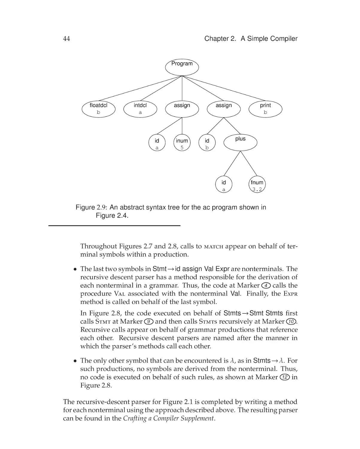
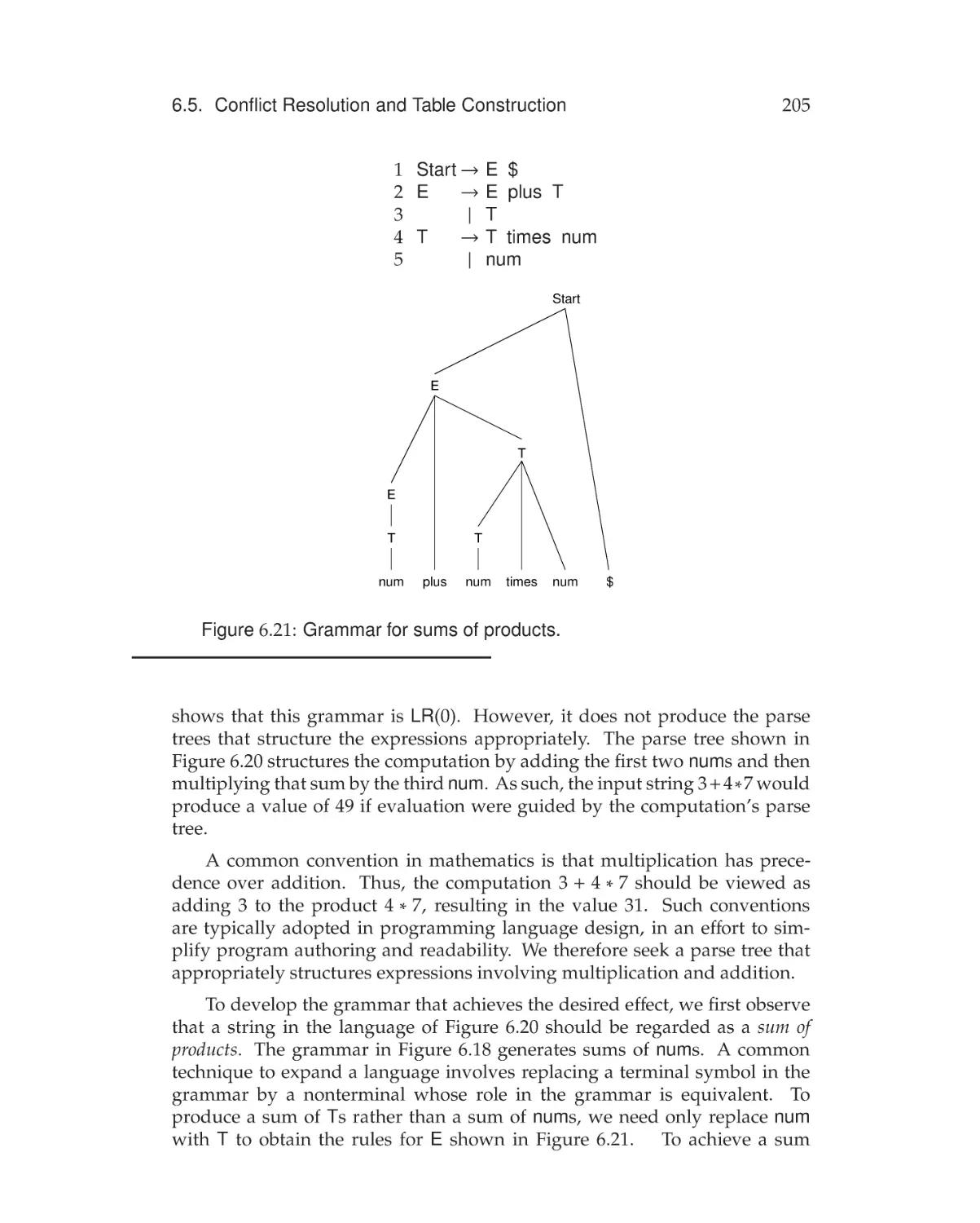
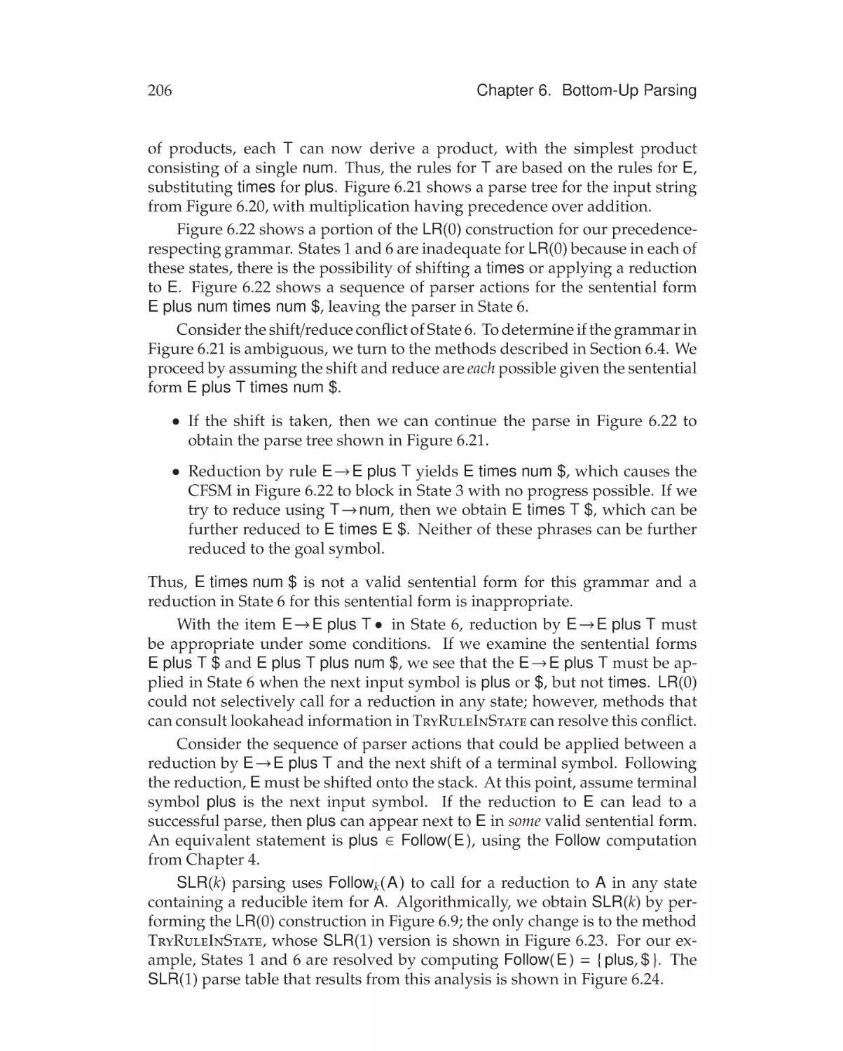
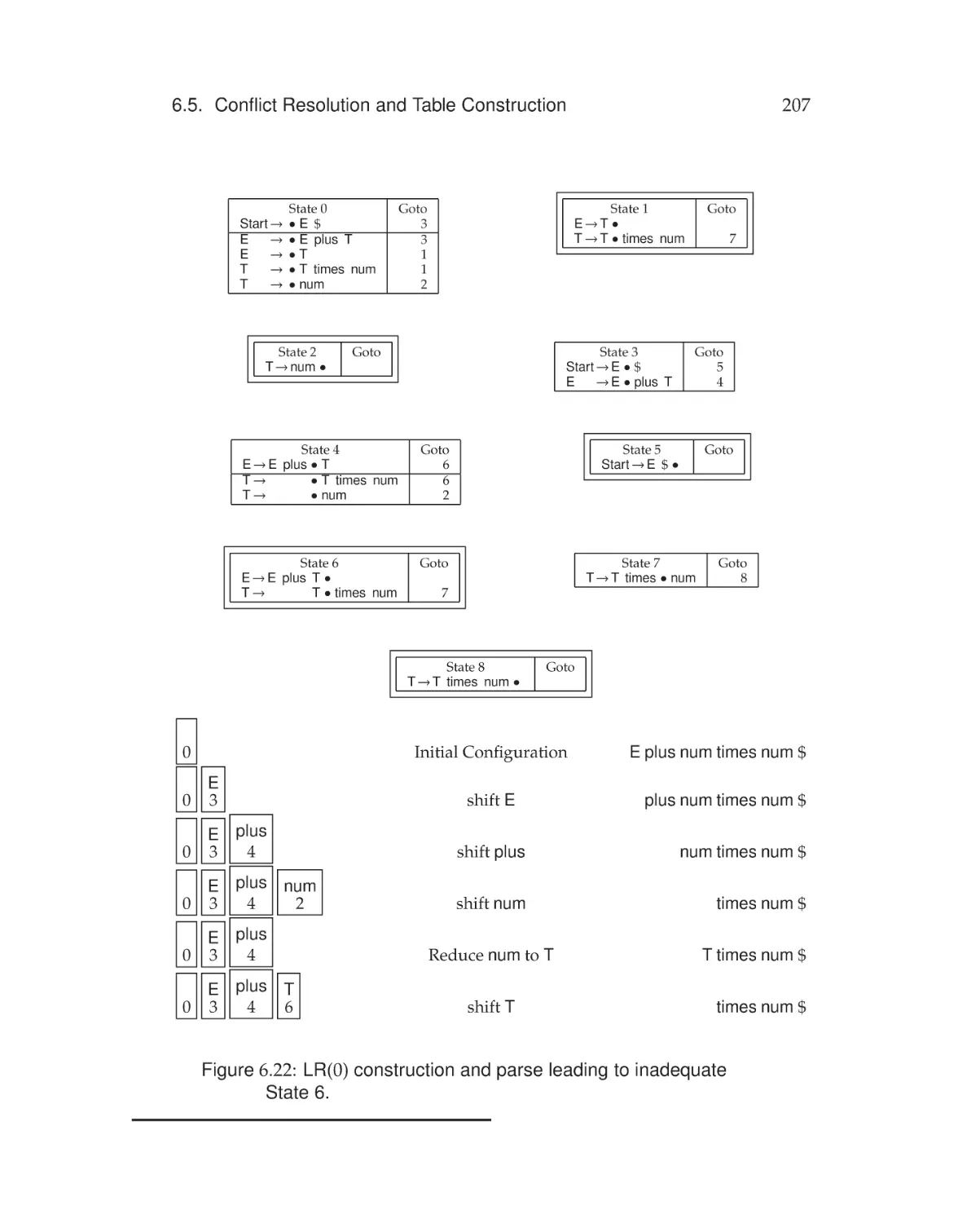
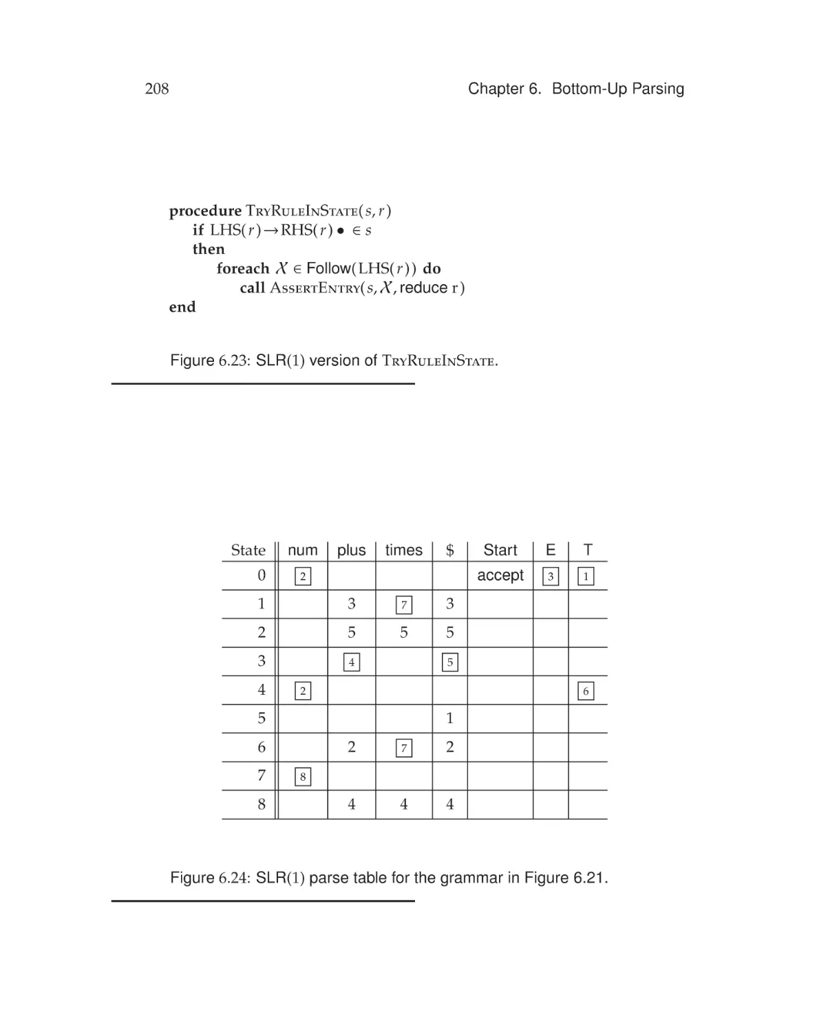
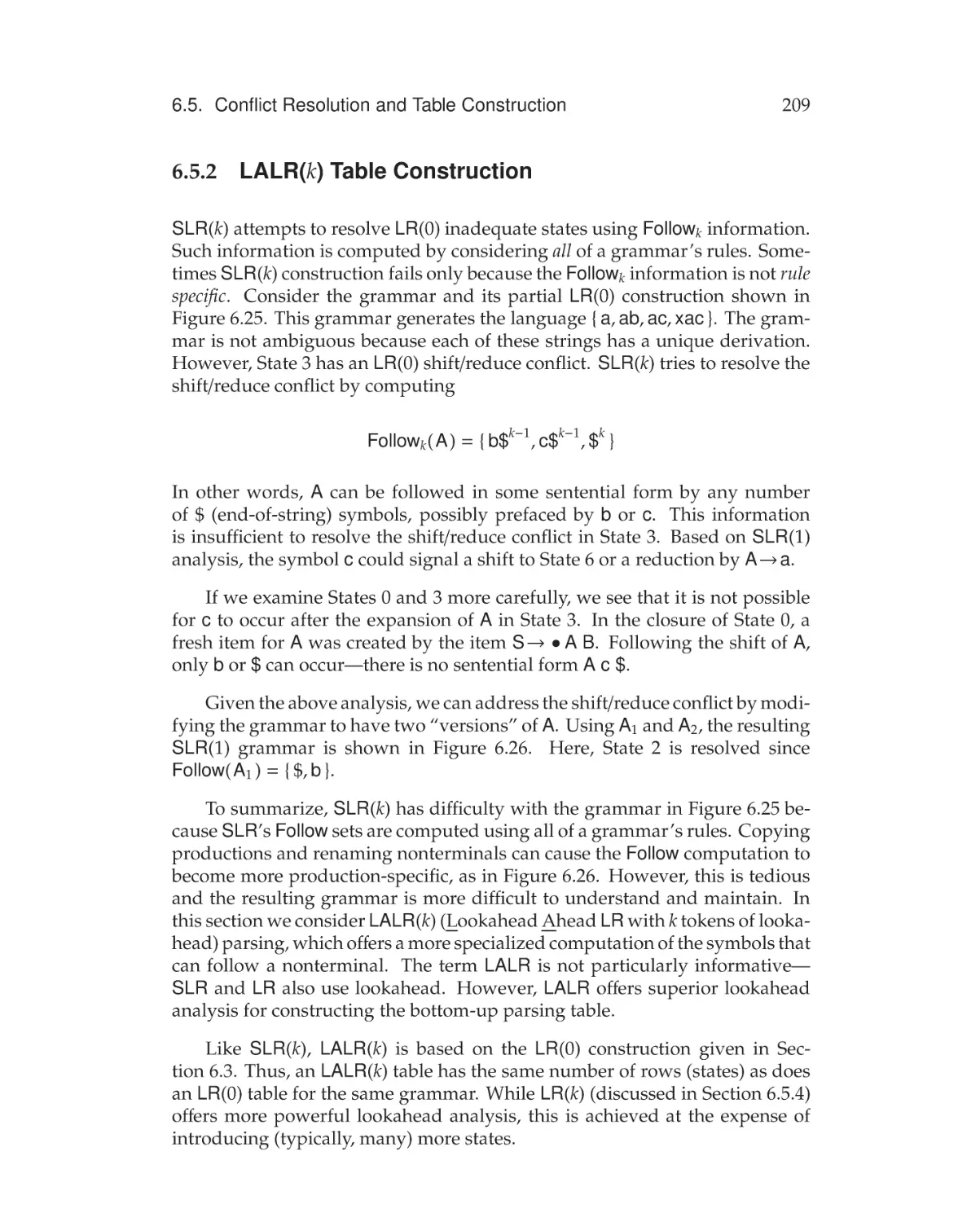
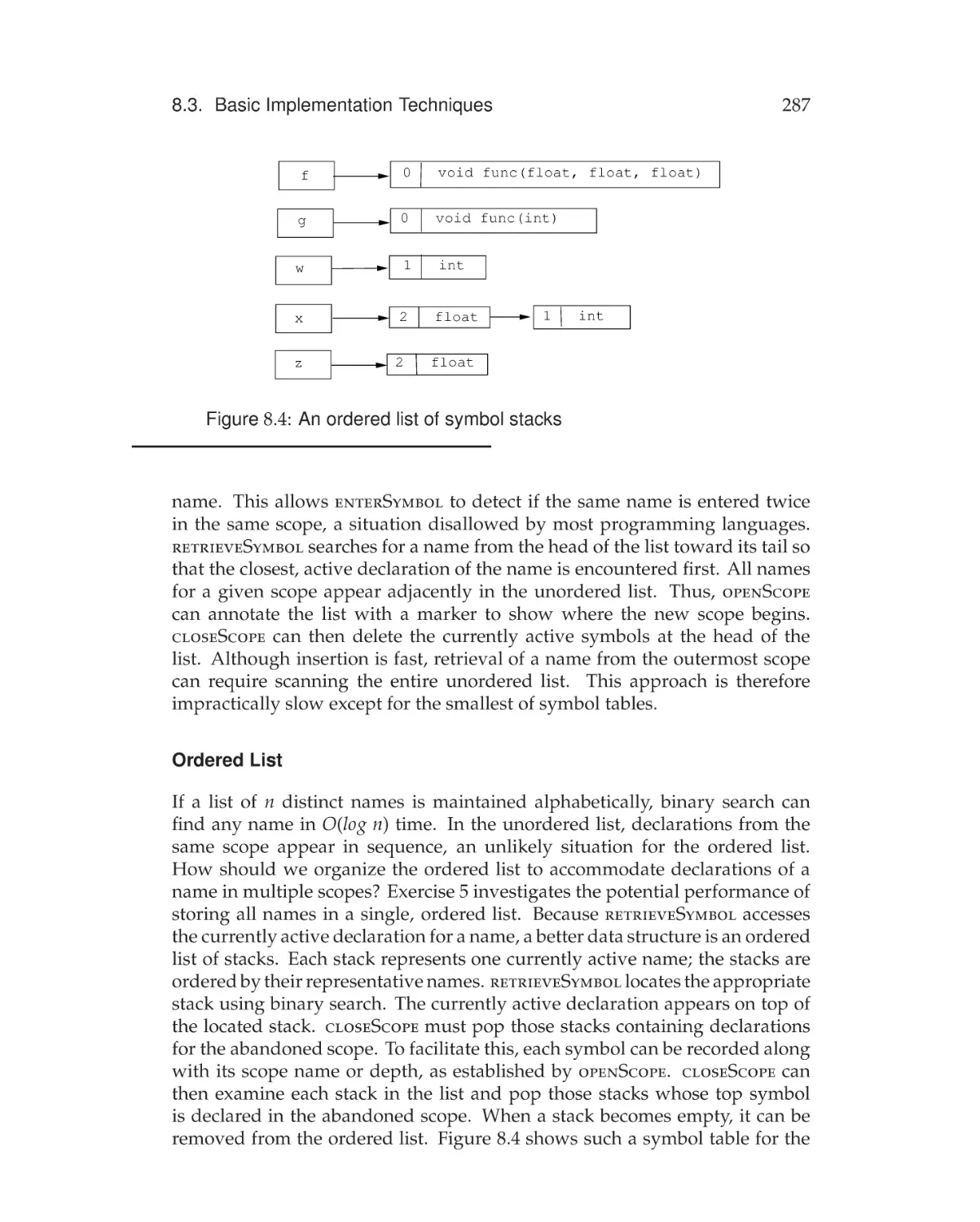
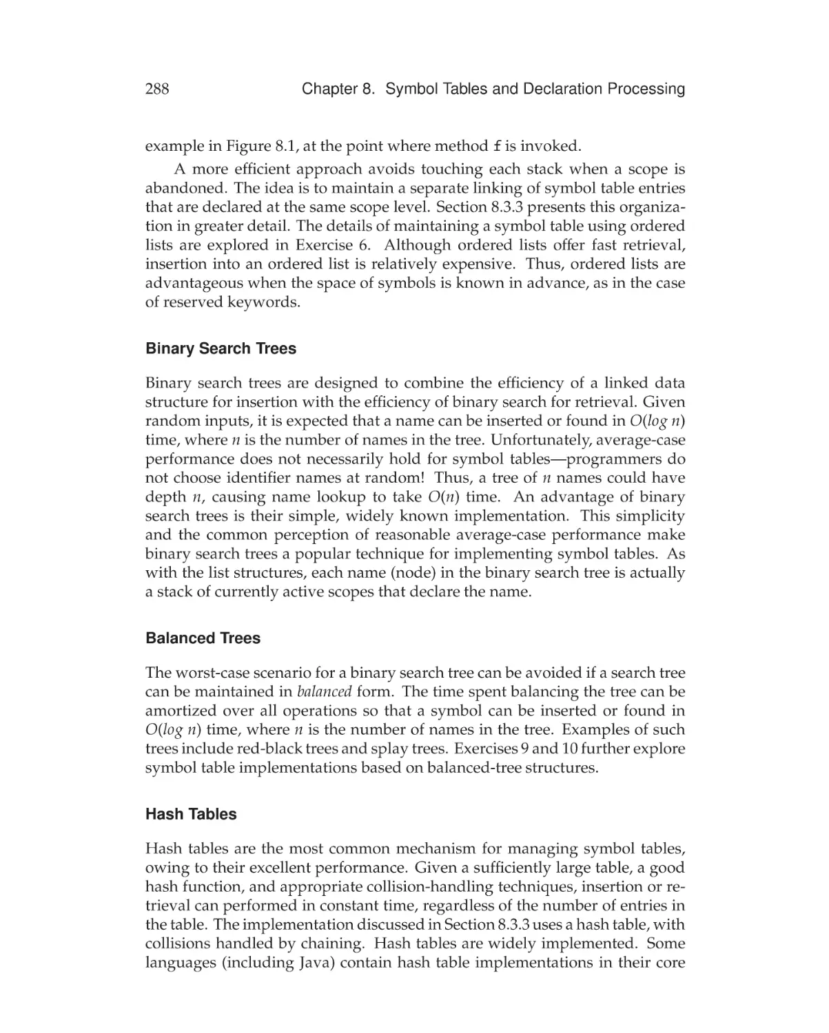
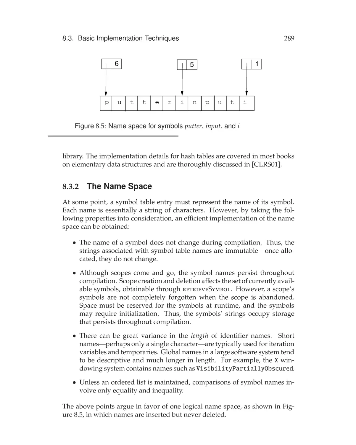
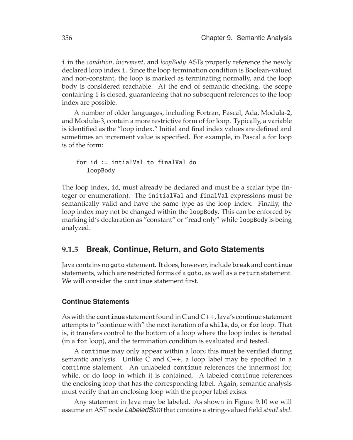
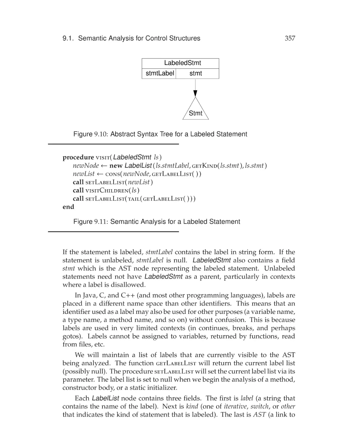
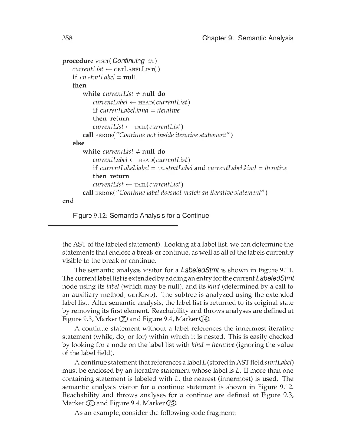
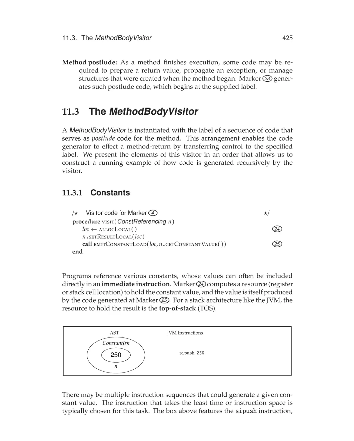
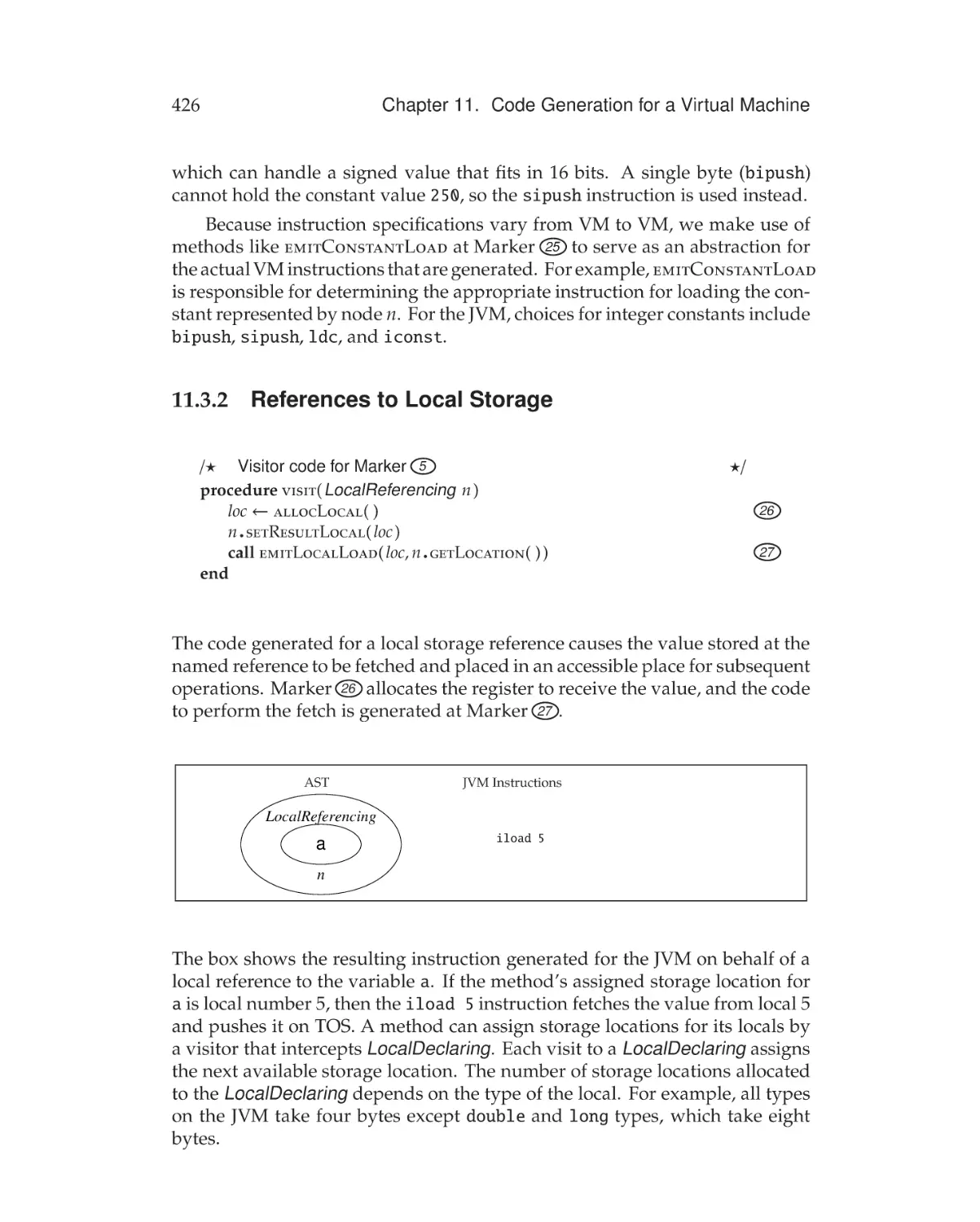
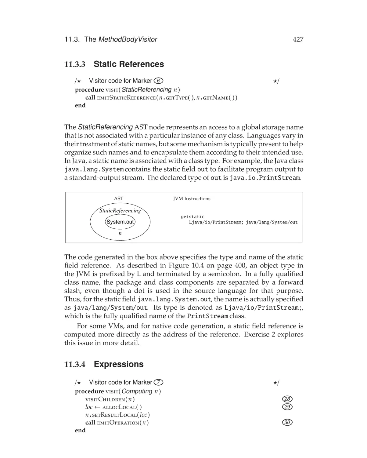
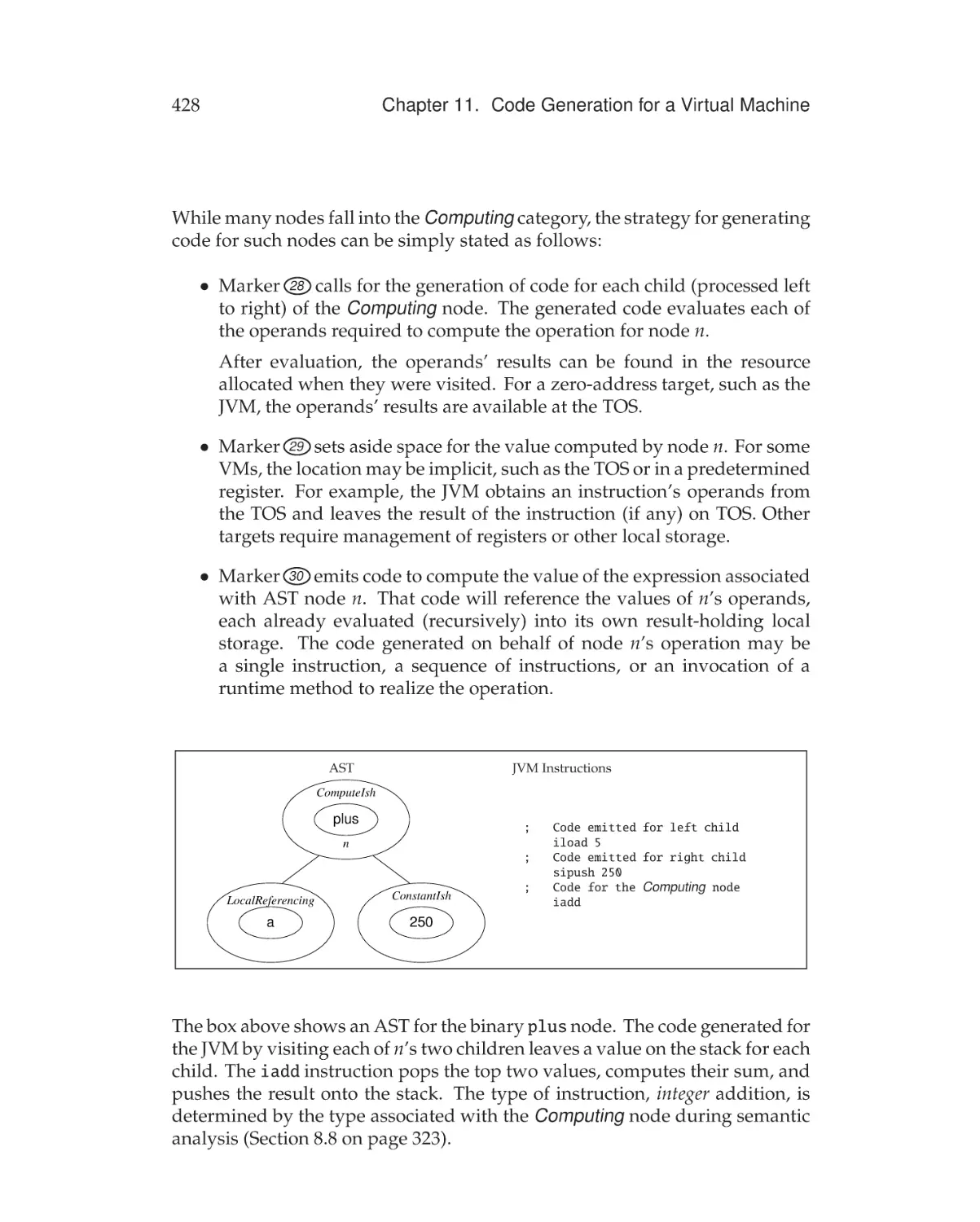
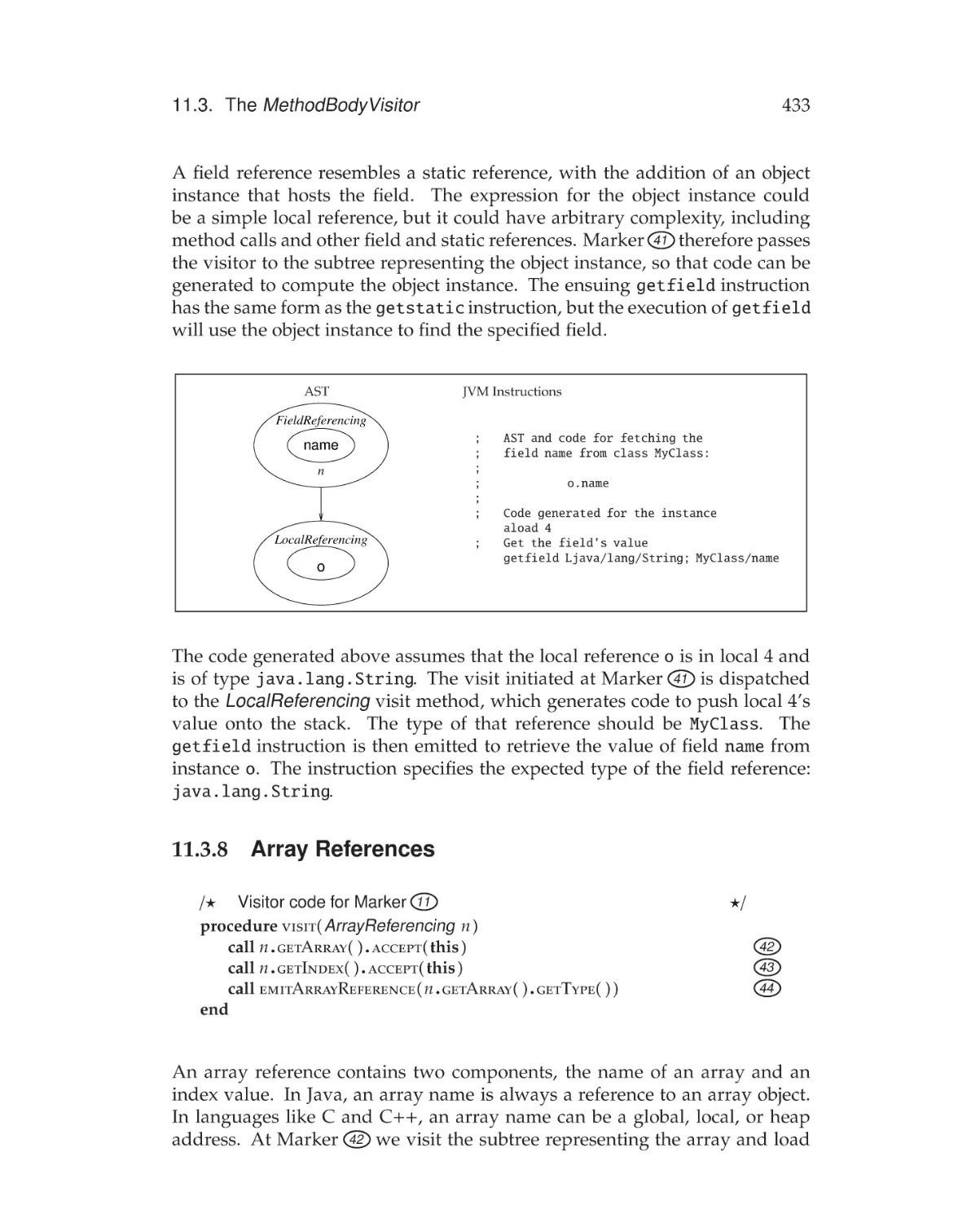
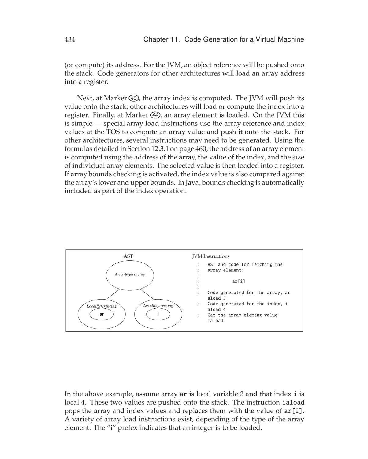
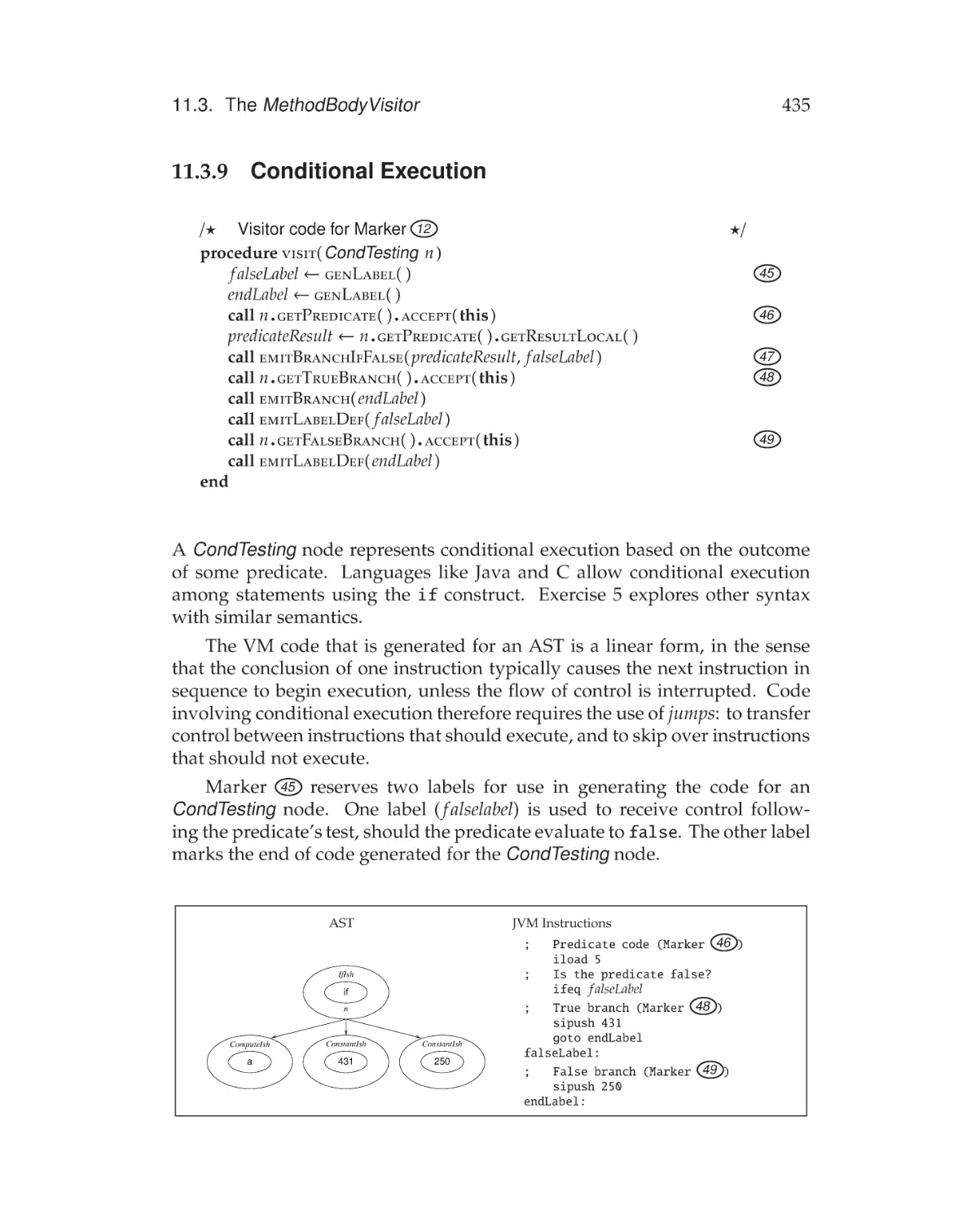
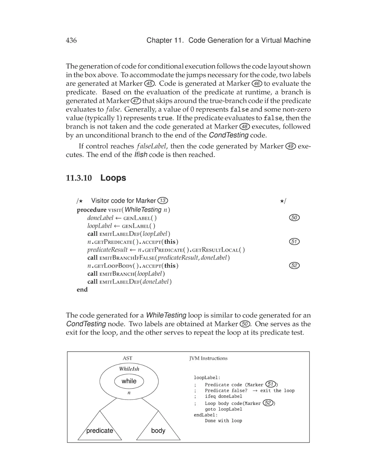
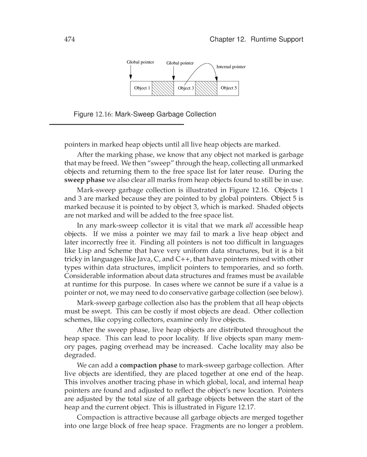
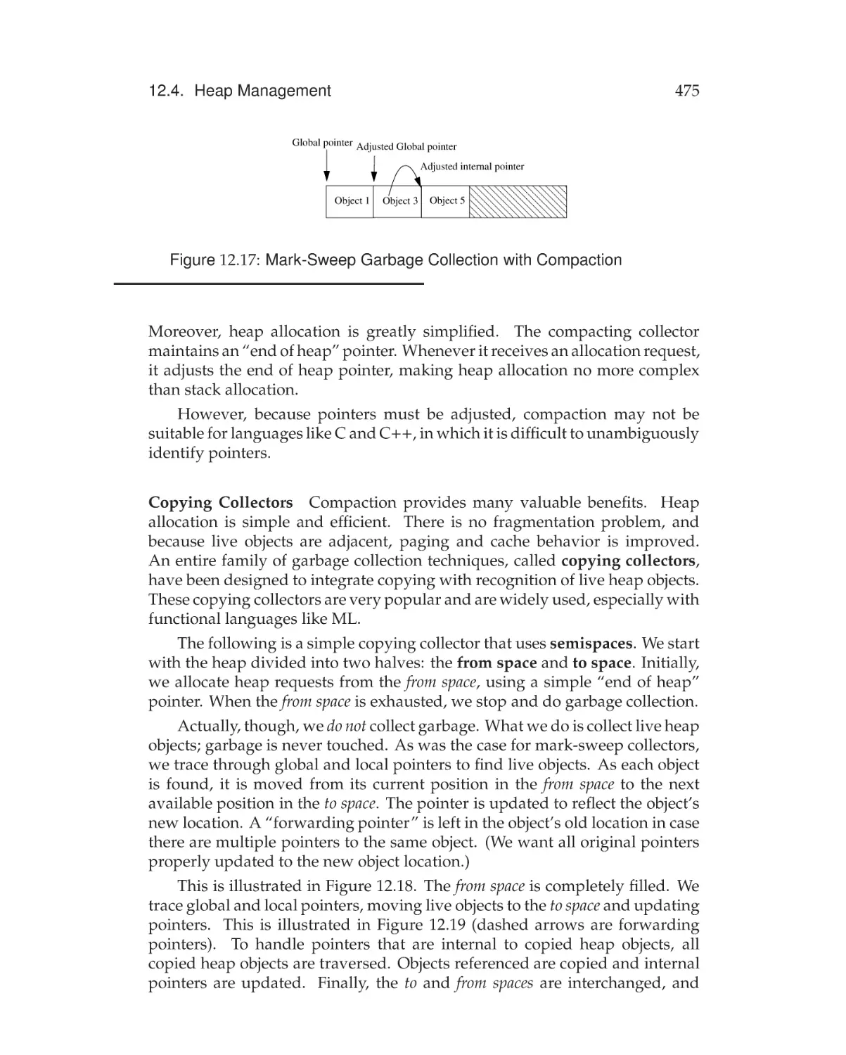
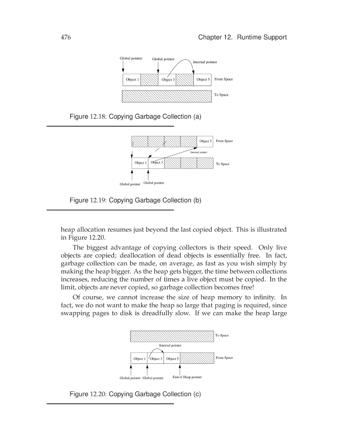
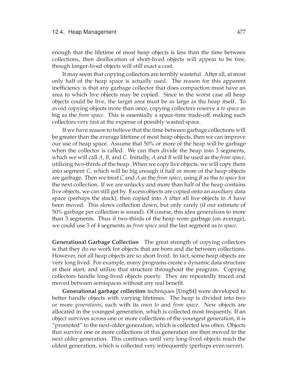
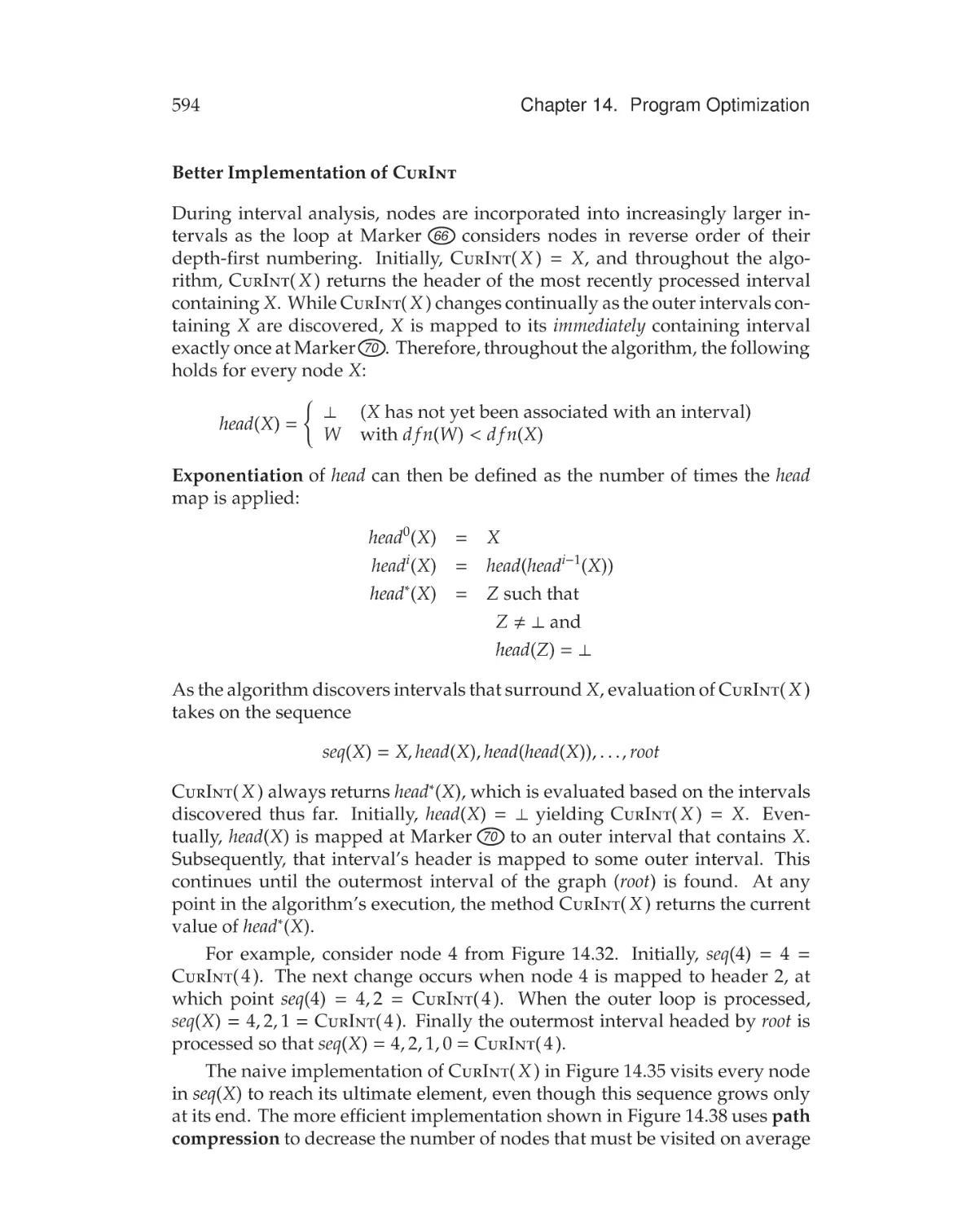
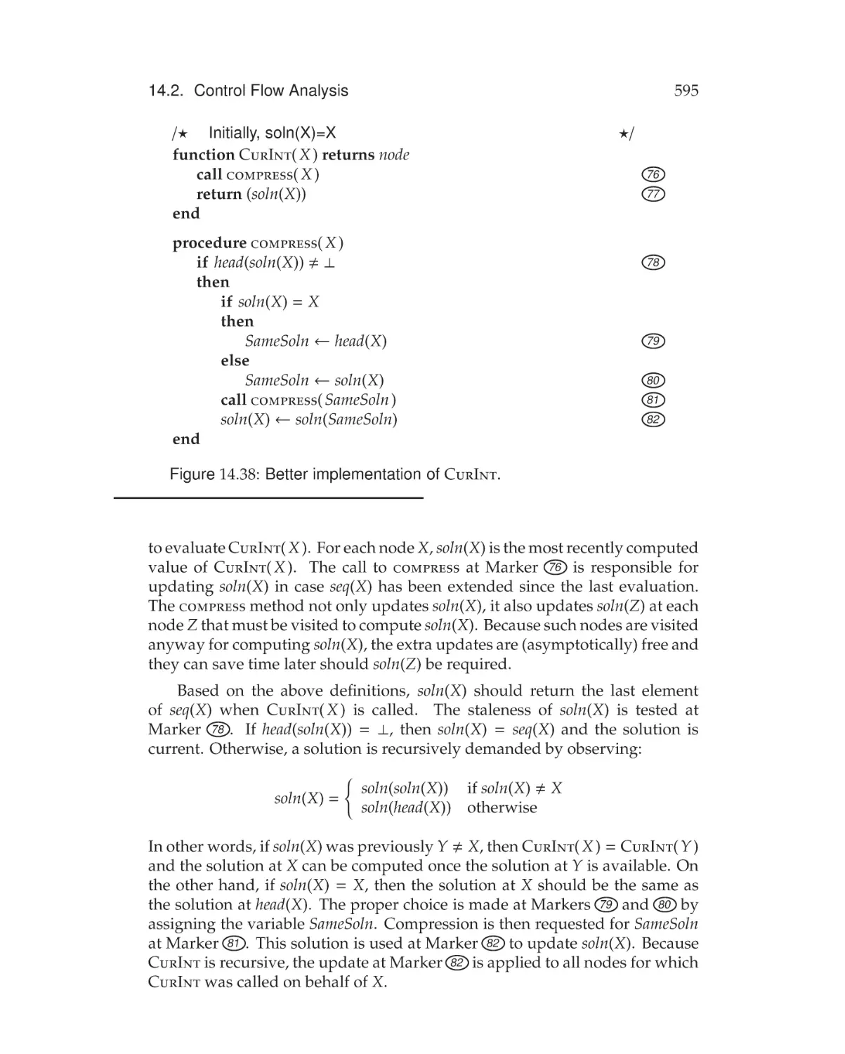
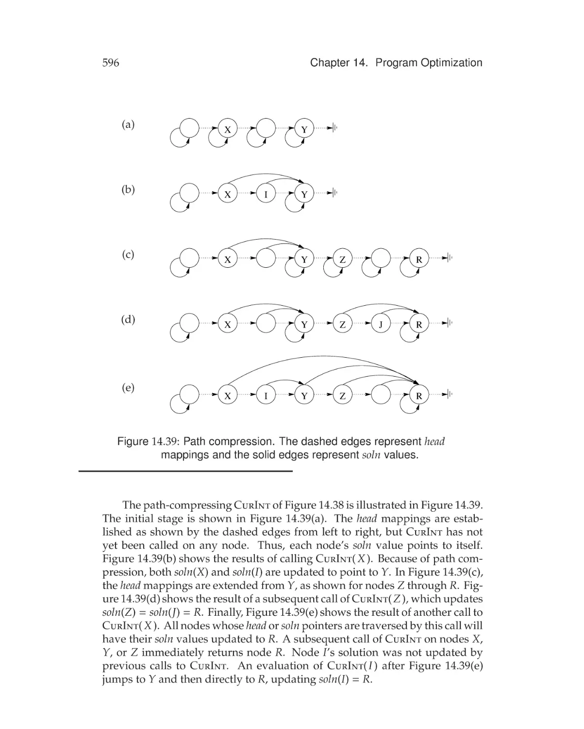
/


Author: Fischer Ch.N. Cytron K.R. LeBlanc R.J.Jr
Tags: programming computer science computer engineering addison-wesley central processor architecture
ISBN: 978-0-13-606705-4
Year: 2009


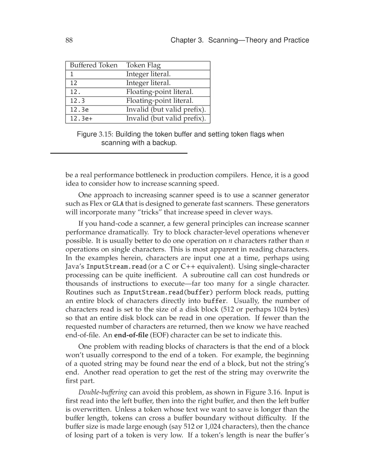
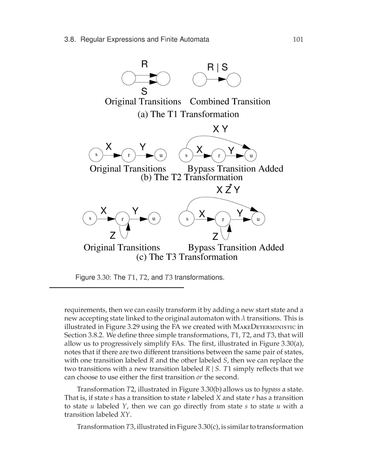
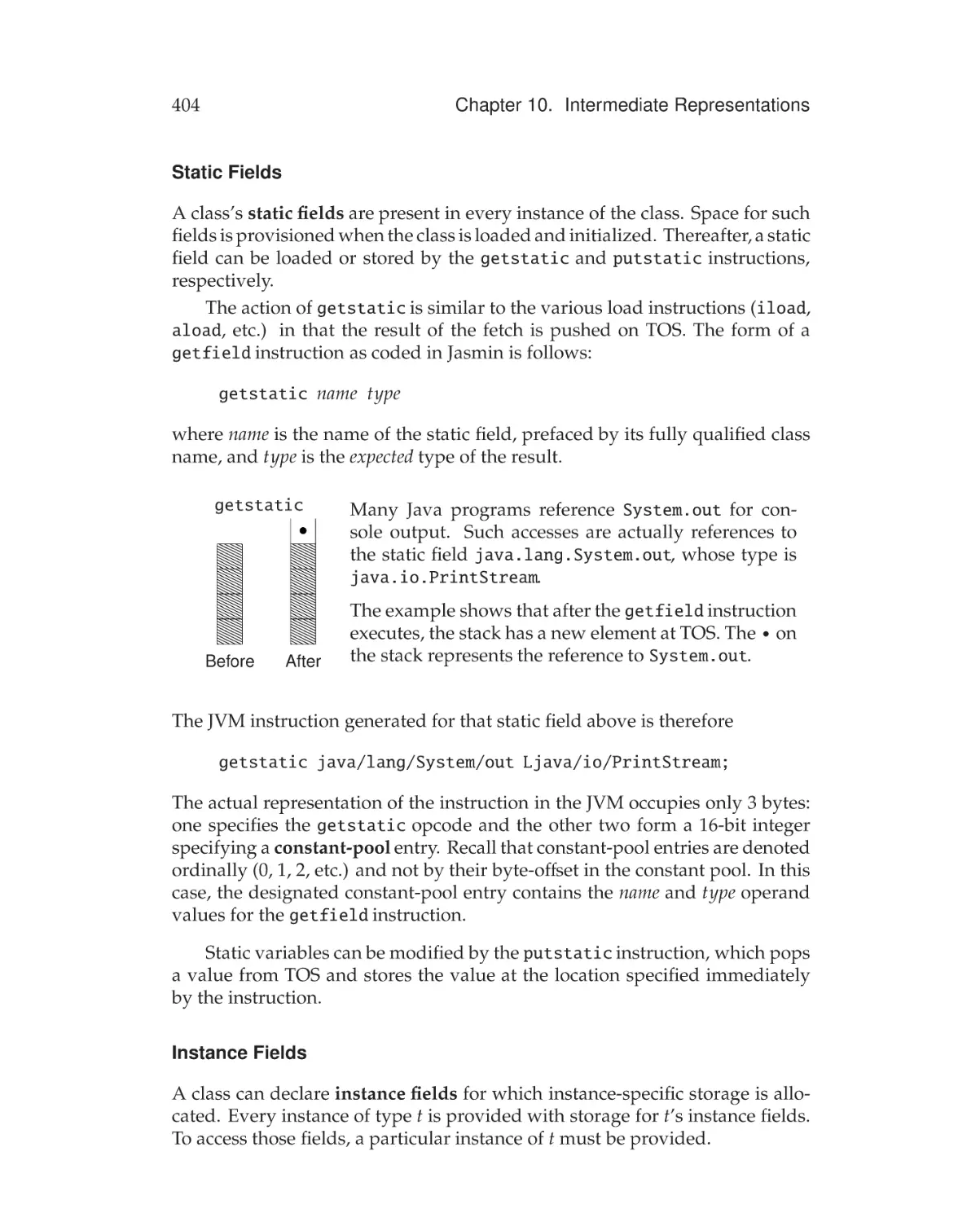
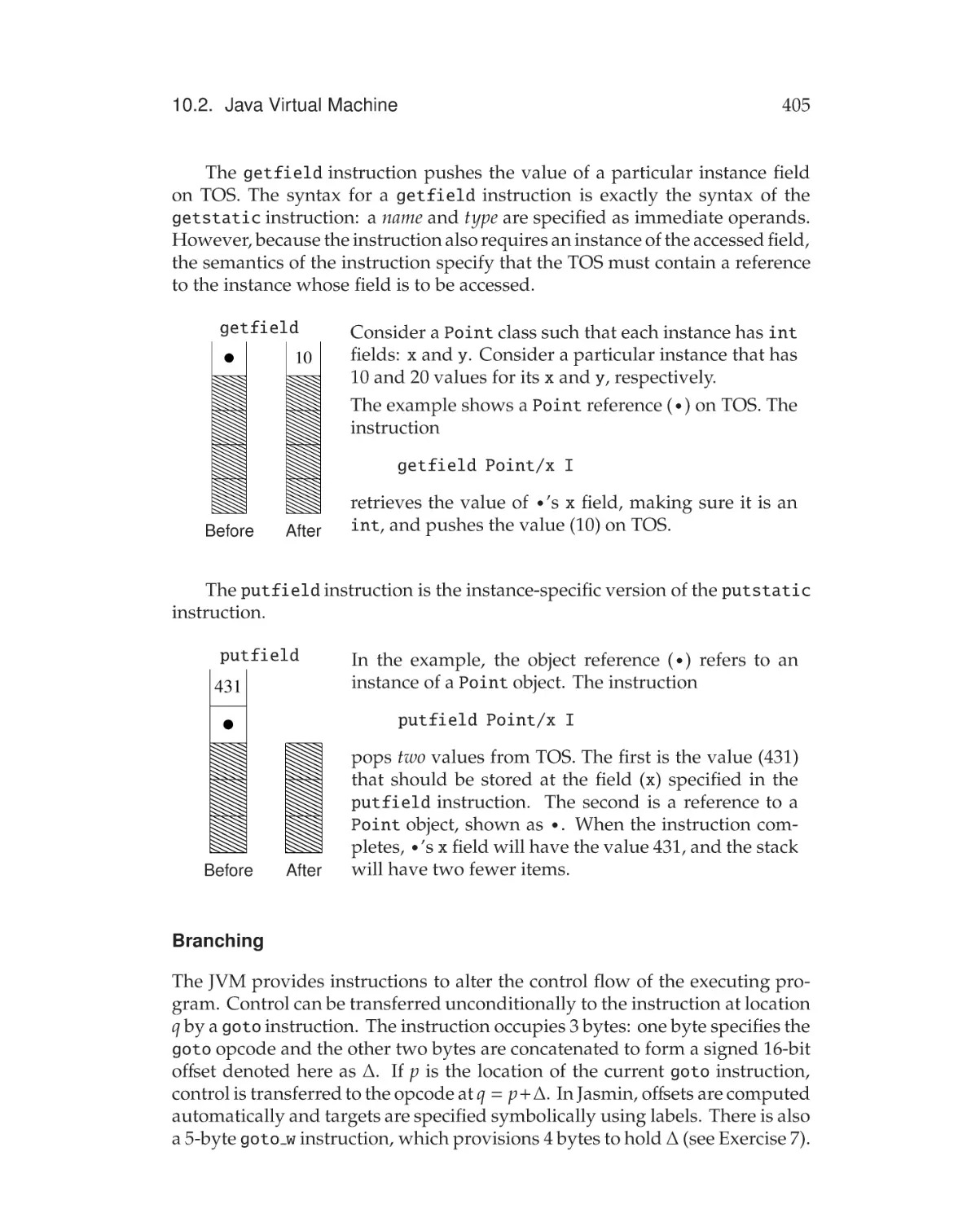
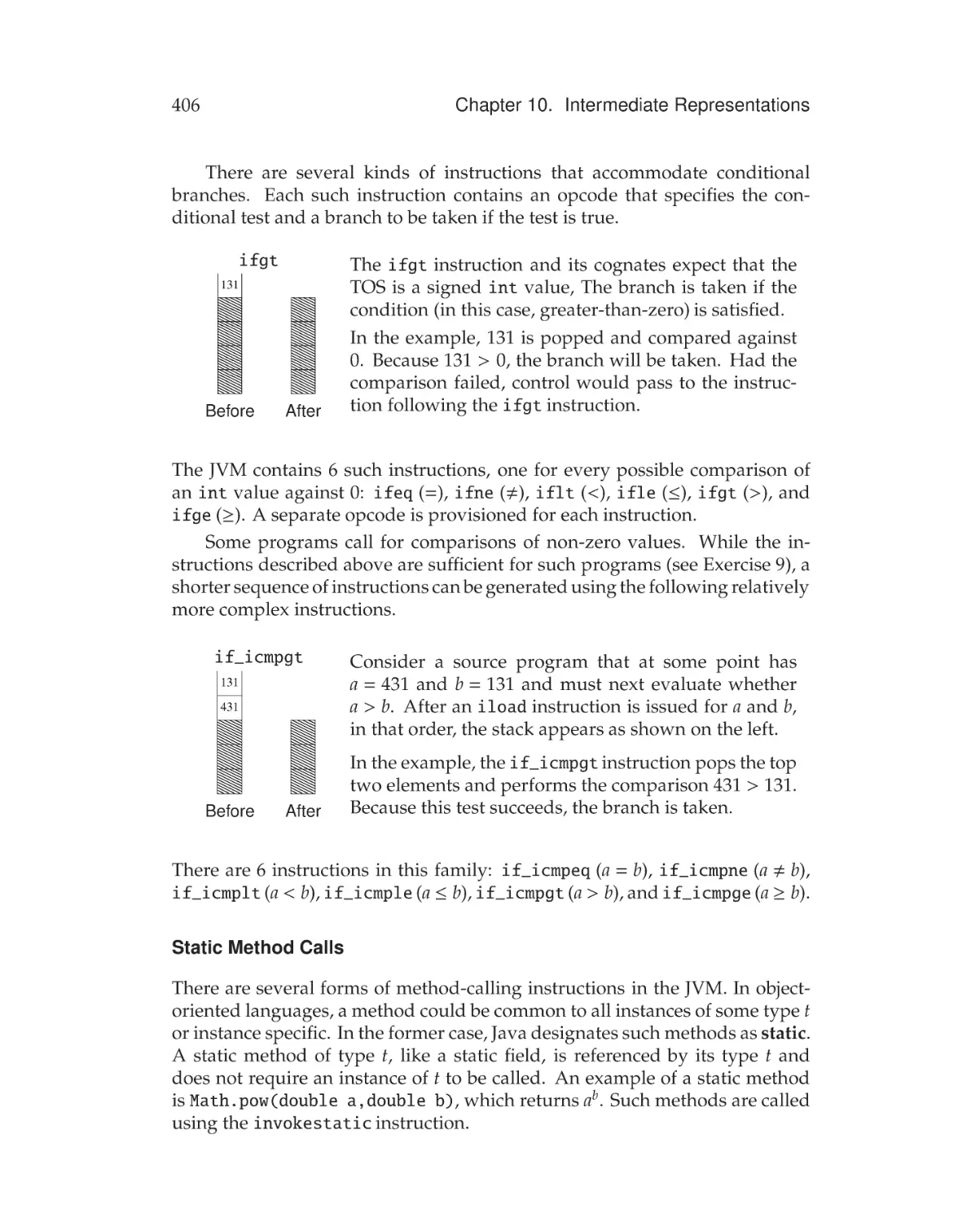
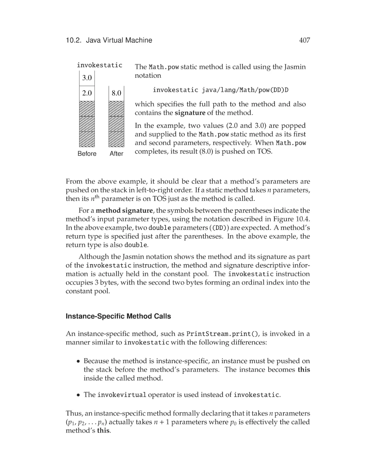
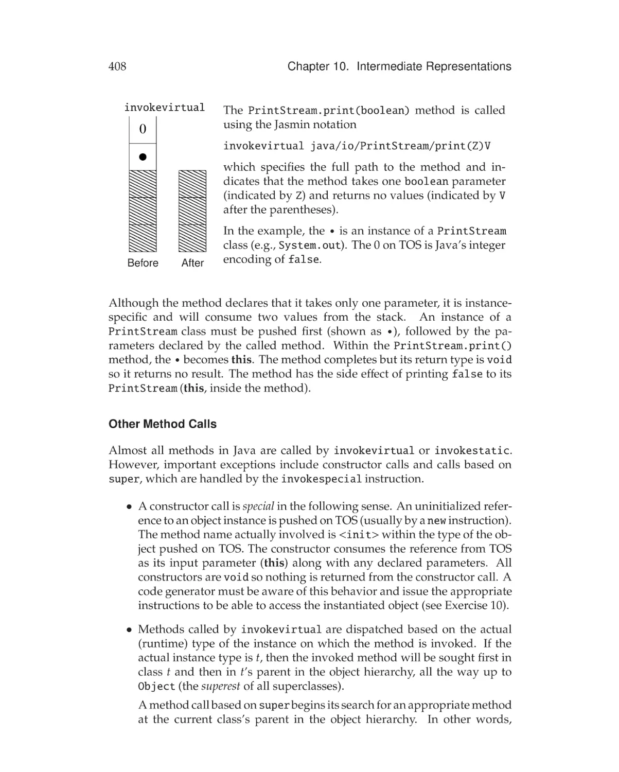
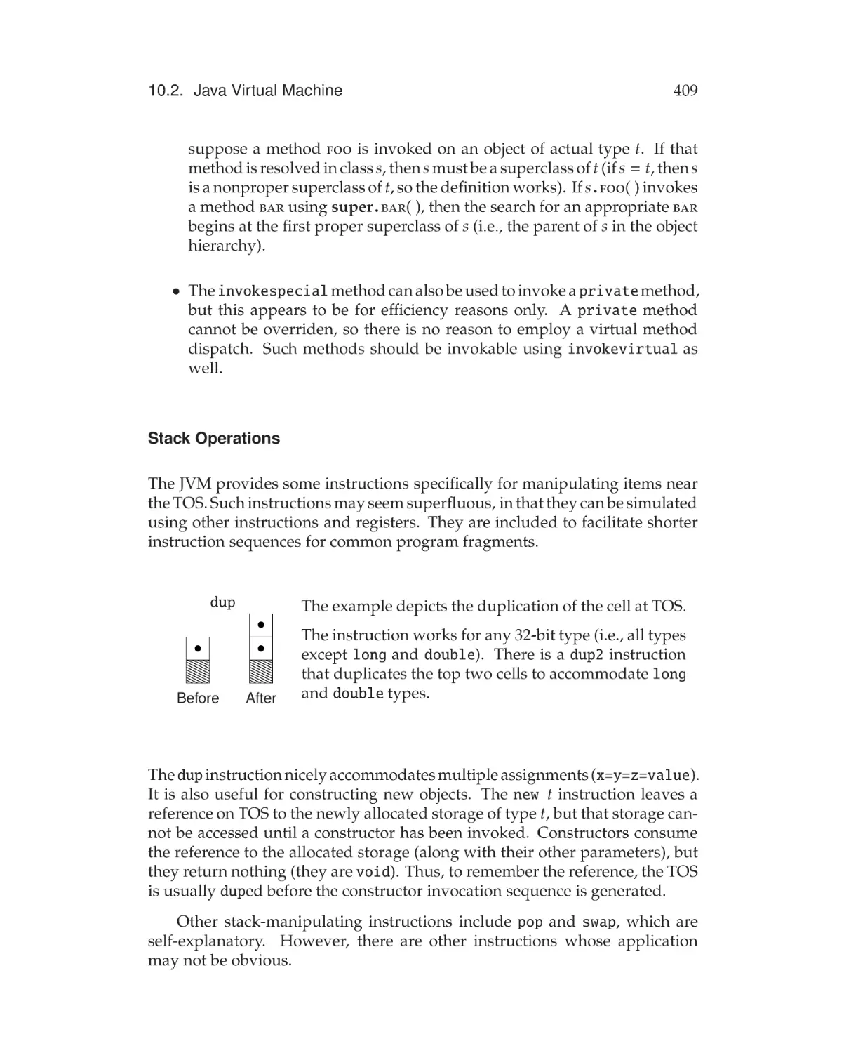
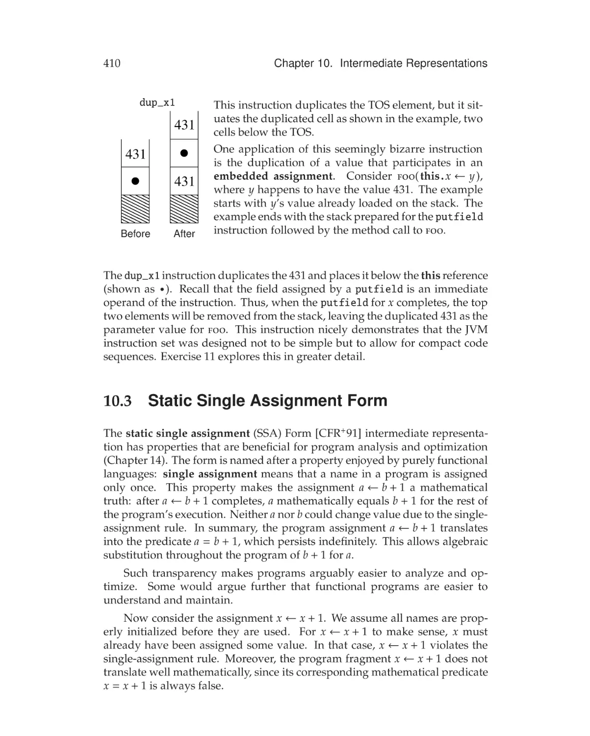
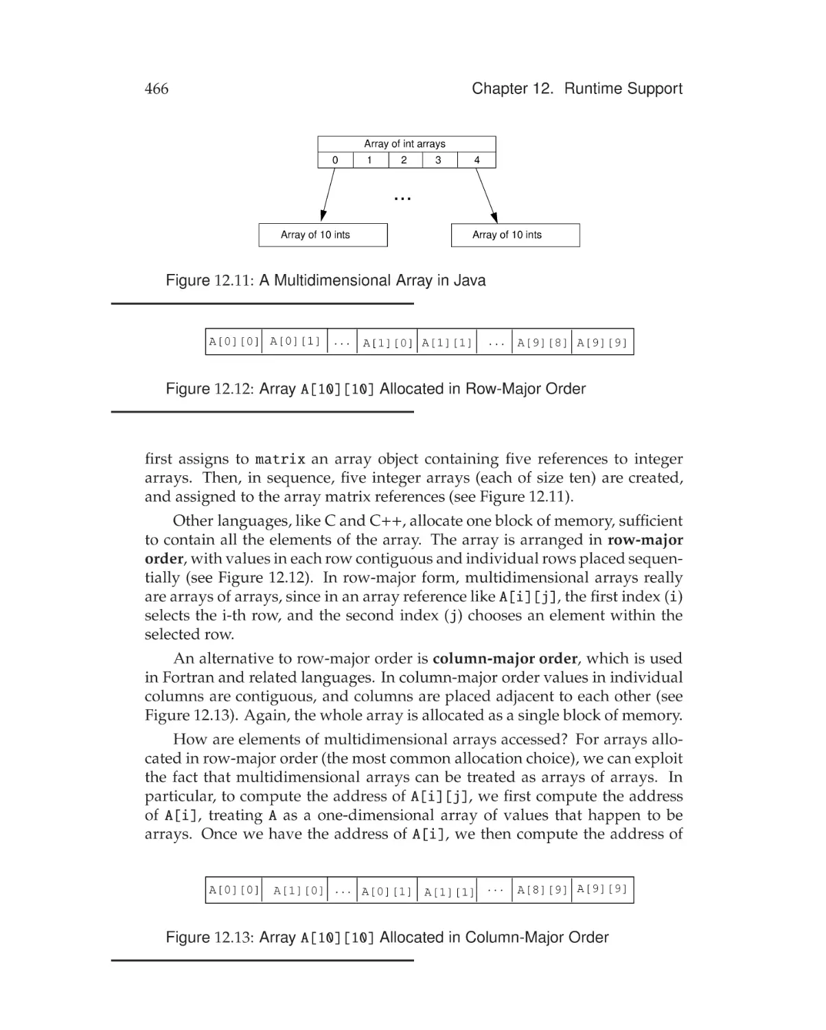
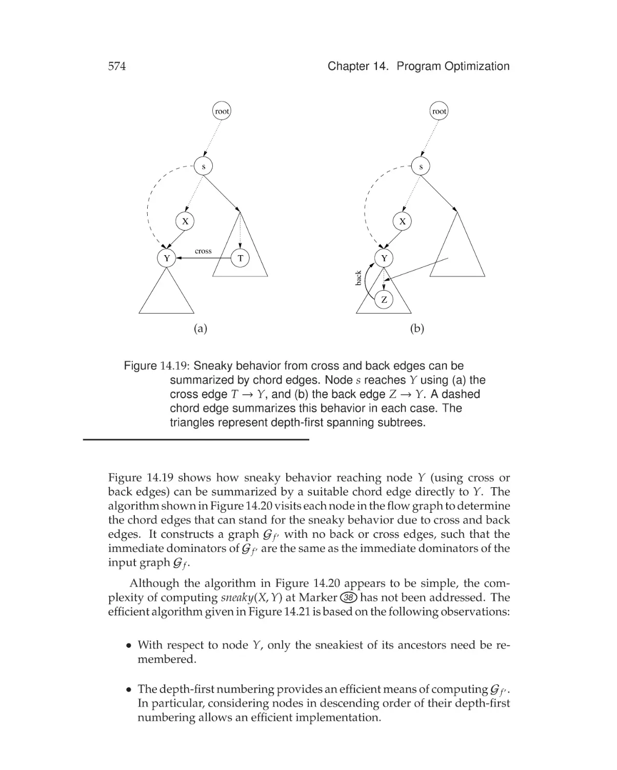
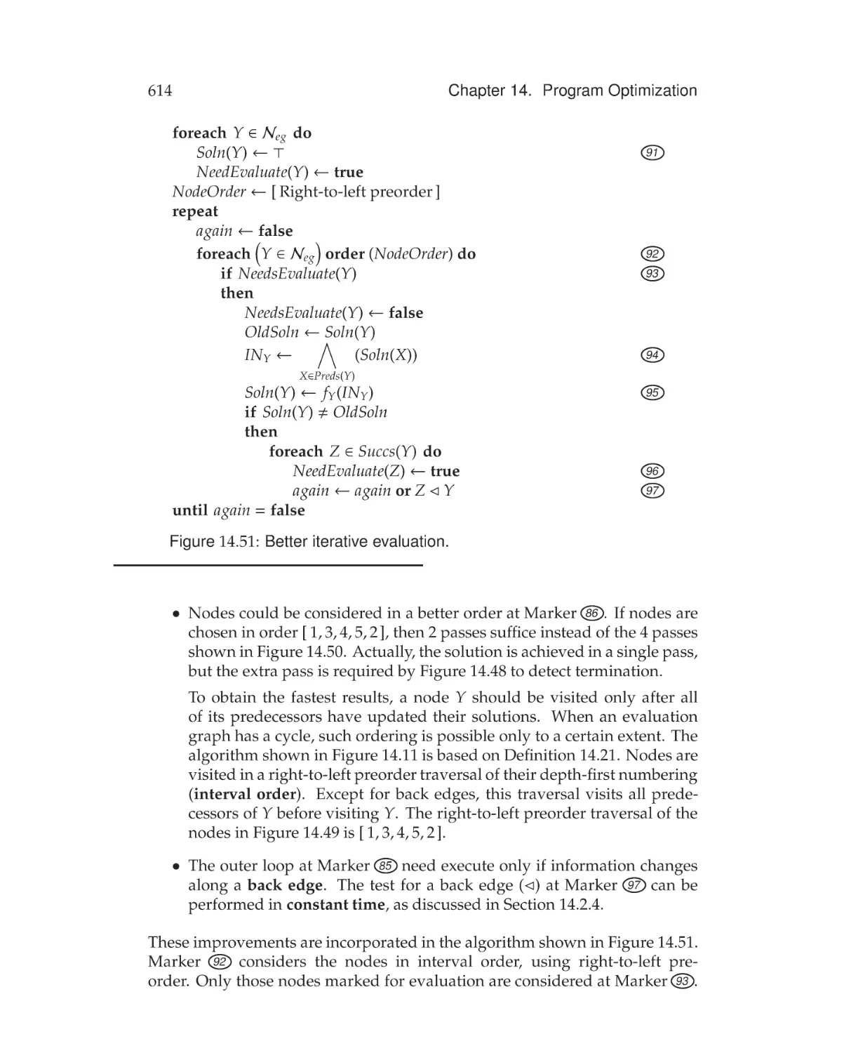
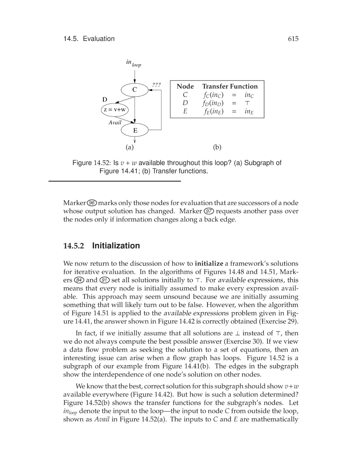
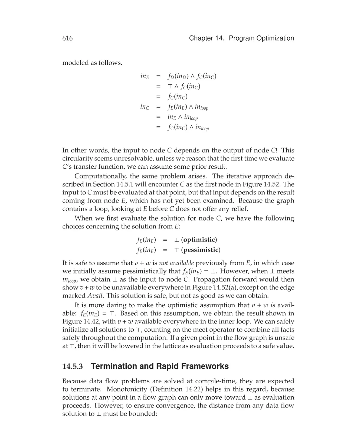
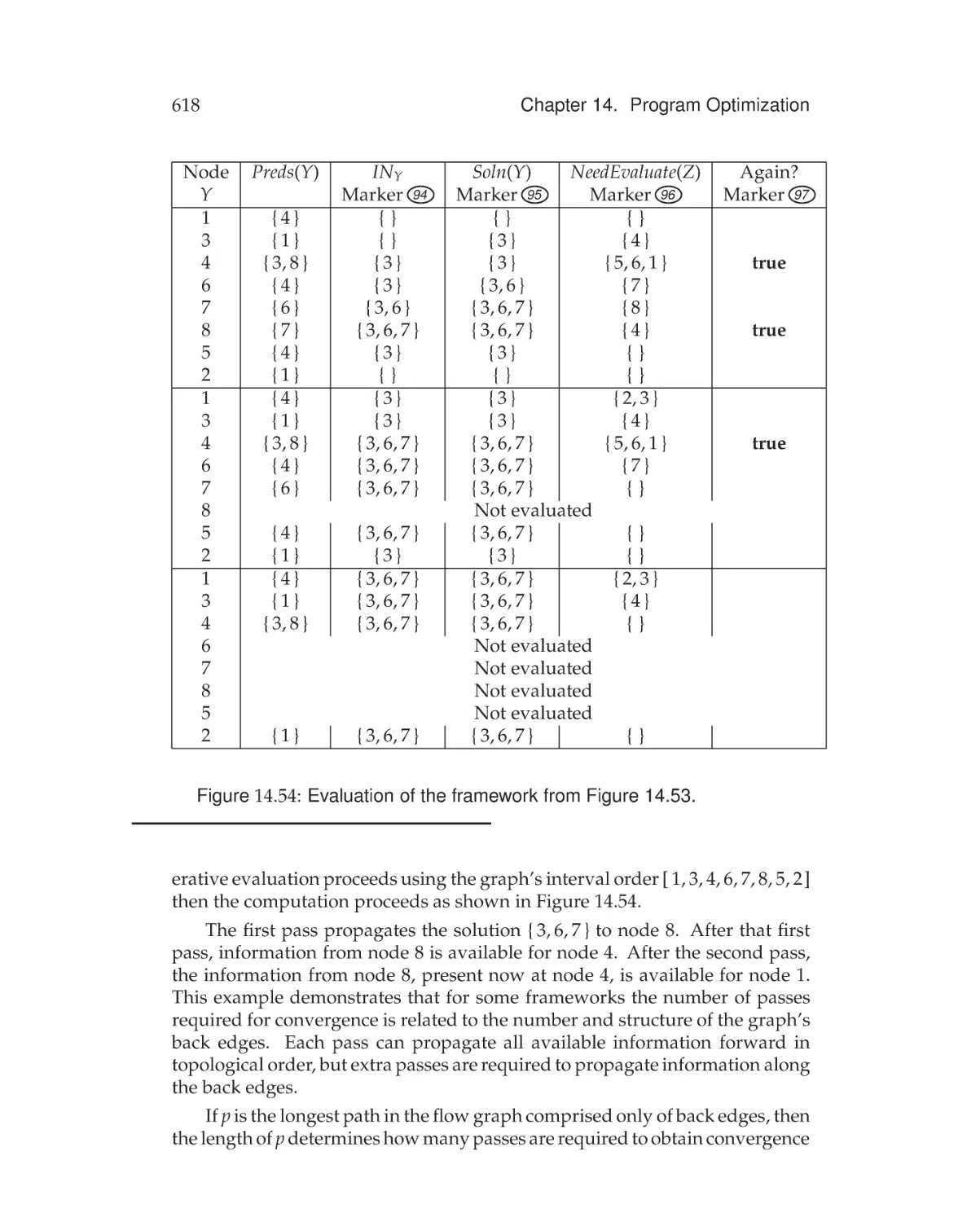
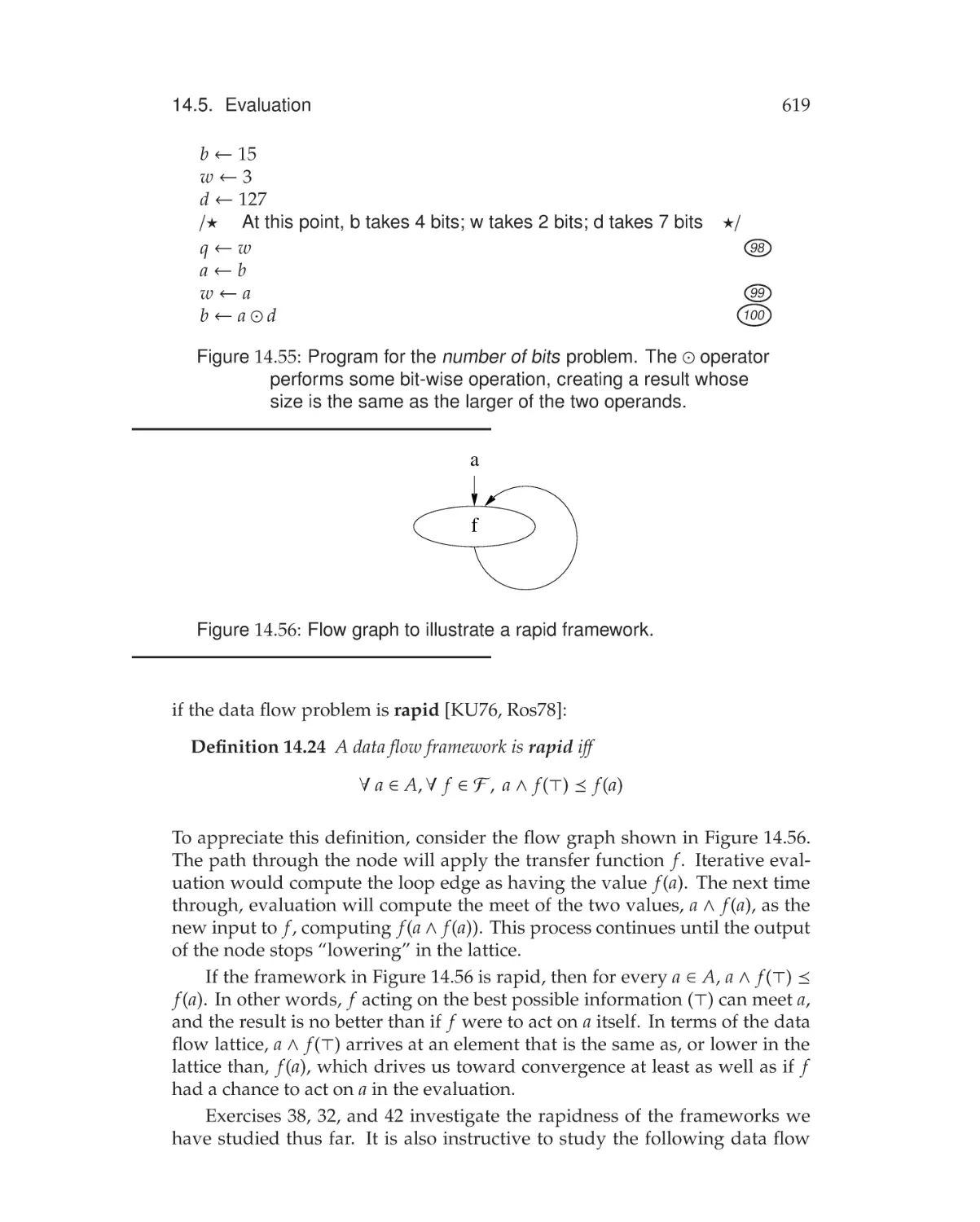
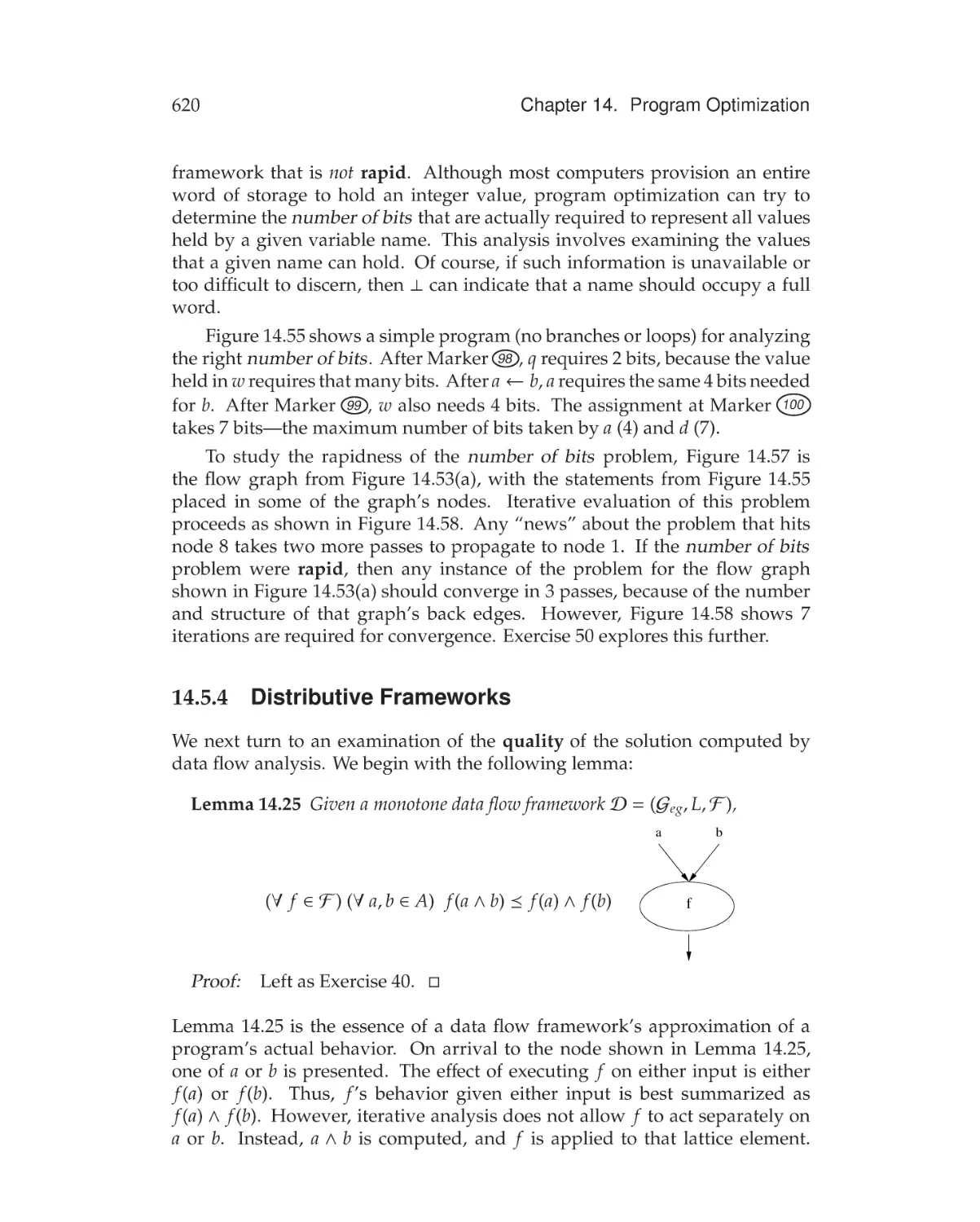
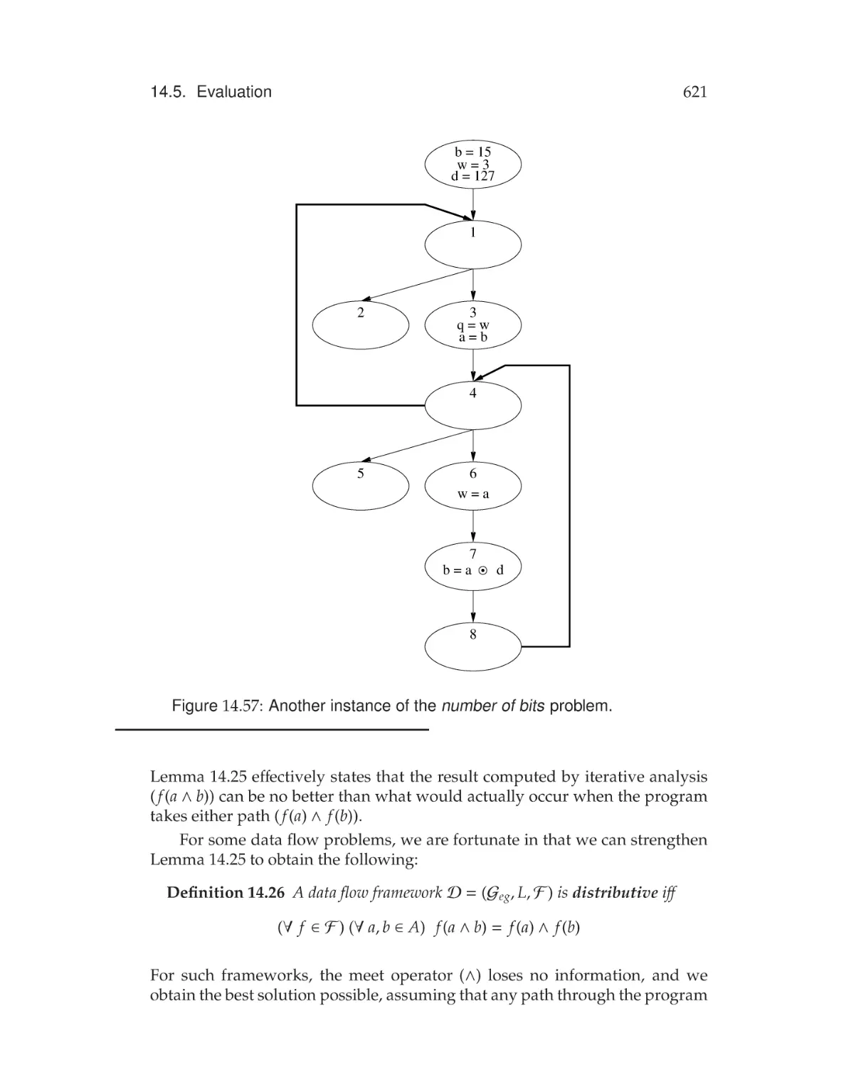
Text
8gV[i^c\
V8dbe^aZg
8=6GA:HC#;>H8=:G
8dbejiZgHX^ZcXZh
Jc^kZgh^ind[L^hXdch^cÄBVY^hdc
GDC@#8NIGDC
8dbejiZgHX^ZcXZVcY:c\^cZZg^c\
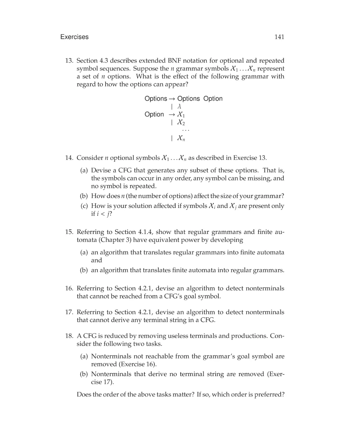
LVh]^c\idcJc^kZgh^in
G>8=6G9?#AZ7A6C8!?g#
8dbejiZgHX^ZcXZ
VcYHd[ilVgZ:c\^cZZg^c\
HZViiaZJc^kZgh^in
Addison-Wesley
Boston Columbus Indianapolis New York San Francisco Upper Saddle River
Amsterdam Cape Town Dubai London Madrid Milan Munich Paris Montreal Toronto
Delhi Mexico City Sao Paulo Sydney Hong Kong Seoul Singapore Taipei Tokyo
Editor-in-Chief: Michael Hirsch
Acquisitions Editor: Matt Goldstein
Editorial Assistant: Chelsea Bell
Managing Editor: Jeff Holcomb
Director of Marketing: Margaret Waples
Marketing Manager: Erin Davis
Marketing Coordinator: Kathryn Ferranti
Media Producer: Katelyn Boller
Senior Manufacturing Buyer: Carol Melville
Senior Media Buyer: Ginny Michaud
Art Director: Linda Knowles
Cover Designer: Elena Sidorova
Printer/Binder: Hamilton Printing Co.
Cover Printer: Lehigh Phoenix Hagerstown
Many of the designations used by manufacturers and sellers to distinguish their products are claimed as
trademarks. Where those designations appear in this book, and Addison-Wesley was aware of a
trademark claim, the designations have been printed in initial caps or all caps.
The programs and applications presented in this book have been included for their instructional value.
They have been tested with care, but are not guaranteed for any particular purpose. The publisher does
not offer any warranties or representations, nor does it accept any liabilities with respect to the
programs or applications.
Library of Congress Cataloging-in-Publication Data
Fischer, Charles N.
Crafting a compiler / Charles N. Fischer, Ron K. Cytron, Richard J. LeBlanc, Jr.
p. cm. -- (Crafting a compiler with C)
Includes bibliographical references and index.
ISBN 978-0-13-606705-4 (alk. paper)
1. Compilers (Computer programs) I. Cytron, Ron K. (Ronald Kaplan), 1958- II. LeBlanc, Richard J.
(Richard Joseph), 1950- III. Title.
QA76.76.C65F57 2009
005.4'53--dc22
2009038265
Copyright © 2010 Pearson Education, Inc., publishing as Addison-Wesley. All rights reserved.
Manufactured in the United States of America. This publication is protected by Copyright, and
permission should be obtained from the publisher prior to any prohibited reproduction, storage in a
retrieval system, or transmission in any form or by any means, electronic, mechanical, photocopying,
recording, or likewise. To obtain permission(s) to use material from this work, please submit a written
request to Pearson Education, Inc., Permissions Department, 501 Boylston Street, Suite 900, Boston,
Massachusetts, 02116.
10 9 8 7 6 5 4 3 2 1—HA—13 12 11 10 09
Addison-Wesley
is an imprint of
www.pearsonhighered.com
ISBN 10: 0-13-606705-0
ISBN 13: 978-0-13-606705-4
Preface
Much has changed since Crafting a Compiler, by Fischer and LeBlanc, was
published in 1988. While instructors may remember the 5 41 -inch floppy disk of
software that accompanied that text, most students today have neither seen nor
held such a disk. Many changes have occurred in the programming languages
that students experience in class and in the marketplace. In 1991 the book
was available in two forms, with algorithms presented in either C or Ada.
While C remains a popular language, Ada has become relatively obscure and
did not achieve its predicted popularity. The C++ language evolved from
C with the addition of object-oriented features. JavaTM was developed as a
simpler object-oriented language, gaining popularity because of its security
and ability to be run within a Web browser. The College Board Advanced
Placement curriculum moved from Pascal to C++ to Java.
While much has changed, students and faculty alike continue to study and
teach the subject of compiler construction. Research in the area of compilers
and programing language translation continues at a brisk pace, as compilers
are tasked with accommodating an increasing diversity of architectures and
programming languages. Software development environments depend on
compilers interacting successfully with a variety of software toolchain components such as syntax-informed editors, performance profilers, and debuggers.
All modern software efforts rely on their compilers to check vigorously for
errors and to translate programs faithfully.
Some texts experience relatively minor changes over time, acquiring perhaps some new exercises or examples. This book reflects a substantive revision
of the material from 1988 and 1991. While the focus of this text remains on
teaching the fundamentals of compiler construction, the algorithms and approaches have been brought into modern practice:
• Coverage of topics that have faded from practical use (e.g., attribute
grammars) has been minimized or removed altogether.
• Algorithms are presented in a pseudocode style that should be familiar to
students who have studied the fundamental algorithms of our discipline.
iii
iv
Preface
Pseudocode enables a concise formulation of an algorithm and a rational
discussion of the algorithm’s purpose and construction.
The details of implementation in a particular language have been relegated to the Crafting a Compiler Supplement which is available online:
http://www.pearsonhighered.com/fischer/
• Parsing theory and practice are organized to facilitate a variety of pedagogical approaches.
Some may study the material at a high level to gain a broad view of topdown and bottom-up parsing. Others may study a particular approach
in greater detail.
• The front- and back-end phases of a compiler are connected by the abstract syntax tree (AST), which is created as the primary artifact of parsing. Most compilers build an AST, but relatively few texts articulate its
construction and use.
The visitor pattern is introduced for traversing the AST during semantic
analysis and code generation.
• Laboratory and studio exercises are available to instructors.
Instructors can assign some components as exercises for the students
while other components are supplied from our course-support Web site.
Some texts undergo revision by the addition of more graduate-level material.
While such information may be useful in an advanced course, the focus of
Crafting a Compiler remains on the undergraduate-level study of compiler construction. A graduate course could be offered using Chapters 13 and 14, with
the earlier portions of the text serving as reference material.
Text and Reference
As a classroom text, this book is oriented toward a curriculum that we have
developed over the past 25 years. The book is very flexible and has been
adopted for courses ranging from a three-credit upper-level course taught in
a ten-week quarter to a six-credit semester-long graduate course. The text
is accessible to any student who has a basic background in programming,
algorithms, and data structures. The text is well suited to a single semester or
quarter offering because its flexibility allows an instructor to craft a syllabus
according to his or her interests. Author-sponsored solutions are available for
those components that are not studied in detail. It is feasible to write portions
of a compiler from parsing to code generation in a single semester.
Preface
v
This book is also a valuable professional reference because of its complete
coverage of techniques that are of practical importance to compiler construction. Many of our students have reported, even some years after their graduation, of their successful application of these techniques to problems they
encounter in their work.
Instructor Resources
The Web site for this book can be found at http://www.pearsonhighered.
com/fischer/. The material posted for qualified instructors includes sample
laboratory and project assignments, studio (active-learning) sessions, libraries
of code that can be used as class-furnished solutions, and solutions to selected
exercises.
For access to these materials, qualified instructors should contact their
local Pearson Representative by visiting http://www.pearsonhighered.com,
by sending email to computing@aw.com, or by visiting the Pearson Instructor
Resource Center at http://www.pearsonhighered.com/irc/.
Student Resources
The book’s Web site at http://www.pearsonhighered.com/fischer/ contains
working code for examples used throughout the book, including code for the
toy language ac that is introduced in Chapter 2. The site also contains tutorial
notes and a page with links to various compiler-construction tools.
Access to these materials may be guarded by a password that is distributed
with the book or obtained from an instructor.
Project Approach
This book offers a comprehensive coverage of relevant theoretical topics in
compiler construction. However, a cohesive implementation project is typically an important aspect of planning a curriculum in compiler construction.
Thus, the book and the online materials are biased in favor of a sequence of
exploratory exercises, culminating in a project, to support learning this material.
Lab exercises, studio sessions, and course projects appear in the Crafting a
Compiler Supplement, and readers are invited to send us other materials or links
for posting at our Web site. The exercises parallel the chapters and progression
of material presented in the text. For example, Chapter 2 introduces the toy
vi
Preface
language ac to give an overview of the compilation process. The Web site
contains full, working versions of the scanner, parser, semantics analyzer, and
code generator for that language. These components will be available in a
variety of source programming languages.
The Web site also offers material in support of developing a working
compiler for a simple language modeled after Java. This allows instructors to
assign some components as exercises while other components are provided
to fill in any gaps. Some instructors may provide the entire compiler and ask
students to implement extensions. Polishing and refining existing components
can also be the basis of class projects.
Pseudocode and Guides
A significant change from the Fischer and LeBlanc text is that algorithms
are no longer presented in any specific programming language such as C
or Ada. Instead, algorithms are presented in pseudocode using a style that
should be familiar to those who have studied even the most fundamental
algorithms [CLRS01]. Pseudocode simplifies the exposition of an algorithm
by omitting unnecessary detail. However, the pseudocode is suggestive of
constructs used in real programming languages, so implementation should be
straightforward. An index of all pseudocode methods is provided as a guide
at the end of this book.
The text makes extensive use of abbreviations (including acronyms) to
simplify exposition and to help readers acquire the terminology used in compiler construction. Each abbreviation is fully defined automatically at its first
reference in each chapter. For example, AST has already been used in this preface, as an abbreviation of abstract syntax tree, but context-free grammar (CFG)
has not. For further help, an index of all abbreviations appears as a guide at
the end of the book. The full index contains abbreviations and indicates where
they are referenced throughout the book. Terms such as guide are shown in
boldface. Each reference to such terms is included in the full index.
Using this Book
An introductory course on compiler construction could begin with Chapters 1,
2, and 3. For parsing technique, either top-down (Chapter 5) or bottom-up
(Chapter 6) could be chosen, but some instructors will choose to cover both.
Material from Chapter 4 can be covered as necessary to support the parsing
techniques that will be studied. Chapter 7 articulates the AST and presents the
visitor pattern for its traversal. Some instructors may assign AST-management
utilities as a lab exercise, while others may use the utilities provided by the
vii
Preface
Web site. Various aspects of semantic analysis can then be covered at the
instructor’s discretion in Chapters 8 and 9. A quarter-based course could end
here, with another quarter continuing with the study of code generation, as
described next.
Chapter 10 provides an overview of the Java Virtual Machine (JVM),
which should be covered if students will generate JVM code in their project.
Code generation for such virtual machines is covered in Chapter 11. Instructors
who prefer students to generate machine code could skip Chapters 10 and 11
and cover Chapters 12 and 13 instead. An introductory course could include
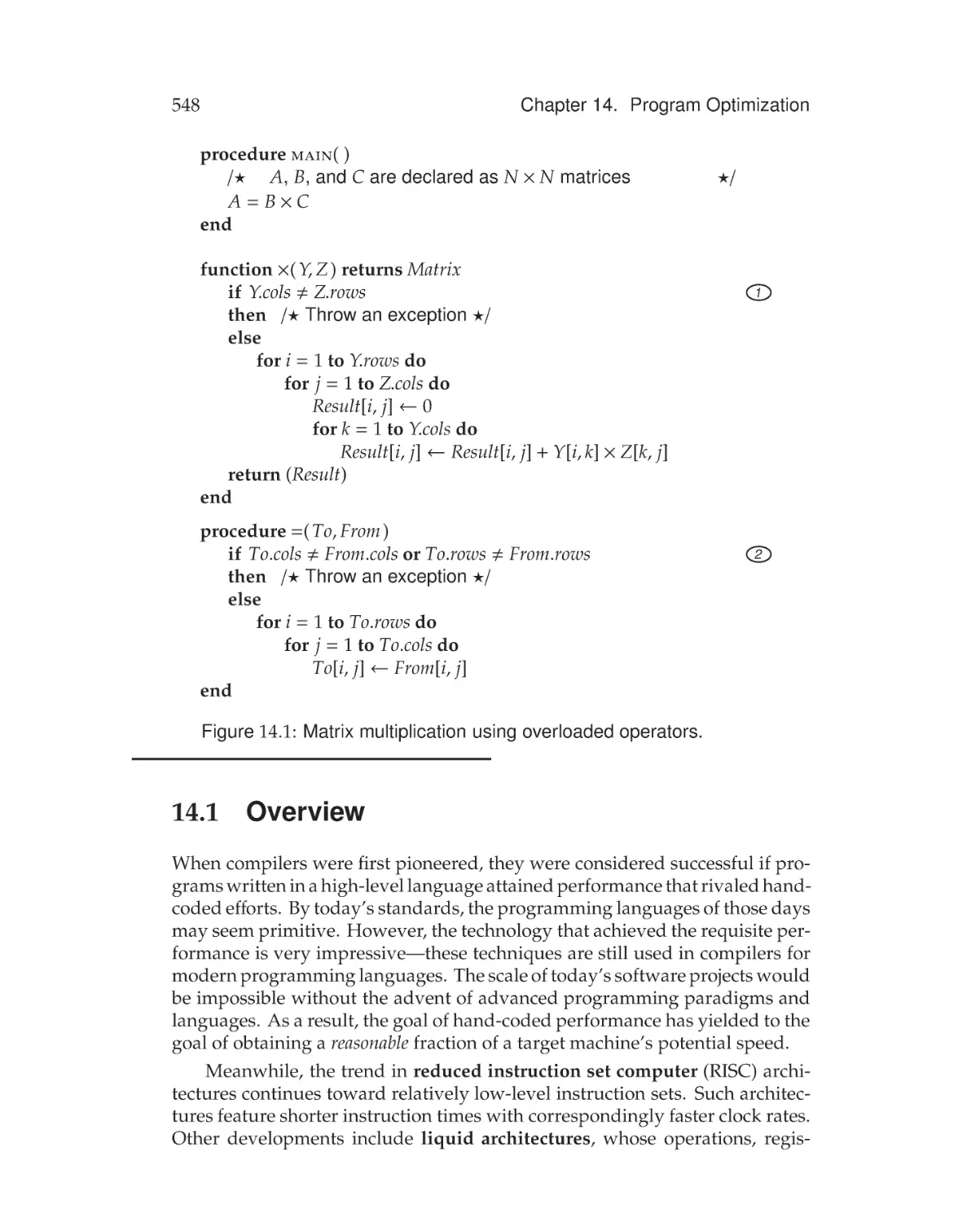
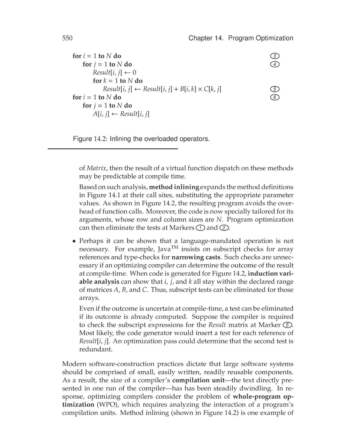
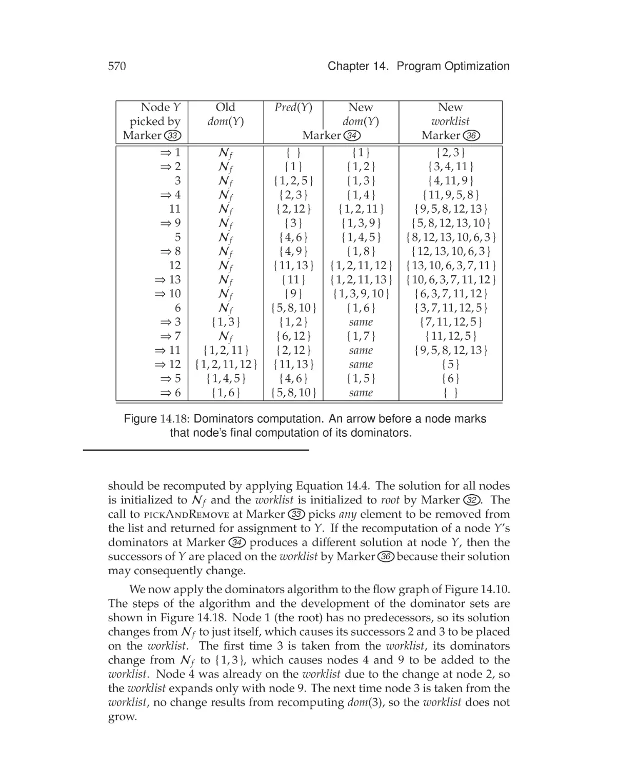
material from the beginning of Chapter 14 on automatic program optimization.
Further study could include more detail of the parsing techniques covered
in Chapters 4, 5, and 6. Semantic analysis and type checking could be studied
in greater breadth and depth in Chapters 8 and 9. Advanced concepts such as
static single assignment (SSA) Form could be introduced from Chapters 10
and 14. Advanced topics in program analysis and transformation, including data flow frameworks, could be drawn from Chapter 14. Chapters 13
and 14 could be the basis for a gradute compiler course, with earlier chapters
providing useful reference material.
Chapter Descriptions
Chapter 1
Introduction
The text begins with an overview of the compilation process. The concepts
of constructing a compiler from a collection of components are emphasized.
An overview of the history of compilers is presented and the use of tools for
generating compiler components is introduced.
Chapter 2
A Simple Compiler
The simple language ac is presented, and each of the compiler’s components
is discussed with respect to translating ac to another language, dc. These
components are presented in pseudocode, and complete code can be found in
the Crafting a Compiler Supplement.
Chapter 3
Scanning—Theory and Practice
The basic concepts and techniques for building the lexical analysis components
of a compiler are presented. This discussion includes the development of handcoded scanners as well as the use of scanner-generation tools for implementing
table-driven lexical analyzers.
Chapter 4
Grammars and Parsing
This chapter covers the fundamentals of formal language concepts, including context-free grammars, grammar notation, derivations, and parse trees.
Grammar-analysis algorithms are introduced that are used in Chapters 5 and 6.
viii
Chapter 5
Preface
Top-Down Parsing
Top-down parsing is a popular technique for constructing relatively simple
parsers. This chapter shows how such parsers can be written using explicit
code or by constructing a table for use by a generic top-down parsing engine.
Syntactic error diagnosis, recovery, and repair are discussed.
Chapter 6
Bottom-Up Parsing
Most compilers for modern programming languages use one of the bottomup parsing techniques presented in this chapter. Tools for generating such
parsers automatically from a context-free grammar are widely available. The
chapter describes the theory on which such tools are built, including a sequence
of increasingly sophisticated approaches to resolving conflicts that hamper
parser construction for some grammars. Grammar and language ambiguity
are thoroughly discussed, and heuristics are presented for understanding and
resolving ambiguous grammars.
Chapter 7
Syntax-Directed Translation
This marks the mid-point of the book in terms of a compiler’s components.
Prior chapters have considered the lexical and syntactic analysis of programs.
A goal of those chapters is the construction of an AST. In this chapter, the
AST is introduced and an interface is articulated for constructing, managing,
and traversing the AST. This chapter is pivotal in the sense that subsequent
chapters depend on understanding both the AST and the visitor pattern that
facilitates traversal and processing of the AST. The Crafting a Compiler Supplement contains a tutorial on the visitor pattern, including examples drawn from
common experiences.
Chapter 8
Symbol Tables and Declaration Processing
This chapter emphasizes the use of a symbol table as an abstract component
that can be utilized throughout the compilation process. A precise interface is
defined for the symbol table, and various implementation issues and ideas are
presented. This discussion includes a study of the implementation of nested
scopes.
The semantic analysis necessary for processing symbol declarations is introduced, including types, variables, arrays, structures, and enumerations. An
introduction to type checking is presented, including object-oriented classes,
subclasses, and superclasses.
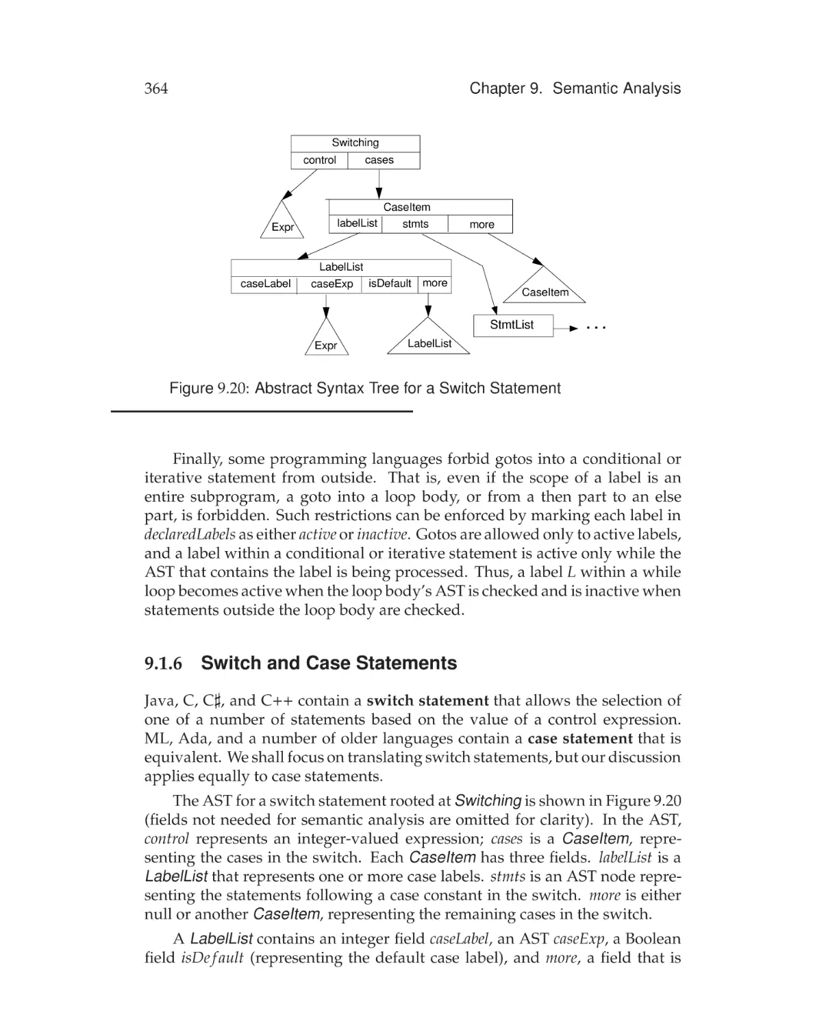
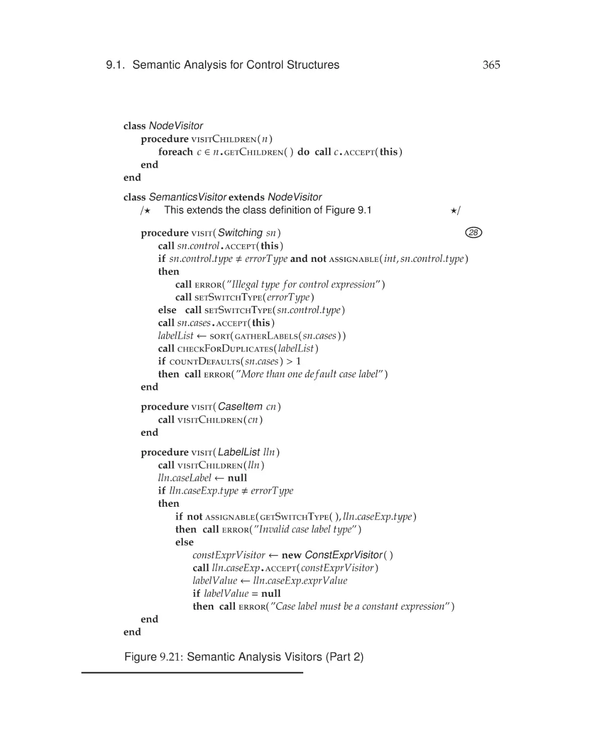
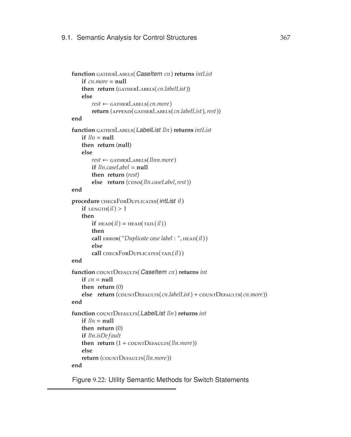
Chapter 9
Semantic Analysis
Additional semantic analysis is required for language specifications that are
not easily checked while parsing. Various control structures are examined,
including conditional branches and loops. The chapter includes a discussion
of exceptions and the semantic analysis they require at compile-time.
ix
Preface
Chapter 10
Intermediate Representations
This chapter considers two intermediate representations are are widely used
by compilers. The first is the JVM instruction set and bytecode format, which
has become the standard format for representing compiled Java programs.
For readers who are interested in targeting the JVM in a compiler project,
Chapters 10 and 11 provide the necessary background and techniques. The
other representation is SSA Form, which is used by many optimizing compilers. This chapter defines SSA Form, but its construction is delayed until
Chapter 14, where some requisite definitions and algorithms are presented.
Chapter 11
Code Generation for a Virtual Machine
This chapter considers code generation for a virtual machine (VM). The advantages of considering such a target is that many of the details of runtime
support are subsumed by the VM. For example, most VMs offer an unlimited
number of registers, so that the issue of register allocation, albeit interesting,
can be postponed until the fundamentals of code generation are mastered.
The VM’s instruction set is typically at a higher level than machine code. For
example, a method call is often supported by a single VM instruction, while
the same call would require many more instructions in machine code.
While an eager reader interested in generating machine code may be
tempted to skip Chapter 11, we recommend studying this chapter before
attempting code generation at the machine-code level. The ideas from this
chapter are easily applied to Chapters 12 and 13, but they are easier to understand from the perspective of a VM.
Chapter 12
Runtime Support
Much of the functionality embedded in a VM is its runtime support (e.g.,
its support for managing storage). This chapter discusses various concepts
and implementation strategies for providing the runtime support needed for
modern programming languages. Study of this material can provide an understanding of the construction of a VM. For those who write code generators
for a target architecture (Chapter 13), runtime support must be provided, so
the study of this material is essential to creating a working compiler.
The chapter includes discussion of storage that is statically allocated, stack
allocated, and heap allocated. References to nonlocal storage are considered,
along with implementation structures such as frames and displays to support
such references.
Chapter 13
Target Code Generation
This chapter is similar to Chapter 11, except that the target of code generation
is a relatively low-level instruction set when compared with a VM. The chapter
includes a thorough discussion of topics that arise in such code generation,
including register allocation, management of temporaries, code scheduling,
instruction selection, and some basic peephole optimization.
x
Chapter 14
Preface
Program Optimization
Most compilers include some capability for improving the code they generate.
This chapter considers some of the practical techniques commonly used by
compilers for program optimization. Advanced control flow analysis structures and algorithms are presented. An introduction to data flow analysis
is presented by considering some fundamental optimizations that are relatively easy to implement. The theoretical foundation of such optimizations is
studied, and the chapter includes construction and use of SSA Form.
Acknowledgements
We collectively thank the following people who have supported us in preparing this text. We thank Matt Goldstein of Pearson Publishing for his patience
and support throughout the revision process. We apologize to Matt’s predecessors for our delay in preparing this text. Jeff Holcomb provided technical
guidance in Pearson’s publication process, for which we are very grateful.
Our text was greatly improved at the hands of our copy editors. Stephanie
Moscola expeditiously and expertly proofread and corrected every chapter of
this text. She was extraordinarily thorough, and any remaining errors are the
authors’ fault. We are grateful for her keen eye and insightful suggestions. We
thank Will Benton for his editing of Chapters 12 and 13 and his authoring of
Section 12.5. We thank Aimee Beal who was retained by Pearson to copyedit
this book for style and consistency.
We are very grateful to the following colleagues for their time spent reviewing our work and providing valuable feedback: Ras Bodik (University of
California–Berkeley), Scott Cannon (Utah State University), Stephen Edwards
(Columbia University), Stephen Freund (Williams College), Jerzy Jaromczyk
(University of Kentucky), Hikyoo Koh (Lamar University), Sam Midkiff (Purdue University), Tim O’Neil (University of Akron), Kurt Stirewalt (Michigan
State University), Michelle Strout (Colorado State University), Douglas Thain
(University of Notre Dame), V. N. Venkatakrishnan (University of Illinois–
Chicago), Elizabeth White (George Mason University), Sherry Yang (Oregon
Institute of Technology), and Qing Yi (University of Texas–San Antonio).
Charles Fischer My fascination with compilers began in 1965 in Mr. Robert
Eddy’s computer lab. Our computer had all of 20 kilobytes of main memory,
and our compiler used punched cards as its intermediate form, but the seed
was planted.
My education really began at Cornell University, where I learned the depth
and rigor of computing. David Gries’ seminal compiler text taught me much
and set me on my career path.
Preface
xi
The faculty at Wisconsin, especially Larry Landweber and Tad Pinkerton,
gave me free rein in developing a compiler curriculum and research program.
Tad, Larry Travis and Manley Draper, at the Academic Computing Center, gave
me the time and resources to learn the practice of compiling. The UW-Pascal
compiler project introduced me to some outstanding students, including my
co-author Richard LeBlanc. We learned by doing, and that became my teaching
philosophy.
Over the years my colleagues, especially Tom Reps, Susan Horwitz, and
Jim Larus, freely shared their wisdom and experience; I learned much. On
the architectural side, Jim Goodman, Guri Sohi, Mark Hill, and David Wood
taught me the subtleties of modern microprocessors. A compiler writer must
thoroughly understand a processor to harness its full power.
My greatest debt is to my students who brought enormous energy and
enthusiasm to my courses. They eagerly accepted the challenges I presented.
A full compiler, from scanner to code generator, must have seemed impossible
in one semester, but they did it, and did it well. Much of that experience
has filtered its way into this text. I trust it will be helpful in teaching a new
generation how to craft a compiler.
Ron K. Cytron My initial interest and subsequent research into programming
languages and their compilers are due in large part to the outstanding mentors
who have played pivotal roles in my career. Ken Kennedy, of blessed memory,
taught my compilers classes at Rice University. The courses I now teach are
patterned after his approach, especially the role that lab assignments play in
helping students understand the material. Ken Kennedy was an outstanding
educator, and I can only hope to connect with students as well as he could.
He hosted me one summer at IBM T.J. Watson Research Labs, in Yorktown
Heights, New York, where I worked on software for automatic parallelization.
During that summer my investigations naturally led me to the research of
Dave Kuck and his students at the University of Illinois.
I still consider myself so very fortunate that Dave took me on as his
graduate student. Dave Kuck is a pioneer in parallel computer architecture
and in the role compilers can play to make to make such advanced systems
easier to program. I strive to follow his example of hard work, integrity, and
perseverance and to pass those lessons on to my students. I also experienced
the vibrancy and fun that stems from investigating ideas in a group, and I have
tried to create similar communities among my students.
My experiences as an undergraduate and graduate student then led me to
Fran Allen of IBM Research, to whom I shall always be grateful for allowing
me to join her newly formed PTRAN group. Fran has inspired generations
of research in data flow analysis, program optimization, and automatic parallelization. She has amazing intuition into the important problems and their
xii
Preface
likely solution. In talking with colleagues, some of our best ideas are due to
Fran and the suggestions, advice, or critiques she has offered us.
Some of the best years of my professional life were spent learning from
and working with Fran and my PTRAN colleagues: Michael Burke, Philippe
Charles, Jong-Deok Choi, Jeanne Ferrante, Vivek Sarkar, and David Shields.
At IBM I also had the privilege of learning from and working with Barry
Rosen, Mark Wegman, and Kenny Zadeck. While the imprint of my friends
and colleagues can be found throughout this text, any mistakes are mine.
If the reader notices that the number 431 appears frequently in this book,
it is an homage to the students who have studied compilers with me at Washington University. I have learned as much from my students as I have taught
them, and my contribution to this book stems largely from my experiences in
the classroom and lab.
Finally, I thank my wife and children for putting up with the time I wanted
to spend working on this book. They have shown patience and understanding
throughout this effort. And thank you, Aunt Carole, for always asking how
this book was coming along.
Richard LeBlanc After becoming more excited about computers than physics
problem sets while getting my B.S. in physics, I moved to Madison and enrolled
at the University of Wisconsin as a computer science Ph.D. student in 1972.
Two years later, a young assistant professor, Charles Fischer, who had just
received his Ph.D. from Cornell, joined the faculty of the Computer Science
Department. The first course he taught was a graduate compiler course, CS
701. I was enrolled in that course and still remember it as a really remarkable
learning experience, all the more impressive since it was his first time teaching
the course. We obviously hit it off well, since this introduction has led to a
rather lengthy series of collaborations.
Through the sponsorship of Larry Travis, I began working at the Academic
Computing Center in the summer of 1974. I was thus already part of that
organization when the UW-Pascal project began a year later. That project
not only gave me the opportunity to apply what I had learned in the two
courses I had just taken, but also some great lessons about the impact of good
design and design reviews. I also benefited from working with two fellow
graduate students, Steve Zeigler and Marty Honda, from whom I learned how
much fun it can be to be part of an effective software development team. We
all discovered the value of working in Pascal, a well-designed language that
requires disciplined thought while programming, and of using a tool that you
are developing, since we bootstrapped from the Pascal P-Compiler to our own
compiler that generated native code for the Univac 1108 early in the project.
Upon completion of my graduate work, I took a faculty position at Georgia Tech, drawn by the warmer weather and an opportunity to be part of
Preface
xiii
a distributed computing research project led by Phil Enslow, who provided
invaluable guidance in the early years of my career. I immediately had the
opportunity to teach a compiler course and attempted to emulate the CS 701
course at Wisconsin, since I strongly believed in the value of the project-based
approach Charles used. I quickly realized that that having the students write
a complete compiler in a 10-week quarter was too much of a challenge. I thus
began using the approach of giving them a working compiler for a very tiny
language and building the project around extending all of the components of
that compiler to compile a more complex language. The base compiler that I
used in my 10-week course became one of the support items distributed with
the Fischer–LeBlanc text.
My career path has taken me to greater involvement with software engineering and educational activities than with compiler research. As I look back
on my early compiler experiences at Wisconsin, I clearly see the seeds of my
interests in both of these areas. The decision that Charles and I made to write
the original Crafting a Compiler was based in our belief that we could help other
instructors offer their students an outstanding educational experience through
a project-based compiler course. With the invaluable help of our editor, Alan
Apt, and a great set of reviewers, I believe we succeeded. Many colleagues
have expressed to me their enthusiasm for our original book and Crafting a
Compiler with C. Their support has been a great reward and it also served as
encouragement toward finally completing this text. Particular thanks go to Joe
Bergin, who went well beyond verbal support, translating some of our early
software tools into new programming languages and allowing us to make his
versions available to other instructors.
My years at Georgia Tech provided me with wonderful opportunities to
develop my interests in computing education. I was fortunate to have been
part of an organization led by Ray Miller and then Pete Jensen during the
first part of my career. Beginning in 1990, I had the great pleasure of working
with Peter Freeman as we created and developed the College of Computing.
Beyond the many ways he mentored me during our work at Georgia Tech, Peter
encouraged my broad involvement with educational issues through my work
with the ACM Education Board, which has greatly enriched my professional
life over the last 12 years.
Finally, I thank my family, including my new granddaughter, for sharing
me with this book writing project, which at times must have seemed like it
would never end.
This page intentionally left blank
Dedication
CNF: To Lisa, always
In memory of Stanley J. Winiasz,
one of the greatest generation
RKC: To Betsy, Jessica, Melanie, and Jacob
In memory of Ken Kennedy
RJL: To Lanie, Aidan, Maria and Evolette
Brief Contents
1
Introduction
2
A Simple Compiler
31
3
Scanning—Theory and Practice
57
4
Grammars and Parsing
113
5
Top-Down Parsing
143
6
Bottom-Up Parsing
179
7
Syntax-Directed Translation
235
8
Symbol Tables and Declaration Processing
279
9
Semantic Analysis
343
1
10 Intermediate Representations
391
11 Code Generation for a Virtual Machine
417
12 Runtime Support
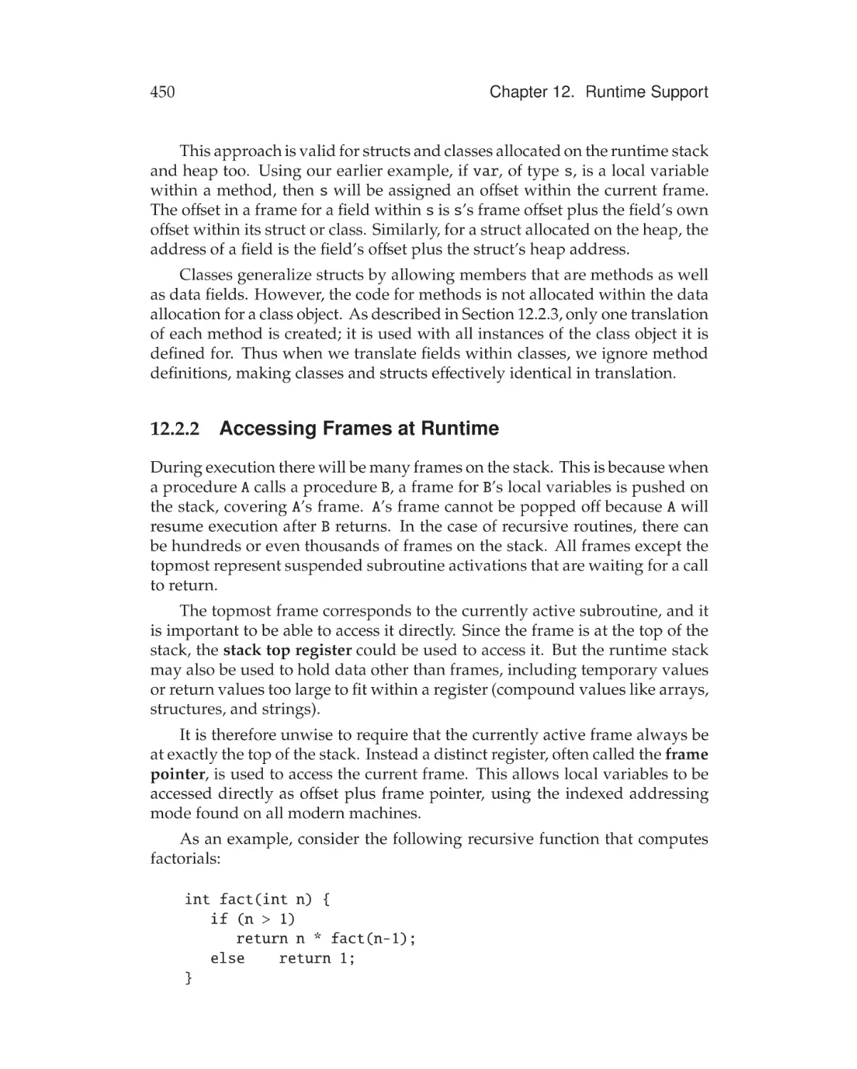
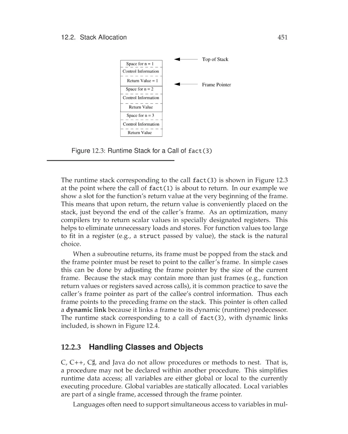
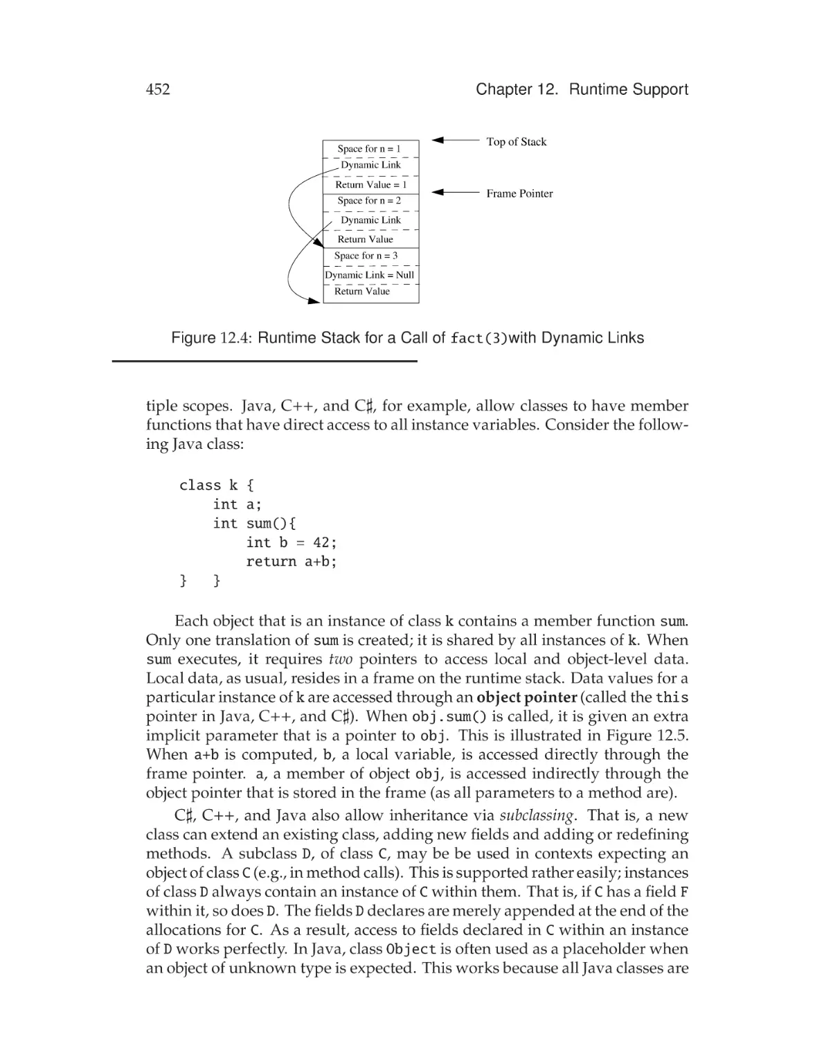
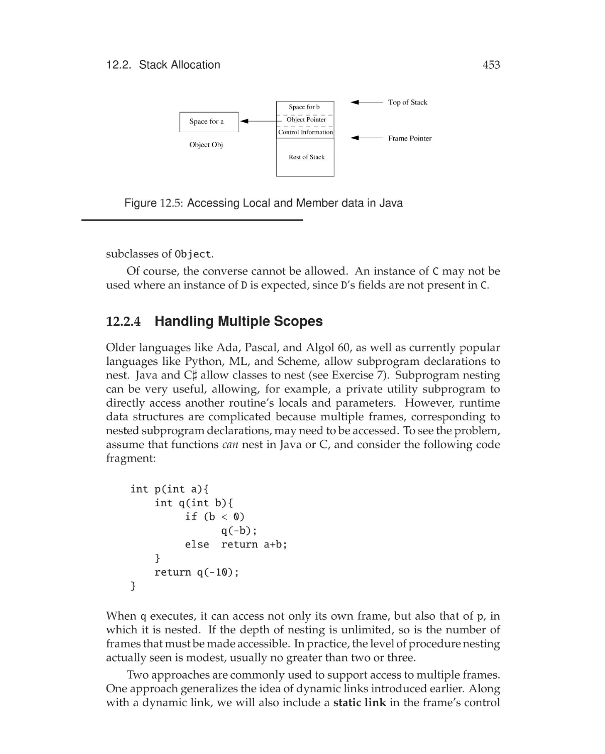
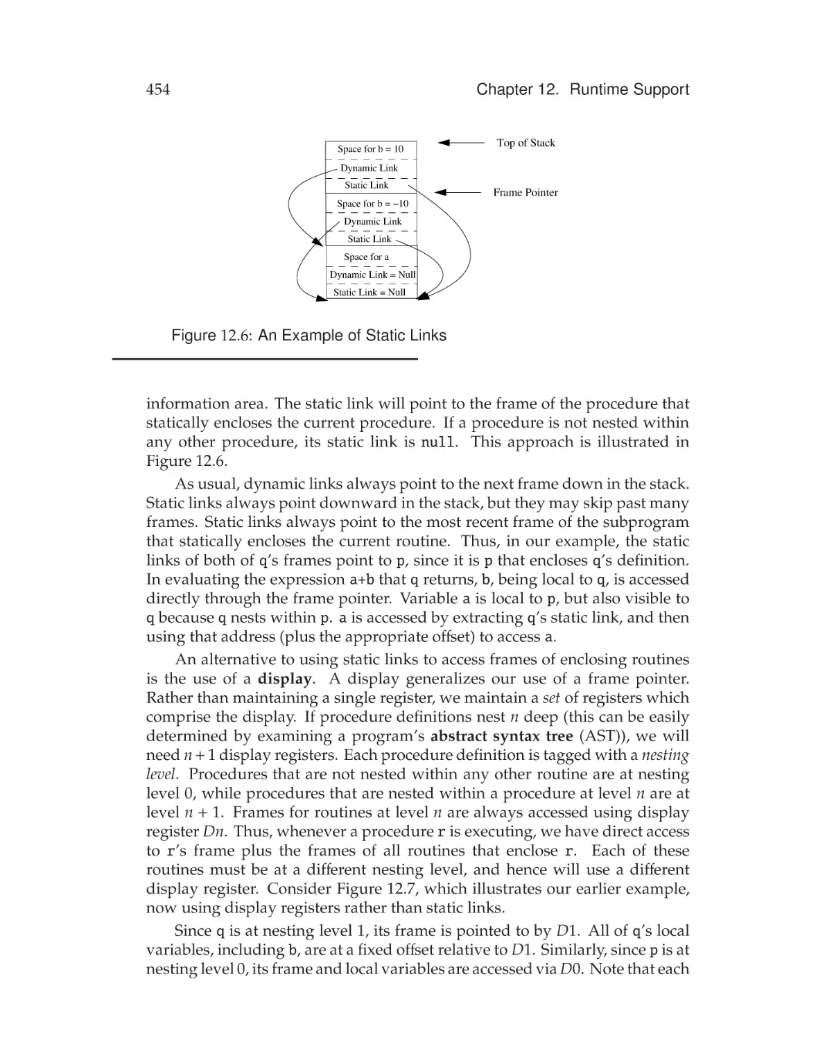
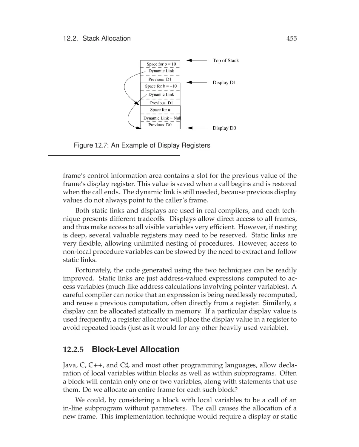
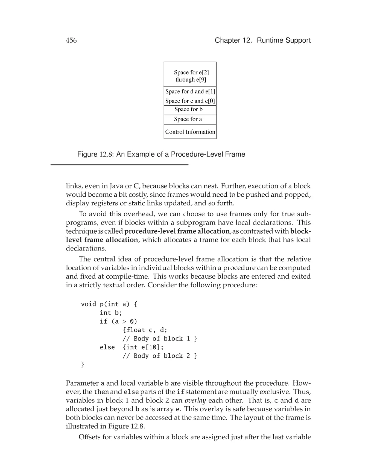
445
13 Target Code Generation
489
14 Program Optimization
547
xvi
Contents
1
Introduction
1
1.1
1.2
History of Compilation . . . . . . . . . . . . . . .
What Compilers Do . . . . . . . . . . . . . . . . .
1.2.1 Machine Code Generated by Compilers
1.2.2 Target Code Formats . . . . . . . . . . .
1.3 Interpreters . . . . . . . . . . . . . . . . . . . . .
1.4 Syntax and Semantics . . . . . . . . . . . . . . .
1.4.1 Static Semantics . . . . . . . . . . . . . .
1.4.2 Runtime Semantics . . . . . . . . . . . .
1.5 Organization of a Compiler . . . . . . . . . . . .
1.5.1 The Scanner . . . . . . . . . . . . . . . .
1.5.2 The Parser . . . . . . . . . . . . . . . . .
1.5.3 The Type Checker (Semantic Analysis) .
1.5.4 Translator (Program Synthesis) . . . . . .
1.5.5 Symbol Tables . . . . . . . . . . . . . . .
1.5.6 The Optimizer . . . . . . . . . . . . . . .
1.5.7 The Code Generator . . . . . . . . . . . .
1.5.8 Compiler Writing Tools . . . . . . . . . .
1.6 Programming Language and Compiler Design .
1.7 Computer Architecture and Compiler Design . .
1.8 Compiler Design Considerations . . . . . . . . .
1.8.1 Debugging (Development) Compilers . .
1.8.2 Optimizing Compilers . . . . . . . . . . .
1.8.3 Retargetable Compilers . . . . . . . . . .
1.9 Integrated Development Environments . . . . .
Exercises . . . . . . . . . . . . . . . . . . . . . . . . .
xvii
.
.
.
.
.
.
.
.
.
.
.
.
.
.
.
.
.
.
.
.
.
.
.
.
.
.
.
.
.
.
.
.
.
.
.
.
.
.
.
.
.
.
.
.
.
.
.
.
.
.
.
.
.
.
.
.
.
.
.
.
.
.
.
.
.
.
.
.
.
.
.
.
.
.
.
.
.
.
.
.
.
.
.
.
.
.
.
.
.
.
.
.
.
.
.
.
.
.
.
.
.
.
.
.
.
.
.
.
.
.
.
.
.
.
.
.
.
.
.
.
.
.
.
.
.
.
.
.
.
.
.
.
.
.
.
.
.
.
.
.
.
.
.
.
.
.
.
.
.
.
.
.
.
.
.
.
.
.
.
.
.
.
.
.
.
.
.
.
.
.
.
.
.
.
.
.
.
.
.
.
.
.
.
.
.
.
.
.
.
.
.
.
.
.
.
.
.
.
.
.
2
4
4
7
9
10
11
12
14
16
16
17
17
18
18
19
19
20
21
22
22
23
23
24
26
xviii
2
Contents
A Simple Compiler
2.1
An Informal Definition of the ac Language . . . . . . . . . . . .
32
2.2
Formal Definition of ac . . . . . . . . . . . . . . . . . . . . . . .
33
2.2.1
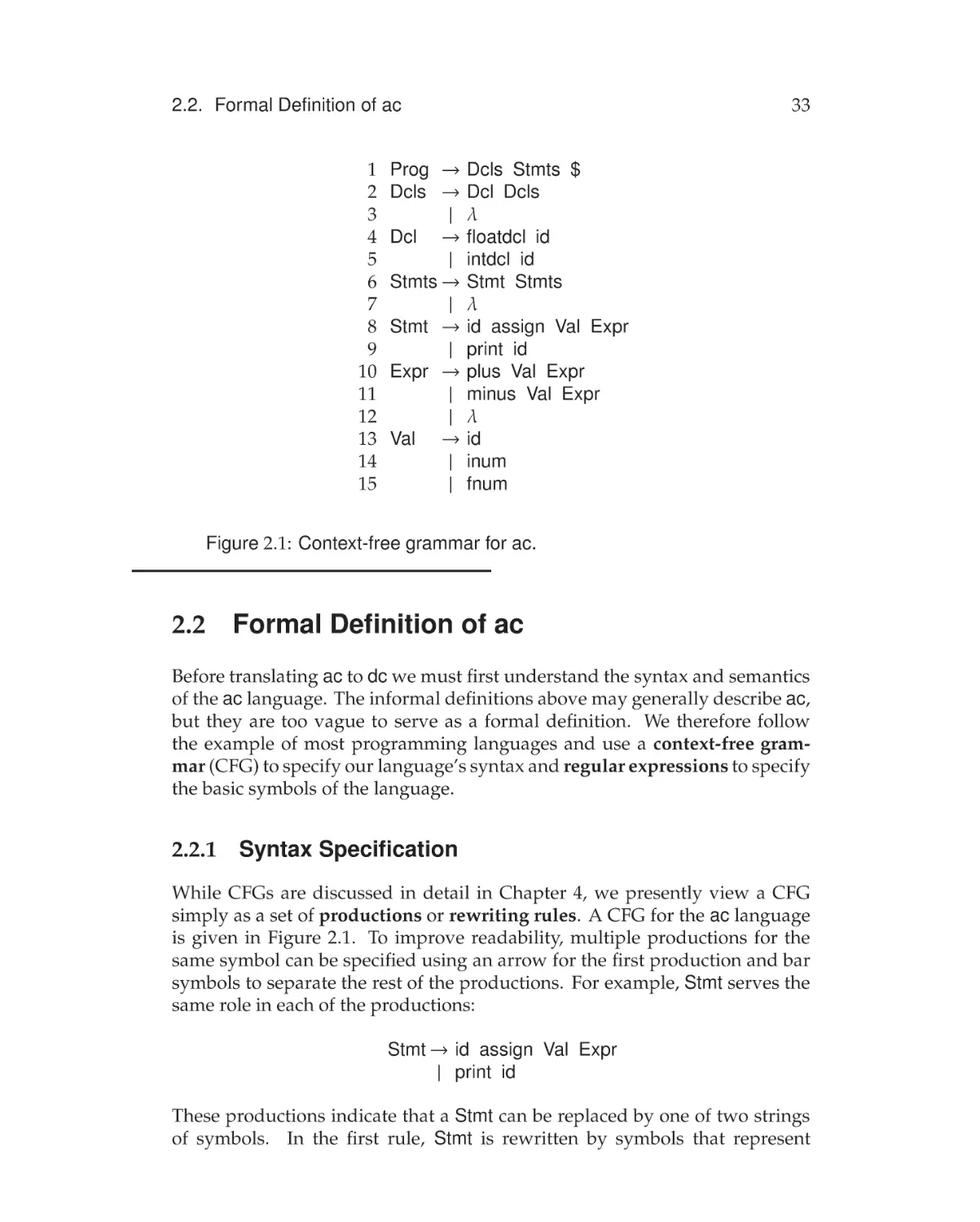
Syntax Specification . . . . . . . . . . . . . . . . . . . .
33
2.2.2
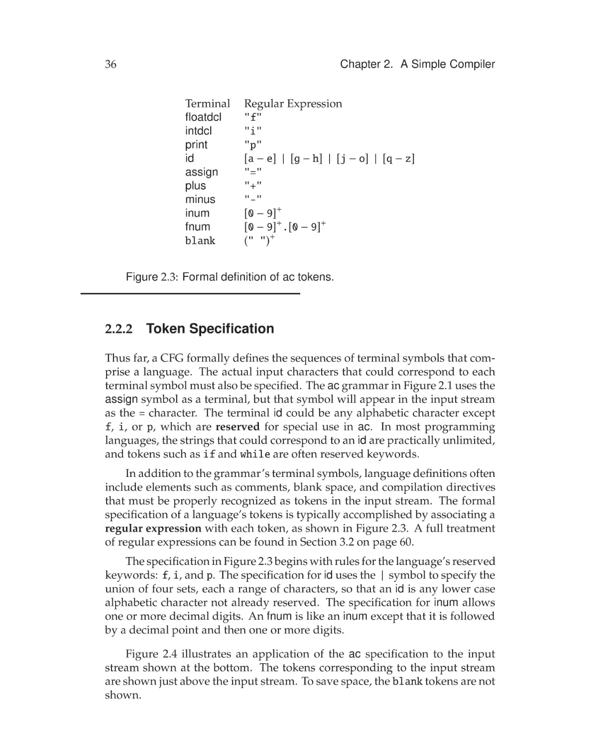
Token Specification . . . . . . . . . . . . . . . . . . . .
36
2.3
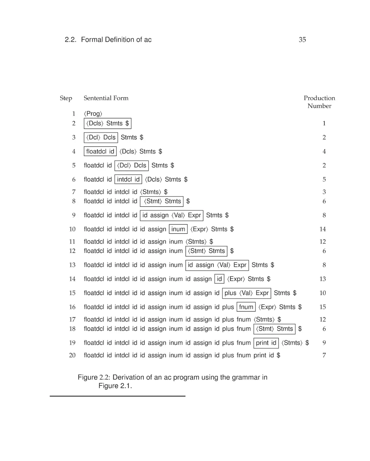
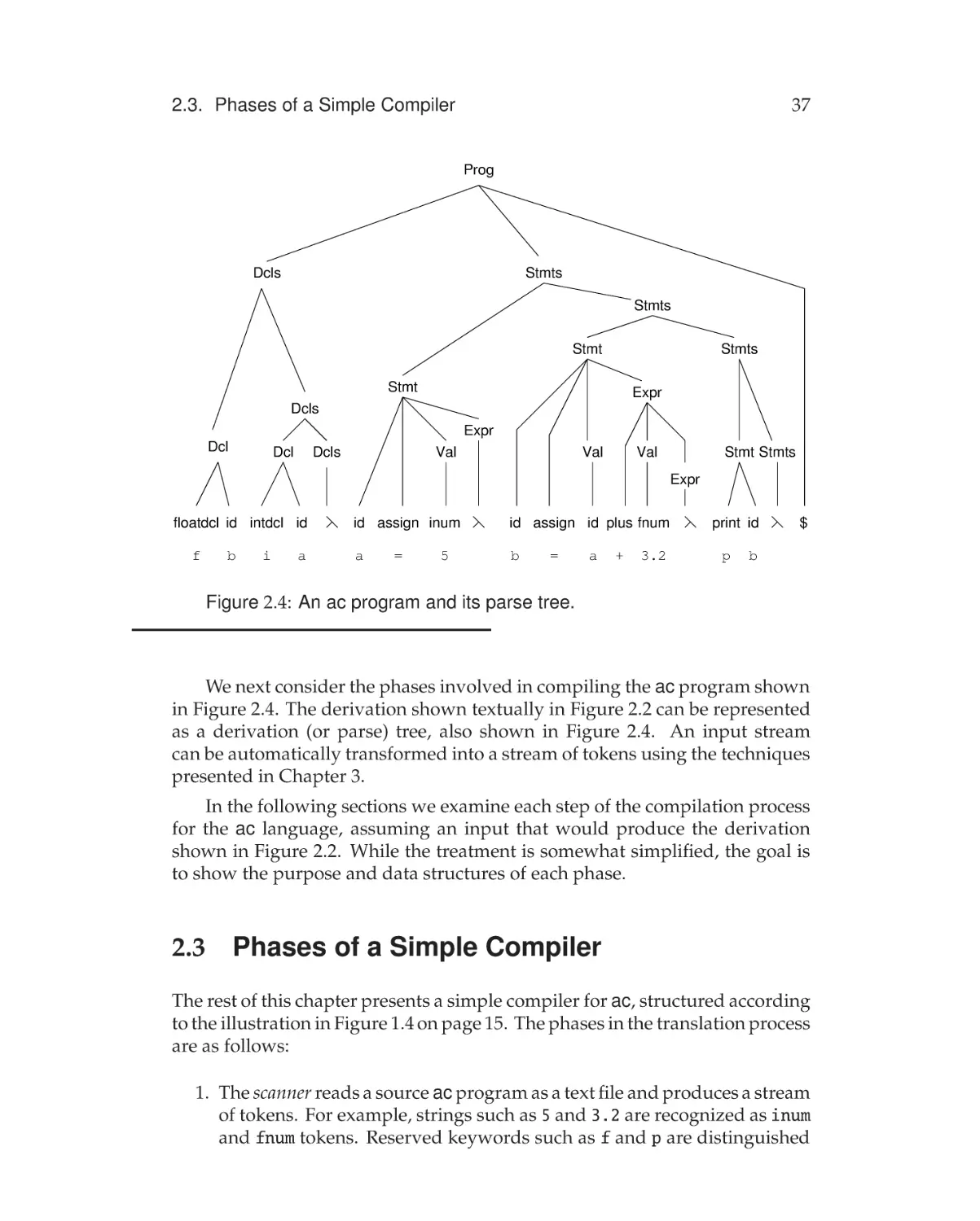
Phases of a Simple Compiler . . . . . . . . . . . . . . . . . . .
37
2.4
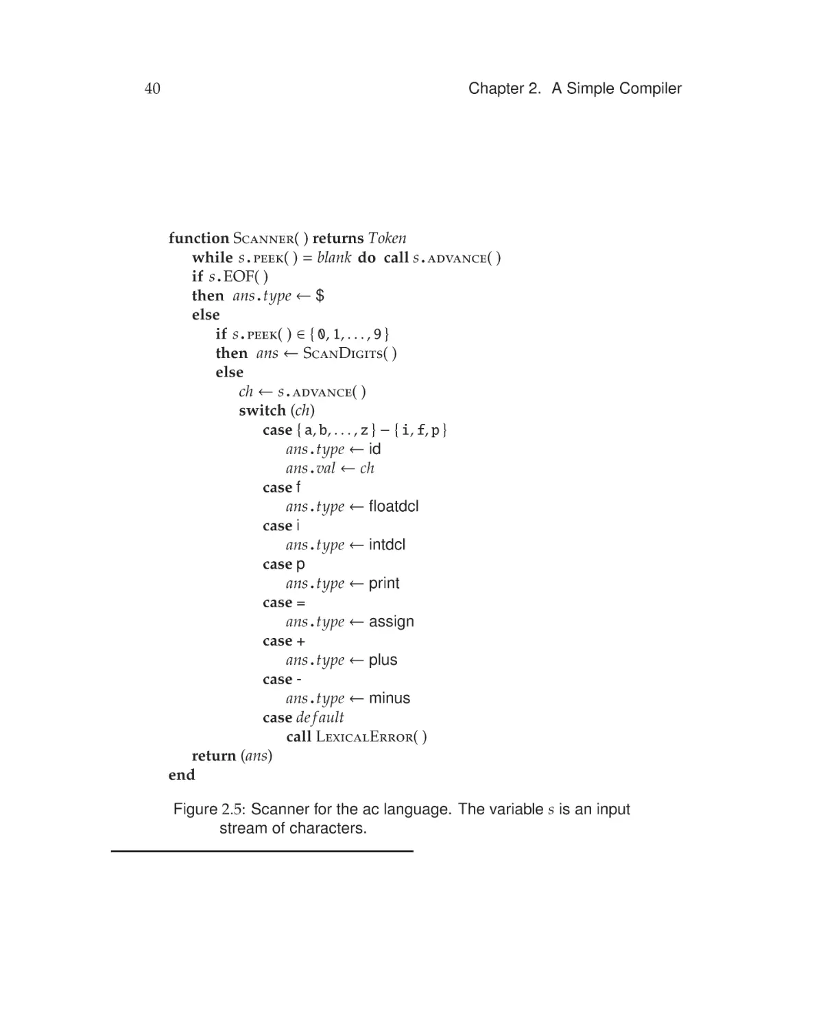
Scanning . . . . . . . . . . . . . . . . . . . . . . . . . . . . . . .
38
2.5
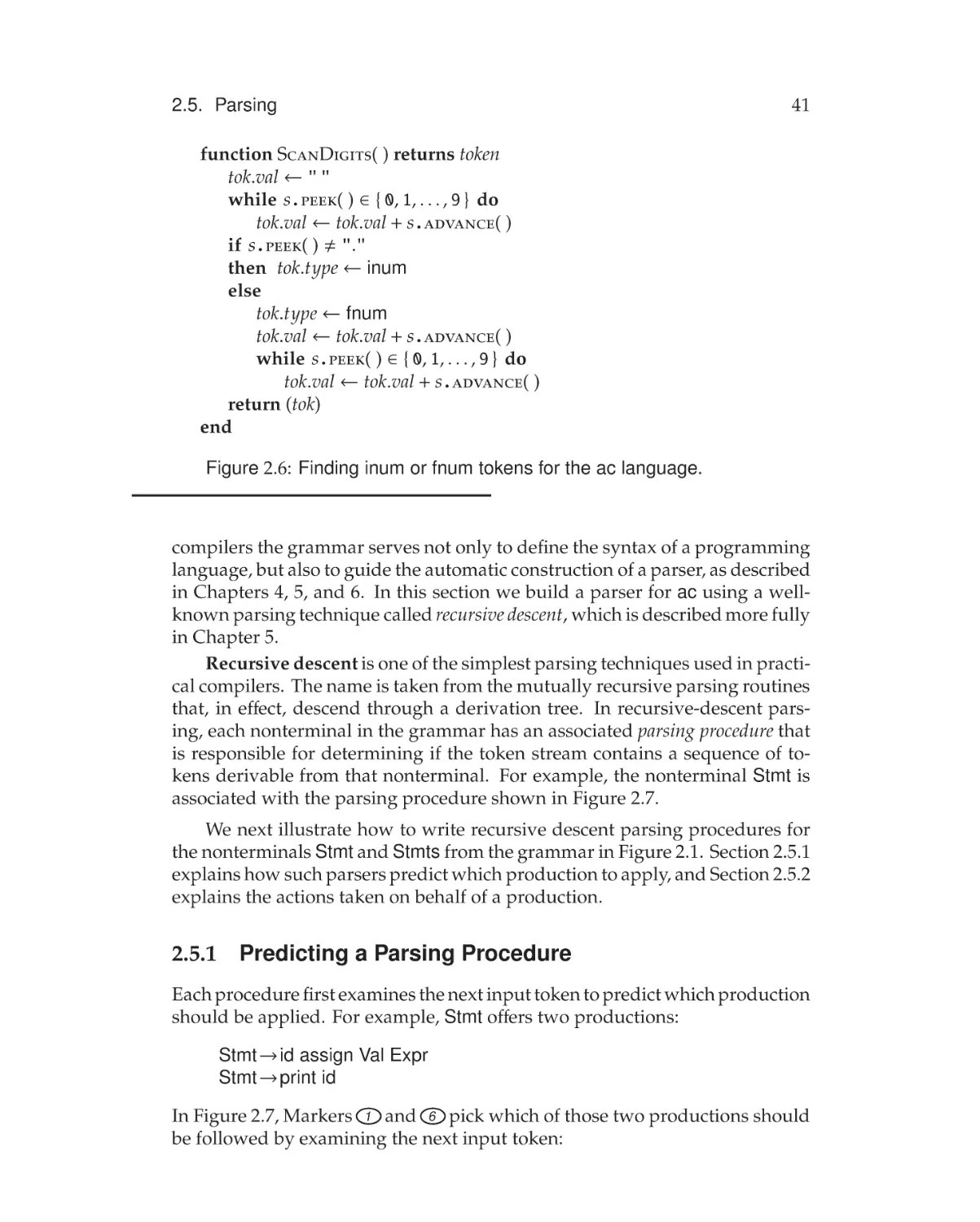
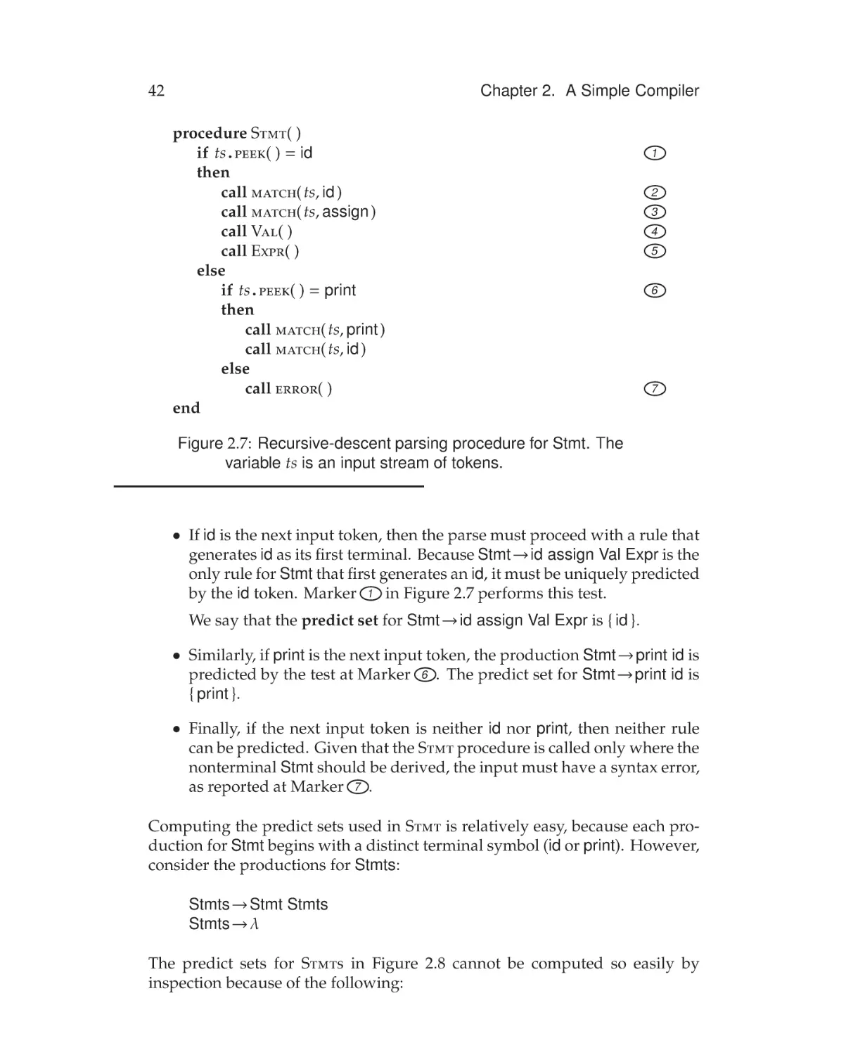
Parsing . . . . . . . . . . . . . . . . . . . . . . . . . . . . . . . .
39
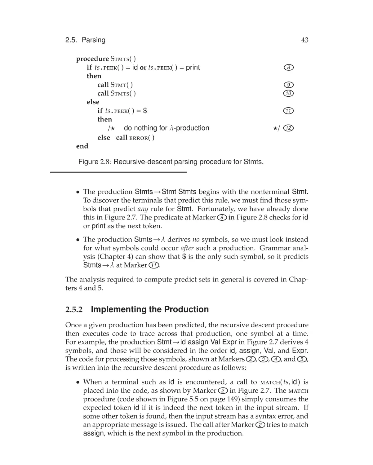
2.5.1
Predicting a Parsing Procedure . . . . . . . . . . . . .
41
2.5.2
Implementing the Production . . . . . . . . . . . . . . .
43
2.6
Abstract Syntax Trees . . . . . . . . . . . . . . . . . . . . . . .
45
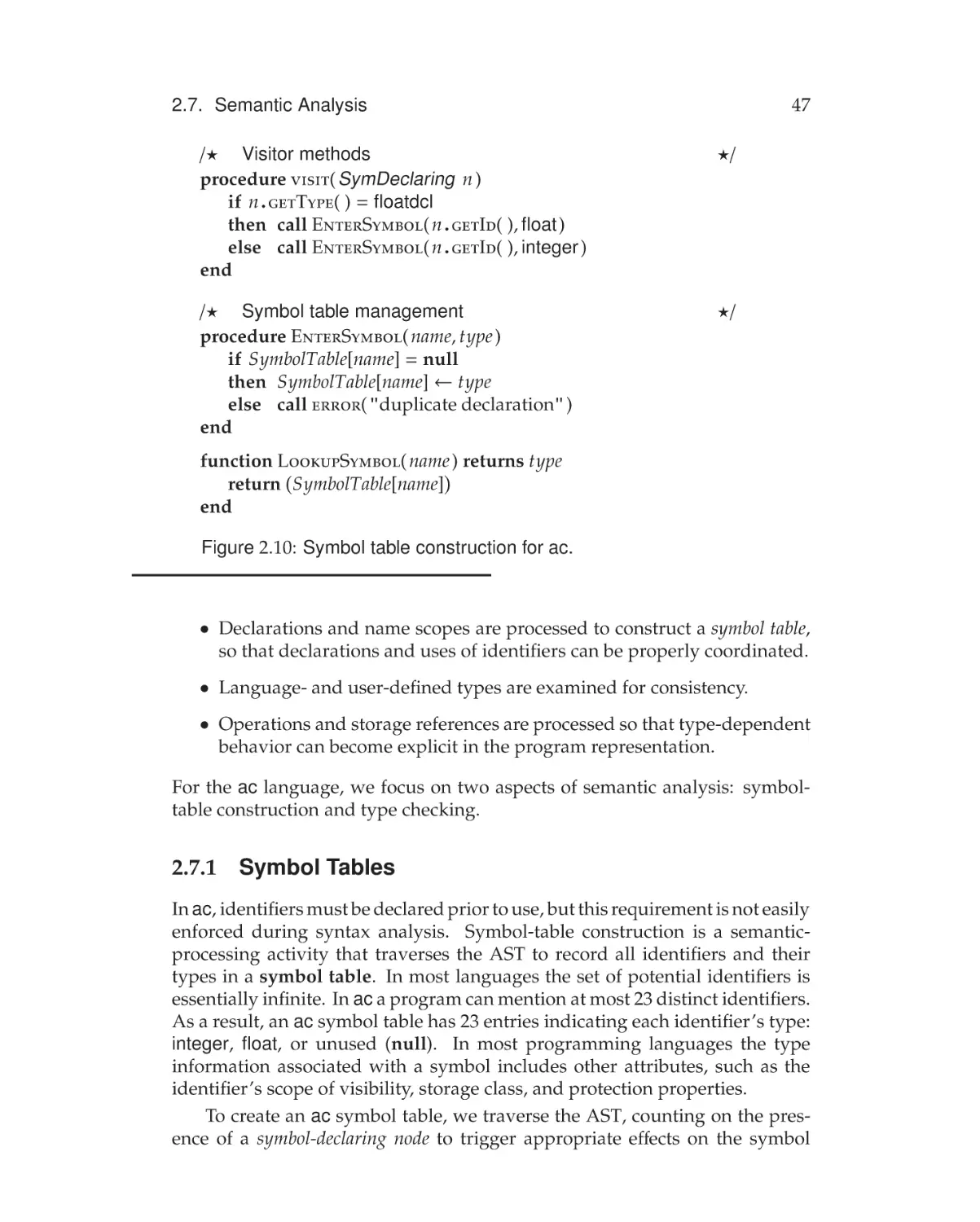
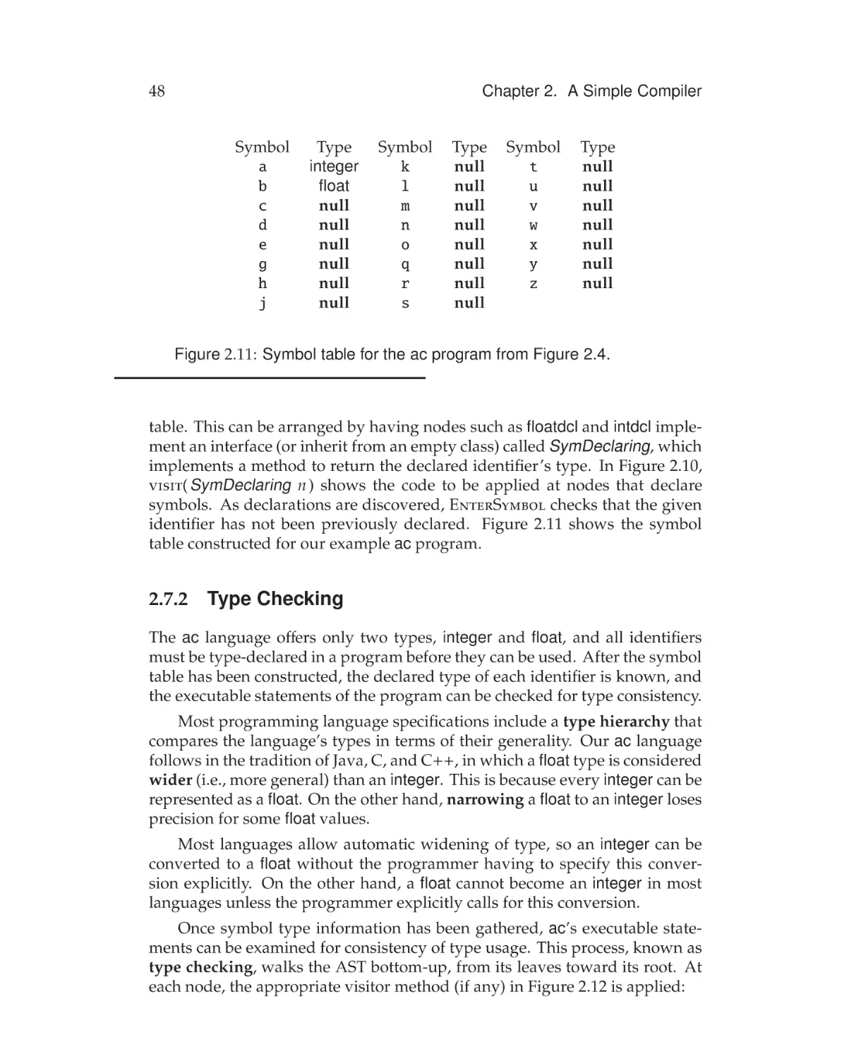
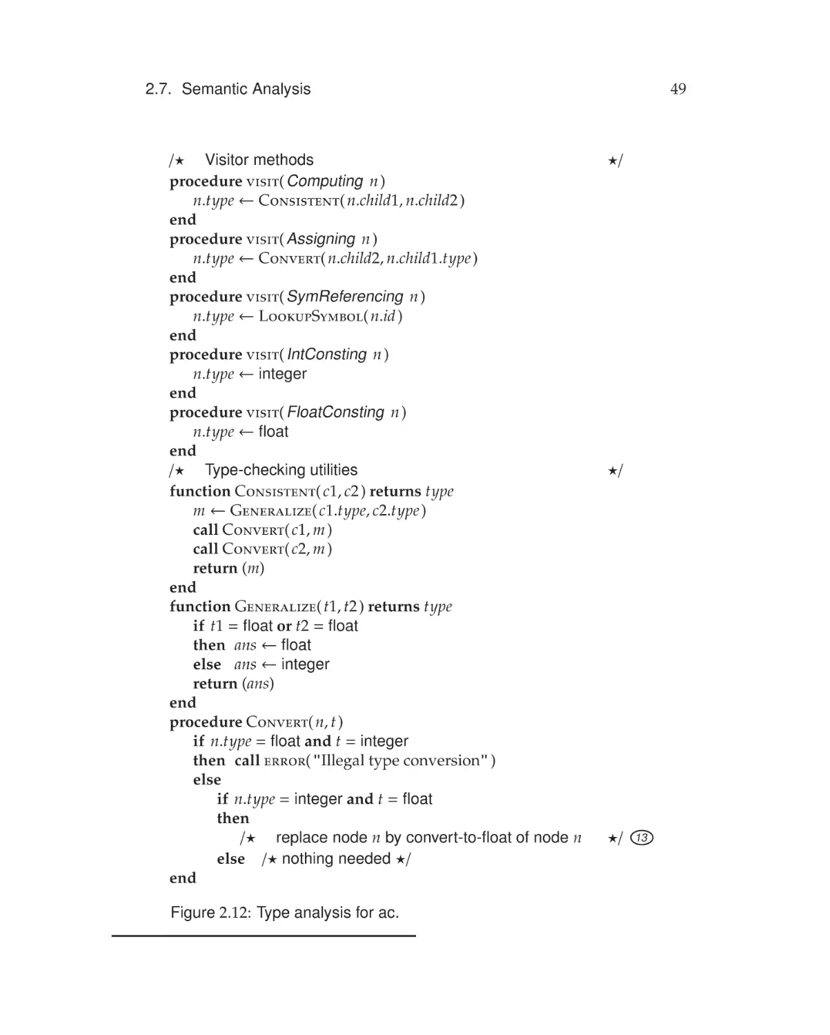
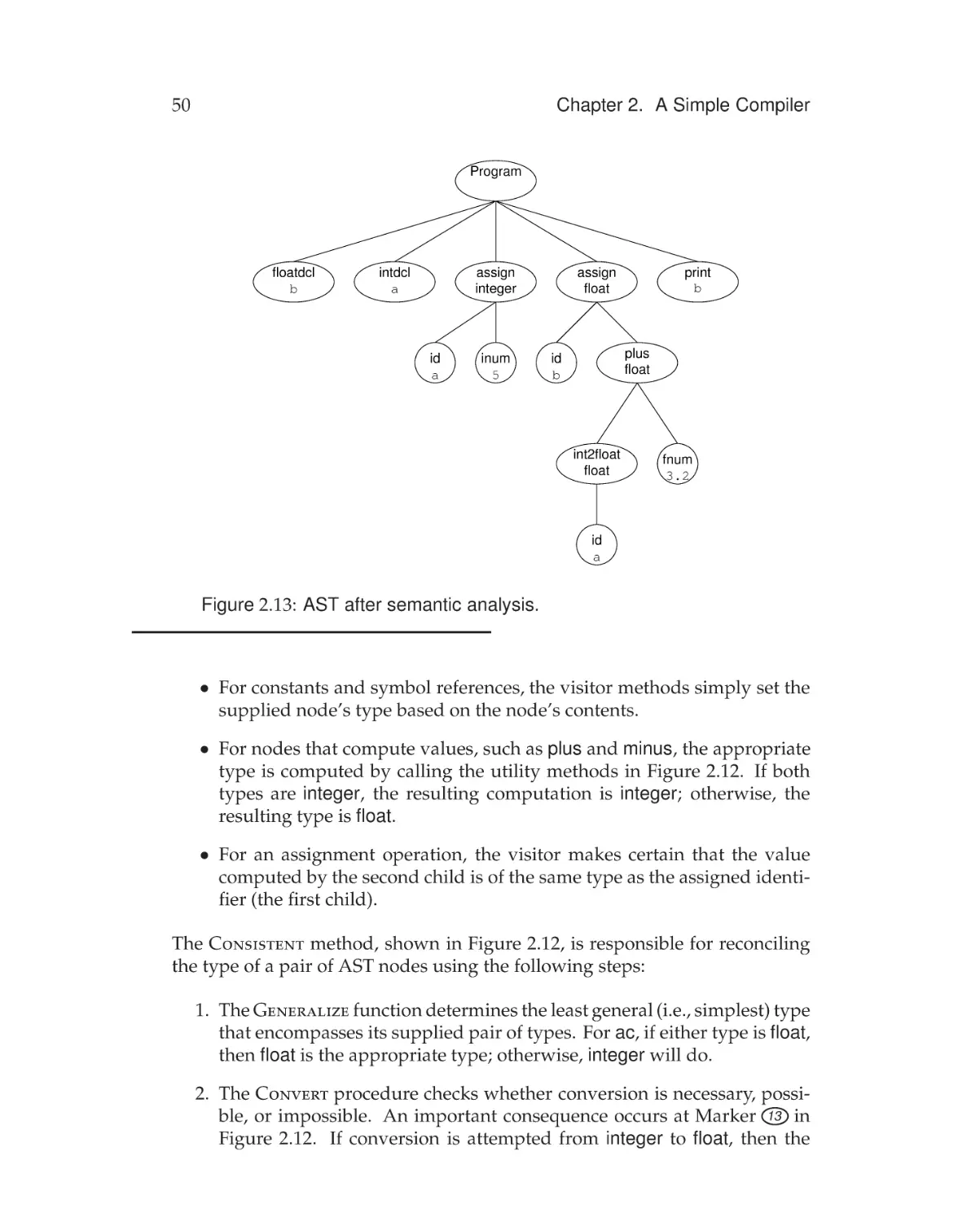
2.7
Semantic Analysis . . . . . . . . . . . . . . . . . . . . . . . . .
46
2.7.1
Symbol Tables . . . . . . . . . . . . . . . . . . . . . . .
47
2.7.2
Type Checking . . . . . . . . . . . . . . . . . . . . . . .
48
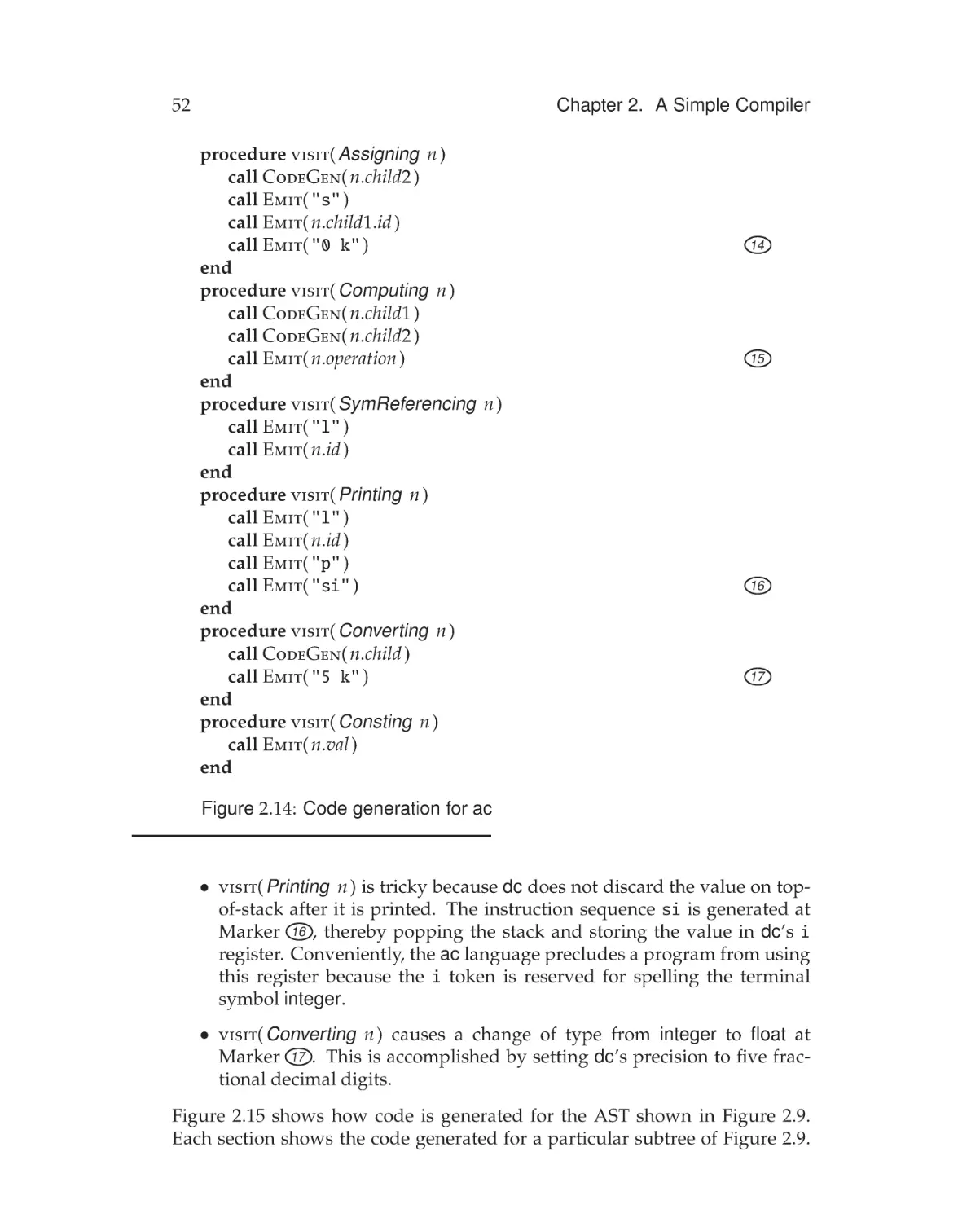
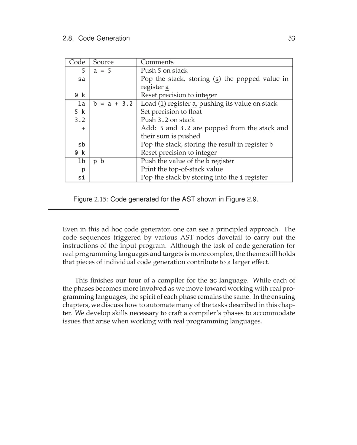
Code Generation . . . . . . . . . . . . . . . . . . . . . . . . . .
51
Exercises . . . . . . . . . . . . . . . . . . . . . . . . . . . . . . . . .
54
2.8
3
31
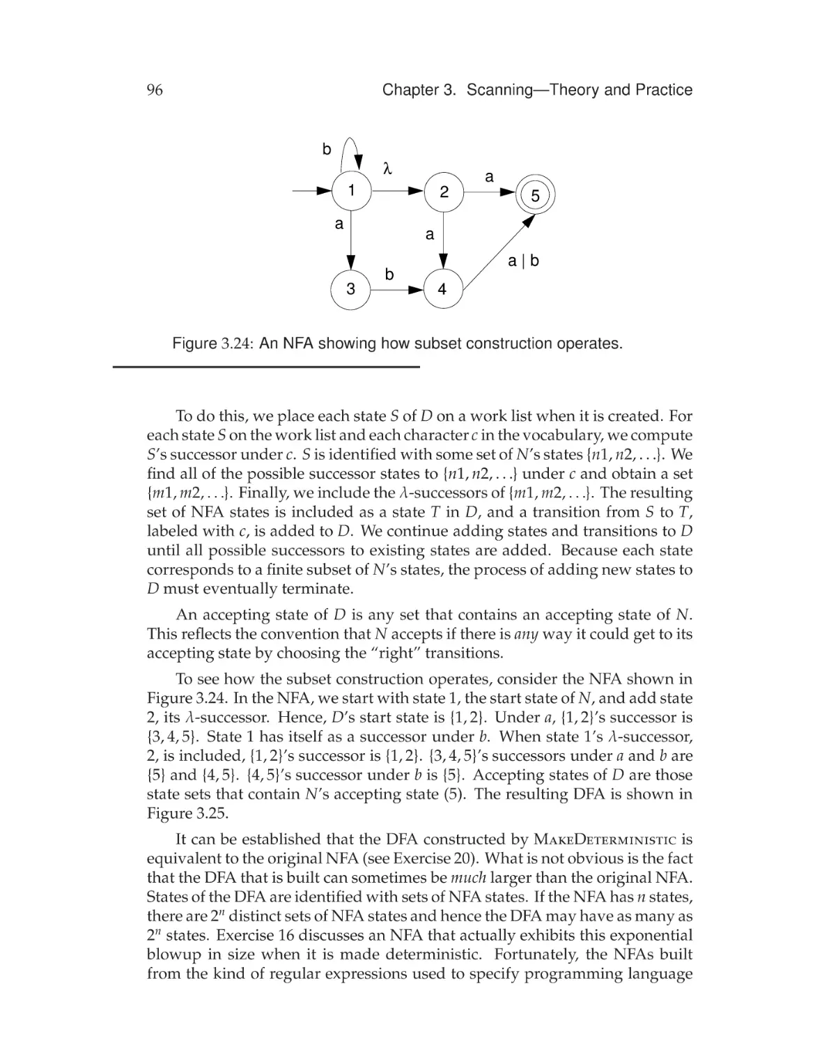
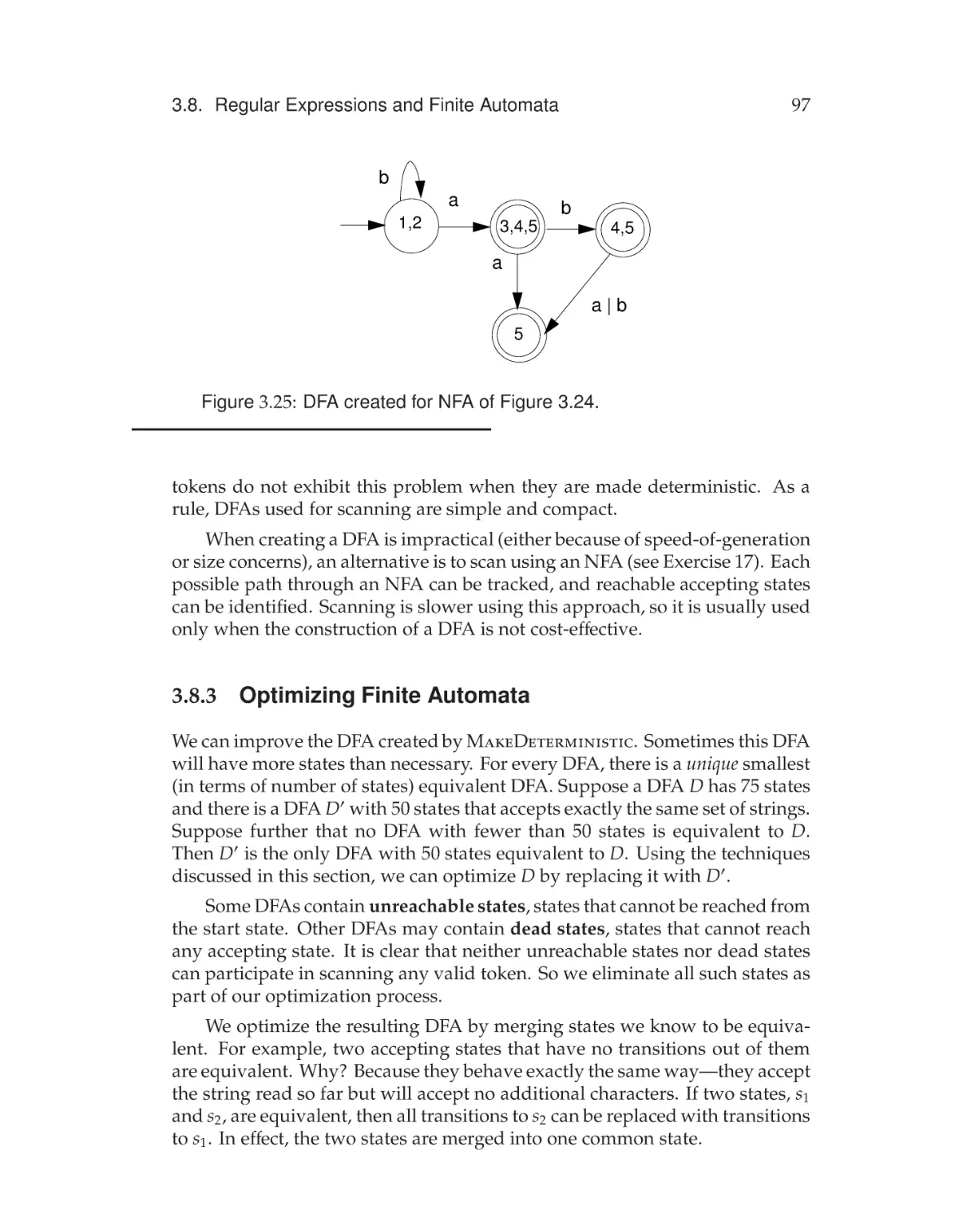
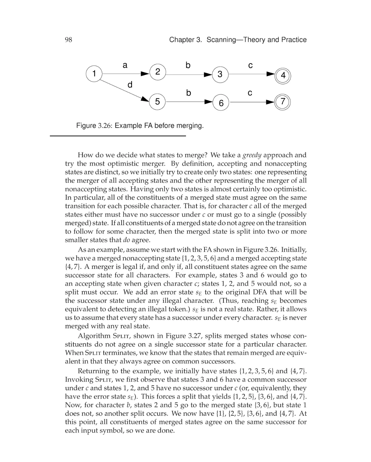
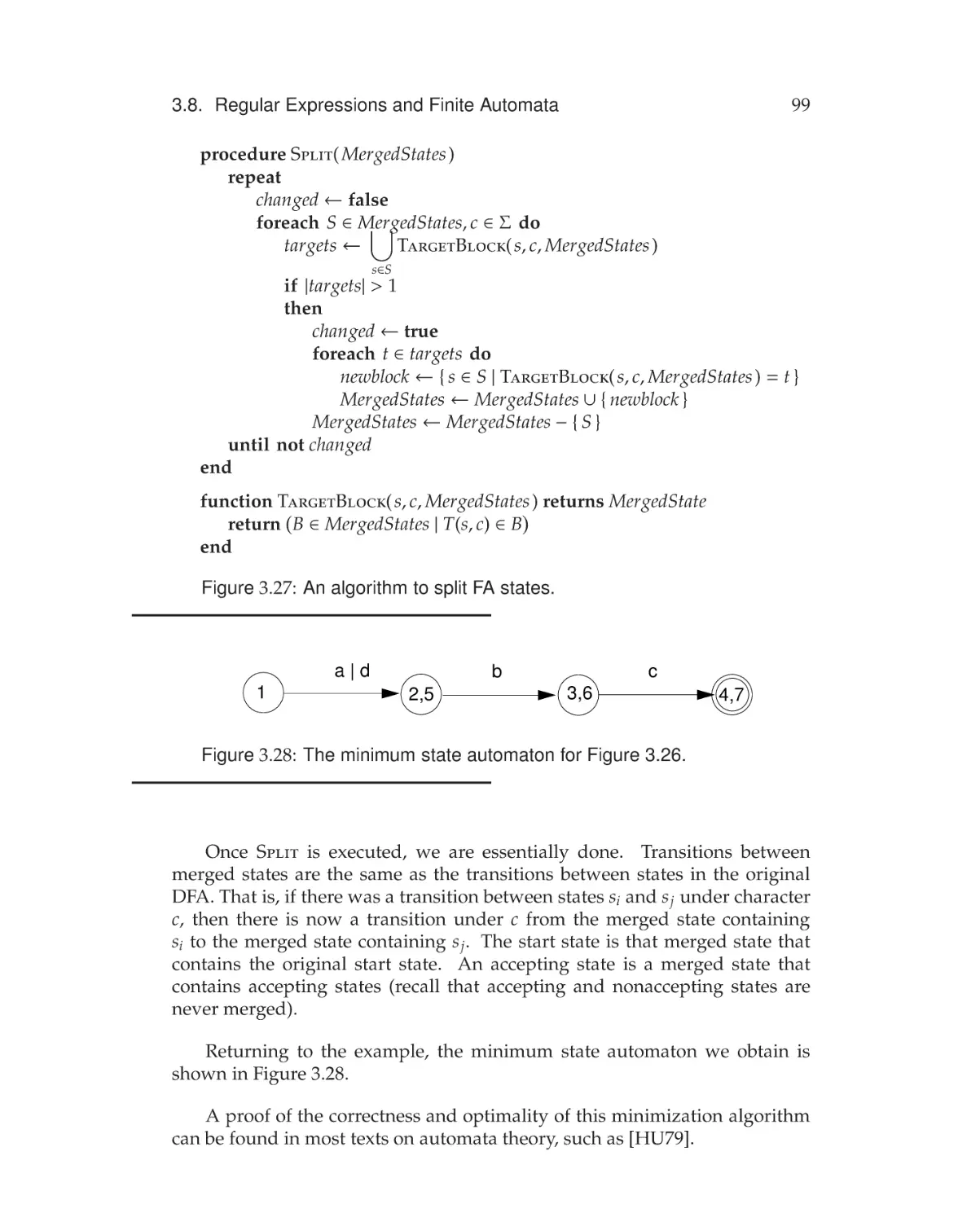
Scanning—Theory and Practice
57
3.1
Overview of a Scanner . . . . . . . . . . . . . . . . . . . . . . .
58
3.2
Regular Expressions . . . . . . . . . . . . . . . . . . . . . . . .
60
3.3
Examples . . . . . . . . . . . . . . . . . . . . . . . . . . . . . .
62
3.4
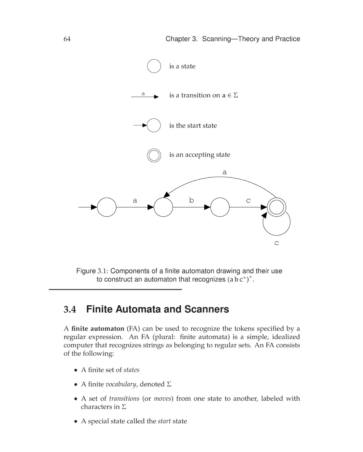
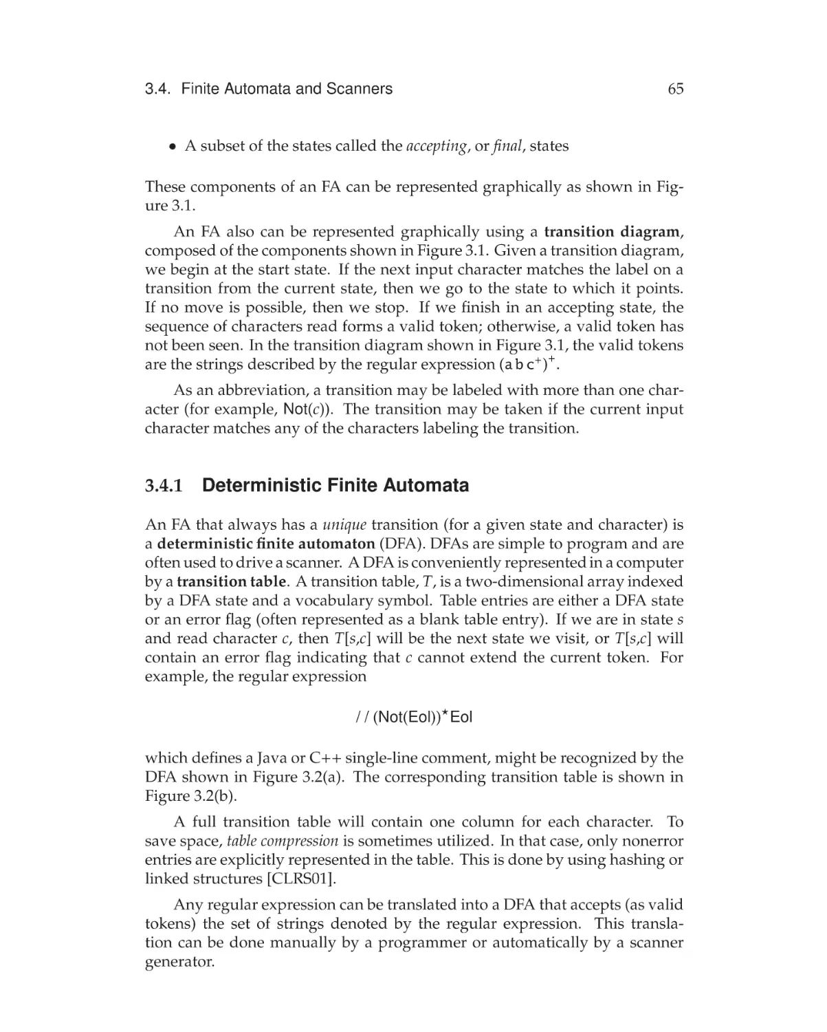
Finite Automata and Scanners . . . . . . . . . . . . . . . . . .
64
3.4.1
Deterministic Finite Automata . . . . . . . . . . . . . .
65
The Lex Scanner Generator . . . . . . . . . . . . . . . . . . . .
69
3.5.1
Defining Tokens in Lex . . . . . . . . . . . . . . . . . .
70
3.5.2
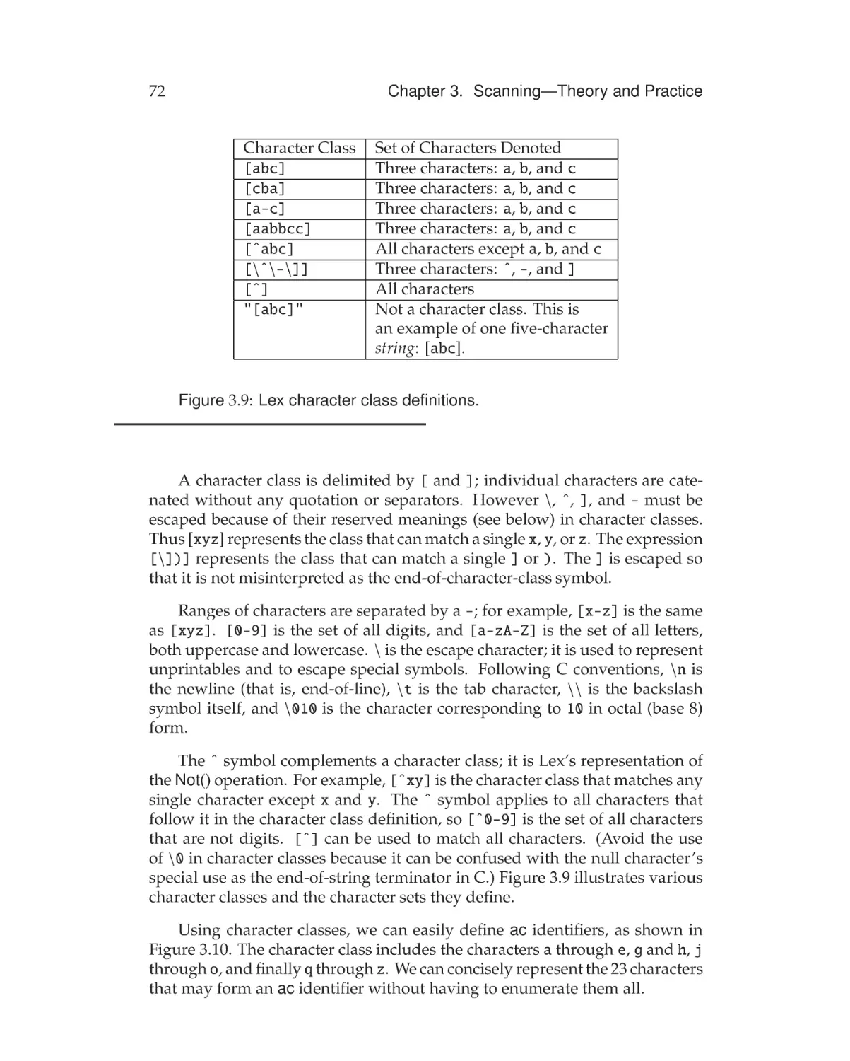
The Character Class . . . . . . . . . . . . . . . . . . . .
71
3.5.3
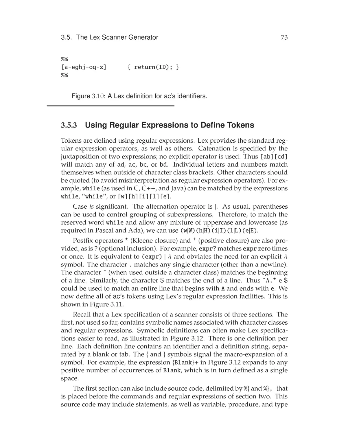
Using Regular Expressions to Define Tokens . . . . .
73
3.5.4
Character Processing Using Lex . . . . . . . . . . . . .
76
Other Scanner Generators . . . . . . . . . . . . . . . . . . . .
77
3.5
3.6
3.7
Practical Considerations of Building Scanners . . . . . . . . .
79
3.7.1
79
Processing Identifiers and Literals . . . . . . . . . . . .
xix
Contents
3.8
3.9
3.7.2
Using Compiler Directives and Listing Source Lines . .
83
3.7.3
3.7.4
Terminating the Scanner . . . . . . . . . . . . . . . . .
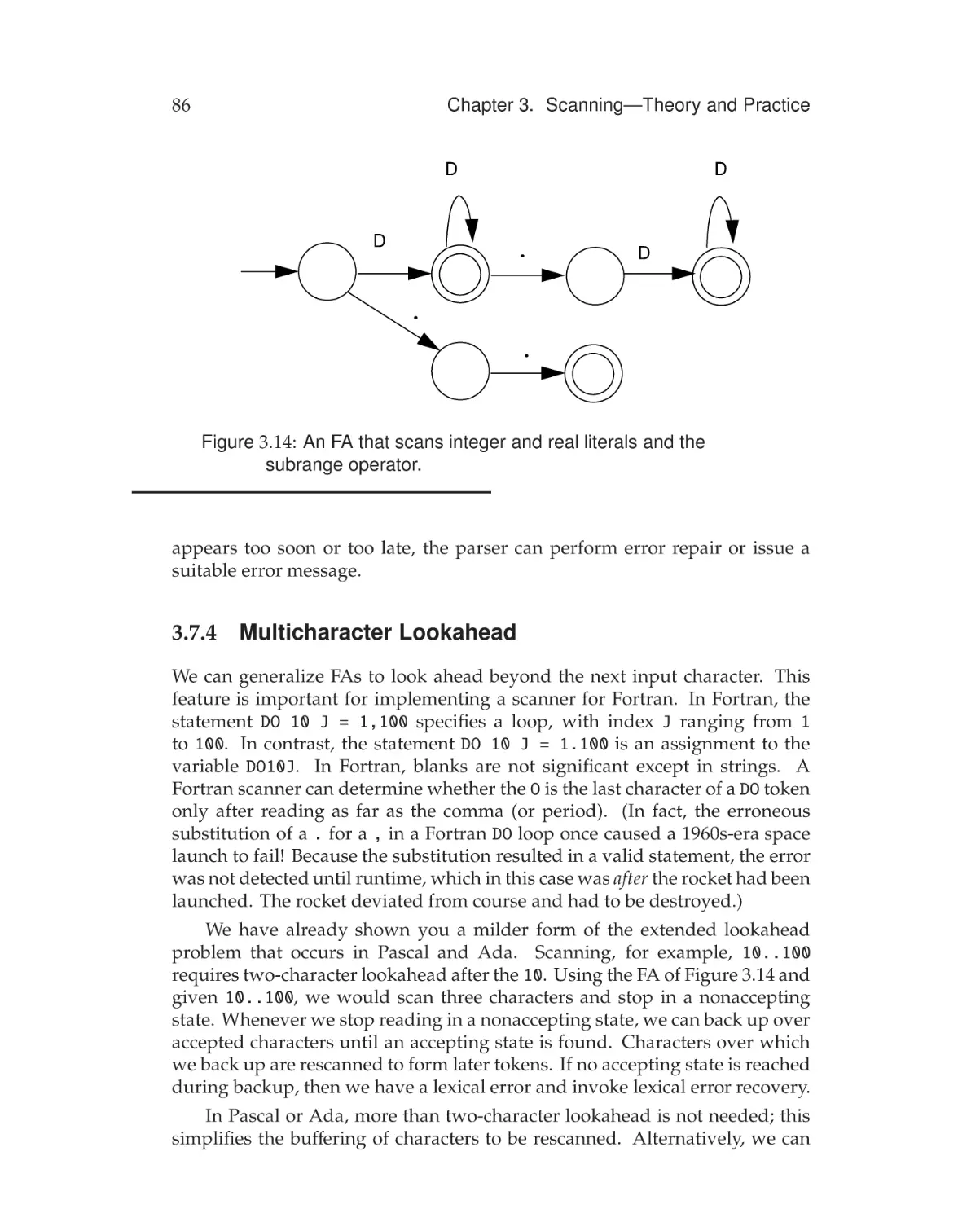
Multicharacter Lookahead . . . . . . . . . . . . . . . . .
85
86
3.7.5
3.7.6
Performance Considerations . . . . . . . . . . . . . . .
Lexical Error Recovery . . . . . . . . . . . . . . . . . .
87
89
Regular Expressions and Finite Automata . . . . . . . . . . . .
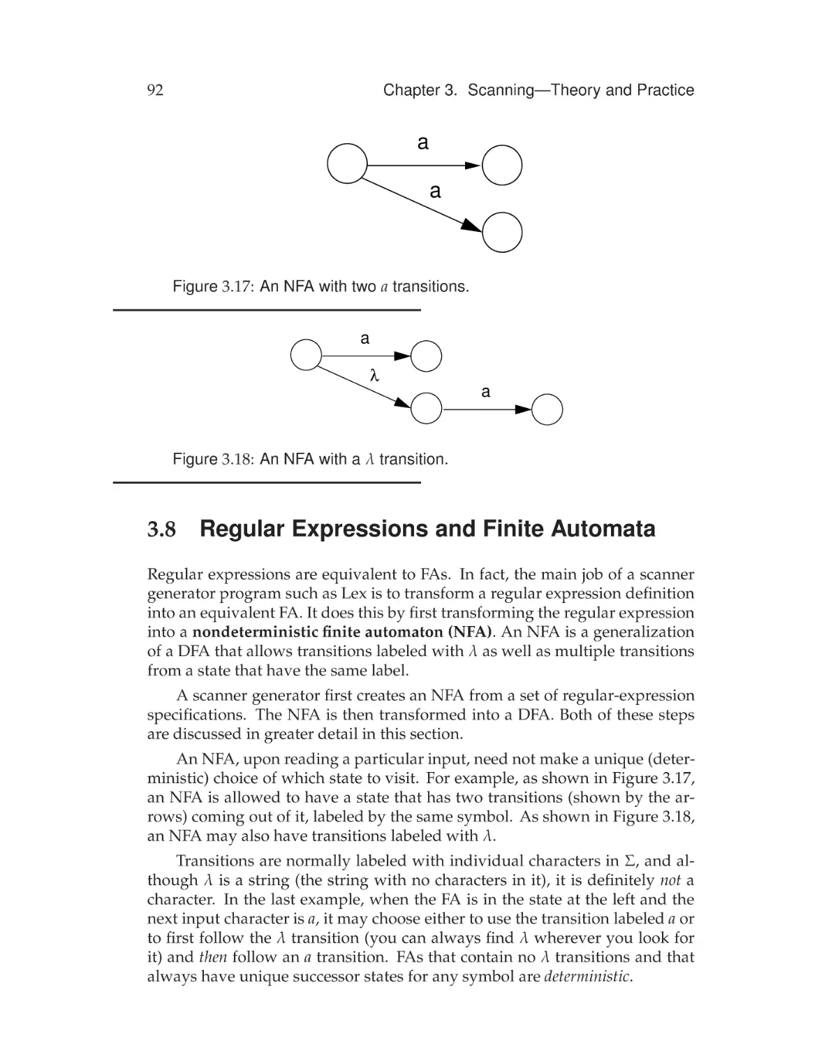
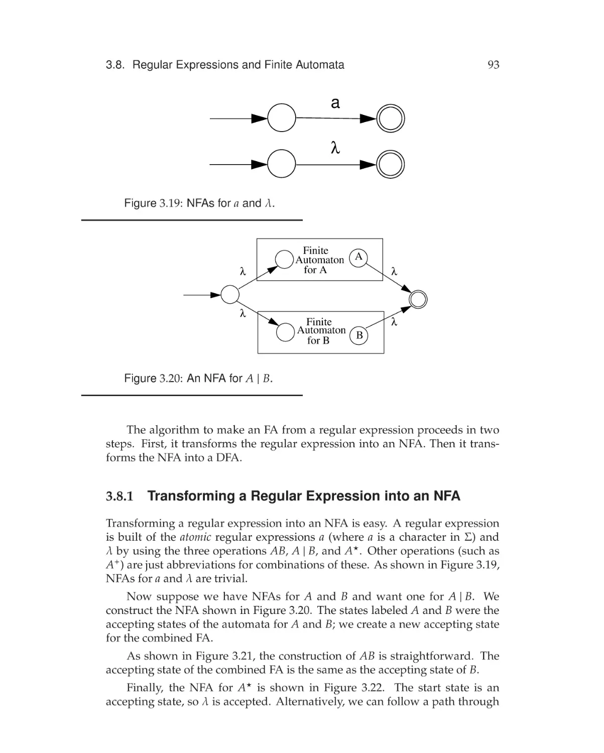
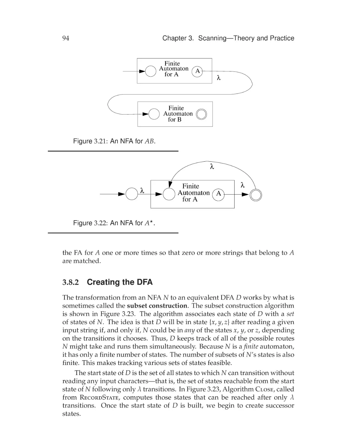
3.8.1 Transforming a Regular Expression into an NFA . . . .
92
93
3.8.2
3.8.3
94
97
Creating the DFA . . . . . . . . . . . . . . . . . . . . . .
Optimizing Finite Automata . . . . . . . . . . . . . . . .
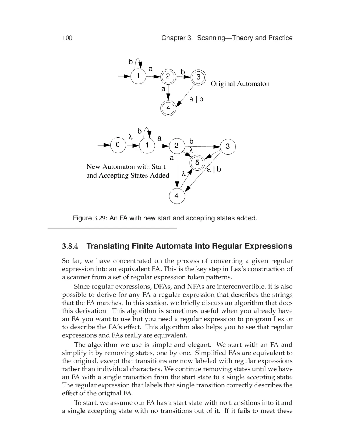
3.8.4 Translating Finite Automata into Regular Expressions . 100
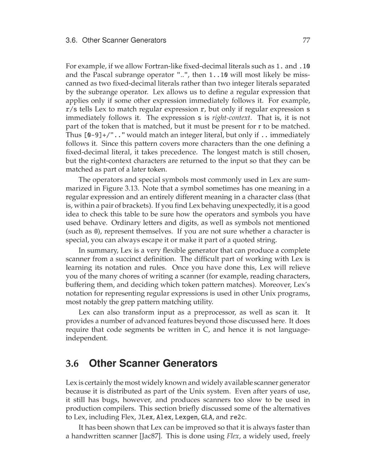
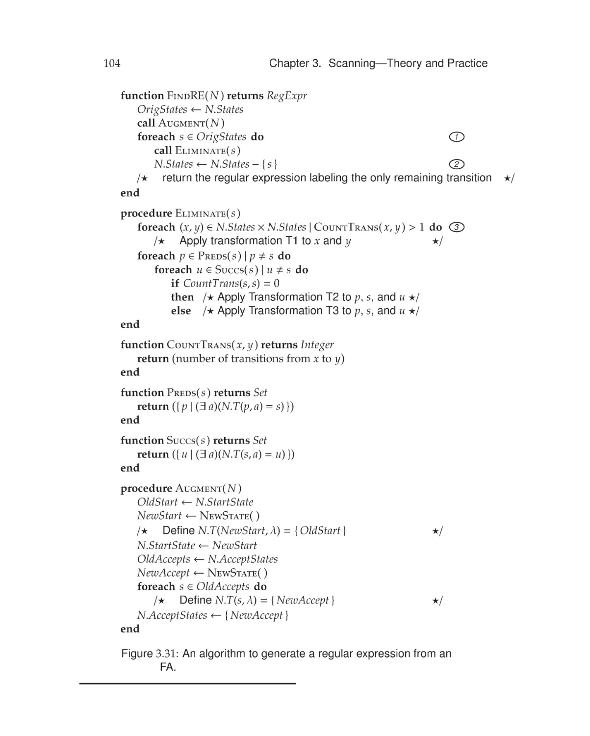
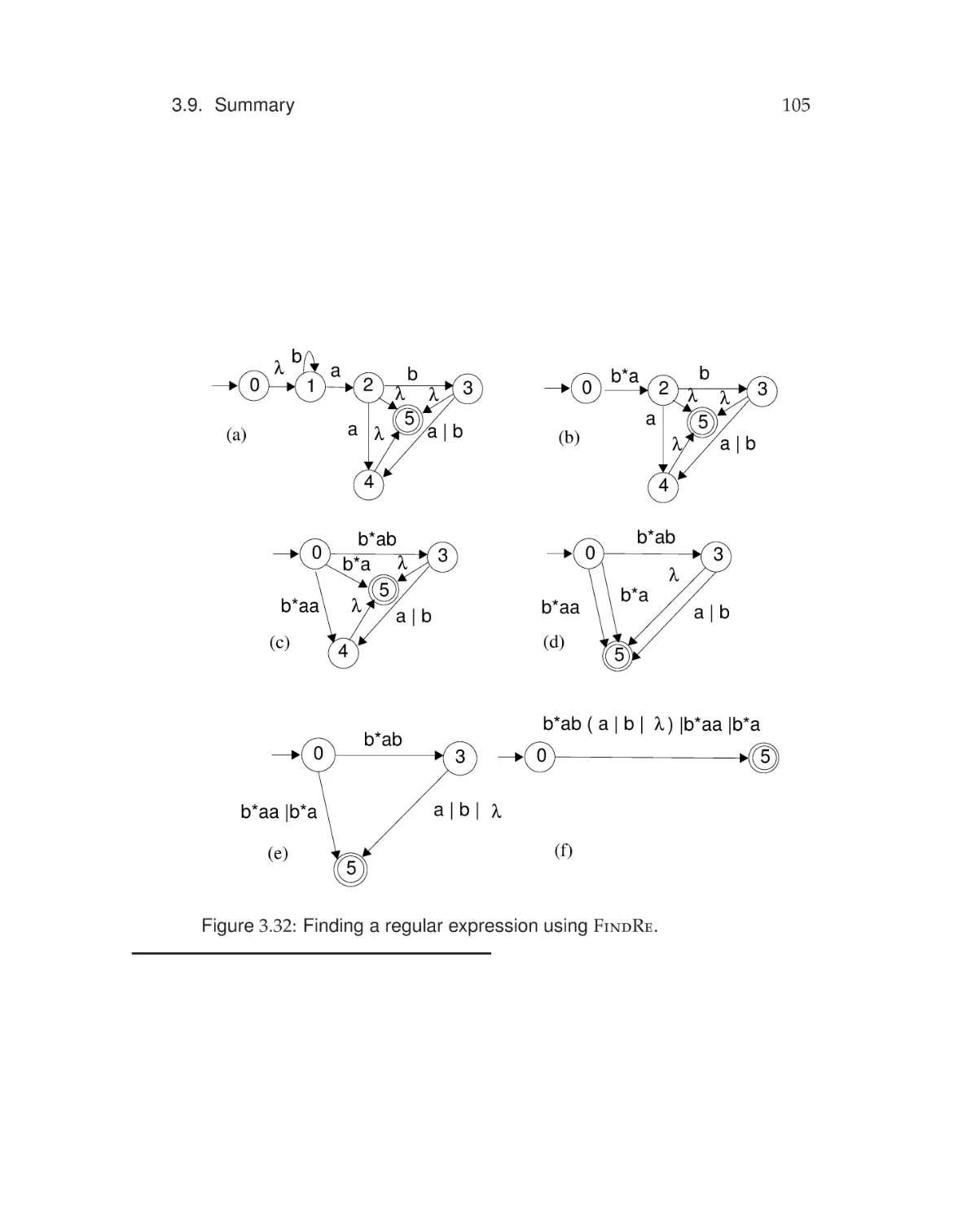
Summary . . . . . . . . . . . . . . . . . . . . . . . . . . . . . . 103
Exercises . . . . . . . . . . . . . . . . . . . . . . . . . . . . . . . . . 106
4
Grammars and Parsing
4.1
Context-Free Grammars . . . . . . . . . . . . . . . . . . . . . . 114
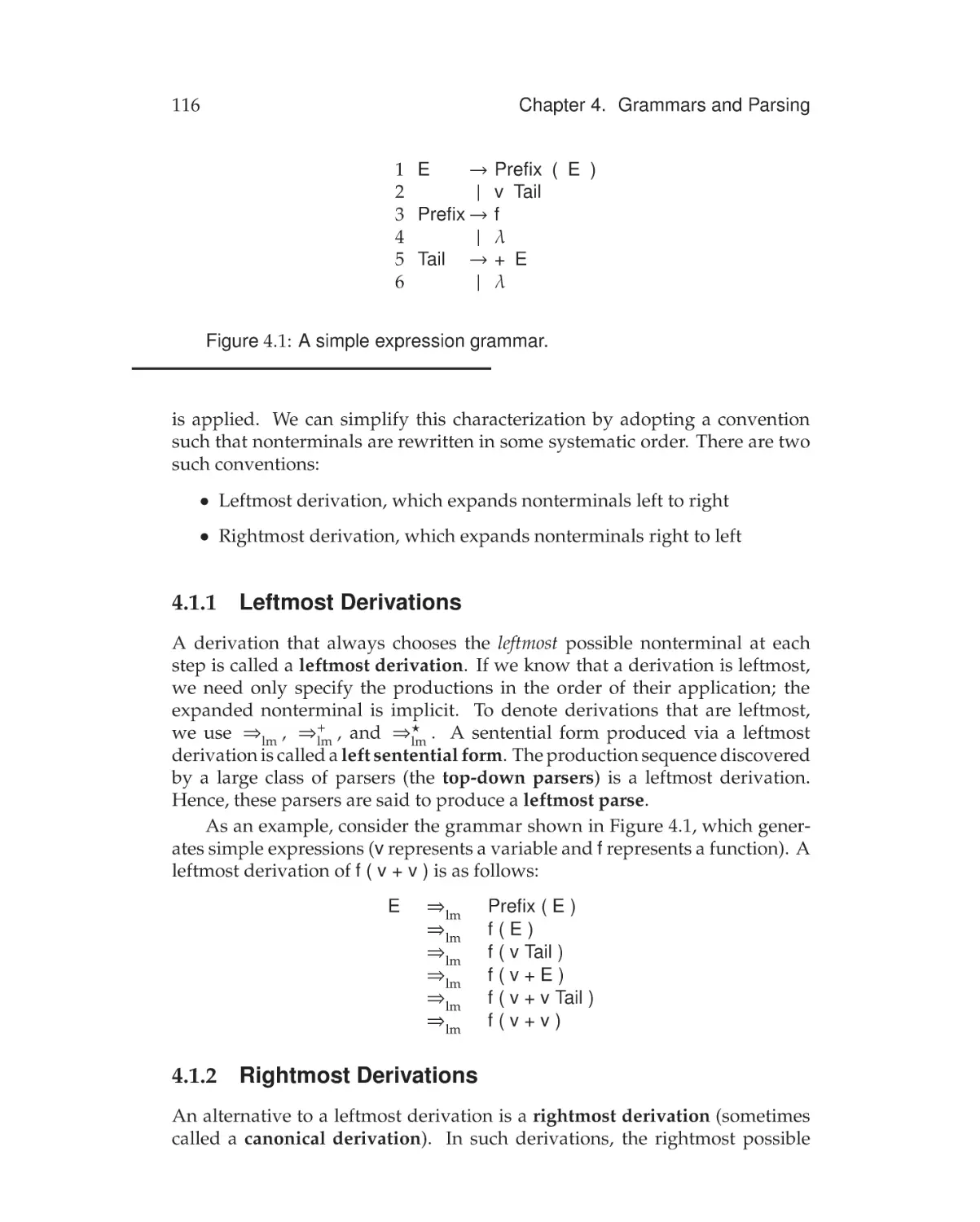
4.1.1 Leftmost Derivations . . . . . . . . . . . . . . . . . . . . 116
4.1.2
4.1.3
4.2
113
Rightmost Derivations . . . . . . . . . . . . . . . . . . . 116
Parse Trees . . . . . . . . . . . . . . . . . . . . . . . . . 117
4.1.4 Other Types of Grammars . . . . . . . . . . . . . . . . . 118
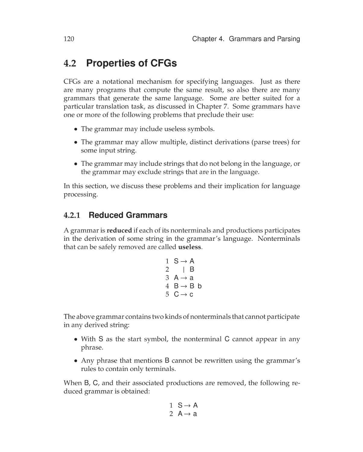
Properties of CFGs . . . . . . . . . . . . . . . . . . . . . . . . . 120
4.2.1
4.2.2
Reduced Grammars . . . . . . . . . . . . . . . . . . . . 120
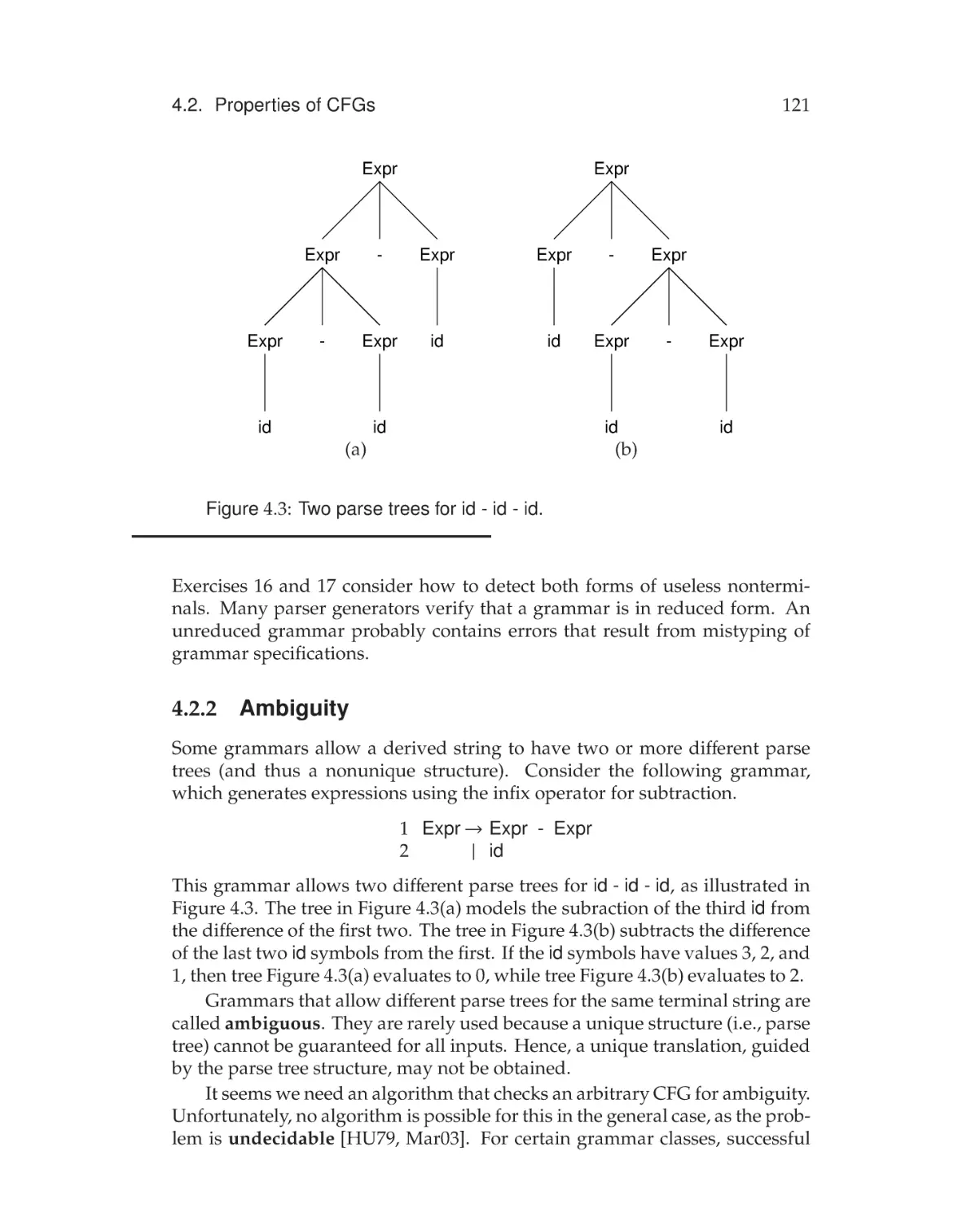
Ambiguity . . . . . . . . . . . . . . . . . . . . . . . . . . 121
4.3
4.2.3 Faulty Language Definition . . . . . . . . . . . . . . . . 122
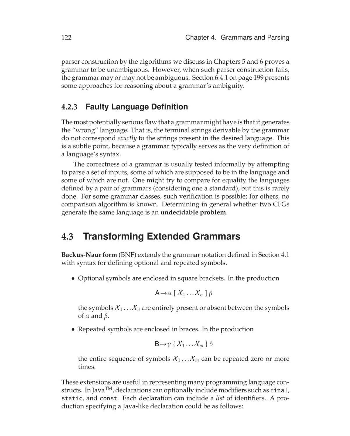
Transforming Extended Grammars . . . . . . . . . . . . . . . . 122
4.4
4.5
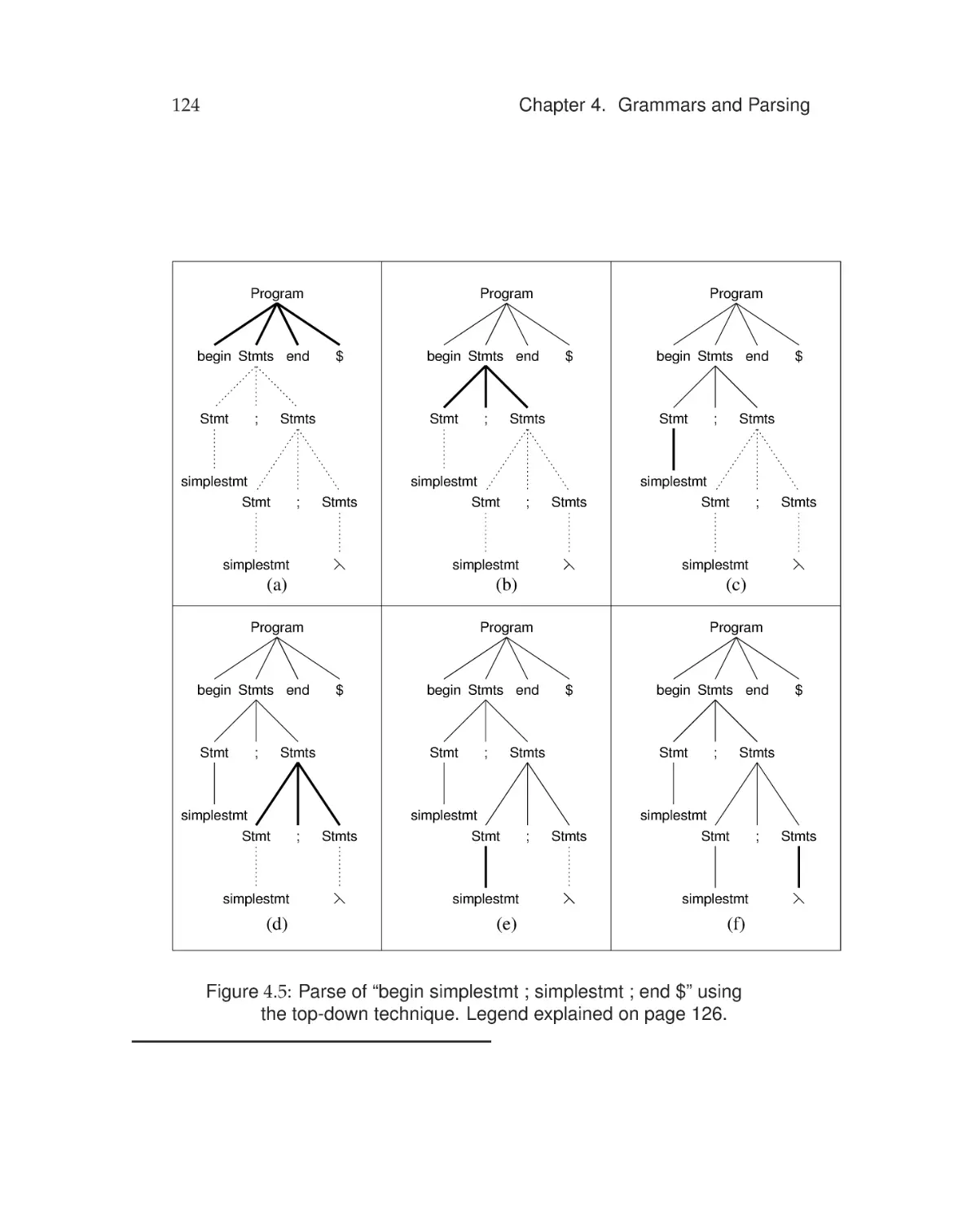
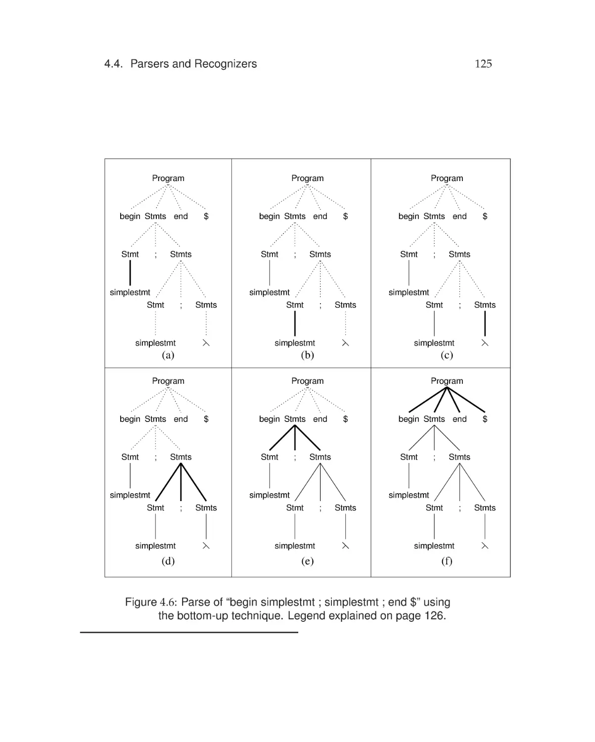
Parsers and Recognizers . . . . . . . . . . . . . . . . . . . . . 123
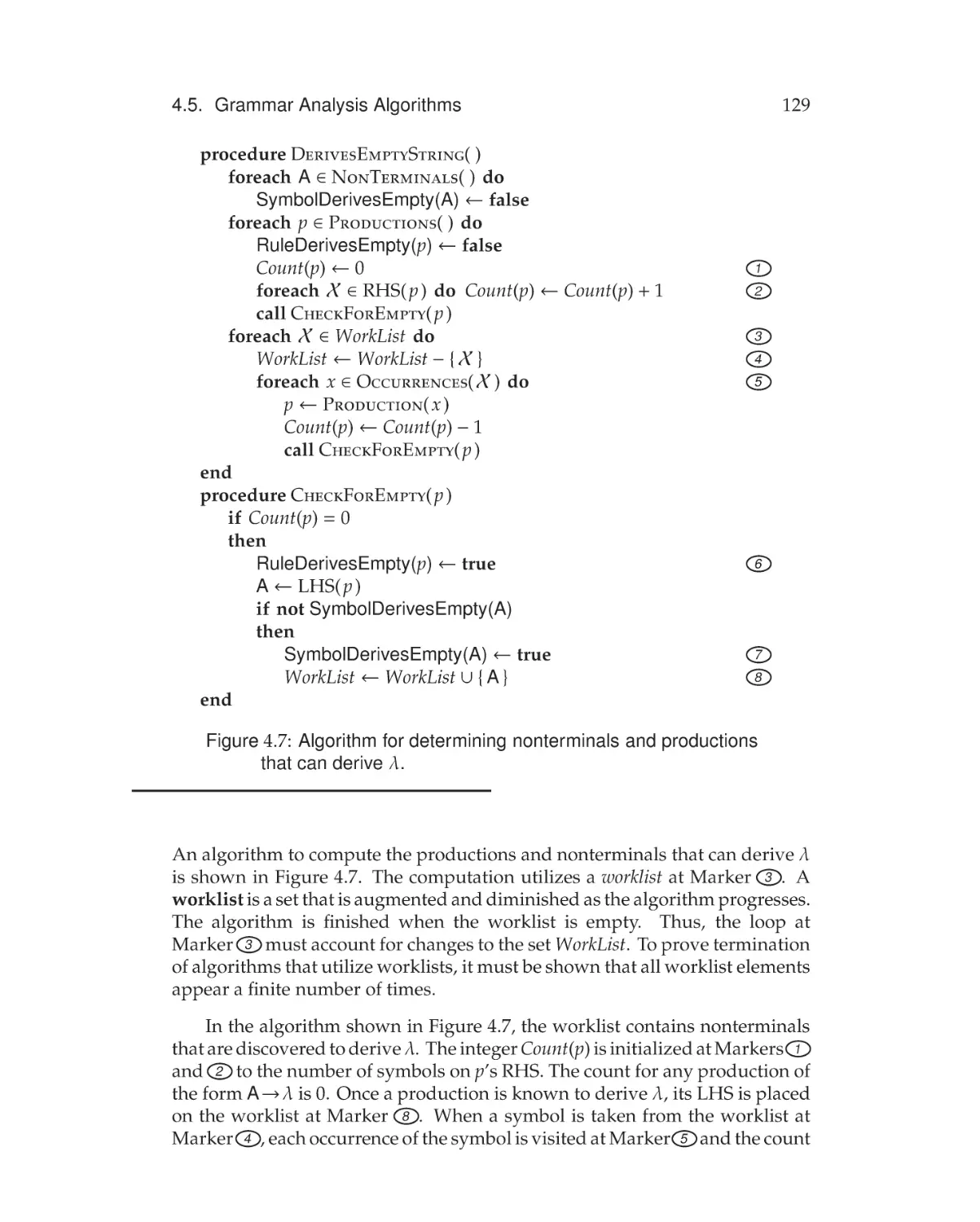
Grammar Analysis Algorithms . . . . . . . . . . . . . . . . . . 127
4.5.1
Grammar Representation . . . . . . . . . . . . . . . . . 127
4.5.2
4.5.3
Deriving the Empty String . . . . . . . . . . . . . . . . . 128
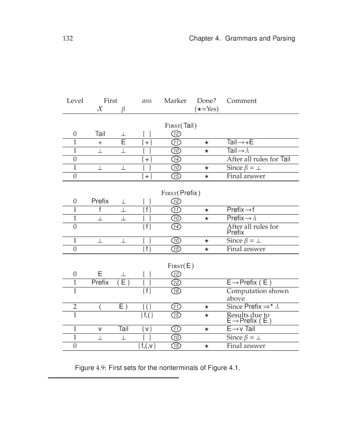
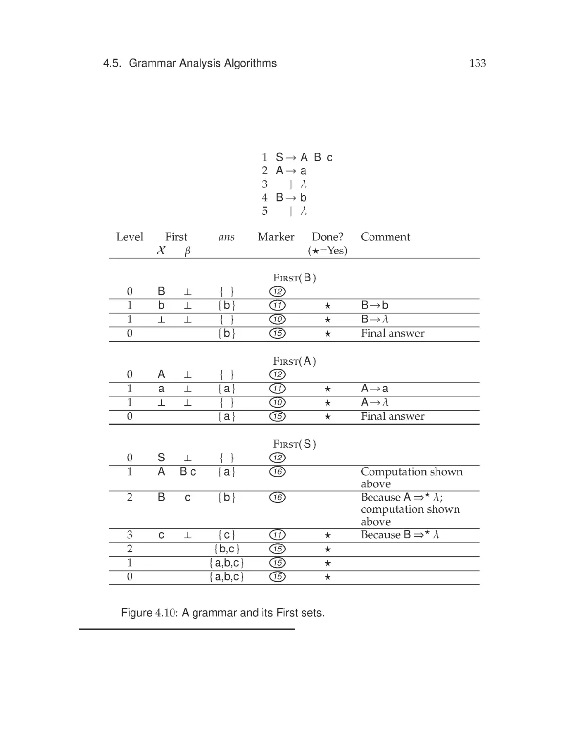
First Sets . . . . . . . . . . . . . . . . . . . . . . . . . . 130
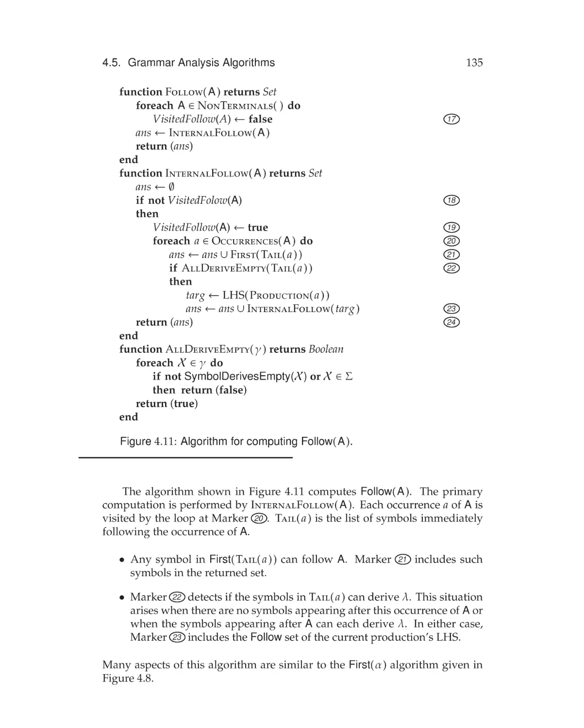
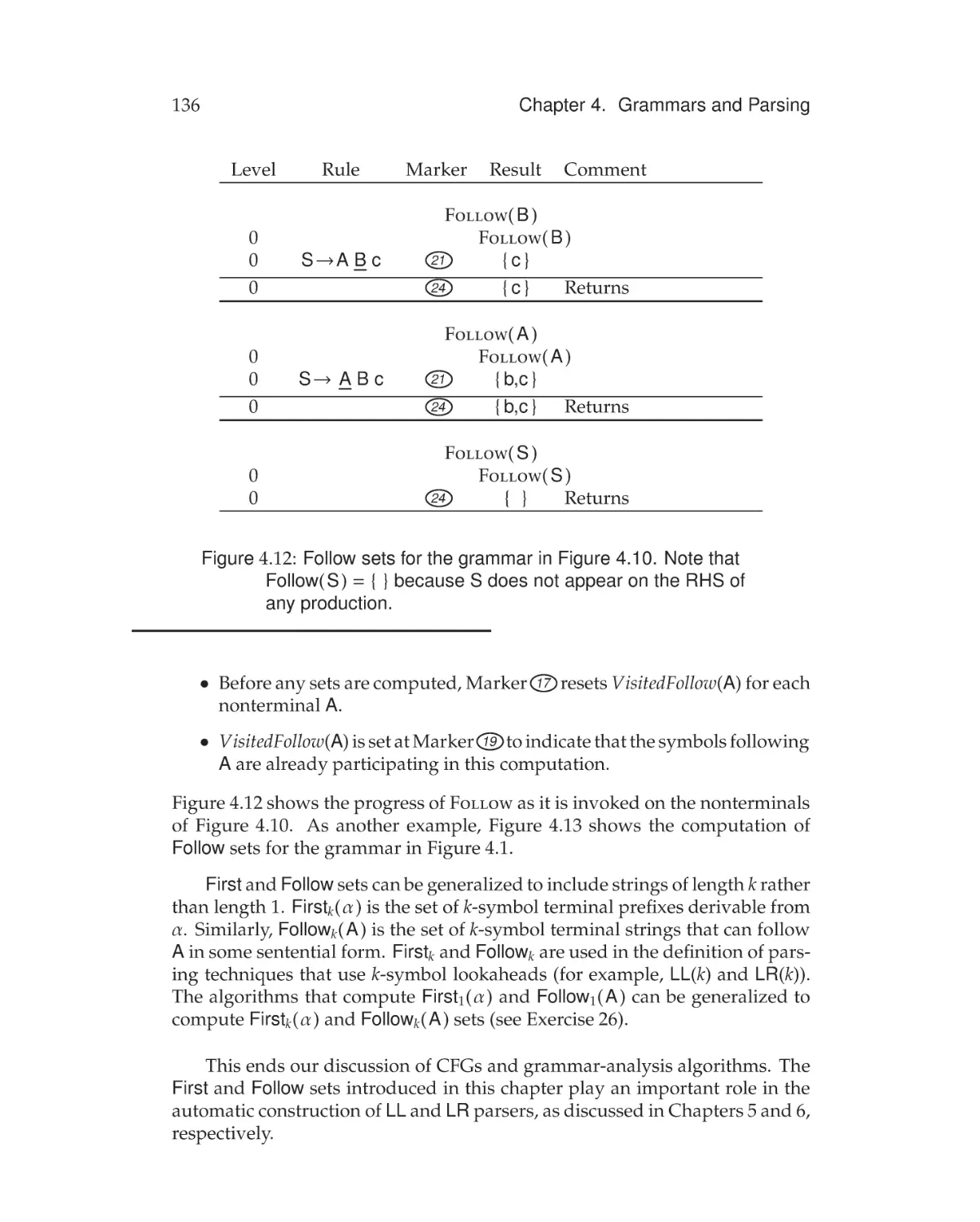
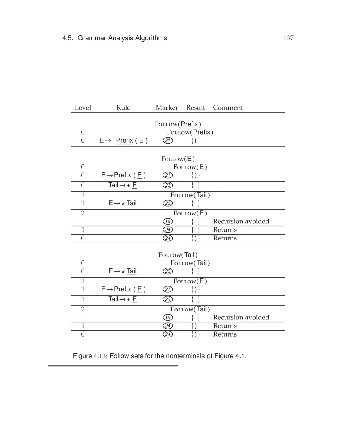
4.5.4 Follow Sets . . . . . . . . . . . . . . . . . . . . . . . . . 134
Exercises . . . . . . . . . . . . . . . . . . . . . . . . . . . . . . . . . 138
xx
5
Contents
Top-Down Parsing
143
5.1
Overview . . . . . . . . . . . . . . . . . . . . . . . . . . . . . . . 144
5.2
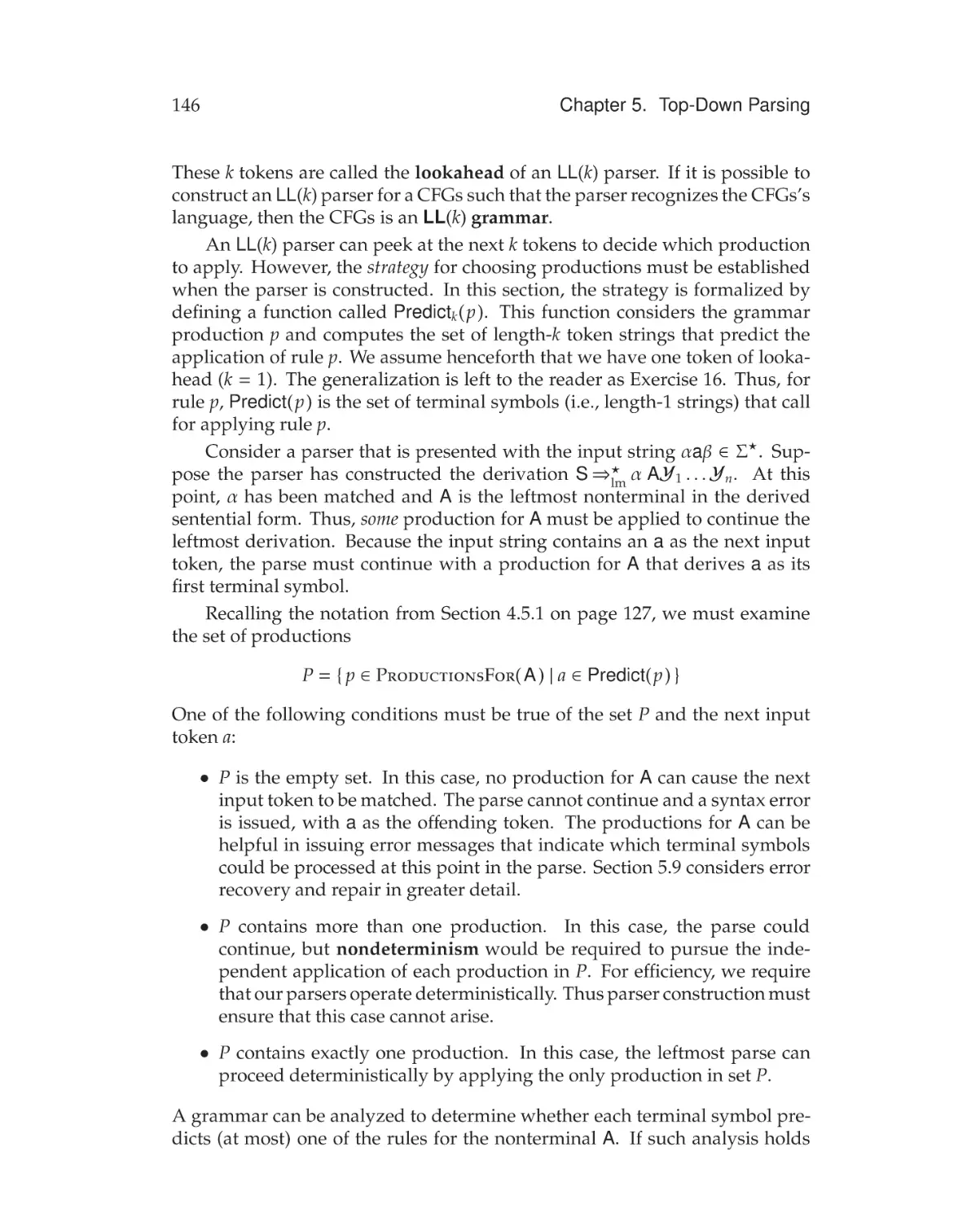
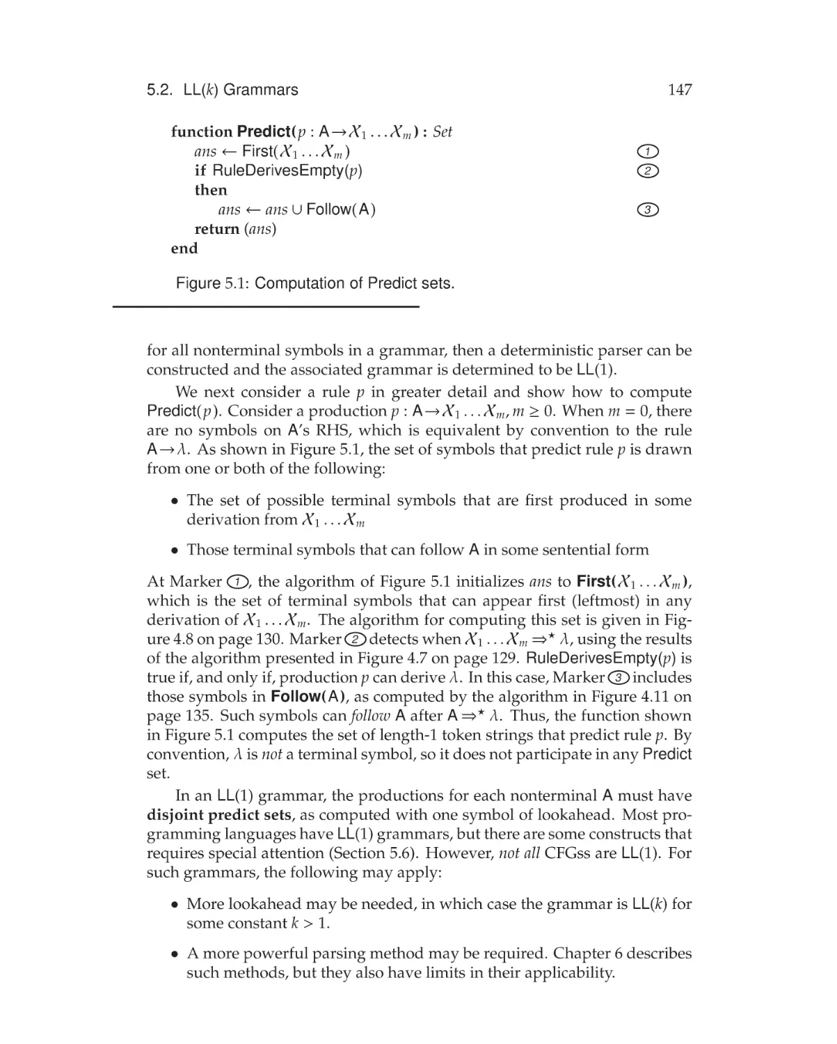
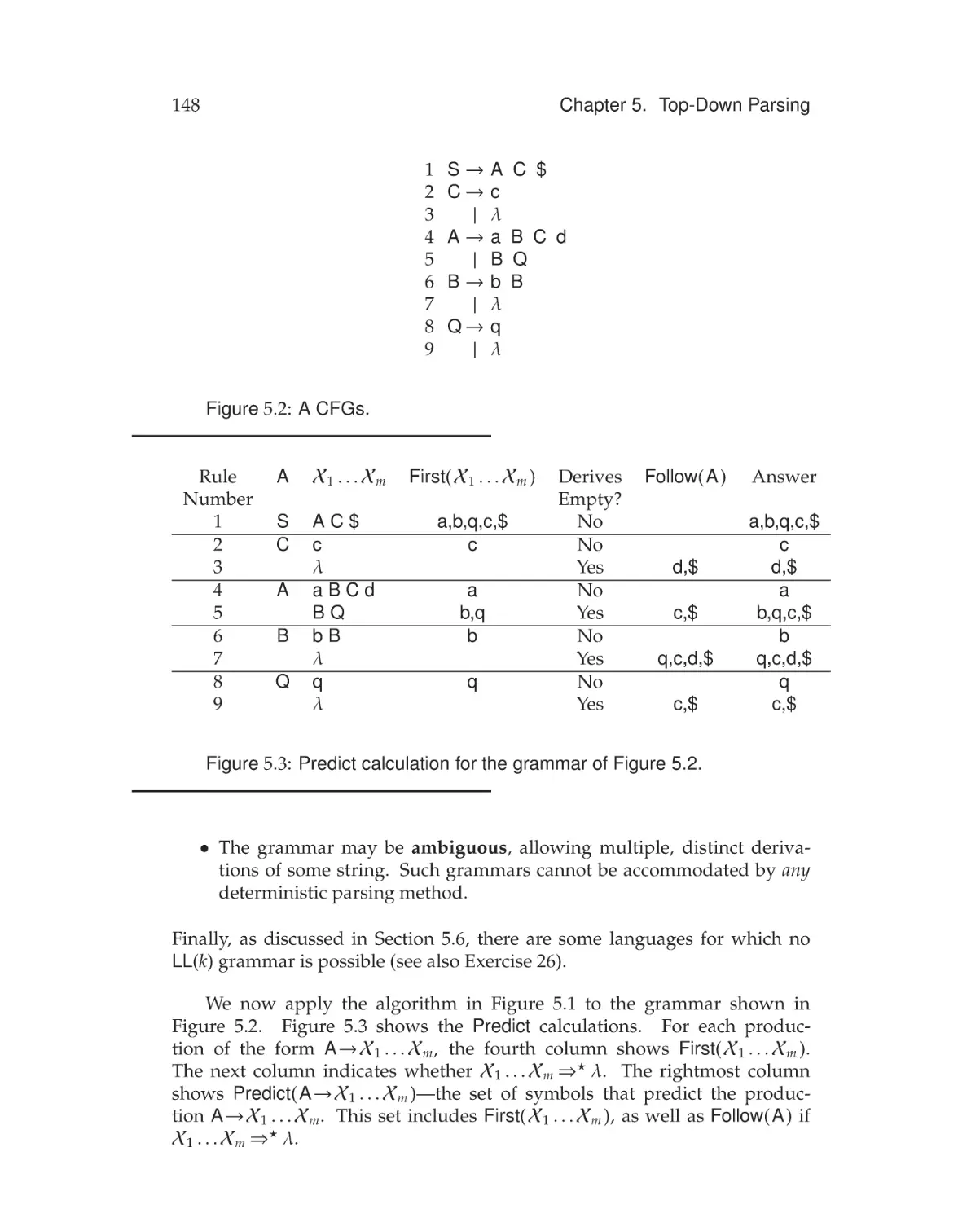
LL(k) Grammars . . . . . . . . . . . . . . . . . . . . . . . . . . 145
5.3
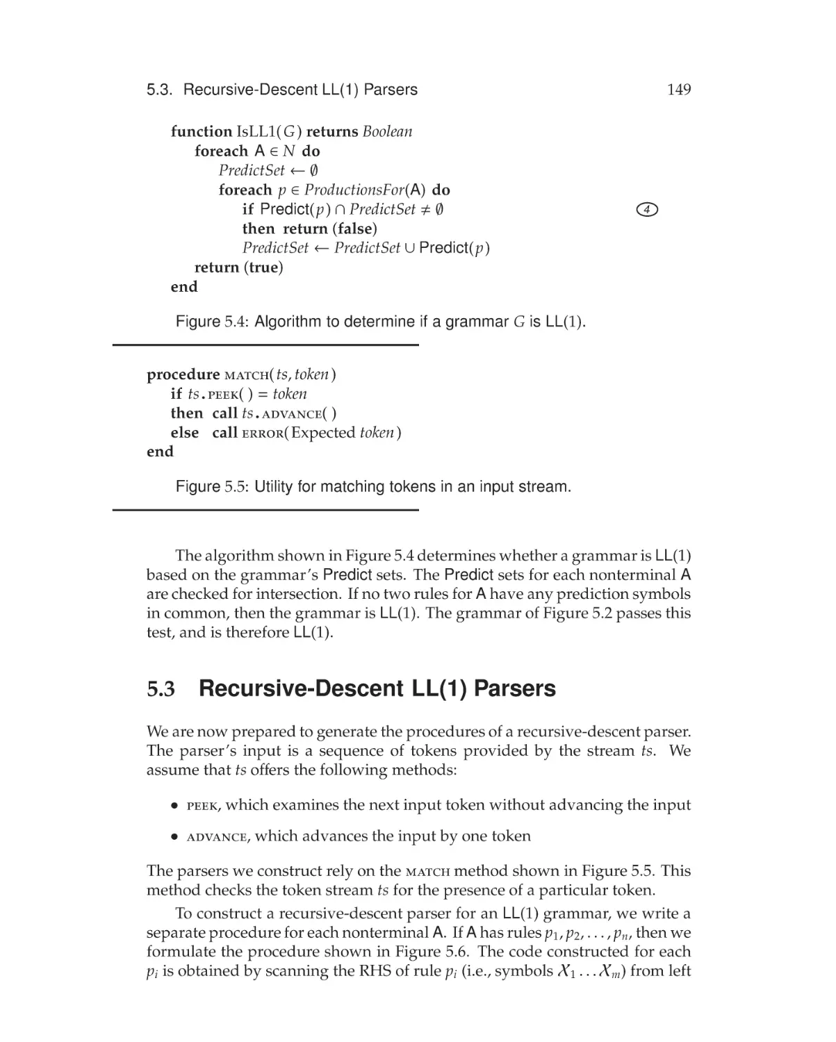
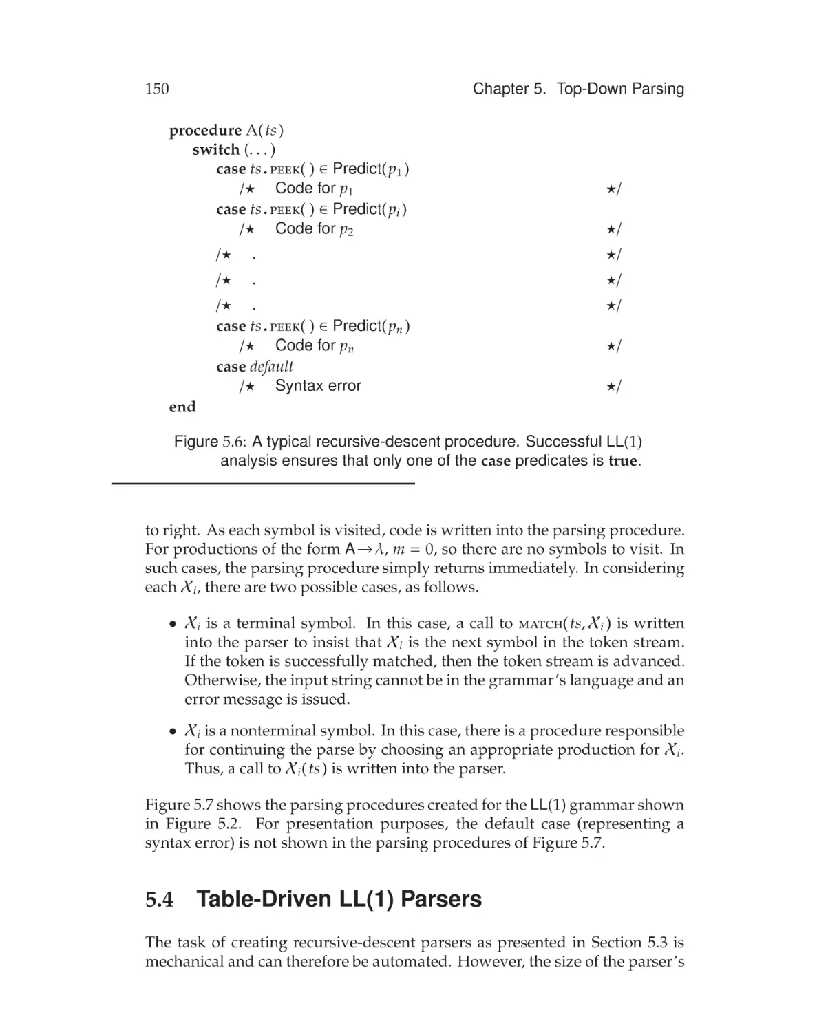
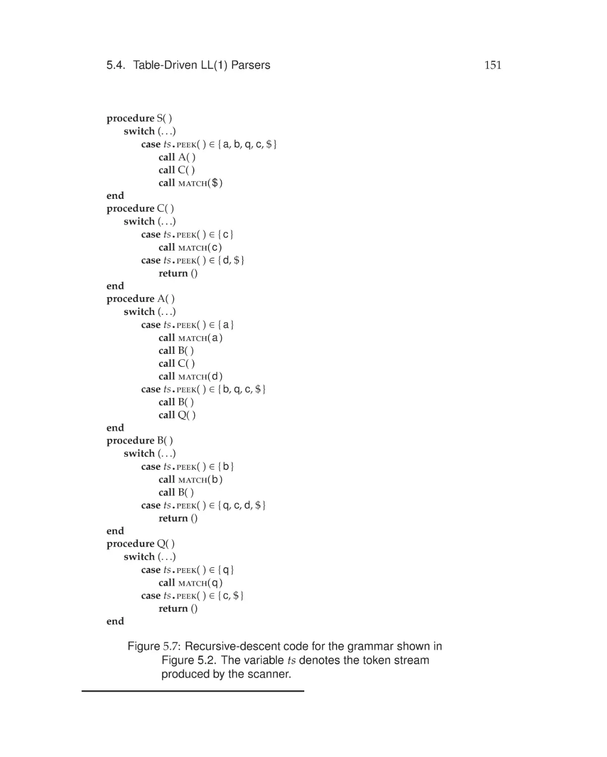
Recursive-Descent LL(1) Parsers . . . . . . . . . . . . . . . . 149
5.4
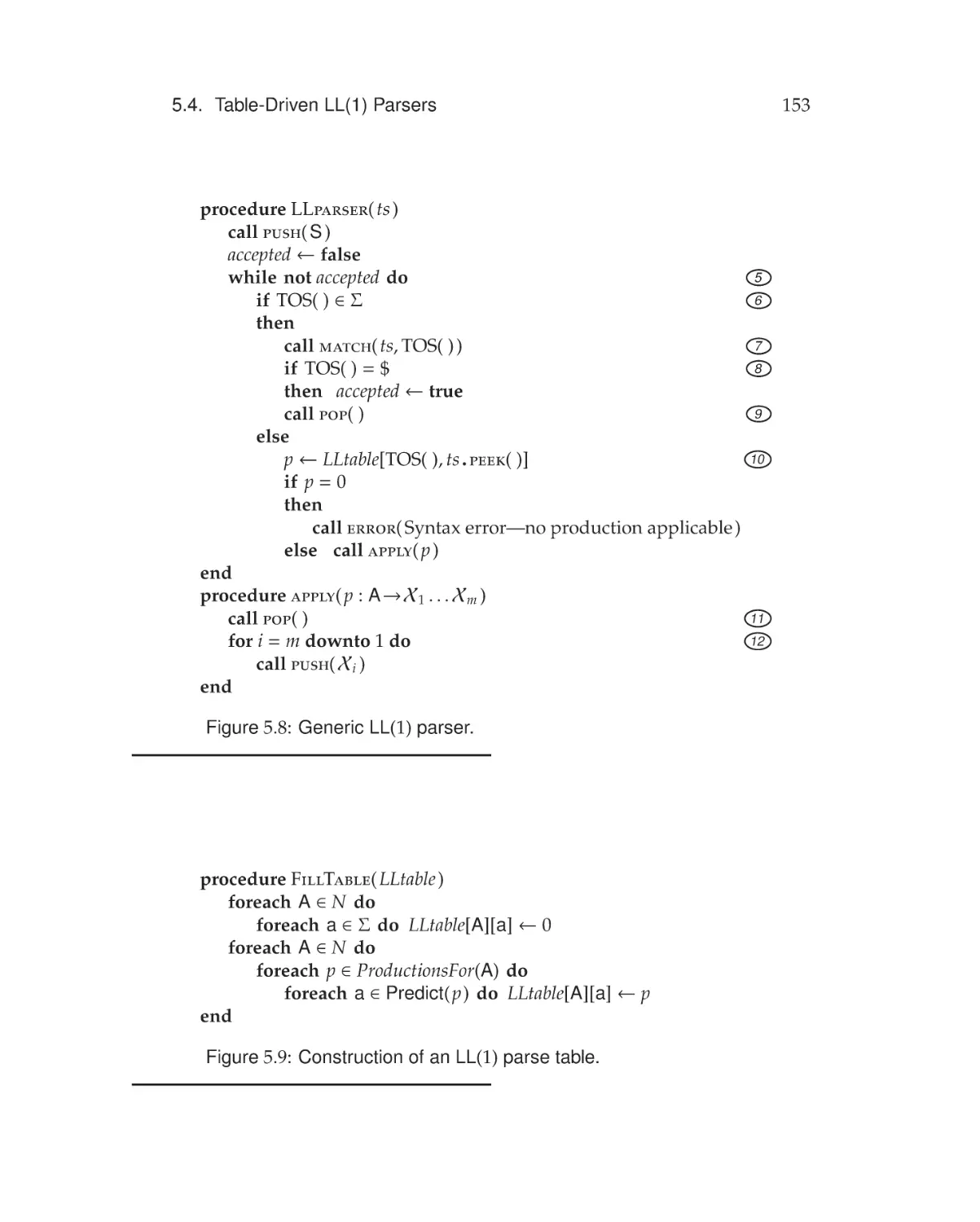
Table-Driven LL(1) Parsers . . . . . . . . . . . . . . . . . . . . 150
5.5
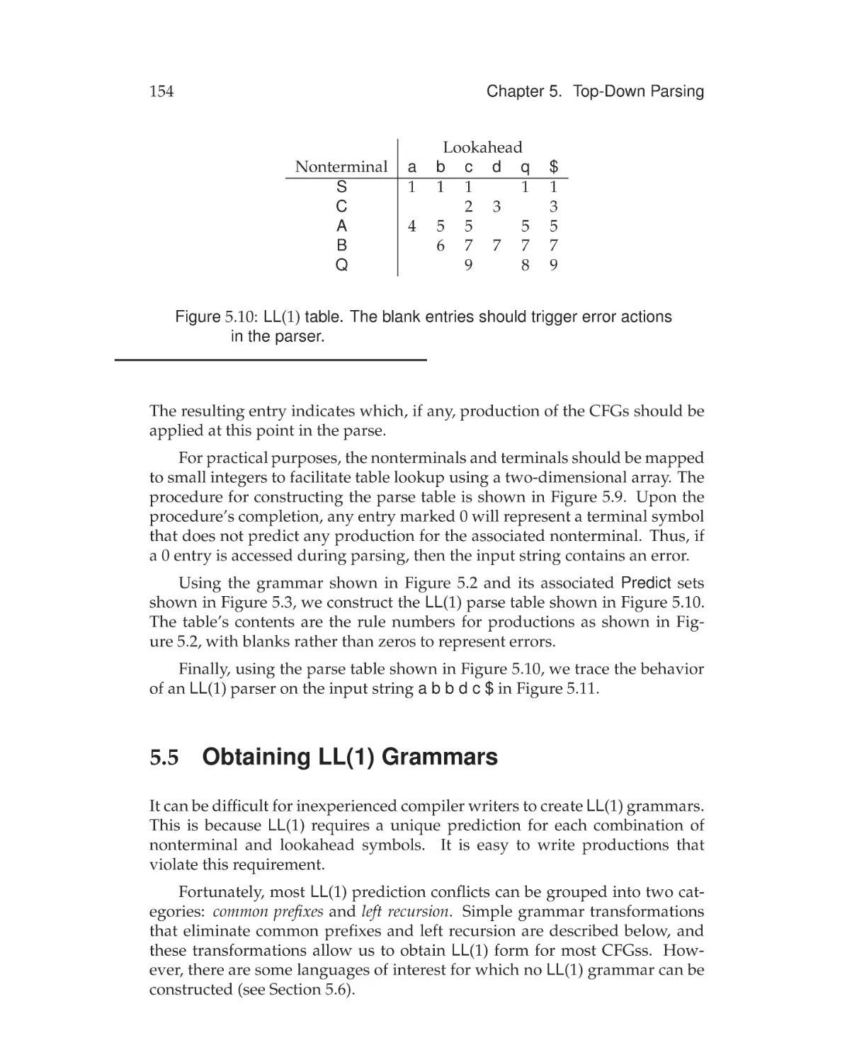
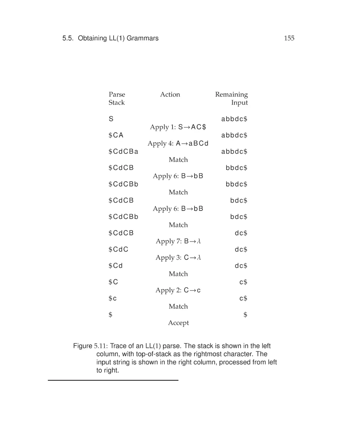
Obtaining LL(1) Grammars . . . . . . . . . . . . . . . . . . . . 154
5.5.1
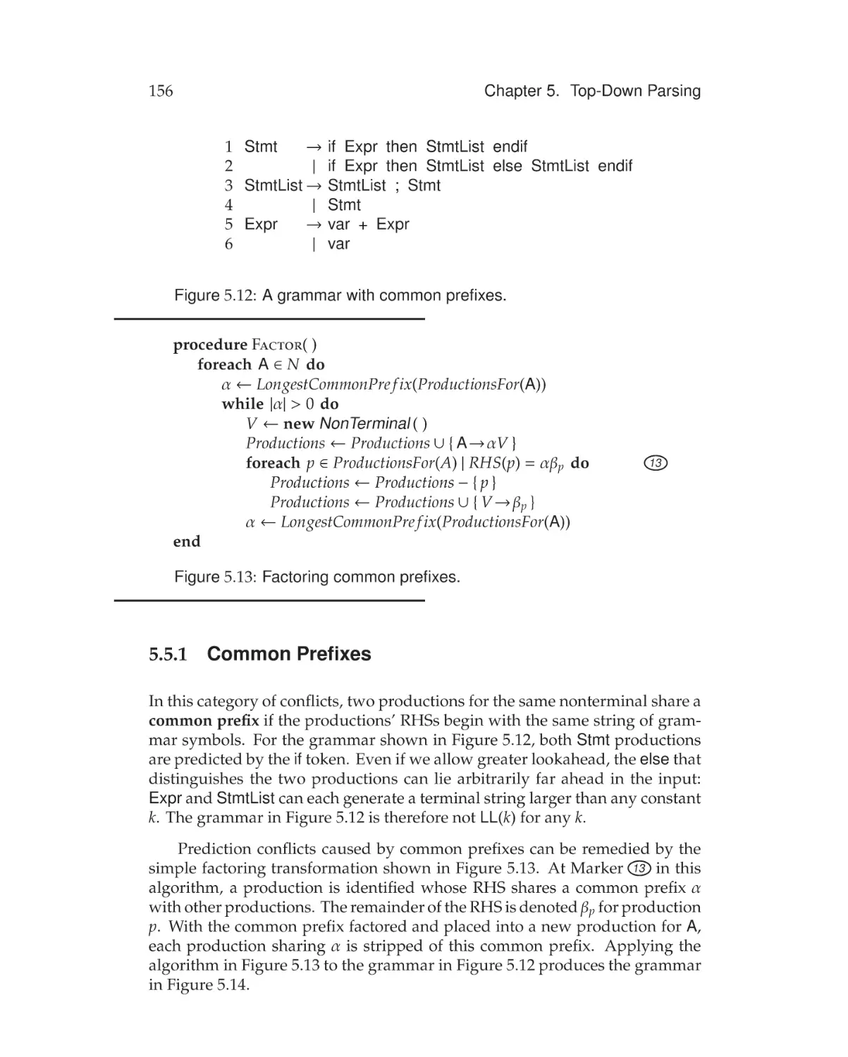
Common Prefixes . . . . . . . . . . . . . . . . . . . . . 156
5.5.2
Left Recursion . . . . . . . . . . . . . . . . . . . . . . . 157
5.6
A Non-LL(1) Language . . . . . . . . . . . . . . . . . . . . . . . 159
5.7
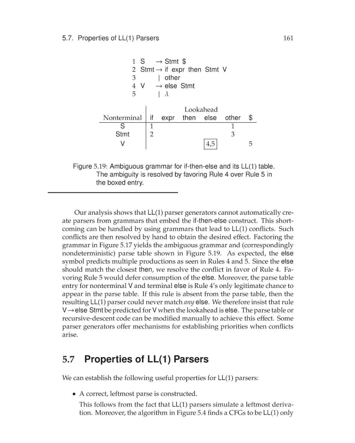
Properties of LL(1) Parsers . . . . . . . . . . . . . . . . . . . . 161
5.8
Parse Table Representation . . . . . . . . . . . . . . . . . . . . 163
5.9
5.8.1
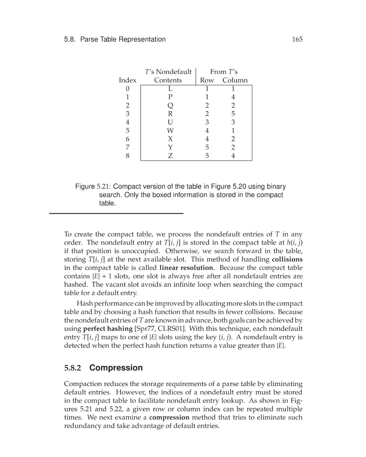
Compaction . . . . . . . . . . . . . . . . . . . . . . . . . 164
5.8.2
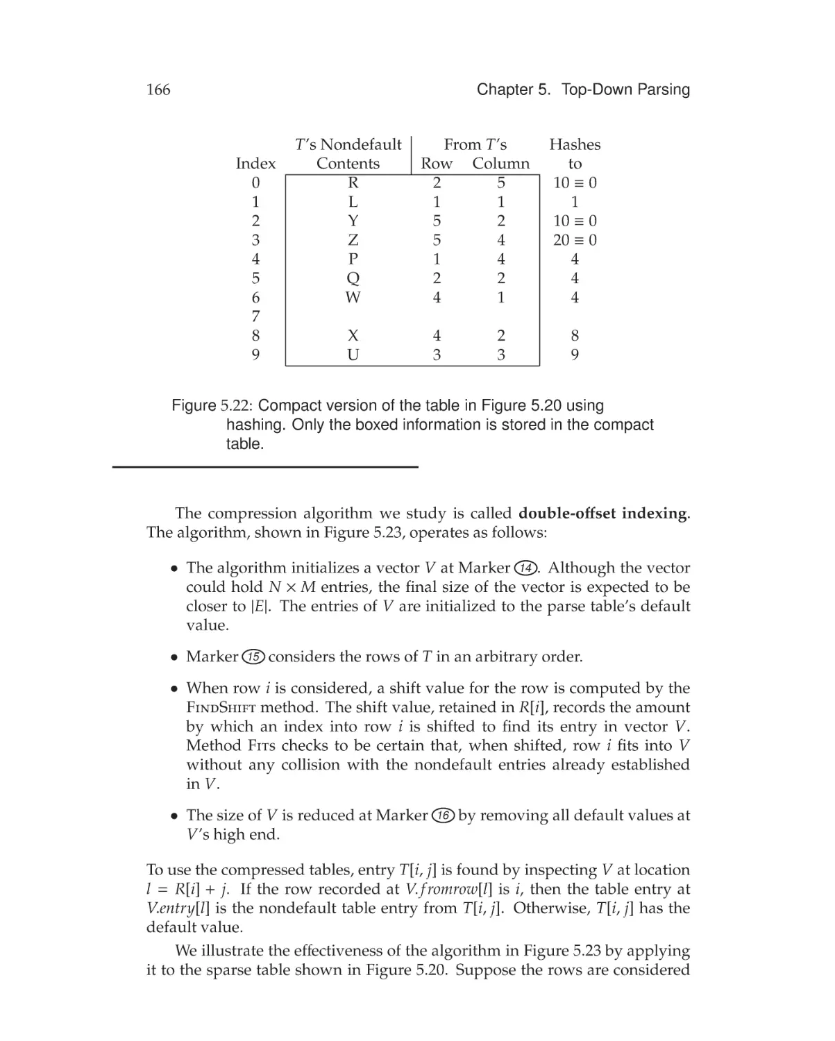
Compression . . . . . . . . . . . . . . . . . . . . . . . . 165
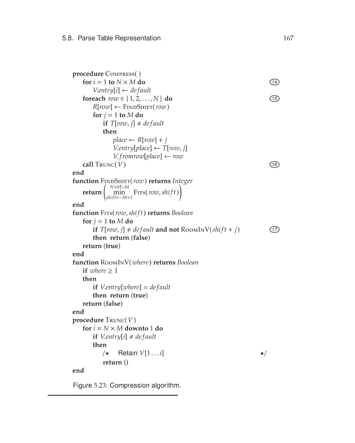
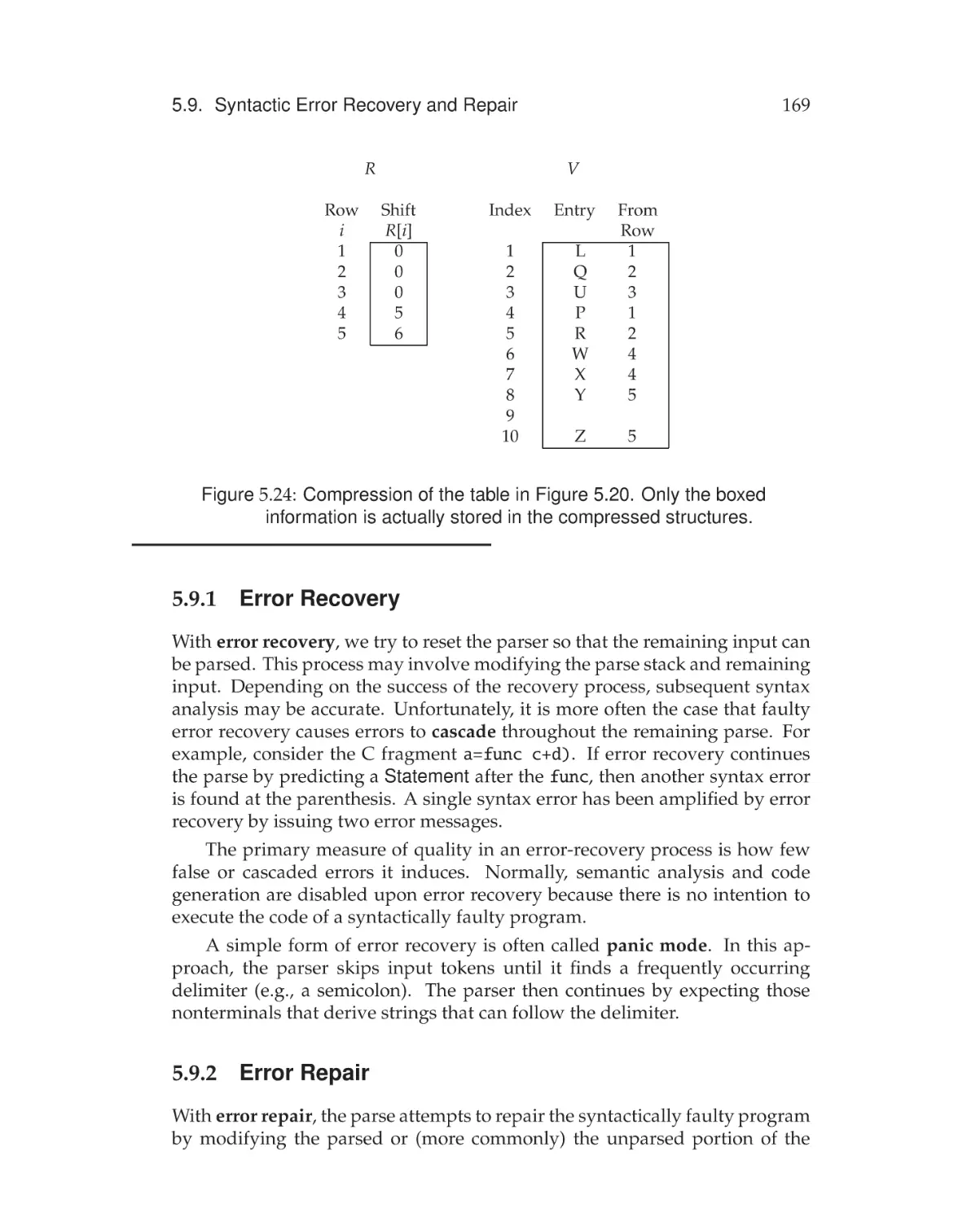
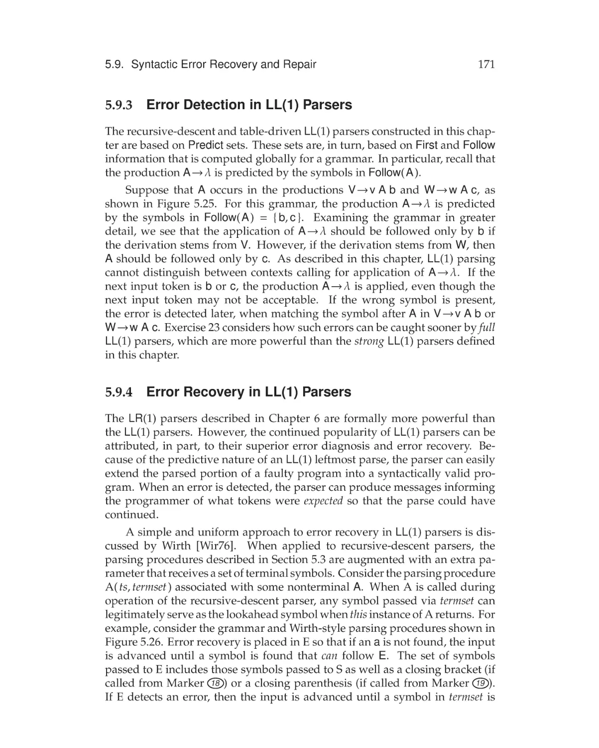
Syntactic Error Recovery and Repair . . . . . . . . . . . . . . 168
5.9.1
Error Recovery . . . . . . . . . . . . . . . . . . . . . . . 169
5.9.2
Error Repair . . . . . . . . . . . . . . . . . . . . . . . . . 169
5.9.3
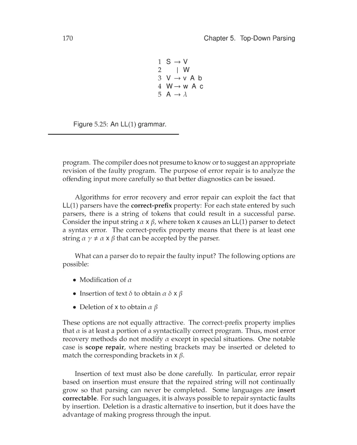
Error Detection in LL(1) Parsers . . . . . . . . . . . . . 171
5.9.4
Error Recovery in LL(1) Parsers . . . . . . . . . . . . . 171
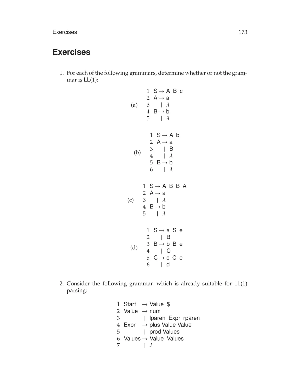
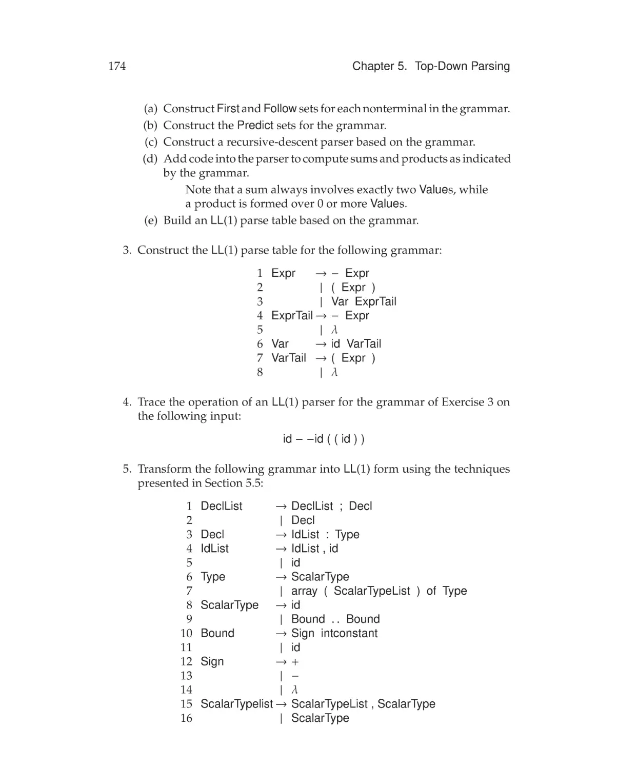
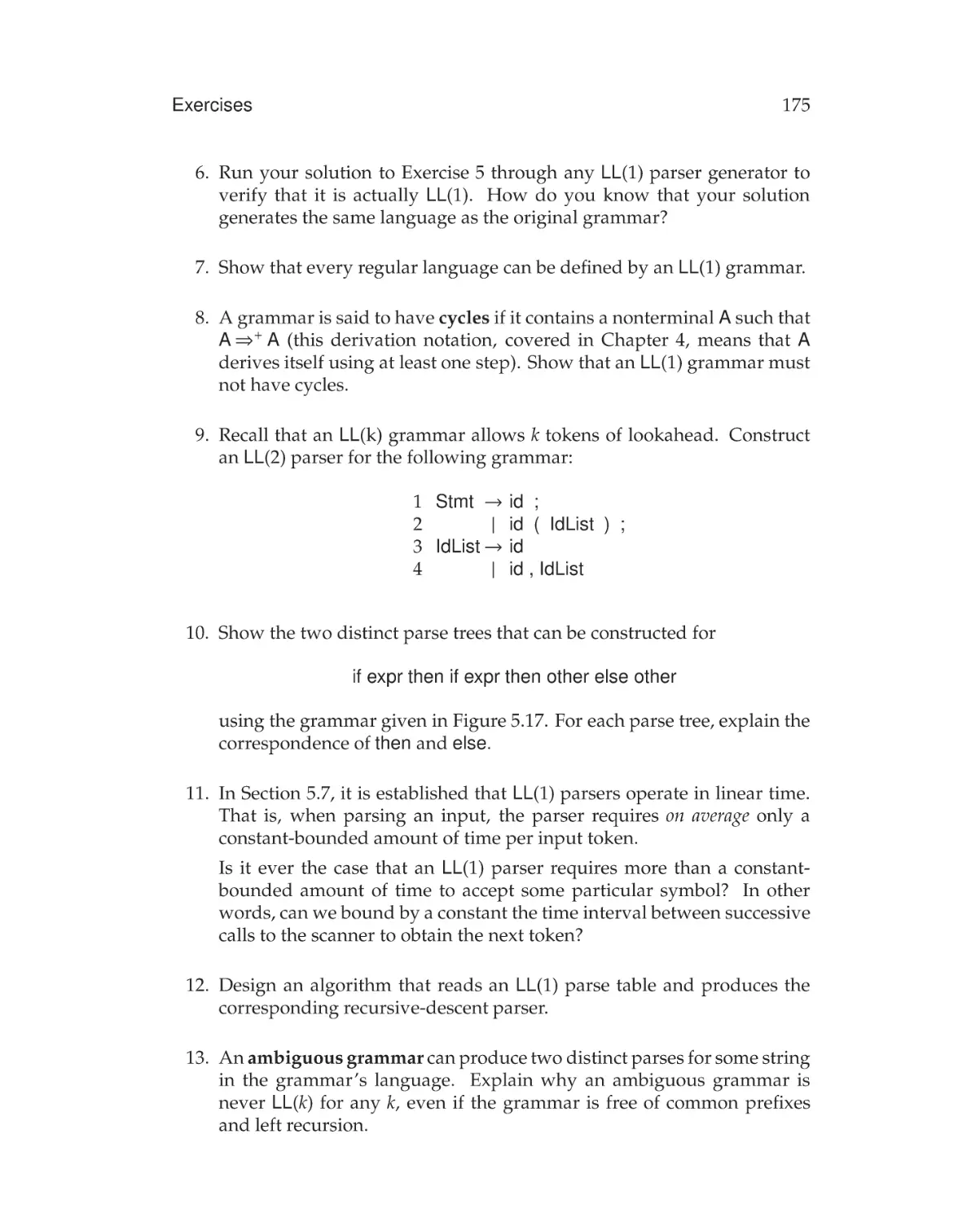
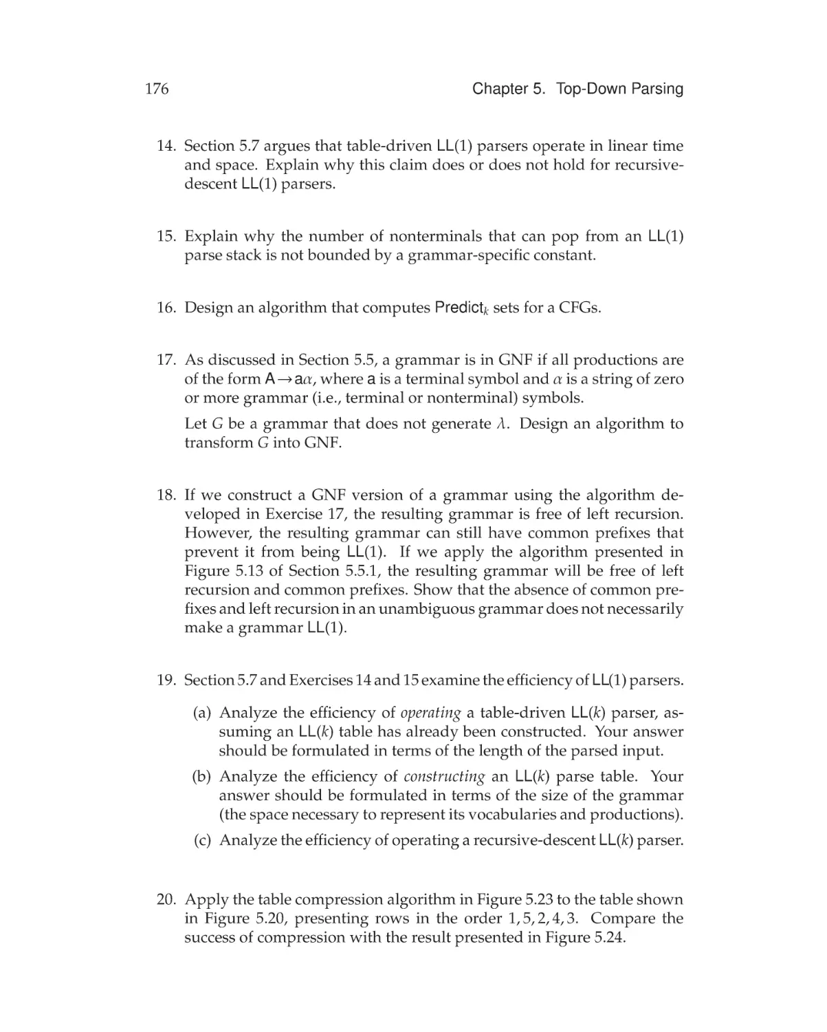
Exercises . . . . . . . . . . . . . . . . . . . . . . . . . . . . . . . . . 173
6
Bottom-Up Parsing
179
6.1
Overview . . . . . . . . . . . . . . . . . . . . . . . . . . . . . . . 180
6.2
Shift-Reduce Parsers . . . . . . . . . . . . . . . . . . . . . . . 181
6.2.1
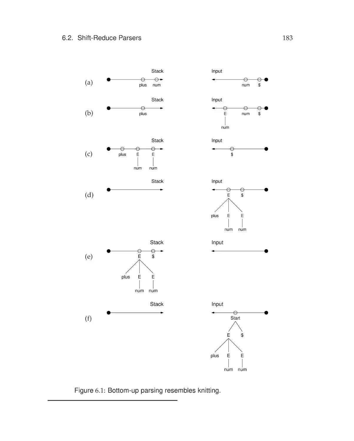
LR Parsers and Rightmost Derivations . . . . . . . . . 182
6.2.2
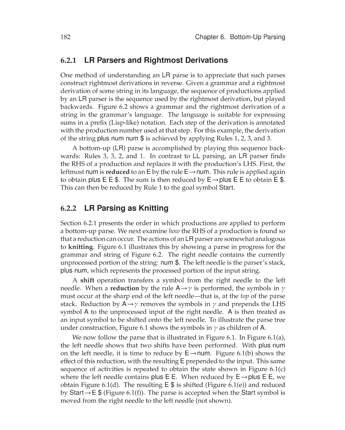
LR Parsing as Knitting . . . . . . . . . . . . . . . . . . . 182
6.2.3
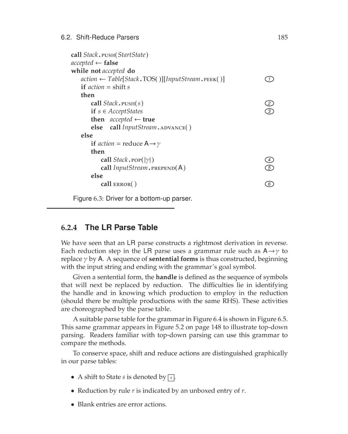
LR Parsing Engine . . . . . . . . . . . . . . . . . . . . . 184
6.2.4
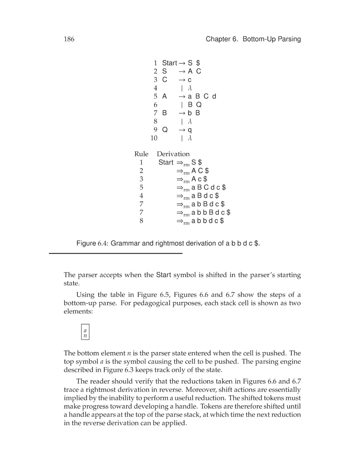
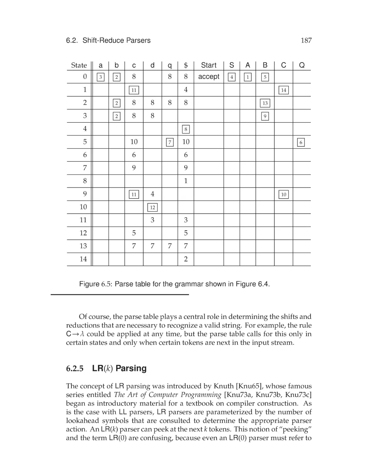
The LR Parse Table . . . . . . . . . . . . . . . . . . . . 185
6.2.5
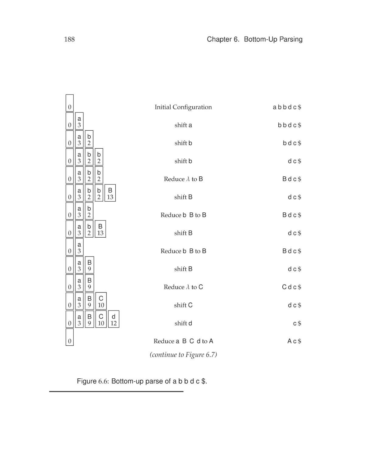
LR(k) Parsing . . . . . . . . . . . . . . . . . . . . . . . . 187
6.3
LR(0) Table Construction . . . . . . . . . . . . . . . . . . . . . 191
6.4
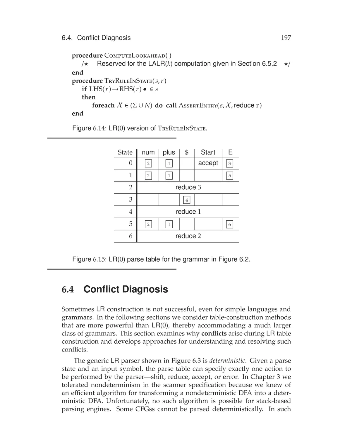
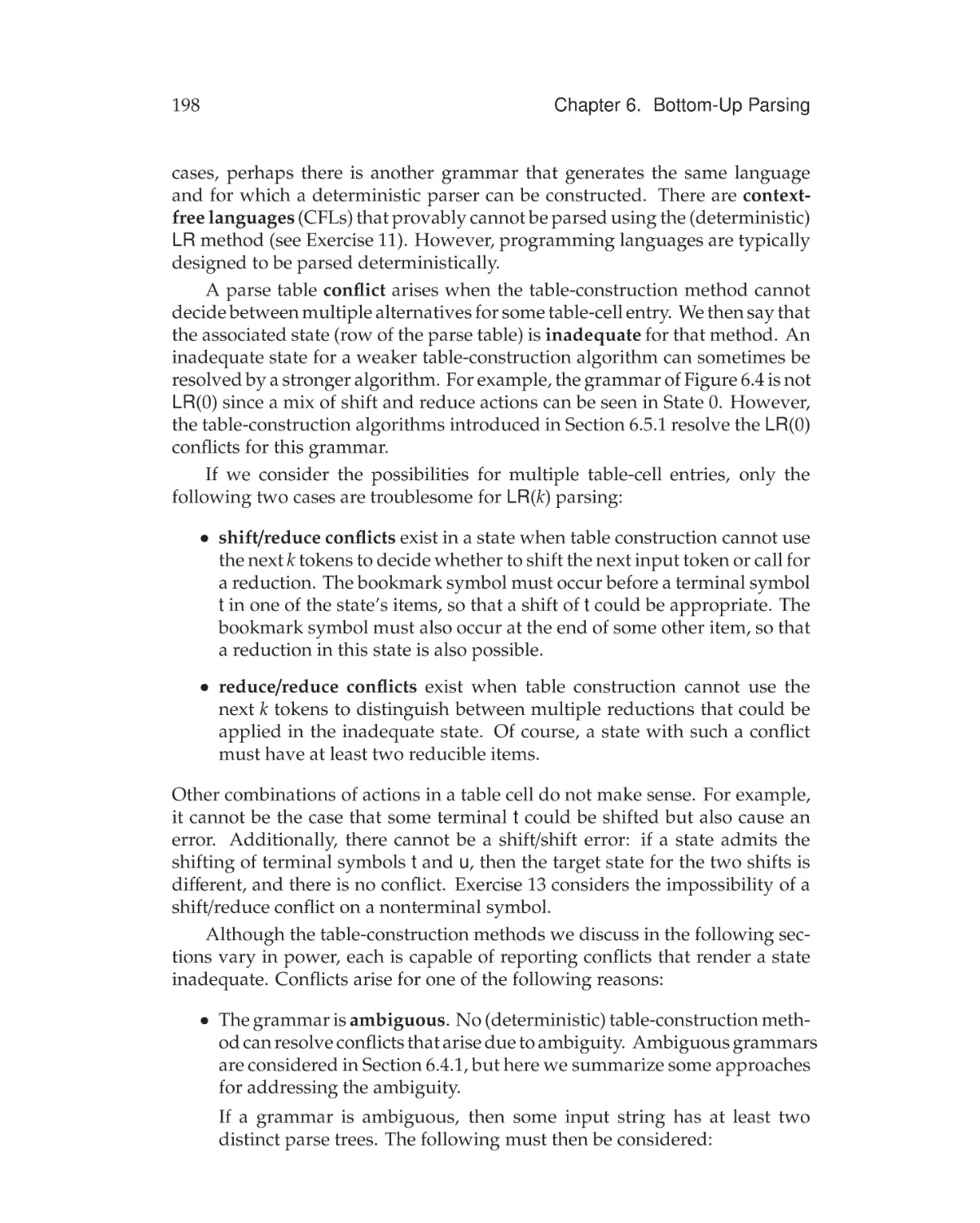
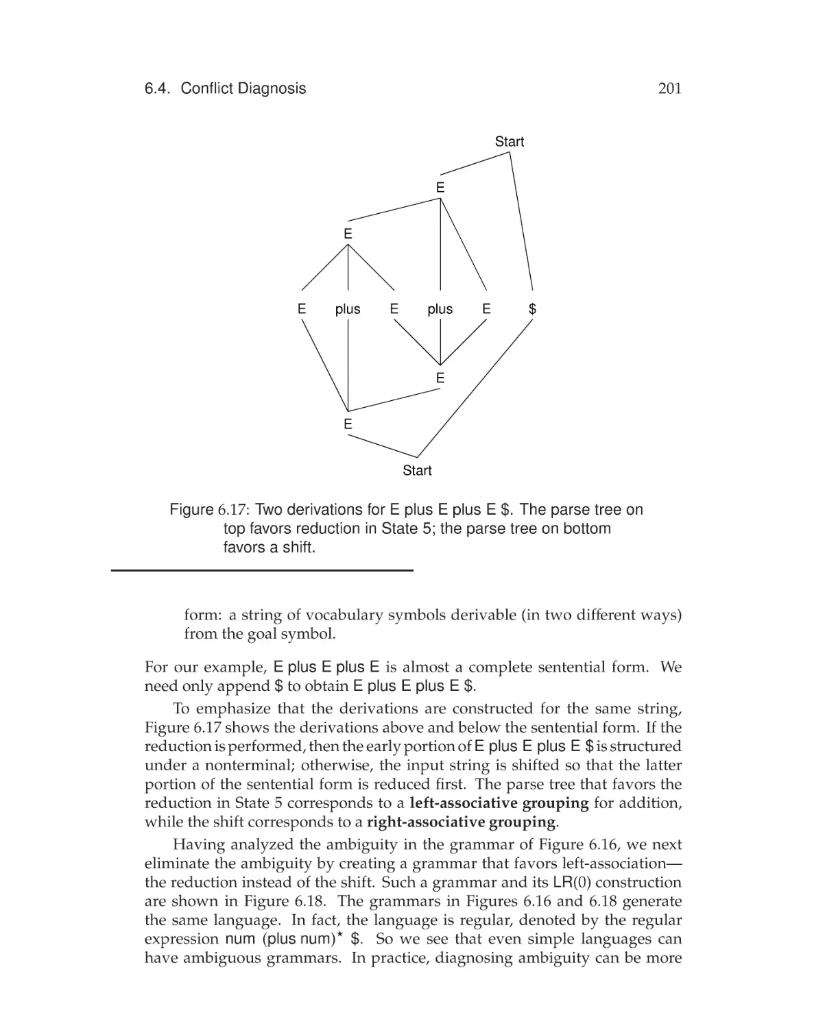
Conflict Diagnosis . . . . . . . . . . . . . . . . . . . . . . . . . 197
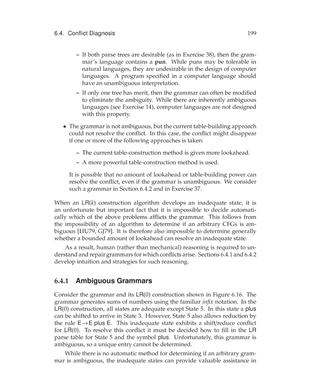
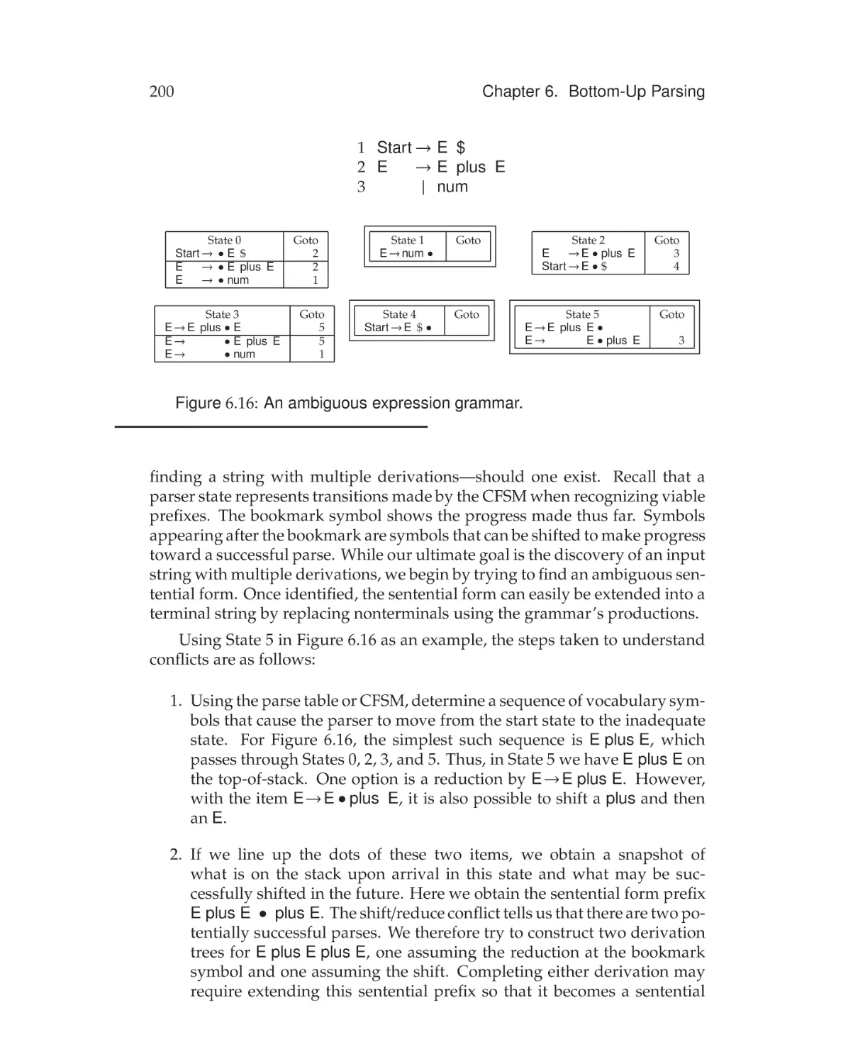
6.4.1
Ambiguous Grammars . . . . . . . . . . . . . . . . . . . 199
xxi
Contents
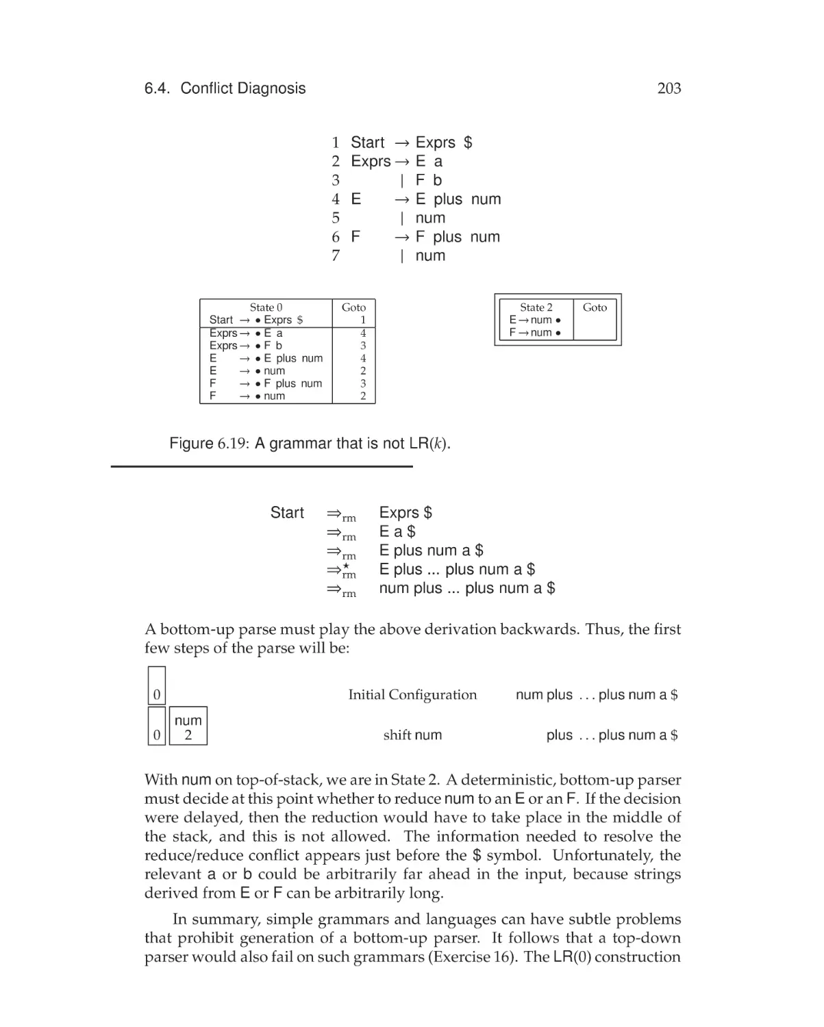
6.4.2
6.5
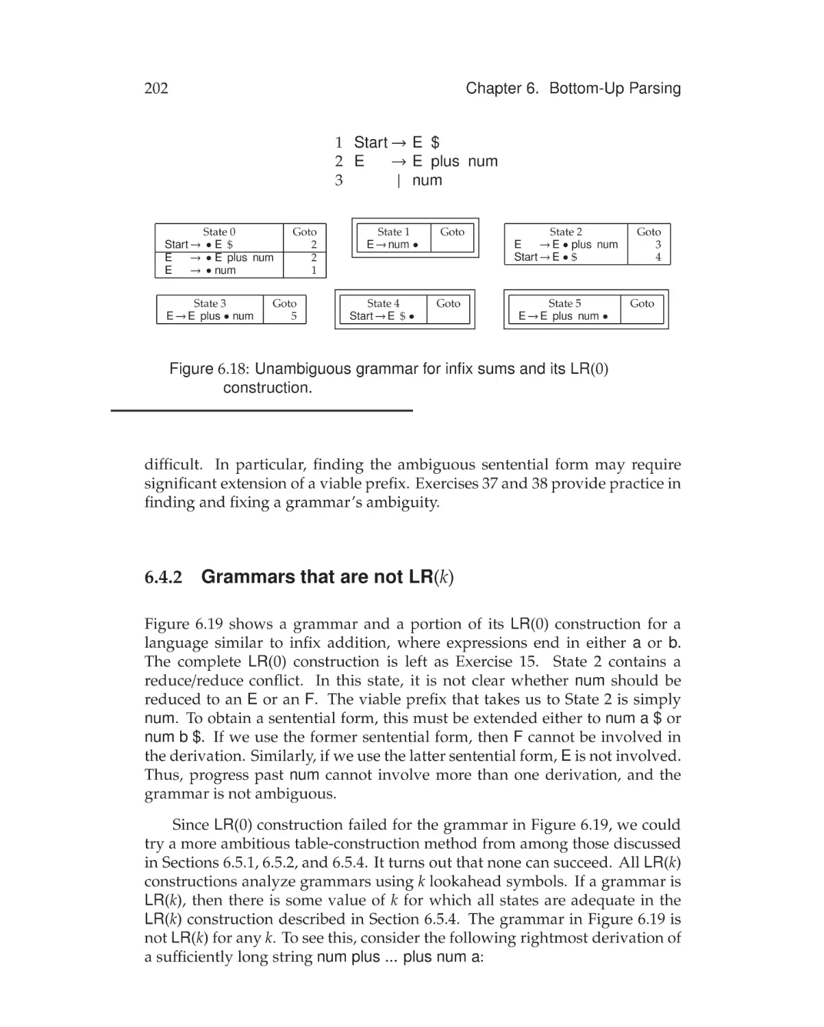
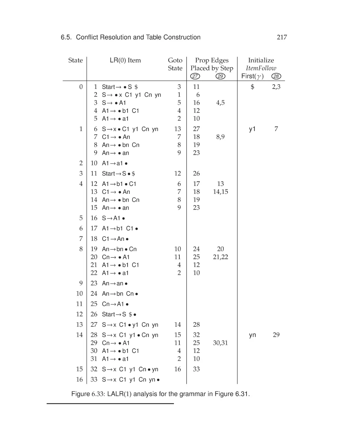
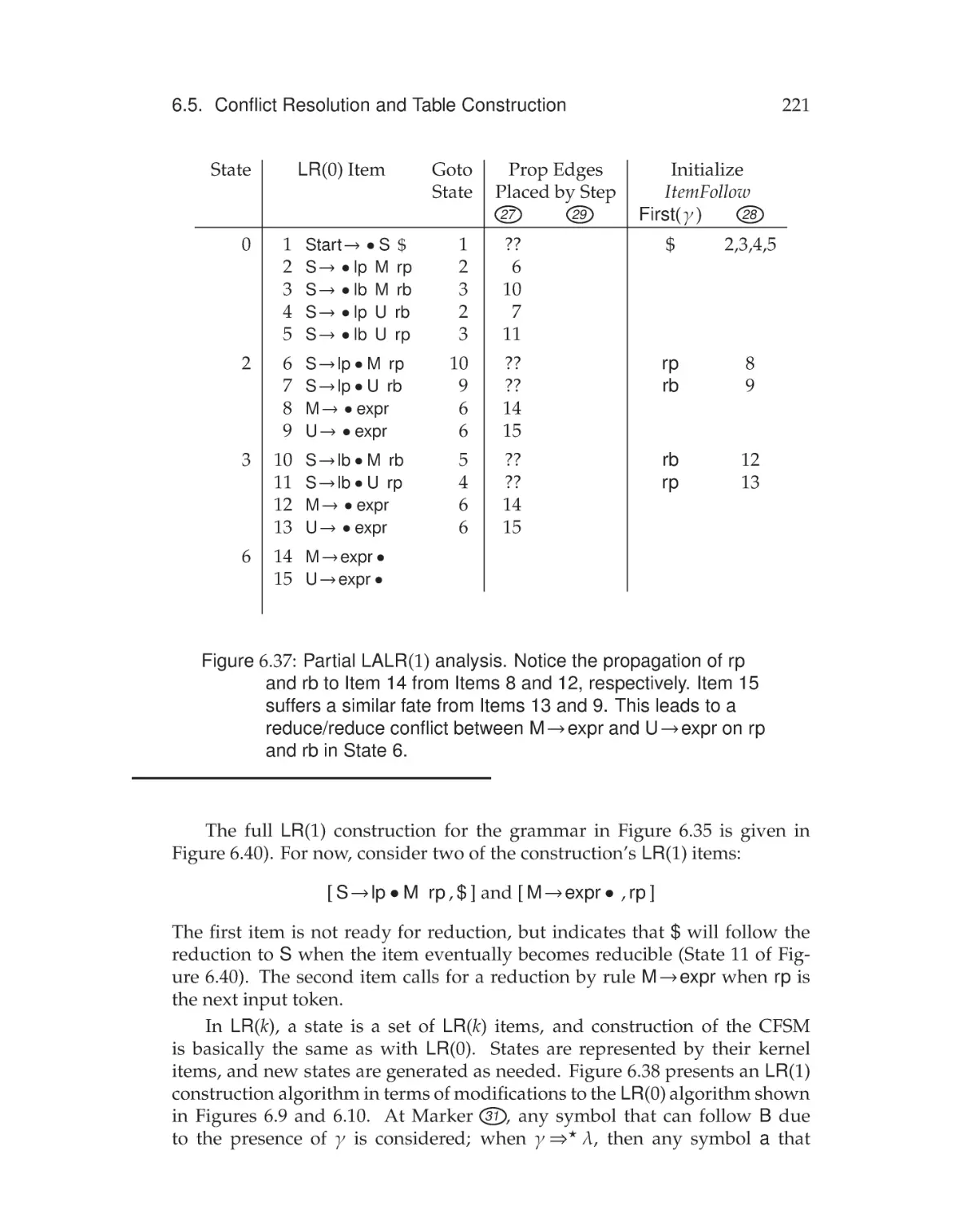
Grammars that are not LR(k) . . . . . . . . . . . . . . . 202
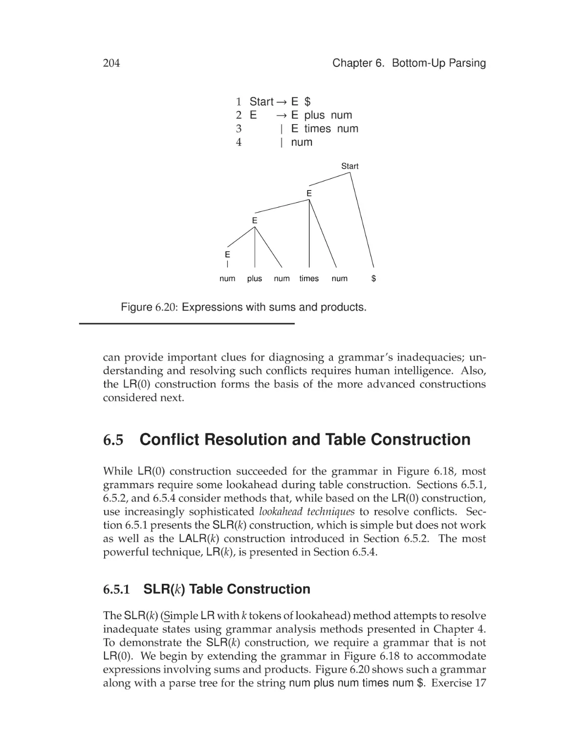
Conflict Resolution and Table Construction . . . . . . . . . . . 204
6.5.1
SLR(k) Table Construction . . . . . . . . . . . . . . . . 204
6.5.2
LALR(k) Table Construction . . . . . . . . . . . . . . . . 209
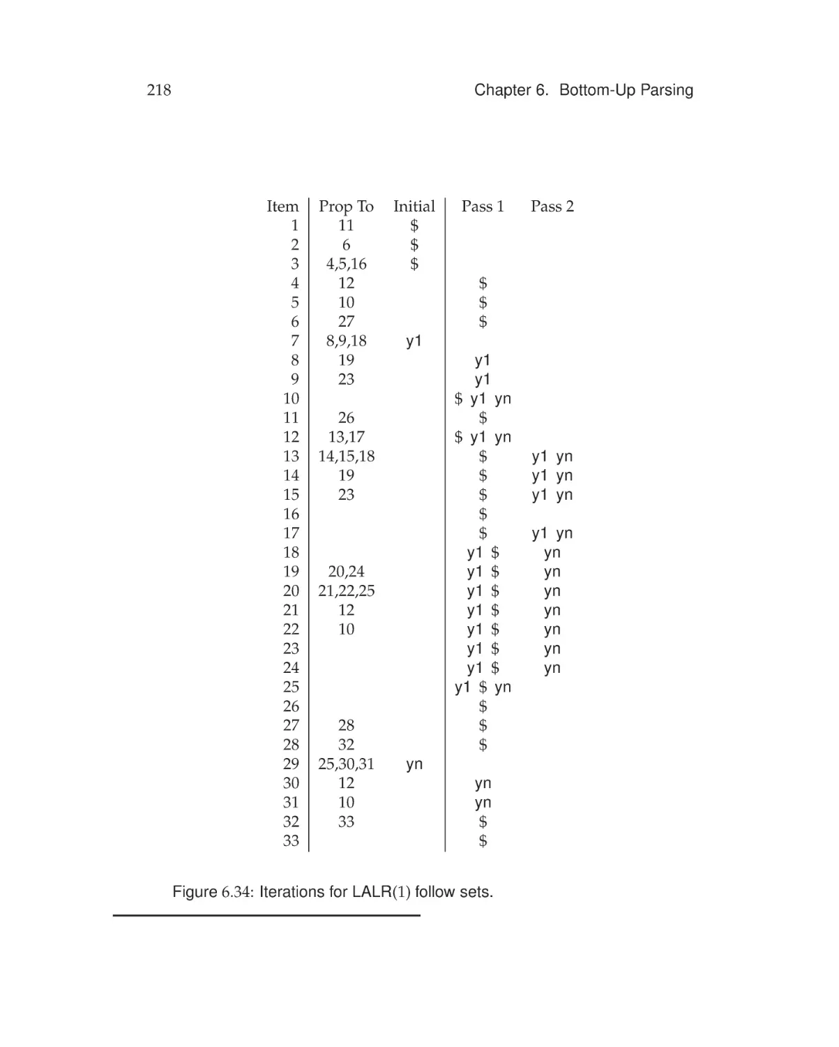
6.5.3
LALR Propagation Graph . . . . . . . . . . . . . . . . . 211
6.5.4
LR(k) Table Construction . . . . . . . . . . . . . . . . . 219
Exercises . . . . . . . . . . . . . . . . . . . . . . . . . . . . . . . . . 224
7
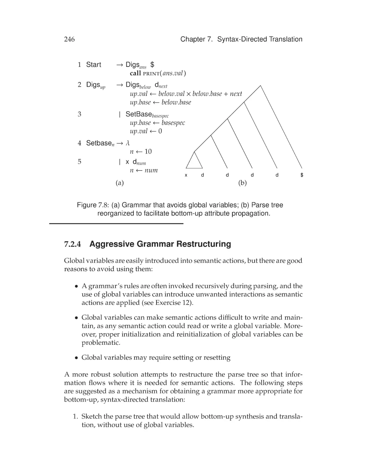
Syntax-Directed Translation
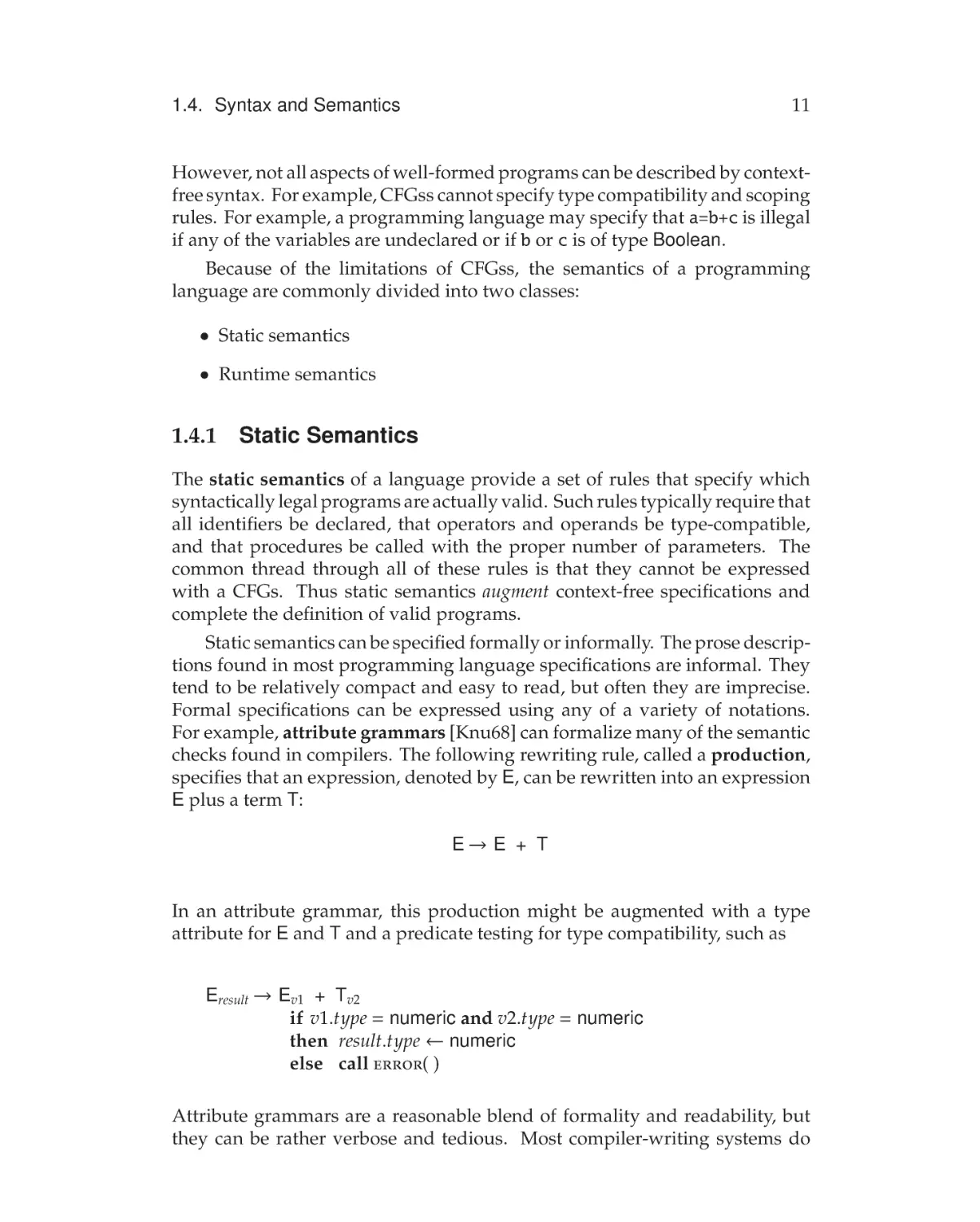
7.1
7.2
235
Overview . . . . . . . . . . . . . . . . . . . . . . . . . . . . . . . 235
7.1.1
Semantic Actions and Values . . . . . . . . . . . . . . . 236
7.1.2
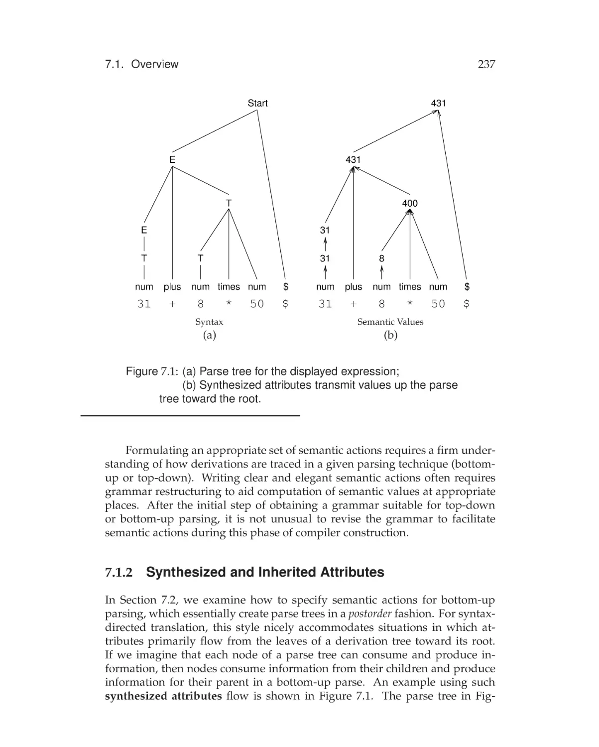
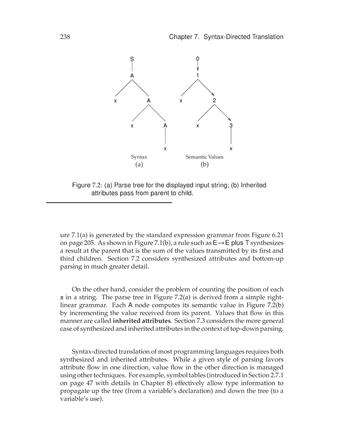
Synthesized and Inherited Attributes . . . . . . . . . . 237
Bottom-Up Syntax-Directed Translation . . . . . . . . . . . . . 239
7.2.1
Example . . . . . . . . . . . . . . . . . . . . . . . . . . . 239
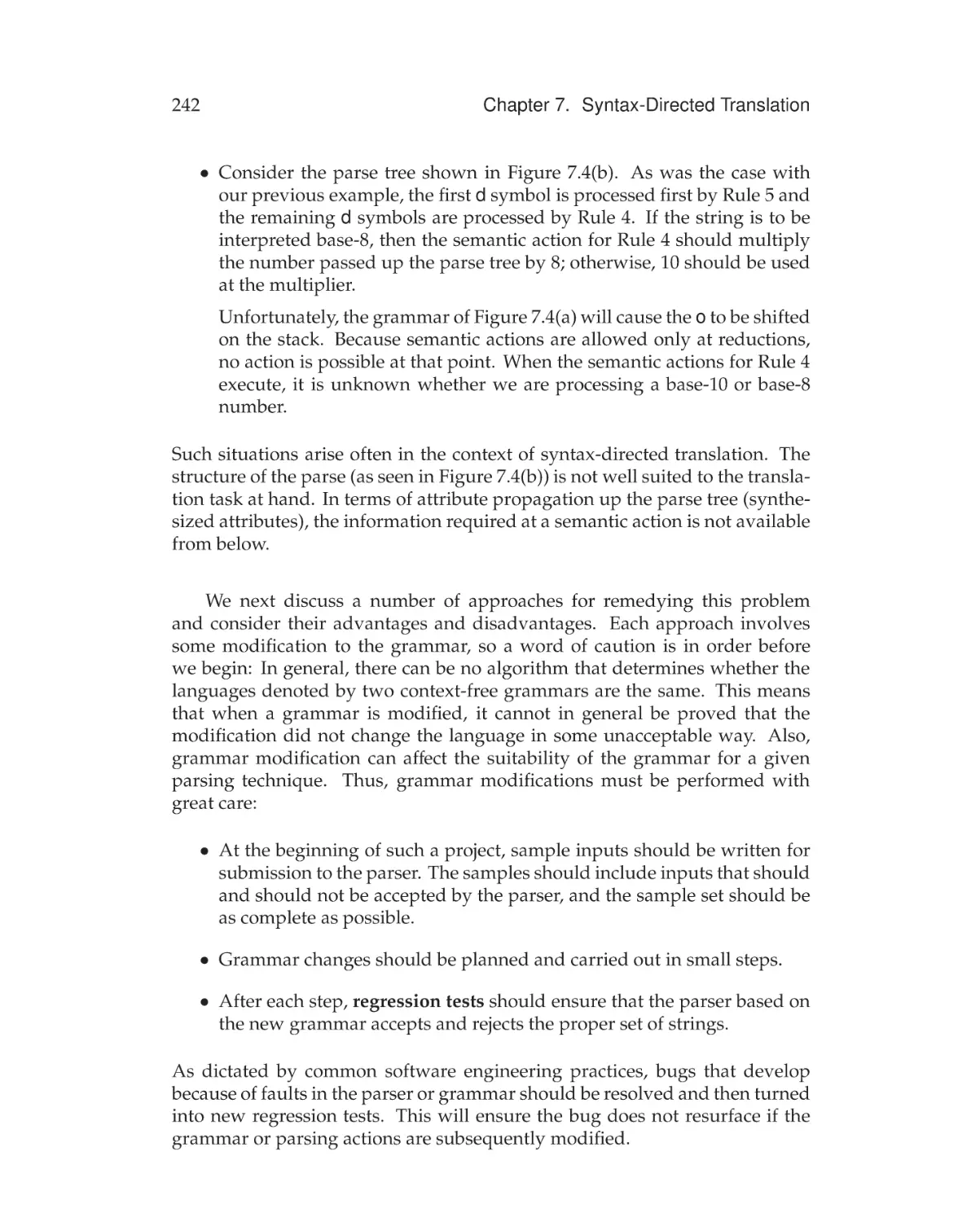
7.2.2
Rule Cloning . . . . . . . . . . . . . . . . . . . . . . . . 243
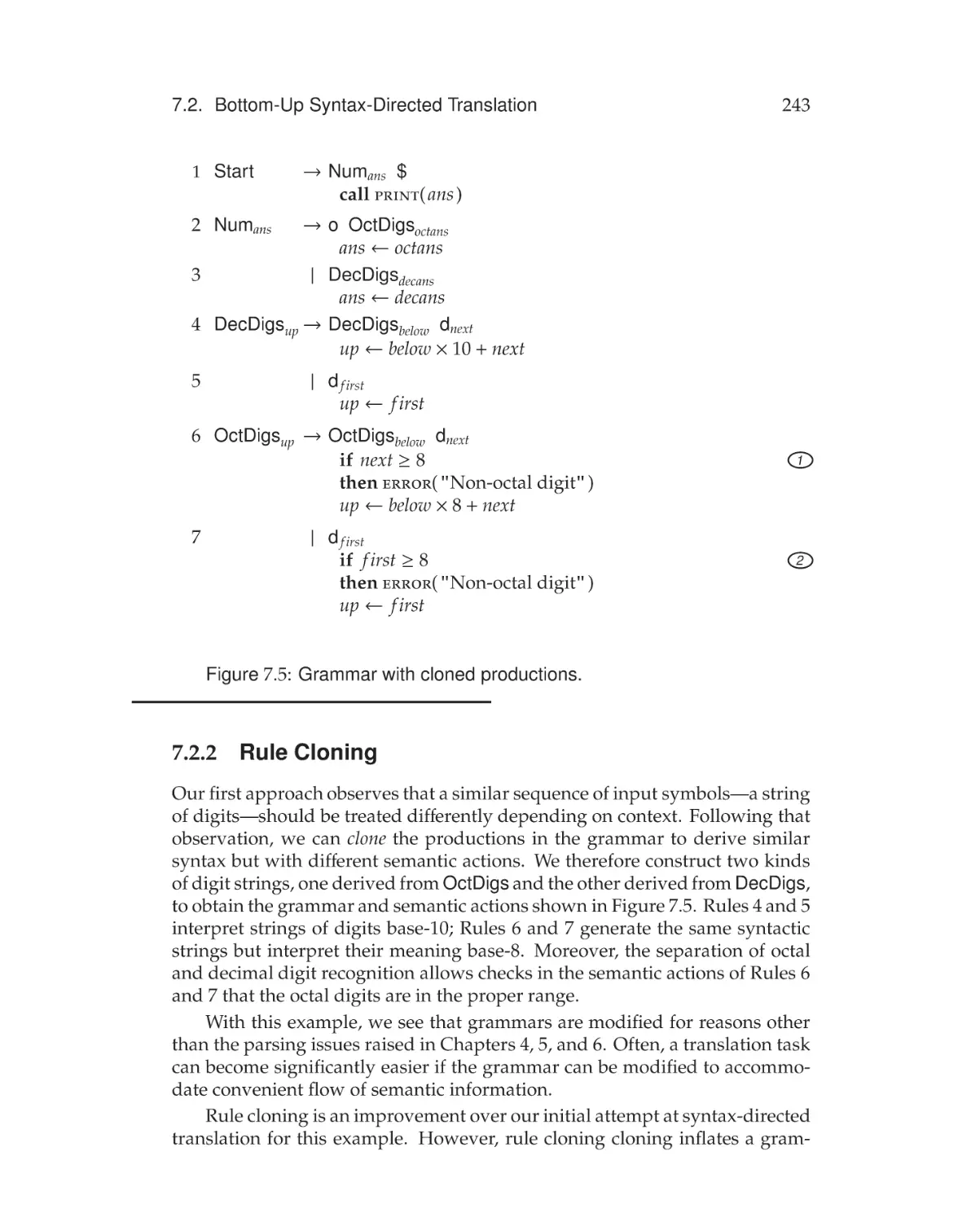
7.2.3
Forcing Semantic Actions . . . . . . . . . . . . . . . . . 244
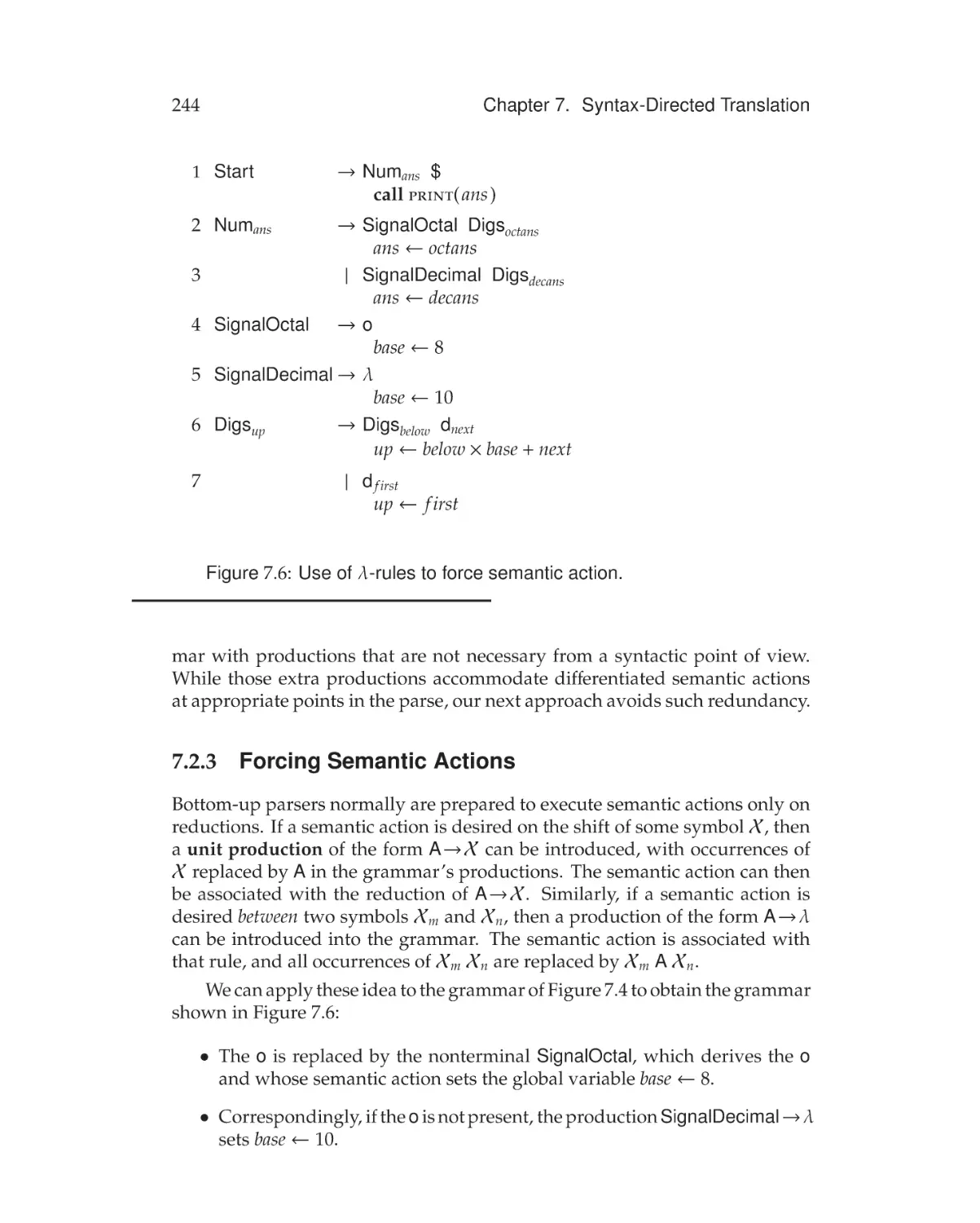
7.2.4
Aggressive Grammar Restructuring . . . . . . . . . . . 246
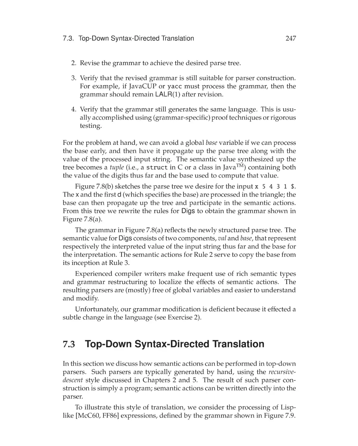
7.3
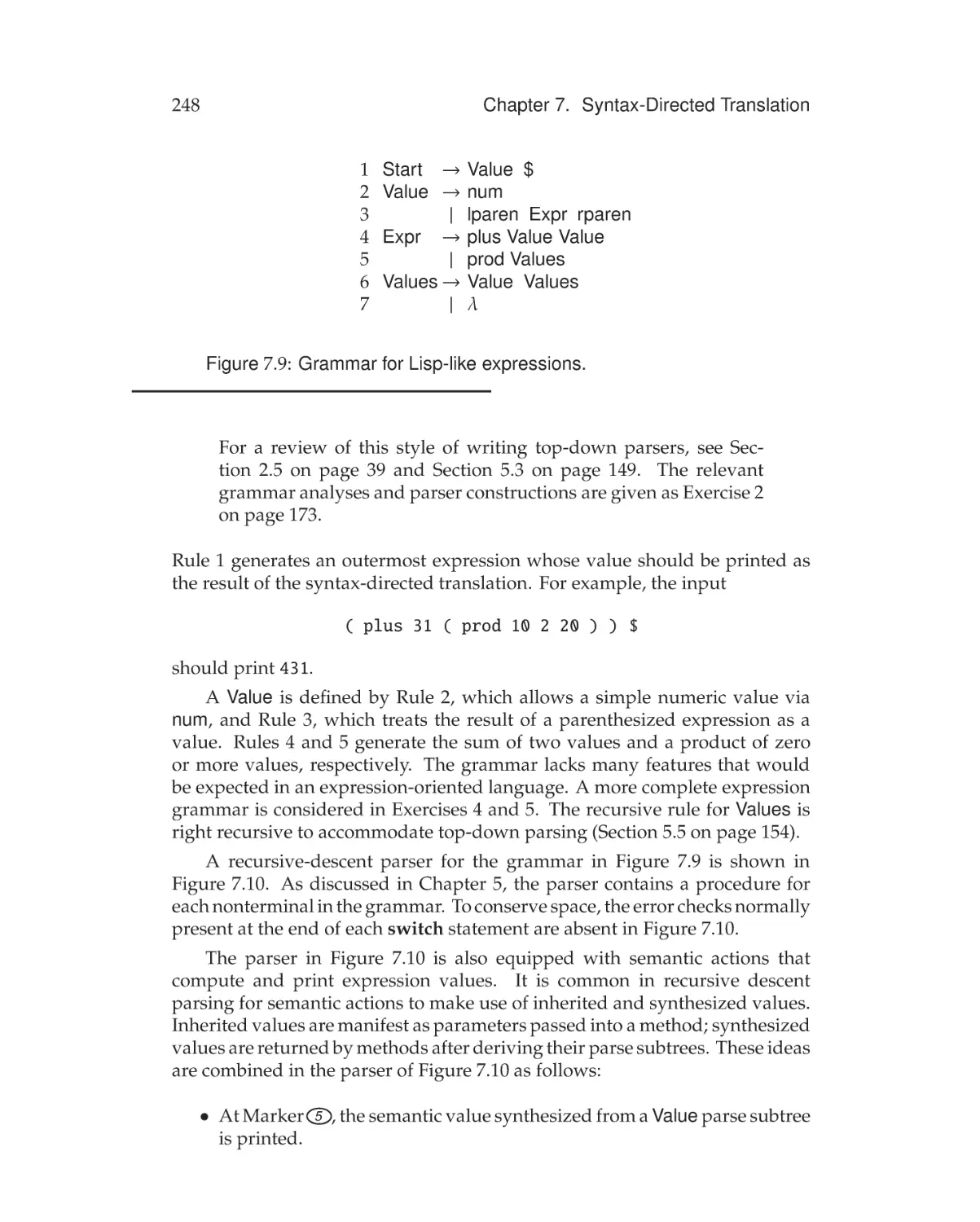
Top-Down Syntax-Directed Translation . . . . . . . . . . . . . 247
7.4
Abstract Syntax Trees . . . . . . . . . . . . . . . . . . . . . . . 250
7.5
7.4.1
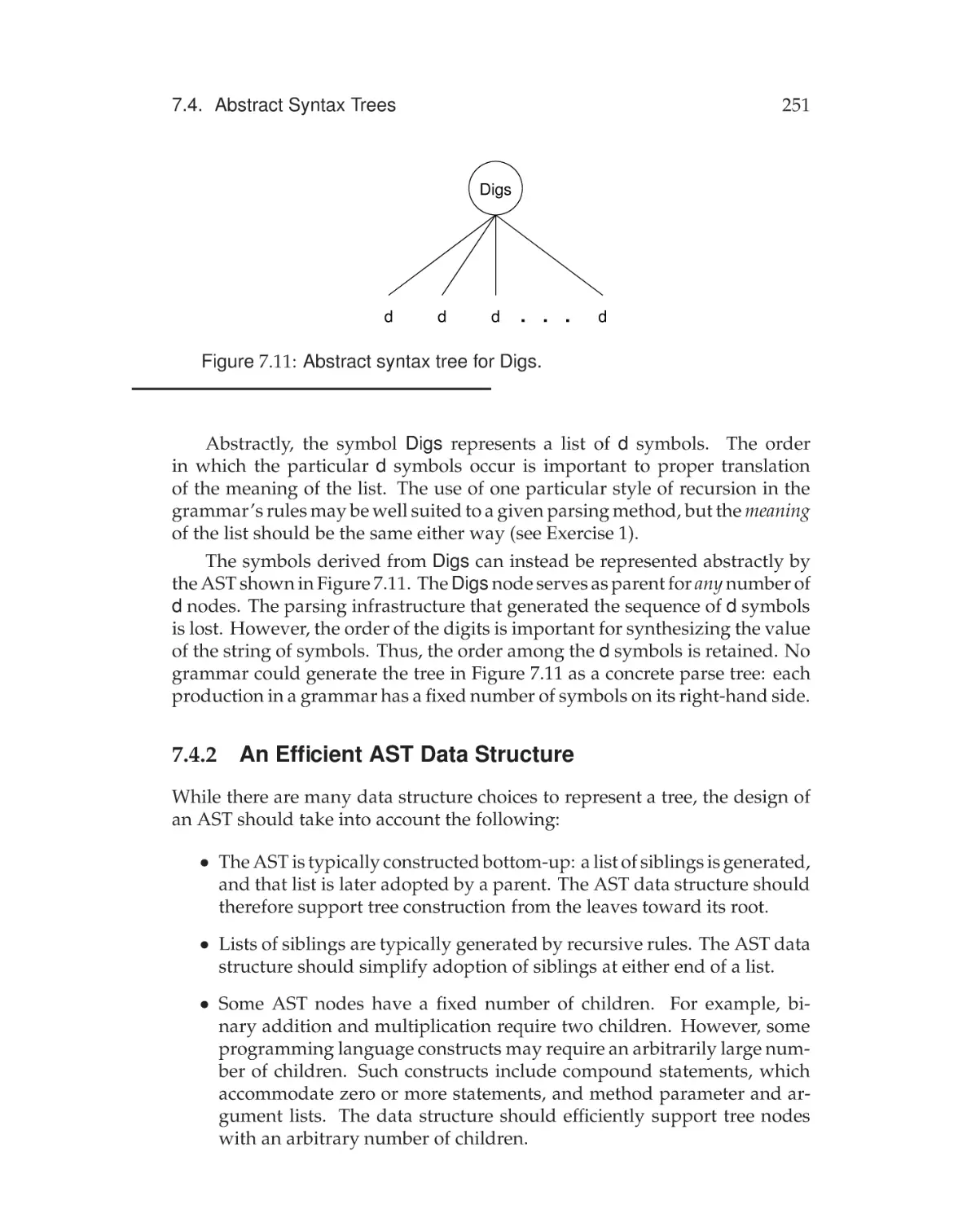
Concrete and Abstract Trees . . . . . . . . . . . . . . . 250
7.4.2
An Efficient AST Data Structure . . . . . . . . . . . . . 251
7.4.3
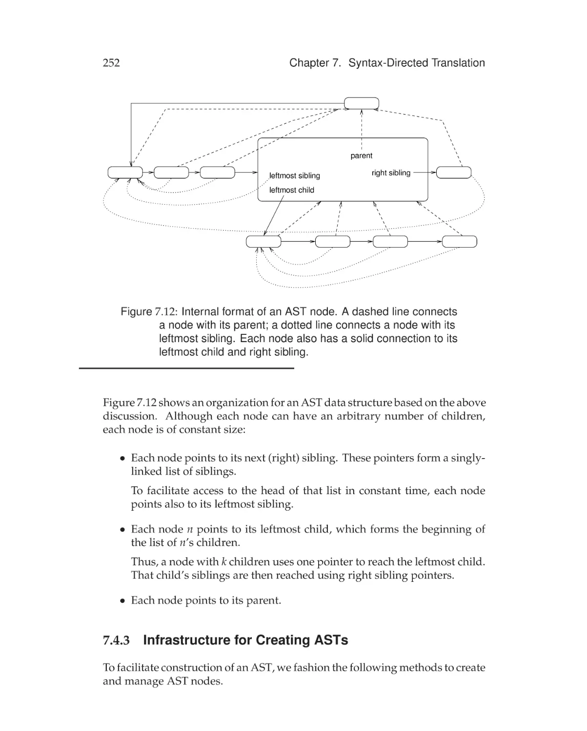
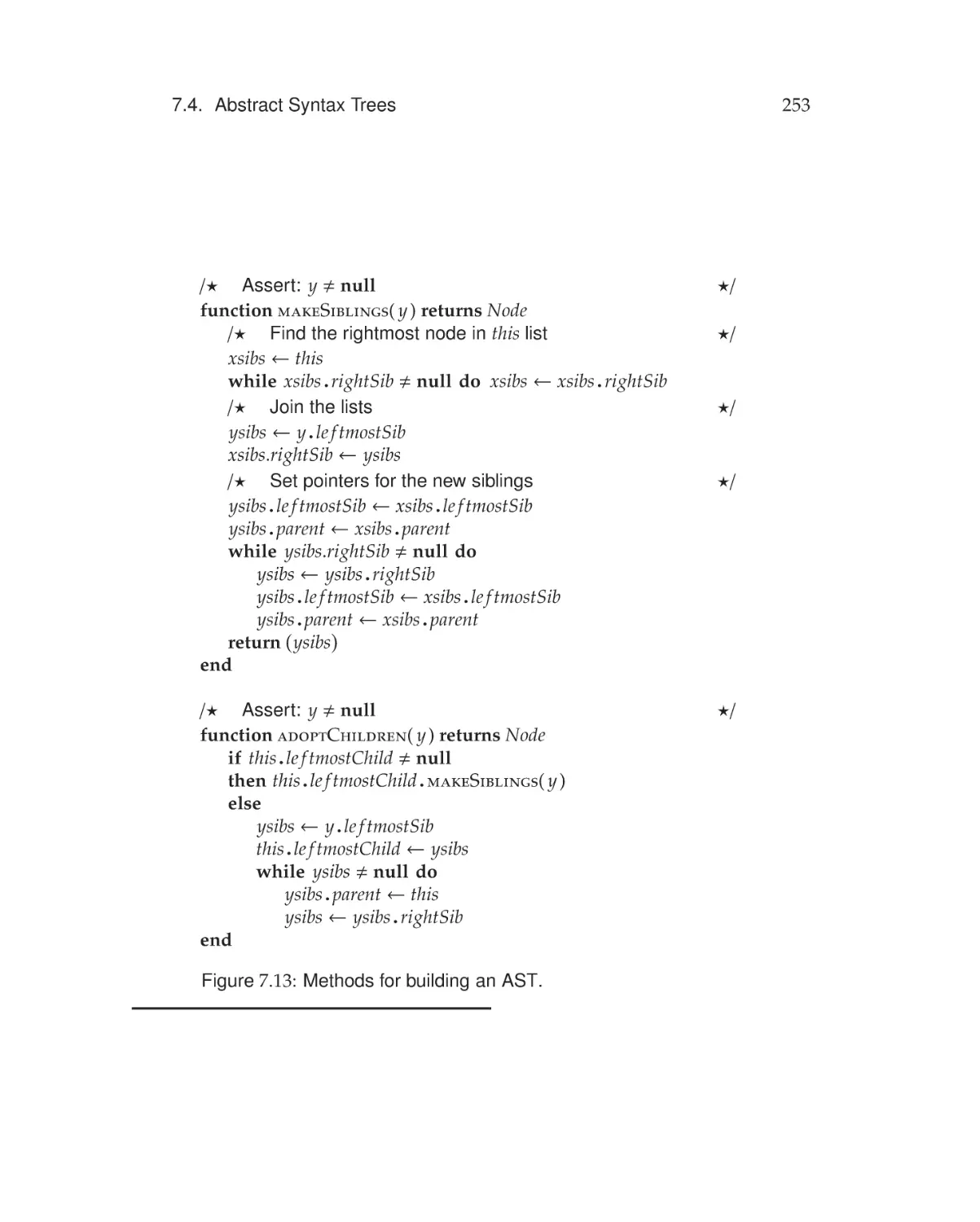
Infrastructure for Creating ASTs . . . . . . . . . . . . . 252
AST Design and Construction . . . . . . . . . . . . . . . . . . . 254
7.5.1
Design . . . . . . . . . . . . . . . . . . . . . . . . . . . . 256
7.5.2
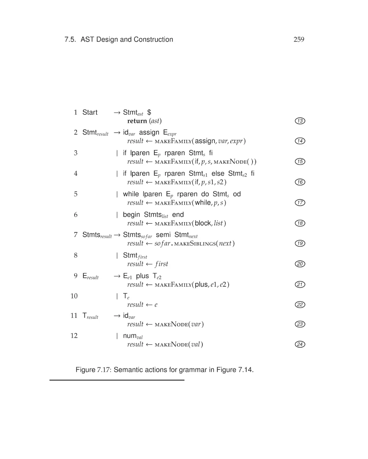
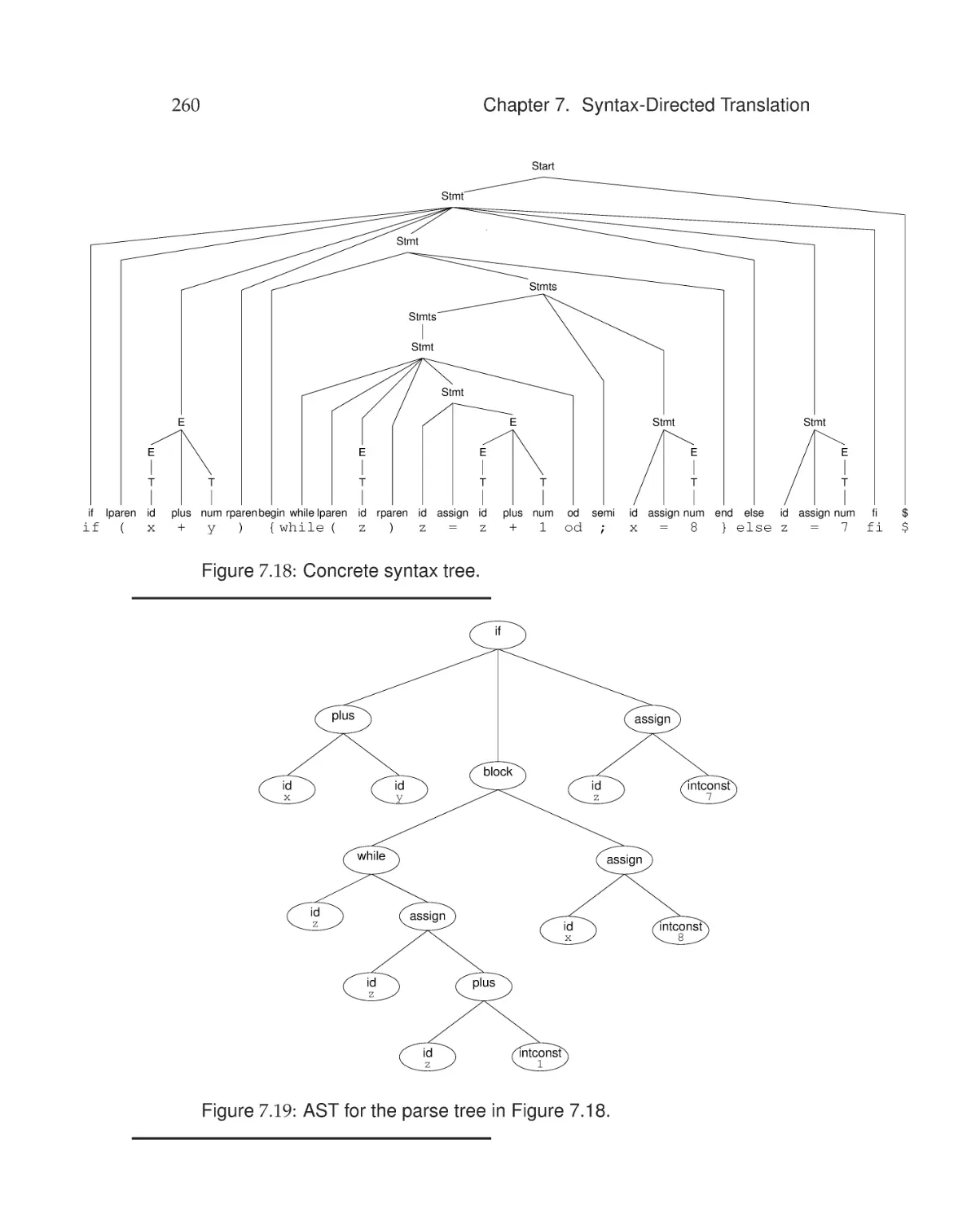
Construction . . . . . . . . . . . . . . . . . . . . . . . . 258
7.6
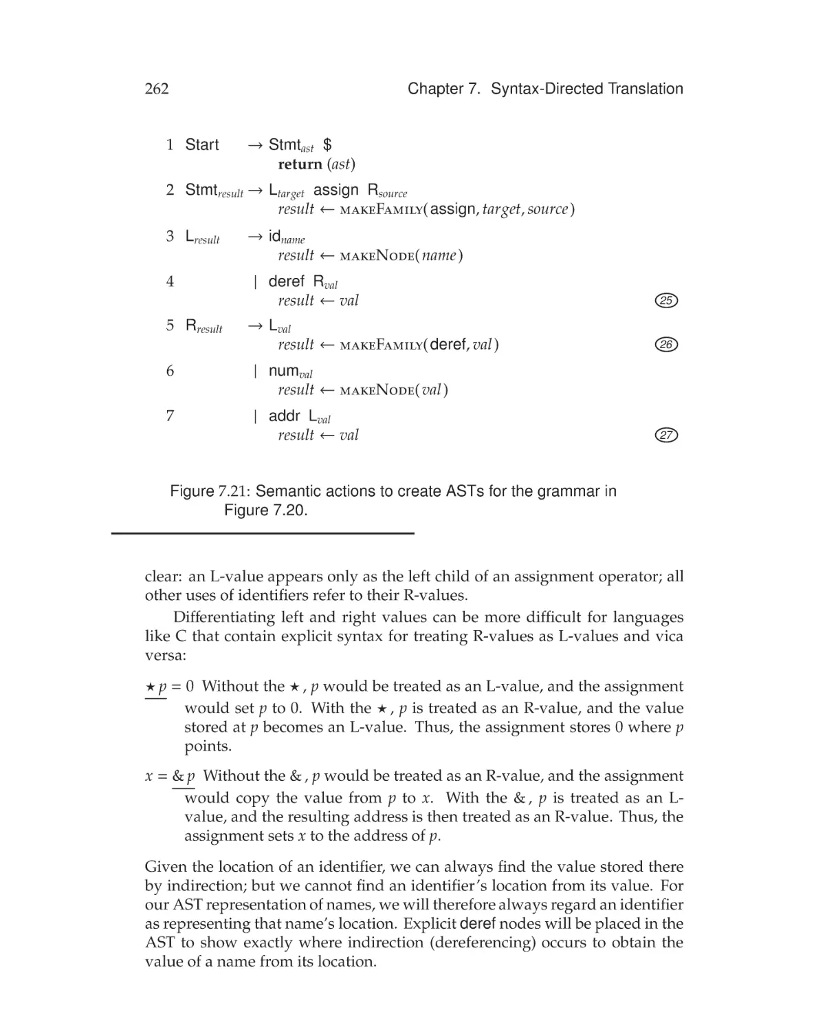
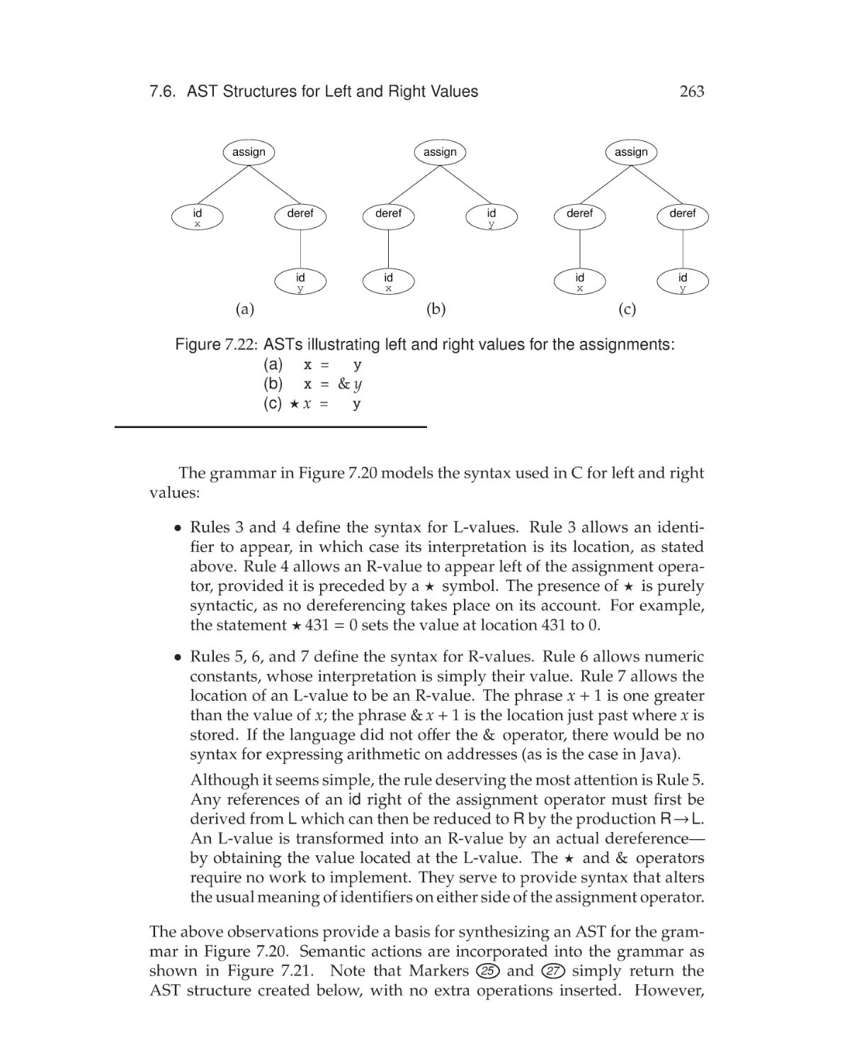
AST Structures for Left and Right Values . . . . . . . . . . . . 261
7.7
Design Patterns for ASTs . . . . . . . . . . . . . . . . . . . . . 264
7.7.1
Node Class Hierarchy . . . . . . . . . . . . . . . . . . . 264
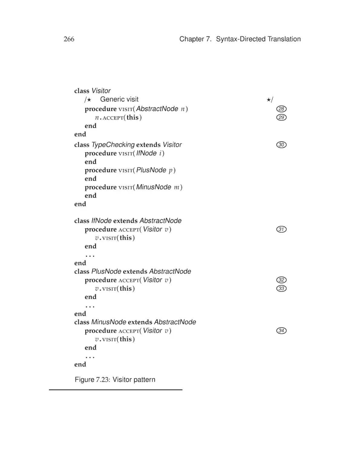
7.7.2
Visitor Pattern . . . . . . . . . . . . . . . . . . . . . . . 265
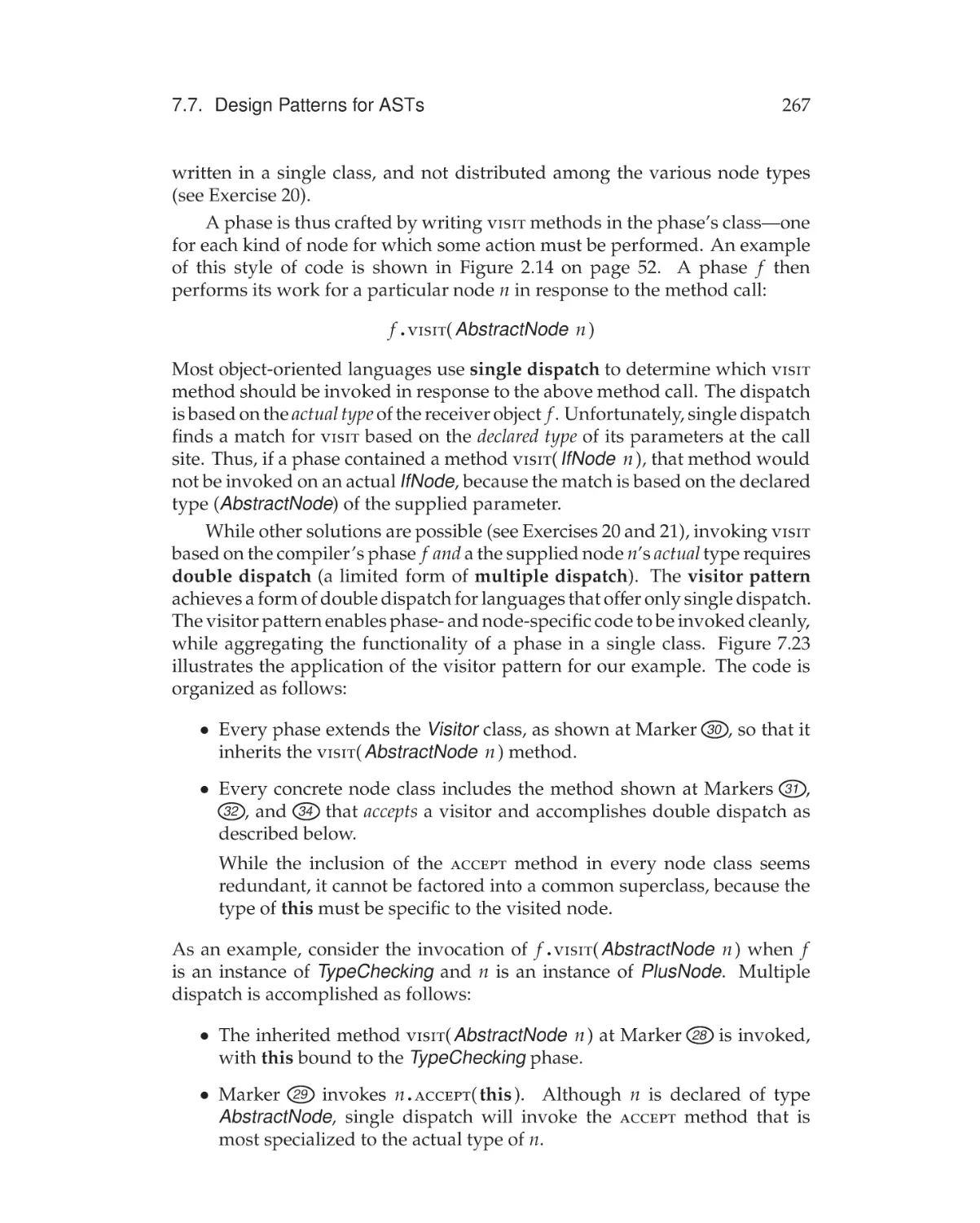
7.7.3
Reflective Visitor Pattern . . . . . . . . . . . . . . . . . 268
Exercises . . . . . . . . . . . . . . . . . . . . . . . . . . . . . . . . . 272
xxii
8
Contents
Symbol Tables and Declaration Processing
8.1
8.2
8.3
8.4
8.5
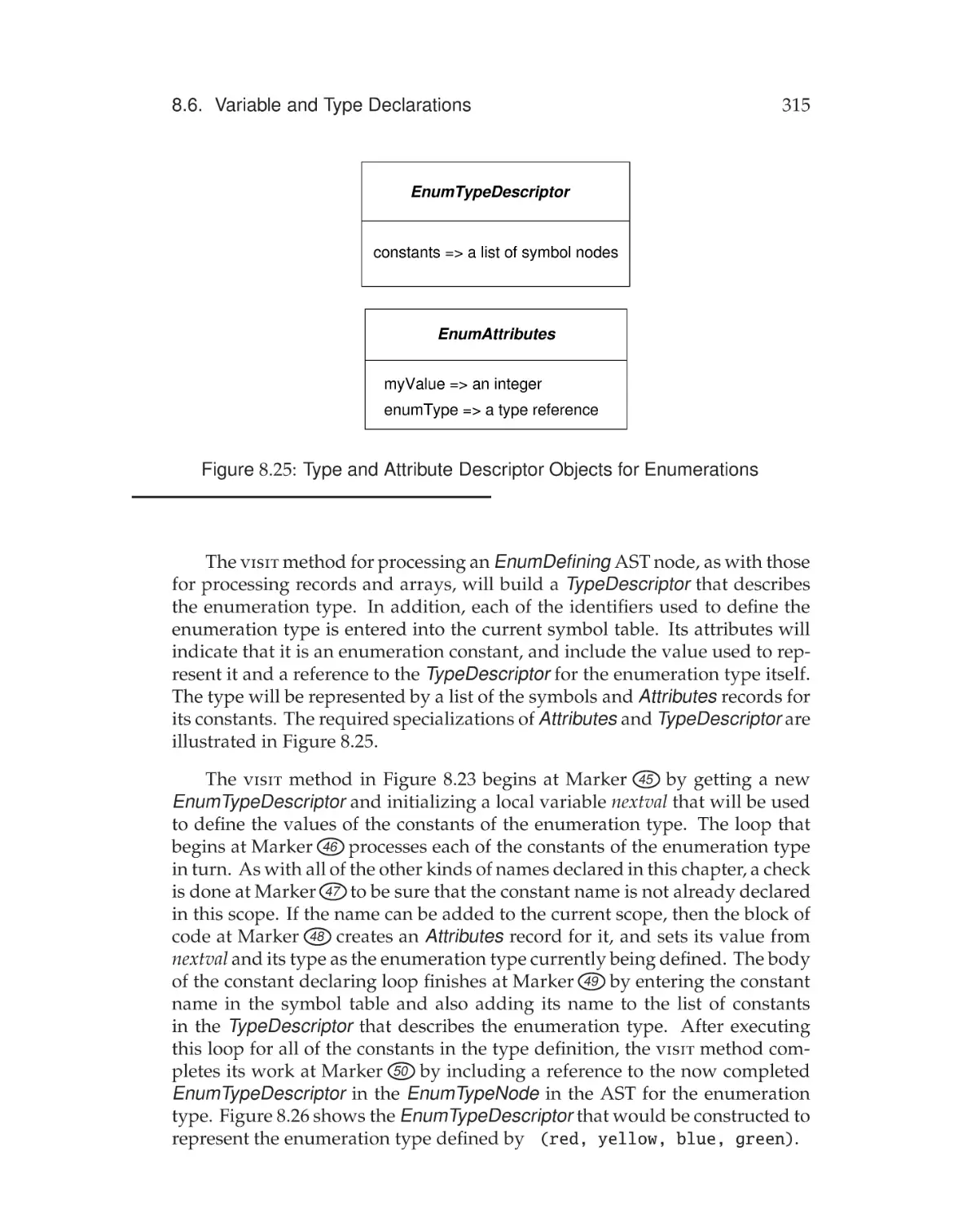
8.6
8.7
8.8
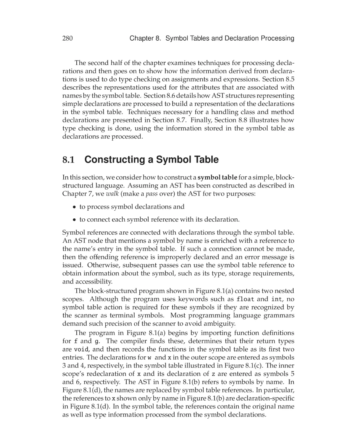
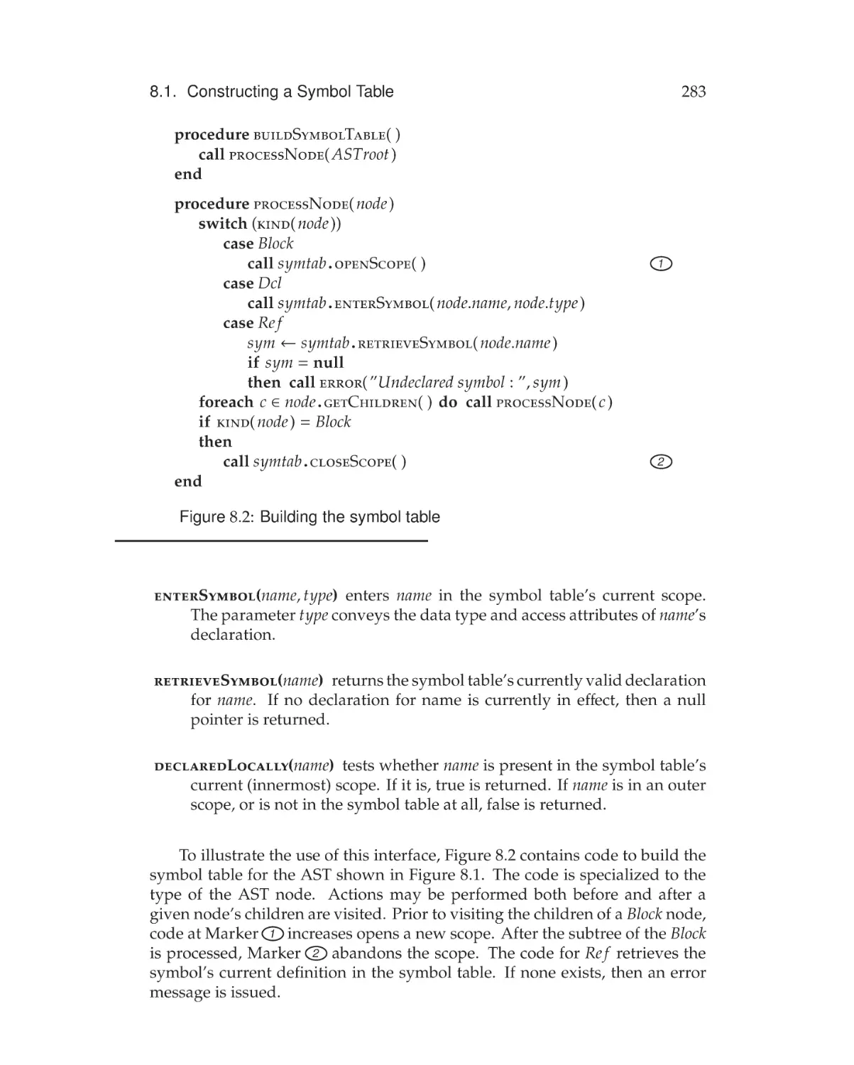
Constructing a Symbol Table . . . . . . . . . . . . . .
8.1.1 Static Scoping . . . . . . . . . . . . . . . . . .
8.1.2 A Symbol Table Interface . . . . . . . . . . . .
Block-Structured Languages and Scopes . . . . . . .
8.2.1 Handling Scopes . . . . . . . . . . . . . . . . .
8.2.2 One Symbol Table or Many? . . . . . . . . . .
Basic Implementation Techniques . . . . . . . . . . .
8.3.1 Entering and Finding Names . . . . . . . . . .
8.3.2 The Name Space . . . . . . . . . . . . . . . .
8.3.3 An Efficient Symbol Table Implementation . .
Advanced Features . . . . . . . . . . . . . . . . . . . .
8.4.1 Records and Typenames . . . . . . . . . . . .
8.4.2 Overloading and Type Hierarchies . . . . . . .
8.4.3 Implicit Declarations . . . . . . . . . . . . . . .
8.4.4 Export and Import Directives . . . . . . . . . .
8.4.5 Altered Search Rules . . . . . . . . . . . . . .
Declaration Processing Fundamentals . . . . . . . . .
8.5.1 Attributes in the Symbol Table . . . . . . . . .
8.5.2 Type Descriptor Structures . . . . . . . . . . .
8.5.3 Type Checking Using an Abstract Syntax Tree
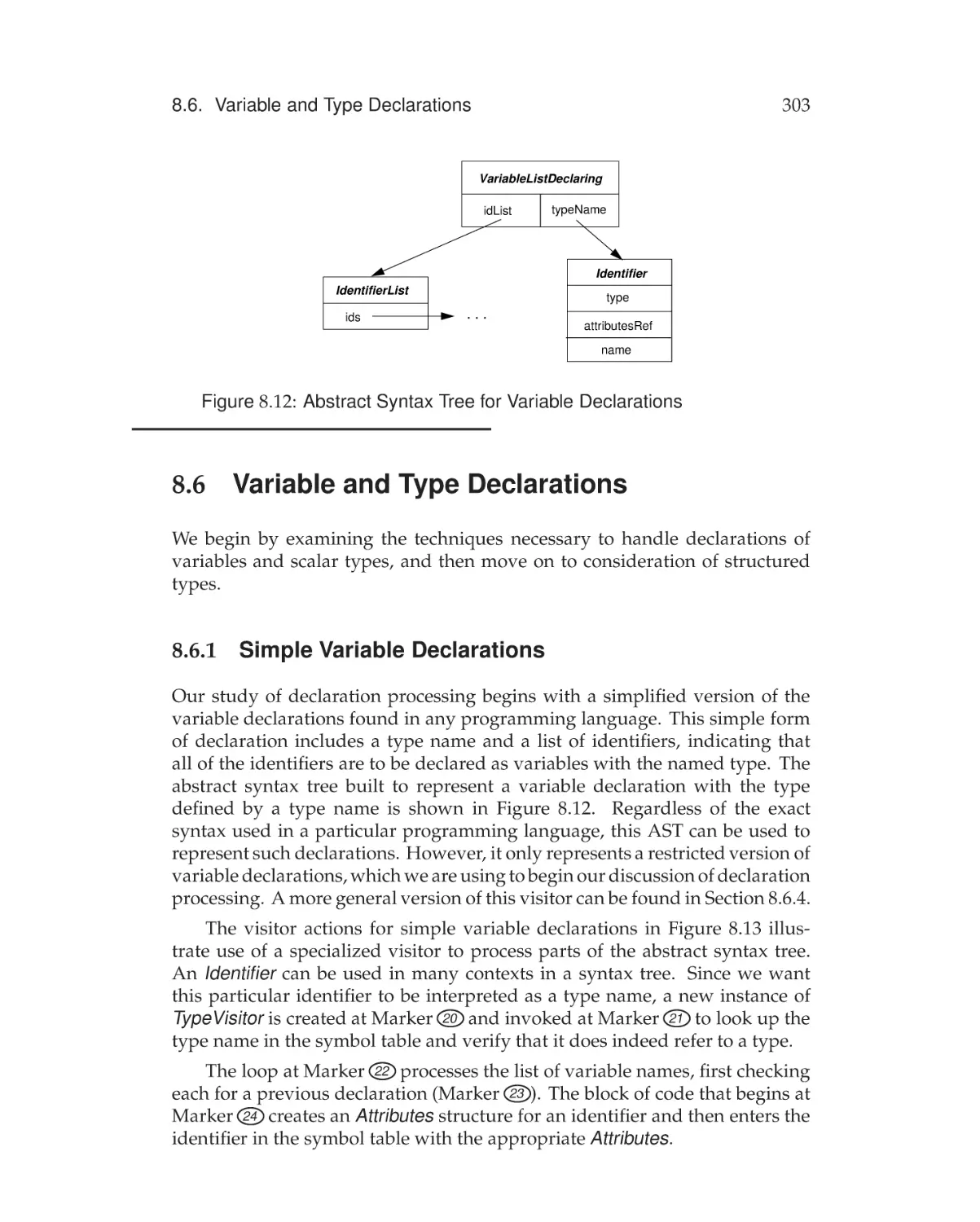
Variable and Type Declarations . . . . . . . . . . . . .
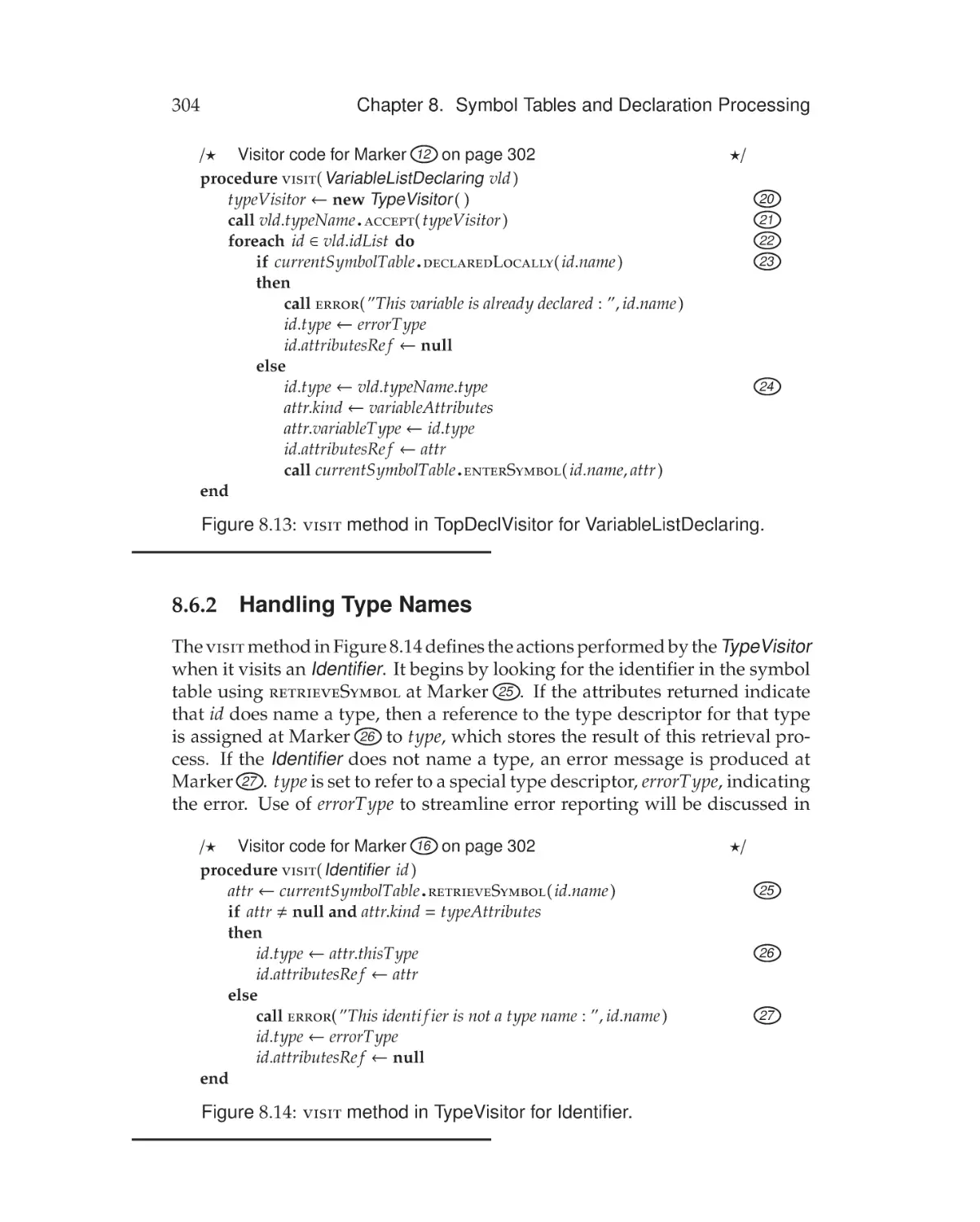
8.6.1 Simple Variable Declarations . . . . . . . . . .
8.6.2 Handling Type Names . . . . . . . . . . . . . .
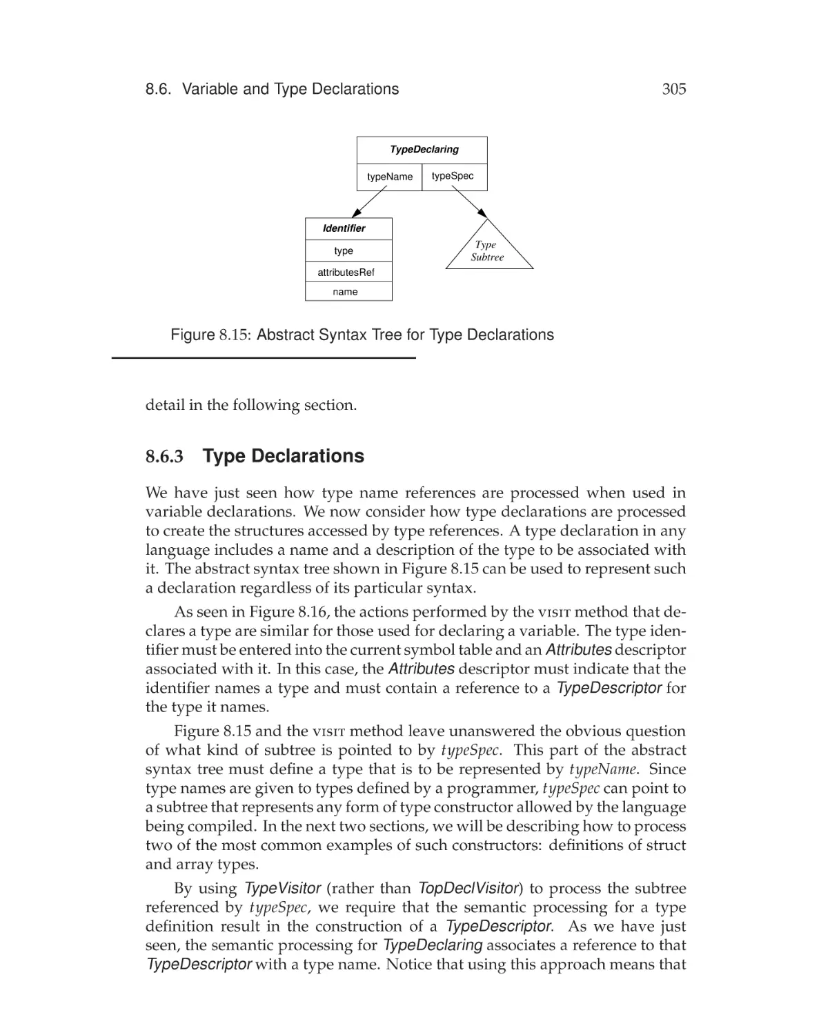
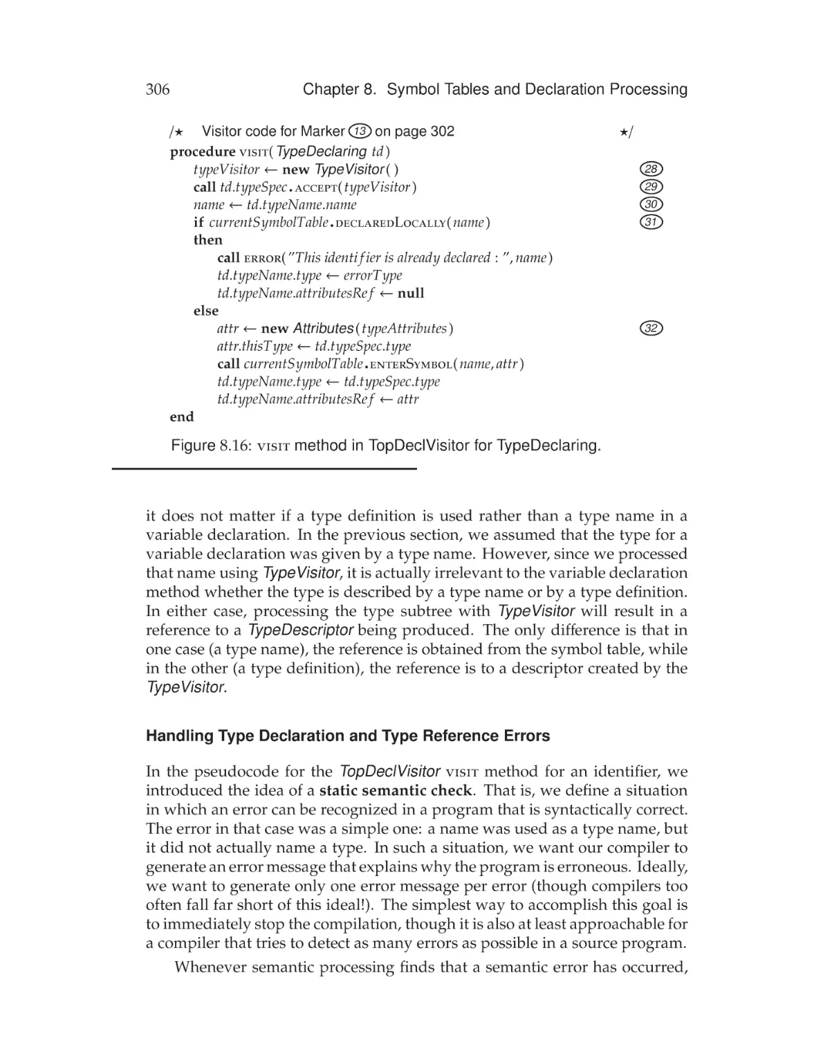
8.6.3 Type Declarations . . . . . . . . . . . . . . . .
8.6.4 Variable Declarations Revisited . . . . . . . .
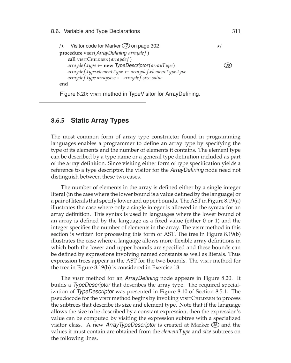
8.6.5 Static Array Types . . . . . . . . . . . . . . . .
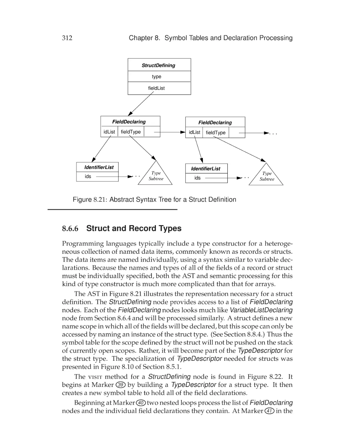
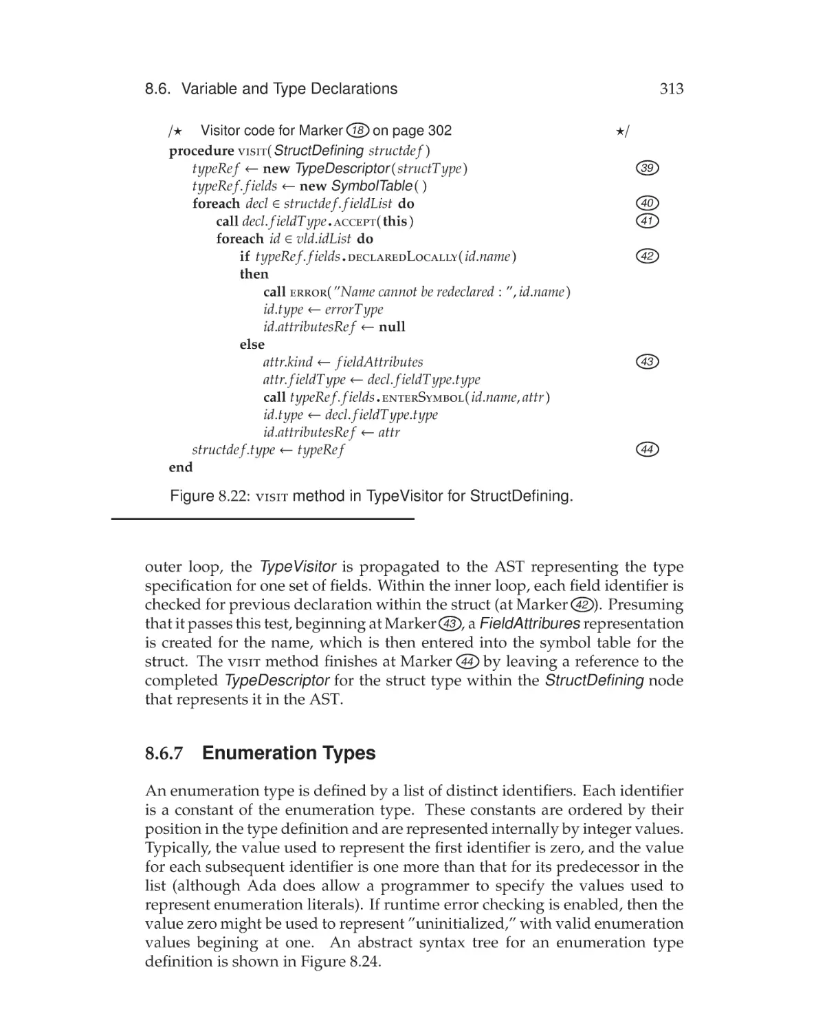
8.6.6 Struct and Record Types . . . . . . . . . . . .
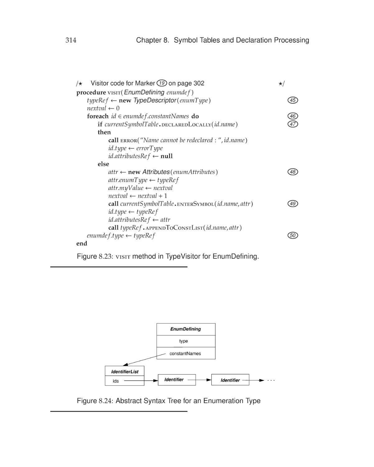
8.6.7 Enumeration Types . . . . . . . . . . . . . . .
Class and Method Declarations . . . . . . . . . . . . .
8.7.1 Processing Class Declarations . . . . . . . . .
8.7.2 Processing Method Declarations . . . . . . . .
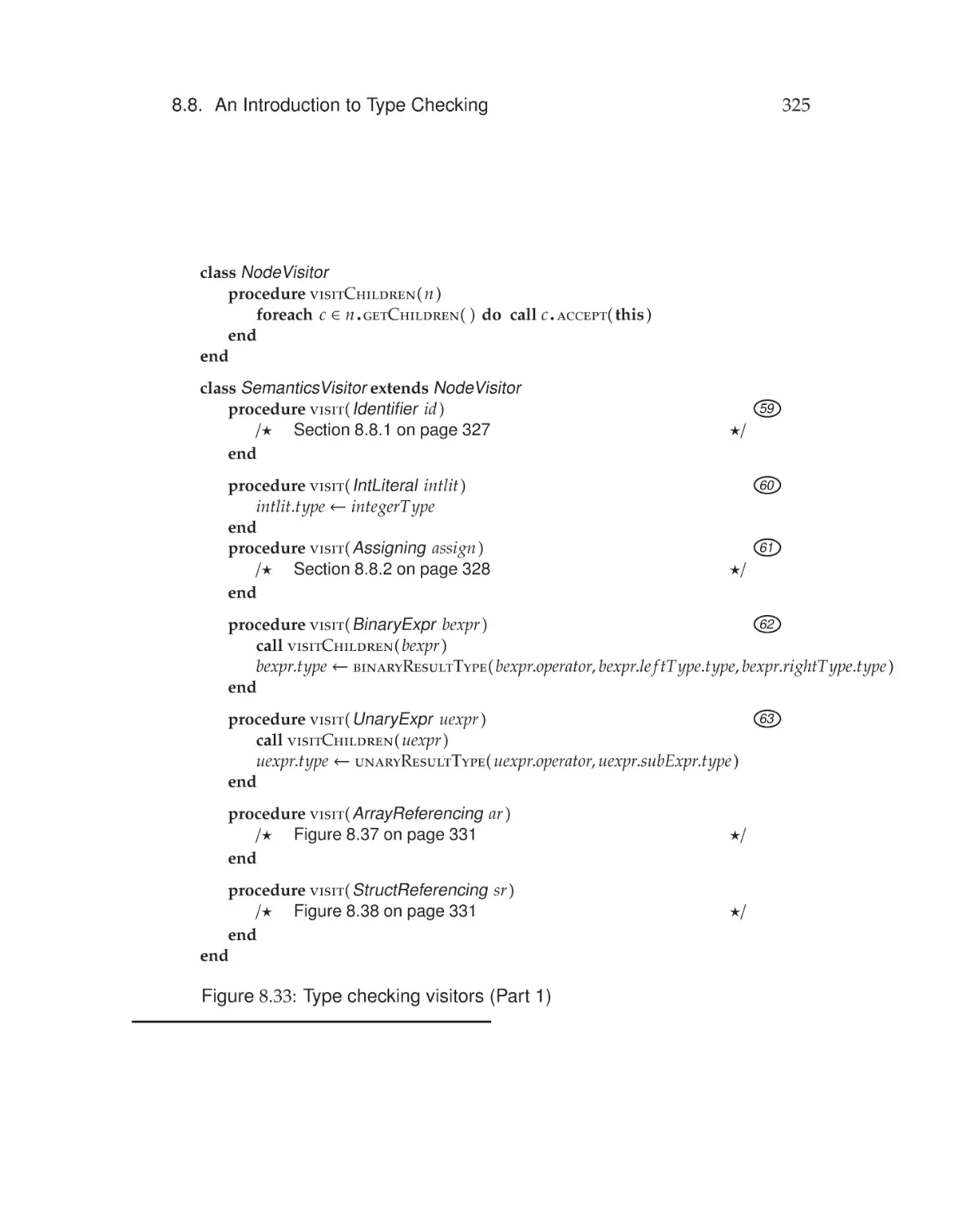
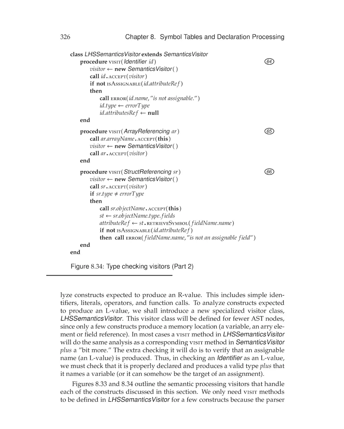
An Introduction to Type Checking . . . . . . . . . . . .
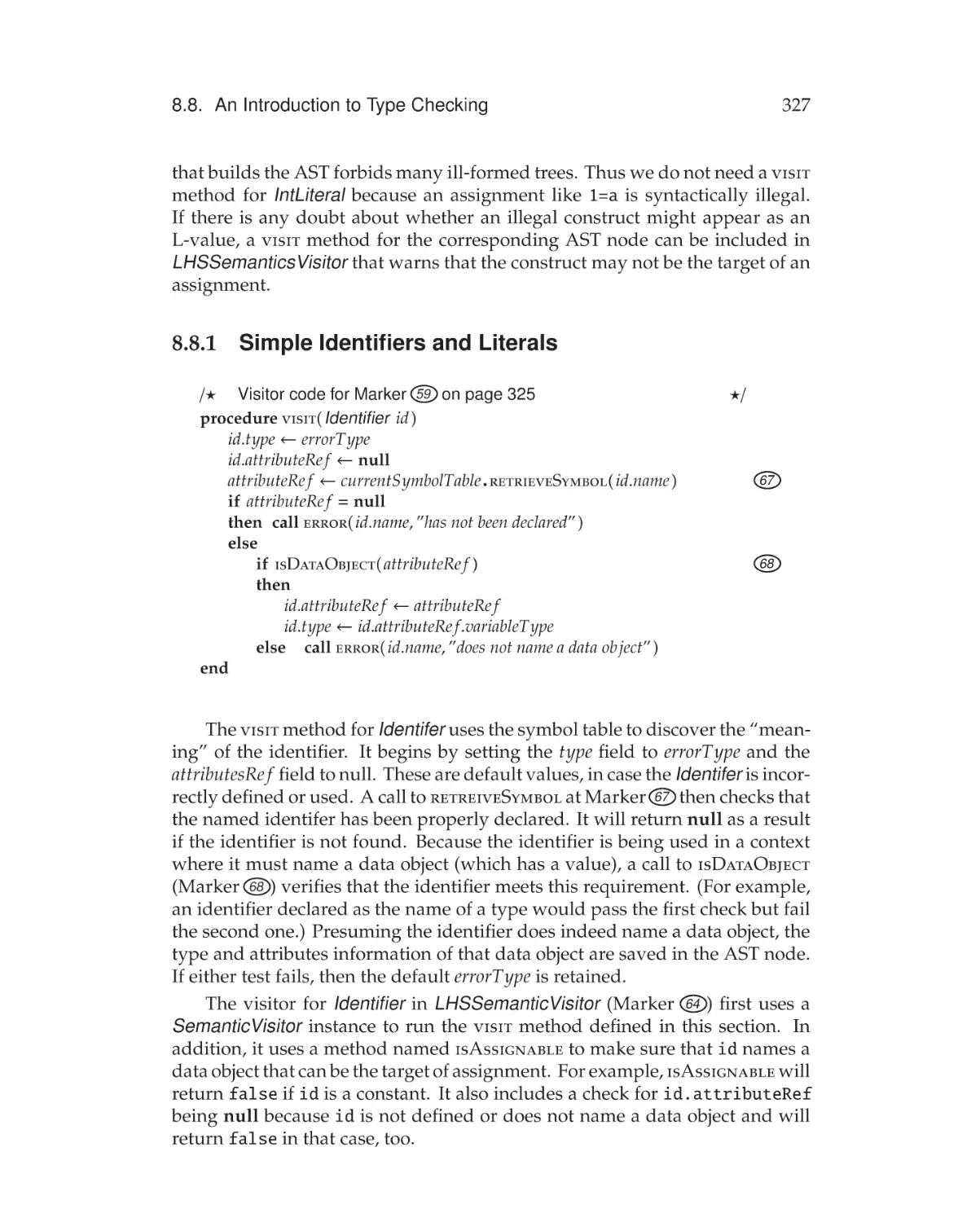
8.8.1 Simple Identifiers and Literals . . . . . . . . .
.
.
.
.
.
.
.
.
.
.
.
.
.
.
.
.
.
.
.
.
.
.
.
.
.
.
.
.
.
.
.
.
.
.
.
.
.
.
.
.
.
.
.
.
.
.
.
.
.
.
.
.
.
.
.
.
.
.
.
.
.
.
.
.
.
.
279
.
.
.
.
.
.
.
.
.
.
.
.
.
.
.
.
.
.
.
.
.
.
.
.
.
.
.
.
.
.
.
.
.
.
.
.
.
.
.
.
.
.
.
.
.
.
.
.
.
.
.
.
.
.
.
.
.
.
.
.
.
.
.
.
.
.
.
.
.
.
.
.
.
.
.
.
.
.
.
.
.
.
.
.
.
.
.
.
.
.
.
.
.
.
.
.
.
.
.
280
282
282
284
284
285
286
286
289
290
293
294
294
296
296
297
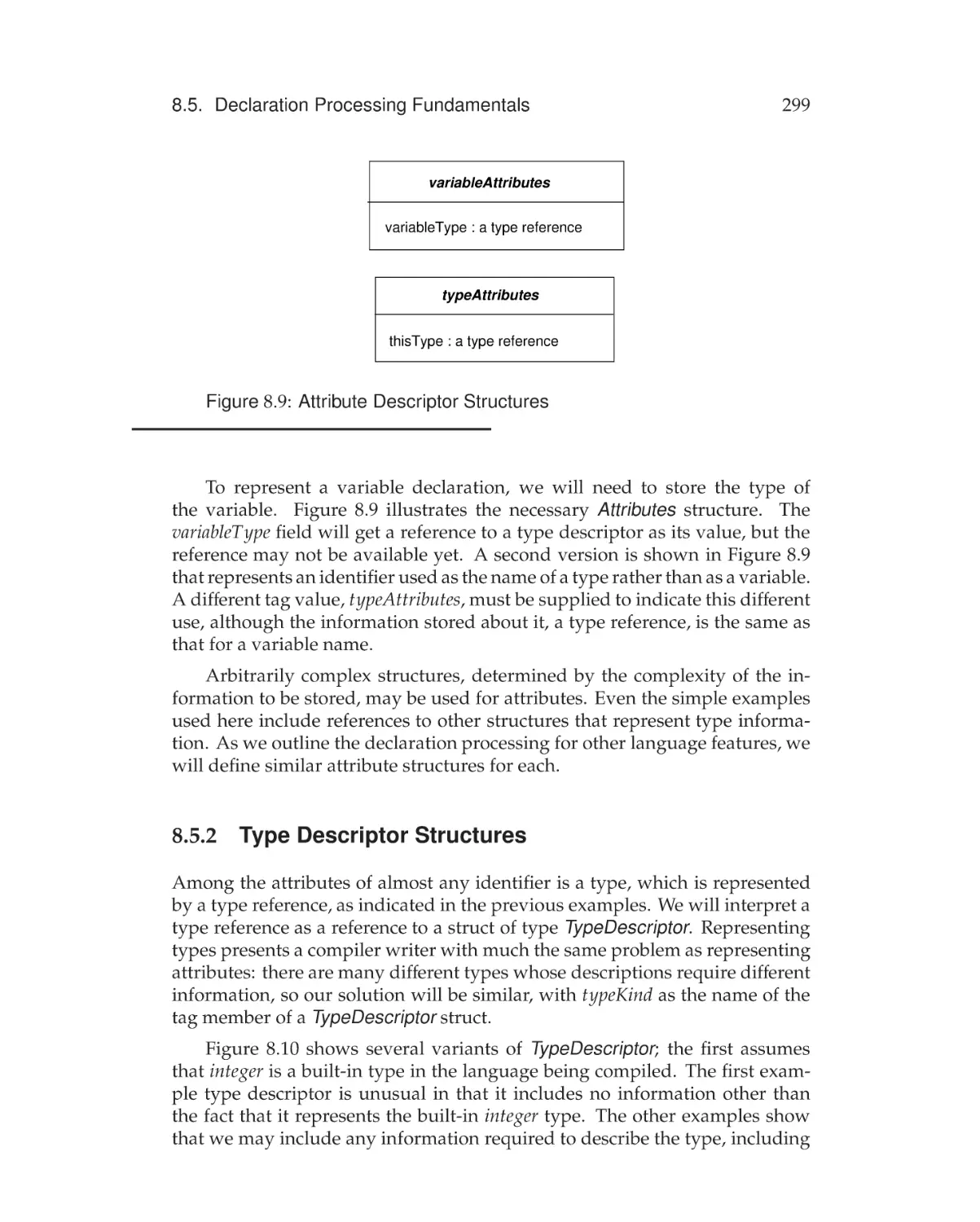
298
298
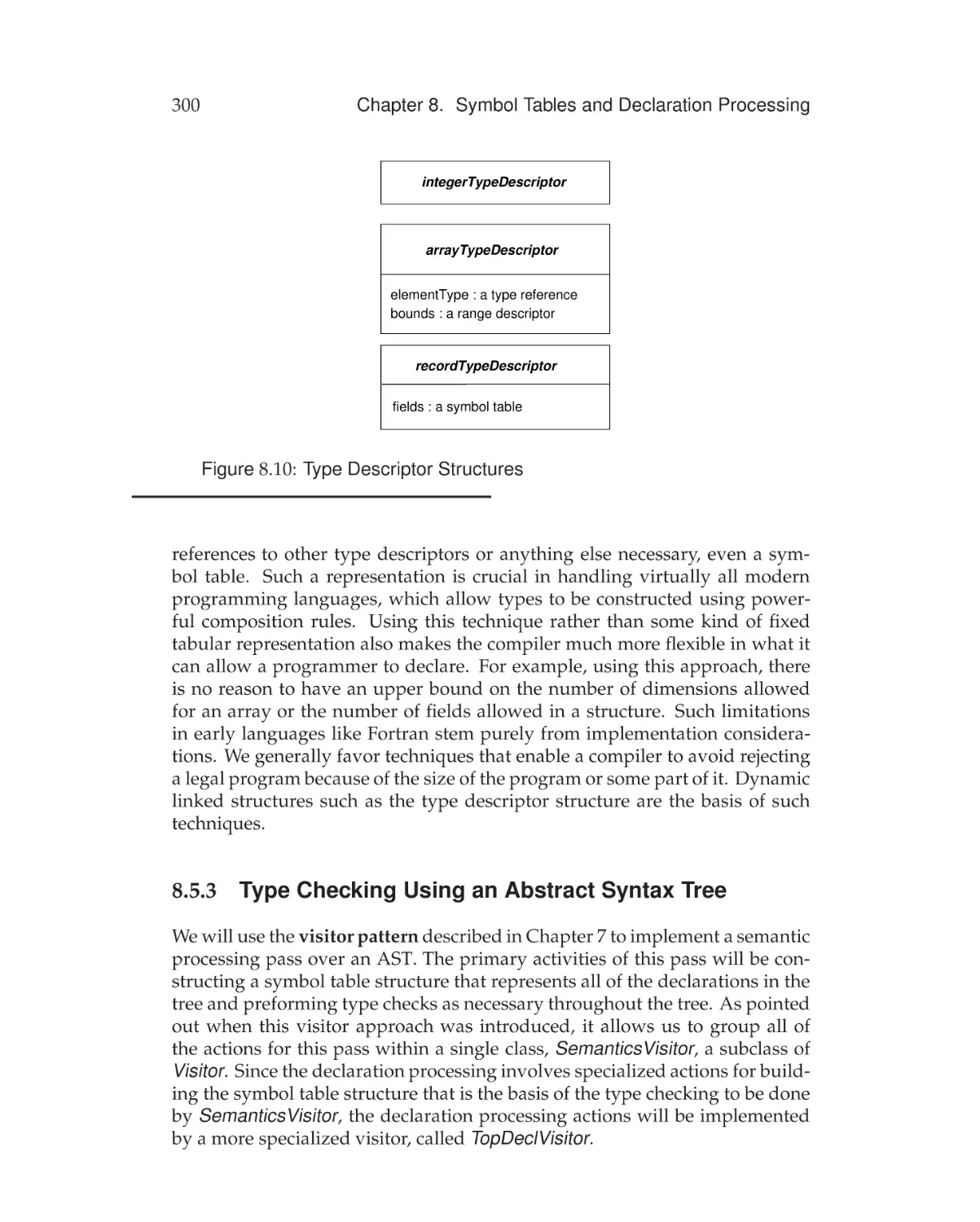
299
300
303
303
304
305
308
311
312
313
316
317
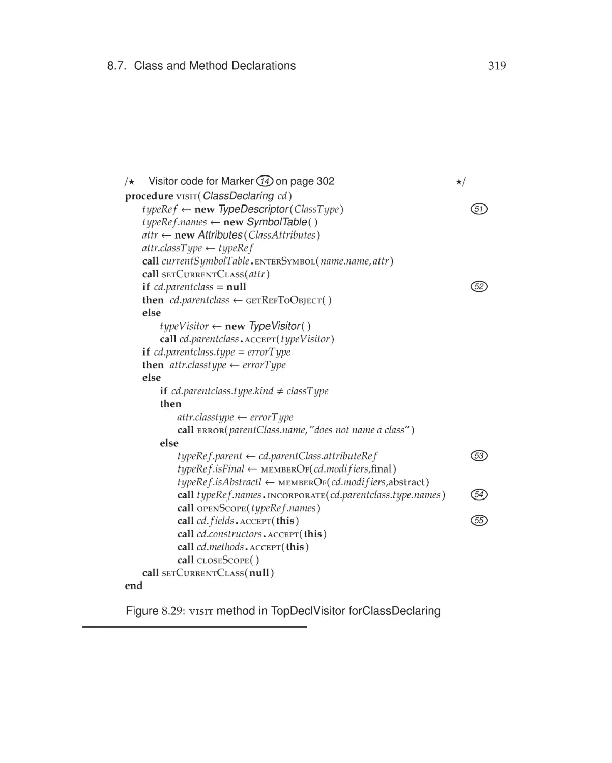
321
323
327
xxiii
Contents
8.9
8.8.2
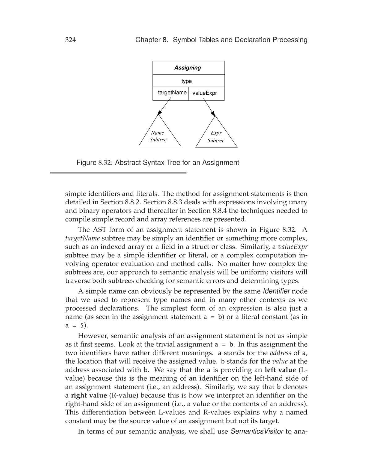
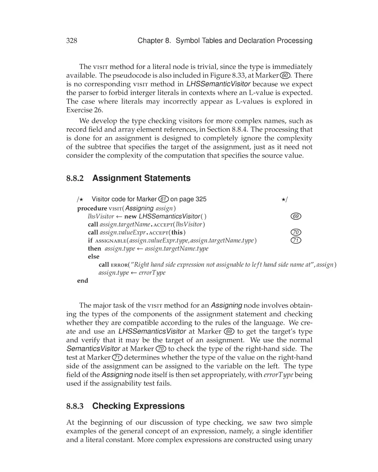
Assignment Statements . . . . . . . . . . . . . . . . . . 328
8.8.3
Checking Expressions . . . . . . . . . . . . . . . . . . . 328
8.8.4
Checking Complex Names . . . . . . . . . . . . . . . . 329
Summary . . . . . . . . . . . . . . . . . . . . . . . . . . . . . . 334
Exercises . . . . . . . . . . . . . . . . . . . . . . . . . . . . . . . . . 336
9
Semantic Analysis
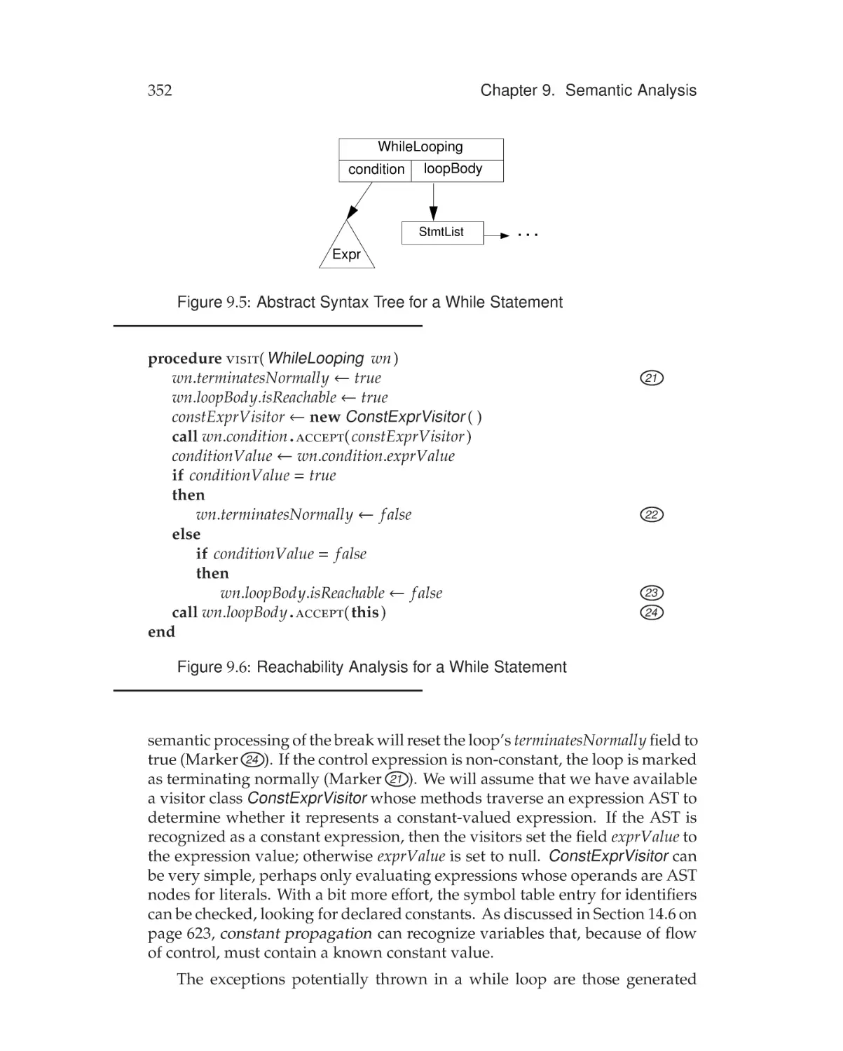
9.1
343
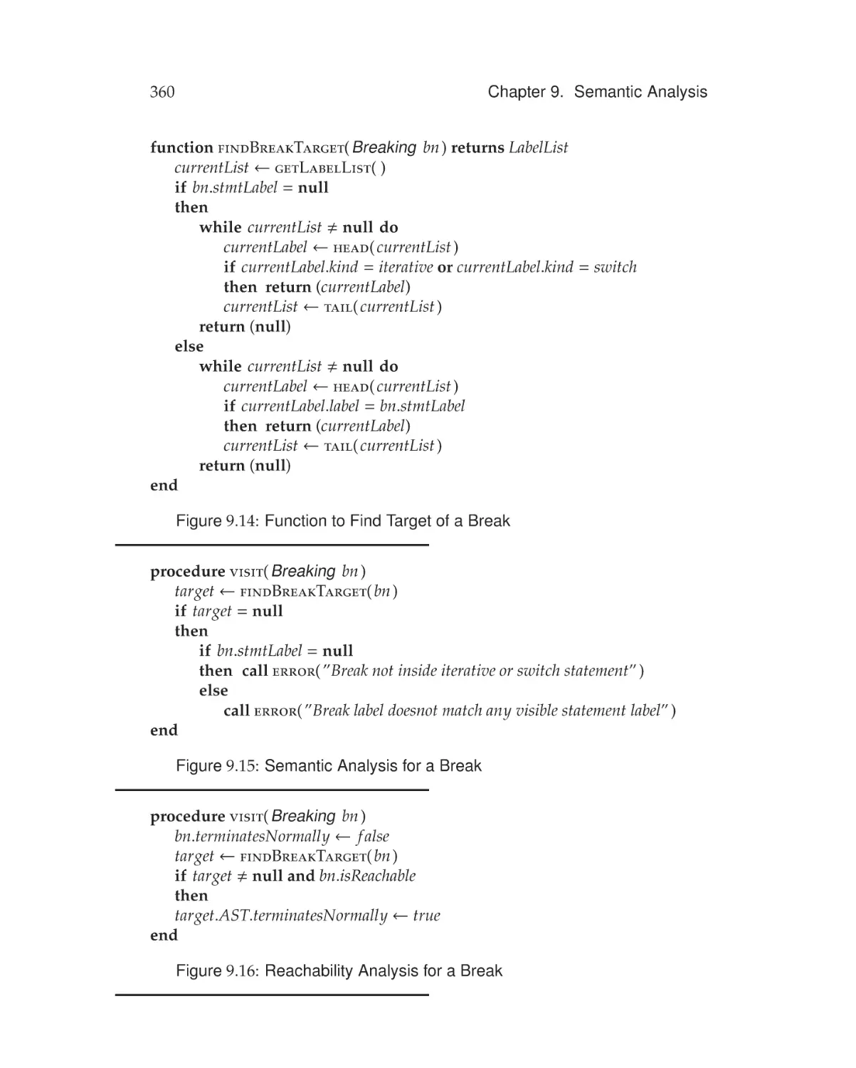
Semantic Analysis for Control Structures . . . . . . . . . . . . 343
9.1.1
Reachability and Termination Analysis . . . . . . . . . 345
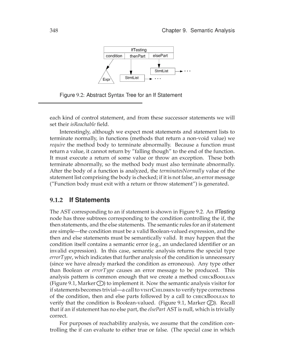
9.1.2
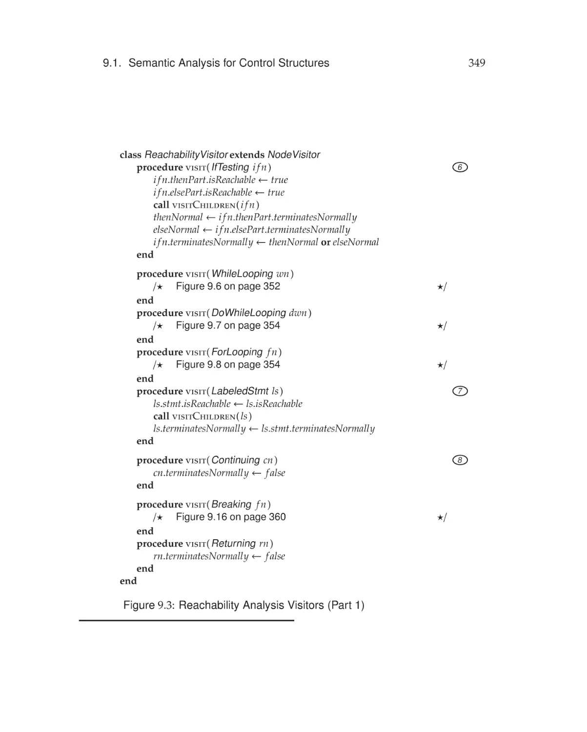
If Statements . . . . . . . . . . . . . . . . . . . . . . . . 348
9.1.3
While, Do, and Repeat Loops . . . . . . . . . . . . . . 350
9.1.4
For Loops . . . . . . . . . . . . . . . . . . . . . . . . . . 353
9.1.5
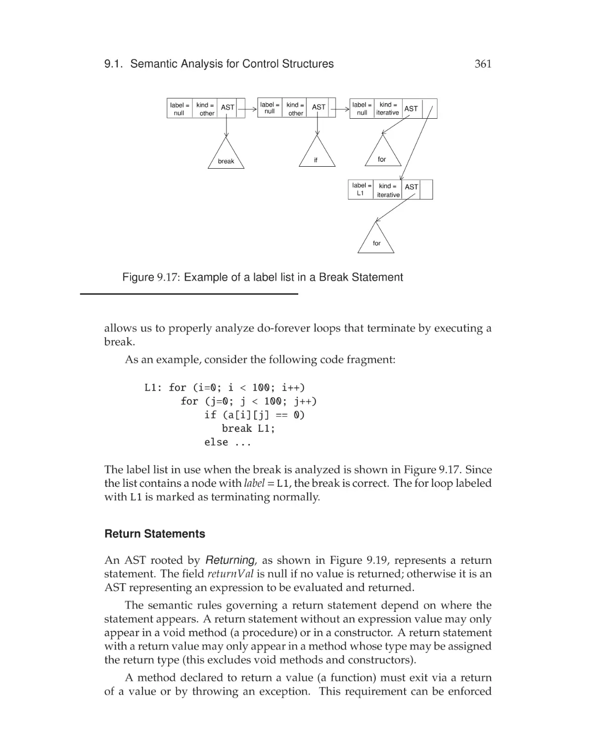
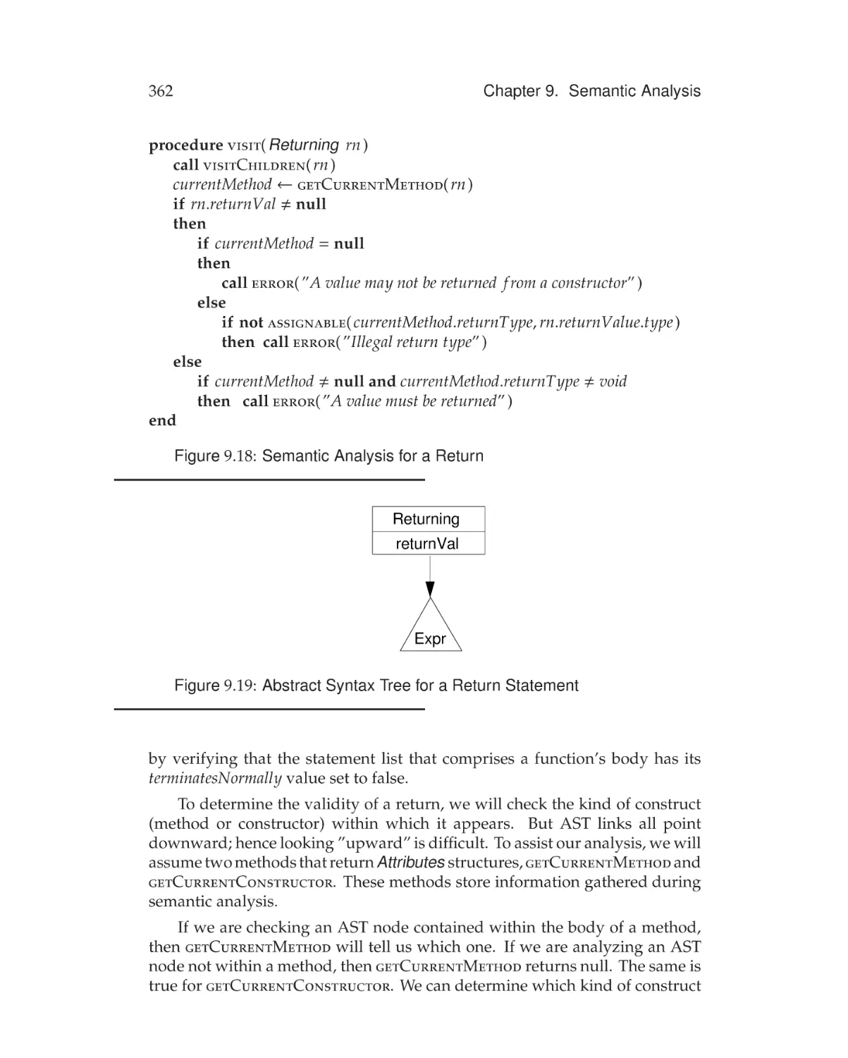
Break, Continue, Return, and Goto Statements . . . . 356
9.1.6
Switch and Case Statements . . . . . . . . . . . . . . . 364
9.1.7
Exception Handling . . . . . . . . . . . . . . . . . . . . 369
9.2
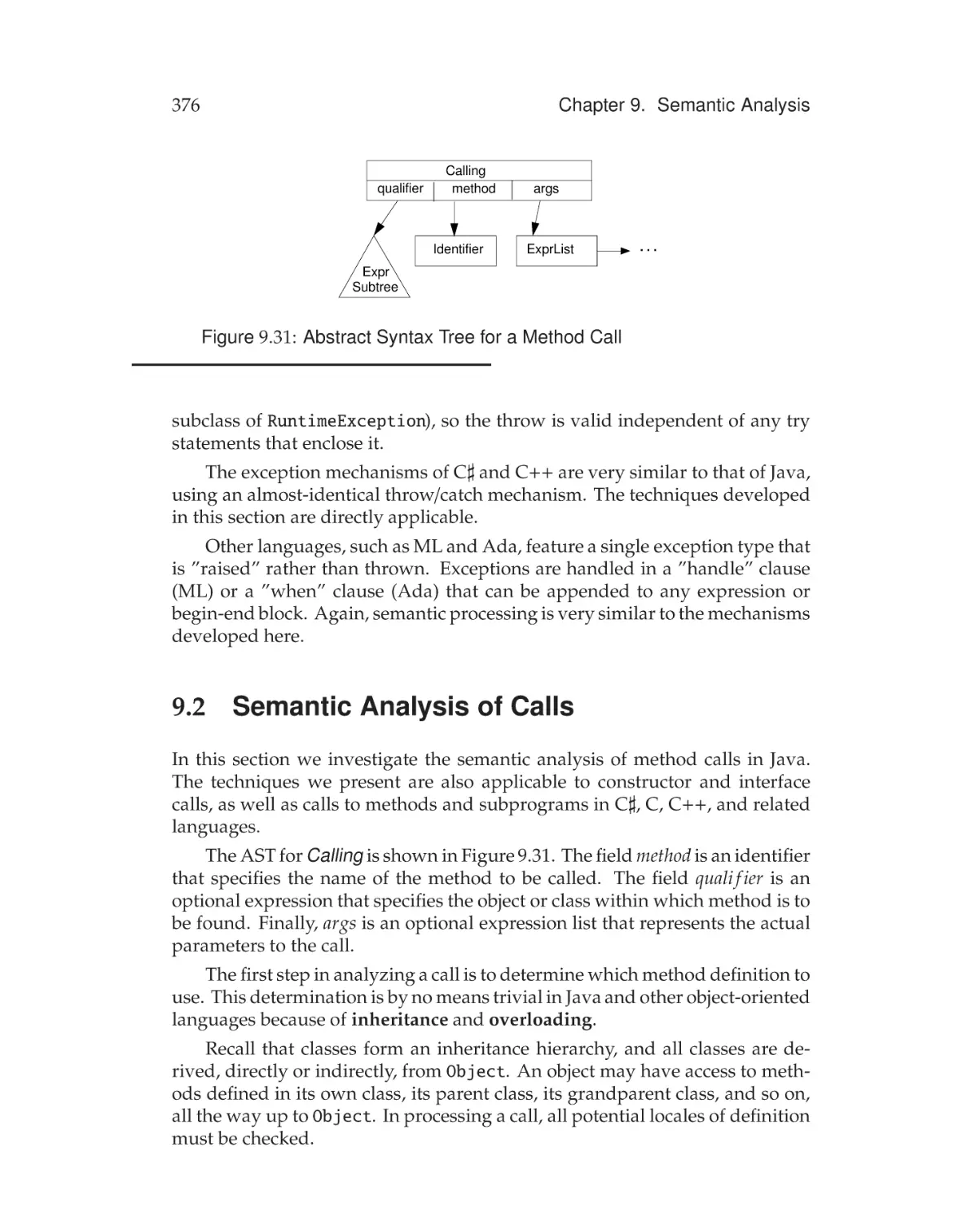
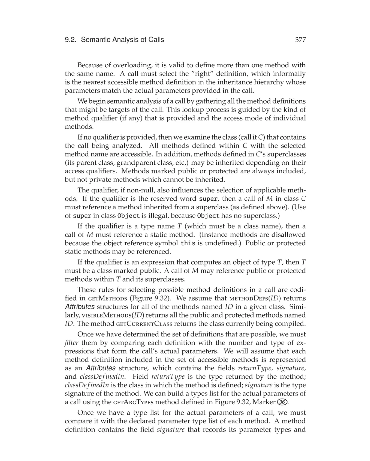
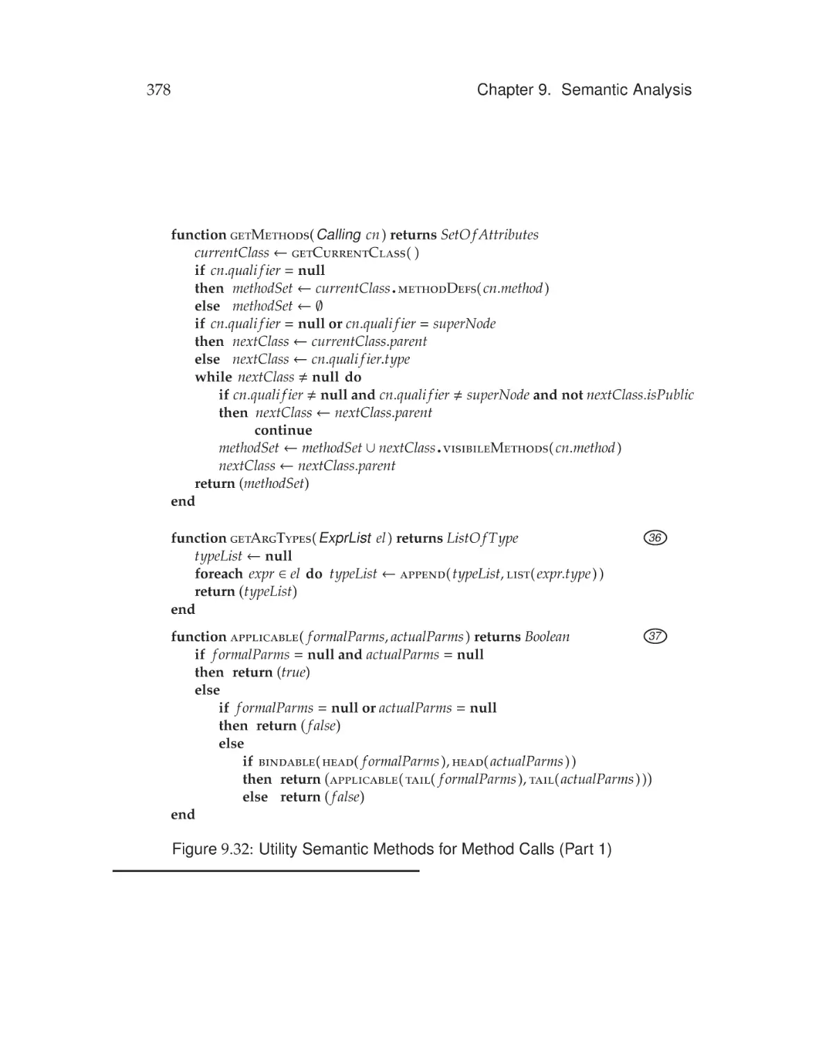
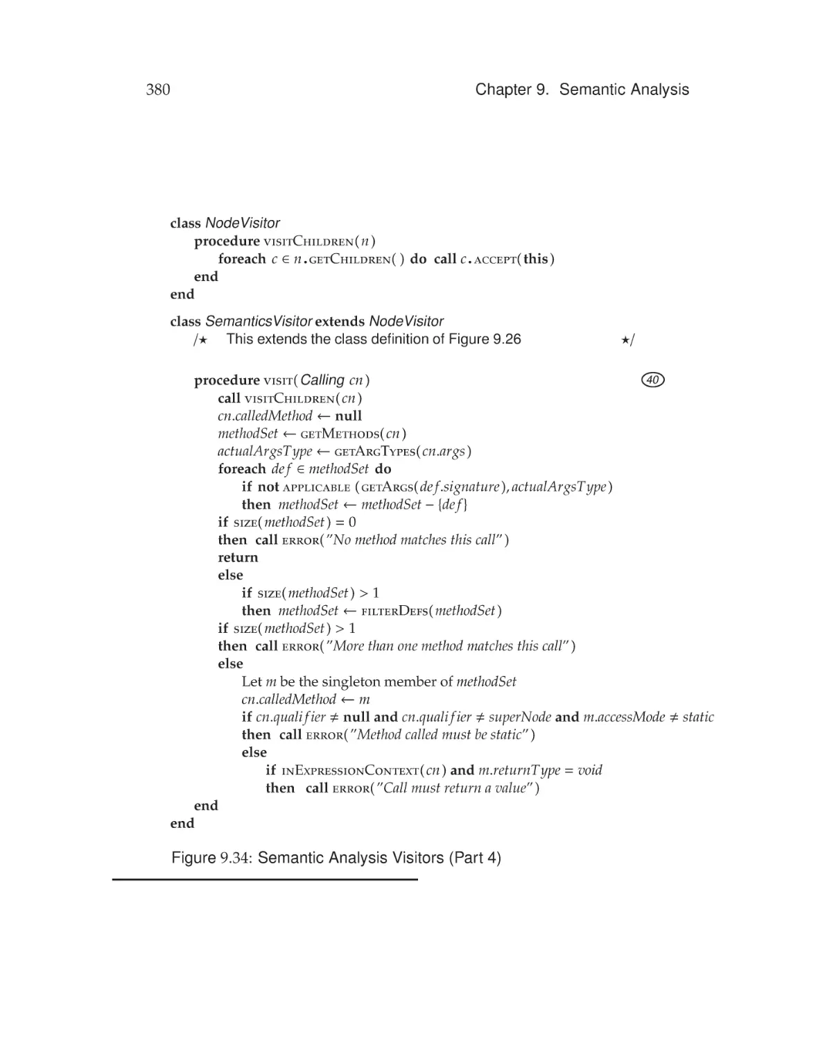
Semantic Analysis of Calls . . . . . . . . . . . . . . . . . . . . 376
9.3
Summary . . . . . . . . . . . . . . . . . . . . . . . . . . . . . . 384
Exercises . . . . . . . . . . . . . . . . . . . . . . . . . . . . . . . . . 385
10 Intermediate Representations
391
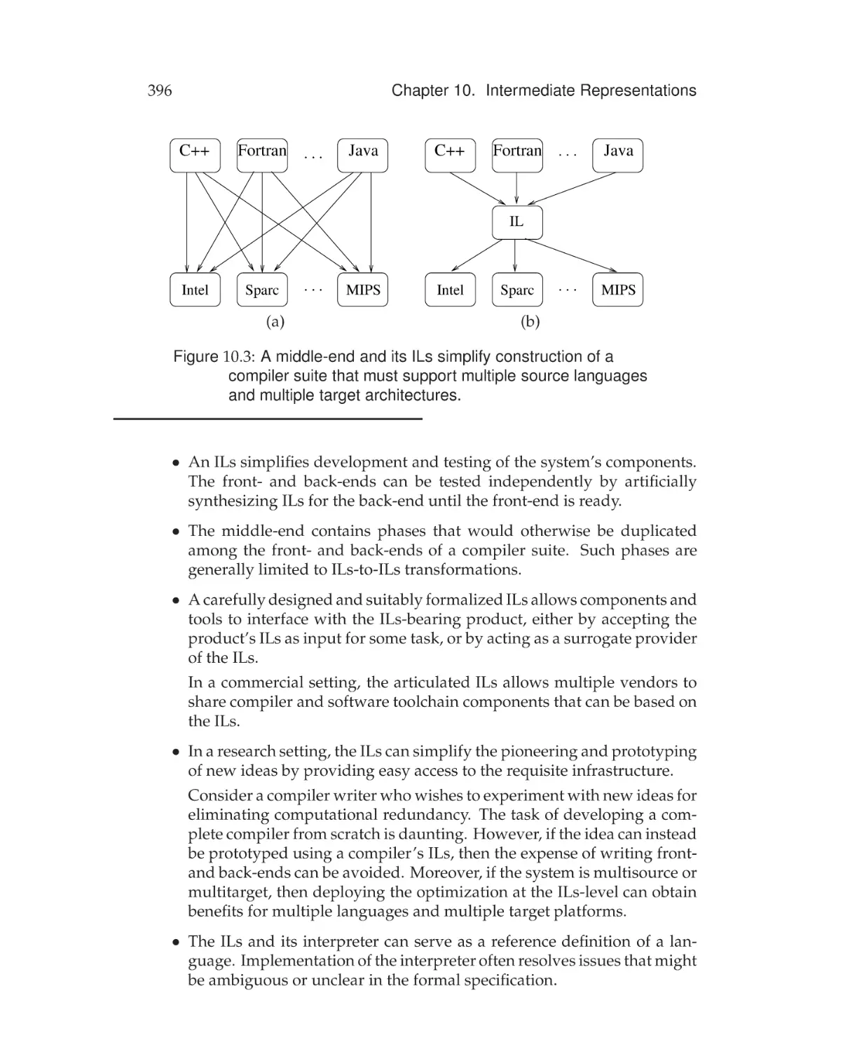
10.1 Overview . . . . . . . . . . . . . . . . . . . . . . . . . . . . . . . 392
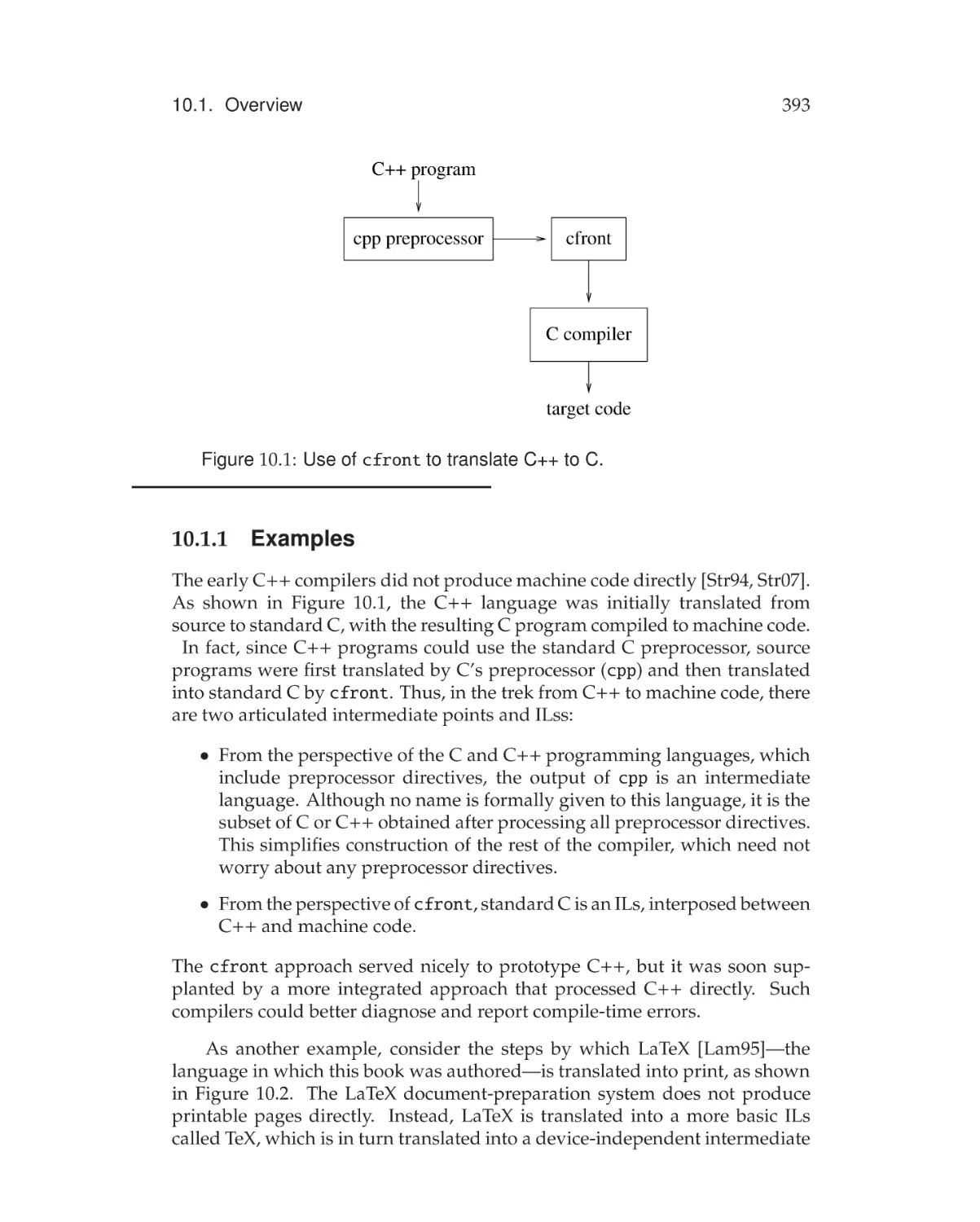
10.1.1 Examples . . . . . . . . . . . . . . . . . . . . . . . . . . 393
10.1.2 The Middle-End . . . . . . . . . . . . . . . . . . . . . . 395
10.2 Java Virtual Machine . . . . . . . . . . . . . . . . . . . . . . . . 397
10.2.1 Introduction and Design Principles . . . . . . . . . . . . 398
10.2.2 Contents of a Class File . . . . . . . . . . . . . . . . . . 399
10.2.3 JVM Instructions . . . . . . . . . . . . . . . . . . . . . . 401
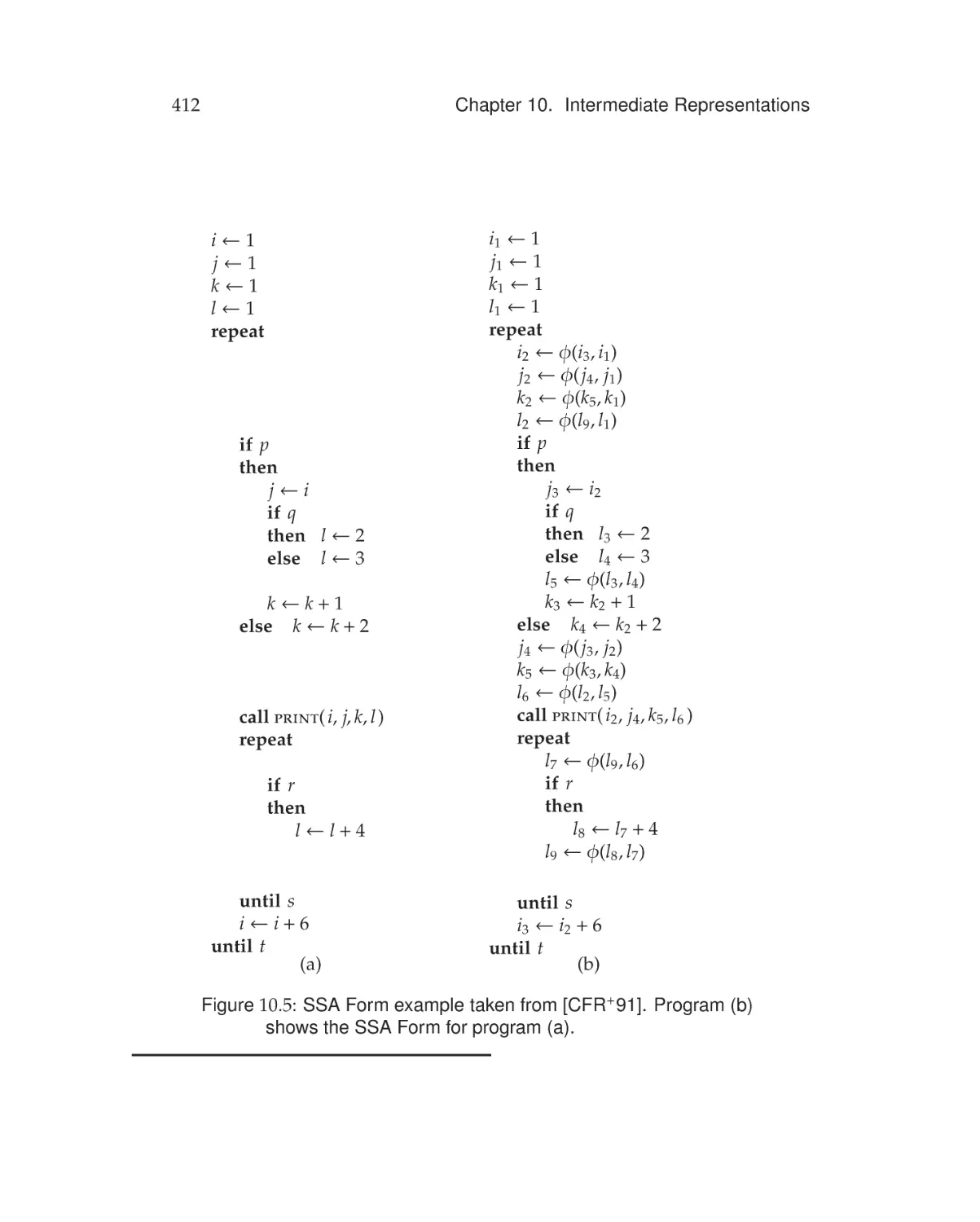
10.3 Static Single Assignment Form . . . . . . . . . . . . . . . . . . 410
10.3.1 Renaming and φ-functions . . . . . . . . . . . . . . . . 411
Exercises . . . . . . . . . . . . . . . . . . . . . . . . . . . . . . . . . 414
xxiv
Contents
11 Code Generation for a Virtual Machine
417
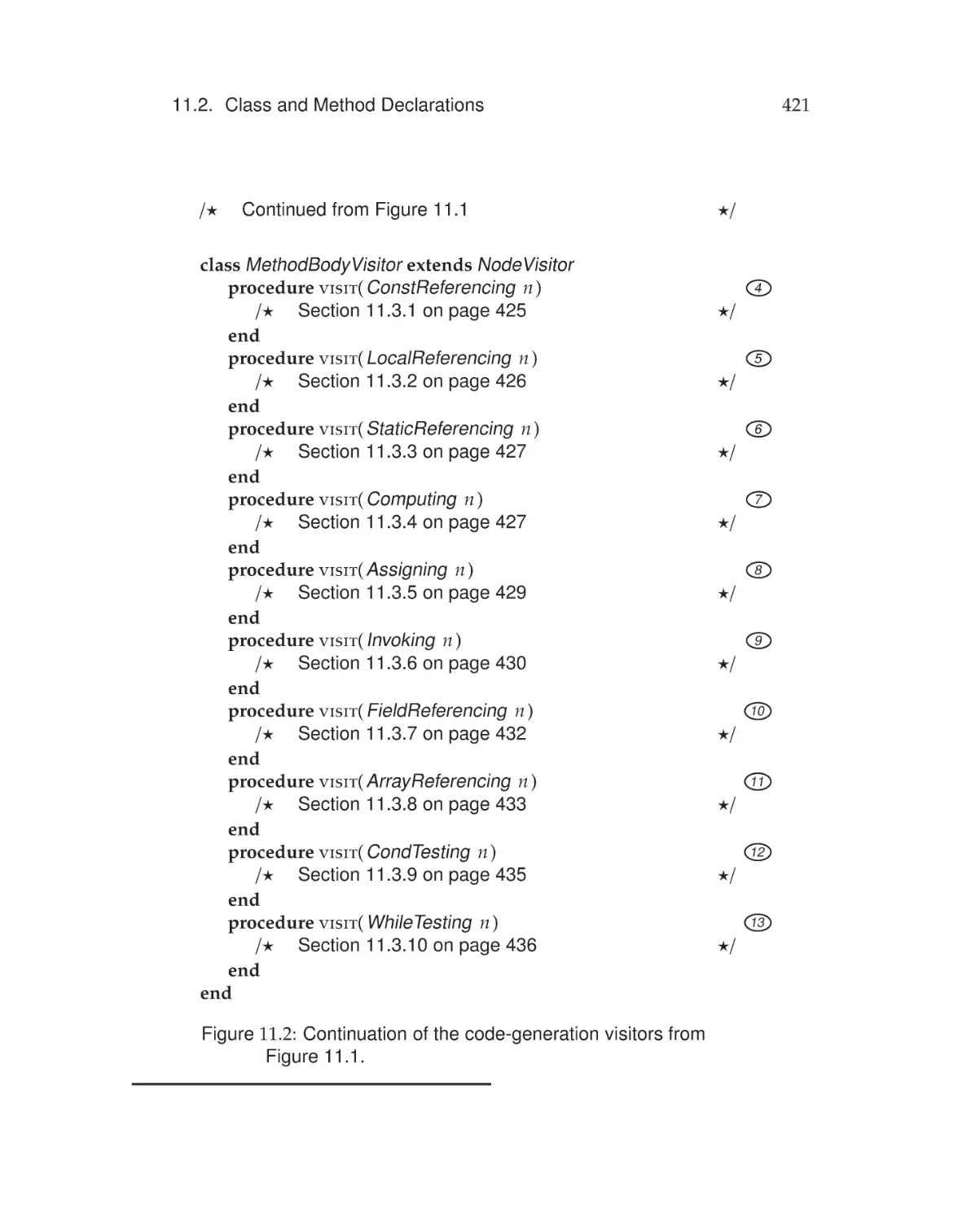
11.1 Visitors for Code Generation . . . . . . . . . . . . . . . . . . . 418
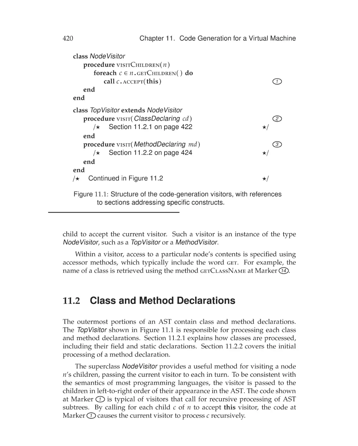
11.2 Class and Method Declarations . . . . . . . . . . . . . . . . . . 420
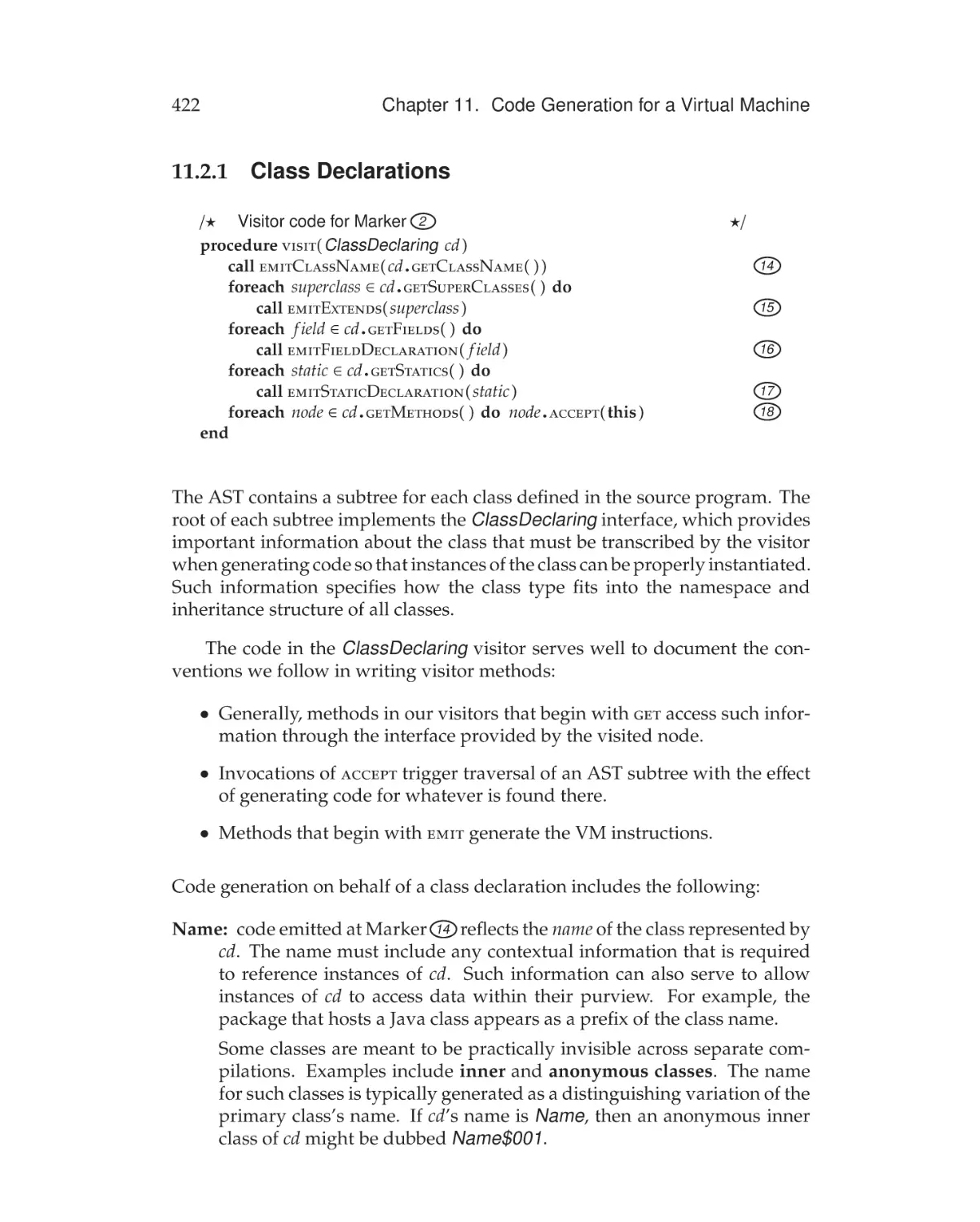
11.2.1 Class Declarations . . . . . . . . . . . . . . . . . . . . . 422
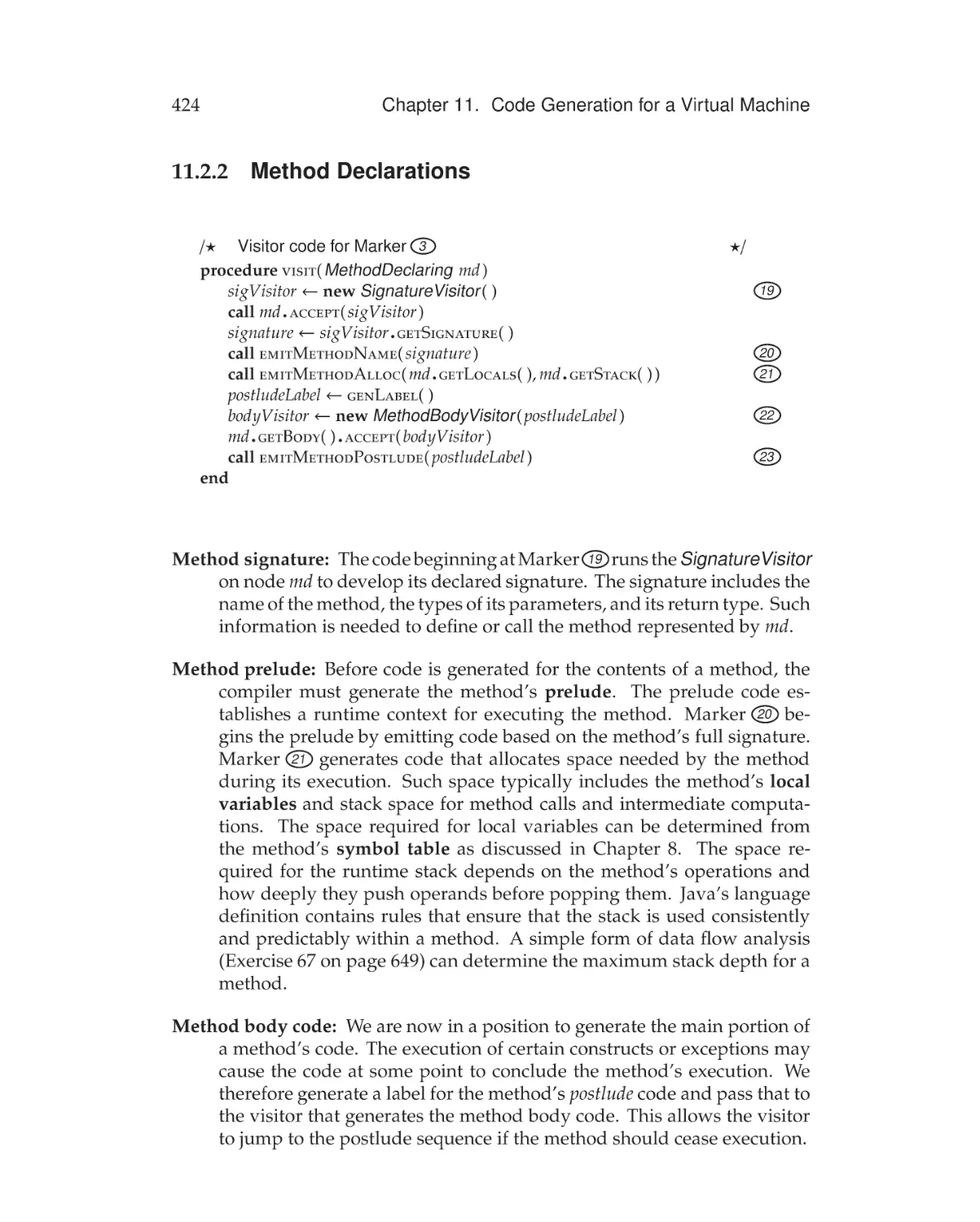
11.2.2 Method Declarations . . . . . . . . . . . . . . . . . . . . 424
11.3 The MethodBodyVisitor . . . . . . . . . . . . . . . . . . . . . . 425
11.3.1 Constants . . . . . . . . . . . . . . . . . . . . . . . . . . 425
11.3.2 References to Local Storage . . . . . . . . . . . . . . . 426
11.3.3 Static References . . . . . . . . . . . . . . . . . . . . . 427
11.3.4 Expressions . . . . . . . . . . . . . . . . . . . . . . . . . 427
11.3.5 Assignment . . . . . . . . . . . . . . . . . . . . . . . . . 429
11.3.6 Method Calls . . . . . . . . . . . . . . . . . . . . . . . . 430
11.3.7 Field References . . . . . . . . . . . . . . . . . . . . . . 432
11.3.8 Array References . . . . . . . . . . . . . . . . . . . . . . 433
11.3.9 Conditional Execution . . . . . . . . . . . . . . . . . . . 435
11.3.10 Loops . . . . . . . . . . . . . . . . . . . . . . . . . . . . 436
11.4 The LHSVisitor . . . . . . . . . . . . . . . . . . . . . . . . . . . 437
11.4.1 Local References . . . . . . . . . . . . . . . . . . . . . 437
11.4.2 Static References . . . . . . . . . . . . . . . . . . . . . 438
11.4.3 Field References . . . . . . . . . . . . . . . . . . . . . . 439
11.4.4 Array References . . . . . . . . . . . . . . . . . . . . . . 439
Exercises . . . . . . . . . . . . . . . . . . . . . . . . . . . . . . . . . 441
12 Runtime Support
445
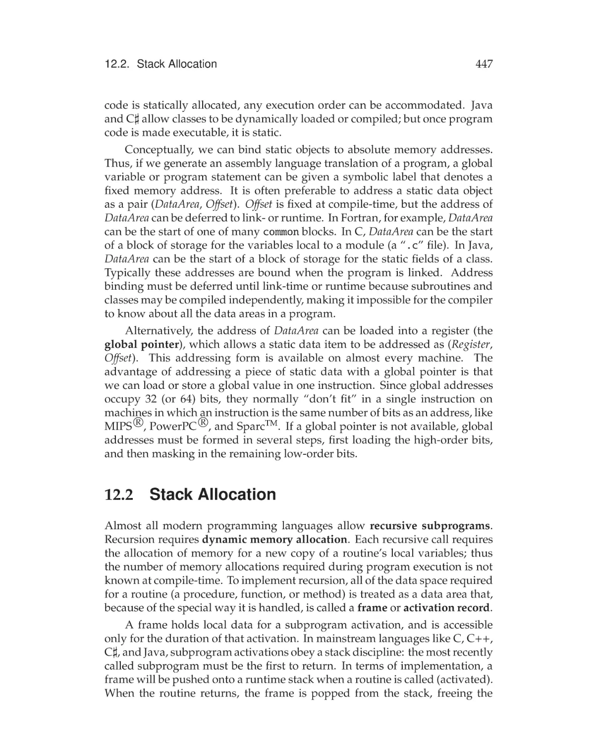
12.1 Static Allocation . . . . . . . . . . . . . . . . . . . . . . . . . . . 446
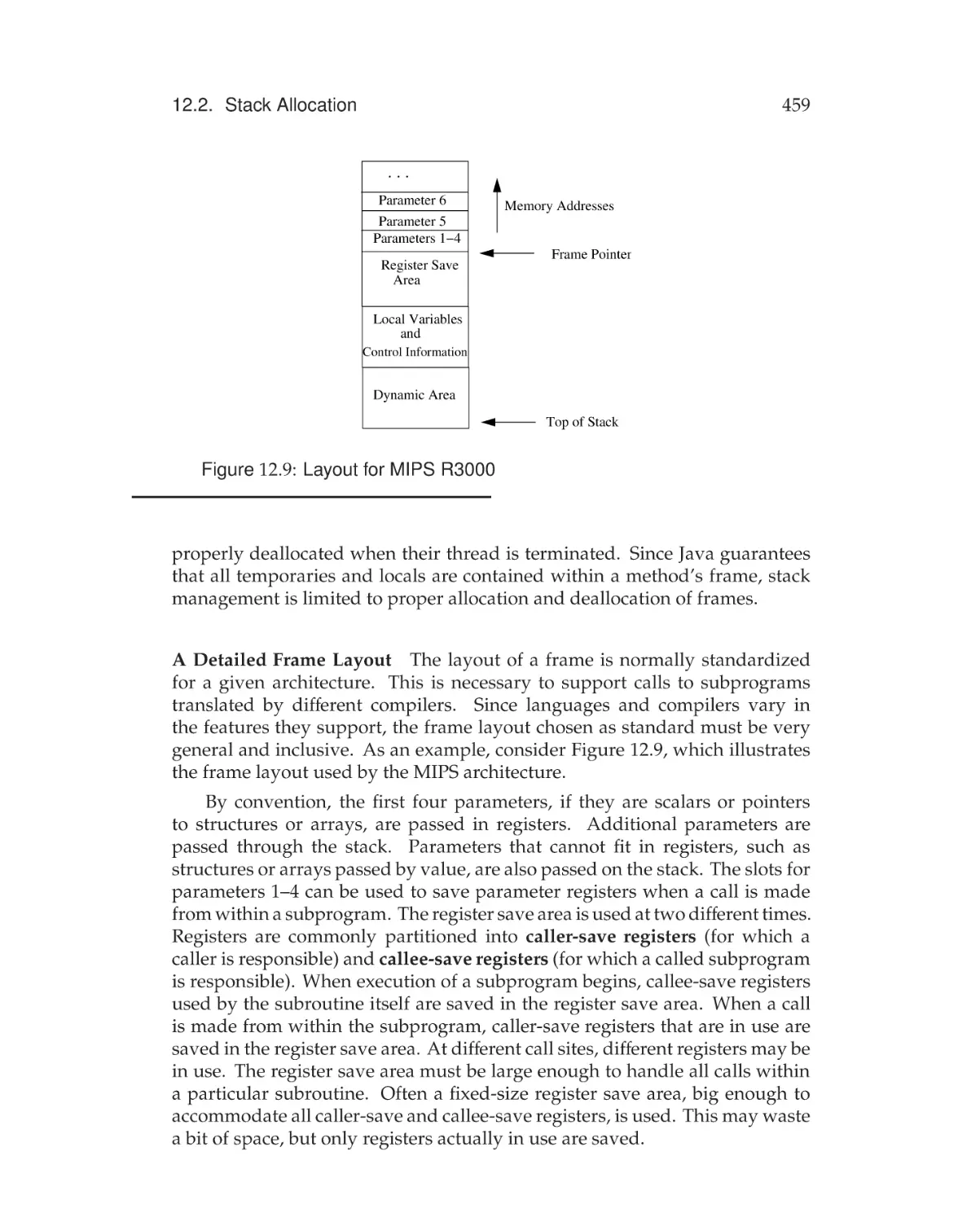
12.2 Stack Allocation . . . . . . . . . . . . . . . . . . . . . . . . . . . 447
12.2.1 Field Access in Classes and Structs . . . . . . . . . . . 449
12.2.2 Accessing Frames at Runtime . . . . . . . . . . . . . . 450
12.2.3 Handling Classes and Objects . . . . . . . . . . . . . . 451
12.2.4 Handling Multiple Scopes . . . . . . . . . . . . . . . . . 453
12.2.5 Block-Level Allocation . . . . . . . . . . . . . . . . . . . 455
xxv
Contents
12.2.6 More About Frames . . . . . .
12.3 Arrays . . . . . . . . . . . . . . . . . .
12.3.1 Static One-Dimensional Arrays
12.3.2 Multidimensional Arrays . . . .
12.4 Heap Management . . . . . . . . . . .
12.4.1 Allocation Mechanisms . . . .
12.4.2 Deallocation Mechanisms . . .
12.4.3 Automatic Garbage Collection
12.5 Region-Based Memory Management
Exercises . . . . . . . . . . . . . . . . . . .
.
.
.
.
.
.
.
.
.
.
.
.
.
.
.
.
.
.
.
.
.
.
.
.
.
.
.
.
.
.
.
.
.
.
.
.
.
.
.
.
.
.
.
.
.
.
.
.
.
.
.
.
.
.
.
.
.
.
.
.
.
.
.
.
.
.
.
.
.
.
.
.
.
.
.
.
.
.
.
.
.
.
.
.
.
.
.
.
.
.
.
.
.
.
.
.
.
.
.
.
.
.
.
.
.
.
.
.
.
.
.
.
.
.
.
.
.
.
.
.
.
.
.
.
.
.
.
.
.
.
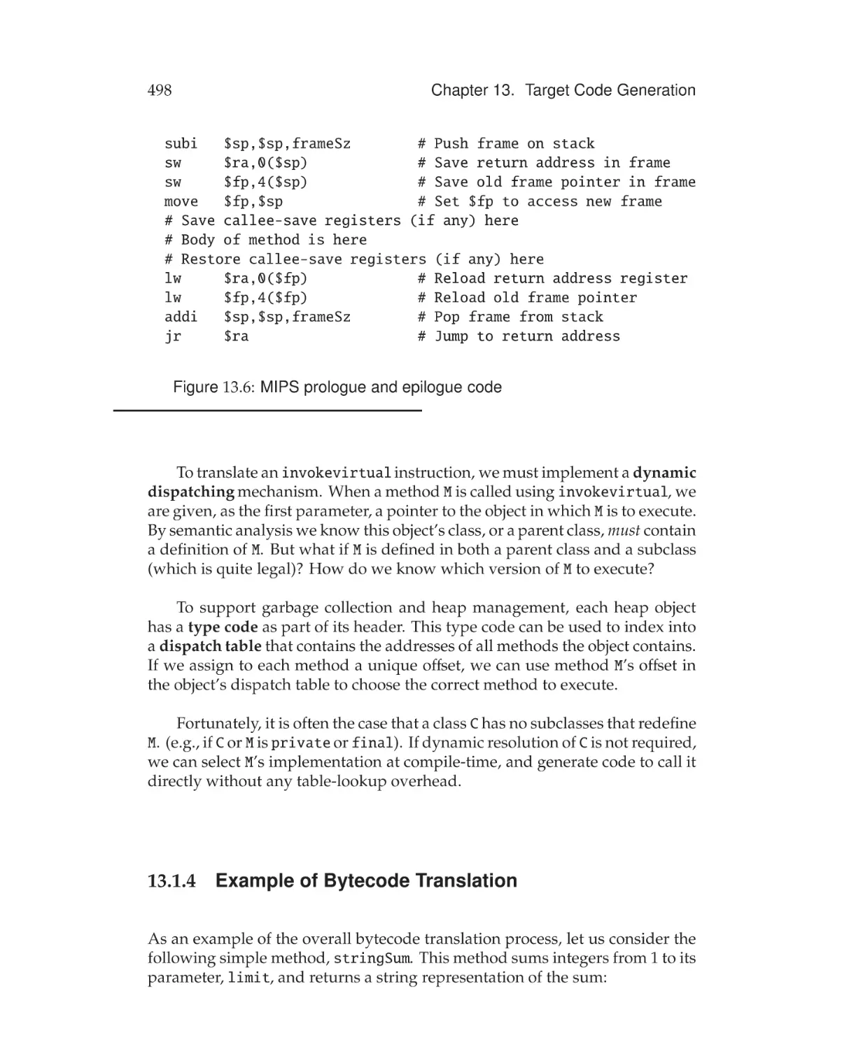
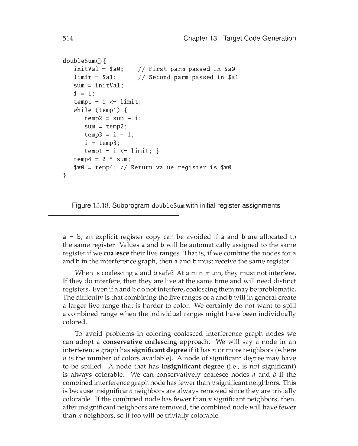
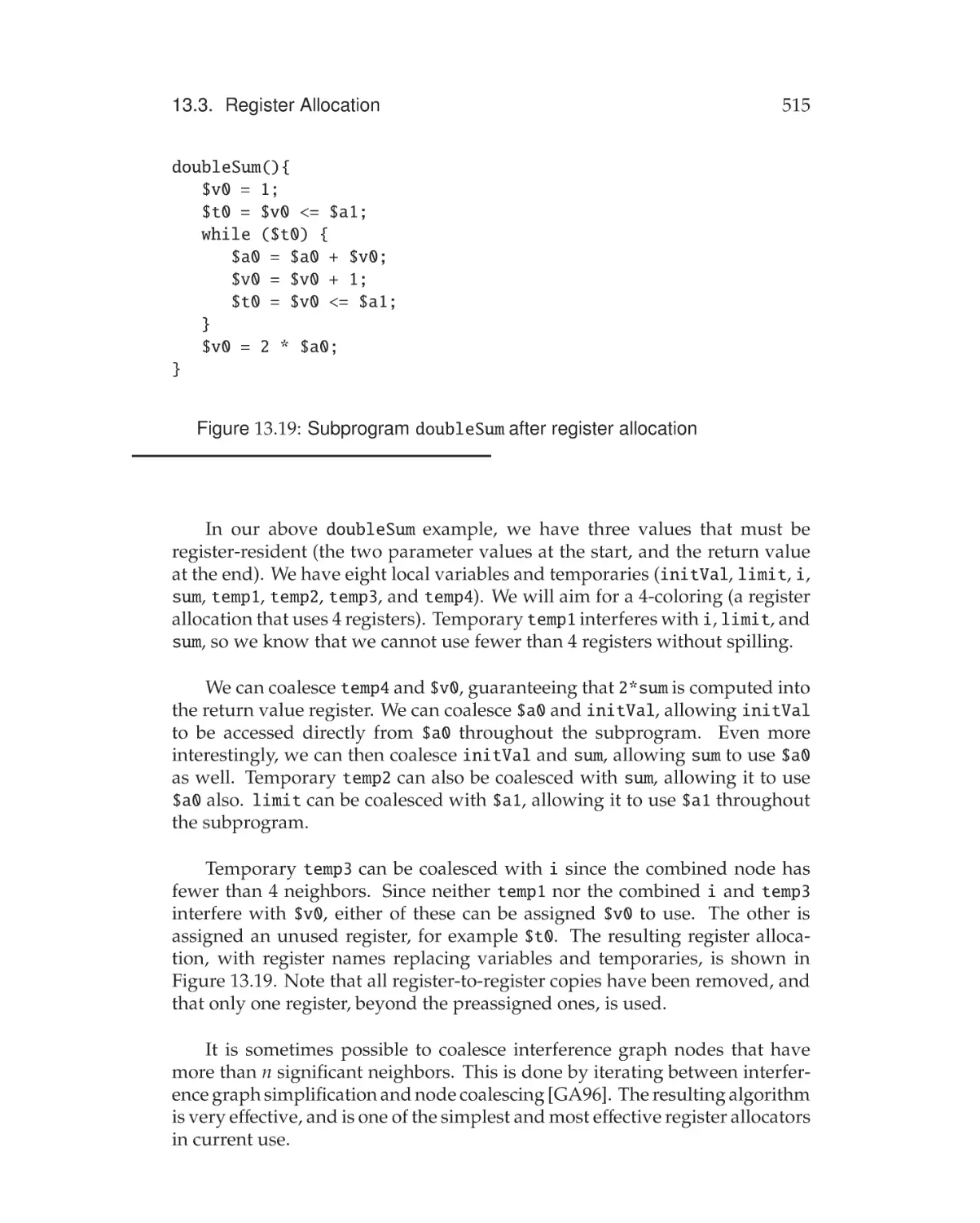
13 Target Code Generation
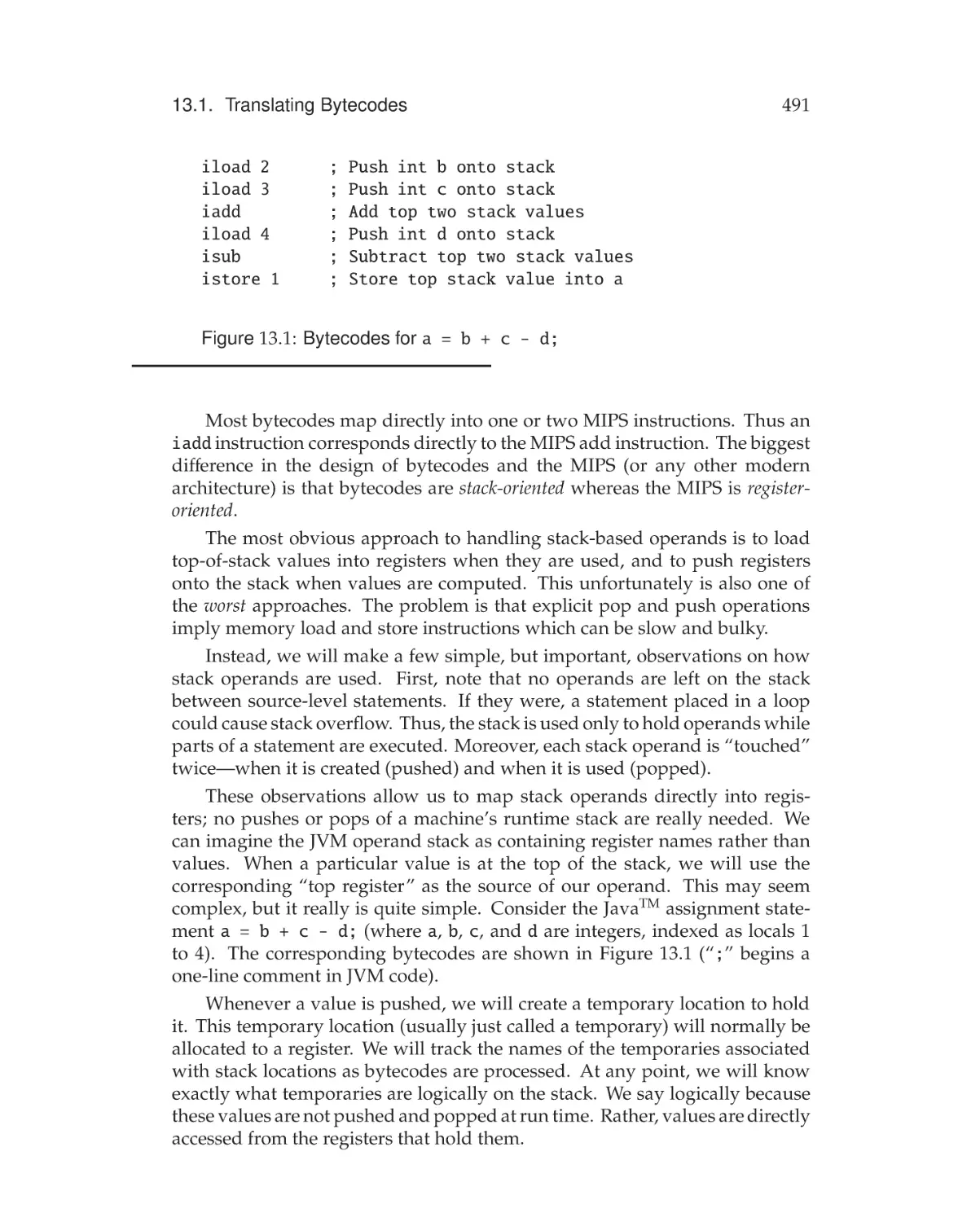
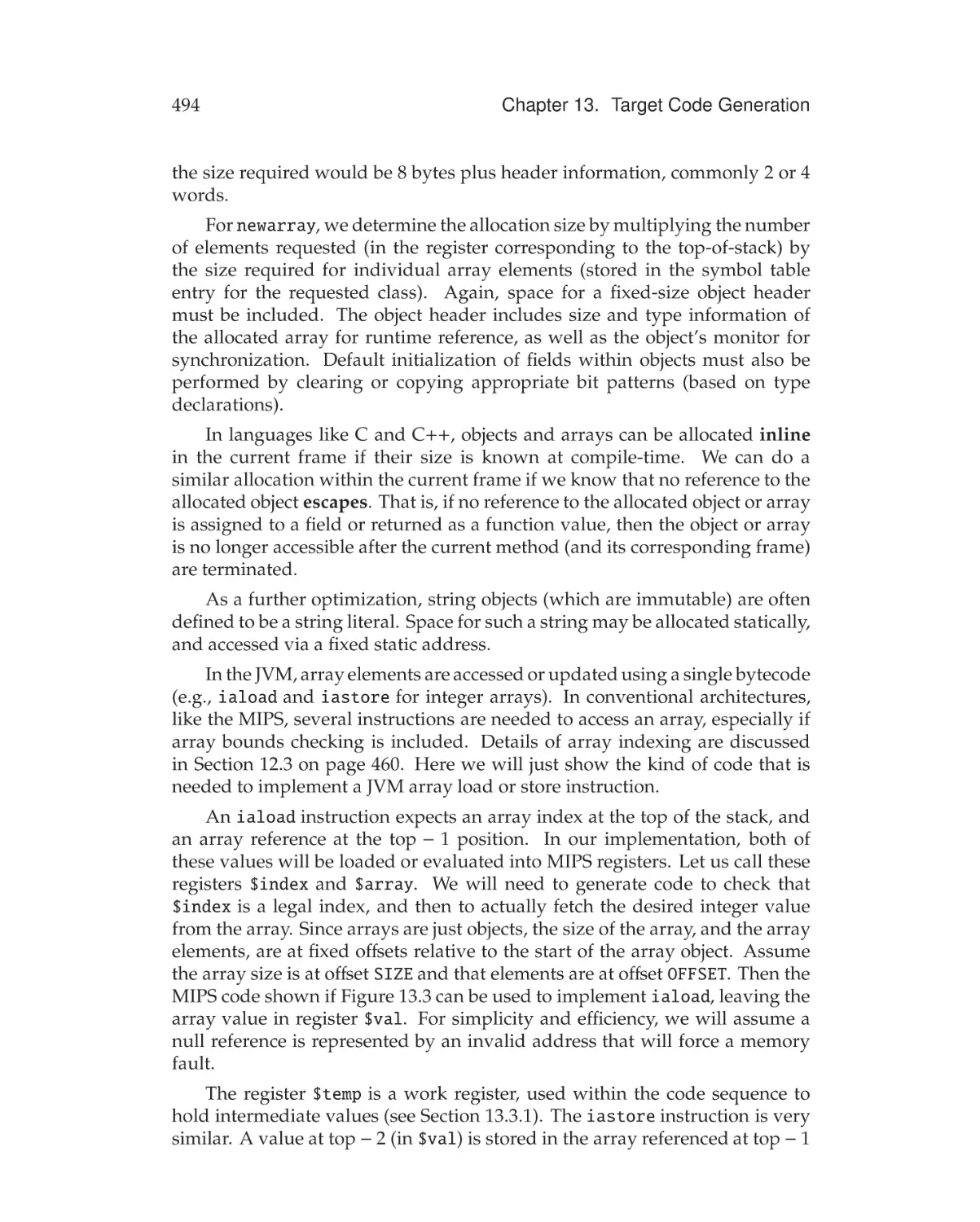
13.1 Translating Bytecodes . . . . . . . . . . . . . . . . . .
13.1.1 Allocating memory addresses . . . . . . . . .
13.1.2 Allocating Arrays and Objects . . . . . . . . .
13.1.3 Method Calls . . . . . . . . . . . . . . . . . . .
13.1.4 Example of Bytecode Translation . . . . . . .
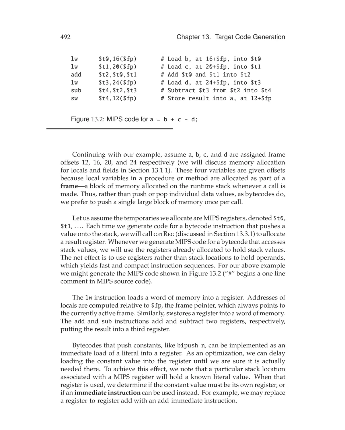
13.2 Translating Expression Trees . . . . . . . . . . . . . .
13.3 Register Allocation . . . . . . . . . . . . . . . . . . . .
13.3.1 On-the-Fly Register Allocation . . . . . . . . .
13.3.2 Register Allocation Using Graph Coloring . . .
13.3.3 Priority-Based Register Allocation . . . . . . .
13.3.4 Interprocedural Register Allocation . . . . . .
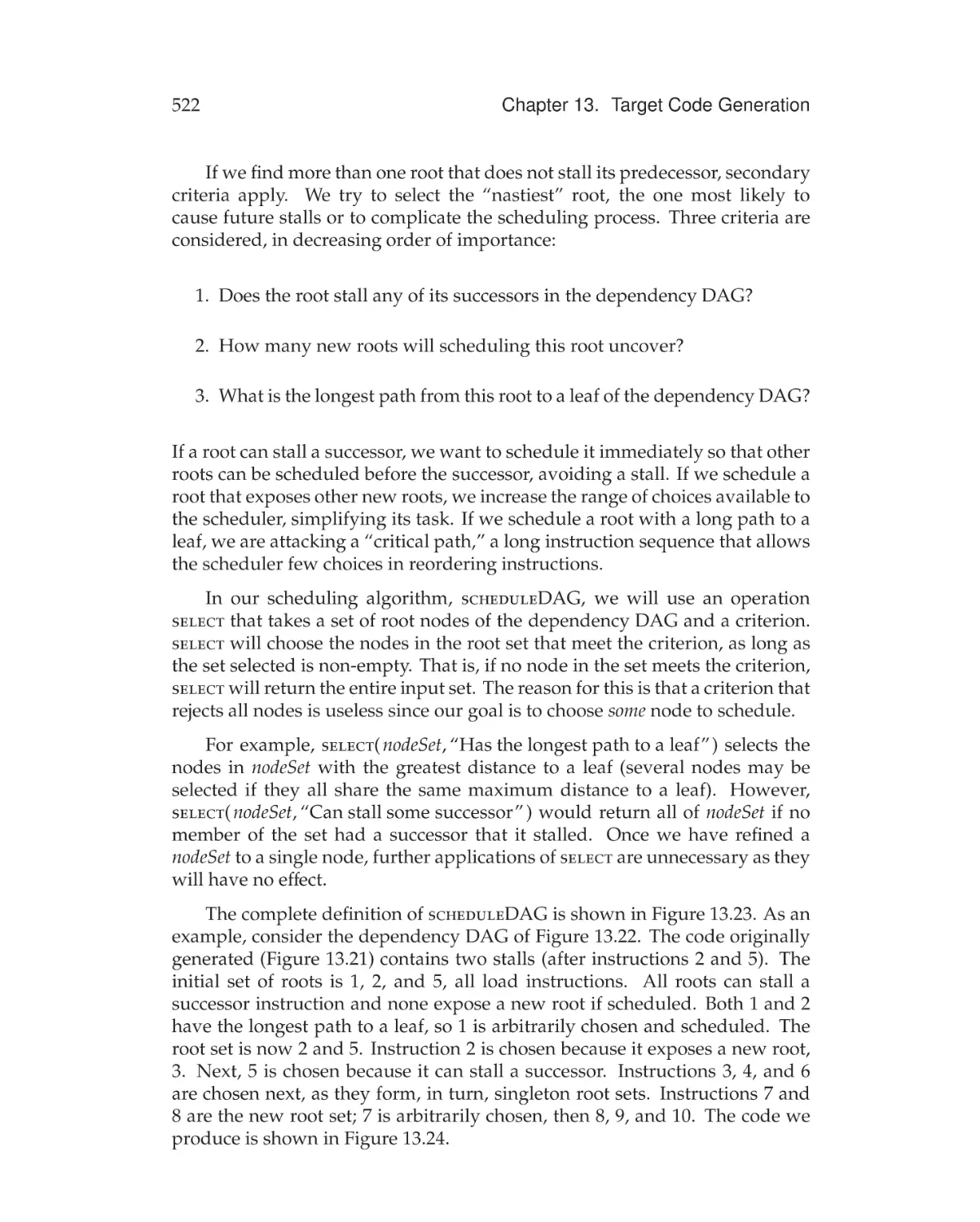
13.4 Code Scheduling . . . . . . . . . . . . . . . . . . . . .
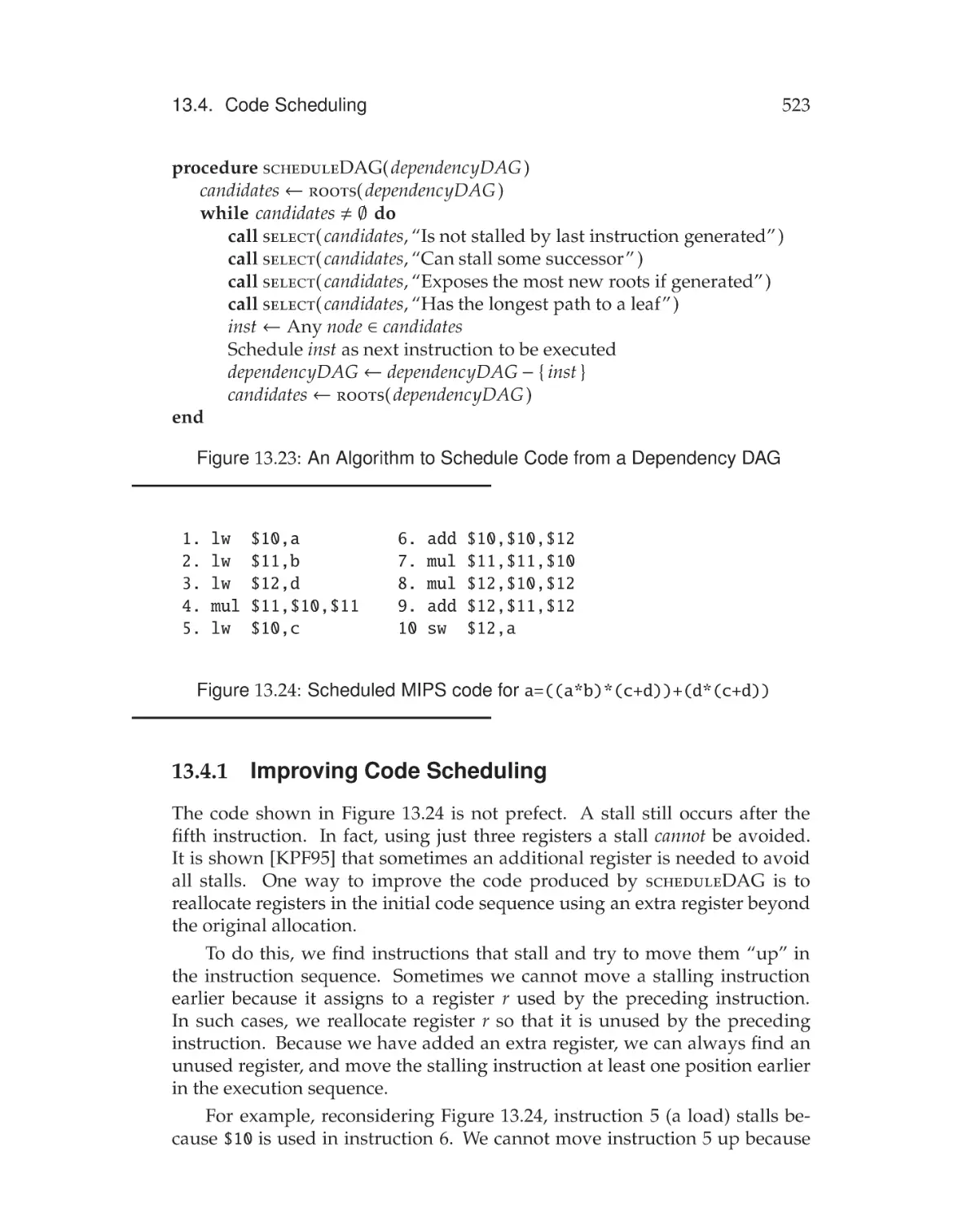
13.4.1 Improving Code Scheduling . . . . . . . . . .
13.4.2 Global and Dynamic Code Scheduling . . . .
13.5 Automatic Instruction Selection . . . . . . . . . . . . .
13.5.1 Instruction Selection Using BURS . . . . . . .
13.5.2 Instruction Selection Using Twig . . . . . . . .
13.5.3 Other Approaches . . . . . . . . . . . . . . . .
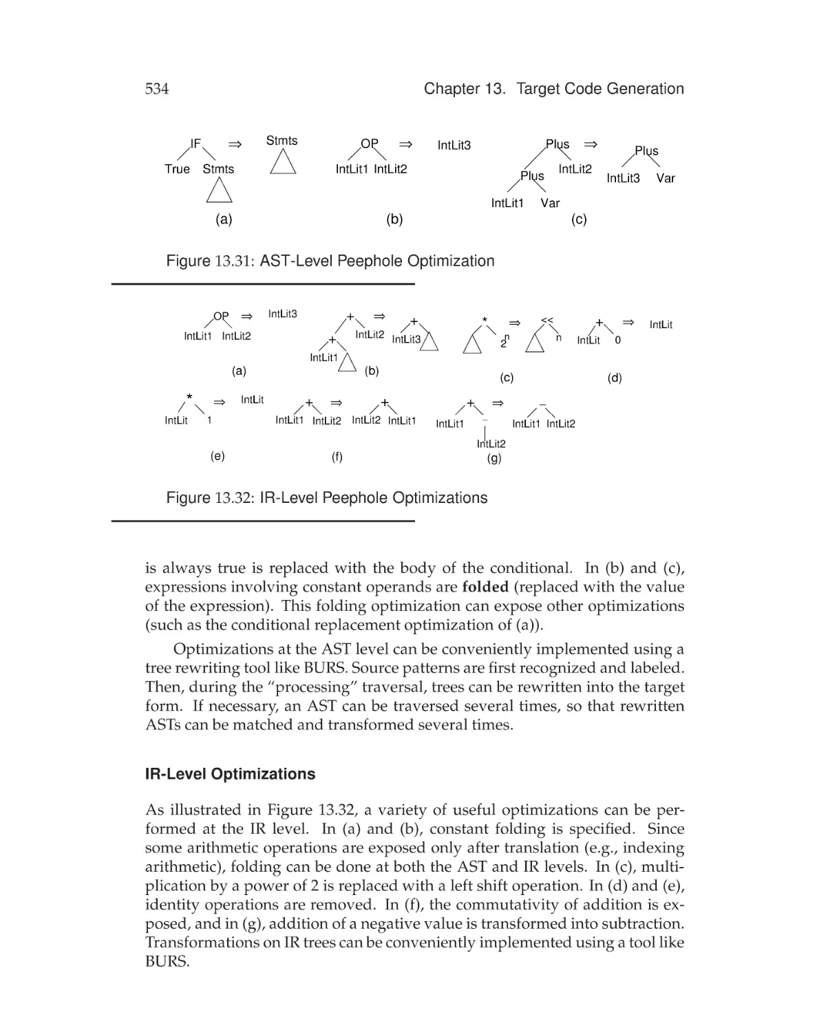
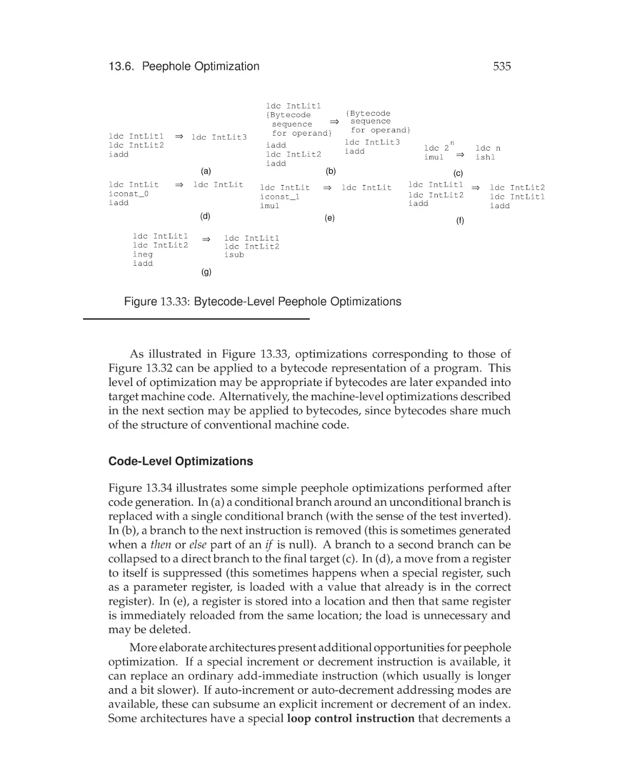
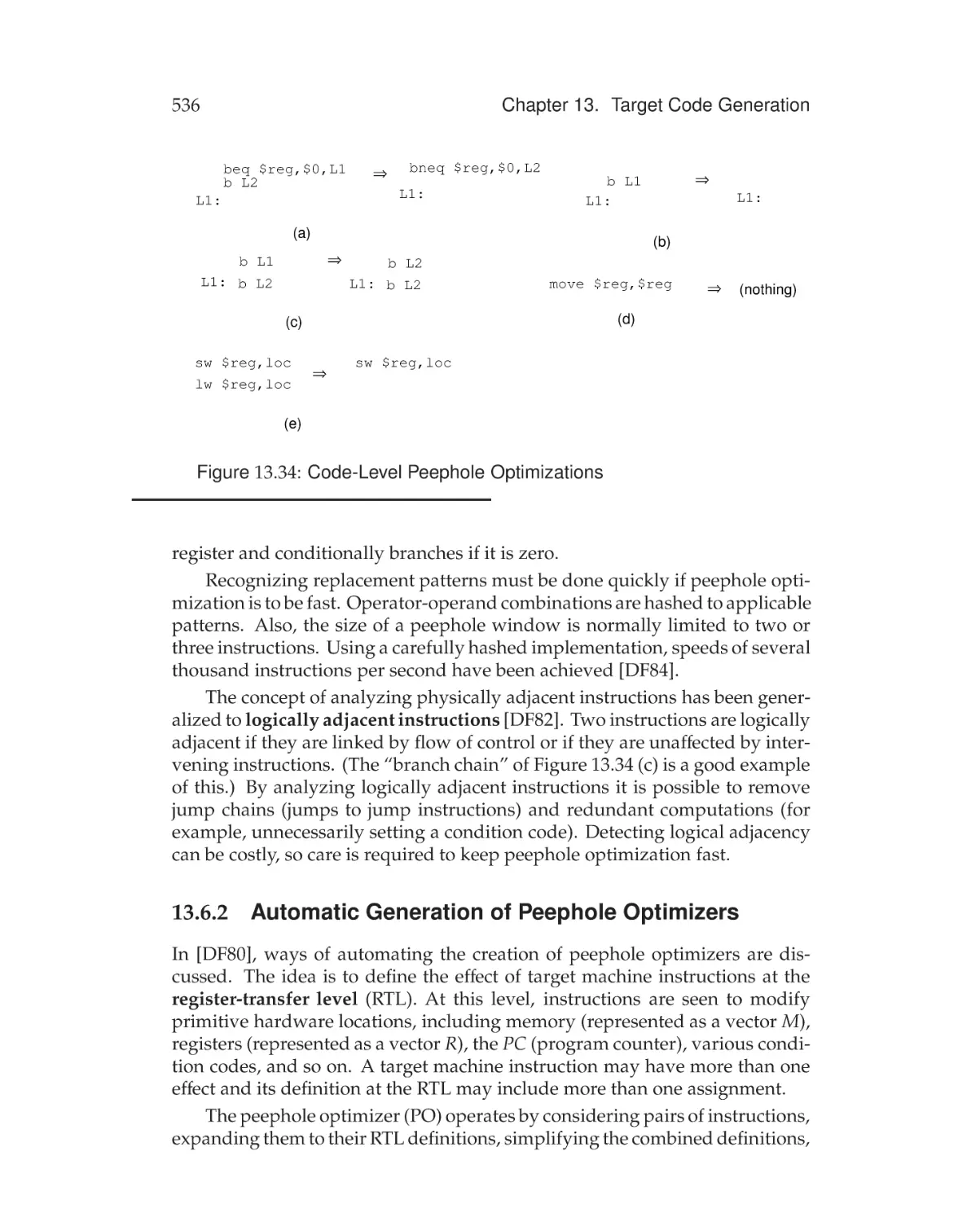
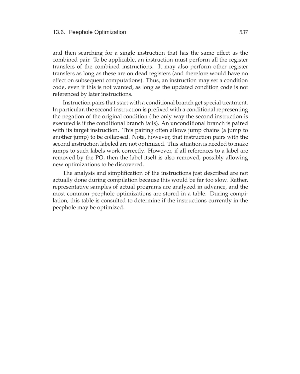
13.6 Peephole Optimization . . . . . . . . . . . . . . . . . .
13.6.1 Levels of Peephole Optimization . . . . . . . .
13.6.2 Automatic Generation of Peephole Optimizers
Exercises . . . . . . . . . . . . . . . . . . . . . . . . . . . .
.
.
.
.
.
.
.
.
.
.
457
460
460
465
468
468
471
472
479
482
489
.
.
.
.
.
.
.
.
.
.
.
.
.
.
.
.
.
.
.
.
.
.
.
.
.
.
.
.
.
.
.
.
.
.
.
.
.
.
.
.
.
.
.
.
.
.
.
.
.
.
.
.
.
.
.
.
.
.
.
.
.
.
.
.
.
.
.
.
.
.
.
.
.
.
.
.
.
.
.
.
.
.
.
.
.
.
.
.
.
.
.
.
.
.
.
.
.
.
.
.
.
.
.
.
.
.
.
.
.
.
490
493
493
496
498
501
505
506
508
516
517
519
523
524
526
529
531
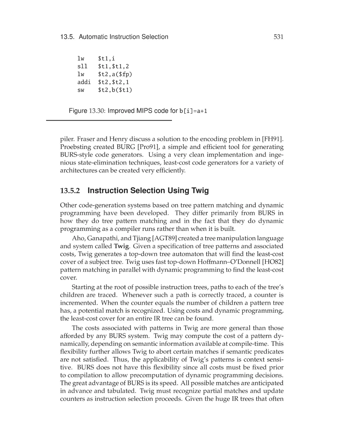
532
532
533
536
538
xxvi
Contents
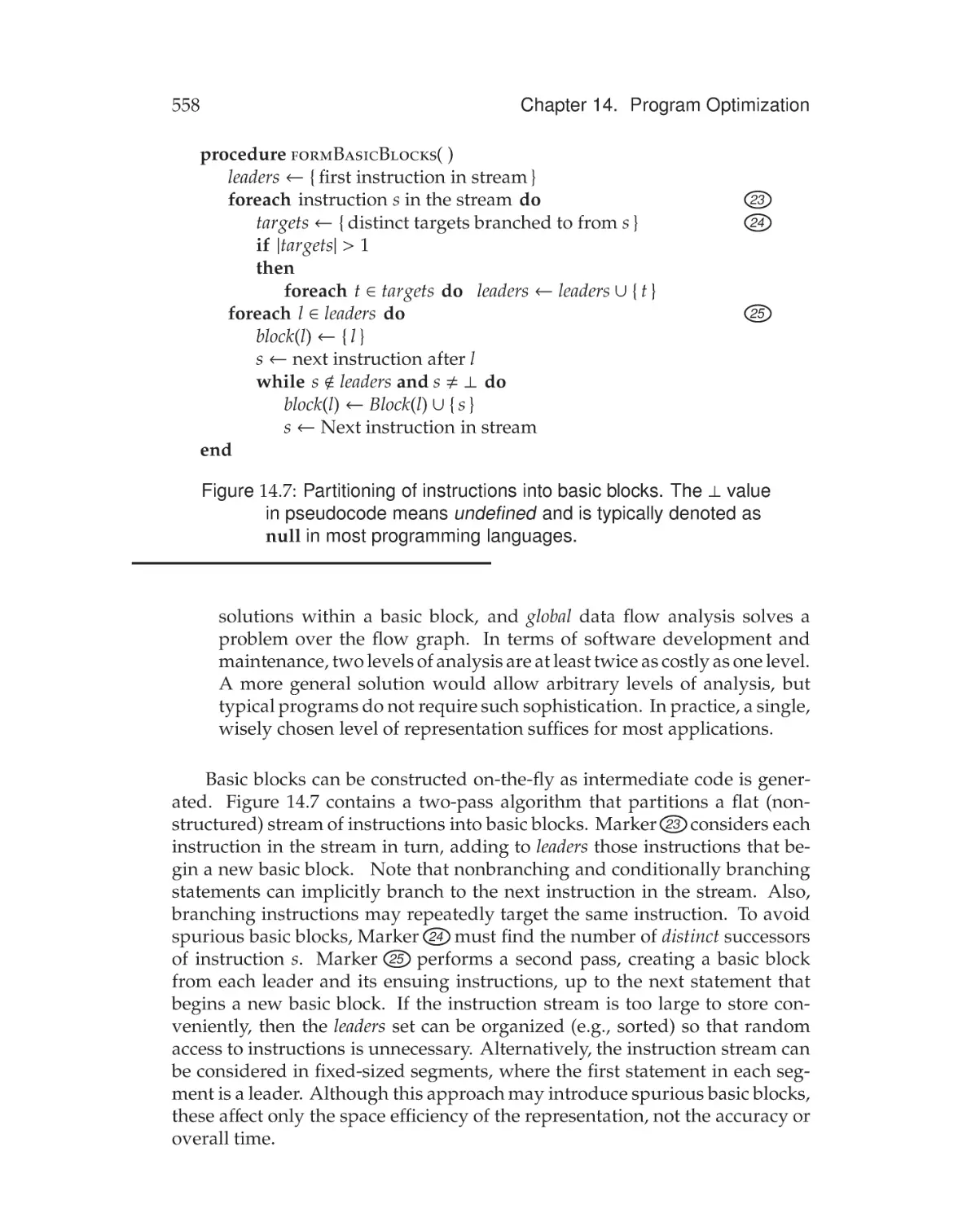
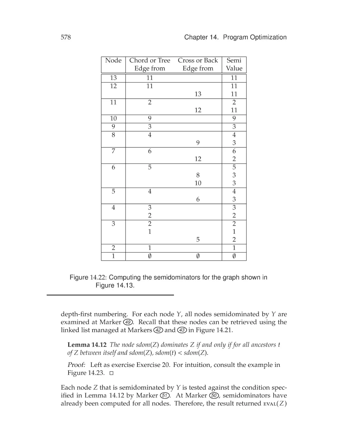
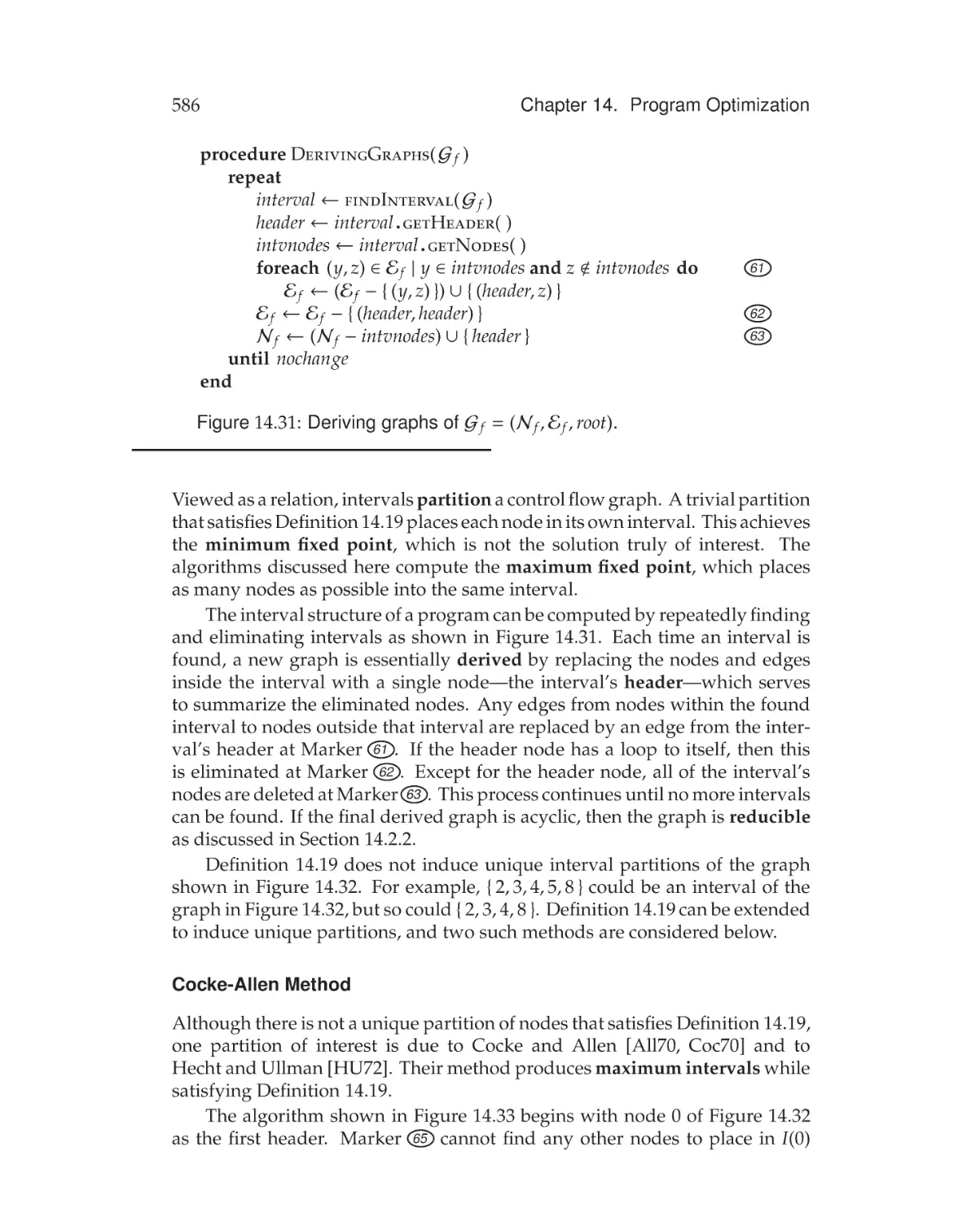
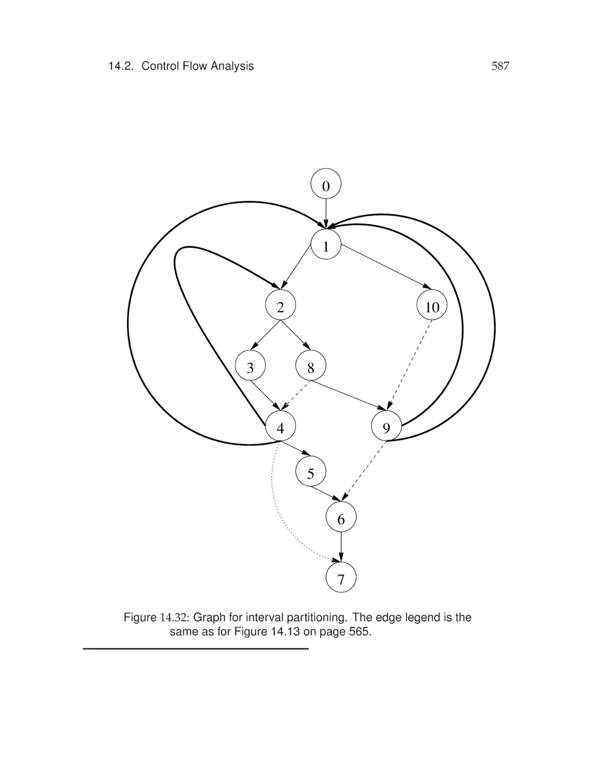
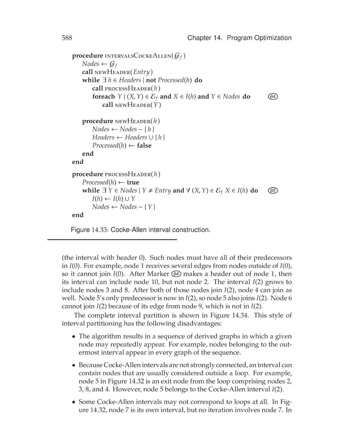
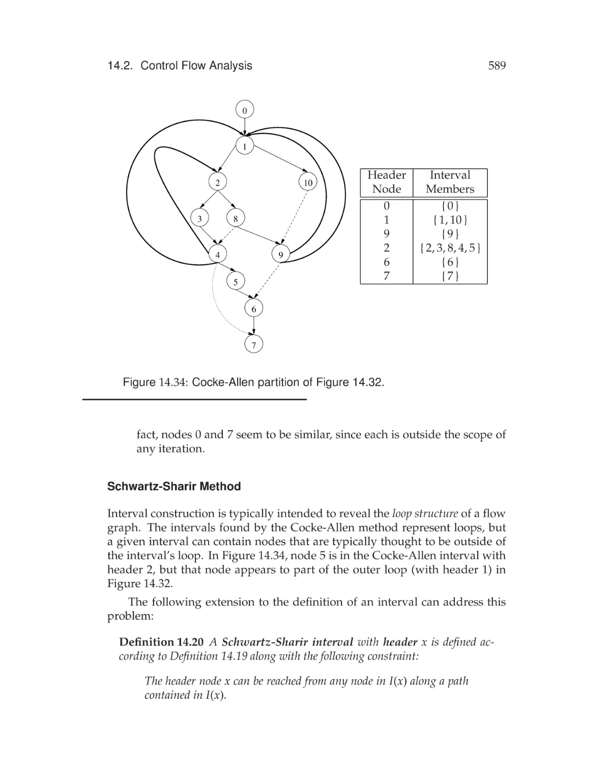
14 Program Optimization
547
14.1 Overview . . . . . . . . . . . . . . . . . . . . . . . . . . . . . . . 548
14.1.1 Why Optimize? . . . . . . . . . . . . . . . . . . . . . . . 549
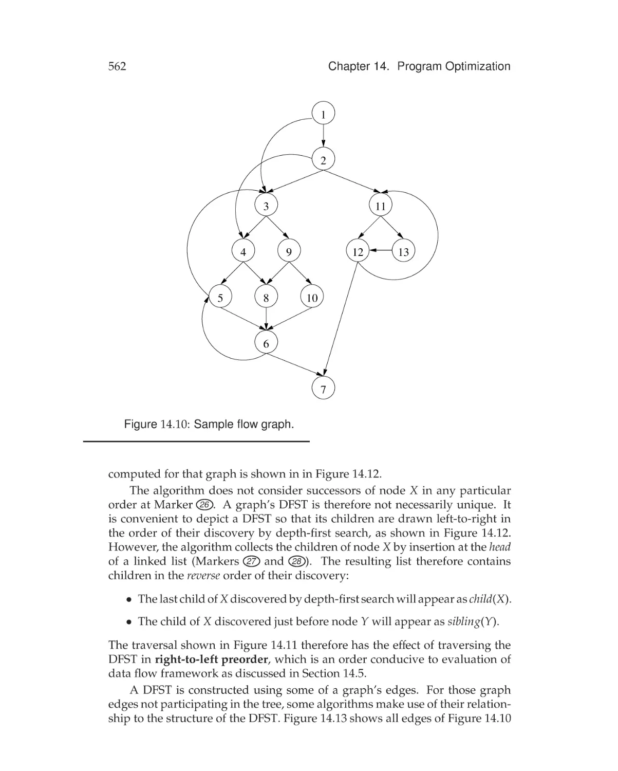
14.2 Control Flow Analysis . . . . . . . . . . . . . . . . . . . . . . . 555
14.2.1 Control Flow Graphs . . . . . . . . . . . . . . . . . . . . 556
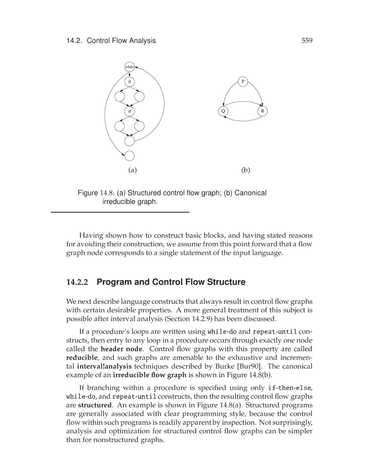
14.2.2 Program and Control Flow Structure . . . . . . . . . . . 559
14.2.3 Direct Procedure Call Graphs . . . . . . . . . . . . . . 560
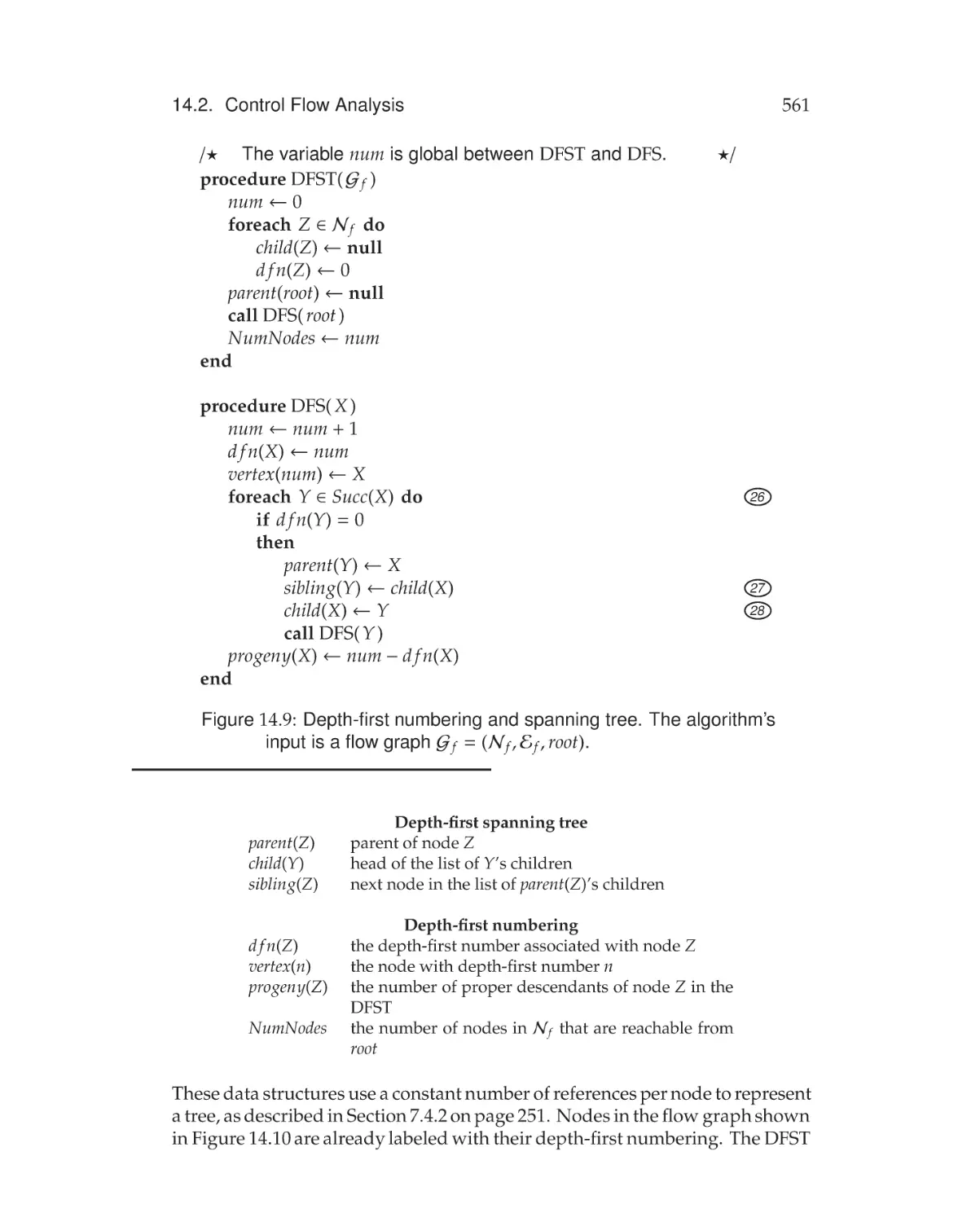
14.2.4 Depth-First Spanning Tree . . . . . . . . . . . . . . . . 560
14.2.5 Dominance . . . . . . . . . . . . . . . . . . . . . . . . . 565
14.2.6 Simple Dominance Algorithm . . . . . . . . . . . . . . . 567
14.2.7 Fast Dominance Algorithm . . . . . . . . . . . . . . . . 571
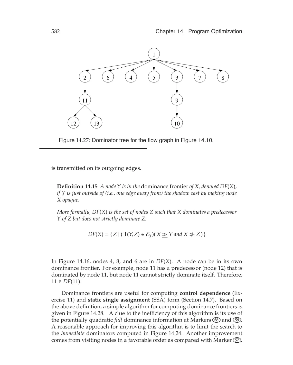
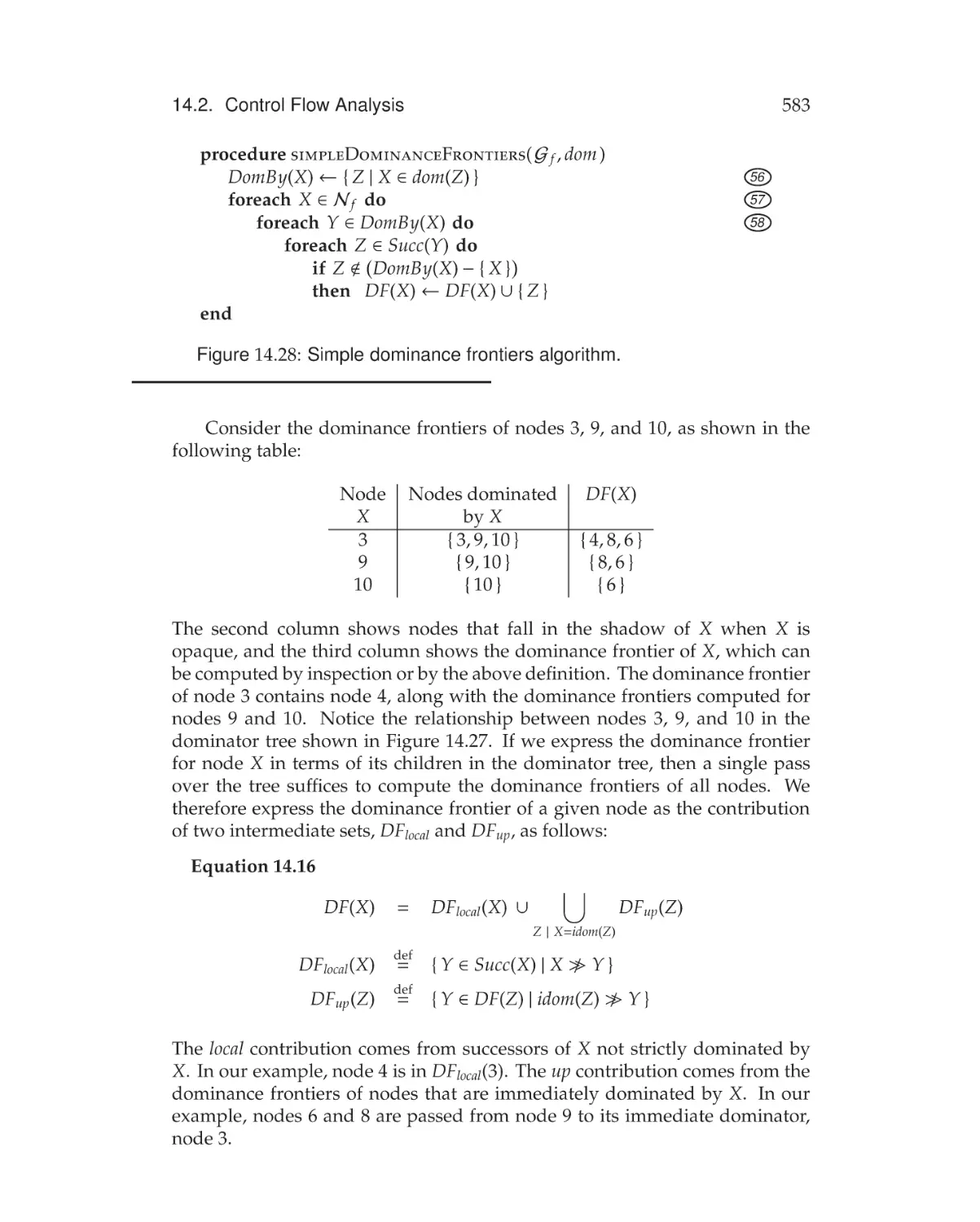
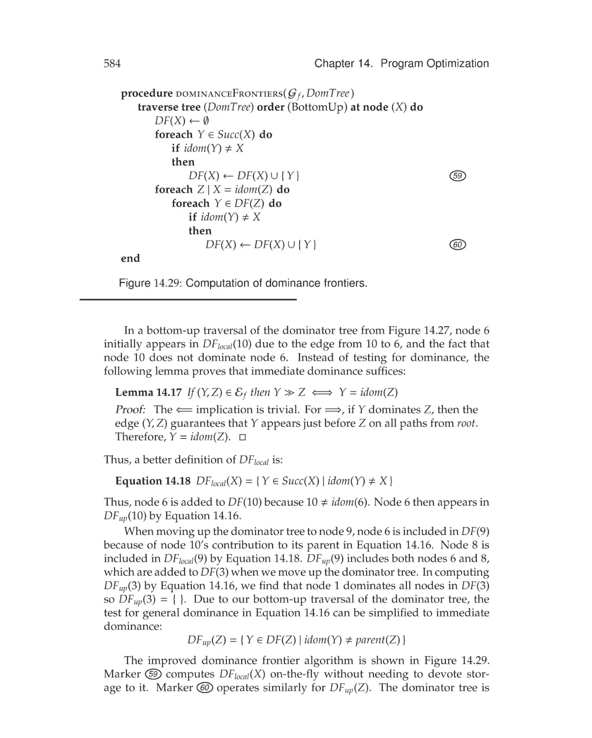
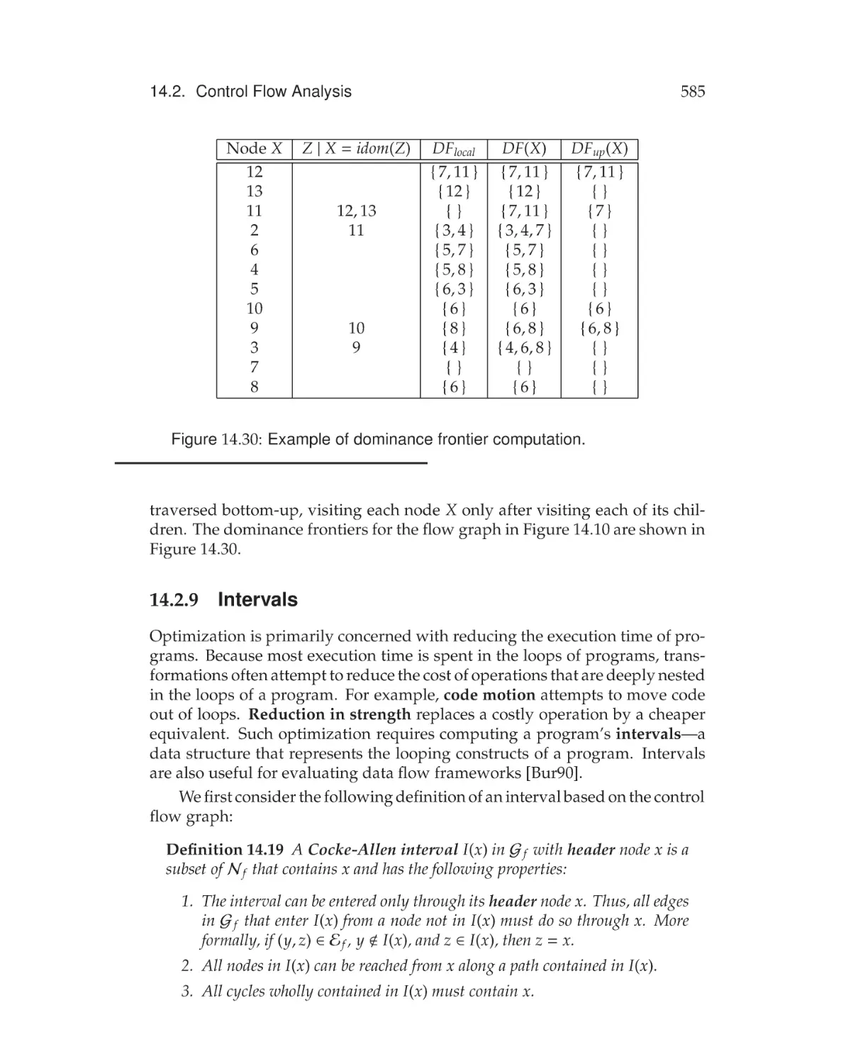
14.2.8 Dominance Frontiers . . . . . . . . . . . . . . . . . . . . 581
14.2.9 Intervals . . . . . . . . . . . . . . . . . . . . . . . . . . . 585
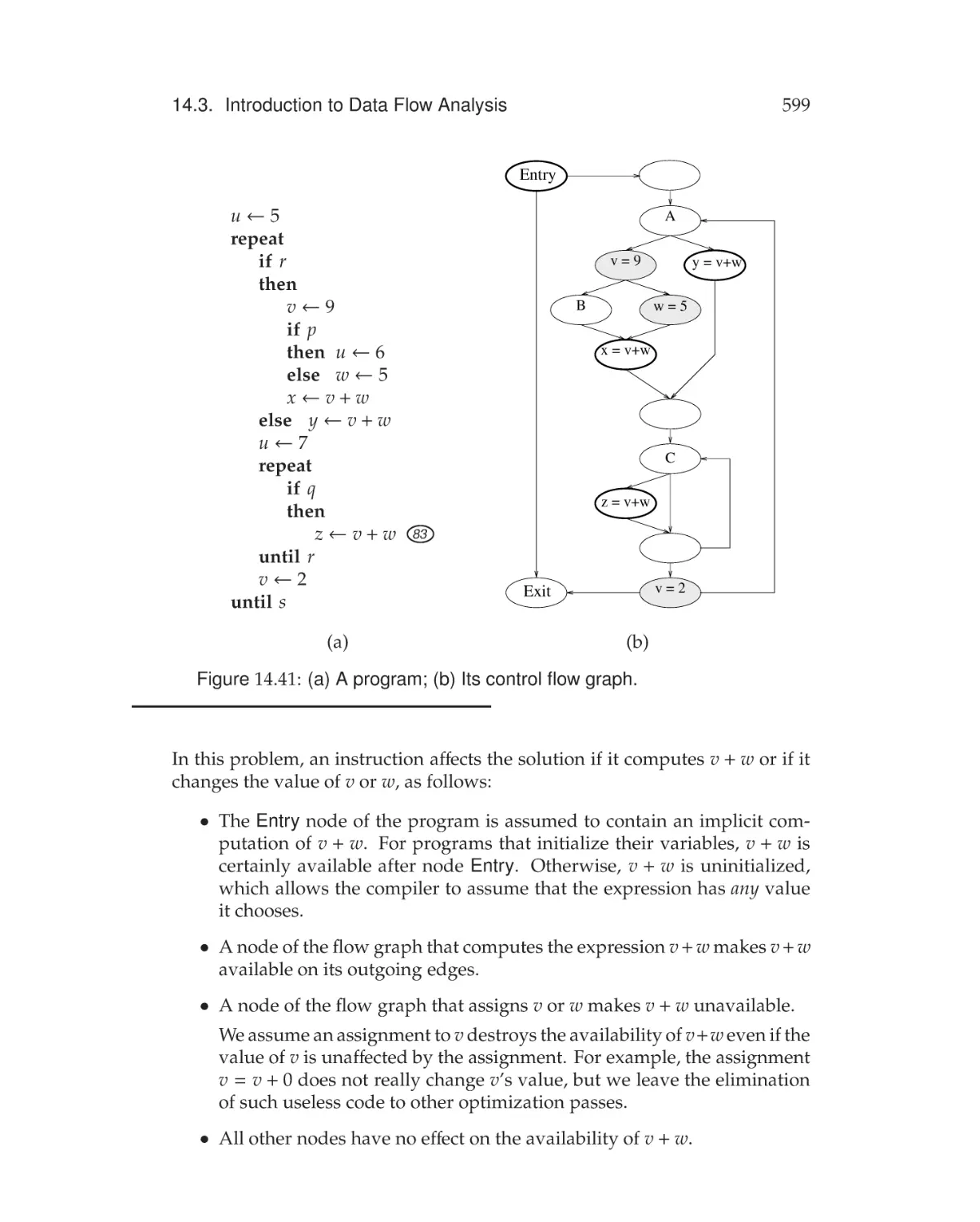
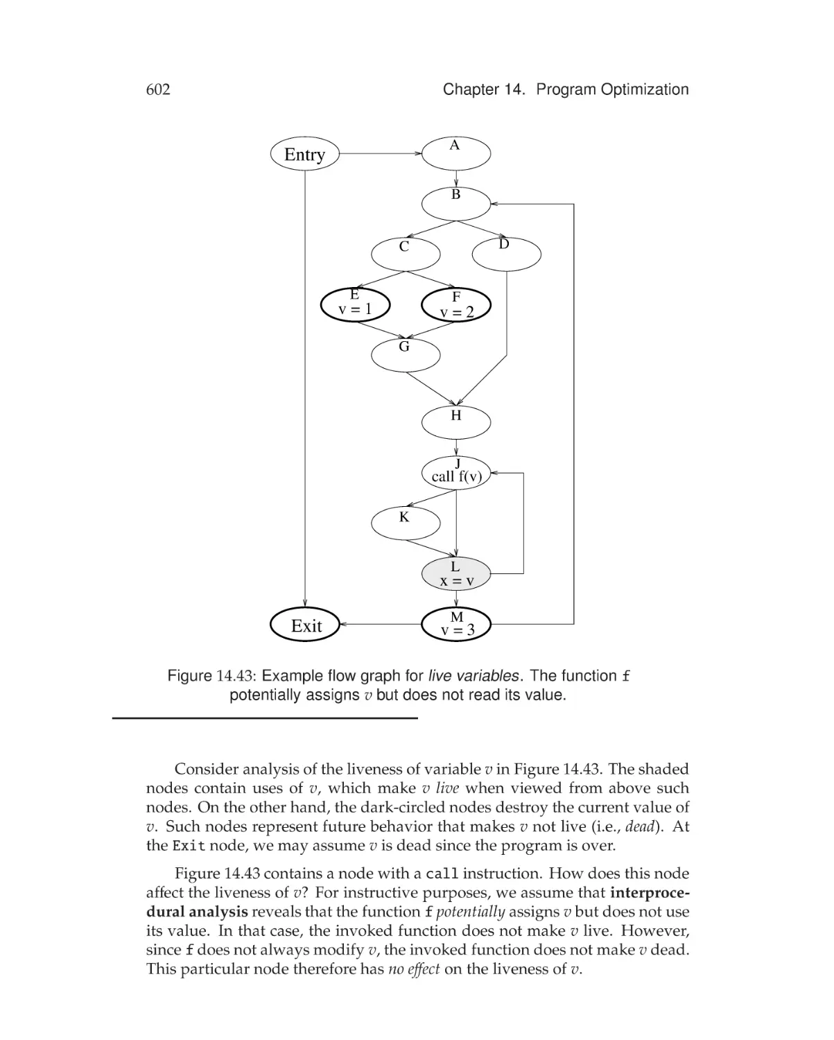
14.3 Introduction to Data Flow Analysis . . . . . . . . . . . . . . . . 598
14.3.1 Available Expressions . . . . . . . . . . . . . . . . . . . 598
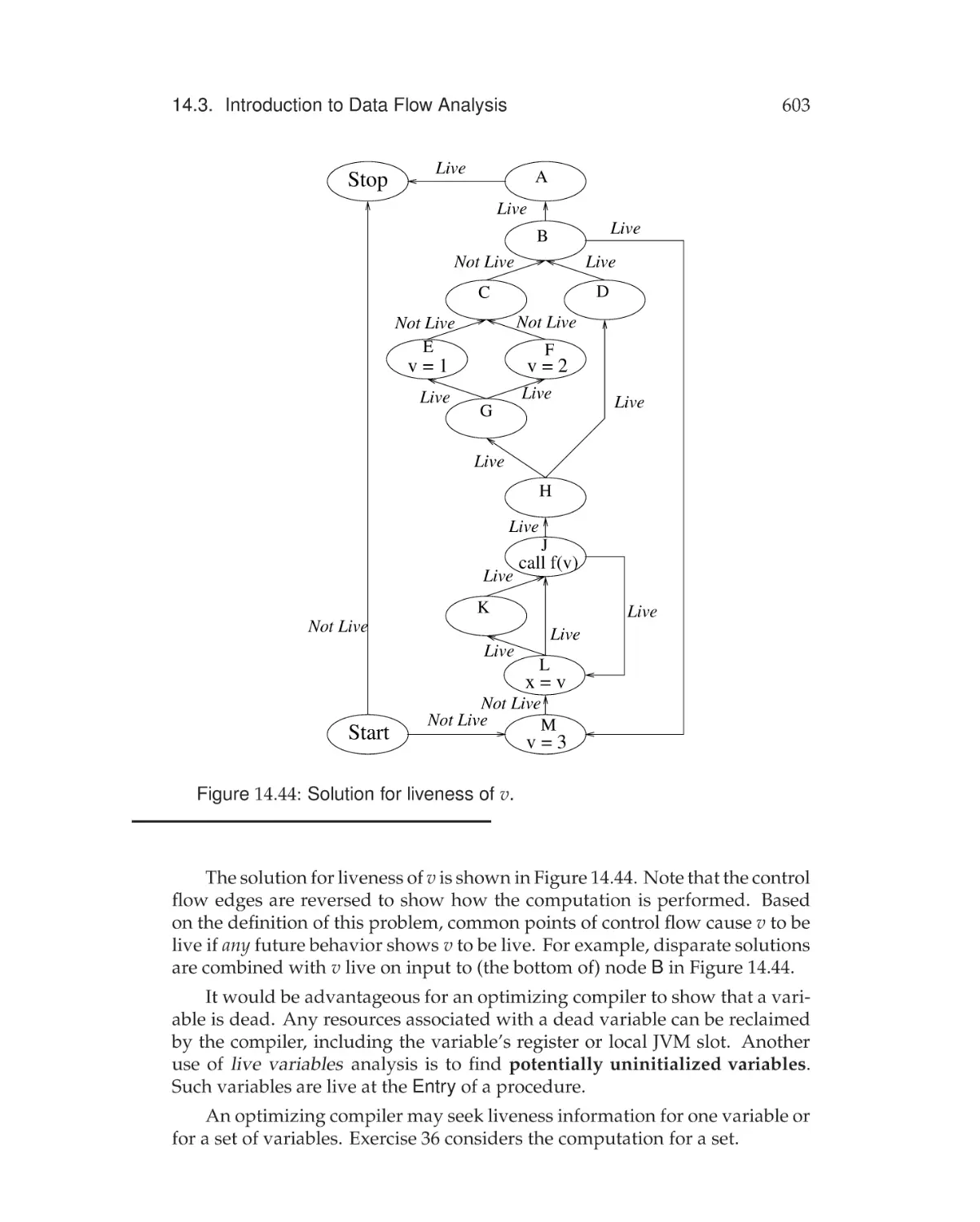
14.3.2 Live Variables . . . . . . . . . . . . . . . . . . . . . . . . 601
14.4 Data Flow Frameworks . . . . . . . . . . . . . . . . . . . . . . . 604
14.4.1 Data Flow Evaluation Graph . . . . . . . . . . . . . . . 604
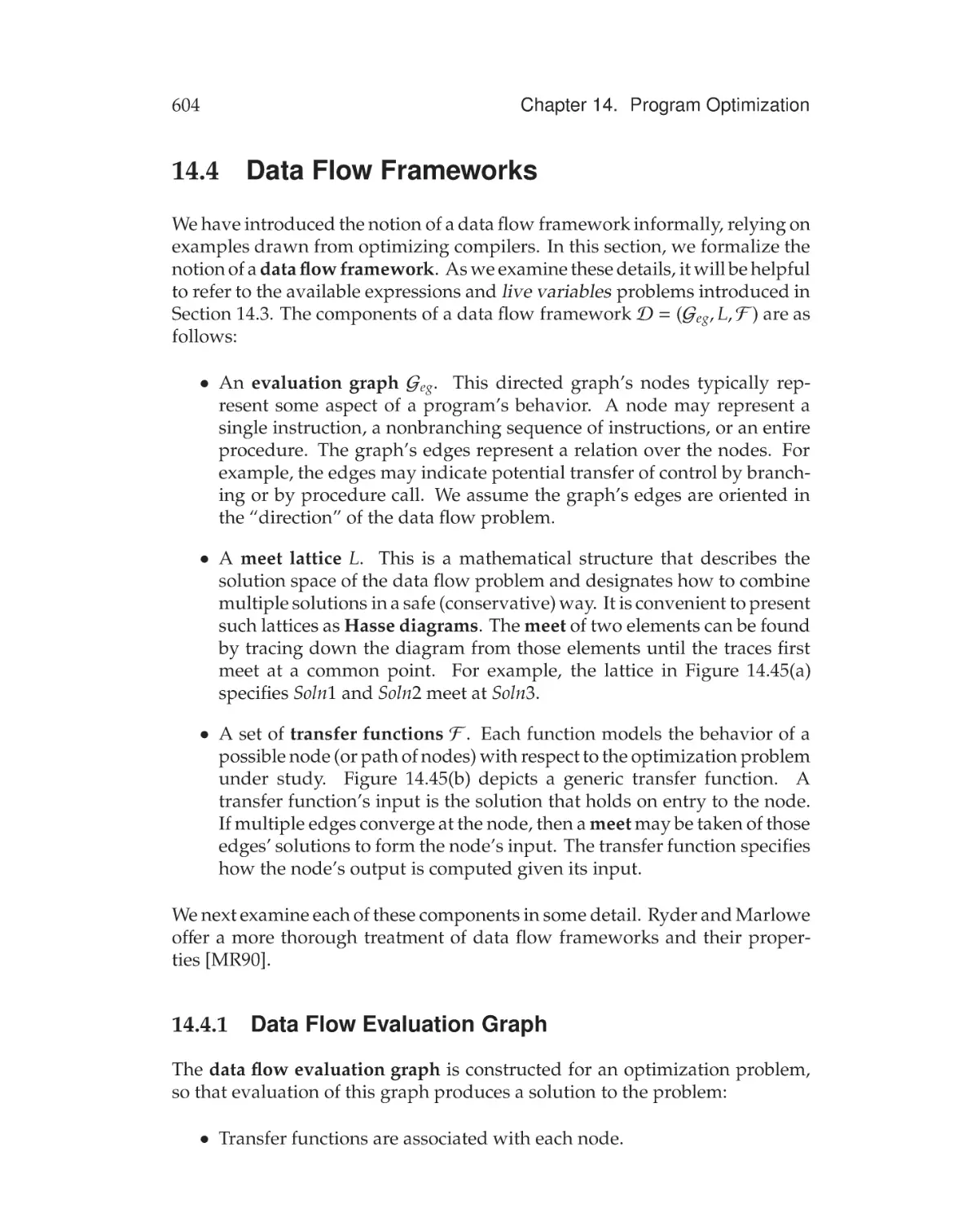
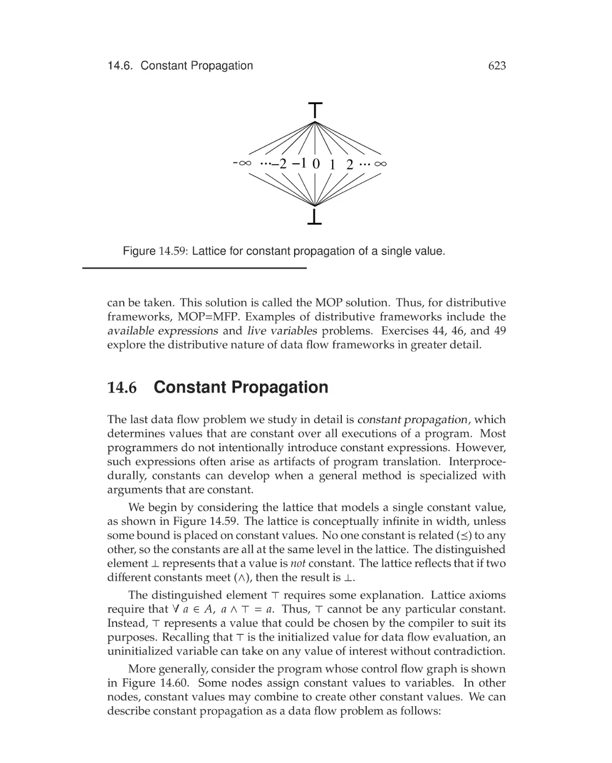
14.4.2 Meet Lattice . . . . . . . . . . . . . . . . . . . . . . . . . 606
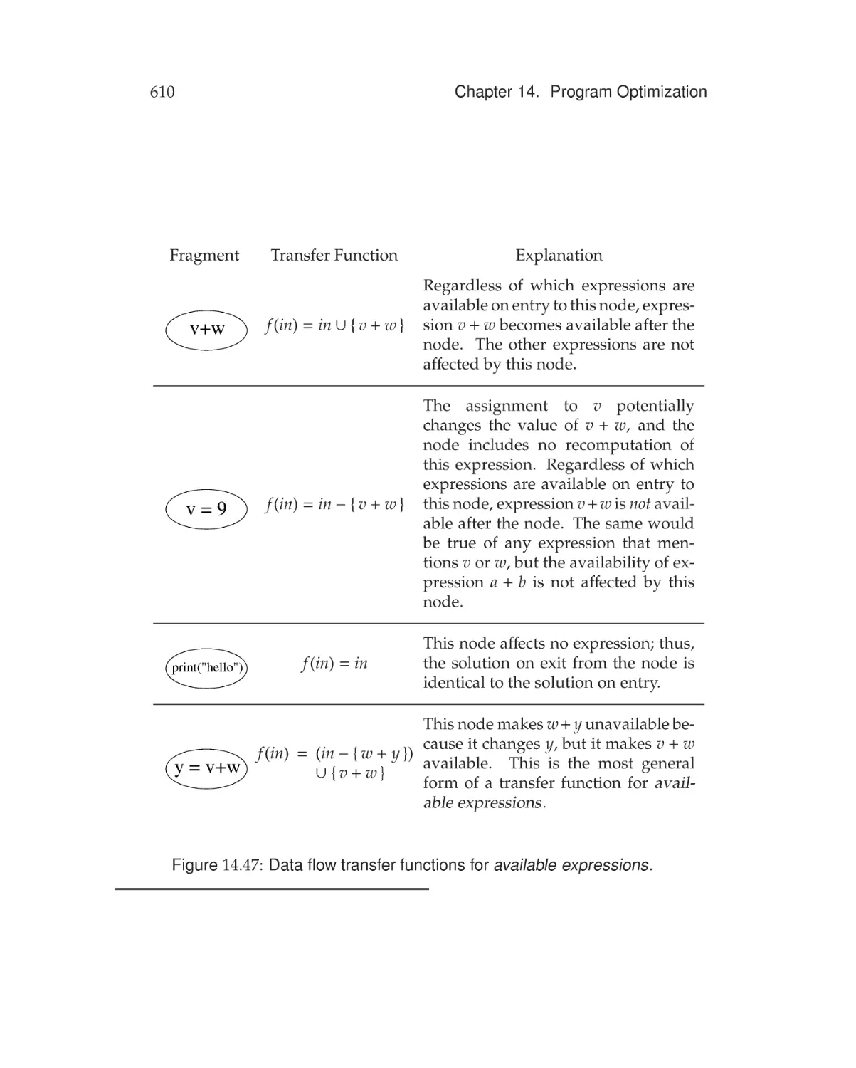
14.4.3 Transfer Functions . . . . . . . . . . . . . . . . . . . . . 608
14.5 Evaluation . . . . . . . . . . . . . . . . . . . . . . . . . . . . . . 611
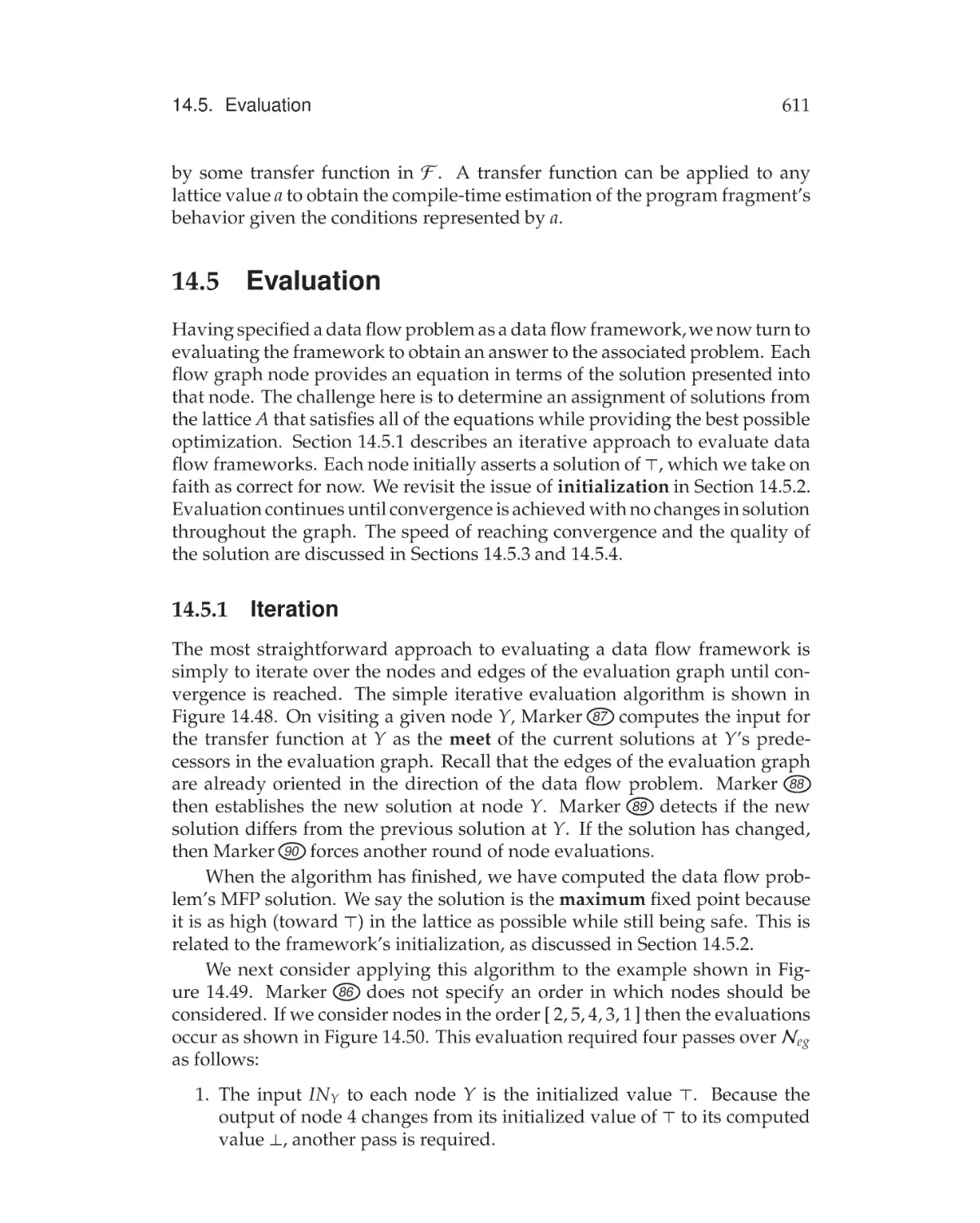
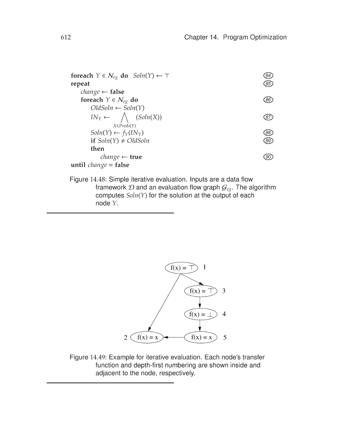
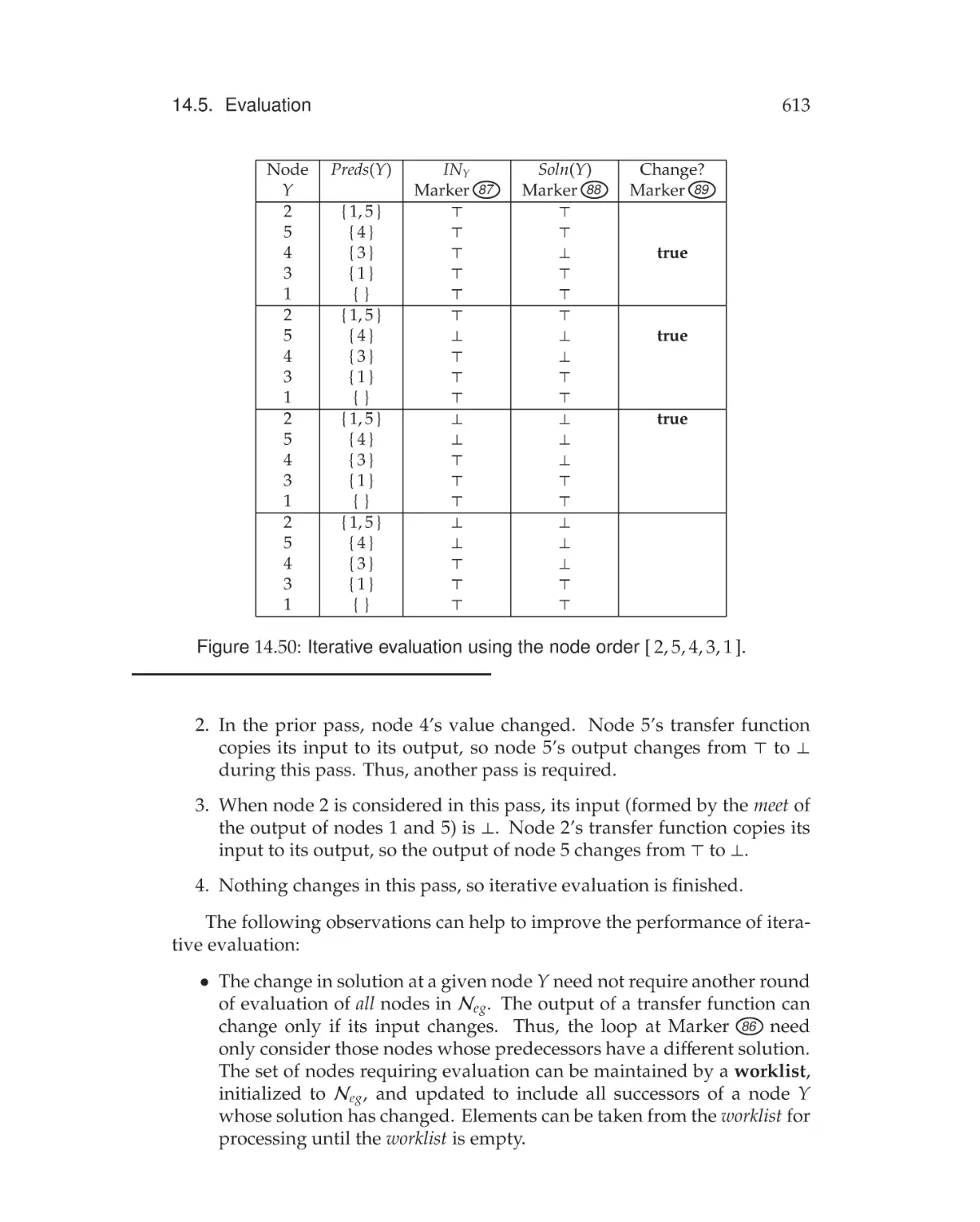
14.5.1 Iteration . . . . . . . . . . . . . . . . . . . . . . . . . . . 611
14.5.2 Initialization . . . . . . . . . . . . . . . . . . . . . . . . . 615
14.5.3 Termination and Rapid Frameworks . . . . . . . . . . . 616
14.5.4 Distributive Frameworks . . . . . . . . . . . . . . . . . . 620
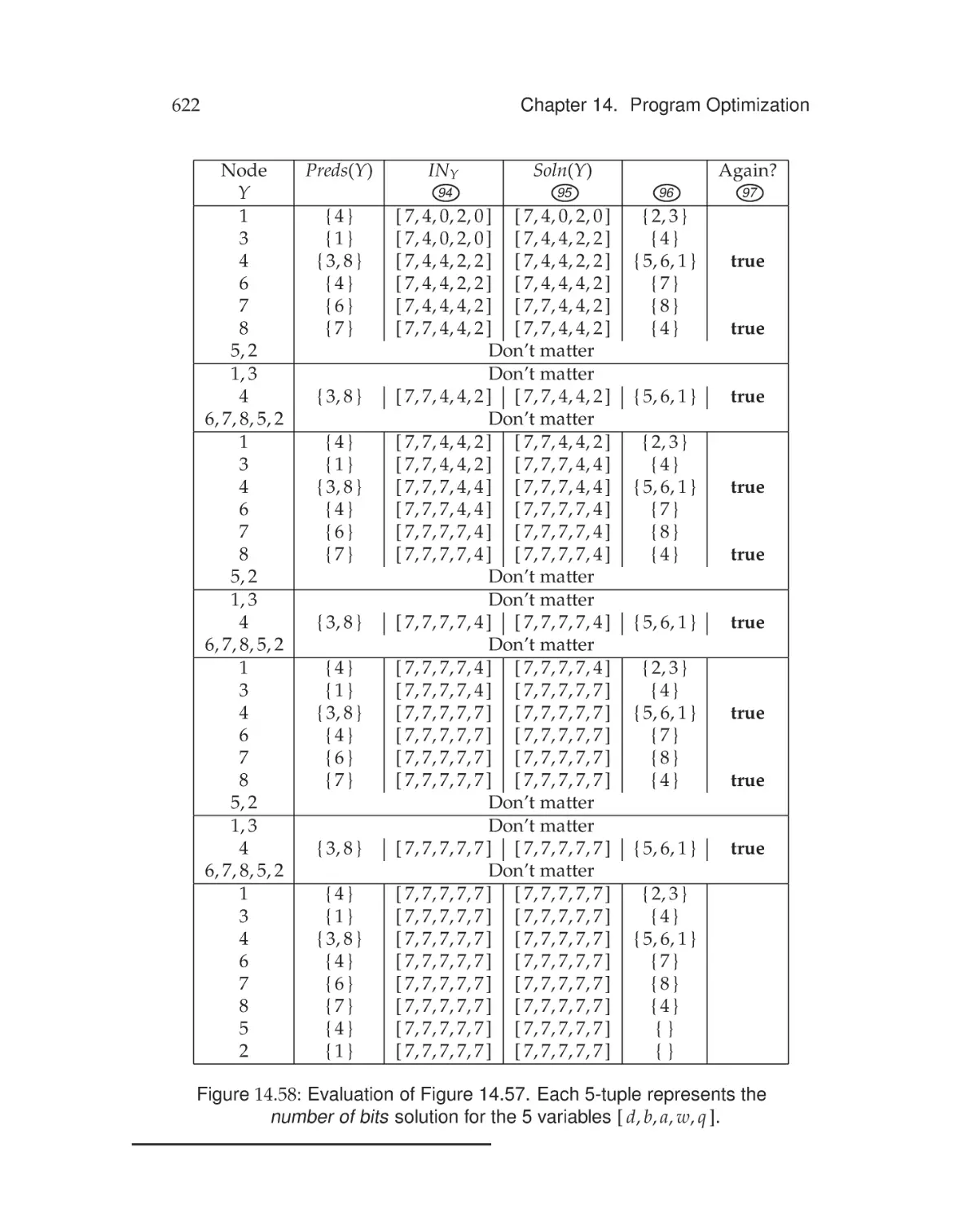
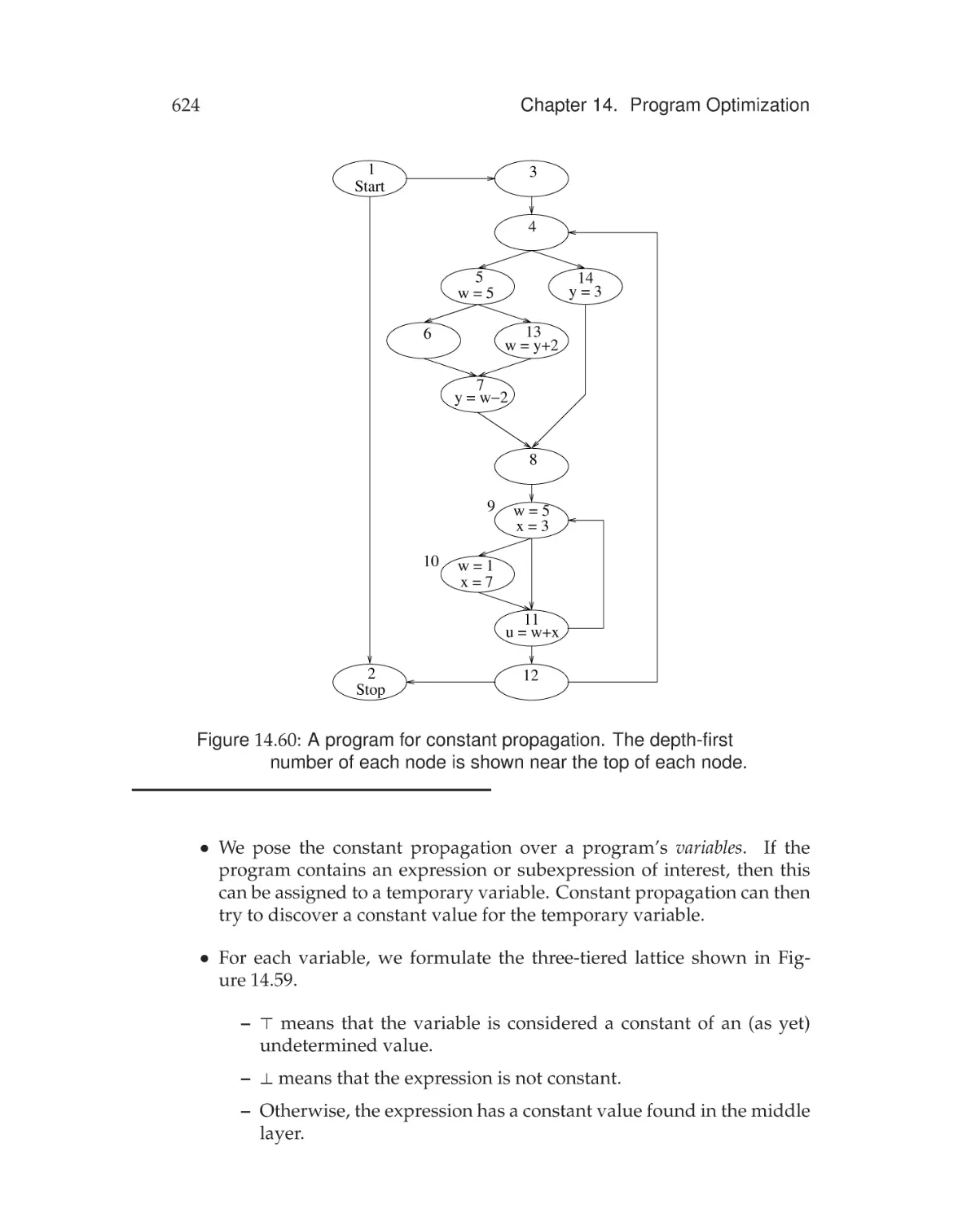
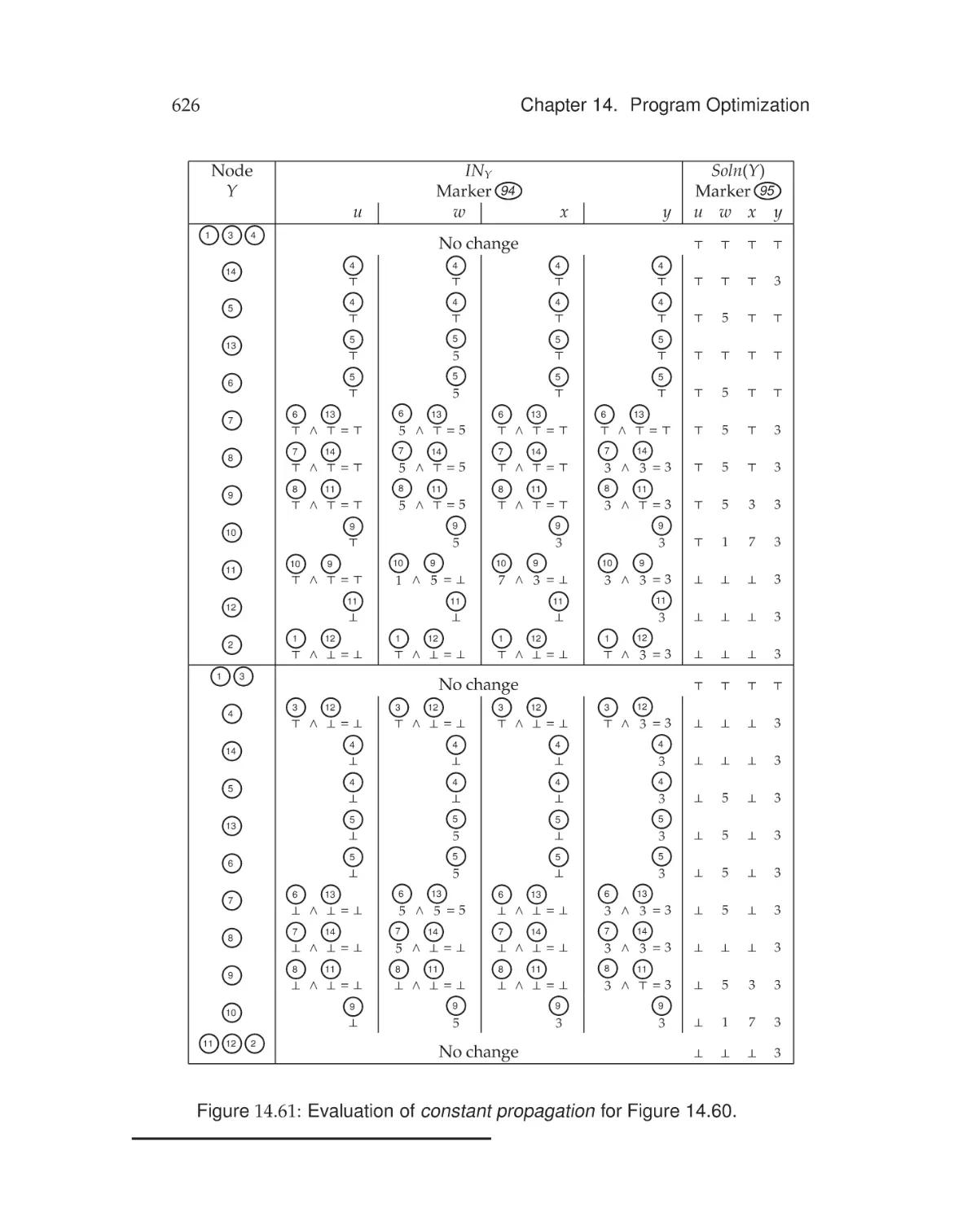
14.6 Constant Propagation . . . . . . . . . . . . . . . . . . . . . . . 623
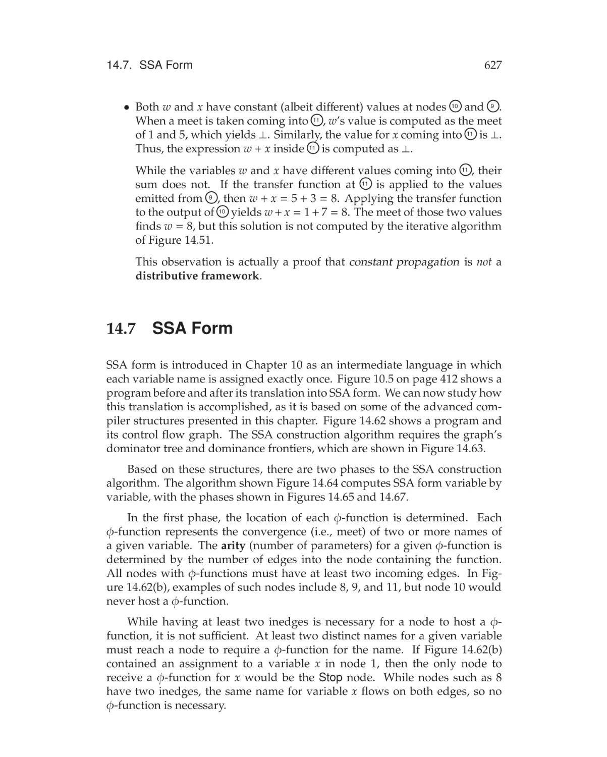
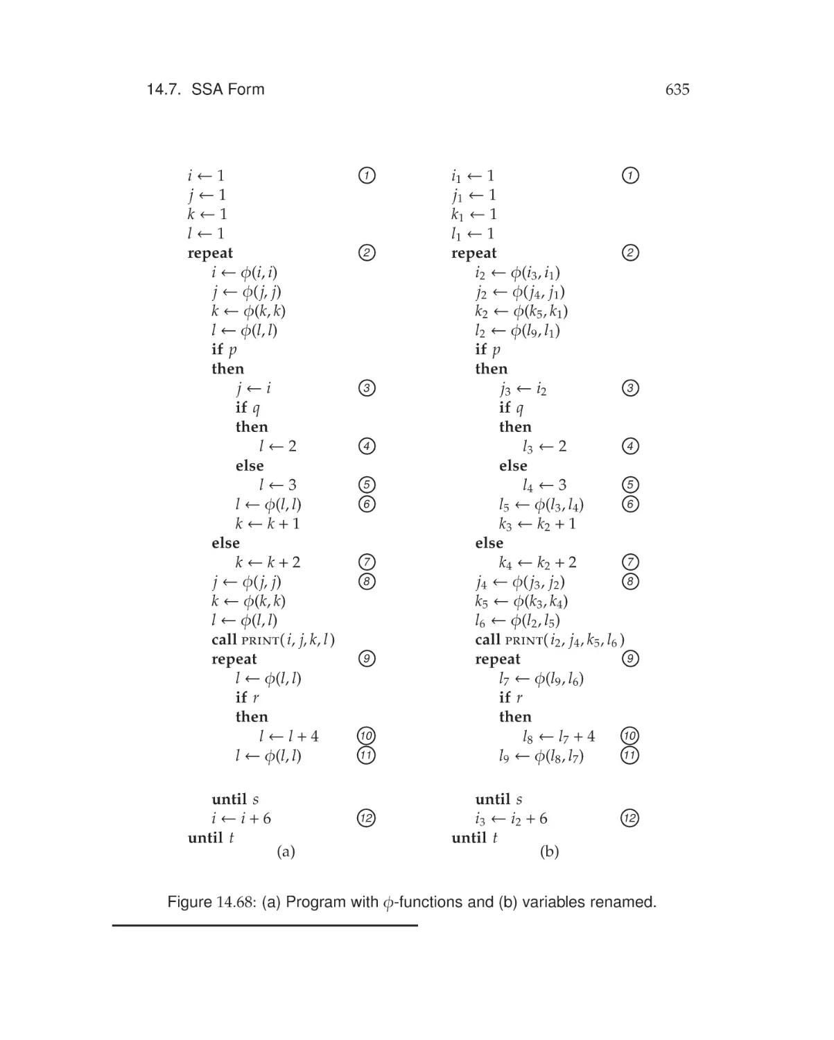
14.7 SSA Form . . . . . . . . . . . . . . . . . . . . . . . . . . . . . . 627
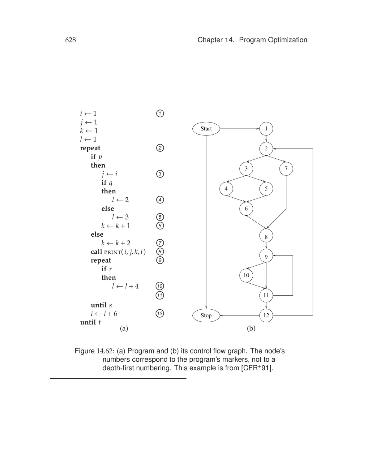
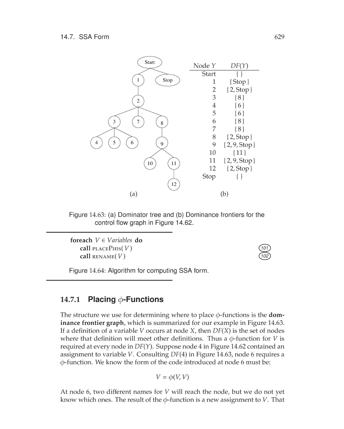
14.7.1 Placing φ-Functions . . . . . . . . . . . . . . . . . . . . 629
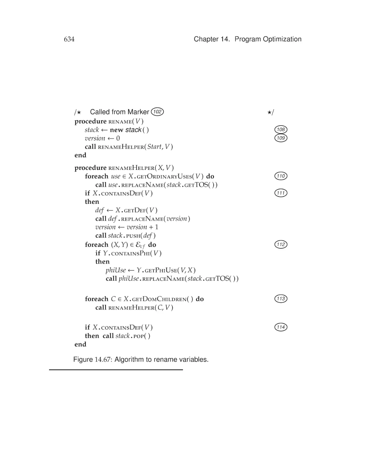
14.7.2 Renaming . . . . . . . . . . . . . . . . . . . . . . . . . . 631
Exercises . . . . . . . . . . . . . . . . . . . . . . . . . . . . . . . . . 636
Contents
xxvii
Bibliography
651
Abbreviations
661
Pseudocode Guide
663
Index
667
This page intentionally left blank
1
Introduction
This chapter presents the history of compiler construction and an overview
of compiler organization. Compilers have tracked and even precipitated the
phenomenal gains in computing speed that have accrued in the relatively
short history of computer science. Section 1.1 presents a historical review
of the development and evolution of the programming languages, computer
architectures, and compilers that are in widespread use today.
The general area we study is language processing, which is concerned
with preparing a program to be run on a computer. Most programs are written in a relatively high-level language. Language processors ensure that a
program conforms to its programming language’s specification, and they often translate the program into a form that is easier to run on a computer. Some
language processors perform more translation than others. At one extreme, an
interpreter runs a program by examining its high-level constructs and simulating their actions. At the other extreme, a compiler translates the high-level
constructs into low-level machine instructions that can be executed directly by
a computer. The differences between compilers and interpreters are discussed
in Section 1.3.
From there, we explain in Section 1.2 what a compiler does and how various compilers can be distinguished from each other: by the kind of machine
code they generate and by the format of the target code they generate.
In Section 1.3, we discuss a kind of language processor called an interpreter and explain how an interpreter differs from a compiler. Section 1.4
discusses the syntax (structure) and semantics (meaning) of programs. Next,
1
2
Chapter 1. Introduction
Programming
Language
Compiler
Machine
Language
Figure 1.1: A user’s view of a compiler.
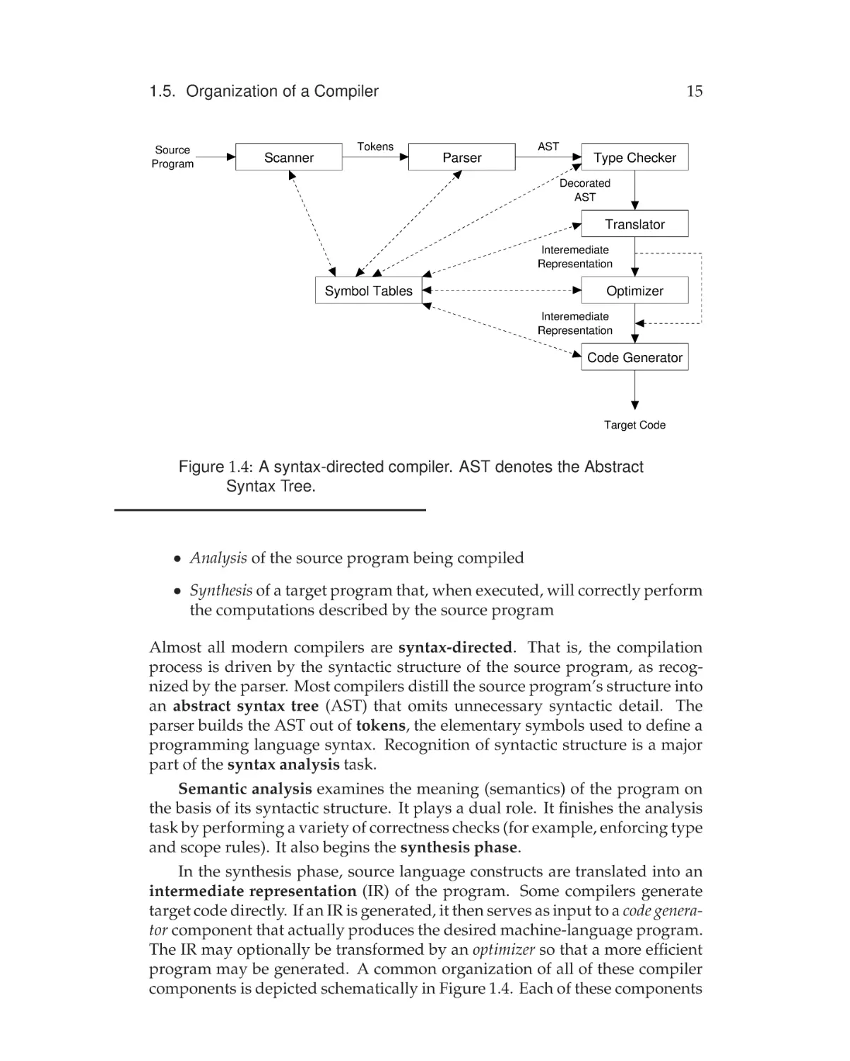
in Section 1.5, we discuss the tasks that a compiler must perform, primarily
analysis of the source program and synthesis of a target program. That section
also covers the parts of a compiler, discussing each in some detail: scanner,
parser, type checker, optimizer and code generator.
In Section 1.6, we discuss the mutual interaction of compiler design and
programming language design. Similarly, in Section 1.7, the influence of
computer architecture on compiler design is covered.
Section 1.8 introduces a number of important compiler variants, including debugging and development compilers, optimizing compilers, and retargetable
compilers. Finally, in Section 1.9, we consider program development environments
that integrate a compiler, editor, and debugger into a single tool.
1.1 History of Compilation
Compilers are fundamental to modern computing. They act as translators,
transforming human-oriented programming languages into computer-oriented machine languages. For most users, a compiler can be viewed as a utility
that performs the transformation illustrated in Figure 1.1. A compiler allows virtually all computer users to ignore the machine-dependent details of
machine language. Therefore, compilers allow programs and programming
expertise to be portable across a wide variety of computers. This is a particularly valuable capability in an age where the cost of software development is so
high and the need for software exists at so many levels, from small embedded
computers to extreme-scale supercomputers.
The term compiler was coined in the early 1950s by Grace Murray Hopper.
Translation was then viewed as the compilation of a sequence of machinelanguage subprograms selected from a library. At that time, compilation was
called automatic programming and there was almost universal skepticism that
it would ever be successful. Today, the automatic translation of programming
languages is an accomplished fact, but programming language translators are
still called compilers.
Among the first real compilers in the modern sense were the Fortran compilers of the late 1950s. They presented the user with a problem-oriented,
largely machine-independent source language. They also performed some
1.1. History of Compilation
3
rather ambitious optimizations to produce efficient machine code, since efficient code was deemed essential for Fortran to compete successfully against
assembly language programming. Machine-independent languages such as
Fortran proved the viability of high-level compiled languages. They paved
the way for the flood of languages and compilers that was to follow.
In the early days, compilers were ad hoc structures; components and
techniques were often devised as a compiler was built. This approach to
constructing compilers lent an aura of mystery to them, and they were viewed
as complex and costly. Today the compilation process is well understood
and compiler construction is routine. Nonetheless, crafting an efficient and
reliable compiler is still a complex task. This book’s primary task is to teach a
mastery of the fundamentals. A concomitant goal is to cover some advanced
techniques and important innovations.
Compilers normally translate conventional programming languages like
JavaTM, C, and C++ into executable machine-language instructions. Compiler technology, however, is far more broadly applicable and has been employed in rather unexpected areas. For example, text-formatting languages like
TeX [Knu98] and LaTeX [Lam95] are really compilers. They translate text and
R
[Pos]
formatting commands into detailed typesetting commands. PostScript
on the other hand, which is generated by many programs, is really a programming language. It is translated and executed by printers and document previewers to produce a readable form of a document. This standardized document-representation language allows documents to be freely
interchanged, independently of how they were created and how they will be
viewed.
Mathematica [Wol99] is an interactive system that intermixes programming with mathematics, solving intricate problems in both symbolic and numeric forms. This system relies heavily on compiler techniques to handle the
specification, internal representation, and solution of problems.
Languages like Verilog [TM08] and VHDL [VHD] address the creation of
very large scale integration (VLSI) circuits. A silicon compiler specifies the
layout and composition of a VLSI circuit mask using standard cell designs. Just
as an ordinary compiler must understand and enforce the rules of a particular
machine language, so must a silicon compiler understand and enforce the
design rules that dictate the feasibility of a given circuit.
Compiler technology is of value in almost any program that presents a
nontrivial text-oriented command set, including the command and scripting
languages of operating systems and the query languages of database systems.
Thus, while our discussion will focus on traditional compilation tasks, innovative readers will undoubtedly find new and unexpected applications for the
techniques presented.
4
Chapter 1. Introduction
1.2 What Compilers Do
Figure 1.1 represents a compiler as a translator of the programming language
being compiled (the source) to some machine language (the target). This description suggests that all compilers do about the same thing, the only difference being their choice of source and target languages. However, the situation
is a bit more complicated. While the issue of the accepted source language is
indeed simple, there are many alternatives in describing the output of a compiler. These go beyond simply naming a particular target computer. Compilers
may be distinguished in two ways:
• By the kind of machine code they generate
• By the format of the target code they generate
These are discussed in the following sections.
1.2.1 Machine Code Generated by Compilers
Compilers may generate any of three types of code by which they can be
differentiated:
• Pure Machine Code
• Augmented Machine Code
• Virtual Machine Code
Pure Machine Code
Compilers may generate code for a particular machine’s instruction set without assuming the existence of any operating system or library routines. Such
machine code is often called pure code because it includes nothing but instructions that are part of that instruction set. This approach is rare because most
compilers rely on runtime libraries and operating system calls to interface with
the generated code. Pure machine code is most commonly used in compilers
for system implementation languages, which are intended for implementing
operating systems or embedded applications. This form of target code can
execute on bare hardware without dependence on any other software.
1.2. What Compilers Do
5
Augmented Machine Code
Far more often, compilers generate code for a machine architecture that is
augmented with operating system routines and runtime language support
routines. The execution of a program generated by such a compiler requires
that a particular operating system be present on the target machine and a
collection of language-specific runtime support routines (I/O, storage allocation, mathematical functions, etc.) be available to the program. Most Fortran
compilers use such software support only for I/O and mathematical functions.
Other compilers assume a much larger range of available functionality. These
may include data transfer instructions (such as, to move bit fields), procedure
call instructions (to pass parameters, save registers, allocate stack space, etc.),
and dynamic storage instructions (to provide for heap allocation).
Virtual Machine Code
The third type of code generated is composed entirely of virtual instructions.
This approach is particularly attractive as a technique for producing code
that can be run easily on a variety of computers. This level of portability
is achieved by writing an interpreter for the virtual machine (VM) on any
target architecture of interest. Code generated by the compiler can then be
run on any architecture for which a VM interpreter is available. Java is an
example of a language for which a VM (the Java Virtual Machine (JVM)
and its bytecode instructions) was defined to accompany the language. Java
applications produce predictable results on any computer for which a JVM
interpreter is available. Similarly, Java applets can be run in any web browser
provisioned with a JVM interpreter.
The advantages of portability obtained by using a VM instruction set can
also make the compiler itself easy to port. For the purposes of this discussion,
assume that the compiler accepts some source language L. Any instance of
this compiler can translate a program written in L into the VM instructions.
If the compiler itself is written in L, then the compiler can compile itself into
VM instructions, which can be executed on any architecture that hosts the VM
interpreter. If the VM is kept simple and clean, the interpreter can be relatively
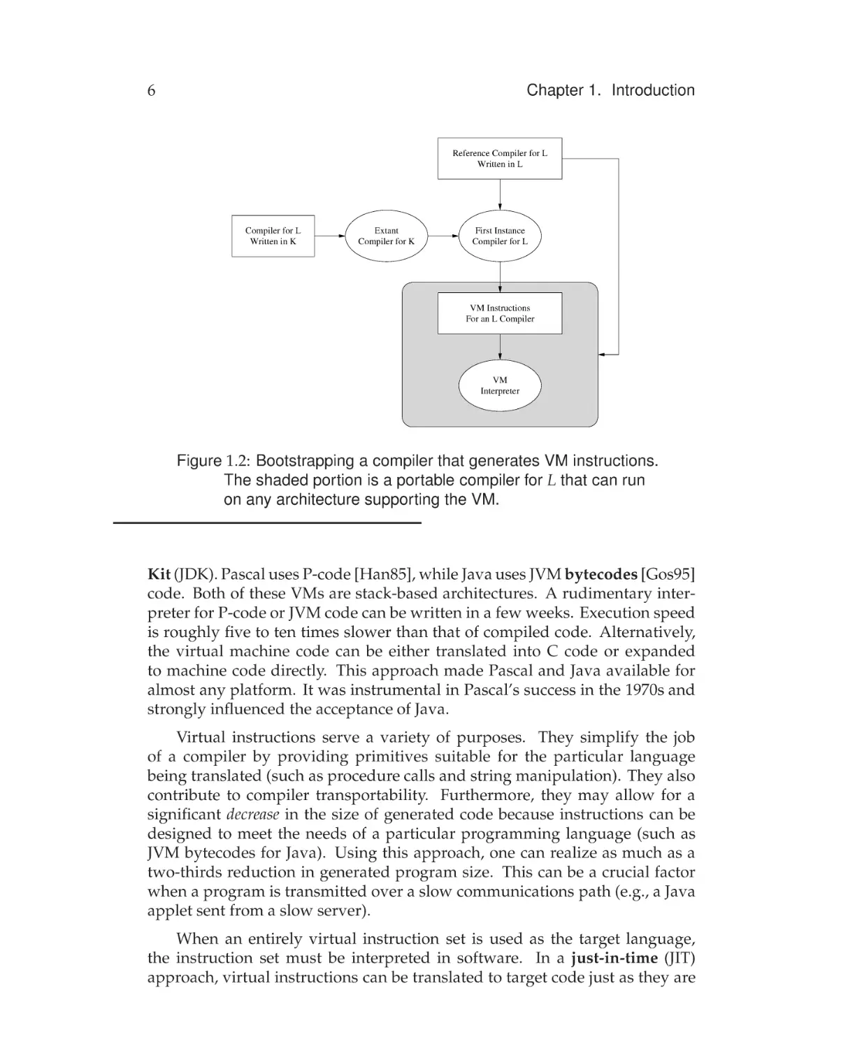
easy to write. The process of porting such a compiler from one architecture
to another is called bootstrapping and is illustrated in Figure 1.2. The very
first instance of an L compiler cannot compile itself, since no such compiler
exists yet. However, the first instance can be written in a language K for which
a compiler or assembler already exists. As shown in Figure 1.2, the result
of that compilation is the first executable instance of a compiler for L. That
first instance is usually discarded after the reference compiler, written in L, is
functioning correctly.
Examples of compilers that target a VM for portability include the early
Pascal compilers and the Java compiler included in the Java Development
6
Chapter 1. Introduction
Reference Compiler for L
Written in L
Compiler for L
Written in K
Extant
Compiler for K
First Instance
Compiler for L
VM Instructions
For an L Compiler
VM
Interpreter
Figure 1.2: Bootstrapping a compiler that generates VM instructions.
The shaded portion is a portable compiler for L that can run
on any architecture supporting the VM.
Kit (JDK). Pascal uses P-code [Han85], while Java uses JVM bytecodes [Gos95]
code. Both of these VMs are stack-based architectures. A rudimentary interpreter for P-code or JVM code can be written in a few weeks. Execution speed
is roughly five to ten times slower than that of compiled code. Alternatively,
the virtual machine code can be either translated into C code or expanded
to machine code directly. This approach made Pascal and Java available for
almost any platform. It was instrumental in Pascal’s success in the 1970s and
strongly influenced the acceptance of Java.
Virtual instructions serve a variety of purposes. They simplify the job
of a compiler by providing primitives suitable for the particular language
being translated (such as procedure calls and string manipulation). They also
contribute to compiler transportability. Furthermore, they may allow for a
significant decrease in the size of generated code because instructions can be
designed to meet the needs of a particular programming language (such as
JVM bytecodes for Java). Using this approach, one can realize as much as a
two-thirds reduction in generated program size. This can be a crucial factor
when a program is transmitted over a slow communications path (e.g., a Java
applet sent from a slow server).
When an entirely virtual instruction set is used as the target language,
the instruction set must be interpreted in software. In a just-in-time (JIT)
approach, virtual instructions can be translated to target code just as they are
1.2. What Compilers Do
7
about to be executed, or when they have been interpreted often enough to
merit translation into target code.
If a virtual instruction set is used often enough, it is possible to develop
special microprocessors that implement the virtual instruction set in hardware. For example, JazelleTM [Jaz] offers hardware support to improve the
performance and power usage of mobile phone applications that execute JVM
instructions.
In summary, most compilers generate code that interfaces with runtime
libraries, operating system utilities, and other software components. VMs can
enhance compiler portability and increase consistency of program execution
across diverse target architectures.
1.2.2 Target Code Formats
Another way that compilers differ from one another is in the format of the
target code they generate. Target formats may be categorized as follows:
• Assembly or other source formats
• Relocatable binary
• Absolute binary
Assembly Language (Source) Format
The generation of assembly code simplifies and modularizes translation. A
number of code-generation decisions (such as instruction and data addresses)
can be left for the assembler. This approach is common for compilers developed as instructional projects or for prototyping programming language
designs. One reason for this is that the assembly code is relatively easy to scrutinize, which makes the compilation process more transparent for students
and prototyping activities.
Generating assembler code is also useful for cross-compilation, where
the compiler executes on one computer but generates code that executes on
another. The symbolic assembly code is easily transferred between different
computers.
Sometimes another programming language, such as C, is generated by a
compiler instead of a specific assembly language. C has in fact been called
a universal assembly language because it is relatively low level yet it is far
more platform independent than any particular assembly language. However,
generation of C code leaves many decisions (such as the runtime representation
of data structures) to a particular C compiler. Full control over such matters is
retained if a compiler generates assembly language.
8
Chapter 1. Introduction
Relocatable Binary Format
Most production-quality compilers do not generate assembly language; direct
generation of target code (in relocatable or absolute binary format) is more efficient and allows the compiler more control over the translation process. It is
nonetheless beneficial for the compiler’s output to be open to scrutiny. Compilers that produce binary format typically can also produce a pseudoassembly
language listing of the generated code. Such a listing shows the instructions
generated by the compiler with annotations to document storage references.
Relocatable binary format is essentially the form of code that most assemblers generate. This format can also be generated directly by a compiler.
External references, local instruction addresses, and data addresses are not
yet bound. Instead, addresses are assigned relative either to the beginning of
the module or to some symbolically named locations. The latter alternative
makes it easy to group together code sequences or data areas. A linkage step
is required to incorporate any support libraries as well as other separately
compiled routines referenced from within a compiled program. The result is
an absolute binary format that is executable.
Both relocatable binary and assembly language formats allow modular
compilation: the decomposition of a large program into separately compiled
pieces. They also allow cross-language support: incorporation of assembler
code and code written and compiled in other high-level languages. Such code
can include I/O, storage allocation, and math libraries that supply functionality
regarded as part of the language’s definition.
Absolute Binary Format
Some compilers generate an absolute binary format that can be directly executed when the compiler is finished. This process is usually faster than the
other approaches. However, the ability to interface with other code may be
limited. In addition, the program must be recompiled for each execution unless some means is provided for archiving the memory image. Compilers
that generate an absolute binary format are useful for student exercises and
prototyping use, where frequent changes are the rule and compilation costs
far exceed execution costs. It also can be useful to avoid saving compiled formats to save file space or to guarantee the use of only the most current library
routines and class definitions.
Summary The code format alternatives and the target code alternatives discussed here show that compilers can differ quite substantially while still performing the same sort of translation task. Some compilers use a combination of
the articulated alternatives. For example, most Java compilers emit bytecodes
9
1.3. Interpreters
Interpreter
Source Program
Encoding
Output
Input
Data
Figure 1.3: An interpreter.
that are subsequently subjected to interpretation or dynamic compilation to
native machine code. The bytecodes are in a sense another source format, but
their encoding is a standard and relatively compact binary format. Java has a
native interface that is designed to allow Java code to interoperate with code
written in other languages. Java also requires dynamic linking of classes used
by an application, so that the origin of such classes can be controlled when an
application is invoked. When a class is first referenced, a class definition may
be remotely fetched, checked, and loaded during program execution.
1.3 Interpreters
Another kind of language processor is the interpreter. Interpreters share some
of the functionality found in compilers, such as syntactic and semantic analyses. However, interpreters differ from compilers in that they execute programs
without explicitly performing much translation. Figure 1.3 illustrates schematically how interpreters work. To an interpreter, a program is merely data that
can be arbitrarily manipulated, just like any other data. The locus of control
during execution resides in the interpreter, not in the user program (i.e., the
user program is passive rather than active).
Interpreters provide a number of capabilities not usually found in compilers, as follows:
• Programs can be easily modified as execution proceeds. This provides a
straightforward interactive debugging capability,since a program can be
modified to pause at points of interest or to display the value of program
variables. Depending on program structure, program modifications may
require reparsing or repeating semantic analysis.
• Languages in which the type of an object is developed dynamically
(e.g., Lisp and Scheme) are easily supported in an interpreter. Some
10
Chapter 1. Introduction
languages (such as Smalltalk and Ruby) allow the type system itself to
change dynamically. Since the user program is continuously reexamined
as execution proceeds, symbols need not have a fixed meaning. For
example, a symbol may denote an integer scalar at one point and a
Boolean array at a later point. Such fluid bindings are more problematic
for compilers, since dynamic changes in the meaning of a symbol make
direct translation into machine code more difficult.
• Interpreters provide a significant degree of machine independence, since
no machine code is generated. All operations are performed within the
interpreter. Porting an interpreter can be as simple as recompiling the
interpreter on a new machine, if the interpreter is written in a language
already supported on that machine.
However, direct interpretation of source programs can involve significant overhead. As execution proceeds, program text must be continuously reexamined.
Identifier bindings, types, and operations may have to be recomputed at each
reference. For languages where such bindings can change arbitrarily, interpretation can be 100 times slower than compiled code. For more static languages
such as C and Java, the cost difference is closer to 10.
Some languages (C, C++, and Java) have both interpreters (for debugging and program development) and compilers (for production work). JIT
compilers offer a combination of interpretation and compilation/execution.
In summary, all language processing involves interpretation at some level.
Interpreters directly interpret source programs or some syntactically transformed versions of them. They may exploit the availability of a source representation to allow program text to be changed as it is executed and debugged.
While a compiler has distinct translation and execution phases, some form of
“interpretation” is still involved. The translation phase may generate a virtual
machine language that is interpreted by software or a real machine language
that is interpreted by a particular computer, either in firmware or hardware.
1.4 Syntax and Semantics
A complete definition of a programming language must include the specification of its syntax (structure) and its semantics (meaning).
Syntax typically means context-free syntax because of the almost universal
use of context-free grammars (CFGs) as a syntactic specification mechanism.
Syntax defines the sequences of symbols that are legal; syntactic legality is
independent of any notion of what the symbols mean. For example, a contextfree syntax might specify that a=b+c is syntactically legal, while b+c=a is not.
11
1.4. Syntax and Semantics
However, not all aspects of well-formed programs can be described by contextfree syntax. For example, CFGss cannot specify type compatibility and scoping
rules. For example, a programming language may specify that a=b+c is illegal
if any of the variables are undeclared or if b or c is of type Boolean.
Because of the limitations of CFGss, the semantics of a programming
language are commonly divided into two classes:
• Static semantics
• Runtime semantics
1.4.1 Static Semantics
The static semantics of a language provide a set of rules that specify which
syntactically legal programs are actually valid. Such rules typically require that
all identifiers be declared, that operators and operands be type-compatible,
and that procedures be called with the proper number of parameters. The
common thread through all of these rules is that they cannot be expressed
with a CFGs. Thus static semantics augment context-free specifications and
complete the definition of valid programs.
Static semantics can be specified formally or informally. The prose descriptions found in most programming language specifications are informal. They
tend to be relatively compact and easy to read, but often they are imprecise.
Formal specifications can be expressed using any of a variety of notations.
For example, attribute grammars [Knu68] can formalize many of the semantic
checks found in compilers. The following rewriting rule, called a production,
specifies that an expression, denoted by E, can be rewritten into an expression
E plus a term T:
E→ E + T
In an attribute grammar, this production might be augmented with a type
attribute for E and T and a predicate testing for type compatibility, such as
Eresult → Ev1 + Tv2
if v1.type = numeric and v2.type = numeric
then result.type ← numeric
else call error( )
Attribute grammars are a reasonable blend of formality and readability, but
they can be rather verbose and tedious. Most compiler-writing systems do
12
Chapter 1. Introduction
not use attribute grammars directly. Instead, they propagate semantic information through a program’s abstract syntax tree (AST) in a manner similar
to the evaluation of attribute grammar systems. The specifics of a portion of
semantics checking are thus written in the compiler as a semantics-checking
phase. Such is the approach taken in this book.
1.4.2 Runtime Semantics
Runtime, or execution, semantics are used to specify what a program computes. These semantics are often specified very informally in a language manual or report. Alternatively, a more formal operational, or interpreter, model can
be used. In such a model, a program “state” is defined and program execution
is described in terms of changes to that state. For example, the semantics of
the statement a = 1 is that the state component corresponding to a is changed
to 1.
A variety of formal approaches to defining the runtime semantics of programming languages have been developed. Three of them, natural semantics,
axiomatic semantics and denotational semantics, are described below.
Natural Semantics
Natural semantics [NN92] (sometimes called structured operational semantics) formalizes the operational approach. Given assertions known to be true
before the evaluations of a construct, we can infer assertions that will hold
after the construct’s evaluation. Natural semantics has been used to define the
semantics of a variety of languages, including standard ML [MTHM97].
Axiomatic Semantics
Axiomatic definitions [Gri81] can be used to model execution at a more abstract level than operational models. They are based on formally specified
relations, or predicates, that relate program variables. Statements are defined by
how they modify these relations.
As an example of axiomatic definitions, the axiom defining var ← exp
states that a predicate involving var is true after statement execution if, and
only if, the predicate obtained by replacing all occurrences of var by exp is
true beforehand. Thus, for y > 3 to be true after execution of the statement
y ← x + 1, the predicate x + 1 > 3 would have to be true before the statement
is executed. Similarly, y = 21 is true after execution of x ← 1 if y = 21 is true
before its execution (this is a roundabout way of saying that changing x doesn’t
affect y). However, if x is an alias (an alternative name) for y, the axiom is
invalid. This is one reason why aliasing is discouraged (or forbidden) in some
language designs.
1.4. Syntax and Semantics
13
The axiomatic approach is good for deriving proofs of program correctness
because it avoids implementation details and concentrates on how relations
among variables are changed by statement execution. Although axioms can
formalize important properties of the semantics of a programming language, it
is difficult to use them to define most programming languages completely. For
example, they do not do a good job of modeling implementation considerations
such as running out of memory.
Denotational Semantics
Denotational models [Sch86] are more mathematical in form than operational
models, but they can accommodate memory stores and fetches that are central
to procedural languages. They rely on notation and terminology drawn from
mathematics, so they are often fairly compact, especially in comparison with
operational definitions.
A denotational definition may be viewed as a syntax-directed definition
that specifies the meaning of a construct in terms of the meaning of its immediate constituents. For example, to define addition, we might use the following
rule:
E[T1 + T2]m = E[T1]m + E[T2]m
This definition says that the value obtained by adding two subexpressions,
T1 and T2, in the context of a memory state m is defined to be the sum of
the arithmetic values obtained by evaluating T1 in the context of m (denoted
E[T1]m) and T2 in the context of m (denoted E[T2]m).
Denotational techniques are quite popular and form the basis for rigorous
definitions of programming languages. Research has shown that it is possible
to convert denotational representations automatically to equivalent representations that are directly executable [Set83, Wan82, App85].
Summary Regardless of how semantics are specified, our concern for precise semantics is motivated by the fact that writing a complete and accurate
compiler for a programming language requires that the language itself be well
defined. While this assertion may seem self-evident, many languages are
defined by imprecise or informal language specifications. Attention is often
given to formal specification of syntax, but the semantics of the language may be
defined via informal prose. The resulting definition inevitably is ambiguous
or incomplete on certain points.
For example, in Java all functions must return via a return expr statement, where expr is assignable to the function’s return type. The following is
therefore illegal:
14
Chapter 1. Introduction
public static int subr(int b) {
if (b != 0)
return b+100;
}
If b is equal to zero, subr fails to return a value. Now consider the following:
public static int subr(int b) {
if (b != 0)
return b+100;
else if (10*b == 0)
return 1;
}
In this case, a proper return is always executed, since the else part is reached
only if b equals zero; this implies that 10*b is also equal to zero. Is the
compiler expected to duplicate this rather involved chain of reasoning? Java
compilers typically assume that a predicate could evaluate to true or false,
even if a detailed program analysis refutes that assumption. Thus a compiler
may reject subr as semantically illegal and in so doing trade simplicity for
accuracy in its analysis. Indeed, the general problem of deciding whether
a particular statement in a program is reachable is undecidable, proved by
reduction from the famous halting problem [HU79]. We certainly cannot ask
our Java compiler literally to do the impossible!
In practice, a trusted reference compiler can serve as a de facto language
definition. That is, a programming language is, in effect, defined by what a
compiler chooses to accept and how it chooses to translate language constructs.
In fact, the operational and natural semantic approaches introduced previously
take this view. A standard interpreter is defined for a language, and the
meaning of a program is precisely whatever the interpreter says. An early
(and very elegant) example of an operational definition is the seminal Lisp
interpreter [McC60]. There, all of Lisp was defined in terms of the actions of
a Lisp interpreter, assuming only seven primitive functions and the notions of
argument binding and function call.
Of course, a reference compiler or interpreter is no substitute for a clear and
precise semantic definition. Nonetheless, it is very useful to have a reference
against which to test a compiler that is under development.
1.5 Organization of a Compiler
Compilers generally perform the following tasks:
15
1.5. Organization of a Compiler
Source
Program
Tokens
AST
Parser
Scanner
Type Checker
Decorated
AST
Translator
Interemediate
Representation
Symbol Tables
Optimizer
Interemediate
Representation
Code Generator
Target Code
Figure 1.4: A syntax-directed compiler. AST denotes the Abstract
Syntax Tree.
• Analysis of the source program being compiled
• Synthesis of a target program that, when executed, will correctly perform
the computations described by the source program
Almost all modern compilers are syntax-directed. That is, the compilation
process is driven by the syntactic structure of the source program, as recognized by the parser. Most compilers distill the source program’s structure into
an abstract syntax tree (AST) that omits unnecessary syntactic detail. The
parser builds the AST out of tokens, the elementary symbols used to define a
programming language syntax. Recognition of syntactic structure is a major
part of the syntax analysis task.
Semantic analysis examines the meaning (semantics) of the program on
the basis of its syntactic structure. It plays a dual role. It finishes the analysis
task by performing a variety of correctness checks (for example, enforcing type
and scope rules). It also begins the synthesis phase.
In the synthesis phase, source language constructs are translated into an
intermediate representation (IR) of the program. Some compilers generate
target code directly. If an IR is generated, it then serves as input to a code generator component that actually produces the desired machine-language program.
The IR may optionally be transformed by an optimizer so that a more efficient
program may be generated. A common organization of all of these compiler
components is depicted schematically in Figure 1.4. Each of these components
16
Chapter 1. Introduction
is described in more detail below. Chapter 2 presents a simple compiler to provide concrete examples of many of the concepts introduced in this overview.
1.5.1 The Scanner
The scanner begins the analysis of the source program by reading the input
text (character by character) and grouping individual characters into tokens
such as identifiers, integers, reserved words, and delimiters. This is the first
of several steps that produce successively higher-level representations of the
input. The tokens are encoded (often as integers) and fed to the parser for
syntactic analysis. When necessary, the actual character string comprising the
token is also passed along for use by the semantic phases. The scanner does
the following:
• It puts the program into a compact and uniform format (a stream of
tokens).
• It eliminates unneeded information (such as comments).
• It processes compiler control directives (for example, turn the listing on
or off and include source text from a specified file).
• It sometimes enters preliminary information into symbol tables (for example, to register the presence of a particular label or identifier).
• It optionally formats and lists the source program.
The main action of building tokens is often driven by token descriptions.
Regular expression notation (discussed in Chapter 3) is an effective approach
to describing tokens. Regular expressions are a formal notation sufficiently
powerful to describe the variety of tokens required by modern programming
languages. In addition, they can be used as a specification for the automatic
generation of finite automata (discussed in Chapter 3) that recognize regular
sets, that is, the sets that regular expressions define. Recognition of regular sets
is the basis of the scanner generator. A scanner generator is a program that
actually produces a working scanner when given only a specification of the
tokens it is to recognize. Scanner generators are a valuable compiler-building
tool.
1.5.2 The Parser
The parser is based on a formal syntax specification such as a CFGs. It reads
tokens and groups them into phrases according to the syntax specification.
Grammars are discussed in Chapters 2 and 4, and parsing is discussed in
1.5. Organization of a Compiler
17
Chapters 5 and 6. Parsers are typically driven by tables created from a CFGs
by a parser generator.
The parser verifies correct syntax. If a syntax error is found, it issues a
suitable error message. Also, it may be able to repair the error (to form a
syntactically valid program) or to recover from the error (to allow parsing to
be resumed). In many cases, syntactic error recovery or repair can be done
automatically by consulting structures created by a suitable parser generator.
As syntactic structure is recognized, the parser usually builds an AST as
a concise representation of program structure. The AST then serves as a basis
for semantic processing. ASTs are discussed in Chapters 2 and 7.
1.5.3 The Type Checker (Semantic Analysis)
The type checker checks the static semantics of each AST node. That is, it
verifies that the construct the node represents is legal and meaningful (that
all identifiers involved are declared, that types are correct, and so on). If the
construct is semantically correct, the type checker decorates the AST node by
adding type information to it. If a semantic error is discovered, a suitable error
message is issued.
Type checking is purely dependent on the semantic rules of the source
language. It is independent of the compiler’s target.
1.5.4 Translator (Program Synthesis)
If an AST node is semantically correct, it can be translated into IR code that
correctly implements the meaning of the AST node. For example, an AST for
a while loop contains two subtrees, one representing the loop’s expression and
the other representing the loop’s body. However, nothing in the AST explicitly
captures the notion that a while loop loops! This meaning is captured when a
while loop’s AST is translated to IR form. In the IR, the notion of testing the
value of the loop control expression and conditionally executing the loop body
is made explicit.
The translator is largely dictated by the semantics of the source language.
Little of the nature of the target machine needs to be made evident. As a
convenience during translation, some general aspects of the target machine
may be exploited (for example, that the machine is byte-addressable or that
it has a runtime stack). However, detailed information on the nature of the
target machine (operations available, addressing, register characteristics, etc.)
is reserved for the code-generation phase.
In simple, nonoptimizing compilers, the translator may generate target
code directly without using an explicit IR. This simplifies a compiler’s design
by removing an entire phase. However, it also makes retargeting the compiler
18
Chapter 1. Introduction
to another machine much more difficult. Most compilers implemented as
instructional projects generate target code directly from the AST, without using
an IR.
More elaborate compilers such as the GNU Compiler Collection (GCC)
may first generate a high-level IR (that is source-language oriented) and then
subsequently translate it into a low-level IR (that is target-machine oriented).
This approach allows a cleaner separation of source and target dependencies.
1.5.5 Symbol Tables
A symbol table is a mechanism that allows information to be associated with
identifiers and shared among compiler phases. Each time an identifier is
declared or used, a symbol table provides access to the information collected
about it. Symbol tables are used extensively during type checking, but they
can also be used by other compiler phases to enter, share, and later retrieve
information about types, variables, procedures, and labels. Compilers may
choose to use other structures to share information between compiler phases.
For example, a program representation such as an AST may be expanded and
refined to provide detailed information needed by optimizers, code generators,
linkers, loaders, and debuggers.
1.5.6 The Optimizer
The IR code generated by the translator is analyzed and transformed into
functionally equivalent but improved IR code by the optimizer. This phase
can be complex, often involving numerous subphases, some of which may
need to be applied more than once. Most compilers allow optimizations to
be turned off so as to speed translation. Nonetheless, a carefully designed
optimizer can significantly speed program execution by simplifying, moving,
or eliminating unneeded computations.
If both a high-level and low-level IR are used, optimizations may be performed in stages. For example, a simple subroutine call may be expanded into
the subroutine’s body, with actual parameters substituted for formal parameters. This is a high-level optimization. Alternatively, a value already loaded
from memory may be reused. This is a low-level optimization.
Optimization can also be done after code generation. An example is peephole optimization. Peephole optimization examines generated code a few
instructions at a time (in effect, through a “peephole”). Common peephole
optimizations include eliminating multiplications by 1 or additions of 0, eliminating a load of a value into a register when the value is already in another
register, and replacing a sequence of instructions by a single instruction with
the same effect. A peephole optimizer does not offer the payoff of a full-scale
1.5. Organization of a Compiler
19
optimizer. However, it can significantly improve code and is often useful for
“cleaning up” after earlier compiler phases.
1.5.7 The Code Generator
The IR code produced by the translator is mapped into target machine code by
the code generator. This phase requires detailed information about the target
machine and includes machine-specific optimization such as register allocation
and code scheduling. Normally, code generators are hand-coded and can be
quite complex, since generation of good target code requires consideration of
many special cases.
The notion of automatic construction of code generators has been actively
studied. The basic approach is to match a low-level IR to target-instruction
templates, with the code generator automatically choosing instructions that
best match IR instructions. This approach localizes the target-machine specifics
of a compiler and, at least in principle, makes it easy to retarget a compiler
to a new target machine. Automatic retargeting is an especially desirable
goal, since a great deal of work is usually needed to move a compiler to a
new machine. The ability to retarget by simply changing the set of target
machine templates and generating (from the templates) a new code generator
is compelling.
A well-known compiler using these techniques is the GCC [GNU]. GCC
is a heavily optimizing compiler that can target over thirty computer architecR
R
, SparcTM, and PowerPC
) and has at least six front
tures (including Intel
ends (including C, C++, Fortran, Ada, and Java).
1.5.8 Compiler Writing Tools
Finally, note that in discussing compiler design and construction, we often talk
of compiler writing tools. These are often packaged as compiler generators
or compiler compilers. Such packages usually include scanner and parser
generators. Some also include symbol table managers, attribute grammar
evaluators, and code-generation tools. More advanced packages may aid in
error repair generation.
These sorts of generators greatly assist the crafting of compilers, but much
of the effort in crafting a compiler lies in writing and debugging the semantic
phases. These routines can be numerous (a type checker and translator is
apparently needed for each distinct AST node) and are usually hand coded.
Judicious application of the visitor pattern can significantly reduce this effort
and make the compiler easier to maintain. Chapters 2 and 7 introduce application of the visitor pattern to semantic analysis. This treatment continues
beyond Chapter 7 as specific semantic issues are addressed.
20
Chapter 1. Introduction
1.6 Programming Language and Compiler Design
Our primary interest is the design and implementation of compilers for modern
programming languages. An interesting aspect of this study is how programming language design and compiler design influence each other. Programming language design obviously influences, and indeed often dictates, how
compilers are crafted. Many clever and sometimes subtle compiler techniques
arise from the need to cope with some programming language construct. A
good example of this is the closure mechanism that was invented to handle
formal procedures. A closure is a special runtime representation for a function. It is usually implemented as a pointer to the function’s body and to its
execution environment. While the concept of a closure is attractive from a
programming language design perspective, implementing closures efficiently
has been challenging for compiler writers [App92, Ken07].
The state of the art in compiler design also strongly affects programming
language design, if only because a programming language that cannot be
compiled effectively has an uphill road to acceptance. Most successful programming language designers (such as the Java language development team)
have extensive compiler design backgrounds.
A programming language that is easy to compile usually has the following
advantages:
• It often is easier to learn, read, and understand. If a feature is hard to
compile, it may well be difficult to understand.
• It will have quality compilers on a wide variety of machines. This fact
is often crucial to a language’s success. For example, C, C++, Java, and
Fortran are widely available and very popular; Ada and Modula-3 have
limited availability and are far less popular.
• Often, better code will be generated. Poor-quality code can be fatal in
major applications.
• Fewer compiler bugs will occur. If a language cannot be easily understood, then discrepancies will arise in the difficult regions of the language’s design. These will in turn lead to compilers that differ in their
interpretation of a program’s meaning.
• The compiler will be smaller, cheaper, faster, more reliable, and more
widely used.
• Compiler diagnostic messages and program development tools will often
be better.
1.7. Computer Architecture and Compiler Design
21
Throughout our discussion of compiler design, we draw ideas, solutions, and
shortcomings from many languages. Our primary focus is on Java and C,
but we also consider Ada, C++, Smalltalk, ML, Pascal, and Fortran. We
concentrate on Java and C because they are representative of the issues posed
by modern language designs. We consider other languages so as to identify
alternative design approaches for crafting a compiler.
1.7 Computer Architecture and Compiler Design
Advances in computer architecture and microprocessor fabrication have spearheaded the computer revolution. At one time, a computer offering one
megaflop performance (1,000,000 floating-point operations per second) was
considered advanced. Computers offering teraflop (one trillion flops) performance are available and petaflop computers (one thousand trillion flops) have
become a matter of packaging (and cooling!) a sufficient number of individual
computers. Meanwhile, each individual computer is often itself a multiprocessor, and each processor in the computer may have multiple cores, each
offering an independent thread of control.
Compiler designers are responsible for making this vast computing capability available to programmers. Although compilers are rarely visibly to the
end users of application programs, they are an essential enabling technology.
The problems encountered in efficiently harnessing the capability of a modern
computing platforms are numerous, as follows:
• Instruction sets for some popular architectures, particularly the Intel
x86 series, are highly nonuniform. Some operations must be done in
registers, while others can be done in memory. Often a number of
distinct register classes exist, each suitable for only a particular class
of operations.
• High-level programming language operations are not always easy to
support. Virtual method dispatch, dynamic heap accesses, and reflective programming constructs can take hundreds or thousands of machine instructions to implement. Exceptions, threads, and concurrency
management are typically more expensive and complex to implement
than most users suspect.
• Essential architectural features such as hardware caches and distributed
processors and memory are difficult to present to programmers in an
architecturally independent manner. Yet misuse of these features can
impose immense performance penalties.
• Effective use of a large number of processors has always posed challenges
to application developers and compiler writers. Many developers have
22
Chapter 1. Introduction
unrealistic expectations concerning how well a compiler can use largescale systems without changing an application. While compilers continually improve [Wol95, AK01], languages are also evolving [CGS+ 05] to
address these challenges.
For some programming languages, runtime checks for data and program integrity are dropped in favor of gains in execution speed. Programming errors
can then go undetected because of that fear that extra checking will slow
down execution unacceptably. The cost of software development and the consequences of program failure have reversed that trend for most programming
efforts. A major complexity in implementing Java is efficiently enforcing the
runtime integrity constraints it imposes.
1.8 Compiler Design Considerations
Compilers are often biased for a particular kind of deployment or user base. In
this section we examine some common design criteria that affect how compilers
are crafted.
1.8.1 Debugging (Development) Compilers
A debugging compiler such as CodeCenter [Cod] is specially designed to
aid in the development and debugging of programs. It carefully scrutinizes
programs and details programmer errors. Often it can tolerate or repair minor
errors (for example, insert a missing comma or parenthesis). Some program
errors can be detected only at runtime. Such errors include invalid subscripts,
misuse of pointers, and illegal file manipulations.
These compilers may include the checking of code that can detect runtime errors and initiate a symbolic debugger. Although debugging compilers
are particularly useful in instructional environments, diagnostic techniques
are of value in all compilers. In the past, development compilers were used
only in the initial stages of program development. When a program neared
completion, compilation switched to a production compiler, which increased
compilation and execution speed by ignoring diagnostic concerns. This strategy has been likened by Tony Hoare to wearing a life jacket in sailing classes
held on dry land, but abandoning the jacket when at sea [Hoa89]! Indeed, it is
becoming increasingly clear that for almost all applications, reliability is more
important than speed. For example, Java mandates runtime checks that C and
C++ do not.
For production systems where quality is a paramount concern, detecting
possible or actual runtime errors is crucial. Tools such as purify [pur] can
add initialization and array bounds checks to already compiled programs,
1.8. Compiler Design Considerations
23
thereby allowing illegal operations to be detected even when source files are
not available. Other tools such as Electric Fence [Piz99] can detect dynamic
storage problems such as buffer overruns and improperly deallocated storage.
1.8.2 Optimizing Compilers
An optimizing compiler is specially designed to produce efficient target code
at the cost of increased compiler complexity and possibly increased compilation times. In practice, all production-quality compilers (those whose output
will be used in everyday work) make some effort to generate reasonable target
code. For example, no add instruction would normally be generated for the
expression i+0.
The term optimizing compiler is actually a misnomer. This is because no
compiler of any sophistication can produce optimal code for all programs. The
reason for this is twofold. First, theoretical computer science has shown that
even so simple a question as whether two programs are equivalent is undecidable: such questions cannot generally be answered by any computer program.
Thus finding the simplest (and most efficient) translation of a program cannot
always be done. Second, many program optimizations require time proportional to an exponential function of the size of the program being compiled.
Thus, optimal code, even when theoretically possible, is often infeasible in
practice.
Optimizing compilers actually use a wide variety of transformations that
improve a program’s performance. The complexity of an optimizing compiler
arises from the need to employ a variety of transforms, some of which interfere
with each other. For example, keeping frequently used variables in registers
reduces their access time but makes procedure and function calls more expensive. This is because registers need to be saved across calls. Many optimizing
compilers provide a number of levels of optimization, each providing increasingly greater code improvements at increasingly greater costs. The choice
of which improvements are most effective (and least expensive) is a matter
of judgment and experience. Chapter 13 discusses some optimizations that
are specific to code generation, such as register allocation. Chapter 14 covers the theory of optimizing compilers in greater detail, including data flow
frameworks and static single-assignment form. Further discussion of a comprehensive optimizing compiler is beyond the scope of this book. However,
compilers that produce high-quality code at reasonable cost are an achievable
goal.
1.8.3 Retargetable Compilers
Compilers are designed for a particular programming language (the source
language) and a particular target computer (the computer for which it will
24
Chapter 1. Introduction
generate code). Because of the wide variety of programming languages and
computers that exist, apparently a large number of similar, but not identical,
compilers must be written. While this situation has decided benefits for those
of us in the compiler writing business, it does make for a lot of duplication
of effort and for a wide variance in compiler quality. As a result, the retargetable compiler has become a concept of increasing importance for language
designers, computer architects, and compiler writers.
A retargetable compiler is one whose target architecture can be changed
without its machine-independent components having to be rewritten. A retargetable compiler is more difficult to write than an ordinary compiler because
target-machine dependencies must be carefully localized. In addition, it is
often difficult for a retargetable compiler to generate code that is as efficient as
that of an ordinary compiler because special cases and machine idiosyncrasies
are harder to exploit. Nonetheless, because a retargetable compiler allows development costs to be shared and provides for uniformity across computers,
it is an important innovation. While discussing the fundamentals of compilation, we concentrate on compilers targeted to a single machine. Chapters 11
and 13 cover some of the techniques needed to provide retargetability.
1.9 Integrated Development Environments
In practice, a compiler is but one tool used in the program development cycle.
Developers edit a program, compile it, and test its performance. This cycle
is repeated many times as the application is developed, often in response to
specification changes and bugs that are discovered. The integrated development environment (IDE) has become a popular tool to integrate this cycle
within a single framework. An IDE allows programs to be built incrementally,
with program checking and testing fully integrated. Of course, an important
component within an IDE is its compiler. An IDE places special demands on
its compiler as follows:
• Most IDEs provide immediate feedback concerning syntax and semantic
problems in the code as the code is entered.
• The IDE focus is typically on the source of a program, with any derived
files (such as object code) carefully managed beyond the user’s view.
• Most IDEs provide key or mouse actions that provide information about
the program as it is developed. For example, a program may have an
object reference o and the developer may wish to see the methods that
can be invoked on o. Such information depends on the declared type of
o as well as the methods defined on objects of that type.
1.9. Integrated Development Environments
25
We focus on the traditional batch compilation approach in which an entire
source file is translated. However, many of the techniques we develop can be
reformulated into incremental form to support IDEs. For example, a parser
can reparse only those portions of a program that have been changed [GM80,
WG97], and a type checker can analyze only portions of an AST that are
affected by program modification. An alternative is to write the compiler as a
sequence of passes over the source code, with its first pass sufficiently fast to
provide an IDE its requisite information. Subsequent passes can complete the
compilation process and generate increasingly sophisticated code.
Summary In this book, we concentrate on the translation of C, C++, and Java.
We use the JVM as a target in Chapter 11, and we address code generation
R
and Sparc architectures in Chapter 13.
for RISC processors such as the MIPS
At the code-generation stage, a variety of current techniques designed to exploit a processor’s capabilities are explored. Like so much else in crafting a
compiler, experience is the best guide. We begin with the translation of a very
simple language in Chapter 2 and work our way up to ever more challenging
translation tasks.
26
Chapter 1. Introduction
Exercises
1. The model of compilation we introduced is essentially batch-oriented.
In particular, it assumes that an entire source program has been written
and that the program will be fully compiled before the programmer
can execute the program or make any changes. An interesting and
important alternative is an interactive compiler. An interactive compiler,
usually part of an integrated program development environment, allows
a programmer to interactively create and modify a program, fixing errors
as they are detected. It also allows a program to be tested before it is fully
written, thereby providing for stepwise implementation and testing.
Redesign the compiler structure of Figure 1.4 to allow incremental compilation. (The key idea is to allow individual phases of a compiler to be
run or rerun without necessarily doing a full compilation.)
2. Most programming languages, such as C and C++, are compiled directly
into the machine language of a “real” microprocessor (for example, an
Intel x86 or Sparc). Java takes a different approach. It is commonly
compiled into the machine language of the JVM. The JVM is not implemented in its own microprocessor, but is instead interpreted on some
existing processor. This allows Java to be run on a wide variety of machines, thereby making it highly platform independent.
Explain why building an interpreter for a virtual machine like the JVM
is easier and faster than building a complete Java compiler. What are the
disadvantages of this virtual machine approach?
3. C compilers are almost always written in C. This raises something of a
“chicken and egg” problem—how was the first C compiler for a particular
system created? If you need to create the first compiler for language X on
system Y, one approach is to create a cross-compiler. A cross-compiler
runs on system Z but generates code for system Y.
Explain how, starting with a compiler for language X that runs on system
Z, you might use cross-compilation to create a compiler for language X,
written in X, that runs on system Y and generates code for system Y.
What extra problems arise if system Y is “bare”—that is, has no operating
R
is written in
system or compilers for any language? (Recall that Unix
C and thus must be compiled before its facilities can be used.)
Exercises
27
4. Cross-compilation assumes that a compiler for language X exists on some
machine. When the first compiler for a new language is created, this
assumption does not hold. In this situation, a bootstrapping approach
can be taken. First, a subset of language X is chosen that is sufficient to
implement a simple compiler. Next, a simple compiler for the X subset
is written in any available language. This compiler must be correct, but
it should not be any more elaborate than is necessary, since it will soon
be discarded. Next, the subset compiler for X is rewritten in the X subset
and then compiled using the subset compiler previously created. Finally,
the X subset, and its compiler, can be enhanced until a complete compiler
for X, written in X, is available.
Assume you are bootstrapping C++ or Java (or some comparable language). Outline a suitable subset language. What language features
must be in the language? What other features are desirable?
5. To allow the creation of camera-ready documents, languages like TeX and
LaTeX have been created. These languages can be thought of as varieties
of programming languages whose output controls a printer or display.
Source language commands control details like spacing, font choice,
point size, and special symbols. Using the syntax-directed compiler
structure of Figure 1.4, suggest the kind of processing that might occur
in each compiler phase if TeX or LaTeX input was being translated.
An alternative to “programming” documents is to use a sophisticated edR
R
R
Word or Adobe
FrameMaker
itor such as that provided in Microsoft
to interactively enter and edit the document. (Editing operations allow
the choice of fonts, selection of point size, inclusion of special symbols,
and so on.) This approach to document preparation is called WYSIWYG—what you see is what you get—because the exact form of the
document is always visible.
What are the relative advantages and disadvantages of the two approaches? Do analogues exist for ordinary programming languages?
6. Although compilers are designed to translate a particular language, they
often allow calls to subprograms that are coded in some other language
(typically, Fortran, C, or assembler). Why are such “foreign calls” allowed? In what ways do they complicate compilation?
28
Chapter 1. Introduction
7. Most C compilers (including the GCC compilers) allow a user to examine the machine instructions generated for a given source program.
Run the following program through such a C compiler and examine the
instructions generated for the for loop. Next, recompile the program,
enabling optimization, and reexamine the instructions generated for the
for loop. What improvements have been made? Assuming that the
program spends all of its time in the for loop, estimate the speedup
obtained. Write a suitable main C function that allocates and initializes
a million-element array to pass to proc. Execute and time the unoptimized and optimized versions of the program and evaluate the accuracy
of your estimate.
int proc(int a[]) {
int sum = 0, i;
for (i=0; i < 1000000; i++)
sum += a[i];
return sum;
}
8. C is sometimes called the universal assembly language in light of its
ability to be very efficiently implemented on a wide variety of computer
architectures. In light of this characterization, some compiler writers
have chosen to generate C code as their output instead of a particular
machine language. What are the advantages to this approach to compilation? Are there any disadvantages?
9. Many computer systems provide an interactive debugger (for example,
gdb or dbx) to assist users in diagnosing and correcting runtime errors.
Although a debugger is run long after a compiler has done its job, the
two tools still must cooperate. What information (beyond the translation of a program) must a compiler supply to support effective runtime
debugging?
10. Assume you have a source program P. It is possible to transform P
into an equivalent program P by reformatting P (by adding or deleting
spaces, tabs, and line breaks), systematically renaming its variables (for
example, changing all occurrences of sum to total), and reordering the
definition of variables and subroutines.
Although P and P are equivalent, they may well look very different.
How could a compiler be modified to compare two programs and determine if they are equivalent (or very similar)? In what circumstances
would such a tool be useful?
Exercises
29
11. The Measure Of Software Similarity (MOSS) [SWA03] tool can detect
similarity of programs written in a variety of modern programming languages. Its main application has been in detecting similarity of programs
submitted in computer science classes, where such similarity may indicate plagiarism (students, beware!). In theory, detecting equivalence of
two programs is undecidable, but MOSS does a very good job of finding
similarity in spite of that limitation.
Investigate the techniques MOSS uses to find similarity. How does MOSS
differ from other approaches for detecting possible plagiarism?
This page intentionally left blank
2
A Simple Compiler
In this chapter we provide an overview of the compilation process by considering a simple translation task for a very small language. This language, called
ac for adding calculator, accommodates two forms of numerical data types, allows computation and printing of numerical values, and offers a small set of
variable names to hold the results of computations.
To simplify both the presentation and implementation of a compiler, we
break the compilation process into a sequence of phases. Each phase is responsible for a particular aspect of the compilation process. The early phases
analyze the syntax of the input program with the goal of generating an abstract representation of the program’s essential information for translation.
The subsequent phases analyze and transform the tree, eventually generating
a translation of the input program in the target language.
The ac language and its compilation are sufficiently simple to facilitate
a relatively quick overview of a compiler’s phases and their associated data
structures. The tools and techniques necessary for undertaking translation
tasks of a more substantial nature are presented in subsequent chapters. Some
code fragments are presented in this chapter to illustrate the basic concepts of
a compiler’s phases. A complete form of the code presented here can be found
in the Crafting a Compiler Supplement.
31
32
Chapter 2. A Simple Compiler
2.1 An Informal Definition of the ac Language
Our language is called ac (for adding calculator). When compared with most
programming languages, ac is relatively simple, yet it serves nicely as a study
for examining the phases and data structures of a compiler. We first define ac
informally:
Types Most programming languages offer a significant number of predefined
data types, with the ability to extend existing types or specify new data
types. In ac, there are only two data types: integer and float. An integer
type is a sequence of decimal numerals, as found in most programming
languages. A float type allows five fractional digits after the decimal
point.
Keywords Most programming languages have a number of reserved keywords, such as if and while, which would otherwise serve as variable
names. In ac, there are three reserved keywords, each limited for simplicity to a single letter: f (declares a float variable), i (declares an integer
variable), and p (prints the value of a variable).
Variables Some programming languages insist that a variable be declared by
specifying the variable’s type prior to using the variable’s name. The
ac language offers only 23 possible variable names, drawn from the
lowercase Roman alphabet and excluding the three reserved keywords
f, i, and p. Variables must be declared prior to using them.
Most programming languages have rules that dictate circumstances under
which a given type can be converted into another type. In some cases, such type
conversion is handled automatically by the compiler, while other cases require
explicit syntax (such as casts) to allow the type conversion. In ac, conversion
from integer type to float type is accomplished automatically. Conversion in
the other direction is not allowed under any circumstances.
For the target of translation, we use the widely available program dc
(for desk calculator), which is a stack-based calculator that uses reverse Polish
notation (RPN). When an ac program is translated into a dc program, the
resulting instructions must be acceptable to the dc program and must faithfully
represent the operations specified in an ac program. Stack-based languages
commonly serve as targets of translation because they lend themselves to
compact representation. Examples include the translation of JavaTM into Java
R
R
into AVM2 for Flash
media, and
Virtual Machine (JVM), ActionScript
R
printable documents into PostScript . Thus, compilation of ac to dc can be
viewed as a study of such larger systems.
2.2. Formal Definition of ac
1
2
3
4
5
6
7
8
9
10
11
12
13
14
15
33
Prog → Dcls Stmts $
Dcls → Dcl Dcls
| λ
Dcl → floatdcl id
| intdcl id
Stmts → Stmt Stmts
| λ
Stmt → id assign Val Expr
| print id
Expr → plus Val Expr
| minus Val Expr
| λ
Val → id
| inum
| fnum
Figure 2.1: Context-free grammar for ac.
2.2 Formal Definition of ac
Before translating ac to dc we must first understand the syntax and semantics
of the ac language. The informal definitions above may generally describe ac,
but they are too vague to serve as a formal definition. We therefore follow
the example of most programming languages and use a context-free grammar (CFG) to specify our language’s syntax and regular expressions to specify
the basic symbols of the language.
2.2.1 Syntax Specification
While CFGs are discussed in detail in Chapter 4, we presently view a CFG
simply as a set of productions or rewriting rules. A CFG for the ac language
is given in Figure 2.1. To improve readability, multiple productions for the
same symbol can be specified using an arrow for the first production and bar
symbols to separate the rest of the productions. For example, Stmt serves the
same role in each of the productions:
Stmt → id assign Val Expr
| print id
These productions indicate that a Stmt can be replaced by one of two strings
of symbols. In the first rule, Stmt is rewritten by symbols that represent
34
Chapter 2. A Simple Compiler
assignment to an identifier. In the second rule, Stmt is rewritten by symbols
that print an identifier’s value.
Productions reference two kinds of symbols: terminals and nonterminals.
A terminal is a grammar symbol that cannot be rewritten. For example, the id,
assign, and $ symbols have no productions in Figure 2.1 that specify how they
can be rewritten. On the other hand, Figure 2.1 does contain productions for
the nonterminal symbols Val and Expr. To ease readability in the grammar,
we adopt the convention that nonterminals begin with an uppercase letter and
terminals are all lowercase letters.
Consider a CFG for some programming language of interest. The CFG
serves as a formal and relatively compact definition of all syntactically correct
programs for that programming language. To generate such a program, we
begin with a special nonterminal known as the CFG’s start symbol, which is
usually the symbol on the left-hand side (LHS) of the grammar’s first rule.
For example, the start symbol in Figure 2.1 is Prog. From the start symbol, we
proceed by replacing it with the right-hand side (RHS) of some production for
that symbol.
We continue by choosing some nonterminal symbol in our derived string
of symbols, finding a production for that nonterminal, and replacing it with
the string of symbols on the production’s RHS. As a special case, the symbol
λ denotes the empty or null string string, which indicates that there are no
symbols on a production’s RHS. The special symbol $ represents the end of
the input stream or file.
We continue applying productions, rewriting nonterminals until none remain. Any string of terminals that can be produced in this manner is considered syntactically valid. Any other string has a syntax error and would not be
a legal program.
To show how the grammar in Figure 2.1 defines legal ac programs, the
derivation of one such program is given in Figure 2.2, beginning with the start
symbol Prog. Each line represents one step in the derivation. In each line, the
leftmost nonterminal (surrounded by angle brackets) is replaced by the boxed
text shown on the next line. The right column shows the production number
by which the derivation step is accomplished. For example, the production
Stmt →id assign Val Expr is applied at step 8 to reach step 9.
Notice that some productions in a grammar serve to generate an unbounded list of symbols from a nonterminal using recursive rules. For example, Stmts →Stmt Stmts (Rule 6) allows an arbitrary number of Stmt symbols
to be produced. Each use of the recursive rule—at steps 7, 11, and 17—
generates another Stmt in Figure 2.2. The recursion is terminated by applying
Stmts →λ (Rule 7) at step 19, thereby causing the remaining Stmts symbol to
be erased. Rules 2 and 3 function similarly to generate an arbitrary number of
Dcl symbols.
2.2. Formal Definition of ac
Step
35
Sentential Form
1
Prog
Production
Number
2
Dcls Stmts $
1
3
Dcl Dcls Stmts $
2
4
floatdcl id Dcls Stmts $
4
5
floatdcl id Dcl Dcls Stmts $
2
6
floatdcl id intdcl id Dcls Stmts $
5
7
8
floatdcl id intdcl id Stmts $
floatdcl id intdcl id Stmt Stmts $
3
6
9
floatdcl id intdcl id id assign Val Expr Stmts $
8
10
floatdcl id intdcl id id assign inum Expr Stmts $
14
11
12
floatdcl id intdcl id id assign inum Stmts $
floatdcl id intdcl id id assign inum Stmt Stmts $
12
6
13
floatdcl id intdcl id id assign inum id assign Val Expr Stmts $
8
14
floatdcl id intdcl id id assign inum id assign id Expr Stmts $
13
15
floatdcl id intdcl id id assign inum id assign id plus Val Expr Stmts $
10
16
floatdcl id intdcl id id assign inum id assign id plus fnum Expr Stmts $
15
17
18
floatdcl id intdcl id id assign inum id assign id plus fnum Stmts $
floatdcl id intdcl id id assign inum id assign id plus fnum Stmt Stmts $
12
6
19
floatdcl id intdcl id id assign inum id assign id plus fnum print id Stmts $
9
20
floatdcl id intdcl id id assign inum id assign id plus fnum print id $
7
Figure 2.2: Derivation of an ac program using the grammar in
Figure 2.1.
36
Chapter 2. A Simple Compiler
Terminal
floatdcl
intdcl
print
id
assign
plus
minus
inum
fnum
blank
Regular Expression
"f"
"i"
"p"
[a − e] | [g − h] | [j − o] | [q − z]
"="
"+"
"-"
[0 − 9]+
[0 − 9]+ .[0 − 9]+
(" ")+
Figure 2.3: Formal definition of ac tokens.
2.2.2 Token Specification
Thus far, a CFG formally defines the sequences of terminal symbols that comprise a language. The actual input characters that could correspond to each
terminal symbol must also be specified. The ac grammar in Figure 2.1 uses the
assign symbol as a terminal, but that symbol will appear in the input stream
as the = character. The terminal id could be any alphabetic character except
f, i, or p, which are reserved for special use in ac. In most programming
languages, the strings that could correspond to an id are practically unlimited,
and tokens such as if and while are often reserved keywords.
In addition to the grammar’s terminal symbols, language definitions often
include elements such as comments, blank space, and compilation directives
that must be properly recognized as tokens in the input stream. The formal
specification of a language’s tokens is typically accomplished by associating a
regular expression with each token, as shown in Figure 2.3. A full treatment
of regular expressions can be found in Section 3.2 on page 60.
The specification in Figure 2.3 begins with rules for the language’s reserved
keywords: f, i, and p. The specification for id uses the | symbol to specify the
union of four sets, each a range of characters, so that an id is any lower case
alphabetic character not already reserved. The specification for inum allows
one or more decimal digits. An fnum is like an inum except that it is followed
by a decimal point and then one or more digits.
Figure 2.4 illustrates an application of the ac specification to the input
stream shown at the bottom. The tokens corresponding to the input stream
are shown just above the input stream. To save space, the blank tokens are not
shown.
37
2.3. Phases of a Simple Compiler
Prog
Dcls
Stmts
Stmts
Stmt
Stmts
Stmt
Expr
Dcls
Expr
Dcl
Dcl
Dcls
Val
Val
Val
Stmt Stmts
Expr
floatdcl id intdcl id
f
b
i
a
id assign inum
id assign id plus fnum
a
b
=
5
=
a
+
3.2
print id
p
$
b
Figure 2.4: An ac program and its parse tree.
We next consider the phases involved in compiling the ac program shown
in Figure 2.4. The derivation shown textually in Figure 2.2 can be represented
as a derivation (or parse) tree, also shown in Figure 2.4. An input stream
can be automatically transformed into a stream of tokens using the techniques
presented in Chapter 3.
In the following sections we examine each step of the compilation process
for the ac language, assuming an input that would produce the derivation
shown in Figure 2.2. While the treatment is somewhat simplified, the goal is
to show the purpose and data structures of each phase.
2.3 Phases of a Simple Compiler
The rest of this chapter presents a simple compiler for ac, structured according
to the illustration in Figure 1.4 on page 15. The phases in the translation process
are as follows:
1. The scanner reads a source ac program as a text file and produces a stream
of tokens. For example, strings such as 5 and 3.2 are recognized as inum
and fnum tokens. Reserved keywords such as f and p are distinguished
38
Chapter 2. A Simple Compiler
from variable names such as a and b. For languages of greater complexity,
the techniques presented in Chapter 3 automate much of this task.
2. The parser processes tokens produced by the scanner, determines the
syntactic validity of the token stream, and creates an abstract syntax
tree (AST) suitable for the compiler’s subsequent activities. Given the
simplicity of ac, we write its parser ad hoc using the recursive-descent style
presented in Chapter 5. While such parsers work well in many cases,
Chapter 6 presents a more popular technique for generating parsers
automatically.
3. The AST created by the parsing task is next traversed to create a symbol
table. This table associates type and other contextual information with
variables used in an ac program. Most programming languages allow
the use of an unbounded number of variable names. Techniques for
processing symbols are discussed more generally in Chapter 8. This
task can be greatly simplified for ac, which allows the use of at most 23
variable names.
4. The AST is next traversed to perform semantic analysis. For ac, such
analysis is fairly minimal. For most programming languages, multiple
passes over the AST may be required to enforce programming language
rules that are difficult to check in the parsing task. Semantic analysis
often decorates or transforms portions of an AST as the actual meaning
of such portions becomes more clear. For example, an AST node for the
+ operator may be replaced with the actual meaning of +, which may
mean floating point or integer addition.
5. Finally, the AST is traversed to generate a translation of the original
program. Necessities such as register allocation and opportunities for
program optimization may be implemented as phases that precede code
generation. For ac, translation is sufficiently simple to be accommodated
in a single code-generation pass.
2.4 Scanning
The scanner’s job is to translate a stream of characters into a stream of tokens,
where each token represents an instance of some terminal symbol. Rigorous
methods for automatically constructing scanners based on regular expressions
(such as those shown in Figure 2.3) are covered in Chapter 3. Here, the
job at hand is sufficiently simple to undertake manually. Figure 2.5 shows
pseudocode for a basic, ad hoc scanner that finds tokens for the ac language.
Each token found by the scanner has the following two components:
2.5. Parsing
39
• A token’s type explains the token’s membership in the terminal alphabet.
All instances of a given terminal have the same token type.
• A token’s semantic value provides additional information about the
token.
For terminals such as plus, no semantic information is required, because only
one token (+) can correspond to that terminal. Other terminals, such as id
and num, require semantic information so that the compiler can record which
identifier or number has been scanned.
The scanner in Figure 2.5 finds the beginning of a token by first skipping
over any blanks. Scanners are often instructed to ignore comments and symbols that serve only to format the text, such as blanks and tabs. Next, using
a single character of lookahead (the peek method), the scanner determines if
the next token will be a num or some other terminal. Because the code for
scanning a number is relatively complex, it is relegated to the ScanDigits procedure shown in Figure 2.6. Otherwise, the scanner is moved to the next input
character (using advance), which suffices to determine the next token.
For most programming languages, the scanner’s job is not so easy. Some
tokens (+) can be prefixes of other tokens (++); other tokens such as comments
and string constants have special symbols involved in their recognition. For
example, a string constant is usually surrounded by quote symbols. If such
symbols are meant to appear literally in the string constant, then they are
usually escaped by a special character such as backslash (\). Variable-length
tokens such as identifiers, constants, and comments must be matched character
by character. If the next character is part of the current token, it is consumed.
When a character that cannot be part of the current token is reached, scanning
is complete. Some input files may contain character sequences that do not
correspond to any token and should be flagged as errors.
The inum- and fnum-finding code in Figure 2.6 is written ad hoc, yet the
logic of its construction is patterned after the tokens’ regular expressions. A
recurring theme in compiler construction is the use of such principled approaches and patterns to guide the crafting of a compiler’s phases.
While the code in Figures 2.5 and 2.6 serves to illustrate the nature of a
scanner, we emphasize that the most reliable and expedient methods for constructing scanners do so automatically from regular expressions, as covered in
Chapter 3. Such scanners are reasonably efficient and correct by construction,
given a correct set of regular-expression specifications for the tokens.
2.5 Parsing
The parser is responsible for determining if the stream of tokens provided
by the scanner conforms to the language’s grammar specification. In most
40
Chapter 2. A Simple Compiler
function Scanner( ) returns Token
while s . peek( ) = blank do call s . advance( )
if s . EOF( )
then ans . type ← $
else
if s . peek( ) ∈ { 0, 1, . . . , 9 }
then ans ← ScanDigits( )
else
ch ← s . advance( )
switch (ch)
case { a, b, . . . , z } − { i, f, p }
ans . type ← id
ans . val ← ch
case f
ans . type ← floatdcl
case i
ans . type ← intdcl
case p
ans . type ← print
case =
ans . type ← assign
case +
ans . type ← plus
case ans . type ← minus
case de f ault
call LexicalError( )
return (ans)
end
Figure 2.5: Scanner for the ac language. The variable s is an input
stream of characters.
2.5. Parsing
41
function ScanDigits( ) returns token
tok.val ← " "
while s . peek( ) ∈ { 0, 1, . . . , 9 } do
tok.val ← tok.val + s . advance( )
if s . peek( ) "."
then tok.type ← inum
else
tok.type ← fnum
tok.val ← tok.val + s . advance( )
while s . peek( ) ∈ { 0, 1, . . . , 9 } do
tok.val ← tok.val + s . advance( )
return (tok)
end
Figure 2.6: Finding inum or fnum tokens for the ac language.
compilers the grammar serves not only to define the syntax of a programming
language, but also to guide the automatic construction of a parser, as described
in Chapters 4, 5, and 6. In this section we build a parser for ac using a wellknown parsing technique called recursive descent, which is described more fully
in Chapter 5.
Recursive descent is one of the simplest parsing techniques used in practical compilers. The name is taken from the mutually recursive parsing routines
that, in effect, descend through a derivation tree. In recursive-descent parsing, each nonterminal in the grammar has an associated parsing procedure that
is responsible for determining if the token stream contains a sequence of tokens derivable from that nonterminal. For example, the nonterminal Stmt is
associated with the parsing procedure shown in Figure 2.7.
We next illustrate how to write recursive descent parsing procedures for
the nonterminals Stmt and Stmts from the grammar in Figure 2.1. Section 2.5.1
explains how such parsers predict which production to apply, and Section 2.5.2
explains the actions taken on behalf of a production.
2.5.1 Predicting a Parsing Procedure
Each procedure first examines the next input token to predict which production
should be applied. For example, Stmt offers two productions:
Stmt →id assign Val Expr
Stmt →print id
In Figure 2.7, Markers 1 and 6 pick which of those two productions should
be followed by examining the next input token:
42
Chapter 2. A Simple Compiler
procedure Stmt( )
if ts . peek( ) = id
then
call match( ts, id )
call match( ts, assign )
call Val( )
call Expr( )
else
if ts . peek( ) = print
then
call match( ts, print )
call match( ts, id )
else
call error( )
end
1
2
3
4
5
6
7
Figure 2.7: Recursive-descent parsing procedure for Stmt. The
variable ts is an input stream of tokens.
• If id is the next input token, then the parse must proceed with a rule that
generates id as its first terminal. Because Stmt →id assign Val Expr is the
only rule for Stmt that first generates an id, it must be uniquely predicted
by the id token. Marker 1 in Figure 2.7 performs this test.
We say that the predict set for Stmt → id assign Val Expr is { id }.
• Similarly, if print is the next input token, the production Stmt → print id is
predicted by the test at Marker 6 . The predict set for Stmt →print id is
{ print }.
• Finally, if the next input token is neither id nor print, then neither rule
can be predicted. Given that the Stmt procedure is called only where the
nonterminal Stmt should be derived, the input must have a syntax error,
as reported at Marker 7 .
Computing the predict sets used in Stmt is relatively easy, because each production for Stmt begins with a distinct terminal symbol (id or print). However,
consider the productions for Stmts:
Stmts → Stmt Stmts
Stmts → λ
The predict sets for Stmts in Figure 2.8 cannot be computed so easily by
inspection because of the following:
43
2.5. Parsing
procedure Stmts( )
if ts . peek( ) = id or ts . peek( ) = print
then
call Stmt( )
call Stmts( )
else
if ts . peek( ) = $
then
/ do nothing for λ-production
else call error( )
end
8
9
10
11
/
12
Figure 2.8: Recursive-descent parsing procedure for Stmts.
• The production Stmts →Stmt Stmts begins with the nonterminal Stmt.
To discover the terminals that predict this rule, we must find those symbols that predict any rule for Stmt. Fortunately, we have already done
this in Figure 2.7. The predicate at Marker 8 in Figure 2.8 checks for id
or print as the next token.
• The production Stmts →λ derives no symbols, so we must look instead
for what symbols could occur after such a production. Grammar analysis (Chapter 4) can show that $ is the only such symbol, so it predicts
Stmts → λ at Marker 11 .
The analysis required to compute predict sets in general is covered in Chapters 4 and 5.
2.5.2 Implementing the Production
Once a given production has been predicted, the recursive descent procedure
then executes code to trace across that production, one symbol at a time.
For example, the production Stmt → id assign Val Expr in Figure 2.7 derives 4
symbols, and those will be considered in the order id, assign, Val, and Expr.
The code for processing those symbols, shown at Markers 2 , 3 , 4 , and 5 ,
is written into the recursive descent procedure as follows:
• When a terminal such as id is encountered, a call to match( ts, id ) is
placed into the code, as shown by Marker 2 in Figure 2.7. The match
procedure (code shown in Figure 5.5 on page 149) simply consumes the
expected token id if it is indeed the next token in the input stream. If
some other token is found, then the input stream has a syntax error, and
an appropriate message is issued. The call after Marker 2 tries to match
assign, which is the next symbol in the production.
44
Chapter 2. A Simple Compiler
Program
floatdcl
b
intdcl
a
assign
id
a
inum
5
assign
print
b
plus
id
b
id
a
fnum
3.2
Figure 2.9: An abstract syntax tree for the ac program shown in
Figure 2.4.
Throughout Figures 2.7 and 2.8, calls to match appear on behalf of terminal symbols within a production.
• The last two symbols in Stmt → id assign Val Expr are nonterminals. The
recursive descent parser has a method responsible for the derivation of
each nonterminal in a grammar. Thus, the code at Marker 4 calls the
procedure Val associated with the nonterminal Val. Finally, the Expr
method is called on behalf of the last symbol.
In Figure 2.8, the code executed on behalf of Stmts →Stmt Stmts first
calls Stmt at Marker 9 and then calls Stmts recursively at Marker 10 .
Recursive calls appear on behalf of grammar productions that reference
each other. Recursive descent parsers are named after the manner in
which the parser’s methods call each other.
• The only other symbol that can be encountered is λ, as in Stmts → λ. For
such productions, no symbols are derived from the nonterminal. Thus,
no code is executed on behalf of such rules, as shown at Marker 12 in
Figure 2.8.
The recursive-descent parser for Figure 2.1 is completed by writing a method
for each nonterminal using the approach described above. The resulting parser
can be found in the Crafting a Compiler Supplement.
2.6. Abstract Syntax Trees
45
2.6 Abstract Syntax Trees
The scanner and parser together accomplish the syntax analysis phase of a
compiler. They ensure that the compiler’s input conforms to a language’s
token and CFG specifications. While the process of compilation begins with
scanning and parsing, following are some aspects of compilation that can be
difficult or even impossible to perform during syntax analysis:
• Most programming language specifications include prose that describes
aspects of the language that cannot be specified in a CFG. For example,
strongly typed languages insist that symbols be used in ways consistent
with their type declaration. For languages that allow new types to be
declared, a CFG cannot presuppose the names of such types nor the
manner in which they should properly be used. Even if the set of types
is fixed by a language, enforcing proper usage usually requires some
context sensitivity that is clearly not available in a CFG.
Some languages use the same syntax to describe phrases whose meaning
cannot be made clear in a CFG. For example, the phrase x.y.z in Java
could mean a package x, a class y, and a static field z. That same phrase
could also mean a local variable x, a field y, and another field z. In
fact, many other meanings are possible: Java provides (6 pages of) rules
to determine which of the possible interpretations holds for a given
phrase, given the packages and classes that are present during a given
compilation.
Most languages allow operators to be overloaded to mean more than
one actual operation. For example, the + operator might mean numerical
addition or the appending of strings. Some languages allow the meaning
of an operator to be defined in the program itself.
In all of the above cases, a programming language’s CFG alone provides
insufficient information to understand the full meaning of a program.
• For relatively simple languages, syntax-directed translation can perform
almost all aspects of program translation during syntax analysis. Compilers written in that fashion are arguably more efficient than compilers
that perform a separate pass over a program for each phase. However,
from a software engineering perspective, the separation of activities and
concerns into phases (such as syntax analysis, semantic analysis, optimization, and code generation) makes the resulting compiler much easier
to write and maintain.
In response to the above concerns, we might consider using the parse tree
as the structure that survives syntax analysis and is used for the remaining
phases. However, as Figure 2.4 shows, such trees can be rather large and
unnecessarily detailed, even for very simple grammars and inputs.
46
Chapter 2. A Simple Compiler
It is therefore common practice to create an artifact of syntax analysis
known as the abstract syntax tree (AST). This structure contains the essential information from a parse tree, but inessential punctuation and delimiters
(braces, semicolons, parentheses, etc.) are not included. For example, Figure 2.9 shows an AST for the parse tree of Figure 2.4. In the parse tree, 8
nodes are devoted to generating the expression a + 3.2, but only 3 nodes are
required to show the essence of that expression in Figure 2.9.
The AST serves as a common, intermediate representation for a program
for all phases after syntax analysis. Such phases may make use of information
in the AST, decorate the AST with more information, or transform the AST.
Thus, the needs of the compiler’s phases must be considered when designing
an AST. For the ac language, such considerations are as follows:
• Declarations need not be retained in source form. However, a record of
identifiers and their declared types must be retained to facilitate symbol
table construction and semantic type checking, as described in Section 2.7.
Each Dcl in the parse tree of Figure 2.4 is represented by a single node in
the AST of Figure 2.9.
• The order of the executable statements is important and must be explicitly
represented, so that code generation (Section 2.8) can issue instructions in
the proper order.
• An assignment statement must retain the identifier that will hold the
computed value and the expression that computes the value. Each assign
node in Figure 2.9 has exactly two children.
• Nodes representing computation such as plus and minus can be represented in the AST as a node specifying the operation with two children
for the operands.
• A print statement must retain the name of the identifier to be printed. In
the AST, the identifier is stored directly in the print node.
It is common to revisit and modify the AST’s design as the compiler is being
written, in response to the needs of the various phases of the compiler. Objectoriented design patterns such visitor facilitate the design and implementation
of the AST, as discussed in Chapter 7.
2.7 Semantic Analysis
The next phase to consider is semantic analysis, which is really a catchall
term for any post-parsing processing that enforces aspects of a language’s
definition that are not easily accommodated by syntax analysis. Examples of
such processing include the following:
47
2.7. Semantic Analysis
/ Visitor methods
procedure visit( SymDeclaring n )
if n . getType( ) = floatdcl
then call EnterSymbol( n . getId( ), float )
else call EnterSymbol( n . getId( ), integer )
end
/
/ Symbol table management
procedure EnterSymbol( name, type )
if SymbolTable[name] = null
then SymbolTable[name] ← type
else call error( "duplicate declaration" )
end
/
function LookupSymbol( name ) returns type
return SymbolTable[name]
end
Figure 2.10: Symbol table construction for ac.
• Declarations and name scopes are processed to construct a symbol table,
so that declarations and uses of identifiers can be properly coordinated.
• Language- and user-defined types are examined for consistency.
• Operations and storage references are processed so that type-dependent
behavior can become explicit in the program representation.
For the ac language, we focus on two aspects of semantic analysis: symboltable construction and type checking.
2.7.1 Symbol Tables
In ac, identifiers must be declared prior to use, but this requirement is not easily
enforced during syntax analysis. Symbol-table construction is a semanticprocessing activity that traverses the AST to record all identifiers and their
types in a symbol table. In most languages the set of potential identifiers is
essentially infinite. In ac a program can mention at most 23 distinct identifiers.
As a result, an ac symbol table has 23 entries indicating each identifier’s type:
integer, float, or unused (null). In most programming languages the type
information associated with a symbol includes other attributes, such as the
identifier’s scope of visibility, storage class, and protection properties.
To create an ac symbol table, we traverse the AST, counting on the presence of a symbol-declaring node to trigger appropriate effects on the symbol
48
Chapter 2. A Simple Compiler
Symbol
a
b
c
d
e
g
h
j
Type
integer
float
null
null
null
null
null
null
Symbol
k
l
m
n
o
q
r
s
Type
null
null
null
null
null
null
null
null
Symbol
t
u
v
w
x
y
z
Type
null
null
null
null
null
null
null
Figure 2.11: Symbol table for the ac program from Figure 2.4.
table. This can be arranged by having nodes such as floatdcl and intdcl implement an interface (or inherit from an empty class) called SymDeclaring, which
implements a method to return the declared identifier’s type. In Figure 2.10,
visit( SymDeclaring n ) shows the code to be applied at nodes that declare
symbols. As declarations are discovered, EnterSymbol checks that the given
identifier has not been previously declared. Figure 2.11 shows the symbol
table constructed for our example ac program.
2.7.2 Type Checking
The ac language offers only two types, integer and float, and all identifiers
must be type-declared in a program before they can be used. After the symbol
table has been constructed, the declared type of each identifier is known, and
the executable statements of the program can be checked for type consistency.
Most programming language specifications include a type hierarchy that
compares the language’s types in terms of their generality. Our ac language
follows in the tradition of Java, C, and C++, in which a float type is considered
wider (i.e., more general) than an integer. This is because every integer can be
represented as a float. On the other hand, narrowing a float to an integer loses
precision for some float values.
Most languages allow automatic widening of type, so an integer can be
converted to a float without the programmer having to specify this conversion explicitly. On the other hand, a float cannot become an integer in most
languages unless the programmer explicitly calls for this conversion.
Once symbol type information has been gathered, ac’s executable statements can be examined for consistency of type usage. This process, known as
type checking, walks the AST bottom-up, from its leaves toward its root. At
each node, the appropriate visitor method (if any) in Figure 2.12 is applied:
49
2.7. Semantic Analysis
/ Visitor methods
procedure visit( Computing n )
n.type ← Consistent( n.child1, n.child2 )
end
procedure visit( Assigning n )
n.type ← Convert( n.child2, n.child1.type )
end
procedure visit( SymReferencing n )
n.type ← LookupSymbol( n.id )
end
procedure visit( IntConsting n )
n.type ← integer
end
procedure visit( FloatConsting n )
n.type ← float
end
/ Type-checking utilities
function Consistent( c1, c2 ) returns type
m ← Generalize( c1.type, c2.type )
call Convert( c1, m )
call Convert( c2, m )
return (m)
end
function Generalize( t1, t2 ) returns type
if t1 = float or t2 = float
then ans ← float
else ans ← integer
return (ans)
end
procedure Convert( n, t )
if n.type = float and t = integer
then call error( "Illegal type conversion" )
else
if n.type = integer and t = float
then
/ replace node n by convert-to-float of node n
else / nothing needed /
end
Figure 2.12: Type analysis for ac.
/
/
/
13
50
Chapter 2. A Simple Compiler
Program
floatdcl
b
intdcl
a
assign
integer
id
a
inum
5
assign
float
print
b
plus
float
id
b
int2float
float
fnum
3.2
id
a
Figure 2.13: AST after semantic analysis.
• For constants and symbol references, the visitor methods simply set the
supplied node’s type based on the node’s contents.
• For nodes that compute values, such as plus and minus, the appropriate
type is computed by calling the utility methods in Figure 2.12. If both
types are integer, the resulting computation is integer; otherwise, the
resulting type is float.
• For an assignment operation, the visitor makes certain that the value
computed by the second child is of the same type as the assigned identifier (the first child).
The Consistent method, shown in Figure 2.12, is responsible for reconciling
the type of a pair of AST nodes using the following steps:
1. The Generalize function determines the least general (i.e., simplest) type
that encompasses its supplied pair of types. For ac, if either type is float,
then float is the appropriate type; otherwise, integer will do.
2. The Convert procedure checks whether conversion is necessary, possible, or impossible. An important consequence occurs at Marker 13 in
Figure 2.12. If conversion is attempted from integer to float, then the
2.8. Code Generation
51
AST is transformed to represent this type conversion explicitly. Subsequent compiler passes (particularly code generation) can then assume a
type-consistent AST in which all operations are explicit.
The results of applying semantic analysis to the AST of Figure 2.9 are shown
in Figure 2.13.
2.8 Code Generation
The final task undertaken by a compiler is the formulation of target-machine
instructions that faithfully represent the semantics (i.e., meaning) of the source
program. This process is called code generation. Our translation exercise
consists of generating source code that is suitable for the dc program, which
is a simple calculator based on a stack machine model. In a stack machine,
most instructions receive their input from the contents at or near the top of
an operand stack. The result of most instructions is pushed on the stack.
Programming languages such as C and Java are frequently translated into a
portable, stack machine representation.
Chapters 11 and 13 discuss code generation in detail. Modern compilers
often generate code automatically, based on a description of the target machine’s instruction set. Our translation task is sufficiently simple to allow an
ad hoc approach.
The AST was transformed and decorated with type information during
semantic analysis. Such information is required for selecting the proper instructions. For example, the instruction set on most computers distinguishes
between float and integer data types.
Code generation proceeds by traversing the AST, starting at its root and
working toward its leaves. As usual, we allow a visitor to apply methods
based on the node’s type, as shown in Figure 2.14.
• visit( Computing n ) generates code for plus and minus. First, the code
generator is called recursively to generate code for the left and right
subtrees. The resulting values will be at top-of-stack, so the appropriate
operator is then emitted (Marker 15 ) to perform the operation.
• visit( Assigning n ) causes the expression to be evaluated. Code is then
emitted to store the value in the appropriate dc register. The calculator’s
precision is then reset to integer by setting the fractional precision to zero
(Marker 14 )
• visit( SymReferencing n ) causes a value to be retrieved from the appropriate dc register and pushed onto the stack.
52
Chapter 2. A Simple Compiler
procedure visit( Assigning n )
call CodeGen( n.child2 )
call Emit( "s" )
call Emit( n.child1.id )
call Emit( "0 k" )
end
procedure visit( Computing n )
call CodeGen( n.child1 )
call CodeGen( n.child2 )
call Emit( n.operation )
end
procedure visit( SymReferencing n )
call Emit( "l" )
call Emit( n.id )
end
procedure visit( Printing n )
call Emit( "l" )
call Emit( n.id )
call Emit( "p" )
call Emit( "si" )
end
procedure visit( Converting n )
call CodeGen( n.child )
call Emit( "5 k" )
end
procedure visit( Consting n )
call Emit( n.val )
end
14
15
16
17
Figure 2.14: Code generation for ac
• visit( Printing n ) is tricky because dc does not discard the value on topof-stack after it is printed. The instruction sequence si is generated at
Marker 16 , thereby popping the stack and storing the value in dc’s i
register. Conveniently, the ac language precludes a program from using
this register because the i token is reserved for spelling the terminal
symbol integer.
• visit( Converting n ) causes a change of type from integer to float at
Marker 17 . This is accomplished by setting dc’s precision to five fractional decimal digits.
Figure 2.15 shows how code is generated for the AST shown in Figure 2.9.
Each section shows the code generated for a particular subtree of Figure 2.9.
53
2.8. Code Generation
Code
5
sa
0 k
la
5 k
3.2
+
sb
0 k
lb
p
si
Source
a = 5
b = a + 3.2
p b
Comments
Push 5 on stack
Pop the stack, storing (s) the popped value in
register a
Reset precision to integer
Load (l) register a, pushing its value on stack
Set precision to float
Push 3.2 on stack
Add: 5 and 3.2 are popped from the stack and
their sum is pushed
Pop the stack, storing the result in register b
Reset precision to integer
Push the value of the b register
Print the top-of-stack value
Pop the stack by storing into the i register
Figure 2.15: Code generated for the AST shown in Figure 2.9.
Even in this ad hoc code generator, one can see a principled approach. The
code sequences triggered by various AST nodes dovetail to carry out the
instructions of the input program. Although the task of code generation for
real programming languages and targets is more complex, the theme still holds
that pieces of individual code generation contribute to a larger effect.
This finishes our tour of a compiler for the ac language. While each of
the phases becomes more involved as we move toward working with real programming languages, the spirit of each phase remains the same. In the ensuing
chapters, we discuss how to automate many of the tasks described in this chapter. We develop skills necessary to craft a compiler’s phases to accommodate
issues that arise when working with real programming languages.
54
Chapter 2. A Simple Compiler
Exercises
1. The CFG shown in Figure 2.1 defines the syntax of ac programs. Explain
how this grammar enables you to answer the following questions.
(a) Can an ac program contain only declarations (and no statements)?
(b) Can a print statement precede all assignment statements?
2. Sometimes it is necessary to modify the syntax of a programming language. This is done by changing the CFG that the language uses. What
changes would have to be made to ac’s CFG (Figure 2.1) to implement
the following changes?
(a) All ac programs must contain at least one statement.
(b) All integer declarations must precede all float declarations.
(c) The first statement in any ac program must be an assignment statement.
3. Extend the ac scanner (Figure 2.5) in the following ways:
(a) A floatdcl can be represented as either f or float, allowing a more
Java-like syntax for declarations.
(b) An intdcl can be represented as either i or int.
(c) A num may be entered in exponential (scientific) form. That is, an ac
num may be suffixed with an optionally signed exponent (1.0e10,
123e-22 or 0.31415926535e1).
4. Write the recursive-descent parsing procedures for all nonterminals in
Figure 2.1.
5. The recursive-descent code shown in Figure 2.7 contains redundant tests
for the presence of some terminal symbols. How would you decided
which ones are redundant?
6. Variables are considered uninitialized after they are declared in some
programming languages. In ac a variable must be given a value in an
assignment statement before it can be correctly used in an expression or
print statement.
Suggest how to extend ac’s semantic analysis (Section 2.7) to detect
variables that are used before they are properly initialized.
Exercises
55
7. Implement semantic actions in the recursive-descent parser for ac to
construct ASTs using the design guidelines in Section 2.6.
8. The grammar for ac shown in Figure 2.1 requires all declarations to
precede all executable statements. In this exercise, the ac language is
extended so that declarations and executable statements can be interspersed. However, an identifier cannot be mentioned in an executable
statement until it has been declared.
(a) Modify the CFG in Figure 2.1 to accommodate this language extension.
(b) Discuss any revisions you would consider in the AST design for ac.
(c) Discuss how semantic analysis is affected by the changes you envision for the CFG and the AST.
9. The abstract tree design for ac uses a single node to represent a print
operation (see Figure 2.9). Consider an alternative design in which the
print operation always has a single id child that represents the variable to
be printed. What are the design and implementation issues associated
with the two approaches?
10. The code in Figure 2.10 examines an AST node to determine its effect on
the symbol table. Explain why the order in which nodes are visited does
or does not matter with regard to symbol-table construction.
11. Figure 2.6 scans an input stream for an inum or fnum based on the regular
expressions for those patterns shown in Figure 2.3. The code in Figure 2.6
does not check for errors.
(a) Where could errors occur in Figure 2.6?
(b) For each error, what action would you take should the error occur?
12. The last fragment of code generated in Figure 2.15 pops the dc stack and
stores the resulting value in register i.
(a) Why was register i chosen to receive the result?
(b) Which other registers could have been chosen without causing any
problems for code that might be generated subsequently?
This page intentionally left blank
3
Scanning—Theory and
Practice
In this chapter, we discuss the theoretical and practical issues involved in
building a scanner. For the purposes of crafting a compiler, the scanner’s job
(as introduced in Section 2.4 on page 38) is to translate an input stream of
characters into a stream of tokens, each corresponding to a terminal symbol of
a programming language. More generally, scanners perform specified actions
triggered by an associated pattern of input characters. Techniques related to
scanning are found in most software components that are tasked with identifying structure in their input. For example, the processing of network packets,
the display of Web pages, and the interpretation of digital video and audio
media require some form scanning.
In Section 3.1, we give an overview of how a scanner operates. Section 3.2
revisits the declarative regular expression notation introduced in Section 2.2 on
page 33, which is particularly well suited to the formal definition of tokens
and the automatic generation of scanners. In Section 3.4, the correspondence
between regular expressions and finite automata is studied. Section 3.5 considers a widely used scanner generator, Lex, as a case study. Lex uses regular
expressions to produce a complete scanner component, ready to be compiled
and deployed on its own or as part of a larger project. Section 3.6 briefly
considers other scanner generators.
In Section 3.7, we discuss the practical considerations needed to build
a scanner and integrate it with the rest of a compiler. These considerations
57
58
Chapter 3. Scanning—Theory and Practice
include anticipating the tokens and contexts that may complicate scanning,
avoiding performance bottlenecks, and recovering from lexical errors.
Section 3.8 describes the theory used by tools such as Lex to turn regular expressions into executable scanners. While this material is not strictly
necessary to craft a compiler, the theoretical aspects of scanning are elegant,
relatively straightforward, and helpful in understanding both the power and
limitations of scanners.
3.1 Overview of a Scanner
The primary function of a scanner is to transform a character stream into a
token stream. A scanner is sometimes called a lexical analyzer, or lexer. The
names “scanner,” “lexical analyzer,” and “lexer” are used interchangeably.
The ac scanner discussed in Chapter 2 was simple and could be coded by any
competent programmer. In this chapter, we develop a thorough and systematic approach to scanning that will allow us to create scanners for complete
programming languages.
We introduce formal notations for specifying the precise structure of tokens. At first glance, this may seem unnecessary because of the simple token
structure found in most programming languages. However, token structure
can be more detailed and subtle than one might expect. For example, consider
string constants in C, C++, and JavaTM, which are surrounded by double
quotes. The contents of the string can be any sequence of characters except the
double quote, as that would terminate the string. A double quote can appear
literally in the string only if it is preceded (escaped) by a backslash. Is this
simple definition really correct? Can a newline character appear in a string?
In C it cannot, unless it is escaped with a backslash. This notation avoids a
“runaway string” that, lacking a closing quote, matches characters intended
to be part of other tokens. While C, C++, and Java allow escaped newlines in
strings, Pascal forbids them. Ada goes further still and forbids all unprintable
characters (precisely because they are normally unreadable). Similarly, are
null (zero-length) strings allowed? C, C++, Java, and Ada allow them, but
Pascal forbids them. In Pascal, a string is a packed array of characters and
zero-length arrays are disallowed.
A precise definition of tokens is necessary to ensure that lexical rules are
clearly stated and properly enforced. Formal definitions also allow a language
designer to anticipate design flaws. For example, virtually all languages provide syntax for specifying certain kinds of rational constants. Such constants
are often specified using decimal numerals such as 0.1 and 10.01. Should
the notation .1 or 10. also be allowed? In C, C++, and Java, such notation
is permitted, but in Pascal and Ada, it is not—and for an interesting reason.
Scanners normally seek to match as many characters as possible. Thus ABC is
3.1. Overview of a Scanner
59
scanned as one identifier rather than three. But now consider the character
sequence 1..10. In Pascal and Ada, this should be interpreted as a range
specifier (1 to 10). However, if we were careless in our token definitions, we
might well scan 1..10 as two constants, 1. and .10, which would lead to an
immediate (and unexpected) syntax error. The fact that two constants cannot
be adjacent is reflected in the context-free grammar (CFG), which is enforced
by the parser, not the scanner.
When a formal specification of token and program structure is given, it
is possible to examine a language for design flaws. For example, we could
analyze all pairs of tokens that can be adjacent to each other and determine
whether the two, if catenated, might be incorrectly scanned. If so, a separator
may be required. In the case of adjacent identifiers and reserved words, a
blank space (whitespace) suffices to distinguish the two tokens. Sometimes,
though, the lexical or program syntax might need to be redesigned. The point
is that language design is far more involved than one might expect, and formal
specifications allow flaws to be discovered before the design is completed.
All scanners, independent of the tokens to be recognized, perform much
the same function. Thus, writing a scanner from scratch means reimplementing components that are common to all scanners; this leads to a significant
duplication of effort. The goal of a scanner generator is to limit the effort of
building a scanner to that of specifying which tokens the scanner is to recognize. Using a formal notation, we tell the scanner generator what tokens we
want recognized. It is then the generator’s responsibility to produce a scanner that meets our specification. Some generators do not produce an entire
scanner. Rather, they produce tables that can be used with a standard driver
program, and this combination of generated tables and standard driver yields
the desired custom scanner.
Programming a scanner generator is an example of declarative programming. That is, unlike in ordinary, or procedural programming, we do not tell
a scanner generator how to scan but simply what to scan. This is a higher-level
approach and in many ways a more natural one. Much recent research in
computer science is directed toward declarative programming styles; examples are database query languages and Prolog, a “logic” programming language. Declarative programming is most successful in limited domains, such
as scanning, where the range of implementation decisions that must be made
automatically is limited. Nonetheless, a long-standing (and as yet unrealized)
goal of computer scientists is to generate an entire production-quality compiler
automatically from a specification of the properties of the source language and
target computer.
Although our primary focus in this book is on producing correct compilers,
performance is sometimes a real concern, especially in widely used “production compilers.” Surprisingly, even though scanners perform a simple task,
they can be significant performance bottlenecks if poorly implemented. This
60
Chapter 3. Scanning—Theory and Practice
because scanners must wade through the text of a program character by character.
Suppose we want to implement a very fast compiler that can compile a
program in a few seconds. We will use 30,000 lines per minute (500 lines per
second) as our goal. (Compilers such as Turbo C++ achieve such speeds.) If an
average line contains 20 characters, the compiler must scan 10,000 characters
per second. On a processor that executes 10,000,000 instructions per second,
even if we did nothing but scanning, we would have only 1,000 instructions
per input character to spend. But because scanning is not the only thing
a compiler does, 250 instructions per character is more realistic. This is a
rather tight budget, considering that even a simple assignment takes several
instructions on a typical processor. Although faster processors are common
these days and 30,000 lines per minute is an ambitious speed, clearly a poorly
coded scanner can dramatically impact a compiler’s performance.
3.2 Regular Expressions
Regular expressions are a convenient way to specify various simple (although
possibly infinite) sets of strings. They are of practical interest because they
can specify the structure of the tokens used in a programming language. In
particular, you can use regular expressions to program a scanner generator.
Regular expressions are widely used in computer applications other than
R
utility grep uses them to define search patterns in files.
compilers. The Unix
Unix shells allow a restricted form of regular expressions when specifying file
lists for a command. Most editors provide a “context search” command that
enables you to specify desired matches using regular expressions.
A set of strings defined by regular expressions is called a regular set. For
purposes of scanning, a token class is a regular set whose structure is defined
by a regular expression. A particular instance of a token class is sometimes
called a lexeme; however, we simply call a string in a token class an instance
of that token. For example, we call the string abc an identifier if it matches the
regular expression that defines the set of valid identifier tokens.
Our definition of regular expressions starts with a finite character set, or
vocabulary (denoted Σ). This vocabulary is normally the character set used
by a computer. Today, the ASCII character set, which contains 128 characters,
is very widely used. Java, however, uses the Unicode character set. This set
includes all of the ASCII characters as well as a wide variety of other characters.
An empty, or null, string is allowed (denoted λ). This symbol represents an
empty buffer in which no characters have yet been matched. It also represents
an optional part of a token. Thus, an integer literal may begin with a plus or
minus, or, if it is unsigned, it may begin with λ.
3.2. Regular Expressions
61
Strings are built from characters in the character set Σ via catenation (that is,
by joining individual characters to form a string). As characters are catenated
to a string, it grows in length. For example, the string do is built by first
catenating d to λ and then catenating o to the string d. The null string, when
catenated with any string s, yields s. That is, s λ ≡ λ s ≡ s. Catenating λ to a
string is like adding 0 to an integer—nothing changes.
Catenation is extended to sets of strings as follows. Let P and Q be sets of
strings. The symbol ∈ represents set membership. If s1 ∈ P and s2 ∈ Q, then
string s1 s2 ∈ (P Q). Small finite sets are conveniently represented by listing
their elements, which can be individual characters or strings of characters.
Parentheses are used to delimit expressions, and |, the alternation operator, is
used to separate alternatives. For example, D, the set of the ten single digits,
is defined as D = (0 | 1 | 2 | 3 | 4 | 5 | 6 | 7 | 8 | 9). In this text, we often
use abbreviations such as (0 | . . . | 9) rather than enumerate a complete list of
alternatives. The . . . symbol is not part of our regular expression notation.
A meta-character is any punctuation character or regular expression operator. A meta-character must be quoted when used as an ordinary character in
order to avoid ambiguity. (Any character or string may be quoted, but unnecessary quotation is avoided to enhance readability.) The following six symbols
are meta-characters: ( ) ’ * + |. The expression ( ’(’ | ’)’ | ; | , ) defines four single
character tokens (left parenthesis, right parenthesis, semicolon, and comma)
that we might use in a programming language. The parentheses are quoted
to show they are meant to be individual tokens and not delimiters in a larger
regular expression.
Alternation can be extended to sets of strings. Let P and Q be sets of
strings. Then string s ∈ (P | Q) if, and only if, s ∈ P or s ∈ Q. For example, if
LC is the set of lowercase letters and UC is the set of uppercase letters, then
(LC | UC) denotes the set of all letters (in either case).
Large (or infinite) sets are conveniently represented by operations on finite
sets of characters and strings. Catenation and alternation may be used. A third
operation, Kleene closure, as defined below, is also allowed. The operator
is the postfix Kleene closure operator. For example, let P be a set of strings. Then
P represents all strings formed by the catenation of zero or more selections
(possibly repeated) from P. (Zero selections are represented by λ.) For example, LC is the set of all words composed only of lowercase letters and of any
length (including the zero-length word, λ).
Precisely stated, a string s ∈ P if, and only if, s can be broken into zero or
more pieces: s = s1 s2 ...sn such that each si ∈ P(n ≥ 0, 1 ≤ i ≤ n). We explicitly
allow n = 0 so that λ is always in P .
Now that we have introduced the operators used in regular expressions,
we can define regular expressions as follows:
• ∅ is a regular expression denoting the empty set (the set containing no
strings). ∅ is rarely used but is included for completeness.
62
Chapter 3. Scanning—Theory and Practice
• λ is a regular expression denoting the set that contains only the empty
string. This set is not the same as the empty set because it does contain
one element.
• The symbol s is a regular expression denoting { s }: a set containing the
single symbol s ∈ Σ.
• If A and B are regular expressions, then A | B, AB, and A are also regular
expressions. They denote, respectively, the alternation, catenation, and
Kleene closure of the corresponding regular sets.
Each regular expression denotes a regular set. Any finite set of strings can be
represented by a regular expression of the form (s1 | s2 | ... | sk ). Thus, the
reserved words of ANSI C can be defined as (auto | break | case | ...).
The following additional operations are also useful. They are not strictly
necessary because their effect can be obtained (perhaps somewhat clumsily)
using the three standard regular operators (alternation, catenation, and Kleene
closure):
• P+ , sometimes called positive closure, denotes all strings consisting of
one or more strings in P catenated together: P = (P+ | λ) and P+ = P P .
For example, the expression (0 | 1)+ is the set of all strings containing one
or more bits.
• If A is a set of characters, Not(A) denotes (Σ - A), that is, all characters
in Σ not included in A. Since Not(A) can never be larger than Σ and
Σ is finite, Not(A) must also be finite. Therefore it is regular. Not(A)
does not contain λ because λ is not a character (it is a zero-length string).
As an example, Not(Eol) is the set of all characters excluding Eol (the
end-of-line character; in Java or C, \n).
It is possible to extend Not() to strings, rather than just Σ. If S is a set of
strings, we can define Not(S) to be (Σ - S), that is, the set of all strings
except those in S. Although Not(S) is usually infinite, it also is regular if
S is regular (Exercise 18).
• If k is a constant, then the set Ak represents all strings formed by catenating k (possibly different) strings from A. That is, Ak = (AAA ...) (k copies).
Thus, (0 | 1)32 is the set of all bit strings exactly 32 bits long.
3.3 Examples
We next provide some examples that use regular expressions to specify some
common programming language tokens. In these definitions, D is the set of
the ten single digits and L is the set of all upper- and lower-case letters.
63
3.3. Examples
• A Java or C++ single-line comment that begins with // and ends with
Eol can be defined as
Comment = // (Not(Eol)) Eol
This regular expression says that a comment begins with two slashes and
ends at the first end-of-line. Within the comment, any sequence of characters is allowed that does not contain an end-of-line. (This guarantees
that the first end-of-line we see ends the comment.)
• A fixed-decimal literal (for example, 12.345) can be defined as
Lit = D+ .D+
One or more digits must be on both sides of the decimal point, so .12
and 35. are excluded.
• An optionally signed integer literal can be defined as
IntLiteral = (’+’ | − | λ ) D+
An integer literal is one or more digits preceded by a plus, minus, or no
sign at all (λ). So that the plus sign is not confused with the positive
closure operator, it is quoted.
• A more complicated example is a comment delimited by ## markers,
which allows single #’s within the comment body:
Comment2 = ## ((# | λ) Not(#)) ##
Any # that appears within this comment’s body must be followed by a
non-# so that a premature end-of-comment marker, ##, is not found.
All finite sets are regular. However, some (but not all) infinite sets are regular.
For example, consider the set of balanced brackets of the form [ [ [ . . . ] ] ].
This set is defined formally as {[m ]m | m ≥1}, and it can be proven that this set
is not regular (Exercise 14). The problem is that any regular expression that
tries to define it either does not get all balanced nestings or includes extra,
unwanted strings.
On the other hand, it is straightforward to write a CFG that defines balanced brackets precisely. Moreover, all regular sets can be defined by CFGs.
Thus, the bracket example shows that CFGs are a more powerful descriptive mechanism than regular expressions. Regular expressions are, however,
quite adequate for specifying token-level syntax. Moreover, for every regular expression we can create an efficient device, called a finite automaton, that
recognizes exactly those strings that match the regular expression’s pattern.
64
Chapter 3. Scanning—Theory and Practice
is a state
a
is a transition on a ∈ Σ
is the start state
is an accepting state
a
a
b
c
c
Figure 3.1: Components of a finite automaton drawing and their use
to construct an automaton that recognizes (a b c+ )+ .
3.4 Finite Automata and Scanners
A finite automaton (FA) can be used to recognize the tokens specified by a
regular expression. An FA (plural: finite automata) is a simple, idealized
computer that recognizes strings as belonging to regular sets. An FA consists
of the following:
• A finite set of states
• A finite vocabulary, denoted Σ
• A set of transitions (or moves) from one state to another, labeled with
characters in Σ
• A special state called the start state
3.4. Finite Automata and Scanners
65
• A subset of the states called the accepting, or final, states
These components of an FA can be represented graphically as shown in Figure 3.1.
An FA also can be represented graphically using a transition diagram,
composed of the components shown in Figure 3.1. Given a transition diagram,
we begin at the start state. If the next input character matches the label on a
transition from the current state, then we go to the state to which it points.
If no move is possible, then we stop. If we finish in an accepting state, the
sequence of characters read forms a valid token; otherwise, a valid token has
not been seen. In the transition diagram shown in Figure 3.1, the valid tokens
are the strings described by the regular expression (a b c+ )+ .
As an abbreviation, a transition may be labeled with more than one character (for example, Not(c)). The transition may be taken if the current input
character matches any of the characters labeling the transition.
3.4.1 Deterministic Finite Automata
An FA that always has a unique transition (for a given state and character) is
a deterministic finite automaton (DFA). DFAs are simple to program and are
often used to drive a scanner. A DFA is conveniently represented in a computer
by a transition table. A transition table, T, is a two-dimensional array indexed
by a DFA state and a vocabulary symbol. Table entries are either a DFA state
or an error flag (often represented as a blank table entry). If we are in state s
and read character c, then T[s,c] will be the next state we visit, or T[s,c] will
contain an error flag indicating that c cannot extend the current token. For
example, the regular expression
/ / (Not(Eol)) Eol
which defines a Java or C++ single-line comment, might be recognized by the
DFA shown in Figure 3.2(a). The corresponding transition table is shown in
Figure 3.2(b).
A full transition table will contain one column for each character. To
save space, table compression is sometimes utilized. In that case, only nonerror
entries are explicitly represented in the table. This is done by using hashing or
linked structures [CLRS01].
Any regular expression can be translated into a DFA that accepts (as valid
tokens) the set of strings denoted by the regular expression. This translation can be done manually by a programmer or automatically by a scanner
generator.
66
Chapter 3. Scanning—Theory and Practice
/
Eol
/
1
2
3
4
(a)
Not(Eol)
State
(b)
1
2
3
4
/
2
3
3
Character
Eol a b
4
3
3
...
3
Figure 3.2: DFA for recognizing a single-line comment. (a) transition
diagram; (b) corresponding transition table.
Coding the DFA
A DFA can be coded in one of two forms:
1. Table-driven
2. Explicit control
In the table-driven form, the transition table that defines a DFA’s actions is
explicitly represented in a runtime table that is “interpreted” by a driver program. In the explicit control form, the transition table that defines a DFA’s
actions appears implicitly as the control logic of the program. Typically, individual program statements correspond to distinct DFA states. For example,
suppose CurrentChar is the current input character. End-of-file is represented
by a special character value, Eof. Using the DFA for the Java comments illustrated previously, the two approaches would produce the programs illustrated
in Figures 3.3 and 3.4.
The table-driven form is commonly produced by a scanner generator; it is
token independent. It uses a simple driver that can scan any token, provided
the transition table is properly stored in T. The explicit control form may be
produced automatically or by hand. The token being scanned is "hardwired"
into the code. This form of a scanner is usually easy to read and often is more
efficient, but it is specific to a single token definition.
The following are two more examples of regular expressions and their
corresponding DFAs:
3.4. Finite Automata and Scanners
67
/ Assume CurrentChar contains the first character to be scanned /
State ← StartState
while true do
NextState ← T[State, CurrentChar]
if NextState = error
then break
State ← NextState
CurrentChar ← read( )
if State ∈ AcceptingStates
then / Return or process the valid token /
else / Signal a lexical error /
Figure 3.3: Scanner driver interpreting a transition table.
1. A Fortran-like real literal (which requires either digits on one or both
sides of a decimal point or just a string of digits) can be defined as
RealLit = (D+ (λ | . )) | (D . D+ )
which corresponds to the DFA shown in Figure 3.5(a).
2. Another form of identifier consists of letters, digits, and underscores. It
begins with a letter and allows no adjacent or trailing underscores. It
may be defined as
ID = L (L | D) ( (L | D)+ )
This definition includes identifiers such as sum or unit cost but excludes one, two , and grand total. The corresponding DFA is shown
in Figure 3.5(b).
Transducers
The scanners shown in Figures 3.3 and 3.4 begin processing characters at some
point in the input stream. They finish either by accepting the token for which
they are programmed or by signaling a lexical error. It is often useful for a
scanner to process the input stream not only to recognize tokens but also to
associate a semantic value with the discovered tokens. For example, a scanner
can find that the input 431 is an integer constant, but it is useful to associate
the value of 431 with that token.
An FA that analyzes or transforms its input beyond simply accepting tokens is called a transducer. The FAs shown in Figure 3.5 recognize a particular
kind of constant and identifier. A transducer that recognizes constants might
68
Chapter 3. Scanning—Theory and Practice
/ Assume CurrentChar contains the first character to be scanned /
if CurrentChar = ’/’
then
CurrentChar ← read( )
if CurrentChar = ’/’
then
repeat
CurrentChar ← read( )
until CurrentChar ∈ { Eol, Eof }
else / Signal a lexical error /
else / Signal a lexical error /
if CurrentChar = Eol
then / Finished recognizing a comment /
else / Signal a lexical error /
Figure 3.4: Explicit control scanner.
.
D
D
(a)
.
D
D
L|D
(b)
_
L
L|D
Figure 3.5: DFAs: (a) floating-point constant; (b) identifier with
embedded underscore.
3.5. The Lex Scanner Generator
69
be responsible for developing the appropriate bit pattern to represent the constant. A transducer that processes identifiers may only have to retain the name
of the identifier. For some languages, the scanner may be further required to
classify the type of the identifier by referring to a symbol table.
A scanner can be turned into a transducer by the appropriate insertion of
actions based on state transitions. Consider the table-driven scanner shown
in Figure 3.3. The transition table shown in Figure 3.2(b) expresses the next
state in terms of the current state and input symbol. An action table can be
formulated that parallels the transition table. Based on the current state and
input symbol, the action table encodes the action that should be performed as
the FA makes the corresponding transition. The encoding could be formulated
as an integer that is then demultiplexed by a switch statement to choose an
appropriate sequence of actions. A more object-oriented approach would
encode the action as an object instance containing a method that performs the
action.
3.5 The Lex Scanner Generator
As a case study in the design of scanner generation tools, we first discuss a
very popular scanner generator, Lex. We then briefly discuss several other
scanner generators.
Lex was developed by M. E. Lesk and E. Schmidt of AT&T Bell Laboratories. It is used primarily with programs written in C or C++ running under
the Unix operating system. Lex produces an entire scanner module, coded in
C, that can be compiled and linked with other compiler modules. A complete
description of Lex and its usage can be found in [LS83] and [Joh83]. Flex [Pax]
is a widely used, freely distributed reimplementation of Lex that produces
faster and more reliable scanners. JFlex is a similar tool for use with Java [KD].
Valid Lex scanner specifications may, in general, be used with Flex without
modification.
The operation of Lex is illustrated in Figure 3.6. The steps are as follows:
1. A scanner specification that defines the tokens to be scanned and how
they are to be processed is presented to Lex.
2. Lex generates a complete scanner coded in C.
3. This scanner is compiled and linked with other compiler components to
create a complete compiler.
Using Lex saves a great deal of effort when programming a scanner. Many
low-level details of the scanner (reading characters efficiently, buffering them,
matching characters against token definitions, and so on) need not be explicitly
70
Chapter 3. Scanning—Theory and Practice
Scanner
Specification
Lex
Scanner
Module
(in C)
Figure 3.6: The operation of the Lex scanner generator.
programmed. Rather, we can focus on the character structure of tokens and
how they are to be processed.
The primary purpose of this section is to show how regular expressions
and related information are presented to scanner generators. A helpful way
to learn Lex is to start with the simple examples presented here and then
gradually generalize them to solve the problem at hand. To inexperienced
readers, Lex’s rules may seem unnecessarily complex. It is best to keep in
mind that the key is always the specification of tokens as regular expressions.
The rest is there simply to increase efficiency and handle various details.
3.5.1 Defining Tokens in Lex
Lex’s approach to scanning is simple. It allows the user to associate regular
expressions with commands coded in C (or C++). When input characters that
match the regular expression are read, the associated commands are executed.
Users of Lex do not specify how to match tokens, except by providing the
regular expressions. The associated commands specify what should be done
when a particular token is matched.
Lex creates a file lex.yy.c that contains an integer function yylex(). This
function is normally called from the parser whenever another token is needed.
The value that yylex() returns is the token code of the token scanned by
Lex. Tokens such as whitespace are deleted simply by having their associated
command not return anything. Scanning continues until a command with a
return in it is executed.
Figure 3.7 illustrates a simple Lex definition for the three reserved words—
f, i, and p—of the ac language introduced in Chapter 2. When a string
matching any of these three reserved keywords is found, then the appropriate
token code is returned. It is vital that the token codes that are returned when a
token is matched are identical to those expected by the parser. If they are not,
then the parser will not see the same token sequence produced by the scanner.
This will cause the parser to generate false syntax errors based on the incorrect
token stream it sees.
It is standard for the scanner and parser to share the definition of token
codes to guarantee that consistent values are seen by both. The file y.tab.h,
3.5. The Lex Scanner Generator
%%
f
i
p
%%
71
{ return(FLOATDCL); }
{ return(INTDCL); }
{ return(PRINT); }
Figure 3.7: A Lex definiton for ac’s reserved words.
declarations
%%
regular expression rules
%%
subroutine definitions
Figure 3.8: The structure of Lex definiton files.
produced by the yacc parser generator (see Chapter 7), is often used to define shared token codes. A Lex token specification consists of three sections
delimited by the pair %%. The general form of a Lex specification is shown in
Figure 3.8.
In the simple example shown in Figure 3.7, we use only the second section, in which regular expressions and corresponding C code are specified.
The regular expressions are simple single-character strings that match only
themselves. The code executed returns a constant value representing the appropriate ac token.
We could quote the strings representing the reserved keywords (f, i, or
p), but since these strings contain no delimiters or operators, quoting them
is unnecessary. If you want to quote such strings to avoid any chance of
misinterpretation, that is allowed in Lex.
3.5.2 The Character Class
Our specification so far is incomplete. None of the other tokens in ac have
been correctly handled, particularly identifiers and numbers. To do this, we
introduce a useful concept: the character class. A character class is a set of
characters treated identically in a token definition. Thus, in the definition of
an ac identifier, all letters (except f, i, and p) form a class since any of them
can be used to form an identifier. Similarly, in a number, any of the ten digits
characters can be used.
72
Chapter 3. Scanning—Theory and Practice
Character Class
[abc]
[cba]
[a-c]
[aabbcc]
[ˆabc]
[\ˆ\-\]]
[ˆ]
"[abc]"
Set of Characters Denoted
Three characters: a, b, and c
Three characters: a, b, and c
Three characters: a, b, and c
Three characters: a, b, and c
All characters except a, b, and c
Three characters: ˆ, -, and ]
All characters
Not a character class. This is
an example of one five-character
string: [abc].
Figure 3.9: Lex character class definitions.
A character class is delimited by [ and ]; individual characters are catenated without any quotation or separators. However \, ˆ, ], and - must be
escaped because of their reserved meanings (see below) in character classes.
Thus [xyz] represents the class that can match a single x, y, or z. The expression
[\])] represents the class that can match a single ] or ). The ] is escaped so
that it is not misinterpreted as the end-of-character-class symbol.
Ranges of characters are separated by a -; for example, [x-z] is the same
as [xyz]. [0-9] is the set of all digits, and [a-zA-Z] is the set of all letters,
both uppercase and lowercase. \ is the escape character; it is used to represent
unprintables and to escape special symbols. Following C conventions, \n is
the newline (that is, end-of-line), \t is the tab character, \\ is the backslash
symbol itself, and \010 is the character corresponding to 10 in octal (base 8)
form.
The ˆ symbol complements a character class; it is Lex’s representation of
the Not() operation. For example, [ˆxy] is the character class that matches any
single character except x and y. The ˆ symbol applies to all characters that
follow it in the character class definition, so [ˆ0-9] is the set of all characters
that are not digits. [ˆ] can be used to match all characters. (Avoid the use
of \0 in character classes because it can be confused with the null character’s
special use as the end-of-string terminator in C.) Figure 3.9 illustrates various
character classes and the character sets they define.
Using character classes, we can easily define ac identifiers, as shown in
Figure 3.10. The character class includes the characters a through e, g and h, j
through o, and finally q through z. We can concisely represent the 23 characters
that may form an ac identifier without having to enumerate them all.
3.5. The Lex Scanner Generator
%%
[a-eghj-oq-z]
%%
73
{ return(ID); }
Figure 3.10: A Lex definition for ac’s identifiers.
3.5.3 Using Regular Expressions to Define Tokens
Tokens are defined using regular expressions. Lex provides the standard regular expression operators, as well as others. Catenation is specified by the
juxtaposition of two expressions; no explicit operator is used. Thus [ab][cd]
will match any of ad, ac, bc, or bd. Individual letters and numbers match
themselves when outside of character class brackets. Other characters should
be quoted (to avoid misinterpretation as regular expression operators). For example, while (as used in C, C++, and Java) can be matched by the expressions
while, "while", or [w][h][i][l][e].
Case is significant. The alternation operator is |. As usual, parentheses
can be used to control grouping of subexpressions. Therefore, to match the
reserved word while and allow any mixture of uppercase and lowercase (as
required in Pascal and Ada), we can use (w|W)(h|H)(i|I)(l|L)(e|E).
Postfix operators (Kleene closure) and + (positive closure) are also provided, as is ? (optional inclusion). For example, expr? matches expr zero times
or once. It is equivalent to (expr) | λ and obviates the need for an explicit λ
symbol. The character . matches any single character (other than a newline).
The character ˆ (when used outside a character class) matches the beginning
of a line. Similarly, the character $ matches the end of a line. Thus ˆA. e $
could be used to match an entire line that begins with A and ends with e. We
now define all of ac’s tokens using Lex’s regular expression facilities. This is
shown in Figure 3.11.
Recall that a Lex specification of a scanner consists of three sections. The
first, not used so far, contains symbolic names associated with character classes
and regular expressions. Symbolic definitions can often make Lex specifications easier to read, as illustrated in Figure 3.12. There is one definition per
line. Each definition line contains an identifier and a definition string, separated by a blank or tab. The { and } symbols signal the macro-expansion of a
symbol. For example, the expression {Blank}+ in Figure 3.12 expands to any
positive number of occurrences of Blank, which is in turn defined as a single
space.
The first section can also include source code, delimited by %{ and %}, that
is placed before the commands and regular expressions of section two. This
source code may include statements, as well as variable, procedure, and type
74
Chapter 3. Scanning—Theory and Practice
%%
(" ")+
f
i
p
[a-eghj-oq-z]
([0-9]+)|([0-9]+"."[0-9]+)
"="
"+"
"-"
%%
{
{
{
{
{
{
{
{
{
/* delete blanks */}
return(FLOATDCL); }
return(INTDCL); }
return(PRINT); }
return(ID); }
return(NUM); }
return(ASSIGN); }
return(PLUS); }
return(MINUS); }
Figure 3.11: A Lex definition for ac’s tokens.
%%
Blank
Digits
Non_f_i_p
%%
{Blank}+
f
i
p
{Non_f_i_p}
{Digits}|({Digits}"."{Digits})
"="
"+"
"-"
%%
" "
[0-9]+
[a-eghj-oq-z]
{
{
{
{
{
{
{
{
{
/* delete blanks */}
return(FLOATDCL); }
return(INTDCL); }
return(PRINT); }
return(ID); }
return(NUM); }
return(ASSIGN); }
return(PLUS); }
return(MINUS); }
Figure 3.12: An alternative definition for ac’s tokens.
3.5. The Lex Scanner Generator
75
declarations that are needed to allow the commands of section two to be
compiled. For example,
%{
#include "tokens.h"
%}
can include the definitions of token values returned when tokens are matched.
Lex’s second section defines a table of regular expressions and corresponding commands in C. The first blank or tab not escaped or not part of a quoted
string or character class is taken as the end of the regular expression. Thus,
one should avoid embedded blanks that are within regular expressions.
When an expression is matched, its associated command is executed. If
an input sequence matches no expression, then the sequence is simply copied
verbatim to the standard output file. Input that is matched is stored in a
global string variable yytext (whose length is yyleng). Commands may alter
yytext in any way. The default size of yytext is determined by YYLMAX,
which is initially defined to be 200. All tokens, even those that will be ignored
(such as comments), are stored in yytext. Hence, you may need to redefine
YYLMAX to avoid overflow. An alternative approach to scanning comments
that is not prone to the danger of overflowing yytext involves the use of start
conditions [LS83, Joh83]. Flex, an improved version of Lex discussed in the
next section, automatically extends the size of yytext when necessary. This
removes the danger that a very long token may overflow the text buffer.
The content of yytext is overwritten as each new token is scanned. Therefore, care must be taken to avoid returning the text of a token using a reference
into yytext. It is safer to copy the contents of yytext (e.g., using strcpy())
before the next call to yylex().
Lex allows regular expressions to overlap (that is, to match the same input
sequences). In the case of overlap, two rules are used to determine which
regular expression is matched:
1. The longest possible match is performed. Lex automatically buffers
characters while deciding how many characters can be matched.
2. If two expressions match exactly the same string, the earlier expression
(in order of definition in the Lex specification) is preferred.
Reserved words are often special cases of the pattern used for identifiers, so
their definitions are placed before the expression that defines an identifier
token. Often a "catchall" pattern is placed at the very end of section two. It is
used to catch characters that do not match any of the earlier patterns and hence
are probably erroneous. Recall that . matches any single character (other than
a newline). It is useful in a catchall pattern. However, avoid a pattern such as
.* because it will consume all characters up to the next newline.
76
Chapter 3. Scanning—Theory and Practice
3.5.4 Character Processing Using Lex
Although Lex is often used to produce scanners, it is really a general-purpose
character-processing tool, programmed using regular expressions. Lex provides no character-tossing mechanism because this would be too special purpose. We may need to process the token text (stored in yytext) before returning
a token code. This is normally done by calling a subroutine in the command
associated with a regular expression. The definitions of such subroutines may
be placed in the final section of the Lex specification. For example, we might
want to call a subroutine to insert an identifier into a symbol table before it is
returned to the parser. For ac, the line
{Non_f_i_p}
{insert(yytext); return(ID);}
could do this, with insert defined in the final section. Alternatively, the
definition of insert could be placed in a separate file containing symbol table
routines. This would allow insert to be changed and recompiled without
Lex’s having to be rerun. (Some implementations of Lex generate scanners
rather slowly.)
In Lex, end-of-file is not handled by regular expressions. A predefined
EndFile token, with a token code of zero, is automatically returned when endof-file is reached at the beginning of a call to yylex(). It is up to the parser to
recognize the zero return value as signifying the EndFile token.
If more than one source file must be scanned, this fact is hidden inside
the scanner mechanism. yylex() uses three user-defined functions to handle
character-level I/O:
input()
output(c)
unput(c)
Reads a single character; zero is returned on end-of-file.
Writes a single character to output.
Puts a single character back into the input to be reread.
When yylex() encounters end-of-file, it calls a user-supplied integer function
named yywrap(). The purpose of this routine is to "wrap up" input processing. It returns the value 1 if there is no more input. Otherwise, it returns zero
and arranges for input() to provide more characters.
The definitions for the input(), output(), unput(), and yywrap() functions may be supplied by the compiler writer (usually as C macros). Lex
supplies default versions that read characters from the standard input and
write them to the standard output. The default version of yywrap() simply
returns 1, thereby signifying that there is no more input. (The use of output()
allows Lex to be used as a tool for producing stand-alone data "filters" for
transforming a stream of data.)
Lex-generated scanners normally select the longest possible input sequence that matches some token definition. Occasionally this can be a problem.
3.6. Other Scanner Generators
77
For example, if we allow Fortran-like fixed-decimal literals such as 1. and .10
and the Pascal subrange operator "..", then 1..10 will most likely be misscanned as two fixed-decimal literals rather than two integer literals separated
by the subrange operator. Lex allows us to define a regular expression that
applies only if some other expression immediately follows it. For example,
r/s tells Lex to match regular expression r, but only if regular expression s
immediately follows it. The expression s is right-context. That is, it is not
part of the token that is matched, but it must be present for r to be matched.
Thus [0-9]+/".." would match an integer literal, but only if .. immediately
follows it. Since this pattern covers more characters than the one defining a
fixed-decimal literal, it takes precedence. The longest match is still chosen,
but the right-context characters are returned to the input so that they can be
matched as part of a later token.
The operators and special symbols most commonly used in Lex are summarized in Figure 3.13. Note that a symbol sometimes has one meaning in a
regular expression and an entirely different meaning in a character class (that
is, within a pair of brackets). If you find Lex behaving unexpectedly, it is a good
idea to check this table to be sure how the operators and symbols you have
used behave. Ordinary letters and digits, as well as symbols not mentioned
(such as @), represent themselves. If you are not sure whether a character is
special, you can always escape it or make it part of a quoted string.
In summary, Lex is a very flexible generator that can produce a complete
scanner from a succinct definition. The difficult part of working with Lex is
learning its notation and rules. Once you have done this, Lex will relieve
you of the many chores of writing a scanner (for example, reading characters,
buffering them, and deciding which token pattern matches). Moreover, Lex’s
notation for representing regular expressions is used in other Unix programs,
most notably the grep pattern matching utility.
Lex can also transform input as a preprocessor, as well as scan it. It
provides a number of advanced features beyond those discussed here. It does
require that code segments be written in C, and hence it is not languageindependent.
3.6 Other Scanner Generators
Lex is certainly the most widely known and widely available scanner generator
because it is distributed as part of the Unix system. Even after years of use,
it still has bugs, however, and produces scanners too slow to be used in
production compilers. This section briefly discussed some of the alternatives
to Lex, including Flex, JLex, Alex, Lexgen, GLA, and re2c.
It has been shown that Lex can be improved so that it is always faster than
a handwritten scanner [Jac87]. This is done using Flex, a widely used, freely
78
Chapter 3. Scanning—Theory and Practice
Symbol
(
)
[
]
{
}
"
\
.
|
*
+
?
/
ˆ
$
-
Meaning in Regular Expressions
matches with ) to group subexpressions.
matches with ( to group subexpressions.
Begins a character class.
Represents itself.
Matches with } to signal macroexpansion.
Matches with { to signal macroexpansion.
Matches with " to delimit
strings.
Escapes individual characters.
Also used to specify a character
by its octal code.
Meaning in Character Classes
Matches any one character except \n.
Alternation (or) operator.
Kleene closure operator (zero
or more matches).
Positive closure operator (one
or more matches).
Optional choice operator (one
or more matches)
Context-sensitive matching operator.
Matches only at the beginning
of a line.
Matches only at the end of a
line.
Represents itself.
Represents itself.
Represents itself.
Represents itself.
Represents itself.
Ends a character class.
Represents itself.
Represents itself.
Represents itself.
Escapes individual characters.
Also used to specify a character
by its octal code.
Represents itself.
Represents itself.
Represents itself.
Represents itself.
Represents itself.
Complements the remaining
characters in the class.
Represents itself.
The range of characters operator.
Figure 3.13: Meaning of operators and special symbols in Lex.
3.7. Practical Considerations of Building Scanners
79
distributed Lex clone. It produces scanners that are considerably faster than
the ones produced by Lex. It also provides options that allow the tuning of the
scanner size versus its speed, as well as some features that Lex does not have
(such as support for 8-bit characters). If Flex is available on your system, you
should use it instead of Lex.
Lex also has been implemented in languages other than C. JFlex [KD] is a
Lex-like scanner generator written in Java that generates Java scanner classes.
It is of particular interest to people writing compilers in Java. Versions of Lex
are also available for Ada and ML.
An interesting alternative to Lex is GLA (Generator for Lexical Analyzers) [Gra88]. GLA takes a description of a scanner based on regular expressions
and a library of common lexical idioms (such as “Pascal comment”) and produces a directly executable (that is, not transition table-driven) scanner written
in C. GLA was designed with both ease of use and efficiency of the generated
scanner in mind. Experiments show it to be typically twice as fast as Flex
and only slightly slower than a trivial program that reads and “touches” each
character in an input file. The scanners it produces are more than competitive
with the best hand-coded scanners.
Another tool that produces directly executable scanners is re2c [BC93].
The scanners it produces are easily adaptable to a variety of environments and
yet scanning speed is excellent.
Scanner generators are usually included as parts of complete suites of
compiler development tools. Other than those already mentioned, some of the
most widely used and highly recommended scanner generators are DLG (part
of the PCCTS tools suite, [Par97]), CoCo/R [Moe90], an integrated scanner/parser
generator, and Rex [GE91], part of the Karlsruhe/CoCoLab Cocktail Toolbox.
3.7 Practical Considerations of Building Scanners
In this section, we discuss the practical considerations involved in building
real scanners for real programming languages. As one might expect, the finite
automaton model developed earlier in the chapter sometimes falls short and
must be supplemented. Efficiency concerns must be addressed. In addition,
some provision for error handling must be incorporated.
We discuss a number of potential problem areas. In each case, solutions are
weighed, particularly in conjunction with the Lex scanner generator discussed
in Section 3.5.
3.7.1 Processing Identifiers and Literals
In simple languages that have only global variables and declarations, the
scanner commonly will immediately enter an identifier into the symbol table,
80
Chapter 3. Scanning—Theory and Practice
if it is not already there. Whether the identifier is entered or is already in the
table, a pointer to the symbol table entry is then returned from the scanner.
In block-structured languages, the scanner generally is not expected to
enter or look up identifiers in the symbol table because an identifier can be
used in many contexts (for example, as a variable, member of a class, or label).
The scanner usually cannot know when an identifier should be entered into
the symbol table for the current scope or when it should return a pointer to an
instance from an earlier scope. Some scanners just copy the identifier into a
private string variable (that cannot be overwritten) and return a pointer to it. A
later compiler phase, the type checker, then resolves the identifier’s intended
usage.
Sometimes a string space is used to store identifiers in conjunction with a
symbol table (see Chapter 8). A string space is an extendable block of memory
used to store the text of identifiers. A string space eliminates frequent calls to
memory allocators such as new or malloc. It also avoids the space overhead of
storing multiple copies of the same string. The scanner can enter an identifier
into the string space and return a pointer into the string space rather than the
actual text.
An alternative to a string space is a hash table that stores identifiers and
assigns to each a unique serial number. A serial number is a small integer that
can be used instead of a string space pointer. All identifiers that have the same
text get the same serial number; identifiers with different texts get different
serial numbers. Serial numbers are ideal indices into symbol tables (which
need not be hashed) because they are small, contiguously assigned integers. A
scanner can hash an identifier when it is scanned and return its serial number
as part of the identifier token.
In some languages, such as C, C++, and Java, case is significant; in others,
such as Ada and Pascal, it is not. When case is significant, identifier text
must be stored or returned exactly as it was scanned. Reserved word lookup
must distinguish between identifiers and reserved words that differ only in
case. However, when case is insignificant, case differences in the spelling of an
identifier or reserved word must be guaranteed to not cause errors. This can
be done by putting all tokens scanned as identifiers into a uniform case before
they are returned or looked up in a reserved word table.
Other tokens, such as literals, require processing before they are returned.
Integer and real (floating) literals are converted to numeric form and returned
as part of the token. Numeric conversion can be tricky because of the danger
of overflow or roundoff errors. It is wise to use standard library routines such
as atoi and atof (in C) (Integer.intValue and Float.floatValue in Java).
For string literals, a pointer to the text of the string (with escaped characters
expanded) should be returned.
The design of C contains a flaw that requires a C scanner to do a bit of
special processing. The character sequence a (* b); can be a call to procedure
3.7. Practical Considerations of Building Scanners
81
a, with *b as the parameter. If a has been declared in a typedef to be a type
name, then this character sequence can also be the declaration of an identifier
b that is a pointer variable (the parentheses are not needed, but they are legal).
C contains no special marker that separates declarations from statements,
so the parser will need some help in deciding whether it is seeing a procedure call or a variable declaration. One way to do this is for the scanner
to create, while scanning and parsing, a table of currently visible identifiers
that have been defined in typedef declarations. When an identifier in this
table is scanned, a special typeid token is returned (rather than an ordinary
identifier token). This allows the parser to distinguish the two constructs
easily, since they now begin with different tokens.
Why does this complication exist in C? The typedef statement was not
in the original definition of C in which the lexical and syntactic rules were
established. When the typedef construct was added, the ambiguity was not
immediately recognized (parentheses, after all, are rarely used in variable
declarations). When the problem was finally recognized, it was too late, and
the “trick” described previously had to be devised to resolve the correct usage.
Processing Reserved Words
Virtually all programming languages have symbols (such as if and while)
that match the lexical syntax of ordinary identifiers. These symbols are
called keywords. If the language has a rule that keywords may not be used
as programmer-defined identifiers, then they are reserved words, that is, they
are reserved for special use.
Most programming languages choose to make keywords reserved. This
simplifies parsing, which drives the compilation process. It also makes programs more readable. For example, in Pascal and Ada, subprograms without
parameters are called as name; (no parentheses required). But what if, for
example, begin and end are not reserved and some devious programmer has
declared procedures named begin and end? The result is a program whose
meaning is not well defined, as shown in the following example, which can be
parsed in many ways:
begin
begin;
end;
end;
begin;
end
With careful design, you can avoid outright ambiguities. For example,
in PL/I keywords are not reserved; procedures are called using an explicit
82
Chapter 3. Scanning—Theory and Practice
call keyword. Nonetheless, opportunities for convoluted usage abound.
Keywords may be used as variable names, allowing the following:
if if then else = then;
The problem with reserved words is that if they are too numerous, they
may confuse inexperienced programmers, who may unknowingly choose an
identifier name that clashes with a reserved word. This usually causes a syntax
error in a program that “looks right” and in fact would be right if the symbol in
question was not reserved. COBOL is infamous for this problem because it has
several hundred reserved words. For example, in COBOL, zero is a reserved
word. So is zeros. So is zeroes!
In Section 3.5.1, we showed how to recognize reserved words by creating
distinct regular expressions for each. This approach was feasible because Lex
(and Flex) allows more than one regular expression to match a character sequence, with the earliest expression that matches taking precedence. Creating
regular expressions for each reserved word increases the number of states in
the transition table that a scanner generator creates. In as simple a language
as Pascal (which has only 35 reserved words), the number of states increases
from 37 to 165 [Gra88]. With the transition table in uncompressed form and
having 127 columns for ASCII characters (excluding null), the number of transition table entries increases from 4,699 to 20,955. This may not be a problem
with modern multimegabyte memories. Still, some scanner generators, such
as Flex, allow you to choose to optimize scanner size or scanner speed.
Exercise 18 establishes that any regular expression may be complemented
to obtain all strings not in the original regular expression. That is, A, the complement of A, is regular if A is. Using complementation of regular expressions
we can write a regular expression for nonreserved identifiers:
(ident | i f | while | . . .)
That is, if we take the complement of the set containing reserved words and all
nonidentifier strings, then we get all strings that are identifiers, excluding the
reserved words. Unfortunately, neither Lex nor Flex provides a complement
operator for regular expressions (ˆ works only on character sets).
We could just write down a regular expression directly, but this is too
complex to consider seriously. Suppose END is the only reserved word and
identifiers contain only letters. Then
L | (LL) | ((LLL)L+ ) | ((L − E )L ) | (L(L − N )L ) | (LL(L − D )L )
defines identifiers that are shorter or longer than three letters, that do not start
with E, that are without N in position two, and so on.
3.7. Practical Considerations of Building Scanners
83
Many hand-coded scanners treat reserved words as ordinary identifiers
(as far as matching tokens is concerned) and then use a separate table lookup
to detect them. Automatically generated scanners can also use this approach,
especially if transition table size is an issue. After an apparent identifier is
scanned, an exception table is consulted to see if a reserved word has been
matched. When case is significant in reserved words, the exception lookup requires an exact match. Otherwise, the token should be translated to a standard
form (all uppercase or lowercase) before the lookup.
There are several ways of organizing an exception table. One obvious
mechanism is a sorted list of exceptions suitable for a binary search. A hash
table also may be used. For example, the length of a token may be used as
an index into a list of exceptions of the same length. If exception lengths are
well distributed, then few comparisons will be needed to determine whether
a token is an identifier or a reserved word. Perfect hash functions are also
possible [Spr77, Cic80]. That is, each reserved word is mapped to a unique
position in the exception table and no position in the table is unused. A token is
either the reserved word selected by the hash function or an ordinary identifier.
If identifiers are entered into a string space or given a unique serial number
by the scanner, then reserved words can be entered in advance. Then, when
a string that looks like an identifier is found to have a serial number or string
space position smaller than the initial position assigned to identifiers, we know
that a reserved word rather than an identifier has been scanned. In fact, with
a little care we can assign initial serial numbers so that they exactly match the
token codes used for reserved words. That is, if an identifier is found to have
a serial number s, where s is less than the number of reserved words, then s
must be the correct token code for the reserved word just scanned.
3.7.2 Using Compiler Directives and Listing Source Lines
Compiler directives and pragmas control compiler options (for example, listings, source file inclusion, conditional compilation, optimizations, and profiling). They may be processed either by the scanner or by subsequent compiler
phases. If the directive is a simple flag, then it can be extracted from a token.
The command is then executed, and finally the token is deleted. More elaborate directives, such as Ada pragmas, have nontrivial structure and need to be
parsed and translated like any other statement.
A scanner may have to handle source inclusion directives. These directives
cause the scanner to suspend the reading of the current file and begin the
reading and scanning of the contents of the specified file. Since an included
file may itself contain an include directive, the scanner maintains a stack of
open files. When the file at the top of the stack is completely scanned, it is
popped and scanning resumes with the file now at the top of the stack. When
the entire stack is empty, end-of-file is recognized and scanning is completed.
84
Chapter 3. Scanning—Theory and Practice
Because C has a rather elaborate macro definition and expansion facility, macro
processing and included files are typically handled by a preprocessing phase
prior to scanning and parsing. The preprocessor, cpp, may in fact be used with
languages other than C to obtain the effects of source file inclusion, macro
processing, and so on.
Some languages (such as C and PL/I) include conditional compilation
directives that control whether statements are compiled or ignored. Such
directives are useful in creating multiple versions of a program from a common
source. Usually, these directives have the general form of an if statement;
hence, a conditional expression will be evaluated. Characters following the
expression will either be scanned and passed to the parser, or ignored until
an end if delimiter is reached. If conditional compilation structures can be
nested, a skeletal parser for the directives may be needed.
Another function of the scanner is to list source lines and to prepare for the
possible generation of error messages. While straightforward, this requires a
bit of care. The most obvious way to produce a source listing is to echo
characters as they are read, using end-of-line characters to terminate a line,
increment line counters, and so on. However, this approach has a number of
shortcomings:
• Error messages may need to be printed. These should appear merged
with source lines, with pointers to the offending symbol.
• A source line may need to be edited before it is written. This may involve
inserting or deleting symbols (for example, for error repair), replacing
symbols (because of macro preprocessing), and reformatting symbols
(to prettyprint a program, that is, to print a program with text properly
indented, if-else pairs aligned, and so on).
• Source lines that are read are not always in a one-to-one correspondence
with source listing lines that are written. For example, in Unix a source
program can legally be condensed into a single line (Unix places no limit
on line lengths). A scanner that attempts to buffer entire source lines
may well overflow buffer lengths.
In light of these considerations, it is best to build output lines (which
normally are bounded by device limits) incrementally as tokens are scanned.
The token image placed in the output buffer may not be an exact image of
the token that was scanned, depending on error repair, prettyprinting, case
conversion, or whatever else is required. If a token cannot fit on an output
line, then the line is written and the buffer is cleared. (To simplify editing, you
should place source line numbers in the program’s listing.) In rare cases, a
token may need to be broken; for example, if a string is so long that its text
exceeds the output line length.
3.7. Practical Considerations of Building Scanners
85
Even if a source listing is not requested, each token should contain the
line number in which it appeared. The token’s position in the source line
may also be useful. If an error involving the token is noted, the line number
and position marker can be used to improve the quality of error messages by
specifying where in the source file the error occurred. It is straightforward
to open the source file and then list the source line containing the error, with
the error message immediately below it. Sometimes, an error may not be
detected until long after the line containing the error has been processed. An
example of this is a goto to an undefined label. If such delayed errors are rare
(as they usually are), then a message citing a line number can be produced,
for example, “Undefined label in statement 101.” In languages that freely
allow forward references, delayed errors may be numerous. For example,
Java allows declarations of methods after they are called. In this case, a file
of error messages keyed with line numbers can be written and later merged
with the processed source lines to produce a complete source listing. Source
line numbers are also required for reporting post-scanning errors in multipass
compilers. For example, a type conversion error may arise during semantic
analysis; associating a line number with the error message greatly helps a
programmer understand and correct the error.
A common view is that compilers should just concentrate on translation
and code generation and leave the listing and prettyprinting (but not error
messages) to other tools. This considerably simplifies the scanner.
3.7.3 Terminating the Scanner
A scanner is designed to read input characters and partition them into tokens.
When the end of the input file is reached, it is convenient to create an end-of-file
pseudocharacter.
In Java, for example, InputStream.read(), which reads a single byte,
returns -1 when end-of-file is reached. A constant, Eof, defined as -1, can
be treated as an “extended” ASCII character. This character then allows the
definition of an EndFile token that can be passed back to the parser. The
EndFile token is useful in a CFG because it allows the parser to verify that the
logical end of a program corresponds to its physical end. In fact, LL(1) parsers
(discussed in Chapter 5) and LALR(1) parsers (discussed in Chapter 6) require
an EndFile token.
What will happen if a scanner is called after end-of-file is reached? Obviously, a fatal error could be registered, but this would destroy our simple
model in which the scanner always returns a token. A better approach is to
continue to return the EndFile token to the parser. This allows the parser to
handle termination cleanly, especially since the EndFile token is normally syntactically valid only after a complete program is parsed. If the EndFile token
86
Chapter 3. Scanning—Theory and Practice
D
D
D
.
D
.
.
Figure 3.14: An FA that scans integer and real literals and the
subrange operator.
appears too soon or too late, the parser can perform error repair or issue a
suitable error message.
3.7.4 Multicharacter Lookahead
We can generalize FAs to look ahead beyond the next input character. This
feature is important for implementing a scanner for Fortran. In Fortran, the
statement DO 10 J = 1,100 specifies a loop, with index J ranging from 1
to 100. In contrast, the statement DO 10 J = 1.100 is an assignment to the
variable DO10J. In Fortran, blanks are not significant except in strings. A
Fortran scanner can determine whether the O is the last character of a DO token
only after reading as far as the comma (or period). (In fact, the erroneous
substitution of a . for a , in a Fortran DO loop once caused a 1960s-era space
launch to fail! Because the substitution resulted in a valid statement, the error
was not detected until runtime, which in this case was after the rocket had been
launched. The rocket deviated from course and had to be destroyed.)
We have already shown you a milder form of the extended lookahead
problem that occurs in Pascal and Ada. Scanning, for example, 10..100
requires two-character lookahead after the 10. Using the FA of Figure 3.14 and
given 10..100, we would scan three characters and stop in a nonaccepting
state. Whenever we stop reading in a nonaccepting state, we can back up over
accepted characters until an accepting state is found. Characters over which
we back up are rescanned to form later tokens. If no accepting state is reached
during backup, then we have a lexical error and invoke lexical error recovery.
In Pascal or Ada, more than two-character lookahead is not needed; this
simplifies the buffering of characters to be rescanned. Alternatively, we can
3.7. Practical Considerations of Building Scanners
87
add a new accepting state to the previous FA that corresponds to a pseudotoken
of the form (D+ .). If this token is recognized, then we strip the trailing . from
the token text and buffer it for later reuse. We then return the token code of an
integer literal. In fact, we are simulating the effect of a context-sensitive match
as provided by Lex’s / operator.
Multiple character lookahead may also be a consideration in scanning
invalid programs. For example, in C (and many other programming languages)
12.3e+q is an invalid token. Many C compilers simply flag the entire character
sequence as invalid (a floating-point value with an illegal exponent). If we
follow our general scanning philosophy of matching the longest valid character
sequence, the scanner could be backed up to produce four tokens. Since this
token sequence (12.3, e, +, q) is invalid, the parser will detect a syntax error
when it processes the sequence. Whether we decide to consider this a lexical
error or a syntax error (or both) is unimportant. Some phase of the compiler
must detect the error.
We can build a scanner that can perform general backup. This allows
the scanner to operate correctly no matter how token definitions overlap. As
each character is scanned, it is buffered and a flag is set indicating whether
the character sequence scanned so far is a valid token (the flag might be the
appropriate token code). If we are not in an accepting state and cannot scan
any more characters, then backup is invoked. We extract characters from the
right end of the buffer and queue them for rescanning. This process continues
until we reach a prefix of the scanned characters flagged as a valid token. This
token is returned by the scanner. If no prefix is flagged as valid, then we have
a lexical error. (Lexical errors are discussed in Section 3.7.6.)
Buffering and backup are essential in general-purpose scanners such as
those generated by Lex. It is impossible to know in advance which regular
expression pattern will be matched. Instead, the generated scanner (using its
internal DFA) follows all patterns that are possible matches. If a particular
pattern is found to be unmatchable, then an alternative pattern that matches
a shorter input sequence may be chosen. The scanner will back up to the
longest input prefix that can be matched, saving buffered characters that will
be matched in a later call to the scanner.
As an example of scanning with backup, consider the previous example
of 12.3e+q. Figure 3.15 shows how the buffer is built and flags are set. When
the q is scanned, backup is invoked. The longest character sequence that is a
valid token is 12.3, so a floating-point literal is returned. The remaining input
e+ is requeued so that it can be rescanned later.
3.7.5 Performance Considerations
Our main concern in this chapter is showing how to write correct and robust
scanners. Because scanners do so much character-level processing, they can
88
Chapter 3. Scanning—Theory and Practice
Buffered Token
1
12
12.
12.3
12.3e
12.3e+
Token Flag
Integer literal.
Integer literal.
Floating-point literal.
Floating-point literal.
Invalid (but valid prefix).
Invalid (but valid prefix).
Figure 3.15: Building the token buffer and setting token flags when
scanning with a backup.
be a real performance bottleneck in production compilers. Hence, it is a good
idea to consider how to increase scanning speed.
One approach to increasing scanner speed is to use a scanner generator
such as Flex or GLA that is designed to generate fast scanners. These generators
will incorporate many “tricks” that increase speed in clever ways.
If you hand-code a scanner, a few general principles can increase scanner
performance dramatically. Try to block character-level operations whenever
possible. It is usually better to do one operation on n characters rather than n
operations on single characters. This is most apparent in reading characters.
In the examples herein, characters are input one at a time, perhaps using
Java’s InputStream.read (or a C or C++ equivalent). Using single-character
processing can be quite inefficient. A subroutine call can cost hundreds or
thousands of instructions to execute—far too many for a single character.
Routines such as InputStream.read(buffer) perform block reads, putting
an entire block of characters directly into buffer. Usually, the number of
characters read is set to the size of a disk block (512 or perhaps 1024 bytes)
so that an entire disk block can be read in one operation. If fewer than the
requested number of characters are returned, then we know we have reached
end-of-file. An end-of-file (EOF) character can be set to indicate this.
One problem with reading blocks of characters is that the end of a block
won’t usually correspond to the end of a token. For example, the beginning
of a quoted string may be found near the end of a block, but not the string’s
end. Another read operation to get the rest of the string may overwrite the
first part.
Double-buffering can avoid this problem, as shown in Figure 3.16. Input is
first read into the left buffer, then into the right buffer, and then the left buffer
is overwritten. Unless a token whose text we want to save is longer than the
buffer length, tokens can cross a buffer boundary without difficulty. If the
buffer size is made large enough (say 512 or 1,024 characters), then the chance
of losing part of a token is very low. If a token’s length is near the buffer’s
3.7. Practical Considerations of Building Scanners
System.out.println("Four score
89
and seven years ago,");
Figure 3.16: An example of double buffering.
length, then we can extend the buffer size, perhaps by using Java-style Vector
objects rather than arrays to implement buffers.
We can speed up a scanner not only by doing block reads, but also by
avoiding unnecessary copying of characters. Because so many characters are
scanned, moving them from one place to another can be costly. A block read
enables direct reading into the scanning buffer rather than into an intermediate
input buffer. As characters are scanned, we need not copy characters from the
input buffer unless we recognize a token whose text must be saved or processed
(an identifier or a literal). With care, we can process the token’s text directly
from the input buffer.
At some point, using a profiling tool such as qpt, prof, gprof, or pixie
may allow you to find unexpected performance bottlenecks in a scanner.
3.7.6 Lexical Error Recovery
A character sequence that cannot be scanned into any valid token results in a
lexical error. Although uncommon, such errors must be handled by a scanner.
It is unreasonable to stop compilation because of what is often a minor error,
so usually we try some sort of lexical error recovery. Two approaches come to
mind:
1. Delete the characters read so far and restart scanning at the next unread
character.
2. Delete the first character read by the scanner and resume scanning at the
character following it.
Both approaches are reasonable. The former can be done by resetting the
scanner and beginning scanning anew. The latter is a bit harder to do but
also is a bit safer (because fewer characters are immediately deleted). Nondeleted characters can be rescanned using the buffering mechanism described
previously for scanner backup.
In most cases, a lexical error is caused by the appearance of some illegal
character, which usually appears as the beginning of a token. In this case, the
two approaches work equally well. The effects of lexical error recovery might
well create a syntax error, which will be detected and handled by the parser.
Consider . . . for$tnight. . . . The $ would terminate scanning of for. Since
no valid token begins with $, it would be deleted. Then tnight would be
90
Chapter 3. Scanning—Theory and Practice
scanned as an identifier. The result would be . . . for tnight. . . , which will
cause a syntax error. Such occurrences are unavoidable.
However, a good syntactic error-repair algorithm will often make some
reasonable repair. In this case, returning a special warning token when a
lexical error occurs can be useful. The semantic value of the warning token
is the character string that is deleted to restart scanning. The warning token
warns the parser that the next token is unreliable and that error repair may
be required. The text that was deleted may be helpful in choosing the most
appropriate repair.
Certain lexical errors require special care. In particular, runaway strings
and comments should receive special error messages.
Handling Runaway Strings and Comments Using Error Tokens
In Java, strings are not allowed to cross line boundaries, so a runaway string is
detected when an end-of-line character is reached within the string body. Ordinary recovery heuristics are often inappropriate for this error. In particular,
deleting the first character (the double quote character) and restarting scanning will almost certainly lead to a cascade of further “false” errors because
the string text is inappropriately scanned as ordinary input.
One way to catch runaway strings is to introduce an error token. An error
token is not a valid token; it is never returned to the parser. Rather, it is a
pattern for an error condition that needs special handling. We use an error
token to represent a string terminated by an Eol rather than a double quote.
For a valid string, in which internal double quotes and backslashes are escaped
(and no other escaped characters are allowed), we can use
” (Not( ” | Eol | \) | \” | \\ ) ”
For a runaway string, we can use
” (Not( ” | Eol | \) | \” | \\ ) Eol
When a runaway string token is recognized, a special error message should
be issued. Further, the string may be repaired and made into a correct string
by returning an ordinary string token with the opening double quote and
closing Eol stripped (just as ordinary opening and closing double quotes are
stripped). Note, however, that this repair may or may not be “correct.” If the
closing double quote is truly missing, the repair will be good. If it is present
on a succeeding line, however, a cascade of inappropriate lexical and syntactic
errors will follow until the closing double quote is finally reached.
Some PL/I compilers issue special warnings if comment delimiters appear
within a string. Although such strings are legal, they almost always result
3.7. Practical Considerations of Building Scanners
91
from errors that cause a string to extend farther than was intended. A special
string token can be used to implement such warnings. A valid string token is
returned and an appropriate warning message is issued.
In languages such as C, C++, Java, and Pascal, which allow multiline
comments, improperly terminated (that is, runaway) comments present a similar problem. A runaway comment is not detected until the scanner finds a
close comment symbol (possibly belonging to some other comment) or until
end-of-file is reached. Clearly, a special error message is required.
Consider the Pascal-style comments that begin with a { and end with a }.
(Comments that begin and end with a pair of characters, such as /* and */ in
Java, C, and C++, are a bit trickier to get right; see Exercise 6.)
Correct Pascal comments are defined quite simply: { Not(}) }
To handle comments terminated by Eof, the error token approach can be
used: { Not(}) Eof
To handle comments closed by a close comment belonging to another
comment (for example, {. . . missing close comment. . . { normal comment }),
we issue a warning (but not an error message; this form of comment is lexically
legal). In particular, a comment containing an open comment symbol in its
body is most probably a symptom of the kind of omission depicted previously.
We therefore split the legal comment definition into two tokens. The one
that accepts an open comment in its body causes a warning message to be
printed ("Possible unclosed comment"). This results in the following token
definitions:
{ Not({ | }) }
+
{ (Not({ | }) { Not({ | }) ) }
{ Not(}) Eof
matches correct comments that do not contain an open comment in their bodies
matches correct, but suspect, comments
that contain at least one open comment in
their bodies
matches a runaway comment terminated
by end-of-file
Single-line comments, found in Java and C++, are always terminated by an
end-of-line character and so do not fall prey to the runaway comment problem.
They do, however, require that each line of a multiline comment contain an
open comment marker. Note, too, that we mentioned previously that balanced
brackets cannot be correctly scanned using regular expressions and finite automata. A consequence of this limitation is that nested comments cannot be
properly scanned using conventional techniques. This limitation causes problems when we want comments to nest, particularly when we “comment-out”
a piece of code (which itself may well contain comments). Conditional compilation constructs, such as #if and #endif in C and C++, are designed to safely
disable the compilation of selected parts of a program.
92
Chapter 3. Scanning—Theory and Practice
a
a
Figure 3.17: An NFA with two a transitions.
a
λ
a
Figure 3.18: An NFA with a λ transition.
3.8 Regular Expressions and Finite Automata
Regular expressions are equivalent to FAs. In fact, the main job of a scanner
generator program such as Lex is to transform a regular expression definition
into an equivalent FA. It does this by first transforming the regular expression
into a nondeterministic finite automaton (NFA). An NFA is a generalization
of a DFA that allows transitions labeled with λ as well as multiple transitions
from a state that have the same label.
A scanner generator first creates an NFA from a set of regular-expression
specifications. The NFA is then transformed into a DFA. Both of these steps
are discussed in greater detail in this section.
An NFA, upon reading a particular input, need not make a unique (deterministic) choice of which state to visit. For example, as shown in Figure 3.17,
an NFA is allowed to have a state that has two transitions (shown by the arrows) coming out of it, labeled by the same symbol. As shown in Figure 3.18,
an NFA may also have transitions labeled with λ.
Transitions are normally labeled with individual characters in Σ, and although λ is a string (the string with no characters in it), it is definitely not a
character. In the last example, when the FA is in the state at the left and the
next input character is a, it may choose either to use the transition labeled a or
to first follow the λ transition (you can always find λ wherever you look for
it) and then follow an a transition. FAs that contain no λ transitions and that
always have unique successor states for any symbol are deterministic.
93
3.8. Regular Expressions and Finite Automata
a
λ
Figure 3.19: NFAs for a and λ.
λ
λ
Finite
Automaton A
for A
Finite
Automaton B
for B
λ
λ
Figure 3.20: An NFA for A | B.
The algorithm to make an FA from a regular expression proceeds in two
steps. First, it transforms the regular expression into an NFA. Then it transforms the NFA into a DFA.
3.8.1 Transforming a Regular Expression into an NFA
Transforming a regular expression into an NFA is easy. A regular expression
is built of the atomic regular expressions a (where a is a character in Σ) and
λ by using the three operations AB, A | B, and A . Other operations (such as
A+ ) are just abbreviations for combinations of these. As shown in Figure 3.19,
NFAs for a and λ are trivial.
Now suppose we have NFAs for A and B and want one for A | B. We
construct the NFA shown in Figure 3.20. The states labeled A and B were the
accepting states of the automata for A and B; we create a new accepting state
for the combined FA.
As shown in Figure 3.21, the construction of AB is straightforward. The
accepting state of the combined FA is the same as the accepting state of B.
Finally, the NFA for A is shown in Figure 3.22. The start state is an
accepting state, so λ is accepted. Alternatively, we can follow a path through
94
Chapter 3. Scanning—Theory and Practice
Finite
Automaton
for A
A
λ
Finite
Automaton
for B
Figure 3.21: An NFA for AB.
λ
λ
Finite
Automaton A
for A
λ
Figure 3.22: An NFA for A .
the FA for A one or more times so that zero or more strings that belong to A
are matched.
3.8.2 Creating the DFA
The transformation from an NFA N to an equivalent DFA D works by what is
sometimes called the subset construction. The subset construction algorithm
is shown in Figure 3.23. The algorithm associates each state of D with a set
of states of N. The idea is that D will be in state {x, y, z} after reading a given
input string if, and only if, N could be in any of the states x, y, or z, depending
on the transitions it chooses. Thus, D keeps track of all of the possible routes
N might take and runs them simultaneously. Because N is a finite automaton,
it has only a finite number of states. The number of subsets of N’s states is also
finite. This makes tracking various sets of states feasible.
The start state of D is the set of all states to which N can transition without
reading any input characters—that is, the set of states reachable from the start
state of N following only λ transitions. In Figure 3.23, Algorithm Close, called
from RecordState, computes those states that can be reached after only λ
transitions. Once the start state of D is built, we begin to create successor
states.
95
3.8. Regular Expressions and Finite Automata
function MakeDeterministic( N ) returns DFA
D.StartState ← RecordState( { N.StartState })
foreach S ∈ WorkList do
WorkList ← WorkList − { S }
N.T(s, c) )
foreach c ∈ Σ do D.T(S, c) ← RecordState(
s∈S
D.AcceptStates ← { S ∈ D.States | S ∩ N.AcceptStates ∅ }
end
function Close( S, T ) returns Set
ans ← S
repeat
changed ← false
foreach s ∈ ans do
foreach t ∈ T(s, λ) do
if t ans
then
ans ← ans ∪ { t }
changed ← true
until not changed
return (ans)
end
function RecordState( s ) returns Set
s ← Close( s, N.T )
if s D.States
then
D.States ← D.States ∪ { s }
WorkList ← WorkList ∪ { s }
return (s)
end
Figure 3.23: Construction of a DFA D from an NFA N.
96
Chapter 3. Scanning—Theory and Practice
b
λ
a
1
2
a
5
a
3
a|b
b
4
Figure 3.24: An NFA showing how subset construction operates.
To do this, we place each state S of D on a work list when it is created. For
each state S on the work list and each character c in the vocabulary, we compute
S’s successor under c. S is identified with some set of N’s states {n1, n2, . . .}. We
find all of the possible successor states to {n1, n2, . . .} under c and obtain a set
{m1, m2, . . .}. Finally, we include the λ-successors of {m1, m2, . . .}. The resulting
set of NFA states is included as a state T in D, and a transition from S to T,
labeled with c, is added to D. We continue adding states and transitions to D
until all possible successors to existing states are added. Because each state
corresponds to a finite subset of N’s states, the process of adding new states to
D must eventually terminate.
An accepting state of D is any set that contains an accepting state of N.
This reflects the convention that N accepts if there is any way it could get to its
accepting state by choosing the “right” transitions.
To see how the subset construction operates, consider the NFA shown in
Figure 3.24. In the NFA, we start with state 1, the start state of N, and add state
2, its λ-successor. Hence, D’s start state is {1, 2}. Under a, {1, 2}’s successor is
{3, 4, 5}. State 1 has itself as a successor under b. When state 1’s λ-successor,
2, is included, {1, 2}’s successor is {1, 2}. {3, 4, 5}’s successors under a and b are
{5} and {4, 5}. {4, 5}’s successor under b is {5}. Accepting states of D are those
state sets that contain N’s accepting state (5). The resulting DFA is shown in
Figure 3.25.
It can be established that the DFA constructed by MakeDeterministic is
equivalent to the original NFA (see Exercise 20). What is not obvious is the fact
that the DFA that is built can sometimes be much larger than the original NFA.
States of the DFA are identified with sets of NFA states. If the NFA has n states,
there are 2n distinct sets of NFA states and hence the DFA may have as many as
2n states. Exercise 16 discusses an NFA that actually exhibits this exponential
blowup in size when it is made deterministic. Fortunately, the NFAs built
from the kind of regular expressions used to specify programming language
97
3.8. Regular Expressions and Finite Automata
b
a
1,2
b
3,4,5
4,5
a
a|b
5
Figure 3.25: DFA created for NFA of Figure 3.24.
tokens do not exhibit this problem when they are made deterministic. As a
rule, DFAs used for scanning are simple and compact.
When creating a DFA is impractical (either because of speed-of-generation
or size concerns), an alternative is to scan using an NFA (see Exercise 17). Each
possible path through an NFA can be tracked, and reachable accepting states
can be identified. Scanning is slower using this approach, so it is usually used
only when the construction of a DFA is not cost-effective.
3.8.3 Optimizing Finite Automata
We can improve the DFA created by MakeDeterministic. Sometimes this DFA
will have more states than necessary. For every DFA, there is a unique smallest
(in terms of number of states) equivalent DFA. Suppose a DFA D has 75 states
and there is a DFA D with 50 states that accepts exactly the same set of strings.
Suppose further that no DFA with fewer than 50 states is equivalent to D.
Then D is the only DFA with 50 states equivalent to D. Using the techniques
discussed in this section, we can optimize D by replacing it with D .
Some DFAs contain unreachable states, states that cannot be reached from
the start state. Other DFAs may contain dead states, states that cannot reach
any accepting state. It is clear that neither unreachable states nor dead states
can participate in scanning any valid token. So we eliminate all such states as
part of our optimization process.
We optimize the resulting DFA by merging states we know to be equivalent. For example, two accepting states that have no transitions out of them
are equivalent. Why? Because they behave exactly the same way—they accept
the string read so far but will accept no additional characters. If two states, s1
and s2 , are equivalent, then all transitions to s2 can be replaced with transitions
to s1 . In effect, the two states are merged into one common state.
98
Chapter 3. Scanning—Theory and Practice
a
2
1
c
b
3
d
c
b
5
4
6
7
Figure 3.26: Example FA before merging.
How do we decide what states to merge? We take a greedy approach and
try the most optimistic merger. By definition, accepting and nonaccepting
states are distinct, so we initially try to create only two states: one representing
the merger of all accepting states and the other representing the merger of all
nonaccepting states. Having only two states is almost certainly too optimistic.
In particular, all of the constituents of a merged state must agree on the same
transition for each possible character. That is, for character c all of the merged
states either must have no successor under c or must go to a single (possibly
merged) state. If all constituents of a merged state do not agree on the transition
to follow for some character, then the merged state is split into two or more
smaller states that do agree.
As an example, assume we start with the FA shown in Figure 3.26. Initially,
we have a merged nonaccepting state {1, 2, 3, 5, 6} and a merged accepting state
{4, 7}. A merger is legal if, and only if, all constituent states agree on the same
successor state for all characters. For example, states 3 and 6 would go to
an accepting state when given character c; states 1, 2, and 5 would not, so a
split must occur. We add an error state sE to the original DFA that will be
the successor state under any illegal character. (Thus, reaching sE becomes
equivalent to detecting an illegal token.) sE is not a real state. Rather, it allows
us to assume that every state has a successor under every character. sE is never
merged with any real state.
Algorithm Split, shown in Figure 3.27, splits merged states whose constituents do not agree on a single successor state for a particular character.
When Split terminates, we know that the states that remain merged are equivalent in that they always agree on common successors.
Returning to the example, we initially have states {1, 2, 3, 5, 6} and {4, 7}.
Invoking Split, we first observe that states 3 and 6 have a common successor
under c and states 1, 2, and 5 have no successor under c (or, equivalently, they
have the error state sE ). This forces a split that yields {1, 2, 5}, {3, 6}, and {4, 7}.
Now, for character b, states 2 and 5 go to the merged state {3, 6}, but state 1
does not, so another split occurs. We now have {1}, {2, 5}, {3, 6}, and {4, 7}. At
this point, all constituents of merged states agree on the same successor for
each input symbol, so we are done.
99
3.8. Regular Expressions and Finite Automata
procedure Split( MergedStates )
repeat
changed ← false
foreach S ∈ MergedStates,
c ∈ Σ do
targets ←
TargetBlock( s, c, MergedStates )
s∈S
if |targets| > 1
then
changed ← true
foreach t ∈ targets do
newblock ← { s ∈ S | TargetBlock( s, c, MergedStates ) = t }
MergedStates ← MergedStates ∪ { newblock }
MergedStates ← MergedStates − { S }
until not changed
end
function TargetBlock( s, c, MergedStates ) returns MergedState
return B ∈ MergedStates | T(s, c) ∈ B
end
Figure 3.27: An algorithm to split FA states.
a|d
1
c
b
2,5
3,6
4,7
Figure 3.28: The minimum state automaton for Figure 3.26.
Once Split is executed, we are essentially done. Transitions between
merged states are the same as the transitions between states in the original
DFA. That is, if there was a transition between states si and s j under character
c, then there is now a transition under c from the merged state containing
si to the merged state containing s j . The start state is that merged state that
contains the original start state. An accepting state is a merged state that
contains accepting states (recall that accepting and nonaccepting states are
never merged).
Returning to the example, the minimum state automaton we obtain is
shown in Figure 3.28.
A proof of the correctness and optimality of this minimization algorithm
can be found in most texts on automata theory, such as [HU79].
100
Chapter 3. Scanning—Theory and Practice
b
a
1
b
2
3
a
Original Automaton
a|b
4
0
λ
b
a
1
b
λ
2
a
3
5
New Automaton with Start
and Accepting States Added
λ
a|b
4
Figure 3.29: An FA with new start and accepting states added.
3.8.4 Translating Finite Automata into Regular Expressions
So far, we have concentrated on the process of converting a given regular
expression into an equivalent FA. This is the key step in Lex’s construction of
a scanner from a set of regular expression token patterns.
Since regular expressions, DFAs, and NFAs are interconvertible, it is also
possible to derive for any FA a regular expression that describes the strings
that the FA matches. In this section, we briefly discuss an algorithm that does
this derivation. This algorithm is sometimes useful when you already have
an FA you want to use but you need a regular expression to program Lex or
to describe the FA’s effect. This algorithm also helps you to see that regular
expressions and FAs really are equivalent.
The algorithm we use is simple and elegant. We start with an FA and
simplify it by removing states, one by one. Simplified FAs are equivalent to
the original, except that transitions are now labeled with regular expressions
rather than individual characters. We continue removing states until we have
an FA with a single transition from the start state to a single accepting state.
The regular expression that labels that single transition correctly describes the
effect of the original FA.
To start, we assume our FA has a start state with no transitions into it and
a single accepting state with no transitions out of it. If it fails to meet these
101
3.8. Regular Expressions and Finite Automata
R
R|S
S
Original Transitions Combined Transition
(a) The T1 Transformation
XY
X
Y
s
r
u
s
X
Y
r
u
Original Transitions
Bypass Transition Added
(b) The T2 Transformation
X Z* Y
s
X
Y
r
u
s
X
r
Y
u
Z
Z
Bypass Transition Added
Original Transitions
(c) The T3 Transformation
Figure 3.30: The T1, T2, and T3 transformations.
requirements, then we can easily transform it by adding a new start state and a
new accepting state linked to the original automaton with λ transitions. This is
illustrated in Figure 3.29 using the FA we created with MakeDeterministic in
Section 3.8.2. We define three simple transformations, T1, T2, and T3, that will
allow us to progressively simplify FAs. The first, illustrated in Figure 3.30(a),
notes that if there are two different transitions between the same pair of states,
with one transition labeled R and the other labeled S, then we can replace the
two transitions with a new transition labeled R | S. T1 simply reflects that we
can choose to use either the first transition or the second.
Transformation T2, illustrated in Figure 3.30(b) allows us to bypass a state.
That is, if state s has a transition to state r labeled X and state r has a transition
to state u labeled Y, then we can go directly from state s to state u with a
transition labeled XY.
Transformation T3, illustrated in Figure 3.30(c), is similar to transformation
102
Chapter 3. Scanning—Theory and Practice
T2. It, too, allows us to bypass a state. Suppose state s has a transition to state
r labeled X and state r has a transition to itself labeled Z, as well as a transition
to state u labeled Y. We can go directly from state s to state u with a transition
labeled XZ Y. The Z term reflects that once we reach state r, we can cycle
back into r zero or more times before finally proceeding to u.
We use transformations T2 and T3 as follows. We consider, in turn, each
pair of predecessors and successors a state s has and use T2 or T3 to link
a predecessor state directly to a successor state. In this case, s is no longer
needed—all paths through the FA can bypass it. Since s is not needed, we
remove it. The FA is now simpler because it has one fewer states. By removing
all states other than the start state and the accepting state (using transformation
T1 when necessary), we will reach our goal. We will have an FA with only one
transition, and the label on this transition will be the regular expression we
want. FindRe, shown in Figure 3.31, implements this algorithm. The algorithm
begins by invoking Augment, which introduces new start and accept states.
The loop at Marker 1 considers each state s of the FA in turn. Transformation
T1 ensures that each pair of states is connected by at most one transition. This
transformation is performed prior to processing s at Marker 3 . State s is then
eliminated by considering the cross-product of states with edges to and from
s. For each such pair of states, transformation T2 or T3 is applied. State s is
then removed at Marker 2 , along with all edges to or from state s. When
the algorithm terminates, the only states left are NewStart and NewAccept,
introduced by Augment. The regular expression for the FA labels the transition
between these two states.
As an example, we find the regular expression corresponding to the FA
in Section 3.8.2. The original FA, with a new start state and accepting state
added, is shown in Figure 3.32(a). State 1 has a single predecessor, state 0, and
a single successor, state 2. Using a T3 transformation, we add an arc directly
from state 0 to state 2 and remove state 1. This is shown in Figure 3.32(b).
State 2 has a single predecessor, state 0, and three successors, states 2, 4, and 5.
Using three T2 transformations, we add arcs directly from state 0 to states 3,
4, and 5. State 2 is removed. This is shown in Figure 3.32(c).
State 4 has two predecessors, states 0 and 3. It has one successor, state 5.
Using two T2 transformations, we add arcs directly from states 0 and 3 to state
5. State 4 is removed. This is shown in Figure 3.32(d). Two pairs of transitions
are merged using T1 transformations to produce the FA in Figure 3.32(e).
Finally, state 3 is bypassed with a T2 transformation and a pair of transitions
is merged with a T1 transformation, as shown in Figure 3.32(f). The regular
expression we obtain is
b ab(a | b | λ) | b aa | b a
By expanding the parenthesized subterm and then factoring a common term,
3.9. Summary
103
we obtain
b aba | b abb | b ab | b aa | b a ≡ b a(ba | bb | b | a | λ)
Careful examination of the original FA verifies that this expression correctly
describes it.
3.9 Summary
We have discussed three equivalent and interchangeable mechanisms for
defining tokens: the regular expression, the deterministic finite automaton,
and the nondeterministic finite automaton. Regular expressions are convenient for programmers because they allow the specification of token structure
without regard for implementation considerations. Deterministic finite automata are useful in implementing scanners because they define token recognition simply and cleanly, on a character-by-character basis. Nondeterministic
finite automata form a middle ground. Sometimes they are used for definitional purposes, when it is convenient to draw a simple automaton as a “flow
diagram” of characters that are to be matched. Sometimes they are directly
executed (see Exercise 17), when translation to deterministic finite automata is
too costly or inconvenient. Familiarity with all three mechanisms will allow
you to use the one best suited to your needs.
104
Chapter 3. Scanning—Theory and Practice
function FindRE( N ) returns RegExpr
OrigStates ← N.States
call Augment( N )
1
foreach s ∈ OrigStates do
call Eliminate( s )
2
N.States ← N.States − { s }
/ return the regular expression labeling the only remaining transition
end
procedure Eliminate( s )
foreach (x, y) ∈ N.States × N.States | CountTrans( x, y ) > 1 do
/ Apply transformation T1 to x and y
/
foreach p ∈ Preds( s ) | p s do
foreach u ∈ Succs( s ) | u s do
if CountTrans(s, s) = 0
then / Apply Transformation T2 to p, s, and u /
else / Apply Transformation T3 to p, s, and u /
end
function CountTrans( x, y ) returns Integer
return number of transitions from x to y
end
function Preds( s ) returns Set
return { p | (∃ a)(N.T(p, a) = s) }
end
function Succs( s ) returns Set
return ({ u | (∃ a)(N.T(s, a) = u) })
end
procedure Augment( N )
OldStart ← N.StartState
NewStart ← NewState( )
/ Define N.T(NewStart, λ) = { OldStart }
N.StartState ← NewStart
OldAccepts ← N.AcceptStates
NewAccept ← NewState( )
foreach s ∈ OldAccepts do
/ Define N.T(s, λ) = { NewAccept }
N.AcceptStates ← { NewAccept }
end
/
/
Figure 3.31: An algorithm to generate a regular expression from an
FA.
3
/
105
3.9. Summary
0
λ
b
1
(a)
a
b
λ λ 3
5
a λ
a|b
2
0
b*a
2 λ
a
0
b*aa
(c)
b*aa
4
(d)
0
λ
(e)
b*ab
0
b*a
a|b
λ
3
a|b
5
b*ab ( a | b | λ ) |b*aa |b*a
3
0
5
a|b| λ
b*aa |b*a
3
4
b*ab
3
b*a λ
5
λ
a|b
b*ab
λ
5
(b)
4
b
(f)
5
Figure 3.32: Finding a regular expression using FindRe.
106
Chapter 3. Scanning—Theory and Practice
Exercises
1. Assume the following text is presented to a C scanner:
main(){
const float payment = 384.00;
float bal;
int month = 0;
bal=15000;
while (bal>0){
printf("Month: %2d Balance: %10.2f\n", month, bal);
bal=bal-payment+0.015*bal;
month=month+1;
}
}
What token sequence is produced? For which tokens must extra information be returned in addition to the token code?
2. How many lexical errors (if any) appear in the following C program?
How should each error be handled by the scanner?
main(){
if(1<2.)a=1.0else a=1.0e-n;
subr(’aa’,"aaaaaa
aaaaaa");
/* That’s all
}
3. Write regular expressions that define the strings recognized by the FAs
in Figure 3.33 on page 107.
4. Write DFAs that recognize the tokens defined by the following regular
expressions:
(a) (a | (bc) d)
+
(b) ((0 | 1) (2 | 3)+ ) | 0011
(c) (a Not(a)) aaa
107
Exercises
b
a
a
b
b
a
d
a
c
b
c
a
c
b
Figure 3.33: FA for Exercise 3.
5. Write a regular expression that defines a C-like, fixed-decimal literal
with no superfluous leading or trailing zeros. That is, 0.0, 123.01, and
123005.0 are legal, but 00.0, 001.000, and 002345.1000 are illegal.
6. Write a regular expression that defines a C-like comment delimited by
/* and */. Individual *’s and /’s may appear in the comment body, but
the pair */ may not.
7. Define a token class AlmostReserved to be those identifiers that are not
reserved words but that would be if a single character were changed.
Why is it useful to know that an identifier is “almost” a reserved word?
How would you generalize a scanner to recognize AlmostReserved tokens
as well as ordinary reserved words and identifiers?
108
Chapter 3. Scanning—Theory and Practice
8. When a compiler is first designed and implemented, it is wise to concentrate on correctness and simplicity of design. After the compiler is
fully implemented and tested, you may need to increase compilation
speed. How would you determine whether the scanner component of a
compiler is a significant performance bottleneck? If it is, what might you
do to improve performance (without affecting compiler correctness)?
9. Most compilers can produce a source listing of the program being compiled. This listing is usually just a copy of the source file, perhaps
embellished with line numbers and page breaks. Assume you are to
produce a prettyprinted listing.
(a) How would you modify a Lex scanner specification to produce a
prettyprinted listing?
(b) How are compiler diagnostics and line numbering complicated
when a prettyprinted listing is produced?
10. For most modern programming languages, scanners require little context information. That is, a token can be recognized by examining its text
and perhaps one or two lookahead characters. In Ada, however, additional context is required to distinguish between a single tic (comprising
an attribute operator, as in data’size) and a tic-character-tic sequence
(comprising a quoted character, as in ’x’). Assume that a Boolean flag
can parse char is set by the parser when a quoted character can be
parsed. If the next input character is a tic, can parse char can be used
to control how the tic is scanned. Explain how the can parse char flag
can be cleanly integrated into a Lex-created scanner. The changes you
suggest should not unnecessarily complicate or slow the scanning of
ordinary tokens.
11. Unlike C, C++, and Java, Fortran generally ignores blanks and therefore
may need extensive lookahead to determine how to scan an input line.
A typical example of this is DO 10 I = 1 , 10, which produces seven
tokens, in contrast with DO 10 I = 1 . 10, which produces three tokens.
(a) How would you design a scanner to handle the extended lookahead
that Fortran requires?
(b) Lex contains a mechanism for doing lookahead of this sort. How
would you match the identifier (DO10I) in this example?
109
Exercises
12. Because Fortran generally ignores blanks, a character sequence containing n blanks can be scanned as many as 2n different ways. Are each
of these alternatives equally probable? If not, how would you alter
the design you proposed in Exercise 11 to examine the most probable
alternatives first?
13. You are to design the ultimate programming language, “Utopia 2010.”
You have already specified the language’s tokens using regular expressions and the language’s syntax using a CFG. Now you want to determine those token pairs that require whitespace to separate them (such as
else a) and those that require extra lookahead during scanning (such as
10.0e-22). Explain how you could use the regular expressions and CFG
to automatically find all token pairs that need special handling.
14. Show that the set {[k ]k | k ≥ 1} is not regular. Hint: Show that no fixed
number of FA states is sufficient to exactly match left and right brackets.
15. Show the NFA that would be created for the following expression using
the techniques of Section 3.8:
(ab c) | (abc )
Using MakeDeterministic, translate the NFA into a DFA. Using the
techniques of Section 3.8.3, optimize the DFA you created into a minimal
state equivalent.
16. Consider the following regular expression:
(0 | 1) 0(0 | 1)(0 | 1)(0 | 1) . . . (0 | 1)
Display the NFA corresponding to this expression. Show that the equivalent DFA is exponentially bigger than the NFA you presented.
110
Chapter 3. Scanning—Theory and Practice
17. Translation of a regular expression into an NFA is fast and simple. Creation of an equivalent DFA is slower and can lead to a much larger
automaton. An interesting alternative is to scan using NFAs, thus obviating the need to ever build a DFA. The idea is to mimic the operation of
the Close and MakeDeterministic routines (as defined in Section 3.8.2)
while scanning. A set of possible states, rather than a single current state,
is maintained. As characters are read, transitions from each state in the
current set are followed, thereby creating a new set of states. If any state
in the current set is final, then the characters read will comprise a valid
token.
Define a suitable encoding for an NFA (perhaps a generalization of the
transition table used for DFAs) and write a scanner driver that can use
this encoding by following the set-of-states approach outlined previously. This approach to scanning will surely be slower than the standard
approach, which uses DFAs. Under what circumstances is scanning
using NFAs attractive?
18. Assume e is any regular expression. e represents the set of all strings not
in the regular set defined by e. Show that e is a regular set.
Hint: If e is a regular expression, then there is an FA that recognizes the
set defined by e. Transform this FA into one that will recognize e.
19. Let Rev be the operator that reverses the sequence of characters within
a string. For example, Rev(abc) = cba. Let R be any regular expression.
Rev(R) is the set of strings denoted by R, with each string reversed. Is
Rev(R) a regular set? Why or why not?
20. Prove that the DFA constructed by MakeDeterministic in Section 3.8.2
is equivalent to the original NFA. To do so, you must show that an input
string can lead to a final state in the NFA if, and only if, that same string
will lead to a final state in the corresponding DFA.
21. You have scanned an integer literal into a character buffer (perhaps
yytext). You now want to convert the string representation of the literal
into numeric (int) form. However, the string may represent a value too
large to be represented in int form. Explain how to convert a string
representation of an integer literal into numeric form with full overflow
checking.
Exercises
111
22. Write Lex regular expressions (using character classes if you wish) that
match the following sets of strings:
(a) The set of all unprintable ASCII characters (those before the blank
and the very last character)
(b) The string ["""] (that is, a left bracket, three double quotes, and a
right bracket)
(c) The string x12,345 (your solution should be far less than 12,345 characters in length)
23. Write a Lex program that examines the words in an ASCII file and lists
the ten most frequently used words. Your program should ignore case
and should ignore words that appear in a predefined “don’t care” list.
What changes in your program are needed to make it recognize singular
and plural nouns (for example, cat and cats) as the same word? How
about different verb tenses (walk versus walked versus walking)?
24. Let Double be the set of strings defined as {s | s = ww}. Double contains
only strings composed of two identical repeated pieces. For example, if
you have a vocabulary of the ten digits 0 to 9, then the following strings
(and many more!) are in Double: 11, 1212, 123123, 767767, 98769876, . . . .
Assume you have a vocabulary consisting only of the single letter a. Is
Double a regular set? Why or why not?
Assume you now have a vocabulary consisting of the two letters, a and
b. Is Double a regular set? Why or why not?
25. Let Seq(x, y) be the set of all strings (of length 1 or more) composed of
alternating x’s and y’s. For example, Seq(a, b) contains a, b, ab, ba, aba, bab,
abab, baba, and so on.
Write a regular expression that defines Seq(x, y).
Let S be the set of all strings (of length 1 or more) composed of a’s, b’s,
and c’s that start with an a and in which no two adjacent characters are
equal. For example, S contains a, ab, abc, abca, acab, acac, . . . but not c, aa,
abb, abcc, aab, cac, . . . . Write a regular expression that defines S. You may
use Seq(x, y) within your regular expression if you wish.
26. Let AllButLast be a function that returns all of a string but its last character.
For example, AllButLast(abc) = ab. AllButLast(λ) is undefined. Let R be
any regular expression that does not generate λ. AllButLast(R) is the set
of strings denoted by R, with AllButLast applied to each string. Thus,
AllButLast(a+ b) = a+ . Show that AllButLast(R) is a regular set.
112
Chapter 3. Scanning—Theory and Practice
27. Let F be any NFA that contains λtransitions. Write an algorithm that
transforms F into an equivalent NFA F that contains no λ transitions.
Note: You need not use the subset construction, since you are creating an
NFA, not a DFA.
28. Let s be a string. Define Insert(s) to be the function that inserts a # into
each possible position in s. If s is n characters long, then Insert(s) returns
a set of n + 1 strings (since there are n + 1 places, a # may be inserted in a
string of length n).
For example, Insert(abc) = { #abc, a#bc, ab#c, abc# }. Insert applied to a set
of strings is the union of Insert applied to members of the set. Thus,
Insert(ab, de) = { #ab, a#b, ab#, #de, d#e, de# }.
Let R be any regular set. Show that Insert(R) is a regular set.
Hint: Given an FA for R, construct one for Insert(R).
29. Let D be any deterministic finite automaton. Assume that you know D
contains exactly n states and that it accepts at least one string of length n
or greater. Show that D must also accept at least one string of length 2n
or greater.
4
Grammars and Parsing
For natural languages such as English or German, we are accustomed to using
rules of grammar to define proper sentence structure. Such rules may define
phrases in terms of subjects, verbs, and objects. Sentences could then defined
in terms of phrases and conjunctions. A properly structured sentence can be
diagrammed to show how its components conform to a language’s grammar.
Grammars can also explain what is absent or superfluous in a malformed sentence. A sentence’s ambiguity can often be explained by providing multiple
diagrams for the same sentence (see Exercises 1 and 2).
Grammars thus serve as a concise definition of how meaningful sentences
in a language can be constructed and as a tool for diagnosing malformed
sentences. The first test of a sentence’s validity is typically its adherence to
the language’s grammar. Of course, it is possible to construct sentences in a
natural language that are grammatically correct but still make no sense. In
other words, a natural language’s grammar captures a small but important
aspect of a sentence’s validity with respect to a language.
A compiler’s front-end performs several steps to establish the validity of
its input. An input stream is scanned for tokens as discussed in Chapter 3.
Tokens defined using regular sets could be processed by scanners that were
constructed automatically from the regular-set specifications. Just as regular
sets guide the actions of an automatically constructed scanner, so also can the
actions of the parsers described in Chapters 5 and 6 be guided by a grammar
that specifies a programming language’s syntax.
113
114
Chapter 4. Grammars and Parsing
Modern programming languages often contain a grammar in their specification as a guide to those who teach, study, or use the language. Based on the
analysis discussed in this chapter, such grammars can also participate in the
automatic construction of syntax-checking parsers. Programming language
rules that are not easily expressed by grammars are enforced during the semantic analyses discussed in Chapters 7, 8, and 9. In Chapter 2, we discuss
the rudiments of context-free grammars (CFGs) and define a simple language
using a CFGs. Here, we formalize the definition and notation for CFGss and
present algorithms that analyze such grammars in preparation for the parsing
techniques covered in Chapters 5 and 6.
4.1 Context-Free Grammars
Formally, a language is a set of finite-length strings over a finite alphabet.
Because most interesting languages are infinite sets, we cannot define such
languages by enumerating their elements. A context-free grammar (CFG) is
a compact, finite representation of a language, defined by the following four
components:
• A finite terminal alphabet Σ. This is the set of tokens produced by the
scanner. We always augment this set with the token $, which signifies
end-of-input.
• A finite nonterminal alphabet N. Symbols in this alphabet are variables
of the grammar.
• A start symbol S ∈ N that initiates all derivations. S is also called the
goal symbol.
• A finite set of productions P (sometimes called rewriting rules) of the
form A → X1 . . . Xm , where A ∈ N, Xi ∈ N ∪ Σ, 1 ≤ i ≤ m, and m ≥ 0. The
only valid production with m = 0 is of the form A→ λ, where λ denotes
the empty string.
These components are often expressed as G = ( N, Σ, P, S ), which is the formal
definition of a CFG. The terminal and nonterminal alphabets must be disjoint
(i.e., Σ ∩ N = ∅). The vocabulary V of a CFG is the set of terminal and
nonterminal symbols (i.e., V = Σ ∪ N).
A CFG is essentially a recipe for creating strings. Starting with S, nonterminals are rewritten using the grammar’s productions until only terminals
remain. A rewrite using the production A →α replaces the nonterminal A with
the vocabulary symbols in α. As a special case, a rewrite using the production
A →λ causes A to be erased. Each rewrite is a step in a derivation of the
115
4.1. Context-Free Grammars
resulting string. The set of terminal strings derivable from S comprises the
context-free language of grammar G, denoted L(G).
In describing parsers, algorithms, and grammars, consistency is useful in
denoting symbols and strings of symbols. We therefore adopt the following
notation:
Names Beginning With
Uppercase
Lowercase and punctuation
X, Y
Other Greek letters
Represent Symbols In
N
Σ
N∪Σ
(N ∪ Σ)
Examples
A, B, C, Prefix
a, b, c, if, then, (, ;
X i , Y3
α, γ
Using this notation, we write a production as A →α or A →X1 . . . Xm , depending on whether the detail of the production’s right-hand side (RHS) is of interest. This format emphasizes that a production’s left-hand side (LHS) must
be a single nonterminal while the RHS is a string of zero or more vocabulary
symbols.
There is often more than one way to rewrite a given nonterminal; in such
cases, multiple productions share the same LHS symbol. Instead of repeating
the LHS symbol, an “or notation” is used.
A→ α
| β
···
| ζ
This is an abbreviation for the following sequence of productions:
A→ α
A→ β
···
A→ ζ
If A →γ is a production, then αAβ ⇒ αγβ denotes one step of a derivation using
this production. We extend ⇒ to ⇒+ (derives in one or more steps) and ⇒
(derives in zero or more steps). If S ⇒ β, then β is said to be a sentential form
of the CFG. SF(G) denotes the set of sentential forms of grammar G. Thus
L(G) = { w ∈ Σ | S ⇒+ w }. Also, L(G) = SF(G) ∩ Σ . That is, the language of
G is simply those sentential forms of G that are terminal strings.
Throughout a derivation, if more than one nonterminal is present in a
sentential form, then there is a choice as to which nonterminal should be
expanded in the next step. Thus to characterize a derivation sequence, we need
to specify, at each step, which nonterminal is expanded and which production
116
Chapter 4. Grammars and Parsing
1 E
→
2
|
3 Prefix →
4
|
5 Tail →
6
|
Prefix ( E )
v Tail
f
λ
+ E
λ
Figure 4.1: A simple expression grammar.
is applied. We can simplify this characterization by adopting a convention
such that nonterminals are rewritten in some systematic order. There are two
such conventions:
• Leftmost derivation, which expands nonterminals left to right
• Rightmost derivation, which expands nonterminals right to left
4.1.1 Leftmost Derivations
A derivation that always chooses the leftmost possible nonterminal at each
step is called a leftmost derivation. If we know that a derivation is leftmost,
we need only specify the productions in the order of their application; the
expanded nonterminal is implicit. To denote derivations that are leftmost,
we use ⇒lm , ⇒+lm , and ⇒lm . A sentential form produced via a leftmost
derivation is called a left sentential form. The production sequence discovered
by a large class of parsers (the top-down parsers) is a leftmost derivation.
Hence, these parsers are said to produce a leftmost parse.
As an example, consider the grammar shown in Figure 4.1, which generates simple expressions (v represents a variable and f represents a function). A
leftmost derivation of f ( v + v ) is as follows:
E
⇒lm
⇒lm
⇒lm
⇒lm
⇒lm
⇒lm
Prefix ( E )
f(E)
f ( v Tail )
f(v+E)
f ( v + v Tail )
f(v+v)
4.1.2 Rightmost Derivations
An alternative to a leftmost derivation is a rightmost derivation (sometimes
called a canonical derivation). In such derivations, the rightmost possible
117
4.1. Context-Free Grammars
nonterminal is always expanded. This derivation sequence may seem less
intuitive given the English convention of processing information left to right.
However, such derivations are produced by an important class of parsers,
namely the bottom-up parsers discussed in Chapter 6.
As a bottom-up parser discovers the productions that derive a given token
sequence, it traces a rightmost derivation, but the productions are applied in
reverse order. That is, the last step taken in a rightmost derivation is the first
production applied by the bottom-up parser; the first step involving the start
symbol is the parser’s final production. The sequence of productions applied
by a bottom-up parser is called a rightmost or canonical parse. For derivations
that are rightmost, the notation ⇒rm , ⇒+rm , and ⇒rm is used. A sentential
form produced via a rightmost derivation is called a right sentential form. A
rightmost derivation of the grammar shown in Figure 4.1 is as follows.
E
⇒rm
⇒rm
⇒rm
⇒rm
⇒rm
⇒rm
Prefix ( E )
Prefix ( v Tail )
Prefix ( v + E )
Prefix ( v + v Tail )
Prefix ( v + v )
f(v+v)
4.1.3 Parse Trees
A derivation is often represented by a parse tree (sometimes called a derivation
tree). A parse tree has the following characteristics:
• It is rooted by the grammar’s start symbol S.
• Each node is either a grammar symbol or λ.
• Its interior nodes are nonterminals. An interior node and its children
represent the application of a production. That is, a node representing
a nonterminal A can have offspring X1 , X2 , . . . , Xm if, and only if, there
exists a grammar production A→ X1 X2 . . . Xm . When a derivation is
complete, each leaf of the corresponding parse tree is either a terminal
symbol or λ.
Figure 4.2 shows the parse tree for f ( v + v ) using the grammar from Figure 4.1.
Parse trees serve nicely to visualize how a string is structured by a grammar.
A leftmost or rightmost derivation is essentially a textual representation of a
parse tree, but the derivation also conveys the order in which the productions
are applied.
A sentential form is derivable from a grammar’s start symbol. Hence,
a parse tree must exist for every sentential form. Given a sentential form
118
Chapter 4. Grammars and Parsing
E
Prefix
(
E
v
)
Tail
f
+
E
v
Tail
Figure 4.2: The parse tree for f ( v + v) .
and its parse tree, a phrase of the sentential form is a sequence of symbols
descended from a single nonterminal in the parse tree. A simple or prime
phrase is a phrase that contains no smaller phrase. That is, it is a sequence of
symbols directly derived from a nonterminal. The handle of a sentential form
is the leftmost simple phrase. (Simple phrases cannot overlap, so “leftmost”
is unambiguous.) Given the parse tree of Figure 4.2 and the sentential form
f ( v Tail ), f and v Tail are simple phrases and f is the handle. Handles are
important because they represent individual derivation steps, which can be
recognized by various parsing techniques.
4.1.4 Other Types of Grammars
Although CFGs serve well to characterize syntax, most programming languages contain rules that are not expressible using CFGs. For example, the
rule that variables must be declared before they are used cannot be expressed
because a CFG provides no mechanism for transmitting to the body of a program the exact set of variables that has been declared. In practice, syntactic
details that cannot be represented in a CFG are considered part of the static
semantics and are checked by semantic routines (along with scope and type
rules).
119
4.1. Context-Free Grammars
The following grammars are relevant to programming language translation:
• Regular grammars, which are less powerful than CFGs
• Context-sensitive and unrestricted grammars, which are more powerful
Regular Grammars
A CFG that is limited to productions of the form A→ a B or C→ d is a regular
grammar. Each rule’s RHS consists of either a symbol from Σ ∪ { λ } followed
by a nonterminal symbol or just a symbol from Σ ∪ { λ }. As the name suggests, a regular grammar defines a regular set (see Exercise 15.) We observed
in Chapter 3 that the language { [i ]i | i ≥ 1 } is not regular. This language is
generated by the following CFG:
1 S→ T
2 T→ [ T ]
3
| λ
This grammar establishes that the languages definable by regular grammars
(regular sets) are a proper subset of the context-free languages.
Beyond Context-Free Grammars
CFGs can be generalized to create richer notational mechanisms. A contextsensitive grammar requires that nonterminals be rewritten only when they
appear in a particular context (for example, αAβ →αδβ), provided the rule
never causes the sentential form to contract in length. An unrestricted or type0 grammar is the most general. It allows arbitrary patterns to be rewritten.
Although context-sensitive and unrestricted grammars are more powerful
than CFGs, they also are far less useful for the following reasons:
• Efficient parsers for such grammars do not exist. Without a parser, a
grammar definition cannot participate in the automatic construction of
compiler components.
• It is difficult to prove properties about such grammars. For example, it
would be daunting to prove that a given type-0 grammar generates the
C programming language.
Efficient parsers for many classes of CFGs do exist. Hence, CFGs present a
nice balance between generality and practicality.
120
Chapter 4. Grammars and Parsing
4.2 Properties of CFGs
CFGs are a notational mechanism for specifying languages. Just as there
are many programs that compute the same result, so also there are many
grammars that generate the same language. Some are better suited for a
particular translation task, as discussed in Chapter 7. Some grammars have
one or more of the following problems that preclude their use:
• The grammar may include useless symbols.
• The grammar may allow multiple, distinct derivations (parse trees) for
some input string.
• The grammar may include strings that do not belong in the language, or
the grammar may exclude strings that are in the language.
In this section, we discuss these problems and their implication for language
processing.
4.2.1 Reduced Grammars
A grammar is reduced if each of its nonterminals and productions participates
in the derivation of some string in the grammar’s language. Nonterminals
that can be safely removed are called useless.
1
2
3
4
5
S→
|
A→
B→
C→
A
B
a
B b
c
The above grammar contains two kinds of nonterminals that cannot participate
in any derived string:
• With S as the start symbol, the nonterminal C cannot appear in any
phrase.
• Any phrase that mentions B cannot be rewritten using the grammar’s
rules to contain only terminals.
When B, C, and their associated productions are removed, the following reduced grammar is obtained:
1 S→ A
2 A→ a
121
4.2. Properties of CFGs
Expr
Expr
Expr
Expr
-
Expr
Expr
-
Expr
-
Expr
id
id
Expr
-
id
id
id
(a)
Expr
id
(b)
Figure 4.3: Two parse trees for id - id - id.
Exercises 16 and 17 consider how to detect both forms of useless nonterminals. Many parser generators verify that a grammar is in reduced form. An
unreduced grammar probably contains errors that result from mistyping of
grammar specifications.
4.2.2 Ambiguity
Some grammars allow a derived string to have two or more different parse
trees (and thus a nonunique structure). Consider the following grammar,
which generates expressions using the infix operator for subtraction.
1 Expr → Expr - Expr
2
| id
This grammar allows two different parse trees for id - id - id, as illustrated in
Figure 4.3. The tree in Figure 4.3(a) models the subraction of the third id from
the difference of the first two. The tree in Figure 4.3(b) subtracts the difference
of the last two id symbols from the first. If the id symbols have values 3, 2, and
1, then tree Figure 4.3(a) evaluates to 0, while tree Figure 4.3(b) evaluates to 2.
Grammars that allow different parse trees for the same terminal string are
called ambiguous. They are rarely used because a unique structure (i.e., parse
tree) cannot be guaranteed for all inputs. Hence, a unique translation, guided
by the parse tree structure, may not be obtained.
It seems we need an algorithm that checks an arbitrary CFG for ambiguity.
Unfortunately, no algorithm is possible for this in the general case, as the problem is undecidable [HU79, Mar03]. For certain grammar classes, successful
122
Chapter 4. Grammars and Parsing
parser construction by the algorithms we discuss in Chapters 5 and 6 proves a
grammar to be unambiguous. However, when such parser construction fails,
the grammar may or may not be ambiguous. Section 6.4.1 on page 199 presents
some approaches for reasoning about a grammar’s ambiguity.
4.2.3 Faulty Language Definition
The most potentially serious flaw that a grammar might have is that it generates
the “wrong” language. That is, the terminal strings derivable by the grammar
do not correspond exactly to the strings present in the desired language. This
is a subtle point, because a grammar typically serves as the very definition of
a language’s syntax.
The correctness of a grammar is usually tested informally by attempting
to parse a set of inputs, some of which are supposed to be in the language and
some of which are not. One might try to compare for equality the languages
defined by a pair of grammars (considering one a standard), but this is rarely
done. For some grammar classes, such verification is possible; for others, no
comparison algorithm is known. Determining in general whether two CFGs
generate the same language is an undecidable problem.
4.3 Transforming Extended Grammars
Backus-Naur form (BNF) extends the grammar notation defined in Section 4.1
with syntax for defining optional and repeated symbols.
• Optional symbols are enclosed in square brackets. In the production
A →α [ X1 . . . Xn ] β
the symbols X1 . . . Xn are entirely present or absent between the symbols
of α and β.
• Repeated symbols are enclosed in braces. In the production
B→ γ { X1 . . . Xm } δ
the entire sequence of symbols X1 . . . Xm can be repeated zero or more
times.
These extensions are useful in representing many programming language constructs. In JavaTM , declarations can optionally include modifiers such as final,
static, and const. Each declaration can include a list of identifiers. A production specifying a Java-like declaration could be as follows:
4.4. Parsers and Recognizers
123
foreach p ∈ Prods of the form “ A →α [ X1 . . . Xn ] β ” do
N ← NewNonTerm( )
p ← “ A →α N β ”
Prods ← Prods ∪ { “ N → X1 . . . Xn ” }
Prods ← Prods ∪ { “ N → λ ” }
foreach p ∈ Prods of the form “ B →γ { X1 . . . Xm } δ ” do
M ← NewNonTerm( )
p ← “ B →γ M δ ”
Prods ← Prods ∪ { “ M → X1 . . . Xn M ” }
Prods ← Prods ∪ { “ M → λ ” }
Figure 4.4: Algorithm to transform a BNF grammar into standard
form.
Declaration → [ final ] [ static ] [ const ] Type identifier { , identifier }
This declaration insists that the modifiers be ordered as shown. Exercises 13
and 14 consider how to specify the optional modifiers in any order.
Although BNF can be useful, algorithms for analyzing grammars and
building parsers assume the standard grammar notation as introduced in
Section 4.1. The algorithm in Figure 4.4 transforms extended BNF grammars
into standard form. For the BNF syntax involving braces, the transformation
uses right recursion on M to allow zero or more occurrences of the symbols
enclosed within braces. This transformation also works using left recursion—
the resulting grammar would have generated the same language.
As discussed in Section 4.1, a particular derivation (e.g., leftmost or rightmost) depends on the structure of the grammar. It turns out that right-recursive
rules are more appropriate for top-down parsers, which produce leftmost
derivations. Similarly, left-recursive rules are more suitable for bottom-up
parsers, which produce rightmost derivations.
4.4 Parsers and Recognizers
Compilers are expected to verify the syntactic validity of their inputs with
respect to a grammar that defines the programming language’s syntax. Given
a grammar G and an input string x, the compiler must determine if x ∈ L(G).
An algorithm that performs this test is called a recognizer.
For language translation, we must determine not only the string’s validity,
but also its structure, or parse tree. An algorithm for this task is called a parser.
Generally, there are two approaches to parsing:
124
Chapter 4. Grammars and Parsing
Program
begin Stmts end
Stmt
;
Program
$
Stmts
simplestmt
Stmt
;
begin Stmts end
Stmt
Stmts
;
Program
$
Stmts
simplestmt
Stmt
;
begin Stmts end
Stmt
Stmts
;
Stmts
simplestmt
Stmt
;
simplestmt
simplestmt
simplestmt
(a)
(b)
(c)
Program
Program
Program
begin Stmts end
Stmt
;
$
Stmts
simplestmt
Stmt
;
begin Stmts end
Stmt
Stmts
;
$
Stmts
simplestmt
Stmt
;
begin Stmts end
Stmt
Stmts
$
;
Stmts
$
Stmts
simplestmt
Stmt
simplestmt
simplestmt
simplestmt
(d)
(e)
(f)
Figure 4.5: Parse of “begin simplestmt ; simplestmt ; end $” using
the top-down technique. Legend explained on page 126.
;
Stmts
125
4.4. Parsers and Recognizers
Program
begin Stmts end
Stmt
;
Program
$
Stmts
simplestmt
Stmt
;
begin Stmts end
Stmt
Stmts
;
Program
$
Stmts
simplestmt
Stmt
;
begin Stmts end
Stmt
Stmts
;
Stmts
simplestmt
Stmt
;
simplestmt
simplestmt
simplestmt
(a)
(b)
(c)
Program
Program
Program
begin Stmts end
Stmt
;
$
Stmts
simplestmt
Stmt
;
begin Stmts end
Stmt
Stmts
;
$
Stmts
simplestmt
Stmt
;
begin Stmts end
Stmt
Stmts
$
;
Stmts
$
Stmts
simplestmt
Stmt
simplestmt
simplestmt
simplestmt
(d)
(e)
(f)
Figure 4.6: Parse of “begin simplestmt ; simplestmt ; end $” using
the bottom-up technique. Legend explained on page 126.
;
Stmts
126
Chapter 4. Grammars and Parsing
• A parser is considered top-down if it generates a parse tree by starting
at the root of the tree (the start symbol), expanding the tree by applying
productions in a depth-first manner. A top-down parse corresponds to
a preorder traversal of the parse tree. Top-down parsing techniques are
predictive in nature because they always predict the production that is to
be matched before matching actually begins. The top-down approach
includes the recursive-descent parser discussed in Chapter 2.
• The bottom-up parsers generate a parse tree by starting at the tree’s
leaves and working toward its root. A node is inserted in the tree only
after its children have been inserted. A bottom-up parse corresponds to
a postorder traversal of the parse tree.
The following grammar generates the skeletal block structure of a programming language.
1 Program → begin Stmts end $
2 Stmts → Stmt ; Stmts
3
| λ
4 Stmt
→ simplestmt
5
| begin Stmts end
Using this grammar, Figures 4.5 and 4.6 illustrate a top-down and bottomup parse of the string begin simplestmt ; simplestmt ; end $. Each box shows
one step of the parse, with the particular rule denoted by bold lines between
a parent (the rule’s LHS) and its children (the rule’s RHS). Solid, non-bold
lines indicate rules that have already been applied; dashed lines indicate rules
that have not yet been applied. For example, Figure 4.5(a) shows the rule
Program →begin Stmts end $ applied as the first step of a top-down parse.
Figure 4.6(f) shows the same rule applied as the last step of a bottom-up parse.
When specifying a parsing technique, we must state whether a leftmost
or rightmost parse will be produced. The best-known and most widely used
top-down and bottom-up parsing strategies are called LL and LR, respectively.
These names seem rather arcane, but they reflect how the input is processed
and which kind of parse is produced. In both cases, the first character (L) states
that the token sequence is processed from left to right. The second letter (L or
R) indicates whether a leftmost or rightmost parse is produced. The parsing
technique can be further characterized by the number of lookahead symbols
(i.e., symbols beyond the current token) that the parser may consult to make
parsing choices. LL(1) and LR(1) parsers are the most common, requiring only
one symbol of lookahead.
4.5. Grammar Analysis Algorithms
127
4.5 Grammar Analysis Algorithms
It is often necessary to analyze a grammar to determine if it is suitable for
parsing and, if so, to construct tables that can drive a parsing algorithm. In
this section, we discuss a number of important analysis algorithms that build
upon the basic concepts of grammars and derivations. These algorithms are
central to the automatic construction of parsers, as discussed in Chapters 5
and 6.
4.5.1 Grammar Representation
The algorithms presented in this chapter refer to a collection of utilities for
accessing and modifying representations of a CFG. The efficiency of these
algorithms is affected by the data structures upon which these utilities are
built. In this section, we examine how to represent CFGs efficiently. We
assume that the implementation programming language offers the following
constructs directly or by augmentation:
• A set is an unordered collection of distinct entities.
• A list is an ordered collection of entities. A entity can appear multiple
times in a list.
• An iterator is a construct that enumerates the contents of a set or list.
As discussed in Section 4.1, a grammar formally contains two disjoint sets of
symbols, Σ and N, which contain the grammar’s terminal and nonterminal
symbols, respectively. Grammars also contain a designated start symbol and
a set of productions. The following observations are relevant to obtaining an
efficient representation for grammars:
• Symbols are rarely deleted from a grammar.
• Transformations such as those shown in Figure 4.4 can add symbols and
productions to a grammar.
• Grammar-based algorithms typically visit all rules for a given nonterminal or visit all occurrences of a given symbol in the productions.
• Most algorithms process a production’s RHS one symbol at a time.
Based on these observations, we represent a production by its LHS symbol and
a list of the symbols on its RHS. The empty string λ is not represented explicitly
as a symbol. Instead, a production A→ λ has an empty list of symbols for its
RHS. The collection of grammar utilities is as follows.
128
Chapter 4. Grammars and Parsing
Grammar( S ): Creates a new grammar with start symbol S. The grammar
does not yet contain any productions.
Production( A, rhs ): Creates a new production for nonterminal A and returns
a descriptor for the production. The iterator rhs supplies the symbols for
the production’s RHS.
Productions( ): Returns an iterator that visits each of the grammar’s productions in no particular order.
Nonterminal( A ): Adds A to the set of nonterminals. An error occurs if A
is already a terminal symbol. The function returns a descriptor for the
nonterminal.
Terminal( x ): Adds x to the set of terminals. An error occurs if x is already a
nonterminal symbol. The function returns a descriptor for the terminal.
NonTerminals( ): Returns an iterator for the set of nonterminals.
Terminals( ): Returns an iterator for the set of terminal symbols.
IsTerminal( X ): Returns true if X is a terminal; otherwise, returns false.
RHS( p ): Returns an iterator for the symbols on the RHS of production p.
LHS( p ): Returns the nonterminal defined by production p.
ProductionsFor( A ): Returns an iterator that visits each production for nonterminal A.
Occurrences( X ): Returns an iterator that visits each occurrence of X in the
RHS of all rules.
Production( y ): Returns a descriptor for the production A →α where α contains the occurrence y of some vocabulary symbol.
Tail( y ): Accesses the symbols appearing after an occurrence. Given a symbol
occurrence y in the rule A →α y β, Tail( y ) returns an iterator for the
symbols in β.
4.5.2 Deriving the Empty String
One of the most common grammar computations determines which nonterminals can derive λ. This information is important because such nonterminals
may disappear during a parse and hence must be handled carefully. Determining if a nonterminal can derive λ is not entirely trivial because the derivation
can take more than one step:
A ⇒ BCD ⇒ BC ⇒ B ⇒ λ.
129
4.5. Grammar Analysis Algorithms
procedure DerivesEmptyString( )
foreach A ∈ NonTerminals( ) do
SymbolDerivesEmpty(A) ← false
foreach p ∈ Productions( ) do
RuleDerivesEmpty(p) ← false
Count(p) ← 0
foreach X ∈ RHS( p ) do Count(p) ← Count(p) + 1
call CheckForEmpty( p )
foreach X ∈ WorkList do
WorkList ← WorkList − { X }
foreach x ∈ Occurrences( X ) do
p ← Production( x )
Count(p) ← Count(p) − 1
call CheckForEmpty( p )
end
procedure CheckForEmpty( p )
if Count(p) = 0
then
RuleDerivesEmpty(p) ← true
A ← LHS( p )
if not SymbolDerivesEmpty(A)
then
SymbolDerivesEmpty(A) ← true
WorkList ← WorkList ∪ { A }
end
1
2
3
4
5
6
7
8
Figure 4.7: Algorithm for determining nonterminals and productions
that can derive λ.
An algorithm to compute the productions and nonterminals that can derive λ
is shown in Figure 4.7. The computation utilizes a worklist at Marker 3 . A
worklist is a set that is augmented and diminished as the algorithm progresses.
The algorithm is finished when the worklist is empty. Thus, the loop at
Marker 3 must account for changes to the set WorkList. To prove termination
of algorithms that utilize worklists, it must be shown that all worklist elements
appear a finite number of times.
In the algorithm shown in Figure 4.7, the worklist contains nonterminals
that are discovered to derive λ. The integer Count(p) is initialized at Markers 1
and 2 to the number of symbols on p’s RHS. The count for any production of
the form A → λ is 0. Once a production is known to derive λ, its LHS is placed
on the worklist at Marker 8 . When a symbol is taken from the worklist at
Marker 4 , each occurrence of the symbol is visited at Marker 5 and the count
130
Chapter 4. Grammars and Parsing
function First( α ) returns Set
foreach A ∈ NonTerminals( ) do VisitedFirst(A) ← false
ans ← InternalFirst( α )
return (ans)
end
function InternalFirst( Xβ ) returns Set
if Xβ = ⊥
then return (∅)
if X ∈ Σ
then return ({ X })
/ X is a nonterminal.
/
ans ← ∅
if not VisitedFirst(X)
then
VisitedFirst(X) ← true
foreach rhs ∈ ProductionsFor(X) do
ans ← ans ∪ InternalFirst( rhs )
if SymbolDerivesEmpty(X)
then ans ← ans ∪ InternalFirst( β )
return (ans)
end
9
10
11
12
13
14
15
16
Figure 4.8: Algorithm for computing First( α).
of the associated production is decremented by 1. This process continues until
the worklist is exhausted. The algorithm establishes two structures related to
derivations of λ, as follows:
• RuleDerivesEmpty(p) indicates whether or not production p can derive λ.
When every symbol in rule p’s RHS can derive λ, Marker 6 establishes
that p can derive λ.
• SymbolDerivesEmpty(A) indicates whether or not the nonterminal A can
derive λ. When any production for A can derive λ, Marker 7 establishes
that A can derive λ.
Both forms of information are useful in the grammar analysis and parsing
algorithms discussed in Chapters 4, 5, and 6.
4.5.3 First Sets
A set commonly consulted by parser generators is First( α ). This is the set of
all terminal symbols that can begin a sentential form derivable from the string
131
4.5. Grammar Analysis Algorithms
of grammar symbols in α. Formally,
First( α) = { a ∈ Σ | α ⇒ a β }
Some texts include λ in First( α ) if α ⇒ λ. Those approaches ultimately require
frequent subtraction of λ from symbol sets. We adopt the convention of never
including λ in First( α), even if α ⇒ λ. When the results from the algorithm
shown in Figure 4.7 are available, α derives λ if and only if every symbol in α
derives λ.
First( α) is computed by scanning α from left to right. If α begins with
a terminal symbol a, then clearly First( α ) = { a }. If a nonterminal symbol
A is encountered, then the grammar productions for A must be consulted.
Nonterminals that can derive λ potentially disappear during a derivation, so
the computation must account for this as well.
As an example, consider the nonterminals Tail and Prefix from the grammar in Figure 4.1. Each nonterminal has one production that contributes
information directly to the nonterminal’s First set. Each nonterminal also has
a λ-production, which contributes nothing. The solutions are as follows:
First( Tail )
First( Prefix )
= {+}
= {f}
In some situations, the First set of one symbol can depend on the First sets of
other symbols. To compute First( E ), the production E→ Prefix ( E ) requires
computation of First( Prefix). Because Prefix ⇒ λ, First( ( E ) ) must also be
included. The resulting set: First( E) = { v, f, ( }.
The primary computation for the algorithm shown in Figure 4.8 is carried
out by the function InternalFirst, whose input argument is the string Xβ.
If Xβ is not empty, then X is the string’s first symbol and β is the rest of the
string. InternalFirst then computes its answer as follows:
• The empty set is returned if Xβ is empty at Marker 10 . We denote this
condition by ⊥ to emphasize that the empty set is represented by a null
list of symbols.
• If X is a terminal, then First( Xβ) is { X } at Marker
11
.
• The only remaining possibility is that X is a nonterminal. If VisitedFirst(X)
is false, then the productions for X are recursively examined for inclusion. Otherwise, X’s productions already participate in the current
computation.
• At Marker 15 we test if X can derive λ, as determined previously by
the algorithm in Figure 4.7. If X can derive λ, then we must include all
symbols in First( β ).
132
Chapter 4. Grammars and Parsing
Level
X
First
β
0
1
1
0
1
0
Tail
+
⊥
⊥
E
⊥
⊥
⊥
0
1
1
0
Prefix
f
⊥
1
0
⊥
0
1
1
E
Prefix
2
1
(
1
1
0
v
⊥
⊥
⊥
⊥
⊥
⊥
(E)
E)
Tail
⊥
ans
{ }
{+}
{ }
{+}
{ }
{+}
{ }
{f}
{ }
{f}
{ }
{f}
{ }
{ }
{f}
Marker
Done?
(=Yes)
Comment
First( Tail )
12
11
10
14
10
15
Tail →+E
Tail →λ
After all rules for Tail
Since β = ⊥
Final answer
First( Prefix )
12
11
10
14
10
15
Prefix→ f
Prefix→ λ
After all rules for
Prefix
Since β = ⊥
Final answer
First( E )
12
12
16
{(}
{ f,( }
11
15
{v}
{ }
{ f,(,v }
11
10
15
E→ Prefix ( E )
Computation shown
above
Since Prefix ⇒ λ
Results due to
E→ Prefix ( E )
E→ v Tail
Since β = ⊥
Final answer
Figure 4.9: First sets for the nonterminals of Figure 4.1.
133
4.5. Grammar Analysis Algorithms
1 S→ A B c
2 A→ a
3
| λ
4 B→ b
5
| λ
Level
First
X
β
ans
Marker
⊥
⊥
⊥
{ }
{b}
{ }
{b}
12
{ }
{a}
{ }
{a}
12
Comment
First( B )
0
1
1
0
B
b
⊥
0
1
1
0
A
a
⊥
0
1
S
A
⊥
Bc
{ }
{a}
12
2
B
c
{b}
16
3
2
1
0
c
⊥
{c}
{ b,c }
{ a,b,c }
{ a,b,c }
⊥
⊥
⊥
Done?
(=Yes)
11
10
15
B→ b
B→ λ
Final answer
A→ a
A→ λ
Final answer
First( A )
11
10
15
First( S )
16
11
15
15
15
Figure 4.10: A grammar and its First sets.
Computation shown
above
Because A ⇒ λ;
computation shown
above
Because B ⇒ λ
134
Chapter 4. Grammars and Parsing
Figure 4.9 shows the progress of First as it is invoked on the nonterminals
of Figure 4.1. The level of recursion is shown in the leftmost column. Each
call to First( Xβ ) is shown with nonblank entries in the X and β columns. A
“” indicates that the call does not recurse further. Figure 4.10 shows another
grammar and the computation of its First sets. For brevity, recursive calls to
InternalFirst on null strings are omitted.
Termination of First( A) must be handled properly in grammars where the
computation of First( A) appears to depend on First( A ), as follows:
A→ B
···
B→ C
···
C→ A
In this grammar, First( A ) depends on First( B ), which depends on First( C),
which depends on First( A). In computing First( A), we must avoid endless
iteration or recursion. A sophisticated algorithm could preprocess the grammar to determine such cycles of dependence. We leave this as Exercise 19
and present a clearer but slightly less efficient algorithm in Figure 4.8. This
algorithm avoids endless computation by remembering which nonterminals
have already been visited, as follows:
• First( α ) is computed by invoking First( α ).
• Before any sets are computed, Marker
nonterminal A.
9
resets VisitedFirst(A) for each
• VisitedFirst(X) is set at Marker 13 to indicate that the productions of A
already participate in the computation of First( α).
4.5.4 Follow Sets
Parser-construction algorithms often require the computation of the set of
terminals that can follow a nonterminal A in some sentential form. Because we
augment grammars to contain an end-of-input token ($), every nonterminal
except the goal symbol must be followed by some terminal. Formally, for
A ∈ N,
Follow( A ) = { b ∈ Σ | S ⇒+ α A b β }.
Follow( A ) provides the right context associated with nonterminal A. For
example, only those terminals in Follow( A ) can occur after a production for A
is applied.
135
4.5. Grammar Analysis Algorithms
function Follow( A ) returns Set
foreach A ∈ NonTerminals( ) do
VisitedFollow(A) ← false
ans ← InternalFollow( A )
return (ans)
end
function InternalFollow( A ) returns Set
ans ← ∅
if not VisitedFolow(A)
then
VisitedFollow(A) ← true
foreach a ∈ Occurrences( A ) do
ans ← ans ∪ First( Tail( a ) )
if AllDeriveEmpty( Tail( a ) )
then
targ ← LHS( Production( a ) )
ans ← ans ∪ InternalFollow( targ )
return (ans)
end
function AllDeriveEmpty( γ ) returns Boolean
foreach X ∈ γ do
if not SymbolDerivesEmpty(X) or X ∈ Σ
then return (false)
return (true)
end
17
18
19
20
21
22
23
24
Figure 4.11: Algorithm for computing Follow( A ).
The algorithm shown in Figure 4.11 computes Follow( A ). The primary
computation is performed by InternalFollow( A ). Each occurrence a of A is
visited by the loop at Marker 20 . Tail( a ) is the list of symbols immediately
following the occurrence of A.
• Any symbol in First( Tail( a ) ) can follow A. Marker
symbols in the returned set.
21
includes such
• Marker 22 detects if the symbols in Tail( a ) can derive λ. This situation
arises when there are no symbols appearing after this occurrence of A or
when the symbols appearing after A can each derive λ. In either case,
Marker 23 includes the Follow set of the current production’s LHS.
Many aspects of this algorithm are similar to the First( α ) algorithm given in
Figure 4.8.
136
Chapter 4. Grammars and Parsing
Level
0
0
0
0
0
0
0
0
Rule
Marker
Result
Comment
S →A B c
Follow( B )
Follow( B )
21
{c}
24
{c}
Returns
S→ A B c
Follow( A )
Follow( A )
21
{ b,c }
24
{ b,c } Returns
Follow( S )
Follow( S )
24
{ }
Returns
Figure 4.12: Follow sets for the grammar in Figure 4.10. Note that
Follow( S) = { } because S does not appear on the RHS of
any production.
• Before any sets are computed, Marker
nonterminal A.
17
resets VisitedFollow(A) for each
• VisitedFollow(A) is set at Marker 19 to indicate that the symbols following
A are already participating in this computation.
Figure 4.12 shows the progress of Follow as it is invoked on the nonterminals
of Figure 4.10. As another example, Figure 4.13 shows the computation of
Follow sets for the grammar in Figure 4.1.
First and Follow sets can be generalized to include strings of length k rather
than length 1. Firstk ( α ) is the set of k-symbol terminal prefixes derivable from
α. Similarly, Followk ( A ) is the set of k-symbol terminal strings that can follow
A in some sentential form. Firstk and Followk are used in the definition of parsing techniques that use k-symbol lookaheads (for example, LL(k) and LR(k)).
The algorithms that compute First1 ( α) and Follow1 ( A ) can be generalized to
compute Firstk ( α) and Followk ( A ) sets (see Exercise 26).
This ends our discussion of CFGs and grammar-analysis algorithms. The
First and Follow sets introduced in this chapter play an important role in the
automatic construction of LL and LR parsers, as discussed in Chapters 5 and 6,
respectively.
137
4.5. Grammar Analysis Algorithms
Level
0
0
0
0
0
1
1
2
Rule
E → Prefix ( E )
E → Prefix ( E )
Tail → + E
E→ v Tail
1
0
0
0
1
1
1
2
1
0
E→ v Tail
E → Prefix ( E )
Tail → + E
Marker
Result
Comment
Follow( Prefix )
Follow( Prefix )
21
{(}
Follow( E )
Follow( E )
21
{)}
23
{ }
Follow( Tail )
23
{ }
Follow( E )
18
{ }
Recursion avoided
24
{ }
Returns
24
{)}
Returns
Follow( Tail )
Follow( Tail )
23
{ }
Follow( E )
21
{)}
23
{ }
Follow( Tail )
18
{ }
Recursion avoided
24
{)}
Returns
24
{)}
Returns
Figure 4.13: Follow sets for the nonterminals of Figure 4.1.
138
Chapter 4. Grammars and Parsing
Exercises
1. While ambiguity is avoided in programming languages, (some) humor
can be derived from ambiguity in natural languages. For each of the
following English sentences, explain why it is ambiguous. First try to
determine multiple grammar diagrams for the sentence. If only one
such diagram exists, explain why the meaning of the words makes the
sentence ambiguous.
(a) I saw an elephant in my pajamas.
(b) I cannot recommend this student too highly.
(c) I saw her duck.
(d) Students avoid boring professors.
(e) Milk drinkers turn to powder.
2. In some programming languages, the same symbol can have different
meanings in the same statement. For example, PL/I allows the statement
IF IF = THEN THEN = ELSE; ELSE ELSE = END; END
For the following bizarre English sentence, determine the role of each
“buffalo” by analyzing the grammar of the sentence:
Buffalo buffalo Buffalo buffalo buffalo buffalo Buffalo buffalo.
3. Transform the following grammar into a standard CFG using the algorithm in Figure 4.4:
1
2
3
4
5
S
→
Number →
Sign
→
|
Digs
→
Number
[ Sign ] [ Digs period ] Digs
plus
minus
digit { digit }
4. Design a language and context-free grammar to represent the following
languages:
(a) The set of strings of base-8 numbers
(b) The set of strings of base-16 numbers
(c) The set of strings of base-1 numbers
(d) A language that offers base-8, base-16, and base-1 numbers
139
Exercises
5. Describe the language denoted by each of the following grammars:
(a)
(b)
(c)
(d)
({ A, B, C }, { a, b, c }, ∅, A)
({ A, B, C }, { a, b, c }, { A→ B C }, A)
({ A, B, C }, { a, b, c }, { A→ A a, A→ b }, A)
({ A, B, C }, { a, b, c }, { A→ B B, B →a, B →b, B→ c }, A)
6. What are the difficulties associated with constructing a grammar whose
generated strings are decimal representations of irrational numbers?
7. A grammar for infix expressions follows:
1
2
3
4
5
6
7
Start →
E
→
|
T
→
|
F
→
|
E $
T plus E
T
T times F
F
( E )
num
(a) Show the leftmost derivation of the following string.
num plus num times num plus num $
(b) Show the rightmost derivation of the following string.
num times num plus num times num $
(c) Describe how this grammar structures expressions, in terms of the
precedence and left- or right- associativity of operators.
8. Consider the following two grammars.
(a)
1 Start → E $
2 E
→ ( E plus E
3
| num
(b)
1 Start → E $
2 E
→ E ( plus E
3
| num
Which of these grammars, if any, is ambiguous? Prove your answer by
showing two distinct derivations of some input string for the ambiguous
grammar(s).
140
Chapter 4. Grammars and Parsing
9. Compute First and Follow sets for the nonterminals of the following
grammar.
1 S→ a S e
2
| B
3 B→ b B e
4
| C
5 C→ c C e
6
| d
10. Compute First and Follow sets for each nonterminal in ac grammar from
Chapter 2, reprised as follows.
1
2
3
4
5
6
7
8
9
10
11
12
13
14
→
→
|
Dcl
→
|
Stmts →
|
Stmt
→
|
ExprTail →
|
|
Val
→
|
Prog
Dcls
Dcls Stmts $
Dcl Dcls
λ
floatdcl id
intdcl id
Stmt Stmts
λ
id assign Val ExprTail
print id
plus Val ExprTail
minus Val ExprTail
λ
id
num
11. Compute First and Follow sets for each nonterminal in Exercise 3.
12. As discussed in Section 4.3, the algorithm in Figure 4.4 could use left
or right recursion to transform a repeated sequence of symbols into
standard grammar form. A production of the form A→ A α is said to
be left recursive. Similarly, a production of the form A →β A is said
to be right recursive. Show that any grammar that contains left- and
right-recursive rules for the same LHS nonterminal must be ambiguous.
141
Exercises
13. Section 4.3 describes extended BNF notation for optional and repeated
symbol sequences. Suppose the n grammar symbols X1 . . . Xn represent
a set of n options. What is the effect of the following grammar with
regard to how the options can appear?
Options →
|
Option →
|
Options Option
λ
X1
X2
···
| Xn
14. Consider n optional symbols X1 . . . Xn as described in Exercise 13.
(a) Devise a CFG that generates any subset of these options. That is,
the symbols can occur in any order, any symbol can be missing, and
no symbol is repeated.
(b) How does n (the number of options) affect the size of your grammar?
(c) How is your solution affected if symbols Xi and X j are present only
if i < j?
15. Referring to Section 4.1.4, show that regular grammars and finite automata (Chapter 3) have equivalent power by developing
(a) an algorithm that translates regular grammars into finite automata
and
(b) an algorithm that translates finite automata into regular grammars.
16. Referring to Section 4.2.1, devise an algorithm to detect nonterminals
that cannot be reached from a CFG’s goal symbol.
17. Referring to Section 4.2.1, devise an algorithm to detect nonterminals
that cannot derive any terminal string in a CFG.
18. A CFG is reduced by removing useless terminals and productions. Consider the following two tasks.
(a) Nonterminals not reachable from the grammar’s goal symbol are
removed (Exercise 16).
(b) Nonterminals that derive no terminal string are removed (Exercise 17).
Does the order of the above tasks matter? If so, which order is preferred?
142
Chapter 4. Grammars and Parsing
19. The algorithm presented in Figure 4.8 retains no information between
invocations of First. As a result, the solution for a given nonterminal
might be computed multiple times.
(a) Modify the algorithm so it remembers and references valid previous
computations of First( A ), A ∈ N.
(b) Frequently an algorithm needs First sets computed for all X ∈ N.
Devise an algorithm that efficiently computes First sets for all nonterminals in a grammar. Analyze the efficiency of your algorithm.
Hint: Consider constructing a directed graph whose vertices represent nonterminals. Let an edge (A, B) represent that First( B) depends on First( A).
(c) Repeat this exercise for the Follow sets.
20. Prove that First( A ) correctly computes First( A ) for any A ∈ N.
21. Prove that Follow( A ) correctly computes Follow( A ) for any A ∈ N.
22. Let G be any CFG and assume λ L(G). Show that G can be transformed
into a language-equivalent CFG that uses no λ-productions.
23. A unit production is a rule of the form A →B. Show that any CFG that
contains unit productions can be transformed into a language-equivalent
CFG that uses no unit productions.
24. Some CFGs denote a language with an infinite number of strings; others
denote finite languages. Devise an algorithm that determines whether a
given CFG generates an infinite language.
Hint: Use the results of Exercises 22 and 23 to simplify the analysis.
25. Let G be an unambiguous CFG without λ-productions.
(a) If x ∈ L(G), show that the number of steps needed to derive x is
linear in the length of x.
(b) Does this linearity result hold if λ-productions are included?
(c) Does this linearity result hold if G is ambiguous?
26. The algorithms in Figures 4.8 and 4.11 compute First( α ) and Follow( A).
(a) Modify the algorithm in Figure 4.8 to compute Firstk ( α ).
Hint: Consider formulating the algorithm so that when Firsti ( α ) is
computed, enough information is retained to compute Firsti+1 ( α ).
(b) Modify the algorithm in Figure 4.11 to compute Followk ( A ).
5
Top-Down Parsing
Chapter 2 presents a recursive-descent parser for the syntax analysis phase of a
small compiler. Manual construction of such parsers is both time consuming
and error prone, especially when applied at the scale of a real programming
language. At first glance, the code for a recursive-descent parser may appear
to be written ad hoc. Fortunately, there are principles at work. This chapter
discusses these principles and their applications in tools that automate the
parsing phase of a compiler.
Recursive-descent parsers belong to the more general class of top-down
(also called LL) parsers, which were introduced in Chapter 4. In this chapter, we discuss top-down parsers in greater detail, analyzing the conditions
under which such parsers can be reliably and automatically constructed from
grammars. Our analysis builds on the algorithms and grammar-processing
concepts presented in Chapter 4.
Top-down parsers are in theory not as powerful as the bottom-up parsers
we study in Chapter 6. However, because of their simplicity, performance,
and excellent error diagnostics, top-down parsers have been constructed for
many programming languages, almost always using the recursive-descent
approach. Such parsers are also convenient for prototyping relatively simple
front-ends of larger systems that require a rigorous definition and treatment
of the system’s input.
143
144
Chapter 5. Top-Down Parsing
5.1 Overview
In this chapter, we study the following two forms of top-down parsers:
• Recursive-descent parsers contain a set of mutually recursive procedures that cooperate to parse a string. Code for these procedures can be
written directly from a suitable grammar.
• Table-driven LL parsers use a generic LL(k) parsing engine and a parse
table that directs the activity of the engine. The entries for the parse table
are determined by the particular LL(k) grammar. The notation LL(k) is
explained below.
Fortunately, context-free grammars (CFGs) with certain properties can be used
to generate such parsers automatically. Tools that operate in this fashion are
generally called compiler compilers or parser generators. They take a grammar description file as input and attempt to produce a parser for the language
defined by the grammar. The term “compiler compiler” applies because the
parser generator is itself a compiler: it accepts a high-level expression of a program (the grammar definition file) and generates an executable form of that
program (the parser). This approach makes parsing one of the easiest and
most reliable phases of compiler construction for the following reasons:
• When the grammar serves as a language’s definition, parsers can be
automatically constructed to perform syntax analysis in a compiler. The
rigor of the automatic construction guarantees that the resulting parser
is faithful to the language’s syntactic specification.
• When a language is revised, updated, or extended, the associated modifications can be applied to the grammar description to generate a parser
for the new language.
• When parser construction is successful through the techniques described
in this chapter, the grammar is proved unambiguous. While devising an algorithmic test for grammar ambiguity is impossible, parserconstruction techniques are of great use to language designers in developing intuition as to why a grammar might be ambiguous.
As discussed in Chapters 2 and 4, every string in a grammar’s language can be
generated by a derivation that begins with the grammar’s start symbol. While
it is relatively straightforward to use a grammar’s productions to generate
sample strings in its language, reversing this process does not seem as simple.
That is, given an input string, how can we show why the string is or is not in
the grammar’s language? This is the parsing problem, and in this chapter we
consider a parsing technique that is successful with many CFGss. This parsing
technique is known by the following names:
5.2. LL(k) Grammars
145
• Top-down, because the parser begins with the grammar’s start symbol
and grows a parse tree from its root to its leaves.
• Predictive, because the parser must predict at each step in the derivation
which grammar rule is to be applied next.
• LL(k), because these techniques scan the input from left to right (the first
“L” of LL), produce a leftmost derivation (the second “L” of LL), and use
k symbols of lookahead.
• Recursive descent, because this kind of parser can be implemented by a
collection of mutually recursive procedures.
In Section 5.2, we identify a subset of CFGss known as the LL(k) grammars.
In Sections 5.3 and 5.4, we show how to construct recursive-descent and
table-driven LL parsers from LL(1) grammars—an efficient subset of the LL(k)
grammars. For grammars that are not LL(1), Section 5.5 considers grammar
transformations that can eliminate non-LL(1) properties. Unfortunately, some
languages have no LL(k) grammar, as discussed in Section 5.6. Section 5.7
establishes some useful properties of LL grammars and parsers. Parse table
representations are considered in Section 5.8. Because parsers are typically
responsible for discovering syntax errors in programs, Section 5.9 considers
how an LL(k) parser might respond to syntactically faulty inputs.
5.2 LL(k) Grammars
The following is a reprise from Chapter 2 of the process for constructing a
recursive-descent parser from a CFGs.
• A parsing procedure is associated with each nonterminal A.
• The procedure associated with A is charged with accomplishing one step
of a derivation by choosing and applying one of A’s productions.
• The parser chooses the appropriate production for A by inspecting the
next k tokens (terminal symbols) in the input stream. The Predict set
for production A →α is the set of tokens that trigger application of that
production.
• The Predict set for A →α is determined primarily by the detail in α—the
right-hand side (RHS) of the production. Other CFGs productions may
participate in the computation of a production’s Predict set.
Generally, the choice of production can be predicated on the next k tokens of
input, for some constant k chosen before the parser is pressed into service.
146
Chapter 5. Top-Down Parsing
These k tokens are called the lookahead of an LL(k) parser. If it is possible to
construct an LL(k) parser for a CFGs such that the parser recognizes the CFGs’s
language, then the CFGs is an LL(k) grammar.
An LL(k) parser can peek at the next k tokens to decide which production
to apply. However, the strategy for choosing productions must be established
when the parser is constructed. In this section, the strategy is formalized by
defining a function called Predictk ( p). This function considers the grammar
production p and computes the set of length-k token strings that predict the
application of rule p. We assume henceforth that we have one token of lookahead (k = 1). The generalization is left to the reader as Exercise 16. Thus, for
rule p, Predict( p) is the set of terminal symbols (i.e., length-1 strings) that call
for applying rule p.
Consider a parser that is presented with the input string αaβ ∈ Σ . Suppose the parser has constructed the derivation S ⇒lm α AY1 . . . Yn . At this
point, α has been matched and A is the leftmost nonterminal in the derived
sentential form. Thus, some production for A must be applied to continue the
leftmost derivation. Because the input string contains an a as the next input
token, the parse must continue with a production for A that derives a as its
first terminal symbol.
Recalling the notation from Section 4.5.1 on page 127, we must examine
the set of productions
P = { p ∈ ProductionsFor( A ) | a ∈ Predict( p ) }
One of the following conditions must be true of the set P and the next input
token a:
• P is the empty set. In this case, no production for A can cause the next
input token to be matched. The parse cannot continue and a syntax error
is issued, with a as the offending token. The productions for A can be
helpful in issuing error messages that indicate which terminal symbols
could be processed at this point in the parse. Section 5.9 considers error
recovery and repair in greater detail.
• P contains more than one production. In this case, the parse could
continue, but nondeterminism would be required to pursue the independent application of each production in P. For efficiency, we require
that our parsers operate deterministically. Thus parser construction must
ensure that this case cannot arise.
• P contains exactly one production. In this case, the leftmost parse can
proceed deterministically by applying the only production in set P.
A grammar can be analyzed to determine whether each terminal symbol predicts (at most) one of the rules for the nonterminal A. If such analysis holds
147
5.2. LL(k) Grammars
function Predict( p : A →X1 . . . Xm ) : Set
ans ← First( X1 . . . Xm )
if RuleDerivesEmpty(p)
then
ans ← ans ∪ Follow( A)
return (ans)
end
1
2
3
Figure 5.1: Computation of Predict sets.
for all nonterminal symbols in a grammar, then a deterministic parser can be
constructed and the associated grammar is determined to be LL(1).
We next consider a rule p in greater detail and show how to compute
Predict( p ). Consider a production p : A→ X1 . . . Xm , m ≥ 0. When m = 0, there
are no symbols on A’s RHS, which is equivalent by convention to the rule
A →λ. As shown in Figure 5.1, the set of symbols that predict rule p is drawn
from one or both of the following:
• The set of possible terminal symbols that are first produced in some
derivation from X1 . . . Xm
• Those terminal symbols that can follow A in some sentential form
At Marker 1 , the algorithm of Figure 5.1 initializes ans to First( X1 . . . Xm ),
which is the set of terminal symbols that can appear first (leftmost) in any
derivation of X1 . . . Xm . The algorithm for computing this set is given in Figure 4.8 on page 130. Marker 2 detects when X1 . . . Xm ⇒ λ, using the results
of the algorithm presented in Figure 4.7 on page 129. RuleDerivesEmpty(p) is
true if, and only if, production p can derive λ. In this case, Marker 3 includes
those symbols in Follow( A), as computed by the algorithm in Figure 4.11 on
page 135. Such symbols can follow A after A ⇒ λ. Thus, the function shown
in Figure 5.1 computes the set of length-1 token strings that predict rule p. By
convention, λ is not a terminal symbol, so it does not participate in any Predict
set.
In an LL(1) grammar, the productions for each nonterminal A must have
disjoint predict sets, as computed with one symbol of lookahead. Most programming languages have LL(1) grammars, but there are some constructs that
requires special attention (Section 5.6). However, not all CFGss are LL(1). For
such grammars, the following may apply:
• More lookahead may be needed, in which case the grammar is LL(k) for
some constant k > 1.
• A more powerful parsing method may be required. Chapter 6 describes
such methods, but they also have limits in their applicability.
148
Chapter 5. Top-Down Parsing
1
2
3
4
5
6
7
8
9
S→
C→
|
A→
|
B→
|
Q→
|
A
c
λ
a
B
b
λ
q
λ
C $
B C d
Q
B
Figure 5.2: A CFGs.
Rule
Number
1
2
3
4
5
6
7
8
9
A
X1 . . . Xm
First( X1 . . . Xm )
S
C
AC$
c
λ
aBCd
BQ
bB
λ
q
λ
a,b,q,c,$
c
A
B
Q
a
b,q
b
q
Derives
Empty?
No
No
Yes
No
Yes
No
Yes
No
Yes
Follow( A )
d,$
c,$
q,c,d,$
c,$
Answer
a,b,q,c,$
c
d,$
a
b,q,c,$
b
q,c,d,$
q
c,$
Figure 5.3: Predict calculation for the grammar of Figure 5.2.
• The grammar may be ambiguous, allowing multiple, distinct derivations of some string. Such grammars cannot be accommodated by any
deterministic parsing method.
Finally, as discussed in Section 5.6, there are some languages for which no
LL(k) grammar is possible (see also Exercise 26).
We now apply the algorithm in Figure 5.1 to the grammar shown in
Figure 5.2. Figure 5.3 shows the Predict calculations. For each production of the form A→ X1 . . . Xm , the fourth column shows First( X1 . . . Xm ).
The next column indicates whether X1 . . . Xm ⇒ λ. The rightmost column
shows Predict( A→ X1 . . . Xm )—the set of symbols that predict the production A →X1 . . . Xm . This set includes First( X1 . . . Xm ), as well as Follow( A) if
X1 . . . Xm ⇒ λ.
149
5.3. Recursive-Descent LL(1) Parsers
function IsLL1( G ) returns Boolean
foreach A ∈ N do
PredictSet ← ∅
foreach p ∈ ProductionsFor(A) do
if Predict( p ) ∩ PredictSet ∅
then return (false)
PredictSet ← PredictSet ∪ Predict( p)
return (true)
end
4
Figure 5.4: Algorithm to determine if a grammar G is LL(1).
procedure match( ts, token )
if ts . peek( ) = token
then call ts . advance( )
else call error( Expected token )
end
Figure 5.5: Utility for matching tokens in an input stream.
The algorithm shown in Figure 5.4 determines whether a grammar is LL(1)
based on the grammar’s Predict sets. The Predict sets for each nonterminal A
are checked for intersection. If no two rules for A have any prediction symbols
in common, then the grammar is LL(1). The grammar of Figure 5.2 passes this
test, and is therefore LL(1).
5.3 Recursive-Descent LL(1) Parsers
We are now prepared to generate the procedures of a recursive-descent parser.
The parser’s input is a sequence of tokens provided by the stream ts. We
assume that ts offers the following methods:
• peek, which examines the next input token without advancing the input
• advance, which advances the input by one token
The parsers we construct rely on the match method shown in Figure 5.5. This
method checks the token stream ts for the presence of a particular token.
To construct a recursive-descent parser for an LL(1) grammar, we write a
separate procedure for each nonterminal A. If A has rules p1 , p2 , . . . , pn , then we
formulate the procedure shown in Figure 5.6. The code constructed for each
pi is obtained by scanning the RHS of rule pi (i.e., symbols X1 . . . Xm ) from left
150
Chapter 5. Top-Down Parsing
procedure A( ts )
switch (. . . )
case ts . peek( ) ∈ Predict( p1 )
/ Code for p1
case ts . peek( ) ∈ Predict( pi )
/ Code for p2
/
/
/
.
/
/
.
/
/ .
case ts . peek( ) ∈ Predict( pn )
/ Code for pn
case default
/ Syntax error
/
/
/
end
Figure 5.6: A typical recursive-descent procedure. Successful LL(1)
analysis ensures that only one of the case predicates is true.
to right. As each symbol is visited, code is written into the parsing procedure.
For productions of the form A → λ, m = 0, so there are no symbols to visit. In
such cases, the parsing procedure simply returns immediately. In considering
each Xi , there are two possible cases, as follows.
• Xi is a terminal symbol. In this case, a call to match( ts, Xi ) is written
into the parser to insist that Xi is the next symbol in the token stream.
If the token is successfully matched, then the token stream is advanced.
Otherwise, the input string cannot be in the grammar’s language and an
error message is issued.
• Xi is a nonterminal symbol. In this case, there is a procedure responsible
for continuing the parse by choosing an appropriate production for Xi .
Thus, a call to Xi ( ts ) is written into the parser.
Figure 5.7 shows the parsing procedures created for the LL(1) grammar shown
in Figure 5.2. For presentation purposes, the default case (representing a
syntax error) is not shown in the parsing procedures of Figure 5.7.
5.4 Table-Driven LL(1) Parsers
The task of creating recursive-descent parsers as presented in Section 5.3 is
mechanical and can therefore be automated. However, the size of the parser’s
5.4. Table-Driven LL(1) Parsers
procedure S( )
switch (. . .)
case ts . peek( ) ∈ { a, b, q, c, $ }
call A( )
call C( )
call match( $ )
end
procedure C( )
switch (. . .)
case ts . peek( ) ∈ { c }
call match( c )
case ts . peek( ) ∈ { d, $ }
return ()
end
procedure A( )
switch (. . .)
case ts . peek( ) ∈ { a }
call match( a )
call B( )
call C( )
call match( d )
case ts . peek( ) ∈ { b, q, c, $ }
call B( )
call Q( )
end
procedure B( )
switch (. . .)
case ts . peek( ) ∈ { b }
call match( b )
call B( )
case ts . peek( ) ∈ { q, c, d, $ }
return ()
end
procedure Q( )
switch (. . .)
case ts . peek( ) ∈ { q }
call match( q )
case ts . peek( ) ∈ { c, $ }
return ()
end
Figure 5.7: Recursive-descent code for the grammar shown in
Figure 5.2. The variable ts denotes the token stream
produced by the scanner.
151
152
Chapter 5. Top-Down Parsing
code grows with the size of the grammar. Moreover, the overhead of method
calls and returns can be a source of inefficiency. In this section we examine how
to construct a table-driven LL(1) parser. Actually, the parser itself is standard
across all grammars, so we need only provide an adequate parse table.
To make the transition from explicit code to table-driven processing, we
use a stack to simulate the actions performed by match and by the calls to the
nonterminals’ procedures. In addition to the methods typically provided by
a stack, we assume that the top-of-stack contents can be obtained nondestructively (without popping the stack) via the method TOS.
In code form, the generic LL(1) parser is given in Figure 5.8. At each
iteration of the loop at Marker 5 , the parser performs one of the following
actions:
• If the top-of-stack is a terminal symbol, then match is called. This
method, defined in Figure 5.5, ensures that the next token of the input stream matches the top-of-stack symbol. If successful, the call to
match advances the token input stream. For the table-driven parser, the
matching top-of-stack symbol is popped at Marker 9 .
• If the top-of-stack is some nonterminal symbol A, then the appropriate
production A →X1 . . . Xm is determined by table lookup at Marker 10 .
If a valid production is found, then apply is called to pop the A from the
top of the stack (Marker 11 ). The symbols X1 . . . Xm are then pushed at
Marker 12 onto the stack starting with Xm , so that the resulting top-ofstack is X1 .
The parse is complete when the end-of-input symbol is matched at Marker
8
.
Given a CFGs that has passed the IsLL1 test in Figure 5.4, we next examine
how to build its LL(1) parse table. The rows and columns of the parse table
are labeled by the nonterminals and terminals of the CFGs, respectively. The
table, consulted at Marker 10 in Figure 5.8, is indexed by the top-of-stack
symbol (obtained by the TOS( ) call) and by the next input token (obtained by
the ts . peek( ) call).
Each nonblank entry in a row is a production that has the row’s nonterminal as its left-hand side (LHS) symbol. A production is typically represented
by its rule number in the grammar. The table is used as follows:
• The nonterminal symbol at the top-of-stack determines which row is
chosen.
• The next input token (i.e., the lookahead) determines which column is
chosen.
153
5.4. Table-Driven LL(1) Parsers
procedure LLparser( ts )
call push( S )
accepted ← false
while not accepted do
if TOS( ) ∈ Σ
then
call match( ts, TOS( ) )
if TOS( ) = $
then accepted ← true
call pop( )
else
p ← LLtable[TOS( ), ts . peek( )]
if p = 0
then
call error( Syntax error—no production applicable )
else call apply( p )
end
procedure apply( p : A →X1 . . . Xm )
call pop( )
for i = m downto 1 do
call push( Xi )
end
Figure 5.8: Generic LL(1) parser.
procedure FillTable( LLtable )
foreach A ∈ N do
foreach a ∈ Σ do LLtable[A][a] ← 0
foreach A ∈ N do
foreach p ∈ ProductionsFor(A) do
foreach a ∈ Predict( p) do LLtable[A][a] ← p
end
Figure 5.9: Construction of an LL(1) parse table.
5
6
7
8
9
10
11
12
154
Chapter 5. Top-Down Parsing
Nonterminal
S
C
A
B
Q
a
1
4
Lookahead
b c d q
1 1
1
2 3
5 5
5
6 7 7 7
9
8
$
1
3
5
7
9
Figure 5.10: LL(1) table. The blank entries should trigger error actions
in the parser.
The resulting entry indicates which, if any, production of the CFGs should be
applied at this point in the parse.
For practical purposes, the nonterminals and terminals should be mapped
to small integers to facilitate table lookup using a two-dimensional array. The
procedure for constructing the parse table is shown in Figure 5.9. Upon the
procedure’s completion, any entry marked 0 will represent a terminal symbol
that does not predict any production for the associated nonterminal. Thus, if
a 0 entry is accessed during parsing, then the input string contains an error.
Using the grammar shown in Figure 5.2 and its associated Predict sets
shown in Figure 5.3, we construct the LL(1) parse table shown in Figure 5.10.
The table’s contents are the rule numbers for productions as shown in Figure 5.2, with blanks rather than zeros to represent errors.
Finally, using the parse table shown in Figure 5.10, we trace the behavior
of an LL(1) parser on the input string a b b d c $ in Figure 5.11.
5.5 Obtaining LL(1) Grammars
It can be difficult for inexperienced compiler writers to create LL(1) grammars.
This is because LL(1) requires a unique prediction for each combination of
nonterminal and lookahead symbols. It is easy to write productions that
violate this requirement.
Fortunately, most LL(1) prediction conflicts can be grouped into two categories: common prefixes and left recursion. Simple grammar transformations
that eliminate common prefixes and left recursion are described below, and
these transformations allow us to obtain LL(1) form for most CFGss. However, there are some languages of interest for which no LL(1) grammar can be
constructed (see Section 5.6).
155
5.5. Obtaining LL(1) Grammars
Parse
Stack
Action
Remaining
Input
abbdc$
S
Apply 1: S→ A C $
$CA
Apply 4: A →a B C d
$CdCBa
abbdc$
abbdc$
Match
$CdCB
Apply 6: B →b B
$CdCBb
bbdc$
bbdc$
Match
$CdCB
Apply 6: B →b B
$CdCBb
bdc$
bdc$
Match
$CdCB
Apply 7: B →λ
$CdC
dc$
dc$
Apply 3: C→λ
$Cd
dc$
Match
$C
c$
Apply 2: C→ c
$c
c$
Match
$
$
Accept
Figure 5.11: Trace of an LL(1) parse. The stack is shown in the left
column, with top-of-stack as the rightmost character. The
input string is shown in the right column, processed from left
to right.
156
Chapter 5. Top-Down Parsing
1 Stmt
→
2
|
3 StmtList →
4
|
5 Expr
→
6
|
if Expr then StmtList endif
if Expr then StmtList else StmtList endif
StmtList ; Stmt
Stmt
var + Expr
var
Figure 5.12: A grammar with common prefixes.
procedure Factor( )
foreach A ∈ N do
α ← LongestCommonPre f ix(ProductionsFor(A))
while |α| > 0 do
V ← new NonTerminal ( )
Productions ← Productions ∪ { A→ αV }
foreach p ∈ ProductionsFor(A) | RHS(p) = αβp do
Productions ← Productions − { p }
Productions ← Productions ∪ { V → βp }
α ← LongestCommonPre f ix(ProductionsFor(A))
end
13
Figure 5.13: Factoring common prefixes.
5.5.1 Common Prefixes
In this category of conflicts, two productions for the same nonterminal share a
common prefix if the productions’ RHSs begin with the same string of grammar symbols. For the grammar shown in Figure 5.12, both Stmt productions
are predicted by the if token. Even if we allow greater lookahead, the else that
distinguishes the two productions can lie arbitrarily far ahead in the input:
Expr and StmtList can each generate a terminal string larger than any constant
k. The grammar in Figure 5.12 is therefore not LL(k) for any k.
Prediction conflicts caused by common prefixes can be remedied by the
simple factoring transformation shown in Figure 5.13. At Marker 13 in this
algorithm, a production is identified whose RHS shares a common prefix α
with other productions. The remainder of the RHS is denoted βp for production
p. With the common prefix factored and placed into a new production for A,
each production sharing α is stripped of this common prefix. Applying the
algorithm in Figure 5.13 to the grammar in Figure 5.12 produces the grammar
in Figure 5.14.
157
5.5. Obtaining LL(1) Grammars
1
2
3
4
5
6
7
8
→
→
|
StmtList →
|
Expr
→
V2
→
|
Stmt
V1
if Expr then StmtList V1
endif
else StmtList endif
StmtList ; Stmt
Stmt
var V2
+ Expr
λ
Figure 5.14: Factored version of the grammar in Figure 5.12.
procedure EliminateLeftRecursion( )
foreach A ∈ N do
if ∃ r ∈ ProductionsFor(A) | RHS(r) = Aα
then
X ← new NonTerminal ( )
Y ← new NonTerminal ( )
foreach p ∈ ProductionsFor(A) do
if p = r
then Productions ← Productions ∪ { A→ X Y }
else Productions ← Productions ∪ { X →RHS(p) }
Productions ← Productions ∪ { Y → αY, Y →λ }
end
Figure 5.15: Eliminating left recursion.
5.5.2 Left Recursion
A production is left recursive if its LHS symbol is also the first symbol of its
RHS. In Figure 5.14, the production StmtList →StmtList ; Stmt is left-recursive.
This definition extends to nonterminals: a nonterminal is left-recursive if it is
the LHS symbol of a left-recursive production.
Grammars with left-recursive productions can never be LL(1). To see this,
assume that some lookahead symbol t predicts the application of the leftrecursive production A →Aβ. With recursive-descent parsing, the application
of this production will cause procedure A to be invoked repeatedly without
advancing the input. With the state of the parse unchanged, this behavior will
continue indefinitely. Similarly, with table-driven parsing, application of this
production will repeatedly push Aβ on the stack without advancing the input.
158
Chapter 5. Top-Down Parsing
1
2
3
4
5
6
7
8
9
10
→
→
|
StmtList →
X
→
Y
→
|
Expr
→
V2
→
|
Stmt
V1
if Expr then StmtList V1
endif
else StmtList endif
X Y
Stmt
; Stmt Y
λ
var V2
+ Expr
λ
Figure 5.16: LL(1) version of the grammar in Figure 5.14.
Consider the following left-recursive rules.
1 A→ A α
2
| β
Each time Rule 1 is applied, an α is generated. The recursion ends when
Rule 2 prepends a β to the string of α symbols. Using the regular-expression
notation developed in Chapter 3, the grammar generates βα . The algorithm
in Figure 5.15 obtains a grammar that also generates βα . However, the β is
generated first. The α symbols are then generated via right recursion. Applying
this algorithm to the grammar in Figure 5.14 results in the grammar shown in
Figure 5.16. Since X appears as the LHS of only one production, X’s unique
RHS can be automatically substituted for all uses of X. This allows Rules 4
and 5 of Figure 5.14 to be replaced with StmtList →Stmt Y.
The algorithms presented in Figures 5.13 and 5.15 typically succeed in obtaining an LL(1) grammar. However, some grammars require greater thought
to obtain an LL(1) version (some of these are included as exercises at the end
of this chapter). All grammars that include the $ (end-of-input) symbol can be
rewritten into a form where all right-hand sides begin with a terminal symbol;
this form is called Greibach normal form (GNF) (see Exercise 17). Once a
grammar is in GNF, factoring of common prefixes is straightforward. Surprisingly, even this transformation does not guarantee that a grammar will be
LL(1) (see Exercise 18). In fact, as we discuss in the next section, language constructs do exist that have no LL(1) grammar. Fortunately, such constructs are
rare in practice and can be handled by modest extensions to the LL(1) parsing
technique.
159
5.6. A Non-LL(1) Language
1 S
→
2 Stmt →
3
|
4
|
Stmt $
if expr then Stmt else Stmt
if expr then Stmt
other
Figure 5.17: Grammar for if-then-else.
5.6 A Non-LL(1) Language
Almost all common programming language constructs can be specified by
LL(1) grammars. One notable exception, however, is the if-then-else construct
present in programming languages such as JavaTM and C. The if-then-else
language defined in Figure 5.16 has an endif token that closes each if. For
languages that lack this delimiter, the if-then-else construct is subject to the
so-called dangling else problem. This occurs when a sequence of nested conditionals contains more thens than elses, which leaves open the correspondence
of thens to elses. Programming languages resolve this issue by mandating
that each else is matched to its closest, otherwise unmatched then.
We next show that no LL(k) parser can handle languages that embed the
if-then-else construct shown in Figure 5.17. This grammar has common prefixes that can be removed by the algorithm in Figure 5.13, but this grammar
has a more serious problem. As demonstrated by Exercises 10 and 13, the
grammar in Figure 5.17 is ambiguous and is therefore not suitable for LL(k)
parsing. Recall that an ambiguous grammar can produce at least two distinct
parses for some string in the grammar’s language. Ambiguity and its possible
remediation are considered in greater detail in Chapter 6.
We do not intend to use the grammar of Figure 5.17 for LL(k) parsing.
Instead, we study the language of this grammar to show that no LL(k) grammar
exists for this language. In studies of this kind, it is convenient to redact
unnecessary detail to expose a language’s problematic aspects. In the language
defined by the grammar of Figure 5.17, the if expr then Stmt portion serves as
an opening bracket and the else Stmt portion serves as an optional closing bracket.
Thus, the language of Figure 5.17 is structurally equivalent to the dangling
bracket language (DBL) defined as follows:
DBL = { [i ] j | i ≥ j ≥ 0 }.
We next show that DBL is not LL(k) for any k.
We can gain some insight into the problem by considering some grammars
for DBL. Our first attempt is the grammar shown in Figure 5.18(a), in which CL
generates an optional closing bracket. Superficially, the grammar appears to
160
Chapter 5. Top-Down Parsing
1 S → [ S CL
2
| λ
3 CL → ]
4
| λ
1 S→ [ S
2
| T
3 T→ [ T ]
4
| λ
(a)
(b)
Figure 5.18: Attempts to create an LL(1) grammar for DBL.
be LL(1) because it is free of left recursion and common prefixes. However, the
ambiguity present in the grammar of Figure 5.17 is retained in this grammar.
Any sentential form containing CL CL can generate the terminal ] two ways,
depending on which CL generates the ] and which generates λ. Thus, the
string [ [ ] has two distinct parses.
To resolve the ambiguity, we create a grammar that follows the Java and
C convention: Each ] is matched with the nearest unmatched [. This approach
results in the grammar shown in Figure 5.18(b). This grammar generates
zero or more unmatched opening brackets followed by zero or more pairs
of matching brackets. In fact, this grammar is parsable using most bottomup techniques (such as SLR(1), which is discussed in Chapter 6). While this
grammar is factored and is not left-recursive, it is not LL(1) because the [ token
is in the predict sets for both rules for S (Rules 1 and 2 of Figure 5.18(b)). The
following analysis explains why this grammar is not LL(k) for any k:
[
∈
Predict( S →[ S )
[
[[
∈
∈
Predict( S →T)
Predict2 ( S →[ S)
[[
∈ Predict2 ( S →T)
···
[k
[k
∈
∈
Predictk ( S →[ S)
Predictk ( S →T)
In particular, when an LL parser sees only open brackets, it cannot decide
whether to predict a matched or an unmatched open bracket. Bottom-up
parsers have an advantage here because they can delay applying a production
until an entire RHS is matched. On the other hand, top-down methods cannot
delay. Rather, they must predict a production based on the first (or first k)
symbols derivable from a RHS. To parse languages containing if-then-else
constructs, the ability to postpone segments of the parse is crucial.
161
5.7. Properties of LL(1) Parsers
1 S
→
2 Stmt →
3
|
4 V
→
5
|
Nonterminal
S
Stmt
V
if
1
2
Stmt $
if expr then Stmt V
other
else Stmt
λ
expr
Lookahead
then else
4,5
other
1
3
$
5
Figure 5.19: Ambiguous grammar for if-then-else and its LL(1) table.
The ambiguity is resolved by favoring Rule 4 over Rule 5 in
the boxed entry.
Our analysis shows that LL(1) parser generators cannot automatically create parsers from grammars that embed the if-then-else construct. This shortcoming can be handled by using grammars that lead to LL(1) conflicts. Such
conflicts are then resolved by hand to obtain the desired effect. Factoring the
grammar in Figure 5.17 yields the ambiguous grammar and (correspondingly
nondeterministic) parse table shown in Figure 5.19. As expected, the else
symbol predicts multiple productions as seen in Rules 4 and 5. Since the else
should match the closest then, we resolve the conflict in favor of Rule 4. Favoring Rule 5 would defer consumption of the else. Moreover, the parse table
entry for nonterminal V and terminal else is Rule 4’s only legitimate chance to
appear in the parse table. If this rule is absent from the parse table, then the
resulting LL(1) parser could never match any else. We therefore insist that rule
V →else Stmt be predicted for V when the lookahead is else. The parse table or
recursive-descent code can be modified manually to achieve this effect. Some
parser generators offer mechanisms for establishing priorities when conflicts
arise.
5.7 Properties of LL(1) Parsers
We can establish the following useful properties for LL(1) parsers:
• A correct, leftmost parse is constructed.
This follows from the fact that LL(1) parsers simulate a leftmost derivation. Moreover, the algorithm in Figure 5.4 finds a CFGs to be LL(1) only
162
Chapter 5. Top-Down Parsing
if the Predict sets of a nonterminal’s productions are disjoint. Thus, the
LL(1) parser traces the unique, leftmost derivation of an accepted string.
• All grammars in the LL(1) class are unambiguous.
If a grammar is ambiguous, then some string has two or more distinct
leftmost derivations. When two such derivations are compared, there
must be a nonterminal A for which at least two different productions
could be applied to obtain the different derivations. In other words, with
a lookahead token of x, a derivation could continue by applying A →α
or A →β. It follows that x ∈ Predict( A→ α ) and x ∈ Predict( A →β ). Thus,
the test at Marker 4 in Figure 5.4 determines that such a grammar is
not LL(1).
• All table-driven LL(1) parsers operate in linear time and space with
respect to the length of the parsed input. (Exercise 14 examines whether
recursive-descent parsers are equally efficient.)
Consider the number of actions that can be taken by an LL(1) parser when
the token x is presented as lookahead. Some number of productions will
be applied before x is either matched or found to be in error.
– Suppose a grammar is λ-free. In this case, no production can be
applied twice without advancing the input. Otherwise, the cycle
involving the same production would continue to be applied indefinitely. This condition should have been reported as an error when
the LL(1) parser was constructed.
– If the grammar does include λ, then the number of nonterminals
that could pop from the stack because of the application of λ-rules
is proportional to the length of the input. Exercise 15 explores this
point in more detail.
Thus, each input token induces a bounded number of parser actions. It
follows that the parser operates in linear time.
The LL(1) parser consumes space for the lookahead buffer and for the
parse stack. The lookahead buffer is of constant size, but the stack grows
and contracts during parsing. However, the maximum stack used during
any parse is proportional to the length of the parsed input, for either of
the following reasons:
– The stack grows only when a production is applied of the form
A →α. As argued previously, no production could be applied twice
without advancing the input and, correspondingly, decreasing the
stack size. If we regard the number and size of a grammar’s productions to be bounded by some constant, then each input token
contributes to a constant increase in stack size.
5.8. Parse Table Representation
163
– If the parser’s stack grew superlinearly, then the the parser would
require more than linear time just to push entries on the stack.
5.8 Parse Table Representation
Many entries in the parse tables of Figures 5.10 and 5.19 are blank. In an array
implementation, such entries would be filled by an otherwise unused integer
such as zero. If a parser accesses a zero entry while parsing some input string
then the string is determined to contain an syntax error. With respect to the
non-zero entries, LL(1) parse tables tend to be sparsely populated because the
Predict sets for most productions are small relative to the size of the grammar’s
terminal vocabulary. For example, an LL(1) parser was constructed for a subset
of Ada using a grammar that contained 70 terminals and 138 nonterminals. Of
the 9660 potential LL(1) parse table entries, only 629 (6.5%) allowed the parse
to continue.
In some parse tables, blanks are not prevalent, but a single action is repeated across many columns. For example, action 1 is predicted for nonterminal S in the parse table of Figure 5.10 for all possible lookahead symbols
except d.
Given such statistics, it makes sense to view a row’s most popular entry as
a default. We then strive to represent the nondefault entries efficiently. Generally, consider a two-dimensional parse table with N rows, M columns, and E
nondefault entries. The parse table constructed in Section 5.4 occupies space
proportional to N × M. Especially when E
N × M, our goal is to represent
the parse table using space proportional to E. Although modern workstations
are equipped with ample storage to handle LL(1) tables for any practical LL(1)
grammar, most computers operate more efficiently when storage accesses exhibit greater locality. A smaller parse table loads faster and makes better use of
high-speed storage. Thus, it is worthwhile to consider sparse representations
for LL(1) parse tables. However, any increase in space efficiency must not
adversely affect the efficiency of accessing the parse table.
We next consider strategies for decreasing the storage required to represent
parse tables. The table shown in Figure 5.20 serves as an example for the
techniques presented below. In a table used for LL(1) parsing, the table entries
(L, P, Q, etc.) would be integers denoting a grammar rule. Similar tables are
used for the bottom-up parsing methods presented in Chapter 6. Although
the table’s entries encode information differently for bottom-up parsing, the
space-reducing techinques presented below are equally applicable to such
tables.
164
Chapter 5. Top-Down Parsing
Row
1
2
3
4
5
1
L
W
Column
2 3 4
P
Q
U
X
Y
Z
5
R
Figure 5.20: Sparse table T.
5.8.1 Compaction
We begin by considering compaction methods that convert a table T into a
representation devoid of default entries. Such methods operate as follows.
1. The nondefault entries of T are stored in compacted form.
2. A mapping is provided from the index pair (i, j) to the set E ∪ { de f ault }.
3. The LL(1) parser is modified. Wherever the parser accesses T[i, j], the
mapping is applied to (i, j) and the compacted form supplies the contents
of T[i, j].
Binary Search
The compacted form can be achieved by listing the nondefault entries in order
of their appearance in T, scanning from left to right, top to bottom. For the
original table shown in Figure 5.20, the resulting compact table using binary
search is shown in Figure 5.21. If row r of the compact table contains the
nondefault entry T[i, j], then row r also contains i and j, which are necessary
for key comparison when the table is searched. We save space if 3 × E < N × M,
assuming each table entry takes one unit of storage. Because the data is sorted
by row and column, the compact table can be accessed by binary search. Given
E nondefault entries, each access takes O(log(E)) time.
Hash Table
The compact table shown in Figure 5.22 uses |E| + 1 slots and stores T[i, j] at a
location determined by hashing i and j, using the hash function
h(i, j) = (i × j) mod (|E| + 1)
165
5.8. Parse Table Representation
Index
0
1
2
3
4
5
6
7
8
T’s Nondefault
Contents
L
P
Q
R
U
W
X
Y
Z
From T’s
Row Column
1
1
1
4
2
2
2
5
3
3
4
1
4
2
5
2
5
4
Figure 5.21: Compact version of the table in Figure 5.20 using binary
search. Only the boxed information is stored in the compact
table.
To create the compact table, we process the nondefault entries of T in any
order. The nondefault entry at T[i, j] is stored in the compact table at h(i, j)
if that position is unoccupied. Otherwise, we search forward in the table,
storing T[i, j] at the next available slot. This method of handling collisions
in the compact table is called linear resolution. Because the compact table
contains |E| + 1 slots, one slot is always free after all nondefault entries are
hashed. The vacant slot avoids an infinite loop when searching the compact
table for a default entry.
Hash performance can be improved by allocating more slots in the compact
table and by choosing a hash function that results in fewer collisions. Because
the nondefault entries of T are known in advance, both goals can be achieved by
using perfect hashing [Spr77, CLRS01]. With this technique, each nondefault
entry T[i, j] maps to one of |E| slots using the key (i, j). A nondefault entry is
detected when the perfect hash function returns a value greater than |E|.
5.8.2 Compression
Compaction reduces the storage requirements of a parse table by eliminating
default entries. However, the indices of a nondefault entry must be stored
in the compact table to facilitate nondefault entry lookup. As shown in Figures 5.21 and 5.22, a given row or column index can be repeated multiple
times. We next examine a compression method that tries to eliminate such
redundancy and take advantage of default entries.
166
Chapter 5. Top-Down Parsing
Index
0
1
2
3
4
5
6
7
8
9
T’s Nondefault
Contents
R
L
Y
Z
P
Q
W
From T’s
Row Column
2
5
1
1
5
2
5
4
1
4
2
2
4
1
X
U
4
3
2
3
Hashes
to
10 ≡ 0
1
10 ≡ 0
20 ≡ 0
4
4
4
8
9
Figure 5.22: Compact version of the table in Figure 5.20 using
hashing. Only the boxed information is stored in the compact
table.
The compression algorithm we study is called double-offset indexing.
The algorithm, shown in Figure 5.23, operates as follows:
• The algorithm initializes a vector V at Marker 14 . Although the vector
could hold N × M entries, the final size of the vector is expected to be
closer to |E|. The entries of V are initialized to the parse table’s default
value.
• Marker
15
considers the rows of T in an arbitrary order.
• When row i is considered, a shift value for the row is computed by the
FindShift method. The shift value, retained in R[i], records the amount
by which an index into row i is shifted to find its entry in vector V.
Method Fits checks to be certain that, when shifted, row i fits into V
without any collision with the nondefault entries already established
in V.
• The size of V is reduced at Marker
V’s high end.
16
by removing all default values at
To use the compressed tables, entry T[i, j] is found by inspecting V at location
l = R[i] + j. If the row recorded at V. f romrow[l] is i, then the table entry at
V.entry[l] is the nondefault table entry from T[i, j]. Otherwise, T[i, j] has the
default value.
We illustrate the effectiveness of the algorithm in Figure 5.23 by applying
it to the sparse table shown in Figure 5.20. Suppose the rows are considered
167
5.8. Parse Table Representation
procedure Compress( )
for i = 1 to N × M do
V.entry[i] ← de f ault
foreach row ∈ { 1, 2, . . . , N } do
R[row] ← FindShift( row )
for j = 1 to M do
if T[row, j] de f ault
then
place ← R[row] + j
V.entry[place] ← T[row, j]
V. f romrow[place] ← row
call Trunc( V )
end
function FindShift(
row ) returns Integer
N×M−M
return
min Fits( row, shi f t )
14
15
16
shi f t=−M+1
end
function Fits( row, shi f t ) returns Boolean
for j = 1 to M do
if T[row, j] de f ault and not RoomInV( shi f t + j )
then return (false)
return (true)
end
function RoomInV( where ) returns Boolean
if where ≥ 1
then
if V.entry[where] = de f ault
then return (true)
return (false)
end
procedure Trunc( V )
for i = N × M downto 1 do
if V.entry[i] de f ault
then
/ Retain V[1 . . . i]
return ()
end
Figure 5.23: Compression algorithm.
17
/
168
Chapter 5. Top-Down Parsing
in order 1, 2, 3, 4, 5. The resulting structures, shown in Figure 5.24, can be
explained as follows:
Row 1: This row cannot be negatively shifted because it has an entry in column
1. Thus, R[1] is 0 and V[1 . . . 5] represents row 1, with nondefault entries
at index 1 and 4.
Row 2: This row can merge into V without shifting, because its nondefault
values (columns 2 and 5) can be accommodated at 2 and 5, respectively.
Row 3: Similarly, row 3 can be accommodated by V without any shifting.
Row 4: When this row is considered, the first slot of V that can accommodate
its leftmost column is slot 6. Thus, R[4] = 5 and row 4’s nondefault
entries are placed at 6 and 7.
Row 5: Finally, columns 2 and 4 of row 5 can be accommodated at 8 and 10,
respectively. Thus, R[5] = 6.
As suggested by the pseudocode at Marker 15 , rows can be presented to
FindShift in any order. However, the size of the resulting compressed table
can depend on the order in which rows are considered. Exercises 20 and 21
explore this point further. In general, finding a row ordering that achieves
maximum compression is an NP-complete problem [GJ79]. This means that
the best-known algorithms for obtaining optimal compression would have
to try all row permutations. However, compression heuristics work well in
practice. When compression is applied to the Ada LL(1) parse table mentioned
previously, the number of entries drops from 9660 to 660. This result is only
0.3% off from the 629 nondefault entries in the original table.
5.9 Syntactic Error Recovery and Repair
A compiler should produce a useful set of diagnostic messages when presented
with a faulty input. Thus, when a single error is detected, it is usually desirable
to continue processing the input to detect additional errors. Generally, parsers
can continue syntax analysis using one of the following approaches:
• With error recovery, the parser attempts to ignore the current error. The
parser enters a configuration where it is able to continue processing the
input.
• Error repair is more ambitious. The parser attempts to correct the syntactically faulty program by modifying the input to obtain an acceptable
parse.
In this section, we explore each of these approaches in turn. We then examine
error detection and recovery for LL(1) parsers.
169
5.9. Syntactic Error Recovery and Repair
R
Row
i
1
2
3
4
5
V
Shift
R[i]
0
0
0
5
6
Index
1
2
3
4
5
6
7
8
9
10
Entry
L
Q
U
P
R
W
X
Y
Z
From
Row
1
2
3
1
2
4
4
5
5
Figure 5.24: Compression of the table in Figure 5.20. Only the boxed
information is actually stored in the compressed structures.
5.9.1 Error Recovery
With error recovery, we try to reset the parser so that the remaining input can
be parsed. This process may involve modifying the parse stack and remaining
input. Depending on the success of the recovery process, subsequent syntax
analysis may be accurate. Unfortunately, it is more often the case that faulty
error recovery causes errors to cascade throughout the remaining parse. For
example, consider the C fragment a=func c+d). If error recovery continues
the parse by predicting a Statement after the func, then another syntax error
is found at the parenthesis. A single syntax error has been amplified by error
recovery by issuing two error messages.
The primary measure of quality in an error-recovery process is how few
false or cascaded errors it induces. Normally, semantic analysis and code
generation are disabled upon error recovery because there is no intention to
execute the code of a syntactically faulty program.
A simple form of error recovery is often called panic mode. In this approach, the parser skips input tokens until it finds a frequently occurring
delimiter (e.g., a semicolon). The parser then continues by expecting those
nonterminals that derive strings that can follow the delimiter.
5.9.2 Error Repair
With error repair, the parse attempts to repair the syntactically faulty program
by modifying the parsed or (more commonly) the unparsed portion of the
170
Chapter 5. Top-Down Parsing
1
2
3
4
5
S →
|
V →
W→
A →
V
W
v A b
w A c
λ
Figure 5.25: An LL(1) grammar.
program. The compiler does not presume to know or to suggest an appropriate
revision of the faulty program. The purpose of error repair is to analyze the
offending input more carefully so that better diagnostics can be issued.
Algorithms for error recovery and error repair can exploit the fact that
LL(1) parsers have the correct-prefix property: For each state entered by such
parsers, there is a string of tokens that could result in a successful parse.
Consider the input string α x β, where token x causes an LL(1) parser to detect
a syntax error. The correct-prefix property means that there is at least one
string α γ α x β that can be accepted by the parser.
What can a parser do to repair the faulty input? The following options are
possible:
• Modification of α
• Insertion of text δ to obtain α δ x β
• Deletion of x to obtain α β
These options are not equally attractive. The correct-prefix property implies
that α is at least a portion of a syntactically correct program. Thus, most error
recovery methods do not modify α except in special situations. One notable
case is scope repair, where nesting brackets may be inserted or deleted to
match the corresponding brackets in x β.
Insertion of text must also be done carefully. In particular, error repair
based on insertion must ensure that the repaired string will not continually
grow so that parsing can never be completed. Some languages are insert
correctable. For such languages, it is always possible to repair syntactic faults
by insertion. Deletion is a drastic alternative to insertion, but it does have the
advantage of making progress through the input.
5.9. Syntactic Error Recovery and Repair
171
5.9.3 Error Detection in LL(1) Parsers
The recursive-descent and table-driven LL(1) parsers constructed in this chapter are based on Predict sets. These sets are, in turn, based on First and Follow
information that is computed globally for a grammar. In particular, recall that
the production A→ λ is predicted by the symbols in Follow( A ).
Suppose that A occurs in the productions V→ v A b and W → w A c, as
shown in Figure 5.25. For this grammar, the production A →λ is predicted
by the symbols in Follow( A ) = { b, c }. Examining the grammar in greater
detail, we see that the application of A →λ should be followed only by b if
the derivation stems from V. However, if the derivation stems from W, then
A should be followed only by c. As described in this chapter, LL(1) parsing
cannot distinguish between contexts calling for application of A →λ. If the
next input token is b or c, the production A → λ is applied, even though the
next input token may not be acceptable. If the wrong symbol is present,
the error is detected later, when matching the symbol after A in V →v A b or
W →w A c. Exercise 23 considers how such errors can be caught sooner by full
LL(1) parsers, which are more powerful than the strong LL(1) parsers defined
in this chapter.
5.9.4 Error Recovery in LL(1) Parsers
The LR(1) parsers described in Chapter 6 are formally more powerful than
the LL(1) parsers. However, the continued popularity of LL(1) parsers can be
attributed, in part, to their superior error diagnosis and error recovery. Because of the predictive nature of an LL(1) leftmost parse, the parser can easily
extend the parsed portion of a faulty program into a syntactically valid program. When an error is detected, the parser can produce messages informing
the programmer of what tokens were expected so that the parse could have
continued.
A simple and uniform approach to error recovery in LL(1) parsers is discussed by Wirth [Wir76]. When applied to recursive-descent parsers, the
parsing procedures described in Section 5.3 are augmented with an extra parameter that receives a set of terminal symbols. Consider the parsing procedure
A( ts, termset ) associated with some nonterminal A. When A is called during
operation of the recursive-descent parser, any symbol passed via termset can
legitimately serve as the lookahead symbol when this instance of A returns. For
example, consider the grammar and Wirth-style parsing procedures shown in
Figure 5.26. Error recovery is placed in E so that if an a is not found, the input
is advanced until a symbol is found that can follow E. The set of symbols
passed to E includes those symbols passed to S as well as a closing bracket (if
called from Marker 18 ) or a closing parenthesis (if called from Marker 19 ).
If E detects an error, then the input is advanced until a symbol in termset is
172
Chapter 5. Top-Down Parsing
1 S→ [ E ]
2
| ( E )
3 E→ a
procedure S( ts, termset )
switch ()
case ts . peek( ) ∈ { [ }
call match( [ )
call E( ts, termset ∪ { ] } )
call match( ] )
case ts . peek( ) ∈ { ( }
call match( ( )
call E( ts, termset ∪ { ) } )
call match( ) )
end
procedure E( ts, termset )
if ts . peek( ) = a
then call match( ts, a )
else
call error( Expected an a )
while ts . peek( ) termset do call ts . advance( )
end
18
19
Figure 5.26: A grammar and its Wirth-style, error-recovering parser.
found. Because end-of-input can follow S, every termset includes $. In the
worst case, the input program is advanced until $, at which point all pending
parsing procedures can exit.
Summary This concludes our study of LL parsers. Given an LL(1) grammar, we have studied how to construct recursive-descent or table-driven LL(1)
parsers. Grammars that are not LL(1) can often be converted to LL(1) form
by eliminating left recursion and by factoring common prefixes. Some programming language constructs are inherently non-LL(1). Intervention by the
compiler writer can often resolve the conflicts that arise in such cases. Alternatively, more powerful parsing methods can be considered, such as those
presented in Chapter 6.
173
Exercises
Exercises
1. For each of the following grammars, determine whether or not the grammar is LL(1):
(a)
(b)
(c)
(d)
1 S→ A B c
2 A→ a
3
| λ
4 B→ b
5
| λ
1 S→ A b
2 A→ a
3
| B
4
| λ
5 B→ b
6
| λ
1 S→ A B B A
2 A→ a
3
| λ
4 B→ b
5
| λ
1 S→ a S e
2
| B
3 B→ b B e
4
| C
5 C→ c C e
6
| d
2. Consider the following grammar, which is already suitable for LL(1)
parsing:
1
2
3
4
5
6
7
Start → Value $
Value → num
| lparen Expr rparen
Expr → plus Value Value
| prod Values
Values → Value Values
| λ
174
Chapter 5. Top-Down Parsing
(a)
(b)
(c)
(d)
Construct First and Follow sets for each nonterminal in the grammar.
Construct the Predict sets for the grammar.
Construct a recursive-descent parser based on the grammar.
Add code into the parser to compute sums and products as indicated
by the grammar.
Note that a sum always involves exactly two Values, while
a product is formed over 0 or more Values.
(e) Build an LL(1) parse table based on the grammar.
3. Construct the LL(1) parse table for the following grammar:
1
2
3
4
5
6
7
8
→
|
|
ExprTail →
|
Var
→
VarTail →
|
Expr
− Expr
( Expr )
Var ExprTail
− Expr
λ
id VarTail
( Expr )
λ
4. Trace the operation of an LL(1) parser for the grammar of Exercise 3 on
the following input:
id − −id ( ( id ) )
5. Transform the following grammar into LL(1) form using the techniques
presented in Section 5.5:
1
2
3
4
5
6
7
8
9
10
11
12
13
14
15
16
→
|
Decl
→
IdList
→
|
Type
→
|
ScalarType →
|
Bound
→
|
Sign
→
|
|
ScalarTypelist →
|
DeclList
DeclList ; Decl
Decl
IdList : Type
IdList , id
id
ScalarType
array ( ScalarTypeList ) of Type
id
Bound . . Bound
Sign intconstant
id
+
−
λ
ScalarTypeList , ScalarType
ScalarType
175
Exercises
6. Run your solution to Exercise 5 through any LL(1) parser generator to
verify that it is actually LL(1). How do you know that your solution
generates the same language as the original grammar?
7. Show that every regular language can be defined by an LL(1) grammar.
8. A grammar is said to have cycles if it contains a nonterminal A such that
A ⇒+ A (this derivation notation, covered in Chapter 4, means that A
derives itself using at least one step). Show that an LL(1) grammar must
not have cycles.
9. Recall that an LL(k) grammar allows k tokens of lookahead. Construct
an LL(2) parser for the following grammar:
1 Stmt → id ;
2
| id ( IdList ) ;
3 IdList → id
4
| id , IdList
10. Show the two distinct parse trees that can be constructed for
if expr then if expr then other else other
using the grammar given in Figure 5.17. For each parse tree, explain the
correspondence of then and else.
11. In Section 5.7, it is established that LL(1) parsers operate in linear time.
That is, when parsing an input, the parser requires on average only a
constant-bounded amount of time per input token.
Is it ever the case that an LL(1) parser requires more than a constantbounded amount of time to accept some particular symbol? In other
words, can we bound by a constant the time interval between successive
calls to the scanner to obtain the next token?
12. Design an algorithm that reads an LL(1) parse table and produces the
corresponding recursive-descent parser.
13. An ambiguous grammar can produce two distinct parses for some string
in the grammar’s language. Explain why an ambiguous grammar is
never LL(k) for any k, even if the grammar is free of common prefixes
and left recursion.
176
Chapter 5. Top-Down Parsing
14. Section 5.7 argues that table-driven LL(1) parsers operate in linear time
and space. Explain why this claim does or does not hold for recursivedescent LL(1) parsers.
15. Explain why the number of nonterminals that can pop from an LL(1)
parse stack is not bounded by a grammar-specific constant.
16. Design an algorithm that computes Predictk sets for a CFGs.
17. As discussed in Section 5.5, a grammar is in GNF if all productions are
of the form A →aα, where a is a terminal symbol and α is a string of zero
or more grammar (i.e., terminal or nonterminal) symbols.
Let G be a grammar that does not generate λ. Design an algorithm to
transform G into GNF.
18. If we construct a GNF version of a grammar using the algorithm developed in Exercise 17, the resulting grammar is free of left recursion.
However, the resulting grammar can still have common prefixes that
prevent it from being LL(1). If we apply the algorithm presented in
Figure 5.13 of Section 5.5.1, the resulting grammar will be free of left
recursion and common prefixes. Show that the absence of common prefixes and left recursion in an unambiguous grammar does not necessarily
make a grammar LL(1).
19. Section 5.7 and Exercises 14 and 15 examine the efficiency of LL(1) parsers.
(a) Analyze the efficiency of operating a table-driven LL(k) parser, assuming an LL(k) table has already been constructed. Your answer
should be formulated in terms of the length of the parsed input.
(b) Analyze the efficiency of constructing an LL(k) parse table. Your
answer should be formulated in terms of the size of the grammar
(the space necessary to represent its vocabularies and productions).
(c) Analyze the efficiency of operating a recursive-descent LL(k) parser.
20. Apply the table compression algorithm in Figure 5.23 to the table shown
in Figure 5.20, presenting rows in the order 1, 5, 2, 4, 3. Compare the
success of compression with the result presented in Figure 5.24.
177
Exercises
21. Although table-compression is an NP-complete problem, explain why
the following heuristic works well in practice:
Rows are considered in order of decreasing density of nondefault entries. (That is, rows with the greatest number of
nondefault entries are considered first.)
Apply this heuristic to the table shown in Figure 5.20 and describe the
results.
22. A sparse array can be represented as a vector of rows, with each row
represented as a list of nondefault column entries. Thus, the nondefault
entry at T[i, j] would appear as an element of list R[i]. The element
would contain both its column identification (j) and the nondefault entry
(T[i, j]).
(a) Express the table shown in Figure 5.20 using this format.
(b) Compare the effectiveness of this representation with those given
in Section 5.8. Consider both the savings in space and any increase
or decrease in access time.
23. Section 5.9.3 contains an example where the production A →λ is applied
using an invalid lookahead token. With Follow sets computed globally
for a given grammar, the style of LL(1) parsing described in this chapter
is known as strong LL(1). A full LL(1) parser applies a production only
if the next input token is valid. Design an algorithm for constructing full
LL(1) parse tables.
Hint: If a grammar contains n occurrences of the nonterminal A, then
consider splitting this nonterminal so that each occurrence is a unique
symbol. Thus, A is split into A1 , A2 , . . . , An . Each new nonterminal has
productions similar to A, but the context of each nonterminal can differ.
24. Consider the following grammar:
1
2
3
4
5
S →
|
V →
W→
A →
V
W
v A b
w A c
λ
Is this grammar LL(1)? Is the grammar full LL(1), as defined in Exercise 23?
178
Chapter 5. Top-Down Parsing
25. Section 5.9.4 describes an error recovery method that relies on dynamically constructed sets of Follow symbols. Compare these sets with the
Follow information computed for full LL(1) in Exercise 23.
26. As pointed out in Section 5.6, there are some languages that are not LL(k)
for any k. In other words, given k tokens of lookahead, where k can be
chosen as any integer constant, there is no top-down parsing technique
that can recognize the language.
Using the alphabet { a, b }, devise such a language and explain why no
LL(k) grammar exists for that language.
6
Bottom-Up Parsing
Because of their power, efficiency, and ease of construction, bottom-up parsers
are commonly used in the syntax-checking phase of a compiler. Grammar
features that are problematic for top-down parsing (Chapter 5), such as leftrecursive productions and common prefixes, can typically be accommodated
without issue in bottom-up parsing. For example, the grammar shown in
Figure 5.12 on page 156 is sufficiently clear to serve as a definition of its
language’s syntax. However, due to common prefixes and left-recursive rules,
that grammar is not suitable for top-down parsing. When those problems
are addressed, the grammar shown in Figure 5.16 on page 158 is obtained.
Unfortunately, that grammar does not clearly articulate the language’s syntax.
It turns out that the original grammar in Figure 5.12, while unsuitable for
top-down parsing, is usable as is for bottom-up parsing. In fact, bottom-up
parsers can handle the largest class of grammars that allow parsing to proceed
deterministically (i.e., without backtracking). For many programming languages, grammars suitable for bottom-up parsing serve as the very definition
of the language’s syntax.
Given a suitable grammar, top-down parsers can be constructed automatically using the techniques described in Chapter 5. This chapter discusses
analogous techniques and tools for automatically constructing bottom-up
parsers. These parser generators or compiler compilers are useful not only
because they automatically construct tables that drive bottom-up parsing, but
also because they are powerful diagnostic tools for developing or modifying
grammars.
179
180
Chapter 6. Bottom-Up Parsing
When language extensions are considered (e.g., C to C++), the syntax
modifications are usually prototyped using the language’s grammar. Analysis
performed by the parser generator can reveal problems with the proposed
syntax extensions. By proceeding carefully, a language designer can ensure
that old programs retain their meaning in the extended language.
6.1 Overview
In Chapter 5, we learned how to construct top-down (also called LL) parsers
based on context-free grammars (CFGs) that had certain properties. The
fundamental concern of an LL parser is which production to choose in expanding a given nonterminal. This choice is based on the parser’s current
state and on a peek at the unconsumed portion of the parser’s input string.
The derivations and parse trees produced by LL parsers are constructed as
follows: the leftmost nonterminal is expanded at each step, and the parse tree
grows systematically—top-down, from left to right. The LL parser begins with
the tree’s root, which is labeled with the grammar’s goal symbol. Suppose
that A is the next nonterminal to be expanded, and that the parser chooses
the production A →γ. In the parse tree, the node corresponding to this A is
supplied with children that are labeled with the symbols in γ.
In this chapter, we study bottom-up (also called LR) parsers, whose operation can be compared with top-down parsers as follows:
• A bottom-up parser begins with the parse tree’s leaves and moves toward
its root. A top-down parser moves the parse tree’s root toward its leaves.
• A bottom-up parser traces a rightmost derivation in reverse. A top-down
parser traces a leftmost derivation.
• A bottom-up parser uses a grammar rule to replace the rule’s right-hand
side (RHS) with its left-hand side (LHS). A top-down parser does the
opposite, replacing a rule’s LHS with its RHS.
Figures 4.5 and 4.6 illustrate the differences between a top-down and a bottomup parse. The style of parsing considered in this chapter is known by the
following names:
• Bottom-up, because the parser works its way from the terminal symbols
to the grammar’s goal symbol
• Shift-reduce, because the two most prevalent actions taken by the parser
are to shift symbols onto the parse stack and to reduce a string of such
symbols located at the top-of-stack to one of the grammar’s nonterminals
6.2. Shift-Reduce Parsers
181
• LR(k), because such parsers scan the input from the left (the “L” in LR)
producing a rightmost derivation (the “R” in LR) in reverse, using k
symbols of lookahead
Unfortunately, the term LR denotes both the generic bottom-up parsing engine
as well as a particular technique for constructing the engine’s tables. It should
be clear in context which meaning is intended.
In an LL parser, each state is committed to expand a particular nonterminal.
On the other hand, an LR parser can concurrently anticipate the eventual
success of multiple nonterminals. This flexibility makes LR parsers more
general than LL parsers.
Tools for the automatic construction of LR parsers are available for a variety
of platforms, including ML, JavaTM, C, and C++. Suppose a parser generator
for a platform t emits a program p based on a supplied grammar g. All parsers
generated by this parser generator are compiled using t. Thus, while p is
compiled by t, the resulting program will parse input according to grammar g.
For example, yacc1 is a popular parser generator that emits C code. If yacc is
given a grammar for the syntax of Fortran, then the resulting parser is compiled
using C. However, the resulting parser performs syntax analysis for Fortran.
The syntax of most modern programming languages is defined by grammars
that are suitable for automatic parser generation using LR techniques.
The basic properties and actions of a generic LR parser are introduced in
Sections 6.1 and 6.2. Section 6.3 presents the most basic table-construction
method for LR parsers. Section 6.4 considers problems that prevent automatic
LR parser construction. Sections 6.5.1, 6.5.2, and 6.5.4 discuss table-building
algorithms of increasing sophistication and power. Of particular interest is the
LALR(1) technique covered in Section 6.5.2, which is used in most LR parser
generators. The formal definition of most modern programming languages
includes an LALR(1) grammar to specify the language’s syntax.
6.2 Shift-Reduce Parsers
In this section, we examine the operation of an LR parser, assuming that an
LR parse table has already been constructed to guide the parser’s actions.
The reader may be understandably curious about how the table’s entries are
determined. However, table-construction techniques are best considered after
obtaining a solid understanding of an LR parser’s operation.
We describe the operation of an LR parser informally in Sections 6.2.1
and 6.2.2. Section 6.2.3 describes a generic LR parsing engine whose actions
are guided by the parse table defined in Section 6.2.4. Section 6.2.5 presents
LR(k) parsing more formally.
1 The
tool yacc’s name stands for yet another compiler compiler.
182
Chapter 6. Bottom-Up Parsing
6.2.1 LR Parsers and Rightmost Derivations
One method of understanding an LR parse is to appreciate that such parses
construct rightmost derivations in reverse. Given a grammar and a rightmost
derivation of some string in its language, the sequence of productions applied
by an LR parser is the sequence used by the rightmost derivation, but played
backwards. Figure 6.2 shows a grammar and the rightmost derivation of a
string in the grammar’s language. The language is suitable for expressing
sums in a prefix (Lisp-like) notation. Each step of the derivation is annotated
with the production number used at that step. For this example, the derivation
of the string plus num num $ is achieved by applying Rules 1, 2, 3, and 3.
A bottom-up (LR) parse is accomplished by playing this sequence backwards: Rules 3, 3, 2, and 1. In contrast to LL parsing, an LR parser finds
the RHS of a production and replaces it with the production’s LHS. First, the
leftmost num is reduced to an E by the rule E →num. This rule is applied again
to obtain plus E E $. The sum is then reduced by E →plus E E to obtain E $.
This can then be reduced by Rule 1 to the goal symbol Start.
6.2.2 LR Parsing as Knitting
Section 6.2.1 presents the order in which productions are applied to perform
a bottom-up parse. We next examine how the RHS of a production is found so
that a reduction can occur. The actions of an LR parser are somewhat analogous
to knitting. Figure 6.1 illustrates this by showing a parse in progress for the
grammar and string of Figure 6.2. The right needle contains the currently
unprocessed portion of the string: num $. The left needle is the parser’s stack,
plus num, which represents the processed portion of the input string.
A shift operation transfers a symbol from the right needle to the left
needle. When a reduction by the rule A→ γ is performed, the symbols in γ
must occur at the sharp end of the left needle—that is, at the top of the parse
stack. Reduction by A →γ removes the symbols in γ and prepends the LHS
symbol A to the unprocessed input of the right needle. A is then treated as
an input symbol to be shifted onto the left needle. To illustrate the parse tree
under construction, Figure 6.1 shows the symbols in γ as children of A.
We now follow the parse that is illustrated in Figure 6.1. In Figure 6.1(a),
the left needle shows that two shifts have been performed. With plus num
on the left needle, it is time to reduce by E →num. Figure 6.1(b) shows the
effect of this reduction, with the resulting E prepended to the input. This same
sequence of activities is repeated to obtain the state shown in Figure 6.1(c)
where the left needle contains plus E E. When reduced by E → plus E E, we
obtain Figure 6.1(d). The resulting E $ is shifted (Figure 6.1(e)) and reduced
by Start → E $ (Figure 6.1(f)). The parse is accepted when the Start symbol is
moved from the right needle to the left needle (not shown).
183
6.2. Shift-Reduce Parsers
Stack
(a)
plus
num
Stack
(b)
Input
num
$
num
$
Input
plus
E
num
Stack
(c)
plus
E
E
num
num
Stack
Input
$
Input
(d)
plus
Stack
(e)
plus
E
$
E
E
num
num
Stack
E
$
E
E
num
num
Input
Input
(f)
Start
plus
Figure 6.1: Bottom-up parsing resembles knitting.
E
$
E
E
num
num
184
Chapter 6. Bottom-Up Parsing
1 Start → E $
2 E
→ plus E E
3
| num
Rule
1
2
3
3
Derivation
Start ⇒rm E $
⇒rm plus E E $
⇒rm plus E num $
⇒rm plus num num $
Figure 6.2: Grammar and rightmost derivation of plus num num $.
Based on the input string and the sequence of shift and reduce actions,
symbols transfer back and forth between the needles. The artifact of the
knitting is the parse tree, shown on the last needle if the input string is accepted.
6.2.3 LR Parsing Engine
Before considering an example in some detail, we present a simple driver
for our shift-reduce parser in Figure 6.3. The parsing engine is driven by
a table, whose entries are discussed in Section 6.2.4. The table is indexed at
Marker 1 using the parser’s current state and the next (as yet, unprocessed)
input symbol. The current state of the parser is defined by the contents of the
parser’s stack. To avoid rescanning the stack’s contents prior to each parser
action, state information is computed and stored with each symbol shifted onto
the stack. Thus, Marker 1 need only consult the state information associated
with the stack’s topmost symbol. The parse table calls for a shift or reduce as
follows:
• Marker
2
performs a shift of the next input symbol to state s.
• A reduction occurs at Markers 4 and 5 . The RHS of a production is
popped off the stack and its LHS symbol is prepended to the input.
The parser continues to perform shift and reduce actions until one of the
following situations occurs:
• The input is reduced to the grammar’s goal symbol at Marker
input string is accepted.
• No valid action is found at Marker
a syntax error.
1
3
. The
. In this case, the input string has
185
6.2. Shift-Reduce Parsers
call Stack . push( StartState )
accepted ← false
while not accepted do
action ← Table[Stack . TOS( )][InputStream . peek( )]
if action = shift s
then
call Stack . push( s )
if s ∈ AcceptStates
then accepted ← true
else call InputStream . advance( )
else
if action = reduce A→ γ
then
call Stack . pop( |γ| )
call InputStream . prepend( A )
else
call error( )
1
2
3
4
5
6
Figure 6.3: Driver for a bottom-up parser.
6.2.4 The LR Parse Table
We have seen that an LR parse constructs a rightmost derivation in reverse.
Each reduction step in the LR parse uses a grammar rule such as A →γ to
replace γ by A. A sequence of sentential forms is thus constructed, beginning
with the input string and ending with the grammar’s goal symbol.
Given a sentential form, the handle is defined as the sequence of symbols
that will next be replaced by reduction. The difficulties lie in identifying
the handle and in knowing which production to employ in the reduction
(should there be multiple productions with the same RHS). These activities
are choreographed by the parse table.
A suitable parse table for the grammar in Figure 6.4 is shown in Figure 6.5.
This same grammar appears in Figure 5.2 on page 148 to illustrate top-down
parsing. Readers familiar with top-down parsing can use this grammar to
compare the methods.
To conserve space, shift and reduce actions are distinguished graphically
in our parse tables:
• A shift to State s is denoted by
s
.
• Reduction by rule r is indicated by an unboxed entry of r.
• Blank entries are error actions.
186
Chapter 6. Bottom-Up Parsing
1
2
3
4
5
6
7
8
9
10
Rule
1
2
3
5
4
7
7
8
Start →
S
→
C
→
|
A
→
|
B
→
|
Q
→
|
S
A
c
λ
a
B
b
λ
q
λ
$
C
B C d
Q
B
Derivation
Start ⇒rm S $
⇒rm A C $
⇒rm A c $
⇒rm a B C d c $
⇒rm a B d c $
⇒rm a b B d c $
⇒rm a b b B d c $
⇒rm a b b d c $
Figure 6.4: Grammar and rightmost derivation of a b b d c $.
The parser accepts when the Start symbol is shifted in the parser’s starting
state.
Using the table in Figure 6.5, Figures 6.6 and 6.7 show the steps of a
bottom-up parse. For pedagogical purposes, each stack cell is shown as two
elements:
a
n
The bottom element n is the parser state entered when the cell is pushed. The
top symbol a is the symbol causing the cell to be pushed. The parsing engine
described in Figure 6.3 keeps track only of the state.
The reader should verify that the reductions taken in Figures 6.6 and 6.7
trace a rightmost derivation in reverse. Moreover, shift actions are essentially
implied by the inability to perform a useful reduction. The shifted tokens must
make progress toward developing a handle. Tokens are therefore shifted until
a handle appears at the top of the parse stack, at which time the next reduction
in the reverse derivation can be applied.
187
6.2. Shift-Reduce Parsers
State
a
b
c
0
3
2
8
1
d
q
$
Start
S
A
B
8
8
accept
4
1
5
4
11
2
2
8
8
3
2
8
8
8
8
Q
14
13
9
4
8
5
10
6
6
6
7
9
9
7
8
9
C
10
6
1
11
4
10
12
11
3
12
5
13
7
14
10
3
5
7
7
7
2
Figure 6.5: Parse table for the grammar shown in Figure 6.4.
Of course, the parse table plays a central role in determining the shifts and
reductions that are necessary to recognize a valid string. For example, the rule
C→ λ could be applied at any time, but the parse table calls for this only in
certain states and only when certain tokens are next in the input stream.
6.2.5 LR(k) Parsing
The concept of LR parsing was introduced by Knuth [Knu65], whose famous
series entitled The Art of Computer Programming [Knu73a, Knu73b, Knu73c]
began as introductory material for a textbook on compiler construction. As
is the case with LL parsers, LR parsers are parameterized by the number of
lookahead symbols that are consulted to determine the appropriate parser
action. An LR(k) parser can peek at the next k tokens. This notion of “peeking”
and the term LR(0) are confusing, because even an LR(0) parser must refer to
188
Chapter 6. Bottom-Up Parsing
0
Initial Configuration
0
a
3
0
a
3
b
2
0
a
3
b
2
0
a
3
0
abbdc$
shift a
bbdc$
shift b
bdc$
b
2
shift b
dc$
b
2
b
2
Reduce λ to B
a
3
b
2
b B
2 13
0
a
3
b
2
0
a
3
b
2
0
a
3
0
a
3
B
9
shift B
0
a
3
B
9
Reduce λ to C
0
a
3
B
9
C
10
0
a
3
B
9
C
10
0
shift B
Reduce b B to B
B
13
shift B
Reduce b B to B
d
12
Bdc$
dc$
Bdc$
dc$
Bdc$
dc$
Cdc$
shift C
dc$
shift d
c$
Reduce a B C d to A
(continue to Figure 6.7)
Figure 6.6: Bottom-up parse of a b b d c $.
Ac$
189
6.2. Shift-Reduce Parsers
(continued from Figure 6.6)
0
0
A
1
0
A
1
0
A
1
0
A
1
c
11
0
c$
shift c
$
shift C
Reduce A C to S
0
S
4
0
S
4
$
8
0
0
shift A
Reduce c to C
C
14
C$
$
S$
shift S
$
shift $
$
Reduce S $ to Start
Start
0
Ac$
shift Start
Start $
$
Accept
Figure 6.7: Continued bottom-up parse of a b b d c $.
the next input token, for the purpose of indexing the parse table to determine
the appropriate action. The “0” in LR(0) refers not to the lookahead at parsetime, but rather to the lookahead used in constructing the parse table. At
parse-time, LR(0) and LR(1) parsers index the parse table using one token of
lookahead; for k ≥ 2, an LR(k) parser uses k tokens of lookahead.
The number of columns in an LR(k) parse table grows dramatically with
k. For example, an LR(3) parse table is indexed by the parse state to select a
row, and by the next 3 input tokens to select a column. If the terminal alphabet
has n symbols, then the number of distinct three-token sequences is n3 . More
generally, an LR(k) table has nk columns for a token alphabet of size n. To keep
the size of parse tables within reason, most parser generators are limited to
one token of lookahead. Some parser generators do make selected use of extra
lookahead where such information is helpful.
Most of this chapter is devoted to the problems of constructing LR parse
tables. Before we consider such techniques, it is instructive to formalize the
190
Chapter 6. Bottom-Up Parsing
definition of LR(k) in terms of the properties an LR(k) parser must possess. All
shift-reduce parsers operate by shifting symbols and examining lookahead
information until the end of the handle is found. Then the handle is reduced to
a nonterminal, which replaces the handle on the stack. An LR(k) parser, guided
by its parse table, must decide whether to shift or reduce, knowing only the
symbols already shifted (left context) and the next k lookahead symbols (right
context).
A grammar is LR(k) if, and only if, it is possible to construct an LR parse
table such that k tokens of lookahead allows the parser to recognize exactly
those strings in the grammar’s language. An important property of an LR
parse table is that each cell accommodates only one entry. In other words, the
LR(k) parser is deterministic—exactly one action can occur at each step.
We next formalize the properties of an LR(k) grammar, using the following
definitions and notation from Chapter 4:
• If S ⇒ β, then β is a sentential form of a grammar with goal symbol S.
• Firstk ( α ) is the set of length-k terminal prefixes that can be derived from α.
Assume that in some LR(k) grammar there are two sentential forms αβw and
αβy with w, y ∈ Σ . These sentential forms share a common prefix αβ. Furthermore, with the prefix αβ on the stack, assume that their k-token lookahead sets
are identical: Firstk ( w) = Firstk ( y ). Suppose the parse table calls for reduction
by A →β given the left context of αβ and the k-token lookahead present in
w; this results in αAw. With the same lookahead information in y, the LR(k)
parser must make the same decision: αβy becomes αAy. Formally, a grammar
is LR(k) if, and only if, the following conditions imply αAy = γBx.
• S ⇒rm αAw ⇒rm αβw
• S ⇒rm γBx ⇒rm αβy
• Firstk ( w) = Firstk ( y )
This implication allows reduction by A →β whenever αβ is on top-of-stack and
the k-symbol lookahead is Firstk ( w). In other words, LR(k) parsers are defined
such that they can always determine the correct reduction given the following:
• The left context up to the end of the handle
• The next k symbols of the input
This definition is instructive in that it defines the minimum properties a grammar must possess to be parsable by LR(k) techniques. It does not tell us how
to build a suitable LR(k) parser; in fact, the primary contribution of Knuth’s
early work [Knu65] was an algorithm for LR(k) construction. We begin with
6.3. LR(0) Table Construction
191
the simplest LR(0) parser, which lacks sufficient power for most applications.
After examining problems that arise in LR(0) construction we turn to the more
powerful LR(1) parsing method and its variants.
When LR parser construction fails, the associated grammar may be ambiguous (as discussed in Section 6.4.1). For other grammars, the parser may require
more information about the unconsumed input string (lookahead). In fact,
some grammars require an unbounded amount of lookahead (Section 6.4.2). In
either case, the parser-generator identifies inadequate parsing states that are
useful for resolving the problem. While it can be shown that there can be
no algorithm to determine if a grammar is ambiguous, Section 6.4 describes
techniques that work well in practice.
6.3 LR(0) Table Construction
The table-construction methods discussed in this chapter analyze a grammar
to devise a parse table suitable for use in the generic parser presented in Figure 6.3. Each symbol in the terminal and nonterminal alphabets corresponds
to a column of the table. The analysis proceeds by exploring the state-space
of the parser. Each state corresponds to a row of the parse table. Because the
state-space is necessarily finite, this exploration must terminate at some point.
After the parse table’s rows have been determined, analysis then attempts
to fill in the cells of the table. Because we are interested only in deterministic
parsers, each table cell can hold one entry. An important outcome of the LR
construction methods is the determination of inadequate states—states that
lack sufficient information to place at most one parsing action in each column.
We begin by considering LR(0) table construction for the grammar shown
in Figure 6.2. In constructing the parse table, we are required to consider the
parser’s progress in recognizing a rule’s right-hand side (RHS). For example,
consider the rule E→plus E E. Prior to reducing the RHS to E, each component
of the RHS must be found. A plus must be identified, then two Es must be
found. Once these three symbols are on top-of-stack, then it is possible for the
parser to apply the reduction and replace the three symbols with the left-hand
side (LHS) symbol E.
To keep track of the parser’s progress, we introduce the notion of an LR(0)
item—a grammar production with a bookmark that indicates the current
progress through the production’s RHS. The bookmark is analogous to the
“progress bar” present in many applications, which indicates the completed
fraction of a task. Figure 6.8 shows the progress of the bookmark symbol ( • )
through all of the possible LR(0) items for the production E →plus E E. A
fresh item has its marker at the extreme left, as in E→ • plus E E. When
the marker is at the extreme right, as in E →plus E E • , we say the item
is reducible. A rule of the form A → λ deserves special consideration. The
192
Chapter 6. Bottom-Up Parsing
LR(0) item
E→ • plus E E
E→ plus • E E
E→ plus E • E
E→ plus E E •
Progress of rule in this state
Beginning of rule
Processed a plus, expect an E
Expect another E
Handle on top-of-stack, ready to reduce
Figure 6.8: LR(0) items for production E→ plus E E.
symbol λ denotes that there is nothing on this rule’s RHS. We make this clear
when representing such rules as items. For A →λ, the only possible item is the
reducible A → • .
We now define a parser state as a set of LR(0) items. While each state is
formally a set, we drop the usual braces notation and simply list the the set’s
elements (items). The LR(0) construction algorithm is shown in Figure 6.9.
The start state for our parser—nominally state 0—is formed at Marker 7
by including fresh items for each of the grammar’s goal-symbol productions.
For our example grammar in Figure 6.2, we initialize the start state with
Start → • E $. The algorithm maintains WorkList—a set of states that need to
be processed by the loop at Marker 8 . Each state formed during processing
is passed through AddState, which determines at Marker 9 if the set of items
has already been identified as a state. If not, then a new state is constructed at
Marker 10 . The resulting state is added to WorkList at Marker 11 . The state’s
row in the parse table is initialized at Marker 12 .
The processing of a state begins when the loop at Marker 8 extracts a state
s from the WorkList. When ComputeGoto is called on state s, the following
steps are performed:
1. The closure of state s is computed at Marker 17 . If a nonterminal
B appears just after the bookmark symbol ( • ), then in state s we can
process a B once one has been found. Transitions from state s must
include actions that can lead to discovery of a B. Closure in Figure 6.10
returns a set that includes its supplied set of items along with fresh items
for B’s rules. The addition of fresh items can trigger the addition of
still more fresh items. Because the computed answer is a set, no item
is added twice. The loop at Marker 14 continues until nothing new is
added. Thus, this loop eventually terminates.
2. Marker 18 determines transitions from s. When a new state is added
during LR(0) construction, Marker 12 sets all actions for this state as
error. Transitions are defined for each grammar symbol X that appears
after the bookmark. ComputeGoto in Figure 6.10 defines a transition at
Marker 20 from s to a (potentially new) state that reflects the parser’s
193
6.3. LR(0) Table Construction
function ComputeLR0( Grammar ) returns (Set, State)
States ← ∅
StartItems ← { Start → • RHS( p ) | p ∈ ProductionsFor( Start ) }
StartState ← AddState( States, StartItems )
while (s ← WorkList . ExtractElement( )) ⊥ do
call ComputeGoto( States, s )
return ((States, StartState))
end
function AddState( States, items ) returns State
if items States
then
s ← newState(items)
States ← States ∪ { s }
WorkList ← WorkList ∪ { s }
Table[s][] ← error
else s ← FindState(items)
return (s)
end
function AdvanceDot( state, X ) returns Set
return { A→ αX • β | A →α • Xβ ∈ state }
end
7
8
9
10
11
12
13
Figure 6.9: LR(0) construction.
progress after shifting across every item in this state with X after the
bookmark. All such items indicate transition to the same state since the
parsers we construct must operate deterministically. In other words, the
parse table has only one entry for a given state and symbol.
We now construct an LR(0) parse table for the grammar shown in Figure 6.2. In
Figure 6.11 each state is shown as a separate box. The kernel of state s is the set
of items explicitly represented in the state. We use the convention of drawing
a line within a state to separate the kernel and closure items, as in States 0, 1,
and 5. In the other states, no item contains a • before a nonterminal, so no
closure items are indicated for those states. Next to each item in each state is
the state number reached by shifting the symbol next to the item’s bookmark.
In Figure 6.11 the transitions are also shown with labeled edges between
the states. If a state contains a reducible item, then the state is double-boxed.
The edges and double-boxed states emphasize that the basis for LR parsing is
a deterministic finite automaton (DFA), called the characteristic finite-state
machine (CFSM).
A viable prefix of a right sentential form is any prefix that does not extend beyond its handle. Formally, a CFSM recognizes its grammar’s viable
194
Chapter 6. Bottom-Up Parsing
function Closure( state ) returns Set
ans ← state
repeat
prev ← ans
foreach A→ α • Bγ ∈ ans do
foreach p ∈ ProductionsFor( B ) do
ans ← ans ∪ { B→ • RHS( p ) }
until ans = prev
return (ans)
end
procedure ComputeGoto( States, s )
closed ← Closure( s )
foreach X ∈ (N ∪ Σ) do
RelevantItems ← AdvanceDot( closed, X )
if RelevantItems ∅
then
Table[s][X] ← shift AddState( States, RelevantItems )
end
14
15
16
17
18
19
20
Figure 6.10: LR(0) closure and transitions.
State 0
Start → • E $
E
→ • plus E E
E
→ • num
Goto
3
1
2
E
State 3
Start → E • $
plus
E
$
State 4
Start → E $ •
Goto
num
plus
State 1
E → plus • E E
E→
• plus E E
E→
• num
Goto
4
Goto
5
1
2
num
State 2
E → num •
Goto
num
plus
State 5
E → plus E • E
E→
• plus E E
E→
• num
Goto
6
1
2
E
State 6
E → plus E E •
Goto
Figure 6.11: LR(0) computation for Figure 6.2, shown as a
characteristic finite-state machine. State 0 is the initial state,
and the double-boxed states are accept states.
195
6.3. LR(0) Table Construction
Sentential
Prefix
Transitions
plus plus num
plus plus E num
plus plus E E
plus E num
plus E E
E$
States 1, 1, and 2
States 1, 1, 5, and 2
States 1, 1, 5, and 6
States 1, 5, and 2
States 1, 5, and 6
States 1, 3, and 4
Resulting
Sentential Form
plus plus num num num $
plus plus E num num $
plus plus E E num $
plus E num $
plus E E $
E$
Start
Figure 6.12: Processing of plus plus num num num $ by the LR(0)
machine in Figure 6.11.
prefixes. Each transition shifts the symbols of a valid sentential form. When
the automaton arrives in a double-boxed state, it has processed a viable prefix
that ends with a handle. The handle is the RHS of the (unique) reducible item
in the state. At this point, a reduction can be performed. The sentential form
produced by the reduction can be processed anew by the CFSM. This process
can be repeated until the grammar’s goal symbol is shifted (successful parse)
or the CFSM blocks (an input error).
For the input string plus plus num num num $, Figure 6.12 shows the results of repeatedly presenting the (reverse) derived sentential forms to the
CFSM. This approach serves to illustrate how a CFSM recognizes viable prefixes. However, it is unnecessary to make repeated passes over an input
string’s sentential forms. For example, each of the repeated passes over the
input string’s first two tokens (plus plus) causes the parser to enter State 1.
Because the CFSM is deterministic, processing a given sequence of vocabulary
symbols always has the same effect. Thus, the parsing algorithm given in
Figure 6.3 does not make repeated passes over the derived sentential forms.
Instead, the parse state is recorded after each shift so that the current parse
state is always associated with whatever symbol happens to be on top of stack.
As reductions eat into the stack, the symbol exposed at the new top-of-stack
bears the current state, which is the state the CFSM would reach if it rescanned
the entire prefix of the current sentential form up to, and including, the current
top-of-stack symbol.
If a grammar is LR(0), then the construction discussed in this section has
the following properties (refer to Figure 6.11 as a reference):
• Given a syntactically correct input string, the CFSM will block only in
double-boxed states, which call for a reduction. The CFSM clearly shows
that no progress can occur unless a reduction takes place.
196
Chapter 6. Bottom-Up Parsing
procedure CompleteTable( Table, grammar )
call ComputeLookahead( )
foreach state ∈ Table do
foreach rule ∈ Productions(grammar) do
call TryRuleInState( state, rule )
call AssertEntry( StartState, GoalSymbol, accept)
end
procedure AssertEntry( state, symbol, action )
if Table[state][symbol] = error
then Table[state][symbol] ← action
else
call ReportConflict( Table[state][symbol], action )
end
21
22
23
Figure 6.13: Completing an LR(0) parse table.
• There is at most one item present in any double-boxed state—the rule
that should be applied upon entering the state. Upon reaching such
states, the CFSM has completely processed a rule. The associated item is
reducible, with the marker moved as far right as possible.
• If the CFSM’s input string is syntactically invalid, then the parser will
enter a state such that the offending terminal symbol cannot be shifted.
The table established during LR(0) construction at Marker 20 in Figure 6.10 is
almost suitable for parsing by the algorithm in Figure 6.3. Each state is a row
of the table, and the columns represent grammar symbols. Entries are present
only where the LR(0) construction allows transition between states—these are
the shift actions. To complete the table we apply the algorithm in Figure 6.13,
which establishes the appropriate reduce actions.
For LR(0), the decision to call for a reduce is reflected in the code of
Figure 6.14; arrival in a double-boxed state signals a reduction irrespective of
the next input token. As reduce actions are inserted, AssertEntry reports any
conflicts that arise when a given state and grammar symbol call for multiple
parsing actions. Marker 22 allows an action to be asserted only if the relevant
table cell was previously undefined (cells are initialized to the value of error
at Marker 12 ). Finally, Marker 21 calls for acceptance when the goal symbol
is shifted in the table’s start state. Given the construction in Figure 6.11 and
the grammar in Figure 6.2, LR(0) analysis yields the parse table is shown in
Figure 6.15.
197
6.4. Conflict Diagnosis
procedure ComputeLookahead( )
/ Reserved for the LALR(k) computation given in Section 6.5.2
end
procedure TryRuleInState( s, r )
if LHS( r ) →RHS( r ) • ∈ s
then
foreach X ∈ (Σ ∪ N) do call AssertEntry( s, X, reduce r )
end
/
Figure 6.14: LR(0) version of TryRuleInState.
State
num
plus
0
2
1
1
2
1
2
Start
E
accept
3
5
reduce 3
3
4
4
5
$
reduce 1
2
1
6
6
reduce 2
Figure 6.15: LR(0) parse table for the grammar in Figure 6.2.
6.4 Conflict Diagnosis
Sometimes LR construction is not successful, even for simple languages and
grammars. In the following sections we consider table-construction methods
that are more powerful than LR(0), thereby accommodating a much larger
class of grammars. This section examines why conflicts arise during LR table
construction and develops approaches for understanding and resolving such
conflicts.
The generic LR parser shown in Figure 6.3 is deterministic. Given a parse
state and an input symbol, the parse table can specify exactly one action to
be performed by the parser—shift, reduce, accept, or error. In Chapter 3 we
tolerated nondeterminism in the scanner specification because we knew of
an efficient algorithm for transforming a nondeterministic DFA into a deterministic DFA. Unfortunately, no such algorithm is possible for stack-based
parsing engines. Some CFGss cannot be parsed deterministically. In such
198
Chapter 6. Bottom-Up Parsing
cases, perhaps there is another grammar that generates the same language
and for which a deterministic parser can be constructed. There are contextfree languages (CFLs) that provably cannot be parsed using the (deterministic)
LR method (see Exercise 11). However, programming languages are typically
designed to be parsed deterministically.
A parse table conflict arises when the table-construction method cannot
decide between multiple alternatives for some table-cell entry. We then say that
the associated state (row of the parse table) is inadequate for that method. An
inadequate state for a weaker table-construction algorithm can sometimes be
resolved by a stronger algorithm. For example, the grammar of Figure 6.4 is not
LR(0) since a mix of shift and reduce actions can be seen in State 0. However,
the table-construction algorithms introduced in Section 6.5.1 resolve the LR(0)
conflicts for this grammar.
If we consider the possibilities for multiple table-cell entries, only the
following two cases are troublesome for LR(k) parsing:
• shift/reduce conflicts exist in a state when table construction cannot use
the next k tokens to decide whether to shift the next input token or call for
a reduction. The bookmark symbol must occur before a terminal symbol
t in one of the state’s items, so that a shift of t could be appropriate. The
bookmark symbol must also occur at the end of some other item, so that
a reduction in this state is also possible.
• reduce/reduce conflicts exist when table construction cannot use the
next k tokens to distinguish between multiple reductions that could be
applied in the inadequate state. Of course, a state with such a conflict
must have at least two reducible items.
Other combinations of actions in a table cell do not make sense. For example,
it cannot be the case that some terminal t could be shifted but also cause an
error. Additionally, there cannot be a shift/shift error: if a state admits the
shifting of terminal symbols t and u, then the target state for the two shifts is
different, and there is no conflict. Exercise 13 considers the impossibility of a
shift/reduce conflict on a nonterminal symbol.
Although the table-construction methods we discuss in the following sections vary in power, each is capable of reporting conflicts that render a state
inadequate. Conflicts arise for one of the following reasons:
• The grammar is ambiguous. No (deterministic) table-construction method can resolve conflicts that arise due to ambiguity. Ambiguous grammars
are considered in Section 6.4.1, but here we summarize some approaches
for addressing the ambiguity.
If a grammar is ambiguous, then some input string has at least two
distinct parse trees. The following must then be considered:
6.4. Conflict Diagnosis
199
– If both parse trees are desirable (as in Exercise 38), then the grammar’s language contains a pun. While puns may be tolerable in
natural languages, they are undesirable in the design of computer
languages. A program specified in a computer language should
have an unambiguous interpretation.
– If only one tree has merit, then the grammar can often be modified
to eliminate the ambiguity. While there are inherently ambiguous
languages (see Exercise 14), computer languages are not designed
with this property.
• The grammar is not ambiguous, but the current table-building approach
could not resolve the conflict. In this case, the conflict might disappear
if one or more of the following approaches is taken:
– The current table-construction method is given more lookahead.
– A more powerful table-construction method is used.
It is possible that no amount of lookahead or table-building power can
resolve the conflict, even if the grammar is unambiguous. We consider
such a grammar in Section 6.4.2 and in Exercise 37.
When an LR(k) construction algorithm develops an inadequate state, it is
an unfortunate but important fact that it is impossible to decide automatically which of the above problems afflicts the grammar. This follows from
the impossibility of an algorithm to determine if an arbitrary CFGs is ambiguous [HU79, GJ79]. It is therefore also impossible to determine generally
whether a bounded amount of lookahead can resolve an inadequate state.
As a result, human (rather than mechanical) reasoning is required to understand and repair grammars for which conflicts arise. Sections 6.4.1 and 6.4.2
develop intuition and strategies for such reasoning.
6.4.1 Ambiguous Grammars
Consider the grammar and its LR(0) construction shown in Figure 6.16. The
grammar generates sums of numbers using the familiar infix notation. In the
LR(0) construction, all states are adequate except State 5. In this state a plus
can be shifted to arrive in State 3. However, State 5 also allows reduction by
the rule E→ E plus E. This inadequate state exhibits a shift/reduce conflict
for LR(0). To resolve this conflict it must be decided how to fill in the LR
parse table for State 5 and the symbol plus. Unfortunately, this grammar is
ambiguous, so a unique entry cannot be determined.
While there is no automatic method for determining if an arbitrary grammar is ambiguous, the inadequate states can provide valuable assistance in
200
Chapter 6. Bottom-Up Parsing
1 Start → E $
2 E
→ E plus E
3
| num
State 0
Start → • E $
E
→ • E plus E
E
→ • num
State 3
E → E plus • E
E→
• E plus E
E→
• num
Goto
2
2
1
Goto
5
5
1
State 1
E → num •
Goto
State 4
Start → E $ •
Goto
State 2
E
→ E • plus E
Start → E • $
State 5
E → E plus E •
E→
E • plus E
Goto
3
4
Goto
3
Figure 6.16: An ambiguous expression grammar.
finding a string with multiple derivations—should one exist. Recall that a
parser state represents transitions made by the CFSM when recognizing viable
prefixes. The bookmark symbol shows the progress made thus far. Symbols
appearing after the bookmark are symbols that can be shifted to make progress
toward a successful parse. While our ultimate goal is the discovery of an input
string with multiple derivations, we begin by trying to find an ambiguous sentential form. Once identified, the sentential form can easily be extended into a
terminal string by replacing nonterminals using the grammar’s productions.
Using State 5 in Figure 6.16 as an example, the steps taken to understand
conflicts are as follows:
1. Using the parse table or CFSM, determine a sequence of vocabulary symbols that cause the parser to move from the start state to the inadequate
state. For Figure 6.16, the simplest such sequence is E plus E, which
passes through States 0, 2, 3, and 5. Thus, in State 5 we have E plus E on
the top-of-stack. One option is a reduction by E→ E plus E. However,
with the item E→ E • plus E, it is also possible to shift a plus and then
an E.
2. If we line up the dots of these two items, we obtain a snapshot of
what is on the stack upon arrival in this state and what may be successfully shifted in the future. Here we obtain the sentential form prefix
E plus E • plus E. The shift/reduce conflict tells us that there are two potentially successful parses. We therefore try to construct two derivation
trees for E plus E plus E, one assuming the reduction at the bookmark
symbol and one assuming the shift. Completing either derivation may
require extending this sentential prefix so that it becomes a sentential
201
6.4. Conflict Diagnosis
Start
E
E
E
plus
E
plus
E
$
E
E
Start
Figure 6.17: Two derivations for E plus E plus E $. The parse tree on
top favors reduction in State 5; the parse tree on bottom
favors a shift.
form: a string of vocabulary symbols derivable (in two different ways)
from the goal symbol.
For our example, E plus E plus E is almost a complete sentential form. We
need only append $ to obtain E plus E plus E $.
To emphasize that the derivations are constructed for the same string,
Figure 6.17 shows the derivations above and below the sentential form. If the
reduction is performed, then the early portion of E plus E plus E $ is structured
under a nonterminal; otherwise, the input string is shifted so that the latter
portion of the sentential form is reduced first. The parse tree that favors the
reduction in State 5 corresponds to a left-associative grouping for addition,
while the shift corresponds to a right-associative grouping.
Having analyzed the ambiguity in the grammar of Figure 6.16, we next
eliminate the ambiguity by creating a grammar that favors left-association—
the reduction instead of the shift. Such a grammar and its LR(0) construction
are shown in Figure 6.18. The grammars in Figures 6.16 and 6.18 generate
the same language. In fact, the language is regular, denoted by the regular
expression num (plus num) $. So we see that even simple languages can
have ambiguous grammars. In practice, diagnosing ambiguity can be more
202
Chapter 6. Bottom-Up Parsing
1 Start → E $
2 E
→ E plus num
3
| num
State 0
Start → • E $
E
→ • E plus num
E
→ • num
State 3
E → E plus • num
Goto
2
2
1
Goto
5
State 1
E → num •
State 4
Start → E $ •
Goto
Goto
State 2
E
→ E • plus num
Start → E • $
State 5
E → E plus num •
Goto
3
4
Goto
Figure 6.18: Unambiguous grammar for infix sums and its LR(0)
construction.
difficult. In particular, finding the ambiguous sentential form may require
significant extension of a viable prefix. Exercises 37 and 38 provide practice in
finding and fixing a grammar’s ambiguity.
6.4.2 Grammars that are not LR(k)
Figure 6.19 shows a grammar and a portion of its LR(0) construction for a
language similar to infix addition, where expressions end in either a or b.
The complete LR(0) construction is left as Exercise 15. State 2 contains a
reduce/reduce conflict. In this state, it is not clear whether num should be
reduced to an E or an F. The viable prefix that takes us to State 2 is simply
num. To obtain a sentential form, this must be extended either to num a $ or
num b $. If we use the former sentential form, then F cannot be involved in
the derivation. Similarly, if we use the latter sentential form, E is not involved.
Thus, progress past num cannot involve more than one derivation, and the
grammar is not ambiguous.
Since LR(0) construction failed for the grammar in Figure 6.19, we could
try a more ambitious table-construction method from among those discussed
in Sections 6.5.1, 6.5.2, and 6.5.4. It turns out that none can succeed. All LR(k)
constructions analyze grammars using k lookahead symbols. If a grammar is
LR(k), then there is some value of k for which all states are adequate in the
LR(k) construction described in Section 6.5.4. The grammar in Figure 6.19 is
not LR(k) for any k. To see this, consider the following rightmost derivation of
a sufficiently long string num plus ... plus num a:
203
6.4. Conflict Diagnosis
1
2
3
4
5
6
7
Start →
Exprs →
Exprs →
E
→
E
→
F
→
F
→
State 0
• Exprs $
•E a
•F b
• E plus num
• num
• F plus num
• num
Start →
Exprs →
|
E
→
|
F
→
|
Exprs $
E a
F b
E plus num
num
F plus num
num
Goto
1
4
3
4
2
3
2
State 2
E → num •
F → num •
Goto
Figure 6.19: A grammar that is not LR(k).
Start
⇒rm
⇒rm
⇒rm
⇒rm
⇒rm
Exprs $
Ea$
E plus num a $
E plus ... plus num a $
num plus ... plus num a $
A bottom-up parse must play the above derivation backwards. Thus, the first
few steps of the parse will be:
0
0
Initial Configuration
num
2
shift num
num plus . . . plus num a $
plus . . . plus num a $
With num on top-of-stack, we are in State 2. A deterministic, bottom-up parser
must decide at this point whether to reduce num to an E or an F. If the decision
were delayed, then the reduction would have to take place in the middle of
the stack, and this is not allowed. The information needed to resolve the
reduce/reduce conflict appears just before the $ symbol. Unfortunately, the
relevant a or b could be arbitrarily far ahead in the input, because strings
derived from E or F can be arbitrarily long.
In summary, simple grammars and languages can have subtle problems
that prohibit generation of a bottom-up parser. It follows that a top-down
parser would also fail on such grammars (Exercise 16). The LR(0) construction
204
Chapter 6. Bottom-Up Parsing
1 Start → E $
2 E
→ E plus num
3
| E times num
4
| num
Start
E
E
E
num
plus
num
times
num
$
Figure 6.20: Expressions with sums and products.
can provide important clues for diagnosing a grammar’s inadequacies; understanding and resolving such conflicts requires human intelligence. Also,
the LR(0) construction forms the basis of the more advanced constructions
considered next.
6.5 Conflict Resolution and Table Construction
While LR(0) construction succeeded for the grammar in Figure 6.18, most
grammars require some lookahead during table construction. Sections 6.5.1,
6.5.2, and 6.5.4 consider methods that, while based on the LR(0) construction,
use increasingly sophisticated lookahead techniques to resolve conflicts. Section 6.5.1 presents the SLR(k) construction, which is simple but does not work
as well as the LALR(k) construction introduced in Section 6.5.2. The most
powerful technique, LR(k), is presented in Section 6.5.4.
6.5.1 SLR(k) Table Construction
The SLR(k) (Simple LR with k tokens of lookahead) method attempts to resolve
inadequate states using grammar analysis methods presented in Chapter 4.
To demonstrate the SLR(k) construction, we require a grammar that is not
LR(0). We begin by extending the grammar in Figure 6.18 to accommodate
expressions involving sums and products. Figure 6.20 shows such a grammar
along with a parse tree for the string num plus num times num $. Exercise 17
205
6.5. Conflict Resolution and Table Construction
1 Start → E $
2 E
→ E plus T
3
| T
4 T
→ T times num
5
| num
Start
E
T
E
T
num
T
plus
num
times
num
$
Figure 6.21: Grammar for sums of products.
shows that this grammar is LR(0). However, it does not produce the parse
trees that structure the expressions appropriately. The parse tree shown in
Figure 6.20 structures the computation by adding the first two nums and then
multiplying that sum by the third num. As such, the input string 3 + 4 ∗7 would
produce a value of 49 if evaluation were guided by the computation’s parse
tree.
A common convention in mathematics is that multiplication has precedence over addition. Thus, the computation 3 + 4 ∗ 7 should be viewed as
adding 3 to the product 4 ∗ 7, resulting in the value 31. Such conventions
are typically adopted in programming language design, in an effort to simplify program authoring and readability. We therefore seek a parse tree that
appropriately structures expressions involving multiplication and addition.
To develop the grammar that achieves the desired effect, we first observe
that a string in the language of Figure 6.20 should be regarded as a sum of
products. The grammar in Figure 6.18 generates sums of nums. A common
technique to expand a language involves replacing a terminal symbol in the
grammar by a nonterminal whose role in the grammar is equivalent. To
produce a sum of Ts rather than a sum of nums, we need only replace num
with T to obtain the rules for E shown in Figure 6.21. To achieve a sum
206
Chapter 6. Bottom-Up Parsing
of products, each T can now derive a product, with the simplest product
consisting of a single num. Thus, the rules for T are based on the rules for E,
substituting times for plus. Figure 6.21 shows a parse tree for the input string
from Figure 6.20, with multiplication having precedence over addition.
Figure 6.22 shows a portion of the LR(0) construction for our precedencerespecting grammar. States 1 and 6 are inadequate for LR(0) because in each of
these states, there is the possibility of shifting a times or applying a reduction
to E. Figure 6.22 shows a sequence of parser actions for the sentential form
E plus num times num $, leaving the parser in State 6.
Consider the shift/reduce conflict of State 6. To determine if the grammar in
Figure 6.21 is ambiguous, we turn to the methods described in Section 6.4. We
proceed by assuming the shift and reduce are each possible given the sentential
form E plus T times num $.
• If the shift is taken, then we can continue the parse in Figure 6.22 to
obtain the parse tree shown in Figure 6.21.
• Reduction by rule E→ E plus T yields E times num $, which causes the
CFSM in Figure 6.22 to block in State 3 with no progress possible. If we
try to reduce using T→num, then we obtain E times T $, which can be
further reduced to E times E $. Neither of these phrases can be further
reduced to the goal symbol.
Thus, E times num $ is not a valid sentential form for this grammar and a
reduction in State 6 for this sentential form is inappropriate.
With the item E→ E plus T • in State 6, reduction by E →E plus T must
be appropriate under some conditions. If we examine the sentential forms
E plus T $ and E plus T plus num $, we see that the E →E plus T must be applied in State 6 when the next input symbol is plus or $, but not times. LR(0)
could not selectively call for a reduction in any state; however, methods that
can consult lookahead information in TryRuleInState can resolve this conflict.
Consider the sequence of parser actions that could be applied between a
reduction by E →E plus T and the next shift of a terminal symbol. Following
the reduction, E must be shifted onto the stack. At this point, assume terminal
symbol plus is the next input symbol. If the reduction to E can lead to a
successful parse, then plus can appear next to E in some valid sentential form.
An equivalent statement is plus ∈ Follow( E), using the Follow computation
from Chapter 4.
SLR(k) parsing uses Followk ( A) to call for a reduction to A in any state
containing a reducible item for A. Algorithmically, we obtain SLR(k) by performing the LR(0) construction in Figure 6.9; the only change is to the method
TryRuleInState, whose SLR(1) version is shown in Figure 6.23. For our example, States 1 and 6 are resolved by computing Follow( E ) = { plus, $ }. The
SLR(1) parse table that results from this analysis is shown in Figure 6.24.
207
6.5. Conflict Resolution and Table Construction
Start →
E
→
E
→
T
→
T
→
State 0
•E $
• E plus T
•T
• T times num
• num
State 2
T → num •
Goto
3
3
1
1
2
State 1
E→T •
T → T • times num
Goto
State 3
Start → E • $
E
→ E • plus T
Goto
7
Goto
5
4
State 4
E → E plus • T
T→
• T times num
T→
• num
Goto
6
6
2
State 5
Start → E $ •
State 6
E → E plus T •
T→
T • times num
Goto
State 7
T → T times • num
Goto
8
7
State 8
T → T times num •
0
Goto
Goto
Initial Configuration
E plus num times num $
0
E
3
0
E
3
plus
4
shift plus
num times num $
0
E
3
plus num
4
2
shift num
times num $
0
E
3
plus
4
0
E
3
plus T
4
6
shift E
Reduce num to T
shift T
plus num times num $
T times num $
times num $
Figure 6.22: LR(0) construction and parse leading to inadequate
State 6.
208
Chapter 6. Bottom-Up Parsing
procedure TryRuleInState( s, r )
if LHS( r ) →RHS( r ) • ∈ s
then
foreach X ∈ Follow( LHS( r ) ) do
call AssertEntry( s, X, reduce r )
end
Figure 6.23: SLR(1) version of TryRuleInState.
State
0
num
plus
times
$
2
1
3
7
3
2
5
5
5
3
4
4
2
T
accept
3
1
6
1
6
8
E
5
5
7
Start
2
7
2
4
4
4
8
Figure 6.24: SLR(1) parse table for the grammar in Figure 6.21.
209
6.5. Conflict Resolution and Table Construction
6.5.2 LALR(k) Table Construction
SLR(k) attempts to resolve LR(0) inadequate states using Followk information.
Such information is computed by considering all of a grammar’s rules. Sometimes SLR(k) construction fails only because the Followk information is not rule
specific. Consider the grammar and its partial LR(0) construction shown in
Figure 6.25. This grammar generates the language { a, ab, ac, xac }. The grammar is not ambiguous because each of these strings has a unique derivation.
However, State 3 has an LR(0) shift/reduce conflict. SLR(k) tries to resolve the
shift/reduce conflict by computing
k−1
Followk ( A) = { b$
k−1
, c$
k
,$ }
In other words, A can be followed in some sentential form by any number
of $ (end-of-string) symbols, possibly prefaced by b or c. This information
is insufficient to resolve the shift/reduce conflict in State 3. Based on SLR(1)
analysis, the symbol c could signal a shift to State 6 or a reduction by A→ a.
If we examine States 0 and 3 more carefully, we see that it is not possible
for c to occur after the expansion of A in State 3. In the closure of State 0, a
fresh item for A was created by the item S→ • A B. Following the shift of A,
only b or $ can occur—there is no sentential form A c $.
Given the above analysis, we can address the shift/reduce conflict by modifying the grammar to have two “versions” of A. Using A1 and A2 , the resulting
SLR(1) grammar is shown in Figure 6.26. Here, State 2 is resolved since
Follow( A1 ) = { $, b }.
To summarize, SLR(k) has difficulty with the grammar in Figure 6.25 because SLR’s Follow sets are computed using all of a grammar’s rules. Copying
productions and renaming nonterminals can cause the Follow computation to
become more production-specific, as in Figure 6.26. However, this is tedious
and the resulting grammar is more difficult to understand and maintain. In
this section we consider LALR(k) (Lookahead Ahead LR with k tokens of lookahead) parsing, which offers a more specialized computation of the symbols that
can follow a nonterminal. The term LALR is not particularly informative—
SLR and LR also use lookahead. However, LALR offers superior lookahead
analysis for constructing the bottom-up parsing table.
Like SLR(k), LALR(k) is based on the LR(0) construction given in Section 6.3. Thus, an LALR(k) table has the same number of rows (states) as does
an LR(0) table for the same grammar. While LR(k) (discussed in Section 6.5.4)
offers more powerful lookahead analysis, this is achieved at the expense of
introducing (typically, many) more states.
210
Chapter 6. Bottom-Up Parsing
1
2
3
4
5
6
7
State 0
Start → • S $
S
→ •A B
S
→ •a c
S
→ •x A c
A
→ •a
Start →
S
→
|
|
A
→
B
→
|
S
A
a
x
a
b
λ
$
B
c
A c
Goto
4
2
3
1
3
State 3
S→a • c
A→a •
Goto
6
Figure 6.25: A grammar that is not SLR(k).
1
2
3
4
5
6
7
8
State 0
Start → • S $
S
→ • A1 B
S
→ •a c
S
→ • x A2 c
A1 → • a
Goto
3
4
2
1
2
Start →
S
→
|
|
A1 →
A2 →
B
→
|
S $
A1 B
a c
x A2 c
a
a
b
λ
State 2
S →a • c
A1 → a •
Goto
8
Figure 6.26: An SLR(1) grammar for the language defined in
Figure 6.25.
6.5. Conflict Resolution and Table Construction
211
procedure TryRuleInState( s, r )
if LHS( r ) →RHS( r ) • ∈ s
then
foreach X ∈ Σ do
if X ∈ ItemFollow((s, LHS( r ) →RHS( r ) • ))
then call AssertEntry( s, X, reduce r )
end
Figure 6.27: LALR(1) version of TryRuleInState.
Due to its balance of power and efficiency, LALR(1) is the most popular
LR table-building method. To obtain LALR(1), we redefine the following two
methods from Figure 6.14:
TryRuleInState In the LALR(1) version shown in Figure 6.27, a reduce action
is asserted only for those symbols that can occur after the reduction, according to ItemFollow. Exercise 26 investigates the relationship between
an ItemFollow set and Follow as computed for SLR.
ComputeLookahead Figure 6.28 contains code to build and evaluate a lookahead propagation graph. The ItemFollow((state, item)) sets keep track of the
symbols that can follow the item when its reduction occurs (i.e., when
the bookmark is fully to the right). The details of the propagation graph
are discussed in Section 6.5.3.
6.5.3 LALR Propagation Graph
We have not formally named each LR(0) item, but an item occurs at most
once in any state. Thus, the pair (s, A→α • β) suffices to identify an item
A →α • β that occurs in state s. For each valid state and item pair, Marker 24
in Figure 6.28 creates a vertex v in the LALR propagation graph. Each item in
an LR(0) construction is represented by a vertex in this graph. The ItemFollow
sets are initially empty, except for the augmenting item Start → • S $ in the
LR(0) start-state. Edges are placed in the graph between items i and j when
the symbols that follow the reducible form of item i should be included in
the corresponding set of symbols for item j. For the purposes of lookahead
analysis, the input string can be considered to end with an arbitrary number
of $ (end-of-input) symbols. Marker 25 forces the entire program, derived
from any rule for Start, to be followed by $.
Marker 26 of the algorithm in Figure 6.28 considers items of the form
A →α • Bγ in state s. This generic item indicates that the bookmark is just
before the symbol B, with grammar symbols in α appearing before the bookmark, and grammar symbols in γ appearing after B. Note that α or γ could
212
Chapter 6. Bottom-Up Parsing
be absent, in which case α = λ or γ = λ, respectively. The symbol B is always present unless the grammar rule is A→ λ. The lookahead computation
is specifically concerned with A →α • Bγ when B is a nonterminal, because
Closure in Figure 6.10 adds items to state s for each of B’s productions. The
symbols that can follow B depend on γ, which is either absent or present in the
item. Also, even when γ is present, it is possible that γ ⇒ λ. The algorithm
in Figure 6.28 takes these cases into account as follows:
• For the item A →α • Bγ, any symbol in First( γ) can follow each closure
item B→ • δ. This is true even when γ is absent: in such cases, First( λ) =
∅. Thus, Marker 28 places symbols from First( γ) in the ItemFollow sets
for each B → • δ in state s.
ItemFollow sets are useful only when the bookmark progresses to the
point of a reduction. B → • δ is only the promise of a reduction to B once
δ has been found. Thus, the lookahead symbols must accompany the
bookmark’s progress across δ so they are available for B → δ • in the
appropriate state. Such migration of lookahead symbols is represented
by propagation edges.
• Edges must be placed in the propagation graph when the symbols that are
associated with one item should be added to the symbols associated with
another item. The two situations that call for the addition of propagation
edges are as follows:
– As described above, lookahead symbols introduced by Marker 28
are useful only when the bookmark has advanced to the end of the
rule. In LR(0), the CFSM contains an edge from state s to state t when
the advance of the bookmark symbol for an item in state s creates an
item in state t. For lookahead propagation in LALR, the edges are
more specific—Marker 27 places edges in the propagation graph
between items, not states.
Specifically, an edge is placed from an item A →α • Bγ in state s to
the item A →αB • γ in state t obtained by advancing the bookmark,
if t is the CFSM state reached by processing a B in state s.
– Consider again the item A →α • Bγ and the closure items introduced
when B is a nonterminal. When γ ⇒ λ, either because γ is absent
or because the string of symbols in γ can derive λ, then any symbol
that can follow A can also follow B. Thus, Marker 29 places a
propagation edge from the item for A to the item for B.
The edges placed by these steps are used at Marker 30 to affect the
appropriate ItemFollow sets. The loop at Marker 30 continues until no
changes are observed in any ItemFollow set. This loop must eventually
terminate because the lookahead sets are increased only by symbols
drawn from a finite alphabet (Σ).
213
6.5. Conflict Resolution and Table Construction
procedure ComputeLookahead( )
call BuildItemPropGraph( )
call EvalItemPropGraph( )
end
procedure BuildItemPropGraph( )
foreach s ∈ States do
foreach item ∈ state do
v ← Graph . AddVertex( (s, item) )
ItemFollow(v) ← ∅
foreach p ∈ ProductionsFor( Start ) do
ItemFollow((StartState, Start→ • RHS( p ))) ← { $ }
foreach s ∈ States do
foreach A→ α • Bγ ∈ s do
v ← Graph . FindVertex( (s, A→ α • Bγ) )
call Graph . AddEdge( v, (Table[s][B], A→αB • γ) )
foreach (w ← (s, B→ • δ)) ∈ Graph.Vertices do
ItemFollow(w) ← ItemFollow(w) ∪ First( γ)
if AllDeriveEmpty( γ )
then call Graph . AddEdge( v, w )
end
procedure EvalItemPropGraph( )
repeat
changed ← false
foreach (v, w) ∈ Graph.Edges do
old ← ItemFollow(w)
ItemFollow(w) ← ItemFollow(w) ∪ ItemFollow(v)
if ItemFollow(w) old
then changed ← true
until not changed
end
Figure 6.28: LALR(1) version of ComputeLookahead.
24
25
26
27
28
29
30
214
Chapter 6. Bottom-Up Parsing
LR(0) Item
State
Goto
State
Prop Edges
Placed by Step
27
0
1
1
2
3
4
5
Start→ • S $
S→ • A B
S→ • a c
S→ • x A c
A→ • a
6 S→x • A c
7 A→ • a
4
2
3
1
3
13
8
11
6
12
9
10
18
19
2
8 S→A • B
9 B→ • b
10 B → •
8
7
17
16
3
11 S → a • c
12 A → a •
6
15
4
13 Start→ S • $
5
14
5
14 Start→ S $ •
6
15 S → a c •
7
16 B → b •
8
17 S → A B •
9
18 S → x A • c
11
20
10
19 A → a •
11
20 S → x A c •
29
5
Initialize
ItemFollow
28
First( γ )
$
b
2,3,4
5
c
7
9,10
Figure 6.29: LALR(1) analysis of the grammar in Figure 6.25.
Now consider the grammar in Figure 6.25 and its LALR(1) construction shown
in Figure 6.29. The items listed under the column for Marker 27 are the
targets of edges placed in the propagation graph to carry symbols to the point
of reduction. For example, consider Items 6 and 7. For the item S →x • A c, we
have γ = c. Thus, when the item A → • a is generated in Item 7, c can follow
the reduction to A. Marker 28 therefore adds c directly to Item 5’s ItemFollow
set. However, c is not useful until it is time to apply the reduction A→ a. Thus,
propagation edges are placed between Items 7 and 19 by Marker 27 .
In most cases, lookahead is either generated (when First( γ) ∅) or propagated (when γ = λ). However, it is possible that First( γ) ∅ and γ ⇒ λ, as in
Item 2. Here, γ = B; we have First( B ) = { b } but we also have B ⇒ λ. Thus,
Marker 28 causes b to contribute to Item 5’s ItemFollow set. Additionally, the
215
6.5. Conflict Resolution and Table Construction
Item
1
2
3
4
5
6
7
8
9
10
11
12
13
14
15
16
17
18
19
20
Prop To
13
5,8
11
6
12
18
19
9,10,17
16
Initial
$
$
$
$
b
Pass 1
$
$
c
15
14
20
$
$
$
$
b $
$
$
$
$
$
$
c
$
Figure 6.30: Iterations for LALR(1) follow sets.
ItemFollow set at Item 2 is forwarded to Item 5 by a propagation edge placed
by Marker 29 . Finally, the lookahead present at Item 2 must make its way
to Item 17 where it can be consulted when the reduction S→ A B is applied.
Thus, propagation edges are placed by Marker 27 between Items 2 and 8 and
between Items 8 and 17.
Constructing the propagation graph is only half of the process we need to
compute lookahead sets. Once LALR(1) construction has established the propagation graph and has initialized the ItemFollow sets, as shown in Figure 6.29,
the propagation graph can be evaluated. EvalItemPropGraph in Figure 6.28
evaluates the graph by iteratively propagating lookahead information along
the graph’s edges until no new information appears.
In Figure 6.30 we trace the progress of this algorithm on our example. The
“Initial” column shows the lookahead sets established by Marker 28 . The loop
at Marker 30 unions lookahead sets as determined by the propagation graph’s
edges. For the example we have considered thus far, the loop at Marker 30
converges after a single pass. As written, the algorithm requires a second pass
to detect that no lookahead sets change after the first pass. We do not show
216
Chapter 6. Bottom-Up Parsing
1
2
3
4
5
6
7
8
9
Start →
S
→
|
A1 →
|
An →
|
C1 →
Cn →
S $
x C1 y1 Cn yn
A1
b1 C1
a1
bn Cn
an
An
A1
Figure 6.31: LALR(1) analysis: grammar.
3
4
12
13
14
19
20
21
Figure 6.32: Embedded propagation subgraph.
the second pass in Figure 6.30.
The loop at Marker 30 continues until no ItemFollow set is changed from
the previous iteration. The number of iterations prior to convergence depends
on the structure of the propagation graph. The graph with edges specified
in Figure 6.30 is acyclic—such graphs can be evaluated completely in a single
pass.
In general, multiple passes can be required for convergence. We illustrate
this using Figure 6.33, which records how an LALR(1) propagation graph is
constructed for the grammar shown in Figure 6.31. Figure 6.34 shows the
progress of the loop at Marker 30 . The lookahead sets for a given item are
the union of the symbols displayed in the three rightmost columns. For this
example, the sets converge after two passes, but a third pass is necessary to
detect this. Two passes are necessary, because the propagation graph embeds
the graph shown in Figure 6.32. This graph contains a cycle with one “retreating” backedge. Information cannot propagate from item 20 to 12 in a
single pass. Exercise 28 explores how to extend the grammar in Figure 6.31
so that convergence can require any number of iterations. In practice, LALR(1)
lookahead computations converge quickly, usually in one or two passes.
In summary, LALR(1) is a powerful parsing method and is the basis for
most bottom-up parser generators. To achieve greater power, more lookahead
can be applied, but this is rarely necessary. LALR(1) grammars are available
for all popular programming languages.
217
6.5. Conflict Resolution and Table Construction
LR(0) Item
State
Goto
State
Prop Edges
Placed by Step
27
0
1
29
1
2
3
4
5
Start→ • S $
S → • x C1 y1 Cn yn
S → • A1
A1→ • b1 C1
A1→ • a1
3
1
5
4
2
11
6
16
12
10
6
7
8
9
S → x • C1 y1 Cn yn
C1 → • An
An→ • bn Cn
An→ • an
13
7
8
9
27
18
19
23
12
26
6
7
8
9
17
18
19
23
13
14,15
10
11
4
2
24
25
12
10
20
21,22
2
10 A1→ a1 •
3
11 Start→ S • $
4
12
13
14
15
5
16 S → A1 •
6
17 A1→ b1 C1 •
7
18 C1 → An •
8
19
20
21
22
9
23 An→ an •
A1→ b1 • C1
C1 → • An
An→ • bn Cn
An→ • an
An→ bn • Cn
Cn → • A1
A1→ • b1 C1
A1→ • a1
10
24 An→ bn Cn •
11
25 Cn → A1 •
12
26 Start→ S $ •
13
27 S → x C1 • y1 Cn yn
14
28
14
28
29
30
31
S → x C1 y1 • Cn yn
Cn → • A1
A1→ • b1 C1
A1→ • a1
15
11
4
2
32
25
12
10
15
32 S → x C1 y1 Cn • yn
16
33
16
33 S → x C1 y1 Cn yn •
Initialize
ItemFollow
First( γ ) 28
$
2,3
y1
7
yn
29
4,5
8,9
30,31
Figure 6.33: LALR(1) analysis for the grammar in Figure 6.31.
218
Chapter 6. Bottom-Up Parsing
Item
1
2
3
4
5
6
7
8
9
10
11
12
13
14
15
16
17
18
19
20
21
22
23
24
25
26
27
28
29
30
31
32
33
Prop To
11
6
4,5,16
12
10
27
8,9,18
19
23
Initial
$
$
$
Pass 2
$
$
$
y1
y1
y1
$ y1 yn
$
$ y1 yn
$
$
$
$
$
y1 $
y1 $
y1 $
y1 $
y1 $
y1 $
y1 $
y1 $ yn
$
$
$
26
13,17
14,15,18
19
23
20,24
21,22,25
12
10
28
32
25,30,31
12
10
33
Pass 1
yn
yn
yn
$
$
Figure 6.34: Iterations for LALR(1) follow sets.
y1 yn
y1 yn
y1 yn
y1 yn
yn
yn
yn
yn
yn
yn
yn
6.5. Conflict Resolution and Table Construction
1
2
3
4
5
6
7
Start →
S
→
|
|
|
M
→
U
→
S $
lp M
lb M
lp U
lb U
expr
expr
219
rp
rb
rb
rp
Figure 6.35: A grammar that is not LALR(k).
6.5.4 LR(k) Table Construction
In this section we describe an LR table-construction method that accommodates all deterministic, context-free languages. While that may seem attractive, LR(k) parsing is not very practical because even LR(1) tables (k = 1) are
typically much larger than the LR(0) tables upon which SLR(k) and LALR(k)
parsing are based. Moreover, it is rare that LR(1) can handle a grammar for
which LALR(1) construction fails. We present such a grammar in Figure 6.35,
but such grammars do not arise very often in practice. When LALR(1) fails, it
is typically for one of the following reasons:
• The grammar is ambiguous—LR(k) cannot help.
• More lookahead is needed—LR(k) can help (for k > 1). However, LALR(k)
might suffice in such cases.
• No amount of lookahead suffices—LR(k) cannot help.
The grammar in Figure 6.35 allows strings generated by the nonterminal M
to be surrounded by matching parentheses (lp and rp) or braces (lb and rb). The
grammar also allows S to generate strings with unmatched punctuation. The
unmatched expressions are generated by the nonterminal U. The grammar can
easily be expanded by replacing the terminal expr with a nonterminal that derives arithmetic expressions, such as E in the grammar of Figure 6.21. While M
and U generate the same terminal strings, the grammar distinguishes between
them so that a semantic action can report the mismatched punctuation—using
reduction by U→ expr.
A portion of the LALR(1) analysis of the grammar in Figure 6.35 is shown
in Figure 6.37; the complete analysis is left for Exercise 29. Consider the
lookaheads that will propagate into State 6. For Item 14, which calls for the
reduction M→ expr, rp is sent to Item 8 and then to Item 14. Also, rb is sent
to Item 12 and then to Item 14. Thus, ItemFollow(14) = { rb, rp }. Similarly,
220
Chapter 6. Bottom-Up Parsing
State 0
Start → • S $
S
→ • lp M
S
→ • lb M
S
→ • lp U
S
→ • lb U
State 3
S → lb • M rb
S → lb • U rp
M → • expr
U → • expr
Goto
5
4
6
6
State 7
S → lb M rb •
State 10
S → lp M • rp
rp
rb
rb
rp
Goto
1
2
3
2
3
State 1
Start → S • $
State 4
S → lb U • rp
Goto
Goto
11
Goto
8
State 5
S → lb M • rb
State 8
S → lb U rp •
State 11
S → lp M rp •
State 13
Start → S $ •
Goto
13
Goto
Goto
State 2
S → lp • M rp
S → lp • U rb
M → • expr
U → • expr
Goto
7
State 6
M → expr •
U → expr •
State 9
S → lp U • rb
State 12
S → lp U rb •
Goto
10
9
6
6
Goto
Goto
12
Goto
Goto
Figure 6.36: LR(0) construction.
we compute ItemFollow(15) = { rb, rp }. Thus, State 6 contains a reduce/reduce
conflict. For LALR(1), the rules M→ expr and U→ expr can each be followed
by either rp or rb.
Because LALR(1) is based on LR(0), there is exactly one state with the
kernel of State 6. Thus, States 2 and 3 must share State 6 when shifting an expr.
If only we could split State 6, so that State 2 shifts to one version and State 3
shifts to the other, then the lookaheads in each state could resolve the conflict
between M→ expr and U→ expr. The LR(1) construction causes such splitting,
because a state is uniquely identified not only by its kernel from LR(0) but also
its lookahead information.
SLR(k) and LALR(k) supply information to LR(0) states to help resolve
conflicts. In LR(k), such information is part of the items themselves. For LR(k),
we extend an item’s notation from A →α • β to [ A→ α • β , w ]. For LR(1), w
is a (terminal) symbol that can follow A when this item becomes reducible.
For LR(k), k ≥ 0, w is a k-length string that can follow A after reduction. If
symbols x and y can both follow A when A→ α • β becomes reducible, then the
corresponding LR(1) state contains both [ A →α • β , x ] and [ A →α • β , y ].
Notice how nicely the notation for LR(k) generalizes LR(0). For LR(0),
w must be a 0-length string. The only such string is λ, which provides no
information at a possible point of reduction, since λ does not occur as input.
221
6.5. Conflict Resolution and Table Construction
LR(0) Item
State
Goto
State
Prop Edges
Placed by Step
27
29
Initialize
ItemFollow
28
First( γ )
0
1
2
3
4
5
Start→ • S $
S → • lp M rp
S → • lb M rb
S → • lp U rb
S → • lb U rp
1
2
3
2
3
??
6
10
7
11
$
2,3,4,5
2
6
7
8
9
S → lp • M rp
S → lp • U rb
M → • expr
U → • expr
10
9
6
6
??
??
14
15
rp
rb
8
9
3
10
11
12
13
S → lb • M rb
S → lb • U rp
M → • expr
U → • expr
5
4
6
6
??
??
14
15
rb
rp
12
13
6
14 M → expr •
15 U → expr •
Figure 6.37: Partial LALR(1) analysis. Notice the propagation of rp
and rb to Item 14 from Items 8 and 12, respectively. Item 15
suffers a similar fate from Items 13 and 9. This leads to a
reduce/reduce conflict between M→ expr and U →expr on rp
and rb in State 6.
The full LR(1) construction for the grammar in Figure 6.35 is given in
Figure 6.40). For now, consider two of the construction’s LR(1) items:
[ S →lp • M rp , $ ] and [ M →expr • , rp ]
The first item is not ready for reduction, but indicates that $ will follow the
reduction to S when the item eventually becomes reducible (State 11 of Figure 6.40). The second item calls for a reduction by rule M →expr when rp is
the next input token.
In LR(k), a state is a set of LR(k) items, and construction of the CFSM
is basically the same as with LR(0). States are represented by their kernel
items, and new states are generated as needed. Figure 6.38 presents an LR(1)
construction algorithm in terms of modifications to the LR(0) algorithm shown
in Figures 6.9 and 6.10. At Marker 31 , any symbol that can follow B due
to the presence of γ is considered; when γ ⇒ λ, then any symbol a that
222
Chapter 6. Bottom-Up Parsing
Marker 7 : We initialize StartItems by including LR(1) items that have $ as
the follow symbol:
StartItems ← { [ Start → • RHS( p ) , $ ] | p ∈ ProductionsFor( Start ) }
.
Marker 13 : We augment the LR(0) item so that AdvanceDot returns the
appropriate LR(1) items:
return { [ A → αX • β , a ] | [ A →α • Xβ , a ] ∈ state }
Marker
: This entire loop is replaced by the following:
foreach [ A →α • Bγ , a ] ∈ ans do
foreach p ∈ ProductionsFor( B ) do
foreach b ∈ First( γa ) do
ans ← ans ∪ { [ B → • RHS( p ) , b ] }
15
31
Figure 6.38: Modifications to Figures 6.9 and 6.10 to obtain an LR(1)
parser
procedure TryRuleInState( s, r )
if [ LHS( r ) → RHS( r ) • , w ] ∈ s
then call AssertEntry( s, w, reduce r )
end
Figure 6.39: LR(1) version of TryRuleInState.
can follow A can also follow B. Thus, Marker 31 considers each symbol
in First( γa ). The current state receives an item for reach rule for B and each
possible follow symbol. Figure 6.14 shows TryRuleInState—the LR(0) method
for determining if a state calls for a particular reduction. The LR(1) version of
TryRuleInState is shown in Figure 6.39.
Figure 6.40 shows the LR(1) construction for the grammar in Figure 6.35.
States 6 and 14 would be merged under LR(0). For LR(1), these states differ
by the lookaheads associated with the reducible items. Thus, LR(1) is able to
resolve what would have been a reduce/reduce conflict under LR(0).
The number of states (such as States 6 and 14) that split during LR(1)
construction is usually much larger. Instead of constructing a full LR(1) parse
table, one could begin with LALR(1), which is based on the LR(0) construction.
States could then be split selectively. As discussed in Exercise 35, LR(k) can
resolve only the reduce/reduce conflicts that arise during LALR(k) construction.
A shift/reduce conflict in LALR(k) will also be present in the corresponding
LR(k) construction. Exercise 36 considers how to split LR(0) states on demand
223
6.5. Conflict Resolution and Table Construction
State 0
[ Start → • S $
[S
→ • lp M
[S
→ • lb M
[S
→ • lp U
[S
→ • lb U
, $]
rp , $ ]
rb , $ ]
rb , $ ]
rp , $ ]
State 3
[ S → lb • M rb , $ ]
[ S → lb • U rp , $ ]
[ M → • expr , rb ]
[ U → • expr , rp ]
Goto
1
2
3
2
3
Goto
5
4
14
14
State 1
[ Start → S • $ , $ ]
State 4
[ S → lb U • rp , $ ]
State 6
[ M → expr • , rp ]
[ U → expr • , rb ]
Goto
State 7
[ S → lb M rb • , $ ]
State 9
[ S → lp U • rb , $ ]
Goto
12
State 10
[ S → lp M • rp , $ ]
State 12
[ S → lp U rb • , $ ]
Goto
Goto
13
Goto
8
Goto
Goto
11
State 13
[ Start → S $ • , $ ]
Goto
State 2
[ S → lp • M rp , $ ]
[ S → lp • U rb , $ ]
[ M → • expr , rp ]
[ U → • expr , rb ]
Goto
10
9
6
6
State 5
[ S → lb M • rb , $ ]
Goto
7
State 8
[ S → lb U rp • , $ ]
Goto
State 11
[ S → lp M rp • , $ ]
Goto
State 14
[ M → expr • , rb ]
[ U → expr • , rp ]
Goto
Figure 6.40: LR(1) construction.
in response to reduce/reduce conflicts that arise in LALR(k) constructions.
Summary
This concludes our study of bottom-up parsers. We have investigated a number of LR table-building methods, from LR(0) to LR(1). The intermediate
methods—SLR(1) and LALR(1)—are the most practical. In particular, LALR(1)
provides excellent conflict resolution and generates very compact tables. Tools
based on LALR(1) grammars are available for most languages. Such tools are
indispensable for language modification and extension. Changes can be prototyped using an LALR(1) grammar for the language’s syntax. When conflicts
occur, the methods discussed in Section 6.4 help identify why the proposed
modification may not work.
Because of their efficiency and power, LALR(1) grammars are available
for most modern programming languages. Indeed, the syntax of modern
programming languages is commonly designed with LALR(1) parsing in mind.
224
Chapter 6. Bottom-Up Parsing
Exercises
1. Build the CFSM and the parse table for the grammar shown in Figure 6.2.
2. Using the knitting analogy of Section 6.2.2, show the sequence of LR
shift and reduce actions for the grammar of Figure 6.2 on the following
strings:
(a) plus plus num num num $
(b) plus num plus num num $
3. Figures 6.6 and 6.7 trace a bottom-up parse of an input string using the
table shown in Figure 6.5. Trace the parse of the following strings.
(a) q $
(b) c $
(c) a d c $
4. Build the CFSM for the following grammar:
1
2
3
4
5
6
7
8
9
10
11
12
Prog
→
Block →
StmtList →
|
Stmt
→
|
Var
→
|
Expr
→
|
T
→
|
Block $
begin StmtList end
StmtList semi Stmt
Stmt
Block
Var assign Expr
id
id lb Expr rb
Expr plus T
T
Var
lp Expr rp
5. Show the LR parse table for the CFSM constructed in Exercise 4.
225
Exercises
6. Which of following grammars are LR(0)? Explain why.
(a)
1 S
→
2 StmtList →
3
|
4 Stmt
→
StmtList $
StmtList semi Stmt
Stmt
s
(b)
1 S
→
2 StmtList →
3
|
4 Stmt
→
StmtList $
Stmt semi StmtList
Stmt
s
(c)
1 S
→
2 StmtList →
3
|
4 Stmt
→
StmtList $
StmtList semi StmtList
Stmt
s
(d)
1 S
→
2 StmtList →
3 StTail →
4
|
StmtList $
s StTail
semi StTail
λ
7. Show that the CFSM corresponding to a LL(1) grammar has the following
property. Each state has exactly one kernel item if the grammar is λ-free.
8. Prove or disprove that all λ-free LL(1) grammars are LR(0).
9. Explain why the following grammar is unambiguous:
1 Start →
2
|
3 Single →
4
|
5 Double →
6
|
Single a
Double b
0 Single 1
0 1
0 Double 1 1
0 1 1
226
Chapter 6. Bottom-Up Parsing
10. Show the LR(0) construction for the following grammars:
(a)
(b)
(c)
(d)
1
2
3
4
5
6
7
Start →
S
→
E
→
|
P
→
|
|
S
id
E
P
id
lp
id
$
assign E semi
plus P
1
2
3
4
5
6
7
8
Start →
S
→
A
→
|
E
→
|
P
→
|
S
id
id
E
E
P
id
lp
$
assign A semi
assign A
1
2
3
4
5
6
7
8
9
Start →
S
→
A
→
|
E
→
|
|
P
→
|
S
id
id
E
E
P
P
id
lp
1
2
3
4
5
6
7
8
9
Start →
→
S
A
→
Pre →
|
E
→
|
P
→
|
S $
id assign A semi
Pre E
Pre id assign
λ
E plus P
P
id
lp A rp
E rp
assign E
plus P
A rp
$
assign A semi
assign A
plus P
plus
A rp
227
Exercises
(e)
(f)
(g)
1
2
3
4
5
6
7
8
9
Start →
S
→
A
→
Pre →
|
E
→
|
A
→
|
S $
id assign A semi
Pre E
id assign Pre
λ
E plus P
P
id
lp A rp
1
2
3
4
5
6
7
8
9
10
11
12
Start →
S
→
A
→
|
E
→
|
P
→
|
|
|
|
V
→
S
id
id
E
E
P
id
lp
lp
lb
lb
id
1
2
3
4
5
6
7
8
9
Start →
S
→
A
→
|
E
→
|
P
→
|
|
S
id
id
E
E
P
id
lp
lp
$
assign A semi
assign A
plus P
A
V
A
V
semi A
comma
comma
semi V
rp
V rp
A rb
rb
$
assign A semi
assign A
plus P
id semi id rp
A rp
11. Explain why the language defined by the grammar in Exercise 9 is inherently nondeterministic—there is no LALR(k) grammar for such languages.
12. Given the claim of Exercise 11, explain why the following statement is
true or false:
There is no LR(k) grammar for the language
{ 0n 1n a } ∪ { 0n 12n b }.
228
Chapter 6. Bottom-Up Parsing
13. Discuss why is it not possible during LR(0) construction to obtain a
shift/reduce conflict on a nonterminal.
14. Discuss why there cannot be an unambiguous CFGs for the language
{ ai b j ck | i = j or j = k; i, j, k ≥ 1 }
15. Complete the LR(0) construction for the grammar in Figure 6.19.
16. Show that LL(1) construction fails for an unambiguous grammar that is
not LR(1).
17. Show that the grammar in Figure 6.20 is LR(0).
18. Complete the LR(0) construction for the grammar shown in Figure 6.25.
Your state numbers should agree with those shown in the partial LR(0)
construction.
19. Which of the grammars in Exercise 10 are LR(0)? Justify your answers.
20. Complete the SLR(1) construction for the grammar shown in Figure 6.26.
Show the resulting parse table.
21. Extend the grammar given in Figure 6.21 to accommodate standard expressions involving addition, subtraction, multiplication, and division.
Model the syntax and semantics for these operators according to Java
or C.
22. Extend the grammar as directed in Exercise 21, but introduce an exponentiation operator that is right-associating. Let the operator (denoted by
“”) have the highest priority, so that the value of 3 + 4 × 5 2 is 103.
23. Repeat Exercise 22, but add the ability to enclose expressions with parentheses to control how expressions are grouped together. Thus, the value
of ((3 + 4) × 5) 2 is 1225.
24. Which of the grammars in Exercise 10 are SLR(1)? Justify your answers.
25. Generalize the algorithm given in Section 6.5.1 from SLR(1) to SLR(k).
229
Exercises
26. Show that the following holds for any LALR(1) construction:
(a) For any state s containing the item A →α • β,
ItemFollow((s, A→α • β)) ⊆ Follow( A)
(b)
s
A →αi • βi ∈s
ItemFollow((s, A→ αi • βi )) = Follow( A )
27. Perform the LALR(1) construction for the following grammar:
1
2
3
4
5
6
7
8
9
10
11
12
13
Start →
S
→
|
A1 →
|
A2 →
|
A3 →
|
C1 →
C2 →
|
C3 →
S $
x C1 y1 C2 y2 C3 y3
A1
b1 C1
a1
b2 C2
a2
b3 C3
a3
A2
A1
A3
A2
28. Recall the EvalItemPropGraph algorithm given in Figure 6.28. Using
the grammars in Figure 6.31 and Exercise 27 as a guide, show how to
generate a LALR(1) grammar that requires n iterations for ItemFollow sets
to converge in EvalItemPropGraph.
29. For the grammar shown in Figure 6.35, complete the LALR(1) construction from Figure 6.37.
30. Which of the grammars in Exercise 10 are LALR(1)? Justify your answers.
31. Show the LR(1) construction for the grammar in Exercise 4.
230
Chapter 6. Bottom-Up Parsing
32. Define the quasi-identical states of an LR(1) parsing machine to be
those states whose kernel productions are identical. Such states are
distinguished only by the lookahead symbols associated with their productions. Given the LR(1) machine built for Exercise 31, complete the
following:
(a) List the quasi-identical states of the LR(1) machine.
(b) Merge each set of quasi-identical states to obtain an LALR(1) machine.
33. Starting with the CFSM built in Exercise 4, compute the LALR(1) lookahead information. Compare the resulting LALR(1) machine with the
machine obtained in Exercise 32.
34. Which of the grammars in Exercise 10 are LR(1)? Justify your answers.
35. Consider a grammar G and its LALR(1) construction. Suppose that a
shift/reduce conflict occurs in G’s LALR(1) construction. Prove that G’s
LR(1) construction also contains a shift/reduce conflict.
36. Describe an algorithm that computes LALR(1) and then splits states as
needed in an attempt to address conflicts. Take note of the issue raised
in Exercise 35.
37. Using a grammar for the C programming language, try to extend the
syntax to allow nested function definitions. For example, you might
allow function definitions to occur inside any compound statement.
Report on any difficulties you encounter and discuss possible solutions.
Justify the particular solution you adopt.
38. Using a grammar for the C programming language, try to extend the
syntax so that a compound statement can appear to compute a value. In
other words, allow a compound statement to appear wherever a simple
constant or identifier could appear. Semantically, the value of a compound statement could be the value associated with its last statement.
Report on any difficulties you encounter and discuss possible solutions.
Justify the particular solution you adopt.
39. In Figure 6.3, Marker 2 pushes a state on the parse stack. In the bottomup parse shown in Figures 6.6 and 6.7, stack cells show both the state
and the input symbol causing the state’s shift onto the stack. Explain
why the input symbol’s presence in the stack cell is superfluous.
231
Exercises
40. Recall the dangling else problem introduced in Chapter 5. A grammar
for a simplified language that allows conditional statements follows:
1 Start → Stmt $
2 Stmt → if e then Stmt else Stmt
3
| if e then Stmt
4
| other
Explain why the grammar is or is not LALR(1).
41. Consider the following grammar:
1
2
3
4
5
6
7
→
→
|
Matched →
|
Unmatched →
|
Start
Stmt
Stmt $
Matched
Unmatched
if e then Matched else Matched
other
if e then Matched else Unmatched
if e then Unmatched
(a) Explain why the grammar is or is not LALR(1).
(b) Is the language of this grammar the same as the language of the
grammar in Exercise 40? Why or why not?
42. Repeat Exercise 41, adding the production Unmatched →other to the
grammar.
43. Consider the following grammar:
1
2
3
4
5
6
7
→
→
|
Matched →
|
Unmatched →
|
Start
Stmt
Stmt $
Matched
Unmatched
if e then Matched else Matched
other
if e then Matched else Unmatched
if e then Stmt
(a) Explain why the grammar is or is not LALR(1).
(b) Is the language of this grammar the same as the language of the
grammar in Exercise 40? Why or why not?
232
Chapter 6. Bottom-Up Parsing
44. Based on the material in Exercises 40, 41, and 43, construct an LALR(1)
grammar for the language defined by the following grammar:
1 Start → Stmt $
2 Stmt → if e then Stmt else Stmt
3
| if e then Stmt
4
| while e Stmt
5
| repeat Stmt until e
6
| other
45. Show that there exist non-LL(1) grammars that are
(a) LR(0)
(b) SLR(1)
(c) LALR(1)
46. Normally, an LR parser traces a rightmost derivation (in reverse).
(a) How could an LR parser be modified to produce a leftmost parse as
LL(1) parsers do? Describe your answer in terms of the algorithm
in Figure 6.3.
(b) Would it help if we knew that the LR table was constructed for an
LL grammar? Explain your reasoning.
47. For each of the following, construct an appropriate grammar:
(a) The grammar is SLR(3) but not SLR(2).
(b) The grammar is LALR(2) but not LALR(1).
(c) The grammar is LR(2) but not LR(1).
(d) The grammar is LALR(1) and SLR(2) but not SLR(1).
48. Construct a single grammar that has all of the following properties:
• It is SLR(3) but not SLR(2).
• It is LALR(2) but not LALR(1).
• It is LR(1).
49. For every k > 1 show that there exist grammars that are SLR(k + 1),
LALR(k + 1), and LR(k + 1) but not SLR(k), LALR(k), or LR(k).
233
Exercises
50. Consider the grammar generated by 1 ≤ i, j ≤ n, i j using the following
template:
S → Xi zi
Xi → y j Xi
| yj
The resulting grammar has O(n2 ) productions.
(a) Show that the CFSM for this grammar has O(2n ) states.
(b) Explain why the grammar is, or is not, SLR(1).
51. The bottom-up parsing techniques given in this chapter are more powerful than top-down techniques given in Chapter 5.
Using the alphabet { a, b }, devise a language that is not LL(k) for any k
but is LR(k) for some k. What property of LR(k) parsing allows such a
grammar to be constructed?
This page intentionally left blank
7
Syntax-Directed
Translation
The parsers discussed in Chapters 5 and 6 can recognize syntactically valid
inputs. However, compilers are typically required to perform some translation of the input source into a target representation, as discussed in Chapter 2.
Some compilers are completely syntax-directed, translating programs in a single phase without taking any intermediate steps. Most compilers accomplish
translation using multiple phases. Instead of repeatedly scanning the input
program, compilers typically create an intermediate structure called the abstract syntax tree (AST) as a by-product of the parse. The AST then serves as
a mechanism for conveying information between compiler phases.
In this chapter we study how to formulate grammars and productiontriggered code sequences to enable syntax-directed translation or to create an
AST for subsequent phases.
7.1 Overview
The work performed by a compiler while parsing is generally termed syntaxdirected translation. The grammar on which the parser is based causes a specific
sequence of derivation steps to be taken for a given input program. In constructing the derivation, a parser performs a sequence of syntactic actions as
235
236
Chapter 7. Syntax-Directed Translation
described in Chapters 5 and 6; such actions (e.g., shift and reduce for bottom-up
parsing) are concerned only with the grammar’s terminal and nonterminal
symbols.
7.1.1 Semantic Actions and Values
To achieve syntax-directed translation, we insert code into the parser that
executes in concert with the parser’s syntactic actions.
Semantic actions Each production can have an associated code sequence that
will execute when the production is applied. There is no imposed limit
on what the code sequence can do, and the code is typically compiled
with the parser. Such code can therefore print messages, stop the parsing
activity, or manipulate the compiler’s data structures.
Operations that execute in concert with productions are called semantic
actions, because they usually address compilation concerns beyond the
grammar’s syntax that are related to the meaning of a program.
Semantic values When a semantic action is performed for the production
A→ X1 . . . Xn , the semantic actions associated with the production are
given access to a set of semantic values related to the production, one
for each symbol. In a bottom-up parse, the semantic values for X1 . . . Xn
are available when A → X1 . . . Xn is applied, and the semantic actions
determine a value for A. In a top-down parse, a value for A is available
as the production is applied, and the symbols X1 . . . Xn have values just
after the production is applied.
For terminal symbols, their values originate from the scanner. For example, the syntactic token id has a specific value—the name of the associated
identifier—when a production involving id is applied. The associated
semantic actions can then reference the identifier’s name, perhaps for the
purpose of generating code to load or store the value associated with the
identifier, or to enter the name in a symbol table.
For nonterminals, productions have already been applied to compute
their semantic values. The semantic action associated with a production
typically computes a value to be associated with A based on the values
already assigned to X1 . . . Xn .
In automatically generated parsers, the parser driver (Figure 6.3 on page 185 for
bottom-up parsing) is usually responsible for executing the semantic actions.
To simplify calling conventions, the driver and the grammar’s semantic actions
are written in the same programming language. Semantic actions are also
easily inserted into ad hoc parsers by specifying code sequences that execute
in concert with the parser.
237
7.1. Overview
Start
431
E
431
T
400
E
31
T
T
num
plus
31
+
31
num times num
8
*
50
8
$
num
plus
$
31
+
num times num
8
*
Syntax
Semantic Values
(a)
(b)
50
$
$
Figure 7.1: (a) Parse tree for the displayed expression;
(b) Synthesized attributes transmit values up the parse
tree toward the root.
Formulating an appropriate set of semantic actions requires a firm understanding of how derivations are traced in a given parsing technique (bottomup or top-down). Writing clear and elegant semantic actions often requires
grammar restructuring to aid computation of semantic values at appropriate
places. After the initial step of obtaining a grammar suitable for top-down
or bottom-up parsing, it is not unusual to revise the grammar to facilitate
semantic actions during this phase of compiler construction.
7.1.2 Synthesized and Inherited Attributes
In Section 7.2, we examine how to specify semantic actions for bottom-up
parsing, which essentially create parse trees in a postorder fashion. For syntaxdirected translation, this style nicely accommodates situations in which attributes primarily flow from the leaves of a derivation tree toward its root.
If we imagine that each node of a parse tree can consume and produce information, then nodes consume information from their children and produce
information for their parent in a bottom-up parse. An example using such
synthesized attributes flow is shown in Figure 7.1. The parse tree in Fig-
238
Chapter 7. Syntax-Directed Translation
S
0
A
1
x
x
A
x
A
2
x
3
x
x
Syntax
Semantic Values
(a)
(b)
Figure 7.2: (a) Parse tree for the displayed input string; (b) Inherited
attributes pass from parent to child.
ure 7.1(a) is generated by the standard expression grammar from Figure 6.21
on page 205. As shown in Figure 7.1(b), a rule such as E →E plus T synthesizes
a result at the parent that is the sum of the values transmitted by its first and
third children. Section 7.2 considers synthesized attributes and bottom-up
parsing in much greater detail.
On the other hand, consider the problem of counting the position of each
x in a string. The parse tree in Figure 7.2(a) is derived from a simple rightlinear grammar. Each A node computes its semantic value in Figure 7.2(b)
by incrementing the value received from its parent. Values that flow in this
manner are called inherited attributes. Section 7.3 considers the more general
case of synthesized and inherited attributes in the context of top-down parsing.
Syntax-directed translation of most programming languages requires both
synthesized and inherited attributes. While a given style of parsing favors
attribute flow in one direction, value flow in the other direction is managed
using other techniques. For example, symbol tables (introduced in Section 2.7.1
on page 47 with details in Chapter 8) effectively allow type information to
propagate up the tree (from a variable’s declaration) and down the tree (to a
variable’s use).
7.2. Bottom-Up Syntax-Directed Translation
239
7.2 Bottom-Up Syntax-Directed Translation
We now consider how to incorporate semantic actions into bottom-up parsers.
Such parsers are almost always generated automatically by tools (e.g., JavaCUP,
yacc, Bison) that allow incorporation of code sequences that execute as reductions are performed. Such parsers also execute shift actions, but no provision
is generally made for semantic actions when symbols are shifted.
Consider an LR parser that is about to perform a reduction using the
production
A →X1 . . . Xn
As discussed in Chapter 6, the symbols X1 . . . Xn are on top-of-stack prior to
the reduction, with Xn topmost. The reduction pops n symbols from the stack
and pushes the symbol A onto the stack. It is likely that previous reductions
have associated semantic values with the symbols X1 . . . Xn in the bottomup parse. The semantic action associated with the reduction consists of an
arbitrary fragment of code that can reference semantic values associated with
X1 . . . Xn and can associate a semantic value with the resulting A.
The notation for referencing a given semantic value varies among parsergenerating tools. For example, yacc and Bison use the ordinal occurrence of
the symbol in semantic action code: $i denotes the semantic value of Xi and $0
denotes A’s semantic value. Other tools (e.g., JavaCUP) use the notation X:val
to specify val as the semantic value associated with X. In effect, the bottom-up
parser operates two stacks:
• The syntactic stack (also called the parse stack) manipulates terminal and
nonterminal symbols as described in Chapter 6
• The semantic stack manipulates semantic values associated with the grammar symbols.
The code for maintaining both stacks is generated automatically by the parser
generator, based on the grammar and semantic-action code specified by the
compiler writer.
7.2.1 Example
Consider the translation task of computing the value of a string of base-10
digits. For example, given the input 4 3 1 $, the translation would produce
the numerical value 431. This task—normally handled by the scanning phase
of a compiler—is illustrated here as a for syntax-directed, bottom-up translation using the grammar shown in Figure 7.3(a). The grammar is augmented
with semantic actions, shown beneath each production. Semantic values are
denoted by subscripts on grammar symbols. For example, the variable ans is
240
Chapter 7. Syntax-Directed Translation
Start
Digs
431
1 Start → Digsans $
call print( ans )
2 Digsup → Digsbelow dnext
up ← below × 10 + next
3
| d f irst
up ← f irst
(a)
Digs
43
Digs
4
d 4
d 3
d 1
$
(b)
Figure 7.3: (a) Grammar with semantic actions; (b) Parse tree and
propagated semantic values for the input 4 3 1 $.
specified as the semantic value associated with the Digs symbol in Rule 1. The
code associated with a production is shown indented beneath the production.
For example, the code beneath Rule 1 causes the final value passed up the
parse tree (ans) to be printed.
Because each nonterminal is the result of some production, the semantic
values associated with nonterminals are computed by semantic action code
segments. The values associated with terminal symbols must be established
by the scanner. For example, Rule 3 in Figure 7.3 includes the symbol d f irst . The
syntactic element d represents a decimal digit, as discovered by the scanner;
the semantic tag f irst represents the digit’s value, which must also be provided
by the scanner. Parser generators offer methods for declaring the type of the
semantic symbols; for the sake of simplicity we omit type declarations in our
examples. In the grammar of Figure 7.3(a), all semantic tags would be declared
of type integer.
We now analyze how the semantic actions in Figure 7.3(a) compute the
base-10 value of the digit string. To appreciate the interaction of Rules 2
and 3, we examine the order in which a bottom-up parse applies these rules.
Figure 7.3(b) shows a parse tree for the input string 4 3 1 $. In Chapter 6 we
learned that a bottom-up parse traces a rightmost derivation in reverse. The
rules for Digs are therefore applied as follows:
Digs → d In a bottom-up parse, Rule 1 must be applied first, so d corresponds
to the first input digit 4. The semantic action up ← f irst causes the value
of the first digit (4) to be assigned to the semantic value for Digs. Semantic
241
7.2. Bottom-Up Syntax-Directed Translation
Start
Num
Digs
1 Start → Num $
2 Num → o Digs
3
| Digs
4 Digs → Digs d
5
| d
(a)
Digs
Digs
o
d4
d3
d1
$
(b)
Figure 7.4: (a) Grammar and (b) parse tree for the input o 4 3 1 $.
actions such as these are often called copy rules because they serve only
to propagate values up the parse tree.
Digs → Digs d Each subsequent d is processed by Rule 2. The semantic action
up ← below × 10 + next multiplies the value computed thus far (below) by
10 and then adds in the semantic value of the current d (next).
This example illustrates that left-recursive rules are amenable to semantic
processing of input text from left to right in a bottom-up parser. Exercise 1
considers the problem of computing a digit string’s value when the grammar
rule is right recursive.
Figure 7.4(a) extends our language slightly, so that a string of digits is
optionally prefaced with an o; a parse tree showing the new syntax is shown
in Figure 7.4(b). Rule 3 generates strings of digits that should be interpreted
base-10. Rule 2 generates an o followed by a string of digits that should be
interpreted base-8 (octal).
While the grammar in Figure 7.4(a) suffices to parse the language described
above, it suffers from the following drawbacks:
• The nonterminal Digs generates a string of decimal digits, even in cases
where those digits should be interpreted base-8. Octal digits should be
restricted to 0–7, but the grammar of Figure 7.4(a) is inconvenient to
enforce that restriction. Rules 4 and 5 need to process base-10 as well as
base-8 digits. Enforcing base-8 digits at Rule 2 would require rescanning
the digits that reduced to Digs.
242
Chapter 7. Syntax-Directed Translation
• Consider the parse tree shown in Figure 7.4(b). As was the case with
our previous example, the first d symbol is processed first by Rule 5 and
the remaining d symbols are processed by Rule 4. If the string is to be
interpreted base-8, then the semantic action for Rule 4 should multiply
the number passed up the parse tree by 8; otherwise, 10 should be used
at the multiplier.
Unfortunately, the grammar of Figure 7.4(a) will cause the o to be shifted
on the stack. Because semantic actions are allowed only at reductions,
no action is possible at that point. When the semantic actions for Rule 4
execute, it is unknown whether we are processing a base-10 or base-8
number.
Such situations arise often in the context of syntax-directed translation. The
structure of the parse (as seen in Figure 7.4(b)) is not well suited to the translation task at hand. In terms of attribute propagation up the parse tree (synthesized attributes), the information required at a semantic action is not available
from below.
We next discuss a number of approaches for remedying this problem
and consider their advantages and disadvantages. Each approach involves
some modification to the grammar, so a word of caution is in order before
we begin: In general, there can be no algorithm that determines whether the
languages denoted by two context-free grammars are the same. This means
that when a grammar is modified, it cannot in general be proved that the
modification did not change the language in some unacceptable way. Also,
grammar modification can affect the suitability of the grammar for a given
parsing technique. Thus, grammar modifications must be performed with
great care:
• At the beginning of such a project, sample inputs should be written for
submission to the parser. The samples should include inputs that should
and should not be accepted by the parser, and the sample set should be
as complete as possible.
• Grammar changes should be planned and carried out in small steps.
• After each step, regression tests should ensure that the parser based on
the new grammar accepts and rejects the proper set of strings.
As dictated by common software engineering practices, bugs that develop
because of faults in the parser or grammar should be resolved and then turned
into new regression tests. This will ensure the bug does not resurface if the
grammar or parsing actions are subsequently modified.
7.2. Bottom-Up Syntax-Directed Translation
1 Start
243
→ Numans $
call print( ans )
→ o OctDigsoctans
ans ← octans
3
| DecDigsdecans
ans ← decans
4 DecDigsup → DecDigsbelow dnext
up ← below × 10 + next
2 Numans
5
| d f irst
up ← f irst
6 OctDigsup → OctDigsbelow dnext
if next ≥ 8
then error( "Non-octal digit" )
up ← below × 8 + next
7
| d f irst
if f irst ≥ 8
then error( "Non-octal digit" )
up ← f irst
1
2
Figure 7.5: Grammar with cloned productions.
7.2.2 Rule Cloning
Our first approach observes that a similar sequence of input symbols—a string
of digits—should be treated differently depending on context. Following that
observation, we can clone the productions in the grammar to derive similar
syntax but with different semantic actions. We therefore construct two kinds
of digit strings, one derived from OctDigs and the other derived from DecDigs,
to obtain the grammar and semantic actions shown in Figure 7.5. Rules 4 and 5
interpret strings of digits base-10; Rules 6 and 7 generate the same syntactic
strings but interpret their meaning base-8. Moreover, the separation of octal
and decimal digit recognition allows checks in the semantic actions of Rules 6
and 7 that the octal digits are in the proper range.
With this example, we see that grammars are modified for reasons other
than the parsing issues raised in Chapters 4, 5, and 6. Often, a translation task
can become significantly easier if the grammar can be modified to accommodate convenient flow of semantic information.
Rule cloning is an improvement over our initial attempt at syntax-directed
translation for this example. However, rule cloning cloning inflates a gram-
244
Chapter 7. Syntax-Directed Translation
1 Start
→ Numans $
call print( ans )
→ SignalOctal Digsoctans
ans ← octans
| SignalDecimal Digsdecans
ans ← decans
SignalOctal → o
base ← 8
SignalDecimal → λ
base ← 10
Digsup
→ Digsbelow dnext
up ← below × base + next
2 Numans
3
4
5
6
7
| d f irst
up ← f irst
Figure 7.6: Use of λ-rules to force semantic action.
mar with productions that are not necessary from a syntactic point of view.
While those extra productions accommodate differentiated semantic actions
at appropriate points in the parse, our next approach avoids such redundancy.
7.2.3 Forcing Semantic Actions
Bottom-up parsers normally are prepared to execute semantic actions only on
reductions. If a semantic action is desired on the shift of some symbol X, then
a unit production of the form A→ X can be introduced, with occurrences of
X replaced by A in the grammar’s productions. The semantic action can then
be associated with the reduction of A→ X. Similarly, if a semantic action is
desired between two symbols Xm and Xn , then a production of the form A →λ
can be introduced into the grammar. The semantic action is associated with
that rule, and all occurrences of Xm Xn are replaced by Xm A Xn .
We can apply these idea to the grammar of Figure 7.4 to obtain the grammar
shown in Figure 7.6:
• The o is replaced by the nonterminal SignalOctal, which derives the o
and whose semantic action sets the global variable base ← 8.
• Correspondingly, if the o is not present, the production SignalDecimal → λ
sets base ← 10.
245
7.2. Bottom-Up Syntax-Directed Translation
1 Start
→ Numans $
call print( ans )
→ x SetBase Digsbaseans
ans ← baseans
| SetBaseTen Digsdecans
ans ← decans
SetBase
→ dval
base ← val
SetBaseTen → λ
base ← 10
Digsup
→ Digsbelow dnext
if next ≥ base
then error( "Digit outside allowable range" )
up ← below × base + next
2 Numans
3
4
5
6
7
| d f irst
if f irst ≥ base
then error( "Digit outside allowable range" )
up ← f irst
Figure 7.7: Strings with an optionally specified base.
This grammar avoids copying the productions that generate a string of digits;
instead, the grammar assigns and references a global variable (base) as a sideeffect of processing an o (Rule 4) or λ (Rule 5).
We expand our example yet again, using the terminal x to indicate that the
next digit is the base to which the subsequent digits should be interpreted. If
no x is present, then the digits should be interpreted base-10, as before. Some
examples of legal inputs and their interpretation are as follows:
Input
4 3 1 $
x 8 4 3 1 $
x 5 4 3 1 $
Meaning
43110
4318
4315
Value (base-10)
431
281
116
A grammar for the new language is shown in Figure 7.7. Unit- and λproductions are introduced to set the global variable base properly.
3
4
246
Chapter 7. Syntax-Directed Translation
1 Start
→ Digsans $
call print( ans.val )
2 Digsup
→ Digsbelow dnext
up.val ← below.val × below.base + next
up.base ← below.base
3
| SetBasebasespec
up.base ← basespec
up.val ← 0
4 Setbasen → λ
n ← 10
5
| x dnum
n ← num
x
d
d
(a)
d
d
$
(b)
Figure 7.8: (a) Grammar that avoids global variables; (b) Parse tree
reorganized to facilitate bottom-up attribute propagation.
7.2.4 Aggressive Grammar Restructuring
Global variables are easily introduced into semantic actions, but there are good
reasons to avoid using them:
• A grammar’s rules are often invoked recursively during parsing, and the
use of global variables can introduce unwanted interactions as semantic
actions are applied (see Exercise 12).
• Global variables can make semantic actions difficult to write and maintain, as any semantic action could read or write a global variable. Moreover, proper initialization and reinitialization of global variables can be
problematic.
• Global variables may require setting or resetting
A more robust solution attempts to restructure the parse tree so that information flows where it is needed for semantic actions. The following steps
are suggested as a mechanism for obtaining a grammar more appropriate for
bottom-up, syntax-directed translation:
1. Sketch the parse tree that would allow bottom-up synthesis and translation, without use of global variables.
7.3. Top-Down Syntax-Directed Translation
247
2. Revise the grammar to achieve the desired parse tree.
3. Verify that the revised grammar is still suitable for parser construction.
For example, if JavaCUP or yacc must process the grammar, then the
grammar should remain LALR(1) after revision.
4. Verify that the grammar still generates the same language. This is usually accomplished using (grammar-specific) proof techniques or rigorous
testing.
For the problem at hand, we can avoid a global base variable if we can process
the base early, and then have it propagate up the parse tree along with the
value of the processed input string. The semantic value synthesized up the
tree becomes a tuple (i.e., a struct in C or a class in JavaTM) containing both
the value of the digits thus far and the base used to compute that value.
Figure 7.8(b) sketches the parse tree we desire for the input x 5 4 3 1 $.
The x and the first d (which specifies the base) are processed in the triangle; the
base can then propagate up the tree and participate in the semantic actions.
From this tree we rewrite the rules for Digs to obtain the grammar shown in
Figure 7.8(a).
The grammar in Figure 7.8(a) reflects the newly structured parse tree. The
semantic value for Digs consists of two components, val and base, that represent
respectively the interpreted value of the input string thus far and the base for
the interpretation. The semantic actions for Rule 2 serve to copy the base from
its inception at Rule 3.
Experienced compiler writers make frequent use of rich semantic types
and grammar restructuring to localize the effects of semantic actions. The
resulting parsers are (mostly) free of global variables and easier to understand
and modify.
Unfortunately, our grammar modification is deficient because it effected a
subtle change in the language (see Exercise 2).
7.3 Top-Down Syntax-Directed Translation
In this section we discuss how semantic actions can be performed in top-down
parsers. Such parsers are typically generated by hand, using the recursivedescent style discussed in Chapters 2 and 5. The result of such parser construction is simply a program; semantic actions can be written directly into the
parser.
To illustrate this style of translation, we consider the processing of Lisplike [McC60, FF86] expressions, defined by the grammar shown in Figure 7.9.
248
Chapter 7. Syntax-Directed Translation
1
2
3
4
5
6
7
Start → Value $
Value → num
| lparen Expr rparen
Expr → plus Value Value
| prod Values
Values → Value Values
| λ
Figure 7.9: Grammar for Lisp-like expressions.
For a review of this style of writing top-down parsers, see Section 2.5 on page 39 and Section 5.3 on page 149. The relevant
grammar analyses and parser constructions are given as Exercise 2
on page 173.
Rule 1 generates an outermost expression whose value should be printed as
the result of the syntax-directed translation. For example, the input
( plus 31 ( prod 10 2 20 ) ) $
should print 431.
A Value is defined by Rule 2, which allows a simple numeric value via
num, and Rule 3, which treats the result of a parenthesized expression as a
value. Rules 4 and 5 generate the sum of two values and a product of zero
or more values, respectively. The grammar lacks many features that would
be expected in an expression-oriented language. A more complete expression
grammar is considered in Exercises 4 and 5. The recursive rule for Values is
right recursive to accommodate top-down parsing (Section 5.5 on page 154).
A recursive-descent parser for the grammar in Figure 7.9 is shown in
Figure 7.10. As discussed in Chapter 5, the parser contains a procedure for
each nonterminal in the grammar. To conserve space, the error checks normally
present at the end of each switch statement are absent in Figure 7.10.
The parser in Figure 7.10 is also equipped with semantic actions that
compute and print expression values. It is common in recursive descent
parsing for semantic actions to make use of inherited and synthesized values.
Inherited values are manifest as parameters passed into a method; synthesized
values are returned by methods after deriving their parse subtrees. These ideas
are combined in the parser of Figure 7.10 as follows:
• At Marker
is printed.
5
, the semantic value synthesized from a Value parse subtree
249
7.3. Top-Down Syntax-Directed Translation
procedure Start( )
switch (. . .)
case ts . peek( ) ∈ { num, lparen }
ans ← Value( )
call match( $ )
call print( ans )
end
function Value( ) returns int
switch (. . .)
case ts . peek( ) ∈ { num }
call match( num )
ans ← num . ValueOf( )
return (ans)
case ts . peek( ) ∈ { lparen }
call match( lparen)
ans ← Expr( )
call match( rparen)
return (ans)
end
function Expr( ) returns int
switch (. . .)
case ts . peek( ) ∈ { plus }
call match( plus )
op1 ← Value( )
op2 ← Value( )
return op1 + op2
case ts . peek( ) ∈ { prod }
call match( prod )
ans ← Values( 1 )
return (ans)
end
function Values( thus f ar ) returns int
case ts . peek( ) ∈ { num, lparen }
next ← Value( )
ans ← Values( thus f ar × next )
return (ans)
case ts . peek( ) ∈ { rparen }
return thus f ar
end
Figure 7.10: Recursive-descent parser with semantic actions. The
variable ts is the token stream produced by the scanner.
5
6
7
8
9
10
11
12
250
Chapter 7. Syntax-Directed Translation
• Markers 6 and 7 capture the values synthesized from adjacent Value
subtrees to form their sum. The result is synthesized by the return at
Marker 8 .
• The parameter thus f ar of Values represents the product of the factors
parsed so far. Marker 9 causes Values to inherit the value of an empty
partial product (i.e., 1).
The product continues at Marker 11 by incorporating the next factor,
which is synthesized at Marker 10 .
The product finishes at Marker 12 , when the production Values →λ
is applied. The partial product passed in as thus f ar is the complete
product, and the return at Marker 12 initiates synthesis of that value up
the Values call-chain.
7.4 Abstract Syntax Trees
While many of a compiler’s tasks could be performed in a single phase via
syntax-directed translation, modern software practices discourage implementing so much functionality to a single component such as the parser. Tasks
such as semantic analysis, symbol table construction, program optimization,
and code generation are each deserving of separate treatment in a compiler.
Squeezing all of those tasks into a single compiler phase is an admirable feat
of engineering, but the resulting compiler is difficult to understand, extend,
and maintain.
We therefore consider the design and implementation of a data structure,
known as the AST, that will serve as the central data structure for all postparsing activities. The goal of syntax-directed translation is then simplified to
the construction of an AST. The AST must be concise, but it must also be sufficiently flexible to accommodate the diversity of post-parsing phases. It is not
uncommon to revisit the design of the AST during the life cycle of a compiler’s
development. As discussed in Section 7.7, object-oriented techniques such as
the visitor pattern facilitate robust compiler design, separation of concerns, and
phase interoperability.
7.4.1 Concrete and Abstract Trees
We begin by distinguishing concrete from abstract syntax trees, as first discussed
in Section 2.6 on page 45. Parse trees such those shown in Figures 7.3 and 7.4
are concrete, in the sense that they show every detail of the parse. Consider
the nonterminal Digs and the parse tree shown in Figure 7.3. The tree leans to
the left because the rules for Digs are left recursive. If these rules were right
recursive, then the parse subtree for Digs would change accordingly.
251
7.4. Abstract Syntax Trees
Digs
d
d
d
. . .
d
Figure 7.11: Abstract syntax tree for Digs.
Abstractly, the symbol Digs represents a list of d symbols. The order
in which the particular d symbols occur is important to proper translation
of the meaning of the list. The use of one particular style of recursion in the
grammar’s rules may be well suited to a given parsing method, but the meaning
of the list should be the same either way (see Exercise 1).
The symbols derived from Digs can instead be represented abstractly by
the AST shown in Figure 7.11. The Digs node serves as parent for any number of
d nodes. The parsing infrastructure that generated the sequence of d symbols
is lost. However, the order of the digits is important for synthesizing the value
of the string of symbols. Thus, the order among the d symbols is retained. No
grammar could generate the tree in Figure 7.11 as a concrete parse tree: each
production in a grammar has a fixed number of symbols on its right-hand side.
7.4.2 An Efficient AST Data Structure
While there are many data structure choices to represent a tree, the design of
an AST should take into account the following:
• The AST is typically constructed bottom-up: a list of siblings is generated,
and that list is later adopted by a parent. The AST data structure should
therefore support tree construction from the leaves toward its root.
• Lists of siblings are typically generated by recursive rules. The AST data
structure should simplify adoption of siblings at either end of a list.
• Some AST nodes have a fixed number of children. For example, binary addition and multiplication require two children. However, some
programming language constructs may require an arbitrarily large number of children. Such constructs include compound statements, which
accommodate zero or more statements, and method parameter and argument lists. The data structure should efficiently support tree nodes
with an arbitrary number of children.
252
Chapter 7. Syntax-Directed Translation
parent
leftmost sibling
right sibling
leftmost child
Figure 7.12: Internal format of an AST node. A dashed line connects
a node with its parent; a dotted line connects a node with its
leftmost sibling. Each node also has a solid connection to its
leftmost child and right sibling.
Figure 7.12 shows an organization for an AST data structure based on the above
discussion. Although each node can have an arbitrary number of children,
each node is of constant size:
• Each node points to its next (right) sibling. These pointers form a singlylinked list of siblings.
To facilitate access to the head of that list in constant time, each node
points also to its leftmost sibling.
• Each node n points to its leftmost child, which forms the beginning of
the list of n’s children.
Thus, a node with k children uses one pointer to reach the leftmost child.
That child’s siblings are then reached using right sibling pointers.
• Each node points to its parent.
7.4.3 Infrastructure for Creating ASTs
To facilitate construction of an AST, we fashion the following methods to create
and manage AST nodes.
253
7.4. Abstract Syntax Trees
/ Assert: y null
function makeSiblings( y ) returns Node
/ Find the rightmost node in this list
xsibs ← this
while xsibs . rightSib null do xsibs ← xsibs . rightSib
/ Join the lists
ysibs ← y . le f tmostSib
xsibs.rightSib ← ysibs
/ Set pointers for the new siblings
ysibs . le f tmostSib ← xsibs . le f tmostSib
ysibs . parent ← xsibs . parent
while ysibs.rightSib null do
ysibs ← ysibs . rightSib
ysibs . le f tmostSib ← xsibs . le f tmostSib
ysibs . parent ← xsibs . parent
return ysibs
end
/ Assert: y null
function adoptChildren( y ) returns Node
if this . le f tmostChild null
then this . le f tmostChild . makeSiblings( y )
else
ysibs ← y . le f tmostSib
this . le f tmostChild ← ysibs
while ysibs null do
ysibs . parent ← this
ysibs ← ysibs . rightSib
end
Figure 7.13: Methods for building an AST.
/
/
/
/
/
254
Chapter 7. Syntax-Directed Translation
makeNode( t ) is a factory method that creates a node whose contents and
accessor methods depend on the type of t.
For example, makeNode( int n ) instantiates a node that represents the
constant integer n and that offers an accessor method that returns n.
makeNode( Symbol s ) instantiates a node for a symbol s. Methods must
be included to set and get the symbol table entry for s, from which its
type, protection, and scope information can be retrieved.
makeNode( Operator o ) instantiates a node for an operation, such as
addition or subtraction. Details of the operation must be provided by
accessor methods.
makeNode( ) instantiates a null node that explicitly represents the absence of structure. For consistency in processing an AST, it is better to
have a null node than to have gaps in the AST or null pointers.
x . makeSiblings( y ) causes y to become x’s sibling, using the code shown in
Figure 7.13. In the case where x has no right sibling and y is its own
leftmost sibling, y becomes x’s right sibling.
More generally, x is a (typically rightmost) node on a list of siblings xsibs;
y is a node on a (typically singleton) list of siblings ysibs. The method
appends the lists xsibs and ysibs. All siblings point to x’s parent as their
parent and to x’s leftmost sibling as their leftmost sibling.
To facilitate chaining of nodes through recursive grammar rules, this
method returns a reference to the rightmost sibling resulting from the
invocation.
x . adoptChildren( y ) adopts y and all of its siblings under the parent x, using
the code shown in Figure 7.13.
makeFamily( op, kid1 , kid2 , . . . , kidn ) is included for convenience. This method
generates a family with exactly n children under a parent node op. The
code for the most common case (n = 2) is:
function makeFamily( op, kid1, kid2 ) returns Node
return makeNode(op) . adoptChildren( kid1 . makeSiblings( kid2 ) )
end
With our AST data structure and methods in place, we next consider issues
related to the design of a particular AST based on a given grammar and
language translation problem.
7.5 AST Design and Construction
Because the AST is centrally involved in most of a compiler’s activities, its
design can and should evolve with the functionality of the compiler. A prop-
7.5. AST Design and Construction
255
erly designed AST simplifies both the work required within a single compiler
phase as well as the manner in which the compiler phases communicate. There
are important forces that influence the design of an AST:
• It should be possible to unparse (i.e., reconstitute) an AST into a form
whose execution is sufficiently similar to the execution of the program
represented by the AST.
Thus, the AST nodes must hold sufficient information to recall the essential elements of the program fragment they represent.
• The implementation of an AST should be decoupled from the essential
information represented within the AST.
Accessors are therefore provided to hide a node’s internal representation
and to facilitate interoperability in the compiler’s phases.
• Because the phases of a compiler view elements of an AST in fundamentally different ways, there is no single class hierarchy that can serve to
describe AST nodes for all purposes.
The class structure of AST nodes is therefore designed for expediency of
constructing the AST. Use of the AST by a compiler’s phases is facilitated
by the various phase-specific interfaces implemented by an AST’s nodes.
Given a source programming language L, the development of a grammar and
the design of an appropriate AST structure typically proceed as follows:
1. An unambiguous grammar for L is devised. The grammar may contain
productions that serve specifically to disambiguate the grammar. Recall
a grammar is unambiguous if a top-down or bottom-up parser can be
constructed for the grammar.
2. An AST for L is devised. The AST design typically discards grammar
details concerned with disambiguation. Semantically useless symbols
and punctuation such as , and ; are also omitted. The AST retains
sufficient information to allow the compiler’s phases to perform their
work efficiently and cleanly.
3. Semantic actions are placed in the grammar to construct the AST. The
design of the AST may require grammar modifications to simplify or
localize construction. The semantic actions can rely on the methods
described in Section 7.4.3 to create and manipulate the AST’s nodes and
edges.
4. Passes of the compiler are designed. Each phase may place new requirements on the AST in terms of its structure and contents; the grammar
and the design of the AST may need to be revisited.
We illustrate the above methodology with the following example.
256
Chapter 7. Syntax-Directed Translation
1
2
3
4
5
6
7
8
9
10
11
12
Start → Stmt $
Stmt → id assign E
| if lparen E rparen Stmt else Stmt fi
| if lparen E rparen Stmt fi
| while lparen E rparen do Stmt od
| begin Stmts end
Stmts → Stmts semi Stmt
| Stmt
E
→ E plus T
| T
T
→ id
| num
Figure 7.14: Grammar for a simple language.
7.5.1 Design
Figure 7.14 shows a grammar for a language that is relatively simple but contains features found in most programing languages. The language uses only
integer data types, so declarations are unnecessary. We begin by considering
each portion of the grammar in Figure 7.14 with the purpose of designing its
AST structure.
Assignment statements Type analysis and code generation will require information about the target of the assignment and the value that will be
stored at that target. The AST structure for an assignment statement
can therefore be close to its concrete syntax. The assignment operator
becomes the parent of the identifier and expression subtree, as shown in
Figure 7.15(a).
if statements There are two forms of if statements in the grammar: Rule 3
generates an else clause and Rule 4 does not. We could design separate
AST structures for each, but a more consistent approach views the second
form as an instance of the first, with a null node inserted to represent the
else clause.
Figure 7.15(c) show an AST structure suitable for both cases. The concrete syntax uses 6–8 symbols for an if statement, but most of those are
punctuation required by the source language’s syntax. Those symbols
serve to disambiguate the language and make programs written in the
language easier to read. However, only the essential elements are retained in Figure 7.15(c): the predicate that is tested by the statement and
257
7.5. AST Design and Construction
assign
variable
plus
expression
expression
(a)
(b)
if
predicate
expression
while
alternative
alternative
predicate
(c)
loop body
(d)
block
statement
statement
statement
(e)
Figure 7.15: AST structures: A specific node is designated by an
ellipse. Tree structure of arbitrary complexity is designated by
a triangle.
E
plus
E
T
T
id
plus
num
a
+
5
(a)
id
a
num
5
(b)
Figure 7.16: (a) Derivation of a + 5 from E;
(b) Abstract representation of a + 5.
258
Chapter 7. Syntax-Directed Translation
the resulting code that should be executed, if any, based on the outcome
of that test.
while statements The AST structure shown in Figure 7.15(d) retains the two
essential elements of a while statement: the predicate expression and the
loop body.
Block of statements Rules 6, 7, and 8 work together to synthesize a block
(sequence) of statements. As with the digits example of Figure 7.11, we
need only record the order of the statements. The result of Rule 6 is
therefore the structure shown in Figure 7.15(e).
plus operations The section of the grammar in Figure 7.14 that derives symbols from E has rules that serve only to disambiguate the grammar. The
concrete syntax derived from E is shown in Figure 7.16(a). By eliminating structure unnecessary for translation, we arrive at the AST design
shown in Figure 7.16(b). A nodes such as plus that represents binary
(two-operand) operations becomes a parent with two children that supply the operands.
The arithmetic operations can thus be modeled after the assignment
structure in Figure 7.15(a), with the assignment operator replaced by the
given arithmetic operator. The result, shown in Figure 7.15(b), represents
the sum of its two children.
7.5.2 Construction
Next, semantic actions must be added into the parser to construct the AST
structures shown in Figure 7.15. When the parse is finished, the AST is returned
as its artifact at Marker 13 . Markers 14 , 15 , 16 , and 17 synthesize the
structures shown in Figure 7.15 for assign, if, and while statements. A block
of statements is generated at Marker 18 , assuming that Stmts does its job
properly and returns a list of siblings—one for each statement in the block.
The list is begun with the Stmt first reduced at Marker 20 . Thereafter, each
succeeding Stmt is added to the sibling list at Marker 19 . The rules for E
work similarly, with the first operand of the sum reduced at Marker 22 . The
plus structure is generated at Marker 21 . Leaf nodes for variables and integer
constants are generated at Markers 23 and 24 .
Figure 7.18 shows a concrete syntax tree for a program written in the
language defined by the grammar in Figure 7.14. The semantic actions of
Figure 7.17 create the AST shown in Figure 7.19.
7.5. AST Design and Construction
1 Start
→ Stmtast $
return (ast)
2 Stmtresult → idvar assign Eexpr
result ← makeFamily( assign, var, expr )
3
4
5
6
9 Eresult
10
11 Tresult
12
13
14
| if lparen Ep rparen Stmts fi
result ← makeFamily( if, p, s, makeNode( ) )
15
| if lparen Ep rparen Stmts1 else Stmts2 fi
result ← makeFamily( if, p, s1, s2 )
16
| while lparen Ep rparen do Stmts od
result ← makeFamily( while, p, s )
17
| begin Stmtslist end
result ← makeFamily( block, list )
18
7 Stmtsresult → Stmtsso f ar semi Stmtnext
result ← so f ar . makeSiblings( next )
8
259
| Stmt f irst
result ← f irst
→ Ee1 plus Te2
result ← makeFamily( plus, e1, e2 )
| Te
result ← e
19
20
21
22
→ idvar
result ← makeNode( var )
23
| numval
result ← makeNode( val )
24
Figure 7.17: Semantic actions for grammar in Figure 7.14.
260
Chapter 7. Syntax-Directed Translation
Start
Stmt
Stmt
Stmts
Stmts
Stmt
Stmt
E
E
T
if
if
lparen id
(
x
T
E
E
T
T
T
plus num rparen begin while lparen id rparen id assign id
+
Stmt
E
y
)
{ while (
z
)
z
=
plus num
z
+
1
od
semi
od
;
Stmt
E
E
T
T
id assign num end
x
=
8
Figure 7.18: Concrete syntax tree.
if
plus
assign
block
id
x
id
y
id
z
while
id
z
intconst
7
assign
assign
id
z
id
x
plus
id
z
intconst
1
Figure 7.19: AST for the parse tree in Figure 7.18.
intconst
8
else
id assign num
} else z
=
7
fi
$
fi
$
7.6. AST Structures for Left and Right Values
1
2
3
4
5
6
7
Start →
Stmt →
L
→
|
R
→
|
|
261
Stmt $
L assign R
id
deref R
L
num
addr L
Figure 7.20: Grammar for left and right values.
7.6 AST Structures for Left and Right Values
When an identifier is used in a programming language, it typically means one of
the following: the value associated with the name, or the the location (address)
at which a value is stored. Programming language definitions specify when
an identifier means its value or its location—most often, the meaning depends
on the context in which the identifier is used. For example, the assignment
statement
x=y
references two identifiers, but their location on either side of the assignment
operator significantly changes their meaning:
x = y The identifier y refers to the value of y. Such usage is commonly called a
right value (R-value), from its appearance to the right of the assignment
operator.
Some programming language elements have only right-value forms. A
constant’s value can be referenced, but the location of a constant is typically beyond reference, and languages prohibit changing a constant’s
value. An object’s self reference (this) is typically available only in
right-value form.
x = y The identifier x refers to the location of x, not its value. Such usage is
called the left value (L-value) of x from its appearance to the left of the
assignment operator.
Some languages provide a mechanism by which any R-value can be
treated as an L-value using a dereference operator. For example, the expression e in C allows the R-value of e to serve as an L-value. Other
languages (e.g., Java) carefully limit L-values so as to reduce the possibility of changing storage unintentionally.
For the language defined in Figure 7.14, and in the ASTs generated from that
grammar, the meaning of an identifier in terms of its R-value or L-value is
262
Chapter 7. Syntax-Directed Translation
1 Start
→ Stmtast $
return (ast)
2 Stmtresult → Ltarget assign Rsource
result ← makeFamily( assign, target, source )
3 Lresult
4
5 Rresult
→ idname
result ← makeNode( name )
| deref Rval
result ← val
→ Lval
result ← makeFamily( deref, val )
6
| numval
result ← makeNode( val )
7
| addr Lval
result ← val
25
26
27
Figure 7.21: Semantic actions to create ASTs for the grammar in
Figure 7.20.
clear: an L-value appears only as the left child of an assignment operator; all
other uses of identifiers refer to their R-values.
Differentiating left and right values can be more difficult for languages
like C that contain explicit syntax for treating R-values as L-values and vica
versa:
p = 0 Without the , p would be treated as an L-value, and the assignment
would set p to 0. With the , p is treated as an R-value, and the value
stored at p becomes an L-value. Thus, the assignment stores 0 where p
points.
x = & p Without the & , p would be treated as an R-value, and the assignment
would copy the value from p to x. With the & , p is treated as an Lvalue, and the resulting address is then treated as an R-value. Thus, the
assignment sets x to the address of p.
Given the location of an identifier, we can always find the value stored there
by indirection; but we cannot find an identifier’s location from its value. For
our AST representation of names, we will therefore always regard an identifier
as representing that name’s location. Explicit deref nodes will be placed in the
AST to show exactly where indirection (dereferencing) occurs to obtain the
value of a name from its location.
263
7.6. AST Structures for Left and Right Values
assign
assign
id
x
(a)
deref
deref
id
y
id
x
assign
id
y
(b)
deref
deref
id
x
id
y
(c)
Figure 7.22: ASTs illustrating left and right values for the assignments:
(a) x = y
(b) x = & y
(c) x = y
The grammar in Figure 7.20 models the syntax used in C for left and right
values:
• Rules 3 and 4 define the syntax for L-values. Rule 3 allows an identifier to appear, in which case its interpretation is its location, as stated
above. Rule 4 allows an R-value to appear left of the assignment operator, provided it is preceded by a symbol. The presence of is purely
syntactic, as no dereferencing takes place on its account. For example,
the statement 431 = 0 sets the value at location 431 to 0.
• Rules 5, 6, and 7 define the syntax for R-values. Rule 6 allows numeric
constants, whose interpretation is simply their value. Rule 7 allows the
location of an L-value to be an R-value. The phrase x + 1 is one greater
than the value of x; the phrase & x + 1 is the location just past where x is
stored. If the language did not offer the & operator, there would be no
syntax for expressing arithmetic on addresses (as is the case in Java).
Although it seems simple, the rule deserving the most attention is Rule 5.
Any references of an id right of the assignment operator must first be
derived from L which can then be reduced to R by the production R→ L.
An L-value is transformed into an R-value by an actual dereference—
by obtaining the value located at the L-value. The and & operators
require no work to implement. They serve to provide syntax that alters
the usual meaning of identifiers on either side of the assignment operator.
The above observations provide a basis for synthesizing an AST for the grammar in Figure 7.20. Semantic actions are incorporated into the grammar as
shown in Figure 7.21. Note that Markers 25 and 27 simply return the
AST structure created below, with no extra operations inserted. However,
264
Chapter 7. Syntax-Directed Translation
Marker 26 inserts a node indicating an actual dereference (fetch through a
pointer). Figure 7.22 shows the ASTs for various uses of the operators
and & .
7.7 Design Patterns for ASTs
With the AST established as the primary post-parsing artifact of compilation,
we now consider the AST’s role in the remaining phases. Chapter 2 presented
an overview of compilation, demonstrating the use of an AST for semantic
analysis and code generation in Sections 2.7 and 2.8. While the infrastructure
for creating and managing ASTs could be based on the coverage in Sections 7.4
and 7.5 alone, it is worthwhile to consider how those tasks could be simplified
through application of modern, object-oriented principles and techniques.
Design patterns [GHJV95] have emerged as a mechanism for capturing
idiomatic gestures in software and reasoning about effective solutions to common design problems. While a complete treatment of design patterns is beyond
this text, we discuss one design pattern that can be applied with great success
in crafting a compiler. A guiding principle that greatly facilitates understanding when to apply a design pattern is that patterns are generally meant to save
time and effort in developing and maintaining software. Patterns can make
software easier to understand, thereby facilitating maintenance and modification. Patterns can also simplify software construction by helping developers
recognize problems that already have reasonable solutions.
7.7.1 Node Class Hierarchy
Chapter 2 presented a small language and considered construction of its AST
in Section 2.6 on page 45. Figure 2.9 on page 44 shows an example of such
an AST, which includes nodes that declare variables, represent computations,
and call for the printing of a variable’s value.
The node-management issues presented in Section 7.4 are common to all
nodes, so it is reasonable to have every node of Figure 2.9 extend a base class
that can connect siblings, adopt children, and facilitate traversal of an AST.
Beyond those basic functions, what class hierarchy should we impose on the
node types of an AST? To answer that question, we must look at how the
various compiler phases treat the AST nodes.
Consider the phases described in Sections 2.7 and 2.8. There is a close
physical and logical resemblance between the plus and assign nodes: both
have two children and both are involved in computation. However, their
treatment varies substantially by phase:
7.7. Design Patterns for ASTs
265
• Type analysis in Figure 2.12 on page 49 attempts to reconcile the type
of the subtrees beneath a plus node by finding the least-general type t
that is suitable for the subtrees. The values used by the plus node are
converted to type t, and the result of the addition is also of type t.
Type analysis of an assign node in Figure 2.12 on page 49 attempts to
coerce the right subtree to match the type of the left subtree, so that the
value to be stored is appropriate for the variable receiving that value.
• The distinction between left and right values differs as well for code
generation in Figure 2.14 on page 52. Within a plus tree, identifiers are
assumed to represent their right values. For an assign node, identifiers
within the right subtree are right values, but the target of the assignment
is a left value.
On the other hand, some nodes are treated similarly by almost every phase:
• The plus and minus nodes of the ac language in Chapter 2 can be treated
identically except for the arithmetic operation performed on their subtrees.
• Treatment of the if construct in most programming languages is very
similar to the ternary operator (e.g., ? in C and Java), even though the
specifics and nature of their syntax is very different.
It turns out there is no single node class hierarchy that is well suited to all
phases of compilation. While one hierarchy may be well suited to semantic
analysis, code generation or optimization phases becomes harder to write
when saddled with a class hierarchy that favors some other phase.
As a result, the node class hierarchy is relatively flat. Node management
is placed in a common superclass, say AbstractNode. Each type of node (if,
plus, etc.) is then a simple extension of AbstractNode with enough constructspecific functionality to allow the phases to do their work. Superclasses can be
introduced to simplify AST construction, by factoring common code between
node types. However, the resulting class hierarchy should not necessarily be
considered as a basis for designing the compiler’s phases.
7.7.2 Visitor Pattern
The next issue to consider is the crafting of a compiler phase, in terms of
the classes available to host such code, and the node organization established
thus far. ASTs for Languages like Java contain ∼50 node types, and compilers
like the GNU Compiler Collection (GCC) have ∼200 phases. To manage
the relatively large space of potential phase and node interactions, modern
software engineering principles dictate that the code for a phase should be
266
Chapter 7. Syntax-Directed Translation
class Visitor
/ Generic visit
procedure visit( AbstractNode n )
n . accept( this )
end
end
class TypeChecking extends Visitor
procedure visit( IfNode i )
end
procedure visit( PlusNode p )
end
procedure visit( MinusNode m )
end
end
class IfNode extends AbstractNode
procedure accept( Visitor v )
v . visit( this )
end
/
28
29
30
31
...
end
class PlusNode extends AbstractNode
procedure accept( Visitor v )
v . visit( this )
end
32
end
class MinusNode extends AbstractNode
procedure accept( Visitor v )
v . visit( this )
end
34
33
...
...
end
Figure 7.23: Visitor pattern
267
7.7. Design Patterns for ASTs
written in a single class, and not distributed among the various node types
(see Exercise 20).
A phase is thus crafted by writing visit methods in the phase’s class—one
for each kind of node for which some action must be performed. An example
of this style of code is shown in Figure 2.14 on page 52. A phase f then
performs its work for a particular node n in response to the method call:
f . visit( AbstractNode n )
Most object-oriented languages use single dispatch to determine which visit
method should be invoked in response to the above method call. The dispatch
is based on the actual type of the receiver object f . Unfortunately, single dispatch
finds a match for visit based on the declared type of its parameters at the call
site. Thus, if a phase contained a method visit( IfNode n ), that method would
not be invoked on an actual IfNode, because the match is based on the declared
type (AbstractNode) of the supplied parameter.
While other solutions are possible (see Exercises 20 and 21), invoking visit
based on the compiler’s phase f and a the supplied node n’s actual type requires
double dispatch (a limited form of multiple dispatch). The visitor pattern
achieves a form of double dispatch for languages that offer only single dispatch.
The visitor pattern enables phase- and node-specific code to be invoked cleanly,
while aggregating the functionality of a phase in a single class. Figure 7.23
illustrates the application of the visitor pattern for our example. The code is
organized as follows:
• Every phase extends the Visitor class, as shown at Marker
inherits the visit( AbstractNode n ) method.
30
, so that it
• Every concrete node class includes the method shown at Markers 31 ,
32 , and 34 that accepts a visitor and accomplishes double dispatch as
described below.
While the inclusion of the accept method in every node class seems
redundant, it cannot be factored into a common superclass, because the
type of this must be specific to the visited node.
As an example, consider the invocation of f . visit( AbstractNode n ) when f
is an instance of TypeChecking and n is an instance of PlusNode. Multiple
dispatch is accomplished as follows:
• The inherited method visit( AbstractNode n ) at Marker
with this bound to the TypeChecking phase.
28
is invoked,
• Marker 29 invokes n . accept( this ). Although n is declared of type
AbstractNode, single dispatch will invoke the accept method that is
most specialized to the actual type of n.
268
Chapter 7. Syntax-Directed Translation
Thus, with n actually of type PlusNode, the method at Marker 32 is
invoked. Within that method, the declared type of this is PlusNode—the
type of the containing class.
• Finally, Marker 33 is executed, which invokes a method within the
particular visitor (TypeChecking) that has signature visit( PlusNode ).
Thus, the effect of f . visit( AbstractNode n ) to invoke a method within f that
is specialized by the actual type of n.
7.7.3 Reflective Visitor Pattern
Section 7.7.2 is a classic application of the visitor pattern to achieve double
dispatch in a language offering only single dispatch. From a code-authoring
perspective, the following disadvantages remain:
• Every concrete node class must include the method visit( Visitor ) to
achieve double dispatch based on the node’s type. That method cannot be moved into a superclass because the parameter supplied to the
visit method must match the node type that accepted the visitor.
• Every visitor must be prepared to visit any concrete node type, even if
such nodes require no action on the part of a given visitor.
To avoid redundancy and clutter, an EmptyVisitor class could be constructed that offers a visit method for every node type that simply returns without performing any actions. A useful visitor could extend
the EmptyVisitor class and override those visit methods in which some
actions must take place.
• Within a phase visitor, the visit methods’ signatures are limited to node
class types. A phase is not able to factor commonality of treatment
into a single method except by delegation from methods that intercept
a concrete node type. As discussed in Section 7.7.1, there is no single
inheritance hierarchy that is well suited to every phase.
By using reflection, we can view node types on a per-visitor basis and avoid the
need to specify visit methods for every node type. Reflection is a programming language’s ability to inspect, reason about, manipulate, and act upon
elements of the language, such as object types.
The code for a reflective visitor is shown in Figure 7.24. The method
visit( AbstractNode n ) does not call n . accept( this ) to perform the second
dispatch, as was the case at Marker 29 . Instead, the dispatch method is invoked at Marker 36 to determine the best match for visiting the supplied node
n. The reflective visitor works as follows:
269
7.7. Design Patterns for ASTs
class ReflectiveVisitor
/ Generic visit
procedure visit( AbstractNode n )
this . dispatch( n )
end
procedure dispatch( Object o )
/ Find and invoke the visit( n ) method
/
/
35
36
/
whose declared parameter n is the closest match /
/ for the actual type of o.
/
end
procedure defaultVisit( AbstractNode n )
foreach AbstractNode c ∈ Children(n) do this . visit( c )
end
end
37
class IfNode
extends AbstractNode
implements { NeedsBooleanPredicate }
end
class WhileNode
extends AbstractNode
implements { NeedsBooleanPredicate }
end
class PlusNode
extends AbstractNode
implements { NeedsCompatibleTypes }
end
38
class TypeChecking extends ReflectiveVisitor
procedure visit( NeedsBooleanPredicate nbp )
/ Check the type of nbp . getPredicate( )
end
procedure visit( NeedCompatibleTypes nct )
end
procedure visit( NeedsLeftChildType nlct )
end
end
40
Figure 7.24: Reflective Visitor
39
41
/
42
43
270
Chapter 7. Syntax-Directed Translation
1. An extension of ReflectiveVisitor is instantiated, such as TypeChecking
at Marker 40 . We denote the instance of that visitor as v.
2. The invocation v . visit( root ) initiates the TypeChecking visitor’s processing of the AST at the root node of the AST.
3. With root processed as a generic AbstractNode, the invocation is matched
by single dispatch with the method visit( AbstractNode n ) at Marker 35 .
4. At Marker 36 , the dispatch method is called to accomplish the second
dispatch, by determining reflectively which particular visit should be
invoked, as follows.
All methods in the actual visitor (TypeChecking) are examined, and the
visit method that accepts a node type most closely matched to the supplied
node’s actual type is invoked. The nature of this matching process is
described below.
If no suitable match is found, then the method at Marker 37 is invoked as
a default action, and its behavior passes the visitor along to the children
of the supplied node.
Note that the defaultVisit( Object o ) at Marker 37 method can be redefined by a reflective visitor subclass, so this default behavior can be
customized.
How do we find the visit method in a reflective visitor v that is most appropriate for handling node n?
• If node n’s type is t, then the method visit( t ) is the exact match that
would have been found by the nonreflective visitor in Figure 7.23. If v
contains such a method, then it is the best choice to handle node n.
• If no exact match is found, then the search widens to find a visit method
that can handle a superclass of t.
A class in C++ may lack a unique immediate superclass, because C++ allows
multiple inheritance. Every class (except Object) has a unique superclass in
Java. However, classes in Java can implement any number of interfaces. Thus,
the search for visit( w ), where w is a wider type than t, does not necessarily
yield a unique result.
In practice, the reflective visitor is crafted so that the desired match is
clearly present in the visitor and easily found by the widening process, as
follows.
• The instantiable node type hierarchy is largely disregarded. If a node has
actual type t, then it is unlikely that a visitor will offer a method visit( t ).
7.7. Design Patterns for ASTs
271
• Instead, the behavior of the visitor is considered in terms of its common
treatment of an AST’s nodes.
For example, consider the while and if statements. While the structure
of those statements differs greatly, each involves a predicate whose type
should be Boolean (true or false).
• A TypeChecking phase that checks predicates for proper type should
treat the predicates of the while and if statements similarly. To achieve
this effect, we arrange for the if and while nodes to inherit from a
common class that will be handled by the TypeChecking visitor.
The if and while node types implement the NeedsBooleanPredicate
interface at Markers 38 and 39 in Figure 7.24.
The TypeChecking visitor intercepts such nodes with the visit method
shown at Marker 41 .
The interfaces (or abstract classes) associated with a given node type allow clear
and proper treatment of that node type for each visitor that must perform
some action for such a node. Moreover, the visitor code itself becomes self
documenting, in the sense that the visit methods capture the intent and scope
of the visitor based on the abstract classes and the properties they represent.
An implementation of the reflective visitor pattern, and the application of that
pattern to some examples, can be found in the Crafting a Compiler Supplement.
Summary
Syntax-directed translation can accomplish translation directly via semantic
actions that execute in concert with top-down or bottom-up parses. More
commonly, an AST is constructed as a by-product of the parse; the AST serves
as a record of the parse as well as a repository for information created and
consumed by a compiler’s phases. The design of an AST is routinely revised
to simplify or facilitate compilation.
272
Chapter 7. Syntax-Directed Translation
Exercises
1. Consider a right-recursive formulation for Digs of Figure 7.3, resulting
in the following grammar.
1 Start → Digsans $
call print( ans )
2 Digsup → dnext Digsbelow
up ← below × 10 + next
3
| d f irst
up ← f irst
Are the semantic actions still correct? If so, explain why they are still
valid; if not, provide a set of semantic actions that does the job properly.
2. The grammar in Figure 7.8 is almost faithful to the language originally
defined in Figure 7.7. To appreciate the difference, compare how each
grammar treats the input string x 5 $.
(a) In what respects do the grammars generate different languages?
(b) Modify the grammar in Figure 7.8 to maintain its style of semantic
processing but to respect the language definition in Figure 7.7.
3. The language generated by the grammar in Figure 7.8 uses the terminal x
to introduce the base. A more common convention is to separate the base
from the string of digits by some terminal symbol. Instead of x 8 4 3 1
to represent 4318 , a language following the common convention would
use 8 x 4 3 1.
(a) Design an LALR(1) grammar for such a language and specify the
semantic actions that compute the string’s numeric value. In your
solution, allow the absence of a base specification to default to base
10, as in Figure 7.8.
(b) Discuss the tradeoffs of this language and your grammar as compared with the language and grammar of Figure 7.8.
273
Exercises
4. Consider the addition of the the rule
Expr → sum Values
to the grammar in Figure 7.9.
(a) Does this change make the grammar ambiguous?
(b) Is the grammar still LL(1) parseable?
(c) Show how the semantic actions in Figure 7.10 must be changed to
accommodate this new language construct; modify the grammar if
necessary but avoid use of global variables.
5. Consider the addition of the rule
Expr →mean Values
to the grammar in Figure 7.9. This rule defines an expression that computes the average of its values, defined by:
(mean v1 v2 . . . vn ) =
v1 + v2 + . . . vn
n
(a) Does this new rule render the grammar ambiguous?
(b) Is the grammar still LL(1) parseable?
(c) Describe your approach for syntax-directed translation of this new
construct.
(d) Modify the grammar of Figure 7.10 accordingly and insert the appropriate semantic actions into Figure 7.10.
6. Although arithmetic expressions are typically evaluated from left to
right, the semantic actions in Values cause a product computed from
right to left. Modify the grammar and semantic actions of Figures 7.9
and 7.10 so that products are computed from left to right.
7. Verify that the grammar in Figure 7.14 is unambiguous using an LALR(1)
parser generator.
274
Chapter 7. Syntax-Directed Translation
8. Suppose that the terminals assign, deref, and addr correspond to the
input symbols =, , and &, respectively. Using the grammar in Figure 7.20
• show parse trees for the following strings;
• show where indirections actually occur by circling the parse tree
nodes that correspond to the rule R→ L.
(a) x = y
(b) x = y
(c) x = y
(d) x = y
(e) x = & y
(f) 16 = 256
9. Construct an LL(1) grammar for the language in Figure 7.14.
10. Consider extending the grammar in Figure 7.14 to include binary subtraction and unary negation, so that the expression
minus y minus x times 3
has the effect of negating y prior to subtraction of the product of x and 3.
(a) Following the steps outlined in Section 7.4, modify the grammar
to include these new operators. Your grammar should grant negation strongest precedence, at a level equivalent to deref. Binary
subtraction can appear at the same level as binary addition.
(b) Modify the chapter’s AST design to include subtraction and negation by including a minus operator node.
(c) Install the appropriate semantic actions into the parser.
11. Modify the grammar and semantic actions of Figure 7.3 so that the rule for
Digs is right recursive. Your semantic actions should create the identical
AST.
275
Exercises
12. The grammar below generates nested lists of numbers. The semantic
actions are intended to count the number of elements just inside each
parenthesized list. For each list found by Rule 2, Marker 44 prints out
the number of elements found just inside the list.
For example, the input
( ( 1 2 3 ) ( 1 2 3 4 5 6 ) )
should print 3, 6, and 2.
1 Start
→ Listavg $
2 Listresult
→ lparen Operandsops rparen
print( count )
3
| numval
4 Operands → Operands List
count ← count + 1
5
| List
count ← 1
(a) The grammar uses a global variable count to determine the number
of elements in a list. What is wrong with that approach?
(b) Change the semantic actions so that the appropriate values are synthesized by the rules to allow counting without a global variable.
13. Using a standard LALR(1) grammar for C or Java, find syntactic punctuation that can be eliminated without introducing LALR(1) conflicts.
Explain why the (apparently unnecessary) punctuation is included in
the language. As a hint, consider the parentheses that surround the
predicate of an if statement.
14. The semantic actions in Figure 7.5 contains a test for non-octal digits
at Markers 1 and 2 . Rewrite the grammar so that such testing is
performed on behalf of exactly one production. Hint: Consider the use
of a unit production as discussed in Section 7.2.3.
15. The semantic actions in Figure 7.7 contains a test for non-octal digits
at Markers 3 and 4 . Rewrite the grammar so that such testing is
performed on behalf of exactly one production. Hint: Consider the use
of a unit production as discussed in Section 7.2.3.
44
276
Chapter 7. Syntax-Directed Translation
class IfNode extends AbstractNode
procedure typeCheck( )
/ Type-checking code for an if
end
procedure codeGen( )
/ Generate code for an if
end
/
/
...
end
class PlusNode extends AbstractNode
procedure typeCheck( )
/ Type-checking code for a plus
end
procedure codeGen( )
/ Generate code for a plus
end
/
/
...
end
...
Figure 7.25: Inferior design: phase code distributed among node
types.
16. Figure 7.8(a) does not check that digits are within range of the specified
base. Insert semantic actions to perform such checks, rewriting the
grammar if necessary to support such checking as cleanly and concisely
as possible.
17. The semantic values shown in Figure 7.2(b) serve to count the position
of each x in a string.
(a) What grammar is implied by the parse tree of Figure 7.2(a)?
(b) Why is that grammar unsuitable for top-down parsing?
(c) Transform the grammar so that it is suitable for top-down parsing.
(d) Write a recursive-descent parser based on your grammar.
(e) Add semantic actions into the parser that compute the semantic
values as shown in Figure 7.2(b) using only inherited attribute flow.
(f) Add more semantic actions to your parser that return (synthesize)
the total number of x symbols found in the string.
Exercises
277
foreach AbstractNode n ∈ AST do
switch (n . getType( ))
case IfNode
call f . visit( IfNode ⇓ n )
case PlusNode
call f . visit( PlusNode ⇓ n )
case MinusNode
call f . visit( MinusNode ⇓ n )
Figure 7.26: An alternative for achieving double dispatch.
18. Compute the location of each x and the total number of x symbols, as
in Exercise 17, using bottom-up parser with semantic actions. You may
restructure the grammar as you see fit, but use only synthesized attribute
flow.
19. Based on the discussion of Section 7.4 and using the pseudocode in
Figure 7.13 as a guide, design a set of AST classes and methods to support
AST construction in a real programing language.
20. In contrast to the approach discussed in Section 7.7.2, Figure 7.25 shows
the partial results of a design in which each phase contributes code to
each node type.
(a) What are the advantages and disadvantages of the approach used
in Figure 7.25?
(b) How does the visitor pattern discussed in Section 7.7.2 address the
disadvantages?
21. In contrast with the approaches discussed in Sections 7.7.2 and 7.7.3,
consider the idea sketched in Figure 7.26.
(a) What are the advantages and disadvantages of the approach used
in Figure 7.26?
(b) How does the visitor pattern discussed in Sections 7.7.2 and 7.7.3
address the disadvantages?
278
Chapter 7. Syntax-Directed Translation
22. In addition to the NeedsBooleanPredicate type discussed in Section 7.7.3,
Figure 7.24 references the following types: NeedCompatibleTypes and
NeedsLeftChildType.
(a) Which node types inherit from those types?
(b) Describe the actions that should be performed by the visitor at
Markers 42 and 43 on behalf of the NeedCompatibleTypes and
NeedsLeftChildType types.
8
Symbol Tables and
Declaration Processing
Chapter 7 considered the construction of an abstract syntax tree (AST) as an
artifact of a top-down or bottom-up parse. On its own, a top-down or bottomup parser cannot fully accomplish the compilation of modern programming
languages. The AST serves to represent the source program and to coordinate
information contributed by the various passes of a compiler. This chapter
begins with a presentation of one such pass—the harvesting of symbols from
an AST. Most programming languages allow the declaration, definition, and
use of symbolic names to represent constants, variables, methods, types, and
objects. The compiler checks that such names are used correctly, based on the
programming language’s definition.
The first half of this chapter describes the organization and implementation
of a symbol table. This structure records the names and important attributes
of a program’s names. Examples of such attributes include a name’s type,
scope, and accessibility. We are interested in two aspects of a symbol table: its
use and its organization. Section 8.1 defines a simple symbol table interface
and shows how to use this interface to manage symbols for a block-structured
language. Section 8.2 explains the effects of program scopes on symbol table
management. Section 8.3 examines various implementations of a symbol table.
Advanced topics, such as type definitions, inheritance, and overloading are
considered in Section 8.4.
279
280
Chapter 8. Symbol Tables and Declaration Processing
The second half of the chapter examines techniques for processing declarations and then goes on to show how the information derived from declarations is used to do type checking on assignments and expressions. Section 8.5
describes the representations used for the attributes that are associated with
names by the symbol table. Section 8.6 details how AST structures representing
simple declarations are processed to build a representation of the declarations
in the symbol table. Techniques necessary for a handling class and method
declarations are presented in Section 8.7. Finally, Section 8.8 illustrates how
type checking is done, using the information stored in the symbol table as
declarations are processed.
8.1 Constructing a Symbol Table
In this section, we consider how to construct a symbol table for a simple, blockstructured language. Assuming an AST has been constructed as described in
Chapter 7, we walk (make a pass over) the AST for two purposes:
• to process symbol declarations and
• to connect each symbol reference with its declaration.
Symbol references are connected with declarations through the symbol table.
An AST node that mentions a symbol by name is enriched with a reference to
the name’s entry in the symbol table. If such a connection cannot be made,
then the offending reference is improperly declared and an error message is
issued. Otherwise, subsequent passes can use the symbol table reference to
obtain information about the symbol, such as its type, storage requirements,
and accessibility.
The block-structured program shown in Figure 8.1(a) contains two nested
scopes. Although the program uses keywords such as float and int, no
symbol table action is required for these symbols if they are recognized by
the scanner as terminal symbols. Most programming language grammars
demand such precision of the scanner to avoid ambiguity.
The program in Figure 8.1(a) begins by importing function definitions
for f and g. The compiler finds these, determines that their return types
are void, and then records the functions in the symbol table as its first two
entries. The declarations for w and x in the outer scope are entered as symbols
3 and 4, respectively, in the symbol table illustrated in Figure 8.1(c). The inner
scope’s redeclaration of x and its declaration of z are entered as symbols 5
and 6, respectively. The AST in Figure 8.1(b) refers to symbols by name. In
Figure 8.1(d), the names are replaced by symbol table references. In particular,
the references to x shown only by name in Figure 8.1(b) are declaration-specific
in Figure 8.1(d). In the symbol table, the references contain the original name
as well as type information processed from the symbol declarations.
281
8.1. Constructing a Symbol Table
Block
import f(float, float, float)
import g(int)
int w,x
{
float x,z
f(x,w,z)
}
g(x)
Code
Dcls
{
Dcl w
Dcl x
Block
Call
Dcls
Code
g
Dcl z
Call
f
Args
Ref x
Ref w
Args
}
Dcl x
(a)
Symbol
Number
1
Symbol
Name
f
g
w
x
x
z
2
3
4
5
6
Ref x
Ref z
Attributes
(b)
void func(float,float,float)
void func(int)
int
int
float
float
Block
Code
Dcls
Dcl 3
Dcl 4
Block
Call
Dcls
Code
Ref 2
Dcl 6
Call
Ref 1
Args
Ref 5
Ref 3
(c)
Dcl 5
Args
Ref 4
Ref 6
(d)
Figure 8.1: Symbol table processing for a block-structured program
282
Chapter 8. Symbol Tables and Declaration Processing
8.1.1 Static Scoping
Modern programming languages offer scopes to confine the activity of a name
to a prescribed region of a program. A name may be declared no more than
once in any given scope. For statically scoped, block-structured languages,
references are typically resolved to the declaration in their closest containing
scope. Additionally, most languages contain directives to promote a given
declaration or reference to the program’s global scope—a name space shared
by all compilation units. Section 8.4.4 discusses these issues in greater detail.
Proper use of scopes results in programs whose behavior is easier to understand. Figure 8.1(a) shows a program with two nested scopes. Declared
in the program’s outer scope, w is available in both scopes. The activity of z
is confined to the inner scope. The name x is available in both scopes, but
the meaning of x changes when the inner scope redeclares x. In general, the
static scope of an identifier includes its defining block as well as any contained
blocks that do not themselves contain a declaration for the identifier.
Languages are typically designed to use punctuation or keywords to define
static scopes. For example, in C and JavaTM, scopes are opened and closed by
the appropriate braces, as shown in Figure 8.1(a). In these languages, a scope
can declare types and variables. However, methods (function definitions)
cannot appear in inner scopes. In, Ada and other languages with Algol-like
syntax, the reserved keywords begin and end open and close scopes, respectively. Within each scope, types, variables, and procedures can be declared.
In some languages, references to names in outer scopes can incur overhead at runtime. As discussed in Chapter 11, an important consideration is
whether a language allows the nested declaration of methods. C and Java
prohibit this, while ML allows functions to be defined in any scope. For C and
Java, a method’s local variables can be flattened by renaming nested symbols
and moving their declaration to the method’s outermost scope. Exercise 14
considers this in greater detail.
8.1.2 A Symbol Table Interface
A symbol table is responsible for tracking which declaration is in effect when
a reference to the symbol is encountered. In this section, we define a symbol
table interface for processing symbols in a block-structured, statically scoped
language. The methods in our interface are as follows:
openScope() opens a new scope in the symbol table. New symbols are entered in the resulting scope.
closeScope() closes the most recently opened scope in the symbol table.
Symbol references subsequently revert to outer scopes.
283
8.1. Constructing a Symbol Table
procedure buildSymbolTable( )
call processNode( ASTroot )
end
procedure processNode( node )
switch (kind( node ))
case Block
call symtab . openScope( )
case Dcl
call symtab . enterSymbol( node.name, node.type )
case Re f
sym ← symtab . retrieveSymbol( node.name )
if sym = null
then call error( ”Undeclared symbol : ”, sym )
foreach c ∈ node . getChildren( ) do call processNode( c )
if kind( node ) = Block
then
call symtab . closeScope( )
end
1
2
Figure 8.2: Building the symbol table
enterSymbol(name, type) enters name in the symbol table’s current scope.
The parameter type conveys the data type and access attributes of name’s
declaration.
retrieveSymbol(name) returns the symbol table’s currently valid declaration
for name. If no declaration for name is currently in effect, then a null
pointer is returned.
declaredLocally(name) tests whether name is present in the symbol table’s
current (innermost) scope. If it is, true is returned. If name is in an outer
scope, or is not in the symbol table at all, false is returned.
To illustrate the use of this interface, Figure 8.2 contains code to build the
symbol table for the AST shown in Figure 8.1. The code is specialized to the
type of the AST node. Actions may be performed both before and after a
given node’s children are visited. Prior to visiting the children of a Block node,
code at Marker 1 increases opens a new scope. After the subtree of the Block
is processed, Marker 2 abandons the scope. The code for Re f retrieves the
symbol’s current definition in the symbol table. If none exists, then an error
message is issued.
284
Chapter 8. Symbol Tables and Declaration Processing
8.2 Block-Structured Languages and Scopes
Most programming languages allow scopes to be nested statically, based on
concepts introduced by Algol 60. Languages that allow nested name scopes
are known as block-structured languages. While the mechanisms that open
and close scopes can vary by language, we assume that the openScope and
closeScope methods are the uniform mechanism for opening and closing
scopes in the symbol table. In this section, we consider various language
constructs that call for the opening and closing of scopes. We also consider
the issue of allocating a symbol table for each scope as compared with using a
single, global symbol table.
8.2.1 Handling Scopes
Every symbol reference in an AST occurs in the context of defined scopes. The
scope defined by the innermost such context is known as the current scope.
The scopes defined by the current scope and its surrounding scopes are known
as the open scopes or currently active scopes. All other scopes are said to be
closed. Based on these definitions, current, open, and closed scopes are not
fixed attributes; instead, they are defined relative to a particular point in the
program. The following are some common visibility rules that define the
interpretation of a name in the presence of multiple scopes:
• At any point in the text of a program, the accessible names are those that
are declared in the current scope and in all other open scopes.
• If a name is declared in more than one open scope, then a reference to the
name is resolved to the innermost declaration—the one that most closely
surrounds the reference.
• New declarations can be made only in the current scope.
Most languages offer mechanisms to install or resolve symbol names in the
outermost, program-global scope. In C, names bearing the extern attribute
are resolved globally. In Java, a class can reference any class’s public static
fields, but these fields do not populate a single, flat name space. Instead, each
such field must be fully qualified by its containing class.
Programming languages have evolved to allow various useful levels of
scoping. C and C++ offer a compilation-unit scope where names declared outside of all methods are available within the compilation unit’s methods. Java
offers a package-level scope in which classes can be organized into packages
that can access all package-scoped methods and fields. In C, every function
definition is available in the global scope, unless the definition has the static
attribute. In C++ and Java, names declared within a class are available to all
8.2. Block-Structured Languages and Scopes
285
methods in the class. In Java and C++, a class’s fields and methods bearing
the protected attribute are available to the class’s subclasses. The parameters
and local variables of a method are available within the given method. Finally,
names declared within a statement-block are available in all contained blocks,
unless the name is redeclared in an inner scope.
8.2.2 One Symbol Table or Many?
As noted above, there are two common approaches to implementing blockstructured symbol tables. A symbol table may be associated with each scope
or all symbols may be entered in a single, global table. A single symbol table
must accommodate multiple, active declarations of the same symbol. Despite
this complication, searching for a symbol can be faster in a single symbol table.
We next consider this issue in greater detail.
An Individual Table for Each Scope
If an individual table is created for each scope, some mechanism must be in
place to ensure that a search produces the name defined by the nested-scope
rules. Because name scopes are opened and closed in a last-in, first-out (LIFO)
manner, a stack is an appropriate data structure for organizing such a search.
Thus, a scope stack of symbol tables can be maintained, with one entry in the
stack for each open scope. The innermost scope appears at the top of the stack.
The next containing scope is second from the top, and so forth. When a new
scope is opened, openScope creates and pushes a new symbol table on the
stack. When a scope is closed, closeScope, the top symbol table is popped.
A disadvantage of this approach is that we may need to search for a name
in a number of symbol tables before the symbol is found. The cost of this
stack search varies from program to program, depending on the number of
nonlocal name references and the depth of nesting of open scopes. In fact, it
is widely known that most lookups of symbols in block-structured languages
return symbols in the inner- or outer-most scopes. With a table per scope,
intermediate scopes must be checked before an outermost declaration can be
returned.
An example of this symbol table organization is shown in Figure 8.3.
One Symbol Table
In this organization, all names in a compilation unit’s scopes are entered into
the same table. If a name is declared in different scopes, then the scope name
or depth helps identify the name uniquely in the table. With a single symbol
table, retrieveSymbol need not chain through scope tables to locate a name.
286
Chapter 8. Symbol Tables and Declaration Processing
z
float
x
int
f
x
float
w
int
g
Current Scope
Outer Scope
void func
(float,float,float)
void func(int)
Outermost Scope
Figure 8.3: A stack of symbol tables, one per scope
Section 8.3.3 describes this kind of symbol table in greater detail. Such a
symbol table is shown in Figure 8.8 on page 293.
8.3 Basic Implementation Techniques
Any implementation of the interface presented in Section 8.1 must correctly
insert and find symbols. Depending on the number of names that must be
accommodated and other performance considerations, a variety of implementations is possible. Section 8.3.1 examines some common approaches for organizing symbols in a symbol table. Section 8.3.2 considers how to represent the
symbol names themselves. Based on this discussion, Section 8.3.3 proposes an
efficient symbol table implementation.
8.3.1 Entering and Finding Names
We begin by considering various approaches for organizing the symbols in
the symbol table. For each approach, we examine the time needed to insert
symbols, retrieve symbols, and maintain scopes. These actions are not typically
performed with equal frequency. A name can be declared no more than once
in each scope, but names are typically referenced multiple times. It is therefore
reasonable to expect that retrieveSymbol is called more frequently than the
other methods in our symbol table interface. Thus, we pay particular attention
to the cost of retrieving symbols.
Unordered List
This is the simplest possible storage mechanism. The only data structure
required is an array, with insertions occurring at the next available location. For
added flexibility, a linked list or resizable array avoids the limitations imposed
by a fixed-size array. In this representation, enterSymbol inserts a name at the
head of the unordered list. The scope name (or depth) is recorded with the
287
8.3. Basic Implementation Techniques
f
0
void func(float, float, float)
g
0
void func(int)
w
1
int
x
2
float
z
2
float
1
int
Figure 8.4: An ordered list of symbol stacks
name. This allows enterSymbol to detect if the same name is entered twice
in the same scope, a situation disallowed by most programming languages.
retrieveSymbol searches for a name from the head of the list toward its tail so
that the closest, active declaration of the name is encountered first. All names
for a given scope appear adjacently in the unordered list. Thus, openScope
can annotate the list with a marker to show where the new scope begins.
closeScope can then delete the currently active symbols at the head of the
list. Although insertion is fast, retrieval of a name from the outermost scope
can require scanning the entire unordered list. This approach is therefore
impractically slow except for the smallest of symbol tables.
Ordered List
If a list of n distinct names is maintained alphabetically, binary search can
find any name in O(log n) time. In the unordered list, declarations from the
same scope appear in sequence, an unlikely situation for the ordered list.
How should we organize the ordered list to accommodate declarations of a
name in multiple scopes? Exercise 5 investigates the potential performance of
storing all names in a single, ordered list. Because retrieveSymbol accesses
the currently active declaration for a name, a better data structure is an ordered
list of stacks. Each stack represents one currently active name; the stacks are
ordered by their representative names. retrieveSymbol locates the appropriate
stack using binary search. The currently active declaration appears on top of
the located stack. closeScope must pop those stacks containing declarations
for the abandoned scope. To facilitate this, each symbol can be recorded along
with its scope name or depth, as established by openScope. closeScope can
then examine each stack in the list and pop those stacks whose top symbol
is declared in the abandoned scope. When a stack becomes empty, it can be
removed from the ordered list. Figure 8.4 shows such a symbol table for the
288
Chapter 8. Symbol Tables and Declaration Processing
example in Figure 8.1, at the point where method f is invoked.
A more efficient approach avoids touching each stack when a scope is
abandoned. The idea is to maintain a separate linking of symbol table entries
that are declared at the same scope level. Section 8.3.3 presents this organization in greater detail. The details of maintaining a symbol table using ordered
lists are explored in Exercise 6. Although ordered lists offer fast retrieval,
insertion into an ordered list is relatively expensive. Thus, ordered lists are
advantageous when the space of symbols is known in advance, as in the case
of reserved keywords.
Binary Search Trees
Binary search trees are designed to combine the efficiency of a linked data
structure for insertion with the efficiency of binary search for retrieval. Given
random inputs, it is expected that a name can be inserted or found in O(log n)
time, where n is the number of names in the tree. Unfortunately, average-case
performance does not necessarily hold for symbol tables—programmers do
not choose identifier names at random! Thus, a tree of n names could have
depth n, causing name lookup to take O(n) time. An advantage of binary
search trees is their simple, widely known implementation. This simplicity
and the common perception of reasonable average-case performance make
binary search trees a popular technique for implementing symbol tables. As
with the list structures, each name (node) in the binary search tree is actually
a stack of currently active scopes that declare the name.
Balanced Trees
The worst-case scenario for a binary search tree can be avoided if a search tree
can be maintained in balanced form. The time spent balancing the tree can be
amortized over all operations so that a symbol can be inserted or found in
O(log n) time, where n is the number of names in the tree. Examples of such
trees include red-black trees and splay trees. Exercises 9 and 10 further explore
symbol table implementations based on balanced-tree structures.
Hash Tables
Hash tables are the most common mechanism for managing symbol tables,
owing to their excellent performance. Given a sufficiently large table, a good
hash function, and appropriate collision-handling techniques, insertion or retrieval can performed in constant time, regardless of the number of entries in
the table. The implementation discussed in Section 8.3.3 uses a hash table, with
collisions handled by chaining. Hash tables are widely implemented. Some
languages (including Java) contain hash table implementations in their core
289
8.3. Basic Implementation Techniques
6
p
u
1
5
t
t
e
r
i
n
p
u
t
i
Figure 8.5: Name space for symbols putter, input, and i
library. The implementation details for hash tables are covered in most books
on elementary data structures and are thoroughly discussed in [CLRS01].
8.3.2 The Name Space
At some point, a symbol table entry must represent the name of its symbol.
Each name is essentially a string of characters. However, by taking the following properties into consideration, an efficient implementation of the name
space can be obtained:
• The name of a symbol does not change during compilation. Thus, the
strings associated with symbol table names are immutable—once allocated, they do not change.
• Although scopes come and go, the symbol names persist throughout
compilation. Scope creation and deletion affects the set of currently available symbols, obtainable through retrieveSymbol. However, a scope’s
symbols are not completely forgotten when the scope is abandoned.
Space must be reserved for the symbols at runtime, and the symbols
may require initialization. Thus, the symbols’ strings occupy storage
that persists throughout compilation.
• There can be great variance in the length of identifier names. Short
names—perhaps only a single character—are typically used for iteration
variables and temporaries. Global names in a large software system tend
to be descriptive and much longer in length. For example, the X windowing system contains names such as VisibilityPartiallyObscured.
• Unless an ordered list is maintained, comparisons of symbol names involve only equality and inequality.
The above points argue in favor of one logical name space, as shown in Figure 8.5, in which names are inserted but never deleted.
290
Chapter 8. Symbol Tables and Declaration Processing
Name
Type
Var
Level
Hash
Depth
Figure 8.6: A symbol table entry
In Figure 8.5, each string is referenced by a pair of fields. One field
specifies the string’s origin in the string buffer, and the other field specifies the
string’s length. If the names are managed so that the buffer contains at most
one occurrence of any name, then the equality of two strings can be tested
by comparing the strings’ references. If they differ in origin or length, then
the strings cannot be the same. The Java class String contains the method
intern that maps any string to a unique reference for the string. The strings in
Figure 8.5 do not share any common characters. Exercise 11 considers string
spaces, which store shared substrings more compactly. In some languages,
the suffix of a name can suffice to locate the name. For example, a reference of
String in a Java program defaults to java.lang.String. Exercise 12 considers
the organization of name spaces to accommodate such access.
8.3.3 An Efficient Symbol Table Implementation
We have examined issues of symbol management and representation. Based
on the discussion up to this point, we next present an efficient symbol table
implementation. Figure 8.6 shows the layout of a symbol table entry containing
the following fields:
Name is a reference to the symbol name space, organized as described in
Section 8.3.2. The name is required to locate the symbol in a chain of
symbols with the same hash table location.
Type is a reference to the type information associated with the symbol’s declaration. Such information is processed as described in Section 8.6.
Hash threads symbols whose names hash to the same value. In practice, such
symbols are doubly linked to facilitate symbol deletion.
Var is a reference to the next outer declaration of this same name. When the
scope containing this declaration is abandoned, the referenced declaration becomes the currently active declaration for the name. Thus, this
field essentially represents a stack of scope declarations for its symbol
name.
Level threads symbols declared in the same scope. This field facilitates symbol
deletion when a scope is abandoned.
8.3. Basic Implementation Techniques
291
Depth records the nesting depth of a symbol. It is useful in checking if a
symbol at a given nesting level is already entered.
There are two index structures for the symbol table: a hash table and a
scope display. The hash table allows efficient lookup and entry of names, as
described in Section 8.3.1. The scope display maintains a list of symbols that
are declared at the same level. In particular, the ith entry of the scope display
references a list of symbols currently active at scope depth i. Such symbols are
linked by their level field. Moreover, each active symbol’s var field is essentially
a stack of declarations for the associated variable.
Figure 8.7 shows the pseudocode for this symbol table implementation.
Figure 8.8 shows the table that results from applying this implementation to
the example in Figure 8.1, at the point where method f is invoked. Figure 8.8
assumes the following unlikely situation with respect to the hash function:
• f and g hash to the same location.
• w and z hash to the same location.
• All symbols are clustered in the same part of the table.
The code in Figure 8.7 relies on the following methods:
delete(sym) removes the symbol table entry sym from the collision chain
found at HashTable.get(sym.name). The symbol is not destroyed—it is
simply removed from the collision chain. In particular, its var and level
fields remain intact.
add(sym) adds the symbol sym to the collision chain at HashTable.get(sym.name).
Prior to the call to add, there is no entry in the table for sym.
When closeScope is invoked to abandon the currently active scope, each
symbol in the scope is visited by the loop at Marker 3 . Each such symbol is
removed from the hash table at Marker 4 . If an outer scope definition exists
for the symbol, then the definition is inserted into the hash table at Marker 5 .
Thus, the var field serves to maintain a stack of active scope declarations for
each symbol. The level field allows closeScope to operate in time proportional
to the number of symbols affected by abandoning the current scope. Amortized
over all symbols, this adds a constant overhead to the management of each
declared symbol.
retrieveSymbol examines a collision chain to find the desired symbol. The
loop at Marker 6 accesses all symbols that hash to the same table location,
that is the chain that should contain the desired name. The code at Marker 7
follows the entries’ hash fields until the chain is exhausted or the symbol is
located. A properly managed hash table should have very short collision
292
Chapter 8. Symbol Tables and Declaration Processing
procedure openScope( )
depth ← depth + 1
scopeDisplay[depth] ← null
end
procedure closeScope( )
foreach sym ∈ scopeDisplay[depth] do
prevsym ← sym.var
call delete( sym )
if prevsym null
then call add( prevsym )
depth ← depth − 1
end
3
4
5
function retrieveSymbol( name ) returns Symbol
sym ← HashTable . get( name )
while sym null do
if sym.name = name
then return sym
sym ← sym.hash
return (null)
end
procedure enterSymbol( name, type )
oldsym ← retrieveSymbol( name )
if oldsym null and oldsym.depth = depth
then call error( ”Duplicate de f inition o f ”, name )
newsym ← createNewSymbol( name, type )
/ Add to scope display
newsym.level ← scopeDisplay[depth]
newsym.depth ← depth
scopeDisplay[depth] ← newsym
/ Add to hash table
if oldsym = null
then call add( newsym )
else
call delete( oldsym )
call add( newsym )
newsym.var ← oldsym
end
function declaredLocally( name ) returns Boolean
/ See Exercise 7.
end
Figure 8.7: Symbol table management
6
7
8
9
10
/
/
/
293
8.4. Advanced Features
Hash
Table
Scope
Display
f
void func
(float,float,float)
V
L
H
g
V
L
H
w
void func(int)
V
L
H
L
H
0
1
z
float
int
V
2
x
float
x
int
V
L
H
V
L
H
Figure 8.8: Detailed layout of the symbol table for Figure 8.1. The V,
L, and H fields abbreviate the Var, Level, and Hash fields,
respectively
chains. Thus, we expect that only a few iterations of the loop at Marker 6
should be necessary to locate a symbol or to detect that the symbol has not
been properly declared.
enterSymbol first locates the currently active definition for name, should
any exist in the table. Marker 9 checks that no declaration already exists
in the current scope. A new symbol table entry is generated at Marker 10 .
The symbol is added to those in the current scope by linking it into the scope
display. The remaining code inserts the new symbol into the table. If an active
scope contains a definition of the symbol name, then that name is removed
from the table and referenced by the var field of the new symbol.
Recalling the discussion in Section 8.2.2, an alternative approach segregates symbols by scope. A stack of symbol tables results (one symbol table per
scope), as shown in Figure 8.3. The code to manage such a structure is left as
an exercise. (See Exercise 4.)
8.4 Advanced Features
We next examine how to extend the simple symbol table framework to accommodate advanced features of modern programming languages. Extensions to
our simple framework fall generally in the following categories:
• Name augmentation (overloading)
294
Chapter 8. Symbol Tables and Declaration Processing
• Name hiding and promotion
• Modification of search rules
In each case, it is appropriate to rethink the symbol table design to arrive at
an efficient, correct implementation of the desired features. In the following
sections, we discuss the essential issues associated with each feature. However,
we leave the details of the implementation as exercises.
8.4.1 Records and Typenames
Most languages allow aggregate data structures to be defined using the struct
and record type constructors. Because such structures can be nested, access
to a field may involve navigating through many containers before the field
can be reached. In C, Ada, and Pascal, such fields are accessed by completely
specifying the containers and the field. Thus, the reference a.b.c.d accesses
field b of structure a, field c of structure designated by a.b, and finally field
d of structure a.b.c. COBOL and PL/I allow intermediate containers to be
omitted if the reference can be unambiguously resolved. In such languages,
a.b.c.d might be abbreviated as a.c or c.d. This idea has not met with general
acceptance, partly because programs that use such abbreviations are difficult
to read. It is also possible that a.d is a mistake, but the compiler silently accepts
the reference by filling in missing containers.
Structures can be nested arbitrarily deeply. Thus, structures are typically
implemented using a tree. Each structure is represented as a node; its children
represent the structure’s subfield. Alternatively, a structure can be represented
by a symbol table whose entries are the record’s subfields. Exercise 15 considers the implementation of structures in symbol tables.
C offers the typedef construct, which establishes a name as an alias for
a type. As with record types, it is convenient to establish an entry in the
symbol table for the typedef. In fact, most C compilers use scanners that
must distinguish between ordinary names and typenames. This is typically
accomplished through a back door call to the symbol table to lookup each
identifier. If the symbol table shows that the name is an active typename, then
the scanner returns a typename token. Otherwise, an ordinary identifier token
is returned.
8.4.2 Overloading and Type Hierarchies
The notion of an identifier has thus far been restricted to a string containing
the identifier’s name. Situations can arise where the name alone is insufficient
to locate a desired symbol. Object-oriented languages such as C++ and Java
allow method overloading. A method can be defined multiple times, provided
8.4. Advanced Features
295
that each definition has a unique type signature. The type signature of a
method includes the number and types of its parameters and its return type.
With overloading, a program can contain the method print(int) as well as
print(String).
When the type signatures are included, the compiler comes to view a
method definition not only in terms of its name but also in terms of its type
signature. The symbol table must be capable of entering and retrieving the
appropriate symbol for a method. In one approach to method overloading,
the type signature of a method is encoded along with its name. For example,
the method M that accepts an integer and returns void is encoded as M(int) :
void. It then becomes necessary to include a method’s type signature each
time a method name is retrieved from the symbol table. Alternatively, the
symbol table could simply record a method along with a list of its overloaded
definitions. In the AST, method invocations point to the entire list of method
definitions. Subsequently, semantic processing scans the list to make certain
that a valid definition of the method occurs for each invocation. (See Section 9.2
on page 376.)
Some languages, such as C++ and Ada, allow operator symbols to be
overloaded. For example, the meaning of + would change if its arguments
are strings instead of numbers. The symbol table for such languages must be
capable of determining the definition of an operator symbol in every scope.
Ada allows literals to be overloaded. For example, the symbol diamond
could participate simultaneously in two different enumeration types: as a
playing card suit and as a gem.
Pascal and Fortran employ a small degree of overloading in that the same
symbol can represent the invocation of a method as well as the value of the
method’s result. For such languages, the symbol table contains two entries.
One represents the method while the other represents a name for the value
returned by the method. It is clear in context whether the name means the value
returned by the method or the method itself. As demonstrated in Figure 8.1,
semantic processing makes an explicit connection between a name and its
symbol.
C also has overloading to a certain degree. A program can use the same
name as a local variable, a struct name, and a label. Although it is unwise to
write such confusing programs, C allows this because it is clear in each context
which definition of a name is intended. (See Exercise 16.)
Languages such as Java and C++ offer type extension through subclassing.
The symbol table could contain a method resize(Shape), while the program
invokes the method resize(Rectangle). If Rectangle is a subclass of Shape,
then the invocation should resolve to the method resize(Shape). However,
if the program contains a resize method for both Rectangle and Shape types,
then resolution should choose the method whose formal parameters most
296
Chapter 8. Symbol Tables and Declaration Processing
closely match the types of the supplied parameters. (See Section 9.2 for more
details.)
8.4.3 Implicit Declarations
In some languages, the appearance of a name in a certain context serves to
declare the name as well. As a common example, consider the use of labels
in C. A label is introduced as an identifier followed by a colon. Unlike Pascal,
the program need not declare the use of such labels in advance. In Fortran, the
type of an identifier for which no declaration is offered can be inferred from
the identifier’s first letter. In Ada, a index is implicitly declared to be of the
same type as the range specifier. Moreover, a new scope is opened for the loop
so that the loop index cannot clash with an existing variable. (See Exercise 17.)
Implicit declarations are almost always introduced in a programming language for the convenience of those who use the language rather than those
who implement it. Taking this point further, implicit declarations may ease
the task of writing programs at the expense of those who must later read them.
In any event, the compiler is responsible for supporting such features.
8.4.4 Export and Import Directives
Export rules allow a programmer to specify that some local scope names are
to become visible outside that scope. This selective visibility is in contrast to
the usual block-structured scope rule, which causes local scope names to be
invisible outside the scope. Export rules are typically associated with modularization features such as Ada packages, C++ classes, C compilation units, and
Java classes. These language features help a programmer organize a program’s
files by their functionality.
In Java, the public attribute causes the associated field or method to be
known outside its class. To prevent name clashes, each class can situate itself
in a package hierarchy through the package directive. Thus, the String class
provided in the Java core library is actually part of the java.lang package.
In contrast, all methods in C are known outside of their compilation units,
unless the static attribute is bestowed. The static methods are available
only within their compilation units.
With an export rule, each compilation unit advertises its offerings. In a
large software system, the space of available global names can become polluted
and disorganized. To manage this, compilation units are typically required
to specify which names they wish to import. In C and C++, the use of a
header file includes declarations of methods and structures that can be used
by the compilation unit. In Java, the import directive specifies the classes
and packages that a compilation unit might access. Ada’s use directive serves
essentially the same purpose.
8.4. Advanced Features
297
To process the export and import directives, the compiler typically examines the import directives to obtain a list of potentially external references.
These references are then examined by the compiler to determine their validity, to the extent that is possible at compile time. In Java, the import directives
serve to initialize the symbol table so that references to abbreviated classes
(String for java.lang.String) can be resolved.
8.4.5 Altered Search Rules
Pascal’s with statement is a good example of a feature that alters the way in
which symbols are found in the symbol table. If a Pascal program contains
the phrase with R do S, then within the statements in S, the compiler must
first try to resolve an identifier reference as a field of the record R. If no valid
reference is found in record R, then the symbol table is searched as usual. This
feature allows the programmer to avoid frequently restating R inside S, which
is advantageous if R is actually a complex name. Moreover, in such a case,
the compiler can usually generate faster code, since it is likely that there are
multiple references to fields of the record R within S.
Forward references also affect a symbol table’s search rules. Consider a set
of recursive data structures or methods. In the program, the set of definitions
must be presented in some linear order. It is inevitable that a portion of the
program will reference a definition that has not yet been processed. Forward
references suspend the compiler’s skepticism concerning undeclared symbols.
A forward reference is essentially a promise that a complete definition will
eventually be provided.
Some languages require that forward references be announced. In C, it is
considered good style to declare an as-yet-undefined function so that its types
are known at all call points. In fact, some compilers require such declarations.
On the other hand, a C structure may contain a field that is a pointer to itself.
For example, each element in a linked list contains a pointer to another element.
It is customary to process such forward references in two passes. The first pass
makes note of type references that should be checked in the second pass.
Symbol Table Summary
Although the interface for a symbol table is quite simple, the details underlying
a symbol table’s implementation play a significant role in the performance of
the symbol table. Most modern programming languages are statically scoped.
The symbol table organization presented in this chapter efficiently represents
scope-declared symbols in a block-structured language. Each language places
its own requirements on how symbols can be declared and used. Most languages include rules for symbol promotion to a global scope. Issues such as
298
Chapter 8. Symbol Tables and Declaration Processing
inheritance, overloading, and aggregate data types must be considered when
designing a symbol table.
8.5 Declaration Processing Fundamentals
This section presents the approach we use to represent the information that
must be associated with identifiers in the symbol table and begins our discussion of the techniques used to process declarations and do type checking on
an abstract syntax tree (AST) representation of a program.
8.5.1 Attributes in the Symbol Table
In the discussion in Section 8.1.2, symbol tables were presented as a means
for associating identifiers with some attribute information. We did not specify
what kind of information was included in the attributes associated with an
identifier or how it was represented. These topics are considered in this
section.
The attributes of an identifier generally include anything the compiler
knows about it. Because a compiler’s main source of information about identifiers is declarations, attributes can be thought of as internal representations
of declarations. Compilers do generate some attribute information internally,
typically from the context in which the declaration of an identifier appears.
Some languages define use of an identifier as an implicit declaration, in which
case all of the attribute information must be constructed by the compiler when
a first use is encountered. Identifiers are used in many different ways in
a modern programming language, including as variables, constants, types,
procedures, classes, and fields. Every identifier, therefore, will not have the
same set of attributes associated with it. Rather, it will have a set of attributes
corresponding to its usage and thus to its declaration.
We need a data structure to store the variety of information necessary
to represent the attributes associated with the many different uses of names
that occur in a program. This capability can be achieved by using a struct
that contains a tag indicating the kind of attributes being stored and a union
with one alternative corresponding to each possible value of the tag. Using
an object-based approach, we could define an abstract class named Attributes
and an appropriate subclass to represent the information that must be stored
to describe each kind of declaration.
In the pseudocode that follows, we will use the struct approach, since
that will allow us to keep the code a bit simpler. The tag will be named kind
and names for members will be introduced as needed. Translation to an objectbased approach should be obvious, with each distinct tag value indicating the
need for a corresponding subclass of Attributes.
8.5. Declaration Processing Fundamentals
299
variableAttributes
variableType : a type reference
typeAttributes
thisType : a type reference
Figure 8.9: Attribute Descriptor Structures
To represent a variable declaration, we will need to store the type of
the variable. Figure 8.9 illustrates the necessary Attributes structure. The
variableType field will get a reference to a type descriptor as its value, but the
reference may not be available yet. A second version is shown in Figure 8.9
that represents an identifier used as the name of a type rather than as a variable.
A different tag value, typeAttributes, must be supplied to indicate this different
use, although the information stored about it, a type reference, is the same as
that for a variable name.
Arbitrarily complex structures, determined by the complexity of the information to be stored, may be used for attributes. Even the simple examples
used here include references to other structures that represent type information. As we outline the declaration processing for other language features, we
will define similar attribute structures for each.
8.5.2 Type Descriptor Structures
Among the attributes of almost any identifier is a type, which is represented
by a type reference, as indicated in the previous examples. We will interpret a
type reference as a reference to a struct of type TypeDescriptor. Representing
types presents a compiler writer with much the same problem as representing
attributes: there are many different types whose descriptions require different
information, so our solution will be similar, with typeKind as the name of the
tag member of a TypeDescriptor struct.
Figure 8.10 shows several variants of TypeDescriptor; the first assumes
that integer is a built-in type in the language being compiled. The first example type descriptor is unusual in that it includes no information other than
the fact that it represents the built-in integer type. The other examples show
that we may include any information required to describe the type, including
300
Chapter 8. Symbol Tables and Declaration Processing
integerTypeDescriptor
arrayTypeDescriptor
elementType : a type reference
bounds : a range descriptor
recordTypeDescriptor
fields : a symbol table
Figure 8.10: Type Descriptor Structures
references to other type descriptors or anything else necessary, even a symbol table. Such a representation is crucial in handling virtually all modern
programming languages, which allow types to be constructed using powerful composition rules. Using this technique rather than some kind of fixed
tabular representation also makes the compiler much more flexible in what it
can allow a programmer to declare. For example, using this approach, there
is no reason to have an upper bound on the number of dimensions allowed
for an array or the number of fields allowed in a structure. Such limitations
in early languages like Fortran stem purely from implementation considerations. We generally favor techniques that enable a compiler to avoid rejecting
a legal program because of the size of the program or some part of it. Dynamic
linked structures such as the type descriptor structure are the basis of such
techniques.
8.5.3 Type Checking Using an Abstract Syntax Tree
We will use the visitor pattern described in Chapter 7 to implement a semantic
processing pass over an AST. The primary activities of this pass will be constructing a symbol table structure that represents all of the declarations in the
tree and preforming type checks as necessary throughout the tree. As pointed
out when this visitor approach was introduced, it allows us to group all of
the actions for this pass within a single class, SemanticsVisitor, a subclass of
Visitor. Since the declaration processing involves specialized actions for building the symbol table structure that is the basis of the type checking to be done
by SemanticsVisitor, the declaration processing actions will be implemented
by a more specialized visitor, called TopDeclVisitor.
8.5. Declaration Processing Fundamentals
301
The actions to be performed bySemanticsVisitor and TopDeclVisitor for
each node type will be specified in the sections that follow in the form of a
visit method which takes an instance of the node type as a parameter. The
exact same actions could be implemented by methods defined directly within
the classes defining the abstract syntax tree node types. The disadvantage of
this latter approach is that the code implementing the semantics pass would
be scattered across many class definitions. These same actions can also be
used even if the implementation language for a compiler does not support
objects. A recursive traversal equivalent to that implemented by the visitor
pattern can be performed by a single routine containing a large switch or case
statement with an alternative for each kind of node in an abstract syntax tree.
Once execution of the tree traversal defined by SemanticsVisitor is finished, the
analysis phase of the compiler is complete. Subsequent chapters will describe
additional phases of the compiler that ultimately synthesize the target code it
produces.
A reflective mechanism for achieving such double dispatch is presented
in Section 7.7.3 on page 268. A review of that material may be helpful before
proceeding with this chapter.
Figure 8.11 provides an outline of the declarations processing visitors that
will be described in Section 8.6, which covers variable and type declarations,
and Section 8.7, which handles classes and methods. A given visitor is typically
tasked with performing a relatively narrow set of activities. For the purposes
of processing declarations, it is helpful to organize the visitors as follows:
SemanticsVisitor is the top-level visitor for processing declarations and doing semantic checking on an AST’s nodes. There must be a visit method
defined by SemanticsVisitor or one of its specializations for every kind
of AST node. In addition to the declaration processing visitor to follow,
type checking visitors are discusses in Section 8.8 and Chapter 9.
TopDeclVisitor is a specialized visitor invoked by SemanticsVisitor for processing declarations. It is responsible for building the symbol table
structures corresponding to variable, type, class and method declarations. In the case of method declarations, it also initiates processing of
each method’s contents.
TypeVisitor is a specialized visitor used to handle an identifier that represents
a type or a syntactic form that defines a type (such as an array).
For each AST node of interest, we present algorithm-style code in the form
of a visit method that illustrates a strategy for processing the construct in the
context of a declaration-handling pass over the AST .
302
Chapter 8. Symbol Tables and Declaration Processing
class NodeVisitor
procedure visitChildren( n )
foreach c ∈ n . getChildren( ) do
call c . accept( this )
end
end
11
class SemanticsVisitor extends NodeVisitor
/ visit methods for other node types are defined in Section 8.8 /
end
class TopDeclVisitor extends SemanticsVisitor
procedure visit( VariableListDeclaring vld )
/ Section 8.6.1 on page 303
end
procedure visit( TypeDeclaring td )
/ Section 8.6.3 on page 305
end
procedure visit( ClassDeclaring cd )
/ Section 8.7.1 on page 317
end
procedure visit( MethodDeclaring md )
/ Section 8.7.2 on page 321
end
end
class TypeVisitor extends TopDeclVisitor
procedure visit( Identifier id )
/ Section 8.6.2 on page 304
end
procedure visit( ArrayDefining arrayde f )
/ Section 8.6.5 on page 311
end
procedure visit( StructDefining structde f )
/ Section 8.6.6 on page 312
end
procedure visit( EnumDefining enumde f )
/ Section 8.6.7 on page 313
end
end
12
/
13
/
14
/
15
/
16
/
17
/
18
/
19
/
Figure 8.11: Structure of the declarations visitors, with references to
sections addressing specific constructs.
303
8.6. Variable and Type Declarations
VariableListDeclaring
idList
typeName
Identifier
IdentifierList
ids
type
...
attributesRef
name
Figure 8.12: Abstract Syntax Tree for Variable Declarations
8.6 Variable and Type Declarations
We begin by examining the techniques necessary to handle declarations of
variables and scalar types, and then move on to consideration of structured
types.
8.6.1 Simple Variable Declarations
Our study of declaration processing begins with a simplified version of the
variable declarations found in any programming language. This simple form
of declaration includes a type name and a list of identifiers, indicating that
all of the identifiers are to be declared as variables with the named type. The
abstract syntax tree built to represent a variable declaration with the type
defined by a type name is shown in Figure 8.12. Regardless of the exact
syntax used in a particular programming language, this AST can be used to
represent such declarations. However, it only represents a restricted version of
variable declarations, which we are using to begin our discussion of declaration
processing. A more general version of this visitor can be found in Section 8.6.4.
The visitor actions for simple variable declarations in Figure 8.13 illustrate use of a specialized visitor to process parts of the abstract syntax tree.
An Identifier can be used in many contexts in a syntax tree. Since we want
this particular identifier to be interpreted as a type name, a new instance of
TypeVisitor is created at Marker 20 and invoked at Marker 21 to look up the
type name in the symbol table and verify that it does indeed refer to a type.
The loop at Marker 22 processes the list of variable names, first checking
each for a previous declaration (Marker 23 ). The block of code that begins at
Marker 24 creates an Attributes structure for an identifier and then enters the
identifier in the symbol table with the appropriate Attributes.
304
Chapter 8. Symbol Tables and Declaration Processing
/ Visitor code for Marker 12 on page 302
procedure visit( VariableListDeclaring vld )
typeVisitor ← new TypeVisitor ( )
call vld.typeName . accept( typeVisitor )
foreach id ∈ vld.idList do
if currentSymbolTable . declaredLocally( id.name )
then
call error( ”This variable is already declared : ”, id.name )
id.type ← errorType
id.attributesRe f ← null
else
id.type ← vld.typeName.type
attr.kind ← variableAttributes
attr.variableType ← id.type
id.attributesRe f ← attr
call currentSymbolTable . enterSymbol( id.name, attr )
end
/
20
21
22
23
24
Figure 8.13: visit method in TopDeclVisitor for VariableListDeclaring.
8.6.2 Handling Type Names
The visit method in Figure 8.14 defines the actions performed by the TypeVisitor
when it visits an Identifier. It begins by looking for the identifier in the symbol
table using retrieveSymbol at Marker 25 . If the attributes returned indicate
that id does name a type, then a reference to the type descriptor for that type
is assigned at Marker 26 to type, which stores the result of this retrieval process. If the Identifier does not name a type, an error message is produced at
Marker 27 . type is set to refer to a special type descriptor, errorType, indicating
the error. Use of errorType to streamline error reporting will be discussed in
/ Visitor code for Marker 16 on page 302
procedure visit( Identifier id )
attr ← currentSymbolTable . retrieveSymbol( id.name )
if attr null and attr.kind = typeAttributes
then
id.type ← attr.thisType
id.attributesRe f ← attr
else
call error( ”This identi f ier is not a type name : ”, id.name )
id.type ← errorType
id.attributesRe f ← null
end
Figure 8.14: visit method in TypeVisitor for Identifier.
/
25
26
27
305
8.6. Variable and Type Declarations
TypeDeclaring
typeName
typeSpec
Identifier
type
Type
Subtree
attributesRef
name
Figure 8.15: Abstract Syntax Tree for Type Declarations
detail in the following section.
8.6.3 Type Declarations
We have just seen how type name references are processed when used in
variable declarations. We now consider how type declarations are processed
to create the structures accessed by type references. A type declaration in any
language includes a name and a description of the type to be associated with
it. The abstract syntax tree shown in Figure 8.15 can be used to represent such
a declaration regardless of its particular syntax.
As seen in Figure 8.16, the actions performed by the visit method that declares a type are similar for those used for declaring a variable. The type identifier must be entered into the current symbol table and an Attributes descriptor
associated with it. In this case, the Attributes descriptor must indicate that the
identifier names a type and must contain a reference to a TypeDescriptor for
the type it names.
Figure 8.15 and the visit method leave unanswered the obvious question
of what kind of subtree is pointed to by typeSpec. This part of the abstract
syntax tree must define a type that is to be represented by typeName. Since
type names are given to types defined by a programmer, typeSpec can point to
a subtree that represents any form of type constructor allowed by the language
being compiled. In the next two sections, we will be describing how to process
two of the most common examples of such constructors: definitions of struct
and array types.
By using TypeVisitor (rather than TopDeclVisitor) to process the subtree
referenced by typeSpec, we require that the semantic processing for a type
definition result in the construction of a TypeDescriptor. As we have just
seen, the semantic processing for TypeDeclaring associates a reference to that
TypeDescriptor with a type name. Notice that using this approach means that
306
Chapter 8. Symbol Tables and Declaration Processing
/ Visitor code for Marker 13 on page 302
procedure visit( TypeDeclaring td )
typeVisitor ← new TypeVisitor ( )
call td.typeSpec . accept( typeVisitor )
name ← td.typeName.name
if currentSymbolTable .declaredLocally( name )
then
call error( ”This identi f ier is already declared : ”, name )
td.typeName.type ← errorType
td.typeName.attributesRe f ← null
else
attr ← new Attributes ( typeAttributes )
attr.thisType ← td.typeSpec.type
call currentSymbolTable .enterSymbol( name, attr )
td.typeName.type ← td.typeSpec.type
td.typeName.attributesRe f ← attr
end
/
28
29
30
31
32
Figure 8.16: visit method in TopDeclVisitor for TypeDeclaring.
it does not matter if a type definition is used rather than a type name in a
variable declaration. In the previous section, we assumed that the type for a
variable declaration was given by a type name. However, since we processed
that name using TypeVisitor, it is actually irrelevant to the variable declaration
method whether the type is described by a type name or by a type definition.
In either case, processing the type subtree with TypeVisitor will result in a
reference to a TypeDescriptor being produced. The only difference is that in
one case (a type name), the reference is obtained from the symbol table, while
in the other (a type definition), the reference is to a descriptor created by the
TypeVisitor.
Handling Type Declaration and Type Reference Errors
In the pseudocode for the TopDeclVisitor visit method for an identifier, we
introduced the idea of a static semantic check. That is, we define a situation
in which an error can be recognized in a program that is syntactically correct.
The error in that case was a simple one: a name was used as a type name, but
it did not actually name a type. In such a situation, we want our compiler to
generate an error message that explains why the program is erroneous. Ideally,
we want to generate only one error message per error (though compilers too
often fall far short of this ideal!). The simplest way to accomplish this goal is
to immediately stop the compilation, though it is also at least approachable for
a compiler that tries to detect as many errors as possible in a source program.
Whenever semantic processing finds that a semantic error has occurred,
8.6. Variable and Type Declarations
307
it will return a reference to a special TypeDescriptor that we will refer to as
errorType. That particular value will be a signal to the code that initiated
semantic processing that an error has been detected and that an error message
has already been generated. In this calling context, an explicit check may be
made for errorType or it may be treated like any other TypeDescriptor. In the
specific instance of the variable declaration pseudocode, the possibility of an
errorType return can be ignored. It works perfectly well to declare variables
with errorType as their type. In fact, doing so prevents later, unnecessary error
messages. That is, if a variable is left undeclared because of a type error in
its declaration, each time it is used, the compiler will generate an undeclared
variable error message. In later sections, we will see other uses of errorType to
avoid the generation of extraneous error messages.
Type Compatibility
One question remains to be answered: Just what does it mean for types to be
the same or for a constraint (as used in Ada) to be compatible with a type?
Ada and Pascal have a strict definition of type equivalence that says that every
type definition defines a new, distinct type that is incompatible with all other
types. This definition means that the declarations
A, B : ARRAY (1..10) OF Integer;
C, D : ARRAY (1..10) OF Integer;
are equivalent to
type
A, B
type
C, D
Type1 is ARRAY (1..10) OF Integer;
: Type1;
Type2 is ARRAY (1..10) OF Integer;
: Type2;
A and B are of the same type and C and D are of the same type. However, the
two types are defined by distinct type definitions and thus are incompatible.
As a result, assignment of the value of C to A would be illegal. This rule is
easily enforced by a compiler. Since every type definition generates a distinct
type descriptor, the test for type equivalence requires only a comparison of
pointers.
Other languages, most notably C, C++ and Algol 68, use different rules
to define type equivalence. The most common alternative is to use structural
type equivalence. As the name suggests, two types are equivalent under
this rule if they have the same definitional structure. Thus Type1 and Type2
from the previous example would be considered equivalent. At first glance,
this rule appears to be a much more useful choice because it seems more
convenient for programmers using the language. However, counterbalancing
308
Chapter 8. Symbol Tables and Declaration Processing
this convenience is the fact that the structural type equivalence rule makes
it impossible for a programmer to get full benefit from the concept of type
checking. That is, even if a programmer wants the compiler to distinguish
between Type1 and Type2 because they represent different concepts in the
program despite their identical implementations, the compiler is unable to do
so.
Structural equivalence is also much harder to implement. Rather than
being determined by a single pointer comparison, a parallel traversal of two
type descriptor structures is required. The code to do such a traversal requires
special cases for each of the type descriptor alternatives. Another approach
does the comparison work as a type definition is processed by the semantic
checking pass through the tree. The type being defined is compared against
previously defined types so that equivalent types are represented by the same
data structure, even though they are defined separately. This technique allows
the type equivalence test to be implemented by a pointer comparison, but it requires an indexing mechanism that makes it possible to tell during declaration
processing whether each newly defined type is equivalent to any previously
defined type.
Further, the recursion possible within pointer type definitions poses subtle difficulties to the implementation of a structural type equivalence test.
Consider the problem of writing a routine that can determine whether the
following two Ada types are structurally equivalent (access means ”points
to”):
type A is access B;
type B is access A;
Even though such a definition is meaningless semantically, it is syntactically
legal (presuming there is an incomplete type definition to introduce the name
B before the definition of A). Thus a compiler for a language with structural
type equivalence rules must be able to make the appropriate determination—
that A and B are equivalent. If parallel traversals are used to implement the
equivalence test, then the traversal routines must ”remember” which type
descriptors they have visited during the comparison process in order to avoid
an infinite loop. Suffice it to say that comparing pointers to type descriptors is
much simpler!
8.6.4 Variable Declarations Revisited
Declarations of variables and, more generally, data members of classes can
be more complex than the simple form shown in Section 8.6.1. Types need
not be specified by a name, but can be constructed by a variety of syntactic
forms. To cover the cases, the AST for declarations shown in Figure 8.17
309
8.6. Variable and Type Declarations
VariableListDeclaring
modifiers : a modifierSet
itemIdList
itemType
...
Type
Subtree
initialization
IdentifierList
ids
Expression
Subtree
Figure 8.17: AST for Generalized Variable Declarations
includes a reference to a type subtree similar to the one used in Figure 8.15 of
Section 8.6.3. The visit method for these generalized variable declarations in
Figure 8.18 begins at Marker 33 just like the one Section 8.6.1, since it does
not matter whether the type of the variables being declared is specified by a
name or a type definition. An optional initialization subtree is also shown as
part of the VariableListDeclaring AST node in Figure 8.17. If initialization is
present (Marker 34 ), it is analyzed and checked for assignment compatibility
with the declared type (Marker 35 ). Initialization is required if a constant
is being declared, and appropriate checking is included in the visitor actions
(Marker 36 ).
Depending on the language being compiled, the declaration syntax may
include one or more modifiers, such as const, static, public, etc. Because many
combinations of such modifiers may be possible, we have designed our AST to
simply represent all of the modifiers present as a set rather than have different
AST nodes representing each of the modifier keywords. Corresponding nodes
would be present in the parse tree, but they are eliminated and instead are
represented by the modifier set during AST creation. At Marker 37 , we assume
an extension to the Attributes descriptor for variables defined in Figure 8.9 to
store this modifier set. Any visit method that needs information about the
attributes of a variable can check this set. The body of the declaration loop
ends after id.name is entered into the symbol table and the type and attributeRe f
fields in its AST node are set. The method ends once the entire list of variable
names has been processed.
310
Chapter 8. Symbol Tables and Declaration Processing
/ Generalized visitor code for Marker 12
/
procedure visit( VariableListDeclaring vld )
33
typeVisitor ← new TypeVisitor ( )
call vld.itemType . accept( typeVisitor )
declType ← vld.itemType.type
34
if vld.initialization null
then
checkingVisitor ← new SemanticsVisitor ( )
call vld.initialization .accept( checkingVisitor )
35
if not assignable( vld.initialization.type, declType )
then
call error( ”Initialization expression not assignable to variable type at”, vld )
else
36
if const ∈ vld.modi f iers
then
call error( ”Initialization expression missing in constant declaration at”, vld )
foreach id ∈ vld.itemIdList do
if currentSymbolTable . declaredLocally( id.name )
then
call error( ”Variable name cannot be redeclared : ”, id.name )
id.type ← errorType
id.attributesRe f ← null
else
attr.kind ← variableAttributes
attr.variableType ← declType
37
attr.modi f iers ← declType
call currentSymbolTable . enterSymbol( id.name, attr )
id.type ← declType
id.attributesRe f ← attr
end
Figure 8.18: Code for TopDeclVisitor’s VariableListDeclaring
ArrayDefining
size
ArrayDefining
elementType
Type
Subtree
IntegerLiteral
value
lower
upper
Constant
Expression
Subtree
elementType
Constant
Expression
Subtree
Type
Subtree
Size of array specified
Upper and lower bounds included
(a)
(b)
Figure 8.19: Abstract Syntax Trees for Array Definitions
311
8.6. Variable and Type Declarations
/ Visitor code for Marker 17 on page 302
procedure visit( ArrayDefining arrayde f )
call visitChildren( arrayde f )
arrayde f.type ← new TypeDescriptor ( arrayType )
arrayde f.type.elementType ← arrayde f.elementType.type
arrayde f.type.arraysize ← arrayde f.size.value
end
/
38
Figure 8.20: visit method in TypeVisitor for ArrayDefining.
8.6.5 Static Array Types
The most common form of array type constructor found in programming
languages enables a programmer to define an array type by specifying the
type of its elements and the number of elements it contains. The element type
can be described by a type name or a general type definition included as part
of the array definition. Since visiting either form of type specification yields a
reference to a type descriptor, the visitor for the ArrayDefining node need not
distinguish between these two cases.
The number of elements in the array is defined either by a single integer
literal (in the case where the lower bound is a value defined by the language) or
a pair of literals that specify lower and upper bounds. The AST in Figure 8.19(a)
illustrates the case where only a single integer is allowed in the syntax for an
array definition. This syntax is used in languages where the lower bound of
an array is defined by the language as a fixed value (either 0 or 1) and the
integer specifies the number of elements in the array. The visit method in this
section is written for processing this form of AST. The tree in Figure 8.19(b)
illustrates the case where a language allows more-flexible array definitions in
which both the lower and upper bounds are specified and these bounds can
be defined by expressions involving named constants as well as literals. Thus
expression trees appear in the AST for the two bounds. The visit method for
the tree in Figure 8.19(b) is considered in Exercise 18.
The visit method for an ArrayDefining node appears in Figure 8.20. It
builds a TypeDescriptor that describes the array type. The required specialization of TypeDescriptor was presented in Figure 8.10 of Section 8.5.1. The
pseudocode for the visit method begins by invoking visitChildren to process
the subtrees that describe its size and element type. Note that if the language
allows the size to be described by a constant expression, then the expression’s
value can be computed by visiting the expression subtree with a specialized
visitor class. A new ArrayTypeDescriptor is created at Marker 38 and the
values it must contain are obtained from the elementType and size subtrees on
the following lines.
312
Chapter 8. Symbol Tables and Declaration Processing
StructDefining
type
fieldList
FieldDeclaring
idList
FieldDeclaring
fieldType
idList
IdentifierList
ids
...
Type
Subtree
...
fieldType
IdentifierList
ids
...
Type
Subtree
Figure 8.21: Abstract Syntax Tree for a Struct Definition
8.6.6 Struct and Record Types
Programming languages typically include a type constructor for a heterogeneous collection of named data items, commonly known as records or structs.
The data items are named individually, using a syntax similar to variable declarations. Because the names and types of all of the fields of a record or struct
must be individually specified, both the AST and semantic processing for this
kind of type constructor is much more complicated than that for arrays.
The AST in Figure 8.21 illustrates the representation necessary for a struct
definition. The StructDefining node provides access to a list of FieldDeclaring
nodes. Each of the FieldDeclaring nodes looks much like VariableListDeclaring
node from Section 8.6.4 and will be processed similarly. A struct defines a new
name scope in which all of the fields will be declared, but this scope can only be
accessed by naming an instance of the struct type. (See Section 8.8.4.) Thus the
symbol table for the scope defined by the struct will not be pushed on the stack
of currently open scopes. Rather, it will become part of the TypeDescriptor for
the struct type. The specialization of TypeDescriptor needed for structs was
presented in Figure 8.10 of Section 8.5.1.
The visit method for a StructDefining node is found in Figure 8.22. It
begins at Marker 39 by building a TypeDescriptor for a struct type. It then
creates a new symbol table to hold all of the field declarations.
Beginning at Marker 40 two nested loops process the list of FieldDeclaring
nodes and the individual field declarations they contain. At Marker 41 in the
313
8.6. Variable and Type Declarations
/ Visitor code for Marker 18 on page 302
procedure visit( StructDefining structde f )
typeRe f ← new TypeDescriptor ( structType )
typeRe f. f ields ← new SymbolTable ( )
foreach decl ∈ structde f. f ieldList do
call decl. f ieldType . accept( this )
foreach id ∈ vld.idList do
if typeRe f. f ields . declaredLocally( id.name )
then
call error( ”Name cannot be redeclared : ”, id.name )
id.type ← errorType
id.attributesRe f ← null
else
attr.kind ← f ieldAttributes
attr. f ieldType ← decl. f ieldType.type
call typeRe f. f ields . enterSymbol( id.name, attr )
id.type ← decl. f ieldType.type
id.attributesRe f ← attr
structde f.type ← typeRe f
end
/
39
40
41
42
43
44
Figure 8.22: visit method in TypeVisitor for StructDefining.
outer loop, the TypeVisitor is propagated to the AST representing the type
specification for one set of fields. Within the inner loop, each field identifier is
checked for previous declaration within the struct (at Marker 42 ). Presuming
that it passes this test, beginning at Marker 43 , a FieldAttribures representation
is created for the name, which is then entered into the symbol table for the
struct. The visit method finishes at Marker 44 by leaving a reference to the
completed TypeDescriptor for the struct type within the StructDefining node
that represents it in the AST.
8.6.7 Enumeration Types
An enumeration type is defined by a list of distinct identifiers. Each identifier
is a constant of the enumeration type. These constants are ordered by their
position in the type definition and are represented internally by integer values.
Typically, the value used to represent the first identifier is zero, and the value
for each subsequent identifier is one more than that for its predecessor in the
list (although Ada does allow a programmer to specify the values used to
represent enumeration literals). If runtime error checking is enabled, then the
value zero might be used to represent ”uninitialized,” with valid enumeration
values begining at one. An abstract syntax tree for an enumeration type
definition is shown in Figure 8.24.
314
Chapter 8. Symbol Tables and Declaration Processing
/ Visitor code for Marker 19 on page 302
procedure visit( EnumDefining enumde f )
typeRe f ← new TypeDescriptor ( enumType )
nextval ← 0
foreach id ∈ enumde f.constantNames do
if currentSymbolTable . declaredLocally( id.name )
then
call error( ”Name cannot be redeclared : ”, id.name )
id.type ← errorType
id.attributesRe f ← null
else
attr ← new Attributes ( enumAttributes )
attr.enumType ← typeRe f
attr.myValue ← nextval
nextval ← nextval + 1
call currentSymbolTable . enterSymbol( id.name, attr )
id.type ← typeRe f
id.attributesRe f ← attr
call typeRe f . appendToConstList( id.name, attr )
enumde f.type ← typeRe f
end
/
45
46
47
48
49
50
Figure 8.23: visit method in TypeVisitor for EnumDefining.
EnumDefining
type
constantNames
IdentifierList
ids
Identifier
Identifier
Figure 8.24: Abstract Syntax Tree for an Enumeration Type
...
8.6. Variable and Type Declarations
315
EnumTypeDescriptor
constants => a list of symbol nodes
EnumAttributes
myValue => an integer
enumType => a type reference
Figure 8.25: Type and Attribute Descriptor Objects for Enumerations
The visit method for processing an EnumDefining AST node, as with those
for processing records and arrays, will build a TypeDescriptor that describes
the enumeration type. In addition, each of the identifiers used to define the
enumeration type is entered into the current symbol table. Its attributes will
indicate that it is an enumeration constant, and include the value used to represent it and a reference to the TypeDescriptor for the enumeration type itself.
The type will be represented by a list of the symbols and Attributes records for
its constants. The required specializations of Attributes and TypeDescriptor are
illustrated in Figure 8.25.
The visit method in Figure 8.23 begins at Marker 45 by getting a new
EnumTypeDescriptor and initializing a local variable nextval that will be used
to define the values of the constants of the enumeration type. The loop that
begins at Marker 46 processes each of the constants of the enumeration type
in turn. As with all of the other kinds of names declared in this chapter, a check
is done at Marker 47 to be sure that the constant name is not already declared
in this scope. If the name can be added to the current scope, then the block of
code at Marker 48 creates an Attributes record for it, and sets its value from
nextval and its type as the enumeration type currently being defined. The body
of the constant declaring loop finishes at Marker 49 by entering the constant
name in the symbol table and also adding its name to the list of constants
in the TypeDescriptor that describes the enumeration type. After executing
this loop for all of the constants in the type definition, the visit method completes its work at Marker 50 by including a reference to the now completed
EnumTypeDescriptor in the EnumTypeNode in the AST for the enumeration
type. Figure 8.26 shows the EnumTypeDescriptor that would be constructed to
represent the enumeration type defined by (red, yellow, blue, green).
316
Chapter 8. Symbol Tables and Declaration Processing
EnumTypeDescriptor
constants
SymbolList
Symbol
Symbol
Symbol
Symbol
Red
Yellow
Blue
Green
symbols
EnumAttributes
EnumAttributes
EnumAttributes
EnumAttributes
0
1
2
3
Figure 8.26: Representation of an Enumeration Type
8.7 Class and Method Declarations
Declarations of classes in Java, C++, or any other language generally require
processing that is much like the struct definitions in Section 8.6.6. Because
classes have a number of additional capabilities, the details will necessarily be
more complex. As with structs, classes encapsulate a collection of declarations.
Thus a symbol table will be created for each new class to provide a unique
name space for the declarations in the class. A class defines a type, just as
a struct does. However, a class declaration includes a name for that type, in
contrast to the struct definition, which may be used as the type for a variable
without there being any name for the struct type. Thus the visit method for
a class declaration will not only construct a TypeDescriptor for the class, but
also create an entry in the current symbol table for the class name.
Methods are an important part of class declarations, since they generally
define the external interface used to access an instance of the class. Methods
introduce one new concept that we have not used in our discussion of declaration processing, a signature , defined by the types of the parameters and
the return type of the method. Information about the signature of a method
must be constructed as the method declaration is processed and stored in the
symbol table as part of the information associated with the method name.
8.7. Class and Method Declarations
317
One new mechanism is necessary to implement the semantic checking required by classes and methods. Certain validity checks described in Chapter 9
will require reference to the class or method currently being compiled. Our
AST representation does not readily provide access to this information, since
the node representing the current class or method may be arbitrarily far up
the tree and, in addition, our tree nodes as described thus far do not include
upward links. Rather than making a radical change in our representation, we
introduce several methods that are defined as visible within all of our visit
methods. The best way to implement these methods depends on the particular language being used, so no concrete implementation is specified here. The
methods are:
procedure setCurrentClass( ClassAttributes c )
function getCurrentClass( ) returns ClassAttributes
procedure setCurrentMethod( MethodAttributes m )
function getCurrentMethod( ) returns MethodAttributes
procedure setCurrentConstructor( MethodAttributes m )
function getCurrentConstructor( ) returns MethodAttributes
The visit methods in this section will make use of the set methods as
processing begins for declarations of each kind of construct. Various visit
methods in Chapter 9 will use the get methods to access the information
they need about the context in which they are operating. Note that these
methods distinguish between the context created by a constructor declaration
and a method declaration, though both are represented by a MethodAttributes
structure.
8.7.1 Processing Class Declarations
A class declaration may specify a parent class to which the defined class is
related by inheritance. In some languages, such as Java, a class declaration
may begin with modifiers such as abstract and f inal, which affect properties
or uses of the class. Java class declarations may also name a set of interfaces
implemented by the class. The AST node in Figure 8.27 includes subtrees
for all of these features except interfaces implemented. That feature will be
considered separately.
As has typically been the case for our declarations-processing visitors, the
visit method for a ClassDeclaring node works with the AST subtrees accessible
from the node as needed in order to implement a class declaration. The code
in Figure 8.29 begins at Marker 51 with the creation of a TypeDescriptor for
the class and the creation of a symbol table to hold the names declared within
the class. These steps are followed by creation of an Attributes structure for the
class and entry of the name of the class in the current symbol table. Figure 8.28
illustrates the information that is associated with the class name in its symbol
318
Chapter 8. Symbol Tables and Declaration Processing
ClassDeclaring
Identifier
type
name
modifiers
parentclass
fields
constructors
methods
Identifier
type
attributeRef
attributeRef
name
name
List of
variableDeclaring
List of
methodDeclaring
List of
constructorDeclaring
Figure 8.27: Abstract Syntax Tree for a Class Declaration
ClassTypeDescriptor
parent => a class type reference
names => a symbol table
isFinal => a Boolean
isAbstract => a Boolean
MethodAttributes
signature => a signature descriptor
returnType => a type reference
locals => a symbol table
ClassAttributes
isDefinedIn => a class type reference
modifiers => a set of modifier values
classType => a type reference
Figure 8.28: Attributes and Type Descriptor for Class Declarations
table entry. The value of currentClass is set so that it references the Attributes
descriptor of this class.
Next, at Marker 52 , we check to see if a parent class name was supplied in
the declaration. If not, an AST node that refers to the class Object is attached to
this node. Otherwise, an instance of TypeVisitor is created to process the node
referenced by parentClass. If an error occurs during the visit to parentClass,
or if parentClass.name is not a class name, then the TypeDescriptor for the
current class declaration will be replaced by errorType and the rest of the class
declaration is not processed. A misnamed parent class would likely cause more
errors to be reported if the field and method declarations were processed, so
we choose to skip over these components of the declaration in order to achieve
our goal of generating only one error message per error in the source code.
If parentClass.name does designate a class, then processing continues at
319
8.7. Class and Method Declarations
/ Visitor code for Marker 14 on page 302
/
procedure visit( ClassDeclaring cd )
typeRe f ← new TypeDescriptor ( ClassType )
typeRe f.names ← new SymbolTable ( )
attr ← new Attributes ( ClassAttributes )
attr.classType ← typeRe f
call currentSymbolTable . enterSymbol( name.name, attr )
call setCurrentClass( attr )
if cd.parentclass = null
then cd.parentclass ← getRefToObject( )
else
typeVisitor ← new TypeVisitor ( )
call cd.parentclass . accept( typeVisitor )
if cd.parentclass.type = errorType
then attr.classtype ← errorType
else
if cd.parentclass.type.kind classType
then
attr.classtype ← errorType
call error( parentClass.name, ”does not name a class” )
else
typeRe f.parent ← cd.parentClass.attributeRe f
typeRe f.isFinal ← memberOf( cd.modi f iers,final )
typeRe f.isAbstractl ← memberOf( cd.modi f iers,abstract )
call typeRe f.names . incorporate( cd.parentclass.type.names )
call openScope( typeRe f.names )
call cd. f ields . accept( this )
call cd.constructors . accept( this )
call cd.methods . accept( this )
call closeScope( )
call setCurrentClass( null )
end
Figure 8.29: visit method in TopDeclVisitor forClassDeclaring
51
52
53
54
55
320
Chapter 8. Symbol Tables and Declaration Processing
Marker 53 , where values are designated for the rest of the fields of the type
descriptor for the class. Since only a limited number of modifiers are possible in
a class declaration, fields have been included in the type descriptor to record
the presence or absence of each possible modifier. Going on to the code at
Marker 54 , a new symbol table feature is required in order to handle name
resolution within the body of a class. All of the names declared in the parent
class (and its ancestor classes) must be directly visible as the body is being
processed. We assume there is a symbol table method named incorporate
available to implement this extended lookup rule. It is used to include the
names visible in the parent class in the symbol table defined for the current
class (TypeRe f.names). After this step, that symbol table is set as the currently
open name scope. This step creates the appropriate symbol table environment
for processing the f ields, constructors, and methods subtrees. The three calls
beginning at Marker 55 propagate the current TopDeclVisitor to each of these
subtrees. In the last steps of this method, the symbol table for this class is
popped off the symbol table stack so that the symbol environment returns to
what it was before the execution of this visitor, with the addition of the name
of this class to that environment, and the value of currentClass is returned to
null, since we are no longer within a class declaration. If nested classes are
allowed by the language being compiled, we would instead restore a saved
value in this last statement.
The visit method as written above deals with modifiers f inal and abstract,
as are included in Java. These modifiers put restrictions on how the class name
can be used, and thus imply additional checks in appropriate visit methods.
In fact, fully implementing the meaning of f inal requires the addition of a
check to this ClassDeclaring visitor. Just after the check is done for parentClass
naming a class, we must also add a check that the class it names has not been
declared to be f inal. On the other hand, abstract will require a check elsewhere
that the name of an abstract class is not used in a constructor.
The symbol table requirements of classes make the use of a separate symbol
table structure for each scope, as illustrated in Figure 8.3, a more appropriate
technique for object-oriented languages than the alternative single symbol
table structure approach detailed in Section 8.3.3. In addition, the inclusion of
the incorporate method in the interface requires us to consider yet another
requirement on our data structure. With the addition of this feature, the
lookup process for a name must proceed first up the list of symbol tables
for ancestor classes before traversing through the stack of scopes that enclose
the current classes (which may include another class, if nested classes are
allowed by the language). Multiple inheritance complicates the picture still
further. Exercise 23 considers the impact of this combination of features. One
more change to the symbol table interface is required to handle class (and
method) declarations. A new version of openScope is used just after the call
to incorporate at Marker 54 . It takes a symbol table as a parameter, in this
321
8.7. Class and Method Declarations
MethodDeclaring
Identifier
type
name
modifiers
parameters
attributeRef
returnType
type
body
name
List of
paramDeclaring
Identifier
attributeRef
name
Subtree of
Declarations
and Statements
Figure 8.30: Abstract Syntax Tree for a Method Declaration
case, the symbol table for the current class, and makes that symbol table the
new open scope. It can be distinguished from the previously defined version
of openScope by standard overloading resolution rules.
The final feature of classes that we will consider in this section is the
list of interface names that may be part of a class declaration in Java. Each
interface has a set of declarations associated with it, again represented by a
symbol table. After all of the declarations of a class have been processed, its
declarations must be checked against each of the interfaces specified, in order
to ensure that all of the interfaces are indeed fully implemented by the class.
The list of interfaces must become one of the fields of the class type so that
appropriate type checking can be done when an instance of the class is used
in a context that requires an object conforming to an interface.
8.7.2 Processing Method Declarations
The AST node in Figure 8.30 illustrates the information available to the visit
method for a method declaration. As with other declarations, the visit to a
MethodDeclaring node will create a new entry in the current symbol table for
the method name. Since the body defines a new scope, as is the case for a class,
a new nested symbol table will be created by this visit method.
The MethodDeclaring visitor is found in Figure 8.31. It does not make a
call to visitChildren, as was the case for the visit method for a ClassDeclaring
node. Rather, the various subtrees referenced by the MethodDeclaring node
are processed by visitors in a more customized way. This process begins at
Marker 56 , where an instance of TypeVisitor is created for the returnType. The
result of this visit, found in the type field of the Identifier node referenced by
returnType, is set as the return type of the method. Note that no check is
done for errorType, since we want to process the rest of this declaration even
322
Chapter 8. Symbol Tables and Declaration Processing
/ Visitor code for Marker 15 on page 302
procedure visit( MethodDeclaring md )
typeVisitor ← new TypeVisitor ( )
call md.returnType . accept( typeVisitor )
attr ← new Attributes ( MethodAttributes )
attr.returnType ← md.returnType.type
attr.modi f iers ← md.modi f iers
attr.isDe f inedIn ← getCurrentClass( )
attr.locals ← new SymbolTable ( )
call currentSymbolTable . enterSymbol( name.name, attr )
md.name.attributeRe f ← attr
call openScope( attr.locals )
oldCurrentMethod ← getCurrentMethod( )
call setCurrentMethod( attr )
call md.parameters . accept( this )
attr.signature ← parameters.signature . addReturn( attr.returntype )
call md.body . accept( this )
call setCurrentMethod( oldCurrentMethod )
call closeScope( )
end
/
56
57
58
Figure 8.31: visit method in TopDeclVisitor for MethodDeclaring.
if the name given for the return type did not designate a valid type. Next, an
Attributes descriptor for the method is created, with the return type, a newly
created symbol table, and the value of currentClass being used to provide
values for three of its fields. (See Figure 8.28 for the details of an Attributes
descriptor for a method.) This symbol table is set as the current symbol scope
and the Attributes descriptor for the method is set as the currentMethod before
processing of the rest of the subtrees of the MethodDeclaring node begins.
Note that the old value of currentMethod is saved so that it can be restored at
the end of this method. If nested methods are allowed by the language, this
step will make sure that the surrounding method is referenced again after this
method declaration is finished. If nested methods are not allowed, then the
restore step should return the currentMethod reference to a null value.
The modi f iers field of the AST node was simply copied to the Attributes
descriptor for the method rather than interpreting the values of the modifier
set, as we did in the visit method for a ClassDeclaring node. Because of the
many modifiers that can be specified for a method, it is simpler just to carry
along the set of modifiers that were part of the declaration and let other visitors
look for values in this set when needed.
At Marker 57 , the current TopDeclVisitor is propagated to the list of parameter declarations. The visit method for the ParameterDeclaring node referenced by parameters will encounter a sequence of formal parameter names and
8.8. An Introduction to Type Checking
323
their types that define the interface to the method. This visitor enters all of the
names in the symbol table, similar to variables, and constructs a descriptor for
the list of parameter types, which is subsequently incorporated in the Attributes
descriptor for the method. Details of this method are left as an exercise. (See
Exercise 22.) Since the final subtree representing the body of the method consists of a combination of declarations and executable statements, we have to
consider what will happen as we propagate the current TopDeclVisitor to this
subtree. When a declaration is encountered, the appropriate visit method
declared within TopDeclVisitor will be invoked. When a statement is encountered during traversal of the list, no corresponding method will be found in
TopDeclVisitor. Since the parent class of TopDeclVisitor is SemanticsVisitor,
visit methods declared within that class for statement AST nodes will be invoked when corresponding statement nodes are visited. visit methods for
statement nodes are described in Section 8.8 and Chapter 9. Finally, the value
of currentMethod is returned to null, since we are no longer within a method
declaration, and the visit method returns the symbol table stack to its original
state before completing its actions for the MethodDeclaring node.
Java includes one additional significant feature as part of method declarations. A method may include a list of exceptions that might be thrown by execution of the method. A complete implementation of Java method declarations
requires a reference to this list of exceptions as part of the MethodDeclaring AST
node and a visit method to process the exception list. In addition the Attributes
descriptor for the method must be extended to include a declaredThrowsList for
use by the visit methods that handle throws, as defined in Section 9.1.7 on
page 369.
Constructors are much like methods, except that no return type is specified,
since the type they return is the type of the class in which they are declared.
Certain restrictions apply to constructors, depending on the language being
compiled. A visit method for a ConstructorDeclaring node will look much like
the method defined here for a MethodDeclaring node.
8.8 An Introduction to Type Checking
Sections 8.6 and 8.7 presented the methods defined in TopDeclVisitor that
process declarations in order to collect information in the symbol table. In
this section, we define the actions performed by SemanticsVisitor that use the
information in symbol table to check types and other semantic requirements
as it visits the AST nodes for the executable parts of a program.
We begin our discussion of semantic checking by defining the type checking requirements for names and expressions in the context of an assignment
statement. After a general discussion of the interpretation of names in this
context, Section 8.8.1 presents the visit methods used for semantic analysis of
324
Chapter 8. Symbol Tables and Declaration Processing
Assigning
type
targetName
Name
Subtree
valueExpr
Expr
Subtree
Figure 8.32: Abstract Syntax Tree for an Assignment
simple identifiers and literals. The method for assignment statements is then
detailed in Section 8.8.2. Section 8.8.3 deals with expressions involving unary
and binary operators and thereafter in Section 8.8.4 the techniques needed to
compile simple record and array references are presented.
The AST form of an assignment statement is shown in Figure 8.32. A
targetName subtree may be simply an identifier or something more complex,
such as an indexed array or a field in a struct or class. Similarly, a valueExpr
subtree may be a simple identifier or literal, or a complex computation involving operator evaluation and method calls. No matter how complex the
subtrees are, our approach to semantic analysis will be uniform; visitors will
traverse both subtrees checking for semantic errors and determining types.
A simple name can obviously be represented by the same Identifier node
that we used to represent type names and in many other contexts as we
processed declarations. The simplest form of an expression is also just a
name (as seen in the assignment statement a = b) or a literal constant (as in
a = 5).
However, semantic analysis of an assignment statement is not as simple
as it first seems. Look at the trivial assignment a = b. In this assignment the
two identifiers have rather different meanings. a stands for the address of a,
the location that will receive the assigned value. b stands for the value at the
address associated with b. We say that the a is providing an left value (Lvalue) because this is the meaning of an identifier on the left-hand side of
an assignment statement (i.e., an address). Similarly, we say that b denotes
a right value (R-value) because this is how we interpret an identifier on the
right-hand side of an assignment (i.e., a value or the contents of an address).
This differentiation between L-values and R-values explains why a named
constant may be the source value of an assignment but not its target.
In terms of our semantic analysis, we shall use SemanticsVisitor to ana-
325
8.8. An Introduction to Type Checking
class NodeVisitor
procedure visitChildren( n )
foreach c ∈ n . getChildren( ) do call c . accept( this )
end
end
class SemanticsVisitor extends NodeVisitor
procedure visit( Identifier id )
/ Section 8.8.1 on page 327
end
procedure visit( IntLiteral intlit )
intlit.type ← integerType
end
procedure visit( Assigning assign )
/ Section 8.8.2 on page 328
end
59
/
60
61
/
62
procedure visit( BinaryExpr bexpr )
call visitChildren( bexpr )
bexpr.type ← binaryResultType( bexpr.operator, bexpr.le f tType.type, bexpr.rightType.type )
end
procedure visit( UnaryExpr uexpr )
call visitChildren( uexpr )
uexpr.type ← unaryResultType( uexpr.operator, uexpr.subExpr.type )
end
procedure visit( ArrayReferencing ar )
/ Figure 8.37 on page 331
end
procedure visit( StructReferencing sr )
/ Figure 8.38 on page 331
end
end
Figure 8.33: Type checking visitors (Part 1)
/
/
63
326
Chapter 8. Symbol Tables and Declaration Processing
class LHSSemanticsVisitor extends SemanticsVisitor
procedure visit( Identifier id )
visitor ← new SemanticsVisitor ( )
call id . accept( visitor )
if not isAssignable( id.attributeRe f )
then
call error( id.name, ”is not assignable.” )
id.type ← errorType
id.attributesRe f ← null
end
procedure visit( ArrayReferencing ar )
call ar.arrayName . accept( this )
visitor ← new SemanticsVisitor ( )
call ar . accept( visitor )
end
procedure visit( StructReferencing sr )
visitor ← new SemanticsVisitor ( )
call sr . accept( visitor )
if sr.type errorType
then
call sr.objectName . accept( this )
st ← sr.objectName.type. f ields
attributeRe f ← st . retrieveSymbol( f ieldName.name )
if not isAssignable( id.attributeRe f )
then call error( f ieldName.name, ”is not an assignable f ield” )
end
end
64
65
66
Figure 8.34: Type checking visitors (Part 2)
lyze constructs expected to produce an R-value. This includes simple identifiers, literals, operators, and function calls. To analyze constructs expected
to produce an L-value, we shall introduce a new specialized visitor class,
LHSSemanticsVisitor. This visitor class will be defined for fewer AST nodes,
since only a few constructs produce a memory location (a variable, an arry element or field reference). In most cases a visit method in LHSSemanticsVisitor
will do the same analysis as a corresponding visit method in SemanticsVisitor
plus a ”bit more.” The extra checking it will do is to verify that an assignable
name (an L-value) is produced. Thus, in checking an Identifier as an L-value,
we must check that it is properly declared and produces a valid type plus that
it names a variable (or it can somehow be the target of an assignment).
Figures 8.33 and 8.34 outline the semantic processing visitors that handle
each of the constructs discussed in this section. We only need visit methods
to be defined in LHSSemanticsVisitor for a few constructs because the parser
327
8.8. An Introduction to Type Checking
that builds the AST forbids many ill-formed trees. Thus we do not need a visit
method for IntLiteral because an assignment like 1=a is syntactically illegal.
If there is any doubt about whether an illegal construct might appear as an
L-value, a visit method for the corresponding AST node can be included in
LHSSemanticsVisitor that warns that the construct may not be the target of an
assignment.
8.8.1 Simple Identifiers and Literals
/ Visitor code for Marker 59 on page 325
procedure visit( Identifier id )
id.type ← errorType
id.attributeRe f ← null
attributeRe f ← currentSymbolTable . retrieveSymbol( id.name )
if attributeRe f = null
then call error( id.name, ”has not been declared” )
else
if isDataObject( attributeRe f )
then
id.attributeRe f ← attributeRe f
id.type ← id.attributeRe f.variableType
else call error( id.name, ”does not name a data object” )
end
/
67
68
The visit method for Identifer uses the symbol table to discover the “meaning” of the identifier. It begins by setting the type field to errorType and the
attributesRe f field to null. These are default values, in case the Identifer is incorrectly defined or used. A call to retreiveSymbol at Marker 67 then checks that
the named identifer has been properly declared. It will return null as a result
if the identifier is not found. Because the identifier is being used in a context
where it must name a data object (which has a value), a call to isDataObject
(Marker 68 ) verifies that the identifier meets this requirement. (For example,
an identifier declared as the name of a type would pass the first check but fail
the second one.) Presuming the identifier does indeed name a data object, the
type and attributes information of that data object are saved in the AST node.
If either test fails, then the default errorType is retained.
The visitor for Identifier in LHSSemanticVisitor (Marker 64 ) first uses a
SemanticVisitor instance to run the visit method defined in this section. In
addition, it uses a method named isAssignable to make sure that id names a
data object that can be the target of assignment. For example, isAssignable will
return false if id is a constant. It also includes a check for id.attributeRef
being null because id is not defined or does not name a data object and will
return false in that case, too.
328
Chapter 8. Symbol Tables and Declaration Processing
The visit method for a literal node is trivial, since the type is immediately
available. The pseudocode is also included in Figure 8.33, at Marker 60 . There
is no corresponding visit method in LHSSemanticVisitor because we expect
the parser to forbid interger literals in contexts where an L-value is expected.
The case where literals may incorrectly appear as L-values is explored in
Exercise 26.
We develop the type checking visitors for more complex names, such as
record field and array element references, in Section 8.8.4. The processing that
is done for an assignment is designed to completely ignore the complexity
of the subtree that specifies the target of the assignment, just as it need not
consider the complexity of the computation that specifies the source value.
8.8.2 Assignment Statements
/
/ Visitor code for Marker 61 on page 325
procedure visit( Assigning assign )
69
lhsVisitor ← new LHSSemanticsVisitor ( )
call assign.targetName . accept( lhsVisitor )
70
call assign.valueExpr . accept( this )
71
if assignable( assign.valueExpr.type, assign.targetName.type )
then assign.type ← assign.targetName.type
else
call error( ”Right hand side expression not assignable to le f t hand side name at”, assign )
assign.type ← errorType
end
The major task of the visit method for an Assigning node involves obtaining the types of the components of the assignment statement and checking
whether they are compatible according to the rules of the language. We create and use an LHSSemanticsVisitor at Marker 69 to get the target’s type
and verify that it may be the target of an assignment. We use the normal
SemanticsVisitor at Marker 70 to check the type of the right-hand side. The
test at Marker 71 determines whether the type of the value on the right-hand
side of the assignment can be assigned to the variable on the left. The type
field of the Assigning node itself is then set appropriately, with errorType being
used if the assignability test fails.
8.8.3 Checking Expressions
At the beginning of our discussion of type checking, we saw two simple
examples of the general concept of an expression, namely, a single identifier
and a literal constant. More complex expressions are constructed using unary
329
8.8. An Introduction to Type Checking
BinaryExpr
UnaryExpr
type
type
operator
operator
leftExpr
rightExpr
subExpr
Figure 8.35: Abstract Syntax Tree Representations for Unary and
Binary Expressions
and binary operators, as represented by at ASTs shown in Figure 8.35. The
nodes referenced by le f tExpr, rightExpr, and subExpr in the figure can reference
any kind of expression subtree. Whether simple or complex, they are analyzed
by the appropriate semantic visitor.
visit methods for binary and unary operators are defined in Figure 8.33
at Marker 62 and Marker 63 . Each of the methods starts by propagating the
visitor traversal to the operand expressions, after which only the types they
produce are of interest.
The type checking done by these visit methods depends on the operator
and the types of the operands. The pseudocode for the visitors uses the functions binaryResultType and unaryResultType to examine the operator and
operands to determine whether they describe a legal operation according to
the definition of the language being compiled. If the specified operation is
meaningful, then the type of the result of the operation is returned; otherwise,
the result of the call must be errorType. Consider a few examples. Adding
integers is allowed in all programming languages, with the result being an
integer. Addition of an integer and a float will produce a float in most languages, but in a language that does not allow implicit type conversions, such
an expression is erroneous. Typically, comparision of two arithmetic values
yields a Boolean result.
8.8.4 Checking Complex Names
We now examine the type checking that must be done when references to
elements of arrays or fields of structs are analyzed. The AST representations
of array and struct references are illustrated in Figure 8.36. These trees are
actually simplified a bit, since objectName in a StructReferencing node and
arrayName in an ArrayReferencing node need not always be Identifier nodes.
330
Chapter 8. Symbol Tables and Declaration Processing
ArrayReferencing
StructReferencing
type
type
arrayName
Identifier
indexExpr
objectName
fieldName
Identifier
Identifier
type
type
attributeRef
attributeRef
attributeRef
name (a)
name (a)
name (b)
type
Expr
Subtree
Figure 8.36: Abstract Syntax Trees for Array and Struct References
More generally, they reference subtrees that correspond to a data object, with
an Identifier node a simple, but common, case.
The visit method for an ArrayReferencing AST node is found in Figure 8.37.
The method begins with a call to visitChildren. As noted above, arrayName
can reference an arbitrarily complex subtree, just as the indexExpr subtree can
be any expression. For our type checking purposes, we are only interested in
the type field in the root node of each of these subtrees, which is set by the
visits initiated by visitChildren.
The test at Marker 73 checks whether the arrayName subtree does designate an array. The check at Marker 74 checks the type of the indexExpr
subtree. This check is designed for languages that require arrays to be indexed
by integers (most do). A more complex check must be added if the language
being implemented allows enumerated types as array indices.
The LHSSemanticsVisitor visit method for arrays is shown at Marker 65 .
It visits its arrayName subtree to verify that the array is assignable. (Many
languages allow arrays to be declared const or final.) It then calls the corresponding visit method in SemanticsVisitor to do the rest of the semantic
analysis.
The pseudocode for the visit method for a StructReferencing AST node
is found in Figure 8.38. The method does not begin with the usual call to
visitChildren. Rather, we only traverse the AST referenced by the objectName
field. The reason for this departure from the usual practice is seen at Marker 79 ,
where the f ieldName is interpreted in the symbol table context provided by
the objectName subtree. Prior to doing so, the method checks whether this
subtree evaluation has resulted in an error (Marker 77 ) and then ensures that
it does indeed name a structure (Marker 78 ). Following our convention for
error reporting, no error message is necessary in the first instance, while failure
of the local check at Marker 78 does produce a message appropriate for the
331
8.8. An Introduction to Type Checking
procedure visit( ArrayReferencing ar )
call visitChildren( ar )
if ar.arrayName.type = errorType
then ar.type ← errorType
else
if ar.arrayName.kind arrayTypeDescriptor
then
call error( ar.arrayName, ”is not an array” )
ar.type ← errorType
else
ar.type ← ar.arrayName.type.elementType
if ar.indexExpr.type errorType and ar.indexExpr.type integer
then
call error( ”Index expression is not an integer : ”, ar.indexExpr )
end
72
73
74
75
Figure 8.37: Type checking array references
procedure visit( StructReferencing sr )
76
call sr.objectName . accept( this )
77
if sr.objectName.type = errorType
then sr.type ← errorType
else
78
if sr.objectName.type structTypeDescriptor
then
call error( sr.objectName, ”does not name a struct.” )
sr.type ← errorType
else
79
st ← sr.objectName.type. f ields
attributeRe f ← st . retrieveSymbol( f ieldName.name )
if attributeRe f = null
then
call error( f ieldName.name, ”is not a f ield o f ”, sr.objectName. )
sr.type ← errorType
else sr.type ← attributeRe f. f ieldType
end
Figure 8.38: Type checking structure references
332
Chapter 8. Symbol Tables and Declaration Processing
error recognized. Finally, beginning at Marker 79 , the meaning of f ieldName
is retrieved from the structure’s symbol table and its type is returned as the
type of this reference. As would be expected, an appropriate error message is
produced if the name is not found.
The LHSSemanticsVisitor visit method for structs is shown at Marker 66 .
It first calls the normal semantic visitor to verify that a valid struct and field are
present. If so, it then does two additional checks. First, it visits the objectName
subtree to verify that the struct is assignable. It then looks up the f ieldName’s
attributes and checks that the field is assignable (to cover the case in which an
individual field may be marked as const or final).
Complex Name Example
Figure 8.39 illustrates the AST that would be used to represent the name
s.a[i+1].f. This name includes a structure name, a field name, which names
an array of structures, and the name of a field of one of the array elements.
Thus Figure 8.39 includes two StructReferencing nodes (nodes 1 and 4), and
one ArrayReferencing node (node 2). When the visit method for node 1 in
SemanticsVisitor is invoked to process this name, the type checking process
will proceed through the following steps:
1. Through the call to the accept method at Marker 76 in Figure 8.38, the
type checking traversal immediately moves to node 2.
2. The visit method for an ArrayReferencing node in Figure 8.37 begins with
a call to visitChildren, which first invokes the accept method for node
4. (Node 5 will be visited later as a result of this call to visitChildren.)
3. Once again, the StructReferencing visit method uses the call to the accept
method at Marker 76 to propagate the traversal on to the node referenced
by its objectName field, node 6 in this case.
4. The meaning of name s is retrieved from the symbol table. Presuming
that s names a data object, its type will be set as the value of the type field
on node 6. Control will then return to the visit method for node 4.
5. The code at Marker 78 in Figure 8.38 checks that the type just retrieved
for s is a structure. Presuming that it is, the identifier a from the name
field in node 7 will be looked up in the symbol table associated with
struct s. The type retrieved for a (an array) will be set as the value of
the type field of node 4. Control will then return to the visit method for
node 2.
Note that the type checking traversal was not propagated to node 7. If
that had been done, then a would have been looked up in the symbol
table for the current scope rather than the one associated with structure s.
333
8.8. An Introduction to Type Checking
1
StructReferencing
type
objectName
fieldName
2
3
Identifier
ArrayReferencing
type
type
attributeRef
arrayName
indexExpr
name (f)
5
4
BinaryExpr
StructReferencing
type
type
operator (+)
objectName
fieldName
leftExpr
7
6
Identifier
9
Identifier
Identifier
rightExpr
8
type
type
type
attributeRef
attributeRef
attributeRef
name (s)
name (a)
name (i)
IntLiteral
type
value (1)
Figure 8.39: AST for Array and Struct Example
6. The second iteration within the execution of visitChildren for node 2
invokes the accept method for node 5.
7. The visit method at Marker
62
in Figure 8.33 is executed for node 5.
8. This method begins with a call to visitChildren, which first invokes the
accept method for node 8.
9. The meaning of name i is retrieved from the symbol table. Our assumption in this example is that it is an integer, so integer is set as the value of
the type field on node 8. Control returns to the visitor for node 5.
10. visitChildren then invokes the accept method for node 9. The visit
method at Marker 60 in Figure 8.33 immediately assigns integer as the
value of the type field in node 9 and then returns.
11. The call to binaryResultType in the visit method for the BinaryExpr node
will result in integer being assigned as the value of the type field in node
5. Control then returns to the visitor for node 2.
334
Chapter 8. Symbol Tables and Declaration Processing
12. After checking that the type of node 4 is an array and verifying that
the type of the index expression represented by node 5 is indeed integer
(Marker 75 in Figure 8.37), this visitor sets the type field of node 2 to the
elementType field of type of node 4. Control then returns to the visitor
for node 1.
13. The code at Marker 78 in Figure 8.38 checks that the type just set for
node 2 designates a structure. Presuming that it does, the identifier f
from the name field in node 3 is looked up in the symbol table associated
with the struct type of node 2. The type retrieved for f will be set as the
value of the type field of node 1 and control will then return to the visitor
that invoked the traversal on node 1.
While this may seem like a rather complex process, it is important to
understand that it enables the code for each visit method to deal with local
information only. (Reaching down for field names is a special case, where
the f ieldName subtree can only be an Identifier node.) Names composed in
arbitrarily complex ways can always be handled with the simple steps defined
for each kind of AST node. In particular, the type checking done within each
node never depends on the structure of the AST below or surrounding the node
being processed, only on local information and the type fields of subtrees.
8.9 Summary
Although the interface for a symbol table is quite simple, the details underlying
a symbol table’s implementation play a significant role in the performance of
the symbol table. Most modern programming languages are statically scoped.
The symbol table organization presented in this chapter efficiently represents
scope-relative symbols in a block-structured language. Each language places
its own requirements on how symbols can be declared and used. Most languages include rules for symbol promotion to a global scope. Issues such
as inheritance, overloading, and aggregate data types should be considered
when designing a symbol table. A symbol table is used to associate names
with a variety of information, generally referred to as atttributes; types are a
common, distinguished kind of attribute. Types and other attributes are represented by complex, customized data structures designed based on language
characteristics to store the appropriate descriptive information.
This chapter made extensive use of the visitor pattern first introduced in
Chapter 7 to process an abstract syntax tree. visit methods associated with
nodes of the tree representing declarations build the symbol table and the
structures associated with names declared in the program being compiled.
This same mechanism also accomplishes type checking during declaration
8.9. Summary
335
processing and when applied to the AST nodes representing the executable
parts of the program.
In the design of the visit methods, two goals were paramount. The first
was that the operation of each method must be based on only the AST node
with which it is associated and information supplied by processing the subtrees it references, while avoiding any dependency on the structure of any
surrounding parts of the AST. The second principle was that checking must
produce clear error messages so that a programmer can easily identify the
program error that produced any particular message. The notion of using an
errorType to deal with type errors was presented. Use of this technique in a
consistent way throughout the visit methods is an effective way to minimize
the number of error messages generated by the compiler, thus highlighting
problems more precisely for the programmer.
336
Chapter 8. Symbol Tables and Declaration Processing
Exercises
1. The two data structures most commonly used to implement symbol
tables in production compilers are binary search trees and hash tables.
What are the advantages and disadvantages of using each of these data
structures for symbol tables?
2. Consider a program in which the variable is declared as a method’s
parameter and as one of the method’s local variables. A programming
language includes parameter hiding if the local variable’s declaration can
mask the parameter’s declaration. Otherwise, the situation described in
this exercise results in a multiply defined symbol. With regard to the
symbol table interface presented in Section 8.1.2, explain the implicit
scope-changing actions that must be taken if the language calls for
(a) parameter hiding
(b) no parameter hiding
3. Describe two alternative approaches to handling multiple scopes in a
symbol table, and list the actions required to open and close a scope for
each alternative. Trace the sequence of actions that would be performed
for each alternative during compilation of the program in Figure 8.1.
4. Figure 8.7 provides code to create a single symbol table for all scopes.
Recalling the discussion of Section 8.2.2, an alternative approach segregates symbols by scope, as shown in Figure 8.3. Modify the code of
Figure 8.7 to manage a stack of symbol tables, one for each active scope.
Retain the symbol table interface as defined in Section 8.1.2.
5. Recalling the discussion of Section 8.3.1, suppose that all active names
are contained in a single, ordered list. An identifier would appear k times
in the list if there are currently k active scopes that declare the identifier.
(a) How would you implement the methods defined in Section 8.1.2
so that retrieveSymbol finds the appropriate declaration of a given
identifier?
(b) Explain why the lookup time does or does not remain O(log n) for
a list of n entries.
Exercises
337
6. Design and implement a symbol table using the ordered list data structure suggested in Section 8.3.1. Discuss the time required to perform
each of the methods defined in Section 8.1.2.
7. Extend the symbol table implementation of Figure 8.7 to include an implementation of declaredLocally(name). Recall that declaredLocally
tests whether name is present in the symbol table’s current (innermost)
scope. If it is, true is returned. If name is in an outer scope, or is not in
the symbol table at all, false is returned.
8. Program a symbol table manager using the interface described in Section 8.1.2 and the implementation described in Section Section 8.3.3.
9. Program a symbol table manager using the interface described in Section 8.1.2. Maintain the symbol table using red-black trees. Describe the
performance characteristics of this approach.
10. Program a symbol table manager using the interface described in Section 8.1.2. Maintain the symbol table using splay trees. Describe the
performance characteristics of this approach.
11. Each string in Figure 8.5 occupies its own space in the string buffer. Suppose the strings were added in the following order: i, input, and putter.
If the strings could share common characters, then these three strings
could be represented using only 8 character slots. Design a symbol table
string-space manager that allows strings to overlap, retaining the representation of each string as an offset and length pair, as described in
Section 8.3.2.
12. Some languages allow special access to names that are actually suffixes
of complex names. In Java, the classes in the package java.lang are
available, so that the java.lang.Integer class can be referenced simply as
Integer. This feature is also available for any explicitly imported classes.
Similarly, Pascal’s with statement allows field names to be abbreviated
in the applicable blocks. Design a name space that supports the efficient
retrieval of such abbreviated names, under the specified conditions. Be
sure to document any changes you wish to make to the symbol table
interface given in Section 8.1.2.
338
Chapter 8. Symbol Tables and Declaration Processing
13. As discussed in Section 8.4.1, some languages allow a series of field references to be abbreviated, providing the abbreviation can uniquely locate
the desired field. Certainly, the last field of such a reference must appear
in the abbreviation. Moreover, the first field is necessary to distinguish
the reference from other instances of the same type. We therefore assume
that the first and last fields must appear in an abbreviation.
As an example, the reference a.b.c.d could be abbreviated a.d if records
a and b do not contain their own d field.
Design an algorithm to allow such abbreviations, taking into consideration that the first and last fields of the reference cannot be omitted.
Integrate your solution into the implementation of retrieveSymbol in
Section 8.3.3.
14. Consider the following C program:
int func() {
int x, y;
x = 10;
{
int x;
x = 20;
y = x;
}
return(x * y);
}
The identifier x is declared in the method’s outer scope. Another declaration occurs within the nested scope that assigns y. In C, the nested
declaration of x could be regarded as a declaration of some other name,
provided that the inner scope’s reference to is appropriately renamed x.
Design a set of AST visitor methods that
• Renames and moves nested variable declarations to the method’s
outermost scope
• Appropriately renames symbol references to preserve the meaning
of the program
15. Using the symbol table interface given in Section 8.1.2, describe how
to implement structures (structs in C) under each of the following assumptions:
• All structures and fields are entered in a single symbol table.
• A structure is represented by its own symbol table, whose contents
are the structure’s subfields.
339
Exercises
16. As mentioned in Section 8.4.2, C allows the same identifier to appear as a
struct name, a label, and an ordinary variable name. Thus, the following
is a valid C program:
main() {
struct xxx {
int a,b;
} c;
int xxx;
xxx:
c.a = 1;
}
In C, the structure name never appears without the terminal struct preceding it. The label can only be used as the target of a goto statement.
Explain how to use the symbol table interface given in Section 8.1.2 to
allow all three varieties of xxx to coexist in the same scope.
17. Describe how you would use the symbol table interface given in Section 8.1.2 to localize the declaration and effects of a loop iteration variable.
As an example, consider the variable in the Java-like statement
for (int i=1; i<10; ++i)
{ . . . }
In this exercise, we seek the following:
• The declaration of i cannot possibly conflict with any other declaration of i.
• The effects on this i are confined to the body of the loop. That is, the
scope of i includes the expressions of the for statement as well as
its body, represented above as ... . The value of the loop’s iteration
variable is undefined when the loop exits.
18. Write a visit method for handling the array type definitions represented
by the AST in Figure 8.19(b), with upper and lower bounds included
in array specification. Note that some type checking on the bounds
expressions will be required in this method.
340
Chapter 8. Symbol Tables and Declaration Processing
19. Consider the following program fragment:
typedef
struct {
int x,y;
} *Pair;
Pair *(pairs[23]);
The typedef establishes Pair as a typename, defined as a pointer to a
record of two integers. The declaration for pairs uses the typename, but
adds one more level of indirection to an array of 23 Pairs. Describe how
to implement typedef in C using the techniques presented in Section 8.6.
Your design for typedef must be accommodate further type construction
using typedefs.
20. Draw a diagram of the symbol table entries, attribute descriptors, and
type descriptors that would result from processing the declarations in
Exercise 19.
21. Extend the visit method in Section 8.7.1 to handle the feature in Java that
allows a list of interfaces implemented as part of a class declaration (as
described at the end of that section). Interface declarations themselves
are similar to class declarations. Write a visit method for processing
interface declarations.
22. Write the visit method that is applied to a list of paramDeclaring nodes,
as described in Section 8.7.2.
23. Section 8.7.2 presented the need for an incorporate method as part of a
symbol table interface in order to add the names in a parent class and its
ancestors to the symbol table of a class. Propose two possible implementations of retrieveSymbol in a symbol table that includes incorporate
in its interface and explain their relative advantages and disadvantages.
How will your implementations and analysis have to change to handle
multiple inheritance?
24. Draw a diagram of the symbol table entries, attribute descriptors and
type descriptors that would result from processing the declaration of
LHSSemanticVisitor in Figure 8.34.
Exercises
341
25. Presuming that Java is the language being compiled, outline the implementation of isAsignable( dataObect ), as used in the visit methods of
LHSSemanticVisitor in Figure 8.34.
26. Recall from Section 8.8 that special checking must be done for names
that are used on the left-hand side of an assignment. The visitor class
LHSSemanticVisitor was introduced for this purpose. Section 8.8.1 noted
that since a parser will not allow a literal to appear as the target of
an assignment, no visit method for handling literals was included in
LHSSemanticVisitor .
• For a language of your choice, identify any other contexts in a
program where an L-value is required.
• Do the syntactic rules of the language guarantee that a literal can
not appear in these contexts?
• Write appropriate LHSSemanticVisitor visit methods for the AST
nodes corresponding to any literals allowed by the language.
27. For the language of your choice, outline the implementation of the
method assignable( valueType, targetType ), as introduced in the visit
method for an Assigning AST node in Section 8.8.2.
This page intentionally left blank
9
Semantic Analysis
9.1 Semantic Analysis for Control Structures
Control structures are an essential component of all programming languages.
With control structures a programmer can combine individual statements and
expressions to form an unlimited number of specialized program constructs.
Some languages constructs, such as the if, switch, and case statements,
provide for conditional execution of selected statements. Others, such as
while, do, and for loops, provide for iteration (or repetition) of the body of a
looping construct. Still other statements, such as the break, continue, throw,
return, and goto statements force program execution to depart from normal
sequential execution of statements.
The exact form of control structures differs in various programming languages. For example, in C, C++, C, and JavaTM, if statements do not use
a then keyword; in Pascal, ML, Ada, and many other languages, then is
required.
Minor syntactic differences are unimportant when semantic analysis is
performed by a compiler. We can ignore syntactic differences by analyzing an
abstract syntax tree (Section 7.4 on page 250). Recall that an abstract syntax
tree (AST) represents the essential structure of a construct while hiding minor
variations in source level representation. Using an AST, we can discuss the
semantic analysis of fundamental constructs such as conditional and looping
343
344
Chapter 9. Semantic Analysis
statements without any concern about exactly how they are represented at the
source level.
A common way to organize the semantic analysis of a program is to
create a number of semantic analysis methods, one for each kind of AST
node. To understand the semantic analysis of a particular kind of construct (an
expression, or assignment, or call) you need merely examine the corresponding
AST node’s semantic analysis method.
Using the visitor approach we developed in Chapters 7 and 8, we can
factor all our semantic analysis into a number of specialized visitors, each
implementing a portion of the overall semantic analysis task. In this chapter
we shall focus on three aspects of semantic analysis: type correctness, reachability
and termination, and exceptions.
Type correctness is the essence of semantic analysis. We visit an AST node
and its children to verify that the types of all components conform to programming language rules. Thus, in an if statement, the control expression must be
semantically valid and return a Boolean value. Because other structures may
have similar (or even identical) type rules, the visitor classes that implement
type correctness may share methods, leading to simpler and more reliable
analysis.
Reachability and termination analysis, as discussed below (Section 9.1.1),
determines whether a construct terminates normally (many do not!) and
whether a construct can be reached during execution. Java and C require this
semantic analysis. Even languages such as C and C++, for which this analysis
is optional, benefit from enhanced error analysis.
Almost all modern programming languages include some form of exception handling. In analyzing expressions and statements, we must be aware
of the fact that constructs may throw an exception rather than terminate normally. Java requires accounting for all checked exceptions. That is, if a checked
exception is thrown (see Section 9.1.7), then it must either be caught in a catch
block or listed in a method’s throw list.
To enforce this rule, we will accumulate the checked exceptions that can be
generated by a given construct. Each AST node that contains an expression or
statement will have a throwsSet field. This field will reference a set of exception
types. The throwsSet will be propagated as ASTs are analyzed. It will be used
when catch blocks, methods, and constructors are analyzed.
We will organize semantic analysis using the following visitors:
SemanticsVisitor is used to check that the type rules imposed on language
constructs are satisfied. This includes checking that control expressions
are Boolean-valued, that parameters have correct types in calls, that
expected types are returned from calls, and so forth. This analysis, often
called static semantics, is a necessary part of all compilers.
9.1. Semantic Analysis for Control Structures
345
ReachabilityVisitor is a specialized visitor used to analyze control structures
for reachability and proper termination. These visitors set two flags,
isReachable and terminatesNormally, used for error analysis and optional
code optimization.
ThrowsVisitor is a specialized visitor used to collect information about throws
that may ”escape” from a given construct. These visitors compute the
throwsSet field, which records exceptions that may be thrown.
9.1.1 Reachability and Termination Analysis
An important issue in analyzing Java control structures is reachability. Java requires that unreachable statements be detected during semantic analysis with
suitable error messages generated. For example, in the statement sequence:
...; return; a=a+1; ...
the assignment statement must be marked as unreachable during semantic
analysis.
Reachability analysis is conservative. In general, determining whether a
given statement can be reached is very difficult. In fact, it is impossible!
Computer science theorists have proven that it is undecidable whether a given
statement is ever executed, even when we know in advance all of the data that
a program will access (reachability is a variant of the famous halting problem
first discussed in [Tur36]).
Because our analyses will be conservative, we will not detect all occurrences of unreachable statements. However, the statements we recognize as
unreachable will definitely be erroneous, so our analysis will certainly be useful. In fact, even in languages like C and C++, which do not require reachability
analysis, we can still produce useful warnings about unreachable statements
that may well be erroneous.
To detect unreachable statements during semantic analysis, we will add
two Boolean-valued fields to the ASTs that represent statements and statement
lists. The first, isReachable, marks whether a statement or statement list is considered reachable. We will issue an error message for any non-null statement
or statement list for which isReachable is false.
The second field, terminatesNormally, marks whether a given statement or
statement list is expected to terminate normally. A statement that terminates
normally will continue execution ”normally” with the next statement that
follows. Some statements (such as a break, continue, or return) may force
execution to proceed to a statement other than the normal successor statement.
These statements are marked with terminatesNormally set to false. Similarly, a
loop may never terminate its iteration (e.g., for(;;) {a=a+1;}). Loops that do
346
Chapter 9. Semantic Analysis
not terminate (using a conservative analysis) also have their terminatesNormally
flag set to false.
The isReachable and terminatesNormally fields are set according to the following rules:
• If isReachable is true for a statement list, then it is also true for the first
statement in the list.
• If terminatesNormally is false for the last statement in a statement list,
then it is also false for the whole statement list.
• The statement list that comprises the body of a method, constructor, or
static initializer is always considered reachable (its isReachable value is
true).
• A local variable declaration or an expression statement (assignment,
method call, heap allocation, variable increment, or decrement) always
has terminatesNormally set to true (even if the statement has isReachable
set to false). (This is done so that all of the statements following an
unreachable statement do not generate error messages.)
• A null statement or statement list never generates an error message if its
isReachable field is false. Rather, the isReachable value is propagated to
the statement’s (or statement list’s) successor.
• If a statement has a predecessor (it is not the first statement in a list),
then its isReachable value is equal to its predecessor’s terminatesNormally
value. That is, a statement is reachable if and only if its predecessor
terminates normally.
As an example, consider the following method body:
void example() {
int v; v++; return; ; v=10; v=20; }
This method body is considered reachable, and thus, so is the declaration of
v. This declaration and the increment of variable v complete normally, but the
return does not (see Section 9.1.5). The null statement following the return is
unreachable, and propagates this fact to the assignment of 10, which generates
an error message. This assignment terminates normally, so its successor is
considered reachable.
In the following sections we will study the semantic analysis of the control
structures of Java. Included in this analysis will be whether or not the statement
in question terminates normally. We will set the terminatesNormally value for
347
9.1. Semantic Analysis for Control Structures
class NodeVisitor
procedure visitChildren( n )
foreach c ∈ n . getChildren( ) do call c . accept( this )
end
end
class SemanticsVisitor extends NodeVisitor
procedure checkBoolean( c )
if c.type Boolean and c.type errorType
then call error( ”Require Boolean type at”, c )
end
1
procedure visit( IfTesting i f n )
call visitChildren( i f n )
call checkBoolean( i f n.condition )
end
2
procedure visit( WhileLooping wn )
call visitChildren( wn )
call checkBoolean( wn.condition )
end
3
procedure visit( DoWhileLooping dwn )
call visitChildren( dwn )
call checkBoolean( dwn.condition )
end
4
procedure visit( ForLooping f n )
call openScope( )
call visitChildren( f n )
if f n.condition null
then call checkBoolean( f n.condition )
call closeScope( )
end
5
procedure visit( LabeledStmt ls )
/ Figure 9.11 on page 357
end
procedure visit( Continuing cn )
/ Figure 9.12 on page 358
end
procedure visit( Breaking bn )
/ Figure 9.15 on page 360
end
procedure visit( Returning rn )
/ Figure 9.18 on page 362
end
end
Figure 9.1: Semantic Analysis Visitors (Part 1)
/
/
/
/
348
Chapter 9. Semantic Analysis
IfTesting
condition
thenPart
elsePart
StmtList
Expr
StmtList
...
...
Figure 9.2: Abstract Syntax Tree for an If Statement
each kind of control statement, and from these successor statements we will
set their isReachable field.
Interestingly, although we expect most statements and statement lists to
terminate normally, in functions (methods that return a non-void value) we
require the method body to terminate abnormally. Because a function must
return a value, it cannot return by ”falling though” to the end of the function.
It must execute a return of some value or throw an exception. These both
terminate abnormally, so the method body must also terminate abnormally.
After the body of a function is analyzed, the terminatesNormally value of the
statement list comprising the body is checked; if it is not false, an error message
(”Function body must exit with a return or throw statement”) is generated.
9.1.2 If Statements
The AST corresponding to an if statement is shown in Figure 9.2. An IfTesting
node has three subtrees corresponding to the condition controlling the if, the
then statements, and the else statements. The semantic rules for an if statement
are simple—the condition must be a valid Boolean-valued expression, and the
then and else statements must be semantically valid. It may happen that the
condition itself contains a semantic error (e.g., an undeclared identifier or an
invalid expression). In this case, semantic analysis returns the special type
errorType, which indicates that further analysis of the condition is unnecessary
(since we have already marked the condition as erroneous). Any type other
than Boolean or errorType causes an error message to be produced. This
analysis pattern is common enough that we create a method checkBoolean
(Figure 9.1, Marker 1 ) to implement it. Now the semantic analysis visitor for
if statements becomes trivial—a call to visitChildren to verify type correctness
of the condition, then and else parts followed by a call to checkBoolean to
verify that the condition is Boolean-valued. (Figure 9.1, Marker 2 ). Recall
that if an if statement has no else part, the elsePart AST is null, which is trivially
correct.
For purposes of reachability analysis, we assume that the condition controlling the if can evaluate to either true or false. (The special case in which
349
9.1. Semantic Analysis for Control Structures
class ReachabilityVisitor extends NodeVisitor
procedure visit( IfTesting i f n )
i f n.thenPart.isReachable ← true
i f n.elsePart.isReachable ← true
call visitChildren( i f n )
thenNormal ← i f n.thenPart.terminatesNormally
elseNormal ← i f n.elsePart.terminatesNormally
i f n.terminatesNormally ← thenNormal or elseNormal
end
procedure visit( WhileLooping wn )
/ Figure 9.6 on page 352
end
procedure visit( DoWhileLooping dwn )
/ Figure 9.7 on page 354
end
procedure visit( ForLooping f n )
/ Figure 9.8 on page 354
end
procedure visit( LabeledStmt ls )
ls.stmt.isReachable ← ls.isReachable
call visitChildren( ls )
ls.terminatesNormally ← ls.stmt.terminatesNormally
end
6
/
/
/
7
procedure visit( Continuing cn )
cn.terminatesNormally ← f alse
end
procedure visit( Breaking f n )
/ Figure 9.16 on page 360
end
procedure visit( Returning rn )
rn.terminatesNormally ← f alse
end
end
Figure 9.3: Reachability Analysis Visitors (Part 1)
8
/
350
Chapter 9. Semantic Analysis
the condition can be resolved at compile-time is explored in Exercise 1.) Thus,
the if and then parts are both marked as reachable. An if statement terminates normally if either its then part or its else part terminates normally. Since
null statements terminate trivially, an if-then statement (with a null else part)
always terminates normally. This analysis is detailed in Figure 9.3, Marker 6 .
Since we assume all components of an if statement are reachable, any
exception thrown in a subtree of an IfTesting node can ”escape” from the
if. We create a method gatherThrows (Figure 9.4, Marker 9 ) that visits all
subtrees of an AST node and returns the union of the throwsSet found in each
subtree. Throws analysis for an if is simply a call to gatherThrows (Figure 9.4,
Marker 10 ).
As an example, consider the following statement:
if (b) a=1; else a=2;
Semantic analysis first checks the condition expression, b, which must produce
a Boolean value. Then, the then and else parts are checked; these must be valid
statements. Since assignment statements always complete normally, so does
the if statement.
The modularity of our AST formulation is apparent here. The semantic
checks applied to the control expression b are the same as the checks used for
all expressions. Similarly, the semantic checks applied to the then and else
statements are those applied to all statements. Nested if statements cause no
difficulties; the same semantic checks are applied each time an IfTesting node
is encountered.
9.1.3 While, Do, and Repeat Loops
The AST corresponding to a while statement is shown in Figure 9.5. A
WhileLooping node has two subtrees corresponding to the condition controlling the loop and the loop body. The semantic rules for a while statement are
identical to those of an if statement—the condition must be a valid Booleanvalued expression and the loop body must be semantically valid. Semantic
analysis is implemented by calls to visitChildren and checkBoolean (Figure 9.1, Marker 3 ).
The reachability visitor for while loops is shown in Figure 9.6. Because doforever loops are common, this analysis must consider the special case where
the control expression of the loop is a constant. If the control expression is false,
then the statement list comprising the loop body is marked as unreachable
(Marker 23 ). If the control expression is true, the while loop is marked as
abnormally terminating because it is an infinite loop (Marker 22 ). It may be
that the loop body contains a reachable break statement. If this is the case,
351
9.1. Semantic Analysis for Control Structures
class ThrowsVisitor extends NodeVisitor
procedure gatherThrows( n )
call visitChildren( n )
ans ← ∅
foreach c ∈ n . getChildren( ) do ans ← ans ∪ c.throwsSet
n.throwsSet ← ans
end
procedure visit( IfTesting i f n )
call gatherThrows( i f n )
end
procedure visit( WhileLooping wn )
call gatherThrows( wn )
end
procedure visit( DoWhileLooping dwn )
call gatherThrows( dwn )
end
procedure visit( ForLooping f n )
call gatherThrows( f n )
end
procedure visit( LabeledStmt ls )
call gatherThrows( ls )
end
procedure visit( Continuing cn )
cn.throwsSet ← ∅
end
procedure visit( Breaking bn )
bn.throwsSet ← ∅
end
procedure visit( Returning rn )
call gatherThrows( rn )
end
procedure visit( Switching sn )
call gatherThrows( sn )
end
procedure visit( CaseItem cn )
call gatherThrows( cn )
end
procedure visit( LabelList lln )
/ Constant-valued expressions cannot throw exceptions
lln.throwsSet ← ∅
end
end
Figure 9.4: Throws Analysis Visitors (Part 1)
9
10
11
12
13
14
15
16
17
18
19
20
/
352
Chapter 9. Semantic Analysis
WhileLooping
condition
loopBody
StmtList
...
Expr
Figure 9.5: Abstract Syntax Tree for a While Statement
procedure visit( WhileLooping wn )
wn.terminatesNormally ← true
wn.loopBody.isReachable ← true
constExprVisitor ← new ConstExprVisitor ( )
call wn.condition . accept( constExprVisitor )
conditionValue ← wn.condition.exprValue
if conditionValue = true
then
wn.terminatesNormally ← f alse
else
if conditionValue = f alse
then
wn.loopBody.isReachable ← f alse
call wn.loopBody . accept( this )
end
21
22
23
24
Figure 9.6: Reachability Analysis for a While Statement
semantic processing of the break will reset the loop’s terminatesNormally field to
true (Marker 24 ). If the control expression is non-constant, the loop is marked
as terminating normally (Marker 21 ). We will assume that we have available
a visitor class ConstExprVisitor whose methods traverse an expression AST to
determine whether it represents a constant-valued expression. If the AST is
recognized as a constant expression, then the visitors set the field exprValue to
the expression value; otherwise exprValue is set to null. ConstExprVisitor can
be very simple, perhaps only evaluating expressions whose operands are AST
nodes for literals. With a bit more effort, the symbol table entry for identifiers
can be checked, looking for declared constants. As discussed in Section 14.6 on
page 623, constant propagation can recognize variables that, because of flow
of control, must contain a known constant value.
The exceptions potentially thrown in a while loop are those generated
9.1. Semantic Analysis for Control Structures
353
by the loop control condition and the loop body. Throws analysis again
uses gatherThrows to gather and return each subtree’s throwsSet (Figure 9.4,
Marker 11 ).
As an example, consider the following statement:
while (i >= 0) {
a[i--] = 0; }
The control expression, i >= 0, is first checked to see if it is a valid Booleanvalued expression. Then, the loop body is checked for possible semantic errors.
Since the control expression is non-constant, the loop body is assumed to be
reachable and the loop is marked as terminating normally.
Do-While and Repeat Loops
Java, C, and C++ contain a variant of the while loop, the do-while loop. A
do-while loop is simply a while loop that evaluates and tests its termination
condition after executing the loop body rather than before. Assuming the
same AST structure as a while loop, the semantic analysis visitor (Figure 9.1,
Marker 4 ) and throws analysis visitor (Figure 9.4, Marker 12 ) are identical
to those of the while loop.
The reachability visitor for a do-while is shown in Figure 9.7. Reachability
rules for a do-while loop differ from those of a while loop. Since the loop body
always executes at least once, the special case of a false control expression can
be ignored. Initially, terminatesNormally is set to false (Marker 25 ). It can
be reset to true during reachability analysis of the loop body (Marker 26 ) if
the body contains a reachable break statement. For non-constant loop control expressions, a do-while loop terminates normally if the loop body does
(Marker 27 ).
A number of languages, including Pascal and Modula-3, contain a repeatuntil loop. This is essentially a do while loop except for the fact that the loop
is terminated when the control condition becomes true rather than false. The
semantic analysis of a repeat-until loop is almost identical to that of a do while
loop. The only change is that the special case of a non-terminating loop occurs
when the control expression is false rather than true.
9.1.4 For Loops
For loops are normally used to step an index variable through a range of
values. However, for loops in C, C++, C, and Java are really a generalization
of while loops. Consider the AST for a for loop, as shown in Figure 9.9.
354
Chapter 9. Semantic Analysis
procedure visit( DoWhileLooping dwn )
dwn.loopBody.isReachable ← true
25
dwn.terminatesNormally ← f alse
26
call dwn.loopBody . accept( this )
constExprVisitor ← new ConstExprVisitor ( )
call dwn.condition . accept( constExprVisitor )
conditionValue ← dwn.condition.exprValue
27
if conditionValue true
then
bodyNormal ← dwn.loopBody.terminatesNormally
dwn.terminatesNormally ← dwn.terminatesNormally or bodyNormal
end
Figure 9.7: Reachability Analysis for a Do-While Statement
procedure visit( ForLooping f n )
f n.terminatesNormally ← true
f n.loopBody.isReachable ← true
if f n.condition null
then
constExprVisitor ← new ConstExprVisitor ( )
call f n.condition . accept( constExprVisitor )
conditionValue ← f n.condition.exprValue
if conditionValue = true
then f n.terminatesNormally ← f alse
else
if conditionValue = f alse
then f n.loopBody.isReachable ← f alse
else f n.terminatesNormally ← f alse
call f n.loopBody . accept( this )
end
Figure 9.8: Reachability Analysis for a For Loop
355
9.1. Semantic Analysis for Control Structures
ForLooping
initializer
increment
condition
loopBody
StmtList
Stmt or Expr
...
Expr
Stmt or Expr
Figure 9.9: Abstract Syntax Tree for a For Loop
As was the case with while loops, the for loop’s AST contains subtrees
corresponding to the loop’s termination condition (condition) and its body
(loopBody). In addition, it contains ASTs corresponding to the loop’s initialization (initializer) and its end-of-loop increment (increment).
There are a few differences that must be properly handled. Unlike the
while loop, the for loop’s termination condition is optional. (This allows doforever loops of the form for (;;) {...}). In C++, C, and Java, an index
local to the for loop may be declared, so a new symbol table name scope must
be opened, and later closed, during semantic analysis.
The semantic analysis visitor is defined in Figure 9.1 at Marker 5 . A new
name scope is opened in case a loop index is declared in the initializer AST.
Next, all subtrees are semantically analyzed using visitChildren. If condition
is non-null, a call to checkBoolean verifies that condition is Boolean-valued.
Finally, the name scope associated with the for loop is closed.
Reachability analysis, as defined in Figure 9.8, is very similar to that performed for while loops. A null termination condition or a constant control
expression equal to true represent a non-terminating loop. In these cases, the
for loop is marked as not terminating normally (though a break within the
loop body may change this when the loop body is analyzed). A termination
condition that is a constant expression equal to false causes the loop body
to be marked as unreachable. If the control expression is non-null and nonconstant, the loop is marked as terminating normally. The throws analysis
visitor for for loops is shown in Figure 9.4 at Marker 13 . Again, it is just a call
to gatherThrows.
As an example, consider the following for loop:
for (int i=0; i < 10; i++)
a[i] = 0;
First a new name scope is created for the loop. When the declaration of i in
the initializer AST is processed, it is placed in this new scope (since all new
declarations are placed in the innermost open scope). Thus, the references to
356
Chapter 9. Semantic Analysis
i in the condition, increment, and loopBody ASTs properly reference the newly
declared loop index i. Since the loop termination condition is Boolean-valued
and non-constant, the loop is marked as terminating normally, and the loop
body is considered reachable. At the end of semantic checking, the scope
containing i is closed, guaranteeing that no subsequent references to the loop
index are possible.
A number of older languages, including Fortran, Pascal, Ada, Modula-2,
and Modula-3, contain a more restrictive form of for loop. Typically, a variable
is identified as the ”loop index.” Initial and final index values are defined and
sometimes an increment value is specified. For example, in Pascal a for loop
is of the form:
for id := intialVal to finalVal do
loopBody
The loop index, id, must already be declared and must be a scalar type (integer or enumeration). The initialVal and finalVal expressions must be
semantically valid and have the same type as the loop index. Finally, the
loop index may not be changed within the loopBody. This can be enforced by
marking id’s declaration as ”constant” or ”read only” while loopBody is being
analyzed.
9.1.5 Break, Continue, Return, and Goto Statements
Java contains no goto statement. It does, however, include break and continue
statements, which are restricted forms of a goto, as well as a return statement.
We will consider the continue statement first.
Continue Statements
As with the continue statement found in C and C++, Java’s continue statement
attempts to ”continue with” the next iteration of a while, do, or for loop. That
is, it transfers control to the bottom of a loop where the loop index is iterated
(in a for loop), and the termination condition is evaluated and tested.
A continue may only appear within a loop; this must be verified during
semantic analysis. Unlike C and C++, a loop label may be specified in a
continue statement. An unlabeled continue references the innermost for,
while, or do loop in which it is contained. A labeled continue references
the enclosing loop that has the corresponding label. Again, semantic analysis
must verify that an enclosing loop with the proper label exists.
Any statement in Java may be labeled. As shown in Figure 9.10 we will
assume an AST node LabeledStmt that contains a string-valued field stmtLabel.
9.1. Semantic Analysis for Control Structures
357
LabeledStmt
stmtLabel
stmt
Stmt
Figure 9.10: Abstract Syntax Tree for a Labeled Statement
procedure visit( LabeledStmt ls )
newNode ← new LabelList ( ls.stmtLabel, getKind( ls.stmt ), ls.stmt )
newList ← cons( newNode, getLabelList( ) )
call setLabelList( newList )
call visitChildren( ls )
call setLabelList( tail( getLabelList( ) ) )
end
Figure 9.11: Semantic Analysis for a Labeled Statement
If the statement is labeled, stmtLabel contains the label in string form. If the
statement is unlabeled, stmtLabel is null. LabeledStmt also contains a field
stmt which is the AST node representing the labeled statement. Unlabeled
statements need not have LabeledStmt as a parent, particularly in contexts
where a label is disallowed.
In Java, C, and C++ (and most other programming languages), labels are
placed in a different name space than other identifiers. This means that an
identifier used as a label may also be used for other purposes (a variable name,
a type name, a method name, and so on) without confusion. This is because
labels are used in very limited contexts (in continues, breaks, and perhaps
gotos). Labels cannot be assigned to variables, returned by functions, read
from files, etc.
We will maintain a list of labels that are currently visible to the AST
being analyzed. The function getLabelList will return the current label list
(possibly null). The procedure setLabelList will set the current label list via its
parameter. The label list is set to null when we begin the analysis of a method,
constructor body, or a static initializer.
Each LabelList node contains three fields. The first is label (a string that
contains the name of the label). Next is kind (one of iterative, switch, or other
that indicates the kind of statement that is labeled). The last is AST (a link to
358
Chapter 9. Semantic Analysis
procedure visit( Continuing cn )
currentList ← getLabelList( )
if cn.stmtLabel = null
then
while currentList null do
currentLabel ← head( currentList )
if currentLabel.kind = iterative
then return
currentList ← tail( currentList )
call error( ”Continue not inside iterative statement” )
else
while currentList null do
currentLabel ← head( currentList )
if currentLabel.label = cn.stmtLabel and currentLabel.kind = iterative
then return
currentList ← tail( currentList )
call error( ”Continue label doesnot match an iterative statement” )
end
Figure 9.12: Semantic Analysis for a Continue
the AST of the labeled statement). Looking at a label list, we can determine the
statements that enclose a break or continue, as well as all of the labels currently
visible to the break or continue.
The semantic analysis visitor for a LabeledStmt is shown in Figure 9.11.
The current label list is extended by adding an entry for the current LabeledStmt
node using its label (which may be null), and its kind (determined by a call to
an auxiliary method, getKind). The subtree is analyzed using the extended
label list. After semantic analysis, the label list is returned to its original state
by removing its first element. Reachability and throws analyses are defined at
Figure 9.3, Marker 7 and Figure 9.4, Marker 14 .
A continue statement without a label references the innermost iterative
statement (while, do, or for) within which it is nested. This is easily checked
by looking for a node on the label list with kind = iterative (ignoring the value
of the label field).
A continue statement that references a label L (stored in AST field stmtLabel)
must be enclosed by an iterative statement whose label is L. If more than one
containing statement is labeled with L, the nearest (innermost) is used. The
semantic analysis visitor for a continue statement is shown in Figure 9.12.
Reachability and throws analyses for a continue are defined at Figure 9.3,
Marker 8 and Figure 9.4, Marker 15 .
As an example, consider the following code fragment:
359
9.1. Semantic Analysis for Control Structures
label =
null
kind =
other
AST
continue
label =
null
kind =
other
AST
label =
L1
kind =
iterative
if
AST
while
Figure 9.13: Example of a label list in a Continue Statement
L1: while (p != null) {
if (p.val < 0)
continue
else ... }
The label list in use when the continue is analyzed is shown in Figure 9.13.
Since the list contains a node with kind = iterative, the continue is correct.
In C and C++, semantic analysis is even simpler. Continues do not use
labels, so the innermost iterative statement is always selected. This means that
we need only the null stmtLabel case in Figure 9.12.
Break Statements
In Java, an unlabeled break statement has the same meaning as the break
statement found in C, C, and C++. The innermost while, do, for, or switch
statement is exited, and execution continues with the statement immediately
following the exited statement. Thus, a reachable break forces the statement it
references to terminate normally.
A labeled break exits the enclosing statement with a matching label (not
necessarily a while, do, for, or switch statement), and continues execution with
that statement’s successor (again, if reachable, it forces normal termination
of the labeled statement). For both labeled and unlabeled breaks, semantic
analysis must verify that a suitable target statement for the break exists.
We will use the function findBreakTarget, defined in Figure 9.14, to determine the AST node that a break references (illegal breaks return null). The
function uses getLabelList, introduced in the last section, to enumerate possible targets. For unlabeled breaks, it searches for a node with kind equal to
iterative or switch. For labeled breaks, it tries to find a node with a matching
label (its kind field does not matter).
Semantic analysis verifies that findBreakTarget can find a valid target
(Figure 9.15). Reachability analysis sets the terminatesNormally field of the
break target to true if the break is marked as reachable (Figure 9.16). This
360
Chapter 9. Semantic Analysis
function findBreakTarget( Breaking bn ) returns LabelList
currentList ← getLabelList( )
if bn.stmtLabel = null
then
while currentList null do
currentLabel ← head( currentList )
if currentLabel.kind = iterative or currentLabel.kind = switch
then return (currentLabel)
currentList ← tail( currentList )
return (null)
else
while currentList null do
currentLabel ← head( currentList )
if currentLabel.label = bn.stmtLabel
then return (currentLabel)
currentList ← tail( currentList )
return (null)
end
Figure 9.14: Function to Find Target of a Break
procedure visit( Breaking bn )
target ← findBreakTarget( bn )
if target = null
then
if bn.stmtLabel = null
then call error( ”Break not inside iterative or switch statement” )
else
call error( ”Break label doesnot match any visible statement label” )
end
Figure 9.15: Semantic Analysis for a Break
procedure visit( Breaking bn )
bn.terminatesNormally ← f alse
target ← findBreakTarget( bn )
if target null and bn.isReachable
then
target.AST.terminatesNormally ← true
end
Figure 9.16: Reachability Analysis for a Break
361
9.1. Semantic Analysis for Control Structures
label =
null
kind =
other
AST
break
label =
null
kind =
other
AST
if
label = kind =
AST
null iterative
for
label = kind = AST
L1
iterative
for
Figure 9.17: Example of a label list in a Break Statement
allows us to properly analyze do-forever loops that terminate by executing a
break.
As an example, consider the following code fragment:
L1: for (i=0; i < 100; i++)
for (j=0; j < 100; j++)
if (a[i][j] == 0)
break L1;
else ...
The label list in use when the break is analyzed is shown in Figure 9.17. Since
the list contains a node with label = L1, the break is correct. The for loop labeled
with L1 is marked as terminating normally.
Return Statements
An AST rooted by Returning, as shown in Figure 9.19, represents a return
statement. The field returnVal is null if no value is returned; otherwise it is an
AST representing an expression to be evaluated and returned.
The semantic rules governing a return statement depend on where the
statement appears. A return statement without an expression value may only
appear in a void method (a procedure) or in a constructor. A return statement
with a return value may only appear in a method whose type may be assigned
the return type (this excludes void methods and constructors).
A method declared to return a value (a function) must exit via a return
of a value or by throwing an exception. This requirement can be enforced
362
Chapter 9. Semantic Analysis
procedure visit( Returning rn )
call visitChildren( rn )
currentMethod ← getCurrentMethod( rn )
if rn.returnVal null
then
if currentMethod = null
then
call error( ”A value may not be returned f rom a constructor” )
else
if not assignable( currentMethod.returnType, rn.returnValue.type )
then call error( ”Illegal return type” )
else
if currentMethod null and currentMethod.returnType void
then call error( ”A value must be returned” )
end
Figure 9.18: Semantic Analysis for a Return
Returning
returnVal
Expr
Figure 9.19: Abstract Syntax Tree for a Return Statement
by verifying that the statement list that comprises a function’s body has its
terminatesNormally value set to false.
To determine the validity of a return, we will check the kind of construct
(method or constructor) within which it appears. But AST links all point
downward; hence looking ”upward” is difficult. To assist our analysis, we will
assume two methods that return Attributes structures, getCurrentMethod and
getCurrentConstructor. These methods store information gathered during
semantic analysis.
If we are checking an AST node contained within the body of a method,
then getCurrentMethod will tell us which one. If we are analyzing an AST
node not within a method, then getCurrentMethod returns null. The same is
true for getCurrentConstructor. We can determine which kind of construct
9.1. Semantic Analysis for Control Structures
363
we are in (and details of its declaration) by using the reference that is non-null.
The details of semantic analysis for return statements appears in Figure 9.18. We assume getCurrentMethod().returnType gives us the type returned by the method currently being translated (this type may be void). The
auxiliary method assignable(T1,T2) tests whether type T2 is assignable to type
T1 (using the assignability rules of the language being compiled).
C and C++ have semantic rules very similar to those of Java. A value
may only be returned from a non-void function and the value returned must
be assignable to the function’s return type. In C, a return without a value is
allowed in a non-void function (with undefined behavior).
Goto Statements
Java contains no goto statement, but many other languages, including C, C,
and C++, do. These languages, and almost all languages that allow gotos,
restrict them to be intraprocedural. That is, a label and all gotos that reference
it must be in the same procedure or function.
As noted above, identifiers used as labels are usually considered distinct
from identifiers used for other purposes. Thus, in C, C, and C++, the statement:
a: a=a+1;
is legal. Labels may be kept in a separate symbol table, distinct from the main
symbol table used to store ordinary declarations.
Labels need not be defined before they are used; ”forward gotos” are
allowed. Semantic checking must guarantee that all labels used in gotos are in
fact defined somewhere in the current method.
Because of potential forward references, it is a good idea to check labels
and gotos in two steps. First, the AST that represents the entire body of a
method or subprogram is traversed, gathering all label declarations into a
declaredLabels table stored as part of the current subprogram’s symbol table.
Duplicate labels are detected as declaredLabels is built.
During normal semantic processing of the body of a subprogram (after declaredLabels has been built), an AST for a goto can access declaredLabels
(through the current subprogram’s symbol table). Checking for valid label
references (whether forward or not) is straightforward.
A few languages, such as Pascal, allow nonlocal gotos. A nonlocal goto
transfers control out of a subprogram (forcing a return) to a label in a scope that
contains the current procedure. Nonlocal gotos can be checked by maintaining
a stack (or list) of declaredLabels tables, one for each nested procedure. A goto
is valid if its target appears in any of the declaredLabels tables.
364
Chapter 9. Semantic Analysis
Switching
cases
control
CaseItem
labelList
Expr
stmts
more
LabelList
caseLabel
caseExp
isDefault
more
CaseItem
StmtList
Expr
...
LabelList
Figure 9.20: Abstract Syntax Tree for a Switch Statement
Finally, some programming languages forbid gotos into a conditional or
iterative statement from outside. That is, even if the scope of a label is an
entire subprogram, a goto into a loop body, or from a then part to an else
part, is forbidden. Such restrictions can be enforced by marking each label in
declaredLabels as either active or inactive. Gotos are allowed only to active labels,
and a label within a conditional or iterative statement is active only while the
AST that contains the label is being processed. Thus, a label L within a while
loop becomes active when the loop body’s AST is checked and is inactive when
statements outside the loop body are checked.
9.1.6 Switch and Case Statements
Java, C, C, and C++ contain a switch statement that allows the selection of
one of a number of statements based on the value of a control expression.
ML, Ada, and a number of older languages contain a case statement that is
equivalent. We shall focus on translating switch statements, but our discussion
applies equally to case statements.
The AST for a switch statement rooted at Switching is shown in Figure 9.20
(fields not needed for semantic analysis are omitted for clarity). In the AST,
control represents an integer-valued expression; cases is a CaseItem, representing the cases in the switch. Each CaseItem has three fields. labelList is a
LabelList that represents one or more case labels. stmts is an AST node representing the statements following a case constant in the switch. more is either
null or another CaseItem, representing the remaining cases in the switch.
A LabelList contains an integer field caseLabel, an AST caseExp, a Boolean
field isDe f ault (representing the default case label), and more, a field that is
365
9.1. Semantic Analysis for Control Structures
class NodeVisitor
procedure visitChildren( n )
foreach c ∈ n . getChildren( ) do call c . accept( this )
end
end
class SemanticsVisitor extends NodeVisitor
/ This extends the class definition of Figure 9.1
/
28
procedure visit( Switching sn )
call sn.control . accept( this )
if sn.control.type errorType and not assignable( int, sn.control.type )
then
call error( ”Illegal type f or control expression” )
call setSwitchType( errorType )
else call setSwitchType( sn.control.type )
call sn.cases . accept( this )
labelList ← sort( gatherLabels( sn.cases ) )
call checkForDuplicates( labelList )
if countDefaults( sn.cases ) > 1
then call error( ”More than one de f ault case label” )
end
procedure visit( CaseItem cn )
call visitChildren( cn )
end
procedure visit( LabelList lln )
call visitChildren( lln )
lln.caseLabel ← null
if lln.caseExp.type errorType
then
if not assignable( getSwitchType( ), lln.caseExp.type )
then call error( ”Invalid case label type” )
else
constExprVisitor ← new ConstExprVisitor ( )
call lln.caseExp . accept( constExprVisitor )
labelValue ← lln.caseExp.exprValue
if labelValue = null
then call error( ”Case label must be a constant expression” )
end
end
Figure 9.21: Semantic Analysis Visitors (Part 2)
366
Chapter 9. Semantic Analysis
either null or another LabelList (representing the remainder of the list). The
caseExp AST represents a constant expression that labels a case within the
switch; when it is evaluated, caseLabel will hold its value.
A number of steps are needed to check the semantic correctness of a
switch statement. The control expression and all the statements in the case
body must be type-checked. The control expression must be an integer type
(enumerations, if available, are also allowed). Each case label must be a
constant expression assignable to the type of the control expression. No two
case labels may have the same value. At most, one default label may appear
within the switch body.
The semantic visitors used to enforce these rules are shown in Figure 9.21.
Utility methods used by the semantic visitors are defined in Figure 9.22.
Method gatherLabels (defined for both CaseItem and LabelList) walks an AST
for a switch and gathers all labels into an integer list. checkForDuplicates
takes a sorted label list and compares adjacent list values to find duplicate labels. Method countDefaults (defined for both CaseItem and LabelList) walks
an AST for a switch statement, counting how many default cases have been
defined (more than one is illegal). The semantic visitor for LabelList uses the
visitor class ConstExprVisitor introduced in Section 9.1.3. Visitors from this
class determine whether an expression AST represents a constant value. If so,
the value is placed in field exprValue. Otherwise, this field is set to null.
Reachability analysis for switch statements is defined in Figure 9.23. A
switch statement can terminate normally in a number of ways. Although
uncommon, an empty switch body trivially terminates normally. If the last
switch group (case labels followed by a statement list) terminates normally,
so does the switch (since execution ”falls through” to the succeeding statement). If any of the statements within a switch body contain a reachable break
statement, then the entire switch can terminate normally.
We first mark the whole switch as not terminating normally. This will
be updated to true if cases is null, if a reachable break is encountered while
checking the switch body, or if the stmts AST of the last CaseItem in the AST
is marked as terminating normally.
As an example of our semantic analysis techniques, consider the following
switch statement:
switch(p) {
case 2:
case 3:
case 5:
case 7: isPrime = true; break;
case 4:
case 6:
case 8:
9.1. Semantic Analysis for Control Structures
function gatherLabels( CaseItem cn ) returns intList
if cn.more = null
then return (gatherLabels( cn.labelList ))
else
rest ← gatherLabels( cn.more )
return (append( gatherLabels( cn.labelList ), rest ))
end
function gatherLabels( LabelList lln ) returns intList
if lln = null
then return (null)
else
rest ← gatherLabels( llnn.more )
if lln.caseLabel = null
then return (rest)
else return (cons( lln.caseLabel, rest ))
end
procedure checkForDuplicates( intList il )
if length( il ) > 1
then
if head( il ) = head( tail( il ) )
then
call error( ”Duplicate case label : ”, head( il ) )
else
call checkForDuplicates( tail( il ) )
end
function countDefaults( CaseItem cn ) returns int
if cn = null
then return (0)
else return (countDefaults( cn.labelList ) + countDefaults( cn.more ))
end
function countDefaults( LabelList lln ) returns int
if lln = null
then return (0)
if lln.isDe f ault
then return (1 + countDefaults( lln.more ))
else
return (countDefaults( lln.more ))
end
Figure 9.22: Utility Semantic Methods for Switch Statements
367
368
Chapter 9. Semantic Analysis
class ReachabilityVisitor extends NodeVisitor
/ This extends the class definition of Figure 9.3
/
procedure visit( Switching sn )
sn.terminatesNormally ← f alse
call visitChildren( sn )
if sn.cases = null
then sn.terminatesNormally ← true
else
sn.terminatesNormally ← sn.terminatesNormally or sn.cases.terminatesNormally
end
procedure visit( CaseItem cn )
cn.stmts.isReachable ← true
call visitChildren( cn )
if cn.more = null
then cn.terminatesNormally ← cn.stmts.terminatesNormally
else cn.terminatesNormally ← cn.more.terminatesNormally
end
end
Figure 9.23: Reachability Analysis Visitors (Part 2)
case 9: isPrime = false; break;
default: isPrime = checkIfPrime(p);
}
Assume that p is declared as an integer variable. We check p and find it a
valid control expression. The label list is built by examining each CaseItem
and LabelList in the AST. We verify that each case label is a valid constant
expression that is assignable to p. The case statements are checked and found
to be valid. Since the last statement in the switch (the default) terminates
normally, so does the entire switch statement. The label list returned by
gatherLabels is {2, 3, 5, 7, 4, 6, 8, 9}. After sorting, we have {2, 3, 4, 5, 6, 7, 8, 9}.
No two adjacent elements in the sorted list are equal. Finally, we count the
number of default labels; a count of 1 is valid.
The semantic rules for switch statements in C and C++ are almost identical
to those of Java. C adds a requirement that ”fall throughs” from one leg of a
switch statement to another are illegal. That is, given:
switch(p) {
case 0: isZero = true;
case 1: print(p);
}
with a value of 0 for p, after isZero is set, execution attempts to print p’s value.
This construct is legal in C, C++, and Java, but not C. We can check for this
9.1. Semantic Analysis for Control Structures
369
C error by requiring that in each CaseItem, stmts.terminatesNormally be false.
Such an analysis is also useful in producing helpful warning messages, since
forgetting a break at the end of a case is a common error.
Other languages include a case statement that is similar in structure to the
switch statement. The latest versions of Java and C allow enumerations as
well as integers in case statements.
Ada generalizes a case label to a range of case values (e.g., in Java notation,
case 1..10, denotes 10 distinct case values). Semantic checks that look for
duplicate case values and check for complete coverage of possible control
values must be generalized to handle ranges rather than single values.
9.1.7 Exception Handling
Most modern programming languages, including Java and C, provide an exception handling mechanism. During execution, an exception may be thrown,
either explicitly (via a throw statement) or implicitly (due to an execution error). Thrown exceptions may be caught by an exception handler.
Exceptions form a clean and general mechanism for identifying and handling unexpected or erroneous situations. They are clearer and more efficient
than using error flags or gotos. Though we will focus on Java and C’s exception handling mechanism, most recent language designs, including C++, Ada,
and ML, include a very similar exception mechanism.
Java exceptions are typed. An exception throws an object that is an instance of class Throwable or one of its subclasses. The object thrown may
contain fields that characterize the precise nature of the problem the exception
represents, or the class may be empty (with its type signifying all necessary
information).
Java exceptions are classified as either checked or unchecked. A checked
exception thrown in a statement must be caught in an enclosing try statement
or listed in the throws list of the enclosing method or constructor.
An unchecked exception (defined as an object assignable to either class
RuntimeException or class Error) may optionally be handled in a try statement. If uncaught, unchecked exceptions will terminate execution. Unchecked
exceptions represent errors that may appear almost anywhere (such as accessing a null reference or using an illegal array index). These exceptions usually
force termination, so explicit handlers may clutter a program without adding
any benefit (termination is the default for uncaught exceptions).
We will first consider the semantic checking needed for a try statement.
The AST for a try is shown in Figure 9.24. The AST for the catch clauses found
in a try statement is shown in Figure 9.25.
Semantic processing for a try is defined in Figure 9.26 at Marker 29 . All
three components of the try, the try body, the catch clauses, and the optional
370
Chapter 9. Semantic Analysis
Trying
tryBody
StmtList
catches
final
...
StmtList
...
Catching
Figure 9.24: Abstract Syntax Tree for a Try Statement
Catching
catchIdDecl catchBody
CatchIdDeclaring
type
ident
StmtList
more
...
Catching
Figure 9.25: Abstract Syntax Tree for a Catch Block
finally statements are analyzed. Semantic analysis of the catch clauses is
defined at Marker 30 .
Catch clauses require careful analysis. Each clause introduces a new identifier, the parameter of the clause. This identifier must be declared as an
exception (of class Throwable or a subclass of it). The parameter is made local
to the body of the catch clause by opening, and later closing, a new name
scope.
Using method subsumesLaterCatches, defined in Figure 9.27, we verify
that the current catch clause does not ”hide” later catches. This is a reachability
issue—some exception type must be able to reach, and activate, each of the
catch clauses in a try statement.
Throws analysis for try statements is defined in Figure 9.28 at Marker 32 .
Catch clauses and finally statements are visited to collect the exceptions they
might throw. Before the try body is analyzed, we must include the exception
types declared in the try’s catch clauses. We maintain a ”catch list” containing
all exception types potentially handled by enclosing try blocks. At the start
of analysis for a method or constructor, this list is null. Assume the method
getCatchList gives us the current catch list. Before updating the catch list
to include exceptions in the current catch clauses, we save the current catch
list into currentCatchList. The call to updateCatchList adds exceptions in the
current catch clauses to the catch list. Now the try body can be analyzed.
After its analysis, the catch list is restored using setCatchList. Once we
371
9.1. Semantic Analysis for Control Structures
class NodeVisitor
procedure visitChildren( n )
foreach c ∈ n . getChildren( ) do call c . accept( this )
end
end
class SemanticsVisitor extends NodeVisitor
/ This extends the class definition of Figure 9.21
procedure visit( Trying tn )
call visitChildren( tn )
end
/
29
30
procedure visit( Catching cn )
if not assignable( Throwable, cn.catchIdDecl.type )
then
call error( ”Illegal type f or catch identi f ier” )
cn.catchIdDecl.type ← errorType
else
if subsumesLaterCatches( cn.catchIdDecl.type, cn.more )
then call error( ”This catch hides later catches” )
call openScope( )
attr.kind ← variableAttributes
attr.variableType ← cn.catchIdDecl.type . getTypeDescriptor( )
call currentSymbolTable .enterSymbol( cn.catchIdDecl.ident.name, attr )
call cn.catchBody . accept( this )
call closeScope( )
call cn.more . accept( this )
end
31
procedure visit( Throwing tn )
call visitChildren( tn )
if tn.thrownVal.type errorType and not assignable( Throwable, tn.thrownVal.type )
then call error( ”Illegal type f or throw” )
end
end
Figure 9.26: Semantic Analysis Visitors (Part 3)
372
Chapter 9. Semantic Analysis
function subsumesLaterCatches( exceptionType, Catching cn ) returns Boolean
if cn = null
then return f alse
else
if assignable( exceptionType, cn.catchIdDecl.type )
then return (true)
else
return subsumesLaterCatches( exceptionType, cn.more )
end
procedure processCatch( SetOfType throwsSet, Catching cn )
f ilteredThrowsSet ← filterThrows( throwsSet, cn.catchIdDecl.type )
if f ilteredThrowsSet = throwsSet
then call error( ”No throws reach this catch” )
else
if cn.more null
then call processCatch( f ilteredThrowsSet, cn.more )
end
function filterThrows( SetOfType throwsSet, exceptionType ) returns SetO f Type
ans ← ∅
foreach t ∈ throwsSet do
if not assignable( exceptionType, t )
then ans ← ans ∪ t
return (ans)
end
function filterCatches( SetOfType throwsSet, Catching cn ) returns SetO f Type
if cn.more = null
then return filterThrows( throwsSet, cn.catchIdDecl.type )
else
return filterCatches( filterThrows( throwsSet, cn.catchIdDecl.type ), cn.more )
end
procedure updateCatchList( Catching cn )
call extendCatchList( cn.catchIdDecl.type )
if cn.more null
then call updateCatchList( cn.more )
end
Figure 9.27: Utility Semantic Methods for Try and Throw Statements
9.1. Semantic Analysis for Control Structures
373
know the exceptions potentially thrown in the try block, we call processCatch
(Figure 9.27) to verify that some exception can reach each of the catch clauses in
the try. Finally, we call filterCatches (Figure 9.27) to determine the exceptions
that can ”escape” from the current try body (an exception need not be handled
locally).
Reachability visitors for try statements are defined in Figure 9.29. The
try body, finally statements, and all catch bodies are marked as reachable
(processCatch helped verify this). A try terminates normally if the try body
or any catch clause can terminate normally and the finally statements also
terminate normally.
The AST for a throw statement is shown in Figure 9.30. Semantic analysis
(Figure 9.26, Marker 31 ) verifies that the type of value thrown is a valid
exception (a type assignable to Throwable).
Throws analysis (Figure 9.28, Marker 34 ) verifies that if a checked exception is thrown, an enclosing try block can catch the exception or the enclosing method or constructor has included the exception in its throws list.
We call getCatchList to get the exceptions mentioned in all enclosing try
blocks. The exceptions in the current method’s throws list is obtained by calling getDeclThrowsList. We join these two lists together and call filterThrows
to remove exceptions that can match the thrown exception. If no exceptions are
removed, the thrown exception is not properly handled and an error message
is issued.
As an example, consider the following Java code fragment:
class ExitComputation extends Exception{};
try { ...
if (cond)
throw new ExitComputation();
if (v < 0.0)
throw new ArithmeticException();
else a = Math.sqrt(v);
... }
catch (e ExitComputation) {return 0;}
A new checked exception, ExitComputation, is declared. In the try statement,
we first check the catch clause. The current catch list is extended with an entry
for type ExitComputation. The try body is then checked. Focusing on throw
statements, we first process a throw of an ExitComputation object. This is
a valid subclass of Throwable, and ExitComputation is on the current catch
list, so no errors are detected. Next, the throw of an ArithmeticException
is checked. It too is a valid exception type. It is an unchecked exception (a
374
Chapter 9. Semantic Analysis
class ThrowsVisitor extends NodeVisitor
/ This extends the class definition of Figure 9.4
procedure gatherThrows( n )
call visitChildren( n )
ans ← ∅
foreach c ∈ n . getChildren( ) do ans ← ans ∪ c.throwsSet
n.throwsSet ← ans
end
/
32
procedure visit( Trying tn )
call tn.catches . accept( this )
call tn. f inal . accept( this )
currentCatchList ← getCatchList( )
call updateCatchList( tn.catches )
call tn.tryBody . accept( this )
call setCatchList( currentCatchList )
call processCatch( tn.tryBody.throwsSet, tn.catches )
tn.throwsSet ← filterCatches( tryBody.throwsSet, tn.catches )
tn.throwsSet ← tn.throwsSet ∪ tn.catches.throwsSet ∪ tn. f inal.throwsSet
end
procedure visit( Catching cn )
call gatherThrows( cn )
end
33
34
procedure visit( Throwing tn )
call visitChildren( tn )
thrownType ← tn.thrownVal.type
tn.throwsSet ← tn.thrownVal.throwsSet ∪ thrownType
if assignable( RuntimeException, thrownType ) or assignable( Error, thrownType )
then return
else
throwTargets ← getCatchList( ) ∪ getDeclThrowsList( )
f ilteredTargets ← filterThrows( throwTargets, thrownType )
if size( throwTargets ) = size( f ilteredTargets )
then
call error( ”Type thrown not f ound in enclosing catch or declared throws list” )
end
35
procedure visit( Calling cn )
call gatherThrows( cn )
if cn.calledMethod null
then
cn.throwsSet ← cn.throwsSet ∪ cn.calledMethod.declaredThrowsList
end
end
Figure 9.28: Throws Analysis Visitors (Part 2)
9.1. Semantic Analysis for Control Structures
375
class ReachabilityVisitor extends NodeVisitor
/ This extends the class definition of Figure 9.23
/
procedure visit( Trying tn )
tn.tryBody.isReachable ← true
tn. f inal.isReachable ← true
call visitChildren( tn )
catchOrTryOK ← tn.catches.terminatesNormally or tn.tryBody.terminatesNormally
tn.terminatesNormally ← catchOrTryOK and tn. f inal.terminatesNormally
end
procedure visit( Catching cn )
cn.catchBody.isReachable ← true
call visitChildren( cn )
cn.terminatesNormally ← cn.catchBody.terminatesNormally
if cn.more null
then
cn.terminatesNormally ← cn.terminatesNormally or cn.more.terminatesNormally
end
procedure visit( Throwing tn )
tn.terminatesNormally ← f alse
end
procedure visit( Calling cn )
cn.terminatesNormally ← true
end
end
Figure 9.29: Reachability Analysis Visitors (Part 3)
Throwing
thrownVal
Expr
Figure 9.30: Abstract Syntax Tree for a Throw Statement
376
Chapter 9. Semantic Analysis
qualifier
Calling
method
Identifier
args
ExprList
...
Expr
Subtree
Figure 9.31: Abstract Syntax Tree for a Method Call
subclass of RuntimeException), so the throw is valid independent of any try
statements that enclose it.
The exception mechanisms of C and C++ are very similar to that of Java,
using an almost-identical throw/catch mechanism. The techniques developed
in this section are directly applicable.
Other languages, such as ML and Ada, feature a single exception type that
is ”raised” rather than thrown. Exceptions are handled in a ”handle” clause
(ML) or a ”when” clause (Ada) that can be appended to any expression or
begin-end block. Again, semantic processing is very similar to the mechanisms
developed here.
9.2 Semantic Analysis of Calls
In this section we investigate the semantic analysis of method calls in Java.
The techniques we present are also applicable to constructor and interface
calls, as well as calls to methods and subprograms in C, C, C++, and related
languages.
The AST for Calling is shown in Figure 9.31. The field method is an identifier
that specifies the name of the method to be called. The field quali f ier is an
optional expression that specifies the object or class within which method is to
be found. Finally, args is an optional expression list that represents the actual
parameters to the call.
The first step in analyzing a call is to determine which method definition to
use. This determination is by no means trivial in Java and other object-oriented
languages because of inheritance and overloading.
Recall that classes form an inheritance hierarchy, and all classes are derived, directly or indirectly, from Object. An object may have access to methods defined in its own class, its parent class, its grandparent class, and so on,
all the way up to Object. In processing a call, all potential locales of definition
must be checked.
9.2. Semantic Analysis of Calls
377
Because of overloading, it is valid to define more than one method with
the same name. A call must select the ”right” definition, which informally
is the nearest accessible method definition in the inheritance hierarchy whose
parameters match the actual parameters provided in the call.
We begin semantic analysis of a call by gathering all the method definitions
that might be targets of the call. This lookup process is guided by the kind of
method qualifier (if any) that is provided and the access mode of individual
methods.
If no qualifier is provided, then we examine the class (call it C) that contains
the call being analyzed. All methods defined within C with the selected
method name are accessible. In addition, methods defined in C’s superclasses
(its parent class, grandparent class, etc.) may be inherited depending on their
access qualifiers. Methods marked public or protected are always included,
but not private methods which cannot be inherited.
The qualifier, if non-null, also influences the selection of applicable methods. If the qualifier is the reserved word super, then a call of M in class C
must reference a method inherited from a superclass (as defined above). (Use
of super in class Object is illegal, because Object has no superclass.)
If the qualifier is a type name T (which must be a class name), then a
call of M must reference a static method. (Instance methods are disallowed
because the object reference symbol this is undefined.) Public or protected
static methods may be referenced.
If the qualifier is an expression that computes an object of type T, then T
must be a class marked public. A call of M may reference public or protected
methods within T and its superclasses.
These rules for selecting possible method definitions in a call are codified in getMethods (Figure 9.32). We assume that methodDefs(ID) returns
Attributes structures for all of the methods named ID in a given class. Similarly, visibleMethods(ID) returns all the public and protected methods named
ID. The method getCurrentClass returns the class currently being compiled.
Once we have determined the set of definitions that are possible, we must
filter them by comparing each definition with the number and type of expressions that form the call’s actual parameters. We will assume that each
method definition included in the set of accessible methods is represented
as an Attributes structure, which contains the fields returnType, signature,
and classDe f inedIn. Field returnType is the type returned by the method;
classDe f inedIn is the class in which the method is defined; signature is the type
signature of the method. We can build a types list for the actual parameters of
a call using the getArgTypes method defined in Figure 9.32, Marker 36 .
Once we have a type list for the actual parameters of a call, we must
compare it with the declared parameter type list of each method. A method
definition contains the field signature that records its parameter types and
378
Chapter 9. Semantic Analysis
function getMethods( Calling cn ) returns SetO f Attributes
currentClass ← getCurrentClass( )
if cn.quali f ier = null
then methodSet ← currentClass . methodDefs( cn.method )
else methodSet ← ∅
if cn.quali f ier = null or cn.quali f ier = superNode
then nextClass ← currentClass.parent
else nextClass ← cn.quali f ier.type
while nextClass null do
if cn.quali f ier null and cn.quali f ier superNode and not nextClass.isPublic
then nextClass ← nextClass.parent
continue
methodSet ← methodSet ∪ nextClass . visibileMethods( cn.method )
nextClass ← nextClass.parent
return (methodSet)
end
function getArgTypes( ExprList el ) returns ListO f Type
typeList ← null
foreach expr ∈ el do typeList ← append( typeList, list( expr.type ) )
return typeList
end
36
37
function applicable( f ormalParms, actualParms ) returns Boolean
if f ormalParms = null and actualParms = null
then return (true)
else
if f ormalParms = null or actualParms = null
then return f alse
else
if bindable( head( f ormalParms ), head( actualParms ) )
then return applicable( tail( f ormalParms ), tail( actualParms ) )
else return f alse
end
Figure 9.32: Utility Semantic Methods for Method Calls (Part 1)
379
9.2. Semantic Analysis of Calls
function moreSpecific( de f 1, de f 2 ) returns Boolean
if bindable( de f 1.classDe f inedIn, de f 2.classDe f inedIn )
then
arg1 ← de f 1.argTypes
arg2 ← de f 2.argTypes
while arg1 null do
if bindable( head( arg1 ), head( arg2 ) )
then
arg1 ← tail( arg1 )
arg2 ← tail( arg2 )
else return f alse
return (true)
else return f alse
end
38
function filterDefs( methodDe f Set ) returns Boolean
changes ← true
while changes do
changes ← f alse
foreach de f 1 ∈ methodDe f Set do
foreach de f 2 ∈ methodDe f Set do
if de f 1 de f 2 and moreSpecific ( de f 1, de f 2 )
then
methodDe f Set ← methodDe f Set − {de f 1}
changes ← true
return methodDe f Set
end
39
Figure 9.33: Utility Semantic Methods for Method Calls (Part 2)
return type. The method getArgs extracts a list of parameter types from the
method signature. This list is compared with the list of actual parameter types.
But what exactly defines a match between formal and actual parameters?
First, both argument lists must have the same length—this is easy to check.
Next, each actual parameter must be ”bindable” to its corresponding formal
parameter.
Bindable means that it is legal to use an actual parameter whenever the
corresponding formal parameter is referenced. In Java, bindable is almost
the same as assignable. When interfaces are considered, a class object may
sometimes be bound even if it may not be directly assigned.
Now checking the feasibility of using a particular method definition in a
call is straightforward (we check that the number of parameters is correct and
that each parameter is bindable). This is detailed in Figure 9.32, Marker 37 ,
which defines the method applicable( f ormalParms, actualParms). If applicable
380
Chapter 9. Semantic Analysis
class NodeVisitor
procedure visitChildren( n )
foreach c ∈ n . getChildren( ) do call c . accept( this )
end
end
class SemanticsVisitor extends NodeVisitor
/ This extends the class definition of Figure 9.26
/
40
procedure visit( Calling cn )
call visitChildren( cn )
cn.calledMethod ← null
methodSet ← getMethods( cn )
actualArgsType ← getArgTypes( cn.args )
foreach de f ∈ methodSet do
if not applicable ( getArgs( de f.signature ), actualArgsType )
then methodSet ← methodSet − {de f }
if size( methodSet ) = 0
then call error( ”No method matches this call” )
return
else
if size( methodSet ) > 1
then methodSet ← filterDefs( methodSet )
if size( methodSet ) > 1
then call error( ”More than one method matches this call” )
else
Let m be the singleton member of methodSet
cn.calledMethod ← m
if cn.quali f ier null and cn.quali f ier superNode and m.accessMode static
then call error( ”Method called must be static” )
else
if inExpressionContext( cn ) and m.returnType = void
then call error( ”Call must return a value” )
end
end
Figure 9.34: Semantic Analysis Visitors (Part 4)
9.2. Semantic Analysis of Calls
381
returns true, a particular method definition can be used; otherwise, it is immediately rejected as not applicable to the call being processed.
After filtering out those method definitions that are not applicable (because
of an incorrect argument count or an argument type mismatch), we count the
number of method definitions still under consideration. If it is zero, we have
an invalid call (no accessible method can be called without error). If the count
is one, we have a correct call.
If two or more method definitions are still under consideration, then we
need to choose the most appropriate definition. Two issues are involved here.
First, if a method is redefined in a subclass, we want to use the redefinition.
For example, let method M() be defined in both classes C and D:
class C { void M() { ... } }
class D extends C { void M() { ... } }
If we call M() in an instance of class D, we want to use the definition of M in D,
even though C’s definition is visible and type-correct.
Second, it may also happen that one definition of a method M takes an object
of class A as a parameter, whereas another definition of M takes a subclass of A
as a parameter. An example of this is:
class A { void M(A parm) { ... } }
class B extends A { void M(B parm) { ... } }
Now consider a call M(b) in class B, where b is of type B. Both definitions of
M are possible, since an object of class B may always be used where a parameter
of its parent class (A) is expected. In this case we prefer to use the definition of
M(B parm) in class B because it is a ”closer match” to the call M(b) that is being
analyzed.
We now formalize the notion of one method definition being a ”closer
match” than another. We define a method definition D to be more specific
than another definition E if D’s class is bindable to E’s class and each of D’s
parameters is bindable to the corresponding parameter of E. This definition
captures the notion that we prefer a method definition in a subclass to an
otherwise identical definition in a parent class (a subclass may be assigned
to a parent class, but not vica versa. Similarly, we prefer arguments that
involve a subclass over arguments that involve a parent class (as was the
case in the example of M(A parm) and M(B parms) used above). A method
moreSpecific(de f 1, de f 2) that tests whether method definition de f 2 is more
specific than method definition de f 1 is presented in Figure 9.33, Marker 38 .
If we have more than one accessible method definition that matches a particular argument list in a call, then we will filter out less-specific definitions.
If, after filtering, only one definition remains (called the maximally specific
382
Chapter 9. Semantic Analysis
definition), we know it is the correct definition to use. Otherwise, the choice
of definition is ambiguous and we must issue an error message. The process of filtering out less-specific method definitions is detailed in Figure 9.33,
Marker 39 , which defines the method filterDefs(methodDe f Set).
After we have reduced the set of possible method definitions down to a
single definition, semantic analysis is almost complete. We must check for the
following special cases of method calls:
• Method calls qualified by a class name (className.method) must be to
a static method.
• A call to a method that returns void may not appear in an expression
context (where a value is expected).
The complete semantic analysis for a method call, as developed above, is
defined in Figure 9.34, Marker 40 .
As an example of how method calls are checked, consider the call of M(arg)
in method test:
class A { void M(A parm) {...}
void M() {...} }
class B extends A { void M(B parm) {...}
void test(B arg) {M(arg);}}
At the call of M(arg), three definitions of M are visible. All are accessible. Two
of the three (those that take one parameter) are applicable to the call. The
definition of M(B parm) in B is more specific than the definition of M(A parm)
in A, so it is selected as the target of the call.
In all of the rules used to select among overloaded definitions, it is important to observe that the result type of a method is never used to decide if
a definition is applicable. Java does not allow two method definitions with
the same name that have identical parameters, but different result types, to
coexist. Neither do C or C++. For example, the following two definitions
force a multiple definition error:
int add(int i, int j) {...}
double add(int i, int j) {...}
This form of overloading is disallowed because it significantly complicates the
process of deciding which overloaded definition to choose. Not only must
the number and types of arguments be considered, but also the context within
which result types are used. For example in:
9.2. Semantic Analysis of Calls
383
int i = 1 - add(2,3);
a semantic analyzer would have to conclude that the definition of add that
returns a double is inappropriate because a double, subtracted from 1 would
yield a double, which cannot be used to initialize an integer variable.
A few languages, such as Ada, do allow overloaded method definitions
that differ only in their result type. An analysis algorithm that can analyze this
more general form of overloading may be found in [Bak82].
Interface and Constructor Calls
In addition to methods, Java and C allow calls to interfaces and constructors.
The techniques we have developed apply directly to these constructs. An interface is an abstraction of a class specifying a set of method definitions without
their implementations. For purposes of semantic analysis, implementations
are unimportant. When a call to an interface is made, the methods declared in
the interface (and perhaps its superinterfaces) are searched to find all declarations that are applicable. Once the correct declaration is identified, we can be
sure that a corresponding implementation will be available at runtime.
Constructors are similar to methods in definition and structure. Constructors are called in object creation expressions (using new) and in other constructors; they can never be called in expressions or statements. A constructor can
be recognized by the fact that it has no result type (not even void). Once a
constructor call is recognized as valid (by examining where it appears), the
techniques developed above to select the appropriate declaration for a given
call can be used.
Subprogram Calls in Other Languages
The chief difference between method calls in Java and C and subprogram
calls in languages such as C and C++ is that subprograms need not appear
within classes. Rather, subprograms are defined at the global level (within a
compilation unit). Languages such as ML and Python also allow subprograms
to be declared locally, just like local variables and constants. Some languages
allow overloading; others require a unique declaration for a given name.
Processing calls in these languages follows the same pattern as in Java and
C. Using scoping and visibility rules, possible declarations corresponding to
a given call are gathered. If overloading is disallowed, the nearest declaration
is used. Otherwise, a set of possible declarations is gathered. The number and
type of arguments in the call is matched against the possible declarations. If a
single suitable declaration is not selected, a semantic error results.
384
Chapter 9. Semantic Analysis
9.3 Summary
Semantic analysis is an essential component of the translation process. Type
checking—the essence of semantic analysis—filters program errors and sets
up effective program translation. Because semantic analysis spans many concerns, the use of semantic visitors allows an implementor to divide the overall
analysis into small, easily understood components. Reachability analysis, for
example, can augment standard type checking without obscuring its essential
requirements.
Notions of overloading and inheritance can complicate method calls. It
is important to remember that the basic calling mechanism—evaluate parameters and transfer control to a subprogram—is elegant and universal. Succeeding programming languages will undoubtedly add further refinements to
semantic analysis, but the fundamental principles developed in this chapter
will continue to be at the core of crafting a compiler.
385
Exercises
Exercises
1. Extend the semantic analysis, reachability, and throws visitors for if statements (Section 9.1.2) to handle the special case in which the condition
expression can be evaluated, at compile time, to true or false.
2. Assume that we add a new kind of conditional statement to C or Java,
the signtest. Its structure is:
signtest
neg:
zero:
pos:
}
( exp ) {
stmts
stmts
stmts
The integer expression exp is evaluated. If it is negative, the statements
following neg are executed. If it is zero, the statements following zero
are executed. If it is positive, the statements following pos are executed.
Show the AST you would use for this construct. Revise the semantic
analysis, reachability, and throws visitors for if statements (Section 9.1.2)
to handle the signtest.
3. Assume we add a new kind of looping statement, the exit-when loop to C
or Java. This loop is of the form:
loop
statements1
exit when expression
statements2
end
First, the statements in statements1 are executed. Then, expression
is evaluated. If it is true, then the loop is exited. Otherwise, the statements in statements2 and statements1 are executed. Next expression
is reevaluated and the loop is conditionally exited. This process repeats
until expression eventually becomes true (or else the loop iterates forever).
Show the AST you would use for this construct. Revise the semantic
analysis, reachability, and throws visitors for while loops (Section 9.1.3)
to handle this form of loop. Be sure the special case of expression being
constant-valued is handled properly.
386
Chapter 9. Semantic Analysis
4. Some languages, such as Ada, allow switch statements to have cases
labeled with a range of values. For example, with ranges, we might have
the following (using Java or C syntax):
switch (j) {
case 1..10,20,30..35 : option = 1; break;
case 11,13,15,21..29 : option = 2; break;
case 14,16,36..50
: option = 3; break;
}
How would you change the semantic analysis, reachability, and throws
visitors of Section 9.1.6 to allow case label ranges?
5. Consider the following program fragment:
...
while (a) {
if (b)
break;
else if (c)
a = update(a);
continue;
else return;
print(a,b,c)
}
...
Note that no matter which leg of the if is executed, the print statement
cannot be reached. This is quite possibly an error, and certainly deserves
a warning message.
Explain how the isReachable and terminatesNormally values set during reachability analysis can be used to conclude that the above print
statement is unreachable.
6. Recall that in Java and C a method M is required to list all checked
exceptions that might be thrown to a caller of M. In testing M it might
be helpful to verify that each exception listed in M’s ”throws list” really
can be thrown.
Explain how to use the techniques of Section 9.1.7 to verify that each
listed exception in a throws list of method M can potentially reach a
caller of M. Be sure to include exceptions thrown by methods called
from M (either directly or indirectly).
387
Exercises
7. Some programming languages, such as Ada, require that within a for
loop, the loop index should be treated like a constant. That is, the only
way that a loop index can change is via the loop update mechanism listed
in the loop header. Thus (using Java syntax):
for (i=1;i<100;i++)
print(i)
is legal, but:
for (i=1;i<100;i++)
print(--i)
is not legal.
Explain how to change the semantic analysis visitor of Section 9.1.4 to
enforce read-only access to a loop index within a loop body.
8. When methods are used as functions, calls may be nested. Thus, given a
method:
int t(int a, int b, int c){ ... }
the following call is legal:
z = t(0, 1, t(2, t(3,4,5), 6));
Are the semantic analysis techniques developed in Section 9.2 adequate
to handle nested method calls? What if the methods being called are
overloaded?
9.
(a) Certain data that a method manipulates may require special protection. For example, a password or account number should only be
”touched” by code we know to be trustworthy.
Assume that in a program we can mark a variable as secure. A
secure variable can only be manipulated by methods within the
package containing the original declaration of the secure variable.
Outline how the semantic analysis techniques of this chapter can
be used to verify that a secure variable does not ”leak” out of the
package that ”owns” it.
(b) The analysis suggested in part (a) may be too restrictive in that it
disallows the use of all library methods, even very benign ones.
Suggest a way of tagging selected library methods as ”trusted.” We
will generalize the security analysis of part (a) by allowing secure
data to be passed to trusted library methods. Note that library
methods that can print a variable or write it into a file are never
trusted.
388
Chapter 9. Semantic Analysis
10. One of the problems with the class structure used by Java and C is
that field and method declarations (which are terse) are intermixed with
method implementations (which can be lengthy and detailed). As a
result, it can be hard to casually ”browse” a class definition.
As an alternative, assume we modify the structure of a class to separate declarations and implementations. A class begins with class declarations. These are variable and constant declarations (completely unchanged) as well as method headers (without method bodies).
An ”implemented as” section follows, which contains the bodies of each
method declared in the class. Each method declared in the class must
have a body defined in this section, and no body may be defined unless
it has been previously declared. Here is a simple example of this revised
class structure:
class demo {
char skip = ’\n’;
int f();
void main();
implemented as
f:
{return 10;}
main:
{print("Ans =",f(),skip); }
}
What changes are needed in the semantic analysis of classes and methods
to implement this new class structure?
11. Just as variables and fields may be initialized, some programming languages allow formal parameters in methods to be initialized. An initialized parameter provides a default value. In a call of a method, a user may
choose to not provide an explicit parameter value, choosing the default
instead. For example, given:
int power(int base, int expo = 2) {
/* compute base**expo */}
the calls power(100,2) and power(100) both compute the same value
(1002).
What changes would be needed in the semantic analysis of method calls
to correctly handle initialized formal parameters? Be sure to consider
how overload resolution is affected.
Exercises
389
12. Most programming languages, including C, C++, C, and Java pass
parameters positionally. That is, the first value in the argument list is the
first parameter, the next value is the second parameter, and so on.
For long parameter lists this approach is tedious and error prone. It
is easy to forget the exact order in which parameters must be passed.
An alternative to positional parameters is keyword parameters. Each
parameter value is labeled with the name of the formal parameter it represents. The order in which parameters are passed is now unimportant.
For example, assume method M is declared with four parameters, a to
d. The call M(1,2,3,4), using ordinary positional form, can be rewritten
as M(d:4,a:1,c:3,b:2). The two calls have identical effects; only the
notation used to match actual parameters to formal parameters differs.
What changes would be needed in the semantic analysis of calls, as
defined in Figure 9.34, to allow keyword parameters?
13. As mentioned in Section 9.1.6, C, C++, and Java allow non-null cases in
a switch statement to ”fall through” to the next case if they do not end
with a break statement. This option is occasionally useful, but far more
often leads to unexpected errors. Suggest how the semantic analysis of
switch statements (Figure 9.21) can be extended to issue a warning for
non-null cases that do not end in a break. (The very last case never needs
a break since there are no further cases to ”fall into.”)
14. Modern programming languages severely restrict the use of labels and
gotos. Java, for example, allows no gotos at all (though labeled breaks
and continues are allowed).
In early programming languages, rules were very different. Gotos were
widely used. Moreover, label variables were sometimes allowed. That
is, a variable of type label could be defined. Label values could be
assigned to label variables, and gotos to label variables were allowed.
Thus, the following might appear:
Label L;
...
if (option)
L = target1;
else L = target2;
...
goto L;
What changes are needed in the semantic analysis of gotos if label variables are allowed? What can happen if a label inside an active method
is allowed to ”escape” outside the method?
390
Chapter 9. Semantic Analysis
15. The method inExpressionContext is used in the visit method for Calling
nodes (Figure 9.34) to determine if a call is being used in a context where
a return value is expected. But the calling context is found above the
Calling node in the AST and these trees have no upward links.
Suggest how inExpressionContext might be efficiently implemented.
10
Intermediate
Representations
Compilers translate programs from their source form into a representation
that is suitable for interpretation or execution. The chapters of this book have
thus far considered the scanning, parsing, and semantic analysis of programs
written in source languages such as JavaTM and C++. The abstract syntax
tree (AST) was introduced in Chapter 7 to represent the source program in
a form that omits unnecessary syntactic detail. Semantic information was
developed in Chapters 8 and 9 to prepare the AST for code generation. The
next and final step of a simple compiler is code generation. Code generation
for a virtual machine is considered in Chapter 11. Chapters 12 and 13 consider
runtime support and code-generation techniques for low-level targets.
Preparation for generating code for a given architecture should include
gaining some familiarity with the architecture. Such studies may include
reading a specification of the code that will be generated, examining code sequences from other compilers, and writing some sample sequences by hand.
In this chapter, we examine a form of code known as an intermediate representation (IR). Where such representations are sufficiently formalized, documented, and widely used, they are often merit designation as intermediate
languages (ILs).
Intermediate representations and languages are typically more concise and
abstract than lower-level target languages. We therefore study intermediate
391
392
Chapter 10. Intermediate Representations
code generation in Chapter 11 before proceeding to lower-level code generation in Chapter 13. This allows us to focus on the code-generation process in
Chapter 11 without having to explain or understand the details of a machine’s
instruction set. For example, the Java Virtual Machine (JVM) contains an
instruction (invokevirtual) that performs a virtual method call. This single
instruction simplifies the discussion of code-generation strategies in Chapter 11. At a lower level, many instructions must be generated to accomplish
the call and its return, as described in Section 13.1.3 on page 496.
The comparatively high level of the instructions found in intermediate
representations assumes also that a fair amount of runtime support is present
in the virtual machine that interprets the intermediate representation. Continuing with the example of a virtual method invocation, runtime support must
be present for managing the storage that can be accessed by the method. The
details of providing such support are covered in Chapter 12.
Intermediate representations have many advantages, and most compilers
use one or more levels of intermediate representation before generating their
ultimate target code. Section 10.1 considers the rationale of using intermediate
representations. Section 10.2 presents an overview of the Java Virtual Machine,
which is used extensively in Chapter 11, as an example of intermediate code
generation. Section 10.3 presents static single assignment form as an intermediate
representation with properties conducive to program optimization.
Studying these and other IRs offers insight into programming language
design as well as preparation for code generation.
10.1 Overview
Most applications are written in relatively high-level source languages such
as C++ or Java. Such languages offer extensible data and control abstractions
that are conducive to algorithmic expression. However, most computers lack
any native comprehension of such high-level languages. They rely instead
on compilers to translate source programs into some target machine language,
the instructions of which typically operate on a dramatically reduced scale.
Compilers and other programming language translation tools bridge the semantic gap between high- and low-level program representations. That gap
is typically traversed as a sequence of steps, each involving an intermediate
representation.
For example, a compiler might accept Java programs as input and ultiR
architecture. Interposed
mately produce machine instructions for an Intel
between the original source and ultimate target, a class file might be generated
according to the specification of the JVM. Other intermediate representations
may be produced as well, both before and after the class file is generated.
393
10.1. Overview
C++ program
cpp preprocessor
cfront
C compiler
target code
Figure 10.1: Use of cfront to translate C++ to C.
10.1.1 Examples
The early C++ compilers did not produce machine code directly [Str94, Str07].
As shown in Figure 10.1, the C++ language was initially translated from
source to standard C, with the resulting C program compiled to machine code.
In fact, since C++ programs could use the standard C preprocessor, source
programs were first translated by C’s preprocessor (cpp) and then translated
into standard C by cfront. Thus, in the trek from C++ to machine code, there
are two articulated intermediate points and ILss:
• From the perspective of the C and C++ programming languages, which
include preprocessor directives, the output of cpp is an intermediate
language. Although no name is formally given to this language, it is the
subset of C or C++ obtained after processing all preprocessor directives.
This simplifies construction of the rest of the compiler, which need not
worry about any preprocessor directives.
• From the perspective of cfront, standard C is an ILs, interposed between
C++ and machine code.
The cfront approach served nicely to prototype C++, but it was soon supplanted by a more integrated approach that processed C++ directly. Such
compilers could better diagnose and report compile-time errors.
As another example, consider the steps by which LaTeX [Lam95]—the
language in which this book was authored—is translated into print, as shown
in Figure 10.2. The LaTeX document-preparation system does not produce
printable pages directly. Instead, LaTeX is translated into a more basic ILs
called TeX, which is in turn translated into a device-independent intermediate
394
Chapter 10. Intermediate Representations
LaTeX source
LaTeX to TeX
TeX to dvi
ps to printer
dvi to ps
pixels
Figure 10.2: Translation from LaTeX into print.
representation called dvi, which may in turn undergo several translations
before producing print.
Intermediate representations are often deployed to enhance portability. In
this case, TeX does not target any one printer, but instead produces a set of
binary data structures called dvi. A separate program reads the dvi intermediate representation and produces viewable or printable pages. Thus, TeX need
not undergo modification to accommodate a new kind of printer. Instead, a
new program is written (or an old one is modified) to translate the relatively
simpler dvi representation into a printer’s “instruction set” (e.g., PostScript).
In consideration of the above examples, ILss in a translation system face
the following challenges:
• An intermediate language must be precisely defined. Failure to define
these languages carefully can have the same negative consequences as
imprecise definitions of programming languages.
• Translators and processors must be crafted for an ILs and any IRs. Where
such tools operate beyond the user’s focal plane, care must be taken to
make the tools as transparent as possible. For example, C developers
may be unaware that the cpp preprocessor is invoked before the actual
C compiler.
• Connections must be made between levels so that feedback from intermediate steps can be related to the source program. For example, the
output from cpp may contain errors that are caught downstream by the C
compiler. Messages about such errors should reference the original source
lines, and not the text or line number of an intermediate representation
beyond the user’s view.
10.1. Overview
395
The extra steps associated with use of an intermediate language raise justifiable concerns of efficiency. A given system that uses ILss may not enjoy the
performance of a competing product that avoids ILss and takes a more direct
approach. The benefits and cost of an ILs must be analyzed and compared.
While gratuitous levels of intermediate representation are unwise, thoughtful
system designs include ILss to simplify the task at hand as well as reduce the
cost of adapting and maintaining the given system. In support of this, we
next examine some principles and examples concerning the role of ILss in an
effective programming language translation system.
10.1.2 The Middle-End
For a compiler, the terms front-end and back-end refer to the phases responsible for parsing the input language and generating the target language,
respectively. Most compilers are structured with a set of components between
the front- and back-ends, commonly called the compiler’s middle-end. While
such a term may seem nonsensical, the collection of phases situated between a
compiler’s front-end and back-end can greatly simplify the crafting of a compiler. In particular, compiler suites that host multiple source languages and
target multiple instruction sets obtain great leverage from a middle-end.
Consider a suite of compilers (such as GNU Compiler Collection (GCC))
for s source languages (C++, Fortran, Java, etc.) and t target architectures (Intel,
R
, etc.). If a different product is needed for each situation, then
SparcTM, MIPS
this suite might contain s × t source- and target-specific compilers, as shown
in Figure 10.3(a). However, this work can be reduced to s + t effort if an ILs
can be introduced between the source and target specifications, as shown in
Figure 10.3(b). Now the suite contains s front-ends and t back-ends: each
front-end translates its source language to the ILs; each back-end translates
the ILs into native code for its architecture. The middle-end processes the ILs
in ways that benefit all of the sources and targets.
Additional advantages obtained by crafting a compiler to include a middleend and formally defining its ILs are as follows:
• An IL allows various system components to interoperate by facilitating
access to information about the program undergoing translation.
For example, the IL may contain symbolic information such as variable
names, variable types, and source line numbers; such information could
be useful in the debugger. Similarly, program development tools such as
class browsers and performance profilers, operating at different points
in the software development cycle, can share and utilize program information through the IL.
396
Chapter 10. Intermediate Representations
C++
Fortran
...
Java
C++
Fortran . . .
Java
IL
Intel
Sparc
(a)
...
MIPS
Intel
Sparc
...
MIPS
(b)
Figure 10.3: A middle-end and its ILs simplify construction of a
compiler suite that must support multiple source languages
and multiple target architectures.
• An ILs simplifies development and testing of the system’s components.
The front- and back-ends can be tested independently by artificially
synthesizing ILs for the back-end until the front-end is ready.
• The middle-end contains phases that would otherwise be duplicated
among the front- and back-ends of a compiler suite. Such phases are
generally limited to ILs-to-ILs transformations.
• A carefully designed and suitably formalized ILs allows components and
tools to interface with the ILs-bearing product, either by accepting the
product’s ILs as input for some task, or by acting as a surrogate provider
of the ILs.
In a commercial setting, the articulated ILs allows multiple vendors to
share compiler and software toolchain components that can be based on
the ILs.
• In a research setting, the ILs can simplify the pioneering and prototyping
of new ideas by providing easy access to the requisite infrastructure.
Consider a compiler writer who wishes to experiment with new ideas for
eliminating computational redundancy. The task of developing a complete compiler from scratch is daunting. However, if the idea can instead
be prototyped using a compiler’s ILs, then the expense of writing frontand back-ends can be avoided. Moreover, if the system is multisource or
multitarget, then deploying the optimization at the ILs-level can obtain
benefits for multiple languages and multiple target platforms.
• The ILs and its interpreter can serve as a reference definition of a language. Implementation of the interpreter often resolves issues that might
be ambiguous or unclear in the formal specification.
397
10.2. Java Virtual Machine
For example, the storage model described in the JVM specification has
been refined and improved based on common implementations of the
specification. The Descriptive Intermediate Attributed Notation for
Ada (DIANA) was developed as a formal specification of information
that should be communicated between the front- and back-end of an Ada
compiler.
• Interpreters written for a well defined ILs are helpful in testing compilers
and porting a compiler among platforms.
• An ILs enables the crafting of a retargetable code generator, which
greatly enhances the compiler’s portability. Numerous compilers have
been developed using ILss for this reason [CG83, Ott84]:
Source Language
Pascal
Java
Ada
Intermediate Language
P-code
JVM
DIANA
The most popular and widely ported compiler suite is the GCC, which
offers multiple levels of ILss.
In summary, ILss play an important role in reducing the cost and complexity
of compilers. Some are designed to support a specific language. For example, the JVM is intended to support interpretation of Java, and DIANA was
designed specifically for Ada. However, other ILss are formulated to support
diverse front- and back-ends. The GCC includes two ILss, one that represents
source programs at a relatively high level and another that represents machine
R
compiler suite uses Common Interinstructions abstractly. The Microsoft
mediate Language (CIL) as an ILs and the Common Language Runtime (CLR)
as a generic interpreter of CIL.
We next examine several IRs, with the goal of understanding their structure before proceeding to the code generation and optimization material of
Chapters 11, 13, and 14.
10.2 Java Virtual Machine
We next describe some specifics of an ILs that has served as the reference
platform for interpreting Java programs. The JVM interprets Java class files,
which represent the code and data of a Java class. Although the Java language
continues to evolve, the JVM has been relatively stable and serves well as a
target for intermediate code generation in Chapter 11.
398
Chapter 10. Intermediate Representations
10.2.1 Introduction and Design Principles
The JVM interprets class files, which are binary encodings of the data and
instructions needed to execute a Java program. To simplify exposition, the
contents of a class file are typically discussed in printable form. For example,
the instruction that specifies integer addition has the numerical value of 96,
but we typically refer to it as iadd.
Notation for describing various aspects of the JVM class files is borrowed
from the JVM reference [JVM] and the Jasmin user manual [Mey]. The JVM is
designed with the following principles in mind:
Compactness Because JVMs are deployed in browsers and mobile devices,
Java class files are designed to be relatively compact. In particular, the JVM’s
instructions are in nearly zero-address form so that most instructions manipulate data at the top of Java’s runtime stack. We refer to the topmost location
as top-of-stack (TOS).
For example, the iadd instruction pops two items off the stack and pushes
their sum onto the TOS. Only a single byte is needed to represent such an
operation because the instruction’s operands are implicit. Generally, such
compaction is achieved with a loss of runtime performance: stack manipulation is generally slower than processing operands in a register file.
The goal of compactness drives the design of JVM instructions to include
multiple instructions that accomplish the same effect. For example, there are
many ways to push 0 on TOS. The shortest instruction, iconst 0, takes only
a single byte. The most general instruction, ldc w 0, takes 3 bytes for the instruction and consumes a constant-pool entry. While the iconst 0 instruction
is not strictly necessary, its inclusion allows greater code compaction, because
pushing 0 on TOS is a frequent operation.
Safety Because the JVM may be deployed in an environment that cannot
tolerate badly behaved programs, the JVM’s instructions are designed to execute safely: an instruction can reference storage only if said storage is of the
type allowed by the instruction and only if the storage is located in an area
appropriate for access. Moreover, the instructions are designed so that most
safety errors can be caught prior to executing code.
In a pure zero-address form (which the JVM is not), a register load is
accomplished by computing a register number that is pushed on TOS. A load
instruction then pops the register number from the stack, accesses the register’s
contents, and pushes the contents on TOS.
From a security point of view, the purely zero-address form is problematic
because the registers that could be accessed by a load instruction may not be
known until runtime. For example, the zero-address form allows a method
10.2. Java Virtual Machine
399
to compute a register number and leave it on TOS to serve as the operand
of a subsequent load instruction. While the zero-address approach is more
general, and runtime checks could be deployed to check the validity of a
load instruction, a more reliable and efficient approach would check such
instructions prior to running the code.
As a compromise, the load instruction in the JVM is not zero-address, but
instead specifies the register number as an immediate operand of the instruction. For example, the instruction iload 5 causes the contents of register 5 to
be pushed on TOS. When the class file is loaded, the instruction is checked to
ensure that register 5 falls within the range of registers its method can access.
The instruction will always access register 5, because the immediate operands
of an instruction cannot be changed at runtime. Thus, by discovering that the
register reference is valid prior to running the code, no further checks of this
kind are necessary at runtime.
When a class file is loaded, many other checks are performed by the
bytecode verifier. The JVM instruction set and class file format are designed
to facilitate such checks.
10.2.2 Contents of a Class File
A JVM class file is organized into sections called attributes that contain various
information about the compiled class. Here we cover only those attributes
that are most relevant to the code-generation topics discussed in Chapter 11.
Throughout this discussion we describe various aspects of the JVM using the
human-readable Jasmin syntax to denote the binary information contained in
a class file.
Types
Like Java, the JVM offers primitive and reference types. Types are generally
used to specify the signature of fields and methods, and most instructions
require inputs of a certain type. Primitive types in the JVM are designated by
a single character, as shown in Figure 10.4.
A reference type t is designated as Lt; with t specified as follows. Each
R
-like
dot in the type is replaced by a forward slash, which results in a Unix
file path to the class file for the type. The JVM uses such paths to locate a
class file at runtime. For example, the String type in Java is actually found
in the java.lang package. Its full type name is therefore java.lang.String
and it has the type designation Ljava/lang/String; in the JVM. Because of its
need to represent String constants efficiently, the JVM is aware of the String
reference type, almost as if it were a primitive type.
400
Chapter 10. Intermediate Representations
Type
boolean
byte
double
float
int
long
short
void
Reference type t
Array of type a
JVM designation
Z
B
D
F
I
J
S
V
Lt;
[a
Figure 10.4: Java types and their designation in the JVM. All of the
integer-valued types are signed. For reference types, t is a
fully qualified class name. For array types, a can be a
primitive, reference, or array type.
As shown in Figure 10.4, the JVM can construct an array of a given type
(primitive or reference). While the result of the construction is a form of
a reference type, it is formally designated using the array character [. For
aesthetic purposes, it might be nice if the opening bracket of the designation
were balanced by a closing bracket, but such is not the case. Remember that
the JVM and Jasmin syntax are rarely read or written directly by humans. The
syntax is therefore designed to be terse rather than familiar.
Constant Pool
Java programs refer to various runtime constants, and these are usually allocated in a class’s constant pool. The constant pool is designed as a tagged
union as discussed in Chapter 8. Each entry represents a constant of a given
type, such as int, float, or java.lang.String, and each can take as much
room as it needs in the constant pool. An int might take only four bytes, but
a String’s allocated space will depend on its length.
A constant is referenced by its ordinal position (0, 1, 2, etc.) in the constant
pool, and not by a byte-offset into the pool (see Exercises 2 and 3). For some
instructions (e.g., ldc), a constant-pool reference occupies a single byte. Other
instructions (e.g., ldc w) provision two bytes for a constant-pool reference.
10.2. Java Virtual Machine
401
10.2.3 JVM Instructions
While an exhaustive list of the JVM’s instructions appears elsewhere [Mey,
JVM], we describe members of various families of instructions to provide an
overview of the JVM instruction set.
Arithmetic
JVM instructions that compute results based on simple mathematical functions
operate by popping their required number of operands (typically 2) from the
runtime stack, computing the required result, and finally pushing the result
on TOS.
iadd
5
7
12
Before
After
The iadd instruction pops the top two elements off of
the stack and pushes their sum onto the stack. The
instruction expects the operands to be primitive int
types, and the result is also int type. All operations
involving int types are performed using 32-bit, two’s
complement arithmetic. Such arithmetic never throws
any exceptions: overflow or underflow occur silently.
Instructions that perform addition on other primitive types are fadd (float),
ladd (long), and dadd (double). There are no instructions for integer types that
are shorter than int, such as byte and short. Such arithmetic is performed on
int types with precision lost as data are stored. Instructions are available for
performing the usual arithmetic operations such as subtraction, multiplication,
division, and remainder.
Register Traffic
As is frequently the case with IRs, the JVM has (practically) an unlimited
number of virtual registers it can reference. Each method declares how many
registers it can reference, and the JVM sets aside space for those registers for
each invocation of the method. Such space is usually allocated in a method’s
stack frame (see Section 12.2 on page 447).
JVM registers typically host a method’s local variables, which are similar to a machine’s architected registers (Section 13.3 on page 505). Registers
starting from 0 are set aside for a method’s parameters. For static methods,
register 0 holds the method’s first declared parameter. For instance-based
methods, register 0 holds this (the object’s self-reference) and register 1 holds
the method’s first declared parameter. When a method is invoked, parameter
402
Chapter 10. Intermediate Representations
values are automatically popped from the caller’s stack and deposited into the
low-numbered registers.
The JVM’s registers are untyped, so they can hold any kind of value. For
values that require two registers (long and double types), an even-odd pair of
registers must be used.
iload
23
Before
After
The iload instruction pushes the contents of a JVM
register on TOS. The instruction must contain an immediate operand designating the register whose contents should be loaded. The register is unaffected by
the instruction.
If register 2 contains the value 23, then the example
shows the results of executing iload 2.
To facilitate compression, the JVM has some single-byte instructions that load
low-numbered registers. The iload 2 instruction takes two bytes: one for
the instruction and one for the operand. The operation can be abbreviated as
iload 2, which takes only a single byte, as the opcode implies that register 2
is loaded.
istore
131
Before
After
Instructions are also available for moving data from the
stack to a register. The istore instruction pops a value
from the stack and stores it in the register specified as
an immediate operand of the instruction.
In the example, an istore 10 would pop the value 131
from the stack and store it in register 10. There is no
abbreviated form of this instruction because register 10
is beyond the registers provisioned for the single-byte
istore instructions.
There are variations of iload and istore for each type of data that can be
loaded or stored. For example, fload n reads a float value from register n
and pushes it on TOS. There are no register instructions specific to the boolean
type. The JVM uses an int representation for boolean, with 0 representing
false and 1 representing true. Types char, byte, and short are similarly
treated as int at the register level, because 32 bits can accommodate their
values as well.
All reference types are loaded and stored using aload and astore instructions, respectively. An object reference takes the same space as an int: 32 bits.
The value of 0 is reserved to represent null.
10.2. Java Virtual Machine
403
A compiler is free to use a method’s registers in any manner, provided that
register usage respects type consistency. For example, suppose register 4 holds
a reference to an object after an astore 4 instruction. The reference cannot be
pushed onto the stack as an int using an iload 4 instruction. Such an error
is detected by the bytecode verification phase of the JVM.
Registers and Types
Although registers are untyped, most Java execution environments are required to perform static analysis (often called bytecode verification) on the
JVM code to ensure that values flow in and out of registers without compromising Java’s type system. Such analysis prevents a JVM program from loading a
reference to an object (using aload) and subsequently performing math on the
reference to trick the JVM into accessing storage inappropriately. In the iload
example on page 402, analysis can show that the stack’s top contains an int
value. Whatever instruction consumes that value must type-match successfully with the int value. For example, an istore 3 would successfully pop
the 23 from TOS and store it in register 3. However, an fstore 3 would be
detected by the analysis as a faulty instruction when the analysis is performed
(prior to executing the code).
In this regard, the JVM appears to be stricter than the Java language:
an int value can be treated as a float without casting in Java. However,
it is important to understand that the transition from int to float, while
allowed by the language without casting, is nonetheless a type transformation.
Semantic analysis as described in Chapters 2 and 8 can insert the int-to-float
type conversion, which is then realized by generating an i2f instruction.
i2f
23
23.0
Before
After
The JVM type conversion instructions operate by popping a value off the stack and pushing its converted
value. The stack must contain a value of the appropriate type at its top,
In the example, the int 23 is at the TOS. When the instruction has finished, the value is effectively replaced
by its float representation.
The bit patterns for 23 and 23.0 are markedly different, with the former in two’s
complement and the latter in IEEE floating point format. Moreover, bytecode
verification tracks the type of the stack cells, and the i2f instruction leaves a
cell of type float on TOS.
404
Chapter 10. Intermediate Representations
Static Fields
A class’s static fields are present in every instance of the class. Space for such
fields is provisioned when the class is loaded and initialized. Thereafter, a static
field can be loaded or stored by the getstatic and putstatic instructions,
respectively.
The action of getstatic is similar to the various load instructions (iload,
aload, etc.) in that the result of the fetch is pushed on TOS. The form of a
getfield instruction as coded in Jasmin is follows:
getstatic name type
where name is the name of the static field, prefaced by its fully qualified class
name, and type is the expected type of the result.
getstatic
Before
After
Many Java programs reference System.out for console output. Such accesses are actually references to
the static field java.lang.System.out, whose type is
java.io.PrintStream.
·
The example shows that after the getfield instruction
executes, the stack has a new element at TOS. The on
the stack represents the reference to System.out.
The JVM instruction generated for that static field above is therefore
getstatic java/lang/System/out Ljava/io/PrintStream;
The actual representation of the instruction in the JVM occupies only 3 bytes:
one specifies the getstatic opcode and the other two form a 16-bit integer
specifying a constant-pool entry. Recall that constant-pool entries are denoted
ordinally (0, 1, 2, etc.) and not by their byte-offset in the constant pool. In this
case, the designated constant-pool entry contains the name and type operand
values for the getfield instruction.
Static variables can be modified by the putstatic instruction, which pops
a value from TOS and stores the value at the location specified immediately
by the instruction.
Instance Fields
A class can declare instance fields for which instance-specific storage is allocated. Every instance of type t is provided with storage for t’s instance fields.
To access those fields, a particular instance of t must be provided.
405
10.2. Java Virtual Machine
The getfield instruction pushes the value of a particular instance field
on TOS. The syntax for a getfield instruction is exactly the syntax of the
getstatic instruction: a name and type are specified as immediate operands.
However, because the instruction also requires an instance of the accessed field,
the semantics of the instruction specify that the TOS must contain a reference
to the instance whose field is to be accessed.
getfield
10
Consider a Point class such that each instance has int
fields: x and y. Consider a particular instance that has
10 and 20 values for its x and y, respectively.
The example shows a Point reference ( ) on TOS. The
instruction
·
getfield Point/x I
Before
After
·
retrieves the value of ’s x field, making sure it is an
int, and pushes the value (10) on TOS.
The putfield instruction is the instance-specific version of the putstatic
instruction.
putfield
431
·
In the example, the object reference ( ) refers to an
instance of a Point object. The instruction
putfield Point/x I
Before
After
pops two values from TOS. The first is the value (431)
that should be stored at the field (x) specified in the
putfield instruction. The second is a reference to a
Point object, shown as . When the instruction completes, ’s x field will have the value 431, and the stack
will have two fewer items.
·
·
Branching
The JVM provides instructions to alter the control flow of the executing program. Control can be transferred unconditionally to the instruction at location
q by a goto instruction. The instruction occupies 3 bytes: one byte specifies the
goto opcode and the other two bytes are concatenated to form a signed 16-bit
offset denoted here as Δ. If p is the location of the current goto instruction,
control is transferred to the opcode at q = p+Δ. In Jasmin, offsets are computed
automatically and targets are specified symbolically using labels. There is also
a 5-byte goto w instruction, which provisions 4 bytes to hold Δ (see Exercise 7).
406
Chapter 10. Intermediate Representations
There are several kinds of instructions that accommodate conditional
branches. Each such instruction contains an opcode that specifies the conditional test and a branch to be taken if the test is true.
ifgt
131
Before
After
The ifgt instruction and its cognates expect that the
TOS is a signed int value, The branch is taken if the
condition (in this case, greater-than-zero) is satisfied.
In the example, 131 is popped and compared against
0. Because 131 > 0, the branch will be taken. Had the
comparison failed, control would pass to the instruction following the ifgt instruction.
The JVM contains 6 such instructions, one for every possible comparison of
an int value against 0: ifeq (=), ifne (), iflt (<), ifle (≤), ifgt (>), and
ifge (≥). A separate opcode is provisioned for each instruction.
Some programs call for comparisons of non-zero values. While the instructions described above are sufficient for such programs (see Exercise 9), a
shorter sequence of instructions can be generated using the following relatively
more complex instructions.
if_icmpgt
131
431
Before
After
Consider a source program that at some point has
a = 431 and b = 131 and must next evaluate whether
a > b. After an iload instruction is issued for a and b,
in that order, the stack appears as shown on the left.
In the example, the if_icmpgt instruction pops the top
two elements and performs the comparison 431 > 131.
Because this test succeeds, the branch is taken.
There are 6 instructions in this family: if_icmpeq (a = b), if_icmpne (a b),
if_icmplt (a < b), if_icmple (a ≤ b), if_icmpgt (a > b), and if_icmpge (a ≥ b).
Static Method Calls
There are several forms of method-calling instructions in the JVM. In objectoriented languages, a method could be common to all instances of some type t
or instance specific. In the former case, Java designates such methods as static.
A static method of type t, like a static field, is referenced by its type t and
does not require an instance of t to be called. An example of a static method
is Math.pow(double a,double b), which returns ab . Such methods are called
using the invokestatic instruction.
407
10.2. Java Virtual Machine
invokestatic
3.0
2.0
8.0
The Math.pow static method is called using the Jasmin
notation
invokestatic java/lang/Math/pow(DD)D
which specifies the full path to the method and also
contains the signature of the method.
Before
After
In the example, two values (2.0 and 3.0) are popped
and supplied to the Math.pow static method as its first
and second parameters, respectively. When Math.pow
completes, its result (8.0) is pushed on TOS.
From the above example, it should be clear that a method’s parameters are
pushed on the stack in left-to-right order. If a static method takes n parameters,
then its nth parameter is on TOS just as the method is called.
For a method signature, the symbols between the parentheses indicate the
method’s input parameter types, using the notation described in Figure 10.4.
In the above example, two double parameters ((DD)) are expected. A method’s
return type is specified just after the parentheses. In the above example, the
return type is also double.
Although the Jasmin notation shows the method and its signature as part
of the invokestatic instruction, the method and signature descriptive information is actually held in the constant pool. The invokestatic instruction
occupies 3 bytes, with the second two bytes forming an ordinal index into the
constant pool.
Instance-Specific Method Calls
An instance-specific method, such as PrintStream.print(), is invoked in a
manner similar to invokestatic with the following differences:
• Because the method is instance-specific, an instance must be pushed on
the stack before the method’s parameters. The instance becomes this
inside the called method.
• The invokevirtual operator is used instead of invokestatic.
Thus, an instance-specific method formally declaring that it takes n parameters
(p1 , p2 , . . . pn ) actually takes n + 1 parameters where p0 is effectively the called
method’s this.
408
Chapter 10. Intermediate Representations
invokevirtual
0
The PrintStream.print(boolean) method is called
using the Jasmin notation
invokevirtual java/io/PrintStream/print(Z)V
which specifies the full path to the method and indicates that the method takes one boolean parameter
(indicated by Z) and returns no values (indicated by V
after the parentheses).
·
Before
After
In the example, the is an instance of a PrintStream
class (e.g., System.out). The 0 on TOS is Java’s integer
encoding of false.
Although the method declares that it takes only one parameter, it is instancespecific and will consume two values from the stack. An instance of a
PrintStream class must be pushed first (shown as ), followed by the parameters declared by the called method. Within the PrintStream.print()
method, the becomes this. The method completes but its return type is void
so it returns no result. The method has the side effect of printing false to its
PrintStream (this, inside the method).
·
·
Other Method Calls
Almost all methods in Java are called by invokevirtual or invokestatic.
However, important exceptions include constructor calls and calls based on
super, which are handled by the invokespecial instruction.
• A constructor call is special in the following sense. An uninitialized reference to an object instance is pushed on TOS (usually by a new instruction).
The method name actually involved is <init> within the type of the object pushed on TOS. The constructor consumes the reference from TOS
as its input parameter (this) along with any declared parameters. All
constructors are void so nothing is returned from the constructor call. A
code generator must be aware of this behavior and issue the appropriate
instructions to be able to access the instantiated object (see Exercise 10).
• Methods called by invokevirtual are dispatched based on the actual
(runtime) type of the instance on which the method is invoked. If the
actual instance type is t, then the invoked method will be sought first in
class t and then in t’s parent in the object hierarchy, all the way up to
Object (the superest of all superclasses).
A method call based on super begins its search for an appropriate method
at the current class’s parent in the object hierarchy. In other words,
10.2. Java Virtual Machine
409
suppose a method foo is invoked on an object of actual type t. If that
method is resolved in class s, then s must be a superclass of t (if s = t, then s
is a nonproper superclass of t, so the definition works). If s . foo( ) invokes
a method bar using super . bar( ), then the search for an appropriate bar
begins at the first proper superclass of s (i.e., the parent of s in the object
hierarchy).
• The invokespecial method can also be used to invoke a private method,
but this appears to be for efficiency reasons only. A private method
cannot be overriden, so there is no reason to employ a virtual method
dispatch. Such methods should be invokable using invokevirtual as
well.
Stack Operations
The JVM provides some instructions specifically for manipulating items near
the TOS. Such instructions may seem superfluous, in that they can be simulated
using other instructions and registers. They are included to facilitate shorter
instruction sequences for common program fragments.
dup
Before
The example depicts the duplication of the cell at TOS.
After
The instruction works for any 32-bit type (i.e., all types
except long and double). There is a dup2 instruction
that duplicates the top two cells to accommodate long
and double types.
The dup instruction nicely accommodates multiple assignments (x=y=z=value).
It is also useful for constructing new objects. The new t instruction leaves a
reference on TOS to the newly allocated storage of type t, but that storage cannot be accessed until a constructor has been invoked. Constructors consume
the reference to the allocated storage (along with their other parameters), but
they return nothing (they are void). Thus, to remember the reference, the TOS
is usually duped before the constructor invocation sequence is generated.
Other stack-manipulating instructions include pop and swap, which are
self-explanatory. However, there are other instructions whose application
may not be obvious.
410
Chapter 10. Intermediate Representations
dup_x1
431
431
431
Before
After
This instruction duplicates the TOS element, but it situates the duplicated cell as shown in the example, two
cells below the TOS.
One application of this seemingly bizarre instruction
is the duplication of a value that participates in an
embedded assignment. Consider foo( this . x ← y ),
where y happens to have the value 431. The example
starts with y’s value already loaded on the stack. The
example ends with the stack prepared for the putfield
instruction followed by the method call to foo.
·
The dup_x1 instruction duplicates the 431 and places it below the this reference
(shown as ). Recall that the field assigned by a putfield is an immediate
operand of the instruction. Thus, when the putfield for x completes, the top
two elements will be removed from the stack, leaving the duplicated 431 as the
parameter value for foo. This instruction nicely demonstrates that the JVM
instruction set was designed not to be simple but to allow for compact code
sequences. Exercise 11 explores this in greater detail.
10.3 Static Single Assignment Form
The static single assignment (SSA) Form [CFR+ 91] intermediate representation has properties that are beneficial for program analysis and optimization
(Chapter 14). The form is named after a property enjoyed by purely functional
languages: single assignment means that a name in a program is assigned
only once. This property makes the assignment a ← b + 1 a mathematical
truth: after a ← b + 1 completes, a mathematically equals b + 1 for the rest of
the program’s execution. Neither a nor b could change value due to the singleassignment rule. In summary, the program assignment a ← b + 1 translates
into the predicate a = b + 1, which persists indefinitely. This allows algebraic
substitution throughout the program of b + 1 for a.
Such transparency makes programs arguably easier to analyze and optimize. Some would argue further that functional programs are easier to
understand and maintain.
Now consider the assignment x ← x + 1. We assume all names are properly initialized before they are used. For x ← x + 1 to make sense, x must
already have been assigned some value. In that case, x ← x + 1 violates the
single-assignment rule. Moreover, the program fragment x ← x + 1 does not
translate well mathematically, since its corresponding mathematical predicate
x = x + 1 is always false.
10.3. Static Single Assignment Form
411
In the discussion that follows, we call an assignment to x a def (short for
definition) of x. Any other reference to x is called a use of x. SSA Form was
developed as an intermediate representation for programs written in any language. The single assignment rule is relaxed to apply statically: assignment to
a given name can appear only once in a source program. Once SSA Form is
achieved, the value supplied for any given use of a name such as x can be associated with exactly one def of x. This property allows algebraic substitution
of program analysis information that flows from a def to each use.
SSA Form allows a statement such as a ← b + 1 to execute multiple times,
but that statement can be the only one that defines a. Algorithms that compute
and use SSA Form are covered in Chapter 14. We describe the approach more
informally here, so that SSA Form can be computed by hand. We consider
monolithic programs (no procedure calls) that reference only scalar variables
(no arrays) and constants. Extensions are considered in the Exercises 13, 14,
and 15.
10.3.1 Renaming and φ-functions
The first step in obtaining SSA Form is to rename the defs of a program so that
each is unique. A simple approach that leaves the program relatively intact is
to rename each def using an integer subscript. This task can be done separately
for each name in the original program, as shown below for v:
v1 ← 4
v←4
← v1 + 5
←v+5
v2 ← 6
v←6
← v2 + 7
←v+7
When the program on the right is obtained, v1 and v2 are treated as distinct
names. They are renamed in this way only to show that their original name
was v. For code without branches, renaming suffices to compute SSA Form.
In other cases, special care must be taken to manage the confluence of values
flowing from multiple defs of the same name:
if p
if p
then v1 ← 4
then v ← 4
else v2 ← 6
else v ← 6
v3 ← φ(v1 , v2 )
← v3 + 5
←v+5
← v3 + 7
←v+7
The φ(v1 , v2 ) function articulates the point in the program where v1 and v2
converge. Without the φ-function, both defs would reach each of the uses that
follow. The introduction of the new assignment to v3 prevents such behavior.
Conceptually, φ-functions could be placed anywhere in a program. If
placed at point p in a program, then the φ-function would have a parameter
412
Chapter 10. Intermediate Representations
i←1
j←1
k←1
l←1
repeat
if p
then
j←i
if q
then l ← 2
else l ← 3
k ←k+1
else k ← k + 2
call print( i, j, k, l )
repeat
if r
then
l←l+4
until s
i←i+6
until t
(a)
i1 ← 1
j1 ← 1
k1 ← 1
l1 ← 1
repeat
i2 ← φ(i3 , i1 )
j2 ← φ( j4 , j1 )
k2 ← φ(k5 , k1 )
l2 ← φ(l9 , l1 )
if p
then
j3 ← i2
if q
then l3 ← 2
else l4 ← 3
l5 ← φ(l3 , l4 )
k3 ← k2 + 1
else k4 ← k2 + 2
j4 ← φ( j3 , j2 )
k5 ← φ(k3 , k4 )
l6 ← φ(l2 , l5 )
call print( i2 , j4 , k5 , l6 )
repeat
l7 ← φ(l9 , l6 )
if r
then
l8 ← l7 + 4
l9 ← φ(l8 , l7 )
until s
i3 ← i2 + 6
until t
(b)
Figure 10.5: SSA Form example taken from [CFR+ 91]. Program (b)
shows the SSA Form for program (a).
10.3. Static Single Assignment Form
413
for each distinct statement that could execute just before p. In the example
above, the if-then-else construct results in two statements that could execute
just before the φ-function, and it therefore has two parameters. The values
supplied for the parameters are the values of v transmitted through each
statement that could execute just before the φ-function.
Clearly, a φ-function with a single parameter serves no purpose. The
parameter can simply pass through without being renamed. The trick in
computing SSA Form is to determine the minimum number of φ-functions
that must be placed so that each use is reached by a unique def. A more
complete example is shown in Figure 10.5.
414
Chapter 10. Intermediate Representations
Exercises
1. Show as many instruction sequences as you can that occupy fewer than
10 bytes and have the effect of pushing 0 on the runtime stack. Your
instructions can temporarily modify any storage you wish, but at the
end of the sequence, the only noticeable change should be the new topof-stack cell containing 0.
2. Investigate the layout of the JVM constant pool and design an algorithm
to discover the type and value of the ith entry.
3. As described in Section 10.2.2, a constant-pool entry is referenced by its
ordinal location in the pool. Why was the JVM’s constant pool designed
in this fashion when it would surely be faster for programs to specify the
byte-offset of a constant-pool entry directly?
4. Why are there two instructions (ldc and ldc w) for pushing a constant
value on top of the runtime stack?
5. The form of the getstatic instruction is described in Section 10.2.3 as
having both a name and a type. While the name is certainly necessary to
access the desired static field, is the type information really necessary?
Recall that the accessed field has a declared type in the class defining the
field.
6. The getstatic instruction described in Section 10.2.3 requires that the
static field’s name be specified as an immediate operand of the instruction.
Suppose the JVM instead had a getarbitrary instruction that could load
a value from some arbitrary location. Instead of specifying the field by its
name in an immediate operand, the location’s address would be found
at TOS.
What are the implications of such an instruction on the performance and
security of the JVM?
7. The JVM has two instructions for unconditional jumps: goto and goto w.
Determine the appropriate conditions for using each instruction.
Exercises
415
8. The ifeq instruction provisions only 2 bytes for the branch offset. Unlike
goto, there is no corresponding goto w instruction for ifeq. Explain how
you would generate code so that a successful outcome of ifeq could reach
a target that is too far to be reached by a 16 bit offset.
9. Consider the C or Java ternary expression: (a > b) ? c : d , which leaves
either c or d on TOS depending on the outcome of the comparison.
Assume all variables are type int, but do not assume that any of them
are 0. Explain how you would generate code for the comparison that uses
only the ifne instruction for branching (no other if or goto instructions
are allowed).
10. A constructor call consumes the TOS reference to the class instance it
should initialize. All constructors are void, so they do not return any
kind of result. However, Java programs expect to obtain the result of the
constructor call on TOS after the constructor has finished. By what JVM
instruction sequence can this be accomplished?
11. The text includes a discussion of the dup_x1 instruction as applied to the
code fragment: foo( this . x ← y ). Develop a code sequence that leaves
y’s value (431) on the stack after the embedded assignment, without
using any of the dup instructions. Note that 431 is not a constant here: it
happens to be the value that was loaded for y.
12. Figure 10.5 shows a sequence of φ-functions before the call to the print
method. Why is a φ-function not needed for i at that point?
13. Investigate how arrays are treated in SSA Form.
14. Investigate how heap-allocated storage is treated in SSA Form.
15. Investigate how method calls are treated in SSA Form.
16. What is the difference between a def of x and its L-value as described in
Section 7.6 on page 261?
This page intentionally left blank
11
Code Generation for a
Virtual Machine
In this chapter, we take a final step in program translation by traversing an
abstract syntax tree (AST) and generating a form of code that is suitable for a
virtual machine. The construction of an AST (Chapter 7) and its subsequent
semantic processing (Chapters 8 and 9) have developed all of the information
that is necessary to translate a source program into some form of interpretable
or executable code. The AST serves well for expressing the structure and the
meaning of a source program. However, its design is purposefully abstract,
and thus independent of any particular architecture specification. Moreover,
the AST nicely represents the nested structure of programs written in a modern
programming language, while the instructions executed by most architectures
are more linear in nature.
In Chapters 5 and 6, parsing techniques are presented that check an input
program’s syntax based on a programming language’s grammar. While the
grammar provides an automatic structure for regulating the parser’s activity,
the translation of the source program into a suitable AST requires actions
that are inserted by hand. In this chapter, code generation is essentially the
inverse of the parsing process. A program’s AST provides a structure that
can be traversed automatically, but the actions required to synthesize code are
formulated by hand.
Code-generation issues are discussed here and in Chapter 13, and the
differences in treatment are as follows:
417
418
Chapter 11. Code Generation for a Virtual Machine
• The target of code generation here is virtual machine (VM) code, which
is fairly close in form and semantics to a source language. Chapter 13
considers machine-level targets that bear little resemblance to source languages. For example, the VMs considered in this chapter offer intrinsic
treatment of objects, virtual method calls, and JavaTM data types such
as String and boolean. In Chapter 13, translation strategies must be
introduced to implement such features properly.
• The resource issues that must be addressed in code generation are relatively simple for VMs, but require a more sophisticated treatment in
Chapter 13. For example, the VM here can reference an almost unlimited
number of registers, while the targets in Chapter 13 have a relatively
small number of architected registers.
While a reader concerned mostly with native code generation may be tempted
to skip this material and jump to Chapters 12 and 13, we recommend studying
this chapter first as a relatively gentle introduction to the techniques of code
generation and as a foundation for the material presented in Chapter 13.
11.1 Visitors for Code Generation
As was the case with semantic processing, code generation makes extensive use
of the visitor pattern presented in Chapter 7, which allows method dispatch to
be based on a given visitor and the actual type of a given node. Code based on
the visitor pattern can be authored in a single class, so that the tasks ascribed
to a given visitor are easily aggregated across AST node types. The actual
code executed within a visitor is based on the runtime type of the visited node
(binary addition, local variable reference, etc.) and the type of the visitor itself.
A reflective mechanism for achieving such double dispatch is presented
in Section 7.7.3 on page 268. A review of that material may be helpful before
proceeding with this chapter.
A given visitor is typically tasked with performing a relatively narrow set
of activities. For the purposes of code generation, it is helpful to organize the
code-generating phase using the following visitors:
TopVisitor is the top-level visitor for processing an AST’s nodes. It is responsible for processing class and method declarations, and it also initiates
processing of each method’s contents.
MethodBodyVisitor generates code for the constructs found within a method.
The visitor accepts a label at which the method’s postlude code will be
generated, so that proper method termination can be achieved from any
point in the method.
11.1. Visitors for Code Generation
419
While this visitor bears most of the responsibility of code generation,
some exceptional circumstances must be handled by the other visitors
described below.
LHSVisitor is responsible for generating code for the left-hand side of assignment statements. Recall from semantic analysis (Chapter 9) that
the meaning of a variable name changes across an assignment operator (e.g., = in Java). On the left side, a name means the address of the
variable; nearly everywhere else, a name means the value of the variable. As another example, some languages (such as C++ and Pascal)
include notation for reference parameters, which are transmitted using
their address instead of their value.
The LHSVisitor will be directed to process portions of an AST in which
a name denotes its address instead of its value. Within such subtrees,
other names may refer to values, as dictated by a particular programming
language’s semantics. The visitors call each other as needed to develop
the requisite addresses and values of names.
SignatureVisitor is responsible for visiting an AST subtree that corresponds
to a method definition or method invocation and developing the signature of the associated method. The signature typically includes the name
of the method, a representation of the number and type of the method’s
parameters, and the return type of the method.
This visitor is necessary when a method’s signature is required, as the
code-generating visitor would otherwise generate code to invoke the
method. More detail about developing a method’s type signature can be
found in Section 8.4.2 on page 294 and Section 8.7 on page 316.
The visitors facilitate organization of the code generator into sections of code
with related function. For each AST construct of interest, we present algorithmstyle code in the form of a visit method that illustrates one strategy for generating code for the construct. Exercises at the end of this chapter explore
alternative strategies.
At some point in each of the code-generation visit methods, actual code
must be emitted. The syntax and specification of such code depend on the
actual form of the VM code. To illustrate the principles of code generation
with concrete code sequences, we show the results of code generation using
instructions and directives from the Java Virtual Machine (JVM). Section 10.2
on page 397 describes the format of those instructions and provides resources
for further investigation of the JVM instruction set.
The coding convention within the visitors is to pass a visitor a node using the node’s accept method. When a node accepts a visitor, actions are
performed that are appropriate to both the visitor and the node at hand. For
example, the action taken to visit a node’s children at Marker 1 causes each
420
Chapter 11. Code Generation for a Virtual Machine
class NodeVisitor
procedure visitChildren( n )
foreach c ∈ n . getChildren( ) do
call c . accept( this )
end
end
class TopVisitor extends NodeVisitor
procedure visit( ClassDeclaring cd )
/ Section 11.2.1 on page 422
end
procedure visit( MethodDeclaring md )
/ Section 11.2.2 on page 424
end
end
/ Continued in Figure 11.2
1
2
/
3
/
/
Figure 11.1: Structure of the code-generation visitors, with references
to sections addressing specific constructs.
child to accept the current visitor. Such a visitor is an instance of the type
NodeVisitor, such as a TopVisitor or a MethodVisitor.
Within a visitor, access to a particular node’s contents is specified using
accessor methods, which typically include the word get. For example, the
name of a class is retrieved using the method getClassName at Marker 14 .
11.2 Class and Method Declarations
The outermost portions of an AST contain class and method declarations.
The TopVisitor shown in Figure 11.1 is responsible for processing each class
and method declarations. Section 11.2.1 explains how classes are processed,
including their field and static declarations. Section 11.2.2 covers the initial
processing of a method declaration.
The superclass NodeVisitor provides a useful method for visiting a node
n’s children, passing the current visitor to each in turn. To be consistent with
the semantics of most programming languages, the visitor is passed to the
children in left-to-right order of their appearance in the AST. The code shown
at Marker 1 is typical of visitors that call for recursive processing of AST
subtrees. By calling for each child c of n to accept this visitor, the code at
Marker 1 causes the current visitor to process c recursively.
421
11.2. Class and Method Declarations
/
Continued from Figure 11.1
class MethodBodyVisitor extends NodeVisitor
procedure visit( ConstReferencing n )
/ Section 11.3.1 on page 425
end
procedure visit( LocalReferencing n )
/ Section 11.3.2 on page 426
end
procedure visit( StaticReferencing n )
/ Section 11.3.3 on page 427
end
procedure visit( Computing n )
/ Section 11.3.4 on page 427
end
procedure visit( Assigning n )
/ Section 11.3.5 on page 429
end
procedure visit( Invoking n )
/ Section 11.3.6 on page 430
end
procedure visit( FieldReferencing n )
/ Section 11.3.7 on page 432
end
procedure visit( ArrayReferencing n )
/ Section 11.3.8 on page 433
end
procedure visit( CondTesting n )
/ Section 11.3.9 on page 435
end
procedure visit( WhileTesting n )
/ Section 11.3.10 on page 436
end
end
Figure 11.2: Continuation of the code-generation visitors from
Figure 11.1.
/
4
/
5
/
6
/
7
/
8
/
9
/
10
/
11
/
12
/
13
/
422
Chapter 11. Code Generation for a Virtual Machine
11.2.1 Class Declarations
/ Visitor code for Marker 2
procedure visit( ClassDeclaring cd )
call emitClassName( cd . getClassName( ) )
foreach superclass ∈ cd . getSuperClasses( ) do
call emitExtends( superclass )
foreach f ield ∈ cd . getFields( ) do
call emitFieldDeclaration( f ield )
foreach static ∈ cd . getStatics( ) do
call emitStaticDeclaration( static )
foreach node ∈ cd . getMethods( ) do node . accept( this )
end
/
14
15
16
17
18
The AST contains a subtree for each class defined in the source program. The
root of each subtree implements the ClassDeclaring interface, which provides
important information about the class that must be transcribed by the visitor
when generating code so that instances of the class can be properly instantiated.
Such information specifies how the class type fits into the namespace and
inheritance structure of all classes.
The code in the ClassDeclaring visitor serves well to document the conventions we follow in writing visitor methods:
• Generally, methods in our visitors that begin with get access such information through the interface provided by the visited node.
• Invocations of accept trigger traversal of an AST subtree with the effect
of generating code for whatever is found there.
• Methods that begin with emit generate the VM instructions.
Code generation on behalf of a class declaration includes the following:
Name: code emitted at Marker 14 reflects the name of the class represented by
cd. The name must include any contextual information that is required
to reference instances of cd. Such information can also serve to allow
instances of cd to access data within their purview. For example, the
package that hosts a Java class appears as a prefix of the class name.
Some classes are meant to be practically invisible across separate compilations. Examples include inner and anonymous classes. The name
for such classes is typically generated as a distinguishing variation of the
primary class’s name. If cd’s name is Name, then an anonymous inner
class of cd might be dubbed Name$001.
11.2. Class and Method Declarations
423
For most classes, where visibility of the class is essential across separate
compilations, the name must be consistently formulated at Marker 14
and everywhere the class is referenced. Languages like C++ require
that parametric type values be included in the class name, so that the
code generated for Vector<int> can be distinguished from the code for
Vector<double>.
Inheritance: a specification of cd’s superclass(es) is emitted at Marker 15 .
Such information is necessary to realize the method calls and instance
variables that are inherited by cd.
All Java objects (except Object) extend exactly one Java class. Thus,
inheritance in Java can be specified as a single superclass extended by cd
and a set of interfaces implemented by cd.
For languages like C++ that offer multiple inheritance, code must be
generated to include information from all of cd’s superclasses.
Instance variables (fields): for each field declared in the class, information
about the field’s name, type, and access permission is generated at
Marker 16 . When combined with information from cd’s superclasses,
such information allows provisioning of the data area required for each
instance of cd.
Static variables: these are processed at Marker 17 like instance variables, but
they are allocated just once. All instances of cd access the same storage
for static variables.
For JVM code generation, the class instantiation information can be described
succinctly, relying on runtime interpretation of the descriptions to initialize
class instances appropriately. A more thorough treatment of such initialization—
including static and instance variable allocation and virtual method table
construction—is presented in Section 13.1.3 on page 496.
As its final step, the visit( ClassDeclaring ) method initiates translation of
each method defined in class cd. By calling for each method node to accept
this visitor, the code at Marker 18 causes the current visitor (TopVisitor) to
process node recursively. This action triggers the processing of node by the
visit( MethodDeclaring ) code presented next.
424
Chapter 11. Code Generation for a Virtual Machine
11.2.2 Method Declarations
/ Visitor code for Marker 3
procedure visit( MethodDeclaring md )
sigVisitor ← new SignatureVisitor ( )
call md . accept( sigVisitor )
signature ← sigVisitor . getSignature( )
call emitMethodName( signature )
call emitMethodAlloc( md . getLocals( ), md . getStack( ) )
postludeLabel ← genLabel( )
bodyVisitor ← new MethodBodyVisitor ( postludeLabel )
md . getBody( ) . accept( bodyVisitor )
call emitMethodPostlude( postludeLabel )
end
/
19
20
21
22
23
Method signature: The code beginning at Marker 19 runs the SignatureVisitor
on node md to develop its declared signature. The signature includes the
name of the method, the types of its parameters, and its return type. Such
information is needed to define or call the method represented by md.
Method prelude: Before code is generated for the contents of a method, the
compiler must generate the method’s prelude. The prelude code establishes a runtime context for executing the method. Marker 20 begins the prelude by emitting code based on the method’s full signature.
Marker 21 generates code that allocates space needed by the method
during its execution. Such space typically includes the method’s local
variables and stack space for method calls and intermediate computations. The space required for local variables can be determined from
the method’s symbol table as discussed in Chapter 8. The space required for the runtime stack depends on the method’s operations and
how deeply they push operands before popping them. Java’s language
definition contains rules that ensure that the stack is used consistently
and predictably within a method. A simple form of data flow analysis
(Exercise 67 on page 649) can determine the maximum stack depth for a
method.
Method body code: We are now in a position to generate the main portion of
a method’s code. The execution of certain constructs or exceptions may
cause the code at some point to conclude the method’s execution. We
therefore generate a label for the method’s postlude code and pass that to
the visitor that generates the method body code. This allows the visitor
to jump to the postlude sequence if the method should cease execution.
425
11.3. The MethodBodyVisitor
Method postlude: As a method finishes execution, some code may be required to prepare a return value, propagate an exception, or manage
structures that were created when the method began. Marker 23 generates such postlude code, which begins at the supplied label.
11.3 The MethodBodyVisitor
A MethodBodyVisitor is instantiated with the label of a sequence of code that
serves as postlude code for the method. This arrangement enables the code
generator to effect a method-return by transferring control to the specified
label. We present the elements of this visitor in an order that allows us to
construct a running example of how code is generated recursively by the
visitor.
11.3.1 Constants
/ Visitor code for Marker 4
procedure visit( ConstReferencing n )
loc ← allocLocal( )
n . setResultLocal( loc )
call emitConstantLoad( loc, n . getConstantValue( ) )
end
/
24
25
Programs reference various constants, whose values can often be included
directly in an immediate instruction. Marker 24 computes a resource (register
or stack cell location) to hold the constant value, and the value is itself produced
by the code generated at Marker 25 . For a stack architecture like the JVM, the
resource to hold the result is the top-of-stack (TOS).
AST
JVM Instructions
ConstantIsh
250
sipush 250
n
There may be multiple instruction sequences that could generate a given constant value. The instruction that takes the least time or instruction space is
typically chosen for this task. The box above features the sipush instruction,
426
Chapter 11. Code Generation for a Virtual Machine
which can handle a signed value that fits in 16 bits. A single byte (bipush)
cannot hold the constant value 250, so the sipush instruction is used instead.
Because instruction specifications vary from VM to VM, we make use of
methods like emitConstantLoad at Marker 25 to serve as an abstraction for
the actual VM instructions that are generated. For example, emitConstantLoad
is responsible for determining the appropriate instruction for loading the constant represented by node n. For the JVM, choices for integer constants include
bipush, sipush, ldc, and iconst.
11.3.2 References to Local Storage
/ Visitor code for Marker 5
procedure visit( LocalReferencing n )
loc ← allocLocal( )
n . setResultLocal( loc )
call emitLocalLoad( loc, n . getLocation( ) )
end
/
26
27
The code generated for a local storage reference causes the value stored at the
named reference to be fetched and placed in an accessible place for subsequent
operations. Marker 26 allocates the register to receive the value, and the code
to perform the fetch is generated at Marker 27 .
AST
JVM Instructions
LocalReferencing
a
iload 5
n
The box shows the resulting instruction generated for the JVM on behalf of a
local reference to the variable a. If the method’s assigned storage location for
a is local number 5, then the iload 5 instruction fetches the value from local 5
and pushes it on TOS. A method can assign storage locations for its locals by
a visitor that intercepts LocalDeclaring. Each visit to a LocalDeclaring assigns
the next available storage location. The number of storage locations allocated
to the LocalDeclaring depends on the type of the local. For example, all types
on the JVM take four bytes except double and long types, which take eight
bytes.
427
11.3. The MethodBodyVisitor
11.3.3 Static References
/ Visitor code for Marker 6
procedure visit( StaticReferencing n )
call emitStaticReference( n . getType( ), n . getName( ) )
end
/
The StaticReferencing AST node represents an access to a global storage name
that is not associated with a particular instance of any class. Languages vary in
their treatment of static names, but some mechanism is typically present to help
organize such names and to encapsulate them according to their intended use.
In Java, a static name is associated with a class type. For example, the Java class
java.lang.System contains the static field out to facilitate program output to
a standard-output stream. The declared type of out is java.io.PrintStream.
AST
JVM Instructions
StaticReferencing
System.out
getstatic
Ljava/io/PrintStream; java/lang/System/out
n
The code generated in the box above specifies the type and name of the static
field reference. As described in Figure 10.4 on page 400, an object type in
the JVM is prefixed by L and terminated by a semicolon. In a fully qualified
class name, the package and class components are separated by a forward
slash, even though a dot is used in the source language for that purpose.
Thus, for the static field java.lang.System.out, the name is actually specified
as java/lang/System/out. Its type is denoted as Ljava/io/PrintStream;,
which is the fully qualified name of the PrintStream class.
For some VMs, and for native code generation, a static field reference is
computed more directly as the address of the reference. Exercise 2 explores
this issue in more detail.
11.3.4 Expressions
/ Visitor code for Marker 7
procedure visit( Computing n )
visitChildren( n )
loc ← allocLocal( )
n . setResultLocal( loc )
call emitOperation( n )
end
/
28
29
30
428
Chapter 11. Code Generation for a Virtual Machine
While many nodes fall into the Computing category, the strategy for generating
code for such nodes can be simply stated as follows:
• Marker 28 calls for the generation of code for each child (processed left
to right) of the Computing node. The generated code evaluates each of
the operands required to compute the operation for node n.
After evaluation, the operands’ results can be found in the resource
allocated when they were visited. For a zero-address target, such as the
JVM, the operands’ results are available at the TOS.
• Marker 29 sets aside space for the value computed by node n. For some
VMs, the location may be implicit, such as the TOS or in a predetermined
register. For example, the JVM obtains an instruction’s operands from
the TOS and leaves the result of the instruction (if any) on TOS. Other
targets require management of registers or other local storage.
• Marker 30 emits code to compute the value of the expression associated
with AST node n. That code will reference the values of n’s operands,
each already evaluated (recursively) into its own result-holding local
storage. The code generated on behalf of node n’s operation may be
a single instruction, a sequence of instructions, or an invocation of a
runtime method to realize the operation.
AST
JVM Instructions
ComputeIsh
plus
;
n
;
LocalReferencing
ConstantIsh
a
250
;
Code emitted for left child
iload 5
Code emitted for right child
sipush 250
Code for the Computing node
iadd
The box above shows an AST for the binary plus node. The code generated for
the JVM by visiting each of n’s two children leaves a value on the stack for each
child. The iadd instruction pops the top two values, computes their sum, and
pushes the result onto the stack. The type of instruction, integer addition, is
determined by the type associated with the Computing node during semantic
analysis (Section 8.8 on page 323).
429
11.3. The MethodBodyVisitor
11.3.5 Assignment
/ Visitor code for Marker 8
procedure visit( Assigning n )
lhsVisitor ← new LHSVisitor ( this )
call n . getLHS( ) . accept( lhsVisitor )
call n . getRHS( ) . accept( this )
call lhsVisitor . emitStore( n . getRHS( ) . getResultLocal( ) )
end
/
31
32
33
34
For most languages, evaluation of an assignment statement begins with its
left-hand side, which could involve function calls, field references, and array
index computations. In left-to-right evaluation order, those expressions must
be evaluated before the statement’s right-hand side can be evaluated. A special
left-hand side (LHS) visitor is needed, because the name that is assigned by
the AST node refers to that name’s location and not its value. That visitor
is constructed at Marker 31 , and the details of that visitor are discussed in
Section 11.4. The left-hand side visitor processes the subtree corresponding to
the assignment’s left-hand side at Marker 32 .
Many VMs are assignment safe, in the sense that programs cannot modify
storage arbitrarily. To limit the impact of an assignment statement, some VMs
restrict the form of an assignment’s left-hand side so that safety checks can
be performed at compile-time. For safety issues that cannot be checked at
compile-time, code is generated to perform the check at runtime. This distinction in meaning is best addressed by a specialized visitor. After Marker 32
finishes, all code for processing the left-hand side is generated, except the final
store instruction.
Next, the right-hand side of an assignment statement is an expression
whose code can be generated as usual by the code-generation visitor. Names
appearing on an assignment statement’s right-hand side denote their value.
The code generated on behalf of a LocalReferencing, FieldReferencing or
ArrayReferencing AST node causes such values to be loaded into the appropriate resource (register or stack cell).
After both sides of the assignment have been processed, the appropriate
instruction is generated at Marker 34 to cause the value to be written to the
appropriate location.
430
Chapter 11. Code Generation for a Virtual Machine
AST
JVM Instructions
AssignIsh
=
n
;
LocalReferencing
ComputeIsh
a
plus
;
LocalReferencing
ConstantIsh
a
250
Code emitted for Computing
iload 5
sipush 250
iadd
Code emitted by LHSVisitor
istore 5
The results of processing a sample Assigning node are shown in the box above.
The LHSVisitor determines at Marker 32 that the assignment will store into
the local variable associated with a, but no code is generated yet. All but the
last instruction are generated by recursive application of the visitor to the right
subtree of the Assigning node, initiated at Marker 33 . The final instruction
is generated at Marker 34 . The details of the LHSVisitor are discussed in
Section 11.4.
11.3.6 Method Calls
/ Visitor code for Marker 9
procedure visit( Invoking n )
sigVisitor ← new SignatureVisitor ( )
call n . accept( sigVisitor )
usageSignature ← sigVisitor . getSignature( )
matchedSignature ← findSignature( usageSignature )
if not n . isVoid( )
then
loc ← allocLocal( )
call n . setResultLocal( loc )
if not n . isStatic( )
then
call n . getInstance( ) . accept( this )
foreach param ∈ n . getParams( ) do call param . accept( this )
if n . isVirtual( )
then call emitVirtualMethodCall( n )
else call emitNonVirtualMethodCall( n )
end
/
35
36
37
38
39
40
11.3. The MethodBodyVisitor
431
Before discussing the specifics of code generation for method calls, we point
out that the interface offered by an Invoking node serves to decouple it from any
specific AST representation. For example, n . getInstance( ) returns the node
whose computation evaluates to the instance on which the method should
be called, if it is a non-static method. Similarly, n . getParams( ) returns an
iteration of the method’s explicit parameters. Decoupling the AST’s representation from its interfaces follows sound software-engineering principles and
is observed wherever possible in this chapter.
For most languages, invoking a method requires not only the name of
the method, but also some information about the method’s parameters, return
value, and object instance on which the call is made. The SignatureVisitor
accepts the Invoking node to develop the method signature, which is retrieved
at Marker 35 . For some languages, the method call’s signature is just the
beginning of identifying the actual method that will be invoked. For example,
if a parameter is supplied as type int and the only method that otherwise
matches the signature expects that parameter as type double, then that method
may suffice for the call by widening the actual parameter an int to a double.
Marker 36 is charged with finding the method that suffices for the signature
developed at Marker 35 . If none is available, or if the choice of method is
ambiguous, then an error is reported.
The code generated for a method call depends on the following attributes
of an Invoking node:
• The method may return a value, in which case a resource must be allocated to hold the results. Marker 37 sets aside a resource if the invoked
method is not void.
For zero-address targets such as the JVM, the result will be returned on
TOS when the invoked method returns. In that case, no resource needs
to be reserved explicitly for the result.
• The method may be static, in which case the parameters are exactly as
presented in the method call, or the method may be invoked on an object
instance, denoted here as the method’s receiver. The code for evaluating
the receiver is generated at Marker 38 .
Most runtime architectures treat the receiver as an extra parameter, in
addition to the parameters explicitly provided. For example, the JVM
architecture specifies that the receiver should be passed as the first parameter to a non-static method.
• The method may be virtual, in which case the runtime type of the receiver
plays an important role in the method call. The VM may have internal
support for determining a method call based on the receiver; for example,
the JVM has an invokevirtual instruction. If no such instruction is
432
Chapter 11. Code Generation for a Virtual Machine
available, then a small table is typically generated that is indexed by
the receiver’s runtime type. The table contains method pointers so that
the appropriate method is dispatched based on the receiver type. More
detail on this is presented in Section 13.1.3 on page 496.
We use o.foo(a, 250) as an example to illustrate the code generated on
behalf of an Invoking node. We assume o is an instance of MyClass, and is
allocated to local 4. The method foo in MyClass accepts two int parameters
and returns a boolean. An AST for o.foo(a, 250) is shown in the box below.
The code generated for the AST treats o as if it were an extra parameter to foo,
evaluating it ahead of foo’s specified parameters, and causing the contents of
local 4 to be pushed on the stack as an address (aload 4). Marker 39 visits the
parameters in left-to-right order, generating code to evaluate each and pushing
the resulting value on TOS.
AST
InvokeIsh
foo
n
LocalReferencing
params
o
LocalReferencing
ConstantIsh
a
250
JVM Instructions
;
AST and code for invoking the
;
method foo from class MyClass:
;
;
o.foo(a, 250)
;
;
Marker 38 emits code
;
for the instance o:
aload 4
;
Marker 39 emits code
;
for the parameters:
iload 5
sipush 250
;
The method call
invokevirtual MyClass/foo(II)Z
The JVM specified signature for foo is (II)Z. This indicates that foo has
two explicit int parameters (denoted by (II)) and a boolean return value
(denoted by Z).
11.3.7 Field References
/ Visitor code for Marker 10
procedure visit( FieldReferencing n )
call n . getInstance( ) . accept( this )
call emitFieldReference( n . getType( ), n . getName( ) )
end
/
41
433
11.3. The MethodBodyVisitor
A field reference resembles a static reference, with the addition of an object
instance that hosts the field. The expression for the object instance could
be a simple local reference, but it could have arbitrary complexity, including
method calls and other field and static references. Marker 41 therefore passes
the visitor to the subtree representing the object instance, so that code can be
generated to compute the object instance. The ensuing getfield instruction
has the same form as the getstatic instruction, but the execution of getfield
will use the object instance to find the specified field.
AST
JVM Instructions
FieldReferencing
name
n
LocalReferencing
o
;
;
;
;
;
;
;
AST and code for fetching the
field name from class MyClass:
o.name
Code generated for the instance
aload 4
Get the field’s value
getfield Ljava/lang/String; MyClass/name
The code generated above assumes that the local reference o is in local 4 and
is of type java.lang.String. The visit initiated at Marker 41 is dispatched
to the LocalReferencing visit method, which generates code to push local 4’s
value onto the stack. The type of that reference should be MyClass. The
getfield instruction is then emitted to retrieve the value of field name from
instance o. The instruction specifies the expected type of the field reference:
java.lang.String.
11.3.8 Array References
/ Visitor code for Marker 11
procedure visit( ArrayReferencing n )
call n . getArray( ) . accept( this )
call n . getIndex( ) . accept( this )
call emitArrayReference( n . getArray( ) . getType( ) )
end
/
42
43
44
An array reference contains two components, the name of an array and an
index value. In Java, an array name is always a reference to an array object.
In languages like C and C++, an array name can be a global, local, or heap
address. At Marker 42 we visit the subtree representing the array and load
434
Chapter 11. Code Generation for a Virtual Machine
(or compute) its address. For the JVM, an object reference will be pushed onto
the stack. Code generators for other architectures will load an array address
into a register.
Next, at Marker 43 , the array index is computed. The JVM will push its
value onto the stack; other architectures will load or compute the index into a
register. Finally, at Marker 44 , an array element is loaded. On the JVM this
is simple — special array load instructions use the array reference and index
values at the TOS to compute an array value and push it onto the stack. For
other architectures, several instructions may need to be generated. Using the
formulas detailed in Section 12.3.1 on page 460, the address of an array element
is computed using the address of the array, the value of the index, and the size
of individual array elements. The selected value is then loaded into a register.
If array bounds checking is activated, the index value is also compared against
the array’s lower and upper bounds. In Java, bounds checking is automatically
included as part of the index operation.
AST
JVM Instructions
;
;
;
;
;
;
ArrayReferencing
LocalReferencing
LocalReferencing
;
ar
i
;
AST and code for fetching the
array element:
ar[i]
Code generated for the array, ar
aload 3
Code generated for the index, i
aload 4
Get the array element value
iaload
In the above example, assume array ar is local variable 3 and that index i is
local 4. These two values are pushed onto the stack. The instruction iaload
pops the array and index values and replaces them with the value of ar[i].
A variety of array load instructions exist, depending of the type of the array
element. The ”i” prefex indicates that an integer is to be loaded.
435
11.3. The MethodBodyVisitor
11.3.9 Conditional Execution
/ Visitor code for Marker 12
procedure visit( CondTesting n )
f alseLabel ← genLabel( )
endLabel ← genLabel( )
call n . getPredicate( ) . accept( this )
predicateResult ← n . getPredicate( ) . getResultLocal( )
call emitBranchIfFalse( predicateResult, f alseLabel )
call n . getTrueBranch( ) . accept( this )
call emitBranch( endLabel )
call emitLabelDef( f alseLabel )
call n . getFalseBranch( ) . accept( this )
call emitLabelDef( endLabel )
end
/
45
46
47
48
49
A CondTesting node represents conditional execution based on the outcome
of some predicate. Languages like Java and C allow conditional execution
among statements using the if construct. Exercise 5 explores other syntax
with similar semantics.
The VM code that is generated for an AST is a linear form, in the sense
that the conclusion of one instruction typically causes the next instruction in
sequence to begin execution, unless the flow of control is interrupted. Code
involving conditional execution therefore requires the use of jumps: to transfer
control between instructions that should execute, and to skip over instructions
that should not execute.
Marker 45 reserves two labels for use in generating the code for an
CondTesting node. One label ( f alselabel) is used to receive control following the predicate’s test, should the predicate evaluate to false. The other label
marks the end of code generated for the CondTesting node.
AST
JVM Instructions
Predicate code (Marker 46 )
iload 5
;
Is the predicate false?
ifeq f alseLabel
;
True branch (Marker 48 )
sipush 431
goto endLabel
falseLabel:
;
False branch (Marker 49 )
sipush 250
endLabel:
;
IfIsh
if
n
ComputeIsh
ConstantIsh
ConstantIsh
a
431
250
436
Chapter 11. Code Generation for a Virtual Machine
The generation of code for conditional execution follows the code layout shown
in the box above. To accommodate the jumps necessary for the code, two labels
are generated at Marker 45 . Code is generated at Marker 46 to evaluate the
predicate. Based on the evaluation of the predicate at runtime, a branch is
generated at Marker 47 that skips around the true-branch code if the predicate
evaluates to f alse. Generally, a value of 0 represents false and some non-zero
value (typically 1) represents true. If the predicate evaluates to false, then the
branch is not taken and the code generated at Marker 48 executes, followed
by an unconditional branch to the end of the CondTesting code.
If control reaches f alseLabel, then the code generated by Marker
cutes. The end of the Ifish code is then reached.
49
exe-
11.3.10 Loops
/ Visitor code for Marker 13
procedure visit( WhileTesting n )
doneLabel ← genLabel( )
loopLabel ← genLabel( )
call emitLabelDef( loopLabel )
n . getPredicate( ) . accept( this )
predicateResult ← n . getPredicate( ) . getResultLocal( )
call emitBranchIfFalse( predicateResult, doneLabel )
n . getLoopBody( ) . accept( this )
call emitBranch( loopLabel )
call emitLabelDef( doneLabel )
end
/
50
51
52
The code generated for a WhileTesting loop is similar to code generated for an
CondTesting node. Two labels are obtained at Marker 50 . One serves as the
exit for the loop, and the other serves to repeat the loop at its predicate test.
AST
JVM Instructions
WhileIsh
loopLabel:
;
Predicate code (Marker 51 )
;
Predicate false? → exit the loop
;
ifeq doneLabel
;
Loop body code(Marker 52 )
goto loopLabel
endLabel:
Done with loop
while
n
predicate
body
437
11.4. The LHSVisitor
The predicate and loop body are shown abstractly in the above box, as each
could involve a nontrivial amount of generated code. However, the visitor is
recursively applied to the root of each of the subtrees, so that the constructs
already considered can trigger proper code generation.
11.4 The LHSVisitor
The visitors presented thus far are value-oriented, in the sense that when they
encounter a name in a program, they generate code to compute the value of that
name. In some cases, such as on the left-hand side of an assignment statement,
a name denotes its location instead of its value.
However, it is not the the case that all names appearing left of an assignment
operator denote locations and stores. For example, consider the assignment
statement a.b.c = 5, where a, b, and c are object references. The only actual
store is to field c. The references to a and b are loads, not stores.
The code sketch for the LHSVisitor is shown in Figure 11.3. The constructor for the LHSVisitor is passed the instance of a MethodBodyVisitor that
is currently processing the AST. That instance can be used in the LHSVisitor
whenever a value needs to be generated. We use the active instance of a
MethodBodyVisitor rather than a new one, so that the state of the code generator is available. For example, the active instance of a MethodBodyVisitor
contains a reference to the postlude label for the current method. That label is
necessary to facilitate a clean method-return in the generated code.
For Java and the JVM, there are three cases that must be handled by the
LHSVisitor in terms of the type of AST node that can appear as the target of an
assignment statement, and these are discussed below.
11.4.1 Local References
/ Visitor code for Marker 54
procedure visit( LocalReferencing n )
call setStore( new LocalStore ( n . getType( ), n . getLocation( ) ) )
end
/
58
An assignment to a local name requires no further computation. Marker 58
sets the store instruction to be a local store, parameterized by the type of the
instruction (int, double, object reference, etc.) and the location associated
with the local reference. Recall that Marker 34 retrieves the store instruction
from the LHSVisitor after the left-hand side has been processed.
438
Chapter 11. Code Generation for a Virtual Machine
class LHSVisitor extends NodeVisitor
constructor LHSVisitor( MethodBodyVisitor valueVisitor )
this . valueVisitor ← valueVisitor
end
procedure visit( LocalReferencing n )
/ Section 11.4.1 on page 437
end
procedure visit( StaticReferencing n )
/ Section 11.4.2 on page 438
end
procedure visit( FieldReferencing n )
/ Section 11.4.3 on page 439
end
procedure visit( ArrayReferencing n )
/ Section 11.4.4 on page 439
end
end
53
54
/
55
/
56
/
57
/
Figure 11.3: Structure of the left-hand side visitor.
AST
JVM Instructions
LocalReferencing
a
;
Instruction saved for later use:
istore 5
n
The box shows the instruction saved at Marker
associated with local 5 and its type is int.
58
if the local reference a is
11.4.2 Static References
/ Visitor code for Marker 55
procedure visit( StaticReferencing n )
call setStore( new StaticStore ( n . getType( ), n . getName( ) ) )
end
/
59
Code generation for assignments to statics resembles assignments to locals.
Marker 59 creates an instruction that will assign the static name contained
in the StaticReferencing node. The type of that reference may be required to
generate the appropriate instruction.
439
11.4. The LHSVisitor
AST
StaticReferencing
JVM Instructions
;
System.out
Instruction saved for later use:
putstatic
Ljava/io/PrintStream; java/lang/System/out
n
The box shows the instruction saved by Marker
static field out of the java.lang.System class.
59
for an assignment to the
11.4.3 Field References
/ Visitor code for Marker 56
procedure visit( FieldReferencing n )
call n . getInstance( ) . accept( valueVisitor )
call setStore( new FieldStore ( n . getType( ), n . getName( ) ) )
end
/
60
61
For a field reference, the instance containing the field must be evaluated first.
Marker 60 causes the relevant code to be generated by having the AST subtree that represents the object instance accept the MethodBodyVisitor that was
captured at Marker 53 . The instruction for storing the field is then saved for
later use at Marker 61 .
AST
JVM Instructions
FieldReferencing
name
n
LocalReferencing
o
;
;
;
;
;
;
;
AST and code for storing the
field name from class MyClass:
o.name
Code generated for the instance
aload 4
Instruction saved for later use:
putfield Ljava/lang/String; MyClass/name
11.4.4 Array References
/ Visitor code for Marker 57
procedure visit( ArrayReferencing n )
call n . getArray( ) . accept( valueVisitor )
call n . getIndex( ) . accept( valueVisitor )
call setStore( new ArrayStore ( n . getArray( ) . getType( ) ) )
end
/
62
63
64
440
Chapter 11. Code Generation for a Virtual Machine
To translate an array reference used as a left-hand side, we first visit the array
name, Marker 62 . In Java this will push a reference to an array object. In
languages like C and C++ an array address will be loaded into a register.
Next, at Marker 63 , the array index is computed. The JVM will push its
value onto the stack; other architectures will load or compute the index into a
register.
Finally, at Marker 64 , we prepare a store instruction that will be issued
once the value to be stored is determined. On the JVM this is simple — special
array store instructions use the array reference, index value and right-hand
side value found at the TOS to store the right-hand side value into the proper
array element. Array bounds checking is included too.
For other architectures, several instructions may need to be generated to
compute the address of the selected array element. Again, we use the formulas
detailed in Section 12.3.1 on page 460. The selected element address is placed
in a register. If array bounds checking is activated, the index value is also
compared againt the array’s lower and upper bounds. Then a suitable store
instruction is saved, and later generated (when the value to be stored into the
array element is known).
AST
AssignIsh
=
ConstantIsh
ArrayReferencing
250
LocalReferencing
ar
LocalReferencing
i
JVM Instructions
;
AST and code for the
;
assignment:
;
;
ar[i] = 250
;
;
Code generated for the array, ar
aload 3
;
Code generated for the index, i
aload 4
;
Code generated for 250
sipush 250
;
Code to store into the array element
iastore
In the above example, assume array ar is local variable 3 and that index i is
local 4. Since this is an assignment, code generastion begins with the Assignish
visitor defined at Marker 31 . The LHSVistor for ArrayReferencing is activated.
It pushes first a reference to the array ar and then the value of the index, i. It
then stores away, for later generation, an array store instruction, iastore.
Control returns to the Assignish visitor, which visits the assignment’s
right-hand side. This pushes the constant 250 onto the stack. At this point, a
rererence to ar, the value of i and 250 are on the stack. Now the array store
instruction we earlier saved is generated (Marker 34 ). The top three stack
values are popped, and the selected array element is updated.
Exercises
441
Exercises
1. In most object-oriented languages, objects can reference themselves using
a reserved keyword such as self or this.
(a) Assuming that an object’s self-reference is in local 0, write a visit
method for MethodBodyVisitor, visit( ThisReferencing ), that generates code to compute the value of the self-reference.
(b) Write the corresponding visit( ThisReferencing ) method for the
LHSVisitor.
2. As described in Section 11.3.3, a static reference has the following two
components in the JVM:
• The type of the reference;
• The fully qualified name of the reference, including its host class.
From a security perspective for the JVM, investigate why static references
are as described above.
(a) Why is the type of the reference included with each getstatic
instruction?
(b) It might be more efficient to use the relative offset of a static field
within a class in lieu of its name. Why are offsets not used in the
JVM getstatic instruction?
3. Design an AST node that implements the CondTesting interface to accommodate an if statement with no else clause.
(a) How do you satisfy the CondTesting interface while indicating that
the if statement has no else clause?
(b) How is the code-generation strategy presented in Section 11.3.9
affected by your design?
4. Consider the code-generation strategy presented in Section 11.3.9. A
conditional jump to f alseLabel is taken, when the predicate is false, to
skip over code that should execute only when the predicate is true.
Rewrite the code-generation strategy so that the conditional jump is
taken when the predicate is true, to skip over code that should execute
only when the predicate is false.
442
Chapter 11. Code Generation for a Virtual Machine
5. Languages like Java and C allow conditional execution among statements
using the if construct. Those languages also allow conditional selection
of an expression value using the ternary operator, which chooses one
of two expressions based on the truth of a predicate. For example, the
expression b ? 3 : 5 has value 3 if b is true; otherwise, it has value
5.
(a) Can the ternary operator be represented by an CondTesting node in
the AST? If not, design an appropriate AST node for representing
the ternary operator.
(b) How does the treatment of the ternary operator differ from the
treatment of an if statement during semantic analysis?
(c) How does code generation differ for the two constructs?
6. Lisp offers a generalization of an if statement known as cond.
(a) Investigate the syntax and semantics of the cond construct and document your findings. Aim for a general treatment based on examining specific languages that offer cond-like constructs.
(b) Design an AST representation for cond and define interfaces to
access the components of a cond construct.
(c) Write a code-generation visitor for cond based on your AST interfaces.
7. Languages like C++ and Java offer the switch statement as another
construct for managing conditional execution.
(a) Investigate the syntax and semantics of the switch and document
your findings. Be mindful of the semantics of break and its role in
the execution of a switch statement. Note any type restrictions on
the expression supplied to a switch statement.
(b) Design an AST representation for switch and define interfaces to
access the components of a cond construct.
(c) Write a code-generation visitor for cond based on your AST interfaces. Generate code based on one of the following strategies:
• Conditional execution is managed by predicate tests and jumps,
in the style of an if statement.
• A lookup table is generated with (value, label) pairs (cf. JVM
lookupswitch instruction). If the switch’s expression has a
given value, then execution proceeds at its associated label. A
default label is also provided as the outcome for expressions
whose value does not appear in the table.
Exercises
443
• A jump table is generated containing only labels (cf. JVM
tableswitch instruction). The switch expression value is used
to index the table, starting at 0, and execution proceeds with
the resulting label. A default label is provisioned and is chosen
as the outcome if the expression’s value is larger than accommodated by the table.
(d) Compare and contrast the above code-generation strategies for the
switch statement. Under which conditions is a given strategy better
or worse than the others?
8. The semantics of a WhileTesting node accommodate Java and C’s while
constructs. Languages like Java have other syntax for itneration, such
as Java’s do-while construct. The body of the loop is executed, and
the predicate is then tested. If the predicate is true, then the body is
executed again. Execution continues to loop in this manner until the
predicate becomes false.
The sense of the predicate is consistent, in that iteration ceases when the
predicate test is false. However, the do-while construct executes the
loop body before the test. The CondTesting node represents constructs
where the predicate is tested before the loop body is executed.
How would you accommodate the do-while statement? What changes
are necessary across a compiler’s phases, from syntax analysis to code
generation?
9. Some languages offer iteration constructs like C’s for statment, which aggregates the loop’s initialization, termination, and repetition constructs
into a single construct.
Investigate the syntax and semantics of C’s for statement. Develop an
AST node and suitable interface to represent its components. Design and
implement its code-generation visitor.
10. Later versions of Java offer the so-called “enhanced for” statement. Investigate the syntax and semantics of that statement. Develop an AST
node and suitable interface to represent the statement. Design and implement its code-generation visitor.
11. Section 11.3.10 generates code that emits the predicate test as instructions
that occur before the loop body. Write a visitor method that generates
the loop body’s instructions first, but preserves the semantics of the
WhileTesting node (the predicate must execute first).
12. Write a visitor method to generate code for a Returning AST node. Recall
that the node may, or may not, require evaluation of the return value.
This page intentionally left blank
12
Runtime Support
We now consider how program structures are implemented in a computer’s
memory. The evolution of programming language design has led to the creation of increasingly sophisticated methods of runtime storage organization.
Arrays, for example, can be allocated as a single fixed-size block of memory.
Newer languages allow array sizes to be set during execution. Flex arrays can
even be expanded as needed by a program.
Originally, all data were global, with a lifetime that spanned the entire program. Correspondingly, all storage allocation was static. During translation,
a data object or instruction sequence was simply placed at a fixed memory
address for the entire execution of a program.
In the 1960’s, languages like Lisp and Algol 60 introduced local variables,
which are accessible only during the execution of a subprogram. This feature
led to the notion of stack allocation. When a procedure or method is called,
a new frame is pushed on a runtime stack. A frame contains space for all of
the local variables in a particular procedure. When a procedure returns, its
frame is popped and the space taken by its locals is reclaimed. Therefore, only
procedures that are actually executing are allocated space. Inactive procedures
claim no data space, making large programs far more space efficient than in
earlier translations, which used only static allocation. Moreover, recursive
procedures, which require multiple frames for separate nested activations of
the same procedure, can be implemented cleanly and naturally.
445
446
Chapter 12. Runtime Support
First Lisp and subsequently languages like C, C++, C, and JavaTM , popularized dynamically allocated data that can be created or released at any
time during execution. Dynamic data require heap allocation, which allows
memory blocks to be allocated and freed at any time and in any order during
program execution. With dynamic allocation, the number and size of data objects need not be fixed in advance. Each program execution can “customize”
its memory allocation needs.
All memory allocation techniques utilize the notion of a data area. A data
area is a block of storage known by the compiler to have uniform storage
allocation requirements. That is, all objects in a data area share the same data
allocation policy. The global variables of a program can comprise a data area.
Space for all variables is allocated when execution of a program begins, and
variables remain allocated until execution terminates. Similarly, a block of
data allocated by a call to new or malloc forms a single data area, because the
entire block remains allocated until it is explicitly freed or collected.
We will begin our study of memory allocation with static allocation in
Section 12.1. Stack-based memory allocation is investigated in Section 12.2.
The structure and layout of arrays are considered in Section 12.3 and heap
storage is studied in Section 12.4.
12.1 Static Allocation
In the earliest programming languages, including all assembly languages,
COBOL, and Fortran, all storage allocation was static. Space for data objects
was allocated at a fixed memory address for the lifetime of a program. Use
of static allocation is feasible only when the number and size of all objects to
be allocated is known at compile-time. Static allocation makes storage allocation almost trivial, but it can also be quite wasteful of space. As a result,
programmers sometimes found it necessary to overlay variables. In Fortran,
for example, the equivalence statement was commonly used to reduce storage needs by forcing two variables to share the same memory locations. (The
C/C++ union construct can do this too.) Overlaying impairs program readability because assignment to one variable implicitly changes the value of another.
As a consequence, it can also lead to subtle programming errors.
In more modern languages, static allocation is used for global variables that
are fixed in size and accessible throughout program execution. It is also used
for program literals (constants) that need to be fixed throughout execution.
Static allocation is used for static and extern variables in C/C++ and for
static fields in C and Java classes. Static allocation is also routinely used for
program code, since fixed runtime addresses are required in branch and call
instructions. Also, since control flow within a program is very hard to predict,
it is difficult to know which instructions will be needed next. Accordingly, if
12.2. Stack Allocation
447
code is statically allocated, any execution order can be accommodated. Java
and C allow classes to be dynamically loaded or compiled; but once program
code is made executable, it is static.
Conceptually, we can bind static objects to absolute memory addresses.
Thus, if we generate an assembly language translation of a program, a global
variable or program statement can be given a symbolic label that denotes a
fixed memory address. It is often preferable to address a static data object
as a pair (DataArea, Offset). Offset is fixed at compile-time, but the address of
DataArea can be deferred to link- or runtime. In Fortran, for example, DataArea
can be the start of one of many common blocks. In C, DataArea can be the start
of a block of storage for the variables local to a module (a “.c” file). In Java,
DataArea can be the start of a block of storage for the static fields of a class.
Typically these addresses are bound when the program is linked. Address
binding must be deferred until link-time or runtime because subroutines and
classes may be compiled independently, making it impossible for the compiler
to know about all the data areas in a program.
Alternatively, the address of DataArea can be loaded into a register (the
global pointer), which allows a static data item to be addressed as (Register,
Offset). This addressing form is available on almost every machine. The
advantage of addressing a piece of static data with a global pointer is that
we can load or store a global value in one instruction. Since global addresses
occupy 32 (or 64) bits, they normally “don’t fit” in a single instruction on
machines in which an instruction is the same number of bits as an address, like
R
R
, PowerPC
, and SparcTM. If a global pointer is not available, global
MIPS
addresses must be formed in several steps, first loading the high-order bits,
and then masking in the remaining low-order bits.
12.2 Stack Allocation
Almost all modern programming languages allow recursive subprograms.
Recursion requires dynamic memory allocation. Each recursive call requires
the allocation of memory for a new copy of a routine’s local variables; thus
the number of memory allocations required during program execution is not
known at compile-time. To implement recursion, all of the data space required
for a routine (a procedure, function, or method) is treated as a data area that,
because of the special way it is handled, is called a frame or activation record.
A frame holds local data for a subprogram activation, and is accessible
only for the duration of that activation. In mainstream languages like C, C++,
C, and Java, subprogram activations obey a stack discipline: the most recently
called subprogram must be the first to return. In terms of implementation, a
frame will be pushed onto a runtime stack when a routine is called (activated).
When the routine returns, the frame is popped from the stack, freeing the
448
Chapter 12. Runtime Support
p(int a) {
double b;
double c[10];
b = c[a] * 2.51;
}
Figure 12.1: A Simple Subprogram
Space for c
Space for b
Padding
Space for a
Total size= 104
Offset = 24
Offset = 16
Offset = 8
Control Information
Offset = 0
Figure 12.2: Frame for Procedure p
routine’s local data. To see how stack allocation works, consider the C++
subprogram shown in Figure 12.1. Procedure p requires space for the parameter a as well as the local variables b and c. It also needs space for control
information, such as the return address (a subprogram may be called from
many different places). As the procedure is compiled, the space requirements
of the procedure are recorded (in the procedure’s symbol table). In particular,
the offset of each data item relative to the beginning of the frame is stored in
the symbol table. The total amount of space needed, and thus the size of the
frame, is also recorded. The memory required for each individual variable
(and hence an entire frame) is machine dependent. Different architectures
may assume different sizes for primitive values like integers or addresses. It
is wise to avoid “hard coding” machine dependent quantities in a compiler.
Instead, calls to a target environment class can be made.
In our example, assume p’s control information requires 8 bytes (this size
is usually the same for all methods and subprograms). Assume parameter a
requires 4 bytes, local variable b requires 8 bytes, and local array c requires
80 bytes. Because many machines require that word and doubleword data be
aligned, it is common practice to pad a frame (if necessary) so that its size is
a multiple of 4 or 8 bytes. This guarantees a useful invariant: at all times the
top of the stack is properly aligned. Figure 12.2 shows p’s frame.
Within p, each local data object is addressed by its offset relative to the
12.2. Stack Allocation
449
start of the frame. This offset is a fixed constant, determined at compile-time.
Because we normally store the start of the frame in a register, each piece of
data can be addressed as a (Register, Offset) pair, which is a standard addressing
mode in almost all computer architectures. For example, if register R points
to the beginning of p’s frame, variable b can be addressed as (R, 16) , with
the offset value of 16 actually being added to the contents of R at runtime as
instructions are decoded and executed. Normally, the literal 2.51 of procedure
p is not stored in p’s frame because the values of local data that are stored in a
frame disappear with it at the end of a call. If 2.51 were stored in the frame,
its value would have to be initialized before each call. It is easier and more
efficient to allocate literals in a static area, often called a literal pool or constant
pool. Java uses a constant pool to store literals, type, method, and interface
information as well as class and field names.
12.2.1 Field Access in Classes and Structs
Just as local variables are assigned an offset within the current frame, fields
within a class or struct definition are also assigned offsets relative to the beginning of the data object. Consider the following struct definition:
struct s {
int a;
double b;
double c[10];
}
As each field is processed it is assigned an offset, starting at zero. Thus a is
given an offset of 0. b’s offset is determined by the size of fields that precede it,
augmented with alignment restrictions. Integers typically require 4 bytes, and
doubles must be allocated at addresses that are a multiple of 8, so b gets an
offset of 8. Array c is assigned an offset of 16, and the size of the entire struct
is 96 bytes.
Using this simple scheme, we may use the following formula to compute
the address of a field within a class or struct:
address(struct. f ield) = address(struct) + offset( f ield)
For example, if we declare:
struct s
var;
and s is assigned a static address of 4000, then the address of var.b is 4000+8 =
4008.
450
Chapter 12. Runtime Support
This approach is valid for structs and classes allocated on the runtime stack
and heap too. Using our earlier example, if var, of type s, is a local variable
within a method, then s will be assigned an offset within the current frame.
The offset in a frame for a field within s is s’s frame offset plus the field’s own
offset within its struct or class. Similarly, for a struct allocated on the heap, the
address of a field is the field’s offset plus the struct’s heap address.
Classes generalize structs by allowing members that are methods as well
as data fields. However, the code for methods is not allocated within the data
allocation for a class object. As described in Section 12.2.3, only one translation
of each method is created; it is used with all instances of the class object it is
defined for. Thus when we translate fields within classes, we ignore method
definitions, making classes and structs effectively identical in translation.
12.2.2 Accessing Frames at Runtime
During execution there will be many frames on the stack. This is because when
a procedure A calls a procedure B, a frame for B’s local variables is pushed on
the stack, covering A’s frame. A’s frame cannot be popped off because A will
resume execution after B returns. In the case of recursive routines, there can
be hundreds or even thousands of frames on the stack. All frames except the
topmost represent suspended subroutine activations that are waiting for a call
to return.
The topmost frame corresponds to the currently active subroutine, and it
is important to be able to access it directly. Since the frame is at the top of the
stack, the stack top register could be used to access it. But the runtime stack
may also be used to hold data other than frames, including temporary values
or return values too large to fit within a register (compound values like arrays,
structures, and strings).
It is therefore unwise to require that the currently active frame always be
at exactly the top of the stack. Instead a distinct register, often called the frame
pointer, is used to access the current frame. This allows local variables to be
accessed directly as offset plus frame pointer, using the indexed addressing
mode found on all modern machines.
As an example, consider the following recursive function that computes
factorials:
int fact(int n) {
if (n > 1)
return n * fact(n-1);
else
return 1;
}
451
12.2. Stack Allocation
Space for n = 1
Top of Stack
Control Information
Return Value = 1
Space for n = 2
Frame Pointer
Control Information
Return Value
Space for n = 3
Control Information
Return Value
Figure 12.3: Runtime Stack for a Call of fact(3)
The runtime stack corresponding to the call fact(3) is shown in Figure 12.3
at the point where the call of fact(1) is about to return. In our example we
show a slot for the function’s return value at the very beginning of the frame.
This means that upon return, the return value is conveniently placed on the
stack, just beyond the end of the caller’s frame. As an optimization, many
compilers try to return scalar values in specially designated registers. This
helps to eliminate unnecessary loads and stores. For function values too large
to fit in a register (e.g., a struct passed by value), the stack is the natural
choice.
When a subroutine returns, its frame must be popped from the stack and
the frame pointer must be reset to point to the caller’s frame. In simple cases
this can be done by adjusting the frame pointer by the size of the current
frame. Because the stack may contain more than just frames (e.g., function
return values or registers saved across calls), it is common practice to save the
caller’s frame pointer as part of the callee’s control information. Thus each
frame points to the preceding frame on the stack. This pointer is often called
a dynamic link because it links a frame to its dynamic (runtime) predecessor.
The runtime stack corresponding to a call of fact(3), with dynamic links
included, is shown in Figure 12.4.
12.2.3 Handling Classes and Objects
C, C++, C, and Java do not allow procedures or methods to nest. That is,
a procedure may not be declared within another procedure. This simplifies
runtime data access; all variables are either global or local to the currently
executing procedure. Global variables are statically allocated. Local variables
are part of a single frame, accessed through the frame pointer.
Languages often need to support simultaneous access to variables in mul-
452
Chapter 12. Runtime Support
Space for n = 1
Top of Stack
Dynamic Link
Return Value = 1
Space for n = 2
Frame Pointer
Dynamic Link
Return Value
Space for n = 3
Dynamic Link = Null
Return Value
Figure 12.4: Runtime Stack for a Call of fact(3)with Dynamic Links
tiple scopes. Java, C++, and C, for example, allow classes to have member
functions that have direct access to all instance variables. Consider the following Java class:
class k {
int a;
int sum(){
int b = 42;
return a+b;
}
}
Each object that is an instance of class k contains a member function sum.
Only one translation of sum is created; it is shared by all instances of k. When
sum executes, it requires two pointers to access local and object-level data.
Local data, as usual, resides in a frame on the runtime stack. Data values for a
particular instance of k are accessed through an object pointer (called the this
pointer in Java, C++, and C). When obj.sum() is called, it is given an extra
implicit parameter that is a pointer to obj. This is illustrated in Figure 12.5.
When a+b is computed, b, a local variable, is accessed directly through the
frame pointer. a, a member of object obj, is accessed indirectly through the
object pointer that is stored in the frame (as all parameters to a method are).
C, C++, and Java also allow inheritance via subclassing. That is, a new
class can extend an existing class, adding new fields and adding or redefining
methods. A subclass D, of class C, may be be used in contexts expecting an
object of class C (e.g., in method calls). This is supported rather easily; instances
of class D always contain an instance of C within them. That is, if C has a field F
within it, so does D. The fields D declares are merely appended at the end of the
allocations for C. As a result, access to fields declared in C within an instance
of D works perfectly. In Java, class Object is often used as a placeholder when
an object of unknown type is expected. This works because all Java classes are
453
12.2. Stack Allocation
Space for b
Space for a
Top of Stack
Object Pointer
Control Information
Object Obj
Frame Pointer
Rest of Stack
Figure 12.5: Accessing Local and Member data in Java
subclasses of Object.
Of course, the converse cannot be allowed. An instance of C may not be
used where an instance of D is expected, since D’s fields are not present in C.
12.2.4 Handling Multiple Scopes
Older languages like Ada, Pascal, and Algol 60, as well as currently popular
languages like Python, ML, and Scheme, allow subprogram declarations to
nest. Java and C allow classes to nest (see Exercise 7). Subprogram nesting
can be very useful, allowing, for example, a private utility subprogram to
directly access another routine’s locals and parameters. However, runtime
data structures are complicated because multiple frames, corresponding to
nested subprogram declarations, may need to be accessed. To see the problem,
assume that functions can nest in Java or C, and consider the following code
fragment:
int p(int a){
int q(int b){
if (b < 0)
q(-b);
else return a+b;
}
return q(-10);
}
When q executes, it can access not only its own frame, but also that of p, in
which it is nested. If the depth of nesting is unlimited, so is the number of
frames that must be made accessible. In practice, the level of procedure nesting
actually seen is modest, usually no greater than two or three.
Two approaches are commonly used to support access to multiple frames.
One approach generalizes the idea of dynamic links introduced earlier. Along
with a dynamic link, we will also include a static link in the frame’s control
454
Chapter 12. Runtime Support
Space for b = 10
Top of Stack
Dynamic Link
Static Link
Frame Pointer
Space for b = −10
Dynamic Link
Static Link
Space for a
Dynamic Link = Null
Static Link = Null
Figure 12.6: An Example of Static Links
information area. The static link will point to the frame of the procedure that
statically encloses the current procedure. If a procedure is not nested within
any other procedure, its static link is null. This approach is illustrated in
Figure 12.6.
As usual, dynamic links always point to the next frame down in the stack.
Static links always point downward in the stack, but they may skip past many
frames. Static links always point to the most recent frame of the subprogram
that statically encloses the current routine. Thus, in our example, the static
links of both of q’s frames point to p, since it is p that encloses q’s definition.
In evaluating the expression a+b that q returns, b, being local to q, is accessed
directly through the frame pointer. Variable a is local to p, but also visible to
q because q nests within p. a is accessed by extracting q’s static link, and then
using that address (plus the appropriate offset) to access a.
An alternative to using static links to access frames of enclosing routines
is the use of a display. A display generalizes our use of a frame pointer.
Rather than maintaining a single register, we maintain a set of registers which
comprise the display. If procedure definitions nest n deep (this can be easily
determined by examining a program’s abstract syntax tree (AST)), we will
need n + 1 display registers. Each procedure definition is tagged with a nesting
level. Procedures that are not nested within any other routine are at nesting
level 0, while procedures that are nested within a procedure at level n are at
level n + 1. Frames for routines at level n are always accessed using display
register Dn. Thus, whenever a procedure r is executing, we have direct access
to r’s frame plus the frames of all routines that enclose r. Each of these
routines must be at a different nesting level, and hence will use a different
display register. Consider Figure 12.7, which illustrates our earlier example,
now using display registers rather than static links.
Since q is at nesting level 1, its frame is pointed to by D1. All of q’s local
variables, including b, are at a fixed offset relative to D1. Similarly, since p is at
nesting level 0, its frame and local variables are accessed via D0. Note that each
455
12.2. Stack Allocation
Space for b = 10
Top of Stack
Dynamic Link
Previous D1
Space for b = −10
Display D1
Dynamic Link
Previous D1
Space for a
Dynamic Link = Null
Previous D0
Display D0
Figure 12.7: An Example of Display Registers
frame’s control information area contains a slot for the previous value of the
frame’s display register. This value is saved when a call begins and is restored
when the call ends. The dynamic link is still needed, because previous display
values do not always point to the caller’s frame.
Both static links and displays are used in real compilers, and each technique presents different tradeoffs. Displays allow direct access to all frames,
and thus make access to all visible variables very efficient. However, if nesting
is deep, several valuable registers may need to be reserved. Static links are
very flexible, allowing unlimited nesting of procedures. However, access to
non-local procedure variables can be slowed by the need to extract and follow
static links.
Fortunately, the code generated using the two techniques can be readily
improved. Static links are just address-valued expressions computed to access variables (much like address calculations involving pointer variables). A
careful compiler can notice that an expression is being needlessly recomputed,
and reuse a previous computation, often directly from a register. Similarly, a
display can be allocated statically in memory. If a particular display value is
used frequently, a register allocator will place the display value in a register to
avoid repeated loads (just as it would for any other heavily used variable).
12.2.5 Block-Level Allocation
Java, C, C++, and C, and most other programming languages, allow declaration of local variables within blocks as well as within subprograms. Often
a block will contain only one or two variables, along with statements that use
them. Do we allocate an entire frame for each such block?
We could, by considering a block with local variables to be a call of an
in-line subprogram without parameters. The call causes the allocation of a
new frame. This implementation technique would require a display or static
456
Chapter 12. Runtime Support
Space for e[2]
through e[9]
Space for d and e[1]
Space for c and e[0]
Space for b
Space for a
Control Information
Figure 12.8: An Example of a Procedure-Level Frame
links, even in Java or C, because blocks can nest. Further, execution of a block
would become a bit costly, since frames would need to be pushed and popped,
display registers or static links updated, and so forth.
To avoid this overhead, we can choose to use frames only for true subprograms, even if blocks within a subprogram have local declarations. This
technique is called procedure-level frame allocation,as contrasted with blocklevel frame allocation, which allocates a frame for each block that has local
declarations.
The central idea of procedure-level frame allocation is that the relative
location of variables in individual blocks within a procedure can be computed
and fixed at compile-time. This works because blocks are entered and exited
in a strictly textual order. Consider the following procedure:
void p(int a) {
int b;
if (a > 0)
{float c, d;
// Body of block 1 }
else {int e[10];
// Body of block 2 }
}
Parameter a and local variable b are visible throughout the procedure. However, the then and else parts of the if statement are mutually exclusive. Thus,
variables in block 1 and block 2 can overlay each other. That is, c and d are
allocated just beyond b as is array e. This overlay is safe because variables in
both blocks can never be accessed at the same time. The layout of the frame is
illustrated in Figure 12.8.
Offsets for variables within a block are assigned just after the last variable
12.2. Stack Allocation
457
in the enclosing scope within the procedure. Thus, both c and e[] are placed
after b because both block 1 and block 2 are enclosed by the block comprising
p’s body. As blocks are compiled, a “high-water mark” is maintained that represents the maximum offset used by any local variable. This high-water mark
determines the size of the overall frame. Thus, a[9] occupies the maximum
offset within the frame, so its location determines the size of p’s frame.
The process of assigning local variables procedure-level offsets is sometimes done using scope flattening. That is, local declarations are mapped to
equivalent procedure-level declarations. This process is particularly effective
if procedure-level register allocation is part of the compilation process (see
Section 13.3.2 on page 508).
12.2.6 More About Frames
We now consider briefly a number of language and hardware issues that affect
the design and use of frames at runtime.
Closures In C it is possible to create a pointer to a function. Since a function’s
frame is created only when it is called, a function pointer is implemented as
the function’s entry point address. In C++, pointers to member functions of a
class are allowed. When the pointer is used, a particular instance of the class
must be provided by the user program. That is, two pointers are needed, one
to the function itself and a second to the class instance in which it resides.
This second pointer allows the member function to correctly access local data
belonging to the class.
Other languages, particularly functional languages like Lisp, Scheme, and
ML, are much more general in their treatment of functions. Functions are firstclass objects. They can be stored in variables and data structures, constructed
during execution, and returned as function results.
Runtime creation and manipulation of functions can be extremely useful.
For example, it is sometimes the case that the computation of f(x) takes a
significant amount of time. Once f(x) is known, a common optimization,
called memoizing, records the pair (x,f(x)) so that subsequent calls to f
with argument x can use the known value of f(x) rather than recompute it.
In ML it is possible to write a function memo that takes a function f and an
argument arg. memo computes f(arg) and also returns a “smarter” version of
f that has the value of f(arg) “built into” it. This smarter version of f can be
used instead of f in all subsequent computations:
fun memo(fct,parm)= let val ans = fct(parm) in
(ans, fn x=> if x=parm then ans else fct(x)) end;
458
Chapter 12. Runtime Support
When the version of fct returned by memo is called, it will access the values
of parm, fct, and ans, which are used in its definition. After memo returns, its
frame must be preserved since that frame contains parm, fct and ans within it.
In general, when a function is created or manipulated, we must maintain
a pair of pointers. One is to the machine instructions that implement the
function, and the other is to the frame (or frames) that represent the function’s
execution environment. This pair of pointers is called a closure. Note also that
when functions are first-class objects, a frame corresponding to a call may
be accessed after the call terminates. This means frames can not be routinely
allocated on the runtime stack. Instead, they may be allocated in the heap and
garbage-collected, just like user-created data. Intuitively this may seem to be
inefficient, but Appel [App96] has shown that in some circumstances heap
allocation of frames can be faster than stack allocation.
Cactus Stacks Many programming languages allow the concurrent execution of more than one computation in the same program. Units of concurrent
execution are sometimes called tasks, processes, or threads. In some cases a new
system-level process is created (as in the case of fork in C). Because significant
operating system overhead is involved, such processes are called heavyweight
processes. A less expensive alternative is to execute several threads of control in a single system-level process. Because much less state is involved,
computations that execute concurrently in a single system process are called
lightweight processes.
A good example of lightweight processes are threads in Java. As illustrated
below, a Java program may initiate several calls to methods that will execute
simultaneously:
public static void main (String args[]) {
new AudioThread("Audio").start();
new VideoThread("Video").start();
}
Here, two instances of Thread subclasses are started, and each executes concurrently with the other. One thread might implement the audio portion of an
application, while the other implements the video portion.
Since each thread can initiate its own sequence of calls (and possibly start
more threads), all the resulting frames cannot be pushed on a single runtime
stack (the exact order in which threads execute is unpredictable). Instead, each
thread gets its own stack segment in which frames it creates may be pushed.
This stack structure is sometimes called a cactus stack, since it is reminiscent of
the saguaro cactus, which sends out arms from the main trunk and from other
arms. It is important that the thread handler be designed so that segments are
459
12.2. Stack Allocation
...
Parameter 6
Memory Addresses
Parameter 5
Parameters 1−4
Register Save
Area
Frame Pointer
Local Variables
and
Control Information
Dynamic Area
Top of Stack
Figure 12.9: Layout for MIPS R3000
properly deallocated when their thread is terminated. Since Java guarantees
that all temporaries and locals are contained within a method’s frame, stack
management is limited to proper allocation and deallocation of frames.
A Detailed Frame Layout The layout of a frame is normally standardized
for a given architecture. This is necessary to support calls to subprograms
translated by different compilers. Since languages and compilers vary in
the features they support, the frame layout chosen as standard must be very
general and inclusive. As an example, consider Figure 12.9, which illustrates
the frame layout used by the MIPS architecture.
By convention, the first four parameters, if they are scalars or pointers
to structures or arrays, are passed in registers. Additional parameters are
passed through the stack. Parameters that cannot fit in registers, such as
structures or arrays passed by value, are also passed on the stack. The slots for
parameters 1–4 can be used to save parameter registers when a call is made
from within a subprogram. The register save area is used at two different times.
Registers are commonly partitioned into caller-save registers (for which a
caller is responsible) and callee-save registers (for which a called subprogram
is responsible). When execution of a subprogram begins, callee-save registers
used by the subroutine itself are saved in the register save area. When a call
is made from within the subprogram, caller-save registers that are in use are
saved in the register save area. At different call sites, different registers may be
in use. The register save area must be large enough to handle all calls within
a particular subroutine. Often a fixed-size register save area, big enough to
accommodate all caller-save and callee-save registers, is used. This may waste
a bit of space, but only registers actually in use are saved.
460
Chapter 12. Runtime Support
The local variables and control information area contains space for all local
variables. It also contains space for the return address register, and the value
of the caller’s frame pointer. The value of a static link or display register may
be saved here if they are needed. The stack top may be reset, upon return, by
adding the size of the parameter area to the frame pointer. (On the MIPS, as
well as on many other computers, the stack grows downward, from high to low
addresses.)
The details of subroutine calls are explored more thoroughly in Section 11.1
on page 418 (at the bytecode level) and Section 13.1.3 on page 496 (at the
machine code level).
Because the Java Virtual Machine (JVM) is designed to run on a wide
variety of architectures and only interacts with external code through a welldefined native interface, the exact details of its runtime frame layout are unspecified. A particular implementation (such as the JVM running on a MIPS
processor), chooses a particular layout, similar to that shown in Figure 12.9.
Some languages allow the size of a frame to be expanded during execution.
In C, for example, alloca allocates space on demand on the stack. Space is
pushed beyond the end of the frame. Upon return, this space is automatically
freed when the frame is popped.
Some languages allow the creation of dynamic arrays whose bounds are
set at runtime when a frame is pushed (e.g., int data[max(a,b)]). At the
start of a subprogram’s execution, array bounds are evaluated and necessary
space is pushed in the dynamic area of the frame.
C and C++ allow subroutines like printf and scanf to have a variable
number of arguments. The MIPS frame design supports such routines, since
parameter values are placed, in order, just above the frame pointer.
Non-scalar return values can be handled by treating the return value as
the “zero-th parameter.” As an optimization, calls to functions that return a
non-scalar result sometimes pass an address as the zero-th parameter. This
represents a place where the return value can be stored prior to return. Otherwise, the return value is left on the stack by the function.
12.3 Arrays
12.3.1 Static One-Dimensional Arrays
One of the most fundamental data structures in programming languages is the
array. The simplest kind of array is one that has a single index and constant
bounds. An example (in C or C++) is:
int a[100];
461
12.3. Arrays
An array can allocated in memory as a sequence of N identical data objects,
where N is determined by the declared size of the array. Hence in the above
example 100 consecutive integers are allocated.
An array, like all other data structures, has a size and possibly an alignment
requirement. An array’s size is easily computed as:
size(array) = NumberO f Elements ∗ size(Element)
If the bounds of an array are included within its memory allocation (as is
the case for Java and C), the array’s memory requirement must be increased
accordingly.
Many processors impose an alignment restriction on data. For example,
integers, which are usually a word (four bytes) in size, often must be placed at
memory addresses that are a multiple of four. An array’s alignment restriction
is that of its components. Thus an integer array must be word-aligned if
integers must be word-aligned.
Sometimes padding is needed to guarantee alignment of all array elements. For example, given the C declaration:
struct s {int a; char b;} ar[100];
each element of array ar (a struct named s) must be padded to a size of 8
bytes. This is necessary to guarantee that ar[i].a, an integer field, is always
word-aligned.
When arrays are copied, size information is used to determine how many
bytes to copy. Either a series of load/store instructions or a copy loop can be
used, depending on the size of the array.
In C, C++, Java and C, all arrays are zero-based (the first element of an
array is always at position 0). This rule leads to a very simple formula for the
address of an array element:
address(A[i]) = address(A) + i ∗ size(Element)
For example, using the declaration of ar as an array of struct s given above:
address(ar[5]) =
=
address(ar) + 5 ∗ size(s)
address(ar) + 5 ∗ 8 = address(ar) + 40
Computing the address of a field within an array of structures is easy too.
As discussed in Section 12.2.1:
address(struct. f ield) = address(struct) + offset( f ield)
462
Chapter 12. Runtime Support
Thus
address(struct[i]. f ield) = address(struct[i]) + offset( f ield)
= address(struct) + i ∗ size(struct) + offset( f ield)
For example,
address(ar[5].b) = address(ar[5]) + offset(b)
= address(ar) + 40 + 4
= address(ar) + 44
In Java and C, arrays are allocated as objects; all the elements of the array are
allocated within the object. Exactly how the objects are allocated is unspecified
by Java’s definition, but a sequential contiguous allocation, just like C and C++,
is the most natural and efficient implementation.
Array Bounds Checking
An array reference is legal only if the index used is in bounds. References
outside the bounds of an array are undefined and dangerous, as data unrelated
to the array may be read or written. Java, with its attention to security, checks
that an array index is in range when an array load or array store instruction is
executed. An illegal index forces an ArrayIndexOutOfBoundsException. Since
the size of an array object is stored within the object, checking the validity of
an index is easy, though it does slow access to arrays.
In C and C++ array indices out of bounds are also illegal. Most compilers do not implement bounds checking, and hence program errors involving
access beyond array bounds are common.
Why is bounds checking so often ignored? Certainly speed is an issue.
Checking an index involves two checks (lower and upper bounds) and each
check involves several instructions (to load a bound, compare it with the index,
and conditionally branch to an error routine). Using unsigned arithmetic,
bounds checking can be reduced to a single comparison (since a negative
index, considered unsigned, looks like a very large positive value). Using the
techniques of Chapter 14, redundant bounds checks can often be optimized
away. Still, array indexing is a very common operation, and bounds checking
adds a real cost (though buggy programs are costly too!).
A less obvious impediment to bounds checking in C and C++ is the fact
that array names are often treated as equivalent to a pointer to the array’s first
element. That is, an int[] and a *int are often considered synonymous. When
an array pointer is used to index an array, we do not know what the upper
bound of the array is. Moreover, many C and C++ programs intentionally
violate array bounds rules, initializing a pointer one position before the start
463
12.3. Arrays
of an array or allowing a pointer to progress one position past the end of an
array.
We can support array bounds checking by including a ”size” parameter
with every array passed as a parameter and every pointer that steps through
an array. This size value serves as an upper bound, indicating the extent of
access allowed. Nevertheless, it is clear that bounds checking is a difficult
issue in languages where the difference between pointers and array addresses
is blurred.
Array parameters often require information beyond a pointer to the array’s data values. This includes information on the array’s size (to implement
assignment) and information on the array’s bounds (to allow subscript checking). An array descriptor (sometimes called a dope vector), containing this
information, can be passed for array parameters instead of just a data pointer.
Non-Zero Lower Bounds
In C, C++ and Java, arrays always have a lower bound of zero. This simplifies
array indexing. Still, a single fixed lower bound can lead to clumsy code
sequences. Consider an array indexed by years. Having learned in 1999 not
to represent years as just two digits, we may prefer to use a full four-digit year
as an index. Assuming we really want to only use years of the twentieth and
early twenty-first centuries, an array starting at 0 is very clumsy. But so is
explicitly subtracting 1900 from each index before using it.
A few languages, like Pascal and Ada, have already solved this problem.
An array of the form A[low..high] may be declared, where all indices in the
range low, ..., high are allowed. With this array form, we can easily declare an
array indexed by four digit years: data[1900..2020].
With a non-zero lower bound, our formula for the size of an array must
be generalized a bit:
size(array) = (UpperBound − LowerBound + 1) ∗ size(Element)
How much does this generalization complicate array indexing? Actually,
surprisingly little. If we take the Java approach, we just include the lower
bound as part of the array object we allocate. If we compute an element
address in the code we generate, the address formula introduced above needs
to be changed a little:
address(A[i]) = address(A) + (i − low) ∗ size(Element)
We subtract the array’s lower bound (low) before we multiply by the element
size. Now it is clear why a lower bound of zero simplifies indexing—a subtraction of zero from the array index can be skipped. But the above formula
464
Chapter 12. Runtime Support
can be rearranged to:
address(A[i]) = address(A) + (i ∗ size(Element)) − (low ∗ size(Element))
= address(A) − (low ∗ size(Element)) + (i ∗ size(Element))
We now note that low and size(Element) are normally compile-time constants,
so the expression (low ∗ size(Element)) can be reduced to a single value, bias.
Now we have:
address(A[i]) = address(A) − bias + (i ∗ size(Element))
The address of an array is normally a static address (a global) or an offset
relative to a frame pointer (a local). In either case, the bias value can be folded
into the array’s address, forming a new address or frame offset reduced by the
value of bias.
For example, if we declare an array int data[1900..2020], and assign
data an address of 10000, we get a bias value of 1900 ∗ size(int) = 7600. In
computing the address of data[i] we compute 2400 + i ∗ 4. This is exactly the
same form that we used for zero-based arrays.
Even if we allocate arrays in the heap (using new or malloc), we can use
the same approach. Rather than storing a pointer to the array’s first element,
we store a pointer to its virtual ”zero-th” element (which is what subtracting
bias from the array address gives us). We do need to be careful when we assign
such arrays though; we must copy data beginning with first valid position in
the array. Still, indexing is far more common than copying, so this approach
is a very reasonable one.
Dynamic and Flex Arrays
Some languages, including Algol 60, Ada, Java, and C support dynamic
arrays whose bounds and size are determined at runtime. When the scope of
a dynamic array is entered, its bounds and size are evaluated and fixed. Space
for the array is then allocated. The bounds of a dynamic array may include
parameters, variables, and expressions. For example, if C were extended to
allow dynamic arrays, a subprogram P might include the declaration:
int examScore[numOfStudents()];
Because the size of a dynamic array is not known at compile-time, we cannot
allocate space for it statically or in a frame. Instead, we must allocate space
either on the stack (just past the current frame) or in the heap (Java does this).
A pointer to the location of the array is stored in the scope in which the array
is declared. The size of the array (and perhaps its bounds) are also stored.
Using our above example, we would allocate space for examScores as shown
465
12.3. Arrays
Array Values for
examScore
Size of examScore
Pointer to
examScore
Frame for P
Runtime Stack
Figure 12.10: Allocation of a Dynamic Array
in Figure 12.10. Within P’s frame we allocate space for a pointer to examScore’s
values as well as it size.
Accessing a dynamic array requires an extra step. First the location of the
array is loaded from a global address or from an offset within a frame. Then, as
usual, an offset within the array is computed and added to the array’s starting
location.
A variant of the dynamic array is the flex array, which can expand its
bounds during execution. (The Java Vector class implements a flex array.)
When a flex array is created, it is given a default size. If during execution an
index beyond the array’s current size is used, the array is expanded to make
the index legal. Since the ultimate size of a flex array is not known when the
array is initially allocated, we store the flex array in the heap, and point to it.
Whenever a flex array is indexed, the array’s current size is checked. If it is
too small, another larger array is allocated, values from the old allocation are
copied to the new allocation, and the array’s pointer is reset to point to the
new allocation.
When a dynamic or flex array is passed as a parameter, it is necessary to
pass an array descriptor that includes a pointer to the array’s data values as
well as information on the array’s bounds and size. This information is needed
to support indexing and assignment.
12.3.2 Multidimensional Arrays
In most programming languages multidimensional arrays may be treated as
arrays of arrays. In Java, for example, the declaration:
int matrix[][] = new int[5][10];
466
Chapter 12. Runtime Support
Array of int arrays
0
1
2
3
4
...
Array of 10 ints
Array of 10 ints
Figure 12.11: A Multidimensional Array in Java
A[0][0] A[0][1]
...
A[1][0] A[1][1]
...
A[9][8] A[9][9]
Figure 12.12: Array A[10][10] Allocated in Row-Major Order
first assigns to matrix an array object containing five references to integer
arrays. Then, in sequence, five integer arrays (each of size ten) are created,
and assigned to the array matrix references (see Figure 12.11).
Other languages, like C and C++, allocate one block of memory, sufficient
to contain all the elements of the array. The array is arranged in row-major
order, with values in each row contiguous and individual rows placed sequentially (see Figure 12.12). In row-major form, multidimensional arrays really
are arrays of arrays, since in an array reference like A[i][j], the first index (i)
selects the i-th row, and the second index (j) chooses an element within the
selected row.
An alternative to row-major order is column-major order, which is used
in Fortran and related languages. In column-major order values in individual
columns are contiguous, and columns are placed adjacent to each other (see
Figure 12.13). Again, the whole array is allocated as a single block of memory.
How are elements of multidimensional arrays accessed? For arrays allocated in row-major order (the most common allocation choice), we can exploit
the fact that multidimensional arrays can be treated as arrays of arrays. In
particular, to compute the address of A[i][j], we first compute the address
of A[i], treating A as a one-dimensional array of values that happen to be
arrays. Once we have the address of A[i], we then compute the address of
A[0][0]
A[1][0] . . . A[0][1] A[1][1] . . .
A[8][9] A[9][9]
Figure 12.13: Array A[10][10] Allocated in Column-Major Order
467
12.3. Arrays
1
6
2
7
3
8
4
9
5
10
1
6
2
7
3
4
8
9
5
10
Transposed Array
Original Array
Figure 12.14: An Example of Array Transposition
X[j], where X is the starting address of A[i].
Let us look at the actual computations needed. Assume array A is declared
to be an n by m array (e.g., it is declared as T A[n][m], where T is the type of
the array’s elements). We now know that:
address(A[i][ j]) = address(X[ j]) where X = address(A[i])
address(A[i]) = address(A) + i ∗ size(T) ∗ m
Now:
address(X[ j]) = address(X) + j ∗ size(T)
Putting these together:
address(A[i][ j]) = address(A) + i ∗ size(T) ∗ m + j ∗ size(T)
= address(A) + (i ∗ m + j) ∗ size(T)
Computation of the address of elements in a column-major array is a
bit more involved, but we can make a useful observation. First, recall that
transposing an array involves interchanging its rows and columns. That is, the
first column of the array becomes the first row of the transposed array, the
second column becomes the second row and so on (see Figure 12.14).
Now observe that a column-major ordering of elements in an array corresponds to a row-major ordering in the transposition of that array. Allocate
an n-by-m array, A, in column-major order and consider any element A[i][j].
Now transpose A into AT, an m-by-n array, and allocate it in row-major order.
Element AT[j][i] will always be the same as A[i][j].
What this means is that we have a clever way of computing the address of
A[i][j] in a column-major array. We simply compute the address of AT[j][i],
468
Chapter 12. Runtime Support
where AT is treated as a row-major array with the same address as A, but with
interchanged row and column sizes (A[n][m] becomes AT[m][n]).
As an example, refer to Figure 12.14. The array on the left represents a
5-by-2 array of integers. In column-major order, the array’s elements appear
in the order 1 to 10. Similarly, the array on the right represents a 2-by-5 array
of integers; in row-major order, the array’s elements appear in the order 1
to 10. It is easy to see that a value in position [i][j] in the left array always
corresponds to the value at [j][i] in the right (transposed) array.
12.4 Heap Management
The most flexible storage allocation mechanism is heap allocation. Any number of data objects can be allocated and freed at any time and in any order. A
storage pool, usually called a heap, is used. Heap allocation is enormously
popular. It is difficult to imagine a non-trivial Java or C program that does not
use new or malloc.
Heap allocation and deallocation is far more complicated than is the case
for static or stack allocation. Complex mechanisms may be needed to satisfy
a request for space. Indeed, in some cases all of the heap (tens or hundreds
of megabytes) may need to be examined. It takes great care to make heap
management fast and efficient.
12.4.1 Allocation Mechanisms
A request for heap space may be explicit or implicit. An explicit request involves
a call to a routine like new or malloc, with a request for a specific number of
bytes. An explicit pointer or reference to the newly allocated space is returned
(or a null pointer if the request could not be honored).
Some languages allow the creation of data objects of unknown size, which
may involve an implicit heap allocation. Assume that in C++, as in Java,
the + operator is overloaded to represent string concatenation. That is, the
expression Str1 + Str2 creates a new string representing the concatenation
of strings Str1 and Str2. There is no compile-time bound on the sizes of Str1
and Str2, so heap space must be allocated to hold the newly created string.
Whether allocation is explicit or implicit, a heap allocator is needed. This
routine takes a size parameter and examines unused heap space to find free
space that satisfies the request. A heap block is returned. This block will be big
enough to satisfy the space request, but it may well be bigger. Allocated heap
blocks are almost always single- or double-word aligned to avoid alignment
problems in heap-allocated arrays or class instances. Heap blocks contain
a header field (usually a word) that contains the size of the block as well
12.4. Heap Management
469
as auxiliary bookkeeping information. (The size information is necessary to
properly “recycle” the block if it is later deallocated.) A minimum heap block
size (commonly 16 bytes) is usually imposed to simplify bookkeeping and
guarantee alignment.
The complexity of heap allocation depends in large measure on how heap
deallocation is done. Initially, the heap is one large block of unallocated
memory. Memory requests can be satisfied by simply modifying an “end of
heap” pointer, very much as a stack is pushed by modifying a stack pointer.
Heap allocation gets more involved when previously allocated heap objects
are deallocated and reused. Some deallocation techniques compact the heap,
moving all “in use” objects to one end of the heap. This means unused heap
space is always contiguous, making allocation (via a heap pointer) almost
trivial.
Some heap deallocation algorithms have the useful property that their
speed depends not on the total number of heap objects allocated, but rather
only on those objects still in use. If most heap objects “die” soon after their
allocation (and often this does seem to be the case), deallocation of these objects
is essentially free.
Unfortunately, many deallocation techniques do not perform compaction.
Deallocated objects must be stored for future reuse. The most common approach is to create a free space list. A free space list is a linked (or doublylinked) list that contains all the heap blocks known to not be in use. Initially
it contains one immense block representing the entire heap. As heap blocks
are allocated, this block shrinks. When heap blocks are returned, they are
appended to the free space list.
The most common way of maintaining the free space list is to append
blocks to the head of the list as they are deallocated. This simplifies deallocation
a bit, but makes coalescing of free space difficult.
It often happens that two blocks that are physically adjacent in the heap
are eventually deallocated. If we can recognize that the two blocks are now
both free and adjacent, then they can be coalesced into one larger free block.
One large block is preferable to two smaller blocks since the combined block
can satisfy requests too large for either of the individual blocks.
The boundary tags approach [Knu73a] allows us to identify and coalesce
adjacent free heap blocks. Each heap block, whether allocated or on the free
space list, contains a tag word on both of its ends. This tag word contains a flag
indicating “free” or “in use” and the size of the block. When a block is freed,
the boundary tags of its neighbors are checked. If either or both neighbors are
marked as free, then they are unlinked from the free space list and coalesced
with the current free block.
A free space list may also be kept in address order; that is, sorted in order
of increasing heap addresses. Boundary tags are no longer needed to identify
470
Chapter 12. Runtime Support
adjacent free blocks, though maintenance of the list in sorted order is now
more expensive.
When a request for n bytes of heap space is received, the heap allocator
must search the free space list for a block of sufficient size. But how much
of the free space list is to be searched? (It may contain many thousands of
blocks.) What if no free block exactly matches the current request? There are
many approaches that might be used. We will consider briefly a few of the
most widely used techniques.
Best Fit The free space list is searched, perhaps exhaustively, for the free
block that most closely matches the requested size. This minimizes wasted
heap space, though it may create tiny fragments too small to be used very
often. If the free space list is very long, a best fit search may be quite slow.
Segregated free space lists (see below) may be preferable.
First Fit The first free heap block of sufficient size is used. Unused space
within the block is split off and linked as a smaller free space block. This
approach is fast, but may “clutter” the beginning of the free space list with a
number of blocks too small to satisfy most requests.
Next Fit This is a variant of first fit in which succeeding searches of the free
space list begin at the position where the last search ended rather than at the
head of the list. The idea is to “cycle through” the entire free space list rather
than always revisiting free blocks at the head of the list. This approach reduces
fragmentation (in which blocks are split into small, difficult to use pieces).
However, it also reduces locality (how densely packed active heap objects
are). If we allocate heap objects that are widely distributed throughout the
heap, we may increase cache misses and page faults, significantly impacting
performance.
Segregated Free Space Lists There is no reason why we must have only one
free space list. An alternative is to have several, indexed by the size of the
free blocks they contain. Experiments have shown that programs frequently
request only a few “magic sizes.” If we divide the heap into segments, each
holding only one size, we can maintain individual free space lists for each
segment. Because heap object size is fixed, no headers are needed.
A variant of this approach is to maintain lists of objects of special “strategic” sizes (16, 32, 64, 128, etc.) When a request for size s is received, a block of
the smallest size ≤ s is selected (with excess size unused within the allocated
block).
12.4. Heap Management
471
Another variant is to maintain a number of free space lists, each containing
a range of sizes. When a request for size s is received, the free space list covering
s’s range is searched using a best fit strategy.
Fixed-Size Subheaps Rather than linking free objects onto lists according to
their size, we can divide the heap into a number of subheaps, each allocating
objects of a single fixed size. We can then use a bitmap to track an object’s
allocation status. That is, each object is mapped to a single bit in a large array.
A 1 indicates the object is in use; a 0 indicates it is free. We need no explicit
headers or free space lists. Moreover, since all objects are of the same size, any
object whose status bit is 0 may be allocated. However, subheaps may be used
unevenly, which can lead to poor memory utilization.
12.4.2 Deallocation Mechanisms
Allocating heap space is fairly straightforward. Requests for space are satisfied
by adjusting an end-of-heap pointer, or by searching a free space list. But how
do we deallocate heap memory no longer in use? Sometimes we may never
need to deallocate. If heap objects are allocated infrequently or are very longlived, deallocation is unnecessary. We simply fill heap space with “in use”
objects.
Unfortunately, many (perhaps most) programs cannot simply ignore deallocation. Many programs allocate huge numbers of short-lived heap objects.
If we “pollute” the heap with large numbers of dead objects (that are no
longer accessible), locality can be severely impacted, with active objects spread
throughout a large address range. Long-lived or continuously running programs can also be plagued by memory leaks, in which dead heap objects
slowly accumulate until a program’s memory needs exceed system limits.
User-Controlled Deallocation Deallocation can be manual or automatic.
Manual deallocation involves explicit programmer-initiated calls to routines
like free(p) or delete(p). Pointer p identifies the heap object to be freed. The
object’s size is stored in its header. The object may be merged with adjacent
unused heap objects (if boundary tags or an address-ordered free space list is
used). It is then added to a free space list for subsequent reallocation.
It is the programmer’s responsibility to free unneeded heap space by
executing deallocation commands. The heap manager merely keeps track of
freed space and makes it available for later reuse. The really hard decision
(when space should be freed) is shifted to the programmer, possibly leading
to catastrophic dangling pointer errors. Consider the following C program
fragment:
472
Chapter 12. Runtime Support
q = p = malloc(1000);
free(p);
/* code containing a number of malloc’s */
q[100] = 1234;
After p is freed, q is a dangling pointer. That is, q points to heap space that is no
longer considered allocated. Calls to malloc may reassign the space pointed to
by q. Assignment through q is illegal, but this error is almost never detected.
Such an assignment may change data that is now part of another heap object,
leading to very subtle errors. It may even change a header field or a free space
link, causing the heap allocator itself to fail.
12.4.3 Automatic Garbage Collection
The alternative to manual deallocation of heap space is automatic deallocation,
commonly called garbage collection. Compiler-generated code and support
subroutines track pointer usage. After a heap object is no longer live, the object
is automatically deallocated (collected) and made available for subsequent
reuse.
Garbage collection techniques vary greatly in their speed, effectiveness,
and complexity. We shall consider briefly some of the most important approaches. For a more thorough discussion see [Wil92, JL96].
Reference Counting One of the oldest and simplest garbage collection techniques is reference counting. A field is added to the header of each heap
object. This field, the object’s reference count, records how many references
(pointers) to the heap object exist. When an object’s reference count reaches
zero, it is garbage and may be added to the free space list for future reuse.
The reference count field must be updated whenever a reference is created,
copied, or destroyed. When a subprogram returns, the reference counts for
all objects pointed to by local variables must be decremented. Similarly, when
a reference count reaches zero and an object is collected, all pointers in the
collected object must also be followed and corresponding reference counts
decremented.
As shown in Figure 12.15, reference counting has particular difficulty with
circular heap structures. If pointer p is set to null, the object’s reference count is
reduced to 1. Now both objects have a non-zero count, but neither is accessible
through any external pointer. That is, the two objects are garbage, but will not
be recognized as such.
If circular structures are rare, this deficiency will not be much of a problem.
If they are common, then an auxiliary technique, like mark-sweep collection,
will be needed to collect garbage that reference counting misses.
473
12.4. Heap Management
Global pointer P
Reference Count = 2
Link
Data
Reference Count = 1
Link
Data
Figure 12.15: An Example of Circular Structures
An important aspect of reference counting is that it is incremental. That
is, whenever a pointer is manipulated, a small amount of work is done to
support garbage collection. This is both an advantage and a disadvantage. It
is an advantage in that the cost of garbage collection is smoothly distributed
throughout a computation. A program does not need to stop when heap space
grows short and do a lengthy collection. This can be crucial when fast real-time
response is required. (We do not want the controls of an aircraft to suddenly
“freeze” for a second or two while a program collects garbage!)
The incremental nature of reference counting can also be a disadvantage
when garbage collection is not really needed. If we have a complex data
structure in which pointers are frequently updated, but in which few objects
ever are discarded, reference counting always adjusts counts that rarely, if ever,
go to zero.
How big should a reference count field be? Interestingly, experience has
shown that it does not need to be particularly large. Often only a few bits
suffice. The idea here is that if a count ever reaches the maximum representable
count (perhaps 7 or 15 or 31), we “lock” the count at that value. Objects with a
locked reference count will never ever be detected as garbage by their counts,
but they can be collected using other techniques when circular structures are
collected.
In summary, reference counting is a simple technique whose incremental
nature is sometimes useful. Because of its inability to handle circular structures and its significant per-pointer operation cost, other garbage collection
techniques, as described below, are often more attractive alternatives.
Mark-Sweep Collection Rather than incrementally collecting garbage as
pointers are manipulated, we can take a batch approach. We do nothing
until heap space is nearly exhausted. Then we execute a marking phase,
which aims to identify all live (non-garbage) heap objects.
Starting with global pointers and pointers in stack frames, we mark reachable heap objects (perhaps setting a bit in the object’s header). We then follow
474
Chapter 12. Runtime Support
Global pointer
Object 1
Global pointer
Object 3
Internal pointer
Object 5
Figure 12.16: Mark-Sweep Garbage Collection
pointers in marked heap objects until all live heap objects are marked.
After the marking phase, we know that any object not marked is garbage
that may be freed. We then “sweep” through the heap, collecting all unmarked
objects and returning them to the free space list for later reuse. During the
sweep phase we also clear all marks from heap objects found to still be in use.
Mark-sweep garbage collection is illustrated in Figure 12.16. Objects 1
and 3 are marked because they are pointed to by global pointers. Object 5 is
marked because it is pointed to by object 3, which is marked. Shaded objects
are not marked and will be added to the free space list.
In any mark-sweep collector it is vital that we mark all accessible heap
objects. If we miss a pointer we may fail to mark a live heap object and
later incorrectly free it. Finding all pointers is not too difficult in languages
like Lisp and Scheme that have very uniform data structures, but it is a bit
tricky in languages like Java, C, and C++, that have pointers mixed with other
types within data structures, implicit pointers to temporaries, and so forth.
Considerable information about data structures and frames must be available
at runtime for this purpose. In cases where we cannot be sure if a value is a
pointer or not, we may need to do conservative garbage collection (see below).
Mark-sweep garbage collection also has the problem that all heap objects
must be swept. This can be costly if most objects are dead. Other collection
schemes, like copying collectors, examine only live objects.
After the sweep phase, live heap objects are distributed throughout the
heap space. This can lead to poor locality. If live objects span many memory pages, paging overhead may be increased. Cache locality may also be
degraded.
We can add a compaction phase to mark-sweep garbage collection. After
live objects are identified, they are placed together at one end of the heap.
This involves another tracing phase in which global, local, and internal heap
pointers are found and adjusted to reflect the object’s new location. Pointers
are adjusted by the total size of all garbage objects between the start of the
heap and the current object. This is illustrated in Figure 12.17.
Compaction is attractive because all garbage objects are merged together
into one large block of free heap space. Fragments are no longer a problem.
475
12.4. Heap Management
Global pointer Adjusted Global pointer
Adjusted internal pointer
Object 1
Object 3
Object 5
Figure 12.17: Mark-Sweep Garbage Collection with Compaction
Moreover, heap allocation is greatly simplified. The compacting collector
maintains an “end of heap” pointer. Whenever it receives an allocation request,
it adjusts the end of heap pointer, making heap allocation no more complex
than stack allocation.
However, because pointers must be adjusted, compaction may not be
suitable for languages like C and C++, in which it is difficult to unambiguously
identify pointers.
Copying Collectors Compaction provides many valuable benefits. Heap
allocation is simple and efficient. There is no fragmentation problem, and
because live objects are adjacent, paging and cache behavior is improved.
An entire family of garbage collection techniques, called copying collectors,
have been designed to integrate copying with recognition of live heap objects.
These copying collectors are very popular and are widely used, especially with
functional languages like ML.
The following is a simple copying collector that uses semispaces. We start
with the heap divided into two halves: the from space and to space. Initially,
we allocate heap requests from the from space, using a simple “end of heap”
pointer. When the from space is exhausted, we stop and do garbage collection.
Actually, though, we do not collect garbage. What we do is collect live heap
objects; garbage is never touched. As was the case for mark-sweep collectors,
we trace through global and local pointers to find live objects. As each object
is found, it is moved from its current position in the from space to the next
available position in the to space. The pointer is updated to reflect the object’s
new location. A “forwarding pointer” is left in the object’s old location in case
there are multiple pointers to the same object. (We want all original pointers
properly updated to the new object location.)
This is illustrated in Figure 12.18. The from space is completely filled. We
trace global and local pointers, moving live objects to the to space and updating
pointers. This is illustrated in Figure 12.19 (dashed arrows are forwarding
pointers). To handle pointers that are internal to copied heap objects, all
copied heap objects are traversed. Objects referenced are copied and internal
pointers are updated. Finally, the to and from spaces are interchanged, and
476
Chapter 12. Runtime Support
Global pointer
Object 1
Global pointer
Object 3
Internal pointer
Object 5
From Space
To Space
Figure 12.18: Copying Garbage Collection (a)
Object 5
From Space
Internal pointer
Object 1
Object 3
To Space
Global pointer Global pointer
Figure 12.19: Copying Garbage Collection (b)
heap allocation resumes just beyond the last copied object. This is illustrated
in Figure 12.20.
The biggest advantage of copying collectors is their speed. Only live
objects are copied; deallocation of dead objects is essentially free. In fact,
garbage collection can be made, on average, as fast as you wish simply by
making the heap bigger. As the heap gets bigger, the time between collections
increases, reducing the number of times a live object must be copied. In the
limit, objects are never copied, so garbage collection becomes free!
Of course, we cannot increase the size of heap memory to infinity. In
fact, we do not want to make the heap so large that paging is required, since
swapping pages to disk is dreadfully slow. If we can make the heap large
To Space
Internal pointer
Object 1
Object 3
Global pointer Global pointer
Object 5
End of Heap pointer
Figure 12.20: Copying Garbage Collection (c)
From Space
12.4. Heap Management
477
enough that the lifetime of most heap objects is less than the time between
collections, then deallocation of short-lived objects will appear to be free,
though longer-lived objects will still exact a cost.
It may seem that copying collectors are terribly wasteful. After all, at most
only half of the heap space is actually used. The reason for this apparent
inefficiency is that any garbage collector that does compaction must have an
area to which live objects may be copied. Since in the worst case all heap
objects could be live, the target area must be as large as the heap itself. To
avoid copying objects more than once, copying collectors reserve a to space as
big as the from space. This is essentially a space-time trade-off, making such
collectors very fast at the expense of possibly wasted space.
If we have reason to believe that the time between garbage collections will
be greater than the average lifetime of most heap objects, then we can improve
our use of heap space. Assume that 50% or more of the heap will be garbage
when the collector is called. We can then divide the heap into 3 segments,
which we will call A, B, and C. Initially, A and B will be used as the from space,
utilizing two-thirds of the heap. When we copy live objects, we will copy them
into segment C, which will be big enough if half or more of the heap objects
are garbage. Then we treat C and A as the from space, using B as the to space for
the next collection. If we are unlucky and more than half of the heap contains
live objects, we can still get by. Excess objects are copied onto an auxiliary data
space (perhaps the stack), then copied into A after all live objects in A have
been moved. This slows collection down, but only rarely (if our estimate of
50% garbage per collection is sound). Of course, this idea generalizes to more
than 3 segments. Thus if two-thirds of the heap were garbage (on average),
we could use 3 of 4 segments as from space and the last segment as to space.
Generational Garbage Collection The great strength of copying collectors
is that they do no work for objects that are born and die between collections.
However, not all heap objects are so short lived. In fact, some heap objects are
very long lived. For example, many programs create a dynamic data structure
at their start, and utilize that structure throughout the program. Copying
collectors handle long-lived objects poorly. They are repeatedly traced and
moved between semispaces without any real benefit.
Generational garbage collection techniques [Ung84] were developed to
better handle objects with varying lifetimes. The heap is divided into two
or more generations, each with its own to and from space. New objects are
allocated in the youngest generation, which is collected most frequently. If an
object survives across one or more collections of the youngest generation, it is
“promoted” to the next-older generation, which is collected less often. Objects
that survive one or more collections of this generation are then moved to the
next older generation. This continues until very long-lived objects reach the
oldest generation, which is collected very infrequently (perhaps even never).
478
Chapter 12. Runtime Support
The advantage of this approach is that long-lived objects are filtered out,
greatly reducing the cost of repeatedly processing them. Of course, some
long-lived objects will become unreachable and these will be caught when
their generation is eventually collected.
An unfortunate complication of generational techniques is that although
we collect older generations infrequently, we must still trace their pointers in
case they reference an object in a newer generation. If this is not done, we
may mistake a live object for a dead one. When an object is promoted to an
older generation, we can check to see if it contains a pointer into a younger
generation. If it does, we record its address so that we can trace and update
its pointer. We must also detect when an existing pointer inside an object is
changed. Sometimes we can do this by checking “dirty bits” on heap pages
to see which have been updated. We then trace all objects on a page that is
dirty. Otherwise, whenever we assign to a pointer that already has a value,
we record the address of the pointer that is changed. This information then
allows us to only trace those objects in older generations that might point to
younger objects.
Experience shows that carefully designed generational garbage collectors
can be very effective. They focus on objects most likely to become garbage, and
spend little overhead on long-lived objects. Generational garbage collectors
are widely used in practice.
Conservative Garbage Collection The garbage collection techniques we
have studied all require that we identify pointers to heap objects accurately.
In strongly typed languages like Java or ML, this can readily be done. We can
table the addresses of all global pointers. We can include a code value in a
frame (or use the return address stored in a frame) to determine the routine to
which a frame corresponds. This allows us to then determine what offsets in
the frame contain pointers. When heap objects are allocated, we can include a
type code in the object’s header, again allowing us to identify pointers internal
to the object.
Languages like C and C++ are weakly typed, and this makes identification
of pointers much harder. Pointers may be typecast into integers and then back
into pointers. Pointer arithmetic allows pointers into the middle of an object.
Pointers in frames and heap objects need not be initialized, and may contain
random values. Pointers may overlay integers in unions, making the current
type a dynamic property.
As a result of these complications, C and C++ have the reputation of
being incompatible with garbage collection. Surprisingly, this belief is false.
Using conservative garbage collection, C and C++ programs can be effectively
garbage collected.
The basic idea is simple. If we cannot be sure whether a value is a pointer
or not, we will be conservative and assume it is a pointer. If what we think is
12.5. Region-Based Memory Management
479
a pointer is not, we may retain an object that is really dead, but we will find
all valid pointers, and never incorrectly collect a live object. We may mistake
an integer (or a floating value, or even a string) as a pointer, so compaction in
any form cannot be done. However, mark-sweep collection will work.
Garbage collectors that work with ordinary C programs have been developed [BW88]. User programs need not be modified. They simply are linked
to different library routines, so that malloc and free properly support the
garbage collector. When new heap space is required, dead heap objects may
be automatically collected, rather than relying entirely on explicit free commands (though frees are allowed, they sometimes simplify or speed heap
reuse).
With garbage collection available, C programmers need not worry about
explicit heap management. This reduces programming effort and eliminates
errors in which objects are prematurely freed, or perhaps never freed. In
fact, experiments have shown [ZG92] that conservative garbage collection
is very competitive in performance with application-specific manual heap
management.
12.5 Region-Based Memory Management
Stack allocation is straightforward to implement and exhibits predictable, minimal overheads. However, it is inflexible when compared to heap allocation;
all of the objects in a stack frame exist for the lifetime of a particular procedure activation. Heap allocation is more flexible than stack allocation, but
requires careful implementation. Heap management also depends on garbage
collection, which may introduce unpredictable latencies in program execution, or intricate manual storage management, which can lead to subtle and
devastating bugs.
Region-based memory management aims to combine the predictable performance of stack allocation with the flexibility of heap allocation. Regionbased memory management is an automated technique and, like garbage
collection, is immune to dangling pointer errors. Unlike heap allocation with
garbage collection, though, region-based memory management does not need
to stop the program to free unused memory. As such, it can be particularly
suitable for real-time applications with latency requirements.
A region, like a heap, is an area of memory in which new objects can be
allocated as they are needed. The major difference between regions and heaps
is that it is impossible to deallocate an individual object from a region. Rather,
an entire region is deallocated at once. Therefore, a region may grow in size,
but it will never shrink.
Region-based approaches to memory management require that programs
are annotated with region creation and deletion operations, and that allocation
480
Chapter 12. Runtime Support
statements (like new or malloc) specify in which region an object is to be
allocated. Typically, regions are organized in a stack and have lexically scoped
lifetimes. In this respect, region-based memory management can be similar to
stack allocation. However, regions are more flexible than frames because it is
possible to allocate an object into a region other than the region on top of the
stack.
As an example, consider three procedures, A, B, and C. Each procedure
begins by creating a new region and ends by destroying that region. A calls
B and B calls C. It is possible for C to allocate an object in the region created
by A. As a consequence, this object will be available during the lifetimes of C,
B, and A, but it will be deallocated just before A returns, when A destroys its
region.
Because the maximum lifetime of an object is essentially decided at compiletime based on the region in which it is allocated, region-based memory management need not stop the program to identify garbage objects. In addition,
because entire regions are deallocated at once, region-based memory management can perform many individual deallocations in essentially constant
time and limit the sort of heap fragmentation possible under other manual
or automatic heap management approaches. However, region-based memory
management requires that the input program is annotated with region creation and destruction operations, and that object allocations include a region
parameter.
It is trivial to generate region annotations that are merely correct; one need
only create a single region at the beginning of the program, allocate every
object in this region, and destroy this region before the program terminates.
However, such a program would hardly use memory efficiently. Statically
identifying region annotations that are correct and waste as little memory
as possible is a much trickier problem. Effective programming with explicit
regions would thus be quite difficult (not to mention tedious). Furthermore,
leaving region management to the programmer would enable him or her to
introduce dangling pointer errors by deallocating a region when an object
contained within it is still live.
Fortunately, systems that support region-based memory management typically generate region annotations automatically. In order to do this, compilers
include an analysis called region inference, which determines where to place
region creation and destruction operations as well as which regions should
hold particular objects. Like all sound static analyses, region inference is conservative in that it may not identify the region annotations that correspond to
the best possible use of memory. However, region inference is guaranteed to
be safe, in that the region annotations it identifies will never result in dangling
pointers or other runtime memory errors.
Region inference analyses and region-based memory managers typically
require languages with strong type systems that are relatively easy to analyze
12.5. Region-Based Memory Management
481
precisely. Therefore, languages like C typically do not admit effective region
inference algorithms, but support for regions is included in some real-time Java
systems, many ML compilers, and in the Cyclone language, which is a C-like
language that includes many interesting features from ML-family languages.
Improving the precision of region inference analyses is an active and fruitful
field of research. Tofte and Talpin [TT97] present an early overview of regionbased memory management; Henglein, Makholm, and Niss [HMN05] present
a contemporary and comprehensive summary of the field.
482
Chapter 12. Runtime Support
Exercises
1. Show the frame layout corresponding to the following C function:
int f(int a, char *b){
char c;
double d[10];
float e;
...
}
Assume control information requires 3 words and that f’s return value
is left on the stack. Be sure to show the offset of each local variable in the
frame and be sure to provide for proper alignment (integers and floats
on word boundaries and doubles on doubleword boundaries).
2. Local variables are normally allocated within a frame, providing for automatic allocation and deallocation when a frame is pushed and popped.
Under what circumstance must a local variable be dynamically allocated? Are there any advantages to allocating a local variable statically
(i.e., giving it a single fixed address)? Under what circumstances is static
allocation for a local permissible?
3. Using the code below, show the sequence of frames, with dynamic links,
on the stack when r(3) is executed assuming we start execution (as
usual) with a call to main().
r(flag){
printf("Here !!!\n"); }
q(flag){
p(flag+1); }
p(int flag){
switch(flag){
case 1: q(flag);
case 2: q(flag);
case 3: r(flag); }
main(){
p(1); }
483
Exercises
4. Consider the following C-like program that allows subprograms to nest.
Show the sequence of frames, with static links, on the stack when r(16)
is executed assuming we start execution (as usual) with a call to main().
Explain how the values of a, b, and c are accessed in r’s print statement.
p(int a){
q(int b){
r(int c){
print(a+b+c);
}
r(b+3);
}
s(int d){
q(d+2);
}
s(a+1);
}
main(){
p(10);
}
5. Reconsider the C-like program shown in Exercise 4, this time assuming
display registers are used to access frames (rather than static links).
Explain how the values of a, b, and c are accessed in r’s print statement.
6. Consider the following C function. Show the content and structure of
f’s frame. Explain how the offsets of f’s local variables are determined.
int f(int a, int b[]){
int i = 0, sum = 0;
while (i < 100){
int val = b[i]+a;
if (b[i]>b[i+1]) {
int swap = b[i];
b[i] = b[i+1];
b[i+1] = swap;
} else {
int avg = (b[i]+b[i+1])/2;
b[i] = b[i+1] = avg; }
484
Chapter 12. Runtime Support
sum += val;
i++;
}
return sum;
}
7. Although the first release of Java did not allow classes to nest, subsequent
releases did. This introduced problems of nested access to objects, similar
to those found when subprograms are allowed to nest. Consider the
following Java class definition:
class Test {
class Local {
int b;
int v(){return a+b;}
Local(int val){b=val;}
}
int a = 456;
void m(){
Local temp = new Local(123);
int c = temp.v();
}
}
Note that method v() of class Local has access to field a of class Test
as well as field b of class Local. However, when temp.v() is called, it
is given a direct reference only to temp. Suggest a variant of static links
that can be used to implement nested classes so that access to all visible
objects is provided.
8. Consider the following C/C++ structure declarations:
struct {int a; float b; int c[10];} s;
struct {int a; float b; } t[10];
Choose your favorite computer architecture. Show the code that would
be generated for s.c[5] assuming s is statically allocated at address
1000. What code would be generated for t[3].b if t is allocated within
a frame at offset 200?
485
Exercises
9. Assume that in C we have the declaration int a[5][10][20], where a is
allocated at address 1000. What is the address of a[i][j][k] assuming
a is allocated in row-major order? What is the address of a[i][j][k]
assuming a is allocated in column-major order?
10. Most programming languages (including Pascal, Ada, C, and C++) allocate global aggregates (records, arrays, structs, and classes) statically,
while local aggregates are allocated within a frame. Java, on the other
hand, allocates all aggregates in the heap. Access to them is via object
references allocated statically or within a frame. Is it less efficient to access an aggregate in Java because of its mandatory heap allocation? Are
there any advantages to forcing all aggregates to be uniformly allocated
in the heap?
11. In Java, subscript validity checking is mandatory. Explain what changes
would be needed in C or C++ (your choice) to implement subscript
validity checking. Be sure to address the fact that pointers are routinely
used to access array elements. Thus you should be able to checks array
accesses that are done through pointers, including pointers that have
been incremented or decremented.
12. Assume we add a new option to C++ arrays that are heap-allocated, the
flex option. A flex array is automatically expanded in size if an index
beyond the array’s current upper limit is accessed. Thus we might see:
ar = new flex int[10]; ar[20] = 10;
The assignment to position 20 in ar forces an expansion of ar’s heap
allocation. Explain what changes would be needed in array accessing to
implement flex arrays. What should happen if an array position beyond
an array’s current upper limit is read rather than written?
13. Fortran library subprograms are often called from other programming
languages. Fortran assumes that multidimensional arrays are stored
in column-major order; most other languages assume row-major order.
What must be done if a C program (which uses row-major order) passes a
multidimensional array to a Fortran subprogram. What if a Java method,
which stores multidimensional arrays as arrays of array object references,
passes such an array to a Fortran subprogram?
486
Chapter 12. Runtime Support
14. Recall that offsets within a record or struct must sometimes be adjusted
upward due to alignment restrictions. Thus in the following two C
structs, S1 requires 6 bytes whereas S2 requires only 4 bytes.
struct {
char c1;
short s;
char c2;
} S1;
struct {
char c1;
char c2;
short s;
} S2;
Assume we have a list of the fields in a record or struct. Each is characterized by its size and alignment restriction. (A field with an alignment
restriction r must be assigned an offset that is a multiple of r.)
Give an algorithm that determines an ordering of fields and minimizes
the overall size of a record or struct while maintaining all alignment restrictions. How does the execution time of your algorithm (as measured
in number of execution steps) grow as the number of fields increases?
15. Assume we organize a heap using reference counts. What operations
must be done when a pointer to a heap object is assigned? What operations must be done when a scope is opened and closed?
16. Some languages, including C and C++, contain an operation that creates
a pointer to a data object. That is, p = &x takes the address of object x,
whose type is t, and assigns it to p, whose type is t*.
How is management of the runtime stack complicated if it is possible to
create pointers to arbitrary data objects in frames? What restrictions on
the creation and copying of pointers to data objects suffice to guarantee
the integrity of the runtime stack?
17. Consider a heap allocation strategy we shall term worst fit. Unlike best
fit, which allocates a heap request from the free space block that is closest
to the requested size, worst fit allocates a heap request from the largest
available free space block. What are the advantages and disadvantages
of worst fit as compared with the best fit, first fit, and next fit heap
allocation strategies?
Exercises
487
18. The performance of complex algorithms is often evaluated by simulating
their behavior. Create a program that simulates a random sequence
of heap allocations and deallocations. Use it to compare the average
number of iterations that the best fit, first fit, and next fit heap allocation
techniques require to find and allocate space for a heap object.
19. In a strongly typed language such as Java, all variables and fields have
a fixed type known at compile-time. What runtime data structures are
needed in Java to implement the mark phase of a mark-sweep garbage
collector in which all accessible (“live”) heap objects are marked?
20. The second phase of a mark-sweep garbage collector is the sweep phase,
in which all unmarked heap objects are returned to the free space list.
Detail the actions needed to step through the heap, examining each object
and identifying those that have not been marked (and hence are garbage).
21. In a language like C or C++ (without unions), the marking phase of a
mark-sweep garbage collector is complicated by the fact that pointers
to active heap objects may reference data within an object rather than
the object itself. For example, the sole pointer to an array may be to an
internal element, or the sole pointer to a class object may be a pointer to
one of the object’s fields.
How must your solution to Exercise 19 be modified if pointers to data
within an object are allowed?
22. One of the attractive aspects of conservative garbage collection is its
simplicity. We need not store detailed information on what global, local,
and heap variables are pointers. Rather, any word that might be a heap
pointer is treated as if is a pointer.
What criteria would you use to decide if a given word in memory is
possibly a pointer? How would you adapt your answer to Exercise 21 to
handle what appear to be pointers to data within a heap object?
23. One of the most attractive aspects of copying garbage collectors is that
collecting garbage actually costs nothing since only live data objects are
identified and moved. Assuming that the total amount of heap space live
at any point is constant, show that the average cost of garbage collection
(per heap object allocated) can be made arbitrarily cheap simply by
increasing the memory size allocated to the heap.
488
Chapter 12. Runtime Support
24. Copying garbage collection can be improved by identifying long-lived
heap objects and allocating them in an area of the heap that is not
collected.
What compile-time analyses can be done to identify heap objects that
will be long lived? At runtime, how can we efficiently estimate the “age”
of a heap object (so that long-lived heap objects can be specially treated)?
25. An unattractive aspect of both mark-sweep and copying garbage collection is that they are batch-oriented. That is, they assume that periodically
a computation can be stopped while garbage is identified and collected.
In interactive or real-time programs, pauses can be quite undesirable.
An attractive alternative is concurrent garbage collection in which a
garbage collection process runs concurrently with a program.
Consider both mark-sweep and copying garbage collectors. What phases
of each can be run concurrently while a program is executing (that is,
while the program is changing pointers and allocating heap objects)?
What changes to garbage collection algorithms can facilitate concurrent
garbage collection?
13
Target Code Generation
Ultimately, each compiler must focus its translation on the capabilities of a
particular machine architecture. In some cases, such as the Java Virtual Machine (JVM) and Microsoft Intermediate Language (MSIL), the architecture
is virtual. Virtual machines allow program execution on a wide variety of
computing platforms at the cost of an additional layer of software—the virtual
machine simulator.
More traditionally, a compiler targets its translation to a particular machine
architecture implemented in an actual physical microprocessor. Examples
R
R
x86 processor series as well as the SparcTM, MIPS
, and
include the Intel
R
PowerPC processors. In all cases, whether the architecture is virtual or real,
the code generator must decide how to map program code and data into a
processor’s memory. Fast and flexible data access is essential. Moreover, the
capabilities of each processor should be effectively exploited, allowing fast and
reliable program execution.
In this chapter we explore how intermediate forms, such as JVM bytecodes
and abstract syntax tree (AST) subtrees, are translated into executable form.
Collectively, this process is called code generation, though code generation
actually involves a number of individual tasks that must be handled.
At this point in the translation process, the compiler has produced an intermediate form, such as the JVM bytecodes discussed in Chapter 10. This
is accomplished by the code-generation visitors discussed in Chapters 2, 7,
489
490
Chapter 13. Target Code Generation
and 11. The bytecodes may be interpreted by a bytecode interpreter. Alternatively, we may wish to further the translation process and produce machine
instructions native to a particular computer of interest.
The first problem we will face is instruction selection. Instruction selection is highly target-machine dependent; it involves choosing a particular
instruction sequence to realize a portion of the intermediate representation.
Even for one simple bytecode instruction we may have a choice of possible
implementations. For example, the iinc instruction, which adds a constant to
a local variable, might be implemented by loading the variable into a register,
loading the constant into a second register, doing a register-to-register add,
and storing the result back into the variable. Alternatively, we might choose
to keep the variable in a register, allowing implementation using only a single
add-immediate instruction.
Besides instruction selection, we must also deal with register allocation
and code scheduling. Register allocation aims to use registers effectively by
minimizing register spilling (storing a value held in a register and reloading
the register with something else). Because memory transactions take considerably more time than arithmetic instructions on most processors, even a
few unnecessary loads and stores can significantly reduce the speed of an instruction sequence. Code scheduling is concerned with the order in which
generated instructions are executed. Not all valid instruction orderings are
equally good—some incur unnecessary delays.
We shall first consider how bytecodes may be efficiently translated to
machine-level instructions. Techniques that optimize the code we generate
will be considered next, particularly the translation of expressions in tree
forms. A variety of techniques that support efficient use of registers, especially
graph coloring will be discussed. Approaches to code scheduling will next
be studied. Techniques that allow us to easily and automatically retarget a
code generator to a new computer will then be discussed. Finally, a form of
optimization that is particularly useful at the code-generation level, peephole
optimization, will be studied.
13.1 Translating Bytecodes
We will first consider how to translate the bytecodes produced by the techniques discussed in Chapter 11 into conventional machine code. Each computer architecture has its own machine instruction set. Examples include the
Intel x86 architecture, the Sparc, the Alpha, the PowerPC, and the MIPS.
In this chapter we use the MIPS R3000 instruction set. This architecture is
clean, easy to use, and a good representative of modern reduced instruction
set computer (RISC) architectures. The MIPS R3000 is also supported by
SPIM [Lar90], a widely available MIPS interpreter written in C.
13.1. Translating Bytecodes
iload 2
iload 3
iadd
iload 4
isub
istore 1
;
;
;
;
;
;
491
Push int b onto stack
Push int c onto stack
Add top two stack values
Push int d onto stack
Subtract top two stack values
Store top stack value into a
Figure 13.1: Bytecodes for a = b + c - d;
Most bytecodes map directly into one or two MIPS instructions. Thus an
iadd instruction corresponds directly to the MIPS add instruction. The biggest
difference in the design of bytecodes and the MIPS (or any other modern
architecture) is that bytecodes are stack-oriented whereas the MIPS is registeroriented.
The most obvious approach to handling stack-based operands is to load
top-of-stack values into registers when they are used, and to push registers
onto the stack when values are computed. This unfortunately is also one of
the worst approaches. The problem is that explicit pop and push operations
imply memory load and store instructions which can be slow and bulky.
Instead, we will make a few simple, but important, observations on how
stack operands are used. First, note that no operands are left on the stack
between source-level statements. If they were, a statement placed in a loop
could cause stack overflow. Thus, the stack is used only to hold operands while
parts of a statement are executed. Moreover, each stack operand is “touched”
twice—when it is created (pushed) and when it is used (popped).
These observations allow us to map stack operands directly into registers; no pushes or pops of a machine’s runtime stack are really needed. We
can imagine the JVM operand stack as containing register names rather than
values. When a particular value is at the top of the stack, we will use the
corresponding “top register” as the source of our operand. This may seem
complex, but it really is quite simple. Consider the JavaTM assignment statement a = b + c - d; (where a, b, c, and d are integers, indexed as locals 1
to 4). The corresponding bytecodes are shown in Figure 13.1 (“;” begins a
one-line comment in JVM code).
Whenever a value is pushed, we will create a temporary location to hold
it. This temporary location (usually just called a temporary) will normally be
allocated to a register. We will track the names of the temporaries associated
with stack locations as bytecodes are processed. At any point, we will know
exactly what temporaries are logically on the stack. We say logically because
these values are not pushed and popped at run time. Rather, values are directly
accessed from the registers that hold them.
492
Chapter 13. Target Code Generation
lw
lw
add
lw
sub
sw
$t0,16($fp)
$t1,20($fp)
$t2,$t0,$t1
$t3,24($fp)
$t4,$t2,$t3
$t4,12($fp)
#
#
#
#
#
#
Load b, at 16+$fp, into $t0
Load c, at 20+$fp, into $t1
Add $t0 and $t1 into $t2
Load d, at 24+$fp, into $t3
Subtract $t3 from $t2 into $t4
Store result into a, at 12+$fp
Figure 13.2: MIPS code for a = b + c - d;
Continuing with our example, assume a, b, c, and d are assigned frame
offsets 12, 16, 20, and 24 respectively (we will discuss memory allocation
for locals and fields in Section 13.1.1). These four variables are given offsets
because local variables in a procedure or method are allocated as part of a
frame—a block of memory allocated on the runtime stack whenever a call is
made. Thus, rather than push or pop individual data values, as bytecodes do,
we prefer to push a single large block of memory once per call.
Let us assume the temporaries we allocate are MIPS registers, denoted $t0,
$t1, . . .. Each time we generate code for a bytecode instruction that pushes a
value onto the stack, we will call getReg (discussed in Section 13.3.1) to allocate
a result register. Whenever we generate MIPS code for a bytecode that accesses
stack values, we will use the registers already allocated to hold stack values.
The net effect is to use registers rather than stack locations to hold operands,
which yields fast and compact instruction sequences. For our above example
we might generate the MIPS code shown in Figure 13.2 (“#” begins a one line
comment in MIPS source code).
The lw instruction loads a word of memory into a register. Addresses of
locals are computed relative to $fp, the frame pointer, which always points to
the currently active frame. Similarly, sw stores a register into a word of memory.
The add and sub instructions add and subtract two registers, respectively,
putting the result into a third register.
Bytecodes that push constants, like bipush n, can be implemented as an
immediate load of a literal into a register. As an optimization, we can delay
loading the constant value into the register until we are sure it is actually
needed there. To achieve this effect, we note that a particular stack location
associated with a MIPS register will hold a known literal value. When that
register is used, we determine if the constant value must be its own register, or
if an immediate instruction can be used instead. For example, we may replace
a register-to-register add with an add-immediate instruction.
13.1. Translating Bytecodes
493
13.1.1 Allocating memory addresses
As we learned in Section 12.2 on page 447, local variables and parameters
are allocated in the frame associated with a procedure or method. Therefore
we must map each JVM local variable into a unique frame offset, used to
address the variable in load and store instructions. Since a frame contains
some fixed-size control information followed by local data, a simple formula
like offset = const + size ∗ index suffices, where index is the JVM index assigned
to a variable, size is the size (in bytes) of each stack value, const is the size (in
bytes) of the fixed-size control area in the frame, and offset is the frame offset
used in generated MIPS code.
Static fields of classes are assigned fixed, static addresses when a class
is compiled. These addresses are used whenever a static field is referenced.
Instance fields are accessed as an offset relative to the beginning of a particular
object. The compiler must provision for the instance fields of all superclasses
of the compiled class. In Java, the Object class has no instance fields. Thus, if
we had a class Complex defined as
class Complex extends Object { float re; float im;}
then the two fields re and im, each one word in size, can be given offsets
of 0 and 4, respectively, within instances of the class. The JVM instruction
getfield Complex/im F fetches field im of the Complex object referenced by
the top-of-stack. The F in the instruction denotes the type of the field (as
discussed in Section 10.2.2 on page 399). Translation is straightforward. We
first look up the offset of field im in class Complex, which is 4. A pointer to the
referenced object is in the register corresponding to top-of-stack, say $t0. We
could add 4 to $t0, but since the MIPS has an indexed addressing mode that
adds a constant to a register automatically (denoted const($reg)), we need
generate no code. We simply generate lw $t1,4($t0), which loads the field
into register $t1, and which now corresponds to the top-of-stack.
13.1.2 Allocating Arrays and Objects
In Java, and hence in the JVM, all instantiated objects are allocated on the heap.
To translate a new or newarray bytecode, we will need to call a heap allocation
subroutine, like malloc in C. We pass the size of the object required and receive
a pointer to a newly allocated block of heap memory. For a new bytecode, the
size required is determined by the number and size of the fields in the object.
In addition, a fixed-size header (to store the size and type of the object) is
required. The overall memory size needed can be computed when the class
definition of the object is compiled. In our earlier example of a Complex object,
494
Chapter 13. Target Code Generation
the size required would be 8 bytes plus header information, commonly 2 or 4
words.
For newarray, we determine the allocation size by multiplying the number
of elements requested (in the register corresponding to the top-of-stack) by
the size required for individual array elements (stored in the symbol table
entry for the requested class). Again, space for a fixed-size object header
must be included. The object header includes size and type information of
the allocated array for runtime reference, as well as the object’s monitor for
synchronization. Default initialization of fields within objects must also be
performed by clearing or copying appropriate bit patterns (based on type
declarations).
In languages like C and C++, objects and arrays can be allocated inline
in the current frame if their size is known at compile-time. We can do a
similar allocation within the current frame if we know that no reference to the
allocated object escapes. That is, if no reference to the allocated object or array
is assigned to a field or returned as a function value, then the object or array
is no longer accessible after the current method (and its corresponding frame)
are terminated.
As a further optimization, string objects (which are immutable) are often
defined to be a string literal. Space for such a string may be allocated statically,
and accessed via a fixed static address.
In the JVM, array elements are accessed or updated using a single bytecode
(e.g., iaload and iastore for integer arrays). In conventional architectures,
like the MIPS, several instructions are needed to access an array, especially if
array bounds checking is included. Details of array indexing are discussed
in Section 12.3 on page 460. Here we will just show the kind of code that is
needed to implement a JVM array load or store instruction.
An iaload instruction expects an array index at the top of the stack, and
an array reference at the top − 1 position. In our implementation, both of
these values will be loaded or evaluated into MIPS registers. Let us call these
registers $index and $array. We will need to generate code to check that
$index is a legal index, and then to actually fetch the desired integer value
from the array. Since arrays are just objects, the size of the array, and the array
elements, are at fixed offsets relative to the start of the array object. Assume
the array size is at offset SIZE and that elements are at offset OFFSET. Then the
MIPS code shown if Figure 13.3 can be used to implement iaload, leaving the
array value in register $val. For simplicity and efficiency, we will assume a
null reference is represented by an invalid address that will force a memory
fault.
The register $temp is a work register, used within the code sequence to
hold intermediate values (see Section 13.3.1). The iastore instruction is very
similar. A value at top − 2 (in $val) is stored in the array referenced at top − 1
495
13.1. Translating Bytecodes
bltz
lw
slt
beqz
$index,badIndex
$temp,SIZE($array)
$temp,$index,$temp
$temp,badIndex
sll
$temp,$index,2
add
lw
$temp,$temp,$array
$val,OFFSET($temp)
#
#
#
#
#
#
#
#
#
#
Branch to badIndex if $index<0
Load size of array into $temp
$temp = $index < size of array
Branch to badIndex if
$index >= size of array
multiply $index by 4 (size of
an int) using a left shift
Compute $array + 4*$index
Load word at
$array + 4*$index + OFFSET
Figure 13.3: MIPS code for iaload bytecode
bltz
lw
slt
beqz
$index,badIndex
$temp,SIZE($array)
$temp,$index,$temp
$temp,badIndex
sll
$temp,$index,2
add
sw
$temp,$temp,$array
$val,OFFSET($temp)
#
#
#
#
#
#
#
#
#
#
Branch to badIndex if $index<0
Load size of array into $temp
$temp = $index < size of array
Branch to badIndex if
$index >= size of array
multiply $index by 4 (size of
an int) using a left shift
Compute $array + 4*$index
Load $val into word at
$array + 4*$index + OFFSET
Figure 13.4: MIPS code for iastore bytecode
($array) using the index at the top of the stack ($index). We can use the code
shown in Figure 13.4 to implement an iastore instruction:
The MIPS code we have chosen for array indexing looks rather complex
and expensive, especially since arrays are a very commonly used data structure. Part of this complexity is due to the fact that we have included array
bounds checking, as required in Java. In C and C++, array bounds are rarely
checked at runtime, allowing for faster (but less secure) code.
In many cases it is possible to optimize or entirely eliminate array bounds
checks. On architectures that support unsigned arithmetic, the check for an
index too large and the check for an index too small (less than zero) can be
combined. The trick is to do an unsigned comparison between the array index
and the array size. A negative index will be equivalent to a very large unsigned
value (since its leftmost bit will be one), making it greater than the array size.
In a for loop, it is often possible to determine that a loop index is bounded
496
Chapter 13. Target Code Generation
by known lower and upper bounds. With this information, arrays indexed
by the loop index may be known to be “in range,” eliminating any need
for explicit checking. Similarly, once an array bound is checked, subsequent
checks of the same bound are unnecessary until the index is changed. Thus,
in a[i] = 100 - a[i], a[i] needs to be checked only once.
If array bounds checks are optimized away, or simply suppressed, array
indexing is much more efficient, typically three (or fewer) instructions (a shift
or multiply, an add, and a load or store). In the case where the array index is a
compile-time constant (e.g., a[100]), we can reduce this to a single instruction
by doing the computation of size ∗ index + offset at compile-time and using
it directly in a load or store instruction. If the array index is a loop index
variable, then reduction in strength (Section 14.1.1 on page 549) can increment
the index variable by the appropriate amount each time around the loop, thus
eliminating the multiply instruction.
13.1.3 Method Calls
The JVM makes method calls very simple. Many of the details of a call are
hidden. In implementing an invokestatic or invokevirtual bytecode, we
must make such hidden details explicit.
Let us look at invokestatic first. In the bytecode version of the call,
parameters are pushed onto the stack, and a static method, qualified by its
class and type (to support overloading) is accessed. In our MIPS translation,
the parameters will be in registers, which is fine since that is how most current
architectures pass scalar (word-sized) parameters.
We will need to guarantee that parameters are placed in the correct registers. On the MIPS, the first four scalar parameters are passed in registers
$a0 to $a3; remaining parameters and non-scalar parameters are pushed onto
the runtime stack. In our translation, we can generate explicit register copy
instructions to move argument values (already in registers) to the correct registers. If we wish to avoid these extra copy instructions, we can compute the
parameters directly into the correct registers. This is called register targeting.
Essentially, when the parameter is computed, we mark the target register into
which the parameter will be computed to be the appropriate argument register. Graph coloring (as discussed in Section 13.3.2) makes targeting fairly easy
to do. For parameters that are to be passed on the runtime stack, we simply
extend the stack (by adjusting the top-of-stack register, $sp) and then store
excess parameters into the locations just added.
To transfer control to the subprogram, we issue a jal (jump and link)
instruction. This instruction transfers control to the start of the method to be
called, using an address recorded when the subprogram was translated and
stores a return address in the return address register $ra.
497
13.1. Translating Bytecodes
move
li
sw
jal
$a0,$t0
$a1,2
$t0,32($fp)
f
lw
sw
$t0,32($fp)
$v0,a
#
#
#
#
#
#
#
Copy $t0 to parm register 1
Load 2 into parm register 2
Store $t0 across call
Call function f
Function value is in $v0
Restore $t0
Store function value in a
Figure 13.5: MIPS code for the function call a = f(i,2);
Additional details must be handled to complete our translation of an
invokestatic instruction. Since variable and expression values may be held
in registers at the point of call, these registers must be saved prior to execution
of the method. All registers that hold values that may be destroyed during the
call (by the instructions in the called method’s body) are saved on the stack
and restored after the method completes execution. Registers may be saved by
the caller (these are caller-save registers) or by the method to be called (these
are callee-save registers). It does not matter if the caller or callee does the
saving (often both save selected registers), but any register holding a program
value needed after the call must be protected.
If a non-local or global variable is held in a register, it must be saved prior
to a call in its assigned memory location. This guarantees that the subprogram
will see the correct value during the call. Upon return, registers holding nonlocal or global variables must be reloaded since the subprogram may have
updated their values.
As an example, consider the function call a = f(i,2);, where a is a static
field, f is a static method and i is a local variable held in register $t0, a callersave register. Assume that a storage temporary, assigned frame offset 32, is
created to hold the value of $t0 across the call. The MIPS code shown in
Figure 13.5 is produced.
When a method is called, space for its frame must be pushed, and the frame
and stack pointers must be properly updated. This is normally done in the
prologue of the called method, just before its body is executed. Similarly, after
a method is finished, its frame must be popped, and frame and stack pointers
properly reset. This is done in the method’s epilogue, just before branching
back to the caller’s return address. The exact code sequences vary according
to hardware and operating system conventions. The MIPS instructions shown
in Figure 13.6 can be used to push, and later pop, a method’s frame. (The size
of the frame, frameSz, is determined when the method is compiled and all its
local declarations are processed; on the MIPS architecture, the runtime stack
grows downward.)
498
Chapter 13. Target Code Generation
subi
$sp,$sp,frameSz
# Push frame on stack
sw
$ra,0($sp)
# Save return address in frame
sw
$fp,4($sp)
# Save old frame pointer in frame
move
$fp,$sp
# Set $fp to access new frame
# Save callee-save registers (if any) here
# Body of method is here
# Restore callee-save registers (if any) here
lw
$ra,0($fp)
# Reload return address register
lw
$fp,4($fp)
# Reload old frame pointer
addi
$sp,$sp,frameSz
# Pop frame from stack
jr
$ra
# Jump to return address
Figure 13.6: MIPS prologue and epilogue code
To translate an invokevirtual instruction, we must implement a dynamic
dispatching mechanism. When a method M is called using invokevirtual, we
are given, as the first parameter, a pointer to the object in which M is to execute.
By semantic analysis we know this object’s class, or a parent class, must contain
a definition of M. But what if M is defined in both a parent class and a subclass
(which is quite legal)? How do we know which version of M to execute?
To support garbage collection and heap management, each heap object
has a type code as part of its header. This type code can be used to index into
a dispatch table that contains the addresses of all methods the object contains.
If we assign to each method a unique offset, we can use method M’s offset in
the object’s dispatch table to choose the correct method to execute.
Fortunately, it is often the case that a class C has no subclasses that redefine
M. (e.g., if C or M is private or final). If dynamic resolution of C is not required,
we can select M’s implementation at compile-time, and generate code to call it
directly without any table-lookup overhead.
13.1.4 Example of Bytecode Translation
As an example of the overall bytecode translation process, let us consider the
following simple method, stringSum. This method sums integers from 1 to its
parameter, limit, and returns a string representation of the sum:
13.1. Translating Bytecodes
499
iconst_0
; Push 0
istore_1
; Store into variable #1 (sum)
iconst_1
; Push 1
istore_2
; Store into variable #2 (i)
goto L2
; Go to end of loop test
L1: iload_1
; Push var #1 (sum) onto stack
iload_2
; Push var #2 (i) onto stack
iadd
; Add sum + i
istore_1
; Store sum + i into var #1 (sum)
iinc 2 1
; Increment var #2 (i) by 1
L2: iload_2
; Push var #2 (i)
iload_0
; Push var #0 (limit)
if_icmple L1 ; Goto L1 if i <= limit
iload_1
; Push var #1 (sum) onto stack
; Call toString:
invokestatic
java/lang/Integer/toString(I)Ljava/lang/String;
areturn
; Return String reference to caller
Figure 13.7: Bytecodes for method stringSum
public static String stringSum(int limit){
int sum = 0;
for (int i = 1; i <= limit; i++)
sum += i;
return Integer.toString(sum);
}
The bytecodes listed in Figure 13.7 implement stringSum.
In analyzing stringSum, we see references to three local variables (including the limit parameter). Adding in two words of control information, we
conclude that a frame size of 5 words (20 bytes) is required: limit will be
placed at offset 8, sum at offset 12, and i at offset 16.
In the code shown in Figure 13.8, we will follow the MIPS convention
that one word function values, including object references, will be returned in
register $v0. We will also exploit the fact that register $0 always contains a
zero value. The code we generate will begin with a method prologue (to push
stringSum’s frame) then a line-by-line translation of its bytecodes, followed
by an epilogue to pop stringSum’s frame and return to its caller.
500
Chapter 13. Target Code Generation
L1:
L2:
subi
sw
sw
move
sw
sw
li
sw
j
lw
lw
add
sw
lw
addi
sw
lw
lw
sle
bnez
lw
move
jal
lw
lw
addi
jr
$sp,$sp,20
# Push frame on stack
$ra,0($sp)
# Save return address
$fp,4($sp)
# Save old frame pointer
$fp,$sp
# Set $fp to access new frame
$a0,8($fp)
# Store limit in frame
$0,12($fp)
# Store 0 ($0) into sum
$t0,1
# Load 1 into $t0
$t0,16($fp)
# Store 1 into i
L2
# Go to end of loop test
$t1,12($fp)
# Load sum into $t1
$t2,16($fp)
# Load i into $t2
$t3,$t1,$t2
# Add sum + i into $t3
$t3,12($fp)
# Store sum + i into sum
$t4,16($fp)
# Load i into $t2
$t4,$t4,1
# Increment $t4 by 1
$t4,16($fp)
# Store $t4 into i
$t5,16($fp)
# Load i into $t5
$t6,8($fp)
# Load limit into $t6
$t7,$t5,$t6
# set $t7 = i <= limit
$t7,L1
# Goto L1 if i <= limit
$t8,12($fp)
# Load sum into $t8
$a0,$t8
# Copy $t8 to parm register
String_toString_int_ # Call toString
# String ref now is in $v0
$ra,0($fp)
# Reload return address
$fp,4($fp)
# Reload old frame pointer
$sp,$sp,20
# Pop frame from stack
$ra
# Jump to return address
Figure 13.8: MIPS code for method stringSum
13.2. Translating Expression Trees
501
13.2 Translating Expression Trees
So far we have concentrated on generating code from ASTs. We now focus on
generating code from expression trees. In an expression tree, interior nodes
represent operators, and leaves represent variables and constants. Many ASTs
use this format for expressions, so much of this discussion applies to ASTs as
well.
An expression tree may be traversed and translated in many different orders. Normally, a left-to-right postorder traversal is used when translating
expressions. A left-to-right postorder traversal always produces a valid translation. However, alternative traversals may lead to better code (if exceptions,
which must be tested in source order, are not a concern).
Consider the expression (a-b) + ((c+d)+(e*f)). The most obvious
translation would compute (a-b) first, leaving the subtraction result in one of
the two registers that held a and b. Three other registers are then required to
translate (c+d)+(e*f). Two registers are required for c+d, with one holding
the result of the sum; the register not holding the sum can be one of the two
registers required to translate c+d, but this means an additional register is
needed. Translation of ((c+d)+(e*f)) thus takes 3 registers. A total of four
registers is used for the entire expression.
However, as we show below, if the right subexpression, (c+d)+(e*f), is
evaluated first, only three registers are needed, because once this subexpression is computed its value can be held in one register, using the other two
registers to compute (a-b).
We now consider an algorithm that determines the minimum number of
registers needed to evaluate any expression or subexpression. We ignore for
the moment any special properties of operators, such as associativity. The
algorithm labels each node in a tree with the minimum number of registers
needed to evaluate the subexpression rooted by that node. This labeling
is called Sethi-Ullman numbering [SU70]. Once the minimum number of
registers needed for each expression and subexpression is known, we traverse
the tree in a manner that generates optimal code (that is, code that minimizes
register use and hence register spilling).
As we did in previous sections, we assume a MIPS-like machine model
which requires that all operands be register-resident. The algorithm works in
postorder, first labeling leaves of the tree. All leaves are labeled with 1, since
one register is needed to hold a variable or constant. Consider the following
cases for an interior node n, which is assumed to be a binary operator (see
Exercise 31):
• Suppose each of n’s operands (subtrees) requires the same number of
registers (say, r) for its computation. Once either subtree is evaluated, its
result must be held in some register while the other subtree is evaluated.
502
Chapter 13. Target Code Generation
procedure registerNeeds( T )
if T.kind = Identi f ier or T.kind = IntegerLiteral
then T.regCount ← 1
else
call registerNeeds( T.le f tChild )
call registerNeeds( T.rightChild )
if T.le f tChild.regCount = T.rightChild.regCount
then T.regCount ← T.rightChild.regCount + 1
else
T.regCount ← max( T.le f tChild.regCount, T.rightChild.regCount )
end
Figure 13.9: An Algorithm to Label Expression Trees with Register
Needs
In the case considered here, that other subtree also requires r registers.
Thus r + 1 registers are required to cover the other subtree’s computation
as well as to hold the result from the already computed subtree.
Node n can therefore be evaluated using r + 1 registers in this case.
• If n’s subtrees require a different number of registers, say rle f t and rright ,
then the tree rooted at n can be evaluated as follows. Suppose rright > rle f t .
We evaluate the right subtree first, with the result held in one register.
Because the left subtree needs fewer registers than the right subtree, we
can reuse the right subtree’s registers for evaluation of the left subtree,
except for the register holding the right subtree’s result.
Node n can therefore be evaluated using max(rle f t , rright ) registers in this
case. A symmetric argument can be applied when rright < rle f t .
This analysis leads to the algorithm shown in Figure 13.9.
As an example of this algorithm, registerNeeds would label the expression
tree for (a-b) + ((c+d)+(e*f)) as shown in Figure 13.10 (regCount for each
node is shown at its bottom).
We can use the regCount labeling to drive a simple, but optimal, code
generator, treeCg, defined in Figure 13.12. treeCG takes a labeled expression
tree and a list of registers it may use. It generates code to evaluate the tree,
leaving the result of the expression in the first register on the list. If treeCG
is given too few registers, it will spill registers, as necessary, into storage
temporaries. (We use the standard list manipulation functions head and tail.
head returns the first element of a list; tail returns all but the first list element.
Neither changes the list parameter it uses.)
503
13.2. Translating Expression Trees
+
3
−
+
2
3
a
b
1
1
+
*
2
2
c
d
e
f
1
1
1
1
Figure 13.10: Expression Tree for (a-b) + ((c+d)+(e*f)) with
Register Needs.
lw
lw
add
lw
lw
mul
add
lw
lw
sub
add
$10,
$11,
$10,
$11,
$12,
$11,
$10,
$11,
$12,
$11,
$10,
c
d
$10,
e
f
$11,
$10,
a
b
$11,
$11,
$11
$12
$11
$12
$10
#
#
#
#
#
#
#
#
#
#
#
Load c into register 10
Load d into register 11
Compute c + d into register 10
Load e into register 11
Load f into register 12
Compute e * f into register 11
Compute (c + d) + (e * f) into reg 10
Load a into register 11
Load b into register 12
Compute a - b into register 11
Compute (a-b)+((c+d)+(e*f)) into reg 10
Figure 13.11: MIPS code for (a-b) + ((c+d)+(e*f))
504
Chapter 13. Target Code Generation
procedure treeCG( T, regList )
r1 ← head( regList )
r2 ← head( tail( regList ) )
if T.kind = Identi f ier
then
/ Load a variable.
/
call generate( lw, r1, T.Identi f ierName )
else
if T.kind = IntegerLiteral
then
/ Load a literal.
/
call generate( li, r1, T.IntegerValue )
else
/ T.kind must be a binary operator.
/
le f t ← T.le f tChild
right ← T.rightChild
if le f t.regCount ≥ length( regList ) and right.regCount ≥ length( regList )
then
/ Must spill a register into memory.
/
call treeCG( le f t, regList )
/ Get memory location.
/
temp ← getTemp( )
call generate( sw, r1, temp )
call treeCG( right, regList )
call generate( lw, r2, temp )
/ Free memory location.
/
call freeTemp( temp )
call generate( T.operation, r1, r2, r1 )
else
/ There are enough registers; no spilling is needed. /
if le f t.regCount ≥ right.regCount
then
call treeCG( le f t, regList )
call treeCG( right, tail( regList ) )
call generate( T.operation, r1, r1, r2 )
else
call treeCG( right, regList )
call treeCG( le f t, tail( regList ) )
call generate( T.operation, r1, r2, r1 )
end
Figure 13.12: An Algorithm to Generate Optimal Code from Expression
Trees
13.3. Register Allocation
505
As an example, if we call treeCG with the labeled tree of Figure 13.10
and three registers, ($10, $11 and $12), we obtain the code sequence shown in
Figure 13.11.
treeCG illustrates nicely the principle of register targeting. Code is generated in such a way that the final result appears in the targeted register without
any unnecessary moves.
Because our simple machine model requires that all operands be loaded
into registers, commutative operators (for which exp1 op exp2 is identical to
exp2 op exp1) cannot be exploited by the treeGC algorithm to reduce register
usage. However, most computer architectures are not entirely symmetric.
Thus, in the MIPS R3000 architecture, some operations (like add and subtract)
allow the right operand to be immediate. Immediate operands are small literal
values included directly into an instruction; they need not be explicitly loaded
into registers (see Exercise 8). For commutative operators, a small literal used
as a left operand can be treated as if it were a right operand.
Some operations, like addition and multiplication are associative. Operands of an associative operator may be processed in any order. Thus, mathematically, (a + b) + c and a + (b + c) are identical. Regrouping operands of
associative operators can reduce the number of registers needed to evaluate
an expression (see Exercise 9). For example, using registerNeeds we can
establish that (a+b)+(c+d) requires three registers whereas a+b+c+d requires
only two registers. Unfortunately, because of overflow and rounding issues,
computer arithmetic is often not truly associative. For example, if a and b
equal 1, c equals maxint, and d equals −10, (a+b)+(c+d) will evaluate correctly, whereas a+b+c+d may overflow. Most languages are careful to specify
when such reordering is allowed, so that compilers can move operands only
when it is absolutely safe to do so.
13.3 Register Allocation
Modern RISC architectures require that most operands reside in registers. The
techniques explained in Section 13.2 use registers as necessary for translating
expression trees, but each use of a variable name causes its value to be loaded
into some register.
A machine’s registers can be used to greater advantage if the association
between a variable name and a register persists over several uses of that
variable. For example, if register $11 can be allocated to the variable a for a
reasonable portion of a method’s execution, then loads and stores for a could
be satisfied by the relatively fast machine register instead of the relatively
slower program memory. Reducing memory traffic in this manner can have a
substantial impact on program performance.
506
Chapter 13. Target Code Generation
An essential component of any code generator is therefore its register
allocator. Machine registers are assigned to program variables and expressions. Since registers are limited in number, they must be reclaimed (reused)
throughout a program.
A register allocator may be a simple on-the-fly algorithm that assigns and
reclaims registers as code is generated. We will consider on-the-fly techniques
first. More thorough register allocators, that consider the register needs of an
entire subprogram or program will be considered next.
13.3.1 On-the-Fly Register Allocation
Most computers have distinct integer (general purpose) and floating register
sets. In organizing our register allocator, we will divide each register set into
a number of classes:
• Allocatable registers
• Reserved registers
• Work registers
Allocatable registers are explicitly allocated and freed by compile-time calls
to register management routines. While allocated, registers are protected from
use by any but the current “owner” of the register. It is therefore possible
to guarantee that a register containing a data value will not be incorrectly
changed by another use of the same register.
Requests for allocatable registers are usually generic; that is, requests are
for any member of a register class, not for a particular register in that class.
Usually any member of a register class will do. Further, generic requests
eliminate the problem that arises if a particular requested register is already in
use but many other registers in the same class are available.
A register, once allocated, must be freed by the compiler when its assignment to a particular task is completed. A register is usually freed in response
to an explicit directive issued by a semantic routine. This directive also allows
us to mark the last use of a register as dead. This is valuable information
because better code may be possible if the contents of a register do not need to
be preserved.
Reserved and work registers, on the other hand, are never explicitly allocated or freed. Reserved registers are assigned a fixed function throughout
a program. Examples include display registers (Section 12.2.4 on page 453),
stack-top registers, argument and return value registers, and return address
registers. Since the function of reserved registers is set by the hardware or
operating system, and they are in use for all of a program or procedure, it is
unwise to use such registers for other than their designated purpose.
13.3. Register Allocation
507
Work registers may be used at any time by any code-generation routine.
Work registers may safely be used only in local code sequences, over which
the code generator has complete control. That is, if we were generating code
to do an indexing operation on an array (say, a[i+j]), it would be wrong to
use a work register to hold the address of the array because computation of
i+j might also use the same work register. An allocatable register would, of
course, be protected. Work registers are useful in several circumstances:
• Sometimes we need a register for a very brief time. (For example, in
compiling a = b we load b into a register and then immediately store
the register into a.) Using a work register saves the overhead of allocating
and then immediately freeing a register.
• Many instructions require that their operands be in registers. Since work
registers are always free, we need not worry about there being no free
registers. If necessary, we can load values from memory into work
registers, execute an instruction or two, then save needed values back
into memory.
• We can pretend we have more registers than we really do. Such registers,
sometimes called virtual registers or pseudo-registers, can be simulated
by allocating them in memory and placing their values into work registers when they are used in instructions.
In general, reserved registers are identified in advance by hardware and operating systems conventions. Sometimes work registers are also established
in advance, and if they are not, we can choose three or four for this purpose.
The remaining registers can be marked allocatable. They will hold temporary values, and may also be used to hold frequently accessed variables and
constants.
The getReg and freeReg methods
To allocate and free registers, we will create two methods, getReg and freeReg.
getReg will allocate a single allocatable register and return its index. (If we
have both integer and float registers, we will create getReg and getFloatReg.)
A register allocated by a call to getReg remains allocated to the caller until it
is returned.
What happens if no more registers are available for allocation? In simple
compilers we can simply terminate compilation with a message that the program requires more registers than are available. Modern computers routinely
have 20 or more allocatable registers. Unless registers are used aggressively
to hold program variables and constants across a relatively large section of a
program (Section 13.3.2), the chances are remote that a “real-life” program will
exhaust the allocatable registers.
508
Chapter 13. Target Code Generation
A more robust register allocator should not simply terminate when registers are exhausted. It can instead return pseudo-registers allocated in memory
(in the frame of the procedure currently being translated). Pseudo-registers
are encoded as integers greater than the indices of the real hardware registers. An array regAddr[] maps pseudo-registers into their memory addresses.
Pseudo-registers are used exactly like real registers. Modern RISC architectures preclude memory-to-memory moves, insisting that values be loaded
into and stored from architected registers. For such architectures, a load into
a pseudo-register requires an architected work register to receive the value
from memory. The pseudo-register then receives the value by a store from the
work register. Stores into pseudo-registers similarly require a work register to
accomplish the store.
In some situations we may need to allocate temporary values in memory
rather than registers. This occurs when the temporary is too large to fit in a
register (e.g., a struct returned by a function call) or when we need to be able
to create a pointer to the temporary (most computers do not allow indirect
references to registers). If we need storage-based temporaries, we can create
getTemp and freeTemp functions that essentially parallel getReg and freeReg.
Temporaries allocated for a procedure are placed in the procedure’s frame
(effectively they are anonymous local declarations). Temporaries used by
the main program (and any other non-recursive procedure) may be allocated
statically.
In some languages we may need to allocate temporaries whose size is not
known at compile-time. For example, if we use the + operator to concatenate
C-style strings, then the size of str1 + str2 will not in general be known
until runtime. The temporary used to hold the result of such an expression
cannot be allocated statically or in a frame. Instead, we can allocate space for
the temporary in the heap, reserving the space for a fixed-size pointer on the
stack.
13.3.2 Register Allocation Using Graph Coloring
Using registers effectively is essential in generating efficient code for modern
computers. We have already studied how to allocate registers in trees and “onthe-fly ” as code is generated. In this section we address a greater challenge—
how to allocate registers effectively through a relatively long-lived section of
code. Since individual procedures (functions, methods, etc.) are the basic
units of compilation in modern compilers, we have raised our sights from
individual statements or expressions to entire procedure bodies.
Register allocation at the level of an entire procedure is called procedurelevel allocation, in contrast to allocation at the level of a single expression or
basic block, which is termed local register allocation. The term global register
allocation is often used for procedure-level register allocation.
13.3. Register Allocation
main() {
a = f(x);
print(a);
....
a = g(y)
print(a);
}
509
// Start of first live range
// End of first live range
// Start of second live range
// End of second live range
Figure 13.13: Example of Live Ranges
At the procedure level, a register allocator usually has many values that
might profitably reside in registers: local and global variables, constants, temporaries containing available expressions, parameters, and return values, etc.).
Each value that might profitably reside in a register is called a register candidate; typically there are many more register candidates than there are registers.
Procedure-level register allocators do not usually allocate a register to a
single variable throughout the body of a subprogram. Rather, when possible,
variables that do not interfere with each other are assigned to the same register.
Thus, if variable a is used only at the top of a subprogram, and variable b is
used only at the bottom of the subprogram, a and b may share the same register.
To enhance sharing, register candidates are divided into live ranges. A live
range is the span of instructions in which a given value may be accessed, from
its initial creation to its last use. For variables, a live range runs from its point
of initialization or assignment to its last use. For expressions and constants,
a live range spans from their first to final use. In Figure 13.13, variable a is
broken into two separate and independent live ranges. Each is treated as a
separate register candidate.
A live range can be readily computed using the static single assignment (SSA) form (described in Section 10.3 on page 410), since each use of
a variable is tied to unique assignment. More generally, live variables can be
computed (as described in Chapter 14) to determine the set of variable names
or expressions that are live at any point in a program. Alternatively, one can
avoid live range computation and simply treat each variable, parameter, or
constant as a distinct register candidate.
The Interference Graph
One of the central problems in procedure-level register allocation is deciding
which live ranges may share the same register and which may not. A live
range l is said to interfere with another live range m if l’s definition point (or
510
Chapter 13. Target Code Generation
proc() {
a = 100;
b = 0;
for (i=0;i<10;i++)
b = b + i * i;
print(a, b);
c = 100;
print(a*c);
}
Figure 13.14: A Simple Procedure with Candidates for Procedure-level
Register Allocation.
b
a
c
i
Figure 13.15: Interference Graph for procedure of Figure 13.14
beginning) is part of m’s range. In other words, l and m cannot share the same
register if at the point l is first computed or loaded, m is also in use.
To represent all of the interferences in a subprogram (there normally are
many), an interference graph is built. Nodes of the graph are the live ranges of
the subprogram. An arc exists between live ranges l and m if l interferes with
m or m interferes with l (the arc is undirected). Consider the simple procedure
shown in Figure 13.14. It has four register candidates, a, b, c, and i. The live
ranges for a, b, and i all interfere with each other; c’s live range interferes only
with a’s. This interference information is concisely shown in the interference
graph of Figure 13.15.
With an interference graph, the problem of allocating registers reduces to
a well-known problem, that of coloring the nodes of a graph. In the graph
coloring problem, we must determine whether n colors suffice to color a
graph, given the rule that no two nodes connected by an arc may share the
same color. This exactly models register allocation, where n is the number of
registers we have available and each color represents a different register.
13.3. Register Allocation
511
The problem of determining whether a graph is “n-colorable” is NPcomplete [GJ79]. This means the best-known algorithms that solve this problem exactly have a time bound that is exponential in the size of the graph. As
a result, register allocators based on graph coloring normally use heuristics to
solve the coloring problem approximately.
We will first consider an approach to register allocation using coloring
devised by Chaitin [CAC+ 81]. Initially, the algorithm assumes that all register
candidates can be allocated registers. This is often an impossible goal, so
the interference graph is tested to see if it is n-colorable (the NP-complete
problem, which we discuss below), where n is the number of registers available
for allocation. If the interference graph is n-colorable, a register allocation is
produced from the colors assigned to the interference graph.
If the graph is not n-colorable, it is simplified. A node (corresponding to
a live range) is selected and spilled. That is, the live range is denied a register.
Instead, whenever it is assigned to or used, it is loaded from or stored into
memory using work registers (similar to the pseudo-registers of Section 13.3.1).
Since the live range that was spilled is no longer a register candidate it is
removed from the interference graph. The graph is simpler and may now be ncolorable. If it is, our register allocation is successful; all remaining candidates
can be allocated registers. If the graph still is not n-colorable, we select and
spill another candidate, further simplifying the graph. This process continues
until an n-colorable graph is obtained.
Two questions arise. How do we decide if a graph is n-colorable? (Recall
this is currently considered to be a very hard problem.) If a graph is not
n-colorable, how do we choose the “right” register candidate to spill?
In testing for n-colorability, Chaitin made the following simple but powerful observation. If a node in the interference graph has fewer than n neighbors,
that node can always be colored (just choose any color not assigned to any of
its neighbors). Such nodes (termed unconstrained nodes) are removed from
the interference graph. This simplifies the graph, often making further nodes
unconstrained. Sometimes all nodes are removed, demonstrating that the
graph is n-colorable.
When only nodes with n or more neighbors remain, a node is spilled to
allow the graph to be simplified. Chaitin suggests that in choosing a node to
spill, two criteria be considered. First, the cost of spilling a node should be
considered. That is, we compute the extra loads and stores that will have to
be executed should a live range be spilled, weighted by the loop nesting level.
Each level of loop nesting is arbitrarily assumed to add a factor of 10 to costs.
Thus a live range in a single loop has its loads and stores multiplied by 10, a
doubly nested loop multiplies loads and stores by 100, etc.
The second criterion Chaitin used is the number of neighbors a node has.
The greater the number of neighbors a node has, the greater the number of
512
Chapter 13. Target Code Generation
procedure GCRegAlloc( proc, regCount )
ig ← buildInterferenceGraph( proc )
stack ← ∅
while ig ∅ do
if ∃ d ∈ ig | neighborCount(d) < regCount
then
ig ← ig − { d }
call push( d )
else
d ← findSpillNode( ig )
ig ← ig − { d }
/ Generate code to spill d’s live range
while stack ∅ do
d ← pop( )
reg(d) ← any register not assigned to neighbors(d)
end
function findSpillNode( ig ) returns Node
bestCost ← ∞
foreach n ∈ ig do
cost(n)
if neighborCount(n) < bestCost
then
ans ← n
cost(n)
bestCost ← neighborCount(n)
return (ans)
end
/
Figure 13.16: Chaitin’s graph coloring register allocator.
interferences that will be removed by spilling the node. Chaitin suggests that
the node with the smallest value of cost/neighbors is the best node to spill. That
is, the ideal node to spill is one that has a low spill cost and many neighbors,
yielding a very small cost/neighbors value.
Chaitin’s algorithm is shown in Figure 13.16. As an example, consider the
interference graph of Figure 13.15. Assume only two registers are available for
allocation. Since c has only one neighbor, it is immediately removed from the
graph and pushed on a stack for later register allocation. a, b, and i all have
two neighbors. One will have to be spilled. a has a very low cost (3) because
it is referenced only 3 times, all outside of the loop. b and i are used inside
the loop and have much higher costs. Since all three nodes have the same
number of neighbors, a is correctly chosen as the proper node to spill. After
a is removed, i and b become unconstrained. When registers are assigned, i
and b get different registers and c can be assigned either register. a gets no
13.3. Register Allocation
513
int doubleSum(int initVal, int limit){
int sum = initVal;
for (int i=1; i <= limit; i++)
sum += i;
return 2*sum;
}
Figure 13.17: The subprogram doubleSum
register. Rather, whenever it is used, it is loaded from or stored into a memory
location, just like an ordinary variable.
Improvements to Graph Coloring Register Allocators
Briggs et al. [BCT94] suggest a number of useful improvements to Chaitin’s
approach. They point out that nodes with the smallest number of neighbors
ought to be removed first from the interference graph. This is because nodes
with few neighbors are the easiest to color and hence they ought to be processed
last during the phase in which stacked nodes are popped and colored.
Another improvement follows from the observation that as nodes are removed to simplify the interference graph, they need not be spilled immediately.
Rather, removed nodes should be stacked just like unconstrained nodes. When
nodes are colored, constrained nodes may be colorable (because they happen
to have neighbors that share the same color or happen to have neighbors that
are also marked to be spilled). Constrained nodes that cannot be colored are
spilled only when we are sure they are uncolorable.
Register allocators need to handle two other problems. Assignments between register values are common. We would like to reduce register moves by
assigning the source and target values in the assignment to the same register,
making the assignment a trivial one. Moreover, architectural and operating
system constraints sometimes force values to be assigned to specific registers.
We would like our allocator to try to choose register assignments that anticipate
and adhere to predetermined register conventions.
To see how coloring allocators can handle register moves and preallocated
registers, consider the simple subprogram doubleSum shown in Figure 13.17.
When doubleSum is translated, many short-lived temporary locations are created. Moreover, rules involving register allocation for parameters and return
values are enforced. Prior to register allocation, doubleSum has the form shown
in Figure 13.18.
The explicit use of register names in doubleSum represents live ranges that
must be assigned to a particular register; such nodes are said to be precolored.
If variables a and b are both allocated to registers, and we have the assignment
514
Chapter 13. Target Code Generation
doubleSum(){
initVal = $a0;
// First parm passed in $a0
limit = $a1;
// Second parm passed in $a1
sum = initVal;
i = 1;
temp1 = i <= limit;
while (temp1) {
temp2 = sum + i;
sum = temp2;
temp3 = i + 1;
i = temp3;
temp1 = i <= limit; }
temp4 = 2 * sum;
$v0 = temp4; // Return value register is $v0
}
Figure 13.18: Subprogram doubleSum with initial register assignments
a = b, an explicit register copy can be avoided if a and b are allocated to
the same register. Values a and b will be automatically assigned to the same
register if we coalesce their live ranges. That is, if we combine the nodes for a
and b in the interference graph, then a and b must receive the same register.
When is coalescing a and b safe? At a minimum, they must not interfere.
If they do interfere, then they are live at the same time and will need distinct
registers. Even if a and b do not interfere, coalescing them may be problematic.
The difficulty is that combining the live ranges of a and b will in general create
a larger live range that is harder to color. We certainly do not want to spill
a combined range when the individual ranges might have been individually
colored.
To avoid problems in coloring coalesced interference graph nodes we
can adopt a conservative coalescing approach. We will say a node in an
interference graph has significant degree if it has n or more neighbors (where
n is the number of colors available). A node of significant degree may have
to be spilled. A node that has insignificant degree (i.e., is not significant)
is always colorable. We can conservatively coalesce nodes a and b if the
combined interference graph node has fewer than n significant neighbors. This
is because insignificant neighbors are always removed since they are trivially
colorable. If the combined node has fewer than n significant neighbors, then,
after insignificant neighbors are removed, the combined node will have fewer
than n neighbors, so it too will be trivially colorable.
13.3. Register Allocation
515
doubleSum(){
$v0 = 1;
$t0 = $v0 <= $a1;
while ($t0) {
$a0 = $a0 + $v0;
$v0 = $v0 + 1;
$t0 = $v0 <= $a1;
}
$v0 = 2 * $a0;
}
Figure 13.19: Subprogram doubleSum after register allocation
In our above doubleSum example, we have three values that must be
register-resident (the two parameter values at the start, and the return value
at the end). We have eight local variables and temporaries (initVal, limit, i,
sum, temp1, temp2, temp3, and temp4). We will aim for a 4-coloring (a register
allocation that uses 4 registers). Temporary temp1 interferes with i, limit, and
sum, so we know that we cannot use fewer than 4 registers without spilling.
We can coalesce temp4 and $v0, guaranteeing that 2*sum is computed into
the return value register. We can coalesce $a0 and initVal, allowing initVal
to be accessed directly from $a0 throughout the subprogram. Even more
interestingly, we can then coalesce initVal and sum, allowing sum to use $a0
as well. Temporary temp2 can also be coalesced with sum, allowing it to use
$a0 also. limit can be coalesced with $a1, allowing it to use $a1 throughout
the subprogram.
Temporary temp3 can be coalesced with i since the combined node has
fewer than 4 neighbors. Since neither temp1 nor the combined i and temp3
interfere with $v0, either of these can be assigned $v0 to use. The other is
assigned an unused register, for example $t0. The resulting register allocation, with register names replacing variables and temporaries, is shown in
Figure 13.19. Note that all register-to-register copies have been removed, and
that only one register, beyond the preassigned ones, is used.
It is sometimes possible to coalesce interference graph nodes that have
more than n significant neighbors. This is done by iterating between interference graph simplification and node coalescing [GA96]. The resulting algorithm
is very effective, and is one of the simplest and most effective register allocators
in current use.
516
Chapter 13. Target Code Generation
13.3.3 Priority-Based Register Allocation
Hennessy and Chow [CH90] and Larus and Hilfinger [LH86] suggest interesting alternatives to Chaitin’s graph coloring approach. After unconstrained
nodes (which are trivially colorable) are removed from the interference graph,
a priority is computed for each remaining node. This priority is similar to
Chaitin’s cost estimate, except that it normalizes the cost using the size of the
live range. That is, if two live ranges have the same cost, but one is smaller
(in terms of the number of instructions it spans), the smaller live range ought
to be given preference over the larger one. Thus, the smaller the live range is,
the shorter the span of instructions in which it ties up a register. The priority
function recommended is cost/size(liverange). The greater the priority of a live
range, the more likely it is to receive a register.
Another important difference is that when a node cannot be colored (because its neighbors have been allocated all of the available colors), the node
is split rather than being spilled. That is, if possible, the live range is divided
into two smaller live ranges. Loads and stores are placed at the boundary of
the split ranges, but each split live range may be allocated a (possibly different) register. Because split ranges usually have fewer interferences than the
original range, split ranges are often colorable when the original range is not.
There are many ways a live range may be split into smaller ranges. The
following simple heuristic is often used:
1. Remove the first instruction of the live range (usually a load or computation), putting it into a new live range, NR.
2. Move successors to instructions in NR from the original live range to NR
as long as NR remains colorable.
The idea is to break off at least one instruction, and then add instructions
as long as the split range appears colorable. Instructions not split off remain
in what is left of the original live range, which may be split again. Single
definitions or uses that cannot be colored are spilled.
A priority-based register allocator, PriorityRegAlloc, is shown in Figure 13.20. Reconsider the interference graph of Figure 13.15, assuming two
registers, $r1 and $r2. Variable c is unconstrained; it is trivial to color and
will be handled after all other variables have been allocated registers. a, b,
and i are all constrained. i has the highest priority for register allocation,
since assigning it a register saves 51 loads and stores, and it spans only two
statements. Assume it is assigned register $r1. Variable b has the next highest
priority (22 loads and stores saved). It is given $r2. Variable a is the last
candidate in constrained, but it cannot be colored. We split it into two smaller
live ranges, a1 and a2. a1 is the single assignment at the top of the procedure.
Range a2 spans the two print statements. a1 is effectively spilled since its
13.3. Register Allocation
517
range is a single instruction. a2 interferes with b but not i. Hence it receives
$r1. Finally, c receives $r2.
13.3.4 Interprocedural Register Allocation
The register allocators we have considered thus far are limited by the fact that
they consider only one subprogram at a time; interprocedural interactions are
ignored. Thus, when a subprogram is called, either the caller or callee must
save and restore any registers that both might use. When registers are used
aggressively to hold a large number of variables, constants, and expressions,
saving and restoring common registers can make calls costly. Similarly, if a
number of subprograms access the same global variable, each must load and
later save the variable when it is used.
Interprocedural register allocation improves overall register allocation by
identifying and removing register conflicts across calls. Wall [Wal86] considers
interprocedural register allocation for architectures with a large number of
registers. His goal is to assign registers so that caller and callee never use the
same register. This guarantees that no saves or restores are needed during a
call, making the call very inexpensive.
First, a priority estimate (similar to that of the previous section) is computed for each local variable or constant that might be kept in a register. These
priorities are weighted by estimates of the execution frequency of each procedure. That is, variables used by frequently executed subroutines have a much
higher priority than those of infrequently executed subroutines. This is reasonable, since we want to use registers most effectively in those subprograms
that are executed most often. If procedure a calls b, the register allocator places
the locals of a and b in different registers. Otherwise, a local of a and a local
of b can share a common register. Groups of locals, one from each of a set of
subprograms that can never be simultaneously active, are grouped together.
The priority of a group is the sum of the priorities of all its member locals.
Registers are then auctioned. The group with the highest overall priority
gets the first register. The next-highest-priority group gets the next register, and
so forth. Global variables are handled by placing them in singleton groups,
with a priority equal to the total savings that result in all subprograms by
having the globals register-resident.
Wall found improvements from 10% to 28% in execution speed, while from
83% to 99% of all dynamic memory references to data were removed. Since
Wall’s scheme eliminates all saving and restoring, it works best when a large
number of registers are available for allocation (52 in his tests). When fewer
registers are available, saving and restoring must be included. Now the cost of
giving a subprogram an extra register is compared to the benefit of having that
register available for local use. If save-restore costs are less than the benefits,
code is added to save and restore the registers.
518
Chapter 13. Target Code Generation
procedure PriorityRegAlloc( proc, regCount )
ig ← buildInterferenceGraph( proc )
unconstrained ← { n ∈ nodes(ig)| neighborCount( n ) < regCount }
constrained ← { n ∈ nodes(ig)| neighborCount( n ) ≥ regCount }
while constrained ∅ do
foreach c ∈ constrained | ¬colorable( c ) and canSplit( c ) do
c1, c2 ← split( c )
constrained ← constrained − { c }
if neighborCount( c1 ) < regCount
then unconstrained ← unconstrained ∪ { c1 }
else constrained ← constrained ∪ { c1 }
if neighborCount( c2 ) < regCount
then unconstrained ← unconstrained ∪ { c2 }
else constrained ← constrained
∪ { c2 }
d ∈ unconstrained and
foreach d ∈ neighbors( c ) |
neighborCount( d ) ≥ regCount
do
unconstrained ← unconstrained − { d }
constrained ← constrained ∪ { d }
/ All nodes in constrained are colorable or cannot be split. /
p ← GetMaxPriority( constrained )
if colorable( p )
then Color p
else Spill p
Color all nodes ∈ unconstrained
end
function GetMaxPriority( nodeSet ) returns Node
bestPriority ← − ∞
foreach n ∈ nodeSet do
if priority( n ) > bestPriority
then
ans ← n
bestPriority ← priority( n )
return (ans)
end
Figure 13.20: A priority-based graph coloring register allocator
519
13.4. Code Scheduling
When we account for interprocedural effects, it is possible to assign registers and position save-restore code in such a way that optimal register allocation is obtained [KF96]. The improvements in execution speed that result can
sometimes be dramatic.
Some architectures, most notably the Sparc, provide register windows.
When a call is made, the callee is provided a set of architected registers that
are physically distinct from the caller’s architected registers. Each such set
of registers is termed a window into the relatively large number of available
physical registers. This reduces the cost of calls, as saving and restoring of
registers is done automatically. Register windows are allowed to overlap
partially to facilitate parameter-passing through registers. Some registers may
remain common across calls to facilitate access to global values.
13.4 Code Scheduling
We have already discussed the issues of instruction selection and register allocation in code generation. Modern computer architectures have introduced a
new problem—code scheduling. Most modern computers utilize a pipelined
architecture. This means that instructions are processed in stages, with an
instruction progressing from stage to stage until it is completed. A number
of instructions can be in different stages of execution at the same time. This
is very important since instruction execution overlaps, allowing much faster
execution speeds.
What happens if one instruction being executed needs a value produced
by an earlier instruction that has not yet completed execution? Normally this
is not a problem; pipelines are designed to make results available as soon as
possible. In a few cases however, a needed operand may not be available.
Then we have a stalled pipeline, delaying execution of an instruction (and its
successors) until the needed value is available.
Most current pipelined architectures are delayed load. This means that
a register value fetched by a load instruction is not available in the very next
cycle. Instead it is delayed for one or more execution cycles. For example, on a
MIPS R3000 processor, loads are delayed by one instruction. This delay allows
other instructions to be executed while the processor’s cache is searched for
the fetched value. However, if the instruction immediately following the load
references the register, then the processor stalls while the cache is searched.
Thus the following instruction sequence, though valid, would stall:
lw
add
$12, b
$10, $11, $12
# Load b into register 12
# Add reg 11 and reg 12 into reg 10
Stalls are not inevitable after a load. If another instruction can be placed
520
Chapter 13. Target Code Generation
between a load and the instruction that uses the loaded value, instruction
execution proceeds without delay. Thus the following instructions would be
delay-free:
lw $12, b
li $11, 100
add $10, $11, $12
# Load b into register 12
# Load 100 into register 11
# Add reg 11 and reg 12 into reg 10
The role of instruction scheduling is to order instructions so that stalls (and their
delays) are minimized. The nature of processor stalls is generally architectureand implementation-specific. For example, the MIPS stall described above
might be avoided by superscalar processors that attempt out-of-order instruction execution.
Code scheduling is normally done at the basic block level. A basic block
is a linear sequence of instructions that contains no branches except at its very
end. Instructions within a basic block are always executed sequentially as a
unit. During code scheduling, all the instructions within a basic block are
analyzed to determine an execution order that produces correct computations
with a minimum of interlocks or delays. We will consider a simple but effective
postpass code scheduler devised by Gibbons and Muchnick [GM86].
Postpass code schedulers operate after code has been generated and registers have been chosen. They are very flexible and general because they
can handle code generated by any compiler (or even hand-coded assembly
language programs). However, because instructions and registers have already been selected, they cannot modify choices already made, even to avoid
interlocks.
A code scheduler tries to move apart instructions that will interlock. However, instructions cannot be reordered haphazardly. Loads of a register must
precede use of that register, and stores of a register must follow instructions
that compute the register’s value. We use a dependency DAG to represent dependencies between instructions. Nodes of the directed acyclic graph (DAG)
are instructions that are to be scheduled. An arc exists from instruction i to
instruction j if instruction i must be executed before instruction j. Thus, arcs
are added between instructions that load or compute a register and instructions that use or store that register. Similarly, an arc is added between a load
from memory location A and a subsequent store into location A. Also, an arc
is added between a store into location B and any subsequent load or store
involving location B. In the case of aliasing, where we cannot be certain at
compile-time as to the location that is referenced by a load or store instruction,
we make worst-case assumptions. Thus, a load through a pointer p must precede a store into any location p might alias, and a store through p must precede
any load or store involving a location p might alias.
As an example, assume we generate the MIPS code shown in Figure 13.21
521
13.4. Code Scheduling
1.
2.
3.
4.
5.
lw
lw
mul
lw
lw
$10,a
$11,b
$11,$10,$11
$10,c
$12,d
6.
7.
8.
9.
10.
add
mul
mul
add
sw
$10,$10,$12
$11,$11,$10
$12,$10,$12
$12,$11,$12
$12,a
Figure 13.21: MIPS code for a=((a*b)*(c+d))+(d*(c+d))
5
1
2
6
4
3
8
9
7
10
Figure 13.22: Dependency DAG for a=((a*b)*(c+d))+(d*(c+d))
for the expression a=((a*b)*(c+d))+(d*(c+d)). Figure 13.22 illustrates the
corresponding dependency DAG. Double-circled nodes are loads, the critical
nodes in this example because they can stall.
Dependency DAGs have the property that any topological sort of the
nodes represents a valid execution order. That is, as long as an instruction is
scheduled before any of its successors in the dependency DAG, it will execute
properly. Any node that is a root of the dependency DAG may be scheduled
immediately. It is then removed from the DAG, and again any resulting root
may be scheduled. Our goal in scheduling instructions will be to choose roots
that avoid stalls. In fact, the first rule in our scheduling algorithm is just that:
When choosing a root to schedule, choose one that will not be stalled
by the most recently scheduled node.
Sometimes we cannot find a root that does not stall its predecessor. Not all
instruction sequences are stall-free.
522
Chapter 13. Target Code Generation
If we find more than one root that does not stall its predecessor, secondary
criteria apply. We try to select the “nastiest” root, the one most likely to
cause future stalls or to complicate the scheduling process. Three criteria are
considered, in decreasing order of importance:
1. Does the root stall any of its successors in the dependency DAG?
2. How many new roots will scheduling this root uncover?
3. What is the longest path from this root to a leaf of the dependency DAG?
If a root can stall a successor, we want to schedule it immediately so that other
roots can be scheduled before the successor, avoiding a stall. If we schedule a
root that exposes other new roots, we increase the range of choices available to
the scheduler, simplifying its task. If we schedule a root with a long path to a
leaf, we are attacking a “critical path,” a long instruction sequence that allows
the scheduler few choices in reordering instructions.
In our scheduling algorithm, scheduleDAG, we will use an operation
select that takes a set of root nodes of the dependency DAG and a criterion.
select will choose the nodes in the root set that meet the criterion, as long as
the set selected is non-empty. That is, if no node in the set meets the criterion,
select will return the entire input set. The reason for this is that a criterion that
rejects all nodes is useless since our goal is to choose some node to schedule.
For example, select( nodeSet, “Has the longest path to a leaf” ) selects the
nodes in nodeSet with the greatest distance to a leaf (several nodes may be
selected if they all share the same maximum distance to a leaf). However,
select( nodeSet, “Can stall some successor” ) would return all of nodeSet if no
member of the set had a successor that it stalled. Once we have refined a
nodeSet to a single node, further applications of select are unnecessary as they
will have no effect.
The complete definition of scheduleDAG is shown in Figure 13.23. As an
example, consider the dependency DAG of Figure 13.22. The code originally
generated (Figure 13.21) contains two stalls (after instructions 2 and 5). The
initial set of roots is 1, 2, and 5, all load instructions. All roots can stall a
successor instruction and none expose a new root if scheduled. Both 1 and 2
have the longest path to a leaf, so 1 is arbitrarily chosen and scheduled. The
root set is now 2 and 5. Instruction 2 is chosen because it exposes a new root,
3. Next, 5 is chosen because it can stall a successor. Instructions 3, 4, and 6
are chosen next, as they form, in turn, singleton root sets. Instructions 7 and
8 are the new root set; 7 is arbitrarily chosen, then 8, 9, and 10. The code we
produce is shown in Figure 13.24.
523
13.4. Code Scheduling
procedure scheduleDAG( dependencyDAG )
candidates ← roots( dependencyDAG )
while candidates ∅ do
call select( candidates, “Is not stalled by last instruction generated” )
call select( candidates, “Can stall some successor” )
call select( candidates, “Exposes the most new roots if generated” )
call select( candidates, “Has the longest path to a leaf” )
inst ← Any node ∈ candidates
Schedule inst as next instruction to be executed
dependencyDAG ← dependencyDAG − { inst }
candidates ← roots( dependencyDAG )
end
Figure 13.23: An Algorithm to Schedule Code from a Dependency DAG
1.
2.
3.
4.
5.
lw
lw
lw
mul
lw
$10,a
$11,b
$12,d
$11,$10,$11
$10,c
6.
7.
8.
9.
10
add
mul
mul
add
sw
$10,$10,$12
$11,$11,$10
$12,$10,$12
$12,$11,$12
$12,a
Figure 13.24: Scheduled MIPS code for a=((a*b)*(c+d))+(d*(c+d))
13.4.1 Improving Code Scheduling
The code shown in Figure 13.24 is not prefect. A stall still occurs after the
fifth instruction. In fact, using just three registers a stall cannot be avoided.
It is shown [KPF95] that sometimes an additional register is needed to avoid
all stalls. One way to improve the code produced by scheduleDAG is to
reallocate registers in the initial code sequence using an extra register beyond
the original allocation.
To do this, we find instructions that stall and try to move them “up” in
the instruction sequence. Sometimes we cannot move a stalling instruction
earlier because it assigns to a register r used by the preceding instruction.
In such cases, we reallocate register r so that it is unused by the preceding
instruction. Because we have added an extra register, we can always find an
unused register, and move the stalling instruction at least one position earlier
in the execution sequence.
For example, reconsidering Figure 13.24, instruction 5 (a load) stalls because $10 is used in instruction 6. We cannot move instruction 5 up because
524
1.
2.
3.
4.
5.
Chapter 13. Target Code Generation
lw
lw
lw
lw
mul
$10,a
$11,b
$12,d
$13,c
$11,$10,$11
6.
7.
8.
9.
10.
add
mul
mul
add
sw
$10,$13,$12
$11,$11,$10
$12,$10,$12
$12,$11,$12
$12,a
Figure 13.25: Delay-free MIPS code for a=((a*b)*(c+d))+(d*(c+d))
instruction 4 uses a previous value of $10, loaded in instruction 1. If we add an
additional register, $13, to our allocation, we can load it in instruction 5 (taking
care to reference $13 rather than $10 in instruction 6). Now instruction 5 can
be moved earlier in the sequence, avoiding a stall. The resulting delay-free
code is shown in Figure 13.25.
It is evident that there is a tension between code scheduling, which tries
to increase the number of registers used (to avoid stalls), and code generation, which seeks to reduce the number of registers used (to avoid spills and
make registers available for other purposes). An alternative to postpass code
scheduling is an integrated approach that intermixes register allocation and
code scheduling.
The Goodman–Hsu [GH88] algorithm is a well-known integrated register
allocator and code scheduler. As long as registers are available, it uses them
to improve code scheduling by loading needed values into distinct registers.
This allows loads to “float” to the beginning of the code sequence, eliminating
stalls in later instructions that use the loaded values. When registers grow
scarce, the algorithm switches emphasis and begins to schedule code to free
registers. When sufficient registers are available, it resumes scheduling to
avoid stalls. Experience has shown that this approach balances nicely the
need to use registers sparingly and yet avoid stalls whenever possible.
13.4.2 Global and Dynamic Code Scheduling
Although we have focused on code scheduling at the basic block level, researchers have also studied global code scheduling [BR91]. Instructions may
be moved upward, past the beginning of a basic block, to predecessor blocks in
the control flow graph. We may need to move instructions out of a basic block
because basic blocks are often very small, sometimes only an instruction or two
in size. Moreover, certain instructions, like loads and floating point multiplies
and divides, can incur long latencies. For example, a load that misses in the
primary cache may stall for 10 or more cycles; a miss in the secondary cache
(to main memory) can cost 100 or more cycles.
13.4. Code Scheduling
525
As a result, code schedulers often seek to move loads as early as possible
in an instruction sequence. There are several complicating factors, however.
To what predecessor block should we move an instruction? Ideally, to a predecessor that is control equivalent; that is, a predecessor that will be executed
if, and only if, the current block is executed. An example of this is moving an
instruction that follows an if statement to a position that precedes the if (and
thereby past both arms of the if ). An alternative is to move an instruction to
a block that dominates it (that is, to a block that is a necessary predecessor).
Now, however, the moved instruction may become a speculative instruction—it may be executed unnecessarily on some execution paths. Thus, if an
instruction is moved from a then part to a position above the if, the instruction
will be executed even when the else part is selected. Speculative instructions
may waste computational resources by executing useless instructions. What
is worse, if a speculative instruction faults (for example, a load through a null
or illegal pointer), a false runtime error may be reported.
Even if we can move an instruction freely upward, how far should we
move it? If we move the instruction too far forward it will “tie up” a register
for an extended period, making register allocation harder and less effective.
Some architectures, like the DEC alpha, provide a prefetch instruction. This
instruction allows data to be loaded into the primary cache in advance, reducing the chance that a register load will miss. Again, placement of preloads is
a tricky scheduling issue. We want to preload early enough to hide the delays
incurred in loading the cache. But, if we preload too early, we may displace
other useful cache data, causing cache misses when these data are used.
R
, PowerPC) include
Many modern computer architectures (Intel Pentium
a sophisticated dynamic scheduling facility. These designs, sometimes called
out of order architectures or OOO, delay instructions that are not ready to execute, and dynamically choose successor instructions that are ready to execute.
These designs are far less sensitive to compiler-generated code schedules. In
fact, dynamically scheduled architectures are particularly effective in executing old programs (“dusty decks”) that were created before code scheduling
was even invented.
Even with dynamically scheduled architectures, compiler-generated code
scheduling is still an important issue. Loads, especially loads that frequently
miss in the primary cache, must be moved early enough to hide the long delays
a cache miss implies. Even the best current architectures cannot look dozens or
hundreds of instructions ahead for a load that might miss in the cache. Rather,
compilers must identify those instructions that might incur the greatest delays
and move them earlier in the instruction sequence.
526
Chapter 13. Target Code Generation
13.5 Automatic Instruction Selection
An important aspect of code generation is instruction selection. After a translation for a particular construct is determined, the machine-level instructions
that implement the translation must be chosen. Thus, we may decide to implement a switch statement using a jump table. If so, instructions that index
into the jump table and execute an indirect jump must be generated.
Often several different instruction sequences can implement a particular
translation. Even something as simple as a+1 can be implemented by loading 1 into a register and generating an add instruction, or by generating an
increment or add-immediate instruction. We normally want the smallest or
fastest instruction sequence. Thus, an add-immediate instruction is preferred
because it avoids an explicit load.
In simple RISC architectures, the choice of potential instruction sequences
is limited because almost all operands must be loaded into registers before
they can be used (immediate operands being a notable exception). Further,
the variety of addressing modes provided is also spartan; often only absolute
and indexed addresses are allowed.
Older architectures, like the Motorola 680x0 and Intel x86, are much more
elaborate. Many different operation codes are provided, and a wide variety of
addressing modes are available. Operands do not always need to be loaded
into registers; addressing modes can fetch operands indirectly and can increment and decrement registers. Different register classes (e.g., address registers
and data registers) are used in different instructions (in a non-interchangeable
manner) and particular registers are sometimes “wired into” certain instructions. The JVM also has a relatively elaborate instruction set because its design
was based on achieving compact code sequences. As a result, there are several
ways to increment the contents of a register, but one sequence of bytecode
instructions achieves that effect most compactly.
For very complex architectures, a method of systematizing and automating
instruction selection is vital. Even for simpler architectures, it may be necessary
to “extend” a code generator when a successor architecture is introduced. Very
ambitious compilers may aim to compile into more than one target architecture,
mandating alternative instruction sequences for different target machines.
Instruction selection is often simplified by translating source language constructs into a very low-level tree-structured intermediate representation (IR).
In this IR, leaves represent registers, memory locations, or literal values,
and internal nodes represent basic operations on operand values. Detailed
data access patterns and manipulations are exposed. Consider the statement
b[i]=a+1, where b is an array of integers, i is a global integer variable, and a is
a local variable accessed through the frame register, $fp. The statement’s treestructured IR is shown in Figure 13.26. This representation is very similar to
527
13.5. Automatic Instruction Selection
INVISIBLE
=
+
+
* fetch
b
fetch
4
1
+
i
$fp a
Figure 13.26: Low-Level IR Representation of b[i]=a+1
fetch
fetch
reg →
reg1 →
adr
+
reg1 →
+
reg2
intlit
reg2 offset
lw $reg,adr
lw $reg1,offset($reg2)
addi $reg1,$reg2,intlit
=
reg1 →
reg1 →
*
reg2
intlit
mul $reg1,$reg2,intlit
void →
*
reg2
4
+
reg2
reg1 offset
sll $reg1,$reg2,2
sw $reg2,offset($reg1)
Figure 13.27: IR Tree Patterns for Various MIPS Instructions
the AST representation of a program (as discussed in Section 7.4 on page 250)
except that memory traffic and address computations are explicit:
• Leaves corresponding to identifiers are their addresses (if globals) or
offsets (if locals).
• Explicit memory fetches (using the fetch operator) are shown, as is the
multiply by 4 needed to build a valid word address for an element of an
array of integers.
A tree-structured IR may also be used to define the effect of each instruction
of a computer. A tree defines the computation performed by the instruction
as well as the kind of value it produces. This is illustrated in Figure 13.27
in which tree-structured patterns (or productions) are used to define valid IR
trees.
Now instruction selection for a given IR tree becomes a matter of matching
instruction patterns against the generated IR such that the IR tree is covered
528
Chapter 13. Target Code Generation
(a)
(c)
(b)
=
=
=
+
+
+
b
* fetch 1
fetch
4 +
+
fetch
*
b
+
+
1
b
reg fetch 1
reg 4 +
+
i
$fp a
$fp a
$fp a
(d)
(e)
=
+
b
(f)
=
+
reg reg 1
+
b
void
reg
reg
Figure 13.28: Instruction Selection Using Patterns
(parsed) with adjacent patterns. That is, we find a subtree in the IR translation
that matches exactly the pattern for some instruction. That subtree is then
replaced with the pattern’s left-hand side. The process is repeated until the
entire IR tree is reduced to a single node. This is very similar to ordinary
bottom-up parsing (Chapter 6).
As instruction patterns are matched, their corresponding machine-language
instructions are generated. Registers can be allocated “on the fly” using the
techniques of Section 13.3.1. Alternatively, pseudo-registers can be allocated
as code is generated, and then later mapped to real registers using the graph
coloring techniques of Section 13.3.2.
As an example, reconsider the IR tree corresponding to b[i]=a+1 shown
in Figure 13.28 (tree a). We first match a load of i (tree b). Next, a multiply
by 4 is matched (tree c). Then, an indexed load is generated for the local
variable a (tree d). Finally, an add-immediate (tree e) and a store instruction
(tree f) reduce the IR tree to void. The instructions generated (assuming calls
to getReg and freeReg as code is generated) are shown in Figure 13.29.
13.5. Automatic Instruction Selection
lw
mul
lw
addi
sw
529
$t1,i
$t1,$t1,4
$t2,a($fp)
$t2,$t2,1
$t2,b($t1)
Figure 13.29: MIPS code for b[i]=a+1
13.5.1 Instruction Selection Using BURS
It is often the case that more than one instruction sequence can implement
the same construct. In terms of IR trees, different reductions of the same tree,
yielding different instruction sequences, may be possible. How can we choose
the instruction sequence to be generated?
A very elegant approach involves assigning costs to instruction patterns.
The cost of an instruction is set when a code generator is built. This cost
may be the size of an instruction, its execution speed, the number of memory
references the instruction makes, or any criterion that measures how “good”
an instruction is. When given a choice, we will prefer a cheaper instruction
over a more expensive one.
Now matching of instruction patterns to an IR tree is generalized so that
a least-cost cover is obtained. That is, the pattern matcher guarantees that
the matches it selects have the lowest possible cost. Thus, using the measure of quality selected when the code generator was built, the best possible
instruction sequence is generated.
To guarantee that a least-cost cover of an IR tree is found, we use dynamic
programming. Starting at the leaves of the tree, we mark each leaf with
the lowest cost possible to reduce the leaf to each of the nonterminals. (A
nonterminal, as in context-free productions, is the symbol that appears on
the left-hand side of an instruction pattern). Next, we consider the interior
nodes just above the leaves. Each instruction pattern that correctly matches
the interior node and has the correct number of children is considered. The cost
of the pattern plus the costs of the node’s children are considered. The node
is marked with the cheapest cost possible to reduce the tree to each possible
nonterminal. We continue traversing the IR tree, until the root node is reached.
The lowest cost found to reduce the tree to any nonterminal is selected as the
best cover.
IR trees for a large program or subroutine can easily comprise tens or
hundreds of thousands of nodes. The extensive processing needed for each
node would appear to make least-cost instruction selection using patterns a
very slow process. Happily this is not the case.
530
Chapter 13. Target Code Generation
An approach based on bottom-up rewriting systems (BURS) [PLG88]
theory allows very fast instruction selectors (and code generators) to be built.
Code generators built using BURS theory can be extremely fast because all
dynamic programming is done in advance when a special BURS automaton is
built. During compilation, it is only necessary to make two traversals of the
IR tree: one bottom-up traversal to label each node with a state that encodes
all optimal matches and a second top-down traversal that uses these states
to select and generate code. It has been reported that careful encodings can
produce an automaton that executes fewer than 90 RISC instructions per node
to do both traversals.
The automaton that labels the tree is a simple finite state machine, similar
to that used in shift-reduce parsers (Chapter 6). A bottom-up walk of the tree
is performed, and the label for any given node is determined by a table lookup
given the operator at the node and the states that label each of its children. The
automaton that emits code is equally simple in design. The code to be emitted
is determined by the state that labels a node and by the nonterminal to which
that node should be reduced—another table lookup.
As an example, the instruction patterns of Figure 13.27 would all be given
a cost of 1 except for mul, which would be given a cost of 3. This is because
mul is actually implemented by the MIPS assembler using three hardware
instructions, whereas all the other instructions are implemented using a single
instruction. Returning to the example of Figure 13.26, all the leaves would
be labeled with a state indicating that no reductions of individual leaf nodes
are possible. Visiting i’s parent with its state, the fetch would be labeled with
a state indicting that application of an lw pattern is possible, at a cost of 1.
Going in turn to its parent (a * operator), the state reached would show that,
although two reductions are possible (patterns for both mul and sll match),
the two reductions are not of equal cost. sll is cheaper and will apply. That
is, the instruction selector has recognized a well-known trick: multiplication
by a power of two can often be implemented more efficiently by doing a left
shift rather than an explicit multiply.
The automaton continues labeling the rest of the nodes; the remaining
matches are identical to those illustrated in Figure 13.28. The state labeling the
root tells us that the final instruction to be generated (to implement the assignment) will be an sw. The two subtrees are visited to generate the instructions
needed to implement them. We therefore generate the root’s instruction after
returning from recursive visits to both children, guaranteeing that the store’s
operands are computed prior to its execution. We generate the code shown in
Figure 13.30.
Two difficulties arise in creating a BURS-style code generator: efficiently
generating the states and state transition tables (because all potential dynamic
programming decisions are done at table-generation time, they must be done
efficiently), and creating an efficient encoding of the automata for use in a com-
13.5. Automatic Instruction Selection
lw
sll
lw
addi
sw
531
$t1,i
$t1,$t1,2
$t2,a($fp)
$t2,$t2,1
$t2,b($t1)
Figure 13.30: Improved MIPS code for b[i]=a+1
piler. Fraser and Henry discuss a solution to the encoding problem in [FH91].
Proebsting created BURG [Pro91], a simple and efficient tool for generating
BURS-style code generators. Using a very clean implementation and ingenious state-elimination techniques, least-cost code generators for a variety of
architectures can be created very efficiently.
13.5.2 Instruction Selection Using Twig
Other code-generation systems based on tree pattern matching and dynamic
programming have been developed. They differ primarily from BURS in
how they do tree pattern matching and in the fact that they do dynamic
programming as a compiler runs rather than when it is built.
Aho, Ganapathi, and Tjiang [AGT89] created a tree manipulation language
and system called Twig. Given a specification of tree patterns and associated
costs, Twig generates a top-down tree automaton that will find the least-cost
cover of a subject tree. Twig uses fast top-down Hoffmann–O’Donnell [HO82]
pattern matching in parallel with dynamic programming to find the least-cost
cover.
Starting at the root of possible instruction trees, paths to each of the tree’s
children are traced. Whenever such a path is correctly traced, a counter is
incremented. When the counter equals the number of children a pattern tree
has, a potential match is recognized. Using costs and dynamic programming,
the least-cost cover for an entire IR tree can be found.
The costs associated with patterns in Twig are more general than those
afforded by any BURS system. Twig may compute the cost of a pattern dynamically, depending on semantic information available at compile-time. This
flexibility further allows Twig to abort certain matches if semantic predicates
are not satisfied. Thus, the applicability of Twig’s patterns is context sensitive. BURS does not have this flexibility since all costs must be fixed prior
to compilation to allow precomputation of dynamic programming decisions.
The great advantage of BURS is its speed. All possible matches are anticipated
in advance and tabulated. Twig must recognize partial matches and update
counters as instruction selection proceeds. Given the huge IR trees that often
532
Chapter 13. Target Code Generation
need to be translated, even a little extra processing at each node can represent
a significant slowdown.
13.5.3 Other Approaches
One of the first instruction selection techniques based on tree rewriting was
that of Cattell [Cat80]. First, the effect of each instruction was described using
a register-transfer notation. Then, a code generator “discovered” appropriate
code sequences by matching instructions against IR trees. That is, the code
generator explored ways to decompose an IR tree into combinations of special
primitive trees, using backtracking if necessary. Because this process could be
very slow, a catalog of the tree patterns that were implemented was precomputed. At compile-time, this catalog was searched to find available instruction
sequences.
Glanville and Graham [GG78] observed that the problem of matching code
templates against an IR tree is very similar to the problem of matching productions against a token sequence during parsing. They cleverly reformulated
the template-matching problem in context-free parsing terms. Using standard
shift-reduce parsers augmented to handle multiple template matches, instruction selection could be automated.
A limitation of the Graham-Glanville approach is that it is purely syntactic.
It simply matches, in a context-free manner, sequences of symbols. Ganapathi
and Fischer [GF85] suggested adding attributes to code templates. Attributes
allow types, sizes, and values to influence instruction selection.
The back-end generator (BEG) [ESL89] finds a least-cost cover of the
tree using dynamic programming techniques that are essentially identical to
Twig’s. Like Twig, BEG can guard patterns with semantic predicates. A BEG
specification, in addition to having instruction patterns, includes a description
of the register set of the target machine. This specification automatically generates the register allocator. Experiments show code quality and code-generation
times to be comparable to handwritten code generators.
Fraser, Hanson, and Proebsting [FHP92] developed a code-generator generator based on naive pattern matching and dynamic programming. This
system, iburg, maintains the same interface as BURG. Although iburg code
generators are slower than those generated by BURG, iburg presents a simple
and efficient framework for the development of pattern-based code generators.
13.6 Peephole Optimization
To produce high-quality code, it is necessary to recognize a multitude of special
cases. For example, it is clear we would like to avoid generating code for an
13.6. Peephole Optimization
533
addition of zero to an operand. But where should we check for this special
case? In each translation routine that might generate an add? In each codegeneration routine that might emit an add instruction?
Rather than distribute knowledge of special cases throughout translation and code-generation routines, it is often preferable to utilize a distinct
peephole optimization phase that looks for special cases and replaces them
with improved code. Peephole optimization may be performed on ASTs,
IR trees [TvSS82] or generated code [McK65]. As the term “peephole” suggests, a small window of two or three instructions or nodes is examined. If
the instructions in the peephole match a particular pattern, they are replaced
with a replacement sequence. After replacement, the new instructions are
reconsidered for further optimization.
In general, we represent the collection of special cases that define a peephole optimizer as a list of pattern-replacement pairs. Thus,
pattern =⇒ replacement
means that if an instruction sequence or tree matching the pattern is seen, it
is replaced with the replacement sequence. If no pattern applies, the code
sequence remains unchanged. Clearly, the number of special cases that might
be included is unlimited. We will illustrate where peephole optimization can
be employed and the kinds of optimizations that can be realized.
13.6.1 Levels of Peephole Optimization
In general there are three places where peephole optimization may be profitably employed. After parsing and type checking, a program is represented
in AST form. Here, peephole optimization may be used to optimize the AST,
recognizing special cases at the source level that are independent of how a
construct is translated, or the code that is generated for it.
After translation, a program is represented in an IR or bytecode form. Here,
peephole optimization can recognize optimizations that simplify or restructure
an IR tree or bytecode sequence. These optimizations are independent of the
actual target machine or the exact code sequences used to implement an IR
tree or bytecodes.
Finally, after code generation, peephole optimization can replace pairs
or triples of target machine instructions with shorter or simpler instruction
sequences. At this level, the optimization is highly dependent on the details
of a machine’s instruction set.
AST-Level Optimizations
In Figure 13.31 we illustrate optimizations that can simplify or improve an
AST representation of a program. In (a), an if statement whose condition
534
Chapter 13. Target Code Generation
⇒
IF
True
Stmts
⇒
OP
Stmts
IntLit1 IntLit2
Plus
IntLit1
(a)
⇒
Plus
IntLit3
IntLit2
Plus
IntLit3
Var
Var
(b)
(c)
Figure 13.31: AST-Level Peephole Optimization
OP
⇒
+
IntLit3
IntLit1 IntLit2
+
⇒
+
⇒
*
IntLit2 IntLit3
<<
n
⇒
+
n
2
IntLit
IntLit
0
IntLit1
(a)
*
IntLit
⇒
1
IntLit
(b)
+
⇒
(c)
+
IntLit1 IntLit2 IntLit2 IntLit1
⇒
+
IntLit1
−
(d)
−
IntLit1 IntLit2
IntLit2
(e)
(f)
(g)
Figure 13.32: IR-Level Peephole Optimizations
is always true is replaced with the body of the conditional. In (b) and (c),
expressions involving constant operands are folded (replaced with the value
of the expression). This folding optimization can expose other optimizations
(such as the conditional replacement optimization of (a)).
Optimizations at the AST level can be conveniently implemented using a
tree rewriting tool like BURS. Source patterns are first recognized and labeled.
Then, during the “processing” traversal, trees can be rewritten into the target
form. If necessary, an AST can be traversed several times, so that rewritten
ASTs can be matched and transformed several times.
IR-Level Optimizations
As illustrated in Figure 13.32, a variety of useful optimizations can be performed at the IR level. In (a) and (b), constant folding is specified. Since
some arithmetic operations are exposed only after translation (e.g., indexing
arithmetic), folding can be done at both the AST and IR levels. In (c), multiplication by a power of 2 is replaced with a left shift operation. In (d) and (e),
identity operations are removed. In (f), the commutativity of addition is exposed, and in (g), addition of a negative value is transformed into subtraction.
Transformations on IR trees can be conveniently implemented using a tool like
BURS.
535
13.6. Peephole Optimization
ldc IntLit1
ldc IntLit2
iadd
⇒ ldc IntLit3
ldc IntLit
iconst_0
iadd
⇒
(a)
ldc IntLit
ldc IntLit1
{Bytecode
{Bytecode
⇒ sequence
sequence
for operand}
for operand}
ldc
IntLit3
iadd
iadd
ldc IntLit2
iadd
(b)
ldc IntLit
iconst_1
imul
(d)
ldc IntLit1
ldc IntLit2
ineg
iadd
⇒
⇒
ldc IntLit
(e)
n
ldc 2
imul ⇒
ldc n
ishl
(c)
ldc IntLit1 ⇒
ldc IntLit2
iadd
ldc IntLit2
ldc IntLit1
iadd
(f)
ldc IntLit1
ldc IntLit2
isub
(g)
Figure 13.33: Bytecode-Level Peephole Optimizations
As illustrated in Figure 13.33, optimizations corresponding to those of
Figure 13.32 can be applied to a bytecode representation of a program. This
level of optimization may be appropriate if bytecodes are later expanded into
target machine code. Alternatively, the machine-level optimizations described
in the next section may be applied to bytecodes, since bytecodes share much
of the structure of conventional machine code.
Code-Level Optimizations
Figure 13.34 illustrates some simple peephole optimizations performed after
code generation. In (a) a conditional branch around an unconditional branch is
replaced with a single conditional branch (with the sense of the test inverted).
In (b), a branch to the next instruction is removed (this is sometimes generated
when a then or else part of an if is null). A branch to a second branch can be
collapsed to a direct branch to the final target (c). In (d), a move from a register
to itself is suppressed (this sometimes happens when a special register, such
as a parameter register, is loaded with a value that already is in the correct
register). In (e), a register is stored into a location and then that same register
is immediately reloaded from the same location; the load is unnecessary and
may be deleted.
More elaborate architectures present additional opportunities for peephole
optimization. If a special increment or decrement instruction is available, it
can replace an ordinary add-immediate instruction (which usually is longer
and a bit slower). If auto-increment or auto-decrement addressing modes are
available, these can subsume an explicit increment or decrement of an index.
Some architectures have a special loop control instruction that decrements a
536
Chapter 13. Target Code Generation
beq $reg,$0,L1
b L2
L1:
⇒
bneq $reg,$0,L2
L1:
(a)
L1:
(b)
⇒
b L1
L1: b L2
b L2
L1: b L2
move $reg,$reg
⇒
(nothing)
(d)
(c)
sw $reg,loc
lw $reg,loc
⇒
b L1
L1:
⇒
sw $reg,loc
(e)
Figure 13.34: Code-Level Peephole Optimizations
register and conditionally branches if it is zero.
Recognizing replacement patterns must be done quickly if peephole optimization is to be fast. Operator-operand combinations are hashed to applicable
patterns. Also, the size of a peephole window is normally limited to two or
three instructions. Using a carefully hashed implementation, speeds of several
thousand instructions per second have been achieved [DF84].
The concept of analyzing physically adjacent instructions has been generalized to logically adjacent instructions [DF82]. Two instructions are logically
adjacent if they are linked by flow of control or if they are unaffected by intervening instructions. (The “branch chain” of Figure 13.34 (c) is a good example
of this.) By analyzing logically adjacent instructions it is possible to remove
jump chains (jumps to jump instructions) and redundant computations (for
example, unnecessarily setting a condition code). Detecting logical adjacency
can be costly, so care is required to keep peephole optimization fast.
13.6.2 Automatic Generation of Peephole Optimizers
In [DF80], ways of automating the creation of peephole optimizers are discussed. The idea is to define the effect of target machine instructions at the
register-transfer level (RTL). At this level, instructions are seen to modify
primitive hardware locations, including memory (represented as a vector M),
registers (represented as a vector R), the PC (program counter), various condition codes, and so on. A target machine instruction may have more than one
effect and its definition at the RTL may include more than one assignment.
The peephole optimizer (PO) operates by considering pairs of instructions,
expanding them to their RTL definitions, simplifying the combined definitions,
13.6. Peephole Optimization
537
and then searching for a single instruction that has the same effect as the
combined pair. To be applicable, an instruction must perform all the register
transfers of the combined instructions. It may also perform other register
transfers as long as these are on dead registers (and therefore would have no
effect on subsequent computations). Thus, an instruction may set a condition
code, even if this is not wanted, as long as the updated condition code is not
referenced by later instructions.
Instruction pairs that start with a conditional branch get special treatment.
In particular, the second instruction is prefixed with a conditional representing
the negation of the original condition (the only way the second instruction is
executed is if the conditional branch fails). An unconditional branch is paired
with its target instruction. This pairing often allows jump chains (a jump to
another jump) to be collapsed. Note, however, that instruction pairs with the
second instruction labeled are not optimized. This situation is needed to make
jumps to such labels work correctly. However, if all references to a label are
removed by the PO, then the label itself is also removed, possibly allowing
new optimizations to be discovered.
The analysis and simplification of the instructions just described are not
actually done during compilation because this would be far too slow. Rather,
representative samples of actual programs are analyzed in advance, and the
most common peephole optimizations are stored in a table. During compilation, this table is consulted to determine if the instructions currently in the
peephole may be optimized.
538
Chapter 13. Target Code Generation
Exercises
1. Consider the following Java method:
public static int fact(int n){
if (n == 0)
return 1;
else return n*fact(n-1); }
Using your favorite Java compiler, show the JVM bytecodes that would
be generated for this method. Explain what each of the generated bytecodes contributes to the execution of the methods.
If the “public static” prefix is removed, the Java method becomes a
valid C or C++ function. Compile it using your favorite compiler on your
favorite processor using no optimization. List the machine instructions
generated and show which machine instructions correspond to each
generated JVM bytecode.
2. On many processors, certain designated registers must be used to hold
a parameter to a subprogram or a return value from a function. Suggest
how the techniques of Section 13.1 could be extended so that when
bytecodes are translated, parameters and return values are computed
directly into the designated register (without any unnecessary registerto-register moves).
3. Recall that a key to generating efficient target-machine code from bytecodes is to avoid explicit stack manipulations for bytecode operands.
Rather, machine registers are used to hold “stacked” values.
Assume we use the techniques of Section 13.3.1 to allocate registers onthe-fly. Explain how we could tag each bytecode, prior to code generation, with the machine registers the bytecode will use for its operands
and result value. (These tags would then be used to “fill in” register
names when bytecodes are expanded to machine code.)
539
Exercises
4. A common subprogram optimization is inlining. At the point of call,
the body of the called method is substituted for the call, with actual
parameter values used to initialize local variables that represent formal
parameters.
Assume we have the bytecodes that represent the body of subprogram
P that is marked private or final (and hence cannot be redefined in a
subclass). Assume further that P takes n parameters and uses m local
variables. Explain how we could substitute the bytecodes representing
P’s body for a call to P, prior to machine code generation. What changes
in the body must be made to guarantee that the substituted bytecodes
do not “clash” with other bytecodes in the context of call?
5. Array bounds checks are mandatory in Java and C. They are very
useful in catching errors, but are also fairly expensive, especially in
loops. It is often the case that conditional branches provide information
useful in optimizing or even eliminating unnecessary bounds checks.
For example, in
while (i < 10) {
print(a[i++]);
}
we know i must be less than 10 whenever array a is indexed. Moreover,
since i is never decreased in the loop, a single check that i is non-negative
at loop entrance suffices.
Suggest ways in which information provided by conditional branches
(in conditionals and loops) can be exploited when code to index arrays
is generated.
6. Show the expression tree, with registerNeeds labeling, that corresponds
to the expression a+(b+(c+((d+e)*(f/g)))).
Show the code that would be generated using the treeCG code generator.
7. Recall from Section 13.2 that registerNeeds gives the minimum number
of registers needed to evaluate an expression without spilling registers
to memory. Show that expressions of unbounded size exist that require
only 2 registers for evaluation. Show that for any value of m, expressions
exist that always require at least m registers.
540
Chapter 13. Target Code Generation
8. Some computer architectures include an immediate operation of the form
op $reg1,$reg2,val
that computes $reg1 = $reg2 op val. In an immediate instruction, val
does not need to be loaded into a register; it is extracted directly from
the instruction’s bit pattern.
Explain how to extend registerNeeds and treeCG to accommodate architectures that include immediate operations.
9. Sometimes the code generated for an expression tree can be improved
if the associative property of operators like + and * is exploited. For
example, if the following expression is translated using treeCG, four
registers will be needed:
(a+b) * (c+d) * ((e+f) / (g-h))
Even if the commutativity of + and * is exploited, four registers are still
required. However, if the associativity of multiplication is exploited to
evaluate multiplicands from right to left, then only three registers are
needed. First ((e+f)/(g-h)) is evaluated, then (c+d)*((e+f)/(g-h)),
and finally (a+b)*(c+d)*((e+f)/(g-h)).
Write a routine associate that reorders the operands of associative operations to reduce register needs. (Hint: Allow associative operators to
have more than two operands.)
10. In Section 13.4 we saw that many modern architectures are delayed load.
That is, a value loaded into a register may not be used in the next instruction; a delay of one or more instructions is imposed (to allow time
to access the cache).
The treeCG routine of Section 13.2 is not designed to handle delayed
loads. Hence, it almost always generates instruction sequences that stall
at selected loads.
Show that if an instruction sequence (of length 4 or more) generated by
treeCG is given an additional register, it is possible to reorder the generated instructions to avoid all stalls for a processor with a one instruction
load delay. (It will be necessary to reassign the register used by some
operands to utilize the extra register.)
541
Exercises
11. Following the example of doubleSum (page 515), convert the stringSum
function (page 499) into a form that makes explicit register assignments
for temporaries, live ranges, parameters, and return values. Then, create
the interference graph for stringSum. Use this interference graph and
GCRegAlloc to assign registers to stringSum, assuming three registers
are available (including $a0, the parameter register, and $vo (the return
value register)).
12. Assume we have the following method:
int f(int i) {
g(1,i);
}
At the point where the second parameter of g is loaded, we have a
conflict if we require that parameters be passed in registers. In particular,
i is passed in using the first parameter register. But when the second
parameter of g is loaded, the first parameter register is already loaded
with the value 1, possibly making i inaccessible. How can a register
allocator deal with the problem of reuse of dedicated parameter registers?
That is, what rules should be followed in determining where a parameter
value is to be allocated throughout a subprogram or method?
13. In GCRegAlloc, we spill a live range if we are unable to color it. An alternative to spilling a live range is to split it, as is done in PriorityRegAlloc.
What changes are needed in GCRegAlloc if we split an uncolorable live
range rather than spill it?
14. At the site of a method call, we may need to save registers currently in use
(lest they be overwritten by the method about to be executed). Assume
we allocate registers using GCRegAlloc. Explain how to determine
which registers are in use at a particular method call.
15. Assume we have n registers available to allocate to a subprogram. Explain how, using either GCRegAlloc or PriorityRegAlloc, we can estimate the total cost of register spills within the subprogram. How could
this cost estimate be used in deciding how many registers to allocate to
a subprogram?
542
Chapter 13. Target Code Generation
16. In performing on-the-fly register allocation, some implementations store
freed registers on a stack. Thus, the most recently freed register will be the
next register to be allocated. On the other hand, other implementations
place freed registers at the back of a queue. Thus, the least-recently freed
register will be the next to be allocated. (This is often called round robin
allocation.)
From the point of view of a postpass code scheduler, which of the register
reallocation implementations (stack vs. queue) is preferable? Why?
17. The scheduleDAG code scheduler of Section 13.4 assumes that instructions that can stall have unit delay. That is, one instruction must separate
an instruction that can stall from the first use of the value it produces.
It may happen that some instructions have n cycle delays, meaning n
instructions must separate the instruction from the first use of the value
it produces.
How must scheduleDAG be modified to handle instructions that have
n cycle delays?
18. The scheduleDAG code scheduler is a postpass code scheduler. That
is, it schedules instructions after registers have been allocated. It is possible to create a dependency DAG in terms of instructions that reference
pseudo-registers. After instructions are scheduled, the pseudo-registers
are mapped to real registers. Such a scheduler is a prepass scheduler,
since it operates before register allocation.
It is important to note that the order in which instructions are scheduled
will affect the number of registers that are needed later. For example,
scheduling all loads immediately will force each load to use a different register. Scheduling some loads after other operations may allow
registers to be reused.
If scheduleDAG is used as a prepass code scheduler, how should it be
modified so that the number of pseudo-registers in use is a criterion in
selecting the next instruction to schedule? That is, scheduling an instruction that increases the number of registers that will be needed should be
discouraged unless it serves to avoid stalls in the code schedule.
543
Exercises
19. It is sometimes the case that we need to schedule a small block of code
that forms the body of a frequently executed loop. For example
for (i=2; a <1000000; i++)
a[i] = a[i-1]*a[i-2]/1000.0;
Operations like floating point multiplication and division sometimes
have significant delays (5 or more cycles). If a loop body is small, code
scheduling cannot do much; there are not enough instructions to cover
all the delays. In such a situation loop unrolling may help. The body
of loop is replicated n times, with loop indices and loop limits suitably
modified. For example, with n = 2, the above loop would become
for (i=2; a <999999; i+=2){
a[i] =
a[i-1]*a[i-2]/1000.0;
a[i+1] = a[i]*a[i-1]/1000.0;}
A larger loop body gives a code scheduler more instructions that can be
placed after instructions that may stall. How can we determine the value
of n (the loop unrolling factor) necessary to cover all (or most) of the
delays in a loop body? What factors limit how large n (or an unrolled
loop body) should be allowed to become?
20. The scheduleDAG code scheduler is very optimistic with respect to
loads. It schedules them assuming that they always hit in the primary
cache. Real loads are not always so cooperative. Assume we can identify
load instructions most likely to miss. How should scheduleDAG be
modified to use “probability of cache miss” information in scheduling
instructions?
21. Assume we extend the IR tree patterns defined in Figure 13.27 with the
patterns for the MIPS add and load-immediate instructions shown in
Figure 13.35.
Show how the IR tree of Figure 13.36, corresponding to
A[i+1] = (1+i)*1000,
would be matched. What MIPS instructions would be generated?
544
Chapter 13. Target Code Generation
reg1 →
reg →
+
reg2
intlit
reg3
li $reg,intlit
add $reg1,$reg2,$reg3
Figure 13.35: MIPS Instruction Patterns
=
*
+
*
A
+
fetch
4
1000
+
1
fetch
1
i
i
Figure 13.36: IR tree corresponding to A[i+1] = (1+i)*1000
22. Code generators that use IR tree pattern matching still have the problem
of allocating registers for the generated code. Suggest how an on-thefly register allocator can be integrated with pattern matching to form a
complete code generator.
23. Instructions like the MIPS load-immediate instruction are complicated
by the fact that the immediate operand may be too big to fit in a single
instruction. In fact immediate operands that are too big force two instructions to be generated: a load-upper-immediate instruction that fills
in the upper half of a word followed by an or-immediate instruction that
fills in the lower half of a word.
545
Exercises
NonTerm →
OP
NonTerm
...
NonTerm →
terminal
NonTerm
Figure 13.37: Simple Tree Patterns
How can costs and IR tree patterns be used to specify to an instruction
selector that two alternative translations are possible depending on the
size of an immediate operand?
24. Assume we have tree-structured instruction patterns limited to the two
forms shown in Figure 13.37.
That is, a nonterminal may generate a single terminal symbol or it may
generate an operator, all of whose children are nonterminals.
Give an algorithm that can walk any IR tree and determine whether it
can be covered (matched) using a set of productions limited to the two
forms described above.
25. Assume that we now add cost values (integer literals greater than or
equal to 0) to instruction patterns limited to the two forms described in
Exercise 24. Extend the algorithm you proposed in Exercise 24 so that
it now finds a least-cost cover. That is, your algorithm should choose
productions that minimize the overall cost of matching a given IR tree.
26. The following instruction sequence often appears in Java programs:
a[i] = ...
... = a[i];
That is, an element of an array is stored, then that same element is immediately reused. Suggest a peephole optimization rule, at the bytecode
level, that would recognize this situation and optimize it using the dup
bytecode.
546
Chapter 13. Target Code Generation
27. Machines like the MIPS and Sparc have delayed branch instructions.
That is, the instruction immediately following a branch is executed prior
to transferring control to the target of the branch.
Often, compilers simply generate a nop instruction after a branch, effectively hiding the effects of the delayed branch. Suggest a peephole
optimization pattern for unconditional branches followed by a nop that
swaps the instruction prior to the branch into the “delay slot” that follows it. Can this optimization always be done, or must some conditions
be met to make the swap valid?
Now consider a delayed conditional branch in which the value of a register
is tested. If the condition is met, the instruction following the conditional
branch is executed, and then the branch is taken. Otherwise, instructions
following the conditional branch are executed (as usual); no branch is
taken. Suggest a peephole optimization pattern that allows the instruction preceding a conditional branch to be moved after it as long as the
swapped instruction does not affect the register tested by the conditional
branch.
28. Many architectures include a load-negative instruction that loads the negation of a value into a register. That is, the value, while being loaded, is
subtracted from zero, with the difference stored into the register. Suggest
two instruction-level peephole optimization patterns that can make use
of a load-negative instruction.
29. After a peephole optimization is performed, the optimized instruction
that is substituted for the original instructions is reconsidered for further
peephole optimizations. Give at least three examples of cases in which
peephole optimizations may be profitably cascaded.
30. Assume we have a peephole optimizer that has n replacement patterns.
The most obvious approach to implementing such an optimizer is to try
each pattern in turn, leading to an optimizer whose speed is proportional
to n.
Suggest an alternative implementation, based on hashing, that is largely
independent of n. That is, the number of patterns considered may be
doubled without automatically doubling the optimizer’s execution time.
31. The Sethi-Ullman numbering algorithm presented in Section 13.2 assumed that all expression tree nodes are binary. Develop a generalization
of the Sethi-Ullman numbering algorithm given in Figure 13.9 that can
be applied to trees whose nodes have an arbitrary number of children.
14
Program Optimization
This book has so far discussed the analysis and synthesis required to translate
a programming language into interpretable or executable code. The analysis is
concerned with making sure that the source program conforms to the definition
of the programming language in which the program is written. After the
compiler has verified that the source program conforms, synthesis takes over to
translate the program. The target of this translation is typically an interpretable
or executable instruction set. Thus, code generation consists of translating
a portion of a program into a sequence of instructions that preserves the
program’s meaning.
As is true for most languages, there are multiple ways to say the same thing.
In Chapter 13, instruction selection is presented as a mechanism for choosing
an efficient sequence of instructions for the target machine. In this chapter, we
examine more aggressive techniques for improving a program’s performance.
Section 14.1 introduces program optimization—its role in a compiler, its organization, and its potential for improving program performance. Section 14.2
covers some fundamental data structures and algorithms for representing a
program’s control flow. Section 14.3 presents data flow analysis—a technique
for determining useful properties of a program at compile-time. The rest of
this chapter considers advanced analysis and optimization techniques.
547
548
Chapter 14. Program Optimization
procedure main( )
/ A, B, and C are declared as N × N matrices
A=B×C
end
function ×( Y, Z ) returns Matrix
if Y.cols Z.rows
then / Throw an exception /
else
for i = 1 to Y.rows do
for j = 1 to Z.cols do
Result[i, j] ← 0
for k = 1 to Y.cols do
Result[i, j] ← Result[i, j] + Y[i, k] × Z[k, j]
return (Result)
end
procedure =( To, From )
if To.cols From.cols or To.rows From.rows
then / Throw an exception /
else
for i = 1 to To.rows do
for j = 1 to To.cols do
To[i, j] ← From[i, j]
end
/
1
2
Figure 14.1: Matrix multiplication using overloaded operators.
14.1 Overview
When compilers were first pioneered, they were considered successful if programs written in a high-level language attained performance that rivaled handcoded efforts. By today’s standards, the programming languages of those days
may seem primitive. However, the technology that achieved the requisite performance is very impressive—these techniques are still used in compilers for
modern programming languages. The scale of today’s software projects would
be impossible without the advent of advanced programming paradigms and
languages. As a result, the goal of hand-coded performance has yielded to the
goal of obtaining a reasonable fraction of a target machine’s potential speed.
Meanwhile, the trend in reduced instruction set computer (RISC) architectures continues toward relatively low-level instruction sets. Such architectures feature shorter instruction times with correspondingly faster clock rates.
Other developments include liquid architectures, whose operations, regis-
14.1. Overview
549
ters, and data paths can be reconfigured. Special-purpose instructions have
also been introduced, such as the MMX instructions for Intel machines. These
instructions facilitate graphics and numerical computations. Such architectural innovations cannot succeed unless compilers can make effective use of
both RISC and the more specialized instructions. Thus, collaboration between
computer architects, language designers, and compiler writers continues to be
strong.
The programming language community has defined the semantic gap
as a (subjective) measure of the distance between a compiler’s source and
target languages. As this gap continues to widen, the compiler community
is challenged to build efficient bridges. These challenges come from many
sources. Examples include object-orientation, mobile code, active network
components, and distributed object systems. Compilers must produce excellent code quickly, quietly, and—of course—correctly.
14.1.1 Why Optimize?
Although its given name is a misnomer, it is certainly the goal of program
optimization to improve a program’s performance. Truly optimal performance
cannot be achieved automatically, as the task subsumes problems that are
known to be undecidable [Mar03]. It can be proven that there is no algorithm
that can handle all instances of an undecidable problem. The main areas in
which program optimizers strive for improvement are discussed in this section,
beginning with the example shown in Figure 14.1. In this program, variables
A, B, and C are of type Matrix. For simplicity, we assume all matrices are of
size N × N. The × and = operators are overloaded as shown to perform matrix
multiplication and assignment, respectively, using the function and procedure
provided in Figure 14.1.
High-Level Language Features
High-level languages contain features that offer flexibility and generality at
the cost of some runtime efficiency. Optimizing compilers attempt to recover
performance for such features in the following ways:
• Perhaps it can be shown that a given feature is not used by some portion
of a program.
In the example of Figure 14.1, suppose that the Matrix type is extended
to SymMatrix—with definitions of the Matrix methods optimized for
symmetric matrices. If A and B are actually of type SymMatrix, then
languages that offer virtual function dispatch are obligated to call the
most specialized method for an object’s actual type. However, if the
compiler can determine that × and = are not redefined in any subclass
550
Chapter 14. Program Optimization
for i = 1 to N do
for j = 1 to N do
Result[i, j] ← 0
for k = 1 to N do
Result[i, j] ← Result[i, j] + B[i, k] × C[k, j]
for i = 1 to N do
for j = 1 to N do
A[i, j] ← Result[i, j]
3
4
5
6
Figure 14.2: Inlining the overloaded operators.
of Matrix, then the result of a virtual function dispatch on these methods
may be predictable at compile time.
Based on such analysis, method inlining expands the method definitions
in Figure 14.1 at their call sites, substituting the appropriate parameter
values. As shown in Figure 14.2, the resulting program avoids the overhead of function calls. Moreover, the code is now specially tailored for its
arguments, whose row and column sizes are N. Program optimization
can then eliminate the tests at Markers 1 and 2 .
• Perhaps it can be shown that a language-mandated operation is not
necessary. For example, JavaTM insists on subscript checks for array
references and type-checks for narrowing casts. Such checks are unnecessary if an optimizing compiler can determine the outcome of the result
at compile-time. When code is generated for Figure 14.2, induction variable analysis can show that i, j, and k all stay within the declared range
of matrices A, B, and C. Thus, subscript tests can be eliminated for those
arrays.
Even if the outcome is uncertain at compile-time, a test can be eliminated
if its outcome is already computed. Suppose the compiler is required
to check the subscript expressions for the Result matrix at Marker 5 .
Most likely, the code generator would insert a test for each reference of
Result[i, j]. An optimization pass could determine that the second test is
redundant.
Modern software-construction practices dictate that large software systems
should be comprised of small, easily written, readily reusable components.
As a result, the size of a compiler’s compilation unit—the text directly presented in one run of the compiler—has has been steadily dwindling. In response, optimizing compilers consider the problem of whole-program optimization (WPO), which requires analyzing the interaction of a program’s
compilation units. Method inlining (shown in Figure 14.2) is one example of
551
14.1. Overview
for i = 1 to N do
for j = 1 to N do
A[i, j] ← 0
for k = 1 to N do
A[i, j] ← A[i, j] + B[i, k] × C[k, j]
7
8
Figure 14.3: Fusing the loop nests.
the benefits of WPO. Even if a method cannot be inlined, WPO can generate a
version of the invoked method that is customized to its calling context. In other
words, the trend toward reusable code can result in systems that are general
but not as efficient as they could be. Optimizing compilers try to regain some
of the lost performance.
Target-Specific Optimization
Portability ranks high among the goals of today’s programming languages.
Ideally, once a program is written in a high-level language, it should be
movable without modification to any computing system that supports the
language. Architected interpretive languages such as the Java Virtual Machine (JVM) support portability nicely. Any computer that hosts a JVM interpreter can run any Java program. But the question remains—how fast?
Although most modern computers are based on RISC principles, the details of
their instruction sets vary widely. Moreover, various models for a given architecture can also differ with regard to their storage hierarchies, their instruction
timings, and their degree of concurrency.
Continuing with our example, the program shown in Figure 14.2 is an
improvement over the version shown in Figure 14.1, but it is possible to obtain
still better performance. Consider the behavior of the matrix Result. The values
of Result are computed in the loop nest at Markers 3 and 4 —one element
at a time. Each of these elements is then copied from Result to A by the loop
nest at Marker 6 . Poor performance can be expected on any non-uniform
memory access (NUMA) system that cannot accommodate Result at its fastest
storage level. Better performance can be obtained if the data is accumulated
in a register and then stored directly in A. Optimizing compilers that feature
loop fusion can identify that the outer two loop nests at Markers 3 and 6
are structurally equivalent. Dependence analysis can show that each element
of Result is computed independently. The loops can then be fused to obtain
the program shown in Figure 14.3 in which the Result matrix is eliminated.
552
Chapter 14. Program Optimization
ri ← 1
while ri ≤ N do
rj ← 1
while r j ≤ N do
rA ← (Addr(A) + (((ri − 1) × N + (r j − 1))) × 4)
(ra ) ← 0
rk ← 1
rsum ← −
while rk ≤ N do
rA ← (Addr(A) + (((ri − 1) × N + (r j − 1))) × 4)
rB ← (Addr(B) + (((ri − 1) × N + (rk − 1))) × 4)
rC ← (Addr(C) + (((rk − 1) × N + (r j − 1))) × 4)
rsum ← rA
rprod ← rB × rC
rsum ← rsum + rprod
rA ← (Addr(A) + (((i − 1) × N + ( j − 1))) × 4)
(ra ) ← rsum
rk ← rk + 1
k ← rk
rj ← rj + 1
j ← rj
ri ← ri + 1
i ← ri
9
10
11
12
13
Figure 14.4: Low-level code sequence. The operator denotes
indirection: x causes its operand x to be evaluated and then
treated as an address.
Artifacts of Program Translation
In the process of translating a program from a source to a target language,
compilers can introduce spurious computations. As discussed in Chapter 13,
compilers try to keep frequently accessed variables in fast registers. For example, it is likely that the iteration variables in Figure 14.3 are kept in registers.
Figure 14.4 shows the results of straightforward code generation for the loops
in Figure 14.3.
The loops contain instructions at Markers 11 , 12 , and 13 that store the
iteration variable register in the named variable. However, this particular
program does not require a value for the iteration variables when the loops are
finished. Thus, such stores are unnecessary. In Chapter 13, register allocation
can avoid such saves if the iteration variable can be allocated a register without
spilling.
Because code generation is mechanically invoked for each program ele-
553
14.1. Overview
FourN ← 4 × N
for i = 1 to N do
for j = 1 to N do
a ← &(A[i, j])
b ← &(B[i, 1])
c ← &(C[1, j])
while b < &(B[i, 1]) + FourN do
a ← a + b × c
b←b+4
c ← c + FourN
Figure 14.5: Optimized matrix multiply.
ment, it is easy to generate redundant computations. For example, Markers 9
and 10 compute the address of A[i, j]. Only one such computation is necessary.
Conceivably, the code generator could be written to account for these
conditions as it generates code. Superficially, this may seem desirable, but
modern compiler design practices dictate otherwise:
• Such concerns can greatly complicate the task of writing the code generator. Issues such as instruction selection and register allocation are
the primary concerns of the code generator. Generally, it is wiser to
craft a compiler by combining simple, single-purpose transformations
that are easily understood, programmed, and maintained. Each such
transformation is often called a pass of the compiler.
• There are typically many portions of a compiler that can generate superfluous code. It is more efficient to write one compiler pass that is
dedicated to the removal of unnecessary computations than to duplicate
that functionality throughout the compiler.
For example, dead code elimination and unreachable code elimination remove unnecessary computations. Most compilers include these passes, if only
to clean up after themselves.
Continuing with our example, consider code generation for Figure 14.3.
Let us assume that each array element occupies 4 bytes and that subscripts are
specified in the range of 1..N. The code for indexing the array element A[i, j]
becomes
Addr(A) + (((i − 1) × N + ( j − 1))) × 4
which takes
4
2
6
integer “+” and “−”
integer “×”
integer operations
554
Since Marker
takes
Chapter 14. Program Optimization
8
has 4 such array references, each execution of this statement
16
8
3
1
1
1
30
integer “+” and “−”
integer “×”
loads
floating “+”
floating “×”
store
instructions
Thus, the loop contains 2 floating-point instructions and 24 fixed-point instructions. On superscalar architectures that support concurrent fixed- and
floating-point instructions, this loop can pose a severe bottleneck for the fixedpoint unit.
The computation can be greatly improved by the following optimizations
that are available in most compilers:
• Loop-invariant detection can determine that the (address) expression
A[i, j] does not change at Marker 8 .
• Reduction in strength can replace the address computations for the
matrices with simple increments of an index variable. The iteration
variables themselves can disappear, with loop termination based on the
subscript addresses.
The result of applying these optimizations on the innermost loop is shown
in Figure 14.5. The inner loop now contains 2 floating-point and 2 fixedpoint operations—a balance that greatly improves the loop’s performance on
modern processors.
A Series of Small Passes
It is expedient to organize an optimizing compiler as a series of passes. Each
pass should have a narrowly defined goal, so that its scope is easily understood.
This facilitates development of each pass as well as the integration of the
separate passes into an optimizing compiler. For example, it should be possible
to run the dead code elimination pass at any point to remove useless code.
Certainly this pass would be run prior to code generation. However, the
effectiveness of an individual pass as well as the overall speed of the optimizing
compiler can be improved by sweeping away unnecessary code.
To facilitate development and interoperability, it is useful for each pass
to accept and produce programs in the intermediate language (IL) of the
compiler, as shown in Figure 10.3 on page 396.
14.2. Control Flow Analysis
555
Unfortunately, the passes of a compiler can interact in subtle ways. For
example, code motion can rearrange a program’s computations to make better
use of a given architecture. However, as the distance between a variable’s
definition and its uses increases, so does the pressure on the register allocator.
Thus, it is often the case that a compiler’s optimizations are somewhat at
odds with each other. Ideally, the passes of an optimizing compiler should
be fairly independent, so that they can be reordered and retried as situations
require [CGH+ 05].
14.2 Control Flow Analysis
This section describes structures that represent a program’s flow of control.
A flow graph is essentially a finite-state automaton whose nodes represent
various locations in a program and whose edges indicate possible transition
among these locations. As a system of highways interconnects cities on a map,
so do flow graphs serve as a roadmap for optimization. The nodes of a flow
graph represent sites where optimization information can be generated or consumed; the graph’s edges are conduits for combining and further propagating
such information.
Definition 14.1 A flow graph G = (N, E, root) is a directed graph: N is a set
(of nodes) and E is a binary relation on N. The root node is the distinguished
entry node of the flow graph: ∀ X ∈ N, (X, root) E.
Although flow graphs are quite general, we are concerned with representing
the following levels of program behavior:
• A control flow graph Gc f represents potential execution paths within
a procedure. Generally, each node in Nc f corresponds to a straight-line
sequence of operations; each edge in Ec f represents potential transfer
of execution from the end of one sequence to the beginning of another.
Control flow graphs are used in intraprocedural analyses.
• A procedure call graph Gpc represents potential execution paths between
the procedures of a program. Each node in Npc corresponds to a procedure of the program; each edge in Epc represents a potential procedure
call. Procedure call graphs are used in interprocedural analyses.
The diversity of programming constructs such as loops, alternate entry points,
procedure exits, recursion, and arbitrary goto statements could conceivably
yield flow graphs of no discernible structure. However, trends in programming languages and software development practices tend to yield programs
whose structure is relatively clear and whose flow graphs enjoy properties
conducive to efficient analysis.
556
Chapter 14. Program Optimization
In practice, the behavior of a program is captured by multiple flow graphs,
each of differing granularity, according to the expected benefits of optimization at various levels. For example, each node of the procedure call graph is a
procedure that is itself represented by an intraprocedural control flow graph.
Theory and practice alike suggest the benefits of this organization, and a compiler designer must consider the expense and expected benefits of representing
program behavior at a given level.
14.2.1 Control Flow Graphs
From an optimization point of view, the nodes of a control flow graph represent a sequence of operations. Efficiency considerations aside, a sequence could
correspond to a single machine instruction or to an entire program, because at
some level, each can be viewed as a sequence of instructions whose execution
modifies the state of a computation. However, the choice of node composition deserves careful attention, because the chosen level of representation
substantially affects the precision and efficiency of analysis and optimization.
Suppose a variable x is always assigned the constant value 2 or 3 within a
program. If the behavior of the entire program is represented by a single flow
graph node, then x is not constant with respect to this level of representation.
On the other hand, if a node represents a single machine instruction, then there
are many more points at which a variable could be constant. However, such
fine granularity is inefficient for most programs. In our example, x most likely
retains the same value for a large number of instructions.
Thus, the representation level must be chosen with care: sufficiently fine
to represent useful information yet sufficiently coarse to avoid excessive redundancy. Some popular approaches are as follows:
• Programmers tend to construct procedures whose statements accomplish
meaningful changes in program state. Thus, a common strategy is to
associate a node with each statement. Often, extra nodes are introduced
to place the flow graph in a canonical form (see Figure 14.40 on page 597).
• Another approach especially suitable for language-independent optimization is to associate a node with each statement or instruction of the
compiler’s intermediate language (see Chapter 10).
• If a given level of granularity is too fine, then instructions can be grouped
into maximal straight-line sequences, or basic blocks. A node then represents the longest sequence that is entered only at its first operation and
terminates after any operation with more than one successor. Thus, in
any trace of a program’s execution, no instruction from a basic block can
appear unless all instructions of that block appear, and the instructions
of a basic block always appear in the same order.
557
14.2. Control Flow Analysis
procedure
foo( d, x, y, z, f, g, h, c )
if d = 15
then
x←0
y←x+y∗z
call bar( x, y )
z←2
if f ∗ g + h = 12
then
y←3
x←4
else
z←5
while c < 12 do
x←6
y←7
y←8
end
L1:
L2:
L3:
L4:
L5:
(a)
procedure foo( d, x, y, z, f, g, h, c )
14
if (d 15) then goto L2
15
x←0
t1 ← y ∗ z
y ← x + t1
call bar( x, y )
z←2
t2 ← f ∗ g
t3 ← t2 + h
if (t3 12) then goto L1
16
y←3
x←4
17
goto L5
18
z←5
19
if (c ≥ 12) then goto L4
20
x←6
y←7
goto L3
21
y←8
goto L5
22
end
(b)
Figure 14.6: (a) Source program; (b) Intermediate text and basic block
decomposition of the source program.
Figure 14.6 shows a program and the basic block partition of its intermediate
code. Each of the statements found at Marker 14 through Marker 22 begins a
new basic block. Notice that the block at Marker 15 contains a procedure call.
At this level of analysis, control flow within the procedure bar is obscured, so
the procedure call does not interrupt the basic block.
Although organization of statements into basic blocks may improve space
efficiency, some reasons for avoiding basic blocks are as follows:
• With respect to large address spaces, sparse flow graphs consume very
little space, even where program behavior is modeled at a relatively fine
level.
• There is almost no time saved in organizing instructions into basic blocks,
especially if these blocks must be “opened up” each time a node is visited.
• There are two levels of data flow analysis typically associated with a
graph comprised of basic blocks: local data flow analysis establishes
558
Chapter 14. Program Optimization
procedure formBasicBlocks( )
leaders ← { first instruction in stream }
foreach instruction s in the stream do
targets ← { distinct targets branched to from s }
if |targets| > 1
then
foreach t ∈ targets do leaders ← leaders ∪ { t }
foreach l ∈ leaders do
block(l) ← { l }
s ← next instruction after l
while s leaders and s ⊥ do
block(l) ← Block(l) ∪ { s }
s ← Next instruction in stream
end
23
24
25
Figure 14.7: Partitioning of instructions into basic blocks. The ⊥ value
in pseudocode means undefined and is typically denoted as
null in most programming languages.
solutions within a basic block, and global data flow analysis solves a
problem over the flow graph. In terms of software development and
maintenance, two levels of analysis are at least twice as costly as one level.
A more general solution would allow arbitrary levels of analysis, but
typical programs do not require such sophistication. In practice, a single,
wisely chosen level of representation suffices for most applications.
Basic blocks can be constructed on-the-fly as intermediate code is generated. Figure 14.7 contains a two-pass algorithm that partitions a flat (nonstructured) stream of instructions into basic blocks. Marker 23 considers each
instruction in the stream in turn, adding to leaders those instructions that begin a new basic block. Note that nonbranching and conditionally branching
statements can implicitly branch to the next instruction in the stream. Also,
branching instructions may repeatedly target the same instruction. To avoid
spurious basic blocks, Marker 24 must find the number of distinct successors
of instruction s. Marker 25 performs a second pass, creating a basic block
from each leader and its ensuing instructions, up to the next statement that
begins a new basic block. If the instruction stream is too large to store conveniently, then the leaders set can be organized (e.g., sorted) so that random
access to instructions is unnecessary. Alternatively, the instruction stream can
be considered in fixed-sized segments, where the first statement in each segment is a leader. Although this approach may introduce spurious basic blocks,
these affect only the space efficiency of the representation, not the accuracy or
overall time.
559
14.2. Control Flow Analysis
while
P
if
if
(a)
Q
R
(b)
Figure 14.8: (a) Structured control flow graph; (b) Canonical
irreducible graph.
Having shown how to construct basic blocks, and having stated reasons
for avoiding their construction, we assume from this point forward that a flow
graph node corresponds to a single statement of the input language.
14.2.2 Program and Control Flow Structure
We next describe language constructs that always result in control flow graphs
with certain desirable properties. A more general treatment of this subject is
possible after interval analysis (Section 14.2.9) has been discussed.
If a procedure’s loops are written using while-do and repeat-until constructs, then entry to any loop in a procedure occurs through exactly one node
called the header node. Control flow graphs with this property are called
reducible, and such graphs are amenable to the exhaustive and incremental interval!analysis techniques described by Burke [Bur90]. The canonical
example of an irreducible flow graph is shown in Figure 14.8(b).
If branching within a procedure is specified using only if-then-else,
while-do, and repeat-until constructs, then the resulting control flow graphs
are structured. An example is shown in Figure 14.8(a). Structured programs
are generally associated with clear programming style, because the control
flow within such programs is readily apparent by inspection. Not surprisingly,
analysis and optimization for structured control flow graphs can be simpler
than for nonstructured graphs.
560
Chapter 14. Program Optimization
14.2.3 Direct Procedure Call Graphs
This section describes the program call graph Gpc , which is the interprocedural
counterpart of the control flow graph. In general, construction of an accurate
Gpc can be considerably more difficult than construction of a control flow graph.
In some languages, methods are dispatched virtually, which can make it
difficult to decide which method is actually called. For languages with higherorder functions or procedure variables, sophisticated data flow techniques are
required even to approximate the procedure call graph [GC01]. Here, we limit
our discussion to construction of direct procedure call graphs, which are useful
for interprocedural analysis and straightforward to compute.
Each procedure corresponds to a node of Gpc . An edge is placed between
nodes P and Q if P can invoke Q by its name (i.e., procedure variables are
not allowed). Any sequence of procedure invocations (without return) has a
corresponding path in this flow graph. Because a flow graph can only simulate
finite-state behavior, we cannot expect Gpc to model the stack-like behavior of
procedure calls.
Although the graph of Figure 14.8(b) reflects how procedures might call
each other, returns from procedure calls at not explicitly represented. For
example, the graph does not show any transfer of control from R to P when R
returns from a call by P. A supergraph [Mye81] could be created with an edge
from R and Q to P, showing the behavior of return statements. However,
such a graph cannot easily distinguish between P and R calling each other
recursively and the situation where R returns control to P.
Optimizations and data flow analyses can be formulated over control
flow graphs and procedure call graphs alike. Although the techniques for
describing and solving these problems are similar, we expect more accurate
solutions for intraprocedural problems because intraprocedural control flow
analysis is generally more accurate.
14.2.4 Depth-First Spanning Tree
One abstraction of a flow graph is its depth-first spanning tree (DFST), which is
useful for computing the dominator tree (Section 14.2.5) and interval partition
(Section 14.2.9) of a flow graph. The DFST of a flow graph contains all of the
flow graph’s nodes and just enough of the flow graph’s edges to constitute a
tree.
The depth-first search algorithm shown in Figure 14.9 builds the DFST of a
flow graph while computing its depth-first numbering. The algorithm accepts
a flow graph G f = (N f , E f ) and takes O(E f ) time and O(N f ) space to produce
the following data structures:
561
14.2. Control Flow Analysis
/ The variable num is global between DFST and DFS.
procedure DFST( G f )
num ← 0
foreach Z ∈ N f do
child(Z) ← null
d f n(Z) ← 0
parent(root) ← null
call DFS( root )
NumNodes ← num
end
/
procedure DFS( X )
num ← num + 1
d f n(X) ← num
vertex(num) ← X
foreach Y ∈ Succ(X) do
if d f n(Y) = 0
then
parent(Y) ← X
sibling(Y) ← child(X)
child(X) ← Y
call DFS( Y )
progeny(X) ← num − d f n(X)
end
26
27
28
Figure 14.9: Depth-first numbering and spanning tree. The algorithm’s
input is a flow graph G f = (N f , E f , root).
parent(Z)
child(Y)
sibling(Z)
d f n(Z)
vertex(n)
progeny(Z)
NumNodes
Depth-first spanning tree
parent of node Z
head of the list of Y’s children
next node in the list of parent(Z)’s children
Depth-first numbering
the depth-first number associated with node Z
the node with depth-first number n
the number of proper descendants of node Z in the
DFST
the number of nodes in N f that are reachable from
root
These data structures use a constant number of references per node to represent
a tree, as described in Section 7.4.2 on page 251. Nodes in the flow graph shown
in Figure 14.10 are already labeled with their depth-first numbering. The DFST
562
Chapter 14. Program Optimization
1
2
11
3
5
12
9
4
8
13
10
6
7
Figure 14.10: Sample flow graph.
computed for that graph is shown in in Figure 14.12.
The algorithm does not consider successors of node X in any particular
order at Marker 26 . A graph’s DFST is therefore not necessarily unique. It
is convenient to depict a DFST so that its children are drawn left-to-right in
the order of their discovery by depth-first search, as shown in Figure 14.12.
However, the algorithm collects the children of node X by insertion at the head
of a linked list (Markers 27 and 28 ). The resulting list therefore contains
children in the reverse order of their discovery:
• The last child of X discovered by depth-first search will appear as child(X).
• The child of X discovered just before node Y will appear as sibling(Y).
The traversal shown in Figure 14.11 therefore has the effect of traversing the
DFST in right-to-left preorder, which is an order conducive to evaluation of
data flow framework as discussed in Section 14.5.
A DFST is constructed using some of a graph’s edges. For those graph
edges not participating in the tree, some algorithms make use of their relationship to the structure of the DFST. Figure 14.13 shows all edges of Figure 14.10
563
14.2. Control Flow Analysis
procedure rightToLeftTraversal( root )
call visitNode( root )
end
procedure visitNode( n )
c ← child(n)
while c null do
/ Preorder code goes here
call visitNode( c )
/ Postorder code goes here
c ← sibling(c)
end
/
29
/
30
Figure 14.11: Right-to-left DFST traversal.
superimposed on the tree of Figure 14.12. Recall that the words ancestor, descendant, and child refer to nodes in tree data structure (such as a DFST), while
the words successor and predecessor refer to nodes of a graph. Each edge in E f
can then be uniquely described with respect to a given DFST for G f as follows:
Tree: A tree edge appears in both E f and the given DFST for G f . In Figure 14.13, the tree edges are shown with normal, solid lines. For example,
4 → 8 is a tree edge.
Back: A back edge connects a node Y with an ancestor X of Y. In Figure 14.13,
the back edges are shown in bold: 6 → 5, 5 → 3, and 12 → 11.
Chord: A chord edge connects a node X with a proper descendant of X. In
Figure 14.13, the dotted edges 2 → 4 and 1 → 3 are the only chord edges.
Cross: The remaining edges are cross edges. If a DFST is drawn so that a
node’s children appear left to right in order of their depth-first discovery,
then a graph’s cross edges are always oriented from right to left when
superimposed on the DFST. In Figure 14.13, the cross edges are drawn
with dashes: 8 → 6, 9 → 8, 10 → 6, 12 → 7, and 13 → 12.
The data structures computed by the algorithm of Figure 14.9 suffice to determine the type of any edge due to the following theorem:
Theorem 14.2 Node Y is in the depth-first spanning subtree rooted at X,denoted
X Y, if and only if
d f n(X) ≤ d f n(Y) ≤ d f n(X) + progeny(X)
Proof: Left as Exercise 13.
564
Chapter 14. Program Optimization
1
2
3
4
5
11
9
8
12
13
10
6
7
Y
1
2
3
4
5
6
7
8
9
10
11
12
13
progeny(Y)
12
11
7
4
2
1
0
0
1
0
2
0
0
parent(Y)
null
1
2
3
4
5
6
4
3
9
2
11
11
child(Y)
2
11
9
8
6
7
null
null
10
10
13
null
null
sibling(Y)
null
null
null
null
null
null
null
5
4
null
3
null
12
Figure 14.12: Depth-first spanning tree of the flow graph from
Figure 14.10 and the tree’s representation as a data structure.
565
14.2. Control Flow Analysis
1
2
3
4
5
11
9
8
12
13
10
6
7
Figure 14.13: Superposition of edges from Figure 14.10 on the DFST
of Figure 14.12. Back edges are bold, cross edges are
dashed, and chord edges are dotted. All other edges are tree
edges from the DFST.
Thus, once the depth-first numbering has been computed, a constant-time
test can determine if X is a ancestor of Y. Figure 14.14 shows how to use the
structures developed by the algorithm of Figure 14.9 to determine the type of
an edge X → Y with respect to a DFST. The property satisfied by a flow graph
edge or path is denoted below the edge or path symbol.
14.2.5 Dominance
Another useful set of abstractions for program analysis and optimization are
the dominance data structures—in particular, the dominator tree of a flow
graph. The dominators of node Z act like a sequence of gates in a flow
graph: control flow can reach Z only by passing through Z’s dominators. The
various forms of dominance are defined with respect to a control flow graph
G f = (N f , E f , root) as follows:
566
Chapter 14. Program Optimization
Property
Test
X −→ Y
parent(Y) = X
tree
X −→ Y
chord
d f n(X) < d f n(Y)
and
parent(Y) X
X −→ Y
Y X
back
X −→ Y
cross
d f n(X) ≥ d f n(Y)
Y X
and
Figure 14.14: Determining the relationship of edge X → Y.
Definition 14.3
• Node Y dominates node Z, denoted Y Z, iff every path in G f from root
to Z includes node Y. A node always dominates itself.
• Node Y strictly dominates Z, denoted Y
Z, iff Y
Z and Y Z.
• The immediate dominator of node Z, denoted idom(Z), is the closest strict
dominator of Z:
Y = idom(Z) ⇐⇒ (Y
Z and ∀ X
Z, X
Y)
• The dominator tree for G f has nodes N f ; Y is a parent of Z in this tree iff
Y = idom(Z).
As a simple example, consider a sequence of nodes X1 , X2 , . . . , Xn where control
flow enters the sequence only at X1 , exits only after Xn , and control transfers
only from node Xi to node Xi+1 . Such an example is shown in Figure 14.15(a)
for n = 3. Recalling the discussion of Section 14.2.1, such a sequence is essentially a basic block and might be represented by a single node in the flow
graph. However, if the nodes are distinct in the flow graph as shown in Figure 14.15(a), then each Xi dominates nodes in { X j | j ≥ i }, strictly dominates
nodes in { X j | j > i }, and immediately dominates node Xi+1 .
As another example, consider the flow graph for an if-then-else statement as shown in Figure 14.15(b). In this graph, node A immediately dominates nodes B, C, and D. The control flow graph in Figure 14.15(c) models a
loop where node F decides whether to continue or terminate the loop. Node E
dominates all of the nodes; node F dominates nodes F, G, and H; nodes G
and H dominate only themselves.
A visual interpretation of dominance is shown in Figure 14.16. Suppose
the root node of a flow graph is a light source, and the edges of the flow graph
567
14.2. Control Flow Analysis
X1
X2
E
A
B
C
X3
D
(a)
(b)
F
G
H
(c)
Figure 14.15: Flow graph examples for dominance.
act as fibers along which light can be transmitted. To find the nodes dominated
by X, imagine that X is opaque: any light entering X is blocked and cannot
be transmitted along edges leaving X. Nodes that fall in the resulting shadow
cast by X are strictly dominated by X. With node 3 opaque in Figure 14.16,
light cannot travel to nodes 9 or 10. Thus node 3 dominates nodes 3, 9, and 10.
Light reaches node 4 from node 2, so 4 is not dominated by node 3.
14.2.6 Simple Dominance Algorithm
We first examine an algorithm that determines all dominators of each node in
a flow graph G f = (N f , E f ). The algorithm is based on the observation that
a node Z is dominated by itself and by any node that dominates all of Z’s
predecessors. In other words, to reach Z, control flow must pass through one
of Z’s flow graph predecessors. Any node Y that dominates each predecessor
of Z must appear on every path from root to Z.
Equation 14.4 The nodes that dominate Z can be determined as follows:
dom(Y)
dom(Z) = { Z } ∪
(Y,Z)∈E f
Each node of the flow graph contributes such an equation, and we seek a
solution that satisfies every equation while providing the best answer. This
style of problem formulation is very similar to the formulation of the data flow
problems we study in Section 14.4, so it is worthwhile to examine this method
in some detail.
Consider applying Equation 14.4 to the graph shown in Figure 14.15(c).
Applying Equation 14.4 to node E yields dom(E) = { E }. The equation written
568
Chapter 14. Program Optimization
1
2
3
4
11
9
5
8
12
13
10
6
7
Figure 14.16: Visual interpretation of dominance. With node 1 as a light
source, nodes 9 and 10 are in the shadow cast when node 3 is
opaque. Node 3 therefore strictly dominates nodes 9 and 10.
for node F requires knowing the solution at node G:
dom(F) = { F } ∪ (dom(E) ∩ dom(G))
It is no easier to resolve node G since its solution depends on node F. Thus, before applying Equation 14.4 to node F, it seems we require an initial assumption
about the solution at nodes such as G. A safe (but ultimately inferior) approach
is to assume each solution is initially the empty set (∅). From that assumption,
the solutions develop as follows:
dom(E) =
dom(F) =
=
=
=
dom(G) =
=
dom(H) =
=
{E}
{ F } ∪ (dom(E) ∩ dom(G))
{ F } ∪ ({ E } ∩ ∅)
{F}∪ ∅
{F}
{ G } ∪ dom(F)
{ F, G }
{ H } ∪ dom(F)
{ F, H }
569
14.2. Control Flow Analysis
procedure simpleDominators( G f )
foreach X ∈ N f do dom(X) ← N f
worklist ← root
while worklist ∅ do
Y ← worklist . pickAndRemove(
)
newdom ← { Y } ∪
dom(X)
(X,Y)∈E f
if newdom dom(Y)
then
dom(Y) ← newdom
foreach (Y, Z) ∈ E f do worklist ← worklist ∪ { Z }
end
31
32
33
34
35
36
Figure 14.17: Dominators algorithm.
This solution is a fixed point:
• For each node Z under consideration, every node in dom(Z) does dominate Z. For example, both F and H dominate node H.
• Further application of Equation 14.4 at any node does not change the
solution at any node.
Although the system of equations is satisfied, we have obtained the minimum
instead of maximum fixed point solution. In the above example, node E
should dominate all nodes, but it appears only in dom(E). For each node Z, we
would like dom(Z) to be as large as possible while satisfying Equation 14.4.
While establishing a fixed point solution of this system of equations, an
intermediate solution at node Z is obtained by applying Equation 14.4 to
the intermediate solutions at the predecessors of Z. The difference between
successive solutions at node Z can only be attributed to the intersection ( )
operation in Equation 14.4 acting on changes in solutions at the predecessors
of Z.
If initially assuming dom(Y) = ∅ results in the minimum fixed point, then
we might (correctly) guess that initializing dom(Y) = N f results in the maximum fixed point. Intuitively, the intersection operator whittles away at the
solution at each node in the flow graph, because set intersection can never produce a set larger than its inputs. To obtain the largest final solution at node Z,
we must trust (or, better yet, prove) that repeated applications of Equation 14.4
throughout the flow graph eventually stabilize to a safe fixed point.
Most data flow algorithms maintain a list of nodes or computations that
must be considered by the algorithm before it is done. The dominators algorithm shown in Figure 14.17 maintains a worklist of nodes whose dominators
570
Node Y
picked by
Marker 33
⇒1
⇒2
3
⇒4
11
⇒9
5
⇒8
12
⇒ 13
⇒ 10
6
⇒3
⇒7
⇒ 11
⇒ 12
⇒5
⇒6
Chapter 14. Program Optimization
Old
dom(Y)
Pred(Y)
New
dom(Y)
Marker
Nf
Nf
Nf
Nf
Nf
Nf
Nf
Nf
Nf
Nf
Nf
Nf
{ 1, 3 }
Nf
{ 1, 2, 11 }
{ 1, 2, 11, 12 }
{ 1, 4, 5 }
{ 1, 6 }
{ }
{1}
{ 1, 2, 5 }
{ 2, 3 }
{ 2, 12 }
{3}
{ 4, 6 }
{ 4, 9 }
{ 11, 13 }
{ 11 }
{9}
{ 5, 8, 10 }
{ 1, 2 }
{ 6, 12 }
{ 2, 12 }
{ 11, 13 }
{ 4, 6 }
{ 5, 8, 10 }
34
{1}
{ 1, 2 }
{ 1, 3 }
{ 1, 4 }
{ 1, 2, 11 }
{ 1, 3, 9 }
{ 1, 4, 5 }
{ 1, 8 }
{ 1, 2, 11, 12 }
{ 1, 2, 11, 13 }
{ 1, 3, 9, 10 }
{ 1, 6 }
same
{ 1, 7 }
same
same
{ 1, 5 }
same
New
worklist
Marker 36
{ 2, 3 }
{ 3, 4, 11 }
{ 4, 11, 9 }
{ 11, 9, 5, 8 }
{ 9, 5, 8, 12, 13 }
{ 5, 8, 12, 13, 10 }
{ 8, 12, 13, 10, 6, 3 }
{ 12, 13, 10, 6, 3 }
{ 13, 10, 6, 3, 7, 11 }
{ 10, 6, 3, 7, 11, 12 }
{ 6, 3, 7, 11, 12 }
{ 3, 7, 11, 12, 5 }
{ 7, 11, 12, 5 }
{ 11, 12, 5 }
{ 9, 5, 8, 12, 13 }
{5}
{6}
{ }
Figure 14.18: Dominators computation. An arrow before a node marks
that node’s final computation of its dominators.
should be recomputed by applying Equation 14.4. The solution for all nodes
is initialized to N f and the worklist is initialized to root by Marker 32 . The
call to pickAndRemove at Marker 33 picks any element to be removed from
the list and returned for assignment to Y. If the recomputation of a node Y’s
dominators at Marker 34 produces a different solution at node Y, then the
successors of Y are placed on the worklist by Marker 36 because their solution
may consequently change.
We now apply the dominators algorithm to the flow graph of Figure 14.10.
The steps of the algorithm and the development of the dominator sets are
shown in Figure 14.18. Node 1 (the root) has no predecessors, so its solution
changes from N f to just itself, which causes its successors 2 and 3 to be placed
on the worklist. The first time 3 is taken from the worklist, its dominators
change from N f to { 1, 3 }, which causes nodes 4 and 9 to be added to the
worklist. Node 4 was already on the worklist due to the change at node 2, so
the worklist expands only with node 9. The next time node 3 is taken from the
worklist, no change results from recomputing dom(3), so the worklist does not
grow.
14.2. Control Flow Analysis
571
The only node that changes on second computation is node 5. When
dom(5) was first computed, its predecessor node 6 had dominators N f , so that
dom(5) = { 1, 4, 5 }. After node 4 is removed from dom(6), node 5 is placed on
the worklist and its recomputation establishes its dominators as { 1, 5 }.
14.2.7 Fast Dominance Algorithm
The simple dominance algorithm is easy to program and performs efficiently
for most flow graphs. Nonetheless, most compilers use the “fast” algorithm,
due to Lengauer and Tarjan [LT79], for the following reasons:
• The fast algorithm requires only O(E f α(E f , N f )) time, where α is a function with very slow growth. Experimentally, the algorithm presented in
this section is faster than the algorithm in Figure 14.17 on all but the
smallest of flow graphs.
• The algorithm in Figure 14.17 computes the set dom(Y) = { X | X Y }, but
the optimization problems we study do not usually require computing all
of Y’s dominators. For example, the algorithms discussed in Section 14.7
require only immediate dominance—information found in a dominator
tree. The fast algorithm directly computes the dominator tree, from
which all dominators of a node can be easily obtained.
• The dominators algorithm uses O(N f 2 ) space, while the faster algorithm
requires only O(N f ) space.
The fast dominance algorithm is also a useful exercise in applying depth-first
numbering and traversing the DFST. These structures will also be used in
computing the interval partition of a flow graph in Section 14.2.9.
The term fast applies here because of the following result [LT79]. If a
graph has m nodes and n edges, then the best implementation of the fast algorithm runs in O(mα(m, n)) time, where α(m, n) is an extremely slow-growing
functional inverse of the Ackermann function. In other words, the algorithm
runs in almost linear time in the size of the flow graph. The implementation
discussed here is a simpler formulation, also found in [LT79], which runs in
O(m log n) time. A faster algorithm has been developed that runs in linear
time [GT04], but that algorithm is more complex and it uses structures similar
to the algorithm described here.
Observe that the dominators of each node Y in Figure 14.18 are ancestors
of Y in the DFST shown in Figure 14.12: For example, the dominators of node
8 include all of its ancestors. However, not all of a node’s ancestors dominate
that node. For example, the dominators of node 9 do not include its ancestor
(node 2).
572
Chapter 14. Program Optimization
Lemma 14.5 If X Y in G f , then X must be an ancestor of Y in the depth-first
spanning tree of G f .
Proof: Suppose by contradiction that X is not an ancestor of Y in the
DFST. Then there exists a path (of tree edges) from root to Y that does not
contain X, so X cannot dominate Y.
It follows that the immediate dominator of Y, idom(Y), is a proper ancestor of
Y in the DFST.
Recall from Section 14.2.4 that edges of a flow graph are classified as
tree, chord, back, or cross edges with respect to a DFST of the flow graph.
Figure 14.13 shows such a classification for the edges of Figure 14.10 with
respect to the DFST show in Figure 14.12. The fast algorithm uses these edge
classifications and performs the following steps:
1. A new graph G f is created from G f with the same nodes, tree edges, and
at least the same chord edges as found in a DFST for G f . However, G f
has neither cross nor back edges. With respect to dominance, the effects
of all cross and back edges are represented by forward (tree or chord)
edges in G f .
2. Immediate dominators are computed for G f , which contains sufficient
chord edges so that X = idom(Y) in G f iff X = idom(Y) in G f .
In other words, the algorithm eliminates back and cross edges in favor of tree
and (potentially new) chord edges. This reduces the original problem to the
simpler problem of computing immediate dominance for graphs having only
forward edges.
Elimination of Cross and Back Edges
From Lemma 14.5, we know that Y’s immediate dominator is some DFST
ancestor of Y.
Lemma 14.6 Node s can be the immediate dominator of Y only if there is a flow
graph path
+
p = (s → Y)
such that s and Y are the only DFST ancestors of Y in p.
Proof: Suppose that s dominates Y, but no such path p exists in the flow
graph. The flow graph must then contain a path
+
+
s→W→Y
14.2. Control Flow Analysis
573
where s is a proper ancestor of W, which is a proper ancestor of Y, and
there is no path p in the graph from s that reaches Y without including W.
We then have the relation
s
W
Y
which precludes s from immediately dominating Y.
Definition 14.7 Consider nodes A, B, and C in a DFST. Node B is between A
and C iff A B, B C, A B, and B C. In other words, A is a proper ancestor
of B and B is a proper ancestor of C.
The intervening ancestors between A and C are defined as the set of all nodes
that are between A and C.
In Figure 14.19(b), nodes X and Y are the intervening ancestors between s
and Z.
Based on Lemma 14.6, imagine that an ancestor s of Y tries to establish
itself as Y’s immediate dominator. It can do so by using a path that avoids all
nodes in the DFST between itself and Y. Such a path can be as simple as an
edge from s to Y.
Definition 14.8 Node s is a sneaky ancestor of Y if s can reach Y using a path
that avoids all ancestors between s and Y.
The manner in which node s can be a sneaky ancestor of Y can be analyzed
with respect to the flow graph edge classification given in Section 14.2.4:
(s −→ Y): The DFST parent of Y is vacuously sneaky. There are no intervening
tree
ancestors, and parent(Y) can certainly reach Y.
(s −→ Y): If (s, Y) ∈ E f , then s is sneaky by definition.
chord
+
(s → T −→ Y): If Y is the target of a cross edge, then Figure 14.19(a) shows
cross
how s could initiate a path that avoids intervening ancestors and concludes with the edge T → Y. The effect is the same as if E f contained the
edge (s, Y), as shown by the dashed edge in Figure 14.19(a).
In this case, we say that s is sneaky using the cross edge T → Y.
+
(s → Z −→ Y): If Y is the target of a back edge, then Figure 14.19(b) shows
back
how s could initiate a path that avoids intervening ancestors, enters the
depth-first spanning subtree rooted at Y, and concludes with the edge
Z → Y. The effect is the same as if E f contained the edge (s, Y), as shown
by the dashed edge in Figure 14.19(b).
In this case, we say that s is sneaky using the back edge Z → Y.
574
Chapter 14. Program Optimization
root
root
s
s
X
cross
T
Y
back
Y
X
Z
(a)
(b)
Figure 14.19: Sneaky behavior from cross and back edges can be
summarized by chord edges. Node s reaches Y using (a) the
cross edge T → Y, and (b) the back edge Z → Y. A dashed
chord edge summarizes this behavior in each case. The
triangles represent depth-first spanning subtrees.
Figure 14.19 shows how sneaky behavior reaching node Y (using cross or
back edges) can be summarized by a suitable chord edge directly to Y. The
algorithm shown in Figure 14.20 visits each node in the flow graph to determine
the chord edges that can stand for the sneaky behavior due to cross and back
edges. It constructs a graph G f with no back or cross edges, such that the
immediate dominators of G f are the same as the immediate dominators of the
input graph G f .
Although the algorithm in Figure 14.20 appears to be simple, the complexity of computing sneaky(X, Y) at Marker 38 has not been addressed. The
efficient algorithm given in Figure 14.21 is based on the following observations:
• With respect to node Y, only the sneakiest of its ancestors need be remembered.
• The depth-first numbering provides an efficient means of computing G f .
In particular, considering nodes in descending order of their depth-first
numbering allows an efficient implementation.
575
14.2. Control Flow Analysis
procedure eliminateCrossBackEdges( )
Nf ← Nf
foreach Y ∈ N f do
foreach X ∈ Preds(Y) do
foreach s ∈ sneaky(X, Y) do E f ← E f ∪ { (s, Y) }
end
37
38
function sneaky( X, Y ) returns { nodes }
return { s | s is a sneaky ancestor of Y using edge (X, Y) }
end
Figure 14.20: Elimination of back and cross edges.
Suppose Y has multiple sneaky ancestors, s1 and s2 , where s1 is an ancestor
of s2 in the DFST. Since s1 can reach Y without involving s2 , node s2 cannot
dominate Y. Introducing the edge (s2 , Y) into G f would be superfluous for
computing idom(Y). In processing edges to Y, Marker 38 in Figure 14.20 need
place only one edge in G f —for the sneakiest ancestor of Y:
Definition 14.9 The semidominator 1 of Y, denoted sdom(Y), is the depth-first
number of the sneakiest DFST ancestor of Y. Because sdom(Y) is sneaky, there
must be a flow graph path from sdom(Y) to Y that avoids all of Y’s ancestors
between itself and sdom(Y).
Although a semidominator is formally defined as the depth-first number of
a node, it is often convenient to refer to the node instead of its depth-first
number. A node with depth-first number n can therefore be denoted as n,
avoiding the vertex(n) notation, when this is clear in context.
The depth-first numbering of a graph allows a more formal definition of
sdom(Y):
Definition 14.10 Given nodes s and Y, s Y, let P be the set of all paths in G f
of the form
s → v1 → v2 → . . . → vn → Y
such that ∀i d f n(vi ) > d f n(Y). All such paths are sneaky, since no vi can be a
proper ancestor of Y. Then
d f n(s)
sdom(Y) = min
∗
s→Y∈P
half-dominator, the term semidominator is taken from the paper describing the fast
dominance algorithm [LT79]. The use of this name becomes clearer when we compute immediate
dominators from semidominators.
1 Literally
576
Chapter 14. Program Optimization
Marker 40 in Figure 14.21 invokes the eval function on each predecessor X of node Y. The eval method considers X and all of its ancestors that
have already been visited thus far by Marker 39 , returning the one that has
the sneakiest semidominator. That ancestor is received as a at Marker 40 .
If sdom(a) is sneakier than what has been found so far for Y, then Y’s semindominator is updated at Marker 41 . Each node Y contributes a single
edge (sdom(Y), Y) to E f at Marker 45 .
Marker 37 in Figure 14.20 does not consider nodes in any particular order,
but the fast algorithm in Figure 14.21 considers nodes in reverse order of their
depth-first numbering. When visiting node Y, semidominators have already
been computed for any cross or back edges to Y, because the source of each
such edge is depth-first numbered greater than Y.
At Markers 42 and 43 , the algorithm maintains a linked list of nodes
with the same semidominator. This structure is used in Figure 14.24 to visit all
nodes semidominated by a given node.
The computation of semidominators for the graph shown in Figure 14.13
is given in Figure 14.22. Figure 14.23 shows the graph G f created from the
graph of Figure 14.13, with all cross and back edges eliminated in favor of tree
and chord edges.
Dominators of a Graph with Tree and Chord Edges
The fast dominance algorithm is next concerned with determining immediate
dominators for graphs with neither cross nor back edges, such as the one
shown in Figure 14.23. If node n receives a curved edge, then the source of that
edge is n’s semidominator; otherwise, n’s DFST parent is its semidominator.
For example, a curved edge in Figure 14.23 shows that node 3 serves as node 5’s
semidominator, with node 4 as node 5’s parent in the DFST. Node 9 receives
no curved edges, so its semidominator is its DFST parent, node 3.
Unfortunately, a node may not be dominated by its semidominator. For
example, node 5 is semidominated by node 3, but Figure 14.18 indicates that
dom(5) = { 1, 5 }. Thus node 3 does not dominate node 5, so it certainly cannot
serve as 5’s immediate dominator. This situation happens when a node’s
semidominator is bypassed by one of its ancestors. In Figure 14.23, node 3
would have dominated node 5 if not for the edge 2 → 4, which bypasses 3.
Node 2 would have then dominated node 5 except that it also is bypassed by
the edge 1 → 3.
Lemma 14.11 If sdom(Y) dominates Y, then sdom(Y) is the immediate dominator of Y.
Proof: We need only show that no ancestor of Y between itself and
sdom(Y) can dominate Y. From Definition 14.10, there must be a path
577
14.2. Control Flow Analysis
procedure semiDominators( G f )
foreach X ∈ N f do
sdom(X) ← d f n(X)
s.head(X) ← ancestor(X) ← null
for n = NumNodes downto 2 do
Y ← vertex(n)
foreach X ∈ Pred(Y) do
a ← eval( X )
if sdom(a) < sdom(Y)
then sdom(Y) ← sdom(a)
s.next(Y) ← s.head(vertex(sdom(Y)))
s.head(vertex(sdom(Y))) ← Y
ancestor(Y) ← parent(Y)
Nf ← Nf
E f ← { (vertex(sdom(Y)), Y) | Y ∈ N f }
E f ← E f ∪ { all DFST tree edges }
end
function eval( X ) returns node
sneakiest ← ∞
for p = X repeat p ← ancestor(p) do
if p = ⊥
then return accomplice
else
if sdom(p) < sneakiest
then
accomplice ← p
sneakiest ← sdom(p)
end
39
40
41
42
43
44
45
46
Figure 14.21: Semidominator algorithm.
+
sdom(Y) → Y such that all intermediate nodes are depth-first numbered
greater than Y. Such a path prevents any ancestor of Y between itself and
sdom(Y) from dominating Y.
Lemma 14.11’s one-way implication helps explain the term semidominator:
sdom(Y) is sometimes the immediate dominator of Y. However, it is possible
that sdom(Y) does not even dominate Y, as shown by the examples above and
by the illustration in Figure 14.25. Even in this case, sdom(Y) plays a role in
computing Y’s immediate dominator in the algorithm of Figure 14.24. This
algorithm performs two passes (described below) to compute the immediate
dominators for N f . The dominators of N f are also the dominators of N f .
In the first pass, Marker 48 considers nodes in the reverse order of their
578
Chapter 14. Program Optimization
Node
13
12
Chord or Tree
Edge from
11
11
11
2
10
9
8
9
3
4
7
6
6
5
Cross or Back
Edge from
13
12
9
12
8
10
5
4
4
3
2
2
1
6
3
5
2
1
1
∅
∅
Semi
Value
11
11
11
2
11
9
3
4
3
6
2
5
3
3
4
3
3
2
2
1
2
1
∅
Figure 14.22: Computing the semidominators for the graph shown in
Figure 14.13.
depth-first numbering. For each node Y, all nodes semidominated by Y are
examined at Marker 49 . Recall that these nodes can be retrieved using the
linked list managed at Markers 42 and 43 in Figure 14.21.
Lemma 14.12 The node sdom(Z) dominates Z if and only if for all ancestors t
of Z between itself and sdom(Z), sdom(t) < sdom(Z).
Proof: Left as exercise Exercise 20. For intuition, consult the example in
Figure 14.23.
Each node Z that is semidominated by Y is tested against the condition specified in Lemma 14.12 by Marker 51 . At Marker 50 , semidominators have
already been computed for all nodes. Therefore, the result returned eval( Z )
579
14.2. Control Flow Analysis
1
2
3
4
5
11
9
8
12
13
10
6
7
Figure 14.23: Dominator-equivalent flow graph from Figure 14.13 with
only chord and DFST tree edges. The chord edges represent
the semindominator relation (Figure 14.22) for nodes whose
parent is not their semidominator.
at Marker 50 can determine if sdom(Z) dominates Z. If Y = sdom(Z) happens
to dominate Z, then Y is established as idom(Z) at Marker 52 . Otherwise,
we have the situation described previously for Figure 14.23 and shown more
explicitly in Figure 14.25. Some ancestor s of Z bypasses Y by semidominating
t. In this case, if s is the lowest-numbered node to bypass Y with respect to Z,
then nodes t and Z have the same immediate dominator:
Lemma 14.13 In the situation shown in Figure 14.25, dom(t) = dom(Z) if s is
the lowest-numbered semidominator of all ancestors of Z between sdom(Z) and Z.
Proof: Left as Exercise 21.
Corollary 14.14 In Lemma 14.13, if s = sdom(Z) then idom(Z) = vertex(s).
Figure 14.26 shows a trace of the loop at Marker 48 . Although the loop counts
down by depth-first number, the actual node under consideration is node Z,
semidominated by node Y, at Marker 49 . Figure 14.26 shows the accomplice
t found at Marker 50 by calling eval. Node s is set to t’s semidominator and
then compared to Z’s semidominator at Marker 51 .
580
Chapter 14. Program Optimization
procedure fastDominators( G f )
foreach X ∈ N f do ancestor(X) ← null
for n = NumNodes downto 1 do
Y ← vertex(n)
foreach { Z | n = sdom(Z) } do
t ← eval( Z )
s ← sdom(t)
if s = n
then
idom(Z) ← Y
else
idom(Z) ← null
SameDomAs(Z) ← t
foreach c ∈ Children(Y) do ancestor(c) ← Y
for n = 2 to NumNodes do
Z ← vertex(n)
if idom(Z) = null
then idom(Z) ← idom(SameDomAs(Z))
idom(root) ← null
end
47
48
49
50
51
52
53
54
55
Figure 14.24: Algorithm for computing immediate dominators of a
graph with no cross or back edges. The function eval is taken
from Figure 14.21, but the ancestor map is reset at Marker 47 .
s
Y
t
Z
Figure 14.25: A node’s semidominator does not necessarily dominate
that node.
581
14.2. Control Flow Analysis
Node
Y
13
12
11
10
9
8
7
6
5
4
3
2
1
Z at
t at
s at
idom(Z)
SameDomAs(Z)
49
50
51
52
53
12
13
12
13
11
11
11
11
10
10
9
9
5
6
8
9
4
7
11
2
3
4
4
4
9
3
3
11
2
3
2
2
2
3
1
1
2
1
1
Figure 14.26: Trace of the loop at Marker
4
4
4
3
3
3
2
1
1
48
.
Given the information as shown in Figure 14.26, the final pass processes
nodes in increasing order of their depth-first number, starting with node 2. Each
node either has its immediate dominator already computed in Figure 14.26, or
else its immediate dominator is known to be the same as some node of lower
depth-first number. Nodes 2 and 3 are known to have node 1 as their immediate
dominator. Node 4 has the same immediate dominator as node 3, which can
now be resolved as node 1. Nodes 5 and 6 have the same immediate dominator
as node 4, which can now be resolved as node 1. This process continues until
the dominator tree is obtained, as shown in Figure 14.27.
14.2.8 Dominance Frontiers
Sections 14.2.6 and 14.2.7 discuss dominators of a flow graph. If X ∈ dom(Y),
then X appears on all paths in the flow graph from root to Y. Figure 14.16 on
page 568 provides a visual interpretation of dominance. If the root of the flow
graph is a light source and light is transmitted along edges, then nodes strictly
dominated by X are in the shadow cast by making X opaque, so that no light
582
Chapter 14. Program Optimization
1
2
6
4
5
11
12
3
7
8
9
13
10
Figure 14.27: Dominator tree for the flow graph in Figure 14.10.
is transmitted on its outgoing edges.
Definition 14.15 A node Y is in the dominance frontier of X, denoted DF(X),
if Y is just outside of (i.e., one edge away from) the shadow cast by making node
X opaque.
More formally, DF(X) is the set of nodes Z such that X dominates a predecessor
Y of Z but does not strictly dominate Z:
DF(X) = { Z | (∃ (Y, Z) ∈ E f )( X
Y and X Z ) }
In Figure 14.16, nodes 4, 8, and 6 are in DF(X). A node can be in its own
dominance frontier. For example, node 11 has a predecessor (node 12) that is
dominated by node 11, but node 11 cannot strictly dominate itself. Therefore,
11 ∈ DF(11).
Dominance frontiers are useful for computing control dependence (Exercise 11) and static single assignment (SSA) form (Section 14.7). Based on
the above definition, a simple algorithm for computing dominance frontiers is
given in Figure 14.28. A clue to the inefficiency of this algorithm is its use of
the potentially quadratic full dominance information at Markers 56 and 58 .
A reasonable approach for improving this algorithm is to limit the search to
the immediate dominators computed in Figure 14.24. Another improvement
comes from visiting nodes in a favorable order as compared with Marker 57 .
583
14.2. Control Flow Analysis
procedure simpleDominanceFrontiers( G f , dom )
DomBy(X) ← { Z | X ∈ dom(Z) }
foreach X ∈ N f do
foreach Y ∈ DomBy(X) do
foreach Z ∈ Succ(Y) do
if Z DomBy(X) − { X }
then DF(X) ← DF(X) ∪ { Z }
end
56
57
58
Figure 14.28: Simple dominance frontiers algorithm.
Consider the dominance frontiers of nodes 3, 9, and 10, as shown in the
following table:
Node
X
3
9
10
Nodes dominated
by X
{ 3, 9, 10 }
{ 9, 10 }
{ 10 }
DF(X)
{ 4, 8, 6 }
{ 8, 6 }
{6}
The second column shows nodes that fall in the shadow of X when X is
opaque, and the third column shows the dominance frontier of X, which can
be computed by inspection or by the above definition. The dominance frontier
of node 3 contains node 4, along with the dominance frontiers computed for
nodes 9 and 10. Notice the relationship between nodes 3, 9, and 10 in the
dominator tree shown in Figure 14.27. If we express the dominance frontier
for node X in terms of its children in the dominator tree, then a single pass
over the tree suffices to compute the dominance frontiers of all nodes. We
therefore express the dominance frontier of a given node as the contribution
of two intermediate sets, DFlocal and DFup , as follows:
Equation 14.16
DF(X)
=
DFlocal (X) ∪
DFup (Z)
Z | X=idom(Z)
DFlocal (X)
def
=
{ Y ∈ Succ(X) | X Y }
DFup (Z)
def
{ Y ∈ DF(Z) | idom(Z) Y }
=
The local contribution comes from successors of X not strictly dominated by
X. In our example, node 4 is in DFlocal (3). The up contribution comes from the
dominance frontiers of nodes that are immediately dominated by X. In our
example, nodes 6 and 8 are passed from node 9 to its immediate dominator,
node 3.
584
Chapter 14. Program Optimization
procedure dominanceFrontiers( G f , DomTree )
traverse tree (DomTree) order BottomUp at node (X) do
DF(X) ← ∅
foreach Y ∈ Succ(X) do
if idom(Y) X
then
DF(X) ← DF(X) ∪ { Y }
foreach Z | X = idom(Z) do
foreach Y ∈ DF(Z) do
if idom(Y) X
then
DF(X) ← DF(X) ∪ { Y }
end
59
60
Figure 14.29: Computation of dominance frontiers.
In a bottom-up traversal of the dominator tree from Figure 14.27, node 6
initially appears in DFlocal (10) due to the edge from 10 to 6, and the fact that
node 10 does not dominate node 6. Instead of testing for dominance, the
following lemma proves that immediate dominance suffices:
Lemma 14.17 If (Y, Z) ∈ E f then Y
Z ⇐⇒ Y = idom(Z)
Proof: The ⇐= implication is trivial. For =⇒, if Y dominates Z, then the
edge (Y, Z) guarantees that Y appears just before Z on all paths from root.
Therefore, Y = idom(Z).
Thus, a better definition of DFlocal is:
Equation 14.18 DFlocal (X) = { Y ∈ Succ(X) | idom(Y) X }
Thus, node 6 is added to DF(10) because 10 idom(6). Node 6 then appears in
DFup (10) by Equation 14.16.
When moving up the dominator tree to node 9, node 6 is included in DF(9)
because of node 10’s contribution to its parent in Equation 14.16. Node 8 is
included in DFlocal (9) by Equation 14.18. DFup (9) includes both nodes 6 and 8,
which are added to DF(3) when we move up the dominator tree. In computing
DFup (3) by Equation 14.16, we find that node 1 dominates all nodes in DF(3)
so DFup (3) = { }. Due to our bottom-up traversal of the dominator tree, the
test for general dominance in Equation 14.16 can be simplified to immediate
dominance:
DFup (Z) = { Y ∈ DF(Z) | idom(Y) parent(Z) }
The improved dominance frontier algorithm is shown in Figure 14.29.
Marker 59 computes DFlocal (X) on-the-fly without needing to devote storage to it. Marker 60 operates similarly for DFup (Z). The dominator tree is
585
14.2. Control Flow Analysis
Node X
12
13
11
2
6
4
5
10
9
3
7
8
Z | X = idom(Z)
12, 13
11
10
9
DFlocal
{ 7, 11 }
{ 12 }
{}
{ 3, 4 }
{ 5, 7 }
{ 5, 8 }
{ 6, 3 }
{6}
{8}
{4}
{}
{6}
DF(X)
{ 7, 11 }
{ 12 }
{ 7, 11 }
{ 3, 4, 7 }
{ 5, 7 }
{ 5, 8 }
{ 6, 3 }
{6}
{ 6, 8 }
{ 4, 6, 8 }
{}
{6}
DFup (X)
{ 7, 11 }
{}
{7}
{}
{}
{}
{}
{6}
{ 6, 8 }
{}
{}
{}
Figure 14.30: Example of dominance frontier computation.
traversed bottom-up, visiting each node X only after visiting each of its children. The dominance frontiers for the flow graph in Figure 14.10 are shown in
Figure 14.30.
14.2.9 Intervals
Optimization is primarily concerned with reducing the execution time of programs. Because most execution time is spent in the loops of programs, transformations often attempt to reduce the cost of operations that are deeply nested
in the loops of a program. For example, code motion attempts to move code
out of loops. Reduction in strength replaces a costly operation by a cheaper
equivalent. Such optimization requires computing a program’s intervals—a
data structure that represents the looping constructs of a program. Intervals
are also useful for evaluating data flow frameworks [Bur90].
We first consider the following definition of an interval based on the control
flow graph:
Definition 14.19 A Cocke-Allen interval I(x) in G f with header node x is a
subset of N f that contains x and has the following properties:
1. The interval can be entered only through its header node x. Thus, all edges
in G f that enter I(x) from a node not in I(x) must do so through x. More
formally, if (y, z) ∈ E f , y I(x), and z ∈ I(x), then z = x.
2. All nodes in I(x) can be reached from x along a path contained in I(x).
3. All cycles wholly contained in I(x) must contain x.
586
Chapter 14. Program Optimization
procedure DerivingGraphs( G f )
repeat
interval ← findInterval( G f )
header ← interval . getHeader( )
intvnodes ← interval . getNodes( )
foreach (y, z) ∈ E f | y ∈ intvnodes and z intvnodes do
E f ← (E f − { (y, z) }) ∪ { (header, z) }
E f ← E f − { (header, header) }
N f ← (N f − intvnodes) ∪ { header }
until nochange
end
61
62
63
Figure 14.31: Deriving graphs of G f = (N f , E f , root).
Viewed as a relation, intervals partition a control flow graph. A trivial partition
that satisfies Definition 14.19 places each node in its own interval. This achieves
the minimum fixed point, which is not the solution truly of interest. The
algorithms discussed here compute the maximum fixed point, which places
as many nodes as possible into the same interval.
The interval structure of a program can be computed by repeatedly finding
and eliminating intervals as shown in Figure 14.31. Each time an interval is
found, a new graph is essentially derived by replacing the nodes and edges
inside the interval with a single node—the interval’s header—which serves
to summarize the eliminated nodes. Any edges from nodes within the found
interval to nodes outside that interval are replaced by an edge from the interval’s header at Marker 61 . If the header node has a loop to itself, then this
is eliminated at Marker 62 . Except for the header node, all of the interval’s
nodes are deleted at Marker 63 . This process continues until no more intervals
can be found. If the final derived graph is acyclic, then the graph is reducible
as discussed in Section 14.2.2.
Definition 14.19 does not induce unique interval partitions of the graph
shown in Figure 14.32. For example, { 2, 3, 4, 5, 8 } could be an interval of the
graph in Figure 14.32, but so could { 2, 3, 4, 8 }. Definition 14.19 can be extended
to induce unique partitions, and two such methods are considered below.
Cocke-Allen Method
Although there is not a unique partition of nodes that satisfies Definition 14.19,
one partition of interest is due to Cocke and Allen [All70, Coc70] and to
Hecht and Ullman [HU72]. Their method produces maximum intervals while
satisfying Definition 14.19.
The algorithm shown in Figure 14.33 begins with node 0 of Figure 14.32
as the first header. Marker 65 cannot find any other nodes to place in I(0)
587
14.2. Control Flow Analysis
0
1
10
2
3
8
9
4
5
6
7
Figure 14.32: Graph for interval partitioning. The edge legend is the
same as for Figure 14.13 on page 565.
588
Chapter 14. Program Optimization
procedure intervalsCockeAllen( G f )
Nodes ← G f
call newHeader( Entry )
while ∃ h ∈ Headers | not Processed(h) do
call processHeader( h )
foreach Y | (X, Y) ∈ E f and X ∈ I(h) and Y ∈ Nodes do
call newHeader( Y )
64
procedure newHeader( h )
Nodes ← Nodes − { h }
Headers ← Headers ∪ { h }
Processed(h) ← false
end
end
procedure processHeader( h )
Processed(h) ← true
while ∃ Y ∈ Nodes | Y Entry and ∀ (X, Y) ∈ E f X ∈ I(h) do
I(h) ← I(h) ∪ Y
Nodes ← Nodes − { Y }
end
65
Figure 14.33: Cocke-Allen interval construction.
(the interval with header 0). Such nodes must have all of their predecessors
in I(0). For example, node 1 receives several edges from nodes outside of I(0),
so it cannot join I(0). After Marker 64 makes a header out of node 1, then
its interval can include node 10, but not node 2. The interval I(2) grows to
include nodes 3 and 8. After both of those nodes join I(2), node 4 can join as
well. Node 5’s only predecessor is now in I(2), so node 5 also joins I(2). Node 6
cannot join I(2) because of its edge from node 9, which is not in I(2).
The complete interval partition is shown in Figure 14.34. This style of
interval partitioning has the following disadvantages:
• The algorithm results in a sequence of derived graphs in which a given
node may repeatedly appear. For example, nodes belonging to the outermost interval appear in every graph of the sequence.
• Because Cocke-Allen intervals are not strongly connected, an interval can
contain nodes that are usually considered outside a loop. For example,
node 5 in Figure 14.32 is an exit node from the loop comprising nodes 2,
3, 8, and 4. However, node 5 belongs to the Cocke-Allen interval I(2).
• Some Cocke-Allen intervals may not correspond to loops at all. In Figure 14.32, node 7 is its own interval, but no iteration involves node 7. In
589
14.2. Control Flow Analysis
0
1
2
3
10
8
9
4
5
Header
Node
0
1
9
2
6
7
Interval
Members
{0}
{ 1, 10 }
{9}
{ 2, 3, 8, 4, 5 }
{6}
{7}
6
7
Figure 14.34: Cocke-Allen partition of Figure 14.32.
fact, nodes 0 and 7 seem to be similar, since each is outside the scope of
any iteration.
Schwartz-Sharir Method
Interval construction is typically intended to reveal the loop structure of a flow
graph. The intervals found by the Cocke-Allen method represent loops, but
a given interval can contain nodes that are typically thought to be outside of
the interval’s loop. In Figure 14.34, node 5 is in the Cocke-Allen interval with
header 2, but that node appears to part of the outer loop (with header 1) in
Figure 14.32.
The following extension to the definition of an interval can address this
problem:
Definition 14.20 A Schwartz-Sharir interval with header x is defined according to Definition 14.19 along with the following constraint:
The header node x can be reached from any node in I(x) along a path
contained in I(x).
590
Chapter 14. Program Optimization
Definition 14.19 requires that all nodes in I(h) are reachable from the header
node h by paths contained in I(h). The additional constraint in Definition 14.20
makes the nodes of an interval strongly connected. All nodes in an interval
can reach each other without including any nodes outside the interval. For
example, the Schwartz-Sharir interval with header 2 in Figure 14.32 excludes
node 5, which is instead placed in the interval with header 1.
The algorithm in Figure 14.35 is taken from Schwartz and Sharir [SS78,
SS79], which in turn is based on an algorithm by Tarjan [Tar72]. Irreducible
graphs are detected in Figure 14.35 at Marker 73 . Exercises 23 and 24 explore
approaches for dealing with irreducible flow graphs (see Figure 14.8(b)). The
algorithm’s efficiency is obtained as follows:
• Nodes are considered in a “clever” order. In comparison to the algorithm
in Figure 14.33, this fast algorithm considers nodes in the reverse order
of their depth-first numbering, discovering inner intervals before outer
ones.
• Throughout its analysis, the algorithm maintains path-compressed information to evaluate CurInt( X ): the interval currently associated with
node X. Initially, CurInt( X ) returns its input node X. As the algorithm
proceeds, CurInt( X ) continues to return the header node of the most
recently formed interval that includes, directly or indirectly, the node X.
As an example, consider how the evaluation of CurInt( 3 ) changes as loops
are discovered from innermost to outermost. Node 3 initially participates in
no interval, so CurInt( 3 ) returns 3. Node 3 subsequently joins the innermost
interval with header 2; at that point, CurInt( 3 ) = 2. This interval will eventually be incorporated into the outermost interval with header 1, at which time
CurInt( 3 ) = 1.
We next apply the algorithm in Figure 14.35 to the flow graph shown in
Figure 14.32, with the results shown in Figure 14.36. Note that each vertex of the
flow graph is already labeled with its depth-first number. Marker 66 considers
the flow graph nodes in reverse order of their depth-first numbering, so that
headers of inner loops are processed before headers of outer loops. Marker 68
determines if node h can be the header of an interval by looking for back edges
to node h, applying the constant-time test described in Section 14.2.4. A back
edge to h originates at some node l in the depth-first spanning subtree rooted
at h. Thus, h and l are in a strongly-connected interval with header h. Node 2
is the first header so identified in Figure 14.32, as shown in Figure 14.36.
The set ReachUnder contains those nodes that can reach the header h by
paths ending with a back edge to h. Intuitively, such nodes belong in a loop
with single-entry h. The set is initialized at Marker 68 to contain the source
of any back edge. Instead of adding a node v directly to ReachUnder, the
algorithm consistently adds CurInt( v ), so that a node v is represented by its
591
14.2. Control Flow Analysis
procedure intervalsSchwartzSharir( G f , DFST )
foreach node ∈ N f do head(node) ← ⊥
for n = |N f | downto 2 do
h ← vertex(n)
ReachUnder ← { CurInt( l ) | (l, h) ∈ E f and h l }
while ∃ y ∈ (ReachUnder − { h }) | head(y) = ⊥ do
head(y) ← h
foreach X ∈ { CurInt( x ) | x ∈ Preds(y) } do
if h X
then
/ Irreducible graph (Exercises 23 and 24)
ReachUnder ← ReachUnder ∪ { X }
foreach y | head(y) = ⊥ do head(y) ← root
foreach node ∈ N f do Members(node) ← ∅
traverse tree (DFST) order (Pre R-L) at node (n) do
Members(head(n)) ← Members(head(n)) ∪ { n }
end
66
67
68
69
70
71
72
/
73
74
75
function CurInt( X ) returns node
if head(X) = ⊥
then return (X)
else return (CurInt( head(X) ))
end
Figure 14.35: Schwartz-Sharir intervals algorithm.
0
1
2
3
10
Header
h
ReachUnder
set at
Node
y
New
nodes
67
69
70
71
2
{4}
{ 4, 3, 8 }
{ 4, 3, 8, 2 }
{ 2, 6, 9 }
{ 2, 6, 9, 1 }
{ 2, 6, 9, 1, 5 }
{ 2, 6, 9, 1, 5, 10 }
{ 2, 6, 9, 1, 5, 10 }
4
3
8
2
6
9
5
10
{ 0, 1, 7 }
{ 3, 8 }
{2}
{2}
{ 2, 1 }
{ 5, 9 }
{ 2, 10 }
{2}
{1}
8
1
4
9
5
6
0
7
Figure 14.36: The Schwartz-Sharir intervals of Figure 14.32.
592
Chapter 14. Program Optimization
most recently formed containing interval. For the header 2, ReachUnder is
initialized at Marker 68 to { CurInt( 4 ) } = { 4 }, because 4 was not previously
associated with any interval.
The ReachUnder set is extended by the loop at Marker 69 . A node y is
mapped to its containing interval h at Marker 70 , where head(y) changes from
⊥ to h. In our example, this establishes head(4) = 2. Marker 71 then considers
predecessors of y, which can also reach the header by a path using a back
edge. In our example, Marker 71 considers nodes 3 and 8. The mapping
CurInt is applied to these nodes, and ReachUnder includes the unmapped
nodes 3 and 8 after the loop at Marker 71 . As the set ReachUnder grows,
the loop at Marker 69 considers only unmapped nodes. Thus, the loop at
Marker 69 will next choose either node 3 or node 8. If node 3 is chosen, then
head(3) = 2 is established at Marker 70 , and the loop at Marker 69 adds node
2 to ReachUnder.
Our example now has ReachUnder = { 4, 3, 8, 2 }, with nodes 2 and 8 unmapped. Our example continues as loop Marker 69 considers node 8. After
mapping Header(8) = 2, ReachUnder does not change because node 8’s sole
predecessor is already in ReachUnder. Loop Marker 69 excludes the header h
for the following reasons:
• Even though node 2 belongs in the interval with header 2, we leave
head(2) = ⊥, so that an interval’s header node can represent its interval
for subsequent containment in outer intervals.
• If the header h were processed as any other node in ReachUnder, then the
loop at Marker 69 would include nodes that can reach h by tree, chord,
or cross edges to h. Such nodes are not necessarily strongly connected
with h, and ReachUnder already contains the appropriate predecessors of
h after Marker 68 .
Thus, loop Marker 69 is finished and the interval with header 2 is complete.
The algorithm continues as loop Marker 66 looks for a lower-numbered
node that receives a back edge. Such a node is found when loop Marker 66
reaches node 1. The set of nodes with back edges to node 1 is { 4, 8, 6, 9 }.
Applying CurInt to these nodes allows nodes 4 and 8 to be represented by their
header node 2. At Marker 68 , ReachUnder is initialized to { 2, 6, 9 }. Eventually,
the loop at Marker 69 maps these nodes to the interval with header 1. The set
ReachUnder is eventually expanded at Marker 71 to include nodes 5 and 10.
When the loop at Marker 66 is finished processing the header 1, head(y) = 1
for y ∈ { 2, 5, 6, 9, 10 }. The header node 1 remains unmapped.
All strongly connected regions are now identified, but nodes outside any
loop remain unmapped. The algorithm maps all such nodes into an interval
headed by the root of the flow graph at Marker 74 . Alternatively, the flow
graph could be augmented with an edge from its exit to its entry, rendering
593
14.2. Control Flow Analysis
Node
0
1
10
2
8
9
3
4
5
6
7
Header
0 1 2
X
X
X
X
X
X
X
X
X
X
X
Figure 14.37: Nodes from Figure 14.32 listed in interval order. The
interval header for each node is marked with an X.
the outermost interval strongly connected. All nodes except the flow graph
root could then be processed by the algorithm prior to Marker 74 .
Although intervals could have been constructed as they were discovered,
the algorithm postpones construction until Marker 75 , so that nodes can be
organized into intervals using the following special order:
Definition 14.21 Consider a flow graph G f = (N f , E f ) and its associated depthfirst spanning tree T.
1. The topological order of G f using T is defined by the partially ordered set
TopOrder(G f , T) = (N f , ):
X Y ⇐⇒ (X, Y) ∈ E f and YX
Thus, nodes X and Y are topologically ordered iff they are related by a tree,
chord, or cross edge in their flow graph.
2. Given an interval h constructed from G f using T, the interval order of
h is a total ordering of the interval’s nodes that respects the partial order
TopOrder(G f , T).
As described in Section 14.5.1, algorithms that propagate information through
paths of an interval are most efficient if nodes are visited in interval order.
Recalling the discussion in Section 14.2.4, interval order is obtained by adding
nodes to intervals in a right-to-left preorder traversal of the depth-first spanning tree. Figure 14.37 lists nodes in this order and shows how they are
partitioned into intervals.
594
Chapter 14. Program Optimization
Better Implementation of CurInt
During interval analysis, nodes are incorporated into increasingly larger intervals as the loop at Marker 66 considers nodes in reverse order of their
depth-first numbering. Initially, CurInt( X ) = X, and throughout the algorithm, CurInt( X ) returns the header of the most recently processed interval
containing X. While CurInt( X ) changes continually as the outer intervals containing X are discovered, X is mapped to its immediately containing interval
exactly once at Marker 70 . Therefore, throughout the algorithm, the following
holds for every node X:
⊥ (X has not yet been associated with an interval)
head(X) =
W with d f n(W) < d f n(X)
Exponentiation of head can then be defined as the number of times the head
map is applied:
head0 (X) =
i
head (X) =
head∗ (X) =
X
head(headi−1(X))
Z such that
Z ⊥ and
head(Z) = ⊥
As the algorithm discovers intervals that surround X, evaluation of CurInt( X )
takes on the sequence
seq(X) = X, head(X), head(head(X)), . . ., root
CurInt( X ) always returns head∗ (X), which is evaluated based on the intervals
discovered thus far. Initially, head(X) = ⊥ yielding CurInt( X ) = X. Eventually, head(X) is mapped at Marker 70 to an outer interval that contains X.
Subsequently, that interval’s header is mapped to some outer interval. This
continues until the outermost interval of the graph (root) is found. At any
point in the algorithm’s execution, the method CurInt( X ) returns the current
value of head∗ (X).
For example, consider node 4 from Figure 14.32. Initially, seq(4) = 4 =
CurInt( 4 ). The next change occurs when node 4 is mapped to header 2, at
which point seq(4) = 4, 2 = CurInt( 4 ). When the outer loop is processed,
seq(X) = 4, 2, 1 = CurInt( 4 ). Finally the outermost interval headed by root is
processed so that seq(X) = 4, 2, 1, 0 = CurInt( 4 ).
The naive implementation of CurInt( X ) in Figure 14.35 visits every node
in seq(X) to reach its ultimate element, even though this sequence grows only
at its end. The more efficient implementation shown in Figure 14.38 uses path
compression to decrease the number of nodes that must be visited on average
595
14.2. Control Flow Analysis
/ Initially, soln(X)=X
function CurInt( X ) returns node
call compress( X )
return (soln(X))
end
procedure compress( X )
if head(soln(X)) ⊥
then
if soln(X) = X
then
SameSoln ← head(X)
else
SameSoln ← soln(X)
call compress( SameSoln )
soln(X) ← soln(SameSoln)
end
/
76
77
78
79
80
81
82
Figure 14.38: Better implementation of CurInt.
to evaluate CurInt( X ). For each node X, soln(X) is the most recently computed
value of CurInt( X ). The call to compress at Marker 76 is responsible for
updating soln(X) in case seq(X) has been extended since the last evaluation.
The compress method not only updates soln(X), it also updates soln(Z) at each
node Z that must be visited to compute soln(X). Because such nodes are visited
anyway for computing soln(X), the extra updates are (asymptotically) free and
they can save time later should soln(Z) be required.
Based on the above definitions, soln(X) should return the last element
of seq(X) when CurInt( X ) is called. The staleness of soln(X) is tested at
Marker 78 . If head(soln(X)) = ⊥, then soln(X) = seq(X) and the solution is
current. Otherwise, a solution is recursively demanded by observing:
soln(X) =
soln(soln(X)) if soln(X) X
soln(head(X)) otherwise
In other words, if soln(X) was previously Y X, then CurInt( X ) = CurInt( Y )
and the solution at X can be computed once the solution at Y is available. On
the other hand, if soln(X) = X, then the solution at X should be the same as
the solution at head(X). The proper choice is made at Markers 79 and 80 by
assigning the variable SameSoln. Compression is then requested for SameSoln
at Marker 81 . This solution is used at Marker 82 to update soln(X). Because
CurInt is recursive, the update at Marker 82 is applied to all nodes for which
CurInt was called on behalf of X.
596
Chapter 14. Program Optimization
(a)
X
(b)
X
(c)
X
Y
Z
(d)
X
Y
Z
Y
Z
(e)
X
Y
I
I
Y
R
J
R
R
Figure 14.39: Path compression. The dashed edges represent head
mappings and the solid edges represent soln values.
The path-compressing CurInt of Figure 14.38 is illustrated in Figure 14.39.
The initial stage is shown in Figure 14.39(a). The head mappings are established as shown by the dashed edges from left to right, but CurInt has not
yet been called on any node. Thus, each node’s soln value points to itself.
Figure 14.39(b) shows the results of calling CurInt( X ). Because of path compression, both soln(X) and soln(I) are updated to point to Y. In Figure 14.39(c),
the head mappings are extended from Y, as shown for nodes Z through R. Figure 14.39(d) shows the result of a subsequent call of CurInt( Z ), which updates
soln(Z) = soln(J) = R. Finally, Figure 14.39(e) shows the result of another call to
CurInt( X ). All nodes whose head or soln pointers are traversed by this call will
have their soln values updated to R. A subsequent call of CurInt on nodes X,
Y, or Z immediately returns node R. Node I’s solution was not updated by
previous calls to CurInt. An evaluation of CurInt( I ) after Figure 14.39(e)
jumps to Y and then directly to R, updating soln(I) = R.
597
14.2. Control Flow Analysis
G
G
P
H
H
X2
X2
X1
X1
L
L
Y1
E1
Y2
(a)
E2
Y1
Y2
(b)
Figure 14.40: (a) Control flow graph; (b) Augmented graph with
preheader P and postexits E1 and E2.
Augmented Flow Graphs
After interval analysis identifies the loop structure of a program, optimizations
may try to reorganize computations inside and outside the loops. To facilitate
further analysis and optimization, the flow graph can be augmented with
explicit interval entry and exit nodes. Figure 14.40 demonstrates interval
augmentation as follows:
Preheader Node P is introduced into the graph as the preheader for the interval with header H. Instead of entering a node at its header, each entry is
redirected to P. Thus, the edge (G, H) is changed to (G, P) and a new edge
(P, H) is introduced. The preheader is a convenient place to move code
out of the loop. It can be suitably protected by the loop’s continuation
predicate if necessary.
Postexits The interval shown in Figure 14.40(a) has three exits: from X1 and
L to Y1, and from X2 to Y2. For each node outside the interval that is
the successor of a node inside the interval, we introduce a postexit node.
In Figure 14.40(b), edges into Y1 are redirected to E1, and similarly with
Y2 and E2. Each exit node then has a single edge to its associated node.
Edges are therefore introduced from E1 to Y1 and from E2 to Y2.
The bold edges in Figure 14.40(b) connect the preheader node P with each
postexit node, facilitating reduction of an interval-derived graph.
598
Chapter 14. Program Optimization
14.3 Introduction to Data Flow Analysis
As discussed in Section 14.1, an optimizing compiler is typically organized
as a series of passes. Each pass may require approximate information about
the program’s runtime behavior to do its job. Data flow frameworks offer a
unified and mathematically appealing structure for such analysis.
In Section 14.4 we present a more rigorous formulation of data flow frameworks. Here, we discuss some data flow problems informally, examining a
few popular optimization problems and reasoning about their data flow formulation. For each problem, we are interested in the following:
• What is the effect of a code sequence on the solution to the problem?
• When branching in a program converges, how do we summarize the
solution so that we need not keep track of branch-specific behavior?
• What are the best and worst possible solutions?
We use the program and control flow graph shown in Figure 14.41 as an
example.
Local solutions to the above questions are combined by data flow analysis
to arrive at a global solution. By local, we mean information that is present
on a given edge because of an adjacent node’s behavior. By global, we mean
that a solution can be found for every edge of a flow graph.
14.3.1 Available Expressions
Figure 14.41 contains several computations of the expression v + w. If we can
show that the particular value of v + w computed at Marker 83 is already
available, then there is no need to recompute the expression at Marker 83 .
More specifically, an expression expr is available at edge e of a flow graph if
the past behavior of the program necessarily includes a computation of the
value of expr as it would appear on edge e. The available expressions data
flow problem analyzes programs to determine such information.
To solve the available expressions problem, a compiler must examine a
program to determine that expression expr is available at edge e, regardless of
how the program arrives at edge e. If a compiler simply executed a program to
find such information, then an infinite loop could prevent the compiler from
finishing. Finding such loops is in general undecidable [Mar03]. Compilers
instead perform static analysis, which symbolically interprets a program and
avoids infinite loops.
Returning to our example, v + w is available at Marker 83 if every path
arriving at Marker 83 computes v + w without a subsequent change to v or w.
599
14.3. Introduction to Data Flow Analysis
Entry
u←5
repeat
if r
then
v←9
if p
then u ← 6
else w ← 5
x←v+w
else y ← v + w
u←7
repeat
if q
then
z←v+w
until r
v←2
until s
(a)
A
v=9
B
y = v+w
w=5
x = v+w
C
z = v+w
83
v=2
Exit
(b)
Figure 14.41: (a) A program; (b) Its control flow graph.
In this problem, an instruction affects the solution if it computes v + w or if it
changes the value of v or w, as follows:
• The Entry node of the program is assumed to contain an implicit computation of v + w. For programs that initialize their variables, v + w is
certainly available after node Entry. Otherwise, v + w is uninitialized,
which allows the compiler to assume that the expression has any value
it chooses.
• A node of the flow graph that computes the expression v + w makes v + w
available on its outgoing edges.
• A node of the flow graph that assigns v or w makes v + w unavailable.
We assume an assignment to v destroys the availability of v+w even if the
value of v is unaffected by the assignment. For example, the assignment
v = v + 0 does not really change v’s value, but we leave the elimination
of such useless code to other optimization passes.
• All other nodes have no effect on the availability of v + w.
600
Chapter 14. Program Optimization
Start
Avail
Avail
Not Avail
A
Not Avail
Not Avail
v=9
Not Avail
y = v+w
Not Avail
v=8
Not Avail
Avail
w=5
Not Avail
x = v+w
Avail
Avail
Avail
Avail
Avail
z = v+w
Avail
Avail
Stop
Not Avail
Avail
v=2
Figure 14.42: Solution throughout the flow graph of Figure 14.41(b) for
the availability of expression v + w.
In Figure 14.41(b), the shaded nodes make v + w unavailable. The nodes with
dark circles make v + w available. When two solutions are present at the input
of a node, we summarize them by assuming the worst case. For example, the
input to node A contains an implicit computation of v + w. However, on the
loop edge into node A, v + w is not available, because the node sponsoring that
edge changes the value of v. We must therefore assume that the current value
of v + w is not available on entry to node A.
Based on the above reasoning, information can be pushed through the
graph to reach the solution shown on each edge of Figure 14.42. The Entry
and Exit nodes have been replaced by Start and Stop nodes to indicate the
direction of data flow propagation. In the solution shown in Figure 14.42,
v + w is available on the edge entering the node that represents Marker 83
14.3. Introduction to Data Flow Analysis
601
in Figure 14.41(a). Thus, the program can be optimized by eliminating that
computation of v + w.
In this example, we explored the availability of a single expression v + w.
Programs typically contain many expressions and compilers often generate
more expressions than are written explicitly in programs (e.g., to compute the
byte offset of a subscript expression). Optimizing compilers usually take one
of the following approaches to identify expressions of interest:
• The compiler may identify an expression such as v + w as important,
in the sense that eliminating its computation can significantly improve
the program’s performance. In this situation, the optimizing compiler
may selectively evaluate the availability of a single expression. SSA
Form (Section 14.7) and sparse evaluation graphs [CCF91] facilitate such
selective analysis.
• The compiler may compute availability of all expressions, without regard
to the importance of the results. In this situation, it is common to formulate a set of expressions and compute the availability of its members.
Section 14.4 and Exercise 35 consider this in greater detail.
14.3.2 Live Variables
We next examine an optimization problem related to register allocation. As
discussed in Chapter 13, k registers suffice for a program whose interference
graph is k-colorable. In this graph, each node represents one of the program’s
variables. An edge is placed between two nodes if their associated variables
are simultaneously live. A variable v is live at control flow graph edge e if the
future behavior of the program can reference the value of v that is present at
edge e. In other words, the value of a live variable is potentially of future use
in the program. Thus, register allocation relies on computing live variables to
build the interference graph.
The live variables problem can be solved by data flow analysis techniques.
It is related to available expressions in that they are two of the four problems
commonly called the bit-vectoring data flow problems (Exercise 39).
In the available expressions solution shown in Figure 14.42, information
follows the orientation of the control flow graph. Information is collected at
the inedges of a node, pushed through the node, and transmitted on the node’s
outedges. Such data flow problems are called forward. On the other hand,
solving the live variables problem requires characterizing the future behavior
of a program. Such data flow problems are called backward. Information
is collected at a node’s outedges, pushed backward through the node, and
transmitted out of the node on its inedges.
602
Chapter 14. Program Optimization
A
Entry
B
D
C
E
F
v=1
v=2
G
H
J
call f(v)
K
L
x=v
Exit
M
v=3
Figure 14.43: Example flow graph for live variables . The function f
potentially assigns v but does not read its value.
Consider analysis of the liveness of variable v in Figure 14.43. The shaded
nodes contain uses of v, which make v live when viewed from above such
nodes. On the other hand, the dark-circled nodes destroy the current value of
v. Such nodes represent future behavior that makes v not live (i.e., dead). At
the Exit node, we may assume v is dead since the program is over.
Figure 14.43 contains a node with a call instruction. How does this node
affect the liveness of v? For instructive purposes, we assume that interprocedural analysis reveals that the function f potentially assigns v but does not use
its value. In that case, the invoked function does not make v live. However,
since f does not always modify v, the invoked function does not make v dead.
This particular node therefore has no effect on the liveness of v.
603
14.3. Introduction to Data Flow Analysis
Stop
Live
A
Live
Live
B
Not Live
Live
C
D
Not Live
E
Not Live
v=1
v=2
Live
F
Live
G
Live
Live
H
Live
J
Live
call f(v)
K
Live
Not Live
Live
Live
L
x=v
Start
Not Live
Not Live
M
v=3
Figure 14.44: Solution for liveness of v.
The solution for liveness of v is shown in Figure 14.44. Note that the control
flow edges are reversed to show how the computation is performed. Based
on the definition of this problem, common points of control flow cause v to be
live if any future behavior shows v to be live. For example, disparate solutions
are combined with v live on input to (the bottom of) node B in Figure 14.44.
It would be advantageous for an optimizing compiler to show that a variable is dead. Any resources associated with a dead variable can be reclaimed
by the compiler, including the variable’s register or local JVM slot. Another
use of live variables analysis is to find potentially uninitialized variables.
Such variables are live at the Entry of a procedure.
An optimizing compiler may seek liveness information for one variable or
for a set of variables. Exercise 36 considers the computation for a set.
604
Chapter 14. Program Optimization
14.4 Data Flow Frameworks
We have introduced the notion of a data flow framework informally, relying on
examples drawn from optimizing compilers. In this section, we formalize the
notion of a data flow framework. As we examine these details, it will be helpful
to refer to the available expressions and live variables problems introduced in
Section 14.3. The components of a data flow framework D = (Geg , L, F ) are as
follows:
• An evaluation graph Geg . This directed graph’s nodes typically represent some aspect of a program’s behavior. A node may represent a
single instruction, a nonbranching sequence of instructions, or an entire
procedure. The graph’s edges represent a relation over the nodes. For
example, the edges may indicate potential transfer of control by branching or by procedure call. We assume the graph’s edges are oriented in
the “direction” of the data flow problem.
• A meet lattice L. This is a mathematical structure that describes the
solution space of the data flow problem and designates how to combine
multiple solutions in a safe (conservative) way. It is convenient to present
such lattices as Hasse diagrams. The meet of two elements can be found
by tracing down the diagram from those elements until the traces first
meet at a common point. For example, the lattice in Figure 14.45(a)
specifies Soln1 and Soln2 meet at Soln3.
• A set of transfer functions F . Each function models the behavior of a
possible node (or path of nodes) with respect to the optimization problem
under study. Figure 14.45(b) depicts a generic transfer function. A
transfer function’s input is the solution that holds on entry to the node.
If multiple edges converge at the node, then a meet may be taken of those
edges’ solutions to form the node’s input. The transfer function specifies
how the node’s output is computed given its input.
We next examine each of these components in some detail. Ryder and Marlowe
offer a more thorough treatment of data flow frameworks and their properties [MR90].
14.4.1 Data Flow Evaluation Graph
The data flow evaluation graph is constructed for an optimization problem,
so that evaluation of this graph produces a solution to the problem:
• Transfer functions are associated with each node.
605
14.4. Data Flow Frameworks
Soln IN
Soln1
Soln2
OUT = f(IN)
Soln3
Soln OUT
(a)
(b)
Figure 14.45: (a) A meet lattice; (b) A node’s transfer function.
• Information converging at a node is combined as directed by the meet
lattice.
• As described in Section 14.5, information is propagated through the data
flow evaluation graph to obtain a solution.
For the problems considered here, a flow graph’s nodes represent some component of a program’s behavior and its edges represent potential transfer of
control between nodes. In posing an optimization problem as a data flow
framework, the resulting framework is said to be:
• forward, if the solution at a node can depend only on the program’s
past behavior. Evaluating such problems involves propagating information forward through the flow graph. Thus, the control flow graph in
Figure 14.41(b) serves as the data flow evaluation graph in Figure 14.42
for analyzing the availability of the expression v + w in the program of
Figure 14.41(a).
• backward, if the solution at a node can depend only on the program’s
future behavior. The live variables problem introduced in Section 14.3.2
is such a problem. For live variables , a suitable data flow evaluation
graph is the reverse control flow graph, as shown in Figure 14.44.
• bidirectional, if both past and future behavior is relevant.
In this chapter, we discuss only forward or backward problems, and we orient
the edges of a data flow evaluation graph in the direction of the data flow
problem. With this assumption, information always propagates in the direction of the graph’s edges. It is convenient to augment data flow evaluation
606
Chapter 14. Program Optimization
graphs with a Start and Stop node, and an edge from Start to Stop, as shown
in Figures 14.42 and 14.44.
In compilers where space is at a premium, nodes of a control flow graph
typically correspond to the maximal straight-line sequences (the basic blocks)
of a program. While this design conserves space, program analysis and optimization must then occur at two levels: within and between the basic blocks.
These two levels are called local and global data flow analysis, respectively.
An extra level of analysis complicates our discussion and can increase the
expense of writing, maintaining, and documenting an optimizing compiler.
We therefore formulate data flow evaluation graphs whose nodes model the
R
instruction.
effects of perhaps a single JVM or MIPS
14.4.2 Meet Lattice
As with all lattices, the meet lattice represents a partial order imposed on a
set. Formally, the meet lattice is defined by the tuple
L = A, , ⊥, , ∧
which has the following components:
• A solution space A. In a data flow framework, the relevant set is the
space of all possible solutions to the data flow problem. Exercise 36
considers the live variables problem, posed over a set of n variables.
Since each variable is either live or not live, the set of possible solutions
contains 2n elements. Fortunately, we need not enumerate or represent
all elements in this large set. In fact, some data flow problems (e.g.,
constant propagation discussed in Section 14.6) have an infinite solution
space.
• The meet operator ∧. The partial order present in the lattice directs how
to combine (summarize) multiple solutions to a data flow problem. In
Figure 14.42, the first node of the outer loop receives two edges—v + w is
available on one edge and not available on the other. The meet operation
(∧) serves to summarize the two solutions. Mathematically, ∧ is associative and commutative, so multiple solutions are easily summarized by
applying ∧ pairwise in any order.
• Distinguished elements and ⊥. Lattices associated with data flow
frameworks always include the following distinguished elements of A:
– intuitively is the solution that allows the most optimization.
– ⊥ intuitively is the solution that prevents or inhibits optimization.
14.4. Data Flow Frameworks
607
• The comparison operator . The meet lattice includes a reflexive partial
order, denoted by . Given two solutions a and b from set A, it must be
true that a b or a b. If a b, then solution a is no better than solution
b. Further, if a ≺ b, then solution a is strictly worse than b—optimization
based on solution a will not be as good as with solution b. If a b, then
solutions a and b are incomparable.
For example, consider the problem of live variables , computed for the set
of variables { v, w }. As discussed in Section 14.3.2, the storage associated
with variables found not to be live can be reused. Thus, optimization is
improved when fewer variables are found to be live. So, the set { v, w } is
worse than the set { v } or the set { w }. In other words, { v, w } { v } and
{ v, w } { w }. However, the solution { v } cannot be compared with the
set { w } ({ v } { w }). In both cases, one variable is live, and data flow
analysis cannot prefer one to the other for live variables .
At this point, it is important to develop an intuitive understanding of the lattice,
especially its distinguished elements and ⊥. For each analysis problem there
is some solution that admits the greatest amount of optimization. This solution
is always in the lattice. Recalling available expressions , the best solution
would make every expression available—all recomputations could then be
eliminated. Correspondingly, ⊥ represents the solution that admits the least
amount of optimization. A simple device for remembering this arrangement
is that is always drawn at the top of a lattice diagram, as in Heaven (i.e.,
good optimization); ⊥ is always drawn at the bottom, as in Hell (i.e., poor
optimization).
For available expressions , ⊥ implies that no expressions can be eliminated.
For live variables , represents that no variables are live, while ⊥ represents
that all variables are live. Recall that liveness means only that a variable’s
current value might be used in the future. Assurance that a variable’s current
value is useful is a different optimization problem, as considered by Exercise 38.
While the informal notions of and ⊥ are helpful for understanding data
flow frameworks, a more rigorous specification of the lattice’s properties is
given in Figure 14.46.
Some texts introduce the join lattice, in which the best solution is ⊥ and
the worst solution is . Fortunately, it is possible to study all of data flow
analysis using only the meet lattices we have introduced here. Intuitively, a
join lattice can be turned into a meet lattice by flipping it upside down. The
resulting data flow framework then solves the complement of the join lattice’s
problem. For example, a dead variables analysis could be performed on a join
lattice, but we can solve live variables instead using a meet lattice.
608
Chapter 14. Program Optimization
Finally, we can consider data flow evaluation in the context of a meet
lattice. While this is discussed more fully in Section 14.5, we can identify some
points (elements) of interest in the lattice in addition to and ⊥:
• Some point in the lattice represents the best solution for a given data flow
problem. That solution holds no matter what path is taken at runtime
in the control flow graph. If each possible path is considered separately,
then the best solution would be the meet of each of those path’s solutions.
Most programs contain loops and have apparently an infinite number of
such paths.
Nonetheless, for some problems (Section 14.5.4), it is possible to compute
the lattice element known as the meet over all paths (MOP) solution even
for programs with an infinite number of possible paths.
• Consider any lattice element b such that b MOP. Such an element is safe
in the sense that optimization based on b cannot contradict information
on any possible program path. The ⊥ element is always safe but results
in the least amount of optimization.
Correspondingly, consider any element a for which MOP ≺ a. Such an
element is unsafe in the sense that optimization based on a may not
properly preserve a program’s meaning. The element may or may not
be unsafe, depending on MOP, because MOP .
• Data flow evaluation (Section 14.5) terminates by finding a safe solution
at or below MOP. This solution is called the maximum fixed point (MFP)
as it represents the fixed point of the computation and it is as good a
solution as can be computed by an iterative approach that summarizes
a node’s inputs using meet.
These issues are considered again in Section 14.5.4.
14.4.3 Transfer Functions
Our data flow framework needs a mechanism to describe the effects of a fragment of program code—specifically, the code represented by a path through
the flow graph. Consider a single node of the data flow evaluation graph.
Referring to Figure 14.45(b), a solution is present on entry to the node and the
transfer function is responsible for converting this input solution to a value
that holds after the node executes. Mathematically, the node’s behavior can be
modeled as a function whose domain and range are the meet lattice A.
We denote the set of all such transfer functions in a data flow framework
as F . Each function must be total—defined on every possible input. Moreover,
we shall require each function to behave monotonically—the function cannot
produce a better result when presented with a worse input:
609
14.4. Data Flow Frameworks
Property
Explanation
a∧a= a
The combination of two identical solutions is
trivial.
a b ⇐⇒ a ∧ b = a
If a is worse than b, then combining a and b
must yield a; if a = b, then the combination is
simply a, as above.
a∧b
a∧b
a
b
The combination of a and b can be no better
than a or b.
a∧=a
Since is the best solution, combining with
changes nothing.
a∧⊥=⊥
Since ⊥ is the worst solution, any combination
that includes ⊥ will be ⊥.
Figure 14.46: Meet lattice properties.
Definition 14.22 A data flow framework is monotone iff
(∀ a, b ∈ A) (∀ f ∈ F ) a b ⇐⇒ f (a) f (b)
Consider the available expressions problem, posed for the expressions v + w,
w + y, and a + b. Figure 14.47 shows some fragments of a program and explains
the transfer function that models each fragment’s effects. The last example
in Figure 14.47 shows the most general form of a transfer function for this
problem. This is often written in the form f (in) = (in − KILL) ∪ GEN, where
KILL and GEN are node-specific constants that represent the expressions that
become unavailable and available, respectively, due to the node’s behavior.
The complete set of transfer functions F for available expressions includes
all such functions for every possible value of KILL and GEN. If there are n
expressions in an available expressions problem, then there are 2n possible
values for KILL. The same argument holds for GEN, so that the total size of F
is O(2n ).
Because transfer functions are mathematical, they can model not only the
effects of a single node but also the effects along any path through a program.
If a node with transfer function f is followed by a node with transfer function
g, then the cumulative effect of both nodes on input a is modeled by g( f (a)). In
other words, any potential program behavior—brief or lengthy—is modeled
610
Chapter 14. Program Optimization
Fragment
Transfer Function
Explanation
f (in) = in ∪ { v + w }
Regardless of which expressions are
available on entry to this node, expression v + w becomes available after the
node. The other expressions are not
affected by this node.
v=9
f (in) = in − { v + w }
The assignment to v potentially
changes the value of v + w, and the
node includes no recomputation of
this expression. Regardless of which
expressions are available on entry to
this node, expression v + w is not available after the node. The same would
be true of any expression that mentions v or w, but the availability of expression a + b is not affected by this
node.
print("hello")
f (in) = in
This node affects no expression; thus,
the solution on exit from the node is
identical to the solution on entry.
v+w
y = v+w
This node makes w + y unavailable because it changes y, but it makes v + w
f (in) = (in − { w + y })
available. This is the most general
∪ {v+ w}
form of a transfer function for available expressions .
Figure 14.47: Data flow transfer functions for available expressions .
14.5. Evaluation
611
by some transfer function in F . A transfer function can be applied to any
lattice value a to obtain the compile-time estimation of the program fragment’s
behavior given the conditions represented by a.
14.5 Evaluation
Having specified a data flow problem as a data flow framework, we now turn to
evaluating the framework to obtain an answer to the associated problem. Each
flow graph node provides an equation in terms of the solution presented into
that node. The challenge here is to determine an assignment of solutions from
the lattice A that satisfies all of the equations while providing the best possible
optimization. Section 14.5.1 describes an iterative approach to evaluate data
flow frameworks. Each node initially asserts a solution of , which we take on
faith as correct for now. We revisit the issue of initialization in Section 14.5.2.
Evaluation continues until convergence is achieved with no changes in solution
throughout the graph. The speed of reaching convergence and the quality of
the solution are discussed in Sections 14.5.3 and 14.5.4.
14.5.1 Iteration
The most straightforward approach to evaluating a data flow framework is
simply to iterate over the nodes and edges of the evaluation graph until convergence is reached. The simple iterative evaluation algorithm is shown in
Figure 14.48. On visiting a given node Y, Marker 87 computes the input for
the transfer function at Y as the meet of the current solutions at Y’s predecessors in the evaluation graph. Recall that the edges of the evaluation graph
are already oriented in the direction of the data flow problem. Marker 88
then establishes the new solution at node Y. Marker 89 detects if the new
solution differs from the previous solution at Y. If the solution has changed,
then Marker 90 forces another round of node evaluations.
When the algorithm has finished, we have computed the data flow problem’s MFP solution. We say the solution is the maximum fixed point because
it is as high (toward ) in the lattice as possible while still being safe. This is
related to the framework’s initialization, as discussed in Section 14.5.2.
We next consider applying this algorithm to the example shown in Figure 14.49. Marker 86 does not specify an order in which nodes should be
considered. If we consider nodes in the order [ 2, 5, 4, 3, 1 ] then the evaluations
occur as shown in Figure 14.50. This evaluation required four passes over Neg
as follows:
1. The input INY to each node Y is the initialized value . Because the
output of node 4 changes from its initialized value of to its computed
value ⊥, another pass is required.
612
Chapter 14. Program Optimization
foreach Y ∈ Neg do Soln(Y) ←
repeat
change ← false
foreach Y ∈ Neg do
OldSoln ← Soln(Y)
INY ←
(Soln(X))
84
85
86
87
X∈Preds(Y)
Soln(Y) ← fY (INY )
if Soln(Y) OldSoln
then
change ← true
until change = false
88
89
90
Figure 14.48: Simple iterative evaluation. Inputs are a data flow
framework D and an evaluation flow graph Geg . The algorithm
computes Soln(Y) for the solution at the output of each
node Y.
f(x) =
2
f(x) = x
1
f(x) =
3
f(x) =
4
f(x) = x
5
Figure 14.49: Example for iterative evaluation. Each node’s transfer
function and depth-first numbering are shown inside and
adjacent to the node, respectively.
613
14.5. Evaluation
Node
Y
2
5
4
3
1
2
5
4
3
1
2
5
4
3
1
2
5
4
3
1
Preds(Y)
{ 1, 5 }
{4}
{3}
{1}
{}
{ 1, 5 }
{4}
{3}
{1}
{}
{ 1, 5 }
{4}
{3}
{1}
{}
{ 1, 5 }
{4}
{3}
{1}
{}
INY
Marker
⊥
⊥
⊥
⊥
⊥
87
Soln(Y)
Marker 88
⊥
⊥
⊥
⊥
⊥
⊥
⊥
⊥
⊥
Change?
Marker 89
true
true
true
Figure 14.50: Iterative evaluation using the node order [ 2, 5, 4, 3, 1 ].
2. In the prior pass, node 4’s value changed. Node 5’s transfer function
copies its input to its output, so node 5’s output changes from to ⊥
during this pass. Thus, another pass is required.
3. When node 2 is considered in this pass, its input (formed by the meet of
the output of nodes 1 and 5) is ⊥. Node 2’s transfer function copies its
input to its output, so the output of node 5 changes from to ⊥.
4. Nothing changes in this pass, so iterative evaluation is finished.
The following observations can help to improve the performance of iterative evaluation:
• The change in solution at a given node Y need not require another round
of evaluation of all nodes in Neg . The output of a transfer function can
change only if its input changes. Thus, the loop at Marker 86 need
only consider those nodes whose predecessors have a different solution.
The set of nodes requiring evaluation can be maintained by a worklist,
initialized to Neg , and updated to include all successors of a node Y
whose solution has changed. Elements can be taken from the worklist for
processing until the worklist is empty.
614
Chapter 14. Program Optimization
foreach Y ∈ Neg do
Soln(Y) ←
NeedEvaluate(Y) ← true
NodeOrder ← [ Right-to-left preorder ]
repeat
again ← false
foreach Y ∈ Neg order (NodeOrder) do
if NeedsEvaluate(Y)
then
NeedsEvaluate(Y) ← false
OldSoln ← Soln(Y)
INY ←
(Soln(X))
91
92
93
94
X∈Preds(Y)
Soln(Y) ← fY (INY )
if Soln(Y) OldSoln
then
foreach Z ∈ Succs(Y) do
NeedEvaluate(Z) ← true
again ← again or Z Y
until again = false
95
96
97
Figure 14.51: Better iterative evaluation.
• Nodes could be considered in a better order at Marker 86 . If nodes are
chosen in order [ 1, 3, 4, 5, 2 ], then 2 passes suffice instead of the 4 passes
shown in Figure 14.50. Actually, the solution is achieved in a single pass,
but the extra pass is required by Figure 14.48 to detect termination.
To obtain the fastest results, a node Y should be visited only after all
of its predecessors have updated their solutions. When an evaluation
graph has a cycle, such ordering is possible only to a certain extent. The
algorithm shown in Figure 14.11 is based on Definition 14.21. Nodes are
visited in a right-to-left preorder traversal of their depth-first numbering
(interval order). Except for back edges, this traversal visits all predecessors of Y before visiting Y. The right-to-left preorder traversal of the
nodes in Figure 14.49 is [ 1, 3, 4, 5, 2 ].
• The outer loop at Marker 85 need execute only if information changes
along a back edge. The test for a back edge () at Marker 97 can be
performed in constant time, as discussed in Section 14.2.4.
These improvements are incorporated in the algorithm shown in Figure 14.51.
Marker 92 considers the nodes in interval order, using right-to-left preorder. Only those nodes marked for evaluation are considered at Marker 93 .
615
14.5. Evaluation
in loop
C
D
z = v+w
???
Node
C
D
E
Transfer Function
fC (inC ) = inC
fD (inD ) =
fE (inE ) = inE
Avail
E
(a)
(b)
Figure 14.52: Is v + w available throughout this loop? (a) Subgraph of
Figure 14.41; (b) Transfer functions.
Marker 96 marks only those nodes for evaluation that are successors of a node
whose output solution has changed. Marker 97 requests another pass over
the nodes only if information changes along a back edge.
14.5.2 Initialization
We now return to the discussion of how to initialize a framework’s solutions
for iterative evaluation. In the algorithms of Figures 14.48 and 14.51, Markers 84 and 91 set all solutions initially to . For available expressions , this
means that every node is initially assumed to make every expression available. This approach may seem unsound because we are initially assuming
something that will likely turn out to be false. However, when the algorithm
of Figure 14.51 is applied to the available expressions problem given in Figure 14.41, the answer shown in Figure 14.42 is correctly obtained (Exercise 29).
In fact, if we initially assume that all solutions are ⊥ instead of , then
we do not always compute the best possible answer (Exercise 30). If we view
a data flow problem as seeking the solution to a set of equations, then an
interesting issue can arise when a flow graph has loops. Figure 14.52 is a
subgraph of our example from Figure 14.41(b). The edges in the subgraph
show the interdependence of one node’s solution on other nodes.
We know that the best, correct solution for this subgraph should show v+w
available everywhere (Figure 14.42). But how is such a solution determined?
Figure 14.52(b) shows the transfer functions for the subgraph’s nodes. Let
inloop denote the input to the loop—the input to node C from outside the loop,
shown as Avail in Figure 14.52(a). The inputs to C and E are mathematically
616
Chapter 14. Program Optimization
modeled as follows.
inE
inC
=
fD (inD ) ∧ fC (inC )
=
=
∧ fC (inC )
fC (inC )
=
=
fE (inE ) ∧ inloop
inE ∧ inloop
=
fC (inC ) ∧ inloop
In other words, the input to node C depends on the output of node C! This
circularity seems unresolvable, unless we reason that the first time we evaluate
C’s transfer function, we can assume some prior result.
Computationally, the same problem arises. The iterative approach described in Section 14.5.1 will encounter C as the first node in Figure 14.52. The
input to C must be evaluated at that point, but that input depends on the result
coming from node E, which has not yet been examined. Because the graph
contains a loop, looking at E before C does not offer any relief.
When we first evaluate the solution for node C, we have the following
choices concerning the solution from E:
fE (inE )
fE (inE )
=
=
⊥ (optimistic)
(pessimistic)
It is safe to assume that v + w is not available previously from E, in which case
we initially assume pessimistically that fE (inE ) = ⊥. However, when ⊥ meets
inloop , we obtain ⊥ as the input to node C. Propagation forward would then
show v + w to be unavailable everywhere in Figure 14.52(a), except on the edge
marked Avail. This solution is safe, but not as good as we can obtain.
It is more daring to make the optimistic assumption that v + w is available: fE (inE ) = . Based on this assumption, we obtain the result shown in
Figure 14.42, with v + w available everywhere in the inner loop. We can safely
initialize all solutions to , counting on the meet operator to combine all facts
safely throughout the computation. If a given point in the flow graph is unsafe
at , then it will be lowered in the lattice as evaluation proceeds to a safe value.
14.5.3 Termination and Rapid Frameworks
Because data flow problems are solved at compile-time, they are expected
to terminate. Monotonicity (Definition 14.22) helps in this regard, because
solutions at any point in a flow graph can only move toward ⊥ as evaluation
proceeds. However, to ensure convergence, the distance from any data flow
solution to ⊥ must be bounded:
617
14.5. Evaluation
1
2
3
f
3
4
6
5
f
6
7
f
7
Data Flow Framework
Specification
A
⊥
ab
a∧b
2{ 1, 2, 3, 4, 5, 6, 7, 8 }
∅
{ 1, 2, 3, 4, 5, 6, 7, 8 }
a⊇b
a∪b
Node
3
6
7
all others
Transfer Function
f3 (in) = in ∪ { 3 }
f6 (in) = in ∪ { 6 }
f7 (in) = in ∪ { 7 }
f (in) = in
8
(a)
(b)
Figure 14.53: (a) Flow graph; (b) Data flow framework.
Definition 14.23 A lattice has finite descending chains if ∀ a ∈ A, the path
from a to ⊥ in the lattice is finite.
The above requirement does not insist that A is finite, but it does require a
limit on the number of times a solution can move toward ⊥ without actually
reaching ⊥. Iterative evaluation can continue only if the solution at some node
continues to change. For monotone frameworks (Definition 14.22), a solution
at any point in the flow graph progresses toward ⊥ if it changes at all. Thus,
termination is guaranteed for any data flow problem whose lattice has finite
descending chains.
Termination is clearly essential for the optimization phase of a compiler.
Because an optimization phase typically calls for the solution of multiple data
flow problems, some understanding of the computational cost of each problem
is necessary for crafting the optimization phase. In this section we study a class
of data flow problems that converge as quickly as can be expected.
A flow graph and data flow framework are given in Figure 14.53. The meet
lattice’s domain A is the set of all subsets (power set) of { 1, 2, 3, 4, 5, 6, 7, 8 }. If it-
618
Node
Y
1
3
4
6
7
8
5
2
1
3
4
6
7
8
5
2
1
3
4
6
7
8
5
2
Chapter 14. Program Optimization
Preds(Y)
{4}
{1}
{ 3, 8 }
{4}
{6}
{7}
{4}
{1}
{4}
{1}
{ 3, 8 }
{4}
{6}
INY
Marker 94
{}
{}
{3}
{3}
{ 3, 6 }
{ 3, 6, 7 }
{3}
{}
{3}
{3}
{ 3, 6, 7 }
{ 3, 6, 7 }
{ 3, 6, 7 }
{4}
{1}
{4}
{1}
{ 3, 8 }
{ 3, 6, 7 }
{3}
{ 3, 6, 7 }
{ 3, 6, 7 }
{ 3, 6, 7 }
{1}
{ 3, 6, 7 }
Soln(Y)
NeedEvaluate(Z)
Marker 95
Marker 96
{}
{}
{3}
{4}
{3}
{ 5, 6, 1 }
{ 3, 6 }
{7}
{ 3, 6, 7 }
{8}
{ 3, 6, 7 }
{4}
{3}
{}
{}
{}
{3}
{ 2, 3 }
{3}
{4}
{ 3, 6, 7 }
{ 5, 6, 1 }
{ 3, 6, 7 }
{7}
{ 3, 6, 7 }
{}
Not evaluated
{ 3, 6, 7 }
{}
{3}
{}
{ 3, 6, 7 }
{ 2, 3 }
{ 3, 6, 7 }
{4}
{ 3, 6, 7 }
{}
Not evaluated
Not evaluated
Not evaluated
Not evaluated
{ 3, 6, 7 }
{}
Again?
Marker 97
true
true
true
Figure 14.54: Evaluation of the framework from Figure 14.53.
erative evaluation proceeds using the graph’s interval order [ 1, 3, 4, 6, 7, 8, 5, 2]
then the computation proceeds as shown in Figure 14.54.
The first pass propagates the solution { 3, 6, 7 } to node 8. After that first
pass, information from node 8 is available for node 4. After the second pass,
the information from node 8, present now at node 4, is available for node 1.
This example demonstrates that for some frameworks the number of passes
required for convergence is related to the number and structure of the graph’s
back edges. Each pass can propagate all available information forward in
topological order, but extra passes are required to propagate information along
the back edges.
If p is the longest path in the flow graph comprised only of back edges, then
the length of p determines how many passes are required to obtain convergence
619
14.5. Evaluation
b ← 15
w←3
d ← 127
/ At this point, b takes 4 bits; w takes 2 bits; d takes 7 bits
q←w
a←b
w←a
b←ad
/
98
99
100
Figure 14.55: Program for the number of bits problem. The operator
performs some bit-wise operation, creating a result whose
size is the same as the larger of the two operands.
a
f
Figure 14.56: Flow graph to illustrate a rapid framework.
if the data flow problem is rapid [KU76, Ros78]:
Definition 14.24 A data flow framework is rapid iff
∀ a ∈ A, ∀ f ∈ F , a ∧ f () f (a)
To appreciate this definition, consider the flow graph shown in Figure 14.56.
The path through the node will apply the transfer function f . Iterative evaluation would compute the loop edge as having the value f (a). The next time
through, evaluation will compute the meet of the two values, a ∧ f (a), as the
new input to f , computing f (a ∧ f (a)). This process continues until the output
of the node stops “lowering” in the lattice.
If the framework in Figure 14.56 is rapid, then for every a ∈ A, a ∧ f ()
f (a). In other words, f acting on the best possible information () can meet a,
and the result is no better than if f were to act on a itself. In terms of the data
flow lattice, a ∧ f () arrives at an element that is the same as, or lower in the
lattice than, f (a), which drives us toward convergence at least as well as if f
had a chance to act on a in the evaluation.
Exercises 38, 32, and 42 investigate the rapidness of the frameworks we
have studied thus far. It is also instructive to study the following data flow
620
Chapter 14. Program Optimization
framework that is not rapid. Although most computers provision an entire
word of storage to hold an integer value, program optimization can try to
determine the number of bits that are actually required to represent all values
held by a given variable name. This analysis involves examining the values
that a given name can hold. Of course, if such information is unavailable or
too difficult to discern, then ⊥ can indicate that a name should occupy a full
word.
Figure 14.55 shows a simple program (no branches or loops) for analyzing
the right number of bits . After Marker 98 , q requires 2 bits, because the value
held in w requires that many bits. After a ← b, a requires the same 4 bits needed
for b. After Marker 99 , w also needs 4 bits. The assignment at Marker 100
takes 7 bits—the maximum number of bits taken by a (4) and d (7).
To study the rapidness of the number of bits problem, Figure 14.57 is
the flow graph from Figure 14.53(a), with the statements from Figure 14.55
placed in some of the graph’s nodes. Iterative evaluation of this problem
proceeds as shown in Figure 14.58. Any “news” about the problem that hits
node 8 takes two more passes to propagate to node 1. If the number of bits
problem were rapid, then any instance of the problem for the flow graph
shown in Figure 14.53(a) should converge in 3 passes, because of the number
and structure of that graph’s back edges. However, Figure 14.58 shows 7
iterations are required for convergence. Exercise 50 explores this further.
14.5.4 Distributive Frameworks
We next turn to an examination of the quality of the solution computed by
data flow analysis. We begin with the following lemma:
Lemma 14.25 Given a monotone data flow framework D = (Geg , L, F ),
a
(∀ f ∈ F ) (∀ a, b ∈ A) f (a ∧ b) f (a) ∧ f (b)
Proof:
b
f
Left as Exercise 40.
Lemma 14.25 is the essence of a data flow framework’s approximation of a
program’s actual behavior. On arrival to the node shown in Lemma 14.25,
one of a or b is presented. The effect of executing f on either input is either
f (a) or f (b). Thus, f ’s behavior given either input is best summarized as
f (a) ∧ f (b). However, iterative analysis does not allow f to act separately on
a or b. Instead, a ∧ b is computed, and f is applied to that lattice element.
621
14.5. Evaluation
b = 15
w=3
d = 127
1
2
3
q=w
a=b
4
5
6
w=a
7
b=a
d
8
Figure 14.57: Another instance of the number of bits problem.
Lemma 14.25 effectively states that the result computed by iterative analysis
( f (a ∧ b)) can be no better than what would actually occur when the program
takes either path ( f (a) ∧ f (b)).
For some data flow problems, we are fortunate in that we can strengthen
Lemma 14.25 to obtain the following:
Definition 14.26 A data flow framework D = (Geg , L, F ) is distributive iff
(∀ f ∈ F ) (∀ a, b ∈ A) f (a ∧ b) = f (a) ∧ f (b)
For such frameworks, the meet operator (∧) loses no information, and we
obtain the best solution possible, assuming that any path through the program
622
Chapter 14. Program Optimization
Node
Y
1
3
4
6
7
8
5, 2
1, 3
4
6, 7, 8, 5, 2
1
3
4
6
7
8
5, 2
1, 3
4
6, 7, 8, 5, 2
1
3
4
6
7
8
5, 2
1, 3
4
6, 7, 8, 5, 2
1
3
4
6
7
8
5
2
Preds(Y)
{4}
{1}
{ 3, 8 }
{4}
{6}
{7}
{ 3, 8 }
{4}
{1}
{ 3, 8 }
{4}
{6}
{7}
{ 3, 8 }
{4}
{1}
{ 3, 8 }
{4}
{6}
{7}
{ 3, 8 }
{4}
{1}
{ 3, 8 }
{4}
{6}
{7}
{4}
{1}
INY
Soln(Y)
94
95
[ 7, 4, 0, 2, 0 ] [ 7, 4, 0, 2, 0 ]
[ 7, 4, 0, 2, 0 ] [ 7, 4, 4, 2, 2 ]
[ 7, 4, 4, 2, 2 ] [ 7, 4, 4, 2, 2 ]
[ 7, 4, 4, 2, 2 ] [ 7, 4, 4, 4, 2 ]
[ 7, 4, 4, 4, 2 ] [ 7, 7, 4, 4, 2 ]
[ 7, 7, 4, 4, 2 ] [ 7, 7, 4, 4, 2 ]
Don’t matter
Don’t matter
[ 7, 7, 4, 4, 2 ] [ 7, 7, 4, 4, 2 ]
Don’t matter
[ 7, 7, 4, 4, 2 ] [ 7, 7, 4, 4, 2 ]
[ 7, 7, 4, 4, 2 ] [ 7, 7, 7, 4, 4 ]
[ 7, 7, 7, 4, 4 ] [ 7, 7, 7, 4, 4 ]
[ 7, 7, 7, 4, 4 ] [ 7, 7, 7, 7, 4 ]
[ 7, 7, 7, 7, 4 ] [ 7, 7, 7, 7, 4 ]
[ 7, 7, 7, 7, 4 ] [ 7, 7, 7, 7, 4 ]
Don’t matter
Don’t matter
[ 7, 7, 7, 7, 4 ] [ 7, 7, 7, 7, 4 ]
Don’t matter
[ 7, 7, 7, 7, 4 ] [ 7, 7, 7, 7, 4 ]
[ 7, 7, 7, 7, 4 ] [ 7, 7, 7, 7, 7 ]
[ 7, 7, 7, 7, 7 ] [ 7, 7, 7, 7, 7 ]
[ 7, 7, 7, 7, 7 ] [ 7, 7, 7, 7, 7 ]
[ 7, 7, 7, 7, 7 ] [ 7, 7, 7, 7, 7 ]
[ 7, 7, 7, 7, 7 ] [ 7, 7, 7, 7, 7 ]
Don’t matter
Don’t matter
[ 7, 7, 7, 7, 7 ] [ 7, 7, 7, 7, 7 ]
Don’t matter
[ 7, 7, 7, 7, 7 ] [ 7, 7, 7, 7, 7 ]
[ 7, 7, 7, 7, 7 ] [ 7, 7, 7, 7, 7 ]
[ 7, 7, 7, 7, 7 ] [ 7, 7, 7, 7, 7 ]
[ 7, 7, 7, 7, 7 ] [ 7, 7, 7, 7, 7 ]
[ 7, 7, 7, 7, 7 ] [ 7, 7, 7, 7, 7 ]
[ 7, 7, 7, 7, 7 ] [ 7, 7, 7, 7, 7 ]
[ 7, 7, 7, 7, 7 ] [ 7, 7, 7, 7, 7 ]
[ 7, 7, 7, 7, 7 ] [ 7, 7, 7, 7, 7 ]
Again?
96
{ 2, 3 }
{4}
{ 5, 6, 1 }
{7}
{8}
{4}
{ 5, 6, 1 }
{ 2, 3 }
{4}
{ 5, 6, 1 }
{7}
{8}
{4}
{ 5, 6, 1 }
{ 2, 3 }
{4}
{ 5, 6, 1 }
{7}
{8}
{4}
{ 5, 6, 1 }
97
true
true
true
true
true
true
true
true
true
{ 2, 3 }
{4}
{ 5, 6, 1 }
{7}
{8}
{4}
{}
{}
Figure 14.58: Evaluation of Figure 14.57. Each 5-tuple represents the
number of bits solution for the 5 variables [ d, b, a, w, q ].
623
14.6. Constant Propagation
...−2 −1 0 1 2 ...
Figure 14.59: Lattice for constant propagation of a single value.
can be taken. This solution is called the MOP solution. Thus, for distributive
frameworks, MOP=MFP. Examples of distributive frameworks include the
available expressions and live variables problems. Exercises 44, 46, and 49
explore the distributive nature of data flow frameworks in greater detail.
14.6 Constant Propagation
The last data flow problem we study in detail is constant propagation , which
determines values that are constant over all executions of a program. Most
programmers do not intentionally introduce constant expressions. However,
such expressions often arise as artifacts of program translation. Interprocedurally, constants can develop when a general method is specialized with
arguments that are constant.
We begin by considering the lattice that models a single constant value,
as shown in Figure 14.59. The lattice is conceptually infinite in width, unless
some bound is placed on constant values. No one constant is related () to any
other, so the constants are all at the same level in the lattice. The distinguished
element ⊥ represents that a value is not constant. The lattice reflects that if two
different constants meet (∧), then the result is ⊥.
The distinguished element requires some explanation. Lattice axioms
require that ∀ a ∈ A, a ∧ = a. Thus, cannot be any particular constant.
Instead, represents a value that could be chosen by the compiler to suit its
purposes. Recalling that is the initialized value for data flow evaluation, an
uninitialized variable can take on any value of interest without contradiction.
More generally, consider the program whose control flow graph is shown
in Figure 14.60. Some nodes assign constant values to variables. In other
nodes, constant values may combine to create other constant values. We can
describe constant propagation as a data flow problem as follows:
624
Chapter 14. Program Optimization
1
Start
3
4
5
w=5
14
y=3
13
w = y+2
6
7
y = w−2
8
9
10
w=5
x=3
w=1
x=7
11
u = w+x
2
Stop
12
Figure 14.60: A program for constant propagation. The depth-first
number of each node is shown near the top of each node.
• We pose the constant propagation over a program’s variables. If the
program contains an expression or subexpression of interest, then this
can be assigned to a temporary variable. Constant propagation can then
try to discover a constant value for the temporary variable.
• For each variable, we formulate the three-tiered lattice shown in Figure 14.59.
– means that the variable is considered a constant of an (as yet)
undetermined value.
– ⊥ means that the expression is not constant.
– Otherwise, the expression has a constant value found in the middle
layer.
14.6. Constant Propagation
625
• The meet operator is applied using the lattice shown in Figure 14.59. The
lattice is applied separately for each variable of interest.
• The transfer function at node Y interprets the node by substituting the
node’s incoming solution for each variable used in the node’s expression.
Suppose node v is computed using the variables in set U. The solution
for variable v after node Y is computed as follows:
– If any variable in U has value ⊥, then v has value ⊥. For example,
if x has value ⊥, then the expression w + x has value ⊥ even if w is
constant or .
– Otherwise, if any variable in U has value , then v has value . For
example, if y has value , then the expression y + 2 is also .
– Finally, if all variables in U have constant value, then the expression
is evaluated and the constant value is assigned to v.
Figure 14.61 shows the evaluation of Figure 14.60 by the algorithm from
Figure 14.51. Initially, the value of every solution is . Each node is then
considered in interval order: [ 1, 3, 4, 14, 5, 13, 6, 7, 8, 9, 10, 11, 12, 2]. Nodes 5
and 14 are straightforward, in that they assert values for w and y, respectively,
regardless of their input solutions. When 13 is evaluated, the current value
for y is , which could be any constant. Thus, with w = y + 2, w can also be
any constant and its solution is emitted as . When 7 is evaluated, the input
value for y is computed as the meet of 6 ’s value of 5 with 13 ’s value of .
Thus, at least for this iteration, w has the value 5 and 7 computes y using
y = w − 2 = 3. It is important to notice that y is ultimately found to be the
constant 3 only because we initially gave it a value of .
The rest of the nodes are processed in the first iteration as shown in Figure 14.61, but no constants are found except those emitted by a single node
based on an assignment from a constant. In the second iteration, the solutions
for all the variables are propagated along the back edges, but all solutions
converge in this iteration.
The example in Figure 14.60 serves to illustrate the following features of
constant propagation :
• The graph has a path to 13 that avoids initialization of y. Data flow
evaluation in Figure 14.61 nonetheless finds that y is constant almost
everywhere in the flow graph. Although an uninitialized variable may
indicate a programming error, the optimizer can assume an uninitialized
variable has any value of choice without fear of contradiction.
If a programming language’s semantics insist on implicit initialization
of all variables (e.g. to 0), then such initialization must be represented
by an assignment to these variables at the Start node.
626
Chapter 14. Program Optimization
Node
Y
1
3
u
4
5
13
6
8
9
4
4
4
4
4
5
5
5
5
5
5
5
5
5
13
6
13
5 ∧ =5
∧ =
7
7
7
14
14
6
∧ =
∧ =
7
14
5 ∧ =5
∧ =
3 ∧ 3 =3
8
8
8
11
5 ∧ =5
∧ =
9
1 ∧ 5 =⊥
11
12
9
12
∧ ⊥=⊥
∧ ⊥=⊥
3
3
3
3
3 ∧ 3 =3
12
3
1
∧ ⊥=⊥
4
∧ ⊥=⊥
14
5
13
6
12
3
∧ ⊥=⊥
∧ 3 =3
7
8
9
2
∧ 3 =3
⊥
⊥
⊥
3
4
4
4
4
⊥
⊥
⊥
3
5
5
5
5
⊥
5
⊥
3
5
5
5
5
13
6
5 ∧ 5 =5
7
14
⊥
5
6
13
14
3
6
13
3 ∧ 3 =3
7
7
5 ∧ ⊥=⊥
⊥ ∧ ⊥=⊥
3 ∧ 3 =3
8
8
8
8
11
⊥ ∧ ⊥=⊥
11
⊥ ∧ ⊥=⊥
5
5
3
5
3
5
3
3
1
7
3
⊥
⊥
⊥
3
⊥
⊥
⊥
3
⊥
⊥
⊥
3
⊥
⊥
⊥
3
⊥
⊥
⊥
3
⊥
5
⊥
3
⊥
5
⊥
3
⊥
5
⊥
3
⊥
5
⊥
3
⊥
⊥
⊥
3
⊥
5
3
3
⊥
1
7
3
⊥
⊥
⊥
3
11
3 ∧ =3
9
9
9
9
⊥
5
3
3
No change
5
14
⊥ ∧ ⊥=⊥
11
13
⊥ ∧ ⊥=⊥
14
3
4
4
⊥ ∧ ⊥=⊥
10
∧ ⊥=⊥
12
4
⊥ ∧ ⊥=⊥
7
3
4
⊥
6
12
12
No change
12
11
⊥
1
9
11
⊥
1
9
10
7 ∧ 3 =⊥
11
⊥
1
3 ∧ =3
3
10
11
9
5
10
9
∧ =
9
10
11
14
8
11
Soln(Y)
Marker 95
u w x y
13
∧ =
12
12
5
6
13
10
11
4
9
2
y
4
∧ =
11
x
4
6
7
94
No change
14
1
INY
Marker
w
Figure 14.61: Evaluation of constant propagation for Figure 14.60.
14.7. SSA Form
627
• Both w and x have constant (albeit different) values at nodes 10 and 9 .
When a meet is taken coming into 11 , w’s value is computed as the meet
of 1 and 5, which yields ⊥. Similarly, the value for x coming into 11 is ⊥.
Thus, the expression w + x inside 11 is computed as ⊥.
While the variables w and x have different values coming into 11 , their
sum does not. If the transfer function at 11 is applied to the values
emitted from 9 , then w + x = 5 + 3 = 8. Applying the transfer function
to the output of 10 yields w + x = 1 + 7 = 8. The meet of those two values
finds w = 8, but this solution is not computed by the iterative algorithm
of Figure 14.51.
This observation is actually a proof that constant propagation is not a
distributive framework.
14.7 SSA Form
SSA form is introduced in Chapter 10 as an intermediate language in which
each variable name is assigned exactly once. Figure 10.5 on page 412 shows a
program before and after its translation into SSA form. We can now study how
this translation is accomplished, as it is based on some of the advanced compiler structures presented in this chapter. Figure 14.62 shows a program and
its control flow graph. The SSA construction algorithm requires the graph’s
dominator tree and dominance frontiers, which are shown in Figure 14.63.
Based on these structures, there are two phases to the SSA construction
algorithm. The algorithm shown Figure 14.64 computes SSA form variable by
variable, with the phases shown in Figures 14.65 and 14.67.
In the first phase, the location of each φ-function is determined. Each
φ-function represents the convergence (i.e., meet) of two or more names of
a given variable. The arity (number of parameters) for a given φ-function is
determined by the number of edges into the node containing the function.
All nodes with φ-functions must have at least two incoming edges. In Figure 14.62(b), examples of such nodes include 8, 9, and 11, but node 10 would
never host a φ-function.
While having at least two inedges is necessary for a node to host a φfunction, it is not sufficient. At least two distinct names for a given variable
must reach a node to require a φ-function for the name. If Figure 14.62(b)
contained an assignment to a variable x in node 1, then the only node to
receive a φ-function for x would be the Stop node. While nodes such as 8
have two inedges, the same name for variable x flows on both edges, so no
φ-function is necessary.
628
Chapter 14. Program Optimization
i←1
j←1
k←1
l←1
repeat
if p
then
j←i
if q
then
l←2
else
l←3
k ←k+1
else
k ←k+2
call print( i, j, k, l )
repeat
if r
then
l←l+4
1
Start
1
2
2
4
5
4
6
5
6
8
7
8
9
9
10
10
11
11
until s
i←i+6
until t
12
(a)
7
3
3
12
Stop
(b)
Figure 14.62: (a) Program and (b) its control flow graph. The node’s
numbers correspond to the program’s markers, not to a
depth-first numbering. This example is from [CFR+ 91].
629
14.7. SSA Form
Start
1
Stop
2
3
4
5
7
8
6
9
10
11
Node Y
Start
1
2
3
4
5
6
7
8
9
10
11
12
Stop
DF(Y)
{}
{ Stop }
{ 2, Stop }
{8}
{6}
{6}
{8}
{8}
{ 2, Stop }
{ 2, 9, Stop }
{ 11 }
{ 2, 9, Stop }
{ 2, Stop }
{}
12
(a)
(b)
Figure 14.63: (a) Dominator tree and (b) Dominance frontiers for the
control flow graph in Figure 14.62.
foreach V ∈ Variables do
call placePhis( V )
call rename( V )
101
102
Figure 14.64: Algorithm for computing SSA form.
14.7.1 Placing φ-Functions
The structure we use for determining where to place φ-functions is the dominance frontier graph, which is summarized for our example in Figure 14.63.
If a definition of a variable V occurs at node X, then DF(X) is the set of nodes
where that definition will meet other definitions. Thus a φ-function for V is
required at every node in DF(Y). Suppose node 4 in Figure 14.62 contained an
assignment to variable V. Consulting DF(4) in Figure 14.63, node 6 requires a
φ-function. We know the form of the code introduced at node 6 must be:
V = φ(V, V)
At node 6, two different names for V will reach the node, but we do not yet
know which ones. The result of the φ-function is a new assignment to V. That
630
Chapter 14. Program Optimization
/
/ Called from Marker 101
procedure placePhis( V )
foreach node ∈ Ncg do node . hasPhi ← node . processed ← false
foreach de f ∈ de f s(V) do call addNode( de f . getNode( ) )
worklist ← ∅
while worklist ∅ do
X ← worklist . pickAndRemove( )
foreach Y ∈ DF(X) do
if not Y . hasPhi
then
Y . hasPhi ← true
At node Y, place V ← φ(V, . . . , V)
call addNode( Y )
end
103
104
105
106
107
procedure addNode( node )
if not node . processed
then
worklist ← worklist ∪ { node }
node . processed ← true
end
Figure 14.65: Placement of φ-functions.
assignment may in turn meet other names for V, so the φ-placement algorithm
iterates over dominance frontiers until all nodes needing φ-functions have
them.
The algorithm for placing φ-functions is given in Figure 14.65. The method
placePhis is called separately for each variable V in a program. Prior to
processing the variable V, Marker 104 sets the per-node flags hasPhi and
processed to false.
• The hasPhi flag keeps track of whether its associated node already has a
φ-function for the current variable V. Only one such function is needed
at any node.
• The processed flag keeps track of whether a definition of V has been put
on the worklist for the current variable V.
Marker 105 considers definition sites for V in any order. For each node X that
defines V, Marker 106 ensures that every node Y in DF(X) has a φ-function
for V. Recall that the arity of the φ-function is determined by the number of
inedges to node Y. Each φ-function placed in the program is itself a definition
14.7. SSA Form
631
site for V. Marker 107 makes sure that the definition site is considered by the
algorithm for further φ placement. Figure 14.66 shows the results of placing
φ-functions for our example.
14.7.2 Renaming
The final step in constructing SSA form is to rename all of the definition sites so
they are unique. While we simply add subscripts to create unique names, the
variables i2 and i3 are as distinct from each other as are x and y. The subscripts
enable us to visually track the origin of each name and to see the progress of
the renaming algorithm.
The primary structure used in the renaming algorithm is the dominator
tree, although the control flow graph is also consulted. Each definition site is
given a unique name by adding a subscript, as described above. The challenge
for this part of SSA construction is determining the unique definition site that
reaches a given use of a variable name. There are two cases:
• Each original (non-φ) use of a variable name v is reached by the definition
of v that appears in the node that most closely dominates that use.
• A given use of v in a φ-function is reached by the definition of v that flows
on its associated inedge to the node containing the φ-function. From the
definition of dominance frontiers, if a φ-function appears at some node
Z, then Z is in the dominance frontier of X, and X must dominate some
predecessor Y of Z. The definition of v that reaches Y is the definition
that reaches the use of v using the edge (Y, Z) into the φ-function at Z.
When the algorithm is at a node Y, it can check whether a φ-function
exists at a successor Z of Y and forward the appropriate name for v to
the φ-function.
The algorithm for renaming variables is in Figure 14.67, and the results of
applying the algorithm to our example are shown in Figure 14.68.
Markers 108 and 109 initialize the stack and version variables, which are
used in the renameHelper method. The stack keeps track of the version of the
current variable V that reaches any ordinary uses. The version variable keeps
track of the name that will be created for the next definition of V (Vversion ). The
renaming algorithm makes the following assumptions:
• The Start node is assumed to contain a definition of every variable,
which the algorithm will number as version 0. Thus, the stack, while
initially empty, receives the definition of V from Start in the initial call to
renameDomtree.
632
Chapter 14. Program Optimization
i←1
j←1
k←1
l←1
repeat
1
2
if p
then
j←i
if q
then
l←2
else
l←3
3
4
5
6
k←k+1
else
k←k+2
7
8
call print( i, j, k, l )
repeat
if r
then
l←l+4
9
10
11
until s
i←i+6
until t
12
(a)
i←1
j←1
k←1
l←1
repeat
i ← φ(i, i)
j ← φ( j, j)
k ← φ(k, k)
l ← φ(l, l)
if p
then
j←i
if q
then
l←2
else
l←3
l ← φ(l, l)
k←k+1
else
k←k+2
j ← φ( j, j)
k ← φ(k, k)
l ← φ(l, l)
call print( i, j, k, l )
repeat
l ← φ(l, l)
if r
then
l← l+4
l ← φ(l, l)
until s
i← i+6
until t
Figure 14.66: (a) Program and (b) φ placement.
1
2
3
4
5
6
7
8
9
10
11
12
(b)
14.7. SSA Form
633
• At Marker 110 , all uses of V in a node X are assumed to be upwards
exposed, meaning that they are not reached by any definition of V in
node X. If a node X has internal definitions and uses of V, then X
could always be split into multiple nodes such that all uses are upwards
exposed in each node.
• All definitions are killing, which means that the associated name is completely and certainly defined at the definition site. Exercise 56 considers
the issue of arrays, which are typically not completely defined by an
assignment. For example, an assignment to A[i] changes only part of
the name A. Exercise 57 considers the issue of method calls, which may
not certainly define a name. For example, the name v may be assigned
conditionally within a called method.
634
Chapter 14. Program Optimization
/ Called from Marker 102
procedure rename( V )
stack ← new stack ( )
version ← 0
call renameHelper( Start, V )
end
procedure renameHelper( X, V )
foreach use ∈ X . getOrdinaryUses( V ) do
call use . replaceName( stack . getTOS( ) )
if X . containsDef( V )
then
def ← X . getDef( V )
call def . replaceName( version )
version ← version + 1
call stack . push( def )
foreach (X, Y) ∈ Ec f do
if Y . containsPhi( V )
then
phiUse ← Y . getPhiUse( V, X )
call phiUse . replaceName( stack . getTOS( ) )
foreach C ∈ X . getDomChildren( ) do
call renameHelper( C, V )
if X . containsDef( V )
then call stack . pop( )
end
Figure 14.67: Algorithm to rename variables.
/
108
109
110
111
112
113
114
635
14.7. SSA Form
i←1
j←1
k←1
l←1
repeat
i ← φ(i, i)
j ← φ( j, j)
k ← φ(k, k)
l ← φ(l, l)
if p
then
j←i
if q
then
l←2
else
l←3
l ← φ(l, l)
k←k+1
else
k←k+2
j ← φ( j, j)
k ← φ(k, k)
l ← φ(l, l)
call print( i, j, k, l )
repeat
l ← φ(l, l)
if r
then
l←l+4
l ← φ(l, l)
until s
i←i+6
until t
1
2
3
4
5
6
7
8
9
10
11
12
(a)
1
i1 ← 1
j1 ← 1
k1 ← 1
l1 ← 1
2
repeat
i2 ← φ(i3 , i1 )
j2 ← φ( j4 , j1 )
k2 ← φ(k5 , k1 )
l2 ← φ(l9 , l1 )
if p
then
3
j3 ← i2
if q
then
4
l3 ← 2
else
5
l4 ← 3
6
l5 ← φ(l3 , l4 )
k3 ← k2 + 1
else
7
k4 ← k2 + 2
8
j4 ← φ( j3 , j2 )
k5 ← φ(k3 , k4 )
l6 ← φ(l2 , l5 )
call print( i2 , j4 , k5 , l6 )
9
repeat
l7 ← φ(l9 , l6 )
if r
then
10
l8 ← l7 + 4
11
l9 ← φ(l8 , l7 )
until s
i3 ← i2 + 6
until t
(b)
12
Figure 14.68: (a) Program with φ-functions and (b) variables renamed.
636
Chapter 14. Program Optimization
Exercises
1. Using a common programming language, construct a program whose
control flow graph is the one shown in Figure 14.41.
2. Cycles in a procedure call graph do not necessarily indicate recursion.
Write code for methods P, Q, and R so that the methods are not recursive,
yet they have Figure 14.8(b) as their procedure call graph.
3. Arguments concerning the likely structure of control flow graphs do not
easily extend to procedure call graphs. In general, we should not expect
structured or reducible procedure call graphs. Consider the recursivedescent parser shown in Figure 5.7 on page 151. Build its procedure call
graph and analyze its structure.
4. For a procedure call graph, invocation of procedure P implies that all
DFST ancestors of P have been invoked. Thus, at runtime, the maximum
depth of a method-call stack is at least the height of a graph’s DFST.
Given a cycle-free call graph for a program P, devise an algorithm that
computes the maximum depth of a method-call stack for P.
5. The algorithm in Figure 14.9 creates a DFST by picking a node Y at
Marker 26 such that (X, Y) is an edge in the DFST if Y has not previously
been discovered.
(a) For an irreducible flow graph (e.g., Figure 14.8(b)), show that the
edges of the flow graph that are identified as back edges depend
on the order in which edges are considered by Marker 26 .
(b) Prove that for a reducible flow graph, the same back edges are found
in any depth-first traversal that starts at the flow graph’s root node.
(c) How many distinct DFSTs can be found for a flow graph G f =
(N f , E f )?
6. Prove the following theorem:
Theorem 14.27 A flow graph G f is reducible iff for all back edges (X, Y),
Y dominates X
7. Analyze the worst-case time complexity for the dominators algorithm
given in Figure 14.17.
637
Exercises
8. Dominance is defined by Definition 14.3 on page 566. A related concept
is postdominance, which can be defined as follows:
Definition 14.28 A graph has a distinguished exit node if it contains one
node z such that z has no successors and z can be reached from all nodes in
the graph.
Definition 14.29 If a graph G f has a distinguished exit node z, then the
reverse of G f is the flow graph defined by (N f , { (x, y) | (y, x) ∈ E f }, z) and
G f is said to be reversible.
Definition 14.30
• Node Z postdominates node Y if every path from Y includes node Z.
A node always postdominates itself.
• Node Z strictly postdominates Y if Z Y and Z postdominates Y.
• The immediate postdominator of node Y is the closest strict postdominator of Y.
• The postdominator forest for G f has nodes N f ; Z is a parent of Y
in this forest if and only iff Z immediately postdominates Y.
If G f has an exit node, then the postdominator forest is a tree.
Draw the postdominator tree for each of the flow graphs shown in Figure 14.15.
9. Given the definition of postdominance from Exercise 8, prove the following theorem:
Theorem 14.31 Node X dominates node Y in a reversible flow graph G f
iff node Y postdominates node X in the reverse of G f .
10. Use Theorem 14.31 to create an algorithm that computes the postdominators of a flow graph.
638
Chapter 14. Program Optimization
11. Consider the following definition of control dependence:
Definition 14.32
• A node Z is control dependent on a node X (using edge e = (X, Y)) if
Z postdominates a successor Y of X but Z does not strictly postdominate X.
• Let CD(X) denote the set of nodes that are control dependent on X:
Z ∈ CD(X) ⇐⇒ ∃Y | Z is control dependent on X using edge (X, Y)
• A control dependence graph for Gc f =(Nc f ,Ec f ) is defined as
Gcd = (Nc f , { (X, Z) | Z ∈ CD(X) })
Build a control dependence graph for each of the graphs shown in Figure 14.15.
12. Based on the Definitions 14.15, 14.30, and 14.32, investigate the relationship between dominance frontiers and the control dependence graph.
Show how to construct control dependence graphs using some simple
graph transformations and the algorithm given in Figure 14.29.
13. Prove Theorem 14.2.
14. The table shown in Figure 14.14 uses d f n(X) ≥ d f n(Y) as part of the test
for determining a cross edge. What happens if that test is changed to
d f n(X) > d f n(Y)?
15. Devise an algorithm that computes semidominators for the control flow
graphs of structured programs.
16. Devise an algorithm that computes the dominator tree for the control
flow graphs of structured programs.
17. Nodes are not considered in any particular order by Marker
dominators algorithm given in Figure 14.17.
33
in the
(a) Devise a node ordering that generally provides for the best efficiency.
(b) Compare the efficiency of your better node ordering with the evaluation shown in Figure 14.18.
(c) For reducible flow graphs, how many passes are needed for your
node ordering to converge for the dominance computation?
639
Exercises
18. Consider a DFST T and the right-to-left preorder traversal given in Figure 14.11. Prove that nodes are visited in the same order by a reverse
postorder traversal. Such a traversal is accomplished by first listing
the nodes in postorder and then visiting the nodes in reverse of their
appearance on that listing.
19. Marker 31 initializes dom(X) (the dominators of node X) to be N f (all
nodes in the flow graph). Based on the relationship between a node’s
dominators and a graph’s DFST, what set of nodes is more suitable for
initializing dom(X)?
20. Prove Lemma 14.12. For intuition, consult the example in Figure 14.23.
21. Prove Lemma 14.13.
22. Prove the correctness of Marker
55
in the algorithm of Figure 14.24.
23. Show how to adapt the algorithm in Figure 14.35 so that irreducible
intervals are resolved in favor of strong connectivity, at the expense of
having multiple entries to irreducible loops.
24. Show how to adapt the algorithm in Figure 14.35 so that irreducible
intervals are resolved in favor of being single-entry, at the expense of
losing strong connectivity of irreducible loops.
25. Recall the transformation experienced by the inner loops as the program
in Figure 14.1 was optimized into the program shown in Figure 14.5.
Apply these same transformations to the outer loops of Figure 14.5.
26. Dead code elimination removes computations from a program that do
not affect the program’s output. Consider a simple programming language with the usual assignment and arithmetic operations. There are no
looping or conditional statements. The language includes the statement
print var, which prints the contents of the specified variable.
Every statement of the form print var is live, and so are all statements
that contribute to the computation of variables whose values are printed.
Design a data flow framework that determines those computations that
can be removed as dead code.
640
Chapter 14. Program Optimization
27. Some computations in a program may be unreachable, in the sense that
no control flow path can cause such statements to execute. Using control
flow analysis techniques, determine which statements of a program are
unreachable.
28. The store to memory through a in Figure 14.5 appears in the most
deeply nested loop. Describe the analysis and transformations that are
necessary to move the store out of the loop and show the result of the
optimization.
29. Apply the algorithm of Figure 14.51 to the available expressions problem
given in Figure 14.41 using a table such as the one shown in Figure 14.50
to display the computation. You should obtain the solution shown in
Figure 14.42.
30. Repeat Exercise 29, but modify the algorithm in Figure 14.51 at Marker 84
so that all nodes’ solutions are initialized to ⊥ instead of . How does
your result differ from the solution shown in Figure 14.42?
31. Apply the algorithm of Figure 14.51 to the live variables problem given in
Figure 14.43 using a table such as the one shown in Figure 14.50 to display
the computation. You should obtain the solution shown in Figure 14.44.
32. Consider the data flow problem given in Figure 14.53. Assume that every
transfer function for such a framework is of the form f (in) = (in − KILL) ∪
GEN, where KILL and GEN are function-specific constants. Prove that
such a data flow framework is rapid. Your proof must be based on the
framework, not on the specific flow graph shown in Figure 14.53(a).
33. Verify that the data flow framework given in Figure 14.53 obeys the
meet-lattice properties that appear in Figure 14.46.
34. Consider an instance of the available expressions data flow problem that
is defined for n expressions.
(a) Draw the lattice for n = 1, clearly labeling and ⊥.
(b) Draw the meet lattice for n = 3, clearly labeling and ⊥.
(c) Describe the meet lattice for an arbitrary value of n. What do the
“levels” of the lattice represent?
641
Exercises
35. The bit-vectoring data flow problems earn their name from a common
representation for finite sets—the bit vector. In this representation, a slot
is reserved for each element in the set. If e ∈ S, then e’s slot is true in the
bit vector that represents set S.
Describe how bit vectors can be applied to the available expressions
problem for a set of n expressions. In particular, describe how a bit
vector is affected by
(a) the transfer function at a node.
(b) the application of the meet operator.
36. The live variables problem for a set of n variables can be solved as a data
flow problem.
(a) Define the formal framework, using the components given in Section 14.4. The transfer function at node Y is defined by the following
formula (from Section 14.4.3):
fY (in) = (in − KillY ) ∪ GenY
Figure 14.47 shows how transfer functions model a node’s behavior
for available expressions . Offer a similar set of diagrams and transfer functions for live variables . In particular, explain how KillY and
GenY are determined for live variables for a node Y.
(b) Now consider the use of bit vectors to solve live variables . The
transfer function can be implemented as described in Exercise 35.
How is the meet operation performed? What are and ⊥?
37. Some optimization problems, such as constant propagation , are concerned with the flow of values in a program. One way to track such
values is to distinguish each definition of a given variable (e.g., x) by
giving each definition a unique name (as with SSA form).
Each assignment to x is called a definition site (def for short) of x. If
there are multiple defs of x, then these are suitably renamed so that they
are distinct. For example, the def of x at node 3 might be renamed as an
assignment to x3 . Unlike SSA form, the renaming of x to x3 is still a def
of x and not a def of a completely new variable name.
The reaching definitions problem can be stated as follows:
• The only nodes of interest are those that assign to a variable. The
transfer function for all other nodes is simply f (in) = in.
642
Chapter 14. Program Optimization
• Some assignments to a variable completely and certainly redefine
the variable. In such cases, the node generates a new def of the
variable and kills all other defs of the same variable name. Nodes E
and F in Figure 14.43 completely and certainly define the variable v.
All other defs of v that reach node E cannot reach any further, and
the node generates the def vE that propagates out of node E.
• Some assignments assign to a name without certainty. For example,
the call to f at node J in Figure 14.43 might modify v (assuming v is
passed by reference), but it is difficult to say with certainty that v will
be modified. Such an assignment is called a wounding definition.
Any defs of v that reach node J continue to propagate forward,
along with v J defined at node J.
• Some assignments assign to a name, but not completely. For example, an assignment to the array element A[i] assigns to the name
A but does not completely modify A. Such an assignment is also
treated as a wounding definition.
• When multiple paths converge at a node, the set of defs that propagates forward is the union of the defs that propagate on the edges
into the node.
(a) Is this a forward or backward problem?
(b) What is the value of (the best solution)?
(c) Describe how to model a node’s behavior with a transfer function,
using Figure 14.47 as a guide.
(d) How are solutions summarized at common control flow points?
(e) Formally define the components (Section 14.4) of the reaching definitions data flow framework.
(f) Prove or disprove that your framework is rapid.
(g) Prove or disprove that your framework is distributive.
38. Liveness shows that a variable is potentially of future use in a program.
The very busy expressions problem determines if an expression’s current
value is certainly of future use. An expression e is very busy at a point P
in a control flow graph if every path after point P contains a use of the
current value of e at P.
(a) Is this a forward or backward problem?
(b) What is the value of (the best solution)?
(c) Describe the effects of a node on an expression, using Figure 14.47
as a guide.
643
Exercises
(d) How are solutions summarized at common control flow points?
(e) How would you determine very busy expressions for a set of expressions?
(f) Formally define the framework for very busy expressions .
(g) Prove or disprove that your framework is rapid.
(h) Prove or disprove that your framework is distributive.
39. The following data flow problems are known as the bit-vectoring data
flow problems:
• available expressions (Section 14.3.1 and Exercise 35)
• live variables (Section 14.3.2 and Exercise 36)
• very busy expressions (Exercise 38)
• reaching definitions (Exercise 37)
Summarize these problems by entering each into its proper position in
the following table:
Forward
Backward
Any path
All paths
The columns refer to whether information is pushed forward or backward to achieve a solution to the problem. The rows refer to how information is summarized by the meet (∧) operator: information is conserved
if it occurs on any paths or all paths.
40. From Definition 14.22 and the lattice properties given in Figure 14.46,
prove Lemma 14.25.
41. Prove the following lemma:
Lemma 14.33 For a lattice where the meet operator (∧) is set intersection (∩) or set union (∪):
• (∀ x ∈ A)(∀ y ∈ A)(∀ z ∈ A) (x ∧ y) ∪ z = (x ∪ z) ∧ (y ∪ z)
• (∀ x ∈ A)(∀ y ∈ A)(∀ z ∈ A) (x ∧ y) ∩ z = (x ∩ z) ∧ (y ∩ z)
644
Chapter 14. Program Optimization
42. Prove that all four bit-vectoring data flow problems in Exercise 39 are
rapid. Instead of writing four separate proofs, base your proof on the
generic form of a transfer function
fY (in)
= (in − KillY ) ∪ GenY
= (in ∩ NKillY ) ∪ GenY
and Lemma 14.33. The above reformulation of NKillY as the complement
of KILLY allows the transfer function to be stated in terms of set union
and intersection.
43. Prove or disprove that constant propagation is a rapid data flow problem.
44. Prove or disprove that available expressions is a distributive data flow
problem (Definition 14.26).
45. Generalize the proof from Exercise 44 to prove or disprove that all four
bit-vectoring data flow problems in Exercise 39 are distributive. Use
Lemma 14.33 and the generic form of the transfer function given in
Exercise 42.
46. Prove or disprove that constant propagation is a distributive data flow
problem.
47. Consider generalizing the problem of constant propagation to that of
range analysis. For each variable, we wish to associate a minimum and
maximum value, such that the actual value of the variable (at that site
in the program) at runtime is guaranteed to fall between the two values.
For example, consider the following program.
x←5
y←3
if p
then
115
z←x+y
else
116
z←x−y
w←z
After their assignment, variable x has range 5 . . . 5 and variable y has
range 3 . . . 3. The effect of Marker 115 gives z the range 8 . . . 8. The effect
of Marker 116 gives z the range 2 . . . 2. The assignment for w therefore
gets the range 2 . . . 8.
645
Exercises
(a) Sketch the data flow lattice for a single variable. Be specific about
the values for and ⊥.
(b) Is this a forward or backward propagation problem?
(c) If the variable v could have range r1 or r2 , describe how to compute
the meet of these two ranges.
48. Prove or disprove that range analysis is a rapid data flow problem.
49. Prove or disprove that range analysis is a distributive data flow problem.
50. Figure 14.58 shows the evaluation of the number of bits problem for the
flow graph shown in Figure 14.57. The number of iterations taken to
reach convergence proves that the number of bits problem is not rapid.
Construct a different proof, based on Definition 14.24. In other words,
find an f and a for an instance of the number of bits problem that violates
Definition 14.24. Hint: The instance given in Figure 14.57 provides
inspiration for finding a suitable f and a.
51. Given a monotone data flow framework, is it decidable whether a node’s
transfer function always returns the same value? In other words, can it
be decided for an arbitrary f ∈ F that (∃ k ∈ A) (∀ a ∈ A) f (a) = k? If this
is undecidable, provide a proof. It is decidable, provide an algorithm.
52. Given a monotone data flow framework, is it decidable whether a node’s
transfer function always returns its input? In other words, can it be decided for an arbitrary f ∈ F that (∀ a ∈ A) f (a) = a? If this is undecidable,
provide a proof. It is decidable, provide an algorithm.
53. Consider the following definition:
Definition 14.34 A data flow framework is idempotent iff
(∀ a ∈ A) (∀ f ∈ F ) f ( f (x)) = f (x)
Prove or disprove that the bit-vectoring data flow problems are idempotent.
54. Verify that the dominator and dominance frontiers shown in Figure 14.63
are correct for the flow graph shown in Figure 14.62(b).
646
Chapter 14. Program Optimization
55. Figure 14.65 computes the location of φ-functions one variable at a time.
Before the algorithm moves from one variable to the next, the flags hasPhi
and processed are reset to false.
Devise a more efficient algorithm that does not require resetting the flags
between variables. Hint: you can change the type of hasPhi and processed
from Boolean to integer.
56. SSA form requires that a definition of a name completely define that
name. Array assignments typically modify part, but not all, of the named
array. For example, assignment to A[i] leaves all elements of A other than
A[i] unchanged.
Develop an approach for translating array assignments and references
into SSA form, so that each assignment to an array does completely define
the named array.
57. SSA form requires that each definition site for a name be explicitly represented in a program. Consider a call to foo( v ) where foo may, or
may not, assign v. For example, the only assignment to v in foo may be
programmed to occur only if v = 0.
Develop an approach for translating method calls into SSA form, so that
each call that may modify a given variable v surely does so every time
the method is called. Hint: if a method does not assign its own value to
v, then what value should v have on return from that method?
58. A reference r is said to may alias a name n if a load or store of r can be a
load or store of n. This information is needed by Exercise 59 to determine
the program names that may be affected by a given reference.
The set of all names a given reference may alias is called that reference’s
may alias set. Investigate how may alias sets can be computed using
data flow analysis techniques. Compare the techniques you discover by
their cost and accuracy. What are the consequences of over- or underdetermining the correct may-alias sets for a reference?
647
Exercises
x=3
x=3
x=5
=x
=x
=x
Figure 14.69: Constant propagation example.
59. The SSA form discussion in Section 14.7 is limited to programs whose
references to names are explicit. If a programming language includes
pointers, then the names possibly affected by a given pointer indirection
are not explicitly stated in the program.
Develop an approach for translating programs with pointers into SSA
form. Distinguish between pointer references as follows:
• Some pointer references may alias a given set of names. Stores or
loads through such pointer references may, or may not, affect those
names.
• Some pointer references must alias a given set of names. Stores or
loads through such pointer references are guaranteed to affect those
names.
60. Compute SSA form for the program shown in Figure 14.60.
61. The data flow framework for constant propagation can be applied to programs in SSA form by applying the meet operator at φ-functions [WZ91].
Compare the efficiency and results of evaluating constant propagation
on Figure 14.60 in its original form and in its SSA form.
648
Chapter 14. Program Optimization
root
X
a
b
Y
(a)
(b)
Figure 14.70: (a) Control flow graph; (b) Data flow lattice.
62. Another approach to constant propagation is to compute reaching definitions (Exercise 37) for each variable. The potentially constant value of
a given use of a variable v is determined by computing the meet of the
reaching definitions’ solutions for constant propagation .
(a) Consider the control flow graph shown in Figure 14.69. Compute
reaching definitions for the flow graph and then analyze where
meets are required for constant propagation .
(b) Now compute SSA form for Figure 14.69 and recompute a solution
for constant propagation using reaching definitions .
(c) How many meets are computed in each approach? What property
of SSA form makes problems like constant propagation easier to
solve?
63. Many optimizations and transformations have been proposed in literature that rely on SSA form. Some examples include the following:
• The constant propagation problem with consideration for branches
that cannot be taken [WZ91].
• A value numbering algorithm [AWZ88].
Using a digital library [ACM], investigate these and other algorithms
that compute or use SSA form.
64. SSA form has been implemented in the GNU Compiler Collection (GCC)
suite. Investigate the implementation and compare the algorithms that
construct and use SSA form to the classic algorithms given in this book.
649
Exercises
65. Consider a data flow framework with the lattice shown in Figure 14.70(b).
The transfer functions associated with Figure 14.70(a) are as follows:
∀ in froot (in)
=
fX ()
fX (a)
= ⊥
= a
fX (b)
fX (⊥)
= b
=
∀ in fY (in)
= in
What happens when the algorithm of Figure 14.51 is applied to this
framework and flow graph? What causes that behavior?
66. Reconsider Exercise 65, but with the following transfer functions:
∀ in froot (in)
= a
fX ()
fX (a)
=
= b
fX (b)
fX (⊥)
= a
= ⊥
∀ in fY (in)
= in
67. Section 11.2.2 on page 424 described the code that must be generated for
a JVM, which includes a bound on how much stack is needed to perform
the operations within a method. Each JVM instruction affects the stack in
a predictable way, based on the number of operands it must pop and the
results it must push when the instruction has completed. For example,
the iadd instruction pops two operands and pushes one result on the
stack.
(a) Investigate Java’s rules concerning how the stack can be manipulated by a method and develop a data flow framework that determines the maximum number of stack slots needed for performing
the instructions within a given method.
(b) Describe , ⊥, and the rest of the lattice.
(c) How does meet (∧) work for your framework?
(d) In what sense are two elements of the lattice related by ?
(e) Prove or disprove that your framework is rapid.
(f) Prove or disprove that your framework is distributive.
This page intentionally left blank
Bibliography
[ACM]
ACM. The ACM Digital Library. http://www.acm.org/dl/.
[AGT89]
Alfred V. Aho, Mahadevan Ganapathi, and Steven W. K. Tjiang.
Code generation using tree matching and dynamic programming. In ACM Transactions on Programming Languages and Systems,
11(4):491–516, October 1989.
[AK01]
Randy Allen and Ken Kennedy. Optimizing Compilers for Modern
Architectures: A Dependence-based Approach. Morgan Kaufmann,
San Francisco, CA, 2001.
[All70]
Frances E. Allen. Control flow analysis. In Proceedings of the Symposium on Compiler Optimization, pages 1–19, Urbana-Champaign,
Illinois, 1970. ACM.
[App85]
Andrew W. Appel. Semantics-directed code generation. In Proceedings of the ACM SIGACT-SIGPLAN Symposium on Principles of
Programming Languages, pages 315–324, New Orleans, Louisiana,
1985. ACM.
[App92]
Andrew W. Appel. Compiling with Continuations. Cambridge University Press, New York, NY, 1992.
[App96]
Andrew Appel. Empirical and analytic study of stack versus
heap cost for languages with closures. In Journal of Functional
Programming, 6(1):47–74, 1996.
[AWZ88]
B. Alpern, M. N. Wegman, and F. K. Zadeck. Detecting equality
of variables in programs. In Proceedings of the ACM SIGPLANSIGACT Symposium on Principles of Programming Languages, pages
1–11, San Diego, California, 1988. ACM.
[Bak82]
T. P. Baker. A one-pass algorithm for overload resolution in Ada. In
ACM Transactions on Programming Languages and Systems, 4(4):601–
614, 1982.
651
652
Bibliography
[BC93]
Peter Bumbulis and Donald D. Cowan. Re2c: a more versatile
scanner generator. In ACM Letters on Programming Languages and
Systems, 2(1-4):70–84, 1993.
[BCT94]
Preston Briggs, Keith D. Cooper, and Linda Torczon. Improvements to graph coloring register allocation. In ACM Transactions
on Programming Languages and Systems, 16(3):428–455, May 1994.
[BR91]
David Bernstein and Michael Rodeh. Global instruction scheduling for superscalar machines. In Proceedings of the ACM SIGPLAN Conference on Programming language Design and Implementation, pages 241–255, Toronto, Ontario, 1991. ACM.
[Bur90]
Michael Burke. An interval-based approach to exhaustive and
incremental interprocedural data-flow analysis. In ACM Transactions on Programming Languages and Systems, 12(3):341–395, 1990.
[BW88]
Hans-Juergen Boehm and Mark Weiser. Garbage collection in an
uncooperative environment. In Software: Practice and Experience,
18(9):807–820, 1988.
[CAC+ 81]
G. J. Chaitin, M. Auslander, A. Chandra, J. Cocke, M. Hopkins,
and P. Markstein. Register allocation via coloring. In Computer
Languages 6, pages 47–57, January 1981.
[Cat80]
R. G. Cattell. Automatic derivation of code generators from machine descriptions. In ACM Transactions on Programming Languages
and Systems, 2(2):173–190, 1980.
[CCF91]
Jong-Deok Choi, Ron Cytron, and Jeanne Ferrante. Automatic
construction of sparse data flow evaluation graphs. In Proceedings
of the ACM SIGPLAN-SIGACT Symposium on Principles of Programming Languages, pages 55–66, Orlando, Florida, 1991. ACM.
[CFR+ 91]
Ron Cytron, Jeanne Ferrante, Barry K. Rosen, Mark N. Wegman,
and F. Kenneth Zadeck. Efficiently computing static single assignment form and the control dependence graph. In ACM Transactions
on Programming Languages and Systems, 13(4):451–490, 1991.
[CG83]
Frederick C. Chow and Mahadevan Ganapathi. Intermediate languages in compiler construction—a bibliography. In SIGPLAN
Notices, 18(11):21–23, 1983.
[CGH+ 05]
Keith D. Cooper, Alexander Grosul, Timothy J. Harvey, Steven
Reeves, Devika Subramanian, Linda Torczon, and Todd Waterman. ACME: adaptive compilation made efficient. In Proceedings
Bibliography
653
of the ACM SIGPLAN-SIGBED Conference on Languages, Compilers, and Tools for Embedded Systems, pages 69–77, Chicago, Illinois,
2005. ACM.
[CGS+ 05]
Philippe Charles, Christian Grothoff, Vijay Saraswat, Christopher
Donawa, Allan Kielstra, Kemal Ebcioglu, Christoph von Praun,
and Vivek Sarkar. X10: an object-oriented approach to nonuniform cluster computing. In SIGPLAN Notices, 40(10):519–538,
2005.
[CH90]
Fred C. Chow and John L. Hennessy. The priority-based coloring
approach to register allocation. In ACM Transactions on Programming Languages and Systems, 12(4):501–536, October 1990.
[Cic80]
Richard J. Cichelli. Minimal Perfect Hash Functions Made Simple.
In Communications of the ACM, 21(1):17–19, 1980.
[CLRS01]
Thonas H. Cormen, Charles E. Leiserson, Ronald L. Rivest, and
Cliff Stein. Introduction to Algorithms, Second Edition. The MIT
Press and McGraw-Hill, San Francisco, 2001.
[Coc70]
John Cocke. Global common subexpression elimination. In Proceedings of the Symposium on Compiler Optimization, pages 20–24,
Urbana-Champaign, Illinois, 1970. ACM.
[Cod]
Integrated Computer Solutions, Inc. CodeCenter. http://www.
ics.com/products/centerline/codecenter/.
[DF80]
Jack W. Davidson and Christopher W. Fraser. The design and
application of a retargetable peephole optimizer. In ACM Transactions on Programming Languages and Systems, 2(2):191–202, 1980.
[DF82]
Jack W. Davidson and Christopher W. Fraser. Eliminating redundant object code. In Proceedings of the ACM SIGPLAN-SIGACT
Symposium on Principles of Programming Languages, pages 128–132,
Albuquerque, New Mexico, 1982. ACM.
[DF84]
J. W. Davidson and C. W. Fraser. Automatic generation of peephole optimizations. In Proceedings of the ACM SIGPLAN Symposium
on Compiler Construction, pages 111–116, Montreal, Quebec, 1984.
[ESL89]
H. Emmelmann, F.-W. Schröer, and Rudolf Landwehr. Beg: a generator for efficient back ends. In Proceedings of the ACM SIGPLAN
Conference on Programming Language Design and Implementation,
pages 227–237, Portland, Oregon, 1989. ACM.
[FF86]
Daniel P. Friedman and Matthias Felleisen. The little LISPer (2nd
ed.). SRA School Group, USA, 1986.
654
Bibliography
[FH91]
Christopher W. Fraser and Robert R. Henry. Hard-coding bottomup code generation tables to save time and space. In Software –
Practice and Experience, 21:1–12, January 1991.
[FHP92]
Christopher W. Fraser, David R. Hanson, and Todd A. Proebsting. Engineering a simple, efficient code generator generator. In
ACM Letters on Programming Languages and Systems, 1(3):213–226,
September 1992.
[GA96]
Lal George and Andrew W. Appel. Iterated register coalescing. In ACM Transactions on Programming Languages and Systems,
18(3):300–324, 1996.
[GC01]
David Grove and Craig Chambers. A framework for call graph
construction algorithms. In ACM Transactions on Programming
Languages and Systems, 23(6):685–746, 2001.
[GE91]
J. Grosch and H. Emmelmann. A toolbox for compiler constructon.
In Lecture Notes in Computer Science, 477:106–116, 1991.
[GF85]
Mahadevan Ganapathi and Charles N. Fischer. Affix grammar
driven code generation. In ACM Transactions on Programming Languages and Systems, 7(4):560–599, October 1985.
[GG78]
R. Steven Glanville and Susan L. Graham. A new method for compiler code generation. In Proceedings of the ACM SIGACT-SIGPLAN
Symposium on Principles of Programming Languages, pages 231–254,
Tucson, Arizona, 1978. ACM.
[GH88]
James R. Goodman and Wei-Chung Hsu. Code scheduling and
register allocation in large basic blocks. In Proceedings of the International Conference on Supercomputing, pages 442–452, Saint Malo,
France, 1988.
[GHJV95]
Erich Gamma, Richard Helm, Ralph Johnson, and John Vlissides. Design Patterns: Elements of Reusable Object-Oriented Software. Addison-Wesley, Reading, MA, 1995.
[GJ79]
M. R. Garey and D. S. Johnson. Computers and Intractability. W. H.
Freeman, San Francisco, CA, 1979.
[GM80]
Carlo Ghezzi and Dino Mandrioli. Augmenting parsers to support
incrementality. In Journal of the ACM, 27(3):564–579, 1980.
[GM86]
Phillip Gibbons and Steven S. Muchnick. Efficient instruction
scheduling for a pipelined architecture. In Proceedings of the ACM
SIGPLAN Symposium on Compiler Construction, pages 11–16, Palo
Alto, California, 1986.
Bibliography
655
[GNU]
Free Software Foundation. GNU Compiler Collection. http://gcc.
gnu.org/.
[Gos95]
James Gosling. Java intermediate bytecodes. In ACM SIGPLAN
Workshop on Intermediate Representations, pages 111–118, San Francisco, California, 1995. ACM.
[Gra88]
Robert W. Gray. γ-gla–a generator for lexical analyzers that programmers can use. In USENIX Conference Proceedings, pages 147–
160, Berkeley, CA, 1988. USENIX.
[Gri81]
David Gries. The Science of Programming. Springer Verlag, Berlin,
1981.
[GT04]
Loukas Georgiadis and Robert E. Tarjan. Finding dominators
revisited: extended abstract. In Proceedings of the ACM SIGACTSIAM Symposium on Discrete Algorithms, pages 869–878, New Orleans, Louisiana, 2004. ACM.
[Han85]
Per Brinch Hansen. Brinch Hansen on Pascal Compilers. PrenticeHall, Englewood Cliffs, NJ, 1985.
[HMN05]
Fritz Henglein, Henning Makholm, and Henning Niss. Effect type
systems and region-based memory management. In Advanced
Topics In Types And Programming Languages, chapter 3, pages 87–
133. The MIT Press, Cambridge, MA, 2005.
[HO82]
Christoph M. Hoffmann and Michael J. O’Donnell. Pattern matching in trees. In Journal of the ACM, 29(1):68–95, 1982.
[Hoa89]
C. A. R. Hoare. The varieties of programming language. In Proceedings of the International Joint Conference on Theory and Practice of
Software Development, pages 1–18, Barcelona, Spain, 1989.
[HU72]
Matthew S. Hecht and Jeffrey D. Ullman. Flow graph reducibility.
In Proceedings of the ACM Symposium on Theory of Computing, pages
238–250, Denver, Colorado, 1972. ACM.
[HU79]
J. E. Hopcroft and J. D. Ullman. Introduction to Automata Theory, Languages and Computation. Addison-Wesley, Reading, Massachusetts, 1979.
[Jac87]
Van Jacobson. Tuning UNIX Lex or it’s NOT true what they
say about Lex. In USENIX Conference Proceedings, pages 163–164,
Washington, DC, 1987. USENIX.
[Jaz]
ARM Holdings.
Jazelle Technology.
http://www.arm.com/
products/multimedia/java/jazelle.html.
656
Bibliography
[JL96]
Richard Jones and Rafael Lins. Garbage collection: algorithms for
automatic dynamic memory management. John Wiley & Sons, Inc.,
New York, NY, 1996.
[Joh83]
S.C. Johnson. YACC - Yet another Compiler Compiler. Bell Laboratories, Murray Hill, NJ, 1983.
[JVM]
Sun Microsystems, Inc. JVM Reference. http://java.sun.com/
docs/books/jvms/second edition/html/VMSpecTOC.doc.html.
[KD]
Gerwin Klein and Régis Décamps. JFlex Home Page. http://
jflex.de/.
[Ken07]
Andrew Kennedy. Compiling with continuations, continued.
In Proceedings of the ACM SIGPLAN International Conference on
Functional Programming, pages 177–190, Freiburg, Germany, 2007.
ACM.
[KF96]
Steven M. Kurlander and Charles N. Fischer. Minimum cost interprocedural register allocation. In Proceedings of the ACM SIGPLANSIGACT Symposium on Principles of Programming Languages, pages
230–241, St. Petersburg Beach, Florida, 1996. ACM.
[Knu65]
Donald E. Knuth. On the translation of languages from left to
right. In Information and Control, 8:607–639, 1965.
[Knu68]
Donald E. Knuth. Semantics of context-free languages. In Theory
of Computing Systems, 2(2):127–145, June 1968.
[Knu73a]
Donald E. Knuth. The Art of Computer Programming. Volume 1:
Fundamental Algorithms. Addison-Wesley, New York, NY, 1973.
[Knu73b]
Donald E. Knuth. The Art of Computer Programming. Volume 2:
Seminumerical Algorithms. Addison-Wesley, New York, NY, 1973.
[Knu73c]
Donald E. Knuth. The Art of Computer Programming. Volume 3:
Sorting and Searching. Addison-Wesley, New York, NY, 1973.
[Knu98]
Donald E. Knuth. Digital Typography. 1998.
[KPF95]
Steven M. Kurlander, Todd A. Proebsting, and Charles N. Fischer. Efficient instruction scheduling for delayed-load architectures. In ACM Transactions on Programming Languages and Systems,
17(5):740–776, 1995.
[KU76]
John B. Kam and Jeffrey D. Ullman. Global data flow analysis and
iterative algorithms. In Journal of the ACM, 23(1):158–171, 1976.
Bibliography
657
[Lam95]
Leslie Lamport. LaTeX: A Document Preparation System. AddisonWesley, Reading, MA, 1995.
[Lar90]
J. R. Larus. Spim s20: A mips r2000 stimulator. Technical Report
TR966, University of Wisconsin, Madison, 1990.
[LH86]
J. R. Larus and P. N. Hilfinger. Register allocation in the spur lisp
compiler. In ACM SIGPLAN Symposium on Compiler Construction,
pages 255–263, Palo Alto, CA, 1986.
[LS83]
M.E. Lesk and E. Schmidt. LEX - A Lexical Analyzer Generator. Bell
Laboratories, Murray Hill, NJ, 1983.
[LT79]
Thomas Lengauer and Robert Endre Tarjan. A fast algorithm
for finding dominators in a flowgraph. In ACM Transactions on
Programming Languages and Systems, 1(1):121–141, July 1979.
[Mar03]
John C. Martin. Introduction to Languages and the Theory of Computation. McGraw-Hill, San Francisco, 2003.
[McC60]
John McCarthy. Recursive functions of symbolic expressions and
their computation by machine, Part I. In Communications of the
ACM, 3(4):184–195, 1960.
[McK65]
W. M. McKeeman. Peephole optimization. In Communications of
the ACM, 8(7):443–444, 1965.
[Mey]
Jonathan Meyer. Jasmin Home Page. SourceForge. http://jasmin.
sourceforge.net/.
[Moe90]
Hanspeter Moessenboeck. Coco/r - a generator for fast compiler
front-ends. Technical report, ETH Zurich, 1990.
[MR90]
T. J. Marlowe and B. G. Ryder. Properties of data flow frameworks:
a unified model. In Acta Informatica, 28(2):121–163, 1990.
[MTHM97] Robin Milner, Mads Tofte, Robert Harper, and David McQueen.
The Definition of Standard ML (Revised). MIT Press, Cambridge,
MA, May 1997.
[Mye81]
Eugene W. Myers. A precise inter-procedural data flow algorithm.
In Proceedings of the ACM SIGACT-SIGPLAN Symposium on Principles of Programming Languages, pages 219–230, Williamsburg, VA,
1981.
[NN92]
Hanne Riis Nielson and Flemming Nielson. Semantics with applications: a formal introduction. John Wiley & Sons, Inc., New York,
NY, 1992.
658
Bibliography
[Ott84]
Karl J. Ottenstein.
Intermediate languages in compiler
construction—a supplemental bibliography. In SIGPLAN Notices,
19(7):25–27, 1984.
[Par97]
Terence J. Parr. Language Translation Using PCCTS and C++. Automata Publishing, San Jose, CA, 1997.
[Pax]
Vern Paxton. Flex Home Page.
sourceforge.net/.
[Piz99]
Cesare Pizzi. Memory access error checkers. In Linux Journal,
page 26, 1999.
[PLG88]
E. Pelegrı́-Llopart and S. L. Graham. Optimal code generation for
expression trees: an application burs theory. In Proceedings of the
ACM SIGPLAN-SIGACT Symposium on Principles of Programming
Languages, pages 294–308, San Diego, California, 1988. ACM.
[Pos]
Adobe Systems. PostScript Language Reference Manual. http://
www.adobe.com/products/postscript/pdfs/PLRM.pdf.
[Pro91]
Todd Proebsting. Simple and efficient burs table generation. Technical Report TR1065, University of Wisconsin, Madison, 1991.
[pur]
IBM Rational. purify. http://www.ibm.com/software/awdtools/
purify/.
[Ros78]
Barry K. Rosen. Monoids for rapid data flow analysis. In Proceedings of the ACM SIGACT-SIGPLAN Symposium on Principles
of Programming Languages, pages 47–59, Tucson, Arizona, 1978.
ACM.
[Sch86]
David A. Schmidt. Denotational Semantics: A Methodology for Language Development. Allyn and Bacon, 1986. Out of print but can be
found at http://people.cis.ksu.edu/∼schmidt/text/densem.
html.
[Set83]
Ravi Sethi. Control flow aspects of semantics-directed compiling. In ACM Transactions on Programming Languages and Systems,
5(4):554–595, 1983.
[Spr77]
Renzo Sprugnoli. Perfect hashing functions: a single probe retrieving method for static sets. In Communications of the ACM,
20(11):841–850, 1977.
[SS78]
J. T. Schwartz and M. Sharir. Tarjan’s fast interval finding algorithm. SETL Newsletter 204, Courant Institute of Mathematical
Sciences, New York University, 1978.
SourceForge.
http://flex.
659
Bibliography
[SS79]
J. T. Schwartz and M. Sharir. A design for optimizations of the
bitvectoring class. Courant Computer Science Report 17, Courant
Institute of Mathematical Sciences, New York University, September 1979.
[Str94]
Bjarne Stroustrup. The design and evolution of C++.
Press/Addison-Wesley, New York, NY, 1994.
[Str07]
Bjarne Stroustrup. Evolving a language in and for the real world:
C++ 1991-2006. In Proceedings of the ACM SIGPLAN Conference
on History of Programming Languages, pages 4–1–4–59, San Diego,
California, 2007. ACM.
[SU70]
Ravi Sethi and J. D. Ullman. The generation of optimal code for
arithmetic expressions. In Journal of the ACM, 17(4):715–728, 1970.
[SWA03]
Saul Schleimer, Daniel S. Wilkerson, and Alex Aiken. Winnowing:
local algorithms for document fingerprinting. In Proceedings of the
ACM SIGMOD International Conference on Management of Data,
pages 76–85, San Diego, California, 2003. ACM.
[Tar72]
Robert Tarjan. Depth-first search and linear graph algorithms. In
SIAM Journal of Computing, 1,2:146–160, September 1972.
[TM08]
Donald Thomas and Philip Moorby. The Verilog Hardware Description Language. Springer Verlag, Berlin, 2008.
[TT97]
Mads Tofte and Jean-Pierre Talpin. Region-based memory management. In Information and Computation, pages 109–176, 1997.
[Tur36]
Alan Turing. On computable numbers with an application to
entscheidungsproblem. In Proceedings of the London Mathematical
Society, series 2, pages 230–265, 1936.
[TvSS82]
Andrew S. Tanenbaum, Hans van Staveren, and Johan W. Stevenson. Using peephole optimization on intermediate code. In ACM
Transactions on Programming Languages and Systems, 4(1):21–36,
1982.
[Ung84]
David Ungar. Generation scavenging: A non-disruptive high performance storage reclamation algorithm. In Proceedings of the ACM
SIGSOFT-SIGPLAN Software Engineering Symposium on Practical
Software Development Environments, pages 157–167, Pittsburgh, PA,
1984. ACM.
[VHD]
IEEE. VHDL Analysis and Standardization Group. http://www.
eda.org/vhdl-200x/.
ACM
660
Bibliography
[Wal86]
D. W. Wall. Global register allocation at link time. In Proceedings of
the SIGPLAN Symposium on Compiler Construction, pages 264–275,
Palo Alto, CA, 1986.
[Wan82]
Mitchell Wand. Deriving target code as a representation of continuation semantics. In ACM Transactions on Programming Languages
and Systems, 4(3):496–517, 1982.
[WG97]
Tim A. Wagner and Susan L. Graham. Incremental analysis of
real programming languages. In Proceedings of the ACM SIGPLAN
Conference on Programming Language Design and Implementation,
pages 31–43, Las Vegas, NV, 1997. ACM.
[Wil92]
Paul R. Wilson. Uniprocessor garbage collection techniques. In
Lecture Notes in Computer Science, 637:1–42, 1992.
[Wir76]
Niklaus Wirth. Algorithms + Data Structures = Programs. PrenticeHall, Englewood Cliffs, NJ, 1976.
[Wol95]
Michael Wolfe. High-Performance Compilers for Parallel Computing.
Addison Wesley, Reading, MA, 1995.
[Wol99]
Stephen Wolfram. The Mathematica Book, Fourth Edition. Cambridge University Press, New York, NY, 1999.
[WZ91]
Mark N. Wegman and F. Kenneth Zadeck. Constant propagation
with conditional branches. In ACM Transactions on Programming
Languages and Systems, 13(2):181–210, 1991.
[ZG92]
Benjamin Zorn and Dirk Grunwald. Empirical measurements
of six allocation-intensive C programs. In SIGPLAN Notices,
27(12):71–80, 1992.
Abbreviations
AST (abstract syntax tree), iv, 12,
15, 38, 46, 235, 279, 391,
417, 454, 489
GNF (Greibach normal form), 158
IDE (integrated development environment), 24
IL (intermediate language), 391, 554
IR (intermediate representation), 15,
391, 526
BEG (back-end generator), 532
BNF (Backus-Naur form), 122
BURS (bottom-up rewriting systems),
530
JDK (Java Development Kit), 6
JIT (just-in-time), 6
JVM (Java Virtual Machine), vii, 5,
32, 392, 419, 460, 489, 551
CFG (context-free grammar), vi, 10,
33, 59, 114, 144, 180
CFL (context-free language), 198
CFSM (characteristic finite-state machine), 193
CIL (Common Intermediate Language), 397
CLR (Common Language Runtime),
397
L-value (left value), 261, 324
LHS (left-hand side), 34, 115, 152,
180, 191, 429
DAG (directed acyclic graph), 520
DBL (dangling bracket language),
159
DFA (deterministic finite automaton), 65, 193
DFST (depth-first spanning tree),
560
DIANA (Descriptive Intermediate
Attributed Notation for Ada),
397
MFP (maximum fixed point), 608
MOP (meet over all paths), 608
MOSS (Measure Of Software Similarity), 29
MSIL (Microsoft Intermediate Language), 489
NFA (nondeterministic finite automaton), 92
NUMA (non-uniform memory access), 551
R-value (right value), 261, 324
RHS (right-hand side), 34, 115, 145,
180, 191
RISC (reduced instruction set computer), 490, 548
RPN (reverse Polish notation), 32
EOF (end-of-file), 88
FA (finite automaton), 64
GCC (GNU Compiler Collection),
18, 265, 395, 648
661
662
RTL (register-transfer level), 536
SSA (static single assignment), vii,
410, 509, 582
TOS (top-of-stack), 398, 425
VLSI (very large scale integration),
3
VM (virtual machine), ix, 5, 418
WPO (whole-program optimization),
550
Abbreviations
Pseudocode Guide
defaultVisit, 269
DerivesEmptyString, 129
DerivingGraphs, 586
DFS, 561
DFST, 561
dispatch, 269
dominanceFrontiers, 584
accept, 266
addNode, 630
AddState, 193
adoptChildren, 253
AdvanceDot, 193
AllDeriveEmpty, 135
applicable, 378
apply, 153
AssertEntry, 196
Augment, 104
Eliminate, 104
eliminateCrossBackEdges, 575
EliminateLeftRecursion, 157
EnterSymbol, 47
enterSymbol, 292
eval, 577
EvalItemPropGraph, 213
Expr, 249
BuildItemPropGraph, 213
buildSymbolTable, 283
checkBoolean, 347
checkForDuplicates, 367
CheckForEmpty, 129
Close, 95
closeScope, 292
Closure, 194
codeGen, 276
CompleteTable, 196
Compress, 167
compress, 595
ComputeGoto, 194
ComputeLookahead, 197, 213
ComputeLR0, 193
Consistent, 49
Convert, 49
countDefaults, 367
CountTrans, 104
CurInt, 591, 595
Factor, 156
fastDominators, 580
FillTable, 153
filterCatches, 372
filterDefs, 379
filterThrows, 372
findBreakTarget, 360
FindRE, 104
FindShift, 167
findSpillNode, 512
First, 130
Fits, 167
Follow, 135
foo, 557
formBasicBlocks, 558
gatherLabels, 367
declaredLocally, 292
663
664
gatherThrows, 351, 374
GCRegAlloc, 512
Generalize, 49
getArgTypes, 378
GetMaxPriority, 518
getMethods, 378
InternalFirst, 130
InternalFollow, 135
intervalsCockeAllen, 588
intervalsSchwartzSharir, 591
IsLL1, 149
LLparser, 153
LookupSymbol, 47
main, 548
MakeDeterministic, 95
makeFamily, 254
makeSiblings, 253
match, 149
moreSpecific, 379
newHeader, 588
openScope, 292
placePhis, 630
Preds, 104
PriorityRegAlloc, 518
processCatch, 372
processHeader, 588
processNode, 283
RecordState, 95
registerNeeds, 502
rename, 634
renameHelper, 634
retrieveSymbol, 292
rightToLeftTraversal, 563
RoomInV, 167
ScanDigits, 41
Scanner, 40
scheduleDAG, 523
Pseudocode Guide
semiDominators, 577
simpleDominanceFrontiers, 583
simpleDominators, 569
sneaky, 575
Split, 99
Start, 249
Stmt, 42
Stmts, 43
subsumesLaterCatches, 372
Succs, 104
TargetBlock, 99
treeCG, 504
Trunc, 167
TryRuleInState, 197, 208, 211, 222
typeCheck, 276
updateCatchList, 372
Value, 249
Values, 249
visit (AbstractNode ), 266, 269
visit (ArrayDefining ), 302, 311
visit (ArrayReferencing ), 325, 326,
331, 421, 433, 438, 439
visit (Assigning ), 49, 52, 325, 328,
421, 429
visit (BinaryExpr ), 325
visit (Breaking ), 347, 349, 351, 360
visit (Calling ), 374, 375, 380
visit (CaseItem ), 351, 365, 368
visit (Catching ), 371, 374, 375
visit (ClassDeclaring ), 302, 319, 420,
422
visit (Computing ), 49, 52, 421, 427
visit (CondTesting ), 421, 435
visit (Consting ), 52
visit (ConstReferencing ), 421, 425
visit (Continuing ), 347, 349, 351,
358
visit (Converting ), 52
visit (DoWhileLooping ), 347, 349,
351, 354
visit (EnumDefining ), 302, 314
665
Pseudocode Guide
visit (FieldReferencing ), 421, 432,
438, 439
visit (FloatConsting ), 49
visit (ForLooping ), 347, 349, 351,
354
visit (Identifier ), 302, 304, 325–327
visit (IfNode ), 266
visit (IfTesting ), 347, 349, 351
visit (IntConsting ), 49
visit (IntLiteral ), 325
visit (Invoking ), 421, 430
visit (LabeledStmt ), 347, 349, 351,
357
visit (LabelList ), 351, 365
visit (LocalReferencing ), 421, 426,
437, 438
visit (MethodDeclaring ), 302, 322,
420, 424
visit (MinusNode ), 266
visit (NeedCompatibleTypes ), 269
visit (NeedsBooleanPredicate ), 269
visit (NeedsLeftChildType ), 269
visit (PlusNode ), 266
visit (Printing ), 52
visit (Returning ), 347, 349, 351, 362
visit (StaticReferencing ), 421, 427,
438
visit (StructDefining ), 302, 313
visit (StructReferencing ), 325, 326,
331
visit (Switching ), 351, 365, 368
visit (SymDeclaring ), 47
visit (SymReferencing ), 49, 52
visit (Throwing ), 371, 374, 375
visit (Trying ), 371, 374, 375
visit (TypeDeclaring ), 302, 306
visit (UnaryExpr ), 325
visit (VariableListDeclaring ), 302,
304, 310
visit (WhileLooping ), 347, 349, 351,
352
visit (WhileTesting ), 421, 436
visitChildren, 302, 325, 347, 365,
371, 380, 420
visitNode, 563
This page intentionally left blank
Index
advance, 149
AdvanceDot (code), 193
Aho, Alfred V., 531
Alex, 77
Algol 60, 284, 445, 453, 464
Algol 68, 307
alias, 12, 520
alignment restriction, 461
AllDeriveEmpty (code), 135
Allen, Frances E., 585, 586
allocatable registers, 506
almost linear time, 571
aload, 402–404
Alpha, 490
α (alpha), 115
alternation, 61
ambiguity, viii, 113, 121–122
ambiguous grammar, see grammar
anonymous class, 422
ANSI, 62
Appel, Andrew, 458
applicable (code), 378
apply (code), 153
arity, 627
ASCII, 60
assembly code, 7
AssertEntry (code), 196
assignment safe, 429
associative operators, 505
AST, iv, vi, viii, 12, 15, 17–19, 25, 38,
46–48, 50–53, 55, 235, 250–
258, 260–265, 270, 271, 274,
277, 279, 280, 298, 300, 301,
303, 308, 309, 311–313, 315,
Σ, 60
α, 115
β, 115
γ, 115
λ, 60
, 563, 614
φ, 411–413, 627, 629–631
absolute binary format, 8
abstract syntax tree, 343
see AST, iv, 12, 15, 38, 46, 235,
279, 391, 417, 454, 489
ac, v–vii, 31–55, 58, 70–74, 76, 140,
265
accept (code), 266
accepted string, 184
accepting state of finite automaton,
65
Ackermann function, 571
Ackermann, Wilhelm, 571
action table, 69
ActionScript, 32
activation record, 447
Ada, iii, vi, 19–21, 58, 59, 73, 79–81,
83, 86, 108, 163, 168, 282,
294–296, 307, 308, 313, 343,
356, 364, 369, 376, 383, 386,
387, 397, 453, 463, 464, 485
adding calculator, 32
addNode (code), 630
address order, 469
AddState (code), 193
Adobe, 27
adoptChildren (code), 253
667
668
317, 318, 322–324, 326, 327,
329, 330, 332, 334, 335, 338,
339, 341, 391, 417–420, 422,
427–429, 431, 432, 435, 437,
439, 441–443, 454, 489, 501,
527, 533, 534
astore, 402, 403
attribute grammar, iii, 11
attributes, 298
Augment (code), 104
augmented flow graph, 597
augmented machine code, 5
automatic code generation, 19
automatic programming, 2
available expressions, 598, 601, 607,
609, 610, 615, 623, 640, 641,
643, 644
AVM2, 32
axiomatic definitions, 12
back edge, 563, 590, 614, 636
back-end, 395
back-end generator
see BEG, 532
Backus-Naur form, 122–123, 138
see BNF, 122
backward data flow problem, 601,
605
balanced tree, 288
basic block, 520, 556, 606
batch compilation, 25
BEG, 532
β (beta), 115
between, 573
bidirectional data flow problems,
605
binary search, 164
binary search tree, 288
Bindable, 379
bipush, 426
Bison, 239
bit vector, 641
bit-vectoring data flow problems,
see data flow problems
Index
bitmap, 471
block-level frame allocation, 456
block-structured languages, 284
BNF, 122, 123, 141
Boolean, 271
bootstrapping, 27
bootstrapping compiler, 5
bottom-up parsing, 126, 180
bottom-up rewriting systems
see BURS, 530
boundary tags, 469
Briggs, Preston, 513
BuildItemPropGraph (code), 213
buildSymbolTable (code), 283
BURG, 531
Burke, Michael, 559
BURS, 530, 531, 534
bytecode verification, 403
bytecode verifier, 399
bytecodes, 6
C, iii, vi, 3, 6, 7, 10, 19–22, 25–28, 48,
58, 62, 69–73, 75–77, 79–
81, 84, 87, 88, 91, 106–108,
119, 159, 160, 169, 180, 181,
228, 230, 247, 261–263, 265,
275, 282, 284, 294–297, 307,
338–340, 343–345, 353, 356,
357, 359, 363, 364, 368, 376,
383, 385, 386, 389, 393, 394,
415, 433, 435, 440, 442, 443,
446, 447, 451, 453, 455–458,
460–464, 466, 468, 471, 474,
475, 478, 479, 481–487, 490,
493–495, 508, 538
C, 51, 343, 344, 353, 355, 359, 363,
364, 368, 369, 376, 382, 383,
386, 388, 389, 446, 447, 451–
453, 455, 461, 462, 464, 539
C++, iii, 3, 10, 19–22, 25–27, 48, 58,
60, 63, 65, 69, 70, 73, 80, 88,
91, 108, 180, 181, 270, 284,
285, 294–296, 307, 316, 343–
345, 353, 355–357, 359, 363,
Index
364, 368, 369, 376, 382, 383,
389, 391–393, 395, 419, 423,
433, 440, 442, 446–448, 451,
452, 455, 457, 460–463, 466,
468, 474, 475, 478, 484–487,
494, 495, 538
cactus stack, 458
callee-save registers, 459, 497
caller-save registers, 459, 497
canonical derivation, 116
canonical parse, 117
cascade, 169
case statement, 364
catenation, 61
Cattell, R. G., 532
CFG, vi, 10, 11, 16, 17, 33, 34, 36, 45,
54, 55, 59, 63, 85, 109, 114,
115, 118–122, 127, 136, 138,
141, 142, 144–148, 152, 154,
161, 176, 180, 197, 199, 228
notation, 115
CFL, 198
cfront, 393
CFSM, 193, 195, 196, 200, 206, 212,
221, 224, 225, 230, 233
Chaitin, Greg, 511
character class, 71
characteristic finite-state machine
see CFSM, 193
checkBoolean (code), 347
checked exception, 344, 369
checkForDuplicates (code), 367
CheckForEmpty (code), 129
chord edge, 563
Chow, Fred C., 516
CIL, 397
circular heap structures, 472
class file, 392
Close (code), 95
closed scope, 284
closeScope (code), 292
Closure (code), 194
closure, 20, 192, 458
CLR, 397
669
coalesce, 514
coalescing of free space, 469
COBOL, 82, 294, 446
Cocke, John, 585, 586
Cocktail Toolbox, 79
CoCo/R, 79
code generation, 51, 489
code generator, 19
code motion, 555, 585
code portability, 5
code scheduling, 490, 519
CodeCenter, 22
codeGen (code), 276
column-major order, 466
Common Intermediate Language
see CIL, 397
Common Language Runtime
see CLR, 397
common prefix, 156
commutative operators, 505
compaction, 164
compaction phase, 474
compilation unit, 550
compiler, 1
analysis, 15
name coined, 2
synthesis, 15
compiler compiler, 19, 144, 179
compiler directive, 83
compiler generator, 19
compiler temporary, 491
compiler writing tools, 19
complement, 607
complement of character set, 62
complement of regular set, 62
CompleteTable (code), 196
Compress (code), 167
compress (code), 595
ComputeGoto (code), 194
ComputeLookahead (code), 197, 213
ComputeLR0 (code), 193
concurrent garbage collection, 488
cond, 442
conflict, viii, 198
670
conflicts, see reduce/reduce conflicts,
see shift/reduce conflicts,
197
conservative coalescing, 514
conservative garbage collection, 478
Consistent (code), 49
constant folding, 534
constant pool, 400, 404
constant propagation, 352, 606, 623,
625–627, 641, 647, 648
constant-time test
back edges, 565, 614
constants
rational, 58
strings, 58
context sensitivity, 45
context-free grammar, 114–116
see CFG, vi, 10, 33, 59, 114, 144,
180
context-free language, 115
see CFL, 198
context-sensitive grammar, 119
control dependence, 582, 638
control dependence graph, 638
control equivalent, 525
control flow analysis, 547
control flow graph, 555, 598
Convert (code), 49
copying collectors, 475
correct prefix property, 170
countDefaults (code), 367
CountTrans (code), 104
cpp, 393, 394
cross edge, 563
cross-compilation, 7
cross-compiler, 26
cross-language support, 8
CurInt (code), 591, 595
current scope, 284
current state, 184
currently active scopes, 284
Cyclone, 481
dadd, 401
Index
DAG, 520–523, 542
dangling bracket language
see DBL, 159
dangling else, 159, 231
dangling pointer, 471
data area, 446
data flow analysis, x, 547
data flow evaluation graph, 604
data flow framework, 23, 598, 604
distributive, see distributive
idempotent, 645
initialization, 611, 615
optimistic, 616
pessimistic, 616
quality, 620
rapid, see rapid
data flow problems, 598
available expressions, 598, 601,
607, 609, 610, 615, 623, 640,
641, 643, 644
bit-vectoring, 601, 641, 643, 645
constant propagation, 352, 606,
623, 625–627, 641, 647, 648
dead variables, 607
live variables, 509, 601–607, 623,
640, 641, 643
number of bits, 619–622, 645
range analysis, 645
reaching definitions, 641–643,
648
value numbering, 648
very busy expressions, 642, 643
DBL, 159, 160
dbx, 28
dc, vii, 32, 33, 51, 52, 55
dead code elimination, 553, 554, 639
dead objects, 471
dead states, 97
dead variables, 607
debugging compiler, 22
declarative programming, 59
declaredLocally (code), 292
decorator pattern, 17
def, 411, 415, 641
Index
defaultVisit (code), 269
definition, 411
definition site, 641
delayed branch instructions, 546
delayed load, 519
denotational semantics, 13
dependence analysis, 551
dependency DAG, 520
depth-first spanning tree
see DFST, 560
between, 573
subtree test, 563
derivation, 114
notation, 115
derived graph, 586
DerivesEmptyString (code), 129
DerivingGraphs (code), 586
Descriptive Intermediate Attributed
Notation for Ada
see DIANA, 397
design patterns, 264
desk calculator, 51
deterministic, 190
deterministic finite automaton, 65–
69, 92, 103
see DFA, 65, 193
development compiler, 22
DFA, 65–68, 87, 92–100, 106, 109,
110, 112, 193, 197
DFS (code), 561
DFST, 560–563, 565, 571–573, 575–
577, 579, 636, 639
DFST (code), 561
DIANA, 397
directed acyclic graph
see DAG, 520
disjoint Predict sets, 147
dispatch (code), 269
dispatch table, 498
display, 454
distributive, 621, 642–645, 649
distributive framework, 627
DLG, 79
dominance frontier graph, 629
671
dominance frontiers, 631
dominanceFrontiers (code), 584
domination, 525
dominator, 566
dominator tree, 565, 566, 631
dope vector, 463
double dispatch, 267, 301, 418
double-buffering, 88
double-offset indexing, 166
dup, 409, 415
dup2, 409
dup_x1, 410, 415
dusty decks, 525
dvi, 394
dynamic array, 460, 464
dynamic dispatching, 498
dynamic link, 451
dynamic linking, 9
dynamic memory allocation, 447
dynamic programming, 529
dynamic scheduling, 525
dynamically allocated data, 446
Electric Fence, 23
Eliminate (code), 104
eliminateCrossBackEdges (code),
575
EliminateLeftRecursion (code), 157
embedded assignment, 410
empty set, 61
empty string, 34, 114, 128–130
end-of-file
see EOF, 88
EnterSymbol (code), 47
enterSymbol (code), 292
EOF, 88
error recovery, 168, 169
error repair, 168, 169
insert correctable, 170
error token, 90
escape character, 58
escape sequence, 39
escaped reference, 494
eval (code), 577
672
EvalItemPropGraph (code), 213
evaluation graph, 604
exception handling, 344, 369
executable semantics, 13
execution semantics, 12
exit node, 637
explicit control finite automaton, 66
export directives, 296
Expr (code), 249
expression grammar, 139
expression trees, 501
F , 608
FA, 64, 65, 67, 69, 86, 87, 92–94, 98–
104, 106, 107, 109, 110, 112
Factor (code), 156
fadd, 401
fastDominators (code), 580
FillTable (code), 153
filterCatches (code), 372
filterDefs (code), 379
filterThrows (code), 372
final state of finite automaton, 65
findBreakTarget (code), 360
FindRE (code), 104
FindShift (code), 167
findSpillNode (code), 512
finite automaton, 64–69
see FA, 64
finite descending chains, 617
First (code), 130
First sets, 130–134, 147
Fischer, Charles N., 532
Fits (code), 167
fixed point, 569
Flash, 32
Flex, 69, 75, 77, 79, 82, 88
flex array, 445, 465
fload, 402
flow graph, 555
fluid bindings, 10
Follow (code), 135
Follow sets, 134–136, 147
foo (code), 557
Index
formBasicBlocks (code), 558
Fortran, 2, 3, 5, 19–21, 27, 67, 77,
86, 108, 109, 181, 295, 296,
300, 356, 395, 446, 447, 485
forward data flow problem, 601,
605
forward edge, 572
fragmentation, 470
frame, 445, 447, 492
frame pointer, 450
FrameMaker, 27
Fraser, Christopher W., 531, 532
free space list, 469
freeReg, 507
from space, 475
front-end, 395
fstore, 403
γ (gamma), 115
Ganapathi, Mahadevan, 531, 532
garbage collection, 472
gatherLabels (code), 367
gatherThrows (code), 351, 374
GCC, 18, 19, 28, 265, 395, 397, 648
GCRegAlloc (code), 512
gdb, 28
Generalize (code), 49
Generational garbage collection, 477
getArgTypes (code), 378
getfield, 404, 405
GetMaxPriority (code), 518
getMethods (code), 378
getReg, 507
getstatic, 404, 405, 414
Gibbons, Phillip, 520
GLA, 77, 79, 88
Glanville, R. Steven, 532
global code scheduling, 524
global data flow analysis, 606
global pointer, 447
global scope, 282
global solution, 598
GNF, 158, 176
GNU Compiler Collection
673
Index
see GCC, 18, 265, 395, 648
goal symbol, 114
Goodman, James R., 524
Goodman–Hsu algorithm, 524
goto, 405, 414, 415
gprof, 89
Graham, Susan L., 532
grammar, 113
ambiguous, 121, 148, 159, 175,
198
cycles, 175
inherently nondeterministic, 227
properties, 120–122
puns, 199
representation, 127–128
graph coloring, 510
greedy algorithm, 98
Greek letters (notation), 115
Greibach normal form
see GNF, 158
grep, 60, 77
guide, vi
halting problem, 14, 345
handle, 118, 185
Hanson, David R., 532
hash tables, 80, 164, 288, 290
collisions, 165
linear resolution, 165
perfect hashing, 165
Hasse diagrams, 604
Hasse, Helmut, 604
header, 585, 586
header node, 559
heap, 468
heap allocation, 446, 468
heap allocator, 468
heap block, 468
heap deallocation, 469
Heaven and Hell, 607
heavyweight processes, 458
Hecht, Matthew, 586
Henglein, Fritz, 481
Hennessy, John L., 516
Henry, Robert R., 531
high-level languages, 3
Hilfinger, P.N., 516
Hoare, C. A. R. (Tony), 22
Hoffmann, Christoph M., 531
Hopper, Grace Murray, 2
Hsu, Wei-Chung, 524
i2f, 403
iadd, 398, 401, 428, 649
iaload, 494
iastore, 494
iburg, 532
iconst, 398
IDE, 24, 25
IEEE floating point, 403
if_icmpeq, 406
if_icmpge, 406
if_icmpgt, 406
if_icmple, 406
if_icmplt, 406
if_icmpne, 406
ifeq, 406, 415
ifge, 406
ifgt, 406
ifle, 406
iflt, 406
ifne, 406, 415
iinc, 490
IL, 391, 393–397, 554
iload, 399, 402–404, 406
immediate dominator, 566
immediate instruction, 425, 492
immediate operand, 399, 414, 505
immediate postdominator, 637
implicit declaration, 296
implicit operands, 398
import directives, 296
inadequate state, 191, 198
incremental compilation, 25
induction variable analysis, 550
inheritance, 376
inheritance hierarchy, 376
inherited attributes, 238
674
inline allocation, 494
inner class, 422
input(), 76
insignificant degree, 514
instance fields, 404
instruction selection, 490, 526, 547
integer overflow, 505
integrated development environment
see IDE, 24
integrated register allocator and code
scheduler, 524
Intel, 19, 21, 26, 392, 395, 489, 490,
525, 526, 549
interactive compiler, 26
interactive debugger, 28
interactive debugging, 9
interface, 321
interference graph, 510, 601
intermediate language
see IL, 391, 554
intermediate representation
see IR, 15, 391, 526
InternalFirst (code), 130
InternalFollow (code), 135
interpreter, 1, 9
interprocedural analysis, 555, 602
interval, 585
analysis, 559
Cocke-Allen, 585
header, 585, 589
order, 593, 614
postexit, 597
preheader, 597
Schwartz-Sharir, 589
intervalsCockeAllen (code), 588
intervalsSchwartzSharir (code), 591
intervening ancestors, 573
intraprocedural, 363
intraprocedural analysis, 555
invokespecial, 408, 409
invokestatic, 406–408, 496, 497
invokevirtual, 392, 407, 408, 496,
498
Index
IR, 15, 17–19, 391, 392, 394, 397, 401,
526–534, 543–545
irreducible flow graph, 559
IsLL1 (code), 149
isReachable, 345
istore, 402, 403
iterator, 127
Jasmin, 398–400, 404, 405, 407, 408
Java, iii, vi, ix, 3, 5, 6, 8–10, 13, 14,
19–22, 25–27, 32, 45, 48,
51, 54, 58, 60, 62, 63, 65,
66, 69, 73, 79, 80, 85, 88–
91, 108, 122, 159, 160, 181,
228, 247, 261, 263, 265, 270,
275, 282, 284, 285, 288, 290,
294–297, 316, 317, 320, 321,
323, 337, 339, 340, 343–346,
353, 355–357, 359, 363, 364,
368, 369, 373, 376, 379, 382,
383, 385–389, 391, 392, 395,
397–400, 403, 404, 406, 408,
415, 418, 419, 422–424, 427,
433–435, 437, 440, 442, 443,
446, 447, 449, 451–453, 455,
456, 458, 459, 461–464, 468,
474, 478, 481, 484, 485, 487,
491, 493, 495, 538, 539, 545,
550, 551, 649
Java bytecodes, 8
Java Development Kit
see JDK, 6
Java Native Interface, 9
Java Virtual Machine
see JVM, vii, 5, 32, 392, 419, 460,
489, 551
JavaCUP, 239, 247
Jazelle, 7
JDK, 6
JFlex, 69, 79
JIT, 6, 10
JLex, 77
join lattices, 607
jump table, 443
675
Index
just-in-time
see JIT, 6
JVM, vii, ix, 5–7, 25, 26, 32, 392, 397–
406, 409, 410, 414, 415, 419,
423, 425–428, 430–443, 460,
489, 491, 493, 494, 496, 526,
538, 551, 603, 606, 649
JVM class file
attributes, 399
JVM Instruction
aload, 402–404
astore, 402, 403
bipush, 426
dadd, 401
dup, 409, 415
dup2, 409
dup_x1, 410, 415
fadd, 401
fload, 402
fstore, 403
getfield, 404, 405
getstatic, 404, 405, 414
goto, 405, 414, 415
i2f, 403
iadd, 398, 401, 428, 649
iaload, 494
iastore, 494
iconst, 398
if_icmpeq, 406
if_icmpge, 406
if_icmpgt, 406
if_icmple, 406
if_icmplt, 406
if_icmpne, 406
ifeq, 406, 415
ifge, 406
ifgt, 406
ifle, 406
iflt, 406
ifne, 406, 415
iinc, 490
iload, 399, 402–404, 406
invokespecial, 408, 409
invokestatic, 406–408, 496, 497
invokevirtual, 392, 407, 408,
496, 498
istore, 402, 403
ladd, 401
ldc, 398, 400, 414
lookupswitch, 442
new, 409
pop, 409
putfield, 405, 410
putstatic, 404, 405
sipush, 425, 426
swap, 409
tableswitch, 443
Kam, John B., 619
kernel, 193
keyword, 81
keyword parameters, 389
killing definition, 633, 642
Kleene closure, 61
knitting, 182
Knuth, Donald E., 469
L-value, 261–263, 324, 326–328, 341
label variables, 389
ladd, 401
LALR
propagation graph, 211
λ (lambda), 60
language, 114
language processing, 1
Larus, J.R., 516
LaTeX, 3, 27, 393, 394
lattice bottom, 606
lattice partial order, 607
lattice top, 606
ldc, 398, 400, 414
least-cost cover, 529, 545
left recursive, 140, 157
left sentential form, 116
left value
see L-value, 261, 324
left-associative grouping, 201
left-hand side
676
see LHS, 34, 115, 152, 180, 191,
429
leftmost derivation, 116
leftmost parse, 116
Lengauer, Thomas, 571
Lesk, Mike, 69
Lex, 57, 58, 69–79, 82, 87, 92, 100,
108, 111
Lex, 69–77
character class, 71
input(), 76
lex.yy.c, 70
output(char), 76
unput(char), 76
y.tab.h, 70
yyleng, 75
yylex(), 70, 76
YYLMAX, 75
yytext, 75
yywrap(), 76
lex.yy.c, 70
lexeme, 60
lexer, 58
Lexgen, 77
lexical analyzer, 58
lexical error, 89
lexical error recovery, 89
LHS, 34, 115, 126, 127, 129, 135, 140,
152, 157, 158, 180, 182, 184,
191, 429
lightweight processes, 458
liquid architectures, 548
Lisp, 9, 14, 182, 247, 248, 442, 445,
446, 457, 474
list, 127
live range, 509
live variables, 509, 601–607, 623,
640, 641, 643
LL
LL(k) grammar, 145, 146
parse table, 152
parsing, 126
LLparser (code), 153
local data flow analysis, 606
Index
local register allocation, 508
local solution, 598
local variables, 401, 424, 445
logically adjacent instructions, 536
lookahead, 146, 152
lookahead buffer, 162
lookup table, 442
lookupswitch, 442
LookupSymbol (code), 47
loop control instruction, 535
loop fusion, 551
loop unrolling, 543
loop unrolling factor, 543
loop-invariant detection, 554
LR item, 191
bookmark, 191
fresh, 191
reducible, 191
LR parsing, 126
LR(k) parsing, 181
main (code), 548
MakeDeterministic (code), 95
makeFamily (code), 254
makeSiblings (code), 253
Makholm, Henning, 481
marking phase, 473
Marlowe, Thomas J., 604
match (code), 149
Mathematica, 3
maximally specific definition, 382
maximum fixed point, 569, 586
see MFP, 608
maximum intervals, 586
maximum solution, 611
may alias, 646, 647
Measure Of Software Similarity
see MOSS, 29
meet, 604, 608, 611, 647–649
meet lattice, 604, 606, 607
meet operator ∧, 606
meet over all paths
see MOP, 608
megaflops, 21
677
Index
memoizing, 457
memory leaks, 471
merging finite automaton states, 97
meta-character, 61
method epilogue, 497
method inlining, 550
method overloading, 294
method prelude, 424
method prologue, 497
method signature, 407, 431
MFP, 608, 611, 623
Microsoft, 27, 397
Microsoft Intermediate Language
see MSIL, 489
middle-end, 395
minimum fixed point, 569, 586
MIPS, 25, 395, 447, 489–501, 503,
505, 519–521, 523, 524, 527,
529–531, 543, 544, 546, 606
ML, 12, 21, 79, 181, 282, 343, 364,
369, 376, 383, 453, 457, 475,
478, 481
MMX, 549
Modula-2, 356
Modula-3, 20, 353, 356
modular compilation, 8
monitor, 494
monotone data flow framework, 608,
609
MOP, 608, 623
moreSpecific (code), 379
MOSS, 29
Motorola, 526
MSIL, 489
Muchnick, Steven S., 520
multicore processors, 21
multidimensional arrays, 465
multiple dispatch, 267
multiple inheritance, 270, 423
must alias, 647
narrowing casts, 550
natural semantics, 12
new, 409
newHeader (code), 588
NFA, 92–97, 100, 109, 110, 112
Niss, Henning, 481
non-uniform memory access
see NUMA, 551
nondeterministic finite automaton,
103
see NFA, 92
nonlocal gotos, 363
nonlocal storage, ix
nonterminal, 34, 529
nonterminal alphabet, 114
Not operator, 62
NP-completeness, 168
null string, 34, 60
NUMA, 551
number of bits, 619–622, 645
O’Donnell, Michael J., 531
object pointer, 452
OOO, 525
open scopes, 284
openScope (code), 292
operator overloading, 45
optimizer, 18
optimizing compiler, 23
out of order architectures, 525
output(char), 76
overloading, 376
of methods, 496
P-code, 6, 397
padding, 461
panic mode, 169
parse table
default entry, 163
nondefault entry, 163
parse tree, 117, 123
parser, 16, 123
parser generator, 17, 144, 179
parser state, 192
parsing
deterministic, 179
full LL(1), 177
678
nondeterministic, 146
predictive, 145
procedures, 145
recursive-descent, 144, 145
strong LL(1), 177
table compression, 165
table-driven, 144
top-down, 145
partition, 586
Pascal, iii, 5, 6, 21, 58, 59, 73, 77, 79–
82, 86, 91, 294–297, 307,
337, 343, 353, 356, 363, 397,
419, 453, 463, 485
pass, 553, 598
path compression, 590, 594
PCCTS, 79
peek, 149
peephole optimization, 18, 533
Pentium, 525
petaflops, 21
φ-functions, 411–413, 627, 629–631
phrase, 118
pipelined architecture, 519
pixie, 89
PL/I, 81, 84, 90, 138, 294
placePhis (code), 630
pointer exponentiation, 594
pop, 409
portability, 2, 397
positive closure, 62
postdominance, 637
postdominator, 637
postdominator forest, 637
postpass code scheduler, 520, 542
PostScript, 3, 32, 394
power set, 617
PowerPC, 19, 447, 489, 490, 525
pragama, 83
precolored, 513
predict sets, 42, 145–149
disjoint, 147
Preds (code), 104
prefetch instruction, 525
prepass scheduler, 542
Index
prime phrase, 118
priority, 516
PriorityRegAlloc (code), 518
procedural programming, 59
procedure call graph, 555
procedure-level frame allocation, 456
procedure-level allocation, 508
processCatch (code), 372
processHeader (code), 588
processNode (code), 283
production, 11, 33
production compiler, 22
Proebsting, Todd, 531, 532
prof, 89
program optimization, 18
Prolog, 59
pseudo-registers, 507, 508
pseudoassembly language, 8
pseudocode, iii, vi
puns, see grammar
pure machine code, 4
purify, 22
putfield, 405, 410
putstatic, 404, 405
Python, 383, 453
qpt, 89
quasi-identical states, 230
R-value, 261–263, 324, 326
range analysis, 645
rapid, 619, 620, 640, 642–645, 649
re2c, 77, 79
reachability, 345
reaching definitions, 641–643, 648
receiver, 431
recognizer, 123
RecordState (code), 95
recursive descent, 41
recursive procedures, 445
recursive subprograms, 447
reduce action, 182
reduce/reduce conflicts, 198
reduced grammar, 120
679
Index
reduced instruction set computer
see RISC, 490, 548
reducible flow graph, 559, 586, 636
reducible item, 196
reduction in strength, 496, 554, 585
reference compiler, 14
reference count, 472
reference counting, 472
reference parameter, 419
reflection, 21, 268
region inference, 480
region-based memory management,
479
register allocation, ix, 490, 505, 555
global, 508
live variable analysis, 601
on-the-fly, 506
register auction, 517
register candidate, 509
register targeting, 496, 505
register windows, 519
register-transfer level
see RTL, 536
registerNeeds (code), 502
registers
untyped, 402
virtual, 401
regression tests, 242
regular expression, 16, 33, 36, 60–
63, 103
regular grammar, 119
regular set, 16, 60, 113
relocatable binary format, 8
rename, 411
rename (code), 634
renameHelper (code), 634
reserved keywords, 32, 36
reserved registers, 506
reserved word, 81
retargetable code generator, 397
retargetable compiler, 24
retargeting, 19
retrieveSymbol (code), 292
return address, 448
reverse flow graph, 637
reverse Polish notation
see RPN, 32
reverse postorder traversal, 639
reversible graph, 637
rewriting rules, 33, 114
Rex, 79
RHS, 34, 115, 119, 126–130, 136, 145,
147, 149, 156–158, 160, 180,
182, 184, 185, 191, 192, 195
right context, 134
right recursive, 140
right sentential form, 117
right value
see R-value, 261, 324
right-associative grouping, 201
right-context operator in lex, 77
right-hand side
see RHS, 34, 115, 145, 180, 191
right-to-left preorder, 562
rightmost derivation, 116
rightmost parse, 117
rightToLeftTraversal (code), 563
RISC, 490, 505, 508, 526, 530, 548,
549, 551
RoomInV (code), 167
Rosen, Barry K., 619
round robin allocation, 542
row-major order, 466
RPN, 32
RTL, 536
Ruby, 10
runaway comment, 91
runtime semantics, 12
runtime stack, 398
runtime support, 392
Ryder, Barbara G., 604
safe solution, 608
ScanDigits (code), 41
Scanner (code), 40
scanner, 16
scanner generator, 16, 59
scheduleDAG (code), 523
680
Scheme, 9, 453, 457, 474
Schmidt, Eric, 69
Schwartz, Jacob T., 589, 590
scope display, 291
scope flattening, 457
scope repair, 170
semantic actions, 236
semantic analysis, 15, 17, 46, 114
semantic analysis methods, 344
semantic gap, 392, 549
semantic value, 39, 67, 236
semantics, 10
semidominator, 575, 577
semiDominators (code), 577
semispaces, 475
sentential form, 115, 185, 190
serial number, 80
set, 127
Sethi, Ravi, 501
Sethi-Ullman numbering, 501, 546
Sharir, Micha, 589, 590
shift action, 182
shift-reduce
left vs. right association, 201
parsers, 190
parsing, 180
shift/reduce conflicts, 196, 198
Σ (Sigma), 60
signature, 316, 419
significant degree, 514
silicon compiler, 3
simple phrase, 118
simpleDominanceFrontiers (code),
583
simpleDominators (code), 569
single assignment, 410
single dispatch, 267
sipush, 425, 426
SLR(k), 204
Smalltalk, 10, 21
sneakiest ancestor, 575
sneaky (code), 575
sneaky ancestor, 573
solution space, 606
Index
source language, 4, 392
Sparc, 19, 25, 26, 395, 447, 489, 490,
519, 546
speculative instruction, 525
SPIM, 490
Split (code), 99
split live range, 516
SSA, vii, ix, x, 410–413, 415, 509,
582, 601, 627, 629, 631, 641,
646–648
stack allocation, 445
stack frame, 401
stack machine, 51
stack top register, 450
stalled pipeline, 519
Start (code), 249
start state of finite automaton, 64
start symbol, 34, 114
state of finite automaton, 64
static, 401
static analysis, 403, 598
static fields, 404
static link, 453
static method, 406
static scope, 282
static semantic check, 306
static semantics, 11, 17, 344
static single assignment
see SSA, vii, 410, 509, 582
static single-assignment form, 23
Stmt (code), 42
Stmts (code), 43
strict dominator, 566
strict postdominator, 637
string space, 80, 290
strongly connected, 590
structural type equivalence, 307
structured graphs, 559
structured operational semantics, 12
structured programs, 638
subclass, 295
subheaps, 471
subset construction, 94
subsumesLaterCatches (code), 372
Index
Succs (code), 104
Supplement
algorithm implementations, iv
instructor resources, v
labs and studios, iv
projects, v–vi
recursive-descent parser, 44
reflective visitor pattern, viii,
271
simple compiler, 31
student resources, v
swap, 409
sweep phase, 474
switch statement, 364
symbol table, 18, 47, 69, 280, 424
syntactic error recovery, 17
syntactic error repair, 17
syntax, 10
syntax analysis, 15, 45
syntax error, 34
syntax-directed, 15, 45, 235
synthesis, 17
synthesized attributes, 237
system implementation languages,
4
table compression, 65
table-driven finite automaton, 66
tableswitch, 443
tagged union, 298, 400
Talpin, Jean-Pierre, 481
target language, 4
TargetBlock (code), 99
Tarjan, Robert E., 571, 590
temporary location, 491
teraflops, 21
terminal, 34
terminal alphabet, 114
terminatesNormally, 345
ternary operator, 415, 442
TeX, 3, 27, 393, 394
this, 401
thread, 458
Tjiang, Steven W. K, 531
681
to space, 475
Tofte, Mads, 481
token, 15, 16, 38
top-down parsing, 116, 126, 144
top-of-stack
see TOS, 398, 425
topological order, 593
topological sort, 521
TOS, 398, 399, 401–410, 414, 415,
425, 426, 428, 431, 432, 434,
440
total function, 608
transducer, 67
transfer functions, 604, 608
transition diagram, 65
transition in finite automaton, 64
transition table, 65
translating finite automata, 100–103
translation, 17
tree edge, 563
treeCG (code), 504
Trunc (code), 167
TryRuleInState (code), 197, 208, 211,
222
Twig, 531
two’s complement, 401
type checker, 17
type checking, 300, 323
type code, 498
type compatibility, 307
type conversion, 32, 403
type descriptor, 299
type equivalence, 307
type error handling, 306
type signature, 295
type-0 grammar, 119
typeCheck (code), 276
types
casts, 32
checking, 48
hierarchy, 48
narrowing, 48
widening, 48
682
Ullman, Jeffrey D., 501, 586, 619
unchecked exception, 369
unconstrained nodes, 511
undecidable problem, 14, 23, 29,
121, 122, 549, 598
Unicode, 60
uninitialized variables, 54, 603
unit production, 142, 244
universal assembly language, 7, 28
Unix, 26, 60, 69, 77, 84, 399
unput(char), 76
unreachable code elimination, 553,
640
unreachable states, 97
unrestricted grammar, 119
unsafe solution, 608
updateCatchList (code), 372
upwards exposed uses, 633
use, 411
useless nonterminal, 120
Value (code), 249
value numbering, 648
Values (code), 249
Verilog, 3
very busy expressions, 642, 643
very large scale integration
see VLSI, 3
VHDL, 3
viable prefix, 193
virtual, 431
virtual function dispatch, 549
virtual machine, 392, 417, 489
see VM, ix, 5, 418
virtual machine code, 5
virtual method call, 560
virtual registers, 507
visit (AbstractNode ), 266, 269
visit (ArrayDefining ), 302, 311
visit (ArrayReferencing ), 325, 326,
331, 421, 433, 438, 439
visit (Assigning ), 49, 52, 325, 328,
421, 429
visit (BinaryExpr ), 325
Index
visit (Breaking ), 347, 349, 351, 360
visit (Calling ), 374, 375, 380
visit (CaseItem ), 351, 365, 368
visit (Catching ), 371, 374, 375
visit (ClassDeclaring ), 302, 319, 420,
422
visit (Computing ), 49, 52, 421, 427
visit (CondTesting ), 421, 435
visit (Consting ), 52
visit (ConstReferencing ), 421, 425
visit (Continuing ), 347, 349, 351,
358
visit (Converting ), 52
visit (DoWhileLooping ), 347, 349,
351, 354
visit (EnumDefining ), 302, 314
visit (FieldReferencing ), 421, 432,
438, 439
visit (FloatConsting ), 49
visit (ForLooping ), 347, 349, 351,
354
visit (Identifier ), 302, 304, 325–327
visit (IfNode ), 266
visit (IfTesting ), 347, 349, 351
visit (IntConsting ), 49
visit (IntLiteral ), 325
visit (Invoking ), 421, 430
visit (LabeledStmt ), 347, 349, 351,
357
visit (LabelList ), 351, 365
visit (LocalReferencing ), 421, 426,
437, 438
visit (MethodDeclaring ), 302, 322,
420, 424
visit (MinusNode ), 266
visit (NeedCompatibleTypes ), 269
visit (NeedsBooleanPredicate ), 269
visit (NeedsLeftChildType ), 269
visit (PlusNode ), 266
visit (Printing ), 52
visit (Returning ), 347, 349, 351, 362
visit (StaticReferencing ), 421, 427,
438
visit (StructDefining ), 302, 313
683
Index
visit (StructReferencing ), 325, 326,
331
visit (Switching ), 351, 365, 368
visit (SymDeclaring ), 47
visit (SymReferencing ), 49, 52
visit (Throwing ), 371, 374, 375
visit (Trying ), 371, 374, 375
visit (TypeDeclaring ), 302, 306
visit (UnaryExpr ), 325
visit (VariableListDeclaring ), 302,
304, 310
visit (WhileLooping ), 347, 349, 351,
352
visit (WhileTesting ), 421, 436
visitChildren (code), 302, 325, 347,
365, 371, 380, 420
visitNode (code), 563
visitor acceptance, 419
visitor pattern, iv, vi, viii, 19, 46,
267, 300, 418
VLSI, 3
VM, ix, 5–7, 418, 419, 422, 426–429,
431, 435
vocabulary, 60, 114
vocabulary in finite automaton, 64
Wall, David W., 517
whole-program optimization
see WPO, 550
widening, 431
Word, 27
work registers, 507
worklist algorithm, 129, 613
wounding definition, 642
WPO, 550, 551
WYSIWYG, 27
x86, 21, 26
y.tab.h, 70
yacc, 71, 181, 239, 247
yyleng, 75
yylex(), 70, 76
YYLMAX, 75
yytext, 75
yywrap(), 76
zero-address form, 398
zero-based arrays, 461