/


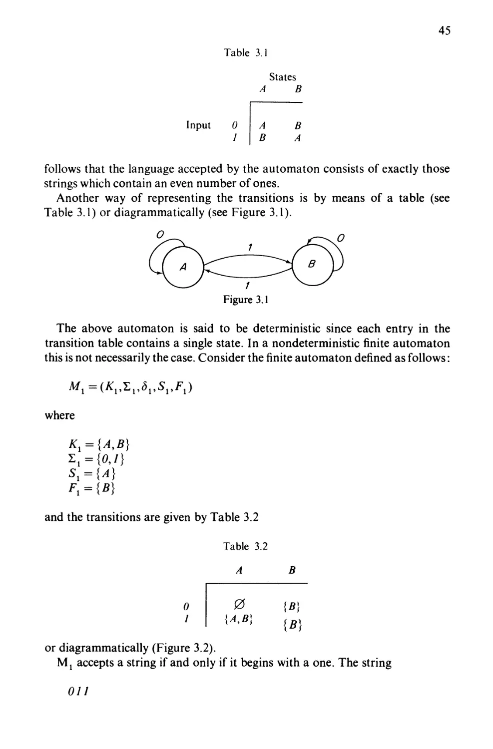


Text
0 W • I I
0 \
The Design
and Construction
of Compilers
Robin Hunter
Department of Computer Science,
University of Strathclyde
JOHN WILEY & SONS
Chichester • New York • Brisbane • Toronto
Copyright © 1981 by John Wiley & Sons Ltd
Reprinted with corrections, January 1983
All rights reserved.
No part of this book may be reproduced by any means, nor
transmitted, nor translated into a machine language without
the written permission of the publisher.
British Library Cataloguing in Publication Data:
Hunter, Robin
The design and construction of compilers. —
(Wiley series in computing)
1. Compiling (Electronic computers)
2. Electronic digital computers
I. Title
001.64*25 QA76.6
ISBN 0 471 28054 2
Photosetting by Thomson Press (India) Limited, New Delhi,
and printed and bound by The Pitman Press, Bath.
To
Kate, Andrew, and Ian
Contents
Preface xi
Chapter 1 The Compilation Process 1
1.1 Relationship between Languages and Machines 2
1.2 Aspects of the Compilation Process 11
1.3 Design of a Compiler 14
Exercises 16
Chapter 2 Language Definition 18
2.1 Syntax and Semantics 18
2.2 Grammars 19
2.3 Formal Definition of Programming Languages 29
2.4 The Parsing Problem 34
Exercises 40
Chapter 3 Lexical Analysis 42
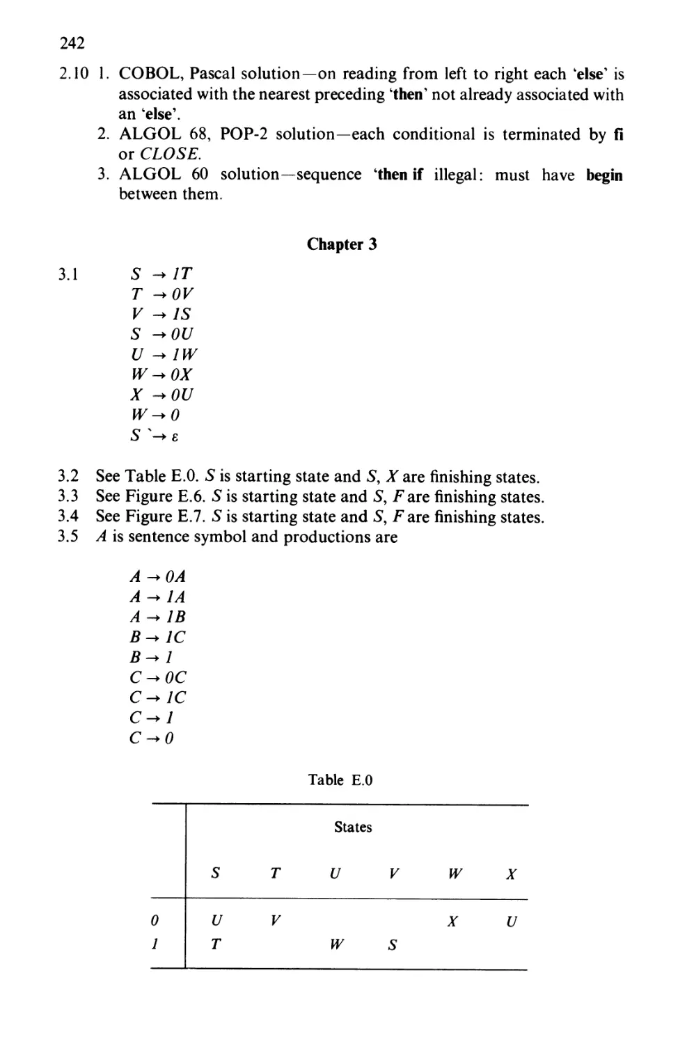
3.1 Recognition of Symbols 42
3.2 Output from the Lexical Analyser 51
3.3 Comments, etc. 54
3.4 Problems concerning particular languages 54
Exercises 56
Chapter 4 Context-Free Grammars and Top-Down Syntax Analysis 58
4.1 Context-Free Grammars 58
4.2 Method of Recursive Descent 64
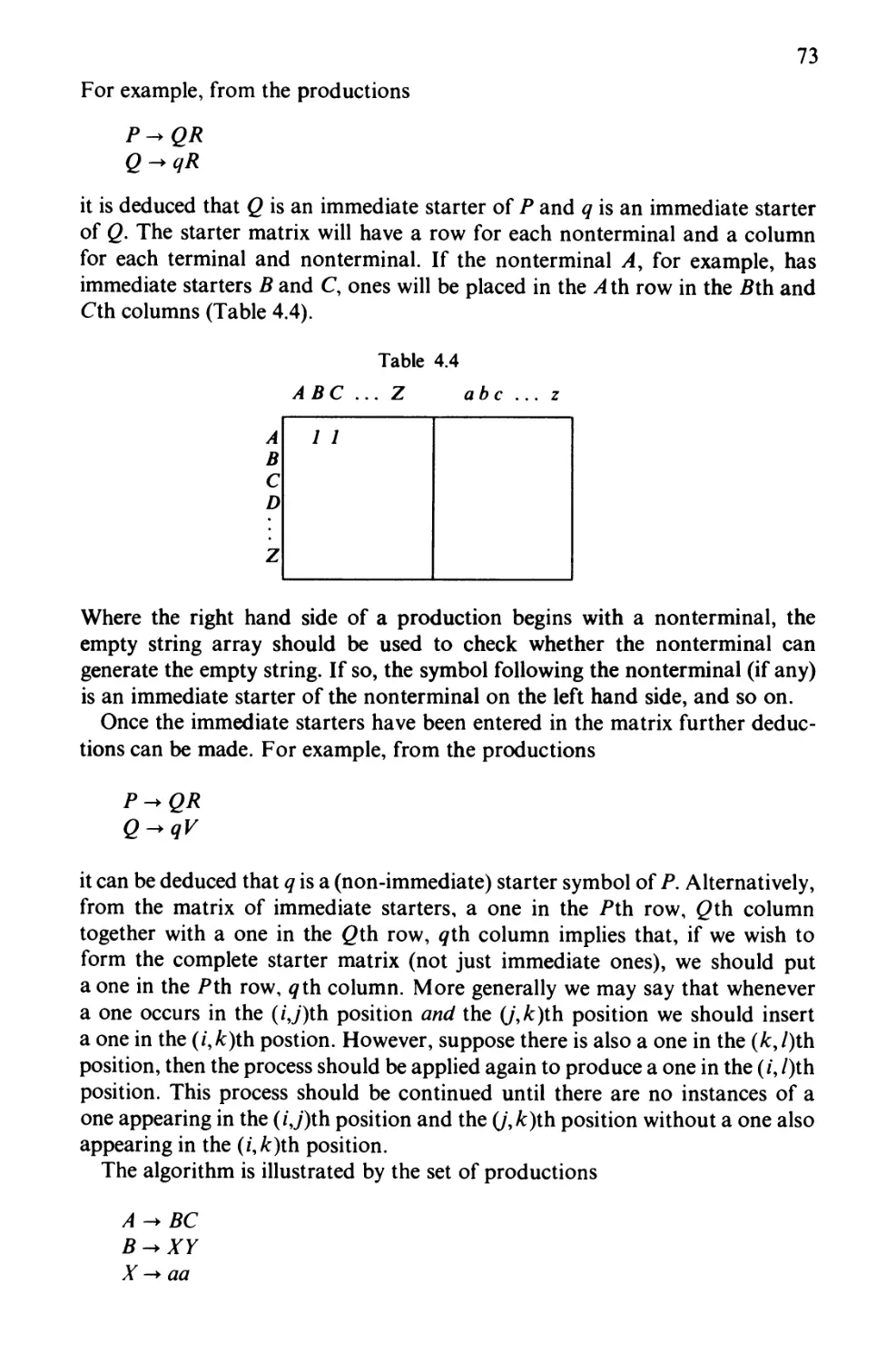
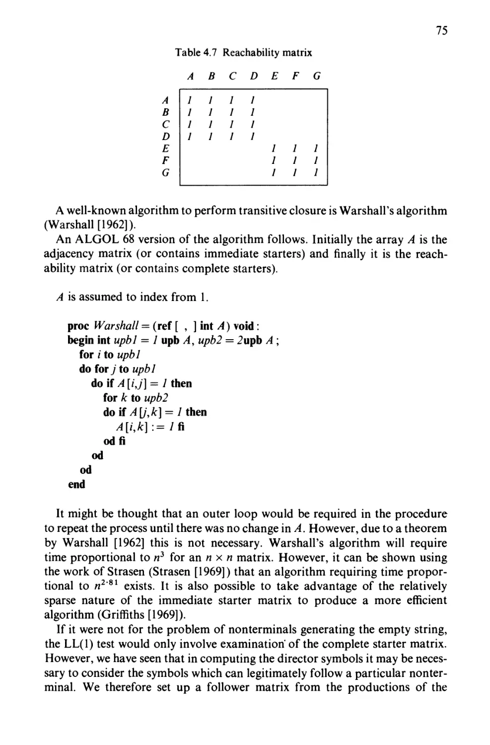
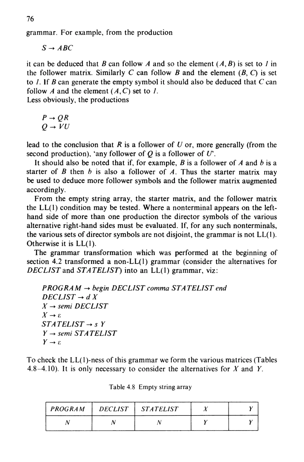
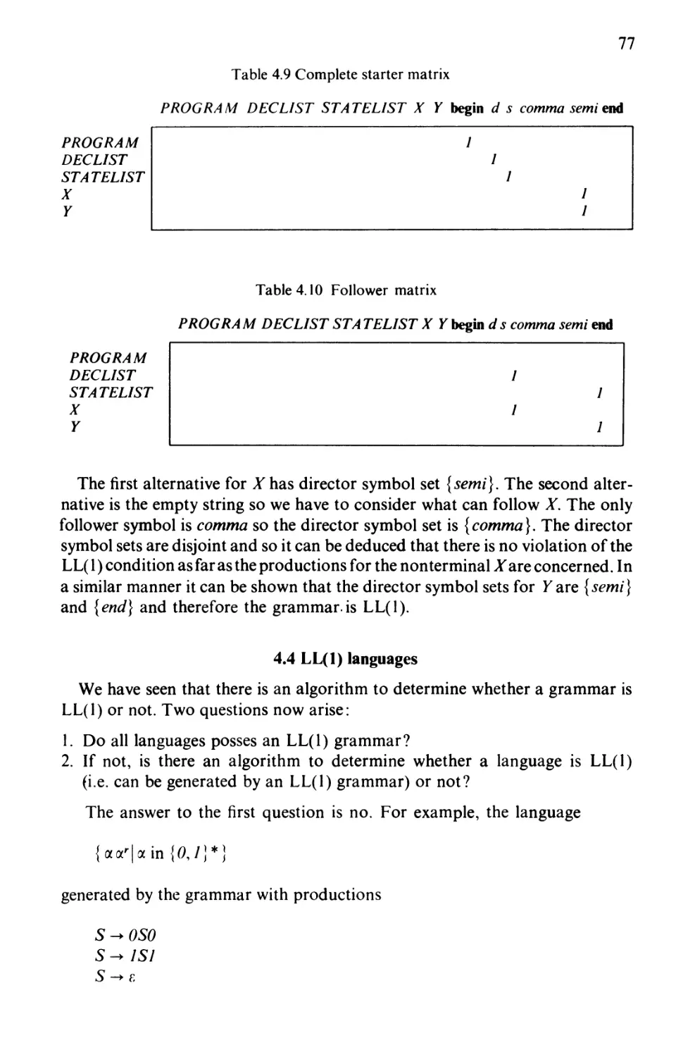
4.3 LL (1) Grammars 67
4.4 LL (1) Languages 77
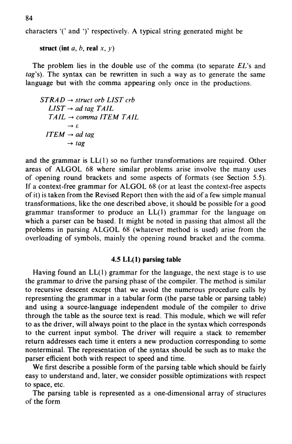
4.5 LL(1) Parsing Table 84
Exercises 94
Chapter 5 Bottom-Up Syntax Analysis 97
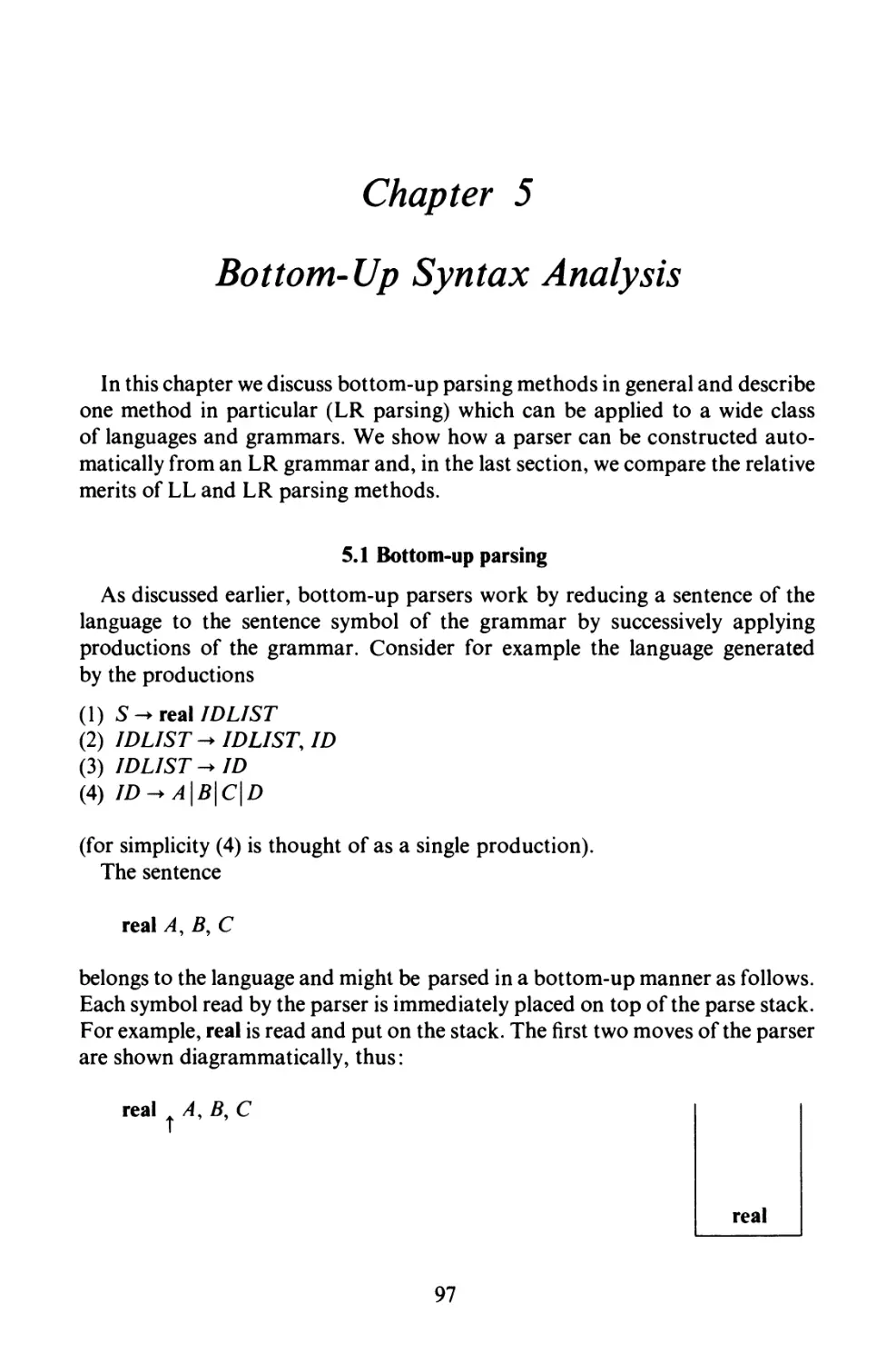
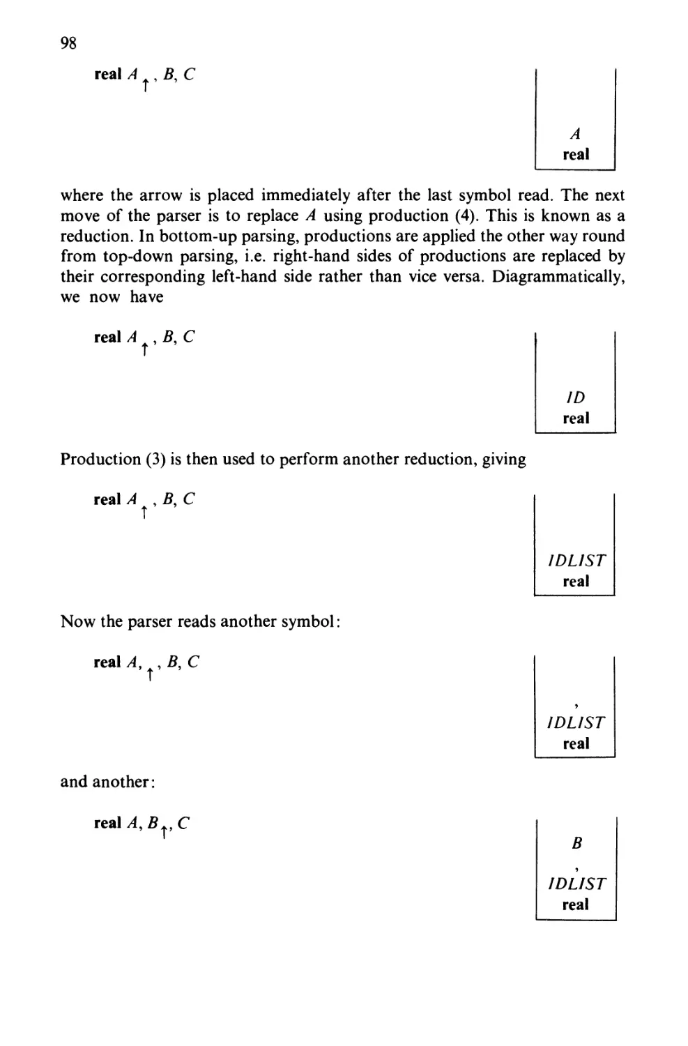
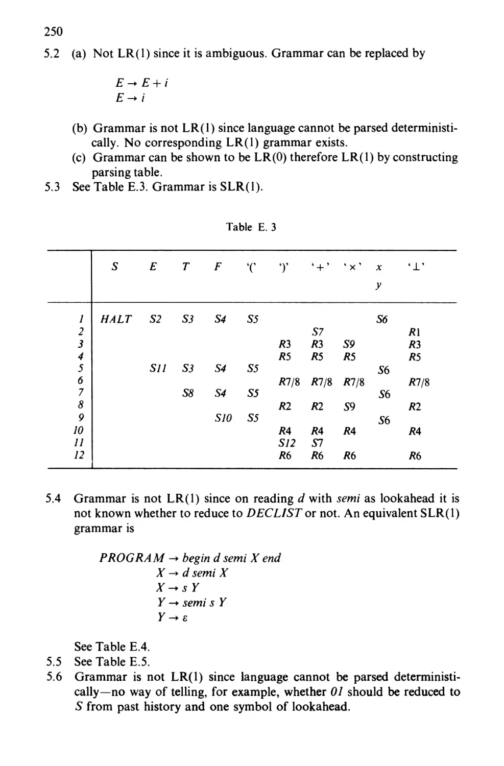
5.1 Bottom-Up Parsing 97
5.2 LR (1) Grammars and Languages 101
5.3 LR Parsing Tables 103
Vlll
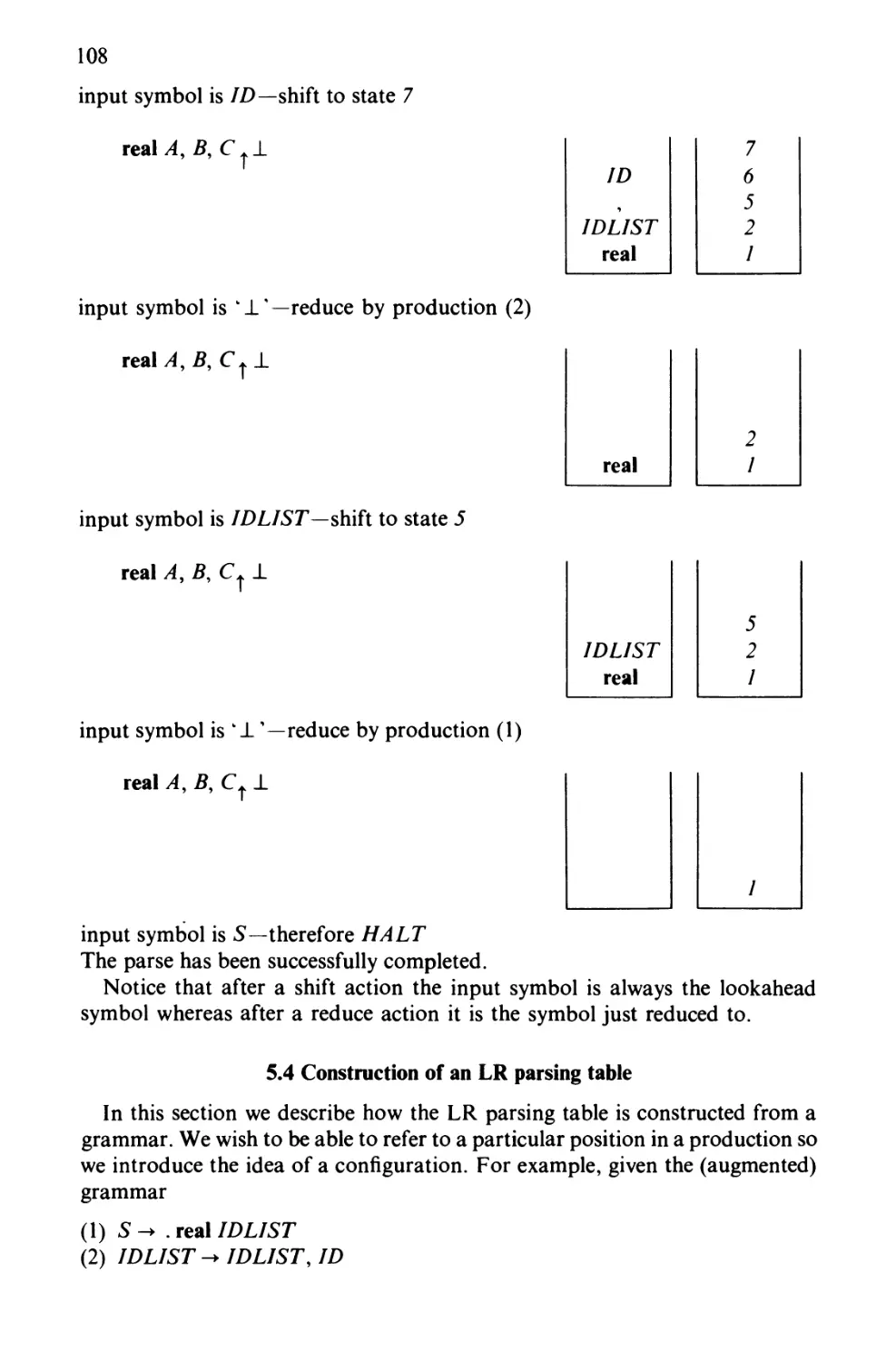
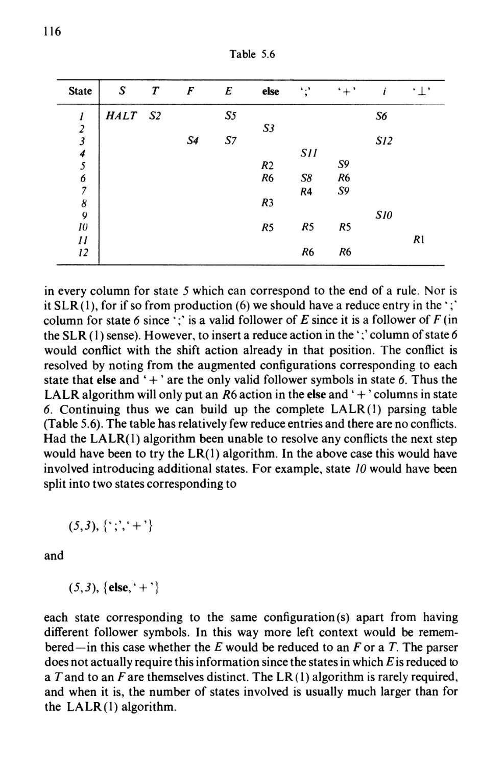
5.4 Construction of an LR Parsing Table 108
5.5 LL versus LR Parsing Methods 117
Exercises 121
Chapter 6 Embedding Actions in Syntax 123
6.1 Production of Quadruples 123
6.2 Symbol Table Manipulation 127
6.3 Other Applications 132
Exercises 133
Chapter 7 Compiler Design 135
7.1 Number of Passes 135
7.2 Intermediate Languages 143
7.3 Target Language 144
Exercises 145
Chapter 8 Symbol and Mode Tables 146
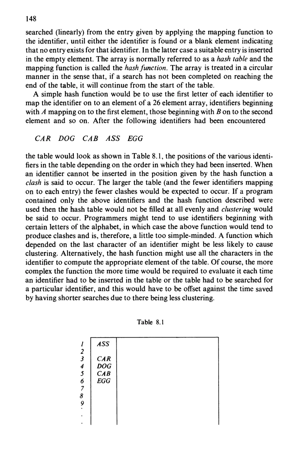
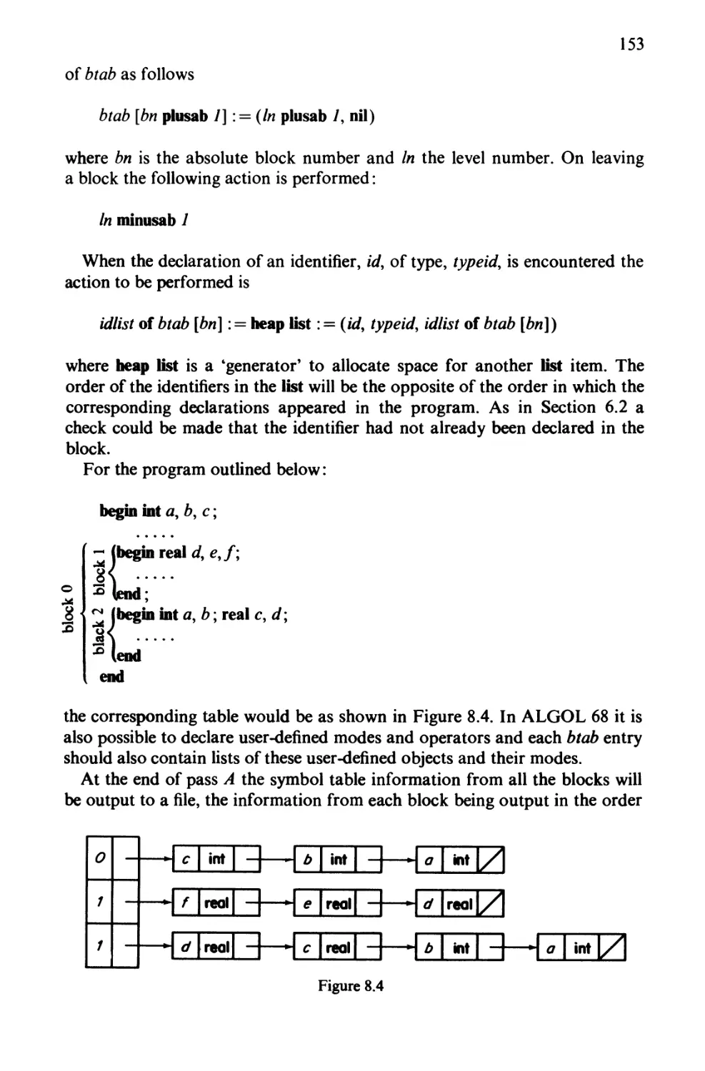
8.1 Symbol Tables 146
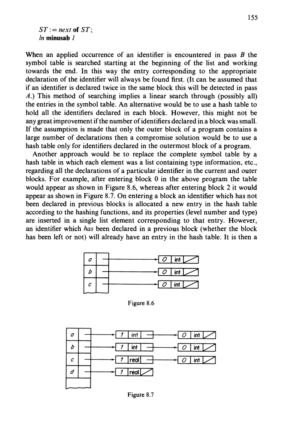
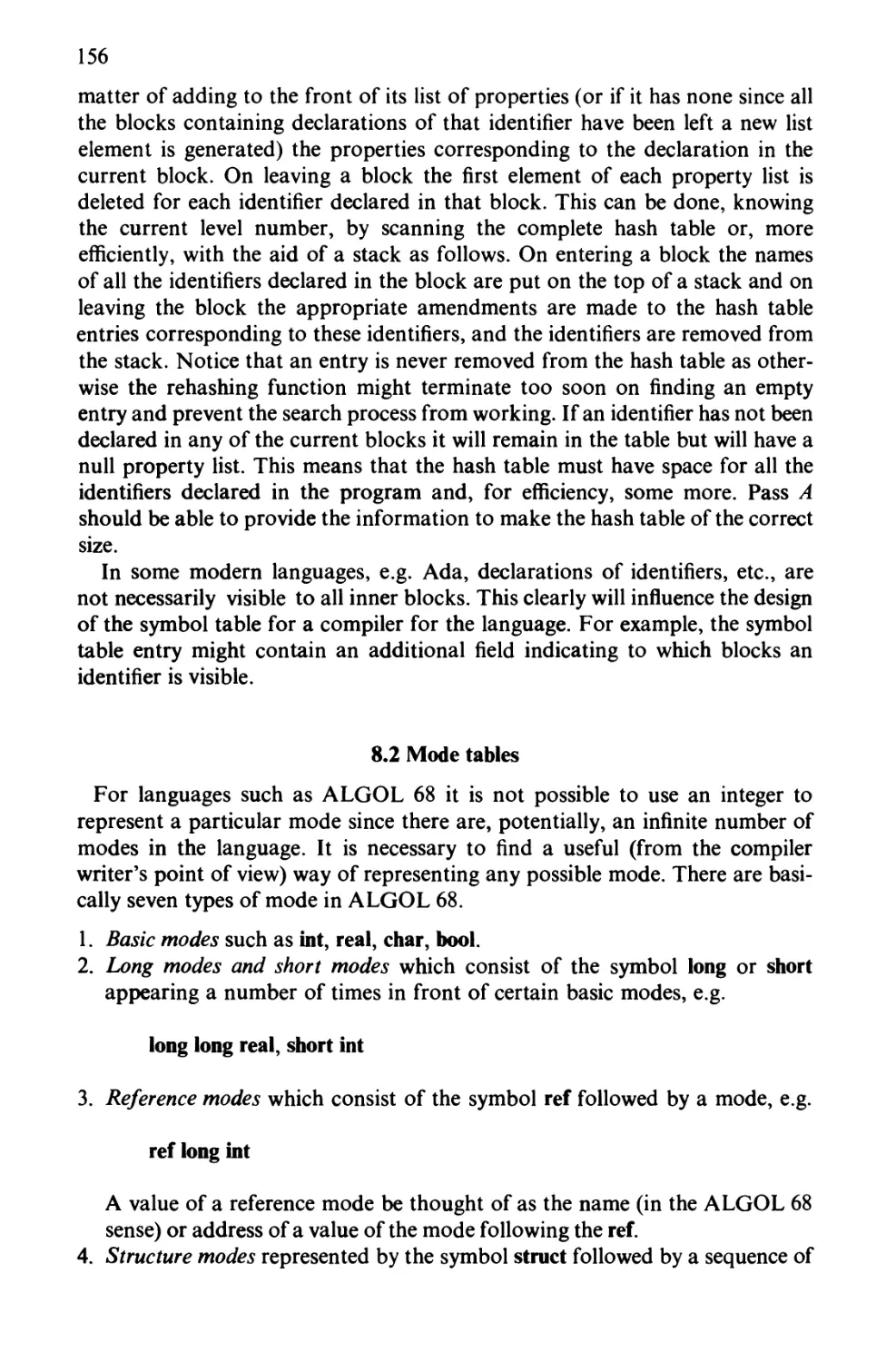
8.2 Mode Tables 156
Exercises 161
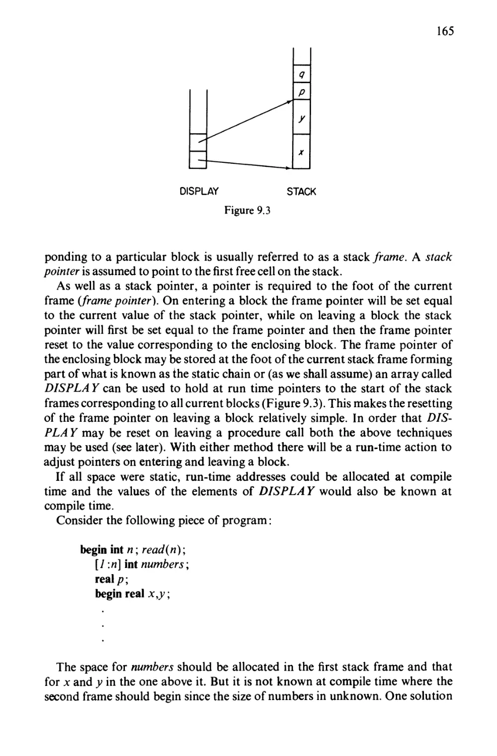
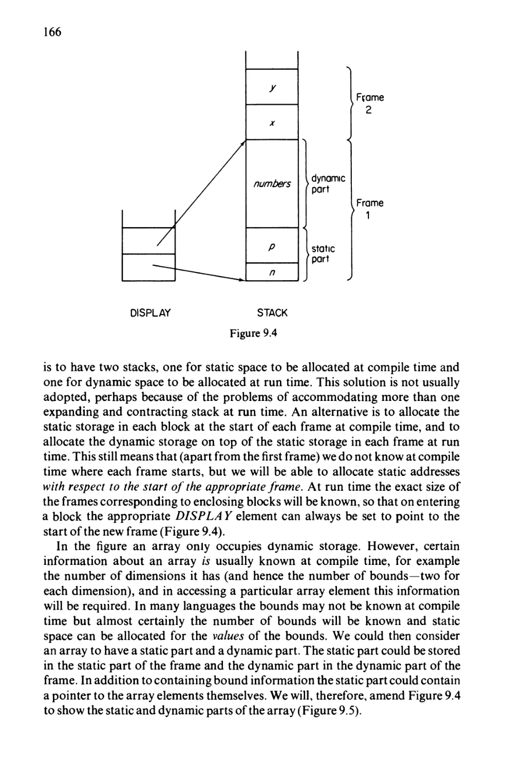
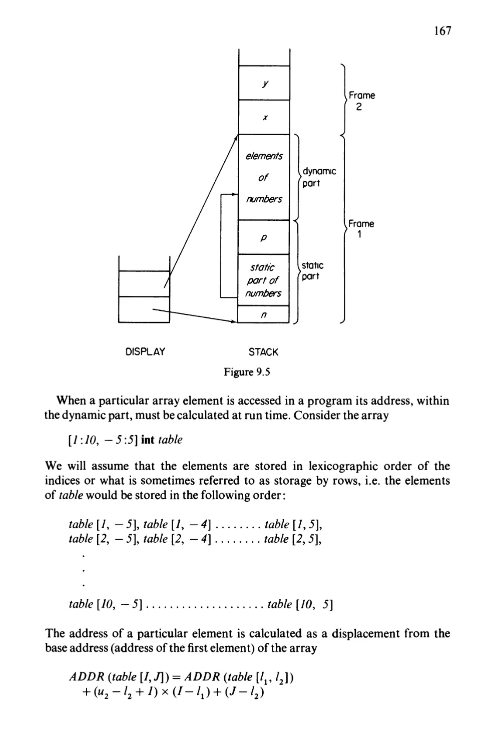
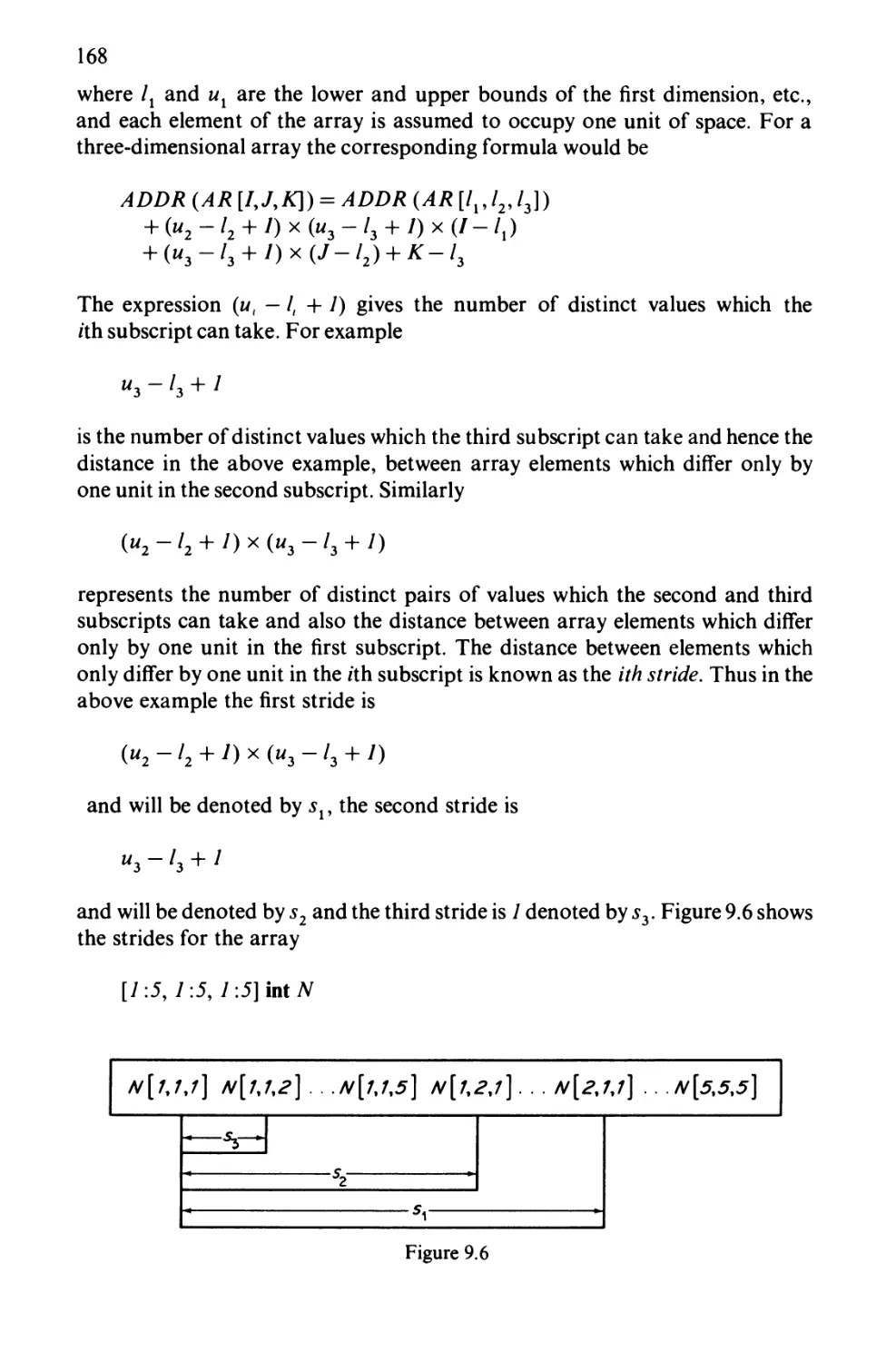
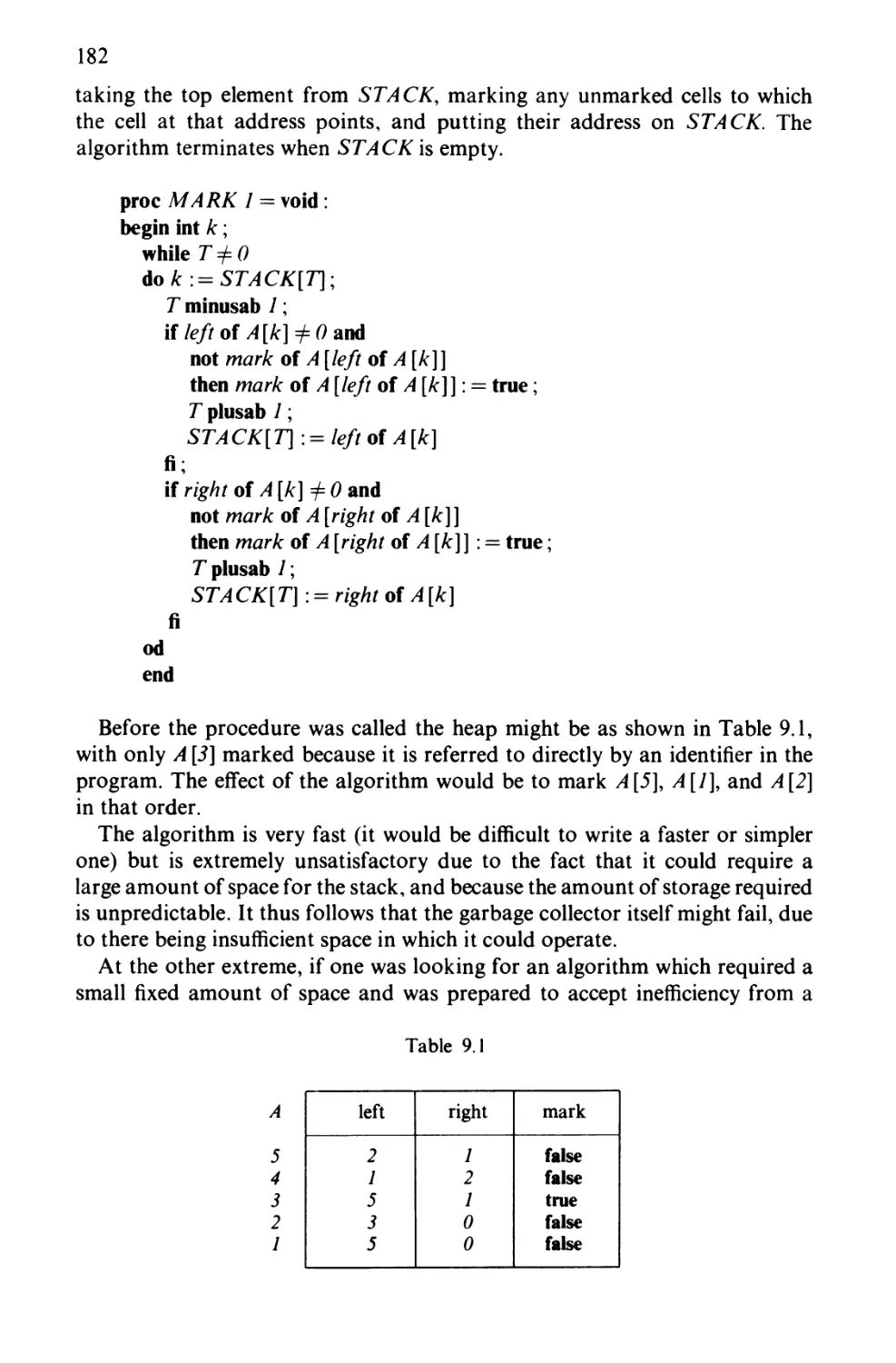
Chapter 9 Storage Allocation 162
9.1 The Run-Time Stack 162
9.2 The Heap 176
Exercises 185
Chapter 10 Code Generation 187
10.1 Intermediate Code 187
10.2 Data Structures for Code Generation 192
10.3 Generating Code for Some Typical Constructs 196
10.4 Type Considerations 202
10.5 Compile Time versus Run Time 205
Exercises 206
Chapter 11 Generation of Machine Code 208
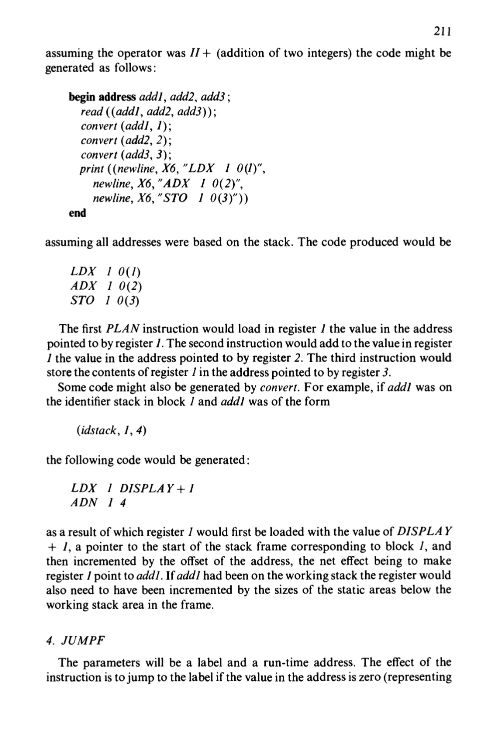
11.1 Generalities 208
11.2 Examples of Machine Code Generation 210
11.3 Object Code Optimization 213
Exercises 213
Chapter 12 Error Recovery and Diagnostics 215
12.1 Types of Error 215
12.2 Lexical Errors 216
12.3 Bracket Errors 218
12.4 Syntax Errors 220
IX
12.5 Non-Context-Free Errors 224
12.6 Run-Time Errors 227
12.7 Limit Errors 228
Exercises 229
Chapter 13 Writing Reliable Compilers 230
13.1 Use of Formal Definition 230
13.2 Modular Design 232
13.3 Checking the Compiler 235
Exercises 235
Solutions to Exercises 237
Bibliography 258
Index
261
Preface
This book deals firstly with the design and secondly with the construction
of compilers for high-level programming languages. While the emphasis
therefore is on the design aims of compiler projects and how they might be
achieved, the practical details of compiler writing have not been overlooked
and the background to much of the text is the compiler work which has taken
place in the Computer Science Department in the University of Strathclyde
over the last few years.
The book should be suitable as a basis for an undergraduate course on
compilers and has been used as such in the University of Strathclyde. It deals
with the implementation of block-structured languages such as ALGOL 60,
PL/1, ALGOL 68, Pascal, or Ada and reference is made frequently to aspects
of particular languages. Algorithms are described in an actual programming
language (ALGOL 68) but students not familiar with this particular language
should not have difficulty following them. The exercises at the end of each
chapter are intended to stimulate the student to think more about how
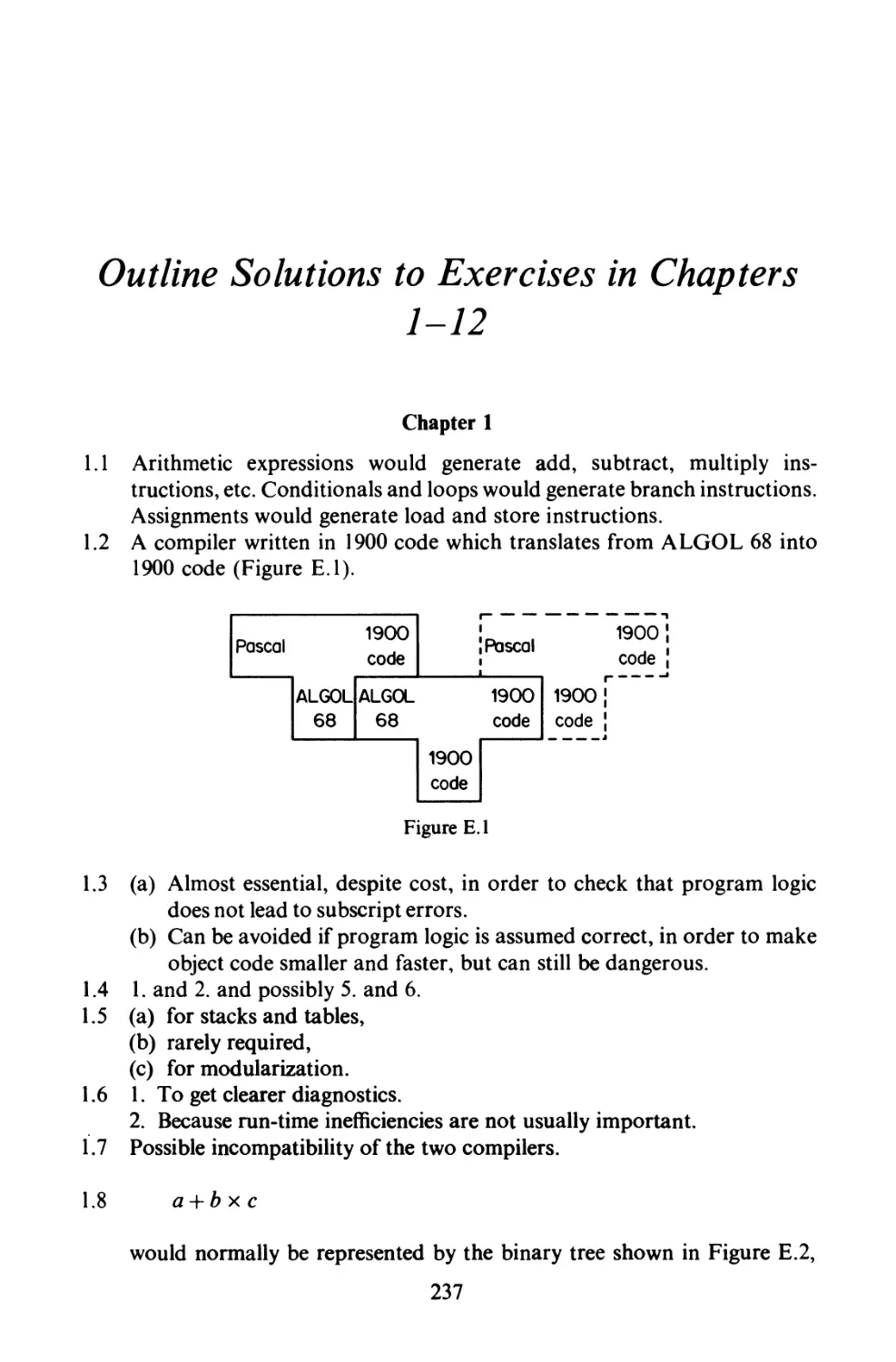
compilers are constructed; outline solutions to the exercises in chapters 1-12
are given at the end of the book.
Chapter 1 discusses the compilation process in general terms, as well as the
relationship between high level programming languages and typical computers,
while Chapter 2 goes on to discuss the formal definition of programming
languages. Chapter 3 covers lexical analysis and Chapters 4 and 5 are concerned
with top-down and bottom-up methods of syntax analysis.
Chapter 6 describes how a context-free grammar can be used as a
framework for the compiler actions and Chapter 7 deals with the overall design of
compilers with particular emphasis on the design of multi-pass compilers.
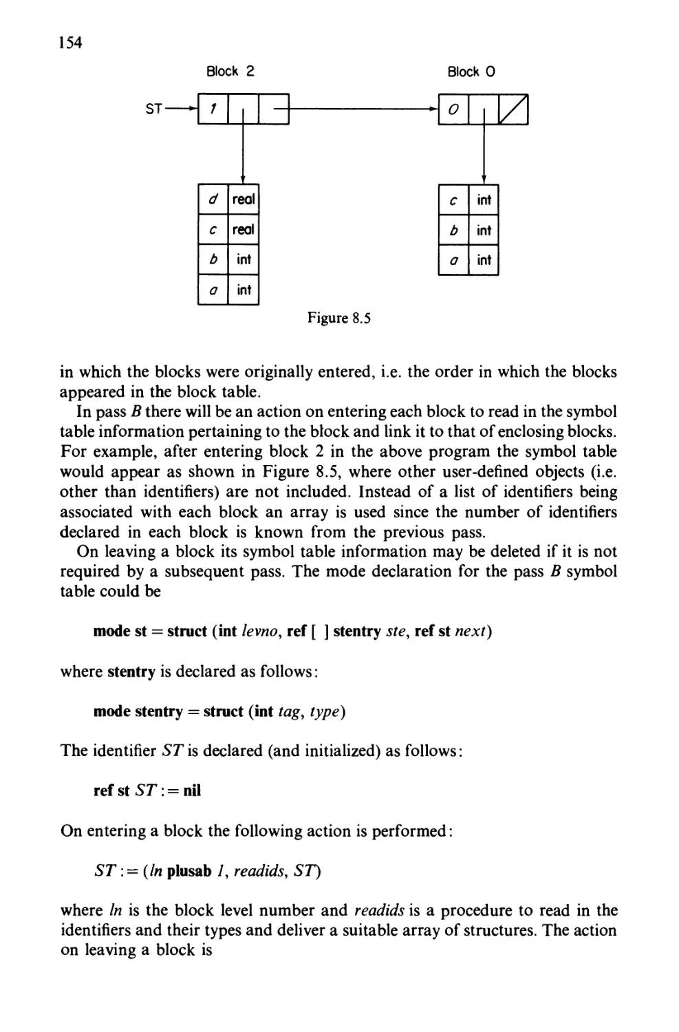
The structure of symbol tables and mode (or type) tables for languages
with complex types is dealt with in Chapter 8, while Chapter 9 is concerned
with local and global storage allocation. Chapters 10 and 11 deal with code
generation and the use of a machine-independent intermediate code.
Chapter 12 is a discussion of methods of error recovery and diagnosis
while Chapter 13 introduces ideas concerned with the production of reliable
compilers.
Xll
Acknowledgements
I am very grateful to a number of colleagues and students who have read
all or part of the manuscript and commented on it. In particular I would like
to thank Dr A. D. McGettrick and Mr R. R. Patel for their constructive
comments and I am indebted to Miss A. Whitelaw for checking the LR parsing
tables using the YACC compiler-compiler.
The manuscript was typed by Mrs M. MacDougall, Mrs U. Melville, and
Miss A. Wisley and I am very grateful to them for their careful work. My
wife, Kate, has helped in many ways with the preparation of the manuscript
and for this and her constant support I am extremely grateful.
I would also like to thank the publishers, John Wiley and Sons, for their
help and for the opportunity to write the book in the first place.
Chapter 1
The Compilation Process
Programs written in high-level (or problem-oriented) programming
languages have to be translated into equivalent machine code programs before they
can be executed on a computer. High-level languages have existed since the
mid-1950's: early examples of such languages were FORTRAN and COBOL,
while ALGOL 68, Pascal, and Ada are examples of more recently designed
high-level languages. A program which will translate any program written
in a particular high-level language into an equivalent program in some other
language (usually the code for some particular machine) is called a compiler.
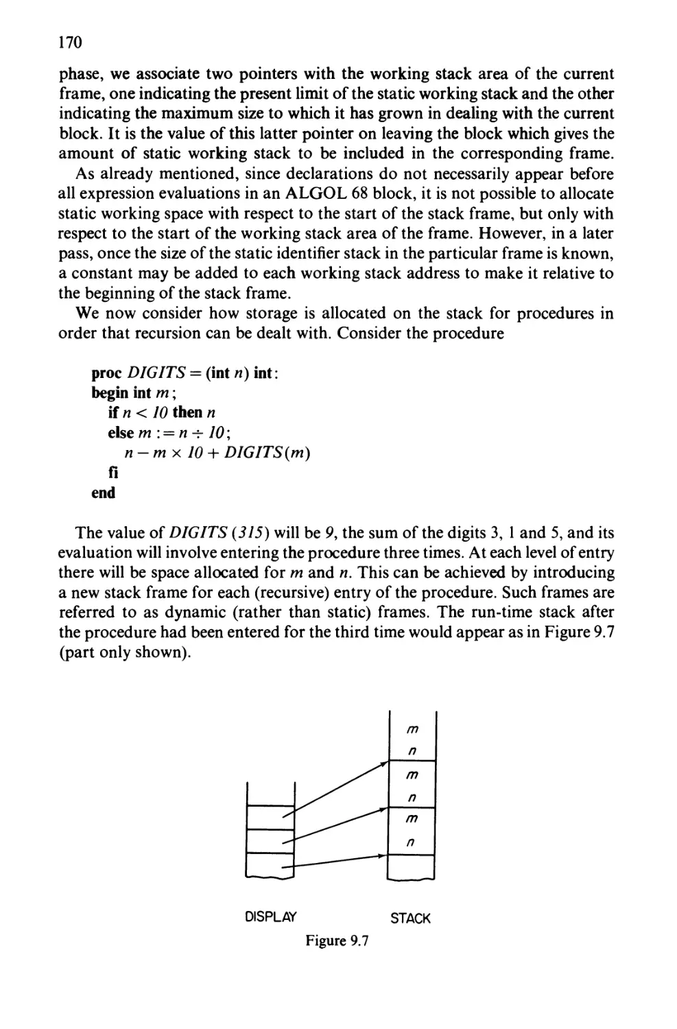
Compiling a program consists of analysis, determining the intended effect
of the program, followed by synthesis, generating the equivalent machine-code
program. In the course of analysis a compiler should be able to detect if the
input program is invalid in any sense (i.e. does not belong to the language for
which the compiler was written) and if so return an appropriate message to
the programmer. This aspect of compilation is referred to as error detection.
Compiler technology has made considerable advances over the last twenty-
five years. Early compilers used rather ad hoc methods, tended to be slow, and
were written in a rather unstructured way. (A brief history of compiler writing
can be found in Bauer [1974].) More modern compilers tend to use more
systematic methods, are relatively fast, and tend to be structured so as to
separate out the distinct aspects of compilation as far as possible.
Instead of translating each program into machine code and then executing
it, an alternative approach is first to translate the program into an intermediate
language and then to translate and execute each intermediate language
statement as it is encountered. A program which will translate and execute a program
written in a high-level language in this way is called an interpreter. The
advantages of an interpreter over a compiler are:
1. It is often easier to communicate error messages to the user in terms of the
original program.
2. The intermediate language version of the program is often more compact
than the machine code produced by a compiler.
3. An alteration to part of a program need not involve recompiling the whole
program.
Interactive languages such as BASIC are often implemented by means of
1
an interpreter, a common intermediate language being some form of Reverse
Polish Notation (see Section 10.1). A good text book on implementing
interactive languages is Brown [1979]. The chief disadvantage of an interpreter is
that programs tend to run relatively slowly since intermediate code statements
have to be translated each time they are executed, though the time penalty may
not be too significant depending on the design of the intermediate language.
A compromise is the mixed-code approach of Dakin and Poole [1973] in which
the part of the program most frequently executed is compiled and the rest
interpreted. This tends to save space since that part of the program which is
to be interpreted is likely to be much more compact than the compiled code.
An extension of this idea, referred to as Throw-Away Compiling' is due to
Brown [1976].
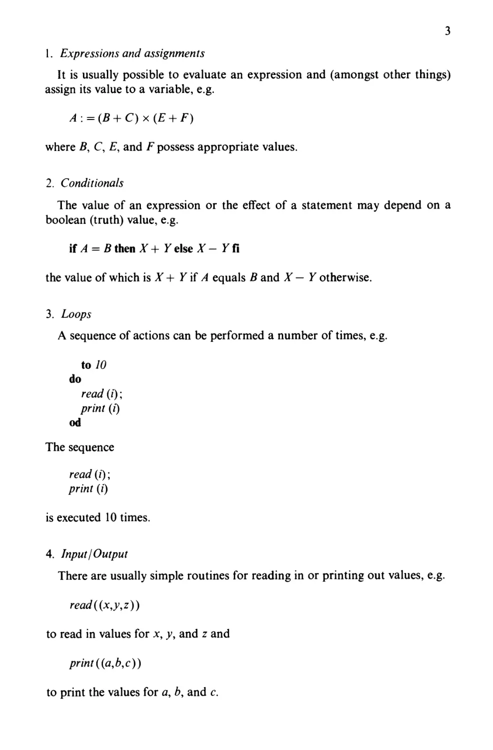
In this book we will be mainly concerned with compilers rather than
interpreters, though many of the ideas could be applied to either. In discussing
compilers we will refer to the program to be compiled as the source program
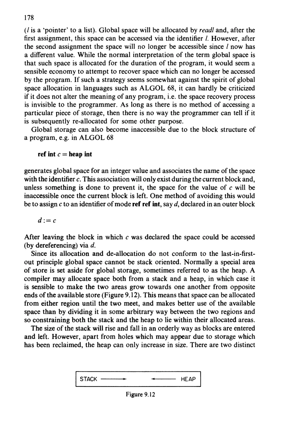
(or source text), and the machine code produced as the object code (figure 1.1).
Similarly, the high-level language may be referred to as the source language
and the machine language as the object language.
Source J c j(er ^Object
program code
Figure 1.1
In this chapter we discuss the characteristics of high-level languages and
typical computers and the various aspects of the compilation process. This
leads us on to consider the overall design of compilers.
1.1 Relationship between languages and machines
While the differences between the various high-level languages can be very
significant from the users' (and the implementors') point of view, it is the
similarities between these languages which we wish to emphasize in this section
in order to try to indicate the sort of tasks the compiler has to perform. Typical
of the high-level languages we will have in mind are BASIC, FORTRAN,
PL/1, Pascal, ALGOL 68, and (possibly to a slightly lesser extent) COBOL.
The program fragments which we use to illustrate points will be in ALGOL 68
but could just as well be in any of the other languages and readers unfamiliar
with ALGOL 68 should not have any great problems in following them.
Languages
Features that most high-level languages have in common are:
3
1. Expressions and assignments
It is usually possible to evaluate an expression and (amongst other things)
assign its value to a variable, e.g.
A: = (B+C)x(E + F)
where B, C, £, and F possess appropriate values.
2. Conditionals
The value of an expression or the effect of a statement may depend on a
boolean (truth) value, e.g.
\fA = BttenX+ YeiseX- Kfi
the value of which is X + Y if A equals B and X — Y otherwise.
3. Loops
A sequence of actions can be performed a number of times, e.g.
to/0
do
read (/);
print (i)
od
The sequence
read (/);
print (i)
is executed 10 times.
4. Input/Output
There are usually simple routines for reading in or printing out values, e.g.
read((x,y,z))
to read in values for x, y, and z and
print ((a9b9c))
to print the values for a, b, and c.
4
5. Procedures I Subroutines I Functions
It is usually possible to give a program a reasonable structure by dividing it
into modules (and possibly submodules, etc.) and writing each module as a
separate procedure or subroutine. For example, if a program involved from
time to time the calculation of the average of an array of real numbers the
following procedure might be written:
proc average = ([ ] real row) real:
begin real sum: = 0 ;
for / from lwb row to upb row
do sum plusab row [i]
od;
sum /(upb row — lwb row + 1)
end
and assuming a had been declared as
[7:70] real a
average could be called, for example, as follows:
print {average (a))
6. Blocks
All programs require storage for values of variables, etc. In most languages
it is possible for variables required in different parts of a program to share
the same storage. This aspect of programming languages is usually referred
to as block structure, a block being defined as a piece of program containing
some declarations of variables, etc., e.g.
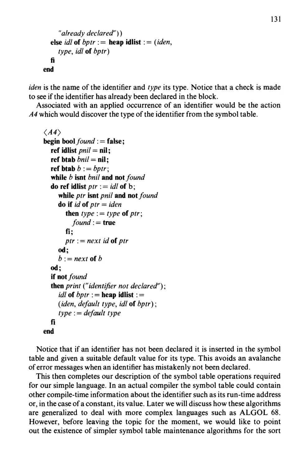
begin int a, b;
print ((a xfact, b xfact))
end
the space required for a and b being allocated on entering the block and
deallocated on leaving the block.
Languages such as BASIC and FORTRAN do not really have block structure
and Pascal only has it in a limited form. More modern-type languages such as
the ALGOL languages and the United States Department of Defence language,
Ada, all have block structure. In this book we will assume for the main part
that the source language is block structured. Non-block-structured languages
will tend to be easier to compile as far as storage allocation, etc., is concerned.
We will not at this stage say a great deal about the differences between the
various high-level languages in, for example, the ways in which loops or
5
conditionals are provided or the types of operators available. For a good
summary of language differences from a compiler writer's point of view see
Aho and Ullman [1977].
One language feature which substantially affects the structure of a compiler
is the idea of type. In most languages each possible value belongs to one of a
finite or infinite number of types, while each type corresponds to a finite or
infinite number of values. For example, the set of all integers, real numbers,
or characters in some character set might be regarded as a type. In Pascal the
idea exists of a sub-type corresponding, for example, to integers in a certain
range and many languages have aggregate types corresponding to arrays or
records. Modes in ALGOL 68 correspond roughly to types but are more
general. For example, there is a mode
proc (real) real
corresponding to a procedure with one real parameter and a real result. In this
book we use both the terms mode and type: mode mainly in the context of
ALGOL 68 and type otherwise.
Some languages, such as ALGOL 68 and Pascal, are said to be strongly
typed or to have static types, i.e. the types of all values in the program are
known at compile time. This introduces redundancy into the language and
increases the checking which can be done at compile time. For example
char x : = 3
would be detected as illegal by the compiler. In PL/1, which is also strongly
typed, the above 'error' would not be detected since there are so many implicit
type conversions (e.g. integer to character).
Languages such as POP-2, APL, and LISP are said to be weakly-typed, or
to have dynamic types, since types are not known until run time. For example,
in POP-2 the declaration
VARSX, Y\
means that X and Y can take values of any type. An assignment such as
X^Y
(assignments go from left to right in POP-2) would always be legal.
However, in
X+ Y
the application of the dyadic operator + to X and Y may or may not be legal
depending on the current types of X and K This can only be checked at run
6
time and such run-time checking must be included in the object code with the
inevitable cost of slowing down the object program.
A compromise between static and dynamic types is to make the types static
in the main part, but to have an extra type (called, for example, any type or
general) the values of which can be any of the other types in the language. This
approach is adopted by CPL and ESPOL (Burroughs ALGOL 60 superset).
A third approach to types is that taken by BCPL, which only has one type,
which can be thought of as a bit pattern, and
A + B
means addition of bit patterns. Distinct types may exist in the mind of the
programmer but are unknown to the program or the implementation. It is the
programmer's responsibility not to attempt to add a boolean and an integer.
No type-checking is possible at compile time or run time.
Machines
As in BCPL, the concept of type or mode is not present in machine code.
The computer deals with bit patterns without attaching any meaning to them.
Computers, like languages, very greatly in detail, but it is possible to list a
number of typical characteristics in order to illuminate the task which the
compiler has to perform. The features of individual machines relate less to their
usefulness to the programmer and more to cost-benefit trade-offs in the overall
design of the computer. Features common to most machines include:
1. Linear main store
This is a sequence of bit-groups in which information is stored. Each bit-
group is usually referred to as a word and might typically contain 16, 24, or,
32 bits (binary digits). The position of a word in the memory is usually referred
to as its address. Addresses usually run from 0 to 2" — 1 where n is some integer.
(In some computers the unit of memory is referred to as the byte, which is
usually about 8 bits and is the amount of space required to store a single
character. Bytes usually have distinct addresses.)
2. Registers
Like a word in the main store, a register can be used for storing data. Registers
are usually involved in all arithmetic operations performed by the computer
and the time taken to store a value in or retrieve a value from a register is much
less than for a word in main store. There are usually only a small (possibly
8 or 16) number of registers in any computer.
7
3. Instruction set
Each machine has a set of instructions, referred to as its machine code. Each
instruction consists of a sequence of binary digits and can usually take several
parameters, also sequences of binary digits. These parameters might typically
involve the name of a register or an address in the main store. Each instruction
(including parameters) usually occupies an exact number of words (or possibly
half-words) and can be stored in the main store during execution of the program.
Some machine codes have fixed length instructions (e.g. ICL 1900 series),
others variable length instructions (e.g. IBM 370 series). Using mnemonics
in place of binary numbers for instruction codes and decimal numbers in place
of sequences of binary digits elsewhere, typical machine code instructions
might be
LDX 1 4444
meaning load the contents of address 4444 into register /. (Since it may not
be known in advance in which part of the main store the program will reside
during execution, the address fields are usually not absolute but relative to
some base value.),
STO 2 2000
meaning store the contents of register 2 in address 2000,
ADX2 102
meaning add the contents of address 102 to what is in register 2,
BRN 4000
meaning jump (or branch) to address 4000 and continue executing instructions
from that address.
Other features of machines, which do not particularly concern us from the
compilation point of view, are:
4. Control unit
For interpreting the machine code instructions and arranging for them to
be executed.
5. Arithmetic unit
This is where the various arithmetic operations, tests, etc. are performed.
The job of the compiler, therefore, is to produce executable code from the
8
source code. In some cases the compiler will only go as far as producing assembly
code for the particular machine and the final stage of producing machine code
will be performed by a separate program called an assembler. Assembly code
is similar to machine code but mnemonics are used for instructions and
addresses, and labels can be used as the destinations of jumps. An assembler has a
relatively simple task to perform and most of the compiler's work is concerned
with translating the relatively sophisticated constructs of the high-level language
into the relatively simple machine code or assembly code of the computer
concerned.
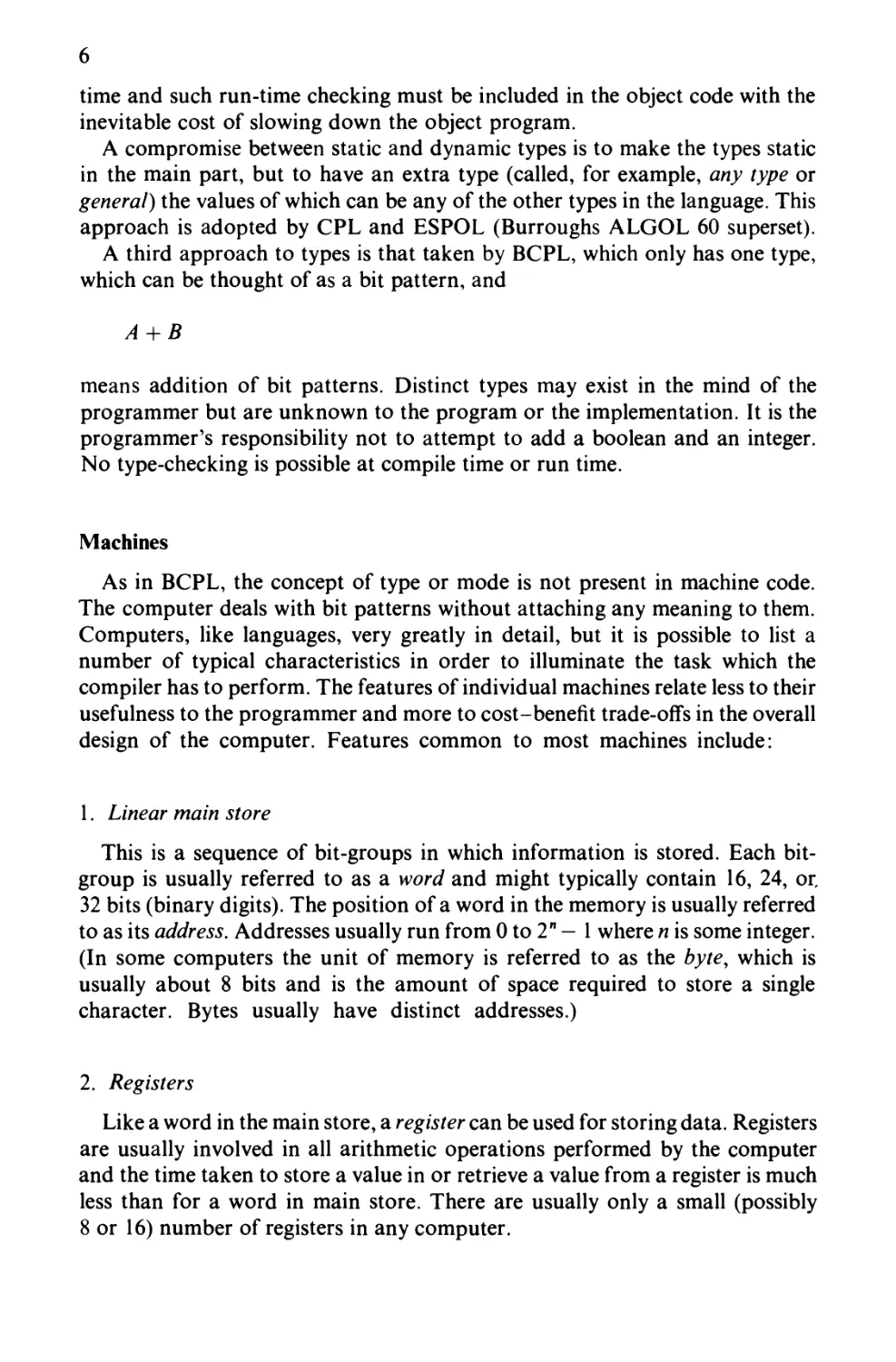
A compiler, therefore, involves two languages and in addition there is the
language in which the compiler is written. In the simplest cases this is the
machine code of the computer on which it is to run. However, we shall see
this is not always the case.
PL/1 1900
code
1900
code
Figure 1.2
A large letter T can be used to represent a compiler. For example, a compiler
for PL/1 written in ICL 1900 code to produce 1900 code could be represented
as in Figure 1.2, the top left-hand corner giving the source language, the top
right-hand corner giving the object language, and the bottom of the T giving
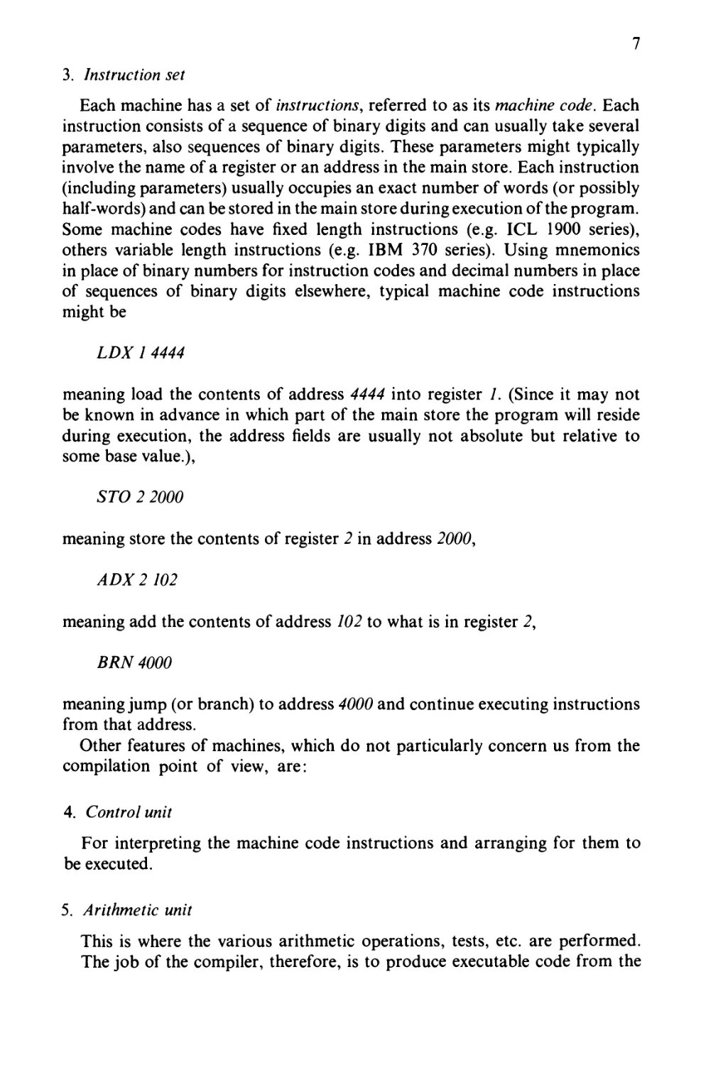
the language the compiler is written in. A cross-compiler produces code for
some machine other than the host machine, for example Figure 1.3 represents
a compiler written in 1900 code to compile FORTRAN programs in to PDP-11
code. Using this compiler FORTRAN programs could be compiled on a
1900 and run on a PDP-11.
FORTRAN
1900
code
Figure 1.3
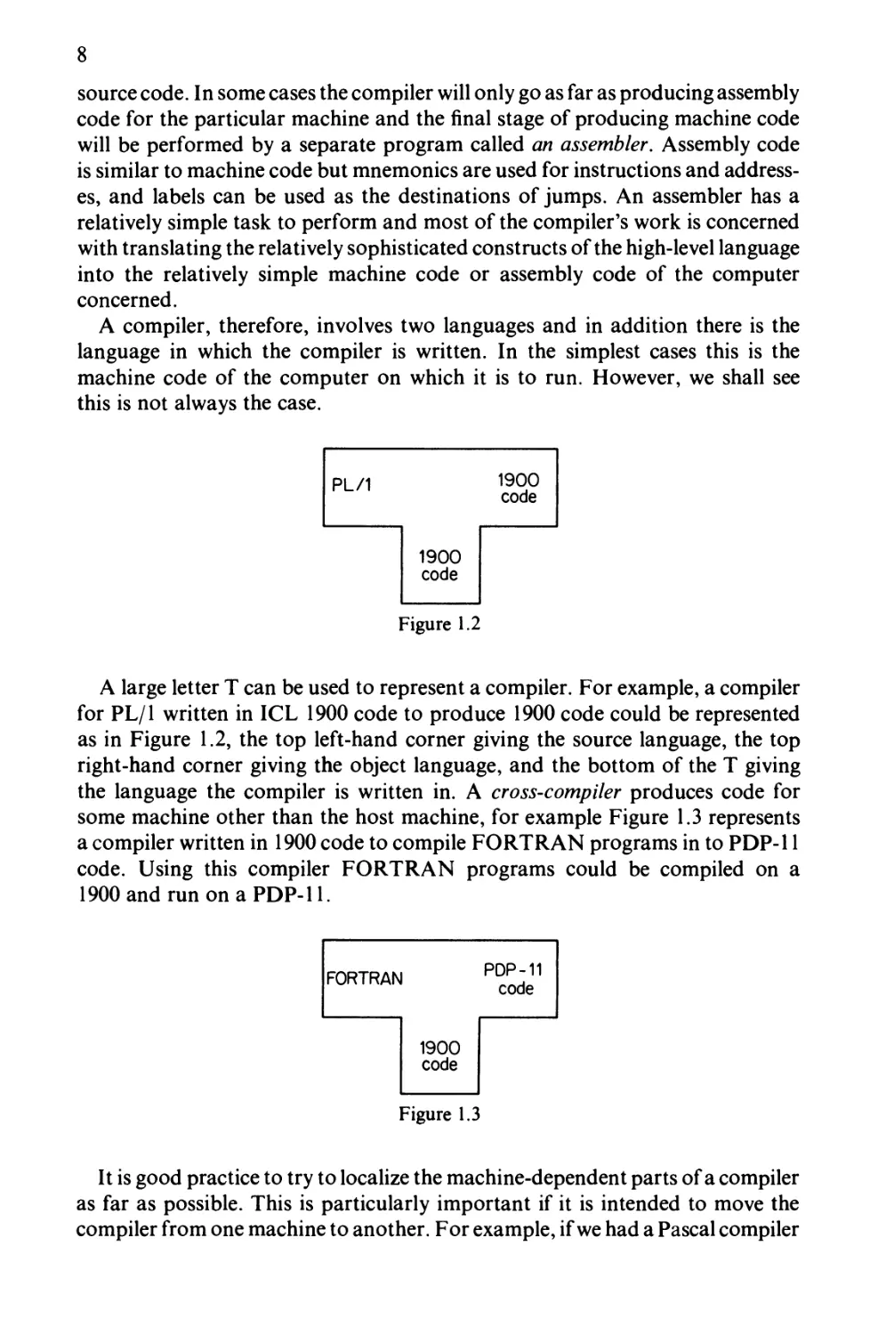
It is good practice to try to localize the machine-dependent parts of a compiler
as far as possible. This is particularly important if it is intended to move the
compiler from one machine to another. For example, if we had a Pascal compiler
9
written in FORTRAN to produce code for machine A (Figure 1.4) then to
run the compiler on machine A we would need first of all to translate it into
A-code by means of a FORTRAN compiler written in A-code and producing
A-code (Figure 1.5). From the two compilers illustrated we are able to produce
a third compiler by using the second compiler to compile the first one (Figure
Pascal A-code
FORTRAN
Figure 1.4
FORTRAN A-code
A-code
Figure 1.5
Pascal A-code
A-code
Figure 1.6
Pascal
FORTRAN
A-code
FORTRAN
A-code
Pascal
A-code
A-code
A-code
Figure 1.7
o
Pascal
FORTRAN
M- code
FORTRAN
1
Assembler
M-code
Assembler
M-code
FORTRAN
M-code
M- code
Pascal
M-code
M - code
M-code
Figure 1.8
11
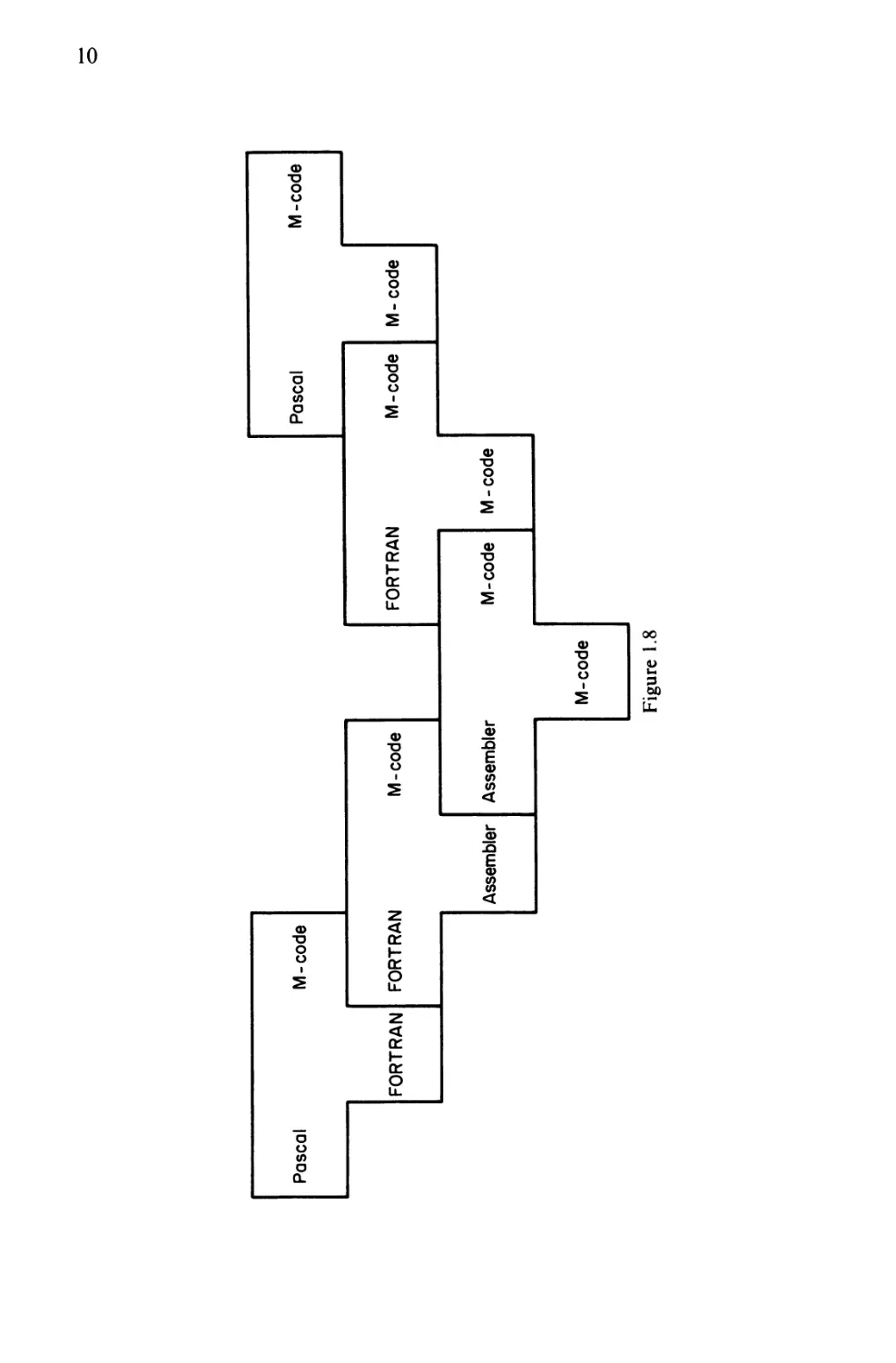
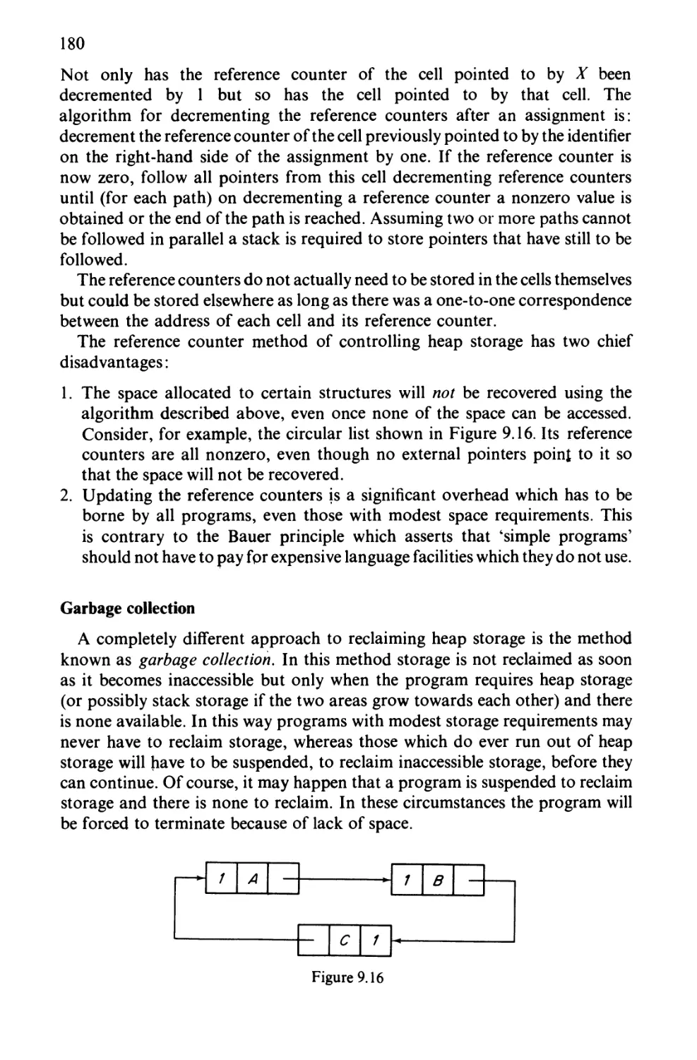
1.6). This can be demonstrated by joining the T diagrams together according
to simple rules (Figure 1.7) where the rules for combining the T diagrams
state that arms of the middle T must refer to the same languages as the adjacent
legs of the left and right T, and also the two top T's must have the same languages
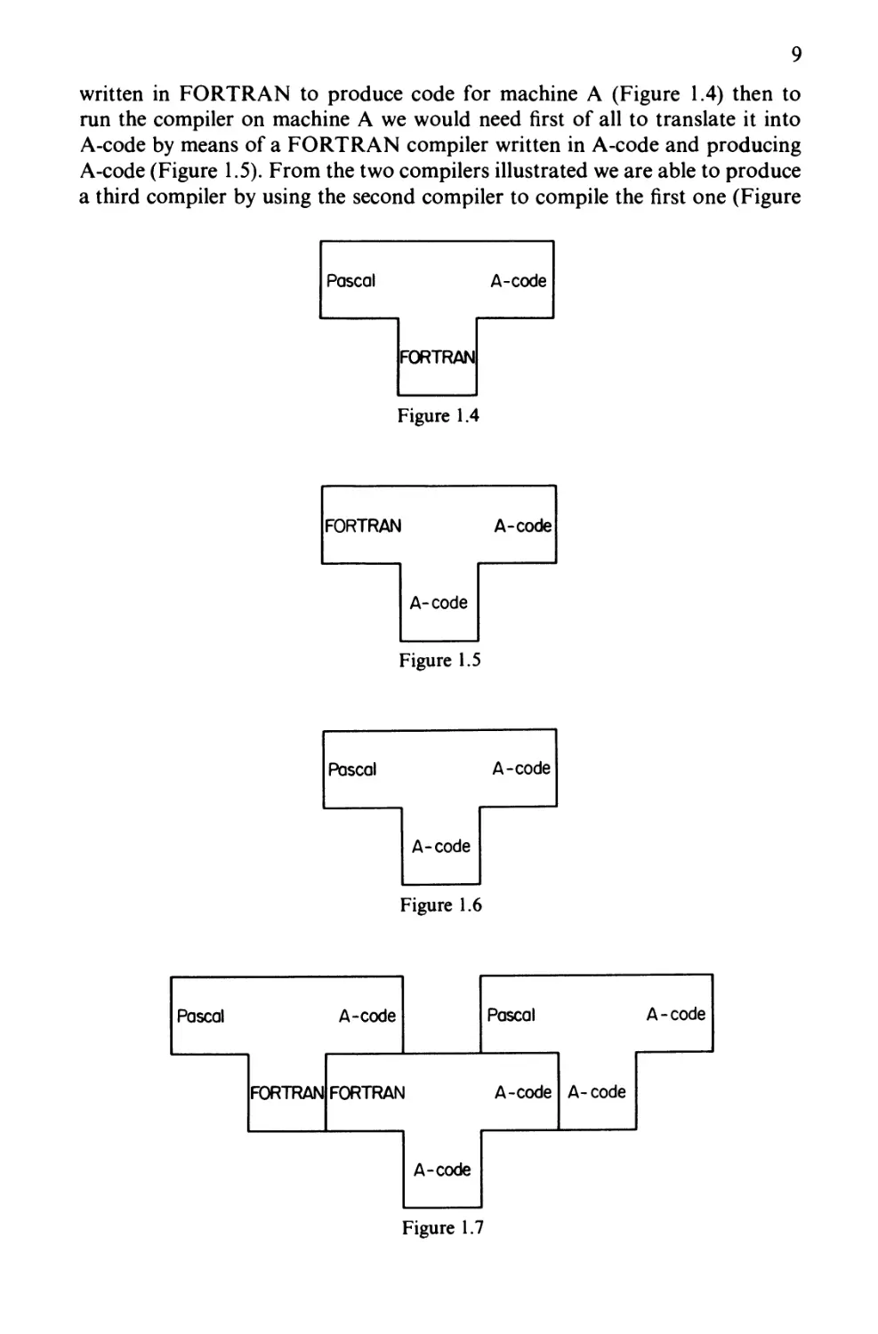
in the left-hand and right-hand corners. More complex T diagrams can also
be produced (e.g. Figure 1.8). The idea of the T diagram is due to Bratman
[1961].
By altering the code produced by the original compiler in the first example
to, say, B-code, the code for some machine B, and assuming there is a
FORTRAN compiler which runs on machine B to produce B-code, we can
also produce a Pascal compiler for machine B.
1.2 Aspects of the compilation process
For our discussion of typical features of machines and languages we should
now have some idea of the sort of tasks the compiler has to perform. There are
two main stages. First it has to recognize the structure and meaning of the
program to be compiled and then it has to produce a machine (or assembly)
code program with the same meaning. The two stages are often referred to as
(a) analysis,
(b) synthesis.
Conceptually, analysis must take place before synthesis, but in practice they
may take place almost in parallel. The source language definition will attribute
a meaning to every legal construction in the language (but not to any illegal
ones) and having recognized each construction involved in the program the
analyser is able to determine what the effect of the program should be. The
synthesizer can then produce appropriate object code.
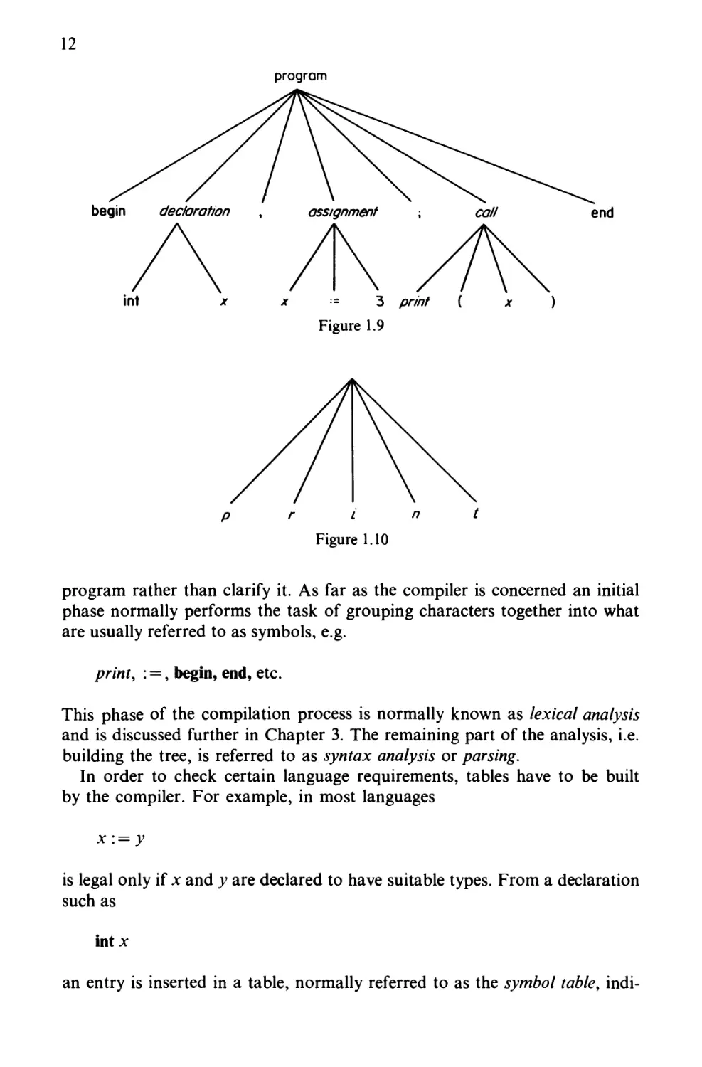
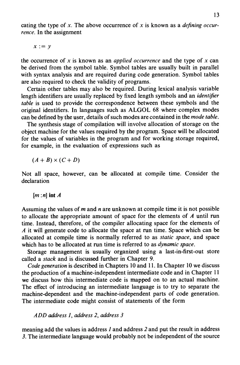
A convenient method of representing the structure of a program is by means
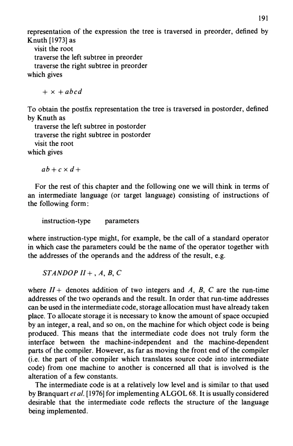
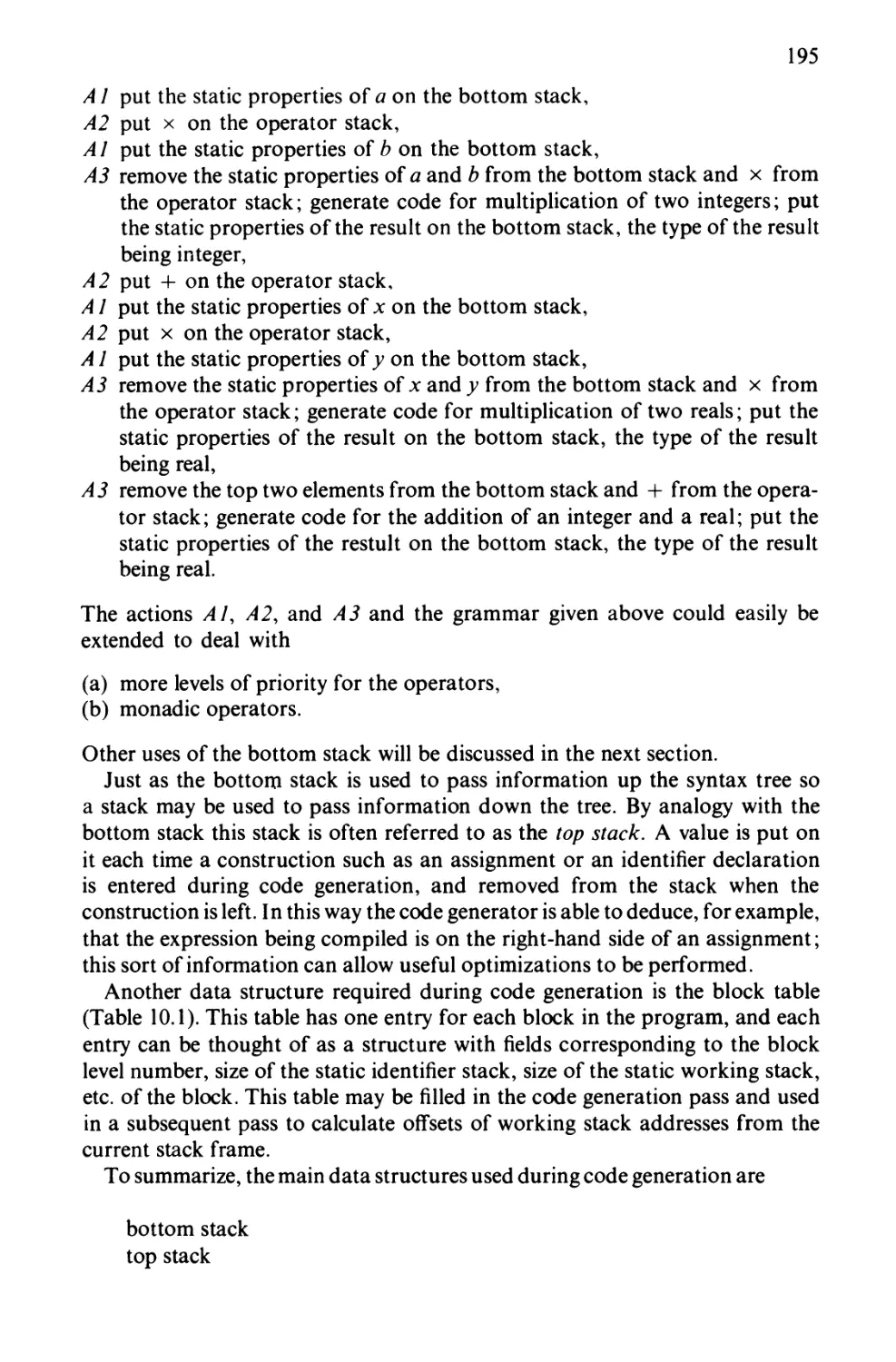
of a tree diagram. Consider the program
begin int x\
x := 3;
print(x)
end
The corresponding tree would be as shown in Figure 1.9, which shows more
clearly the structure of the program. We can think of the analyser building the
tree (usually called the parse tree) and the synthesizer traversing the tree
(visiting all the nodes in some predetermined order) to produce machine code.
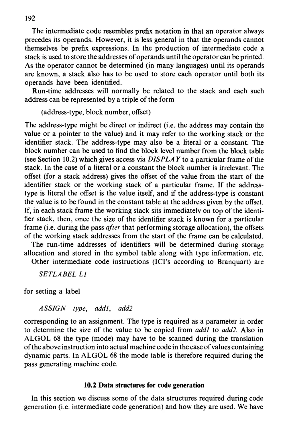
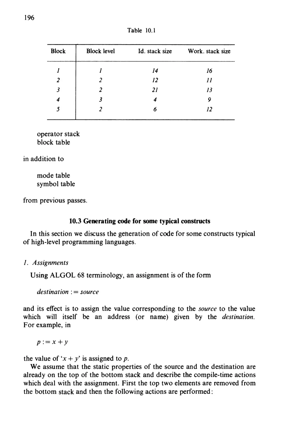
It might be considered rather arbitrary that the terminal nodes (nodes with
no subtrees below them) of the parse tree should be identifiers such as print,
or language words such as begin, and not individual characters. The terminal
node labelled print could be replaced by the subtree shown in Figure 1.10,
but to the human reader at least this would tend to obscure the structure of the
12
begin declaration , assignment ; call end
A A\A\\
int x x := 3 pr//7/ ( jr )
Figure 1.9
p r L n t
Figure 1.10
program rather than clarify it. As far as the compiler is concerned an initial
phase normally performs the task of grouping characters together into what
are usually referred to as symbols, e.g.
print, : =, begin, end, etc.
This phase of the compilation process is normally known as lexical analysis
and is discussed further in Chapter 3. The remaining part of the analysis, i.e.
building the tree, is referred to as syntax analysis or parsing.
In order to check certain language requirements, tables have to be built
by the compiler. For example, in most languages
x:=y
is legal only if x and y are declared to have suitable types. From a declaration
such as
int x
an entry is inserted in a table, normally referred to as the symbol table, indi-
13
eating the type of x. The above occurrence of x is known as a defining
occurrence. In the assignment
x : = y
the occurrence of x is known as an applied occurrence and the type of x can
be derived from the symbol table. Symbol tables are usually built in parallel
with syntax analysis and are required during code generation. Symbol tables
are also required to check the validity of programs.
Certain other tables may also be required. During lexical analysis variable
length identifiers are usually replaced by fixed length symbols and an identifier
table is used to provide the correspondence between these symbols and the
original identifiers. In languages such as ALGOL 68 where complex modes
can be defined by the user, details of such modes are contained in the mode table.
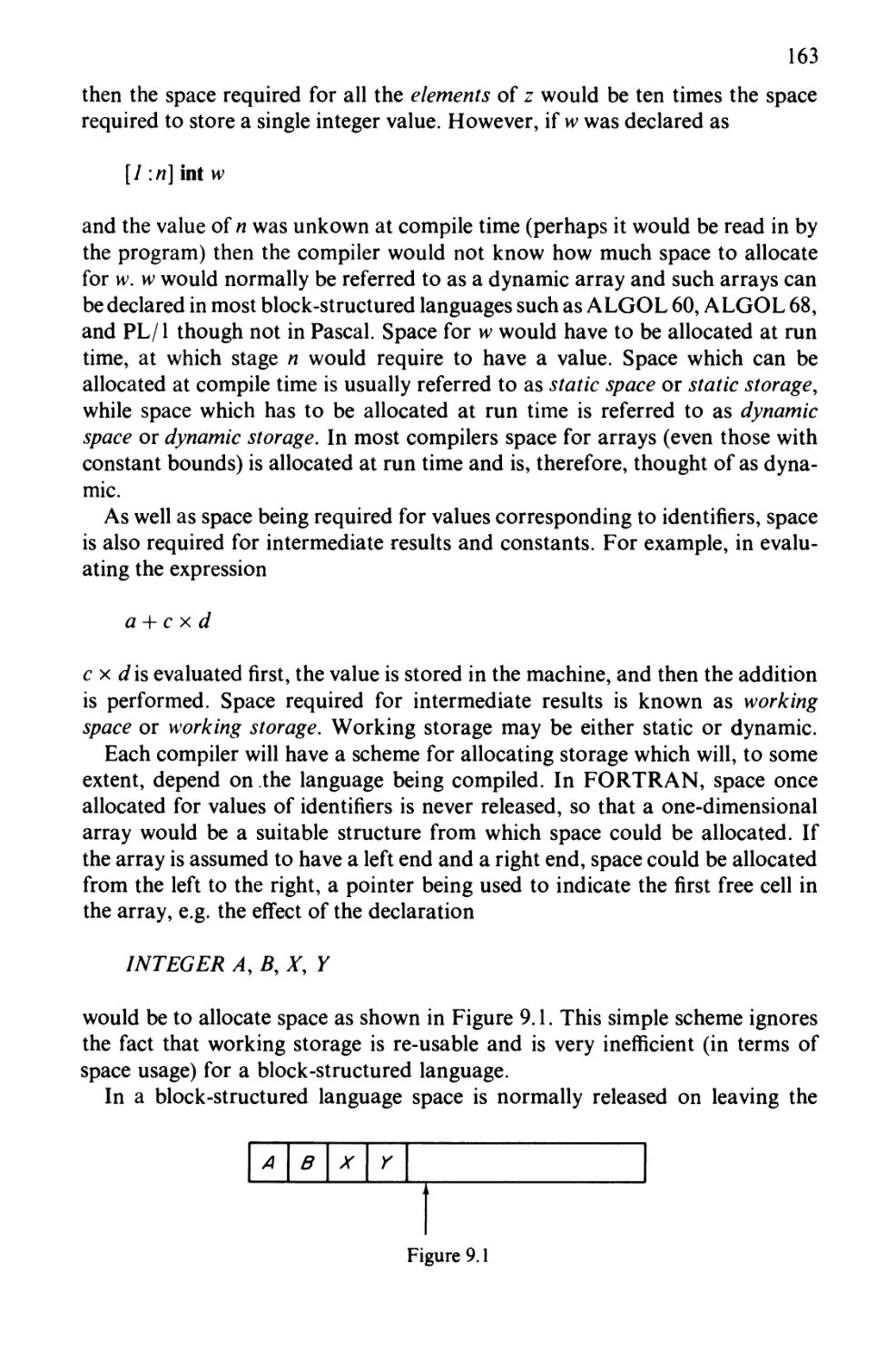
The synthesis stage of compilation will involve allocation of storage on the
object machine for the values required by the program. Space will be allocated
for the values of variables in the program and for working storage required,
for example, in the evaluation of expressions such as
(A + B)x(C+ D)
Not all space, however, can be allocated at compile time. Consider the
declaration
[m :n] int A
Assuming the values of m and n are unknown at compile time it is not possible
to allocate the appropriate amount of space for the elements of A until run
time. Instead, therefore, of the compiler allocating space for the elements of
A it will generate code to allocate the space at run time. Space which can be
allocated at compile time is normally referred to as static space, and space
which has to be allocated at run time is referred to as dynamic space.
Storage management is usually organized using a last-in-first-out store
called a stack and is discussed further in Chapter 9.
Code generation is described in Chapters 10 and 11. In Chapter 10 we discuss
the production of a machine-independent intermediate code and in Chapter 11
we discuss how this intermediate code is mapped on to an actual machine.
The effect of introducing an intermediate language is to try to separate the
machine-dependent and the machine-independent parts of code generation.
The intermediate code might consist of statements of the form
ADD address 7, address 2, address 3
meaning add the values in address 1 and address 2 and put the result in address
3. The intermediate language would probably not be independent of the source
14
language (though attempts have been made to produce universal intermediate
languages, see e.g. Poole [1974]) but would reflect the basic actions of the
source language and be at a high enough level to be implemented efficiently
on a typical computer.
In many compilers there is no explicit separation of the two aspects of code
generation. However, if portability is to be a feature of the compiler, it is
desirable to keep the machine-dependent and the machine-independent parts
of the compiler as separate as possible.
The final code produced should, of course, have the same meaning as the
original program. However, expressions will have been broken down into
their basic components, modes will have disappeared, and all values will be
represented as bit patterns. Program structure (such as conditionals and loops)
will be represented by tests, jumps, and labels. The program will be much less
intelligible but will now be executable on the particular machine.
In this section we have tried to explain some of the various aspects of the
compilation process. The details of how the various phases of the compiler
are organized and how they fit together are described in later chapters.
1.3 Design of a compiler
We mentioned earlier that a compiler is in some sense defined by the high-
level language it accepts and the machine code (more generally some other
language) which it produces. However, it does not follow that, for example,
all FORTRAN compilers for the PDP-11 series will be identical. Of course,
two compilers written by different compiler writers (or teams of compiler
writers) could hardly be expected to be identical, though they ought to produce
identical, or equivalent, object code from the same source code. One reason
why two compilers implementing the same language on the same machine
may differ is that the writers may have had different design aims in mind when
they were writing them. Possible design aims are
1. to produce efficient object code,
2. to produce small object programs,
3. to minimize the time taken to compile programs,
4. to keep the compiler as small as possible,
5. to produce a compiler with good diagnostic and error recovery capabilities,
6. to produce a reliable compiler.
Unfortunately, these aims are to some extent conflicting. A compiler will
almost certainly take a little (or even a lot) longer if it is to produce efficient
code. Some of the standard optimizing techniques (Gries [1971]) such as
eliminating redundant code, removing code sequences from loops, etc., can
be extremely time-consuming. Also a compiler which goes though elaborate
optimization routines is bound to be larger than one which does not. The size
of the compiler may also be related to the time it takes to compile a program.
In computing it is often not possible to optimize both space and time. One
15
is usually done at the expense of the other. The compiler writer has to decide
at an early stage which factors he is most anxious to optimize and then be
prepared to take deliberate steps to optimize these factors, knowing that it
may well be at the expense of other related factors. In addition he may wish
to minimize the time spent in writing the compiler, and this factor alone may
prevent certain elaborate optimization techniques being included.
Programmers will expect a helpful message indicating where the fault lies
when they submit an illegal program and will not be satisfied with a formal
reply that their program 4is not in the language which the compiler has been
designed to translate'. Also, having detected an error in their program, they
will not expect the compiler to give in and stop compiling, but to continue
analysing the program in an attempt to spot any further errors. Compilers
vary greatly in their diagnostic and error recovery capabilities, though this is
not a property which should conflict greatly with the other design aims
mentioned above. Admittedly a compiler which gives helpful messages and
recovers gracefully after an error has been detected may, as a result, be a little
larger but this should be more than compensated for by the increase in
programmer efficiency. A compiler with good diagnostic and error recovery capabilities
should not as a result take any longer to compile correct programs. The problem
of recovery from errors (especially syntax ones), however, is not simple and
no completely satisfactory solution seems to be available. For more details
see Chapter 12.
Of course, reliability should be a design aim of every compiler. Compilers
are often very large programs and to be confident of the correctness of any
compiler in a formal sense is beyond the present state of the art. Good overall
design is of paramount importance. If the different phases of the process can
be kept relatively distinct and if each phase is structured in as natural a way as
possible then reliability is more probable. In addition, if the compiler can be
based as far as possible on a clear and unambiguous formal definition of the
language, and automatic aids such as parser generators are used, then the
chances of producing a reliable compiler should be enhanced. The compiler,
of course, must be thoroughly tested. This applies not only to the complete
compiler but also to the individual parts before they are assembled. Reliability
is discussed further in Chapter 13.
It is not uncommon for a manufacturer to offer more than one compiler for
a language on a range of machines. An early example of this was the Whetstone
and Kidsgrove compilers offered by English Electric for the KDF9 computer.
The Whetstone compiler was a fast-compile-slow-run compiler while the
Kidsgrove one was slow to compile but produced very efficient machine code.
The idea was that users would develop their programs using the Whetstone
compiler, and then recompile them using the Kidsgrove compiler for production
runs. In the same way IBM have produced more than one PL/1 compiler for
their 370 range.
The design aims of a compiler will often depend on the environment in which
the compiler is to be used. If the compiler is to be used mainly by undergraduate
16
students who will rarely run their programs after the development phase is
completed satisfactorily, then the efficiency of the machine code is less important
than the speed of compilation and the diagnostic capabilities. In a commercial
environment the priorities may be reversed. In a student environment, a batch
compiler which remains in core (mainstore) while a number of programs are
compiled and run leads to an efficient use of the available hardware.
An important design decision in constructing a compiler is the number of
passes it will have. Each time the source text, or a version of it, is read by the
compiler is regarded as a single pass. From a simplicity point of view single-
pass compilers are attractive. However, not all languages allow single-pass
compilation and, from a structural point of view, it may be cleaner and simpler
to perform distinct phases of compilation in separate passes. In order to achieve
single-pass compilation some compiler writers implement only a subset of the
language, for example, by insisting that identifiers are declared before they
are used in source programs.
Producing a multi-pass compiler would normally involve the design of
intermediate languages for inter-pass versions of the source text. There would
also be tables built by one pass which would be required for inspection by a
subsequent pass or passes. The organization of a multi-pass compiler, therefore,
tends to be more complicated than for a single-pass one, though the individual
passes may be relatively straightforward and may provide a convenient method
of splitting the job between a number of individuals or groups of individuals
without introducing unduly complicated interfaces. Finally, it should be added
that not all compilers have a fixed number of passes. In some compilers the
number of passes required to compile a program depends on whether all
identifiers were declared before use, etc., or on the degree of optimization
required by the programmer. This topic is discussed further in Chapter 7.
The compiler writer will have to choose a language in which to write his
compiler. Increasingly, high-level languages are being used, either general
purpose languages such as ALGOL 68, Pascal, or PL/1, or so called software
writing languages such as BCPL or PL 360. There is something to be said for
writing a compiler for a language in the language itself. Not only does this
mean that the implementor only has to think in terms of one language, but it
means that the compiler can be used to compile itself, a good test for any
compiler and an aid to portability.
Exercises
1.1 Write down some more typical features of high-level languages and
indicate what sort of machine code instructions would be generated when
they were translated.
1.2 A compiler translates Pascal into ICL 1900 machine code and is written
in ALGOL 68. What further piece of software would be required in order
to run Pascal programs on an ICL 1900 machine? Illustrate your answer
by means of a T diagram.
17
1.3 Some compilers generate code to check array subscripts at run time to
see they are within the declared bounds of the array. Discuss the arguments
for and against implementing such checks
(a) during program development,
(b) during production runs.
1.4 A FORTRAN compiler has to be implemented within a relatively short
timescale. Which of the six design aims in Section 1.3 do you think would
be hardest to achieve?
1.5 Which of the following high-level language facilities do you think would
be useful to the compiler writer:
(a) arrays,
(b) real arithmetic,
(c) procedures?
1.6 Give arguments in favour of using an interpreter rather than a compiler
in a student environment.
1.7 What possible problem do you see in the KDF9 approach of offering
separate compilers for development and production work?
1.8 In some languages the programmer is able to choose the relative priorities
of operators. How might this affect the parse tree of a particular program?
1.9 What would you expect to be the chief design aims for a compiler for a
software writing language?
1.10 What particular feature would you expect in a compiler for an interactive
language such as BASIC?
Chapter 2
Language Definition
Before writing a compiler it is necessary (or at least highly desirable) to have a
clear and unambiguous definition of the source language. Unfortunately,
however, while methods for defining some aspects of programming languages are
well-developed, full and clear definitions of languages to be implemented are not
always available. Furthermore, the formal definition of a programming
language cannot necessarily be used directly by the compiler writer. In this
chapter we introduce a few of the methods used to define programming
languages. For a fuller discussion on the topic see Marcotty, Ledgard, and Bochmann
[1976]. We also discuss the parsing problem—how to decide whether a sequence
of symbols belongs to a particular language or not.
2.1 Syntax and semantics
A language can be thought of as consisting of a number of strings (sequences
of symbols); and the definition of a language defines which strings belong to
the language (the syntax of the language) and the meaning of these strings
(the semantics of the language). For a finite language (i.e. one consisting of
only a finite number of strings) the syntax of the language could be defined
by giving a list of the strings. For example, a language might consist of the
strings
abc
xyz
Those strings which belong to a language are usually referred to as sentences
of the language. Most languages of interest consist of an infinite number of
sentences so that their syntax cannot be defined by listing the sentences. For
example, the sentences of a language might be 'all strings consisting only of
O's and / Y, for example
101 1100 11001
would be in the language, in which case the phrase in quotes would seem a
reasonable definition of the syntax. However, English is not very suitable
18
19
for defining the syntax of more complex languages, and it is usual to adopt a
more formal approach in defining the syntax of programming languages,
as we will see later.
The semantics of a language attribute a meaning to all sentences of the
language. For example
begin int k; read (k); print (k + /) end
is a sentence of ALGOL 68 and, from the semantics of ALGOL 68, the meaning
of the above program in terms of declaring an identifier, reading a value for
it, evaluating, and printing an expression could be deduced. As with syntax,
the semantics of a language are usually described in a fairly formal way.
However, methods of defining semantics are not so well-developed as those for
syntax, and further developments in this area are required before completely
satisfactory formal definitions of programming languages will be a reality.
Further progress in this field may eventually lead to the possibility of producing
compilers automatically from the formal definition. In the next section we
discuss the problem of specifying the syntax of a language.
2.2 Grammars
We begin by introducing some terminology. Curly brackets are used to
denote sets, e.g.
{1,2,3}
denotes the set containing the integers 1, 2, and 3. Union (u) and intersection
(n) of sets are defined as usual:
{1,2,3} u {3,4,5} = {1,2,3,4,5}
{l,2,3}n{3,4,5} = {3}.
We say set A includes (3) set B if every element of B is an element of A, e.g.
{3,4,5} 2{3}.
Similarly set B is included in (Q) set A if every element in B is also in A, e.g.
{3} £{3,4,5}.
We use e to indicate that an element is contained in a set, e.g.
3e{3,4,5}
The empty set is denoted by 0 . Therefore,
20
{1,2} n {3,4,5} =0
If A is the set
{2,4,9,8}
and we define B as
B= {x\xeA and x is even}
then B is the set
{2,4,8}-
B is defined by a predicate, in this case \xe A and x is even'.
We define an alphabet (or vocabulary) to be a set of symbols. For example,
it might be the Roman or the Greek alphabet or the decimal digits 0-9. An
alphabet D could be
D= {0,1,2,3,4,5,6,7,8,9,}
If A is an alphabet, A* (the closure of A) is used to denote the set of all strings
(including the empty string consisting of zero symbols) composed of symbols
from A. A+ is used to denote the set of all strings (excluding the empty string)
composed of symbols from A. The empty string is usually denoted by £.
The syntax of a language can be defined using set notation, e.g.
L={0nln\n>0}
In English, the language consists of all strings consisting of zero or more 0's
followed by the same number of /'s. The empty string is included in the
language.
Other syntaxes which could be defined in this way include
1. {anbncn\n>0}
2. {ambn\m,n>0}
i.e. a number of a's followed by a number (not necessarily the same) of 6's, e.g.
aaabb
would be in the language.
3. {xm\m is prime}
4. {ambncp\m = norn = p}.
21
All these syntaxes are a good deal less complex than those of most programming
languages and a more useful way of defining the syntax of a programming
language is by means of a grammar. A grammar consists (in part) of a set of
rules for generating sentences of a language. Take, for example, the syntax
defined earlier in this section:
{Onln\n>0}.
The following rules can be used to generate the sentences:
1. S-+0S1
2. S-+e
To derive a sentence of the language proceed as follows. Start with the symbol
S and replace it by 0S1 or e. If S still appears in the resultant string it may
again be replaced using one of the rules, and so on. Any string produced in
this way which does not contain S is a sentence of the language. For example
S=>0S1=>00S11 =>000S111=>000111
The sequence of steps above is referred to as a derivation of the string 000111,
and the symbol => is used to separate the steps in the derivation. All sentences
in the language can be derived using the two rules and any string which cannot
be derived using the two rules is not a sentence of the language. A grammar
is often (and aptly) referred to as a rewriting system. We now define a grammar
more formally.
A grammar is defined to be a quadruple
(KT,KN,P,S)
where VT is an alphabet whose symbols are known as terminal symbols (or
simply terminals), VN is an alphabet whose symbols are known as nonterminal
symbols (or nonterminals), and VT and VN have no symbols in common, i.e.
Kis defined to be VT u KN.
P is a set of productions (or rules), each element of which consists of a pair
(a,/?) where a is in K + and /? is in V*. a is normally known as the left part of the
production and /? is known as the right part, and a production is written
S e KN and is normally referred to as the sentence symbol (or axiom) and is
the starting point in producing any sentence in the language.
22
A grammar generating the language
{onr|«>o}
is G0 where
G0 = ({OJ}AS}9P9S)
and
/>={S-0S/, S-+e}
A grammar generating strings in the set
{ambn\m,n>0}
is G1=({fl,fc},{S,i4,B},J>,S)
where the elements of P are
S->AB
A^aA
A -+ e
B^bB
B^e
Starting with the sentence symbol S and successively using one of the
productions to replace a nonterminal in the derived string, we can generate the string
aaabb:
S => AB => aAB => aaAB => aaaAB => aaaB => aaabB
=> aaabb B => aaabb
Each string which can be derived from the sentence symbol (e.g. aAB, aaaB
above) is called a sentential form. A sentence is a sentential form containing
only terminal symbols.
+
y =>d
G
means that the string (of symbols) 5 can be derived from the string y by one or
more applications of productions of the grammar G. (G can be omitted if it
is clear which grammar is intended.) It can be seen from the above that
+
aAB => aaabB
Gt
23
Similarly,
* s
y=>o
G
means that the string S can be derived from the string y by zero or more
applications of productions of the grammar G (again G can be omitted in appropriate
circumstances). For example
aAB=>aaabB
aAB^>aAB
Where exactly one application of a production is involved the symbol =>
is used, e.g.
AB=>aAB
g,
or, omitting the Gv
AB^aAB
In this book we will normally use small letters (or strings of small letters)
to denote terminals of a grammar and capital letters (or strings of capital
letters) to denote nonterminals of a grammar. Where ambiguity might arise
with sequences of letters denoting terminals or nonterminals, spaces will be
used to separate the symbols in a production. Strings of terminals and/or
nonterminals will usually be represented by Greek letters.
The sentences of a language can usually be generated by more than one
grammar; two grammars generating the same language are said to be equivalent.
For example, Gx is equivalent to G2 defined as follows:
G2 = ({a9b}9 {5,K},P, S)
where the elements of P are
S^aS
S-+a
S-+b
S^bY
Y^b
Y^bY
24
From the compiler writer's point of view one grammar may be much more
suitable than another as a basis for the syntax analysis phase of compilation.
In the examples so far, the left parts of productions have always consisted
of a single nonterminal. However, it is clear from the definition of a grammar
that this need not be so. Consider the grammar
G3 = ({a}9{S9N9Q9R}9P9S)
where the elements of P are
S^QNQ
QN^QR
RN - NNR
RQ -► NNQ
The language generated is
{ai2H)\n>0}
A typical derivation is
S => QNQ => QRQ => QNNQ
=> QRNQ => QNNRQ => QNNNNQ
^> aaaa
The reader should be able, by considering the roles of N9 Q9 and R in the above
derivation, to convince himself that the language generated is the one stated.
It should be noticed, for example, that R serves to duplicate N.
By restricting the types of productions which can appear in a grammar we can
define a number of special classes of grammars. One standard classification
is known as the Chomsky hierarchy, which may be described as follows.
Any grammar of the form defined previously is referred to as a type-0
grammar.
If, however, a grammar has the property that for all productions of the form
\*\*\P\
where | a| denotes the length of a, i.e. the number of symbols in a, and similarly
for | j8|, then the grammar is said to be,of type 1 or context sensitive.
If the grammar has the further property that all left parts consist of a single
nonterminal symbol then the grammar is said to be of type 2 or context free.
25
If each production of the grammar is of one of the forms
A^aB
where a is a terminal symbol and A and B are nonterminal symbols then the
grammar is said to be of type 3 or right linear or regular.
A left linear grammar defined analogously to a right linear grammar, i.e.
with all rules of either of the forms
A-+a
A^> Ba
is also said to be of type 3 or regular.
Clearly the hierarchy is inclusive, that is all type-3 grammars are type-
2 grammars and all type-1 grammars are type-0 grammars, etc. Corresponding
to the hierarchy of grammars is a hierarchy of languages. For example, if
a language can be generated by a type-2 grammar it is referred to as a type-2
language and if a language can be generated by a type-3 grammar it is referred
to as a type-3 language. Again the hierarchy is inclusive. Also the inclusions
are proper in that there exist languages which are type i but not type (/ + 1)
(0 < i < 2).
For example, it can be shown that the language generated by G3 above
is context sensitive and not context free i.e. no context-free grammar exists
which generates the language. Similarly the language generated by G0 is
context free and not regular. However, the fact that a language can be generated
by a nonregular context-free grammar does not necessarily mean that it is
nonregular. For example, grammar Gt is context free but not regular, but the
language generated by it is regular since it can also be generated by grammar
G2. (Strictly speaking, it is L{G2) — e which is regular but it is usual to extend
the definitions of type-3 grammars to include productions of the form S -► e
where S is the sentence symbol.) The Chomsky hierarchy is significant as far
as programming languages are concerned. The fewer the restrictions put on
the grammar the finer the constraints that can be put on the language generated.
Type-3 grammars can be used to describe certain features of programming
languages. For example, the following productions can be used to generate
identifiers as defined in many programming languages:
WENT -> letter
WENT- letter REST
REST -> letter
REST-* digit
REST -> letter REST
REST-+digit REST
26
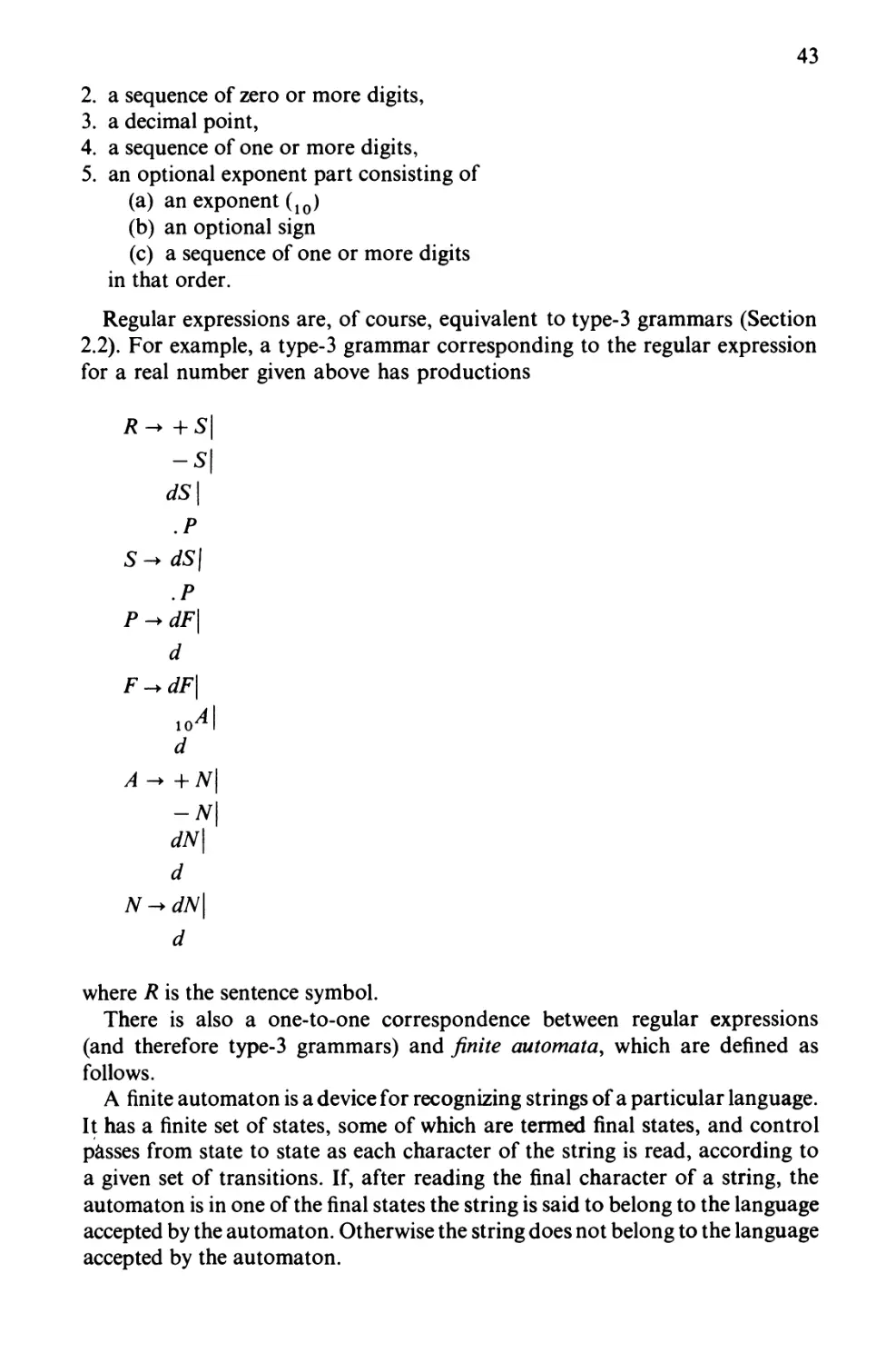
where letter and digit are terminals. It is sometimes convenient to group right-
hand sides of productions with the same left-hand side together. The above
grammar could also be written as
IDENT^ letter\letter REST
REST^ letter\digit\letter REST\digit REST
where the vertical bar can be read as 'or'.
Many 'local' features of programming languages can be represented by
type-3 grammars, e.g. constants, language words, and strings. However, it
can be shown that type-3 grammars are strictly limited in the types of languages
they can generate. We now define regular expressions and state without proof
that type-3 grammars generate exactly all regular expressions (see Aho and
Ullman [1972], page 118).
Given an alphabet A, then the following are regular expressions:
1. an element of A (or the empty string).
If P and Q are regular expressions then so also are:
2. PQ (P followed by Q).
3. P\Q(PorQ).
4. P* (zero or more occurrences of P).
Over the alphabet { a,b,c}
a*b\ca*
is a regular expression describing a language including the following strings
(amongst others):
aab
c
caa
ab
ca
If we think of regular expressions being built using the three operators
concatenate (represented by juxtaposition)
then in writing regular expressions * has the highest priority followed by
concatenation followed by |.
The operator | (alternatively represented by + ) is commutative and
associative, i.e. for regular expressions P, Q, R
27
P\Q = Q\P (commutative)
(P\Q)R = P\(Q\R) (associative).
Concatenation is associative but not commutative.
Brackets may be used to overwrite the priorities normally associated with
these operators. Thus over the alphabet {a,b}
(aab\ab)*
is a regular expression describing a language including the following strings:
£
aababaab
ababab
aabaabaabab
A regular expression describing an identifier would be
L(L\D)*
where L stands for a letter and D for a digit.
A regular expression is said to generate a regular set. For example, the regular
expression
(a\b)e
generates the regular set {ac, be}. Clearly a regular set can be generated by
more than one regular expression (if only because '|' is commutative). Normally
we will not distinguish between a regular expression and the set it generates.
Other properties of regular sets are:
1. There exists an algorithm to determine whether a string belongs to a given
regular set (defined by a regular expression).
2. There exists an algorithm to determine whether two regular expressions
generate the same regular set.
The above properties turn out to be extremely useful from the compiler
writer's point of view.
Regular expressions, however, do have their limitations. For example,
patterns of matching brackets of arbitrary length cannot be defined by a regular
expression and consequently cannot be generated by a type-3 grammar.
Consider the language consisting of strings of opening and closing brackets-
plus the empty string-with the following properties:
1. on reading from left to right the number of closing brackets encountered
never exceeds the number of opening brackets encountered,
2. each string contains the same number of opening and closing brackets.
28
For example, the following strings would be in the language:
((( )))
( )( )(( ))
(( )( )(( )( )))
but the following would not:
( ))(( ) -rule 1
((( )( )) -rule 2
There is no way the above language can be expressed as a regular expression
(see Minsky [1967], p. 72) or generated by a type-3 grammar.
However, the context-free grammar with the following productions generates
the language:
S->(S)
S^SS
In most programming languages there are a number of pairs of brackets
which have to be matched, e.g.
(ML begin end, iffi, dood
and, of course, each opening bracket must be matched by the appropriate
closing bracket, e.g.
begin ( )end
is a suitable bracket structure whereas
begin (end)
is not. A context-free grammar is able to specify these sorts of constraints.
Context-free grammars go a long way towards describing the syntactic
properties of programming languages and are normally used as the basis of the syntax
analysis phase of compilation. However, there are some properties of typical
programming languages which cannot be expressed by means of a context-
free grammar. For example, the assignment
X: = Y
may only be legal if X and Y have been declared to have appropriate types.
If X and Y have been declared as
29
intA^char Y
the assignment (at least in ALGOL 68) would be illegal. This sort of condition
cannot be specified by a context-free grammar and compilers normally perform
type checking, etc., separate from the formal syntax analysis phase. We shall
see in the next section, however, that it is possible to extend the idea of a context-
free grammar to include some non-context-free properties of languages.
It appears, therefore, that the more general the class of grammar used, the
more features of typical programming languages we are able to describe.
However, the more general the grammar, the more complex is the machine
(or program) required to recognize the strings of the corresponding language.
We will see in Chapter 3 that the class of recognizer associated with a type-3
grammar is a finite automaton or a finite state machine—a machine with a
finite number of states between which control passes as the symbols of a string
are read, the string being accepted or not depending on which state the machine
reaches finally. For a language generated by a context-free grammar a
pushdown automaton is (in general) required, i.e. a finite automaton plus a stack;
while for context-sensitive languages a linear bounded automaton is required,
i.e. a Turing machine with a finite amount of tape. Finally, a type-0 language
requires a Turing machine as a recognizer.
For a full description of these machines and proofs of the equivalence of
the various classes of languages and their related automata see Hopcroft and
Ullman [1969].
2.3 Formal definition of programming languages
By the formal definition of a programming language we mean the complete
description of the syntax and semantics of the language.
Formal definitions of programming languages are useful in the areas of
program proving and language design, and it could be argued that certain
languages contain features which reflect the method of formal definition
used at the design stage. However, as far as we are concerned here there are
two main reasons why formal definitions of programming languages are
desirable.
1. Programmers wish to be able to find authoritative answers to questions they
may have about the syntax and semantics of the language. Language
manuals and text books may provide some information about the language
but are often ambiguous or uninformative on the finer points of the language.
2. Compiler writers wish a precise definition of the language they are
implementing, preferably in a form which can be readily implemented.
These two needs tend to be conflicting. 1. suggests that the definition should
be readable, and that a programmer familiar with the method of definition
should not have too much difficulty in obtaining an answer to a question
about the language. 2. suggests that the definition should be in a form from which
30
an analyser (at least) can be readily built with as little human intervention as
possible. In Chapter 4 we will see that the most natural (and readable) grammars
are not always in a form from which a parser can be built automatically. In
particular certain parsing methods nearly always require the grammar to be
transformed before it can be used to build a syntax analyser.
One of the first attempts to define a language formally was the ALGOL
60 report. Much of the syntax was described by means of a context-free
grammar, the remainder of the syntax and the semantics being described in
English. The original report contained many ambiguities and even the revised
report (Naur [1963]) was not free from them (Knuth [1967]).
A further development in the techniques of formal definition was the ALGOL
W report (Bauer, Becker, Graham, and Satterthwaite [ 1968]) in which an attempt
was made to include some type information in the formal part of the syntax.
The revised report on ALGOL 68 (van Wijngaarden et ai [1975]) used a
two-level grammar (W-grammar—named after its inventor A. van Wijngaarden)
to define the complete syntax of the language. The idea of using a two-level
grammar is that, just as the production rules of a conventional grammar
provide a finite way of describing a language consisting of an infinite number
of strings, so in the ALGOL 68 Report (from now on the terms ALGOL 68
and the ALGOL 68 Report imply revised ALGOL 68 and the Revised Report
respectively) a second grammar is used to generate an infinite number of
productions which in turn generate the sentences of the language ALGOL 68.
In other words, although ALGOL 68 cannot be generated by means of a
context-free grammar, which by definition may only have a finite set of
productions, the (simple?) extension of allowing the grammar to have an infinite set
of productions is a sufficient generalization for a grammar generating ALGOL
68 to be specified. In fact any type-0 language can be generated by such a
grammar. This means we are dealing with rather a powerful concept and,
in view of the type of recognizer required for type-0 languages, possibly too
powerful a concept for defining programming languages whose non-context-
free features tend to be of a fairly simple nature.
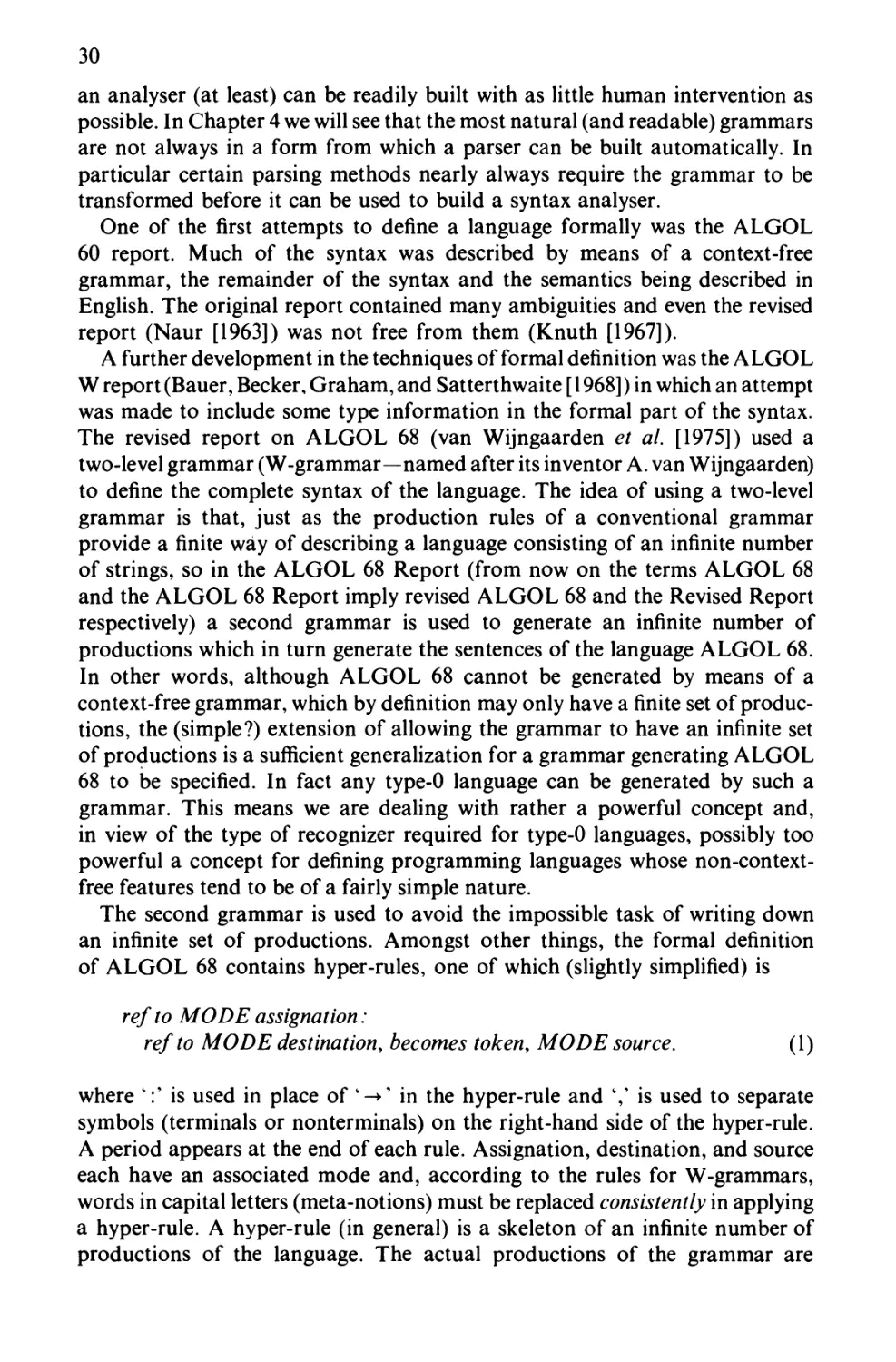
The second grammar is used to avoid the impossible task of writing down
an infinite set of productions. Amongst other things, the formal definition
of ALGOL 68 contains hyper-rules, one of which (slightly simplified) is
ref to MODE assignation :
refto MODE destination, becomes token, MODE source. (1)
where k:' is used in place of '-»' in the hyper-rule and Y is used to separate
symbols (terminals or nonterminals) on the right-hand side of the hyper-rule.
A period appears at the end of each rule. Assignation, destination, and source
each have an associated mode and, according to the rules for W-grammars,
words in capital letters (meta-notions) must be replaced consistently in applying
a hyper-rule. A hyper-rule (in general) is a skeleton of an infinite number of
productions of the language. The actual productions of the grammar are
31
obtained by consistently replacing the meta-notions in a hyper-rule by means of
terminal meta-productions using the meta-rules of the language. The
metarules form a context-free grammar of which the meta-notions are nonterminals
and the terminal meta-productions (which contain no capital letters) are the
terminals. Notice that the idea of a sentence symbol does not exist in this
grammar.
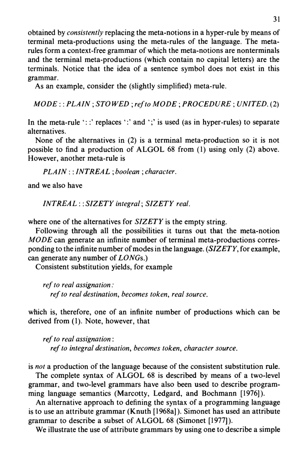
As an example, consider the (slightly simplified) meta-rule.
MODE :: PLAIN ; STO WED ; refto MODE ; PROCEDURE ; UNITED. (2)
In the meta-rule '::' replaces 4:' and fc;' is used (as in hyper-rules) to separate
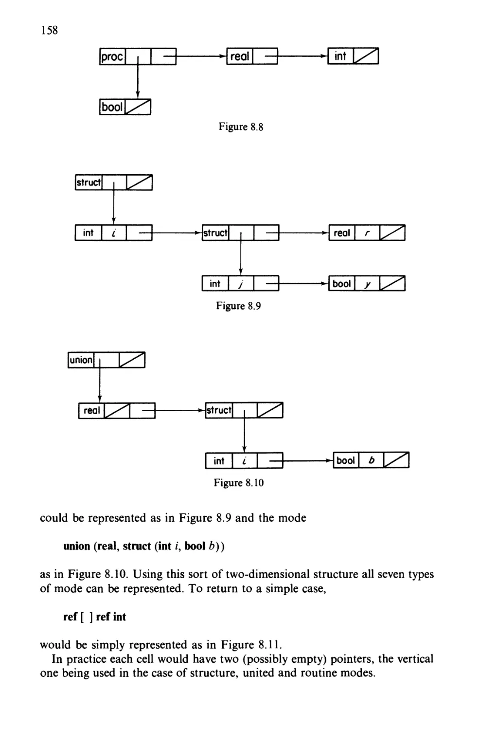
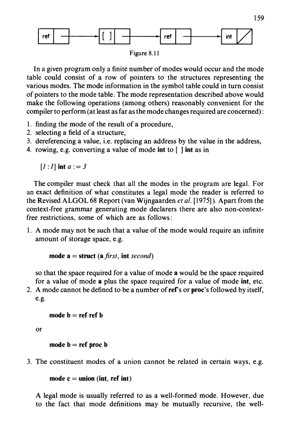
alternatives.
None of the alternatives in (2) is a terminal meta-production so it is not
possible to find a production of ALGOL 68 from (1) using only (2) above.
However, another meta-rule is
PLAIN :: INT REAL ; boolean ; character.
and we also have
INTREAL :: SIZETY integral; SIZETY real.
where one of the alternatives for SIZETY is the empty string.
Following through all the possibilities it turns out that the meta-notion
MODE can generate an infinite number of terminal meta-productions
corresponding to the infinite number of modes in the language. {SIZETY, for example,
can generate any number of LONGs.)
Consistent substitution yields, for example
refto real assignation:
refto real destination, becomes token, real source.
which is, therefore, one of an infinite number of productions which can be
derived from (1). Note, however, that
refto real assignation:
refto integral destination, becomes token, character source.
is not a production of the language because of the consistent substitution rule.
The complete syntax of ALGOL 68 is described by means of a two-level
grammar, and two-level grammars have also been used to describe
programming language semantics (Marcotty, Ledgard, and Bochmann [1976]).
An alternative approach to defining the syntax of a programming language
is to use an attribute grammar (Knuth [1968a]). Simonet has used an attribute
grammar to describe a subset of ALGOL 68 (Simonet [1977]).
We illustrate the use of attribute grammars by using one to describe a simple
32
programming language. The language has block structure like ALGOL 60
or ALGOL 68 and we associate with each block a list of identifiers and their
modes (or types). Identifiers may have one of two modes int and bool and are
terminals of the grammar at this level of description. Declarations can be
described by the context-free productions
dec -»int id
dec -» bool id
where we have departed from our normal convention of using lower case letters
only for terminals.
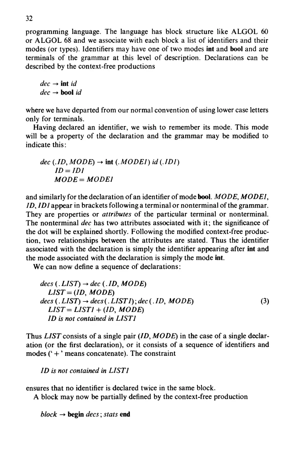
Having declared an identifier, we wish to remember its mode. This mode
will be a property of the declaration and the grammar may be modified to
indicate this:
dec (.ID, MODE) - int {.MODEI) id (.ID1)
ID = JD1
MODE=MODEl
and similarly for the declaration of an identifier of mode bool. MODE, MODE1,
ID, ID! appear in brackets following a terminal or nonterminal of the grammar.
They are properties or attributes of the particular terminal or nonterminal.
The nonterminal dec has two attributes associated with it; the significance of
the dot will be explained shortly. Following the modified context-free
production, two relationships between the attributes are stated. Thus the identifier
associated with the declaration is simply the identifier appearing after int and
the mode associated with the declaration is simply the mode int.
We can now define a sequence of declarations:
decs (. LIST) -+dec(. ID, MODE)
LIST = (ID, MODE)
decs (. LIST) - decs (. LIST1) ,dec(. ID, MODE) (3)
LIST= LIST1 + (ID, MODE)
ID is not contained in LIST1
Thus LIST consists of a single pair (ID, MODE) in the case of a single
declaration (or the first declaration), or it consists of a sequence of identifiers and
modes (' +' means concatenate). The constraint
ID is not contained in LIST1
ensures that no identifier is declared twice in the same block.
A block may now be partially defined by the context-free production
block -► begin decs; stats end
33
We now superimpose the non-context-free requirements
block (ENV) -► begin decs (. LIST); stats (ENV1) end
ENV1 = L/ST + ENV
The environment in which the stats are executed is the environment of the
block itself augmented by decs. This environment is passed into the individual
statements
stats (ENV) -► stat (ENV)
stats (ENV) -► stats (ENV); stat (ENV) (4)
and we assume for simplicity that a stat takes one of the forms
stat (ENV) -► id (MODEL ID!) :=id(MODE2. ID2)
MODE1 = search (/£>/, ENV)
MODE2 = search (ID2, ENV)
MODE! = MODE2
or
stat (ENV) -► block (ENV)
The function search will search the environment in an outwards direction
to find the appropriate declaration of the identifier and hence its mode. An
error will be indicated if a suitable declaration cannot be found.
Attributes are used to describe context-sensitive (or perhaps more correctly
non-context-free) aspects of a programming language. They can be used to
pass information from the left-hand side of a production to the right-hand
side as in (4). These are called inherited attributes. They can also be used to pass
information from the right-hand side of a production to the left-hand side
as in (3) and then they are called synthesized attributes. In the above example,
within each set of brackets the inherited attributes precede the synthesized
ones, the elements of each list being separated by commas and the two lists
being separated by a period.
Attribute grammars have the advantage of looking like context-free
grammars but of being able to specify non-context-free features of languages.
In fact any type-0 language can be described by means of an attribute grammar.
The fact that programming languages are naturally thought of as context-free
languages with non-context-free constraints added means that attribute
grammars are well suited to describing them. Techniques are also available for
producing efficient analysers automatically from suitable attribute grammars,
and this together with their readability means that attribute grammars come
close to meeting the two main aims of language definition mentioned at the
beginning of this section.
34
Other well-known methods of describing the syntax of programming
languages include the Vienna Definition Language for PL/1 (Lucas and Walk
[1969]) and Ledgard's Production Systems (Ledgard [1974]).
2.4 The parsing problem
We have shown how a grammar can be used to generate programs in a given
programming language. However, the problem which the compiler has to deal
with is not how to generate programs but how to check strings of symbols
to see if they belong to the language and, if they do, to recognize the structure
of the strings in terms of the productions of the grammar. This problem is
known as the parsing problem and, before investigating it more deeply, we
introduce one or two new ideas.
Consider the grammar with productions
1. E^>E+T
2. £- T
3. T- TxF
4. T^F
5. F->(E)
6. F->x
7. F->y
(E is the sentence symbol).
Clearly the string
(x + y) x x
is in the language. In particular it could have been derived as follows:
E=>T
=>TxF
=>F x F
=>(£") x F
=>(E+T)xF
=>(T+T)xF
=>(F+T) xF
=>(jc + r)xf
=>(x + F)x F
=>(*+ y) x F
=>(*+ y) x x
Alternatively it could have been derived as follows:
E=>T
=>TxF
35
=>T x x
=> F x x
=>(E)x x
=>(£+ T)x x
=>(E+F)x x
=>(E + y) x x
=>(T + y) xx
=> (F + y) x x
=> (x + y) x x
Notice that at each stage in the first derivation the leftmost nonterminal in
the sentential form was replaced using one of the productions of the grammar.
This derivation is, therefore, known as a leftmost derivation. In the second
derivation the rightmost nonterminal in the sentential form was replaced at each
stage using one of the productions. This is, therefore, known as a rightmost
derivation. There are also other derivations of the sentence which are neither
leftmost nor rightmost.
We define the leftmost parse of a sentence to be the sequence of productions
used to generate the sentence by a leftmost derivation In the above case
leftmost parse might be written
2X4,5J,2,4fi,4Jfi
The rightmost parse of a sentence is the reverse of the sequence of productions
used to generate the sentence by a rightmost derivation, e.g. in the above
case the rightmost parse would be
6,4,2 J,4 J,5,4,6,3,2
The reason why the sequence of productions is given in reverse order is related
to the fact that rightmost parsing is normally associated with reducing a sentence
to the sentence symbol rather than generating a sentence from the sentence
symbol (see bottom-up parsing later). Note that each production is used the
same number of times in the two derivations (or parses).
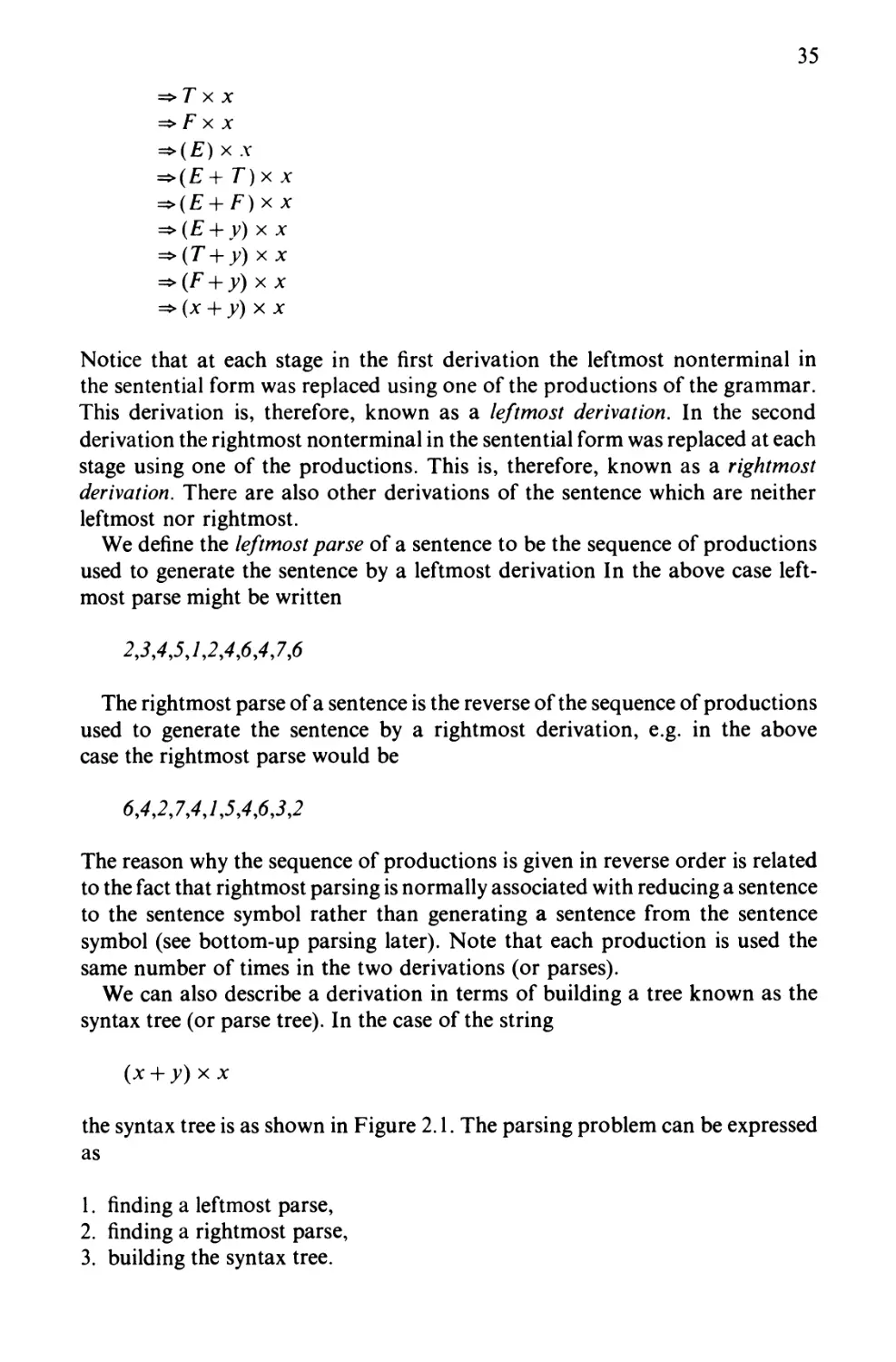
We can also describe a derivation in terms of building a tree known as the
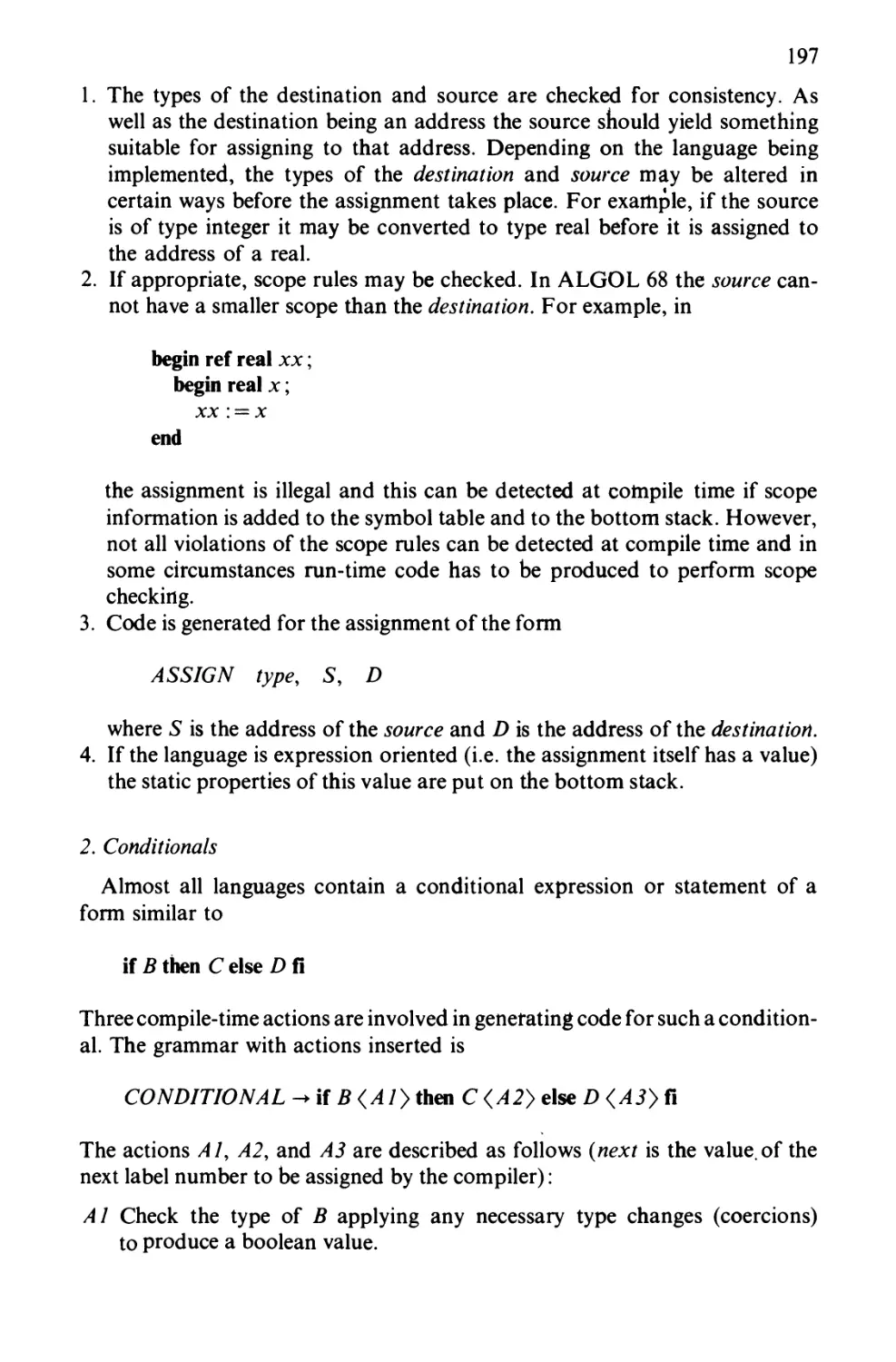
syntax tree (or parse tree). In the case of the string
(x-\-y)x x
the syntax tree is as shown in Figure 2.1. The parsing problem can be expressed
as
1. finding a leftmost parse,
2. finding a rightmost parse,
3. building the syntax tree.
36
Figure 2.1
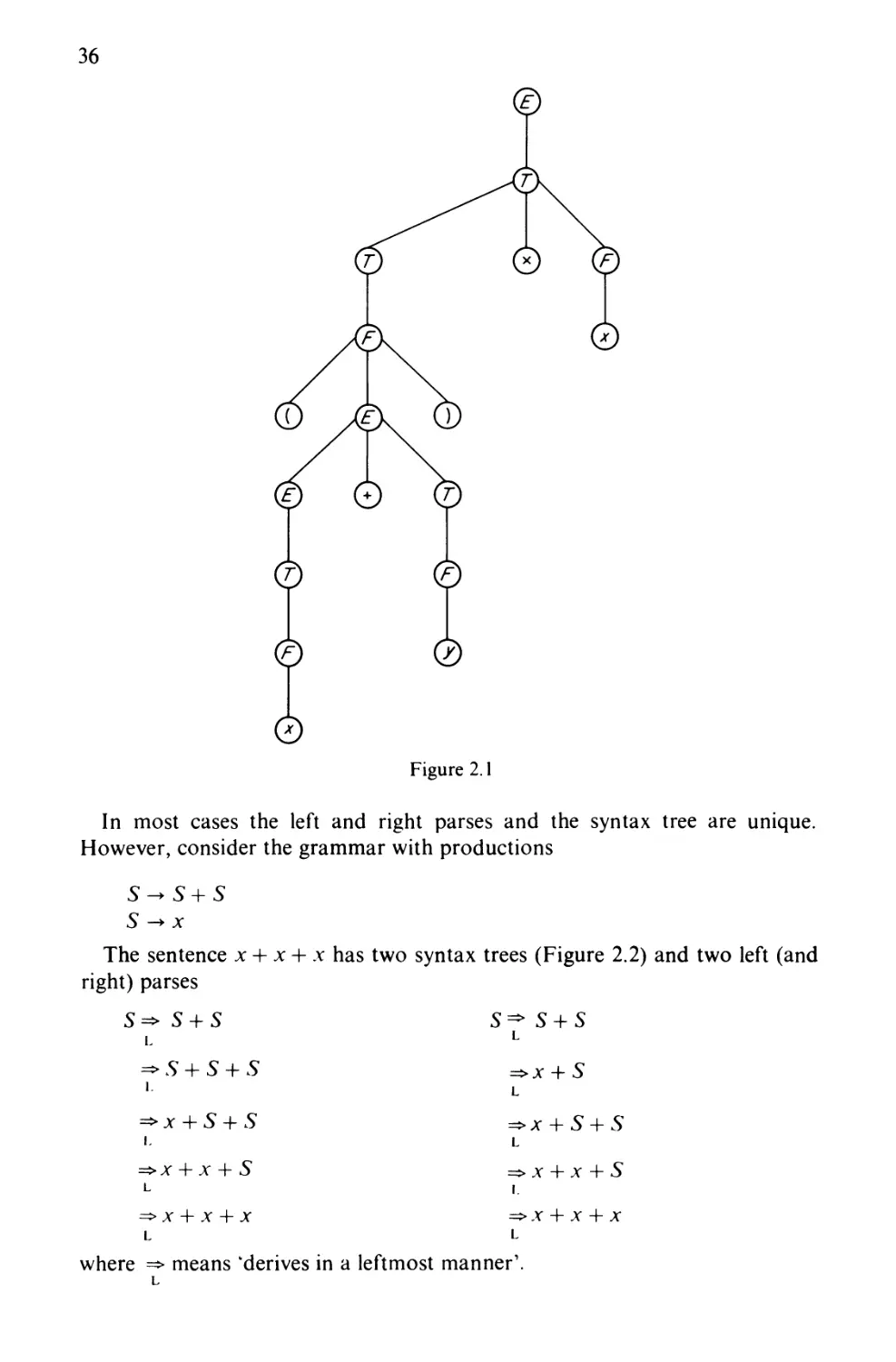
In most cases the left and right parses and the syntax tree are unique.
However, consider the grammar with productions
S -> x
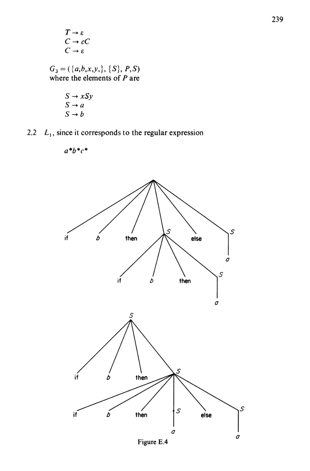
The sentence x + x + x has two syntax trees (Figure 2.2) and two left (and
right) parses
s + s + s
L
=>x + S
■jr + S + S
►A- + S + S
»x + x 4- 5"
• * + * + S
► x 4- x 4- x
X + X + X
where => means 'derives in a leftmost manner'.
L
37
© 0
© © 0 ©
Figure 2.2
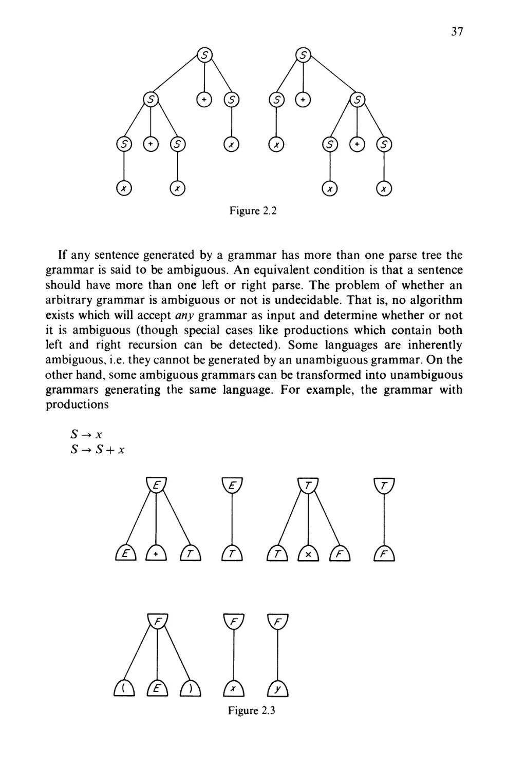
If any sentence generated by a grammar has more than one parse tree the
grammar is said to be ambiguous. An equivalent condition is that a sentence
should have more than one left or right parse. The problem of whether an
arbitrary grammar is ambiguous or not is undecidable. That is, no algorithm
exists which will accept any grammar as input and determine whether or not
it is ambiguous (though special cases like productions which contain both
left and right recursion can be detected). Some languages are inherently
ambiguous, i.e. they cannot be generated by an unambiguous grammar. On the
other hand, some ambiguous grammars can be transformed into unambiguous
grammars generating the same language. For example, the grammar with
productions
S
S
x
•S + jc
^
(h
^
(h
^ ^
ri\ r*\ fh (2^ (h
Figure 2.3
38
is unambiguous and generates the same language as the ambiguous grammar
discussed earlier. For most parsing methods an unambiguous grammar is
required. If there exists an algorithm to determine whether a given grammar is
suitable for a particular parsing method, and the parsing method can only
be applied to a subset of the unambiguous grammars, then we have an algorithm
which may be used to show that a grammar is unambiguous (but not to show
that it is ambiguous).
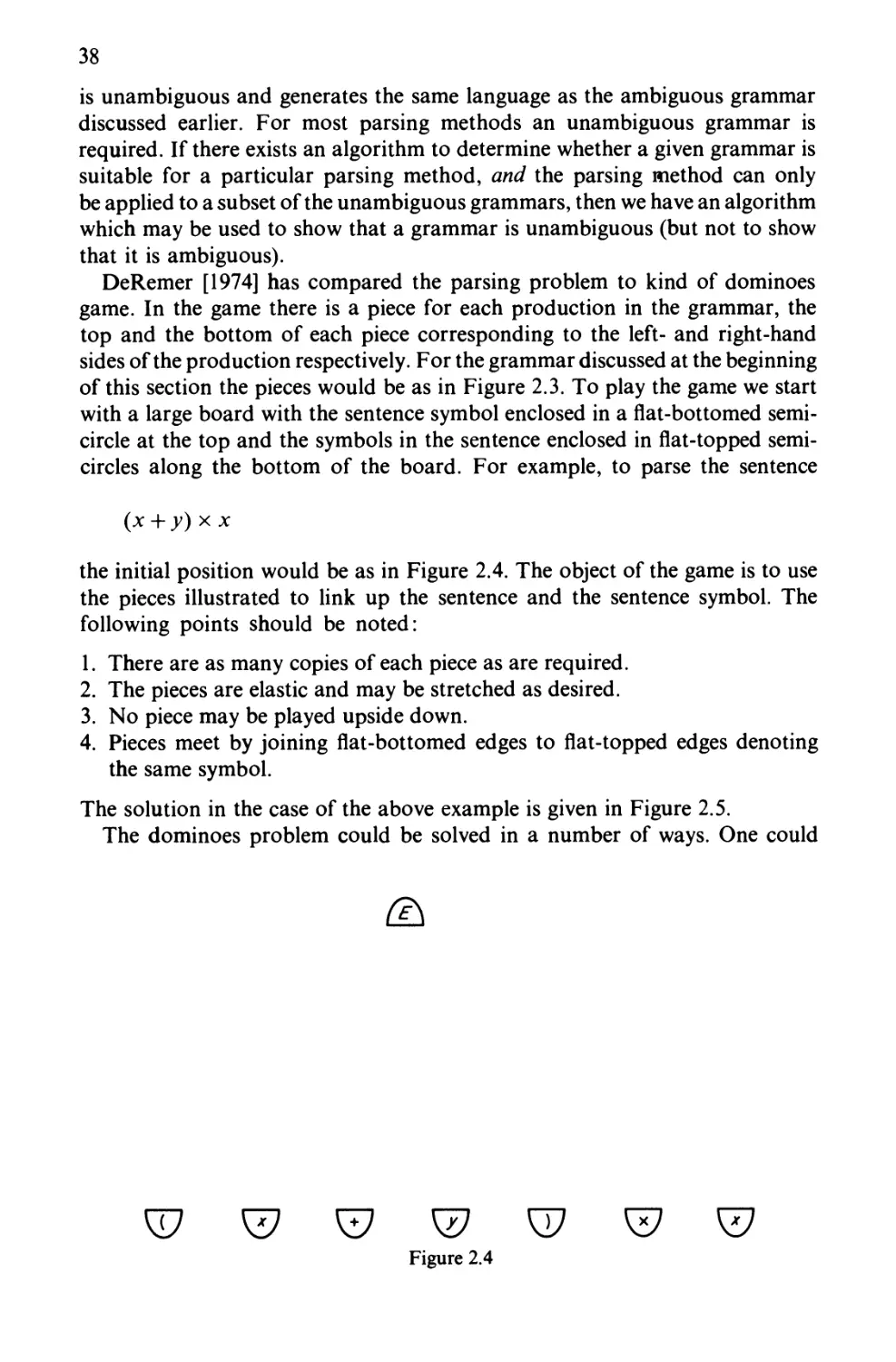
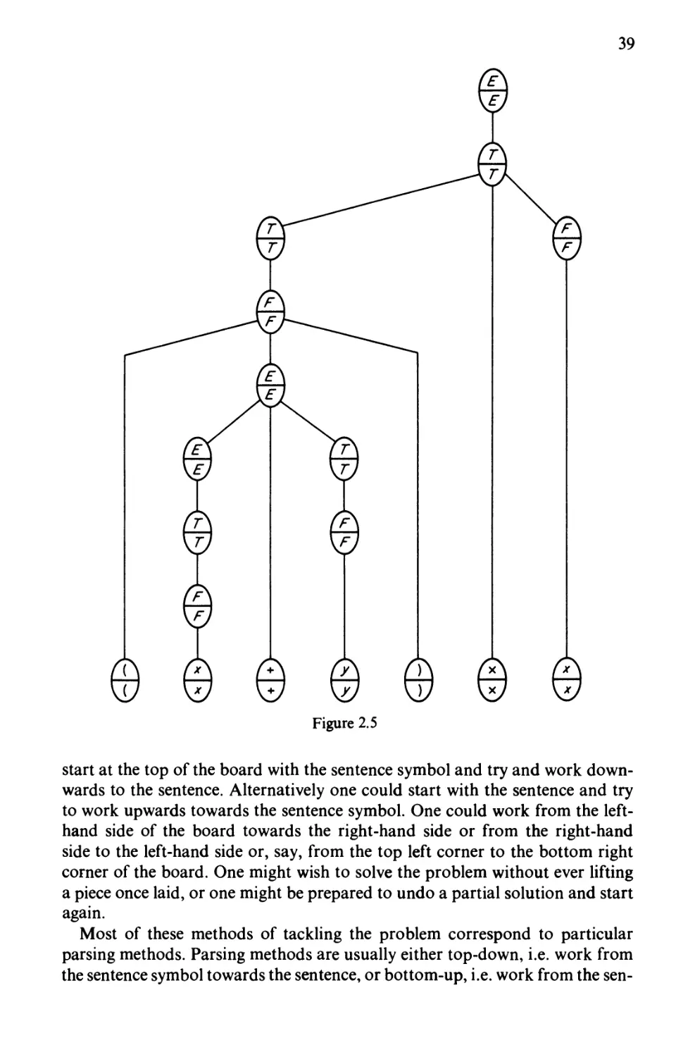
DeRemer [1974] has compared the parsing problem to kind of dominoes
game. In the game there is a piece for each production in the grammar, the
top and the bottom of each piece corresponding to the left- and right-hand
sides of the production respectively. For the grammar discussed at the beginning
of this section the pieces would be as in Figure 2.3. To play the game we start
with a large board with the sentence symbol enclosed in a flat-bottomed
semicircle at the top and the symbols in the sentence enclosed in flat-topped
semicircles along the bottom of the board. For example, to parse the sentence
(x + y)x x
the initial position would be as in Figure 2.4. The object of the game is to use
the pieces illustrated to link up the sentence and the sentence symbol. The
following points should be noted:
1. There are as many copies of each piece as are required.
2. The pieces are elastic and may be stretched as desired.
3. No piece may be played upside down.
4. Pieces meet by joining flat-bottomed edges to flat-topped edges denoting
the same symbol.
The solution in the case of the above example is given in Figure 2.5.
The dominoes problem could be solved in a number of ways. One could
^7 £7 ^7 KD ^37 ^ ^7
Figure 2.4
39
(h (h (*S (h Ch (h (h
KD \*J W \D \JJ W W
Figure 2.5
start at the top of the board with the sentence symbol and try and work
downwards to the sentence. Alternatively one could start with the sentence and try
to work upwards towards the sentence symbol. One could work from the left-
hand side of the board towards the right-hand side or from the right-hand
side to the left-hand side or, say, from the top left corner to the bottom right
corner of the board. One might wish to solve the problem without ever lifting
a piece once laid, or one might be prepared to undo a partial solution and start
again.
Most of these methods of tackling the problem correspond to particular
parsing methods. Parsing methods are usually either top-down, i.e. work from
the sentence symbol towards the sentence, or bottom-up, i.e. work from the sen-
40
tence towards the sentence symbol, although it is possible to mix the two
approaches. It is normal to read the sentence being parsed from left to right, though
from a parsing point of view it may be as simple (or simpler) to read it from right
to left. The idea of never lifting a piece once laid in the dominoes game
corresponds to that of never going back on a decision to apply a particular production
in the parsing process. Going back on a parsing decision is sometimes known
as backtracking. Parsing methods are said to be nondeterministic or
deterministic depending on whether backtracking can take place or not. Non-
deterministic parsing methods can be very expensive in space and time, and
make it very difficult to insert compile-time actions in the parser which might
later have to be undone, such as building the symbol table, etc. In this book
we deal almost entirely with deterministic parsing methods. In Chapter 4
we describe the LL method, which is top-down and uses leftmost derivations,
and in Chapter 5 we describe the LR method, which is bottom-up and uses
rightmost derivations. We deal mainly with context-free parsing but the
techniques can generally be extended to deal with certain classes of more general
grammars such as attribute grammars (Watt [1974]) and affix grammars (Koster
[1974]). W-grammars are less suitable for parsing because of their greater
generality.
Exercises
2.1 Give grammars for the following languages:
Lx = {ambncp\m,n,p>0}
L2 = {ambmcp\m,p>0}
L3 = {xnayn\n>0}u{xnbf\n>0}
2.2 State with reasons which, if any, of the above languages are regular.
2.3 Find a regular grammar generating the same language as the grammar
with the following productions (S is the sentence symbol):
S^AB
A->X\Y
X->x\xX
Y->y\yY
B -► b\bB
2.4 Write down the regular expression generated by the grammar in Exercise
2.3.
2.5 Show that the grammar with the following productions is ambiguous:
S -► if b then S else S
-+ifb then S
-► a
41
2.6 In a certain grammar S is the sentence symbol and the productions are
S - real JDLIST
1DLJST -► IDLIST, ID
1DLIST-+1D
ID-* a
ID->b
ID^c
Give the parse tree for the sentence
real a, b, c
2.7 Derive a grammar generating all strings (including the empty string)
over the alphabet {0,7}.
2.8 Consider the following grammar with sentence symbol PROGRAM:
PROGRAM - begin DECS; ST A TS end
DECS -rf; DECS
d
STATS -j; STATS
s
Give the leftmost and the rightmost derivations of
begin s\ s\ d; dend
2.9 An identifier in FORTRAN consists of a sequence of up to six letters
and digits, of which the first character must be a letter. Derive
(a) a regular expression for an identifier,
(b) a type-3 grammar generating exactly all the FORTRAN identifiers.
2.10 Most languages have a conditional clause or statement similar to that
described in Exercise 2.5. Explain how the potential ambiguity is avoided
or resolved in some languages with which you are familiar.
Chapter 3
Lexical Analysis
Conceptually the first phase of the compilation process is Lexical Analysis,
i.e. the grouping together of strings of characters denoting identifiers, constants,
or language words, etc., into single symbols. In one-pass compilers, of course,
the process will take place in parallel with other compilation phases. However,
whether or not lexical analysis constitutes a distinct pass of the compiler, it is
convenient in describing the construction of a compiler, as well as in
constructing one, to think of lexical analysis as a distinct phase of compilation. In this
chapter we discuss how the various symbols are recognized, and we describe
the tables which the lexical analyser has to build for its own use, and for use by
later phases of the compiler. We also discuss particular problems encountered
in writing lexical analysers for ALGOL 68 and other languages.
3.1 Recognition of symbols
The process of lexical analysis is greatly simplified by the nature of the
strings which have to be recognized. Examples are identifiers, e.g.
first date I no1234
real numbers, e.g.
1.23 6.0 34.2910- 20
language words, e.g.
begin for case
All these strings can be generated by regular expressions. For example, real
numbers can be generated by the regular expression
( + | - |) digit*, digit digit*(l0( + | - |) digit digit* |)
from which it is seen that a real number consists of
1. an optional sign,
42
43
2. a sequence of zero or more digits,
3. a decimal point,
4. a sequence of one or more digits,
5. an optional exponent part consisting of
(a) an exponent (10)
(b) an optional sign
(c) a sequence of one or more digits
in that order.
Regular expressions are, of course, equivalent to type-3 grammars (Section
2.2). For example, a type-3 grammar corresponding to the regular expression
for a real number given above has productions
fl- + S|
-s\
dS\
.P
S^ dS\
.P
P^dF\
d
F-+dF\
d
A-++N\
-N\
dN\
d
N^dN\
d
where R is the sentence symbol.
There is also a one-to-one correspondence between regular expressions
(and therefore type-3 grammars) and finite automata, which are defined as
follows.
A finite automaton is a device for recognizing strings of a particular language.
It has a finite set of states, some of which are termed final states, and control
passes from state to state as each character of the string is read, according to
a given set of transitions. If, after reading the final character of a string, the
automaton is in one of the final states the string is said to belong to the language
accepted by the automaton. Otherwise the string does not belong to the language
accepted by the automaton.
44
More formally, a finite automaton is defined by five characteristics:
1. A finite set of states, K.
2. A finite input alphabet, I.
3. A set of transitions, 6
4. A starting state S (SeK).
5. A set of final states F(Fg K).
We can write a finite automaton as a 5-tuple
M = (K,I,<5,S,F)
Consider the following example where
the states are A and B9
the input alphabet is {0,/},
the initial state is A,
the set of final states is {A},
the transitions are
d(A,0) = A
d(AJ) = B
d(Bfi) = B
8(BJ) = A
meaning 'on reading a 0 in state A, control is passed to state A' and so on.
On reading the string
0 WOW 11
control will pass successively through the states
A,A,B,B,B,A9A9B,A
in that order. Since A is a final state the string is accepted by the finite automaton,
However, on reading the string
00111
the automaton passes through the states
A,A,A9B9A9B
in that order and, since B is not a final state, the string is not accepted, i.e. the
string does not belong to the language accepted by the automaton. Since
zeros do not affect the state of the automaton but each one changes its state
from A to B or B to A, and the initial state is the same as the final state, it
45
Input
able
0
1
3.1
States
A B
A B
B A
follows that the language accepted by the automaton consists of exactly those
strings which contain an even number of ones.
Another way of representing the transitions is by means of a table (see
Table 3.1) or diagrammatically (see Figure 3.1).
Figure 3.1
The above automaton is said to be deterministic since each entry in the
transition table contains a single state. In a nondeterministic finite automaton
this is not necessarily the case. Consider the finite automaton defined as follows:
M1=(/:pIp(51,51,F1)
where
Kl={A,B}
£,={0,/}
St = {A}
and the transitions are given by Table 3.2
Table 3.2
A B
0
{B}
or diagrammatically (Figure 3.2).
Mj accepts a string if and only if it begins with a one. The string
on
46
UO
B
Figure 3.2
cannot be accepted as there is no transition from A on reading a 0.
The string
1
will be accepted since there is a transition (more generally a sequence of
transitions) leading to a final state on reading the string. There is also a transition
leading to a nonfinal state {A to A) but this does not affect the acceptability
of the string. For a nondeterministic finite automaton therefore it is necessary
to try all possible sequences of transitions before concluding that a string
cannot be accepted by the automaton. This can be done either by trying all
possibilities in parallel or one after the other. If only one route can be tried
at a time (as is usually the case) then backtracking is required, i.e. it is necessary
to re-read all or part of the string while another route is investigated. This
can clearly be very time consuming.
Corresponding to Mx there is a deterministic finite automaton M2 accepting
the same language where
M2 = (K2
,I2,(52,S2,F2
and
K2 = {A,B,C}
22 = {0,/}
S2 = {A}
and the transitions are given by Table 3.3
0
1
Tab
A
C
B
le 3.3
B
B
B
C
C
C
or diagrammatically (Figure 3.3).
47
Figure 3.3
Like A/p M2 accepts a string of zeros and ones if and only if the string begins
with a /. However, in attempting to recognize a string using M2, backtracking
is never required since from any state there is exactly one transition to another
state on reading a particular input symbol. This means that using M2 the time
taken to recognize a string is proportional to the length of the string.
It can be shown that corresponding to each nondeterministic finite automaton
there corresponds a deterministic finite automaton accepting the same language.
The proof involves letting the states in the deterministic automaton correspond
to subsets of the states of the nondeterministic one. For example, state B in
M2 corresponds to the set of states {A, B] of Mx and state Cin M2 corresponds
to 0, the empty set of states of Mx.
The relevance to lexical analysis is that corresponding to each type-3 language
there is a deterministic finite automaton which recognizes strings of the
language. For example, strings generated by the grammar Gt with productions
A^IA
A^ IB
A^l
B^OB
B-+1B
B^O
B^l
where A is the sentence symbol, are recognized by Mt or M2. The grammar
is obtained from the nondeterministic finite automaton, A/p as follows:
1. The starting state of the automaton becomes the sentence symbol of the
grammar.
2. Corresponding to the transitions
8(AJ) = A
S(AJ) = B
48
8(B,0) = B
S(B,1) = B
we have the productions
A^IA
A-*1B
B->0B
B->1B
and corresponding to the fact that in state A there is a transition on reading
a 1 to a final state (B) we have
A-*l
and similarly
B-+0
Conversely, the automaton Mj could have been deduced from the grammar.
The automaton M2 corresponds to the grammar G2 with productions
A^IB
A->0C
A->1
B->0B
B-+1B
B^O
B^l
C->0C
which contains the useless nonterminal C but is equivalent to Gl. The grammar
G2 is said to be 'unclean' since it contains a nonterminal which does not generate
any terminal symbols.
Writing a lexical analyser consists in part of simulating the various automata
to recognize identifiers, numbers, reserved words, etc. A finite automaton to
recognize a real number would be given by Figure 3.4. SI is the starting state
and S4 and S7 the final states. S8 is the failure state. The automaton is
deterministic and can be obtained from the type-3 grammar at the beginning of
the section in two stages. First a nondeterministic automaton whose states
(apart from the final one) correspond to the nonterminals of the grammar is
derived and then this automaton is made deterministic.
49
Figure 3.4
From the automaton a procedure to recognize a real number can be written.
The procedure delivers true or false depending on whether a real number is
recognized or not.
proc realno = bool:
begin char in; int / : = 1;
while read (in); digit (in) or
sign (in) or in = "." or in = "10"
do
/: = case / in
if sign (in) or digit (in) then 2
elif in = "." then 3
50
else 8 fi,
if digit (in) then 2
elif w='."then J
else 8 fi,
if digit (in) then 4
else £ fi,
if digit (in) then 4
elif w = "10" then 5
else 5 fi,
if rf/g/f (in) then 7
elif j/g/i (in) then 6
else £ fi,
if digit (in) then 7
else £ fi,
if digit (in) then 7
else 8 fi,
£esac
od;
backspace (standin);
i = 4 or i=7
end
The existence of procedures digit, which tests a character to see if it is a digit,
and sign which tests for a ' +' or a ' — ' are assumed. The procedure terminates
when it comes to a character which cannot be contained in a real number. This
last character, which is presumed to be the start of some other symbol, is then
'unread'.
Where two symbols can begin with the same character, or string of
characters, it may be necessary to 'merge' their recognition procedures.
We have demonstrated that, given a finite automaton accepting strings
of a regular language, it is not difficult to write a procedure to recognize such
strings. Of course, for every finite automaton there is a corresponding regular
expression, which for a real number was given earlier as
( + | - |) digit* . digit digit* (10( + | - |) digit digit*\)
A procedure to recognize a real number can be written from the regular
expression
proc realnol = void:
begin char in; read (in);
if sign (in) then read (in) fi;
while digit (in)
do read (in)
od;
51
if in = "." then read (in)
else error fi;
if digit (in) then read (in)
else error fi;
while digit (in)
do
read (in)
od;
if /« = "10" then rasd (m);
if sign (in) then rajrf (/ft) fi;
if digit (in) then re#rf (in) else error fi;
while digit (in)
do read (in)
od
fi;
backspace (standin)
end
error is a procedure which is assumed to take appropriate action when an error
situation arises.
Recognizers can be written from regular expressions or finite automata
almost as fast as one can write and it is not difficult to automate the process.
3.2 Output from the Lexical Analyser
The lexical analyser will transform the source program in to a sequence of
symbols. In doing so, arbitrary length identifiers and constants will be replaced
by fixed length symbols. Language words, too, will be replaced by some
standard representation. For example, language words might be replaced by integers,
identifiers by the letter / followed by an integer, constants by the letter C
followed by an integer, and so on. The integers involved cannot of course be
of arbitrary length and therefore it is usual to limit the number of identifiers
and constants that may appear in a program to be less than some reasonably
large integer. This restriction should not be noticed by the vast majority of
users. However, if the limit is ever reached a clear message should be output
by the compiler.
The codes produced for language words will be program independent.
For example, begin might be replaced by 77 and for by 22. In the case of
identifiers, however, the standard identifiers such as read, print, pi will always have
the same codes but user-defined identifiers will be allocated codes by the lexical
analyser in the order in which they are encountered, the first identifier being
e.g. 77, the second 12, and so on. Each occurrence of a particular identifier
(at whatever block level) will be replaced by the same code. This means that
an identifier table giving the code for each identifier must be kept by the lexical
analyser. After lexical analysis each identifier will have been consistently
52
Code
49
50
51
52
53
Identifier
►ran
Figure 3.5
replaced and, strictly speaking, there will be no further need for the identifier
table. However, it may be useful for providing diagnostics to the user in terms
of the source language if errors are discovered at a later stage of compilation.
For this reason the identifier table is usually retained throughout the
compilation process.
Storage of the identifier table usually requires a data structure capable of
holding arbitrary length identifiers. An obvious solution is to use lists, where
each list element corresponds to a letter of an identifier and 0 represents the
null pointer (Figure 3.5).
In ALGOL 68 the identifier table would require the following mode
declarations:
mode list = struct (char /, ref list next);
mode idtable = [/ :p] struct (int code, ref list ident)
The large number of pointers used in the above structure tends to waste
space and an alternative would be to use a row of characters or a reference to
a row of characters to represent the letters of the identifier, e.g.
mode idtable 1 = [/ :p] struct (int code, ref [ ] char ident)
In either case the identifier table itself would need to be expandable. One way
of achieving this would be to make the identifier table a list, but a better solution
is probably to use a flexible array. However, instead of expanding the array
one element at a time when it becomes full, it is more efficient to start off with
an array of, say, 50 elements, and add 10 or 20 elements each time the array
has to be extended. The flexible effect can also be achieved in ALGOL 68
(and possibly other languages) by using a reference to a row mode and copying
the elements into a larger row every time the table has to be expanded.
A somewhat different approach to implementing an identifier table is to
store all the characters forming the various identifiers in a single array of
53
Code
51
52
53
Length
3
1
4
Pointer
u
N
E
Figure 3.6
characters, and to let each identifier table entry contain a pointer to the start
of the character string corresponding to the particular identifier and a count
of the number of characters it contains. When checking to see if a particular
identifier is already in the table it is only necessary to do a character-by-character
comparison with those identifiers already in the table which happen to be of the
appropriate length (Figure 3.6).
A similar type of table is required for constants. Some compilers check the
length of constants and evaluate them during lexical analysis. The length of
constant which is allowable, however, usually depends on the host machine,
and it would seem more satisfactory just to store the arbitrary length constants
in a table at the lexical analysis stage rather than to introduce machine
dependencies at such an early stage of the compilation process. The constant
table will be required at a later stage of compilation, but what the lexical
analyser must pass to the syntax analyser is that a constant of a particular
type has been stored in the constant table at a specific address. The value at
the address may not be required until the final phase of code generation but its
type will be required during the analysis stage. The lexical analyser will pass
to the syntax analyser a code of the form TXXX (where XXX denotes the
constant table entry where the value is to be found and T its type). As an
alternative, 'small' integer constants may be passed as literals rather than as pointers
to the constant table. For example, C001C009 could represent the integers 1 to 9.
ALGOL 68 programs may contain user-defined bold identifiers (or bold
tags) such as
list max
which are used to define modes or operators. The lexical analyser treats these
in a similar way to identifiers by putting them in a table which is passed on to
later passes for diagnostic purposes.
54
3.3 Comments, etc.
As well as passing on a representation of the symbols in the source program
the lexical analyser may insert additional information into the source text
or remove strings of characters from the text. An example of the former is
line numbers. For diagnostic purposes, especially for a multi-pass compiler,
it is useful to be able to refer to program errors by means of line numbers in the
original source text. It is simple for the lexical analyser to insert line numbers
into the program as it is being processed, and these line numbers can be passed
on to subsequent passes as long as program errors are liable to be detected
(probably as far as machine-code generation if constants are not checked
until this stage).
Comments are included in programs solely for the benefit of the human
reader. They do not concern the compiler in any way and will normally be
removed by the lexical analyser. ALGOL 68 programs may also include
pragmatic remarks which, like commentary, do not affect the meaning of programs.
However, pragmatic remarks are of interest to the compiler and may affect
the manner in which compilation takes place. They are used to convey messages
from the programmer to the compiler concerning, for example, whether a
particular section of program should be optimized with respect to execution
time or whether a particular method of error recovery should be used. Pragmatic
remarks may concern one particular phase of the compiler, such as the lexical
analyser or the code generator, or they may concern more than one phase of
the compiler. Where a pragmatic remark concerns only the lexical analyser
then it will be removed at this stage. Otherwise it will be passed on.
3.4 Problems concerning particular languages
For the main part a lexical analyser will base its decisions on information
contained in the symbol it is processing. One would normally expect a lexical
analyser to accept (and to be happy with) any sequence of symbols belonging
to the language being compiled. In recognizing an integer constant, for example,
the lexical analyser would not be concerned whether it followed an operator or
a begin symbol or whether it occurred within a procedure declaration or a do
statement. A problem can arise when the way in which characters are combined
to form symbols depends on the context. In FORTRAN, for example, in the
sequence
DO 7 1=1,5
up till the moment when the comma has been read "DO" could be the language
word or alternatively part of the identifier
DO 7 I
To resolve the ambiguity the lexical analyser has to do some lookahead. The
55
problem arises because in FORTRAN spaces are not significant. In PL/1
language words are (in the main) not reserved and certain ambiguities can
require an arbitrary amount of lookahead to resolve. In COBOL, language
words (over 100 of them) are reserved and cannot be used as identifiers. In
BASIC and ALGOL 68 language words take a different form from identifiers
and cannot be confused with them.
In ALGOL 68, however, another problem arises. Assuming operators to
be symbols of the language, the sequence of characters
< =
might be interpreted as an operator (usual meaning iess than or equal to').
However, the same sequence of characters could also occur in an ALGOL 68
program within the declaration of the operator <, e.g.
op < = ...
In this case 4<' is an operator and 4 = ' is a symbol separating the operator
name from the routine defining it.
In this case the lexical analyser would be expected to pass on ' <' and 4 ='
as two distinct symbols. For the lexical analyser to be able to distinguish
between the compound symbol
< =
and the pair of symbols ' <' and ' =' appearing in succession it is necessary
for the lexical analyser to have some context information. Clearly if op precedes
4 < =' it should be treated as two separate symbols. Similarly in the following
context where we have a sequence of operator declarations separated by commas
op >=...,< =
' < 'and 4 =' are distinct symbols. To cope with these sorts of situations it is
occasionally necessary (at least to avoid complications at a later stage) for a
lexical analyser for ALGOL 68 to know something about the context in which
it is operating.
Formats also cause complications in ALGOL 68. Within a format (used
for input/output) certain letters such as X, Y9 L have well-defined meanings
whereas elsewhere they might be taken to be identifiers (or parts of identifiers).
Each format is surrounded by a pair of format symbols (usually dollar symbols)
so that the lexical analyser always knows whether it is within a format or not
and can interpret the letters X, Y, L, etc. accordingly. A complication arises
in that formats can contain closed clauses (blocks) inside which, of course,
the normal interpretation should again be used for these characters. In
$n(x- l)x9 dd%
56
x — 1 spaces (the second x is an alignment symbol denoting a space) are taken
before writing (assuming the format is being used in connection with output)
a two-digit integer.
It is also possible for a closed clause within a format to contain a format,
and so on to any depth. A suitable structure for a lexical analyser to deal with
the situation would be for it to consist of two mutually recursive procedures,
one corresponding to each of the modes in which it is required to operate.
We have already mentioned that a program may contain user-defined bold
tags denoting modes or operators. However, as far as the lexical analyser is
concerned, the context information necessary to distinguish between user-
defined modes and user-defined operators is not available and bold tags are
simply passed on as such. Each implementation of ALGOL 68 will have a
method of representing bold tags (and languages words) in a program, the
two most common representations of the language word begin being
'BEGIN' and .BEGIN
The lexical analyser could be designed to accept more than one representation
of bold symbols, with one particular representation being assumed unless the
programmer indicated otherwise by means of a pragmat. A standard
representation for ALGOL 68 is described in Hansen and Boom [1977].
Were it not for points like those described in this section, the production of
lexical analysers would be a fairly straightforward process and lexical analysers
could be produced automatically by means of a lexical analyser generator,
which accepted as input the syntax of the various symbols of a particular
language and output a lexical analyser for the language.
Lexical analysis may be relatively straightforward, but as far as compilation
time is concerned it turns out to be rather expensive. For many compilers
around half the time taken to compile a program is taken up by lexical analysis.
This is largely unavoidable because of the character nature of the input and if
it were not so, for some particular compiler, this would tend to suggest that
some of the other phases of the compiler were not as efficient as they might be.
Exercises
3.1 Write down the productions of a type-3 grammar generating the regular
expression
(101)* (010)*
3.2 Derive a finite automaton corresponding to the regular expression in
Exercise 3.1.
3.3 Derive a nondeterministic finite automaton accepting the regular
expression
(101)* (110)*
57
Figure 3.7
3.4 Derive a deterministic automaton accepting the regular expression in
Exercise 3.3.
3.5 Give a type-3 grammar corresponding to the finite automaton described
by Figure 3.7, where A is the starting state and C the final state. How
would you describe the language?
3.6 Write a procedure to recognize strings of the language accepted by the
automaton in Exercise 3.5.
3.7 A fixed point number is defined to be an optional sign followed by a
string of zero or more digits, followed by a point, followed by a string of
zero or more digits; containing at least one digit (before or after the point).
Write a procedure to recognize such a number.
3.8 A goods train may have one or two engines at the front, followed by one
or more trucks, followed by a guards van. Write a procedure to recognize
a goods train.
3.9 Suggest data structures suitable for implementing a constant table.
3.10 Suggest an alternative to mutually recursive procedures for dealing with
the two lexical analysis modes required for ALGOL 68 (i.e. within and
outside formats).
Chapter 4
Context-Free Grammars and Top-Down
Syntax Analysis
In the last chapter we discussed the recognition problem for type-3 languages,
and showed that a finite automaton could be used to recognize any type-3
language. Furthermore, we found that we could always use a deterministic
automaton, so that backtracking was never required. While type-3 grammars
are suitable for generating the symbols which are constructed during lexical
analysis, they are not so suitable for describing the ways in which these symbols
can be combined to form sentences of typical programming languages. For
example, as we have already mentioned in Chapter 2, bracket matching cannot be
specified by means of a type-3 grammar. Context-free grammars, although
not able to specify all properties of typical programming languages, are more
general and therefore more suitable as a basis for the syntax analysis (parsing)
phase of compilation.
In this chapter we discuss the properties of context-free grammars and their
relation to automata theory. We also describe top-down methods of syntax
analysis. Bottom-up methods are described in Chapter 5.
4.1 Context-free grammars
Traditionally, context-free grammars have been used as a basis for the
syntax analysis phase of compilation. Where a programming language cannot
be generated by a context-free grammar it is always possible to find a context-
free grammar which generates a superset of the language, i.e. generates a
language which contains the given programming language. Using this grammar
as a basis for syntax analysis means that certain restrictions in the actual language
(e.g. that all identifiers in the program are declared) will not be checked by
the parser. However, it is usually not difficult to incorporate other actions in
the compiler (e.g. by the use of a symbol table) to perform the necessary checks
on the source program.
From the definition of a context-free grammar given in Chapter 2 it is clear
that the class of context-free grammars is more powerful (i.e. can generate
more languages) than the class of regular grammars but less powerful than
the context-sensitive grammars. The language
58
59
{a"b*\n>0}
is context free but not regular. It is generated by the grammar with productions
S^aSb
S -» £
On the other hand, the language
{a»bnc"\n>0}
is context sensitive but not context free.
There are a number of characteristics of context-free grammars, and proofs
of most of the following results can be found in Hopcroft and Ullman [1969].
/. Canonical form
(a) Every context-free grammar is equivalent to (i.e. generates the same
language as) a grammar in Chomsky Normal Form, i.e. with all productions
of the form
A -+ BC
A -» a
with the usual convention regarding terminals and nonterminals.
(b) Every context-free grammar is equivalent to a grammar in Greibach
Normal Form, i.e. with all productions of the form
A-+boi
where a is a (possibly empty) string of nonterminals.
2. Self embedding
Self-embedding is defined as follows. If in a grammar G there is a nonterminal,
A say, for which
A %>ol, Act,
G 1 2
where a, and a2 are non-empty strings of terminals and/or nonterminals
then the grammar is said to contain self embedding. For example, the following
two grammars contain self-embedding:
1. G1=({5},{«,*},/>,5)
where the elements of P are
60
S^aSb
S -► £
2. G2 = ({S,,4}, {begin, end, [ , ]},/\S)
where the elements of P are
S -» begin /4 end
S-+e
In the latter case both A and 5 are said to exhibit the self-embedding property.
A theoretical result states that any context-free grammar which does not
contain self-embedding is equivalent to a regular grammar or (alternatively)
generates a regular language. It is also the case that a regular grammar cannot
contain self-embedding. It is self-embedding that effectively distinguishes
between context-free (nonregular) languages and regular languages. As can
be seen from the second example above, matching brackets, etc., involves
self-embedding and therefore cannot be specified by a regular grammar.
3. Pumping lemma
For any context-free language, L, there exists a constant k such that any
sentence z of the language whose length is greater than k can be written in the
form
z = uvwxy where | vwx \ < k
and v and x are not both the empty string and the string
uvlwxly (for / > 0)
is in L.
This lemma can be used to show that certain languages are not context
free. Consider the language
{aa|ae{0,/}*}
({0,/}* is the closure of {0,7} as defined in Section 2.2). From the lemma
any string z of length > k, can be written
uvwxy
where \vwx\ <k, |vx\ =/= 0 and uVwxly{i > 0) is in the language
Let a consist of k 0's followed by k Ps so that z is of the form
000 ... 01111 ... 1000 ... 01111 ... 1
61
This string can be written in the form
uvwxy
but since \vwx\ < k either
1. v and x are both in the first half of z or are both in the second half, or
2. vx contains /'s from the first half of the string and O's from the second
half of the string.
In the first case uwy will be formed by removing 0's and 7's from the first half
or the second half of z (but not both). Thus uwy will not be in the language.
In the second case uwy will be formed from z by removing 7's from the first
half and 0's from the second half of z. Again the resultant string will not be
in the language.
We have thus shown that the given string cannot be expressed in the form
uvwxy
in such a way that uwy is also in the language. This contradicts the pumping
lemma and therefore the language is not context free.
Similarly it can be shown that the languages
{anbncn\n>0}
{al\iis prime}
are not context free.
From a parsing point of view it is important to know what type of automaton
is capable of recognizing a context-free language. The answer is a push-down
automaton which is equivalent to a finite automaton with the addition of a
push-down store or stack. A move of the push-down automaton consists of
either
(a) reading an input symbol, replacing the top symbol on the stack by a
(possibly empty) string of symbols, and changing state, or
(b) as (a), but without reading an input symbol.
A push-down automaton may be represented by a tuple
(K9I.X,S9q09Z0)
where
K is a finite set of states
I is the input alphabet
Tis the push-down alphabet
S is a set of transitions
q0 is the initial state
Z0 is a push-down symbol which is initially on the stack.
62
For example, consider the push-down automaton M defined as follows:
K={A}
I ={<(',')'}
r={o,/}
5 is given by
8(AJ,r) = (A9IO)
(meaning in state A with / on top of stack on reading '(' goto state A and
replace / by 10).
8(A,0,X) = (A900)
8(A909y) = (A9e)
8(A9/9a) = (A9e)
M recognizes matched pairs of brackets. Opening brackets (represented
by O) are put on the stack and removed when a corresponding closing bracket
is encountered. The bracket string is accepted if reading the complete string
leaves the stack empty. This is the normal way by which push-down automata
accept strings, though it is also possible to define push-down automata that
accept by final state, and the two types can be shown to be equivalent.
The push-down automaton described above was deterministic, i.e. for each
admissible input symbol there was a unique transition. As for finite automata,
we can also define nondeterministic push-down automata which may contain
a set of transitions for a given input, state, and stack contents.
Consider the language
{aa'|ain{0,/}*}
ar denotes a reversed.
The language is accepted by the following nondeterministic push-down
automaton
M = ({A9B}9{091)9{I9091}969A9I)
where transitions are given by
S(A9I90) = {(A9I0)}
8(A9I91) = {(A9I1)}
S(A9090) = {(A900)9(B9e)}
5(A9l9l) = {(A9ll)9(B9e)}
S(A90,1) = {(A,01)}
63
8{A,1,0) = {(A,10)}
5(B,0,0) = {(B,e)}
8(B,l,l) = {(B,e)}
8(B,I,e)={(B,e)}
8(A,I,e)={(A,e)}
State A corresponds to having read less than half the string and state B to having
read more than half the string. As the first half is being read symbols are put
on the stack (state A), and, as the second half is being read, each symbol is
checked against the top symbol of the stack and one symbol is removed from
the stack. The problem is knowing when the midpoint of the string has been
reached. A necessary condition is that two consecutive ones or two consecutive
zeros are read. However, this is not a sufficient condition. Consider, for example,
the string
01011011011010
The two ones in position 4 and 5 might be thought to mark the middle of the
string and without (in general) an arbitrary amount of lookahead there is no
way of telling whether it is the middle or not. Hence the alternative transitions
in state A when the incoming symbol and the top of the stack are identical.
This makes the push-down automaton nondeterministic and it is difficult to see
how it could be otherwise. Indeed, this is borne out by the theory which asserts
that there exist nondeterministic push-down automata which accept context-
free languages which are not accepted by any deterministic push-down
automata. Thus, while for a regular language we could always find a deterministic
automaton which would accept it, the corresponding result does not hold for
context-free languages. Thus, it is not possible to find deterministic automata
corresponding to some context-free languages. When it is recalled that
deterministic finite automata were produced from nondeterministic ones by merging
states where two or more transitions led to different states, it is not surprising
that the same approach does not work with push-down automata when
alternative transitions may affect the stack in different ways.
Parsing involves effectively simulating the appropriate push-down
automaton and the effect of the above is that some context-free languages cannot
be parsed deterministically (i.e. without backtracking). How important this
is from the compiler writer's point of view depends on whether typical
programming languages can be parsed deterministically or not. We define a deterministic
language to be one which can be parsed deterministically; it turns out that
most programming languages are deterministic, or at least almost so.
There is a one-to-one correspondence between context-free grammars and
push-down automata and it may depend on which grammar we use to generate
a language as to whether the corresponding push-down automaton is
deterministic or not. We say that a parsing method is deterministic (for a particular
grammar) if no backtracking is involved in parsing the grammar. Some
64
languages can be parsed deterministically by one parsing method but not by
another. In particular, some languages can be parsed deterministically from
the bottom up but not from the top down. In this book we will be concerned
almost entirely with deterministic parsing methods. Nondeterministic methods
may not be too intolerable for line-oriented languages such as BASIC or
FORTRAN but for highly recursive languages such as ALGOL 68 or Pascal,
where the compiler may have to backtrack over not just the current line but
over a large part of a program, the overheads are just not acceptable. Another
disadvantage of backtracking is that it may involve undoing compiler actions
which take place in parallel with syntax analysis.
4.2 Method of recursive descent
A well-known and easy-to-implement top-down deterministic parsing
method is known as the method of recursive descent. Using it, a syntax analyser
can be written from a suitable grammar and, furthermore, can be written
almost as fast as one can write.
Consider, for example, the language generated by the grammar with the
following productions:
PROGRAM -► begin DEC LI ST comma ST AT ELI ST end
DEC LIST - d semi DECLIST
DEC LI ST -► d
ST A TELIST - s semi ST A TELIST
STATELIST-+s
We first modify the grammar to the following:
PROGRAM -> begin DECLIST comma STATELIST end
DECLIST - d X
X -► semi DECLIST
X^e
STATELIST-+s Y
Y -► semi STATELIST
r-£
Now we write a procedure to recognize each nonterminal. Starting with
the sentence symbol (PROGRAM) we have
proc PROGRA M = void:
begin if symbol =/= begin then error fi;
symbol: = lexical;
DECLIST;
if symbol =/= comma then error fi;
symbol: = lexical;
65
STATELJST',
if symbol =/= end then error fi
end;
proc DEC LI ST =void:
begin if symbol =£ rf then error fi;
symbol: = lexical;
end;
proc A' = void:
if symbol = semi then
symbol \= lexical, DEC LI ST
elif symbol = comma
then skip
else error
fi;
proc 57^ TELIST = void:
begin if symbol =/= 5 then error fi;
symbol: = lexical;
r
end;
proc K = void:
if symbol = seraz then
symbol \= lexical', STATELJST
elif symbol = e^rf then skip
else error
fi;
In the above procedures a number of assumptions have been made:
1. error is a procedure to deal with syntax errors; the details do not concern
us here,
2. lexical is a procedure which reads characters of source text and delivers the
next symbol. Alternatively, if lexical analysis is performed by a previous
pass lexical simply reads the next symbol,
3. semi, comma, etc. are identifiers whose values are the compile-time
representations of the corresponding terminals,
4. before PROGRAM is called the following assignment has taken place:
symbol: = lexical.
Parsing a sentence of the language could involve many recursive calls of the
procedures corresponding to the nonterminals in the grammar. If we choose
66
to represent the grammar in a slightly different way this recursion can be
replaced by iteration:
PROGRAM -► begin DEC LI ST comma ST AT ELI ST end
DEC LIST -► d {semi d)*
ST A TELIST - s (semi s)*
where (x)* means zero or more occurrences of x. The procedures for DEC LI ST
and STATELISTthen become
proc DECLIST =void:
begin if symbol =/= d then error fi;
symbol: = lexical;
while symbol = semi
do symbol: = lexical;
if symbol =/= rf then error fi;
symbol: = lexical
od
end;
proc 57^ TELIST = void:
begin if symbol =/= 5 then error fi;
symbol: = lexical;
while symbol = jew/
do symbol: = lexical;
if symbol =/= s then error fi;
symbol: = lexical
od
end
Replacing recursion by iteration is likely to make the analyser more efficient
and also (arguably) more readable.
The advantages of writing a recursive descent parser are fairly obvious.
The main one is the speed at which the parser can be written from the
corresponding grammar. Another is that, because of the close correspondence
between the grammar and the parser, there is a high probability that the parser
will be correct, or at least any errors will be of a simple nature. The disadvantages
of the method, though perhaps less obvious, are no less real. The high incidence
of procedure calls during syntax analysis are likely to make the parser relatively
slow, and, compared with some table-driven parsing methods to be described
later, the parser is likely to be rather large. Although the method is well suited
to the insertion of code generation actions in the parser, this inevitably leads
to different phases of compilation becoming intermixed. This does not lead to
reliable or to easily maintainable compilers and tends to introduce machine
dependencies into the parser. The recursive descent parsing method is, however,
67
related to another well-known top-down parsing method which avoids most
of the problems and is discussed in the next section.
4.3 LL(1) grammars
An LL(1) grammar is one type of grammar from which a top-down
deterministic parser can be produced. As a preliminary to defining an LL( 1) grammar
more precisely we introduce the idea of an s-grammar.
Definition An s-grammar is one in which:
1. The right-hand side of each production begins with a terminal.
2. Where a nonterminal appears on the left-hand side of more than one
production, the corresponding right-hand sides begin with different
terminals.
Condition 1. is similar to saying the grammar is in Greibach Normal Form
except that the terminal at the start of each right-hand side may be followed by
nonterminals and/or terminals.
Condition 2. is what helps us to write a deterministic top-down parser,
since, in deriving a sentence of the language, it is always possible to distinguish
between the alternative productions for a leftmost nonterminal in the sentential
form by examining a single lookahead symbol.
The grammar with productions
S-+pX
S-+qY
X^aXb
X-+x
Y-+aYd
is an ^-grammar whereas the following grammar which generates the same
language is not:
S- T
R^pX
T^qY
X^aXb
X^x
Y^aYd
Y-+y
since two of the right-hand sides do not begin with terminals.
It is extremely easy to detect whether a given grammar is an ^-grammar or
not, and in some cases a grammar which is not an ^-grammar can be transformed
into an ^-grammar without affecting the language generated.
68
Consider the problem of parsing the string
paaaxbbb
using the ^-grammar above. Starting with the sentence symbol S we try to
generate the string. A leftmost derivation is used and the result is shown below.
Source string
paaaxbbb
paaaxbbb
t
paaaxbbb
t
paaaxbbb
t
paaaxbbb
t
paaaxbbb
T
Derivation
S
= > pX
T
= > paXb
t
= > paaXbb
T
= > paaaXbbb
t
= > paaaxbbb
As the derivation takes place initial terminals in the sentential form are checked
off against symbols in the spurce string. At each stage of the derivation the
upward arrow indicates the point up to which the source has been read and the
initial terminals of the derivation checked. Where the leftmost nonterminal
in the sentential form can be replaced using more than one production the
appropriate production can always be chosen by examining the next symbol
of the input string for, since we are dealing with an ^-grammar, the right-hand
sides of the alternative productions will begin with distinct terminals.
We see therefore that it is always possible to write a deterministic top-down
parser for a language generated by an ^-grammar. An LL(1) grammar is a
generalization of an ^-grammar and we will see that the way in which it is
generalized will still allow us to construct deterministic top-down parsers.
The two L's in LL(1) refer to the fact that strings are parsed from Left to
right and Leftmost derivations are used. The 1 denotes the fact that alternative
productions are chosen by means of a single symbol of lookahead. The
terminology is due to Knuth [1971] and the properties of LL(1) grammars have also
been investigated by Foster [1968]. We first note that, even though the right-
hand side of a production does not start with a terminal, it may be possible
to deduce that a given alternative for some nonterminal symbol may only
give rise to strings which begin with one of a particular set of terminals. For
example, from the productions
S- RY
69
S-+TZ
R-+paXb
T-*qaYd
it can be deduced that the production
S- RY
should only be applied in a top-down parse (assuming there are no other
productions for R) when the lookahead symbol is/?. Similarly the production
S-+TZ
should only be applied when the lookahead symbol is q.
This leads us to introduce the idea of sets of starter symbols defined as follows:
aeS(A)oA =>a<x
where A is a nonterminal symbol, a is a string of terminals and/or nonterminals,
and S(A) denotes the set of starter symbols of A. In the grammar with
productions
P -> Ac
P-+Bd
A -+a
A -> aA
B-+b
B-+bB
a and b are starter symbols for P. We also define the set of starter symbols for
string of terminals and/or nonterminals as follows:
<365(a) <xx =>aP
where a and j8 are strings of terminals and/or nonterminals (/? may be empty).
A necessary condition for a grammar to be LL(1) is that the sets of starter
symbols for alternative right-hand sides of productions are disjoint.
Care should be taken when a nonterminal at the start of a right-hand side
can generate the empty string. For example, in
P-+AB
P^BG
A -» aA
A -» £
B-+c
70
B-*bB
we have
S(AB) = {a,b,c]
since A can generate the empty string, and
S(BG) = {b,c}
so the grammar is not LL(1).
Consider also the grammar with productions
T->AB
A^PQ
A->BC
P^pP
P->s
Q^lQ
Q ->e
B^bB
B^e
C^cC
c-+f
giving
S(PQ) = {pM
and
S(BC) = {b,e)
However, since PQ can generate the empty string, the lookahead symbol
on applying the production
A^PQ
could be b or e, possible follower symbols of A; and a single lookahead symbol
is not sufficient to distinguish between the two alternative right-hand sides for
A since b and e are also starter symbols for EC
For this reason, we introduce what Griffiths [1974] calls "director symbols',
defined as follows. If A is a nonterminal the director symbols of A are
S(A) + (if A can generate the empty string
then all the symbols which can follow A).
More generally, for a given alternative a of a nonterminal P(P -> a)
we have
DS(P, a) = {a\aeS((x) or (a 4 £ and aeF(P))}
where F(P) is the set of symbols which can follow P. In the previous example
the sets of director symbols are
71
DS(A,PQ) = {p,q,b,e}
DS(A,BC) = {b,e}
Since the sets are not disjoint, the grammar cannot form the basis of a
deterministic top-down parser using one lookahead symbol to distinguish between
alternative right-hand sides.
We are now ready to define an LL(1) grammar. A grammar is said to be
LL(1) if, for every nonterminal appearing on the left-hand side of more than
one production, the sets of director symbols corresponding to the right-hand
sides of the alternative productions are disjoint. All LL(1) grammars can be
parsed deterministically from the top down.
For a given grammar there exists an algorithm for determining whether
it is LL(1) or not and we now describe such an algorithm.
First it is necessary to determine which nonterminals can generate the empty
string. To do this we set up a one-dimensional array with one element for
each nonterminal. Each element of the array may take one of three values,
YES, NO, or UNDECIDED. Initially all the elements are set to UNDECIDED.
We scan the grammar as many times as are required to set each element to
YES or NO.
On the first scan all productions containing terminals are eliminated. If this
leads to the elimination of all productions for some nonterminal the value
NO is assigned to the appropriate element of the array. Secondly, for each
production with £ on the right-hand side the value YES is assigned to the array
element corresponding to the nonterminal on the left-hand side and all
productions for that nonterminal are removed from the grammar.
If subsequent scans are required (i.e. some array elements still have the value
UNDECIDED) the following actions take place:
1. Each production with a symbol on the right-hand side which cannot generate
the empty string (as given by the values of the appropriate array element)
is eliminated from the grammar. If there are no other productions for the
nonterminal on the left-hand side of the eliminated production then the
value of the array element corresponding to that nonterminal is set to NO.
2. Each nonterminal on the right-hand side of a production which can generate
the empty string is deleted from the production. If the right-hand side of
a production becomes empty the value YES is assigned to the array element
corresponding to the nonterminal on the left-hand side and all productions
for that nonterminal are removed from the grammar.
This process is continued until a complete scan of the grammar produces
no change in the values of the array elements. Assuming the grammar was
clean in the first instance (i.e. all nonterminals could generate terminal strings,
or the empty string) the array elements will now all be set to YES or NO.
As an example of the process, consider the grammar
1. A^XYZ
2. X-+PQ
72
3. Y - RS
4. R -► TV
5. P^e
6. P-a
7. 0 -> aa
8. £?-►£
9. S^cc
10. r-><«
11. t/->•*>*>
12. Z->e
After the first pass the array will be as shown in Table 4.1, and the grammar
will be reduced to
1. A^XYZ
2. X->PQ
3. Y^RS
4. R^TU Table 4.1
A
U
X
U
Y
U
R
U
P
Y
Q
Y
S
N
T
N
V
N
7
Y
U-UNDECIDED
Y-YES
N-NO
After the second pass the array will be as shown in Table 4.2, and the grammar
becomes
Table 4.2
A
U
X
Y
Y
N
R
N
P
Y
Q
Y
S
N
T
N
U
N
Z
Y
1. A-+XY
A further pass completes the array (Table 4.3).
Table 4.3
A
N
X
Y
Y
N
R
N
P
Y
Q
Y
S
N
T
N
U
N
Z
Y
The next step is to form a matrix showing all the immediate starters
of each nonterminal, the term immediate starter being used to denote those
symbols which can be seen to be starters by the inspection of a single production.
For example, from the productions
73
P-+QR
Q^qR
it is deduced that Q is an immediate starter of P and q is an immediate starter
of Q. The starter matrix will have a row for each nonterminal and a column
for each terminal and nonterminal. If the nonterminal A, for example, has
immediate starters B and C, ones will be placed in the ,4 th row in the Bth and
Cth columns (Table 4.4).
Table 4.4
ABC ... Z abc ... z
A **
B\
C\
D\
Z\
Where the right hand side of a production begins with a nonterminal, the
empty string array should be used to check whether the nonterminal can
generate the empty string. If so, the symbol following the nonterminal (if any)
is an immediate starter of the nonterminal on the left hand side, and so on.
Once the immediate starters have been entered in the matrix further
deductions can be made. For example, from the productions
P-+QR
Q^qV
it can be deduced that q is a (non-immediate) starter symbol of P. Alternatively,
from the matrix of immediate starters, a one in the ^th row, £th column
together with a one in the (?th row, qlh column implies that, if we wish to
form the complete starter matrix (not just immediate ones), we should put
a one in the Pth row, ^th column. More generally we may say that whenever
a one occurs in the (/,y)th position and the (/,/t)th position we should insert
a one in the (/,/c)th postion. However, suppose there is also a one in the (/c,/)th
position, then the process should be applied again to produce a one in the (/, /)th
position. This process should be continued until there are no instances of a
one appearing in the (/j)th position and the (j>k)l\i position without a one also
appearing in the (i,/r)th position.
The algorithm is illustrated by the set of productions
A^BC
B^XY
X -»aa
74
Table 4.5
ABC ... X Y a
A
B
C
X
Y
i Q
i
© 1
©
/
from which three ones can be readily inserted in the immediate starter matrix
and, by deduction, three further ones can be inserted in the complete starter
matrix corresponding to the fact that A" is a non-immediate starter of A, and
a is a non-immediate starter of B and also of A (Table 4.5). Non-immediate
starters are circled in the table.
The process is known as finding the transitive closure of the matrix and
has an analogy in graph theory. For example, from Figure 4.1 we can produce
Figure 4.1
a matrix, known as the adjacency matrix, which contains ones to indicate
neighbouring vertices, e.g. A is a neighbour of C, so a one will be inserted
in position (A, C) and so on. (A is assumed to be a neighbour of itself.) From
the adjacency matrix the transitive closure operation may be performed
to produce the reachability matrix which has ones corresponding to vertices
which have paths joining them (Tables 4.6 and 4.7).
Table 4.6 Adjacency matrix
A B C D E F G
A
B
C
D
E
F
G
f/
/
/
/
/
/
/
/
/
i
i
i
75
Table 4.7 Reachability matrix
A B C D E F G
1
1
1
1
1
1
1
1
1
1
1
1
1
1
1
1
1
1
1
1
1
1
1
1
1
A well-known algorithm to perform transitive closure is Warshall's algorithm
(Warshall [1962]).
An ALGOL 68 version of the algorithm follows. Initially the array A is the
adjacency matrix (or contains immediate starters) and finally it is the
reachability matrix (or contains complete starters).
A is assumed to index from 1.
proc Warshall = (ref [ , ] int A) void:
begin int upbl = / upb A, upb2 = 2upb A ;
for / to upbl
do for 7 to upbl
do if A [ij] = 1 then
for k to upb2
do if A \j\k] = 1 then
A[i9k]:= /fi
odfi
od
od
end
It might be thought that an outer loop would be required in the procedure
to repeat the process until there was no change in A. However, due to a theorem
by Warshall [1962] this is not necessary. WarshalFs algorithm will require
time proportional to n3 for an n x n matrix. However, it can be shown using
the work of Strasen (Strasen [1969]) that an algorithm requiring time
proportional to n2'sl exists. It is also possible to take advantage of the relatively
sparse nature of the immediate starter matrix to produce a more efficient
algorithm (Griffiths [1969]).
If it were not for the problem of nonterminals generating the empty string,
the LL(1) test would only involve examination of the complete starter matrix.
However, we have seen that in computing the director symbols it may be
necessary to consider the symbols which can legitimately follow a particular
nonterminal. We therefore set up a follower matrix from the productions of the
76
grammar. For example, from the production
S- ABC
it can be deduced that B can follow A and so the element (A,B) is set to / in
the follower matrix. Similarly C can follow B and the element (B, C) is set
to /. If B can generate the empty symbol it should also be deduced that C can
follow A and the element (A,C) set to /.
Less obviously, the productions
P-+QR
Q-+VU
lead to the conclusion that R is a follower of U or, more generally (from the
second production), 'any follower of Q is a follower of IT.
It should also be noted that if, for example, B is a follower of A and b is a
starter of B then b is also a follower of A. Thus the starter matrix may
be used to deduce more follower symbols and the follower matrix augmented
accordingly.
From the empty string array, the starter matrix, and the follower matrix
the LL(1) condition may be tested. Where a nonterminal appears on the left-
hand side of more than one production the director symbols of the various
alternative right-hand sides must be evaluated. If, for any such nonterminals,
the various sets of director symbols are not disjoint, the grammar is not LL(1).
Otherwise it is LL(1).
The grammar transformation which was performed at the beginning of
section 4.2 transformed a non-LL(l) grammar (consider the alternatives for
DEC LIST and STATELIST) into an LL(1) grammar, viz:
PROGRAM -► begin DEC LI ST comma STATELIST end
DEC LIST -+dX
X -► semi DECLIST
X^E
ST A TELIST - s Y
Y -> semi STATELIST
Y->e
To check the LL(l)-ness of this grammar we form the various matrices (Tables
4.8-4.10). It is only necessary to consider the alternatives for X and Y.
Table 4.8 Empty string array
PROGRAM
N
DECLIST
N
STATELIST
N
X
Y
Y
Y
77
Table 4.9 Complete starter matrix
PROGRAM DEC LIST STATELIST X Y begin d s comma semi end
PROGRAM
DECLIST
STATELIST
X
Y
I
I
I
I
I
PROGRAM
DECLIST
STATELIST
X
Y
Table 4.10 Follower matrix
PROGRA M DECLIST ST A TELIST X Y begin d s comma semi end
The first alternative for X has director symbol set {semi}. The second
alternative is the empty string so we have to consider what can follow X. The only
follower symbol is comma so the director symbol set is {comma}. The director
symbol sets are disjoint and so it can be deduced that there is no violation of the
LL( 1) condition as far as the productions for the nonterminal A"are concerned. In
a similar manner it can be shown that the director symbol sets for Fare {semi}
and {end} and therefore the grammar.is LL(1).
4.4 LL(1) languages
We have seen that there is an algorithm to determine whether a grammar is
LL(1) or not. Two questions now arise:
1. Do all languages posses an LL(1) grammar?
2. If not, is there an algorithm to determine whether a language is LL(1)
(i.e. can be generated by an LL(1) grammar) or not?
The answer to the first question is no. For example, the language
{aa'|ain {0,1)*}
generated by the grammar with productions
S-+0S0
S-+IS1
S-+F.
78
is not LL(1). As we saw in Section 4.1 the language generated is not acceptable
by any deterministic push-down automaton (this point was not actually proved)
and is therefore not generated by any LL(1) grammar. Thus we see that a
grammar which is not LL(1) may or may not generate an LL(1) language or,
expressed another way, given a non-LL(l) grammar it may or may not be
possible to transform it into an LL(1) grammar generating the same language.
This is where the second question arises. Is there an algorithm to determine
whether a language is LL(1)? The answer is no and the problem is said to be
undecidable or unsolvable. That is, it is known from theoretical considerations
that no such algorithm exists, at least not one which is guaranteed to work in
every case. Any attempt at such an algorithm is liable to loop indefinitely
in certain cases.
How important is this result in practice? It turns out that the 'obvious'
grammar for most programming languages is not LL(1). However, it is usually
possible to represent the vast majority of the context-free features of a
programming language by means of an LL(1) grammar. The problem then is, given
a grammar which is not LL(1), to find an equivalent LL(1) grammar. Since
there is no algorithm to tell us whether such an LL(1) grammar exists it follows
that there is none to find out if suitable transformations exist and to perform
them. In certain cases, however, the transformations can be readily spotted.
For example, the transformations required to transform the grammar
introduced at the beginning of Section 4.2 were fairly simple. Many compiler
writers with suitable experience have little difficulty in transforming grammars
manually to remove their non-LL(l) features. However, there are considerable
dangers associated with manual transformations, the chief one being that,
with the best will in the world, the person performing a transformation may
inadvertently alter the language generated by the grammar. If our aim is to
produce reliable compilers then it is wise to avoid manual transformations
as far as possible.
However, if there is no completely general automatic process available
to transform grammars into LL(1) form, what alternative is available to
us? The lack of general solution to the problem does not mean that it cannot
be solved for special cases. Before considering how to do this, let us look at
what is involved in transforming a grammar into LL(1) form.
/. Removal of left recursion
A grammar containing left recursion is not LL(1). Consider the rules
A -» Aol (left recursion in A)
A -> a
In this case a is a starter symbol for both alternatives of the nonterminal A.
In a similar way it can be shown that a grammar containing a left recursive
cycle cannot be LL(1), e.g.
79
A-+BC
B^CD
C^AE
It can be shown that a grammar containing a left recursive cycle can be
transformed into one containing only direct left recursion, and further, by the
introduction of additional nonterminals, left recursion can be removed
completely (in fact it is replaced by right recursion which is not a problem
as far as the LL(1) property is concerned). The two results follow in fact from
the Greibach Normal Form theorem mentioned in Section 4.1
As an example, consider the grammar with productions
S^Aa
A^Bb
B^Cc
C^Dd
C^e
D^Az
which has a left recursive cycle involving A, B, C, D. To replace this cycle by
direct left recursion we can proceed as follows. Impose an ordering on the
nonterminals, viz:
S, A, B, C, D
Consider all productions of the form
where Xf and Xj are nonterminals and y is a string of terminal and nonterminal
symbols. No action is taken for those rules for which y>z. However, this
inequality cannot hold for all the rules if a left recursive cycle is present. For
the ordering we have chosen, the only rule which we deal with is
D^Az
since A precedes D in the ordering. The procedure now is to substitute for A
using all productions with A on the left-hand side. This gives
D^Bbz
Since B precedes D in the ordering the process is repeated to give
D - Ccbz
80
and once more to give two rules
D -» ecbz
D -► Ddcbz
The transformed grammar is now
S^Aa
A^Bb
B^Cc
C^Dd
D -» ecbz
D -► Ddcbz
All productions are now of the required form and the left recursive cycle
has been replaced by direct left recursion.
To remove the direct left recursion we proceed as follows.
Introduce a new nonterminal symbol Z and replace the productions
D -► ecbz
D -> Ddcbz
by
D -» ecbz
D -¥ ecbzZ
Z -► dcbz
Z -► dcbzZ
Notice that before and after the transformation D generates the regular
expression
(ecbz) (dcbz)*
More generally it can be shown that if a nonterminal A appears on the left-
hand side of r + s productions, r of which involve direct left recursion and s
of which do not, i.e.
A -» A ap A -» A <x2, .. ., A -» A ar
A^Pl9A^P29 ...9A^P,
then it can be shown (Hopcroft and Ullman [1969]) that these productions
can be replaced by
81
Z -» a, ) . .
Z^a.Zj
An informal proof consists of noting that before and after the transformation
A generates the regular expression
(/?1|/?2|...|/?s)(a1|a2|...|ar)*
An alternative method of removing left recursion (due to Foster) is given in
Griffiths [1974].
It is always possible to remove left recursion from a grammar and it is not
difficult to write a program to deal with the general case.
2. Factorization
In many cases non-LL(l) grammars can be made LL(1) by a process of
factorization. An example of this can be seen at the beginning of Section 4.2
Similarly, the productions
S-» aSb
S^aSc
S -» £
can be transformed by factorization into
S^aSX
S-£
X-*b
the resultant grammar being LL(1)
However, this process cannot be automated to deal with the general case.
If it could then this would contradict the unsolvable nature of the problem of
determining whether a language is LL(1) or not. The following example
illustrates the sort of thing which can happen.
Consider the productions
1. P^Qx
2. P - Ry
3. Q^sQm
5. R^sRn
6. *-r
A
A
Pi
1 < i < s
The director symbol sets for the two alternatives for P both contain s and
82
in an attempt to 'factorize out' s we substitute for Q and R on the right-hand
sides of 1. and 2., giving
P -» sQmx
P -► qx
P -► sRny
P -+ ry
which can be replaced by
P -» qx
P ^ ry
P^> sPy
Px -» Qwx
/^ -> /to>>
The productions for Px are similar to the original ones for P and have nondisjoint
director symbols. We could deal with these productions in a similar way to
that in which we dealt with the P ones
Px -» sQmmx
Px -► qmx
Px -» s/torty
Pl -» r/iy
and factorizing
Pj -» pi
Pj -* my
P\ ~* sPi
P2 -» Qmmx
P2 -* /^i/iy
.P2 is again like Pj and P but longer, and by now it should be apparent that
the process will not terminate. Any algorithm which attempts to transform
a grammar into LL(1) form is bound to fail (or loop) for certain inputs. The
cleverer (and more complicated) the algorithm, the more cases with which
it may be able to deal, but there will always be some inputs which defeat it.
How then is a compiler writer to find an LL(1) grammar on which to base his
syntax analyser for the language he has to compile? The answer probably is
by using an (imperfect) tool to transform the grammar he has for the language.
An example of such a tool is SID (Syntax Improving Device), due to Foster
[1968]. Though imperfect', SID is able to transform many non-LL(l) grammars
into LL(1) form and has proved an invaluable tool for compiler writers
(including the author) in Britain and elsewhere.
83
The question may be asked as to what the compiler writer should do when
his grammar transformer is unable to produce an LL(1) grammar. He must
then try to identify, from the output of the transformer, which part of the
grammar is causing the problem, and either transform this part of the grammar
manually into LL(1) form or rewrite it in a form with which the transformer can
cope. This is always assuming the language is LL(1). If it is not, then an LL(1)
parser cannot be produced without altering the language being implemented. If
the language is not LL(1) the output from the transformer may indicate why
this is so.
From a user's point of view, there are four situations which can arise from
using a typical grammar transformer corresponding to whether the language
is LL(1) or not and whether the transformer is 'clever' enough to do the 'correct'
thing for the given input, i.e. convert the grammar to LL(1) form if possible
or give a suitable diagnostic if not. The possibilities are represented diagram-
matically in Table 4.11.
Table 4.11
Language LL(1)
Grammar transformed
successfully
Transformer loops or halts
explaining why grammar
cannot be transformed
Language not LL(1)
Suitable message given
Transformer loops
The top half of the table corresponds to the more satisfactory outputs from
the transformer, and the bottom half to the less satisfactory ones. The more
ingenious the transformer program the more often the output will be satisfactory
but, due to the unsolvable nature of the problem, any transformer will have
inputs which will defeat it.
For a language such as ALGOL 68, relatively few aspects of the syntax seem
to defeat a good transformer. The sort of thing which has caused problems
with at least one transformer is illustrated by the following piece of syntax
for a structure actual declarer:
STRA D -> struct orb LIST crb
LIST-* EL
LIST - EL comma LIST
EL -> ad FIELDS
FIELDS - tag
FIELDS -► tag comma FIELDS
where ad can be real or int, a tag is an identifier and orb and crb denote the
84
characters \" and y respectively. A typical string generated might be
struct (int a, b, real x, y)
The problem lies in the double use of the comma (to separate EL's and
tag's). The syntax can be rewritten in such a way as to generate the same
language but with the comma appearing only once in the productions.
ST RAD -> struct orb LIST crb
LIST-* ad tag TAIL
TAIL - comma ITEM TAIL
-> e
ITEM -> ad tag
-* tag
and the grammar is LL(1) so no further transformations are required. Other
areas of ALGOL 68 where similar problems arise involve the many uses
of opening round brackets and some aspects of formats (see Section 5.5).
If a context-free grammar for ALGOL 68 (or at least the context-free aspects
of it) is taken from the Revised Report then with the aid of a few simple manual
transformations, like the one described above, it should be possible for a good
grammar transformer to produce an LL(1) grammar for the language on
which a parser can be based. It might be noted in passing that almost all the
problems in parsing ALGOL 68 (whatever method is used) arise from the
overloading of symbols, mainly the opening round bracket and the comma.
4.5 LL(1) parsing table
Having found an LL(1) grammar for the language, the next stage is to use
the grammar to drive the parsing phase of the compiler. The method is similar
to recursive descent except that we avoid the numerous procedure calls by
representing the grammar in a tabular form (the parse table or parsing table)
and using a source-language independent module of the compiler to drive
through the table as the source text is read. This module, which we will refer
to as the driver, will always point to the place in the syntax which corresponds
to the current input symbol. The driver will require a stack to remember
return addresses each time it enters a new production corresponding to some
nonterminal. The representation of the syntax should be such as to make the
parser efficient both with respect to speed and time.
We first describe a possible form of the parsing table which should be fairly
easy to understand and, later, we consider possible optimizations with respect
to space, etc.
The parsing table is represented as a one-dimensional array of structures
of the form
85
mode parsel = struct (list terminals,
int jump, bool accept, stack, return, error)
where
mode list = struct (string term, ref list next)
The table itself is declared as
[/ \ptsize] parsel pt
We also require a stack for return addresses and a stack pointer:
flex [0 :25] int stack
int Sptr :=0;
There will be one element of the parse table corresponding to each step of
the parsing process. There are a number of different types of steps in the process,
namely:
1. Checking whether the lookahead symbol is a director symbol for a particular
right-hand side of a production. If it is not, and there is an alternative right-
hand side, this can be checked next. In the special case where the right-
hand side begins with a terminal then the director symbol set will consist
only of this terminal.
2. Checking a terminal appearing on the right-hand side of a production.
3. Checking a nonterminal. This will involve checking that the lookahead
symbol is contained in one of the director symbol sets for the nonterminal,
stacking a return address, and jumping to the first production for the
nonterminal. In the case of a nonterminal appearing at the end of the right-hand
side it is not necessary to stack a return address.
There will therefore be one element of the parsing table for each production
of the grammar and for each occurrence of a terminal or nonterminal on the
right-hand side of a production. In addition there is a parsing table element
for each occurrence of the empty string on the right hand side of a production.
The driver will consist of a loop, the body of which will process an element
of the parsing table and identify the next element to be processed. The jump
field will normally give the next element to be processed unless the return
field is true, in which case the address of the next element is taken from the
stack (this corresponds to the end of a production). Also, if the lookahead
symbol is not contained in the list of terminals and the error field is false, the
following parsing table element should be processed with the same lookahead
symbol (this is how alternative right-hand sides are dealt with).
In the procedure which follows, la is a boolean which determines whether a
86
new lookahead symbol is to be read before processing the next parse table
element. It is set to false, for example, when the lookahead symbol is not a
director symbol for a particular right-hand side and the director symbol set
corresponding to another right-hand side is to be tried. If the lpokahead symbol
is not contained in the current set of director symbols and the error field of the
parsel is true a syntax error will be indicated. If the stack field of the parsel being
processed is true the next parsel address is stacked prior to jumping to the
address given by the jump field.
A call
parse (pt)
of procedure parse will start the driver where
proc parse = {[] parsel pt) bool:
begin int / : = /;
push 0;
bool la : = true;
string lookahead';
while if la then lookahead : =- lexread fi;
lookahead j=" 1" and / =/= 0
do if lookahead oneof terminals of pt [i\
then la : = accept of pt [i];
if return of pt [/] then /: = pop
else if stack of pt [/'] then push (/'+/) fi;
/ : = jump of pt [/]
fi
elif error of pt [i] then
syntax error
else / plusab l\la\— false
fi
od;
/ = 0 and lookahead = " _L"
end
* _L * is assumed to be a special symbol appearing after the end of the sentence.
The procedures push and pop and the operator oneof are defined as follows:
proc push = (int x) void:
begin if Sptr > upb stack then stack plusab 10 fi;
stack [Sptr] : = x;
Sptr plusab /
end;
proc pop = int:
begin Sptr minusab /;
if Sptr < 0 then stack empty fi;
87
stack [Sptr]
end;
prio oneof = / ;
op oneof = (string la, ref list /) bool:
begin bool result : = false; list //:=/;
while (// inst nil) and not result
do if la = term of //
then result: = true
else //: = next of //
H
od;
result
end
nil denotes the end of a list in ALGOL 68 and plusab is defined as follows
(in addition to its standard meaning):
op plusab = (ref flex [ ] int S, int /') ref flex [ ] int:
begin [0: upb S + /] int temp;
temp[0:upbS] :=5;
for j from upb S + / to upb temp
do temp [/] : = 0
od;
S: = temp
end
In addition syntax error and stack empty are suitable procedures for dealing
with these situations, and lexread delivers a string corresponding to a single
symbol of the language.
The driver is completely independent of the language being parsed and can
be used in a number of compilers. It is relatively small so that most of the
space occupied by the parser relates to the parse table whose size will be
proportional to that of the grammar (language). For 'large' languages therefore
the size of the parser is roughly proportional to the size of the grammar. As
an illustration we derive the parsing table for the following grammar:
(1) PROG R A M -> begin DEC LI ST comma ST A TELIST end
(2) DECLJST^dX
(3) X -> semi DECLIST
(4) X^e
(5) STATELJST- s Y
(6) Y - semi STATELJST
(7) Y-+e
First we represent the grammar diagrammatically as in Figure 4.2. The
numbers in brackets on the left and right of the figure give the indexes of the
corresponding elements of the parse table. From the figure the parse table can
be formed (Table 4.12). 0 appears in jump field where this field is irrelevant.
88
(D
PROGRAM
„ G
(7)
(10)
(11)
DECLIST
D
(15)
(18)
(19)
begin
DECLIST
STATELIST
end
3
*,
Xz
semi
DECLIST
(2)
(3)
(4)
(5)
(6)
(8)
(9)
(12)
(13)
Figure 4.2
89
Table 4.12
1
2
3
4
5
6
7
8
9
10
11
12
13
14
15
16
17
18
19
20
21
22
terminals
{begin}
{begin}
{d}
{comma}
«
{end}
{J}
{d}
{semi, comma}
{semi}
{comma}
{semi}
id}
{comma}
{'}
w
{semi, end}
{semi}
{end}
{semi}
i')
{end}
jump
2
3
7
5
15
0
8
9
10
12
14
13
7
0
16
17
18
20
22
21
15
0
accept
false
true
false
true
false
true
false
true
false
false
false
true
false
false
false
true
false
false
false
true
false
false
stack
false
false
true
false
true
false
false
false
false
false
false
false
false
false
false
false
false
false
false
false
false
false
return
false
false
false
false
false
true
false
false
false
false
false
false
false
true
false
false
false
false
false
false
false
true
error
true
true
true
true
true
true
true
true
true
false
true
true
true
true
true
true
true
false
true
true
true
true
Consider the sentence (followed by 11')
begin dsemi d comma s semi s endl
The sentence is parsed as follows.
action
parse-stack
begin is read and checked;
gotopt[2]
begin is checked and accepted;
gotopt[3]
d is read and checked;
4 is stacked';
gotopt[7]
4
0
(Contd.)
d is checked;
gotopt[8)
d is checked and accepted;
gotopt[9]
semi is read and checked;
go topt[10]
10 semi is checked;
gotopt[J2]
12 semi is checked and accepted;
go to pt[13]
13 d is read and checked;
gotopt[7]
d is checked;
gotopt[8]
d is checked and accepted;
gotopt[9]
comma is read and checked;
gotopt[10]
4
0
4
0
4
0
4
0
4
0
4
0
4
0
4
0
10
comma does not check with semi;
error is false—go to pt[ll]
91
4
0
11
comma is checked;
go to pt[14]
4
0
14
comma is checked;
return is true—pop 4;
gotopt[4]
comma is checked and accepted;
gotopt[5]
s is read and checked;
6 is stacked;
gotopt[15]
6
0
15
s is checked;
go to pt[16]
6
0
16
s is checked and accepted;
gotopt[17]
6
0
17
semi is read and checked;
go topt[18]
6
0
18
semi is checked;
go to pt[20]
6
0
(Contd.)
20 semi is checked and accepted;
gotopt[21]
21 s is read and checked;
gotopt[15]
15 sis checked;
go to pt[16]
16 s is checked and accepted;
gotopt[17]
17 end is read and checked;
go topt[18]
18 end does not check with semi;
error is false—go to pt[19]
19 end is checked;
gotopt[22]
22 end is checked;
return is true—pop 6;
gotopt[6]
end is checked and accepted;
return is true—pop 0;
i:=0
6
0
6
0
6
0
6
0
6
0
6
0
6
0
0
parse terminates
93
Notice that some terminals are checked more than once. This could perhaps
be avoided if one was prepared to delay in terms of parsing steps (though not
in terms of source text read) the detection of certain syntax errors. It is also
possible to cut down on the number of elements in the parse table.
It is desirable to keep the parsing table elements as small as possible and,
in return for restricting the number of terminals in the grammar and the range
of jumps within the parse table, it may be possible to pack each parse table
element into a machine word (24 bits on the ICL 1900 range). This is likely
to slow down the parser at compile time because of the unpacking which has
to be done but, in return, the parse table can probably be kept as small as a
few thousand words even for quite large languages like ALGOL 68. As we
will see again later, when we discuss bottom-up parsing methods, parsing table
size is more often a problem to the compiler writer than is the speed of the parser.
Given an LL(1) grammar a program can be written to produce the
corresponding parsing table. The algorithm involved has much in common with the
LL(1) test and the two are often combined, as, for example, in the SID/SAG
package produced by RSRE at Malvern. The driver module, of course, can be
used over and over again for different compilers so that, given suitable software
tools, it should be possible to produce an LL(1) parser from a grammar with
a minimum of effort.
The LL(1) parsing method possesses a number of desirable features:
1. It is deterministic, i.e. backtracking is never required.
2. Parsing time is (roughly) proportional to the length of the program. We
will see later that this may not be true for the compilation process as a whole
since some compile-time actions, such as table searching, may take time
dependent on the size of the tables which in turn depends roughly on the
size of the program.
3. The method is associated with good diagnostic and error recovery
capabilities since syntax errors are recognized at the first inadmissible symbol
and the parsing table will then have available a list of possible continuation
symbols. Error recovery techniques are discussed in Chapter 12.
4. The parsing tables tend to be small compared with those associated with
other parsing methods.
5. LL(1) parsing can be applied to a wide class of languages—all those with
LL(1) grammars. However, it should be added that in most cases the
'obvious' grammar for a programming language is not LL(1) and the
grammar has to be transformed into an LL(1) grammar before the method
can be applied. LR(1) parsing, as we shall see in the next chapter, can be
applied to an even wider class of languages and grammar transformations
94
are rarely required. The relative merits of the two methods will be discussed
in the next chapter.
We can extend the idea of LL(1) grammars to that of LL(k) grammars
where k (k> 1) symbols of lookahead can be used to distinguish between
alternative productions for nonterminals. The parser will then have to consider
lookahead strings of length k and since this may introduce many more
possibilities the problem becomes that much more complex. In practice even LL(2)
grammars are rarely used for parsing, though a grammar which was locally
LL(2) could from the basis of an LL(1) parser which was allowed an extra
symbol of lookahead when required.
The grammar at the beginning of Section 4.2 is LL(2), whereas the grammar
with the following productions is LL(3):
PROGRAM -► begin DEC LI ST semi ST AT ELI ST end
DECLIST - dsemi DEC LI ST
d
ST A TELIST - s semi ST A TELIST
s
An equivalent LL(1) grammar is
PROGRAM -► begin dsemi Xend
X -» d semi X
X ^sY
Y -£
Y -» semi s Y
Exercises
4.1 State, giving reasons, which of the following languages are deterministic:
(a) {acar |ain {0,1}*}
(b) {caar|ain{a,fc}*}
(ar means a reversed)
(c) {onr|«>o}
(d) {0r\2n\n>0}
(e) {Vr|n>0}u{0nl2',|rt>0}
4.2 Show that the following languages are not context free:
(a) {anbncn\n>0}
(b) {al\i is prime}
4.3 Write a recursive descent parser corresponding to the grammar with
productions (E is the sentence symbol)
95
£- TG
G- + TG
E
T^FU
U -► xFU
c
F-(£)
identifier
4 A context-free grammar is said to be a ^-grammar if (and only if) it has
the following properties:
1. the right-hand side of each production either begins with a terminal
or is empty,
2. for each nonterminal appearing on the left-hand side of more than one
production the sets of director symbols corresponding to the right-
hand sides of alternative productions are disjoint.
Deduce
(a) any </-grammar is LL(1),
(b) any ^-grammar is a ^-grammar,
(c) any LL(1) grammar can be transformed into a </-grammar.
5 Give LL( 1) grammars for each of the following languages:
1. {0nal2n\n>0}
2. {a| a is in {0, /}* and does not contain two consecutive 7's}
3. { a | a consists of an equal number of 0's and Ts ]
6 Convert the grammar with the following productions into LL(1) form
(E is the sentence symbol):
E^E+T
£-> T
T- Tx F
T->F
F-+(E)
F-jc
F^y
7 Is the grammar with the following productions LL(1) or not? Give a
reason for your answer.
S-+AB
S^PQx
A -> xy
A -»m
B^bC
C^bC
C-+e
96
P^pP
P^e
Q^qQ
(S is the sentence symbol).
4.8 Deduce that all LL(1) grammars are unambiguous.
4.9 Build an LL(1) parsing table for the language defined by the LL(1)
grammar with productions
PROGRAM -► begin dsemi X end
X -► d semi X
X->s Y
Y-+e
Y -» semi s Y
4.10 Build an LL(1) parsing table for the language defined by the grammar
in Exercise 4.6.
Chapter 5
Bottom-Up Syntax Analysis
In this chapter we discuss bottom-up parsing methods in general and describe
one method in particular (LR parsing) which can be applied to a wide class
of languages and grammars. We show how a parser can be constructed
automatically from an LR grammar and, in the last section, we compare the relative
merits of LL and LR parsing methods.
5.1 Bottom-up parsing
As discussed earlier, bottom-up parsers work by reducing a sentence of the
language to the sentence symbol of the grammar by successively applying
productions of the grammar. Consider for example the language generated
by the productions
(1) S-> real ID LI ST
(2) IDLIST^IDLIST, ID
(3) IDLIST^ID
(4) ID-+A\B\C\D
(for simplicity (4) is thought of as a single production).
The sentence
real A, B, C
belongs to the language and might be parsed in a bottom-up manner as follows.
Each symbol read by the parser is immediately placed on top of the parse stack.
For example, real is read and put on the stack. The first two moves of the parser
are shown diagrammatically, thus:
real A A, £, C
t
real
97
98
real A A , B,
t
A
real
where the arrow is placed immediately after the last symbol read. The next
move of the parser is to replace A using production (4). This is known as a
reduction. In bottom-up parsing, productions are applied the other way round
from top-down parsing, i.e. right-hand sides of productions are replaced by
their corresponding left-hand side rather than vice versa. Diagrammatically,
we now have
real A ,B,C
t
Production (3) is then used to perform another reduction, giving
real A , £, C
t
Now the parser reads another symbol:
real A, , B, C
t
and another:
ID
real
IDL1ST
real
IDLIST
real
real^,^t,C
B
IDLIST
real
99
The next two moves are reductions using productions (4) and (2):
real A9 B , C
t
ID
1DLJST
real
real A, £ , C
T
IDLJST
real
followed by two more symbols being read:
real A, B, C
t
IDLJST
real
real A, B, C
C
IDLIST
real
The final three moves are all reductions using productions (4), (2), and (1):
real A, B, C
t
ID
IDLIST
real
real A, B, C
t
IDLIST
real
100
real A, B, C
t
The parse is complete when the stack contains only the sentence symbol and
the complete sentence has been read. The parse stack corresponds to part of a
push-down automaton as described in Chapter 4.
There are two types of move which a bottom-up parser makes:
1. Shift moves in which a symbol is read and stacked. This corresponds to
moving one place along some production of the grammar.
2. Reduce moves in which the top so many elements of the stack are replaced
by some nonterminal of the grammar using a production of the grammar.
Bottom-up parsing methods are nearly always deterministic and the only
problem the parser can have is knowing in a particular situation whether to
reduce or shift or, if two different reduce moves are possible, which, if any,
to perform. Of course, a necessary condition for a reduce move to take place is
that the right-hand side of some production appears on the top of the stack.
However, this is not necessarily a sufficient condition as can be seen from the
above example where it would have been incorrect to have reduced using (1)
in the situation
real A , £,
t
IDLIST
real
though not in the situation
real A, £, C
IDLIST
real
It is also possible for the right-hand side of more than one production to
appear on the top of the stack, for example in the situation
real A, B C
ID
IDLIST
real
101
where it is correct to reduce using production (2) but incorrect to reduce using
production (3).
A deterministic bottom-up parsing method will provide some decision
criterion when these conflicts arise. For example, the decision may be made by
considering one or more lookahead symbols (as in LL parsing) or from the
information available in the parse stack. If we consider the sentence used in the
above example to be followed by an end marker, fcl \ say, then when the stack
contained
/DUST
real
whether to shift or to reduce by (1) is determined by whether the lookahead
symbol is 7 or *_L\
Some bottom-up parsing methods, such as precedence and bounded context
methods (Gries [1971]), can be applied only to a relatively small subset of
languages. The LR method is the most general available in that it can be applied
to all languages (and grammars) which can be parsed deterministically. An
LR(&) grammar is one which, when used as the basis of a bottom-up parser,
all shift-reduce and reduce-reduce conflicts can be resolved by means of the
text read so far and a fixed amount of lookahead (at most k symbols). The L
in LR indicates that the strings are read from Left to right and the R that a
Rightmost parse is obtained. It should now be clear why the productions used
in a rightmost parse, which is usually associated with a bottom-up method, are
listed in the opposite order to that which would have been obtained by starting
with the sentence symbol and working in a rightmost way towards the sentence
(see Section 2.4).
Knuth's original description of LR parsing (Krluth [1965]) made the method
appear rather cumbersome and inefficient. However, the later work of Aho
and Johnson [1974], De Remer [1971], and others have made the method more
attractive from a practical point of view.
5.2 LR (1) grammars and languages
We explained in the last section what is meant by an LR(/r) grammar. In
practice the value of k is always 0 or 1. To consider sets of even two lookahead
symbols in resolving conflicts would make the method extremely cumbersome.
Moreover, it would not allow us to parse any more languages using the method,
for it can be shown that any language which is LR(/r) is also LR(1) (i.e. can be
generated by an LR(1) grammar) and indeed LR (0), if each sentence is assumed
to be followed by an end marker (Hopcroft and Ullman [1969], p. 185). So
while there exist grammars which are LR(2) and not LR(1), for example
(1)
(2)
(3)
S->
S->
F-»
F,S
F
ah
102
(4) L - t
(5) L^t,L
there are no languages which are LR(2) and not LR(1). Thistis quite different
from the LL case where by increasing the value of k it was always possible
(though not very practicable) to parse more languages. The grammar with
the above productions is not LR(1) since after reading the handle (a handle is
an initial substring of a sentence)
at
and given the lookahead symbol Y the parser cannot tell whether to reduce
using (4) or to shift. Two lookahead symbols can be used to resolve the conflict.
For example the lookahead pair
J
would indicate a shift, while the pair
,a
would indicate a reduction.
However, according to the theory, these must be an LR(1) grammar
generating the same language. A possible grammar is
S^atF
F^JTEMF
e
ITEM -* a t
t
The non-LR(l)-ness of the grammar is removed by allowing the ',' to appear
only once in the grammar. However, the above grammar shows that lookahead
symbols alone are not always sufficient to resolve conflicts. In some cases the
left context also has to be taken into account. For example, whether the sequence
at with the lookahead symbol 7
should be reduced to ITEM or not depends on whether it is the first occurrence
of the sequence or not. Fortunately, as we shall see, the decision whether to
reduce or not in LR parsing does not in general require a complete scan of the
left context or the contents of the stack.
As already mentioned, the LR method can be applied to all languages which
can be parsed deterministically. In particular, all LL( 1) grammars and languages
are LR(1). This follows from the fact that the decision to apply a particular
production during LL(1) parsing is based on the nonterminal in the sentential
103
form to be replaced, together with a single symbol of lookahead, whereas
when the decision to perform a reduction in the LR( 1) case is taken the complete
right-hand side of the production has been put on the stack and a, further symbol
of lookahead has been read. This means that there is at least as much
information available on which to base the decision to apply a particular production
in the LR(1) case as there is in the LL(1) case. This can be shown diagram-
matically:
LL(1) decision point LR( 1) decision point
i i
y act. Iff
ya a I ft represents the sentential form, immediately after in the LL(1) case and
immediately before in the LR(1) case, the production A ^ acn (say) is applied.
Also there exist grammars and languages which are LR(1) and not LL(1).
For example, the grammar of Section 5.1 was LR(1) and not LL(1). The fact
that it contains left recursion is sufficient to prevent it being LL( 1). Left recursion
does not cause problems in LR parsing.
Since all languages which can be parsed deterministically possess an LR(0)
grammar, we might have been expected to have confined our attention to LR(0)
grammars for the rest of this chapter. However, many typical features of
programming language grammars are not LR(0) while they do tend to be LR(l),
so that by considering LR(1) grammars we can usually avoid the problems of
grammar transformations which are nearly always required using the LL
method.
This is a plus point for LR parsing, especially when one remembers the
undecidable nature of the transformation problem. It seems appropriate here
to mention some decidability results regarding LR grammars.
1. It is decidable whether a grammar is LR(/c) for a given k. In particular it is
decidable whether a grammar is LR(0) or LR(l).
2. It is undecidable whether there exists a k for which a given grammar is
LR(/c). This result is not of great practical importance from a parsing point
of view since we are not generally interested in LR(/r) grammars where
k> 1.
As the basis for a syntax analyser, LR(1) grammars possess some attractive
features. Their greater generality and the fact that transformations are rarely
required seem to give them the edge over LL grammars. In Section 5.5 we
discuss how the two types of grammar compare in practice. Meanwhile, in the
next two sections, we discuss how LR parsers are produced.
5.3 LR parsing tables
In Section 5.1 we saw in general terms how a bottom-up parser works. What
was missing from the explanation was the method of deciding whether to
104
perform a particular reduction when the right-hand side of a production
appeared on the top of the stack. The missing piece of the jigsaw is the parsing
table and it is this table which enables the correct decision to be made in each
instance. In this section we describe the form of the table (which is quite different
from the LL table) and how it is used, and in the next section we describe how
the table is formed from the grammar. The productions of the grammar were
(1) S - real/Z)L/Sr
(2) IDLIST^ /DUST, ID
(3) IDLIST^ID
(4) ID^A\B\C\D
The parsing table consists of a rectangular matrix with columns for each
terminal and nonterminal in the grammar plus the end marker, and a row
corresponding to each state in which the parser may be in. We explain later the
precise significance of the states, but in the meantime note that each state
corresponds to a position in a production which the parser has reached. The
parsing table for the grammar of Section 5.1 would be as shown in Table 5.1.
The language-independent part of the parser, or the driver as we called it in the
last chapter, makes use of two stacks (though see Exercise 5.10) which may be
referred to as the symbol stack and the state stack. There are four types of entry
in the parsing table:
1. Shift entries of the form 57; meaning stack the symbol corresponding to
the column on the symbol stack, stack 7 on the state stack and go to state 7.
If the input symbol is a terminal, accept it.
2. Reduce entries of the form R4; meaning reduce by production (4), i.e.
assuming n is the number of symbols on the right-hand side of production
(4), remove n items from the symbol stack and n items from the state stack
and goto the state on the top of the state stack. The nonterminal on the left-
hand side of production (4) should be considered as the next input symbol.
3. Error entries which are blank in the table and correspond to syntax
errors.
Table 5.1
State
1
2
3
4
5
6
7
S
HALT
IDLIST
S5
ID
S4
S7
real
S2
v
R4
R3
S6
R2
A
B
C
D
S3
S3
T
R4
R3
R\
R2
105
4. Halt entry(ies) which, when encountered, complete the parse.
Let us consider how the string
real A,B, Cl
would be parsed using the above parsing table. At each stage we show the
contents of the symbol stack and the state stack. Initially we are in state /
which is stacked
symbol
stack
state
stack
real ,4, B, Cl
t
input symbol is real —from the table entry (7, real),
shift to state 2
real A, B, Cl
input symbol is A—shift to state 3
real/I , B, Cl
input symbol is '/—reduce by production (4)
real A , £, Cl
T
real
A
real
2
1
3
2
1
real
2
J
106
input symbol is /jD—shift to state 4
real/* , B, C±
input symbol is '/—reduce by production (3)
real A B, CI
input symbol is IDLIST—shift to state 5
real/* B, CI
input symbol is '/—shift to state 6
real ,4, A B, CI
t
input symbol is B—shift to state 3
ID
real
real
IDLIST
real
IDLIST
real
reaM, B C±
B
input symbol is '/—reduce by production (4)
IDLIST
real
real ,4, B C±
input symbol is ID—shift to state 7
real 4 A . CI
ID
input symbol is '/—reduce by production (2)
real A, B* , C±
input symbol is ID LI ST—shift to state 5
real A,B+, C±
t
input symbol is '/—shift to state 6
real ,4, B, C±
t
input symbol is C—shift to state 3
real A, £, C 1
input symbol is ' 1 '—reduce by production (4)
IDLIST
real
real
IDLIST
real
IDLIST
real
IDLIST
real
reaM, B, C. 1
108
input symbol is /Z)—shift to state 7
real A, B, C^±
ID
IDLIST
real
7
6
5
2
1
input symbol is '1'—reduce by production (2)
real A, B, C^±
real
input symbol is IDLIST—shift to state 5
real A, B, Cj. 1
input symbol is '± '—reduce by production (1)
real A, B, Ct 1
2
I
IDLIST
real
5
2
I
I
input symbol is 5—therefore HALT
The parse has been successfully completed.
Notice that after a shift action the input symbol is always the lookahead
symbol whereas after a reduce action it is the symbol just reduced to.
5.4 Construction of an LR parsing table
In this section we describe how the LR parsing table is constructed from a
grammar. We wish to be able to refer to a particular position in a production so
we introduce the idea of a configuration. For example, given the (augmented)
grammar
(1) 5- .real IDLIST
(2) IDLIST -+IDLIST, ID
109
(3) I DUST -> ID
(4) ID-+A\B\C\D
the dot corresponds to the configuration (7,0) i.e. production (1) position 0—
whereas the configuration (7,7) would correspond to the dot appearing
immediately after real in production (1), and (2,0) would correspond to the
dot appearing before IDLIST on the right-hand side of production (2).
Configurations will be used to represent the progress of a parse. For example, the
configuration (2,2) would indicate that the right-hand side of production (2)
had been recognized up to an including the comma. At any stage of a parse,
a number of right-hand sides of productions may be partially recognized.
The states in the parsing table correspond roughly to the configurations in
the grammar, the difference being that configurations which are
indistinguishable to the parser are represented by the same state. For example, if (7,0) is
considered to correspond to state 7 and (7, 7) is considered to correspond to
state 2 then in the above grammar (2,0), (3,0), and (4,0) will also correspond
to state 2. We say that the closure of (7, 7) is the set of configurations
{(1,1), (2,0), (3,0), (4,0)}
From a given state not corresponding to the end of a production we can
reach another state by inputing a terminal or nonterminal symbol. This state
is said to be the successor state of the original state. To form the parsing table
we must first find all the states in the grammar. We do this by starting at
configuration (7,0) and successively performing closure and successor operations
until each configuration is included in some state. Where a number of
configurations are contained in a single closure each of these configurations will
correspond to the same state. A new configuration reached by a successor
operation is referred to as a core configuration. If the configuration is followed
by a nonterminal, the configurations corresponding to putting the dot at the
extreme left of each right-hand side of a production for that nonterminal
(and so on recursively) are all in the closure of the core configuration. Taking
as an example the previous grammar, there are clearly seven states, which may
be described as follows:
core closure
state 7 (7,0) {(7,0)}
state2 (7,7) {(7,7), (2,0), (3,0), (4,0)}
state 3 (4,1) {{4,1)}
state 4 (3,1) {(3,1)}
state 5 {(2,7), (7,2)} {(2,7), (7,2)}
stated (2,2) {(2,2), (4,0)}
state 7 (2,3) {(2,3)}
110
The various states are located in the grammar as follows:
(1) S-; real 2 IDLIST 5
(2) IDLIST
(3) IDLIST
(4) 1D^{26)A\B\C\D3
■2 IDLIST 56 ID7
2ID4
Notice that a configuration can correspond to more than one state and there
can be more than one configuration in the core since the successors of two
configurations in the same closure may be indistinguishable. For example,
configurations (/,/) and (2,0) in the above example are both followed by
IDLIST making (1,2) and (2, /) indistinguishable before the closure operation
(which yields no additional configurations in this case) has taken place. The
number of states in the parser corresponds to the number of sets of
indistinguishable configurations in the grammar. The reason for two or more states
corresponding to a single configuration relates to the previous history of the parse.
Thus a state can contain 'left context' information. However, only one state
(state 3) appears at the end of production (4) since we do not allow more than
one state for the same set of configurations. Thus state 3 does not retain any
left context information. From the core and closure sets above it can be seen
that states 2 and 6 do not correspond to the same set of configurations.
Shift actions by the parser correspond to successor operations in finding
the states. The shift actions in the parsing table can therefore be inserted from
the above information regarding the location of the states in the grammar
(Table 5.2). The position of the entries follows immediately from the grammar
given above, e.g. from production (2). we have 'in state 2 on reading IDLIST
goto state 5' and 'in state 5 on reading comma goto state 6\ etc. The problem
of inserting reduce actions in the table is complex. Whether a reduction takes
place or not can in general depend on the current left context and the lookahead
symbol. However, the only states in which reductions can possibly occur are
Table 5.2
State
1
2
3
4
5
6
7
S
IDLIST
S5
ID
S4
S7
real
S2
»
S6
A
B
C
D
S3
S3
'1'
Ill
Table 5.3
State
1
2
3
4
5
6
7
S
R4
R3
R2
IDLIST
S5
R4
R3
R2
ID
S4
R4
R3
S7
R2
real
S2
R4
R3
R2
'»'
R4
R3
S6
R2
A
B
C
D
R4
R3
S3
R2
'±'
R4
R3
R2
those which can correspond to the ends of rules, in this case states 3,4, 5, and 7.
In the special case of an LR(0) grammar the lookahead symbol is irrelevant
and reduce actions can be put in every column of the table in each state
corresponding to the end of a rule. If this grammar were LR(0) we could put R4 in
every column of state 3, R3 in every column of state 4, R\ in every column of
state 5, and R2 in every column of state 7. However, in state 5 there is already a
shift entry in one column. We cannot put a reduce entry in the same box, and
we have a shift/reduce conflict. The LR(0) constructer algorithm does not work
(since the grammar is not LR(0)) and we must try something else. The only
problem concerns state 5 and we can in fact enter the other reduce actions,
giving Table 5.3.
State 5 is said to be inadequate, and we try to resolve the problem by
computing the lookahead symbols which would indicate a reduction in this
state as opposed to a shift. From productions (1) and (2) it can be seen that
the only possible lookahead symbols are '1* and ',' and a reduction is only
appropriate if the lookahead symbol is * ±' whereas the parser should shift
to state 6 if the lookahead symbol is \\ We therefore insert R\ in the 5th row
in the column corresponding to * ± \ This introduces no conflict and the
inadequacy of the state has been resolved. When all inadequacies can be resolved
in this way the grammar is said to be simple LR(1), or SLR(l).
Similarly, by considering lookahead symbols some of the reduce actions in
states 5, < and 7 can be removed from the table. The effect of not doing so is
to delay in terms of parser steps (though not in terms of source text read) the
detection of certain syntax errors. The removal of these entries and the insertion
of the HALT entry gives Table 5.4, which we have met before.
The insertion of the HALT entry is facilitated by adding an extra production
to the grammar:
S'-> S 1
1 HALT
The distinction between LR(1) and SLR(l) grammars lies in the fact that in
112
Table 5.4
State
1
2
3
4
5
6
7
S
HALT
IDLIST
S5
ID
S4
S7
real
S2
4 1
R4
R3
S6
R2
A
B
C
D
S3
S3
'±'
R4
Rl
R\
Rl
computing the lookahead symbols in the SLR(l) constructer algorithm no
attention was paid to left context whereas in the more general case left context
may well have to be taken into account, to the extent that a given symbol may
or may not be a valid follower depending on the left context. However, to remove
the inadequacies for the most general LR(1) grammars it may be necessary to
introduce many more states into the parsing table by redefining what we mean
by a configuration to include the set of (follower) symbols which (for a particular
parse history) may be lookahead symbols when a reduction by the production
takes place. For example, referring to the grammar used so far throughout
this section state 1 could be defined by
(A0),1
whereas state 6 could be defined to include the two configurations
(2,2), C±\7)
(¥,0),O±W)
The follower symbols are the symbols which can validly follow the nonterminal
on the left-hand side of the production when a reduction takes place. When
it comes to inserting reduce actions, these are only placed in the columns
containing valid follower symbols for the particular configuration. In the most
general LR constructer algorithm, states which correspond to identical sets
of configurations (in the SLR(l) sense) but with non-identical follower symbol
sets are considered distinct. This can led to a considerable increase in the
number of states in the parsing table and hence in the size of the parsing table
itself. However, this algorithm allows us to parse all languages which can be
generated by LR(1) grammars.
Fortunately the full generality of the LR(1) constructer algorithm is rarely
required and in practice most features of programming languages turn out to
113
LR (1)
LALR(1)
SLR(1 )
Weak precedence
LR(O)
LL(1)
Simple precedence
Figure 5.1 Grammar hierarchy
be SLR(l). As can be seen from Figure 5.1 the SLR(l) grammars include the
weak precedence and simple precedence grammars as well as the LL(1)
grammars.
Even in cases where the grammar is not SLR(l) the full LR(1) treatment is
not always required. If the states which are identical apart from their follower
symbol sets are merged into a single state with follower sets the unions of the
various follower sets, and no inadequacies occur in forming the parsing table,
the grammar is said to be LALR(l) (lookahead LR(1)). The LALR(l) parsing
table has the same number of states as the SLR(l) table but the follower sets
take left context into account.
Consider the grammar
(l)
(2)
(3)
(4)
(5)
(6)
S-
r-»
r->
F-
E-*
£-»
jT 2 else 3F4;
1E5
ll6>8
3E7
(7,3)£(5,7) +
(1,3) ''«*, 12)
11
9l
10
where the state numbers have been added.
The 12 states correspond to the following configurations (in the extended
meaning of the term):
state /
state 2
state 3
state 4
state 5
state 6
state 7
state 8
state 9
state 10
state 11
state 12
(1,0), {
(2,0), {
(3,0), {
(5,0), {
(6,0), {
(UX <
(1,2), 1
(40),
(5,0), \
(6,0), {
(1,3), \
(2,1),\
(5,1), \
(3,1), \
(6,1),
(4,1),
(5,1),
(3,2),
(5,2),
(5,3),
(1,4),
(6,1),
•1'}
else}
else}
else' + '}
>lse' + '}
'J-'}
'J-'}
IV}
[';',' + '}
('J-'}
else}
>be,' + '}
else}
(else,' + '}
;else}
(';',else,' + '}
(';')else,' + '}
{'!'}
{';','+'}
In determining the follower sets the following rules apply:
1. In configuration (1,0) the follower set is {1} since the left-hand side of
the production is the sentence symbol which does not appear on the right-
hand side of any production. (For a grammar in which the sentence symbol
does not have this property it may be desirable to introduce a new sentence
symbol 5" with the property, by means of an extra production,
ff->S±)
2. In performing the closure operation to identify other configurations
corresponding to some core state(s) the follower sets can also be determined.
For example, since configuration (1,0) precedes a nonterminal, T,
configurations corresponding to the extreme left of the right-hand sides of pro-
115
ductions for T are in the closure, and followers of T in production (1) make
up the follower sets. In this way
(2,0) {else}
(3,0), {else}
are configurations (in the LALR (1) sense) of state 7. (5,0) and (6,0) are
also configurations in state 7. In the case of (6,0) else is in the follower set
since it can follow E since it is a follower of T. + is also in the follower set
since E may have been 'called' from production '5\ Thus the LALR (1)
configuration is
((5,0), {else,' + '}
Similarly
(5,0), {else,'+ '}
is in state 7.
3. Performing a successor operation on a configuration does not affect the
follower set. For example, (7,0) in state 7 and (7,7) in state 2 have the same
follower set ({ 1}). However, in state 9 (configuration (5,2)) the follower
sets corresponding to configurations (5,7), {else,' + '}, (state 5) and (5,7),
{';'/ + '}, (state 7) have been merged since the LALR algorithm does not
allow distinct states for nondistinct sets of SLR (or LR(0)) configurations.
Table 5.5 shows the parsing table with the shift entries inserted.
The grammar is not LR (0) since, for example, we cannot put reduce entries
Table 5.5
State
1
2
3
4
5
6
7
8
9
10
U
12
S
T
S2
F
S4
E
S5
S7
else
S3
t .5
Sll
S8
' + '
S9
S9
i
S6
S12
S10
'±'
116
Table 5.6
State
1
2
3
4
5
6
7
8
9
10
11
12
S
HALT
T
S2
F
S4
E
S5
S7
else
S3
R2
R6
R3
R5
v
Sll
S8
R4
R5
R6
' + '
59
R6
S9
R5
R6
i
S6
S12
S10
'!'
R\
in every column for state 5 which can correspond to the end of a rule. Nor is
it SLR (1), for if so from production (6) we should have a reduce entry in the k;'
column for state 6 since k;' is a valid follower of E since it is a follower of F (in
the SLR (1) sense). However, to insert a reduce action in the';' column of state 6
would conflict with the shift action already in that position. The conflict is
resolved by noting from the augmented configurations corresponding to each
state that else and ' + ' are the only valid follower symbols in state 6. Thus the
LALR algorithm will only put an R6 action in the else and ' +' columns in state
6. Continuing thus we can build up the complete LALR(l) parsing table
(Table 5.6). The table has relatively few reduce entries and there are no conflicts.
Had the LALR(l) algorithm been unable to resolve any conflicts the next step
would have been to try the LR(1) algorithm. In the above case this would have
involved introducing additional states. For example, state 10 would have been
split into two states corresponding to
(5,3), {';',' + '}
and
(5,5), {else,' + '}
each state corresponding to the same configuration (s) apart from having
different follower symbols. In this way more left context would be
remembered—in this case whether the E would be reduced to an F or a T. The parser
does not actually require this information since the states in which £ is reduced to
a Tand to an Fare themselves distinct. The LR(1) algorithm is rarely required,
and when it is, the number of states involved is usually much larger than for
the LA LR(1) algorithm.
117
The parsing algorithm described earlier is the same whether the grammar
is LR(0), SLR(l), LALR(l), or LR(l). It is only the algorithm for constructing
the parsing table which becomes more complex the more general the grammar.
The size of the table, i.e. the number of states, is the same whether the LR(0),
SLR(l), or LALR(l) algorithm is used. It is only the LR(1) algorithm which
produces a larger table. An algorithm to decide whether a grammar is LR(1)
consists of trying to form the LR(0) parsing table. If this can be done without
introducing any conflicts the grammar is LR(0) and therefore LR(l). If
conflicts arise the SLR(l) algorithm is tried. If this is successful the grammar is
SLR(l) and therefore LR(1). Otherwise the LALR(l) algorithm is tried and if
this resolves all the conflicts the grammar is LALR(l), and therefore LR(1).
Finally, if conflicts remain, the LR(1) algorithm is performed and the grammar
is LR(1) or not according to whether any shift/reduce or reduce/reduce conflicts
remain. Of course the LR(1) algorithm could have been tried in the first case,
but in the vast majority of cases this would take much longer than trying the
simpler algorithms first. The typical LR(1) parser generator will proceed by
trying the various algorithms in order of increasing complexity. Programming
language grammars are often SLR(l) and nearly always LALR(l)
A class of grammars which are not LR(1) are the ambiguous grammars
(Section 2.4). The problem of whether a grammar is ambiguous or not is
unsolvable. However, since no LR(1) grammars are ambiguous, the LR(1)
algorithm can tell us that a grammar is unambiguous. However, it does not
follow that the failure of the LR(1) algorithm means that the grammar is
ambiguous. Otherwise we would have a definitive test for ambiguity in a
grammar, contradicting the unsolvable nature of the problem.
The rectangular parsing tables which we have described are fast to access
and provide good diagnostic facilities (since each blank entry could be
associated with a different error message). However, they take up far too much
space, possibly as much as 50K words for an ALGOL 68 syntax. There are
well-known techniques for storing sparse matrices, and many of these can be
applied to LR parsing tables. In addition, there are other efficient methods of
storing the tables which take into account their particular features (Horning
[1974a]). As one might expect, something has to be paid for the increased space
efficiency. This tends to be in terms of time taken to access a particular element
of the parse table, but it can also mean the later detection of syntax errors,
later that is in the sense that more parser actions have taken place before an
error is recognized, rather than that more symbols of the program have been
read.
5.5 LL versus LR parsing Methods
Both LL and LR parsing methods have a good deal in their favour. Both
are deterministic and have the ability to detect syntax errors at the earliest
possible moment. LR methods have the advantage that they apply to a wider
class of grammars and languages, and that grammar transformations are not
118
normally required. However, it is worth considering how important these
theoretical advantages of LR parsers over LL ones turn out to be in practice.
If one uses a good grammar transformer to try to transform a context-free
grammar for ALGOL 68 based on the Revised Report, our own experience
suggests that only a few parts of the grammar will be difficult to transform and
will have to be dealt with manually.
We give three examples of grammar features which have caused problems
with the grammar transformer we have experience of. For further details see
Hunter, McGettrick, and Patel [1977].
1. Suppose the grammar G2 has productions
S ^CO\CL
CO -► orb EC stick SC stick SC crb
EC -» u semi EC\u
CL -► orb SC crb
SC - PLU semi SC\PLU
PLU - lab PLU\u
{CO = conditional clause, CL = closed clause, EC = enquiry clause, SC =
serial clause, PLU = 'possibly labelled unit', u = unit, orb — opening round
bracket, etc.}
The problem arises from the fact that units cannot be labelled in an
enquiry clause (occurring in a conditional clause) whereas they may be
labelled in a serial clause (occurring in a closed) and the grammar transformer
is not able to cope. The language, however, is LL(1) but is necessary to
'merge' the rules for closeds and conditionals to obtain the LL(1) grammar
G2 with productions
S -+orbT
T ^labV\uW
V -+labV\uX
W -► crb\semi T\stick SC stick SC crb
X -► semi V\crb
SC - PLUY
Y -+semi PLU Y\e
PLU ^ lab PLU\u
The grammar G2 is LL(1).
2. Suppose the grammar G3, which when slightly generalized generates
structure actual declarers in ALGOL 68, has productions
STRAD -+ struct FPACK
FPACK -► orb FIELDS crb
FIELDS - FIELD comma FIELDS I FIELD
119
FIELD - ad LIST
LIST -» tag\tag comma LIST
Here again our grammar transformer is unable to produce an LL(1)
grammar. The problem is the double use of the comma, and the grammar
is similar to the one described at the beginning of Section 5.2. (and also in
section 4.4) A manual transformation similar to the one described there
produces an LL(1) grammar.
3. Another part of the ALGOL 68 grammar which is difficult to transform
to LL(1) form concerns formats. For example, an insertion is defined as
follows (grammar G4):
INSERT - LITALIGNS\ALIGNS\LIT
LIT -► REPL denote LIT1 \ REPL denote
REPL -► nerepl\e
LIT I -» nerepl denote\nerepl denote LIT I
ALIGNS - ALIGN ALIGNS\ALIGN
ALIGN -► REPL code LIT\REPL code
{INSERT = insertion, ALIGN = alignment, LIT= literal, REPL =
replicator, nerepl = non-empty replicator, denote = denotation, etc.} G4 can be
transformed manually to LL(1) form (G5)
INSERT^ nerepl ANER\denote ADEN\code ACODE
A NER -► denote A DEN\ code A CODE
ADEN -► nerepl ANER\code ACODE\e
ACODE - INSERT\e
The three grammars Gv G3, and G4 represent the three principal points
where the grammar transformer was unable to transform our ALGOL 68
grammar into LL(1) form. It is interesting to consider, therefore, whether or
not-these grammars are LR(1).
Gt is not LR(1) since on reading the string
and with semi as the lookahead symbol it is not known whether to reduce to
PLU using the second alternative for PLU or to shift according to the first
alternative for EC. Thus there is an unresolvable shift/reduce conflict.
G3 is not LR(1) since on reading the string
struct (ad tag
with the lookahead symbol comma it is not know whether to reduce to LIST as
in the first alternative for LIST, or to shift as in the second alternative. Again
an unresolvable shift/reduce conflict.
120
G4 is also not LR(1) since on reading the string
code
with the lookahead symbol nerepl it is not known whether to reduce by the
second alternative for ALIGN, or to shift according to the first alternative.
Again a shift/reduce conflict.
It appears therefore that, on the occasions where manual transformations
were required to make the grammar LL(1), the grammar would still have had
to be transformed before it could have formed the basis of an LR parser, thus
suggesting that the theoretical advantage of LR parsers over LL parsers (i.e.
their greater generality) is not so significant in practice. With a good grammar
transformer, apart from the sort of problems mentioned above, the fact that
the grammar has to be transformed does not really cause any problems for
the compiler writer, and in most cases he will not even have to look at the
transformed grammar. It is the relatively few cases, like those mentioned above,
where the transformer is not able to cope, and either loops or produces a
misleading diagnostic, which cause the problems. Unfortunately, it appears that
these parts of the grammar are often not LR(1) and difficulties arise whichever
parsing method is used.
There are good reasons why we wish to avoid manual transformations if at
all possible. First, the transformations may be difficult to find; and secondly,
it is often difficult to ensure that they do not alter the language generated.
The two parsing methods could also be compared with respect to table size
and parse time. The use of single words for the elements of the LL parsing
table can keep the size of a typical ALGOL 68 parse table down to about 4K
words. Using the type of LR parsing table described in Section 5.3 the
corresponding size for an LR parsing table is about 50K. However, the comparison
is not entirely fair, since the optimizations mentioned in the last section can
be used to reduce this figure by about 90%. However, the LL method does appear
to have the edge over the LR method as far as parsing table size is concerned.
Cohen and Roth [1978] have compared the maximum, minimum, and average
times taken to parse sentences using LL and SLR parsers. They provide estimates
for the relative efficiencies of the two methods in the context of the DEC PDP-10
machine. The results show that the LL method is faster by about 50%
Both parsing methods are well suited to embedding actions in the syntax
to perform aspects of the compilation process. We shall see how this is done in
LL parsers in the next chapter. For LR parsers the actions are usually associated
with reductions, and dummy rules are often introduced into the grammar
where actions are required other than at the ends of rules. This does not affect
the LR(l)-ness of the grammar so long as the grammar is LL(1).
Individual compiler writers tend to have a preference for one or other of the
two methods described (and indeed between top-down and bottom-up parsing)
and the issues are often debated. In practice, the method used often depends
on the availability of a good parser generator of whatever type.
121
Exercises
1 Give grammars other than the ones described in the last chapter which are:
(a) LR(0)
(b) SLR(l) but not LR(0)
(c) LR(1) but not SLR(l)
2 State, giving reasons, which of the following grammars are LR(1):
(a) E-+E + E
£-/
(b) S^OSO
-+1S1
-+0
-/
(c) S->0S0
0S1
c
Where the grammar is not LR(1) give an equivalent LR(1) grammar
if one exists.
3 Form the parsing table for the grammar with productions (S is the sentence
symbol):
£-►£
E->E+T
£-► T
T-» TxF
F-(£)
F-* x
Is the grammar SLR(l)?
4 Deduce that the following grammar is not LR(1) (PROGRAM is the
sentence symbol):
PROGRAM - begin DEC LI ST semi ST AT ELI ST end
DECLIST - d semi DEC LIST
d
ST A TELIST - s semi ST A TELIST
s
Transform the grammar into an equivalent SLR(l) grammar and construct
the corresponding parsing table.
122
5.5 Produce a parsing table for the grammar (5 is the sentence symbol):
S^atF
F^JTEMF
e
ITEM -► a t
t
5.6 Deduce that the following grammar is not LR(1) (5 is the sentence
symbol):
S- 750
S^OSJ
S- 10
S-0/
5.7 Is (a) the grammar in Exercise 5.6
(b) the language generated by the grammar in Exercise 5.6
LR(&)foranyA;?
5.8 Show that the following grammar is not LR(1) but is LR(2):
S- V: = E
S^LS
L^I:
Suggest how the non-LR(l)-ness might be dealt with at the lexical
analysis stage.
5.9 What advantage might there be in constructing an SLR(l) parsing table
from a grammar which was LR(0)?
5.10 Does the LR parsing method require the use of two stacks (symbol
stack and state stack) or could the two stacks be merged into one? Give
a reason for your answer.
5.11 Deduce that all regular languages are LR(1).
Chapter 6
Embedding Actions in Syntax
Although it is often convenient to consider the analysis and synthesis stages
of compilation as distinct processes, in many cases they will take place in
parallel. Clearly this must be the case for a one-pass compiler, but even with
multi-pass compilers, generation of object code, or perhaps some sort of
intermediate code, will often take place along with syntax analysis. This should not
be surprising when one realizes that once the syntax analyser has recognized,
say, an assignment, it is natural to output code for an assignment at that point.
In this chapter we discuss how a grammar may contain calls of actions not only
to generate code but also to perform other compilation tasks such as building
and interrogating symbol tables, etc.
6.1 Production of quadruples
As an example of how actions may be inserted in a grammar to generate
code we discuss the problem of breaking down arithmetic expressions into
quadruples. The expressions will be defined by a grammar with the following
productions:
S^EXP
EXP -► TERM
EXP + TERM
TERM - FACT
TERM x FACT
FACT^ -FACT
ID
(EXP)
ID ^ a\b\c\d\e
where S is the sentence symbol.
Examples of expressions are
(0 + b) x c
ax b + c
axb+cxdxe
123
124
The identifiers are all single letters: this avoids having to consider lexical
analysis.
A grammar for quadruples has the following productions:
QUAD - OPERAND OP1 OPERAND = INT
OP2 OPERAND = INT
OPERAND - INT
ID
INT - DIGIT
DIGIT INT
DIGIT ^0\1\2\3\4\5\6\7\8\9
ID ^ a\b\c\d\e
OP I -►-fix
0/>2- -
Examples of quadruples are
-a = 4
a + b = 7
6 + 3 = 11
and the expression
(-a + b)x (c + d)
would correspond to the following sequence of quadruples:
-a = l
l + b = 2
c + d=3
2x3 = 4
the integers on the left-hand sides of the equal signs referring to other
quadruples. Having formed the quadruples it is not difficult to generate machine
code from them, and many compilers translate into an intermediate code
based on quadruples. The object of this section is to demonstrate how actions
may be inserted in the expression grammar to generate the corresponding
quadruples. Actions will be enclosed in angle brackets, <, > and will be named
Al, A2, ... .In this case four distinct actions are required. The algorithm
makes use of a stack, and quadruple numbers are allocated by means of an
integer variable. The actions are
A1 to insert an item on the stack,
A 2 to remove three items from {he stack, print them out followed by an ' =' and
the next quadruple number to be allocated, and put this integer on the stack,
125
A3 to remove two items from the stack, print them out followed by an fc ='
and the next quadruple number to be allocated, and put this integer on
the stack,
A4 to remove a single item from the stack.
The grammar with these actions added is
S-+EXP(A4}
EXP - TERM
EXP+(A1} TERM(A2}
TERM - FACT
TERM x (Al) FACT (A2)
FACT^ - (Al) FACT {A3)
ID(Aiy
(EXP)
ID ^ a\b\c\d\e
Al is used to stack all identifiers and operators, and A2 and A3 produce
dyadic and monadic quadruples respectively. We can write the code for the
actions in ALGOL 68 assuming the following declarations:
[/ :20] union (int, char) stack;
int ptr : = 0, quadno : = 0;
char in
in is assumed to have the value of the last character (or symbol) read.
The actions are
<A1>
stack [ptr plusab 1]:= in
<A2}
begin
for / from ptr — 2 to ptr
do print stack [i]
od;
print (( " = ", quadno plusab /, newline));
stack [ptr minusab 2] : = quadno
end
<A3}
begin
for / from ptr — J to ptr
do print stack [i]
od;
print ((" = ", quadno plusab /, newline));
126
stack [ptr minusab 1] := quadno
end
<A4>.
ptr minusab /
As an example we follow through the conversion of
( - a + b) x (c + d)
into quadruples. Action AI will take place after each identifier and each
operator has been recognized, action A2 after the second operand of each
dyadic operator, and action A3 after the first (and only) operand of each monadic
operator. A4 will be executed once only when the complete expression has been
read.
Last character read
Action
Output
(minus)
+
b
)
x
(
c
+
d
Al, stack'-'
Al, stack a
A3, unstack 2
elements, stack
Al, stack '4-'
Al, stack b
A2, unstack 3
elements, stack
Al, stack 4 x '
/'
T
Al, stack c
Al, stack'-f'
Al, stack d
A2, unstack 3
elements, stack '3'
A2, unstack 3
elements, stack '4'
A4, unstack /
element
a=l
l + b = 2
c + d=3
2x3 = 4
The following points should be noted:
1. In the above example we never had to compare the priorities of two operators
since this information was contained in the grammar.
127
2. The method could easily be extended to cope with languages with many
different operator priorities, e.g. ALGOL 68
3. The grammar was left recursive since rules of the form
TERM -+FACTx TERM
imply a different order of evaluation: (A x (B x C)), for example, rather
than ((A x B) x C). However, we can transform the left recursive rules
into equivalent right recursive ones with actions in the corresponding
places by the introduction of new nonterminals, e.g.
TERM - FACT
TERM^ TERMx (Al} FACT (A2}
is equivalent to
TERM ^ FACT NEW
NEW^e
x (Aiy FACT <A2} NEW
Moreover, the transformation can be done automatically so that, for simplicity,
it is preferable to think in terms of the original (left recursive) rules.
The idea of an (LL) syntax analyser generator can be extended to include
actions embedded in the syntax. Just as one can 'call' a rule from within another
rule so one could call an action when it appears in the grammar.
The amount of 4code' in the above example is remarkably small and, as will
be seen from other examples using this technique, the most difficult part of
the exercise often lies in determining where the actions should appear in the
grammar rather than in writing the code for the actions.
6.2 Symbol table manipulation
Since the grammar used by the syntax analyser is normally context free,
some method must be found of specifying the non-context-free parts of the
language. For example, in many languages identifiers may not be used unless
they have been declared, and there are restrictions on the ways in which values
of different types may be used in a program. Most compilers use a symbol
table to keep track of the identifiers that have been declared and their types.
In ALGOL 68 the symbol table is also required to contain information
concerning user-defined modes and operators.
When an identifier is declared, e.g.
int a
128
we say that we have a defining occurrence of a. However, a may occur in a
different context, e.g.
a:=4 or a + b or read(a)
and these would be applied occurrences of a.
The compiler action concerned with a defining occurrence of an identifier
(or user-defined mode or operator) is to put the object in the symbol table,
whereas the action associated with an applied occurrence of an identifier, etc.,
is to search the symbol table to find the entry corresponding to the defining
occurrence of the object and so obtain its type and (possibly) other compile-
time properties.
In many languages the same identifier may be used to represent different
objects in different parts of the program, the program structure being used to
distinguish between the different objects represented by the same identifier, e.g.
begin int a;
end;
begin char a
end
In the first block a is of mode ref int in ALGOL 68 (i.e. its value refers to
an object of mode int) whereas in the second block a is of mode ref char. Thus
a represents two different objects in the two blocks.
Just as the program has a block structure, so the symbol table must have
a block structure to distinguish between the different uses of the same identifier.
Let us consider a language with the following properties:
1. The defining occurrence of an identifier must occur (textually) before any
applied occurrences.
2. All declarations in a block must occur immediately after the begin, i.e.
before any statements or clauses.
3. Given an applied occurrence of an identifier, the corresponding defining
occurrence is in the smallest enclosing block containing a declaration of
that identifier.
4. An identifier cannot be declared more than once in the same block.
3. and 4. are common to virtually all block-structured languages, while 2. is
true for ALGOL 60 and 1. is a restriction occurring in some implementation
of ALGOL 60.
129
We will assume that the syntax of identifier declarations is given by the rules
DEC -► real IDS\integer IDS\boolean IDS
IDS - id
IDS-* IDS, id
and a block is defined as
BLOCK - begin DECS; ST A TS end
where
DECS - Z)£CS ; DEC
DECS - Z)£C
STATS ^ STATS ;s
STATS ^s
The symbol table might have the structure shown in Figure 6.1.
At any point in the parse the blocks in the chain would be those currently
entered, and those identifiers which had already been declared would be in the
identifier list for the block in which they had been declared.
The following structures might be used to represent the symbol table:
mode btab = struct (int levno, ref idlist idl, ref btab next)
mode idlist = struct (int id, type, ref idlist next id)
in which we assume that identifiers and types are represented by integers.
bptr-
levno
levno
levno
r\d
type
Ld
type
Ld
type
z
Ld
type
z
lid
type
Ld
type
z
Figure 6.1
130
There would be a pointer to the symbol table element corresponding to the
smallest enclosing block. It would be declared initially as
ref btab bptr : = nil (the null pointer)
and there would be actions associated with block entry and block exit
BLOCK - begin (Al} DECS ; STATS (A2} end
where
<A1>
bptr : = heap btab: = (In plusab /, nil, bptr)
where In represents the current block level number (i.e. the depth of nesting)
and is initially zero.
<A2>
begin In minusab 1;
bptr : = next of bptr
end
There would also be an action for each defining occurrence of an identifier.
The action would appear in the grammar as follows:
IDS-* id (A3}
IDSJd(A3}
(Notice that the left recursion would allow us to specify a special action
associated with the first identifier in the list. Similarly, right recursion would allow
us to specify a particular action for the last identifier.)
The action would be as follows:
<A3}
begin ref idlist pnil = nil;
ref idlist ptr : = idl of bptr;
bool error : = false;
while ptr isnt pnil
do
if id of ptr = iden then
error : = true; ptr : = pnil
fi;
ptr := next id of ptr
od;
if error then print (("identifier", iden,
131
"already declared"))
else idl of bptr : = heap idlist: = (iden,
type, idl of bptr)
fi
end
iden is the name of the identifier and type its type. Notice that a check is made
to see if the identifier has already been declared in the block.
Associated with an applied occurrence of an identifier would be the action
A4 which would discover the type of the identifier from the symbol table.
<A4>
begin bool found : = false;
ref idlist pnil = nil;
ref btab6m/ = nil;
ref btskbb :=bptr;
while b isnt bnil and not found
do ref idlist ptr : = idl of b;
while ptr isnt pnil and not found
do if id of ptr = iden
then type := type of ptr;
found: = true
fi;
/?fr : = next id of ptr
od;
ft : = rtexf of b
od;
if not found
then /?n>*/ ("identifier not declared");
idl of &/?fr : = heap idlist: =
(iden, default type, idl of bptr);
type : = default type
fi
end
Notice that if an identifier has not been declared it is inserted in the symbol
table and given a suitable default value for its type. This avoids an avalanche
of error messages when an identifier has mistakenly not been declared.
This then completes our description of the symbol table operations required
for our simple language. In an actual compiler the symbol table could contain
other compile-time information about the identifier such as its run-time address
or, in the case of a constant, its value. Later we will discuss how these algorithms
are generalized to deal with more complex languages such as ALGOL 68.
However, before leaving the topic for the moment, we would like to point
out the existence of simpler symbol table maintenance algorithms for the sort
132
of language discussed in this section. The disadvantage of these simple
algorithms is that they are not easily generalized to deal with more complex
languages.
For a language with the properties described earlier in this section a suitable
data structure for the symbol table would be a stack, each element of which
was a symbol table entry.
On encountering a declaration the corresponding symbol table entry would be
put on top of the stack and on leaving a block all the symbol table entries
corresponding to declarations in that block would be removed from the stack,
and the stack pointer lowered to its position on entering the block. The result
would be that at any time during the parse the symbol table entries
corresponding to all the current identifiers would be on the stack and relating applied
and defining occurrences of identifiers would involve searching the stack from
the top downwards. The use of a stack for a symbol table in place of the more
complex linked structure would save a great deal of space required for pointers
in the case of the linked structure. The following example indicates how the
method would work.
outline program
begin int a, b
symbol table
begin int c, d
end;
begin int e,f
end
end
/
e
b
a
int
int
int
int
The symbol table is shown after begin int e,/has been encountered
6.3 Other applications
The previous examples have shown that the idea of embedding actions in
a grammar gives rise to a compiler design which is simple and elegant and leads
to actions being performed at the appropriate level in the grammar. The
compiler writer should be able to consider each level independently and the
grammar provides the framework for the complete compiler.
133
It has been said before that a compiler is simply a program which takes as
its input a program in a particular language and produces as output the
corresponding program in some machine code. The fact that the output is machine
code is not particularly relevant so far as the syntax analyser js concerned and
the idea of a 'syntax analyser' which produces some other type of output is
worth some consideration. The technique of embedding actions in a grammar
can be extended to produce almost any program whose input can be defined
by a grammar. We illustrate the idea with some examples.
/. Layout program
The idea of a program which accepts as input any program in a language
such as ALGOL 60 or ALGOL 68 and outputs the program neatly laid out
according to some convention is not new. Many such programs have been
written, and one approach is to use a syntax analyser for the language concerned,
augmented by suitable actions to perform the laying out. After all, the layout
conventions are almost certainly closely related to the syntactic structure of the
program and this approach is therefore natural and simple. Also, it should not
be difficult to alter the layout convention merely by adding, deleting, or altering
some of the actions. Of course, the layout program would be unable to cope
with syntactically incorrect 'programs'.
2. Program analysers
The following tasks, each of which analyses programs in a particular way,
can also be treated in a similar manner:
(a) Listing of the identifiers used in each block.
(b) Counting the number of occurrences of various types of clauses,
statements, etc.
(c) Optimization of source code. Here the output is another version of the
program in the same language.
The input to the analyser need not even be in a programming language as
long as its format can be defined by a grammar. A program which reads in
a football league table, together with a set of results, and updates the table could
be written naturally in this way. It is not even necessary to specify the input
precisely; spaces and newlines, for example, could be ignored by the input
procedure.
Exercises
6.1 Show how the example of Section 6.1 can be amended to produce postfix
notation in place of quadruples. (In postfix notation each operator
appears immediately after its operands. For example, the (infix) expression
(a + b) x (c + d)
134
would become
ab + cd+ x
in postfix notation.)
6.2 Give an example to show that the insertion of an action in a grammar
may prevent it being converted into LL(1) form.
6.3 In the example in Section 6.1 is it necessary to stack the operator if there
is only one operator with each priority?
6.4 In some languages the priority of an operator can be declared by the
programmer. How would you expect the syntax analyser to cope with
this facility?
6.5 Give examples of inputs (other than programs) which might be processed
by a syntax analyser.
6.6 What problems do you see in writing a completely satisfactory 'layout'
program?
6.7 Explain how the values of integer constants could be determined during
lexical analysis by means of inserting actions in an appropriate grammar.
6.8 What form would you expect the symbol table to take in BASIC or
FORTRAN?
6.9 What are the arguments in favour of allowing declarations to appear
almost anywhere within a block?
6.10 In this chapter we have introduced the idea of the parsing table being
able to 'call' compile-time actions. How will the parse table elements
and the LL(1) driver described in Section 4.5 have to be modified as
a result?
Chapter 7
Compiler Design
In this chapter we discuss in more detail the issues involved in designing a
compiler. In Chapter 6 we chose examples where lexical analysis was not
necessary and where compile-time information such as types was always
available when required. By so doing we avoided considering some aspects of the
problem. Actual programming languages are usually more complex and it
is the particular features of the language to be compiled which to some extent
dictate the overall design of the compiler. Other factors include the
environment in which the compiler is to be used, whether compile-time or run-time
efficiency is more important, and what emphasis is to be placed on good
diagnostic and error recovery capabilities.
7.1 Number of passes
Many compiler writers find the idea of a one-pass compiler attractive,
partly no doubt because there is no need to worry about inter-pass
communication, intermediate languages, and so on. It is also not difficult to associate
program errors with the original source text, nor do problems exist as to how
one pass should patch up an error in order to hand over something sensible
to the following pass. One-pass compilers are usually faster than multi-pass
compilers, unless they become unduly involved in backtracking or lookahead
to resolve problems which could have been better dealt with by adding another
pass. However, they may produce slower object code since they are unlikely
to be able to perform extensive optimizations.
Some languages, such as FORTRAN and Pascal, can be fully compiled
in one pass, and in many cases where a language cannot be compiled in a single
pass, one-pass compilers have been written for subsets or dialects of the
language. The usual restriction which such compilers require is that all
identifiers, etc., are declared (textually) before they are used. In some cases a language
extension has to be introduced so that, for example in the case of mutually
recursive types or procedures, an object can be 'declared' before it is fully
defined. Some ALGOL 60 compilers', for instance, have required labels to be
declared and the ALGOL 68R compiler written at the Royal Signals and Radar
Establishment at Malvern, England, has a 'declaration' of the form
mode abc
135
136
to indicate that the bold tag abc is a mode to be fully defined later and not a
user-defined operator (also denoted by a bold tag in ALGOL 68). The 'forward'
facility in Pascal allows mutually recursive procedures to be dealt with in a
single pass in a similar manner.
As well as one-pass compilers for dialects of languages which require two
or more pass compilers to compile the full language, there are also multi-pass
compilers written for dialects of languages which would require extra passes
to compile programs in the full language. However, for the rest of this section
we will confine ourselves to the problem of determining the minimum number
of passes required to be able to compile all programs in a particular language,
and will not allow ourselves the luxury of restricting the language or adding
super-language features to it to assist the compiler writer.
It is first necessary to consider in a little more detail what we mean by a
compiler pass. If a certain phase (or group of phases) of the compilation process
involves reading the source text, or a translation of it, into some intermediate
language then it is usually regarded as a pass. For the purpose of determining
the minimum number of passes required to compile a language we shall not
allow a pass to perform an arbitrary amount of lookahead (though a fixed
amount of lookahead may be required by the syntax analyser) since then it
could be argued that almost any language could be compiled in a single pass.
Not all the work performed by a compiler is necessarily part of one of the
passes. Some compilers may reorganize tables or sort modes in between passes.
If a compilation phase does not involve reading the source code (or a version
of it) then it should not be regarded as a pass. Suppose, however, a phase
of the compiler has to read a skeleton of the source text which merely gives the
structure of the source program but is devoid of most of the detail. Does this
constitute a pass or not? We would probably say yes since, even though certain
details of the program may be missing, from a structural point of view the
complete program is read and the length of the skeleton will be approximately
proportional to the length of the program.
Passes may be forward or backward, i.e. a pass may read the source from
left to right (as is most usual) or from right to left. The minimum number of
passes required to compile a language may depend on whether all the passes
are forward or whether some are backward and some forward. The idea of a
backward pass may be appealing from an aesthetic point of view but with
some operating systems and filing systems may not be trivial to implement.
The need for more than one pass usually arises because some information
required by the compiler is not available at the appropriate time. For example,
to compile
x + y
in many languages it is necessary to know the types of x and y in order to
identify the operator + which could mean the addition of two integers, or
two real numbers, or a real and an integer, and so on. If the defining occurrences
137
of x and y are allowed to follow their applied occurrences code cannot, in
general, be generated in a single pass. In ALGOL 60 this precise problem does
not arise but in the case of mutually recursive procedures one procedure has
inevitably to be declared before the other one. Suppose, for example, the body
of procedure A contains a call or calls of procedure B and procedure B contains
a call or calls of procedure A. If procedure A is declared first the compiler will
not be able to generate code for a call of B within A without knowing the types
of the parameters (if any) of B and, in the case of a procedure returning a result
(function), the type of the result may be required to identify an operator,
say. The only reasonable solution to this problem is to allow the compiler to
have an extra pass before code generation in order to determine the types of
identifiers, etc., and enter them in the symbol table for use by subsequent passes.
ALGOL 60 could theoretically be compiled in two passes using this approach,
though many of the early ALGOL 60 compilers (Naur [1964]) had many more
passes, often around seven or eight. The reason was probably to keep the
maximum amount of space required by the compiler at any time as small as possible,
but there are also conceptual reasons for separating the distinct aspects of the
compilation process into separate passes.
Many languages, for reasons similar to that of ALGOL 60, require at least
two passes. Full ALGOL 68 compilers seem typically to have between four
and eight passes and it is interesting to consider how many passes are strictly
necessary to compile the language. As in ALGOL 60, in order to generate
code the mode (or type) of each identifier, constant, etc. is required, and since
declarations of identifiers may appear after their use at least two passes are
certainly needed. One might then imagine a pass which scanned the program,
noting the modes of all the identifiers and putting this information in a symbol
table for use during the following pass which would generate the code. However,
it is not possible for the first pass to recognize all declarations since the sequence
abc abc
could be a declaration of an identifier abc of mode ref abc or an expression
of the form
monadic operator "abc" identifier "abc"
To resolve the ambiguity it is necessary to determine whether abc is a user-
defined mode or a user-defined operator. In either case there will be a
corresponding declaration of abc, though not necessarily before its applied occurrence
in
abc abc
The problem requires another pass for its solution. In ALGOL 68 terminology
abc is a bold tag, and bold tags may be used to represent user-defined modes
138
or user-defined operators. The information about whether a bold tag represents
a mode or an operator may occur textually after it is required by the pass which
inserts mode information in the symbol table, and a previous pass is required
to set up tables containing information about how bold tags are used in the
various blocks of the program.
It now appears that compiling ALGOL 68 requires at least three passes.
One reason why ALGOL 68 may require more than three passes is connected
with the overloading of the opening bracket symbol '('. The symbol may be
used to start a conditional clause, a case clause, a routine, a collateral, or a
closed clause as well as being used in place of an opening square bracket when
subscripting arrays, etc. The meaning of
(real x, y9 int a, b) real
cannot be determined until the closing bracket has been read. Up till that point
the fragment could either be the start of a routine or a closed clause (or a
conditional or case clause). We have seen in Section 5.5 that the grammars for a
closed clause and a conditional can be merged so that they can be expressed
in LL( 1) form, and it is not difficult to see that the same can be done for a closed
clause and a routine (or even for all the four possibilities mentioned above).
The effect of this is that the parser will not be aware whether it is dealing with
a closed clause or a routine until the difference becomes apparent (at the closing
bracket in the above example). It appears therefore from a parsing point of
view that this overloading of the opening bracket symbol causes no problems.
However, if the parser is to have actions embedded in it to generate code or
update tables then problems do arise. One would expect different actions to
be performed after
real x
had been read, depending on whether it formed part of a closed clause or a
routine. If it occurred in a closed clause it would be an identifier declaration,
and appropriate insertions would be made in the symbol table, whereas if the
same fragment occurred in a routine the corresponding action would be to
note the mode of one of the parameters which would in turn contribute to the
mode of the routine itself.
Does the opening bracket in a routine require an extra pass for compilation?
One way of avoiding it might be to perform an action which effectively combined
the actions described above wherever there was any doubt whether an identifier
declaration or a formal parameter was involved. This approach, however,
would require table entries to be removed once the ambiguity had been resolved.
Alternatively the lexical analyser might be allowed some lookahead in order
to recognize routine opening brackets which it could replace by some distinct
symbol. Although, since a routine may have an arbitrarily large number of
parameters, the amount of lookahead could be arbitrarily large, in practice it
139
would probably be quite small. The problem is essentially one of transmitting
information back along the source text and, apart from using lookahead or
a backward pass, one approach would be to adopt the same solution as was
used to solve the problem of applied occurrences of identifiers occurring before
the corresponding defining occurrences; that is to set up a table containing the
necessary information during an early pass for the use of later passes. There
could be a table entry for every opening bracket in the program and once its
type had been determined the table could be updated to show this information.
The following example illustrates a typical program fragment in which
opening brackets appear:
(square : = (int q) int : q 12;
a:=(b\c\d)...
The opening brackets represent begin, the start of a routine, and if, respectively.
An algorithm to fill the bracket table would proceed as follows. Each time
an opening bracket was encountered a new table entry would be allocated and
its address put on a stack. In the case of a conditional clause or a case clause
the type of the opening bracket would be recognized at the second stick (|),
if any, or the closing bracket (case clauses have at least two elements). The
table entry corresponding to the address on top of the stack would be updated
and on encountering the closing bracket the address on top of the stack would
be removed. If on reaching the closing bracket the construction was clearly
not a conditional or a case then a decision would be delayed until a colon
(indicating a routine) was encountered or not, and then the appropriate table entry
would be updated and the stack decremented by one. This phase can be
combined with other ones and, if the meanings of bold tags are known when it is
executed, closed clauses and routines can be distinguished by the time the
closing bracket has been read since the last element of a closed clause cannot
be a declaration.
From a code generation point of view it is not essential to be able to distinguish
between conditional clauses and closed clauses on reading the opening bracket.
However, for diagnostic purposes (and possibly to keep the parsing table as
small as possible) it can be useful. Consider the following example
(a := b\ L.c : = d\a = c\x\y)
The above fragment contains a syntax error since labels are not allowed between
the if (represented by an opening bracket) and the then (represented by |) in a
conditional clause. However, if the opening bracket has not been recognized
as an if, an error message cannot be given until the | is encountered.
An alternative to introducing a bracket table is to have an extra backward
pass immediately prior to syntax analysis. This pass would use a stack as
described earlier but instead of inserting information in a table would actually
amend the source text, replacing opening brackets by distinct symbols indicating
140
their meaning. A single forward pass could also be used if the source text
was held in some form of direct access store and a stack was used to remember
the addresses of the opening brackets until their meaning was clear, at which
stage the source text would be amended to include this information.
A bracket pass may also be used to do some checking of the source text.
In ALGOL 68 an if must be matched by a fi and an opening bracket by a
closing bracket, i.e. the sequences
if )
or
( fi
are illegal (and similarly for cases, etc.). A bracket pass can check for consistency
in this respect and simply replace opening and closing brackets by if, fi, case,
etc. as appropriate which will help to reduce the size of the grammar (and
hence the parsing table).
In ALGOL 68 square brackets are normally used in connection with arrays
for both defining and applied occurrences, e.g.
[/ :n] real x
or
x[4]
However, in a full implementation (matching) round brackets could be
used in place of square ones. This inevitably introduces complications as far
as the analysis stage of compilation is concerned. First let us consider applied
occurrences.
S(ij')
may be either a 'slice' of an array or a call (of a routine) depending on the mode
of S. The mode of 5, of course, may not be known when this piece of text is
first encountered, therefore the above fragment is ambiguous until full
information concerning modes is available. (In general S could be replaced by a
clause delivering a row (array) or a routine.) The final analysis pass requires
this information anyway and can, therefore, determine the meaning of
S(U)
and generate code if required. This is an example of a sense in which the parsing
of ALGOL 68 is mode-dependent, i.e. constructions cannot be fully recognized
without mode information.
141
Consider now defining occurrences, e.g.
(m:n) int S
By the time int (or some other declarer, standard or user-defined) is read it
is clear to the analyser that a declaration of a row is involved. However, from
the point of view of performing appropriate actions it would have been helpful
to have recognized the opening bracket as essentially a 'square' one. This could
be incorporated in the bracket pass described earlier.
The analysis stage of compilation may consist of several passes over the
source text (or a translation of it), each of which may perform one or more
phases of the compilation process. For example, in a typical ALGOL 68
compiler, the lexical analysis phase and an identification of bold tags phase
may take place in parallel within the same pass. In a well-constructed compiler,
however, the two phases would appear as separate as possible from the compiler
writer's point of view even though they would be executed in parrallel at compile
time. One way of achieving this would be for the lexical analyser to be written
as a procedure for the bold tag phase to call whenever a new symbol was to be
read. In this way the bold tag phase would effectively see the source text as if
lexical analysis had taken place in a previous pass, and the lexical analysis
phase would know nothing about the workings of the bold tag phase. From the
point of view of modularity, documentation, and maintenance, as well as of
reliability, such an approach is almost essential.
Each pass of the analysis stage may be syntax directed, i.e. based on a
grammar. However, the grammar may be different for each pass. For example,
if the pass was only concerned with declarations in order to determine types,
priorities of operators would be irrelevant, and the difference between calls and
slices would be unimportant. However, the final analysis pass would require
to be able to form a full syntax tree for code generation, and would require
to be based on the full context-free grammar. The grammar used in the earlier
pass would correspond to a superset of the language generated by the grammar
used in the later pass. The more permissive grammar of the earlier pass would
tend to be smaller, and to have a correspondingly smaller parsing table than
that of the later pass.
Non-context-free requirements of the language would normally be
represented by actions embedded in a context-free grammar. These actions might be to
insert information in a symbol table or bold tag table, or to search one of these
tables for mode or other information. The actions would correspond to
attributes in an attribute grammar or meta-notions in a two-level grammar.
Corresponding to each attribute or meta-notion in the grammar there would appear
an action in one or other of the passes of the analysis stage. For example,
the pass which recognized identifier declarations would include actions to
insert mode information in the symbol table, whereas a subsequent pass would
include actions to search the symbol table for this information. The checking
of the non-context-free aspects of the language can be thought of as being
142
spread over a number of compilation passes in a similar way to that in which the
context-free aspects are dealt with. There is an algorithm to determine the
minimum number of passes required to analyse a given attribute grammar (Boch-
mann[1973]).
Further reasons why ALGOL 68 (or other) compilers may have additional
passes are associated with the model for machine code generation used, what
optimizations are required, and whether portability is an aim. Some of these
points will be discussed in Chapters 10 and 11.
We have seen that an ALGOL 68 compiler requires at least three passes if
it is to be able to analyse all ALGOL 68 programs. However, not every ALGOL
68 program will require all three passes for analysis. For example, a program
may not have any applied occurrences of identifiers occurring before their
defining occurrences and may not contain any user-defined modes or operators.
In this case the program could be compiled in a single pass. It would seem
wasteful for such a program to have to be processed by three compilation passes
when only one was really required. The compiler, however, is not going to
know (unless the user is expected to tell it) at the start of compilation whether
passes are required to build up the symbol tables, etc., before analysis can be
completed, or whether a single pass could be used instead. A solution adopted
by the Manchester ALGOL 68 compiler for the MU5 (Barringer and Lindsey
[1977]) is to assume that analysis can be completed in a single pass until this
is found to be impossible.
Consider the following example:
begin int p;
begin proc q = void:
begin... p; ...
end;
proc p = void:
The compiler could try to complete the analysis of the above program in
a single pass. Information would be inserted in the tables as it is encountered
and compilation would proceed under the assumption that everything was
declared before use until this was found not to be the case. In the above example,
the applied occurrence of/? within the body of procedure of q would be assumed
initially to refer to the/? declared in the outer block. However, when a declaration
of p was encountered within the same block it would then be realized that a
wrong assumption had been made, and the attempt to complete analysis in
one pass would be abandoned. However, the compiler would continue to read
the source text in order to accumulate as much symbol table information as
possible for use by the following pass which would again try to analyse the
program fully, this time with the aid of some symbol table information. It
143
is obvious that spurious error messages could appear due to a wrong assumption
in an early pass, but these would not be communicated to the user in the first
instance.
The benefit of such a scheme is that programs would be analysed in as few
passes as possible—often in a single pass—whereas only those programs which
require them will use the maximum number of passes.
In the ALGOL 68 compiler being written at the University of Strathclyde
lexical analysis alone is performed in the first pass. This means that at the end of
the first pass it is known whether either of the symbols op or mode appears in
the program. If op does not appear then bold tags in the program (apart from
language words such as begin, for, etc.) must correspond to user-defined
modes, whereas if mode does not appear then any bold tags must correspond
to user-defined operators. With this information available the pass for
identifying bold tags can often be omitted when compiling programs.
We have confined our discussion mainly to ALGOL 68. However, the same
sort of analysis could be used to determine the minimum number of passes
required to compile other languages. It turns out, as we have mentioned, that
many compilers contain more passes than are theoretically required to compile
programs in the source language.
7.2 Intermediate languages
One penalty for writing a compiler containing more than one pass is that
there is usually a need to design intermediate languages in which to represent
the source text between passes (i.e. as the output from one pass and the input to
the following pass). This problem can be approached at two levels. First there
is the source text after lexical analysis. As we saw in Chapter 3, one of the main
actions performed by lexical analysis is to replace variable length objects such
as identifiers, constants, etc. by fixed length symbols. The simplest form that
these symbols may take is integers. The source text after lexical analysis,
therefore, might consist of a sequence of integers, some of which corresponded
to language words while others represented pointers into the identifier table
or the constant table and so on. This intermediate form of the program would
not itself contain all the information in the original source text, but together
with the tables formed during lexical analysis would contain essentially the
same information.
In contrast, the sort of intermediate language produced by one of the final
passes would be much closer to machine code, e.g. quadruples, and will be
discussed in the next section.
What about the code output by passes 2 or 3 of a typical five-pass compiler?
Would it resemble more the first type of intermediate code or the second? The
answer is probably the first. In fact, the intermediate language output by the
first few passes may be the same. After all, the earlier passes are used largely
to build tables for the later passes to use, and several passes may actually read
the same version of the source text though the information they will find in the
144
tables will be different. Alternatively, the intermediate language may be the
same but successive passes will enrich the source text by inserting additional
information in it (e.g. meanings of brackets, etc.) required by the parser.
One way of looking at a multi-pass compiler is that it consists of a number of
preliminary passes to set up the symbols tables, etc., and (possibly) to enrich
the source text so that analysis (and possibly code generation) can be completed
in a single pass.
7.3 Target language
It is sometimes possible to separate the machine-independent and machine-
dependent parts of a compiler. This is obviously desirable if the compiler is to
be portable and one method is to define a language, sometimes known as the
target language, which acts as an interface between the two parts, the machine-
independent part of the compiler translating the source code into the target
language and the machine-dependent part translating from the target language
into the particular machine code. If the same target language (and a common
implementation language) could be used the problem of implementing m
languages on n machines would essentially involve writing m + n pieces of
software, i.e. m machine-independent 'front ends' of compilers and n machine-
dependent 'back ends' of compilers, rather than m x n complete compilers.
The target language could also be thought of as a machine, usually called an
abstract machine, since the front end of a compiler will see it like an object
machine. There are a number of examples of such universal target languages or
abstract machines, e.g. JANUS (Poole [1974]), but the idea does not seem to
work out as well as one might have hoped. It would appear that, to
accommodate a wide range of languages, the target language has to be at too low a level
to be implemented efficiently on all the machines. It seems better to design a
target language for translating a particular high-level language into or for
implementing on a particular machine. For example, CTL (common target
language) is used by most of the compilers on the MU5 machine as a target
language. On the other hand, BCPL (Richards [1971]) has been implemented
on many machines using OCODE or INTCODE as a target language and
Branquart et al. [1976] have designed a target language for ALGOL 68 which
could be implemented on many machines. In the latter case some knowledge
of the object machine is required by the front end of the compiler but this only
amounts to knowing how much space is required for an integer value, a real
value, and so on. This is necessary since storage allocation is performed prior
to production of the target language. It would be possible to allocate space
without this machine-dependent information but it would make the handling
of run-time addresses unduly complicated.
In this chapter we have discussed some aspects of the design of compilers,
especially how they are split up into phases and passes and the design of
intermediate languages. In the next few chapters we will be concerned with the design
of symbol and mode tables and models for storage allocation.
145
Exercises
7.1 Give reasons why languages are not always designed so that they can
be compiled in a single pass.
7.2 Give reasons why it might be desirable to include more passes in a compiler
than are strictly necessary to compile the language concerned.
7.3 Comment on the statement that a one-pass compiler is likely to be more
helpful from a diagnostic point view.
7.4 Mention a language feature which would be well suited to a backward
compiler pass.
7.5 Give arguments for and against 'readable' intermediate languages.
7.6 Do you think the compiler should give an indication of the pass in which
it discovers a programming error?
7.7 The MU5 ALGOL 68 compiler has a 'variable' number of passes. Give
arguments against this approach.
7.8 In what ways might the design of a compiler be influenced by the machine
on which it is to run?
7.9 If the chief design aim for a compiler was portability how might this
affect its overall structure?
7.10 If the chief design aim for a compiler was reliability how might this affect
its overall structure?
Chapter 8
Symbol and Mode Tables
Symbol tables are used by the syntax analyser for storing type (or mode)
information about identifiers, etc., and (possibly) by the code generator for
storing run-time addresses of values. The type information may consist simply
of an integer, representing a type, in languages containing only a finite number
of types or, in languages containing potentially an infinite number of types
(modes), such as ALGOL 68 or Pascal, may consist of a pointer to a mode
table whose entries are structures representing the mode. In this chapter we
consider first symbol tables and later mode tables.
8.1 Symbol tables
For languages such as FORTRAN or BASIC the symbol table can take a
fairly simple form. FORTRAN, for example, has only a finite (and small)
number of types and each type can be represented by an integer. For example,
the type 'integer' might be represented by 1 and the type 'real' by 2. The symbol
table might then be an array of entries of the form
identifier, type
Identifiers in FORTRAN cannot be more than six (two in BASIC) characters
long so that the actual identifiers can be stored in the symbol table rather than
some post lexical analysis representation of them.
The following actions can be associated with the symbol table:
1. When an identifier is encountered for the first time (i.e. it does not already
appear in the table) it will be entered in the table along with its type. If an
identifier is not introduced by an explicit declaration such as
REALX
its type can be deduced from its initial letter (/ to N inclusive imply integer,
otherwise real).
2. When an identifier is encountered which has already been entered in the
table its type is determined by the appropriate entry.
146
147
Using this model the identifiers will appear in the table in the same order as
they first occurred in the program. Each time the analyser comes across an
identifier it will check to see if the identifier is in the table and, if it is not, an
appropriate entry will be inserted at the end of the table. In those cases in which
the identifier is not in the table this will involve searching the complete table
element by element; and even in those cases in which the identifier is in the table,
half the table on average will be searched. The type of search involved is usually
referred to as a linear search, and performing linear searches on large tables
can be very time consuming. If the identifiers were arranged in alphabetical
order, then the search could be performed much faster by successively halving
the table until the identifier was either found or shown to be absent (binary
search method). However, the time involved in sorting the entries into order
each time a new entry was added would be likely to more than outweigh the
gains (unless of course there were many more searches than insertions). Another
solution is to use a hashing method.
To introduce the idea of hashing, suppose for a moment that FORTRAN
allowed only identifiers consisting of a single letter so that there would be 26
possible identifiers and the symbol table could consist of an array with 26
entries, one for each possible identifier. This would mean that no searching
would be required to find if a table entry existed for a particular identifier
since any entry for the identifier A would be in the first element, and so on. This
sort of approach might just about be feasible for BASIC in which all identifiers
are usually of one of the forms
letter
letter digit
letter dollar
or
letter percent
allowing only 338 possible identifiers. However, for FORTRAN the number
of possible identifiers, though finite, is very large and for ALGOL 60, ALGOL
68, or Pascal the number of possible identifiers is infinite.
A generalization of the scheme described above is to use an array with more
elements than the maximum number of identifiers expected to appear in a
program and to define a mapping (called the hash function) from each possible
identifier on to an element of the array. The mapping of course, will not be
one-to-one as we had previously, but many (possibly an infinite number of)
identifiers will map on to the same array element. Each time a FORTRAN
identifier is encountered the corresponding array element will be examined to
see if it contains an entry. If not, the identifier is not already in the symbol
table and an appropriate entry can be made. If the element is non-empty it is
examined to see if the entry corresponds to the identifier in question. If not,
the next entry is examined in the same way and so on until an empty element
or an entry corresponding to the identifier is found. The symbol table is thus
148
searched (linearly) from the entry given by applying the mapping function to
the identifier, until either the identifier is found or a blank element indicating
that no entry exists for that identifier. In the latter case a suitable entry is inserted
in the empty element. The array is normally referred to as a hash table and the
mapping function is called the hash function. The array is treated in a circular
manner in the sense that, if a search has not been completed on reaching the
end of the table, it will continue fronj the start of the table.
A simple hash function would be to use the first letter of each identifier to
map the identifier on to an element of a 26 element array, identifiers beginning
with A mapping on to the first element, those beginning with B on to the second
element and so on. After the following identifiers had been encountered
CAR DOG CAB ASS EGG
the table would look as shown in Table 8.1, the positions of the various
identifiers in the table depending on the order in which they had been inserted. When
an identifier cannot be inserted in the position given by the hash function a
clash is said to occur. The larger the table (and the fewer identifiers mapping
on to each entry) the fewer clashes would be expected to occur. If a program
contained only the above identifiers and the hash function described were
used then the hash table would not be filled at all evenly and clustering would
be said to occur. Programmers might tend to use identifiers beginning with
certain letters of the alphabet, in which case the above function would tend to
produce clashes and is, therefore, a little too simple-minded. A function which
depended on the last character of an identifier might be less likely to cause
clustering. Alternatively, the hash function might use all the characters in the
identifier to compute the appropriate element of the table. Of course, the more
complex the function the more time would be required to evaluate it each time
an identifier had to be inserted in the table or the table had to be searched for
a particular identifier, and this would have to be offset against the time saved
by having shorter searches due to there being less clustering.
Table 8.1
ASS
CAR
DOG
CAB
EGG
149
Up till now we have dealt with clashes by simply trying the next element of
the table (in a cyclic manner) until the identifier or an empty element is found.
Other methods could also be used to find another element in the table when the
one indicated by the hash function was already full. We require a rule which will
take us from one entry in the table to another in such a way that successive
applications of the rule will (if necessary) lead to all the entries of the table
before any entry is encountered for the second time. The action performed by
the hash function is usually referred to as primary hashing and the calculation
of further addresses in the table is known as secondary hashing or rehashing.
The rehash function considered so far consists merely of adding one (cyclically)
to the table address. This rehash function has the property, along with all rehash
functions, that if n is some address in the table and p is the number of entries
in the table,
n, rehash (n), rehash2 («).... rehash9'1 (n)
are all distinct addresses and
rehash p (n) = n
The following procedure defines the rehash function described above:
proc rehash = (int n) int:
if n < p then n + 1 else / fi
This rehash function tends to cause clusters in the table as any chance
occurrence of a cluster tends to grow due to rehashing. It would be preferable
if the rehash function were to find an address well away from the one it started
with. If the number of elements in the table were prime then instead of the
rehash function adding one to an address it could add any positive integer,
h, such that h <p\ giving the rehash function
proc rehash 1 = (int«) int:
\f n + h<p then n + h
else n + h — p fi
A suitable value of h will tend to minimize clustering. Since p is prime the
rehash function will successively deliver all the addresses in the table before
repeating itself. For this property to hold it is not actually necessary that p
is prime but h and p must be relatively prime, i.e. have no common factors
other than one.
There is a great deal more that could be said about hashing and rehashing and
the reader is referred to Hall [1975] for further information. We hope the
principle is clear and we now consider other approaches to the problem. For
example, we could avoid rehashing completely by linking together items which
150
\A6E\
\BAT\
\CAT\
\COW\
ACASE\
V\
Figure 8.1
overflowed the table (see Figure 8.1), the only cost apparently involved being the
space for the pointers.
An alternative structure for holding ordered items is a binary tree. The
binary tree in Figure 8.2 can be considered as five items (or nodes), each of which
consists of an identifier and its type, etc., and two pointers to other nodes or nil
pointers in the case of the nodes containing BUS, HADDOCK, and MOUSE.
A binary tree is defined to consist of a finite set of nodes which is either
empty or consists of a root (the node containing LEMON) and two disjoint
binary trees called the left and right subtrees of the root. A binary tree consisting
of zero nodes is referred to as the empty binary tree and is denoted by
0
in the diagram. Otherwise, the subtree of a node is indicated by means of a
pointer.
K
LEMON
J
]/
EGG
A
|/| MOUSE \\/\
|/| BUS |~[^
\/\haddock\ [/J
Figure 8.2
The binary tree in Figure 8.2 is said to be of depth 2 and the node containing
BUS is said to be at distance 2 from the one containing LEMON. The node
containing EGG is said to be a descendant of the node containing LEMON.
The binary tree above is ordered (alphabetically) from left to right or, more
precisely, the nodes are in alphabetical order when the tree is traversed in
inorder. Knuth [1973] gives the following (recursive) algorithm for traversing
a binary tree in inorder:
traverse the left subtree in inorder
visit the root
traverse the right subtree in inorder.
151
y__
LEMON
\
Y
HADDOCK
i
|/| MOUSE \\/\
V\ &G 1 l/l
|/| BUS \\f\
Figure 8.3
It is always possible to add a new node to the binary tree in its appropriate
place in the ordering and the time taken to search for a node depends only on the
depth of the tree. This time will be a minimum (on average) for a tree containing
a given number of nodes if the tree is balanced, i.e. the distances of all the
terminal nodes (nodes with no descendants) from the root differ by no more
than one. The tree pictured in Figure 8.2 is balanced whereas that in Figure 8.3
is not.
A binary tree can be built up by adding nodes one at a time, the first node
being the root and the next one being inserted to its right or left as appropriate,
and so on. Whether the final tree is balanced or not will depend on the order
in which the nodes are inserted. If the tree is not balanced there will exist a
binary tree with the same inorder order of nodes which is balanced. Reasonably
efficient algorithms exist for balancing trees (replacing a tree by a corresponding
balanced one) and in some circumstances it may be worthwhile rebalancing
a tree after each insertion. This will depend mainly on the relative frequency of
searches and insertions.
The cost of using a binary tree as a symbol table or dictionary is largely the
extra space required for the pointers. However, in comparing binary trees and
hash tables for use as symbol tables, it should be remembered that in order
to work efficiently and avoid too much clustering a hash table should be
significantly (possibly 50%) larger than the maximum number of entries it is likely
to contain.
The problem of setting up and searching symbol tables in a compiler is often
(depending on the language being compiled) more complex than we have
described so far. As discussed in Chapter 6, most modern languages have a
block structure associated with them so that different blocks may contain
occurrences of the same identifier with different meanings. For example, in
ALGOL 68 we could have the following program:
begin int m : = 4;
begin char m = "A";
152
print (m)
end;
begin int m : = 1;
print (m)
end;
print (m)
end
and the output would be
A 14
according to the rules for relating applied and defining occurrences of
identifiers in the language. As far as the symbol table is concerned it must contain
entries corresponding to each of the three declarations of m in the program
and the table must be constructed in such a way that the appropriate entry
for m will be found each time the table is searched on encountering an applied
occurrence of m.
Another complication is that in many languages, such as ALGOL 68 (but
not Pascal) identifiers may be used textually before they are declared. This
usually means that one compiler pass will build the symbol table while only a
subsequent pass or passes will search it. We will assume that pass A puts
information in the symbol table for use by a later pass, pass B. Pass A will
have a block table associated with it which could be array of structures of the
form
mode btable = struct (int levno, ref list idlist)
where the mode list is as follows:
mode list = struct (int tag, type, ref list next)
tag is an integer representation of an identifier (assuming lexical analysis
has taken place) and type its type (or mode). Each block will correspond to an
element of an array btab declared as
[l:n] btable btab
The integer field levno will denote the level of each block, i.e. the number of
outer blocks which enclose it. Each block will have associated with it a list
of identifiers (and possibly other user-defined objects) and their types. If the
number of types in the language is finite an integer can be used to represent
the type, otherwise a structure or a pointer to a mode table (see next section)
may be required.
The compile-time action on entering a block in pass A is to initialize anelement
153
of btab as follows
btab [bn plusab /] := (In plusab 7, nil)
where bn is the absolute block number and In the level number. On leaving
a block the following action is performed:
In minusab 1
When the declaration of an identifier, id, of type, typeid, is encountered the
action to be performed is
idlist of btab [bn]: = heap list: = (id, typeid, idlist of btab [bn])
where heap list is a 'generator' to allocate space for another list item. The
order of the identifiers in the list will be the opposite of the order in which the
corresponding declarations appeared in the program. As in Section 6.2 a
check could be made that the identifier had not already been declared in the
block.
For the program outlined below:
©
8
3
begin int a,b,c;
~ (begin real d, e,f;
begin int a, b; real c, d;
the corresponding table would be as shown in Figure 8.4. In ALGOL 68 it is
also possible to declare user-defined modes and operators and each btab entry
should also contain lists of these user-defined objects and their modes.
At the end of pass A the symbol table information from all the blocks will
be output to a file, the information from each block being output in the order
0
1
1
—n^jintl —
—^ f | real | -
—T d |reol| -
—*\ b | int | —
I I I .1
■" "*| e I reoi|
—H c lrcoM ""
1 i | . . 1 yi
M o 1 m? \s I
|—*] o | real [/ |
»| d | int I | m
a 1 int [/J
Figure 8.4
154
Block 2
Block 0
ST-
Vd
c
b
a
real
real
int
int
Figure 8.5
c
b
a
int]
int
int
in which the blocks were originally entered, i.e. the order in which the blocks
appeared in the block table.
In pass B there will be an action on entering each block to read in the symbol
table information pertaining to the block and link it to that of enclosing blocks.
For example, after entering block 2 in the above program the symbol table
would appear as shown in Figure 8.5, where other user-defined objects (i.e.
other than identifiers) are not included. Instead of a list of identifiers being
associated with each block an array is used since the number of identifiers
declared in each block is known from the previous pass.
On leaving a block its symbol table information may be deleted if it is not
required by a subsequent pass. The mode declaration for the pass B symbol
table could be
mode st = struct (int levno, ref [ ] stentry ste, ref st next)
where stentry is declared as follows:
mode stentry = struct (int tag, type)
The identifier ST is declared (and initialized) as follows:
ref st ST: = nil
On entering a block the following action is performed:
ST:=(ln plusab /, readids, ST)
where In is the block level number and readids is a procedure to read in the
identifiers and their types and deliver a suitable array of structures. The action
on leaving a block is
155
ST : = next of ST;
In minusab /
When an applied occurrence of an identifier is encountered in pass B the
symbol table is searched starting at the beginning of the list and working
towards the end. In this way the entry corresponding to the appropriate
declaration of the identifier will always be found first. (It can be assumed that
if an identifier is declared twice in the same block this will be detected in pass
A.) This method of searching implies a linear search through (possibly all)
the entries in the symbol table. An alternative would be to use a hash table to
hold all the identifiers declared in each block. However, this might not be
any great improvement if the number of identifiers declared in a block was small.
If the assumption is made that only the outer block of a program contains a
large number of declarations then a compromise solution would be to use a
hash table only for identifiers declared in the outermost block of a program.
Another approach would be to replace the complete symbol table by a
hash table in which each element was a list containing type information, etc.,
regarding all the declarations of a particular identifier in the current and outer
blocks. For example, after entering block 0 in the above program the table
would appear as shown in Figure 8.6, whereas after entering block 2 it would
appear as shown in Figure 8.7. On entering a block an identifier which has not
been declared in previous blocks is allocated a new entry in the hash table
according to the hashing functions, and its properties (level number and type)
are inserted in a single list element corresponding to that entry. However,
an identifier which has been declared in a previous block (whether the block
has been left or not) will already have an entry in the hash table. It is then a
H O I int \^\
H O 1 int 1^1
H O I int 1^1
Figure 8.6
I 1 lintl -4-
int
H * Ml H-
H 1 IreolU^I
O lint L^|
H O I int \^\
Figure 8.7
156
matter of adding to the front of its list of properties (or if it has none since all
the blocks containing declarations of that identifier have been left a new list
element is generated) the properties corresponding to the declaration in the
current block. On leaving a block the first element of each property list is
deleted for each identifier declared in that block. This can be done, knowing
the current level number, by scanning the complete hash table or, more
efficiently, with the aid of a stack as follows. On entering a block the names
of all the identifiers declared in the block are put on the top of a stack and on
leaving the block the appropriate amendments are made to the hash table
entries corresponding to these identifiers, and the identifiers are removed from
the stack. Notice that an entry is never removed from the hash table as
otherwise the rehashing function might terminate too soon on finding an empty
entry and prevent the search process from working. If an identifier has not been
declared in any of the current blocks it will remain in the table but will have a
null property list. This means that the hash table must have space for all the
identifiers declared in the program and, for efficiency, some more. Pass A
should be able to provide the information to make the hash table of the correct
size.
In some modern languages, e.g. Ada, declarations of identifiers, etc., are
not necessarily visible to all inner blocks. This clearly will influence the design
of the symbol table for a compiler for the language. For example, the symbol
table entry might contain an additional field indicating to which blocks an
identifier is visible.
8.2 Mode tables
For languages such as ALGOL 68 it is not possible to use an integer to
represent a particular mode since there are, potentially, an infinite number of
modes in the language. It is necessary to find a useful (from the compiler
writer's point of view) way of representing any possible mode. There are
basically seven types of mode in ALGOL 68.
1. Basic modes such as int, real, char, bool.
2. Long modes and short modes which consist of the symbol long or short
appearing a number of times in front of certain basic modes, e.g.
long long real, short int
3. Reference modes which consist of the symbol ref followed by a mode, e.g.
ref long int
A value of a reference mode be thought of as the name (in the ALGOL 68
sense) or address of a value of the mode following the ref.
4. Structure modes represented by the symbol struct followed by a sequence of
157
fields, each having a mode and a selector, enclosed in brackets, e.g.
struct (int /, real r, string address)
Structure modes correspond to records or structures in other languages.
5. Row modes represented by [ ] or [,] or [,,], etc., followed by a mode, e.g.
[ ] int [, ] long real
used to denote values of mode row of int (one-dimensional array) or row-
row of long real (two-dimensional array).
6. United modes represented by the symbol union followed by a sequence of
mode representations (declarers) in brackets, e.g.
union (real, int)
and used to denote values which may belong to one of the constituent modes.
7. Routine modes represented by the symbol proc followed by a list of modes
of the parameters in brackets, followed by the mode of the result, e.g.
proc (real, real) int
and used to denote values which are routines (procedures).
We now consider what type of data structure would be suitable for
representing all seven types of mode. Apart from structure, united, and routine modes,
a mode could readily be represented by a sequence of symbols, e.g.
[ ] long real
ref ref int
ref[ ]ref[ ] bool
Either an array or a list could be used to represent the mode, though a list
might be slightly more convenient since the compiler would build up the mode
structure from left to right on scanning the program, and the space required to
represent each mode would not be known when its first symbol was encountered.
Structure, union, and routine modes might be dealt with as follows. The
declarer
proc (real, int) bool
denoting a value of mode procedure-with-a-real-parameter-and-integer-
parameter-giving-a-boolean-result might be represented by a structure with
separate pointers to the list of parameters and the result (Figure 8.8). Similarly,
the mode
struct (int /, struct (inty, bool y), real r)
158
proc
boolL^l
struct
int i
TZ\
union
real \^\
real
Figure 8.1
Hstruct
int J j
Figure 8.9
Hstruct
int
Figure 8.10
[int
reol I r \///\
H bool | / Lx^|
H bool b
could be represented as in Figure 8.9 and the mode
union (real, struct (int /, bool b))
as in Figure 8.10. Using this sort of two-dimensional structure all seven types
of mode can be represented. To return to a simple case,
ref [ ] ref int
would be simply represented as in Figure 8.11.
In practice each cell would have two (possibly empty) pointers, the vertical
one being used in the case of structure, united and routine modes.
159
ref
[ ]
ref
int
Z
Figure 8.11
In a given program only a finite number of modes would occur and the mode
table could consist of a row of pointers to the structures representing the
various modes. The mode information in the symbol table could in turn consist
of pointers to the mode table. The mode representation described above would
make the following operations (among others) reasonably convenient for the
compiler to perform (at least as far as the mode changes required are concerned):
1. finding the mode of the result of a procedure,
2. selecting a field of a structure,
3. dereferencing a value, i.e. replacing an address by the value in the address,
4. rowing, e.g. converting a value of mode int to [ ] int as in
[/:•/] int a : = J
The compiler must check that all the modes in the program are legal. For
an exact definition of what constitutes a legal mode the reader is referred to
the Revised ALGOL 68 Report (van Wijngaarden et al. [1975]). Apart from the
context-free grammar generating mode declarers there are also non-context-
free restrictions, some of which are as follows:
1. A mode may not be such that a value of the mode would require an infinite
amount of storage space, e.g.
mode a = struct (a first, int second)
so that the space required for a value of mode a would be the space required
for a value of mode a plus the space required for a value of mode int, etc.
2. A mode cannot be defined to be a number of ref s or proc's followed by itself,
eg.
mode b = ref ref b
or
mode b = ref proc b
3. The constituent modes of a union cannot be related in certain ways, e.g.
mode c = union (int, ref int)
A legal mode is usually referred to as a well-formed mode. However, due
to the fact that mode definitions may be mutually recursive, the well-
160
formedness of modes cannot in general be checked until the end of the pass
which sets up the mode table. For example, in
mode a = struct (int /, b binf)
mode b = struct (bool b, ref a link)
a and b are both examples of well-formed modes but this could not be
checked until both mode declarations had been encountered. The following
pair of mode declarations constitute two illegal modes:
mode c = (int /, dy)
mode d = long c
It should be clear from the foregoing that there can be more than one way
of representing the same mode in a program. For example, in
mode m = ref int;
int a; m b — a
a and b have the same mode. Similarly, the modes
union (real, int)
and
union (real, union (real, int))
are the same. A representation of a mode, e.g.
union (int, real)
is referred to as a spelling of a mode. If two different spellings represent the
same mode they are said to be equivalent. An ALGOL 68 compiler will have
to be able to test the equivalance of modes (or more correctly of spellings of
modes); an algorithm for testing the equivalence of modes has been published
by Koster [1969].
The mode table is likely to be involved in several passes of an ALGOL 68
compiler. An early pass will be used to recognize declarers and by the end of
that pass modes can be fully recognized and checked for well-formedness.
During the following pass the mode table may be used to assist in the
recognition of operators. For example, in
a + b
the meaning of + depends on the modes of a and b which can be determined
161
from the mode table via the symbol table. The mode table may also be used
by a later pass in implementing assignments involving complex modes where
it is necessary to scan the data structure representing the mode.
Exercises
8.1 What are (a) the advantages and (b) the disadvantages of the restricted
form that BASIC identifiers may take?
8.2 In FORTRAN the type of an identifier can usually be deduced from its
first letter. Does this make a symbol table unnecessary? Give a reason
for your answer.
8.3 How would the problem of inserting identifiers in a hash table be
simplified if a lexical analysis pass had already taken place?
8.4 Certain languages have standard identifiers such as SIN and COS.
Describe how these identifiers might be inserted
(a) in a simple hash table,
(b) in a block structured symbol table.
8.5 Discuss the pros and cons of using pointers in a hash table as described in
Section 8.1.
8.6 Identifiers are stored in alphabetical order in a one-dimensional array
of strings. How would you set up a balanced binary tree with these
identifiers as nodes such that on traversing the tree in inorder the identifiers
would appear in alphabetical order?
8.7 What advantages do you see from the user's point of view of being able
to use identifiers before they have been declared?
8.8 'In an ALGOL 68 compiler the mode table should have exactly one
representation of each mode in the program.' Discuss this statement.
8.9 State, giving reasons, which of the following mode declarations are
illegal in ALGOL 68:
(a) mode x = union (real, ref real)
(b) mode y = union (union (real, char), char)
(c) mode z = struct (zz, int no)
8.10 Are the following modes well-formed in ALGOL 68?
mode a = ref ref b
mode b = proc a
Give a reason for your answer.
Chapter 9
Storage Allocation
Having recognized the structure (and the meaning) of a program it is necessary
to allocate space for values of variables, etc. and to put the corresponding
addresses, where appropriate, in the symbol table. The storage allocation phase
is relatively language and machine independent, and would be fairly similar
for a great many block-structured languages being implemented on most
typical machines. It essentially consists of mapping the values which appear
in a program on to the memory of the machine. If we assume we are
implementing a typical block-structured language, and the machine has a linear store,
then a stack or last-in-first-out store seems to be the most appropriate device
on which to base our storage allocation. In this chapter we describe the classical
run time stack structure for local storage allocation, and also consider how
global space can be allocated in a separate area called the heap.
9.1 The run-time stack
Almost every program will require some space in which to store values of
variables and intermediate values of expressions. For example, if an identifier
is declared as
int x
indicating that x can take on values (one at a time) of type integer then the
compiler will need to allocate space for values of x, i.e. sufficient space to store
any integer within a certain range, the exact limits in the size of the integer
being dependent on the particular machine (usually an integral number or
words or bytes). Similarly, if y is declared as
struct (int number, real size, bool ri)y
then the compiler will have to allocate space for the value of y, in this case
sufficient space to store an integer value, a real value and a boolean value.
In both the above cases the compiler would have no difficulty in calculating the
amount of space required to store the value. Similarly, if z was declared as
[7 :10] int z
162
163
then the space required for all the elements of z would be ten times the space
required to store a single integer value. However, if w was declared as
[/ :n] int w
and the value of n was unkown at compile time (perhaps it would be read in by
the program) then the compiler would not know how much space to allocate
for w. w would normally be referred to as a dynamic array and such arrays can
be declared in most block-structured languages such as ALGOL 60, ALGOL 68,
and PL/1 though not in Pascal. Space for w would have to be allocated at run
time, at which stage n would require to have a value. Space which can be
allocated at compile time is usually referred to as static space or static storage,
while space which has to be allocated at run time is referred to as dynamic
space or dynamic storage. In most compilers space for arrays (even those with
constant bounds) is allocated at run time and is, therefore, thought of as
dynamic.
As well as space being required for values corresponding to identifiers, space
is also required for intermediate results and constants. For example, in
evaluating the expression
a + c x d
c x dis evaluated first, the value is stored in the machine, and then the addition
is performed. Space required for intermediate results is known as working
space or working storage. Working storage may be either static or dynamic.
Each compiler will have a scheme for allocating storage which will, to some
extent, depend on the language being compiled. In FORTRAN, space once
allocated for values of identifiers is never released, so that a one-dimensional
array would be a suitable structure from which space could be allocated. If
the array is assumed to have a left end and a right end, space could be allocated
from the left to the right, a pointer being used to indicate the first free cell in
the array, e.g. the effect of the declaration
INTEGER A,B,X,Y
would be to allocate space as shown in Figure 9.1. This simple scheme ignores
the fact that working storage is re-usable and is very inefficient (in terms of
space usage) for a block-structured language.
In a block-structured language space is normally released on leaving the
Va
8
X
Y
Figure 9.1
164
L_J Li
1 c I \p
y \y\ \y
X \ X \ X
(1)
(2)
Figure 9.2
(3)
block in which it is allocated. A suitable storage allocation mechanism would
be to allow the pointer in the above example to move back to the left when space
is released. This is equivalent to having a run-time stack or last-in-first-out
store, though it is customary to show a stack growing from the bottom up.
(Some authors, however, prefer a downward-pointing stack.)
For the following outline of a program snapshots of the run-time stack are
shown at various stages of its execution in Figure 9.2.
begin real x, y
(i)
begin int cy d
(2)
end;
begin char /?, q
(3)
end
end
In the figure x, y9 etc. indicate the space occupied by the values of these
identifiers at run time and we have assumed a real value occupies twice as
much space as an integer or character one. The section of the stack corres-
165
DISPLAY STACK
Figure 9.3
ponding to a particular block is usually referred to as a stack frame. A stack
pointer is assumed to point to the first free cell on the stack.
As well as a stack pointer, a pointer is required to the foot of the current
frame {frame pointer). On entering a block the frame pointer will be set equal
to the current value of the stack pointer, while on leaving a block the stack
pointer will first be set equal to the frame pointer and then the frame pointer
reset to the value corresponding to the enclosing block. The frame pointer of
the enclosing block may be stored at the foot of the current stack frame forming
part of what is known as the static chain or (as we shall assume) an array called
DISPLA Y can be used to hold at run time pointers to the start of the stack
frames corresponding to all current blocks (Figure 9.3). This makes the resetting
of the frame pointer on leaving a block relatively simple. In order that
DISPLA Y may be reset on leaving a procedure call both the above techniques
may be used (see later). With either method there will be a run-time action to
adjust pointers on entering and leaving a block.
If all space were static, run-time addresses could be allocated at compile
time and the values of the elements of DISPLA Y would also be known at
compile time.
Consider the following piece of program:
begin int n\ read{ri)\
[1 :n] int numbers;
real/?;
begin real x,y;
The space for numbers should be allocated in the first stack frame and that
for x and y in the one above it. But it is not known at compile time where the
second frame should begin since the size of numbers in unknown. One solution
166
Ffame
2
dynamic
Frame
1
DISPLAY
STACK
Figure 9.4
is to have two stacks, one for static space to be allocated at compile time and
one for dynamic space to be allocated at run time. This solution is not usually
adopted, perhaps because of the problems of accommodating more than one
expanding and contracting stack at run time. An alternative is to allocate the
static storage in each block at the start of each frame at compile time, and to
allocate the dynamic storage on top of the static storage in each frame at run
time. This still means that (apart from the first frame) we do not know at compile
time where each frame starts, but we will be able to allocate static addresses
with respect to the start of the appropriate frame. At run time the exact size of
the frames corresponding to enclosing blocks will be known, so that on entering
a block the appropriate DISPLA Y element can always be set to point to the
start of the new frame (Figure 9.4).
In the figure an array only occupies dynamic storage. However, certain
information about an array is usually known at compile time, for example
the number of dimensions it has (and hence the number of bounds—two for
each dimension), and in accessing a particular array element this information
will be required. In many languages the bounds may not be known at compile
time but almost certainly the number of bounds will be known and static
space can be allocated for the values of the bounds. We could then consider
an array to have a static part and a dynamic part. The static part could be stored
in the static part of the frame and the dynamic part in the dynamic part of the
frame. In addition to containing bound information the static part could contain
a pointer to the array elements themselves. We will, therefore, amend Figure 9.4
to show the static and dynamic parts of the array (Figure 9.5).
167
Frame
dynamic
part
static
Frame
1
DISPLAY STACK
Figure 9.5
When a particular array element is accessed in a program its address, within
the dynamic part, must be calculated at run time. Consider the array
[7:70, - 5:5] int table
We will assume that the elements are stored in lexicographic order of the
indices or what is sometimes referred to as storage by rows, i.e. the elements
of table would be stored in the following order:
table [7, - 5], table [1,-4] table [7, 5],
table [2, - 5], table [2,-4] table [2, 5],
table [10, -5] table [10, 5]
The address of a particular element is calculated as a displacement from the
base address (address of the first element) of the array
ADDR (table [1,J]) = ADDR (table [/p /J)
+ („-/+7) x (/-/,) + (/-/,)
168
where lx and ux are the lower and upper bounds of the first dimension, etc.,
and each element of the array is assumed to occupy one unit of space. For a
three-dimensional array the corresponding formula would be
ADDR (AR [/,7,/q) = ADDR (AR [/p/2, /3])
+ (W2-/2 + /)x(W3-/3 + /)x(/-/1)
+ («3 -l3 + l)x(J-l2) + K-l3
The expression (u, — /, + 7) gives the number of distinct values which the
/th subscript can take. For example
is the number of distinct values which the third subscript can take and hence the
distance in the above example, between array elements which differ only by
one unit in the second subscript. Similarly
(w2-/2 + /)x 0,3-/3 + /)
represents the number of distinct pairs of values which the second and third
subscripts can take and also the distance between array elements which differ
only by one unit in the first subscript. The distance between elements which
only differ by one unit in the /th subscript is known as the ith stride. Thus in the
above example the first stride is
(u2-l2 + l)x(u3-l3 + l)
and will be denoted by sx, the second stride is
«3-/3 + 7
and will be denoted by s2 and the third stride is / denoted by sr Figure 9.6 shows
the strides for the array
[7:5,7:5, 7:5]intW
Af[t,t,t] A/[t,t,2].
—h—
./v[/,/,5] N\1,2,1\..
-2
5\
• H[2JJ]
. n[5%5%5)
Figure 9.6
169
If each array element had occupied an amount of space r then the strides would
have been obtained by multiplying each of the above quantities by r.
Clearly the calculation of addresses of array elements can be a
time-consuming process at run time. This is a reason for advising programmers to avoid
array accesses as far as possible, especially when many-dimensional arrays
are involved. However, the various strides can be calculated once only and
stored in the static part of the array along with the bounds. This static
information is often referred to as the descriptor of the array. The static part of an
array might then contain a pointer to the array elements, together with the
lower and upper bounds and the stride for each dimension. The lower and
upper bounds will be required for checking that subscripts are within the array
bounds, and the strides and the lower bounds will be required for accessing
particular array elements.
We now consider how working storage is allocated using the stack. In many
languages, e.g. ALGOL 60, all identifiers must be declared in a block before
any expressions can be evaluated. It follows, therefore, that working storage
can be allocated on top of the space allocated for values corresponding to
identifiers (usually called the identifier stack) in a particular stack frame. More
particularly, static working space can be allocated on top of the static identifier
stack and dynamic working space can be allocated on top of the dynamic
identifier stack. In the case of ALGOL 68, where identifier declarations can
come after expression evaluation, it may be necessary to think in terms of the
identifier stack and the working stack as being two distinct stacks during the
storage allocation phase, which may nevertheless be concatenated for
subsequent passes.
During compilation the static identifier stack will grow as identifiers are
declared. However, the static working stack may not only increase in size, it
may also decrease in size. Consider, for example
x: = a + b x c
In the course of evaluating the expression
a + b x c
working space will be required for the value of b x c before the addition is
performed. The same working space can be used for the result of the addition.
However, after the assignment has taken place this space can be released as
it is no longer required.
Dynamic working space has to be controlled at run time. Static working space,
however, can be controlled at compile time. The amount of static working
space which has to be allocated on each frame is not the amount of working
space required at the end of each block (which is usually zero) but the maximum
working space required at any point within the block. For the static working
stack this can be determined at compile time if, during the storage allocation
170
phase, we associate two pointers with the working stack area of the current
frame, one indicating the present limit of the static working stack and the other
indicating the maximum size to which it has grown in dealing with the current
block. It is the value of this latter pointer on leaving the block which gives the
amount of static working stack to be included in the corresponding frame.
As already mentioned, since declarations do not necessarily appear before
all expression evaluations in an ALGOL 68 block, it is not possible to allocate
static working space with respect to the start of the stack frame, but only with
respect to the start of the working stack area of the frame. However, in a later
pass, once the size of the static identifier stack in the particular frame is known,
a constant may be added to each working stack address to make it relative to
the beginning of the stack frame.
We now consider how storage is allocated on the stack for procedures in
order that recursion can be dealt with. Consider the procedure
proc DIGITS = (int n) int:
begin int m;
if n < 10 then n
else m : = n^-10;
n-mx 10 + DIGITS(m)
fi
end
The value of DIGITS (315) will be 9, the sum of the digits 3, 1 and 5, and its
evaluation will involve entering the procedure three times. At each level of entry
there will be space allocated for m and n. This can be achieved by introducing
a new stack frame for each (recursive) entry of the procedure. Such frames are
referred to as dynamic (rather than static) frames. The run-time stack after
the procedure had been entered for the third time would appear as in Figure 9.7
(part only shown).
m
n
m
n
m
n
DISPLAY STACK
Figure 9.7
171
Methods of calling parameters
In describing the storage required to implement the procedure DIGITS
it was assumed that space would require to be allocated for the formal parameter
n. This would depend on the method being used to communicate between the
actual parameter in the procedure call, for example 315 in the call DIGITS
(315), and the formal parameter in the procedure declaration, n in the
declaration of DIGITS. Different languages use different methods of 'calling
parameters' ; most languages, in fact, offer the programmer a choice of at least
two methods of calling parameters.
Some of these methods are described briefly here. By the term 'procedure
body' we mean the executable part of the procedure, i.e. the part contained
between begin and end in DIGITS
Call by value
The actual parameter (which may be an expression) is evaluated and its
value copied into space allocated for the formal parameter. This is one of the
methods available in ALGOL 60 and Pascal where the formal parameter may
also behave like a local variable and can be assigned to within the procedure
body. However, such an assignment does not affect the value of the actual
parameter and this method of call cannot be used to deliver a result from a
procedure. Call by value is an efficient method of passing information into
a procedure where large arrays do not make the copying process expensive.
Call by name
This is the alternative method available in ALGOL 60. It involves textually
replacing the formal parameter in the procedure body by the actual parameter
before executing the procedure body. Where the actual parameter is an
expression, the expression will have to be evaluated each time the corresponding
formal parameter appears in the procedure body. This tends to be expensive but
can be useful in certain circumstances. Call by name is not usually provided in
more modern languages than ALGOL 60 since the same effect can usually be
obtained by using a procedure as a parameter of a procedure, and this approach
should make the programmer more aware of the cost involved. From an
implementation point of view, the effect of textual substitution can be obtained
by providing a special run-time routine to evalute the expression
corresponding to the actual parameter, a call of the routine effectively replacing each
occurrence of the formal parameter in the procedure body.
Call by result
As in call by value, space is allocated for the value of the formal parameter
on entering the procedure. However, no initial value is assigned to the formal
172
parameter. The procedure body may (and almost certainly does) assign to the
formal parameter and, on leaving the procedure, the value currently held by
the formal parameter is copied into the actual parameter. This method is
useful for communicating a result from a procedure and is available in ALGOL
W.
Call by value and result
The method, also available in ALGOL W, is a combination of call by value
and call by result and involves copying on entering and leaving the procedure.
Call by reference
In this method the address of the formal parameter is assumed to be the
address of the actual parameter, unless the actual parameter is an expression
in which case the expression is evaluated and its value put in an address
allocated to the formal parameter. The effect is, therefore, similar to call by value
for expressions and, otherwise, smilar to call by name and is a good compromise
method available in many languages.
In ALGOL 68 the formal and actual parameters are made to be equivalent
by means of an identity declaration. For example, the effect of the call
DIGITS (315)
would be that the identity declaration
int n = 315
would be elaborated on entering the procedure. The effect is very similar to
call by value described above except that an assignment to n in the procedure
body would not be possible because its mode is int (and not ref int).
As another example take the procedure
proc square = (ref int a) void:
a \=a\2
The effect of the call
square (p)
would be that the identity declaration
ref int a = p
173
would be elaborated on entering the procedure. Assuming p was of mode
ref int this would make a simply another way of writing/?. The effect, therefore,
would be very similar to that of call by reference. ALGOL 68, therefore, has
only one method of calling parameters but this method is powerful enough to
simulate most of the methods used in other languages.
Environment for executing procedures
When a procedure is executed in ALGOL 68 it is done in the environment
of the procedure declaration and not in that of the call. For example, consider
the following piece of program:
begin int a = 2;
proc increment = (ref int n) void:
n plusab a;
begin int a = 3;
intp \ = 4\
increment (p)
The call of
increment (p)
will add 2 top, i.e. the a appearing in the procedure body is the one declared at
the start of the program not the one declared in the inner block. For this reason
when a procedure is called an adjustment must be made to the run-time stack
so that the frame corresponding to the procedure body sits immediately on
top of that corresponding to the block containing its declaration. Otherwise
run-time addresses of the form (block number, offset) would refer to the wrong
frame. In practice, instead of altering the stack by removing several frames, it
is possible to alter DISPLAY so that access via D ISP LA Y gives the appearance
of the stack having been altered. This alteration should take place immediately
after the parameters have been evaluated, since parameters are evaluated in
the environment of the call (see Figure 9.8).
The display should, of course, be reset on leaving the procedure by use of
the static chain.
One way of implementing the correspondence between actual and formal
parameters is to introduce an additional block level, sometimes referred to
as a pseudo-block, in which to evaluate the actual parameters. Once they
have been evaluated, the stack frame corresponding to this block can be used
as the frame for the procedure body, after the display has been adjusted. This
helps to avoid unnecessary copying of parameters.
174
Before entering procedure
After entering procedure
DISPLAY
STACK
DISPLAY
STACK
Figure 9.8
By this time it should be realized that entering and leaving blocks and
procedures can be expensive in terms of time, and it might be wondered, especially
for programs with many block levels, whether some of the time spent adjusting
DISPLATs etc. might be avoided. One possibility would be not to introduce
a new frame on the stack every time a new block is entered but, except where
procedures are concerned (which we will discuss in a moment), have a single
stack frame for all stack values. This would completely remove the overheads
of block entry and exit, but would mean that non-overlapping blocks could not
share storage which would introduce a space penalty in return for the time
saved. Perhaps an obliging compiler could operate in two alternative modes,
one which optimized the speed at which the program would run (no overheads
on entering or leaving blocks) and one which optimized the space occupied by
the object program at run time (conventional approach regarding block entry
and exit). The programmer could set a switch to indicate in which mode he
wished the compiler to operate. If the language were ALGOL 68 this would
presumably be done by means of a pragmat. If it is not considered desirable
to give the programmer this type of choice, or the two solutions seem rather
extreme, the compiler writer may, in circumstances where he expects the
disadvantages to outweigh the benefits, take upon himself not to create a new
stack frame where conventionally he would have. In ALGOL 68, for example,
it could be argued that in the loop
for / to 10 do
print (i)
a new frame should be created for the controlled variable /. However, as there
can be no other declarations with the same range this could hardly be considered
worthwhile.
As far as procedures are concerned a new stack frame would still be required
175
for each (dynamic) entry of a procedure, at least if recursion is to be
implemented.
Parallel processing
If parallel processing may occur in the language being implemented, i.e.
a number of processes may be active simultaneously or merged in some arbitrary
way, then a stack becomes unsuitable as a model for storage allocation, since
space is no longer necessarily released in the order opposite to that in which it
was allocated. (The last-in-first-out principle no longer applies.) However,
a suitable generalization of a stack can be used, namely to allow the stack to
have branches like a tree, each branch corresponding to one of the concurrent
processes. For example, the implementation of the ALGOL 68 parallel clause
par (A, B, C)
where A, B, and C are processes to be executed in parallel would involve
allocating space on the run-time 'stack' shown in Figure 9.9.
Storage of other values
We now discuss how some more complex values might be stored.
1. Structures in ALGOL 68 (records in some other languages) could occupy
contiguous space on the stack. For example, a value of mode
struct (int /, real r, bool b)
could be stored on the stack simply as an integer value, followed by a real
value, followed by a boolean value and would occupy the same amount of
space as that occupied by these three values put together.
Figure 9.9
176
Actual mode
Static part
- Pointer to dynamic
part (if any)
Figure 9.10
2. Unions in ALGOL 68 would require static space equal to the maximum
static space required by any of the component modes plus space to indicate
which of the component modes the value belonged to (Figure 9.10).
Variants in Pascal would not require the actual mode indicator since this
cannot be checked at run time.
3. Local generators in ALGOL 68 need to have space allocated for them on the
dynamic stack, as the amount of space required for them is not necessarily
known at compile time (a local generator, for example, can appear inside
a loop). However, each static appearance of a local generator can be noted
at compile time and space allocated on the static stack for a pointer to
point to its current dynamic instance at run time.
For further details of special run-time organization techniques for ALGOL
68 see Hill [1974].
9.2 The heap
So far we have considered only local storage, which is well suited to a stack-
based allocation system. The conventional block structure associated with most
programming languages ensures that space is normally released in the opposite
order to that in which it was orginally allocated. However, in programs
involving lists and other data structures containing pointers it is often necessary for
space to be retained beyond the block in which it is allocated.
As an example, consider how a list of characters might be set up in ALGOL 68.
A suitable mode declaration would be
mode list = struct (union (char, ref list) head, ref list tail)
A typical list could be shown diagrammatically as in Figure 9.11, where A
represents the character k A\ and so on. Each element consists of a head, which
A | —|—^| | | -| »\ E I/]
| B | —|—-| C | —|—-\ D [/\
Figure 9.11
177
is a character or a pointer to another list, and a tail, which is a pointer to another
list or the null list represented by
0
The same list could be written as
(A(BCD)E)
where the brackets are used to delimit lists and sublists.
The following procedure could be used to read * as data and set up the
corresponding list:
proc readl = ref list:
begin char in;
read (in);
read (in);
if in = ")";
then nil
else ref list / = heap list;
if in = "("
then read (backspace);
head of /: = readl
else head of /: = in
fi;
read (backspace);
tail oil := readl;
I
fi
end
read (backspace) can be used in ALGOL 68 to 'unread' the last character read.
The procedure is entered recursively for each head and tail which is itself a
list. Space for each list element is allocated globally (i.e. for the duration of the
program) by means of a generator of the form
heap list
There would be no point in using a procedure to set up a list if on leaving the
procedure all the space for the elements of the list were to be de-allocated.
Consider, however, the following fragment of program:
ref list / := readl;
/: = nil
178
(/ is a 'pointer' to a list). Global space will be allocated by readl and, after the
first assignment, this space can be accessed via the identifier /. However, after
the second assignment the space will no longer be accessible since / now has
a different value. While the normal interpretation of the term global space is
that such space is allocated for the duration of the program, it would seem a
sensible economy to attempt to recover space which can no longer be accessed
by the program. If such a strategy seems somewhat against the spirit of global
space allocation in languages such as ALGOL 68, it can hardly be criticized
if it does not alter the meaning of any program, i.e. the space recovery process
is invisible to the programmer. As long as there is no method of accessing a
particular piece of storage, then there is no way the programmer can tell if it
is subsequently re-allocated for some other purpose.
Global storage can also become inaccessible due to the block structure of
a program, e.g. in ALGOL 68
ref int c = heap int
generates global space for an integer value and associates the name of the space
with the identifier c. This association will only exist during the current block and,
unless something is done to prevent it, the space for the value of c will be
inaccessible once the current block is left. One method of avoiding this would
be to assign c to an identifier of mode ref ref int, say d, declared in an outer block
d:=c
After leaving the block in which c was declared the space could be accessed
(by dereferencing) via d.
Since its allocation and de-allocation do not conform to the last-in-first-
out principle global space cannot be stack oriented. Normally a special area
of store is set aside for global storage, sometimes referred to as the heap. A
compiler may allocate space both from a stack and a heap, in which case it
is sensible to make the two areas grow towards one another from opposite
ends of the available store (Figure 9.12). This means that space can be allocated
from either region until the two meet, and makes better use of the available
space than by dividing it in some arbitrary way between the two regions and
so constraining both the stack and the heap to lie within their allocated areas.
The size of the stack will rise and fall in an orderly way as blocks are entered
and left. However, apart from holes which may appear due to storage which
has been reclaimed, the heap can only increase in size. There are two distinct
STACK - HEAP
Figure 9.12
179
philosophies for controlling the heap. One uses what are usually called reference
counters and the other goes by the picturesque name of garbage collection.
We discuss each in turn.
Reference counters
When reference counters are used, space is reclaimed immediately it can
no longer be accessed by the program. The heap is considered as a sequence
of consecutive cells each of which contains a field (the reference counter),
invisible to the programmer, which contains a count of the number of other
cells or values on the stack which point to it. Reference counters are updated
during the execution of the program and, when a particular counter becomes
zero, the corresponding space can be recovered. The algorithm for updating
reference counters is not trivial, as can be seen from the following example.
Suppose, for simplicity, that each cell has three fields, the first field being the
reference counter. This will allow us to demonstrate how the reference counter
technique can be used to control list storage. The idea can be generalized to
deal with more complex structures. If X is an identifier which points to a list
its value could be as shown in Figure 9.13.
Y:=tailofX
Figure 9.13
The effect of the assignment would be as shown in Figure 9.14.
X:=Z
x
The next assignment might be giving Figure 9.15.
Vo
A
1
B
1
C
z
Figure 9.15
180
Not only has the reference counter of the cell pointed to by X been
decremented by 1 but so has the cell pointed to by that cell. The
algorithm for decrementing the reference counters after an assignment is:
decrement the reference counter of the cell previously pointed to by the identifier
on the right-hand side of the assignment by one. If the reference counter is
now zero, follow all pointers from this cell decrementing reference counters
until (for each path) on decrementing a reference counter a nonzero value is
obtained or the end of the path is reached. Assuming two or more paths cannot
be followed in parallel a stack is required to store pointers that have still to be
followed.
The reference counters do not actually need to be stored in the cells themselves
but could be stored elsewhere as long as there was a one-to-one correspondence
between the address of each cell and its reference counter.
The reference counter method of controlling heap storage has two chief
disadvantages:
1. The space allocated to certain structures will not be recovered using the
algorithm described above, even once none of the space can be accessed.
Consider, for example, the circular list shown in Figure 9.16. Its reference
counters are all nonzero, even though no external pointers point to it so
that the space will not be recovered.
2. Updating the reference counters is a significant overhead which has to be
borne by all programs, even those with modest space requirements. This
is contrary to the Bauer principle which asserts that 'simple programs'
should not have to pay fpr expensive language facilities which they do not use.
Garbage collection
A completely different approach to reclaiming heap storage is the method
known as garbage collection. In this method storage is not reclaimed as soon
as it becomes inaccessible but only when the program requires heap storage
(or possibly stack storage if the two areas grow towards each other) and there
is none available. In this way programs with modest storage requirements may
never have to reclaim storage, whereas those which do ever run out of heap
storage will have to be suspended, to reclaim inaccessible storage, before they
can continue. Of course, it may happen that a program is suspended to reclaim
storage and there is none to reclaim. In these circumstances the program will
be forced to terminate because of lack of space.
;
8
C \ 1 h
Figure 9.16
181
The process which reclaims the storage when the program is suspended is
known as the garbage collector. It has two phases:
1. Marking phase in which all the addresses (or cells) which can be accessed
(directly or indirectly) by identifiers in the program are marked either by
altering a bit in the cell itself or in a storage map elsewhere.
2. Compaction phase in which all the marked cells are moved to one end of
the heap (the end furthest away from the stack if the two areas grow towards
one another).
The compaction phase is not trivial since it may involve changing pointers.
In this section, however, we confine our attention to the marking phase and
discuss some of the possible algorithms for performing it. A critical factor
of course is the amount of working space available for the garbage collector.
Since it is shortage of space which has caused the garbage collector to be called
in the first place, it would not be sensible for the garbage collector itself to
require a large (let alone an unpredictable) amount of space. It is also of course
desirable that the garbage collector should be efficient from a time point of
view, so that programs will spend as small a proportion of their time as possible
performing (unproductive) garbage collection.
Whatever the process involved it is rarely possible to optimize both space and
time and often some compromise between the two aims has to be accepted.
Garbage collection is no exception to this principle, and it is the choice of such
compromises which makes the study of algorithms to perform the marking
phase ef garbage collection of such interest.
It should be apparent that finding the cells that can be accessed from a
program, in general, involves traversing trees since cells can contain pointers
to other cells. All paths represented by such pointers must be followed,
presumably one at a time, and the 'obvious' place to store pointers still to be followed
is on a stack. The first algorithm to be described does exactly this. For
simplicity, it is assumed that each cell has a maximum of two pointers and a field,
invisible to the programmer, for the mark. The store is, therefore, represented
by an array of structures of the form
struct (int left, right, bool mark)
the left and right fields being integer pointers to other cells, with zero being
used to represent the null pointer. For the purposes of the algorithm we are only
concerned with the pointer fields and the mark, and other (possible) fields
are not shown.
The algorithm is represented by procedure MARK 1 in which STACK is the
stack used by the garbage collector to store pointers and T is the stack pointer
which points to the top element. A is an array of structures, indexed from 1,
representing the heap. After having set all the marks to false, the cells referred
to directly by identifiers in the program or other values on the run-time stack
are marked and their addresses put on STACK The algorithm proceeds by
182
taking the top element from STACK, marking any unmarked cells to which
the cell at that address points, and putting their address on STACK. The
algorithm terminates when STACK is empty.
proc MARK 1 = void :
begin int k;
while T + 0
do k:=STACK[T\;
T minusab /;
if left of A[k]±0 and
not mark of A [left of A [k]]
then mark of A [left of A [k] ]: =
T plusab /;
STACK[T] := left of A[k]
fi;
if right of A[k]±0 and
not mark of A [right of A [k]]
then mark of A [right of A [k]] :
r plusab /;
STACK[T] := right of A[k]
fi
od
end
Before the procedure was called the heap might be as shown in Table 9.1,
with only A [3] marked because it is referred to directly by an identifier in the
program. The effect of the algorithm would be to mark A [5], A[l], and A [2]
in that order.
The algorithm is very fast (it would be difficult to write a faster or simpler
one) but is extremely unsatisfactory due to the fact that it could require a
large amount of space for the stack, and because the amount of storage required
is unpredictable. It thus follows that the garbage collector itself might fail, due
to there being insufficient space in which it could operate.
At the other extreme, if one was looking for an algorithm which required a
small fixed amount of space and was prepared to accept inefficiency from a
Table 9.1
left
2
1
5
3
5
right
1
2
1
0
0
mark
false
false
true
false
false
true;
true;
183
time point of view, it is difficult to improve on the algorithm given by procedure
MARK 2, which requires working space for only three integers, k, kf and k2.
It operates by scanning the whole heap for pointers from marked cells to
unmarked cells, marking these unmarked cells and remembering the smallest
address of a cell so marked. It then repeats this process, but starting at the
smallest address marked last time, until during a complete scan no new cells
are marked. It may be necessary to scan the heap many times, and the algorithm
will be particularly inefficient if there are a lot of backward pointers in the heap.
As in the previous algorithm, it is assumed that cells referred to directly by
identifiers in the program or other values on the run-time stack are already
marked. The cells in the heap are represented by the array A with bounds 7, M:
proc MARK 2 = void:
begin int k, kl,k2\
kl:=l;
while k2 : = kl; kl :=M + 1;
for k from k2 to M
do if mark of A [k]
then if left of A[k]±0md
not mark of A [left of A [k] ];
then mark of A [left of A [k]]: =
k1 : = min {left of A[k], kl)
fi;
if right of A[k]±0md
not mark of A [right of A [k] ]
then mark of A[right of A[k]] :
kl : = min {right of A [k], kl)
fi
fi
od;
kl <M
do skip
od
end
min is a procedure whose value is the minimum of its two parameters.
If the algorithm is applied to the example discussed in connection with the
previous algorithm, MARK /, the cells are marked in the same order (5, /, 2).
Both the algorithms described so far are rather unsatisfactory (though for
different reasons). It is, however, possible to combine the two algorithms in
such a way as to attempt to obtain the benefits (but not the drawbacks) of them
both. The resultant algorithm is described in detail in Knuth [1968 b], p. 415,
and is outlined as follows.
Instead of using an arbitrary sized stack as in MARK 1 a fixed size stack is
used. The larger it can be, the less time the algorithm is likely to take. For a
true;
true;
184
Top
Bottom
Figure 9.17
sufficiently large stack the algorithm proceeds exactly like MARK 1. Since,
however, the stack cannot be extended, the algorithm has to be able to deal
with stack overflow, should it occur. What happens is as follows. If the stack
becomes full, one value is removed to leave space for another to be added, and an
integer variable is used to remember the lowest address removed from the stack
in this way (similar to what happens in MARK2). The stack is used in a circular
manner with two pointers, one to the top and one to the bottom, thus avoiding
having to move all the elements of the stack when one element is removed
(see Figure 9.17). The algorithm proceeds for the most part like MARK 1
and when the stack is empty it terminates, unless some elements have been
removed from the stack due to overflow. If this has happened, the lowest address
which has 'dropped out' of the stack is known and the heap must be scanned
from this address in a process similar to that performed by procedure MARK2.
Any further addresses which are required to be marked are put on the stack and,
if at the end of the scan the stack is empty, the algorithm terminates. Otherwise,
it behaves like MARK 1 again and so alternating between the two modes
until it (necessarily) terminates.
To summarize, the algorithm (call it MARK 3) behaves like MARK 1 when
0 0B00
IZDZI
Figure 9.18
185
0H000
^W\
Figure 9.19
the stack is large enough, and otherwise like a mixture of MA RK1 and MA RK 2.
It is a good compromise between the algorithms given by MARK 1 and MARK2
which (for a large enough stack) will work efficiently most of the time and,
otherwise, will at least not fail.
Another approach is due to Schorr and Waite and is also fully described in
Knuth [1968b]. It differs from the previous algorithms in that during the marking
phase of garbage collection the structures which have to be traversed are
temporarily altered, to provide return routes so that all paths may be followed.
This avoids using an arbitrary sized stack. For example, suppose the binary
tree shown in Figure 9.18 had to be traversed then, when the marking
phase had reached the bottom left-hand cell, the tree would look as shown in
Figure 9.19.
Of course, once marking is complete, the structure will have been restored
to its original form. The algorithm requires one extra field associated with each
cell to keep track of which paths have been followed, and several pointer
variables to be used when pointers are being manipulated. As with MARK 7,
the time taken by the algorithm is proportional to the number of cells to be
marked but the constant of proportionality is larger.
Exercises
9.1 In a conventional block-structured language how might a programmer
take advantage of the fact that storage is re-usable?
9.2 What cost is involved in accessing values via a DISPLA Y mechanism?
How might this be avoided for static values in a language which did not
have procedures?
9.3 Rather than each stack frame containing space for working storage a
separate stack could be used. Discuss the advantages and disadvantages of
this alternative.
9.4 In a certain language values are either defined globally or are local to a
186
particular procedure, recursive procedures are not allowed, and procedure
calls cannot be nested. How would these restrictions simplify the
organization of the run-time stack?
9.5 In an ALGOL 60 block all declarations must occur before any statements
(or expressions). How would this restriction simplify the organization
of the run-time stack?
9.6 In many cases the effect of calling a parameter of a procedure by reference
and by value and result is the same. Explain how a program might be
written to illustrate the difference between the two methods.
9.7 In Pascal it is not possible to tell the actual mode of a variant (like a
union in ALGOL 68) at run time. Explain how this might affect the way in
which values which are variants are stored (compared with unions in
ALGOL 68).
9.8 Discuss whether reference counter or garbage collection management
of the heap would be preferable in a real-time environment.
9.9 Suggest how algorithm MA RK 2, to perform the marking phase of garbage
collection, might be speeded up with the aid of a preliminary scan over
the heap.
9.10 Schorr and Wake's algorithm could be used simply to traverse a binary
tree in preorder (see Section 10.1). What advantages would it offer over
more conventional methods?
Chapter 10
Code Generation
We have already noted that the compilation process can be thought of as
consisting of two stages called analysis and synthesis. Chapters 10 and 11
(and to a large extent Chapter 9) deal with the synthesis stage. Having analysed
the program and tabulated the information required for code generation, the
compiler should then proceed to build the appropriate machine code program.
Code is generated by traversing the parse tree built by the analyser. This is
normally done in parallel with building the tree but could also be done in a
later pass. If two separate passes are involved then a representation of the
complete parse tree will require to be passed between the two passes.
In the text two chapters we assume that the actual production of machine
code involves two distinct passes:
1. production of a machine independent intermediate code (or target language),
2. production of machine code (or assembly code) for a specific machine.
In many compilers only one pass would be involved.
10.1 Intermediate code
Intermediate codes (or target languages) can be designed at different levels.
On the one hand, the intermediate code may be produced by simply breaking
down the complex structures of the source language into more manageable
units, while on the other hand, the intermediate code (often referred to as
a target language in this case) may be a sort of generalized machine code
readily translatable into code for an actual machine. Generation of intermediate
code may come before or after storage allocation. In the former case the code
will use the program identifiers (or their post-lexical analysis representations)
and compiler-assigned identifiers as operands, while in the latter case
runtime addresses may be used.
Quadruples (see Chapter 6) are one type of intermediate code. For example,
the expression
(- a + b) x (c + d)
187
188
might be represented in quadruples as
-a=l
l + b = 2
c + d = 3
2x3 = 4
in which the integers correspond to compiler-assigned identifiers. Quadruples
can be thought of as a high-level intermediate code. Such a code is often referred
to as a three-address code, two addresses being for the operands (except
where monadic operators are involved) and one for the result. An alternative
to quadruples is triples (two-address code), each triple consisting of two
operand addresses and an operator. Where an operand is itself a triple the
position of the triple is used thus avoiding the need for a result address in each
triple.
The expression
a + b + cx d
could be represented in quadruples as
a + b=l
c x d=2
1 + 2 = 3
and in triples as
a + b
c x d
1 + 2
Triples are more compact than quadruples but their use causes complications
if the compiler has an optimizing phase which moves intermediate" code
statements around. The best solution to this problem is to use indirect triples, i.e.
an operand which refers to a previously evaluated triple points to an entry in a
table of pointers to triples, rather than to the triple itself.
Both triples and quadruples can be extended to deal with language constructs
other than expressions. For example, the assignment
a: = b
could be expressed as
a:=b = l
189
as a quadruple, and
a: = b
as a triple.
Similarly, a conditional clause such as
if a then b else c fi
could be thought of as an expression with three operands requiring four
addressees a quadruple and three as a triple.
Other popular types of intermediate code are prefix notation and postfix
notation. In prefix notation each Operator appears before its operands and in
postfix notation each operator appears after its operands. This is in contrast
to the more usual (infix) notation where (dyadic) operators appear between
their operands, e.g. the infix expression
a 4- b
would appear as
+ ab
in prefix notation and
ab +
in postfix notation.
Prefix notation is also known as Polish notation after the country of its
originator, Lukasiewicz, and postfix notation is also known as reverse Polish
notation. More complex expressions can be expressed in these notations in
a similar way, e.g.
(a + b) x (c + d)
becomes in prefix form
x + ab + cd
and in postfix form
ab + cd + x
each operator coming immediately before, in the case of prefix notation, and
after, in the case of postfix notation, its operands.
190
Brackets are no longer required in prefix and postfix notations since there
is never any doubt as to which operands belong to a particular operator.
There is no such thing as operator precedence in these notations, though
clearly this must be taken into account in transforming infix expressions into
prefix or postfix expressions.
The rearrangement involved in transforming
{a + b) x (c + d)
into
ab + cd+ x
can be performed using a stack and the algorithm involved is well known
(see, for example, Rohl [1975]). Alternatively the transformation can be based
on a grammar for infix expressions and involves three actions:
1. print an identifier when it is encountered on reading the infix expression from
left to right,
2. stack an operator when it is encountered,
3. print out the operator which is on top of the stack on encountering the end
of an expression (or sub-expression).
The method is very similar to the one described in Chapter 6 to produce
quadruples and the reader is invited to code the actions.
Prefix and postfix expressions can also be obtained from the binary tree
representation of an expression. For example, the expression
(a + b)x c + d
could be represented by the binary tree in Figure 10.1. To obtain the prefix
Figure 10.1
191
representation of the expression the tree is traversed in preorder, defined by
Knuth[1973]as
visit the root
traverse the left subtree in preorder
traverse the right subtree in preorder
which gives
+ x +abed
To obtain the postfix representation the tree is traversed in postorder, defined
by Knuth as
traverse the left subtree in postorder
traverse the right subtree in postorder
visit the root
which gives
ab + c x d +
For the rest of this chapter and the following one we will think in terms of
an intermediate language (or target language) consisting of instructions of
the following form:
instruction-type parameters
where instruction-type might, for example, be the call of a standard operator
in which case the parameters could be the name of the operator together with
the addresses of the operands and the address of the result, e.g.
STANDOPII+,A, B, C
where // + denotes addition of two integers and A, B, C are the run-time
addresses of the two operands and the result. In order that run-time addresses
can be used in the intermediate code, storage allocation must have already taken
place. To allocate storage it is necessary to know the amount of space occupied
by an integer, a real, and so on, on the machine for which object code is being
produced. This means that the intermediate code does not truly form the
interface between the machine-independent and the machine-dependent
parts of the compiler. However, as far as moving the front end of the compiler
(i.e. the part of the compiler which translates source code into intermediate
code) from one machine to another is concerned all that is involved is the
alteration of a few constants.
The intermediate code is at a relatively low level and is similar to that used
by Branquart et al. [1976] for implementing ALGOL 68. It is usually considered
desirable that the intermediate code reflects the structure of the language
being implemented.
192
The intermediate code resembles prefix notation in that an operator always
precedes its operands. However, it is less general in that the operands cannot
themselves be prefix expressions. In the production of intermediate code a
stack is used to store the addresses of operands until the operator can be printed.
As the operator cannot be determined (in many languages) until its operands
are known, a stack also has to be used to store each operator until both its
operands have been identified.
Run-time addresses will normally be related to the stack and each such
address can be represented by a triple of the form
(address-type, block number, offset)
The address-type might be direct or indirect (i.e. the address may contain the
value or a pointer to the value) and it may refer to the working stack or the
identifier stack. The address-type may also be a literal or a constant. The
block number can be used to find the block level number from the block table
(see Section 10.2) which gives access via DISPLA Y to a particular frame of the
stack. In the case of a literal or a constant the block number is irrelevant. The
offset (for a stack address) gives the offset of the value from the start of the
identifier stack or the working stack of a particular frame. If the address-
type is literal the offset is the value itself, and if the address-type is constant
the value is to be found in the constant table at the address given by the offset.
If, in each stack frame the working stack sits immediately on top of the
identifier stack, then, once the size of the identifier stack is known for a particular
frame (i.e. during the pass after that performing storage allocation), the offsets
of the working stack addresses from the start of the frame can be calculated.
The run-time addresses of identifiers will be determined during storage
allocation and stored in the symbol table along with type information, etc.
Other intermediate code instructions (Id's according to Branquart) are
SETLABEL LI
for setting a label
ASSIGN type, add I, add2
corresponding to an assignment. The type is required as a parameter in order
to determine the size of the value to be copied from addl to add2. Also in
ALGOL 68 the type (mode) may have to be scanned during the translation
of the above instruction into actual machine code in the case of values containing
dynamic parts. In ALGOL 68 the mode table is therefore required during the
pass generating machine code.
10.2 Data structures for code generation
In this section we discuss some of the data structures required during code
generation (i.e. intermediate code generation) and how they are used. We have
193
already mentioned in the last section that a value stack is required to store
addresses of operands before they can be output as parameters of an ICI. Other
information can also be stored on this stack which Branquart refers to as the
bottom stack. For example, a value may have associated with it
(a) a run-time address,
(b) a type,
(c) a scope,
in addition to information valuable for diagnostic purposes. This is all static
information since (at least for most languages) it is deducible at compile time.
For example, the address of an integer may be known at compile time though
perhaps not its actual value.
In translating
A + B
the static properties of A are first put on the bottom stack. We can imagine
each element of the bottom stack being a structure with a field for each of the
static properties. In the case of identifiers the static properties are found in
the symbol table. Secondly, the operator + is put on the operator stack and
then the static properties of B are added to the bottom stack. The operator
is then removed from the operator stack and its two operands from the bottom
stack. The types of the operands are used to identify the operator and code is
then generated. Finally the static properties of the result are put on the bottom
stack.
This process can be generalized to deal with more complex expressions, for
example those generated by the grammar with productions
EXP ^ TERM \
EXP+TERM\
EXP-TERM
TERM - FACT\
TERM x FACT\
TERM I FACT
FA CT -» constant \
identifier]
(EXP)
Actions are required after reading an identifier or a constant, after an operator,
and after the second operand of each operator. The actions are:
A1 After an identifier or a constant (i.e. a leaf of the syntax tree), put the
corresponding static properties on the bottom stack.
A2 After an operator, put the operator symbol on the operator stack.
A3 After a right-hand operand (which may itself be an expression), unstack
the operator and its two operands, generate appropriate code once the
194
operator has been identified, and stack the static properties of the result.
The type of the result is known when the operator has been identified, e.g.
addition of two integers always gives an integer.
The grammar with the actions inserted is
EXP - TERM
EXP+(A2} TERM (A3}
EXP-(A2} TERM (A3}
TERM - FACT
TERMx (A2} FACT (A3}
TERMKA2} FACT (A3)
FACT -> constant (Al}
identifier (Al}
(EXP)
The bottom stack is used, in part, to transmit type information up the syntax
tree. Consider the syntax tree shown in Figure 10.2, corresponding to the
expression
a x b-\- x x y
Given that a and b are values of type integer and .x: and y are values of type real,
the compiler can deduce by use of the bottom stack that the + at the top of
the tree represents addition of an integer and a real. We can rewrite the
expression showing where each of the actions Al, A2, and A3 would be called
in its translation
a(Al} x(A2}b(Al}(A3} + <A2}x<Al} x(A2}y(Al}(A3)(A3)
The action A3 corresponds to the application of an operator and it can be
seen from the above that each call of A3 corresponds to where the operator
would have appeared in postfix form. Effectively the operator stack is being
used to form postfix notation. The following would therefore be the sequence
of events in translating the expression:
a b x y
Figure 10.2
195
A1 put the static properties of a on the bottom stack,
A2 put x on the operator stack,
AI put the static properties of b on the bottom stack,
A3 remove the static properties of a and b from the bottom stack and x from
the operator stack; generate code for multiplication of two integers; put
the static properties of the result on the bottom stack, the type of the result
being integer,
A2 put + on the operator stack,
AI put the static properties of x on the bottom stack,
A2 put x on the operator stack,
A1 put the static properties of y on the bottom stack,
A3 remove the static properties of x and y from the bottom stack and x from
the operator stack; generate code for multiplication of two reals; put the
static properties of the result on the bottom stack, the type of the result
being real,
A3 remove the top two elements from the bottom stack and + from the
operator stack; generate code for the addition of an integer and a real; put the
static properties of the restult on the bottom stack, the type of the result
being real.
The actions Al, A2, and A3 and the grammar given above could easily be
extended to deal with
(a) more levels of priority for the operators,
(b) monadic operators.
Other uses of the bottom stack will be discussed in the next section.
Just as the bottom stack is used to pass information up the syntax tree so
a stack may be used to pass information down the tree. By analogy with the
bottom stack this stack is often referred to as the top stack. A value is put on
it each time a construction such as an assignment or an identifier declaration
is entered during code generation, and removed from the stack when the
construction is left. In this way the code generator is able to deduce, for example,
that the expression being compiled is on the right-hand side of an assignment;
this sort of information can allow useful optimizations to be performed.
Another data structure required during code generation is the block table
(Table 10.1). This table has one entry for each block in the program, and each
entry can be thought of as a structure with fields corresponding to the block
level number, size of the static identifier stack, size of the static working stack,
etc. of the block. This table may be filled in the code generation pass and used
in a subsequent pass to calculate offsets of working stack addresses from the
current stack frame.
To summarize, the main data structures used during code generation are
bottom stack
top stack
196
Table 10.1
Block
1
2
3
4
5
Block level
1
2
2
3
2
Id.
stack
14
12
21
4
6
size
Work
stack size
16
11
13
9
12
operator stack
block table
in addition to
mode table
symbol table
from previous passes.
10.3 Generating code for some typical constructs
In this section we discuss the generation of code for some constructs typical
of high-level programming languages.
/. Assignments
Using ALGOL 68 terminology, an assignment is of the form
destination : = source
and its effect is to assign the value corresponding to the source to the value
which will itself be an address (or name) given by the destination.
For example, in
p: = x+y
the value of 'x + y* is assigned to p.
We assume that the static properties of the source and the destination are
already on the top of the bottom stack and describe the compile-time actions
which deal with the assignment. First the top two elements are removed from
the bottom stack and then the following actions are performed:
197
1. The types of the destination and source are checked for consistency. As
well as the destination being an address the source should yield something
suitable for assigning to that address. Depending on the language being
implemented, the types of the destination and source may be altered in
certain ways before the assignment takes place. For example, if the source
is of type integer it may be converted to type real before it is assigned to
the address of a real.
2. If appropriate, scope rules may be checked. In ALGOL 68 the source
cannot have a smaller scope than the destination. For example, in
begin ref real xx;
begin real x;
xx : = x
end
the assignment is illegal and this can be detected at compile time if scope
information is added to the symbol table and to the bottom stack. However,
not all violations of the scope rules can be detected at compile time and in
some circumstances run-time code has to be produced to perform scope
checking.
3. Code is generated for the assignment of the form
ASSIGN type, 5, D
where S is the address of the source and D is the address of the destination.
4. If the language is expression oriented (i.e. the assignment itself has a value)
the static properties of this value are put on the bottom stack.
2. Conditionals
Almost all languages contain a conditional expression or statement of a
form similar to
if B then C else D fi
Three compile-time actions are involved in generating code for such a
conditional. The grammar with actions inserted is
CONDITIONAL - if B <A1} then C </*2> else D (A3} fi
The actions Al, A2, and A3 are described as follows (next is the value.of the
next label number to be assigned by the compiler):
Al Check the type of B applying any necessary type changes (coercions)
to produce a boolean value.
198
Output code to jump to L(next} if B is false
JUMPF L(next}9 (address of B}
Stack the value of next (the operator stack could normally be used).
Increment next by 1.
(Angle brackets (<, >) round "next" and "address of B" are used to indicate
the values of these quantities and should not be confused with the use of
angle brackets to surround actions in productions of a grammar.)
A 2 Generate code to jump over the else part (i.e. jump to end of the conditional)
GOTO L(next}
Unstack label number (stacked by A I), call it /, generate code to place
label
SETLABEL L(i}
Stack value of next.
Increment next by 1.
A3 Unstack label number (/).
Generate code to place label
SETLABEL L</>
If the conditional is itself an expression (rather than a statement) the compiler
must know where its value is to be stored irrespective of whether the then part
or the else part is evaluated. This can be achieved by specifying an address
which points to the value or by moving the value given by the then part or the
else part to a specified address.
Nested conditional expressions or statements can be dealt with in a manner
similar to that described above.
3. Identifier declarations
We assume that the types of all the identifiers are completely known from
a previous pass and have been entered in the symbol table. During the code
generation pass addresses are allocated.
Consider the declaration
somemode x
The following are the corresponding compile-time actions:
1. The symbol table is searched for the entry corresponding to x.
2. The current value of the identifier stack pointer gives the address to be alio-
199
cated for x which is, therefore,
(idstack, current block number, idstack pointer)
This address is inserted in the symbol table and the identifier stack pointer
is incremented by the static size of the value corresponding to x. (In ALGOL
68, if the mode of x began with ref, space might be allocated for the value
referred to by x and not x itself and a different address type used to
indicate this.)
3. If x has a dynamic part, e.g. in the case of an array, code is generated to
allocate the dynamic space at run time.
4. Loops
Consider the following simple form of the loop:
for / to 10 do something od
Four actions are required to generate code. They are placed as follows:
for i (Aiy to 10 <A2} do {A3} something (A4} od
The effect of the various actions are as follows:
A1 Allocate space for /, the controlled variable.
Put a / in this space initially
MOVE'l\ address {controlled variable)
A 2 Generate code to store the value of the upper limit on the working stack
MOVE address (ulimit), (wostack, current block number,
wostack pointer)
(wostack pointer is the working stack pointer.) Increment the working
stack pointer and decrement the bottom stack pointer where static
properties of upper limit had been stored.
A3 Place a label
SETLABEL L(next>
Increment next by 1.
Output code to compare the controlled variable with the upper limit
and jump to L(next} if controlled variable > upper limit
JUMPG L(next}, address (controlled variable), address (ulimit)
200
Stack value of next.
Stack value of next — 1.
Increment next by /.
A4 Generate code to increment controlled variable
PLUS address (controlled variable), 1
Unstack label number (/). Generate code to jump to L</>
GOTO L</>
Unstack label number (/)
Place label at end of loop
SETLABEL(j}
The loop
for / to 10 do something od
would generate code of the form
MOVE *1\ address (controlled variable)
MOVE address (ulimit), wostack pointer
SETLABELL1
JUMPG L2 address (controlled variable), address (ulimit)
(something)
PLUS address (controlled variable), 1
GOTO LI
SETLABEL L2
Action A4 can be modified if the increment for the controlled variable is other
than the default value of 1, e.g. in
for / by 5 to 10 do
This may involve evaluating an expression and storing it in the working stack
to be used as the increment. In ALGOL 68 the increment is evaluated once
before entering the loop and cannot be changed thereafter.
Similarly in
for / from m + n to 20 do
the initial value of the controlled variable can be an expression whose value
has been stored in the working stack. The case of a negative increment for the
controlled variable can also be dealt with.
201
If the loop contains a while part, as for example in
for i to 10 while a < b do
then action A3 must be modified to consider the value of the while part as well
as the value of the controlled variable in deciding whether to jump out of the
loop, either test being sufficient to terminate the loop.
5. Block entry and exit
We will assume on entering a block (a serial clause with declarations in
ALGOL 68) that certain information is available from a previous pass. This
will include a mode and a symbol table for the block giving the types or modes
of all identifiers, etc. The following are then the main actions required on
entering a block:
1. Read in the symbol table information for the block and attach it to that of
the enclosing blocks in such a way that 'outward' searches can be made
for defining occurrences of identifiers, etc. See Section 8.1.
2. Stack (idstack pointer).
Stack (wostack pointer).
Stack (block number).
These values all refer to the enclosing block and may be required again
after the block just entered has been left
idstack pointer : = 0
wostack pointer : = 0
3. Generate code to amend DISPLA Y
BLOCK ENTR Y block number
4. Increase block level number by 1.
Increment gbn (greatest block number used so far) by 1 and assign to block
number.
5. Read in mode information and append to mode table (if language has
'complex' modes such as ALGOL 68).
On leaving a block the corresponding actions are:
1. Update block table to give size of identifier stack, etc., for block being left.
2. Remove symbol table information for block being left (see Section 8.1).
3. Generate code to amend display
BLOCK EXIT block number
4. Unstack (block number).
202
Unstack (wostack pointer).
Unstack (idstack pointer).
Decrease block level number by 1.
5. Copy result (if necessary) into stack frame of calling block.
6. Applied occurrences
The compile-time action corresponding to an applied occurrence of an
identifier, e.g. x, in
x + 4
is
1. The symbol table is searched for the entry corresponding to the defining
occurrence, e.g.
int x
of the identifier.
2. The static properties of the value corresponding to the identifier are stacked
on the bottom stack.
Other terminals (in the grammar) such as constants, etc., also imply stacking
their static properties on the bottom stack.
10.4 Type considerations
In considering how the code generator deals with certain typical constructions
in high-level programming languages we have said little about the problems
caused by types. These can vary from relatively simple as in FORTRAN or
BASIC to relatively complex as in ALGOL 68 or PL/1. In an ALGOL 68
compiler more than half the code is likely to be taken up in dealing with modes.
The problem with ALGOL 68' someone once said 'is learning all the
coercions that can take place.' This may be correct but the inference that a
relatively large number of coercions (or automatic mode changes) can take
place is, to say the least, misleading. Compared with PL/1, where automatic
mode changes such as integer to character or character to real seem to occur
in almost any context, the scope for coercions in ALGOL 68 is extremely
limited. There are six possible coercions:
1. Deproceduring e.g. going from mode proc real to mode real
2. Dereferencing e.g. going from mode ref real to mode real
3. Uniting e.g. going from mode real to mode union (real, char)
4. Rowing e.g. going from mode real to mode [ ] real
5. Widening e.g. going from mode int to mode real
6. Voiding e.g. going from mode int to mode void
203
Whether a coercion can take place or not depends on the syntactic position.
For example, only deproceduring (calling a procedure without parameters) can
take place on the left-hand side of an assignment, whereas any of the six
coercions can take place on the right-hand side. More than one coercion may
sometimes have to be applied; for example, if x is of mode ref real and a is of
mode ref int before the assignment
x : = a
can take place a has first to be dereferenced and then widened.
Syntactic positions are designated soft, weak, meek, firm, or strong according
to the coercions which can take place in them. For example, the left-hand side
of an assignment is soft (only deproceduring allowed) whereas the right-hand
side is strong (any coercion allowed). In addition to limiting the types of
coercions allowed in a given syntactic position there are rules governing the order
in which the various coercions take place. For example, uniting can only take
place once and it cannot occur after rowing. It is possible to define a grammar
which generates all the allowable coercion sequences in a given syntactic
position, e.g.
SOFT -» deprocedure \
deprocedure SOFT
Any sentence generated by SOFT is an allowable sequence of coercions in a
soft syntactic position (e.g. the left-hand side of an assignment).
For a meek position (e.g. the subscript in A [/]) the corresponding rules are
MEEK -» deprocedure \
deprocedure MEEK \
dereference \
dereference MEEK
In other words in a meek position it is possible to dereference and deprocedure
any number of times in any order; for example, from mode
ref proc ref int
to mode int.
In a strong position (e.g. right-hand side of an assignment or a parameter
in a procedure call) the rules are
STRONG - dereference STRONG \
deprocedure STRONG \
unite |
unite ROW\
204
widen \
widen widen \
widen ROW\
widen widen ROW\
ROW
ROW-> row|
row ROW
voiding being ignored at this stage.
The mode before any coercions have been applied is known as the a priori
mode and the mode after all the coercions have been applied is known as the
a posteriori mode. In the case of strong and meek syntactic positions both the
a priori and the a posteriori modes are known. In other cases the a priori mode
is known, and also some information about the a posteriori mode, for example
that it must begin with struct or ref struct as in a selection or that it must not
begin with proc as on the left-hand side of an assignment. The compiler has to
use the appropriate grammar to try to generate a suitable coercion sequence
from the a priori mode, either to the known a posteriori mode or to an
appropriate a posteriori mode. If no coercion sequence can be found the program is
syntactically incorrect. On the other hand if a suitable sequence exists the
compiler will then apply the coercions in order, possibly generating run-time code
in the process.
Voiding is a special coercion in that if effectively throws away a mode (and
a value). It occurs, for example, at semi-colons as in
x: = y;
Whether voiding is the only coercion to be performed or whether other coercions
are applied first depends on the nature of the construction which produced the
value being voided. For example, in the case of an assignment, e.g.
p\=q
the value of p is simply voided without any other coercions taking place no
matter what the mode of p. However, in
where p is an applied occurrence of an identifier and the mode of/? begins with
proc or ref proc, etc.,/? should be deprocedured, or dereferenced and deprocedur-
ed, before being voided. This is more or less what one would expect but implies
that when voiding is taking place the compiler must know the type of
construction from which the value is delivered as well as the mode of the value. For a
fuller discussion of voiding see McGettrick [1978].
205
Another complication concerns choice clauses. In
x + if b then 1 else 23 fi
it is necessary to know the mode of the right-hand operand of + at compile
time. This means that the alternatives of the choice clause must all be coerced
to a common mode known as the target mode. The process is known as balancing
and the rules imply that strong coercion sequences may be applied to all bar
one of the alternatives to which only coercion sequences appropriate to the
syntactic position of the choice clause may be applied. In the above example
the choice clause is in a firm syntactic position which does not allow widening.
However, within the choice clause one alternative may be strongly coerced
which can involve widening. In this case the target mode is real and the first
alternative should be widened whereas the second alternative (which is
effectively in a firm position) should not be coerced. For an algorithm for determining
the target mode in a choice clause see Koch and Oeters [1977].
The action of the compiler in dealing with choice clauses is to stack the static
properties of all the alternatives of the choice clause on the bottom stack and
then deduce the target mode and the various coercion sequences for each
alternative. Should any of these coercion sequences involve generation of run-time
code this can be output to a separate stream and pointers inserted between the
two streams so that the code can be merged in the correct order during the
following pass.
10.5 Compile time versus run time
We have seen from examples that the code generator performs some actions
at compile time such as manipulating the bottom stack, etc., as well as generating
code for other actions to be performed at run time. Exactly what can be done
at compile time and what has to be left until run time depends to some extent
on the language being compiled. For example, in POP-2, in which the types
of identifiers are dynamic (i.e. may change dynamically at run time), all type
checking has to be done at run time and code has to be generated to perform it.
In ALGOL 68, however, modes are static (i.e. known at compile time) and
mode checking can be performed during compilation.
However, while the language is the main determining factor in deciding what
is done at compile time and what is done at run time the compiler writer does
have some discretion in the matter. For example, in ALGOL 68 it is not
altogether clear whether dereferencing should involve any run-time action.
At first sight it would appear not, since it merely involves replacing one value
in the computer memory by another value, also in the computer memory, and
so it ought to be possible to alter the run-time address at compile time. The
new address will be the one pointed to by the original address and, although
the value of the pointer may not be known at compile time, the new address
206
can be denoted by changing the address type of the original address to
indicate an extra level of indirection. But can a value be dereferenced an
arbitrary number of times at compile time without code being generated?
If so, we must be able to indicate an arbitrary number of levels of indirection in
our address types—hardly a practical possibility. This means that in certain
cases a run-time action (to move a value to a new address) is required to perform
dereferencing.
It may be desirable to perform additional work at compile time to improve
the efficiency of the code produced. This is usually known as optimization and
can involve removing code from loops where this does not affect the meaning
of the program, not evaluating identical expressions more than once, etc. A
description of some well-known optimizing techniques can be found in Gries
[1971]. In addition, in ALGOL 68, for example, copying of complex data
structures at run time can sometimes be avoided by careful analysis at compile
time (Simpson [1976]).
Compilers which perform extensive optimizations will almost certainly
take longer to compile programs than those which do not. It depends on the
design aims of the compiler what optimizations are included. According to
Horning [1974b], some local optimizations (e.g. peep-hole optimizations—see
Section 11.3) are so inexpensive at compile time as to be almost always worth
including, whereas most global optimization techniques are only appropriate
where the need for run-time efficiency predominates over all else.
Exercises
10.1 Express the following expression:
(a) in triples,
(b) in quadruples.
(o + Hc)x (d+e+f)
Why are indirect triples used?
What problems are involved in converting expressions involving monadic
operators into reverse Polish notation?
In some early compilers expressions were first converted into fully
parenthesized form before code was generated, e.g.
fl + hc
was replaced by
(fl + (6x c))
What are the advantages and disadvantages of this approach?
10.5 In some languages all operators have the same priority but are evaluated
10.2
10.3
10.4
207
strictly from left to right, i.e.
a-vb x c
is evaluated as
(a + b)x c
Comment on this design feature from an implementation point of view.
10.6 In APL all operators have the same priority but expressions are evaluated
from right to left, i.e.
a + b x c
is evaluated as
a + (b x c)
How does this affect implementation?
10.7 In some early compilers the type of each identifier was inserted in the
source text adjacent to the identifier itself. What advantages and
disadvantages do you see in this approach?
10.8 Outline how a case or switch statement in a language with which you are
familiar might be implemented.
10.9 Outline how a goto statement might be implemented.
10.10 Comment on the form of the intermediate code instructions described
in this chapter from an efficiency point of view.
Chapter 11
Generation of Machine Code
In this chapter we discuss the final task of the compiler, namely to produce
machine code for a specific machine. For the purpose of description it is simpler
to assume that assembly code is produced (as indeed may be the case). The
Intermediate Code (or Target Code) from which the Assembly Code is produced
is assumed to be machine (though not necessarily language) independent. In
general each intermediate code instruction will give rise to a sequence of
assembly code instructions including, possibly, calls of assembly code
subroutines. The translation of each intermediate code instruction is assumed
to be independent of the translation of the preceding or succeeding intermediate
code instructions except, possibly, through its effect on compile-time global
variables.
We will sometimes refer to the task of producing code from the intermediate
code as translation, to distinguish it from the process of generating intermediate
code which we have referred to as code generation.
11.1 Generalities
The translator will consist of a sequence of global declarations of procedures,
etc., followed by a loop consisting of a case clause with an element for each
type of intermediate code instruction, i.e. it will have the following form:
global declarations
do case read(n)\ n
in, , ,
esac
od
assuming the various types of intermediate code instructions are each
represented by integers. (A string could be used but this would be much less
efficient as table look-up would be required before the appropriate element of
the case clause could be selected.) The translation is terminated by reading a
special value for n which leads to a jump out of the loop.
Each element of the case clause (apart from the one which terminates the
translator) will require to read the parameters of the intermediate code
instruction. The parameters would be mainly of two forms:
208
209
1. integers corresponding to types (possibly pointers to the mode table),
2. run-time addresses of the form: address-type, block number, offset.
The modes in the mode table may have been inserted during syntax analysis
from declarations such as
inty
or even
amode k
where amode is a user-defined mode. However, they may also have been inserted
during code generation where modes can be produced as the results of operators
or by means of coercions in ALGOL 68. Rather than contain all the modes in
the program the mode table used by the translator may only contain those
modes appearing as parameters in the intermediate code.
The block number in the run-time addresses (where present) will be converted
to a block level number using the block table so that the appropriate level
of DISPLAY can be accessed. During translation the sizes of each area
of the various stack frames will be known. This will allow the offset fields of
addresses, which may, for example, refer to the working stack area of the frame,
to be made relative to the start of the frame. Some address-types will disappear at
this stage, e.g. those which require offsets to be relative to the working stack.
However, it will still be necessary to distinguish between direct and indirect
addresses. Where the machine does not allow indirect addressing this may have
to be simulated by means of index registers. For example, in the ICL 1900
LDX2 0(1)
(0(1) means address 0 modified by the value in register 7) causes the contents of
the address pointed to by register 7 to be loaded into register 2. Where the address
type is literal the offset will not have to be converted in any way and where the
constant table is involved the appropriate entry can be accessed. At this stage
the compiler should check that entries in the constant table are of an appropriate
length for the machine (or implementation). The translator will generate errors
where constants are too long, etc. These are the only errors generated by the
translator.
The translation of an intermediate code instruction will involve reading the
parameters, converting the addresses as appropriate, and generating suitable
code.
A standard procedure can be used to convert addresses which may itself
generate code to allow for indirection. A call of this procedure of the form
convert (addJ, 1)
would cause register 7 to point to the value in add!
210
11.2 Examples of machine code generation
Most of the intermediate code instructions whose translation is described
here have already been met in Section 10.3. The code produced in each case is
PLAN, the Assembly Code for the ICL 1900 range.
/. SETLABEL
The element of the case clause to deal with this instruction would read
begin string label;
read {label);
print {(newline, label, X3, "NULL"))
end
where the value of X3 is the string containing three spaces. The code generated
if the label is L23 is
L23 NULL
where NULL is the dummy instruction (i.e. it does nothing). Labels are assumed,
for simplicity, to be three characters long.
2. GOTO
The appropriate part of the translator is
begin string label;
read {label);
print {{newline, X6/'BRN'\ X69 label))
end
where the value of X6 is the string containing six spaces. The code generated
if the label is L23 is
BRN L23
meaning 'branch to label L23\
3. Call of a standard operator
The parameters will be the particular operator involved, the addresses of the
operands, and an address for the result. The operator could be used to select an
element of an inner case clause to generate appropriate code. For example
211
assuming the operator was // + (addition of two integers) the code might be
generated as follows:
begin address add I, add2, add3;
read {{add7, add2, add3))\
convert (addl, 7);
convert (add2, 2);
convert {add3, 5);
print ((newline,X6/'LDX 10(1)",
newline,X6,"ADX 1 0(2)",
newline,X6/'STO 10(3)"))
end
assuming all addresses were based on the stack. The code produced would be
LDX 1 0(1)
ADX 1 0(2)
STO 1 0(3)
The first PLAN instruction would load in register 1 the value in the address
pointed to by register 7. The second instruction would add to the value in register
7 the value in the address pointed to by register 2. The third instruction would
store the contents of register 7 in the address pointed to by register 3.
Some code might also be generated by convert. For example, if addl was on
the identifier stack in block 7 and addl was of the form
(idstack, 7, 4)
the following code would be generated:
LDX 1 DISPLAY+1
ADN 1 4
as a result of which register 7 would first be loaded with the value of DISPLA Y
+ 7, a pointer to the start of the stack frame corresponding to block 7, and
then incremented by the offset of the address, the net effect being to make
register 7 point to addl. If addl had been on the working stack the register would
also need to have been incremented by the sizes of the static areas below the
working stack area in the frame.
4. JUMPF
The parameters will be a label and a run-time address. The effect of the
instruction is to jump to the label if the value in the address is zero (representing
212
false). The appropriate part of the translator would be
begin string label \
address addl;
read ((label, addl)) \
convert (addl, 1);
print ((newline, X6, "LDX 1 0(7)", newline, X6, "BZE l", X2, label))
end
and the code produced other than from the call of convert, assuming the label
to be L23 is
LDX 1 0(1)
BZE 1 L23
(BZE is the mnemonic for branch if zero).
5. ASSIGN
The parameters are an integer (representing a type or a pointer to the mode
table), a source address, S, and a destination address, D. The compile-time
action is
begin int m; address addl, add2;
read ((m, addl, add2));
convert (addl, 1);
convert (add2, 2);
scan (m)
end
scan generates code to copy an element of type, m, from the address pointed
to by register 1 to the address pointed to by register 2. If the type is simple, e.g.
real or int, this only involves copying the values of one or more consecutive
addresses using the MOVE instruction in PLAN. For example,
MOVE 1 2
will move the contents of the two consecutive addresses from the address pointed
to by register / to the two consecutive addresses starting with the address
pointed to by register 2, the final values of the two registers being unchanged.
However, in general the type could be a structure or an array. The case of a
structure is dealt with by applying scan recursively to each of the elements
of the structure incrementing registers 1 and 2 after dealing with each element.
Dealing with an array, however, is more complicated. Clearly the static part must
213
be copied (i.e. the descriptor) bat so also must the dynamic part (the elements
of the array itself). This involves calling scan with appropriate pointers for
copying the dynamic part in registers / and 2. The old values of registers I and
2 must not be lost, however, (imagine the array was an element of a structure)
and a stack is required to stack their values along with other quantities. In
general, an arbitrary-sized stack is required since types can be arbitrarily
complex. Presumably, however, any implementation will put some (arbitrary)
restriction on the size of the stack.
11.3 Object code optimization
As discussed at the end of Chapter 10, compilers vary in the extent to which
they attempt to optimize the object code produced to make the program run in as
short a time as possible. Certain local optimizations, referred to as peep-hole
optimizations, are nearly always worth doing and are described briefly in this
section. Consider the following three sequences of object code:
1. LDX I 2
LDX 2 1
Having loaded the contents of register 2 into register / there is clearly no
point in then loading the contents of register / into register 2 in the very next
instruction. The second instruction (as long as it is unlabelled) is clearly
redundant and can be removed.
2. BRN L23
unlabelled instructions
where BRN denotes unconditional branch. There is no way in which a
series of unlabelled instructions following an unconditional branch can
be executed and they can therefore be removed.
3. BRN L2
L2 BRN LI
In this case the same effect may be obtained by replacing the first instruction
by
BRN LI
Such optimizations can be performed as the code is generated, are easily
implemented, and are inexpensive as far as compile time is concerned.
Exercises
11.1 Suggest advantages and disadvantages of compiling into assembly
code rather than direct into machine code.
214
11.2 Write algorithms to translate the following intermediate code instructions
introduced in Chapter 10:
1. MOVE
2. JUMPG
11.3 What additional action would convert have to take in dealing with
indirect addresses?
11.4 What complications might be caused by passing labels as integers
(i.e. 23, rather than L23) in intermediate code instructions?
11.5 In the various algorithms given to translate the intermediate code
instructions, declarations of the same identifiers appear. How might
this be avoided? What are the advantages and disadvantages of this
alternative approach?
11.6 In what circumstances would you expect the translator to generate
calls of assembly code routines?
11.7 The effect of convert might have been to put the value in a register
rather than to make a register point to the value. Suggest why the former
approach is not taken.
11.8 An assignment in ALGOL 68, for example, involves mode scanning
in general. In what other circumstances might mode scanning be
required?
11.9 Indicate what would be involved in implementing the peep-hole
optimizations described in Section 11.3.
11.10 The third optimization in Section 11.3 assumes that the two unconditional
branches occur in consecutive instructions. Outline how the more general
case might be dealt with.
Chapter 12
Error Recovery and Diagnostics
In this chapter we consider, perhaps rather belatedly, how a compiler should
deal with programs containing programming errors. The compiler writer should
plan from the outset how his compiler will deal with programs containing
errors, since many (if not the majority of) programs submitted to the compiler
will contain at least one error. Having avoided, up till now, the complications
involved in detecting and recovering from errors we now wish to emphasize
the importance of dealing with errors properly in a practical and useful compiler.
We shall, however, only consider errors which can be detected by the
compiler, or which will lead to an error situation at run time. We will not be concerned
with formal techniques of program proving, and programming errors which
do not affect the validity of the program (perhaps writing a ' —' instead of a
4 + ') will not be detected at compile time or run time.
If a program submitted to the compiler is, strictly speaking, not in the source
language an unfriendly compiler might simply inform the user of this fact
without giving any indication as to where an error may have been made. Most
users, quite rightly, would find this approach unsatisfactory and would expect
the compiler
(a) to indicate exactly where the (first) programming error lay,
(b) to continue compiling (or at least analysing) the program after the first
error was found in order to detect any further errors.
We shall see later (Section 12.4) that it is not always possible to achieve
(a) since the effect of a programming error is not necessarily to invalidate the
program stream at the point where the error was made. As far as (b) is concerned
this too is not a simple problem. If the program stream has become invalid it is
not clear what action the compiler should take in order to continue analysing
the program. Possibilities include the insertion, deletion, or replacement of
symbols in the program stream; various techniques of error recovery (as it is
called) are discussed in Section 12.4.
12.1 Types of error
There are a number of ways in which errors may arise in a program:
1. The programmer does not fully understand the language in which he is
writing and uses an invalid program construction.
215
216
2. The programmer is not sufficiently careful in his use of a construction in
the language and forgets to declare an identifier or to match an opening
bracket with a closing bracket, or something similar.
3. The programmer makes a slip in writing or typing the program and
misspells a language word or some other symbol in the program.
The three types of error would be detected in different ways by the compiler.
Type-1 errors would probably be caught by the parser and a message
pinpointing the symbol at which the program stream became illegal would be generated.
Type-2 errors fall into two distinct categories. Those which relate to non-
context-free features of the language, such as not declaring an identifier, would
be detected by one of the routines for accessing the symbol table called by the
parser during syntax analysis. Other errors such as missing brackets might
be detected by the parser itself or, in the case of bracket matching, might be
detected by a special bracket-matching phase or pass (see Section 7.1). Type-3
errors would normally be detected during lexical analysis though, in the case
of a mis-spelt identifier, one of the symbol table actions would again be involved.
There is one other type of error which can occur. This corresponds to a
program trying to divide by zero or read past the end of a file, or something
similar. Such errors are known as run-time errors and cannot, in general,
be detected at compile time.
In the rest of this chapter we discuss how the various types of error—lexical,
bracket matching, syntax, non-context-free and run-time—are detected
and reported in terms meaningful to the programmer. We also discuss error
recovery techniques for each type of error.
12.2 Lexical errors
The job of the lexical analyser is to assemble sequences of characters into
symbols of the source language. In so doing it has to work solely on local
information. It has very little memory and no lookahead. It follows that the only
errors which will be detected during lexical analysis will be caused by the lexical
analyser being unable to assemble some sequence of characters into symbols.
Lexical errors can occur in a number of ways:
1. One of the characters may be illegal, i.e. it cannot occur within any symbol,
in which case the lexical analyser may either ignore the character or replace
it by some other character.
2. In attempting to assemble a language word, for example a bold word in
ALGOL 60, it may be discovered that the sequence of letters does not
correspond to any such word. In this case it may be possible to use a word-
matching algorithm to identify a language word with a slightly different
spelling. If this does not work then, assuming language words are delimited
by quotes, as in
BEGIN'
217
it may be worth checking if the sequence of letters starts with a language
word. If so the insertion of one or two quotes may make the sequence
legal. For example, in ALGOL 60 the lexical analyser would have difficulty
with
(a) BEGIN INTEGER
or
(b) RE A LAB
However the insertion of two quotes in (a) and a single quote in (b) giving
(a) BEGIN' INTEGER'
and
(b) REAL AB
solves the problem.
In ALGOL 68 there are an infinite number of possible 'bold tags' and a
'wrongly spelt' bold tag would be accepted by the lexical analyser.
3. In assembling numbers the lexical analyser would have difficulty in dealing
with a sequence such as
42.34.41
One possibility would be to assume, whatever mistake had been made, that
a single number had been intended and warn the programmer that a
particular default value had been taken for the number.
4. The effect of a missing character in a program is often that the lexical analyser
is unable to separate one symbol from another. In some cases two symbols
will appear as one to the lexical analyser. For example, if the + was omitted
in
A + B
the lexical analyser would simply pass on the identifier AB without signalling
any error at that stage. The omission of + in
1 + A
however would cause an error though it might be difficult for the lexical
analyser to know whether to categorize
IA
218
as an illegal identifier, an illegal number, or what. In some cases it may be
best to break up illegal sequences into shorter legal ones. Thus IA would be
number 1 followed by the identifier A. An error would then be discovered
by the syntax analyser.
5. A common problem for the lexical analyser occurs when a string quote
is missing, as in, for example,
string food := 'BREAD
which may mean that for the rest of the program opening quotes and closing
quotes are confused with the effect that what is inside quotes is thought to
be outside quotes and vice versa, and almost certainly an avalanche of error
messages is produced. A clever analyser might be able to detect an unlikely
sequence of characters within quotes (e.g. end) and recover by inserting a
quote in an appropriate place. A similar problem occurs with comments in
ALGOL 60 and ALGOL 68 and with formats in ALGOL 68. These
difficulties would be much less severe if language designers used different symbols
for opening and closing comments, etc.
There are some compilers which do not proceed beyond the first pass in which
an error is discovered. However, if the aim is to discover the maximum number
of errors, it is desirable to proceed further if at all possible. The lexical analyser
must therefore hand over to the following pass (or phase) a sequence of valid
symbols (not necessarily a valid sequence of symbols). For lexically correct
programs this presents no problem. For lexically incorrect programs, sequences
of characters may have to be ignored or inserted, spelling may have to be altered,
or strings may have to be split into valid symbols. Ignoring sequences of
characters would seem to be the simplest expedient but is almost certain to lead
to syntax errors later. The methods used by the lexical analyser to recover from
illegal input tend to be rather ad hoc and in practice will almost certainly depend
on the language being compiled and the way in which programmers are expected
to use it. One possibility which might be worth exploring is that, where the
lexical analyser is unable to recognize any valid symbol or symbols from a
string of characters, it should return a special 'don't know' symbol which the
syntax analyser, which normally has a list of valid continuation symbols, can
interpret as it thinks appropriate.
12.3 Bracket errors
Bracket errors are relatively easy to detect and some compilers have a bracket
matching (and bracket identification) phase prior to full syntax analysis. If
only one type of brackets is involved (e.g. fc(' and fc)') then checking can be
done by means of an integer counter set initially to zero, incremented by one
for each opening bracket, and decremented by one for each closing bracket.
The bracket sequence is legal unless
219
1. the counter is ever negative, or
2. the counter is nonzero on completion.
The following bracket structures would be legal:
(( ) ( ) ( ))
( ) (((( ))))
whereas the following would not:
()())((
since the counter goes negative and
( ) (( )
since the counter is nonzero on completion.
In most programming languages a number of types of bracket can occur,
eg.
( )
if fi
case esac
begin end
It is not sufficient to apply the above algorithm treating all opening brackets
likek (' and all closing brackets likek)' since the sequence
[( ])
should not be considered legal. It is necessary to match each closing bracket
with a corresponding opening bracket. The algorithm uses a stack and proceeds
by reading the bracket structure from left to right, placing each opening bracket
on top of the stack. When a closing bracket is encountered the corresponding
opening bracket is removed from the stack. The bracket sequence is legal unless:
1. On reading a closing bracket it does not correspond to the opening bracket
on top of the stack, or the stack is empty.
2. The stack is non-empty on completion.
A bracket error should result in a clear message from the compiler such as
BRA CKET MIS MA TCH
If the error resulted from a missing closing bracket then the type of the missing
bracket could be deduced from the bracket on the top of the stack. A possible
220
recovery when a bracket error occurs is to assume a missing closing bracket,
remove the opening bracket from the top of the stack, and output a message
suggesting the source of the error such as (assuming IF had been on the top of
the stack)
MISSING FI?
The diagnostic, however, will not normally appear at the point where the
omission occurred since the error will go un-noted until another closing bracket
(of a different type) is encountered. Assuming syntax analysis is to follow, it
is desirable that the bracket structure is repaired. Consider the (illegal) program
fragment
if b then a* else (/? + # x r T2 fi
A closing ')' has been omitted. This fact will not be discovered until the fi is
encountered. However, it is not clear whether the fc)' should have occurred
after r or after q or, less likely, after p or 2. There is no way of knowing what
the programmer intended and the easiest 'correction' is to insert the closing
bracket immediately before the fi. This should at least allow syntax analysis
to continue without generating another error message due to the missing bracket.
More sophisticated repair algorithms exist and are discussed in Backhouse
[1979].
12.4 Syntax errors
The term syntax error is used to denote an error which would be detected
by a context-free parser. LL(1) and LR(1) parsers have the desirable feature
that they are both able to detect a syntactically incorrect program at the first
inadmissible symbol, i.e. a message can be generated on reading a symbol which
cannot follow the symbol sequence read so far, in any legal program. Some
parsers (e.g. operator precedence parsers) do not have this property. In this
section we shall assume that syntax errors are detected at the earliest possible
opportunity.
In describing error recovery methods we will tend to think in terms of LL(1)
parsers, though most of the ideas could readily be extended to LR(1) parsers.
As with bracket errors, syntax errors are not necessarily discovered close to
the point where the programmer made a mistake. The error point (where the
error is detected) may relate to an error of omission or commission earlier in
the program. We illustrate the point with reference to ALGOL 68. Consider the
loop
while x > y do something od
The syntax of the language does not allow a semi-colon before the do. However,
221
we show that the parser would be unable to indicate an error at that point if a
semi-colon was present.
In ALGOL 68 an infinite loop (one which would cause the program to loop
an infinite number of times unless halted by a construction such as a goto) may
be written as follows:
do
something else
od
In a program we could have two loops nested as follows:
while x : = /; do something else od; a > y
do something od
where the while part of the outer loop is a serial clause (more correctly an enquiry
clause) containing a unit which is an infinite loop. The point of interest is that
the program fragment contains the sequence
;do
So if we had written
while x > y; do something od
no syntax error should be reported at the semi-colon or at the do since the syntax
analyser could not at that stage exclude the possibility that the do was the start
of an infinite loop rather than being associated with the preceding while. Of
course another do would be expected to go with the while and this before any
bracket structures which had been opened prior to the while had been closed.
The error (assuming there was one) would be detected on reading some closing
bracket and a message would be output—possibly many lines of program after
the" illegal semi-colon had occurred.
Having indicated a syntax error the parser will in most cases try to continue
parsing. To do so it may have to delete symbols, insert symbols, or change
symbols (delete and insert symbols). There are a number of error recovery
strategies and some of the simpler ones are described here. Virtually all of them
work well in some cases and badly in others. The aim of a good strategy is to
detect as many syntax errors as possible and to generate as few error messages
as possible due to each syntax error. The best methods are usually language
dependent, i.e. they depend on a knowledge of the source language and how it is
used.
1. Panic mode
One of the most common methods of recovering from syntax errors is what
is referred to as panic mode. When an inadmissible symbol is encountered
222
all subsequent source text is ignored until a suitable delimiter such as a
semi-colon or end is encountered. This delimiter will terminate some
construction in the language and items are removed from the parse stack until
the return address from which this construction was called is encountered.
This item is also removed from the stack and parsing continues from that
address in the parsing table with the next input symbol. The method is fairly
easy to implement but suffers from the disadvantage that possibly-long
sequences of code corresponding to the symbols which were ignored are
not analysed.
2. Deletion of symbols
This method is also easy to implement and does not involve altering the parse
stack at all. When an inadmissible symbol is read this symbol and subsequent
symbols from the source string are deleted until an admissible symbol is
found. Although this could involve the deletion of a long sequence of symbols
it works quite well in certain cases, for example in
c := d+ 5; end
where the semi-colon is illegal, the recovery would be ideal. Deletion of
brackets, however, will usually upset the bracket structure of the program
and lead to further syntax errors.
3. Insertion of symbols
An LL(1) parser should always have available a set of valid continuation
symbols at any stage of the parse. It may be sensible in some cases to repair
the program by inserting one of these symbols in front of the inadmissible
symbol causing the error. For example, the sequence
end begin
is never legal in ALGOL 68. However the insertion of a semi-colon between
end and begin may allow the parser to continue. (Further information
available to the parser might suggest that a comma would be more
appropriate.) More generally we could say (for ALGOL 68) that if a syntax error
occurs and the inadmissible symbol is one of
begin, if, case, (
and the previous symbol read was one of
end, fi, esac,)
then the insertion of a semi-colon (or a comma) might allow the parser to
continue. Of course even if the parser is able to continue, the 'wrong'
insertion may have been made. For example the symbol omitted by the
programmer between say an end and a begin may have been a' +' or a' —'.
223
4. Error rules
One way of recovering from certain types of syntax error is to extend the
syntax of the language to include programs containing these errors. This
does not mean that the errors would go undetected, since actions could be
inserted in the grammar to report them, but the parser would not consider
the input illegal and would not require to recover in any way. Examples
of errors which might be dealt with in this way include semi-colons before
end, as in ALGOL 68, or the omission of a semi-colon before the sequence
L:end
in ALGOL 60. The extra rules inserted in the grammar are usually referred
to as 'error rules'. Inevitably they make the grammar (and the parser)
larger and it is not practical to include them other than for the most common
programming errors. Care must also be taken that the inclusion of these
extra rules does not make the grammar ambiguous.
Warnings
As well as indicating syntax errors the parser can also issue warnings when it
encounters a legal, but unlikely, sequence of symbols, e.g.
;do
which we have seen can occur in ALGOL 68 programs but rarely occurs in
syntactically correct programs. An action can be inserted in the grammar so
that every time a do is read the previous symbol is inspected to see if it is a
semicolon. If so, a warning message is output indicating the point at which an error
may have been made. If there is no syntax error in the program no error message
will appear and the warning can be ignored. If a syntax error is indicated which
can be related to the warning message then the warning message may assist
in pinpointing the error.
Warnings are useful in certain cases but do involve overheads since, as was
seen in the above example, an action had to be performed every time a do was
read, whether or not it was preceded by a semi-colon.
Syntax error messages
Each time a syntax error is detected by the parser an appropriate message
should be printed. For example, a message such as
SYNTAX ERROR IN LINE 22
might be given or the location of the error might be described more fully as
being at
LINE 22 SYMBOL 4
224
In either case the user is likely to complain that the message is not very explicit
in that there is no indication of what the programmer did wrong. As we have
seen, the actual programming error may have occurred much earlier in the
program and the parser can only indicate an error when it comes across an
inadmissible symbol. If a programmer submits a program supposed to be written
in PL/1, but with a syntax error, there is no way in which the compiler can decide
which PL/1 program the programmer should have written. What a compiler
might be able to do however is to deduce the minimum distance repair, i.e. the
repair involving the minimum number of insertions of symbols to and deletions
of symbols from the program text, which would result in a syntactically correct
program. Notice that we use the term minimum distance repair and not (as
some authors) minimum distance correction, as there is no guarantee that the
repair actually produces the program originally intended. The purpose of the
repair is to allow the parser to continue analysing the program. For a discussion
of algorithms to perform minimum distance repairs see Backhouse [1979].
While minimum distance repairs seem attractive from a theoretical point of
view they are inefficient to perform, since it is often necessary to backtrack over
parts of programs already analysed and to undo compiler actions already
performed. Most compilers do not attempt this type of repair and the only type
of recovery which they perform is the insertion, deletion, or alteration of
symbols at the point where an error is detected. This being the case, there is not
much more information the compiler can give the user other than a clear
identification of where an error was detected. One further piece of information which
may be available to the compiler is the context in which the error was discovered;
for example it may have been within an assignment or an array bound or
a procedure call. This information may not always be a great help to the user but
it does indicate what type of construction the parser was trying to recognize
when the error was discovered and this may be helpful in finding the actual
programming error. It may also be possible to indicate to the user what symbols
would have been admissible when the inadmissible symbol was encountered
and this too may assist the user to correct the program. Where the parser is
able (in certain limited cases) to make an intelligent guess as to what was the
actual programming error it may correct the program (for the benefit of
subsequent passes) as long as it is made clear to the user what action has been taken.
The problem of correcting a program (rather than repairing it in the sense
described above) requires a knowledge of what the programmer really intended.
A classical Computer Science examination question takes the form 'Correct
the following program ' However, what is the student expected to do?
Is he to deduce the minimum distance correction (which may not be unique)
required to produce a syntactically correct program, or is he to alter the text
to produce the program he imagines the programmer (or examiner) intended
to write? The problem does not seem to be well defined.
12.5 Non-context-free errors
We have already seen that certain language features occurring in typical
225
programming languages cannot be described by means of a context-free
grammar. The parser therefore is generally based on a context-free grammar
which generates a superset of the language being compiled. As far as the parsing
table is concerned, therefore, programs with undeclared identifiers, etc., will
be syntactically correct. However, any such non-context-free errors will be
detected by actions embedded in the context-free grammar, and called by the
parser, which interrogate the symbol table, etc. Assuming the identifier table
created during lexical analysis is still available, clear messages can usually be
output corresponding to this type of error, for example
IDENTIFIER xyz NOT DECLARED
TYPES NOT CO MP A TIBLE IN ASSIGNMENT
and in ALGOL 68
ILLEGAL MODE DECLARA TION
BALANCING NOT POSSIBLE
Since the parser itself has not detected an error no recovery is necessary.
However, unless some action is taken one error may give rise to an avalanche of
messages. For example, if an identifier is mis-spelt in a declaration, e.g.
int Wednesday
every applied occurrence of
Wednesday
could result in the error message
IDENTIFIER Wednesday NOT DECLARED
To avoid this the identifier Wednesday should be inserted in the symbol table
the first time an undeclared identifier of that name is discovered. A type will
also have to be put in the table corresponding to the undeclared identifier.
There may not be much information on which to deduce the intended type of
the identifier and many compilers assume a default type of int or real. A better
strategy is to have a special type, say sptype, to be associated with such identifiers.
As far as the compiler is concerned sptype will have the following properties:
1. It can be coerced to any type/mode.
2. If a value of type sptype occurs as an operand, the operator is identified by
means of the other operand if there is one, any ambiguity being resolved
in an arbitrary manner.
3. As far as the analyser is concerned a value of type sptype may be selected
from or sliced, etc., though of course it may not be possible to produce
appropriate code.
226
Another error which can arise is that an identifier may be declared twice in
the same block. Each time an identifier is declared a check should be made to
see if the same identifier name has been declared within the current block.
If so, a message such as
IDENTIFIER blank ALREADY DECLARED IN BLOCK
should be generated. To avoid ambiguities only one entry for each identifier
should appear in the symbol table at each block level. What action should the
compiler take when it encounters a second or subsequent declaration of an
identifier within a block? For a one-pass compiler it is best to retain the existing
entry since it may already have been used by the analyser, and replacing it by
information obtained from a later declaration might make the compiler appear
to behave inconsistently. A more optimal solution might be to do a detailed
compile-time analysis of part of the program to see how the identifier is used
in the block, and to deduce which of the alternative declarations is more
appropriate.
Type errors
The rules regarding where values of various types may appear in a program
are, in most cases, not context free. If an identifier has been declared in such a
way that integers can be assigned to it, it is illegal in many languages to try and
assign a character to it. For strongly-typed languages (e.g. Pascal, ALGOL 68)
such an error can be detected at compile time with the aid of the symbol table.
In ALGOL 68 sequences of coercions (see Section 10.4) can be used to convert
a value of one mode to some other mode. When a situation arises in a program
in which the a priori mode of a value cannot be coerced into a suitable a posteriori
mode then an ALGOL 68 compiler is liable to output a message such as
MODE char CANNOT BE COERCED TO int
This may well help to identify the error but is not likely to help the beginner
programmer who is not familiar with the jargon. Suppose the error was
i:=c
where / is of mode ref int and c is of mode char then a more meaningful message
might have been
MODES NOT COMPA TIBLE IN ASSIGNMENT
As we have already seen (Section 8.2), mode declarations in ALGOL 68 are
defined partly by context-free rules and partly by non-context-free rules. For
example, the following mode declarations are legal as far as the context-free
227
rules are concerned but do not satisfy the non-context-free ones:
mode x = y
mode y = ref x
Due to the possibility of a mode declaration involving another user-defined
mode (e.g. mutually recursive modes) it is not possible to detect such errors,
in general, until all modes have been fully declared, and messages corresponding
to such errors may occur between passes of the compiler.
Other errors which correspond to non-context-free aspects of typical
languages are:
1. Incorrect number of array subscripts.
2. Incorrect number of parameters for a procedure or function call.
3. Type (or mode) of actual parameter in call is not compatible with type of
formal parameter.
4. Operator cannot be identified from its operands.
The compiler is usually able to give clear messages when these types of error
occur.
12.6 Run-time errors
Fault conditions can occur in programs at run time which cannot possibly
be anticipated at compile time. Explicit divisions by zero, e.g.
m/0
could of course be detected at compile time. But the expression
m/n
could also involve division by 0 (if n happened to be zero when the expression
was evaluated) and this could not (in general) be detected at compile time.
Other possible run-time faults include:
1. An array subscript out of range.
2. Integer overflow (caused, for example, by trying to add together the two
largest integers which the implementation allows).
3. Trying to read beyond the end of a file.
In languages with dynamic types a much wider class of errors will not be
detectable until run time. These include type errors connected with assignments
and the identification of operators.
Language designers usually try as far as possible to eliminate errors that
cannot be detected until run time (see Uzgalis, Eggert and Book [1977]). One
solution is to try and define away the problem. For example, the result of divid-
228
ing anything by zero could be defined to be zero, an out of range subscript could
be defined to be equivalent to some value within the subscript range, some
standard action could be taken when an attempt is made to read beyond the
end of a file, and so on. In COBOL the programmer is able to specify the action
to be taken on reaching the end of a file and, in a similar way, the programmer
might be able to specify the action to be taken on the occurrence of other
runtime errors.
The danger of defining away the problem is that programming or data errors
may go undetected. Presumably programmers do not normally expect division
by zero to occur when their programs are run, and would wish to be told if this
were to happen. However, they might not wish their program to stop being
executed just because this had occurred. A compromise is to print out
runtime error messages as they occur, but allow the program to take some default
action so that it can continue running, thus allowing further run-time errors
to be detected. This approach is analogous to providing error recovery in the
parsing phase of compilation.
In the case of a run-time error it is not always easy to tell the programmer,
in terms he can understand, exactly what has gone wrong. The program by
this time is in machine code, whereas the programmer is only likely to
understand references to the source code version. For this reason the run-time system
may have access to the identifier and other tables, and may keep track of the
line numbers in the source program. The tables required for diagnostic purposes
may not be in core when the program is running but may be loaded on the
occurrence of a run-time error. In addition to printing an error message it
may be possible to print out a profile of the program when the error occurred,
including the values of all variables, etc. This is particularly helpful in
identifying errors caused by uninitialized variables.
12.7 Limit errors
We have assumed up till now that a compiler should be able to compile
any program written in the appropriate source language. However, this cannot
be so, if only because of the finite size of the machine on which it is running.
A good compiler should have as few arbitrary limits as possible and limits,
where they exist, should be such as to accommodate the majority of reasonable
sized programs. Possible limits which may be reached include:
1. size of programs which can be compiled,
2. number of entries in the symbol table or identifier table,
3. size of the parse stack or other compile-time stack.
If the various tables share space it may be the total space available which
may be the limitation, rather than the space for a particular table.
For each limit which exists there is a possibility of a program causing the
compiler to exceed it. What is important is that, when this happens, the compiler
should behave in a well-defined way by giving a clear message to the user as
to which particular limit has been reached.
229
Exercises
12.1 Would you expect the implementation of a good error recovery method
to slow down the compilation time of a program with no errors?
12.2 Some languages use 'reserved' identifiers as language words. What
advantage does this offer as far as error detection is concerned?
12.3 Discuss language features which might encourage or discourage
programmers to make errors.
12.4 Discuss language features which might or might not lead to helpful
error messages.
12.5 Explain how the existence of the dummy statement (consisting of no
symbols) in ALGOL 60 and Pascal can allow the misuse of semi-colons
in these languages to go undetected.
12.6 What advantage do the commentary delimiters in Pascal ('{V}')
offer over those in ALGOL 68 (co, co) as far as error recovery is
concerned ?
12.7 Would you expect an error recovery strategy to be independent of the
source language?
12.8 Possible sources of run-time errors could be detected at compile time.
Do you think this would be a useful facility?
12.9 In some compilers it is possible to switch off subscript checking at run
time. Why do you think this facility is offered and how useful to you think
it would be?
12.10 Suggest how it might be possible to write a compiler with only one limit
as far as space was concerned, i.e. programs would only fail to compile
due to lack of space if all the space available to the compiler was
exhausted.
Chapter 13
Writing Reliable Compilers
An early draft of this chapter was entitled 'Writing Correct Compilers'.
However, on reflection, the title was much too ambitious. The idea of being
able to say with any certainty that a compiler was correct in the sense that any
input to it would produce the appropriate output (either object code or error
messages) would appear to be beyond the state of the art at present. Most
compilers are imperfect to the extent that at least a few programs will not be
compiled correctly, will not be accepted by the compiler, or will cause the
compiler to fail or go into a loop. In Chapter 1 we discussed possible design
aims for a compiler, one of which was reliability. In this chapter we return to
this aspect of compiler design in discussing the relationship between the formal
definition of a language and its implementation, modular design, and compiler
verification.
13.1 Use of formal definition
The formal definition of a language describes (1) its syntax and (2) its
semantics. As far as the syntax is concerned it is convenient from the implementor's
point of view to consider separately:
(a) context-free aspects,
(b) non-context-free aspects,
As we have seen, the context-free grammar, corresponding to the context-
free aspects of the language, can usually be transformed into a context-free
parser by means of a suitable parser generator. Moreover, the fact that this can
be done by means of a program (rather than manually) gives one more
confidence in the reliability of the resultant parser. The two-level grammar used to
define ALGOL 68 is of course a generalization of a context-free grammar, and
care must be taken in identifying the underlying context-free grammar to be
input to the parser generator. This can be done to a large extent by suppressing
meta-notions and predicates concerned with modes, defining, and applied
occurrences, etc. Assuming, however, that the 'correct' context-fr^e grammar
is fed into the parser generator the parser produced is likely to be highly
reliable.
The compiler of course must incorporate a recognizer for the complete
230
231
language (including non-context-free aspects). The idea of basing this recognizer
on a Chomsky type 0 or a two-level W grammar is not feasible. Such a
recognizer would be equivalent to a Turing machine, and for efficiency reasons some
less general model has to be found. Most of the non-context-free aspects of
ALGOL 68, for example, can be expressed by means of an attribute grammar
(Simonet [1977]) and techniques have been developed for building parsers
automatically from certain classes of attribute grammars (Watt [1974]).
The revised ALGOL 68 Report may also be implemented more directly
(than via attribute grammars). Meta-notions, where they occur, can usually
be replaced by actions in a context-free grammar.
For example, in
REF to MODE NEST assignation: REF TO MODE NEST destination,
becomes token, MODE NEST source.
An action after destination can be used to stack its mode and an action after
source can be used to check the compatibility of the modes of the source and
the destination and to derive the sequence of coercions to be applied to the
source and destination. In this way the two-level grammar can, to a large
extent, be reduced to a context-free grammar with actions embedded in it,
from which a parser containing calls of appropriate actions can be built.
Predicates are also used in the Revised Report to enforce certain non-context-
free conditions. For example, in
MODE1 NEST source: strong MODE2 NEST unit,
where MODEl deflexes to MODE2.
we have a predicate
where MODEl deflexes to MODE2
which is used to ensure that the two modes are related by 4deflexing\ An action
inserted in an appropriate place in the grammar can be used to perform the
deflexing. The action consists of calling a procedure deflexes with parameter
MODEL The definition of the predicate deflexes is given in the Report (Section
4.7.1) and a call of the corresponding procedure may be recursive.
As we have discussed earlier (Section 7.1), it is not possible to analyse every
ALGOL 68 program in a single pass over the source text. This is because
certain information regarding modes of values, etc., may not be available
when it is required. The corresponding problem in analysing a two-level
grammar in the manner described above is that it may not be possible to
perform some of the compiler actions to enforce non-context-free requirements
unless symbol tables, etc., have been built by previous passes. A solution is
to use the same context-free grammar for each pass of the compiler during the
analysis stage, but to include in each pass only the actions relevant to that pass.
232
For example, in one pass actions would be inserted to construct symbol tables,
and in another to interrogate them, and so on. The various context-free
grammars with actions, when merged together, would correspond to the two-level
grammar in the Revised Report.
A consequence of this type of approach is that the compiler writer would
require an understanding of the language sufficient to be able to appreciate
the tasks that each pass would require to perform. However, apart from that,
the production of an analyser could be performed more or less automatically.
In particular, the procedures corresponding to predicates could in many cases
be written more or less directly from the Report (though in some cases at great
cost from an efficiency point of view). We have also seen in Chapter 10 that
the detection of coercion sequences can also be based almost directly on the
Report. A compiler-compiler based on two-level grammars which was used
to write the Manchester ALGOL 68 compiler (Barringer and Lindsey [1977])
is described by Koster [1974].
Clearly, from the compiler writer's point of view it would be preferable if
the formal definition of the language were such that it could be implemented
more or less directly, though to some extent this might conflict with other
requirements for a formal definition. For a discussion of the relationship
between the formal definition of a language and its implementation see Griffiths
[1975]. For an article on how the non-context-free aspects of ALGOL 60
and BASIC can be expressed using a formal notation see Williams [1978].
13.2 Modular design
We have discussed in previous chapters the various processes which a
compiler has to perform. In a one-pass compiler all these processes will be
performed in parallel and even in a multi-pass compiler several processes
may take place in parallel in the same pass. For example, one pass may include
lexical analysis and syntax analysis while another pass may include storage
allocation and code generation.
In the interests of reliability, ease of updating, etc., it is usually desirable
that the code for the different phases of compilation contained in a single pass
should be kept as separate as possible. This can often be done by making one
phase call another as a procedure. A common example of this is where the
syntax analyser calls the lexical analyser as a procedure. Alternatively, when
the two phases have equal status, coroutines may be used or the phases may
be regarded as cooperating sequential processes (Dijkstra [1968]).
Where the code of a particular pass consists largely of actions called by a
parser, the actions themselves being elements of a case clause, the following
strategy might be used to separate the code corresponding to the two (say)
phases making up the pass. The case clause containing the actions called by the
parser would be of the form
case / in
action /,
action 2,
action^,
233
esac
where action I might be of the form
begin prologue',
phase 1 (/);
phase2 (/);
epilogue
end
where phase 1 was a procedure of the form
proc phase] = (int no) void:
begin case no in
esac
end
so that a call of phase 1(1) would involve executing the first element of the
case clause within phase], being the aspects of action] involving phase!. The
procedure phase 2 would be similar in form to phase 1 and prologue would
contain any actions such as unstacking compile-time values required for both the
phase] action and the phase2 action. Similarly, epilogue would perform actions
such as stacking values produced byphase] and phase2. The presence of prologue
and epilogue is to avoid inefficiencies caused by the same sub-actions being
performed by both phases.
Not only is it desirable that the code for distinct phases is kept as separate
as possible but it is also preferable that phases know as little as possible about
each other. The syntax analyser, for example, does not require to know how
the lexical analyser assembles characters into symbols; all it requires is that
it can call a routine which will deliver the next symbol. The code generator
does not need to know how addresses are allocated as long as it can obtain
them when necessary from the symbol table, while it is the storage allocator's
job to allocate addresses and, where appropriate, insert the addresses in the
symbol table. Neither the code generator nor the storage allocator needs to be
aware of the structure of the symbol table as long as suitable routines are
provided to access and update the table.
In languages such as Ada, which include modules or packages, it is possible
to hide identifiers from parts of a program that do not require to access them.
234
It is also possible to hide identifiers in ALGOL 68R. When a program segment
is compiled separately, identifiers will only be visible to following segments
if they are explicitly inserted in the keep list associated with the segment.
The following segment declares an array to be used as a stack, together with
a stack pointer and procedures push and pop for putting an item on the stack
and taking one off respectively:
stackseg
begin [1:50] int stack;
int stackptr : = 0\
proc push = (int v) void:
begin if stackptr =/= 50
then stackptr plusab 1;
stack [stackptr] : = v
else full
fi
end;
proc pop — int;
begin int v;
if stackptr =£ 0
then v : = stack [stackptr];
stackptr minusab /
else empty
fi;
V
end;
skip
end
keep push, pop
where, as usual, full and empty are procedures to deal with overflow and
underflow situations respectively.
Once the segment has been compiled and put in the album, myalbum, it
is possible to compile another segment, mainprog, of the following form:
mainprog with stackseg from myalbum
begin
end
Within the segment mainprog the procedures push and pop may be used to
access the stack declared in segment stackseg but there is no way of accessing
the identifier stack or the identifier stackptr. It would be possible to change the
235
data structure representing the stack say to a list, rewrite the procedures push
and pop, and recompile the segment stackseg. If the old compiled version of
stackseg in the album was replaced by the new one, mainprog could then be
run with the new type of stack, without itself being altered in any way.
In a similar way a structure representing a symbol table could be declared
in a separate segment together with procedures to access and update the symbol
table. If the names of these procedures were put on the keep list and nothing
else, the only way in which other segments could access the symbol table would
be by means of the routines designed for that purpose. Further, if the
implementation language offered suitable facilities, it might be possible to allow one
phase of the compiler to access the symbol table but not to update it and to
allow another phase to access it or update it. As with the example involving
a stack it would be possible to alter the structure of the symbol table and the
procedures for accessing and updating it without affecting the rest of the
compiler.
It seems reasonable to expect that by keeping the various aspects of the
compilation process as distinct as possible the chances of each aspect being
implemented correctly will be increased. The overall design of the compiler
of course should also be correct. The policies advocated in this section are
not claimed to be particularly novel or original, but merely the application of
good structured programming design techniques to the particular problem
of compiler writing. It should also be noted that the choice of implementation
language can contribute towards the reliability of the compiler.
13.3 Checking the compiler
As for other programs, a compiler should not be considered reliable until
it has been thoroughly tested with sample input. Rather, however, than writing
the complete compiler and then checking it, it is better to check each aspect
individually as the compiler is being written, to eliminate most of the faults.
It will also be necessary to test the complete compiler for overall design faults.
Programs to check the compiler should, preferably, not be written by the
implementors but by others not familiar with the details of the implementation.
Alternatively, random programs may be generated for testing purposes with
the aid of the parser (see Housais [1977]).
Exercises
These exercises are based on Chapters 1-13 inclusive. Most are of the essay
type and solutions are not given.
13.1 Discuss the importance of identifying the design aims of a compiler
project at the outset.
13.2 Discuss the factors involved in establishing the optimal number of
programmers which should be involved in a particular compiler writing
project.
236
13.3 A compiler-writing team has to produce a number of compilers to be
run on the same machine. To what extent might they make use of source-
language-independent modules to build the compilers?
13.4 Describe how you might go about choosing an implementation language
for a compiler.
13.5 Is it necessary for a compiler writer to be thoroughly familiar with the
language he is implementing?
13.6 Do you feel the various aspects of compiler construction have been
dealt with in the correct order in this book? If so, justify the ordering.
If not, suggest an alternative.
13.7 Suggest research topics in the area of compiler construction.
13.8 What difficulties would be involved in writing a compiler for the English
language?
13.9 A decompiler translates from object code to source code. Discuss the
problems involved in writing one.
13.10 Discuss aspects involved in writing a compiler for Pascal or FORTRAN
or whichever language you are most familiar with.
Outline Solutions to Exercises in Chapters
1-12
Chapter 1
Arithmetic expressions would generate add, subtract, multiply
instructions, etc. Conditionals and loops would generate branch instructions.
Assignments would generate load and store instructions.
A compiler written in 1900 code which translates from ALGOL 68 into
1900 code (Figure E.l).
Pascal
ALGOL
68
1900
code
ALGOL
68
1900
code
Pascal
1900
code
1900
code
1900 j
code j
Figure E. 1
1.3 (a) Almost essential, despite cost, in order to check that program logic
does not lead to subscript errors,
(b) Can be avoided if program logic is assumed correct, in order to make
object code smaller and faster, but can still be dangerous.
1.4 1. and 2. and possibly 5. and 6.
1.5 (a) for stacks and tables,
(b) rarely required,
(c) for modularization.
1.6 1. To get clearer diagnostics.
2. Because run-time inefficiencies are not usually important.
1.7 Possible incompatibility of the two compilers.
1.8 a + bxc
would normally be represented by the binary tree shown in Figure E.2,
237
1.1
1.2
+
a /\
b c
Figure E.2
but if + had been declared to have a higher priority than x the tree would
be as shown in Figure E.3.
X
C
a b
Figure E.3
1.9 Efficient object code and small object programs.
1.10 Line by line compilation.
Chapter 2
2.1 Gx=({aJ>^M^C£\P,S)
where the elements of P are
S- ABC
A -> aA
A -£
B-+bB
C-+cC
C-+e
G2 = ({a9b9c9},{T,C,S},P,S)
where the elements of P are
S-+ TC
T^aTb
239
C^cC
C -* £
G3 = ({a,b,x,y,}, {S},P,S)
where the elements of P are
S -* xSy
S -* a
S^b
2.2 L,, since it corresponds to the regular expression
a*b*c*
Figure E.4
240
2.3 Productions are
S-+xV
S-+yT
V->xV
V->bB
V-+b
T-+yT
T->bB
T-+b
B^bB
B^b
2.4 (xx*\yy*)bb*
2.5 The sentence
if l> then if b then a else a
has two syntax trees (Figure E.4).
2.6 See Figure E.5.
2.7 G = ({0,1},{S},P,S)
IDLIST
IDLIST
Figure E.5
where the elements of P are
S^OS
S-> IS
8 PROGRA M ==> begin DECS ; ST A TS end
=> begin d\ DECS, ST A TS end
=> begin d; d; STATS end
=> begin d\ d\ s\ STATS end
t> begin d; d; s; s end
PROGRA M =g> begin DECS; ST/* 75 end
=g> begin DECS ;s, STATS end
=> begin DECS ;s;s end
=> begin rf; DECS;s;s end
=jj> begin d;d;s; send
9 (a) tester (/ef fer | digit \) {letter \ digit \) {letter \ digit \)
{letter \ digit \) {letter \ digit\)
(b) G = {{letter, digit), {R, S, T, U, V}, P, S)
S -► letter
S -► letter R
R -► letter S
R -► digit S
R -► letter
R -► digit
S -> letter T
S -► digit T
S -► letter
S -> digit
T -> letter U
T - digit U
T -> letter
T -> digit
U -► letter V
U - digit V
U -► letter
U -► digit
V -► letter
V -» digit
2.10 1. COBOL, Pascal solution—on reading from left to right each 'else' is
associated with the nearest preceding 'then' not already associated with
an 'else'.
2. ALGOL 68, POP-2 solution—each conditional is terminated by fi
or CLOSE.
3. ALGOL 60 solution—sequence 'then if illegal: must have begin
between them.
Chapter 3
3.1 S ^ IT
T ^0V
V - IS
S -+0U
U -+ 1W
W-+0X
X -+0U
W->0
S '->•£
3.2 See Table E.O. S is starting state and S, X are finishing states.
3.3 See Figure E.6. S is starting state and S, Fare finishing states.
3.4 See Figure E.7. S is starting state and S, fare finishing states.
3.5 A is sentence symbol and productions are
A-*0A
A-* 1A
A^ IB
B-7C
B- 7
C->0C
C-+ 1C
C-*l
C-*0
Table E.O
0
1
s
u
T
T
V
States
U
W
V
S
W
X
X
u
243
Figure E.6
Figure E.7
244
The language consists of strings of zeros and ones containing at least
two consecutive ones.
3.6 proc double ones = bool:
begin int n, p; bool ok : = false;
read (n)\
whilep : = n\ read(n);
n = 0 or n = 1 and not ok
do if p= 1 and n= 1
then ok : = true
H
od;
while n = 0 or n = 1
do read (n)
od;
ok
end
The procedure assumes the string of zeros and ones is terminated by some
other integer.
3.7 proc fixed poin t = void :
begin char in; read (in);
bool dig : = false;
if in = " + " or in = " — "
then read (in)
fi;
if digit (in)
then dig : = true;
read (in)
fi;
while digit (in)
do read (in)
od;
if in =/= "."
then error
else read (in)
fi;
if digit (in)
then dig : = true; read (in)
fi;
while digit (in)
do read (in)
od;
if not dig
then ?/Tor
fi
end
245
The procedures digit and error are assumed.
3.8 proc train = void:
begin rollingstock in;
read (in);
if in = engine
then read (in)
else error
ft;
if in = engine
then read (in)
fi;
if in = truck
then read (in)
else error
fi;
while in = truck
do read (in)
od;
if //i =£ guards van
then error
fi
end
3.9 An array of strings would be one possibility.
3.10 A boolean variable could be used to denote the two modes. Advantage-
avoids overheads of recursion. Disadvantage—variable would have
to be tested each time a compiler action was not identical for the two
modes.
Chapter 4
4.1 (a) Deterministic since c denotes the middle of a string and the second
half can be matched against the first half using a stack.
(b) Not deterministic since the middle of the string cannot be determined
on reading from left to right, therefore it is not known when to start
matching.
(c) Deterministic—similar to (a).
(d) Deterministic—similar to (c).
(e) Not deterministic—no way of knowing whether to take a '0' off stack
for every 'V read or only for every second '/' read.
4.2 (a) Use the pumping lemma and assume language is context free. For
sufficiently large k the string
akbkck
can be written in the form
uvwxy
246
where | vwx\ < k and | vx\ =£ 0 and for / > 0 the string
uv'wx'y
is also in the language. Letting / = 0
uwy
is in the language. But uwy is obtained from uvwxy by removing v
and x and, since | vwx\ < k, v and x together cannot contain <s's, 6's,
and c's (i.e. vwx cannot stretch across the k 6's). Therefore uwy must
still contain k a's or k c's but it cannot contain k #'s, 6's, and c's since
| vx\ =£ 0. Therefore, it cannot contain an equal number of a's, 6's and
c's and is not in the language. Thus we have a contradiction and the
language is not context free,
(b) Use the pumping lemma and assume the language is context free.
For a sufficiently large prime k,
p = ak
can be expressed as
uvwxy
where \vwx\ < k and | vx\ =/= 0 and for / > 0
uv'wx'y
is in the language. Such strings are of length p + / x / where p is the
length of uwy and / is the length of vx which is not zero. Not all these
lengths are prime. For example,
P+Pl
is not prime. Hence contradiction and language is not context free.
4.3 proc£ = void:
begin T\
G
end;
proc T= void:
begin F\
U
end
proc F = void :
begin if in = "("
247
then read (in); E;
if w = ")"
then read (in)
else error
fi
elif identifier (in)
then read (in)
else error
fi
end;
proc U = void:
begin if in = " x "
then read (in); F; U
fi
end;
proc G = void:
begin if in = " 4- "
then read (in); T; G
fi
end
4.4 (a) This follows from 2.
(b) Any ^-grammar satisfies 1. and 2.
Table E. 1
terminals jump accept stack return error
1
2
3
4
5
6
7
8
9
10
11
12
13
14
15
16
17
18
19
{begin}
{begin}
{d}
{semi}
{d,s}
{end}
{d}
{s}
{d)
{semi}
{d,s}
{'}
{end, semi}
{end}
{semi}
{end}
{semi}
{*}
{end, semi}
2
3
4
5
7
0
9
12
10
11
7
13
14
16
17
0
18
19
14
false
true
true
true
false
true
false
false
true
true
false
true
false
false
false
false
true
true
false
false
false
false
false
true
false
false
false
false
false
false
false
false
false
false
false
false
false
false
false
false
false
false
false
true
false
false
false
false
false
false
false
false
false
true
false
false
false
true
true
true
true
true
true
false
false
true
true
true
true
true
false
true
true
true
true
true
248
(c) The transformation can be performed by repeatedly replacing
leftmost nonterminals using productions of the grammar until a q-
grammar is obtained.
4.5 S is the sentence symbol in each case:
1. S^OSll
S-a
2. S-*0S
S-> IT
S -» £
r->e
3. S^ IT
s^ou
T^OX
t/- IX
Table E. 2
terminals jump accept stack return error
1 1
2
3
4
5
6 |
7
8
9
10
11
1-2
13
14
15 \
16
17 \
18 {
19 )
20 \
21 |
22 (
23 {
24
25 |
26 ,
!(,^}
(G^}
! + .-l.»
[ (,*,*)
[(,*■*)
[x, + ,±,)}
[ + )
(1,)}
[ + }
[(,*,//
[ + ,!.)}
[10}
M
[ + ,!,)}
i*}
((,*,//
Lx, + ,±,)}
r+,l,)}
i()
I*}
W
r(}
'(,*,*}
[>}
r*}
M
2
4
7
5
79
13
9
12
10
4
7
0
15
18
16
19
13
0
22
25
26
23
1
0
0
0
false
false
false
false
false
false
false
false
true
false
false
false
false
false
true
false
false
false
false
false
false
true
false
true
true
true
false
true
false
false
true
false
false
false
false
true
false
false
false
false
false
true
false
false
false
false
false
false
true
false
false
false
false
false
false
false
false
false
false
false
false
false
false
true
false
false
false
false
false
true
false
false
false
false
false
true
true
true
true
true
true
true
true
true
false
true
true
true
true
true
false
true
true
true
true
true
false
false
true
true
true
true
true
true
249
T^JUU
U^OTT
X-*S
X^E
4.6 The productions for E and T prevent the grammar from being LL(1).
Replace these productions by
E-*TX
X-* + TX
X->£
T^FY
r->. xfy
4.7 No, since x is a Director Symbol for both productions for S.
4.8 A sentence generated by an LL(1) grammar cannot have two leftmost
derivations since this would imply that two alternative productions for
some nonterminal had a common Director Symbol.
4.9 See Table E.l.
4.10 See Table E.2.
Chapter 5
5.1 (a)S^aYc
y- Ybb
Y^b
(S is the sentence symbol).
(b) E^E+T
E^T
T^TxF
T^F
F^(E)
(E is the sentence symbol).
(c) P->D = S
/>->S
D-*x
(P is the sentence symbol).
250
5.2 (a) Not LR(1) since it is ambiguous. Grammar can be replaced by
£-£+/
£-/
(b) Grammar is not LR(1) since language cannot be parsed deterministi-
cally. No corresponding LR(1) grammar exists.
(c) Grammar can be shown to be LR(0) therefore LR(l) by constructing
parsing table.
5.3 See Table E.3. Grammar is SLR(l).
Table E. 3
1
2
3
4
5
6
7
8
9
10
11
12
S
HALT
E
S2
SU
T
S3
S3
S8
F
S4
S4
S4
S10
r
S5
S5
S5
S5
y
R3
R5
Rl/8
R2
R4
S12
R6
' + '
S7
R3
R5
*7/8
R2
R4
SI
R6
* x '
S9
R5
#7/8
59
R4
R6
X
y
S6
56
56
56
'1'
R\
R3
R5
Rl/S
Rl
R4
R6
5.4 Grammar is not LR(1) since on reading d with semi as lookahead it is
not known whether to reduce to DECLISTor not. An equivalent SLR(l)
grammar is
PROGRAM -» begin dsemi X end
X -> d semi X
X-+sY
Y -► semi s Y
See Table E.4.
5.5 See Table E.5.
5.6 Grammar is not LR(1) since language cannot be parsed deterministi-
cally—no way of telling, for example, whether 01 should be reduced to
S from past history and one symbol of lookahead.
Table E. 4
251
1
2
3
4
5
6
7
8
9
10
11
12
13
14
PROGRAM X
HALT
S5
S9
Y
Sll
S14
begin
S2
semi
S4
S8
S12
S12
d
S3
S7
S7
s
S10
S10
S13
end
S6
R2
R5
R3
R5
R4
'!'
R\
Table E. 5
1
2
3
4
5
6
7
8
9
10
S
HALT
F
S4
S7
ITEM
S6
»
S5
S5
R4
R5
a
S2
S8
t
S3
S10
S9
T
R3
Rl
R3
R2
R4
R5
252
5.7 (a) No.
(b) No.
5.8 Grammar is not LR(1) since on reading '/' with lookahead ':' an LR(1)
parser does not know whether to reduce by production (4) or not. The
problem can be avoided by replacing the sequence': = ' by a single symbol
during lexical analysis.
5.9 Errors might be discovered at an earlier stage of the parse (in terms of
reductions performed, though not in terms of symbols read) by having
fewer reduce actions and more error indications in the parsing table.
5.10 Stacks could be merged since there are no parsing actions which add or
remove an item from one stack and not the other. Strictly speaking the
symbol stack is not required.
5.11 Each regular language corresponds to a deterministic finite automaton
from which an LR(1) parsing table can be derived.
Chapter 6
6.1 The action after an identifier would be simply to print it. Each operator,
however, would be stacked, and would be unstacked and printed at the
end of the TERM or FACT.
6.2 E-+E+T
E^(A1}E-T
6.3 No.
6.4 After an operator was read its priority would be checked before it was
handed over to the parser.
6.5 1. Algebraic expressions.
2. Lists of names and addresses.
6.6 1. Finite width of paper only allows indenting to a certain depth.
2. Different programmers have different indenting conventions.
6.7 By use of the following grammar:
/-> + !/
-> - t/<A#>
U -+d(A}
d(A}U
where the actions are
<M>
sum : = — sum
sum := 10 x sum + d
where sum is initially zero and d is the value of the last digit read.
6.8 No need for block structure d tables as described in the chapter: arrays
could be used.
6.9 1. More natural programming style allowing an identifier to be declared
when it is required.
253
2. Fewer program errors caused by missing declarations.
6.10 Each call of an action will correspond to an extra element of the parse
table.
Chapter 7
7.1 1. To provide a natural method of allowing mutually recursive procedures,
etc.
2. To allow the overloading of certain symbols.
7.2 1. To keep the compiler small,
2. To optimize the object code.
3. To give good compile-time diagnostics.
7.3 For—the original source code is still available. Against—may be possible
to give syntax error messages at an earlier point in the source program
with a multi-pass compiler.
7.4 1. Recognizing routine headings in ALGOL 68.
2. Dealing with declarations in Pascal.
7.5 For—helpful in debugging compiler. Against—reading and writing
between passes possibly inefficient.
7.6 May help explain subsequent error messages.
7.7 Time may be wasted by parser as a result of making an invalid assumption
in an earlier pass.
7.8 1. Compiler might take advantage of machine features such as a hardware
stack.
2. Optimizations performed by the compiler might relate to capabilities
of the machine.
3. Design of code generator might depend on the number of registers
available.
7.9 1. No machine dependencies in 'front end'.
2. Use of abstract machine easily implementable on most computers.
7.10 1. Structure of compiler might relate closely to definition of source
language.
2. Compilation phases might be separated logically.
Chapter 8
(a) For—simple identifier table and simple hashing functions for symbol
table.
(b) Against—cannot use mnemonic identifiers.
No, since default types can be overwritten.
Identifiers might have been replaced by consecutive integers which could
be used as indexes to table.
(a) Could be inserted in hash table before user-defined identifiers in
fixed positions, which would not require to be recalculated for each
program.
(b) Would be inserted in a special outermost block.
8.1
8.2
8.3
8.4
254
8.5 For—avoids clustering in the symbol table itself and symbol table can
hold an arbitrary number of identifiers. Against—space taken up by
the pointers.
8.6 Find the middle of the array and make this element the root of the tree.
The left and right subtrees would be formed from the two halves of the
array, and so on.
8.7 To declare mutually recursive procedures, etc.
8.8 For—saves space in the mode table. Against—for each new mode
encountered a check must be made to see if it is already in the mode table.
8.9 (a) Illegal; real, ref real too closely related.
(b) Legal; equivalent to union (real, char).
(c) Illegal; would require an infinite amount of space.
8.10 No. A mode cannot be defined to be a number of refs and/or proc's
followed by itself.
Chapter 9
9.1 By declaring variables locally, where possible.
9.2 The process of accessing a value on the stack using DISPLA Y involves
adding an offset to the start address of DISPLA Y, following a pointer,
and adding another offset. This could be partly avoided by having a
separate stack for static values if procedures did not have to be
implemented.
9.3 Advantage—no need for extra compiler pass to make working stack
offsets relative to start of frame. Disadvantage—complication of having
multiple stacks at run time.
9.4 Global space could be allocated for the duration of the program and local
space would be shared by the procedures. Total space required would
be given by — global space + maximum space required by any procedure.
9.5 In compiling a block all static identifier space could be allocated before
any static working space, thus working stack offsets from the start of the
frame would be known when working space was allocated. Also run-time
benefits in controlling dynamic working space.
9.6 Suppose y is the formal parameter of a procedure called by reference or
value and result, and x is the corresponding actual parameter. Assign
a new value to x within the procedure and print y. My is called by reference
the new value of x will be printed whereas if y is called by value and result
the previous value of y will be printed.
9.7 Variants do not need space for the actual mode/type.
9.8 Garbage collection is not satisfactory in a real-time environment since
it can cause the program to be stopped for an indeterminate time. The
use of reference counters is more satisfactory even though the program
may be slowed down a little as a result.
9.9 As described in the chapter, the more backward pointers there are the
255
longer the algorithm is likely to take. A preliminary scan could be used to
determine which end of the heap the algorithm should start at.
9.10 No need to use recursion or a stack.
Chapter 10
10.1 (a) a + b
1 + c
d+e
*+/
2x4
(b) a + b = l
l + c = 2
d+e = 3
3+f=4
2x4 = 5
10.2 So that the triples can be rearranged (e.g. during optimization) without
altering the triples themselves.
10.3 To avoid ambiguity a monadic operator must be represented differently
from the corresponding dyadic operator in the reverse Polish produced.
10.4 Advantage—removes operator precedence thus allowing simple
algorithms to perform translation. Disadvantage—not optimal approach with
regard to compile time.
10.5 No need for a value stack at compile time as long as brackets cannot
be used to specify priorities.
10.6 All values have to be stacked at compile time until the right-hand side
of the expression is reached, unless brackets are involved.
10.7 May save a certain amount of table lookup but will lengthen source
text considerably.
10.8 The code generated for an ALGOL 68 case statement might be of the
following form:
GOTOLO
SETLABEL LI
first element
GOTO LE
SETLABEL L2
second element
GOTO LE
SETLABEL LO
256
SWITCH address (I)
GOTO LI
GOTO L2
SETLABEL LE
The 'SWITCH* instruction will perform a jump to the appropriate
'GOTO' following it.
10.9 Main steps are:
1. Check label is in symbol table—cannot jump into block.
2. Generate code to adjust DISPLA Y if jumping out of block.
3. Generate jump instruction.
10.10 Good from compiler writer's point of view since easy to read. Table
lookup required during translation of intermediate code instructions.
Chapter 11
11.1 Advantages—may be possible to use standard linker and assembler.
Disadvantages—possibly less efficient, extra pass required.
11.2 1. read((addl,add2))\
convert (addl, 7);
convert (add2, 2);
print ((newline, X6/'MOVE 1 1"))
2. read {{label, addl))\
convert (addJ, 7);
print ((newline, X6, "LDX 1 0(7)",
newline, X6, "BGT 7", X2, label))
assuming all addresses are stack based.
11.3 Generate, e.g.
LDX 1 0(1)
11.4 In many languages it is not possible to print 'L' immediately followed
by an integer.
11.5 By declaring all such identifiers at the outermost level. Advantage-
fewer declarations. Disadvantage—possibly less readable code.
11.6 When a single compile-time action generated more than (say) eight
assembly code instructions.
11.7 Not all values can fit in a register.
11.8 Any time a value has to be copied, for example on leaving a block.
11.9 It would be necessary to remember the last two assembly code
instructions generated at all times.
11.10 Each unconditional jump would be checked to see if it led to an
unconditional jump.
257
Chapter 12
12.1 No.
12.2 Errors may be detected at an earlier stage since the compiler will not
confuse language words with user-defined identifiers as is possible in
FORTRAN and PL/1.
12.3 Arbitrary rules tend to encourage errors. Research has shown that using
the semi-colon as a separator rather than a terminator leads to more
programming errors, as does the overuse of certain characters.
12.4 Strict typing tends to lead to clearer error messages; see also Exercise 12.2.
12.5 x;end
is interpreted as
x
semi-colon
dummy statement
end
12.6 The opening and closing commentary symbols are not identical.
12.7 No.
12.8 No—there would probably be too many.
12.9 To make the program run faster—useful, but dangerous.
12.10 It would be necessary to move tables, etc., as they filled the space
originally allocated to them.
Bibliography
Aho, A. V. and Johnson, S. C. [1974]. 'LR parsing', Computing Surveys, 6, 99-124.
Aho, A. V. and Ullman, J. D. [1972]. The Theory of Parsing, Translation, and Compiling.
Vol. 1: Parsing, Prentice-Hall, Englewood Cliffs, N. J.
Aho, A. V. and Ullman, J. D. [1977]. Principles of Compiler Design, Addison-Wesley,
Reading, Mass.
Backhouse, R. C. [1979]. Syntax of Programming Languages, Theory and Practice, Prentice
Hall, Englewood Cliffs, N. J.
Barringer, H. and Lindsey, C. H. [1977]. 'The Manchester ALGOL 68 Compiler, Part 1.'
Proc. 5th annual Hi Conference, Guidel, France.
Bauer, F. L. and Eickel, J. (Eds) [1974]. Compiler Construction, an Advanced Course,
Springer-Verlag, New York.
Bauer, F. L. [1974]. 'Historical Remarks on Compiler Construction.' In F. L. Bauer and
J. Eickel (Eds), Compiler Construction, an Advanced Course, Springer-Verlag, New
York. pp. 603-621.
Bauer, H., Becker, S., Graham, S. and Satterthwaite, E. [1968]. ALGOL W Language
Description, Computer Science Department, Stanford University.
Bochmann, G. V. [1973]. 'Semantic Evaluation from Left to Right.' CACM, 19, 55-62.
Branquart, P., Cardinael, J. -P., Lewi, J., Delescaille, J. -P. and Vanbegin, M. [1976].
An Optimised Translation Process and its Application to ALGOL 68, Lecture Notes in
Computer Science, 38, Springer-Verlag, New York.
Bratman, H. [1961]. 'An Alternate Form of the UNCOL Diagram.' CACM, 4, 142.
Brown, P. J. [1976]. 'Throw-Away Compiling.' Software Practice and Experience, 6, No.
3, 423-434.
Brown, P. J. [1979]. Writing Interactive Compilers and Interpreters, Wiley, Chichester.
Cohen, J. and Roth, M. S. [1978]. 'Analyses of Deterministic Parsing Algorithms.' CACM,
21, No 6, 448-458.
Dakin, R. J. and Poole, P. C. [1973]. VA Mixed Code Approach.' Computer Journal,
16, No. 3, 219-222.
DeRemer, F. L. [1971]. 'Simple LR(fc) Grammars.' CACM, 14, 453-460.
DeRemer, F. L. [1974]. 'Review of Formalisms and Notation.' In F. L. Bauer and J. Eickel
(Eds), Compiler Construction, an Advanced Course, Springer-Verlag, New York
pp. 42-56.
Dijkstra, E. W. [1968]. 'Cooperating Sequential Processes.' In F. Genuys (Ed.),
Programming Languages, Academic Press, New York. pp. 43-112.
Foster, J. M. [1968]. 'A Syntax Improving Device.' Computer Journal, 11, 31-34.
Gries, D. [1971]. Compiler Construction for Digital Computers, Wiley, New York.
Griffiths, M. [1969]. 'Analyse Deterministe et Compilateurs'. Thesis, University of
Grenoble, October 1969.
Griffiths, M. [1974]. 'LL(l) Grammars and Analysers.', In F. L. Bauer and J. Eickel
(Eds), Compiler Construction, an Advanced Course, Springer-Verlag, New York.
pp. 57-84.
258
259
Griffiths, M. [1975]. 'Relationship between the Definition and Implementation of a
Language.' In G. Goos and J. Hartmanis (Eds), Software Engineering—An Advanced
Course (Munich 1972), Lecture Notes in Computer Science, Springer-Verlag, New York.
Hall, P. A. V. [1975]. Computational Structures, MacDonald and Jane's/American Elsevier.
Hansen, W. J. and Boom, H. [1977]. 'The Report on the Standard Hardware
Representation for ALGOL 68.' SIGPLAN Notices, 12, No. 5, 80-87.
Hill, U. [1974]. 'Special Run-Time Organisation Techniques for ALGOL 68.' In F. L.
Bauer and J. Eickel (Eds), Compiler Construction, an Advanced Course, Springer-Verlag,
New York. pp. 222-252.
Hopcroft, J. E. and Ullman, J. D. [1969]. Formal Languages and their Relation to Automata,
Addison-Wesley, Reading Mass.
Horning, J. J. [1974a]. 'LR Grammars and Analysers.' In F. L. Bauer and J. Eickel (Eds),
Compiler Construction, an Advanced Course, Springer-Verlag, New York. pp. 85-108.
Horning, J. J. [1974b]. 'Structuring Compiler Development.' In F. L. Bauer and J. Eickel
(Eds), Compiler Construction, an Advanced Course, Springer-Verlag, New York.
pp. 498-524.
Housais, B. [1977]. 'Verification of an ALGOL 68 Implementation.' Proc. Strathclyde
ALGOL 68 Conference, SIGPLAN Notices, 12, No. 6, 117-128.
Hunter, R. B., McGettrick, A. D., and Patel, R. R. [1977]. 'LL versus LR parsing with
illustrations from ALGOL 68.' Proc. Strathclyde ALGOL 68 Conference, SIGPLAN
Notices, 12, No. 6, 49-53.
Knuth, D. E. [1965]. 'On the Translation of Languages from Left to Right.' Information
and Control, 8, 607-639.
Knuth, D. E. [1967]. 'The Remaining Trouble Spots in ALGOL 60.' CACM, 10, No. 10,
611.
Knuth, D. E. [1968a]. 'Semantics of Context-free Languages.' Maths Systems Theory,
2, No. 2, 127-145.
Knuth, D. E. [1968b]. The Art of Computer Programming, 1, Fundamental Algorithms,
1st ed. Addison-Wesley, Reading, Mass.
Knuth, D. E. [1971]. 'Topdown Syntax Analysis.' Acta Informatica, 1, 79-110.
Knuth, D. E. [1973]. The Art of Computer Programming, 7, Fundamental Algorithms,
2nd ed. Addison-Wesley, Reading, Mass.
Koch, W. and Oeters, C. [1977]. 'Balancing, Canonical Mode Representation and Separate
Compilation in the Berlin ALGOL 68 Implementation.' Proc. 5th annual Hi Conference,
Guidel, France.
Koster, C. H. A. [1969]. 'On Infinite Modes.' ALGOL BULLETIN, AB30, 86-89.
Koster, C. H. A. [1974]. 'Using the CDL Compiler-Compiler.' In F. L. Bauer and J. Eickel
(Eds), Compiler Construction, an Advanced Course, Springer-Verlag, New York.
pp. 366-426.
Ledgard, H. F. [1974]. 'Production Systems: or Can we do better than BNF?' CACM,
10, No. 2, 94-102.
Lucas, P., and Walk, K. [1969]. 'On the Formal Description of PL/1.' Annual Review
Automatic Programming, 6, No. 3, 105-182.
McGettrick, A. D. [1978]. ALGOL 68—a First and Second Course, Cambridge University
Press, London.
Marcotty, M., Ledgard, H. F., and Bochmann, G. V. [1976]. 'A Sampler of Formal
Definitions.' A CM Computing Surveys, 8, No. 2.
Minsky, M. L. [1967]. Computation: Finite and Infinite Machines, Prentice-Hall, Englewood
Cliffs, N. J.
Naur, P. (Ed.) [1963]. 'Revised Report on the Algorithmic Language ALGOL 60.' CACM,
6, No. 1, 1-17.
Naur, P. [1964]. 'The Design of the GIER Algol Compiler.' Annual Review Automatic
Programming, 4, 49-85.
Poole, P. C. [1974]. 'Portable and Adaptable Compilers.' In F. L. Bauer and J. Eickel
260
(Eds), Compiler Construction, an Advanced Course, Springer-Verlag, New York.
pp. 427-497.
Richards, M. [1971]. 'The Portability of the BCPL Compiler.' Software Practice and
Experience, 1, 135-146.
Rohl, J. S. [1975]. An Introduction to Compiler Writing, MacDonald and Jane's/American
Elsevier.
Simonet, M. [1977]. 'An Attribute Description of a Subset of ALGOL 68.' Proc. Strathclyde
ALGOL 68 Conference, SIGPLAN Notices, 12, No. 6, 129-137.
Simpson, D. S. [1976]. Efficient Code Generation for an ALGOL 68 Compiler. Ph.D.
Thesis, Department of Computer Science, University of Manchester.
Strasen, V., [1969]. 'Gaussian Elimination is not Optimal.' Numerische Mathematik,
13, 354-356.
Uzgalis, R., Eggert, P., and Book, E. [1977]. Report for System Development
Corporation, Sunnyvale, California,
van Wijngaarden, A., Mailloux, B. J., Peck, J. E. L., Koster, C. H. A., Sintzoff, M., Lindsey,
C. H., Meertens, L. G. L. T. and Fisker, R. G. [1975]. 'Revised Report on Algorithmic
Language ALGOL 68.' Acta Informatica, 5, Nos. 1-3.
Warshall, S. [1962]. 'A theorem on Boolean matrices.' J ACM, 9, 11-12.
Watt, D. A. [1974]. 'Analysis-oriented Two-level Grammars.' Ph.D. Thesis, University
of Glasgow.
Williams, M. H. [1978]. 'Static Semantic features of ALGOL 60 and BASIC Computer
Journal, 61, No. 3, 234-242.
Index
2-level grammar 30, 31, 141, 230-232
1900 code 8
Absolute block number 153
Abstract machine 144
Action 123-134, 138,141,146,153, 154,
190-205, 214, 223-228, 231-233
Actual mode 176
indicator 176
Actual parameter 171-173, 227
Ada 1,4,156,233
Address 6, 7, 8, 53, 139, 140, 149, 156,
159,189-199, 206, 209-212, 233
field 7
type 192, 199, 206, 209
Adjacency matrix 74, 75
Affix grammar 40
Aggregate type 5
Aho,A.V. 5,26, 101
Album 234-235
ALGOL 60 6, 30, 32,128, 133,135,137,
147,163,169,171,186,216-218,
223,229,232
ALGOL 68 1,2, 5,13, 16, 19, 29, 30, 31,
32, 42, 52-57, 64, 75, 83-88, 93,
117-119,125,127,131,133,
136-145,146,147,151-156,160,
161,163,169-178,186,191-206,
209, 214, 217-229, 230
ALGOL 68R 135, 234
ALGOL 68 Report 30
ALGOL language 4
ALGOL W 30,172
Algorithm 37, 38, 71-78, 82, 93,112, 117,
124,131,132,139,142,150,151,
160,179-186,190, 205, 214, 219, 224
Alignment symbol 56
Alphabet 20,21, 44, 148
Alphabetical order 147, 150,161
Alteration of symbols 224
Alternative 31
Ambiguity 23, 29, 137, 138, 225, 226
Ambiguous grammar 37, 38, 40, 117, 223
Analyser 11, 30, 33, 66, 133, 141, 147,
218,225,226,232
Analysis 1,11, 53, 123, 142, 187
stage 231
APL5,207
a posteriori mode 204, 226
Applied occurrence 13, 128-132, 137,
139,140,142,152, 155,202,204,
225,230
a priori mode 204, 226
Arithmetic expression 123
Arithmetic unit 7
Array 5, 52, 71, 72, 138, 140, 147, 148,
157,161,163-181,199,234
access 169
element 167-169
subscript 17, 227
Assembler 8, 10
Assembly code 8,187, 208, 210, 213
subroutine 208, 214
Assignment 3, 5, 161, 169,171,178-180,
188,192,195-204,214,227
Attribute 32, 33, 141
grammar 31, 33, 40, 141, 142, 231
Augmented configuration 116
Automata theory 58
Automaton 43-49, 57, 61
Axiom 21
Back end 144
Backhouse, R. C. 220,224
Backtracking, 40, 46, 47, 58, 63, 64, 93,
135,224
Backward pass 136,139,145
Backward pointer 183
Balanced tree 151,161
Balancing 205
Barrainger, H. 142, 232
Base address 167
262
BASIC 1, 2, 4, 17, 64, 134, 146, 147, 161,
202,232
Basic mode 156
Batch compiler 16
Bauer, F. L. 1
Bauer, H., 30
Bauer principle 180
BCPL6, 16, 144
Becker, S. 30
Binary digit 7
Binary search method 147
Binary tree 150,151,186, 190
Bit 6,181
pattern 6,14
Block 4, 32, 55,128-134,138,142,
151-156,164-178,186, 195,201,
202,211,226
entry 130,174, 201
exit 130,174, 201
level 51,173,174,226
number 130,153,155,156,192, 201,
202,209
number 192, 201, 209
structure 4,128, 151,176, 178
structured language 128,162,163,185
structured symbol table 161
table 152,154,192,195,196, 201, 209
Bochman,G. V. 18,31,142
Bold identifier 53
Bold symbol 56
Bold tag 53, 56,136-143,217
phase 141
table 141
Bold word 216
Book, E. 227
Boolean 3
Boom, H. 56
Bottom stack 193-197, 202, 205
pointer 199
Bottom-up method 101
Bottom-up parser 100-103
Bottom-up parsing 35, 39, 40, 64, 93,
97-101,120
Bottom-up syntax analysis 97
Bound 166,169
Bounded-context (parsing) 101
Bound information 166
Bracket error 216-220
Bracket identification phase 218
Bracket matching 58, 216
phase 216,218
Bracket pass 140, 141
Brackets 27, 28, 218-222
Bracket sequence 219
Bracket structure 219-222
Bracket table 139
Branch 7, 212
Branquart, P. 144, 191-193
Bratman, H. 11
Brown, P. J. 2
Byte 6,162
Call 137, 140,141, 173, 208, 212, 233
by name 171, 172
by reference 172,173, 186
byresultl71,172
byvaluel71,172
by value and result 172, 186
of standard operator 210
Canonical form 59
Case clause 138,139, 208, 210, 232, 233
Case statement 207
Cell 179-185
Character 6
Choice clause 205
Chomsky hierarchy 24-25
Chomsky Normal Form 59
Circular list 180
Clash 148
Clause 128,133, 140
Clean grammar 71
Closed (clause) 55, 56, 118,138, 139
Closing bracket 138-140, 216-221
Closing quote 218
Closure 20, 60,109,110,115
operation 109, 110,114
set 110
Cluster 149
Clustering 148-151
COBOL 1-2, 55, 228
Code 53,123,127,137,138,187,188,
193,197-206,208-213, 222, 232
generation 13, 53,137,139,141,187,
192,195,198,208,209,232
action 66
pass 195
generator 54, 146, 202, 205, 233
Coercion 197, 202-204, 209, 226
sequence 203-205, 232
Cohen, J. 120
Collateral 138
Colon 139
Comma 84, 119,222
Comment 54, 218
Commentary 54
Common target language 144
Compaction phase 181
Compilation time 56
263
Compiler 1-2, 6, 8,12, 14-18, 24, 29, 42,
51-58, 66, 78, 84,88,124,127,131,
135-137,141-145,151,156-161,
163,174,178,187,188,191,194,
197,198, 202-207, 208, 209,
215-218, 224-229, 230-236
action 64, 224
assigned identifier 187,188
checking 235
construction 236
design 132,144, 230
verification 230
Compiler-compiler 232
Compile time 5,13,93,141,163-169,
176,193,197,205,206,213,215,
216, 226-229
action 93,134,152,196-198, 202, 212
analysis 226
efficiency 135
global variables 208
information 131,135
properties 128
representation 65
value 233
Complete starter 75
matrix 74, 75
Complex mode 161
Component mode 176
Compound symbol 55
Conditional 3, 5,14,197, 198
clause 118,138,139,189
expression 197,198
statement 197,198
Configuration 108-116
Conflict 116,117
Consistent substitution 31
Constant 51-54,131,134,137,143,163,
170,191-193, 202
bounds 163
table 53, 57,143,192,209
Constituent mode 159
Context-free aspects 230
Context-free features (of a programming
language)78
Context-free grammar 24, 28, 29, 30, 31,
58-60, 84, 95,118,141,159, 225,
230-232
Context-free language 25, 33, 60-63, 94
Context-free parser 220
Context free parsing 40
Context-free rule 226
Context information 55, 56
Context-sensitive grammar 24, 58, 59
Context-sensitive language 25, 29
Continuation symbol 93, 218, 222
Controlled variable 174,199-201
Control unit 7
Cooperating sequential process 232
Core 110
configuration 109
set 110
Coroutine 232
Correctness 15
Counter 219
CPL6
Cross-compiler 8
CTL144
Current block 155,156,165,178, 226
Current frame 165, 170
Current stack frame 195
Dakin, R. J. 2
Data 177
error 228
structure 52, 57, 132, 157, 161,176,
192,195,206,235
Declaration 12, 32, 33, 55,132,134,135,
137,139,141,146,152-156,163,
170-174,186,198, 201, 209, 214,
225,226
Declarer 160
Decompiler 236
DEC PDP-10 machine 120
Default action 228
Default type 225
Default value 131,217
Defining occurence 13, 128-132,136,
139,140-142,152, 201, 202, 230
Deflexing231
Deletion of symbols 215, 221-224
Delimiter 222
Deproceduring 202, 203
Depth (of binary tree) 150,151
Dereferencing 159,202, 205, 206
DeRemer, F. L. 38,101
Derivation 21, 35, 68
Descendant node 150
Descriptor 169, 213
Design aim 14,17,145, 206, 235
Design fault 235
Destination 196,197,231
address 212
Deterministic bottom-up parsing 101
Deterministic finite automaton 45-48, 57,
58,63
Deterministic language 63,94
Deterministic (parsing) 40, 63, 64, 93
264
Deterministic push-down automaton 62,
63,78
Deterministic top-down parser 68, 71
Development phase 16
Diagnostic 14,15, 16, 52-54, 83, 93,117,
120,135,145,215,220,228
Dialect 135,136
Dictionary 151
Dijkstra, E. W. 232
Dimension 166
Direct access store 140
Direct address 209
Direct left recursion 79, 80
Director symbol 70-76, 82-86, 95
set 77, 81, 85, 86
DISPLAY 165,173,174, 185,192, 201,
209,211
Display element 166
Division by zero 216, 227, 228
Documentation 141
Dollar symbol 55
Dominoes 38, 40
Dot 109
Driver 84, 88, 93, 104
Dummy instruction 210
Dummy rule 120
Dummy statement 229
Dyadic operator 5, 126, 189
Dyadic quadruple 125
Dynamic array 163
Dynamic frame 170
Dynamic identifier stack 169
Dynamic part 166, 167, 192, 199, 213
Dynamic space 13, 163, 166, 199
Dynamic stack 176
Dynamic storage 163,166
Dynamic type 5, 6, 227
Dynamic working space 169
Efficiency 156,207,232
Eggert, P. 227
else part 198
Embedding actions in a grammar 123,
133,134
Empty binary tree 150
Empty string 20, 31, 60, 69-71, 85
array 71, 75, 76
Enclosing block 166
End marker 101, 104
Endoffile216,227,228
Engine 57
English Electric 15
English language 236
Enquiry clause 118,221
Environment 33,173
Equivalence of grammars 23, 48
Error 5, 15, 52, 54,135,209,215-229
detection 1,229
entry 104
field 85, 86
message 117,131, 139,143,218,
221-229,230
point 220
recovery 14,15, 54, 93,135, 215, 216,
220,255,259
strategy 221, 229
rule 223
ESPOL6
Execution time 34
Exponent part 43
Expression 3,13,14, 123-126, 137,162,
163,169-172,186,187-198, 200,
206, 207,227
Factorization 81
Fault 235
Field 159,179, 181, 185, 193,195
File 153
Filing system 136
Final pass 143
Final state 43-48, 57, 62
Finite automaton 29, 43-51, 56, 58, 61
Finite state machine 29
Firm position 203, 205
Fixed length instruction 7
Fixed length symbol 143
Fixed point number 57
Flexible array 52
Follower matrix 75, 76
Follower set 114,115
Follower symbol 70, 76, 77,112, 115,116
set 112,113
Football league table 133
Formal definition 15, 230, 232
of a programming language 29
Formal parameter 138, 171-173, 227
Format 55-57, 84, 119, 133, 218
FORTRAN 1, 2, 4, 8, 9,10,11,14,17,
41,54,55,64,134,135,146,147,
161,163,202,236
'Forward' facility 136
Forward pass 136, 140
Foster, J. M. 68, 81, 82
Frame 166, 169-174,185,192, 209, 211
pointer 165
Front end 144,191
Fully parenthesized form 206
265
Function 4
call 227
Garbage collection 179,180,185, 186
Garbage collector 181,182
General purpose language 16
Generator 153,177
Global declaration 208
Global optimization 206
Global space 162,178
allocation 178
Global storage 178
Goods train 57
Goto 210
Goto statement 207, 221
Graham, S. 30
Grammar 21-25, 30-37, 38, 40, 41, 47,
48, 59, 64-96,97,101-104,108-122,
123-127,130-134,138-141,190-204,
223,231
hierarchy 113
transformation 76, 78, 80, 81, 93,103,
117,127
transformer 83,118-120
Graph theory 74
Greibach Normal Form 59, 67, 79
Gries,D. 14,101,206
Griffiths, M. 70, 75, 81, 232
Guards van 57
Hall, P. A. V. 149
Halt entry 105
Handle 102
Hansen, W.J. 56
Hash function 147-149, 155
Hashing 147,149
Hash table 148,151,155,156,161
Head 176,177
Heap 162,176-186
storage 180
High-level intermediate code 188
High-level language 1, 2, 8,14,16, 144
High-level programming language 196,
202
Hill, U. 176
Hole 178
Hopcroft,J. E.29,59,80, 101
Horning, J. J. 117
Host machine 8, 53
Housais, B. 235
Hunter, R. B. 18
Hyper-rule 30, 31
IBM 15
IBM 370 7, 15,
ICI192,193
ICL 1900 7, 8,16,93,210
Identification of operators 227
Identifier 13, 51-55,124-133,135-139,
143, 146-156,161,162-169,178,
180-183,187,190-198, 201-207,
214,216-218,225-228, 233,234
declaration 129,138,141,169,195,
198
list 129-131
stack 169,192,201,211
pointer 198, 199
table 13, 51-53,143,225,228
Identity declaration 172
Illegal mode 160
Immediate starter 73, 75
matrix 74, 75
Implementation 6, 56,128, 140, 171, 207,
209, 213, 227, 229, 230, 232, 235
language 235, 236
Inadequacy 112, 113
Inadequate (state) 111
Inadmissible symbol 220-224
Index register 209
Indirect address 209, 214
Indirect addressing 209
Indirection 206, 209
Indirect triple 188,206
Infinite loop 221
Infix expression 133, 189,190
Infix notation 189
Inherent ambiguity 37
Inherited attribute 33
Initial state 61
Inner block 156, 173
Inorder150,151,161
Input 3, 45,133, 134, 143, 218, 223, 235
alphabet 61
procedure 133
string 68
symbol 47, 61, 84, 104-108, 222
Input/output 55
Insertion 119, 147, 151
of symbols 215, 221-224
Instruction 7, 8, 210
type 191
INTCODE 144
Integer overflow 227
Interactive language 17
Intermediate code 2,13,123, 124, 143,
182,189-192,208,209
generation 192
instruction 192, 207, 208-210, 214
statement 188
266
Intermediate language 1, 2, 13,16,135,
136,143-145,191
Intermediate result 163
Intermediate value 162
Interpass communication 135
Interpreter 1, 2,17
Iteration 66
JANUS 144
Johnson, S. C. 101
Jump 7, 8,14,93,208,211
field 85, 86, 89
KDF915,17
keep list 234, 235
Kidsgrove compiler 15
Knuth, D. E. 30, 31, 68, 101, 150, 183,
185,191
Knoch,W. 205
Koster, C. H. A. 40, 160, 232
Label 8,14,139,192, 198,199, 210-214
number 197-200
LALR algorithm 115-117
LALR(l) configuration 115
LALR(l) grammar 113, 117
LALR(l) parsing table 113, 116
Language 14, 22, 24, 40-47, 56-68, 77,
78, 82, 84, 88, 93, 96, 97,101-103,
112,117,120,127-134,135-145,
146,151-157,161,163,169,
171-175,185,191-193,197,201,
205-207, 215-229, 230-232, 236
definition 18, 33, 230
design 29
extension 135
independent 162
word 51, 55, 56,143,216,217,
229
Last-in-first-out store 13, 162, 164
Layout convention 133
Layout program 133, 134
Leaf 193
Ledgard.H.F. 18,31,34
Ledgard's Production Systems 34
Left context 102,110-116
Leftmost derivation 35, 41, 68
Leftmost parse 35
Left part 21
Left recursion 78, 79, 81, 103,130
Left recursive cycle 78-80
Left recursive grammar 127
Left recursive rule 127
Left subtree 150, 191
Lexical analyser 48, 51-56, 138, 141,
216-218,232,233
generator 56
Lexical analysis 12, 13, 42, 47, 51, 56, 57,
58,65,122,124,134,135,141,143,
146,152,161,216,225,232
phase 141
Lexical error 216
Lexicogfaphic order 167
Limit error 228
Lindsey,C. H. 142,232
Linear bounded automaton 29
Linear search 147, 148, 155
Linear store 162
Line number 54, 228
Line-oriented language 64
Linked structure 132
LISP 5
List 52, 155, 157, 176-179, 235
element 156, 177
storage 179
Literal 53,192,209
LL grammar 103
LL method 103
LL parser 118, 120
LL parsing 40, 97, 101,117
table 120
LL syntax analyser generator 127
LL table 104
LL(1) condition 76, 77
LL(1) driver 134
LL(1) form 134,138
LL(1) grammar 67-71, 76-78, 82-84,
93-96,102,103,113,118-120
LL(1) language 77, 78, 83, 102,103,118
LL(1) parser 83, 93, 220, 222
LL(1) parsing 93, 102
table 84, 96
LL(l)test75,93
LL(2) grammar 93, 94
LL(3) grammar 94
LL(k) grammar 93
Local generator 176
Local optimization 213
Local storage 162, 176
Local variable 171
Long mode 156
Lookahead 55, 63, 68, 93,101,103,
135-139,216
LR(1) grammar 113
symbol 69-71, 85, 86,101,102,
108-112,119,120
Loop 3, 4,14,85,174,176,199-201, 206,
208,220,221,230
267
Lower bound 168,169
LR Constructer Algorithm 112
LR grammar 103
LR method 102
LR parser 118,120
LR parsing 40, 97,101-103, 117
table 108,117,120
LR(0) configuration 115
LR(0) constructer algorithm 111, 117
LR(0) grammar 101,103, 111, 115,117,
121,122
LR(0) parsing table 117
LR(1) algorithm 116,117
LR(1) constructer algorithm 112
LR(1) grammar 101-103,112,117-122
LR(1) language 101-103, 122
LR(1) parser 220
generator 117
LR(1) parsing 93
LR(2) grammar 101,122
LR(2) language 102
LR(*) grammar 101,103
LR(A:) language 122
Lucas, P. 34
Lukasiewicz 189
McGettrick, A. D. 118, 204
Machine 6, 8,14,144,145,162,187,191,
208,209, 228, 236
Machine code 1, 6, 7, 8,11,14,16,124,
133,143,144,187,192,213,228
generation 54,142, 208, 210
program 187
Machine dependency 53, 66
Machine-dependent information 144
Machine-dependent part 191
Machine independency 162
Machine-independent intermediate code
187
Machine-independent part 191
Machine word 93
Main store 6, 7
Maintenance 141
Manchester ALGOL 68 compiler 142,
232
Manual transformation 78,119,120
Many-dimensional array 169
Mapping 147,148
function 148
Marcotty, M. 18, 31
Marking phase 181,185,186
Matrix 73,74, 76,104
Meek position 203,204
Memory 216
Meta-notion 30, 31, 141, 230, 231
Meta-rule 31
Methods of calling parameters 171
Minimum distance correction 224
Minimum distance repair 224
Minsky, M. L. 28
Mode 5, 6,13, 14, 31, 32, 53, 56, 57,128,
136-138,140,141,146,152-161,
173,175,192,199-205, 209, 226,
227,230,231
change 159
checking 205
declaration 160,161,176, 226, 227
declarer 159
equivalence 160
information 140,141,159,192, 201
representation 159
scanning 214
structure 157
table 13, 144, 146,152-161,192,196,
201,209,212
Model 147, 231
Modular design 230, 232
Modularity 141
Module 4, 233
Monadic operator 126,188, 206
Monadic quadruple 125
Move 99,100
MU5 142,144,145
Multi-pass compiler 16, 54,123,135,144,
232
Mutually recursive modes 159
Mutually recursive procedures 135-137
Mutually recursive types 135
Name 156
Naur, P. 30,137
Node 150,151,161
Non-context-free aspects 230-232
Non-context-free error 216, 224, 225
Non-context-free feature 216
Non-context-free requirements 141
Non-context-free restriction 159
Non-context-free rule 226
Nondeterministic finite automaton
45-48, 56, 63
Nondeterministic parsing method 40,
64
Nondeterministic push-down automaton
62,63
Nonfinal state 46
Non-immediate starter 73, 74
Non-LL(l) grammar 81, 82
268
Nonterminal 21-25, 31, 32, 35, 48, 59,
64-85, 93, 95, 100-104,109,112,
114,127
symbol 21, 68,109
Null list 177
Null pointer 52,181
Number 217, 218
Oeters, C. 205
Object code 2, 6,14,123,191, 213, 230,
236
optimization 213
Object machine 13,144
Object language 2, 8
Object program 6,14, 174
OCODE 144
Offset 192,195,209,211
One-dimensional array 163
One-pass compiler 123,135,136,145,
226,232
Opening bracket 216-220
symbol 138-141
Opening quote 218
Opening round bracket 84
Opening square bracket 138
Operand 126,133,187-193, 205, 210,
225,227
address 188
Operating system 136
Operator 5, 17,53-56, 125,126,133,134,
136-138,141,160,188-194, 206,
207,209-211,225,227
precedence 190
parser 220
priority 127
stack 193-198
symbol 193
Optimization 135, 142, 195, 206, 213
of parse table 84
of source code 133
Optimizing phase 188
Optimizing techniques 14, 15, 206
Ordering (of nonterminals) 79
Outer block 155,178
Out of range subscript 228
Output 3, 56,133,143,152,230
Overflow 184, 234
Overloading of symbols 84, 138
Package 233
Panic mode 221
Parallel clause 175
Parallel processing 175
Parameter 5, 7, 137, 138,157,171, 173,
183,186,191-193, 203,208-212,231
Parse 35,100,105,108-110,129,132
stack 97,100,101,222,228
table 84-89, 92, 93,117
element 86, 93,134
time 120
tree 11,17, 35, 37, 41,187
Parser 30, 58, 66, 88, 93, 94, 97, 98,
100-104,109-111,116,138,144,
216,220-225,230-232,235
action 117
generators, 120,230
Parsing 12, 58, 63, 68
phase 84,228
problem 18, 34, 38
process 85
table 85, 88, 93, 104-117,121,122,
134,139-141,222,225
element 85, 92
size 93,120
time 93
Pascal 1, 2, 4, 5,9,10,11,16, 64,135,
136,146,147,152,163,171,176,
186, 226, 229, 236
Pass 16,72,135-145,152,154,160,161,
169,170,187,192-198, 201, 205,
218,224,227,231,232
Patel,R. R. 118
Path 180,181,185
PDP-11 8,14
Peep-hole optimization 206, 213, 214
Phase 15,54,136,139,141,144,218,232,
233,235
PL/1 2, 5, 8,15,16, 55,163, 202, 224
PL 360 16
PLAN 210, 211
Pointer 52, 53,130,132,143,146,
150-161,163-170,176-184,188,
192,205,209-213
variable 185
Polish notation 189
Poole, P. C. 2,14,144
POP-2 5, 205
Portability 14, 142, 145
Postfix expression 190
Postfix form 194
Postfix notation 133, 134,189,190,194
Postfix representation 191
Post-lexical analysis representation 187
Postorder 191
Pragmat56,174
Pragmatic remarks 54
Precedence (parsing) 101
Predicate 20, 230-232
269
Prefix expression 190,192
Prefix notation 189,190,192
Prefix representation 190
Preorder 186,191
Primary hashing 149
Priority 141
of operator 134,195, 206, 207
Procedure 4,17, 57, 64, 65, 79,137,141,
142,149,154,157,170-177,
182-186,203, 208, 209, 231-235
body 171-173
call 66, 84,165,186,203,227
declaration 171,173
entry 175
Process 82,123,175,181,183,184,193,
232
Production rule 30
Productions 21-24, 30, 31, 34, 35, 36, 38,
41,43,47,48,56,59,64,67-85,
94^96, 97-121,123,124,193
Program 1, 7,11,12, 51-56, 81,93,127,
128,133,134,136-139,142,143,
147-161,162-167,173,174,
177-186,187,195, 204, 206, 213,
215-229, 230
analyser 133
construction 215
profile 228
proving 29, 215
stream 215, 216
structure 128
text 224
Programmer 235
efficiency 15
Programming error 215, 223, 224, 228
Programming language 58, 63, 78,112,
133,135,176,219,225
Property list 156
Pseudo block 173
Pumping lemma 60, 61
Push-down alphabet 61
Push-down automaton 29, 61-63,100
Push-down store 61
Push-down symbol 61
^-grammar 95
Quadruple number 124, 125
Quadruples 123-126,133,143,187-190,
206
Quote 217, 218
Range 174
Reachability matrix 74, 75
Real number 42, 49, 50
Real-time environment 186
Recognition procedure 50
Record 5,157,175
Recognizer 29, 30, 51, 230, 231
Recursion 66, 170,175
Recursive call 65
Recursive descent 64, 84, 94
parser 66
Recursive procedure 56, 57, 186
Reduce 106-108,119,120
action 108-112,116
entry 104, 111,115,116
move 100
Reduce-reduce conflict 101,117
Reduction 98-104,110-112,120
Redundancy 5
Reference counter 179,180,186
Reference mode 156
Register 6, 7, 209-214
Regular expression 26, 27, 28, 40,41-43,
50,51,56,57,80,81
Regular grammar 25, 40, 58, 60
Regular language 25, 50, 60, 63,122
Regular set 27
Rehash function 149,156
Rehashing 149
Reliability 15,141, 145, 230, 232, 235
Repair algorithm 220
Replacement of symbols 215
Research topic 236
Reserved identifier 229
Reserved word 55
Result 5,137, 157,171,172,188-195,
202,211
address 188
of a procedure 159
Return address 85, 222
Return field 85
Reverse Polish Notation 2,189, 206
Revised Report (on ALGOL 68) 30, 84,
118,159,231,232
Richards, M. 144
Right-linear grammar 25
Rightmost derivation 35, 41
Rightmost parse 35, 101
Right part 21
Right recursion 79,130
Right subtree 150,191
Rohl,J. S. 190
Root 150,151,191
Roth, M.S. 120
Round bracket 140
Routine 55, 138,139,140, 157, 216, 233,
235
270
Routine—(contd)
mode 157,158
opening bracket 138
Row 141, 212, 213
mode 157
Rowing 202
Royal Signals and Radar Establishment
(RSRE) 93,135
Rule 21, 80, 111, 116,120,127,149,152,
203,205,223
Run time 5,13,17,163-169,174,176,
186,199, 205, 206, 215, 227, 229
action 165, 205, 206
address 131, 144,146,165,173,187,
191-193,205,209,211
code 197, 204, 205
efficiency 135, 206
error 216,227-229
fault 227
organization 176
routine 171
stack 162,164,170-175,181-186
system 228
Satterthwaite, E. 30
Schorr, H. 185,186
Scope 193
checking 197
information 197
rule 197
Search 151
Secondary hashing 149
Segment 234, 235
Selection 204
Selector 157
Self-embedding 59, 60
Semantics 18,19, 21, 30, 31, 230
Semi-colon 204, 220-223, 229
Sentence 18,19, 21, 23, 35-41, 58, 60, 65,
67, 68, 86, 89, 97, 100-102,120, 203
symbol 21, 22, 31, 35, 38-41, 43, 47,
64,68,94,95,97,100,101,114,
121-123
Sentential form 22, 35, 67, 68,102,103
Serial clause 201, 221
Set 19
s-grammar 67, 68, 95
Shift 102,105-111, 119, 120
action 108, 110,116
entry 104,111,115
move 100
Shift-reduce conflict 101, 111, 117-120
SID 82
SID/SAG 93
Simonet, M. 31, 231
Simple precedence grammar 113
Simpson, D. S. 206
Single pass 137
Single-pass compiler 16
Skeleton program 136
Slice 140,141
SLT configuration 115
SLR parser 120
SLR(l) constructer algorithm 112,
117
SLR(l) grammar 111-117,121
SLR(l) parsing table 122
Soft position 203
Software 144
Software writing language 16,17
Source 196,197, 231
address 212
code 8,14,136,144,191,228,
236
language 2, 8, 11,13,14,18, 52,143,
187,215,216,221,228,229
independent modules 236
program 2, 51, 54, 58,136,228
string 68, 222
text 2,16, 54, 65, 92, 111, 135,136,
139-144, 207, 222, 231
Space 13, 14, 56,137, 153,162-185,191,
199,210,229
efficiency 117
recovery 178
Sparse matrix 117
Special type 225
Spelling 216, 218
of a mode 160
Square bracket 140
Stack 13, 29, 61-63, 84, 85, 97,100-104,
124,125,132,134,139,140,156,
162-185,190-195,211,213,
219-222,234,235
element 184
field 86
frame 165,170-174, 202, 209, 211
overflow 184
pointer 85, 132,165,234
storage 180
Standard declarer 141
Standard identifier 161
Standard operator 191
Standard representation of ALGOL 68
56
Starter matrix 73, 76
Starter symbol 69, 70, 78
Starting state 44-48, 57
271
State 44-47,-61, 63, 104-116
number 113
stack 104,105,122
Statement 3, 128, 133,186,198
Static address 166
Static area 211
Static chain 165, 173
Static identifier stack 169,170,195
Static information 169, 193
Static part 166,169,176,212
Static property 193-199, 202, 205
Static size 199
Static space 13,163,166,176
Static stack 176
Static storage 163, 166
Static type 5, 6
Static value 185
Static working space 169,170
Static working stack 170, 195
Stick (symbol) 139
Storage 13,163,170-174, 178-185, 191
allocation 144, 162, 175,187,191,192,
232
mechanism 164
phase 169
allocator 233
management 13
map 181
space 159
Store 178
Strasen, V. 75
Stride 168, 169
String 18, 21, 27, 41-47, 50-54, 57, 59-62,
68, 84,105,119,120,161, 208, 210,
218
Strongly typed 5
language 226
Strong position 203, 204
Structure 52, 129,146,150,152,157-159,
163,175,180,181,185,193,195,
212,213,235
actual declarer 83,118
mode 156-158
Structured programming 235
Sub-action 233
Sub-expression 190
Sublist 177
Subroutine 4
Subscript 168,169
range 228
Subset 135
Subtree 11,150
Successor operation 109, 110,115
Successor state 109
Super-language feature 136
Superset 141
Switch statement 207
Symbol 12, 20, 42, 51, 54, 56, 65, 68,
70-75, 88, 98-105,112,117,125,
138,141,143,216-224,233
sequence 220
stack 104,105,122
table 12, 13, 40, 58, 123,127-134,
137-144,146,147,151-161,162,
192-202, 216,228,231-235
action 216, 226
element 130
entry 132, 156
information 154
maintenance algorithm 131
operation 131
Syntactic position 203-205
Syntactic structure 133
Syntax 18-21, 29, 30, 31, 56, 83, 84,120,
123,127,129,220,223,230
analyser 30, 53, 64, 82,103,123, 127,
133,134,136,146,218,221,232,
233
analysis 12,13, 24, 28, 29, 58, 64, 66,
123,139, 209,216-220,232
error 65, 92, 93,104, 111, 139, 216-224
message 223
tree 35, 36, 141,193-195
Syntax Improving Device 82
Synthesis 1,11, 13,123,187
Synthesized attribute 33
Synthesizer 11
Table 42, 53,104,110,111,117,136-144,
146-156,195,225,228,233
address 149
driven parsing method 66
entry 105,138,139, 147
searching 93
size 120
Tail 177
Target code 208
Target language 144, 187, 191
Target mode 205
T diagram 8,11, 16
Terminal 21, 23, 25, 26, 31, 32, 59, 65-73,
79,85,92-95,104,202
meta-production 31
node 11
symbol 21, 22, 48, 109
Test 14
Text 140
Textual substitution 171
272
then part 198
Three-address code 188
Throw-Away Compiling 2
Time 14,181,183
Top-down parse 69
Top-down parser 67
Top-down parsing 39, 40, 64,67,98,120
Top-down syntax analysis 58
Top stack 195
Transformation problem 103
Transformed grammar 120
Transition 44-48, 61-63
Transitive closure 74, 75
Translation 208-210
Translator 208-214
Tree 11,175,185,187,191,194
diagram 11
traversal 181
Triple 188,189, 206
Truck 57
Tuple 44, 61
Turing machine 29, 231
Two-address code 188
Two-pass compiler 136
Type 5, 6,13, 32,53,127-131,135-141,
146,150-155,161,192-202,212,
213,225-227
change 197
checking 205
conversion 5
error 226, 227
information 155
Type-0 grammar 24, 231
Type-0 language 25,29, 30, 33
Type-1 grammar 24
Type-1 language 25
Type-2 grammar 24
Type-2 language 25
Type-3 grammar 25, 26, 28, 29, 41, 43,
48, 56, 57, 58
Type-3 language 25, 47, 58
Types of error 215, 216
Ullman, J. D. 5, 26, 29, 59, 80,101
Unambiguous (grammar) 95
Unclean grammar 48
Unconditional branch 213, 214
Undecidable problem 37, 78
Underflow 234
Uninitialized variables 228
Unit 118, 221
United mode 157,158
Uniting 202
Universal intermediate language 14
University of Strathclyde 143
Unlabelled instruction 213
Unsolvable problem 78
Upper bound 168,169
Upper limit 199
User-defined declarer 141
User-defined mode 56,127,128,137,
142,143,153, 209, 227
User-defined object 152-154
User-defined operator 56,127,128,
136-138,142,143,153
Uzgalis, R. 227
Value 3,14,146,156-159,162-184,186,
192-206, 211-214, 225, 228, 231
stack 193
van Wijngaarden, A. 30,159
Variable 3,4,162
Variable length instruction 7
Variant 176,186
Vertices 74
Vienna Definition Language 34
Visibility 156
Vocabulary 20
Voiding 202,204
Waite,W. 1'85,186
Walk, K. 34
Warning 223
Warshall,S.75
Warshall's algorithm 75
Watt, D. A. 40, 231
Weakly-typed 5
Weak position 203
Weak precedence grammar 113
Well-formed mode 159-161
W-grammar30,40,231
Whetstone compiler 15
while part 201, 221
Widening 202, 205
Williams, M. H. 232
Word 6, 7,162
Word-matching algorithm 216
Working space 163,169,181,183
Working stack 169,192, 199, 200, 209,
211
address 170,192,195
area 170, 209, 211
pointer 199
Working storage 13,163,169,185