» » A S • !

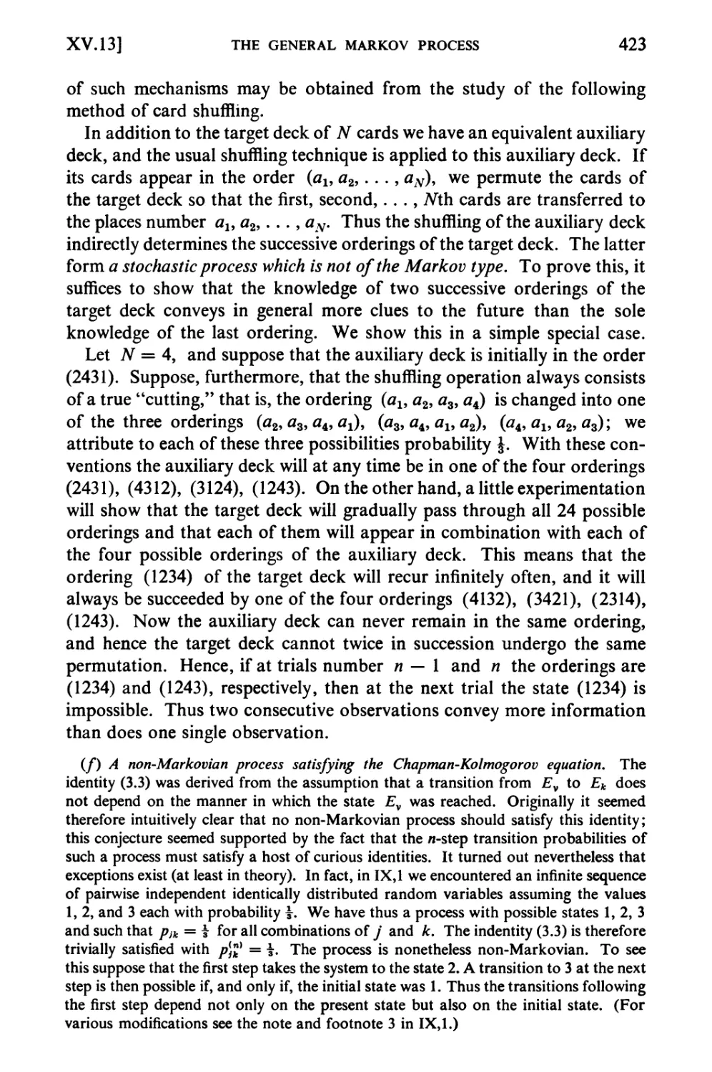
An Introduction
to Probability Theory
and Its Applications
WILLIAM FELLER (1906-1970)
Eugene Higgins Projessor of Mathematics
Princeton University
VOLUME I
THIRD EDITION
Revised Printing
John Wiley & Sons, Inc.
New York • London • Sydney

10 9876543
Copyright, 1950 by William Feller
Copyright © 1957, 1968 by John Wiley & Sons, Inc.
All Rights Reserved. This book or any part thereof
must not be reproduced in any form without the
written permission of the publisher.
Library of Congress Catalog Card Number: 68-11708
Printed in the United States of America

To
O. E. Neugebauer:
o et praesidium et duke decus meum

Preface to the Third Edition
WHEN THIS BOOK WAS FIRST CONCEIVED (MORE THAN 25 YEARS AGO)
few mathematicians outside the Soviet Union recognized probability as a
legitimate branch of mathematics. Applications were limited in scope,
and the treatment of individual problems often led to incredible
complications. Under these circumstances the book could not be written for
an existing audience, or to satisfy conscious needs. The hope was rather
to attract attention to little-known aspects of probability, to forge links
between various parts, to develop unified methods, and to point to
potential applications. Because of a growing interest in probability, the
book found unexpectedly many users outside mathematical disciplines.
Its widespread use was understandable as long as its point of view was
new and its material was not otherwise available. But the popularity
seems to persist even now, when the contents of most chapters are
available in specialized works streamlined for particular needs. For this reason
the character of the book remains unchanged in the new edition. I hope
that it will continue to serve a variety of needs and, in particular, that
it will continue to find readers who read it merely for enjoyment and
enlightenment.
Throughout the years I was the grateful recipient of many
communications from users, and these led to various improvements. Many sections
were rewritten to facilitate study. Reading is also improved by a better
typeface and the superior editing job by Mrs. H. McDougal: although
a professional editor she has preserved a feeling for the requirements of
readers and reason.
The greatest change is in chapter III. This chapter was introduced
only in the second edition, which was in fact motivated principally by
the unexpected discovery that its enticing material could be treated by
elementary methods. But this treatment still depended on combinatorial
artifices which have now been replaced by simpler and more natural
probabilistic arguments. In essence this chapter is new.
Most conspicuous among other additions are the new sections on
branching processes, on Markov chains, and on the De Moivre-Laplace
theorem. Chapter XIII has been rearranged, and throughout the book
Vll

viii
PREFACE TO THE THIRD EDITION
there appear minor changes as well as new examples and problems.
I regret the misleading nature of the author index, but I felt obliged to
state explicitly whenever an idea or example could be traced to a particular
source. Unfortunately this means that quotations usually refer to an
incidental remark, and are rarely indicative of the nature of the paper
quoted. Furthermore, many examples and problems were inspired by
reading non-mathematical papers in which related situations are dealt
with by different methods. (That newer texts now quote these
non-mathematical papers as containing my examples shows how fast probability
has developed, but also indicates the limited usefulness of quotations.)
Lack of space as well as of competence precluded more adequate
historical indications of how probability has changed from the semi-
mysterious discussions of the 'twenties to its present flourishing state.
For a number of years I have been privileged to work with students
and younger colleagues to whose help and inspiration I owe much.
Much credit for this is due to the support by the U.S. Army Research
Office for work in probability at Princeton University. My particular
thanks are due to Jay Goldman for a thoughtful memorandum about his
teaching experiences, and to Loren Pitt for devoted help with the proofs.
William Feller
July, 1967

Preface to the First Edition
IT WAS THE AUTHOR'S ORIGINAL INTENTION TO WRITE A BOOK ON
analytical methods in probability theory in which the latter was to be
treated as a topic in pure mathematics. Such a treatment would have
been more uniform and hence more satisfactory from an aesthetic point
of view; it would also have been more appealing to pure mathematicians.
However, the generous support by the Office of Naval Research of work
in probability theory at Cornell University led the author to a more
ambitious and less thankful undertaking of satisfying heterogeneous needs.
It is the purpose of this book to treat probability theory as a self-
contained mathematical subject rigorously, avoiding non-mathematical
concepts. At the same time, the book tries to describe the empirical
background and to develop a feeling for the great variety of practical
applications. This purpose is served by many special problems, numerical
estimates, and examples which interrupt the main flow of the text. They
are clearly set apart in print and are treated in a more picturesque language
and with less formality. A number of special topics have been included
in order to exhibit the power of general methods and to increase the
usefulness of the book to specialists in various fields. To facilitate reading,
detours from the main path are indicated by stars. The knowledge of
starred sections is not assumed in the remainder.
A serious attempt has been made to unify methods. The specialist
will find many simplifications of existing proofs and also new results.
In particular, the theory of recurrent events has been developed for the
purpose of this book. It leads to a new treatment of Markov chains
which permits simplification even in the finite case.
The examples are accompanied by about 340 problems mostly with
complete solutions. Some of them are simple exercises, but most of
them serve as additional illustrative material to the text or contain various
complements. One purpose of the examples and problems is to develop
the reader's intuition and art of probabilistic formulation. Several
previously treated examples show that apparently difficult problems may
become almost trite once they are formulated in a natural way and put
into the proper context.
IX

X
PREFACE TO THE FIRST EDITION
There is a tendency in teaching to reduce probability problems to pure
analysis as soon as possible and to forget the specific characteristics of
probability theory itself. Such treatments are based on a poorly defined
notion of random variables usually introduced at the outset. This book
goes to the other extreme and dwells on the notion of sample space,
without which random variables remain an artifice.
In order to present the true background unhampered by measurability
questions and other purely analytic difficulties this volume is restricted
to discrete sample spaces. This restriction is severe, but should be welcome
to non-mathematical users. It permits the inclusion of special topics
which are not easily accessible in the literature. At the same time, this
arrangement makes it possible to begin in an elementary way and yet to
include a fairly exhaustive treatment of such advanced topics as random
walks and Markov chains. The general theory of random variables and
their distributions, limit theorems, diffusion theory, etc., is deferred to a
succeeding volume.
This book would not have been written without the support of the
Office of Naval Research. One consequence of this support was a fairly
regular personal contact with J. L. Doob, whose constant criticism and
encouragement were invaluable. To him go my foremost thanks. The
next thanks for help are due to John Riordan, who followed the
manuscript through two versions. Numerous corrections and improvements
were suggested by my wife who read both the manuscript and proof.
The author is also indebted to K. L. Chung, M. Donsker, and S.
Goldberg, who read the manuscript and corrected various mistakes;
the solutions to the majority of the problems were prepared by S. Goldberg.
Finally, thanks are due to Kathryn Hollenbach for patient and expert
typing help; to E. Elyash, W. Hoffman, and J. R. Kinney for help in
proofreading.
William Feller
Cornell University
January 1950

Note on the Use of the Book
THE EXPOSITION CONTAINS MANY SIDE EXCURSIONS AND DOES NOT ALWAYS
progress from the easy to the difficult; comparatively technical sections
appear at the beginning and easy sections in chapters XV and XVII.
Inexperienced readers should not attempt to follow many side lines, lest
they lose sight of the forest for too many trees. Introductory remarks
to the chapters and stars at the beginnings of sections should facilitate
orientation and the choice of omissions. The unstarred sections form a
self-contained whole in which the starred sections are not used.
A first introduction to the basic notions of probability is contained in
chapters I, V, VI, IX; beginners should cover these with as few digressions
as possible. Chapter II is designed to develop the student's technique
and probabilistic intuition; some experience in its contents is desirable,
but it is not necessary to cover the chapter systematically: it may prove
more profitable to return to the elementary illustrations as occasion arises
at later stages. For the purposes of a first introduction, the elementary
theory of continuous distributions requires little supplementary
explanation. (The elementary chapters of volume 2 now provide a suitable
text.)
From chapter IX an introductory course may proceed directly to
chapter XI, considering generating functions as an example of more
general transforms. Chapter XI should be followed by some applications
in chapters XIII (recurrent events) or XII (chain reactions, infinitely
divisible distributions). Without generating functions it is possible to
turn in one of the following directions: limit theorems and fluctuation
theory (chapters VIII, X, III); stochastic processes (chapter XVII);
random walks (chapter III and the main part of XIV). These chapters
are almost independent of each other. The Markov chains of chapter
XV depend conceptually on recurrent events, but they may be studied
independently if the reader is willing to accept without proof the basic
ergodic theorem.
Chapter III stands by itself. Its contents are appealing in their own
right, but the chapter is also highly illustrative for new insights and new
methods in probability theory. The results concerning fluctuations in
XI

xii
NOTE ON THE USE OF THE BOOK
coin tossing show that widely held beliefs about the law of large numbers
are fallacious. They are so amazing and so at variance with common
intuition that even sophisticated colleagues doubted that coins actually
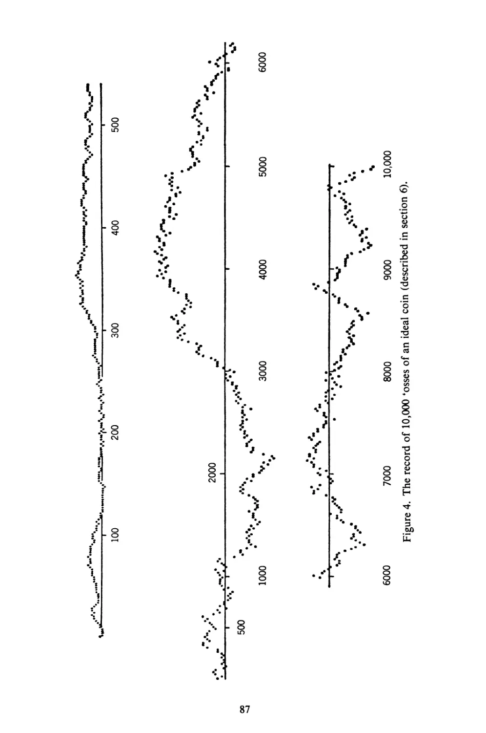
misbehave as theory predicts. The record of a simulated experiment is
therefore included in section 6. The chapter treats only the simple coin-
tossing game, but the results are representative of a fairly general situation.
The sign ► is used to indicate the end of a proof or of a collection of
examples.
It is hoped that the extensive index will facilitate coordination between
the several parts.

Contents
chapter Page
Introduction: The Nature of Probability Theory . 1
1. The Background 1
2. Procedure 3
3. "Statistical" Probability 4
4. Summary 5
5. Historical Note 6
I The Sample Space 7
1. The Empirical Background 7
2. Examples 9
3. The Sample Space. Events 13
4. Relations among Events 14
5. Discrete Sample Spaces 17
6. Probabilities in Discrete Sample Spaces: Preparations 19
7. The Basic Definitions and Rules 22
8. Problems for Solution 24
II Elements of Combinatorial Analysis 26
1. Preliminaries 26
2. Ordered Samples 28
3. Examples 31
4. Subpopulations and Partitions 34
*5. Application to Occupancy Problems 38
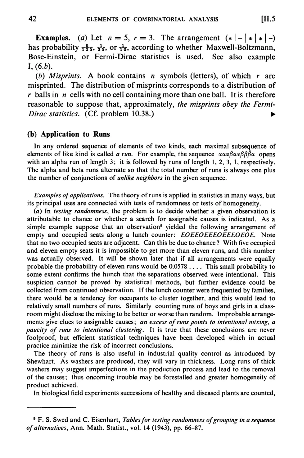
*5a. Bose-Einstein and Fermi-Dirac Statistics 40
*5b. Application to Runs 42
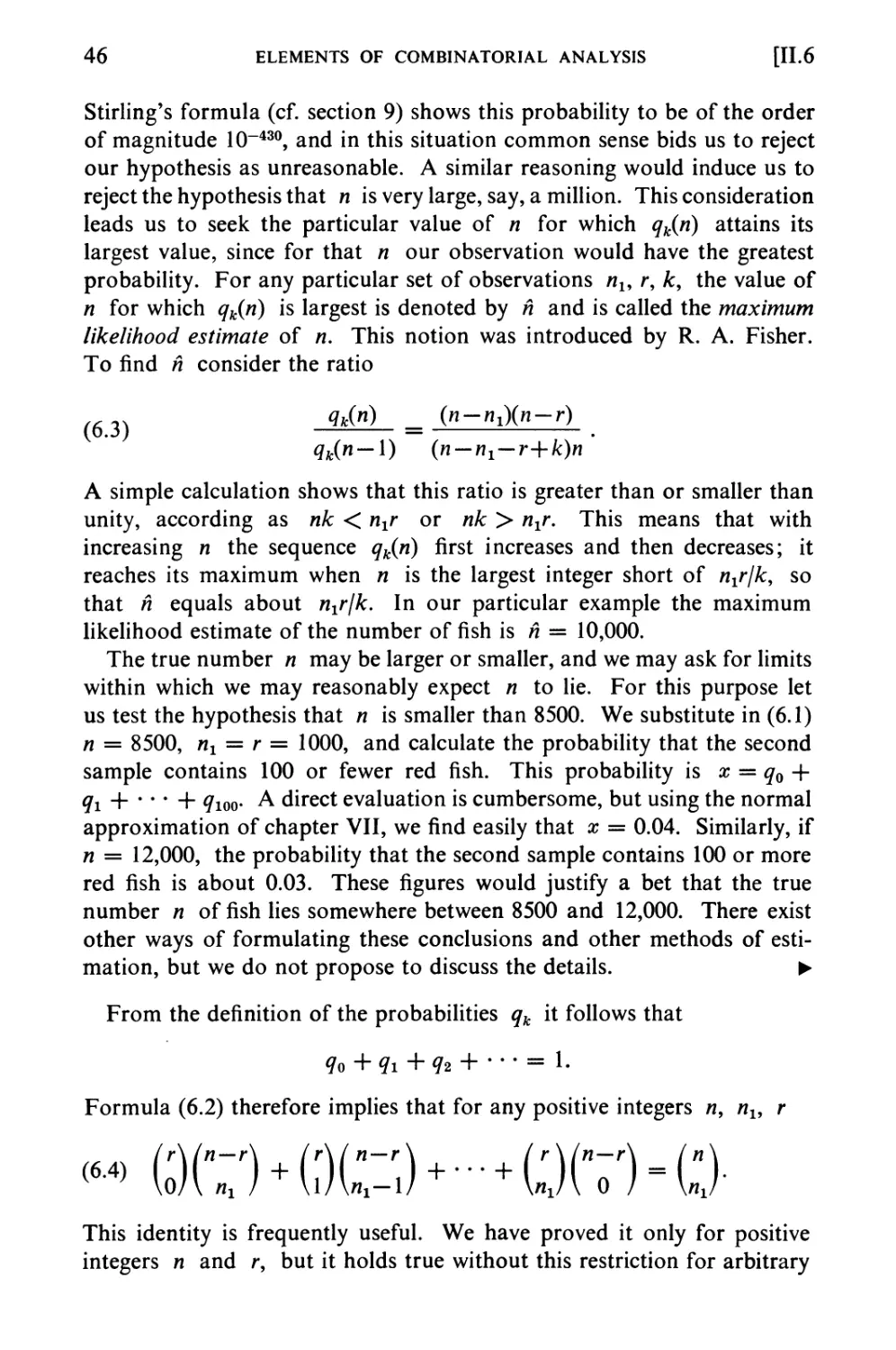
6. The Hypergeometric Distribution 43
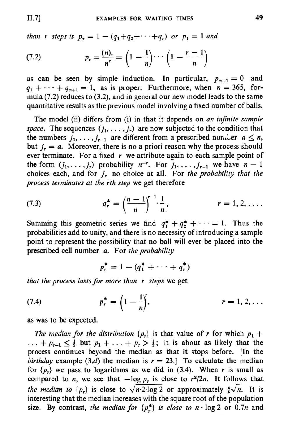
7. Examples for Waiting Times 47
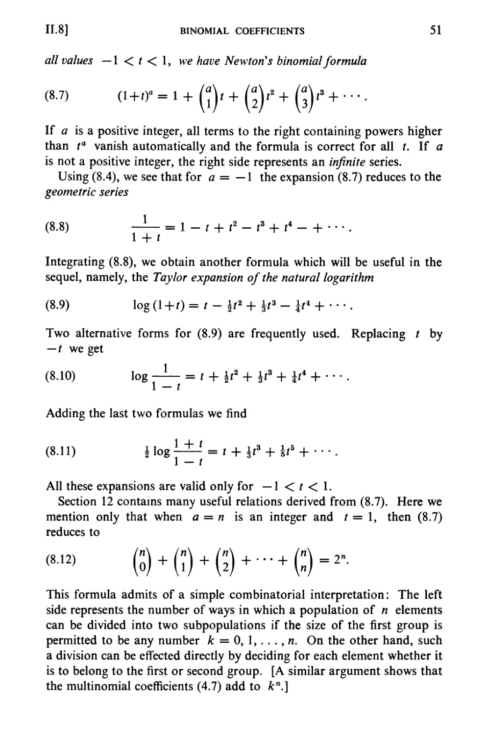
8. Binomial Coefficients 50
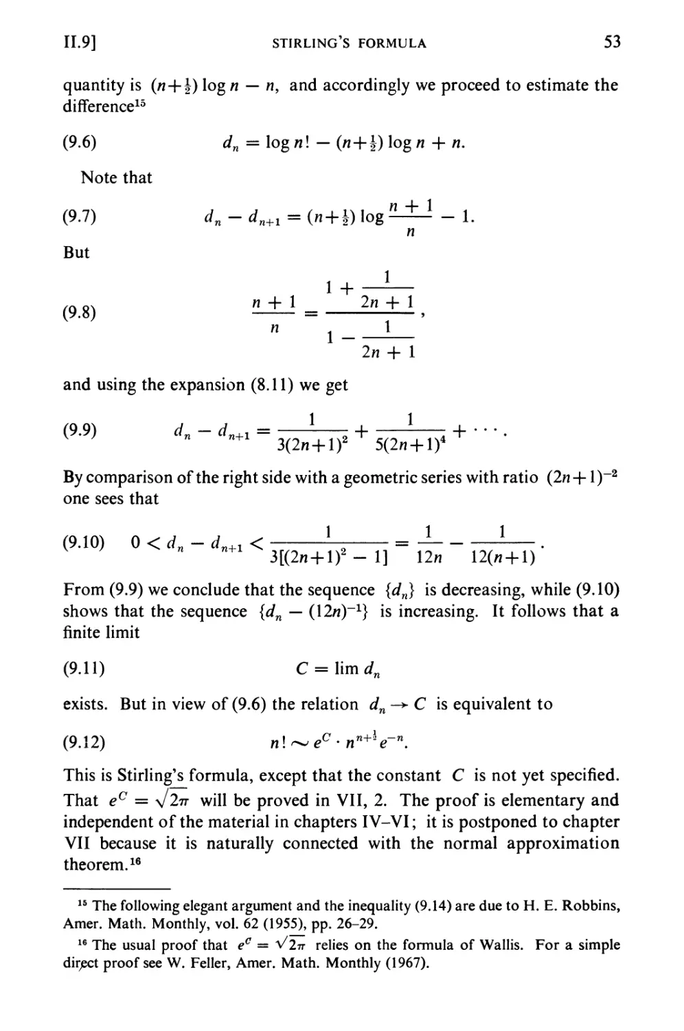
9. Stirling's Formula 52
Problems for Solution: 54
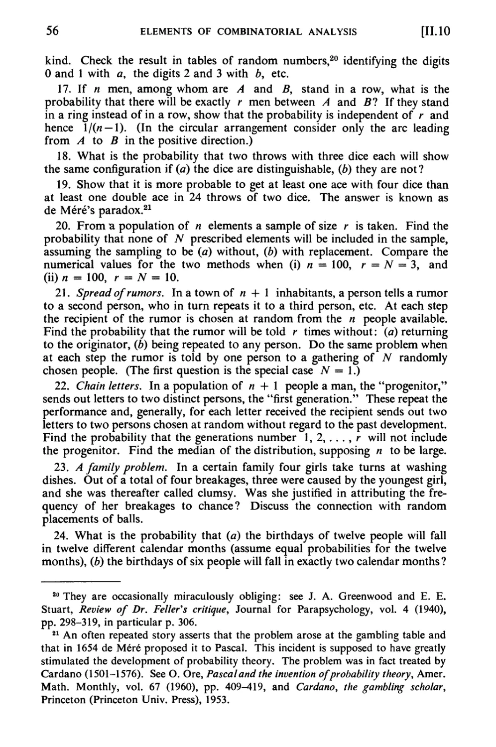
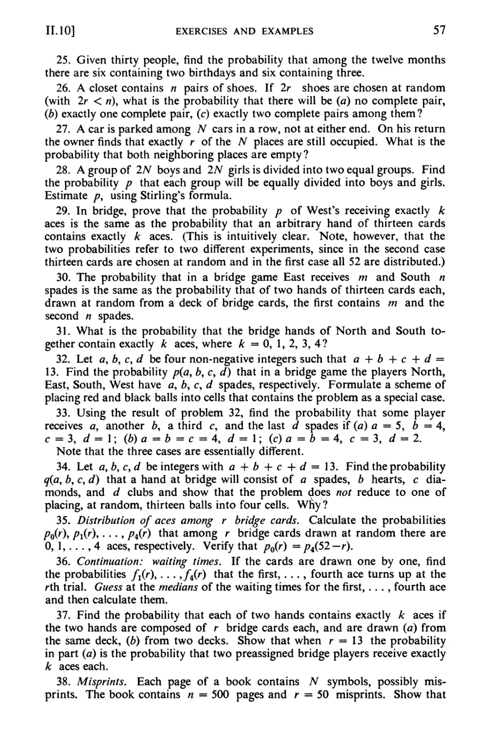
10. Exercises and Examples 54
* Starred sections are not required for the understanding of the sequel and should
be omitted at first reading.
xiii

xiv contents
chapter Page
11. Problems and Complements of a Theoretical
Character 58
12. Problems and Identities Involving Binomial
Coefficients 63
*III Fluctuations in Coin Tossing and Random Walks . 67
1. General Orientation. The Reflection Principle ... 68
2. Random Walks: Basic Notions and Notations ... 73
3. The Main Lemma 76
4. Last Visits and Long Leads 78
*5. Changes of Sign 84
6. An Experimental Illustration 86
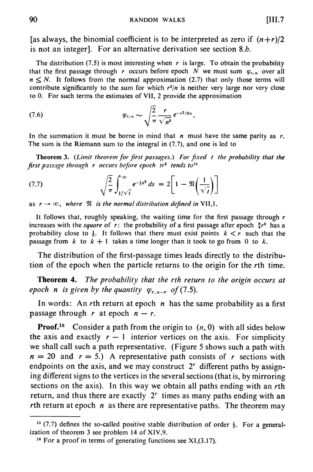
7. Maxima and First Passages 88
8. Duality. Position of Maxima 91
9. An Equidistribution Theorem 94
10. Problems for Solution 95
*IV Combination of Events 98
1. Union of Events 98
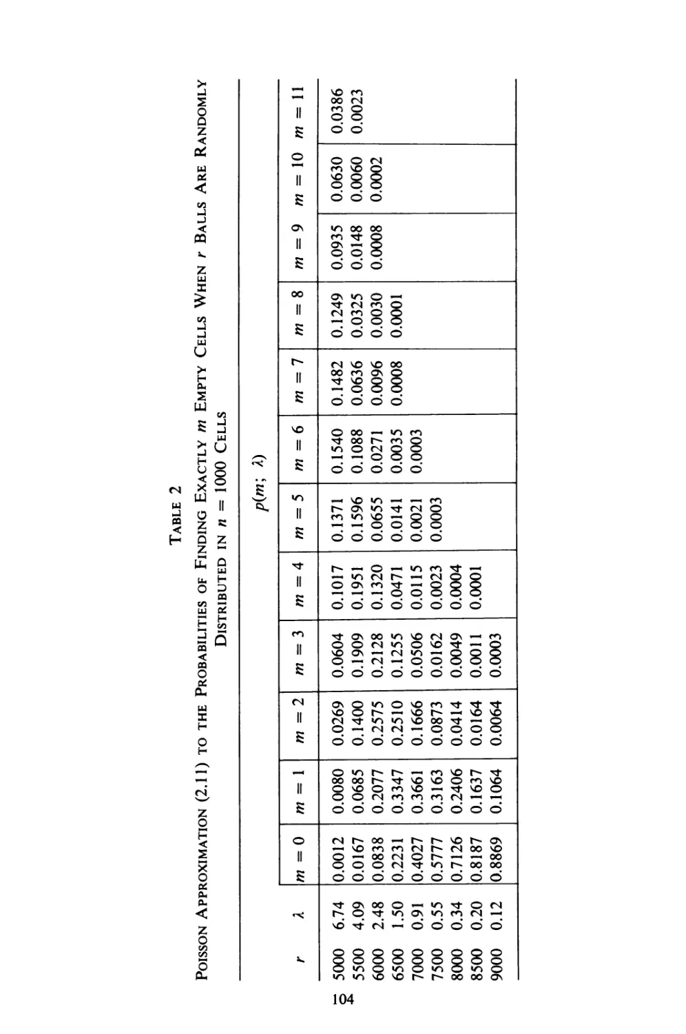
2. Application to the Classical Occupancy Problem . . 101
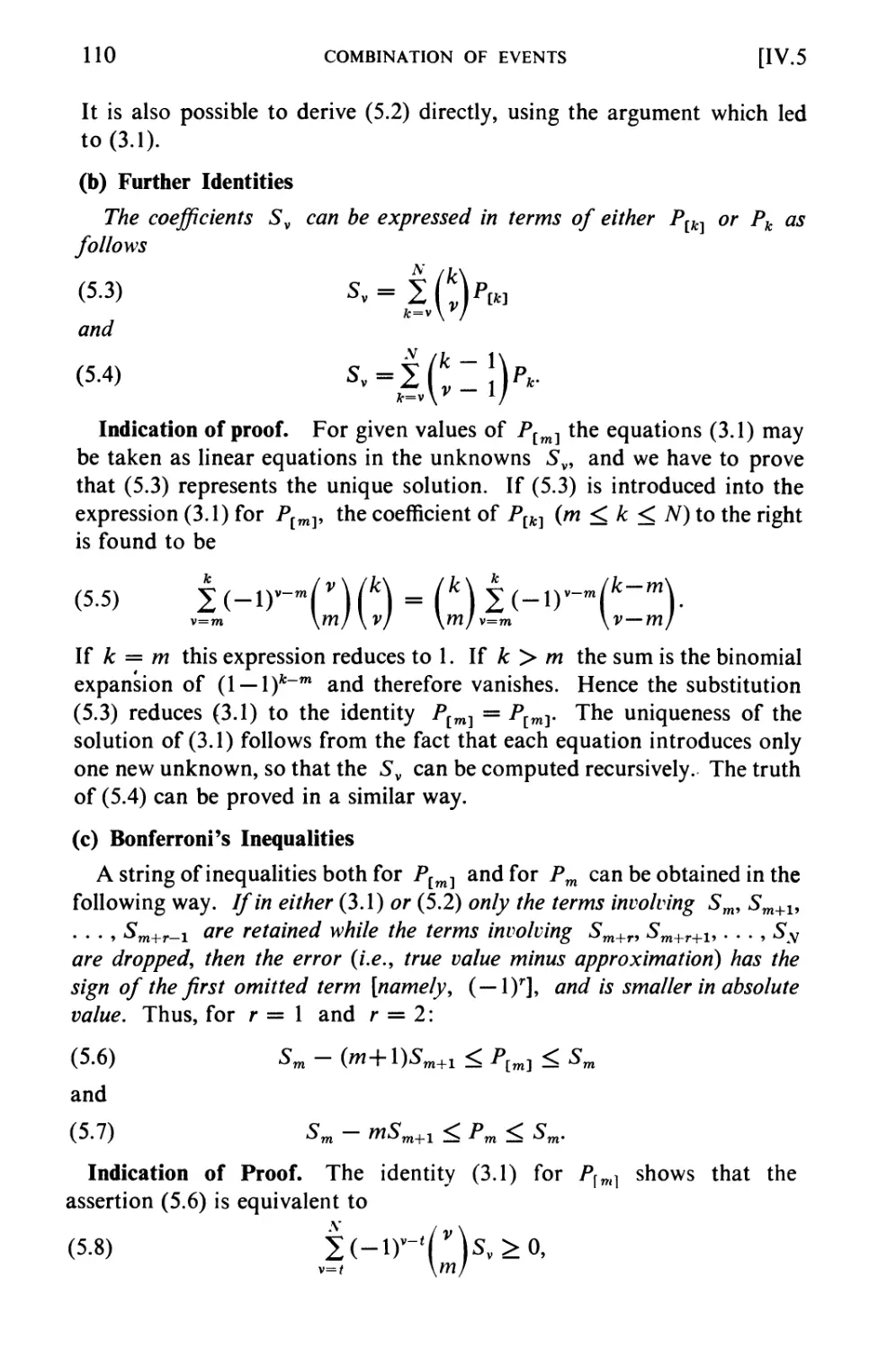
3. The Realization of m among N events 106
4. Application to Matching and Guessing 107
5. Miscellany 109
6. Problems for Solution Ill
V Conditional Probability. Stochastic Independence . 114
1. Conditional Probability 114
2. Probabilities Defined by Conditional Probabilities.
Urn Models 118
3. Stochastic Independence 125
4. Product Spaces. Independent Trials 128
*5. Applications to Genetics 132
*6. Sex-Linked Characters 136
*7. Selection 139
8. Problems for Solution 140
VI The Binomial and the Poisson Distributions .... 146
1. Bernoulli Trials 146
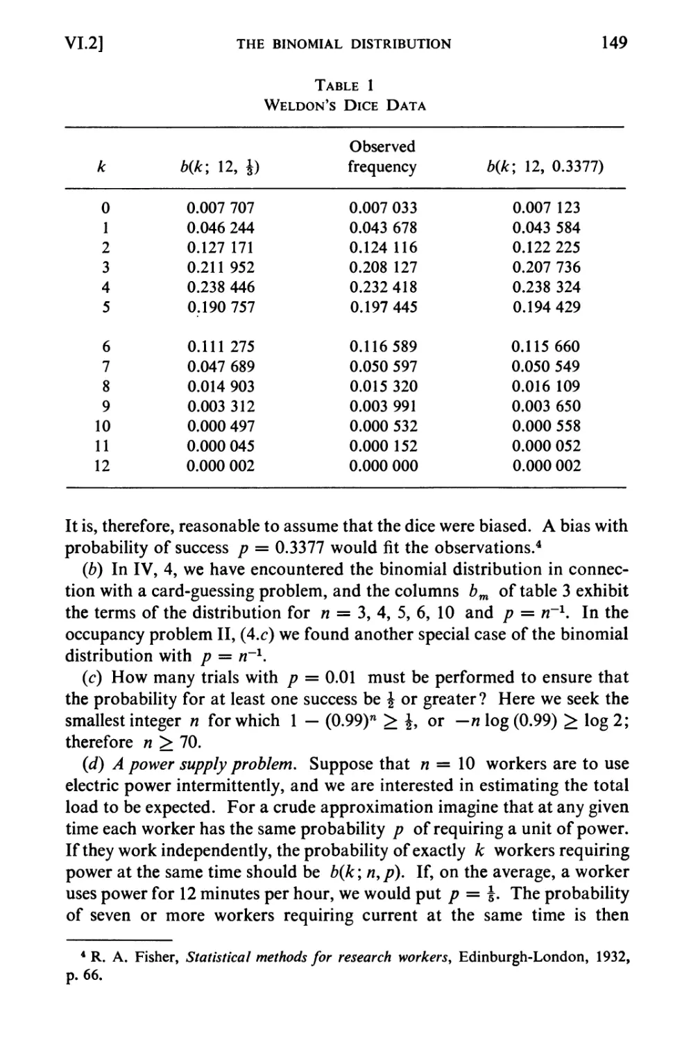
2. The Binomial Distribution 147
3. The Central Term and the Tails 150
4. The Law of Large Numbers 152

contents xv
chapter Page
5. The Poisson Approximation 153
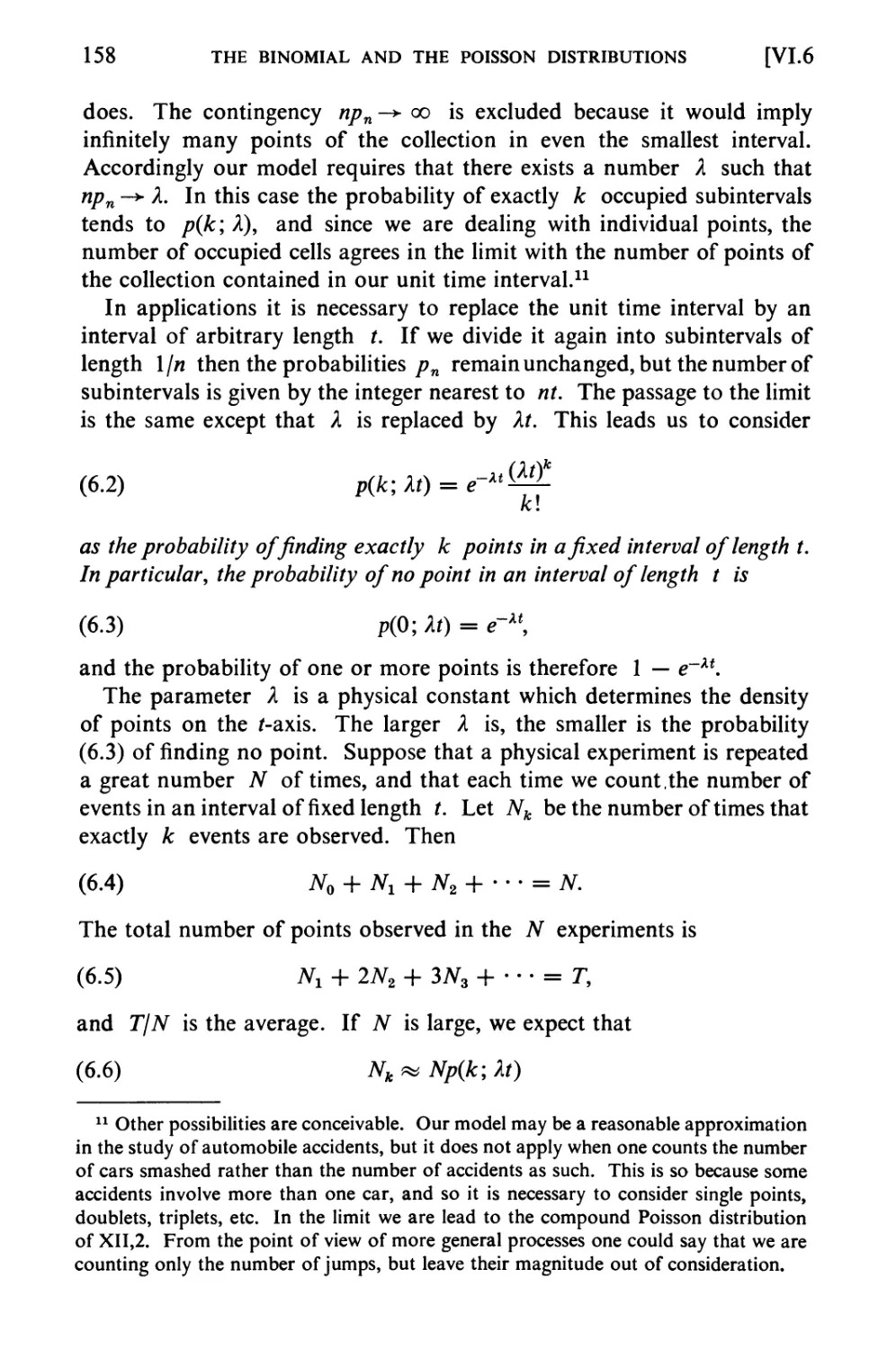
6. The Poisson Distribution 156
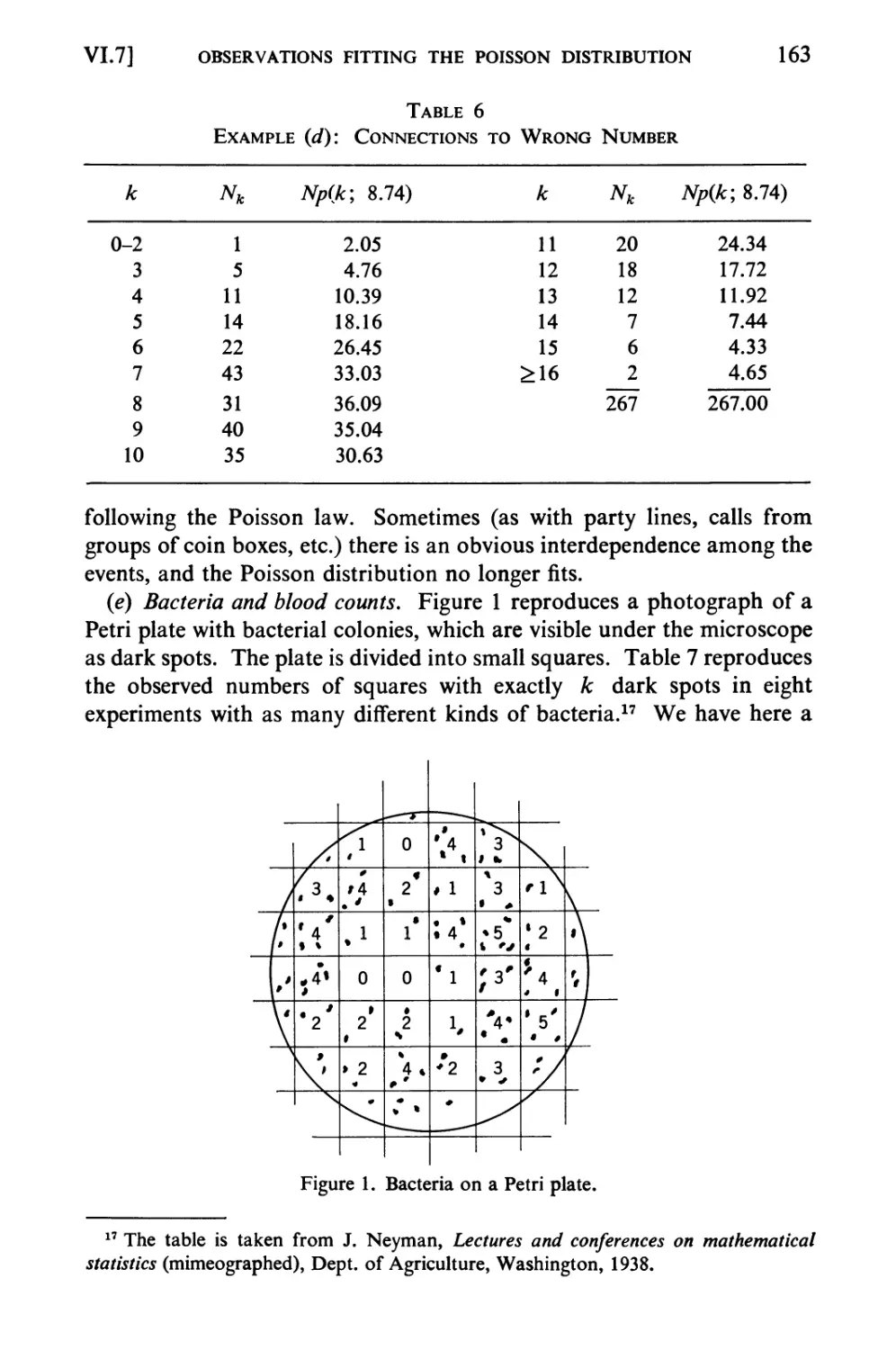
7. Observations Fitting the Poisson Distribution .... 159
8. Waiting Times. The Negative Binomial Distribution 164
9. The Multinomial Distribution 167
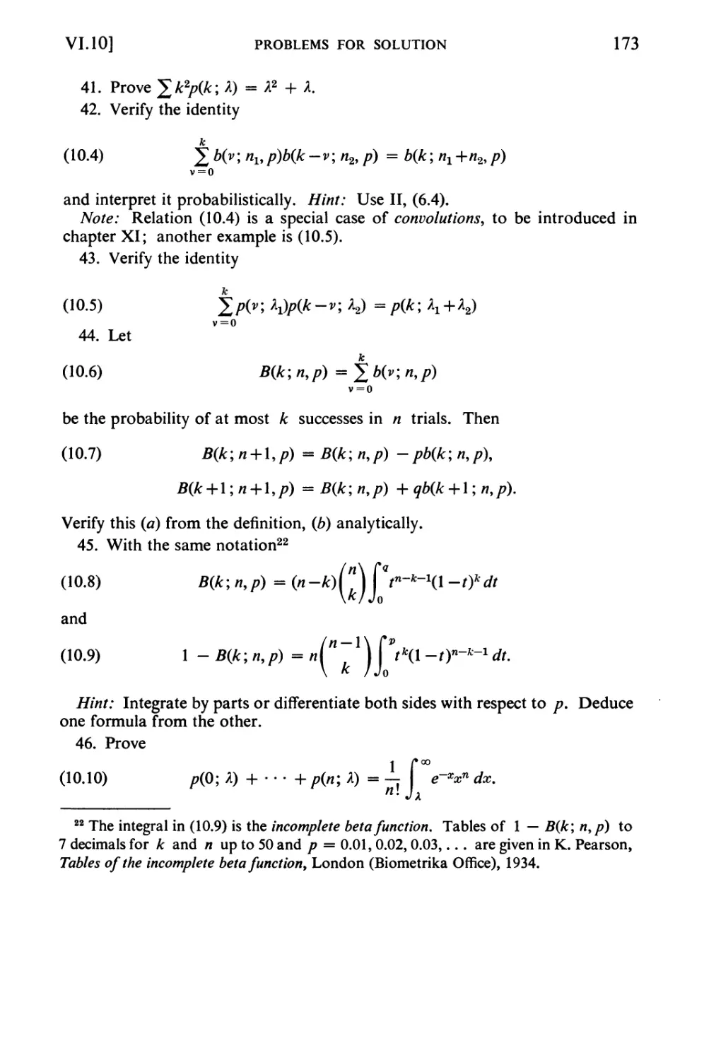
10. Problems for Solution 169
VII The Normal Approximation to the Binomial
Distribution 174
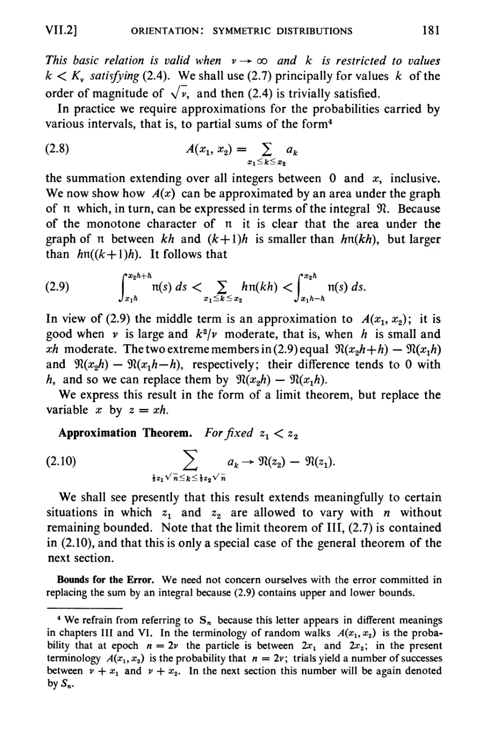
1. The Normal Distribution 174
2. Orientation: Symmetric Distributions 179
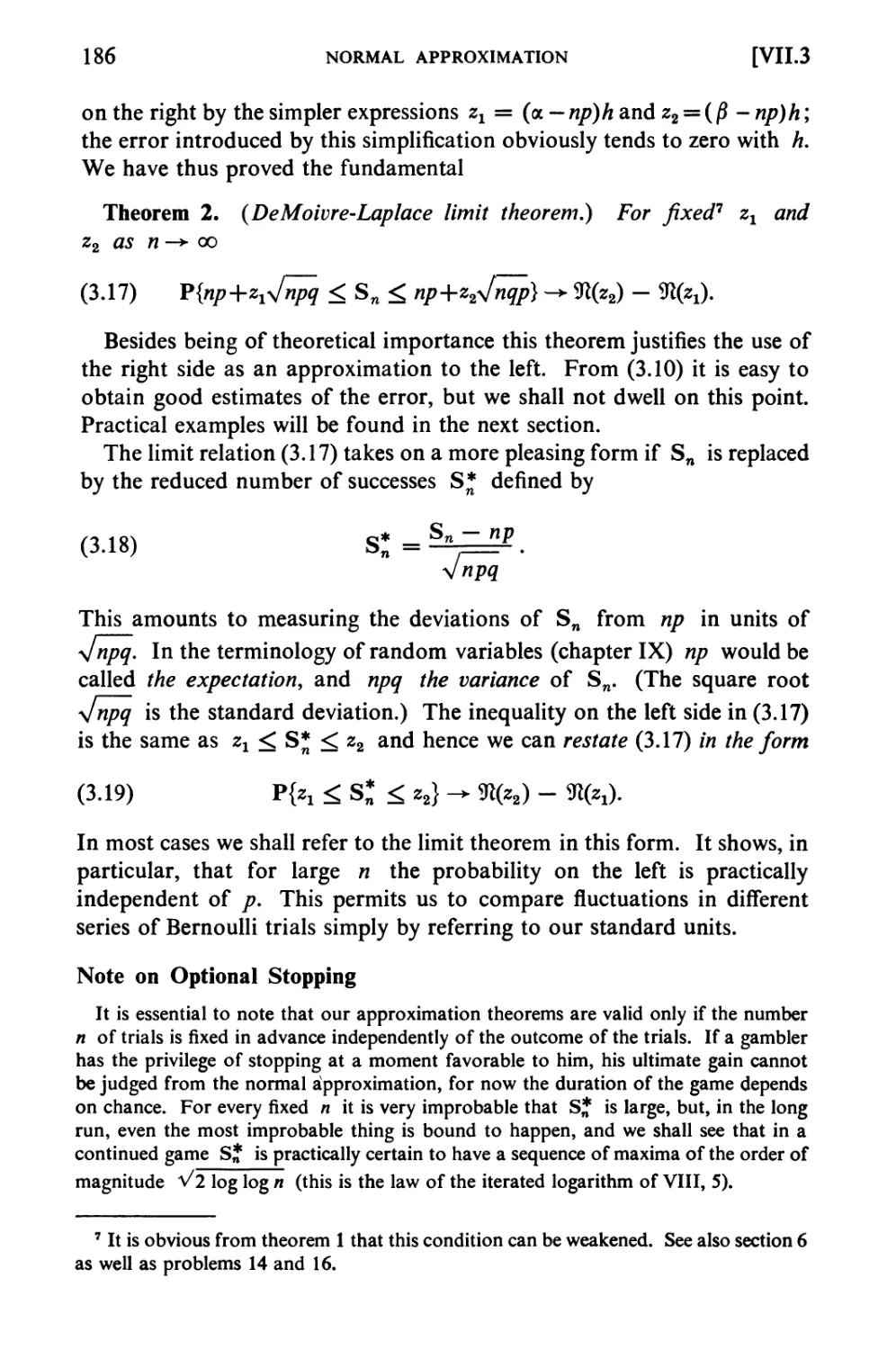
3. The DeMoivre-Laplace Limit Theorem 182
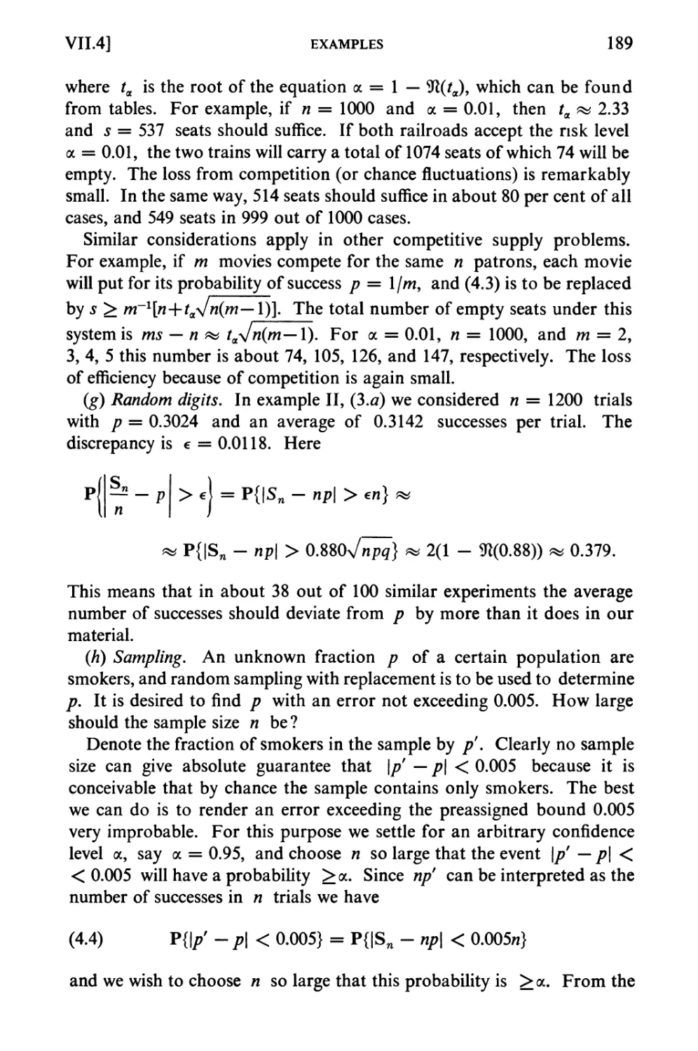
4. Examples 187
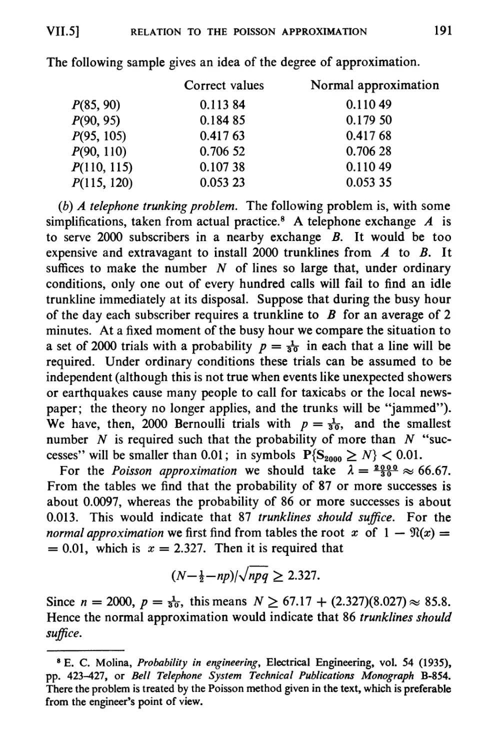
5. Relation to the Poisson Approximation 190
*6. Large Deviations 192
7. Problems for Solution 193
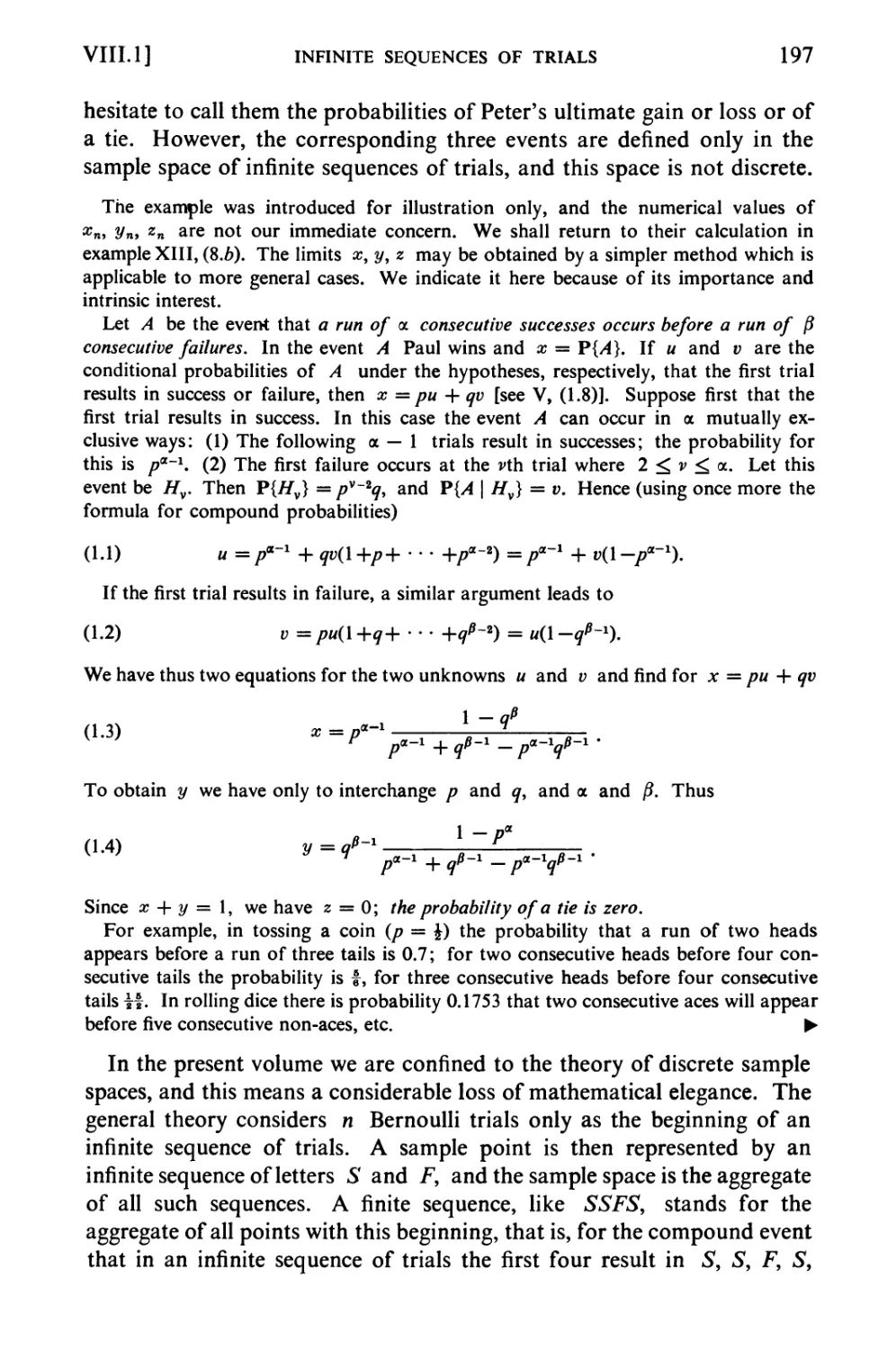
♦VIII Unlimited Sequences of Bernoulli Trials 196
1. Infinite Sequences of Trials 196
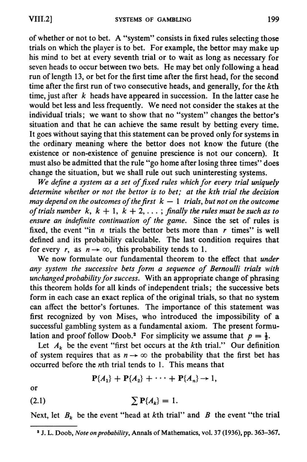
2. Systems of Gambling 198
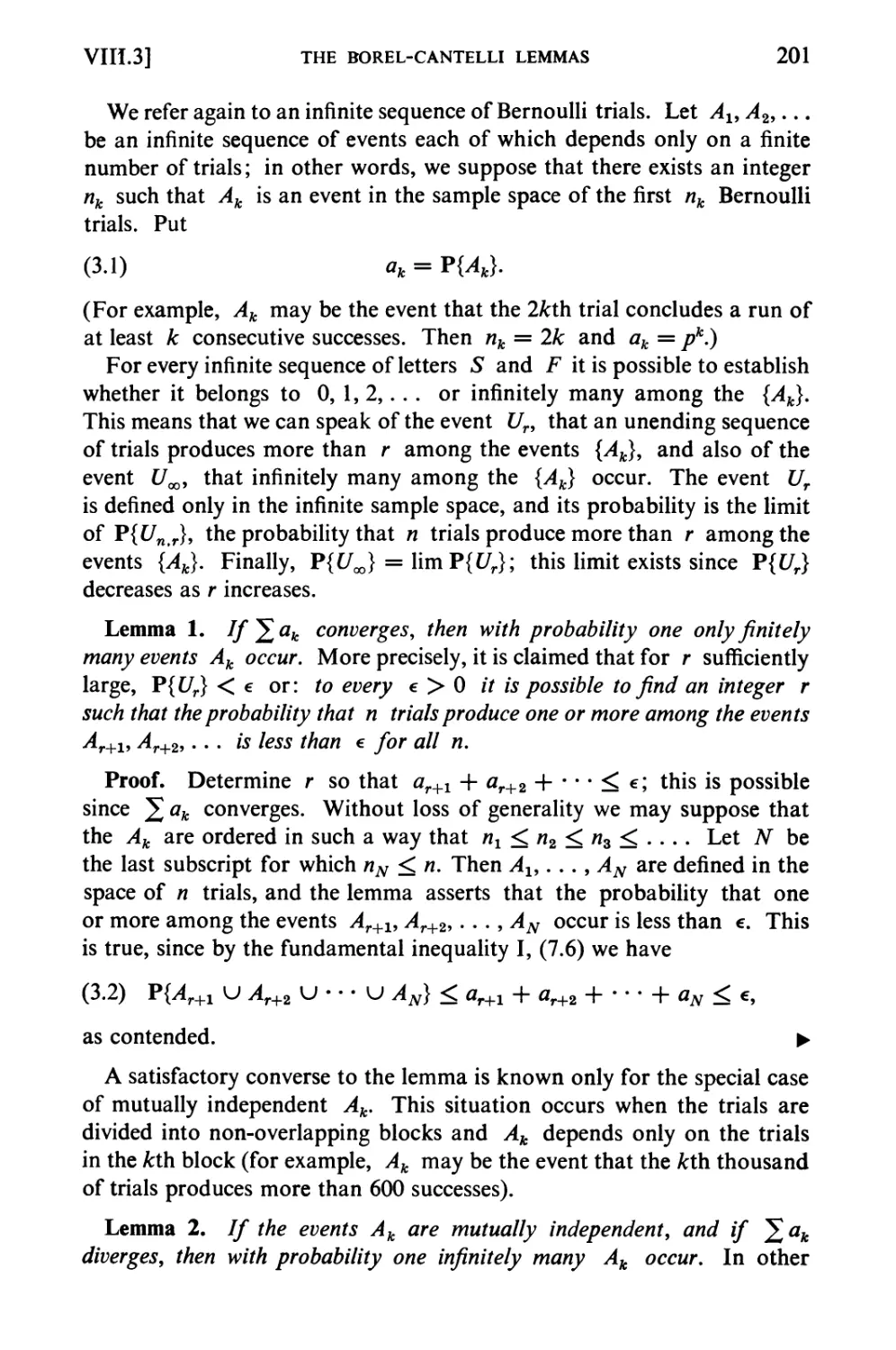
3. The Borel-Cantelli Lemmas 200
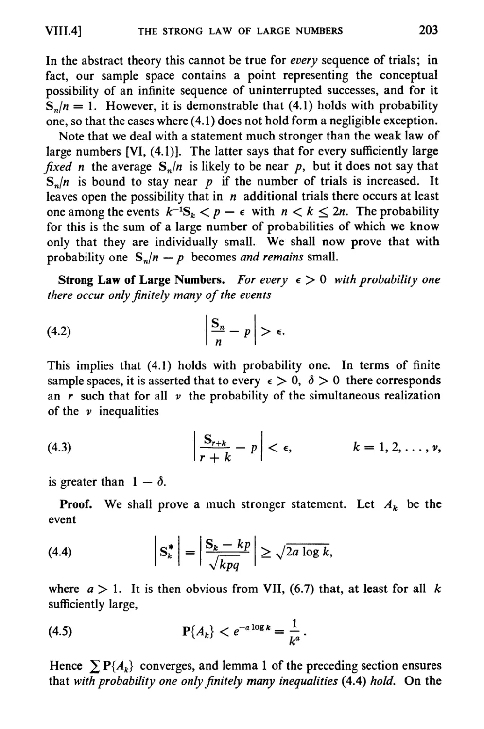
4. The Strong Law of Large Numbers 202
5. The Law of the Iterated Logarithm 204
6. Interpretation in Number Theory Language .... 208
7. Problems for Solution 210
IX Random Variables; Expectation 212
1. Random Variables 212
2. Expectations 220
3. Examples and Applications 223
4. The Variance 227
5. Co variance; Variance of a Sum 229
6. Chebyshev's Inequality 233
*7. Kolmogorov's Inequality 234
*8. The Correlation Coefficient 236
9. Problems for Solution 237
X Laws of Large Numbers 243
1. Identically Distributed Variables 243
*2. Proof of the Law of Large Numbers 246
3. The Theory of "Fair" Games 248

XVI
contents
chapter Page
*4. The Petersburg Game 251
5. Variable Distributions 253
*6. Applications to Combinatorial Analysis 256
*7. The Strong Law of Large Numbers 258
8. Problems for Solution 261
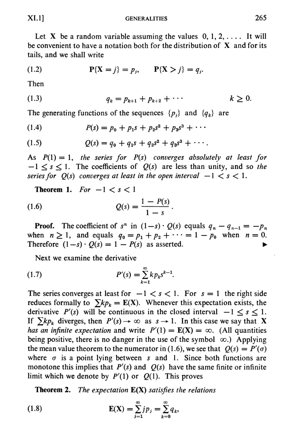
XI Integral Valued Variables. Generating Functions . 264
1. Generalities 264
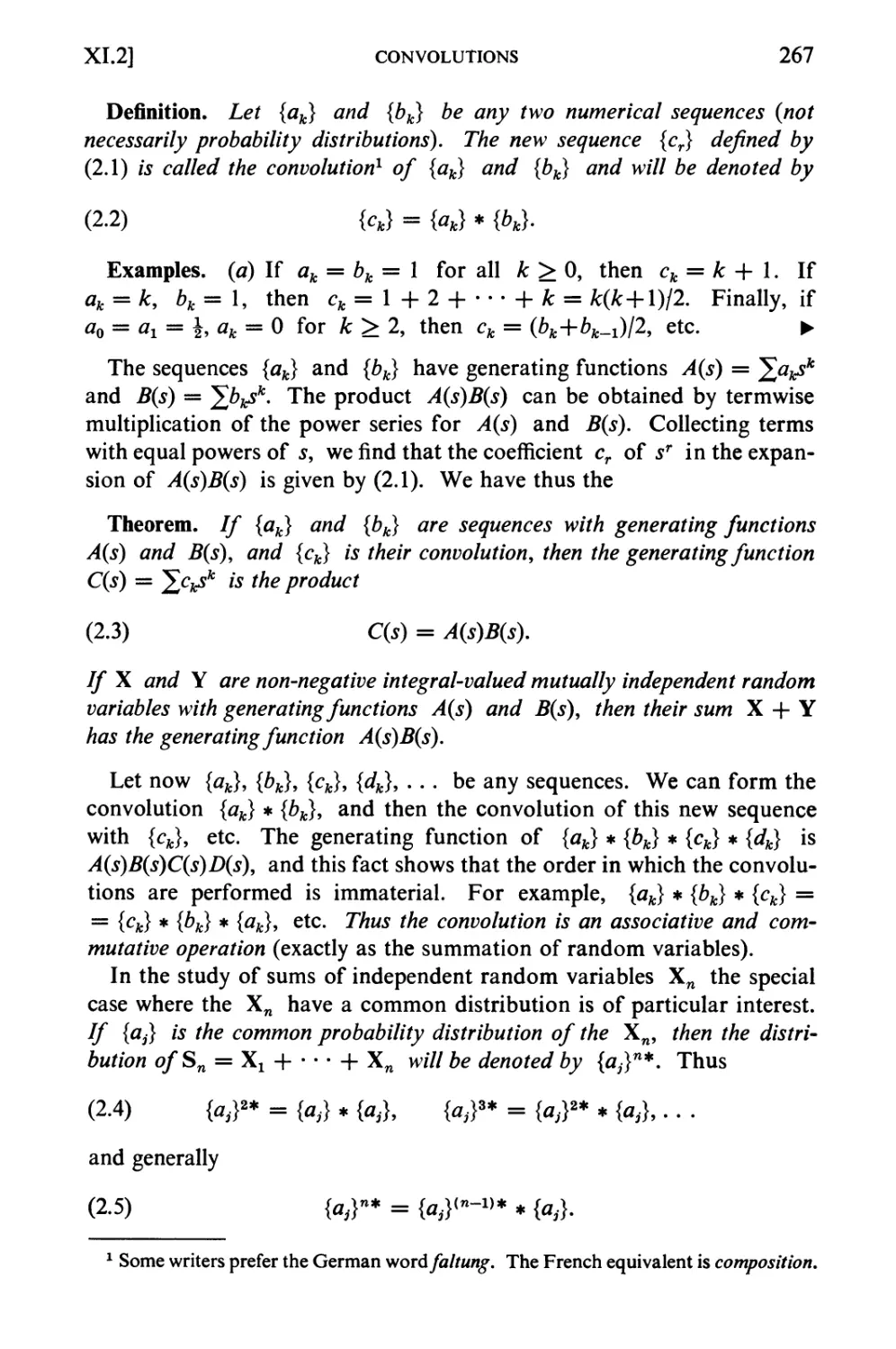
2. Convolutions 266
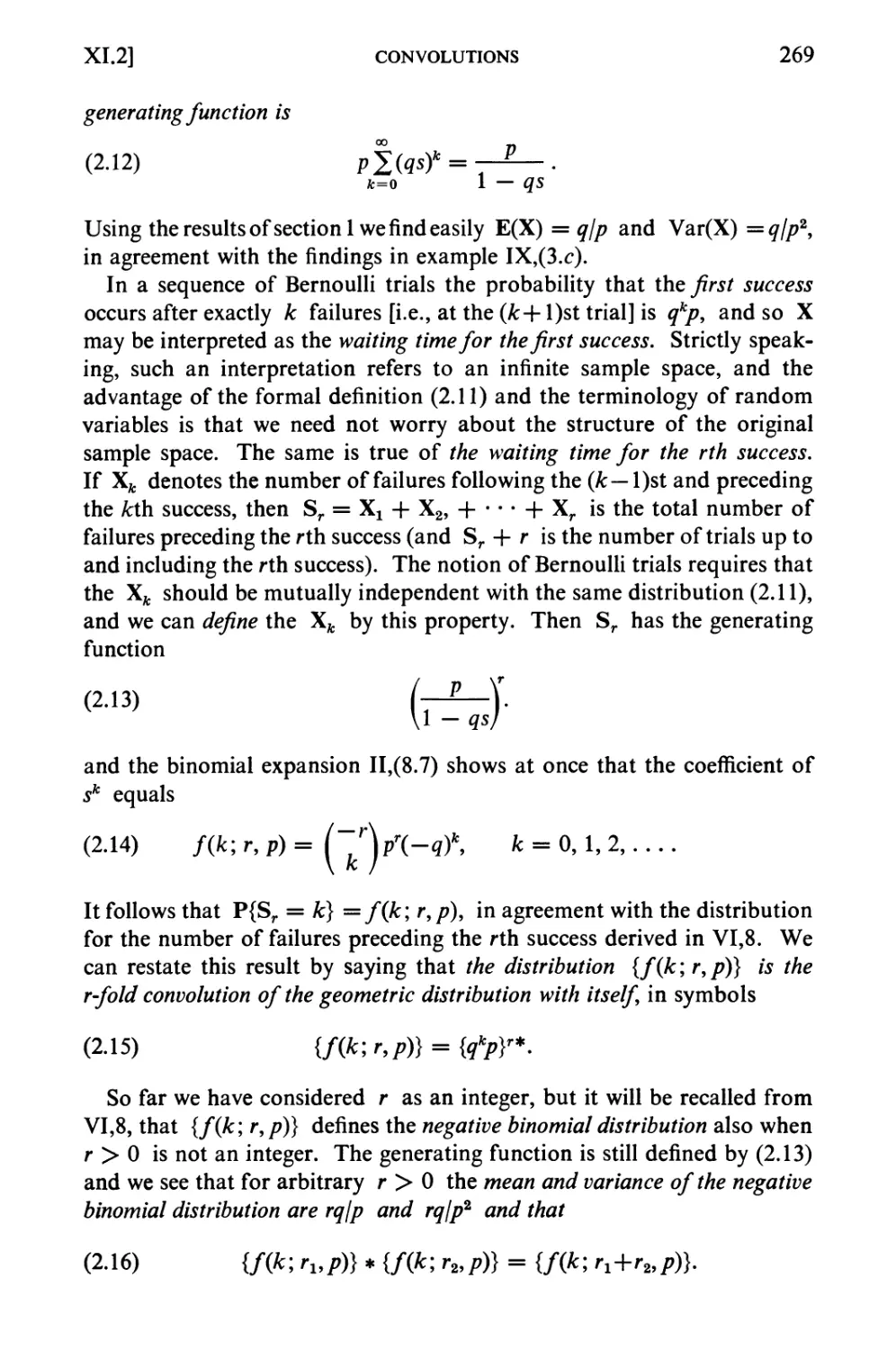
3. Equalizations and Waiting Times in Bernoulli Trials 270
4. Partial Fraction Expansions 275
5. Bivariate Generating Functions 279
*6. The Continuity Theorem 280
7. Problems for Solution 283
*XII Compound Distributions. Branching Processes . . . 286
1. Sums of a Random Number of Variables 286
2. The Compound Poisson Distribution 288
2a. Processes with Independent Increments 292
3. Examples for Branching Processes 293
4. Extinction Probabilities in Branching Processes . . . 295
5. The Total Progeny in Branching Processes 298
6. Problems for Solution 301
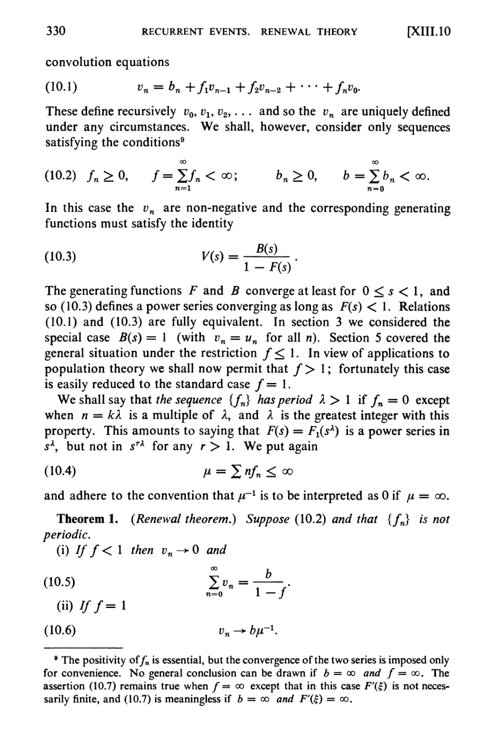
XIII Recurrent Events. Renewal Theory 303
1. Informal Preparations and Examples 303
2. Definitions 307
3. The Basic Relations 311
4. Examples 313
5. Delayed Recurrent Events. A General Limit Theorem 316
6. The Number of Occurrences of 8 320
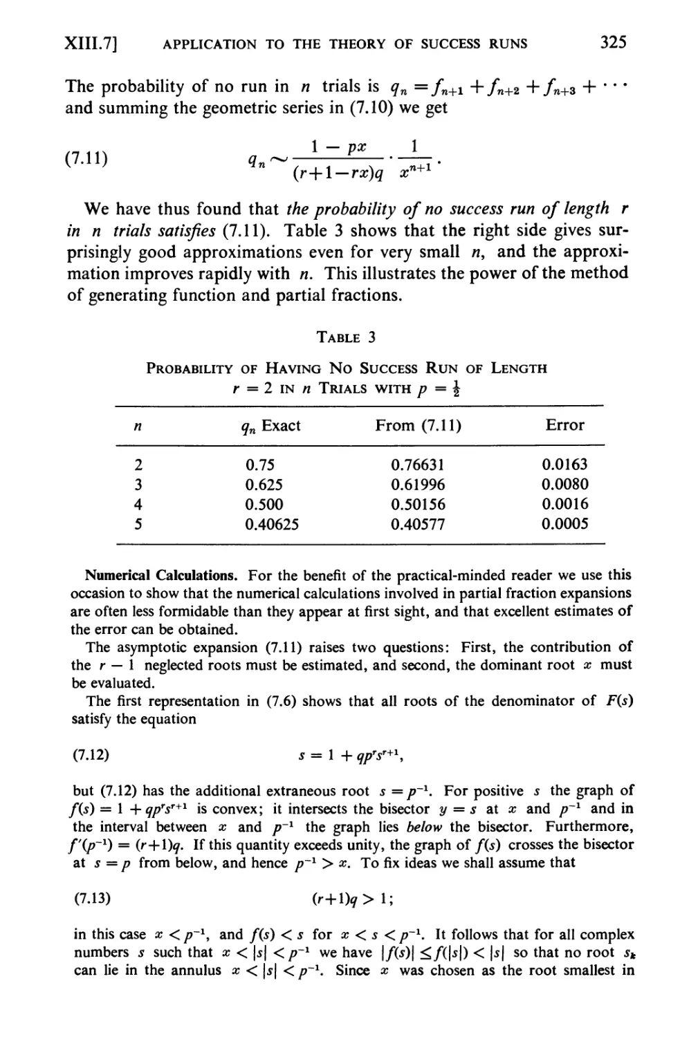
*7. Application to the Theory of Success Runs 322
*8. More General Patterns 326
9. Lack of Memory of Geometric Waiting Times . . . 328
10. Renewal Theory 329
*11. Proof of the Basic Limit Theorem 335
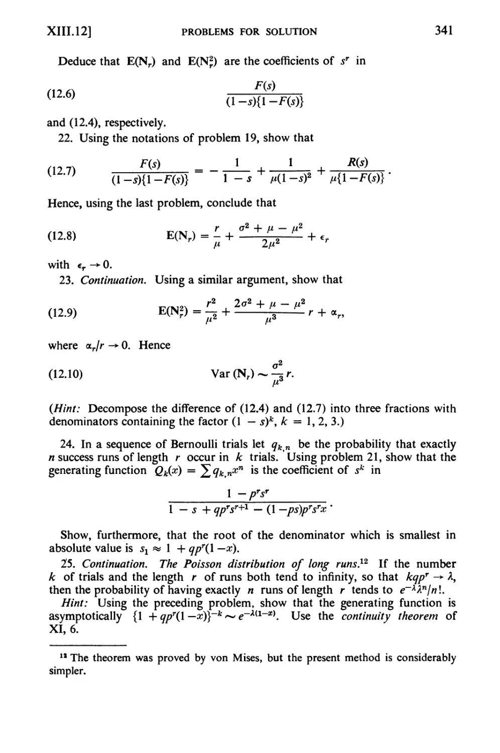
12. Problems for Solution 338
XIV Random Walk and Ruin Problems 342
1. General Orientation 342
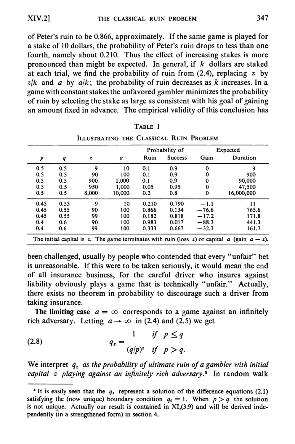
2. The Classical Ruin Problem 344

contents
xvii
chapter Page
3. Expected Duration of the Game 348
*4. Generating Functions for the Duration of the Game
and for the First-Passage Times 349
*5. Explicit Expressions 352
6. Connection with Diffusion Processes 354
*7. Random Walks in the Plane and Space 359
8. The Generalized One-Dimensional Random Walk
(Sequential Sampling) 363
9. Problems for Solution 367
XV Markov Chains 372
1. Definition 372
2. Illustrative Examples 375
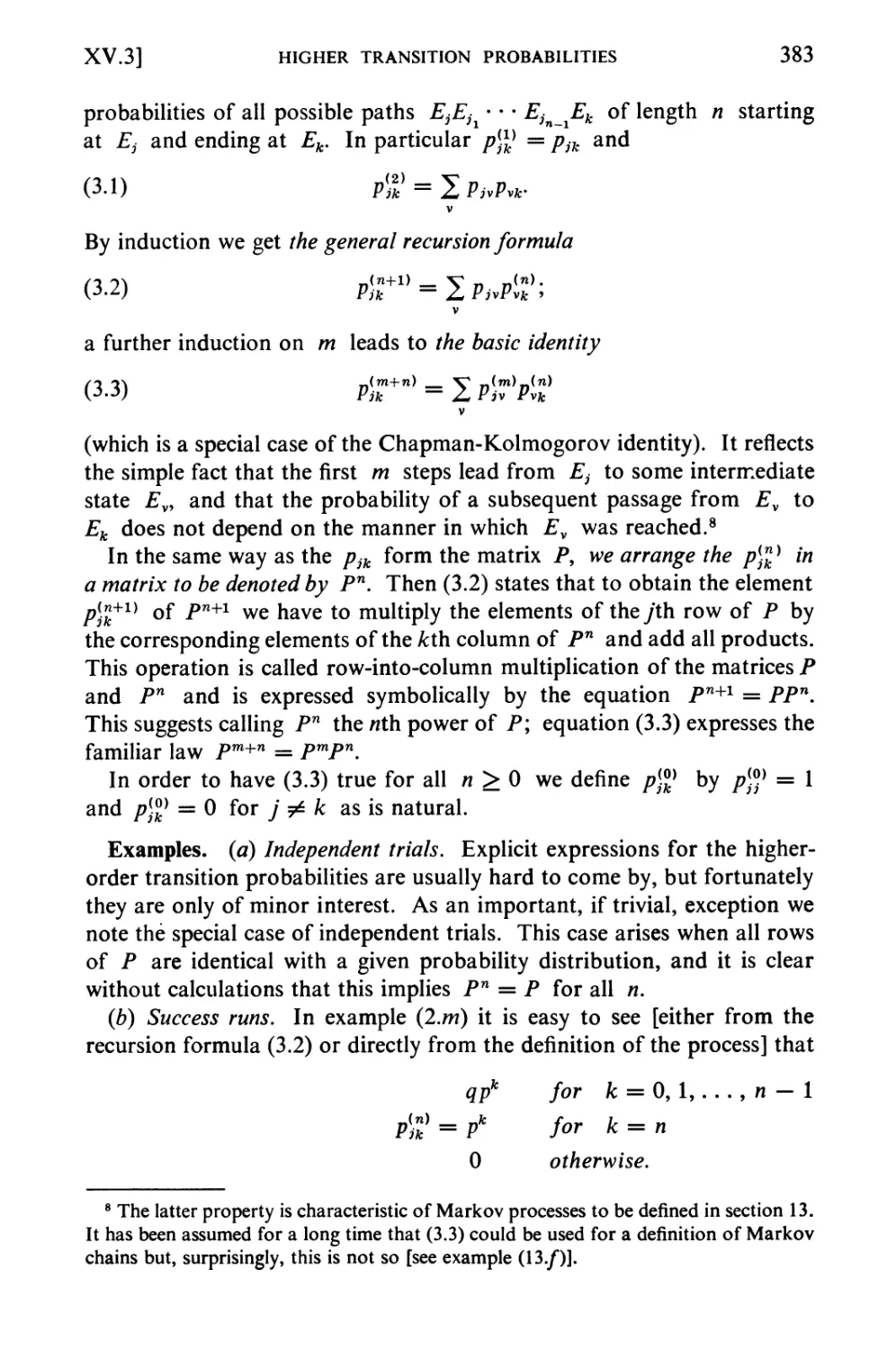
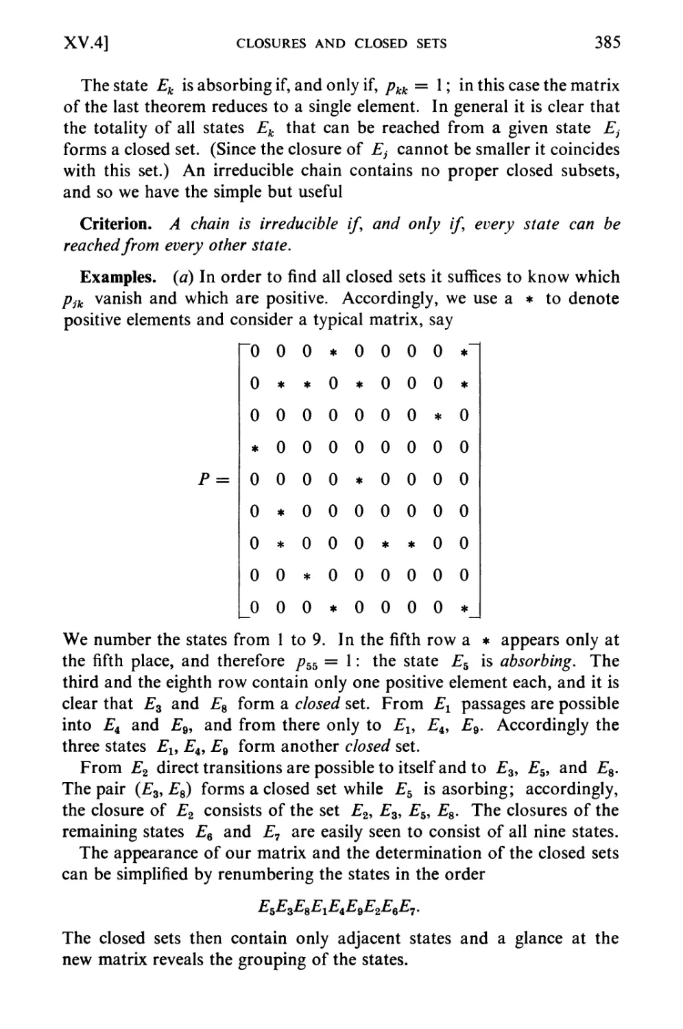
3. Higher Transition Probabilities 382
4. Closures and Closed Sets 384
5. Classification of States 387
6. Irreducible Chains. Decompositions 390
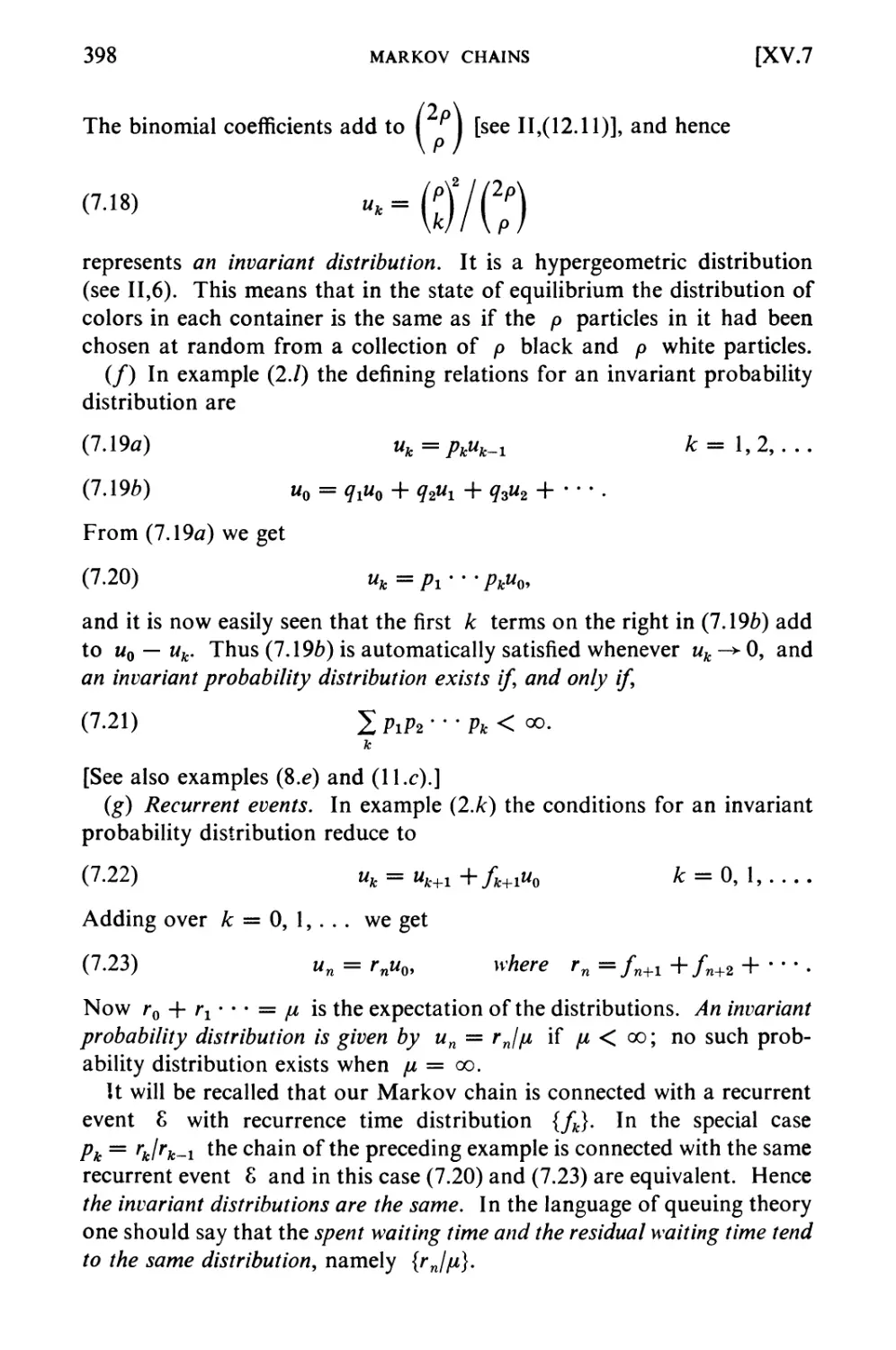
7. Invariant Distributions 392
8. Transient Chains 399
9. Periodic Chains 404
10. Application to Card Shuffling 406
*11. Invariant Measures. Ratio Limit Theorems .... 407
*12. Reversed Chains. Boundaries 414
13. The General Markov Process 419
14. Problems for Solution 424
*XVI Algebraic Treatment of Finite Markov Chains . . 428
1. General Theory 428
2. Examples 432
3. Random Walk with Reflecting Barriers 436
4. Transient States; Absorption Probabilities 438
5. Application to Recurrence Times 443
XVII The Simplest Time-Dependent Stochastic Processes . 444
1. General Orientation. Markov Processes 444
2. The Poisson Process 446
3. The Pure Birth Process 448
*4. Divergent Birth Processes 451
5. The Birth and Death Process 454
6. Exponential Holding Times 458

XV111
CONTENTS
chapter Page
7. Waiting Line and Servicing Problems 460
8. The Backward (Retrospective) Equations 468
9. General Processes 470
10. Problems for Solution 478
Answers to Problems 483
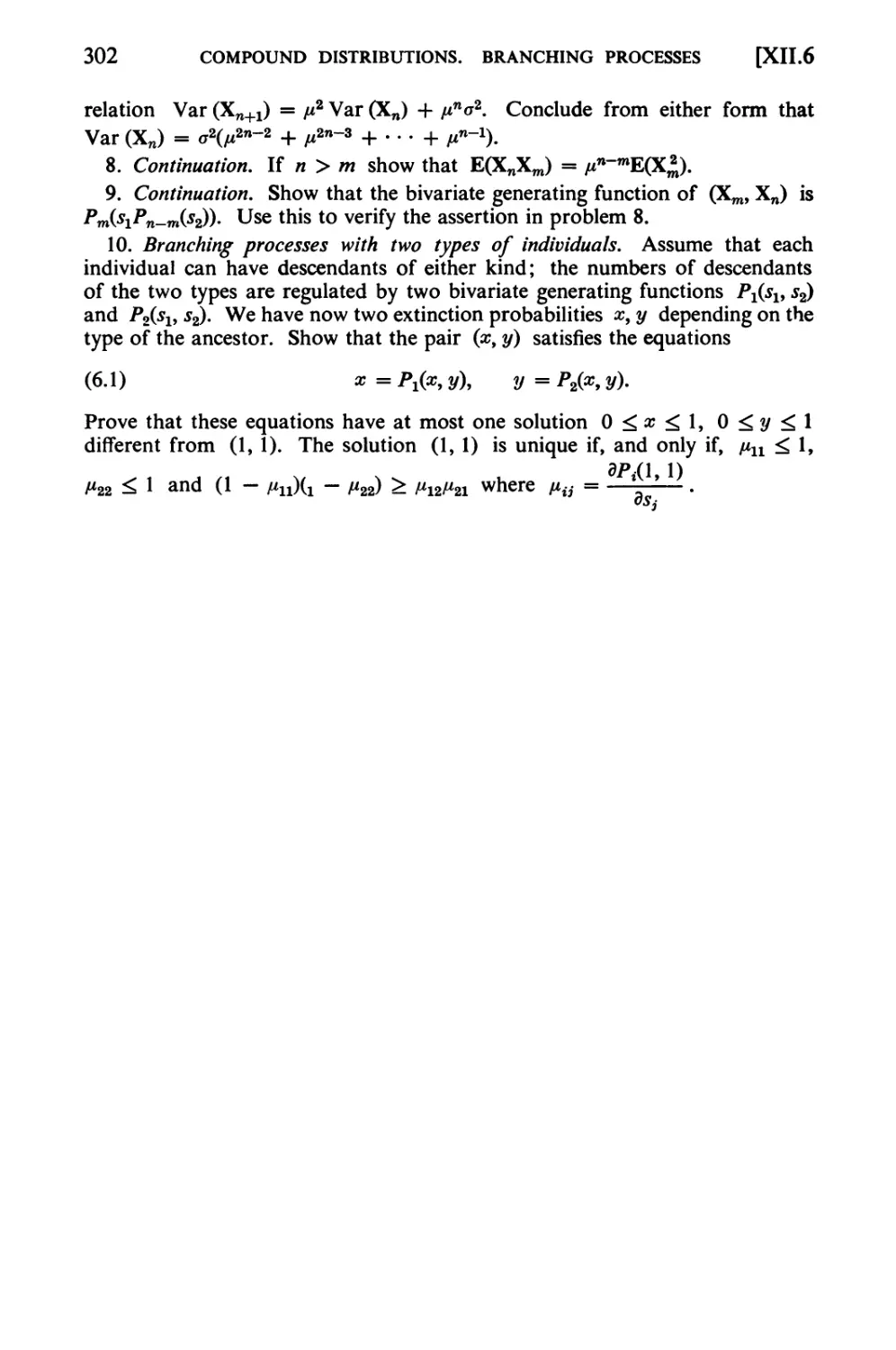
Index 499

INTRODUCTION
The Nature
of Probability Theory
1. THE BACKGROUND
Probability is a mathematical discipline with aims akin to those, for
example, of geometry or analytical mechanics. In each field we must
carefully distinguish three aspects of the theory: (a) the formal logical
content, (b) the intuitive background, (c) the applications. The character,
and the charm, of the whole structure cannot be appreciated without
considering all three aspects in their proper relation.
(a) Formal Logical Content
Axiomatically, mathematics is concerned solely with relations among
undefined things. This aspect is well illustrated by the game of chess. It
is impossible to "define" chess otherwise than by stating a set of rules.
The conventional shape of the pieces may be described to some extent,
but it will not always be obvious which piece is intended for "king." The
chessboard and the pieces are helpful, but they can be dispensed with.
The essential thing is to know how the pieces move and act. It is
meaningless to talk about the "definition" or the "true nature" of a pawn or a king.
Similarly, geometry does not care what a point and a straight line "really
are." They remain undefined notions, and the axioms of geometry specify
the relations among them: two points determine a line, etc. These are
the rules, and there is nothing sacred about them. Different forms of
geometry are based on different sets of axioms, and the logical structure of
non-Euclidean geometries is independent of their relation to reality.
Physicists have studied the motion of bodies under laws of attraction
different from Newton's, and such studies are meaningful even if Newton's
law of attraction is accepted as true in nature.
1

2
THE NATURE OF PROBABILITY THEORY
(b) Intuitive Background
In contrast to chess, the axioms of geometry and of mechanics have
an intuitive background. In fact, geometrical intuition is so strong that it
is prone to run ahead of logical reasoning. The extent to which logic,
intuition, and physical experience are interdependent is a problem into
which we need not enter. It is certain that intuition can be trained and
developed. The bewildered novice in chess moves cautiously, recalling
individual rules, whereas the experienced player absorbs a complicated
situation at a glance and is unable to account rationally for his intuition.
In like manner mathematical intuition grows with experience, and it is
possible to develop a natural feeling for concepts such as four-dimensional
space.
Even the collective intuition of mankind appears to progress. Newton's
notions of a field of force and of action at a distance and Maxwell's
concept of electromagnetic waves were at first decried as "unthinkable" and
"contrary to intuition." Modern technology and radio in the homes have
popularized these notions to such an extent that they form part of the
ordinary vocabulary. Similarly, the modern student has no appreciation
of the modes of thinking, the prejudices, and other difficulties against
which the theory of probability had to struggle when it was new.
Nowadays newspapers report on samples of public opinion, and the magic of
statistics embraces all phases of life to the extent that young girls watch
the statistics of their chances to get married. Thus everyone has acquired
a feeling for the meaning of statements such as "the chances are three in
five." Vague as it is, this intuition serves as background and guide for the
first step. It will be developed as the theory progresses and acquaintance
is made with more sophisticated applications.
(c) Applications
The concepts of geometry and mechanics are in practice identified with
certain physical objects, but the process is so flexible and variable that no
general rules can be given. The notion of a rigid body is fundamental and
useful, even though no physical object is rigid. Whether a given body
can be treated as if it were rigid depends on the circumstances and the
desired degree of approximation. Rubber is certainly not rigid, but in
discussing the motion of automobiles on ice textbooks usually treat the
rubber tires as rigid bodies. Depending on the purpose of the theory, we
disregard the atomic structure of matter and treat the sun now as a ball of
continuous matter, now as a single mass point.
In applications, the abstract mathematical models serve as tools, and
different models can describe the same empirical situation. The manner
in which mathematical theories are applied does not depend on preconceived

PROCEDURE
3
ideas; it is a purposeful technique depending on, and changing with,
experience. A philosophical analysis of such techniques is a legitimate study,
but is is not within the realm of mathematics, physics, or statistics. The
philosophy of the foundations of probability must be divorced from
mathematics and statistics, exactly as the discussion of our intuitive space
concept is now divorced from geometry.
2. PROCEDURE
The history of probability (and oft mathematics in general) shows a
stimulating interplay of theory and applications; theoretical progress
opens new fields of applications, and in turn applications lead to new
problems and fruitful research. The theory of probability is now applied
in many diverse fields, and the flexibility of a general theory is required to
provide appropriate tools for so great a variety of needs. We must
therefore withstand the temptation (and the pressure) to build the theory,
its terminology, and its arsenal too close to one particular sphere of
interest. We wish instead to develop a mathematical theory in the way
which has proved so successful in geometry and mechanics.
We shall start from the simplest experiences, such as tossing a coin or
throwing dice, where all statements have an obvious intuitive meaning.
This intuition will be translated into an abstract model to be generalized
gradually and by degrees. Illustrative examples will be provided to
explain the empirical background of the several models and to develop the
reader's intuition, but the theory itself will be of a mathematical character.
We shall no more attempt to explain^the "trua'meaning" of probability
than the modern physicist dwells on the "rearmeaning" of mass and
energy or the geometer discusses the nature of a point. Instead, we shall
prove theorems and show how they are applied.
Historically, the original purpose of the theory of probability was to
describe the exceedingly narrow domain of experience connected with
games of chance, and the main effort was directed to the calculation of
certain probabilities. In the opening chapters we too shall calculate a
few typical probabilities, but it should be borne in mind that numerical
probabilities are not the principal object of the theory. Its aim is to
discover general laws and to construct satisfactory theoretical models.
Probabilities play for us the same role as masses in mechanics. The
motion of the planetary system can be discussed without knowledge of the
individual masses and without contemplating methods for their actual
measurements. Even models for non-existent planetary systems may be
the object of a profitable and illuminating study. Similarly, practical and
useful probability models may refer to non-observable worlds. For example,

4
THE NATURE OF PROBABILITY THEORY
billions of dollars have been invested in automatic telephone exchanges.
These are based on simple probability models in which various possible
systems are compared. The theoretically best system is built and the others
will never exist. In insurance, probability theory is used to calculate the
probability of ruin; that is, the theory is used to avoid certain undesirable
situations, and consequently it applies to situations that are not actually
observed. Probability theory would be effective and useful even if not a
single numerical value were accessible.
3. "STATISTICAL" PROBABILITY
The success of the modern mathematical theory of probability is bought
at a price: the theory is limited to one particular aspect of "chance."
The intuitive notion of probability is connected with inductive reasoning
and with judgments such as "Paul is probably a happy man," "Probably
this book will be a failure," "Fermat's conjecture is probably false."
Judgments of this sort are of interest to the philosopher and the logician,
and they are a legitimate object of a mathematical theory.1 It must be
understood, however, that we are concerned not with modes of inductive
reasoning but with something that might be called physical or statistical
probability. In a rough way we may characterize this concept by saying
that our probabilities do not refer to judgments but to possible outcomes
of a conceptual experiment. Before we speak of probabilities, we must
agree on an idealized model of a particular conceptual experiment such as
tossing a coin, sampling kangaroos on the moon, observing a particle under
diffusion, counting the number of telephone calls. At the outset we must
agree on the possible outcomes of this experiment (our sample space) and
the probabilities associated with them. This is analogous to the procedure
in mechanics where fictitious models involving two, three, or seventeen
mass points are introduced, these points being devoid of individual
properties. Similarly, in analyzing the coin tossing game we are not
concerned with the accidental circumstances of an actual experiment:
the object of our theory is sequences (or arrangements) of symbols such as
"head, head, tail, head,. . . ." There is no place in our system for
speculations concerning the probability that the sun will rise tomorrow.
Before speaking of it we should have to agree on an (idealized) model
which would presumably run along the lines "out of infinitely many worlds
1 B. O. Koopman, The axioms and algebra of intuitive probability, Ann. of Math. (2),
vol. 41 (1940), pp. 269-292, and The bases of probability, Bull. Amer. Math. Soc, vol. 46
(1940), pp. 763-774.
For a modern text based on subjective probabilities see L. J. Savage, The foundations
of statistics, New York (John Wiley) 1954.

SUMMARY
5
one is selected at random. . . ." Little imagination is required to construct
such a model, but it appears both uninteresting and meaningless.
The astronomer speaks of measuring the temperature at the center of
the sun or of travel to Sirius. These operations seem impossible, and yet
it is not senseless to contemplate them. By the same token, we shall not
worry whether or not our conceptual experiments can be performed; we
shall analyze abstract models. In the back of our minds we keep an
intuitive interpretation of probability which gains operational meaning in
certain applications. We imagine the experiment performed a great many
times. An event with probability 0.6 should be expected, in the long run,
to occur sixty times out of a hundred. This description is deliberately
vague but supplies a picturesque intuitive background sufficient for the
more elementary applications. As the theory proceeds and grows more
elaborate, the operational meaning and the intuitive picture will become
more concrete.
4. SUMMARY
We shall be concerned with theoretical models in which probabilities
enter as free parameters in much the same way as masses in mechanics.
They are applied in many and variable ways. The technique of
applications and the intuition develop with the theory.
This is the standard procedure accepted and fruitful in other
mathematical disciplines. No alternative has been devised which could
conceivably fill the manifold needs and requirements of all branches of the
growing entity called probability theory and its applications.
We may fairly lament that intuitive probability is insufficient for
scientific purposes, but it is a historical fact. In example I, (6.6), we shall discuss
random distributions of particles in compartments. The appropriate, or
"natural," probability distribution seemed perfectly clear to everyone and
has been accepted without hesitation by physicists. It turned out, however,
that physical particles are not trained in human common sense, and the
"natural" (or Boltzmann) distribution has to be given up for the Einstein-
Bose distribution in some cases, for the Fermi-Dirac distribution in others.
No intuitive argument has been offered why photons should behave
differently from protons and why they do not obey the "a priori" laws.
If a justification could now be found, it would only show that intuition
develops with theory. At any rate, even for applications freedom and
flexibility are essential, and it would be pernicious to fetter the theory to
fixed poles.
It has also been claimed that the modern theory of probability is too
abstract and too general to be useful. This is the battle cry once raised
by practical-minded people against Maxwell's field theory. The argument

6
THE NATURE OF PROBABILITY THEORY
could be countered by pointing to the unexpected new applications
opened by the abstract theory of stochastic processes, or to the new
insights offered by the modern fluctuation theory which once more belies
intuition and is leading to a revision of practical attitudes. However, the
discussion is useless; it is too easy to condemn. Only yesterday the
practical things of today were decried as impractical, and the theories
which will be practical tomorrow will always be branded as valueless
games by the practical men of today.
5. HISTORICAL NOTE
The statistical, or empirical, attitude toward probability has been
developed mainly by R. A. Fisher and R. von Mises. The notion of sample
space2 comes from von Mises. This notion made it possible to build up a
strictly mathematical theory of probability based on measure theory.
Such an approach emerged gradually in the 'twenties under the influence
of many authors. An axiomatic treatment representing the modern
development was given by A. Kolmogorov.3 We shall follow this line,
but the term axiom appears too solemn inasmuch as the present volume
deals only with the simple case of discrete probabilities.
2 The German word is Merkmalraum (label space), von Mises' basic treatise
Wahrscheinlichkeitsrechnung appeared in 1931. A modernized version (edited and
complemented by Hilda Geiringer) appeared in 1964 under the title Mathematical
theory of probability and statistics, New York (Academic Press), von Mises'
philosophical ideas are best known from his earlier booklet of 1928, revised by H. Geiringer:
Probability, statistics and truth, London (Macmillan), 1957.
8 A. Kolmogoroff, Grundbegriffe der Wahrscheinlichkeitsrechnung, Berlin (Springer)
1933. An English translation (by N. Morrison) appeared in 1956: Foundations of the
theory of probability t New York (Chelsea).

CHAPTER I
The Sample Space
1. THE EMPIRICAL BACKGROUND
The mathematical theory of probability gains practical value and an
intuitive meaning in connection with real or conceptual experiments such
as tossing a coin once, tossing a coin 100 times, throwing three dice,
arranging a deck of cards, matching two decks of cards, playing roulette,
observing the life span of a radioactive atom or a person, selecting a
random sample of people and observing the number of left-handers in it,
crossing two species of plants and observing the phenotypes of the
offspring; or with phenomena such as the sex of a newborn baby, the
number of busy trunklines in a telephone exchange, the number of calls
on a telephone, random noise in an electrical communication system,
routine quality control of a production process, frequency of accidents,
the number of double stars in a region of the skies, the position of a particle
under diffusion. All these descriptions are rather vague, and, in order to
render the theory meaningful, we have to agree on what we mean by
possible results of the experiment or observation in question.
When a coin is tossed, it does not necessarily fall heads or tails; it can
roll away or stand on its edge. Nevertheless, we shall agree to regard
"head" and "tail" as the only possible outcomes of the experiment. This
convention simplifies the theory without affecting its applicability.
Idealizations of this type are standard practice. It is impossible to measure
the life span of an atom or a person without some error, but for theoretical
purposes it is expedient to imagine that these quantities are exact numbers.
The question then arises as to which numbers can actually represent the
life span of a person. Is there a maximal age beyond which life is
impossible, or is any age conceivable? We hesitate to admit that man can grow
1000 years old, and yet current actuarial practice admits no bounds to the
possible duration of life. According to formulas on which modern
mortality tables are based, the proportion of men surviving 1000 years is of the
7

8
THE SAMPLE SPACE
[1.1
order of magnitude of one in 1010 —a number with 1027 billions of zeros.
This statement does not make sense from a biological or sociological point
of view, but considered exclusively from a statistical standpoint it certainly
does not contradict any experience. There are fewer than 1010 people born
in a century. To test the contention statistically, more than 101()36 centuries
would be required, which is considerably more than 101()34 lifetimes of the
earth. Obviously, such extremely small probabilities are compatible with
our notion of impossibility. Their use may appear utterly absurd, but
it does no harm and is convenient in simplifying many formulas.
Moreover, if we were seriously to discard the possibility of living 1000 years,
we should have to accept the existence of maximum age, and the
assumption that it should be possible to live x years and impossible to live x years
and two seconds is as unappealing as the idea of unlimited life.
Any theory necessarily involves idealization, and our first idealization
concerns the possible outcomes of an "experiment" or "observation."
If we want to construct an abstract model, we must at the outset reach a
decision about what consitutes a possible outcome of the (idealized)
experiment.
For uniform terminology, the results of experiments or observations
will be called events. Thus we shall speak of the event that of five coins
tossed more than three fell heads. Similarly, the "experiment" of
distributing the cards in bridge1 may result in the "event" that North has two
aces. The composition of a sample ("two left-handers in a sample of 85")
and the result of a measurement ("temperature 120°," "seven trunklines
busy") will each be called an event.
We shall distinguish between compound (or decomposable) and simple
(or indecomposable) events. For example, saying that a throw with two
dice resulted in "sum six" amounts to saying that it resulted in "(1, 5) or
(2, 4) or (3, 3) or (4, 2) or (5, 1)," and this enumeration decomposes the
event "sum six" into five simple events. Similarly, the event "two odd
faces" admits of the decomposition "(1, 1) or (1, 3) or ... or (5, 5)" into
nine simple events. Note that if a throw results in (3, 3), then the same
throw results also in the events "sum six" and "two odd faces"; these
events are not mutually exclusive and hence may occur simultaneously.
1 Definition of bridge and poker. A deck of bridge cards consists of 52 cards arranged
in four suits of thirteen each. There are thirteen face values (2, 3, ..., 10, jack, queen,
king, ace) in each suit. The four suits are called spades, clubs, hearts, diamonds.
The last two are red, the first two black. Cards of the same face value are called of
the same kind. For our purposes, playing bridge means distributing the cards to four
players, to be called North, South, East, and West (or N, S, E, W, for short) so that
each receives thirteen cards. Playing poker, by definition, means selecting five cards
out of the pack.

1.2]
EXAMPLES
9
As a second example consider the age of a person. Every particular value
x represents a simple event, whereas the statement that a person is in his
fifties describes the compound event that x lies between 50 and 60. In
this way every compound event can be decomposed into simple events, that
is to say, a compound event is an aggregate of certain simple events.
If we want to speak about "experiments" or "observations" in a
theoretical way and without ambiguity, we must first agree on the simple
events representing the thinkable outcomes; they define the idealized
experiment. In other words: The term simple (or indecomposable) event
remains undefined in the same way as the terms point and line remain
undefined in geometry. Following a general usage in mathematics the
simple events will be called sample points, or points for short. By definition,
every indecomposable result of the {idealized) experiment is represented by
one, and only one, sample point. The aggregate of all sample points will
be called the sample space. All events connected with a given (idealized)
experiment can be described as aggregates of sample points.
Before formalizing these basic conventions, we proceed to discuss a
few typical examples which will play a role further on.
2. EXAMPLES
(a) Distribution of the three balls in three cells. Table 1 describes all
possible outcomes of the "experiment" of placing three balls into three
cells.
Each of these arrangements represents a simple event, that is, a sample
point. The event A "one cell is multiply occupied" is realized in the
arrangements numbered 1-21, and we express this by saying that the event
A is the aggregate of the sample points 1-21. Similarly, the event B "first
cell is not empty" is the aggregate of the sample points 1, 4-15, 22-27.
1. {abc | - | - }
2. {- \abc\ -}
3. { - | - | abc)
A.{ab | c\ -}
5.{ac\ b | - }
6. { be | a | - }
7. {ab | - | c)
8- {a c | - | b }
9- { be | - | a }
Table 1
10. {a | be | - }
11. {b \ac\ -}
12. { e | ab | - }
13. {a | - | be}
14. { b | - | a c}
15- { c\ - \ab)
16. { - \ab | c)
17. {- \ac\ b}
18. {- | be \a }
19. { - | a | be}
20. { - | b | a c)
21. { - | c\ab }
22. {a \ b \ c}
23. {a | c | b }
24. { b | a | c}
25. { b | c | a }
26. { c\a | b }
27. { c\ b \a }.

10
THE SAMPLE SPACE
[1.2
The event C defined by "both A and B occur" is the aggregate of the
thirteen sample points 1,4-15. In this particular example it so happens that
each of the 27 points belongs to either A or B (or to both); therefore the
event "either A or B or both occur" is the entire sample space and occurs
with absolute certainty. The event D defined by "A does not occur"
consists of the points 22-27 and can be described by the condition that
no cell remains empty. The event "first cell empty and no cell multiply
occupied" is impossible (does not occur) since no sample point satisfies
these specifications.
(b) Random placement of r balls in n cells. The more general case of
r balls in n cells can be studied in the same manner, except that the
number of possible arrangements increases rapidly with r and n. For
r = 4 balls in n = 3 cells, the sample space contains already 64 points,
and for r = n = 10 there are 1010 sample points; a complete tabulation
would require some hundred thousand big volumes.
We use this example to illustrate the important fact that the nature of
the sample points is irrelevant for our theory. To us the sample space
(together with the probability distribution defined in it) defines the
idealized experiment. We use the picturesque language of balls and cells,
but the same sample space admits of a great variety of different practical
interpretations. To clarify this point, and also for further reference, we
list here a number of situations in which the intuitive background varies; all
are, however, abstractly equivalent to the scheme of placing r balls into n
cells, in the sense that the outcomes differ only in their verbal description.
The appropriate assignment of probabilities is not the same in all cases
and will be discussed later on.
(6,1). Birthdays. The possible configurations of the birthdays of r
people correspond to the different arrangements of r balls in n =
365 cells (assuming the year to have 365 days).
(b,2). Accidents. Classifying r accidents according to the weekdays
when they occurred is equivalent to placing r balls into n = 7 cells.
(b,3). In firing at n targets, the hits correspond to balls, the targets to
cells.
(b,4). Sampling. Let a group of r people be classified according to,
say, age or profession. The classes play the role of our cells, the people
that of balls.
(b,5). Irradiation in biology. When the cells in the retina of the eye
are exposed to light, the light particles play the role of balls, and the
actual cells are the "cells" of our model. Similarly, in the study of
the genetic effect of irradiation, the chromosomes correspond to the
cells of our model and a-particles to the balls.

1.2]
EXAMPLES
11
(6,6). In cosmic ray experiments the particles reaching Geiger counters
represent balls, and the counters function as cells.
(b,l). An elevator starts with r passengers and stops at n floors.
The different arrangements of discharging the passengers are replicas
of the different distributions of r balls in n cells.
(6,8). Dice. The possible outcomes of a throw with r dice
correspond to placing r balls into n = 6 cells. When tossing a coin we are
in effect dealing with only n = 2 cells.
(6,9). Random digits. The possible orderings of a sequence of r
digits correspond to the distribution of r balls (= places) into ten cells
called 0, 1,...,9.
(6,10). The sex distribution of r persons. Here we have n = 2 cells
and r balls.
(6,11). Coupon collecting. The different kinds of coupons represent
the cells; the coupons collected represent the balls.
(6,12). Aces in bridge. The four players represent four cells, and
we have r = 4 balls.
(6,13). Gene distributions. Each descendant of an individual (person,
plant, or animal) inherits from the progenitor certain genes. If a
particular gene can appear in n forms Al9. .., An, then the
descendants may be classified according to the type of the gene: The descendants
correspond to the balls, the genotypes Al9...., An to the cells.
(6,14). Chemistry. Suppose that a long-chain polymer reacts with
oxygen. An individual chain may react with 0, 1, 2,... oxygen
molecules. Here the reacting oxygen molecules play the role of balls
and the polymer chains the role of cells into which the balls are put.
(6,15). Theory of photographic emulsions. A photographic plate is
covered with grains sensitive to light quanta: a grain reacts if it is
hit by a certain number, r, of quanta. For the theory of black-white
contrast we must know how many cells are likely to be hit by the r
quanta. We have here an occupancy problem where the grains
correspond to cells, and the light quanta to balls. (Actually the situation is
more complicated since a plate usually contains grains of different
sensitivity.)
(6,16). Misprints. The possible distributions of r misprints in the
n pages of a book correspond to all the different distributions of r balls
in n cells, provided r is smaller than the number of letters per page.
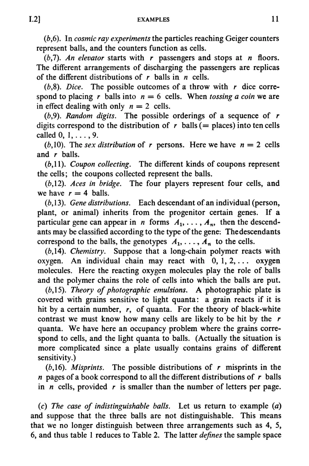
(c) The case of indistinguishable balls. Let us return to example (a)
and suppose that the three balls are not distinguishable. This means
that we no longer distinguish between three arrangements such as 4, 5,
6, and thus table 1 reduces to Table 2. The latter defines the sample space

12
THE SAMPLE SPACE
[1.2
of the ideal experiment which we call "placing three indistinguishable balls
into three cells" and a similar procedure applies to the case of r balls
in n cells.
Table 2
1. {***
2. {-
3. {-
4. {**
5. {** |
_
***
_
♦
~
-}
- )
***}
" }
* }
6. { *
7. { *
8. {-
9- {-
10. { *
| **
| -
| **
1 *
1 *
i -)
i**}
i *}
i**}
i *}•
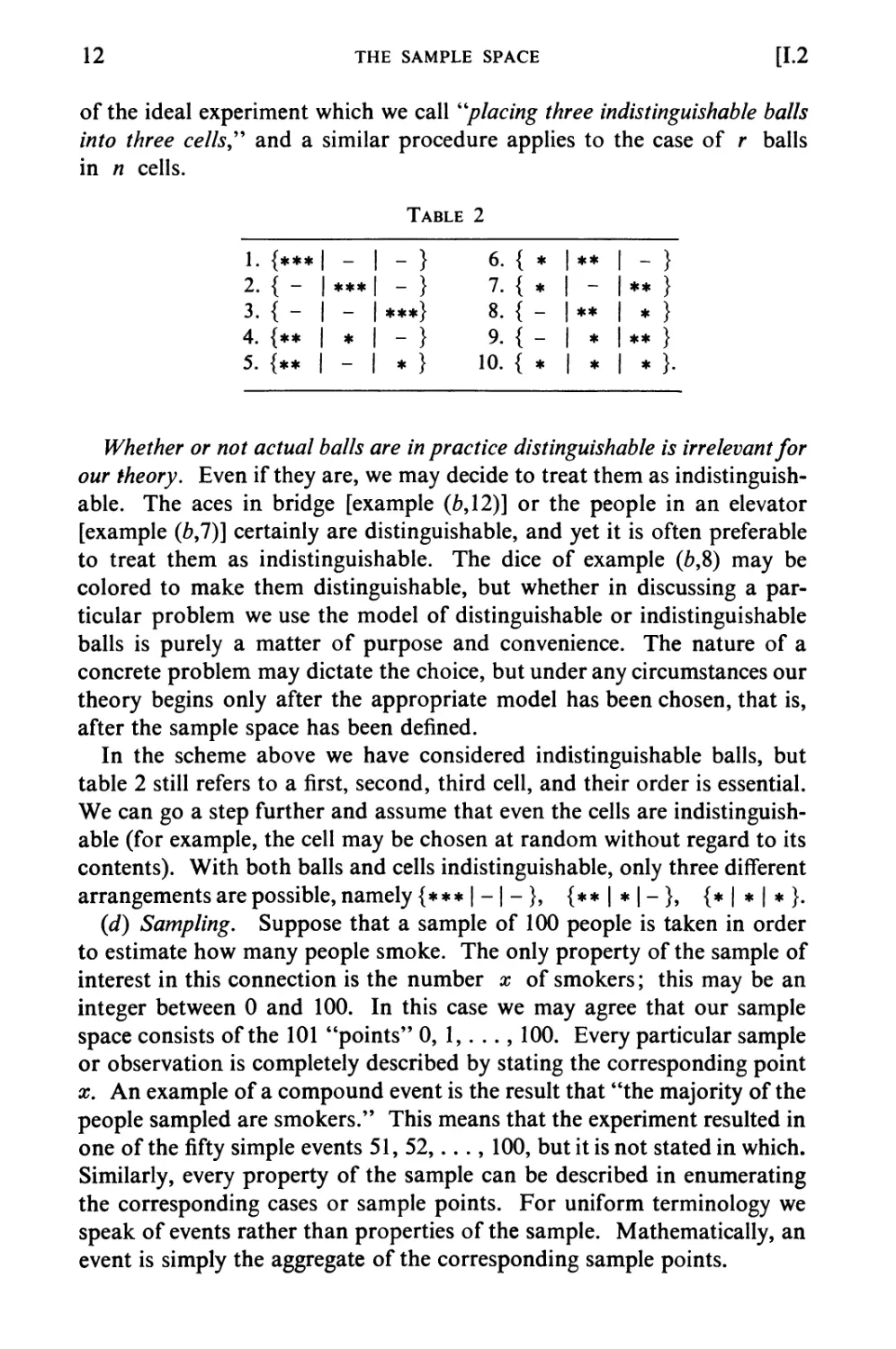
Whether or not actual balls are in practice distinguishable is irrelevant for
our theory. Even if they are, we may decide to treat them as
indistinguishable. The aces in bridge [example (6,12)] or the people in an elevator
[example (b,7)] certainly are distinguishable, and yet it is often preferable
to treat them as indistinguishable. The dice of example (6,8) may be
colored to make them distinguishable, but whether in discussing a
particular problem we use the model of distinguishable or indistinguishable
balls is purely a matter of purpose and convenience. The nature of a
concrete problem may dictate the choice, but under any circumstances our
theory begins only after the appropriate model has been chosen, that is,
after the sample space has been defined.
In the scheme above we have considered indistinguishable balls, but
table 2 still refers to a first, second, third cell, and their order is essential.
We can go a step further and assume that even the cells are
indistinguishable (for example, the cell may be chosen at random without regard to its
contents). With both balls and cells indistinguishable, only three different
arrangements are possible, namely {*** | - | - }, {** | * | - }, {*|*|*}.
(d) Sampling. Suppose that a sample of 100 people is taken in order
to estimate how many people smoke. The only property of the sample of
interest in this connection is the number x of smokers; this may be an
integer between 0 and 100. In this case we may agree that our sample
space consists of the 101 "points" 0, 1,..., 100. Every particular sample
or observation is completely described by stating the corresponding point
x. An example of a compound event is the result that "the majority of the
people sampled are smokers." This means that the experiment resulted in
one of the fifty simple events 51, 52,..., 100, but it is not stated in which.
Similarly, every property of the sample can be described in enumerating
the corresponding cases or sample points. For uniform terminology we
speak of events rather than properties of the sample. Mathematically, an
event is simply the aggregate of the corresponding sample points.

1.3]
THE SAMPLE SPACE. EVENTS
13
(e) Sampling {continued). Suppose now that the 100 people in our
sample are classified not only as smokers or non-smokers but also as
males or females. The sample may now be characterized by a quadruple
(Ms, Fs, Mn, Fn) of integers giving in order the number of male and
female smokers, male and female non-smokers. For sample points we
take the quadruples of integers lying between 0 and 100 and adding to
100. There are 176,851 such quadruples, and they constitute the sample
space (cf. II, 5). The event "relatively more males than females smoke"
means that in our sample the ratio MjMn is greater than FJFn. The
point (73, 2, 8, 17) has this property, but (0, 1, 50, 49) has not. Our event
can be described in principle by enumerating all quadruples with the
desired property.
(/) Coin tossing. For the experiment of tossing a coin three times, the
sample space consists of eight points which may conveniently be represented
by HHH, HHT, HTH, THH, HTT, THT, TTH, TTT. The event A,
"two or more heads," is the aggregate of the first four points. The event
B, "just one tail," means either HHT, or HTH, or THH; we say that
B contains these three points.
(g) Ages of a couple. An insurance company is interested in the age
distribution of couples. Let x stand for the age of the husband, y for
the age of the wife. Each observation results in a number-pair (x, y).
For the sample space we take the first quadrant of the #,?/-plane so that
each point x > 0, y > 0 is a sample point. The event A, "husband is
older than 40," is represented by all points to the right of the line x = 40;
the event B, "husband is older than wife," is represented by the angular
region between the #-axis and the bisector y = x, that is to say, by the
aggregate of points with x > y; the event C, "wife is older than 40," is
represented by the points above the line y = 40. A geometric
representation of the joint age distributions of two couples requires a
four-dimensional space.
(h) Phase space. In statistical mechanics, each possible "state" of a
system is called a "point in phase space." This is only a difference in
terminology. The phase space is simply our sample space; its points are
our sample points.
3. THE SAMPLE SPACE. EVENTS
It should be clear from the preceding that we shall never speak of
probabilities except in relation to a given sample space (or, physically, in
relation to a certain conceptual experiment). We start with the notion of a
sample space and its points; from now on they will be considered given.
They are the primitive and undefined notions of the theory precisely as the

14
THE SAMPLE SPACE
[1.4
notions of "points" and "straight line" remain undefined in an axiomatic
treatment of Euclidean geometry. The nature of the sample points does
not enter our theory. The sample space provides a model of an ideal
experiment in the sense that, by definition, every thinkable outcome of the
experiment is completely described by one, and only one, sample point. It
is meaningful to talk about an event A only when it is clear for every
outcome of the experiment whether the event A has or has not occurred.
The collection of all those sample points representing outcomes where
A has occurred completely describes the event. Conversely, any given
aggregate A containing one or more sample points can be called an
event; this event does, or does not, occur according as the outcome of the
experiment is, or is not, represented by a point of the aggregate A. We
therefore define the word event to mean the same as an aggregate of sample
points. We shall say that an event A consistsof (or contains) certain points,
namely those representing outcomes of the ideal experiment in which A
occurs.
Example. In the sample space of example (l.a) consider the event
U consisting of the points number 1, 7, 13. This is a formal and
straightforward definition, but U can be described in many equivalent ways.
For example, U may be defined as the event that the following three
conditions are satisfied: (1) the second cell is empty, (2) the ball a is in the
first cell, (3) the ball b does not appear after c. Each of these conditions
itself describes an event. The event Ux defined by the condition (1) alone
consists of points 1, 3, 7-9, 13-15. The event U2 defined by (2) consists
of points 1, 4, 5, 7, 8, 10, 13, 22, 23; and the event U3 defined by (3)
contains the points 1-4, 6, 7, 9-11, 13, 14, 16, 18-20, 22, 24, 25. The
event U can also be described as the simultaneous realization of all three
events Ul9 U2, t/3. ►
The terms "sample point" and "event" have an intuitive appeal, but
they refer to the notions of point and point set common to all parts of
mathematics.
We have seen in the preceding example and in (l.a) that new events can
be defined in terms of two or more given events. With these examples in
mind we now proceed to introduce the notation of the formal algebra of
events (that is, algebra of point sets).
4. RELATIONS AMONG EVENTS
We shall now suppose that an arbitrary, but fixed, sample space S is
given. We use capitals to denote events, that is, sets of sample points.
The fact that a point x is contained in the event A is denoted by x e A.

1.4]
RELATIONS AMONG EVENTS
15
Thus x g Q for every point x. We write A = B only if the two events
consist of exactly the same points.
In general, events will be defined by certain conditions on their points,
and it is convenient to have a symbol to express the fact that no point
satisfies a specified set of conditions. The next definition serves this purpose.
Definition 1. We shall use the notation A = 0 to express that the
event A contains no sample points (is impossible). The zero must be
interpreted in a symbolic sense and not as the numeral.
To every event A there corresponds another event defined by the
condition "A does not occur." It contains all points not contained in A.
Definition 2. The event consisting of all points not contained in the
event A will be called the complementary event (or negation) of A and will
be denoted by A'. In particular, S' = 0.
Figures 1 and 2. Illustrating relations among events. In Figure 1 the domain within
heavy boundaries is the union A u B u C. The triangular {heavily shaded) domain is
the intersection ABC. The moon-shaped (lightly shaded) domain is the intersection of
B with the complement of A u C.
With any two events A and B we can associate two new events
defined by the conditions "both A and B occur" and "either A or B or
both occur." These events will be denoted by AB and A U B,
respectively. The event AB contains all sample points which are common to
A and B. If A and B exclude each other, then there are no points
common to A and B and the event AB is impossible; analytically, this
situation is described by the equation
(4.1) AB = 0
which should be read "A and B are mutually exclusive" The event
AB' means that both A and B' occur or, in other words, that A but
not B occurs. Similarly, A'B' means that neither A nor B occurs.
The event A\JB means that at least one of the events A and B occurs;

16
THE SAMPLE SPACE
[1.4
it contains all sample points except those that belong neither to A nor
to B.
In the theory of probability we can describe the event AB as the
simultaneous occurrence of A and B. In standard mathematical
terminology AB is called the (logical) intersection of A and B. Similarly,
A U B is the union of A and B. Our notion carries over to the case of
events A, B, C, D,
Definition 3. To every collection A, B,C,. . . of events we define two
new events as follows. The aggregate of the sample points which belong to
all the given sets will be denoted by ABC . . . and called the intersection2,
{or simultaneous realization) of A, B, C,. . . . The aggregate of sample
points which belong to at least one of the given sets will be denoted by
A U B U C. . . and called the union (or realization of at least one) of the
given events. The events A, B, C,. . . are mutually exclusive if no two
have a point in common, that is, if AB = 0, AC = 0,. . ., BC = 0,. . . .
We still require a symbol to express the statement that A cannot
occur without B occurring, that is, that the occurrence of A implies the
occurrence of B. This means that every point of A is contained in B.
Think of intuitive analogies like the aggregate of all mothers, which
forms a part of the aggregate of all women: All mothers are women but
not all women are mothers.
Definition 4. The symbols A <= B and B => A are equivalent and
signify that every point of A is contained in B; they are read, respectively,
"A implies B" and "B is implied by A". If this is the case, we shall
also write B — A instead of BA' to denote the event that B but not A
occurs.
The event B — A contains all those points which are in B but not
in A. With this notation we can write A' = S — A and A — A = 0.
Examples, (a) If A and B are mutually exclusive, then the occurrence
of A implies the non-occurrence of B and vice versa. Thus AB = 0
means the same as A ^ B' and as B <= A'.
(b) The event A — AB means the occurrence of A but not of both
A and B. Thus A - AB = AB'.
(c) In the example (2.g), the event AB means that the husband is
older than 40 and older than his wife; AB' means that he is older than
2 The standard mathematical notation for the intersection of two or more sets is
A n B or A n B n C, etc. This notation is more suitable for certain specific
purposes (see IV, 1 of volume 2). At present we use the notation AB, ABC, etc.,
since it is less clumsy in print.

1.5]
DISCRETE SAMPLE SPACES
17
40 but not older than his wife. AB is represented by the infinite trapezoidal
region between the a>axis and the lines x = 40 and y = x, and the
event AB' is represented by the angular domain between the lines
x = 40 and y = x, the latter boundary included. The event AC means
that both husband and wife are older than 40. The event A KJ C means
that at least one of them is older than 40, and A \J B means that the
husband is either older than 40 or, if not that, at least older than his wife
(in official language, "husband's age exceeds 40 years or wife's age,
whichever is smaller").
id) In example (2.a) let Ei be the event that the cell number i is
empty (here i = 1,2,3). Similarly, let Si9 Di9 Ti9 respectively, denote
the event that the cell number i is occupied simply, doubly, or triply.
Then EXE2 = T3, and SXS2 c s8, and D1D2 = 0. Note also that
7\ c: E2, etc. The event DY U D2 U Z)3 is defined by the condition that
there exist at least one doubly occupied cell.
(e) Bridge (cf. footnote 1). Let A, B, C, D be the events, respectively,
that North, South, East, West have at least one ace. It is clear that at
least one player has an ace, so that one or more of the four events must
occur. Hence ^u5uCuD = S is the whole sample space. The
event ABCD occurs if, and only if, each player has an ace. The event
"West has all four aces" means that none of the three events A, B, C
has occurred; this is the same as the simultaneous occurrence of A' and
B' and C or the event A'B'C.
(J) In the example (2.g) we have BC <= A: in words, "if husband is
older than wife (B) and wife is older than 40 (C), then husband is older
that 40 (A).'9 How can the event A — BC be described in words? *
5. DISCRETE SAMPLE SPACES
The simplest sample spaces are those containing only a finite number,
n, of points. If n is fairly small (as in the case of tossing a few coins),
it is easy to visualize the space. The space of distributions of cards in
bridge is more complicated, but we may imagine each sample point
represented on a chip and may then consider the collection of these chips as
representing the sample space. An event A (like "North has two aces")
is represented by a certain set of chips, the complement A' by the
remaining ones. It takes only one step from here to imagine a bowl with
infinitely many chips or a sample space with an infinite sequence of points
Ei, L2, E$,....
Examples, (a) Let us toss a coin as often as necessary to turn up one
head. The points of the sample space are then EY = H, E2= TH,
E3 = TTH, £4 = TTTH, etc. We may or may not consider as thinkable

18
THE SAMPLE SPACE
[1.5
the possibility that H never appears. If we do, this possibility should be
represented by a point E0.
(b) Three players a, b, c take turns at a game, such as chess, according
to the following rules. At the start a and b play while c is out. The
loser is replaced by c and at the second trial the winner plays against c
while the loser is out. The game continues in this way until a player wins
twice in succession, thus becoming the winner of the game. For simplicity
we disregard the possibility of ties at the individual trials. The possible
outcomes of our game are then indicated by the following scheme:
(*) aa, ace, aebb, acbaa, acbacc, acbaebb, acbacbaa,. . .
bb, bec, bcaa, bcabb, beabec, bcabcaa, bcabcabb,....
In addition, it is thinkable that no player ever wins twice in succession, in
which case the play continues indefinitely according to one of the patterns
(**) acbacbacbacb . . . , bcabcabcabca....
The sample space corresponding to our ideal "experiment" is defined by
(*) and (**) and is infinite. It is clear that the sample points can be
arranged in a simple sequence by taking first the two points (**) and
continuing with the points of (*) in the order aa, bb, ace, bec,.... [See
problems 5-6, example Y,(2.a), and problem 5 of XV, 14.] ►
Definition. A sample space is called discrete if it contains only finitely
many points or infinitely many points which can be arranged into a simple
sequence El9 E2, . . . .
Not every sample space is discrete. It is a known theorem (due to
G. Cantor) that the sample space consisting of all positive numbers is not
discrete. We are here confronted with a distinction familiar in mechanics.
There it is usual first to consider discrete mass points with each individual
point carrying a finite mass, and then to pass to the notion of a continuous
mass distribution, where each individual point has zero mass. In the first
case, the mass of a system is obtained simply by adding the masses of the
individual points; in the second case, masses are computed by integration
over mass densities. Quite similarly, the probabilities of events in discrete
sample spaces are obtained by mere additions, whereas in other spaces
integrations are necessary. Except for the technical tools required, there
is no essential difference between the two cases. In order to present actual
probability considerations unhampered by technical difficulties, we shall
take up only discrete sample spaces. It will be seen that even this special
case leads to many interesting and important results.
In this volume we shall consider only discrete sample spaces.

1.6] PROBABILITIES IN DISCRETE SAMPLE SPACES: PREPARATIONS 19
6. PROBABILITIES IN DISCRETE SAMPLE
SPACES: PREPARATIONS
Probabilities are numbers of the same nature as distances in geometry or
masses in mechanics. The theory assumes that they are given but need
assume nothing about their actual numerical values or how they are
measured in practice. Some of the most important applications are of a
qualitative nature and independent of numerical values. In the relatively
few instances where numerical values for probabilities are required, the
procedures vary as widely as do the methods of determining distances.
There is little in common in the practices of the carpenter, the practical
surveyor, the pilot, and the astronomer when they measure distances.
In our context, we may consider the diffusion constant, which is a notion
of the theory of probability. To find its numerical value, physical
considerations relating it to other theories are required; a direct measurement
is impossible. By contrast, mortality tables are constructed from rather
crude observations. In most actual applications the determination of
probabilities, or the comparison of theory and observation, requires
rather sophisticated statistical methods, which in turn are based on a
refined probability theory. In other words, the intuitive meaning of
probability is clear, but only as the theory proceeds shall we be able to see
how it is applied. All possible "definitions" of probability fall far short
of the actual practice.
When tossing a "good" coin we do not hesitate to associate probability
J with either head or tail. This amounts to saying that when a coin is
tossed n times all 2n possible results have the same probability. From a
theoretical standpoint, this is a convention. Frequently, it has been
contended that this convention is logically unavoidable and the only
possible one. Yet there have been philosophers and statisticians defying
the convention and starting from contradictory assumptions (uniformity
or non-uniformity in nature). It has also been claimed that the
probabilities i are due to experience. As a matter of fact, whenever refined statistical
methods have been used to check on actual coin tossing, the result has been
invariably that head and tail are not equally likely. And yet we stick to
our model of an "ideal" coin, even though no good coins exist. We
preserve the model not merely for its logical simplicity, but essentially for
its usefulness and applicability. In many applications it is sufficiently
accurate to describe reality. More important is the empirical fact that
departures from our scheme are always coupled with phenomena such as
an eccentric position of the center of gravity. In this way our idealized
model can be extremely useful even if it never applies exactly. For
example, in modern statistical quality control based on Shewhart's methods,

20
THE SAMPLE SPACE
[1.6
idealized probability models are used to discover "assignable causes" for
flagrant departures from these models and thus to remove impending
machine troubles and process irregularities at an early stage.
Similar remarks apply to other cases. The number of possible
distributions of cards in bridge is almost 1030. Usually we agree to consider
them as equally probable. For a check of this convention more than 1030
experiments would be required—thousands of billions of years if every
living person played one game every second, day and night. However,
consequences of the assumption can be verified experimentally, for
example, by observing the frequency of multiple aces in the hands at
bridge. It turns out that for crude purposes the idealized model describes
experience sufficiently well, provided the card shuffling is done better than
is usual. It is more important that the idealized scheme, when it does not
apply, permits the discovery of "assignable causes" for the discrepancies,
for example, the reconstruction of the mode of shuffling. These are
examples of limited importance, but they indicate the usefulness of
assumed models. More interesting cases will appear only as the theory
proceeds.
Examples, (a) Distinguishable balls. In example (2.a) it appears
natural to assume that all sample points are equally probable, that is, that
each sample point has probability £,. We can start from this definition and
investigate its consequences. Whether or not our model will come
reasonably close to actual experience will depend on the type of phenomena
to which it is applied. In some applications the assumption of equal
probabilities is imposed by physical considerations; in others it is
introduced to serve as the simplest model for a general orientation, even though
it quite obviously represents only a crude first approximation [e.g.,
consider the examples (2.6,1), birthdays; (2.6,7), elevator problem; or
(2.6,11) coupon collecting].
(6) Indistinguishable balls: Bose-Einstein statistics. We now turn to the
example (2.c) of three indistinguishable balls in three cells. It is possible
to argue that the actual physical experiment is unaffected by our failure to
distinguish between the balls; physically there remain 27 different
possibilities, even though only ten different forms are disinguishable. This
consideration leads us to attribute the following probabilities to the ten
points of table 2.
Point number: 1 2 3456789 10
Probability: -2V ^ ^ J J i i J i f .
It must be admitted that for most applications listed in example (2.6)

1.6] PROBABILITIES IN DISCRETE SAMPLE SPACES: PREPARATIONS 21
this argument appears sound and the assignment of probabilities
reasonable. Historically, our argument was accepted for a long time without
question and served in statistical mechanics as the basis for the derivation
of the Maxwell-Boltzmann statistics for the distribution of r balls in n
cells. The greater was the surprise when Bose and Einstein showed that
certain particles are subject to the Bose-Einstein statistics (for details see
11,5). In our case with r = n = 3, this model attributes probability iV
to each of the ten sample points.
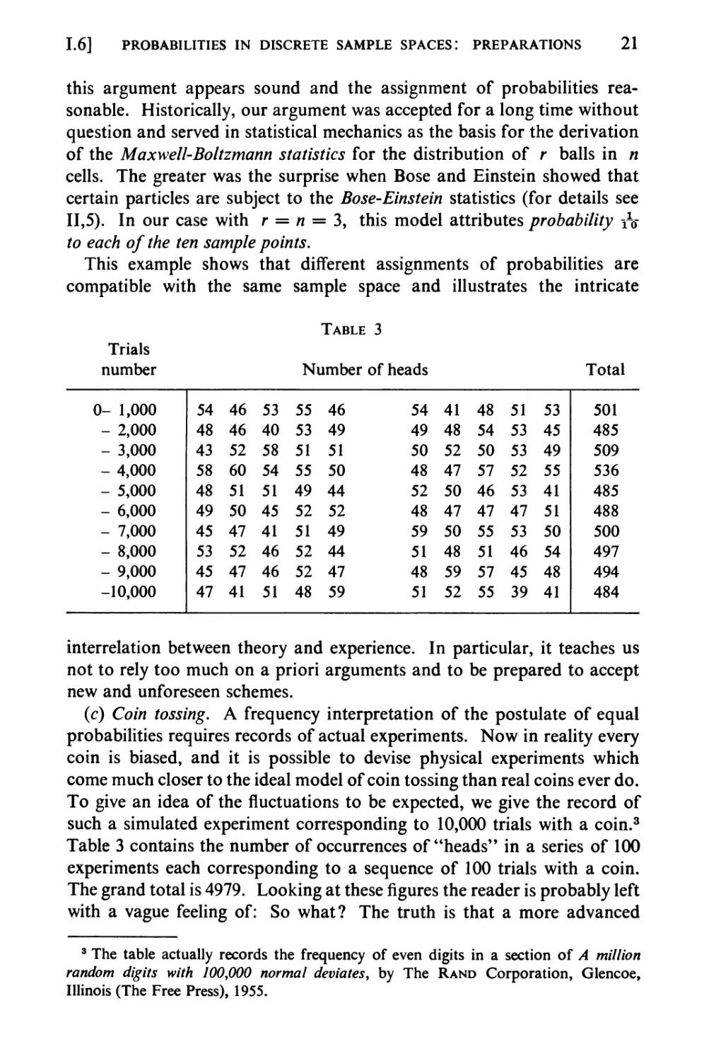
This example shows that different assignments of probabilities are
compatible with the same sample space and illustrates the intricate
Table 3
Trials
number Number of heads Total
0- 1,000
- 2,000
- 3,000
- 4,000
- 5,000
- 6,000
- 7,000
- 8,000
- 9,000
-10,000
54
48
43
58
48
49
45
53
45
47
46
46
52
60
51
50
47
52
47
41
53
40
58
54
51
45
41
46
46
51
55
53
51
55
49
52
51
52
52
48
46
49
51
50
44
52
49
44
47
59
54
49
50
48
52
48
59
51
48
51
41
48
52
47
50
47
50
48
59
52
48
54
50
57
46
47
55
51
57
55
51
53
53
52
53
47
53
46
45
39
53
45
49
55
41
51
50
54
48
41
501
485
509
536
485
488
500
497
494
484
interrelation between theory and experience. In particular, it teaches us
not to rely too much on a priori arguments and to be prepared to accept
new and unforeseen schemes.
(c) Coin tossing. A frequency interpretation of the postulate of equal
probabilities requires records of actual experiments. Now in reality every
coin is biased, and it is possible to devise physical experiments which
come much closer to the ideal model of coin tossing than real coins ever do.
To give an idea of the fluctuations to be expected, we give the record of
such a simulated experiment corresponding to 10,000 trials with a coin.3
Table 3 contains the number of occurrences of "heads" in a series of 100
experiments each corresponding to a sequence of 100 trials with a coin.
The grand total is 4979. Looking at these figures the reader is probably left
with a vague feeling of: So what? The truth is that a more advanced
3 The table actually records the frequency of even digits in a section of A million
random digits with 100,000 normal deviates, by The Rand Corporation, Glencoe,
Illinois (The Free Press), 1955.

22
THE SAMPLE SPACE
[1.7
theory is necessary to judge to what extent such empirical data agree with
our abstract model. (Incidentally, we shall return to this material in
111,6.) ►
7. THE BASIC DEFINITIONS AND RULES
Fundamental Convention. Given a discrete sample space S with
sample points El9 E2,. . . , we shall assume that with each point Ej there
is associated a number, called the probability of Ej and denoted by P{£,-}. It
is to be non-negative and such that
(7.1) P{£1} + P{£2} + ...= 1.
Note that we do not exclude the possibility that a point has probability
zero. This convention may appear artificial but is necessary to avoid
complications. In discrete sample spaces probability zero is in practice
interpreted as an impossibility, and any sample point known to have
probability zero can, with impunity, be eliminated from the sample space.
However, frequently the numerical values of the probabilities are not
known in advance, and involved considerations are required to decide
whether or not a certain sample point has positive probability.
Definition. The probability P{A} of any event A is the sum of the
probabilities of all sample points in it.
By (7.1) the probability of the entire sample space S is unity, or
P{S} = 1. It follows that for any event A
(7.2) 0<P{^} < 1.
Consider now two arbitrary events A1 and A2. To compute the
probability P^iU^} that either Ax or A2 or both occur, we have to
add the probabilities of all sample points contained either in A1 or in A2,
but each point is to be counted only once. We have, therefore,
(7.3) P^U^J^P^J + P^}.
Now, if E is any point contained both in A1 and in A2, then P{E}
occurs twice in the right-hand member but only once in the left-hand
member. Therefore, the right side exceeds the left side by the amount
P{AXA2}9 and we have the simple but important
Theorem. For any two events Ax and A2 the probability that either
Ax or A2 or both occur is given by
(7.4) P{A^A2) = P^J + P{A2} - P{,Ma}.

1.7]
THE BASIC DEFINITIONS AND RULES
23
If AXA2 = 0, that is, if Ax and A2 are mutually exclusive, then (7.4)
reduces to
(7.5) PM1U^2} = P{^1} + P{^2}.
Example. A coin is tossed twice. For sample space we take the four
points ////, HT, TH, TT, and associate with each probability J. Let Ax
and A2 be, respectively, the events "head at first and second trial."
Then Ax consists of HH and HT, and A2 of TH and HH.
Furthermore A = A1KJA2 contains the three points HH, HT, and TH,
whereas AXA2 consists of the single point HH. Thus
P{^U^2} = i + i-i = |. ►
The probability Y{AX\JA2\J • • • \JAn} of the realization of at least
one among n events can be computed by a formula analogous to (7.4),
derived in IV, 1. Here we note only that the argument leading to (7.3)
applies to any number of terms. Thus for arbitrary events Al9 A2,. . .
the inequality
(7.6) P{^1u^2u • • •} < P{^} + P{^2} + • • •
holds. In the special case where the events Al9 A2,. .. are mutually
exclusive, we have
(7.7) P^iU^U • • •} = V{AX} + P{A2} + • • •
Occasionally (7.6) is referred to as Boole's inequality.
We shall first investigate the simple special case where the sample
space has a finite number, N, of points each having probability \/N. In
this case, the probability of any event A equals the number of points
in A divided by N. In the older literature, the points of the sample space
were called "cases," and the points of A "favorable" cases (favorable
for A). If all points have the same probability, then the probability of an
event A is the ratio of the number of favorable cases to the total number
of cases. Unfortunately, this statement has been much abused to provide
a "definition" of probability. It is often contended that in every finite
sample space probabilities of all points are equal. This is not so. For a
single throw of an untrue coin, the sample space still contains only the two
points, head and tail, but they may have arbitrary probabilities p and
q, with p + q = 1. A newborn baby is a boy or girl, but in applications
we have to admit that the two possibilities are not equally likely. A
further counterexample is provided by (6.6). The usefulness of sample
spaces in which all sample points have the same probability is restricted

24
THE SAMPLE SPACE
[1.8
almost entirely to the study of games of chance and to combinatorial
analysis.
8. PROBLEMS FOR SOLUTION
1. Among the digits 1, 2, 3, 4, 5 first one is chosen, and then a second selection
is made among the remaining four digits. Assume that all twenty possible
results have the same probability. Find the probability that an odd digit will
be selected (a) the first time, (b) the second time, (c) both times.
2. In the sample space of example (2.a) attach equal probabilities to all 27
points. Using the notation of example (4.d), verify formula (7.4) for the two
events Ax = Sx and A2 = S2. How many points does StS2 contain?
3. Consider the 24 possible arrangements (permutations) of the symbols
1234 and attach to each probability -2-£. Let At be the event that the digit i
appears at its natural place (where i = 1, 2, 3, 4). Verify formula (7.4).
4. A coin is tossed until for the first time the same result appears twice in
succession. To every possible outcome requiring n tosses attribute probability
1/2W-1. Describe the sample space. Find the probability of the following events:
(a) the experiment ends before the sixth toss, (b) an even number of tosses is
required.
5. In the sample space of example (5.b) let us attribute to each point of (*)
containing exactly k letters probability l/2fc. (In other words, aa and bb
carry probability \, acb has probability J, etc.) (a) Show that the probabilities
of the points of (*) add up to unity, whence the two points (**) receive
probability zero, (b) Show that the probability that a wins is t*. The probability
of b winning is the same, and c has probability f of winning, (c) The
probability that no decision is reached at or before the kth turn (game) is l/2fc_1.
6. Modify example (5.b) to take account of the possibility of ties at the
individual games. Describe the appropriate sample space. How would you
define probabilities ?
7. In problem 3 show that AXA2AZ c= A^ and AXA2A'Z <= A'A.
8. Using the notations of example (4.d) show that (a) S^D^ = 0; (b)
SYD2 c: E3; (c) E3 - D2SX => S2DV
9. Two dice are thrown. Let A be the event that the sum of the faces is
odd, B the event of at least one ace. Describe the events AB, A u B, AB'.
Find their probabilities assuming that all 36 sample points have equal
probabilities.
10. In example (2.^), discuss the meaning of the following events:
(a) ABC, (b) A - AB, (c) ABC.
11. In example (2.^), verify that AC^B.
12. Bridge (cf. footnote 1). For k = 1,2, 3, 4 let Nk be the event that
North has at least k aces. Let Sk, Ek, Wk be the analogous events for South,
East, West. Discuss the number x of aces in West's possession in the events
(a) W[, (b) N2S2, (c) N[S[E[, {d) W2 - Wz,
(e) N^E.W,, (f) NZWV (g) (N2 u S2)E2.
13. In the preceding problem verify that
(a) Sz c: s2, (b) S3W2 = 0, (c) iVAf^! = 0,
id) N2S2 <= W[, (e) (N2 u S2)W3 = 0, (f) W, = N&K.

1.8]
PROBLEMS FOR SOLUTION
25
14. Verify the following relations.4
(a) (A u BY = A'B'. (b) (A u B) - B = A - AB = AB'.
(c) AA = A u A = A. (d) (A -AB) uB = ^uB,
(e) (A VB) - AB = AB' u /TB. (/) ^'u5' = 04J&)'.
fc) 04 u B)C = ACv BC.
15. Find simple expressions for
(a) (A u B)(A u BO, (6) 04 u £)04' u 2?)04 u B')9 (c) (A u B)(B u C).
16. State which of the following relations are correct and which incorrect:
(a) (A u B) - C = A u (B-C).
(6) /*£C = /*£(C u B).
(c) A u BuC = Av (B-AB) u (C-/JC).
tf)/4uB = (^-AB) u B.
(e) AB v BC V CA => ABC.
if) (AB u BC u CA) c (^ u £ u C).
(A) /*£C c ,* u B.
(i) ^uBuC)'= /TBC".
(/) 04 u £)'C = ^'Cu B'C
(k) (A u B)C = ABC.
(I) 04 u £)'C = C -C(Akj B).
17. Let ,4, B, C be three arbitrary events. Find expressions for the events
that of A, B, C:
(a) Only A occurs. (b) Both A and B, but not C, occur.
(c) All three events occur. (d) At least one occurs.
(e) At least two occur. (/) One and no more occurs.
(g) Two and no more occur. (h) None occurs.
(0 Not more than two occur.
18. The union A u B of two events can be expressed as the union of two
mutually exclusive events, thus: A u B = A u (B—AB). Express in a similar
way the union of three events A, B, C.
19. Using the result of problem 18 prove that
= P{A) + P{B} + P{C} - P{AB} - P{AC} - P{BC} + P{ABC}
[This is a special case of IV, (1.5).]
4 Notice that (A U BY denotes the complement of A U B, which is not the same
as A' U B'. Similarly, (AB)' is not the same as A'B'.

CHAPTER II
Elements
of Combinatorial Analysis
This chapter explains the basic notions of combinatorial analysis and
develops the corresponding probabilistic background; the last part
describes some simple analytic techniques. Not much combinatorial
analysis is required for the further study of this book, and readers without
special interest in it should pass as soon as possible to chapter V, where
the main theoretical thread of chapter I is taken up again. It may be best
to read the individual sections of the present chapter in conjunction with
related topics in later chapters.
In the study of simple games of chance, sampling procedures, occupancy
and order problems, etc., we are usually dealing with finite sample spaces
in which the same probability is attributed to all points. To compute the
probability of an event A we have then to divide the number of sample
points in A ("favorable cases") by the total number of sample points
("possible cases"). This is facilitated by a systematic use of a few rules
which we shall now proceed to review. Simplicity and economy of
thought can be achieved by adhering to a few standard tools, and we shall
follow this procedure instead of describing the shortest computational
method in each special case.1
1. PRELIMINARIES
Pairs. With m elements au . . ., am and n elements bl9. . ., bn9 it is
possible to form mn pairs (aj9 bk) containing one element from each group.
1 The interested reader will find many topics of elementary combinatorial analysis
treated in the classical textbook, Choice and chance, by W. A. Whitworth, fifth edition,
London, 1901, reprinted by G. E. Stechert, New York, 1942. The companion volume
by the same author, DCC exercises, reprinted New York, 1945, contains 700 problems
with complete solutions.
26

II1]
PRELIMINARIES
27
Proof. Arrange the pairs in a rectangular array in the form of a
multiplication table with m rows and n columns so that (aj9 bk) stands at the
intersection of theyth row and fcth column. Then each pair appears once
and only once, and the assertion becomes obvious. ►
Examples, (a) Bridge cards (cf. footnote 1 to chapter I). As sets of
elements take the four suits and the thirteen face values, respectively.
Each card is defined by its suit and its face value, and there exist 4-13 = 52
such combinations, or cards.
(b) "Seven-way lamps." Some floor lamps so advertised contain 3
ordinary bulbs and also an indirect lighting fixture which can be operated
on three levels but need not be used at all. Each of these four possibilities
can be combined with 0, 1, 2, or 3 bulbs. Hence there are 4-4 = 16
possible combinations of which one, namely (0, 0), means that no bulb is
on. There remain fifteen (not seven) ways of operating the lamps. ►
Multiplets. Given nx elements al9. . . , ani and n2 elements bly. . . ,
bn2, etc., up to nr elements xl9. . . , xn r\ it is possible to form n^n2 • • • nr
ordered Muplets (Oj , bJ2. . . , Xj) containing one element of each kind.
Proof. If r = 2, the assertion reduces to the first rule. If r = 3,
take the pair (ai9 bj) as element of a new kind. There are nxn2 such pairs
and nz elements ck. Each triple (ai9 bp ck) is itself a pair consisting of
{aiybj) and an element ck; the number of triplets is therefore nxn2nz.
Proceeding by induction, the assertion follows for every r. ►
Many applications are based on the following reformulation of the last
theorem: r successive selections (decisions) with exactly nk choices
possible at the kth step can produce a total of n^n2 • • • nr different
results.
Examples, (c) Multiple classifications. Suppose that people are
classified according to sex, marital status, and profession. The various
categories play the role of elements. If there are 17 professions, then we
have 2 • 2 • 17 = 68 classes in all.
(d) In an agricultural experiment three different treatments are to be
tested (for example, the application of a fertilizer, a spray, and
temperature). If these treatments can be applied on rl9 r2, and r3 levels or
concentrations, respectively, then there exist a total of rxr2rz
combinations, or ways of treatment.
(e) "Placing balls into cells" amounts to choosing one cell for each ball.
With r balls we have r independent choices, and therefore r balls can
be placed into n cells in nr different ways. It will be recalled from
example 1,(2.6) that a great variety of conceptual experiments are abstractly

28
ELEMENTS OF COMBINATORIAL ANALYSIS
[II.2
equivalent to that of placing balls into cells. For example, considering the
faces of a die as "cells," the last proposition implies that the experiment of
throwing a die r times has 6r possible outcomes, of which 5r satisfy the
condition that no ace turns up. Assuming that all outcomes are equally
probable, the event "no ace in r throws" has therefore probability (f)r.
We might expect naively that in six throws "an ace should turn up," but
the probability of this event is only 1 — (f )6 or less than f. [Cf. example
(3-ft).]
(/) Display of flags.2 For a more sophisticated example suppose that r
flags of different colors are to be displayed on n poles in a row. In how
many ways can this be done? We disregard, of course, the absolute
position of the flags on the poles and the practical limitations on the
number of flags on a pole. We assume only that the flags on each pole are
in a definite order from top to bottom.
The display can be planned by making r successive decisions for the
individual flags. For the first flag we choose one among the n poles.
This pole is thereby divided into two segments, and hence there are now
n + 1 choices possible for the position of the second flag. In like manner
it is seen that n + 2 choices are possible for the third flag, and so on. It
follows that n(n + \){n + 2) • • • (n + r — 1) different displays are possible.
►
2. ORDERED SAMPLES
Consider the set or "population" of n elements al9 a2,. . ., an. Any
ordered arrangement as, aJ2,. . ., ajf of r symbols is called an ordered
sample of size r drawn from our population. For an intuitive picture we
can imagine that the elements are selected one by one. Two procedures
are then possible. First, sampling with replacement; here each selection
is made from the entire population, so that the same element can be
drawn more than once. The samples are then arrangements in which
repetitions are permitted. Second, sampling without replacement; here an
element once chosen is removed from the population, so that the sample
becomes an arrangement without repetitions. Obviously, in this case, the
sample size r cannot exceed the population size n.
In sampling with replacement each of the r elements can be chosen
in n ways: the number of possible samples is therefore nr, as can be seen
from the last theorem with nx = n2 = • • • = n. In sampling without
replacement we have n possible choices for the first element, but only
2 H. M. Finucan, A teaching sequence for nHr, The Math. Gazette, vol. 48 (1964),
pp. 440-441.

II.2]
ORDERED SAMPLES
29
n — 1 for the second, n — 2 for the third, etc., and so there are n(n — 1) • • •
(n—r+l) choices in all. Products of this type appear so often that it is
convenient to introduce the notation3
(2.1) („)r = „(„_i)...(„_r+i).
Clearly (n)r = 0 for integers r, n such that r > n. We have thus:
Theorem. For a population of n elements and a prescribed sample
size r, there exist nr different samples with replacement and (n)r samples
without replacement.
We note the special case where r = n. In sampling without
replacement a sample of size n includes the whole population and represents a
reordering (or permutation) of its elements. Accordingly, n elements
al9. .., an can be ordered in (n)n = n • (n— 1) • • • 2 • 1 different ways.
Instead of (n)n we write n\, which is the more usual notation. We see
that our theorem has the following
Corollary. The number of different orderings of n elements is
(2.2) n\ =A2(A2-l)---2-l.
Examples, (a) Three persons A, B, and C form an ordered sample
from the human population. Their birthdays are a sample from the
population of calendar days; their ages are a sample of three numbers.
(b) If by "ten-letter word" is meant a (possibly meaningless) sequence
of ten letters, then such a word represents a sample from the population
of 26 letters. Since repetitions are permitted there are 2610 such words.
On the other hand, in a printing press letters exist not only conceptually
but also physically in the form of type. For simplicity let us assume that
exactly 1,000 pieces of type are available for each letter. To set up a
word in type the printer has to choose ten pieces of type, and here
repetitions are excluded. A word can therefore be set up in (26,000)10
different ways. This number is practically the same as 26,00010 and
exceeds 1044.
(c) Mr. and Mrs. Smith form a sample of size two drawn from the
human population; at the same time, they form a sample of size one
drawn from the population of all couples. The example shows that the
sample size is defined only in relation to a given population. Tossing a
coin r times is one way of obtaining a sample of size r drawn from the
s The notation (n)r is not standard but >yill be used consistently in this book even
when n is not an integer.

30
ELEMENTS OF COMBINATORIAL ANALYSIS
[II.2
population of the two letters H and T. The same arrangement of r
letters H and T is a single sample point in the space corresponding to
the experiment of tossing a coin r times.
(d) Concerning ordering and sampling in practice. When the smoking
habits of a population are investigated by sampling one feels intuitively
that the order within the sample should be irrelevant, and the beginner
is therefore prone to think of samples as not being ordered. But
conclusions from a sample are possible only on the basis of certain probabilistic
assumptions, and for these it is necessary to have an appropriate model for
the conceptual experiment of obtaining a sample. Now such an experiment
obviously involves choices that can be distinguished from each other,
meaning choices that are labeled in some way. For theoretical purposes it
is simplest to use the integers as labels, and this amounts to ordering the
sample. Other procedures may be preferable in practice, but even the
reference to the "third guy interviewed by Jones on Tuesday" constitutes
a labeling. In other words, even though the order within the samples may
be ultimately disregarded, the conceptual experiment involves ordered
samples, and we shall now see that this affects the appropriate assignment
of probabilities. ►
Drawing in succession r elements from a population of size n is an
experiment whose possible outcomes are samples of size r. Their number
is nr or (n)r, depending on whether or not replacement is used. In either
case, our conceptual experiment is described by a sample space in which
each individual point represents a sample of size r.
So far we have not spoken of probabilities associated with our samples.
Usually we shall assign equal probabilities to all of them and then speak
of random samples. The word "random" is not well defined, but when
applied to samples or selections it has a unqiue meaning. The term
random choice is meant to imply that all outcomes are equally probable.
Similarly, whenever we speak of random samples of fixed size r, the
adjective random is to imply that all possible samples have the same
probability, namely, n~r in sampling with replacement and l/(n)r in sampling
without replacement, n denoting the size of the population from which the
sample is drawn. If n is large and r relatively small, the ratio (n)r/nr is
near unity. This leads us to expect that, for large populations and relatively
small samples, the two ways of sampling are practically equivalent (cf.
problems 11.1, 11.2, and problem 35 of VI, 10).
We have introduced a practical terminology but have made no
statements about the applicability of our model of random sampling to reality.
Tossing coins, throwing dice, and similar activities may be interpreted as
experiments in practical random sampling with replacements, and our

II.3]
EXAMPLES
31
probabilities are numerically close to frequencies observed in long-run
experiments, even though perfectly balanced coins or dice do not exist.
Random sampling without replacement is typified by successive drawings
of cards from a shuffled deck (provided shuffling is done much better than
is usual). In sampling human populations the statistician encounters
considerable and often unpredictable difficulties, and bitter experience has
shown that it is difficult to obtain even a crude image of randomness.
Exercise. In sampling without replacement the probability for any fixed element of
the population to be included in a random sample of size r is
(n-\)r _ _ n—r _ r
(n)r n n '
In sampling with replacement the probability that an element be included at least once
is 1 - (1 - l/w)r.
3. EXAMPLES
The examples of this section represent special cases of the following
problem. A random sample of size r with replacement is taken from a
population of n elements. We seek the probability of the event that in
the sample no element appears twice, that is, that our sample could have
been obtained also by sampling without replacement. The last theorem
shows that there exist nr different samples in all, of which (n)r satisfy
the stipulated condition. Assuming that all arrangements have equal
probability, we conclude that the probability of no repetition in our sample is
Mr = n(ft-l)' ' '(n-r+1) ^
nr nr
The following concrete interpretations of this formula will reveal surprising
features.
(a) Random sampling numbers. Let the population consist of the ten
digits 0, 1,. . ., 9. Every succession of five digits represents a sample of
size r = 5, and we assume that each such arrangement has probability
10~5. By (3.1), the probability that five consecutive random digits are all
different is p = (10)510"5 = 0.3024.
We expect intuitively that in large mathematical tables having many
decimal places the last five digits will have many properties of randomness.
(In ordinary logarithmic and many other tables the tabular difference is
nearly constant, and the last digit therefore varies regularly.) As an
experiment, sixteen-place tables were selected and the entries were counted
whose last five digits are all different. In the first twelve batches of a

32 ELEMENTS OF COMBINATORIAL ANALYSIS [II.3
hundred entries each, the number of entries with five different digits
varied as follows: 30, 27, 30, 34, 26, 32, 37, 36, 26, 31, 36, 32. Small-
sample theory shows that the magnitude of the fluctuations is well within
the expected limits. The average frequency is 0.3142, which is rather close
to the theoretical probability, 0.3024 [cf. example VII, (4.g)].
Consider next the number e = 2.71828 The first 800 decimals4
form 160 groups of five digits each, which we arrange in sixteen batches
of ten each. In these sixteen batches the numbers of groups in which all
five digits are different are as follows:
3, 1, 3, 4, 4, 1, 4, 4, 4, 2, 3, 1, 5, 4, 6, 3.
The frequencies again oscillate around the value 0.3024, and small-
sample theory confirms that the magnitude of the fluctuations is not larger
than should be expected. The overall frequency of our event in the 160
groups is ^6-0- = 0.325, which is reasonably close to p = 0.3024.
(b) If n balls are randomly placed into n cells, the probability that each
cell will be occupied equals n \\nn. It is surprisingly small: For n = 7 it
is only 0.00612 .... This means that if in a city seven accidents occur each
week, then {assuming that all possible distributions are equally likely)
practically all weeks will contain days with two or more accidents, and on the
average only one week out of 165 will show a uniform distribution of one
accident per day. This example reveals an unexpected characteristic of
pure randomness. (All possible configurations of seven balls in seven cells
are exhibited in table 1, section 5. The probability that two or more cells
remain empty is about 0.87.) For n = 6 the probability n\ n~n equals
0.01543 .... This shows how extremely improbable it is that in six throws
with a perfect die all faces turn up. [The probability that a particular face
does not turn up is about J; cf. example (l.e).]
(c) Elevator. An elevator starts with r = 1 passengers and stops at
n = 10 floors. What is the probability p that no two passengers leave
at the same floor? To render the question precise, we assume that all
arrangements of discharging the passengers have the same probability
(which is a crude approximation). Then
p = 10"7(10)7 = (10-9-8-7-6-5-4)10-7 = 0.06048.
When the event was once observed, the occurrence was deemed remarkable
4 For farther-going results obtained by modern computers see R. G. Stoneham,
A study of 60,000 digits of the transcendental e, Amer. Math. Monthly, vol. 72 (1965),
pp. 483-500 and R. K. Pathria, A statistical study of the first 10,000 digits of it,
Mathematics of Computation, vol. 16 (1962), pp. 188-197.

II.3]
EXAMPLES
33
and odds of 1000 to 1 were offered against a repetition. (Cf. the answer to
problem 10.43.)
(d) Birthdays. The birthdays of r people form a sample of size r from
the population of all days in the year. The years are not of equal length,
and we know that the birth rates are not quite constant throughout the
year. However, in a first approximation, we may take a random selection
of people as equivalent to random selection of birthdays and consider the
year as consisting of 365 days.
With these conventions we can interpret equation (3.1) to the effect that
the probability that all r birthdays are different equals5
365r \ 365/ \ 365/ \ 365 J
Again the numerical consequences are astounding. Thus for r = 23
people we have p < J, that is, for 23 people the probability that at least
two people have a common birthday exceeds £.
Formula (3.2) looks forbidding, but it is easy to derive good numerical
approximations to p. If r is small, we can neglect all cross products and
have in first approximation6
(3.3) ^i-1+2 + -^ + (^-1) = i-!lLzl).
365 730
For r = 10 the correct value is p = 0.883 . . . whereas (3.3) gives tr^e
approximation 0.877.
For larger r we obtain a much better approximation by passing to
logarithms. For small positive x we have log(l— x) & —x, and thus
from (3.2)
(3.4) to8pw,l+2 + - + (r-D,_rfe:±)a
365 730
For r = 30 this leads to the approximation 0.3037 whereas the correct
value is p = 0.294. For r < 40 the error in (3.4) is less than 0.08. (For
a continuation see section 7. See also answer to problem 10.44.)
5 Cf. R. von Mises, Ueber Aufteilungs- und Besetzungs-Wahrscheinlichkeiten, Revue
de la Faculte des Sciences de l'Universite d'Istanbul, N. S. vol. 4 (1938-1939), pp. 145-
163.
6 The sign ^ signifies that the equality is only approximate. Products of the form
(3.2) occur frequently, and the described method of approximation is of wide use.

34 ELEMENTS OF COMBINATORIAL ANALYSIS [II.4
4. SUBPOPULATIONS AND PARTITIONS
As before, we use the term population of size n to denote an aggregate
of n elements without regard to their order. Two populations are
considered different only if one contains an element not contained in the other.
Consider a subpopulation of size r of a given population consisting of
n elements. An arbitrary numbering of the elements of the subpopulation
changes it into an ordered sample of size r and, conversely, every such
sample can be obtained in this way. Since r elements can be numbered in
r! different ways, it follows that there are exactly r! times as many
samples as there are subpopulations of size r. The number of sub-
populations of size r is therefore given by {n)rjr\. Expressions of this
kind are known as binomial coefficients, and the standard notation for
them is
/4 jx (n\ _ (w)_r _ n(n-l)- • • (n-r + 1)
0-2-
1 •2---(r-l)-r
We have now proved
Theorem 1. A population of n elements possesses I I different sub-
populations of size r < n.
In other words, a subset of r elements can be chosen in I I different
ways. Such a subset is uniquely determined by the n — r elements not
belonging to it, and these form a subpopulation of size n — r. It follows
that there are exactly as many subpopulations of size r as there are sub-
populations of size n — r, and hence for 1 < r < n we must have
(4.2)
0= (.-,)•
To prove equation (4.2) directly we observe that an alternative way of
writing the binomial coefficient (4.1) is
a-
(4-3) . ,
' ' r\(n-r)\
[This follows on multiplying numerator and denominator of (4.1) by
(n—r)\.] Note that the left side in equation (4.2) is not defined for r = 0,
but the right side is. In order to make equation (4.2) valid for all integers
r such that 0 < r < n, we now define
(4.4) (jj) = 1, 0! = 1,
and (n\ = 1.

II.4]
SUBPOPULATIONS AND PARTITIONS
35
Examples, (a) Bridge and poker (cf. footnote 1 of chapter I). The order
of the cards in a hand is conventionally disregarded, and hence there exist
I \ =635,013,559,600 different hands at bridge, and (52J =2,598,960
hands at poker. Let us calculate the probability, x, that a hand at poker
contains five different face values. These face values can be chosen in
/13\
I I ways, and corresponding to each card we are free to choose one of
the four suits. It follows that x = 45 • I I / I I, which is
approximately 0.5071. For bridge the probability of thirteen different face values
is 413/( J or, approximately, 0.0001057.
(b) Each of the 50 states has two senators. We consider the events that
in a committee of 50 senators chosen at random: (1) a given state is
represented, (2) all states are represented.
In the first case it is better to calculate the probability q of the
complementary event, namely, that the given state is not represented. There are
100 senators, and 98 not from the given state. Hence,
-Q/Q-
50 -49= 0.24747
100-99
Next, the theorem of section 2 shows that a committee including one
senator from each state can be chosen in 250 different ways. The
probability that all states are included in the committee is, therefore, p =
250 /1 I. Using Stirling's formula (cf. section 9), it can be shown that
p <* V2^ • 5 • 2~50 ^ 4.126 • 10"14.
(c) An occupancy problem. Consider once more a random distribution
of r balls in n cells (i.e., each of the nr possible arrangements has
probability n~r). To find the probability, pk, that a specified cell contains
exactly k balls (k = 0, 1,. . ., r) we note that the k balls can be chosen
in I I ways, and the remaining r — k balls can be placed into the
remaining n—\ cells in (w—l)r-fc ways. It follows that
This is a special case of the so-called binomial distribution which will be
taken up in chapter VI. Numerical values will be found in table 3 of
chapter IV. ►

36
ELEMENTS OF COMBINATORIAL ANALYSIS
[II.4
The distinction between distinguishable and indistinguishable elements
has similarities to the relationship between a subpopulation and the
corresponding ordered samples. Deleting all subscripts in an arrangement
(or grouping) of r elements al9..., ar yields an arrangement of r
indistinguishable letters. Conversely, an arbitrary numbering of the r
letters in an arrangement of the latter kind produces an arrangement of
the letters al9.. . , ar. This procedure yields r! different arrangements
provided, of course, that any interchange of at and ak counts as
rearrangement. The following examples show how this principle can be
applied and extended to situations in which the elements ak are only
partially identified.
Examples, (d) Flags of one or two colors. In example (1./) it was
shown that r flags can be displayed on n poles in N = n(n+\) • • •
(n + r— 1) different ways. We now consider the same problem for flags of
one color (considered indistinguishable). Numbering the flags of such a
display yields exactly r! displays of r distinguishable flags and hence r
flags of the same color can be displayed in Njr\ ways.
Suppose next that p among the flags are red (and indistinguishable) and
q are blue (where p + q = r). It is easily seen that every display of r
numbered flags can be obtained by numbering the red flags from 1 to p
and the blue flags from p + 1 to p + q. It follows that the number of
different displays is now N/(p\ql).
(e) Orderings involving two kinds of elements. Let us consider the number
of sequences of length p + q consisting of p alphas and q betas.
Numbering the alphas from 1 to p and the betas from p + 1 to p + q
yields an ordered sequence of p + q distinguishable elements. There are
(p+q)l such sequences, and exactly p\ q! among them correspond to the
same ordering of alphas and betas. Accordingly, p alphas and q betas
can be arranged in exactly
(p+qV. = (p+q\ = (p+q\
p!«! \ P ) \ q I
distinguishable ways.
The same result follows directly from theorem 1 and the fact that all
orderings of p alphas and q betas can be obtained by choosing p
among p + q available places and assigning them to the alphas.
(/) The number of shortest polygonal paths (with horizontal and
vertical segments) joining two diagonally opposite vertices of a chessboard
equals ( ) = 12,870. ►

II.4]
SUBPOPULATIONS AND PARTITIONS
37
Theorem 2. Let rl9. . . , rk be integers such that
(4.6) rx + r2 + • • • + rk = n, r, > 0.
77ze number of ways in which a population of n elements can be divided into
k ordered parts (partitioned into k subpopulations) of which the first
contains rx elements, the second r2 elements, etc., is
[The numbers (4.7) are called multinomial coefficients.]
Note that the order of the subpopulations is essential in the sense that
(rx = 2, r2 = 3) and (rx = 3, r2 = 2) represent different partitions;
however, no attention is paid to the order within the groups. Note also that
0! = 1 so that the vanishing rt in no way affect formula (4.7). Since it
is permitted that rt = 0, the n elements are divided into k or fewer
subpopulations. The case ri > 0 of partitions into exactly k classes
is treated in problem 11.7.
Proof. A repeated use of (4.3) will show that the number (4.7) may
be rewritten in the form
<«> o("-?)("-rr)~i-*-^)
On the other hand, in order to effect the desired partition, we have first
to select rx elements out of the given n\ of the remaining n — rx
elements we select a second group of size r2, etc. After forming the
(A:—l)st group there remain n — rx — r2 — • • • — rk_x = rk elements,
and these form the last group. We conclude that (4.8) indeed represents the
number of ways in which the operation can be performed. ►
Examples, (g) Bridge. At a bridge table the 52 cards are partitioned
into four equal groups and therefore the number of different situations is
52! • (13!)"4 = (5.36 . . .) • 1028. Let us now calculate the probability that
each player has an ace. The four aces can be ordered in 4! = 24 ways,
and each order represents one possibility of giving one ace to each player.
The remaining 48 cards can be distributed in (48 !)(12 !)~4 ways. Hence the
required probability is 24 • 48! • (13)4/52! = 0.105
(h) Dice. A throw of twelve dice can result in 612 different outcomes, to
all of which we attribute equal probabilities. The event that each face
appears twice can occur in as many ways as twelve dice can be arranged in
six groups of two each. Hence the probability of the event is 12 !/(26 • 612) =
0.003438 ....

38
ELEMENTS OF COMBINATORIAL ANALYSIS
[II.5
*5. APPLICATION TO OCCUPANCY PROBLEMS
The examples of chapter 1,2, indicate the wide applicability of the model
of placing randomly r balls into n cells. In many situations it is necessary
to treat the balls as indistinguishable. For example, in statistical studies of
the distribution of accidents among weekdays, or of birthdays among
calendar days, one is interested only in the number of occurrences, and
not in the individuals involved. Again, throwing r dice is equivalent to a
placement of r balls into n = 6 cells. Although it would be possible to
keep track of the r individual results, one prefers usually to specify only
the numbers of aces, twos, etc. In such situations we may still suppose the
balls numbered, but we focus our attention on events that are independent
of the numbering. Such an event is completely described by its occupancy
numbers rl9 r2,. . . , rn, where rk stands for the number of balls in the
A:th cell. Every w-tuple of integers satisfying
(5.1) ri + r2 + ---+rn = r, rk > 0
describes a possible configuration of occupancy numbers. With
indistinguishable balls two distributions are distinguishable only if the
corresponding n-tuples (rl5. . . , rn) are not identical. We now prove that:
(i) The number of distinguishable distributions [i.e. the number of different
solutions of equation (5.1)] is7
(//) The number of distinguishable distributions in which no cell remains
empty is (J^J-
Proof. We represent the balls by stars and indicate the n cells by the
n spaces between n + 1 bars. Thus |***|*||||****| [s used as a
symbol for a distribution of r = 8 balls in n = 6 cells with occupancy
numbers 3, 1,0, 0, 0, 4. Such a symbol necessarily starts and ends with a
bar, but the remaining n — 1 bars and r stars can appear in an arbitrary
order. In this way it becomes apparent that the number of distinguishable
distributions equals the number of ways of selecting r places out of
n + r — 1, namely Arn.
* The material of this section is useful and illuminating but will not be used explicitly
in the sequel.
7 The special case r = 100, n = 4 has been used in example I, (2.e).

II.5] APPLICATION TO OCCUPANCY PROBLEMS 39
The condition that no cell be empty imposes the restriction that no two
bars be adjacent. The r stars leave r — 1 spaces of which n — 1 are to
be occupied by bars: thus we have I I choices and the assertion is
proved. ^
Examples, (a) There are I I distinguishable results of a throw
with r indistinguishable dice.
(b) Partial derivatives. The partial derivatives of order r of an analytic
function f(xl9. . ., xn) of n variables do not depend on the order of
differentiation but only on the number of times that each variable appears.
Thus each variable corresponds to a cell, and hence there exist I I
different partial derivatives of rth order. A function of three variables has
fifteen derivatives of fourth order and 21 derivatives of fifth order. ►
Consider now n fixed integers satisfying (5.1). The number of
placements of r balls in n cells resulting in the occupancy numbers rl9. . . , rn
is given by theorem 4.2. Assuming that all nr possible placements are
equally probable, the probability to obtain the given occupancy numbers
rl9. . . , rn equals
(5.3) ——^ /r'.
This assignment of probabilities was used in all applications mentioned
so far, and it used to be taken for granted that it is inherent to the intuitive
notion of randomness. No alternative assignment has ever been suggested
on probabilistic or intuitive grounds. It is therefore of considerable
methodological interest that experience compelled physicists to replace the
distribution (5.3) by others which originally came as a shock to intuition.
This will be discussed in the next subsection. [In physics (5.3) is known as
the Maxwell-Boltzmann distribution.]
In various connections it is necessary to go a step farther and to consider the cells
themselves as indistinguishable; this amounts to disregarding the order among the
occupancy numbers. The following example is intended to explain a routine method
of solving problems arising in this way.
Example, (c) Configurations of r — 1 balls in n = 1 cells. (The cells may be
interpreted as days of the week, the balls as calls, letters, accidents, etc.) For the sake
of definiteness let us consider the distributions with occupancy numbers 2, 2, 1, 1, 1, 0, 0
appearing in an arbitrary order. These seven occupancy numbers induce a partition of
the seven cells into three subpopulations (categories) consisting, respectively, of the
two doubly occupied, the three singly occupied, and the two empty cells. Such a
partition into three groups of size 2, 3, and 2 can be effected in 7! -=- (2! • 3! • 2!)

40
ELEMENTS OF COMBINATORIAL ANALYSIS
[II.5
ways. To each particular assignment of our occupancy numbers to the seven cells there
correspond 7! -=- (2! • 2! • 1! • 1! • 1! • 0! • 0!) = 7! -r (2! • 2!) different distributions
of the r = 7 balls into the seven cells. Accordingly, the total number of distributions
such that the occupancy numbers coincide with 2, 2, 1, 1, 1, 0, 0 in some order is
(5.4)
7!
7!
2!3!2! 2!2!
It will be noticed that this result has been derived by a double application of (4.7),
namely to balls and to cells. The same result can be derived and rewritten in many ways,
Table 1
Random Distributions of 7 Balls in 7 Cells
Occupancy
numbers
1,1,1,1,1,1,1
2,1, 1,1,1,1,0
2,2,1,1,1,0,0
2,2,2, 1,0,0,0
3,1, 1, 1,1,0,0
3,2, 1, 1,0,0,0
3, 2, 2, 0, 0, 0, 0
3,3, 1,0,0,0,0
4, 1, 1, 1,0,0,0
4,2,1,0,0,0,0
4, 3, 0, 0, 0, 0, 0
5, 1, 1,0,0,0,0
5, 2, 0, 0, 0, 0, 0
6, 1,0,0,0,0,0
7, 0, 0, 0, 0, 0, 0
Number of
arrangements equals
7! x 7!
7!
5!
2!3!2!
3!3!
4! 2!
2!3!
2!4!
2!4!
3!3!
4!
5!
2! 4!
5!
5!
6!
divided by
x 1!
x 2!
x 2!2!
x 2!2!2!
x 3!
x 3!2!
x 3!2!2!
x 3!3!
x 4!
x 4!2!
x 4!3!
x 5!
x 5!2!
x 6!
x 7!
Probability (number
of arrangements
divided by 77)
0.006 120
0.128 518
0.321 295
0.107 098
0.107 098
0.214 197
0.026 775
0.017 850
0.035 699
0.026 775
0.001 785
0.005 355
0.001 071
0.000 357
0.000 008
but the present method provides the s
problems. (Cf. problems 43-45 of secti
implest routine technique for a great variety of
ion 10.) Table 1 contains the analogue to (5.4)
and the probabilities for all possible configurations of occupancy numbers in the case
r = n = 7. ►
(a) Bose-Einstein and Fermi-Dirac statistics
Consider a mechanical system of r indistinguishable particles. In
statistical mechanics it is usual to subdivide the phase space into a large
number, n, of small regions or cells so that each particle is assigned to one
cell. In this way the state of the entire system is described in terms of a
random distribution of the r particles in n cells. Offhand it would seem
that (at least with an appropriate definition of the n cells) all nr
arrangements should have equal probabilities. If this is true, the physicist speaks

II.5] APPLICATION TO OCCUPANCY PROBLEMS 41
of Maxwell-Boltzmann statistics (the term "statistics" is here used in a
sense peculiar to physics). Numerous attempts have been made to prove
that physical particles behave to accordance with Maxwell-Boltzmann
statistics, but modern theory has shown beyond doubt that this statistics
does not apply to any known particles; in no case are all nr arrangements
approximately equally probable. Two different probability models have
been introduced, and each describes satisfactorily the behavior of one type
of particle. The justification of either model depends on its success.
Neither claims universality, and it is possible that some day a third model
may be introduced for certain kinds of particles.
Remember that we are here concerned only with indistinguishable
particles. We have r particles and n cells. By Bose-Einstein statistics
we mean that only distinguishable arrangements are considered and that each
is assigned probability \\Ar%n with Arn defined in (5.2). It is shown in
statistical mechanics that this assumption holds true for photons, nuclei,
and atoms containing an even number of elementary particles.8 To describe
other particles a third possible assignment of probabilities must be
introduced. Fermi-Dirac statistics is based on these hypotheses: (1) it is
impossible for two or more particles to be in the same cell, and (2) all
distinguishable arrangements satisfying the first condition have equal
probabilities. The first hypothesis requires that r < n. An arrangement
is then completely described by stating which of the n cells contain a
particle; and since there are r particles, the corresponding cells can be
chosen in I J ways. Hence, with Fermi-Dirac statistics there are in all
W (nV1
possible arrangements, each having probability I J . This model
applies to electrons, neutrons, and protons. We have here an instructive
example of the impossibility of selecting or justifying probability models by
a priori arguments. In fact, no pure reasoning could tell that photons and
protons would not obey the same probability laws. (Essential differences
between Maxwell-Boltzmann and Bose-Einstein statistics are discussed in
section 11, problems 14-19.)
To sum up: the probability that cells number 1,2,...,/! contain
rl9 r2,. . . , rn balls, respectively (where rx + • • • + rn = r) is given by (5.3)
under Maxwell-Boltzmann statistics; it is given by \\Arn under Bose-
Einstein statistics; and it equals I J under Fermi-Dirac statistics provided
each ri equals 0 or 1. W
8 Cf. H. Margenau and G. M. Murphy, The mathematics of physics and chemistry,
New York (Van Nostrand), 1943, Chapter 12.

42 ELEMENTS OF COMBINATORIAL ANALYSIS [II.5
Examples, (a) Let n = 5, r = 3. The arrangement (* | - | * | * | -)
has probability rf 5, £s, or To, according to whether Maxwell-Boltzmann,
Bose-Einstein, or Fermi-Dirac statistics is used. See also example
I, (6.6).
(b) Misprints. A book contains n symbols (letters), of which r are
misprinted. The distribution of misprints corresponds to a distribution of
r balls in n cells with no cell containing more than one ball. It is therefore
reasonable to suppose that, approximately, the misprints obey the Fermi-
Dirac statistics. (Cf. problem 10.38.) ►
(b) Application to Runs
In any ordered sequence of elements of two kinds, each maximal subsequence of
elements of like kind is called a run. For example, the sequence aaa/?aa/?/?/?a opens
with an alpha run of length 3; it is followed by runs of length 1, 2, 3, 1, respectively.
The alpha and beta runs alternate so that the total number of runs is always one plus
the number of conjunctions of unlike neighbors in the given sequence.
Examples of applications. The theory of runs is applied in statistics in many ways, but
its principal uses are connected with tests of randomness or tests of homogeneity.
(a) In testing randomness, the problem is to decide whether a given observation is
attributable to chance or whether a search for assignable causes is indicated. As a
simple example suppose that an observation9 yielded the following arrangement of
empty and occupied seats along a lunch counter: EOEEOEEEOEEEOEOE. Note
that no two occupied seats are adjacent. Can this be due to chance? With five occupied
and eleven empty seats it is impossible to get more than eleven runs, and this number
was actually observed. It will be shown later that if all arrangements were equally
probable the probability of eleven runs would be 0.0578 .... This small probability to
some extent confirms the hunch that the separations observed were intentional. This
suspicion cannot be proved by statistical methods, but further evidence could be
collected from continued observation. If the lunch counter were frequented by families,
there would be a tendency for occupants to cluster together, and this would lead to
relatively small numbers of runs. Similarly counting runs of boys and girls in a
classroom might disclose the mixing to be better or worse than random. Improbable
arrangements give clues to assignable causes; an excess of runs points to intentional mixing, a
paucity of runs to intentional clustering. It is true that these conclusions are never
foolproof, but efficient statistical techniques have been developed which in actual
practice minimize the risk of incorrect conclusions.
The theory of runs is also useful in industrial quality control as introduced by
Shewhart. As washers are produced, they will vary in thickness. Long runs of thick
washers may suggest imperfections in the production process and lead to the removal
of the causes; thus oncoming trouble may be forestalled and greater homogeneity of
product achieved.
In biological field experiments successions of healthy and diseased plants are counted,
9 F. S. Swed and C. Eisenhart, Tables for testing randomness of grouping in a sequence
of alternatives, Ann. Math. Statist., vol. 14 (1943), pp. 66-87.

II.6]
THE HYPERGEOMETRIC DISTRIBUTION
43
and long runs are suggestive of contagion. The meteorologist watches successions of
dry and wet months10 to discover clues to a tendency of the weather to persist.
(b) To understand a typical problem of homogeneity, suppose that two drugs have
been applied to two sets of patients, or that we are interested in comparing the efficiency
of two treatments (medical, agricultural, or industrial). In practice, we shall have two
sets of observations, say, ax, a2,.. ., aa and f$u /52» • • •» ft> corresponding to the two
treatments or representing a certain characteristic (such as weight) of the elements of
two populations. The alphas and betas are numbers which we imagine ordered in
increasing order of magnitude: <xl < a2 < • • • < aa and Px < fi2 < • • • <, fib. We now pool
the two sets into one sequence ordered according to magnitude. An extreme case is
that all alphas precede all betas, and this may be taken as indicative of a significant
difference between the two treatments or populations. On the other hand, if the two
treatments are identical, the alphas and betas should appear more or less in random
order. Wald and Wolfowitz11 have shown that the theory of runs can be often
advantageously applied to discover small systematic differences. (An illustrative example,
but treated by a different method, will be found in III, \.b.) ►
Many problems concerning runs can be solved in an exceedingly simple manner.
Given a indistinguishable alphas and b indistinguishable betas, we know from
O
example (4.?) that there are I I distinguishable orderings. If there are nx alpha
runs, the number of beta runs is necessarily one of the numbers nx ± 1 or /il#
Arranging the a alphas in nx runs is equivalent to arranging them into nx cells, none
(a-\\
of which is empty. By the last lemma this can be done in I I distinguishable
\n1 — 1/
ta-\ \(b-\\
ways. It follows, for example, that there are I II I arrangements with nx
alpha runs and nx + \ beta runs (continued in problems 20-25 of section 11).
(c) In physics, the theory of runs is used in the study of cooperative phenomena. In
Ising's theory of one-dimensional lattices the energy depends on the number of unlike
neighbors, that is, the number of runs. ►
6. THE HYPERGEOMETRIC DISTRIBUTION
Many combinatorial problems can be reduced to the following form.
In a population of n elements nx are red and n2 = n — n1 are black.
A group of r elements is chosen at random. We seek the probability
qk that the group so chosen will contain exactly k red elements. Here
k can be any integer between zero and n1 or r, whichever is smaller.
To find qk, we note that the chosen group contains k red and r — k
10 W. G. Cochran, An extension of Gold's method of examining the apparent
persistence of one type of weather, Quarterly Journal of the Royal Meteorological Society,
vol. 64, No. 277 (1938), pp. 631-634.
11 A. Wald and J. Wolfowitz, On a test whether two samples are from the same
population, Ann. Math. Statist., vol. 2 (1940), pp. 147-162.

44 ELEMENTS OF COMBINATORIAL ANALYSIS [II.6
black elements. The red ones can be chosen in j J different ways and the
n—n^ ^
black ones in J ways. Since any choice of k red elements may be
combined with any choice of black ones, we find
(*)(-)
(6.1) qk =
(")
The system of probabilities so defined is called the hypergeometric
distribution.12 Using (4.3), it is possible to rewrite (6.1) in the form
...MS).
Note. The probabilities qk are defined only for k not exceeding r or
la\
nl9 but since I 1=0 whenever b > a, formulas (6.1) and (6.2) give
\b)
qk = 0 if either k > nx or k > r. Accordingly, the definitions (6.1) and
(6.2) may be used for all k ^> 0, provided the relation qk = 0 is
interpreted as impossibility.
Examples, (a) Quality inspection. In industrial quality control, lots
of size n are subjected to sampling inspection. The defective items in the
lot play the role of "red" elements. Their number nx is, of course,
unknown. A sample of size r is taken, and the number k of defective
items in it is determined. Formula (6.1) then permits us to draw inferences
about the likely magnitude of nx\ this is a typical problem of statistical
estimation, but is beyond the scope of the present book.
(b) In example (4.6), the population consists of n = 100 senators of
whom nx = 2 represent the given state (are "red"). A group of r = 50
senators is chosen at random. It may include k = 0,1, or 2 senators
from the given state. From (6.2) we find, remembering (4.4),
50 • 49 50
q0 = q2= J = 0.24747 . . . , qx = — = 0.50505 ....
*° H2 100-99 H1 99
The value q0 was obtained in a different way in example (4.6).
12 The name is explained by the fact that the generating function (cf. chapter XI)
of {qk} can be expressed in terms of hypergeometric functions.

II.6]
THE HYPERGEOMETRIC DISTRIBUTION
45
(c) Estimation of the size of an animal population from recapture data.13
Suppose that 1000 fish caught in a lake are marked by red spots and
released. After a while a new catch of 1000 fish is made, and it is found
that 100 among them have red spots. What conclusions can be drawn
concerning the number of fish in the lake ? This is a typical problem of
statistical estimation. It would lead us too far to describe the various
methods that a modern statistician might use, but we shall show how the
hypergeometric distribution gives us a clue to the solution of the problem.
We assume naturally that the two catches may be considered as random
samples from the population of all fish in the lake. (In practice this
assumption excludes situations where the two catches are made at one
locality and within a short time.) We also suppose that the number offish
in the lake does not change between the two catches.
We generalize the problem by admitting arbitrary sample sizes. Let
n = the (unknown) number of fish in the lake.
nx = the number offish in the first catch. They play the role of red balls.
r = the number offish in the second catch.
k = the number of red fish in the second catch.
qk(n) = the probability that the second catch contains exactly k red fish.
In this formulation it is rather obvious that qk(n) is given by (6.1).
In practice nl9 r, and k can be observed, but n is unknown. Notice that
we consider n as an unknown fixed number which in no way depends on
chance. We know that nx + r — k different fish were caught, and therefore
n > nx + r — k. This is all that can be said with certainty. In our
example we had nx = r = 1000 and k = 100; it is conceivable that the
lake contains only 1900 fish, but starting from this hypothesis, we are
led to the conclusion that an event of a fantastically small probability
has occurred. In fact, assuming that there are n = 1900 fish in all, the
probability that two samples of size 1000 each will between them exhaust
the entire population is by (6.1),
1000\ /900\ /1900X-1 = (1000!)2
100 / \900/ \1000/ ~ 100! 1900! '
13 This example was used in the first edition without knowledge that the method is
widely used in practice. Newer contributions to the literature include N. T. J. Bailey,
On estimating the size of mobile populations from recapture data, Biometrika, vol. 38
(1951), pp. 293-306, and D. G. Chapman, Some properties of the hypergeometric
distribution with applications to zoological sample censuses, University of California
Publications in Statistics, vol. 1 (1951), pp. 131-160.

46
ELEMENTS OF COMBINATORIAL ANALYSIS
[II.6
Stirling's formula (cf. section 9) shows this probability to be of the order
of magnitude 10~430, and in this situation common sense bids us to reject
our hypothesis as unreasonable. A similar reasoning would induce us to
reject the hypothesis that n is very large, say, a million. This consideration
leads us to seek the particular value of n for which qk(n) attains its
largest value, since for that n our observation would have the greatest
probability. For any particular set of observations nu r, k, the value of
n for which qk(n) is largest is denoted by h and is called the maximum
likelihood estimate of n. This notion was introduced by R. A. Fisher.
To find h consider the ratio
(6 3) 4fcQ) = (n-HxXn-r)
qk(n-\) (n-n^r+tyn'
A simple calculation shows that this ratio is greater than or smaller than
unity, according as nk < n^r or nk > n^r. This means that with
increasing n the sequence qk(n) first increases and then decreases; it
reaches its maximum when n is the largest integer short of n^/k, so
that h equals about nxr\k. In our particular example the maximum
likelihood estimate of the number offish is h — 10,000.
The true number n may be larger or smaller, and we may ask for limits
within which we may reasonably expect n to lie. For this purpose let
us test the hypothesis that n is smaller than 8500. We substitute in (6.1)
n = 8500, «x = r = 1000, and calculate the probability that the second
sample contains 100 or fewer red fish. This probability is x — q0 +
#i + • • • + #ioo- A direct evaluation is cumbersome, but using the normal
approximation of chapter VII, we find easily that x = 0.04. Similarly, if
n = 12,000, the probability that the second sample contains 100 or more
red fish is about 0.03. These figures would justify a bet that the true
number n offish lies somewhere between 8500 and 12,000. There exist
other ways of formulating these conclusions and other methods of
estimation, but we do not propose to discuss the details. ►
From the definition of the probabilities qk it follows that
?o + qi +q2 + ' * * = 1-
Formula (6.2) therefore implies that for any positive integers n, nl9 r
«•<> (;)(r)+(;)a+-+(;J(T)=(;>
This identity is frequently useful. We have proved it only for positive
integers n and r, but it holds true without this restriction for arbitrary

II.7]
EXAMPLES FOR WAITING TIMES
47
positive or negative numbers n and r (it is meaningless if n1 is not a
positive integer). (An indication of two proofs is given in section 12,
problems 8 and 9.)
The hypergeometric distribution can easily be generalized to the case
where the original population of size n contains several classes of elements.
For example, let the population contain three classes of sizes nl9 n2, and
n — n1 — n2, respectively. If a sample of size r is taken, the probability
that it contains kx elements of the first, k2 elements of the second, and
r — kx — k2 elements of the last class is, by analogy with (6.1),
(;:)(;i)(n::i;)/(:)-
It is, of course, necessary that
kx < nl9 k2< n2, r — kx — k2 < n — nx — n2.
Example, (d) Bridge. The population of 52 cards consists of four
classes, each of thirteen elements. The probability that a hand of thirteen
cards consists of five spades, four hearts, three diamonds, and one club is
TO(X)/®-
7. EXAMPLES FOR WAITING TIMES
In this section we shall depart from the straight path of combinatorial
analysis in order to consider some sample spaces of a novel type to which
we are led by a simple variation of our occupancy problems. Consider
once more the conceptual "experiment" of placing balls randomly into
n cells. This time, however, we do not fix in advance the number r of
balls but let the balls be placed one by one as long as necessary for a
prescribed situation to arise. Two such possible situations will be discussed
explicitly: (i) The random placing of balls continues until for the first time
a ball is placed into a cell already occupied. The process terminates when the
first duplication of this type occurs, (ii) We fix a cell {say cell number 1)
and continue the procedure of placing balls as long as this cell remains empty.
The process terminates when a ball is placed into the prescribed cell.
A few interpretations of this model will elucidate the problem.
Examples, (a) Birthdays. In the birthday example (3.d), the n = 365
days of the year correspond to cells, and people to balls. Our model (i)
now amounts to this: If we select people at random one by one, how many
people shall we have to sample in order to find a pair with a common

48
ELEMENTS OF COMBINATORIAL ANALYSIS
[II.7
birthday? Model (ii) corresponds to waiting for my birthday to turn up
in the sample.
(b) Key problem. A man wants to open his door. He has n keys, of
which only one fits the door. For reasons which can only be surmised,
he tries the keys at random so that at each try each key has probability
rr1 of being tried and all possible outcomes involving the same number of
trials are equally likely. What is the probability that the man will succeed
exactly at the rth trial ? This is a special case of model (ii). It is interesting
to compare this random search for the key with a more systematic
approach (problem 11 of section 10; see also problem 5 in V, 8).
(c) In the preceding example we can replace the sampling of keys by a
sampling from an arbitrary population, say by the collecting of coupons.
Again we ask when the first duplication is to be expected and when a
prescribed element will show up for the first time.
(d) Coins and dice. In example I, (5.a) a coin is tossed as often as
necessary to turn up one head. This is a special case of model (ii) with n = 2.
When a die is thrown until an ace turns up for the first time, the same
question applies with n = 6. (Other waiting times are treated in problems
21, 22, and 36 of section 10, and 12 of section 11.) ^
We begin with the conceptually simpler model (i). It is convenient to
use symbols of the form (jl9j2, •.. ,jr) to indicate that the first, second,...,
rth ball are placed in cells number jl9j2, • • • ,jr anc* tnat tne process
terminates at the rth step. This means that the j\ are integers between 1
and n\ furthermore, jl9. . . Jr_x are all different, but jr equals one
among them. Every arrangement of this type represents a sample point.
For r only the values 2, 3,. . ., n + 1 are possible, since a doubly
occupied cell cannot appear before the second ball or after the (n + \)st
ball is placed. The connection of our present problem with the old model
of placing a fixed number of balls into the n cells leads us to attribute to
each sample point (jl9. . . ,/r) involving exactly r balls the probability
n~r. We proceed to show that this convention is permissible (i.e., that our
probabilities add to unity) and that it leads to reasonable results.
For a fixed r the aggregate of all sample points (jl9. . . ,jr) represents
the event that the process terminates at the rth step. According to (2.1) the
numbers j\,. . . ,jr-i can be chosen in (n)r_i different ways; for jr we
have the choice of the r — 1 numbers jl9. . . ,jr_v It follows that the
probability of the process terminating at the rth step is
a.,, ,,.fifci^=i>_(,_i)...(,_-i2).'-iii,
n \ nj \ n } n
with q1 = 0 and q2 = 1/fl. The probability that the process lasts for more

II.7]
EXAMPLES FOR WAITING TIMES
49
than r steps is pT = 1 — (qi+q2+~' '+qr) or pt= I and
as can be seen by simple induction. In particular, pn+1 = 0 and
qx + • • • + qn+i = 1, as is proper. Furthermore, when n = 365,
formula (7.2) reduces to (3.2), and in general our new model leads to the same
quantitative results as the previous model involving a fixed number of balls.
The model (ii) differs from (i) in that it depends on an infinite sample
space. The sequences (jl9. . . ,jr) are now subjected to the condition that
the numbers jl9.. . ,yr-i are different from a prescribed number a < n,
but jr = a. Moreover, there is no a priori reason why the process should
ever terminate. For a fixed r we attribute again to each sample point of
the form (jl9. . . Jr) probability n~r. For j\,. . . ,yr_i we have n — 1
choices each, and for jr no choice at all. For the probability that the
process terminates at the rth step we get therefore
(7.3) rf.^ljpl, r-1,2,....
Summing this geometric series we find q* + q\ + • • • = 1. Thus the
probabilities add to unity, and there is no necessity of introducing a sample
point to represent the possibility that no ball will ever be placed into the
prescribed cell number a. For the probability
p*r = i - (q* + ■ ■ • + q*T)
that the process lasts for more than r steps we get
(7.4) pr* = U-% r=l,2,...
as was to be expected.
The median for the distribution {pr} is that value of r for which px +
... + /v_i < i but /?! + ...+ pr > i; it is about as likely that the
process continues beyond the median as that it stops before. [In the
birthday example (2>.d) the median is r = 23.] To calculate the median
for {pr} we pass to logarithms as we did in (3.4). When r is small as
compared to n, we see that —log/?r is close to r2/2n. It follows that
the median to {pr} is close to Vfl-2-log 2 or approximately f Vn. It is
interesting that the median increases with the square root of the population
size. By contrast, the median for {/?*} is close to n • log 2 or O.ln and

50 ELEMENTS OF COMBINATORIAL ANALYSIS [II.8
increases linearly with n. The probability of the waiting time in model
(ii) to exceed n is (1 — n'1)" or, approximately, e-1 = 0.36788 ....
8. BINOMIAL COEFFICIENTS
We have used binomial coefficients I I only when n is a positive
integer, but it is very convenient to extend their definition. The number
(x)r introduced in equation (2.1), namely
(8.1) (x)r = x(x-\)--(x-r+\)
is well defined for all real x provided only that r is a positive integer.
For r = 0 we put (x)0 = 1. Then
(x\ (x)r x(x-l)--(x-r+\)
defines the binomial coefficients for all values of x and all positive integers
r. For r = 0 we put, as in (4.4), 11 = 1 and 0! = 1. For negative
integers r we define
(8.3) lX\ =0, r < 0.
We shall never use the symbol I I if r is not an integer.
It is easily verified that with this definition we have, for example,
(8.4)
(/)=(-!)' ( /) =(-l)r(r+l).
Three important properties will be used in the sequel. First, for any
positive integer n
(8.5) \ )=0 ifeither r>n or r<°-
Second, for any number x and any integer r
These relations are easily verified from the definition. The proof of the
next relation can be found in calculus textbooks: for any number a and

II.8]
BINOMIAL COEFFICIENTS
51
all values — 1 < t < 1, we have Newton's binomial formula
(8.7) (i+o°=i + ^t+^2y+^t*+■ ■..
If a is a positive integer, all terms to the right containing powers higher
than ta vanish automatically and the formula is correct for all t. If a
is not a positive integer, the right side represents an infinite series.
Using (8.4), we see that for a = — 1 the expansion (8.7) reduces to the
geometric series
(8.8) —— = 1 - t + t2 - tz + r4 - + • • • .
1 + t
Integrating (8.8), we obtain another formula which will be useful in the
sequel, namely, the Taylor expansion of the natural logarithm
(8.9) log (1+0 = / - |f2 + ^3 - \t* + • • •.
Two alternative forms for (8.9) are frequently used. Replacing / by
— t we get
(8.10) log —— = t + it2 + if3 + ^ + • • • .
1 — t
Adding the last two formulas we find
(8.11) ilog— = t + ^ + if5 + • • • .
1 — t
All these expansions are valid only for — 1 < t < 1.
Section 12 contains many useful relations derived from (8.7). Here we
mention only that when a = n is an integer and / = 1, then (8.7)
reduces to
<*-'2> (5)+(;)+(2)+-+(:;h--
This formula admits of a simple combinatorial interpretation: The left
side represents the number of ways in which a population of n elements
can be divided into two subpopulations if the size of the first group is
permitted to be any number k = 0, 1,. . . , n. On the other hand, such
a division can be effected directly by deciding for each element whether it
is to belong to the first or second group. [A similar argument shows that
the multinomial coefficients (4.7) add to kn.]

52
ELEMENTS OF COMBINATORIAL ANALYSIS
[II.9
9. STIRLING'S FORMULA
An important tool of analytical probability theory is contained in a
classical theorem14 known as
Stirling's formula:
(9.1) n\ ~ J**nn+he~n
where the sign ~ is used to indicate that the ratio of the two sides tends to
unity as n -> oo.
This formula is invaluable for many theoretical purposes and can be
used also to obtain excellent numerical approximations. It is true that
the difference of the two sides in (9.1) increases over all bounds, but it is
the percentage error which really matters. It decreases steadily, and
Stirling's approximation is remarkably accurate even for small n. In
fact, the right side of (9.1) approximates 1! by 0.9221 and 2! by 1.919
and 5! = 120 by 118.019. The percentage errors are 8 and 4 and 2,
respectively. For 10! = 3,628,800 the approximation is 3,598,600 with
an error of 0.8 per cent. For 100! the error is only 0.08 per cent.
Proof of Stirling's formula. Our first problem is to derive some sort of
estimate for
(9.2) log n\ = log 1 + log 2 + • • • + log n.
Since log a: is a monotone function of x we have
(9.3) log x dx < log k < log x dx.
Jk-l Jk
Summing over k = 1,. . . , n we get
(9.4) log x dx < log n! < log x dx
or
(9.5) n\ogn - n < lognl < (n + l) log(w+l) - n.
This double inequality suggests comparing logw! with some quantity
close to the arithmetic mean of the extreme members. The simplest such
14 James Stirling, Methodus differentiate, 1730.

II.9] STIRLING'S FORMULA 53
quantity is (n + J) log n — n, and accordingly we proceed to estimate the
difference15
(9.6) dn = log n\ - (n + \) log n + n.
Note that
(9.7) dn - dn+l = (* + *) log^-1 - 1.
But
(9.8)
1+ '
n + 1 = In + 1
n ~1 1
In + 1
and using the expansion (8.11) we get
(9.9) dn - dn+1 = + + • •
+ 3(2n + l)2 5(2n + l)4
By comparison of the right side with a geometric series with ratio (2n+1)
one sees that
(9.10) 0 < dn - dn+1 <
-2
one sees that
1 1 1
3[(2n + l)2- 1] 12n 12(/i + l)
From (9.9) we conclude that the sequence {dn} is decreasing, while (9.10)
shows that the sequence {dn — (12«)-1} is increasing. It follows that a
finite limit
(9.11) C = \imdn
exists. But in view of (9.6) the relation dn -> C is equivalent to
(9.12) n!~ ec-nn+-e-n.
This is Stirling's formula, except that the constant C is not yet specified.
That ec = \J2tt will be proved in VII, 2. The proof is elementary and
independent of the material in chapters IV-VI; it is postponed to chapter
VII because it is naturally connected with the normal approximation
theorem.16
15 The following elegant argument and the inequality (9.14) are due to H. E. Robbins,
Amer. Math. Monthly, vol. 62 (1955), pp. 26-29.
16 The usual proof that ec = V2n relies on the formula of Wallis. For a simple
direct proof see W. Feller, Amer. Math. Monthly (1967).

54 ELEMENTS OF COMBINATORIAL ANALYSIS [11.10
Refinements. The inequality (9.10) has a companion inequality in the reverse
direction. Indeed, from (9.9) it is obvious that
(9*13) dn — dn+1 > ———— > ——■—- — ——— .
3(2«+1)2 12« + 1 12(/i + l) + 1
It follows that the sequence {dn — (12/1 + 1)-1} decreases. Since {dn — (12«)-1}
increases this implies the double inequality
(914) c+T2^n<rf»<c + i-
Substituting into (9.6), and anticipating that ec = V27r, we get
(9.15) Vl^r nn+*e-n • e(l2"+l)-1 < n\ < V2^ nn+h~n • e(lln)_1
This double inequality supplements Stirling's formula in a remarkable manner. The
ratio of the extreme members is close to 1 — (12/i2)-1, and hence the right-hand
member in (9.15) overestimates nl, but with an error of less than 9n~2 per cent. In
reality the error is much smaller;17 for n — 2 the right side in (9.15) yields 2.0007, for
n = 5 we get 120.01.
PROBLEMS FOR SOLUTION
Note: Sections 11 and 12 contain problems of a different character and
diverse complements to the text.
10. EXERCISES AND EXAMPLES
Note: Assume in each case that all arrangements have the same probability.
1. How many different sets of initials can be formed if every person has one
surname and (a) exactly two given names, (b) at most two given names, (c) at
most three given names ?
2. Letters in the Morse code are formed by a succession of dashes and dots
with repetitions permitted. How many letters is it possible to form with ten
symbols or less ?
3. Each domino piece is marked by two numbers. The pieces are symmetrical
so that the number-pair is not ordered. How many different pieces can be
made using the numbers 1,2, ...,«?
4. The numbers 1, 2,..., n are arranged in random order. Find the
probability that the digits (a) 1 and 2, (b) 1, 2, and 3, appear as neighbors in the order
named.
17 Starting from (9.9) it is possible to show that dn = C + (12/*)-1 - (360/13)"1 + • • •
where the dots indicate terms dominated by a multiple of n~*.

11.10]
EXERCISES AND EXAMPLES
55
5. A throws six dice and wins if he scores at least one ace. B throws twelve
dice and wins if he scores at least two aces. Who has the greater probability
to win?18
Hint: Calculate the probabilities to lose.
6. (a) Find the probability that among three random digits there appear
exactly 1, 2, or 3 different ones, (b) Do the same for four random digits.
7. Find the probabilities pr that in a sample of r random digits no two are
equal. Estimate the numerical value of p10, using Stirling's formula.
8. What is the probability that among k random digits (a)0 does not appear;
(Jb) 1 does not appear; (c) neither 0 nor 1 appears; (d) at least one of the two
digits 0 and 1 does not appear ? Let A and B represent the events in (a) and
(b). Express the other events in terms of A and B.
9. If n balls are placed at random into n cells, find the probability that
exactly one cell remains empty.
10. At a parking lot there are twelve places arranged in a row. A man
observed that there were eight cars parked, and that the four empty places were
adjacent to each other (formed one run). Given that there are four empty
places, is this arrangement surprising (indicative of non-randomness) ?
11. A man is given n keys of which only one fits his door. He tries them
successively (sampling without replacement). This procedure may require 1,
2,..., n trials. Show that each of these n outcomes has probability nr1.
12. Suppose that each of n sticks is broken, into one long and one short part.
The 2n parts are arranged into n pairs from which new sticks are formed.
Find the probability (a) that the parts will be joined in the original order, (b)
that all long parts are paired with short parts.19
13. Testing a statistical hypothesis. A Cornell professor got a ticket twelve
times for illegal overnight parking. All twelve tickets were given either Tuesdays
or Thursdays. Find the probability of this event. (Was his renting a garage
only for Tuesdays and Thursdays justified ?)
14. Continuation. Of twelve police tickets none was given on Sunday. Is
this evidence that no tickets are given on Sundays ?
15. A box contains ninety good and ten defective screws. If ten screws are
used, what is the probability that none is defective?
16. From the population of five symbols a, b, c, d, e, a sample of size 25 is
taken. Find the probability that the sample will contain five symbols of each
18 This paraphrases a question addressed in 1693 to I. Newton by the famous
Samuel Pepys. Newton answered that "an easy computation" shows A to be at an
advantage. On prodding he later submitted the calculations, but he was unable to
convince Pepys. For a short documented account see E. D. Schell, Samuel Pepys,
Isaac Newton, and probability, The Amer. Statistician, vol. 14 (1960), pp. 27-30. There
reference is made to Private correspondence and miscellaneous papers of Samuel Pepys,
London (G. Bell and Sons), 1926.
19 When cells are exposed to harmful radiation, some chromosomes break and play
the role of our "sticks." The "long" side is the one containing the so-called centromere.
If two "long" or two "short" parts unite, the cell dies. See D. G. Catcheside, The
effect of X-ray dosage upon the frequency of induced structural changes in the
chromosomes o/'Drosophila Melanogaster, Journal of Genetics, vol. 36 (1938), pp. 307-320.

56 ELEMENTS OF COMBINATORIAL ANALYSIS [11.10
kind. Check the result in tables of random numbers,20 identifying the digits
0 and 1 with a, the digits 2 and 3 with b, etc.
17. If n men, among whom are A and B, stand in a row, what is the
probability that there will be exactly r men between A and B? If they stand
in a ring instead of in a row, show that the probability is independent of r and
hence l/(« —1). (In the circular arrangement consider only the arc leading
from A to B in the positive direction.)
18. What is the probability that two throws with three dice each will show
the same configuration if (a) the dice are distinguishable, (b) they are not?
19. Show that it is more probable to get at least one ace with four dice than
at least one double ace in 24 throws of two dice. The answer is known as
de Mere's paradox.21
20. From a population of n elements a sample of size r is taken. Find the
probability that none of N prescribed elements will be included in the sample,
assuming the sampling to be (a) without, (b) with replacement. Compare the
numerical values for the two methods when (i) n = 100, r = N = 3, and
(ii) n = 100, r = N = 10.
21. Spread of rumors. In a town of n + 1 inhabitants, a person tells a rumor
to a second person, who in turn repeats it to a third person, etc. At each step
the recipient of the rumor is chosen at random from the n people available.
Find the probability that the rumor will be told r times without: (a) returning
to the originator, {b) being repeated to any person. Do the same problem when
at each step the rumor is told by one person to a gathering of N randomly
chosen people. (The first question is the special case N = \.)
22. Chain letters. In a population of n + 1 people a man, the "progenitor,"
sends out letters to two distinct persons, the "first generation." These repeat the
performance and, generally, for each letter received the recipient sends out two
letters to two persons chosen at random without regard to the past development.
Find the probability that the generations number 1, 2,. . ., r will not include
the progenitor. Find the median of the distribution, supposing n to be large.
23. A family problem. In a certain family four girls take turns at washing
dishes. Out of a total of four breakages, three were caused by the youngest girl,
and she was thereafter called clumsy. Was she justified in attributing the
frequency of her breakages to chance? Discuss the connection with random
placements of balls.
24. What is the probability that (a) the birthdays of twelve people will fall
in twelve different calendar months (assume equal probabilities for the twelve
months), (b) the birthdays of six people will fall in exactly two calendar months ?
20 They are occasionally miraculously obliging: see J. A. Greenwood and E. E.
Stuart, Review of Dr. Feller's critique, Journal for Parapsychology, vol. 4 (1940),
pp. 298-319, in particular p. 306.
21 An often repeated story asserts that the problem arose at the gambling table and
that in 1654 de Mere proposed it to Pascal. This incident is supposed to have greatly
stimulated the development of probability theory. The problem was in fact treated by
Cardano (1501-1576). See O. Ore, Pascal and the invention of probability theory, Amer.
Math. Monthly, vol. 67 (1960), pp. 409-419, and Cardano, the gambling scholar,
Princeton (Princeton Univ. Press), 1953.

11.10]
EXERCISES AND EXAMPLES
57
25. Given thirty people, find the probability that among the twelve months
there are six containing two birthdays and six containing three.
26. A closet contains n pairs of shoes. If 2r shoes are chosen at random
(with 2r < n), what is the probability that there will be (a) no complete pair,
(b) exactly one complete pair, (c) exactly two complete pairs among them ?
27. A car is parked among N cars in a row, not at either end. On his return
the owner finds that exactly r of the N places are still occupied. What is the
probability that both neighboring places are empty ?
28. A group of 2N boys and 2N girls is divided into two equal groups. Find
the probability p that each group will be equally divided into boys and girls.
Estimate /?, using Stirling's formula.
29. In bridge, prove that the probability p of West's receiving exactly k
aces is the same as the probability that an arbitrary hand of thirteen cards
contains exactly k aces. (This is intuitively clear. Note, however, that the
two probabilities refer to two different experiments, since in the second case
thirteen cards are chosen at random and in the first case all 52 are distributed.)
30. The probability that in a bridge game East receives m and South n
spades is the same as the probability that of two hands of thirteen cards each,
drawn at random from a deck of bridge cards, the first contains m and the
second n spades.
31. What is the probability that the bridge hands of North and South
together contain exactly k aces, where k =0, 1, 2, 3, 4?
32. Let a, b, c, d be four non-negative integers such that a+b+c+d=
13. Find the probability p(a, b, c, d) that in a bridge game the players North,
East, South, West have a, b9 c, d spades, respectively. Formulate a scheme of
placing red and black balls into cells that contains the problem as a special case.
33. Using the result of problem 32, find the probability that some player
receives a, another b, a third c, and the last d spades if (a) a = 5, b — 4,
c = 3, d = 1; (b) a = b = c = 4, d = 1; (c) a = b = 4, c = 3, d = 2.
Note that the three cases are essentially different.
34. Let a, b, c, d be integers with a+b+c+d = 13. Find the probability
q(a, b, c, d) that a hand at bridge will consist of a spades, b hearts, c
diamonds, and d clubs and show that the problem does not reduce to one of
placing, at random, thirteen balls into four cells. Why ?
35. Distribution of aces among r bridge cards. Calculate the probabilities
p0(r)9 pi(r),..., /?4(r) that among r bridge cards drawn at random there are
0, 1,..., 4 aces, respectively. Verify that p0(r) =/?4(52— r).
36. Continuation: waiting times. If the cards are drawn one by one, find
the probabilities /i(r),. .. ,/400 that the first,. .., fourth ace turns up at the
rth trial. Guess at the medians of the waiting times for the first,.. ., fourth ace
and then calculate them.
37. Find the probability that each of two hands contains exactly k aces if
the two hands are composed of r bridge cards each, and are drawn (a) from
the same deck, (b) from two decks. Show that when r = 13 the probability
in part (a) is the probability that two preassigned bridge players receive exactly
k aces each.
38. Misprints. Each page of a book contains JV symbols, possibly
misprints. The book contains n = 500 pages and r = 50 misprints. Show that

58 ELEMENTS OF COMBINATORIAL ANALYSIS [11.11
(a) the probability that pages number 1, 2,. . ., n contain, respectively, ru
r2, . . . ,rn misprints equals
oo-o/a-
(b) for large N this probability may be approximated by (5.3). Conclude that
the r misprints are distributed in the n pages approximately in accordance with a
random distribution of r balls in n cells. (Note. The distribution of the r
misprints among the N available places follows the Fermi-Dirac statistics.
Our assertion may be restated as a general limiting property of Fermi-Dirac
statistics. Cf. section 5.a.)
Note: The following problems refer to the material of section 5.
39. If rx indistinguishable things of one kind and r2 indistinguishable things
of a second kind are placed into n cells, find the number of distinguishable
arrangements.
40. If rx dice and r2 coins are thrown, how many results can be
distinguished ?
41. In how many different distinguishable ways can rx white, r2 black, and
rz red balls be arranged ?
42. Find the probability that in a random arrangement of 52 bridge cards no
two aces are adjacent.
43. Elevator. In the example (3.c) the elevator starts with seven passengers
and stops at ten floors. The various arrangements of discharge may be denoted
by symbols like (3, 2, 2), to be interpreted as the event that three passengers leave
together at a certain floor, two other passengers at another floor, and the last
two at still another floor. Find the probabilities of the fifteen possible
arrangements ranging from (7) to (1, 1, 1, 1, 1, 1, 1).
44. Birthdays. Find the probabilities for the various configurations of the
birthdays of 22 people.
45. Find the probability for a poker hand to be a (a) royal flush (ten, jack,
queen, king, ace in a single suit); (b) four of a kind (four cards of equal face
values); (c) full house (one pair and one triple of cards with equal face values);
(d) straight (five cards in sequence regardless of suit); (e) three of a kind (three
equal face values plus two extra cards); (/) two pairs (two pairs of equal face
values plus one other card); (g) one pair (one pair of equal face values plus three
different cards).
11. PROBLEMS AND COMPLEMENTS OF A
THEORETICAL CHARACTER
1. A population of n elements includes np red ones and nq black ones
(p + q = 1). A random sample of size r is taken with replacement. Show
that the probability of its including exactly k red elements is
(11.1) (")/>¥"*.

11.11] PROBLEMS AND COMPLEMENTS OF A THEORETICAL CHARACTER 59
2. A limit theorem for the hypergeometric distribution. If n is large and
njn = p, then the probability qk given by (6.1) and (6.2) is close to (11.1).
More precisely,
A comparison of this and the preceding problem shows: For large populations
there is practically no difference between sampling with and without replacement.
3. A random sample of size r without replacement is taken from a population
of n elements. The probability ur that TV given elements will all be included
in the sample is
[The corresponding formula for sampling with replacement is given by (11.10)
and cannot be derived by a direct argument. For an alternative form of (11.3)
cf. problem 9 of IV, 6.]
4. Limiting form. If n -* oo and r -> oo so that r/n -*/?, then ur -* pN
(cf. problem 13).
Note:22 Problems 5-13 refer to the classical occupancy problem (Boltzmann-
Maxwell statistics): That is, r balls are distributed among n cells and each
of the nr possible distributions has probability n~r.
5. The probability pk that a given cell contains exactly k balls is given by
the binomial distribution (4.5). The most probable number is the integer v
such that (r—n + l)/n <v <,(r + \)jn. (In other words, it is asserted that
Po <Pi < ' • * <Pv-i ^Pv > Pv+i > " ' > pr\ c^ problem 15.)
6. Limiting form. If n -* oo and r -> oo so that the average number
A = r/n of balls per cell remains constant, then
(11.4) pk-+e-xlklk\.
(This is the Poisson distribution, discussed in chapter VI; for the corresponding
limit theorem for Bose-Einstein statistics see problem 16.)
7. Let A(r, n) be the number of distributions leaving none of the n cells
empty. Show by a combinatorial argument that
(11.5) A(r9n + 1) = | ('\ A(r-k,n).
22 Problems 5-19 play a role in quantum statistics, the theory of photographic plates,
G-M counters, etc. The formulas are therefore frequently discussed and discovered in
the physical literature, usually without a realization of their classical and essentially
elementary character. Probably all the problems occur (although in modified form) in
the book by Whitworth quoted at the opening of this chapter.

60 ELEMENTS OF COMBINATORIAL ANALYSIS [11.11
Conclude that
(11.6) A(rtn)=Z (-l)v (") (n-vf.
Hint: Use induction; assume (11.6) to hold and express A(r—k,n) in
(11.5) accordingly. Change the order of summation and use the binomial
formula to express A(r, n + X) as the difference of two simple sums. Replace
in the second sum v + 1 by a new index of summation and use (8.6).
Note: Formula (11.6) provides a theoretical solution to an old problem but
obviously it would be a thankless task to use it for the calculation of the probability
x, say, that in a village of r = 1900 people every day of the year is a birthday.
In IV,2 we shall derive (11.6) by another method and shall obtain a simple
approximation formula (showing, e.g., that x = 0.135, approximately).
8. Show that the number of distributions leaving exactly m cells empty is
(n\ (n\ n-m /n—m\
\ A(r,n-m) = (I 2 ("D* ( y \ (n-m-vf.
9. Show without using the preceding results that the probability
Pm(r, n) = n~rEm(r, n)
of finding exactly m cells empty satisfies
(11.8) pm(r + l,n) = pjr, n) —— + />m+1(r, n) -
n n
10. Using the results of problems 7 and 8, show by direct calculation that
(11.8) holds. Show that this method provides a new derivation (by induction
on r) of (11.6).
11. From problem 8 conclude that the probability xm(r, n) of finding m or
more cells empty equals
(n\ n-m /n—m\/ m _j_ v\r m
(For m ^ n this expression reduces to zero, as is proper.)
Hint: Show that xm(r, n) — pm(r, n) = xm+1(r, n).
12. The probability that each of N given cells is occupied is
(11.10) u(r, n) = n~r f () A(k, N)(n -N)r~k
fc=o \kj
Conclude that
(11.11) M(^)=|(-l)v^)(l-^.

11.11] PROBLEMS AND COMPLEMENTS OF A THEORETICAL CHARACTER 61
[Use the binomial theorem. For N = n we have u(r, n) = n~rA(r, ri).
Note that (11.11) is the analogue of (11.3) for sampling with replacement?*
For an alternative derivation see problem 8 of IV, 6.]
13. Limiting form. For the passage to the limit described in problem 4 one
has u(r, n) -* (1 -e~v) v.
Note: In problems 14-19, r and n have the same meaning as above, but we
assume that the balls are indistinguishable and that all distinguishable
arrangements have equal probabilities {Bose-Einstein statistics).
14. The probability that a given cell contains exactly k balls is
(n+r-k-2\ I/n+r-l\
(1U2) »-( r-k )/( r J"
15. Show that when n > 2 zero is the most probable number of balls in
any specified cell, or more precisely, q0 > qx > • • • (cf. problem 5).
16. Limit theorem. Let n -* oo and r -* oo, so that the average number of
particles per cell, rfn, tends to A. Then
(11.13) qk
(1 +A)*+1
(The right side is known as the geometric distribution.)
17. The probability that exactly m cells remain empty is
18. The probability that group of m prescribed cells contains a total of
exactly j balls is
, v [m+j-\\[n-m+r-j-\\ I[n+r-\\
23 Note that w(r, n) may be interpreted as the probability that the waiting time
up to the moment when the Nth element joins the sample is less than r. The result may
be applied to random sampling digits: here w(r, 10) — u{r— 1, 10) is the probability
that a sequence of r elements must be observed to include the complete set of all ten
digits. This can be used as a test of randomness. R. E. Greenwood [Coupon collector's
test for random digits, Mathematical Tables and Other Aids to Computation, vol. 9
(1955), pp. 1-5] tabulated the distribution and compared it to actual counts for the
corresponding waiting times for the first 2035 decimals of it and the first 2486 decimals
of e. The median of the waiting time for a complete set of all ten digits is 27. The
probability that this waiting time exceeds 50 is greater than 0.05, and the probability of
the waiting time exceeding 75 is about 0.0037.

62 ELEMENTS OF COMBINATORIAL ANALYSIS [11.11
19. Limiting form. For the passage to the limit of problem 4 we have
01.16) a Am) -> (m+J~ | P\ .
Hi \ m-\ )(\+p)m+J
(The right side is a special case of the negative binomial distribution to be
introduced in VI, 8.)
Theorems on Runs. In problems 20-25 we consider arrangements of r1 alphas
and r2 betas and assume that all arrangements are equally probable [see example
(4.e)]. This group of problems refers to section 5b.
20. The probability that the arrangement contains exactly k runs of either
kind is
—(r;)(r:)/rr)
when k = 2v is even, and
™ -«-(('■:')(::,> (r:)r;'))/(T)
when k = 2v + 1 is odd.
21. Continuation. Conclude that the most probable number of runs is an
integer k such that —^- < k < ———I- 3. (Hint: Consider the ratios
8 'i + r2 rx+ r2
P2V+2IP2V and /^y+i/Pav-i-)
22. The probability that the arrangement starts with an alpha run of length
v > 0 is (r^rjir.i +r2)v+i- {Hint: Choose the v alphas and the beta which
must follow it.) What does the theorem imply for v = 0?
23. The probability of having exactly k runs of alphas is
-C;::)(T)/(T)-
Hint: This follows easily from the second part of the lemma of section 5.
Alternatively (11.19) may be derived from (11.17) and (11.18), but this procedure
is more laborious.
24. The probability that the nih. alpha is preceded by exactly m betas is
(il2o) (i+?22~m){m+rl)/{ri?)-
25. The probability for the alphas to be arranged in k runs of which kx
are of length 1, k2 of length 2,.. ., kv of length v (with kx + • • • + kv = k) is

11.12] PROBLEMS AND IDENTITIES INVOLVING BINOMIAL COEFFICIENTS 63
12. PROBLEMS AND IDENTITIES INVOLVING
BINOMIAL COEFFICIENTS
1. For integral n ^ 2
'-0*CD—•
+ • • • = W2"-1
(12.1)
CHCHC)
+ • • • = o,
+ ... =n(n-\)2n-2
Hint: Use the binomial formula.
2. Prove that for positive integers n, k
<-o©-(X::)-on-*Q(-;v
More generally24
^ 2(:)(;::)^=(;)d^.
3. For any a > 0
(rH-'cr)-
If a is an integer, this can be proved also by repeated differentiation of the
geometric series ^xk = (1 —a?)-1.
4. Prove that
02.5) (2r)2~2w=(~i)w(^2)'
\ C:,2) —>■-(!)■
5. For integral non-negative « and r and all real a
.1 (T) - Q - CD •
Hint: Use (8.6). The special case n = a is frequently used.
24 The reader is reminded of the convention (8.5): // v runs through all integers,
only finitely many terms in the sum in (12.3) are different from zero.

64 ELEMENTS OF COMBINATORIAL ANALYSIS [11.12
6. For arbitrary a and integral n > 0
02-7) l(-iy0=(-ir{a~n1)-
Hint: Use (8.6).
7. For positive integers r, k
ixt:)-r:y
(a) Prove this using (8.6). (b) Show that (12.8) is a special case of (12.7). (c)
Show by an inductive argument that (12.8) leads to a new proof of the first part
of the lemma of section 5. (d) Show that (12.8) is equivalent to
(12M ±('\ -(" + ').
8. In section 6 we remarked that the terms of the hypergeometric distribution
should add to unity. This amounts to saying that for any positive integers
- oc)♦ row--oc)-n-
Prove this by induction. Hint: Prove first that equation (12.9) holds for a = 1
and all b.
9. Continuation. By a comparison of the coefficients of tn on both sides of
(12.10) (1 +r)a(l +r)& = (1 +r)a+&
prove more generally that (12.9) is true for arbitrary numbers ay b (and
integral «).
10. Using (12.9), prove that
«■»■> (3r*(H2--eF-0-
11. Using (12.11), prove that
(12 12) f (2")! - P"T
12. Prove that for integers 0 < a < b
1,—OCK-,)-
Hint: Using (12.4) show that (12.11) is a special case of (12.9). Alternatively,
compare the coefficients of J""1 in (1 -t)a(\ -t)~b~2 = (1 -0a_&"2.

11.12] PROBLEMS AND IDENTITIES INVOLVING BINOMIAL COEFFICIENTS 65
13. By specialization derive from (12.9) the identities
<- cm--(0"-('r)
and
?<-"0(7)-n-
valid if k, n, and r are positive integers. Hint: Use (12.4).
14. Using (12.9), prove that25 for arbitrary a, b and integral k
o2i6) |n:,_1)r,-,)_rr)
Hint: Apply (12.4) back and forth. Alternatively, use (12.10) with changed signs
of the exponents.
Note the important special cases b = 1,2.
15. Referring to the problems of section 11, notice that (11.12), (11.14),
(11.15), and (11.16) define probabilities. In each the quantities should therefore
add to unity. Show that this is implied, respectively, by (12.8), (12.9), (12.16),
and the binomial theorem.
16. From the definition of A(r, n) in problem 7 of section 11 it follows that
A{r, n) = 0 if r < n and A(n, n) = n\. In other words
n /n\ 0
02.17) j (-ir-fc , W= ,
fc=o \k) n\
if r < n
if r = n.
(a) Prove (12.17) directly by reduction from n to n — 1. (b) Next prove (12.17)
by considering the rth derivative of (1 — e1)71 at t = 0. (c) Generalize (12.17)
by starting from (11.11) instead of (11.6).
\7. If 0 < N < n prove by induction that for each integer r > 0
* /N\ /n-N\
(12,8) 2 (-D' ( ,) 0.-* -(,-„)'*•
(Note that the right-hand member vanishes when r < N and when r > n.)
Verify (12.18) by considering the rth derivative of tn~N(t-\)N at t = 1.
18. Prove by induction (using the binomial theorem)
<-» Qi-QJ+-+<-^C)i-'+i+5+-+=-
n-\
Verify (12.19) by integrating the identity 2 0 ~0V = {1 - (1 -f)w}f_1.
o
25 For a more elegant proof see problem 15 of IX, 9.

66 ELEMENTS OF COMBINATORIAL ANALYSIS [11.12
19. Show that for any positive integer m
(12.20) (x +y +*)m = 2 -TTT-7 *V*fl
*~ a\ b\ c\
where the summation extends over all non-negative integers a, b, c, such that
a + b + c = m.
20. Show that T(a + 1) = aT(a) for all a > 0, whence
(12.21) (-*\ =(_i)* £(^±>.
21. Prove that for any positive integers a and b
mil) (a + l)(a+2)---(a+n) b\
(12-22) {b + mb+2)---{b+n)~J.n ■
22. The gamma function is defined by
/• 00
(12.23) TOr) = t*^e-%dt
Jo
where # > 0. Show that T(x) ~ a/2tt £-*#*-*. [Notice that if x = « is an
integer, T(«) = (n-l)L]
23. Let a and r be arbitrary positive numbers and n a positive integer.
Show that
(12.24) a(a +r)(a +2r) • • • (a +nr) ~ CVW+V+W.
V2^ "
The constant C is equal to _. , x.
r(fl/r) _
24. Using the results of the preceding problem, show that
n- ™ *(*+rXfl+2r)---(*+nr) r(6/r) (a_&)/r
25. From (8.10) conclude
(12.26) e-tni-t) < i _ t = e-ty o < t < 1.

CHAPTER III*
Fluctuations in Coin Tossing
and Random Walks
This chapter digresses from our main topic, which is taken up again
only in chapter V. Its material has traditionally served as a first orientation
and guide to more advanced theories. Simple methods will soon lead us
to results of far-reaching theoretical and practical importance. We shall
encounter theoretical conclusions which not only are unexpected but
actually come as a shock to intuition and common sense. They will reveal
that commonly accepted notions concerning chance fluctuations are without
foundation and that the implications of the law of large numbers are
widely misconstrued. For example, in various applications it is assumed
that observations on an individual coin-tossing game during a long time
interval will yield the same statistical characteristics as the observation of
the results of a huge number of independent games at one given instant.
This is not so. Indeed, using a currently popular jargon we reach the
conclusion that in a population of normal coins the majority is necessarily
maladjusted. [For empirical illustrations see section 6 and example (4.6).]
Until recently the material of this chapter used to be treated by analytic
methods and, consequently, the results appeared rather deep. The
elementary method1 used in the sequel is therefore a good example of the
newly discovered power of combinatorial methods. The results are fairly
representative of a wider class of fluctuation phenomena2 to be discussed
* This chapter may be omitted or read in conjunction with the following chapters.
Reference to its contents will be made in chapters X (laws of large numbers), XI (first-
passage times), XIII (recurrent events), and XIV (random walks), but the contents
will not be used explicitly in the sequel.
1 The discovery of the possibility of an elementary approach was the principal
motivation for the second edition of this book (1957). The present version is new and
greatly improved since it avoids various combinatorial tricks.
2 See footnote 12.
67

68
RANDOM WALKS
[III.l
in volume 2. All results will be derived anew, independently, by different
methods. This chapter will therefore serve primarily readers who are not
in a hurry to proceed with the systematic theory, or readers interested in
the spirit of probability theory without wanting to specialize in it. For
other readers a comparison of methods should prove instructive and
interesting. Accordingly, the present chapter should be read at the reader's
discretion independently of, or parallel to, the remainder of the book.
1. GENERAL ORIENTATION.
THE REFLECTION PRINCIPLE
From a formal point of view we shall be concerned with arrangements
of finitely many plus ones and minus ones. Consider n = p + q symbols
el5. . . , en, each standing either for +1 or for — 1; suppose that there
are p plus ones and q minus ones. The partial sum sk = €1 + • • • + efc
represents the difference between the number of pluses and minuses
occurring at the first k places. Then
(1.1) sk - 5fc_x = ek = ±1, s0 = 0, sn=p -q,
where k — 1,2, ... ,n.
We shall use a geometric terminology and refer to rectangular coordinates
t, x; for definiteness we imagine the /-axis is horizontal, the a>axis vertical.
The arrangement (el5. . . , en) will be represented by a polygonal line
whose kth side has slope efc and whose kth vertex has ordinate sk. Such
lines will be called paths.
Definition. Let n > 0 and x be integers. A path (sl9 s2,. . ., sn)
from the origin to the point (n, x) is a polygonal line whose vertices have
abscissas 0, 1,. . . , n and ordinates s0, sl9. . ., sn satisfying (1.1) with
sn = x.
We shall refer to n as the length of the path. There are 2n paths of
length n. If p among the efc are positive and q are negative, then
(1.2) n=p+q, x=p-q.
A path from the origin to an arbitrary point (n, x) exists only if n and
x are of the form (1.2). In this case the p places for the positive ek can
be chosen from the n = p + q available places in
a.3» ,„-('*)-(T)
different ways. For convenience we define Nnx = 0 whenever n and x

III. 1] GENERAL ORIENTATION. THE REFLECTION PRINCIPLE 69
are not of the form (1.2). With this convention there exist exactly NUtX
different paths from the origin to an arbitrary point (n, x).
Before turning to the principal topic of this chapter, namely the theory
of random walks, we illustrate possible applications of our scheme.
Examples, (a) The ballot theorem. The following amusing proposition
was proved in 1878 by W. A. Whitworth, and again in 1887 by J. Bertrand.
Suppose that, in a ballot, candidate P scores p votes and candidate Q
scores q votes, where p > q. The probability that throughout the counting
there are always more votes for P than for Q equals (p—q)l(p+q)>
Similar problems of arrangements have attracted the attention of students
of combinatorial analysis under the name of ballot problems. The recent
renaissance of combinatorial methods has increased their popularity, and
it is now realized that a great many important problems may be
reformulated as variants of some generalized ballot problem.3
O N
Figure 1. Illustrating positive paths. The figure shows also that there are exactly as
many strictly positive paths from the origin to the point (2/i, 0) as there are non-
negative paths from the origin to (2n—2, 0).
The whole voting record may be represented by a path of length p + q
in which efc = +1 if the A:th vote is for P; conversely, every path from
the origin to the point (p + q, p — q) can be interpreted as a record of
a voting with the given totals p and q. Clearly sk is the number of votes
by which P leads, or trails, just after the A:th vote is cast. The candidate
P leads throughout the voting if, and only if, s1 > 0,. . . , sn > 0, that
is, if all vertices lie strictly above the /-axis. (The path from 0 to Nx in
figure 1 is of this type.) The ballot theorem assumes tacitly that all
admissible paths are equally probable. The assertion then reduces to the
theorem proved at the end of this section as an immediate consequence of
the reflection lemma.
(b) Galton's rank order test* Suppose that a quantity (such as the height
3 A survey of the history and the literature may be found in Some aspects of the
random sequence, by D. E. Barton and C. L. Mallows [Ann. Math. Statist., vol. 36
(1965), pp. 236-260]. These authors discuss also various applications. The most recent
generalization with many applications in queuing theory is due to L. Takacs.
4 J. L. Hodges, Biometrika, vol. 42 (1955), pp. 261-262.

70
RANDOM WALKS
[III.l
of plants) is measured on each of r treated subjects, and also on each of
r control subjects. Denote the measurements by al9. . . 9 ar and bl9...,
br, respectively. To fix ideas, suppose that each group is arranged in
decreasing order: a1 > a2 > • • • and bx > b2 > . . . . (To avoid
trivialities we assume that no two observations are equal.) Let us now
combine the two sequences into one sequence of n = 2r numbers
arranged in decreasing order. For an extremely successful treatment all the
a's should precede the 6's, whereas a completely ineffectual treatment
should result in a random placement of a's and 6's. Thus the efficiency
of the treatment can be judged by the number of different a's that
precede the b of the same rank, that is, by the number of subscripts
k for which ak > bk. This idea was first used in 1876 by F. Galton
for data referred to him by Charles Darwin. In this case r equaled
15 and the a's were ahead 13 times. Without knowledge of the actual
probabilities Galton concluded that the treatment was effective. But,
assuming perfect randomness, the probability that the a's lead 13
times or more equals i-6-. This means that in three out of sixteen cases a
perfectly ineffectual treatment would appear as good or better than the
treatment classified as effective by Galton. This shows that a quantitative
analysis may be a valuable supplement to our rather shaky intuition.
For an interpretation in terms of paths write efc = +1 or — 1 according
as the A:th term of the combined sequence is an a or a b. The resulting
path of length 2r joins the origin to the point (2r, 0) of the f-axis.
The event ak > bk occurs if, and only if, s2k_x contains at least k plus
ones, that is, if s^^ > 0. This entails s2k > 0, and so the (2k— l)st and
the 2kth sides are above the f-axis. It follows that the inequality ak > bk
holds v times if, and only if, 2v sides lie above the /-axis. In section 9
we shall prove the unexpected result that the probability for this is l/(r+1),
irrespective of v. (For related tests based on the theory of runs see II, 5.6.)
(c) Tests of the Kolmogorov-Smirnov type. Suppose that we observe two
populations of the same biological species (animals or plants) living at
different places, or that we wish to compare the outputs of two similar
machines. For definiteness let us consider just one measurable
characteristic such as height, weight, or thickness, and suppose that for each of
the two populations we are given a sample of r observations, say
al9. . . 9ar and bl9. . . , br. The question is roughly whether these data
are consistent with the hypothesis that the two populations are statistically
identical. In this form the problem is vague, but for our purposes it is
not necessary to discuss its more precise formulation in modern statistical
theory. It suffices to say that the tests are based on a comparison of the
two empirical distributions. For every t denote by A(t) the fraction
k/n of subscripts i for which at < t. The function so defined over the

III.l] GENERAL ORIENTATION. THE REFLECTION PRINCIPLE 71
real axis is the empirical distribution of the a's. The empirical distribution
B is defined in like manner. A refined mathematical theory originated
by N. V. Smirnov (1939) derives the probability distribution of the
maximum of the discrepancies \A(t) — B(t)\ and of other quantities which can
be used for testing the stated hypothesis. The theory is rather intricate,
but was greatly simplified and made more intuitive by B. V. Gnedenko
who had the lucky idea to connect it with the geometric theory of paths.
As in the preceding example we associate with the two samples a path of
length 2r leading from the origin to the point (2r, 0). To say that the
two populations are statistically indistinguishable amounts to saying that
ideally the sampling experiment makes all possible paths equally probable.
Now it is easily seen that \A(t) — B(t)\ > f for some t if, and only if,
|sfc| > f r for some k. The probability of this event is simply the
probability that a path of length 2r leading from the origin to the point (0, 2r)
is not constrained to the interval between ±fr. This probability has
been known for a long time because it is connected with the ruin problem
in random walks and with the physical problem of diffusion with absorbing
barriers. (See problem 3.)
This example is beyond the scope of the present volume, but it illustrates
how random walks can be applied to problems of an entirely different
nature.
(d) The ideal coin-tossing game and its relation to stochastic processes.
A path of length n can be interpreted as the record of an ideal experiment
consisting of n successive tosses of a coin. If +1 stands for heads, then
sk equals the (positive or negative) excess of the accumulated number of
heads over tails at the conclusion of the A:th trial. The classical description
introduces the fictitious gambler Peter who at each trial wins or loses a
unit amount. The sequence sl9 s2, • . . , sn then represents Peter's
successive cumulative gains. It will be seen presently that they are subject to
chance fluctuations of a totally unexpected character.
The picturesque language of gambling should not detract from the
general importance of the coin-tossing model. In fact, the model may
serve as a first approximation to many more complicated chance-dependent
processes in physics, economics, and learning theory. Quantities such as
the energy of a physical particle, the wealth of an individual, or the
accumulated learning of a rat are supposed to vary in consequence of
successive collisions or random impulses of some sort. For purposes of a
first orientation one assumes that the individual changes are of the same
magnitude, and that their sign is regulated by a coin-tossing game. Refined
models take into account that the changes and their probabilities vary from
trial to trial, but even the simple coin-tossing model leads to surprising,
indeed to shocking, results. They are of practical importance because they

72
RANDOM WALKS
[III.l
show that, contrary to generally accepted views, the laws governing a
prolonged series of individual observations will show patterns and averages
far removed from those derived for a whole population. In other words,
currently popular psychological tests would lead one to say that in a
population of "normal" coins most individual coins are "maladjusted."
It turns out that the chance fluctuations in coin tossing are typical for
more general chance processes with cumulative effects. Anyhow, it stands
to reason that if even the simple coin-tossing game leads to paradoxical
results that contradict our intuition, the latter cannot serve as a reliable
guide in more complicated situations. <
\ /
\/
Figure 2. Illustrating the reflection principle.
It is as surprising as it is pleasing that most important conclusions can be
drawn from the following simple lemma.
Let A = (a, a) and B = (b, /?) be integral points in the positive
quadrant: b > a > 0, a > 0, (} > 0. By reflection of A on the /-axis
is meant the point A' = (a, —a). (See figure 2.) A path from A to B
is defined in the obvious manner.
Lemma.5 {Reflection principle.) The number of paths from A to B
which touch or cross the x-axis equals the number of all paths from A' to B.
Proof. Consider a path (sa = a, sa+1,... , sb = /?) from A to B
having one or more vertices on the /-axis. Let / be the abscissa of the
first such vertex (see figure 2); that is, choose / so that sa > 0, ...,5t_! >0,
st = 0. Then (-sa, -^a+1,. . . , —st_l9 st = 0, st+1, st+2, ...,sb) is a
5 The reflection principle is used frequently in various disguises, but without the
geometrical interpretation it appears as an ingenious but incomprehensible trick. The
probabilistic literature attributes it to D. Andre (1887). It appears in connection with
the difference equations for random walks in XIV, 9. These are related to some
partial differential equations where the reflection principle is a familiar tool called
method of images. It is generally attributed to Maxwell and Lord Kelvin. For the use
of repeated reflections see problems 2 and 3.

III.2] RANDOM WALKS: BASIC NOTIONS AND NOTATIONS 73
path leading from A' to B and having T = (/, 0) as its first vertex on
the /-axis. The sections AT and A'T being reflections of each other,
there exists a one-to-one correspondence between all paths from A' to
B and such paths from A to B that have a vertex on the #-axis. This
proves the lemma. ►
As an immediate consequence we prove the result discussed in example
(a). It will serve as starting point for the whole theory of this chapter.
The ballot theorem. Let n and x be positive integers. There are
x
exactly - Nn>x paths (sl9 . . . , sn = x) from the origin to the point (n, x)
such that $! > 0,. . ., sn > 0.
Proof. Clearly there exist exactly as many admissible paths as there
are paths from the point (1,1) to (n, x) which neither touch or cross the
/-axis. By the last lemma the number of such paths equals
with p and q defined in (1.2). A trite calculation shows that the right
side equals Nnx(p—q)/(p+q), as asserted. ►
2. RANDOM WALKS: BASIC NOTIONS AND
NOTATIONS
The ideal coin-tossing game will now be described in the terminology
of random walks which has greater intuitive appeal and is better suited
for generalizations. As explained in the preceding example, when a path
(sl9. . ., sp) is taken as record of p successive coin tossings the partial
sums sl9. . ., sp represent the successive cumulative gains. For the
geometric description it is convenient to pretend that the tossings are
performed at a uniform rate so that the «th trial occurs at epoch6 n. The
successive partial sums sl9. . ., sn will be marked as points on the vertical
x-axis; they will be called the positions of a "particle" performing a
random walk. Note that the particle moves in unit steps, up or down, on a
6 Following J. Riordan, the word epoch is used to denote points on the time axis
because some contexts use the alternative terms (such as moment, time, point) in
different meanings. Whenever used mathematically, the word time will refer to an
interval or duration. A physical experiment may take some time, but our ideal trials
are timeless and occur at epochs.

74
RANDOM WALKS
[III.2
line. A path represents the record of such a movement. For example, the
path from O to N in figure 1 stands for a random walk of six steps
terminating by a return to the origin.
Each path of length p can be interpreted as the outcome of a random
walk experiment; there are 2P such paths, and we attribute probability
2~p to each. (Different assignments will be introduced in chapter XIV.
To distinguish it from others the present random walk is called symmetric.)
We have now completed the definition of the sample space and of the
probabilities in it, but the dependence on the unspecified number p is
disturbing. To see its role consider the event that the path passes through
the point (2, 2). The first two steps must be positive, and there are 2P~2
paths with this property. As could be expected, the probability of our
event therefore equals \ regardless of the value of p. More generally, for
any k < p it is possible to prescribe arbitrarily the first k steps, and
exactly 2p~k paths will satisfy these k conditions. It follows that an
event determined by the first k < p steps has a probability independent of
p. In practice, therefore, the number p plays no role provided it is
sufficiently large. In other words, any path of length n can be taken as
the initial section of a very long path, and there is no need to specify the
latter length. Conceptually and formally it is most satisfactory to consider
unending sequences of trials, but this would require the use of non-
denumerable sample spaces. In the sequel it is therefore understood that
the length p of the paths constituting the sample space is larger than the
number of steps occurring in our formulas. Except for this we shall be
permitted, and glad, to forget about p.
To conform with the notations to be used later on in the general theory
we shall denote the individual steps generically by Xl9 X2,. . . and the
positions of the particle by Sl9 S2,. . . . Thus
(2.1) SW = X1 + --- + XW, S0 = 0.
From any particular path one can read off the corresponding values of
Xl9 X2,. . . ; that is, the Xfc are functions of the path.7 For example,
for the path of figure 1 clearly X1 = X2 = X4 = 1 and X3 = X5 =
= X6= -1.
We shall generally describe all events by stating the appropriate
conditions on the sums Sk. Thus the event "at epoch n the particle is at the
point r" will be denoted by {Sn = r}. For its probability we write pnr.
(For smoother language we shall describe this event as a "visit" to r at
7 In the terminology to be introduced in chapter IX the Xk are random variables.

III.2] RANDOM WALKS: BASIC NOTIONS AND NOTATIONS 75
epoch n.) The number Nnr of paths from the origin to the point (n, r)
is given by (1.3), and hence
(2.2) pnr = P{Sn = r} = In + r|2-",
where it is understood that the binomial coefficient is to be interpreted as
zero unless («+r)/2 is an integer between 0 and n, inclusive.
A return to the origin occurs at epoch k if Sfc = 0. Here k is
necessarily even, and for k = 2v the probability of a return to the origin equals
p2v 0. Because of the frequent occurrence of this probability we denote it
by w2v. Thus
(2.3)
,2V = (2;):
When the binomial coefficient is expressed in terms of factorials, Stirling's
formula II, (9.1) shows directly that
(2.4) u2v -L
y/lTV
where the sign ~ indicates that the ratio of the two sides tends to 1 as
v -> oo; the right side serves as excellent approximation8 to w2v even for
moderate values of v.
Among the returns to the origin the first return commands special
attention. A first return occurs at epoch 2v if
(2.5) Sl5*0,...,S2v_l5*0, but S2v = 0.
The probability for this event will be denoted by /2v. By definition
/o = 0.
The probabilities f2n and u2n are related in a noteworthy manner. A
visit to the origin at epoch In may be the first return, or else the first
return occurs at an epoch 2k < 2n and is followed by a renewed return
2n — 2k time units later. The probability of the latter contingency is
f2ku2n-2k because there are 22%fc paths of length 2k ending with a first
return, and 22n~2ku2n_2k paths from the point (2k, 0) to (2n, 0). It
follows that
(2'6) "2n =/2W2n-2 +/4W2n-4 + * ' * + UrVto « > 1.
(See problem 5.)
8 For the true value w10 = 0.2461 we get the approximation 0.2523; for w20 =
0.1762 the approximation is 0.1784. The per cent error decreases roughly in inverse
proportion to v.

76
RANDOM WALKS
[III.3
The normal approximation. Formula (2.2) gives no direct clue as to the range within
which Sn is likely to fall. An answer to this question is furnished by an approximation
formula which represents a special case of the central limit theorem and will be proved9
in VII, 2.
The probability that a < Sn < b is obtained by summing probabilities pn,r over
all r between a and b. For the evaluation it suffices to know the probabilities for all
inequalities of the form Sn > a. Such probabilities can be estimated from the fact
that for all x as n -> oo
i r°°
(2.7) P{Sn > xVn} — 1 - 9l(x) = —= e-W dt
where 9t stands for the normal distribution function defined in VII, 1. Its nature is of
no particular interest for our present purposes. The circumstance that the limit exists
shows the important fact that for large n the ratios SjVn are governed approximately
by the same probabilities and so the same approximation can be used for all large n.
The accompanying table gives a good idea of the probable range of Sn. More and
better values will be found in table 1 of chapter VII.
Table 1
X
P{Sn > xVn}
0.5
0.309
1.0
0.159
1.5
0.067
2.0
0.023
2.5
0.006
3.0
0.001
3. THE MAIN LEMMA
As we saw, the probability of a return to the origin at epoch 2v equals
the quantity u2v of (2.3). As the theory of fluctuations in random walks
began to take shape it came as a surprise that almost all formulas involved
this probability. One reason for this is furnished by the following simple
lemma, which has a mild surprise value of its own and provides the key
to the deeper theorems of the next section.
Lemma l.10 The probability that no return to the origin occurs up to and
including epoch 2n is the same as the probability that a return occurs at
epoch 2n. In symbols,
(3.1) P{SX * 0,. . . , S2n ^ 0} = P{S2n = 0} = u2n.
9 The special case required in the sequel is treated separately in VII, 2 without
reference to the general binomial distribution. The proof is simple and can be inserted
at this place.
10 This lemma is obvious from the form of the generating function S/2frs2* [see
XI, (3.6)] and has been noted for its curiosity value. The discovery of its significance
is recent. For a geometric proof see problem 7.

III.3] THE MAIN LEMMA 77
Here, of course, n > 0. When the event on the left occurs either all the
S, are positive, or all are negative. The two contingencies being equally
probable we can restate (3.1) in the form
(3.2) P{SX > 0,. . . , S2n > 0} = \u2n.
Proof. Considering all the possible values of S2n it is clear that
(3.3) P{SX > 0,. . . , S2n > 0} = | P{S1 > 0,. . ., S^ > 0,S2n = 2r}
r=l
(where all terms with r > n vanish). By the ballot theorem the number
of paths satisfying the condition indicated on the right side equals
A^2n_i,2r-i — ^2n-i.2r+i» an(* so the rth term of the sum equals
2\P2n-1.2r-l ~~ P2n-l,2r+l)'
The negative part of the rth term cancels against the positive part of the
(r+l)st term with the result that the sum in (3.3) reduces to ip2n-i,v It
is easily verified that p2n-i,i = u2n anc* this concludes the proof. ►
The lemma can be restated in several ways; for example,
(3.4) P{S1 > 0,. . ., S2n > 0} = u2n.
Indeed, a path of length In with all vertices strictly above the #-axis passes
through the point (1, 1). Taking this point as new origin we obtain a path
of length 2n — \ with all vertices above or on the new a>axis. It follows
that
(3.5) P{SX > 0,. . . , S2n > 0} = iP{S1 > 0,. . ., S^ > 0}.
But S2n_! is an odd number, and hence S2n_! > 0 implies that also
S2n ^ 0. The probability on the right in (3.5) is therefore the same as
(3.4) and hence (3.4) is true. (See problem 8.)
Lemma 1 leads directly to an explicit expression for the probability
distribution for the first return to the origin. Saying that a first return
occurs at epoch In amounts to saying that the conditions
Sx * 0,. .. , S2k * 0
are satisfied for k = n — 1, but not for k = n. In view of (3.1) this
means that
(3.6) f2n = w2n_2 - u2n, n = 1, 2,

78
RANDOM WALKS
[1II.4
A trite calculation reduces this expression to
(3.7) f2n = u2n.
In — 1
We have thus proved
Lemma 2. The probability that the first return to the origin occurs at
epoch 2n is given by (3.6) or (3.7).
It follows from (3.6) that f2 +/4 + • • • = 1. In the coin-tossing
terminology this means that an ultimate equalization of the fortunes
becomes practically certain if the game is prolonged sufficiently long. This
was to be anticipated on intuitive grounds, except that the great number of
trials necessary to achieve practical certainty comes as a surprise. For
example, the probability that no equalization occurs in 100 tosses is about
0.08.
4. LAST VISIT AND LONG LEADS
We are now prepared for a closer analysis of the nature of chance
fluctuations in random walks. The results are startling. According to
widespread beliefs a so-called law of averages should ensure that in a
long coin-tossing game each player will be on the winning side for about
half the time, and that the lead will pass not infrequently from one player
to the other. Imagine then a huge sample of records of ideal coin-tossing
games, each consisting of exactly 2n trials. We pick one at random and
observe the epoch of the last tie (in other words, the number of the last
trial at which the accumulated numbers of heads and tails were equal).
This number is even, and we denote it by 2k (so that 0 < k < ri).
Frequent changes of the lead would imply that k is likely to be relatively
close to n, but this is not so. Indeed, the next theorem reveals the
amazing fact that the distribution of k is symmetric in the sense that any
value k has exactly the same probability as n — k. This symmetry
implies in particular that the inequalities k > n\2 and k < n\2 are
equally likely.11 With probability \ no equalization occurred in the second
half of the game, regardless of the length of the game. Furthermore, the
probabilities near the end points are greatest; the most probable values
for k are the extremes 0 and n. These results show that intuition leads
to an erroneous picture of the probable effects of chance fluctuations. A
few numerical results may be illuminating.
11 The symmetry of the distribution for k was found empirically by computers and
verified theoretically without knowledge of the exact distribution (4.1). See D. Blackwell,
P. Dewel, and D. Freedman, Ann. Math. Statist., vol. 35 (1964), p. 1344.

III.4]
LAST VISIT AND LONG LEADS
79
Examples, (a) Suppose that a great many coin-tossing games are
conducted simultaneously at the rate of one per second, day and night, for a
whole year. On the average, in one out of ten games the last equalization
will occur before 9 days have passed, and the lead will not change during
the following 356 days. In one out of twenty cases the last equalization
takes place within 2\ days, and in one out of a hundred cases it occurs
within the first 2 hours and 10 minutes.
(b) Suppose that in a learning experiment lasting one year a child was
consistently lagging except, perhaps, during the initial week. Another
child was consistently ahead except, perhaps, during the last week. Would
the two children be judged equal ? Yet, let a group of 11 children be exposed
to a similar learning experiment involving no intelligence but only chance.
One among the 11 would appear as leader for all but one week, another as
laggard for all but one week.
The exact probabilities for the possible values of k are given by
Theorem 1. (Arc sine law for last visits.) The probability that up to and
including epoch 2n the last visit to the origin occurs at epoch 2k is given by
(4.1) a2fc>2n = u2ku2n_2k, k = 0, 1,. . . , n.
Proof. We are concerned with paths satisfying the conditions S2fc = 0
and S2fc+1 5^ 0, ..., S2n ^ 0. The first 2k vertices can be chosen in
22ku2k different ways. Taking the point (2k, 0) as new origin and using
(3.1) we see that the next (2n—2k) vertices can be chosen in 22n~2ku2n_2k
ways. Dividing by 22n we get (4.1). ►
It follows from the theorem that the numbers (4.1) add to unity. The
probability distribution which attaches weight cn2k2n to the point 2k
will be called the discrete arc sine distribution of order n, because the
inverse sine function provides excellent numerical approximations. The
distribution is symmetric in the sense that a2fc 2n = a2n_2fc 2n. For n = 2
the three values are %, -f, § \ for n — 10 see table 2. The central term is
always smallest.
The main features of the arc sine distributions are best explained by
Table 2
Discrete Arc Sine Distribution of Order 10
a2fc,20
k =0
k = 10
0.1762
k = 1
k =9
0.0927
k =2
k =8
0.0736
k =3
k =1
0.0655
k =4
k =6
0.0617
k =5
0.0606

80 RANDOM WALKS
means of the graph of the function
(4.2) /(*) =
1
[III.4
0 < x < 1.
7TyJx(l — x)
Using Stirling's formula it is seen that u2n is close to 1/V™, except when
4
3
2
1
0
-I
1
0.1
1
0.2
1
0.3
1
0.4
1
0.5
0.6
1
0.7
1
0.8
1
0.9
1
1.
Figure 3. Graph off(x) = ==
(4.3). ir\'x(\ - x)
. The construction explains the approximation
n is very small. This yields the approximation
1
(4.3)
n
where xk = - ;
the error committed is negligible except when k is extremely close to 0
or n. The right side equals the area of a rectangle with height f(xk)
whose basis is the interval of length \jn centered at xk (see figure 3).
For 0 < p < q < 1 and large n the sum of the probabilities a2fc 2n with
pn < k < qn is therefore approximately equal to the area under the graph
of / and above the interval p < x <q. This remains true also for p = 0
and q = 1 because the total area under the graph equals unity which is
also true of the sum over all a2A.i2/i. Fortunately (4.2) can be integrated

o o £
c/ s 2.
G r-* 3
p CD O
£ I" 5'
V5 3 P
P CTQ 3
3 C/i CD
^ £ o
ST ^ °
3 D- o
O n> *+>
O n> ^3
3 i li
p
3
P ^ 2
£ O <T>
* 25. u»
£ p c
8 1'^
2 3 n>
3 C/5 C/5
P "i O
^ 3 £
^ « 5
E- ° a'
■I a*
</>
P CD CD
3^-3
EL op
^< £2. 5'
c> CTQ ..
2, "^
s. s* E
n - o
=T H -
o * 3
~> D-
CD fD CD
^ O ^
O *■» ►-•
SL3S
5 S.
3 a> St
2. S £
o 3 5:
c/i O s.
~ ~* 2
c> HT °°
hO C. °
C < ^
~ JL ST
?r 3 ™
£L p °
y -a
r^
-. £ ^
3 00 >*"
P O £
— ~i C
0 .* £L
3 ? 32
CTQ w<-<
O
V
c
c&
I
I
1?
© © p p p p © p p p
© © © © © © © © © ©
k> k> k> k> k> k> k> k> k> k)
© © © © © © © © © ©
UJUJUJUJUJUJUJUJUJUJ
V000vl0NU4^(>JN)»-O
© © © © © © © © © ©
4^'4^4^4^4^ujujujujuj
N)K)-*-0\0\OOOslO\
s£)UJ^©UJ^©UJ^'0
©©©©©©©©©©
© © © © © ©bob ©
©©©©©©©©©p
;_- !— *— '— 'n- '— U b © ©
4^UJ^-oo4^oo^-©4^©
© © © © © © © © © ©
k) k) k) k) k) k) k) k) k) k)
VOOO««JONU14^UJN> — ©
© © p © © © © © p ©
UJUJUJUJUJUJUJUJUjk)
© © © © © © © © © © ©
lsi4^4^4^4^4^4^4^4^4^4^
©VOOO--JONU14^UJIO^-©
© © © © © © © © © © ©
l/i 4^. 4^ *4^ *4^ 4^ 4^ 4^ 4^ 4^ k)
H
H
N«^
H
X
«
X
/~*\
Q
The Contin
c
0
c
C/3
>
JO
0
Cfl
[NE DlSTR
CO
c
H
O
z
^
II
2
- arc sin
7T
^
Table
UJ
p
T3
O
ximately. M
0
r-t-
3-
P
<-►
!-♦■
3*
O
right side
So"
H^.
3
a-
n>
3
a-
3
of n wh
ich
mean:
^
^
??
HAM
= s
to
??
S
p
0
c/).
3'
<^
H 1
§"1
o3 ^
O
itly and we
0
0
3
c*
a.
<T>
3*
p
^5
5^
O
A
h
A
*-*
and n s
%
cientl)
►—
i
f*1
>
00
H
<
SIT AND
r
O
2:
O
r
m
>
a
CO
00
s? -

82
RANDOM WALKS
[I1I.4
time that the particle spends on the positive side. One feels intuitively that
this fraction is most likely to be close to |, but the opposite is true: The
possible values close to \ are least probable, whereas the extremes k = 0
and k = n have the greatest probability. The analysis is facilitated by the
fortunate circumstance that the theorem again involves the discrete arc
sine distribution (4.1) (which will occur twice more in section 8).
Theorem 2. (Discrete arc sine law for sojourn times.) The probability
that in the time interval from 0 to 2n the particle spends 2k time units on
the positive side and 2n — 2k time units on the negative side equals cx.2kt2n.
(The total time spent on the positive side is necessarily even.)
Corollary.12 If 0 < x < 1, the probability that < xn time units are
spent on the positive side and > (1 — x)n on the negative side tends to
- arc sin \Jx as n —► oo.
7T
Examples, (c) From table 1 it is seen that the probability that in
20 tossings the lead never passes from one player to the other is about
0.352. The probability that the luckier player leads 16 times or more is
about 0.685. (The approximation obtained from the corollary with
x = f is 0.590.) The probability that each player leads 10 times is only
0.06.
(d) Let n be large. With probability 0.20 the particle spends about
97.6 per cent of the time on the same side of the origin. In one out often
cases the particle spends 99.4 per cent of the time on the same side.
(e) In example (a) a coin is tossed once per second for a total of 365 days.
The accompanying table gives the times tv such that with the stated
12 Paul Levy [Sur certains processus stochastiques homogines, Compositia Mathe-
matica, vol. 7 (1939), pp. 283-339] found this arc sine law for Brownian motion and
referred to the connection with the coin-tossing game. A general arc sine limit law for
the number of positive partial sums in a sequence of mutually independent random
variables was proved by P. Erdos and M. Kac, On the number of positive sums of
independent random variables, Bull. Amer. Math. Soc, vol. 53 (1947), pp. 1011-1020. The
wide applicability of the arc sine limit law appeared at that time mysterious. The
whole theory was profoundly reshaped when E. Sparre Andersen made the surprising
discovery that many facets of the fluctuation theory of sums of independent random
variables are of a purely combinatorial nature. [See Mathematica Scandinavica, vol. 1
(1953), pp. 263-285, and vol. 2 (1954), pp. 195-223.] The original proofs were
exceedingly complicated, but they opened new avenues of research and are now greatly
simplified. Theorem 2 was first proved by K. L. Chung and W. Feller by complicated
methods. (See sections XlI,5-6 of the first edition of this book.) Theorem 1 is new.

III.4]
LAST VISIT AND LONG LEADS
83
probability p the less fortunate player will be in the lead for a total time
less than tn.
p
0.9
0.8
0.7
0.6
0.5
0.4
h
153.95
126.10
99.65
75.23
53.45
34.85
days
days
days
days
days
days
P
0.3
0.2
0.1
0.05
0.02
0.01
t*
19.89
8.93
2.24
13.5
days
days
days
hours
2.16 hours
32.4
minutes
Proof of Theorem 2. Consider paths of the fixed length In and denote
by b2k2n the probability that exactly 2k sides lie above the Naxis. We
have to prove that
(4*5) b2kt2v = a2fc,2v
Now (3.4) asserts that b2v 2v = u2v and for reasons of symmetry we have
also b02v = u2v. It suffices therefore to prove (4.5) for 1 < k < v — 1.
Assume then that exactly 2k out of the 2n time units are spent on the
positive side, and \ < k < v — 1. In this case a first return to the origin
must occur at some epoch 2r < 2w, and two contingencies are possible.
First, the 2r time units up to the first return may be spent on the positive
side. In this case r < k <n — 1, and the section of the path beyond the
vertex (2r, 0) has exactly 2k — 2r sides above the axis. Obviously the
number of such paths equals \ • 22r/2r • 22n-2rb2k_2rt2n_2r. The other
possibility is that the 2r time units up to the first return are spent on the
negative side. In this case the section beyond the vertex (2r, 0) has
exactly 2k sides above the axis, whence n — r > k. The number of such
paths equals \ • 22r/2r • 22n~2rb2kt2n_2r, Accordingly, when 1 < k < n - 1
1 fc 1 n—k
(4-°) b2k2n = — £ J2rb2k-2r,2n-2r + ~ 2* 72r^2fc,2n-2r*
Zr=l 2 r=i
We now proceed by induction. The assertion (4.5) is trivially true for
v = 1, and we assume it to be true for v < n — 1. Then (4.6) reduces to
k n—k
(4-7) ^2fc,2n = 2U2n-2k2*J2rU2k-2r + 2M2fc Z« J2rU2n-2k-2r'
r=l r=l
In view of (2.6) the first sum equals u2k while the second equals u2n_2k.
Hence (4.5) is true also for v = n. ►

84
RANDOM WALKS
[III.5
[A paradoxical result connected with the arc sine law is contained in
problem 4 of XIV,9.]
*5. CHANGES OF SIGN
The theoretical study of chance fluctuations confronts us with many
paradoxes. For example, one should expect naively that in a prolonged
coin-tossing game the observed number of changes of lead should increase
roughly in proportion to the duration of the game. In a game that lasts
twice as long, Peter should lead about twice as often. This intuitive
reasoning is false. We shall show that, in a sense to be made precise, the
number of changes of lead in n trials increases only as \Jn: in 100«
trials one should expect only 10 times as many changes of lead as in n
trials. This proves once more that the waiting times between successive
equalizations are likely to be fantastically long.
We revert to random walk terminology. A change of sign is said to
occur at epoch n if Sn_x and Sn+1 are of opposite signs, that is, if the
path crosses the axis. In this case Sn = 0, and hence n is necessarily an
even (positive) integer.
Theorem l.13 The probability fr2n+i that up to epoch 2n + 1 there
occur exactly r changes of sign equals 2p2n+12r+1. In other words
(5.1) fr.2n+1 = 2P{S2n+1 = 2r + 1}, r = 0, 1, . . . .
Proof. We begin by rephrasing the theorem in a more convenient
form. If the first step leads to the point (1,1) we take this point as the
origin of a new coordinate system. To a crossing of the horizontal axis
in the old system there now corresponds a crossing of the line below the
new axis, that is, a crossing of the level — 1. An analogous procedure is
applicable when Sx = —1, and it is thus seen that the theorem is fully
equivalent to the following proposition: The probability that up to epoch
2n the level —1 is crossed exactly r times equals 2p2n+12r+1.
Consider first the case r = 0. To say that the level — 1 has not been
crossed amounts to saying that the level —2 has not been touched (or
crossed). In this case S2n is a non-negative even integer. For k > 0 we
conclude from the basic reflection lemma of section 1 that the number of
paths from (0,0) to (2n,2k) that do touch the level —2 equals the
number of paths to (2n, 2k + 4). The probability to reach the point
* This section is not used explicitly in the sequel.
13 For an analogous theorem for the number of returns to the origin see problems 9-10.
For an alternative proof see problem 11.

III.5]
CHANGES OF SIGN
85
(2n, 2k) without having touched the level —2 is therefore equal to
P2n,2k — /?2n,2fc+4- Tne probability that the level —2 has not been touched
equals the sum of the quantities for k = 0, 1, 2,... . Most terms cancel,
and we find that our probability equals p2n0 + p2n2. This proves the
assertion when r = 0 because
(5.2) Pin+l.l = biPin.O+Pin.*)
as is obvious from the fact that every path through (2n + 1, 1) passes
through either (2n, 0) or (2n, 2).
Next let r = 1. A path that crosses the level —1 at epoch 2v — 1
may be decomposed into the section from (0, 0) to (2v, —2) and a path
of length 2n — 2v starting at (2v, —2). To the latter section we apply the
result for r = 0 but interchanging the roles of plus and minus. We
conclude that the number of paths of length 2n — 2v starting at (2v, —2)
and not crossing the level — 1 equals the number of paths from (2v, —2)
to (2n + 1, —3). But each path of this kind combines with the initial
section to a path from (0,0) to (2n + 1, —3). It follows that the number
of paths of length 2n that cross the level — 1 exactly once equals the
number of paths from the origin to (2n + 1, —3), that is, 22n+1p2n+13.
This proves the assertion for r = 1.
The proposition with arbitrary r now follows by induction, the
argument used in the second part of the proof requiring no change. (It was
presented for the special case r = 1 only to avoid extra letters.) ►
An amazing consequence of the theorem is that the probability |rn
of r changes of sign in n trials decreases with r:
(5.3) fo.n > fl.n > Kn >
This means that regardless of the number of tosses, the event that the lead
never changes is more probable than any preassigned number of changes.
Examples, (a) The probabilities xr for exactly r changes of sign in
99 trials are as follows:
xr
0.1592
0.1529
0.1412
0.1252
0.1066
0.0873
0.0686
r
1
8
9
10
11
12
13
xr
0.0517
0.0375
0.0260
0.0174
0.0111
0.0068
0.0040

86
RANDOM WALKS
[III.6
(b) The probability that in 10,000 trials no change of sign occurs is about
0.0160. The probabilities xr for exactly r changes decrease very slowly;
for r = 10, 20, 30 the values are xr = 0.0156, 0.0146, and 0.0130. The
probability that in 10,000 trials the lead changes at most 10 times is about
0.0174; in other words, one out of six such series will show not more than
10 changes of lead. ►
A pleasing property of the identity (5.1) is that it enables us to apply the normal
approximation derived in section 2. Suppose that n is large and x a fixed positive
number. The probability that fewer than xVn changes of sign occur before epoch n
is practically the same as 2P{Sn < 2xVn }, and according to (2.7) the last probability
tends to $l(2x) — £ as n -> oo. We have thus
Theorem 2. (Normal approximation.) The probability that fewer than xvn changes
of sign occur before epoch n tends to 29t(2#) — 1 as n -> oo.
It follows that the median for the number of changes of sign is about 0.337Vn;
this means that for n sufficiently large it is about as likely that there occur fewer than
0.337 Vn changes of sign than that occur more. With probability to there will be fewer
than 0.0628 Vn changes of sign, etc.14
6. AN EXPERIMENTAL ILLUSTRATION
Figure 4 represents the result of a computer experiment simulating
10,000 tosses of a coin; the same material is tabulated in example I, (6.c).
The top line contains the graph of the first 550 trials; the next two lines
represent the entire record of 10,000 trials the scale in the horizontal
direction being changed in the ratio 1:10. The scale in the vertical
direction is the same in the two graphs.
When looking at the graph most people feel surprised by the length of
the intervals between successive crossings of the axis. As a matter of fact,
the graph represents a rather mild case history and was chosen as the
mildest among three available records. A more startling example is
obtained by looking at the same graph in the reverse direction; that is,
reversing the order in which the 10,000 trials actually occurred (see section
8). Theoretically, the series as graphed and the reversed series are equally
legitimate as representative of an ideal random walk. The reversed random
14 This approximation gives iV for the probability of at most 6 equalizations in 10,000
trials. This is an underestimate, the true value being about 0.112.

'M...S.H.* St
1 I 1—
100 200 300 400 500
*J+J
• V • . 2000
-*^—■ '.X ■;•">/' 1—
/V •' .V- %'VHfti
wi , , ^
500 •• .v.. •.\.v.'v%"
o
»•• • • . a-^1
1000 ' V. . 3000 4000 5000 6000
• • • *
' s.v J ,v '-*' . '-.V'l% T-^r r*—r
• • •••« . ^ «^, .v*»* • •
VA* / • /:.+ • %\
6000 7000 8000 9000 10,000
Figure 4. The record of 10,000 'osses of an ideal coin (described in section 6).

88 RANDOM WALKS [III.7
walk has the following characteristics. Starting from the origin
the path stays on the
negative side positive side
for the first 7804 steps next 8 steps
next 2 steps next 54 steps
next 30 steps next 2 steps
next 48 steps next 6 steps
next 2046 steps
Total of 9930 steps Total of 70 steps
Fraction of time: 0.993 Fraction of time: 0.007
This looks absurd, and yet the probability that in 10,000 tosses of a
perfect coin the lead is at one side for more than 9930 trials and at the
other for fewer than 70 exceeds to. In other words, on the average one
record out of ten will look worse than the one just described. By contrast,
the probability of a balance better than in the graph is only 0.072.
The original record of figure 4 contains 78 changes of sign and 64 other
returns to the origin. The reversed series shows 8 changes of sign and 6
other returns to the origin. Sampling of expert opinion revealed that even
trained statisticians expect much more than 78 changes of sign in 10,000
trials, and nobody counted on the possibility of only 8 changes of sign.
Actually the probability of not more than 8 changes of sign exceeds 0.14,
whereas the probability of more than 78 changes of sign is about 0.12.
As far as the number of changes of sign is concerned the two records stand
on a par and, theoretically, neither should cause surprise. If they seem
startling, this is due to our faulty intuition and to our having been exposed
to too many vague references to a mysterious "law of averages."
7. MAXIMA AND FIRST PASSAGES
Most of our conclusions so far are based on the basic lemma 3.1, which
in turn is a simple corollary to the reflection principle. We now turn our
attention to other interesting consequences of this principle.
Instead of paths that remain above the #-axis we consider paths that
remain below the line x = r, that is, paths satisfying the condition
(7.1) S0<r, S1<r,...,Sn<r.
We say in this case that the maximum of the path is < r. (The maximum
is > 0 because S0 = 0.) Let A = (n, k) be a point with ordinate
k < r. A path from 0 to A touches or crosses the line x = r if it
violates the condition (7.1). By the reflection principle the number of such

III.7] MAXIMA AND FIRST PASSAGES 89
paths equals the number of paths from the origin to the point A' =
= (n, 2r — k) which is the reflection of A on the line x = r. This proves
Lemma 1. Let k < r. The probability that a path of length n leads
to A = (n, k) and has a maximum > r equals pn,2r-k = P{Sn = 2r — k).
The probability that the maximum equals r is given by the difference
Pn.2r-k ~ Pn,2r+2-k- Summing over all k < r we obtain the probability
that an arbitrary path of length n has a maximum exactly equal to r.
The sum is telescoping and reduces to pnr + pn>r+1. Now pnr vanishes
unless n and r have the same parity, and in this case pn>r+1 = 0. We
have thus
Theorem 1. The probability that the maximum of a path of length n
equals r > 0 coincides with the positive member of the pair pnr and
Pn.r+l-
For r = 0 and even epochs the assertion reduces to
(7.2) Pfo < 0, S2 < 0,. . . , S2n < 0} = u2n.
This, of course, is equivalent to the relation (3.4) which represents one
version of the basic lemma. Accordingly, theorem 1 is a generalization of
that lemma.
We next come to a notion that plays an important role in the general
theory of stochastic processes. A first passage through the point r > 0 is
said to take place at epoch n if
(7.3) Sx < r,. . ., S^ < r, Sn = r.
In the present context it would be preferable to speak of a first visit, but
the term first passage, which originates in the physical literature, is well
established; furthermore, the term visit is not applicable to continuous
processes.
Obviously a path satisfying (7.3) must pass through (n — 1, r — 1) and
its maximum up to epoch n — 1 must equal r — 1. We saw that the
probability for this event equals pn_ltT_x — pn_1>r+1, and so we have
Theorem 2. The probability cprn that the first passage through r occurs
at epoch n is given by
(7-4) <Pr.n = \[Pn-\.r-\ ~ ^n-l.r+ll-
A trite calculation shows that
<7'5) *.-;r(sirV-

90
RANDOM WALKS
[III.7
[as always, the binomial coefficient is to be interpreted as zero if (n+r)/2
is not an integer]. For an alternative derivation see section S.b.
The distribution (7.5) is most interesting when r is large. To obtain the probability
that the first passage through r occurs before epoch N we must sum <pr,n over all
n ^ N. It follows from the normal approximation (2.7) that only those terms will
contribute significantly to the sum for which r2jn is neither very large nor very close
to 0. For such terms the estimates of VII, 2 provide the approximation
(7.6) <prtH~ /-.-^e-r2/2\
In the summation it must be borne in mind that n must have the same parity as r.
The sum is the Riemann sum to the integral in (7.7), and one is led to
Theorem 3. (Limit theorem for first passages.) For fixed t the probability that the
first passage through r occurs before epoch tr2 tends to15
yi£;*-'''*=2H(^)]
as r -* oo, where $1 is the normal distribution defined in VI 1,1.
It follows that, roughly speaking, the waiting time for the first passage through r
increases with the square of r: the probability of a first passage after epoch fr2 has a
probability close to £. It follows that there must exist points k < r such that the
passage from k to k + 1 takes a time longer than it took to go from 0 to k.
The distribution of the first-passage times leads directly to the
distribution of the epoch when the particle returns to the origin for the rth time.
Theorem 4. The probability that the rth return to the origin occurs at
epoch n is given by the quantity q>rtn_r of (7.5).
In words: An rth return at epoch n has the same probability as a first
passage through r at epoch n — r.
Proof.16 Consider a path from the origin to (/?, 0) with all sides below
the axis and exactly r — 1 interior vertices on the axis. For simplicity
we shall call such a path representative. (Figure 5 shows such a path with
n = 20 and r = 5.) A representative path consists of r sections with
endpoints on the axis, and we may construct 2r different paths by
assigning different signs to the vertices in the several sections (that is, by mirroring
sections on the axis). In this way we obtain all paths ending with an rth
return, and thus there are exactly 2r times as many paths ending with an
rth return at epoch n as there are representative paths. The theorem may
15 (7.7) defines the so-called positive stable distribution of order J. For a
generalization of theorem 3 see problem 14 of XIV,9.
16 For a proof in terms of generating functions see XI,(3.17).

III.8]
DUALITY. POSITION OF MAXIMA
91
be therefore restated as follows: There are exactly as many representative
paths of length n as there are paths of length n — r ending with a first
passage through r. This is so, because if in a representative path we delete
the r sides whose left endpoints are on the axis we get a path of length
n — r ending with a first passage through r. This procedure can be
reversed by inserting r sides with negative slope starting at the origin and
the r — 1 vertices marking the first passages through 1, 2,. . . , r — 1.
(See figure 5.) ►
N/ /K*
/ 3 \ / 4 s / 5
\ / \ /
Figure 5. Illustrating first passages and returns to the origin.
It follows that the limit theorem for first returns is also applicable to
rth returns as r —► oo: the probability that the rth return to the origin
occurs before epoch tr2 tends to the quantity (7.7).
This result reveals another unexpected feature of the chance fluctuations
in random walks. In the obvious sense the random walk starts from scratch
every time when the particle returns to the origin. The epoch of the rth
return is therefore the sum of r waiting times which can be interpreted as
"measurements of the same physical quantity under identical conditions."
It is generally believed that the average of r such observations is bound to
converge to a "true value." But in the present case the sum is practically
certain to be of the order of magnitude r2, and so the average increases
roughly in proportion to r. A closer analysis reveals that one among the
r waiting times is likely to be of the same order of magnitude as the whole
sum, namely r2. In practice such a phenomenon would be attributed to an
"experimental error" or be discarded as "outlier." It is difficult to see
what one does not expect to see.
8. DUALITY. POSITION OF MAXIMA
Every path corresponds to a finite sequence of plus ones and minus ones,
and reversing the order of the terms one obtains a new path. Geometrically

92
RANDOM WALKS
[1II.8
the new path is obtained by rotating the given path through 180 degrees
about its right endpoint, and taking the latter as origin of a new coordinate
system. To every class of paths there corresponds in this way a new class
of the same cardinality. If the steps of the original random walk are
Xl5 X2,. . ., Xn, then the steps of the new random walk are defined by
(8.1) X1 = Xn,. . . , Xn = Xv
The vertices of the new random walk are determined by the partial sums
(8.2) s; = xr + • • • + x; = s„ - sn_,
(whence S* = 0 and S* = Sn). We shall refer to this as the dual random
walk. To every event defined for the original random walk there
corresponds an event of equal probability in the dual random walk, and in
this way almost every probability relation has its dual. This simple method
of deriving new relations is more useful than might appear at first sight.
Its full power will be seen only in volume 2 in connection with general
random walks and queuing theory, but even in the present context we can
without effort derive some interesting new results.
To show this we shall review a few pairs of dual events, listing in each
case the most noteworthy aspect. In the following list n is considered
given and, to simplify language, the endpoint (n, Sn) of the path will be
called terminal point. It is convenient to start from known events in the
dual random walk.
(a) First-passage times. From (8.2) it is clear that the events defined,
respectively, by
(8.3) S*>0, j=l,2,...,n,
and
(8.4) Sw > S„ j = 0, 1,. . ., n - 1
are dual to each other. The second signifies that the terminal point was not
visited before epoch n. We know from (3.2) that the first event has
probability iu2v when n = 2v > 0 is even; for n = 2v + 1 the probability
is the same because S*v > 0 implies S*v+1 > 0. Accordingly, the
probability that a first passage through a positive point takes place at epoch n
equals \u2v where v = \n or v = i(n — 1). (This is trivially true also
for n = 1, but false for n = 0.) The duality principle leads us here to
an interesting result which is not easy to verify directly.
(b) Continuation. In the preceding proposition the terminal point was
not specified in advance. Prescribing the point r of the first passage means

III.8]
DUALITY. POSITION OF MAXIMA
93
supplementing (8.4) by the condition Sn = r. The dual event consists of
the path from the origin to («, r) with all intermediate vertices above the
axis. The number of such paths follows directly from the reflection lemma
[with A = (1, 1) and B = (n, r)], and we get thus a new proof for (7.4).
(c) Maximum at the terminal point. A new pair of dual events is defined
when the strict inequalities > in (8.3) and (8.4) are changed to >. The
second event occurs whenever the term Sn is maximal even when this
maximum was already attained at some previous epoch.17 Referring to
(3.4)oneseesthattheprobability of this event equals u2v where v = \n or
v = ^(h + 1). it is noteworthy that the probabilities are twice the
probabilities found under (a).
(d) The event that k returns to the origin have taken place is dual to the
event that k visits to the terminal point occurred before epoch n. A
similar statement applies to changes of sign. (For the probabilities see
section 5 and problems 9-10.)
(e) Arc sine law for the first visit to the terminal point. Consider a
randomly chosen path of length n = 2v. We saw under (a) that with
probability \u2v the value S2v is positive and such that no term of the
sequence S0, Sl5. . . , S2v_i equals S2v. The same is true for negative
S2v, and hence the probability that the value S2v is not attained before
epoch 2v equals u2v; this is also the probability of the event that S2v = 0
in which the terminal value is attained already at epoch 0. Consider now
more generally the event that the first visit to the terminal point takes place
at epoch 2k (in other words, we require that S2fc = S2v but S^ S2v for
j < 2k). This is the dual to the event that the last visit to the origin took
place at epoch 2k, and we saw in section 4 that such visits are governed by
the discrete arc sine distribution. We have thus the unexpected result
that with probability a2fc 2v = u2ku2v_2k the first visit to the terminal point
S2v took place at epoch 2v — 2k (k = 0, 1,. . , v). It follows, in particular,
that the epochs 2k and 2v — 2k are equally probable. Furthermore, very
early and very late first visits are much more probable than first visits at
other times.
(/) Arc sine law for the position of the maxima. As a last example of the
usefulness of the duality principle we show that the results derived under
(a) and (c) yield directly the probability distribution for the epochs at which
the sequence S0, Sl5. . . , Sn reaches its maximum value. Unfortunately
the maximum value can be attained repeatedly, and so we must distinguish
17 In the terminology used in chapter 12 of volume 2 we are considering a weak
ladder point in contrast to the strict ladder points treated under (a).

94
RANDOM WALKS
[III.9
between the first and the last maximum. The results are practically the
same, however.
For simplicity let n = 2v be even. The first maximum occurs at epoch
k if
(8.5a) S0 < St, . . ., Sw < Sk
Sfc+i < Sfc, ... , S2v < Sfc.
Let us write k in the form k = 2p or k = 2p + 1. According to (a)
the probability of (8.5a) equals \u2p, except when p = 0. The event
(8.56) involves only the section of the path following the epoch k and
its probability obviously equals the probability that in a path of length
2v — k all vertices lie below or on the /-axis. It was shown under (c)
that this probability equals u2v_2p. Accordingly, if 0 < k < 2v the
probability that in the sequence S0, . . . , S2v the first maximum occurs at epochs
k = 2/o or k = 2p + 1 is given by \u2pu2v_2p. For k = 0 and k = 2v
the probabilities are u2v and iu2v, respectively.
(For the last maximum the probabilities for the epochs 0 and 2v are
interchanged; the other probabilities remain unchanged provided k is
written in the form k — 2p or k — 2p — 1.)
We see that with a proper pairing of even and odd subscripts the position
of the maxima becomes subject to the discrete arc sine distribution.
Contrary to intuition the maximal accumulated gain is much more likely to
occur towards the very beginning or the very end of a coin-tossing game
than somewhere in the middle.
9. AN EQUIDISTRIBUTION THEOREM
We conclude this chapter by proving the theorem mentioned in
connection with Galton's rank order test in example (l.b). It is instructive in that
it shows how an innocuous variation in conditions can change the character
of the result.
It was shown in section 4 that the number of sides lying above the a>axis
is governed by the discrete arc sine distribution. We now consider the same
problem but restricting our attention to paths leading from the origin to a
point of the #-axis. The result is unexpected in itself and because of the
striking contrast to the arc sine law.
Theorem. The number of paths of length 2n such that S2n = 0 and
exactly 2k of its sides lie above the axis is independent of k and equal to
22nuJ(n + \) = 2*»+1/2w+2. (Here k = 0, 1,. . ., n.)

111.10] PROBLEMS FOR SOLUTION 95
Proof. We consider the cases k = 0 and k = n separately. The
number of paths to (2n, 0) with all sides above the #-axis equals the
number of paths from (1, 1) to (2aj, 0) which do not touch the line directly
below the #-axis. By the reflection principle this number equals
This proves the assertion for k = n and, by symmetry, also for k = 0.
For 1 < k < n — 1 we use induction. The theorem is easily verified
when n = 1, and we assume it correct for all paths of length less than In.
Denote by 2r the epoch of the first return. There are two possibilities.
If the section of the path up to epoch 2r is on the positive side we must
have 1 < r < k and the second section has exactly 2k — 2r sides above
the axis. By the induction hypothesis a path satisfying these conditions
can be chosen in
y2n—2r j2n—2
(9.2) 2 f2r ' ■ - W2w_2r = "~ ~~ U2r-2U2n-2r
n — r + 1 r(n — r+l)
different ways. On the other hand, if the section up to the first return to the
origin is on the negative side, then the terminal section of length 2n — 2r
contains exactly 2k positive sides, and hence in this case n — r > k.
For fixed r the number of paths satisfying these conditions is again given
by (9.2). Thus the numbers of paths of the two types are obtained by
summing (9.2) over 1 < r < k and 1 < r < n — k, respectively. In
the second sum change the summation index r to p = n + \— r. Then
p runs from k + 1 to n, and the terms of the sum are identical with (9.2)
when r is replaced by p. It follows that the number of paths with k
positive sides is obtained by summing (9.2) over 1 < r < n. Since k does not
appear in (9.2) the sum is independent of k as asserted. Since the total
number of paths is 22nu2n this determines the number of paths in each
category. (For a direct evaluation see problem 13.) ►
An analogous theorem holds also for the position of the maxima. (See
problem 14.)
10. PROBLEMS FOR SOLUTION
1. (a) If a > 0 and b > 0, the number of paths (sl9 s2,. . ., sn) such that
s± > -b9.. ., sn_1 > -b, sn=a equals Nn>a - JVw>a+2&.
(b) If b > a > 0 there are Nn>a — A^n2&_0 paths satisfying the conditions
Si < b,.. ., 5^! < b, sn = a.
2. Let a > c > 0 and b > 0. The number of paths which touch the line
x = a and then lead to (nt c) without having touched the line x = — b equals

96
RANDOM WALKS
[111.10
An.2a__c — Nn.2a+2b+c (Note that this includes paths touching the line x — —b
before the line x = a.)
3. Repeated reflections. Let a and 6 be positive, and —b < c < a. The
number of paths to the point {n, c) which meet neither the line x — —b nor
x = a is given by the series
,2fc(a+&)+c ^n,2fc(a-fb)4-2a—c)>
the series extending over all integers k from — oo to oo, but having only finitely
many non-zero terms.
Hint: Use and extend the method of the preceding problem.
Note. This is connected with the so-called ruin problem which arises in
gambling when the two players have initial capitals a and b so that the game
terminates when the accumulated gain reaches either a or —b. For the
connection with statistical tests, see example (l.c).
(The method of repeated reflections will be used again in problem 17 of
XIV,9 and in connection with diffusion theory in volume 2; X,5.)
4. From lemma 3.1 conclude (without calculations) that
HU2n + «2w2n-2 + * * * + «2n«0 = *•
5. Show that
*.-<-■>■(-*) /--<-»-*(!!)•
Derive the identity of the preceding problem as well as (2.6) from II, (12.9).
6. Prove geometrically that there are exactly as many paths ending at
{In + 2, 0) and having all interior vertices strictly above the axis as there are
paths ending at {In, 0) and having all vertices above or on the axis. Therefore
P{SX > 0, . . . , S2n_x > 0, S2n = 0} = 2/2n+2.
Hint: Refer to figure 1.
7. Prove lemma 3.1 geometrically by showing that the following
construction establishes a one-to-one correspondence between the two classes of paths:
Given a path to {In, 0) denote its leftmost minimum point by M = {k, m).
Reflect the section from the origin to M on the vertical line t — k and slide
the reflected section to the endpoint {In, 0). If M is taken as origin of a
new coordinate system the new path leads from the origin to {In, 2m) and has
all vertices strictly above or on the axis. (This construction is due to E. Nelson.)
8. Prove formula (3.5) directly by considering the paths that never meet the
line x = — 1.
9. The probability that before epoch 2n there occur exactly r returns to
the origin equals the probability that a return takes place at epoch In and is
preceded by at least r returns. Hint: Use lemma 3.1.
10. Continuation. Denote by zr2n the probability that exactly r returns to
the origin occur up to and including epoch 2n. Using the preceding problem
show that zr2n = Pr 2n + pr+lt2n + • • • where pTt2n is the probability that the
rth return occurs at epoch 2n. Using theorem 7.4 conclude that
1 (2n~r\
zr.2n — 22n-r ' I I*
I

III. 10]
PROBLEMS FOR SOLUTION
97
11. Alternative derivation for the probabilities for the number of changes of sign.
Show that
J n-l
*r,2n-l — ~ 2l* J2kl*r—1.2n-l—2k + *r.2n—l-2k\-
L k=l
Assuming by induction that (5.1) holds for all epochs prior to In — 1 show
that this reduces to
n-l
£r.2n-l = 2 2« J2kP2n-2k,2r
1
which is the probability of reaching the point (2n, 2r) after a return to the origin.
Considering the first step and using the ballot theorem conclude that (5.1) holds.
12. The probability that S2n = 0 and the maximum of Sx, . . . , S2r?_i equals
k is the same as P{S2n = 2k) - P{S2n = 2k + 2}. Prove this by reflection.
13. In the proof of section 9 it was shown that
V 1 1
2, r(ii-r + l) U*-*U*n-*r ~ n~Tl "2n'
Show that this relation is equivalent to (2.6). Hint: Decompose the fraction.
14. Consider a path of length 2n with S2n = 0. We order the sides in
circular order by identifying 0 and 2n with the result that the first and the
last side become adjacent. Applying a cyclical permutation amounts to viewing
the same closed path with (k, Sk) as origin. Show that this preserves maxima,
but moves them k steps ahead. Conclude that when all 2n cyclical
permutations are applied the number of times that a maximum occurs at r is independent
of r.
Consider now a randomly chosen path with S2n = 0 and pick the place of
the maximum if the latter is unique; if there are several maxima, pick one at
random. This procedure leads to a number between 0 and 2n — 1. Show
that all possibilities are equally probable.

CHAPTER IV*
Combination of Events
This chapter is concerned with events which are defined in terms of
certain other events Al9 A2, . . . , AN. For example, in bridge the event A,
"at least one player has a complete suit," is the union of the four events
Ak, "player number k has a complete suit" (k = 1,2,3,4). Of the events
Ak one, two, or more can occur simultaneously, and, because of this
overlap, the probability of A is not the sum of the four probabilities ~P{Ak}.
Given a set of events Ax, . . . , AN, we shall show how to compute the
probabilities that 0, 1, 2, 3,. . . among them occur.1
1. UNION OF EVENTS
If A1 and A2 are two events, then A = A1KJ A2 denotes the event
that either Ax or A2 or both occur. From I, (7.4) we know that
(1.1) P{A} = P{^} + P{A2} - P{^2}.
We want to generalize this formula to the case of N events Al9 A2,. . . ,
As\ that is, we wish to compute the probability of the event that at least
one among the Ak occurs. In symbols this event is
A = Ax U A2 U • • • U As.
For our purpose it is not sufficient to know the probabilities of the
individual events Ak, but we must be given complete information concerning
all possible overlaps. This means that for every pair (/,y), every triple
(i,j,k), etc., we must know the probability of Ai and Aj9 or Ai9 Aj9 and
* The material of this chapter will not be used explicitly in the sequel. Only the
first theorem is of considerable importance.
1 For further information see M. Frechet, Les probabilites associees a un systeme
(Tevenements compatibles et dependants, Actualites scientifiques et industrielles, nos.
859 and 942, Paris, 1940 and 1943.
98

IV. 1]
UNION OF EVENTS
99
Ak9 etc., occurring simultaneously. For convenience of notation we shall
denote these probabilities by the letter p with appropriate subscripts. Thus
(1.2) Pi = F{At}9 Pii = P{,M,}, pm = P{^A}>
The order of the subscripts is irrelevant, but for uniqueness we shall always
write the subscripts in increasing order; thus, we write /?3,7,ii and not
Pi,3,ii- Two subscripts are never equal. For the sum of all /?'s with r
subscripts we shall write Sr9 that is, we define
(1.3) Si = I>;, S2 = y£pij, S<i = y£pm,
Here i <j < k < • • • < N, so that in the sums each combination
appears once and only once; hence Sr has I I terms. The last sum,
SN, reduces to the single term />il2,3....,Ar, which is the probability of the
simultaneous realization of all TV events. For iV = 2 we have only the
two terms 5X and S29 and (1.1) can be written
(1.4) P{^} = S1- S2.
The generalization to an arbitrary number N of events is given in the
following
Theorem. The probability Px of the realization of at least one among
the events Al9 A29 . . . , AN is given by
(1.5) Px = S, - S2 + S3 - 54 + ± 5V.
Proof. We prove (1.5) by the so-called method of inclusion and
exclusion (cf. problem 26). To compute P1 we should add the probabilities
of all sample points which are contained in at least one of the Ai9 but each
point should be taken only once. To proceed systematically we first take
the points which are contained in only one Ai9 then those contained in
exactly two events Ai9 and so forth, and finally the points (if any)
contained in all A±. Now let E be any sample point contained in exactly n
among our N events A^ Without loss of generality we may number the
events so that E is contained in Al9 A29 . . . , An but not contained in
An+l9 An+29. . . 9 AN. Then P{E} appears as a contribution to those
pi9 pij9 pijk,. . . whose subscripts range from 1 to n. Hence P{£} appears
n times as a contribution to Sl9 and I I times as a contribution to
52, etc. In all, when the right-hand side of (1.5) is expressed in terms of

100
COMBINATION OF EVENTS
[IV. 1
the probabilities of sample points we find P{£} with the factor
<'•«> „_(-) + (»3)- + ...±(:).
It remains to show that this number equals 1. This follows at once on
comparing (1.6) with the binomial expansion of (1 — l)n [cf. II, (8.7)]. The
latter starts with 1, and the terms of (1.6) follow with reversed sign. Hence
for every n > 1 the expression (1.6) equals 1. ►
Examples, (a) In a game of bridge let A{ be the event "player number
i has a complete suit." Then ^ = 4 / I I; tne event that both player i
and player j have complete suits can occur in 4-3 ways and has
probability puf = 12/( JI J; similarly we find
--«IOOO-
Finally, /?i,2,3,4 = Pi.2,3, smce whenever three players have a complete suit
so does the fourth. The probability that some player has a complete suit is
therefore Px = 4px — 6p12 + 4/?12,3 — Pi.2.*.*- Using Stirling's formula,
we see that P1 = J • 10~10 approximately. In this particular case P1 is
very nearly the sum of the probabilities of Ai9 but this is the exception
rather than the rule.
(b) Matches (coincidences). The following problem with many variants
and a surprising solution goes back to Montmort (1708). It has been
generalized by Laplace and many other authors.
Two equivalent decks of N different cards each are put into random
order and matched against each other. If a card occupies the same place in
both decks, we speak of a match (coincidence or rencontre). Matches may
occur at any of the N places and at several places simultaneously. This
experiment may be described in more amusing forms. For example, the
two decks may be represented by a set of TV letters and their envelopes,
and a capricious secretary may perform the random matching. Alternatively
we may imagine the hats in a checkroom mixed and distributed at
random to the guests. A match occurs if a person gets his own hat. It is
instructive to venture guesses as to how the probability of a match depends
on N: How does the probability of a match of hats in a diner with 8
guests compare with the corresponding probability at a gathering of
10,000 people? It seems surprising that the probability is practically
independent of TV and roughly f. (For less frivolous applications cf.
problems 10 and 11.)

IV.2] APPLICATION TO THE CLASSICAL OCCUPANCY PROBLEM 101
The probabilities of having exactly 0, 1, 2, 3, . . . matches will be
calculated in section 4. Here we shall derive only the probability Px of at
least 1 match. For simplicity of expression let us renumber the cards
1, 2,. . . , TV in such a way that one deck appears in its natural order, and
assume that each permutation of the second deck has probability 1/iV!.
Let Ak be the event that a match occurs at the fcth place. This means that
card number k is at the A:th place, and the remaining N — 1 cards may
be in an arbitrary order. Clearly pk = (N—iy./Nl = \/N. Similarly, for
every combination i,j we have pu = (N—2)\jN\ = \jN(N—\), etc.
[N\
The sum Sr contains I I terms, each of which equals (N—r)\/NL
Hence Sr = 1/r!, and from (1.5) we find the required probability to be
(1.7) P1=l-- + -- + ---± —.
2! 3! AM
Note that 1 — Pl represents the first N + \ terms in the expansion
(1.8) e-i=i_i+l_± + l_ + ...>
2! 3! 4!
and hence
(1.9) P1^ 1 -e~1 = 0.63212...,
approximately. The degree of approximation is shown in the following
table of correct values of Px:
N= 3 4 5 6 7
Px = 0.66667 0.62500 0.63333 0.63196 0.63214 ►
2. APPLICATION TO THE CLASSICAL
OCCUPANCY PROBLEM
We now return to the problem of a random distribution of r balls in
n cells, assuming that each arrangement has probability rcr. We seek the
probability pm(r, n) of finding exactly m cells empty.2
Let Ak be the event that cell number k is empty (k = 1, 2, . . . ,«).
In this event all r balls are placed in the remaining n — 1 cells, and this
can be done in (n— l)r different ways. Similarly, there are (n—2)r
2 This probability was derived, by an entirely different method, in problem 8 in
II, 11. Compare also the concluding remark in section 3.

102
COMBINATION OF EVENTS
[IV.2
arrangements, leaving two preassigned cells empty, etc. Accordingly
(2.1) Pi =(l- % Pii =(l- -\, Piik =(l- -],...
and hence for every v < n
' h:)H)'
The probability that at least one cell is empty is given by (1.5), and hence
we find for the probability that all cells are occupied
(2.3) p0(r, n) = l-S1 + S2- +
•=!<-'>■(:)('-;')'•
Consider now a distribution in which exactly m cells are empty. These
m cells can be chosen in I I ways. The r balls are distributed among
the remaining n — m cells so that each of these cells is occupied; the
number of such distributions is (n—m)rp0(r, n — m). Dividing by nr we
find for the probability that exactly m cells remain empty
(2.4) pm(r, n) = Q (l - ^Jp0(r, n-m) =
\m] v=o \ v ] \ n J
We have already used the model of r random digits to illustrate the
random distribution of r things in n = 10 cells. Empty cells correspond
in this case to missing digits: if m cells are empty, 10 — m different
digits appear in the given sequence. Table 1 provides a numerical
illustration.
It is clear that a direct numerical evaluation of (2.4) is limited to the case
of relatively small n and r. On the other hand, the occupancy problem is
of particular interest when n is large. If 10,000 balls are distributed in
1000 cells, is there any chance of finding an empty cell? In a group of 2000
people, is there any chance of finding a day in the year which is not a
birthday? Fortunately, questions of this kind can be answered by means
of a remarkably simple approximation with an error which tends to zero
as n —► oo. This approximation and the argument leading to it are typical
of many limit theorems in probability.
Our purpose, then, is to discuss the limiting form of the formula (2.4)
as n —► oo and r —► oo. The relation between r and n is, in principle,

IV.2] APPLICATION TO THE CLASSICAL OCCUPANCY PROBLEM 103
Table 1
Probabilities pm(r9 10) According to (2.4)
m
0
1
2
3
4
5
6
7
8
9
r = 10
0.000 363
0.016 330
0.136 080
0.355 622
0.345 144
0.128 596
0.017 189
0.000 672
0.000 005
0.000 000
r = 18
0.134 673
0.385 289
0.342 987
0.119 425
0.016 736
0.000 876
0.000 014
0.000 000
0.000 000
0.000 000
pm{r, 10) is the probability that exactly m of
the digits 0, 1, . . . , 9 will not appear in a
sequence of r random digits.
arbitrary, but if the average number r\n of balls per cell is excessively
large, then we cannot expect any empty cells; in this case p0(r, n) is
near unity and all pm(r, n) with m > 1 are small. On the other hand, if
r/n tends to zero, then practically all cells must be empty, and in this case
Pm(r> n)^>0 for every fixed m. Therefore only the intermediate case is of
real interest.
We begin by estimating the quantity 5V of (2.2). Since
(n-vy < (n)v < nv
we have
(2.5) nv(l - ^j+T< vl Sv < nv(l - -\.
For 0 < / < 1 it is clear from the expansion II, (8.10) that — log (1 — t)
lies between / and tj(\—t). Therefore
(2.6) |ne-(v+r)/(n-v)|v < v} ^ < {ne-r/ny
Now put for abbreviation
(2.7) ne~rln = X
and suppose that r and n increase in such a way that X remains
constrained to a finite interval 0 < a < X < b. For each fixed v the ratio of

W)l
8500
9000
o o
K> O
O O
8187
8869
o o
1637
1064
o o
0164
0064
o o
8000
o
4^
O
7126
o
2406
o
0414
o
0049
0011
0003
©
0001
o
0004
7500
o
o
5777
o
3163
o
0873
o
0162
o
0023
o
0003
5000
5500
6000
6500
7000
o
SO
o
4027
o
3661
o
1666
o
0506
o
0115
o
0021
o
0003
n- K) 4*> On
Ui 4^ O ^4
O 00 so 4^
o o o o
K) O O O
K> 00 ~ O
U> U> On —
m OO >4 N)
O O O O
u> to O O
U> O On O
■^ n| 00 00
^4 ^4 <-* O
o o o o
K) K) — O
<7i Lrt -U K)
— ^4 Q ON
O <-* O so
O O O O
•— K) — O
K) — so On
t-ft K) O O
Ui 00 so 4^
o o o o
© — — —
4^ U> so O
vl K) Lrt -
*- O ~ ^4
o o o o
o o — *-
*— ON t-ft Ui
4^ L^i so -^4
*- <-* On ^-
o o o o
© to O <-*
U slOO ^
lyi - oo O
o o o o
© Q O —
O O ON 4^
O ^o w oo
00 ON On K)
O O O O
Q O O —
© © U> to
© U> to 4*>
m O U yo
o o o
0935
0148
0008
o o o
0630
0060
0002
o o
0386
0023
•t
>-
s
II
°
s
11
a
II
2
II
2
II
4^
2
II
II
ON
3
II
^4
a
II
00
2
II
SO
2
II
o
2
II
2?
O
>
O
X
>
H
3
D 3
>
dd
>
>
m
>
2!
D
O
2

IV.2] APPLICATION TO THE CLASSICAL OCCUPANCY PROBLEM 105
the extreme members in (2.6) then tends to unity, and so
(2.8) 0 < - - Sv — 0.
This relation holds trivially when X —► 0, and hence (2.8) remains true
whenever r and n increase in such way that X remains bounded. Now
(2.9) e~k - p0(r, n) = |(-l)v(^ - Sv)
v=0 [Vl f
and (2.8) implies that the right side tends to zero. Furthermore, the factor
of p0(r, n — m) in (2.4) may be rewritten as Sm, and we have therefore
for each fixed m
(2.10) pm(r,„)_e-A^_ o.
m\
This completes the proof of the
Theorem.3 If n and r tend to infinity so that X = ne~rln remains
bounded, then (2.10) holds for each fixed m.
The approximating expressions
/m
(2.11) p(m; X) = e~x —
m!
define the so-called Poisson distribution, which is of great importance and
describes a variety of phenomena; it will be studied in chapter VI.
In practice we may use p(m\ X) as an approximation whenever n is
great. For moderate values of n an estimate of the error is required, but
we shall not enter into it.
Examples, (a) Table 2 gives the approximate probabilities of finding
m cells empty when the number of cells is 1000 and the number of balls
varies from 5000 to 9000. For r = 5000 the median value of the number
of empty cells is six: seven or more empty cells are about as probable as
six or fewer. Even with 9000 balls in 1000 cells we have about one chance
in nine to find an empty cell.
(b) In birthday statistics [example II, (3.d)] n = 365, and r is the
number of people. For r = 1900 we find X = 2, approximately. In a
village of 1900 people the probabilities P[m] of finding m days of the year
3 Due (with a different proof) to R. von Mises, Ober Aufteilungs- und Besetzungs-
wahrscheinlichkeiten, Revue de la Faculte des Sciences de TUniversite d'Istanbul, N.S.,
vol. 4 (1939), pp. 145-163.

106 COMBINATION OF EVENTS [IV.3
which are not birthdays are approximately as follows:
Pm = 0.135, Pm = 0.271, P[2] = 0.271, P[3] = 0.180,
P[4] = 0.090, i>[5] = 0.036, P[6] = 0.012, P[7] = 0.003.
(c) When n log n + an balls are placed into n cells and n is large,
the probability of finding all cells occupied is 1 — e~a. ►
Instead of empty cells one may consider cells containing exactly k balls.
The argument used above for the special case k = 0 applies with minor
changes. As von Mises has shown, the probability of finding exactly m
cells with A>tuple occupancy can again be approximated by the Poisson
distribution (2.11), but this time X must be defined as
(2.12)
k\
ft
3. THE REALIZATION OF m AMONG
N EVENTS
The theorem of section 1 can be strengthened as follows.
Theorem. For any integer m with \ < m < N the probability PM
that exactly m among the N events Al9 . . . , AN occur simultaneously is
given by
(3.D pM=sm~ ^ym+l+(m+ym+> -+• • • ± Qs.v
Note: According to (1.5), the probability P[0] that none among the
Aj occurs is
(3.2) P[0] = 1 - P, = 1 - S, + S2 - S3 ± • • • =F SN.
This shows that (3.1) gives the correct value also for m = 0 provided we
put S0 = 1.
Proof. We proceed as in the proof of (1.5). Let E be an arbitrary
sample point, and suppose that it is contained in exactly n among the
TV events Aj. Then P{£} appears as a contribution to P[m] only if
n — m. To investigate how P{E} contributes to the right side of (3.1),
note that P{£"} appears in the sums Sl9 52,. • • , Sn but not in Sn+1,
. . . , SN. It follows that P{£} does not contribute to the right side in
(3.1) if n < m. If n = m, then P{£} appears in one and only one term
of Sm. To complete the proof of the theorem it remains to show that for
n > m the contributions of F{E} to the terms Sm, Sm+l9. . . , Sn on the
right in (3.1) cancel. Now P{£} appears in Sk with the factor II,

IV.4] APPLICATION TO MATCHING AND GUESSING 107
namely the number of A>tuplets that can be formed out of the n events
containing the point E. For n > m the total contribution of P{£} to
the right side in (3.1) is therefore
(3.3) (n)-(n + l)( " ) + (m+2)( " )- + ■■■■
\m) \ m }\m + \) \ m J \m+2J
When the binomial coefficients are expressed in terms of factorials, it is
seen that this expression reduces to
<"> or.")-cr)+--*(:::))■
Within the braces we have the binomial expansion of (1 —l)w_m so that
(3.3) vanishes, as asserted. ►
The reader is asked to verify that a substitution from formula (2.2)
into (3.1) leads directly to (2.4).
4. APPLICATION TO MATCHING AND
GUESSING
In example (l.b) we considered the matching of two decks of cards and
found that Sk = \/k\. Substituting into (3.1), we find the following result.
In a random matching of two equivalent decks of N distinct cards the
probability P[m] of having exactly m matches is given by
[0] ~ "" + ~2\ ~ J\ + "" " " ± (N-2)! T (N-l)! ± AM

108 COMBINATION OF EVENTS [IV.4
Table 3
Probabilities of m Correct Guesses in Calling a Deck of N Distinct Cards
0
1
2
3
4
5
6
7
8
9
10
N = 3
P[m] bm
0.333 0.296
0.500 0.444
... 0.222
0.167 0.037
N=4
P[m] bm
0.375 0.316
0.333 0.422
0.250 0.211
... 0.047
0.042 0.004
N = 5
P[m] bm
0.367 0.328
0.375 0.410
0.167 0.205
0.083 0.051
... 0.006
0.008 0.000
N = 6
P[m\ bm
0.368 0.335
0.367 0.402
0.187 0.201
0.056 0.053
0.021 0.008
... 0.001
0.001 0.000
N = 10
P[m\ bm
0.36788 0.34868
0.36788 0.38742
0.18394 0.19371
0.06131 0.05740
0.01534 0.01116
0.00306 0.00149
0.00052 0.00014
0.00007 0.00001
0.00001
Pm
0.367879
0.367879
0.183940
0.061313
0.015328
0.003066
0.000511
0.000073
0.000009
0.000001
0.000000
The P[m] are given by (4.1), the bm by (4.4). The last column gives the Poisson limits (4.3)
The last relation is obvious. The vanishing of P[n-\] expresses the
impossibility of having N — 1 matches without having all TV cards in
the same order.
The braces on the right in (4.1) contain the initial terms of the expansion
of e-1. For large N we have therefore approximately
(4-2) PM - £
In table 3 the columns headed P[m] give the exact values of P[m] for
N = 3, 4, 5, 6, 10. The last column gives the limiting values
(4-3) Pm = —. ■
ml
The approximation of pm to P[m] is rather good even for moderate
values of N.
For the numbers pm defined by (4.3) we have
Zpk = e-i(l + l+L+L+.. /) = e-ie = J.
Accordingly, the pk may be interpreted as probabilities. Note that (4.3)
represents the special case X = 1 of the Poisson distribution (2.11).
Example. Testing guessing abilities. In wine tasting, psychic
experiments, etc., the subject is asked to call an unknown order of TV things, say,
cards. Any actual insight on the part of the subject will appear as a
departure from randomness. To judge the amount of insight we must appraise
the probability of turns of good luck. Now chance guesses can be made

IV.5]
MISCELLANY
109
according to several systems among which we mention three extreme
possibilities, (i) The subject sticks to one card and keeps calling it. With
this system he is sure to have one, and only one, correct guess in each
series; chance fluctuations are eliminated, (ii) The subject calls each card
once so that each series of N guesses corresponds to a rearrangement of
the deck. If this system is applied without insight, formulas (4.1) should
apply, (iii) A third possibility is that N guesses are made absolutely
independently of each other. There are NN possible arrangements. It is
true that every person has fixed mental habits and is prone to call certain
patterns more frequently than others, but in first approximation we may
assume all Nx arrangements to be equally probable. Since m correct
[N\
and N — m incorrect guesses can be arranged in I I (A^— 1)
different ways, the probability of exactly m correct guesses is now
>N—m
(4.4) bm =
N\(N-\)N~m
\m) NN
[This is a special case of the binomial distribution and has been derived
in example II, (4.c).]
Table 3 gives a comparison of the probabilities of success when guesses
are made in accordance with system (ii) or (iii). To judge the merits of the
two methods we require the theory of mean values and probable
fluctuations. It turns out that the average number of correct chance guesses is one
under all systems; the chance fluctuations are somewhat larger under
system (ii) than (iii). A glance at table 3 will show that in practice the
differences will not be excessive. ►
5. MISCELLANY
(a) The Realization of at Least m Events
With the notations of section 3 the probability Pm that m or more of
the events Al9 . . . , AN occur simultaneously is given by
(5-1) Pm — ^[m] + ^[m+1] + * ' ' + P[Ny
To find a formula for Pm in terms of Sk it is simplest to proceed by
induction, starting with the expression (1.5) for Pt and using the
recurrence relation Pm+1 = Pm — P[m]. We get for m > 1
(5.2) Pm = Sm- (mm_l)S^i +
+ C-!)s»«-(:-?)s-+-±C::)s'

110
COMBINATION OF EVENTS
[IV.5
It is also possible to derive (5.2) directly, using the argument which led
to (3.1).
(b) Further Identities
The coefficients Sv can be expressed in terms of either P[fc] or Pk as
follows
(5.3) Sv=i^Pm
and
(5-4) Sv=2(k-\)pk.
Indication of proof. For given values of P[m] the equations (3.1) may
be taken as linear equations in the unknowns 5V, and we have to prove
that (5.3) represents the unique solution. If (5.3) is introduced into the
expression (3.1) for P[m], the coefficient of Pw (m < k < N) to the right
is found to be
(5.5) i(-iy-m(v)(k) = (k)i(-\y-m(k~m).
v=m vnJXvj \m/v=m \v—m]
If k = m this expression reduces to 1. If k > m the sum is the binomial
expansion of (1 —l)fc-m and therefore vanishes. Hence the substitution
(5.3) reduces (3.1) to the identity P[m} = P[m]. The uniqueness of the
solution of (3.1) follows from the fact that each equation introduces only
one new unknown, so that the Sv can be computed recursively. The truth
of (5.4) can be proved in a similar way.
(c) Bonferroni's Inequalities
A string of inequalities both for P[m] and for Pm can be obtained in the
following way. If in either (3.1) or (5.2) only the terms involving Sm, Sm+1,
. . . , Sm+r_1 are retained while the terms involving Sm+r, Sm+r+1,. . . , Sw
are dropped, then the error (i.e., true value minus approximation) has the
sign of the first omitted term [namely, (— l)r], and is smaller in absolute
value. Thus, for r = 1 and r = 2:
(5.6) Sm - (m+ \)Sm+1 < PM < Sm
and
(5.7) Sm - mSm+1 <Pm< Sm.
Indication of Proof. The identity (3.1) for P{m] shows that the
assertion (5.6) is equivalent to
(5.8) i(-l)v-'(Msv^0,
v=/ \mj

IV.6]
PROBLEMS FOR SOLUTION
111
for every t. Now use (5.3) to write the left side as a linear combination
of the Piky For t <k < N the coefficient of Pm equals
i(-irf)(fc)-(*)i(-iHfc-MV
v=/ \mj\v) \m) v=t \v—m)
The last sum equals I I and is therefore positive (problem 13 of
II, 12). For further inequalities the reader is referred to Frechet's
monograph cited at the beginning of the chapter.
6. PROBLEMS FOR SOLUTION
Note: Assume in each case that all possible arrangements have the same
probability.
1. Ten pair of shoes are in a closet. Four shoes are selected at random. Find
the probability that there will be at least one pair among the four shoes selected.
2. Five dice are thrown. Find the probability that at least three of them show
the same face. (Verify by the methods of II, 5.)
3. Find the probability that in five tossings a coin falls heads at least three
times in succession.
4. Solve problem 3 for a head-run of at least length five in ten tossings.
5. Solve problems 3 and 4 for ace runs when a die is used instead of a coin.
6. Two dice are thrown r times. Find the probability pr that each of the
six combinations (1, 1),..., (6, 6) appears at least once.
I. Quadruples in a bridge hand. By a quadruple we shall understand four
cards of the same face value, so that a bridge hand of thirteen cards may contain
0, 1, 2, or 3 quadruples. Calculate the corresponding probabilities.
8. Sampling with replacement. A sample of size r is taken from a population
of n people. Find the probability ur that N given people will all be included
in the sample. (This is problem 12 of II, 11.)
9. Sampling without replacement. Answer problem 8 for this case and show
that ur -+ px. (This is problem 3 of II, 11, but the present method leads to a
formally entirely different result. Prove their identity.)
10. In the general expansion of a determinant of order N the number of
terms containing one or more diagonal elements is N\ Px defined by (1.7).
II. The number of ways in which 8 rooks can be placed on a chessboard so
that none can take another and that none stands on the white diagonal is
8! (1 -Pi), where Px is defined by (1.7) with N = 8.
12. A sampling (coupon collector's) problem. A pack of cards consists of
s identical series, each containing n cards numbered 1, 2,.. ., n. A random
sample of r > n cards is drawn from the pack without replacement. Calculate
the probability ur that each number is represented in the sample. (Applied
to a deck of bridge cards we get for s = 4, n = 13 the probability that a hand
of r cards contains all 13 values; and for s — 13, n = 4 we get the probability
that all four suits are represented.)

112
COMBINATION OF EVENTS
[1V.6
13. Continuation. Show that as s -* oo one has ur-+p0(r,n) where the
latter expression is defined in (2.3). This means that in the limit our sampling
becomes random sampling with replacement from the population of the numbers
1,2,...,«.
14. Continuation. From the result of problem 12 conclude that
!<->'(;)<
__ \(ns—ks)r = 0
k=
if r < n and for r = n
(a75— A\y)n = sn/f!.
Verify this by evaluating the rth derivative, at x — 0, of
1
_x\ns-r+l
(1 -X)
{i -o-*m
15. In the sampling problem 12 find the probability that it will take exactly
r drawings to get a sample containing all numbers. Pass to the limit as s -* oo.
16. A cell contains N chromosomes, between any two of which an
interchange of parts may occur. If r interchanges occur (which can happen in
INY
I I distinct ways), find the probability that exactly m chromosomes will be
involved.4
17. Find the probability that exactly k suits will be missing in a poker hand.
18. Find the probability that a hand of thirteen bridge cards contains the
ace-king pairs of exactly k suits.
19. Multiple matching. Two similar decks of TV distinct cards each are
matched simultaneously against a similar target deck. Find the probability
um of having exactly m double matches. Show that u0 -* 1 as N -* oo
(which implies that um -*0 for m > 1).
20. Multiple matching. The procedure of the preceding problem is modified
as follows. Out of the 2/V cards /V are chosen at random, and only these N
are matched against the target deck. Find the probability of no match. Prove
that it tends to \je as N -* oo.
21. Multiple matching. Answer problem 20 if r decks are used instead of
two.
22. In the classical occupancy problem, the probability />[m](/:) of finding
exactly m cells occupied by exactly k things is
( _ 1 \mn f r f (n —j)r-Jk
(j-m)\{n-j)\{r-jk)\{k\y
the summation extending over those j > m for which j < n and kj < r.
4 For N = 6 see D. G. Catcheside, D. E. Lea, and J. M. Thoday, Types of
chromosome structural change introduced by the irradiation of tradescantia microspores, Journal
of Genetics, vol. 47 (1945-46), pp. 113-149.

IV.6]
PROBLEMS FOR SOLUTION
113
23. Prove the last statement of section 2 for the case k — 1.
24. Using (3.1), derive the probability of finding exactly m empty cells in
the case of Bose-Einstein statistics.
25. Verify that the formula obtained in 24 checks with II, (11.14).
26. Prove (1.5) by induction on N.

CHAPTER V
Conditional Probability.
Stochastic Independence
With this chapter we resume the systematic exposition of the
fundamentals of probability theory.
1. CONDITIONAL PROBABILITY
The notion of conditional probability is a basic tool of probability
theory, and it is unfortunate that its great simplicity is somewhat obscured
by a singularly clumsy terminology. The following considerations lead in
a natural way to the formal definition.
Preparatory Examples
Suppose a population of N people includes NA colorblind people and
NH females. Let the events that a person chosen at random is colorblind
and a female be A and //, respectively. Then (cf. the definition of
random choice, II, 2)
(l.D F{A] = if> pw = ^f-
We may now restrict our attention to the subpopulation consisting of
females. The probability that a person chosen at random from this sub-
population is colorblind equals NHAjNH, where NHA is the number of
colorblind females. We have here no new notion, but we need a new
notation to designate which particular subpopulation is under
investigation. The most widely adopted symbol is P{A | //}; it may be read "the
probability of the event A (colorblindness), assuming the event H (that
the person chosen is female)." In symbols:
1 ' ' NH P{H}
114

v.i]
CONDITIONAL PROBABILITY
115
Obviously every subpopulation may be considered as a population in its
own right; we speak of a subpopulation merely for convenience of
language to indicate that we have a larger population in the back of our minds.
An insurance company may be interested in the frequency of damages of a
fixed amount caused by lightning (event A). Presumably this company
has several categories of insured objects such as industrial, urban, rural,
etc. Studying separately the damages to industrial objects means to study
the event A only in conjunction with the event H—"Damage is to an
industrial object." Formula (1.2) again applies in an obvious manner.
Note, however, that for an insurance company specializing in industrial
objects the category H coincides with the whole sample space, and
P{A | H} reduces to F{A}.
Finally consider the bridge player North. Once the cards are dealt, he
knows his hand and is interested only in the distribution of the remaining
39 cards. It is legitimate to introduce the aggregate of all possible
distributions of these 39 cards as a new sample space, but it is obviously more
convenient to consider them in conjunction with the given distribution of the
13 cards in North's hand (event H) and to speak of the probability of an
event A (say South's having two aces) assuming the event H. Formula
(1.2) again applies. ►
By analogy with (1.2) we now introduce the formal
Definition. Let H be an event with positive probability. For an
arbitrary event A we shall write
The quantity so defined will be called the conditional probability of A on the
hypothesis H (or for given H). When all sample points have equal
probabilities, P{A | H} is the ratio NAHjNH of the number of sample
points common to A and H, to the number of points in H.
Conditional probabilities remain undefined when the hypothesis has
zero probability. This is of no consequence in the case of discrete sample
spaces'but is important in the general theory.
Though the symbol P{A | H} itself is practical, its phrasing in words is
so unwieldy that in practice less formal descriptions are used. Thus in our
introductory example we referred to the probability that a female is
colorblind instead of saying "the conditional probability that a randomly
chosen person is colorblind given that this person is a female." Often the
phrase "on the hypothesis //" is replaced by "if it is known that H

116 CONDITIONAL PROBABILITY. STOCHASTIC INDEPENDENCE [V.l
occurred." In short, our formulas and symbols are unequivocal, but
phrasings in words are often informal and must be properly interpreted.
For stylistic clarity probabilities in the original sample space are
sometimes called absolute probabilities in contradistinction to conditional ones.
Strictly speaking, the adjective "absolute" is redundant and will be
omitted.
Taking conditional probabilities of various events with respect to a
particular hypothesis H amounts to choosing H as a new sample space
with probabilities proportional to the original ones; the proportionality
factor P{//} is necessary in order to reduce the total probability of the
new sample space to unity. This formulation shows that all general
theorems on probabilities are valid also for conditional probabilities with
respect to any particular hypothesis H. For example, the fundamental
relation for the probability of the occurrence of either A or B or both
takes on the form
(1.4) P{A u B | H} = P{A | //} + P{B | //} - P{AB | //}.
Similarly, all theorems of chapter IV concerning probabilities of the
realization of m among TV events carry over to conditional probabilities,
but we shall not need them.
Formula (1.3) is often used in the form
(1.5) F{AH} = F{A |//}-P{//}.
This is the so-called theorem on compound probabilities. To generalize
it to three events A, B, C we first take H = BC as hypothesis and then
apply (1.5) once more; it follows that
(1.6) P{ABC} = P{A | BC} • P{B | C} • P{C}.
A further generalization to four or more events is straightforward.
We conclude with a simple formula which is frequently useful. Let
Hl9 . . . , Hn be a set of mutually exclusive events of which one necessarily
occurs (that is, the union of Hl9. . . , Hn is the entire sample space).
Then any event A can occur only in conjunction with some Hj9 or in
symbols,
(1.7) A = AHX U AH2 U • • • U AHn.
Since the AH^ are mutually exclusive, their probabilities add. Applying
(1.5) to H = Hj and adding, we get
(1.8)
P{,4} = 2P{yl|tt,}-P{7/,}.

V.l]
CONDITIONAL PROBABILITY
117
This formula is useful because an evaluation of the conditional
probabilities P{A | Hj) is frequently easier than a direct calculation of P{A}.
Examples, (a) Sampling without replacement. From a population of
the n elements 1, 2, . . . , n an ordered sample is taken. Let / and j be
two different elements. Assuming that i is the first element drawn (event
H), what is the probability that the second element is j (event A)l
Clearly P{AH} = 1//i(h—1) and P{A \ H) = l/(n—1). This expresses
the fact that the second choice refers to a population of n — 1 elements,
each of which has the same probability of being chosen. In fact, the most
natural definition of random sampling is: "Whatever the first r choices,
at the (r+\)st step each of the remaining n — r elements has probability
l/(/i—r) to be chosen." This definition is equivalent to that given in
chapter II, but we could not have stated it earlier since it involves the
notion of conditional probability.
(b) Four balls are placed successively into four cells, all 44 arrangements
being equally probable. Given that the first two balls are in different cells
(event H), what is the probability that one cell contains exactly three balls
(event A)? Given H, the event A can occur in two ways, and so
P{A | H} = 2 - 4~2 = J. (It is easy to verify directly that the events H
and AH contain 12 • 42 and 12-2 points, respectively.)
(c) Distribution of sexes. Consider families with exactly two children.
Letting b and g stand for boy and girl, respectively, and the first letter for
the older child, we have four possibilities: bb, bg, gb, gg. These are the
four sample points, and we associate probability J with each. Given that a
family has a boy (event H), what is the probability that both children are
boys (event A)? The event AH means bb, and H means bb, or bg,
or gb. Therefore, F{A | //} = J; in about one-third of the families with
the characteristic H we can expect that A also will occur. It is interesting
that most people expect the answer to be \. This is the correct answer to a
different question, namely: A boy is chosen at random and found to come
from a family with two children; what is the probability that the other child
is a boy? The difference may be explained empirically. With our original
problem we might refer to a card file of families, with the second to a file of
males. In the latter, each family with two boys will be represented twice,
and this explains the difference between the two results.
(d) Stratified populations. Suppose a human population consists of
subpopulations or strata Hx, H2, .... These may be races, age groups,
professions, etc. Let p} be the probability that an individual chosen at
random belongs to Hj. Saying iiqj is the probability that an individual
in Hj is left-handed" is short for "qi is the conditional probability of the
event A (left-handedness) on the hypothesis that an individual belongs to

118 CONDITIONAL PROBABILITY. STOCHASTIC INDEPENDENCE [V.2
Hj" The probability that an individual chosen at random is left-handed is
P\a\ + P2^2 + Pza3 + ' ' '» which is a special case of (1.8). Given that an
individual is left-handed, the conditional probability of his belonging to
stratum //, is
(1.9) P{H,|^}= -WJ— . ^
PlQl + P2<l2 + ' ' *
2. PROBABILITIES DEFINED BY CONDITIONAL
PROBABILITIES. URN MODELS
In the preceding section we have taken the probabilities in the sample
space for granted and merely calculated a few conditional probabilities.
In applications, many experiments are described by specifying certain
conditional probabilities (although the adjective "conditional" is usually
omitted). Theoretically this means that the probabilities in the sample
space are to be derived from the given conditional probabilities. It has
already been pointed out [example (I.a)] that sampling without
replacement is best defined by saying that whatever the result of the r first
selections, each of the remaining elements has the same probability of being
selected at the (r+l)st step. Similarly, in example (l.rf) our stratified
population is completely described by stating the absolute probabilities
Pj of the several strata, and the conditional probability qi of the
characteristic "left-handed" within each stratum. A few more examples will
reveal the general scheme more effectively than a direct description could.
Examples, (a) We return to example 1,(5.6) in which three players
a, b, and c take turns at a game. The scheme (*) on p. 18 describes the
points of the sample space, but we have not yet assigned probabilities to
them. Suppose now that the game is such that at each trial each of the two
partners has probability | of winning. This statement does not contain the
word "conditional probability" but refers to it nonetheless. For it says
that if player a participates in the rth round (event //), his probability
of winning that particular round is \. It follows from (1.5) that the
probability of a winning at the first and second try is J; in symbols, F{aa} = J.
A repeated application of (1.5) shows that F{acc} = £, P{acbb} = re,
etc.; that is, a sample point of the scheme (*) involving r letters has
probability 2~r. This is the assignment of probabilities used in problem 5
in Chapter 1,8 but now the description is more intuitive. (Continued in
problem 14.)
(b) Families. We want to interpret the following statement. "The
probability of a family having exactly k children is pk (where ^pk= 0-
For any family size all sex distributions have equal probabilities." Letting

V.2]
URN MODELS
119
b stand for boy and g for girl, our sample space consists of the points 0
(no children), b, g, bb, bg, gb, gg, bbb, .... The second assumption in
quotation marks can be stated more formally thus: If it is known that the
family has exactly n children, each of the 2n possible sex distributions has
conditional probability 2~n. The probability of the hypothesis is pn, and
we see from (1.5) that the absolute probability of any arrangement of n
letters b and g is pn • 2~n.
Note that this is an example of a stratified population, the families of size
j forming the stratum Hjm As an exercise let A stand for the event "the
family has boys but no girls." Its probability is obviously P{A} =
= /?! • 2_1 + p2 • 2~2 + • • • which is a special case of (1.8). The hypothesis
Hj in this case is "family has j children." We now ask the question: If it
is known that a family has no girls, what is the (conditional) probability
that it has only one child? Here A is the hypothesis. Let H be the
event "only one child." Then AH means "one child and no girl," and
(2.1) P{„ | ,4} - *d«i _ _ PfL-— ,
1 ' ' V{A} p12-1 + p22-2+p32-3+---'
which is a special case of (1.9).
(c) Urn models for aftereffect. For the sake of definiteness consider an
industrial plant liable to accidents. The occurrence of an accident might
be pictured as the result of a superhuman game of chance: Fate has in
storage an urn containing red and black balls; at regular time intervals a
ball is drawn at random, a red ball signifying an accident. If the chance of
an accident remains constant in time, the composition of the urn is always
the same. But it is conceivable that each accident has an aftereffect in that
it either increases or decreases the chance of new accidents. This
corresponds to an urn whose composition changes according to certain rules
that depend on the outcome of the successive drawings. It is easy to invent
a variety of such rules to cover various situations, but we shall be content
with a discussion of the following1
Urn model: An urn contains b black and r red balls. A ball is drawn
at random. It is replaced and, moreover, c balls of the color drawn and d
balls of the opposite color are added. A new random drawing is made from
1 The idea to use urn models to describe aftereffects (contagious diseases) seems to
be due to Polya. His scheme [first introduced in F. Eggenberger and G. Polya, Vber
die Statistik verketteter Vorgange, Zeitschrift fur Angewandte Mathematik and
Mechanik, vol. 3 (1923), pp. 279-289] served as a prototype for many models discussed
in the literature. The model described in the text and its three special cases were
proposed by B. Friedman, A simple urn model, Communications on Pure and Applied
Mathematics, vol. 2 (1949), pp. 59-70.

120 CONDITIONAL PROBABILITY. STOCHASTIC INDEPENDENCE [V.2
the urn (now containing r + b + c + d balls), and this procedure is
repeated. Here c and d are arbitrary integers. They may be chosen
negative, except that in this case the procedure may terminate after finitely
many drawings for lack of balls. In particular, choosing c = — 1 and
d = 0 we have the model of random drawings without replacement which
terminates after r + b steps.
To turn our picturesque description into mathematics, note that it
specifies conditional probabilities from which certain basic probabilities
are to be calculated. A typical point of the sample space corresponding to
n drawings may be represented by a sequence of n letters B and R.
The event "black at first drawing" (i.e., the aggregate of all sequences
starting with B) has probability bj(b+r). If the first ball is black, the
(conditional) probability of a black ball at the second drawing is
(b+c)j(b+r+c+d).
The (absolute) probability of the sequence black, black (i.e., the aggregate
of the sample points starting with BB) is therefore, by (1.5),
(2.2) ^ b_±£_
b + r b + r + c + d
The probability of the sequence black, black, black is (2.2) multiplied by
(b+2c)/(b+r+2c+2d), etc. In this way the probabilities of all sample
points can be calculated. It is easily verified by induction that the
probabilities of all sample points indeed add to unity.
Explicit expressions for the probabilities are not readily obtainable
except in the most important and best-known special case, that of
Polya's urn scheme which is characterized by d = 0, c > 0. Here after
each drawing the number of balls of the color drawn increases, whereas
the balls of opposite color remain unchanged in number. In effect the
drawing of either color increases the probability of the same color at the
next drawing, and we have a rough model of phenomena such as
contagious diseases, where each occurrence increases the probability of further
occurrences. The probability that of n = n1 + n2 drawings the first n±
ones result in black balls and the remaining n2 ones in red balls is given by
(2 2) b(b + c)(b + 2c) - - - (b + n^ — c) • r(r+c) • • ■ (r+n2c — c)
(/? + r)(/? + r+c)(/? + r+2c) . . . (j, + r+wc_c)
Consider now any other ordering of nx black and n2 red balls. In
calculating the probability that n drawings result in this particular order of
colors we encounter the same factors as in (2.3) but rearranged in a new

V.2]
URN MODELS
121
order. It follows that all possible sequences of n1 black and n2 red balls
have the same probability. The analytical simplicity (and hence the easy
applicability) of Polya's urn scheme is due mainly to this characteristic
property. To obtain the probability pn n that n drawings result in n1
black and n2 red balls in any order we must multiply the quantity (2.3)
by I J, namely the number of possible orderings. The use of general
binomial coefficients permits us to rewrite this probability in either of the
following forms:
/«rl + i/c\/nrl + r/c\ (-blc\/-rlc\
(2 4) = \ ni A "2 / = \ ni A n2 )
Pni'n (n-l+(b + r)lc\ /-(b + r)lc\
/n-l+(fc + r)/c\ /-(b + r)lc\
(The discussion of the Polya scheme is continued in problems 18-24.
See also problems 9 and 10 of XVII, 10.)
In addition to the Polya scheme our urn model contains another special
case of interest, namely the
Ehrenfest model2 of heat exchange between two isolated bodies. In
the original description, as used by physicists, the Ehrenfest model
envisages two containers I and II and k particles distributed in them. A
particle is chosen at random and moved from its container into the other
container. This procedure is repeated. What is the distribution of the
particles after n steps? To reduce this to an urn model it suffices to call
the particles in container 1 red, the others black. Then at each drawing the
ball drawn is replaced by a ball of the opposite color, that is, we have
c = — 1, d = 1. It is clear that in this case the process can continue as
long as we please (if there are no red balls, a black ball is drawn
automatically and replaced by a red one). [We shall discuss the Ehrenfest
model in another way in example XV, (2.e).]
The special case c = 0, d > 0 has been proposed by Friedman as a
model of a safety campaign. Every time an accident occurs (i.e., a red ball
is drawn), the safety campaign is pushed harder; whenever no accident
occurs, the campaign slackens and the probability of an accident increases.
(d) Urn models for stratification. Spurious contagion. To continue in the
vein of the preceding example, suppose that each person is liable to
accidents and that their occurrence is determined by random drawings from
2 P. and T. Ehrenfest, Uber zwei bekannte Einwande gegen das Boltzmannsche
H-Theorem, Physikalische Zeitschrift, vol. 8 (1907), pp. 311-314. For a mathematical
discussion see M. Kac, Random walk and the theory of Brownian motion, Amer. Math.
Monthly, vol. 54 (1947), pp. 369-391.

122 CONDITIONAL PROBABILITY. STOCHASTIC INDEPENDENCE [V.2
an urn. This time, however, we shall suppose that no aftereffect exists, so
that the composition of the urn remains unchanged throughout the process.
Now the chance of an accident or proneness to accidents may vary from
person to person or from profession to profession, and we imagine that
each person (or each profession) has his own urn. In order not to
complicate matters unnecessarily, let us suppose that there are just two types of
people (two professions) and that their numbers in the total population
stand in the ratio 1:5. We consider then an urn I containing r1 red and
b1 black balls, and an urn II containing r2 red and b2 black balls. The
experiment "choose a person at random and observe how many accidents
he has during n time units" has the following counterpart: A die is
thrown; if ace appears, choose urn 1, otherwise urn II. In each case n
random drawings with replacement are selected from the urn. Our experiment
describes the situation of an insurance company accepting a new subscriber.
By using (1.8) it is seen that the probability of red at the first drawing is
(2.5) P{K}=^ .-±- + l.-Jj-
6 bx + rx 6 b2 + r2
and the probability of a sequence red, red
(2.6) ?{RR} = - • (—^—^ + ~ ■ (—'-*—T-
6 Xb. + rJ 6 \b2 + rj
No mathematical problem is involved in our model, but it has an
interesting feature which has caused great confusion in applications. Suppose
our insurance company observes that a new subscriber has an accident
during the first year, and is interested in the probability of a further
accident during the second year. In other words, given that the first drawing
resulted in red, we ask for the (conditional) probability of a sequence red,
red. This is clearly the ratio F{RR}/P{R} and is different from P{R}.
For the sake of illustration suppose that
rilibi+rj = 0.6 and r2j{b2+r2) = 0.06.
The probability of red at any drawing is 0.15, but if the first drawing
resulted in red, the chances that the next drawing also results in red are 0.42.
Note that our model assumes no aftereffect in the total population, and yet
the occurrence of an accident for a person chosen at random increases the
odds that this same person will have a second accident. This is, however,
merely an effect of sampling: The occurrence of an accident has no real
effect on the future, but it does serve as an indication that the person
involved has a relatively high proneness to accidents. Continued
observations enable us for this reason to improve our predictions for the future
even though in reality this future is not at all affected by the past.

V.2]
URN MODELS
123
In the statistical literature it has become customary to use the word
contagion instead of aftereffect. The apparent aftereffect of sampling was
at first misinterpreted as an effect of true contagion, and so statisticians
now speak of contagion (or contagious probability distributions) in a
vague and misleading manner. Take, for example, the ecologist searching
for insects in a field. If after an unsuccessful period he finds an insect,
it is quite likely that he has finally reached the proximity of a litter, and in
this case he may reasonably expect increased success. In other words, in
practice every success increases the probability for further success, but once
more this is only a side effect of the increased amount of information
provided by the sampling. No aftereffect is involved, and it is misleading
when the statistician speaks of contagion.
(e) The following example is famous and illustrative, but somewhat
artificial. Imagine a collection of N + I urns, each containing a total of
N red and white balls; the urn number k contains k red and N — k
white balls (k = 0, 1, 2,... , AT). An urn is chosen at random and n
random drawings are made from it, the ball drawn being replaced each
time. Suppose that all n balls turn out to be red (event A). We seek the
(conditional) probability that the next drawing will also yield a red ball
(event B). If the first choice falls on urn number k, then the probability
of extracting in succession n red balls is (k/N)u. Hence, by (1.8),
\n _i_ 2n 4- • • • 4- Nn
(2.7) P{A} = ] +Z + ±-^- .
1 J Nn(N + l)
The event AB means that n + 1 drawings yield red balls, and therefore
p+i I 2n+1 _i_ . . . _i_ nw+1
(2.8) ?{AB} = P{B} =
Nn+\N+1)
The required probability is P{B | A} = F{B}/P{A}.
When N is large the numerator in (2.7) differs relatively little from the
area between the x-axis and the graph of xn between 0 and N. We have
then approximately
1 Cy N 1 1
(2.9) PM} ^ xn dx = ^ .
Nn(N + \)Jo N + 1 n + 1 n + 1
A similar calculation applies to (2.8) and we conclude that for large N
approximately
(2.10) P{B\A}^1±±.
n + 2

124 CONDITIONAL PROBABILITY. STOCHASTIC INDEPENDENCE [V.2
This result can be interpreted roughly as follows: If all compositions of an
urn are equally probable, and if n trials yielded red balls, the probability
of a red ball at the next trial is (n+ \)j(n+2). This is the so-called law of
succession of Laplace (1812).
Before the ascendance of the modern theory, the notion of equal
probabilities was often used as synonymous for "no advance knowledge."
Laplace himself has illustrated the use of (2.10) by computing the
probability that the sun will rise tomorrow, given that it has risen daily for
5000 years or n= 1,826,213 days. It is said that Laplace was ready to
bet 1,826,214 to 1 in favor of regular habits of the sun, and we should be
in a position to better the odds since regular service has followed for
another century. A historical study would be necessary to appreciate
what Laplace had in mind and to understand his intentions. His successors,
however, used similar arguments in routine work and recommended
methods of this kind to physicists and engineers in cases where the
formulas have no operational meaning. We should have to reject the method
even if, for sake of argument, we were to concede that our universe was
chosen at random from a collection in which all conceivable possibilities
were equally likely. In fact, it pretends to judge the chances of the sun's
rising tomorrow from the assumed risings in the past. But the assumed
rising of the sun on February 5, 3123 B.C., is by no means more certain
than that the sun will rise tomorrow. We believe in both for the same
reasons. ^
Note on Bayes's Rule. In (1.9) and (2.2) we have calculated certain conditional
probabilities directly from the definition. The beginner is advised always to do so and
not to memorize the formula (2.12), which we shall now derive. It retraces in a general
way what we did in special cases, but it is only a way of rewriting (1.3). We had a
collection of events Hu H2i. .. which are mutually exclusive and exhaustive, that is,
every sample point belonging to one, and only one, among the Hjm We were interested in
(2.10 P{"^}=TIJP
If (1.5) and (1.8) are introduced into (2.11), it takes the form
P{A | Hk}P{Hk]
(2.12) P{Hk\A} =
JPMI/ttPtfM"
If the events Hk are called causes, then (2.12) becomes "Bayes's rule for the probability
of causes." Mathematically, (2.12) is a special way of writing (1.3) and nothing more.
The formula is useful in many statistical applications of the type described in examples
(b) and (d), and we have used it there. Unfortunately, Bayes's rule has been somewhat
discredited by metaphysical applications of the type described in example (e). In
routine practice this kind of argument can be dangerous. A quality control engineer is
concerned with one particular machine and not with an infinite population of machines

V.3]
STOCHASTIC INDEPENDENCE
125
from which one was chosen at random. He has been advised to use Bayes's rule on the
grounds that it is logically acceptable and corresponds to our way of thinking. Plato
used this type of argument to prove the existence of Atlantis, and philosophers used it
to prove the absurdity of Newton's mechanics. But for our engineer the argument
overlooks the circumstance that he desires success and that he will do better by estimating
and minimizing the sources of various types of errors in prediction and guessing. The
modern method of statistical tests and estimation is less intuitive but more realistic. It
may be not only defended but also applied.
3. STOCHASTIC INDEPENDENCE
In the examples above the conditional probability P{A | H) generally
does not equal the absolute probability T*{A}. Popularly speaking, the
information whether H has occurred changes our way of betting on the
event A. Only when V{A | H) = ~P{A} this information does not permit
any inference about the occurrence of A. In this case we shall say that A
is stochastically independent of H. Now (1.5) shows that the condition
F{A | H} = T*{A} can be written in the form
(3.1) P{AH} = P{A} • P{//}.
This equation is symmetric in A and H and shows that whenever A is
stochastically independent of H, so is H of A. It is therefore preferable
to start from the following symmetric
Definition 1. Two events A and H are said to be stochastically
independent (or independent, for short) if equation (3.1) holds. This definition is
accepted also if P{//} = 0, in which case P{A | H} is not defined. The
term statistically independent is synonymous with stochastically
independent.
In practice one usually has the correct feeling that certain events must be
stochastically independent, or else the probabilistic model would be
absurd. As the following examples will show, there exist nevertheless
situations in which the stochastic independence can be discovered only by
computation.
Examples, (a) A card is chosen at random from a deck of playing
cards. For reasons of symmetry we expect the events "spade" and "ace"
to be independent. As a matter of fact, their probabilities are £ and iV,
and the probability of their simultaneous realization is ^r.
(b) Two true dice are thrown. The events "ace with first die" and "even
face with second" are independent since the probability of their
simultaneous realization, ^ = iV, is the product of their probabilities, namely
£ and \.

126 CONDITIONAL PROBABILITY. STOCHASTIC INDEPENDENCE [V.3
(c) In a random permutation of the four letters (a, b, c, d) the events
"a precedes b" and "c precedes d" are independent. This is intuitively
clear and easily verified.
(d) Sex distribution. We return to example (l.c) but now consider
families with three children. We assume that each of the eight possibilities
bbb, bbg, . . . , ggg has probability -J-. Let H be the event "the family has
children of both sexes," and A the event "there is at most one girl." Then
F{H} = f, and J*{A} = f. The simultaneous realization of A and H
means one of the possibilities bbg, bgb, gbb, and therefore P{AH} =
= f = P{A} • P{//}. Thus in families with three children the two events
are independent. Note that this is not true for families with two or four
children. This shows that it is not always obvious whether or not we have
independence. ►
If H occurs, the complementary event H' does not occur, and vice
versa. Stochastic independence implies that no inference can be drawn
from the occurrence of H to that of A; therefore stochastic independence
of A and H should mean the same as independence of A and H' (and,
because of symmetry, also of A' and H, and of A' and H'). This
assertion is easily verified, using the relation P{//'} = 1 — P{//}. Indeed,
if (3.1) holds, then (since AH' = A - AH)
(3.2) P{AH'} = P{A} - P{AH} = P{A} - P{A} • P{//} =
= P{A} • P{//'},
as expected.
Suppose now that three events A, B, and C are pairwise independent
so that
P{AB} = F{A} • ?{B}
(3.3) P{AC} = P{A} • P{C}
P{BC} = P{B] • P{C}.
One might think that these three relations should imply that also
P{ABC} = P{A}P{B}P{C},
in other words, that the pairwise independence of the three events should
imply that the two events AB and C are independent. This is almost
always true, but in principle it is possible that (3.3) holds and yet
P{ABC} = 0.
Actually such occurrences are so rare that their possibility passed
unnoticed until S. Bernstein constructed an artificial example. It still takes
some search to find a plausible natural example.

V.3]
STOCHASTIC INDEPENDENCE
127
Example, (e) Consider the six permutations of the letters a, b, c as
well as the three triples {a, a, a), (b, b, b), and (c, c, c). We take these
nine triples as points of a sample space and attribute probability i to each.
Denote by Ak the event that the A:th place is occupied by the letter a.
Obviously each of these three events has probability \ while
P{/M2} = PtM8} = P{^M3} = I
The three events are therefore pairwise independent, but they are not
mutually independent because also P{A1A2A3} = £. (The occurrence of
Al and A2 implies the occurrence of A3, and so A3 is not independent
of AXA2.)
We obtain further examples by considering also the events Bk and Ck
consisting, respectively, in the occurrence of the letters b and c at the
fcth place. We have now nine events in all, each with probability \.
Clearly Y{AlB2^ = \ and generally any two events with different subscripts
are independent. On the other hand, the letters appearing at the first two
place? uniquely determine the letter at the third place, and so C3 is not
independent of any among the nine events AXA2,. . . , CXC2 involving the
first two places.3 We shall return to this example at the end of IX, 1. A
further example is contained in problem 26. ►
It is desirable to reserve the term stochastic independence for the case
where not only (3.3) holds, but in addition
(3.4) ?{ABC} = P{A}P{B}F{C}.
This equation ensures that A and BC are independent and also that the
same is true of B and AC, and C and AB. Furthermore, it can now
be proved also that A U B and C are independent. In fact, by the
fundamental relation I, (7.4) we have
(3.5) F{A u B)C} = P{^C} + P{BC} - P{ABC}.
Again applying (3.3) and (3.4) to the right side, we can factor out P{C}.
The other factor is P{A} + F{B} - F{AB} = F{A U B} and so
(3.6) P{A u B)C} = P{(,4 u £)}P{C}.
3 The construction generalizes to r-tuples with r > 3. The sample space then contains
r\ + r points, namely of the r! permutations of the symbols au...,ar and of the r
repetitions of the same symbol a,. To each permutation we attribute probability
l/r2(r — 2)!, and to each repetition probability 1/r2. If Ak is the event that ax occurs
at the A:th place, then the events Ak are pairwise independent, but no three among
them are mutually independent.

128 CONDITIONAL PROBABILITY. STOCHASTIC INDEPENDENCE [V.4
This makes it plausible that the conditions (3.3) and (3.4) together suffice
to avoid embarrassment; any event expressible in terms of A and B will
be independent of C.
Definition 2. The events Au A2,. . . , An are called mutually
independent if for all combinations 1 < i < j < k < • • • < n the
multiplication rules
POM,} = ?{At) V{At)
PIA^A,} = P{A J V{A,) P{^}
(3.7)
PiA.A, ■■■An} = V{AX) P{A2} • ■ • P{AJ
apply
The first line stands for II equations, the second for , etc. We
have, therefore, V2/ V3/
gk)+"+(:hi+i,"-(;kH"-"-'
conditions which must be satisfied. On the other hand, the I I conditions
stated in the first line suffice to insure pairwise independence. The whole
system (3.7) looks like a complicated set of conditions, but it will soon
become apparent that its validity is usually obvious and requires no
checking. It is readily seen by induction [starting with n = 2 and (3.2)]
that
In definition 2 the system (3.7) may be replaced by the system of the 2n
equations obtained from the last equation in (3.7) on replacing an arbitrary
number of events Aj by their complements A/.
4. PRODUCT SPACES. INDEPENDENT TRIALS
We are now finally in a position to introduce the mathematical
counterpart of empirical procedures which are commonly described by phrases
such as continued experimentation, repeated observation, merging of two
samples, combining two experiments and treating them as parts of a whole,
etc. Specifically, the notion of independent trials corresponds to the
intuitive concept of "experiments repeated under identical conditions."
This notion is basic for probability theory and will add more realism to the
examples treated so far.
We first require a notion that is by no means specific for probability

V.4]
PRODUCT SPACES. INDEPENDENT TRIALS
129
theory. The combinatorial product of two sets A and B is the set of all
ordered pairs {a, b) of their elements. We shall denote4 it by {A, B).
The definition carries over trivially to triples (A, B, C), quadruples
(A, B, C, D), and even to infinite sequences.
The notion of combinatorial product is so natural that we have used it
implicitly several times. For example, the conceptual experiment of tossing
a coin three times is described by a sample space of eight points, namely
the triples that can be formed with two letters H and T. This amounts to
saying that the sample space is the combinatorial product of three spaces,
each of which consists of the two points (elements) H and T. More
generally, when we speak of two successive trials we refer to a sample
space S whose points represent the pairs of possible outcomes, and so
S is the combinatorial product of the two sample spaces corresponding to
the individual trials. Given any two conceptual experiments with sample
spaces 91 and 93, it is possible to consider them simultaneously or in
succession. This amounts to considering pairs of possible outcomes, that
is, to introduce the combinatorial product (91, 93) as a new sample space.
The question then arises as to how probabilities should be defined in this
new sample space. The answer varies with circumstances, but before
considering this point we turn to two examples which will clarify ideas and
explain the prevalent terminology.
Examples, (a) Cartesian spaces. When the points of the plane are
represented by pairs (x, y) of real numbers, the plane becomes the
combinatorial product of the two axes. (The fact that geometry in the plane
can be studied without use of coordinates shows that the same space can be
considered from different viewpoints.) The three-dimensional space with
points (x, y, z) may be viewed either as the triple product of the three axes,
or else as the product of the #,?/-plane and the z-axis.
In the plane, the set of points satisfying the two conditions 0 < x < 1
and 0 < y < 1 is the combinatorial product of two unit intervals. Note,
however, that such a description is not possible for arbitrary sets such as
triangles and ellipses. Finally we note that in the (x, y, z)-space the set
defined by the same two inequalities is an infinite cylinder with a square
cross-section. More generally, when interpreted in space, any set whose
definition involves only the x- and ^/-coordinates may be viewed as a
cylinder with generators parallel to the z-axis.
(b) Alphabets and words. Let A consist of the 26 standard letters. The
triple product {A, A, A) is then the aggregate of all triples of letters or, as
4 Another commonly used notation is A X B. The terms combinatorial product
and Cartesian product are synonymous.

130 CONDITIONAL PROBABILITY. STOCHASTIC INDEPENDENCE [V.4
we shall say, all three-letter "words." This viewpoint is used in
communication and coding theory, but then it is not natural to consider words of a
fixed length. Indeed, a message of arbitrary length may be considered a
"word" provided a new symbol for separation (a blank) is added to the
alphabet. It is then no longer necessary to introduce any assumptions
concerning the length of words: Any finite message may be considered as the
beginning of a potentially unending message, just as any written word is
potentially the first of a series. Incidentally, communication theory uses
arbitrary codes, and under its influence it has become common usage to
refer to arbitrary symbols as letters of an alphabet. In this sense one
describes the outcome of n repeated trials as a "message" or "word" of
length n. ►
If S is an arbitrary sample space with points El9 E2,. . . the w-fold
combinatorial product (S, S,. . . , S) of S with itself is referred to as
sample space for a succession of n trials corresponding to S. It is
convenient to describe its points generically by symbols such as (xl9. . . , xn)
where each xi stands for some point of S. By analogy with example (a)
it is usual to refer to the xi as coordinates. The terms set and event are,
of course, interchangeable. What we describe as an event that depends only
on the outcome of the first two trials is generally called a set depending only
on the first two coordinates.5
As already mentioned, all these notions and notations carry over to
infinite sequences. Conceptually these present no difficulties; after all, the
decimal expansion 3.1415. . . represents the number n as a point in an
infinite product space, except that one speaks of the nth decimal rather than
of the nth coordinate. Infinite product spaces are the natural habitat of
probability theory. It is undesirable to specify a fixed number of coin
tossings or a fixed length for a random walk. The theory becomes more
flexible and simpler if we conceive of potentially unending sequences of
trials and then direct our attention to events depending only on the first
few trials. This conceptually simpler and more satisfactory approach
unfortunately requires the technical apparatus of measure theory. The
plan of this volume is to present the basic ideas of probability theory un-
obscured by technical difficulties. For this reason we are restricted to
discrete sample spaces and must be satisfied with the study of finitely many
trials. This means dealing with unspecified or variable sample spaces as
the price for technical simplicity. This solution is unsatisfactory
theoretically, but has little practical effect.
5 That is to say, if (xlt x2,. ..) is a point of this set so are all points (x[, x2,.. .)
such that x[ = xx and x2 = x2. By analogy with example (a), sets depending only on
specified coordinates (in any number) are called cylindrical.

V.4]
PRODUCT SPACES. INDEPENDENT TRIALS
131
We turn to the assignment of probabilities in product spaces. The
various urn models of section 2 can be rephrased in terms of repeated
trials and we have seen, that probabilities of different types can be defined
by means of conditional probabilities. Intuitively speaking, various forms
of dependence between successive trials can be imagined, but nothing
surpasses in importance the notion of independent trials or, more generally,
independent experiments.
To be specific, consider two sample spaces 91 and 93, with points
<*!, a2,. . . and /?l5 f32,. . . carrying probabilities pl9p2, • • . and ql9q2,
.. ., respectively. We interpret the product space (91, 93) as the sample
space describing the succession of the two experiments corresponding to
91 and 93. Saying that these two experiments are independent implies
that the two events "first outcome is a/' and "second outcome is f3k"
are stochastically independent. But this is so only if probabilities in
(91, 23) are defined by the product rule
(4.D P«««, A» =/>«?*•
Such an assignment of probabilities is legitimate6 because these
probabilities add to unity. In fact, summation over all points leads to the double
sum 22/W*> which is the product of the two sums 2/\- anc* 2 ft-
We now establish the convention that the phrase "two independent
experiments" refers to the combinatorial product of two sample spaces with
probabilities defined by the product rule (4.1). This convention applies
equally to the notion of n successive independent experiments.
We speak of repeated independent trials if the component sample spaces
{and the probabilities in them) are identical
This convention enables us, for example, to speak of n independent
coin tossings as an abbreviation of a sample space of 2n points, each
carrying probability 2~w.
An intuitively obvious property of independent experiments deserves
mention. Let A be an event in 91 containing the points ol89 aSz,. . . ;
let similarly B be an event in 93 containing the points fit, pt 9....
Then (A, B) is the event in (91, 93) which consists of all pairs (ocs., /?tfc),
and clearly
(4.2) P{(A, B)} = 22phqh = (2ps)(Z qt) = P{A}P{B}.
The multiplication rule thus extends to arbitrary events in the two
component spaces. This argument applies equally to n independent
experiments and shows that if a system of n events Al9. . . , An is such that
6 Measures defined similarly occur outside probability theory and are called product
measures.

132 CONDITIONAL PROBABILITY. STOCHASTIC INDEPENDENCE [V.5
Ak depends exclusively on the kth experiment, then the events Al9. . . , An
are mutually independent.
The theory of independent experiments is the analytically simplest and most advanced
part of probability theory. It is therefore desirable, when possible, to interpret
complicated experiments as the result of a succession of simpler independent experiments.
The following examples illustrate situations where this procedure is possible.
Examples, (c) Permutations. We have considered the n\ permutations of au
a2,..., an as points of a sample space and attributed probability \jn\ to each. We
may consider the same sample space as representing n — 1 successive independent
experiments as follows. Begin by writing down ax. The first experiment consists in
putting a2 either before or after ax. This done, we have three places for a3 and the
second experiment consists of a choice among them, deciding on the relative order of
au a2y and a3. In general, when au ..., ak are put into some relative order, we
proceed with experiment number k, which consists in selecting one of the k + 1
places for ak+x. In other words, we have a succession of n — 1 experiments of which
the kth can result in k different choices (sample points), each having probability
I Ik. The experiments are independent, that is, the probabilities are multiplicative.
Each permutation of the n elements has probability £ • J • • • l//i, in accordance with
the original definition.
(d) Sampling without replacement. Let the population be (au . .., an). In sampling
without replacement each choice removes an element. After k steps there remain
n — k elements, and the next choice can be described by specifying the number v of
the place of the element chosen (v = 1, 2, ..., n — k). In this way the taking of a
sample of size r without replacement becomes a succession of r experiments where the
first has n possible results, the second n — 1, the third n — 2, etc. We attribute
equal probabilities to all results of the individual experiments and postulate that the r
experiments are independent. This amounts to attributing probability \\{n\ to each
sample in accordance with our definition of random samples. Note that for n = 100,
r = 3, the sample (a13y a40, «si) means choices number 13, 39, 79, respectively: At
the third experiment the seventy-ninth element of the reduced population of n — 2 was
chosen. (With the original numbering the outcomes of the third experiment would
depend on the first two choices.) We see that the notion of repeated independent
experiments permits us to study sampling as a succession of independent operations.
►
*5. APPLICATIONS TO GENETICS
The theory of heredity, originated by G. Mendel (1822-1884), provides
instructive illustrations for the applicability of simple probability models.
We shall restrict ourselves to indications concerning the most elementary
problems. In describing the biological background, we shall necessarily
oversimplify and concentrate on such facts as are pertinent to the
mathematical treatment.
Heritable characters depend on special carriers, called genes. All cells
of the body, except the reproductive cells or gametes, carry exact replicas
* This section treats a special subject and may be omitted.

V.5]
APPLICATIONS TO GENETICS
133
of the same gene structure. The salient fact is that genes appear in pairs.
The reader may picture them as a vast collection of beads on short pieces
of string, the chromosomes. These also appear in pairs, and paired genes
occupy the same position on paired chromosomes. In the simplest case
each gene of a particular pair can assume two forms (alleles), A and a.
Then three different pairs can be formed, and, with respect to this particular
pair, the organism belongs to one of the three genotypes AA, Aa, aa
(there is no distinction between Aa and aA). For example, peas carry a
pair of genes such that A causes red blossom color and a causes white.
The three genotypes are in this case distinguishable as red, pink, and white.
Each pair of genes determines one heritable factor, but the majority of
observable properties of organisms depend on several factors. For some
characteristics (e.g., eye color and left-handedness) the influence of one
particular pair of genes is predominant, and in such cases the effects of
Mendelian laws are readily observable. Other characteristics, such as
height, can be understood as the cumulative effect of a very large number
of genes [cf. example X, (5.c)]. Here we shall study genotypes and
inheritance for only one particular pair of genes with respect to which we have the
three genotypes AA, Aa, aa. Frequently there are N different forms
Al9. . . , AN for the two genes and, accordingly, N(N+\)j2 genotypes
AxAl9 AXA2,. . . , ANAN. The theory applies to this case with obvious
modifications (cf. problem 27). The following calculations apply also to
the case where A is dominant and a recessive. By this is meant that
yltf-individuals have the same observable properties as AA, so that only
the pure aw-type shows an observable influence of the a-gene. All shades of
partial dominance appear in nature. Typical partially recessive properties
are blue eyes, left-handedness, etc.
The reproductive cells, or gametes, are formed by a splitting process and
receive one gene only. Organisms of the pure AA- and ##-genotypes
(or homozygotes) produce therefore gametes of only one kind, but Aa-
organisms (hybrids or heterozygotes) produce A- and a-gametes in equal
numbers. New organisms are derived from two parental gametes from
which they receive their genes. Therefore each pair includes a paternal
and a maternal gene, and any gene can be traced back to one particular
ancestor in any generation, however remote.
The genotypes of offspring depend on a chance process. At every
occasion, each parental gene has probability | to be transmitted, and the
successive trials are independent. In other words, we conceive of the
genotypes of n offspring as the result of n independent trials, each of which
corresponds to the tossing of two coins. For example, the genotypes of
descendants of an Aa x Aa pairing are AA, Aa, aa with respective
probabilities \, \, J. An AA x aa union can have only ^-offspring, etc.

134 CONDITIONAL PROBABILITY. STOCHASTIC INDEPENDENCE [V.5
Looking at the population as a whole, we conceive of the pairing of
parents as the result of a second chance process. We shall investigate only
the so-called random mating, which is defined by this condition: If r
descendants in the first filial generation are chosen at random, then their
parents form a random sample of size r, with possible repetitions, from
the aggregate of all possible parental pairs. In other words, each
descendant is to be regarded as the product of a random selection of parents, and
all selections are mutually independent. Random mating is an idealized
model of the conditions prevailing in many natural populations and in
field experiments. However, if red peas are sown in one corner of the
field and white peas in another, parents of like color will unite more often
than under random mating. Preferential selectivity (such as blondes
preferring blondes) also violates the condition of random mating. Extreme
non-random mating is represented by self-fertilizing plants and artificial
inbreeding. Some such assortative mating systems will be analyzed
mathematically, but for the most part we shall restrict our attention to
random mating.
The genotype of an offspring is the result of four independent random
choices. The genotypes of the two parents can be selected in 3 • 3 ways,
their genes in 2 • 2 ways. It is fortunately possible to combine two
selections and describe the process as one of double selection thus: The
paternal and maternal genes are each selected independently and at random
from the population of all genes carried by males or females, respectively,
of the parental population.
Suppose that the three genotypes AA, Aa, aa occur among males and
females in the same ratios, u:2v:w. We shall suppose u + 2v + w = 1
and call u, 2v, w, the genotype frequencies. Put
(5.1) p = u + v, q = v + w.
Clearly the numbers of A- and a-genes are as p:q, and since p + q = 1
we shall call p and q the gene frequencies of A and a. In each of the
two selections an ,4-gene is selected with probability p, and, because of
the assumed independence, the probability of an offspring being A A is/?2.
The genotype Aa can occur in two ways, and its probability is therefore
2pq. Thus, under random mating conditions an offspring belongs to the
genotypes AA, Aa, or aa with probabilities
(5.2) Wl = p2, 2vx = 2pq, wx = q2.
Examples, (a) All parents are Aa (heterozygotes); then u = w = 0,
2v = 1, and p = q = \. (b) A A- and aw-parents are mixed in equal
proportions; then u = w = \, v = 0, and again p = q = J. (c)

V.5]
APPLICATIONS TO GENETICS
135
Finally, u = w = \, 2v = \\ again p = q = \, In all three cases we
have for the filial generation ux = \, 2v1 = \, wx = £. ►
For a better understanding of the implications of (5.2) let us fix the gene
frequencies p and q (p + q = 1) and consider all systems of genotype
frequencies u, 2v, w for which u + v = p and v + w = q. They all lead
to the same probabilities (5.2) for the first filial generation. Among them
there is the particular distribution
(5.3) u = p2, 2v = 2pq, w = q2.
Consider now a population—as in example (c)—in which the frequencies
u, v, w of the three genotypes are given by (5.3). In accordance with (5.2)
these frequencies are then transmitted unchanged as genotype probabilities
in the next generation. For this reason genotype distributions of the
particular form (5.3) are called stationary or equilibrium distributions. To
every ratio p:q there corresponds such a distribution.
In a large population the actually observed frequencies of the three
genotypes in the filial generation will be close to the theoretical probabilities
as given by (5.2).7 It is highly remarkable that this distribution is stationary
irrespective of the distribution u:2v:w in the parental generation. In
other words, if the observed frequencies coincided exactly with the
calculated probabilities, then the first filial generation would have a stationary
genotype distribution which would perpetuate itself without change in all
succeeding generations. In practice, deviations will be observed, but for
large populations we can say: Whatever the composition of the parent
population may be, random mating will within one generation produce an
approximately stationary genotype distribution with unchanged gene
frequencies. From the second generation on, there is no tendency toward a
systematic change; a steady state is reached with the first filial generation.
This was first noticed by G. H. Hardy,8 who thus resolved assumed
difficulties in Mendelian laws. It follows in particular that under conditions
of random mating the frequencies of the three genotypes must stand in the
ratios p2:2pq:q2. This can in turn be used to check the assumption of
random mating.
7 Without this our probability model would be void of operational meaning. The
statement is made precise by the law of large numbers and the central limit theorem,
which permit us to estimate the effect of chance fluctuations.
8 G. H. Hardy, Mendelian proportions in a mixed population, Letter to the Editor,
Science, N.S., vol. 28 (1908), pp. 49-50. Anticipating the language of chapters IX and
XV, we can describe the situation as follows. The frequencies of the three genotypes in
the /rth generation are three random variables whose expected values are given by (5.2)
and do not depend on n. Their actual values will vary from generation to generation
and form a stochastic process of the Markov type.

136 CONDITIONAL PROBABILITY. STOCHASTIC INDEPENDENCE [V.6
Hardy also pointed out that emphasis must be put on the word
"approximately." Even with a stationary distribution we must expect small changes
from generation to generation, which leads us to the following picture.
Starting from any parent population, random mating tends to establish
the stationary distribution (5.3) within one generation. For a stationary
distribution there is no tendency toward a systematic change of any kind,
but chance fluctuations will change the gene frequencies p and q from
generation to generation, and the genetic composition will slowly drift.
There are no restoring forces seeking to re-establish original frequencies.
On the contrary, our simplified model leads to the conclusion [cf. example
XV, (2./)] that, for a population bounded in size, one gene should
ultimately die out, so that the population would eventually belong to one of
the pure types, AA or aa. In nature this does not necessarily occur
because of the creation of new genes by mutations, selections, and many
other effects.
Hardy's theorem is frequently interpreted to imply a strict stability for
all times. It is a common fallacy to believe that the law of large numbers
acts as a force endowed with memory seeking a return to the original state,
and many wrong conclusions have been drawn from this assumption.
Note that Hardy's law does not apply to the distribution of two pairs of
genes (e.g., eye color and left-handedness) with the nine genotypes AABB,
AABb,. . . , aabb. There is still a tendency to ward a stationary distribution,
but equilibrium is not reached in the first generation (cf. problem 31).
*6. SEX-LINKED CHARACTERS
In the introduction to the preceding section it was mentioned that genes
lie on chromosomes. These appear in pairs and are transmitted as units,
so that all genes on a chromosome stick together.9 Our scheme for the
inheritance of genes therefore applies also to chromosomes as units. Sex
is determined by two chromosomes; females are XX, males XY. The
mother necessarily transmits an X-chromosome, and the sex of offspring
depends on the chromosome transmitted by the father. Accordingly, male
and female gametes are produced in equal numbers. The difference in
birth rate for boys and girls is explained by variations in prenatal survival
chances.
We said that both genes and chromosomes appear in pairs, but there is
an exception inasmuch as the genes situated on the X-chromosome have
* This section treats a special topic and may be omitted.
9 This picture is somewhat complicated by occasional breakings and recombinations
of chromosomes (cf. problem 12 of 11,10).

V.6]
SEX-LINKED CHARACTERS
137
no corresponding gene on Y. Females have two X-chromosomes, and
hence two of such X-linked genes; however, in males the X-genes appear
as singles. Typical are two sex-linked genes causing colorblindness and
haemophilia. With respect to each of them, females can still be classified
into the three genotypes, AA, Aa, aa, but, having only one gene, males
have only the two genotypes A and a. Note that a son always has the
father's Y-chromosome so that a sex-linked character cannot be inherited
from father to son. However, it can pass from father to daughter and from
her to a grandson.
We now proceed to adapt the analysis of the preceding section to the
present situation. Assume again random mating and let the frequencies of
the genotypes A A, Aa, aa in the female population be u, 2v, w,
respectively. As before put p = u + v, q = v + w. The frequencies of the two
male genotypes A and a will be denoted by p and q' {p + q' = 1).
Then p and p are the frequencies of the ,4-gene in the female and male
populations, respectively. The probability for a female descendant to be
of genotype A A, Aa, aa will be denoted by ul9 2vl9 wx; the analogous
probabilities for the male types A and a are p[, q[. Now a male offspring
receives his X-chromosome from the female parent, and hence
(6.1) Pi = P, <li = <l-
For the three female genotypes we find, as in section 5,
(6.2) ux = pp, 2vx = pq' + qp, wx = qq .
Hence
(6.3) p1 = u1 + v1 = h(p+p')> qi = v1 + w1 = \(q+q').
This means that among the male descendants the genes A and a appear
approximately with the frequencies p, q of the maternal population;
the gene frequencies among female descendants are approximately p1
and ql9 or halfway between those of the paternal and maternal
populations. We discern here a tendency toward equalization of the gene
frequencies. In fact, from (6.1) and (6.3) we get
(6.4) pi - Pi = ?(P-P'), q[ - qi = Kq-q')>
and so random mating will in one generation reduce approximately by
one-half the differences between gene frequencies among males and females.
However, it will not eliminate the differences, and a tendency toward
further reduction will subsist. In contrast to Hardy's law, no stationary
situation is reached after one generation. We can pursue the systematic

138 CONDITIONAL PROBABILITY. STOCHASTIC INDEPENDENCE [V.6
component of the changes from generation to generation by neglecting
chance fluctuations and identifying the theoretical probabilities (6.2) and
(6.3) with corresponding actual frequencies in the first filial generation.10
For the second generation we obtain by the same process
(6.5) p2 = i(Pi+Pi) = IP + IP', 42 = Ktfi+tfD = iq + If,
and, of course, p2 = pl9 q2 = qx. A few more trials will lead to the general
expression for the probabilities pn and qn among females of the nth
descendant generation. Put
(6.6) a - Mp+p'), P = k(2q+q').
Then
(6.7)
Pn-l + Pn-1 „,, unP ~ P'
Pn = " -«+(-D T^T
and pn = pn_l9 qn = qn_x. Hence
(6.8) Pn^a, p'n^GL, qn^P* In^P-
The genotype frequencies in the female population, as given by (6.2), are
(6.9) Un = Pn-iP'n-i, 2vn = Pn-tf'n-x + qn-lPn-l> Wn = 4n-l<ln-V
Hence
(6.10) un^ct.\ 2vn^2oLp, ww —/8».
(Note that a + 0 = 1.)
These formulas show that there is a strong systematic tendency, from
generation to generation, toward a state where the genotypes A and a
appear among males with frequencies a and ft, and the female genotypes
AA, Aa, aa have probabilities a2, 2a/?, (i2, respectively. In practice, an
approximate equilibrium will be reached after three or four generations.
To be sure, small chance fluctuations will be superimposed on the described
changes, but the latter represent the prevailing systematic tendency.
Our main conclusion is that under random mating we can expect the
sex-linked genotypes A and a among males, and AA, Aa, aa among
10 In the terminology introduced in footnote 8, pn and qn are the expected values
of the gene frequencies in the nth female generation. With this interpretation the
formulas for pn and qn are no longer approximations but exact.

V.7]
SELECTION
139
females to occur approximately with the frequencies a, /?, a2, 2a/?, (i2,
respectively, where a + f$ = 1.
Application. Many sex-linked genes, like colorblindness, are
recessive and cause defects. Let a be such a gene. Then all a-males and all
tftf-females show the defect. Females of Aa-type may transmit the defect
to their offspring but are not themselves affected. Hence we expect that a
recessive sex-linked defect which occurs among males with frequency a
occurs among females with frequency a2. If one man in 100 is colorblind,
one woman in 10,000 should be affected.
*7. SELECTION
As a typical example of the influence of selection we shall investigate the
case where ^^-individuals cannot multiply. This happens when the a-gene
is recessive and lethal, so that ^^-individuals are born but cannot survive.
Another case occurs when artificial interference by breeding or by laws
prohibits mating of aa-individuals.
Assume random mating among AA- and ^^-individuals but no mating
of aa-types. Let the frequencies with which the genotypes AA, Aa, aa
appear in the total population be u, 2v, w. The corresponding frequencies
for parents are then
(7.1) u*=—^—, 2*;* = —^-, w* = 0.
1 — w 1 — w
We can proceed as in section 5, but we must use the quantities (7.1) instead
of u, 2v, w. Hence, (5.1) is to be replaced by
/TV* U + V V
(7.2) p = , q = .
1 — vv 1 — w
The probabilities of the three genotypes in the first filial generation are
again given by (5.2); that is, ux = p2, 2vx = 2pq, and wx = q2.
As before, in order to investigate the systematic changes from generation
to generation, we have to replace u, v, w by ul9 vl9 w1 and thus obtain
probabilities u2, v2, w2 for the second descendant generation, etc. In
general we get from (7.2)
~ > <ln = ~
1 - Wn 1 - Wn
2t>„+i = 2pnqn9 wn+1 = ql
(7.3)
and
(7.4)
Pn
2
Un+1 — Pn*
* This section treats a special subject and may be omitted.

140 CONDITIONAL PROBABILITY. STOCHASTIC INDEPENDENCE [V.8
A comparison of (7.3) and (7.4) shows that
(n 1\ « Un+1 + Vn+1 Pn 1
(7.5) pn+1 = — = = —
1 - wn+1 1 - qn 1 + qn
and similarly
/n £\ _ Vn+1 Qn
(7.o) Qn+i - — •
1 - Wn+1 1 + In
From (7.6) we can calculate qn explicitly. In fact, taking reciprocals we
get
(7.7) ?;i1 = i+?;1
whence successively
(?8) q^=l + q-\ q? = 2 + q-\
q-1 = 3 + q~\ . . . , q^1 = n + q'1
or
(7.9) qn = -j— , wn+1 = (—^-\
1 + nq \1 + qnj
We see that the unproductive (or undesirable) genotype gradually drops
out, but the process is extremely slow. For q = 0.1 it takes ten
generations to reduce the frequency of a-genes by one-half; this reduces the
frequency of the aa-type approximately from 1 to \ per cent. (If a is sex-
linked, the elimination proceeds much faster; see problem 29. For a
generalized selection scheme see problem 30.)11
8. PROBLEMS FOR SOLUTION
1. Three dice are rolled. If no two show the same face, what is the probability
that one is an ace?
2. Given that a throw with ten dice produced at least one ace, what is the
probability p of two or more aces ?
3. Bridge. In a bridge party West has no ace. What probability should he
attribute to the event of his partner having (a) no ace, (b) two or more aces?
Verify the result by a direct argument.
4. Bridge. North and South have ten trumps between them (trumps being
cards of a specified suit), (a) Find the probability that all three remaining
trumps are in the same hand (that is, either East or West has no trumps). (6)
11 For a further analysis of various eugenic effects (which are frequently different
from the ideas of enthusiastic proponents of sterilization laws) see G. Dahlberg,
Mathematical methods for population genetics, New York and Basel, 1948.

V.8]
PROBLEMS FOR SOLUTION
141
If it is known that the king of trumps is included among the three, what is the
probability that he is "unguarded" (that is, one player has the king, the other the
remaining two trumps) ?
5. Discuss the key problem in example II, (l.b) in terms of conditional
probabilities following the pattern of example (2.a).
6. In a bolt factory machines A, B, C manufacture, respectively, 25, 35,
and 40 per cent of the total. Of their output 5, 4, and 2 per cent are defective
bolts. A bolt is drawn at random from the produce and is found defective.
What are the probabilities that it was manufactured by machines A, B, C?
7. Suppose that 5 men out of 100 and 25 women out of 10,000 are colorblind.
A colorblind person is chosen at random. What is the probability of his being
male? (Assume males and females to be in equal numbers.)
8. Seven balls are distributed randomly in seven cells. If exactly two cells
are empty, show that the (conditional) probability of a triple occupancy of some
cells equals \. Verify this numerically using table 1 of II, 5.
9. A die is thrown as long as necessary for an ace to turn up. Assuming that
the ace does not turn up at the first throw, what is the probability that more than
three throws will be necessary?
10. Continuation. Suppose that the number, n, of throws is even. What is
the probability that n = 2?
11. Let12 the probability pn that a family has exactly n children be v.pn
when n > 1, and p0 = 1 — a.p(\ +p+p2 + - • •)• Suppose that all sex
distributions of n children have the same probability. Show that for k > 1 the
probability that a family has exactly k boys is 2oLpk/(2 —p)k+1.
12. Continuation. Given that a family includes at least one boy, what is
the probability that there are two or more ?
13. Die A has four red and two white faces, whereas die B has two red and
four white faces. A coin is flipped once. If it falls heads, the game continues
by throwing die A alone; if it falls tails, die B is to be used, (a) Show that the
probability of red at any throw is \. (b) If the first two throws resulted in red,
what is the probability of red at the third throw ? (c) If red turns up at the first
n throws, what is the probability that die A is being used? (d) To which
urn model is this game equivalent ?
14. In example (2.a) let xn be the conditional probability that the winner
of the Arth trial wins the entire game given that the game does not terminate
at the Arth trial; let yn and zn be the corresponding probabilities of victory for
the losing and the pausing player, respectively, of the nih. trial, (a) Show that
(*) xn = 2 + 22/n+l> Vn ~ 2Zn+l> zn ~ 2Xn+V
(b) Show by a direct simple argument that in reality xn = x, yn = y, zn = z
are independent of n. (c) Conclude that the probability that player a wins
the game is -h (in agreement with problem 5 in I, 8). (d) Show that xn — f,
Vn = ^> zn = I- is the only bounded solution of (*).
12 According to A. J. Lotka, American family statistics satisfies our hypothesis with
p = 0.7358. See Thforie analytique des associations biologiques II, ActualitSs scien-
tifiques et industrielles, no. 780, Paris, 1939.

142 CONDITIONAL PROBABILITY. STOCHASTIC INDEPENDENCE [V.8
15. Let the events Al9 A2,. . ., An be independent and P{Ak} = pk. Find
the probability p that none of the events occurs.
16. Continuation. Show that always p <, e-2**.
17. Continuation. From Bonferroni's inequality IV, (5.7) deduce that the
probability of k or more of the events Av . . ., An occurring simultaneously
is less than (/?! + •• -+pn)klk\.
18. To Polya's urn scheme, example (2.c). Given that the second ball was
black, what is the probability that the first was black ?
19. To Poly a1 s urn scheme, example il.c). Show by induction that the
probability of a black ball at any trial is bf(b +r).
20. Continuation. Prove by induction: for any m < n the probabilities that
the rath and the nth drawings produce (black, black) or (black, red) are
b(b+c) br
(b +r)(b +r +c) * (b +r)(b +r +c)'
respectively. Generalize to more than two drawings.
21. Time symmetry of Polya's scheme. Let A and B stand for either black
or red (so that AB can be any of the four combinations). Show that the
probability of A at the nth drawing, given that the rath drawing yields By is
the same as the probability of A at the rath drawing when the nth drawing
yields B.
22. In Polya scheme let pk(n) be the probability of k black balls in the
first n drawings. Prove the recurrence relation
/ , t\ ^r +(n-k)c , , .b +(k-l)c
pk(n + \) = pk(n) ———-— + pk_M —
r r b -h r + nc r b — r 4- nc
where p^iri) is to be interpreted as 0. Use this relation for a new proof of
(2.3).
23. The Polya distribution. In (2.4) set
Show that
(8.2) pni<n
(T)(T)
CI") '
remains meaningful for arbitrary (not necessarily rational) constants p > 0,
q > 0, y > 0 such that p + q = l. Verify that pni n > 0 and
n
v=0
In other words, (8.2) defines a probability distribution on the integers 0, l,...,
n. It is called the Polya distribution.

V.8]
PROBLEMS FOR SOLUTION
143
24. Limiting form of the Poly a distribution. If n -> oo, p -> 0, y -> 0 so
that w/7 -> A, /iy -* p-1, then for fixed flx
Verify this and show that for fixed A, p the terms on the right add to unity.
(The right side represents the so-called negative binomial distribution; cf. VI,
8, and problem 37 in VI, 9.)
25. Interpret II, (11.8) in terms of conditional probabilities.
26. Pairwise but not totally independent events. Two dice are thrown and three
events are defined as follows: A means "odd face with first die"; B means
"odd face with second die"; finally, C means "odd sum" (one face even, the
other odd). If each of the 36 sample points has probability 8\, then any two of
the events are independent. The probability of each is £. Nevertheless, the three
events cannot occur simultaneously.
Applications in Biology
27. Generalize the results of section 5 to the case where each gene can have
any of the forms Al9 A2,..., Ak, so that there are k(k + \)j2 genotypes instead
of three (multiple alleles).
28. Brother-sister mating. Two parents are selected at random from a
population in which the genotypes AA, Aa,aa occur with frequencies u, 2v9 w. This
process is repeated in their progeny. Find the probabilities that both parents of
the first, second, third filial generation belong to AA [cf. examples XV, (2.j)
and XVI, (4.6)].
29. Selection. Let a be a recessive sex-linked gene, and suppose that a
selection process makes mating of a-males impossible. If the genotypes A A,
Aa, aa appear among females with frequencies u, 2v, w, show that for female
descendants of the first generation ux = u + v, 2vx = v + w, w1 = 0, and
hence p1 = p + \q, qx = \q. That is to say, the frequency of the a-gene among
females is reduced to one-half.
30. The selection problem of section 7 can be generalized by assuming that
only the fraction I (0 < A <; 1) of the aa-class is eliminated. Show that
_ u + v _v + (1 — K)w
P ~ 1 - Xw' q 1 - Xw '
More generally, (7.3) is to be replaced by
n Pn n l ~ ^« 0
Pn+i " ! _^2, qn+i - l _^*n'
(The general solution of these equations appears to be unknown.)
31. Consider simultaneously two pairs of genes with possible forms (A, a)
and (£, b), respectively. Any person transmits to each descendant one gene
of each pair, and we shall suppose that each of the four possible combinations
has probability J. (This is the case if the genes are on separate chromosomes;
otherwise there is dependence.) There exist nine genotypes, and we assume that

144 CONDITIONAL PROBABILITY. STOCHASTIC INDEPENDENCE [V.8
their frequencies in the parent population are UAABB, UaaBB, UAAbb9 Uaabb,
1UAaBB, ZUAabb, ^UAABb, ?-UaaBhy 4UAaBb> PUt
Pab = UAabb + UAABb + UAaBB + UAaBb>
PAb = UAAbb + UAabb + UAABb + UAaBb->
PaB = UaaBB + UaaBb + UAaBB + UAaBb,
Pab = Uaabb + UAabb + UaaBb + UAaBb-
Compute the corresponding quantities for the first descendant generation. Show
that for it
Pab =Pab~ <$, Pa\ =PAb + <$,
/>£* = PaB + <5, />iV =Pab ~ $
with 2d = pABPab — PAbPaB- The stationary distribution is given by
Pab ~ 2d = PAb + 2(5> etc.
(Notice that Hardy's law does not apply; the composition changes from
generation to generation.)
32. Assume that the genotype frequencies in a population are u = p2, 2v =
2pq, w = q2. Given that a man is of genotype Aa, the probability that his
brother is of the same genotype is (1 +pq)jl.
Note: The following problems are on family relations and give a meaning
to the notion of degree of relationship. Each problem is a continuation of the
preceding one. Random mating and the notations of section 5 are assumed. We
are here concerned with a special case of Markov chains (cf chapter XV). Matrix
algebra simplifies the writing.
33. Number the genotypes A A, Aay aa by 1, 2, 3, respectively, and let
Pik O'j £ = 1, 2, 3) be the conditional probability that an offspring is of genotype
k if it is known that the male (or female) parent is of genotype i. Compute the
nine probabilities pik, assuming that the probabilities for the other parent to
be of genotype 1, 2, 3 are p2, 2pq, q2, respectively.
34. Show that pik is also the conditional probability that the parent is of
genotype k if it is known that the first offspring is of genotype i.
35. Prove that the conditional probability of a grandson (grandfather) to
be of genotype k if it is known that the grandfather (grandson) is of genotype
/ is given by
P(ik = PuPik + Pi2P2k + PidPdk-
[The matrix (/?($) is the square of the matrix (pik).]
36.13 Show that p{fk] is also the conditional probability that a man is of
genotype k if it is known that a specified half-brother is of genotype /.
13 The first edition contained an error since the word brother (two common parents)
was used where a /^//-brother was meant. This is pointed out in C. C. Li and Louis
Sacks, Biometrika, vol. 40 (1954), pp. 347-360.

V.8]
PROBLEMS FOR SOLUTION
145
37. Show that the conditional probability of a man to be of genotype k when
it is known that a specified great-grandfather (or great-grandson) is of genotype
i is given by
„(3) _ n(2)n I n(2)n i n(2)n _ n n(2) i „ „(2) i „ „(2)
Z7 ik — P H /^lfc + /> z2/?2/c -T /> ^Afc — PilP lfc + Pi2P2k + /W3fc '
[The matrix (/?($) is the third power of the matrix (pik). This procedure gives
a precise meaning to the notion of the degree of family relationship.]
38. More generally, define probabilities p{$ that a descendant of the nth
generation is of genotype A: if a specified ancestor was of genotype /. Prove
by induction that the p^ are given by the elements of the following matrix:
p2+pq/2n-1 2pq +q(q-p)/2n-1 q* - q*/!*-1 \
P2 +P(q-p)/2n 2pq + (1 -4pq)/2n q2 + q(p-q)/2n .
p2-p2l2n~l 2pq +p(p-q)l2n-i q2 + pqjl"-* ]
(This shows that the influence of an ancestor decreases from generation to
generation by the factor J.)
39. Consider the problem 36 for a full brother instead of a half-brother.
Show that the corresponding matrix is
#\+pf iq(\+p) \q2 \
ip(\+p) i(\+pq) kq{\+q)Y
ip2 tpQ+q) i0+?)7
40. Show that the degree of relationship between uncle and nephew is the same
as between grandfather and grandson.

CHAPTER VI
The Binomial
and the Poisson Distributions
1. BERNOULLI TRIALS1
Repeated independent trials are called Bernoulli trials if there are only
two possible outcomes for each trial and their probabilities remain the same
throughout the trials. It is usual to denote the two probabilities by p and
q, and to refer to the outcome with probability p as "success," S, and to
the other as "failure," F. Clearly, p and q must be non-negative, and
(1.1) P + q=L
The sample space of each individual trial is formed by the two points
S and F. The sample space of n Bernoulli trials contains 2n points or
successions of n symbols S and F, each point representing one possible
outcome of the compound experiment. Since the trials are independent,
the probabilities multiply. In other words, the probability of any specified
sequence is the product obtained on replacing the symbols S and F by p
and q, respectively. Thus P{(SSFSF • • • FFS)} = ppqpq ' * * qqp.
Examples. The most familiar example of Bernoulli trials is provided
by successive tosses of a true or symmetric coin; here p = q = J. If the
coin is unbalanced, we still assume that the successive tosses are
independent so that we have a model of Bernoulli trials in which the probability p
for success can have an arbitrary value. Repeated random drawings from
an urn of constant composition represent Bernoulli trials. Such trials arise
also from more complicated experiments if we decide not to distinguish
among several outcomes and describe any result simply as A or non-A.
Thus with good dice the distinction between ace (5) and non-ace (F) leads
1 James Bernoulli (1654-1705). His main work, the Ars conjectandi, was published
in 1713.
146

VI.2]
THE BINOMIAL DISTRIBUTION
147
to Bernoulli trials with p = f, whereas distinguishing between even or
odd leads to Bernoulli trials with p = £. If the die is unbalanced, the
successive throws still form Bernoulli trials, but the corresponding
probabilities p are different. Royal flush in poker or double ace in rolling dice
may represent success; calling all other outcomes failure, we have
Bernoulli trials with p = ———— and p = 3V, respectively. Reductions of
this type are usual in statistical applications. For example, washers
produced in mass production may vary in thickness, but, on inspection, they
are classified as conforming (S) or defective (F) according as their thickness
is, or is not, within prescribed limits. ^
The Bernoulli scheme of trials is a theoretical model, and only experience
can show whether it is suitable for the description of specified observations.
Our knowledge that successive tossings of physical coins conform to the
Bernoulli scheme is derived from experimental evidence. The man in the
street, and also the philosopher K. Marbe,2 believe that after a run of
seventeen heads tail becomes more probable. This argument has nothing
to do with imperfections of physical coins; it endows nature with memory,
or, in our terminology, it denies the stochastic independence of successive
trials. Marbe's theory cannot be refuted by logic but is rejected because of
lack of empirical support.
In sampling practice, industrial quality control, etc., the scheme of
Bernoulli trials provides an ideal standard even though it can never be
fully attained. Thus, in the above example of the production of washers,
there are many reasons why the output cannot conform to the Bernoulli
scheme. The machines are subject to changes, and hence the probabilities
do not remain constant; there is a persistence in the action of machines,
and therefore long runs of deviations of like kind are more probable than
they would be if the trials were truly independent. From the point of view
of quality control, however, it is desirable that the process conform to the
Bernoulli scheme, and it is an important discovery that, within certain
limits, production can be made to behave in this way. The purpose of
continuous control is then to discover at an early stage flagrant departures
from the ideal scheme and to use them as an indication of impending
trouble.
2. THE BINOMIAL DISTRIBUTION
Frequently we are interested only in the total number of successes
produced in a succession of n Bernoulli trials but not in their order.
2 Die Gleichformigkeit in der Welt, Munich, 1916. Marbe's theory found wide
acceptance; its most prominent opponent was von Mises.

148 THE BINOMIAL AND THE POISSON DISTRIBUTIONS [VI.2
The number of successes can be 0, 1,. . ., n, and our first problem is to
determine the corresponding probabilities. Now the event "aj trials result
in k successes and n — k failures" can happen in as many ways as k
letters S can be distributed among n places. In other words, our event
contains I I points, and, by definition, each point has the probability
pkqn-k jhjg proves the
Theorem. Let b(k;n,p) be the probability that n Bernoulli trials with
probabilities p for success and q = 1 — p for failure result in k successes
and n — k failures. Then
(2.1) b(k;n,p)=("\fqn-\
In particular, the probability of no success is qn, and the probability of at
least one success is 1 — qn. ►
We shall treat p as a constant and denote the number of successes in n
trials by Sn; then b(k; n,p) = P{Sn = k}. In the general terminology
Sn is a random variable, and the function (2.1) is the "distribution" of this
random variable; we shall refer to it as the binomial distribution. The
attribute "binomial" refers to the fact that (2.1) represents the kth term
of the binomial expansion of (q+p)n. This remark shows also that
b(0; n,p) + b(l;n9p) + ---+ b(n; n,p) = (q+p)n = 1,
as is required by the notion of probability. The binomial distribution has
been tabulated.3
Examples, (a) Weldorfs dice data. Let an experiment consist in
throwing twelve dice and let us count fives and sixes as "success." With
perfect dice the probability of success is p = \ and the number of successes
should follow the binomial distribution b(k; 12, £). Table 1 gives these
probabilities, together with the corresponding observed average
frequencies in 26,306 actual experiments. The agreement looks good, but for
such extensive data it is really very bad. Statisticians usually judge
closeness of fit by the chi-square criterion. According to it, deviations as large
as those observed would happen with true dice only once in 10,000 times.
3 For n <^ 50, see National Bureau of Standards, Tables of the binomial probability
distribution, Applied Mathematics Series, vol. 6 (1950). For 50 <£ n <> 100, see
H. C. Romig, 50-100 Binomial tables, New York (John Wiley and Sons), 1953. For a
wider range see Tables of the cumulative binomial probability distribution, by the Harvard
Computation Laboratory, 1955, and Tables of the cumulative binomial probabilities, by
the Ordnance Corps, ORDP 20-11 (1952).

VI.2] THE BINOMIAL DISTRIBUTION 149
Table 1
Weldon's Dice Data
k
0
1
2
3
4
5
6
7
8
9
10
11
12
Kk; 12, i)
0.007 707
0.046 244
0.127 171
0.211 952
0.238 446
0.190 757
0.111 275
0.047 689
0.014 903
0.003 312
0.000 497
0.000 045
0.000 002
Observed
frequency
0.007 033
0.043 678
0.124 116
0.208 127
0.232 418
0.197 445
0.116 589
0.050 597
0.015 320
0.003 991
0.000 532
0.000 152
0.000 000
b(k; 12, 0.3377)
0.007 123
0.043 584
0.122 225
0.207 736
0.238 324
0.194 429
0.115 660
0.050 549
0.016 109
0.003 650
0.000 558
0.000 052
0.000 002
It is, therefore, reasonable to assume that the dice were biased. A bias with
probability of success p = 0.3377 would fit the observations.4
(b) In IV, 4, we have encountered the binomial distribution in
connection with a card-guessing problem, and the columns bm of table 3 exhibit
the terms of the distribution for n = 3, 4, 5, 6, 10 and p = rr1. In the
occupancy problem II, (4.c) we found another special case of the binomial
distribution with p = n~x.
(c) How many trials with p = 0.01 must be performed to ensure that
the probability for at least one success be \ or greater ? Here we seek the
smallest integer n for which 1 — (0.99)n > J, or —n log (0.99) > log 2;
therefore n > 70.
(d) A power supply problem. Suppose that n = 10 workers are to use
electric power intermittently, and we are interested in estimating the total
load to be expected. For a crude approximation imagine that at any given
time each worker has the same probability p of requiring a unit of power.
If they work independently, the probability of exactly k workers requiring
power at the same time should be b(k; n,p). If, on the average, a worker
uses power for 12 minutes per hour, we would put p = i. The probability
of seven or more workers requiring current at the same time is then
4 R. A. Fisher, Statistical methods for research workers, Edinburgh-London, 1932,
p. 66.

150 THE BINOMIAL AND THE POISSON DISTRIBUTIONS [VI. 3
6(7; 10, 0.2) + • • • + b(\0; 10, 0.2) = 0.0008643584. In other words, if
the supply is adjusted to six power units, an overload has probability
0.00086 . . . and should be expected for about one minute in 1157, that is,
about one minute in twenty hours. The probability of eight or more
workers requiring current at the same time is only 0.0000779264 or about
eleven times less.
(e) Testing sera or vaccines.5 Suppose that the normal rate of infection
of a certain disease in cattle is 25 per cent. To test a newly discovered
serum n healthy animals are injected with it. How are we to evaluate the
result of the experiment? For an absolutely worthless serum the
probability that exactly k of the n test animals remain free from infection may
be equated to b(k; n, 0.75). For k = n = 10 this probability is about
0.056, and for k = n = 12 only 0.032. Thus, if out of ten or twelve test
animals none catches infection, this may be taken as an indication that the
serum has had an effect, although it is not a conclusive proof. Note that,
without serum, the probability that out of seventeen animals at most one
catches infection is about 0.0501. It is therefore stronger evidence in favor
of the serum if out of seventeen test animals only one gets infected than if
out of ten all remain healthy. For n = 23 the probability of at most two
animals catching infection is about 0.0492, and thus two failures out of
twenty-three is again better evidence for the serum than one out of
seventeen or none out of ten.
(/) Another statistical test. Suppose n people have their blood pressure
measured with and without a certain drug. Let the observations be
xl9. . . , xn and x'19. . . , x'n. We say that the ith trial resulted in success if
xi < x\, and in failure if xi > x\. (For simplicity we may assume that no
two measurements lead to exactly the same result.) If the drug has no
effect, then our observation should correspond to n Bernoulli trials with
p = i, and an excessive number of successes is to be taken as evidence
that the drug has an effect. ►
3. THE CENTRAL TERM AND THE TAILS
From (2.1) we see that
/3 jx b(k;n,p) = (n-k+l)p = 1 (n + l)p - k
b(k—l;n,p) kq kq
Accordingly, the term b(k; n, p) is greater than the preceding one for
k < (n+l)p and is smaller for k > (n + \)p. If (n+l)p = m happens
5 P. V. Sukhatme and V. G. Panse, Size of experiments for testing sera or vaccines,
Indian Journal of Veterinary Science and Animal Husbandry, vol. 13 (1943), pp. 75-82.

VI.3]
THE CENTRAL TERM AND THE TAILS
151
to be an integer, then b(m; n,p) = b(m — 1; n,p). There exists exactly
one integer m such that
(3.2) (n + \)p- 1 <m<(n + \)p,
and we have the
Theorem. As k goes from 0 to n, the terms b(k; n,p) first increase
monotonically, then decrease monotonically, reaching their greatest value
when k = m, except that b(m — \; n,p) = b(m; n,p) when m = (n + \)p.
We shall call b(m;n,p) the central term. Often m is called "the
most probable number of successes," but it must be understood that for
large values of n all terms b(k;n,p) are small. In 100 tossings of a true
coin the most probable number of heads is 50, but its probability is less
than 0.08. In the next chapter we shall find that b(m; n,p) is
approximately \j\J2Tmpq.
The probability of having exactly r successes is less interesting than the
probability of at least r successes; that is,
(3.3) V{Sn>r}=Zb(r+v;n,p)
v=0
(The series is only formally infinite since the terms with v > n—r vanish.)
We shall now derive an upper bound for this probability which is useful
even though more sophisticated estimates will be found in the next chapter.
Suppose r > np. It is obvious from (3.1) that the terms of the series
in (3.3) decrease faster than the terms of a geometric series with ratio
1 — (r—np)jrq, and so
(3.4) P{Sn>r}<fr(r;n,p)-^-.
r — np
On the other hand, there are more than r — np integers k such that
m < k < r. The corresponding terms of the binomial distribution add to
less than unity, and none is smaller than b(r; n,p). It follows that this
quantity is at most (r—np)-1, and hence
(3.5) P{Sn>r}<—^_ ,/ r>np.
ir-npf
The same argument could be applied to the left tail, but no calculations are
necessary. In fact, saying that there are at most r successes amounts to
saying that there are at least n — r failures; applying the equivalent of
(3.5) for failures we see that
(3.6) P{Sn<r}^fc^ if r<np.
(np-r)2

152 THE BINOMIAL AND THE POISSON DISTRIBUTIONS [VI.4
The next section will illustrate the usefulness of these inequalities for
estimating the probability of large deviations from the most probable
value m.
4. THE LAW OF LARGE NUMBERS
On several occasions we have mentioned that our intuitive notion of
probability is based on the following assumption. If in n identical trials
A occurs v times, and if n is very large, then vjn should be near the
probability p of A. Clearly, a formal mathematical theory can never
refer directly to real life, but it should at least provide theoretical
counterparts to the phenomena which it tries to explain. Accordingly, we require
that the vague introductory remark be made precise in the form of a
theorem. For this purpose we translate "identical trials" as "Bernoulli
trials" with probability p for success. If Sn is the number of successes
in n trials, then SJn is the average number of successes and should be
near p. It is now easy to give a precise meaning to this. Consider, for
example, the probability that SJn exceeds p + e, where e > 0 is
arbitrarily small but fixed. This probability is the same as P{Sn > n(p+e)},
and by (3.5) this is greater than l/(«e2). It follows that as n increases,
P{Sn >n(p+e)}-0.
We see in the same way that P{Sn < n(p—e)} ->■ 0, and thus
(4.1)
— ~ P
n
<€
In words: As n increases, the probability that the average number of
successes deviates from p by more than any preassigned e tends to zero.
This is one form of the law of large numbers and serves as a basis for the
intuitive notion of probability as a measure of relative frequencies. For
practical applications it must be supplemented by a more precise estimate
of the probability on the left side in (4.1); such an estimate is provided by
the normal approximation to the binomial distribution [cf. the typical
example VII, (4. A)]. Actually (4.1) is a simple consequence of the latter
(problem 12 of VII, 7).
The assertion (4.1) is the classical law of large numbers. It is of very
limited interest and should be replaced by the more precise and more useful
strong law of large numbers (see VIII, 4).
Warning. It is usual to read into the law of large numbers things which it
definitely does not imply. If Peter and Paul toss a perfect coin 10,000
times, it is customary to expect that Peter will be in the lead roughly half
the time. This is not true. In a large number of different coin-tossing

VI.5]
THE POISSON APPROXIMATION
153
games it is reasonable to expect that at any fixed moment heads will be in
the lead in roughly half of all cases. But it is quite likely that the player
who ends at the winning side has been in the lead for practically the whole
duration of the game. Thus, contrary to widespread belief, the time
average for any individual game has nothing to do with the ensemble
average at any given moment. For closer study of other unexpected and
paradoxical properties of chance fluctuations the reader is referred to
chapter III, in particular to the discussion of the arc sine laws.
5. THE POISSON APPROXIMATION6
In many applications we deal with Bernoulli trials where, comparatively
speaking, n is large and p is small, whereas the product
(5.1) X = np
is of moderate magnitude. In such cases it is convenient to use an
approximation to b(k; n, p) which is due to Poisson and which we proceed to
derive. For k = 0 we have
(5.2) b(0;n,p) = (l-p)n= (l - -Y.
Passing to logarithms and using the Taylor expansion II, (8.10), we find
(5.3) log b(0; n, p) = n log (l - -) = -X - f - • • •
\ n) In
so that for large n
(5.4) b(0;n, p) ** e~\
where the sign & is used to indicate approximate equality (in the present
case up to terms of order of magnitude «_1). Furthermore, from (3.1) it is
seen that for any fixed k and sufficiently large n
(5 5) b(k;n,p) = X - (k-l)p ^ X
b(k—l;n,p) kq k
From this we conclude successively that
b(l; n, p) *& X • b(0; n, p) & Xe~x,
6(2; 7i, p) ™ \X • b{\ ;n,p)& iX2e~\
6 Simeon D. Poisson (1781-1840). His book, Recherches sur la probability des juge-
ments en matiire criminelle et en matiire civile, precedees des rigles generates du calcul
des probabilites, appeared in 1837.

154 THE BINOMIAL AND THE POISSON DISTRIBUTIONS [VI.5
and generally by induction
(5.6) b(k;n,p)^fe-\
This is the classical Poisson approximation to the binomial distribution?
In view of its great importance we introduce the notation
(5.7) p(k;X) = e-xf
k\
With this notation p(k; X) should be an approximation to b(k; n, Xjri)
when n is sufficiently large.
Examples, (a) Table 3 of IV,4 tabulates the Poisson probabilities (5.7)
with X = 1 and, for comparison, the binomial distributions with p = \\n
and n = 3, 4, 5, 6, 10. It will be seen that the agreement is surprisingly
good despite the small values of n.
(b) An empirical illustration. The occurrence of the pair (7, 7) among
100 pairs of random digits should follow the binomial distribution with
n = 100 and p = 0.01. The accompanying table 2 shows actual counts,
Nk, in 100 batches of 100 pairs of random digits.8 The ratios NJ100 are
Table 2
An Example of the Poisson Approximation
k
0
1
2
3
4
5
6
7
8
9
b(k; 100,0.01)
0.366 032
0.369 730
0.184 865
0.060 999
0.014 942
0.002 898
0.000 463
0.000 063
0.000 007
0.000 001
p(k; 1)
0.367 879
0.367 879
0.183 940
0.061 313
0.015 328
0.003 066
0.000 511
0.000 073
0.000 009
0.000 001
Nk
41
34
16
8
0
1
0
0
0
0
The first columns illustrate the Poisson approximation to the binomial
distribution. The last column records the number of batches of 100 pairs of
random digits each in which the combination (7, 7) appears exactly k times.
7 For the degree of approximation see problems 33 and 34.
8 M. G. Kendall and Babington Smith, Tables of random sampling numbers, Tracts
for Computers No. 24, Cambridge, 1940.

VI.5]
THE POISSON APPROXIMATION
155
compared with the theoretical binomial probabilities as well as with the
corresponding Poisson approximations. The observed frequencies agree
reasonably with the theoretical probabilities. (As judged by the x2~
criterion, chance fluctuations should, in about 75 out of 100 similar cases,
produce large deviations of observed frequencies from the theoretical
probabilities.)
(c) Birthdays. What is the probability, pk, that in a company of 500
people exactly k will have birthdays on New Year's Day? If the 500
people are chosen at random, we may apply the scheme of 500 Bernoulli
trials with probability of success p = jf65\ For the Poisson approximation
we put A = f §§ = 1.3699
The correct probabilities and their Poisson approximations are as
follows:
A: 0 1 2 3 4 5 6
Binomial 0.2537 0.3484 0.2388 0.1089 0.0372 0.0101 0.0023
Poisson 0.2541 0.3481 0.2385 0.1089 0.0373 0.0102 0.0023
(d) Defective items. Suppose that screws are produced under statistical
quality control so that it is legitimate to apply the Bernoulli scheme of
trials. If the probability of a screw being defective is p = 0.015, then the
probability that a box of 100 screws does not contain a defective one is
(0.985)100 = 0.22061. The corresponding Poisson approximation is
£-i.5 __ 0.22313 . . ., which should be close enough for most practical
purposes. We now ask: How many screws should a box contain in order
that the probability of finding at least 100 conforming screws be 0.8 or
better? If 100 + x is the required number, then x is a small integer. To
apply the Poisson approximation for n = 100 + x trials we should put
X = np, but np is approximately lOOp = 1.5. We then require the
smallest integer x for which
(5.8) Wl +!?+... + U^n > 0.8.
In tables9 we find that for x = 1 the left side is approximately 0.56, and
for x = 2 it is 0.809. Thus the Poisson approximation would lead to the
conclusion that 102 screws are required. Actually the probability of finding
at least 100 conforming screws in a box of 102 is 0.8022 ....
9 E. C. Molina, Poissoiis exponential binomial limit, New York (Van Nostrand),
1942. [These are tables giving p(k; A) and p(k; X) +/>(&+1; X) + • • • for A: ranging
from 0 to 100.]

156 THE BINOMIAL AND THE POISSON DISTRIBUTIONS [VI.6
(e) Centenarians. At birth any particular person has a small chance of
living 100 years, and in a large community the number of yearly births is
large. Owing to wars, epidemics, etc., different lives are not stochastically
independent, but as a first approximation we may compare n births to n
Bernoulli trials with death after 100 years as success. In a stable
community, where neither size nor mortality rate changes appreciably, it is
reasonable to expect that the frequency of years in which exactly k
centenarians die is approximately p(k; X), with X depending on the size
and health of the community. Records of Switzerland confirm this
conclusion.10
(/) Misprints, raisins, etc. If in printing a book there is a constant
probability of any letter being misprinted, and if the conditions of printing
remain unchanged, then we have as many Bernoulli trials as there are
letters. The frequency of pages containing exactly k misprints will then
be approximately p(k; X), where X is a characteristic of the printer.
Occasional fatigue of the printer, difficult passages, etc., will increase the
chances of errors and may produce clusters of misprints. Thus the Poisson
formula may be used to discover radical departures from uniformity or
from the state of statistical control. A similar argument applies in many
cases. For example, if many raisins are distributed in the dough, we should
expect that thorough mixing will result in the frequency of loaves with
exactly k raisins to be approximately p(k; X) with X a measure of the
density of raisins in the dough. ►
6. THE POISSON DISTRIBUTION
In the preceding section the Poisson probabilities (5.7) appear merely as
a convenient approximation to the binomial distribution in the case of
large n and small p. In connection with the matching and occupancy
problems of chapter IV we have studied different probability distributions,
which have also led to the Poisson expressions p(k; X) as a limiting form.
We have here a special case of the remarkable fact that there exist a few
distributions of great universality which occur in a surprisingly great
variety of problems. The three principal distributions, with ramifications
throughout probability theory, are the binomial distribution, the normal
distribution (to be introduced in the following chapter), and the Poisson
distribution
(6.1) p{k;K) = e-xy
which we shall now consider on its own merits.
10 E. J. Gumbel, Les centenaires, Aktuarske Vedy, Prague, vol. 7 (1937), pp. 1-8.

VI.6]
THE POISSON DISTRIBUTION
157
We note first that on adding the quantities (6.1) for k = 0, 1, 2, . . . we
get on the right side e~x times the Taylor series for ek. Hence for any
fixed X the quantities p(k\ X) add to unity, and therefore it is possible
to conceive of an ideal experiment in which p(k; X) is the probability of
exactly k successes. We shall now indicate why many physical
experiments and statistical observations actually lead to such an interpretation
of (6.1). The examples of the next section will illustrate the wide range and
the importance of various applications of (6.1). The true nature of the
Poisson distribution will become apparent only in connection with the
theory of stochastic processes (cf. the new approaches in XI 1,2 and
XVII,2).
Consider a sequence of random events occurring in time, such as
radioactive disintegrations, or incoming calls at a telephone exchange. Each
event is represented by a point on the time axis, and we are concerned with
chance distributions of points. There exist many different types of such
distributions, but their study belongs to the domain of continuous
probabilities which we have postponed to the second volume. Here we shall be
content to show that the simplest physical assumptions lead to p(k\ X) as
the probability of finding exactly k points (events) within a fixed interval
of specified length. Our methods are necessarily crude, and we shall return
to the same problem with more adequate methods in chapters XII and
XVII.
The physical assumptions which we want to express mathematically are
that the conditions of the experiment remain constant in time, and that
non-overlapping time intervals are stochastically independent in the sense
that information concerning the number of events in one interval reveals
nothing about the other. The theory of probabilities in a continuum makes
it possible to express these statements directly, but being restricted to
discrete probabilities, we have to use an approximate finite model and pass
to the limit.
Imagine a unit time interval partitioned into n subintervals of length
\jn. A given collection of finitely many points in the interval may be
regarded as the result of a chance process such that each subinterval has the
same probability pn to contain one or more points of the collection. A
subinterval is then either occupied or empty, and the assumed
independence of non-overlapping time intervals implies that we are dealing with
Bernoulli trials: We assume that the probability for exactly k occupied
subintervals is given by b(k;n,pn). We now refine this discrete model
indefinitely by letting n -> oo. The probability that the whole interval
contains no point of the collection must tend to a finite limit. But this is
the event that no cell is occupied, and its probability is (1 —pn)n. Passing
to logarithms it is seen that this quantity approaches a limit only if npn

158 THE BINOMIAL AND THE POISSON DISTRIBUTIONS [VI.6
does. The contingency npn -> oo is excluded because it would imply
infinitely many points of the collection in even the smallest interval.
Accordingly our model requires that there exists a number X such that
npn -> X. In this case the probability of exactly k occupied subintervals
tends to p(k; X), and since we are dealing with individual points, the
number of occupied cells agrees in the limit with the number of points of
the collection contained in our unit time interval.11
In applications it is necessary to replace the unit time interval by an
interval of arbitrary length t. If we divide it again into subintervals of
length \/n then the probabilities pn remain unchanged, but the number of
subintervals is given by the integer nearest to nt. The passage to the limit
is the same except that X is replaced by Xt. This leads us to consider
(6.2) p{k; Xt) = e~u^
as the probability of finding exactly k points in a fixed interval of length t.
In particular; the probability of no point in an interval of length t is
(6.3) p(0; Xt) = e~"\
and the probability of one or more points is therefore 1 — e~xt.
The parameter X is a physical constant which determines the density
of points on the f-axis. The larger X is, the smaller is the probability
(6.3) of finding no point. Suppose that a physical experiment is repeated
a great number N of times, and that each time we count.the number of
events in an interval of fixed length t. Let Nk be the number of times that
exactly k events are observed. Then
(6.4) N0 + N1 + Nt + --- = N.
The total number of points observed in the N experiments is
(6.5) N, + 2N2 + 3N3 + • • • = T,
and TjN is the average. If TV is large, we expect that
(6.6) Nk ^ Np(k; Xt)
11 Other possibilities are conceivable. Our model may be a reasonable approximation
in the study of automobile accidents, but it does not apply when one counts the number
of cars smashed rather than the number of accidents as such. This is so because some
accidents involve more than one car, and so it is necessary to consider single points,
doublets, triplets, etc. In the limit we are lead to the compound Poisson distribution
of XII,2. From the point of view of more general processes one could say that we are
counting only the number of jumps, but leave their magnitude out of consideration.

VI.7] OBSERVATIONS FITTING THE POISSON DISTRIBUTION 159
(this lies at the root of all applications of probability and will be justified
and made more precise by the law of large numbers in chapter X).
Substituting from (6.6) into (6.5), we find
(6.7) T ** N{p(l; Xt)+2p(2; Xt)+3p(3; Xt)+ • • •} =
= Ne-»ltll + -+(-^f + • • •] = NXt
and hence
(6.8) Xt & T/N.
This relation gives us a means of estimating X from observations and
of comparing theory with experiments. The examples of the next section
will illustrate this point.
Spatial Distributions
We have considered the distribution of random events or points along
the f-axis, but the same argument applies to the distribution of points in
plane or space. Instead of intervals of length / we have domains of area
or volume /, and the fundamental assumption is that the probability of
finding k points in any specified domain depends only on the area or
volume of the domain but not on its shape. Otherwise we have the same
assumptions as before: (1) if t is small, the probability of finding more
than one point in a domain of volume t is small as compared to t; (2)
non-overlapping domains are mutually independent. To find the
probability that a domain of volume t contains exactly k random points, we
subdivide it into n subdomains and approximate the required probability
by the probability of k successes in n trials. This means neglecting the
possibility of finding more than one point in the same subdomain, but our
assumption (1) implies that the error tends to zero as n -> oo. In the limit
we get again the Poisson distribution (6.2). Stars in space, raisins in cake,
weed seeds among grass seeds,, flaws in materials, animal litters in fields
are distributed in accordance with the Poisson law. See examples (l.b)
and (l.e).
7. OBSERVATIONS FITTING THE POISSON
DISTRIBUTION12
(a) Radioactive disintegrations. A radioactive substance emits a-
particles; the number of particles reaching a given portion of space during
12 The Poisson distribution has become known as the law of small numbers or of
rare events. These are misnomers which proved detrimental to the realization of the
fundamental role of the Poisson distribution. The following examples will show how
misleading the two names are.

160 THE BINOMIAL AND THE POISSON DISTRIBUTIONS [VI.7
time t is the best-known example of random events obeying the Poisson
law. Of course, the substance continues to decay, and in the long run the
density of a-particles will decline. However, with radium it takes years
before a decrease of matter can be detected; for relatively short periods
the conditions may be considered constant, and we have an ideal
realization of the hypotheses which led to the Poisson distribution.
In a famous experiment13 a radioactive substance was observed during
N = 2608 time intervals of 7.5 seconds each; the number of particles
reaching a counter was obtained for each period. Table 3 records the
Table 3
Example (a): Radioactive Disintegrations
k
0
1
2
3
4
Nk
57
203
383
525
532
Np(k; 3.870)
54.399
210.523
407.361
525.496
508.418
k
5
6
7
8
9
k > 10
Total
Nk
408
273
139
45
27
16
2608
Np(k; 3.870)
393.515
253.817
140.325
67.882
29.189
17.075
2608.000
number Nk of periods with exactly k particles. The total number of
particles is 7=2^=10,094, the average TjN = 3.870. The
theoretical values Np(k; 3.870) are seen to be rather close to the observed
numbers Nk. To judge the closeness of fit, an estimate of the probable
magnitude of chance fluctuations is required. Statisticians judge the
closeness of fit by the ^-criterion. Measuring by this standard, we should
expect that under ideal conditions about 17 out of 100 comparable cases
would show worse agreement than exhibited in table 3.
(b) Flying-bomb hits on London. As an example of a spatial distribution
of random points consider the statistics of flying-bomb hits in the south
of London during World War II. The entire area is divided into N = 576
small areas of t = I square kilometers each, and table 4 records the
number Nk of areas with exactly k hits.14 The total number of hits is
T=2kNk= 537, the average Xt = TjN = 0.9323 .... The fit of the
13 Rutherford, Chadwick, and Ellis, Radiations from radioactive substances,
Cambridge, 1920, p. 172. Table 3 and the #2-estimate of the text are taken from H. Cramer
Mathematical methods of statistics, Uppsala and Princeton, 1945, p. 436.
14 The figures are taken from R. D. Clarke, An application of the Poisson distribution^
Journal of the Institute of Actuaries, vol. 72 (1946), p. 48.

VI.7] OBSERVATIONS FITTING THE POISSON DISTRIBUTION 161
Poisson distribution is surprisingly good; as judged by the ^-criterion,
under ideal conditions some 88 per cent of comparable observations should
show a worse agreement. It is interesting to note that most people believed
in a tendency of the points of impact to cluster. If this were true, there
would be a higher frequency of areas with either many hits or no hit and a
deficiency in the intermediate classes. Table 4 indicates perfect randomness
and homogeneity of the area; we have here an instructive illustration of
the established fact that to the untrained eye randomness appears as
regularity or tendency to cluster.
Table 4
Example (b): Flying-bomb Hits on London
k 0 12 3 4 5 and over
Nk 229 211 93 35 7 1
Np(k\ 0.9323) 226.74 211.39 98.54 30.62 7.14 1.57
(c) Chromosome interchanges in cells. Irradiation by X-rays produces
certain processes in organic cells which we call chromosome interchanges.
As long as radiation continues, the probability of such interchanges
remains constant, and, according to theory, the numbers Nk of cells with
exactly k interchanges should follow a Poisson distribution. The theory
is also able to predict the dependence of the parameter X on the intensity
of radiation, the temperature, etc., but we shall not enter into these details.
Table 5 records the result of eleven different series of experiments.15
These are arranged according to goodness of fit. The last column indicates
the approximate percentage of ideal cases in which chance fluctuations
would produce a worse agreement (as judged by the #2-standard). The
agreement between theory and observation is striking.
(d) Connections to wrong number. Table 6 shows statistics of telephone
connections to a wrong number.16 A total of N = 267 numbers was
observed; Nk indicates how many numbers had exactly k wrong
connections. The Poisson distribution p(k\ 8.74) shows again an excellent
fit. (As judged by the #2-criterion the deviations are near the median
value.) In Thorndike's paper the reader will find other telephone statistics
15 D. G. Catcheside, D. E. Lea, and J. M. Thoday, Types of chromosome structural
change induced by the irradiation of Tradescantia microspores, Journal of Genetics,
vol. 47 (1945-46), pp. 113-136. Our table is table IX of this paper, except that the
^-levels were recomputed, using a single degree of freedom.
16 The observations are taken from F. Thorndike, Applications of Poisson's probability
summation, The Bell System Technical Journal, vol. 5 (1926), pp. 604-624. This paper
contains a graphical analysis of 32 different statistics.

Table 5
Example (c): Chromosome Interchanges Induced by X-ray
Irradiation

Experiment
number
1
2
3
4
5
6
7
8
9
10
11
Observed Nk
Np(k; 0.35508)
Observed Nk
Np(k\ 0.45601)
Observed Nk
Np(k\ 0.27717)
Observed Nk
Np(k; 0.US08)
Observed Nk
Np(k\ 0.25296)
Observed Nk
Np(k; 0.21059)
Observed Nk
Np(k; 0.28631)
Observed Nk
Np(k; 0.33572)
Observed Nk
Np(k; 0.39867)
Observed Nk
Np(k; 0.40544)
Observed Nfc
Np(k; 0.49339)
Cells with & inl
0
753
752.3
434
432.3
280
278.9
2278
2280.2
593
589.4
639
642.4
359
362.0
493
498.2
793
804.8
579
588.7
444
461.6
, i
266
267.1
195
197.1
75
77.3
273
269.2
143
149.1
141
135.3
109
103.6
176
167.3
339
320.8
254
238.7
252
227.7
terchanges
2
49
47.4
44
44.9
12
10.7
15
15.9
20
18.8
13
14.2
13
14.9
26
28.1
62
64.0
47
48.4
59
56.2
1
^3
5
6.2
9
7.7
1
1.1
0
0.7
3
1.7
0
1.1
1
1.5
2
3.4
5
9.4
3
7.2
1
10.5
Total
N
1073
682
368
2566
759
793
482
697
1199
883
756
X2-
level
in per
cent
95
85
65
65
45
45
40
35
20
20
5
162

VI.7] OBSERVATIONS FITTING THE POISSON DISTRIBUTION 163
Table 6
Example (d): Connections to Wrong Number
k
0-2
3
4
5
6
7
8
9
10
Nk
1
5
11
14
22
43
31
40
35
Np(k; 8.74)
2.05
4.76
10.39
18.16
26.45
33.03
36.09
35.04
30.63
k
11
12
13
14
15
^16
Nk
20
18
12
7
6
2
267
Np(k; 8.74)
24.34
17.72
11.92
7.44
4.33
4.65
267.00
following the Poisson law. Sometimes (as with party lines, calls from
groups of coin boxes, etc.) there is an obvious interdependence among the
events, and the Poisson distribution no longer fits.
(e) Bacteria and blood counts. Figure 1 reproduces a photograph of a
Petri plate with bacterial colonies, which are visible under the microscope
as dark spots. The plate is divided into small squares. Table 7 reproduces
the observed numbers of squares with exactly k dark spots in eight
experiments with as many different kinds of bacteria.17 We have here a
Figure 1. Bacteria on a Petri plate.
17 The table is taken from J. Neyman, Lectures and conferences on mathematical
statistics (mimeographed), Dept. of Agriculture, Washington, 1938.

164 THE BINOMIAL AND THE POISSON DISTRIBUTIONS [VI.8
Table 7
Example (e): Counts of Bacteria
k
Observed Nk
Poisson theor.
Observed Nk
Poisson theor.
Observed Nk
Poisson theor.
Observed Nk
Poisson theor.
Observed Nk
Poisson theor.
Observed Nk
Poisson theor.
Observed Nk
Poisson theor.
Observed Nk
Poisson theor.
0
5
6.1
26
27.5
59
55.6
83
75.0
8
6.8
7
3.9
3
2.1
60
62.6
1
19
18.0
40
42.2
86
82.2
134
144.5
16
16.2
11
10.4
7
8.2
80
75.8
2
26
26.7
38
32.5
49
60.8
135
139.4
18
19.2
11
13.7
14
15.8
45
45.8
3
26
26.4
17
16.7
30
30.0
101
89.7
15
15.1
11
12.0
21
20.2
16
18.5
4
21
19.6
7
9.1
20
15.4
40
43.3
9
9.0
7
7.9
20
19.5
9
7.3
5
13
11.7
16
16.7
7
6.7
8
7.1
19
15
6
8
9.5
7
7.4
7
9.6
7
9
9.6
X2-
Level
97
66
26
63
97
53
85
78
The last entry in each row includes the figures for higher classes and should be
labeled "*" or more."
representative of an important practical application of the Poisson
distribution to spatial distributions of random points. ►
8. WAITING TIMES. THE NEGATIVE
BINOMIAL DISTRIBUTION
Consider a succession of n Bernoulli trials and let us inquire how long
it will take for the rth success to turn up. Here r is a fixed positive integer.
The total number of successes in n trials may, of course, fall short of r,
but the probability that the rth success occurs at the trial number v <, n

VI.8] WAITING TIMES. THE NEGATIVE BINOMIAL DISTRIBUTION 165
is clearly independent of n and depends only on v, r, and p. Since
necessarily v > r, it is preferable to write v = k + r. The probability
that the rth success occurs at the trial number r + k (where k = 0, 1, . . .)
will be denoted by f(k; r,p). It equals the probability that exactly k
failures precede the rth success. This event occurs if, and only if, among
the r + k — 1 trials there are exactly k failures and the following, or
(r+A:)th, trial results in success; the corresponding probabilities are
I • pr~1qk and p, whence
(8.1) f(k;r,p) =
Rewriting the binomial coefficient in accordance with 11,(12.4), we find
the alternative form
(8.2) /(/c; r, p) = (~r) f(-q)\ k = 0, 1, 2,. . . .
Suppose now that Bernoulli trials are continued as long as necessary for
r successes to turn up. A typical sample point is represented by a sequence
containing an arbitrary number, k, of letters F and exactly r letters 5,
the sequence terminating by an S; the probability of such a point is, by
definition, prqk. We must ask, however, whether it is possible that the
trials never end, that is, whether an infinite sequence of trials may produce
00
fewer than r successes. Now 2/(&;r,/?) is the probability that the rth
fc=0
success occurs after finitely many trials; accordingly, the possibility of an
infinite sequence with fewer than r successes can be discounted if, and
only if,
(8.3) If(k;r,p)=L
fc=0
This is so because by the binomial theorem
(8.4) l(~r)(-q)k = (l-q)-r=p-r-
k=o\ k }
Multiplying (8.4) by pr we get (8.3).
In our waiting time problem r is necessarily a positive integer, but the
quantity defined by either (8.1) or (8.2) is non-negative and (8.3) holds for
any positive r. For arbitrary fixed real r > 0 and 0 < p < 1 the
sequence {f(k; r,p)} is called a negative binomial distribution. It occurs
in many applications (and we have encountered it in problem 24 of V, as
n

166 THE BINOMIAL AND THE POISSON DISTRIBUTIONS [VI.8
Table 8
The Probabilities (8.5) in the Match Box Problem
r ur Ur r ur Ur
0
1
2
3
4
5
6
7
8
9
10
11
12
13
14
0.079 589
0.079 589
0.078 785
0.077 177
0.074 790
0.071 674
0.067 902
0.063 568
0.058 783
0.053 671
0.048 363
0.042 989
0.037 676
0.032 538
0.027 676
0.079 589
0.159 178
0.237 963
0.315 140
0.389 931
0.461 605
0.529 506
0.593 073
0.651 855
0.705 527
0.753 890
0.796 879
0.834 555
0.867 094
0.894 770
15
16
17
18
19
20
21
22
23
24
25
26
27
28
29
0.023 171
0.019 081
0.015 447
0.012 283
0.009 587
0.007 338
0.005 504
0.004 041
0.002 901
0.002 034
0.001 392
0.000 928
0.000 602
0.000 379
0.000 232
0.917 941
0.937 022
0.952 469
0.964 752
0.974 338
0.981 676
0.987 180
0.991 220
0.944 121
0.996 155
0.997 547
0.998 475
0.999 077
0.999 456
0.999 688
ur is the probability that, at the moment for the first time a match box is found
empty, the other contains exactly r matches, assuming that initially each box
contained 50 matches. Ur = u0 + wx + • • • + ur is the corresponding
probability of having not more than r matches.
the limiting form of the Polya distribution). When r is a positive integer,
{f(k;r,p)} may be interpreted as the probability distribution for the
waiting time to the rth success; as such it is also called the Pascal
distribution. For r = 1 it reduces to the geometric distribution {pqk}.
Examples, {a) The problem of Banach's match boxes.18 A certain
mathematician always carries one match box in his right pocket and one in
his left. When he wants a match, he selects a pocket at random, the
successive choices thus constituting Bernoulli trials with p = \. Suppose that
initially each box contained exactly N matches and consider the moment
when, for the first time, our mathematician discovers that a box is empty.
18 This example was inspired by a humorous reference to Banach's smoking habits
made by H. Steinhaus in an address honoring Banach. It became unexpectedly popular
in the literature and for this reason I leave the name unchanged. References to Banach's
Oeuvres completes are, of course, spurious.

VI.9]
THE MULTINOMIAL DISTRIBUTION
167
At that moment the other box may contain 0, 1, 2, . . . , N matches, and
we denote the corresponding probabilities by ur. Let us identify "success"
with choice of the left pocket. The left pocket will be found empty at a
moment when the right pocket contains exactly r matches if, and only if,
exactly N—r failures precede the (Af+l)st success. The probability of
this event is f(N—r; N+\, £). The same argument applies to the right
pocket and therefore the required probability is
(8.5) ur = 2f(N-r; N+l, |) = i2^ r\
-2N+r
Numerical values for the case N = 50 are given in table 8. (Cf. problems
21, and 22, and problem 11 of IX,9).
(b) Generalization: Table tennis. The nature of the preceding problem
becomes clearer when one attributes different probabilities to the two
boxes. For a change we interpret this variant differently. Suppose that
Peter and Paul play a game which may be treated as a sequence of
Bernoulli trials in which the probabilities p and q serve as measures for
the players' skill. In ordinary table tennis the player who first accumulates
21 individual victories wins the whole game. For comparison with the
preceding example we consider the general situation where 2v + 1
individual successes are required. The game lasts at least 2v + 1 and at most
4v + 1 trials. Denote by ar the probability that Peter wins at the trial
number 4v + 1 — r. This event occurs if, and only if, in the first 4v — r
trials Peter has scored 2v successes and thereafter wins the (2i>+l)st
trial. Thus
(8.6)
a'={47vr)p2v+lq2v~r-
In our game a0 + • • • + a2N is the probability that Peter wins. The
probability that the game ends exactly at the trial number 4v + 1 — r
is given by ar + br, where br is defined by (8.6) with p and q
interchanged.
If we put 2v = N and p = q = \, the probabilities ar + br reduce
to the probabilities ur of the preceding example. ►
9. THE MULTINOMIAL DISTRIBUTION
The binomial distribution can easily be generalized to the case of n
repeated independent trials where each trial can have one of several
outcomes. Denote the possible outcomes of each trial by El9. . . , Er, and
suppose that the probability of the realization of Et in each trial is

168 THE BINOMIAL AND THE POISSON DISTRIBUTIONS [VI.9
Pi (/ = 1,. . ., r). For r = 2 we have Bernoulli trials; in general, the
numbers /?i are subject only to the condition
(9.1) Pl + -'-+Pr=U Pi><>'
The result of n trials is a succession like EZEXE2.... The probability
that in n trials Ex occurs kx times, E2 occurs k2 times, etc., is
(9.2) p^fipl* • • • Prrl
V ' kx\k2\--kr\ 3
Aere f/*e fct- are arbitrary non-negative integers subject to the obvious
condition
(9.3) kx + kt + • • • + kr = n.
If r = 2, then (9.2) reduces to the binomial distribution with px = p,
p2 = q9 kx = k, k2 = n — k. The proof in the general case proceeds
along the same lines, starting with II, (4.7).
Formula (9.2) is called the multinomial distribution because the right-
hand member is the general term of the multinomial expansion of
(Pi+ ' * ' +pr)n- Its main application is to sampling with replacement when
the individuals are classified into more than two categories (e.g., according
to professions).
Examples, (a) In rolling twelve dice, what is the probability of getting
each face twice? Here El9. . . , E6 represent the six faces, all k{ equal
2, and all /?i equal i Therefore, the answer is 12! 2~66~12 = 0.0034
(b) Sampling. Let a population of TV elements be divided into
subclasses El9. . ., Er of sizes Npl9. . ., Npr. The multinomial distribution
gives the probabilities of the several possible compositions of a random
sample with replacement of size n taken from this population.
(c) Multiple Bernoulli trials. Two sequences of Bernoulli trials with
probabilities of success and failure pl9 ql9 and p2, q2, respectively, may
be considered one compound experiment with four possible outcomes in
each trial, namely, the combinations (S, S), (S, F), (F, S), (F, F). The
assumption that the two original sequences are independent is translated
into the statement that the probabilities of the four outcomes are pxp29
Pia2> <l\Pto ?i?2> respectively. If kl9 k2, k3, fc4 are four integers adding to
n, the probability that in n trials SS will appear kx times, SF k2
times, etc., is
V } kx\ k2\ kz\ kAlFl Hl

VI. 10]
PROBLEMS FOR SOLUTION
169
A special case occurs in sampling inspection. An item is conforming or
defective with probabilities p and q. It may or may not be inspected with
corresponding probabilities p' and q'. The decision of whether an item
is inspected is made without knowledge of its quality, so that we have
independent trials. (Cf. problems 25 and 26, and problem 12 of IX, 9.)
10. PROBLEMS FOR SOLUTION
1. Assuming all sex distributions to be equally probable, what proportion
of families with exactly six children should be expected to have three boys and
three girls ?
2. A bridge player had no ace in three consecutive hands. Did he have
reason to complain of ill luck ?
3. How long has a series of random digits to be in order for the probability
of the digit 7 appearing to be at least yo ?
4. How many independent bridge dealings are required in order for the
probability of a preassigned player having four aces at least once to be \ or
better? Solve again for some player instead of a given one.
5. If the probability of hitting a target is \ and ten shots are fired independently,
what is the probability of the target being hit at least twice ?
6. In problem 5, find the.conditional probability that the target is hit at least
twice, assuming that at least one hit is scored.
7. Find the probability that a hand of thirteen bridge cards selected at random
contains exactly two red cards. Compare it with the corresponding probability
in Bernoulli trials with p = \. (For a definition of bridge see footnote 1, in 1,1.)
8. What is the probability that the birthdays of six people fall in two calendar
months leaving exactly ten months free? (Assume independence and equal
probabilities for all months.)
9. In rolling six true dice, find the probability of obtaining (a) at least one,
(b) exactly one, (c) exactly two, aces. Compare with the Poisson approximations.
10. If there are on the average 1 per cent left-handers, estimate the chances
of having at least four left-handers among 200 people.
11. A book of 500 pages contains 500 misprints. Estimate the chances that
a given page contains at least three misprints.
12. Colorblindness appears in 1 per cent of the people in a certain population.
How large must a random sample (with replacements) be if the probability of
its containing a colorblind person is to, be 0.95 or more?
13. In the preceding exercise, what is the probability that a sample of 100
will contain (a) no, (b) two or more, colorblind people?
14. Estimate the number of raisins which a cookie should contain on the
average if it is desired that not more than one cookie out of a hundred should be
without raisin.
15. The probability of a royal flush in poker is p = . How large
has n to be to render the probability of no royal flush in n hands smaller than
\\e & J? (Note: No calculations are necessary for the solution.)

170 THE BINOMIAL AND THE POISSON DISTRIBUTIONS [VI. 10
16. A book of n pages contains on the average A misprints per page.
Estimate the probability that at least one page will contain more than k misprints.
17. Suppose that there exist two kinds of stars (or raisins in a cake, or flaws
in a material). The probability that a given volume contains j stars of the first
kind is p(j; a), and the probability that it contains k stars of the second
kind is p(k\ b); the two events are assumed to be independent. Prove that
the probability that the volume contains a total of n stars is p(n; a+b).
(Interpret the assertion and the assumptions abstractly.)
18. A traffic problem. The flow of traffic at a certain street crossing is described
by saying that the probability of a car passing during any given second is a
constant p; and that there is no interaction between the passing of cars at different
seconds. Treating seconds as indivisible time units, the model of Bernoulli
trials applies. Suppose that a pedestrian can cross the street only if no car is to
pass during the next three seconds. Find the probability that the pedestrian
has to wait for exactly k =0, 1, 2, 3, 4 seconds. (The corresponding general
formulas are not obvious and will be derived in connection with the theory of
success runs in XIII, 7.)
19. Two people toss a true coin n times each. Find the probability that
they will score the same number of heads.
20. In a sequence of Bernoulli trials with probability p for success, find the
probability that a successes will occur before b failures. {Note: The issue is
decided after at most a + b — 1 trials. This problem played a role in the
classical theory of games in connection with the question of how to divide
the pot when the game is interrupted at a moment when one player lacks a
points to victory, the other b points.)
21. In BanacWs match box problem [example (S.a)] find the probability that at
the moment when the first box is emptied (not found empty) the other contains
exactly r matches (where r = 1, 2,. .., N).
22. Continuation. Using the preceding result, find the probability x that
the box first emptied is not the one first found to be empty. Show that the
expression thus obtained reduces to x = I J 2-2^-1 or £(Mr)"~i,
approximately. \ N I
23. Proofs of a certain book were read independently by two proofreaders
who found, respectively, k± and k2 misprints; k12 misprints were found by
both. Give a reasonable estimate of the unknown number, n, of misprints in the
proofs. (Assume that proofreading corresponds to Bernoulli trials in which
the two proofreaders have, respectively, probabilities px and p2 of catching a
misprint. Use the law of large numbers.)
Note: The problem describes in simple terms an experimental setup used
by Rutherford for the count of scintillations.
24. To estimate the size of an animal population by trapping,19 traps are
set r times in succession. Assuming that each animal has the same probability
q of being trapped; that originally there were n animals in all; and that the
only changes in the situation between the successive settings of traps are that
19 P. A. P. Moran, A mathematical theory of animal trapping, Biometrika, vol. 38
(1951), pp. 307-311.

VI. 10]
PROBLEMS FOR SOLUTION
171
animals have been trapped (and thus removed); find the probability that
the r trappings yield, respectively, nl9 n2,..., nr animals.
25. Multiple Bernoulli trials. In example (9.c) find the conditional
probabilities p and q of (S, F) and (F, S), respectively, assuming that one of these
combinations has occurred. Show that p > \ or p < \, according as p1 > p2
or p2 > pv
26. Continuation.20 If in n pairs of trials exactly m resulted in one of the
combinations (S, F) or (F, S), show that the probability that (S, F) has
occurred exactly k times is b{k; ra, p).
27. Combination of the binomial and Poisson distributions. Suppose that the
probability of an insect laying r eggs is p(r; X) and that the probability of an
egg developing is p. Assuming mutual independence of the eggs, show that
the probability of a total of k survivors is given by the Poisson distribution
with parameter Ip.
Note: Another example for the same situation: the probability of k
chromosome breakages is p(k; A), and the probability of a breakage healing is p.
[For additional examples of a similar nature see IX, (\.d) and XII, 1.]
28. Prove the theorem:2,1 The maximal term of the multinomial distribution
(9.2) satisfies the inequalities
(10.1) nPi - 1 < ki <, (n+r-\)pu i = 1, 2, . . . , r.
Hint: Prove first that the term is maximal if, and only if, pjcj £pi(ki + l)
for each pair (i,j). Add these inequalities for all j, and also for all i 5* j.
29. The terms p(k; A) of the Poisson distribution reach their maximum
when k is the largest integer not exceding L
Note: Problems 30-34 refer to the Poisson approximation of the binomial
distribution. It is understood that A = np.
30. Show that as k goes from 0 to 00 the ratios ak = b(k; n, p)/p(k; X)
first increase, then decrease, reaching their maximum when k is the largest
integer not exceeding X + 1.
31. As k increases, the terms b(k\ n, p) are first smaller, then larger, and
then again smaller than p(k; A).
32. If n -> 00 and p -> 0 so that np = A remains constant, then
b(k;n,p) -+p(k;X)
uniformly for all k.
20 A. Wald, Sequential tests of statistical hypotheses, Ann. Math. Statist., vol. 16
1945), p. 166. Wald uses the results given above to devise a practical method of
comparing two empirically given sequences of trials (say, the output of two machines),
with a view of selecting the one with the greater probability of success. He reduces this
problem to the simpler one of finding whether in a sequence of Bernoulli trials the
frequency of success differs significantly from J.
21 In the first edition it was only asserted that \ki—npi\ ^ r. The present
improvement and its elegant proof are due to P. A. P. Moran.

172 THE BINOMIAL AND THE POISSON DISTRIBUTIONS [VI. 10
33. Show that
34. Conclude from (10.2) that
(10.3) p{k\ A)e**/» > b(k\ n,p) > p(k; A)e-fc2/(n-*)-A2/(n-A>#
Hint- Use II, (12.26).
Note: Although (10.2) is very crude, the inequalities (10.3) provide excellent
error estimates. It is easy to improve on (10.3) by calculations similar to those
used in II, 9. Incidentally, using the result of problem 30, it is obvious that the
exponent on the left in (10.3) may be replaced by ml\n which is <(/?+«_1)A.
Further Limit Theorems
35. Binomial approximation to the hypergeometric distribution. A population
of N elements is divided into red and black elements in the proportion p:q
(where p + q = 1). A sample of size n is taken without replacement. The
probability that it contains exactly k red elements is given by the
hypergeometric distribution of II, 6. Show that as N -> oo this probability approaches
b{k;«,/?).
36. In the preceding problem let p be small, n large, and A = np of
moderate magnitude. The hypergeometric distribution can then be approximated by
the Poisson distribution p(k; K). Verify this directly without using the binomial
approximation.
37. In the negative binomial distribution {f(k; r, p)} of section 8 let q -► 0
and r ^ oo in such a way that rq = A remains fixed. Show that
f(k;r,p) —/?(£; A).
{Note: This provides a limit theorem for the Polya distribution: cf. problem 24
of V, 8.)
38. Multiple Poisson distribution. When n is large and np$ = ^ is moderate
for j = 1,..., r — 1, the multinomial distribution (9.2) can be approximated by
; fc. 2 k2 . . . ; fc_
Wktl'-'k^l
Prove also that the terms of this distribution add to unity. (Note that
problem 17 refers to a double Poisson distribution.)
39. (a) Derive (3.6) directly from (3.5) using the obvious relation
b(k;n,p) = b(n-k;n,q).
(b) Deduce the binomial distribution both by induction and from the general
summation formula IV, (3.1).
40. Prove ^kb(k; n,p) = np, and ^k2b(k; n,p) = n2p2 + npq.

VI. 10] PROBLEMS FOR SOLUTION 173
41. Proved*2/**;*) = & + *•
42. Verify the identity
k
(10.4) ^ ^v» ni* PWk -v',n*P) = °(k I ni + n2, P)
v=0
and interpret it probabilistically. Hint: Use II, (6.4).
Note: Relation (10.4) is a special case of convolutions, to be introduced in
chapter XI; another example is (10.5).
43. Verify the identity
(10.5) |>(*; hW-v, A2) =/>(*; A1+A2)
v=0
44. Let
(10.6) B(k; n,p) = £ b{v\ nyp)
v=0
be the probability of at most k successes in n trials. Then
(10.7) B(k;n + l,p) = B(k;n,p) -pb(k;n,p\
B(k + \\n + \,p) = B(k;n,p) + qb(k +1; w,p).
Verify this (a) from the definition, (b) analytically.
45. With the same notation22
(10.8) B(k; n,p) = (n-k)(" J *tn~k-\\ -tf dt
and
(10.9) 1 - B(k; n,p) = "( ~ J V(l -r)»-*-i rfr.
i/mf: Integrate by parts or differentiate both sides with respect to p. Deduce
one formula from the other.
46. Prove
1 f00
(10.10) p(0; A) + • • • + />(«; ^ = — e~xxn dx.
22 The integral in (10.9) is the incomplete beta function. Tables of 1 — B(k; n,p) to
7 decimals for k and n up to 50 and p = 0.01, 0.02,0.03,... are given in K. Pearson,
Tables of the incomplete beta function, London (Biometrika Office), 1934.

CHAPTER VII
The Normal Approximation
to the Binomial Distribution
The normal approximation to the binomial distribution is of
considerable theoretical and practical value. It played an important role in the
development of probability theory because it lead to the first limit theorem.
From a modern point of view it is only a special case of the central limit
theorem to which we shall return in chapter X, but whose full treatment
must be postponed to volume 2.
The special case p = \ was used in chapter III to obtain limit theorems
for first passages, the number of changes of sign, etc. This special case is
particularly simple, and is therefore treated separately in section 2.
1. THE NORMAL DISTRIBUTION
In order to avoid later interruptions we pause here to introduce two
functions of great importance.
Definition. The function defined by
(1.1) n(.) = -Le-y
V2tt
is called the normal density function; its integral
(1.2) ft(x) = -L f * e~h' dy
\l2iT J-™
is the normal distribution function.
The graph of n(x) is the symmetric, bell-shaped curve shown in figure 1.
Note that different units are used along the two axes: The maximum of
n(x) is \J\I2tt = 0.399, approximately, so that in an ordinary Cartesian
174

VII. 1]
THE NORMAL APPROXIMATION
175
system the curve y = n(x) would be much flatter. [The notations n and
9i are not standard. In the first two editions the more customary <f> and
O were used, but in volume 2 consistency required that we reserve these
letters for other purposes.]
Lemma 1. The domain bounded by the graph of n(x) and the x-axis has
unit area, that is,
(1.3) rC°n(x)dx= 1.
J — 00
Proof. We have
/ /»+oo \2 /*+oo /»+oo
(1.4) I n(a;)da;l = n(x)n(y) dx dy =
\J — oo J J — oo J — oo
1 Z'+OO /»+00 i 2 2
= — e-hx+v)dxdy.
LIT J — oo J — oo
This double integral can be expressed in polar coordinates thus:
(1.5) — f 'dO r°°e-ir2r dr = f "W'V dr = -e~ir
2tt Jo Jo Jo
= 1
o
which proves the assertion. ^
It follows from the definition and the lemma that %l(x) increases
steadily from 0 to \. Its graph (figure 2) is an S-shaped curve with
(1.6) yi(-x) = 1 - SR(a?).
Table 1 gives the values1 of 9Z(a;) for positive x, and from (1.6) we get
yi(-x).
For many purposes it is convenient to have an elementary estimate of
the "tail," 1 — %l(x), for large x. Such an estimate is given by
Lemma 2. As x -> oo
(1.7) 1 -3t(x)r^x-1n(x);
more precisely, the double inequality
(1.8) [x-^-x-^nix) < 1 - yi(x) < x^nix)
holds for every x > 0. (See problem 1.)
1 For larger tables cf. Tables of probability functions, vol. 2, National Bureau of
Standards, New York, 1942. There n(x) and 9t(x) — 9t(—x) are given to 15 decimals
for x from 0 to 1 in steps of 0.0001 and for x > 1 in steps of 0.001.
2 Here and in the sequel the sign ~ is used to indicate that the ratio of the two
sides tends to one.

§
o
00
O
©
r-
o
©
VO
O
o*
wo
o
©
"*
o
d
CO
O
d
CM
O
d
q
d
8
d
ON
wo
CO
wo
d
ON
CO
wo
d
ON
r-
CM
wo
d
ON
co
CM
wo
d
ON
ON
wo
d
ON
wo
wo
d
o
CM
wo
d
o
00
o
wo
d
o
Tt
o
wo
d
wo
d
o
d
CO
wo
r-
wo
d
Tt
r^
wo
d
wo
r-
v©
wo
d
v©
co
v©
wo
d
VO
ON
wo
wo
d
r-
wo
wo
wo
d
r-
wo
wo
d
00
r-
^t
wo
d
00
CO
Tt
wo
d
00
ON
CO
wo
d
l
d
5
NO
d
CO
o
NO
d
«t
VO
o
VO
d
VO
CM
8
d
r-
00
ON
WO
d
00
Tt
ON
wo
d
o
ON
WO
d
r-
00
wo
d
CM
co
00
wo
d
co
ON
r»
WO
d
CM
d
r«
wo
VO
d
o
00
Tt
VO
d
co
«t
3
d
VO
o
Tt
VO
d
00
NO
CO
VO
d
co
co
VO
d
CO
ON
CM
NO
d
wo
wo
CM
VO
d
r-
CM
NO
d
ON
r»
VO
d
CO
d
ON
r-
00
VO
d
«t
«t
00
VO
d
00
o
00
VO
d
CM
r-
r-
VO
d
VO
CO
r-
VO
d
8
r-
VO
d
Tt
VO
VO
NO
d
00
CM
VO
NO
d
ON
WO
VO
d
«t
wo
wo
VO
d
Tt
d
«t
CM
CM
r-
d
o
ON
r^
d
r»
WO
r^
d
CO
CM
r-
d
00
00
o
r-
d
^t
wo
O
r-
d
ON
©
r-
d
wo
00
ON
NO
d
o
WO
ON
NO
d
WO
ON
NO
d
wo
d
ON
Tt
WO
r-
d
00
wo
r-
d
VO
00
Tt
r-
d
«t
wo
Tt
r-
d
CM
CM
«t
r-
d
ON
00
CO
r-
d
r-
WO
CO
r»
d
«t
CM
CO
r-
d
ON
CM
r»
d
r-
WO
CM
r-
d
VO
d
CM
wo
00
r-
d
CO
CM
00
r-
d
«t
ON
r-
r»
d
«t
VO
r-
r-
d
«t
CO
r^
r-
d
«t
o
r-
r-
d
CO
r-
NO
r»
d
CM
Tt
VO
r-
d
CM
VO
r-
d
o
00
wo
r»
d
r-
d
CO
CO
00
d
VO
©
00
d
00
r-
o
00
d
wo
O
00
d
CO
CM
o
00
d
wo
ON
ON
r«
d
r-
VO
ON
r-
d
ON
CO
ON
r-
d
o
ON
r-
d
00
00
r-
d
00
d
o
00
CO
00
d
wo
VO
co
00
d
o
Tt
CO
00
d
wo
CO
00
d
ON
00
CM
00
d
Tt
VO
CM
00
d
00
co
CM
00
d
CM
CM
00
d
vo
00
00
d
ON
wo
00
d
ON
d
CM
VO
00
d
ON
ON
WO
00
d
r-
r»
WO
00
d
^t
wo
wo
00
d
co
wo
00
d
00
o
wo
00
d
wo
00
Tt
00
d
VO
Tt
00
d
00
co
Tt
00
d
CO
Tt
00
d
q
VO
CO
00
00
d
o
00
00
d
o
ON
r-
00
d
o
r-
r-
oo
d
ON
Tt
r-
00
d
ON
CM
r-
00
d
00
r-
00
d
VO
00
VO
oo
d
wo
NO
NO
00
d
CO
«t
VO
00
d
l
wo
o
ON
d
r-
ON
ON
00
d
o
00
ON
00
d
CM
NO
ON
00
d
Tt
Tt
ON
00
d
wo
CM
ON
00
d
r-
8
00
d
00
00
00
00
d
ON
NO
00
00
d
ON
Tt
00
00
d
CM#
r-
r-
ON
d
CM
VO
ON
d
r-
^t
ON
d
CO
ON
d
WO
ON
d
ON
ON
o
ON
ON
CO
00
s
d
VO
NO
o
ON
d
ON
Tt
£
d
CM
co
O
ON
d
CO
ON
CO
ON
d
VO
o
co
ON
d
CM
ON
CM
ON
d
ON
r-
CM
ON
d
wo
VO
CM
ON
d
wo
CM
ON
d
VO
CO
CM
ON
d
CM
CM
CM
ON
d
r-
o
CM
ON
d
CM
ON
ON
d
^
176

*^ «/o co no r-
Tf Tf CO © NO
Tf «/o no r- r»
ON ON ON ON ON
© o* d d d
© I/O uo On CM
co co cm on no
Tf I/O NO NO t*"-
ON On ON ON ON
d d d d d
00 I/O NO CO 00
»^ CM ^ ON UO
Tf I/O NO NO l--
ON ON ON ON ON
d d d d d
NO I/O 00 NO ©
O -^ O X <n
Tf uo no no r-
ON ON ON ON ON
d d d d d
r- r- o no no
—« I/O ON -^ CO
00 00 00 ON ON
ON ON ON ON ON
d d d d d
CM Tf f- CO Tf
^ in oo -n n
00 00 00 ON ON
ON ON ON ON ON
d d d d d
OOO^t -^<N
O <o oo ^ rn
00 00 00 ON ON
ON ON ON ON ON
d d d d d
CO NO ^ ON ^
O Tf oo O co
00 00 00 ON ON
ON ON ON ON ON
d d d d d
N 't ^ - \0
uo no r- oo oo
ON On ON ON ON
ON ON ON On On
d d d d d
~-« co co O no
uo no r- oo oo
ON ON ON ON ON
ON On On ON ON
d d d d d
ON CM CM © «/0
tj- no r- oo oo
ON ON ON ON ON
ON ON ON ON ON
d d d d d
00 »^ »^ ON I/O
Tf no r- oo oo
ON ON ON ON ON
ON ON ON ON ON
d d d d d
O n m
ON ON ON
ON ON ON
ON ON On
d d d
ON CO I/O
00 ON ON
ON ON On
ON ON ON
ON CM Tf
00 ON ON
On ON On
ON ON ON
d d d
ON CM Tf
00 ON ON
ON ON ON
ON ON ON
d d d
Tf I/O ON 00 Tf
on o o r- Tf
CO I/O I/O NO f-
ON ON ON ON ON
d d d d d
00 CM 00 NO ON
ON ON ON ON ON
©'©'©© O
NO © © 00 Tf
Tf no r- r- oo
ON ON ON On ON
ON ON ON ON ON
d d d d d
00 CM Tf
00 ON ON
ON ON ON
ON ON ON
d d d
(N >n ^ ^ oo
oo on on r- co
CO Tf I/O NO f-
ON ON ON On ON
©©©©'©
co oo i/o Tf r-
on co r- o cm
r- oo oo on on
ON ON On On ON
d d d d d
«0 ON ON r- Tf
Tf i/o no r- oo
ON ON ON ON ON
ON ON ON ON ON
d d d d d
00 CM Tf
00 ON ON
ON On ON
ON ON ON
d d d
O «0 CM Tf CM
r- oo oo no co
co Tf i/o no r-
ON On ON ON ON
©'©©©' ©
00 Tf .-h ^ I/O
oo co r- O cm
r- oo oo on on
ON ON ON ON ON
©'©*©© ©
co r- oo r- Tf
Tf uo no r- oo
ON ON ON ON ON
On ON ON ON ON
© © © © ©
00 -h Tf
00 ON ON
ON ON ON
ON ON ON
© © ©
t- Tf CO NO NO
i/o r- r» i/o cm
co Tf i/o no r-
On On On ON ON
© © © © ©
CO © 00 00 CM
00 CO NO ON CM
r- oo oo oo on
On On On ON ON
© © © © ©
-^ no r- no co
Tf iri no r- oo
ON ON On ON ON
ON ON ON ON ON
© © © © ©
r- »^ co
00 ON ON
ON On ON
ON ON On
i/o
Tf
co
ON
©
CM
co
co
ON
©
i/o
CO
NO
Tf
ON
©
CM
>/o
Tf
ON
©
NO
Tf
NO
I/O
ON
©
Tf
i/o
I/O
ON
©
r-
ON
Tf
NO
ON
©
Tf
NO
ON
©
00
ON
r-
ON
©
CO
r-
ON
©
ON
00
r-
r-
ON
©
CO
r»
r»
ON
©
©
CM
NO
CM
00
ON
©
CM
00
ON
©
,
CM
I/O
NO
00
ON
©
NO
00
ON
©
CM
CM
NO
ON
00
ON
©
CO
ON
00
ON
©
co
CM
©
CM
ON
ON
©
00
ON
ON
©
Tf
CM
©
Tf
ON
ON
©
00
CO
ON
ON
©
i/o
CM
i/o
i/o
ON
ON
©
CO
i/o
ON
ON
©
NO
CM
NO
NO
ON
ON
©
I/O
NO
ON
ON
©
r-
CM
I/O
r»
ON
ON
©
Tf
r-
ON
ON
©
00
CM
CM
00
ON
ON
©
00
ON
ON
©
ON
CM
r-
00
ON
ON
©
NO
00
ON
ON
©
©
CO
__
ON
ON
ON
©
©
ON
ON
ON
©
|
CO
CO
ON
ON
ON
©
CO
ON
ON
ON
©
CM
CO
177

-1 -0.67 0 0.67 1
I 50% of area i
^ 68.3% of area >|
95.6% of area
99.7% of area
Figure 1. The normal density function n.
W(x)
I
1
0.9
0.8
0.7
0.6
0.5
-0.4
_L
I
_L
-^x
-3 -2 -1 -0.67 0 0.67 1 2 3
Figure 2. The normal distribution function 91.
178

VII.2] orientation: symmetric distributions 179
Proof. Obviously
(1.9) [1 -3x-*]n(x) < n(x) < [1 +ar»]n(*).
The members are the negatives of the derivatives of those in (1.8), and so
(1.8) follows by integration between x and oo. ►
Note on Terminology. The term distribution function is used in the mathematical
literature for never-decreasing functions of x which tend to 0 as x -+ —oo, and to
1 as x -* oo. Statisticians currently prefer the term cumulative distribution function,
but the adjective "cumulative" is redundant. A density function is a non-negative
function fix) whose integral, extended over the entire a; axis, is unity. The integral
from — oo to a; of any density function is a distribution function. The older term
frequency function is a synonym for density function.
The normal distribution function is often called the Gaussian distribution, but ii was
used in probability theory earlier by DeMoivre and Laplace. If the origin and the
unit of measurement are changed, then $l(x) is transformed into yi((x—a)/b); this
function is called the normal distribution function with mean a and variance b2 (or
standard deviation \b\). The function 2$l(xV2) — 1 is often called error function.
2. ORIENTATION: SYMMETRIC DISTRIBUTIONS
We proceed to explain the use of the normal distribution as an
approximation to the binomial with p = \.
There are two reasons for treating the special case p = \ separately.
First, the calculations are much simpler and therefore convey a better
idea of how the normal distribution enters the problem. Second, this
special case was used in connection with random walks (see 111,2), and it is
therefore desirable to supply a proof which is not obscured by the
technicalities required for unsymmetric distributions.
For definiteness we take n = 2v even, and to simplify notations we put
(2.1) ak = b(v+k; 2v,£);
that is, the ak are the terms of the symmetric binomial distribution
renumbered so as to indicate the distance from the central term; a0 is the
central term, and k runs from — v to v. Since a_k = ak we shall
consider only k ^ 0.
(In the notation of chapter III we have ak = p2v,2k\ trle following proof
does not depend on notions developed after 111,2 and could be inserted
there.)
To get an idea concerning the behavior of the sequence a0, al9 a2,. . .
we shall compare its general term with a0 using the relation
v(v-l) • - - (v-k+1)
(2.2) ak = aQ •
(r+l)(r+2)---(v+fc)
which follows trivially from the definition.

180
NORMAL APPROXIMATION
[VII.2
We are interested only in large values of v, and it will turn out that we
need consider only values k such that kjv is small, because for other k
the terms ak will be negligible. On dividing numerator and denominator
by vk the individual factors take on the form 1 +j/v with j running
from — (k— 1) to k. Now
(2.3) 1 +l = eif*+'"
v
where the dots indicate terms which add to less than (j/v)2. Within this
approximation the fraction in (2.2) reduces to an exponential with
exponent
2 k k2
_f[l + ...+(fc_l)]_ £ = -*.,
V V V
and the error is less than k*/v2. Accordingly, if v —► oo and k varies
within a range 0 < k < Kv such that
(2.4) *;/>»-* o
we have the approximation
(2.5) ak~a0e-k2/\
When the binomial coefficient is expressed in terms of factorials it is seen
from Stirling's formula3 11,(9.1) that
(2.6) fl0=/2"\2-* -L.
W y/irv
Substituting into (2.5) we get
(2.7) ak ~ hn(kh) where h = yjlfv = 2/yfn .
8 Note on the constant in Stirling's formula. It will be recalled from 11,9 that we
have not yet proved that the constant in Stirling's formula coincides with V2n. We
now fill this gap as follows. The constant -n- in (2.6) must be replaced by an unknown
constant; this does not affect the approximation theorem except that the right side in
(2.10) must be multiplied by an unknown constant c, and we have to prove that
c = 1. We use the amended form with zx = 0. The ratio of the two sides tends to 1
as n -> oo. But the tail estimate VI,(3.5) shows that the left side lies between J and
i — 4z~2, whereas for the right side (1.8) yields the double inequality
c > cW(z2)-i] = ic - c[l - 9i(z2)] >ic- cn(z2)lz2.
For z2 sufficiently large the two sides are arbitrarily close to J and to Jc, respectively,
and hence c = 1 as asserted.

VII.2] orientation: symmetric distributions 181
This basic relation is valid when v -> oo and k is restricted to values
k < Kv satisfying (2.4). We shall use (2.7) principally for values k of the
order of magnitude of \Jv, and then (2.4) is trivially satisfied.
In practice we require approximations for the probabilities carried by
various intervals, that is, to partial sums of the form4
(2.8) A(xl9 x2) = ^ ak
Xi<k<X2
the summation extending over all integers between 0 and x, inclusive.
We now show how A(x) can be approximated by an area under the graph
of n which, in turn, can be expressed in terms of the integral 9i. Because
of the monotone character of n it is clear that the area under the
graph of n between kh and (k+l)h is smaller than hn(kh), but larger
than hn((k+l)h). It follows that
l*x2h+h (*x2h
(2.9) n(s) ds < 2 hx^kh) < «(s) ds.
Jx\h Xi<k<x2 J Xih—h
In view of (2.9) the middle term is an approximation to A(xl9 x2); it is
good when v is large and k2/v moderate, that is, when h is small and
xh moderate. The two extreme members in (2.9) equal yi(x2h+h) — Wlfah)
and yi(x2h) — yifah—h), respectively; their difference tends to 0 with
h, and so we can replace them by yi(x2h) — ^{{x-Ji).
We express this result in the form of a limit theorem, but replace the
variable x by z = xh.
Approximation Theorem. For fixed zx < z2
(2.10) 2 ^-^2)-^i).
hziVn<k<hz2^n
We shall see presently that this result extends meaningfully to certain
situations in which z1 and z2 are allowed to vary with n without
remaining bounded. Note that the limit theorem of III, (2.7) is contained
in (2.10), and that this is only a special case of the general theorem of the
next section.
Bounds for the Error. We need not concern ourselves with the error committed in
replacing the sum by an integral because (2.9) contains upper and lower bounds.
4 We refrain from referring to S„ because this letter appears in different meanings
in chapters III and VI. In the terminology of random walks A(xux2) is the
probability that at epoch n = 2v the particle is between 2xx and 2x2; in the present
terminology A(xlt x2) is the probability that n — 2v\ trials yield a number of successes
between v + xx and v + x2. In the next section this number will be again denoted
bySn.

182
NORMAL APPROXIMATION
[VII.3
To estimate the error in the approximation (2.7) we put
(2.11) ak = a0e-k2<v+€i = hn(kh)e€i-€2
so that ex represents the error committed by dropping the higher-order terms in (2.3)
while c2 derives from (2.6). From our derivation it is clear that
<-, ,-2(„i±£-a)+(„(,4)-t).
The error estimates are most interesting for relatively small v, and to cover such cases
we shall assume only that k < iv. Comparing the expansion II, (8.11) with a geometric
series with ratio 1/3 it is seen that the general term in the series in (2.12) is positive and
is less than (y/v)3. The whole series is therefore positive and less than A:4/(4v3). From
11,(8.9) it is similarly seen that the last term is negative and greater than — 3A:2/(4v*).
Thus
3k2 2kx
(2.13) < ex < —-, provided k < \n.
n2 rr
In most applications k and Vn are of comparable magnitude, and the condition
k < w/6 is then trivally satisfied. Under such circumstances (2.13) is rather sharp.
As for (2.6), it follows from the improved version of Stirling's formula 11,(9.15) that
a better approximation for a0 is obtained on multiplying the right side by e1/(4n), and
that under any circumstances
(214) i"i<€2<i + i-
We have thus found precise bounds for the error in the approximations (2.7) and (2.10).
These estimates are applicable even for relatively small values of n.
The main result of this investigation is that the percentage error in (2.7) is of the order
k2\n2 or kAln3, whichever is larger. In practice the estimate is usually applied when
k2\n is large, and in this case the relative error is of the order k*ln3. Our estimates
also point the way how to improve the approximation by appropriate correction terms
(problem 14).
3. THE DEMOIVRE-LAPLACE LIMIT THEOREM
We proceed to show how our approximations can be extended to the
general binomial distribution with p ^ £. The procedure is the same, but
the calculations are more involved. The first complication arises in
connection with the central term of the distribution. As we saw in VI,
(3.2), the index m of the central term is the unique integer of the form
(3.1) m = np + d with —q < d < p.
The quantity d will be ultimately neglected, but it occurs in the
calculations. (In the case p = \ this was avoided by assuming n = 2v even.)

VII.3] THE DEMOIVRE-LAPLACE LIMIT THEOREM 183
As in the preceding section we now renumber the terms of the binomial
distribution and write
(3.2) ak = b(m+k; n, p) = ( n \p^qn-m-*
\m + kj
For definiteness we consider k > 0, but the same argument applies to
k < 0. (Alternatively, the range k < 0 is covered by interchanging p
and q.) In analogy with (2.2) we have now
(3.3) ak = a0- ,___ , «w x ,... , fA*
(n —m)(n —m —1) - - - (n — m — k+l)pk
(m+l)(m+2) • • • (m+k)qk
This can be rewritten in the form
(3.4) ak = a0
(i+«ai+«'i)---(i+«fc-i)
where we put for abbreviation
(3.5) tj=i±A±l,
(n + l)pq
We shall use (3.4) only for values of k for which tk is small, say tk < \.
From the Taylor expansion 11,(8.9) for the logarithm it is then clear that
(3.6) L=Jksmtrf+-
1 + qtt
where the omitted quantity is in absolute value less than tf. Thus
(3.7) ak = a0e-u°+-'+tk-l)+-'
where the dots indicate a quantity that is in absolute value less than5
ktl_x < k3l(npq)\ Now
\k(k-\) + k(d+q)
(3.8) t0 + tx + • • • + tk_, =
(n + l)pq
For simplicity we replace the right side by k2l(2npq) thereby committing
an error less than 2kj{npq). Thus, if we write
(3.9) ak = a0e
n p—k /(2nj>q)+pk
5 We shall be satisfied with very rough bounds for the error term.

184
NORMAL APPROXIMATION
[VII.3
the error term pk satisfies the inequality
(3.10) M<TJL-2 + —
(npq) npq
We next show that
(3.H) a,= "• p-g
m ~n—m _
m\(n-m)\ yjlirnpq'
which generalizes the analogous relation (2.6) in the symmetric case. In
the ideal case where p = m\n the estimate (3.11) is an immediate
consequence of Stirling's formula 11,(9.1). A straightforward differentiation
shows that the middle term in (3.11) assumes its maximum when p = mjn.
Forgiven m we need consider only values of p such that (3.1) holds, and
the minimum of a0 is then assumed at one of the endpoints, that is, for
p = mj{n-\-\) or p = (m + \)j(n+\). With these values for p a direct
application of Stirling's formula again leads to (3.11) except that n is
replaced by n + 1. It follows that (3.11) holds for all possible values of
p. If we put for abbreviation
(3.12) h = *
V
npq
then (3.9) shows that
(3.13) ak~hn(kh)
provided only that k varies with n in such a way that pk -> 0. We have
thus proved
Theorem 1. If n -> oo and k is constrained to an interval k < Kn
such that K*In2-* 0, then (3.13) holds6 uniformly in k\ that is, for every
€ > 0 and n sufficiently large
(3.14) 1 - c < -%- < 1 + c.
hn(kh)
Example. Figure 3 illustrates the case n = 10 and p = i where
npq = 1.6. Considering that n is extremely small the approximation
seems surprisingly good. For k = 0,.. ., 6 the probabilities b(k; n,p)
are 0.1074, 0.2684, 0.3020, 0.2013, 0.0880, 0.0264, 0.0055. The
corresponding approximations (3.13) are 0.0904,0.2307,0.3154,0.2307,0.0904,
0.0189,0.0021. ►
6 When k varies with n in such a way that k3/n2 -> oo the normal approximation
is replaced by a limit theorem of a different type; see problems 13 and 15.

VII.3]
THE DEMOIVRE-LAPLACE LIMIT THEOREM
185
^Sn
Figure 3. The normal approximation to the binomial distribution. The step function
gives the probabilities b(k; 10, £) of k successes in ten Bernoulli trials with p = \.
The continuous curve gives for each integer k the corresponding normal approximation.
The main application of theorem 1 is to obtain approximations to
probabilities of the form
(3.15)
v=a k=a—i
Within the range of applicability of theorem 1 we obtain a good
approximation when we replace ak by hn(kh). This quantity may be interpreted
as the area of a rectangle with height n(kh) whose basis is an interval of
length h centered at kh (see figure 3). As usual we replace the area of the
rectangle by the corresponding area between the #-axis and the graph of
n; as is well known, the error thus committed is negligible in the limit when
h -> 0. When a and ($ are integers we arrive thus at the approximation
(3.16) P{a < Sn < £} ** 9i((a-W + J)A) - Wtf-m-\)h).
It is advisable to use the normal approximation in this form when h is
only moderately small and the greatest possible accuracy is desired. For
the final formulation, however, it is preferable to replace the arguments

186
NORMAL APPROXIMATION
[VII.3
on the right by the simpler expressions zx = (a — np)h and z2 = (j3 - np)h;
the error introduced by this simplification obviously tends to zero with h.
We have thus proved the fundamental
Theorem 2. (DeMoivre-Laplace limit theorem.) For fixed7 z1 and
z2 as n -> oo
(3.17) Y{np^z^njq < Sn <> np+zjnlfp} — 9ife) - 9ife).
Besides being of theoretical importance this theorem justifies the use of
the right side as an approximation to the left. From (3.10) it is easy to
obtain good estimates of the error, but we shall not dwell on this point.
Practical examples will be found in the next section.
The limit relation (3.17) takes on a more pleasing form if Sn is replaced
by the reduced number of successes S* defined by
(3.i8) s; =Sn~Hp.
y/npq
This amounts to measuring the deviations of Sn from np in units of
\/npq. In the terminology of random variables (chapter IX) np would be
called the expectation, and npq the variance of Sn. (The square root
\lnpq is the standard deviation.) The inequality on the left side in (3.17)
is the same as zx < S* < z2 and hence we can restate (3.17) in the form
(3.19) Pfc <S*n< z2} - 9i(z2) - Wfe).
In most cases we shall refer to the limit theorem in this form. It shows, in
particular, that for large n the probability on the left is practically
independent of /?. This permits us to compare fluctuations in different
series of Bernoulli trials simply by referring to our standard units.
Note on Optional Stopping
It is essential to note that our approximation theorems are valid only if the number
n of trials is fixed in advance independently of the outcome of the trials. If a gambler
has the privilege of stopping at a moment favorable to him, his ultimate gain cannot
be judged from the normal approximation, for now the duration of the game depends
on chance. For every fixed n it is very improbable that S* is large, but, in the long
run, even the most improbable thing is bound to happen, and we shall see that in a
continued game S* is practically certain to have a sequence of maxima of the order of
magnitude V2 log log n (this is the law of the iterated logarithm of VIII, 5).
7 It is obvious from theorem 1 that this condition can be weakened. See also section 6
as well as problems 14 and 16.

VII.4]
EXAMPLES
187
4. EXAMPLES
(a) Let p = \ and n = 200. We consider P{95 < Sn < 105}, which
is the probability that in 200 tosses of a coin the number of heads deviates
from 100 by at most 5. Here h = 1/V50 = 0.141421 • • • is relatively
large, and it pays to be careful about the limits of the interval. The use of
(3.16) leads us to the approximation
P{95 < Sn < 105} ** 9?(5.5/0 - 9l(-5.5/0 =
= 291(0.7778 •••)-!= 0.56331.
The true value is 0.56325 .... The smallness of the error is due largely to
the symmetry of the distribution.
(b) Let p = iLo and n = 500. Here h = l/y/Js = 0.14907
Proceeding as before we get
P{50 < Sn < 55} ** 91(5.5/0 - 9l(-0.5/0 =
= 9t(5.5A) + 91(0.5/0 - 1 = 0.3235 • • •
against the correct value 0.3176 ... . The error is about 2 per cent.
(c) The probability that Sn lies within the limits np ± 2\jnpq is about
91(2) - SR(—2) = 0.9545; for np ± l\fnpq the probability is about
0.9973. It is surprising within how narrow limits the chance fluctuations
are likely to lie. For example in 106 tosses of a coin the probability that
the number of heads deviates from the mean 500000 by more than 1000
is less than 0.0455.
(d) Let n = 100, p = 0.3. Table 2 shows in a typical example (for
relatively small n) how the normal approximation deteriorates as the
interval (a, fi) moves away from the central term.
(e) Let us find a number a such that, for large n, the inequality
|S*| > a has a probability near \. For this it is necessary that
9i(a) - 9l(-a) = \
or 91(a) = J. From tables of the normal distribution we find that
a = 0.6745, and hence the two inequalities
(4.1) |Sn - np\ < 0.6745yjnpq and |Sn - np\ > 0.6145yfnpq
are about equally probable. In particular, the probability is about | that
in n tossings of a coin the number of heads lies within the limits
in ± 0.337V n, and, similarly, that in n throws of a die the number of
aces lies within the interval \n ± 0.25\\Tn.

188
NORMAL APPROXIMATION
[VII.4
Table 2
Comparison of the Binomial Distribution for n = 100,
p =o.3 and the Normal Approximation
Number of
successes
9<Sn
12 <Sn
15 ^Sn
18 ^Sw
21 <Sn
24 <Sn
21 <,Sn
31 <Sn
34 ^Sn
37 <Sn
40<Sn
43 ^Sw
46 ^Sn
49^5.
£11
£14
£17
£20
£23
£26
£29
£33
£36
£39
£42
£45
£48
£51
Probability
0.000 006
0.000 15
0.002 01
0.014 30
0.059 07
0.148 87
0.237 94
0.230 13
0.140 86
0.058 89
0.017 02
0.003 43
0.000 49
0.000 05
Normal
approximation
0.000 03
0.000 33
0.002 83
0.015 99
0.058 95
0.144 47
0.234 05
0.234 05
0.144 47
0.058 95
0.015 99
0.002 83
0.000 33
0.000 03
Percentage
error
+400
+ 100
+40
+ 12
0
-3
-2
+2
+3
0
-6
-18
-33
-40
(/) A competition problem. This example illustrates practical
applications of formula (3.17). Two competing railroads operate one train
each between Chicago and Los Angeles; the two trains leave and arrive
simultaneously and have comparable equipment. We suppose that n
passengers select trains independently and at random so that the number
of passengers in each train is the outcome of n Bernoulli trials with
p = \. If a train carries s < n seats, then there is a positive probability
f{s) that more than s passengers will turn up, in which case not all
patrons can be accommodated. Using the approximation (3.17), we find
(4.2) /(s)~l-3ifc^.
If s is so large that f(s) < 0.01, then the number of seats will be sufficient
in 99 out of 100 cases. More generally, the company may decide on an
arbitrary risk level a and determine s so that f(s) < a. For that
purpose it suffices to put
(4.3)
s > \(n+tjri),

VII.4]
EXAMPLES
189
where ta is the root of the equation a = 1 — 9l(0> which can be found
from tables. For example, if n = 1000 and a = 0.01, then ta & 2.33
and s = 537 seats should suffice. If both railroads accept the risk level
a = 0.01, the two trains will carry a total of 1074 seats of which 74 will be
empty. The loss from competition (or chance fluctuations) is remarkably
small. In the same way, 514 seats should suffice in about 80 per cent of all
cases, and 549 seats in 999 out of 1000 cases.
Similar considerations apply in other competitive supply problems.
For example, if m movies compete for the same n patrons, each movie
will put for its probability of success p = \/m, and (4.3) is to be replaced
by s > mr^n+t^ n(m—\)]. The total number of empty seats under this
system is ms — n & ta\ln{m—\). For a = 0.01, n = 1000, and m = 2,
3, 4, 5 this number is about 74, 105, 126, and 147, respectively. The loss
of efficiency because of competition is again small.
(g) Random digits. In example II, (3.a) we considered n = 1200 trials
with p = 0.3024 and an average of 0.3142 successes per trial. The
discrepancy is e = 0.0118. Here
n
> el = P{\Sn - np\ > en} *t
** P{|Sn - np\ > 0.880V«M} ™ 2(1 - 9i(0.88)) ^ 0.379.
This means that in about 38 out of 100 similar experiments the average
number of successes should deviate from p by more than it does in our
material.
(h) Sampling. An unknown fraction p of a certain population are
smokers, and random sampling with replacement is to be used to determine
p. It is desired to find p with an error not exceeding 0.005. How large
should the sample size n be ?
Denote the fraction of smokers in the sample by p'. Clearly no sample
size can give absolute guarantee that \p — p\ < 0.005 because it is
conceivable that by chance the sample contains only smokers. The best
we can do is to render an error exceeding the preassigned bound 0.005
very improbable. For this purpose we settle for an arbitrary confidence
level a, say a = 0.95, and choose n so large that the event \p' — p\ <
< 0.005 will have a probability >a. Since np' can be interpreted as the
number of successes in n trials we have
(4.4) P{|/ -p\< 0.005} = P{|Sn - np\ < 0.005«}
and we wish to choose n so large that this probability is >a. From the

190
NORMAL APPROXIMATION
[VII.5
tables we first find the number za for which 9l(za) — 5R(—za) = a.
Relying on the normal approximation it is then necessary to choose n so
0.005>/«
large that —1=— > za, or n > 40,000/^. This involves the unknown
probability p, but we have under any circumstances pq < £, and so a
sample size n > 10,000z* should suffice.
For the confidence level a = 0.95 we find za = 1.960 and hence a
sample size of n = 40,000 would certainly suffice. A sample of this size
would be costly, but the requirement that \p' — p\ < 0.005 is exceedingly
stringent. If it is only required that \p' — p\ < 0.01, a sample size of
10,000 will suffice (on the same confidence level). The so-called accuracy to
four percentage points means the event \p — p\ < 0.045 and requires only
a sample size of 475: On the average only five out of one hundred random
samples of this size will result in an estimate with a greater error. (The
practical difficulty is usually to obtain a representative sample of any size.)
►
5. RELATION TO THE POISSON APPROXIMATION
The error of the normal approximation will be small if npq is large.
On the other hand, if n is large and p small, the terms b(k; n,p) will be
found to be near the Poisson probabilities p(k; X) with X = np. For small
X only the Poisson approximation can be used, but for large X we can
use either the normal or the Poisson approximation. This implies that for
large values of X it must be possible to approximate the Poisson
distribution by the normal distribution, and in example X, (l.c) we shall see
that this is indeed so (cf. also problem 9). Here we shall be content to
illustrate the point by a numerical and a practical example.
Examples, (a) The Poisson distribution with X = 100 attributes to
the set of integers a,a+\,...,b the probability
P(a, b) = p(a; 100) + p(a+\; 100) + • • • + p(b; 100).
This Poisson distribution may be considered as an approximation to the
binomial distribution with n = 100,000,000 and p = 10~6. Then
npq ^100 and so it is not far-fetched to approximate this binomial
distribution by the normal, at least for values close to the central term 100.
But this means that P(a, b) is being approximated by
9i((6-99.5)/10) - 9i((a-100.5)/10).

VII.5] RELATION TO THE POISSON APPROXIMATION 191
The following sample gives an idea of the degree of approximation.
i>(85, 90)
i>(90, 95)
P(95, 105)
P(90, 110)
P(110, 115)
/>(! 15, 120)
Correct values
0.113 84
0.184 85
0.417 63
0.706 52
0.107 38
0.053 23
Normal approximation
0.110 49
0.179 50
0.417 68
0.706 28
0.110 49
0.053 35
(b) A telephone trunking problem. The following problem is, with some
simplifications, taken from actual practice.8 A telephone exchange A is
to serve 2000 subscribers in a nearby exchange B. It would be too
expensive and extravagant to install 2000 trunklines from A to B. It
suffices to make the number N of lines so large that, under ordinary
conditions, only one out of every hundred calls will fail to find an idle
trunkline immediately at its disposal. Suppose that during the busy hour
of the day each subscriber requires a trunkline to B for an average of 2
minutes. At a fixed moment of the busy hour we compare the situation to
a set of 2000 trials with a probability p = ^r in each that a line will be
required. Under ordinary conditions these trials can be assumed to be
independent (although this is not true when events like unexpected showers
or earthquakes cause many people to call for taxicabs or the local
newspaper; the theory no longer applies, and the trunks will be "jammed").
We have, then, 2000 Bernoulli trials with p = y^, and the smallest
number N is required such that the probability of more than N
"successes" will be smaller than 0.01; in symbols P{S200o > N} < 0.01.
For the Poisson approximation we should take X = ^HP ^ 66.67.
From the tables we find that the probability of 87 or more successes is
about 0.0097, whereas the probability of 86 or more successes is about
0.013. This would indicate that 87 trunklines should suffice. For the
normal approximation we first find from tables the root x of 1 — yi(x) =
= 0.01, which is x = 2.327. Then it is required that
(N-i-np)lJ~n~^ > 2.327.
Since n = 2000, p = £>, this means TV > 67.17 + (2.327)(8.027) ** 85.8.
Hence the normal approximation would indicate that 86 trunklines should
suffice.
8 E. C. Molina, Probability in engineering, Electrical Engineering, vol. 54 (1935),
pp. 423-427, or Bell Telephone System Technical Publications Monograph B-854.
There the problem is treated by the Poisson method given in the text, which is preferable
from the engineer's point of view.

192
NORMAL APPROXIMATION
[VII.6
For practical purposes the two solutions agree. They yield further
useful information. For example, it is conceivable that the installation
might be cheaper if the 2000 subscribers were divided into two groups of
1000 each, and two separate groups of trunklines from A to B were
installed. Using the method above, we find that actually some ten
additional trunklines would be required so that the first arrangement is
preferable. ^
*6. LARGE DEVIATIONS
The DeMoivre-Laplace theorem describes the asymptotic behavior of
P{z1 < S* < z2} for fixed zx and z2. From its derivation it is clear that
the theorem applies also when zx and z2 are permitted to vary with n
in such a way that zx —► oo, provided that the growth is sufficiently slow.
In this case both sides in (3.17) tend to 0, and the theorem is meaningful
only if the ratio of the two sides tends to unity. The next theorem shows to
what extent this is true. To simplify the formulation the double inequality
zi < S* < z2 is replaced by S* > zx. This is justified by the following
lemma, which shows that when zx —► oo the upper limit z2 plays no role.
Lemma. If xn-> oo then for every fixed9 r\ > 0
(6.D p{s;>*n+/?Uo,
p{s:>*„}
that is,
(6.2) F{xn < s; < xn + rj} ~ ?{S*n > xn).
In other words: When S* exceeds xn it is likely to be very close to
xn, and larger values play no role in the limit.
Proof. With the notation (3.2) for the binomial distribution we have
(6.3) P{S: > xn] = l>rn+v, P{S: >xn + rj} = |aSn+v,
v=0 v=0
where rn and sn are integers that differ at most by one unit from
xn\lnpq and {xn+rj)\Jnpq , respectively. Now it is obvious from (3.4)
* The theorem of this section is in general use, but in this volume it will be applied
only in VII, 4 and VIII, 5.
9 The proof will show that it suffices that xnr\ -> oo. For a stronger and more
interesting version see problem 18.

VII.7] PROBLEMS FOR SOLUTION 193
that for large n
(6.4) ^ < 1 - ptk < 1 - - < e-k'\
ak n
and hence
/g ^\ asn+v ^ e-(sn-rn)rn/7i ^ e-\r\xnvQ
arn+v
By assumption xn —► oo, and so the terms of the second series in (6.3) tend
to become negligible in comparison with the corresponding terms of the
first series. ^
We are now in a position to extend the limit theorem as follows.
Theorem. If xn —► oo in such a way that x^jyjn -> 0, then
(6.6) P{S: >*„}~l-9t(*n).
In view of (1.7) the asymptotic relation (6.6) is fully equivalent to
(6.7) P{s*>a;n}~JL.-Le-W
\J2tt xn
Proof. In view of the preceding lemma and theorem 3.1
(6.8) T>{S*n>xn}~fhn(kh)
k=rn
where rn is an integer such that \rnh — xn\ < h. The sum on the right
therefore lies between 1 — ^l(xn—2h) and 1 — 3l(xn+2h). For the
difference of these two quantities we get, using (1.7),
(6.9) 3l(xn+2h) - 9l(xn-2h) < 4hn(xn-2h) -+ 0,
and so the sum in (6.8) is ~1 — 9t(a;n), as asserted. *
For generalizations see problems 14 and 16.
7. PROBLEMS FOR SOLUTION
1. Generalizing (1.7), prove that
(,„ ,_ W__^,-,,{I .J,+ £_!*? +.......
+<-.,>±ig=a}

194 NORMAL APPROXIMATION [VII.7
and that for x > 0 the right side overestimates 1 — 9*0*0 if k is even, and
underestimates if k is odd.
2. For every constant a > 0
(7 2) 1 - Wp+al*) , ^
as a; -> oo.
3. Find the probability that among 10,000 random digits the digit 7 appears
not more than 968 times.
4. Find an approximation to the probability that the number of aces obtained
in 12,000 rollings of a die is between 1900 and 2150.
5. Find a number k such that the probability is about 0.5 that the number
of heads obtained in 1000 tossings of a coin will be between 490 and k.
6. A sample is taken in order to find the fraction / of females in a population.
Find a sample size such that the probability of a sampling error less than 0.005
will be 0.99 or greater.
7. In 10,000 tossings, a coin fell heads 5400 times. Is it reasonable to assume
that the coin is skew ?
8. Find an approximation to the maximal term of the trinomial distribution
9. Normal approximation to the Poisson distribution. Using Stirling's formula,
show that, if A -> oo, then for fixed a < p
(7.3) 2 /<*;A)-*tt(0-N(«).
10. Normal approximation to the hypergeometric distribution. Let n9 mt k be
positive integers and suppose that they tend to infinity in such a way that
(7.4) ► r, ► p, ► a, h{k -rp) -> x
v/ n + m 'n+m^'n+m^' l ?>
where h — l/V(/i + m)pqt{\ — f). Prove that
C)(,:*)/crH"<*>-
Hint: Use the normal approximation to the binomial distribution rather than
Stirling's formula.
11. Normal distribution and combinatorial runs.10 In II, (11.19) we found that
in an arrangement of n alphas and m betas the probability of having exactly
10 A. Wald and J. Wolfowitz, On a test whether two samples are from the same
population, Ann. Math. Statist., vol. 11 (1940), pp. 147-162. For more general results, see
A. M. Mood, The distribution theory of runs, ibid., pp. 367-392.

VII.7] PROBLEMS FOR SOLUTION 195
k runs of alphas is
Let n -> oo, m—► oo so that (7.4) holds. For fixed a < p the probability that the
number of alpha runs lies between nq + a>q vfpn and nq + Pq Vpn tends to
W) - «(«).
12. ^4 /ien> derivation of the law of large numbers. Derive the law of large
numbers of VI, 4 from the de Moivre-Laplace limit theorem.
Limit Theorems for Large Deviations
13. Using the notations of section 3 show that if k varies with n in such a
way that k?ln*^*09 then
(7.7) ak=b(k + m\ n, p) ~ hn(kh) • e~{p-«)™*1\ h = —7= .
Vnpq
This generalizes theorem 3.1.
14. Using the preceding problem and the lemma of section 6 prove the
following
Theorem. If xn varies with n in such a way that x^/n -+ 0 but xn -+ oo,
then
(7.8) P{S* > xn} ~ [1 -<R(zJ]e-<*-«>*«3/< VS).
15. Generalization of problem 13. Put
(7.9) /(*) = | £^Z£pV-<V = £=3*»A + £±£*•*» + ■■■
where h = l/Vnpq. If & varies with n in such a way that fc/w ""** 0 then
(7.10) ak~hn(kh)-e-f{kh).
[When A:3//*2 —0 this reduces to theorem 3.1; when A:4//!3 — 0 we get (7.7);
when kh\n* -+ 0 we get (7.7) with a fourth-degree term added in the exponent,
etc.]
16. Generalization of problem 14. If xn varies with n in such a way that
xn -► oo but xjVn -*0, then
(7.11) P{S* > xn} ~ [1 - fl(sn)>-/<*«>.
When #*//! -* 0 this reduces to (7.8). When a?*//i* one may replace f(xni)
by the fourth-degree polynomial appearing on the right in (7.9), etc.
17. If p > q then P{S* > x) > P{S* < -a} for all large x. Hint: Use
problem 15.
18. If xn -► oo and xjVn -*0 show that
(7.12) P{zn < S* < zn + a/xn} ~ (1 -<r°)P{S* > xn}.
In words: The conditional probability of the event {S* ^ xn + a/#n} given
that S* > #n tends to er*. (A weaker version of this theorem was proved by
Khintchine.)

CHAPTER VIII*
Unlimited Sequences
of Bernoulli Trials
This chapter discusses certain properties of randomness and the
important law of the iterated logarithm for Bernoulli trials. A different
aspect of the fluctuation theory of Bernoulli trials (at least for p = \)
is covered in chapter III.
1. INFINITE SEQUENCES OF TRIALS
In the preceding chapter we have dealt with probabilities connected
with n Bernoulli trials and have studied their asymptotic behavior as
n -> oo. We turn now to a more general type of problem where the
events themselves cannot be defined in a finite sample space.
Example. A problem in runs. Let a and (i be positive integers, and
consider a potentially unlimited sequence of Bernoulli trials, such as
tossing a coin or throwing dice. Suppose that Paul bets Peter that a run of
a consecutive successes will occur before a run of fi consecutive failures.
It has an intuitive meaning to speak of the event that Paul wins, but it
must be remembered that in the mathematical theory the term event
stands for "aggregate of sample points" and is meaningless unless an
appropriate sample space has been defined. The model of a finite number
of trials is insufficient for our present purpose, but the difficulty is solved
by a simple passage to the limit. In n trials Peter wins or loses, or the
game remains undecided. Let the corresponding probabilities be xn, yn, zn
(xn + yn + zn = 1). As the number n of trials increases, the probability
zn of a tie can only decrease, and both xn and yn necessarily increase.
Hence x = lim xn, y = lim yn, and z = lim zn exist. Nobody would
* This chapter is not directly connected with the material covered in subsequent
chapters and may be omitted at first reading.
196

VIII. 1]
INFINITE SEQUENCES OF TRIALS
197
hesitate to call them the probabilities of Peter's ultimate gain or loss or of
a tie. However, the corresponding three events are defined only in the
sample space of infinite sequences of trials, and this space is not discrete.
The example was introduced for illustration only, and the numerical values of
xn, Vn, zn are not our immediate concern. We shall return to their calculation in
example XIII, (8.6). The limits x, y, z may be obtained by a simpler method which is
applicable to more general cases. We indicate it here because of its importance and
intrinsic interest.
Let A be the event that a run of a consecutive successes occurs before a run of ($
consecutive failures. In the event A Paul wins and x = P{A}. If u and v are the
conditional probabilities of A under the hypotheses, respectively, that the first trial
results in success or failure, then x = pu + qv [see V, (1.8)]. Suppose first that the
first trial results in success. In this case the event A can occur in a mutually
exclusive ways: (1) The following a — 1 trials result in successes; the probability for
this is p*-1. (2) The first failure occurs at the *>th trial where 2 <, v < a. Let this
event be Hv. Then P{HV} = pv~2q, and P{A \ Hv} = v. Hence (using once more the
formula for compound probabilities)
(1.1) u = p"-1 + qv{\ +/>+••• +p"-2) = p?-1 + v(\ -pT1).
If the first trial results in failure, a similar argument leads to
(1.2) v = pu(\ +q+ • • • +^~2) = u{\ -qP~l).
We have thus two equations for the two unknowns u and v and find for x = pu + qv
(IJ) -^-1^-+/-"!Vv-
To obtain y we have only to interchange p and q, and a and ($. Thus
1 — Da
(1.4) y = qP-1 f-
Since x + y = 1, we have z = 0; the probability of a tie is zero.
For example, in tossing a coin (p = J) the probability that a run of two heads
appears before a run of three tails is 0.7; for two consecutive heads before four
consecutive tails the probability is £, for three consecutive heads before four consecutive
tails if. In rolling dice there is probability 0.1753 that two consecutive aces will appear
before five consecutive non-aces, etc. ►
In the present volume we are confined to the theory of discrete sample
spaces, and this means a considerable loss of mathematical elegance. The
general theory considers n Bernoulli trials only as the beginning of an
infinite sequence of trials. A sample point is then represented by an
infinite sequence of letters S and F, and the sample space is the aggregate
of all such sequences. A finite sequence, like SSFS, stands for the
aggregate of all points with this beginning, that is, for the compound event
that in an infinite sequence of trials the first four result in S, S, F, S,

198 UNLIMITED SEQUENCES OF BERNOULLI TRIALS [VIII.2
respectively. In the infinite sample space the game of our example can be
interpreted without a limiting process. Take any point, that is, a sequence
SSFSFF.... In it a run of a consecutive S's may or may not occur.
If it does, it may or may not be preceded by a run of /? consecutive F's.
In this way we get a classification of all sample points into three classes,
representing the events "Peter wins," "Peter loses," "no decision." Their
probabilities are the numbers x, y, z, computed above. The only trouble
with this sample space is that it is not discrete, and we have not yet defined
probabilities in general sample spaces.
Note that we are discussing a question of terminology rather than a
genuine difficulty. In our example there was no question about the proper
definition or interpretation of the number x. The trouble is only that for
consistency we must either decide to refer to the number x as "the limit
of the probability xn that Peter wins in n trials" or else talk of the event
"that Peter wins," which means referring to a non-discrete sample space.
We propose to do both. For simplicity of language we shall refer to
events even when they are defined in the infinite sample space; for
precision, the theorems will also be formulated in terms of finite sample
spaces and passages to the limit. The events to be studied in this chapter
share the following salient feature of our example. The event "Peter wins,"
although defined in an infinite space, is the union of the events "Peter wins
at the «th trial" (n = 1,2,...), each of which depends only on a finite
number of trials. The required probability x is the limit of a monotonic
sequence of probabilities xn which depend only on finitely many trials.
We require no theory going beyond the model of n Bernoulli trials; we
merely take the liberty of simplifying clumsy expressions1 by calling certain
numbers probabilities instead of using the term "limits of probabilities."
2. SYSTEMS OF GAMBLING
The painful experience of many gamblers has taught us the lesson that
no system of betting is successful in improving the gambler's chances. If
the theory of probability is true to life, this experience must correspond
to a provable statement.
For orientation let us consider a potentially unlimited sequence of
Bernoulli trials and suppose that at each trial the bettor has the free choice
1 For the reader familiar with general measure theory the situation may be described
as follows. We consider only events which either depend on a finite number of trials or
are limits of monotonic sequences of such events. We calculate the obvious limits of
probabilities and clearly require no measure theory for that purpose. But only general
measure theory shows that our limits are independent of the particular passage to the
limit and are completely additive.

VIII.2]
SYSTEMS OF GAMBLING
199
of whether or not to bet. A "system" consists in fixed rules selecting those
trials on which the player is to bet. For example, the bettor may make up
his mind to bet at every seventh trial or to wait as long as necessary for
seven heads to occur between two bets. He may bet only following a head
run of length 13, or bet for the first time after the first head, for the second
time after the first run of two consecutive heads, and generally, for the kth
time, just after k heads have appeared in succession. In the latter case he
would bet less and less frequently. We need not consider the stakes at the
individual trials; we want to show that no "system" changes the bettor's
situation and that he can achieve the same result by betting every time.
It goes without saying that this statement can be proved only for systems in
the ordinary meaning where the bettor does not know the future (the
existence or non-existence of genuine prescience is not our concern). It
must also be admitted that the rule "go home after losing three times" does
change the situation, but we shall rule out such uninteresting systems.
We define a system as a set of fixed rules which for every trial uniquely
determine whether or not the bettor is to bet; at the kth trial the decision
may depend on the outcomes of the first k — 1 trials, but not on the outcome
of trials number k, k + 1, k + 2,. . . ; finally the rules must be such as to
ensure an indefinite continuation of the game. Since the set of rules is
fixed, the event "in n trials the bettor bets more than r times" is well
defined and its probability calculable. The last condition requires that
for every r, as n-> oo, this probability tends to 1.
We now formulate our fundamental theorem to the effect that under
any system the successive bets form a sequence of Bernoulli trials with
unchanged probability for success. With an appropriate change of phrasing
this theorem holds for all kinds of independent trials; the successive bets
form in each case an exact replica of the original trials, so that no system
can affect the bettor's fortunes. The importance of this statement was
first recognized by von Mises, who introduced the impossibility of a
successful gambling system as a fundamental axiom. The present
formulation and proof follow Doob.2 For simplicity we assume that p = |.
Let Ak be the event "first bet occurs at the A:th trial." Our definition
of system requires that as n -> oo the probability that the first bet has
occurred before the nth trial tends to 1. This means that
P{^} + P{yl2} + --- + P{yln}->lf
or
(2.1) 2P(4J=i.
Next, let Bk be the event "head at A:th trial" and B the event "the trial
2 J. L. Doob, Note on probability, Annals of Mathematics, vol. 37 (1936), pp. 363-367.

200 UNLIMITED SEQUENCES OF BERNOULLI TRIALS [VIII.3
of the first bet results in heads." Then the event B is the union of the
events AXBU A2B2, AZB3,. . . which are mutually exclusive. Now Ak
depends only on the outcome of the first k — 1 trials, and Bk only on
the trial number k. Hence Ak and Bk are independent and F{AkBk} =
= P(4)PW = *P{4J. Thus P{B} = I P{AM = $ 2 W = h
This shows that under this system the probability of heads at the first bet
is \, and the same statement holds for all subsequent bets.
It remains to show that the bets are stochastically independent. This
means that the probability that the coin falls heads at both the first and the
second bet should be \ (and similarly for all other combinations and for
the subsequent trials). To verify this statement let A* be the event that
the second bet occurs at the A:th trial. Let E represent the event "heads
at the first two bets"; it is the union of all events AjB.A*Bk where j < k
(if j > k, then Aj and A* are mutually exclusive and A,A* = 0).
Therefore
(2.2) P{£}=f I V{A,B,A;Bk}.
As before, we see that for fixed j and k >/, the event Bk (heads at
A:th trial) is independent of the event A}BjA* (which depends only on the
outcomes of the first k — 1 trials). Hence
(2.3) P{£} - if 2 PM,BA*} =
j=l k=j+l
= i2V{AtBt} 2 V{At | A,B,}
j=l k=j+l
[cf. V, (1.8)]. Now, whenever the first bet occurs and whatever its outcome,
the game is sure to continue, that is, the second bet occurs sooner or later.
This means that for given AjB, with ¥{ASB}) > 0 the conditional
probabilities that the second bet occurs at the A:th trial must add to unity.
The second series in (2.3) is therefore unity, and we have already seen that
2 ¥{AjBj} = \. Hence P{£} = \ as contended. A similar argument
holds for any combination of trials. ►
Note that the situation is different when the player is permitted to vary
his stakes. In this case there exist advantageous strategies, and the game
depends on the strategy. We shall return to this point in XIV, 2.
3. THE BOREL-CANTELLI LEMMAS
Two simple lemmas concerning infinite sequences of trials are used so
frequently that they deserve special attention. We formulate them for
Bernoulli trials, but they apply to more general cases.

VIII.3]
THE BOREL-CANTELLI LEMMAS
201
We refer again to an infinite sequence of Bernoulli trials. Let Al9 A2,...
be an infinite sequence of events each of which depends only on a finite
number of trials; in other words, we suppose that there exists an integer
nk such that Ak is an event in the sample space of the first nk Bernoulli
trials. Put
(3.1) ak = P{^}.
(For example, Ak may be the event that the 2kth trial concludes a run of
at least k consecutive successes. Then nk = 2k and ak = pk.)
For every infinite sequence of letters S and F it is possible to establish
whether it belongs to 0, 1, 2,. . . or infinitely many among the {Ak}.
This means that we can speak of the event Ur, that an unending sequence
of trials produces more than r among the events {Ak}, and also of the
event U^, that infinitely many among the {Ak} occur. The event Ur
is defined only in the infinite sample space, and its probability is the limit
of P{C/nr}, the probability that n trials produce more than r among the
events {Ak}, Finally, Pjt/^} = lim P{C/r}; this limit exists since P{C/r}
decreases as r increases.
Lemma 1. If^cik converges, then with probability one only finitely
many events Ak occur. More precisely, it is claimed that for r sufficiently
large, P{C/r} < e or: to every e > 0 it is possible to find an integer r
such that the probability that n trials produce one or more among the events
Ar+1, Ar+2,... is less than e for all n.
Proof. Determine r so that ar+1 + ar+2 + • • • < e; this is possible
since ]T ak converges. Without loss of generality we may suppose that
the Ak are ordered in such a way that nx < n2 < nz < . . . . Let AT be
the last subscript for which nN < n. Then Al9. . . , AN are defined in the
space of n trials, and the lemma asserts that the probability that one
or more among the events Ar+1, Ar+2,. . ., AN occur is less than e. This
is true, since by the fundamental inequality I, (7.6) we have
(3.2) F{Ar+1 u Ar+2 u • • • u AN} < ar+1 + ar+2 + • • • + aN < €,
as contended. ►
A satisfactory converse to the lemma is known only for the special case
of mutually independent Ak. This situation occurs when the trials are
divided into non-overlapping blocks and Ak depends only on the trials
in the A:th block (for example, Ak may be the event that the kth thousand
of trials produces more than 600 successes).
Lemma 2. If the events Ak are mutually independent, and if ^ak
diverges, then with probability one infinitely many Ak occur. In other

202 UNLIMITED SEQUENCES OF BERNOULLI TRIALS [VIII.4
words, it is claimed that for every r the probability that n trials produce
more than r among the events Ak tends to 1 as n —► oo.
Proof. Assume the contrary. There exists then an n such that with
positive probability u no event Ak with k > n is realized. But
(3.3) u < (1 -an)(\ -an+1) • • • (1 -an+r)
because the product on the right is the probability that no Ak with
n < k < n + r occurs. Since 1 — x < e~x the product on the right is
<e~(a„+ • • • +an+r)t anci the sum in the exponent can be made arbitrarily large
by choosing r sufficiently large. Thus u = 0 against the hypothesis. ►
Examples, (a) What is the probability that in a sequence of Bernoulli
trials the pattern SFS appears infinitely often ? Let Ak be the event that
the trials number k, k + 1, and k + 2 produce the sequence SFS.
The events Ak are not mutually independent, but the sequence Al9 AA,
A7, Al0,. . . contains only mutually independent events (since no two
depend on the outcome of the same trials). Since ak = p2q is independent
of k, the series ax + aA + a7 + • • • diverges, and hence with probability
one the pattern SFS occurs infinitely often. A similar argument obviously
applies for arbitrary patterns of any length.
(b) Books produced by coin tossing. Consider a message such as
probability is fun written in the Morse code as a finite sequence of dots
and dashes. When we write H for dot and T for dash this message will
appear as a finite succession of heads and tails. It follows from the
preceding example that a prolonged tossing of a coin is certain sooner or
later to produce the given message and to repeat it infinitely often. By the
same token the record of a prolonged coin-tossing game is bound to
contain every conceivable book in the Morse code, from Hamlet to eight-
place logarithmic tables. It has been suggested that an army of monkeys
might be trained to pound typewriters at random in the hope that ultimately
great works of literature would be produced. Using a coin for the same
purpose may save feeding and training expenses and free the monkeys for
other monkey business. ►
4. THE STRONG LAW OF LARGE NUMBERS
The intuitive notion of probability is based on the expectation that the
following is true: If Sn is the number of successes in the first n trials of
a sequence of Bernoulli trials, then
(4.1) ^ ^p.
n

VIII.4] THE STRONG LAW OF LARGE NUMBERS 203
In the abstract theory this cannot be true for every sequence of trials; in
fact, our sample space contains a point representing the conceptual
possibility of an infinite sequence of uninterrupted successes, and for it
SJn = 1. However, it is demonstrable that (4.1) holds with probability
one, so that the cases where (4.1) does not hold form a negligible exception.
Note that we deal with a statement much stronger than the weak law of
large numbers [VI, (4.1)]. The latter says that for every sufficiently large
fixed n the average SJn is likely to be near p, but it does not say that
SJn is bound to stay near p if the number of trials is increased. It
leaves open the possibility that in n additional trials there occurs at least
one among the events A:_1Sfc < p — e with n < k < 2n. The probability
for this is the sum of a large number of probabilities of which we know
only that they are individually small. We shall now prove that with
probability one SJn — p becomes and remains small.
Strong Law of Large Numbers. For every e > 0 with probability one
there occur only finitely many of the events
(4.2)
n
> €.
This implies that (4.1) holds with probability one. In terms of finite
sample spaces, it is asserted that to every e > 0, d > 0 there corresponds
an r such that for all v the probability of the simultaneous realization
of the v inequalities
(4.3) -3*S- - p \< e,
r + k
k = 1, 2,.. ., v,
is greater than 1 — d.
Proof. We shall prove a much stronger statement. Let Ak be the
event
(4.4)
Sfc- kp
yjkpq
> yjla log k,
where a > 1. It is then obvious from VII, (6.7) that, at least for all k
sufficiently large,
(4.5)
P{Ak} < e-alogk =-
Hence 2 P{^*} converges, and lemma 1 of the preceding section ensures
that with probability one only finitely many inequalities (4.4) hold. On the

204 UNLIMITED SEQUENCES OF BERNOULLI TRIALS [VIII.5
other hand, if (4.2) holds, then
\Sn-np
(4.6)
yjnpq I y/pq
and for large n the right side is larger than \J2a\ogn. Hence, the
realization of infinitely many inequalities (4.2) implies the realization of
infinitely many Ak and has therefore probability zero. ►
The strong law of large numbers was first formulated by Cantelli (1917),
after Borel and Hausdorff had discussed certain special cases. Like the
weak law, it is only a very special case of a general theorem on random
variables. Taken in conjunction with our theorem on the impossibility
of gambling systems, the law of large numbers implies the existence of the
limit (4.1) not only for the original sequence of trials but also for all
subsequences obtained in accordance with the rules of section 2. Thus the two
theorems together describe the fundamental properties of randomness which
are inherent in the intuitive notion of probability and whose importance was
stressed with special emphasis by von Mises.
5. THE LAW OF THE ITERATED LOGARITHM
As in chapter VII let us again introduce the reduced number of successes
in n trials
yjnpq
The Laplace limit theorem asserts that P{S* > x) ~ 1 — $l(x). Thus,
for every particular value of n it is improbable to have a large S*, but
it is intuitively clear that in a prolonged sequence of trials S* will sooner
or later take on arbitrarily large values. Moderate values of S* are most
probable, but the maxima will slowly increase. How fast? In the course
of the proof of the strong law of large numbers we have concluded from
(4.5) that with probability one the inequality S* < \J2a log n holds for
each a > 1 and all sufficiently large n. This provides us with an upper
bound for the fluctuations of S*, but this bound is bad. To see this, let
us apply the same argument to the subsequence S*, S*, S*, S*6,... ;
that is, let us define the event Ak by S** > V2a log k. The inequality
(4.5) implies that S** < \l2a log k holds for a > 1 and all sufficiently
large k. But for n = 2k we have log k ~ log log n, and we conclude
that for each a > 1 and all n of the form n = 2k the inequality
(5.2)
S* < y/2a log log n

VIII.5] THE LAW OF THE ITERATED LOGARITHM 205
will hold from some k onward. It is now a fair guess that in reality (5.2)
holds for all n sufficiently large and, in fact, this is one part of the law of
the iterated logarithm. This remarkable theorem3 asserts that V2 log log n
is the precise upper bound in the sense that for each a < 1 the reverse of
the inequality (5.2) will hold for infinitely many n.
Theorem. With probability one we have
S*
(5.3) lim sup n = 1.
n-oo V21oglogn
This means: For A> 1 with probability one only finitely many of the events
(5.4) Sn> np + X^Jlnpq log log n
occur; for X < 1 with probability one (5.4) holds for infinitely many n.
For reasons of symmetry (5.3) implies that
(5.3a) lim inf Syl - = -1.
n-oo V2l0gl0g«
Proof. We start with two preliminary remarks.
(1) There exists a constant c > 0 which depends on /?, but not on n,
such that
(5.5) P{Sn >np}> c
for all n. In fact, an inspection of the binomial distribution shows that
the left side in (5.5) is never zero, and the Laplace limit theorem shows that
it tends to \ as n -> oo. Accordingly, the left side is bounded away from
zero, as asserted.
(2) We require the following lemma: Let x be fixed, and let A be
the event that for at least one k with k < n
(5.6) Sk-kp> x.
Then
(5.7) P{^} < cr*P{Sn -np> x}.
3 A. Khintchine, Vber einen Satz der Wahrscheinlichkeitsrechnung, Fundamenta
Mathematicae, vol. 6 (1924), pp. 9-20. The discovery was preceded by partial results
due to other authors. The present proof is arranged so as to permit straightforward
generalization to more general random variables.

206 UNLIMITED SEQUENCES OF BERNOULLI TRIALS [VIII. 5
For a proof of the lemma let Av be the event that (5.6) holds for
k — v but not for k = 1, 2,. . ., v — 1 (here 1 <, v ^ ri). The events
Al9 A2,. . ., An are mutually exclusive, and A is their union. Hence
(5.8) P{^} = P{^} + • • • + ?{An}.
Next, for v < n let Uv be the event that the total number of successes in
the trials number v + 1, v + 2,. . ., « exceeds (n—v)p. If both ^4V
and Uv occur, then Sn > Sv + (n—v)p > np + x, and since the AVUV
are mutually exclusive, this implies
(5.9) P{SW - np > x} ^ FiA.U,} + ... + P^^^.J + P{^}.
Now ylv depends only on the first v trials and Uv only on the following
n — v trials. Hence Av and C/v are independent, and P{^4VI7V} =
= F{AV}P{UV}. From the preliminary remark (5.5) we know that
P{UV} > c> 0, and so we get from (5.9) and (5.8)
(5.10) P{Sn - np > x} > c J P{^v} = cV{A}.
This proves (5.7).
(3) We now prove the part of the theorem relating to (5.4) with X > 1.
Let y be a number such that
(5.11) \<y<l
and let nr be the integer nearest to yr. Let i?r be the event that the
inequality
(5.12) Sn-np> Xyjlnrpq log log nr
holds for at least one n with nr<n< nr+1. Obviously (5.4) can hold
for infinitely many n only if infinitely many Br occur. Using the first
Borel-Cantelli lemma, we see therefore that it suffices to prove that
(5.13) 2 pW converges.
By the inequality (5.7)
P{Sr} < c-1 P{Snr+1 - nr+1p > Xy/2nrpq log log nr) =
(5.14)
= c"1P{s:r+1>^2-^loglognl
Now w^i/Wr ~ y < K and hence for sufficiently large r
(5.15) ?{Br} <£ c"1 P{S:r+1 > V2A log log nr}.

VIII.5] THE LAW OF THE ITERATED LOGARITHM 207
From VII, (5.2) we get, therefore, for large r,
(5.16) ?{Br} < c-xe~x log log n' =
c(log nrY c{r log yy
Since A > 1, the assertion (5.13) is proved.
(4) Finally, we prove the assertion concerning (5.4) with X < 1. This
time we choose for y an integer so large that
(5.17) 7-^— >r\>X
y
where rj is a constant to be determined later, and put nr = yr. The
second Borel-Cantelli lemma applies only to independent events, and for
this reason we introduce
(5.18) Dr = Snr-Snri;
Dr is the total number of successes following trial number nr_x and up to
and including trial nr\ for it we have the binomial distribution b(k;n,p)
with n = nr — nr_v Let Ar be the event
(5.19) Dr - {rir-n^p > rj>j2pqnr log log nr.
We claim that with probability one infinitely many Ar occur. Since the
various Ar depend on non-overlapping blocks of trials (namely,
«r_i < n < nr), they are mutually independent, and, according to the
second Borel-Cantelli lemma, it suffices to prove that 2 P{^r) diverges.
Now
(5.20) PR} = p(D7("--"-)P > J2 -^— log log A
y \J(nr—nr_x)pq v "r ~ nr-i )
Here nrl(nr—nr_1) = yl(y—\)<rj-19 by (5.17). Hence
(5.21) P{Ar} > pjDr ~ (nr-n^p > 72|?loglog 1
Using again the estimate VII, (6.7) we find for large r
(5.22) P{Ar} > e-"log log w' = *
log log nr (log log nr)(log nry
Since nr = yr and rj < 1, we find that for large r we have P{Ar} > 1/r,
which proves the divergence of ]T P{4-}«

208 UNLIMITED SEQUENCES OF BERNOULLI TRIALS [VIII.6
The last step of the proof consists in showing that Sn in (5.18) can
be neglected. From the first part of the theorem, which has already been
proved, we know that to every e > 0 we can find an TV so that, with
probability 1 — e or better, for all r > N,
(5.23) |SWri - nr_lP\ < Is/lpqn^ log log nr_x.
Now suppose that rj is chosen so close to 1 that
(5.24) 1 - , < f?L^f.
Then from (5.17)
(5.25) 4A2r_1 = 4«ry-i<^-^)2
and hence (5.23) implies
(5.26) SWri - nr_xp > -{ri-X)yj2pqnr log log nr.
Adding (5.26) to (5.19), we obtain (5.4) with n = nr. It follows that, with
probability 1 — e or better, this inequality holds for infinitely many r,
and this accomplishes the proof. ►
The law of the iterated logarithm for Bernoulli trials is a special case of a
more general theorem first formulated by Kolmogorov.4 At present it is
possible to formulate stronger theorems (cf. problems 7 and 8).
6. INTERPRETATION IN NUMBER THEORY
LANGUAGE
Let a: be a real number in the interval 0 < x < 1, and let
(6.1) x = ,axa^az • • •
be its decimal expansion (so that each aj stands for one of the digits
0, 1, .. . , 9). This expansion is unique except for numbers of the form
tf/10w (where a is an integer), which can be written either by means of
an expansion containing infinitely many zeros or by means of an expansion
containing infinitely many nines. To avoid ambiguities we now agree not
to use the latter form.
The decimal expansions are connected with Bernoulli trials with p = yo,
the digit 0 representing success and all other digits failure. If we replace in
4 A. Kolmogoroff, Das Gesetz des iterierten Logarithmus, Mathematische Annalen,
vol. 101 (1929), pp. 126-135.

VIII.6] INTERPRETATION IN NUMBER THEORY LANGUAGE 209
(6.1) all zeros by the letter S and all other digits by F, then (6.1)
represents a possible outcome of an infinite sequence of Bernoulli trials with
p = -±q. Conversely, an arbitrary sequence of letters S and F can be
obtained in the described manner from the expansion of certain numbers
x. In this way every event in the sample space of Bernoulli trials is
represented by a certain aggregate of numbers x. For example, the event
"success at the nth trial" is represented by all those x whose nth decimal
is zero. This is an aggregate of 10n_1 intervals each of length 10~n, and
the total length of these intervals equals iV, which is the probability of our
event. Every particular finite sample sequence of length n corresponds to
an aggregate of certain intervals; for example, the sequence SFS is
represented by the nine intervals 0.01 < x < 0.011,0.02 < x < 0.021,
0.09 < x < 0.091. The probability of each such sample sequence equals
the total length of the corresponding intervals on the #-axis. Probabilities
of more complicated events are always expressed in terms of probabilities
of finite sample sequences, and the calculation proceeds according to the
same addition rule that is valid for the familiar Lebesgue measure on the
#-axis. Accordingly, our probabilities will always coincide with the measure
of the corresponding aggregate of points on the #-axis. We have thus a
means of translating all limit theorems for Bernoulli trials with p = y$
into theorems concerning decimal expansions. The phrase "with
probability one" is equivalent to "for almost all x" or "almost everywhere."
We have considered the random variable Sn which gives the number of
successes in n trials. Here it is more convenient to emphasize the fact
that Sn is a function of the sample point, and we write Sn(x) for the
number of zeros among the first n decimals of x. Obviously the graph of
Sn(x) is a step polygon whose discontinuities are necessarily points of the
form a/l0n, where a is an integer. The ratio Sn(x)/n is called the
frequency of zeros among the first n decimals of x.
In the language of ordinary measure theory the weak law of large
numbers asserts that Sn(x)/n —► -& in measure, whereas the strong law
states that Sn(x)/n —► to almost everywhere. Khintchine's law of the
iterated logarithm shows that
Sn(a:) — n/10 . ^ ,-
(6.2) hm sup , ' = = 0.3 Jl
yjn log log n
for almost all x. It gives an answer to a problem treated in a series of
papers initiated by Hausdorff5 (1913) and Hardy and Littlewood6 (1914).
For a further improvement of this result see problems 7 and 8.
5 F. Hausdorff, Grundziige der Mengenlehre, Leipzig, 1913.
6 Hardy and Littlewood, Some problems of Diophantine approximation, Acta Mathe-
matica. vol. 37 (1914), pp. 155-239.

210 UNLIMITED SEQUENCES OF BERNOULLI TRIALS [VIII.7
Instead of the digit zero we may consider any other digit and can
formulate the strong law of large numbers to the effect that the frequency
of each of the ten digits tends to -^ for almost all x. A similar theorem
holds if the base 10 of the decimal system is replaced by any other base.
This fact was discovered by Borel (1909) and is usually expressed by saying
that almost all numbers are "normal."
7. PROBLEMS FOR SOLUTION
1. Find an integer P such that in rolling dice there are about even chances
that a run of three consecutive aces appears before a non-ace run of length p.
2. Consider repeated independent trials with three possible outcomes A, B,
C and corresponding probabilities /?, q, r (p + q + r = 1). Find the
probability that a run of a consecutive A's will occur before a B-run of length p.
3. Continuation. Find the probability that an A-run of length a will occur
before either a B-run of length p or a C-run of length y.
4. In a sequence of Bernoulli trials let An be the event that a run of n
consecutive successes occurs between the 2wth and the 2w+1st trial. If p > J,
there is probability one that infinitely many An occur; if p < |, then with
probability one only finitely many An occur.
5.7 Denote by Nn the length of the success run beginning at the nth trial
(i.e., N„ = 0 if the nth trial results in F, etc.). Prove that with probability
one
(7.1) limsup-^- = l
r Log a*
where Log denotes the logarithm to the basis \\p.
Hint: Consider the event An that the nth trial is followed by a run of more
than a Log n successes. For a > 1 the calculation is straightforward. For
a < 1 consider the subsequence of trials number al9 a2y... where an is an
integer very close to n Log n.
6. From the law of the iterated logarithm conclude: With probability one
it will happen for infinitely many n that all S* with n < k < \ln are positive.
{Note: Considerably stronger statements can be proved using the results of
chapter III.)
7. Let <j>{t) be a positive monotonically increasing function, and let nr be
the nearest integer to erllo%r. If
(7.2) 2t* -^^
converges, then with probability one, the inequality
(7.3) Sn > np + Vn^ <j>{n)
7 Suggested by a communication from D. J. Newman.

VIII.7]
PROBLEMS FOR SOLUTION
211
takes place only for infinitely many n. Note that without loss of generality we
may suppose that <j>(n) < 10^1oglog«; the law of the iterated logarithm
takes care of the larger <f>(ri).
8. Prove8 that the series (7.2) converges if, and only if,
(7.4) V*2> *-!*•<»>
** n
converges. Hint: Collect the terms for which nr_x < n < nr and note that
nr — nr_x ~nr{\ — 1/logr); furthermore, (7.4) can converge only if
<j>\n) > 2 log log n.
9. From the preceding problem conclude that with probability one
(7.5) limsup[S*-V21oglog«]^|i^=|.
8 Problems 7 and 8 together show that in case of convergence of (7.4) the inequality
(7.3) holds with probability one only for finitely many n. Conversely, if (7.4) diverges,
the inequality (7,3) holds with probability one for infinitely many n. This converse
is much more difficult to prove; cf. W. Feller, The general form of the so-called law of
the iterated logarithm, Trans. Amer. Math. Soc, vol. 54 (1943), pp. 373-402, where
more general theorems are proved for arbitrary random variables. For the special
case of Bernoulli trials with p = J cf. P. Erdos, On the law of the iterated logarithm,
Ann. of Math. (2), vol. 43 (1942), pp. 419-436. The law of the iterated logarithm follows
from the particular case </>(t) = AV2 log log /.

CHAPTER IX
Random Variables; Expectation
1. RANDOM VARIABLES
According to the definition given in calculus textbooks, the quantity
y is called a. function of the real number x if to every x there corresponds
a value y. This definition can be extended to cases where the independent
variable is not a real number. Thus the distance is a function of a pair of
points; the perimeter of a triangle is a function defined on the set of
triangles; a sequence {an} is a function defined for all positive integers;
the binomial coefficient 1,1 is a function defined for pairs of numbers
(x,k) of which the second is a non-negative integer. In the same sense we
can say that the number Sn of successes in n Bernoulli trials is a function
defined on the sample space; to each of the 2W points in this space there
corresponds a number Sn.
A function defined on a sample space is called a random variable.
Throughout the preceding chapters we have been concerned with random variables
without using this term. Typical random variables are the number of
aces in a hand at bridge, of multiple birthdays in a company of n people,
of success runs in n Bernoulli trials. In each case there is a unique rule
which associates a number X with any sample point. The classical theory
of probability was devoted mainly to a study of the gambler's gain, which
is again a random variable; in fact, every random variable can be
interpreted as the gain of a real or imaginary gambler in a suitable game. The
position of a particle under diffusion, the energy, temperature, etc., of
physical systems are random variables; but they are defined in non-
discrete sample spaces, and their study is therefore deferred. In the case of
a discrete sample space we can theoretically tabulate any random variable
X by enumerating in some order all points of the space and associating
with each the corresponding value of X.
The term random variable is somewhat confusing; random function
212

IX. 1]
RANDOM VARIABLES
213
would be more appropriate (the independent variable being a point in
sample space, that is, the outcome of an experiment).
Let X be a random variable and let xl9 x2,. . . be the values which
it assumes;1 in most of what follows the xs will be integers. The
aggregate of all sample points on which X assumes the fixed value xj
forms the event that X = xj9 its probability is denoted by P{X = xs}.
The function
(1.1) P{X = x,} =f(xj) (;=1,2,...)
is called the {probability) distribution2, of the random variable X. Clearly
(1.2) f(^)>0, 2/(**)=!•
With this terminology we can say that in Bernoulli trials the number of
successes Sn is a random variable with probability distribution {b(k; n,p)},
whereas the number of trials up to and including the first success is a
random variable with the distribution {#fc-1/?}.
Consider now two random variables X and Y defined on the same
sample space, and denote the values which they assume, respectively, by
xl9 x2,. . ., and yl9 y2,. . . ; let the corresponding probability
distributions be {/(#,)} and {g(yk)}. The aggregate of points in which the two
conditions X = xi and Y = yk are satisfied forms an event whose
probability will be denoted by P{X = xj9 Y = yk}. The function
(1.3) P{X = xj9 Y = yk} = p(xj9 yk) (;, k = 1, 2,.. .)
is called the joint probability distribution of X and Y. It is best exhibited
in the form of a double-entry table as exemplified in tables 1 and 2.
Clearly
(1.4) P(^,yk)>09 Ip(xj9yk)= 1.
j,k
1 In the standard mathematical terminology the set of values xl9 x2,... should be
called the range of X. Unfortunately the statistical literature uses the term range for the
difference between the maximum and the minimum of X.
2 For a discrete variable X the probability distribution is the function f(xj) defined
on the aggregate of values xi assumed by X. This term must be distinguished from the
term "distribution function," which applies to non-decreasing functions which tend to
Oas x -> — oo and to 1 as x -> oo. The distribution function F(x) of X is defined by
F(x) = P{X ^ x} = 2 M),
Xj<X
the last sum extending over all those x^ which do not exceed x. Thus the distribution
function of a variable can be calculated from its probability distribution and vice versa.
In this volume we shall not be concerned with distribution functions in general.

Table 1
Joint Distribution of (N, Xx) in Example (a)
nV
i
2
3

Distribution
ofXx
0
2/27
6/27
0
8/27
1
0
6/27
6/27
12/27
2
0
6/27
0
6/27
3
1/27
0
0
1/27
E(N) = 19/9, E(N2) = 129/27, Var (N) = 26/81
E(X!) = 1, E(X?) = 45/27, Var (Xx) = 2/3
E(NX!) = 19/9, Cov (N, Xx) = 0.
N is the number of occupied cells, X1 the number of balls in the first cell when 3
balls are distributed randomly in 3 cells.
Table 2
Joint Distribution of (Xx, X2) in Example (a)
\x1
x2\^
0
1
2
3

Distribution
ofXx
0 12 3 |
1/27 3/27 3/27 1/27
3/27 6/27 3/27 0
3/27 3/27 0 0
1/27 0 0 0
8/27 12/27 6/27 1/27
Distribution of X2
8/27
12/27
6/27
1/27
E(Xf) = 1, E(X?) = 45/27, Var (X<) = 2/3
ECXA) = 2/3, Cov (Xl9 X2) = -1/3.
X{ is the number of balls in the /th cell when 3 balls are distributed randomly
in 3 cells.
Distribution of N
1/9
2/3
2/9
214

IX. 1]
RANDOM VARIABLES
215
Moreover, for every fixed j
(1.5) p(xj9 Vl) + pix,, y2) + p(Xj, yz) + • • • = P{X = x,} =f(xj)
and for every fixed k
(1.6) p(xl9 yk) + p(x2, yk) + p(xz, yk) + • • • = P{Y = yk} = g(yk).
In other words, by adding the probabilities in individual rows and
columns, we obtain the probability distributions of X and Y. They may
be exhibited as shown in tables 1 and 2 and are then called marginal
distributions. The adjective "marginal" refers to the outer appearance in
the double-entry table and is also used for stylistic clarity when the joint
distribution of two variables as well as their individual (marginal)
distributions appear in the same context. Strictly speaking, the adjective
"marginal" is redundant.
The notion of joint distribution carries over to systems of more than
two random variables.
Examples, (a) Random placements of 3 balls into 3 cells. We refer to
the sample space of 27 points defined formally in table 1 accompanying
example I, (2.a); to each point we attach probability -2V. Let N denote
the number of occupied cells, and for i = 1, 2, 3 let Xi denote the number
of balls in the cell number /. These are picturesque descriptions. Formally
N is the function assuming the value 1 on the sample points number 1-3;
the value 2 on the points number 4-21; and the value 3 on the points
number 22-27. Accordingly, the probability distribution of N is defined
by P{N=l} = i P{N=2} = |, P{N=3} = f. The joint distributions
of (N, Xx) and of (Xl5 X2) are given in tables 1 and 2.
(b) Multinomial distribution. There are many situations in which the
joint distribution of three random variables is given by the multinomial
distribution (see VI, 9), that is,
(1.7)
P(X -k X -fc X M ^^^(l-Pi-^-Par^-^3.
*l^l — *l> A2 — /C2, A3 — Ktf — 1,1111/ 1 i 1 m '
kx\ k2\ fc3! (n — kx—k2—k3)\
here kl9 k2, and kz are non-negative integers such that k1 + k2 + kz < n.
For example if Xl5 X2, and X3 represent the numbers of ones, twos, and
threes scored in n throws of an ideal die, then their joint distribution is
given by (1.7) with px= p2 = p3 = i. Again, suppose a sample with
replacement is taken from a population consisting of several subpopulations
or strata. If X,- stands for the number of elements in the sample that
belong to theyth subpopulation, then the joint distribution of (X1? X2, X3)
is of the form (1.7).

216 random variables; expectation [IX. 1
To obtain the (marginal) distribution of (Xl5 X2) we have to keep
kx and k2 fixed and sum (1.7) over all possible values of k3i that is,
A:3 = 0,. . . , n — kx — k2. Using the binomial theorem we get the
trinomial distribution
kx\ k2\ (n — kx—k2)\
Summing over k2 = 0,. . ., n — k, we get the distribution of Xx alone:
It reduces to the binomial distribution with p = pv
(c) Geometric distributions. Consider a sequence of Bernoulli trials
continued at least as long as necessary to obtain two successes. Let Xx
be the number of failures preceding the first success, and X2 the number
of failures between the first two successes. The joint distribution of
(XlfX2) is given by
(1.9) T>{X1=j,X2 = k}=q»y
(see VI, 8). Summing over k we get the obvious geometric distribution
for Xx. (This example shows incidentally how the use of random variable
avoids difficulties connected with non-denumerable sample spaces.)
(d) Randomized sampling. A somewhat surprising result is obtained
from a variant of example (b). Suppose that the number of trials is not
fixed in advance but depends on the outcome of a chance experiment in
such a way that the probability of having exactly n trials equals e~xXnjn\.
In other words, the number of trials itself is now a random variable with
the Poisson distribution {e~xXnjn\}. Given the number n of trials, the
event {X1 = kl9 X2 = k2, X3 = kz} has the (conditional) probability
given by the right side in (1.7). To obtain the absolute probability of this
event we must multiply the right side in (1.7) by e~xXn\n\ and sum over
all possible n. For given ki it is, of course, necessary that
n > kx + k2 + fc3.
Introducing the difference r as a new summation index we get
(1.10) P{XX = kl9 X2 = fc2, X3 = fc3} =
_ .-X ttPl)kl(lP2)k'ttP3)k> V m-Pl-P2-PsY
fc1!fc2!fc3! ^ r\
On the right we recognize the exponential series and we can write the final
result in the form
(1.11) P{X1 = k1,X2 = k2,X3 = k3} =
= e-x* apif1. e-xPi (Ml. e-*» (Ml
fcx! fc2! fc3!

IX. 1]
RANDOM VARIABLES
217
Summation over k2 and kz eliminates the second and third factors, and
we see that X1 itself has a Poisson distribution. The curious fact is that
the joint distribution assumes the form of a multiplication table; this will
be described by saying that the three variables X, are mutually independent.
(This example is essentially a reformulation of problem 27 in VI, 10.) ►
With the notation (1.3) the conditional probability of the event Y = yk9
given that X = xj [with f(x}) > 0], becomes
(1.12) p{Y = yfc|X = *,}=£^.
In this way a number is associated with every value of X, and so (1.12)
defines a function of X. It is called the conditional distribution of Y for
given X, and is denoted by P{Y = yk | X}. A glance at tables 1 and 2
shows that the conditional probability (1.12) is in general different from
g(yk). This indicates that inference can be drawn from the values of X
to those of Y and vice versa; the two variables are (stochastically)
dependent. The strongest degree of dependence exists when Y is a
function of X, that is, when the value of X uniquely determines Y. For
example, if a coin is tossed n times and X and Y are the numbers of
heads and tails, then Y = n — X. Similarly, when Y = X2, we can
compute Y from X. In the joint distribution this means that in each row
all entries but one are zero. If, on the other hand, p(xj9 yk) = f(x,)g(yk)
for all combinations of xj9 yk9 then the events X = xi and Y = yk are
independent; the joint distribution assumes the form of a multiplication
table. In this case we speak of independent random variables. They occur
in particular in connection with independent trials; for example, the
numbers scored in two throws of a die are independent. An example of
a different nature is found in example (d).
Note that the joint distribution of X and Y determines the distributions
of X and Y, but that we cannot calculate the joint distribution of X
and Y from their marginal distributions. If two variables X and Y
have the same distribution, they may or may not be independent. For
example, the two variables Xx and X2 in table 2 have the same
distribution and are dependent.
All our notions apply also to the case of more than two variables. We
recapitulate in the formal
Definition. A random variable X is a function defined on a given
sample space, that is, an assignment of a real number to each sample point.
The probability distribution of X is the function defined in (1.1). If two
random variables X and Y are defined on the same sample space, their
joint distribution is given by (13) and assigns probabilities to all combinations

218
RANDOM VARIABLES; EXPECTATION
[IX. 1
(xj> Vu) °f values assumed by X and Y. This notion carries over, in an
obvious manner, to any finite set of variables X, Y, . . . , W defined on the
same sample space. These variables are called mutually independent if
for any combination of values (x, y, . . . , w) assumed by them,
(1.13) P{X = *,Y = y,...,W=H'} =
= P{X = x} P{Y = y) • • • P{W = w).
In V, 4 we have defined the sample space corresponding to n mutually
independent trials. Comparing this definition to (1.13), we see that if
Xk depends only on the outcome of the kth trial, then the variables Xl9..., Xn
are mutually independent. More generally, if a random variable U
depends only on the outcomes of the first k trials, and another variable
V depends only on the outcomes of the last n—k trials, then U and V
are independent (cf. problem 39).
We may conceive of a random variable as a labeling of the points of the
sample space. This procedure is familiar from dice, where the faces are
numbered, and we speak of numbers as the possible outcomes of individual
trials. In conventional mathematical terminology we could say that a
random variable X is a mapping of the original sample space onto a new
space whose points are xl9 x2,. . . . Therefore:
Whenever {/(#,•)} satisfies the obvious conditions (1.2) it is legitimate to
talk of a random variable X, assuming the values xl9 x2, . . . with
probabilities f(xi),f(x2), . . . without further reference to the old sample space;
a new one is formed by the sample points xl9 x2, . . . Specifying a probability
distribution is equivalent to specifying a sample space whose points are real
numbers. Speaking of two independent random variables X and Y with
distributions {/(#,)} and {g(yk)} is equivalent to referring to a sample
space whose points are pairs of numbers (xj9 yk) to which probabilities are
assigned by the rule P{(#„ yk)} = f(xj)g(yk)- Similarly, for the sample space
corresponding to a set of n random variables (X, Y, . . . , W) we can take
an aggregate of points (x, y, . . . , w) in the n-dimensional space to which
probabilities are assigned by the joint distribution. The variables are
mutually independent if their joint distribution is given by (1.13).
Example, (e) Bernoulli trials with variable probabilities. Consider n
independent trials, each of which has only two possible outcomes, S and
F. The probability of S at the A:th trial is pk, that of F is qk = 1 — pk.
If pk = p, this scheme reduces to Bernoulli trials. The simplest way of
describing it is to attribute the values 1 and 0 to S and F. The model is
then completely described by saying that we have n mutually independent
random variables Xfc with distributions P{Xfc = 1} = pk, P{Xfc = 0} = qk.
This scheme is known under the confusing name of "Poisson trials."
[See examples (5.b) and XI, (6.b).] ►

IX.l]
RANDOM VARIABLES
219
It is clear that the same distribution can occur in conjunction with
different sample spaces. If we say that the random variable X assumes
the values 0 and 1 with probabilities J, then we refer tacitly to a sample
spaceconsistingof the two points 0 and 1. But the variable X might have
been defined by stipulating that it equals 0 or 1 according as the tenth
tossing of a coin produces heads or tails; in this case X is defined in a
sample space of sequences (HHT. . .), and this sample space has 210
points.
In principle, it is possible to restrict the theory of probability to sample
spaces defined in terms of probability distributions of random variables.
This procedure avoids references to abstract sample spaces and also to
terms like "trials" and "outcomes of experiments." The reduction of
probability theory to random variables is a short-cut to the use of analysis
and simplifies the theory in many ways. However, it also has the drawback
of obscuring the probability background. The notion of random variable
easily remains vague as "something that takes on different values with
different probabilities." But random variables are ordinary functions, and
this notion is by no means peculiar to probability theory.
Example. (/) Let X be a random variable with possible values
xl9 x2,. . . and corresponding probabilities f(xi),f(x2),.... If it helps
the reader's imagination, he may always construct a conceptual experiment
leading to X. For example, subdivide a roulette wheel into arcs ll9 /2,. . .
whose lengths are as f(x1):f(x2):. . . . Imagine a gambler receiving the
(positive or negative) amount xj if the roulette comes to rest at a point of
/,. Then X is the gambler's gain. In n trials, the gains are assumed to
be n independent variables with the common distribution {/(#,)}. To
obtain two variables with a given joint distribution {p(xj9 yk)} let an arc
correspond to each combination (xj9 yk) and think of two gamblers
receiving the amounts xi and yk9 respectively. ►
If X, Y, Z,. . . are random variables defined on the same sample space,
then any function F(X, Y, Z,. . .) is again a random variable. Its
distribution can be obtained from the joint distribution of X, Y, Z,. . . simply
by collecting the terms which correspond to combinations of (X, Y, Z,...)
giving the same value of F(X, Y, Z,. ..).
Example, (g) In the example illustrated by table 2 the sum Xx + X2
is a random variable assuming the values 0, 1, 2, 3 with probabilities
A", 2-7, ih and -2-7-. The product XXX2 assumes the values 0, 1, and 2 with
probabilities £f, -2-7-, and /7-.
(h) We return to example (c) and consider various functions of Xx and
X2. Most interesting is the sum S = Xx + X2. To obtain P{S = v)
we have to sum (1.9) over all values j, k such that j + k = v. There are

220
RANDOM VARIABLES; EXPECTATION
[IX.2
v + 1 such pairs, and in this special case they all have the same
probability pvq2. Thus P{X = v} = (v+\)qkpv, which is a special case of
VI, (8.1).
Next let U be defined as the smaller of the two variables Xl5 X2; in
other words, U = Xx if X2 > Xx and U = X2 if X2 < Xx. To obtain
P{U = v} we have to sum (1.9) over all pairs (j, k) such that j = v and
k > v, or else j > v and k = v. This leads to two geometric series and
2v 2 2v+l 2
(1.14) P{U = v} = f^- + 2—L. = q*"(l+q)p.
1 - q 1 - q
Here v = 0, 1,
A similar calculation shows that
(1.15) F{X1-X2 = v}=-f^-, v = 0, ±1, ±2,....
►
Note on pairwise independence. As a matter of curiosity we have shown in example
V,(3.e) that three events can be pairwise independent without being mutually
independent. To formulate an analogous result for random variables we consider the
simplest case, namely a sample space consisting of nine points, each carrying probability
£. Six of these points we identify with the various permutations of the numbers 1, 2,
3 while the remaining three points stand for the triples (1,1,1), (2, 2, 2), and (3, 3, 3).
We now introduce three random variables Xl9 X2, X3 such that Xk equals the number
appearing at the kth place. The possible values of these variables are 1, 2, 3 and it is
easily verified that their distributions and joint distributions are given by
(1.16) P{X, = r} = h P{Xj = r, X, = s) = h
[This differs only notationally from the conclusions in example V, (3.e).] It follows
that our three random variables are pairwise independent. On the other hand, the
knowledge of Xx and X2 uniquely determines X3, and so the variables are not
mutually independent.
To go a step further, define a triple (X4, X5, X6) exactly as the triple (Xx, X2, X3)
but independent of it. In this way we obtain six pairwise independent variables satisfying
(1.16). Continuing in like manner we obtain a sequence of variables Xu X2,..., Xn,...
satisfying (1.16) and such that the Xk are pairwise independent without being mutually
independent.3 We shall return to this example in XV, (13./).
2. EXPECTATIONS
To achieve reasonable simplicity it is often necessary to describe
probability distributions rather summarily by a few "typical values." An
example is provided by the median used in the waiting-time problems of
3 The same construction leads to examples in which no three consecutive variables
are independent. Further modifications lead to various counterexamples in the theory
of stochastic processes. See W. Feller, Non-Markovian processes with the semi-group
property, Ann. Math. Statist., vol. 30 (1959), pp. 1252-1253.

IX.2]
EXPECTATIONS
221
II, 7, and the central term of the binomial distribution. Among the
typical values the expectation, or mean, is by far the most important. It
lends itself best to analytical manipulations, and it is preferred by
statisticians because of a property known as sampling stability. Its definition
follows the customary notion of an average. If in a certain population nk
families have exactly k children, the total number of families is n =
= n0 + nx + n2 + • • • and the total number of children
m = nx + 2n2 + 3«3 + • • • .
The average number of children per family is mjn. The analogy between
probabilities and frequencies suggests the following
Definition. Let X be a random variable assuming the values xl9 x2,. . .
with corresponding probabilities f(x1),f(x2),.... The mean or expected
value of X is defined by
(2.1) E(X) = 2VW
provided that the series converges absolutely. In this case we say that X
has a finite expectation. If ^\xk\ f(xk) diverges, then we say that X has
no finite expectation.
It is sometimes convenient to think of probabilities intuitively as limits
of observable frequencies in repeated experiments. This would lead to the
following intuitive interpretation of the expectation. Let an experiment be
repeated n times "under identical conditions," and denote by Xl5..., Xn
the values of X that were actually observed. For large n the average
(Xx+ • • • +Xn)/n should be close to E(X). The laws of large numbers
give substance and precision to this vague intuitive description.
It goes without saying that the most common random variables have
finite expectations; otherwise the concept would be impractical.
However, variables without finite expectations occur in connection with
important recurrence problems in physics. The terms mean, average, and
mathematical expectation are synonymous. We also speak of the mean of
a distribution instead of referring to a corresponding random variable.
The notation E(X) is generally accepted in mathematics and statistics.
In physics X, (X), and (X)Av are common substitutes for E(X).
We wish to calculate expectations of functions such as X2. This function
is a new random variable assuming the values x\; in general, the probability
of X2 = x2k is not f{xk) but f{xk) +f(-xk) and E(X2) is defined as the
sum of xl{f(xk)+f(—xk)}. Obviously under all circumstances
(2.2) E0P) = 2>J/(*»)
provided the series converges. The same procedure leads to the general

222 random variables; expectation [IX.2
Theorem 1. Any function cf>(x) defines a new random variable (f>(X).
If cf>(X) has finite expectation, then
(2.3) E(^(X)) = 2^)/fe);
the series converges absolutely if and only if E(<£(X)) exists. For any
constant a we have E(aX) = aE(X).
If several random variables Xl5. . ., Xn are defined on the same
sample space, then their sum Xx + • • • + Xn is a new random variable.
Its possible values and the corresponding probabilities can be readily
found from the joint distribution of the Xv and thus E(XX + • • • + Xn)
can be calculated. A simpler procedure is furnished by the following
important
Theorem 2. If Xl5 X2,. . ., Xn are random variables with expectations,
then the expectation of their sum exists and is the sum of their expectations:
(2.4) E(XX+ • • • +XW) = E(XX) + • • • + E(XJ.
Proof. It suffices to prove (2.4) for two variables X and Y. Using
the notation (1.3), we can write
(2.5) E(X) + E(Y) = J x,p(xi9 yk) + 2 VkP(xi9 yk),
3,k 3,k
the summation extending over all possible values xj9 yk (which need not be
all different). The two series converge absolutely; their sum can therefore
be rearranged to give ^{xj+yk)p{xj,yk)9 which is by definition the
j,k
expectation of X + Y. This accomplishes the proof. ►
Clearly, no corresponding general theorem holds for products; for
example, E(X2) is generally different from (E(X))2. Thus, if X is the
number scored with a balanced die,
E(X) = 1, but E(X2) = (l+4+9+16+25+36)/6 = 91/6.
However, the simple multiplication rule holds for mutually independent
variables.
Theorem 3. If X and Y are mutually independent random variables
with finite expectations, then their product is a random variable with finite
expectation and
(2.6) E(XY) = E(X)E(Y).

IX.3]
EXAMPLES AND APPLICATIONS
223
Proof. To calculate E(XY) we must multiply each possible value
xjyk with the corresponding probability. Hence
(2.7) e(xy) = 2 Wkfi'MvJ = fe *i/(*i)}{2 v*g(yj\,
the rearrangement being justified since the series converge absolutely. ►
By induction the same multiplication rule holds for any number of
mutually independent random variables.
It is convenient to have a notation also for the expectation of a
conditional probability distribution. If X and Y are two random variables
with the joint distribution (1.3), the conditional expectation E(Y | X) of
Y for given X is the function which at the place xi assumes the value
(2.8) 2 ykY{Y = yk | X = *,} = k ;
* f(*s)
this definition is meaningful only if the series converges absolutely and
f(x,) > 0 for all j.
The conditional expectation E(Y | X) is a new random variable. To
calculate its expectation we have to multiply (2.8) by f{x,) and sum over
xjm The result is
(2.9) E(E(Y | X)) = E(Y).
3. EXAMPLES AND APPLICATIONS
(a) Binomial distribution. Let Sn be the number of successes in n
Bernoulli trials with probability p for success. We know that Sn has
the binomial distribution {b(k; n,p)}, whence E(Sn) = ^kb(k; n,p) =
= np 2 b(k— 1; n — l,p). The last sum includes all terms of the binomial
distribution for n — 1 and hence equals 1. Therefore the mean of the
binomial distribution is
(3.1) E(SJ = np.
The same result could have been obtained without calculation by a
method which is often expedient. Let Xfc be the number of successes
scored at the A:th trial. This random variable assumes only the values 0
and 1 with corresponding probabilities q and p. Hence
E(Xk) = 0-q +\-p=p,

224
RANDOM VARIABLES; EXPECTATION
[IX.3
and since
(3.2) Sn = X, + X2 + • • • + Xw,
we get (3.1) directly from (2.4).
(b) Poisson distribution. If X has the Poisson distribution p(k; X) =
= e~xXklk\ (where k = 0, 1,...) then
E(X) = Jkp(k; X) = X J,p(k-U X).
The last series contains all terms of the distribution and therefore adds
to unity. Accordingly, the Poisson distribution {e~xXk/k\} has the mean h
(c) Negative binomial distribution. Let X be a variable with the
geometric distribution P{X = k} = qkp where k = 0, 1, 2,... . Then
E(X) = qp(\+2q+?>q2+ • • •). On the right we have the derivative of a
geometric series so that E(X) = qp(\—q)~2 = qjp. We have seen in VI,
8, that X may be interpreted as the number of failures preceding the first
success in a sequence of Bernoulli trials. More generally, we have studied
the sample space corresponding to Bernoulli trials which are continued
until the «th success. For r < n, let X1 = X, and let Xr be the number
of failures between the (r— l)st and the rth success. Then each Xv has the
geometric distribution {qkp}, and E(XV) = qjp. The sum
Yr = Xx + - - • + Xr
is the number of failures preceding the rth success. In other words, Yr
is a random variable whose distribution is the negative binomial defined
by either of the two equivalent formulas VI, (8.1) or VI, (8.2). It follows
that the mean of this negative binomial is rqjp. This can be verified by
direct computation. From VI, (8.2) it is clear that
kf(k; r,p) = rp-iqf(k-l; r+l,p),
and the terms of the distribution {f(k— 1; r+1,/?)} add to unity. This
direct calculation has the advantage that it applies also to non-integral r.
On the other hand, the first argument leads to the result without requiring
knowledge of the explicit form of the distribution of X1 + • • • + Xr.
(d) Waiting times in sampling. A population of N distinct elements is
sampled with replacement. Because of repetitions a random sample of
size r will in general contain fewer than r distinct elements. As the
sample size increases, new elements will enter the sample more and more
rarely. We are interested in the sample size Sr necessary for the
acquisition of r distinct elements. (As a special case, consider the population of
N = 365 possible birthdays; here Sr represents the number of people

IX.3]
EXAMPLES AND APPLICATIONS
225
sampled up to the moment where the sample contains r different
birthdays. A similar interpretation is possible with random placements of balls
into cells. Our problem is of particular interest to collectors of coupons
and other items where the acquisition can be compared to random
sampling.4)
To simplify language let us call a drawing successful if it results in
adding a new element to the sample. Then Sr is the number of drawings
up to and including the rth success. Put Xfc = Sfc+1 — Sk. Then Xfc — 1
is the number of unsuccessful drawings between the kth and (fc+l)st
success. During these drawings the population contains N — k elements
that have not yet entered the sample, and so Xk — 1 is the number of
failures preceding the first success in Bernoulli trials with p = (N—k)/N.
In accordance with example (c) therefore E(Xfc) = 1 + qjp = NfcN—k).
Since Sr = 1 + Xx + • • • + Xr we get finally
In particular, E(SN) is the expected number of drawings necessary to
exhaust the entire population. For N = \0 we have E(S5) & 6.5 and
E(S10) ^ 29.3. This means that, on the average, seven drawings suffice
to cover the first half of a population of 10, but the second half will require
an average of some 23 drawings.
To obtain an approximation to (3.3) we interpret (N—k)'1 as area of
a rectangle whose basis is a unit interval centered at N — k, and whose
height is the ordinate of x'1 at that point. Replacing the area of this
rectangle by the area under the graph of x'1 we get the approximation
(3.4) E(Sr) ** AM x~1dx= N log ^f .
jN-r+i N — r + i
As an application choose a < 1 arbitrary and consider the expected
number of drawings to obtain a sample containing the fraction a of the
entire population. This equals E(Sr) when r is the smallest integer
^>ocAT. When JV—► oo the error committed in (3.4) tends to 0, and we find
for the desired expectation in the limit TV log (1— a)-1. Note that all
these results are obtained without use of the probability distribution itself.
[The latter can be derived easily from the occupancy probabilities found
in IV, (2.3).]
4 G. Polya, Eine Wahrscheinlichkeitsaufgabe zur Kundenwerbung, Zeitschrift fur Ange-
wandte Mathematik und Mechanik, vol. 10 (1930), pp. 96-97. Polya treats a slightly
more general problem with diflferent methods. There exists a huge literature treating
variants of the coupon collector's problem. (Cf. problems 24, 25; problems 12-14 in
XI,7; and 12 in 11,11.)

226
RANDOM VARIABLES; EXPECTATION
[IX.3
(e) An estimation problem. An urn contains balls numbered 1 to N.
Let X be the largest number drawn in n drawings when random sampling
with replacement is used. The event X < k means that each of n
numbers drawn is less than or equal to k and therefore P{X <k} =
= (k/N)n. Hence the probability distribution of X is given by
(3.5) pk = P{X = A:} = P{X < k} -? P{X < k - 1} =
= {kn - (k-\)n}N-n.
It follows that
(3.6) E(X) =2kP* = N~n2{kn+1 - (k-l)n+1 - (k-l)n} =
k=l k=l
= N-nI.Nn+1-2(k-l)nY
For large N the last sum is approximately the area under the curve
y = xn from x = 0 to x = N, that is, Nn+1l(n+\). It follows that for
large N
(3.7) E(X) * -JL- N.
n + 1
If a town has N = 1000 cars and a sample of n = 10 is observed, the
expected number of the highest observed license plate (assuming
randomness) is about 910. The practical statistician uses the observed maximum
in a sample to estimate the unknown true number N. This method was
used during the last war to estimate enemy production (cf. problems 8-9.)
(/) Application to a statistical test. This example5 illustrates the practical
use of expectations to avoid cumbersome calculations of probability
distributions.
Spores of the fungus Sordaria are produced in chains of eight. The
chain may break into several parts, and ultimately the spores escape in
projectiles containing from 1 to 8 spores. There are reasons to suppose
that the breakages at the seven links are stochastically independent and
that the links have the same probability p to break. Under this
hypothesis it is theoretically possible to calculate the joint distribution of singlets,
doublets, etc., but this would involve tedious calculations. On the other
hand, for an empirical test of the hypothesis it suffices to know the
expected numbers of singlets, doublets, etc., and these are easily found.
5 Taken from the Inaugural Address of D. R. Cox at Birbeck College (London)
1961. Cox refers to C. T. Ingold and S. A. Hadland, New Phytologist, vol. 58 (1959),
pp. 46-57.

IX.4]
THE VARIANCE
227
For example, the spores located at the ends of the chain have probability
p to become singlets whereas for all other spores this probability equals
p2. By the addition rule therefore the expected number of singlets arising
from one chain is given by ex = 2p + 6p2. A similar argument shows that
the expected number of doublets is e2 = 2qp + 5qp2 where q = \ — p.
In like manner e3 = 2q2p + 4q2p2,. . ., e8 = q1. The expected number of
projectiles is ex + • • • + e8 = 1 + Ip. (This is obvious without
calculations because the expected number of breaks equals Ip, and each break
increases the number of projectiles by 1.)
Table 3
Observed Numbers/fc and Expected Numbers Nck
of Projectiles of Size k in Example (/)
k
1
2
3
4
A
490
343
265
199
N*k
458.3
360.8
281.8
219.7
k
5
6
1
8
h
200
134
72
272
N*k
170.6
131.7
101.1
250.3
In an actual field observation a total of 7251 spores were counted,
apparently coming from a total of N = 907 chains (with 5 spores
undetected). If our probabilistic model is applicable we should have
approximately (\+lp)N = 7251, or p = 0.168. (This argument depends
on the intuitive meaning of expectation, to be justified by the weak law of
large numbers.) The observed number fk of projectiles should be close
to the expected number Nek. As table 3 shows, the discrepancies were not
startling and there is no reason to reject the model. ►
4. THE VARIANCE
Let X be a random variable with distribution {/(#,)}, and let r > 0
be an integer. If the expectation of the random variable Xr, that is,
(4.1) E(Xr) = J *#"(*,),
exists, then it is called the rth moment of X about the origin. If the series
does not converge absolutely, we say that the rth moment does not exist.
Since |X|r_1 < |X|r + 1, it follows that whenever the rth moment exists
so does the (r-l)st, and hence all preceding moments.
Moments play an important role in the general theory, but in the present
volume we shall use only the second moment. If it exists, so does the mean
(4.2) fx = E(X).

228
RANDOM VARIABLES; EXPECTATION
[IX.4
It is then natural to replace the random variable X by its deviation from
the mean, X — fx. Since (x—fj,)2 < 2(x2+ju,2) the second moment of
X — jbt exists whenever E(X2) exists. It is given by
(4.3) E((X-^)2) = J (x2-2ixXj+ix2)f(x}).
3
Splitting the right side into three individual sums, we find it equal to
E(X2) - 2^E(X) + fi2 = E(X2) - fi2.
Definition. Let X be a random variable with second moment E(X2)
and let jn = E(X) be its mean. We define a number called the variance of
X by
(4.4) Var (X) = E((X-^)2) = E(X2) - ^.
Its positive square root {or zero) is called the standard deviation of X.
For simplicity we often speak of the variance of a distribution without
mentioning the random variable. "Dispersion" is a synonym for the now
generally accepted term "variance."
Examples, (a) If X assumes the values ± c, each with probability
i then Var (X) = c2.
(b) If X is the number of points scored with a symmetric die, then
Var (X) = Kl2+22+ • • • +62) - (%)2 = «.
(c) For the Poisson distribution p(k; X) the mean is X [cf. example (3.b)]
and hence the variance ]T k2p(k; X) — X2 = X ]T kp(k— 1; X) — X2 =
= X2(k-l)p(k-l; X) + X2p(k-l;X) - X2 = X2 + X - X2 = X. In
this case mean and variance are equal.
(d) For the binomial distribution [cf. example (3.a)] a similar computation
shows that the variance is
2k2b(k; n,p) - (np)2 = np^kb(k-\; n-\,p) - {npf =
= np{(n-l)p + 1} - (np)2 = npq. ►
The usefulness of the notion of variance will appear only gradually,
in particular, in connection with limit theorems of chapter X. Here we
observe that the variance is a rough measure of spread. In fact, if Var (X) =
= 2 (xj~/*)2f(xj) IS small, then each term in the sum is small. A value
xi for which \xi — jh\ is large must therefore have a small probability
/(#,). In other words, in case of small variance large deviations of X
from the mean jn are improbable. Conversely, a large variance indicates
that not all values assumed by X lie near the mean.
Some readers may be helped by the following interpretation in mechanics. Suppose
that a unit mass is distributed on the x-axis so that the mass /(#,) is concentrated at

IX.5]
covariance; variance of a sum
229
the point xjm Then the mean ju is the abscissa of the center of gravity, and the variance
is the moment of inertia. Clearly different mass distributions may have the same center
of gravity and the same moment of inertia, but it is well known that some important
mechanical properties can be described in terms of these two quantities.
If X represents a measurable quantity like length or temperature, then
its numerical values depend on the origin and the unit of measurement. A
change of the latter means passing from X to a new variable aX + b,
where a and b are constants. Clearly Var(X+6) = Var(X), and hence
(4.5) Var (aX+b) = a2 Var (X).
The choice of the origin and unit of measurement is to a large degree
arbitrary, and often it is most convenient to take the mean as origin and
the standard deviation as unit. We have done so in VII, 3 when we
introduced the normalized number of successes S* = (Sn—np)j\lnpq. In
general, if X has mean fx and variance a2, then X — fx has mean zero
and variance a2, and hence the variable
(4.6) X* = (X-/i)/or (or > 0)
has mean 0 and variance 1. // is called the normalized variable corresponding
to X. In the physicist's language, the passage from X to X* would be
interpreted as the introduction of dimensionless quantities.
5. COVARIANCE; VARIANCE OF A SUM
Let X and Y be two random variables on the same sample space.
Then X + Y and XY are again random variables, and their distributions
can be obtained by a simple rearrangement of the joint distribution of X
and Y. Our aim now is to calculate Var (X+Y). For that purpose we
introduce the notion of covariance, which will be analyzed in greater detail
in section 8. If the joint distribution of X and Y is {p(%j,yk)}, then the
expectation of XY is given by
(5.1) E(XY) = 2W(z,,2/fc),
provided, of course, that the series converges absolutely. Now \Xjyk\ <
< (**+vl)l2 and therefore E(XY) certainly exists if E(X2) and E(Y2)
exist. In this case there exist also the expectations
(5.2) Mx = E(X), ft, = E(Y),
and the variables X — /tx and Y — fiy have means zero. For their
product we have from the addition rule of section 2
(5.3) E((X-/ix)(Y-ft)) = E(XY) - ^E(Y) - ^E(X) + ,xxlxy =
= E(XY) - [xx[xy.

230
RANDOM VARIABLES; EXPECTATION
[IX.5
Definition. The covariance of X and Y is defined by
(5.4) Cov (X, Y) = E((X-^x)(Y-My)) = E(XY) - /iA.
This definition is meaningful whenever X and Y have finite variances.
We know from section 2 that for independent variables E(XY) =
= E(X)E(Y). Hence from (5.4) we have
Theorem 1. If X and Y are independent, then Cov (X, Y) = 0.
Note that the converse is not true. For example, a glance at table 1 shows
that the two variables are dependent, but their covariance vanishes
nevertheless. We shall return to this point in section 8. The next theorem
is important, and the addition rule (5.6) for independent variables is
constantly applied.
Theorem 2. If Xl5. . . , Xn are random variables with finite variances
<r2, . . ., o\, and Sn = Xx + • • • + Xn, then
(5.5) Var (Sn) = £ oj + 2 £ Cov (X„ Xfc)
fc--=l j,k
(n\
the last sum extending over each of the I 1 pairs (Xj9 Xk) with j < k.
In particular, if the X, are mutually independent,
(5.6) Var(Sn) = cr2 + <r2 + --- + cr2.
Proof. Put fxk = E(Xfc) and mn = ^ + • • • + jLin = E(Sn). Then
Sn - ™n = 2 (Xfc-zMfc) and
(5.7) (Sn-mny = 2 (Xfc-^)2 + 2 2 (X,-^,)(Xfc-^).
Taking expectations, we get (5.5). ►
Examples, (a) Binomial distribution {b(k;n,p)}. In example (3.a),
the variables Xfc are mutually independent. We have
E(XD = 0*-q+\*-p=p,
and E(Xfc) = p. Hence o\ = p — p2 = pq, and from (5.6) we see that
the variance of the binomial distribution is npq. The same result was derived
by direct computation in example (4.d).
(b) Bernoulli trials with variable probabilities. Let Xl9. . . , Xn be
mutually independent random variables such that Xfc assumes the values
1 and 0 with probabilities pk and qk = 1 — pk respectively. Then

IX.5]
covariance; variance of a sum
231
E(X)t) = Pk and Var (Xk) = pk-pl = pkqk. Putting again
S„ = Xx + • ■ ■ + X.
we have from (5.6)
(5.8) Var(SJ=i>A.
K=l
As in example (l.e) the variable Sn may be interpreted as the total
number of successes in n independent trials, each of which results in
success or failure. Then p = (px+ • • • +pn)/n is the average probability
of success, and it seems natural to compare the present situation to
Bernoulli trials with the constant probability of success p. Such a
comparison leads us to a striking result. We may rewrite (5.8) in the form
Var (S„) = np - 2/£
Next, it is easily seen (by elementary calculus or induction) that among
all combinations {pk} such that ^pk = np the sum ^p* assumes its
minimum value when all pk are equal. It follows that, if the average
probability of success p is kept constant, Var (Sn) assumes its maximum
value when px = • • • = pn= p. We have thus the surprising result that
the variability ofpk, or lack of uniformity, decreases the magnitude of chance
fluctuations as measured by the variance.6 For example, the number of
annual fires in a community may be treated as a random variable; for a
given average number, the variability is maximal if all households have the
same probability of fire. Given a certain average quality p of n machines,
the output will be least uniform if all machines are equal. (An application
to modern education is obvious but hopeless.)
(c) Card matching. A deck of n numbered cards is put into random
order so that all n! arrangements have equal probabilities. The number
of matches (cards in their natural place) is a random variable Sn which
assumes the values 0, 1, . . . , n. Its probability distribution was derived
in IV, 4. From it the mean and variance could be obtained, but the
following way is simpler and more instructive.
Define a random variable Xfc which is either 1 or 0, according as card
number k is or is not at the fcth place. Then Sn = Xx + • • • + Xn.
Now each card has probability \\n to appear at the A:th place. Hence
P{Xfc = 1} = I/a* and P{Xfc = 0} = (/i-l)//i. Therefore E(Xfc) = \/n,
and it follows that E(Sn) = 1: the average is one match per deck. To
6 For stronger results in the same direction see W. Hoeffding, On the distribution of
the number of successes in independent trials, Ann. Math. Statist., vol. 27 (1956),
pp. 713-721. For an approximation by Poisson distributions see example XI, (6.6).

232
RANDOM VARIABLES; EXPECTATION
[IX.5
find Var(S„) we first calculate the variance a\ of Xk:
(5.,) oc-i-ziy-i^i.
Next we calculate E(X,Xfc). The product XsXk is 0 or 1; the latter is
true if both card number j and card number k are at their proper places,
and the probability for that is l/n(n— 1). Hence
(5.10) E(X,X,) = *
Cov (X,, X,) =
«(n-l)
1 1 1
n(n-l) n2 n\n-\)
Thus finally
(5.11) Var (S„) = n JL=J + 2(")—^— = 1.
n \2/n (n — 1)
We see that both mean and variance of the number of matches are
equal to one. This result may be applied to the problem of card guessing
discussed in IV, 4. There we considered three methods of guessing, one
of which corresponds to card matching. The second can be described as a
sequence of n Bernoulli trials with probability p = l/n, in which case
the expected number of correct guesses is np = 1 and the variance
npq = (n—\)jn. The expected numbers are the same in both cases, but
the larger variance with the first method indicates greater chance
fluctuations about the mean and thus promises a slightly more exciting game.
(With more complicated decks of cards the difference between the two
variances is somewhat larger but never really big.) With the last mode of
guessing the subject keeps calling the same card; the number of correct
guesses is necessarily one, and chance fluctuations are completely
eliminated (variance 0). We see that the strategy of calling cannot influence the
expected number of correct guesses but has some influence on the
magnitude of chance fluctuations.
(d) Sampling without replacement. Suppose that a population consists of
b black and g green elements, and that a random sample of size r is
taken (without repetitions). The number Sk of black elements in the
sample is a random variable with the hypergeometric distribution (see II, 6)
from which the mean and the variance can be obtained by direct
computation. However, the following method is preferable. Define the random
variable Xk to assume the values 1 or 0 according as the A:th element in
the sample is or is not black (k < r). For reasons of symmetry the

IX.6] CHEBYSHEV'S INEQUALITY 233
probability that Xfc = 1 is bj(b+g), and hence
(5.12) E(X„) = -±- , Var (Xk) = -^— .
b + g (b+g)2
Next, if j j£ k, then X,Xk = 1 if they'th and A:th elements of the sample
are black, and otherwise X,Xfc = 0. The probability of X,Xfc = 1 is
b(b-l)l(b+g)(b+g-l), and therefore
(5.13)
Thus
(5.14)
E(X,X,) =
Cov (X^) =
E(Sr) = -^- , V
(b+g)(b+g-l)'
-bg
(b+gf(b+g-l)
rbg I. r - 1
Var(Sr) =
(-
b + g (b+gf 1 b + g-lj
In sampling with replacement we would have the same mean, but the
variance would be slightly larger, namely, rbg/(b+g)2. ^
6. CHEBYSHEV'S INEQUALITY7
We saw that a small variance indicates that large deviations from the
mean are improbable. This statement is made more precisely by Cheby-
shev's inequality, which is an exceedingly useful tool. It presupposes the
existence of a second moment.
Theorem. For any t > 0
(6.1) P{|X| >t}< f~2E(X2).
In particular, if E(X) = /j, then
(6.2) P{|X - ix\ > t) <> t~* Var (X).
Proof. The second inequality is obtained by applying the first to the
variable X — jbt. Using the notations of section 4 we have
(6.3) P{|X| >t}= 2 /(*;) < t~2 2 *!/(**)
\Xj\>t \Xj\>t
the sums extending over those xi that exceed / in absolute value. The
last sum is <E(X2), and so (6.1) is true. ►
7 P. L. Chebyshev (1821-1894).

234
RANDOM VARIABLES; EXPECTATION
[IX.7
Chebyshev's inequality must be regarded as a theoretical tool rather
than a practical method of estimation. Its importance is due to its
universality, but no statement of great generality can be expected to yield
sharp results in individual cases.
Examples, (a) If X is the number scored in a throw of a true die, then
[cf. example (4.6)], ju = f, a2 = ff. The maximum deviation of X from
jbt is 2.5 ^ 3<r/2. The probability of greater deviations is zero, whereas
Chebyshev's inequality only asserts that this probability is smaller than
0.47.
(b) For the binomial distribution {b(k;«,/?)} we have [cf. example
(5.a)] ju = np, a2 = npq. For large n we know that
(6.4) P{|Sn - np\ > xs[n~ri) ** 1 - Hfc) + Vl(-x).
Chebyshev's inequality states only that the left side is less than x~2;
this is obviously a much poorer estimate than (6.4).
*7. KOLMOGOROV'S INEQUALITY
As an example of more refined methods we prove:
Let Xl9. . . , Xn be mutually independent variables with expectations
/bik = E(Xfc) and variances g\. Put
(7.1) Sk = X, + • • • + Xfc
(7.2) mk = E(Sfc) = /*! + ••• + /**,
s^ = Var(Sfc) = cr12+--- + crL
For every t > 0 the probability of the simultaneous realization of the n
inequalities
(7.3) |Sfc - mk\ < tsn, k=l,2,...,n,
is at least 1 — t~2.
For n = 1 this theorem reduces to Chebyshev's inequality. For
n > 1 Chebyshev's inequality gives the same bound for the probability
of the single relation |Sn — raj < tsn, so that Kolmogorov's inequality
is considerably stronger.
Proof. We want to estimate the probability x that at least one of the
inequalities (7.3) does not hold. The theorem asserts that x < t~2.
* This section treats a special topic and should be omitted at first reading.

IX.7] KOLMOGOROV'S INEQUALITY 235
Define n random variables Yv as follows: Yv = 1 if
(7.4) |SV - mv\ > tsn
but
(7.5) |Sfc - mk\ <tsn for k = 1, 2, . . . , v-\;
Yv = 0 for all other sample points. In words, Yv equals 1 at those
points in which the vth of the inequalities (7.3) is theirs* to be violated.
Then at any particular sample point at most one among the Yfc is 1, and
the sum Y1 + Y2 + • • • + Yn can assume only the values 0 or 1; it is 1
if, and only if, at least one of the inequalities (7.3) is violated, and therefore
(7.6) x = P{YX + • • - + Yn = 1}.
Since Yx + • • • + Yn is 0 or 1, we have 2 Yfc < 1. Multiplying by
(Sn—mn)2 and taking expectations, we get
(7-7) lE(Y,(Sn-mn)2) < sn2.
k=l
For an evaluation of the terms on the left we put
(7.8) Ufc = (S„-m„) - (Sk-mk) = £ (X,-/i,).
V=fc+1
Then
(7.9) E(Yfc(Sw-mn)2) = E(Yfc(Sfc-mfc)2) + 2E(YkVk(Sk-mk)) + E(YfcU2).
Now, Ufc depends only on Xk+1,. . ., Xn while Yfc and Sk depend
only on Xl5. . ., Xfc. Hence Ufc is independent of Yk(Sk—mk) and
therefore E(YkUk(Sk-mk)) = E(Yfc(Sfc-mfc))E(Ufc) = 0, since E(Ufc) = 0.
Thus from (7.9)
(7.10) E(Yfc(Sn-mn)2) > E(Yk(Sk-mkn
But Yfc ^ 0 only if |Sfc - mk\ > tsn, so that Yk(Sk-mky > r2^2Yfc.
Combining (7.7) and (7.10), we get therefore
(7.11) si > tVnECti+ • ' ' +Yn).
Since Yx + • • • + Yw equals either 0 or 1, the expectation to the right
equals the probability x defined in (7.6). Thus xt2 < 1 as asserted. ►

236
RANDOM VARIABLES; EXPECTATION
[IX.8
*8. THE CORRELATION COEFFICIENT
Let X and Y be any two random variables with means px and jbty
and positive variances or2 and or2. We introduce the corresponding
normalized variables X* and Y* defined by (4.6). Their covariance is
called the correlation coefficient of X, Y and is denoted by p(X, Y). Thus,
using (5.4),
(8.1) p(X, Y) = Cov (X*, Y*) = C0V (X> Y).
GxGy
Clearly this correlation coefficient is independent of the origins and
units of measurements, that is, for any constants al9 a2, bl9 b2, with
«i > 0, a2> 0, we have pi^X+b^ a2Y+b2) = p(X, Y).
The use of the correlation coefficient amounts to a fancy way of writing
the covariance.8 Unfortunately, the term correlation is suggestive of
implications which are not inherent in it. We know from section 5 that
p(X, Y) = 0 whenever X and Y are independent. It is important to
realize that the converse is not true. In fact, the correlation coefficient
p(X, Y) can vanish even if Y is a function of X.
Examples, (a) Let X assume the values ± 1, ±2 each with probability
J. Let Y = X2. The joint distribution is given by /?(—1, 1) = p(l, 1) =
= p(2, 4) = p{—2, 4) = £. For reasons of symmetry p(X, Y) = 0 even
though we have a direct functional dependence of Y on X.
(b) Let U and V have the same distribution, and let X = U + V,
Y = U - V. Then E(XY) = E(U2) - E(V2) = 0 and E(Y) = 0. Hence
Cov (X, Y) = 0 and therefore also p(X, Y) = 0. For example, X and
Y may be the sum and difference of points on two dice. Then X and Y
are either both odd or both even and therefore dependent. ►
It follows that the correlation coefficient is by no means a general
measure of dependence between X and Y. However, p(X, Y) is
connected with the linear dependence of X and Y.
Theorem. We have always \p(X, Y)| < 1; furthermore, p(X, Y) =
= ± 1 only if there exist constants a and b such that Y = aX + b,
except, perhaps, for values of X with zero probability.
Proof. Let X* and Y* be the normalized variables. Then
(8.2) Var (X* ± Y*) = Var (X*) ± 2 Cov (X*, Y*) + Var (Y*) =
= 2(1±P(X,Y)).
* This section treats a special topic and may be omitted at first reading.
8 The physicist would define the correlation coefficient as "dimensionless covariance."

IX.9]
PROBLEMS FOR SOLUTION
237
The left side cannot be negative; hence |p(X, Y)| < 1. For p(X,Y) = 1
it is necessary that Var (X* — Y*) = 0 which means that with unit
probability the variable X* — Y* assumes only one value. In this case
X* — Y* = const., and hence Y = aX + const, with a = oyjax, A
similar argument applies to the case p(X, Y) = — 1. ►
9. PROBLEMS FOR SOLUTION
1. Seven balls are distributed randomly in seven cells. Let X^ be the number
of cells containing exactly i balls. Using the probabilities tabulated in II,
5, write down the joint distribution of (X2, X3).
2. Two ideal dice are thrown. Let X be the score on the first die and Y
be the larger of two scores, (a) Write down the joint distribution of X and Y.
(6) Find the means, the variances, and the covariance.
3. In five tosses of a coin let X, Y, Z be, respectively, the number of heads,
the number of head runs, the length of the largest head run. Tabulate the 32
sample points together with the corresponding values of X, Y, and Z. By
simple counting derive the joint distributions of the pairs (X, Y), (X, Z), (Y, Z)
and the distributions of X + Y and XY. Find the means, variances, covariances
of the variables.
4. Let X, Y, and Z be independent random variables with the same
geometric distribution {qkp}. Find (a) P{X = Y}; (b) P{X ^ 2Y}; and (c)
P{X + Y ^ Z}.
5. Continuation. Let U be the smaller of X and Y, and put V = X — Y.
Show that U and V are independent.9
6. Let Xx and X2 be independent random variables with Poisson
distributions {p(k; Ax)} and {p(k\ A2)}.
(a) Prove that Xx + X2 has the Poisson distribution {p(k; ^ + X^j).
(b) Show that the conditional distribution of Xx given X± + X2 is binomial,
namely
(9.1) P{XX = k I Xl + X2 = n} = b (k; n, j-^rj) •
7. Let Xx and X2 be independent and have the common geometric
distribution {qkp} (as in problem 4). Show without calculations that the conditional
distribution of Xx given Xx + X2 is uniform, that is,
(9.2) P{XX = k I Xx + X. = n) = jj-L. , k = 0,..., n.
8. Let X1?..., Xr be mutually independent random variables, each having
the uniform distribution P{X< = k} = l/N for k = 1, 2,..., N. Let Un be
the smallest among the Xl9..., X„ and Vn the largest. Find the distributions of
Un and Vn. What is the connection with the estimation problem (3.e)l
9 The geometric distribution is the only probability distribution on the integers for
which this is true. See T. S. Ferguson, A characterization of the geometric distribution,
Amer. Math. Monthly, vol. 72 (1965), pp. 256-260.

238
RANDOM VARIABLES; EXPECTATION
[IX.9
9. Continuation to the estimation problem in example (3.e). (a) Find the joint
distribution of the largest and the smallest observation. Specialize to n = 2.
(Hint: Calculate first P{X < r, Y > s}.)
(b) Find the conditional probability that the first two observations are j
and k, given that X = r.
(c) Find E(X2) and hence an asymptotic expression for Var (X) as N -> a>
(with n fixed).
10. Simulating a perfect coin. Given a biased coin such that the probability
of heads is a, we simulate a perfect coin as follows. Throw the biased coin
twice. Interpret HT as success and TH as failure; if neither event occurs
repeat the throws until a decision is reached, (a) Show that this model leads to
Bernoulli trials with p = \. (b) Find the distribution and the expectation of the
number of throws required to reach a decision.
11. The problem of BanacKs match boxes, example VI,(8.tf). Show that the
expectation of the distribution {ur} is given by /n = (2N+l)w0 — 1. Using
Stirling's formula show that this is approximately IVN/n — 1. (For N = 50
the mean is about 7.04.)
Hint: Start from the relation
(N-r)ur = i(2N+l)ur+1 - IC + IK+I-
Use the fact10 that ^ur = 1.
12. Sampling inspection. Suppose that items with a probability p of being
acceptable are subjected to inspection in such a way that the probability of an
item being inspected is p'. We have four classes, namely, "acceptable and
inspected," "acceptable but not inspected," etc. with corresponding probabilities
pp\ ptf, pq-> <m' where q — 1 — /?, q' — \ — p'. We are concerned with
double Bernoulli trials [see example VI,(9.c)]. Let N be the number of items
passing the inspection desk (both inspected and uninspected) before the first
defective is found, and let K be the (undiscovered) number of defectives among
them. Find the joint distributions of N and K and the marginal distributions.
13. Continuation. Find E — -i andCov(K, N).
U + l)
In industrial practice
the discovered defective item is replaced by an acceptable one so that K/(N + 1)
is the fraction of defectives and measures the quality of the lot. Note that
<™) *
notE(K)/E(N + l).
14. In a sequence of Bernoulli trials let X be the length of the run (of either
successes or failures) started by the first trial, (a) Find the distribution of X,
E(X), Var(X). (b) Let Y be the length of the second run. Find the distribution
of Y, E(Y), Var (Y), and the joint distribution of X, Y.
15. Let X and Y have a common negative binomial distribution. Find
the conditional probability P{X =j \ X + Y = k) and show that the identity
II, (12.16) now becomes obvious without any calculations.11
10 This fact is not obvious analytically; it may be verified by induction on N.
11 This derivation permits generalizations to more than two factors. It is due to
T. K. M. Wisniewski, Amer. Statistician, vol. 20 (1966), p. 25.

IX.9]
PROBLEMS FOR SOLUTION
239
16. If two random variables X and Y assume only two values each, and if
Cov (X, Y) = 0, then X and Y are independent.
17. Birthdays. For a group of n people find the expected number of days
of the year which are birthdays of exactly k people. (Assume 365 days and
that all arrangements are equally probable.)
18. Continuation. Find the expected number of multiple birthdays. How
large should n be to make this expectation exceed 1 ?
19. A man with n keys wants to open his door and tries the keys
independently and at random. Find the mean and variance of the number of trials (a)
if unsuccessful keys are not eliminated from further selections; (b) if they are.
(Assume that only one key fits the door. The exact distributions are given in
II, 7, but are not required for the present problem.)
20. Let (X, Y) be random variables whose joint distribution is the trinomial
defined by (1.8). Find E(X), Var (X), and Cov (X, Y) (a) by direct
computation, (b) by representing X and Y as sums of n variables each and using the
methods of section 5.
21. Find the covariance of the number of ones and sixes in n throws of a
die.
22. In the animal trapping problem 24 of VI, 10, prove that the expected
number of animals trapped at the vth trapping is nqpv~x.
23. If X has the geometric distribution P{X = k} = qkp (where k = 0, 1,
...), show that Var (X) = qp~2. Conclude that the negative binomial
distribution {f(k;r,p)} has variance rqp~2 provided r is a positive integer. Prove
by direct calculation that the statement remains true for all r > 0.
24. In the waiting time problem (3.d) prove that
1 2 r - 1 )
(N-\)2 + (N-2)2 + ' " + (N-r + \)2\
Conclude that N~2E,{SN) r^ ]£ k~2. (Incidentally, the value of this series is
tt2/6.) Hint: Use the variance of the geometric distribution found in the
preceding problem.
25. Continuation. Let Yr be the number of drawings required to include
r preassigned elements (instead of any r different elements as in the text).
Find E(Yr) and Var (Yr). {Note: The exact distribution of Yr was found in
problem 12 of II, 11 but is not required for the present purpose.)
26. The blood-testing problem.12 A large number, N, of people are subject
to a blood test. This can be administered in two ways, (i) Each person can be
12 This problem is based on a technique developed during World War II by R.
Dorfman. In army practice Dorfman achieved savings up to 80 per cent. When the
problem appeared in the first edition it caught widespread attention and led to various
generalizations as well as to new industrial and biological applications. The main
improvement consists in introducing more than two stages. See, for example, M. Sobel
and P. A. Groll, Group testing to eliminate efficiently all defectives in a binomial sample,
The Bell System Journal, vol. 38 (1959), pp. 1179-1252; G. S. Watson, A study of the
group screening method, Technometrics, vol. 3 (1961), pp. 371-388; H. M. Finucan,
The blood-testing problem, Applied Statistics, vol. 13 (1964), pp. 43-50.
Var (Sr) = N\

240
RANDOM VARIABLES; EXPECTATION
[IX.9
tested separately. In this case N tests are required, (ii) The blood samples of
k people can be pooled and analyzed together. If the test is negative, this one
test suffices for the k people. If the test is positive, each of the k persons must
be tested separately, and in all k + 1 tests are required for the k people.
Assume the probability p that the test is positive is the same for all people
and that people are stochastically independent.
(a) What is the probability that the test for a pooled sample of k people will
be positive ?
(b) What is the expected value of the number, X, of tests necessary under
plan (ii)?
(c) Find an equation for the value of k which will minimize the expected
number of tests under the second plan. (Do not try numerical solutions.)
(d) Show that this k is close to l/Vp, and hence that the minimum expected
number of tests is about 2N\/p. (This remark is due to M. S. Raff.)
27. Sample structure. A population consists of r classes whose sizes are in
the proportion pi'.p2: * * * :pr- A random sample of size n is taken with
replacement. Find the expected number of classes not represented in the sample.
28. Let X be the number of a runs in a random arrangement of rx alphas
and r2 betas. The distribution of X is given in problem 23 of II, 11. Find
E(X) and Var(X).
29. In Polya's urn scheme [V,(2.c)] let Xn be one or zero according as the wth
trial results in black or red. Prove p(Xn, Xw) = cj(b+r+c) for n 5* m.
30. Continuation. Let Sn be the total number of black balls extracted in
the first n drawings (that is, Sn = X1 + • • • + Xn). Find E(Sn) and Var (Sn).
Verify the result by means of the recursion formula in problem 22 of V, 8.
Hint: Use problems 19, 20 of V, 8.
31. Stratified sampling. A city has n blocks of which itj have xi
inhabitants each (nx + n2 + • ■ • = n). Let m = E/i^/zi be the mean number of
inhabitants per block and put a2 = n~x Yn^x2 — m2. In sampling without
replacement r blocks are selected at random, and in each the inhabitants are
counted. Let Xx,..., Xr be the respective number of inhabitants. Show that
E(Xi + * * * + Xr) = mr Var (Xx + • • • + Xr) = a r(n~r).
n — 1
(In sampling with replacement the variance would be larger, namely, a2r.)
32. Length of random chains.13 A chain in the #,?/-plane consists of n links,
each of unit length. The angle between two consecutive links is ± a where a
is a positive constant; each possibility has probability J, and the successive
angles are mutually independent. The distance Ln from the beginning to the
end of the chain is a random variable, and we wish to prove that
/o <y\ ^rr2\ 1 + COS a 1 - COS* a
(9.3) E(L*) = n 2 cos a .
71 1 — COS a (1 — COS a)2
Without loss of generality the first link may be assumed to lie in the direction
of the positive #-axis. The angle between the £th link and the positive a>axis
13 This is the two-dimensional analogue to the problem of length of long polymer
molecules in chemistry. The problem illustrates applications to random variables which
are not expressible as sums of simple variables.

IX.9]
PROBLEMS FOR SOLUTION
241
is a random variable Sfc_x where S0 =0, Sk = Sfc_! + Xfca and the Xfc are
mutually independent variables, assuming the values ±1 with probability J.
The projections on the two axes of the kth link are cos Sk_1 and sin Sk_v
Hence for n > 1
ln-\ \2 /n-1 \2
(9.4) L* = 2cosS* + 2sinS* '
\fc=o / U=o /
Prove by induction successively for m < n
(9.5) E(cos S„) = cosn a, E(sin Sn) =0;
(9.6) E((cos Sm) • (cos Sn)) = cosn~ma • E(cos2 Sm)
(9.7) E((sin Sm) • (sin Sn)) = cosw~m a • E(sin2 Sm)
(9.8) E(L2n ) - E(L!Ui) = 1 + 2 cos a • { J^ g
(with L0 = 0) and hence finally (9.3).
33. A sequence of Bernoulli trials is continued as long as necessary to obtain
r successes, where r is a fixed integer. Let X be the number of trials required.
Find14 E(r/X). (The definition leads to infinite series for which a finite expression
can be obtained.)
34. In a random placement of r balls into n cells the probability of finding
exactly m cells empty satisfies the recursion formula 11,(11.8). Let mr be the
expected number of empty cells. From the recursion formula prove that
mr+1 = (1 — «-1)mr, and conclude
—0-3F-
35. Let S„ be the number of successes in n Bernoulli trials. Prove
E(|Sn -np\) =2vqb(v;n,p)
where v is the integer such that np < v < np + 1.
Hint: The left side = £ {np - k)\^\pkqn~k. Alternatively, use VI, (10.7).
36. Let {Xfr} be a sequence of mutually independent random variables with
a common distribution. Suppose that the Xfc assume only positive values and
that E(Xfc) = a and ECX^1) = b exist. Let S„ = Xx + • • • + Xn. Prove that
ECS"1) is finite and that E^S"1) = n'1 for k = 1, 2, . . ., n.
14 This example illustrates the effect of optional stopping. When the number n of
trials is fixed, the ratio of the number N of successes to the number n of trials is a
random variable whose expectation is p. It is often erroneously assumed that the same
is true in our example where the number r of successes is fixed and the number of
trials depends on chance. If p = £ and r = 2, then E(2/X) = 0.614 instead of
0.5; for r = 3 we find E(3/X) = 0.579.

242 random variables; expectation [IX.9
37. Continuation}^ Prove that
\S«) n '
(fc)-
1 + (m -az^ECS"1), if m ^ n.
38. Let Xl9... , Xn be mutually independent random variables with a
common distribution; let its mean be m, its variance cr2. Let X =
= (Xx + • • • +Xn)//i. Prove that16
?M£ <*-*)-
cr*.
39. Let Xl9. .., Xn be mutually independent random variables. Let U be
a function of Xlt..., Xfc and V a function of Xfc+1,..., Xn. Prove that
U and V are mutually independent random variables.
40. Generalized Chebyshev inequality. Let <j>(x) > 0 for x > 0 be mono-
tonically increasing and suppose that E(<£(|X|)) = M exists. Prove that
P{|X| * ,> * -^
41. Schwarz inequality. For any two random variables with finite variances
one has E2(XY) < E(X2)E(Y2). Prove this from the fact that the quadratic
polynomial E((fX+Y)2) is non-negative.
15 The observation that problem 37 can be derived from 36 is due to K. L. Chung.
16 This can be expressed by saying that ^(Xk—X)2/(« — 1) is an unbiased estimator
of cr2.

CH APTE R X
Law of Large Numbers
1. IDENTICALLY DISTRIBUTED VARIABLES
The limit theorems for Bernoulli trials derived in chapters VII and VIII
are special cases of general limit theorems which cannot be treated in this
volume. However, we shall here discuss at least some cases of the law of
large numbers in order to reveal a new aspect of the expectation of a
random variable.
The connection between Bernoulli trials and the theory of random
variables becomes clearer when we consider the dependence of the
number Sn of successes on the number n of trials. With each trial Sn
increases by 1 or 0, and we can write
(i.i) s^^ + .-. + x.,
where the random variable Xfc equals 1 if the A:th trial results in success
and zero otherwise. Thus Sn is a sum of n mutually independent
random variables, each of which assumes the values 1 and 0 with
probabilities p and q. From this it is only one step to consider sums of the
form (1.1) where the Xfc are mutually independent variables with an
arbitrary distribution. The (weak) law of large numbers of VI,4, states
that for large n the average proportion of successes SJn is likely to lie
near p. This is a special case of the following
Law of Large Numbers. Let {XJ be a sequence of mutually independent
random variables with a common distribution. If the expectation ju = E(Xfc)
exists, then for every e > 0 as n —* oo
(1.2)
Xt + • • • + X„
>e -0;
in words, the probability that the average SJn will differ from the
expectation by less than an arbitrarily prescribed e tends to one.
243

244
LAW OF LARGE NUMBERS
[X.1
In this generality the theorem was first proved by Khintchine.1 Older
proofs had to introduce the unnecessary restriction that the variance
Var (Xfc) should also be finite.2 For this case, however, there exists a much
more precise result which generalizes the DeMoivre-Laplace limit theorem
for Bernoulli trials, namely the
Central Limit Theorem. Let {Xk} be a sequence of mutually independent
random variables with a common distribution. Suppose that jlc = E(Xfc) and
a2 = Var (Xfc) exist and let Sn = Xx + • • • + Xn. Then for every fixed fi
(1.3) P(S" ~-^ < p\ - W)
where yi(x) is the normal distribution introduced in VII,1. This theorem
is due to Lindeberg3; Ljapunov and other authors had previously proved
it under more restrictive conditions. It must be understood that this
theorem is only a special case of a much more general theorem whose
formulation and proof are deferred to the second volume. Here we note
that (1.3) is stronger than (1.2), since it gives an estimate for the probability
that the discrepancy \n~xSn — [jl\ is larger than cr/Vn. On the other hand,
the law of large numbers (1.2) holds even when the random variables Xfc
have no finite variance so that it is more general than the central limit
theorem. For this reason we shall give an independent proof of the law of
large numbers, but first we illustrate the two limit theorems.
Examples, (a) In a sequence of independent throws of a symmetric
die let Xfc be the number scored at the A:th throw. Then
E(Xfc) = (l+2+3+4+5+6)/6 = 3.5,
and Var(Xfc) = (l2+22+32+42+52+62)/6-(3.5)2 = M- The law of
large numbers states that for large n the average score SJn is likely to
be near 3.5. The central limit theorem states that
(1.4) P{|Sn - 3.5«| < aV35rt/12} ^ 9i(a) - 9i(-a).
For n = 1000 and a = 1 this reduces to P{3450 < Sn< 3550} ** 0.68.
For a = 0.6744 • • • the right side in (1.4) equals J, and so there are
1 A. Khintchine, Comptes rendus de l'Academie des Sciences, Paris, vol. 189 (1929),
pp. 477-479. Incidentally, the reader should observe the warning given in connection
with the law of large numbers for Bernoulli trials at the end of VI,4.
2 A. Markov showed that the existence of E(|Xfc|1+°) for some a > 0 suffices.
3 J. W. Lindeberg, Eine neue Herleitung des Exponentialgesetzes in der Wahrscheinlich-
keitsrechnung, Mathematische Zeitschrift, vol. 15 (1922), pp. 211-225.

X.1]
IDENTICALLY DISTRIBUTED VARIABLES
245
roughly equal chances that Sn lies within or without the interval
3500 ± 36.
(b) Sampling. Suppose that in a population of N families there are
Nk families with exactly k children (k = 0, 1,... ; ^Nk = N). For a
family chosen at random, the number of children is a random variable
which assumes the value v with probability pv = NJN. A sample of
size n with replacement represents n independent random variables or
"observations" Xl9. . ., Xn, each with the same distribution; SJn is
the sample average. The law of large numbers tells us that for sufficiently
large random samples the sample average is likely to be near ju = ^vpv =
= 2 vNJN, namely the population average. The central limit theorem
permits us to estimate the probable magnitude of the discrepancy and to
determine the sample size necessary for reliable estimates. In practice
both ju and a2 are unknown, but it is usually easy to obtain a preliminary
estimate of a2, and it is always possible to keep to the safe side. If it is
desired that there be probability 0.99 or better that the sample average
SJn differ from the unknown population mean fx by less than y^-, then
the sample size should be such that
(1.5)
Sw - nix
i}
< tt > 0.99.
The root of yi(x) — yi(—x) = 0.99 is x = 2.57 . . . , and hence n should
satisfy y/n/lOa > 2.57 or n > 660a2. A cautious preliminary estimate of
a2 gives us an idea of the required sample size. Similar situations occur
frequently. Thus when the experimenter takes the mean of n
measurements he, too, relies on the law of large numbers and uses a sample mean
as an estimate for an unknown theoretical expectation. The reliability of
this estimate can be judged only in terms of a2, and usually one is
compelled to use rather crude estimates for a2.
(c) The Poisson distribution. In VII,5, we found that for large X the
Poisson distribution {p(k; X)} can be approximated by the normal
distribution. This is really a direct consequence of the central limit theorem.
Suppose that the variables Xfc have a Poisson distribution {p(k; y)}.
Then Sn has a Poisson distribution {p(k; ny)} with mean and variance
equal to ny. Writing X for ny, we conclude that as n -> oo
(1.6) 2 e-xXklkl-+W(P)
the summation extending over all k up to X + ^\JX. It is now obvious
that (1.6) holds also when X approaches oo in an arbitrary manner. This
theorem is used in the theory of summability of divergent series and is of

246
LAW OF LARGE NUMBERS
[X.2
general interest; estimates of the difference of the two sides in (1.6) are
available from the general theory. ►
Note on Variables without Expectation
Both the law of large numbers and the central limit theorem become
meaningless if the expectation /u does not exist, but they can be replaced
by more general theorems supplying the same sort of information. In
the modern theory variables without expectation play an important role
and many waiting and recurrence times in physics turn out to be of this
type. This is true even of the simple coin-tossing game.
Suppose that n coins are tossed one by one. For the kth coin let Xfc
be the waiting time up to the first equalization of the accumulated numbers
of heads and tails. The Xk are mutually independent random variables
with a common distribution: each Xfc assumes only even positive values
and P{Xfc = 2r} =f2r with the probability distribution {f2r} defined in
111,(3.7). The sum Sn = Xx + • • • + Xn has the same distribution as the
waiting time to the nth equalization of the accumulated numbers of heads
and tails or, what amounts to the same, the epoch of the «th return to the
origin in a symmetric random walk. The distribution of Sn was found in
theorem 4 of 111,7, and it was shown that
(1.7) P{Sn<«M->2[l-5R(l/V^)].
We have here a limit theorem of the same character as the central limit
theorem with the remarkable difference that this time the variable SJn2
rather than SJn possesses a limit distribution. In the physicist's language
the Xfc stand for independent measurements of the same physical
quantity, and the theorem asserts that, in probability, the average
(Xx + • • • + Xw)//i
increases linearly with n. This paradoxical result cannot be shrugged off as
representing a pathological case because it turns out that our Xfc are
typical of the waiting times occurring in many physical and economical
processes. The limit theorem (1.7) is also typical of many modern limit
theorems for variables without expectation.4
*2. PROOF OF THE LAW OF LARGE NUMBERS
There is no loss of generality in assuming that /u = E(Xfc) = 0, for
otherwise we would replace Xfc by Xfc — jbt, and this involves merely a
4 For an analogue to the law of large numbers for variables without expectation see
section 4 and problem 13. The surprising consequences of (1.7) were discussed at length
in chapter III.
* This section should be omitted at first reading.

X.2] PROOF OF THE LAW OF LARGE NUMBERS 247
Ufc — Xfc>
vk = o,
v* = o
Vk = ^fc
if \Xk\<dn,
if \Xk\>dn.
change of notation. In the special case where a2 = Var (Xfc) exists the
law of large numbers is a trivial consequence of Chebyshev's inequality
IX,(6.2) according to which
(2.1) P{|SJ>f}<^-
For t = en the right side tends to 0, and so (1.2) is true.
The case where the second moment does not exist is more difficult. The
proof depends on the versatile method of truncation which is a standard
tool in deriving various limit theorems. Let 6 be a positive constant to be
determined later. For each n we define n pairs of random variables as
follows.
(2.2)
Here k = 1,. . . , n and the dependence of the Ufc and Vfc on n must
be borne in mind. By this definition
(2.3) Xfc = Ufc + V,
and to prove the law of large numbers it suffices to show that for given
e > 0 the constant d can be chosen so that as n —► oo
(2.4) P{|u1 + ... + Uw|>l€/i}->0
and
(2.5) P{|Vl + ... + Vw| >*€/!}-*0.
For the proof denote the possible values of the X, by xl9 x2,. . . and
their probabilities by f(x3). Put a = E(|X,|), that is,
(2.6) a = 2 \xt\ /(*,).
The variable Ux is bounded by dn and hence clearly
(2.7) E(UJ) < a dn.
The variables Ul5. . ., Un have the same distribution and are mutually
independent. Therefore
(2.8) Var (Ux + - • - + UW) = n Var (Ux) < nE(Ui) < a dn\
On the other hand, by the very definition of the Ufc as n —* oo
(2.9) E(U1)-E(X1) = 0.

248
LAW OF LARGE NUMBERS
[X.3
It follows that for n sufficiently large
(2.10) E((U1 + - • -+UJ2) < 2a dn2.
The relation (2.4) is now an immediate consequence of Chebyshev's
inequality IX,(6.1) according to which
(2.11) p{|Ul + ... + UJ>ie„}>^.
By choosing d small enough we can make the right side as small as we
please, and so (2.4) is true.
As for (2.5), note that
(2.12) P{V! + • • • + Vn * 0} < nP{V1 * 0}
by the basic inequality 1,(7.6). For arbitrary d > 0 we have
F{W1*0} = P{\Xl\>dn}= y fix,)
\xj\>dn
(2.13)
OH \xj\>5n
The last sum tends to 0 as n -> oo. Therefore also the left side in (2.12)
tends to 0. This statement is stronger than (2.5) and completes the
proof. +>
3. THE THEORY OF "FAIR" GAMES
For a further analysis of the implications of the law of large numbers
we shall use the time-honored terminology of gamblers, but our discussion
bears equally on less frivolous applications, and our two basic assumptions
are more realistic in statistics and physics than in gambling halls. First,
we shall assume that our gambler possesses an unlimited capital so that no
loss can force a termination of the game. (Dropping this assumption leads
to the problem of the gambler's ruin, which from the very beginning has
intrigued students of probability. It is of importance in Wald's sequential
analysis and in the theory of stochastic processes, and will be taken up in
chapter XIV.) Second, we shall assume that the gambler does not have
the privilege of optional stopping; the number n of trials must be fixed in
advance independently of the development of the game. (In reality a player
blessed with an unlimited capital can wait for a run of good luck and quit
at an opportune moment. He is not interested in the probable state at a
prescribed moment, but only in the maximal fluctuations likely to occur in

X.3]
THE THEORY OF "FAIR" GAMES
249
the long run. Light is shed on this problem by the law of the iterated
logarithm rather than by the law of large numbers (see VIII,5).)
The random variable Xfc will be interpreted as the (positive or negative)
gain at the A:th trial of a player who keeps playing the same type of game
of chance. The sum Sn = X1 + • • • + Xn is the accumulated gain in n
independent trials. If the player pays for each trial an entrance fee //
(not necessarily positive), then nju' represents the accumulated entrance
fees, and Sn — n/n' the accumulated net gain. The law of large numbers
applies when /u = E(Xfc) exists. It says roughly that for sufficiently large
n the difference Sn — nju, is likely to be small in comparison to n.
Therefore, if the entrance fee // is smaller than jn, then, for large n,
the player is likely to have a positive gain of the order of magnitude
ndbi—jbt'). For the same reason an entrance fee // > jbt is practically sure
to lead to a loss. In short, the case ju' < ju is favorable to the player,
while jbt' > /u is unfavorable.
Note that nothing is said about the case fi' = jn. The only possible
conclusion in this case is that, for n sufficiently large, the accumulated
gain or loss Sn — n/u will with overwhelming probability be small in
comparison with n. It is not stated whether Sn — n/u is likely to be
positive or negative, that is, whether the game is favorable or unfavorable.
This was overlooked in the classical theory which called p' = ju a "fair"
price and a game with // = ju 'fair." Much harm was done by the
misleading suggestive power of this name. It must be understood that a
"fair" game may be distinctly unfavorable to the player. ^
In applications to gambling and in other simple situations where the
variables Xfc have a finite second moment the notion of "fairness" can be
justified, but when the variance is infinite, the term "fair game" becomes
an absolute misnomer. There is no reason to believe that the accumulated
net gain Sn — n/u' fluctuates around zero. In fact, there exist examples
of''fair" games5 where the probability tends to one that the player will have
sustained a net loss. The law of large numbers asserts that this net loss is
likely to be of smaller order of magnitude than n. However, nothing more
can be asserted. If an is an arbitrary sequence such that ajn —► 0, it is
possible to construct a "fair" game where the probability tends to one that
at the nth trial the accumulated net loss exceeds an. Problem 15 contains
an example where the player has a practical assurance that his loss will
exceed n/logn. This game is "fair," and the entrance fee is unity. It is
difficult to imagine that a player will find it "fair" if he is practically sure
to sustain a steadily increasing loss.
5 W. Feller, Note on the law of large numbers and "fair" games, Ann. Math. Statist.,
vol. 16 (1945), pp. 301-304.

250
LAW OF LARGE NUMBERS
[X.3
It would be a mistake to dismiss such phenomena as pathological or as
being without practical importance. The neglect of random variables
without expectations has done much harm in applications because such
variables play an essential role even in the simplest stochastic processes.
For example, the simple random walk (or coin-tossing game) discussed in
chapter III serves as prototype for many stochastic processes in physics
and economics. As was shown in chapter III, the waiting and first-passage
times in this random walk do not have expectations, and they are therefore
subject to chance fluctuations that appear paradoxical and do not accord
with our intuition. This faulty intuition as well as many modern
applications of probability theory are under the strong influence of traditional
misconceptions concerning the meaning of the law of large numbers and of
a popular mystique concerning a so-called law of averages. These are
inherited from the classical theory in which mathematical analysis was
inevitably interwoven with empirical and metaphysical considerations,
and in which something mystical adhered to the various limit theorems.6
Let us return to the "normal" situations where not only E(Xfc) but also
Var(Xfc) exists. In this case the law of large numbers is supplemented by
the central limit theorem, and the latter tells us that, with a "fair" game,
the long-run net gain Sn — n/u is likely to be of the order of magnitude
y/n and that for large n there are about equal odds for this net gain to be
positive or negative. Thus, when the central limit theorem applies, the
term "fair" appears justified, but even in this case we deal with a limit
theorem with emphasis on the words "long run."
For illustration, consider a slot machine where the player has a
probability of 10~6 to win 106 — 1 dollars, and the alternative of losing the
entrance fee fi' = 1. Here we have Bernoulli trials, and the game is
"fair." In a million trials the player pays as many dollars in entrance fees.
He may hit the jackpot 0, 1, 2, . . . times. We know from the Poisson
approximation to the binomial distribution that, with an accuracy to
several decimal places, the probability of hitting the jackpot exactly k
times is e^/kl. Thus the player has probability 0.368 ... to lose a million,
and the same probability of barely recovering his expenses; he has
probability 0.184 ... to gain exactly one million, etc. Here 106 trials are
equivalent to one single trial in a game with the gain distributed according
to a Poisson distribution. Such a game can be realized, for example, by
matching two large decks of cards as described in IV,4. Nobody would
expect the law of large numbers to become operative in practice after three
6 The student of modern probability theory may be astonished to hear that as late as
1934 leading experts could question the possibility of formulating the basic limit
theorems of probability in purely analytic terms.

X.4]
THE PETERSBURG GAME
251
or four matchings. By the same token, when applied to our slot machine
the law of large numbers is operationally meaningless unless many millions
of trials are involved. Now all fire, automobile, and similar insurance is of
the described type; the risk involves a huge sum, but the corresponding
probability is very small. Moreover, the insured plays ordinarily only one
trial per year, so that the number n of trials never grows large. For him
the game is necessarily "unfair," and yet it is usually economically
advantageous; the law of large numbers is of no relevance to him. As for the
company, it plays a large number of games, but because of the large
variance the chance fluctuations are pronounced. The premiums must be
fixed so as to preclude a huge loss in any specific year, and hence the
company is concerned with the ruin problem rather than the law of large
numbers.
*4. THE PETERSBURG GAME
In the classical theory the notion of expectation was not clearly
disassociated from the definition of probability, and no mathematical
formalism existed to handle it. Random variables with infinite
expectations therefore produced insurmountable difficulties, and even quite recent
discussions appear strange to the student of modern probability. The
importance of variables without expectation has been stressed in the
preceding sections, and it seems appropriate here to give an example for
the analogue of the law of large numbers in the case of such variables.
For that purpose we use the time-honored so-called Petersburg paradox.7
A single trial in the Petersburg game consists in tossing a true coin until
it falls heads; if this occurs at the rth throw the player receives 2r dollars.
In other words, we are dealing with independent random variables
assuming the values 21, 22, 23, . . . with corresponding probabilities 2_1, 2~2,
2~3,.... Their expectation is formally defined by ^r/C^r) witha;r = 2rand
f(xr) = 2~r, so that each term of the series equals 1. Thus the gain has no
finite expectation, and the law of large numbers is inapplicable. Now the
game becomes less favorable to the player when amended by the rule that
he receives nothing if no decision is reached in N tosses (that is, if the coin
falls tails N times in succession). The gain in this less favorable game has
the finite expectation N, and the law of large numbers applies. It follows
that the original game will be "favorable" to the player even if he pays the
entrance fee TV for each trial. This is true for every N, but the larger
N the longer will it take to render a positive gain probable, and so it is
* This section should be omitted at first reading.
7 This paradox was discussed by Daniel Bernoulli (1700-1782). Note that Bernoulli
trials are named after James Bernoulli.

252
LAW OF LARGE NUMBERS
[X.4
meaningless to speak of a "favorable" game. The classical theory
concluded that ii = oo is a "fair" entrance fee, but the modern student will
hardly understand the mysterious discussions of this "paradox."
It is perfectly possible to determine entrance fees with which the
Petersburg game will have all properties of a "fair" game in the classical sense,
except that these entrance fees will depend on the number of trials instead
of remaining constant. Variable entrance fees are undesirable in gambling
halls, but there the Petersburg game is impossible anyway because of
limited resources. In the case of a finite expectation jn = E(Xfc) > 0, a
game is called "fair" if for large n the ratio of the accumulated gain Sn
to the accumulated entrance fees en is likely to be near 1 (that is, if the
difference Sn — en is likely to be of smaller order of magnitude than ew).
If E(Xfc) does not exist, we cannot keep the entrance fees constant, but
must determine en in another way. We shall say that a game with
accumulated entrance fees en is fair in the classical sense if for every e > 0
(4.1)
flt-'l>-hft
This is the complete analogue of the law of large numbers where en = n/u'.
The latter is interpreted by the physicist to the effect that the average of n
independent measurements is bound to be near ju. In the present instance
the average of n measurements is bound to be near ejn. Our limit
theorem (4.1), when it applies, has a mathematical and operational
meaning which does not differ from the law of large numbers.
We shall now show8 that the Petersburg game becomes ''fair'" in the
classical sense if we put en = n Log n, where Log n is the logarithm to
the base 2, that is, 2Logn = n.
Proof. We use the method of truncation of section 2, this time defining
the variables Ufc and \k (k = 1, 2,. .., n) by
(4.2)
Then
(4.3) P{KxSn - 1| > e} < PflU! + • • • + U„ - en\ > een]
+ P{VX + • • • + V„ 5* 0}
because the event on the left cannot occur unless at least one of the events
Ufc — Xfc,
u* = o,
v* = o
Vfc = Xfc
if Xfc ^ a* Log «;
if Xfc > n Log n.
8 This is a special case of a generalized law of large numbers from which necessary
and sufficient conditions for (4.1) can easily be derived; cf. W. Feller, Acta Scientiarum
Litterarum Univ. Szeged, vol. 8 (1937), pp. 191-201.

X.5] VARIABLE DISTRIBUTIONS 253
on the right is realized. Now
(4.4) PlVi + • • • + Vn * 0} < nF{Xl > n Log n} < —— — 0.
Logn
To verify (4.3) it suffices therefore to prove that
(4.5) P{ |UX + • • • + Un - n Log w| > en Logw}^ 0.
Put fjin = E(Ujfe) and g\ = Var(Ufc); these quantities depend on n, but
are common to Ul5 U2,. . ., Un. If r is the largest integer such that
2r < n Log n, then fJLn = r and hence for sufficiently large n
(4.6) Log n < fxn < Log n + Log Log n.
Similarly
(4.7) ol < E(U£) = 2 + 22 + • • • + 2r < 2r+1 < In Log n.
Since the sum Ux + • • • + Un has mean nfxn and variance na\, we
have by Chebyshev's inequality
(4.8) PdUt + • • • + Un - n/ij > e^J < ^-2 < — > 0.
€^n>„ e^ Log n
Now by (4.6) /*n ~ Log n, and hence (4.8) is equivalent to (4.5). ►
5. VARIABLE DISTRIBUTIONS
Up to now we have considered only variables Xfc having the same
distribution. This situation corresponds to a repetition of the same game
of chance, but it is more interesting to see what happens if the type of game
changes at each step. It is not necessary to think of gambling places; the
statistician who applies statistical tests is engaged in a dignified sort of
gambling, and in his case the distribution of the random variables changes
from occasion to occasion.
To fix ideas we shall imagine that an infinite sequence of probability
distributions is given so that for each n we have n mutually independent
variables Xl9. . ., Xn with the prescribed distributions. We assume that
the means and variances exist and put
(5.1) /fc-EOy, <^ = Var(X,).
The sum Sn = Xx + • • • + X„ has mean ntn and variance s* given by
(5.2) mB = ^ + • • • + /xn, s* = a\ + • • ■ + ol

254
LAW OF LARGE NUMBERS
[X.5
[cf. IX,(2.4) and IX,(5.6)]. In the special case of identical distributions we
had mn = n/u, s2n = no2.
The (weak) law of large numbers is said to hold for the sequence {Xfc} if
for every e > 0
(5.3) pj|S*~mJ>e|^0.
The sequence {Xk} is said to obey the central limit theorem if for every
fixed a < (i
(5.4) P{a < S*~m* < p\ - Wtf) - 31(a).
It is one of the salient features of probability theory that both the law of
large numbers and the central limit theorem hold for a surprisingly large
class of sequences {Xfc}. In particular, the law of large numbers holds
whenever the Xk are uniformly bounded, that is, whenever there exists a
constant A such that |Xfc| < A for all k. More generally, a sufficient
condition for the law of large numbers to hold is that
(5.5) ^0.
n
This is a direct consequence of the Chebyshev inequality, and the proof
given in the opening passage of section 2 applies. Note, however, that the
condition (5.5) is not necessary (cf. problem 14).
Various sufficient conditions for the central limit theorem have been
discovered, but all were superseded by the Lindeberg9 theorem according to
which the central limit theorem holds whenever for every e > 0 the truncated
variables Ufc defined by
Vk = Xk- pk if \Xk - fxk\ < esn,
(5.6)
Ufc = 0 if \Xk - ph\ > €Sn,
satisfy the conditions sn —► oo and
(5.7) ^2E(UD-1.
Snk=l
If the Xfc are uniformly bounded, that is, if \Xk\ < A, then Ufc =
= Xfc — jbtk for all n which are so large that ^n > lAe'1. The left side in
(5.7) then equals 1. Therefore the Lindeberg theorem implies that every
uniformly bounded sequence {Xk} of mutually independent random variables
9 J. W. Lindeberg, loc. cit. (footnote 3).

X.5]
VARIABLE DISTRIBUTIONS
255
obeys the central limit theorem, provided, of course, that sn -> oo. It was
found that the Lindeberg conditions are also necessary for (5.4) to hold.10
The proof is deferred to the second volume, where we shall also give
estimates for the difference between the two sides in (5.4).
When variables Xfc have a common distribution we found the central
limit theorem to be stronger than the law of large numbers. This is not so
in general, and we shall see that the central limit theorem may apply to
sequences which do not obey the law of large numbers.
Examples, (a) Let X > 0 be fixed, and let Xfc = ±kx, each with
probability \ (e.g., a coin is tossed, and at the Ath throw the stakes are
±kx). Here ixk = 0, o\ = k2\ and
2A+1
(5.8) s2n = 12A + 22A + 32A + • • • + n2A - .
V 2X + 1
The condition (5.5) is satisfied if X < \. Therefore the law of large
numbers holds if X < i; we proceed to show that it does not hold if X > \.
For k = 1, 2, . . . , n we have |Xfc| = kx < nx, so that for
n > (2A+l)e~2 the truncated variables Ufc are identical with the Xk.
Hence the Lindeberg condition holds, and so
(5.9) P{a < ^^^ Sn < /?} -> W - 91(a).
It follows that Sn is likely to be of the order of magnitude «A+*, so that
the law of large numbers cannot apply for X > \. We see that in this
example the central limit theorem applies for all X > 0, but the law of large
numbers only if X < \.
(b) Consider two independent sequences of 1000 tossings of a coin (or
emptying two bags of 1000 coins each), and let us examine the difference
D of the number of heads. Let the tossings of the two sequences be
numbered from 1 to 1000 and from 1001 to 2000, respectively and define
2000 random variables Xk as follows: If the A:th coin falls tails, then
Xfc = 0. If it falls heads, we put Xfc = 1 for k <> 1000 and Xk= -1,
for k > 1000. Then D = Xx + • • • + X200o- The variables Xk have
mean /uk = ±i and variance g\ = £, and hence E(D) = 0 and
Var(D) = 500. Thus the probability that the difference D will lie within
10 W. Feller, Vber den zentralen Grenzwertsatz der Wahrscheinlichkeitsrechnung
Mathematische Zeitschrift, vol. 40 (1935), pp. 521-559. There also a generalized
central limit theorem is derived which may apply to variables without expectations.
Note that we are here considering only independent variables; for dependent variables
the Lindeberg condition is neither necessary nor sufficient.

256
LAW OF LARGE NUMBERS
[X.6
the limits ±v500a is 9i(a) — 9Z(—a), approximately, and D is
comparable to the deviation S200o — 1000 of the number of heads in 2000
tossings from its expected number 1000.
(c) An application to the theory of inheritance will illustrate the great
variety of conclusions based on the central limit theorem. In V,5, we
studied traits which depend essentially only on one pair of genes (alleles).
We conceive of other characters (like height) as the cumulative effect of
many pairs of genes. For simplicity, suppose that for each particular pair
of genes there exist three genotypes AA, Aa, or aa. Let xl9 x2, and #3
be the corresponding contributions. The genotype of an individual is a
random event, and the contribution of a particular pair of genes to the
height is a random variable X, assuming the three values xu x2, x3 with
certain probabilities. The height is the cumulative effect of many such
random variables Xl5 X2,. . . , Xn, and since the contribution of each is
small, we may in first approximation assume that the height is the sum
Xx + • • • + Xn. It is true that not all the Xfc are mutually independent.
But the central limit theorem holds also for large classes of dependent
variables, and, besides, it is plausible that the great majority of the Xfc can
be treated as independent. These considerations can be rendered more
precise; here they serve only as indication of how the central limit theorem
explains why many biometric characters, like height, exhibit an empirical
distribution close to the normal distribution. This theory permits also the
prediction of properties of inheritance, e.g., the dependence of the mean
height of children on the height of their parents. Such biometric
investigations were initiated by F. Galton and Karl Pearson.11 ►
*6. APPLICATIONS TO COMBINATORIAL
ANALYSIS
We shall give two examples of applications of the central limit theorem
to problems not directly connected with probability theory. Both relate
to the n! permutations of the n elements al9 a2,. . . , an, to each of
which we attribute probability \jn\.
(a) Inversions. In a given permutation the element ak is said to induce
r inversions if it precedes exactly r elements with smaller index (i.e.,
elements which precede ak in the natural order). For example, in
(a^a^a^) the elements ax and a2 induce no inversion, a3 induces
two, a4 none, a5 two, and ae four. In (a^a^a^a^ the element ak
induces k — 1 inversions and there are fifteen inversions in all. The
11 Sir Francis Galton (1822-1911); Karl Pearson (1857-1936).
* This section treats a special topic and may be omitted.

X.6] APPLICATIONS TO COMBINATORIAL ANALYSIS 257
number Xfc of inversions induced by ak is a random variable, and
Sn = X1 + • • • + Xn is the total number of inversions. Here Xfc
assumes the values 0, 1,. . ., k — 1, each with probability l/k, and
therefore
k- 1
(6.1)
1 +22+ — + (fc-l)2 (k - 1\2 fc2- 1
ff* =
_ Ik - 1Y = k^
[ 2 ) 12
The number of inversions produced by ak does not depend on the relative
order of al9 a2,. . ., ak_l9 and the Xk are therefore mutually independent.
From (6.1) we get
(6.2) mn = l+2 + --- + (n-l) _ n(n-l) _ ^
2 4 4
and
, . , 1 i 2 2n3 + 3n2 - 5n n3
(6-3) s-=r2£(fc _1)=—Ti—~r6-
For large n we have esn > w > Ufc, and hence the variables Ufc of the
Lindeberg condition are identical with Xfc. Therefore the central limit
theorem applies, and we conclude that the number Nn of permutations
2
for which the number of inversions lies between the limits — ± - V"3 is,
4 6
asymptotically, given by aj!{91(oc)—9l(—a)}. In particular, for about one-
half of all permutations the number of inversions lies between the limits
iw2±0.1lV^.
(b) Cycles. Every permutation can be broken down into cycles, that is,
groups of elements permuted among themselves. Thus in (a^a^a^a^)
we find that ax and a3 are interchanged, and that the remaining four
elements are permuted among themselves; this permutation contains two
cycles. If an element is in its natural place, it forms a cycle so that the
identity permutation (al9 a2, . . ., an) contains as many cycles as elements.
On the other hand, the cyclical permutations (a2, a3,. . . , an, ax), (a3,
a4,. . ., an, al9 a2)9 etc., contain a single cycle each. For the study of cycles
it is convenient to describe the pemutation by means of arrows indicating
the places occupied by the several elements. For example, l->3 >4 >1
indicates that ax is at the third place, a3 at the fourth, and a4 at the first,
the third step thus completing the cycle. This description continues with
a2, which is the next element in the natural order. In this notation the

258
LAW OF LARGE NUMBERS
[X.7
permutation (a4, a8, al9 a3, a2, a5, a7, aQ) is described by: 1—*3—>4->l;
2—*5—*6—*8—*2; 7—*7. In other words, we construct a permutation
(al9 . . . , an) by a succession of n decisions. First we choose the place i
to be occupied by al9 next the place to be occupied by at, and so forth.
At the 1st, 2nd,. . . , nth step we have n, n — 1,. . ., 1 choices and
exactly one among them completes a cycle.
Let Xfc equal 1 if a cycle is completed at the A:th step in this build-up;
otherwise let Xfc = 0. (In the last example X3 = X7 = X8 = 1 and
Xx = X2 = X4 = X5 = X6 = 0.) Clearly X1 = 1 if, and only if, ax is
at the first place. From our construction it follows that P{Xfc = 1} =
1 n — k
= and P{Xfc = 0} = , and that the variables Xk
n — k + \ n — k + \
are mutually independent.12 Their means and variances are
n — k + 1 (n — k+ly
whence
(6.5) mn = l+i + i + ---+-~logn
2 3 n
and
(6-6) 4 = 2 , n7^n2 ~ lQg n'
k=i(n — k+l)
Sn = X1 + • • • + Xn is the total number of cycles. Its average is mn\
and the number of permutations with cycles between log n + aVlog n and
log« + /wlogfl is given by «!{9l(^)—91(a)}, approximately. The refined
forms of the central limit theorem give more precise estimates.13
*7. THE STRONG LAW OF LARGE NUMBERS
The (weak) law of large numbers (5.3) asserts that for every particular
sufficiently large n the deviation |Sn — mn\ is likely to be small in
comparison to n. It has been pointed out in connection with Bernoulli trials
12 Formally, the distribution of Xk depends not only on k but also on n. It suffices
to reorder the X*, starting from k — n down to k — 1, to have the distribution
depend only on the subscript. [See also example XI, (2.e).]
13 A great variety of asymptotic estimates in combinatorial analysis were derived by
other methods by V. Goncarov, Du domaine d'analyse combinatoire, Bulletin de
rAcademie Sciences URSS, Ser. Math, (in Russian, French summary), vol. 8 (1944),
pp. 3-48. The present method is simpler but more restricted in scope; cf. W. Feller,
The fundamental limit theorems in probability, Bull. Amer. Math. Soc, vol. 51 (1945),
pp. 800-832.
* This section treats a special topic and may be omitted.

X.7] THE STRONG LAW OF LARGE NUMBERS 259
(chapter VIII) that this does not imply that |Sn — mn\ln remains small
for all large n; it can happen that the law of large numbers applies but that
\Sn — mn\jn continues to fluctuate between finite or infinite limits. The
law of large numbers permits only the conclusion that large values of
|Sn — mn\/n occur at infrequent moments.
We say that the sequence Xk obeys the strong law of large numbers if to
every pair e > 0, d > 0, there corresponds an N such that there is
probability 1 — d or better that for every r > 0 all r + 1 inequalities
(7<1) |Sn ~ m"\ < €, n = N, N + 1, . . ., N + r
n
will be satisfied.
We can interpret (7.1) roughly by saying that with an overwhelming
probability |Sn — mn\jn remains small14 for all n > N.
The Kolmogorov Criterion. The convergence of the series
(7.2) 2 <\W
is a sufficient condition for the strong law of large numbers to apply to the
sequence of mutually independent random variables Xk with variances a\.
Proof. Let Av be the event that for at least one n with 2V_1 < n < 2V
the inequality (7.1) does not hold. Obviously it suffices to prove that for
all v sufficiently large and all r
?{AV} + P{AV+1} + • • • + ?{Av+r} < d,
that is, that the series ^1*{AV} converges. Now the event Av implies
that for some n with 2V~X < n < 2V
(7.3) |Sn -mn\>*- V-1
and by Kolmogorov's inequality of IX,7
(7.4) P{,4V} < 4e"2 • s22v • 2"2v.
Hence
(7.5) t P{AV} £ 4c-2| 2-2*2 al = 4^24 2 2~** <Z 8e-2| ^
v=l v=l fc=l fc=l 2v>fc fc=l K
which accomplishes the proof. ►
14 The general theory introduces a sample space corresponding to the infinite
sequence {X*}. The strong law then states that with probability one |Sn — mn\/n
tends to zero. In real variable terminology the strong law asserts convergence almost
everywhere, and the weak law is equivalent to convergence in measure.

Ufc — Xfc>
u* = o,
\k = 0
Vfc = Xfc
if |X*|<*,
// py^*.
260 LAW OF LARGE NUMBERS [X.7
As a typical application we prove the
Theorem. If the mutually independent random variables Xk have a
common distribution {/(#,)} and if jn = E(Xfc) exists, then the strong law
of large numbers applies to the sequence {XJ.
This theorem is, of course, stronger than the weak law of section 1.
The two theorems are treated independently because of the methodological
interest of the proofs. For a converse cf. problems 17 and 18.
Proof. We again use the method of truncation. Two new sequences
of random variables are introduced by
(7.6)
The Ufc are mutually independent, and we proceed to show that they
satisfy Kolmogorov's criterion. For g\ = Var(Ufc) we get
(7.7) a\ < EfljJ) = 2 *?/(*,).
\Xj\<k
Put for abbreviation
(7.8) av= 2 W/(*,)•
v-l<|a?,|<v
Then the series ]T av converges since E(Xfc) exists. Moreover, from (7.7),
(7.9) g\ < ax + 2a2 + 3az + • • • + kak
and
oo v 2 oo v * k ^ oo v oo ^ * oo ^
(7-io) 2 3 ^ 2 r* 2 m< = 2vav2 p < 22°v < «>•
fc=l k=l v=l v=l k=v v=l
Thus the criterion (7.2) holds for {UJ. Now
(7.H) E(Ufc)=^= J *,/(*,)
\Xj\<k
so that jLtk->fx and hence (^i+^2H r-^n)//i-► jM. From the strong
law of large numbers for {UJ we conclude therefore that with probability
1 — 6 or better
(7.12)
<e
k=l
for all n > N provided N is chosen sufficiently large. It remains to
prove that the same assertion holds true when the Ufc are replaced by

X.8]
PROBLEMS FOR SOLUTION
261
Xfc. It suffices obviously to show that N can be chosen so large that with
a probability arbitrarily close to unity the event Ufc = Xfc occurs for all
k > N. This amounts to saying that with probability one only finitely
many among the variables \k are different from zero. By the first Borel-
Cantelli lemma of VIII,3 this is the case whenever the series ]T p{Vfc ¥" 0}
converges, and we now complete the proof by establishing the convergence
of this series. Obviously
(7.13) P{Vn * 0} = 2 /(*,) < ^±1 + ^ + ^±2. +
|z,-|>n n n + 1 n + 2
and hence
av+l y^ av+l
(7.14) 2P{V„#0}^2 2^=2^11 =2>m<°°.
n=lv=n V v=l V n=l v
as asserted.
8. PROBLEMS FOR SOLUTION
1. Prove that the law of large numbers applies in example (5.a) also when
A <; 0. The central limit theorem holds if A > —\.
2. Decide whether the law of large numbers and the central limit theorem
hold for the sequences of mutually independent variables Xfc with distributions
defined as follows (k > 1):
(a)P{Xfc= ±2*}=£;
(b) P{Xk = ±2k} = 2-M+v, P{Xk = 0} = 1 - 2"2fc;
(c) P{X, = ±k} = lldVk), P{Xfc = 0} = 1 - \lVk.
3. Ljapunov's condition (1901). Show that Lindeberg's condition is satisfied
if for some S > 0
-i*2EKX*l2+i)^0.
*m k=l
4. Let the Xk be mutually independent random variables such that Xfc
assumes the 2k + 1 values 0, ±Lk, ±2Lk,. . ., ±kLk, each with probability
1/(2^ + 1). Find conditions on the constants Lk which will ensure that the law
of large numbers and/or the central limit theorem holds for {Xfc}.
5. Do the same problem if Xfc assumes the values ak, —ak, and 0 with
probabilities pk, pk and 1 — 2pk.
Note: The following seven problems treat the weak law of large numbers for
dependent variables.
6. In problem 13 of V, 8 let Xfc = 1 if the £th throw results in red, and
Xk = 0 otherwise. Show that the law of large numbers does not apply.
7. Let the {Xfc} be mutually independent and have a common distribution
with mean ju and finite variance. If Sn = Xx + • • • + Xn, prove that the law

262
LAW OF LARGE NUMBERS
[X.8
of large numbers does not hold for the sequence {Sn} but holds for anSn if
nan -> 0. Hint: Calculate Var (Sl5 . . . , Sn)/n.
8. Let {Xfc} be a sequence of random variables such that Xk may depend on
Xfc-1 and Xfc+1 but is independent of all other X,-. Show that the law of large
numbers holds, provided the Xfc have bounded variances.
9. If the joint distribution of (Xl5..., Xn) is defined for every n so that the
variances are bounded and all covariances are negative, the law of large numbers
applies.
10. Continuation. Replace the condition Cov (X,-, Xfc) ^0 by the assumption
that Cov (X,, Xfc) -► 0 uniformly as \j — k\ -> oo. Prove that the law of large
numbers holds.
11. If |Sn| < en and Var (Sn) > a«2, then the law of large numbers does not
apply to {Xfc}.
12. In the Polya urn scheme [example V, (2.c)] let Xfc equal 1 or 0 according
to whether the kih. ball drawn is black or red. Then Sn is the number of black
balls in n drawings. Prove that the law of large numbers does not apply to
{Xfc}. Hint: Use the preceding problem and problem 30 of IX, 9.
13. The mutually independent random variables Xfc assume the values
r — 2, 3, 4, . . . with probability pr = c/(r2 log r) where c is a constant such
that ^ Pr — 1 • Show that the generalized law of large numbers (4.1) holds if we
put en = c • n log log n.
14. Let {Xn} be a sequence of mutually independent random variables
such that Xn = ±1 with probability (1-2~n)/2 and Xn = ±2W with
probability 2~w_1. Prove that both the weak and the strong law of large numbers
apply to {Xfc}. [Note: This shows that the condition (5.5) is not necessary.]
15. Example of an unfavorable "fair" game. Let the possible values of the
gain at each trial be 0, 2, 22, 23,. . .; the probability of the gain being 2k is
(8-1} Pk = 2*k(k + l)'
and the probability of 0 is p0 = 1 — (px +p2 + ••■)• The expected gain is
(8.2) pi = ^ 2% = (1 -|) + (i-J) + (J-i) + • • • = 1.
Assume that at each trial the player pays a unit amount as entrance fee, so
that after n trials his net gain (or loss) is Sn — n. Show that for every e > 0
the probability approaches unity that in n trials the player will have sustained a
loss greater than (1 — e)w/Log2 n, where Log2 n denotes the logarithm to the
base 2. In symbols, prove that
p!s--«<-^H'
Hint: Use the truncation method of section 4, but replace the bound n Log n
of (4.2) by «/Log2 n. Show that the probability that Ufc = Xfc for all k <> n

X.8]
PROBLEMS FOR SOLUTION
263
tends to 1 and prove that
(8.4) p{|Ul + ...+Un-«E(U1)|<l;^}^l.
(8.5) 1 - —!— >E(UX) > 1 -^-t-1.
Log2 n Log2 n
For details see the paper cited in footnote 5.
16. Let {Xn} be a sequence of mutually independent random variables with
a common distribution. Suppose that the Xn do not have a finite expectation
and let A be a positive constant. The probability is one that infinitely many
among the events |XW| > An occur.
17. Converse to the strong law of large numbers. Under the assumption of
problem 16 there is probability one that |Sn| > An for infinitely many n.
18. A converse to Kolmogorov's criterion. If ^ol/k2 diverges, then there exists
a sequence {Xfc} of mutually independent random variables with Var {Xfc} = o\
for which the strong law of large numbers does not apply. Hint: Prove first
that the convergence of ]T p{lxJ > €"} is a necessary condition for the strong
law to apply.

CHAPTE R XI
Integral-Valued Variables.
Generating Functions
1. GENERALITIES
Among discrete random variables those assuming only the integral
values k = 0, 1, 2,. . . are of special importance. Their study is facilitated
by the powerful method of generating functions which will later be
recognized as a special case of the method of characteristic functions on which
the theory of probability depends to a large extent. More generally, the
subject of generating functions belongs to the domain of operational
methods which are widely used in the theory of differential and integral
equations. In the theory of probability generating functions have been
used since DeMoivre and Laplace, but the power and the possibilities of
the method are rarely fully utilized.
Definition. Let aQ, al9 a2,. .. be a sequence of real numbers. If
(1.1) A(s) = a0 + axs + a2s2 + • • •
converges in some interval — s0 < s < s0, then A(s) is called the generating
function of the sequence {a^.
The variable s itself has no significance. If the sequence {a^ is
bounded, then a comparison with the geometric series shows that (1.1)
converges at least for |s| < 1.
Examples. If a3 = 1 for all j, then A(s) = 1/(1—5). The generating
function of the sequence (0, 0, 1, 1, 1, . . .) is 52/(l— s). The sequence
as = 1/y! has the generating function e8. For fixed n the sequence
tf,- = I .1 has the generating function (\+s)n. If X is the number
scored in a throw of a perfect die, the probability distribution of X has
the generating function (s+s2+s3+s*+s5+s*)/6. ►
264

XI.l]
GENERALITIES
265
Let X be a random variable assuming the values 0, 1, 2, ... . It will
be convenient to have a notation both for the distribution of X and for its
tails, and we shall write
(1.2) P{x =;}=/>„ P{x>y} = «7,.
Then
(1-3) qk = pk+1 + pk+2 + • • • k > 0.
The generating functions of the sequences {/?,} and {qk} are
(1.4) P(s) =p0+ pxs + p2s2 + pjs* + • • •
(1.5) Q(s) = q0 + qxs + q2s* + q3s* + • • • .
As P(\) = 1, the series for P(s) converges absolutely at least for
— 1 < s < 1. The coefficients of Q(s) are less than unity, and so the
series for Q(s) converges at least in the open interval —1 < s < 1.
Theorem 1. For — 1 < s < 1
(..6) «.)-!fS3.
1 — s
Proof. The coefficient of sn in (1—5) • Q(s) equals qn — qn_x = —pn
when n > 1, and equals q0 = px + p2 + • • • = 1 — p0 when n = 0.
Therefore (1 —s) • Q(s) = 1 — P(s) as asserted. ►
Next we examine the derivative
(1.7) P'(s) =lkpksk-\
k=l
The series converges at least for — 1 < s < 1. For 5=1 the right side
reduces formally to ^Jcpk = E(X). Whenever this expectation exists, the
derivative P'(s) will be continuous in the closed interval —1 < s < 1.
If ^kpk diverges, then P'{s) —► oo as 5 —► 1. In this case we say that X
has an infinite expectation and write P'O) = E(X) = oo. (All quantities
being positive, there is no danger in the use of the symbol oo.) Applying
the mean value theorem to the numerator in (1.6), we see that Q(s) = P'(o)
where a is a point lying between s and 1. Since both functions are
monotone this implies that P'(s) and Q(s) have the same finite or infinite
limit which we denote by P'(\) or Q{\). This proves
Theorem 2. The expectation E(X) satisfies the relations
(1-8) E(X)=i>,=i«7„
j=l k=Q

266 INTEGRAL-VALUED VARIABLES. GENERATING FUNCTIONS [XI.2
or in terms of the generating functions,
(1.9) E(X) = P\\) = G(l).
By differentiation of (1.7) and of the relation P'(s) = Q(s) - (l-s)Q'(s)
we find in the same way
(1.10) E(X(X-1)) = ?k(k-\)pk = P'M = 2e'(l).
To obtain the variance of X we have to add E(X) — E2(X) which leads
us to
Theorem 3. We have
(1.11) Var (X) = P"(l) + P\\) - P'2(l) =
= 2Q\\) + Q(\) - Q\\).
In the case of an infinite variance P"(s)-> oo as s—► 1.
The realtions (1.9) and (1.11) frequently provide the simplest means to
calculate E(X) and Var(X).
2. CONVOLUTIONS
If a random variable X assumes only non-negative integral values, then
5X is a well-defined new random variable, and the generating function of
the distribution of X can be written in the compact form E(sx). If X
and Y are independent, so are sx and sY, and hence
E(sx+Y) = E(sx)E(sY).
We proceed to give a different proof for this important result because it will
lead us to a useful generalization.
Let X and Y be non-negative independent integral-valued random
variables with probability distributions P{X =j} = aj and P{Y =j} =
= bj. The event (X = j, Y = k) has probability afik. The sum S =
= X + Y is a new random variable, and the event S = r is the union of
the mutually exclusive events
(X = 0, Y = r), (X = 1, Y = r - 1), . . . , (X = r, Y = 0).
Therefore the distribution cr = P{S = r} is given by
(2.1) cr = a0br + axbr_x + a2br_2 + • • • + tfr_A + arbQ.
The operation (2.1), leading from the two sequences {ak} and {bk} to a
new sequence {ck}, occurs so frequently that it is convenient to introduce
a special name and notation for it.

XI.2]
CONVOLUTIONS
267
Definition. Let {ak} and {bk} be any two numerical sequences (not
necessarily probability distributions). The new sequence {cr} defined by
(2.1) is called the convolution1 of {ak} and {bk} and will be denoted by
(2.2) {ck} = {ak} * {bk}.
Examples, (a) If ak = bk = 1 for all k > 0, then ck = k + 1. If
ak = k, bk= 1, then cfc=l+2 + --- + A; = k(k+\)/2. Finally, if
tfo = #1 = i ak = 0 for fc > 2, then cfc = (6fc+6fc_i)/2> etc. ►
The sequences {aj and {bk} have generating functions ,4(s) = ^a^
and i?(s) = Jfcj-s*. The product ^(5)^(5) can be obtained by termwise
multiplication of the power series for A(s) and B(s). Collecting terms
with equal powers of s, we find that the coefficient cr of sr in the
expansion of A(s)B(s) is given by (2.1). We have thus the
Theorem. If {ak} and {bk} are sequences with generating functions
A(s) and B(s), and {ck} is their convolution, then the generating function
C(s) = 2cfc^fc '5 the product
(2.3) C(s) = A(s)B(s).
If X and Y are non-negative integral-valued mutually independent random
variables with generating functions A(s) and B(s), then their sum X + Y
has the generating function A(s)B(s).
Let now {ak}, {bk}, {ck}, {dk}, ... be any sequences. We can form the
convolution {ak} * {bk}, and then the convolution of this new sequence
with {ck}, etc. The generating function of {ak} * {bk} * {ck} * {dk} is
A(s)B(s)C(s)D(s), and this fact shows that the order in which the
convolutions are performed is immaterial. For example, {ak} * {bk} * {ck} =
= ick} * (M * {tffcK etc- Thus the convolution is an associative and
commutative operation (exactly as the summation of random variables).
In the study of sums of independent random variables Xn the special
case where the Xn have a common distribution is of particular interest.
If {a3) is the common probability distribution of the Xn, then the
distribution ofSn = Xx + h Xn will be denoted by {aj}n*. Thus
(2.4) {a,}2* = {*,} * {a,}, {a,}3* = {a,}2* * {«,},. . .
and generally
(2.5) {a,}-* = {a,}'""1'* * {a,}.
1 Some writers prefer the German word faltung. The French equivalent is composition.

268 INTEGRAL-VALUED VARIABLES. GENERATING FUNCTIONS [XI.2
In words, {a,)n* is the sequence of numbers whose generating function is
An(s). In particular, {a,}1* is the same as {a,}, and {^}°* is defined as
the sequence whose generating function is A°(s) = 1, that is, the sequence
0,0,0,0,...).
Examples, (b) Binomial distribution. The generating function of the
binomial distribution with terms b(k; n,p) = I Apkqn~k is
(2.6) 2 (" W*-* = (q+Ps)n.
k=o\k/
The fact that this generating function is the nth power of q + ps shows
that {b(k; n,p)} is the distribution of a sum Sn = Xx + • • • + Xn of n
independent random variables with the common generating function
q + ps; each variable X, assumes the value 0 with probability q and the
value 1 with probability p. Thus
(2.7) {b(k;n,p)} = {b(k;l,p)}"*.
The representation Sn = Xx + • • • + Xn has already been used [e.g.,
in examples IX,(3.a) and IX, (5.a)]. The preceding argument may be
reversed to obtain a new derivation of the binomial distribution. The
mutliplicative property (q+ps)m(q+ps)n = (q+ps)m+n shows also that
(2.8) {b(k; m,p)} * {b(k; n,p)} = {b(k; m+n,p)}
which is the same as VI,(10.4). Differentiation of (q+ps)n leads also to a
simple proof that E(SJ = np and Var (SJ = npq.
(c) Poisson distribution. The generating function of the distribution
p(k\X) = e-kXklk\ is
(2.9) fe-x(^ = e-x+Xs.
fc=o fc!
It follows that
(2.10) {p(k; X)} * {p(k; fi)} = {P(k; l+p)},
which is the same as VI,(10.5). By differentiation we find again that both
mean and variance of the Poisson distribution equal X [cf. example
IX,(4.c)].
(d) Geometric and negative binomial distributions. Let X be a random
variable with the geometric distribution
(2.11) P{X = k}=q*p, A: = 0,1,2,...
where p and q are positive constants with p + q = 1. The corresponding

XI.2]
CONVOLUTIONS
269
generating function is
(2.12) Pl(qs? = —E—.
fc=o I — qs
Using the results of section 1 we find easily E(X) = qjp and Var(X) =qlp2,
in agreement with the findings in example IX,(3.c).
In a sequence of Bernoulli trials the probability that the first success
occurs after exactly k failures [i.e., at the (A:+l)st trial] is qkp, and so X
may be interpreted as the waiting time for the first success. Strictly
speaking, such an interpretation refers to an infinite sample space, and the
advantage of the formal definition (2.11) and the terminology of random
variables is that we need not worry about the structure of the original
sample space. The same is true of the waiting time for the rth success.
If Xfc denotes the number of failures following the (A:— l)st and preceding
the A:th success, then Sr = Xx + X2, + • • • + Xr is the total number of
failures preceding the rth success (and Sr + r is the number of trials up to
and including the rth success). The notion of Bernoulli trials requires that
the Xfc should be mutually independent with the same distribution (2.11),
and we can define the Xfc by this property. Then Sr has the generating
function
and the binomial expansion 11,(8.7) shows at once that the coefficient of
sk equals
(2.14) f(k; r, p) = (~Af(-q?, k = 0, 1, 2,....
It follows that P{Sr = k} =f(k; r,p), in agreement with the distribution
for the number of failures preceding the rth success derived in VI,8. We
can restate this result by saying that the distribution {f(k; r,p)} is the
r-fold convolution of the geometric distribution with itself, in symbols
(2.15) {f(k;r,p)} = {qkpr*.
So far we have considered r as an integer, but it will be recalled from
VI,8, that {f(k; r,p)} defines the negative binomial distribution also when
r > 0 is not an integer. The generating function is still defined by (2.13)
and we see that for arbitrary r > 0 the mean and variance of the negative
binomial distribution are rq/p and rq/p2 and that
(2.16) {f(k; rltp)} * {/(*; rt,p)} = {f(k; ri+r2,p)}.

270 INTEGRAL-VALUED VARIABLES. GENERATING FUNCTIONS [XI.3
(e) Cycles. In X,(6.6) we studied the number Sn of cycles in a random permutation of
n elements. It was shown that it is possible to represent this random variable as the
sum Sn = Xx + • • • + Xn of n independent variables such that Xk assumes the
two values 1 and 0 with probabilities (n—fc + 1)-1 and (n—k)(n—fc+1)-1, respectively.
It follows immediately that the generating function of Sn is given by the product
(2.17) ^l±i.^lli...l±i.i = (_!)«(-).
n n — 1 21 \ n /
The coefficients of this polynomial determine the probability distribution of Sn, but
an explicit representation requires knowledge of the Stirling numbers. We have here an
example of a very usual situation, namely that the generating function is simpler than
the probability distribution itself. It is therefore fortunate that much information can
be extracted from the generating function. ^
3. EQUALIZATIONS AND WAITING TIMES IN
BERNOULLI TRIALS
We pause here to illustrate the power and the flexibility of the method
of generating functions by a discussion of a few important problems of
methodological interest. The results play a prominent role in the theory of
random walks and may be considered the prototypes of related results in
diffusion theory. They will be derived by different methods in chapter
XIV (see, in particular, sections 4 and 9). In the special case p = \ the
results were derived in a different form by combinatorial methods in
chapter III. A comparison of the methods should prove illuminating.2
In the following we consider Bernoulli trials with probability p for
success. We put Xk = +1 if the A:th trial results in success, and Xfc = — 1
otherwise. In other words, the object of our investigation is a sequence of
mutually independent random variables assuming the values +1 and —1,
with probabilities p and q, respectively. This description is simplest
and most natural, but since it refers to an unending sequence of trials it
leads formally to nondenumerable sample spaces. Actually we shall only
calculate certain probabilities involving a specified finite number of trials,
and so there arise no problems of principle. We could speak of a fixed
number N of trials and let N —> oo, but this would be unnecessary
pedantry and harmful to probabilistic intuition.
As usual we put
(3.1) Sn = Xx + • • - + Xw, S0 = 0.
2 It should be clear from this account that the present section is inserted for purposes
of illustration as well as for its intrinsic interest, but that it is not a prerequisite for the
remainder of this book.

XI.3] EQUALIZATIONS AND WAITING TIMES IN BERNOULLI TRIALS 271
In the time-honored gambling terminology Peter and Paul are playing for
unit stakes and Sn represents Peter's accumulated gain at the conclusion
of the Hth trial. In random walk terminology Sn is the position of a
"particle" which at regular time intervals takes a unit step to the right or to
the left. The random walk is unsymmetric if p ^ J.
(a) Waiting Time for a Gain. The event
(3.2) Sx < 0,. . . , Sn_x < 0, Sw = 1
signifies in gambling terminology that the «th trial is the first to render
Peter's accumulated gain positive. In random walk terminology the first
visit to +1 takes place at the wth step; a more usual description employs
the language of physical diffusion theory and calls (3.2) a first passage
through 1. We seek the probability <f>n of this event. More precisely,
we seek their generating function
(3.3) 0(s) = f<Ans«
n=0
where we put <f>0 = 0 for convenience.3 By definition <j>x = p. If (3.2)
holds for some n > 1 then Sx = — 1 and there exists a smallest subscript
v < n such that Sv = 0. The outcome of the first n trials may now be
described in gambling terminology as follows. (1) At the first trial Peter
loses a unit amount. (2) It takes exactly v — 1 further trials for Peter to
reestablish the initial situation. (3) It takes exactly n — v further trials
for Peter to attain a positive net gain. These three events depend on non-
overlapping blocks of trials and are therefore mutually independent.
From the definition it is clear that the events (2) and (3) have probabilities
<j>v_x and <£n_v, respectively, and so the probability of the simultaneous
realization of all three events is given by the product q(j>y_x(j>n_x. Now the
event (3.2) occurs if, and only if, the events (l)-(3) occur for some v < n.
Summing over all possible v we get
(3.4) </>n = q(<f>l<f>n-2 + <f>2<f>n-3+ ' ' ' + <£n-2<£l)'
It must be remembered that this relation is valid only for n > 1 and that
<f>i= p and <f)0 = 0. Multiplying (3.4) by ^n and summing over n =
= 2, 3,.. . we get therefore on the left <3>(s) — ps. The quantity within
the parenthesis is the (n — l)st term of the convolution {</>„} * {<£„}, and
8 As will be seen later on, the generating function O can be obtained directly by a
simple probabilistic argument. The following less elegant derivation is given because it
provides a good exercise in handling convolution equations, which also appear in
various contexts outside probability theory. (See, for example, problem 6.)

272 INTEGRAL-VALUED VARIABLES. GENERATING FUNCTIONS [XI.3
so the right side leads to qs • 02(s) by the theorem of section 2. We see
thus that the generating function O satisfies the quadratic equation
(3.5) <D(s) - ps = qs®2(s).
Of the two roots one is unbounded near s = 0, and our generating
function is given by the unique bounded solution
(3.6) ofr),1-^1-4!^,
2qs
where yj denotes the positive root. The binomial expansion 11,(8.7)
enables us to write down the coefficients in the form
(3-7) <f>2k^ = t^( J) (4^)*, ** = °-
We are thus in the possession of explicit expressions for the required
probabilities <f>k, but they are of secondary interest; it is more instructive
to extract the relevant information directly from the generating function.
First we note that the sum ]T<£n ls given by
<KD = l-\'-4,
2q
p/q if p<q
1<f>n= 1 if P>q-
In other words: If p <q the probability that the sums Sn remain negative
forever equals (q—p)lq* If p > q this probability is zero so that with
probability one Sn will sooner or later become positive. How long will
it take? An easy calculation shows that O'(l) = (p—qY1 if P > q and
O'(l) =oo if p = q = \. We conclude that when p = \ the number of
trials preceding the first positive sum Sn has infinite expectation.
It is worthwhile to restate this noteworthy result in gambling
terminology. It implies that in an ideal coin-tossing game Peter is theoretically sure
sooner or later to attain a positive net gain, but the expected number of
trials required to achieve this goal is infinite. A player with finite capital
is therefore by no means certain of ever reaching a positive net gain. We
shall return to this question in connection with the ruin problem in chapter
XIV.
The derivation of the quadratic equation (3.5) for O may be described more
concisely in probabilistic terms as follows. Denote by N the first subscript for which
SN > 0. Then N is a random variable in the slightly generalized sense that it is not
defined in the event that Sn <, 0 for all n. (In the terminology of chapter XIII we
(3.8)
and so
(3.9)

XI.3] EQUALIZATIONS AND WAITING TIMES IN BERNOULLI TRIALS 273
should call N a defective variable.) The generating function <X> can now be written in
the form <D(s) = E(sN). If Xx = -1 we have N = 1 + Nx + N2, where Nx is the
number of trials required to increase the partial sums S* from — 1 to 0, and N2 is the
number of subsequent trials required for the increase from 0 to 1. These variables
are independent and have the same distribution as N. For the conditional expectation
of 5N we get therefore
E(5N | X^-l) = E^ + Nl + Nl | X1=-l) = 5<D2(5),
E(5N | X1 = 1) = s.
But
(3.10) E(5N) = />E(5N | Xx = 1) + qE(s™ | Xx = -1),
which reduces to the quadratic equation (3.5) for <X>(s) = E(sN).
(b) Returns to Equilibrium. An equalization of the accumulated
numbers of successes and failures occurs at the A:th trial if Sk = 0.
Borrowing a term from diffusion theory, we describe this event as a return to
equilibrium. The number of trials is necessarily even, and the probability
of a return at the 2nth trial is given by
(3.ii) u2n = PW = (-ir("^)(4p4)n.
From the binomial expansion 11,(8.7) we get for the generating function
(3.12) U(s) = fu2ns2n= 1
° V 1 — 4pqs2
Note that {un} is not a probability distribution because returns to
equilibrium can occur repeatedly.
(c) The First Return to Equilibrium occurs at the 2nth trial if S2n = 0
but Sk 5^ 0 for k = 1, . . . , In — 1. Denote the probability of this event
by hn- (Of course, f2n-i = 0.) We consider separately the two subevents
with X1 = 1 and Xx = — 1 and denote their probabilities by /2+ and
f~n. From what was said under (a) it is clear that /2~ = q<f>2n-i because the
first 2n — 2 partial sums X2 + X3 + • • • + Xfc are <0, but the next is
positive. Using (3.6) we get therefore
a 11\ i7-/ \ v r- 2n ^ v 1 - Vl-4pqs2
(3.13) F (s) = 2, f2ns = 4s<D(s) = .
n=l 2
For reasons of symmetry the generating function of {f+} is obtained by
interchanging p and q. It follows that F+ = F~ and so finally4
(3.14) F(s) = 2 fnsn = 1 - Vl - 4pqs2-
4 An alternative derivation will be found in example XIII,(4.6).

274 INTEGRAL-VALUED VARIABLES. GENERATING FUNCTIONS [XI.3
Interesting conclusions can be drawn from this without using an explicit
form for the coefficients fn. Clearly F(\) equals the probability that a
return to equilibrium occurs sooner or later. Now F(\) = 1 — \p — q\
and so \p — q\ is the probability that no return to equilibrium ever occurs.
that is, Sk 7^ 0 for all k > 0. Only in the symmetric case p = \ is a
return to equilibrium certain. In this case {fn} represents the probability
distribution for the waiting time for the first return. This waiting time has
infinite expectation.
In the symmetric case p = \ we have
(3.15) u(s) = LpQ£.
1 — s2
Since both U and F are power series in s2 this relation differs only
notationally from (1.6), and by theorem 1.1
(3.16) U2n =/2n+2 +/2n+4 + • • • .
In words, when p = \ the probability that S2n = 0 equals the probability
that the 2n sums Sl5..., S2n are different from zero. This result was
derived by different methods in 111,3 and played a basic role in the analysis
of the paradoxical nature of the fluctuations in coin-tossing games.
(d) First Passages and Later Returns. We say that a first passage
through r > 0 occurs at the nth trial if Sn = r but Sk < r for all k <n.
The probability for this will be denoted by <£(nr). The trials following the
first passage through v > 0 form a probabilistic replica of the whole
sequence and hence the number of trials following the first passage through
v up to and including the first passage through v + 1 has the same
distribution {<f>n} as the number of trials up to the first passage through 1.
When p <q the <j>n do not add to unity, but it still makes sense to say
that the waiting time for the first passage is a random variable with the
(possibly defective) distribution {<f>n}. The waiting times between the
successive first passages are mutually independent, and so the total waiting
time for the first passage through r is the sum of r independent variables
with the common distribution {</>n}. The generating function of the first-
passage probabilities <j>y is therefore given by the rth power of O.
[Beginners should verify this statement directly by deriving for <f>w a convolution
equation similar to (2.4) and proceeding by induction.]
A similar argument holds for the probability f^r) that the rth return to
equilibrium occurs at the nth trial. The generating function of {/^r)} is
given by the rth power Fr. Comparing (3.6) and (3.14) one sees immediately

XI.4]
PARTIAL FRACTION EXPANSIONS
275
that
(3.i7) /«;> = (toY4&r.
In the special case p = q = \ this result is contained in theorem 4 of 111,7.
From the generating functions it is easy to derive approximations and limit theorems,
but this depends on the use of Laplace transforms which will be treated only in
chapter XIII of volume 2. There is no systematic way to derive an explicit expression
for /n(r) from the generating function Fr, but a good guess is easily verified from the
form of the generating function. From theorem 4 of III, 7 one can guess that
To verify this conjecture it suffices to note that the identity
Fr(s) = 2F'-1C0 - 4pqs2F'-2(s)
implies the recursion relation
(3.19) /£> = 2/2(rn - 4pqfl:-l\
which is also satisfied by the right side in (3.18). The truth of (3.18) therefore follows
by induction. For an equivalent expression of a different outer appearance see problem
13 of XIV, 9.
4. PARTIAL FRACTION EXPANSIONS
Given a generating function P{s) = ^p^ the coefficients pk can be
found by differentiations from the obvious formula pk = P{k)(0)lkl.
In practice it may be impossible to obtain explicit expressions and, anyhow,
such expressions are frequently so complicated that reasonable
approximations are preferable. The most common method for obtaining such
approximations is based on partial fraction expansions. It is known from
the theory of complex variables that a large class of functions admits of
such expansions, but we shall limit our exposition to the simple case of
rational functions.
Suppose then that the generating function is of the form
(4.1) P(s) = -^
V(s)
where U and V are polynomials without common roots. For simplicity
let us first assume that the degree of U is lower than the degree of V, say
m. Moreover, suppose that the equation V(s) = 0 has m distinct (real
or imaginary) roots sl9 s2,. . ., sm. Then
(4.2)
V(S) = (5-^)(5-52) • ' • (S-Sj,

276 INTEGRAL-VALUED VARIABLES. GENERATING FUNCTIONS [XI.4
and it is known from algebra that P(s) can be decomposed into partial
fractions
(4.3) P(s) = -^- + -£*- +•••+■
where pl9 p2,. . . , pm are constants. To find p1 multiply (4.3) by
sx — s; as s-*s1 the product (s1—s)P(s) tends to pv On the other
hand, from (4.1) and (4.2) we get
-U(s)
(4.4) (si-s)P(s) =
(s-s2)(s-sz) • • • (s-sj
As s -► 5X the numerator tends to — UisJ and the denominator to
(s1—s2)(s1—s3) - - • ($!—sm), which is the same as V'(s^). Thus ^ =
= —U{s^)jV\s^). The same argument applies to all roots, so that for
k <m
(4.5) Pk = =^.
V'(sk)
Given the pk9 we can easily derive an exact expression for the coefficient
of sn in P(s). Write
(4.6) _!__!.'
For |s| < |sfc| we expand the last fraction into a geometric series
1 - s/sk sk \sj \sj
Introducing these expressions into (4.3), we find for the coefficient pn
of sn
Thus, to get pn we have first to find the roots sl9. . . , sm of the
denominator and then to determine the coefficients pl9. . ., pm from (4.5).
In (4.8) we have an exact expression for the probability pn. The labor
involved in calculating all m roots is usually prohibitive, and therefore
formula (4.8) is primarily of theoretical interest. Fortunately a single
term in (4.8) almost always provides a satisfactory approximation. In
fact, suppose that sx is a root which is smaller in absolute value than all
other roots. Then the first denominator in (4.8) is smallest. Clearly, as
n increases, the proportionate contributions of the other terms decrease

XI.4]
PARTIAL FRACTION EXPANSIONS
277
and the first term preponderates. In other words, if sx is a root of V(s) = 0
which is smaller in absolute value than all other roots, then, as n —► oo,
(4-9) P*~-£l
(the sign ~ indicating that the ratio of the two sides tends to 1). Usually
this formula provides surprisingly good approximations even for relatively
small values of n. The main advantage of (4.9) lies in the fact that it
requires the computation of only one root of an algebraic equation.
It is easy to remove the restrictions under which we have derived the
asymptotic formula (4.9). To begin with, the degree of the numerator in
(4.1) may exceed the degree m of the denominator. Let U(s) be of
degree m + r (r > 0); a division reduces P(s) to a polynomial of degree
r plus a fraction t/^s)/F(s) in which U^s) is a polynomial of a degree
lower than m. The polynomial affects only the first r + 1 terms of the
distribution {pn}, and U^jVis) can be expanded into partial fractions as
explained above. Thus (4.9) remains true. Secondly, the restriction that
V(s) should have only simple roots is unnecessary. It is known from
algebra that every rational function admits of an expansion into partial
fractions. If sk is a double root of V(s), then the partial fraction
expansion (4.3) will contain an additional term of the form al(s—sk)2, and this
will contribute a term of the form a(n+\)s~{n+2) to the exact expression
(4.8) for pn. However, this does not affect the asymptotic expansion (4.9),
provided only that sx is a simple root. We note this result for future
reference as a
Theorem. If P{s) is a rational function with a simple root sx of the
denominator which is smaller in absolute value than all other roots, then
the coefficient pn of sn is given asymptotically by pn ~ />i5~(n+1), where
Px is defined in (4.5).
A similar asymptotic expansion exists also in the case where s1 is a
multiple root. (See problem 25.)
Examples.5 (a) Let an be the probability that n Bernoulli trials result
in an even number of successes. This event occurs if an initial failure at
the first trial is followed by an even number of successes or if an initial
success is followed by an odd number. Therefore for n > 1
(4.10) an = qan_x + p(l -an_x), a0=\.
5 A good illustration for the use of partial fractions for numerical approximations is
provided by the theory of success runs in XIII, 7. The explicit expressions for the ruin
probabilities in XIV, 5 and for the transition probabilities in XVI, 1 also depend on the
method of partial fractions.

278 INTEGRAL-VALUED VARIABLES. GENERATING FUNCTIONS [XI.4
Multiplying by sn and adding over n = 1, 2,. .. we get for the generating
function the relation
A(s) — 1 = qsA(s) + ps(l —s)'1 — psA(s)
or
2A(s) = [\-s}-i + [l-(q-p)s}-\
Expanding into geometric series we get finally an explicitly in the form
(4.11) 2an = 1 + {q-p)\
which is in every way preferable to the obvious answer
an = b(0; n, p) + b(2;n,p) + - - .
(b) Let qn be the probability that in n tosses of an ideal coin no run
of three consecutive heads appears. (Note that {qn} is not a probability
distribution; if pn is the probability that the first run of three consecutive
heads ends at the nth trial, then {pn} is a probability distribution, and
qn represents its "tails," qn = pn+1 + pn+2 + •••.)
We can easily show that qn satisfies the recurrence formula
(4.12) qn = iqn_! + \qn_2 + %qn_3, n > 3.
In fact, the event that n trials produce no sequence HHH can occur only
when the trials begin with T, HT, or HHT. The probabilities that the
following trials lead to no run HHH are qn_l9 qn_2, and qn_z,
respectively, and the right side of (4.12) therefore contains the probabilities of the
three mutually exclusive ways in which the event "no run HHH" can
occur.
Evidently q0 = qx = q2 = 1, and hence the qn can be calculated
recursively from (4.12). To obtain the generating function Q(s) = ^qnsn
we multiply both sides by sn and add over n > 3. The result is
Q(s) - 1 - s - 52 = %s{Q(s)-\-s} + ls*{Q(s)-\} + is*Q(s)
or
2s2 + 4s + 8
(4.13) Q(s) =
_ 4s _ 2s2 - s3
The denominator has the root s1 = 1.0873778 . . . and two complex roots.
For |s| < $! we have |4s + 2s2 + s3\ < 4sx + 2s\ + 53 = 8, and the
same inequality holds also when \s\ = sx unless s = sv Hence the other
two roots exceed sx in absolute value. Thus, from (4.9)
(4.14)
1.236840
q" ~ (1.0873778)n+1'

XI.5]
BIVARIATE GENERATING FUNCTIONS
279
where the numerator equals (2sl+4si + S)/(4+4s1+3sl). This is a
remarkably good approximation even for small values of n. It
approximates qz = 0.875 by 0.8847 and ?4 = 0.8125 by 0.81360. The percentage
error decreases steadily, and q12 = 0.41626 ... is given correct to five
decimal places. ►
5. BIVARIATE GENERATING FUNCTIONS
For a pair of integral-valued random variables X, Y with a joint
distribution of the form
(5.1) P{X =J,Y = k}= pik j, k = 0, 1,...
we define a generating function depending on two variables
(5.2) P(s1,s2) = Zpiksisk2.
j,k
Such generating functions will be called bivariate for short.
The considerations of the first two sections apply without essential
modifications, and it will suffice to point out three properties evident from
(5.2):
(a) The generating function of the marginal distributions P{X =j} and
P{Y = k) are A(s) = P(s9 1) and B(s) = P(l, s).
(b) The generating function of X + Y is P(s, s).
(c) The variables X and Y are independent if, and only if, P(sl9 s2) =
= AisjBisz) for all sl9 s2.
Examples, (a) Bivariate Poisson distribution. It is obvious that
(5.3) P(sl9 S2) = «-«i-«r-^i»i+«iH+ft«i«if a. > 0, b > 0
has a power-series expansion with positive coefficients adding up to unity.
Accordingly P(sl9 s2) represents the generating function of a bivariate
probability distribution. The marginal distributions are Poisson
distributions with mean ax + b and a2 + b, respectively, but the sum
X + Y has the generating function e-ai~a2-&+(ai+a2)s+&s2 and is not a
Poisson variable. (It is a compound Poisson distribution; see XII, 2.)
(b) Multinomial distributions. Consider a sequence of n independent
trials, each of which results in E0, El9 or E2 with respective probabilities
P& Pu P* If Xi is the number of occurrences of Ei9 then (Xl5 X2) has
a trinomial distribution with generating function (po+piSx+p^)"- ►

280 INTEGRAL-VALUED VARIABLES. GENERATING FUNCTIONS [XI.6
*6. THE CONTINUITY THEOREM
We know from chapter VI that the Poisson distribution {e~xXkjk\} is
the limiting form of the binomial distribution with the probability p
depending on n in such a way that np-+ X as n -> oo. Then
b(k;n,p)^e-W/kl
The generating function of {b(k;n,p)} is (q+ps)n = {1 — X{\— s)/n}n.
Taking logarithms, we see directly that this generating function tends to
e~M1~s), which is the generating function of the Poisson distribution. We
shall show that this situation prevails in general; a sequence of probability
distributions converges to a limiting distribution if and only if the
corresponding generating functions converge. Unfortunately, this theorem
is of limited applicability, since the most interesting limiting forms of
discrete distributions are continuous distributions (for example, the normal
distribution appears as a limiting form of the binomial distribution).
Continuity Theorem. Suppose that for every fixed n the sequence
a0n, aln, a2>n,... is a probability distribution, that is,
(6.1) ak,n>0, l>fc,n=l.
fc=0
In order that a limit
(6.2) ak = lim akin
n->oo
exists for every k > 0 it is necessary and sufficient that the limit
(6.3) A(s) = lim Zak<nsk
n->oo fc=0
exists for each s in the open interval 0 < s < 1. In this case automatically
(6.4) A(s)=Zaksk.
fc=0
It is obvious that ak > 0 and that ^ak < 1. Note, however, that the
sum may be strictly less than 1. For example, if akn =fk+n then ak = 0
for all k.
* The continuity theorem will be used only in the derivation of the general form for
infinitely divisible distributions in XII, 2 and for the total progeny in branching processes
in XII, 5.

XI.6]
THE CONTINUITY THEOREM
281
Proof.6 Let An(s) stand for the series on the right side in (6.3).
(i) Assume (6.2) and define A(s) by (6.4). Since \akt7i — ak\ < 1 we
have for 0 < s < 1
(6.5) \An(s) - A(s)\ < i \akin - ak\ + -^- .
fc=0 1 — S
If we choose r so large that sr < e(l —5), the right side will be less than
2e for all n sufficiently large. Thus the left side can be made as small as
we please, and so (6.3) is true.
(ii) Assume (6.3). Clearly A(s) depends monotonically on 5, and so
A(0) exists as the limit of A(s) as s -> 0. Now
(6.6) tf0.n < ^nW < <*0.n + ^(Is).
It follows that as n-»oo all limit values of a0n lie between ,4(0) and
A(s) — 5/(1—5). Letting 5—►() we see that a0n-> A(0), and so (6.2)
holds when k = 0.
This argument extends successively to all k. Indeed, for 0 < 5 < 1
(67) An(s) - a0,n ^ A(s) - A(0)
s s
On the left we have a power series with nonnegative coefficients, and (6.7)
is in every way analogous to (6.3). Arguing as before we find first that
the derivative A'(0) exists, and then that aln —► >1'(0). By induction we
get (6.2) for all k. ' ►
Examples, (a) The negative binomial distribution. We saw in example
(2.d) that the generating function of the distribution {f(k;r,p)} is
pr(l—qs)~r. Now let X be fixed, and let/?-> 1, q-+0, and r-> 00 so
that q~Xjr. Then
(6'8) (l- J = [l-telr)'
Passing to logarithms, we see that the right side tends to e~x+Xs, which
is the generating function of the Poisson distribution {e~xXkjk\}. Hence
if r —► 00 and rq -> A, then
(6.9) f(k;r,p)-+e-*f.
ki
8 The theorem is a special case of the continuity theorem for Laplace-Stieltjes
transforms, and the proof follows the general pattern. In the literature the continuity
theorem for generating functions is usually stated and proved under unnecessary
restrictions.

282 INTEGRAL-VALUED VARIABLES. GENERATING FUNCTIONS [XI.6
(b) Bernoulli trials with variable probabilities,7 Consider n independent
trials such that the kth trial results in success with probability pk and in
failure with probability qk = 1 — pk. The number Sn of successes can
be written as the sum Sn = Xx + • • • + Xn of n mutually independent
random variables Xfc with the distributions P{Xfc = 0} = qk,
P{Xk=l}=Pk.
The generating function of Xfc is qk + p^, and hence the generating
function of Sn
(6.10) P(s) = (q1+p1s)(q2+p2s) • • • (qn+pns).
As an application of this scheme let us assume that each house in a
city has a small probability pk of burning on a given day. The sum
Pi + - - - + pn is the expected number of fires in the city, n being the
number of houses. We have seen in chapter VI that if all pk are equal and if the
houses are stochastically independent, then the number of fires is a random
variable whose distribution is near the Poisson distribution. We show now
that this conclusion remains valid also under the more realistic
assumption that the probabilities pk are not equal. This result should increase
our confidence in the Poisson distribution as an adequate description of
phenomena which are the cumulative effect of many improbable events
("successes"). Accidents and telephone calls are typical examples.
We use the now familiar model of an increasing number n of variables
where the probabilities pk depend on n in such a way that the largest
pk tends to zero, but the sum px + p2 + • • • + pn = X remains constant.
Then from (6.10)
(6.11) log P(s) = flog {1 - pk(l-s)}.
k=l
Since /*fc—*0, we can use the fact that log(l— x) = —x — dx, where
0 -> 0 as x -+ 0. It follows that
(6.12) log P(s) = -(l-5)(i(pfc+efcp,)j - -A(l-s),
so that P(s) tends to the generating function of the Poisson distribution.
Hence, Sn has in the limit a Poisson distribution. We conclude that for
large n and moderate values of X = px + p2 + • • • + pn the distribution
of Sn can be approximated by a Poisson distribution. ^
7 See also examples IX, (l.e) and IX, (5.6).

XI.7]
PROBLEMS FOR SOLUTION
283
7. PROBLEMS FOR SOLUTION
1. Let X be a random variable with generating function P(s). Find the
generating functions of X + 1 and 2X.
2. Find the generating functions of (a) P{X < n}, (b) P{X < n }, (c) P{X > n},
(d) P{X > n + 1}, (e) P{X = 2n}.
3. In a sequence of Bernoulli trials let un be the probability that the
combination SF occurs for the first time at trials number n — 1 and n. Find the
generating function, mean, and variance.
4. Discuss which of the formulas of II, 12, represent convolutions and where
generating functions have been used.
5. Let an be the number of ways in which the score n can be obtained by
throwing a die any number of times. Show that the generating function of
{an} is {l-s-s2-sz-s^-s5-s6}-1 - 1.
6. Let an be the number of ways in which a convex polygon P0P1 • • • Pn
with n + 1 sides can be partitioned into triangles by drawing n — 2 (non-
intersecting) diagonals.8 Put a1 = 1. Show that for n > 2
an = axan_x + a2an_2 + • • • + an_^ax.
Find the generating function and an explicit expression for an.
Hint: Assume that one of the diagonals passes through P0 and let k be the
smallest subscript such that P0Pk appears among the diagonals.
Note: Problems 7-11 refer to section 3. The generating functions <X>, U, and
F refer respectively to first passages through 1, returns to equilibrium, and first
returns; see (3.6), (3.12), and (3.14). No calculations are necessary.
7. (a) The probability that a return to equilibrium occurs at or before the nth
trial is given by (1 — s)-1F(s).
(b) Conclude: The generating function for the probability that S, ^ 0
l\ +s
for j = 1,.. ., n is given by / = (1 +s)U(s).
(c) Show that this is equivalent to the proposition following (3.16).
8. The generating function for the probabilities that no return to equilibrium
occurs after the nth trial (exclusive) is given by (1 — s^U^s) \p — q\ .
9. (a) The generating function for P{Sn = r) (with r > 0 fixed) is given by
Qr(s)U(s).
(b) When p = | this is also the generating function for the probability that
Sfc = r for exactly one subscript k <> n.
10. (a) Find the generating function for the probabilities that the event
Sn = r will occur exactly k times (r > 0 and k > 0 fixed).
(b) Do the same problem with "exactly" replaced by "at most."
11. (a) Find the generating function for the probability that the first return to
equilibrium following a first passage through r > 0 occurs at trial number r.
(b) Do the same problem with the words "the first" omitted.
8 The problem appears in G. Polya, Mathematics of plausible reasoning, Princeton
(Princeton University Press), 1954, p. 102.

284 INTEGRAL-VALUED VARIABLES. GENERATING FUNCTIONS [XI.7
12. In the waiting time example IX, (3.d) find the generating function of Sr
(for r fixed). Verify formula IX, (3.3) for the mean and calculate the variance.
13. Continuation. The following is an alternative method for deriving the
same result. Let pn(r) = P{Sr = n). Prove the recursion formula
r — \ n — r + 1
(7.1) pn+i(r) = -^- pn(r) + pn(r -1).
Derive the generating function directly from (7.1).
14. Solve the two preceding problems for r preassigned elements (instead
of r arbitrary ones).
15.9 Let the sequence of Bernoulli trials up to the first failure be called a
turn. Find the generating function and the probabiity distribution of the
accumulated numbers Sr of successes in r turns.
16. Continuation, (a) Let R be the number of successive turns up to the
vth success (that is, the vth success occurs during the Rth turn). Find E(R)
and Var (R). Prove that
p{R = ,}=^y-^r^2).
(b) Consider two sequences of Bernoulli trials with probabilities pl9ql9
and p2, q<i, respectively. Find the probability that the same number of turns will
lead to the Nth success.
17. Let X assume the values 0, 1,.. ., r — 1 each with the same probability
\\r. When r is a composite number, say r = ab, it is possible to represent
X as the sum of two independent integral-valued random variables.
18. Let Sn = Xx + • • • + Xn be the sum of mutually independent variables
each assuming the values 1,2,... ,a with probability \ja. Show that the
generating function is given by
whence for j ^ n
p{sn =;} = a~n f (-\y+*-n-aAn\( \
v=o W \y - n - av)
S in\ I'i—av - 1\
(Only finitely many terms in the sum are different from zero.)
9 Problems 15-16 have a direct bearing on the game of billiards. The probability p
of success is a measure of the player's skill. The player continues to play until he fails.
Hence the number of successes he accumulates is the length of his "turn." The game
continues until one player has scored N successes. Problem 15 therefore gives the
probability distribution of the number of turns one player needs to score k successes,
problem 16 the average duration and the probability of a tie between two players. For
further details cf. O. Bottema and S. C. Van Veen, Kansberekningen bij het biljartspel,
Nieuw Archief voor Wiskunde (in Dutch), vol. 22 (1943), pp. 16-33 and 123-158.

XI.7]
PROBLEMS FOR SOLUTION
285
Note: For a = 6 we get the probability of scoring the sum j + n in a throw
with n dice. The solution goes back to De Moivre.
19. Continuation. The probability P{Sn <y} has the generating function
P(s)l(\ —s) and hence
^>4?<->-(:)(y7)-
20. Continuation: the limiting form. If a -> oo and j -> oo, so that
jja -+x9 then
the summation extending over all v with 0 < v < #.
Afote: This result is due to Lagrange. In the theory of geometric probabilities
the right-hand side represents the distribution function of the sum of n
independent random variables with "uniform" distribution in the interval (0, 1).
21. Let un be the probability that the number of successes in n Bernoulli
trials is divisible by 3. Find a recursive relation for un and hence the generating
function.
22. Continuation: alternative method. Let vn and wn be the probabilities that
Sn is of the form 3v + 1 and 3v + 2, respectively (so that un + vn + wn = 1).
Find three simultaneous recursive relations and hence three equations for the
generating functions.
23. Let X and Y be independent variables with generating functions U(s)
and V(s). Show that P{X - Y =j} is the coefficient of sj in U(s) V{\js\
where j = 0, ±1, ±2,
24. Moment generating fund ions. Let X be a random variable with generating
function P(s\ and suppose that ^pnsn converges for some s0 > 1. Then all
moments mr = E(Xr) exist, and the generating function F(s) of the sequence
mr\r\ converges at least for \s\ <logs0. Moreover
oo yyi
F(s)=Z-fs'=P(es).
r=0 r*
Note: F(s) is usually called the moment generating function, although in
reality it generates mr\r\.
25. Suppose that A(s) = ^ansn is a rational function U(s)l V(s) and that
Si is a root of V(s\ which is smaller in absolute value than all other roots.
If sx is of multiplicity r, show that
Pi /#i+r-l\
**—*«*[ '-1 )
where Pl = (-l)rr! U(Sl)lV^).
26. Bivariate negative binomial distributions. Show that for positive values
of the parameters p%{\ —p1s1— p^~a is the generating function of the
distribution, of a pair (X, Y) such that the marginal distributions of X, Y, and
X + Y are negative binomial distributions.10
10 Distributions of this type were used by G. E. Bates and J. Neyman in investigations
of accident proneness. See University of California Publications in Statistics, vol. 1,
1952.

CHAPTER XII*
Compound Distributions.
Branching Processes
A substantial part of probability theory is connected with sums of
independent random variables, and in many situations the number of terms in
such sums is itself a random variable. We consider here this situation for
the special case of integral-valued random variables, partly to illustrate
the use of generating functions, partly as a preparation for the study of
infinitely divisible distributions and of processes with independent
increments in volume 2.
As a particularly enticing application we describe the elements of the
beautiful theory of branching processes.
1. SUMS OF A RANDOM NUMBER OF VARIABLES
Let {Xfc} be a sequence of mutually independent random variables with
the common distribution P{Xfc =j} —fj and generating function
f{s) = ^fts\ We are often interested in sums
oN = \i + X2 + * " * + XN,
where the number N of terms is a random variable independent of the
X,.. Let P{N = n} = gn be the distribution of N and g(s) = 2>gnsn
its generating function. For the distribution {A,-} of SN we get from the
fundamental formula for conditional probabilities
(1.1) h, = P{SN = ;} = | P{N = n}P{Xx + • • • + Xn = j}.
n=0
If N assumes only finitely many values, the random variable SN is
defined on the sample space of finitely many Xfc. Otherwise the
probabilistic definition of SN as a sum involves the sample space of an infinite
* The contents of this chapter will not be used in the sequel.
286

XII. 1] SUMS OF A RANDOM NUMBER OF VARIABLES 287
sequence {XJ, but we shall be dealing only with the distribution function
of SN: for our purposes we take the distribution (1.1) as definition of the
variable SN on the sample space with points 0, 1, 2,... .
For a fixed n the distribution of X1 + X2 + • • • + Xn is given by the
w-fold convolution of {/J with itself, and therefore (1.1) can be written
in the compact form
(i.2) {/>,}=i *.{//>"•.
n=0
This formula can be simplified by the use of generating functions. The
generating function of {f}n* is fn(s) and it is obvious from (1.2) that
the generating function of the sum SN is given by
(1.3) Ks)=ihjS' = fgnfn(s).
The right side is the power series for g(s) with s replaced by f(s);
hence it equals g(f(s)). This proves the
Theorem. The generating function of the sum SN = Xx + • • • + XN
is the compound fund ion g(f(s)).
The proof can be reformulated in terms of conditional expectations. By definition
(1.4) E(5sn | N = n) =fn(s),
and to obtain h(s) = E(ssn) we have to multiply this quantity by P{N = n} and sum
over n [see IX,(2.9)].
Two special cases are of interest.
(a) If the Xi are Bernoulli variables with P{Xi=l}=/? and
P{X; = 0} = q, then f(s) = q + ps and therefore h(s) = g(q+ps).
(b) If N has a Poisson distribution with mean / then h(s) = e~t+tf{8).
The distribution with this generating function will be called the compound
Poisson distribution. In particular, if the Xi are Bernoulli variables and
N has a Poisson distribution, then h(s) = e~tv+tV8; the sum SN has a
Poisson distribution with mean tp.
Examples, (a) We saw in example VI, (7.c) that X-rays produce
chromosome breakages in cells; for a given dosage and time of exposure
the number N of breakages in individual cells has a Poisson distribution.
Each breakage has a fixed probability q of healing whereas with
probability p = 1 — q the cell dies. Here SN is the number of observable
breakages1 and has a Poisson distribution with mean tp.
1 See D. G. Catcheside, Genetic effects of radiations, Advances in Genetics, edited by
M. Demerec, vol. 2, Academic Press, New York, 1948, pp. 271-358, in particular p. 339.

288 COMPOUND DISTRIBUTIONS. BRANCHING PROCESSES [XII.2
(b) In animal-trapping experiments2 gn represents the probability that
a species is of size n. If all animals have the same probability p of being
trapped, then (assuming stochastic independence) the number of trapped
representatives of one species in the sample is a variable SN with generating
function g(q+ps). This description can be varied in many ways. For
example, let gn be the probability of an insect laying n eggs, and p
the probability of survival of an egg. Then SN is the number of surviving
eggs. Again, let gn be the probability of a family having n children
and let the sex ratio of boys to girls be p:q. Then SN represents the
number of boys in a family.
(c) Each plant has a large number of seeds, but each seed has only a
small probability of survival, and it is therefore reasonable to assume that
the number of survivors of an individual plant has a Poisson distribution.
If {gn} represents the distribution of the number of parent plants,
g(e~k+ks) is the generating function of the number of surviving seeds.
(d) Required service time. Consider a telephone trunkline, a counter,
or any other server with the property that the service times required by
the successive customers may be regarded as independent random variables
Xl9 X2,. . . with a common distribution. The number of customers (or
calls) arriving during a day is itself a random variable N, and the total
service time required by them is therefore a random sum Xx + • • • + XN.
2. THE COMPOUND POISSON DISTRIBUTION
Among the random sums SN = Xx + • • • + XN by far the most
important are those for which N has a Poisson distribution. For reasons
that will presently become apparent we denote the expectation of N by Xt.
If the X, have the common distribution {/J then SN has the compound
Poisson distribution
(2.D (M. = e-"2^T {/,}"*
n=o n!
with the generating function
(2.2) his) = e-kMtf(s\
Examples, (a) Accumulated damage. Suppose that the number of hits
by lightning during any time interval of duration / is a Poisson variable
with expectation Xt. If {fn} is the probability distribution of the damage
2 D. G. Kendall, On some modes of population growth leading to R. A. Fisher's
logarithmic series distribution, Biometrika, vol. 35 (1948), pp. 6-15.

XII.2] THE COMPOUND POISSON DISTRIBUTION 289
caused by an individual hit by lightning, then (assuming stochastic
independence) the total damage during time / has the compound Poisson
distribution (2.1).
(b) Cosmic ray showers. It is generally supposed that the number N
of cosmic ray showers during a time interval of length / has a Poisson
distribution with expectation Xt. For any given counter, the number of
registrations caused by a shower is a random variable with a distribution
{/J. The total number of registrations during a time / is again a random
sum SN with the compound Poisson distribution (2.1).
(c) In ecology it is assumed that the number of animal litters in a plot
has a Poisson distribution with expectation proportional to the area t
of the plot. Let {fk} be the distribution of the number of animals in a
litter and assume that the litters are independent. Under these conditions
the number of animals in the plot is subject to the compound Poisson
distribution (2.1). This model is widely used in practice. ^
It will be noticed that all three examples are closely related to the
phenomena discussed in VI,6 in connection with the Poisson distribution. In
the first two examples a variable SN is associated with every time interval.
[The same is true of example (c) if we agree to treat the area as operational
time.] It is implicit in the model that when an interval is partitioned into
two non-overlapping intervals their contributions are stochastically
independent and add to SN. In terms of the generating function (2.2) this
means that
(2.3) ht+r(s) = ht(s)hr(s).
Every compound Poisson generating function (2.2) satisfies (2.3). We
shall now show that also the converse is true: A family of probability
generating functions ht satisfying (2.3) is necessarily of the form (2.2).
[It must be understood that this statement is true only for integral-valued
random variables. The notion of a compound Poisson distribution remains
meaningful even when the X, have an arbitrary distribution while an
analogue to (2.3) plays an important role in the general theory of stochastic
processes with independent increments. Such processes, however, are not
necessarily subject to compound Poisson distributions.]
The following definition and theorem really refer to probability
distributions on the integers 0, 1,... , but for simplicity they are formulated in
terms of the corresponding generating functions.
Definition. A probability generating function h is called infinitely
divisible if for each positive integer n the nth root Vh is again a probability
generating function.

290 COMPOUND DISTRIBUTIONS. BRANCHING PROCESSES [XII.2
It follows from the next theorem that the statement remains true even
if n > 0 is not an integer. If a family of probability generating functions
satisfy (2.3) then Vht = ht/n, and so ht is infinitely divisible. The
converse to this statement is contained in
Theorem.3 The only infinitely divisible probability generating functions
are those of the form (2.2) with {/J a probability distribution on 0, 1,... .
Proof. Put h(s) = ^Jhksk and suppose that VH is a probability
generating function for each n > 1. Then h0 > 0, for otherwise the
absolute term in the power series for tfh would vanish, and this in turn
would imply that h0 = hx = • • • = hn_x = 0. It follows that tfh (s) —► 1
for every 0 < s < 1 and so
(2.4) log Vhisj/ho = log [1 + (Vmfh~0-1)] - VM^JIh0 - 1,
where the sign ~ indicates that the ratio of the two sides tends to unity.
Combining this relation with its special case for 5=1 we get [since
K\) = 1]
(25) log h(s) - log h0 _ log ^h(s)lh0 _ ^(7) -Vn~0
The right side is a power series with positive coefficients and for s = 1 it
is seen that these coefficients add to unity. Thus for each n the right side
represents a probability generating function and so the left side is the limit
of a sequence of probability generating functions. By the continuity
theorem of XI,6 this implies that the left side itself is the generating function
of a non-negative sequence {f}. Letting s = 1 we see that ^f = 1.
This means that h is of the form (2.2) with Xt =■ — log h0. ►
The theorem may be restated in the form of the
Criterion. A function h is an infinitely divisible probability generating
function if, and only if A(l) = 1 and
(2.6) log ^=l>,sfc where ak>09 ^aH = I < oo.
/i(0) fc=i
Indeed, in (2.6) it suffices to put fk = akjX to reduce h to the canonical
form (2.2) (with / = 1), and this in turn is the generating function of the
compound Poisson distribution defined in (2.1).
3 This is a simple special case of an important theorem of P. Levy.

XII.2] THE COMPOUND POISSON DISTRIBUTION 291
Examples, (d) Comparing (2.2) with the theorem of the preceding
section we see that if the distribution of N is infinitely divisible, the same
is true of the distribution of the random sum SN.
(e) The negative binomial distribution with generating function
(2.7) ht(s) = (—P—V, p + q = 1,
has the property (2.3) and is therefore infinitely divisible. Passing to
logarithms one sees immediately that it is indeed of the form (2.2) with
(2.8) fn=qnl^ X = \ogp~\
{fn} is known as the logarithmic distribution and is used by statisticians in
various contexts.
(/) From the expansions 11,(8.9) and (8.10) it is obvious that when
q = 1 — p > p the functions
m = JjZTpJz±£i9 g{s) = J±^
FVq-ps Ja2_.2o2
p s
satisfy the condition (2.6), and so both / and g are infinitely divisible
probability generating functions. It is interesting to note that
(2.10) f{s) = g{s){q+ps).
We have here a factorization of the infinitely divisible f into two generating
functions, of which only one is infinitely divisible. The possibility of such
factorizations came originally as a great surprise and for a while the topic
attracted much attention. ►
A remarkable property of the compound Poisson distribution has been
the object of some curious speculations. If we put for abbreviation
Xt = Xf the generating function ht of (2.2) can be factored in the form
(2.11)
ht(s) = eV<*-i>. eA2«s2-i>. exz«s*-i),
The product can be infinite, but this has no bearing on our discussion and
we may suppose that only finitely many ^ are positive. The first factor is
the generating function of an ordinary Poisson distribution with
expectation Xxt. The second factor is the generating function for two times a
Poisson variable, that is, the familiar probability e~X2i(X2t)nln\ is carried
by the point 2n rather than n. In like manner the kth factor corresponds
to a Poisson distribution attributing probabilities to the multiples of k.
Thus (2.11) gives a new representation of SN as the sum of independent

292 COMPOUND DISTRIBUTIONS. BRANCHING PROCESSES [XII.2
variables Yl5 Y2,. .. such that Yfc takes on only the values 0, k, 2k,. . .
but has otherwise a Poisson distribution. The content of (2.11) may be
described as follows. Let N, stand for the number of those variables
among Xl5. . . , XN that are equal to j. Then N = Nx + N2 + • • • and
(2.11) states that the variables Nfc are mutually independent and subject to
Poisson distributions.
Example, (g) Automobile accidents. Interpret Xn as the number of
automobiles involved in the nth accident. Under the standard assumption
that the Xn are independent and that the number N of accidents has a
Poisson distribution, the total number of cars involved in the accidents is
given by Xx + • • • + XN and has the compound Poisson distribution
(2.1). We may now consider separately the number Nfc of accidents
involving exactly k cars. According to (2.11) the variables Nfc are mutually
independent and have Poisson distributions. The practical implications
of this result require no comment. ►
[For a generalization of the compound Poisson distribution see example
XVII,(9.a).]
2a. Processes with independent increments
The preceding results gain in interest through their intimate connections with an
important class of stochastic processes. These will now be indicated informally even
though the theory lies beyond the scope of the present book.
To begin with the simplest example consider the number of incoming calls at a
telephone exchange as a function of time. The development at an individual exchange
is described by recording for each / the number Z(/) of calls that arrived between 0
and /. If the successive calls arrived at tl9 t2, ..., then Z(/) = 0 for 0 < t < tu
and generally Z(t) = k for tk < t < tk+i. Conversely, every non-decreasing function
assuming only the values 0, 1, 2, ... represents a possible development at a telephone
exchange. A probabilistic model must therefore be based on a sample space whose
individual points represent functions Z(t) (rather than sequences as in the case of
discrete trials). Probabilities must be assigned in a manner enabling us to deal with
intricate events such as the event that Z(/+l) — Z(/) will ever exceed 17 or that
Z(/) will at some time exceed at + b (the latter event is the main object of the ruin
problem in the collective theory of risk). In the following we shall take it for granted that
such an assignment is indeed possible; our aim is to show that simple and natural
assumptions concerning the nature of the process imply that for every fixed / the
random variable Z(t) must have a compound Poisson distribution.
Similar considerations apply to a great variety of empirical phenomena. Instead of
the number of telephone cl'Is the variable Z(/) may represent the accumulated length
(or cost) of the ensuing conversations, or the number of cars involved in accidents, the
accumulated damage due to lightning, the total consumption of electricity, the
accumulated rainfall, etc. Within the framework of the present chapter we must
assume that the variables Z(/) assume only non-negative integral values, but the
theory can be generalized to arbitrary random variables. We focus our attention on
processes satisfying the following two basic assumptions, which seem natural in many
applications.

XII.3] EXAMPLES FOR BRANCHING PROCESSES 293
(a) The process is time-homogeneous, that is, the distributions of increments
Z(t+h) — Z(t) depend only on the length of the time interval, but not on its position.4
(b) The increments Z(t2) — Z{tx) and Z(/,) — Z(t0) over contiguous time intervals
are mutually independent. The results of the preceding section may now be restated as
follows: //"there exists a process satisfying the postulates (a) and (b), then its increments
Z(t+h) — Z(t) have compound Poisson distributions. In particular, when Z(t) changes
only by unit amounts the variables have simple Poisson distributions. [Cf. (2.11).]
We have thus found a characterization of the simple and compound Poisson
distributions by intrinsic properties; by contrast to the derivation in chapter VI the Poisson
distribution no longer appears as an approximation, but stands on its own rights (one
might say: as an expression of a natural law). Of course, we are now faced with the
converse problem to see whether any family of compound Poisson distributions really
corresponds to a stochastic process. The answer is affirmative, but it turns out
(somewhat surprisingly) that our two postulates do not suffice to describe a unique process.
For a unique description of an interesting class of processes it is necessary to strengthen
the postulate (b) by requiring that for any n the n increments corresponding to a
finite partition t0 < tx < • • • < tn be mutually independent. This is the defining
property of processes with independent increments. Any family of compound Poisson
distributions determines uniquely a process with independent increments, and so no
theoretical difficulties arise. But we have assumed the independence property only for
two intervals. This restricted postulate suffices to determine the form of the
distributions of the increments, but it is possible to construct rather pathological processes
with this property.5 This example illustrates the difficulties inherent in the construction
of a complete model of a stochastic process.
3. EXAMPLES FOR BRANCHING PROCESSES
We shall describe a chance process which serves as a simplified model of
many empirical processes and also illustrates the usefulness of generating
functions. In words the process may be described as follows.
We consider particles which are able to produce new particles of like kind.
A single particle forms the original, or zero, generation. Every particle has
probability pk (k = 0, 1, 2,. . .) of creating exactly k new particles; the
direct descendants of the nth generation form the (n+\)st generation.
The particles of each generation act independently of each other. We are
interested in the size of the successive generations.
4 This condition is less restrictive than might appear at first sight. For example, in
a telephone exchange incoming calls are more frequent during the busiest hour of the
day than, say, between midnight and 1 a.m. ; the process is therefore not homogeneous
in time. However, for obvious reasons telephone engineers are concerned mainly
with the "busy hour" of the day, and for that period the process can be considered
homogeneous. Experience shows also that during the busy hour the incoming traffic
follows the Poisson distribution with surprising accuracy.
5 In such a process the increment Z(/3) — Z(/2) is independent of Z(/2) — Z(tx) as
well as of Z(tx) — Z(/0), and yet may be completely determined by the latter pair. See
W. Feller, Non-Markovian processes with the semi-group property, Ann. Math. Statist.,
vol. 30 (1959), pp. 1252-1253.

294 COMPOUND DISTRIBUTIONS. BRANCHING PROCESSES [XII.3
A few illustrations may precede a rigorous formulation in terms of
random variables.
(a) Nuclear chain reactions. This application became familiar in
connection with the atomic bomb.6 The particles are neutrons, which are subject
to chance hits by other particles. Let p be the probability that the particle
sooner or later scores a hit, thus creating m particles; then q = 1 — p is
the probability that the particle has no descendants; that is, it remains
inactive (is removed or absorbed in a different way). In this scheme the
only possible numbers of descendants are 0 and m, and the
corresponding probabilities are q and p (i.e., p0 = q, pm— p, Pj = 0 for all
other j). At worst, the first particle remains inactive and the process
never starts. At best, there will be m particles of the first generation, m2
of the second, and so on. If p is near one, the number of particles is
likely to increase very rapidly. Mathematically, this number may increase
indefinitely. Physically speaking, for very large numbers of particles the
probabilities of fission cannot remain constant, and also stochastic
independence is impossible. However, for ordinary chain reactions, the
mathematical description "indefinitely increasing number of particles" may be
translated by "explosion."
(b) Survival of family names. Here (as often in life), only male
descendants count; they play the role of particles, and pk is the probability for
a newborn boy to become the progenitor of exactly k boys. Our scheme
introduces two artificial simplifications. Fertility is subject to secular
trends, and therefore the distribution {pk} in reality changes from
generation to generation. Moreover, common inheritance and common
environment are bound to produce similarities among brothers which is contrary
to our assumption of stochastic independence. Our model can be refined
to take care of these objections, but the essential features remain unaffected.
We shall derive the probability of finding k carriers of the family name in
the nth generation and, in particular, the probability of an extinction of
the line. Survival of family names appears to have been the first chain
reaction studied by probability methods. The problem was first treated
by F. Galton (1889); for a detailed account the reader is referred to A.
Lotka's book.7 Lotka shows that American experience is reasonably well
described by the distribution p0 = 0.4825, pk = (0.2126)(0.5893)fc"1
(k > 1), which, except for the first term, is a geometric distribution.
6 The following description follows E. Schroedinger, Probability problems in nuclear
chemistry, Proceedings of the Royal Irish Academy, vol. 51, sect. A, No. 1 (December
1945). There the assumption of spatial homogeneity is removed.
7 Theorie analytique des associations biologiques, vol. 2, Actualites scientifiques et
industrielles, No. 780 (1939), pp. 123-136, Hermann et Cie, Paris.

XII.4] EXTINCTION PROBABILITIES IN BRANCHING PROCESSES 295
(c) Genes and mutations. Every gene of a given organism (V,5) has a
chance to reappear in 1, 2, 3,. . . direct descendants, and our scheme
describes the process, neglecting, of course, variations within the
population and with time. This scheme is of particular use in the study of
mutations, or changes of form in a gene. A spontaneous mutation produces a
single gene of the new kind, which plays the role of a zero-generation
particle. The theory leads to estimates of the chances of survival and of
the spread of the mutant gene. To fix ideas, consider (following R. A.
Fisher) a corn plant which is father to some 100 seeds and mother to an
equal number. If the population size remains constant, an average of two
among these 200 seeds will develop to a plant. Each seed has probability £
to receive a particular gene. The probability of a mutant gene being
represented in exactly k new plants is therefore comparable to the
probability of exactly k successes in 200 Bernoulli trials with probability
p = ^J^, and it appears reasonable to assume that {pk} is, approximately,
a Poisson distribution with mean 1. If the gene carries a biological
advantage, we get a Poisson distribution with mean X > 1.
(d) Waiting lines.8 Interesting applications of branching processes occur
in queuing theory. Roughly speaking, a customer arriving at an empty
server and receiving immediate service is termed ancestor; his direct
descendants are the customers arriving during his service time and forming
a waiting line. This process continues as long as the queue lasts. We shall
return to it in greater detail in example (5.6), and to an even more
interesting variant in example (5.c). ►
4. EXTINCTION PROBABILITIES IN BRANCHING
PROCESSES
Denote by Zn the size of the nth generation, and by Pn the generating
function of its probability distribution. By assumption Z0 = 1 and
(4.1) Pi(s) = P(s)=i/>,s*.
The nth generation can be divided into Zx clans according to the ancestor
in the first generation. This means that Zn is the sum of Z± random
variables Z{*\ each representing the size of the offspring of one member of
the first generation. By assumption each Z^fc) has the same probability
distribution as Zn_x and (for fixed ri) the variables Z^fc) are mutually
8 D.G.Kendall, Some problems in the theory of queues, J. Roy. Statist. Soc. (Series B),
vol. 13 (1951), pp. 151-173, and discussion 173-185.

296 COMPOUND DISTRIBUTIONS. BRANCHING PROCESSES [XII.4
independent. The generating function Pn is therefore given by the
compound function
(4.2) /»„(*) = PiPn-ris)).
This result enables us to calculate recursively all the generating functions.
In view of (4.2) we have P2(s) = P(P(s)), then P3(s) = P(P2(s)\ etc.
The calculations are straightforward, though explicit expressions for Pn
are usually hard to come by. We shall see presently that it is nevertheless
possible to draw important conclusions from (4.2).
Example, (a) Suppose that the number of direct descendants is subject
to the geometric distribution {qpk} where p ^ q. Then P{s) = qj{\—ps)
and an explicit calculation of P2, P& etc., leads us (with some patience)
to the general formula
pn -qn- (pw~1-^n"V
pn+l _ qn+l _ (pn_qn)ps '
(4.3) Pn(s) = q _ _
It is easy to verify that (4.3) indeed satisfies (4.2).
If p = q, we get, letting p -> J,
(4.4) Pn(s) = "-(;-^.
n + 1 — ns
Note that Pn(0) -+ q\p if p > q, but Pn(0) -+ 1 if p < q. We shall now
interpret this result and find its analogue for arbitrary distributions
{/>*}. ►
The first question concerning our branching process is whether it will
continue forever or whether the progeny will die out after finitely many
generations. Put
(4.5) xn = P{Zn = 0} = Pn(0).
This is the probability that the process terminates at or before the nth
generation. By definition xx = p0 and from (4.2) it is clear that
(4.6) xn = />(*„_!).
The extreme cases p0 = 0 and p0 = 1 being trivial, we now suppose that
0 <p0 < 1. From the monotone character of P we conclude then that
x2 = P(p0) > P(0) = xl9 and hence by induction that x1 < x2 < #3 < • • \
It follows that there exists a limit x < 1, and from (4.6) it is clear that
(4.7) x = P(x).
For 0 <, s <, 1 the graph of P(s) is a convex curve starting at the

XII.4] EXTINCTION PROBABILITIES IN BRANCHING PROCESSES 297
point (0,/?0) above the bisector and ending at the point (1, 1) on the
bisector. Accordingly only two situations are possible:
Case (i). The graph is entirely above the bisector. In this case x = 1
is the unique root of the equation (4.7), and so xn —► 1. Furthermore, in
this case 1 — P(s) < 1 — s for all s, and letting s ->■ 1 we see that the
derivative P'(l) satisfies the inequality P'(l) < 1.
Case (ii). The graph of P intersects the bisector at some point
g < 1. Since a convex curve intersects a straight line in at most two
points, in this case P(s) > s for s < a but P(s) < s for a < s < 1.
Then x1 = P(0) < P(a) = a, and by induction xn = Pix^) < P(a) = a.
It follows that xn-> g and so x = a. On the other hand, by the mean
value theorem there exists a point between a and 1 at which the
derivative P' equals one. This derivative being monotone, it follows that
P'(1)>1.
We see thus that the two cases are characterized by P\\) < 1 and
P'(l) > 1, respectively. But
(4.8) V = P'(l)=Ikpk<<x>
fc=o
is the expected number of direct descendants, and we have proved the
interesting
Theorem. If p < 1 the process dies out with probability one. If
however, p > I the probability xn that the process terminates at or
before the nth generation tends to the unique root x < 1 of the equation
(4.7).
In practice the convergence xn —► x is usually rapid and so with a great
probability the process either stops rather soon, or else it continues forever.
The expected size of the wth generation is given by E(ZJ = P'n{\). From
(4.2) we get by the chain rule P'n{\) = P'OVn-iO) = ^(X^), and
hence9
(4.9) E(XJ = ft".
It is not surprising that the process is bound for extinction when p < 1,
but it was not clear a priori that a stable situation is impossible even when
p = 1. When p > 1 one should expect a geometric growth in accordance
with (4.9). This is true in some average sense, but no matter how large p
there is a finite probability of extinction. It is easily seen that Pn(s) —► x
for all s < 1 and this means that the coefficients of s, s2, sz, etc., all tend
to 0. After a sufficient number of generations it is therefore likely that there
9 For further details see the comprehensive treatise by T. E. Harris, The theory of
branching processes, Berlin (Springer), 1963.

298 COMPOUND DISTRIBUTIONS. BRANCHING PROCESSES [XII.5
are either no descendants or else a great many descendants (the
corresponding probabilities being x and 1 — x).
5. THE TOTAL PROGENY IN BRANCHING
PROCESSES
We now turn our attention to the random variable10
(5.1) Yn = 1 + Zx + • • • + Zn
which equals the total number of descendants up to and including the nth
generation and also including the ancestor (zero generation). Letting
n-^oo we get the size of the total progeny which may be finite or infinite.
Clearly, for each n the random variable Yn is well defined and we denote
by Rn the generating function of its probability distribution. Since
Yx = 1 + Z1 we have Ri(s) = sP(s). A recursion formula for Rn can
be derived by the argument of the preceding section, the only difference
being that to obtain Yn we must add the progenitor to the sum of the
progenies of the Z1 members of the first generation. Accordingly
(5.2) Rn(s) = sPiR^is)).
From this recursion formula it is theoretically possible to calculate
successively Rl9 R2,. . . , but the labor is prohibitive. Fortunately it is
possible to discuss the asymptotic behavior of Rn by the geometric
argument used in the preceding section to derive the extinction
probability x.
First we note that for each s < 1
(5.3) R2(s) = sPiR^s)) < sP(s) = R^s)
and by induction it follows that Rn(s) < Rn-i(s). Accordingly Rn(s)
decreases monotonically to a limit p(s), and the latter satisfies
(5.4) P(s) = sP(P(s)) 0<5<1.
From the continuity theorem of XI,6 we know that as limit of probability
generating functions p is the generating function of a sequence of non-
negative numbers pk such that ^pk < 1.
It follows from (5.4) that for fixed s < 1 the value p(s) is a root of the
equation
(5.5) t = sP(t).
10 This section was inspired by I. J. Good, The number of individuals in a cascade
process, Proc. Cambridge Philos. Soc, vol. 45 (1949), pp. 360-363.

XII.5] THE TOTAL PROGENY IN BRANCHING PROCESSES 299
We show that this root is unique. For that purpose we denote again by
x the smallest positive root of x = P(x) (so that x < 1). We observe
that y = sP(t) (with s fixed) is a convex function of / and so its graph
intersects the line y = t in at most two points. But for t = 0 the right
side in (5.5) is greater than the left, whereas the inequality is reversed when
t = x, and also when t = 1; thus (5.5) has exactly one root between 0
and x, and no root between x and 1. Accordingly, p(s) is uniquely
characterized as this root, and we see furthermore that p(s) < x. But
p(\) is obviously a root of / = P(t), and since x is the smallest root of
this equation it is clear that p(\) = x. In other words, p is an honest
probability generating function if, and only if, x = 1. We can summarize
these findings as follows.
Let pk be the probability that the total progeny consists of k elements.
(a) 2 Pk equals the extinction probability x {and 1 — x equals the
probability of an infinite progeny).
(b) The generating function p(s) = 2 Pksk is given by the unique positive
root of (5.5), and p(s) < x.
We know already that with probability one the total progeny is finite
whenever jn <, 1. By differentiation of (5.4) it is now seen that its
expectation equals 1/(1 — jn) when ft < 1 and is infinite when ft = 1.
Examples, (a) In example (4.a) we had P(s) = q/(\—ps), and (5.5)
reduces to the quadratic equation pt2 — t + qs = 0 from which we
conclude that
(5.6) P(s)=l -v; - ^.
(This generating function occurred also in connection with the first-
passage times in XI,3.)
(b) Busy periods. We turn to a more detailed analysis of the queuing
problem mentioned in example (3.d). Suppose for simplicity that customers
can arrive only one at a time and only at integral-valued epochs.11 We
assume that the arrivals are regulated by Bernoulli trials in such a way that
at epoch n a customer arrives with probability p, while with probability
q = 1 — p no arrival takes place. A customer arriving when the server is
free is served immediately, and otherwise he joins the queue (waiting line).
The server continues service without interruption as long as there are
customers in the queue requiring service. We suppose finally that the
11 Following a practice introduced by J. Riordan we use the term epoch for points on
the time axis because the alternative terms such as time, moment, etc., are overburdened
with other meanings.

300 COMPOUND DISTRIBUTIONS. BRANCHING PROCESSES [XII.5
successive service times are independent (integral-valued) random
variables with a common distribution {fik} and generating function f3(s) =
Suppose then that a customer arrives at epoch 0 and finds the server free.
His service time starts immediately. If it has duration n, the counter
becomes free at epoch n provided that no new customer arrives at epochs
1, 2, . . ., n. Otherwise the service continues without interruption. By
busy period is meant the duration of uninterrupted service commencing at
epoch 0. We show how the theory of branching process may be used to
analyze the duration of the busy period.
The customer arriving at epoch 0 initiates the busy period and will be
called ancestor. The first generation consists of the customers arriving
prior to or at the epoch of the termination of the ancestor's service time.
If there are no such direct descendants the process stops. Otherwise the
direct descendants are served successively, and during their service times
their direct descendants join the queue. We have here a branching process
such that the probability x of extinction equals the probability of a
termination of the busy period, and the total progeny consists of all customers
(including the ancestor) arriving during the busy period. Needless to say,
only queues with x = 1 are feasible in practice.
To apply our results we require the generating function P(s) for the
number of direct descendants. By definition this number is determined
by the random sum Xx + • • • + XN where the X, are mutually
independent and assume the values 1 and 0 with probabilities p and q, while
N is the length of the ancestor's service time. Thus in the present situation
P(s) = (3(ps+q), and hence /u = pa where a = /?'(1) is the expected
duration of the service time. It follows that the busy period is certain to
terminate only if pa < 1. The expected number of customers during a busy
period is finite only if pa < 1. In other words, congestion is guaranteed
when pa — 1, and long queues must be the order of the day unless pa
is substantially less than 1.
(c) Duration of the busy period. The preceding example treats the
number of customers during a busy period, but the actual duration of the busy
period is of greater practical interest. It can be obtained by the elegant
device12 of considering time units as elements of a branching process. We
say that the epoch n has no descendants if no customer arrives at epoch n.
If such a customer arrives and his service time lasts r time units, then the
epochs n + 1,. . ., n + r are counted as direct descendants of the epoch.
Suppose that at epoch 0 the server is free. A little reflection now shows that
12 It is due to I. J. Good. See the discussion following Kendall's paper quoted in
example (3.d).

XII.6]
PROBLEMS FOR SOLUTION
301
the branching process originated by the epoch 0 either does not come off at
all or else lasts exactly for the duration of the uninterrupted service time
initiated by a new customer. The generating function for the number of
direct descendants is given by
(5.7) P(s) = q + pp(s).
The root x gives the probability of a termination of the busy period.
The total progeny equals 1 with probability q while with probability p
it equals the duration of the busy period commencing at epoch 0. The
duration of the busy period itself has obviously the generating function
given by P(p(s)). ►
6. PROBLEMS FOR SOLUTION
1. The distribution (1.1) of the random sum SN has mean E(N)E(X) and
variance E(N) Var (X) + Var (N)E2(X). Verify this (a) using the generating
function, (b) directly from the definition and the notion of conditional
expectations.
2. Animal trapping [example (Lb)]. If {gn} is a geometric distribution, so
is the resulting distribution. If {gn} is a logarithmic distribution [cf. (2.8)],
there results a logarithmic distribution with an added term.
3. In N Bernoulli trials, where N is a random variable with a Poisson
distribution, the numbers of successes and failures are stochastically independent
variables. Generalize this to the multinomial distribution (a) directly, (b)
using multivariate generating functions. [Cf. example IX,(1.*/).]
4. Randomization. Let N have a Poisson distribution with mean A, and
let N balls be placed randomly into n cells. Show without calculation that
the probability of finding exactly m cells empty is I J e~Xm/n[l — e~xin\ n~m.
5. Continuation.13 Show that when a fixed number r of balls is placed
randomly into n cells the probability of finding exactly m cells empty equals the
coefficient of e~x K\r\ in the expression above, (a) Discuss the connection
with moment generating functions (problem 24 of XI, 7). (b) Use the result for
an effortless derivation of 11,(11.7).
6. Mixtures of probability distributions. Let {f{} and {g{} be two
probability distributions, a>0, £>0, a + /? = 1. Then {a/i + Pg{} is again a
probability distribution. Discuss its meaning and the connection with the urn
models of V,2. Generalize to more than two distributions. Show that such a
mixture can be a compound Poisson distribution.
7. Using generating functions show that in the branching process Var (Xn+1) =
= fi Var (Xn) + /Li2no2. Using conditional expectations prove the equivalent
13 This elegant derivation of various combinatorial formulas by randomizing a
parameter is due to C. Domb, On the use of a random parameter in combinatorial
problems, Proceedings Physical Society, Sec. A., vol. 65 (1952), pp. 305-309.

302 COMPOUND DISTRIBUTIONS. BRANCHING PROCESSES [XII.6
relation Var (Xn+1) = f*2 Var (Xn) + f*no2. Conclude from either form that
Var (Xn) = a2(/*2n-2 + fi2n~* + • • • + t*71-1).
8. Continuation. If n > m show that E(XwXm) = /in-wE(X^).
9. Continuation. Show that the bivariate generating function of (Xm, Xn) is
Prn(s1Pn_m(s2)). Use this to verify the assertion in problem 8.
10. Branching processes with two types of individuals. Assume that each
individual can have descendants of either kind; the numbers of descendants
of the two types are regulated by two bivariate generating functions Px(sl9 s2)
and P2(-Si> ^2)- We have now two extinction probabilities x, y depending on the
type of the ancestor. Show that the pair (xt y) satisfies the equations
(6.1) *=P1(x,y), v=P2(x,y)-
Prove that these equations have at most one solution O^a^l, 0 <,y <, 1
different from (1, 1). The solution (1, 1) is unique if, and only if, fin <, 1,
fi22 ^ 1 and (1 - v^d - fi22) > /z12/z21 where fi{j = —l—^—.

CHAPTER XIII
Recurrent Events.
Renewal Theory
1. INFORMAL PREPARATIONS AND EXAMPLES
We shall be concerned with certain repetitive, or recurrent, patterns
connected with repeated trials. Roughly speaking, a pattern 8 qualifies
for the following theory if after each occurrence of 8 the trials start from
scratch in the sense that the trials following an occurrence of 8 form a
replica of the whole experiment. The waiting times between successive
occurrences of 8 are mutually independent random variables having the
same distribution.
The simplest special case arises when 8 stands as abbreviation for "a
success occurs" in a sequence of Bernoulli trials. The waiting time up to
the first success has a geometric distribution; when the first success occurs,
the trials start anew, and the number of trials between the rth and the
(r+l)st success has the same geometric distribution. The waiting time up
to the rth success is the sum of r independent variables [example IX,(3.c)j.
This situation prevails also when 8 stands for "a success followed by
failure": The occurrence of the pattern SF reestablishes the initial
situation, and the waiting time for the next occurrence of SF is
independent of the preceding trials. By contrast, suppose that people are sampled
one by one and let 8 stand for "two people in the sample have the same
birthday." This 8 is not repetitive because after its first realization 8
persists forever. If we change the definition to "8 occurs whenever the
birthday of the newly added person is already present in the sample," then
8 can occur any number of times, but after an occurrence of 8 the process
does not start from scratch. This is so because the increasing sample size
makes duplications of birthdays more likely; a long waiting time for the
first double birthday promises therefore a shorter waiting time for the
second duplication, and so the consecutive waiting times are neither
independent nor subject to a common distribution.
303

304 RECURRENT EVENTS. RENEWAL THEORY [XIII. 1
The importance of the theory of recurrent patterns is due to the fact that
such patterns occur frequently in connection with various sequences of
variables (stochastic processes). The laws governing a sequence of random
variables may be so intricate as to preclude a complete analysis but the
existence of a repetitive pattern makes it always possible to discuss
essential features of the sequence, to prove the existence of certain limits, etc.
This approach contributes greatly to the simplification and unification of
many theories.
We proceed to review a few typical examples, some of which are of
intrinsic interest. The first examples refer to the familiar Bernoulli trials,
but the last three involve more complicated schemes. In their description
we use terms such as "server" and "customer," but in each case we give a
mathematical definition of a sequence of random variables which is
complete in the sense that it uniquely determines the probabilities of all possible
events. In practice, not even the basic probabilities can be calculated
explicitly, but it will turn out that the theory of repetitive patterns
nevertheless leads to significant results.
Examples, (a) Return to equilibrium. In a sequence of Bernoulli trials
let 8 stand as abbreviation for "the accumulated numbers of successes and
failures are equal." As we have done before, we describe the trials in terms
of mutually independent random variables Xl9 X2,. . . assuming the
values 1 and — 1 with probabilities p and q, respectively. As usual, we
put
(i.i) s0 = o, sn = x1 + --- + xn.
Then Sn is the accumulated excess of heads over tails, and 8 occurs if,
and only if, Sn = 0. It goes without saying that the occurrence of this
event reestablishes the initial situation in the sense that the subsequent
partial sums Sn+1, Sn+2,. . . form a probabilistic replica of the whole
sequence Sl5 S2,. . . . [Continued in example (4.b).]
(b) Return to equilibrium through negative values. We modify the last
example by stipulating that 8 occurs at the nth trial if
(1.2) Sn = 0, but S^O, ...9Sn^<0.
Again, it is clear that the occurrence of 8 implies that we start from
scratch. [Continued in example (4.c).]
(c) Another variant of example (a) is the event 8 that the accumulated
number of successes equals X times the accumulated number of failures
(where X > 0 is an arbitrary, but fixed, number). If 8 occurs at the wth
trial, it occurs again at the {n+m)t\\ trial only if among the trials number
n + 1,. . ., n + m there occur exactly X times as many successes as

XIII. 1] INFORMAL PREPARATIONS AND EXAMPLES 305
failures. The waiting times between successive occurrences of 8 are
therefore independent and identically distributed. As a special case consider
the event that 6n throws of a perfect die yield exactly n aces. (Continued
in problems 4-5.)
(d) Ladder variables. Adhering to the notations of example (a) we
define a new repetitive pattern 8 by stipulating that 8 occurs at the nth
trial ifSn exceeds all preceding sums, that is, if
(1.3) Sn>0, Sn>S1,...,Sn>Sn_1.
If 8 occurs at the nth trial the process starts from scratch in the
following sense. Assuming (1.3) to hold, 8 occurs at the (n+m)th trial if, and
only if,
(1*4) Sn+W > Sn,. . ., Sn+m > Sn+m_!.
But the differences Sn+k — Sn are simply the partial sums of the residual
sequence Xn+1, Xn+2,. . . and so the reoccurrence of 8 is defined in terms
of this residual sequence exactly as 8 is defined for the whole sequence.
In other words, for the study of 8 the whole past becomes irrelevant every
time 8 occurs. [Continued in example (4.d).]
(e) Success runs in Bernoulli trials. In the preceding examples the
definition of 8 was straightforward, but we turn now to a situation in which a
judicious definition is necessary to make the theory of recurrent patterns
applicable. In the classical literature a "success run of length r" meant an
uninterrupted sequence of either exactly r, or of at least r, successes.
Neither convention leads to a recurrent pattern. Indeed, if exactly r
successes are required, then a success at the (w+l)st trial may undo the run
completed at the nth trial. On the other hand, if at least r successes are
required, then every run may be prolonged indefinitely and it is clear that
the occurrence of a run does not reestablish the initial situation. The
classical theory of runs was rather messy, and a more systematic approach is
possible by defining a run of length r in such a way that it becomes a
recurrent pattern. A first run of length r is uniquely defined, and we now
agree to start counting from scratch every time a run occurs. With this
convention the sequence SSS | SFSSS | SSS | F contains three success
runs of length three (occurring at trials number 3, 8, and 11). It contains
five runs of length two (trials number 2, 4, 7, 9, 11). The formal definition
is as follows: A sequence of n letters S and F contains as many S-runs
of length r as there are non-overlapping uninterrupted blocks containing
exactly r letters S each. With this convention we say that 8 occurs at
the nth trial if a new run of length r is added to the sequence. This defines
a recurrent pattern and greatly simplifies the theory without affecting its
basic features. (Continued in section 7.)

306 RECURRENT EVENTS. RENEWAL THEORY [XIII. 1
(/) Continuation: Related patterns. It is obvious that the
considerations of the preceding example apply to more general patterns, such as the
occurrence of the succession SFSF. More interesting is that no limitation
to a fixed pattern is necessary. Thus the occurrence of "two successes and
three failures" defines a repetitive pattern, and the same is true of "either a
success run of length r or a failure run of length />." (Continued in
section 8.)
(g) Geiger counters. Counters of the type used for cosmic rays and a-
particles may be described by the following simplified model.1 Bernoulli
trials are performed at a uniform rate. A counter is meant to register
successes, but the mechanism is locked for exactly r— 1 trials following
each registration. In other words, a success at the nth trial is registered if,
and only if, no registration has occurred in the preceding r— 1 trials. The
counter is then locked at the conclusion of trials number n,. . , n + r — 1,
and is freed at the conclusion of the (n+r)th trial provided this trial results
in failure. The output of the counter represents dependent trials. Each
registration has an aftereffect, but, whenever the counter is free (not locked)
the situation is exactly the same, and the trials start from scratch. Letting
6 stand for "at the conclusion of the trial the counter is free," we have a
typical recurrent pattern. [Continued in example (4.e).]
(h) The simplest queuing process is defined in terms of a sequence of
Bernoulli trials and a sequence of random variables Xl5 X2,.. . assuming
only positive integral values. The Xfc have a common distribution
{/3fc} and are independent of each other and of the Bernoulli trials. We
interpret success at the nth trial as the arrival at epoch2 n of a customer at
a server (or a call at a telephone trunk line). The variable Xn represents
the service time of the nth customer arriving at the server. At any epoch
the server is either "free" or "busy" and the process proceeds according
to the following rules. Initially (at epoch 0) the server is free. A customer
arriving when the counter is free is served immediately, but following his
arrival the server is busy for the duration of the service time. Customers
arriving when the server is busy form a waiting line (queue). The server
serves customers without interruption as long as there is a demand.
These rules determine the process uniquely, for given a sample sequence
(5, F, S, S, S, F, F, . . .) for the arrival process and a sample sequence
(3, 1, 17, 2,. . .) for the successive service times, it is not difficult to find
1 This is the discrete analogue of the so-called counters of type I. Type II is described
in problem 8.
2 We use the term epoch to denote points on the time axis. Terms such as waiting
time will refer to durations. This practice was introduced by J. Riordan because in
queuing theory the several meanings of words like time, moment, etc., are apt to cause
confusion.

XIII.2]
DEFINITIONS
307
the size of the queue at any epoch, and the waiting time of the nth customer.
In principle, therefore, we should be able to calculate all pertinent
probabilities, but it is not easy to find practicable methods. Now it is clear that
every time the server is free the situation is exactly the same as it is at
epoch 0. In our terminology therefore the contingency "the server is
free" constitutes a recurrent pattern. We shall see that the very existence
of such a recurrent pattern has important consequences; for example,
it implies that the probability distributions for the size of the queue at
epoch n, for the waiting time of the nth customer, and for similar random
variables tend to definite limits when n -> oo (theorem 5.2). In other
words, the existence of a recurrent pattern enables us to prove the existence
of a steady state and to analyze its dominant features.
(i) Servicing of machines. The scope of the method of recurrent patterns
may be illustrated by a variant of the preceding example in which the
arrivals are no longer regulated by Bernoulli trials. To fix ideas, let us
interpret the "customers" as identical machines subject to occasional
breakdowns, and the "server" as a repairman. We adhere to the same
conventions concerning servicing and the formation of queues, but
introduce a new chance mechanism for the "arrivals," that is, for the
breakdowns. Suppose there are N machines in all, and consider two extreme cases.
(a) Suppose first that as long as a machine is in working condition it
has a fixed probability p to break down at the next epoch; when it
breaks down it is replaced by an identical new machine, and the serving
time is interpreted as the time required for the installation of a new
machine. We treat the machines as independent, and the breakdowns
are regulated by N independent sequences of Bernoulli trials. Note
that the more machines are in the queue, the fewer machines are in
working condition, and hence the length of the queue at any epoch
influences the probability of new arrivals (or service calls). This is in
marked contrast to the preceding example, but the contingency "server
is idle" constitutes nevertheless a recurrent pattern because we are
confronted with precisely the same situation whenever it occurs.
(b) Suppose now that every repair has an aftereffect in that it increases
the probabilities of further breakdowns. This implies that the machines
deteriorate steadily and so once a machine breaks down it is impossible
that the favorable initial situation should be repeated. In this case there
is no recurrent pattern to help the analysis. ►
2. DEFINITIONS
We consider a sequence of repeated trials with possible outcomes
Ei (j = 1,2,.. .). They need not be independent (applications to Markov

308 RECURRENT EVENTS. RENEWAL THEORY [XIII.2
chains being of special interest). As usual, we suppose that it is in principle
possible to continue the trials indefinitely, the probabilities Pj^ , Ei,
. . ., Ejn} being defined consistently for all finite sequences. Let 8 be an
attribute of finite sequences; that is, we suppose that it is uniquely
determined whether a sequence (Ejr,. . . , Ejn) has, or has not, the
characteristic 8. We agree that the expression "8 occurs at the nth place in the
(finite or infinite) sequence Ej, EJ2,. . ." is an abbreviation for "The
subsequence E^, EJ2,. . ., Ejn has the attribute 8." This convention
implies that the occurrence of 8 at the nth trial depends soley on the
outcome of the first n trials. It is also understood that when speaking of a
"recurrent event 8," we are really referring to a class of events defined by
the property that 8 occurs. Clearly 8 itself is a label rather than an event.
We are here abusing the language in the same way as is generally accepted
in terms such as "a two-dimensional problem"; the problem itself is
dimensionless.
Definition 1. The attribute 8 defines a recurrent event if:
(a) In order that 8 occurs at the nth and the (n+m)th place of the
sequence (Eh, EJ2,. . . , Ejn ) it is necessary and sufficient that 8 occurs
at the last place in each of the two subsequences (Eh, EJ2,. . ., Ejn) and
(E E E )
V in+i' in+2' * ' * » ^jn+m''
(b) If 8 occurs at the nth place then identically
P{E. ,...,£, } = P{£, ,...,£,} F{E< ,...,£, }.
It has now an obvious meaning to say that 8 occurs in the sequence
(Eh, EJ2,. ..) for the first time at the nth place, etc. It is also clear that
with each recurrent event 8 there are associated the two sequences of
numbers defined for n = 1, 2,. . . as follows
un = P{8 occurs at the nth trial},
(2.1)
fn = P{8 occurs for the first time at the nth trial}.
It will be convenient to define
(2.2) /0 = 0, u0= 1,
and to introduce the generating functions
(2.3) F(s)=ffks\ U(s)=fuksk.
fc=l fc=0
Observe that {uk} is not a probability distribution; in fact, in
representative cases we shall have 2 uk = °°- However, the events "8 occurs for

XIII.2]
DEFINITIONS
309
the first time at the wth trial" are mutually exclusive, and therefore
(2.4) / = F(1) = S/„£1.
n=l
It is clear that 1 — / should be interpreted as the probaiblity that 8 does
not occur in an indefinitely prolonged sequence of trials. If / = 1 we may
introduce a random variable T with distribution
(2.5) P{T = n} =/„.
We shall use the same notation (2.5) even if/< 1. Then T is an improper,
or defective, random variable, which with probability 1 — / does not assume
a numerical value. (For our purposes we could assign to T the symbol
oo, and it should be clear that no new rules are required.)
The waiting time for 8, that is, the number of trials up to and including
the first occurrence of 8, is a random variable with the distribution (2.5);
however, this random variable is really defined only in the space of infinite
sequences (Eh, Eh,. . .).
By the definition of recurrent events the probability that 8 occurs for
the first time at trial number k and for the second time at the nth trial
equals fkfn-k. Therefore the probability /n(2) that 8 occurs for the second
time at the nth trial equals
(2.6) f? = fj^ + f2fn_, + ■■■+ f^U
The right side is the convolution of {fn} with itself and therefore {/n(2)}
represents the probability distribution of the sum of two independent
random variables each having the distribution (2.5). More generally, if
/n(r) is the probability that the rth occurrence of 8 takes place at the nth
trial we have
(2.7) /;> =/1/(;:l» +f&? + • • • +fn-1fr1).
This simple fact is expressed in the
Theorem. Let /n(r) be the probability that the rth occurrence of 8 takes
place at the nth trial. Then {/n(r)} is the probability distribution of the sum
(2.8) T<'> = Tx + T2 + • • • + Tr
of r independent random variables Tl5. . ., Tr each having the distribution
(2.5). In other words: For fixed r the sequence {/n(r)} has the generating
function Fr(s).

310 RECURRENT EVENTS. RENEWAL THEORY [XIII.2
It follows in particular that
(2.9) Iflr) = Fr(l)=f:
In words: the probability that 8 occurs at least r times equals fr (a fact
which could have been anticipated). We now introduce
Definition 2. A recurrent event 8 will be called persistent* if f' = 1
and transient if f < 1.
For a transient 8 the probability fr that it occurs at least r times tends
to zero, whereas for a persistent 8 this probability remains unity. This
can be described by saying with probability one a persistent 8 is bound
to occur infinitely often whereas a transient 8 occurs only a finite number
of times. (This statement not only is a description but is formally correct
if interpreted in the sample space of infinite sequences £,, EJ2,. . . .)
We require one more definition. In Bernoulli trials a return to
equilibrium [example (I.a)] can occur only at an eyert-numbered trial. In this
case f2n+1 = u2n+1 = 0, and the generating functions F(s) and U(s)
are power series in s2 rather than s. Similarly, in example (l.c) if X is
an integer, 8 can occur at the wth trial only if n is a multiple of X + 1. We
express this by saying that 8 is periodic. In essence periodic recurrent
events differ only notationally from non-periodic ones, but every theorem
requires a special mention of the exceptional periodic case. In other words,
periodic recurrent events are a great nuisance without redeeming features
of interest.
Definition 3. The recurrent event 8 is called periodic if there exists an
integer X > 1 such that 8 can occur only at trials number Xt 2X, 3X,.. .
(i.e., un = 0 whenever n is not divisible by X). The greatest X with this
property is called the period of 8.
In conclusion let us remark that in the sample space of infinite sequences
Ej , Ei, . . . the number of trials between the (r— l)st and the rth
occurrence of 8 is a well-defined random variable (possibly a defective one),
having the probability distribution of our Tr. In other words, our
variables Tr really stand for the waiting times between the successive
occurrences of 8 (the recurrence times). We have defined the Tr
analytically in order not to refer to sample spaces beyond the scope of this
volume, but it is hoped that the probabilistic background appears in all
its intuitive simplicity. The notion of recurrent events is designed to
3 In the first edition the terms certain and uncertain were used, but the present
terminology is preferable in applications to Markov chains.

XIII.3]
THE BASIC RELATIONS
311
reduce a fairly general situation to sums of independent random variables.
Conversely, an arbitrary probability distribution {fn}, n = 1, 2, .. . may
be used to define a recurrent event. We prove this assertion by the
Example. Self-renewing aggregates. Consider an electric bulb, fuse,
or other piece of equipment with a finite life span. As soon as the piece
fails, it is replaced by a new piece of like kind, which in due time is
replaced by a third piece, and so on. We assume that the life span is a
random variable which ranges only over multiples of a unit time interval
(year, day, or second). Each time unit then represents a trial with possible
outcomes "replacement" and "no replacement." The successive
replacements may be treated as recurrent events. If fn is the probability that a
new piece will serve for exactly n time units, then {fn} is the distribution
of the recurrence times. When it is certain that the life span is finite, then
2/n = 1 anc*tne recurrent event is persistent. Usually it is known that
the life span cannot exceed a fixed number m, in which case the generating
function F(s) is a polynomial of a degree not exceeding m. In
applications we desire the probability un that a replacement takes place at
time n. This un may be calculated from (3.1). Here we have a class of
recurrent events defined solely in terms of an arbitrary distribution {fn}.
The case /< 1 is not excluded, 1 — / being the probability of an eternal
life of our piece of equipment. ►
3. THE BASIC RELATIONS
We adhere to the notations (2.1)-(2.4) and propose to investigate the
connection between the {fn} and the {un}. The probability that 8
occurs for the first time at trial number v and then again at a later trial
n > v is, by definition, fvun_v. The probability that 6 occurs at the nth
trial for the first time is fn =fnu0. Since these cases are mutually
exclusive we have
(3.1) un =f1un_1 +f2un_2 + - • • +/nw0, n>\.
At the right we recognize the convolution {fk} * {uk} with the generating
function F(s) U(s). At the left we find the sequence {un} with the term
u0 missing, so that its generating function is U(s) — 1. Thus U(s) — 1 =
= F(s) U(s), and we have proved
Theorem 1. The generating functions of {un} and {fn} are related by
(3.2) U(s) =
1 - F(s)

312 RECURRENT EVENTS. RENEWAL THEORY [XIII.3
Note. The right side in (3.2) can be expanded into a geometric series
^Fr(s) converging for \s\ < 1. The coefficient f^ of sn in Fr(s) being
the probability that the rth occurrence of 8 takes place at the nth trial,
(3.2) is equivalent to
(3-3) „,=/«>+/<» + ...;
this expresses the obvious fact that if 8 occurs at the nth trial, it has
previously occurred 0, 1, 2, . . . , n — 1 times. (Clearly f^r) = 0 for
r>n.)
Theorem 2. For 8 to be transient, it is necessary and sufficient that
(3.4) «=Z«i
3 = 0
is finite. In this case the probability f that 8 ever occurs is given by
(3.5) f=11^-.
u
Note. We can interpret uj as the expectation of a random variable
which equals 1 or 0 according to whether 8 does or does not occur at
the yth trial. Hence ux + u2 + • * * + un is the expected number of
occurrences of 8 in n trials, and u — 1 can be interpreted as the expected
number of occurrences of 8 in infinitely many trials.
Proof. The coefficients uk being non-negative, it is clear that U(s)
increases monotonically as ,s-»l and that for each N
N oo
2"n < Hm C7(s) <2>n = u.
n=0 s-*l rc=0
Since U(s)^(\ -f)'1 when /< 1 and £/($)-> oo when /= 1, the
theorem follows. ►
The next theorem is of particular importance.4 The proof is of an
4 Special cases are easily proved (see problem 1) and were known for a long time. A
huge literature tried to improve on the conditions, but it was generally believed that
some restrictions were necessary. In full generality theorem 3 was proved by P. Erdos,
W. Feller, and H. Pollard, A theorem on power series, Bull. Amer. Math. Soc. vol. 55
(1949), pp. 201-204. After the appearance of the first edition it was observed by
K. L. Chung that the theorem could be derived from Kolmogorov's results about the
asymptotic behavior of Markov chains. Many prominent mathematicians proved
various extensions of the theorem to different classes of probability distributions.
These investigations contributed to the methodology of modern probability theory.
Eventually it turned out that an analogue to theorem 3 holds for arbitrary probability
distributions. For an elementary (if not simple) proof see XI,9 of volume 2.

XIII.4]
EXAMPLES
313
elementary nature, but since it does not contribute to a probabilistic
understanding we defer it to the end of the chapter.
Theorem 3. Let 8 be persistent and not periodic and denote by /u the
mean of the recurrence times Tv, that is,
(3.6) it = 2Jf, = F(l)
(possibly ju = oo). Then
(3.7) "n-^"1
as n —► oo (wn —► 0 j///?? wetftf recurrence time is infinite).
The restriction to non-periodic 8 is easily removed. In fact, when 8
has period X the series ^fnsn contains only powers of sx. Let us call
a power series honest if this is not the case for any integer X > 1. Theorem
3 may then be restated to the effect, that if F is an honest probability
generating function and U is defined by (3.2), then un —► 1/F'(1). Now if
8 has period X then F(sx^) is an honest probability generating function,
and hence the coefficients of U(s1/X) converge to XjF'(\). We have thus
Theorem 4. If 8 is persistent and has period X then
(3.8) unX^X\ix
while uk = 0 for every k not divisible by X.
4. EXAMPLES
(a) Successes in Bernoulli trials. For a trite example let 8 stand for
"success" in a sequence of Bernoulli trials. Then un = p for n > 1,
whence
(4.1) U(s) = l—^ and therefore F(s) = —P^-
1 — s 1 — gs
by virtue of (3.2). In this special case theorem 2 merely confirms the
obvious fact that the waiting times between consecutive successes have a
geometric distribution with expectation \\p.
(b) Returns to equilibrium [example (I.a)]. At the kth trial the
accumulated numbers of heads and tails can be equal only if k = In is even, and
in this case the probability of an equalization equals
(4.2) u2n = PVV = ("^)(-4m)".

314 RECURRENT EVENTS. RENEWAL THEORY [XIII.4
From the binomial expansion II, (8.7) it follows therefore that
(4.3) l/(s) = *
V 1 — 4pqs
and hence from (3.2)
(4.4) F(s) = 1 - Vl - 4pqs2.
A second application of the binomial expansion leads to an explicit
expression for f2n. (Explicit expressions for u2n and f2n when p = \ were
derived by combinatorial methods in 111,2-3; the generating functions U
and F were found by other methods in XI,3. It will be noticed that only
the present method requires no artifice.)
For 5=1 the square root in (4.4) equals \p — q\ and so
(4.5) f=\-\p-q\.
Thus returns to equilibrium represent a recurrent event with period 2
which is transient when p ^ q, and persistent in the symmetric case p = q.
The probability of at least r returns to equilibrium equals fr.
When p = q = £ the waiting time for the first return to equilibrium
is a proper random variable, but F'(\) = oo and so the mean recurrence
time ju is infinite. (This follows also from theorem 4 and the fact that
un —► 0.) The fact that the mean recurrence time is infinite implies that the
chance fluctuations in an individual prolonged coin-tossing game are far
removed from the familiar pattern governed by the normal distribution.
The rather paradoxical true nature of these fluctuations was discussed in
chapter III.
(c) Return to equilibrium through negative values. In example (\.b) the
return to equilibrium was subject to the restriction that no preceding
partial sum S, was positive. The distribution of the recurrence times for
this recurrent event is defined by
(4.6) f2n = P{S2n = 0, Sx < 0,. . ., S^ < 0}
and, of course, f^-i = 0. It does not seem possible to find these
probabilities by a direct argument, but they follow easily from the preceding
example. Indeed, a sample sequence (X1?. . ., X2n) satisfying the condition
in (4.6) contains n plus ones and n minus ones, and hence it has the same
probability as (—Xl9. . ., — X2n). Now & first return to equilibrium occurs
either through positive or through negative values, and we conclude that
these two contingencies have the same probability. Thus /2~ = \f2n
where {fn} is the distribution for the returns to equilibrium found in the
preceding example. The generating function for our recurrence times is

XIII.4]
EXAMPLES
315
therefore given by
(4.7) F~(s) = i - Wl - *pqs\
and hence
2 1 — J\ — 4vas2
(4.8) u (s) = = —V1 ;vqs.
1+yJl-Apqs2 2pqs£
The event 6 is transient, the probability that it ever occurs being
\-\\p-q\-
(d) Ladder variables. The first positive partial sum can occur at the A:th
trial only if k = In + 1 is odd. For the corresponding probabilities we
write
(4.9) <£2n+1 = PIS! < 0,. . ., S2n = 0, S2n+1 = 1}.
Thus {<l>k} is the distribution of the recurrent event of example (l.d). Now
the condition in (4.9) requires that X2n+1 = +1, and that the recurrent
event of the preceding example occurs at the 2nth trial. It follows that
fan+i = P ' u2n- With obvious notations therefore
(4.10) 0>(s) = psU-(s) = l-Vl-4pgs*
2qs
This is the generating function for the first-passage times found in XI,(3.6).
An explicit expression for <f>2n+i follows from (4.10) using the binomial
expansion 11,(8.7). This expression for <j>2n+i agrees with that found by
combinatorial methods in theorem 2 of 111,7.
(e) Geiger counters. In example (l.g) the counter remains free if no
registration takes place at epoch 1. Otherwise it becomes locked and is
freed again at epoch r + 1 if no particle arrives at that epoch; the
counter is freed at epoch 2r + 1 if a particle appears at epoch r + 1,
but none at epoch 2r + 1, and so on. The generating function of the
recurrence times is therefore given by
(4.11) qs + qpsr+1 + qp2s2r+1 + • • • = —qS—
1 - psr
(See also problems 7-9.)
(/) The simplest queuing problem [example (1 .A)]. Here the server remains
free if no customer arrives at epoch 1. If a customer arrives there follows
a so-called "busy period" which terminates at the epoch when the counter
first becomes free. The generating function p(s) for the busy period was
derived in example XII,(5.c) using the methods of branching processes.

316 RECURRENT EVENTS. RENEWAL THEORY [XIII.5
It follows that in the present case the generating function of the recurrence
times is given by qs + psp(s), in agreement with XII,(5.7).
(g) Ties in multiple coin games. We conclude with a simple example
showing the possibility of certain conclusions without explicit knowledge
of the generating functions. Let r > 2 be an arbitrary integer and
consider a sequence of simultaneous independent tosses of r coins. Let
6 stand for the recurrent event that all r coins are in the same phase (that
is, the accumulated numbers of heads are the same for all r coins). The
probability that this occurs at the nth trial is
<-> -=2iCoK)'+-+(:)l
On the right we recognize the terms of the binomial distribution with
p — \, and from the normal approximation to the latter we conclude
easily that for each fixed r as n —► oo
(4.13) Kn~(-f2>-2"2/"
\7771/ j
(the summation extending over all integers j between — \n and \n).
But by the very definition of the integral
(4.14) 2 /- J e~2rj2/n -* r°Vixi dx =* V^
V n i J-oo
and hence we conclude that
(4.15) u
L/JL\4(r~1)
'rX-nn]
n V
This implies that ]T un diverges when r < 3, but converges when r > 4.
It follows that 8 is persistent when r < 3 but transient if r > 4. Since
un —► 0 the mean recurrence time is infinite when r < 3. (Compare
problems 2 and 3.) ►
5. DELAYED RECURRENT EVENTS.
A GENERAL LIMIT THEOREM
We shall now introduce a slight extension of the notion of recurrent
events which is so obvious that it could pass without special mention,
except that it is convenient to have a term for it and to have the basic
equations on record.

XIII.5] DELAYED RECURRENT EVENTS. A GENERAL LIMIT THEOREM 317
Perhaps the best informal description of delayed recurrent events is
to say that they refer to trials where we have "missed the beginning and
start in the middle." The waiting time up to the first occurrence of 8
has a distribution {bn} different from the distribution {fn} of the
recurrence times between the following occurrences of 8. The theory
applies without change except that the trials following each occurrence
of 8 are exact replicas of a fixed sample space which is not identical with
the original one.
The situation being so simple, we shall forego formalities and agree
to speak of a delayed recurrent 8 when the definition of recurrent events
applies only if the trials leading up to the first occurrence of 8 are
disregarded; it is understood that the waiting time up to the first appearance of
8 is a random variable independent of the following recurrence times,
although its distribution {bn} may be different from the common distribution
ifn) °ftne recurrence times.
We denote by vn the probability of the occurrence of 8 at the nth trial.
To derive an expression for vn we argue as follows. Suppose that 8
occurs at trial number k < n. Relative to the subsequent trials 8
becomes an ordinary recurrent event and so the (conditional) probability
of a renewed occurrence at the nth trial equals un_k. Now if 8 occurs at
the nth trial this is either its first occurrence, or else the first occurrence
took place at the kth trial for some k < n. Summing over all possibilities
we get
(5.1) Vn = bn + bn_xux + bn_2u2 + • • • + Mn-i + Mn-
We are thus in possession of an explicit expression for vn. [For an
alternative proof see example (lO.a).] The relations (5.1) may be rewritten in
the compact form of a convolution equation:
(5.2) {vn} = {bn} * {un}.
This implies that the corresponding generating functions satisfy the
identity
(5.3) V(s) = B(s)U(s) = B<<S) .
V ' W V 1 - F(s)
Example, (a) In the Bernoulli trials considered in examples (4.a)-(4.d)
the event Sn = 1 is a delayed recurrent event. The waiting time for its
first occurrence has the generating function O of (4.10); the recurrence
times between successive occurrences of {Sn = 1} have the generating
function F of the returns to equilibrium [see (4.4)]. Thus in the present
case V=d>l(\-F). ►

318 RECURRENT EVENTS. RENEWAL THEORY [XIII. 5
It is easy to show that the asymptotic behavior of the probabilities vn
is essentially the same as that of un. To avoid trivialities we assume that
6 is not periodic.5 We know from section 3 that in this case un approaches
a finite limit, and that 2 un < °° if> an(* onty if> £ *s transient.
Theorem 1. If un -> co f/*ew
(5.4) yn -+ 6co w/iere b = ^bk = B(\).
tf 2 Mn = W < °° ^w
(5.5) 2 ». = *«•
Zrc particular, vn —► ^-1 (/" 8 w persistent.
Proof. Let rfc = bk+1 + bk+2 + • * *. Since wn < 1 it is obvious from
(5.1) that for n > k
(5.6) b0un + • • • + bkun_k <vn< b0un + • • • + bkun_k + rk.
Choose k so large that rk < €. For w sufficiently large the leftmost
member in (5.6) is then greater than bco — 2e, whereas the rightmost
member is less than bco + 2e. Thus (5.4) is true. The assertion (5.5)
follows either by summing (5.1) over n, or else from (5.3) on letting 5=1.
►
We turn to a general limit theorem of wide applicability. Suppose that
there are denumerably many possible states E0, El9.. . for a certain
system, and that the transitions from one state to another depend on a
chance mechanism of some sort. For example, in the simple queuing
process (l.A) we say that the system is instate Ek if there are k customers
in the queue, including the customer being served. A problem involving
seventeen servers may require eighteen numbers to specify the state of the
system, but all imaginable states can still be ordered in a sequence
E0, Eu .. . . We need not consider how this is best done, because the
following theorem does not lead to practical methods for evaluating
probabilities. It is a pure existence theorem showing that a steady state
exists under most circumstances encountered in practice. This is of
conceptual interest, but also of practical value because, as a rule,
mathematical analysis of a steady state is much simpler than the study of the
time-dependent process.
We suppose that for n = 1, 2,. . . and every w-tuple (rl5. . ., rn) there
exists a well-defined probability that the states of the system at epochs
5 Periodic recurrent events are covered by theorem 10.2. For a different proof of
theorem 1 see example (lO.ar).

XIII.5] DELAYED RECURRENT EVENTS. A GENERAL LIMIT THEOREM 319
0, 1,. .., n — 1 are represented by (Er9 . . ., Er). We shall not
introduce any particular assumptions concerning the mutual dependence of
these events or the probabilities for the transitions from one state to
another. For simplicity we consider only the probabilities p^ that at
epoch n the system is in state Er. (It will be obvious how the theorem
generalizes to pairs, triples, etc.) The crucial assumption is that there
exists some recurrent event 8 connected with our process. For example,
in the queuing process (l.A) the state E0 represents such a recurrent event.
In this case, if 8 were transient there would exist a positive probability
that the queue does not terminate. This would imply that sooner or later
we would encounter an unending queue, that is, a queue of indefinitely
increasing size. This is a limit theorem of some sort showing that such
servers are impossible in practice. This example should explain the role of
the condition that 8 be persistent. (The non-periodicity is introduced
only to avoid trivialities).
Theorem 2. Assume that there exists a non-periodic persistent (possibly
delayed) recurrent event 8 associated with our process. Then as n —>■ oo
(5.7) pLr,-P,r)
where
(5.8) Ip(r)=l
if the mean recurrence time ft is finite, and p{r) = 0 otherwise.
Proof. Every time when 8 occurs the process starts from scratch.
There exists therefore a well-defined conditional probability g^ that if
8 occurs at some epoch, the state Er occurs n time units later and before
the next occurrence of 8 (here n = 0, 1, . . .). For delayed recurrent
events we require also the probability y^ that Er occurs at epoch n
before the first occurrence of 8. (Clearly y^] = g^ if 8 is not delayed.)
Let us now classify the ways in which Er can occur at epoch n
according to the last occurrence of 8 before epoch n. First, it is possible that
8 did not yet occur. The probability for this is y%K Or else there exists
a k < n such that 8 occurred at epoch k but not between k and n.
The probability for this is vkg{*}_k. Summing over all mutually exclusive
cases we find
(5.9) p<T> = y«'> + g'^v, + g<;l2v2 + ■■■ + g{0r)vn.
(Here we adhere to the notations of theorem 1. For delayed events
v0 = 0; for non-delayed events vk = uk and y^ = g{*\)

320 RECURRENT EVENTS. RENEWAL THEORY [XIII.6
The relation (5.9) is analogous to (5.1) except for the appearance of the
term y^ on the right. This quantity is obviously smaller than the
probability that 8 did not occur before epoch n, and 8 being persistent it
follows that yjlr) -> 0 as n -> oo. For the remaining terms we can apply
theorem 1 with the notational change that uk is replaced by vk and bk
by g{*K Since 8 is persistent vn -► ^_1 and it follows that
Jfc=0
This proves the existence of the limits (5.7). To prove that they add to
unity note that at any epoch the system is in some state and hence
(5.H) Ig{nr) = gn
is the probability that a recurrence time is ^«, that is,
gn = Jn i" Jn+1 + ' ' ' •
Thus
(5.12) IP(r, = i2^« = l
r=0 jit n=0
by XI, (1.8). ►
[The limit theorem in example (10.6) may be treated as a special case
of the present theorem.]
6. THE NUMBER OF OCCURRENCES OF 8
Up to now we have studied a recurrent event 8 in terms of the waiting
times between its successive occurrences. Often it is preferable to consider
the number n of trials as given and to take the number Nn of occurrences
of 8 in the first n trials as basic variable. We shall now investigate the
asymptotic behavior of the distribution of Nn for large n. For simplicity
we assume that 8 is not delayed.
As in (2.8) let T(r) stand for the number of trials up to and including
the rth occurrence of 8. The probability distributions of T(r) and Nn
are related by the obvious identity
(6.1) P{Nn ^ r} = P{T<'> <> n).
We begin with the simple case where 8 is persistent and the distribution
{fn} of its recurrence times has finite mean jbt and variance a2. Since
T(r) is the sum of r independent variables, the central limit theorem of

XIII.6] THE NUMBER OF OCCURRENCES OF 6 321
X,l asserts that for each fixed x as r —► oo
(T(r) - rii ^ \
(6.2) P jrt=- <x\^ g^a.)
where 9t(x) is the normal distribution function. Now let n —>■ oo and
r —► oo in such a way that
(6.3) ~^x\
o^r
then (6.1) and (6.2) together lead to
(6.4) P{Nn>r}^5R(s).
To write this relation in a more familiar form we introduce the reduced
variable
(6.5) N*n = (^Nn-n)/i.
The inequality Nn > r is identical with
(6.6) N*n>^ . 5L-./3!
orVr
«
On dividing (6.3) by r it is seen that njr -► /*, and hence the right side in
(6.6) tends to -x. Since <Jl(-x) = 1 - <Jl(x) it follows that
(6.7) P{N* > -a?} -► 9l(a?) or P{N* < -x] -+ 1 - 5R(a?)f
and we have proved the
Theorem. Normal approximation. If the recurrent event 8 is persistent
and its recurrence times have finite mean p and variance a2, then both the
number T(r) of trials up to the rth occurrence of 8 and the number Nn
of occurrences of 8 in the first n trials are asymptotically normally
distributed as indicated in (6.2) and (6.7).
Note that in (6.7) we have the central limit theorem applied to a
sequence of dependent variables Nn. Its usefulness will be illustrated in
the next section by an application to the theory of runs.
The relations (6.7) make it plausible that
(6.8) E(Nn) ~ n\fr Var (Nn) ~ no*^
where the sign ~ indicates that the ratio of the two sides tends to unity.
To prove (6.8) we note that Nn is the sum of n (dependent) variables Yk

322 RECURRENT EVENTS. RENEWAL THEORY [XIII.7
such that Yfc equals one or zero according as 8 does or does not occur
at the kth trial. Thus E(Yfc) = uk and
(6.9) E(NJ = ux + u2 + • • • + un.
Since un->ii-x this implies the first relation in (6.8). The second follows by
a similar argument (see problem 20).
Unfortunately surprisingly many recurrence times occurring in various
stochastic processes and in applications have infinite expectations. In such
cases the normal approximation is replaced by more general limit theorems
of an entirely different character,6 and the chance fluctuations exhibit
unexpected features. For example, one expects intuitively that E(Nn)
should increase linearly with n "because on the average 8 must occur
twice as often in twice as many trials." Yet this is not so. An infinite mean
recurrence time implies that un —► 0, and then E(Nn)//i —► 0 by virtue of
(6.9). This means that in the long run the occurrences of 8 become rarer
and rarer, and this is possible only if some recurrence times are
fantastically large. Two examples may show how pronounced this phenomenon
is apt to be.
Examples, {a) When 8 stands for a return to equilibrium in a coin-
tossing game [example (4.6) with p = \] we have u2n ~ 1/v irn, and (6.9)
approximates an integral for (jtx)~^\ this implies E(N2n) ~ 2\ln\Tr.
Thus the average recurrence time up to epoch n is likely to increase as
. The curious consequences of this were discussed at length in chapter III.
(b) Returning to example (4.g) consider repeated tosses of r = 3 dice
and let 8 stand for the event that all three coins are in the same phase.
2
• nn
Thus E(NJ increases roughly as logw and so the average of the recurrence
times up to epoch n is likely to be of the fantastic magnitude «/logw. ►
*7. APPLICATION TO THE THEORY OF
SUCCESS RUNS
In the sequel r will denote a fixed positive integer and 8 will stand
for the occurrence of a success run of length r in a sequence of Bernoulli
trials. It is important that the length of a run be defined as stated in
* Sections 7 and 8 treat a special topic and may be omitted.
6 W. Feller, Fluctuation theory of recurrent events, Trans. Amer. Math. Soc, vol. 67
(1949), pp. 98-119.
YYt aaw umi o ia a ptiaiattiii, ictuiiciu tvtiit, aiiu mat un
V3

XIII.7] APPLICATION TO THE THEORY OF SUCCESS RUNS 323
example (l.e), for otherwise runs are not recurrent events, and the
calculations become more involved. As in (2.1) and (2.2), un is the probability
of 8 at the nth trial, and fn is the probability that the first run of length r
occurs at the nth trial.
The probability that the r trials number n,n — \,n — 2, ...,/z — r + 1
result in success is obviously pr. In this case 6 occurs at one among these
r trials; the probability that 8 occurs at the trial number n — k
(k = 0, 1,. .., r — 1) and the following k trials result in k successes
equals un_kpk. Since these r possibilities are mutually exclusive, we get
the recurrence relation7
(7.1) un + un^p + -" + w^i/-1 = pr
valid for n ^ r. Clearly
(7.2) ux = u2 = • • • = u^ = 0, u0 = 1.
On multiplying (7.1) by sn and summing over n = r, r+1, r+2, . . .,
we get on the left side
(7.3) {U(s) - 1}(1 +ps+p*s*+ • • • +pr-V-1)
and on the right side pr(sr+sr+1+ • • •)• The two series are geometric, and
we find that
(7.4) {t/(s)_1}.Lz^):=^
1 — ps 1 — s
or
(7.5) U(s) = l~S + ^^ .
(l-s)(l-/s0
From (3.2), we get now the generating function of the recurrence times:
(7.6) F(s)= PV(l-ps) £Z
l-s + 4/sr+1 1 -qs(l+ps+-- H-p'-y-1)
The fact that F(l) = 1 shows that in a prolonged sequence of trials
the number of runs of any length is certain to increase over all bounds.
The mean recurrence time jlc could be obtained directly from (7.1) since
we know that un -> p-1. Since we require also the variance, it is preferable
7 The classical approach consists in deriving a recurrence relation for /n. This
method is more complicated and does not apply to, say, runs of either kind or patterns
like SSFFSS9 to which our method applies without change [cf. example (8.c)J.

324 RECURRENT EVENTS. RENEWAL THEORY [XIII.7
to calculate the derivatives of F(s). This is best done by implicit
differentiation after clearing (7.6) of the denominator. An easy calculation then
shows that the mean and variance of the recurrence times of runs of length
r are
* if (qff qpr q2
respectively. By the theorem of the last section for large n the number
Nn of runs of length r produced in n trials is approximately normally
Table 2
Mean Recurrence Times for Success Runs if Trials
are Performed at the Rate of One per Second
Length of Run
r = 5
10
15
20
p =0.6
30.7 seconds
6.9 minutes
1.5 hours
19 hours
p = 0.5 (Coins)
1 minute
34.1 minutes
18.2 hours
24.3 days
p = i (Dice)
2.6 hours
28.0 months
18,098 years
140.7 million years
distributed, that is, for fixed a < fi the probability that
(7.8) n- + «ol\ < Nn < 2 + pa \\
tends to 9Z(#) — 9i(a). This fact was first proved by von Mises, by rather
lengthy calculations. Table 2 gives a few typical means of recurrence
times.
The method of partial fractions of XI, 4, permits us to derive excellent
approximations. The second representation in (7.6) shows clearly that
the denominator has a unique positive root s = x. For every real or
complex number s with |s| <, x we have
(7.9) \qs(\+ps+ • • • +/?'-V-1)| < qx(\+px+ • • • +pr~1xr-1) = 1
where the equality sign is possible only if all terms on the left have the
same argument, that is, if s = x. Hence x is smaller in absolute value
than any other root of the denominator in (7.6). We can, therefore, apply
formulas (4.5) and (4.9) of chapter XI with sx = x, letting U(s) =
= prsr(\-ps) and V(s) = 1 - s + qprsr+\ We find, using that V(x) = 0,
(r+l — rx)q xn+1

XIII.7] APPLICATION TO THE THEORY OF SUCCESS RUNS 325
The probability of no run in n trials is qn =fn+i + fn+2 + fn+s + ' " *
and summing the geometric series in (7.10) we get
an) '.-TTT^V-il-
(r+1 — rx)q xn+1
We have thus found that the probability of no success run of length r
in n trials satisfies (7.11). Table 3 shows that the right side gives
surprisingly good approximations even for very small n, and the
approximation improves rapidly with n. This illustrates the power of the method
of generating function and partial fractions.
Table 3
Probability of Having No Success Run of Length
r = 2 in n Trials with p = \
n qn Exact From (7.11) Error
2
3
4
5
0.75
0.625
0.500
0.40625
0.76631
0.61996
0.50156
0.40577
0.0163
0.0080
0.0016
0.0005
Numerical Calculations. For the benefit of the practical-minded reader we use this
occasion to show that the numerical calculations involved in partial fraction expansions
are often less formidable than they appear at first sight, and that excellent estimates of
the error can be obtained.
The asymptotic expansion (7.11) raises two questions: First, the contribution of
the r — 1 neglected roots must be estimated, and second, the dominant root x must
be evaluated.
The first representation in (7.6) shows that all roots of the denominator of F(s)
satisfy the equation
(7.12) 5=1+ qprsr+1,
but (7.12) has the additional extraneous root s = p'1. For positive s the graph of
f(s) = 1 +qprsr+1 is convex; it intersects the bisector y = s at x and p~x and in
the interval between x and p~x the graph lies below the bisector. Furthermore,
f'ip'1) = (r-\-\)q. If this quantity exceeds unity, the graph of f(s) crosses the bisector
at s = p from below, and hence p-1 > x. To fix ideas we shall assume that
(7.13) (r+l)f >1;
in this case x < p-1, and f(s) <s for x < s < /r1. It follows that for all complex
numbers s such that x < |s| < p-1 we have \f(s)\ ^/(|.s|) < |s| so that no root sk
can lie in the annulus x < \s\ < p~x. Since x was chosen as the root smallest in

326 RECURRENT EVENTS. RENEWAL THEORY [XIII.8
absolute value, this implies that
(7.14) Uk\>p~1 when sky*x.
By differentiation of (7.12) it is now seen that all roots are simple.
The contribution of each root to qn is of the same form as the contribution (7.11)
of the dominant root x, and therefore the r — 1 terms neglected in (7.11) are of the
form
psk — 1 1
rsk - (r + 1) qsl*1
We require an upper bound for the first fraction on the right. For that purpose note that
for fixed s > /r1 > (r + 1>_1
(7.16)
pseie — 1
rseie _ (r + !)
rs + r+V
in fact, the quantity on the left obviously assumes its maximum and minimum for
0 = 0 and 6 = it, and a direct substitution shows that 0 corresponds to a minimum,
7r to a maximum. In view of (7.13) and (7.14) we have then
, , 2pn+1 2pn+2
(7.17) \Ak\< P - p
(r + 1 +rp-l)q rq(\ + p)
We conclude that in (7.11) the error committed by neglecting the r — 1 roots different
from x is less in absolute value than
rq(\ +p)
The root x is easily calculated from (7.12) by successive approximations putting
x0 = 1 and xv+1 =f(xv). The sequence will converge monotonically to x, and each
term provides a lower bound for x, whereas any value s such that s >f(s) provides
an upper bound. It is easily seen that
(7.19) x = 1 + qpr + (r + \)(qprY + • • • .
*8. MORE GENERAL PATTERNS
Our method is applicable to more general problems which have been
considered as considerably more difficult than simple runs.
Examples, (a) Runs of either kind. Let 8 stand for "either a success
run of length r or a failure run of length p" [see example (1./)]. We are
dealing with two recurrent events 6X and 62, where 6X stands for "success
run of length r" and 62 for "failure run of length />" and 8 means
"either 8X or 82." To 6X there corresponds the generating function (7.5)
which will now be denoted by U^s). The corresponding generating function
* This section treats a special topic and may be omitted.

XIII.8]
MORE GENERAL PATTERNS
327
U2(s) for 62 is obtained from (7.5) by interchanging p and q and
replacing r by /o. The probability un that 6 occurs at the nth trial is the
sum of the corresponding probabilities for 6X and 62, except that w0 = 1.
It follows that
(8.1) U(s) = UM+ U2(s)- 1.
The generating function F(s) of the recurrence times of 6 is again
F(s) = 1 - U-\s) or
(8 2) F(s) = a-PsWa-^) + (l-<?s)<7psp(l-pV)
1 - s + qprsr+1 + pqpsp+1 - prqpsr+p
The mean recurrence time follows by differentiation
(l-pQ(l-g')
(8.3) fx =
qpr + pqp - prq
As p —► oo, this expression tends to the mean recurrence time of success
runs as given in (7.7).
(b) In VIII, 1, we calculated the probability x that a success run of
length r occurs before a failure run of length p. Define two recurrent
events 6X and 62 as in example (a). Let xn = probability that 8X occurs
for the first time at the nth trial and no 62 precedes it; fn = probability
that 8X occurs for the first time at the nth trial (with no condition on 62).
Define yn and gn as xn and fn, respectively, but with 6X and 62
interchanged.
The generating function for fn is given in (7.6), and G(s) is obtained
by interchanging p and q and replacing r by p. For xn and yn we
have the obvious recurrence relations
(8.4) Xn =fn - (y1fn-1 + y2fn-2+ ' ' ' +Vn-lfl)
yn=gn- (Xlgn-l+^2gn-2+ ' ' ' +^n-lgl\
They are of the convolution type, and for the corresponding generating
functions we have, therefore,
(8.5) X(s) = F(s) - Y(s)F(s)
Y(s) = G(s) - X(s)G(s).
From these two linear equations we get
(8.6) x(5) = F(s){l - G(s)} = G(s){l - F(s)}
1 - F(s)G(s) 1 - F(s)G(s)

328 RECURRENT EVENTS. RENEWAL THEORY [XIII.9
Expressions for xn and yn can again be obtained by the method of
partial fractions. For 5=1 we get X(\) = y£xn = x, the probability
of 6X occurring before 62. Both numerator and denominator vanish,
and AX1) is obtained from L'Hospital's rule differentiating numerator
and denominator: X(l) = G'(l)l[F\\) + CO)}. Using the values
F'(l) = (\-pr)lqpr and G\\) = (\-qp)\pqp from (7.7), we find X(\)
as given in VIII,(1.3).
(c) Consider the recurrent event defined by the pattern SSFFSS.
Repeating the argument of section 7, we easily find that
(8.7) />y = un + pYun_, + p*q*un_h.
Since we know that un —► pr1 we get for the mean recurrence time
/Lt = p~*q~2 + p~2 + p'1. For p = q = J we find ju = 70, whereas
the mean recurrence time for a success run of length 6 is 126. This shows
that, contrary to expectation, there is an essential difference in coin tossing
between head runs and other patterns of the same length. ►
9. LACK OF MEMORY OF GEOMETRIC
WAITING TIMES
The geometric distribution for waiting times has an interesting and
important property not shared by any other distribution. Consider a
sequence of Bernoulli trials and let T be the number of trials up to and
including the first success. Then P{T > k} = qk. Suppose we know that
no success has occurred during the first m trials; the waiting time T
from this mth failure to the first success has exactly the same distribution
{qk} and is independent of the number of preceding failures. In other
words, the probability that the waiting time will be prolonged by k always
equals the initial probability of the total length exceeding k. If the life
span of an atom or a piece of equipment has a geometric distribution, then
no aging takes place; as long as it lives, the atom has the same probability
of decaying at the next trial. Radioactive atoms actually have this property
(except that in the case of a continuous time the exponential distribution
plays the role of the geometric distribution). Conversely, if it is known that
a phenomenon is characterized by a complete lack of memory or aging,
then the probability distribution of the duration must be geometric or
exponential. Typical is a well-known type of telephone conversation often
cited as the model of incoherence and depending entirely on momentary
impulses; a possible termination is an instantaneous chance effect
without relation to the past chatter. By contrast, the knowledge that no
streetcar has passed for five minutes increases our expectation that it will
come soon. In coin tossing, the probability that the cumulative numbers of

XIII. 10]
RENEWAL THEORY
329
heads and tails will equalize at the second trial is J. However, given that
they did not, the probability that they equalize after two additional trials
is only J. These are examples for aftereffect.
For a rigorous formulation of the assertion, suppose that a waiting
time T assumes the values 0, 1, 2,. . . with probabilities p0,pi,p2,
Let the distribution of T have the following property: The conditional
probability that the waiting time terminates at the kth trial, assuming that
it has not terminated before, equals p0 (the probability at the first trial).
We claim that pk = (1—p0)kp0, so that T has a geometric distribution.
For a proof we introduce again the "tails"
qk = Pm + Pk+2 + pk+3 + • • • = P{T > *}.
Our hypothesis is T > k — 1, and its probability is qk_x. The
conditional probability of T = k is therefore pjqk-i, and the assumption is
that for all k > 1
(9.1) -^ = p0.
Ik-i
Now pk = qk_1 — qk, and hence (9.1) reduces to
(9.2) -^ = 1 - p0.
4k-i
Since q0 = p\ + p2 + '' ' = 1 — Po> it follows that qk = (1—/>0)fc+1, and
hence pk = qk_x - qk = (1 - p0)kp0, as asserted. ►
In the theory of stochastic processes the described lack of memory
is connected with the Markovian property; we shall return to it in XV, 13.
10. RENEWAL THEORY
The convolution equations which served as a basis for the theory of
recurrent events are of much wider applicability than appears in the
foregoing sections. We shall therefore restate their analytic content in
somewhat greater generality and describe the typical probabilistic renewal
argument as well as applications to the study of populations of various
sorts.
We start from two arbitrary sequences8 f1,f29. . . and b0, bl9. . . of
real numbers. A new sequence v0, vl9... may then be defined by the
8 We put/o = 0. It is clear from (10.1) that the case 0 </0 < 1 involves only the
change of notations, replacing fk byfk\ (1 —/0) and bk by bk \ (1 — /0).

330 RECURRENT EVENTS. RENEWAL THEORY [XIII. 10
convolution equations
(10.1) vn = bn +f1vn_1 +f2vn_2 + • • • +fnv0.
These define recursively v0, vl9 v2,. . . and so the vn are uniquely defined
under any circumstances. We shall, however, consider only sequences
satisfying the conditions9
OO 00
(10.2) /„ £ 0, /= 2/n < <*>; bn > 0, b = Zbn < oo.
n=l n=0
In this case the vn are non-negative and the corresponding generating
functions must satisfy the identity
(10.3) V(s) = B(s)
1 - F(s)
The generating functions F and B converge at least for 0 < s < 1, and
so (10.3) defines a power series converging as long as F(s) < 1. Relations
(10.1) and (10.3) are fully equivalent. In section 3 we considered the
special case B(s) = 1 (with vn = un for all n). Section 5 covered the
general situation under the restriction /< 1. In view of applications to
population theory we shall now permit that / > 1; fortunately this case
is easily reduced to the standard case / = 1.
We shall say that the sequence {fn} has period X > 1 if fn = 0 except
when n = kX is a multiple of X, and X is the greatest integer with this
property. This amounts to saying that F(s) = FX(5A) is a power series in
5A, but not in srX for any r > 1. We put again
(10.4) V = Infn<«>
and adhere to the convention that jut1 is to be interpreted as 0 if /u = oo.
Theorem 1. (Renewal theorem.) Suppose (10.2) and that {fn} is not
periodic.
(i) If f< 1 then vn-+0 and
(10.5) Ivn = ~±-.
n=0 1 —/
(10.6) vn^b/Lt-1.
9 The positivity of/„ is essential, but the convergence of the two series is imposed only
for convenience. No general conclusion can be drawn if b = oo and / = oo. The
assertion (10.7) remains true when /= oo except that in this case F'(£) is not
necessarily finite, and (10.7) is meaningless if b = oo and F'(g) = oo.

XIII. 10]
RENEWAL THEORY
331
(iii) If f > 1 there exists a unique positive root of the equation F(f) = 1,
and
(10.7) $X- m
Obviously f < 1 and hence the derivative F\S) is finite; (10.7) shows
that the sequence {vn} behaves ultimately like a geometric sequence with
ratio f"1 > 1.
Proof. The assertions (i) and (ii) were proved in section 5. To prove
(iii) it suffices to apply the result (ii) to the sequences {/nfn}, {bnijn}, and
{vn£n} with generating functions given by F(£s), B(ijs), and V(£s),
respectively. ►
We have excluded periodic sequences {/„} because they are of secondary interest.
Actually they present nothing new. Indeed, if {bn} and {/„} have the same period A
then both B(s) and F(s) are power series in sA, and hence the same is true of V(s).
Theorem 1 then applies to the sequences {/n^}, {6„;J, and {vnA} with generating
functions Fis1'*), £(j1/A), and V(sl'x). When F(l) = 1 it follows that vnX -> bX\p.
Now the most general power series B can be written as a linear combination
(10.8) B(s) = B0(s) + sB^s) + • • • + s^B^is)
of A power series Bj each of which involves only powers of sA. Introducing this into
(10.3) and applying the result just stated shows the validity of
Theorem 2. Let (10.2) hold and suppose that {/„} has period A > 1.
(i) If f< 1 then (10.5) holds.
(ii) If f— 1 then for j = 0, 1, . . ., A — 1 as n -> oo
(10.9) unX+j-^}.B}(\)lfi.
(iii) If /> 1 then for j = 0, 1, .. ., X — 1 as n -* oo
(10.10) f^nA+i-^Cf)/^).
In a great variety of stochastic processes it is possible to adapt the
argument used for recurrent events to show that certain probabilities
satisfy an equation of the convolution type like (10.1). Many important
limit theorems appear in this way as simple corollaries of theorem 1.
This approach has now generally supplanted clumsier older methods and
has become known as renewal argument. Its full power appears only when
used for processes with a continuous time parameter, but the first two
examples may serve as an illustration. For further examples see problems
8-9. An application of theorem 1 to a non-probabilistic limit theorem is
contained in example (c). The last two examples are devoted to practical
applications.

332
RECURRENT EVENTS. RENEWAL THEORY [XIII. 10
Examples, (a) Delayed recurrent events. We give a new derivation of
the result in section 5 for a delayed recurrent event 8 with the distribution
{£} for the recurrence times, and the distribution {b5} for the first
occurrence of 8. Let vn stand for the probability that 8 occurs at the
nth trial. We show that (10.1) holds. There are two ways in which 8
can occur at the nth trial. The occurrence may be the first, and the
probability for this is bn. Otherwise there was a last occurrence of 8 before the
nth trial, and so there exists a number 1 <j<n such that 8 did occur
at theyth trial and the next time at the nth trial. The probability for this is
vjfn-j- The cases are mutually exclusive, and so
(10.11) Vn = bn + vxfn_x + v2fn_2 + • • • + tfn-i/i.
which is the same as (10.1). The generating function Kis therefore given
by (10.3) in agreement with the result in section 5. (Though the results
agree even formally, the arguments are different: in section 5 the
enumeration proceeded according to the first appearance of 8 whereas the
present argument uses the last appearance. Both procedures are used in
other circumstances and sometimes lead to formally different equations.)
(b) Hitting probabilities. Consider a sequence of trials with a proper (not
delayed) persistent recurrent event 8. Let v > 0 be an integer. Suppose
that we start to observe the process only after the i>th trial and that
we are interested in the waiting time for the next occurrence of 8. More
formally, for r = 1, 2, . . . denote by wv(r) the probability that the first
occurrence of 8 after the i>th trial takes place at the (i>+r)th trial. Thus
w0(r)=/r and wv(0) = 0. [The wv(r) are called hitting probabilities
because of their meaning in random walks. In other contexts it is more
natural to speak of the distribution of the residual waiting time
commencing at the i>th trial. Cf. example XV,(2.k).]
To determine these probabilities we use the standard renewal argument
as follows. It is possible that 8 occurs for the very first time at the
(i>+r)th trial. The probability for this is fv+r. Otherwise there exists an
integer k < v such that 8 occurred for the first time at the A:th trial. The
continuation of the process after the A:th trial is a probabilistic replica of
the whole process, except that the original vth trial now becomes the
(v—k)th trial. The probability of our event is therefore fkwv-k(r), and
hence for each r > 0
(10.12) wv(r) = fv+r + 2 fkwv_k(r).
k=l
This equation is of the standard type (10.1) with bn =/n+r. We are not
interested in the generating function but wish to describe the asymptotic
behavior of the hitting probabilities for very large v. This is achieved by

XIII. 10]
RENEWAL THEORY
333
theorem 1. Put
00.13) P* =/w-i+/*+2 + • ''
and recall from XI,(1.8) that the mean recurrence time satisfies
(10.14) ix = Pl + p2 + • • • .
If 6 is not periodic we conclude from theorem 1 that as v->-oo
Pr/fj, if ii < oo
(10.15) wv(r)^
0 if ix = oo.
This result is of great interest. In the case of a finite mean recurrence
time it implies that {pjfx} is a probability distribution, and hence
we have a limit theorem of a standard type. If, however, fx = oo the
probability tends to 1 that the waiting time will exceed any given integer r.
In other words, our waiting times behave much worse than the recurrence
times themselves. This unexpected phenomenon has significant
consequences discussed in detail in volume 2. (See also problem 10.)
(c) Repeated averaging. The following problem is of an analytic
character and was treated in various contexts by much more intricate
methods. Suppose that fx + • • • +fr = 1 with f>0. Given any r
numbers vx,. . . ,vr we define fxvr + • • • +frvx as their weighted average.
We now define an infinite sequence vl9 v2,. .. starting with the given
r-tuple and defining vn as the weighted average of the preceding r terms.
In other words, for n > r we define
(10.16) vn=f1vn_1 + --+frvn_r.
Since the sequence /i,/2,. .. terminates with the rth term these equations
are of the form (10.1). We now define the bk so that (10.1) will be true
for all «. This means that we put b0 = v0 = 0 and
(10.17) bk = vk -/!»»_! - • • • -A-iVi k<>r.
(For k > r, by definition bk = 0.) Without any calculations it follows
from theorem 1 that with this repeated averaging the vn tend to a finite
limit. To calculate the limit we have to evaluate b = bx + • • • + br.
With the notation (10.13) for the remainders of ^fk it is obvious from
(10.17) and (10.6) that
(10.18) vlPr_l + ^- + vrPo
/i + 2/2 + ■ ■ • + rfr

334 RECURRENT EVENTS. RENEWAL THEORY [XIII. 10
For example, if r = 3 and one takes arithmetic means, then f1=.f2 =
=f3 = J and
(10.19) vn^l(v1+2v2+3v3).
The ease with which we derived this result should not obscure the fact
that the problem is difficult when taken out of the present context. (For
an alternative treatment see problem 15 of XV, 14.)
Table 1
Illustrating the Development of the Age Distribution
in a Population Described in Example (10.*/)
n:
k = 0
1
2
3
4
0
500
320
74
100
6
1
397
400
148
40
15
2
411.4
317.6
185
80
6
3
412
329.1
146.9
100
12
4
423.8
329.6
152.2
79.4
15
5
414.3
339.0
152.4
82.3
11.9
6
417.0
331.5
156.8
82.4
12.3
7
416.0
333.6
153.3
84.8
12.4
oo
416.7
333.3
154.2
83.3
12.5
The columns give the age distribution of a population of N = 1000 elements at epochs
n = 0, 1,. . . , 7 together with the limiting distribution. The assumed mortalities are-10
/! = 0.20; /2 = 0.43; /3 = 0.17; /4 = 0.17; /5 = 0.03,
so that no piece effectively attains age 5.
(d) Self-renewing aggregates. We return to the example of section 2
where a piece of equipment installed at epoch n has a lifetime with
probability distribution {fn}. When it expires it is immediately replaced
by a new piece of the same character, and so the successive replacements
constitute a persistent recurrent event in a sequence of dependent trials
(whose outcomes decide whether or not a replacement takes place).
Suppose now that the piece of equipment installed at epoch 0 has an
age k rather than being new. This affects only the first waiting time, and
so 6 becomes a delayed recurrent event. To obtain the distribution {bn}
of the first waiting time note that bn is the (conditional) expectation that
a piece will expire at age n + k given that it has attained age k. Thus for
k> 1
(10.20) bn=fn+k/rk where rk =/fc+1 +fk+2 + • • •.
In practice one is not interested in a single piece of equipment but in a
whole population (say the street lamps in a town). Suppose then that the
initial population (at epoch 0) consists of N pieces, among which fik have
10 The roots of the equation 1 — F(s) = 0 are 1, —f, —5, and ±2/. The mean
recurrence time is 2.40.

XIII. 11] PROOF OF THE BASIC LIMIT THEOREM 335
age k (where 2 Pk = N)- Each piece originates a line of descendants
which may require a replacement at epoch n. The expected number vn
of all replacements at epoch n obviously satisfies the basic equations
(10.1) with
(10.21) bn = Z(ikfn+klrk.
We have here the first example where vn is an expectation rather than
a probability; we know only that vn < N.
An easy calculation shows that b = ^bn = N, and so theorem 1 shows
that vn —► N/jLt provided that the replacements are not periodic. This
result implies the existence of a stable limit for the age distribution. In fact,
for a piece to be of age k at epoch n it is necessary and sufficient that it
was installed at epoch n — k and that it survived age k. The expected
number of such pieces is therefore vn_krk and tends to NrJ/n as aj —► oo.
In other words, as time goes on the fraction of the population of age k
tends to rjjbt. Thus the limiting age distribution is independent of the initial
age distribution and depends only on the mortalities fn. A similar result
holds under much wider conditions. For a numerical illustration see
table 1. It reveals the noteworthy fact that the approach to the limit is not
monotone. (See also problems 16-18.)
(e) Human populations. For an example where /= 2/n > 1 we use
the simplest model of a human population. It is analogous to the model
in the preceding example except that the population size is now variable
and female births take over the role of replacements. The novel feature
is that a mother may have any number of daughters, and hence her line
may become extinct, but it may also increase in numbers. We now define
fn the probability, at birth, that a mother will (survive and) at age n give
birth to a female child. (The dependence on the number and the ages of
previous children is neglected.) Then / = 2/n *s tne expected number of
daughters and so in a healthy population/ > 1. Theorem 1 then promises
a population size that increases roughly at the constant rate f, and the
age distribution of the population tends to a limit as described in the
preceding example. The model is admittedly crude but presents
nevertheless some practical interest. The curious dependence of the limiting
behavior f was certainly not predictable without a proper mathematical
analysis. *>
*11. PROOF OF THE BASIC LIMIT THEOREM
In section 3 we omitted the proof of theorem 3 which we now restate as
follows: Let /i,/2,... be a sequence of numbers fn > 0 such that
* This section is not used in the sequel.

336 RECURRENT EVENTS. RENEWAL THEORY [XIII. 11
2/n = 1 and 1 is the greatest common divisor of those n for which
fn > 0. Let u0 = 1 and
(H.l) un =f1un_1 +f2un_2 + • • • + fnu0, n > 1.
Then
00
(11.2) Un^/bt'1 where /J=2n/n
(/j-1 &ewg interpreted as 0 w/jert /j = oo).
In order not to interrupt the argument we preface the proof by two
well-known lemmas that are widely used outside probability.
Let A be the set of all integers n for which fn > 0, and denote by
A+ the set of all positive linear combinations
(11.3) pxax + ••• +prar
of numbers au . . ., ar in A (the pi are positive integers).
Lemma 1. There exists an integer N such that A+ contains all
integers n > N.
Proof. As is known from Euclid, the fact that 1 is the greatest common
divisor of the numbers in A means that it is possible to choose integers
al9. . ., ar in A and (not necessarily positive) integers ci such that
(11.4) Clax + ••• + crar= 1.
Put s = a1 + - • • + ar. Every integer n admits of a unique
representation n = xs + y where x and y are integers and 0 < y < s. Then
(11.5) n=i(z+c#)ak
fc=l
and all the coefficients will be positive as soon as x exceeds y times the
largest among the numbers |cfc|. ►
Lemma 2. (Selection principle.) Suppose that for every integer v > 0
we are given a sequence of numbers z[v), z{2v), . . . such that 0 < z(kv) < 1.
Then there exists a sequence v{1), v{2),. . . —► oo such that as v runs through
it, z[v) tends to a limit for every fixed k.
Proof11 Choose an increasing sequence v^\ v£\ . . . such that as
v runs through it z[v) converges to a limit zv Out of this sequence choose
11 The proof is based on the so-called diagonal method due to G. Cantor (1845-1918).
It has become a standard tool but was shockingly new in Cantor's time.

XIII.ll] PROOF OF THE BASIC LIMIT THEOREM 337
a subsequence v[2), v{22),. . . such that as v runs through it z{2v) —► z2.
Continuing in this way we get for each n a sequence of integers vjn) —► oo
such that as v runs through it z^v) -► zn9 and each vjn) is an element of
the preceding sequence {v\n~1}}. Finally, put v(r) = v{rr). Let r > n.
Except for the first n terms every element v{r) appears in the sequence
v[n\ v[n\ • • •, and hence z{*} -► zn as v runs through the sequence
v(1>, /«, ►
Lemma 3. Let {wn} (/i = 0, ±1, ±2,. . .) be a doubly infinite sequence
of numbers such that 0 < wn < 1 awrf
00
(U-6) wn=2/*wn_fc
/or each n. If w0 = 1 f/ieAj wn = 1 for all n.
Proof. Since
(11-7) vv0=i/tw_,<|/,= l
fc=l k=l
the condition w0 = 1 requires that the two series agree termwise, and so
for each k either /fc = 0 or else w_k = 1. This means that w_a = 1
for every integer a of A. But then the argument used for n = 0 applies
also with n = —a, and we conclude that w_a_b = 1 whenever the integers
a and b are in A. Proceeding by induction we conclude that w_m = 1
for every integer in A+, and hence w_m = 1 for every m > N. But this
implies that for n = —N the right side in (11.6) equals 1 and so w_N = 1.
Letting n = —N+ 1 we find in like manner w_v+i = 1, and proceeding
in this way we find by induction that wn = 1 for all n. ►
Proof of the theorem. Let
(11.8) rj = lim sup un.
n-* oo
It is obvious from (11.1) that 0 < rj < 1, and there exists a sequence
rl9 r2,. . . tending to inlinity such that as v->-oo
(11.9) urv-+r).
For each positive integer v we define a doubly infinite sequence {w(^} by
duo) „<;> = "-" for "^
0 for n < —rv.
For simplicity of expression lemma 2 was formulated for simple sequences,
but it obviously applies to double sequences also. Accordingly, it is

338 RECURRENT EVENTS. RENEWAL THEORY [XIII.12
possible to choose an increasing sequence of integers vu v2,. .. such that
when v runs through it w^v) tends to a limit wn for each n. From the
construction 0 < \vn < r\ and w0 = rj. Furthermore, for each v and
n > — v the definition (11.1) reads
(11-11) U(nV)=ifAV\,
k=l
and in the limit we find the relation (11.6). By lemma 3 therefore wn = rj
for all n.
We are now ready for the final argument. As before we put
(11.12) P*=/*+i+/w-2 + -"
so that r0 = 1 and 2 Pk = P fsee XI, (1.8)]. Summing the defining
relations (11.1) over n = 1, 2,. . ., N and collecting terms we get the
identity
(11.13) PouN + p1uN_1 + • • • + pNu0 = 1.
We use this relation successively for N = vu v2,. . . . As N runs through
this sequence u w_k —► w_k = rj for each k. If 2 Pk — °° it follows that
r\ = 0 and so un —► 0 as asserted. When ^ = 2 /°fc < °° it follows that
r\ = ft'1, and it remains to show that this implies uN —► 17 for any
approach TV —► 00. By the definition of the upper limit we have uN_k <
< rj + e for each fixed k and N sufficiently large. Furthermore un < 1
for all aj. Suppose then that N approaches infinity in such a manner that
uN —► rj0. From (11.13) it is clear that ultimately
(11.14) Porj0 + (Pl+ • • • +pr)(r) + e) + (pr+1 + Pr+2+ •••)>!,
and hence
(n.15) pJyo-y) + rtn+e)^ i-
But jut) = 1 and rj0 < rj by the definition of r\. Since (11.15) is true for
arbitrary e > 0 it follows that rj0 = rj and so uN —► pr1 for any
approach N^>oo. ►
12. PROBLEMS FOR SOLUTION
1. Suppose that F(s) is a polynomial. Prove for this case all theorems of
section 3, using the partial fraction method of XI, 4.
2. Let r coins be tossed repeatedly and let 8 be the recurrent event that for
each of the r coins the accumulated number of heads and tails are equal. Is
8 persistent or transient ? For the smallest r for which 8 is transient, estimate
the probability that 8 ever occurs.

XIII.12]
PROBLEMS FOR SOLUTION
339
3. In a sequence of independent throws of a perfect die let 8 stand for the
event that the accumulated numbers of ones, twos,..., sixes are equal. Show
that 8 is a transient (periodic) recurrent event and estimate the probability /
that 8 will ever occur.
4. In a sequence of Bernoulli trials let 8 occur when the accumulated number
of successes equals A times the accumulated number of failures; here A is a
positive integer. [See example (l.c).] Show that 8 is persistent if, and only if,
pjq = A, that is, p = A/(A + 1). Hint: Use the normal approximation.
5. In a sequence of Bernoulli trials we say that 8 occurs when the accumulated
number of successes is twice the accumulated number of failures and the ratio
has never exceeded 2. Show that 8 is transient and periodic. The generating
function is determined by the cubic equation F(s) = qs(U(s)ps)2. {Hint: U(s)ps
is the generating function for the waiting time for the number of successes to
exceed twice the number of failures.)
6. Let the X, be independent integral-valued random variables with a common
distribution. Assume that these variables assume both positive and negative
values. Prove that the event defined by Sn = 0, Sx < 0,.. ., Sn_± <, 0 is
recurrent and transient.
7. Geiger counters. [See examples (1.^) and (4.e).] Denote by Nn and Zn,
respectively, the number of occurrences of 8 and the number of registrations
up to and including epoch n. Discuss the relationship between these variables
and find asymptotic expressions for E(Zn) and Var (Zn).
8. In Geiger counters of type II every arriving particle (whether registered or
not) locks the counter for exactly r time units (that is, at the r — 1 trials
following the arrival). The duration of the locked time following a registration
is therefore a random variable. Find its generating function G. If 8 is again
the recurrent event that the counter is free, express the generating function F
of the recurrence times in terms of G. Finally, find the mean recurrence time.
9. A more general type of Geiger counters. As in problem 8 we assume that
every arriving particle completely obliterates the effect of the preceding ones, but
we assume now that the time for which a particle locks the counter is a random
variable with a given generating function B(s). [In the preceding problem
B(s) = sr.] Do problem 8 under these more general conditions.
10. For a delayed recurrent event 8 the probabilities vn are constant only
when the generating function of the first occurrence of 8 is given by B(s) =
= [1 —F(s)]//li(\ —s), that is, when bn =fn+i +fn+2 + * * * • Discuss the
relation with the limit theorem for hitting probabilities in example (10.6).
11. Find an approximation to the probability that in 10,000 tossings of a
coin the number of head runs of length 3 will lie between 700 and 730.
12. In a sequence of tossings of a coin let 8 stand for the pattern HTH.
Let rn be the probability that 8 does not occur in n trials. Find the generating
function and use the partial fraction method to obtain an asymptotic expansion.
13. In example (S.a) the expected duration of the game is
A*W(a*i+A*2).
where fix and /li2 are the mean recurrence times for success runs of length r and
failure runs of length p, respectively.

340
RECURRENT EVENTS. RENEWAL THEORY [XIII. 12
14. The possible outcomes of each trial are A, B, and C; the corresponding
probabilities are a, 0, y (a + ft + y = 1). Find the generating function of
the probability that in n trials there is no run of length r: (a) of A% (b) of
A's or B% (c) of any kind.
15. Continuation. Find the probability that the first A-run of length r
precedes the first B-run of length p and terminates at the nth trial. (Hint: The
generating function is of the form X(s) in (8.6) except that p is replaced by a in
the expression for F, and by P in 8.)
16. Self-renewing aggregates. In example (10.*/) find the limiting age
distribution assuming that the lifetime distribution is geometric: fk = qk~xp>
17. Continuation. The initial age distribution {f$k} is called stationary if it
perpetuates itself for all times. Show (without computation) that this is the case
only when pk = rk\ii.
18. Continuation. Denote by wk(n) the expected number of elements at
epoch n that are of age k. Find the determining equations and verify from
them that the population size remains constant. Furthermore, show that the
expected number w0(n) satisfies
w0(n) = H>0(«-l)/i/>o + H^-l)/^ + • • •.
19. Let 8 be a persistent aperiodic recurrent event. Assume that the
recurrence time has finite mean fi and variance a2. Put qn = /n+1 + fn+2 + * * *
and rn = qn+1 + qn+2 + • • •. Show that the generating functions Q(s) and
R(s) converge for s = 1. Prove that
(12.1) „0 + f („n_iU=Jg)
n%\ vj t*Q(s)
and hence that
(12.2) «.+£(*--) -—£-^
20. Let 8 be a persistent recurrent event and Nr the number of occurrences
of 8 in r trials. Prove that
(12.3) E(NJ) =«!+•••+«, + 25«i(«i + - ' -+^-i)
i=l
and hence that E(N^) is the coefficient of ^r in
F*(s) + F(s)
(12.4)
(!_,){! _F(j)}a
(Note that this may be reformulated more elegantly using bivariate generating
functions.)
21. Let qkn = P{Nfc = «}. Show that qkn is the coefficient of sk in
(12.5) J*»iL=M.
1—5

XIII. 12] PROBLEMS FOR SOLUTION 341
Deduce that E(Nr) and E(N£) are the coefficients of sr in
(12.6) ™
(1 -S){1 -F(s)}
and (12.4), respectively.
22. Using the notations of problem 19, show that
(127) F{S) i-+ * + R(S)
( ' (1 -s){\ -F(s)} 1 - s Ml sf t*{l -Hs)}
Hence, using the last problem, conclude that
(12.8) E(Nf) = l+ V, +«r
r a2 + // — //2
with cr—0.
23. Continuation. Using a similar argument, show that
02.9) E(Nr*)=g + 2*2+;-^ + ar,
where ar/r -> 0. Hence
a2
(12.10) Var(Nr) §r.
(Hint: Decompose the difference of (12.4) and (12.7) into three fractions with
denominators containing the factor (1 — s)k, k = 1, 2, 3.)
24. In a sequence of Bernoulli trials let qkn be the probability that exactly
n success runs of length r occur in k trials. Using problem 21, show that the
generating function Qk(x) = ]£ qk,nxn is the coefficient of sk in
1 -prsr
1 - s + qprsr+1 - (1 -ps)prsrx *
Show, furthermore, that the root of the denominator which is smallest in
absolute value is sx ^ 1 + qpr(l —x).
25. Continuation. The Poisson distribution of long runs.12 If the number
k of trials and the length r of runs both tend to infinity, so that kqpr -> A,
then the probability of having exactly n runs of length r tends to e~xhnjn\.
Hint: Using the preceding problem, show that the generating function is
asymptotically {1 + qpr{\ — x)}~k ~ e~X{1~x). Use the continuity theorem of
XI, 6.
12 The theorem was proved by von Mises, but the present method is considerably
simpler.

CHAPTER XIV
Random Walk and Ruin Problems
1. GENERAL ORIENTATION
The first part of this chapter is devoted to Bernoulli trials, and once
more the picturesque language of betting and random walks is used to
simplify and enliven the formulations.
Consider the familiar gambler who wins or loses a dollar with
probabilities p and q, respectively. Let his initial capital be z and let him
play against an adversary with initial capital a — z, so that the combined
capital is a. The game continues until the gambler's capital either is
reduced to zero or has increased to a, that is, until one of the two players
is ruined. We are interested in the probability of the gambler's ruin and the
probability distribution of the duration of the game. This is the classical
ruin problem.
Physical applications and analogies suggest the more flexible
interpretation in terms of the notion of a variable point or "particle" on the a>axis.
This particle starts from the initial position z, and moves at regular time
intervals a unit step in the positive or negative direction, depending on
whether the corresponding trial resulted in success or failure. The position
of the particle after n steps represents the gambler's capital at the
conclusion of the nth trial. The trials terminate when the particle for the first
time reaches either 0 or a, and we describe this by saying that the
particle performs a random walk with absorbing barriers at 0 and a. This
random walk is restricted to the possible positions 1, 2,. . ., a — 1; in
the absence of absorbing barriers the random walk is called unrestricted.
Physicists use the random-walk model as a crude approximation to one-
dimensional diffusion or Brownian motion, where a physical particle is
exposed to a great number of molecular collisions which impart to it a
random motion. The case p > q corresponds to a drift to the right when
shocks from the left are more probable; when p = q = J, the random
walk is called symmetric.
342

XIV. 1]
GENERAL ORIENTATION
343
In the limiting case a-^oo we get a random walk on a semi-infinite
line: A particle starting at z > 0 performs a random walk up to the
moment when it for the first time reaches the origin. In this formulation
we recognize the first-passage time problem; it was solved by elementary
methods in chapter III (at least for the symmetric case) and by the use of
generating functions in XI,3. We shall encounter formulas previously
obtained, but the present derivation is self-contained.
In this chapter we shall use the method of difference equations which
serves as an introduction to the differential equations of diffusion theory.
This analogy leads in a natural way to various modifications and
generalizations of the classical ruin problem, a typical and instructive example
being the replacing of absorbing barriers by reflecting and elastic barriers.
To describe a reflecting barrier, consider a random walk in a finite
interval as defined before except that whenever the particle is at point 1 it has
probability p of moving to position 2 and probability q to stay at 1. In
gambling terminology this corresponds to a convention that whenever the
gambler loses his last dollar it is generously replaced by his adversary so
that the game can continue. The physicist imagines a wall placed at the
point \ of the #-axis with the property that a particle moving from 1
toward 0 is reflected at the wall and returns to 1 instead of reaching 0.
Both the absorbing and the reflecting barriers are special cases of the so-
called elastic barrier. We define an elastic barrier at the origin by the rule
that from position 1 the particle moves with probability p to position 2;
with probability bq it stays at 1; and with probability (\—d)q it moves to 0
and is absorbed (i.e., the process terminates). For d = 0 we have the
classical ruin problem or absorbing barriers, for d = 1 reflecting barriers.
As 6 runs from 0 to 1 we have a family of intermediate cases. The greater
d is, the more likely is the process to continue, and with two reflecting
barriers the process can never terminate.
Sections 2 and 3 are devoted to an elementary discussion of the classical
ruin problem and its implications. The next three sections are more
technical (and may be omitted); in 4 and 5 we derive the relevant generating
functions and from them explicit expressions for the distribution of the
duration of the game, etc. Section 6 contains an outline of the passage to
the limit to the diffusion equation (the formal solutions of the latter being
the limiting distributions for the random walk).
In section 7 the discussion again turns elementary and is devoted to
random walks in two or more dimensions where new phenomena are
encountered. Section 8 treats a generalization of an entirely different type,
namely a random walk in one dimension where the particle is no longer
restricted to move in unit steps but is permitted to change its position in
jumps which are arbitrary multiples of unity. Such generalized random

344 RANDOM WALK AND RUIN PROBLEMS [XIV.2
walks have attracted widespread interest in connection with Wald's theory
of sequential sampling.
The problem section contains essential complements to the text and
outlines of alternative approaches. It is hoped that a comparison of the
methods used will prove highly instructive.
In conclusion it must be emphasized that each random walk represents
a special Markov chain, and so the present chapter serves partly as an
introduction to the next where several random-walk problems (e.g., elastic
barriers) will be reformulated.
2. THE CLASSICAL RUIN PROBLEM
We shall consider the problem stated at the opening of the present
chapter. Let qz be the probability of the gambler's ultimate1 ruin and
pz the probability of his winning. In random-walk terminology qz and
pz are the probabilities that a particle starting at z will be absorbed at 0
and a, respectively. We shall show that pz + qz = 1, so that we need
not consider the possibility of an unending game.
After the first trial the gambler's fortune is either z — 1 or z + 1, and
therefore we must have
(2.1) qz =pqz+i + qqz-\
provided 1 < z < a — 1. For z = 1 the first trial may lead to ruin, and
(2.1) is to be replaced by qx = pq2 + q. Similarly, for z = a — 1 the
first trial may result in victory, and therefore qa_x = qqa-2- To unify our
equations we define
(2.2) q0 =1, qa = 0.
With this convention the probability qz of ruin satisfies (2.1) for z =
= 1,2 €i—l.
Systems of the form (2.1) are known as difference equations, and (2.2)
represents the boundary conditions on qz. We shall derive an explicit
expression for qz by the method of particular solutions, which will also be
used in more general cases.
Suppose first that p ^ q. It is easily verified that the difference
1 Strictly speaking, the probability of ruin is defined in a sample space of infinitely
prolonged games, but we can work with the sample space of n trials. The probability
of ruin in less than n trials increases with n and has therefore a limit. We call this
limit "the probability of ruin." All probabilities in this chapter may be interpreted in
this way without reference to infinite spaces (cf. VIII, 1).

XIV.2]
THE CLASSICAL RUIN PROBLEM
345
equations (2.1) admit of the two particular solutions qx = 1 and qz =
= (qlp)1. It follows that for arbitrary constants A and B the sequence
(2.3) q, = A + B
ei
represents a formal solution of (2.1). The boundary conditions (2.2) will
hold if, and only if, A and B satisfy the two linear equations A + B = 1
and A + B(q/p)a = 0. Thus
(2.4) ,. _ «,IpY-WpY
(q/py - 1
is a formal solution of the difference equation (2.1), satisfying the boundary
conditions (2.2). In order to prove that (2.4) is the required probability
of ruin it remains to show that the solution is unique, that is, that all
solutions of (2.1) are of the form (2.3). Now, given an arbitrary solution
of (2.1), the two constants A and B can be chosen so that (2.3) will agree
with it for z = 0 and 2=1. From these two values all other values can
be found by substituting in (2.1) successively z = 1, 2, 3, ... . Therefore
two solutions which agree for 2 = 0 and 2=1 are identical, and hence
every solution is of the form (2.3).
Our argument breaks down if p = q = \, for then (2.4) is meaningless
because in this case the two formal particular solutions qz = 1 and
qz = (qlp)z are identical. However, when p = q = \ we have a formal
solution in qz = z, and therefore qz = A + Bz is a solution of (2.1)
depending on two constants. In order to satisfy the boundary conditions
(2.2) we must put A = 1 and A + Ba = 0. Hence
(2.5) q, = 1 - - .
a
(The same numerical value can be obtained formally from (2.4) by finding
the limit as />—►!, using L'Hospital's rule.)
We have thus proved that the required probability of the gambler's ruin
is given by (2.4) if p ^ q, and by (2.5) if p = q = \. The probability
pz of the gambler's winning the game equals the probability of his
adversary's ruin and is therefore obtained from our formulas on replacing
p, q, and z by q, p, and a — z, respectively. It is readily seen that
pz + qz = 1, as stated previously.
We can reformulate our result as follows: Let a gambler with an initial
capital 2 play against an infinitely rich adversary who is always willing to
play, although the gambler has the privilege of stopping at his pleasure. The
gambler adopts the strategy of playing until he either loses his capital or

346 RANDOM WALK AND RUIN PROBLEMS [XIV.2
increases it to a {with a net gain a — z). Then qz is the probability of his
losing and 1 — qz the probability of his winning.
Under this system the gambler's ultimate gain or loss is a random
variable G which assumes the values a — z and —z with probabilities
1 — qz and qz, respectively. The expected gain is
(2.6) E(G) = a(l-?,)-*.
Clearly E(G) = 0 if, and only if, p = q. This means that, with the
system described, a "fair" game remains fair, and no "unfair" game can be
changed into a "fair" one.
From (2.5) we see that in the case p = q a player with initial capital
z = 999 has a probability 0.999 to win a dollar before losing his capital.
With q = 0.6, p = 0.4 the game is unfavorable indeed, but still the
probability (2.4) of winning a dollar before losing the capital is about f.
In general, a gambler with a relatively large initial capital z has a
reasonable chance to win a small amount a — z before being ruined.2
[For a surprising consequence of our result see problem 4.]
Let us now investigate the effect of changing stakes. Changing the unit
from a dollar to a half-dollar is equivalent to doubling the initial capitals.
The corresponding probability of ruin q* is obtained from (2.4) on
replacing z by 2z and a by 2a:
m\ ,* (<?/p)2" ~(qlp)2Z , (qlp)" +(g/p)*
( > q'~ (qlpf-1 ~q°' (9/pr+l "
For q > p the last fraction is greater than unity and q* > qz. We restate
this conclusion as follows: if the stakes are doubled while the initial
capitals remain unchanged, the probability of ruin decreases for the player
whose probability of success is p < \ and increases for the adversary (for
whom the game is advantageous)? Suppose, for example, that Peter owns
90 dollars and Paul 10, and let p = 0.45, the game being unfavorable to
Peter. If at each trial the stake is one dollar, table 1 shows the probability
2 A certain man used to visit Monte Carlo year after year and was always successful
in recovering the cost of his vacations. He firmly believed in a magic power over chance.
Actually his experience is not surprising. Assuming that he started with ten times the
ultimate gain, the chances of success in any year are nearly 0.9. The probability of an
unbroken sequence of ten successes is about (1 —rb)10 ^ *_1 ^ 0-37. Thus continued
success is by no means improbable. Moreover, one failure would, of course, be blamed
on an oversight or momentary indisposition.
3 A detailed analysis of other possible strategies will be found in the (not elementary)
book by L. E. Dubbins and L. J. Savage, How to gamble if you must (which has a more
informative subtitle: Inequalities for stochastic processes), New York (McGraw-Hill),
1965.

XIV.2]
THE CLASSICAL RUIN PROBLEM
347
of Peter's ruin to be 0.866, approximately. If the same game is played for
a stake of 10 dollars, the probability of Peter's ruin drops to less than one
fourth, namely about 0.210. Thus the effect of increasing stakes is more
pronounced than might be expected. In general, if k dollars are staked
at each trial, we find the probability of ruin from (2.4), replacing z by
z/k and a by a\k\ the probability of ruin decreases as k increases. In a
game with constant stakes the unfavored gambler minimizes the probability
of ruin by selecting the stake as large as consistent with his goal of gaining
an amount fixed in advance. The empirical validity of this conclusion has
Table 1
Illustrating the Classical Ruin Problem
p
0.5
0.5
0.5
0.5
0.5
0.45
0.45
0.45
0.4
0.4
<7
0.5
0.5
0.5
0.5
0.5
0.55
0.55
0.55
0.6
0.6
The initial capital
z
9
90
900
950
8,000
9
90
99
90
99
is z. The
a
10
100
1,000
1,000
10,000
10
100
100
100
100
Probability of
Ruin
0.1
0.1
0.1
0.05
0.2
0.210
0.866
0.182
0.983
0.333
game terminates with
Success
0.9
0.9
0.9
0.95
0.8
0.790
0.134
0.818
o.oi r
0.667
ruin (loss
Gain
0
0
0
0
0
-1.1
-76.6
-17.2
-88.3
-32.3
Expected
z) or capital
Duration
9
900
90,000
47,500
16,000,000
11
765.6
171.8
441.3
161.7
a (gain a — z).
been challenged, usually by people who contended that every "unfair" bet
is unreasonable. If this were to be taken seriously, it would mean the end
of all insurance business, for the careful driver who insures against
liability obviously plays a game that is technically "unfair." Actually,
there exists no theorem in probability to discourage such a driver from
taking insurance.
The limiting case a = oo corresponds to a game against an infinitely
rich adversary. Letting a -► oo in (2.4) and (2.5) we get
1 if P<.q
(2.8) qz =
(qlpY if p>i-
We interpret qz as the probability of ultimate ruin of a gambler with initial
capital z playing against an infinitely rich adversary* In random walk
4 It is easily seen that the qz represent a solution of the difference equations (2.1)
satisfying the (now unique) boundary condition q0 = 1. When p > q the solution
is not unique. Actually our result is contained in XI,(3.9) and will be derived
independently (in a strengthened form) in section 4.

348 RANDOM WALK AND RUIN PROBLEMS [XIV.3
terminology qz is the probability that a particle starting at z > 0 will
ever reach the origin. It is more natural to rephrase this result as follows:
In a random walk starting at the origin the probability of ever reaching the
position z > 0 equals 1 if p >q and equals (p/q)z when p <q.
3. EXPECTED DURATION OF THE GAME
The probability distribution of the duration of the game will be deduced
in the following sections. However, its expected value can be derived by a
much simpler method which is of such wide applicability that it will now
be explained at the cost of a slight duplication.
We are still concerned with the classical ruin problem formulated at the
beginning of this chapter. We shall assume as known the fact that the
duration of the game has a finite expectation Dz. A rigorous proof will be
given in the next section.
If the first trial results in success the game continues as if the initial
position had been z + 1. The conditional expectation of the duration
assuming success at the first trial is therefore Dz+1 + 1. This argument
shows that the expected duration Dz satisfies the difference equation
(3.1) Dz = pDz+1 + qDz_x +1, 0 < z < a
with the boundary conditions
(3.2) D0 = 0, Da = 0.
The appearance of the term 1 makes the difference equation (3.1)
non-homogeneous. If p 5*^ q, then Dz = z/(q—p) is a formal solution
of (3.1). The difference Az of any two solutions of (3.1) satisfies the
homogeneous equations Az = />AZ+1 + ^Az_l5 and we know already that
all solutions of this equation are of the form A + B(q/p)z. It follows that
when p ^ q all solutions of (3.1) are of the form
(3.3) Dz = —— + A + b(^\.
q - p \pJ
The boundary conditions (3.2) require that
A + B = 0, A + B(qlpY = -a\{q-p\
Solving for A and B, we find
a 1 - (qlp)z
(3.4) Dz =
q - p q - p 1 - (q/pf

XIV.4]
GENERATING FUNCTIONS
349
Again the method breaks down if q = p = \. In this case we replace
zj(q—p) by — z2, which is now a solution of (3.1). It follows that when
P = <7 = £ aU solutions of (3.1) are of the form Dz = —z2 + A + Bz.
The required solution Dz satisfying the boundary conditions (3.2) is
(3.5) Dz = z(a-z).
The expected duration of the game in the classical ruin problem is given
by (3.4) or (3.5), according as p ^ q or p = q = |.
It should be noted that this duration is considerably longer than we
would naively expect. If two players with 500 dollars each toss a coin
until one is ruined, the average duration of the game is 250,000 trials. If a
gambler has only one dollar and his adversary 1000, the average duration
is 1000 trials. Further examples are found in table 1.
As indicated at the end of the preceding section, we may pass to the
limit a —► oo and consider a game against an infinitely rich adversary.
When p > q the game may go on forever, and in this case it makes no
sense to talk about its expected duration. When p < q we get for the
expected duration z(q—p)~19 but when p = q the expected duration is
infinite. (The same result was established in XI,3 and will be proved
independently in the next section.)
*4. GENERATING FUNCTIONS FOR THE DURATION OF
THE GAME AND FOR THE FIRST-PASSAGE TIMES
We shall use the method of generating functions to study the duration
of the game in the classical ruin problem, that is, the restricted random
walk with absorbing barriers at 0 and a. The initial position is z (with
0 < z < a). Let wzn denote the probability that the process ends with
the Arth step at the barrier 0 (gambler's ruin at the wth trial). After the first
step the position is z + 1 or z — 1, and we conclude that for
1 < z < a — 1 and n > 1
(4.1) uZtn+1 = puz+1>n + quz_1>n.
This is a difference equation analogous to (2.1), but depending on the
two variables z and n. In analogy with the procedure of section 2 we
wish to define boundary values «0>n, wan, and uz0 so that (4.1) becomes
valid also for 2=1, z = a — 1, and n = 0. For this purpose we put
(4.2) u0tU = ua>n = 0 when n > 1
* This section together with the related section 5 may be omitted at first reading.

350 RANDOM WALK AND RUIN PROBLEMS [XIV.4
and
(4.3) u0t0 = 1, wz0 = 0 when 0 < z < a.
Then (4.1) holds for all z with 0 < z < a and all n > 0.
We now introduce the generating functions
00
(4.4) Uz(s)=2uZtns\
Multiplying (4.1) by sw+1 and adding for n = 0, 1, 2, . . . , we find
(4.5) Uz(s) = psUz+1(s) + qsUx^(s)9 0 < z < a;
the boundary conditions (4.2) and (4.3) lead to
(4.6) U0(s)=\, Ua(s) = 0.
The system (4.5) represents difference equations analogous to (2.1), and
the boundary conditions (4.6) correspond to (2.2). The novelty lies in the
circumstance that the coefficients and the unknown Uz(s) now depend
on the variable s, but as far as the difference equation is concerned, s
is merely an arbitrary constant. We can again apply the method of
section 2 provided we succeed in finding two particular solutions of (4.5).
It is natural to inquire whether there exist two solutions Uz(s) of the form
Uz(s) = 2.z(s). Substituting this expression into (4.5), we find that A(s)
must satisfy the quadratic equation
(4.7) 2.(s) = psX\s) + qs,
which has the two roots
(a *\ 7 sa 1 +yjl-4pqs2 1 - y/l-4pqs2
(4.8) A^s) = , /2(s) =
2ps 2ps
(we take 0 < s < 1 and the positive square root).
We are now in possession of two particular solutions of (4.5) and
conclude as in section 2 that every solution is of the form
(4.9) Uz(s) = A(s)X[(s) + B(s)%(s)
with A(s) and B(s) arbitrary. To satisfy the boundary conditions (4.6),
we must have A(s) + B(s) = 1 and ^(5)^(5) + B(s)Aa2(s) = 0, whence
(4.10) mm-mm
A?(s)-^(s)

XIV.4]
GENERATING FUNCTIONS
351
Using the obvious relation A1(i)A2(j) = q\p, this simplifies to
(4.11) UJLs)-ffi™-™.
\p) ^(s)-A"2(s)
This is the required generating function of the probability of ruin
(absorption at 0) at the nth trial. The same method shows that the generating
function for the probabilities of absorption at a is given by
(A \2) ^ ~ ^(S)
m - m'
The generating function for the duration of the game is, of course, the sum
of the generating functions (4.11) and (4.12).
Infinite Intervals and First Passages
The preceding considerations apply equally to random walks on the
interval (0, oo) with an absorbing barrier at 0. A particle starting from
the position z > 0 is eventually absorbed at the origin or else the random
walk continues forever. Absorption corresponds to the ruin of a gambler
with initial capital z playing against an infinitely rich adversary. The
generating function Uz(s) of the probabilities uz$n that absorption takes
place exactly at the nth trial satisfies again the difference equations (4.5)
and is therefore of the form (4.9), but this solution is unbounded at infinity
unless A(s) = 0. The other boundary condition is now U0(s) = 1, and
hence B(s) = 1 or
(4.13) U£s) = K(s\
[The same result can be obtained by letting a->oo in (4.11), and
remembering that AX(5)A2(5) = q/p.]
It follows from (4.13) for 5=1 that an ultimate absorption is certain
if P < ?> and has probability (qlp)z otherwise. The same conclusion was
reached in section 2.
Our absorption at the origin admits of an important alternative
interpretation as a first passage in an unrestricted random walk. Indeed, on
moving the origin to the position z it is seen that in a random walk on the
entire line and starting from the origin wzn is the probability that the first
visit to the point — z < 0 takes place at the nth trial. That the
corresponding generating function (4.13) is the zth power of X2 reflects the
obvious fact that the waiting time for the first passage through — z is the
sum of z independent waiting times between the successive first passages
through —1, —2,. . ., —z.
An explicit formula for wzw in the special case p = | was derived by
elementary methods in 111,(7.5). Considering that (n+z)/2 steps must

352 RANDOM WALK AND RUIN PROBLEMS [XIV. 5
lead to the left, and (n—z)/2 to the right, one concludes easily that in
general the same formula holds except that the individual paths have now
probability p(n~z)/y»+*>/* rather than 2~n. Thus
(n+z)/2
(4.14) *■.» = -(, \nVM}"«
where the binomial coefficient is to be interpreted as zero if n and z are
not of the same parity. (Concerning the derivation of this formula from
the generating function see the end of XI,3. An alternative explicit formula
of an entirely different appearance is contained in problem 13.)
*5. EXPLICIT EXPRESSIONS
The generating function Uz of (4.11) depends formally on a square root
but is actually a rational function. In fact, an application of the binomial
theorem reduces the denominator to the form
(5.1) A?(s) - A«(s) = s"Vl -4pqs2 Pa(s)
where Pa is an even polynomial of degree a — 1 when a is odd, and of
degree a — 2 when a is even. The numerator is of the same form except
that a is replaced by a — z. Thus Uz is the ratio of two polynomials
whose degrees differ at most by 1. Consequently it is possible to derive an
explicit expression for the ruin probabilities uzn by the method of partial
fractions described in XI,4. The result is interesting because of its
connection with diffusion theory, and the derivation as such provides an
excellent illustration for the techniques involved in the practical use of
partial fractions.
The calculations simplify greatly by the use of an auxiliary variable <f>
defined by
(5.2) cos <f> = —=— .
2>Jpq ' s
(To 0 < s < 1 there correspond complex values of <f>, but this has no
effect on the formal calculations.) From (4.8)
(5.3) Ax(s) = yfqfp [cos </> + i sin <f>] = V^ e*
while A2(s) equals the right side with i replaced by —i. Accordingly
(5.4) UXs) = QWpy^^=M.
sin a<f>

XIV.5]
EXPLICIT EXPRESSIONS
353
The roots sl9 s2,. . . of the denominator are simple and hence there
exists a partial fraction expansion of the form
(5.5) U^fp).sJlli^ = A + Bs + ^- + --- + -^-.
sin a<f> sx — s sa_! — s
In principle we should consider only the roots sv which are not roots of
the numerator also, but if sv is such a root then Uz(s) is continuous at
s = 5V and hence pv = 0. Such canceling roots therefore do not contribute
to the right side and hence it is not necessary to treat them separately.
The roots sl9. . ., 5a_x correspond obviously to </>v = irvja with
v = 1,.. ., a — 1, and so
1
(5.6) sv = —j= - •
2v pq cos irvja
This expression makes no sense when v = a/2 and a is even, but then
<f>v is a root of the numerator also and this root should be discarded. The
corresponding term in the final result vanishes, as is proper.
To calculate pv we multiply both sides in (5.5) by sv — s and let
s -► 5V. Remembering that sin a<£v = 0 and cos a<f>v = 1 we get
z
Pv = (y/<llp) sin z<f)v • lim
s — sv
s->sv sin a<f>
The last limit is determined by L'Hospital's rule using implicit
differentiation in (5.2). The result is
pv = a'1 - 2\lpq (\Iqlp) sin z<f>v • sin <f>v • sj.
From the expansion of the right side in (5.5) into geometric series we
get for n > 1
a-l ^ z a-1
uz,n = S/VC*"1 = a^ly/pq Wq/p) 2 57*+1 * sin <f>v • sin z<f>v
v=i v=l
and hence finally
(5.7) uZin = fl-i2y-«>/y ■*«>/* "f cos-1 — sin — sin — .
v=i a a a
This, then, is an explicit formula for the probability of ruin at the wth trial.
It goes back to Lagrange and has been derived by classical authors in
various ways,5 but it continues to be rediscovered in the modern literature.
5 For an elementary derivation based on trigonometric interpolation see R. E. Ellis,
Cambridge Math. J., vol. 4 (1844), or his Collected works, Cambridge and London 1863.

354 RANDOM WALK AND RUIN PROBLEMS [XIV.6
It is interesting that the method of images (or of repeated reflections) leads
to another explicit expression for uzn in terms of binomial coefficients
(problem 21). An alternative method for deriving (5.7) is described in
XVI,3.
Passing to the limit as a —* oo we get the probability that in a game
against an infinitely rich adversary a player with initial capital z will be
ruined at the nth trial. (See problem 13.)
A glance at the sum in (5.7) shows that the terms corresponding to the
summation indices v = k and v = a — k are of the same absolute value;
they are of the same sign when n and z are of the same parity and cancel
otherwise. Accordingly uzn = 0 when n — z is odd while for even n — z
and n > 1
(5.8) uz n = fl-i2-Vn-z)/Yn+z,/2 2 cos-1 — sin — sin —
v<a/2 a a a
the summation extending over the positive integers < a/2. This form is
more natural than (5.7) because now the coefficients cos nv/a form a
decreasing sequence and so for large n it is essentially only the first term
that counts.
*6. CONNECTION WITH DIFFUSION PROCESSES
This section is devoted to an informal discussion of random walks in
which the length d of the individual steps is small but the steps are spaced
so close in time that the resultant change appears practically as a
continuous motion. A passage to the limit leads to the Wiener process
(Brownian motion) and other diffusion processes. The intimate connection
between such processes and random walks greatly contributes to the
understanding of both.6 The problem may be formulated in mathematical
as well as in physical terms.
It is best to begin with an unrestricted random walk starting at the origin.
The nth step takes the particle to the position Sn where Sn = Xx + • • • + Xn
is the sum of n independent random variables each assuming the values
+1 and — 1 with probabilities p and q, respectively. Thus
(6.1) E(Sn) = (p-q)n, Var (Sn) = 4pqn.
Figure 4 of in, 6 presents the first 10,000 steps of such a random walk with
p = q = i; to fit the graph to a printed page it was necessary to choose
6 This approach was also fruitful historically. It was fully exploited (though in a
heuristic manner) by L. Bachelier, whose work has inspired A. Kolmogorov to develop
the formal foundations of Markov processes. See, in particular, L. Bachelier, Calcul
des probabilites, Paris (Gauthier-Villars), 1912.

XIV.6] CONNECTION WITH DIFFUSION PROCESSES 355
appropriate scales for the two axes. Let us now go a step further and
contemplate a motion picture of the random walk. Suppose that it is to
take 1000 seconds (between 16 and 17 minutes). To present one million
steps it is necessary that the random walk proceeds at the rate of one step
per millisecond, and this fixes the time scale. What units are we to choose
to be reasonably sure that the record will fit a screen of a given height?
For this question we use a fixed unit of measurement, say inches or feet,
both for the screen and the length of the individual steps. We are then no
longer concerned with the variables Sn, but with 6Sn, where d stands
for the length of the individual steps. Now
(6.2) E((5Sn) = (p-q) dn, Var (6Sn) = 4pq d*n,
and it is clear from the central limit theorem that the contemplated film is
possible only if for n = 1,000,000 both quantities in (6.2) are smaller than
the width of the screen. But if p ^ q and dn is comparable to the width
of the screen, d2n will be indistinguishable from 0 and the film will show
linear motion without visible chance fluctuations. The character of the
random walk can be discerned only when d2n is of a moderate positive
magnitude, and this is possible only when p — q is of a magnitude
comparable to d.
If the question were purely mathematical we should conclude that the
desired graphical presentation is impossible unless p = q, but the
situation is entirely different when viewed from a physical point of view. In
Brownian motion we see particles suspended in a liquid moving in random
fashion, and the question arises naturally whether the motion can be
interpreted as the result of a tremendous number of collisions with smaller
particles in the liquid. It is, of course, an over-simplification to assume
that the collisions are spaced uniformly in time and that each collision
causes a displacement precisely equal to ±d. Anyhow, for a first
orientation we treat the impacts as governed by Bernoulli trials and ask whether
the observed motion of the particles is compatible with this picture. From
actual observations we find the average displacement c and the variance
D for a unit time interval. Denote by r the (unknown) number of
collisions per time unit. Then we must have, approximately,
(6.3) (p-q) dr = c, 4pq d2r = D.
In a simulated experiment no chance fluctuations would be observable
unless the two conditions (6.3) are satisfied with D > 0. An experiment
with p = 0.6 and dr = 1 is imaginable, but in it the variance would be
so small that the motion would appear deterministic: A clump of particles
initially close together would remain together as if it were a rigid body.

356 RANDOM WALK AND RUIN PROBLEMS [XIV.7
Essentially the same consideration applies to many other phenomena
in physics, economics, learning theory, evolution theory, etc., when slow
fluctuations of the state of a system are interpreted as the result of a huge
number of successive small changes due to random impacts. The simple
random-walk model does not appear realistic in any particular case, but
fortunately the situation is similar to that in the central limit theorem.
Under surprisingly mild conditions the nature of the individual changes is
not important, because the observable effect depends only on their
expectation and variance. In such circumstances it is natural to take the
simple random-walk model as universal prototype.
To summarize, as a preparation for a more profound study of various
stochastic processes it is natural to consider random walks in which the
length d of the individual steps is small, the number r of steps per time
unit is large, and p — q is small, the balance being such that (6.3) holds
(where c and D > 0 are given constants). The words large and small
are vague and must remain flexible for practical applications.7
The analytical formulation of the problem is as follows. To every
choice of d, r, and p there corresponds a random walk. We ask what
happens in the limit when (5—^0, r —► oo, and p —► \ in such a manner
that
(6.4) (p-q)$r -+ c, 4pqd2r -+ D.
Two procedures are available. Whenever we are in possession of an
explicit expression for relevant probabilities we can pass to the limit
directly. We shall illustrate this method because it sheds new light on the
normal approximation and the limit theorems derived in chapter III. This
method is of limited scope, however, because it does not lend itself to
generalizations. More fruitful is the start from the difference equations
governing the random walks and the derivation of the limiting differential
equations. It turns out that these differential equations govern well
defined stochastic processes depending on a continuous time parameter.
The same is true of various obvious generalizations of these differential
equations, and so the second method leads to the important general class
of diffusion processes.
7 The number of molecular shocks per time unit is beyond imagination. At the other
extreme, in evolution theory one considers small changes from one generation to the
next, and the time separating two generations is not small by everyday standards. The
number of generations considered is not fantastic either, but may go into many
thousands. The point is that the process proceeds on a scale where the changes appear
in practice continuous and a diffusion model with continuous time is preferable to the
random-walk model.

XIV. 6] CONNECTION WITH DIFFUSION PROCESSES 357
To describe the direct method in the simplest case we continue to denote
by {Sn} the standard random walk with unit steps and put
(6.5) vk,n = P{Sn = *}.
In our accelerated random walk the nth step takes place at epoch njr,
and the position is Snd = kd. We are interested in the probability of
finding the particle at a given epoch / in the neighborhood of a given point
x, and so we must investigate the asymptotic behavior of vk>n when
k -► oo and n -> oo in such a manner that njr -► / and kd -> x. The
event {Sn = k] requires that n and k be of the same parity and takes
place when exactly (n+k)j2 among the first n steps lead to the right.
From the de Moivre-Laplace approximation we conclude therefore that
in our passage to the limit
(6.6) V ~ e-li(n+k)-np-\2/(2npq) _ * e-{k-n(p-q)f/(Bnpq)
\J2irnpq yjlimpq
e-(x-cty/(2Dt)
yJliTDt
where the sign ~ indicates that the ratio of the two sides tends to unity.
Now vktU is the probability of finding Snd between kd and (k+2)d,
and since this interval has length 26 we can say that the ratio i?fc n/(2(5)
measures locally the probability per unit length, that is the probability
density. The last relation in (6.6) implies that the ratio vktJ(2d) tends
to
(6.7) v(t, x) = —±= e-i<*-ct)2/Dtt
\/27TDt
It follows that sums of the probabilities vktU can be approximated by
integrals over v(t, x), and our result may be restated to the effect that with
our passage to the limit
(6.8) P{a < Snd <f$}^ -pL= [ e-hix-ct)2/Dt dx.
yj27TDtJ«
The integral on the right can be expressed in terms of the normal
distribution function 5ft and (6.8) is in fact only a notational variant of the
de Moivre-Laplace limit theorem for the binomial distribution.
The approach based on the appropriate difference equations is more
interesting. Considering the position of the particle at the nth and the
(n+l)st trial it is obvious that the probabilities vktU satisfy the difference
equations
(6.9) vktn+1 = pvk_ltn + qvk+lin.

358 RANDOM WALK AND RUIN PROBLEMS [XIV.6
On multiplying by 2d it follows from our preceding result that the limit
v(t, x) should be an approximate solution of the difference equation
(6.10) v{t+r~\ x) = pv(t, x-6) + qv(t, x+d).
Since v has continuous derivatives we can expand the terms according
to Taylor's theorem. Using the first-order approximation on the left and
second-order approximation on the right we get (after canceling the leading
terms)
(6.U) Mkf) = (9_p)5r.Mfi£) + i(5v^(L£) + ---.
dt dx 2 3ar
In our passage to the limit the omitted terms tend to zero and (6.11)
becomes in the limit
6 Mt^ = _c dv^x) i dh^x)
dt dx 2 dx2
This is a special diffusion equation also known as the Fokker-Planck
equation for diffusion. Our calculations were purely formal and heuristic,
but it will not come as a surprise that the function v of (6.7) indeed
satisfies the differential equation (6.12). Furthermore, it can be shown that
(6.7) represents the only solution of the diffusion equation having the
obvious properties required by the probabilistic interpretation.
The diffusion equation (6.12) can be generalized by permitting the
coefficients c and D to depend on x and t. Furthermore, it possesses
obvious analogues in higher dimensions, and all these generalizations can
be derived directly from general probabilistic postulates. This topic will
be taken up in chapter X of volume 2; here we must be satisfied by these
brief and heuristic indications of the connections between random walks
and general diffusion theory.
As a second example we take the ruin probabilities wzn discussed in
the preceding two sections. The underlying difference equations (4.1)
differ from (6.9) in that the coefficients p and q are interchanged.8 The
formal calculations indicated in (6.11) now lead to a diffusion equation
obtained from (6.12) on replacing — c by c. Our limiting procedure
leads from the probabilities uzn to a function u(t, f) which satisfies this
modified diffusion equation and which has probabilistic significance
8 The reason is that in w2f„ the variable z stands for the initial position whereas the
probability vktn refers to the position at the running time. In the terminology to be
introduced in volume 2, probabilities depending on the initial position satisfy backward
(retrospective) equations, the others forward (or Fokker-Planck) equations. In physics
the latter are sometimes called continuity equations. The same situation will be
encountered in chapter XVII.

XIV.7] RANDOM WALKS IN THE PLANE AND SPACE 359
similar to uz n: In a diffusion process starting at the point f > 0 the
probability that the particle reaches the origin before reaching the point
a > f and that this event occurs in the time interval tx < t < t2 is given
by the integral of w(/, f) over this interval.
The formal calculations are as follows. For uzn we have the explicit
expression (5.8). Since z and n must be of the same parity, uzn
corresponds to the interval between njr and (n+2)/r, and we have to calculate
the limit of the ratio uZt7lrj2 when r—►oo and (5—►() in accordance with
(6.4). The length a of the interval and the initial position z must be
adjusted so as to obtain the limits a and f. Thus z <^> f/(5 and a ~ <x/d.
It is now easy to find the limits for the individual factors in (5.8).
From (6.4) we get 2p ~ 1 + cd/D, and
2q~ 1 -cd/D;
from the second relation in (6.4) we see that d2r —► D. Therefore
(4pq)in(<llp)iz ~ (1 -c2d2lD2)hrt)(l -2cdjD)hl5
(6-13) ^ e-h2t,D . e-cs/D
Similarly for fixed v
I VlTd\n I V27T2d2\tT l2 2rw/ 2
(6.14) (cos —) ~ (1 - ^f-j — <Tiv » Dt/" .
Finally sin V7r5/a ~ vrrd/oL. Substitution into (5.8) leads formally to
(6.15) u(t, f) = ^D^2e-hct^)clD2ve-h^Dtla' sin ^.
v=i a
(Since the series converges uniformly it is not difficult to justify the formal
calculations.) In physical diffusion theory (6.15) is known as Furth's
formula for first passages. [For the limiting case a = oo see problem 14.
For an alternative form of (6.15) see problem 22.]
*7. RANDOM WALKS IN THE PLANE
AND SPACE
In a two-dimensional random walk the particle moves in unit steps in
one of the four directions parallel to the x- and y-axes. For a particle
starting at the origin the possible positions are all points of the plane with
integral-valued coordinates. Each position has four neighbors. Similarly,
in three dimensions each position has six neighbors. The random walk is
defined by specifying the corresponding four or six probabilities. For
* This section treats a special topic and may be omitted at first reading.

360 RANDOM WALK AND RUIN PROBLEMS [XIV.7
simplicity we shall consider only the symmetric case where all directions
have the same probability. The complexity of problems is considerably
greater than in one dimension, for now the domains to which the particle
is restricted may have arbitrary shapes and complicated boundaries take
the place of the single-point barriers in the one-dimensional case.
We begin with an interesting theorem due to Polya.9
Theorem. In the symmetric random walks in one and two dimensions
there is probability one that the particle will sooner or later (and therefore
infinitely often) return to its initial position. In three dimensions, however,
this probability is < 1. (It is about 0.35. The expected number of returns
is then 0.65 2 A:(0.35)fc = 0.35/0.65 ** 0.53.)
Before proving the theorem let us give two alternative formulations,
both due to Polya. First, it is almost obvious that the theorem implies
that in one and two dimensions there is probability 1 that the particle will
pass infinitely often through every possible point; in three dimensions this
is not true, however. Thus the statement "all roads lead to Rome" is,
in a way, justified in two dimensions.
Alternatively, consider two particles performing independent symmetric
random walks, the steps occurring simultaneously. Will they ever meet?
To simplify language let us define the distance of two possible positions
as the smallest number of steps leading from one position to the other.
(This distance equals the sum of absolute differences of the coordinates.)
If the two particles move one step each, their mutual distance either
remains the same or changes by two units, and so their distance either is
even at all times or else is always odd. In the second case the two particles
can never occupy the same position. In the first case it is readily seen that
the probability of their meeting at the nth step equals the probability that
the first particle reaches in In steps the initial position of the second
particle. Hence our theorem states that in two, but not in three, dimensions
the two particles are sure infinitely often to occupy the same position. If
the initial distance of the two particles is odd, a similar argument shows that
they will infinitely often occupy neighboring positions. If this is called
meeting, then our theorem asserts that in one and two dimensions the two
particles are certain to meet infinitely often, but in three dimensions there is
a positive probability that they never meet.
9 G. Polya, Ober eine Aufgabe der Wahrscheinlichkeitsrechnung betreffend die Irrfahrt
im Strassennetz, Mathematische Annalen, vol. 84 (1921), pp. 149-160. The numerical
value 0.35 was calculated by W. H. McCrea and F. J. W. Whipple, Random paths in two
and three dimensions, Proceedings of the Royal Society of Edinburgh, vol. 60 (1940),
pp. 281-298.

XIV.7] RANDOM WALKS IN THE PLANE AND SPACE 361
Proof. For one dimension the theorem has been proved in example
XIII,(4.6) by the method of recurrent events. The proof for two and three
dimensions proceeds along the same lines. Let un be the probability that
the nth trial takes the particle to the initial position. According to theorem
2 of XIII,3, we have to prove that in the case of two dimensions ]T un
diverges, whereas in the case of three dimensions ^un ^ 0.53. In two
dimensions a return to the initial position is possible only if the numbers
of steps in the positive x- and ^-directions equal those in the negative x-
and ^/-directions, respectively. Hence un = 0 if n is odd and [using the
multinomial distribution VI,(9.2)]
n i) = _L y (2n)l = J_/2n\ " /n\2
now
(2/2\2
I . Stirling's formula
shows that u2n is of the order of magnitude \/n, so that %u2n diverges
as asserted.
In three dimensions we find similarly
(7.2) u2n = 6~2n 2 — ,
tj\j\k\k\(n-j-k)\(n-j-k)\
the summation extending over all /, k with j + k < n. It is easily verified
that
(7.3) M2 1/M2(± nl f.
V } 2n 22n\n) tk\3nj\k\(n-j-k)\j
Within the braces we have the terms of a trinomial distrubution, and we
know that they add to unity. Hence the sum of the squares is smaller
than the maximum term within braces, and the latter is attained when both
j and k are about n/3. Stirling's formula shows that this maximum is
of the order of magnitude n'1, and therefore u2n is of the magnitude
l/yjn3 so that ^u2n converges as asserted. ►
We conclude this section with another problem which generalizes the
concept of absorbing barriers. Consider the case of two dimensions where
instead of the interval 0 < x < a we have a plane domain D, that is, a
collection of points with integral-valued coordinates. Each point has four
neighbors, but for some points of D one or more of the neighbors lie
outside D. Such points form the boundary of D, and all other points
are called interior points. In the one-dimensional case the two barriers
form the boundary, and our problem consisted in finding the probability

362 RANDOM WALK AND RUIN PROBLEMS [XIV.7
that, starting from z, the particle will reach the boundary point 0 before
reaching a. By analogy, we now ask for the probability that the particle
will reach a certain section of the boundary before reaching any boundary
point that is not in this section. This means that we divide all boundary
points into two sets B' and B". If (x, y) is an interior point, we seek
the probability u(x, y) that, starting from (x, y), the particle will reach
a point of B' before reaching a point of B". In particular, if B' consists
of a single point, then u(x, y) is the probability that the particle will,
sooner or later, be absorbed at the particular point.
Let (x, y) be an interior point. The first step takes the particle from
(x, y) to one of the four neighbors (x±l, y), (x, y± 1), and if all four of
them are interior points, we have obviously
(7.4) u(x, y) = ±[u(x+l, y) + u(x-l, y) + u(x, y+\) + u(x, y—l)].
This is a partial difference equation which takes the place of (2.1) (with
p = q = i). If (x+\,y) is a boundary point, then its contribution
u{x+\,y) must be replaced by 1 or 0, according to whether (x+l,y)
belongs to B' or B". Hence (7.4) will be valid for all interior points if
we agree that for a boundary point (f, rj) in B' we put w(f, rj) = 1 whereas
w(f, rj) = 0 // (f, rj) is in B". This convention takes the place of the
boundary conditions (2.2).
In (7.4) we have a system of linear equations for the unknowns u(x, y);
to each interior point there correspond one unknown and one equation.
The system is non-homogeneous, since in it there appears at least one
boundary point (f, rj) of B' and it gives rise to a contribution \ on the
right side. If the domain D is finite, there are as many equations as
unknowns, and it is well known that the system has a unique solution if,
and only if, the corresponding homogeneous system (with w(f, rj) = 0
for all boundary points) has no non-vanishing solution. Now u(x, y) is
the mean of the four neighboring values u(x±l,y), u(x,y±\) and
cannot exceed all four. In other words, in the interior u(x, y) has neither
a maximum nor a minimum in the strict sense, and the greatest and the
smallest value occur at boundary points. Hence, if all boundary values
vanish, so does u(x, y) at all interior points, which proves the existence
and uniqueness of the solution of (7.4). Since the boundary values are 0
and 1, all values u(x, y) lie between 0 and 1, as is required for probabilities.
These statements are true also for the case of infinite domains, as can be
seen from a general theorem on infinite Markov chains.10
10 Explicit solutions are known in only a few cases and are always very complicated.
Solutions for the case of rectangular domains, infinite strips, etc., will be found in the
paper by McCrea and Whipple cited in the preceding footnote.

XIV.8] THE GENERALIZED ONE-DIMENSIONAL RANDOM WALK 363
*8. THE GENERALIZED ONE-DIMENSIONAL
RANDOM WALK (SEQUENTIAL SAMPLING)
We now return to one dimension but abandon the restriction that the
particle moves in unit steps. Instead, at each step the particle shall have
probability pk to move from any point x to x + k, where the integer k
may be zero, positive, or negative. We shall investigate the following ruin
problem: The particle starts from a position z such that 0 < z < a; we
seek the probability uz that the particle will arrive at some position <0
before reaching any position >a. In other words, the position of the
particle following the nth trial is the point z + Xx + X2 + • • • + Xn of
the x-axis, where the {Xfc} are mutually independent random variables
with the common distribution {pv}; the process stops when for the first
time either Xx + • • • Xn < — z or Xx + • • • Xn > a — z.
This problem has attracted widespread interest in connection with
sequential sampling. There the Xfc represent certain characteristics of
samples or observations. Measurements are taken until a sum \i +
+ • • • + Xfc falls outside two preassigned limits (our —z and a — z).
In the first case the procedure leads to what is technically known as
rejection, in the second case to acceptance.11
Example, (a) As an illustration, take Bartky's double-sampling
inspection scheme. To test a consignment of items, samples of size TV are taken
and subjected to complete inspection. It is assumed that the samples are
stochastically independent and that the number of defectives in each has
the same binomial distribution. Allowance is made for one defective item
per sample, and so we let Xfc + 1 equal the number of defectives in the
A:th sample. Then for k > 0
and /?_! = qx, px = 0 for x < — 1. The procedural rule is as follows:
A preliminary sample is drawn and, if it contains no defective, the whole
consignment is accepted; if the number of defectives exceeds a, the
whole lot is rejected. In either of these cases the process stops. If,
however, the number z of defectives lies in the range 1 < z < a, the sampling
* This section is not used later on.
11 The general theory of sequential statistical procedures was developed by Abraham
Wald during the Second World War in connection with important practical problems.
Modern treatments can be found in many textbooks on mathematical statistics.
Bartky's scheme described in the example dates from 1943 and seems to have been the
very first sequential sampling procedure proposed in the literature.

364 RANDOM WALK AND RUIN PROBLEMS [XIV.8
continues in the described way as long as the sum is contained between 1
and a. Sooner or later it will become either 0, in which case the
consignment is accepted, or >a, in which case the consignment is rejected. ►
Without loss of generality we shall suppose that steps are possible in
both the positive and negative directions. Otherwise we would have either
uz = 0 or uz = 1 for all z. The probability of ruin at the first step is
obviously
(8.1) rz = p_z + p_z_x + p_z_2 + • • •
(a quantity which may be zero). The random walk continues only if the
particle moved to a position x with 0 < x < a; the probability of a
jump from z to x is px_z, and the probability of subsequent ruin is then
ux. Therefore
a-l
(8.2) uz = 2 "xPx-z + rz.
x=l
Once more we have here a — 1 linear equations for a — 1 unknowns
uz. The system is non-homogeneous, since at least for z = 1 the
probability rx is different from zero (because steps in the negative direction are
possible). To show that the linear system (8.2) possesses a unique solution
we must show that the associated homogeneous system
a-\
(8.3) uz = 2 uxPx_z
x=l
has no solution except zero. To reduce the number of subscripts appearing
in the proof we assume that p_x ^ 0 (but the argument applies equally
to other positive terms with negative index). Suppose, then, that uz
satisfies (8.3) and denote by M the maximum of the values uz. Let
ur = M. Since the coefficients px_z in (8.3) add to <, 1 this equation is
possible for z = r only if those ux that actually appear on the right side
(with positive coefficients) equal M and if their coefficients add to unity.
Hence ur_x = M and, arguing in the same way, wr_2 = wr_3 = • • • =
= ux = M. However, for z = 1 the coefficients px_r in (8.3) add to less
than unity, so that M must be zero.
It follows that (8.2) has a unique solution, and thus our problem is
determined. Again we simplify the writing by introducing the boundary
conditions
Ux = 1 if X<0
(8.4)
ux = 0 if x>a.

XIV.8] THE GENERALIZED ONE-DIMENSIONAL RANDOM WALK 365
Then (8.2) can be written in the form
(8.5) uz = 2 "xPx-z,
the summation now extending over all x [for x > a we have no
contribution owing to the second condition (8.4); the contributions for x < 0
add to rz owing to the first condition].
For large a it is cumbersome to solve a — 1 linear equations directly,
and it is preferable to use the method of particular solutions analogous to
the procedure of section 2. It works whenever the probability distribution
{pk} has relatively few positive terms. Suppose that only the pk with
—v<k<fjL are different from zero, so that the largest possible jumps in
the positive and negative directions are jlc and v, respectively. The
characteristic equation
(8.6) Ipkok=l
is equivalent to an algebraic equation of degree v + /u. If cr is a root of
(8.6), then uz = az is a formal solution of (8.5) for all z, but this solution
does not satisfy the boundary conditions (8.4). If (8.6) has ju + v distinct
roots au cr2,.. ., then the linear combination
(8-7) u, = lAk4
is again a formal solution of (8.5) for all z, and we must adjust the
constants Ak to satisfy the boundary conditions. Now for 0 < z < a only
values x with — v + \ <x <a + fx — 1 appear in (8.5). It suffices
therefore to satisfy the boundary conditions (8.4) for x = 0, —1, —2,
. .., — v + 1, and x = a, a + 1,. . ., a + ju — 1, so that we have
ju + v conditions in all. If ak is a double root of (8.6), we lose one
constant, but in this case it is easily seen that uz = zozk is another formal
solution. In every case the ju + v boundary conditions determine the // + v
arbitrary constants.
Example, (b) Suppose that each individual step takes the particle to
one of the four nearest positions, and we let p_2 = p_x = px = p2 = J.
The characteristic equation (8.6) is cr-2 + cr-1 + a + a2 = 4. To solve
it we put t = g + cr-1: with this substitution our equation becomes
t2 + t = 6, which has the roots t = 2, —3. Solving t = a + a'1 for a
we find the four roots
f**\ 1 -3 +V5 _! -3 - V5 _!
(8.8) a1 = a2=l, <r3 = = <r4 \ <r4 = = <r3\

366 RANDOM WALK AND RUIN PROBLEMS [XIV.8
Since ax is a double root, the general solution of (8.5) in our case is
(8.9) uz = A1 + A2z + Aza\ + AAa\.
The boundary conditions u0 = u_x = 1 and ua = wa+1 = 0 lead to four
linear equations for the coefficients Ai and to the final solution
(8.10) „,,!_£+ (^Xog-oO-0(^-0?-) ^
Numerical Approximations. Usually it is cumbersome to find all the roots, but
rather satisfactory approximations can be obtained in a surprisingly simple way.
Consider first the case where the probability distribution {pk} has mean zero. Then
the characteristic equation (8.6) has a double root at a = 1, and A + Bz is a formal
solution of (8.5). Of course, the two constants A and B do not suffice to satisfy the
fi + v boundary conditions (8.4). However, if we determine A and B so that
A + Bz vanishes for z = a + /u — 1 and equals 1 for z = 0, then A + Bx > 1
for x <; 0 and A + Bx > 0 for a ^ x < a + /z so that /I + Z?z satisfies the
boundary conditions (8.4) with the equality sign replaced by >. Hence the difference
A + Bz — uz is a formal solution of (8.5) with non-negative boundary values, and
therefore A + Bz — uz > 0. In like manner we can get a lower bound for uz by
determining A and B so that A + Bz vanishes for z — a and equals 1 for z =
= — v + 1. Hence
a — z a + ju — z — 1
(8.11) — 7^w2^ — .
a + v — 1 a + ju — 1
This estimate is excellent when a is large as compared to ft + v. [Of course,
w2 ^ (1 — zja) is a better approximation but does not give precise bounds.]
Next, consider the general case where the mean of the distribution {pk} is not zero.
The characteristic equation (8.6) has then a simple root at a = 1. The left side of (8.6)
approaches oo as a ->0 and as a -*> oo. For positive a the curve y = ^pkok is
continuous and convex, and since it intersects the line y = \ at a = 1, there exists
exactly one more intersection. Therefore, the characteristic equation (8.6) has exactly
two positive roots, 1 and ax. As before, we see that A f Ba{ is a formal solution of
(8.5), and we can apply our previous argument to this solution instead of A + Bz. We
find in this case
aj - o{ ol+v-1 - a*
<8-12) a* _ gi-,+i * w ^ a?^-1 - 1 '
and have the
Theorem. The solution of our ruin problem satisfies the inequalities (8.11) // {pk} has
zero mean, and (8.12) otherwise. Here gx is the unique positive root different from 1 of
(8.6), and jli and —v are defined, respectively, as the largest and smallest subscript for
which pk t* 0.
Let m = ££/>fc be the expected gain in a single trial (or expected length of a single
step). It is easily seen from (8.6) that ax > 1 or ox < 1 according to whether m < 0
or m > 0. Letting a -> oo, we conclude from our theorem that in a game against an
infinitely rich adversary the probability of an ultimate ruin is one if and only if m <[ 0.
The duration of game can be discussed by similar methods (cf. problem 9).

XIV.9]
PROBLEMS FOR SOLUTION
367
9. PROBLEMS FOR SOLUTION
Note: Problems 1-4 refer only to section 2 and require no calculations.
1. In a random walk starting at the origin find the probability that the point
a > 0 will be reached before the point — b < 0.
2. Prove that with the notations of section 2:
(a) In a random walk starting at the origin the probability to reach the point
a > 0 before returning to the origin equals p{\ —qi).
(b) In a random walk starting at a > 0 the probability to reach the origin
before returning to the starting point equals qqa_v
3. If q >p, conclude from the preceding problem: In a random walk
starting at the origin the number of visits to the point a > 0 that take place
before the first return to the origin has a geometric distribution with ratio
1 — qqa-v (Why is the condition q >p necessary?)
4. Using the preceding two problems prove the theorem12: The number of
visits to the point a > 0 that take place prior to the first return to the origin
has expectation (plq)a when p <q and 1 when p = q.
5. Consider the ruin problem of sections 2 and 3 for the case of a modified
random walk in which the particle moves a unit step to the right or left, or stays
at its present position with probabilities a, /?, y, respectively (a + /? + y = 1).
(In gambling terminology, the bet may result in a tie.)
6. Consider the ruin problem of sections 2 and 3 for the case where the origin
is an elastic barrier (as defined in section 1). The difference equations for the
probability of ruin (absorption at the origin) and for the expected duration
are the same, but with new boundary conditions.
7. A particle moves at each step two units to the right or one unit to the left,
with corresponding probabilities p and q (p +q = 1). If the starting position
is z > 0, find the probability qz that the particle will ever reach the origin.
(This is a ruin problem against an infinitely rich adversary.)
Hint: The analogue to (2.1) leads to a cubic equation with the particular
solution qz = 1 and two particular solutions of the form ?.z, where X satisfies a
quadratic equation.
8. Continuation.1* Show that q1 equals the probability that in a sequence of
Bernoulli trials the accumulated number of failures will ever exceed twice the
accumulated number of successes.
[When p = q this probability equals (Vfj —1)/2.]
12 The truly amazing implications of this result appear best in the language of fair
games. A perfect coin is tossed until the first equalization of the accumulated numbers
of heads and tails. The gambler receives one penny for every time that the accumulated
number of heads exceeds the accumulated number of tails by m. The ''fair entrance
fee" equals 1 independently of m.
For a different (elementary) proof see problems 1-2 of XI1,10 in volume 2.
13 This problem was formulated by D. J. Newman. That its solution is a simple
corollary to the preceding problem (in the second edition) was observed by W. A.
O'N. Waugh. The reader may try the same approach for the more general problem when
the factor 2 is replaced by some other rational. A solution along different lines was
devised by J. S. Frame. See Solution to problem 4864, Amer. Math. Monthly, vol. 67
(1960), pp. 700-702.

368 RANDOM WALK AND RUIN PROBLEMS [XIV.9
9. In the generalized random-walk problem of section 8 put [in analogy with
(8.1)] Pz =pa_z +pa+i-z +Pa+2-z + "', and let dZin be the probability
that the game lasts for exactly n steps. Show that for n > 1
&ztn+l 2i **x,nPx—z
x=l
with dzl = rz + pz. Hence prove that the generating function dz(a) = Y*dznGn
is the solution of the system of linear equations
a-l
o~xdz{G) - 2 dx{6)px_z =rz + Pz.
x=l
By differentiation it follows that the expected duration ez is the solution of
a-l
x=l
10. In the random walk with absorbing barriers at the points 0 and a and
with initial position z, let wzn(x) be the probability that the nth step takes
the particle to the position x. Find the difference equations and boundary
conditions which determine wz n(x).
11. Continuation. Modify the boundary conditions for the case of two
reflecting barriers (i.e., elastic barriers with S = 1).
12. A symmetric random walk (p = q) has possible positions 1,2,...,
a — 1. There is an absorbing barrier at the origin and a reflecting barrier at
the other end. Find the generating function for the waiting time for absorption.
13. An alternative form for the first-passage probabilities. In the explicit
formula (5.7) for the ruin probabilities let a -> oo. Show that the result is
uzn = 2np{n-z)/2q{n+z)/2 cosw-1 ttx • sin rrx • sin ttxz • dx.
Jo
Consequently, this formula must be equivalent to (4.14). Verify this by showing
that the appropriate difference equations and boundary conditions are satisfied.
14. Continuation: First passages in diffusion. Show that the passage to the
limit described in section 6 leads from the last formula to the expression
z
e-(z+ct)2l(2Dt)
Vl^Dt*
for the probability density for the waiting time for absorption at the origin in a
diffusion starting at the point z > 0. When p = q this result is equivalent to
the limit theorem 3 of 111,7.
Note: In the following problems vXtfl is the probability (6.1) that in an
unrestricted random walk starting at the origin the nth step takes the particle to the
position x. The reflection principle of 'III, 1 leads to an alternative treatment.

XIV.9]
PROBLEMS FOR SOLUTION
369
15. Method of images}* Let p — q —\- In a random walk in (0, oo) with
an absorbing barrier at the origin and initial position at z > 0, let uZfTl(x) be
the probability that the nth step takes the particle to the position x > 0. Show
that uZtTl(x) = vx_mZ%n — vx^z>n. [Hint: Show that a difference equation
corresponding to (4.1) and the appropriate boundary conditions are satisfied.]
16. Continuation. If the origin is a reflecting barrier, then
uz,n\x) = vx-z,n + vx+z-l,n*
17. Continuation. If the random walk is restricted to (0, a) and both barriers
are absorbing, then
(9.1) uz,n(x) = i Xvx-z-2ka,n ~ vx+z-2ka,n}i
k
the summation extending over all k, positive or negative (only finitely many
terms are different from zero). If both barriers are reflecting, equation (9.1)
holds with minus replaced by plus and x + z replaced by x + z — 1.
18. Distribution of maxima. In a symmetric unrestricted random walk
starting at the origin let Mn be the maximum abscissa of the particle in n steps.
Using problem 15, show that
(9.2) P{Mn = z} = vz,n + vz+un.
19. Let Vx(s) = ^vxnsn (cf. the note preceding problem 15). Prove that
Vx(s) = V0(s)^x(s) when x <, 0 and Vx(s) = V0(s)^x(s) when x > 0, where
^(s) and A2(s) are defined in (4.8). Moreover, V0(s) = (1 —4pas2)~i.
Note: These relations follow directly from the fact that ^(s) and A2(s) are
generating functions of first-passage times as explained at the conclusion of
section 4.
20. In a random walk in (0, oo) with an absorbing barrier at the origin and
initial position at z, let uzn{x) be the probability that the «th step takes the
particle to the position x, and let
(9.3) Uz(s;x)=ZuZfn(x)s\
Using problem 19, show that Uz(s;x) = Vx_z(s) — ms)Vx(s). Conclude
(9.4) uZtn(x) = Vx_Zyn - (qjpY • vx+Zi.n.
Compare with the result of problem 15 and derive (9.4) from the latter by
combinatorial methods.
14 Problems 15-17 are examples of the method of images. The term vx_z,n
corresponds to a particle in an unrestricted random walk, and vx+z,n to an "image point."
In (9.1) we find image points starting from various positions, obtained by repeated
reflections at both boundaries. In problems 20-21 we get the general result for the
unsymmetric random walk using generating functions. In the theory of differential
equations the method of images is always ascribed to Lord Kelvin. In the probabilistic
literature the equivalent reflection principle is usually attributed to D. Andre. See
footnote 5 of 111,1.

370 RANDOM WALK AND RUIN PROBLEMS [XIV.9
21. Alternative formula for the probability of ruin (5.7). Expanding (4.11)
into a geometric series, prove that
* /p\ka » [p\ka~z
2ka—z,n
where H>z,n denotes the first-passage probability of (4.14).
22. If the passage to the limit of section 6 is applied to the expression for
uz,n given in the preceding problem, show that the probability density of
the absorption time equals15
1 °°
. e-(ct+2§)c/(2D) 2 (f + 2&a)e-<£+2*a>8/<2-D<>
(Hint: Apply the normal approximation to the binomial distribution.)
23. Renewal method for the ruin problem.1* In the random walk with two
absorbing barriers let uz%n and i/*n be, respectively, the probabilities of
absorption at the left and the right barriers. By a proper interpretation prove
the truth of the following two equations:
V_z(s) = Uz(s)VQ(s) = U?(s)V_JLs)9
Va-z(s) = Uz(s)Va(s) + U*(s)V0(s).
Derive (4.11) by solving this system for Uz(s).
24. Let uzn(x) be the probability that the particle, starting from z, will at
the nth step be at x without having previously touched the absorbing barriers.
Using the notations of problem 23, show that for the corresponding generating
function Uz(s; x) = HuZtn(x)sn we have
Uz(s;x) = Vx_z(s) - Uz(s)Vx(s) - U*(s)Vx_a(s).
(No calculations are required.)
25. Continuation. The generating function Uz(s\x) of the preceding problem
can be obtained by putting Uz(s; x) = Vx_z(s) — Aa((s) — Bl\(s) and
determining the constants so that the boundary conditions Uz(s\x) = 0 for
2=0 and z = a are satisfied. With reflecting barriers the boundary conditions
are U0(s; x) = U-^s^x) and Ua(s;x) = t/^Cs; #)•
26. Prove the formula
»x,n = (27r)-12yn+a;)/2^(n-a;)/2 COSn t • COS tx • dt
J — TT
by showing that the appropriate difference equation is satisfied. Conclude that
, /p\xl2 Cn costx
V(s) = (27T)"1 K — dt.
\qj J.,1 -2^-5-cosr
15 The agreement of the new formula with the limiting form (6.15) is a well-known
fact of the theory of theta functions. See XIX, (5.8) of volume 2.
16 Problems 23-25 contain a new and independent derivation of the main results
concerning random walks in one dimension.

XIV.9]
PROBLEMS FOR SOLUTION
371
27. In a three-dimensional symmetric random walk the particle has
probability one to pass infinitely often through any particular line x = m, y = n.
{Hint: Cf. problem 5.)
28. In a two-dimensional symmetric random walk starting at the origin
the probability that the wth step takes the particle to {x9 y) is
{2n)-22-n (cos a + cos fS)n • cos xol • cos yp • d* dp.
J—IT J —IT
Verify this formula and find the analogue for three dimensions. {Hint: Check
that the expression satisfies the proper difference equation.)
29. In a two-dimensional symmetric random walk let D* = x2 + y2 be
the square of the distance of the particle from the origin at time n. Prove
E(DJ)=/i. [Hint: Calculate EtD^-D*).]
30. In a symmetric random walk in d dimensions the particle has probability
1 to return infinitely often to a position already previously occupied. Hint:
At each step the probability of moving to a new position is at most {2d—l)l{2d).
31. Show that the method described in section 8 works also for the generating
function Uz{s) of the waiting time for ruin.

CHAPTER XV
Markov Chains
1. DEFINITION
Up to now we have been concerned mostly with independent trials which
can be described as follows. A set of possible outcomes El9 E2, . . .,
(finite or infinite in number) is given, and with each there is associated a
probability pk; the probabilities of sample sequences are defined by the
multiplicative property P{(£v Eh,. . ., Ejn)} = pJoph • • • pi%. In the
theory of Markov chains we consider the simplest generalization which
consists in permitting the outcome of any trial to depend on the outcome
of the directly preceding trial (and only on it). The outcome Ek is no
longer associated with a fixed probability pk, but to every pair (£,, Ek)
there corresponds a conditionalprobability pjk; given that Ei has occurred
at some trial, the probability of Ek at the next trial is pjk. In addition to
the pjk we must be given the probability ak of the outcome Ek at the
initial trial. For pjk to have the meaning attributed to them, the
probabilities of sample sequences corresponding to two, three, or four trials
must be defined by
P{(£,> Ek)} = <*iPik> P{(£» Ek> Er)} = <*jP,kPkr>
F{(Ej9 Ek, Er, Es)} = a^pjcrPrs,
and generally
(1.1) P{(£v Eh,. . . , Ejn)} = ahPhhpJih • • -/Vsin-^WV
Here the initial trial is numbered zero, so that trial number one is the
second trial. (This convention is convenient and has been introduced
tacitly in the preceding chapter.)
Several processes treated in the preceding chapters are Markov chains,
but in special cases it is often preferable to use different notations and
modes of description. The principal results of the present chapter concern
the existence of certain limits and equilibrium distributions; they are, of
course, independent of notations and apply to all Markov chains.
372

XV. 1]
DEFINITION
373
Examples, (a) Random walks. A random walk on the line is a Markov
chain, but it is natural to order the possible positions in a doubly infinite
sequence . . . , —2, — 1, 0, 1, 0, . . . . With this order transitions are
possibly only between neighboring positions, that is, pjk = 0 unless
k = y ± 1. With our present notations we would be compelled to order
the integers in a simple sequence, say 0, 1, — 1, 2, — 2, . . . and this would
lead to clumsy formulas for the probabilities pjk. The same remark applies
to random walks in higher dimensions: For actual calculations it is
preferable to specify the points by their coordinates, but the symbolism of the
present chapter can be used for theoretical purposes.
(b) Branching processes. Instead of saying that the wth trial results in
Ek we said in XI 1,3 that the nth generation is of size k. Otherwise, we
were concerned with a standard Markov chain whose transition
probability pjk is the coefficient of a sk in theyth power pj(s) of the given
generating function.
(c) Urn models. It is obvious that several urn models of V.2 represent
Markov chains. Conversely, every Markov chain is equivalent to an urn
model as follows. Each occurring subscript is represented by an urn, and
each urn contains balls marked El9 E2, . . . . The composition of the urns
remains fixed, but varies from urn to urn; in theyth urn the probability to
draw a ball marked Ek is pjk. At the initial, or zero-th, trial an urn is
chosen in accordance with the probability distribution {aj. From that
urn a ball is drawn at random, and if it is marked Ej9 the next drawing is
made from theyth urn, etc. Obviously with this procedure the probability
of a sequence (Ejq, . . . , Ejn) is given by (1.1). We see that the notion of a
Markov chain is not more general than urn models, but the new symbolism
will prove more practical and more intuitive. ►
If ak is the probability of Ek at the initial (or zero-th) trial, we must
have ak > 0 and 2 au — 1 • Moreover, whenever E5 occurs it must be
followed by some Ek, and it is therefore necessary that for all j and k
(1-2) pn + pj2 + pj3 + • • • = 1, pjk > 0.
We now show that for any numbers ak and pjk satisfying these conditions,
the assignment (1.1) is a permissible definition of probabilities in the sample
space corresponding to n + 1 trials. The numbers defined in (1.1) being
non-negative, we need only prove that they add to unity. Fix first y0,y'i>
• • • Jn-i and add the numbers (1.1) for all possible jn. Using (1.2) with
j =yn_i, we see immediately that the sum equals ai pj i • • * pjn_ jn_ .
Thus the sum over all numbers (1.1) does not depend on n, and since
2«z = 1, the sum equals unity for all n.
The definition (1.1) depends formally on the number of trials, but our
argument proves the mutual consistency of the definitions (1.1) for all n.

374
MARKOV CHAINS
[XV. 1
For example, to obtain the probability of the event "the first two trials
result in (£7, Ek)," we have to fix j0 = j andy\ = k, and add the
probabilities (1.1) for all possible y2,y3,. . . ,jn. We have just shown that the
sum is aflrt and is thus independent of n. This means that it is usually
not necessary explicitly to refer to the number of trials; the event (Es ,
. . . , Eir) has the same probability in all sample spaces of more than r
trials. In connection with independent trials it has been pointed out
repeatedly that, from a mathematical point of view, it is most satisfactory to
introduce only the unique sample space of unending sequences of trials
and to consider the result of finitely many trials as the beginning of an
infinite sequence. This statement holds true also for Markov chains.
Unfortunately, sample spaces of infinitely many trials lead beyond the theory
of discrete probabilities to which we are restricted in the present volume.
To summarize, our starting point is the following
Definition. A sequence of trials with possible outcomes El9 E2,.. . is
called a Markov chain1 if the probabilities of sample sequences are defined
by (1.1) in terms of a probability distribution {ak} for Ek at the initial
(or zero-th) trial and fixed conditional probabilities pjk of Ek given that
Ej has occurred at the preceding trial.
A slightly modified terminology is better adapted for applications of
Markov chains. The possible outcomes Ek are usually referred to as
possible states of the system; instead of saying that the nth trial results in
Ek one says that the nth step leads to Ek, or that Ek is entered at the
nth step. Finally, pjk is called the probability of a transition from Ej to
Ek. As usual we imagine the trials performed at a uniform rate so that the
number of the step serves as time parameter.
The transition probabilities pjk will be arranged in a matrix of transition
probabilities
(1.3)
P =
Pll Pl2 Pl3
P21 P22 7*23
Pzi PZ2 PZZ
1 This is not the standard terminology. We are here considering only a special class
of Markov chains, and, strictly speaking, here and in the following sections the term
Markov chain should always be qualified by adding the clause "with stationary transition
probabilities." Actually, the general type of Markov chain is rarely studied. It will be
defined in section 13, where the Markov property will be discussed in relation to general
stochastic processes. There the reader will also find examples of dependent trials that
do not form Markov chains.

XV.2]
ILLUSTRATIVE EXAMPLES
375
where the first subscript stands for row, the second for column. Clearly
P is a square matrix with non-negative elements and unit row sums. Such
a matrix (finite or infinite) is called a stochastic matrix. Any stochastic
matrix can serve as a matrix of transition probabilities; together with our
initial distribution {ak} it completely defines a Markov chain with states
E\, E2y ....
In some special cases it is convenient to number the states starting with
0 rather than with 1. A zero row and zero column are then to be added
to P.
Historical Note. Various problems treated in the classical literature by urn models
now appear as special Markov chains, but the original methods were entirely different.
Furthermore, many urn models are of a different character because they involve
aftereffects, and this essential difference was not properly understood. In fact, the
confusion persisted long after Markov's pioneer work. A. A. Markov (1856-1922)
laid the foundations of the theory of finite Markov chains, but concrete applications
remained confined largely to card-shuffling and linguistic problems. The theoretical
treatment was usually by algebraic methods related to those described in the next
chapter. This approach is outlined in M. Frechet's monograph.2
The theory of chains with infinitely many states was introduced by A. Kolmogorov.8
The new approach in the first edition of this book made the theory accessible to a
wider public and drew attention to the variety of possible applications. Since then
Markov chains have become a standard topic in probability and a familiar tool in
many applications. For more recent theoretical developments see the notes to sections
11 and 12.
2. ILLUSTRATIVE EXAMPLES
(For applications to the classical problem of card-shuffling see section
10.)
(a) When there are only two possible states E1 and E2 the matrix of
transition probabilities is necessarily of the form
Such a chain could be realized by the following conceptual experiment. A
particle moves along the #-axis in such a way that its absolute speed
remains constant but the direction of the motion can be reversed. The
system is said to be in state E1 if the particle moves in the positive
direction, and in state E2 if the motion is to the left. Then/? is the probability
2 Recherches thioriques modernes sur le calcul des probability\ vol. 2 (Theorie des
evenements en chaine dans le cas d'un nombre fini d'etats possibles), Paris, 1938.
3 Anfangsgriinde der Theorie der Markoffschen Ketten mit unendlich vielen moglichen
Zustanden, Matematiceskii Sbornik, N.S., vol. 1 (1936), pp. 607-610. This paper
contains no proofs. A complete exposition was given only in Russian, in Bulletin de
rUniversite d'fitat a Moscou, Sect. A., vol. 1 (1937), pp. 1-15.

376
MARKOV CHAINS
[XV.2
of a reversal when the particle moves to the right, and a the probability
of a reversal when it moves to the left. [For a complete analysis of this
chain see example XVl,(2.a).]
(b) Random walk with absorbing barriers. Let the possible states be
E0, £*!,..., Ep and consider the matrix of transition probabilities
P =
"1
?
0
0
0
0
0
1
0
0
0
p
0
0
0
0
0
p
0
0
•• 0
•• 0
•• 0
•• 1
•• 0
0
0
0
0
0
0'
0
0
p
1
From each of the "interior" states El9. . . , Ep_x transitions are possible
to the right and the left neighbors (with piti+1 = p and piti-\ = q)>
However, no transition is possible from either E0 or Ep to any other
state; the system may move from one state to another, but once E0 or
Ep is reached, the system stays there fixed forever. Clearly this Markov
chain differs only terminologically from the model of a random walk with
absorbing barriers at 0 and p discussed in the last chapter. There the
random walk started from a fixed point z of the interval. In Markov chain
terminology this amounts to choosing the initial distribution so that
az = 1 (and hence ax = 0 for x ^ z). To a randomly chosen initial
state there corresponds the initial distribution ak = l/(/o+l).
(c) Reflecting barriers. An interesting variant of the preceding example
is represented by the chain with possible states El9. . . , Ep and transition
probabilities
* p 0 0 • • • 0 0 0"
p =
0 0 0 0 • • • q 0 p
0 0 0 0 • • • 0 q p
This chain may be interpreted in gambling language by considering two
players playing for unit stakes with the agreement that every time a player
q 0 p 0 •
0 q 0 p ■
•000
•000

XV.2]
ILLUSTRATIVE EXAMPLES
377
loses his last dollar his adversay returns it so that the game can continue
forever. We suppose that the players own between them p + 1 dollars
and say that the system is in state Ek if the two capitals are k and
p — k + 1, respectively. The transition probabilities are then given by
our matrix P. In the terminology introduced in XIV, 1 our chain represents
a random walk with reflecting barriers at the points | and p + J. Random
walks with elastic barriers can be treated in the same way. A complete
analysis of the reflecting barrier chain will be found in XVI,3. [See also
example (7.c).]
(d) Cyclical random walks. Again let the possible states be El9 E2,
. .., Ep but order them cyclically so that Ep has the neighbors Ep_x
and Ev If, as before, the system always passes either to the right or to the
left neighbor, the rows of the matrix P are as in example (b), except that
the first row is (0, p, 0, 0,. . . , 0, q) and the last (/?, 0, 0, 0, . . . , 0, q, 0).
More generally, we may permit transitions between any two states.
Let q0, ql9.. . , qp_x be, respectively, the probability of staying fixed or
moving 1, 2, ...,/> — 1 units to the right (where k units to the right is
the same as p — k units to the left). Then P is the cyclical matrix
P =
#0 ?1 ?2
qP-i ao ?i
°p-2 qP-i ?o
_ qi a2 q*
• qP-2 qP-i
• ?p-3 qP-2
• ?p-4 qP-z
• qP-i qo _
For an analysis of this chain see example XVI,(2.d).
(e) The Ehrenfest model of diffusion. Once more we consider a chain
with the p + 1 states E0, El9 . . , Ep and transitions possible only to
the right and to the left neighbor; this time we put pjJ+i = 1 — j\p and
Pi.i-i=JlP> so that
P =
0
p-1
0
0
0
1
0
2p-i
0
0
0
1-p-l
0
0
0
0
0
1 - 2/j-1 •
0
0
• 0
•• 0
•• 0
•• 0
•• 1
0
0
0
p-
0

378
MARKOV CHAINS
[XV.2
This chain has two interesting physical interpretations. For a discussion
of various recurrence problems in statistical mechanics, P. and T. Ehren-
fest4 described a conceptual urn experiment where p molecules are
distributed in two containers A and B. At each trial a molecule is chosen at
random and moved from its container to the other. The state of the system
is determined by the number of molecules in A. Suppose that at a certain
moment there are exactly k molecules in the container A. At the next
trial the system passes into i^x or Ek+1 according to whether a molecule
in A or B is chosen; the corresponding probabilities are k\p and
(p—k)/p, and therefore our chain describes Ehrenfest's experiment.
However, our chain can also be interpreted as diffusion with a central force,
that is, a random walk in which the probability of a step to the right varies
with the position. From x =j the particle is more likely to move to the
right or to the left according as j < p/2 or j > p/2; this means that the
particle has a tendency to move toward x = p/2, which corresponds to an
attractive elastic force increasing in direct proportion to the distance.
[The Ehrenfest model has been described in example V(2.c); see also
example (l.d) and problem 12.]
(/) The Bernoulli-Laplace model of diffusion.5 A model similar to the
Ehrenfest model was proposed by D. Bernoulli as a probabilistic analogue
for the flow of two incompressible liquids between two containers. This
time we have a total of 2p particles among which p are black and p
white. Since these particles are supposed to represent incompressible
liquids the densities must not change, and so the number p of particles in
each urn remains constant. We say that the system is in state Ek (k = 0,
1, . . . , p) if the first urn contains k white particles. (This implies that it
contains p — k black particles while the second urn contains p — k
white and k black particles). At each trial one particle is chosen from each
urn, and these two particles are interchanged. The transition probabilities
are then given by
(21) Pij-i = l"h Pu+i - I 1. Pa = 2 1
4 P. and T. Ehrenfest, Uber zwei bekannte Einwdnde gegen das Boltzmannsche
H-Theorem, Physikalische Zeitschrift, vol. 8 (1907), pp. 311-314. Ming Chen Wang
and G. E. Uhlenbeck, On the theory of the Brownian motion II, Reviews of Modern
Physics, vol. 17 (1945), pp. 323-342. For a more complete discussion see M. Kac,
Random walk and the theory of Brownian motion, Amer. Math. Monthly, vol. 54 (1947),
pp. 369-391. These authors do not mention Markov chains, but Kac uses methods
closely related to those described in the next chapter. See also B. Friedman, A simple
urn model, Communications on Pure and Applied Mathematics, vol. 2 (1949), pp. 59-70.
5 In the form of an urn model this problem was treated by Daniel Bernoulli in 1769,
criticized by Malfatti in 1782, and analyzed by Laplace in 1812. See I. Todhunter,
A history of the mathematical theory of probability, Cambridge, 1865.

XV.2]
ILLUSTRATIVE EXAMPLES
379
and pjk = 0 whenever \j — k\ > 1 (here j = 0,. . . , p). [For the steady
state distribution see example (7.e); for a generalization of the model see
problem 10.]
(g) Random placements of balls. Consider a sequence of independent
trials each consisting in placing a ball at random in one of p given cells
(or urns). We say that the system is in state Ek if exactly k cells are
occupied. This determines a Markov chain with states E0,. . ., Ep and
transition probabilities such that
(2.2) Pa=l, Pi.i+1-^12
P P
and, of course, pjk = 0 for all other combinations of j and k. If
initially all cells are empty, the distribution {ak} is determined by a0 = 1
and ak = 0 for k > 0. [This chain is further analyzed in example
XVI,(2.e). Random placements of balls were treated from different points
of view in 11,5 and IV,2.]
(h) An example from cell genetics.6 A Markov chain with states E0,
..., EN and transition probabilities
occurs in a biological problem which may be described roughly as follows.
Each cell of a certain organism contains N particles, some of which are
of type A, the others of type B. The cell is said to be in state Ei if it
contains exactly j particles of type A. Daughter cells are formed by cell
division, but prior to the division each particle replicates itself; the
daughter cell inherits N particles chosen at random from the 2/ particles
of type A and 2N — 2/ particles of type B present in the parental cell.
The probability that a daughter cell is in state Ek is then given by the
hypergeometric distribution (2.3).
It will be shown in example (8.6) that after sufficiently many generations
the entire population will be {and remain) in one of the pure states E0 or
EN; the probabilities of these two contingencies are 1 —j/N and jjN,
respectively, where Es stands for the initial state.
61. V. Schensted, Model of subnuclear segregation in the macronucleus of ciliates,
The Amer. Naturalist, vol. 92 (1958), pp. 161-170. This author uses essentially the
methods of chapter XVI, but does not mention Markov chains. Our formulation of the
problem is mathematically equivalent, but oversimplified biologically.

380
MARKOV CHAINS
[XV.2
(/) Examples from population genetics.1 Consider the successive
generations of a population (such as the plants in a corn field) which is kept
constant in size by the selection of N individuals in each generation. A
particular gene assuming the forms A and a has 2N representatives;
if in the «th generation A occurs j times, then a occurs IN — j times.
In this case we say that the population is in state Ej (0 <j < 2N).
Assuming random mating, the composition of the following generation
is determined by 2N Bernoulli trials in which the ,4-gene has probability
j/2N. We have therefore a Markov chain with
(2.4)
>«=om-i
2N-k
In the states E0 and E2n all genes are of the same type, and no exit from
these states is possible. (They are called homozygous.) It will be shown in
example (8.6) that ultimately the population will be fixed at one of the
homozygous states E0 or E2^. If the population starts from the initial
state Ej the corresponding probabilities are 1 — jj{2N) and jl(2N).
This model can be modified so as to take into account possible
mutations and selective advantages of the genes.
(j) A breeding problem. In the so-called brother-sister mating two
individuals are mated, and among their direct descendants two individuals of
opposite sex are selected at random. These are again mated, and the
process continues indefinitely. With three genotypes AA, Aa, aa for
each parent, we have to distinguish six combinations of parents which we
label as follows: Ex = A A x A A, E2 = A A x Aa, Ez = Aa x Aa,
Zs4 = Aa X aa, E5 = aa X aa, £6 = AA x aa. Using the rules of V,5
it is easily seen that the matrix of transition probabilities is in this case
1
1
1~
1
16
0
0
0
0
i
1
4
0
0
0
0
i
i
i
0
1
0
0
1
i
0
0
0
0
1
16
i
1
0
0"
0
i
0
0
0
7 This problem was discussed by different methods by R. A. Fisher and S. Wright.
The formulation in terms of Markov chains is due to G. Malecot, Sur un problime de
probabilites en chaine que pose lagenetique, Comptes rendus de TAcademie des Sciences,
vol. 219(1944), pp. 379-381.

XV.2]
ILLUSTRATIVE EXAMPLES
381
[The discussion is continued in problem 4; a complete treatment is given
in example XVI,(4.6).]
(A:) Recurrent events and residual waiting times. The chain with states E0,
Ei,. . . and transition probabilities
u
0
1
0
0
ft
0
0
1
0
A
0
0
0
1
will be used repeatedly for purposes of illustration; the probabilities fk
are arbitrary except that they must add to unity. To visualize the process
suppose that it starts from the initial state E0. If the first step leads to
Ek_x the system is bound to pass successively through Ek_2, Ek_3,. . . ,
and at the A:th step the system returns to E0, whence the process starts
from scratch. The successive returns to E0 thus represent a persistent
recurrent event 6 with the distribution {fk} for the recurrence times. The
state of the system at any time is determined by the waiting time to the
next passage through E0. In most concrete realizations of recurrent events
the waiting time for the next occurrence depends on future developments
and our Markov chain is then without operational meaning. But the chain
is meaningful when it is possible to imagine that simultaneously with each
occurrence of 8 there occurs a random experiment whose outcome
decides on the length of the next waiting time. Such situations occur in
practice although they are the exception rather than the rule. For example,
in the theory of self-renewing aggregates [example XII 1,(10.*/)] it is
sometimes assumed that the lifetime of a newly installed piece of equipment
depends on the choice of this piece but is completely determined once the
choice is made. Again, in the theory of queues at servers or telephone
trunk lines the successive departures of customers usually correspond to
recurrent events. Suppose now that there are many types of customers
but that each type requires service of a known duration. The waiting time
between two successive departures is then uniquely determined from the
moment when the corresponding customer joins the waiting line. [See
example (7.g).]

382
MARKOV CHAINS
[XV.3
(/) Another chain connected with recurrent even
chain with possible states E0, Eu . . . and transition
>i Pi 0 0 0
P =
q2 0 p2 0 0
93 0 0 pz 0
?4 0 0 0 p,
s. Consider again a
probabilities
where pk + qk = 1. For a picturesque description we may interpret the
state Ek as representing the "age" of the system. When the system reaches
age k the aging process continues with probability pk+1, but with
probability qk+1 it rejuvenates and starts afresh with age zero. The successive
passages through the state E0 again represent a recurrent event and the
probability that a recurrence time equals k is given by the product
P1P2 * * * Pk-iak' It is possible to choose the pk in such a way as to obtain
a prescribed distribution {fk} for the recurrence times; it suffices to put
q1 =/i, then q2 = f2/pl9 and so on. Generally
(2.5)
Pk =
1-/1 A
1 "/I-"'-/*-!
In this way an arbitrary recurrent event 6 with recurrence time
distribution {fk} corresponds to a Markov chain with matrix P determined by
(2.5). At the nth trial the system is in state Ek if, and only if, the trial
number n — k was the last at which 8 occurred (here k = 0, 1, . ..).
This state is frequently called "the spent waiting time." [The discussion
is continued in examples (5.6), (7./), and (8.e).]
(m) Success runs. As a special case of the preceding example consider a
sequence of Bernoulli trials and let us agree that at the nth trial the system
is in the state Ek if the last failure occurred at the trial number n — k.
Here k = 0, 1,. . . and the zeroth trial counts as failure. In other words,
the index k equals the length of the uninterrupted block of successes
ending at the nth trial. The transition probabilities are those of the
preceding example with pk = p and qk = q for all k.
3. HIGHER TRANSITION PROBABILITIES
We shall denote by p{jk] the probability of a transition from E5 to Ek
in exactly n steps. In other words, pffi is the conditional probability of
entering Ek at the nth step given the initial state Ej; this is the sum of the

XV.3]
HIGHER TRANSITION PROBABILITIES
383
probabilities of all possible paths EjEJi • • • EJn_Ek of length n starting
at Ej and ending at Ek. In particular p™ = pjk and
(3.1) P(iV = 2,PivPvk-
V
By induction we get the general recursion formula
(3.2) pT^-Ip^pIV;
V
a further induction on m leads to the basic identity
0.3) p5rn, = ip^>^)
V
(which is a special case of the Chapman-Kolmogorov identity). It reflects
the simple fact that the first m steps lead from Ej to some intermediate
state Ev, and that the probability of a subsequent passage from Ev to
Ek does not depend on the manner in which Ev was reached.8
In the same way as the pjk form the matrix P, we arrange the p\k} in
a matrix to be denoted by Pn. Then (3.2) states that to obtain the element
^(n+i) 0f pn+i we nave t0 multiply the elements of the/th row of P by
the corresponding elements of the A:th column of Pn and add all products.
This operation is called row-into-column multiplication of the matrices P
and Pn and is expressed symbolically by the equation Pn+1 = PPn.
This suggests calling Pn the nth power of P; equation (3.3) expresses the
familiar law Pm+n = PmPn.
In order to have (3.3) true for all n > 0 we define p$ by pf) = 1
and p$ = 0 for j ^ k as is natural.
Examples, (a) Independent trials. Explicit expressions for the higher-
order transition probabilities are usually hard to come by, but fortunately
they are only of minor interest. As an important, if trivial, exception we
note the special case of independent trials. This case arises when all rows
of P are identical with a given probability distribution, and it is clear
without calculations that this implies Pn = P for all n.
(b) Success runs. In example (2.m) it is easy to see [either from the
recursion formula (3.2) or directly from the definition of the process] that
for k = 0, 1,. . . , n — 1
for k = n
otherwise.
8 The latter property is characteristic of Markov processes to be defined in section 13.
It has been assumed for a long time that (3.3) could be used for a definition of Markov
chains but, surprisingly, this is not so [see example (13./)].
qp
p{£ = pk

384
MARKOV CHAINS
[XV.4
In this case it is clear that Pn converges to a matrix such that all elements
in the column number k equal qpk. ►
Absolute Probabilities
Let again ai stand for the probability of the state Ei at the initial (or
zeroth) trial. The (unconditional) probability of entering Ek at the nth
step is then
(3.4) ak = 2 "jPik •
i
Usually we let the process start from a fixed state Ei9 that is, we put
at = 1. In this case a[n) = pftK
We feel intuitively that the influence of the initial state should gradually
wear off so that for large n the distribution (3.4) should be nearly
independent of the initial distribution {a,}. This is the case if (as in the last
example) pffi converges to a limit independent of j, that is, if Pn
converges to a matrix with identical rows. We shall see that this is usually so,
but once more we shall have to take into account the annoying exception
caused by periodicities.
4. CLOSURES AND CLOSED SETS
We shall say that Ek can be reached from Ei if there exists some
n > 0 such that pffi > 0 (i.e., if there is a positive probability of reaching
Ek from Ei including the case Ek = E3). For example, in an unrestricted
random walk each state can be reached from every other state, but from
an absorbing barrier no other state can be reached.
Definition. A set C of states is closed if no state outside C can be reached
from any state Ei in C. For an arbitrary set C of states the smallest closed
set containing C is called the closure of C.
A single state Ek forming a closed set will be called absorbing.
A Markov chain is irreducible if there exists no closed set other than the set
of all states.
Clearly C is closed if, and only if, pjk = 0 whenever j is in C and k
outside C, for in this case we see from (3.2) that pffl = 0 for every n.
We have thus the obvious
Theorem. If in the matrices Pn all rows and all columns corresponding to
states outside the closed set C are deleted, there remain stochastic matrices
for which the fundamental relations (3.2) and (3.3) again hold.
This means that we have a Markov chain defined on C, and this sub-
chain can be studied independently of all other states.

XV.4]
CLOSURES AND CLOSED SETS
385
The state Ek is absorbing if, and only if, pkk = 1; in this case the matrix
of the last theorem reduces to a single element. In general it is clear that
the totality of all states Ek that can be reached from a given state
informs a closed set. (Since the closure of Ej cannot be smaller it coincides
with this set.) An irreducible chain contains no proper closed subsets,
and so we have the simple but useful
Criterion. A chain is irreducible if, and only if, every state can be
reached from every other state.
Examples, (a) In order to find all closed sets it suffices to know which
pjk vanish and which are positive. Accordingly, we use a * to denote
positive elements and consider a typical matrix, say
"0 00*0000*"
0**0*000*
0000000*0
♦ 00000000
/>=|0000*0000
0*0000000
0*000**00
00*000000
0 00*0000*
We number the states from 1 to 9. In the fifth row a * appears only at
the fifth place, and therefore pbb = 1: the state E5 is absorbing. The
third and the eighth row contain only one positive element each, and it is
clear that Ez and Es form a closed set. From E1 passages are possible
into £4 and E9, and from there only to El9 EA, E9. Accordingly the
three states El9 £4, E9 form another closed set.
From E2 direct transitions are possible to itself and to £3, Eb9 and EQ.
The pair (Ez, E8) forms a closed set while E5 is asorbing; accordingly,
the closure of E2 consists of the set E2, Ez, E5, E8. The closures of the
remaining states E6 and E7 are easily seen to consist of all nine states.
The appearance of our matrix and the determination of the closed sets
can be simplified by renumbering the states in the order
The closed sets then contain only adjacent states and a glance at the
new matrix reveals the grouping of the states.

386
MARKOV CHAINS
[XV.4
(b) In the matrix of example (l.j) the states Ex and Eh are absorbing
and there exist no other closed sets.
(c) In the genetics example (2.i) the states E0 and E2N are absorbing.
When 0 <j < IN the closure of Ej contains all states. In example (l.h)
the states E0 and £v are absorbing. ►
Consider a chain with states El9 . . . , Ep such that El9 . . ., Er form
a closed set (r < p). The r by r submatrix of P appearing in the left
upper corner is then stochastic, and we can exhibit P in the form of a
partitioned matrix
(4.1) P=\Q °"
[V V_
The matrix in the upper right corner has r rows and p — r columns and
only zero entries. Similarly, U stands for a matrix with p — r rows and
r columns while V is a square matrix. We shall use the symbolic
partitioning (4.1) also when the closed set C and its complement C" contain
infinitely many states; the partitioning indicates merely the grouping of
the states and the fact that pjk = 0 whenever Ej is in C and Ek in the
complement C". From the recursion formula (3.2) it is obvious that the
higher-order transition probabilities admit of a similar partitioning:
(4.2) Pn =
Qn 0"
We are not at present interested in the form of the elements of the matrix
Un appearing in the left lower corner. The point of interest is that (4.2)
reveals three obvious, but important, facts. First, p\k} = 0 whenever
Ej e C but Ek g C. Second, the appearance of the power Qn indicates
that when both Ej and Ek are in C the transition probabilities pffi are
obtained from the recursion formula (3.2) with the summation restricted
to the states of the closed set C. Finally, the appearance of Vn indicates
that the last statement remains true when C is replaced by its complement
C\ As a consequence it will be possible to simplify the further study of
Markov chains by considering separately the states of the closed set C
and those of the complement C.
Note that we have not assumed Q to be irreducible. If C decomposes
into several closed subsets then Q admits of a further partitioning. There
exist chains with infinitely many closed subsets.
Example, (d) As was mentioned before, a random walk in the plane
represents a special Markov chain even though an ordering of the states in
a simple sequence would be inconvenient for practical purposes. Suppose
now that we modify the random walk by the rule that on reaching the

XV.5]
CLASSIFICATION OF STATES
387
a>axis the particle continues a random walk along this axis without ever
leaving it. The points of the a>axis then form an infinite closed set. On
the other hand, if we stipulate that on reaching the a>axis the particle
remains forever fixed at the hitting point, then every point of the #-axis
becomes an absorbing state. ►
5. CLASSIFICATION OF STATES
In a process starting from the initial state Ei the successive returns to
Ej constitute a recurrent event, while the successive passages through any
other state constitute a delayed recurrent event (as defined in XIII,5). The
theory of Markov chains therefore boils down to a simultaneous study of
many recurrent events. The general theory of recurrent events is applicable
without modifications, but to avoid excessive references to chapter XIII
we shall now restate the basic definitions. The present chapter thus
becomes essentially self-contained and independent of chapter XIII except
that the difficult proof of (5.8) will not be repeated in full.
The states of a Markov chain will be classified independently from two
viewpoints. The classification into persistent and transient states is
fundamental, whereas the classification into periodic and aperiodic states
concerns a technical detail. It represents a nuisance in that it requires
constant references to trivialities; the beginner should concentrate his
attention on chains without periodic states. All definitions in this section
involve only the matrix of transition probabilities and are independent of
the initial distribution {a,}.
Definition 1. The state Ej has period t > 1 if p\f = 0 unless n = vt
is a multiple of t, and t is the largest integer with this property. The
state Ej is aperiodic if no such t > 1 exists.9
To deal with a periodic Ej it suffices to consider the chain at the trials
number t, 2t, 3t, . . . . In this way we obtain a new Markov chain with
transition probabilities p\^\ and in this new chain Ej is aperiodic. In
this way results concerning aperiodic states can be transferred to periodic
states. The details will be discussed in section 9 and (excepting the
following example) we shall now concentrate our attention on aperiodic chains.
Example, (a) In an unrestricted random walk all states have period 2.
In the random walk with absorbing barriers at 0 and p [example (2.b)]
the interior states have period 2, but the absorbing states E0 and Ep are,
of course, aperiodic. If at least one of the barriers is made reflecting
[example (2.c)], all states become aperiodic. ►
9 A state Ej to which no return is possible (for which p\f = 0 for all n > 0)
will be considered aperiodic.

388
MARKOV CHAINS
[XV.5
Notation. Throughout this chapter f^ stands for the probability that in
a process starting from Ej the first entry to Ek occurs at the nth step. We
put /?•> = 0 and
(5-1) /* = 2 /<
in)
k
(5-2) P,=I.nffi.
n=l
Obviously fjk is the probability that, starting from Ei9 the system will
ever pass through Ek. Thus fjk < 1. When fjk = 1 the {f^} is a
proper probability distribution and we shall refer to it as the first-passage
distribution for Ek. In particular, {f}?*} represents the distribution of the
recurrence times for Ej. The definition (5.2) is meaningful only when
fj3= 1, that is, when a return to Ei is certain. In this case ^ < oo is
the mean recurrence time for Ej.
No actual calculation of the probabilities ffl is required for our present
purposes, but for conceptual clarity we indicate how the f^ can be
determined (by the standard renewal argument). If the first passage
through Ek occurs at the i>th trial (1 < v < n — 1) the (conditional)
probability of Ek at the wth trial equals pkl~v). Remembering the
convention that pk°k} = 1 we conclude that
(5-3) P% =!/$&*•
V=l
Letting successively n = 1, 2, . . . we get recursively f£\ fjk2),....
Conversely, if the f^ are known for the pair j, k then (5.3) determines
all the transition probabilities p{jkK
The first question concerning any state E5 is whether a return to it is
certain. If it is certain, the question arises whether the mean recurrence
time jbij is finite or infinite. The following definition agrees with the
terminology of chapter XIII.
Definition 2. The state Ej is persistent if /„ = 1 and transient if
fu < 1-
A persistent state E5 is called null state if its mean recurrence time
fr = oo.
This definition applies also to periodic states. It classifies all persistent
states into null states and non-null states. The latter are of special interest,
and since we usually focus our attention on aperiodic states it is convenient

XV.5]
CLASSIFICATION OF STATES
389
to use the term ergodic for aperiodic, persistent non-null states.10 This
leads us to
Definition 3. An aperiodic persistent state Ej with /Uj < oo is called
ergodic.
The next theorem expresses the conditions for the different types in
terms of the transition probabilities pW. It is of great importance even
though the criterion contained in it is usually too difficult to be useful.
Better criteria will be found in sections 7 and 8, but unfortunately there
exists no simple universal criterion.
Theorem, (i) Ej is transient if, and only if,
(5.4) ip^<oo-
In this case
(5.5) I pjjO < oo
71 = 1
for all i.
(ii) Ej is a (persistent) null state if, and only if
(5.6) | ?$"' = «>, but pJj'-O
n=0
as aj —► oo. In this case
(5.7) p'j'-O
for all /.
(iii) An aperiodic (persistent) state Ej is ergodic if, and only if jbtif < oo.
In this case as aj —► oo
(5.8) Py -./W-
Corollary. If Ej is aperiodic, p\f tends either to 0 or to the limit given
by (5.8).
10 Unfortunately this terminology is not generally accepted. In Kolmogorov's
terminology transient states are called "unessential," but this chapter was meant to
show that the theoretical and practical interest often centers on transient states.
(Modern potential theory supports this view.) Ergodic states are sometimes called
"positive," and sometimes the term "ergodic" is used in the sense of our persistent.
(In the first edition of this book persistent Et were regretably called recurrent.)

390
MARKOV CHAINS
[XV.6
Proof. The assertion (5.4) is contained in theorem 2 of XIII,3. The
assertion (5.5) is an immediate consequence of this and (5.3), but it is also
contained in theorem 1 of XIII,5.
For an aperiodic persistent state Ej theorem 3 of XIII, 3 asserts that
P\V ~* Pi1* wnere the right side is to be interpreted as zero if [ii = oo.
The assertions (5.7) and (5.8) follow again immediately from this and (5.3),
or else from theorem 1 of XIII,5.
Let Ej be persistent and jUj = oo. By theorem 4 of XIII,3 in this case
pffl —* 0, and this again implies (5.7). ►
Examples, (b) Consider the state E0 of the chain of example (2./).
The peculiar nature of the matrix of transition probabilities shows that a
first return at the nth trial can occur only through the sequence
E0 —> Li —> L2 —> • • • —► En_1 —> E0,
and so for n > 1
(5.9) /Jj* = Plp2 • • • pn^qn
and f^ = qv In the special case that the pk are defined by (2.5) this
reduces to f^ =fn. Thus E0 is transient if 2/n < 1- For a persistent
E0 the mean recurrence time p0 of E0 coincides with the expectation of
the distribution {fn}. Finally, if E0 has period t then fn = 0 except
when n is a multiple of /. In short, as could be expected, E0 is under
any circumstances of the same type as the recurrent event 8 associated
with our Markov chain.
(c) In example (4.a) no return to E2 is possible once the system leaves
this state, and so E2 is transient. A slight refinement of this argument
shows that E% and E1 are transient. From theorem 6.4 it follows easily
that all other states are ergodic. ►
6. IRREDUCIBLE CHAINS. DECOMPOSITIONS
For brevity we say that two states are of the same type if they agree in
all characteristics defined in the preceding section. In other words, two
states of the same type have the same period or they are both aperiodic;
both are transient or else both are persistent; in the latter case either both
mean recurrence times are infinite, or else both are finite.
The usefulness of our classification depends largely on the fact that for
all practical purposes it is always possible to restrict the attention to states
of one particular type. The next theorem shows that this is strictly true for
irreducible chains.

XV.6] IRREDUCIBLE CHAINS. DECOMPOSITIONS 391
Theorem 1. All states of an irreducible chain are of the same type
Proof. Let Ej and Ek be two arbitrary states of an irreducible chain.
In view of the criterion of section 4 every state can be reached from every
other state, and so there exist integers r and s such that p$ = a > 0
and p$ = 0 > 0. Obviously
(6.1) Pa > PJkPkk Pkj = xPPkk •
Here j, k, r, and s are fixed while n is arbitrary. For a transient Ei the
left side is the term of a convergent series, and therefore the same is true
of pj£K Furthermore, if pW —► 0 then also pf** —► 0. The same
statements remain true when the roles of j and k are interchanged, and so
either both Ej and Ek are transient, or neither is; if one is a null state,
so is the other.
Finally, suppose that Ej has period /. For n = 0 the right side in
(6.1) is positive, and hence r + s is a multiple of t. But then the left side
vanishes unless n is a multiple of t, and so Ek has a period which is a
multiple of t. Interchanging the roles of j and k we see that these
states have the same period. ►
The importance of theorem 1 becomes apparent in conjunction with
Theorem 2. For a persistent Ej there exists a unique irreducible closed
set C containing Ej and such that for every pair Et, Ek of states in C
(6.2) fik=l and fki=l.
In other words: Starting from an arbitrary state Et in C the system is
certain to pass through every other state of C; by the definition of closure
no exit from C is possible.
Proof. Let Ek be a state that can be reached from Ej. It is then
obviously possible to reach Ek without previously returning to Ej9 and
we denote the probability of this event by a. Once Ek is reached, the
probability of never returning to Ej is 1 —fkj. The probability that,
starting from Ei9 the system never returns to Ei is therefore at least
a(l —fkj). But for a persistent Ej the probability of no return is zero,
and so fkj = 1 for every Ek that can be reached from Ej.
Denote by C the aggregate of all states that can be reached from Ej.
If Ei and Ek are in C we saw that Ei can be reached from Ek, and
hence also E{ can be reached from Ek. Thus every state in C can be
reached from every other state in C, and so C is irreducible by the
criterion of section 4. It follows that all states in C are persistent, and so every
Et can be assigned the role of Ej in the first part of the argument. This
means that fki = 1 for all Ek in C, and so (6.2) is true. ►

392
MARKOV CHAINS
[XV.7
The preceding theorem implies that the closure of a persistent state is
irreducible. This is not necessarily true of transient states.
Example. Suppose that pjk = 0 whenever k < j, but pjf)+i > 0.
Transitions take place only to higher states, and so no return to any state
is possible. Every Ej is transient, and the closure of Ej consists of the
states Ej, Ej+1, Ej+2,. . . , but contains the closed subset obtained by
deleting Ej. It follows that there exist no irreducible sets. ►
The last theorem implies in particular that no transient state can ever
be reached from a persistent state. If the chain contains both types of
states, this means that the matrix P can be partitioned symbolically in
the form (4.1) where the matrix Q corresponds to the persistent states.
Needless to say, Q may be further decomposable. But every persistent
state belongs to a unique irreducible subset, and no transition between
these subsets is possible. We recapitulate this in
Theorem 3. The states of a Markov chain can be divided, in a unique
manner, into non-overlapping sets T, Cl9 C2,. . . such that
(i) T consists of all transient states.
(ii) If Ej is in Cv then fjk = 1 for all Ek in Cv while fjk = 0 for all
Ek outside Cv.
This implies that Cv is irreducible and contains only persistent states of
the same type. The example above shows that all states can be transient,
while example (4.d) proves the possibility of infinitely many Cv.
We derive the following theorem as a simple corollary to theorem 2,
but it can be proved in other simple ways (see problems 18-20).
Theorem 4. In a finite chain there exist no null states, and it is impossible
that all states are transient.
Proof. The rows of the matrix Pn add to unity, and as they contain
a fixed number of elements it is impossible that pffi —► 0 for all pairs
j, k. Thus not all states are transient. But a persistent state belongs to an
irreducible set C. All states of C are of the same type. The fact that
C contains a persistent state and at least one non-null state therefore
implies that it contains no null state. ►
7. INVARIANT DISTRIBUTIONS
Since every persistent state belongs to an irreducible set whose
asymptotic behavior can be studied independently of the remaining states, we
shall now concentrate on irreducible chains. All states of such a chain are
of the same type and we begin with the simplest case, namely chains with

XV.7] INVARIANT DISTRIBUTIONS 393
finite mean recurrence times /u^ To avoid trivialities we postpone the
discussion of periodic chains to section 9. In other words, we consider
now chains whose states are ergodic (that is, they are aperiodic and
persistent with finite mean recurrence times. See definition 5.3).
Theorem. /// an irreducible chain with only ergodic elements the limits
(7.1) uk = lim p&>
n->oo
exist and are independent of the initial state j. Furthermore uk > 0,
(7.2) 2«*=1
and11
(7-3) u, = 2 UfPtj.
i
Conversely, suppose that the chain is irreducible and aperiodic, and that
there exist numbers uk>0 satisfying (7.2)-(7.3). 77?^/? all states are
ergodic, the uk are given by (7.1), and
(7-4) uk = 1/^
where /uk is the mean recurrence time of Ek.
Proof. (/) Suppose the chain irreducible and ergodic, and define uk by
(7.4). Theorem 6.2 guarantees that f{j = 1 for every pair of states, and
so the assertion (7.1) reduces to (5.8). Now
(7.5) pir" = ipi?w
i
As n —► oo the left side approaches uk, while the general term of the sum
on the right tends to Ujpjk. Taking only finitely many terms we infer that
(7.6) uk > 2 u#ik.
j
For fixed i and n the left sides in (7.5) add to unity, and hence
(7.7) * = I>fc<l.
Summing over k in (7.6) we get the relation s > s in which the inequality
sign is impossible. We conclude that in (7.6) the equality sign holds for all
k, and so the first part of the theorem is true.
11 If we conceive of {w,} as a row vector, (7.3) can be written in the matrix form
u = uP.

394
MARKOV CHAINS
[XV.7
(ii) Assume uk > 0 and (7.2)-(7.3). By induction
(7-8) uk-I«iP£}
i
for every n > 1. Since the chain is assumed irreducible all states are of the
same type. If they were transient or null states, the right side in (7.8)
would tend to 0 as n —► oo, and this cannot be true for all k because the
uk add to unity. Periodic chains being excluded, this means that the states
are ergodic and so the first part of the theorem applies. Thus, letting
n -> oo,
(7.9) uk = Zuifi-\
i
Accordingly, the probability distribution {uk} is proportional to the
probability distribution l/^1}, and so uk = fx~x as asserted. ►
To appreciate the meaning of the theorem consider the development of
the process from an initial distribution {#,}. The probability of the state
Ek at the ni\\ step is given by
(7-10) fliB, = 2fl^
i
[see (3.4)]. In view of (7.1) therefore as n —► oo
(7.11) a[n)^uk.
In other words, whatever the initial distribution, the probability of Ek
tends to uk. On the other hand, when {uk} is the initial distribution (that
is, when ak = uk), then (7.3) implies a(kl) = uk, and by induction a{kn) = uk
for all n. Thus an initial distribution satisfying (7.3) perpetuates itself for
all times. For this reason it is called invariant.
Definition. A probability distribution {uk} satisfying (7.3) is called
invariant or stationary (for the given Markov chain).
The main part of the preceding theorem may now be reformulated as
follows.
An irreducible aperiodic chain possesses an invariant probability
distribution {uk} if and only if it is ergodic. In this case uk > 0 for all k, and
the absolute probabilities a[n) tend to uk irrespective of the initial
distribution.
The physical significance of stationarity becomes apparent if we imagine
a large number of processes going on simultaneously. To be specific,
consider TV particles performing independently the same type of random

XV.7]
INVARIANT DISTRIBUTIONS
395
walk. At the nth step the expected number of particles in state Ek equals
Nakn) which tends to Nuk. After a sufficiently long time the distribution
will be approximately invariant, and the physicist would say that he
observes the particles in equilibrium. The distribution {uk} is therefore also
called equilibrium distribution. Unfortunately this term distracts attention
from the important circumstance that it refers to a so-called macroscopic
equilibrium, that is, an equilibrium maintained by a large number of
transitions in opposite directions. The individual particle exhibits no tendency
to equilibrium, and our limit theorem has no implications for the
individual process. Typical in this respect is the symmetric random walk
discussed in chapter III. If a large number of particles perform independently
such random walks starting at the origin, then at any time roughly half of
them will be to the right, the other half to the left of the origin. But this
does not mean that the majority of the particles spends half their time on
the positive side. On the contrary, the arc sine laws show that the majority
of the particles spend a disproportionately large part of their time on the
same side of the origin, and in this sense the majority is not representative
of the ensemble. This example is radical in that it involves infinite mean
recurrence times. With ergodic chains the chance fluctuations are milder,
but for practical purposes they will exhibit the same character whenever
the recurrence times have very large (or infinite) variances. Many
protracted discussions and erroneous conclusions could be avoided by a
proper understanding of the statistical nature of the "tendency toward
equilibrium."
In the preceding theorem we assumed the chain irreducible and aperiodic,
and it is pertinent to ask to what extent these assumptions are essential.
A perusal of the proof will show that we have really proved more than is
stated in the theorem. In particular we have, in passing, obtained the
following criterion applicable to arbitrary chains (including periodic and
reducible chains).
Criterion. If a chain possesses an invariant probability distribution {uk},
then uk = 0 for each Ek that is either transient or a persistent null state.
In other words, uk > 0 implies that Ek is persistent and has a finite
mean recurrence time, but Ek may be periodic.
Proof. We saw that the stationarity of {uk} implies (7.8). If Ek is
either transient or a null state, then pff —► 0 for all j, and so uk = 0
as asserted. ►
As for periodic chains, we anticipate the result proved in section 9 that
a unique invariant probability distribution {uk} exists for every irreducible
chain whose states have finite mean recurrence times. Periodic chains were

396
MARKOV CHAINS
[XV.7
excluded from the theorems only because the simple limit relations (7.1)
and (7.11) take on a less attractive form which detracts from the essential
point without really affecting it.
Examples, (a) Chains with several irreducible components may admit
of several stationary solutions. A trite, but typical, example is presented by
the random walk with two absorbing states E0 and Ep [example (2.6)].
Every probability distribution of the form (a, 0, 0,. . ., 0, 1 — a),
attributing positive weights only to E0 and Ep, is stationary.
(b) Given a matrix of transition probabilities pjk it is not always easy
to decide whether an invariant distribution {uk} exists. A notable
exception occurs when
(7.12) Pik = 0 for \k-j\>l,
that is, when all non-zero elements of the matrix are on the main diagonal
or on a line directly adjacent to it. With the states numbered starting with
0 the defining relations (7.3) take on the form
uo = Poouo + Pioui
(7.13)
"i = Poi^o + Pnui + P21U2,
and so on. To avoid trivialities we assume that pjJ+i > 0 and piti-\ > 0
for all j, but nothing is assumed about the diagonal elements p^. The
equations (7.13) can be solved successively for ul9 u2,. . . . Remembering
that the row sums of the matrix P add to unity we get
(1 \A\ 1, — PQ1 ,. ,, PoiPl2 .. t. _ P01P12P23 ..
(/.14) Mj = W0, U2= UQ, Uz = U0,
P10 P10P21 P10P21P32
and so on. The resulting (finite or infinite) sequence u0, ul9. . . represents
the unique solution of (7.13). To make it a probability distribution the
norming factor u0 must be chosen so that j uk — 1- Such a choice is
possible if, and only if,
(7.15) X PoiPl2P23' * ' P*-1'* < pp.
^ P10P21PZ2 * ' * Pk,k-1
This, then, is the necessary and sufficient condition for the existence of an
invariant probability distribution; if it exists, it is necessarily unique.
[If (7.15) is false, (7.12) is a so-called invariant measure. See section 11.]
In example (S.d) we shall derive a similar criterion to test whether the
states are persistent. The following three examples illustrate the
applicability of our criterion.

XV.7]
INVARIANT DISTRIBUTIONS
397
(c) Reflecting barriers. The example (2.c) (with p < oo) represents the
special case of the preceding example with pjJ+i = p for all j < p and
pSti_1 = q for all j > 1. When the number of states is finite there exists
an invariant distribution with uk proportional to {pjq)k. With infinitely
many states the convergence of (7.15) requires that p < q, and in this
case uk = (1 — p/q)(plq)k. From the general theory of random walks it is
clear that the states are transient when p > q, and persistent null states
when p = q. This will follow also from the criterion in example (%.d).
(d) The Ehrenfest model of diffusion. For the matrix of example (2.e)
the solution (7.14) reduces to
(7.16) "*=(fc)M°' k = 0,...,p.
The binomial coefficients are the terms in the binomial expansion for
(l + \y, and to obtain a probability distribution we must therefore put
u0 = 2~p. The chain has period 2, the states have finite mean recurrence
times, and the binomial distribution with p = \ is invariant.
This result can be interpreted as follows: Whatever the initial number
of molecules in the first container, after a long time the probability of
finding k molecules in it is nearly the same as if the a molecules had been
distributed at random, each molecule having probability \ to be in the
first container. This is a typical example of how our result gains physical
significance.
For large a the normal approximation to the binomial distribution
shows that, once the limiting distribution is approximately established,
we are practically certain to find about one-half the molecules in each
container. To the physicist a = 106 is a small number, indeed. But even
with a = 106 molecules the probability of finding more than 505,000
molecules in one container (density fluctuation of about 1 per cent) is
of the order of magnitude 10~23. With a = 108 a density fluctuation of
one in a thousand has the same negligible probability. It is true that the
system will occasionally pass into very improbable states, but their
recurrence times are fantastically large as compared to the recurrence times of
states near the equilibrium. Physical irreversibility manifests itself in the
fact that, whenever the system is in a state far removed from equilibrium,
it is much more likely to move toward equilibrium than in the opposite
direction.
(e) The Bernoulli-Laplace model of diffusion. For the matrix with
elements (2.1) we get from (7.14)
(7.17) uk=(rfu0, k = 0,...,P.

398
MARKOV CHAINS
[XV.7
The binomial coefficients add to I ^ I [see 11,(12.11)], and hence
represents an invariant distribution. It is a hypergeometric distribution
(see 11,6). This means that in the state of equilibrium the distribution of
colors in each container is the same as if the p particles in it had been
chosen at random from a collection of p black and p white particles.
(/) In example (2./) the defining relations for an invariant probability
distribution are
(7.19a) uk=pkuk_1 k = 1,2,. ..
(7.196) u0 = q±u0 + q2u1 + q3u2 + • • • .
From (7.19a) we get
(7.20) uk =p1" • pku0,
and it is now easily seen that the first k terms on the right in (7.196) add
to u0 — uk. Thus (7.196) is automatically satisfied whenever wfc->0, and
an invariant probability distribution exists if, and only if,
(7.21) J,PiP2' ' ' Pk < °°-
k
[See also examples (S.e) and (ll.c).]
(g) Recurrent events. In example (2.k) the conditions for an invariant
probability distribution reduce to
(7.22) uk = uk+1 +fk+1u0 k = 0,\,
Adding over k = 0, 1, . . . we get
(7.23) Un = rnuQy where rn =fn+1 + fn+2 + ' ' ' .
Now r0 + r1 • • • = ju is the expectation of the distributions. An invariant
probability distribution is given by un = rjfx if ju < oo; no such
probability distribution exists when fx = oo.
It will be recalled that our Markov chain is connected with a recurrent
event 8 with recurrence time distribution {fk}. In the special case
Pk = rklrk-i tne chain of the preceding example is connected with the same
recurrent event 8 and in this case (7.20) and (7.23) are equivalent. Hence
the invariant distributions are the same. In the language of queuing theory
one should say that the spent waiting time and the residual waiting time tend
to the same distribution, namely {rj/u}.

XV.8]
TRANSIENT STATES
399
We derived the basic limit theorems for Markov chains from the theory
of recurrent events. We now see that, conversely, recurrent events could
be treated as special Markov chains. [See also example (1 \.d).]
(h) Doubly stochastic matrices. A stochastic matrix P is called doubly
stochastic if not only the row sums but also the column sums are unity.
If such a chain contains only a finite number, a, of states then uk = a'1
represents an invariant distribution. This means that in macroscopic
equilibrium all states are equally probable. ►
8. TRANSIENT STATES
We saw in section 6 that the persistent states of any Markov chain may
be divided into non-overlapping closed irreducible sets Cl9 C2,. . . . In
general there exists also a non-empty class T of transient states. When
the system starts from a transient state two contingencies arise: Either
the system ultimately passes into one of the closed sets Cv and stays there
forever, or else the system remains forever in the transient set T. Our main
problem consists in determining the corresponding probabilities. Its
solution will supply a criterion for deciding whether a state is persistent or
transient.
Examples, (a) Martingales. A chain is called a martingale if for every
j the expectation of the probability distribution {pjk} equals /, that is, if
(8.1) Ip*k=j.
k
Consider a finite chain with states E0,. . ., Ea. Letting j = 0 and
jr = a in (8.1) we see that p00 = paa = 1, and so E0 and Ea are
absorbing. To avoid trivialities we assume that the chain contains no further
closed sets. It follows that the interior states Eu . . . , Ea_x are transient,
and so the process will ultimately terminate either at E0 or at Ea. From
(8.1) we infer by induction that for all n
(8.2) ipl?k = i.
k=0
But p$ -*■ 0 for every transient Ek, and so (8.2) implies that for all
/>0
(8-3) piT'-i/fl-
In other words, if the process starts with Et the probabilities of ultimate
absorption at E0 and Ea are 1 — if a and i/a, respectively.

400
MARKOV CHAINS
[XV.8
(b) Special cases. The chains of the examples from genetics (2.h) and
(2.i) are of the form discussed in the preceding example with a = N and
a = 2N, respectively. Given the initial state Ei9 the probability of
ultimate fixation at E0 is therefore 1 — ija.
(c) Consider a chain with states E0, El9. . . such that E0 is absorbing
while from other states Ei transitions are possible to the right neighbor
Ej+1 and to E0, but to no other state. For j' ^ 1 we put
(8.4) pi0 = e„ pitj+1 = 1 - €,
where e, > 0. With the initial state Ej the probability of no absorption
at E0 in n trials equals
(8.5) (l-e.Xl-e^) - - • (1-e^^).
This product decreases with increasing n and hence it approaches a limit
. Xj. We infer that the probability of ultimate absorption equals 1 — X5
while with probability Xj the system remains forever at transient states.
In order that Xj > 0 it is necessary and sufficient that ]T €k < °°- ►
The study of the transient states depends on the submatrix of P
obtained by deleting all rows and columns corresponding to persistent states
and retaining only the elements pjk for which both Ei and Ek are
transient. The row sums of this submatrix are no longer unity, and it is
convenient to introduce the
Definition. A square matrix Q with elements qik is substochastic if
<lik > 0 and all row sums are < 1.
In the sense of this definition every stochastic matrix is substochastic
and, conversely, every substochastic matrix can be enlarged to a stochastic
matrix by adding an absorbing state E0. (In other words, we add a top
row 1, 0, 0,. . . and a column whose elements are the defects of the rows
of Q.) It is therefore obvious that what was said about stochastic matrices
applies without essential change also to substochastic matrices. In
particular, the recursion relation (3.2) defines the nth power Qn as the
matrix with elements
(8-6) <4"+1, = 2<?ivC-
V
Denote by a\n) the sum of the elements in the ith row of Qn. Then
for « ^ 1
(8.7) ol«+1) = Zqivoln\

XV.8]
TRANSIENT STATES
401
and this relation remains valid also for n = 0 provided we put g[0) = 1
for all v. The fact that Q is substochastic means that g\1] < <rj0), and
from (8.7) we see now by induction that a\n+1) < g\u). For fixed i
therefore the sequence {g\u)} decreases monotonically to a limit g{ > 0,
and clearly
(8.8) Gi = 2 qivov.
V
The whole theory of the transient states depends on the solutions of this
system of equations. In some cases there exists no non-zero solution (that
is, we have Gi = 0 for all i). In others, there may exist infinitely many
linearly independent solutions, that is, different sequences of numbers
satisfying
(8.9) xt = 2 fcv*v
V
Our first problem is to characterize the particular solution {crj. We are
interested only in solutions {#J such that 0 < x{< 1 for all i. This
can be rewritten in the form 0 < xi< <rj0); comparing (8.9) with (8.7)
we see inductively that xt < G\n) for all «, and so
(8.10) 0<^<1 implies xi < Gt < 1.
The solution {crj will be called maximal, but it must be borne in mind
that in many cases Gt = 0 for all i. We summarize this result in the
following
Lemma. For a substochastic matrix Q the linear system (8.9) possesses
a maximal solution {crj with the property (8.10). These Gt represent
the limits of the row sums of Qn.
We now identify Q with the submatrix of P obtained by retaining
only the elements pjk for which Ei and Ek are transient. The linear
system (8.9) may then be written in the form
(8.11) ** = 2Av*v, E<eT,
T
the summation extending only over those v for which Ev belongs to the
class T of transient states. With this identification <rjw) is the probability
that, with the initial state Ei9 no transition to a persistent state occurs
during the first n trials. Hence the limit Gt equals the probability that
no such transition ever occurs. We have thus
Theorem 1. The probabilities a^ that, starting from Et that the system
stays forever among the transient states are given by the maximal solution
o/(8.11).

402
MARKOV CHAINS
[XV.8
The same argument leads to the
Criterion. In an irreducible12 Markov chain with states E0, El9. ..
the state E0 is persistent if, and only if, the linear system
00
(8.12) ^=2Av^ *'> 1
admits of no solution with 0 < xi <, 1 except xi = 0 for all i.
Proof. We identify the matrix Q of the lemma with the submatrix of
P obtained by deleting the row and column corresponding to E0. The
argument used for theorem 1 shows that oi is the probability that (with
Ej as initial state) the system remains forever among the states Eu E2, . . . .
But if E0 is persistent the probability fi0 of reaching E0 equals 1, and
hence oi = 0 for all /. ►
Examples, (d) As in example (l.b) we consider a chain with states
E0, El9 . . . such that
(8.13) pjk = 0 when \k-j\>\.
To avoid trivialities we assume that pjtj+i ¥" 0 and Pjj-i ^ 0. The chain
is irreducible because every state can be reached from every other state.
Thus all states are of the same type, and it suffices to test the character of
E0. The equations (8.12) reduce to the recursive system
Xl == PllXl + Pl2X2
(8.14)
Pjj-i(xi-xi-i) = Pij+i(xi+i-xi)> J ^ 2-
Thus
(8.15) x, - xi+1 = ftiP»"-P'.'-'{Xl-Xi).
P23P34 * ' ' Pj,j+1
Since p10 > 0 we have x2 — xx > 0, and so a bounded non-negative
solution {xj} exists if, and only if,
(8.16) 2P21'"Pj'J~1<^'
P23 ' ' * Pjj+i
The chain is persistent if and only if the series diverges. In the special
case of random walks we have pjJ+1 = p and pjtj-i = q for all j > 1,
and we see again that the states are persistent if, and only if, p <q.
12 Irreducibility is assumed only to avoid notational complications. It represents no
restriction because it suffices to consider the closure of E0. Incidentally, the criterion
applies also to periodic chains.

XV.8]
TRANSIENT STATES
403
(This chain may be interpreted as a random walk on the line with
probabilities varying from place to place.)
(e) For the matrix of example (2./) the equations (8.12) reduce to
(8.17) xj =pj+lxj+1
and a bounded positive solution exists if, and only if, the infinite product
P1P2' ' ' converges. If the chain is associated with a recurrent event 8,
the pk are given by (2.5) and the product converges if, and only if,
2/i < °°- Thus (as could be anticipated) the chain and 8 are either both
transient, or both persistent. ^
To answer the last question proposed at the beginning of this section,
denote again by T the class of transient states and let C be any closed
set of persistent states. (It is not required that C be irreducible.) Denote
by yt the probability of ultimate absorption in C, given the initial state
E{. We propose to show that the y{ satisfy the system of inhomogeneous
equations
(8.18) & = 2Av2/v + 2Av, E{eT,
T C
the summations extending over those v for which Eve T and Ev e C,
respectively. The system (8.18) may admit of several independent
solutions, but the following proof will show that among them there exists a
minimal solution defined in the obvious manner by analogy with (8.10).
Theorem 2. The probabilities yt of ultimate absorption in the closed
persistent set C are given by the minimal non-negative solution of (&. 18).
Proof. Denote by y\n) the probability that an absorption in C takes
place at or before the nth step. Then for n > 1 clearly
(8-19) y(iH+" = Ip»yin) + I,Pi*
T C
and this is true also for n = 0 provided we put y[0) = 0 for all v. For
fixed i the sequence {y\n)} is non-decreasing, but it remains bounded by
1. The limits obviously satisfy (8.18). Conversely, if {y{} is any non-
negative solution of (8.18) we have yt > y\1} because the second sum in
(8.18) equals y\v. By induction yi>y\n) for all n, and so the limits of
y\n) represent a minimal solution. ►
For an illustration see example (c).

404
MARKOV CHAINS
[XV.9
*9. PERIODIC CHAINS
Periodic chains present no difficulties and no unexpected new features.
They were excluded in the formulation of the main theorem in section 7
only because they are of secondary interest and their description requires
disproportionately many words. The discussion of this section is given for
the sake of completeness rather than for its intrinsic interest. The results
of this section will not be used in the sequel.
The simplest example of a chain with period 3 is a chain with three states
in which only the transitions Ex -> E2 —► Ez —* E1 are possible. Then
/0 1 0\ /0 0 1\ /l 0 0^
P=|0 0 1 ), P2= 1 0 0 1, P3= 0 1 0
\l 0 0/ \0 1 0/ \0 0 1;
We shall now show that this example is in many respects typical.
Consider an irreducible chain with finitely or infinitely many states
Eu E2,. . . . By theorem 6.1 all states have the same period t (we assume
/ > 1). Since in an irreducible chain every state can be reached from every
other state there exist for every state Ek two integers a and b such that
/><«> > 0 and p™ > 0. But p[a+b) > p{$p\g and so a + b must be
divisible by the period t. Keeping b fixed we conclude that each integer
a for which p[ak} > 0 is of the form a + vt where a is a fixed integer
with 0 < a < t. The integer a is characteristic of the state Ek and so
all states can be divided into t mutually exclusive classes G0,. . ., Gt_x
such that
(9.1) if Ek e Ga then p^ = 0 unless n = a + vt.
We imagine the classes G0,. . . , Gt_x ordered cyclically so that Gt_x is
the left neighbor of G0.
It is now obvious that one-step transitions are possible only to a state
in the neighboring class to the right, and hence a path of / steps leads
always to a state of the same class. This implies that in the Markov chain
with transition matrix Pl each class Ga forms a closed set.13 This
18 When t = 3 there are three classes and with the symbolic partitioning introduced
in section 4 the matrix P takes on the form
>0 A 0\
0 0 51
\C 0 0/
where A represents the matrix of transition probabilities from G0 to Glt and so on.

XV.9]
PERIODIC CHAINS
405
set is irreducible because in the original chain every state can be reached
from any other state and within the same class the required number of
steps is necessarily divisible by t. We have thus proved the
Theorem. In an irreducible chain with period t the states can be divided
into t mutually exclusive classes G0,. . . , Gt_x such that (9.1) holds and a
one-step transition always leads to a state in the right neighboring class {in
particular, from Gt_± to G0). In the chain with matrix Pl each class Ga
corresponds to an irreducible closed set.
Using this theorem it is now easy to describe the asymptotic behavior of
the transition probabilities p£\ We know that pffl -> 0 if Ek is either
transient or a persistent null state, and also that all states are of the same
type (section 6). We need therefore consider only the case where each
state Ek has a finite mean recurrence time jnk. Relative to the chain with
matrix P% the state Ek has the mean recurrence time jujt, and relative
to this chain each class Ga is ergodic. Thus, if Ej belongs to Ga
(9.2) lim p\ll) =
w-oo 0 otherwise
and the weights t\iik define a probability distribution on the states of the
class Ga (see the theorem of section 7). Since there are t such classes
the numbers uk = \//jLk define a probability distribution on the integers as
was the case for aperiodic chains. We show that this distribution is
invariant. For this purpose we need relations corresponding to (9.2) when
the exponent is not divisible by the period t.
We start from the fundamental relation
(9.3) pTf) = IPlfi)P^
V
The factor pV] vanishes except when Ev is in Ga+p. (When a + f$ > /
read Ga+p_t for Ga+p.) In this case p[ll) vanishes unless Ek is in
Ga+p, and hence for fixed j8 and Ej in Ga
tluk if Ek e G„+B
(9.4) limp'r'^
w-oo 0 otherwise.
We now rewrite (9.3) in the form
V
Consider an arbitrary state Ek and let Gp be the class to which it belongs.
Then pvk = 0 unless Ev e Gp_l9 and so both sides in (9.5) vanish unless

406
MARKOV CHAINS
[XV. 10
E{ e Gp_v In this case p\kt+1) -> tuk whence
(9.6) uk = 2 "vPvfc-
V
Since Ek is an arbitrary state we have proved that the probability
distribution {uk} is invariant.
10. APPLICATION TO CARD SHUFFLING
A deck of TV cards numbered 1, 2, . . . , TV can be arranged in AH
different orders, and each represents a possible state of the system. Every
particular shuffling operation effects a transition from the existing state
into some other state. For example, "cutting" will change the order
(1, 2, . . . , N) into one of the N cyclically equivalent orders (r, r+1,
. . . , N, 1, 2, . . . , r — 1). The same operation applied to the inverse order
(N, N - 1,. . ., 1) will produce (N - r + 1, N - r,. . . , 1, N, N - 1,
. . . , N — r + 2). In other words, we conceive of each particular shuffling
operation as a transformation Ej —> Ek. If exactly the same operation is
repeated, the system will pass (starting from the given state £,) through
a well-defined succession of states, and after a finite number of steps the
original order will be re-established. From then on the same succession of
states will recur periodically. For most operations the period will be rather
small, and in no case can all states be reached by this procedure.14 For
example, a perfect "lacing" would change a deck of 2m cards from
(1, . . . , 2m) into (1, m + l, 2, m+2,. . . , m, 2m). With six cards four
applications of this operation will re-establish the original order. With
ten cards the initial order will reappear after six operations, so that
repeated perfect lacing of a deck of ten cards can produce only six out of
the 10! = 3,628,800 possible orders.
In practice the player may wish to vary the operation, and at any rate,
accidental variations will be introduced by chance. We shall assume that
we can account for the player's habits and the influence of chance
variations by assuming that every particular operation has a certain probability
(possibly zero). We need assume nothing about the numerical values of
these probabilities but shall suppose that the player operates without
regard to the past and does not know the order of the cards.15 This implies
that the successive operations correspond to independent trials with fixed
probabilities; for the actual deck of cards we then have a Markov chain.
14 In the language of group theory this amounts to saying that the permutation
group is not cyclic and can therefore not be generated by a single operation.
15 This assumption corresponds to the usual situation at bridge. It is easy to devise
more complicated shuffling techniques in which the operations depend on previous
operations and the final outcome is not a Markov chain [cf. example (13.e)].

XV.ll] INVARIANT MEASURES. RATIO LIMIT THEOREMS 407
We now show that the matrix P of transition probabilities is doubly
stochastic [example (7.A)]. In fact, if an operation changes a state (order
of cards) Ej to Ek, then there exists another state Er which it will change
into E^ This means that the elements of theyth column of P are identical
with the elements of the yth row, except that they appear in a different
order. All column sums are therefore unity.
It follows that no state can be transient. If the chain is irreducible and
aperiodic, then in the limit all states become equally probable. In other
words, any kind of shuffling will do, provided only that it produces an
irreducible and aperiodic chain. It is safe to assume that this is usually the
case. Suppose, however, that the deck contains an even number of cards
and the procedure consists in dividing them equally into two parts and
shuffling them separately by any method. If the two parts are put together
in their original order, then the Markov chain is reducible (since not every
state can be reached from every other state). If the order of the two parts is
inverted, the chain will have period 2. Thus both contingencies can arise
in theory, but hardly in practice, since chance precludes perfect regularity.
It is seen that continued shuffling may reasonably be expected to produce
perfect "randomness" and to eliminate all traces of the original order.
It should be noted, however, that the number of operations required for
this purpose is extremely large.16
*11. INVARIANT MEASURES. RATIO LIMIT
THEOREMS
In this section we consider an irreducible chain with persistent null states.
Our main objective is to derive analogues to the results obtained in section
7 for chains whose states have finite mean recurrence times. An
outstanding property of such chains is the existence of an invariant (or stationary)
probability distribution defined by
(11.1) W* = S>vPvlb-
V
We know that no such invariant probability distribution exists when the
mean recurrence times are infinite, but we shall show that the linear
* The next two sections treat topics playing an important role in contemporary
research, but the results will not be used in this book.
16 For an analysis of unbelievably poor results of shuffling in records of extrasensory
perception experiments, see W. Feller, Statistical aspects of ESP, Journal of
Parapsychology, vol. 4 (1940), pp. 271-298. In their amazing A review of Dr. Feller's
critique, ibid., pp. 299-319, J. A. Greenwood and C. E. Stuart try to show that these
results are due to chance. Both their arithmetic and their experiments have a distinct
tinge of the supernatural.

408
MARKOV CHAINS
[XV. 11
system (11.1) still admits of a positive solution {uk} such that ]£ uk — °°-
Such {uk} is called an invariant (or stationary) measure. If the chain is
irreducible and persistent, the invariant measure is unique up to an
arbitrary norming constant.
Examples, (a) Suppose that the matrix P of transition probabilities
is doubly stochastic, that is, the column sums as well as the row sums are
unity. Then (11.1) holds with uk = 1 for all k. This fact is expressed by
saying that the uniform measure is invariant.
(b) Random walks. An interesting special case is provided by the
unrestricted random walk on the line. We number the states in their natural
order from — oo to oo. This precludes exhibiting the transition
probabilities in the standard form of a matrix, but the necessary changes of
notation are obvious. If the transitions to the right and left neighbors have
probabilities p and q, respectively, the system (11.1) takes on the form
Wfc = puk-i + quk+i, -co <k < co.
The states are persistent only if p = q = \, and in this case uk = 1
represents the only positive solution. This solution remains valid if
p ¥" q, except that it is no longer unique; a second non-negative solution
is represented by uk = (plq)k. This example proves that an invariant
measure may exist also for transient chains, but it need not be unique.
We shall return to this interesting point in the next section.
The invariant {w,} measure can be interpreted intuitively if one considers
simultaneously infinitely many processes subject to the same matrix P
of transition probabilities. For each j define a random variable N, with
a Poisson distribution with mean uj9 and consider N, independent
processes starting from E5. We do this simultaneously for all states, assuming
that all these processes are mutually independent. It is not difficult to show
that at any given time with probability one only finitely many processes
will be found in any given state Ek. The number of processes found at the
nth step in state Ek is therefore a random variable X[n) and the invariance
of {uk} implies that E{Xkn)} = uk for all n. (Cf. problem 29.)
(c) In example (7./) we found that an invariant probability distribution
exists only if the series (7.21) converges. In case of divergence (7.20) still
represents an invariant measure provided only that uk —► 0, which is the
same as pxp2 • • • pk —► 0. No invariant measure exists when the product
Pi'' ' pk remains bounded away from 0, for example, when pk= \ —
— (A:+l)~2. In this case the chain is transient.
(d) In example (l.g) the relations (7.23) define an invariant measure
even when jn = oo. ►

XV. 11] INVARIANT MEASURES. RATIO LIMIT THEOREMS 409
In ergodic chains the probabilities pffl tend to the term uk of the
invariant probability distribution. For persistent null chains we shall
prove a weaker version of this result, namely that as AT—* oo for all
Ea and Efi
N
(11.2)
2pI?
in)
=0
N
2>#
The sums on the left represent the expected numbers of passages, in the
first N trials, through E{ and E^ Roughly speaking (11.2) states that
these expectations are asymptotically independent of the initial states
Ea and Efi, and stand in the same proportion as the corresponding terms
of the invariant measures. Thus the salient facts are the same as in the case
of ergodic chains, although the situation is more complicated. On the
other hand, periodic chains now require no special consideration. [In
fact (11.2) covers all persistent chains. For an ergodic chain the numerator
on the left is ~Nu{.]
Relations of the form (11.2) are called ratio limit theorems. We shall
derive (11.2) from a stronger result which was until recently considered a
more complicated refinement. Our proofs will be based on considering
only paths avoiding a particular state Er. Following Chung we call the
forbidden state Er taboo, and the transition probabilities to it are taboo
probabilities.
Definition. Let Er be an arbitrary, but fixed, state. For Ek ^ Er and
n > 1 we define rpffi as the probability that, starting from Ej, the state
Ek is entered at the nth step without a previous passage through Er.
Here Ej is allowed to coincide with Er. We extend this definition to
Ek — Er and n = 0 in the natural way by
n > 1
(11.3)
and
(11.4)
In a
(11.5)
nalytical
rPir = °
1 // £, = Ek
„(0> _ J } k
0 otherwise.
terms we have for n > 0 and Ek ^ E,
(n+l) _ Y in)
rPjk — Z« rPjv Pvk'
In fact, for n = 0 the sum on the right reduces to a single term, namely
pjk. When n > 1 the term corresponding to v = r vanishes by virtue of
(11.3), and so (11.5) is equivalent to the original definition.

410
MARKOV CHAINS
[XV. 11
Introducing Er as taboo state amounts to considering the original
Markov process only until Er is entered for the first time. In an
irreducible persistent chain the state Er is entered with probability one from any
initial state Ej. It follows that in the chain with taboo Er the successive
passages through the initial state Ei forma transient recurrent event; and
the passages through any other state Ek ^ Er form a delayed transient
recurrent event. Thus for Ek ^ Er
(11-6) 2 rP» = r"» < «>
n=0
by the basic theorem 2 of XIII,3. For Ek = Er the summands with
n > 1 vanish and the sum reduces to 1 or 0 according as j = r or
We are now in a position to prove the existence of an invariant measure,
that is, of numbers uk satisfying (11.1). This will not be used in the proof
of theorem 2.
Theorem 1. If the chain is irreducible and persistent, the numbers
(H-7) uk = rTTrk
represent an invariant measure; furthermore uk > 0 for all k and ur = 1.
Conversely, if uk>0 for all k and (11.1) holds, then there exists a
constant X such that uk = X • rirrk.
Here Er is arbitrary, but the asserted uniqueness implies that the
sequences {uk} obtained by varying r differ only by proportionality
factors. Note that the theorem and its proof cover also chains with finite
mean recurrence times.
Proof. If k 5^ r we use (11.5) with j = r. Summing over n = 0,
1, . . . we get
(11.8) r7Trk = ^r7TrvPvk,
v
and so the numbers (11.7) satisfy the defining equations (11.1) at least
when k ?± r. For j = k = r it is clear that
(11-9) ZrP(r:)PVr=flnr + V
V
equals the probability that (in the original chain) the first return to Er
occurs at the (n + l)st step. Since the chain is irreducible and persistent
these probabilities add to unity. Summing (11.9) over n = 0, 1,. .. we

XV. 11] INVARIANT MEASURES. RATIO LIMIT THEOREMS 411
get therefore
(11.10) I>rvPvr=l-
V
But by definition r7Trr = 1, and so (11.8) is true also for k = r.
Accordingly (11.7) represents an invariant measure.
Next consider an arbitrary non-negative invariant measure {uk}. It is
clear from the definition (11.1) that if uk = 0 for some k, then uv = 0
for all v such that pvk > 0. By induction it follows that uv = 0 for
every v such that Ek can be reached from Ev. As the chain is irreducible
this implies that uv = 0 for all v. Thus an invariant measure is strictly
positive (or identically zero).
For the converse part of the theorem we may therefore assume that the
given invariant measure is normed by the condition ur = 1 for some
prescribed r. Then
(11.11) "fc = Pfcr + I>;P>7f
Suppose k J* r. We express the uj inside the sum by means of the
defining relation (11.1) and separate again the term involving ur in the double
sum. The result is
(11-12) Wfc = Prk + rPrk + 2 "v ' rPlk -
Proceeding in like manner we get for every n
(11.13) Uk = Prk + rP«> + • • • + rP™ + 2 «v • rP*-
v*r
Letting n -> oo we see that uk > rirrk. It follows that {uk — r7Trk} defines
an invariant measure vanishing for the particular value k = r. But such
a measure vanishes identically, and so (11.7) is true. ►
It will be seen presently that the following theorem represents a
sharpening of the ratio limit theorem.
Theorem 2. In an irreducible persistent chain
(11-14) 0<fp^-fp^<a^
n=0 n=0
and
(11.15) -1 < — | p^ - — 2 tf < 1
for all N.

412 MARKOV CHAINS [XV. 11
Proof of (11.14). Consider the first entry to Ek; it is clear that for
a 5* k
(11.16) Pi? =2/MT
[This is the same as (5.3).] Summing over n we get
(n.17) ip%<ip%-if::=zp%
w=0 n=0 v=l n=0
which proves the first inequality in (11.14).
Next we note that, starting from Ek, a return to Ek may occur without
intermediate passage through Ea, or else, a first entry to Ea occurs at
the vth step with 1 < v < n. This means that
n
a1 1 *A „(n) *Sn) _i_ V /•(v)_(n—v)
v=l
Summation over w leads to the second inequality in (11.14).
Proof of (11.15). On account of the obvious symmetry in i and j it
suffices to prove the second inequality. We start from the identity
n-l
ai ift\ „(n) An) i 'V ,Jn—v) „(v)
1-19) Pa = iPa + 2 Pa iPa
v=l
which expresses the fact that a return from £t to Et occurs either without
intermediate passage through Ej9 or else the last entry to Ej occurs at
the(rt —i>)th step and the next v steps lead from Ej to Ei without further
return to Ej. Summing over n we get
irir'£>»« + ,»« id?'
(11.20) ~ 7 ^
n=0
by virtue of (11.14). To put this inequality into the symmetric form of
(11.15) it suffices to note that
(11.21) ,7T„ =
j^u
7T
l" 00
In fact, by analogy with (11.16) we have
(11.22) jTTji = jfjt • jTT^

XV. 11] INVARIANT MEASURES. RATIO LIMIT THEOREMS 413
where jfii is the probability of reaching Et from Ei without a previous
return to Ej. The alternative to this event is that a return to Ej occurs
before an entry to Ei9 and hence
(11.23) ,/,,= l-J., = -L.
(The last equation is the basic identity for the transient recurrent event
which consists in a return to Ej without an intermediate passage through
E^) Substituting from (11.23) into (11.22) we get the assertion (11.21),
and this accomplishes the proof. ►
The relation (11.21) leads to the interesting
Corollary 1. If {uk} is an invariant measure, then
(11.24) J7hl=Ui^
Proof. The invariant measure is determined up to a multiplicative
constant, and so the right side in (11.24) is uniquely determined. We may
therefore suppose that {uk} is the invariant measure defined by (11.7)
when the taboo state Er is identified with Ej. But then w, = 1 and
jiTji = u{, and so (11.21) reduces to (11.24). ►
Corollary 2. (Ratio limit theorem.) In an irreducible persistent chain the
ratio limit theorem (11.2) holds.
Proof. The sums of theorem 2 tend to oo as TV—►oo. The ratio of the
two sums in (11.14) therefore tends to unity, and so it suffices to prove
(11.2) for the special choice a = i and f$ = j. But with this choice (11.2)
is an immediate consequence of (11.15) and (11.24). ►
The existence of an invariant measure for persistent chains was first proved by
C. Derman (1954). The existence of a limit in (11.2) was demonstrated by A. Doblin
(1938). Taboo probabilities as a powerful tool in the theory of Markov chains were
introduced by Chung (1953). Further details are given in the first part of his basic
.v
treatise.17 The boundedness of the partial sums V (p]£ — p^) was proved by S.
o
Orey, who considered also the problem of convergence.18
17 Markov chains with stationary transition probabilities, Berlin (Springer), 1960. A
revised edition covering boundary theory is in preparation. (Our notations are not
identical with his.)
18 Sums arising in the theory of Markov chains, Proc. Amer. Math. Soc, vol. 12 (1961),
pp. 847-856.

414
MARKOV CHAINS
[XV. 12
*12. REVERSED CHAINS. BOUNDARIES
When studying the development of a system we are usually interested in
the probabilities of possible future events, but occasionally it is necessary
to study the past. In the special case of a Markov chain we may ask for
the (conditional) probability that at some time in the past the system was
in state £^ given that the present state is £,.
Consider first a chain with a strictly positive invariant probability
distribution {uk}; that is, we assume that uk > 0 and 2 «fc = 1 where
(12.1) uk = ^uvpvk.
V
[Recall from the theorem in section 7 that the invariant probability
distribution of an irreducible chain is automatically strictly positive.]
If the process starts from {uk} as initial distribution, the probability of
finding the system at any time in state E{ equals «,. Given this event,
the conditional probability that n time units earlier the system was in
state Ej equals
(12.2) *JJ
For n = 1 we get
(12.3) qa
(n) UjPji
UjPi
In view of (12.1) it is clear that the q{j are the elements of a stochastic
matrix Q. Furthermore, the probabilities q\f are simply the elements of
the nth power Qn (in other words, the q\f can be calculated from the
q{j in the same manner as the p^] are calculated from the pH). It is now
apparent that the study of the past development of our Markov chain reduces
to the study of a Markov chain with transition probabilities qti. The
absolute probabilities of the new chain coincide, of course, with the invariant
probability distribution {uk}. The probabilities qu are called inverse
probabilities (relative to the original chain) and the procedure leading from
one chain to the other is called reversal of the time. In the special case
where qtj = p{j one says that the chain is reversible; the probability
relations for such a chain are symmetric in time.
We know that an irreducible chain possesses an invariant probability
distribution only if the states have finite mean recurrence times. If the

XV.12]
REVERSED CHAINS. BOUNDARIES
415
states are persistent null states there exists an invariant measure which is
unique except for an arbitrary multiplicative constant. For a transient
chain all contingencies are possible: some chains have no invariant
measure, others infinitely many. [Examples (11.6) and (ll.c).] Under these
circumstances it is remarkable that the transformation (12.3) defines a
stochastic matrix Q whenever {uk} is a strictly positive invariant measure.
The powers of Q are given by (12.2). In this sense every strictly positive
invariant measure defines a reversed Markov chain. Unfortunately the
new transition probabilities qiS cannot be interpreted directly as
conditional probabilities in the old process.19
A glance at (12.3) shows that {w,} is an invariant measure also for the
reversed chain. Furthermore it is clear from (12.2) that either both series
2 q[f and 2 PKh converge or both diverge. It follows that the states
n n
of the two chains are of the same type: if one chain is transient, or persistent,
so is the other.
Examples, (a) The invariant probability distribution corresponding to
the Ehrenfest model [example (2.e)] was found in (7.16). A simple
calculation shows that the Ehrenfest model is reversible in the sense that q{i = p{j.
(6) In example (11.6) we found the invariant measures corresponding
to a random walk on the line in which the transitions to the right and left
neighbor have probabilities p and q, respectively. If we choose uk = 1
for k = 0, ± 1, ±2,. . ., we get qi5 = p}i, and we are led to a new
random walk in which the roles of p and q are interchanged. On the other
hand, the invariant measure with uk — (plq)k yields a reversed random
walk identical with the original one.
(c) In examples (2.A:) and (2./) we introduced two Markov chains related
to a recurrent event 6. For a persistent 6 with finite mean recurrence
time /Lt we saw in example (7.g) that the two chains have the same invariant
probability distribution defined by (7.23). When jlc = oo these relations
define an invariant measure common to the two chains [see examples (1 l.c)
and (ll.rf)]. A simple calculation now shows that the two chains are
obtained from each other by reversing the time. This is not surprising seeing
that the chain of (2.k) concerns the waiting time to the next occurrence of
6 while (2./) refers to the time elapsed from the last occurrence. ►
Consider now an arbitrary irreducible transient chain with an invariant
measure {wj. The equations (12.1) defining an invariant measure may
admit of other solutions, and the question of uniqueness is closely related
19 For an operational interpretation of the qtj it is necessary to consider infinitely
many simultaneous processes, as indicated in example (11.6).

416
MARKOV CHAINS
[XV.12
with the question of uniqueness of the adjoint system of linear equations,20
(12.4) f, = 2ft,£„
V
which played an important role in section 8. This system admits of the
trivial solution S * = c for all i. Any non-negative solution is
automatically strictly positive. (Indeed, Si = 0 would imply S v = 0 for all v
such that piv > 0. This in turn would imply S v = 0 whenever p\*} > 0,
and generally S v = 0 for every state Ev that can be reached from £t.
Thus Sv = 0 for all v because the chain is irreducible.) If {fj is a
non-constant solution then a glance at (12.3) shows that
(12.5) vt = u&
defines an invariant measure for the reverse matrix Q. Conversely, if
{v^ stands for such a measure then (12.5) defines a positive solution of
(12.4). In other words, the positive solutions 0/(12.4) stand in one-to-one
correspondence with the invariant measures of the reversed chain21 with
matrix Q.
In the modern theory of Markov chains and potentials the positive
solutions {ft} and {uk} are used to define boundaries. It is beyond the
scope of this book to describe how this is done, but the following examples
may give some idea of what is meant by an exit boundary.
Examples, (a) Consider a random walk on the infinite line such that
from the position j ^ 0 the particle moves with probability p a unit step
away from the origin, and with probability q a unit step toward the origin.
From the origin the particle moves with equal probabilities to +1 or —1.
We assume p > q.
20 If | stands for the column vector with components £t the system (12.4) reduces
to the matrix equation £ = PS. The system (12.1) corresponds to u = uP where u is
a row vector.
21 For an irreducible persistent chain the invariant measure is unique up to a
multiplicative constant. Since the chains with matrices P and Q are of the same type we
have proved the
Theorem. For an irreducible persistent chain the only non-negative solution of (12.4)
is given by Si = const.
This can be proved also by repeating almost verbatim the last part of the proof of
theorem 11.1. Indeed, by induction we find that for arbitrary i, r, and n
V
For a persistent chain the expression within brackets tends to 1 while the series tends to
0. Hence Si = Sr as asserted.

XV. 12]
REVERSED CHAINS. BOUNDARIES
417
In the Markov chain the states are numbered from — oo to oo, and the
equations (12.4) take on the form
£* = pti+i + q£i-i i > 0.
(12.6) f0 - if, + tf_x
it = qtu-i + pii-i '<0.
Put
(12.7) m: = 1 - W for i > 0, Vi = W* /or ,- < o.
It is easily seen that ft- = iyt and f t. = 1 — 97^ defines two22 non-trivial
solutions of the system (12.6). It follows that our chain is transient, and
so the position of the particle necessarily tends either to +00 or to — 00.
This conclusion can be reached directly from the theory of random walks.
In fact, we know from XIV,2 that when the particle starts from a position
i>0 the probability of ever reaching the origin equals (q/pY. For reasons
of symmetry a particle starting from the origin has equal probabilities to
drift toward +00 or — 00, and so the probability of an ultimate drift to
— 00 equals Hq/pY- We conclude that iyt- is the probability that, starting
from an arbitrary position i, the particle ultimately drifts to + 00. The
drift to —00 has probability 1 — rjt. In the modern theory the situation
would be described by introducing the "exit boundary points" + 00 and
— 00.
(b) The preceding example is somewhat misleading by its simplicity,
and it may therefore be useful to have an example of a boundary consisting
of infinitely many points. For this purpose we consider a random walk in
the #,!/-plane as follows. The ^-coordinate performs an ordinary random
walk in which the steps +1 and — 1 have probabilities p and q < p.
The ^/-coordinate remains fixed except when the ^-coordinate is zero, in
which case the ^/-coordinate decreases by 1. More explicitly, when j ^ 0
only the transitions (/,£)-►(/ + l,k) and (j—l,k) are possible, and
they have probabilities p and q < p, respectively. From (0, A:) the
particle moves with probability p to (l,k—\) and with probability q
to (—1, A:—1).
From the theory of random walks we know that the ^-coordinate is
bound to tend to + 00, and that (with probability one) it will pass only
finitely often through 0. It follows that (excepting an event of zero
probability) the ^/-coordinate will change only finitely often. This means that
22 The most general solution is given by & = A + Brji where A and B are
arbitrary constants. Indeed, these constants can be chosen so as to yield prescribed
values for fx and £_i, and it is obvious from (12.6) that the values for Si and S-i
uniquely determine all Si-

418
MARKOV CHAINS
[XV. 12
after finitely many changes of the ^/-coordinate the particle will remain on
a line y — r. In this sense there are infinitely many "escape routes to
infinity," and for each initial position (J, k) we may calculate23 the
probability £Yl that the particle ultimately settles on the line y = r. It is
easily seen that for fixed r the probabilities f J^ represent a solution of
the system corresponding to (12.4), and that the most general solution is a
linear combination of these particular solutions. Furthermore, the
particular solution ^YJc ls characterized by the intuitively obvious "boundary
condition" that Ij-^-^O as y-* oo except when k = r, in which case
f(.r)-*l. ' ►
These examples are typical in the following sense. Given an irreducible
transient Markov chain it is always possible to define a "boundary" such
that with probability one the state of the system tends to some point of the
boundary. Given a set T on the boundary we can ask for the probability
rj{ that, starting from the initial state Ei9 the system converges to a point
of r. We refer to {rj{} as the absorption probabilities for T. It turns out
that such absorption probabilities are always solutions of the linear
system (12.4) and, conversely, that all bounded solutions of (12.4) are linear
combinations of absorption probabilities. Furthermore, the absorption
probabilities {17J for T are given by the unique solution of (12.4) which
assumes the boundary values 1 on T and the boundary values 0 on the
complement of T on the boundary. We may now form a new stochastic
matrix P with elements
(12.8) Pik = Pik--
This is the conditional probability of a transition from Et to Ek given
that the state ultimately tends to a point of I\ The Markov process with
matrix P may be described as obtained from the original process by
conditioning on the hypothesis of an ultimate absorption in I\ Since the
23 An explicit expression for fj^ can be obtained from the results in XIV,2
concerning one-dimensional random walks. From an initial position i <,0 the
probability that the origin will be touched exactly p > 0 times equals (2qy-\p—q)\ when
1 > 0 this probability equals (qjpYilqy-^p—q). The probability that the origin is
never touched equals 0 for 1 <, 0 and 1 — (qlp)' for 1 > 0. It follows easily that for
i<,0
#J = Vq)k-r-Kp-q) k > r
while for 1 > 0
f i.ri = (qlp)K2q)k-r-1(p-q) k > r
W = 1 " (?//>)'
and, of course, £*f, = 0 when k < r.

XV. 13]
THE GENERAL MARKOV PROCESS
419
future development can never be known in advance such a conditioning
appears at first sight meaningless. It is nevertheless a powerful analytic
tool and has even an operational meaning for processes that have been
going on for a very long time.
A boundary can be defined also for the matrix Q obtained by a reversal
of the time. In general therefore there are two distinct boundaries
corresponding to a given chain. They are called exit and entrance boundaries,
respectively. Roughly speaking, the former refers to the remote future,
the latter to the remote past.
Time-reversed Markov chains were first considered by A. Kolmogorov.24 The role
of the solutions of (12.4) was stressed in the earlier editions of this book. Exit and
entrance boundaries were introduced by W. Feller.25 His construction is satisfactory
when there are only finitely many boundary points, but in general it is simpler to adapt
the construction introduced by R. S. Martin in the theory of harmonic functions. This
was pointed out by J. L. Doob.26 The relativization (12.8) was introduced by Feller;28
an analogous transformation in the theory of classical harmonic functions was defined
at the same time by M. Brelot.27
13. THE GENERAL MARKOV PROCESS
In applications it is usually convenient to describe Markov chains in
terms of random variables. This can be done by the simple device of
replacing in the preceding sections the symbol Ek by the integer k. The
state of the system at time n then is a random variable X(w), which
assumes the value k with probability a{kn); the joint distribution of
X(r» and X(w+X> is given by P{X(n) =j\ X(n+1) = k} = a^pik, and the
joint distribution of (X(0),. . . , X(w)) is given by (1.1). It is also possible,
and sometimes preferable, to assign to Ek a numerical value ek different
from k. With this notation a Markov chain becomes a special stochastic
process,28 or in other words, a sequence of (dependent) random variables29
24 Zur Theorie der Markoffschen Ketten, Mathematische Annalen, vol. 112(1935),
pp. 155-160.
25 Boundaries induced by positive matrices, Trans. Amer. Math. Soc, vol. 83(1956),
pp. 19-54.
26 Discrete potential theory and boundaries, J. Math. Mechanics, vol. 8(1959),
pp. 433-458.
27 Leproblime de Dirichlet. Axiomatique et/rontiire de Martin, J. Math. Pures Appl.,
vol. 35(1956), pp. 297-335.
28 The terms "stochastic process" and "random process" are synonyms and cover
practically all the theory of probability from coin tossing to harmonic analysis. In
practice, the term "stochastic process" is used mostly when a time parameter is
introduced.
29 This formulation refers to an infinite product space, but in reality we are
concerned only with joint distributions of finite collections of the variables.

420
MARKOV CHAINS
[XV.13
(X(0), X(1),. . .)• The superscript n plays the role of time. In chapter
XVII we shall get a glimpse of more general stochastic processes in which
the time parameter is permitted to vary continuously. The term "Markov
process" is applied to a very large and important class of stochastic
processes (with both discrete and continuous time parameters). Even in the
discrete case there exist more general Markov processes than the simple
chains we have studied so far. It will, therefore, be useful to give a
definition of the Markov property, to point out the special condition
characterizing our Markov chains, and, finally, to give a few examples of
non-Markovian processes.
Conceptually, a Markov process is the probabilistic analogue of the
processes of classical mechanics, where the future development is completely
determined by the present state and is independent of the way in which the
present state has developed. These processes differ essentially from
processes with aftereffect (or hereditary processes), such as occur in the theory
of plasticity, where the whole past history of the system influences its
future. In stochastic processes the future is not uniquely determined,
but we have at least probability relations enabling us to make predictions.
For the Markov chains studied in this chapter it is clear that probability
relations relating to the future depend on the present state, but not on the
manner in which the present state has emerged from the past. In other
words, if two independent systems subject to the same transition
probabilities happen to be in the same state, then all probabilities relating to
their future developments are identical. This is a rather vague description
which is formalized in the following
Definition. A sequence of discrete-valued random variables is a Markov
process if corresponding to every finite collection of integers n± < n2 <
< • • • < nr < n, the joint distribution of (X(ni>, X(n*>,. . ., X(n'\ X(n)) is
defined in such a way that the conditional probability ofthe relation X(w) = x
on the hypothesis XUl) = xl9. . ., X(Wr) = xr is identical with the
conditional probability of X(w) = x on the single hypothesis X(Wr) = xr. Here
xl9. . ., xr, are arbitrary numbers for which the hypothesis has a positive
probability.
Reduced to simpler terms, this definition states that, given the present
state xr9 no additional data concerning states of the system in the past can
alter the (conditional) probability of the state a; at a future time.
The Markov chains studied so far in this chapter are obviously Markov
processes, but they have the additional property that their transition
probabilities pjk = P{X(W+1) = k | X(m) =;} are independent of m. The
more general transition probabilities
(13.1) p£-w) = P{X(W) = k | X(m) = j} (m < n)

XV. 13]
THE GENERAL MARKOV PROCESS
421
then depend only on the difference n — m. Such transition probabilities
are called stationary (or time-homogeneous). For a general integral-valued
Markov chain the right side in (13.1) depends on m and n. We shall
denote it by pjk(m, n) so that pjk(n, n + 1) define the one-step transition
probabilities. Instead of (1.1) we get now for the probability of the path
OWi, • • • Jn) the expression
(13.2) <W°' lKi.0,2) • • -p^M-hri).
The proper generalization of (3.3) is obviously the identity
(13.3) pjk(m, n) = 2>,v(m, r)pvk(r, n)
V
which is valid for all r with m < r < n. This identity follows directly
from the definition of a Markov process and also from (13.2); it is called
the Chapman-Kolmogorov equation. [Transition probabilities pjk(m, n)
are defined also for non-Markovian discrete processes, but for them the
factor pvk(r, n) in (13.3) must be replaced by an expression depending not
only on v and k, but also on /.]
The Markov chains studied in this chapter represent the general time-
homogeneous discrete Markov process. We shall not dwell on the time-
inhomogeneous Markov process. The following examples may be helpful
for an understanding of the Markov property and will illustrate situations
when the Chapman-Kolmogorov equation (13.3) does not hold.
Examples of Non-Markovian Processes
(a) The Polya urn scheme [example V,(2.c)]. Let X(w) equal 1 or 0
according to whether the wth drawing results in a black or red ball. The
sequence {X(w)} is not a Markov process. For example,
P{X<3> = 1 | X(2> = 1} = (b+c)l(b+r+c),
but
P{X<3) = 1 | X<2) = 1, X(1) = 1} = (b+2c)l(b+r+2c).
(Cf. problems V, 19-20.) On the other hand, if Y(n) is the number of
black balls in the urn a time n, then {Y(w)} is an ordinary Markov chain
with constant transition probabilities.
(b) Higher sums. Let Y0, Yl5. . . be mutually independent random
variables, and put Sn = Y0 + • • • + Yn. The difference Sn — Sm (with
m <n) depends only on Yw+1,. . ., Yw, and it is therefore easily seen
that the sequence {Sw} is a Markov process. Now let us go one step

422
MARKOV CHAINS
[XV.13
further and define a new sequence of random variables Uw by
Un = S0 + Sx + - - - + Sn = Yn + 2Yn_x + 3Yn_2 + • • • + (n+1) Y0.
The sequence {Un} forms a stochastic process whose probability relations
can, in principle, be expressed in terms of the distributions of the Yk.
The {Un} process is in general not of the Markov type, since there is no
reason why, for example, P{Un = 0 | Un_x = a} should be the same as
V{Vn = 0\Vn_1 = a,Un_2 = b}; the knowledge of Un_x and Un_2
permits better predictions than the sole knowledge of Uw_x.
In the case of a continuous time parameter the preceding summations are
replaced by integrations. In diffusion theory the Yn play the role of
accelerations; the Sn are then velocities, and the Un positions. If only
positions can be measured, we are compelled to study a non-Markovian
process, even though it is indirectly defined in terms of a Markov process.
(c) Moving averages. Again let {Yn} be a sequence of mutually
independent random variables. Moving averages of order r are defined by
X(n) = (Yn+Yn+1+- • •+Yn+r_1)/r. It is easily seen that the X(n) are
not a Markov process. Processes of this type are common in many
applications (cf. problem 25).
(d) A traffic problem. For an empirical example of a non-Markovian
process R. Fiirth30 made extensive observations on the number of
pedestrians on a certain segment of a street. An idealized mathematical model
of this process can be obtained in the following way. For simplicity we
assume that all pedestrians have the same speed v and consider only
pedestrians moving in one direction. We partition the #-axis into segments
Il912,. . . of a fixed length d and observe the configuration of pedestrians
regularly at moments d\v time units apart. Define the random variable
Yfc as the number of pedestrians initially in Ik. At the nth observation
these same pedestrians will be found in Ik_n, whereas the interval Ik will
contain Yk+n pedestrians. The total number of pedestrians within the
interval 0 < x < Nd is therefore given by X(n) = Yn+1 + • • • + Yn+N,
and so our process is essentially a moving average process. The simplest
model for the random variables Yfc is represented by Bernoulli trials. In
the limit as d —► 0 they lead to a continuous model, in which a Poisson
distribution takes over the role of the binomial distribution.
(e) Superposition of Markov processes (composite shuffling). There exist
many technical devices (such as groups of selectors in telephone exchanges,
counters, filters) whose action can be described as a superposition of two
Markov processes with an output which is non-Markovian. A fair idea
30 R. Fiirth, Schwankungserscheinungen in der Physik, Sammlung Vieweg,
Braunschweig, 1920, pp. 17ff. The original observations appeared in Physikalische Zeitschrift,
vols. 19 (1918) and 20 (1919).

XV.13]
THE GENERAL MARKOV PROCESS
423
of such mechanisms may be obtained from the study of the following
method of card shuffling.
In addition to the target deck of N cards we have an equivalent auxiliary
deck, and the usual shuffling technique is applied to this auxiliary deck. If
its cards appear in the order (ax, a2,. . . , aN), we permute the cards of
the target deck so that the first, second,. . ., Mh cards are transferred to
the places number al9 a2,. .., aN. Thus the shuffling of the auxiliary deck
indirectly determines the successive orderings of the target deck. The latter
form a stochastic process which is not of the Markov type. To prove this, it
suffices to show that the knowledge of two successive orderings of the
target deck conveys in general more clues to the future than the sole
knowledge of the last ordering. We show this in a simple special case.
Let N = 4, and suppose that the auxiliary deck is initially in the order
(2431). Suppose, furthermore, that the shuffling operation always consists
of a true "cutting," that is, the ordering (au a2, a3, a4) is changed into one
of the three orderings (a2y az, aA, ax), (a3, a4, al9 a2), (a4, al9 a2, a3); we
attribute to each of these three possibilities probability J. With these
conventions the auxiliary deck will at any time be in one of the four orderings
(2431), (4312), (3124), (1243). On the other hand, a little experimentation
will show that the target deck will gradually pass through all 24 possible
orderings and that each of them will appear in combination with each of
the four possible orderings of the auxiliary deck. This means that the
ordering (1234) of the target deck will recur infinitely often, and it will
always be succeeded by one of the four orderings (4132), (3421), (2314),
(1243). Now the auxiliary deck can never remain in the same ordering,
and hence the target deck cannot twice in succession undergo the same
permutation. Hence, if at trials number n — 1 and n the orderings are
(1234) and (1243), respectively, then at the next trial the state (1234) is
impossible. Thus two consecutive observations convey more information
than does one single observation.
(/) A non-Markovian process satisfying the Chapman-Kolmogorov equation. The
identity (3.3) was derived from the assumption that a transition from Ev to Ek does
not depend on the manner in which the state Ev was reached. Originally it seemed
therefore intuitively clear that no non-Markovian process should satisfy this identity;
this conjecture seemed supported by the fact that the fi-step transition probabilities of
such a process must satisfy a host of curious identities. It turned out nevertheless that
exceptions exist (at least in theory). In fact, in IX, 1 we encountered an infinite sequence
of pairwise independent identically distributed random variables assuming the values
1, 2, and 3 each with probability J. We have thus a process with possible states 1, 2, 3
and such that pjk = i for all combinations of j and k. The indentity (3.3) is therefore
trivially satisfied with pK£ — \. The process is nonetheless non-Markovian. To see
this suppose that the first step takes the system to the state 2. A transition to 3 at the next
step is then possible if, and only if, the initial state was 1. Thus the transitions following
the first step depend not only on the present state but also on the initial state. (For
various modifications see the note and footnote 3 in IX, 1.)

424
MARKOV CHAINS
[XV. 14
14. PROBLEMS FOR SOLUTION
1. In a sequence of Bernoulli trials we say that at time n the state Ex is
observed if the trials number n — 1 and n resulted in SS. Similarly E2, E3, EA
stand for SF9 FS, FF. Find the matrix P and all its powers. Generalize the
scheme.
2. Classify the states for the four chains whose matrices P have the rows
given below. Find in each case P2 and the asymptotic behavior of pfk\
(a) (0,i£),(i<U),(iiO);
(b) (0, 0, 0, 1), (0, 0, 0, 1), (h I 0, 0), (0, 0, 1, 0);
(c) (£, 0, i 0, 0), (i, l i, 0, 0), (i 0, i 0, 0), (0, 0, 0, J, i), (0, 0, 0, i J);
(d) (0, i J, 0, 0, 0), (0, 0, 0, i i J), (0, 0, 0, J, i i), (1, 0, 0, 0, 0, 0),
(1,0, 0,0, 0,0), (1,0, 0,0, 0,0).
3. We consider throws of a true die and agree to say that at epoch n the system
is in state Ei if j is the highest number appearing in the first n throws. Find
the matrix P™ and verify that (3.3) holds.
4. In example (2.j) find the (absorption) probabilities xk and yk that,
starting from Ek, the system will end in Ex or E5, respectively (k = 2, 3, 4, 6).
(Do this problem from the basic definitions without referring to section 8.)
5. Treat example I, (5.6) as a Markov chain. Calculate the probability of
winning for each player.
6. Let E0 be absorbing (that is, put p00 = 1). For j > 0 let /?„ =/? and
Pi,j-i = ?> where p +q = 1. Find the probability/($ that absorption at
Eq takes place exactly at the nth step. Find also the expectation of this
distribution.
7. The first row of the matrix P is given by v09 vl9.... For j > 0 we have
(as in the preceding problem) p^ = p and Pjj-x = ?. Find the distribution of
the recurrence time for E0.
8. For j = 0, 1,... let Pjj+2 = vj anc* Pjo = 1 ~ v>- Discuss the character
of the states.
9. Two reflecting barriers. A chain with states 1,2,..., p has a matrix
whose first and last rows are (q, p, 0,..., 0) and (0,..., 0, q9 p). In all other
rows Pkfk+i = P>Pk,k-i — q> Find the stationary distribution. Can the chain be
periodic?
10. Generalize the Bernoulli-Laplace model of diffusion [example (2./)] by
assuming that there are b > p black particles and w =2p — b white ones.
The number of particles in each :ontainer remains = p.
11. A chain with states E0i El9... has transition probabilities
,..-',! ({),¥-• j^T
where the terms in the sum should be replaced by zero if v > k. Show that

XV. 14]
PROBLEMS FOR SOLUTION
425
Note: This chain occurs in statistical mechanics31 and can be interpreted as
follows. The state of the system is defined by the number of particles in a
certain region of space. During each time interval of unit length each particle
has probability q to leave the volume, and the particles are stochastically
independent. Moreover, new particles may enter the volume, and the
probability of r entrants is given by the Poisson expression e~xhrjr\. The stationary
distribution is then a Poisson distribution with parameter l\q.
12. Ehrenfest model. In example (2.e) let there initially be j molecules in
the first container, and let X(w) = 2k — a if at the nth step the system is in state
k (so that X(n) is the difference of the number of molecules in the two containers).
Let en = E(X(n))- Prove that en+1 = (a-2)eja9 whence en = (1 -2/a)n(2j-a).
(Note that en -> 0 as n -> oo.)
13. Treat the counter problem, example XIII, (l.g), as a Markov chain.
14. Plane random walk with reflecting barriers. Consider a symmetric random
walk in a bounded region of the plane. The boundary is reflecting in the sense
that, whenever in a unrestricted random walk the particle would leave the
region, it is forced to return to the last position. Show that, if every point of
the region can be reached from every other point, there exists a stationary
distribution and that uk = \ja, where a is the number of positions in the
region. (If the region is unbounded the states are persistent null states and
uk = 1 represents an invariant measure.)
15. Repeated averaging. Let {xl9 x2,. . .} be a bounded sequence of numbers
and P the matrix of an ergodic chain. Prove that ^p^Xj -► Sw^. Show
i
that the repeated averaging procedure of example XIII, (lO.c) is a special case.
16. In the theory of waiting lines we ecounter the chain matrix
["/><> Pi Pi Ps " "1
\po Pi P2 Pz "'I
0 Po Pi P2
LO 0 p0 Pl ••J
where {pk} is a probability distribution. Using generating functions, discuss
the character of the states. Find the generating function of the stationary
distribution, if any.
17. Waiting time to absorption. For transient Ei let Y, be the time when
the system for the first time passes into a persistent state. Assuming that the
probability of staying forever in transient states is zero, prove that di = E(Y,)
is uniquely determined as the solution of the system of linear equations
di = 2/V*v + 1,
T
the summation extending over all v such that Ev is transient. However, dv
need not be finite.
31 S. Chandrasekhar, Stochastic problems in physics and astronomy, Reviews of Modern
Physics, vol. 15 (1943), pp. 1-89, in particular p. 45.

426
MARKOV CHAINS
[XV. 14
18. If the number of states is a < oo and if Ek can be reached from Ej9
then it can be reached in a — 1 steps or less (/ ^ k).
19. Let the chain contain a states and let Ej be persistent. There exists
a number q < 1 such that for n > a the probability of the recurrence time of
Ej exceeding n is smaller than qn. {Hint: Use problem 18.)
20. In a finite chain Ej is transient if and only if there exists an Ek such that
Ek can be reached from Ej but not E} from Ek. (For infinite chains this is
false, as shown by random walks.)
21. An irreducible chain for which one diagonal element piS is positive
cannot be periodic.
22. A finite irreducible chain is non-periodic if and only if there exists an n
such that p$ > 0 for all j and k.
23. In a chain with a states let (xl9..., xa) be a solution of the system of
linear equations Xj = Zpjvxv. Prove: (a) If Xj <> 1 for all j then the states
for which xr = 1 form a closed set. (b) If Ej and Ek belong to the same
irreducible set then Xj = xk. (c) In a finite irreducible chain the solution {x^
reduces to a constant. Hint: Consider the restriction of the equations to a
closed set.
24. Continuation. If (xu . . .., xa) is a (complex valued) solution of x5 =
= s^pjvxv with \s\ = 1 but 5^1, then there exists an integer t > 1 such
that s* = 1. If the chain is irreducible, then the smallest integer of this kind is
the period of the chain.
Hint: Without loss of generality assume xl = 1 > |a?v|. Consider successively
the states reached in 1, 2,. . . steps.
25. Moving averages. Let {Yfc} be a sequence of mutually independent
random variables, each assuming the values ±1 with probability \. Put
X(n) = (Yn+Yn+1)/2. Find the transition probabilities
pjk(mt n) = P{X<«> =k\X^ =j},
where m < n and j, k = —1,0, 1. Conclude that {X(n)} is not a Markov
process and that (13.3) does not hold.
26. In a sequence of Bernoulli trials say that the state Ex is observed at
time n if the trials number n — 1 and n resulted in success; otherwise the
system is in E2. Find the «-step transition probabilities and discuss the non-
Markovian character.
Note: This process is obtained from the chain of problem 1 by lumping
together three states. Such a grouping can be applied to any Markov chain and
destroys the Markovian character. Processes of this type were studied by
Harris.32
27. Mixing of Markov chains. Given two Markov chains with the same
number of states, and matrices Px and P2- A new process is defined by an
initial distribution and «-step transition probabilities ^Pf + iP2n- Discuss
the non-Markovian character and the relation to the urn models of V, 2.
82 T. E. Harris, On chains of infinite order, Pacific Journal of Mathematics, vol. 5
(1955), Supplement 1, pp. 707-724.

XV.14]
PROBLEMS FOR SOLUTION
427
28. Let N be a Poisson variable with expectation A. Consider N
independent Markov processes starting at E0 and having the same matrix P.
Denote by Zkn) the number among them after n steps are found in state Ek.
Show that Z{kn) has a Poisson distribution with expectation A -p^K
Hint: Use the result of example XII,(1.6).
29. Using the preceding problem show that the variable X{kn) of example
(11.b) has a Poisson distribution with expectation 2wi/,52> = wfc-

CHAPTER XVI*
Algebraic Treatment
of Finite Markov Chains
In this chapter we consider a Markov chain with finitely many states
El9. . ., Ep and a given matrix of transition probabilities pjk. Our main
aim is to derive explicit formulas for the «-step transition probabilities
Pjk*- We sna^ not require the results of the preceding chapter, except the
general concepts and notations of section 3.
We shall make use of the method of generating functions and shall obtain
the desired results from the partial fraction expansions of XI,4. Our results
can also be obtained directly from the theory of canonical decompositions
of matrices (which in turn can be derived from our results). Moreover,
for finite chains the ergodic properties proved in chapter XV follow from
the results of the present chapter. However, for simplicity, we shall
slightly restrict the generality and disregard exceptional cases which
complicate the general theory and hardly occur in practical examples.
The general method is outlined in section 1 and illustrated in sections
2 and 3. In section 4 special attention is paid to transient states and
absorption probabilities. In section 5 the theory is applied to finding the
variances of the recurrence times of the states Es.
1. GENERAL THEORY
For fixed j and k we introduce the generating function1
(1-1) P*(s) = fp%sn.
* This chapter treats a special topic and may be omitted.
1 Recall that p)^ equals 0 or 1 according as j -^ k or j = k. (The p™ are known
as Kronecker symbols.)
428

XVI. 1]
GENERAL THEORY
429
Multiplying by sp{j and adding over j = 1,. . . , p we get
(1.2) sipijPjk(s) = Pik(s)-p%)-
3=1
This means that for fixed k and s the quantities zj = Pjk(s) satisfy a
system of a linear equations of the form
p
(1.3) zi - sj0pijzj = b{.
3 = 1
The solutions zi of (1.3) are obviously rational functions of s with a
common denominator D(s), the determinant of the system. To conform
with the standard notations of linear algebra we put s = t'1. Then
fDir1) is a polynomial of degree p (called the characteristic polynomial
of the matrix P of transition probabilities pjk). Its roots tl9. . ., tp are
called the characteristic roots (or eigenvalues) of the matrix P.
We now introduce the simplifying assumptions that the characteristic
roots tl9. . . , tp are simple (distinct) and? 5^0. This is a slight restriction
of generality, but the theory will cover most cases of practical interest.
As already stated, for fixed k the p quantities Pjk(s) are rational
functions of s with the common denominator D(s). The roots of D(s)
are given by the reciprocals of the non-vanishing characteristic roots tv.
It follows therefore from the results of XI,4 that there exist constants
b\l} such that3
(1.4) P^s) = —*- + • • - + —2— .
1 — st1 1 — stp
Expanding the fractions into geometric series we get the equivalent
relations
(1-5) Pkn) = b%t\ + ■■■ + b%>t;
valid for all integers n > 0. We proceed to show that the coefficients
b^ are uniquely determined as solutions of certain systems of linear
equations. The quantity p[k+1) can be obtained from (1.5) by changing n
into n + 1, but also by multiplying (1.5) by pH and summing over
2 The condition tr -^ 0 will be discarded presently. A chain with multiple roots is
treated numerically in example (4.6).
3 In theory we should omit those roots tr that cancel against a root of the numerator.
For such roots we put b{£ = 0 and so (1.4) and (1.5) remain valid under any
circumstances.

430 ALGEBRAIC TREATMENT OF FINITE MARKOV CHAINS [XVI. 1
J = 1,. . ., p. Equating the two expressions we get an identity of the form
(i.6) cxt\ + • • • + cpt; = o
valid for all n. This is manifestly impossible unless all coefficients vanish,
and we conclude that
(i.7) i>„fri;' = tvb$
3=1
for all combinations i, k, and v. On multiplying (1.5) by pkr and
summing over k we get in like manner
(1.8) 26^=^.
fc = l
Consider the pby p matrix b{v) with elements b[l}. The relations4 (1.7)
assert that its kih column represents a solution of the p linear equations
(1.9) ifti*i-**, = 0
i=l
with t = tv; similarly (1.8) states that theyth row satisfies
(1.10) IykPkr ~ tyr = 0
with t = tv. The system (1.10) is obtained from (1.9) by interchanging
rows and columns, and so the determinants are the same. The determinant
of (1.9) vanishes only if / coincides with one of the distinct characteristic
values *!,..., tp. In other words, the two systems (1.9) and (1.10) admit
of a non-trivial solution if, and only if, t = tv for some v. We denote
a pair of corresponding solutions by (x[v),. . . , x{pv)) and (y[v),. . ., ypv)).
They are determined up to multiplicative constants, and so
(lid b% = cMzyyy,
where c(v) is a constant (independent of j and k). To find this unknown
constant we note that (1.9) implies by induction that
(1.12) \p%\ = tnXi
3=1
for all n. We use this relation for t = tx, where X is an arbitrary integer
between 1 and p. When pff is expressed in accordance with (1.5) we
4 The two systems (1.7) and (1.8) may be written in the compact matrix form
Pblv) = tvblv) and b^P = tvbiv).

XVI. 1]
GENERAL THEORY
431
find
(1.13) tnxx{ = t^x™ i y^X" + ■■■ + ty^ f y^x[» .
k=l k=l
This represents an identity of the form (1.6) which can hold only if all
coefficients vanish. Equating the coefficients of t% on both sides we get
finally5
(1.14) cU)2y{»4» = 1.
fc=i
This relation determines the coefficient b{£ in (1.11). It is true that the
x(X) and y(kX) are determined only up to a multiplicative constant, but
replacing x(.x) by Ax(.x) and ykX) by BykX) changes c{X) into c{X)/AB,
and the coefficient b\X) remains unchanged.
We summarize this result as follows. The two systems of linear
equations (1.9) and (1.10) admit of non-trivial solutions only for at most p
distinct values of / (the same for both systems). We suppose that there
are exactly p such values tl9. . ., tp, all different from 0. To each tx
choose a non-zero solution (x[X),. . . , xpX)) of (1.9) and a non-zero solution
(y[x\ • • •, y{px)) 0/(UO). With c(X) given by (1.14) we have then for
n = 0, 1,. ..
(1.15) pJj,=icU)a?J«^J.
A=l
We have thus found an explicit expression for all the transition
probabilities.6
The assumption that the characteristic roots are distinct is satisfied in
most practical cases, except for decomposable chains, and these require
only minor changes in the setup (see section 4). Not infrequently,
however, 0 is among the characteristic roots. In this case we put tp = 0. The
novel feature derives from the fact that the determinant D(s) of the system
(1.3) now has only the p — 1 roots t^1,. .., t~^19 and so the generating
function Pjk(s) is the ratio of two polynomials of degree p — 1. The
5 The vanishing of the other coefficients implies that y 2/iA)#Lv> = 0 whenever
X^v. fc=i
6 The final formula (1.15) becomes more elegant in matrix form. Let Xa) be the
column vector (or p by 1 matrix) with elements x$A), and Ya) the row vector (or 1 by
p matrix) with elements y[x\ Then (1.15) takes on the form
i>« = 2 ca)Xa)YU)t$
A=l
and clX) is defined by the scalar equation clX)YiX)XlX) = 1.

432 ALGEBRAIC TREATMENT OF FINITE MARKOV CHAINS [XVI.2
partial fraction expansions require that the degree of the numerator be
smaller than the degree of the denominator, and to achieve this we must
first subtract an appropriate constant from Pjk(s). In this way we obtain
for Pjk(s) a partial fraction expansion differing from (1.4) in that the last
term is replaced by a constant. A glance at (1.15) shows that this affects
the right side only when n = 0. In other words, the explicit representation
(1.15) of p^ remains valid for n > 1 even if tp = 0 (provided the roots
h> • • • 9 lP-\ are distinct and different from zero).
The left side in (1.15) can remain bounded for all n only if \tx\ < 1
for all A. For t = 1 the equations (1.9) have the solution xj = 1 and
so one characteristic root equals 1. Without loss of generality we may put
tx = 1. If the chain is aperiodic we have \tx\ < 1 for all other roots and
one sees from (1.15) that as n —> oo
(1.16) pin>-+eayu.
In other words, the invariant probability distribution is characterized as a
solution of (1.10) with t = 1.
2. EXAMPLES
(a) Consider first a chain with only two states. The matrix of transition
probabilities assumes the simple form
p=(1-p M
\ a 1-olJ
where 0 < p < 1 and 0 < a < 1. The calculations are trivial since they
involve only systems of two equations. The characteristic roots are t1 = \
and ?2 = (1— a— p). The explicit representation (1.15) for p™ maybe
exhibited in matrix form
P« W« p\ , (l-q-p)"/ p -p\
a + p\a p) a + p \—a a /
(where factors common to all four elements have been taken out as factors
to the matrices). This formula is valid for n > 0.
(b) Let
ro o o n
(2.1) P =
0 0 0 1
i i o o
0 0 10

XVI.2]
EXAMPLES
433
[this is the matrix of problem (2.b) in XV,14]. The system (1.9) reduces to
(2.2) a?4 = txl9 a?4 = tx2, K^i+^2) = txz, a?3 = tx4.
To t = 0 there corresponds the solution (1, —1, 0, 0), but we saw that
the characteristic root 0 is not required for the explicit representation of
pffl for n > 1. The standard procedure of eliminating variables shows
that the other characteristic roots satisfy the cubic equation tz = 1. If
we put for abbreviation
(2.3)
= e
= cos § 7T + i sin \tt
(where i2 = — 1) the three characteristic roots are t1 = 1, t2 = 0, and
tz = 02 (which is the same as t3 = 0_1). We have now to solve the
systems (1.9) and (1.10) with these values for t. Since a multiplicative
constant remains arbitrary we may put x[v) = y{^} = 1. The solutions
then coincide, respectively, with the first columns and first rows of the
three matrices in the final explicit representation
(2.4)
Pn = -
6
1
1
1
1
1
1
1
1
2
2
2
2
2
to to
2.
0n
6
1 1 2(9 202"
1 1 2(9 2(92
(92 (92 2 2(9
le e 202 2 J
02n
+ 6
1 1 2(92 2(9'
1 1 2(92 2(9
(9 (9 2 2(92
L(92 (92 2(9 2 .
Since we have discarded the characteristic root t = 0 this formula is
valid only for n > 1.
It is obvious from (2.4) that the chain has period 3. To see the
asymptotic behavior of Pn we note that 1 + 6 + 02 = 0. Using this it is easily
verified that when n —* 00 through numbers of the form n = 3k the rows
of Pn tend to (£, £, 0, 0). For n = 3k + 1 and n = 3k + 2 the
corresponding limits are (0, 0, 0, 1) and (0, 0, 1, 0). It follows that the
invariant probability distribution is given by (i, i, J, J).
(c) Let p + q = 1, and
(2.5)
P =
0 p 0 q~
q 0 p 0
0 q 0 p
lp 0 q 0.
This chain represents a special case of the next example but is treated
separately because of its simplicity. It is easily seen that the system (1.9)
reduces to two linear equations for the two unknowns xx + x3 and

434 ALGEBRAIC TREATMENT OF FINITE MARKOV CHAINS [XVI.2
and hence that the four characteristic roots are given by
(2.6) u = 1, t2 = -l, t3 = Kq-p), h = -Kq-p)>
The corresponding solutions are (1, 1, 1, 1), (—1,1, —1,1), (—i, — l,i, 1),
and (i, -1, -/, 1). [It will be noted that they are of the form (0, 02, 03, 04)
where 0 is a fourth root of unity.] The system (1.10) differs from (1.9)
only in that the roles of p and q are interchanged, and we get therefore
without further calculations
(2.7) pW = i{l + (<7-p)V-*-«}{l + (-l)*+>-"}.
(d) In the general cyclical random walk of example XV, (2.d) the first
row of the matrix P is given by q0,. . ., qp_x and the other rows are
obtained by cyclical permutations. In the special case p = 4 it was shown
in the preceding example that x{.v) and y{kv) are expressible as powers of
the fourth roots of unity. It is therefore natural to try a similar procedure
in terms of the pth root of unity, namely
(2.8) 0 = e2iir/p.
All /oth roots of unity are given by 1, 0, 02,. . . , 0P_1. For r — 1,. . .,
we put
(2.9) tT = Zqvd"
v=0
It is easily verified that for t = tr the systems (1.9) and (1.10) have the
solutions
(2.io) x]r) = erj, y^ = e-rk
and for the corresponding coefficients c{r) we have in all cases c(r) = \jp.
Thus finally7
(2.ii) p£> = p-lP£er{j-k)t?.
7 For n = 0 the right side in (2.11) is defined only when no tr vanishes. Actually
we have proved the validity of (2.11) for n > 1 assuming that the roots tr are distinct,
and this is not necessarily true in the present situation. For example, if qk = p'1 for
all k then t0 = 1, but tx = • • - = /p_i = 0. Even in this extreme case (2.11) remains
valid since the right side yields for all j\ k, and n > 1. Fortunately it is not difficult
to verify (2.11) directly by induction on n. In particular, when n = 1 the factor of qv
in (2.9) reduces to
p-i
V Qr(j-k+v)^
r=0
This sum is zero except when j — k + v = 0 or p, in which case each term equals
one. Hence pfy reduces to qk_, if k>j and to qp+k-j if k </, and this is the
given matrix (pjk).

XVI.2]
EXAMPLES
435
(e) The occupancy problem. Example XV, (2.g) shows that the classical
occupancy problem can be treated by the method of Markov chains.
The system is in state j if there are j occupied and p — j empty cells.
If this is the initial situation and n additional balls are placed at random,
then pffi is the probability that there will be k occupied and p — k
empty cells (so that pffl = 0 if k </). For j = 0 this probability follows
from II, (11.7). We now derive a formula for p(£\ thus generalizing the
result of chapter II.
Since p„ =j/p and piJ+1 = (p-j)lp the system (1.9) reduces to
(2.12) (pi-fa = (p-/>m.
For t = 1 this implies xi = 1 for all j. When t ?* \ it is necessary that
xp = 0, and hence there exists some index r such that xr+1 = 0 but
xr 5^ 0; from (2.12) it follows then that p t — r. The characteristic roots
are therefore given by
(2.13) tr = rlp9 r=l,...,p.
The corresponding solutions of (2.12) are given by
,(r)_ I*
(2.14) x\r =
\J
so that a?j.r) = 0 when j > r. For t = tr the system (1.10) reduces to
(2.15) {r-j)yV = {p-] + V>y{lU
and has the solution
(2.16) <//> = (^)(-D'-r
where, of course, yKp = 0 if j < r. Since #}r) = 0 for j > r and
2/<r) = 0 for j < r we get
and hence
(2.17)
k
n{n) = y
Pjk Z*
c(r, = xMyM =
fimtr:
= 0
On expressing the binomial coefficients in terms of factorials, this formula
simplifies to
(2.i8) pff = (p=Jk)|(i±i)"(_ir'-(k;^
with />«j»» = 0 if k <j. ►
[For a numerical illustration see example (4.6).]

436 ALGEBRAIC TREATMENT OF FINITE MARKOV CHAINS [XVI.3
3. RANDOM WALK WITH REFLECTING BARRIERS
The application of Markov chains will now be illustrated by a complete
discussion of a random walk with states 1, 2,. . ., p and two reflecting
barriers.8 The matrix P is displayed in example XV, (2.c). For 2 < k <
< p — 1 we have pktk+i = p and pktk-i = q\ the first and the last rows
are defined by (q, p, 0,. . ., 0) (0,. . ., 0, q, p).
For convenience of comparisons with the developments in chapter XIV
we now discard the variable t = .y-1 and write the characteristic roots in
the form s"1 (rather than tr); it will be convenient to number them from
0 to p — 1. In terms of the variable s the linear system (1.9) becomes
xi = s(qxx+px2)
(3.1) xt = s(^_i+/wi+i) (/=2> 3,. . ., p-1)
XP = siqx^+pxp).
This system admits the solution xi = 1 corresponding to the root 5=1.
To find all other solutions we apply the method of particular solutions
(which we have used for similar equations in XIV, 4). The middle equation
in (3.1) is satisfied by xi = A* provided that A is a root of the quadratic
equation A = qs + X2ps. The two roots of this equation are
(3.2) Al(s) = 1 + Vl-4^S-, Us) = l-^l-4pqS-'
2ps 2ps
and the most general solution of the middle equation in (3.1) is therefore
(3.3) xi = A(s)*i(s) + BM(s),
where A(s) and B(s) are arbitrary. The first and the last equation in (3.1)
will be satisfied by (3.3) if, and only if, x0 = xx and xp = xp+1. This
requires that A(s) and B(s) satisfy the conditions
A(s){l - ^(s)} + B(s){l - A2(s)} = 0
A(s)%(s){l - ^(s)} + B(s)A?(s){l - X2(s)} = 0.
Conversely, if these two equations hold for some value of s, then (3.3)
represents a solution of the linear system (3.1) and this solution is
identically zero only when Xx(s) = X2(s). Our problem is therefore to find the
8 Part of what follows is a repetition of the theory of chapter XIV. Our quadratic
equation occurs there as (4.7); the quantities A^s) and A2(s) of the text were given
in (4.8), and the general solution (3.3) appears in chapter XIV as (4.9). The two
methods are related, but in many cases the computational details will differ radically.

XVI.3] RANDOM WALK WITH REFLECTING BARRIERS 437
values of s for which
(3.5) A?(s) = X%s) but Xjis) ^ A2(s).
Since ^(s)^) = qlp the first relation implies that A.i(s)y/p/q must be a
(2/>)th root of unity, that is, we must have
(3.6) Us) = JqFpJwr,p
where r is an integer such that 0 < r < 2p. From the definition (3.2)
it follows easily that (3.6) holds only when s = sr where
(3.7) s'1 = 2\Jpq - cos irrjp.
The value s = sp violates the second condition in (3.5); furthermore
sr = s2p_r, and so p distinct characteristic values are given by (3.7) with
r = 0, 1,.. ., p- 1.
Solving (3.4) with s = sr and substituting into (3.3) we get
\i/2 irri //i\(>+1>/2
Trr(y-l)
sin ——
for r = 1, . . . , p — 1 whereas for r = 0
(3.9) xf = 1.
The adjoint system (1.10) reduces to
Vi = sq{y1+y2\
(3.10) yk = sipy^+qy^), (k=2, . . . , p-1)
2/P = sp{yp.x+yp).
The middle equation is the same as (3.1) with p and # interchanged, and
its general solution is therefore obtained from (3.3) by interchanging p
and q. The first and the last equations can be satisfied if s = sr, and a
simple calculation shows that for r = 1, 2,. . . , p— 1 the solution of
(3.10) is
W ^ /p\<*-i>/2. 7rr(k-l)
-l sin — .
(3.11) ^.-(E) s,n^-(E)'
For 50 = 1 we get similarly
(3.12) yi0) = (p/qf.

438 ALGEBRAIC TREATMENT OF FINITE MARKOV CHAINS [XVI.4
It remains to find the coefficients c(r) defined by
(3.13) c,"214rty«',= l.
fc=0
When r = 0 the A:th term of the sum equals (p/q)k and so
(3.14) c<o> = g.(P/g)-l
P (Plq)p-l
except when p = q, in which case c0 = \jp. When r > 1 an elementary,
if tedious, calculation9 leads to
(3.15) c^^/l-Vwcos-)"1.
P\ P)
Accordingly, the general representation (1.15) for the higher transition
probabilities leads to the final result10
(Plq)p - 1 \q) P Z[ 1 - lyjpq cos irr/p
with ^.r) and ^r) defined by (3.8) and (3.11). When p = q the first
term on the right is to be interpreted as \jp.
4. TRANSIENT STATES; ABSORPTION
PROBABILITIES
The theorem of section 1 was derived under the assumption that the
roots tl912,. . . are distinct. The presence of multiple roots does not
require essential modifications, but we shall discuss only a particular
9 The calculations simplify considerably in complex notation using the fact that
sin v = [eiv—e~iv]l(2i). The sum in (3.13) reduces to a linear combination (with
complex coefficients) of sums of the form
p-i
V e2j7rim/p
3=0
where m = 0 or m = ± 1. In the first case the sum equals py in the second 0, and
(3.15) follows trivially.
10 For analogous formulas in the case of one reflecting and one absorbing barrier see
M. Kac, Random walk and the theory of Brownian motion, Amer. Math. Monthly,
vol. 54 (1947), pp. 369-391. The definition of the reflecting barrier is there modified
so that the particle may reach 0; whenever this occurs, the next step takes it to 1.
The explicit formulas are then more complicated. Kac's paper contains also formulas
for plfg in the Ehrenfest model [example XV, (2.e)].

XVI.4] TRANSIENT STATES; ABSORPTION PROBABILITIES 439
case of special importance. The root t1 = 1 is multiple whenever the
chain contains two or more closed subchains, and this is a frequent
situation in problems connected with absorption probabilities. It is easy to
adapt the method of section 1 to this case. For conciseness and clarity,
we shall explain the procedure by means of examples which will reveal the
main features of the general case.
Examples, (a) Consider the matrix of transition probabilities
(4.1)
P =
~i I o o o o"
I j o o o o
0 0 J | 0 0
0 0
0 0
i o i o i j
It is clear that Ex and E2 form a closed set (that is, no transition is
possible to any of the remaining four states; compare XV, 4). Similarly
E3 and E^ form another closed set. Finally, E5 and E6 are transient
states. After finitely many steps the system passes into one of the two
closed sets and remains there.
The matrix P has the form of a partitioned matrix
(4.2)
P =
'A 0 0"
0 £ 0
U V T
where each letter stands for a 2 by 2 matrix and each zero for a matrix
with four zeros. For example, A has the rows (£, f) and (f, J); this is
the matrix of transition probabilities corresponding to the chain formed
by the two states Ex and E2. This matrix can be studied by itself, and
the powers An can be obtained from example (2.a) with p = a = §.
When the powers P2, P3,. . . are calculated, it will be found that the first
two rows are in no way affected by the remaining four rows. More
precisely, Pn has the form
(4.3)
pn _
'An 0 0"
0 Bn 0
Un Vn Tn

440 ALGEBRAIC TREATMENT OF FINITE MARKOV CHAINS [XVI.4
where An, Bn, Tn are the nth powers of A, B, and T, respectively, and
can be calculated11 by the method of section 1 [cf. example (2.a) where all
calculations are performed]. Instead of six equations with six unknowns
we are confronted only with systems of two equations with two unknowns
each.
It should be noted that the matrices Un and Vn in (4.3) are not powers
of U and V and cannot be obtained in the same simple way as An,
Bn, and Tn. However, in the calculation of P2, Pz,. . . the third and
fourth columns never affect the remaining four columns. In other words,
if in Pn the rows and columns corresponding to Ez and £4 are deleted,
we get the matrix
IAn 0 \
(4.4)
\Un T*J
which is the nth power of the corresponding submatrix in P, that is, of
'H o oi
I 1 o o
i o i i *
1111
.6 6 6 6J
Therefore matrix (4.4) can be calculated by the method of section 1, which
in the present case simplifies considerably. The matrix Vn can be
obtained in a similar way.
Usually the explicit forms of Un and Vn are of interest only inasmuch
as they are connected with absorption probabilities. If the system starts
from, say, E5, what is the probability X that it will eventually pass into
the closed set formed by Ex and E2 (and not into the other closed set)?
What is the probability Xn that this will occur exactly at the nth step!
Clearly p^ + p^ is the probability that the considered event occurs at
the nth step or before, that is,
Pn + Pv = K + h + ''' + K
Letting n —► oo, we get A. A preferable way to calculate Xn is as follows.
The (n— l)st step must take the system to a state other than Ex and E2,
that is, to either E5 or E% (since from E3 or Zs4 no transition to Ex
and E2 is possible). The nth step then takes the system to Ex or £2.
11 In T the rows do not add to unity so that T is not a stochastic matrix. The
matrix is substochastic in the sense of the definition in XV, 8. The method of section 1
applies without change, except that t = 1 is no longer a root (so that Tn -► 0).
(4.5)
A 0
U T,

XVI.4] TRANSIENT STATES; ABSORPTION PROBABILITIES 441
Hence
It will be noted that Xn is completely determined by the elements of
Tn_1, and this matrix is easily calculated. In the present case
Pu = P* = KA)"-1 and hence Xn = &(-A)"-2.
(b) Brother-sister mating. We conclude by a numerical treatment of the
chain of example XV, (2.j). The main point of the following discussion is
to show that the canonical representation
(4.6) p£> = 1 tnrc{r)x\r)ylcr)
r=l
remains valid even though t = 1 is a double root of the characteristic
equation.
The system (1.9) of linear equations takes on the form
(4.7) x1 = txl9 Ja?! + \x2 + ixz = tx2,
re^l i 4#2 I J^3 I 4*^4 • 1~6%5 • 8*^6 = ^3
4*^3 "I" ?X1 "I" ¥^5 = ^4» ^5 == ^5> ^3 = ^6>
and these equations exhibit the form of the given matrix. From the first
and fifth equations it is clear that xx = x5 = 0 unless t = 1. For
t t* 1, therefore, the equations reduce effectively to four equations for four
unknowns and the standard elimination of variables leads to a fourth-
degree equation for t as a condition for the compatibility of the four
equations. Since there are six characteristic roots in all it follows that
t = 1 is a double root. It is not difficult to verify that the six characteristic
roots are12
(4.8) h = t2= 1, tz = i t€ = i, h = i + iV5, h = i - iV5.
The corresponding solutions (x[r),. . ., x{6r)) of (4.7) can be chosen as
follows:
(4.9) (l,M,i,0,i), (0, i, t, *, 1, i), (0,1,0,-1,0,0)
(0, 1, -1, 1, 0, -4), (0, 1, -1+V5, 1, 0, 6-2V5),
(0,1,-1-VJ, 1,0, 6+2V?).
12 The root /3 = J can be found by inspection since it corresponds to the simple
solution x2 = —x4 = 1 and xx = x3 = xs = x6 = 0. The cubic equation for the
other roots is of a simple character.

442 ALGEBRAIC TREATMENT OF FINITE MARKOV CHAINS [XVI.4
The next problem is to find the corresponding solutions (y[r),. . ., y{6r))
of the system obtained from (4.7) by interchanging rows and columns. For
r > 3 this solution is determined up to a multiplicative constant, but
corresponding to the double root t1 = t2 = 1 we have to choose among
infinitely many solutions of the form (a, 0, 0, 0, b, 0). The appropriate
choice becomes obvious from the form of the desired representation (4.6).
Indeed, a glance at (4.9) shows that x[r) = 0 except for r = 1, and hence
(4.6) yields p[£ = c(1) y[1} for all k and n. But E1 is an absorbing state
and it is obvious that p\£ = 0 for all k ^ 1. It follows that for r = 1
we must choose a solution of the form {a, 0, 0, 0, 0, 0), and for the same
reason a solution corresponding to r = 2 is (0, 0, 0, 0, b, 0). The
solutions corresponding to the remaining characteristic values are easily found.
(Those chosen in our calculations are exhibited by the second rows of the
matrices below.) The norming constants c(r) are then determined by
(1.14), and in this way we get all the qualities entering the representation
formula (4.6).
In the display of the final result the matrices corresponding to r = 1
and r = 2 have been combined into one. Furthermore, the elements
c(r)^rV{;r) corresponding to r = 5 and r = 6 are of the form a ± by/5.
For typographical convenience and clarity it was necessary to regroup
their contributions in the form a[tg+tg] and by/5[t»-t:].
pn =
20
1
I
i
0
I
0
0
0
0
0
0
0
-1
1
-1
0
4
0 0
0 0
0 0
0 0
0 0
0 0
0
4
-4
4
0
-16
0 0
i o
i o
£ o
1 0
i o
0
-4
4
-4
0
16 -
♦s
0 0
4 -1
-4 1
4 -1
0 0
-16 4
0
0 0
-1 2 0-
0 0 0
1 -2 0
0 0 0
0 0 0
0
-2
2
-2
0
8
^ 40
. '5 — '6
+ -lo~v
0
0
-2 1
0 0
2 -1
0 0
0 0
0
-9
-11
-9
0
-14
'5
0
-4
-5
-4
0
-6
0
0
0
0
0
0
0
6
4
6
0
16 -
0
2
4
2
0
0
0
4
16
4
0
-16
0
4
0
4
0
16
0
6
4
6
0
16
0
2
4
2
0
0
0
-9
-11
-9
0
-14
0
-4
-5
-4
0
-6
0
2
-2
2
0
12
0
0
2
0
0
-4
It is easily verified that this formula is valid for n = 0. On the other hand,
from the structure of the right side in (4.6) it is clear that if (4.6) holds for

XVI.5] APPLICATION TO RECURRENCE TIMES 443
some n then it is valid also for n + 1. In this way the validity of (4.6)
can be established without recourse to the general theory of section 1.
5. APPLICATION TO RECURRENCE TIMES
In problem 19 of XIII,12 it is shown how the mean jlc and the variance
a2 of the recurrence time of a recurrent event 8 can be calculated in terms
of the probabilities un that 8 occurs at the nth trial. If 8 is not periodic,
then
,5.1, ..-! and i(„,-i),£l^£jV,
JLt n=o\ jU/ 2/Lt
provided that a2 is finite.
If we identify 8 with a persistent state Ej9 then un = p\f (and
u0 = 1). In a finite Markov chain all recurrence times have finite variance
(cf. problem 19 of XV, 14), so that (5.1) applies. Suppose that Ei is not
periodic and that formula (1.5) applies. Then t1 = 1 and \tr\ < 1 for
r = 2, 3,. . . , so that p\f -► pff = /lit1. To the term un — jbt'1 of
(5.1) there corresponds
(5.2) ^)-I=2^)C.
f*j r=2
This formula is valid for n > 1; summing the geometric series with ratio
tr, we find
00 / 1 \ P n(r)t
(5.3) 1(pin)_l\=1_£uIjLt
n=l\ IIJ r=2l - tr
Introducing this into (5.1), we find that if E5 is a non-periodic persistent
state, then its mean recurrence time is given by iii = 1/pJ}*, and the variance
of its recurrence time is
(5.4) "5-ft-rf + Vli^
r=2 1 — tr
provided, of course, that formula (1.3) is applicable and tx = 1. The
case of periodic states and the occurrence of double roots require only
obvious modifications.

CHAPTER XVII
The Simplest Time-Dependent
Stochastic Processes1
1. GENERAL ORIENTATION. MARKOV
PROCESSES
The Markov chains of the preceding chapters may be described very
roughly as stochastic processes in which the future development depends
only on the present state, but not on the past history of the process or the
manner in which the present state was reached. These processes involve
only countably many states El9 E2,. . . and depend on a discrete time
parameter, that is, changes occur only at fixed epochs2 t = 0, 1,. .. . In
the present chapter we shall consider phenomena such as telephone calls,
radioactive disintegrations, and chromosome breakages, where changes
may occur at any time. Mathematically speaking, we shall be concerned
with stochastic processes involving only countably many states but
depending on a continuous time parameter. A complete description of such
processes is not possible within the framework of discrete probabilities
and, in fact, we are not in a position to delineate formally the class of
Markov processes in which we are interested. Indeed, to describe the past
history of the process we must specify the epochs at which changes have
occurred, and this involves probabilities in a continuum. Saying that the
future development is independent of the past history has an obvious
intuitive meaning (at least by analogy with discrete Markov chains), but a
formal definition involves conditional probabilities which are beyond the
scope of this book. However, many problems connected with such
1 This chapter is almost independent of chapters X-XVI. For the use of the term
stochastic process see footnote 28 in XV, 13.
2 As in the preceding chapters, when dealing with stochastic processes we use the
term epoch to denote points on the time axis. In formal discussions the word time will
refer to durations.
444

XVII. 1] GENERAL ORIENTATION. MARKOV PROCESSES 445
processes can be treated separately by quite elementary methods provided
it is taken for granted that the processes actually exist. We shall now
proceed in this manner.
To the transition probability pffl of discrete Markov chains there
corresponds now the transition probability Pjk(t), namely the conditional
probability of the state Ek at epoch t+s given that at epoch s < t+s
the system was in state E$. As the notation indicates, it is supposed that
this probability depends only on the duration t of the time interval, but
not on its position on the time axis. Such transition probabilities are
called stationary or time-homogeneous. (However, inhomogeneous
processes will be treated in section 9.) The analogue to the basic relations
XV,(3.3) is the Chapman-Kolmogorov identity
(l.i) PjT+t) = lP<A?)P«M,
j
which is based on the following reasoning. Suppose that at epoch 0 the
system is in state E{. Theyth term on the right then represents the
probability of the compound event of finding the system at epoch r in state
Ej9 and at the later epoch r+t instate Ek. But a transition from E{ at
epoch 0 to Ek at epoch r+t necessarily occurs through some
intermediary state Ej at epoch r and summing over all possible Ei we
see that (1.1) must hold for arbitrary (fixed) r > 0 and t > 0.
In this chapter we shall study solutions of the basic identity (1.1). It will
be shown that simple postulates adapted to concrete situations lead to
systems of differential equations for the Pjk(t), and interesting results can
be obtained from these differential equations even without solving them.
These results are meaningful because our solutions are actually the
transition probabilities of a Markov process which is uniquely determined by
them and the initial state at epoch 0. This intuitively obvious fact3 will
be taken for granted without proof.
For fixed j and t the transition probabilities Pjk(t) define an ordinary
discrete probability distribution. It depends on the continuous parameter
/, but we have encountered many families of distributions involving
continuous parameters. Technically the considerations of the following
sections remain within the framework of discrete probabilities, but this
artificial limitation is too rigid for many purposes. The Poisson
distribution {e~xt(kt)n/n!} may illustrate this point. Its zero term e~xt maybe
8 It is noteworthy, however, that there may exist (rather pathological) non-Markovian
processes with the same transition probabilities. This point was discussed at length in
XII, 2.a, in connection with processes with independent increments (which are a special
class of Markov processes). See also the discussion in section 9, in particular footnote
18.

446 THE SIMPLEST TIME-DEPENDENT STOCHASTIC PROCESSES [XVII.2
interpreted as probability that no telephone call arrives within a time
interval of fixed length t. But then e~xt is also the probability that the waiting
time for the first call exceeds t, and so we are indirectly concerned with a
continuous probability distribution on the time axis. We shall return to
this point in section 6.
2. THE POISSON PROCESS
The basic Poisson process may be viewed from various angles, and here
we shall consider it as the prototype for the processes of this chapter.
The following derivation of the Poisson distribution lends itself best for
our generalizations, but it is by no means the best in other contexts. It
should be compared with the elementary derivation in VI, 6 and the
treatment of the Poisson process in XII, (2.a) as the simplest process with
independent increments.
For an empirical background take random events such as disintegrations
of particles, incoming telephone calls, and chromosome breakages under
harmful irradiation. All occurrences are assumed to be of the same kind,
and we are concerned with the total number Z(t) of occurrences in an
arbitrary time interval of length t. Each occurrence is represented by a
point on the time axis, and hence we are really concerned with certain
random placements of points on a line. The underlying physical
assumption is that the forces and influences governing the process remain constant
so that the probability of any particular event is the same for all time
intervals of duration t, and is independent of the past development of the
process. In mathematical terms this means that the process is a time-
homogeneous Markov process in the sense described in the preceding
section. As stated before, we do not aim at a full theory of such processes,
but shall be content with deriving the basic probabilities
(2.1) Pn(t) = P{Z(r) = n}.
These can be derived rigorously from simple postulates without appeal to
deeper theories.
To introduce notations appropriate for the other processes in this
chapter we choose an origin of time measurement and say that at epoch
t > 0 the system is in state En if exactly n jumps occurred between 0
and t. Then Pn(t) equals the probability of the state En at epoch t,
but Pn(t) may be described also as the transition probability from an
arbitrary state Ei at an arbitrary epoch s to the state Ej+n at epoch
s + t. We now translate our informal description of the process into
properties of the probabilities Pn(t).
Let us partition a time interval of unit length into N subintervals of

XVII.2]
THE POISSON PROCESS
447
length h = TV-1. The probability of a jump within any one among these
subintervals equals 1 — P0(h), and so the expected number of subintervals
containing a jump equals A_1[l— P0(h)]. One feels intuitively that as
h —► 0 this number will converge to the expected number of jumps within
any time interval of unit length, and it is therefore natural to assume4
that there exists a number X > 0 such that
(2.2) A-^l-ZVA)] —A.
The physical picture of the process requires also that a jump always leads
from a state Ei to the neighboring state Ej+1, and this implies that the
expected number of subintervals (of length h) containing more than one
jump should tend to 0. Accordingly, we shall assume that as h —► 0
(2.3) A-i[l -P0(A)-A(A)]-0.
For the final formulation of the postulates we write (2.2) in the form
P0(h) = \—Xh+o{h) where (as usual) o(h) denotes a quantity of smaller
order of magnitude than h. (More precisely, o(h) stands for a quantity
such that hr^oQi) -► 0 as h -► 0.) With this notation (2.3) is equivalent
to Pi(h) = Xh + o(h). We now formulate the
Postulates for the Poisson process. The process starts at epoch 0 from
the state E0. (i) Direct transitions from a state Ej are possible only to
Ej+1. (ii) Whatever the state Ej at epoch t, the probability of a jump
within an ensuing short time interval between t and t+h equals Xh + o(h),
while the probability of more than one jump is o(h).
As explained in the preceding section, these conditions are weaker than
our starting notion that the past history of the process in no way influences
the future development. On the other hand, our postulates are of a purely
analytic character, and they suffice to show that we must have
(2.4) Pn(0 = &L\-«
n\
To prove this assume first n > 1 and consider the event that at epoch
t+h the system is in state En. The probability of this event equals
Pn(t+h), and the event can occur in three mutually exclusive ways. First,
at epoch / the system may be in state En and no jump occurs between t
and t+h. The probability of this contingency is
pn{t)p,{h) = Pn(t)[\-xh] + o{hy
4 The assumption (2.2) is introduced primarily because of its easy generalization to
other processes. In the present case it would be more natural to observe that P0(t)
must satisfy the functional equation P0(t+T) = P0(0P0(t), which implies (2.2).
(See section 6.)

448 THE SIMPLEST TIME-DEPENDENT STOCHASTIC PROCESSES [XVII.3
The second possibility is that at epoch t the system is in state En_x and
exactly one jump occurs between / and t+h. The probability for this is
^n-i(0" M + o(h). Any other state at epoch / requires more than one
jump between t and t+h, and the probability of such an event is o(h).
Accordingly we must have
(2.5) Pn(t+h) = Pn(t)(\ -fa) + Pn-^m + o(h)
and this relation may be rewritten in the form
h h
As h -► 0, the last term tends to zero; hence the limit5 of the left side
exists and
(2.7) P'n(t) = -XPJt) + XP^t) (« £ 1).
For n = 0 the second and third contingencies mentioned above do not
arise, and therefore (2.7) is to be replaced by
(2.8) P0(t+h) = P0(t)(\ - M) + o(h),
which leads to
(2.9) P'0(t) = -XP0(t).
From this and P0(0) = 1 we get P0(t) = e~kt. Substituting this
P0(t) into (2.7) with n = 1, we get an ordinary differential equation for
Pi(t). Since Pi(0) = 0, we find easily that Px(t) = Xte~x\ in agreement
with (2.4). Proceeding in the same way, we find successively all terms of
(2.4).
3. THE PURE BIRTH PROCESS
The simplest generalization of the Poisson process is obtained by
permitting the probabilities of jumps to depend on the actual state of the
system. This leads us to the following
Postulates, (i) Direct transitions from a state Ej are possible only to
Ej+i- (u) If at epoch t the system is in state En the probability of a jump
5 Since we restricted h to positive values, Pn(t) in (2.7) should be interpreted as a
right-hand derivative. It is really an ordinary two-sided derivative. In fact, the term
o(h) in (2.5) does not depend on / and therefore remains unchanged when t is
replaced by t — h. Thus (2.5) implies continuity, and (2.6) implies differentiability in
the ordinary sense. This remark applies throughout the chapter and will not be
repeated.

XVII.3]
THE PURE BIRTH PROCESS
449
within an ensuing short time interval between t and t+h equals Xnh + o(h),
while the probability of more than one jump within this interval is o{h).
The salient feature of this assumption is that the time which the system
spends in any particular state plays no role; there are sudden changes of
state but no aging as long as the system remains within a single state.
Again let Pn{t) be the probability that at epoch / the system is in state
En. The functions Pn(t) satisfy a system of differential equations which
can be derived by the argument of the preceding section, with the only
change that (2.5) is replaced by
(3.1) Pn(t+h) = Pn(t)(\ -Xnh) + P^iftK-ih + o(h).
In this way we get the basic system of differential equations
P'nit) = ~XnPn(t) + h-lPn-x(t) (n > 1),
p&t) = - W).
In the Poisson process it was natural to assume that the system starts
from the initial state E0 at epoch 0. We may now assume more generally
that the system starts from an arbitrary initial state E{. This implies that6
(3.3) />,(<>) =1, Pn(0) = 0 for n*i.
These initial conditions uniquely determine the solution {Pn(t)} of
(3.2). [In particular, P0(t) = Px(t) = • • • = Pw(0 = 0.] Explicit
formulas for Pn(t) have been derived independently by many authors but are
of no interest to us. It is easily verified that for arbitrarily prescribed Xn
the system {Pn(t)} has all required properties, except that under certain
conditions 2 PJJ) < 1 • This phenomenon will be discussed in section 4.
Examples, (a) Radioactive transmutations. A radioactive atom, say
uranium, may by emission of particles or y-rays change to an atom of a
different kind. Each kind represents a possible state of the system, and as
the process continues, we get a succession of transitions E0 —► Ex -> E2 ->
-> • • • —► Em. According to accepted physical theories, the probability
of a transition En —► En+1 remains unchanged as long as the atom is in
state En, and this hypothesis is expressed by our starting supposition.
The differential equations (3.2) therefore describe the process (a fact well
known to physicists). If Em is the terminal state from which no further
6 It will be noticed that PJj) is the same as the transition probability Pin(t) of
section 1.

450 THE SIMPLEST TIME-DEPENDENT STOCHASTIC PROCESSES [XVII.3
transitions are possible, then Xm = 0 and the system (3.2) terminates with
n = m. [For n > m we get automatically Pn(t) = 0.]
(b) The Yule process. Consider a population of members which can
(by splitting or otherwise) give birth to new members but cannot die.
Assume that during any short time interval of length h each member has
probability Xh + o(h) to create a new one; the constant X determines
the rate of increase of the population. If there is no interaction among the
members and at epoch / the population size is n, then the probability
that an increase takes place at some time between t and t+h equals
nXh + o(h). The probability Pn(t) that the population numbers exactly
n elements therefore satisfies (3.2) with Xn = nX, that is,
(3.4) P'n(t) = -nXPn(t) + (n-VXP^it) (n > 1).
W = 0.
Denote the initial population size by i. The initial conditions (3.3) apply
and it is easily verified that for n > i > 0
(3.5) Pn(t)= (^!V"'(1 "*"")""'
and, of course, Pn(t) = 0 for n < i and all t. Using the notation
VI,(8.1) for the negative binomial distribution we may rewrite (3.5) as
pn(t) =/(n - /; /, e~xt). It follows [cf. example IX,(3.c)] that the
population size at epoch t is the sum of i independent random variables each
having the distribution obtained from (3.5) on replacing i by 1. These
/ variables represent the progenies of the i original members of our
population.
This type of process was first studied by Yule7 in connection with the
mathematical theory of evolution. The population consists of the species
within a genus, and the creation of a new element is due to mutations.
7 G. Udny Yule, A mathematical theory of evolution, based on the conclusions of
Dr. J. C. Willis, F.R.S., Philosophical Transactions of the Royal Society, London,
Series B, vol. 213 (1924), pp. 21-87. Yule does not introduce the differential equations
(3.4) but derives Pn(t) by a limiting process similar to the one used in VI,5, for the
Poisson process. Much more general, and more flexible, models of the same type were
devised and applied to epidemics and population growth in an unpretentious and highly
interesting paper by Lieutenant Colonel A. G. M'Kendrick, Applications of mathematics
to medical problems, Proceedings Edinburgh Mathematical Society, vol. 44 (1925),
pp. 1-34. It is unfortunate that this remarkable paper passed practically unnoticed. In
particular, it was unknown to the present author when he introduced various stochastic
models for population growth in Die Grundlagen der Volterraschen Theorie des Kampfes
urns Dasein in wahrscheinlichkeitstheoretischer Behandlung, Acta Biotheoretica, vol. 5
(1939), pp. 11-40.

XVII.4]
DIVERGENT BIRTH PROCESSES
451
The assumption that each species has the same probability of throwing out
a new species neglects the difference in species sizes. Since we have also
neglected the possibility that a species may die out, (3.5) can be expected
to give only a crude approximation.
Furry8 used the same model to describe a process connected with cosmic
rays, but again the approximation is rather crude. The differential
equations (3.4) apply strictly to a population of particles which can split into
exact replicas of themselves, provided, of course, that there is no
interaction among particles. *>
*4. DIVERGENT BIRTH PROCESSES
The solution {Pn(t)} of the infinite system of differential equations
(3.2) subject to initial conditions (3.3) can be calculated inductively, starting
from Pt(t) = e~Xit. The distribution {Pn(t)} is therefore uniquely
determined. From the familiar formulas for solving linear differential
equations it follows also that Pn(t) > 0. The only question left open is
whether {Pn(t)} is a proper probability distribution, that is, whether or
not
(4-1) lPn(t)=\
for all t. We shall see that this is not always so: With rapidly increasing
coefficients Xn it may happen that
(4-2) 2^X1.
When this possibility was discovered it appeared disturbing, but it finds a
ready explanation. The left side in (4.2) may be interpreted as the
probability that during a time interval of duration t only a finite number of
jumps takes place. Accordingly, the difference between the two sides in
(4.2) accounts for the possibility of infinitely many jumps, or a sort of
explosion. For a better understanding of this phenomenon let us compare
our probabilistic model of growth with the familiar deterministic approach.
The quantity Xn in (3.2) could be called the average rate of growth of a
population of size n. For example, in the special case (3.4) we have
Xn = nX, so that the average rate of growth is proportional to the actual
population size. If growth is not subject to chance fluctuations and has a
rate of increase proportional to the instantaneous population size x(t),
* This section treats a special topic and may be omitted.
8 On fluctuation phenomena in the passage of high-energy electrons through lead.
Physical Reviews, vol. 52 (1937), p. 569.

452 THE SIMPLEST TIME-DEPENDENT STOCHASTIC PROCESSES [XVII.4
the latter varies in accordance with the deterministic differential equation
(4.3) *f = Ax(0-
at
It implies that
(4.4) x(t) = iex\
where i = x(0) is the initial population size. It is readily seen that the
expectation ]T w^n(0 °f the distribution (3.5) coincides with x(t), and
thus x{t) describes not only a deterministic growth process, but also the
expected population size in example (3.6).
Let us now consider a deterministic growth process where the rate of
growth increases faster than the population size. To a rate of growth
proportional to x2(t) there corresponds the differential equation
(4.5) ^ = Xx\i)
dt
whose solution is
(4.6) x(t) =
1 - lit
Note that x(t) increases beyond all bounds as / —► 1/Ai. In other words,
the assumption that the rate of growth increases as the square of the
population size implies an infinite growth within a finite time interval.
Similarly, if in (3.4) the Xn increase too fast, there is a finite probability
that infinitely many changes take place in a finite time interval. A precise
answer about the conditions when such a divergent growth occurs is given
by the
Theorem. In order that 2 PJf) = 1 for oil t it is necessary and sufficient
that the series 2 K1 diverges.9
Proof. Put
(4.7) Sk(t) = P0(t) + • • - + Pk(t).
Because of the obvious monotonicity the limit
(4.8) M(t) = lim[l-Sk(t)]
Jc->oo
exists. Summing the differential equations (3.2) over n = 0,.. ., k we
get
(4.9) S'k{i) = -XkPk(t).
9 It is not difficult to see that the inequality ]£ Pn(t) < 1 holds either for all / > 0,
or else for no t > 0. See problem 22.

XVII.4] DIVERGENT BIRTH PROCESSES 453
In view of the initial conditions (3.3) this implies for k > i
(4.10) l-Sk(t) = Xk^Pk(r)dr.
Because of (4.8) the left side lies between n and 1, and hence
(4.11) W) <, j^ds ^ A"1.
Summing for k = i,. . ., n we get for n > i
(4.12) MOtfr1 + --- + K1} < J\(s) ds^i-1 + --- + K1-
When 2 K1 < °° ^e rightmost member remains bounded as n -> oo,
and hence it is impossible that the integrand tends to 1 for all t.
Conversely, if 2 K* = °° we conclude from the first inequality that /bt(t) = 0
for all /, and in view of (4.8) this implies that Sn(t) -> 1, as asserted. ►
The criterion becomes plausible when interpreted probabilistically. The system
spends some time at the initial state £"©, moves from there to Elt stays for a while
there, moves on to E2, etc. The probability P0(t) that the sojourn time in E0 exceeds
t is obtained from (3.2) as P0(t) = e~A°'. This sojourn time, T0, is a random variable,
but its range is the positive /-axis and therefore formally out of bounds for this book.
However, the step from a geometric distribution to an exponential being trivial, we may
with impunity trespass a trifle. An approximation to T0 by a discrete random variable
with a geometric distribution shows that it is natural to define the expected sojourn time
at E0 by
/•oo
(4.13) E(T0) = fcrV X^dt = V1.
Jo
At the epoch when the system enters Eh the state Et takes over the role of the initial
state and the same conclusion applies to the sojourn time T, at £,: The expected
sojourn time at Ef is E(T,) = kj1. It follows that A^1 + A71 H + X~x is the
expected duration of the time it takes the system to pass through E0, Eu ..., En, and
we can restate the criterion of section 4 as follows:
In order that 2 ^n(0 = 1 for all t it is necessary and sufficient that
(4.14) 2E(T^ = 2Ar1 = °°;
that is, the total expected duration of the time spent at E0, Eu E2, . . . must be infinite.
Of course, LQ(t) = 1 — J Pn(t) is the probability that the system has gone through all
states before epoch /.
With this interpretation the possibility of the inequality (4.2) becomes understandable.
If the expected sojourn time at Ej is 2~\ the probability that the system has passed
through all states within time 1 + 2_1 + 2~2 + • • • = 2 must be positive. Similarly,
a particle moving along the a?-axis at an exponentially increasing velocity traverses the
entire axis in a finite time.
[We shall return to divergent birth process in example (9.6).]

454 THE SIMPLEST TIME-DEPENDENT STOCHASTIC PROCESSES [XVII.5
5. THE BIRTH-AND-DEATH PROCESS
The pure birth process of section 3 provides a satisfactory description
of radioactive transmutations, but it cannot serve as a realistic model for
changes in the size of populations whose members can die (or drop out).
This suggests generalizing the model by permitting transitions from the
state En not only to the next higher state En+1 but also to the next lower
state En_x. (More general processes will be defined in section 9.)
Accordingly we start from the following
Postulates. The system changes only through transitions from states to
their nearest neighbors (from En to En+1 or En_± if n > 1, but from E0
to E1 only). If at epoch t the system is in state En, the probability that
between t and t+h the transition En^En+1 occurs equals Xnh + o(h),
and the probability of En^>- En_1 (if n>\) equals jbtnh + o(h). The
probability that during (t, t+h) more than one change occurs is o(h).
It is easy to adapt the method of section 2 to derive differential equations
for the probabilities Pn(t) of finding the system in state En. To calculate
PJj+h)* note that the state £n at epoch t+h is possible only under one
of the following conditions: (1) At epoch / the system is in En and
between t and t+h no change occurs; (2) at epoch t the system is in
En_1 and a transition to En occurs; (3) at epoch t the system is in
En+1 and a transition to En occurs; (4) between t and t+h there occur
two or more transitions. By assumption, the probability of the last event
is o(h). The first three contingencies are mutually exclusive and their
probabilities add. Therefore
(5.1) Pn(t+h) = Pn(t){\-Xnh-fjLnh} +
+ Vi*Pw_i(0 + [*n+1hPn+1(t) + o(h).
Transposing the term Pn(t) and dividing the equation by h we get on the
left the difference ratio of Pn(t), and in the limit as h -> 0
(5.2) P'n(t) = -(Xn+ixn)Pn(t) + (0 + ^n+l^n+l(0.
This equation holds for n > 1. For n = 0 in the same way
(5.3) f;(0 = -aopo(0 + /^1p1(0.
If the initial state is Ei9 the initial conditions are
(5.4) /><(<» = 1, Pn(0) = 0 for n^i.
The birth-and-death process is thus seen to depend on the infinite system
of differential equations (5.2)-(5.3) together with the initial condition (5.4).
The question of existence and of uniqueness of solutions is in this case by
no means trivial. In a pure birth process the system (3.2) of differential

XVII.5]
THE BIRTH-AND-DEATH PROCESS
455
equations was also infinite, but it had the form of recurrence relations;
P0(t) was determined by the first equation and Pn(t) could be calculated
from Pn_i(t). The new system (5.2) is not of this form, and all Pn{t)
must be found simultaneously. We shall here (and elsewhere in this
chapter) state properties of the solutions without proof.10
For arbitrarily prescribed coefficients Xn > 0, jun > 0 there always
exists a positive solution {Pn(t)} of (5.2)-(5 A) such that 2 ^»(0 < 1- If the
coefficients are bounded (or increase sufficiently slowly), this solution is
unique and satisfies the regularity condition 2 ^w(0 = 1 • However, it is
possible to choose the coefficients in such a way that 2 ^*(0 < 1 anc*tnat
there exist infinitely many solutions. In the latter case we encounter a
phenomenon analogous to that studied in the preceding section for the
pure birth process. This situation is of considerable theoretical interest,
but the reader may safely assume that in all cases of practical significance
the conditions of uniqueness are satisfied; in this case automatically
2 Pn(t) = 1 (see section 9).
When X0 = 0 the transition E0 -► Ex is impossible. In the terminology
of Markov chains E0 is an absorbing state from which no exit is possible;
once the system is in E0 it stays there. From (5.3) it follows that in this
case P'Q(t) > 0, so that P0(t) increases monotonically. The limit P0(co)
is the probability of ultimate absorption.
It can be shown (either from the explicit form of the solutions or from
the general ergodic theorems for Markov processes) that under any
circumstance the limits
(5.5) lim Pn(t) = pn
exist and are independent of the initial conditions (5.4); they satisfy the
system of linear equations obtained from (5.2)-(5.3) on replacing the
derivatives on the left by zero.
The relations (5.5) resemble the limit theorems derived in XV,7 for
ordinary Markov chains, and the resemblance is more than formal.
Intuitively (5.5) becomes almost obvious by a comparison of our process
10 The simplest existence proof and uniqueness criterion are obtained by
specialization from the general theory developed by the author (see section 9). Solutions of the
birth-and-death process such that ^ PniO < 1 have recently attracted wide attention.
For explicit treatments see W. Lederman and G. E. Reuter, Spectral theory for the
differential equations of simple birth and death processes. Philosophical Transactions of
the Royal Society, London, Series A, vol. 246 (1954), pp. 387-391; S. Karlin and
J. L. McGregor, The differential equations of birth-and-death processes and the Stieltjes
moment problem, Trans. Amer. Math. Soc, vol. 85 (1957), pp. 489-546, and The
classification of birth and death processes, ibid. vol. 86 (1957), pp. 366-400. See also
W. Feller, The birth and death processes as diffusion processes, Journal de Mathematiques
Pures at Appliquees, vol. 38 (1959), pp. 301-345.

456 THE SIMPLEST TIME-DEPENDENT STOCHASTIC PROCESSES [XVII.5
with a simple Markov chain with transition probabilities
(5-6) Pn,n+1 = T~ ' Pn,n-1 = T-f •
In this chain the only direct transitions are En -> En+1 and En -► En_l9
and they have the same conditional probabilities as in our process; the
difference between the chain and our process lies in the fact that, with
the latter, changes can occur at arbitrary times, so that the number of
transitions during a time interval of length t is a random variable.
However, for large t this number is certain to be large, and hence it is
plausible that for t -> oo the probabilities Pn(t) behave as the
corresponding probabilities of the simple chain.
If the simple chain with transition probabilities (5.6) is transient we
have pn = 0 for all n; if the chain is ergodic the pn define a stationary
probability distribution. In this case (5.5) is usually interpreted as a
"tendency toward the steady state condition" and this suggestive name has
caused much confusion. It must be understood that, except when E0 is
an absorbing state, the chance fluctuations continue forever unabated
and (5.5) shows only that in the long run the influence of the initial
condition disappears. The remarks made in XV, 7 concerning the statistical
equilibria apply here without change.
The principal field of applications of the birth-and-death process is to
problems of waiting times, trunking, etc.; see sections 6 and 7.
Examples, (a) Linear growth. Suppose that a population consists of
elements which can split or die. During any short time interval of length
h the probability for any living element to split into two is Xh + o(h),
whereas the corresponding probability of dying is juh + o(h). Here X
and fx are two constants characteristic of the population. If there is no
interaction among the elements, we are led to a birth and death process
with Xn = nX, /Ltn = nju. The basic differential equations take on the form
(57) n(0=^i(0,
P'n{t) = - {X+ix)nPn{t) + Xin-VtP^it) + f*(n + l)Pn+1(t).
Explicit solutions can be found11 (cf. problems 11-14), but we shall not
11 A systematic way consists in deriving a partial differential equation for the
generating function J Pn(t)sn. A more general process where the coefficients A and
fi in (5.7) are permitted to depend on time is discussed in detail in David G. Kendall,
The generalized "birth and death" process, Ann. Math. Statist., vol. 19 (1948), pp. 1-15.
See also the same author's Stochastic processes and population growth, Journal of the
Royal Statistical Society, B, vol. 11 (1949), pp. 230-265 where the theory is generalized
to take account of the age distribution in biological populations.

XVII.5]
THE BIRTH-AND-DEATH PROCESS
457
discuss this aspect. The limits (5.5) exist and satisfy (5.7) with P'Jjt) = 0.
From the first equation we find p1 = 0, and we see by induction from the
second equation that pn = 0 for all n > 1. If p0 = 1, we may say that
the probability of ultimate extinction is 1. If p0 < 1, the relations
Pi = Pi' * * = 0 imply that with probability 1 — p0 the population
increases over all bounds; ultimately the population must either die out or
increase indefinitely. To find the probability p0 of extinction we compare
the process to the related Markov chain. In our case the transition
probabilities (5.6) are independent of n, and we have therefore an ordinary
random walk in which the steps to the right and left have probabilities
p = Xj{X+pC) and q = juKX+jli), respectively. The state E0 is absorbing.
We know from the classical ruin problem (see XIV, 2) that the probability
of extinction is 1 if p < q and (q/pY if q < p and i is the initial state.
We conclude that in our process the probability p0 = \imP0(t) of ultimate
extinction is 1 if X < p, and (jLt/Xy if X > jli. (This is easily verified
from the explicit solution; see problems 11-14.)
As in many similar cases, the explicit solution of (5.7) is rather
complicated, and it is desirable to calculate the mean and the variance of the
distribution {Pn(t)} directly from the differential equations. We have for
the mean
(5.8) M(0 = |nP„(0-
n=l
We shall omit a formal proof that M(t) is finite and that the following
formal operations are justified (again both points follow readily from
the solution given in problem 12). Multiplying the second equation in
(5.7) by n and adding over n = 1, 2,. . . , we find that the terms
containing n2 cancel, and we get
(5.9) M'(t) = X 2 (n-1)^^(0 - ix 2 (n + \)Pn+1(t) =
= (X-fx)M(t).
This is a differential equation for M(t). The initial population size is /,
and hence Af(0) = i. Therefore
(5.10) M(t) = ie"-"".
We see that the mean tends to 0 or infinity, according as X < jn or
X> jbt. The variance of {Pn(t)} can be calculated in a similar way (cf.
problem 14).
(b) Waiting lines for a single channel. In the simplest case of constant
coefficients Xn = X, jnn = jn the birth-and-death process reduces to a
special case of the waiting line example (l.b) when a = 1.

458 THE SIMPLEST TIME-DEPENDENT STOCHASTIC PROCESSES [XVII.6
6. EXPONENTIAL HOLDING TIMES
The principal field of applications of the pure birth-and-death process is
connected with trunking in telephone engineering and various types of
waiting lines for telephones, counters, or machines. This type of problem
can be treated with various degrees of mathematical sophistication. The
method of the birth-and-death process offers the easiest approach, but this
model is based on a mathematical simplification known as the assumption
of exponential holding times. We begin with a discussion of this basic
assumption.
For concreteness of language let us consider a telephone conversation,
and let us assume that its length is necessarily an integral number of seconds.
We treat the length of the conversation as a random variable X and
assume its probability distribution pn = P{X = n} known. The telephone
line then represents a physical system with two possible states, "busy"
(E0) and "free" (E^. When the line is busy, the probability of a change in
state during the next second depends on how long the conversation has
been going on. In other words, the past has an influence on the future, and
our process is therefore not a Markov process (see XV, 13). This
circumstance is the source of difficulties, but fortunately there exists a simple
exceptional case discussed at length in XIII,9.
Imagine that the decision whether or not the conversation is to be
continued is made each second at random by means of a skew coin. In other
words, a sequence of Bernoulli trials with probability p of success is
performed at a rate of one per second and continued until the first success.
The conversation ends when this first success occurs. In this case the total
length of the conversation, the "holding time," has the geometric
distribution pn = qn~lp. Whenever the line is busy, the probability that it will
remain busy for more than one second is q, and the probability of the
transition E0 —► E1 at the next step is p. These probabilities are now
independent of how long the line was busy.
When it is undesirable to use a discrete time parameter it becomes
necessary to work with continuous random variables. The role of the
geometric distribution for waiting times is then taken over by the exponential
distribution. It is the only distribution having a Markovian character,
that is, endowed with complete lack of memory. In other words, the
probability that a conversation which goes on at epoch x continues beyond
x + h is independent of the past duration of the conversation if, and only
if, the probability that the conversation lasts for longer than / time units
is given by an exponential e~ki. We have encountered this "exponential
holding time distribution" as the zero term in the Poisson distribution
(2.4), that is, as the waiting time up to the occurrence of the first change.

XVII.6]
EXPONENTIAL HOLDING TIMES
459
The method of the birth-and-death process is applicable only if the
transition probabilities in question do not depend on the past; for trunking
and waiting line problems this means that all holding times must be
exponential. From a practical point of view this assumption may at first
sight appear rather artificial, but experience shows that it reasonably
describes actual phenomena. In particular, many measurements have
shown that telephone conversations within a city12 follow the exponential
law to a surprising degree of accuracy. The same situation prevails for
other holding times (e.g., the duration of machine repairs).
It remains to characterize the so-called incoming traffic (arriving calls,
machine breakdowns, etc.). We shall assume that during any time interval
of length h the probability of an incoming call is Xh plus negligible
terms, and that the probability of more than one call is in the limit
negligible. According to the results of section 2, this means that the number of
incoming calls has a Poisson distribution with mean Xt. We shall describe
this situation by saying that the incoming traffic is of the Poisson type with
intensity X.
It is easy to verify the described property of exponential holding times. Denote by
u(t) the probability that a conversation lasts for at least / time units. The probability
u(t+s) that a conversation starting at 0 lasts beyond / + s equals the probability that
it lasts longer than / units multiplied by the conditional probability that a conversation
lasts additional s units, given that its length exceeds /. If the past duration has no
influence, the last conditional probability must equal u(s); that is, we must have
(6.1) u(t+s) = u(t)u(s).
To prove the asserted characterization of exponential holding times it would suffice to
show that monotone solutions of this functional equation are necessarily of the form
e~Xt. We prove a slightly stronger result which is of interest in itself.13
Theorem. Let u be a solution of (6.1) defined for t > 0 and bounded in some interval.
Then either u(t) = 0 for all t, or else u(t) = e~Xi for some constant X.
Proof. Clearly
(6.2) u{a) = u\ia).
Suppose first that u(a) = 0 for some value a. From (6.2) we conclude by induction
that u{l~na) = 0 for all integers n, and from (6.1) it is clear that u(s) = 0 implies
12 Rates for long distance conversations usually increase after three minutes and
the holding times are therefore frequently close to three minutes. Under such
circumstances the exponential distribution does not apply.
13 (6.1) is only a logarithmic variant of the famous Hamel equation /(/ + s) =
=/(/) +f(s). We prove that its solutions are either of the form at or else unbounded
in every interval. (It is known that no such solution is a Baire function, that is, no such
solution can be obtained by series expansions or other limiting processes starting from
continuous functions.)

460 THE SIMPLEST TIME-DEPENDENT STOCHASTIC PROCESSES [XVII.7
u(t) = 0 for all t > s. Thus u(a) = 0 implies that u vanishes identically. Since
(6.2) obviously excludes negative values of u it remains only to consider strictly
positive solutions of (6.1).
Put e~x = w(l) and v(t) = eXtu(t). Then
(6.3) v(t+s) = v(t)v(s) and v(l) = 1.
We have to prove that this implies v(t) = 1 for all t. Obviously for arbitrary positive
integers m and n
(6.4) vl-\ =vml-\= Vv™(T) = 1
and hence v(s) = 1 for all rational s. Furthermore, if v(a) = c then v(na) = cn for
any positive or negative integer n. It follows that if u assumes some value c 5* 1
then it assumes also arbitrarily large values. But using (6.1) with t + s = t it is seen
that v(t—s) = v(t) for all rational s. Accordingly, if a value A is assumed at some
point r, the same value is assumed in every interval, however small. The boundedness
of u in any given interval therefore precludes the possibility of any values 3* 1. ►
7. WAITING LINE AND SERVICING
PROBLEMS
(a) The simplest trunkingproblem.1* Suppose that infinitely many trunks
or channels are available, and that the probability of a conversation
ending between t and t+h is /uh + o(h) (exponential holding time).
The incoming calls constitute a traffic of the Poisson type with parameter
A. The system is in state En if n lines are busy.
It is, of course, assumed that the durations of the conversations are
mutually independent. If n lines are busy, the probability that one of them
will be freed within time h is then njbth + o(h). The probability that within
this time two or more conversations terminate is obviously of the order of
magnitude h2 and therefore negligible. The probability of a new call
arriving is Xh + o(h). The probability of a combination of several calls,
or of a call arriving and a conversating ending, is again o(h). Thus, in the
14 C. Palm, Intensitatsschwankungen im Fernsprechverkehr, Ericsson Technics
(Stockholm), no. 44 (1943), pp. 1-189, in particular p. 57. Waiting line and trunking
problems for telephone exchanges were studied long before the theory of stochastic
processes was available and had a stimulating influence on the development of the
theory. In particular, Palm's impressive work over many years has proved useful. The
earliest worker in the field was A. K. Erlang (1878-1929). See E. Brockmeyer,
H. L. Halstrom, and Arne Jensen, The life and works of A. K. Erlang, Transactions of
the Danish Academy Technical Sciences, No. 2, Copenhagen, 1948. Independently
valuable pioneer work has been done by T. C. Fry whose book, Probability and its
engineering uses. New York (Van Nostrand), 1928, did much for the development of
engineering applications of probability.

XVII.7] WAITING LINE AND SERVICING PROBLEMS 461
notation of section 5
(7.1) Xn = X, pn = np.
The basic differential equations (5.2)-(5.3) take the form
P&t) = -XP0(t) + pP.it)
(7.2)
P'ntt) = -(X+np)Pn(t) + APw-i(0 + (n + l)pPn+1(t)
where n > 1. Explicit solutions can be obtained by deriving a partial
differential equation for the generating function (cf. problem 15). We shall
only determine the quantities pn = \im Pn(t) of (5.5). They satisfy the
equations
tyo = Wi
(7.3)
(X+np)pn = Xpn_Y + (n+\)ppn+1.
We find by induction that pn = p0(Xlp)nlnl, and hence
(7.4) Pn = e~
-0-m(ML
Thus, the limiting distribution is a Poisson distribution with parameter
X\p. It is independent of the initial state.
It is easy to find the mean M(t) = J nPJj). Multiplying the nth equation of (7.2)
by n and adding, we get, taking into account that the Pn(0 add to unity,
(7.5) M\t)=X- fzM(t).
When the initial state is Eu then Af(0) = i, and
(7.6) M(t) = - (1 -e-V) + ierv*.
The reader may verify that in the special case i" = 0 the Pn(t) are given exactly by the
Poisson distribution with mean M{t).
(b) Waiting lines for a finite number of channels.15 We now modify the
last example to obtain a more realistic model. The assumptions are the
same, except that the number a of trunklines or channels is finite. If all a
channels are busy, each new call joins a waiting line and waits until a channel
is freed. This means that all trunklines have a common waiting line.
The word "trunk" may be replaced by counter at a postoffice and
"conversation" by service. We are actually treating the general waiting
15 A. Kolmogoroff, Sur le problime d'attente, Recueil Math&natique [Sbornik],
vol. 38 (1931), pp. 101-106. For related processes see problems 6-8 and 20.

462 THE SIMPLEST TIME-DEPENDENT STOCHASTIC PROCESSES [XVII.7
line problem for the case where a person has to wait only if all a channels
are busy.
We say that the system is in state En if there are exactly n persons either
being served or in the waiting line. Such a line exists only when n > a,
and then there are n — a persons in it.
As long as at least one channel is free, the situation is the same as in the
preceding example. However, if the system is in a state En with n > a,
only a conversations are going on, and hence ju,n = a/u, for n > a. The
basic system of differential equations is therefore given by (7.2) for n < a,
but for n > a by
(7.7) P;(0 = -(X+aix)Pn(t) + XP^t) + aixP^t).
In the special case of a single channel {a — 1) these equations reduce
to those of a birth-and-death process with coefficients independent of n.
The limits pn = lim pn(t) satisfy (7.3) for n < a, and
(7.8) {X+afA)pn = Xpn_x + a[j,pn+1
for n > a. By recursion we find that
(7.9) P.-P.^f", n<a
(7.10) Pn=(^Po, n>a.
a\ an a
The series 2 (pJPo) converges only if
(7.11) \\ti<a.
Hence a limiting distribution {pk} cannot exist when X > ajbt. In this case
pn = 0 for all n, which means that gradually the waiting line grows over
all bounds. On the other hand, if (7.11) holds, then we can determine p0
so that 2 /?n = 1. From the explicit expressions for Pn(t) it can be shown
that the pn thus obtained really represent the limiting distribution of the
Pn(t). Table 1 gives a numerical illustration for a = 3, X/jbt = 2.
(c) Servicing of machines.16 For orientation we begin with the simplest
case and generalize it in the next example. The problem is as follows.
We consider automatic machines which normally require no human care
except that they may break down and call for service. The time required
16 Examples (c) and (d), including the numerical illustrations, are taken from an
article by C. Palm, The distribution of repairmen in servicing automatic machines (in
Swedish), Industritidningen Norden, vol. 75 (1947), pp. 75-80, 90-94, 119-123. Palm
gives tables and graphs for the most economical number of repairmen.

XVII.7] WAITING LINE AND SERVICING PROBLEMS 463
for servicing the machine is again taken as a random variable with an
exponential distribution. In other words, the machine is characterized by
two constants X and jn with the following properties. If at epoch t the
machine is in working state, the probability that it will call for service
before epoch t+h equals Xh plus terms which are negligible in the limit
h —► 0. Conversely, when the machine is being serviced, the probability
that the servicing time terminates before t+h and the machine reverts to
the working state equals jnh + o(h). For an efficient machine X should
be relatively small and /u relatively large. The ratio X/ju is called the
servicing factor.
We suppose that m machines with the same parameters X and jn and
working independently are serviced by a single repairman. A machine which
Table 1
Limiting Probabilities in the Case of a = 3
Channels and X/jj, = 2
n 01234567
Lines busy 0 12 3 3 3 3 3
People waiting 0 0 0 0 12 3 4
pn 0.1111 0.2222 0.2222 0.1481 0.09888 0.0658 0.0439 0.0293
breaks down is serviced immediately unless the repairman is servicing
another machine, in which case a waiting line is formed. We say that the
system is in state En if n machines are not working. For 1 < n < m this
means that one machine is being serviced and n — 1 are in the waiting
line; in the state E0 all machines work and the repairman is idle.
A transition En -► En+1 is caused by a breakdown of one among the
m — n working machines, whereas a transition En -> En_x occurs if the
machine being serviced reverts to the working state. Hence we have a
birth-and-death process with coefficients
(7.12) Xn = (m-n)X, /*0 = 0, ^ = ^2 = • • • = fxm = fx.
For 1 < n < m — 1 the basic differential equations (5.2) become
(7.13) P'n{i) = -{(m-n)X+riPn(t) + {m-n + \)XPn_x{t) + f*Pn+1(t),
while for the limiting states n = 0 and n = m
(1Ua) Po(t) = -mXP0(t) + [APx{t\
P'm{t) = -pPm(t) + XP^t).

464 THE SIMPLEST TIME-DEPENDENT STOCHASTIC PROCESSES [XVII.7
This is finite system of differential equations and can be solved by standard
methods. The limits pn = lim Pn(t) are determined by
mXp0 = ppl9
(7.14) {{m-n)X + /u}pn = {m-n+VjXp^ + fj,pn+1,
Wm = tym-V
Table 2
Erlang's loss Formula
Probabilities pn for the Case Xjfi =0.1,
m = 6
Machines in
n Waiting Line pn
0 0 0.4845
1 0 0.2907
2 1 0.1454
3 2 0.0582
4 3 0.0175
5 4 0.0035
6 5 0.0003
From these equations we get the recursion formula
(7.15) {m-n)Xpn = ppn+1.
Substituting successively n = m — 1, m — 2,. . . , 1, 0, we find
Pm-k~k\U)Pm'
The remaining unknown constant pm can be obtained from the condition
that the pj add to unity. The result is known as Erlang's loss formula:
Typical numerical values are exhibited in table 2.
The probability p0 may be interpreted as the probability of the
repairman's being idle (in the example of table 2 he should be idle about half the

XVII.7] WAITING LINE AND SERVICING PROBLEMS 465
time). The expected number of machines in the waiting line is
m m
(7.17) w=2(fc-l)p*=2fcP*-(l-Po)-
fc=l fc=l
This quantity can be calculated by adding the relations (7.15) for n =
= 0, 1,.. ., m. Using the fact that the pn add to unity, we get
ml - Xw - X(\ -p0) = ju(\ -p0)
or
(7.18) vv = m_i±if(i_/?0).
In the example of table 2 we have w = 6 • (0.0549). Thus 0.0549 is the
average contribution of a machine to the waiting line.
(d) Continuation: several repairmen. We shall not change the basic
assumptions of the preceding problem, except that the m machines are
now serviced by r repairmen (r < w). Thus for n < r the state En
means that r — n repairmen are idle, n machines are being serviced,
and no machine is in the waiting line for repairs. For n > r the state
En signifies that r machines are being serviced and n — r machines are
in the waiting line. We can use the setup of the preceding example except
that (7.12) is obviously to be replaced by
A0 = mX, fx0 = 0,
(7.19) Xn = {m—ri)X, ^n = n^ (1 < " < r)y
Xn = (m—n)X, /Ltn = r/Lt (r < n < m).
We shall not write down the basic system of differential equations but only
the equations for the limiting probabilities pn. For 1 < n < r
(1.20a) {(m-n)X + nfx}pn = (m-n+Wp^ + (n+ \)ju,pn+1
while for r < n < m
(1.20b) {(m-n)X + rjx}pn = (m-n+\)Xpn_x + rfj,pn+1.
For n = 0 obviously mkp0 = jup^ This relation determines the ratio
pjpo, and from (1.20a) we see by induction that for n < r
(7.21) (n+l)wn+1 = (m-n)?ipn;
finally, for n > r we get from (7.206)
(7.22)
WPn+i = (m-n)Xpn.

466 THE SIMPLEST TIME-DEPENDENT STOCHASTIC PROCESSES [XVII.7
These equations permit calculating successively the ratios pjp0. Finally,
p0 follows from the condition 2/?fc = 1. The values in table 3 are obtained
in this way.
A comparison of tables 2 and 3 reveals surprising facts. They refer to
the same machines (Xjp = 0.1), but in the second case we have m = 20
machines and r = 3 repairmen. The number of machines per repairman
Table 3
Probabilities pn for the Case Xjfi = 0.1, m = 20, r = 3
Machines Machines Repairmen
n
0
1
2
3
4
5
6
7
8
9
10
11
12
Serviced
0
1
2
3
3
3
3
3
3
3
3
3
3
Waiting
0
0
0
0
1
2
3
4
5
6
7
8
9
Idle
3
2
1
0
0
0
0
0
0
0
0
0
0
Pn
0.13625
0.27250
0.25888
0.15533
0.08802
0.04694
0.02347
0.01095
0.00475
0.00190
0.00070
0.00023
0.00007
has increased from 6 to 6f, and yet the machines are serviced more
efficiently. Let us define a coefficient of loss for machines by
w — avera8e number of machines in waiting line
m number of machines
and a coefficient of loss for repairmen by
p average number of repairmen idle
r number of repairmen
For practical purposes we may identify the probabilities Pn{t) with their
limits pn. In table 3 we have then w = /?4 + 2p5 + 3/?6 + • • • + 17/^20
and p = 3/?0 + 2px + p2. Table 4 proves conclusively that for our
particular machines (with XjfjL = 0.1) three repairmen per twenty machines are
much more economical than one repairman per six machines.

XVII.7] WAITING LINE AND SERVICING PROBLEMS 467
(e) A power-supply problem.17 One electric circuit supplies a welders
who use the current only intermittently. If at epoch t a welder uses
current, the probability that he ceases using before epoch t+h is jbth +
+ o(h); if at epoch t he requires no current, the probability that he calls
for current before t+h is Xh + o(h). The welders work independently
of each other.
We say that the system is in state En if n welders are using current.
Thus we have only finitely many states E0,. . ., Ea.
Table 4
Comparison of Efficiencies of Two Systems Discussed
in Examples (c) and (d)
(c) (d)
Number of machines
Number of repairmen
Machines per repairman
Coefficient of loss for repairmen
Coefficient of loss for machines
If the system is in state En, then a — n welders are not using current
and the probability for a new call for current within a time interval of
duration h is (a—ri)Xh + o(h); on the other hand, the probability that
one of the n welders ceases using current is njbth + o(h). Hence we have a
birth-and-death process with
(7.25) Xn = (a-n)X, l*n = n[i, 0 < n < a.
The basic differential equations become
P&t) = -aXP0(t) + ixP&X
P'nit) = -{ntx+(a-n)X}Pn{t) + (n + l)fxPn+1(t) +
(7.26)
+ {a-n + \)XPn_1{t\
6
1
6
0.4845
0.0549
20
3
6f
0.4042
0.01694
P&) = -afiPa(t) + APa_x(0.
17 This example was suggested by the problem treated (inadequately) by H. A. Adler
and K. W. Miller, A new approach to probability problems in electrical engineering.
Transactions of the American Institute of Electrical Engineers, vol. 65 (1946), pp.
630-632.

468 THE SIMPLEST TIME-DEPENDENT STOCHASTIC PROCESSES [XVII.8
(Here 1 < n <, a — 1.) It is easily verified that the limiting probabilities
are given by the binomial distribution
-C)(rfJ(r^r
a result which could have been anticipated on intuitive grounds. (Explicit
representations for the Pn(t) are given in problem 17.)
8. THE BACKWARD (RETROSPECTIVE)
EQUATIONS
In the preceding sections we were studying the probabilities Pn(t)
of finding the system at epoch t in state En. This notation is convenient
but misleading, inasmuch as it omits mentioning the initial state E{ of
the system at time zero. For the further development of the theory it is
preferable to revert to the notations of section 1 and to the use of transition
probabilities. Accordingly we denote by Pin(t) the (conditional)
probability of the state En at epoch t + s given that at epoch s the system
was in state E{. We continue to denote by Pn(t) the (absolute) probability
of En at epoch t. When the initial state Et is given, the absolute
probability Pn(t) coincides with Pin(t), but when the initial state is chosen
in accordance with a probability distribution {aj we have
(8.1) Pn(t) = IaiPin(ty
i
For the special processes considered so far we have shown that for
fixed / the transition probabilities Pin{t) satisfy the basic differential
equations (3.2) and (5.2). The subscript i appears only in the initial
conditions, namely
1 for n = i
(8.2) Pin(0) = a
0 otherwise.
As a preparation for the theory of more general processes we now
proceed to show that the same transition probabilities satisfy also a second
system of differential equations. To fix ideas, let us start with the pure
birth process of section 3. The differential equations (3.2) were derived by
prolonging the time interval (0, t) to (0, t+h) and considering the
possible changes during the short time (t, t+h). We could as well have
prolonged the interval (0, i) in the direction of the past and considered
the changes during (—h, 0). In this way we get a new system of
differential equations in which n (instead of i) remains fixed. Indeed, a transition
from E{ at epoch — h to En at epoch t can occur in three mutually

XVII.8] THE BACKWARD (RETROSPECTIVE) EQUATIONS 469
exclusive ways: (1) No jump occurs between — h and 0, and the system
passes from the state Et at epoch 0 to En. (2) Exactly one jump occurs
between —h and 0, and the system passes from the state Ei+1 at
epoch 0 to En at epoch t; (3) more than one jump occurs between
—h and 0. The probability of the first contingency is 1 — Xfi + o(h),
that of the second XJh + o(h), while the third contingency has probability
o(h). As in sections 2 and 3 we conclude that
(8.3) Pin(t+h) = P<n(0(l -m + Pi+U<)W + o(h).
Hence for i > 0 the new basic system now takes the form
(8.4) P'in(t) = -lAnit) + Wl,«(0-
These equations are called the backward equations, and, for distinction,
equations (3.2) are called the forward equations. The initial conditions are
(8.2). [Intuitively one should expect that
(8.5) Pin(t) = 0 if n<U
but pathological exceptions exist; see example (9.6).]
In the case of the birth-and-death process the basic forward equations
(for fixed i) are represented by (5.2)-(5.3). The argument that lead to
(8.4) now leads to the corresponding backward equations
(8.6) P'in(t) = ~{Xi+ixl)PUi) + Wi.»(0 + AMU.nC).
It should be clear that the forward and backward equations are not
independent of each other; the solution of the backward equations with
the initial conditions (8.2) automatically satisfies the forward equations,
except in the rare situations where the solution is not unique.
Example. The Poisson process. In section 2 we have interpreted the
Poisson expression (2.4) as the probability that exactly n calls arrive
during any time interval of length t. Let us say that at epoch t the system is
instate En if exactly n calls arrive within the time interval from 0 to f.
A transition from E{ at tx to En at t2 means that n — i calls arrived
between tx and t2. This is possible only if n > i, and hence we have for
the transition probabilities of the Poisson process
P,„(0 = e-"^! '/ n>i,
(8.7) ("-')!
PiB(0 = 0 if n<i.

470 THE SIMPLEST TIME-DEPENDENT STOCHASTIC PROCESSES [XVII.9
They satisfy the forward equations
(8-8) PUO = -AP,w(0 + ^,n-l(0
as well as the backward equations
(8.9) P'in(t) = -lPin(t) + AP<+liW(0. ►
9. GENERAL PROCESSES
So far the theory has been restricted to processes in which direct
transitions from a state En are possible only to the neighboring states En+1
and En_v Moreover, the processes have been time-homogeneous, that
is to say, the transition probabilities Pin(t) have been the same for all
time intervals of length t. We now consider more general processes in
which both assumptions are dropped.
As in the theory of ordinary Markov chains, we shall permit direct
transitions from any state Et to any state En. The transition probabilities
are permitted to vary in time. This necessitates specifying the two end-
points of any time interval instead of specifying just its length. Accordingly,
we shall write Pin(r, t) for the conditional probability of finding the system
at epoch t instate En, given that at a previous epoch r the state was Et.
The symbol Pin(r, t) is meaningless unless r < /. If the process is
homogeneous in time, then Pin(r, t) depends only on the difference t — r,
and we can write Pin(t) instead of Pin{r, r+t) (which is then independent
of r).
We saw in section 1 that the transition probabilities of
time-homogeneous Markov processes satisfy the Chapman-Kolmogorov equation
(9.1a) Pin(s+t) = lPds)Pjt)-
v
The analogous identity for non-homogeneous processes reads
(9.1b) Pin(r,0 = 2^v(r,5)Fvn(5,0
v
and is valid for r < s < t. This relation expresses the fact that a
transition from the state Et at epoch r to En at epoch t occurs via some
state Ev at the intermediate epoch s, and for Markov processes the
probability Pvn(s, t) of the transition from Ev to En is independent of
the previous state E{. The transition probabilities of Markov processes
with countably many states are therefore solutions of the Chapman-
Kolmogorov identity (9.16) satisfying the side conditions
(9.2) Pik(r,t)>0, 2Pik(r,t)=l.
k

XVII.9]
GENERAL PROCESSES
471
We shall take it for granted without proof that, conversely, such solution
represents the transition probabilities of a Markov process.18 It follows
that a basic problem of the theory of Markov processes consists in finding
all solutions of the Chapman-Kolmogorov identity satisfying the side
conditions (9.2).
The main purpose of the present section is to show that the postulates of
the birth-and-death processes admit of a natural generalization permitting
arbitrary direct transitions Et —► Ej. From these postulates we shall
derive two systems of ordinary differential equations, to be called forward
and backward equations, respectively. Under ordinary circumstances
each of the two systems uniquely determines the transition probabilities.
The forward equations are probabilistically more natural but, curiously
enough, their derivation requires stronger and less intuitive assumptions.
In the time-homogeneous birth-and-death process of section 5 the
starting postulates referred to the behavior of the transition probabilities
Pjk(h) for small h\ in essence it was required that the derivatives P'j1e
exist at the origin. For inhomogeneous processes we shall impose the same
condition on Pjk(t, t+x) considered as functions of x. The derivatives
will have an analogous probabilistic interpretation, but they will be
functions of t.
Assumption 1. To every state En there corresponds a continuous
function cn(t) > 0 such that as h —► 0
(9.3) l-P"^t+h)-,cn(t).
h
Assumption 2. To every pair of states Ej9 Ek with j ^ k there
correspond transition probabilities pjk(t) (depending on time) such that as
h^O
(9.4) Pi&t+h) _ Cj(t)pjk(t) (j ^ k)m
h
18 The notion of a Markov process requires that, given the state Ev at epoch s, the
development of the process prior to epoch s has no influence on the future development.
As was pointed out in section 1, the Chapman-Kolomogorov identity expresses this
requirement only partially because it involves only one epoch t < s and one epoch
t > s. The long-outstanding problem whether there exist non-Markovian processes
whose transition probabilities satisfy (9.1) has now been solved in the affirmative; the
simplest known such process is time-homogeneous and involves only three states E,
[See W. Feller, Ann. Math. Statist., vol. 30 (1959), pp. 1252-1253.] Such processes are
rather pathological, however, and their existence does not contradict the assertion that
every solution of the Chapman-Kolomogorov equation satisfying (9.2) corresponds
(in a unique manner) to a Markov process.

472 THE SIMPLEST TIME-DEPENDENT STOCHASTIC PROCESSES [XVII.9
The pjk(t) are continuous in t, and for every fixed t,j
(9.5) 2P*(0 = 1, P»(0 = 0.
k
The probabilistic interpretation of (9.3) is obvious; if at epoch t the
system is in state En, the probability that between t and t+h a change
occurs is cn{t)h + o(h). The coefficient pjk(t) can be interpreted as the
conditional probability that, if a change from Ei occurs between t and
t+h, this change takes the system from Ej to Ek. In the birth-and-death
process cn(t) = Xn + /un,
(9.6) PjJ+1(t) = -k— , PjtUt) = T^— ,
and pjk(t) = 0 for all other combinations of j and k. For every fixed t
the pjk(t) can be interpreted as transition probabilities of a Markov chain.
The two assumptions suffice to derive a system of backward equations
for the Pj1c(t, t), but for the forward equations we require in addition
Assumption 3. For fixed k the passage to the limit in (9.4) is uniform
with respect to j.
The necessity of this assumption is of considerable theoretical interest
and will be discussed presently.
We proceed to derive differential equations for the Pik{r, t) as functions
of t and k (forward equations). From (9.1) we have
(9.7) Pik(r, t+h) = 2 Pit?, t)Pjk(t, t+h).
3
Expressing the term Pkk(t, t+h) on the right in accordance with (9.3),
we get
(9S) PJ?> t+h) - Pik(r, t) _
K h
= -ck(t)Pik(r, t) + h-'ZP^r, t)Pjk(t, t+h) + • • •
j±k
where the neglected terms tend to 0 with h, and the sum extends over all
j except j = k. We now apply (9.4) to the terms of the sum. Since (by
assumption 3) the passage to the limit is uniform in j, the right side has a
limit. Hence also the left side has a limit, which means that Pik{r, t) has
a partial derivative with respect to /, and
(9.9) dP^J) = _Cfc(0Pifc(r> t) + 2 Pij(T9 t)Cj(t)pjk(t).

XVII.9]
GENERAL PROCESSES
473
This is the basic system of forward differential equations. Here i and r are
fixed so that we have (despite the formal appearance of a partial derivative)
a system of ordinary differential equations™ for the functions Pik{r, t).
The parameters i and r appear only in the initial condition
1 for k = i
(9.10) P«(t,t) =
0 otherwise.
We now turn to the backward equations. In them k and t are kept
constant so that the transition probabilities Pik{r, t) are considered as
functions of the initial data E{ and r. In the formulation of our starting
assumptions the initial variable was kept fixed, but for the derivation of the
backward equations it is preferable to formulate the same conditions with
reference to a time interval from t—h to t. In other words, it is more
natural to start from the following alternative form for the conditions
(9.3) and (9.4):
(9.3a) 1 -Pnn(t-h,t)^ cM
(9Aa) Pdt Kt) ^ c (j ^ k)
h
It is not difficult to prove the equivalence of the two sets of conditions (or
to express them in a unified form), but we shall be content to start from
the alternative form. The remarkable feature of the following derivation
is that no analogue to assumption 3 is necessary.
By the Chapman-Kolmogorov identity (9.16)
(9.11) PJ?-h, 0 = 2 PiXr-h, r)Pvk(r, t),
V
and using (9.3a) with n = i, we get
PJJT-h, t) - Pik(r, t)
(9.12)
h
= -ct{r)Pik(r, t) + hT1TPiJ(T-h,T)PjT, 0 +
19 The standard form would be
x'k{t) = -ck(t)xk{t) + y£xj(t)ci(t)pjk(t).

474 THE SIMPLEST TIME-DEPENDENT STOCHASTIC PROCESSES [XVII.9
Here h~lPiv(r—K T) -* Ci(T)Piv(T) andtne passage to the limit in the sum
to the right in (9.12) is always uniform. In fact, if N > i we have
(9.13) OKh-1 i^T-^rJP^^r1 2 P,v(t-A,t) =
= T'll -lPdr-h,r)^Ci(r)i 1 -JUv(t)).
In view of condition (9.5) the right side can be made arbitrarily small by
choosing TV sufficiently large. It follows that a termwise passage to the
limit in (9.12) is permitted and we obtain
(9.14) tinkl*} = Ci(r)Pik(r, t) - Ci(r) £ P^P^r, t).
UT V
These are the basic backward differential equations. Here k and t
appear as fixed parameters and so (9.14) represents a system of ordinary
differential equations. The parameters k and / appear only in the initial
conditions
1 for i = k
(9.15) PJt, 0 =
0 otherwise.
Example, (a) Generalized Poisson process. Consider the case where all
Ci(t) equal the same constant, c{(t) = A, and the pjk are independent of t.
In this case the pjk are the transition probabilities of an ordinary Markov
chain and (as in chapter XV) we denote its higher transition probabilities
by p%>.
From Ci(t) = A, it follows that the probability of a transition occurring
betwen t and / + h is independent of the state of the system and equals
Xh + o(h). This implies that the number of transitions between t and t
has a Poisson distribution with parameter X{t—r). Given that exactly n
transitions occurred, the (conditional) probability of a passage from j
to k is p$. Hence
(9.16) p!t(T)0 = e^-.|^l)!p<«»
n=o n!
(where, as usual, p^f = 1 and p{$ = 0 for j ^ k). It is easily verified
that (9.16) is in fact a solution of the two systems (9.9) and (9.14) of
differential equations satisfying the boundary conditions.
In particular, if
(9.17) pjk = 0 for k<j, pik=fk-, for k>j
(9.16) reduces to the compound Poisson distribution of XII,2. ^

XVII.9]
GENERAL PROCESSES
475
Our two systems of differential equations were first derived by A.
Kolmogorov in an important paper developing the foundations of the
theory of Markov processes.20 Assuming that the sequence of coefficients
cn{t) remains bounded for each t it was then shown by W. Feller that
there exists a unique solution {PJJc(t, t)} common to both systems, and
that this solution satisfies the Chapman-Kolmogorov identity (9.16) as
well as the side conditions (9.2). Furthermore, in this case neither system
of differential equations possesses any other solutions, and hence the two
systems are essentially equivalent. However, concrete problems soon lead
to equations with unbounded sequences {cn} and, as shown in section 4,
in such cases we sometimes encounter unexpected solutions for which
(9.18) lP*(r,t)<l
k
holds with the strict inequality. It has been shown21 [without any
restrictions on the coefficients cn(t)] that there always exists a minimal solution
{PJJc(t, t)} satisfying both systems of differential equations as well as the
Chapman-Kolmogorov identity (9.16) and (9.18). This solution is called
minimal because
(9.19) Pjk(r, t) > Pjk(r, t)
whenever the left sides satisfy either the backward or the forward
differential equations (together with the trite initial conditions (9.10)]. When the
minimal solution satisfies (9.18) with the equality sign for all t, this implies
that neither the backward nor the forward equations can have any
probabilistically meaningful solutions besides Pjk(r, t). In other words, when
the minimal solution is not defective, the process is uniquely determined
by either system of equations. As stated before, this is so when the
coefficients cn{t) remain bounded for each fixed t.
The situation is entirely different when the minimal solution is defective,
that is, when in (9.18) the inequality sign holds for some (and hence for all)
t. In this case there exist infinitely many honest transition probabilities
20 A. KolmogorofT, Uber die analytischen Methoden in der Wahrscheinlichkeitsrechnung,
Mathematische Annalen, vol. 104 (1931), pp. 415-458.
21 W. Feller, On the integro-differential equations of purely discontinuous Markoff
processes, Trans. Amer. Math. Soc, vol. 48 (1940), pp. 488-515. This paper treats
more general state spaces, but countable state spaces are mentioned as special case of
greatest interest. This was overlooked by subsequent authors who gave more
complicated and less complete derivations. The minimal solution in the time-homogeneous
case is derived in XIV, 7 of volume 2 by the use of Laplace transforms. For a more
complete treatment see W. Feller, On boundaries and lateral conditions for the
Kolmogorov differential equations, Ann. Math., vol. 65 (1957), pp. 527-570.

476 THE SIMPLEST TIME-DEPENDENT STOCHASTIC PROCESSES [XVII.9
satisfying the backward equations and the Chapman-Kolmogorov identity,
and hence there exist infinitely many Markovian processes satisfying the
basic assumptions 1 and 2 underlying the backward equations. Some of
these may satisfy also the forward equations, but in other cases the solution
of the forward equations is unique.22
Example, (b) Birth processes. The differential equations (3.2) for the
time-homogeneous birth process were of the form
(9.20) x'0(t) = -V0(f), x'k{i) = -Xkxk(t) + Vi**-i(0-
These are the forward equations. Since they form a recursive system the
solution is uniquely determined by its initial values for t = 0. For the
transition probabilities we get therefore successively Pik(t) = 0 for all
k<i,
(9.21) Pi{(t) = e'* PM+1(0 = T-^7- (e-^-e^),
and finally for k> i
(9.22) Pik(t) = h-ijyXkSPitJc-i(t-s) ds.
To see that these transition probabilities satisfy the
Chapman-Kolmogorov identity (9.1a) it suffices to notice that for fixed i and s both sides
of the identity represent solutions of the differential equations (9.20)
assuming the same initial values.
The backward equations were derived in (8.4) and are of the form
(9.23) y'ii) = -XiVi{t) + XiVi+1{t).
We have to show that this equation is satisfied by Pik{t) when k is kept
fixed. This is trivially true when k < i because in this case all three terms
in (9.23) vanish. Using (9.21) it is seen that the assertion is true also when
k — i = 0 and k — i = 1. We can now proceed by induction using the
fact that for k > i + 1
(9.24) PiUt) = Vi jyXkS' PU-i(ts) ds.
22 It will be recalled that only assumptions 1 and 2 are probabilistically meaningful
whereas assumption 3 is of a purely analytic character and was introduced only for
convenience. It is unnatural in the sense that not even all solutions of the forward
equations satisfy the imposed uniformity condition. Thus the backward equations
express probabilistically meaningful conditions and lead to interesting processes, but
the same cannot be said of the forward equations. This explains why the whole theory
of Markov processes must be based on the backward equations (or abstractly, on
semi-groups of transformations of functions rather than probability measures).

XVII.9]
GENERAL PROCESSES
477
Assume that the Pik{t) satisfy (9.23) if k - i <> n. For k = i + 1 + n
we can then express the integrand in (9.24) using the right side in (9.23)
with the result that (9.23) holds also for k - i = n + 1.
We have thus proved that a system of transition probabilities Pik(t) is
uniquely determined by the forward equations, and that these probabilities
satisfy the backward equations as well as the Chapman-Kolmogorov
identity.
The backward equations (9.23) may have other solutions. The asserted
minimality property (9.19) of our transition probabilities may be restated
as follows. For arbitrary non-negative solutions of (9.23)
(9.25) if yi(0) = PiM then ylt)^Pik{t)
for all t > 0. Here k is arbitrary, but fixed. This assertion is trivial for
k < i since in this case the right sides vanish. Given yi+1 the solution y{
of (9.23) can be represented explicitly by an integral analogous to (9.22),
and the truth of (9.25) now follows recursively for i = k, k — 1,. . . .
Suppose now that 2 K* < °°- ^ was snown m section 4 that in this case
the quantities
(9.26) L,(r) = 1-|p*(0
Jfc=0
do not vanish identically. Clearly Lt(t) may be interpreted as the
probability that, starting from Ei9 "infinity" is reached before epoch /. It is
also obvious that the L{ are solutions of the differential equations (9.23)
with the initial values L^O) = 0. Consider then arbitrary non-negative
functions Ak and define
(9.27) Pik(t) = Pik{i) +^Li{t-s)Ak{s) ds.
It is easily verified that for fixed k the Pik(t) satisfy the backward
differential equations and Pik(0) = Pik(0). The question arises whether
the Ak(t) can be defined in such a way that the Pik{i) become transition
probabilities satisfying the Chapman-Kolmogorov equation. The answer
is in the affirmative. We refrain from proving this assertion but shall give
a probabilistic interpretation.
The Pik(t) define the so-called absorbing boundary process: When the
system reaches infinity, the process terminates. Doob23 was the first to study
a return process in which, on reaching infinity, the system instantaneously
returns to E0 (or some other prescribed state) and the process starts from
scratch. In such a process the system may pass from E0 to EB either in
88 J. L. Doob, Markoff chains—denumerable case. Trans. Amer. Math. Soc., vol. 58
(1945), pp. 455-473.

478 THE SIMPLEST TIME-DEPENDENT STOCHASTIC PROCESSES [XVII. 10
five steps or in infinitely many, having completed one or several complete
runs from E0 to "infinity." The transition probabilities of this process
are of the form (9.27). They satisfy the backward equations (8.4) or (9.23)
but not the forward equations (9.24) or (8.5). ►
This explains why in the derivation of the forward equations we were
forced to introduce the strange-looking assumption 3 which was
unnecessary for the backward equations: The probabilistically and intuitively
simple assumptions 1-2 are compatible with return processes, for which the
forward equations (9.24) do not hold. In other words, if we start from
the assumptions 1-2 then Kolmogorov's backward equations are satisfied,
but to the forward equations another term must be added.2*
The pure birth process is admittedly too trite to be really interesting,
but the conditions as described are typical for the most general case of the
Kolmogorov equations. Two essentially new phenomena occur, however.
First, the birth process involves only one escape route out to "infinity"
or, in abstract terminology, a single boundary point. By contrast, the
general process may involve boundaries of a complicated topological structure.
Second, in the birth process the motion is directed toward the boundary
because only transitions En —► En+1 are possible. Processes of a different
type can be constructed; for example, the direction may be reversed to
obtain a process in which only transitions En+1 —► En are possible. Such
a process can originate at the boundary instead of ending there. In the
birth-and-death process, transitions are possible in both directions just
as in one-dimensional diffusion. It turns out that in this case there exist
processes analogous to the elastic and reflecting barrier processes of
diffusion theory, but their description would lead beyond the scope of this book.
10. PROBLEMS FOR SOLUTION
1. In the pure birth process defined by (3.2) let ln > 0 for all n. Prove that
for every fixed n > 1 the function Pn(t) first increases, then decreases to 0.
If tn is the place of the maximum, then tx < t2 < t3 < .... Hint: Use
induction; differentiate (3.2).
2. Continuation. If ]T V"1 = °° show that tn -► oo. Hint: If tn -► t, then
for fixed t > r the sequence AnPn(t) increases. Use (4.10).
3. The Yule process. Derive the mean and the variance of the distribution
defined by (3.4). [Use only the differential equations, not the explicit form
(3.5).]
4. Pure death process. Find the differential equations of a process of the
Yule type with transitions only from En to En_v Find the distribution Pn(t\
its mean, and its variance, assuming that the initial state is E{.
For further details see XIV,8 of volume 2.

XVII.10]
PROBLEMS FOR SOLUTION
479
5. Parking lots. In a parking lot with N spaces the incoming traffic is of
the Poisson type with intensity A, but only as long as empty spaces are available.
The occupancy times have an exponential distribution (just as the holding times
in section 7). Find the appropriate differential equations for the probabilities
Pn(t) of finding exactly n spaces occupied.
6. Various queue disciplines. We consider the waiting line at a single channel
subject to the rules given in example (l.b). This time we consider the process
entirely from the point of view of Mr. Smith whose call arrives at epoch 0. His
waiting time depends on the queue discipline, namely the order in which waiting
calls are cleared. The following disciplines are of greatest interest:
(a) Last come last served, that is, calls are cleared in the order of arrival.
(b) Random order, that is, the members of the waiting line have equal
probabilities to be served next.
(c) Last come first served, that is, calls are cleared in the inverse order of
arrival.25
It is convenient to number the states starting with — 1. During Mr. Smith's
actual servicetime the system is said to be in state E0, and at the expiration of
this servicetime it passes into E_x where it stays forever. For n ^ 1 the system
is in state En if Mr. Smith's call is still in the waiting line together with n — 1
other calls that will, or may, be served before Mr. Smith. (The call being served
is not included in the waiting line.) Denote by Pn(t) the probability of En
at epoch t. Prove that
PLx(f) = pP£t)
in all three cases. Furthermore
(a) Under last come last served discipline
K(0 = -/*Pn(f) + t*Pn-i(t), n > 0.
(b) under random order discipline when n ^ 2
Kb) = -v+riPnd) + ^npn+i(o + a/wo,
P[(t)= -(A+zOP^o + i/i/yo
P'Q (t) = -fiP0(t) + ^(0 + \iiPjt) + \iiPJit) + • • •.
(c) Under last come first served discipline for n ^ 2
K«) = -(A+/W) + l*PM(t) + ^n-l(0
K(*)= -(A+/»)Pi(0 + /^«(0
(See also problem 20.)
25 This discipline is meaningful in information-processing machines when the latest
information (or observation) carries greatest weight. The treatment was suggested by
E. Vaulot, Delais d'attente des appels tilephoniques dans Vordre inverse de leur arrivee,
Comptes Rendues, Academie des Sciences, Paris, vol. 238 (1954), pp. 1188-1189.

480 THE SIMPLEST TIME-DEPENDENT STOCHASTIC PROCESSES [XVII. 10
7. Continuation. Suppose that the queue discipline is last come last served
(case a) and that Pr(0) = 1. Show that
(utY~k
8. Continuation. Generalize problem 6 to the case of a channels.
9. The Polya process.2* This is a non-stationary pure birth process with Xn
depending on time:
Show that the solution with initial condition P0(0) = 1 is
/>„(?) = (1 +«»-1/a
(10.2)
Pn{t) = (l+aXl+2a)--{l+(n-l)a}tn(l+at)_n_1/a
Show from the differential equations that the mean and variance are t and
f(1 +at), respectively.
10. Continuation. The Polya process can be obtained by a passage to the
limit from the Polya urn scheme, example V, (2.c). If the state of the system
is defined as the number of red balls drawn, then the transition probability
Ek -► Ek+1 at the (n + l)st drawing is
rinrk r + kc P +ky
(10.3) Dk n = ; =*-
v ' HKn r +b +nc 1 +ny
where p = rj(r+b), y = c/(r+b).
As in the passage from Bernoulli trials to the Poisson distribution, let drawings
be made at the rate of one in h time units and let h -+ 0, n -► oo so that
np -*f, ny -+at. Show that in the limit (10.3) leads to (10.1). Show also
that the Polya distribution V, (2.3) passes into (10.2).
11. Linear growth. If in the process defined by (5.7) A = fi, and Pj(0) = 1,
then
do.4) ™-tt*' ™)=wm*-
The probability of ultimate extinction is 1.
12. Continuation. Assuming a trial solution to (5.7) of the form Pn(t) =
= A(t)Bn(t)t prove that the solution with Px(0) = 1 is
(io.5) p0(o = mo, pn{t) = {i -A*(o}{i -fiBitmmo}^1
26 O. Lundberg, On random processes and their applications to sickness and accident
statistics, Uppsala, 1940.

XVII. 10] PROBLEMS FOR SOLUTION 481
with
i _ M-n)t
<10-6> «'>=, - **-»>« •
13. Continuation. The generating function P(s, t) = ^PniOs71 satisfies the
partial differential equation
(10.7) *£ = {,,_(*+,,), + *»}*?.
14. Continuation. Let M2(t) = ^n2Pn(t) and M{t) = ^nPn{t) (as in section
5). Show that
(10.8) M'2(t) = 2(l-fi)M2(t) + (A+/*)M(f).
Deduce that when A > /* the variance of {Pw(0} is given by
(10.9) *«*-m>*{1 -e^-A)*}(A +/*)/(* -/«).
15. For the process (7.2) the generating function P(s, /) = 2^n(0 sn satisfies
the partial differential equation
(10.10) ^ = (i_s){_AP +
dP\
Its solution is
P(S, t) = ^(l-«)(l-^-|,f)/M{l_(l -5)e-M*}<.
For i=0 this is a Poisson distribution with parameter A(l —e~^)/fi. As
t -+ oo, f/ie distribution {Pn(t)} tends to a Poisson distribution with parameter
16. For the process defined by (7.26) the generating function for the steady
state P(s) = ^p„sn satisfies the partial differential equation
(10.11) (n+te)^ = aZP,
OS
with the solution P = {0*+fc)/(A+/*)}«<
17. For the differential equations (7.26) assume a trial solution of the form
Pn(t) = ("V(l " AY-n.
Prove that this is a solution if, and only if,
A = —— (1 -*-<*+*>«)
A + fJL
18. In the "simplest trunking problem," example (7.a), let Qn(t) be the
probability that starting from En the system will reach E0 before epoch t.

482 THE SIMPLEST TIME-DEPENDENT STOCHASTIC PROCESSES [XVII. 10
Prove the validity of the differential equations
Q'nif) = -(A+»/0Gn(O + AQn+lC) + /^Qn-l('), (« ^ 2)
(10.12)
cKo = -w+/*)Ci(o + ^q2(o + /*
with the initial conditions Qn(0) = 0.
19. Continuation. Consider the same problem for a process defined by an
arbitrary system of forward equations. Show that the Qn(t) satisfy the
corresponding backward equations (for fixed k) with Pok(t) replaced by 1.
20. Show that the differential equations of problem 6 are essentially the same
as the forward equations for the transition probabilities. Derive the
corresponding backward equations.
21. Assume that the solution of at least one of the two systems of (forward and
backward) equations is unique. Prove that the transition probabilities satisfying
this system satisfy the Chapman-Kolmogorov equation (1.1).
Hint: Show that both sides satisfy the same system of differential equations
with the same initial conditions.
22. Let Pik(t) satisfy the Chapman-Komogorov equation (1.1). Supposing
that Pik(t) > 0 and that St(f) = ^Pik(t) <, 1, prove that either S&t) = 1 for
all t or Si(t) < 1 for all t. *
23. Ergodic properties. Consider a stationary process with finitely many
states; that is, suppose that the system of differential equations (9.9) is finite
and that the coefficients cs and pjk are constants. Prove that the solutions
are linear combinations of exponential terms eMt~T) where the real part of A
is negative unless A = 0. Conclude that the asymptotic behavior of the
transition probabilities is the same as in the case of finite Markov chains except that
the periodic case is impossible.

Answers to Problems
CHAPTER I
i. (a) I; (» t; (c) A.
2. The events Sl9 S2, S± u S2, and SXS2 contain, respectively, 12, 12, 18,
and 6 points.
4. The space contains the two points HH and TT with probability \; the
two points HTT and 77f/f with probability £; and generally two points with
probability 2_n when w ^ 2. These probabilities add to 1, so that there is no
necessity to consider the possibility of an unending sequence of tosses. The
required probabilities are jf and f, respectively.
9. P{AB} = i P{A u B} = B, P{^'} = i
12. x = 0 in the events (a), (b)9 and (^).
x = 1 in the events (e) and (/).
a; = 2 in the event (d).
x = 4 in the event (c).
15. (a) ^; (6) ^B; (c) £ u UC).
16. Correct are (c), (</), (e), (/), (/z), (/), (A:), (/). The statement (a) is
meaningless unless C ^ B. It is in general false even in this case, but is correct in the
special case C <= B, AC = 0. The statement (b) is correct if C => ,4£. The
statement (g) should read (A v B) — A = A'B. Finally (k) is the correct
version of (/').
17. (a) ABC; (b) ABC; (c) ABC; (d) A u B u C;
{e) ABkj ACkj BC; (/) ABC u ^'BC u AfBC;
(g) ABC u ABC u ^BC = (^B u AC u J?C) - ^5C;
(A) ^'BC; (0 (^BC)'.
18.^uJ5uC = ^u (B-AB) u {C-C(^uB)} =^uMu CA'B'.
CHAPTER II
1. (a) 263; (b) 262 + 26s = 18,252; (c) 262 + 263 + 264. In a city with
20,000 inhabitants either some people have the same set of initials or at least
1748 people have more than three initials.
2. 2(210-1) =2046.
M iiQi + 1) 1 . 1
483

484 ANSWERS TO PROBLEMS
5. qA=®\ qB =(f)12 + 12(f)11 •*.
6. (a) px = 0.01, p2 = 0.27, /?3 = 0.72.
(b) /?! = 0.001, p2 = 0.063, /?3 = 0.432, />4 = 0.504.
7. pr = (10)r10~r. For example, p3 = 0.72, /?10 = 0.00036288. Stirling's
formula gives p10 = 0.0003598
8. (a) (A)*; (b) (A)*; G%)fc; (</) 2(A)* - (A)fc; (a) ^ and A u A
,(«)„!,,-«. 10. 9/Q=l.
11. The probability of exactly r trials is (/i —l)r_i/(/f)r =/t_1.
12. (a) [1 • 3 • 5 • • • (2AZ-1)]"1 = 2nn\l(2n)\;
(b) n\[l •3---(2«-l)]-1
-'/a-
are
13. On the assumption of randomness the probability that all of twelve
tickets come either on Tuesdays or Thursdays is (f )12 = 0.0000003 There
only I I = 21 pairs of days, so that the probability remains extremely
small even for any two days. Hence it is reasonable to assume that the police
have a system.
14. Assuming randomness, the probability of the event is (f)12 = £ appr.
No safe conclusion is possible.
15. (90)10/(100)10 = 0.330476
16. 25! (5!)"55-25 = 0.00209 ....
2{n-2)r{n-r-\)\ _2{n-r-\)
n\ /</!-1) *
18. {a) YTel (b) y^gg".
19. The probabilities are 1 - (f)4 = 0.517747 ... and 1 - (ff)24 =
= 0.491404
20. (a) (n-N)rl(n)r. (b) (1 -Njn)r. For r = N = 3 the probabilities are
(a) 0.911812 ...; (b) 0.912673 For r = N = 10 they are (a) 0.330476;
(b) 0.348678
21. (a) (1 -Nlny~\ (b) (n)Nr/mNy.
22. (1 -2/n)2r-2; for the median 2r+1 = 0.7n, approximately.
23. On the assumption of randomness, the probabilities that three or four
breakages are caused (a) by one girl, (b) by the youngest girl are, respectively,
ii ^ 0.2 and ■£& w 0.05.
24. (a) 12I/1212 = 0.000054. (b) I ) (26-2)12~6 = 0.00137
± H IT*
66 \ 6 /
25. ^ | , | 12-30 «* 0.00035 ..

ANSWERS TO PROBLEMS
485
U/\13-A:/\13/\l3/ _ \k)\13-k)
30. Cf. problem 29. The probability is
(:%^(l5r)(*r)/(X)-
3L U]U-*)/U]"
/13W 39 \/13-a\/26+flW13-fl-M/13+a+M
U/\13-aj\ b )\U-b)\ c )\ 13-c j
(X)Q
33. (a) 24/7(5, 4, 3, 1); (A) 4/>(4, 4, 4, 1); (c) 12/>(4, 4, 3, 2).
/I3W13W13W13X
34 \aj\bj\c/\dj (cf probiem 33 for the probability that the
hand contains a cards of some suit, b of another, etc.)
35. /70(r) = (52-r)4/(52)4; ft(r) = 4r(52-r)3/(52)4;
A(r) = 6Kr-lX52-ry(52)4;
A(r) = 4r(r-lXr-2X52-r)/(52)4; ^W = r4/(52)4.
36. The probabilities that the waiting times for the first,..., fourth ace
exceed r are
WiW = Po(r)i w2(r) =/70W + Pi(r);
w^r) =/7oW +aW +pdrY>
w^r) = 1 -/74(r).

486
ANSWERS TO PROBLENfS
Next fi(r) = Wi(r-l) - w^r). The medians are % 20, 33, 44.
<»JC)P/(?))'—•
4i-(r;t?,+rr?!- 42- (49)*/(52)«-
rxi r2: r3i
43. P{(7)} = 10 • 10"7 = 0.000 001.
P{(6*1)} =8TnTTft|10"7 =0.000 063.
10* 7*
P{(5'2)} =8nfn-2!5!'10"' =0-000189.
10' 7'
P{(5,1,1)} = yr^fj; • yyyy^ • 10~' = 0.001 512.
P{(4'3)} =8TnT!-3T?!-10"7 =0-000 315.
P{(4,2,1)} =^.^.10-' =0.007 560.
P{(4,1,1,1)} =^L.TTTI[TT!.10- =0.017 640.
10* 7f
p{(3,3,d} =7!2rnTy3fT!'10"7 = 0005040-
P{(3,2,2)} =_HL._Z1_.10-' =0.007 560.
P{(3, 2,1,1)} = ^^ ■ TTT^[T! • 10- = 0.105 840.
P{(3. 1.L 1.1)} = jy^n • im?|1|3| • JO"' = 0.105 840.
P{(2,2,2,1)} --^l-.—^.K^ =0.052 920.
P{(2, 2,1,1,1)} = -™- • 1!1J;2!2, • 10-' = 0.317 520.
10* 7*
P{(2, 1,1,1.1.1)} = ^1- ■ 1!1!1!1!1!2! • 10-' = 0.317 520.
P{(1,1,1,1,1,1,1,)} - jpjj • 7! • 10-' = 0.060480.

ANSWERS TO PROBLEMS 487
44. Letting S, D, T, Q stand for simple, double, triple, and quadruple,
respectively, we have
365'
P{22S} = ^ • 365"22 = 0.524 30.
365' 22'
P{205 + 1D} =TT344!-20T2!-365"22 =0-352 08.
WS+2D} =J§L._2|^.365- =0.096 95.
p{165 + 3D) = 371*,! • Teiimv. •365"22 = °014 29-
365» 22'
P{19S + 17} = ^ • -^ • 365-^ = 0.006 80.
P{17S + 1D + 1T) = ^j ■ 1722;3, • 365-22 = 0.003 36.
P{US + 4D} =|||| 14!222J2!2! • 365~22 = 0001 24.
P{155 + 2JD + ir}=||:-15!222-!3!-365^ =0.00066.
*Ws + iq} = jg, TiTii • 365~22 = o-000w-
; are:
45. Let q = I j = 2,598,960. The probabilities ;
(a) 4/q; (b) 13 • 12 • 4 -q^ = ^^ (c) 13 • 12 • 4 • 6-?"1 = ^;
W) 9.45-r1=^Ao; W I*-(^4-4* -r'-rffc;
CHAPTER IV
1. 99/323. 2. 0.21 .... 3. 1/4. 4. 7/26.
5. 1/81 and 31/66.
6. If /^ is the event that (k, k) does not appear, then from 1(.5)
7. Pu, ,- - Q. Then S, - ,3 («),; i, - Q («),;
^a = 40 f ) />• Numerically, P[o] = 0.09658; Ptl] = 0.0341; P[2] = 0.0001,
approximately.

488 ANSWERS TO PROBLEMS
9. ur = ]T(-i)fc\N)^rrL' See n' (12-18) for a Pr00f that the tw0
results agree.
10. The general term is alkla2k2 • • • aNkN, where (£1? £2> • • • > &at) is a
permutation of (1, 2,..., N). For a diagonal element kv = v.
si» \kj (ns)r
14. Note that, by definition, «r = 0 for r < n and «„ = n! snl(ns)n.
15 « -a -tr i^-i/""M (n5~/:5)r-1
is.*, "r-i-2/ i) ^_jj („,_1)ri •
w~l //I —1\ / k 4- l\r-1
Th.U-squ.ls £<-<>•( t)('—-) '
■M:roi<--(i)Q'
»-«-(?)*-C)(*^)-
P[0] = 0.264, Ptl] = 0.588, P[2] = 0.146, P[3] = 0.002, approximately.
18. Use Q * = Q ^IZH).
P[0] = 0.780217, Pm = 0.204606, P[2] = 0.014845,
P[3] = 0.000330, P[4] = 0.000002, approximately.
N-m
19. m\N\um = J (-l)fc(A^-m-A:)!/A:!.
fc=0
20. Cf. the following formula with r = 2.
21. (rN)lx =
= (^) r*(rAr-2)! - ( ) r\rN-3)\ + + (-l)Nr*(rN-N)\.
"•^ = p3iy!o(-n *)( , )•
25. Use II, (12.16) and (12.4).
26. Put C/tf = Ax u • • • u ^ and note that UN+1 = C/^ u 4^^ and
UNAN+1 = (A1AN+1 U ' " * U G^tf+l)-

ANSWERS TO PROBLEMS
489
CHAPTER V
one ace is
t , (5)3 1 , „ , 10 59
3. (a) (,-)/( ) =0.182 The probability of exactly
4 I | /( | = 0.411 (b) 1 - 0.182 - 0.411 = 0.407, approximately.
4 l„\ ■> W U • ha 7 ^12^ 13
4-(fl)2"p7 = 50' (Z,)2726T = 50-
fi 125. 14£. 80 7 2J0 Q /5\2 in 1 _ f5\2
°» 345> 345> 345- '• 21- *• U/ • 1U» X V6/ •
12. r-^-. 13. (b) f ;(c)2-(l+2n)-1.
2 -/>
14. (</) Put an = xn - f, bn=yn - \, cn =zn - f. Then
Kl + l*»l + k„l = i{l**+il + I Vll + l^n+ll}.
Hence |tfj + |&J + \cn\ increases geometrically.
15. /> = (1 -Pl)(\ -p2) • • • (1 -pn).
16. Use 1 — x < e-aj for 0 < x < 1 or Taylor's series for log (1 —x); cf.
II, (12.26).
18. b+C
b +c +r'
19. Suppose the assertion to be true for the win drawing regardless of b, r,
and c. Considering the two possibilities at the first drawing we find then that
the probability of black at the (w + l)st trial equals
b b + c r b b
b + r b + r + c b + r b + r + c b + r'
20. The preceding problem states that the assertion is true for m = 1 and
all n. For induction, consider the two possibilities at the first trial.
23. Use II, (12.9).
24. The binomial coefficient on the right is the limit of the first factor in the
numerator in (8.2). Note that
26. 2v = 2p(l — p) <, i in consequence of (5.2).

490
ANSWERS TO PROBLEMS
28. (a) u2\ (b) u2 + uv + v2J4; (c) u2 + (25uv+9v2+vw+2uw)l\6.
~~ 2"*
33. pu = /?32 = 2p21 = p, p12 = /?33 = 2/?23 =q> Pis = Pzi = 0, p22 = 4
CHAPTER VI
1. 1%. 2. The probability is 0.02804 3. (9.9)* ^0.1, x ^ 22.
4. 9* ^ \ and (1 -4/?)* ^ \ with /? = ( J /( j. Hence a; ^ 263
and x > 66, respectively.
5. 1 - (0.8)10 - 2(0.8)9 = 0.6242
6. {1 -(0.8)10-2(0.8)9}/{l -(0.8)10} = 0.6993
7- (T) Q/Q =0-003954--' and Qi =0.00952....
8. (122){6-«-2-12-«}.
9. True values: 0.6651 ..., 0.40187 ..., and 0.2009 ...,; Poisson
approximations: 1 - e'1 = 0.6321 ..., 0.3679 .. ., and 0.1839
10. e~2 2 2klkl = 0.143 .... 11. e"1 f Ifrl = 0.080 ....
4 3
12. e-*/100 ^ 0.05 orO 300.
13. e-1 = 0.3679 . . ., 1 - 2 • e"1 = 0.264
14. er* ^ 0.01, x > 5. 15. 1//? = 649,740.
16. 1 -pn where /? = />(0; A) + • • • + p(k\ A).
18. f for k = 0; /?y* for k = 1, 2, 3; and /?^ -/>?6 for k = 4.
19. 2 ( ) 2"2n = ( )2"2n ^ 1/V^w for large n.
^•2 1 ^ I /* V~&1~fc- This can be written in the alternative form
&-1 /a_L^_l\
pa 2( )?fc> where the kth term equals the probability that the ath
success occurs directly after k <, b — 1 failures.
2..., = (^-J-)- 2-—.
# jv /27V—1—r\
22. (a) * = J ^2—* = 2"2iV l( ,y- _ ! )' <» Usc IX> <12*>-
23. fct ^ w/?t, k12 & np12 whence n & kxk2\kx^

ANSWERS TO PROBLEMS
491
where s{ = nx + • • • + n{.
25. p = p1q2(p1q2 +/?2^1)~1.
31. By the Taylor expansion for the logarithm
-*r)
b(0; n,p) = qn = (1 -Xln)n < e~x = p(0; A).
The terms of each distribution add to unity, and therefore it is impossible that
all terms of one distribution should be greater than the corresponding terms
of the other.
32. There are only finitely many terms of the Poisson distribution which
are greater than e, and the remaining ones dominate the corresponding terms
of the binomial distribution.
CHAPTER VII
1. Proceed as in section 1. 2. Use (1.7). 3. 9l(- f$) = 0.143
4. 0.99. 5. 511. 6. 66,400.
7. Most certainly. The inequalities of chapter VI suffice to show that an
excess of more than eight deviations is exceedingly improbable.
8. (Innr^p^l-p^p^-K
CHAPTER VIII
1. p =21.
2. x = pu + qv + rw, where w, v, w are solutions of
1 -p"-1 1 -a*-1
u = rf-1 + (av+rw) — , v = (pu+rw) —■—-—
1 I""/7 * — ?
w =pu + qv + rw = x.
1 -zt"-1
3. u =/?<x~1 + {qv +rw) _—,
1 -o*-1 1 -ry_1
v = (pu+rw) J , w = (pu+qv) ———.
4. Note that P{An} < (2/?)n, but
P{^n} > 1 - (1 -pn)2nl2n > 1 - *<-2i>>tt/2n#
If /? = £, the last quantity is ~-- ; if p > \, then P{An} does not even tend
to zero. 2n
CHAPTER IX
1. The possible combinations are (0,0), (0,1), (0,2), (1,0), (1,1), (2,0),
(2,1), (3,0). Their probabilities are 0.047539, 0.108883, 0.017850, 0.156364,
0.214197, 0.321295, 0.026775, 0.107098.

492
ANSWERS TO PROBLEMS
2. (a) The joint distribution takes on the form of a 6-by-6 matrix. The
main diagonal contains the elements q, 2q,..., 6q where q = 3V On one
side of the main diagonal all elements are 0, on the other q. (b) E(X) = f,
Var(X) =ff, E(Y) = ^, Var(Y) = fffi Cov(X,Y) = W-
3. In the joint distribution of X, Y the rows are 32_1 times (1, 0, 0, 0, 0, 0),
(0, 5, 4, 3, 2, 1,) (0, 0, 6, 6, 3, 0), (0, 0, 0, 1, 0, 0);
of X, Z: (1, 0, 0, 0, 0, 0), (0, 5, 6, 1, 0, 0), (0, 0, 4, 6, 1, 0), (0, 0, 0, 3, 2, 0),
(0,0,0,0,2,0), (0,0,0,0,0,1);
Y, Z: (1, 0, 0, 0), (0, 5, 6, 1), (0, 4, 7, 0), (0, 3, 2, 0), (0, 2, 0, 0), (0, 1, 0, 0).
Distribution of X + Y: (1, 0, 5, 4, 9, 8, 5) all divided by 32, and the values of
X + Y ranging from 0 to 6;
of XY: (1, 5, 4, 3, 8, 1, 6, 0, 3, 1) all divided by 32, the values ranging from 0
to 9.
E(X) = f, E(Y) = f, E(Z) = fi Var (X) = f, Var (Y) = f, Var (Z) = fff.
4. (a)pf(l +q); (b) 1/(1 +q +?2); (c) 1/(1 + q)2.
8. The distribution of Vn is given by (3.5), th2 of Uw follows by symmetry.
9. (a) P{X ^ r, Y ^ s} = N-n(r-s + l)n for r ^ j;
P{X = r, Y = 5} = N-niir-s + l)* - 2(r-s)n + (r-j-l)n},
if r > s, and = N~n if r = s.
<« * = .n,^,^ * 7 < r and * < r.
-n-2
if y :£ r and k = r, or y = r and k £ r.
rn - (r - 1)"
aj = 0 if y > r or A: > r.
(n + l)2(w+2) "
10. Probability for n double throws 2pq(p2+q!!)n-1. Expectation ll(2pq).
12. P{N = n, K = A:} = (" J pn-\qq')k • qp' for /t ^ n.
P{N = »} = (1 -qpYqp'-
p{k = *} = (Wov2 (~*-1) (_^)V =^'*-
13- e(nti) =^nkPk-J(n +1) =^vn?1(1 -jrnjtp+n'r-1 =
= _w^ ^ iog-L
i-#>' (i-#>')2 5?/>
E(K) = £ ; E(N) = ° qP ; Cov (K, N) = X .
/> #7 #7 2
KK, N) = vV/(l -#>').

ANSWERS TO PROBLEMS 493
14. (a) pk = pkq + qkp\ E(X) = pq-1 + qpr*\
Var(X) =pq~2 + qp~2 -2.
(6) ?fc = ply*-1 + 72/-1; P{X = m, Y = «} = /?™+y + ?m+y with m,
n>\\ E(Y) = 2; a2 = Hpf1+#*-V).
,7. (^364"
l-*3651"w.
18. (a) 365{1 -364w • 365~n-«364n"1 • 365~n}; (b) n > 28.
19. (a) fi=n, a2 = (n-l)n; (b) /* = (/i + l)/2, a2 = («2-l)/12.
20. E(X) = nPl; Var (X) = nPl(l -Pl); Cov (X, Y) = -nPlp2.
21. —«/36. This is a special case of problem 20.
25. E(Yr) -2.ir_k + l, Var (Yr) - ^ (r_k + lf ■
26. (a) 1 - qk; (b) E(X) = N {I -qX+k'1}; (c) ^^- = 0.
27. 2(1 —/>,)". Put X, = 1 or 0 according as the/th class is not or is
presented.
28. m) = 'jMR ; Var(X)=/ir2(ri-1)(r2 + 1)
/•l +Z-2 ' ('•l+''2-l)(/-l+/-2)2'
30. E(Sn) = 1—— ; Var (S„) = l '
b+r' '" ^ "' (ft+r)2(6+r+c)-
35-E(7)%H*:!k"=
To derive the last formula from the first, put f(q) = r^k^i \qk.
Using II, (12.4), we find that f'(q) = rqr~\\ —q)~r. The assertion now follows
by repeated integrations by part.
CHAPTER XI
1. sP(s) and P(s2).
2. (a) (1 -si^Pls); (b) (1 -s^sPis); (c) {1 -sP(s)}K\ -s);
(d)p^ + {1 -s-ip(s)}l(\ -s); (e) i{P(Vs) + P(-Vs)}.
3. U(s) = pqs2l(\—ps){\—qs). Expectation = \/pqy Var = (1 — 3pq)lp2q2.
6. The generating function satisfies the quadratic equation A(s) = A\s) + s.
Hence A(s) = \ - \V\ -As and an = h-1( ) .

494 ANSWERS TO PROBLEMS
10. (a) ®r(s)Fk(s) \p - q\
(b) 0^)[1 +F(s) + • • • + F*(*)] \p - ?|.
11. (a) (qlpY<V»{s).
(« (qlp)r*2rW(s).
12. Using the generating function for the geometric distribution of Xv we
have without computation
^ ' ^ - , j ^ - 2*] ^ - (r-l)*j *
13. Pr(j){A^ - (r-l)s} = P^jXAT-r-l^.
j 2s rs
14. Pr(*) =
N - (AT- l)s N - (N-2)s N- (N-r)s'
15. Sr is the sum of r independent variables with a common geometric
distribution. Hence
'•«-(r^y. *.-«m-
16. (a) P{R = r) =Vfp{Sr-i = *}P{X, > v - A:} =
fc=0
v-i , ,/^+A:-2\ , Jr+v-2\
E(R) = 1 + 2!, Var(R)=^f.
17. Note that
1 + J + • • • + S*6-1 - (1 + j + • • - + i?-l)(l + 5° + S2a + • • • + Sib-1)a).
21. «W=0W +2 ( 2 lAM«n_* with w0 = l, Wl=?, */2 = ?2, w3 =
= /*3 + <f. Using the fact that this recurrence relation is of the convolution
typC' yj
1 —qs (1 —qsf
22. un = pwn_^ + qun_l9 vn = pun_x + qvn_l9 wn = pvn_1 + qwn_1. Hence
U(s) - 1 = /wW(a) + qsU(s); V(s) = psU(s) + qs • K($); FF(j) = /wK($) +
CHAPTER XIII
1. It suffices to show that for all roots s 5* 1 of F(s) = 1 we have |s| > 1,
and that \s\ = 1 is possible only in the periodic case.

ANSWERS TO PROBLEMS
495
2. «2n = {( |2-2nl ~ 1/V(7rw)r. Hence 8 is persistent only for r = 2.
For r = 3 the tangent rule for numerical integration gives
* 1 f00 1 , /2 1
3. «6n — a/6/(2tt«)5. Thus w - 1 ^ /_*L art </#. Hence w ^ 1.047
and/^0.045. ^ (2tt)5 Jj
/(A + 1)«\
4. "(A+i)n = I \pXnqn. The ratio of two successive terms is <1
except when p = A/(A + 1). (The assertion is also a consequence of the law of
large numbers.)
6. From 2/J + P{Xi > 0} <, 1 conclude that / < 1 unless P{XX > 0} = 0.
In this case all Xt- < 0 and 8 occurs at the first trial or never.
7. Zn = smallest integer ^(w — Nn)/r. Furthermore E(Zn) ~ np/(q + pr)9
Var (Zn) — w/?^ + pr)~3.
*•Gw=i-7ryj+i •p(s)=^+^^ **=*~r-
9. G(5) = 0 -?*)*(?*) and F(5) as in problem 8#
1 — s + psB(qs)
11. N* « (Nn - 714.3)/22.75; 91(f) - <R(-f) » J.
12. rn = rn_! - Jr^g + br„_z with r0 = rx = r2 = 1;
R(s) = (8 +2s2)(8 -8*+2s2 -53)"1; rn ~ 1.444248(1.139680)-n"1.
14. If an is the probability that an A-run of length r occurs at the /ith trial,
then ^4(j) is given by (7.5) with p replaced by a and q by 1 — a. Let B(s)
and C(s) be the corresponding functions for B- and C-runs. The required
generating functions are [(1 — s)U(s)]~1, where in case (a) U(s) = A(s); in
(b) U(s) = /IC?) + B(s) - 1; in (c) (7(5) = /*(s) + B(s) + C(s) - 2.
15. Use a straightforward combination of the method in example (8.6) and
problem 14.
16. Expected number for age k equals Npqk.
18. wk(n) = vn_krk when w > k and wfc(w) = h-n^k\rk-n when w ^ fc.
19. Note that 1 - F(s) = (1 -s)Q(s) and /*-(?(*)= (1-^(0, whence
C(l) = fi, 2R(l) = o2 - /* + f*2. The power series for Q~\s) =^lun-u^sn
converges for s = 1.
CHAPTER XIV
*• iqlp)^-X if />**> and JT* ^ '"*
3. When q <p, the number of visits is a defective variable.
4. The expected number of visits equals p{\ — qi)lqqar-i = (plqf*
5. The probability of ruin is still given by (2.4) with p = <x(l — y)~\ q =
= 0(1— y)'1. The expected duration of the game is Dz(l— y)~x with Dz given
by (3.4) or (3.5).

496
ANSWERS TO PROBLEMS
6. The boundary conditions (2.2) are replaced by q0 — Sqx = 1 — <5, qa = 0.
To (2.4) there corresponds the solution
_ {(qlpf-lqlpYKl-*)
q* (qlPy(l-d)+dqlp-l'
The boundary conditions (3.2) become D0 = 6Dly Da = 0.
7. To (2.1) there corresponds qz = pqz+2 + ??z-i> and qz = Az is a particular
solution if A = pkz + q, that is, if A = 1 or X2 + X = qp-1. The
probability of ruin is
1 if q > 2p
*-{>/i+HF if q*ip-
10- wz.n+i(x) = Pwz+i.n(x) + qwz-i.n(x) with tne boundary conditions (1)
WoAx) = waAx) = ° J (2> w«l0(») = 0 for z ^ x and wXt0(x) = 1.
11. Replace (1) by w0tU(x) = w1>n(x) and wa>n(x) = wa_ltn(x).
12. Boundary condition: ua>n = w0_1>n. Generating function:
AfCQAg-tQy) + A^Af-ifr) _ l«-*-i(s) + Ag-*-*(.s)
A?"*(^) + *r*0) " *!"*(*) + *2~l(*)
00
18. P{Mn < Z} = 2 ("*-«.» " ^+z.n)
x=l
P{Mn =z}= P{Mn < 2 + 1} - P{Mn < z}.
19. The first passage through x must have occurred at k <> n, and the
particle returned from x in the following n — k steps.
31. The relation (8.2) is replaced by
°^
Vx{s) = s 2, Ux(s)px_z + srz.
The characteristic equation is s ^Pk°k = 1-
CHAPTER XV
1. P has rows (/?, ^, 0, 0), (0, 0,/?, 9), (/?, f, 0, 0), and (0, 0,/?, q). For « > 1
the rows are (/?2, /?^, />£, ^2).
2. (a) The chain is irreducible and ergodic; pffi -► J for all y, &. (Note
that P is doubly stochastic.)
(b) The chain has period 3, with G0| containing jEx and E2\ the state £*4
forms Gl9 and £3 forms G2. We have wx = u2 = J, w3 = «4 = 1.
(c) The states E1 and £3 form a closed set 5lt and £4, Eg another closed
set 5*2, whereas E2 is transient. The matrices corresponding to the closed
sets are 2-by-2 matrices with elements \. Hence p$ -► \ if E} and Ek belong
to the same Sr; p$ — 0; finally /?22> — £ if A: = 1, 3, and /?2£> -^ 0 if
k = 2, 4, 5.

ANSWERS TO PROBLEMS
497
{d) The chain has period 3. Putting a = (0, 0, 0, £, J, \\ b = (1,0, 0, 0,0,0),
c = (0, J, §, 0, 0, 0), we find that the rows of P2 = P5 = • • • are a, b, b9 c, c, c,
those of P3 = P6 = • • • are b, c, c9 a, a, a, those of P = P4 = • • • are
c, #, #, 6, bt b.
3./><•?> =0'/6)«, P® =Wr -((fc-l)/6r if k>j, and /><•£>= 0 if
k <j.
4. *» = (J, i i, £), % = (J, J, f, I).
6. For n !>y
^"" () Z \)pn~^ = („ -j)(_^'-
Generating function (qs)j(l — ps)~j. Expectation j[q.
n^ In - 2\
7. f&} = I »*^ _ Ap*'1-*? for n > 1.
8. The even-numbered states form an irreducible closed set. The probability
of a return to E0 at or before the nth step equals
1 -v0+ v0(l -v2) + v0v2(\ -y4) + • • • + v0v2 • • • v2n_2(\ -v2n) =
= 1 - v0v2Vt • • • v2n
Thus the even states are persistent if, and only if, the last product tends to 0.
The probability that starting from E2r+1 the system remains forever among the
odd (transient) states equals v2r+1v2r+3
9. ur = [1 -plqXplqT+U -(plqYr1-
10. Possible states E0>..., Ew. For j > 0
Pu-i =J(p - w +y>~2> Pij+i = (p -y)(w -y)f>~2,
/to =y(w -y)p~2 + O -j)(p - w +y)p~2
-Q(A)/(2;)-
13.
P =
r?
0
0
0
-?
/>
0
0
0
P
1
0
0
0
1 •
0 •
0 •
0
•• 0
• 0
• 0
■• 0
0"
0
0
1
0_
14. Note that the matrix is doubly stochastic; use example (l.h).
15. Put pkk+1 = 1 for k = 1,..., N - 1, and pNk = pk.
16. Sw^-fc = uk, then U(s) = //0(1 - s)P(s){P(s) -s}'1. For ergodicity it is
necessary and sufficient that fi = P\\) < 1. By L'Hospital's rule U(l)
= w0(l — fj,) whence u0 = (1 — fi)-1.

498
ANSWERS TO PROBLEMS
25. If N > m — 2, the variables Ar(m) and X{n) are independent, and hence
the three rows of the matrix p ^«n) are identical with the distribution of X(n),
namely (£, \t £). For n = m + 1 the three rows are (J, J, 0), (£, £, J),
(0, h £).
CHAPTER XVII
3. E(X) = iext\ Var(X) = ieXi(eXi-\\
4. K = -Ah/>w + A(/i + l)Pw+1.
/>w(r) = r j^-a^A*_X)i-n („ ^ ,)
E(X) = ie~xt; Var (X) = «r"(l -e"A<).
5. P;(r) = -(A+^)Pn(0 + ^n-i(0 + (" + lWn+i(0 for « < A^ - 1 and
^(0 = -NvPxit) + AP^r).
19. The standard method of solving linear differential equations leads to a
system of linear equations.

Index
Absolute probabilities 116; — in Markov
chains 384.
Absorbing barrier in random walks 342,
368, 369, 376; — in higher dimensions
361.
Absorbing boundaries All.
Absorbing states (in Markov chains) 384.
Absorption probabilities: in birth and
death processes 455, 457; in diffusion
358, 367; in Markov chains 399ff.,
418, 424, 425, 438ff.; in random walk
342ff., 362, 367. [cf. Duration of
games; Extinction; First passages;
Ruin problem.]
Acceptance cf. Inspection sampling.
Accidents: as Bernoulli trials with
variable probabilities 282; bomb hits 160;
distribution of damages 288;
occupancy model 10; Poisson distribution
158, 292; urn models 119, 121.
Adler, H. A. and K. W. Miller 467.
Aftereffect: lack of — 329, 458; urn
models 119,122. [cf. Markov property.]
Age distribution in renewal theory 335,
340; (example involving ages of a
couple 13, 17.)
Aggregates, self-renewing 311, 334, 340.
Alleles 133.
Alphabets 129.
Andersen cf. Sparre Andersen, E.
Andre\ D. 72, 369.
Animal populations: recaptures 45;
trapping 170, 239, 288, 301.
Aperiodic cf. Periodic.
Arc sine distributions 79.
Arc sine law for: first visits 93; last
visits 79; maxima 93; sojourn times
82. (Counterpart 94.)
Arrangements cf. Ballot problem;
Occupancy.
Average of distribution = Expectation.
Averages, moving 422, 426.
Averaging, repeated 333, 425.
b{k;n,p) 148.
Bachelier, L. 354.
Backward equations 358, 468, 474, 482.
Bacteria counts 163.
Bailey, N. T. J. 45.
Ballot problem 69, 73.
Balls in cells cf. Occupancy problems.
BanacKs match box problem 166, 170,
238.
Barriers, classification of 343, 376.
Bartky, W. 363.
Barton, D. E. and C. L. Mallows 69.
Bates, G. E. and J. Neyman 285.
Bayes* rule 124.
Bernoulli, D. 251, 378.
Bernoulli, J. 146, 251.
Bernoulli trials: definition 146; infinite
sequences of — 196ff.; interpretation
in number theory 209; recurrent events
connected with — 313ff., 339. [cf. Arc
sine law; Betting; First passage times;
Random walk; Returns to origin;
Success runs etc.]
Bernoulli trials, multiple 168, 171, 238.
Bernoulli trials with variable probabilities
218, 230, 282.
Bernoulli-Laplace model of diffusion 378,
397; generalized — 424.
Bernstein, S. 126.
Bertrand, J. 69.
Beta function 173.
Betting: 256, 344ff., 367 — in games with
infinite expectation 246, 25 Iff., 322;
— on runs 196, 210, 327; — systems
198, 346; three players taking turns 18,
24, 118, 141, 424. [cf. Fair games;
Ruin problem.]
Bias in dice 149.
499

500
INDEX
Billiards 284.
Binomial coefficients 34, 50fT.; identities
for — 63ff., 96, 97, 120.
Binomial distribution 147fT.; central term
150, 180, 184; — combined with
Poisson 171, 287, 301; — as
conditional distr. in Poisson process 237;
convolution of— 173, 268; expectation
223 (absolute — 241); generating
function 268; integrals for — 118, 368,
370; — as limit in Ehrenfest model 397,
for hypergeometric distr. 59, 172;
normal approximation to — 179ff.; —
in occupancy problems 35, 109;
Poisson approximation to — 153fT.,
171-172, 190 (numerical examples 109,
154); tail estimates 151-152, 173,
193fT.; variance 228, 230.
Binomial distribution, the negative cf.
Negative binomial.
Binomial formula 51.
Birth-and-death process 354fT.; backward
equations for — 469; inhomogeneous
— 472; — in servicing problems 460,
478ff.
Birth process 448fT., 478fT.; backward
equations for — 468; divergent —
451ff., 476; general 476.
Birthdays: duplications 33, 105 (table
487); expected numbers 224; as
occupancy problem 10, 47, 102;
Poisson distribution for — 106, 155;
(combinatorial problems involving —
56, 58, 60, 169, 239).
Bivariate: generating functions 279, 340;
— negative binomial 285; — Poisson
172, 279. [cf. Multinomial
distribution.]
Blackwell, D., P. Dewel, and D.
Freedman 78.
Blood: counts 163; — tests 239.
Boltzmann-Maxwellstatistics: 5, 21, 39fT.,
59; as limit for Fermi-Dirac statistics
58. [cf. Occupancy problems.]
Bomb hits (on London) 160.
BonferronVs inequalities 110, 142.
Books produced at random 202.
Boole's inequality 23.
Borel, E. 204, 210.
Borel-Cantelli lemmas 200ff.
Bose-Einstein statistics 5, 20, 40, 61, 113;
negative binomial limit 62.
Bottema, O. and S. C. Van Veen 284.
Boundaries for Markov processes 414fT.,
477.
Branching processes 293fT., 373; — with
two types 301.
Breakage of dishes 56.
Breeding 144, 380, 424, 441.
Brelot, M. 419.
Bridge: ace distribution 11, 57; definition
8; waiting times 57; (problems and
examples 27, 35, 37, 47, 56, 100, 112,
140, 169.) [cf. Matching of cards;
Poker; Shuffling.]
Brockmeyer, E., H. L. Halstrom, and
A. Jensen 460.
Brother-sister mating 143, 380, 441.
Brownian motion cf. Diffusion.
Busy hour 293.
Busy period in queuing 299, 300, 315.
Cantelli, F. P. 204. (Borel-Cantelli
lemmas 200.)
Cantor, G. 18, 336.
Car accidents 158, 292.
Cardano, G. 158.
Cards cf. Bridge; Matching of cards;
Poker; Shuffling.
Cartesian product 129.
Cascade process cf. Branching process.
Catcheside, D. J. 55, 287; —, D. E.
Lea, and J. M. Thoday 112, 161.
Causes, probability of 124.
Cell genetics, a problem in 379, 400.
Centenarians 156.
Central force, diffusion under — 378.
Central limit theorem 244, 254, 261;
applications to combinatorial analysis
256, to random walks 357, to recurrent
events 320. [cf. DeMoivre-Laplace
limit theorem; Normal approximation.]
Chain letters 56.
Chain reaction cf. Branching process.
Chains, length of random — 240.
Chandrasekhar, S. 425.
Changes of sign in random walks 84ff.,
97.
Changing stakes 346.
Channels cf. Servers; Trunking problems.

INDEX
501
Chapman, D. G. 45.
Chapman-Kolmogorov equation: for
Markov chains 383, 421; for non-
Markovian processes 423; for
stochastic processes 445, 470ff., 482.
Characteristic equation 365.
Characteristic roots = eigenvalues 429.
Chebyshev, P. L. 233; — inequality 233,
242.
Chess 111.
Chromosomes 133; breaks and
interchanges of — 55, 112; Poisson
distribution for — 161, 171, 287.
Chung, K. L. 82, 242, 312, 409, 413.
Clarke, R. D. 160.
Classification multiple 27.
Closed sets in Markov chains 384ff.
Cochran, W. G. 43.
Coin tossing: as random walk 71, 343;
— experiments 21, 82, 86; simulation
of — 238; ties in multiple — 316, 338.
[cf. Arc sine laws; Bernoulli trials;
Changes of sign; First passage times;
Leads; Random walk; Returns to
origin; Success runs, etc.]
Coincidences = matches 100, 107;
multiple—112.
Collector's problem 11, 61, 111; waiting
times 48, 225, 239, 284.
Colorblindness: as sex-linked character
139; Poisson distribution for 169.
Combinatorial product 129.
Combinatorial runs cf. Runs,
combinatorial.
Competition problem 188.
Complementary event 15.
Composite Markov process (shuffling) 422.
Composition cf. Convolution.
Compound Poisson distribution 288ff., 474.
Conditional: distribution 217ff., 237;
expectation 223; probability 114ff.
[cf. Transition probabilities.]
Confidence level 189.
Connection to a wrong number 161.
Contagion 43, 120, 480; spurious — 121.
Continuity equation 358.
Continuity theorem 280.
Convolutions 266ff. (special cases 173).
Coordinates and coordinate spaces 130.
Cornell professor 55.
Correlation coefficient 236.
Cosmic rays 11, 289, 451.
Counters cf. Geiger counter; Queuing;
Trunking problems.
Coupon collecting cf. Collector's problem.
Covariance 229ff., 236.
Cox, D. R. 226.
Cramer, H. 160.
Crossing of the axis (in random walks)
84ff., 96.
Cumulative distribution function 179.
Cycles (in permutations) 257, 270.
Cyclical random walk 311, 434.
Cylindrical sets 130.
Dahlberg, G. 140.
Damage cf. Accidents; Irradiation.
Darwin, C. 70.
Death process 478.
Decimals, distribution of: of e and n 32,
61; law of the iterated logarithm 208.
[cf. Random digits.]
Decomposition of Markov chains 390.
Defective items: Poisson distribution for
— 155; (elementary problems 55, 141).
[cf. Inspection sampling.]
Defective random variables 273, 309.
Delayed recurrent events 316ff.; — in
renewal theory 332, 334.
Demoivre, A. 179, 264, 285.
DeMoivre-Laplace limit theorem 182ff.;
application to diffusion 357. [cf.
Central limit theorem; Normal
approximation.]
Density fluctuations 425. [cf. Bernoulli-
Laplace model; Ehrenfest model.]
Density function 179.
Dependent cf. Independent.
Derivatives partial, number of 39.
Derman, C. 413.
Determinants (number of terms
containing diagonal elements) 111.
Dewel, P. 78.
Diagonal method 336.
Dice: ace runs 210, 324; — as occupancy
problem 11; equalization of ones,
twos,... 339; de Mere's paradox 56;
Newton-Pepys problem 55; Weldon's
data 148.
Difference equations 344ff.; method of

502
INDEX
images 369; method of particular
solutions 344, 350, 365; passage to
limit 354ff., 370; several dimensions
362 (— in occupancy problems 59,
284; — for Polya distribution 142,
480). [cf. Renewal theory.]
Difference of events 16.
Diffusion 354ff„ 370; — with central
force 378. [cf. Bernoulli-Laplace model;
Ehrenfest model.]
Dirac-Fermi statistics 5, 41; — for
misprints 42, 57.
Discrete sample space 17ff.
Dishes, test involving breakage of 56.
Dispersion = variance 228.
Distinguishable cf. Indistinguishable.
Distribution: conditional 217ff., 237;
joint 213; marginal 215.
Distribution function 179, 213; empirical
— 71.
Doblin, W. 413.
Domb, C. 301.
Dominant gene 133.
Domino 54.
Doob, J. L. 199, 419, 477.
Dorfman, R. 239.
Doubly stochastic matrices 399.
Drift 342; — to boundary 417.
Duality 91.
Dubbins, L. E. and L. J. Savage 346.
Duration of games: in the classical ruin
problem 348ff.; in sequential sampling
368. [cf. Absorption probabilities; Ex-
tinction; First passage times; Waiting
times.]
8 for recurrent events 303, 308.
e, distribution of decimals 32, 61.
Ecology 289.
Efficiency, tests of'70, 148, 149.
Eggenberger, F. 119.
Ehrenfest, P. andT. 121.
Ehrenfest model: 121, 377; density 425;
reversibility 415; steady state 397.
Eigenvalue = characteristic value 429.
Einstein-Bose statistics 5, 20, 40, 61, 113;
negative binomial limit 62.
Eisenhart, C. and F. S. Swed 42.
Elastic barrier 343, 368, 377.
Elastic force, diffusion under — 378.
Elevator problem 11, 32, 58 (complete
table 486).
Ellis, R. E. 354.
Empirical distribution 71.
Entrance boundary 419.
Epoch 73, 300, 306, 444.
Equalization cf. Changes of sign; Returns
to origin.
Equidistribution theorems 94, 97. [cf.
Steady state.]
Equilibrium, macroscopic 395ff., 456.
Equilibrium, return to cf. Returns to
origin.
Erdos, P. 82, 211, 312.
Ergodic properties: in Markov chains
393ff., 443; — in stochastic processes
455, 482.
Ergodic states 389.
Erlang, A. K. 460; —'s loss formula
464.
Error function 179.
ESP 55, 407.
Essential states 389.
Estimation: from recaptures and trapping
45, 170; from samples 189, 226, 238.
[cf. Tests.]
Estimator, unbiased 242.
Events: 8, 13ff.; compatible — 98;
independent — 125ff.; — in product
spaces 128fT.; simultaneous realization
of—16, 99, 106, 109.
Evolution process (Yule) 450. [cf. Genes.]
Exit boundary 416.
Expectation 220ff.; conditional — 223;
— from generating functions 265;
infinite — 265; — of normal
distribution 179; — of products 227; — of
reciprocals 238, 242; — of sums 222.
Experiments: compound and repeated —
131; conceptual 9ff.
Exponential distribution 446;
characterization by a functional equ. 459.
Exponential holding times 458ff.
Exponential sojourn times 453.
Extinction: in birth and death processes
457; in branching processes 295ff.
(in bivariate branching processes 302);
of family names 294; of genes 136,295,
400. [cf. Absorption probabilities.]
Extra Sensory Perception 55, 407.

INDEX
503
Factorials 29; gamma function 66;
Stirling's formula 52, 66.
Fair games 248ff., 346; — with infinite
expectation 252; unfavorable — 249,
262.
Faltung = convolution.
Families: dishwashing 56; sex
distribution in — 117, 118, 126, 141, 288.
Family names, survival of 294.
Family relations 144.
Family size, geometric distribution for
141,294,295.
"Favorable" cases 23, 26.
Ferguson, T. S. 237.
Fermi-Dirac statistics 5, 40; — for
misprints 42, 58.
Finucan, H. M. 28, 239.
Fire cf. Accidents.
Firing at targets 10, 169.
First passage times in Bernoulli trials and
random walks 88, 271, 274, 343ff.
(Explicit formulas 89, 274, 275, 351,
353, 368; limit theorems 90, 360.)
[cf. Duration of games; Returns to
origin; Waiting times.]
First passage times: in diffusion 359, 368,
370; in Markov chains 388; in
stochastic processes 481. [cf. Absorption
probabilities.]
Fish catches 45.
Fisher, R. A., 6, 46, 149, 380.
Fission 294.
Flags, display of 28, 36.
Flaws in material 159, 170.
Flying bomb hits 160.
Fokker-Planck equation 358.
Forward equations 358, 469, 473, 482.
Frame, J. S. 367.
Frechet, M. 98, 111, 375.
Freedman, D. 78.
Frequency function 179.
Friedman, B. (urn model) 119, 121,
378.
Fry, T. C. 460.
Furry, W. H. 451.
Furth, R. 422; —s formula 359.
G.-M. Counters cf. Geiger counters.
Galton, F. 70, 256, 294; —s rank order
test 69, 94.
Gambling systems 198ff., 345. [cf. Betting.]
Gamma function 66.
Gauss (= normal) distribution 179.
Geiger counters 11, 59; — type I 306, 315;
general types 339; — as Markov chain
425.
Geiringer, H. 6.
Generalized Poisson process 474.
Generating functions 264; bivariate —
279; moment —285, 301.
Genes 132ff.; evolution of frequencies
135ff., 380, 400; inheritance 256;
mutations 295; Yule process 450.
Genetics 132ff.; branching process 295;
Markov chains in — 379, 380, 400;
Yule process 450.
Geometric distribution 216;
characterization 237, 328; convolutions, 269;
exponential limit 458; generating
function 268; — as limit for Bose-Einstein
statistics 61; — as negative binomial
166, 224.
Gnedenko, B. V. 71.
Goncarov, V. 258.
Good, I. J. 298, 300.
Greenwood, J. A. and E. E. Stuart 56,
407.
Greenwood, R. E. 61.
Groll, P. A. and M. Sobel 239.
Grouping of states 426.
Grouping, tests of 42,
Guessing 107.
Gumbel, E. J. 156.
Halstr6m, H. L. 460.
Hamel equation 459.
Hardy, G. H. and J. E. Littlewood
209.
Hard/s law 135; nonapplicability to
pairs 144.
Harris, T. E. 297, 426.
Hausdorff, F. 204, 209.
Heat flow cf. Diffusion; Ehrenfest model.
Heterozygotes 133.
Higher sums 421.
Hitting probabilities 332, 339.
Hodges, J. L. 69.
Hoeffding, W. 231.
Holding times 458fT.; — as branching
process 286.

504
INDEX
Homogeneity, test for — 43.
Homo zygotes 133.
Hybrids 133.
Hypergeometric distribution 43ff.
(moments 232); approximation: by
binomial and by Poisson 59, 172, by
normal distr. 194; multiple — 47; —
as limit in Bernoulli-Laplace model
397.
Hypothesis: for conditional probability
115; statistical — cf. Estimation;
Tests.
Images, method of 11, 369.
Implication 16.
Improper (= defective) random variable
173, 309.
Independence, stochastic 125ff.; — pair-
wise but not mutual 127, 143.
Independent experiments 131.
Independent increments 292.
Independent random variables 111, 241;
pairwise but not mutually — 220.
Independent trials 128ff.
Indistinguishable elements in problems of
occupancy and arrangements 38fT., 58;
(elementary examples 11, 20, 36.)
Infinite moments, 246, 265; limit theorems
involving — 90, 252, 262, 313, 322.
Infinitely divisible distributions 289;
factorization 291.
Inheritance 256. [cf. Genetics.]
Initials 54.
Insect litters and survivors 171, 288.
Inspection sampling 44, 169, 238;
sequential — 363, 368.
Intersection of events 16.
Invariant distributions and measures (in
Markov chains) 392ff., 407ff. (periodic
chains 406). [cf. Stationary
distributions.]
Inverse probabilities (in Markov chains)
414.
Inversions (in combinations) 256.
Irradiation, harmful 10, 55, 112; Poisson
distribution 161, 287.
Irreducible chains 384, 390ff.
Ising's model 43.
Iterated logarithm, law of the 186, 204ff.;
stronger form 211. (Number
theoretical interpretation 208.)
Kac, M. 55, 82, 121,378,438.
Karlin, S. and J. L. McGregor 455.
Kelvin's method of images 11, 369.
Kendall, D. G. 288, 295, 456.
Kendall, M. G. andB. Smith 154.
Key problems 48, 55, 141, 239.
Khintchine, A. 195, 205, 209, 244.
Kolmogorov, A. 6, 208, 312, 354, 375,
389, 419, 461; —'s criterion 259
(converse 263); —'s differential
equations 475; —'s inequality 234. [cf.
Chapman-Kolmogorov equation.]
Kolmogorov-Smirnov type tests 70.
Koopman, B. O. 4.
Kronecker symbols 428.
Ladder variables 305, 315.
Lagrange, J. L. 285, 353.
Laplace, P. S. 100, 179, 264. —'s law of
succession 124. [cf. Bernoulli-Laplace
model; DeMoivre-Laplace limit
theorem.]
Large numbers, strong law of 258, 262;
for Bernoulli trials 203.
Large numbers, weak law of 243ff., 254;
for Bernoulli trials 152, 195, 261; for
dependent variables 261; generalized
form (with infinite expectations) 246,
252; for permutations 256.
Largest observation, estimation from 116,
238.
Last visits (arc sine law) 79.
Leads, distribution of 78ff., 94;
experimental illustration 86ff.; (Galton's
rank order test 69.)
Ledermann, W. and G. E. Reuter
455.
Lefthanders 169.
Levy, Paul 82, 290.
Li, C. C. andL. Sacks 144.
Lightning, damage from 289, 292.
Lindeberg, J. W. 244, 254, 261.
Linear growth process 456, 480.
LlTTLEWOOD, J. E. 209.
Ljapunov, A. 244, 261.
Logarithm, expansion for 51.
Logarithmic distribution 291.
Long chain molecules 11, 240.
Long leads in random walks 78ff.
Loss, coefficient of 466.
Loss formula, Erlang's 464.

INDEX
505
Lotka, A. J. 141,294.
Lunch counter example 42.
Lundberg, O. 480.
McCrea, W. H. and F. J. W. Whipple
360, 362.
McGregor, J. and S. Karlin 455.
M'Kendrick, A. G. 450.
Machine servicing 462ff. [cf. Power
supply.]
Macroscopic equilibrium 395ff., 456. [cf.
Steady state.]
Malecot, G. 380.
Mallows, C. L. and D. E. Barton, 69.
Marbe, K. 147.
Margenau, H. and G. M. Murphy 41.
Marginal distribution 215.
Markov, A. 244, 375.
Markov chains 372ff.; — of infinite order
426; mixing of 426; superposition of
422.
Markov process 419ff.; — with
continuous time 444ff., 470ff. {Markov
property 329.)
Martin, R. S. (boundary) 419.
Martingales 399.
Match box problem 166, 170, 238.
Matches = coincidences 100, 107.
Matching of cards 107ff., 231; multiple —
112.
Mating (assortative and random) 134;
brother-sister mating 143, 380, 441.
Maxima in random walks: position 91 ff.,
96 (arc sine laws 93); distribution 369.
Maximal solution (in Markov chains)
401.
Maximum likelihood 46.
Maxwell, C. 72. [cf. Boltzmann-
Maxwell statistics.]
Mean cf. Expectation.
Median 49, 220.
Memory in waiting times 328, 458.
Mendel, G. 132.
de MirPs paradox 56.
Miller, K. W. and H. A. Adler 467.
Minimal solution: for Kolmogorov
differential equations 475; in Markov chains
403.
Mises, R. von: relating to foundations
6, 147, 199, 204; relating to occupancy
problems 32, 105, 106, 341.
Misprints 11; estimation 170; Fermi-
Dirac distribution for — 42, 58;
Poisson distribution 156, 169.
Mixtures: of distributions 301; of Markov
chains 426; of populations 117, 121.
Molina, E. C. 155, 191.
Moment generating function 285, 301.
Moments 227'; infinite — 246, 265.
Montmort, P. R. 100.
Mood, A. M. 194.
Morse code 54.
Moran, P. A. P. 170.
Moving averages 422, 426.
Multinomial coefficients 37.
Multinomial distribution 167, 215, 239;
generating function 279; maximal term
171, 194; randomized 216, 301.
Multiple Bernoulli trials 168, 171, 238.
Multiple classification 27.
Multiple coin games 316, 338.
Multiple Poisson distribution 172.
Multiplets 27.
Murphy, G. M. and Margenau, H. 41.
Mutations 295.
nandft 174.
tor 29.
Negation 15.
Negative binomial distribution 164ff., 238;
bivariate — 285; —in birth and death
processes 450; expectation 224;
generating function, 268; infinite
divisibility 289; — as limit of Bose-Einstein
statistics 61, and of Polya distr. 143;
Poisson limit of— 166, 281.
Nelson, E. 96.
Newman, D. J. 210, 367.
Newton, I. 55; —'s binomial formula 51.
Neyman, J. 163, 285.
Non-Markovian processes 293, 421, 426;
— satisfying Chapman-Kolmogorov
equation 423, 471.
Normal approximation for: binomial
distribution 76, 179ff. (large deviations
192, 195); changes of sign 86;
combinatorial runs 194; first passages 90;
hypergeometric distribution 194;
permutations 256; Poisson distribution
190, 194, 245; recurrent events 321;
returns to origin 90; success runs 324.
[cf. Central limit theorem.]

506
INDEX
Normal density and distribution 174; tail
estimates 179, 193.
Normalized random variables 229.
Nuclear chain reaction 294.
Null state 388.
Number theoretical interpretations 208.
Occupancy numbers 38.
Occupancy problems 38ff., 58ff., lOlff.,
241; empirical interpretations 9;
multiply occupied cells 112; negative
binomial limit 61; Poisson limit 59,
105; treatment by Markov chains 379,
435, and by randomization 301;
waiting times 47, 225; (elementary
problems 27, 32, 35, 55, 141, 237.)
[cf. Boltzmann-MaxwelI statistics; Bose-
Einstein statistics; Collector's problems.]
Optional stopping 186, 241.
Orderings 29, 36. [cf. Ballot problem;
Runs, combinatorial.]
Ore, O. 56.
Orey, S. 413.
p(k;X)151.
Pairs 26.
Palm, C. 460, 462.
Panse, V. G. and P. V. Sukhatme 150.
Parapsychology 56, 407. (Guessing 107.)
Parking: lots 55, 479; tickets 55.
Partial derivatives 39.
Partial fraction expansions 275ff., 285,
explicit calculations for reflecting
barrier 436ff., — for finite Markov chains
428ff.; for ruin problem 349ff., and for
success runs 322ff.; numerical
calculations 278, 325, 334.
"Particle" in random walks 73, 342.
Particular solutions, method of 344, 347,
365.
Partitioning: of stochastic matrices 386;
of polygons 283.
Partitions, combinatorial 34ff.
Pascal, B. 56; —'s distribution 166.
Pathria, R. K. 32.
Paths in random walks 68.
Pearson, K. 173, 256.
Pedestrians: as non-Markovian process
422; — crossing the street 170.
Pepys, S. 55.
Periodic Markov chains (states) 387, 404ff.
Periodic recurrent events 310.
Permutations 29, 406; — represented by
independent trials 132, 256ff.
Persistent recurrent event 310; limit
theorem 335.
Persistent state 388.
Petersburg paradox 251.
Petri plate 163.
Phase space 13.
Photographic emulsions 11, 59.
it, distribution of decimals 31, 61.
Poisson, S. D. 153.
Poisson approximation or limit for:
Bernoulli trials with variable
probabilities 282; binomial distr. 153ff, 172,
190; density fluctuations 425; hyper-
geometric distr. 172; matching 108;
negative binomial 172, 281; normal
distr. 190, 245; occupancy problems
105,153; stochastic processes 461,462,
480, 481; long success runs 341.
Poisson distribution (the ordinary) 156ff.;
convolutions 173, 266; empirical
observations 159ff.; generating function
268; integral representation 173;
moments 224, 228; normal approximation
190, 194, 245.
Poisson distributions: bivariate 172, 279;
compound 288ff., 474; generalized 474;
multiple 172; spatial 159. (—
combined with binomial distr. 171, 287,
301.)
Poisson process 292,446ff.; backward and
forward equs. 469-470, generalized —
474.
Poisson traffic 459.
Poisson trials (= Bernoulli trials with
variable probabilities) 218, 230, 282.
Poker: definition 8; tabulation 487.
(Elementary problems 35, 58,112,169).
Pollard,H. 312.
Polygons, partitions of 2S3.
Polya, G. 225,283, 360; —'s distribution
142, 143, 166, 172; —process 480; —
urn model 120,142,240,262,480 (— as
non-Markovian process 421).
Polymers 11, 240.
Population 34ff.; — in renewal theory
334-335, 340; stratified — 117.

INDEX
507
Population growth 334-335, 450, 456.
[cf. Branching processes.,]
Positive state 389.
Power supply problems 149, 467.
Product measure 131.
Product spaces 128ff.
Progeny (in branching processes) 298ff.
Prospective equations cf. Forward
equations.
Quality control 42. [cf. Inspection
sampling.}
Queue discipline 479.
Queuing and queues 306, 315, 460ff., 479;
as branching process 295, 299-301;
general limit theorem 320; (a Markov
chain in queuing theory 425.)
Radiation cf. Cosmic rays; Irradiation.
Radioactive disintegrations 157, 159, 328;
differential equations for — 449.
Raff, M. S. 240.
Raisins, distribution of 156, 169.
Random chains 240.
Random choice 30.
Random digits (= random sampling
numbers) 10, 31; normal approximation
189; Poisson approximation 155;
references to — 21, 61. (Elementary
problems 55, 169.)
Random mating 134.
Random placement of balls into cells cf.
Occupancy problems.
Random sampling cf. Sampling.
Random sums 286ff.
Random variables 212ff.; defective — 273,
309; integral valued — 264ff.
normalized — 229. [cf. Independent —.]
Random walks 67ff., 342ff.; cyclical 377,
434; dual —91; generalized — 363ff„
368; invariant measure 408; Markov
chain treatment 373, 376-377, 425,
436ff.; renewal method 370;
reversibility 415; — with variable probabilities
402. [cf. Absorbing barrier; Arc sine
law; Changes of sign; Diffusion;
Duration of games; First passage times;
Leads; Maxima; Reflecting barrier;
Returns to origin; Ruin problem.]
Randomization method; in occupancy
problems 301; in sampling 216. [cf.
Random sums.]
Randomness in sequences 204; tests for —
42, 61. [cf. Tests.]
Range 213.
Rank order test 69, 94.
Ratio limit theorem 407, 413.
Realization of events, simultaneous 16, 99,
106, 109, 142.
Recapture in trapping experiments 45.
Recessive genes 133; sex-linked — 139.
Recurrence times 388; — in Markov
chains 388. [cf. Renewal theorem.]
Recurrent events 3 lOff.; delayed — 316ff.;
Markov chain treatment of— 381-382,
398, 403; number of occurrences of a
— 320ff.; reversibility 415. [cf. Re-
newal theorem.]
Reduced number of successes 186.
Reflecting barriers 343, 367ff.; invariant
distribution 397, 424; Markov chain
for 376, 436ff.; two dimensions 425.
Reflection principle 72, 369. (Repeated
reflections 96, 369ff.)
Rencontre (= matches) 100, 107.
Renewal of aggregates and populations
311, 334-335, 340, 381.
Renewal argument 331.
Renewal method for random walks 370.
Renewal theorem 329; estimates to 340
(for Markov chains 443.)
Repairs of machines 462ff.
Repeated averaging 333, 425.
Replacement cf. Renewal; Sampling.
Residual waiting time 332, 381.
Retrospective equations cf. Backward
equations.
Return process All.
Returns to origin; first return 76-78, 273,
313; — in higher dimensions 360;
nth return 90, 274; — through negative
values 314, 339; number of 96; visits
prior to first — 376. [cf. Changes of
sign; First passage times.]
Reuter, G. E. and W. Ledermann 455.
Reversed Markov chains 414ff.
Riordan, J. 73, 299, 306.
Robbins, H. E. 53.
Romig, H. C. 148.
Ruin problem 342ff.; — in generalized

508
INDEX
random walk 363ff.; renewal method
370; — with ties permitted 367.
Rumors 56.
Runs, combinatorial42, 62; moments 240;
normal approximation 194. [cf. Success
runs.]
Rutherford, E. 170; Rutherford-
Chad wick-Ellis 160.
Sacks, L. and C. C. Li 144.
Safety campaign 121.
Sample point 9.
Sample space 4, 9, 13ff.; discrete 17ff. —
for repeated trials and experiments
128ff.; — in terms of random variables
217.
Sampling 28ff., 59, 132, 232; randomized
— 216; required sample size 189, 245;
sequential — 344, 363; stratified —
240; waiting times 224, 239.
(Elementary problems 10, 12, 56,117,194.) [cf.
Collector's problem; Inspection
sampling
Savage, L. J. 4, 346.
Schell, E. D. 55.
SCHENSTED, I. V. 379.
SCHROEDINGER, E. 294.
Schwarz' inequality 242.
Seeds: Poisson distribution 159; survival
295.
Segregation, subnuclear 379.
Selection (genetic) 139, 143, 295.
Selection principle 336.
Self-renewing aggregates 311, 334, 340.
Senator problem 35, 44.
Sequential sampling 344, 363.
SequentiaI tests 171.
Sera, testing of 150.
Servers cf. Queuing; Trunking Problems.
Service times 457ff.; — as branching
process 288.
Servicing factor 463.
Servicing problems 460, 479. [cf. Power
supply.]
Seven-way lamps 27.
Sex distribution within families 11, 117,
118, 126, 169,288.
Sex-linked characters 136.
Shewhart, W. A. 42.
Shoe problems 57, 111.
Shuffling 406; composite — 422.
Simulation of a perfect coin 238.
Small numbers, law of 159.
Smirnov, N. 70, 71.
Smith, B. andM. G. Kendall, 154.
Sobel, M. and P. A. Groll, 239.
Sojourn times 82, 453.
Sparre-Andersen, E. 82.
Spent waiting time 382.
Spores 226, 379.
Spurious contagion 121.
Stable distribution of order one half 90.
Stakes (effect of changing —) 346.
Standard deviation 228.
Stars (Poisson distribution) 159, 170.
States in a Markov chain 374, 446;
absorbing 384; classification 387.
Stationary distributions: of age 335, 340;
of genotypes 135. [cf. Invariant
distributions and measures; Steady state.]
Stationary transition probabilities 420,445.
Steady state cf. Equilibrium, macroscopic;
Invariant distributions and measures;
Stationary distributions.
Steinhaus, H. 166.
Sterilization laws 140.
Stirling, J. 52; —'s formula 52, 66,180.
Stochastic independence cf. Independence.
Stochastic matrix 375; doubly — 399;
substochastic matrix 400.
Stochastic process (term) 419, 444ff.;
general limit theorem 318; — with
independent increments 292. [cf.
Markov process.]
Stoneham, R. G. 32.
Strategies in games 198, 346.
Stratification, urn models for 121.
Stratified populations 117.
Stratified sampling 240.
Street crossing 170.
Struggle for existence 450.
Stuart, E. E. and J. A. Greenwood, 56,
407.
Substochastic matrix 400.
Successes 146; reduced number of—186.
Success runs: — as recurrent events 305,
322ff., 339; Markov chain for — 383;
Poisson distribution for long — 341; —
of several kinds 326, 339; r successes
before s failures 197, 210.

INDEX
509
Successiony Laplace*s law of 124.
Sukhatme, P. V. and V. G. Panse 150.
Sums of a random number of variables
286ff.
Superposition of Markov processes 422.
Survival cf. Extinction.
Swed, F. S. and C. Eisenhart 42.
Systems of gambling 198, 346.
Table tennis 167.
Taboo states 409.
Takacs, L. 69.
Target shooting 10, 169.
Telephone: holding times 458; traffic
161, 282, 293; trunking 191, 460, 481.
[cf. Busy period; Queuing.]
Tests, statistical: — of effectiveness 70,
149-150; Galton's rank order — 69,
94; Kolmogorov-Smirnov tests 70; —
of homogeneity 43, 70; — of
randomness 42, 61; sequential—171. (Special
— of: blood 239; clumsiness 56; dice
148; guessing abilities 107;
randomness of parking tickets 55; sera and
vaccines 150.) [cf. Estimation.]
Theta functions 370.
Thorndike, F. 161.
Ties: in billiards 284; in games with
several coins or dice 316, 338. [cf.
Returns to origin.]
Time-homogeneous cf. Stationary.
TODHUNTER, I. 378.
Traffic ofPoisson type 459.
Traffic problems 170, 422. [cf.
Telephone.]
Transient recurrent event 310.
Transient state, 388-390, 399ff., 438.
Transition probabilities: in Markov chains
375, 420, (higher — 382); in processes
445, 470ff.
Trapping, animal 170, 239, 288, 301.
Trials (independent and repeated) 128ff.;
random variable representation 217ff.
Trinomial cf. Multinomial.
Truncation method 247.
Trunking problems 191, 460, 481.
Turns: in billiards 284; three players
taking —18, 24, 118, 141.
Uhlenbeck, G. E. and M. C. Wang 378.
Unbiased estimator 242.
Unessential states 389.
Unfavorable "fair" games 249, 262.
Uniform distribution 237, 285.
Uniform measure 408.
Union of events 16; probability of— 101.
Urn models 188ff.; — and Markov chains
373. [cf. Bernoulli-Laplace; Ehrenfest;
Friedman; Laplace; Polya.]
Vaccines, testing of 150.
Variance 227ff.; — calculated from
generating functions 266; — of normal
distribution 179.
Vaulot, E. 479.
Vol terra9 s theory of struggle for existence
450.
Waiting lines cf. Queuing.
Waiting times: memoryless — 328, 458;
residual — 332, 381; spent — 382.
(— in combinatorial problems 47; for
recurrent events 309, 317.) [cf.
Duration of games; First passage times.]
Wald, A. 171, 248, 344, 363; — and
J. Wolfowitz 43, 194.
Watson, G. S. 239.
Waugh, W. A. O'N. 367.
Welders problems 149, 467.
Weldorfs dice data 148-149.
Whipple, F. J. W. and W. H. McCrea
360, 362.
Whitworth, W. A. 26, 69.
Wiener process 354.
Wisniewski, T. K. M. 238.
Wolfowitz, J. and A. Wald 43, 194.
Words 129.
Wright, S. 380.
Wrong number, connections to 161.
X-rays cf. Irradiation.
Yule, G. U. (process) 450, 478.