/


Author: Bochner S.
Tags: mathematics mathematical physics higher mathematics harmonic analysis theory of probability
Year: 2005


Text
HARMONIC ANALYSIS AND THE
THEORY OF PROBABILITY
BY
SALOMON BOCHNER
UNIVERSITY OF CALIFORNIA PRESS
BERKELEY AND LOS ANGELES
1955
PREFACE
This is a tract on some topics in Fourier analysis of finitely and
infinitely many variables and on some topics in the theory of
probability and the connection between the two is a very intimate one
on the whole.
Although drafted in part earlier, more than half of the tract was
actually written while the author was visiting, February-August
1953, the Statistical Laboratory at the University of California,
Berkeley, of which Dr Jerzy Neyman is the Director, and a most
delightful and profitable visit it was.
Special thanks are due to Dr Loeve for listening patiently to
expoundings of half-ready results, and to Mrs Julia Rubalcava, also
of the Laboratory, for preparing the typed copy of the entire
manuscript.
S.B.
CONTENTS
Chapter 1. Approximations page
1.1. Approximation of functions at points 1
1.2. Translation functions 7
1.3. Approximation in norm 9
1.4. Vector-valued functions 11
1.5. Additive set functions 12
1.6. Periodic additive set functions 18
Chapter 2. Fourier Expansions
2.1. Fourier integrals 22
2.2. Positive transforms. Plancherel transforms 25
2.3. Fourier series 28
2.4. Poisson summation formula 30
2.5. Summability. Heat and Laplace equations 33
2.6. Theta relations with spherical harmonics 36
2.7. Expansions in spherical harmonies 40
2.8. Zeta integrals 44
2.9. Zeta series 47
Chapter 3. Closure Properties of Fourier Transforms
3.1. Pseudo-characters and Poisson characters 52
3.2. Pseudo-transforms and positive definite functions 55
3.3. Poisson transforms 59
3.4. Infinitely subdivisible processes ^5
3.5. Absolut^ moments 70
3.6. Locally compact Abelian groups 73
3.7. Random variables 76
3.8. General positivity 80
Vlll
CONTENTS
Chapter 4. Laplace and Mellin Transforms page
4.1. Completely monotone functions in one variable 82
4.2. Completely monotone functions in several variables 86
4.3. Subordination of infinitely subdivisible processes 91
4.4. Subordination of Markoff processes 95
4.5. A theorem of Hardy, Littlewood and Paley 99
4.6. Functions of the Laplace operator 102
4.7. Multidimensional time variable 106
4.8. Riemann's functional equation for zeta functions 108
4.9. Summation formulas and Bessel functions in one and
several variables 112
Chapter 5. Stochastic Processes and Characteristic
functionals
5.L Directed sets of probability spaces 118
5.2. Markoff processes 122
5.3. Length of random paths in homogeneous spaces 127
5.4. Euclidean stochastic processes and their
characteristic functionals 133
5.5. Random functions 137
5.6. Generating functionals 143
Chapter 6. Analysis of Stochastic Processes
6.1. Basic operations with characteristic functionals 145
6.2. Convergence in probability and integration 150
6.3. Convergence in norm 153
6.4. Expansion in series and integrals 156
6.5. Stationarity and orthogonality 160
6.6. Further statements 163
Notes and References 168
Indexes
173
CHAPTER 1
APPROXIMATIONS
1.1. Approximation of functions at points
In ordinary Euclidean space Ek: (£1} ...,£&)>
-oo<g,<oo, j=l,...,&,
for any dimension &^1, the ordinary Lebesgue measure element
dgx...dgfc will usually be denoted by dvg. A function/(gl9...,§7c) will
also be written briefly asf(£) or/(£$), and we will also put
m=(£i+...+8)*.
We take a family of functions
{**&,...,&)}, (i.i.i)
also called 'kernels', subject to the following assumptions. The index B
ranges over 0<R<co and has continuous and occasionally only
integer values. For each R, KR(^) is defined and Lebesgue integrable
over Ekt so that the integrals
J Ek J Eh
exist, and we have Kr(£j) &vg — 1 (!•!•-)
for alii?, and f | X^g,) | etof^Z0 (1.1.8)
J Eh
with jST0 independent of J?; and, what is decisive, for each 8>Q, no
matter how small, we have
Jim f !**(&) | <fog=0. (1.1.4)
We note that for KEfo) £ 0; (1.1.2) implies (1.1.3) with Z0= 1.
Starting from an integrable function K(£l9 ...,£*;) with
L
if*
if we put Z^g1,...,&=2t*Z(2&,...)2gl), (1.1.5)
2
APPROXIMATIONS
then this is a family as just described, since by the change of
variables B£j-^£j, J = 1,..., Jc, we obtain
f KB(^)dv^[ Z(&)dȣ=l,
J Eh J Bjc
J Ek J Ek
J I £15* JlflSltt
and for fixed £> 0 the point set {| £ | 2> .&£} converges to the empty set
as B-^co. Sometimes a statement will be intended only for such
a special family of kernels, as will be indicated by the context.
For a measurable function/(#) =f(#1} ...,a?fc) in Ek we introduce, if
definable, the approximating functions
*a(«)= /(^i-^.'-.^-Q^^.-.,^)^; (1.1.6)
J Ek
and since (1.1.2) implies
f(x)=\ f(x)KE(gl9...,£k)dvi$
J Ek
we obtain sB{x) ~-f(x) = (f(x - g) -/(a;)) JTB(£) dtof,
and our first statement is as follows:
Theorem 1.1.1. Iff(x) is bounded in Ek
\m\^M9 (1.1.7)
then sRix)^~f(x)> i^-^oo
at every point x at which f(x) is continuous Also, iff(x) is continuous in
an open set A, then the convergence is uniform in every compact subset A0.
Proof. We have
I sR(x)-f(x) 1 £ f \f(x-i)-f(x) I. I KB(i) | dve
JJB*
=Ii{R,x)+Iz{R,x).
-f +f
£1^*
Now, 11^.8,^) | £ sup |/(a:—g)—/(a?) | . Z0,
I.SI<*
APPROXIMATIONS
3
and by continuity of f(x) at x this is small for 8 sufficiently small.
However, for S fixed (small) we have
| I2(R3 £) | £ f (|/(*-£) | + |/(a:) |). | KJ£) I <%
J\z\>*
and by (1.1.7) this is g 2M \ EB(g) \ dve, which is small for large
R by exphcit assumption (1.1.4), q.e.d.
The global requirement (1.1.7) was only needed for obtaining
lim f |/(a-£)M*a(g)|<tof=0, (1.1.8)
and it can be relaxed if we correspondingly tighten the assumptions
on KR(£). For any measurable set A in Ek we can introduce the
L^(A)-norm, #^1,
ll/ll* = sup(f \f{x-!i)\HvXl\ (1.L9)
and for A=- Eh this simply is
vl/0
{Sjm]Pdv$
Also, if-4 is the set
-V-i£6<i i«i,...,*, (1.1.10)
and if/(Si,...,£&) is (multi)-periodic with period 1 in each variable,
then the LP(Tfc)-norm is the Z^-norm of f(x) over a fundamental
domain of periodicity. Now, it follows from the Holder inequality
that if, for a given KR(E,), (1.1.8) holds for every function for which
sup f !/(*-£) | tto{<oo, (1.1.11)
then it also holds for every function with finite Lv(Ek) or Z^(Tfc)~norm.
Now, (1.1.11) means that \f(x) | becomes bounded after having been
averaged over a ^-neighbourhood of each point, and for such an f(x),
the integral .
/(&)*&)*>
4
APPROXIMATIONS
is definable, whenever we have
2 sup I K(£1+mv ..., £,+mfc) | <oo, (1.1.12)
the summation extending over all lattice points (ml3..., mk) ,m^Q.
Next, (1.1 J 2) holds in particular if we have for all i;eEk
I *<&■-..& I s-qjjs* d.1.18)
for some 0 > 0, no matter how large, and some p > 0, no matter how
small. Also, if we form the special family (1.1.5), then the estimate
I K*&) I ^i+jR&+p|g|*+p
implies |ia(g)|^_^-
for | £ | ;> £, E> 1, and this secures relation (1.1.8) under the
assumption (1.1.13). We do not claim that the mere condition (1.1.12) would
secure (1.1.8), but it could be shown that the condition
S2*» sup \K(il9...9^\<^9 (1.1,14)
which falls between (1.1.12) and (1.1.13) would already suffice, and
hence the following theorem:
Theorem 1.1.2. For a family of the form (1.1.5), if the kernel K(g)
satisfies (1.1.13), or only (1.1.14), then theorem 1.1.1 also applies if,
globally, f(x) has a finite norm Lp(Ek) or only Lv(Tk).
Ifweput (I for £inTfc,
J-&,.-.,&)-{0 for £notinrfc> d-1-16)
1 fft P
then ^(^jyu *'* ^a?i + ^-'a;*+^efof' (1.1.16)
and in particular for the simple exponential
X(oc;x)~e-w>*K {a,x)&alzl + ... + *hzk (1.1.17)
v Jt sin7rha,- , , ,^
it is xteaO.n-jj^. (1.1.18)
The kernel (1.1.15) is a product kernel, in the sense that we have
mi U=K°(Q...K<>(£k),
where iT°(§) is a kernel in Ev
APPBOXIMATIONS
5
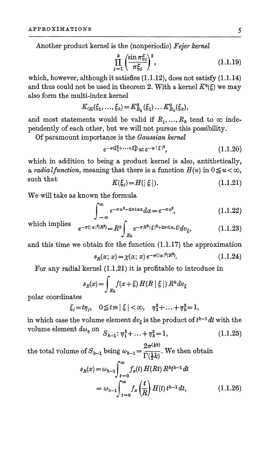
Another product kernel is the (nonperiodic) Fejer kernel
ft (*£)•. ,1.1.19)
which, however, although it satisfies (1.1,12), does not satisfy (1.1.14)
and thus could not be used in theorem 2. With a kernel K°(£) we may
also form the multi-index kernel
and most statements would be valid if Bli...iBk tend to oo
independently of each other, but we will not pursue this possibility.
Of paramount importance is the Gaussian kernel
e-^*--+fi»se-iriei,> (1.1.20)
which in addition to being a product kernel is also, antithetically,
a radial function, meaning that there is a function H(u) in 0 ^u < oo,
such that Kfa)=H{\£\). (1.1.21)
We will take as known the formula
f
e-7r^-27iiax^a==e-7rx^ (1.1.22)
which implies e_„(lM=RJ e_ffE^|2+2„-(a>a^ (LL23)
and this time we obtain for the function (1.1.17) the approximation
*.&(<*; a) =X(<*'> x) <r*(IalW). (1.1.24)
For any radial kernel (1.1.21) it is profitable to introduce in
**(*)« f /(*+g)#(*|£|)2**efof
J Eh
polar coordinates
g,=%, 0^t=|g|<co, 7|+...+7}=l,
in which case the volume element dvg is the product of t^"1 dt with the
volume element do)^ on ^ 2 , , 0 _ ,, _ _„.
* #*-i^i + ---+7l=l, (1.1.26)
2^**>
the total volume of /S^-a being ^fe,x= . We then obtain
1 (f k)
sR{x) = o)kT fx(t)H(Rt)RH^dt
J*=o
= w*_iJ^/» (|) HW **-1^ <LL26)
6
APPBOXIMATIONS
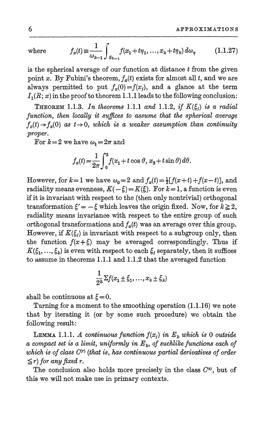
where /«,(*) s ffa+tyv ...,£&+%)<K (1.1.27)
is the spherical average of our function at distance t from the given
point x. By Fubini's theorem, /^(t) exists for almost all t, and we are
always permitted to put fx(Q) =/(%), and a glance at the term
ii(.R; x) in the proof to theorem 1.1.1 leads to the following conclusion:
Theobem 1.1.3. In theorems 1.1.1 and 1.1.2, if K(^) is a radial
function, then locally it suffices to assume that the spherical average
fx(t) ->/a;(0) as t->0, which is a weaker assumption than continuity
proper.
For h=2 we have ^x = 27r and
1 f2
/«(*)« ^ f{xx + t cos 0, z2+t sin 0) dd.
However, for &= 1 we have g>0=2 and/a;(t) = |[/(a:-ht)+/(a; — £)], and
radiality means evenness, K{ — £)=JT(£). For & = 1, a function is even
if it is invariant with respect to the (then only nontrivial) orthogonal
transformation g' = — £ which leaves the origin fixed. Now, for k g: 2,
radiality means invariance with respect to the entire group of such
orthogonal transformations and/^t) was an average over this group.
However, if JBT(^) is invariant with respect to a subgroup only, then
the function /(#+£) may be averaged correspondingly. Thus if
Jl(£1} ..., £fc) is even with respect to each £,5 separately, then it suffices
to assume in theorems 1.1.1 and 1.1.2 that the averaged function
2jtXf(x1±£1,...,xk±£k)
shall be continuous at £ = 0.
Turning for a moment to the smoothing operation (1.1.16) we note
that by iterating it (or by some such procedure) we obtain the
following result:
Lemma 1.1.1. A continuous function f(x^) in Ek which is 0 outside
a compact set is a limit, uniformly in Eh, of suchlike functions each of
which is of class C^ (that is, has continuous partial derivatives of order
g r) for any fixed r.
The conclusion also holds more precisely in the class O00, but of
this we will not make use in primary contexts.
APPBOXIMATIONS
7
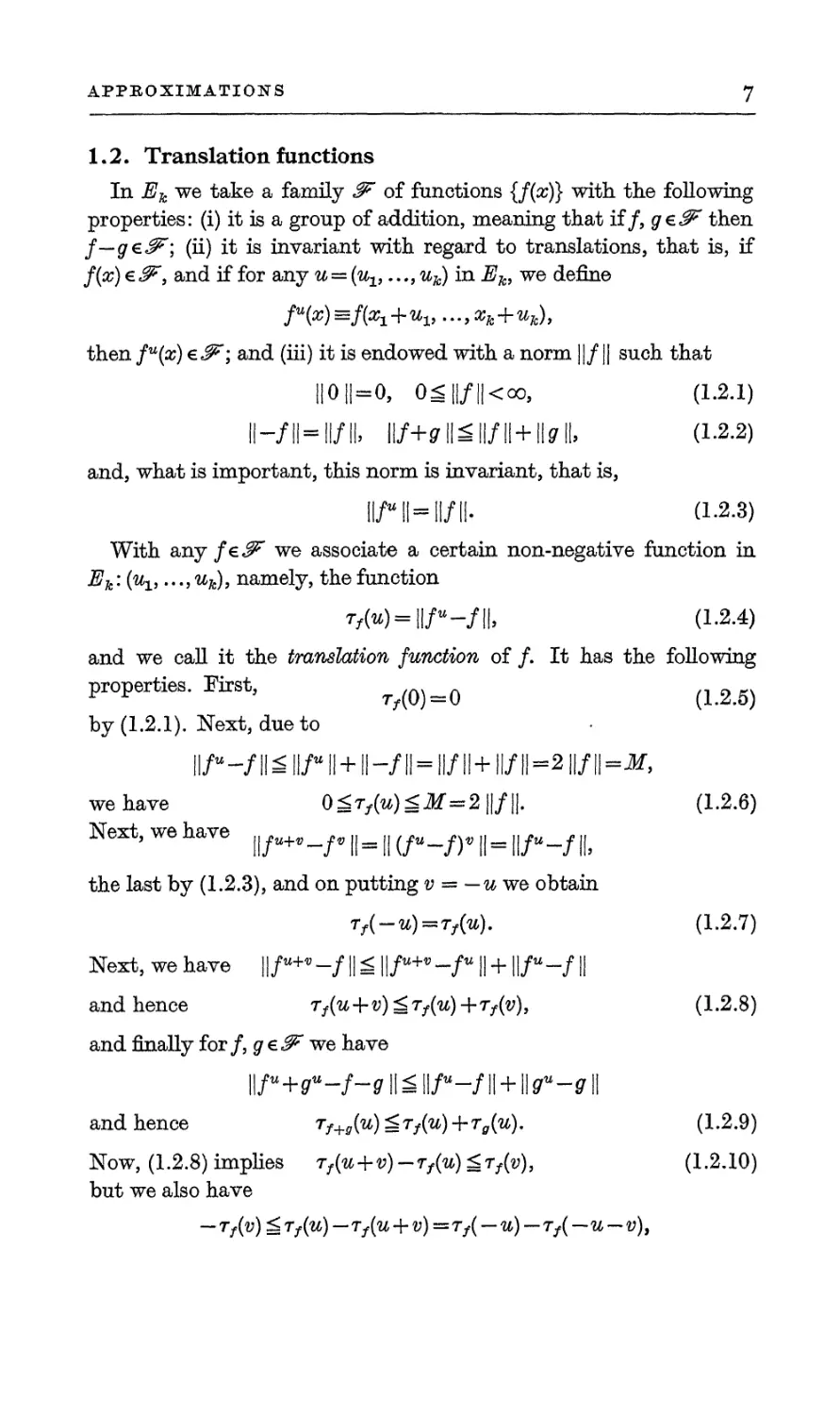
1.2. Translation functions
In Ek we take a family J5" of functions {/(#)} with the following
properties: (i) it is a group of addition, meaning that if/, g€#" then
/—g€j^; (ii) it is invariant with regard to translations, that is, if
f(x) € ^, and if for any u = (ul3..., uk) in Eki we define
fu(x) Es/fo+mx, ..., xk+uk),
then /"(a;) € J5"; and (iii) it is endowed with a norm ||/1| such that
110H = 0, 0£||/||<oo, (1.2.1)
11-/11=11/11, ll/+0ll^ll/ll+ll<7ll, (L2.2)
and, what is important, this norm is invariant, that is,
11/" 11=11/11- d-2.3)
With any/eJ^ we associate a certain non-negative function in
Ek:(%,..., uk), namely, the function
r,(w) = ||/«-/||, (1.2.4)
and we call it the translation function of /. It has the following
properties. First, tM = q (12 5)
by (1.2.1). Next, due to
\\f"-f\\£ Uu 11 +11-/11 = II/H+ ll/H=211/11=-^.
we have 0^rf(u) <M=21|/||. (1.2.6)
Next, we have ||/ll+.-/. ||= „ (ftt_f)v ||= ||/«_/||,
the last by (1.2.3), and on putting v = — w we obtain
rf(~u)~Tf(u). (1.2.7)
Next, we have \\f+* -/1| g ||/w+» -/* || + ||/"-f ||
and hence Tf(u+v)^Tf(u)+Tf(v), (1.2.8)
and finally for /, g € IF we have
ll/w+^-/-^ll^ll/w-/ll + llsrw^ll
and hence Tf+g(u)=Tf(u)+Ta(u)* (1.2.9)
Now, (1.2.8) implies Tf(u+v)-rf(u)£rf(v)9 (1.2.10)
but we also have
APPROXIMATIONS
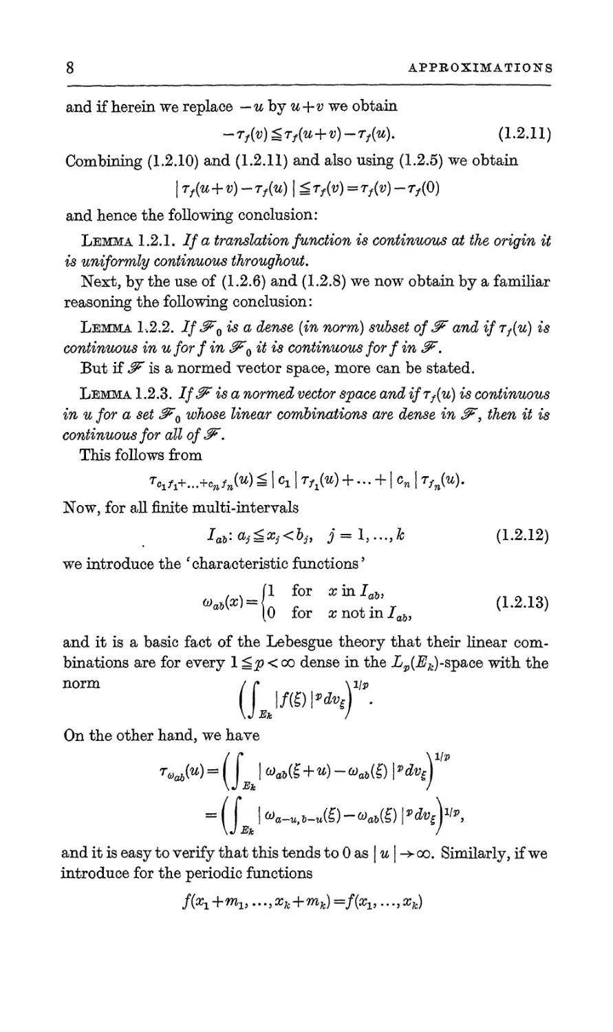
and if herein we replace —ubyu+vwe obtain
-t^St^+d)-^). (1.2.11)
Combining (1.2.10) and (1.2.11) and also using (1.2.5) we obtain
| Tf(U +1>) - Tf(u) | ^ Tf(v) = Tf(v) - Tf(0)
and hence the following conclusion:
Lemma 1.2.1. If a translation function is continuous at the origin it
is uniformly continuous throughout.
Next, by the use of (1.2.6) and (1.2.8) we now obtain by a familiar
reasoning the following conclusion:
Lemma 1,2.2. If<F0 is a dense (in norm) subset of IF and ifrf(u) is
continuous in u for fin !F§ it is continuous for f in IF.
But if W is a normed vector space, more can be stated.
Lemma 1.2.3. If ^ is a normed vector space and ifrf(u) is continuous
in u for a set JFQ whose linear combinations are dense in IF, then it is
continuous for all of IF.
This follows from
^Vi+.-.+W^) S\cx\ rfl{u) + - + K | Tfn(u)-
Now, for all finite multi-intervals
Ia'.ajgXjKbj, j=l,...,& (1.2.12)
we introduce the ' characteristic functionsJ
, . (1 for xmlabi
»a*(v)**L r , T L2-13)
(0 ior x not in Iab,
and it is a basic fact of the Lebesgue theory that their linear
combinations are for every 1 <p < oo dense in the Z^iSy-space with the
norm / /• \i/p
(Jj/B !•**)'
On the other hand, we have
{u)=(L,' wo>(^+m) ~a*®|s>^)1
and it is easy to verify that this tends to 0 as | u | -> oo. Similarly, if we
introduce for the periodic functions
f(x± +m1}...,xk+mk) =f(xl3...,xk)
APPROXIMATIONS
9
the Zr35(TA.)-norm
(L m |6^)1/3,=(Ll/(*+g) '^F'
then linear combinations of periodic functions of the form (1.2.13)
are again dense in norm. Hence the following conclusion:
Theorem 1.2.1. For functions in L^(E^) and (periodic) functions
f in Ly(Tk), l^p<co, the translation functions are (bounded) and
continuous.
We note that the general norm as defined by formula (1.L9) is
invariant with respect to translations, but we do not at all claim that
every function with a finite norm of this kind has a continuous rf(u).
However, if we take any set of functions {#"'} each of which is bounded
and uniformly continuous, and then form their smallest Banach
closure with respect to the norm for a set A of finite Lebesgue measure,
then their translation functions are continuous. If we choose for
{^"'} the simple exponentials
and for A the set Tfc, then the smallest closure is composed of the
almost periodic functions of the Stepanoff class Lp, to which we will
sometimes refer incidentally.
1.3. Approximation in norm
We will now state a certain proposition first in a general version
heuristically and then in a specific version precisely.
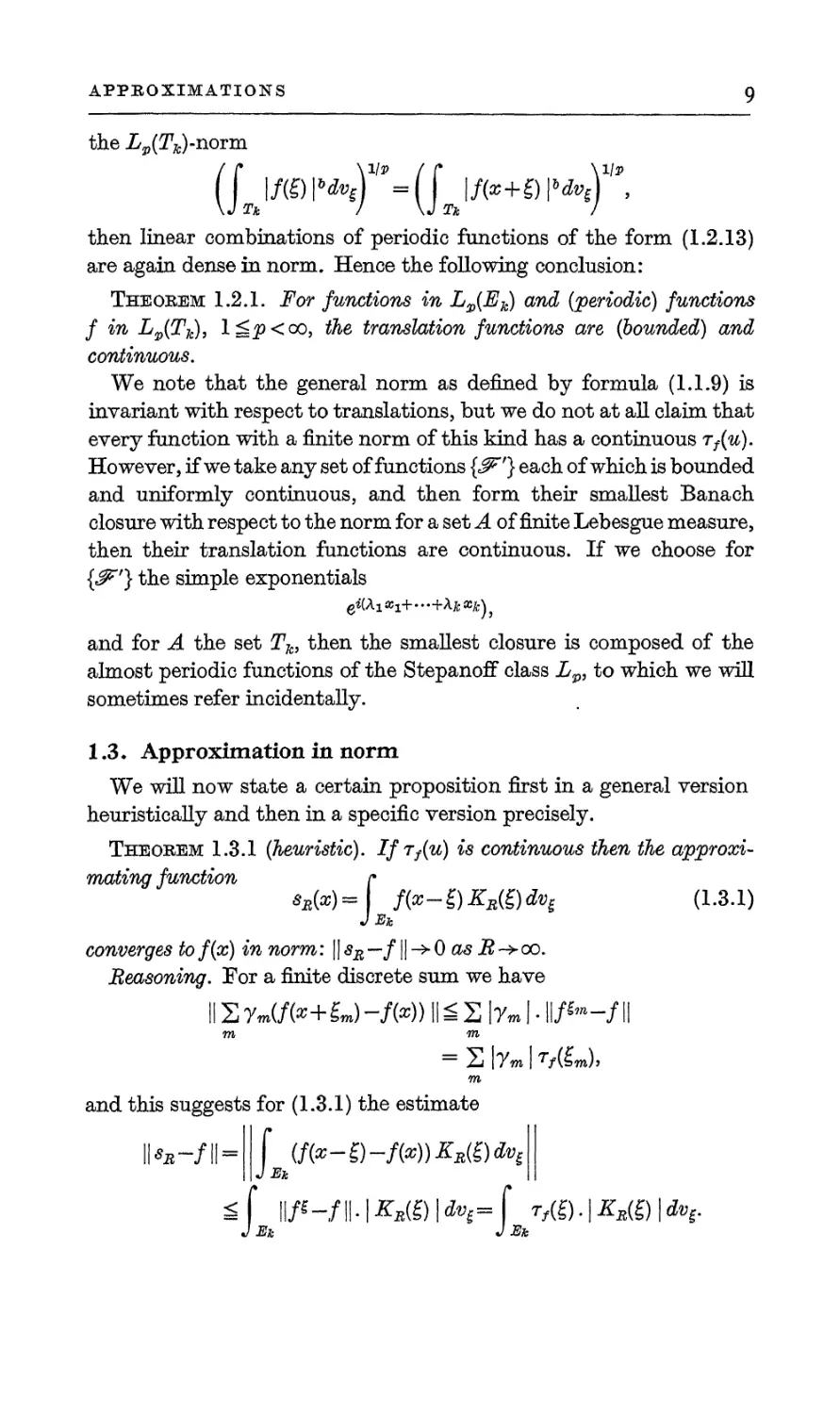
Theorem 1.3.1 (heuristic). If Tf(u) is continuous then the
approximating function r
Sr(x)=\ f(x-e)Zs®dve (1.3.1)
J Eh
converges to f(x) in norm: ||sR —/1| ->-0 as R->oo.
Reasoning. For a finite discrete sum we have
II Sym(/(*+gJ-/(*)) U 2 |y» I • 11/^-/11
m m
= S \7m | Tf(£tn),
m
and this suggests for (1.3.1) the estimate
II«*-f II = 11 I" (/(*-£)-/(*)) **(£)dvi11
IIJ Eh II
<;f ||/f-/||.|^(l)|^=f rM)-\KR(i)\dvt
J Eie J Eh
10
APPROXIMATIONS
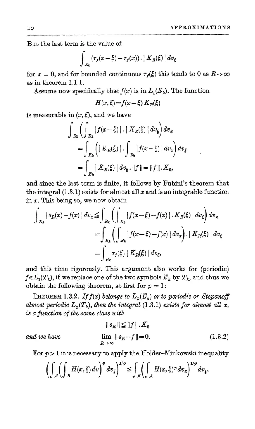
But the last term is the value of
{Tf{x-i)-rf{x)).\KB{i)\dvi
J E
1 Ek
for x = 0, and for bounded continuous 77(g) this tends to 0 as R ~» 00
as in theorem 1.1.1.
Assume now specifically that f{x) is in L-^E^). The function
#(*,g) =■/(*-!) *a(£)
is measurable in (x, E), and we have
f (f |/(*-0|.|tfa(£)|tfoeW
J ifo \J ■#& /
= (* (|JTa(£)|.f |/(*-£)|<WU£
J Ek \ J Ek I
I ^©|^.||/||= ||/||.Z0,
JjB
and since the last term is finite, it follows by Fubini's theorem that
the integral (1.3.1) exists for almost all x and is an integrable function
in x. This being so, we now obtain
f \*R(*)-M\dvm£{ (f \f{x-£)-f{x)\.KE{Z)\dv^\dvx
J Ek J Ek \J Ek J
=£ (J l/(*-SW(*)l*.)-l*a(£)l*e
= f TM)\K*(£)\dv£,
J Ek
and this time rigorously. This argument also works for (periodic)
feLx(Tk), if we replace one of the two symbols Ek by Tki and thus we
obtain the following theorem, at first for p = 1:
Theorem 1.3.2. Iff(x) belongs to Lp(Ek) or to periodic or Stepanoff
almost periodic Lv(Tk)9 then the integral (1.3.1) exists for almost all x,
is a function of the same class with
ll«B IIS 11/11. *0
and we have lim ||^—/|| = 0. (1.3.2)
R-*-co
For p > 1 it is necessary to apply the Holder-Minkowski inequality
{\a{\bH{X' £) ^P dV^lP ~LilAH{X' ®****)"**"*
APPROXIMATIONS
II
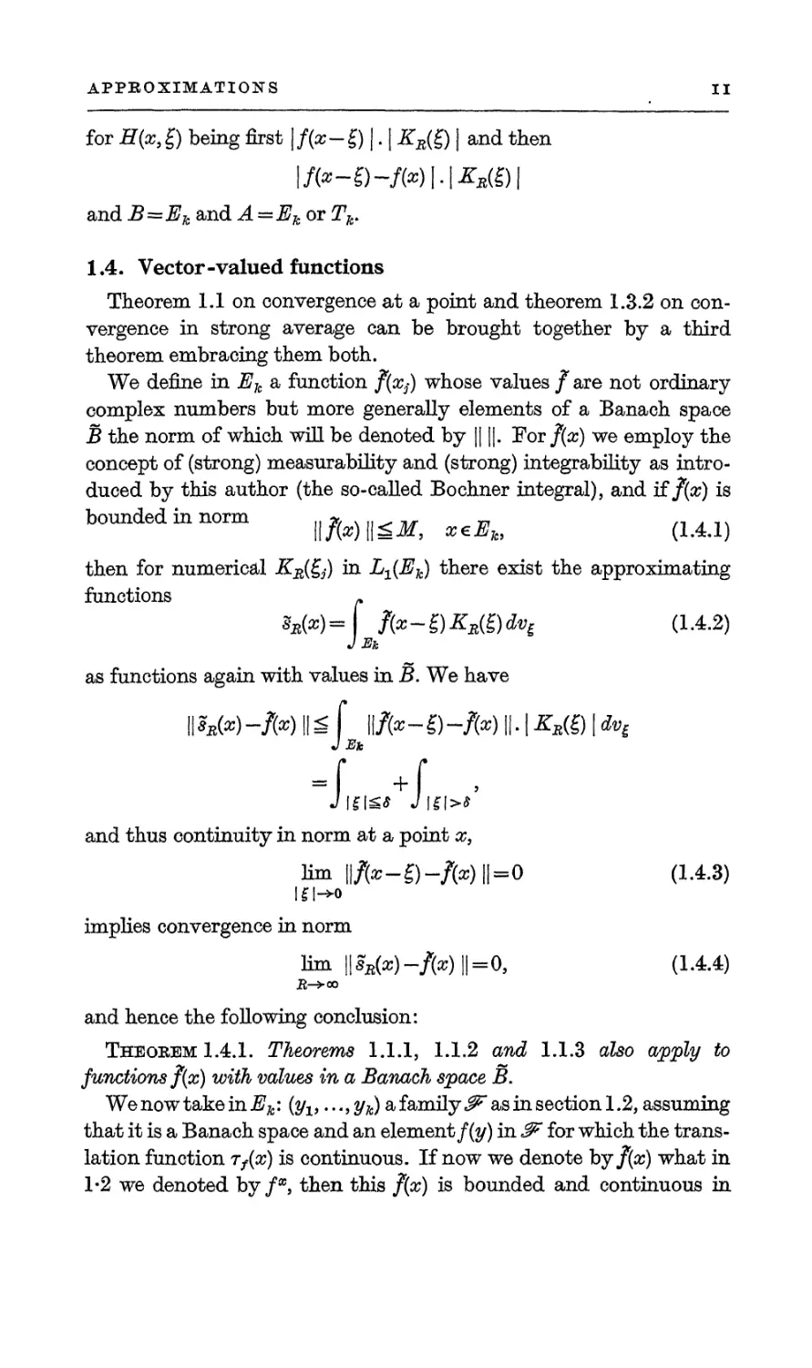
for H(x,g) being first |/(#—£) J. | KR{^) | and then
\f(*-$-f{z)\.\KR<&\
and B=Ek and A =j£fc or 2V
1.4. Vector-valued functions
Theorem 1.1 on convergence at a point and theorem 1.3.2 on
convergence in strong average can be brought together by a third
theorem embracing them both.
We define in Ek a function f{xs) whose values / are not ordinary
complex numbers but more generally elements of a Banach space
5 the norm of which will be denoted by || ||. For f(x) we employ the
concept of (strong) measurability and (strong) integrability as
introduced by this author (the so-called Bochner integral), and if f(x) is
bounded in norm *, ... _- _
\\J{x)\\^M, xeEk, (1.4.1)
then for numerical KR(^) in L±(Ek) there exist the approximating
functions .
**(*) = f{x~£)KR{mn (L4.2)
as functions again with values in B. We have
Pa(*)-/(*)ll = f ll/fc-fl-ftO II-!**(£) |«k{
and thus continuity in norm at a point x,
lim ||/(#-£)-/(z)||=0 (1,4.3)
implies convergence in norm
lim m*)-fa) 11=0, (1.4.4)
B->co
and hence the following conclusion:
Theorem 1.4.1. Theorems 1.1.1, 1.1.2 and 1.1.3 also apply to
functions f(x) with values in a Banach space B.
We now take mEk: (yv..., yk) a family W as in section 1.2, assuming
that it is a Banach space and an element f(y) in & for which the
translation function Tf(x) is continuous. If now we denote hjf(x) what in
1-2 we denoted by /*, then this /(#) is bounded and continuous in
12
APPROXIMATIONS
norm and thus falls under theorem 1.4.1. In a certain formal sense we
can write in (1.4.2)
where sR(y+x) is sR(x), and if our Banach norm is LJJE^ or the
periodic or almost periodic £p(jTfc) then this is rigorously so, for almost
all y> for any given fixed x, as can be realized by assuming first that
f(y) is a finitely valued function as in section 1.2 and then passing to
a limit in norm. But if this is so then relation (1.4.4), if applied at
x = 0, is simply \\sR(y)—f(y) ||->0 in the sense of theorem 1.3.2, and
thus theorem 1.3.2 appears likewise subsumed under theorem 1.4.1.
Now, the (heuristic) theorem 1.3.1 has also a (heuristic) converse
to the effect that if sR(x) converges in norm to f(x) then rf(u) is
continuous. But in the specific version in which we will establish this
rigorously, we will not start out from a point function at all but from
a (more general) set function, prove for it a ' weak' approximation by
sR(x)9 and then show that if this approximation is also a strong one
then the set function is the indefinite integral of a point function, and
Tf(u) is continuous.
1,5. Additive set functions
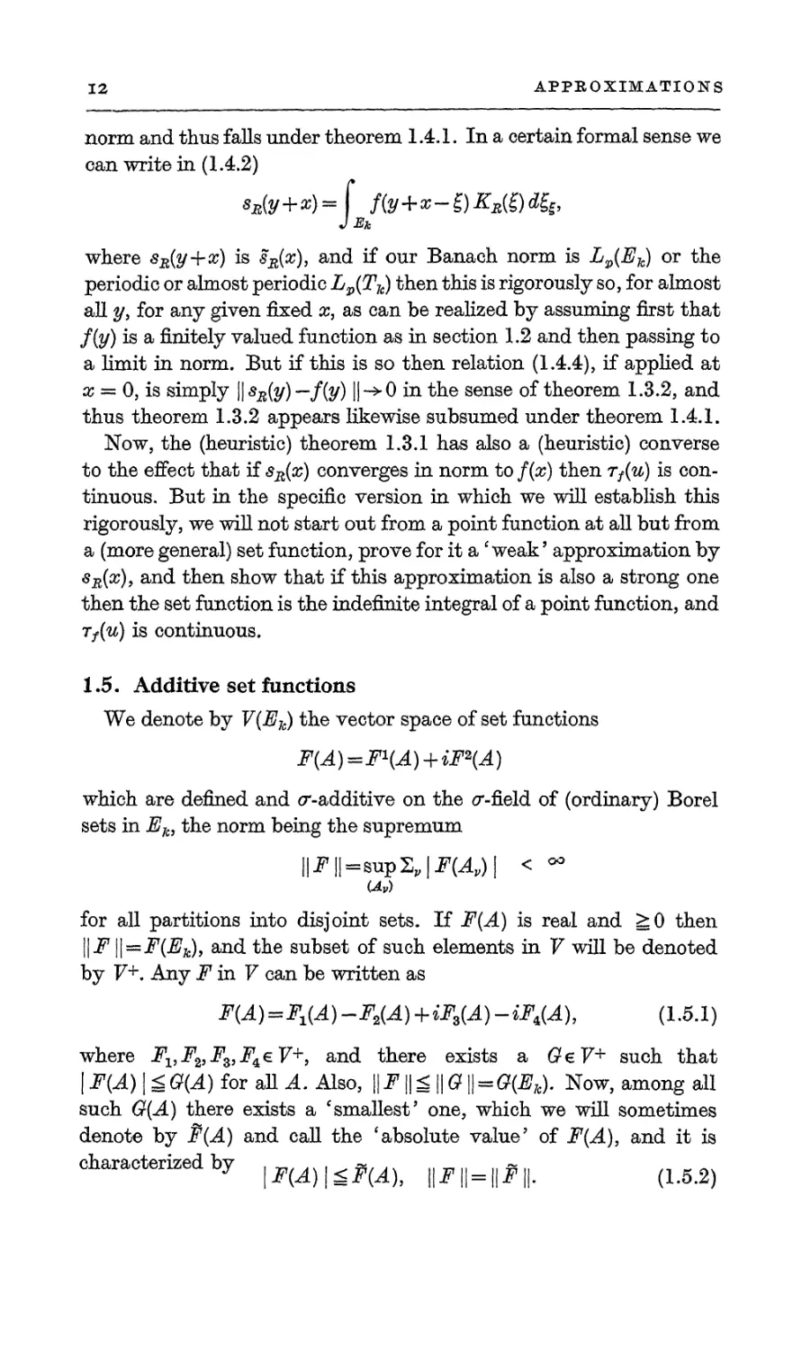
We denote by V{Ek) the vector space of set functions
F(A)=F1(A) + iF2(A)
which are defined and <r-additive on the a'-field of (ordinary) Borel
sets in Ek, the norm being the supremum
||F|| = SupS,|F(A,)| < -
Uv)
for all partitions into disjoint sets. If F(A) is real and 2^0 then
\\F II—jF(jB&), and the subset of such elements in V will be denoted
by F+. Any F in V can be written as
F(A)=Fl(A)-F,(A)+iF3(A)^iF,(A), (1.5.1)
where F1,F2,FZ,F^V+, and there exists a GeV+ such that
|F(A) \&Q(A) for aU A. Also, ||F\\£ \\G||-G(Ek). Now, among all
such G(A) there exists a 'smallest' one, which we will sometimes
denote by P(A) and call the 'absolute value' of F(A), and it is
characterized by j^,,^,, „,„_„*„. (L5jJ
APPROXIMATIONS
13
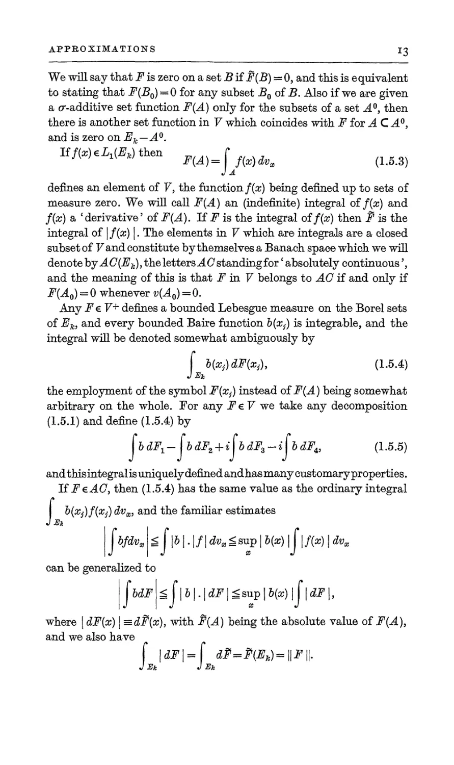
We will say that F is zero on a set B if F(B) — 0, and this is equivalent
to stating that F(B0) = 0 for any subset B0 of B. Also if we are given
a cr-additive set function F(A) only for the subsets of a set A0, then
there is another set function in V which coincides with F for A C A0,
and is zero on Eh—A°.
If/(*)el^)then F(A)=j/{x)dVx (L5.3)
defines an element of F, the function f(x) being defined up to sets of
measure zero. We will call F(A) an (indefinite) integral of f(x) and
f(x) a 'derivative' of F(A). If F is the integral of/(#) then F is the
integral of \f(x) |. The elements in V which are integrals are a closed
subset of V and constitute by themselves a Banach space which we will
denote by A C(Ek). the letters A 0 standing for' absolutely continuous',
and the meaning of this is that F in V belongs to AC if and only if
F(A0) = 0 whenever v(A0) = 0.
Any Fe V+ defines a bounded Lebesgue measure on the Borel sets
of Ek9 and every bounded Baire function b(Xj) is integrable, and the
integral will be denoted somewhat ambiguously by
f bfrddFfa), (1.5.4)
JEk
the employment of the symbol F(Xj) instead of F(A) being somewhat
arbitrary on the whole. For any FeV we take any decomposition
(1.5.1) and define (1.5.4) by
fbdF!- [bdFz + ihdFz-i[bdF^ (1.5.5)
and thisintegralis uniquely defined andhas many customary properties.
If FeAC, then (1.5.4) has the same value as the ordinary integral
b(xi)f{xj) dvx, and the familiar estimates
JJSjc
\jbfdvx\sj\b\.\f\dvx<suy\b(x)\j\f(x)\dvx
can be generalized to
I fbdFUf|b|.|dF|^sup|&^)|f|^F|,
where | dF(x) \ =dff(x), with P{A) being the absolute value of F(A),
and we also have
f \dF\= f dff=P(E!c)=\\F\\.
J Eh J Ek
H
APPROXIMATIONS
The following properties are of considerable importance:
Lemma 1.5.1. If F19 F2e 7, then Fi=F2. that is F1(A)=F2(A) for
all A, whenever * *
c(x) dFx(x) = c(x) dF2(x) (1.5.6)
J Eh J Ei
for every continuous c(x) which vanishes outside a compact set, and (by
lemma 1.1,1) it suffices to assume that c(x) belongs to class C^\ for some
fixed r.
Furthermore, if we are given F in V and a measurable function f0(x)
which is integrable (with regard to ordinary measure) over any compact
set and if we have » »
c(x)dF(x)=\ c(x)f0(x)dx
J Eh J Eh
for all such c(x), then FeAG andfQ(x) is its derivative.
Next, if Fv F2 in 7 have the same value in all' octants'
Ia:-cQ<Xj<aj, j=l,...,k, (1.5.7)
then Fx-sFg. On denoting F(Ia) by F(av ...,ak) we obtain a certain
point function F(x$) which is representative of F(A), and it is this
interpretation of the symbol F(x§) which may be read into the formula
(1.5.4). We will simply put F(xs) € 7, and we note, what is much used
in the theory of probability, that a function F(x$) is in 7+ if and only if
F(x1,...9xk)^F(y1,...,yk) for xx<>yXi...,xkSyk, (1.5.8)
and also £ (-l)t^'+t^F(yj+tj(x3—yj))^0)
F(xx-0,...,xk-0)^F(xx,...,xk), (1.5.9)
]imF(xv...,xk) = 0 if a?,--> —oo (1.5.10)
for a single index j, and
F( + co,..., +oo)s ||.F || <oo. (1.5.11)
We will now take two elements F, G in V and make statements
about them which we will explicitly discuss only if they are both in 7+,
relying on a decomposition (1.5.1) for both of them if they are not.
If we interpret F(A) as a measure in space Ek, and 0(B) as a measure
in a space E\> then on the Borel sets of the product space
E^ElxEl (1.5.12)
there is a product measure /i(C) such, that
fi(AxB)=F(A).G{B). (1.5.13)
APPROXIMATIONS
15
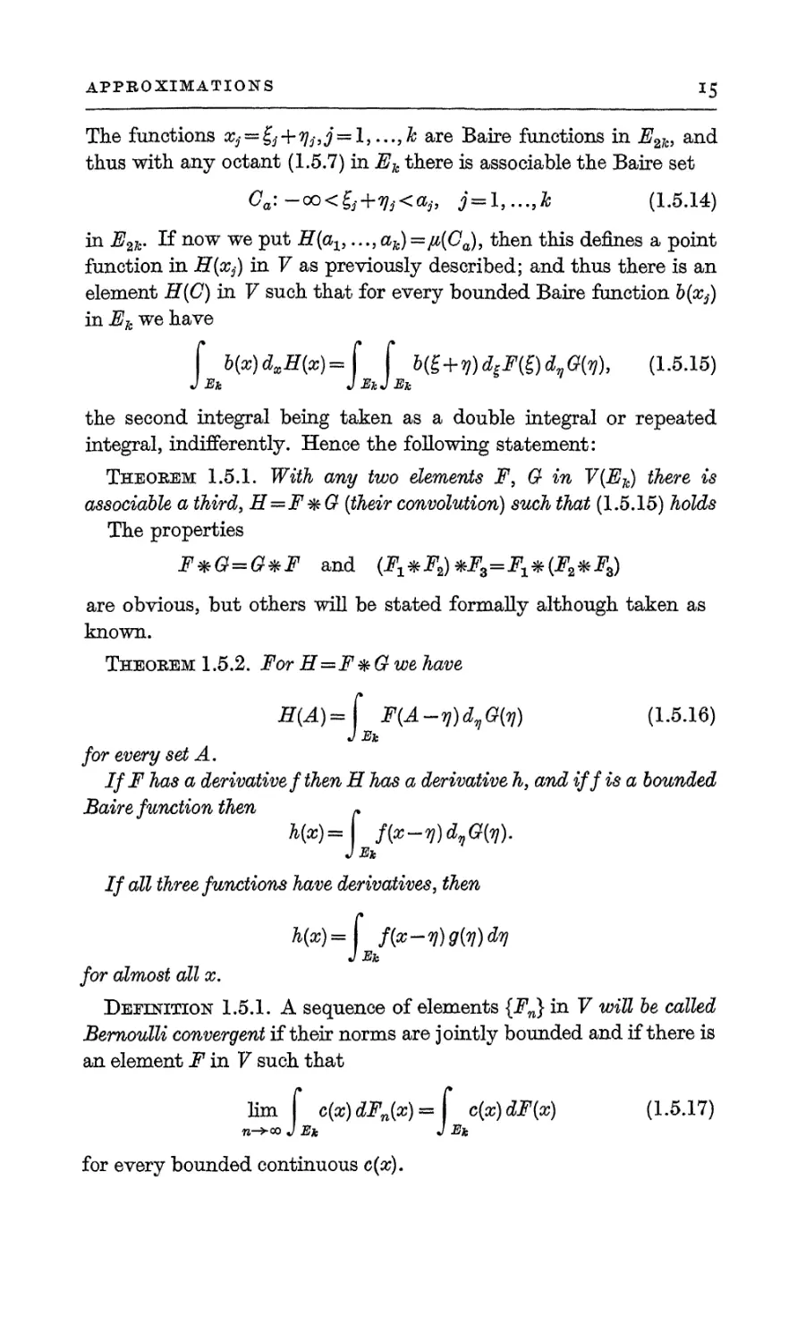
The functions ^ = £5+%.J==l.....& are Baire functions in E2k} and
thus with any octant (1.5.7) in Ek there is associable the Baire set
Ca:-co<^+Vt<^ i = l,...,* (1.5.14)
in E2k. 1^now we Pu^ H(av...,ak) =/i(Ca), then this defines a point
function in H(Xj) in V as previously described; and thus there is an
element H(G) in V such that for every bounded Baire function b(x^
in Ek we have
f b{z)d9H{x)=\ f Hi+V)diF(S)dvG(7j)9 (1.5.15)
J Ek J EkJ Ek
the second integral being taken as a double integral or repeated
integral, indifferently. Hence the following statement:
Theorem 1.5.1. With any two elements F, G in V(Ek) there is
associable a third, H=F*G (their convolution) such that (1.5.15) holds
The properties
F*G=G*F and (F1^F2)*F3=Fi^(F2^F3)
are obvious, but others will be stated formally although taken as
known.
Theorem 1.5.2. For H=F*Gwe have
H{A)=[ F(A-V)dvG(V) (1.5.16)
J Ek
for every set A.
IfF has a derivative f then H has a derivative h, and iff is a bounded
Baire function then »
h(x)=\ f(x-V)dnG{V).
J Ek
If all three functions have derivatives, then
h(x)=\ f(z-i))g{7i)di]
J Ek
for almost all x.
Defection 1.5.1. A sequence of elements {Fn} in V will be called
Bernoulli convergent if their norms are jointly bounded and if there is
an element F in V such that
lim f c(x)dFn{x)^\ c(x)dF(x) (1.5.17)
n-*<x> J Ek J Ek
for every bounded continuous c(x).
i6
APPROXIMATIONS
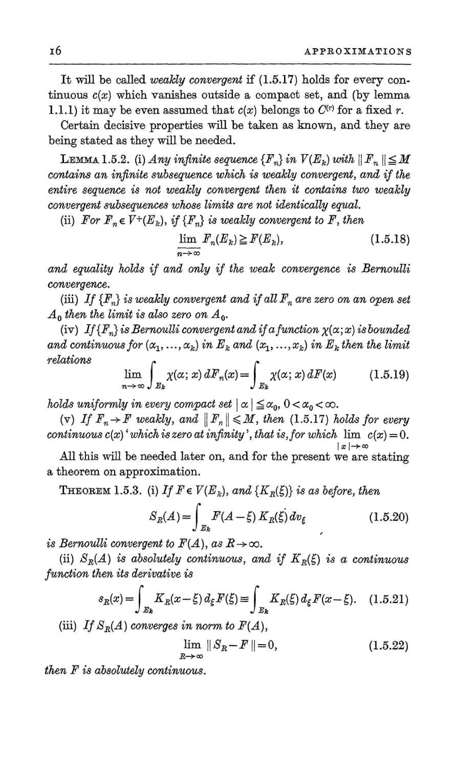
It will be called weakly convergent if (1.5.17) holds for every
continuous c(x) which vanishes outside a compact set, and (by lemma
1.1.1) it may be even assumed that c(x) belongs to C(r) for a fixed r.
Certain decisive properties will be taken as known, and they are
being stated as they will be needed.
Lemma 1.5.2. (i) Any infinite sequence {Fn} in V(Ek) with || Fn\\<>M
contains an infinite subsequence which is weakly convergent, and if the
entire sequence is not weakly convergent then it contains two weakly
convergent subsequences whose limits are not identically equal.
(ii) For Fn € V+(Ek), if {Fn} is weakly convergent to F, then
lim Fn(Ek)>F(Ek), (1.5.18)
and equality holds if and only if the weak convergence is Bernoulli
convergence.
(iii) If {Fn} is weakly convergent and ifallFn are zero on an open set
A0 then the limit is also zero on A0.
(iv) If{Fn} is Bernoulli convergent and if a function X(oc; x) is bounded
and continuous for {ocl9..., cck) in Ek and (xx,..., xk) in Ek then the limit
relations » *
lim X(a;z)dFn(x)=\ X(*;x)dF(z) (1.5.19)
rc-->oo J Ex J Ek
holds uniformly in every compact set \ a | ^ ocQ, 0 < oc0 < oo.
(v) IfFn-+F weakly, and \Fn\^M, then (1.5.17) holds for every
continuous c(x)' which is zero at infinity \ that is, for which lim c(x) = 0.
|a |->oo
All this will be needed later on, and for the present we are stating
a theorem on approximation.
Theorem 1.5.3. (i) IfFe V(Ek), and {KB{£)} is as before, then
^(A)=f F(A-^)KEa)dvi (1.5.20)
is Bernoulli convergent to F(A), as JR~>co.
(ii) 8R(A) is absolutely continuous, and if KR(£) is a continuous
function then its derivative is
**(*)=[ K1Az-g)deF®m f K^d^x-i). (1.5.21)
J Ek J Ek
(iii) IfSR(A) converges in norm to F(A),
lim ||SM-F || = 0, (1.5.22)
then F is absolutely continuous.
APPROXIMATIONS
17
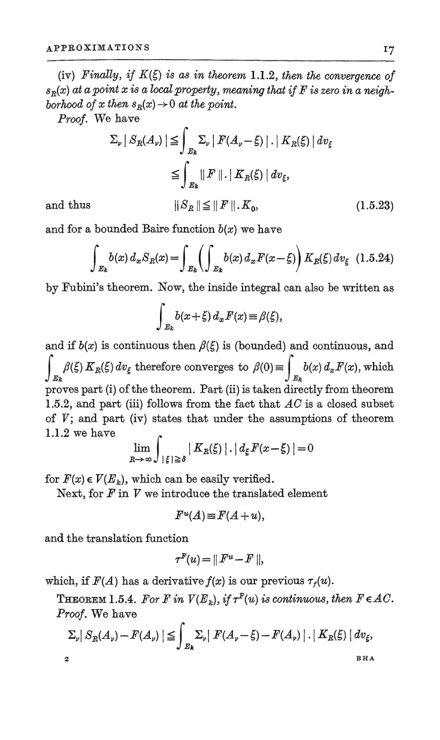
(iv) Finally, if K(^) is as in theorem 1.1.2, then the convergence of
$R(x) at a point xisa local property, meaning that ifF is zero in a
neighborhood of x then sR(x) -> 0 at the point.
Proof. We have
Z, I SR(A,) I £ f £„ I F{Ap-g) I. I KM) I d*e
J Eh
gf llPll.l^gJittoj,
and thus l|SJ,||g||J,||.Z'0l (1.5.23)
and for a bounded Bake function b{x) we have
f 6(*)d(B/Ss(»)=r (f &(*)«*-£))£*(£)<% (1-5.24)
J JET* J Ek\J Ek J
by Fubini's theorem. Now, the inside integral can also be written as
b(x + £)dxF(x)^M),
J E
I Ek
and if b(x) is continuous then /?(£) is (bounded) and continuous, and
/?(£) KR{i) dvg therefore converges to /?(0) s b(#) dxF(x), which
J $* J #*;
proves part (i) of the theorem. Part (ii) is taken directly from theorem
1.5.2, and part (iii) follows from the fact that AC is a closed subset
of V; and part (iv) states that under the assumptions of theorem
1.1.2 we have .
lim |i^(£)|.|<%F(z-£)|=0
for F(#) € V{Eh), which can be easily verified.
Next, for F in V we introduce the translated element
Fu(A)~F(A + u),
and the translation function
r*(w)=||Fw--F||,
which, if F(A) has a derivative f(x) is our previous rf(u).
Theorem 1.5.4. For F in V(Ek), ifTF(u) is continuous, then FeAC.
Proof. We have
S,| 8n{Av)-F{Av) IS f 2,| F{Av-i)-F{Av) \. \ KR{£) \ dvs,
J Eh
i8
APPROXIMATIONS
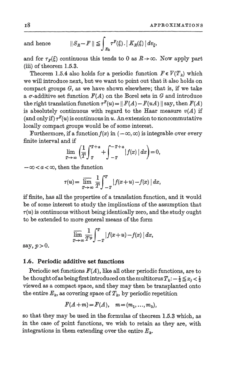
and hence \\SS-F\\ ^ I t*{1-).\Kr{1-) \dv£,
and for tf{E) continuous this tends to 0 as E->co. Now apply part
(iii) of theorem 1.5.3.
Theorem 1.5.4 also holds for a periodic function Fe V(Tk) which
we will introduce next, but we want to point out that it also holds on
compact groups 67, as we have shown elsewhere; that is, if we take
a <7-additive set function F(A) on the Borel sets in G and introduce
the right translation function rF(u) = || F{A) -F(uA) || say, then F(A)
is absolutely continuous with regard to the Haar measure v(A) if
(and only if) tf(u) is continuous in u. An extension to rioncommutative
locally compact groups would be of some interest.
Furthermore, if a function/(#) in ( — oo, oo) is integrable over every
finite interval and if
(I (*T+a r-T+a \
r\ + \m\dx)=o,
1 J T J -T I
—oo < a < oo, then the function
— l rT
t(u) = lim - | f(x + u) -/(a) | dx,
if finite, has all the properties of a translation function, and it would
be of some interest to study the implications of the assumption that
r(u) is continuous without being identically zero, and the study ought
to be extended to more general means of the form
^ -L\ !/(*+«)-/(*) I **.
say,#>0.
1.6. Periodic additive set functions
Periodic set functions F(A), like all other periodic functions, are to
be thought of as being first introduced on the multitorus Tk: — \ ^ Xj < |
viewed as a compact space, and they may then be transplanted onto
the entire Ek, as covering space of Tk, by periodic repetition
F(A+m)=F(A), m=K,...,mfc),
so that they may be used in the formulas of theorem 1.5.3 which, as
in the case of point functions, we wish to retain as they are, with
integrations in them extending over the entire Ek.
APPROXIMATIONS
If now we introduce the symbol V(Tk) to designate the periodic
cr-additive set functions (we will also employ the symbols AC(Tk),
V+(Tk), etc), then we can first of all state as follows:
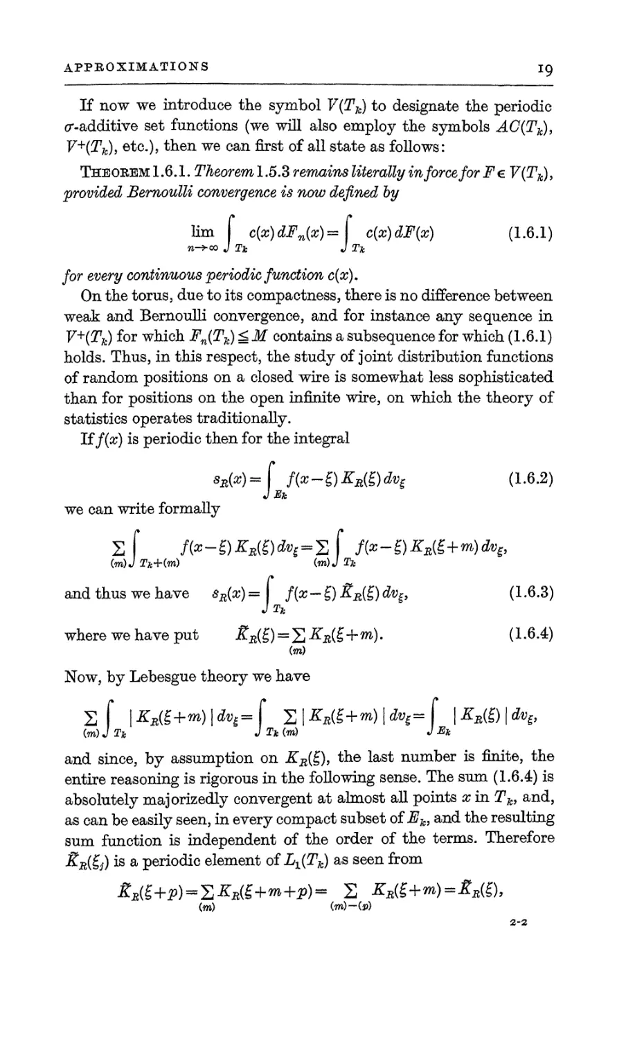
Theorem 1.6.1. Theorem 1.5.3 remains literally in force for F e V(Tk),
provided Bernoulli convergence is now defined by
lim c(x)dFn(x)^\ c(x)dF(x) (1.61)
n->co J Tk J Tk
for every continuous periodic function c(x).
On the torus, due to its compactness, there is no difference between
weak and Bernoulli convergence, and for instance any sequence in
V+(Tk) for which Fn(Tk) ^ M contains a subsequence for which (1.6.1)
holds. Thus, in this respect, the study of joint distribution functions
of random positions on a closed wire is somewhat less sophisticated
than for positions on the open infinite wire, on which the theory of
statistics operates traditionally.
If/(#) is periodic then for the integral
**(*)= f Kx-QK^dv^ (1.6.2)
J Eh
we can write formally
2 f /(* - g) **(£) dvs=2 f /(* - i) KR(i+m) d»e,
(m)J Tk+(m) (m)J Tk
and thus we have sR(x) = f(#—£) S.R(E) dvg, (1.6.3)
J Tk
where we have put J?it(.;) = S K^+m). (1.6.4)
On)
Now, by Lebesgue theory we have
2 f \KR(£+m)\dv^( S|^(g+m)|d^=f \KR(£)\dvi}
(m) J Tk J Tk (m) J Mk
and since, by assumption on KB(^), the last number is finite, the
entire reasoning is rigorous in the following sense. The sum (1.6.4) is
absolutely majorizedly convergent at almost all points x in Tki and,
as can be easily seen, in every compact subset of Ek, and the resulting
sum function is independent of the order of the terms. Therefore
%r(£j) is a periodic element of Lx(Tk) as seen from
(m) (w)—(p)
2-2
20
APPROXIMATIONS
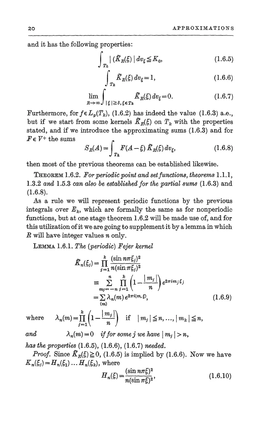
and it has the following properties:
(i^(£)|^£o> (1-6-5)
/.
Tk
f KR£)dvz=l, (1.6.6)
lim [ &R(g)dvi=0. (1.6.7)
Furthermore, for feL!P(TJC)) (1.6.2) has indeed the value (1.6,3) a.e.,
but if we start from some kernels RE(£) on Tk with the properties
stated, and if we introduce the approximating sums (1.6.3) and for
FeF+the sums .
SR(A)~\ F(A~£)KRtt)dvE, (1.6.8)
then most of the previous theorems can be established likewise.
Theobem 1.6.2. For periodic point and set functions, theorems 1.1.1,
1.3.2 and 1.5.3 can also be established for the partial sums (1.6.3) and
(1.6.8).
As a rule we will represent periodic functions by the previous
integrals over Ek9 which are formally the same as for nonperiodic
functions, but at one stage theorem 1.6.2 will be made use of, and for
this utilization of it we are going to supplement it by a lemma in which
jR will have integer values n only.
Lemma 1.6.1. The (periodic) Fejer kernel
ft /ex- A (sin^TT^)2
^^^/A^sin^-)2
Wj= —n 5—1 \ n J
= SA»e2*^, (1.6.9)
(m)
where A» = n l-1—— I if |% | <£n,..., \mk \ £n,
and An(m) = 0 if for some j we have | % | > n,
has the properties (1.6.5), (1.6.6), (1.6.7) needed.
Proof. Since jS^g) ;> 0, (1.6.5) is implied by (1.6.6). Now we have
JU&)«#«&)...#»(&), where
(sinnflf)2 /ift1A\
H-(0-J^gji' (L6-10)
APPBOXIMATIONS
21
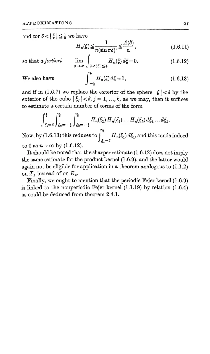
and for 8< | £ | ^ \ we have
sothatajfbrtion lim .ffn(g)eZ£=0. (1.6.12)
We also have j Hn(£) dg = 1, (1.6.13)
and if in (1.6.7) we replace the exterior of the sphere | g | <S by the
exterior of the cube \£j\<S,j — l9...,k9 as we may, then it suffices
to estimate a certain number of terms of the form
f P f ffn(fl) #»(&) • • • Hn{i-k) d£± ... d£7c.
Now, by (1.6.13) this reduces to Hn(£i) d£v an(i this tends indeed
to 0 as n->oo by (1.6.12).
It should be noted that the sharper estimate (1.6.12) does not imply
the same estimate for the product kernel (1.6.9), and the latter would
again not be eligible for application in a theorem analogous to (1.1.2)
on Tk instead of on Ek.
Finally, we ought to mention that the periodic Fejer kernel (1.6.9)
is linked to the nonperiodic Fejer kernel (1.1.19) by relation (1.6.4)
as could be deduced from theorem 2.4.1.
22
CHAPTER 2
FOURIER EXPANSIONS
2.1. Fourier integrals
For the present we will introduce Fourier integrals only for functions
Lx{Ek) and more generally V(Ek), but not for Lj,(Ek)9 p>l, except
that we will summarize statements on Plancherel transforms for
functions L2(Ek) whose theory we will take as known. However, when
introducing Fourier series, we will envisage Lp-classes in general
because it takes very little effort to do so.
If Fe V(Ek), we can introduce the Fourier transform
${a)s<f>F(as)=\ e-^^dFix), (2.1.1)
J Eh
and it is trivial that it is a bounded function,
H{*)U\\F\\, (2.1.2)
and it is also very easy to see that it is uniformly continuous for (a5)
in Ek. If F has a derivative / we will also write
^(ct) = ^/(ct.)==r e-*"*«>*)f(x)dvx. (2.1.3)
J Ek
Theorem 2.1.1. IfF9 67e V(Eh) and H=F*G, then
^K-) = ^K).^(%), (2.1.4)
that is, the transform of a convolution is the product of the transforms.
In particular, iff, geLv then
&(*) = &(«) 0,(a), (2.1.5)
where h(x)=\ f{x~y)g{y)dvyi (2.1.6)
J Ek
the integral existing almost everywhere.
Proof. Put b(x)=e-2ni^^ in formula (1.5.15).
Theorem 2.1.2. IfF,Qe V, and
0(a,)= (V2™^>dF(£), f(Q= te*««£>*>dG(*), (2.1.7)
then \<j>((x)eW>*»dG(a)« fVfc-f)dF(£). (2.1.8)
FOURIER EXPANSIONS
23
Proof. Since
jje**«*>-£>dG{*)dF(g) U jjl«?(«) | -1 dF® | = || 01|. ||F || <oo,
it follows by Fubini's theorem that the integral
eW*.»-&dG(<x,)dF(!z)
!!•
exists, and relation (2.1.8) expresses the equality of the two repeated
integrals by which it can be evaluated.
In the next theorem a function 8(0.3) will be called a convergence
factor if .
\$fa)\dva<co, (2.1.9)
J Ek
and if for its (anti) -transform
#(£.)-= f e^^a)d(a)dva
J Ek
we have | | £(£,) | <fof < oo, \ K^dv^l. (2.1.10)
J E J Ek
Now, the corresponding transform of S(oc^B) is BkK(Bi;1>...,Bi;k),
and if in theorem 2.L2 we put for 67(A) the indefinite integral of Sfa),
then the theorems of chapter 1 imply as follows:
Theorem 2.1.3. The integrals (2.1.3) and (2.LI) can be inverted to
f(x)~\ e27ri^^^>f(oc)dva (2.1.11)
JEh
and F(A)-f dJ"T e**^>a>0*(a)dfoj (2.1.12)
in the following sense:
(i) For any convergence factor 8(a) the approximating function
sR(x)=( $(^eW*>*)<f>f(oc)dva (2.1.13)
converges in norm tof(x),
Km f \f(x)-sR(x)\dvx-0, (2.1.14)
and for the approximating function
**(£)=[ *(^)ea^*^(a)efoa (2.1.15)
24
EOURIER EXPANSIONS
the indefinite integral SR(A)= sR(x)dvx is Bernoulli convergent
J a
to F(A).
(ii) For f(x) bounded, the convergence of sR(x) at a point x is a local
property, and for anyfeLv or even FeV, it is so if
\K(g)\£C(l + (£)"rp)-1l
and in either case, sR(x) ->f(x) iff(%) is continuous at x, and for a radial
K(E) only the spherical average off(^) around x need be continuous at x.
For us the dominant convergence factor will be e~nl a|2 (and not the
Abelian factor eHal) and we are going to utilize the corresponding
sums /•
sR(x)= e-"«aVR2hW*'«tyF(oc)dva (2.1.16)
JEk
for several purposes. If Fls F2eV have equal transforms, then for
F=F1 — F2we have <j>F(cx) — 0, and hence sR(x)=0. But the Bernoulli
limit of a null function is a null function, and thus part (i) of theorem
2.1.3 implies the following uniqueness theorem:
Theorem 2.1.4. If <j>Fi{cx) = (j)F^(x), then FxsF2. If <f>fl(cc)=s$f%{a)
thenfx(x) =/2(^) a.e.
Next, assume that for F in V it so happens that
I \ </>*{(*) \dva<co. (2.1.17)
JEk
Since | e-*«a '2^2) e27**a> | ^ 1 and e-*<"a ' W ~> 1 as R -> oo, the functions
(2.1.16) are then convergent, locally uniformly, towards the function
f0(x) = j eW- a> <f>F{a) dvai (2.1.18)
JEk
and for any continuous c(x) which vanishes outside a compact set
we have _
c(x)sR(x)dva->\ c(x)f0(x)dvx.
J Elc J Ek
However, again by theorem 2.1.3 we have
c(x) sR(x) dva -* c(x) dF(x),
J Ek J Ek
and by the second half of lemma 1.5.1 we obtain the following
conclusion:
Theorem 2.1.5. If for F in V, the transform <j>F(<x) is in 1^(18 m), then
FOURIER EXPANSIONS
25
F(A) is the indefinite integral of the continuous function fQ(x) as given
by the inversion formula (2.LI8).
In particular, iff^Lx and ^f(oc)eLv thenf is a.e. equal to the
continuous function
f0(x)=\ e2^>«>^(a)dv (2.L19)
J 32*
As an incidental application of this theorem we note that a
convergence factor 8(a) as previously introduced may be assumed to be
continuous to start with, in which case it is given by
8(a) =f &-*«**>&K(&)dvs,
J Ek
so that in particular £(0) = L This being so, we will now give the
actual formal definition of a convergence factor.
Definition 2. LI. A convergence factor 8(a) as was used in theorem
2.1.3 is a function with the following properties: 8(a) is continuous and
8(0) = 1, and 8(cc)eLv and its Fourier transform is in Lx.
2.2. Positive transforms. Plancherel transforms
Theorem 2.2.1. If for feL± we have fif(oc)^0, and \f(x) \ ^M for
\x\Sto (that is, if f has a positive transform and is bounded in the
neighborhood of the origin) then <pf^a)eLx andf(x) is equal to the function
/0(s) (see 2.1.19).
This theorem is obviously contained in the following one.
Theorem 2.2.2. IfforFe V we have <f>F(a) ^ — #(a), where #(a) £> 0,
X(oc) eLv and if we have
kcJi
dm)
<M19 Q<t<ao, ' (2.2.1)
or only LB* e~^^dF(i
Jltfl-Si
SM2i (2.2.2)
then <pF(a)eLli and F(A) is the indefinite integral of the function f0(x)
givenby (2.1.18).
Proof. We note that due to ||F || <oo, (2.2.1) is satisfied automatically
for J t J £ 1. Next, (2.2.2) is indeed at least as general as (2.2.1), this
being an abelian theorem, since, if we put G(t) = dF(£), so that
26
EOUR.IER EXPANSIONS
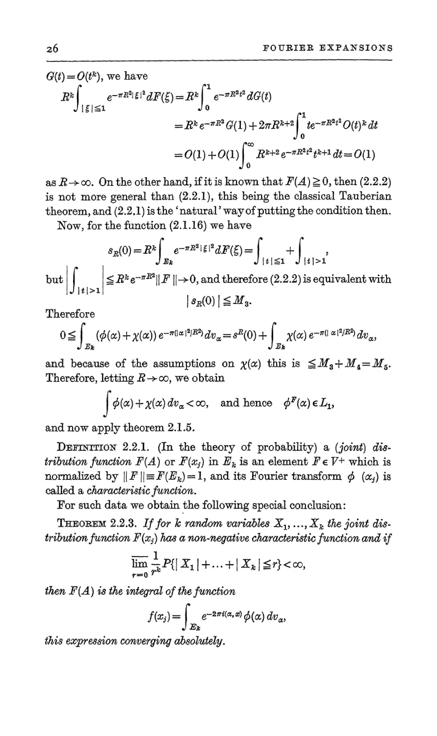
<?(t)^0(tfc),wehave
W f e-"W^dF(£)=Bk P e~"RH*dG(t)
=*R*e~*#G(l) + 2tt^+2f te~"RH20(t)kdt
= 0(l)+0(l)fC0^+2e~^2i2tft+1dt-0(l)
as i?-> oo. On the other hand, if it is known that F(A) ^ 0, then (2.2.2)
is not more general than (2.2.1), this being the classical Tauberian
theorem, and (2.2.1) is the 'natural'way of putting the condition then.
Now, for the function (2.LI6) we have
8B(0)=R*{ e-^i2dF(£)=f +f ,
J Ek J |*|^1 Jl*l>l
l r l
but ^JRfce-7rJR2||F||->0,andtherefore(2.2.2)isequivalentwith
|J|*l>i|
\sR(0)\£Mz.
Therefore
0 £ f (<f>(oc) + #(a)) 6-^>a iWdva=sR(0) + f Z(a) e-»«aI W> dva,
and because of the assumptions on %(a) this is SMZ+M^=MS.
Therefore, letting B~+oo, we obtain
(j> (a) -f #(a) dva < oo, and hence ^(a) € 1^,
and now apply theorem 2.1.5.
Definition 2.2.1. (In the theory of probability) a (joint)
distribution function F(A) or F(%) in Ek is an element FeV+ which is
normalized by \\F\\=F(Ek) — li and its Fourier transform <f> (<x,3) is
called a characteristic function.
For such data we obtain the following special conclusion:
Theoeem 2.2.3. If for h random variables Xv ...,Xfc the joint
distribution function F(xj) has a non-negative characteristic function and if
ltoip{|Z1| + ... + |Xj5|gr}<oo,
ra*o r
then F(A) is the integral of the function
/to)=f e~w>*><f>(a)dvai
this expression converging absolutely.
FOURIER EXPANSIONS 27
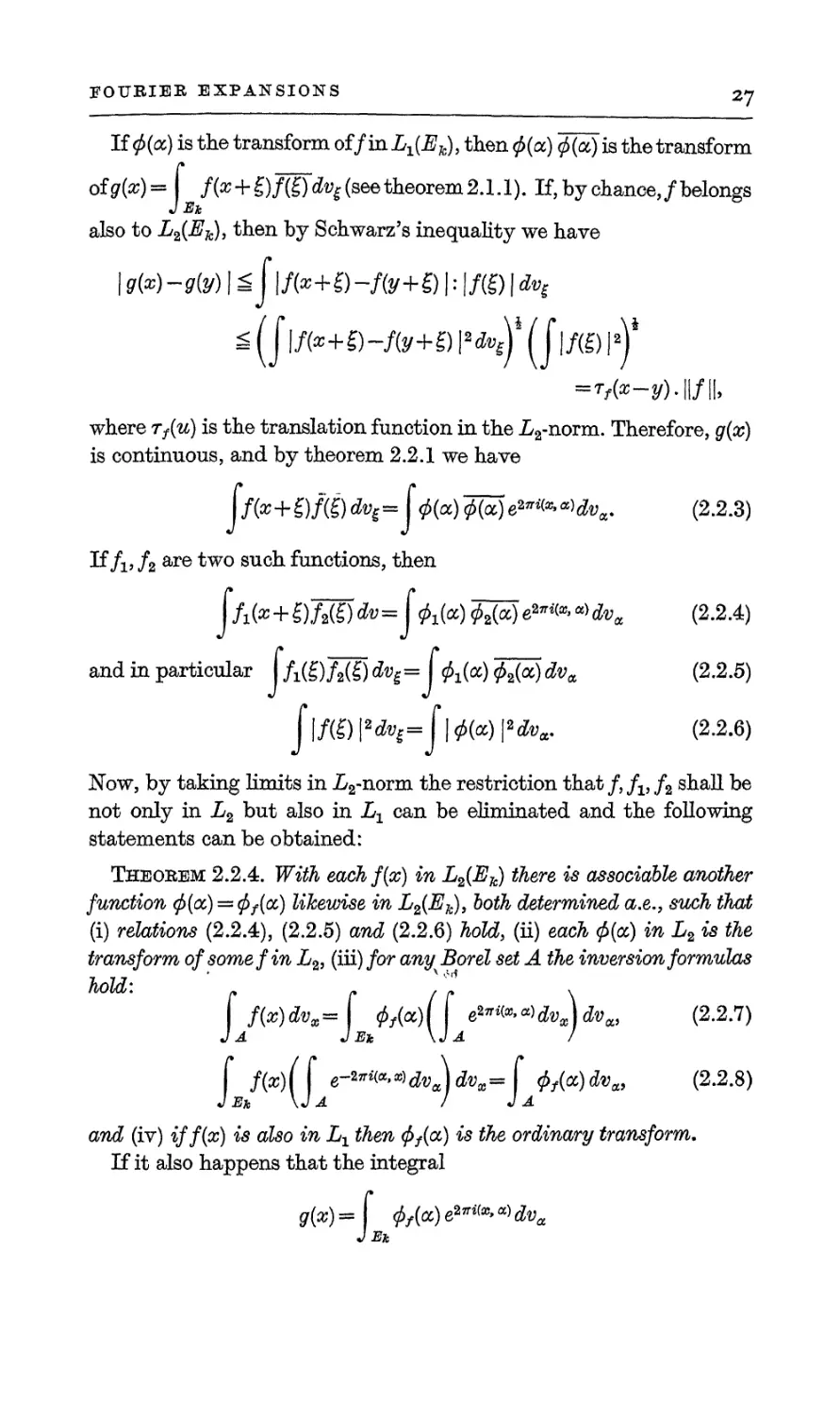
If 0(a) is the transform offiaL^Ej,), then 0(a) 0(a) is the transform
ofg(#)= /(ic + g)/(g)d^(seetheorem2.1.1), If, by chance,/belongs
J Ek
also to L2(Ek), then by Schwarz's inequality we have
I g(x) -g(y) \ S j |/(*+g) -/(y+© |: |/(g) [ A%
^ (J|/(a,+fl-/(jf+£) |2d^ (J|/(g) |«)*
=T/(*-y).||/ll.
where r/w) is the translation function in the L2-norm. Therefore, g(x)
is continuous, and by theorem 2.2.1 we have
!f(x+^)M)dvi=U(oc)W)e^i^Mv^ (2.2.3)
If fl9 /2 are two such functions, then
J/i(* + g)jWl)*= f &(*) 0^2^">d^ (2.2.4)
and in particular A(g)^(|) (tog = &(a) 02(a) dva (2.2.5)
J|/(g)|aetof-J|0(a)|8efoa. (2.2.6)
Now, by taking limits in L2-norm the restriction that /, fl3 f2 shall be
not only in L2 but also in Lx can be eliminated and the following
statements can be obtained:
Theorem 2.2.4. With eachf(x) in L2(Ek) there is associable another
function 0(a) = 0/(a) likewise in L2(Ek), both determined a.e., such that
(i) relations (2.2.4), (2.2.5) and (2.2.6) hold, (ii) each 0(a) in L2 is the
transform of some fin L2, (iii) for any Borel set A the inversion formulas
hold: « f / f \
I f(x)dvm=\ 0y(a)( e»^«)(toBW, (2.2.7)
J A J Ek \J A J
f f(x)({ e~W>*)dv^)dvx~f 0y(a)aX, (2.2.8)
J Ek \J A I J A
and (iv) iff(x) is also in Lx then 0y(a) is the ordinary transform.
If it also happens that the integral
g(z)=\ <pf(oc)e*"i(*>°*dva
J Ek
28
FOURIER EXPANSIONS
is boundedly convergent, say, and if we integrate both sides with
respect to a set A and compare with (2.2.7), we obtain
f(x)dva= g(x)dvx,
J A J A
so that/(a;) ~g(x) ax.
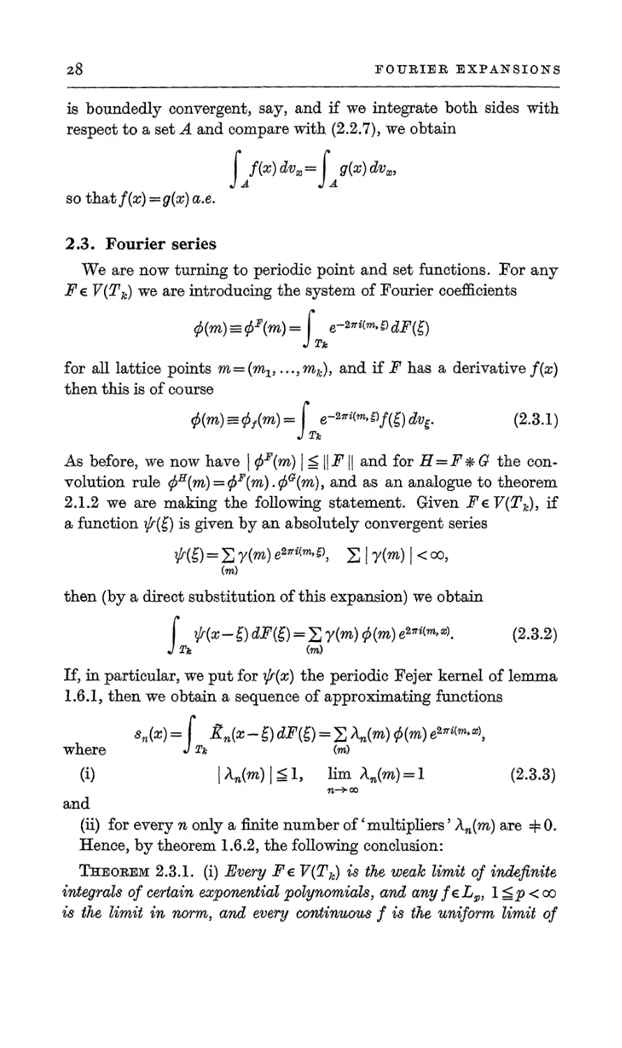
2,3. Fourier series
We are now turning to periodic point and set functions. For any
F € V(Tk) we are introducing the system of Fourier coefficients
0(m)s0*(m)=f e-w^adFig)
J Th
for all lattice points m=(mv ...,mk), and if F has a derivative f(x)
then this is of course
0(m)==^(m)== f e-tottoafffidvg. (2.3.1)
J Th
As before, we now have | <pF(m) \S\\F\\ and for H=F*G the
convolution rule <p3S(m) = <pF(m).<f>G(m), and as an analogue to theorem
2.1.2 we are making the following statement. Given FzV(Tk), if
a function \[r{£) is given by an absolutely convergent series
M) = S 7M e2**^, £ | y(m) \ < oo,
(w)
then (by a direct substitution of this expansion) we obtain
f ^(cr-^dF^^SrW^^)^^^ (2.3.2)
J Th (m)
If, in particular, we put for ijf(x) the periodic Fejer kernel of lemma
1.6.1 j then we obtain a sequence of approximating functions
sn(x) = f Sn(x-g) dP(£) = £ Ajm) 0(m) a*****,
where J i* (m)
(i) | A„(m) | g 1, lim A„(m) = 1 (2.3.3)
tt->00
and
(ii) for every n only a finite number of' multipliers' Xn{m) are =f= 0.
Hence, by theorem 1.6.2, the following conclusion:
Theorem 2.3.1. (i) Every Fe V(Tk) is the weak limit of indefinite
integrals of certain exponential polynomials, and any feL^, I<p<co
is the limit in norm, and every continuous f is the uniform limit of
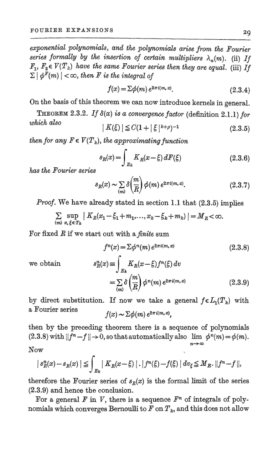
FOURIER EXPANSIONS
20
exponential polynomials, and the polynomials arise from the Fourier
series formally by the insertion of certain multipliers Xn{m). (ii) If
Fv F2e V{Tk) have the same Fourier series then they are equal, (iii) if
S I <f>F(m) I < 00, then F is the integral of
/(#) = 20(m) e27ri^x\ (2.3.4)
On the basis of this theorem we can now introduce kernels in general.
Theorem 2.3.2. Ifd(oc) is a convergence factor (definition 2.1.1)/or
whichalso |Z(fl|SO(l + |fr^ (2.3.5)
then for any Fe V(Th), the approximating function
«*(*)= f KR(cc-£)dF(£) (2.3.6)
J Eh
has the Fourier series
(m\
-U(m)e2^*>. (2.3.7)
KJ
Proof. We have already stated in section 1.1 that (2.3.5) implies
S sup \K^-£i+^>->->Vk-£k+™k)\=MB<co.
(m) x,£<=Tk
For fixed E if we start out with & finite sum
fn(x)=E0w(m) e2*'<w' *> (2.3.8)
we obtain s\(x) = | KR(x-£)fn(£) dv
JEk
(m) W
(m)e2;rz(m,cr) (2.3.9)
by direct substitution. If now we take a general feL^T^ with
a Fourier series ... „ ,, , 9.. ^
then by the preceding theorem there is a sequence of polynomials
(2.3.8) with ||/n -/1| -> 0, so that automatically also lim <j>n{m) = 0(m).
Now
J-Eft
therefore the Fourier series of sR(x) is the formal limit of the series
(2.3.9) and hence the conclusion.
For a general F in V, there is a sequence Fn of integrals of
polynomials which converges Bernoulli to F on Tk, and this does not allow
30
FOURIER EXPANSIONS
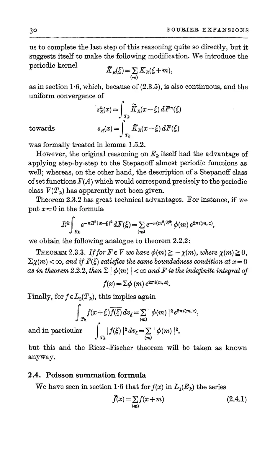
us to complete the last step of this reasoning quite so directly, but it
suggests itself to make the following modification. We introduce the
periodic kernel «) = S^+m),
(m)
as in section 1-6, which, because of (2.3.5), is also continuous, and the
uniform convergence of
J Tk
towards sR(x) = KR(x - g) AF(£)
J Tk
was formally treated in lemma 1.5.2.
However, the original reasoning on Eh itself had the advantage of
applying step-by-step to the Stepanoff almost periodic functions as
well; whereas, on the other hand, the description of a Stepanoff class
of set functions F(A) which would correspond precisely to the periodic
class F(Tfc) has apparently not been given.
Theorem 2.3.2 has great technical advantages. For instance, if we
put x = 0 in the formula
J Bk (w)
we obtain the following analogue to theorem 2.2.2:
Theorem 2.3.3. IfforFe V we have <f>(m) £ — x(w>), where #(m) ;> 0,
S^(rn) < oo, and ifF(£) satisfies the same boundedness condition at # = 0
as in theorem 2.2,2, then 2 | <fi(m) | < oo and F is the indefinite integral of
Finally, forf€L2(Tfc), this implies again
J,
Tk (m)
and in particular | /(£) |2 dv$=S | ^ (m) | 2>
but this and the Riesz-Fischer theorem will be taken as known
anyway.
2.4. Poisson summation formula
We have seen in section 1-6 that forf(x) in L^E^) the series
/fc) = Z/(*+*0 (2A1)
(m)
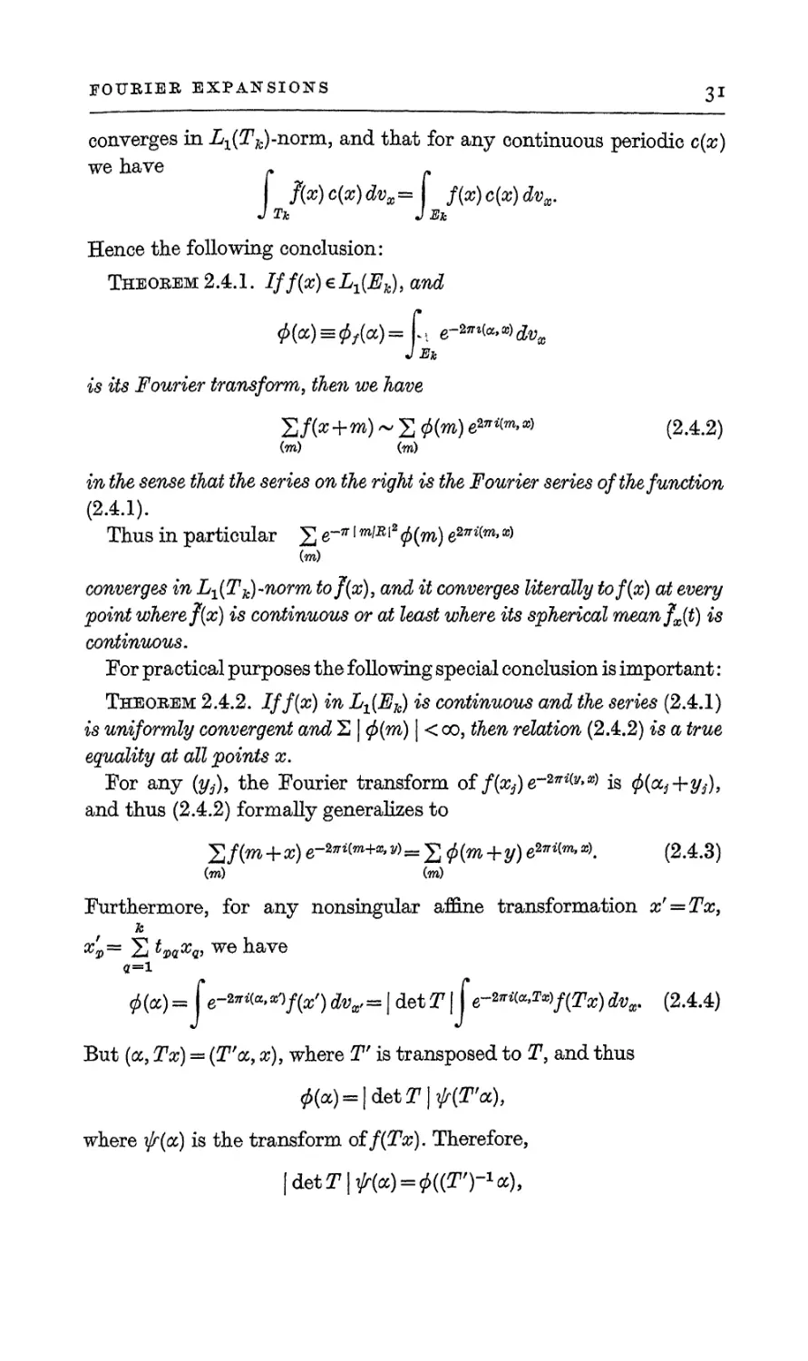
FOURIER EXPANSIONS
31
converges in L^T^-norm, and that for any continuous periodic c(x)
we have -
f{x) c(x) dvx = f(x) c(x) dvx.
J Tk J Bk
Hence the following conclusion:
Theorem2.4.1. Iff{x)eL1{Ek)iand
0(a) = ^a)= L e~27TZMdvx
J Eh
is its Fourier transform, then we have
Itfix+m) ~ £ 0(m) e2**^ (2.4.2)
(m) (m)
in the sense that the series on the right is the Fourier series of the function
(2.4.1).
Thus in particular 2 e-" l™W20(m) e2^™'*)
(m)
converges in L^Tj^-norm tof(x), and it converges literally tof(x) at every
point where f(x) is continuous or at least where its spherical meanfjf) is
continuous.
For practical purposes the following special conclusion is important :
Theorem 2.4.2. Iff{x) in Lx(Ek) is continuous and the series (2.4T)
is uniformly convergent and S | $(m) \ < 00. then relation (2.4.2) is a true
equality at all points x.
For any (y^), the Fourier transform of/(^)e""27r^»^ is $(a3+y3-),
and thus (2.4.2) formally generalizes to
S/(m+x) <r^m+*> y)=%<f)(m+y) e27ri(m> x\ (2.4.3)
(m) (m)
Furthermore, for any nonsingular afline transformation x' = Tx,
k
«-l
<f>(oc) = (e-W^ftz')d%= J detT J \ e^^^fiTx)dvx. (2.4.4)
But (<x, Tx) = (T'a, x), where T is transposed to T, and thus
0(a) = |detT|^(T'a),
where ifr(a) is the transform of f(Tx). Therefore,
\detT\f(a) = <f>((T')-1*)>
32
FOURIER EXPANSIONS
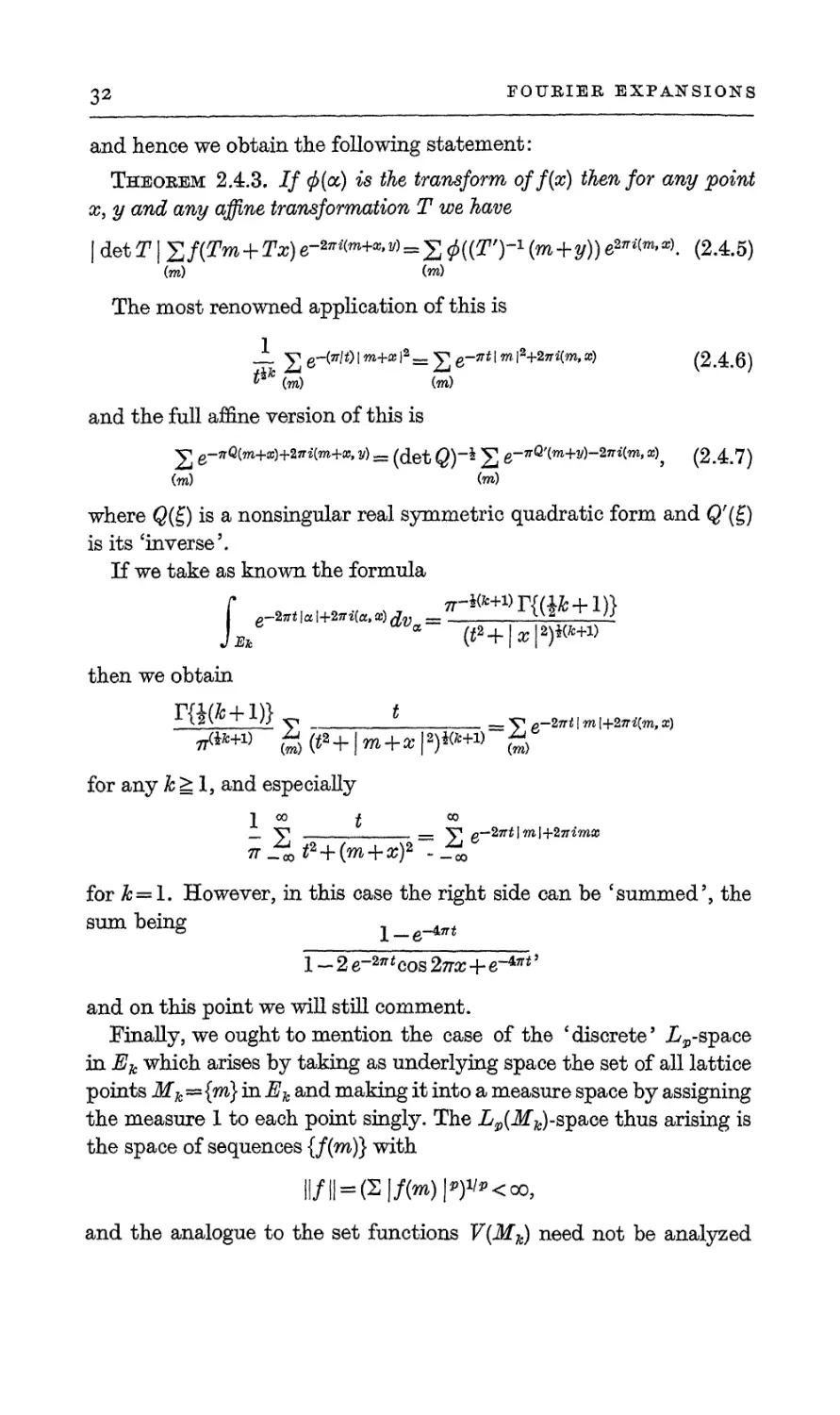
and hence we obtain the following statement:
Theorem 2.4.3. If <f>(a) is the transform off(x) then for any point
x, y and any affine transformation T we have
| det T | %f(Tm + Tx) e-^*<**+*.v> = 2; ^{{T')-1 (m+y)) e27ri(™>*l (2.4.5)
(m) (m)
The most renowned application of this is
_1 j^eHnlt)\m+x\*~^e--7Tt\m\2+27Ti(m,x) (2.4.6)
^fc (to) (m)
and the full affine version of this is
V e-nQ(m+x)+27Ti(m+x, y) _ (^et Q}-\ N£ e-»Q'(m+i/)-2jri(w. x)^ (2.4.7)
(w) (m)
where Q(£) is a nonsingular real symmetric quadratic form and Q'(g)
is its inverse5.
If we take as known the formula
J JE7
g-27rt|al+2jr«(t5t,aB)^ _. .
!a a (t*+1»|*)«*+«
then we obtain
y p—tttt | m l+2rri(m, x)
tt^+D S(**+|ro + a,|«)«*+» &
for any & ^ 1, and especially
1 °° t °°
_ y _ y p—27rt\m\+2nimx
7r^t2 + (m + ^ -^J
for k=l. However, in this case the right side can be 'summed', the
sum being l_e-4^
1-2 e-27r'cos 2nx+e-*nt'
and on this point we will still comment.
Finally, we ought to mention the case of the ' discrete' i^-space
in Ek which arises by taking as underlying space the set of all lattice
points Mh -= {m} in Eh and making it into a measure space by assigning
the measure 1 to each point singly. The Lv{Mk)-space thus arising is
the space of sequences {f(m)} with
||/|| = (S|/(m)|^<oo,
and the analogue to the set functions V(Mk) need not be analyzed
FOURIER EXPANSIONS
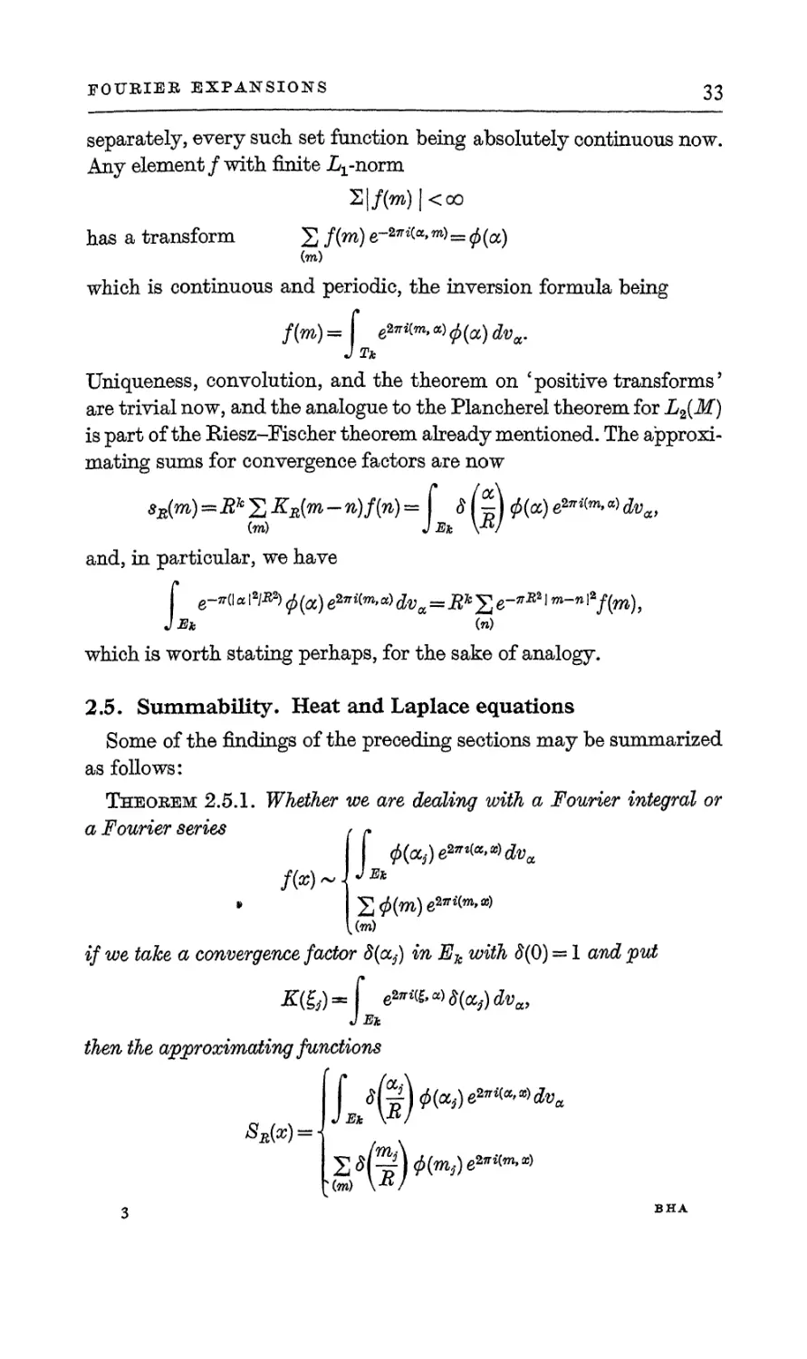
33
separately, every such set function being absolutely continuous now.
Any element / with finite Lx-norm
2|/(*»)|<oo
has a transform £ /(™) e~27^a> m>=<f> (a)
(m)
which is continuous and periodic, the inversion formula being
/(rn)= e27r*w>a^(a)dv
J Tk
Uniqueness, convolution, and the theorem on 'positive transforms'
are trivial now, and the analogue to the Plancherel theorem for L2{M)
is part of the Riesz-Fischer theorem already mentioned. The
approximating sums for convergence factors are now
8dm)=B*XKR(m-n)f(n) = [ s(^) <P(oc)e^^dvaf
(m) J Eh W
and, in particular, we have
f e~^la|2^V(a)e2^(w'a)^^
J Eh (n)
which is worth stating perhaps, for the sake of analogy*
2.5. SummabHity. Heat and Laplace equations
Some of the findings of the preceding sections may be summarized
as follows:
Theorem 2.5.1. Whether we are dealing with a Fourier integral or
a Fourier series / /•
^a^e^^dv^
* S0(w)e27r*(m,aj)
if we take a convergence factor £(%) in Ek with 8(0) = 1 and put
J E
J Eh
then the approximating functions
e*"i&*)jfa)dva
34
FOURIER EXPANSIONS
exist and they have the 'identical' value
sr(x)-b4 K{B{x1^^)i...yR{^-U)Mo)dvt
JEk
This also applies to set functions F(A) instead of point functions f(x),
and it also applies to Fourier series of Bohr and Stepanojf almost
periodic functions.
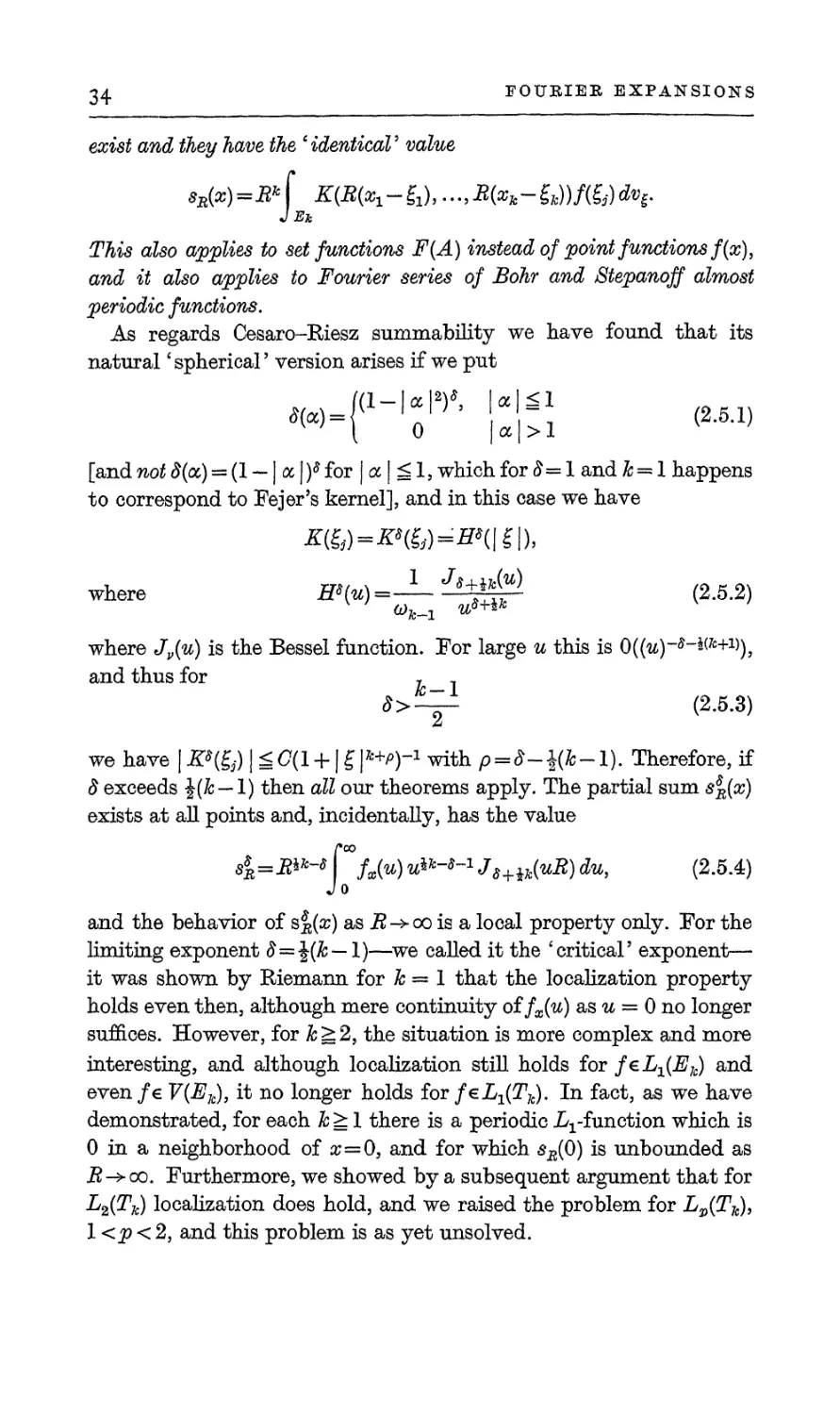
As regards Cesaro-Riesz summability we have found that its
natural'spherical' version arises if we put
\ 0 |a|>l
[and not 8(a) = (1 — | a |)* for | a | ^ 1, which for &= 1 and k — 1 happens
to correspond to Fejer's kernel], and in this case we have
Z&)=Z»&)=ff*(|£|),
where -(«)=J_!?£^> (2.5.2)
where Jp(u) is the Bessel function. For large u this is 0((u)-s-^k+1^),
and thus for ,
8>~ (2.5.3)
we have \KS{& | ^(l + l^l**')"1 with p = 8-%(k~l). Therefore, if
8 exceeds %(lc~ 1) then all our theorems apply. The partial sum s$B(x)
exists at all points and, incidentally, has the value
4=W\M u^-^ Js+ik(uR) du, (2.5.4)
and the behavior of sdR(x) as i2->oo is a local property only. For the
limiting exponent £=|(& — 1)—we called it the 'critical5 exponent—
it was shown by Riemann for k = 1 that the localization property
holds even then, although mere continuity of fx(u) as u = 0 no longer
suffices. However, for k >; 2, the situation is more complex and more
interesting, and although localization still holds for f€Lx(Ek) and
even/e V(Ek), it no longer holds for/eL1(Tfc). In fact, as we have
demonstrated, for each k> 1 there is a periodic ^-function which is
0 in a neighborhood of x=03 and for which sR(Q) is unbounded as
R->cq. Furthermore, we showed by a subsequent argument that for
L2(Tk) localization does hold, and we raised the problem for L^T^),
1 <p < 2, and this problem is as yet unsolved.
FOURIER EXPANSIONS
35
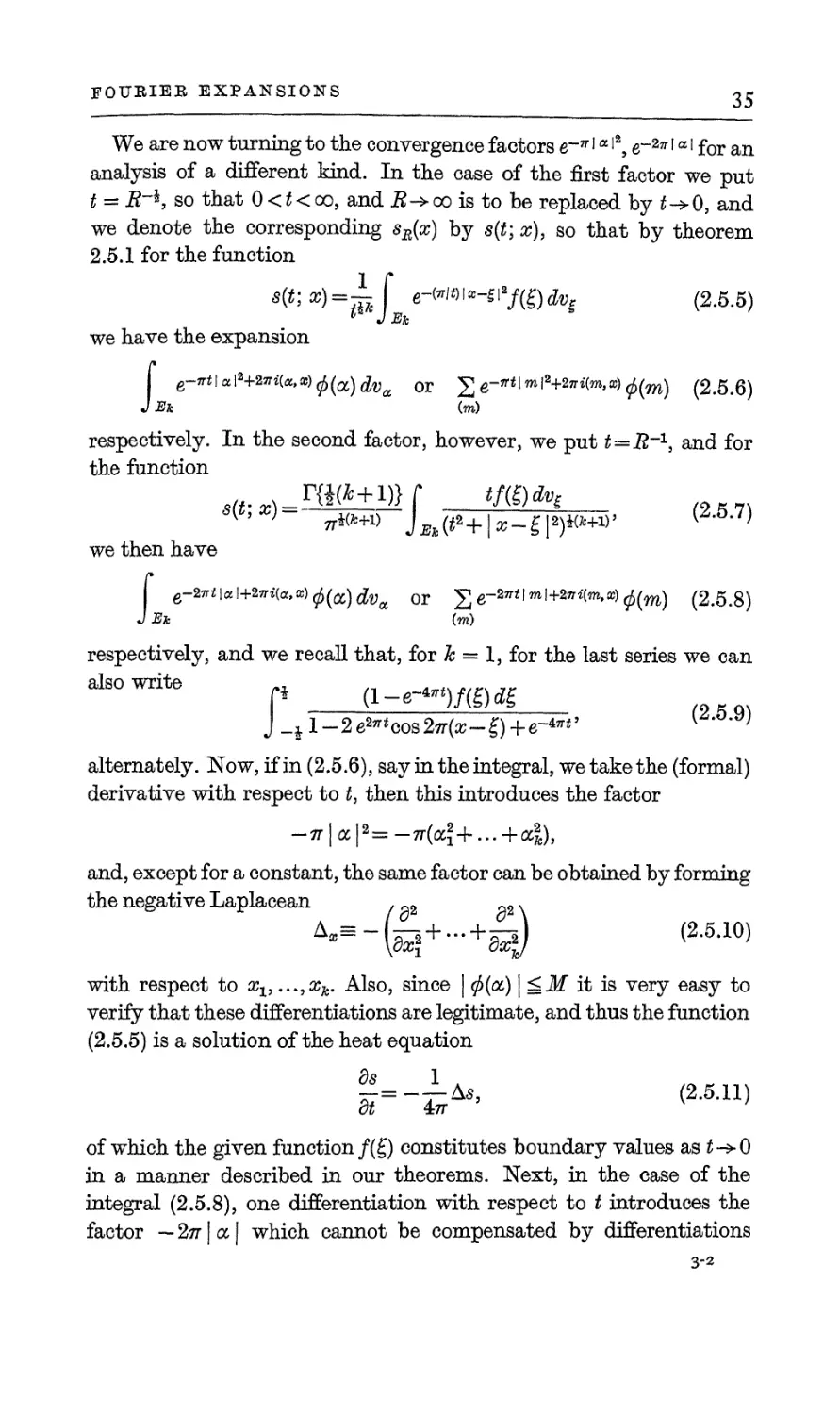
We are now turning to the convergence factors e"n! a >2, e~2n'a' for an
analysis of a different kind. In the case of the first factor we put
t = R~h, so that 0<t<oo, and R->co is to be replaced by t~>0, and
we denote the corresponding sR(x) by s(t; x), so that by theorem
2.5.1 for the function
s(t; x)=± j e-<*W*-i\*f(g)dvs (2.5.5)
we have the expansion
e~^cc\2+27Ti(atx)^a^Va Qr 26-ar*|in|»+2ffi(«i»a0^(w) (2.5.6)
J Ek (m)
respectively. In the second factor, however, we put t=R~13 and for
the function
we then have
e-tvtlal+torHchtiififa)^ or 2 e-a*« iwi+2» *(«,«) 0(m) (2.5.8)
J J2& (m)
respectively, and we recall that, for h = 1, for the last series we can
also *** r d-^)/(g)^
J _j l-2e2^cos27r(^-g)4-e-47r<5 ^ ;
alternately. Now, if in (2.5.6), say in the integral, we take the (formal)
derivative with respect to t, then this introduces the factor
-7r|a|2=-7r(a?+... + 4),
and, except for a constant, the same factor can be obtained by forrning
the negativeLaplacean .-% ^.
A-—te+-+a?) (2'5-10)
with respect to xl9...,xk. Also, since | <j>(a) \ ^M it is very easy to
verify that these differentiations are legitimate, and thus the function
(2.5.5) is a solution of the heat equation
3<? 1
a7=-_AS, (2.5.11)
of which the given function /(£) constitutes boundary values as t->0
in a manner described in our theorems. Next, in the case of the
integral (2.5.8), one differentiation with respect to t introduces the
factor — 27r|a| which cannot be compensated by differentiations
3-2
36
FOURIER EXPANSIONS
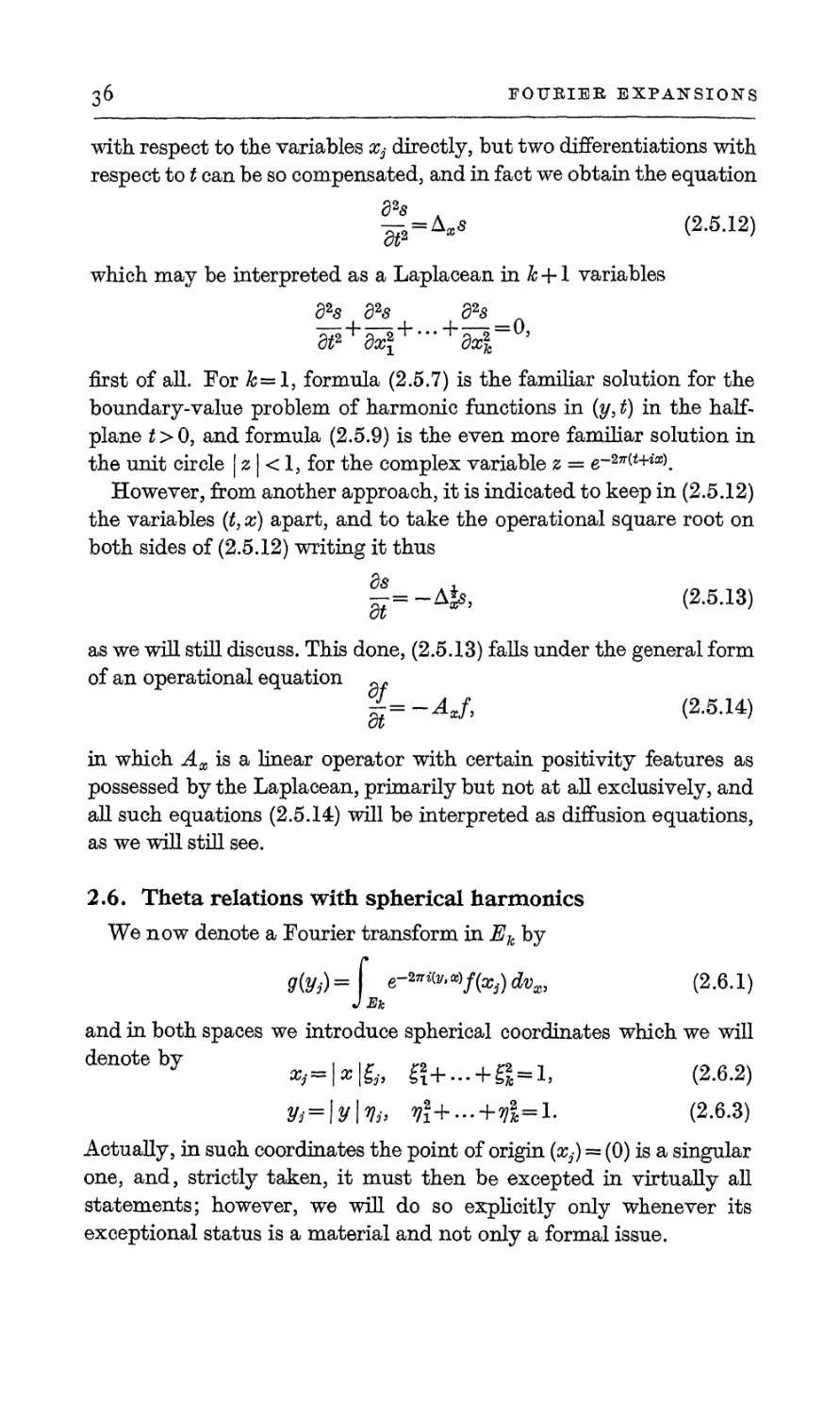
with respect to the variables x3> directly, but two differentiations with
respect to t can be so compensated, and in fact we obtain the equation
¥2 = A,s (2.5.12)
which may be interpreted as a Laplacean in h +1 variables
first of all. For &=1, formula (2.5.7) is the familiar solution for the
boundary-value problem of harmonic functions in (y, t) in the half-
plane t>0, and formula (2.5.9) is the even more familiar solution in
the unit circle | z | < 1, for the complex variable % = e-27T^t+ix\
However, from another approach, it is indicated to keep in (2.5.12)
the variables (t, x) apart, and to take the operational square root on
both sides of (2.5.12) writing it thus
!=-Ak (2.5.13)
as we will still discuss. This done, (2.5.13) falls under the general form
of an operational equation ^
i=-A*f> (2-s-14)
in which Ax is a linear operator with certain positivity features as
possessed by the Laplacean, primarily but not at all exclusively, and
all such equations (2.5.14) will be interpreted as diffusion equations,
as we will still see.
2.6. Theta relations with spherical harmonics
We now denote a Fourier transform in Eh by
gfe)=f e'^y^f(^)dvXi (2.6.1)
J M
and in both spaces we introduce spherical coordinates which we will
denote by . , r ~0 „„ ,
Actually, in such coordinates the point of origin (x5) = (0) is a singular
one, and, strictly taken, it must then be excepted in virtually all
statements; however, we will do so explicitly only whenever its
exceptional status is a material and not only a formal issue.
FOURIER EXPANSIONS
37
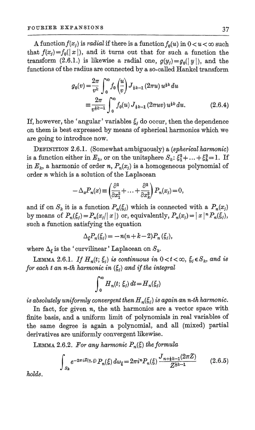
A function f(Xj) is radial if there is a function f0(u) in 0 < u < oo such
that f(^)—f0(\x\), and it turns out that for such a function the
transform (2.6.1.) is likewise a radial one, g(^)=g0(| y|)} and the
functions of the radius are connected by a so-called Hankel transform
2tt f00 (u\
9o(v) = - J o /o I - J Jjm (2t») «** *»
-,-3-i /o(«)-7**-i (a™") «***«• (2.6.4)
"" Jo
If, however, the 'angular' variables ^ do occur, then the dependence
on them is best expressed by means of spherical harmonics which we
are going to introduce now.
Definition 2.6.1. (Somewhat ambiguously) a (spherical harmonic)
is a function either in Ek, or on the unitsphere Sk: E>\-f... + £f=1. If
in Ek, a harmonic of order n, Pn(xi) *s a homogeneous polynomial of
order n which is a solution of the Laplacean
/a2 a2 \
-A,Pn(^)^^ + ...+--|jPn(a;,) = 05
and if on Sk it is a function Pn(^) which is connected with a Pn(Xj)
by means of Pn(&) =Pn(av/| a? |) or, equivalently, Pn(ay,) = | a; |nPw(£y),
such a function satisfying the equation
AzPn&)=-~n(n + Jc-2)Pn(Q,
where Ag is the e curvilinear' Laplacean on 8k.
Lemma 2.6.1. If Hn(t; £,-) is continuous in 0<t<co, ^eSki and is
for each t an n4h harmonic in (^) and if the integral
rCOHn(t;^)dt=Hn(^)
f o
is absolutely uniformly convergent then Hn(^) is again an n-th harmonic.
In fact, for given n, the nth harmonics are a vector space with
finite basis, and a uniform limit of polynomials in real variables of
the same degree is again a polynomial, and all (mixed) partial
derivatives are uniformly convergent likewise.
Lemma 2.6.2. For any harmonic Pn(£) the formula
e-2"«Pn(£) du)^2ni-Pn{i) Jn+i^Z) (2.6.5)
Sk
holds.
r.
L
38
FOURIER EXPANSIONS
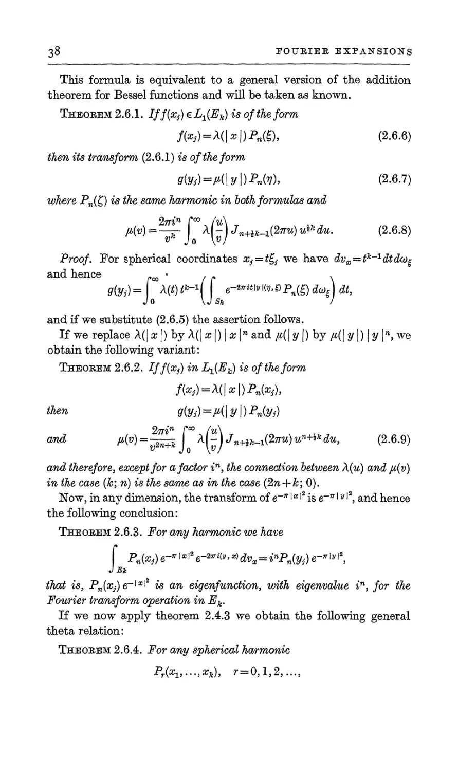
This formula is equivalent to a general version of the addition
theorem for Bessel functions and will be taken as known.
Theorem 2.6.1. Ifffa)£L1{Elc) is of the form
/(*,)=A(|*|)Pn(g), (2.6.6)
then its transform (2,6.1) is of the form
g(yi)=M\y\)Pn(v), (2.6.7)
where Pn(Q is the same harmonic in both formulas and
^v)ss'WJQ Hv) Jn+i^i(2nu)u^du. (2.6.8)
Proof. For spherical coordinates x3- = tg3- we have dv^^^^dtdco^
and hence f «> * / f \
9(y>)=\o X{t)tk\]s e-2nit]MPn®da)zJ dt,
and if we substitute (2.6.5) the assertion follows.
If we replace A([#|) by A(|#|) |#|nand fi(\y\) by /*(|y|) \y\n, we
obtain the following variant:
Theorem 2.6.2. Iff fa) in Lx{Ek) is of the form
ffa) = \(\x\)Pnfa),
then g(yi)=M\y\)Pn(vi)
2ffin f00 [u\
and aw=-^ \QHv) J^-i(27m>unHk du> <2-6-9)
and therefore, except for a factor in> the connection between \(u) and /i(v)
in the case (k; n) is the same as in the case (2n + k; 0).
Now, in any dimension, the transform of e-*"'x >2 is e~n'y '2} and hence
the following conclusion:
Theorem 2.6.3. For any harmonic we have
I Pnfa) e-n >»i2 e~^^^ dvx=inPn{y3) er"ly |2,
that is, Pnfa)e~lx^ is an eigenfunction, with eigenvalue in, for the
Fourier transform operation in Ek.
If we now apply theorem 2.4.3 we obtain the following general
theta relation:
Theorem 2.6.4. For any spherical harmonic
P^,...,^), r = 0,l,2,...,
FOURIER EXPANSIONS
39
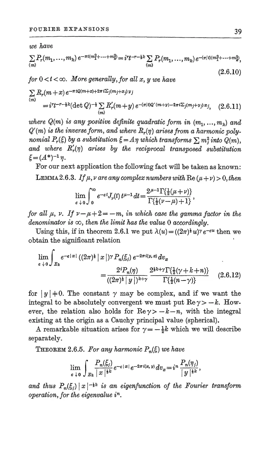
we "have
SPrK, ...,m7c) e-^K+-+m!)=^^-^ S ^-(^i, ...,mfc)e-(^K+-"+™!>,
(w) (m)
(2.6.10)
/or 0 < t < oo. More generally, for all x, y we have
£ Rr(m + X) e-^(™+a)+2™2j(mj+ai) Vj
(m)
-=i^-^7c(det Q)-4 ^ i^(m-f.y) e-(7r'^'(m+2/)-2?ri-^i+^)a;j} (2.6.11)
(m)
where Q(m) is any positive definite quadratic form in (mv ...,mfc) and
Qf(m) is the inverse form, and where Rr(n) arises from a harmonic
polynomial Pr(£) by a substitution £=An which transforms 2 m| into Q(m),
and where R'r(w) arises by the reciprocal transposed substitution
For our next application the following fact will be taken as known:
Lemma2.6.3. If/i, v are any complex numbers with Re (ji + v)> 0, then
J-oJo
lim e-etJv(t)W-1dt=-
for all /i, v. If v—ju, + 2=—m) in which case the gamma factor in the
denominator is oo, then th,e limit has the value 0 accordingly.
Using this, if in theorem 2.6.1 we put X(u) = ((27r)* u)y e~eu then we
obtain the significant relation
lim J e~e i»i ( (2tt)* | a; | )r Pw(&) e-2^> *) dvx
2'P»(7) 2*>^rft(y+t+»)}
((27r)i|y|)*+r r{i(n-y)} * ' ' '
for | y | =[= 0. The constant y may be complex, and if we want the
integral to be absolutely convergent we must put Re y > — Jc.
However, the relation also holds for Rey> — k—n, with the integral
existing at the origin as a Cauchy principal value (spherical).
A remarkable situation arises for y= — \h which we will describe
separately.
Theorem 2.6.5. For any harmonic Pn(£) we have
lim f ^@e^i^e-2^^)d^-i-^-^}
and thus Pn{£>j) \x\-^k is an eigenfunction of the Fourier transform
operation, for the eigenvalue in.
40
FOURIER EXPANSIONS
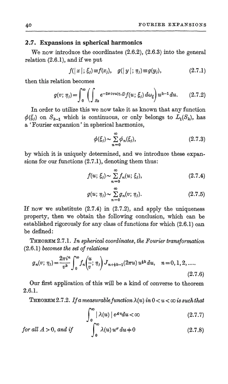
2.7. Expansions in spherical harmonics
We now introduce the coordinates (2.6.2), (2.6.3) into the general
relation (2.6.1), and if we put
/(|a?|;6)3/(2,,), g(\y\;y^g(yi), (2.7.1)
then this relation becomes
g{v; 7,.) =1 M e~27rivu^^f(u; &) do) A uh"1du. (2.7.2)
In order to utilize this we now take it as known that any function
0(6) on Sk_x which is continuous, or only belongs to Li($&), has
a 'Fourier expansion' in spherical harmonics,
#&)-:£<*«&), (2.7.3)
n—0
by which it is uniquely determined, and we introduce these
expansions for our functions (2.7.1), denoting them thus:
/(";&)~S/»(w;&), (2.7.4)
71=0
00
?(«;%)~Z ?.»(«; ft)- (2.7.5)
If now we substitute (2.7.4) in (2.7.2), and apply the uniqueness
property, then we obtain the following conclusion, which can be
established rigorously for any class of functions for which (2.6.1) can
be defined:
Theorem 2.7.1. In spherical coordinates, the Fourier transformation
(2.6.1) becomes the set of relations
2jrin r°° fu \
9n(vi ^) = -^r /nb; VA Jn+ik-i^^^du, n = 0,1,2, ....
(2.7,6)
Our first application of this will be a kind of converse to theorem
2.6.1.
Theorem 2.7.2. If a measurable function X(u)inO<u<oo is such that
|»oo
|A(^)|e^wdu<oo (2.7.7)
/*oo
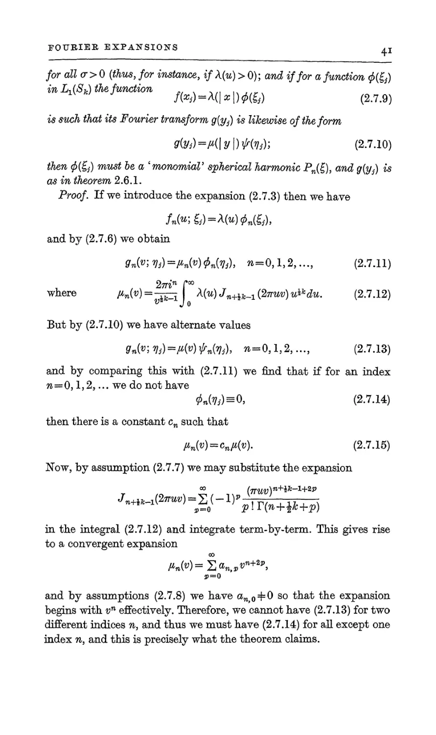
for all A>Q, and if X^u^du+O (2.7.8)
FOURIER EXPANSIONS ^
for allcr>0 (thus, for instance, if \(u) > 0); and if for a function 0(g,)
in L^Sjc) the function ...
f(*i) = M\x\)M£i) (2.7.9)
is such that its Fourier transform g(yj) is likewise of the form
9(y^M\y\)^(vj); (2.7.10)
then <f>(£s) must be a 'monomial* spherical harmonic Pn(£), and g(yj) is
as in theorem 2.6.1.
Proof. If we introduce the expansion (2.7.3) then we have
and by (2.7.6) we obtain
ffn(v'>Vj)=Mv)$n{Vj)> ra=0,l,2,..., (2.7.11)
27Tin f °°
where pn(v) = ----_ X(u) Jn+ik^ (2ttuv) u%kdu. (2,7.12)
But by (2.7.10) we have alternate values
gJviy^Mtffnivj)* n=o,i,2,..., (2,7.13)
and by comparing this with (2.7.11) we find that if for an index
n-=0,1,2,... we do not have
&»foi)«0, (2.7.14)
then there is a constant cn such that
/tnW88^). (2.7.15)
Now, by assumption (2.7.7) we may substitute the expansion
in the integral (2.7.12) and integrate term-by-term. This gives rise
to a convergent expansion
and by assumptions (2.7.8) we have aM>0 + 0 so tnat tne expansion
begins with vn effectively. Therefore, we cannot have (2.7.13) for two
different indices n, and thus we must have (2.7.14) for all except one
index n, and this is precisely what the theorem claims.
42
FOURIER EXPANSIONS
Now, the function \{u)=*urer™*> r^O, satisfies (2.7.7) and (2.7.8)
and hence the following very.special inference:
Theorem 2.7.3. If we have
for two homogeneous polynomials PT{x5), Qs(yj) of some degrees r, s, then
Pr{Xj) is a spherical harmonic, and we have s=r, Qs(y3) = inPT(yj).
In particular, if for a homogeneous polynomial P^) we have
I
Pr(xj) e-»i*iV2*<(v.») dv^cPrfa) e~"^\ (2.7.16)
Eh
then Pr{xj) is a harmonic and c = in.
We now recall that the (inhomogeneous) Hermite polynomials in
one variable En(x), n=0,1,..., after replacing x by (Ztt^x, have the
property
Hn(x) e-™2 e-27riv* dx = inHn(y) e-w2.
However, any polynomial Pn(^) can be expanded into a finite series
S a^^Hnfa) ...Hnk(zk), (2.7.17)
m + .-. + njc^n
and uniquely so. Therefore, the transform of Pn(x}) e~"|a!|!! is
where QB(y,) = S W"^-^^...^^^...^^),
and since Pn(<ty) is a homogeneous harmonic if and only if
we obtain the following theorem:
Theorem 2.7.4. A homogeneous polynomial Pn{xs) is a spherical
harmonic if and only if, on representing it by an expansion (2.7.17), only
such coefficients animtt njt are =f= 0 for which
n1+...+nk=n—4cr, r = 0,l,2,....
Turning now to a somewhat different topic we note that relation
(2.6.9) implies as follows:
Theorem 2.7.5. Subject to assumptions, if we are given on Sk a
FOUBIEB EXPANSIONS
43
function*})^) with the expansion (2.7.Z), and iffor someywithB>ey> -k
we consider on 8% the function with the expansion
then the function ffa) = ((27r)* \x\)y $(£;)
has for fa) 4= (0) the transform
^•) = ((27r)4|y|)-r-^r(7;,)3
in the sense that we have
g(y,) = lim e-« I * i/fo.) e~2™to ») &>„,
e\0JEjc
the limit existing.
Now, as for specific assumptions that are sufficient, we quote the
following theorem:
Theorem 2.7.6. For given y, if 2n is an even integer for which
2n>Rey + p — 1 and if 0(gy) belongs to differentiability class C®n) on
$£, then the function (2.7.18) exists and is continuous and the conclusions
of theorem 2.7.5 hold true.
Also, if q°^Q is an integer for which 2n>Rey+p~ 1+g0, then
pfa) e C<«°>, and thus if(j>{^) e C(°°> then also pfa) € C&\for Re y > - h.
Finally, if 0(^) is {real) analytic on Sk in its 'natural' local
coordinates, then ifry(£j) is also analytic.
The last-made statement on analyticity is non-obvious. The
theorem applies in particular to
where T2h(^j) is a homogeneous polynomial
which is > 0 for | x | =(= 0, and s is a complex number for which
Res<~. (2.7.20)
It suggests itself that the function g(y; s) might also be holomorphie
(that is, complex-analytic) in the parameter s in the half-plane
(2.7.20), and this is not only correct but easy to prove. Altogether we
will have in the next section a rather general theorem from which we
will deduce at the end of section 2.9 that the function (2.7,19) is
g(y,;s)=limf e-*\*\\m *]^, (2.7.19)
e |0 J E
44
FOURIER EXPANSIONS
holomorphic in s and C(c0) in (y5-), for (y5) =|= 0. But the actual analyticity
in the real variables y3- is a much more specific proposition and the
proof will not be reproduced here.
2.8. Zeta integrals
Definition 2.8.1. We say that a function f(xf, s) is an adjusted
Zeta kernel if it has the following structure:
(i) It is defined for (x^) in Ek> and for complex $ in a certain
domain D.
(ii) It is 0 in a fixed neighborhood | x \ < x° of the origin in Ek.
(iii) It is C(00) in the variables x^ and for any combination of
integers ^. . A /rt n _ v
6 ft^O, ...,#*£(> (2.8.1)
the function D*i~*tf(x; *)s d^x^^[ (2.8.2)
is continuous in (x; s) and holomorphic in s3 and what is decisive
(iv) corresponding to each s° in D there exists a neighborhood
N of s° and a real number y=y(N)y y^O, such that for each
combination (2.8.1) we have
as | x | ~> oo, uniformly for s in N.
Definition 2.8.2. In the present context a convergence factor is
a function d(t) of the following description: (i) it is defined and
continuous in 0 ^ t < oo, and 8(0) — 1; (ii) (t) is C(oo) in 0 < t < oo; (iii) we have
dpS(t)
~^ = 0{t-«) as t-^oo (2.8.4)
for every p ^ 0, q ^ 0, so that in particular
S(t) = 0(t-«) as t~>oo (2.8.5)
for every g;>0; and (iv) we have
dp8(t)
—±L = 0(1rv) as t->0 (2.8.6)
for every p > 0 (but not p = 0).
The function £(t) = e~*P is such a convergence factor for every p > 0.
Definitions 2.8.1 and 2.8.2 are such that for any e>0 the product
fe(xj;s)~8(e\x\)f(xj;s) (2.8.7)
FOURIER EXPANSIONS
45
we obtain the relation
is again an adjusted Zeta kernel; and, in consequence of (2.8.3) and
(2.8.5), this new function and each mixed partial derivative of it is
small at infinity in such a manner that for the transform
gjly* *H f er^^v)fe(xf, s)dvx (2.8.8)
J Ek
ition
(27riy1)vi...(2iTiyk)^ge(y,s)= f e-*«*-*D*v'**fe(x;8)dva (2.8.9)
J Ek
for any integers (2.8.1), by means of partial integrations which are
readily justified. But now we claim as follows:
Theorem 2.8.1. If N and y-y(N) are fixed, then for
Pi+-+Pk>Y + k> (2.8.10)
we have
lim I e-*ir*t*.v)])91..-Pkfe(x',8)dvtt = \ e-2nil*>»D*i'"**f{x;8)dval9
e 10 J Ek J Ek
(2.8.11)
uniformly in the neighborhood of every point (y, s).
Proof. If we write D® for Dri—n and put r~rx+... + rfc, then we
have
DWfe(x; s) =8(e | x \) DWf(x; s) + £ DM6(e\x\)D®f(x; s). (2.8.12)
r>0
Now, by (2.8.3), we have
DMf(x; s) = 0 (| x |t-»), | x | ~>oo,
and by (2.8.10) this function thus belongs to Li(i7&), uniformly in N.
Also, 8(e \x |) converges boundedly to 1 as e->0, and thus our theorem
will follow if we verify
lim f | JDW*(e | x |) |. | W>f(x; s) \ dva=Q (2.8.13)
e 10 J Ek '* ' \ & * J
uniformly in 5, for r+s =p,r>0. Now, since/(»; s) — 0 for ] a; | <a;0 it
is not hard to verify, by the use of (2.8.3), that the integral (2.8.13) is
majorized by
| _ 8(et) . tys+K-1 dt=e*-y-* \ \ &r)(t) | tr-s+^-i dt.
J a* \dtr I J ea!o
However, by assumption (2.8.10) the quantity p=p-y—k is >0,
/•oo
and thus e*>-y+fc tends to 0, as e -> 0, for any fixed 9/, no matter how
Jv
46
FOURIER EXPANSIONS
small. Now, if r>05 then, in ex°^t^n, \ 8®(t) | is ^cr(7})t-r, where
cr{rj) ~> 0 as tj -> 0, and thus we only have to verify that
stays bounded as e~>0. But, due to r+s=*p, this is a trivial fact, and
hence the theorem.
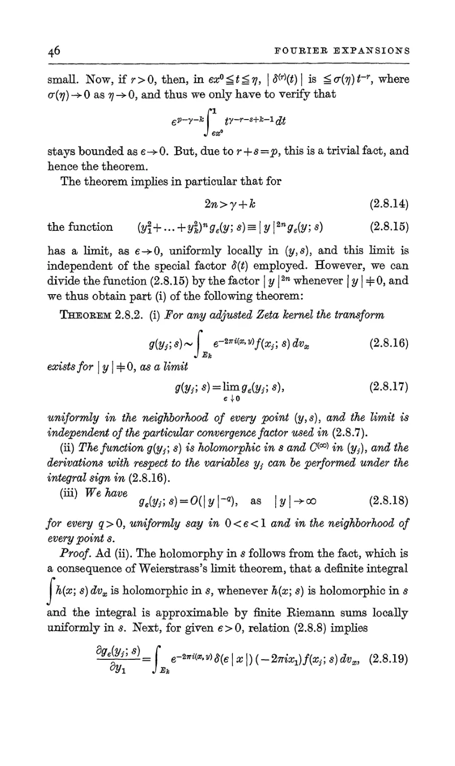
The theorem implies in particular that for
2n>y + k (2.8.14)
the function (yj+... +y\)nge{y; s)=\y\*nge(y; s) (2.8.15)
has a limit, as e~>05 uniformly locally in (y,s)3 and this limit is
independent of the special factor 8(t) employed. However, we can
divide the function (2.8.15) by the factor | y |2n whenever | y | +0, and
we thus obtain part (i) of the following theorem:
Theorem 2.8.2. (i) For any adjusted Zeta kernel the transform
g{yf, *)~\ e-^^f(xj; s) dv* (2.8.16)
J Eh
exists for | y 14=0, as a limit
g{yj;s) = limge(yf,s), (2.8.17)
e 4-0
uniformly in the neighborhood of every point (y,s)i and the limit is
independent of the particular convergence factor used in (2.8.7).
(ii) The function g(yj; s) is holomorphic in s and C(00) in (y^), and the
derivations with respect to the variables y3- can be performed under the
integral sign in (2.8 J6).
(iii) We have . «,. , „, . . /ft«,«v
QAyi\*)=*0{\y\-*), as \y\-+co (2.8.18)
for every q>0, uniformly say in 0<e<l and in the neighborhood of
every point s.
Proof. Ad (ii). The holomorphy in s follows from the fact, which is
a consequence of Weierstrass's limit theorem, that a definite integral
h(x; s) dvx is holomorphic in s, whenever h(x; s) is holomorphic in s
/■
and the integral is approximate by finite Riemann sums locally
uniformly in s. Next, for given e>0, relation (2.8.8) implies
tyeiyf, *)
dy.
3—=\ e-27ri^^S(6\x\)(-2nix1)f(xj;s)dvx, (2.8.19)
i J Bh
FOURIER EXPANSIONS
47
say. But xj(xf, s) is again an adjusted Zeta kernel, and thus, by part
(i), the function (2.8.19) must have a limit, as e ~>0, locally uniformly,
and it now follows that this limit must be
this derivative existing. We can now iterate this procedure, and the
assertion follows.
Ad (iii). The function (2.8.15) has, except for a constant, the value
f e-^>v)&%f(x3.',s)dvx,
where A is the Laplacean. It follows from our proof to theorem 2.8.1
that, for 2n>y + k, this function is bounded in yj9 uniformly for
0 < e < 1 and $ in N, but n can be chosen arbitrarily large whence the
conclusion.
2.9. Zeta series
The unnatural restriction incorporated in definition 2.8.1 that
f(x; s) shall be 0 in a neighborhood of x = 0 was meant to be only
transitory, and we are now going to allow, to the contrary, that it
shall even be undefined and singular at x=0.
Definition 2.9.1. We say that a function/^; s) is a (proper) Zeta
kernel if it is defined for xhxEk except at the origin x—0 and for $ in
a domain D, and if it has properties (iii) and (iv) of definition 2.8.1.
Theorem 2.9.1. (i) Iff(xf, s) is a Zeta kernel then the corresponding
'Zeta fusion' ^. s) = s,e_«/(%.,} (2.9J)
(m)
exists for 2/4=0 on the torus Tk:—\-£yj<\ and for s in D as a limit
Urn %'e~^m>ti8(e | m |)/(%; s) (2.9.2)
e 10 (w)
for any convergence factor 8(t), and has a value independent of it,
uniformly in the neighborhood of every point (y}s), and it is C(c0) in
y and holomorphic in s.
(ii) Also, corresponding toy—Q, the limit
]im[zfd(e\m\)f(m3-;s)- f 8(e\x\)f(x,;s)dv^\ (2.9.3)
ejoLw J\x\^l J
exists, continuously for s in D, and is holomorphic there.
48
FOURIER EXPANSIONS
Proof. Ad (i). We take it as known that it is possible to construct
a continuous function #(t) in 0 < t < oo which is C(00) in 0 < t < oo and for
which we have %(t) = 0 for 0 ^ t < | and #(t) = 1 for f < x(t) < oo. If now,
with the given function f(xf3 $), we construct the new function
^"'H o, *~o,
then/(#,-; s) is on the one hand an adjusted Zeta kernel, and on the
other hand we have /(^; s) —/(#,•; s) for | # | ;> § so that in particular
we have ^,^^3,)^(m.. 5) = j e-2*i(«.s/)/e(%; 5).
(w) (w)
However, by theorem 2.4.1 we have
S^K-+^) = S^^(m,.)/e(m.; 5), (2.9.4)
On)
where ge is the Fourier transform of/, and if we apply all properties
stated for ge in theorem 2.8.2 then our assertion follows.
Ad (ii). For y=*0 the term ge(0) need not have a limit as e->0.
However, if we write
S/^(wi)=S7«(%;*)-^(0),
(m) Cm)
then the left side does have a limit, and a holomorphic one too, again
by theorem 2.8.2. Now
and if we write for this
J|*|Sl J*£|0l.Sl
then the second integral is holomorphic in $ for $ in D, so that we need
subtract only the first integral, and this was done so in formula
(2.9.3).
We now take a homogeneous polynomial T2h(xj) > 0, for #4= 0, as in
section 2.7, and with it we set up any (nonhomogeneous) polynomial
Tfa) ~ T^Xj) + (lower powers),
and we assume that we have T(xi) + 0 for #4=0. For &§:3 it then
follows by monodromy that we can define (^(x^)8 as a holomorphic
function in s for #4=0 and all complex s, and for h—2 we make this
into an additional assumption (which is needed only if T(xs) is non-
FOURIER EXPANSIONS
49
homogeneous). We take some further polynomial Qr{x/j9 say
homogeneous of degree r, and if we put/(a?,; s)^Qr{xi) T{x^s, then this is
a Zeta kernel with D being the entire s-plane. Therefore, theorem
2.9.1 implies immediately parts (i) and (ii) of the following theorem:
Theorem 2.9.2. (i) The function
£(y,.; s) =lim£'e-27r^»m>8(e\m\)
Qrfai)
e|0(m) T(m5-)"
exists, for y=£0 on Tk, and is an entire function in s.
(ii) The Dirichlet series
and the associated integral
I
Qri*j) dvx^H(s), (2.9.5)
being both absolutely convergent in the right half-plane
Bes>^-, (2.9.6)
the holomorphic functions defined by them in this half-plane are such
that their difference has an analytic continuation into the entire plane,
' £(s)—E(s) = entire function.
(iii) Taken separately, the functions £($), H(s) have meromorphic
continuations into the entire s-plane. If T(mj) is homogeneous, then H(s)
and £(s) have (at most) one simple pole at the obvious point
If T(mj) is nonhomogeneous, there is first of all again a simple pole at
the same point (2.9.7) with Hhe same' residue (2.9.8), where T2h is the
highest part of T; and there may also appear other poles, all simple ones,
at the points ,
^r + k-m m==l,2,3,4,..., (2.9.9)
2h
which are placed at equal distances to the left of the first one.
50
FOURIER EXPANSIONS
Proof. Ad (iii). In the homogeneous case we have in the half-plane
(2'9'6) I™ r ***** f &® *,
and in this product the first factor is (2hs —r—Jc)"1 and the second
is an entire function, which gives the conclusion.
If T is not homogeneous, we put
T — Tm + Pm-I " ^2fc( 1 + ~m I >
and if we substitute this in the integral (2.9.5) we obtain, at first
formally,
= 2 (7) f, , ^-1<to-
n*0\ W / JlalSl i2fe
Now, the nth term in this sum is of the kind just discussed, with s
replaced by s+n, and Qr replaced by QrP^-.lf and since the last
expression is an inhomogeneous polynomial of degree ^(2h —l)n, we see
that for n > 0 the term has at most simple poles at the points
s+n= , 0£v£(2h-l)n9
and is holomorphic otherwise. Finally, corresponding to any bounded
domain D of the 5-plane we can find an M such that on putting
the remainder r ° BM(xj; s)dvx
J ! x |^l J-2U
will be absolutely uniformly convergent for s in D and thus will be
holomorphic. From all this our assertion follows.
Finally, returning to integrals instead of series, we take a function
<f>(^) on Sk as in theorem 2.7.6, say in C(00)? and we put
f(xj;s) = \x\^*<f>(£j)
with any real numbers a, b+0, and we consider this in the half-plane
a + b. Re s > — h for which the transform
j e-27ri&>y°)e-eWf(x3-;s)dvx
J Eh
JOUKIEE EXPANSIONS
Si
is definable. With our previous function x(t) we now put
fix,; «) = x(| *|)/C«v, «) + (l -X(\ x \)f(xf, «)=/*(*,; a)+fH&; s),
and then put ^. s)=hm f e-^iix,y)e-ela!lj>r{Xj; s)^ (2.9.10)
e 10 J Eh
for r=l,2. Now, g%i; s) falls under theorem 2.7.6, and is therefore
C(°°) in y and holomorphic in s. For the function g2(^-; s) this is,
however, likewise so, simply because for this function the integration in
(2.9.10) extends effectively only over the unitsphere | x \ ^ 1. Therefore,
the function gx+g2 is likewise so, and this proves a statement made
about the function (2.7.9) near the end of section 2.7.
4-2
52
CHAPTER 3
CLOSURE PROPERTIES OF FOURIER
TRANSFORMS
We will now present an analysis of the principal closure properties of
characteristic functions in general, and for those of (infinitely)
subdivisible processes in particular, and doing the latter immediately in
Ek for general h will require a rather elaborate setting indeed; and
such simple functions as are ei(et*^ and 1 —cos (ax) will be replaced
by more general ones (which we will term 'pseudo-characters' and
1 Poisson characters' respectively) for the sake of greater clarity, we
hope.
3.1. Pseudo-characters and Poisson characters
Definition 3.1.1. A function
X(oc; x)^x(ch> —><**; «i> —»«*) (3.1.1.)
is a pseudo-character if (i) it is defined and continuous in E2k=E%xE%
and is bounded there, | %^. x) | ^M^ (3JL2)
(ii) for (a) — (0), %(<%; x) is a constant in x, but not==0,
X(0;av) = Co=|=0, (3.1.3)
and, what is decisive, (iii) we have
lim I jrto)x(a,;a,)dfoa = 0 (3.1.4)
I cc |—>oo J Eh
for every KeL^Ejc).
Theobem 3.1.1. The class of pseudo-characters is closed under uniform
convergence in E21c, except for property (ii).
In fact, if (3.1.4) holds for a sequence xn having a uniform limit Xo>
then it also holds for #0.
On the other hand, for fixed bounded #, if (3.1.4) holds for a
sequence Kn, for which || Kn—K || -> 0, then it also holds for K. Now,
step functions on the finite intervals Iab: aj^xi<b5 are dense in
Lx(Eh), and hence the following statement:
Theorem 3.L2. A bounded continuous function #(a; x) fulfils (3.L4)
if we have r
lim x(x'>%)dv^0 (3.1.5)
1 x |->oo J lab
for all finite multi-intervals.
CLOSURE PROPERTIES OF FOURIER TRANSFORMS 53
In particular, we have
L
e**>xHva=z n
i-l
ix*
and it follows from
gibx giax
%X
<2|6-g|
~ l + \x\
that (3.1.5) holds, whence the following statement:
Theorem 3.1.3. The function 6%**$ is a pseudo-character (Riemann-
Lebesgue lemma).
Since e*^***) is also a pseudo-character, for any A, we may also state
as follows:
Theorem 3.1.4. IfB(t) in — co<t<ao with 5(0)4=0, is a sum
Scwe<Aw* (3.1.6)
(m)
with Am + 0, E|cw|<oo,
On)
or a uniform limit of such sums (Bohr almost periodic function with
Am 4= 0), then the function
X(a;x)=B(a1x1 + ... + cckxk) (3.1.7)
is a pseudo-character.
For instance, 2 cos (a, #) =e*<a»*> + e~iCa»fl0 is a pseudo-character.
Definition 3.1.2. A Poisson character is a function Q(a; a?) in
Elc x jE^ of the following description:
(i) Q(^x) = c1{l-x^\x)), Cl>0, (3.1.8)
where ^(a; a;) is a pseudo-character, and #(a; a) is real valued, and
Q(oc;x)>0 (3.1.9)
and also Q(0; a;) = 0for alia;, and <9(a; O) = 0for alia. (3.1.10)
(ii) The function q(x) = \ Q(jS; x) dvfi (3.1.11)
is strictly >0 for x4=0 (and not only ^0 as (3.1.9) implies) and
O(oc x)
(iii) the quotient P(a;^) = ^Vr, #4=0, (3.1.12)
q(x)
is bounded and uniformly continuous in the variable a in the point set
0<|a|<a0, 0<|a|gl (3.1.13)
for every a0 > 0.
54 CLOSURE PROPERTIES OP POURIER TRANSFORMS
Important remark. We do not assume that (3.1.12) is uiiiformly
continuous in (3.1.13) as a function in (oc, x) but only that it is uniformly
continuous in a, uniformly in x. For & = 1, for the classical function
Q(oc; x) = (sin ocx)2 and for similar ones the quotient does happen to be
continuous in (a, a?) simultaneously, and all proofs, known to this
author, of the structure theorem for subdivisible processes make
full use of this simplification; but for h > 2 this definitely ceases to be
so and a more systematic approach similar to ours must be sought.
We note that in (3.1.11) and (3.1.13) the unit spheres could be
replaced by others with fixed radii, equal or not, and that, on the
other hand, the constant cx in (3.1.8) could be put equal to 1, which in
the reasoning we will frequently do anyway.
Next, if o)s(fi) is the' indicator function' (characteristic set function)
of the unit sphere | fi | % 1, and if, on putting c1 — 1, we write
q{x)=\ o)s(/3)[l-X(P;x)]da)ji,
then we obtain q(x) = c2—p(x), (3.1.14)
where c2 > 0, and the function
J Ek
tends to 0 as | a; | ->oo by definition 3.1.1. Therefore, in connection
with property (ii) of definition 3.L2 we obtain the following further
property automatically:
(iv) For any fixed n > 0 we have
M1<q{x)<Mz (3.1.15)
for |a?[^??> withO<M1<M2<oo.
Theorem 3.L5. // B{t) in — oo<t<oo is periodic or Bohr almost
periodic, if it is non-negative and even,
B(t)^0, B(-t)=B(t)t (3.1.16)
and if in a neighborhood of t—Owe have
B(t)^c2\t\™+o(\t\™) (3.1.17)
with c2 > 0, m> 0 (m not necessarily integer), then
Q(cc; x)=B(a1x1+... + cijtxk) (3.1.18)
is a Poisson character.
CLOSURE PROPERTIES OF FOURIER TRANSFORMS
55
Also we then have q(x) = c31 x \m+o(\ x \m) (3.1.19)
for \x\->0and
P(a;a) = -
\x\ + "t+CCkjt\\ +P*(a^)' (3'L2°)
where P*(a; x) is continuous in (a,x)for oceE^, a?4=0 and
lim P*(ct;a;)-=0 (3.L21)
uniformly in \ oc | ^ a0 for a?M/ a0 > 0.
Proof. For an almost periodic B(t) there exists the mean value
i r
B{t)dt
3ssKm7T I
T-^oo ■* J 0
which in our case must be >0, and if we put P(t)=c(l —B0(t)) then
X(cc; x)~=B0(oc1xl + ...+ctkxk) is a pseudo-character, first of all.
Next, if in the /?-space we introduce polar coordinates (spherical),
and if for given vectors (x§) and (/?,) we denote the angle between
them by 6, then we have
\{j3,x)\mdvo^\ < |yff|w.|al".(cos0)mefo,
Jl^lSi J\fi\zi
= |#|m \fi\m.\cosd\mdv0=c5\x\m,
and therefore also, if (#)-»0,
\o{\(fi,x)\)\"dvfi=o(\x\<*),
I
'- o(\(cc x) \m)
which proves (3.1.19). Finally, an easy discussion of -, 9. -— will
|#|
prove (3.1.21).
3.2. Pseudo-transforms and positive definite functions
We take the set of all continuous complex-valued functions in
Ek: (oCj) and we define as follows:
Definition 3.2.1. A sequence{ifrn(<x)} is called P-convergent (towards
its P-limit), in symbols ?
!M*)-*J0r(a), (3-2.1)
if we have lim ^w(a) = f{ct) (3.2.2)
uniformly in every compact sphere
0^|a|S<x0, a0>0, (3.2.3)
56 CLOSURE PROPERTIES OF FOURIER TRANSFORMS
A set {i]r(cx)} will be called P-closed if it contains the P-limits of its
sequences. The set of all continuous functions is P-closed and
therefore to any subset $={^(a)} there corresponds a smallest P-closed
set S containing it ('the P-closure of $'), and it is easily seen that S
arises by adding to S all the P-limits of its sequences.
Definition 3.2.2. Given a, fixed pseudo-character, a function 0(t%)
will be called a pseudo-transform if it can be represented with some
F in F+ in the form *
<f>~<f>F(a)=\ X^\x)dF{x). (3.2.4)
Obviously, <f>(cc) is bounded,
|^(a)|^0.||P||, (3.2.5)
and is continuous in a although perhaps not uniformly continuous
mEk.
If we are given a sequence
0»(*)=f x(^;x)dFn(x), (3.2.6)
J Ek
then ^(0) = c0PM(^) (3.2.7)
implies that we have | Fn(Ek) \£MX (3.2.8)
whenever | <fin(Q) | <iM; (3.2.9)
and also if a sequence (3.2.$) converges a.e. and (3.2.8) holds, then the
sequence converges boundedly a.e.
If the sequence Fn is weakly convergent, then the sequence <f>n(a)
need not converge at all, but if Fn is Bernoulli convergent to P0> then
$n(a) is P-convergent to
&>(*)= f x("',x)dF0(x) (3.2.10)
J Ek
(see lemma 1.5.1).
Theorem 3.2.L (i) The set of pseudo-transforms is P-closed. Also, if
a sequence (3.2.6) is convergent at all points,
0w(a)-^(a), (8.2.11)
and if <fi(oc) is continuous at the origin, then
<f>n(*)^<f>(cc) (3.2.12)
and Fn is Bernoulli convergent.
(ii) // (3.2.11) holds a.e. and also (3.2.9) holds, then Fn converges
weakly to F0 and <p{<x) — <fi0(ot) a.e.
CLOSURE PROPERTIES OF FOURIER TRANSFORMS 57
Proof. Due to (3.2.9), and hence (3.2.8), the sequence Fn has a
weakly convergent subsequence. We denote the latter by F'n and its
limit by F'0i and we introduce the transforms
&(*)=] Xtotfffln&h ^=0,1,2,3,.... (3.2.13)
With a family of kernels {KR(oc^)} in Lx we introduce the functions
which are connected by
$'rd*)=\XRfax)dFtix)'
Now, by the very definition of a pseudo-character, ^(a; z)~*0 as
| x | -»oo, uniformly in (3.2.3), and therefore
p
However, if (3.2.11) holds, then
lim 0;E(a) = ^(a)= KR(<£-fi)<f>(J3)dvfi9
n->oo J
and thus we have 0oE(a) = 0u(a)-
Letting B-^co, we hence obtain by theorem IT
0j(a) = 0(a)
at all points where both functions are continuous. However, 0 '0 (a) is
continuous by construction and <fi(a) is continuous at oc = 0 by
assumption, so that we have ^q(0)= lim ^(0). By (3.2.7) we thus have
-^o(-'fc) — l*111 F'n(Ek), and thus Tn is even Bernoulli convergent and
p •
therefore 0n(°O -> 0o(a) = 0(a) •
Now, by explicit assumption, the entire sequence <j>n{ot) is convergent
to (f>(cc), and by what we have just proven, any subsequence of <j>n(a)
must contain a sub-subsequence which is P-convergent and this
implies that the entire sequence must be P-convergent to begin with.
For the second part of the theorem we take any continuous function
C(fl) which is zero outside a compact set and obtain
and thus 0o(/O = 0(/?)? a*e- as claimed.
58 CLOSURE PROPERTIES OF FOURIER TRANSFORMS
Theorem 3.2.1 applies in particular to transforms proper
<p{a) = <f>F(ac)=\ e~^i^HF{x), (3.2.14)
J Eh
and for these the following property is supplementary:
Theorem 3.2.2. ForFe V+ we have
| <f>F(a+h)-<?>F(a) |2^2 ||F||. Real part (<f>F(0)-<f>F(h)), (3.2.15)
and, more generally, for FeV,ifF is the absolute value of F and $ is its
transform then we have
\<f>{a+h)-${oc)\2S2\\F\\. Real part ($(0)-$(h)). (3.2.16)
Proof. | 0(a+A)~0(a) \2s(\ \ er*"W>>*)~\ \ dFj
-^f |sin7r(h3a;)|d^2
and by Schwarz's inequality this is
^f {&m7r(h,x))2d$.{ dF = 2||F||f (l-cos27r(h,a;))dF,
J Eh J Eh J Eh
as claimed.
Theorem 3.2.3. In order that a continuous function 0(%) be
presentable in the form (3.2.L4), withF € V+, it is necessary and sufficient that
it be positive definite in the sense that we have
2 ^"^PvTa^O, (3.2.17)
#,a=i
for any finitely many points a1,a2,...icxF in Ek, and any complex
numbers pv..., pN.
Proof. For an integral (3.2.14) the left side in (3.2.17) has the value
I
N |2
%pP6-*"**.4\ dF(x),
which is indeed > 0.
Conversely, if we start from (3.2T7), then using it for two points
(oc, 0) and arbitrary complex numbers p, cr, it follows that | 0(a) \ <; 0(0),
so that 0(a) is bounded, and this being so, the 'discrete5 condition
(3.2.17) implies its 'integrated' counterpart
if
J Eh J J
ftarfl) p(a) p(fi) dvadv# £ 0 (3.2.18)
Eh
CLOSURE PROPERTIES OF FOURIER TRANSFORMS
59
for any p(oc) e L-^E^. For fixed x and e > 0 we put
p(oc)=e~2e J a |2 e27ri(a> x\
so that J |e-2^«>2+i^i2)^(a--^)e2^^^^)dvad^>0,
and if we make the change of variables (in vectors)
then this implies
J Ek\J Bh J
This means that the function <fie(y) — e~e]yl2(fi(y)> which for e>0
belongs to Lv has a non-negative (anti)-transform, and theorem 2.2.1
implies that <fie(&) has a representation (3.2.14). Letting e^>Q, this
then also applies to {5(a) itself by theorem 3.2.1.
The proof just completed also implies the following statement:
Theorem 3.2.4. If a bounded measurable function <j)(a) satisfies
condition (3.2.18), then it differs from a continuous positive definite function
on a set of measure zero.
3.3. Poisson transforms
Definition 3.3.L Given a fixed Poisson character Q(oc;x) we call
a function ^(^y) a Poisson transform if it is continuous and can be
represented by an integral
^(ay)=f Q(*i;Xi)dF(zs)> -WISO, (3.8.1)
where E'% is the set 0 < | x \ < oo in Ek, that is, the set which arises from
Eh by deletion of the origin. (For a description of the integral see
section 4.1.)
Theorem 3.3.1. (i) If an integral (3.3.1) is finite on an a-set of positive
measure then we have /»
dF(x) <oo (3.3.2)
for some, and hence every, rQ > 0.
(ii) If the integral (3.3.1) is bounded in \fi\£l,or only if
f f(fi)d(fi) <ao, (3.3.3)
J\fi\£l
then f q(xj)dF(x)<oo3 (3.3.4)
60 CLOSURE PROPERTIES OF FOURIER TRANSFORMS
or what is equivalent with it,
[ f q(x) dF{x) + f dF(x) < oo. (3.3.5)
J s'k J \x\>l
whenS'k={0<\x\^l}.
(iii) Conversely, if (3.3.5) holds then ijf(a,) is finite and continuous and
thus a Poisson transform.
Proof. If (3.3.1) is finite on a set of positive measure then there is an
N>0 and a Borel set A with 0<v(A)<oo such that ifr(<x)^N for
(xeA. Now, by definition 3.1.1 the function
X(x) = <oA(fi) xifil a?) dvfi= x(fc x) <h>A
J Etc J A
tends to 0 as | x | ~> oo, and thus we have
Nv(A) £ J^ftf)&>,=J^ (JjiM x)dv#)dFW =£,[»W-X(*)]dvx
J !aj[^r0 J |as|^r0
for r0 sufficiently large,which proves part (i). Part (ii) follows obviously
from . .
tfifi)dvfi=\ q(x)dF(x) (3.3.6)
J\j$\£i J si
by part (ii) of definition 3.1.2. Finally, if in E'h we introduce the set
function 0(A) = q(x) dF(x)9 then (3.3.4) means that 0(E'^ < oo, and,
on the other hand, we can write ^(yff)— P(J5; x)dG(x), and part
(iii) follows from the properties stipulated for P(ft\ x) in definition
3.1.2.
We are now going to make statements on (3.3.1) in case F(A) is
zero either inO<|a?|<lorin|a;|>l.
Theorem 3.3.2. The Poisson transforms of the form
^2(a3)=f Q(oc;x)dF(x) (3.3.7)
are a P-chsed set.
Proof. If a sequence
lft(a)=f Q(oc;x)dFn(x) (3.3.8)
|a>|S.l
CLOSURE PROPERTIES OF FOURIER TRANSFORMS 6l
is P-convergent towards a function rfr(a), then by (3.3.6) we have
Fn(Ek)^M, and since it suffices to show that the limit of a
subsequence of (3.3.8) is of the form (3.3.7) we may immediately add
the assumption that Fn is weakly convergent towards some F(A)
and that the numbers yn—Fn(Ek) are convergent towards some
number y. Thus the functions
Yn-fi(*)=\ x(oc;x)dFn(x)
JI«IS1
are a P-convergent sequence, and by theorem 3.2.1 we therefore have
y-^(a)=f X(^x)dF(x),
J | x I SI
and Fn(Ek)~^F(Ek)=y, which proves the theorem.
Definition 3.3.2. A set {^(a)} will be called P-finite if every
sequence {^n(a)} in it for which
sup liMfl.SJfn (3-3.9)
l^isi
is equi-uniformly continuous in | a | ^ oc0 for every ocQ > 0.
Now, equality (3.3.6) and our assumptions on P(a; x) easily imply
as follows:
Theorem 3.3.3. The set ofPoisson transforms of the form
^i(a)=f Q(a;x)dF(x) (8.3.10)
J si
is P-finite, and for a sequence
!#(<*)= f Q(a;x)dFn(x) (8.3.11)
J a*
the relation (3.3.9) is equivalent with
q(x)dFn(x)SM2. (3.8.12)
L
Definition 3.3.3. We call a function in i?fc: (%) pseudo-Gaussian,
and we denote it by B(cc), if it is a P-limit of a sequence of Poisson
transforms p
#K«H Q(*;x)dFn(x) (3.8.18)
with rn->0.
Any function (3.3.13) is a special case of (3.3.10), and it is not hard
to establish the following theorem:
Theorem 3.3.4. The set of pseudo-Gaussian functions {E(a)} is
P-finite and P-closed.
6Z CLOSURE PROPERTIES OP FOURIER TRANSFORMS
But now we are coming to a key theorem.
Theorem 3.3.5. The set of functions
5(a)+ ^(a), (3.3.14)
where B(<x) is pseudo-Gaussian and xjr1^) is of the form (3.3.10) is the
(smallest) P-closure of the set of functions {^(oc)}.
Proof. It is quite easy to argue that the P-closure of (3.3.10) must
include all functions (3.3.14), but we must show conversely that if
a sequence (3.3.11) is P-convergent towards a function ^(a), then
there exists a function (3.3.10) and a function R(oc) such that
ftlioc) =*R(a) + ^(a). (3.315)
Now, the P-convergence of (3.3.11) implies (3.3.12), and, after
passing to a subsequence if necessary, we may assume that there
is a weak limit F(x) in the sense that, again, q(x) dF(x) <* M2 and
I c(x)dFn{x)-*\ c(x)dF(x), (3.3.16)
J si Js'k
for every continuous c(x) in S'k which vanishes in some neighborhood
of the origin. Now, the function in r,
L
dF(x), 0<r<l,
is monotonely increasing as r decreases. Therefore, it is continuous
for all but countably many values r, and if we keep those excluded
then (3.3.16) implies
f Q(oi;x)dFn(x)->( Q(a;x)dF(x). (3.3.17)
We now form ^x(a) with this F(x), and our theorem will be proven if
we show that the difference
fi(a)«^(a)-^(a)
is pseudo-Gaussian.
Tor each p = 1,2,..., we can pick a value rv < \jp such that
Q(a;z)dF(x)g- for\<z\^p. (3.3.18)
0<\x\grp V
But, for fixed r^ we can find an index n^ such that
.1
J.
I ***(«)-#L(«) I + f «(«,*)d(F -F)
<- (3.3.19)
P
CLOSURE PROPERTIES OF FOURIER TRANSFORMS
63
p
for I a I £p, and from (3.3.18) and (3.3.19) we can put together the
estimate 1 /•
\B(a)-\ Q(a;x)dFnp
I JO<\x\^rp y
for I a I <p, which shows indeed that E(a) is a P-limit of a sequence
(3.8.13).
Theorem 3.3.6. For the set ofPoisson transforms {ft(oc)} the P-closure
is the set of all functions ^a) + ^a^ (3.3.20)
Proof. Obviously all functions (3.3.20) are in the P-closure. Take
now conversely a P-convergent sequence ofPoisson transforms i]fn(oc)
and put yjrjct) = ^J(a) + V^(a)> where
^i(a)=f Q(*,x)dFn(x), ^(*)=f Q(oc;x)dFn(x).
J S'k J.a|>l
By what we already know, after passing to a subsequence, we may
assume that the sequence {^(a)} is P-convergent, its P-limit being
of the form r
22(a) + Q(a; x) dF\x). (3.3.21)
J 4
The differences ^(a) = ^(a) — V^(a) are therefore also P-convergent,
the limit being of the form
I
Q(ot;x)dF*(x). (3.3.22)
l«lisi
But the sum of functions (3.3.21) and (3.3.22) is of the form (3.3.20),
q.e.d.
Theorem 3.3.7. (i). If Q(a-,x) is as in theorem 3.1.5,
Q(a; x)=zB(oc1x1 + ...+ccJcxk), (3.3.23)
then the set of pseudo-Gaussian functions {22(a)} is the P-closure of the
finite linear combinations with positive coefficients of the 'monomials9,
|al£i + ... + a*&|m (3-3.24)
with ZI + ... +£1=1, say.
(ii) For m = 2, {22(a)} are all non-negative quadratic forms
Je
S ^a^a^O.
3>,a—l
(iii) In the representation of a closure element iJr0(ot) as a sum
R(a) + i/r(a) the two addends 22(a), ^(a) are uniquely determined.
Proof. Ad (i). In general, if we can put Q(oc; x) = Ql(cc; x) + Q2(a; x),
ta 2teJ8_o
64 OLOSUKE PROPERTIES OE EOURIER TRANSFORMS
uniformly in | oc \ ^oc0, for every a0> 0, then in the construction of an
E(a) as a limit of a sequence (3.3.13) we may replace each element of
the sequence by -
(P(a;x)dFn(z),
J 0<| x\^rn
without altering the fact that it is P-convergent, and towards M(oc).
Now, in our present case this applies with Q1(oc;x) = \ (a, x) \m, but
every integral r
\oc1x1+...+akxk\mdFn(x), (3.3.25)
J0<|sc[^rn
is a P-limit of approximating Riemann expressions each of which can
be written as a linear combination, with positive coefficients, of
terms (3.3.24).
Conversely, the pseudo-Gaussian functions are a (semi)-vector field
with positive coefficients, but each term (3.3.24) is a pseudo-Gaussian,
since it is a P-limit of expressions (3.3.25), all having identical values,
and corresponding to set functions Fn(A) having the value 1/r™ at the
point rn£1? ...,rn£&5 and being zero everywhere else.
Ad (ii). For m=2 these functions are precisely all quadratic
forms ^0.
Ad (iii). If we envisage two representations
^i(a) + ^i(a) = -B8(a) + ^a(a),
then on putting R-^ct)—J?2(a) = ^2(a) — ^(a) we obtain an identity
.8(0!,...,^)= [ B{alz1 + ...+akzk)dF(z)t (3.3.26)
J K
in which -R(t%) is a homogeneous function of weight m, and
F(A)=F1(A)-Fi(A)
is a set function of mixed sign for which we have
L
\x\m\ dF(x) I + I dF(x) I < 00. (3.3.27)
Jl»l>i
If we divide (3.3.26) by | a |m we obtain
\\a\' '|al/~Jo<|!C|s*|a|m-|^|ml ' ' Wl
\a\ J\x\>$
CLOSURE PROPERTIES 03? FOURIER TRANSFORMS 65
Now, the quotient B{(oc, x))j \ oc \m | x |m is bounded in [a, x), and
therefore the first integral is ^ e for 8^ 8(e) for all oc. But, for fixed 8, since
B((oc,x)) is bounded, the second integral tends to 0 as | oc | ->oo, and
therefore the left side tends to 0 as | oc | ~> 00. But the left side depends
only on the ratios ax: a2:...: ock, and must be identically 0 therefore.
3.4. Infinitely subdivisible processes
We take the same Poisson character Q(oc; x) as before and the
function q(x) obtained from it, and in addition to that a real-valued
function Q(oc; x), not necessarily a character, which is continuous in
(a, x)9 and bounded in x for | oc | <; a0, any oc0 > 0, and for which we have
Km %lLo, (3.4.1)
uniformly in | a | g a0.
Theorem 3.4.1. The 'transform1
^(a) + *#(a)=f (Q(a;^) + iQ(a;^))dF(a;) (3.4.2)
exists for F(A)^0, \ q{x)dF(x)<oo, (3.4.3)
M
and for the set of functions (3.4.2) the F-closure is the set of functions
B(oc) + ir(oc) + ift(a), (3.4.4)
where {B(cc)} are the same pseudo-Gaussian functions as before.
Proof. In other words, the imaginary parts \jr(oc) do not create
pseudo-Gaussian functions of their own, and this, as we will see, is
simply due to assumption (3.4.1), which, as can be readily seen, first
of all secures the existence and continuity of the imaginary parts $*(a)
whenever F(A) satisfies the requirement (3.4.3), although this
requirement was arrived at to suit the needs of the real parts ifr(a)f originally.
Now, if we are given a P-convergent sequence frn+iftn* 'fcnen we
again dissect it into the parts
J si
lft+*#t=f (Q+iQ)dFn, (3.4.6)
J\x\>l
and the sequence (3.4.5) is P-finite again. Therefore, after passing to
66 CLOSURE PROPERTIES OF FOURIER TRANSFORMS
a subsequence, we may assume that in S'k the sequence Fn is weakly
convergent, and we now obtain
^+*&^i?(a)+f (Q+iQ)dF*(A),
because formula (3.1.16) implies that we have
[ QdFnX[QdF\
on account of (3.4.1). This being so, the sequence (3.4.6) is now
likewise P-convergent, and so are therefore the real parts ^*. Therefore,
the sequence Fn(A) if envisaged on the closed set | x | ;> 1 is Bernoulli
convergent there, towards a function F2(A), and thus
tt+i$*n+\ (Q + iQ)dF*(A),
J\afel
which completes the proof.
In the classical case we are given, to start with, the combination
Q + iQ' = 1 - #-**%*. x)=2(sin tt((x, x))*+i sin 2tt(oc, x)
in which, however, Q' does not satisfy requirement (3.4.1). But at the
expense of adding a linear term in the a's outside the integral, this can
be corrected by putting
Q(oc; x) = 2smn(<x,x) — 2n(a,\(%)), (3.4.7)
where in (ociA) = cclX1(x) + ...+ockAk(x) we may take for X3(x) any
continuous function in Ek, for which
i()~\0(l) as \x\ ^oo
holds. In the theory of probability it has become customary to put
Xj(x) = x3-(l + \x\2)"1, and in the theory of generalized Fourier integrals
another normalization is being used but no choice has a stochastic
preference over any other, and in order to emphasize this we will
leave the functions X3-(x) unspecified, although we assume that they
have been chosen fixed.
We are introducing the linear form
^(«)=f;<V*, (SA8)
for any real cP (B for Bernoulli), the general real symmetric form
^(a)= S c^a^^O, (3.4.9)
CLOSURE PROPERTIES OF FOURIER TRANSFORMS
67
(67 for Gauss) and the general function
ijr^oc) = (1 -e-2^*>-27ri(a, X(x)) dF(x) (3.4.10)
for any F(A)^0, f \x\*dF(x)+{ dF(x)<oo (3.4.11)
J S'k J|0!|>1
(P for Poisson) and we claim as follows:
Theorem 3.4.2. If we start out with the set of functions
^°(a) = (1 - e-27Ti(a,s)) ffi(x) (3.4.12)
J Eh
JF(A)£0, %)<«),
then its P-closure is the set of functions
ir{a) = ^(a) + ^(a) + ^p(a), (3.4.13)
with all Bernoulli, Gauss and Poisson addends used.
Also.wehave ijrp(a) — o(\ ol |2) as |a|->oo, (3A14)
and the quantities c^, cm, F(A) in the decomposition (3,4,13) are uniquely
determined.
Proof. If a sequence
^(a)=f (l-e-2^«^))dF^) (3.4.15)
JJSk
is P-convergent then so are its real parts by themselves. Therefore
Js'k J\
x\>l
dFn£M,
and if we put each function (3.4.15) in the form
*E<V**+f {l-e^i^^-2iri(<x,X))dF(x), (3.4.16)
then it follows that the imaginary parts of the integral and the linear
parts outside are both P-finite. Therefore, in a subsequence, the linear
parts and the imaginary parts will be P-convergent, and by using our
previous results it is not hard to see that the P-limits of (3.4.15) will
be the functions (3.4.13) with all possible fa{&), and ^p(a) and some
i/rB(oc). But actually, we can obtain all possible linear parts i/rB(oc),
since any term iocf is the P-limit of l/n(l — e~"*ai/n) as n~>co.
5-2
68 CLOSURE PROPERTIES OP FOURIER TRANSFORMS
Next we note that for | x \ < 1, | a | ^ 1 we have
\*\*.\x\* =
and (3.4.14) follows, by putting
(Q+iQ)dF(x)
and letting | a | ~>oo for 8 small though fixed.
As regards uniqueness we note that if we consider the real part
only, then the addend i/rG(oc) is uniquely determined by part (iii) of
theorem 3.3.7, and we will have to show that if a function ^(a) is of
the form (3.4.16) and F(A) satisfies the general assumption (3.4.11)
then F(A) is uniquely determined by this. With any vector
we form
h = (hx, ...,hft)
1 Jc
TS[^(ai>...Ja,.+h/,...J^)-2^(a1,...,ai,...,afc)
*3=1
+ f(a1)..,ar)iir.,afc)]
= I ^e-2ni(a,x)( 2 (Bm7rhjXj)2\dF(x)
= e-%7Ti(«>xHFh{x),
where Fh(A) = f ( S (sinnh^A dFfa),
and by (3.4.11) we have
Fh(A)^0, Fn{Ek)«x>.
If now we extend Fh(A) from Ek to Ek by assigning the value 0 to the
origin, then by theorem 2.L4, Fh(A) is determined uniquely in Ek and
hence in E'k. Now, for any finite number of vectors hP = (h£, ...,h£),
p = 1,..., r, this then determines uniquely the sum
£ J?™(.4) = f (£ (sin^,)2V(z),
/>~1 J^\/)=-l /
but for an appropriate choice of the vectors h? the integrand on the
right side will be 4=0 for x4=0, and thus F(A) itself is uniquely
determined in E'k, as claimed.
CLOSURE PROPERTIES OP FOURIER TRANSFORMS 69
Definition 3.4.L A family of characteristic functions
$(t;<xj)=\ e~27Ti^>*>dxF(t;x) (3.417)
F(t;A)^0, F{t;Ek) = l9 (3.4.18)
0 < t < oo, will be called an (infinitely) subdivisible process (or law) if
there is a function fifa) such that we have
00; a,) = 6-*^) (3.4.19)
inallt>0, <xeEJc.
Theorem 3.4.3. A family (3.4.17) is of the form (3.4.19) if and only
if we have ,, v ,, ,, v ._ . .„,
J 0(r;a)0(s;a) = 0(r + s;a) (3.4.20)
p
/orr>0,s>Oand 0(t;a)~>l as HO; (3.4.21)
or, what is equivalent with it, if we have
F(r;A)*F(s;A) = F(r+s;A),
that is F(r;A-y)dyF(s; y)=F(r+s; A)3
J En
and if, furthermore, for t^Q, F(t;A) is Bernoulli convergent to the
'identity' distribution J which is concentrated all at #=0, an<d which
can also be characterized by J*G=G,for GeV (or V+).
Proof. It is obvious that (3.4.19) does all this. Conversely, if <f>(t; a)
is as in the theorem, then, on account of
<f>(r+s; cc)-~<f>(r; a) = 0(r; cc)(<f>(s; a)-l),
there is an open set 0 < t < t0(cc) in which we can define a continuous
function log^(t; a) which satisfies the functional equation
log0(r+s; a)=log0(r; oc) -flog0(s; oc)
for 0 < r, s < %tQ(oc). By known properties of this functional equation
we obtain indeed log$(t; oc) = — ti/r(oc) for all t, a as claimed.
Theorem 3.4.4. A function ^(t%) describes a subdivisible law if and
only if it belongs to the closure class (3.4.13) that is, if and only if, it is of
the form
iS^^+SvA+ f (I-e-*"^~2m(cz,\))dF(x),
p p,q J %i
where cp, cm, F(A) are as described before.
7o
CLOSURE PROPERTIES OF FOURIER TRANSFORMS
Proof. (3.4.21) implies
p 1# l-6tu\a5T
so that ^(flfy) belongs to the P-closure. Conversely, if ^(%) is a positive
definite function, then
oo und>(ot)n
o nl
is again positive definite, and thus 0(0) — 0(a) describes a
subdivisible law. But the P-limit of subdivisible laws is again
subdivisible, and hence the theorem.
3.5. Absolute moments
/•oo
For any #*)= e-Z7TiaxdF(x),
FeV.we have
0(a+h)~0(a)_ f00 e-*****-!
_ f00 *
J -00
h / _ oo hx
e-%7Ii**xdF{x),
and since l/hx (e~27rihx— 1) is in absolute value ^ 1 and tends to 1 as
h ~> 0, we see that if we have
;.
\x\\dF{x)\<oo
then 0(a) has a continuous first derivative which can be formed under
the integral. More generally, for any m ^ 1 and any h ^ 1, if we have
I \x\^m\dF(xj)\<(X)i
JJSk
then the Fourier transform 0-F(%) is in C(2m) and the partial derivatives
of order ^ 2m can be formed under the integral; so that in particular,
for k = 1 we have
d2™0(O)
(-l)-J'
(-l)H a2™dF(#). (3.5.1)
da2wl
Now, it is notable that for F(A) ^ 0 these assertions can be significantly
inverted and it will suffice to describe the one-dimensional situation
only. If we put
2m /2m\
A2w0(a)=2 (-1)' ^ 0((m~r)a),
so that in particular
A20(a) = 0(a)-20(O) + 0(-a),
CLOSURE PROPERTIES OF FOURIER TRANSFORMS 71
then we have
JL
y2m
a*
A2m^(a) = (2i)^r (E^)*m7**F(x)9 (3.5.2)
J -_oo \ CCX J
and if now we replace the integral by , for A fixed, let a->0 and
then A ~> oo, then, for Fe V+, we obtain
r.
^dF(^)<Hm-^^-,
whether the quantities are finite or +00. Thus, if the function 0(a)
has what is called a generalized symmetric derivative of order 2?n at
the origin, or only if the corresponding difference quotient is bounded,
then the (2m)th moment is bounded, and the function 0(a) is in C7(2m)
(3.5.1) holds. Thus, for a characteristic function other than 0(a) ==1
the (2m)th derivative at the origin cannot be zero for m ^ 1, and this is
the quickest way of verifying that for p > 2 the function e-l<*iy is not
a characteristic function.
All this is preliminary, and it suggests that for 0<p<2m the
relation roo
\x\vdF(z)<oo
J -00
ought to be in some manner 'equivalentJ with
A2TO0(a) = O(|a|*>),
and we are going to show that such is indeed the case, although not
literally so.
We take in 0 < a g 1 a measurable function A(a) ^ 0 for which
n
a2wA(a)da<oo,
/:
/o
and if we introduce the Poisson transform
ji^x) = (sin 7T0cxfm A(a) da,
multiply both sides of (3.5.2) with a2mA(a) and integrate, we obtain
the following conclusion:
Theorem 3.5.1. We have
I A2m0(#) I A(a)da<oo
/:
JZ CL0SUBE PBOPERTIES OF FOUBIEB TBANSFORMS
if and only if fo(x) dF(x) < oo,
J —00
or what (due to jlc0(x) ^ M0 in | x | ^ X0) is the same if and only if
+ /i0(x)dF(x)<cc.
J -oo JXo
From this we will conclude as follows:
Theobem 3.5.2. If a measurable function A(a) ^ 0 in 0 < a £ 1 is swch
that the function
ji{x)=x2m\ VwA(a)da (3,5.3)
is finite, and if X(a)da=0(ft(x))3 as #->oo, (3.5.4)
Jl/as
then we have + jjl(x) dF(x) < oo (3.5.5)
if and only if | A2m <j)(a) | A(a) da < oo.
Proof, If for ^ ^ 2 we put /£0(#) =/^i(x) +ft2(%), where
fi1(x)=\ (smnocx)2m A(a) da, /£2(#) = (sin7ra#)2?nA(a)da,
Jo J l/as
then we have /£2(#)^ A(a)da, jn1(x)^M1/i(x)
Jl/as
nix
and /^(&)^jtfaa,2w a2mA(a)da = M2^(a;)3
so that (3.5.4) implies
Jf8/t(o;) g/^(a)+/ft2(a?) <Jf4/t(a?),
and our theorem is a consequence of the preceding one.
In particular, if we put A(a)=a~a""1L(l/a), where q<2m and L(x)
in X0 ^ x < oo is a so-called function of slow growth, and is monotonely
decreasing, then by the theory of such functions, ji(x) is bounded
above and below by x?L(x), and condition (3.5.4) is fulfilled, so that
the following specific conclusion ensues:
Theobem 3.5.3. if L(x) in X0£#<oo is a monotonely decreasing
function of slow growth, then, for q < 2m, relation
f:a
jLc(x)dF<oo
CLOSURE PROPERTIES OF FOURIER TRANSFORMS
73
is equivalent with relation
i
^"""lPuckco.
o ^+1 V*,
In particular, if for 0 <p < 2 we introduce
fP(x) = 2 e-a2? cos 2ttx doc
(probability density for a stable symmetric law), then we have
f<oo
I
f1>(x)xpL(x)dx
x »v' •• l=oo-
depending on whether -LI-Ida] ,
J0a \a/ t = oo
whenever L(x) is monotonely decreasing and of slow growth; and this
follows from the fact that we now have
-Aa#x)=2(l-e-«*)~2a»
for small oc. Thus, for instance,
f^xvQogxyL-tdx
/;
is finite for e>0 and infinite for e=0, and similarly for the entire
logarithmic scale.
3.6. Locally compact Abelian groups
If we replace the pair of dual spaces {Ek: {x),Ek: (a)} by the pair
{Tk, Mk}} and if for Fe V+(Tk) we introduce the coefficients
<j>(m)=[ e-27Tiim>x)dF(x)} (3.6.1)
J Tk
then an analogue to theorem 3.2.4 would be vacuous because on Mk
every function is continuous and the analogue to theorem 3.2.3 is as
follows:
Theorem 3.6.1, A sequence {^(m)} is of the form (3.6.1) if and only
if we have
S <j>{m-n)p{m)p{n)^0 (3.6.2)
(m\ (n)
for (m) and (n) ranging over any finite set in Mk.
74
CLOSURE PROPERTIES OP POURIER TRANSFORMS
Proof. As previously, (3.6.2) implies
(m), («)
and on putting m~n+p, the sum is
V e-4e|«+*+iD|2e-i3|p|a^(-p)e-2jri(j»,a!)#
On), (p)
Now, by adding over a suitable number of points t, this will be
Ce.fe(x), where Ce is a positive number and
(»)
Thus we have/e(cr) ^0, and on letting e->0we obtain the conclusion
of the theorem by the use of an analogue to the closure theorem 3.2.1,
easily provable.
Next, since Mh is discrete, P-convergence on it is ordinary
convergence point-by-point, and the following theorem can be obtained
by suitable adaptation of previous syllogisms:
Theorem 3.6.2. IfafamilyF(t; A) e F+(Tfc) satisfies the assumptions
of theorem 3.4.3, but on Tk, then for the Fourier coefficients
0(t;m)=j er^m>*HxF(t\x) (3.6.3)
J Tic
we again have <f>(t; m)^e-t^m\ (3.6.4)
where the function ijr{m) on Mk is in the P-closure of the functions
7jr°(m) = (1 _6-a**<«»»)) dF(x)9 (3.6.5)
JTjc
Fe V+{Th)\ and conversely any element of the P-closure gives rise to
such a family F(t; A).
The closure elements are again of the form
f{m) = i/rB(m) 4- fG{m) + fp(m), (3.6.6)
where i/rB(m) is any form i 2 cpm99 ftG(m) is any P-limit of finite sums
of expressions {a1m1 + ...+aJcmk)*, and
ii*(m)=\ {l-e^^^^2iZrrivsm7Tx^dF{x), (3.6.7)
where T'h*=*Th-(% and F(A) ^Ois defined on T'k and is such that
2 (sin 7Txvf dF{xj) < oo.
CLOSURE PROPERTIES OF FOURIER TRANSFORMS
Also, for given \jr(m) everything in the decomposition (3.6.4) is uniquely
determined.
But now we consider the dual pair {Mk, Tk}, and in this case any
element of V+(Mk) is a sequence {/(m)} for which
/(m)£0, S/(m)<oo, (3.6.8)
On)
and its transform is 0(aj) = 2e-2w*fow)/(w). (3.6.9)
<«)
If we view this transform not as a function on Tk but as a periodic
function on Ek, then it is a particular case of our previous transforms
in Ek, for functions F(A) which have nonzero values only at the
lattice points, and thus theorems 3.2.3 and 3.2.4 apply readily. We
also note that P-convergence on Tk is uniform convergence on Tk9 due
to its compactness.
However, with regard to infinitely subdivisible laws a new
situation arises. If we define them suitably, then the characteristic
functions ^. a \ = ^ &-*"**>»>/(*; m)
On)
have the values e-W*fi, and a function ^(a5) is of this kind if and only
if it belongs to the P-closure of functions representable in the form
2' (1 -e-27^ m>)/(m), (3.610)
On)
with (3.6.8) holding. Now, due to the fact that the origin (m) = (0) is
' isolatedJ in the topology of Mk it can be seen, by going over previous
arguments, that the class of functions (3.6.10) is already P-closed as is,
so that no Gaussian distribution emerges, at least not as a fimit of
Poisson functions, and incidentally, no corrective term of Bernoulli
term is needed either.
Actually, if we view our function (3.6.9) as a periodic function on
Ek then what we have just stated implies that if an exponent (3.4.13)
of a general subdivisible law in Ek happens to be multiperiodic then
it is of the pristine form (3.6.10) perforce, and this assertion could
have been so proven directly, But the reasoning straight on {Mk, Tk}
has the advantage that it can be generalized from Mh to any discrete
Abelian group, the result being as follows.
Let Q: (x) be any locally compact Abelian group and G: (a) its dual
group, and #(a; x) the character from G to 67. If with each F(A) eV+(G)
we associate the function
#*)=(" xte*W(*)> (3-6-n)
CLOSURE PROPERTIES OF FOURIER TRANSFORMS
then we take it as known frome abstract? harmonic analysis that these
functions {^(a)} are continuous positive-definite and P-closed. Also,
if we introduce an infinitely decomposable process as before, then the
exponents {^(a)} are again the P-closure of the set of functions
^>(a)=f (l-x(a;x))dF{z)9 FeV+(G), (3.6.12)
but the actual analytical representation of the closure class is not
known to us, although various parts of our previous statements could
be upheld by making suitable assumptions on the character function
X(oc; x) axiomatically. However, the following statement goes easily
through, without additional assumptions being needed.
Theorem 3.6.3. If the Abelian group G is discrete, that is, equivalently,
if § is compact then the class (3.6.12) is P-closed as is.
In other words, if the values of random variables are the elements
of a discrete commutative group then there are no (joint) Gaussian
distributions for them possible.
3.7. Random variables
Definition 3.7.1. A {Lebesgue) measure space is an ensemble
{R; Sl\ v}, (3.7 J)
in which R: (x) is a general point set, J*: (B) is a <r-field of sets in R
(with R itself being an element) and v~v(B) is a cr-additive measure
on a, Ogi?(jB)^+oo. We will caff (3.7.1) finite if v(R)<oo and
<r-finite if there is in SI a sequence B1CB2CBdC ...~^R such that
v(Bn)<oo, n,= l,2,3,....
If v(R) = l, then, in stochastic contexts, (3.7.1) is a probability
space, and if so viewed we will also denote it by
{n;^;P}, (3.7.2)
with Q = Q: (o)), ^=^: (8), P=P(S), P(Q) = 1.
Definition 3.7.2. We caU (3.71) topological if R is endowed with
a HausdorfT topology and if {@\ v} are such that for each Be& and
each rj > 0 there is a compact set Ov in S such that Ov C B and
v(Cv)>v(B)~7j. (3.7.3)
We call it strictly topological if every Borel set (relative to the given
topology) belongs to ^.
CLOSURE PROPERTIES OF FOURIER TRANSFORMS 77
The following fact will be taken as known.
Theorem 3.7.1. IfR is the EuclideanEkJor anyk^l, and@*=$tfk
is the cr-field of ordinary Borel sets A, then
{Ek; */Jc; v} (3.7.4)
is strictly topological for any cr-additive v(A) on sfk.
If v(A) is a probability measure then in the Euclidean case we may
also denote it by F(A) or F(:ty) as before, and the reason for then
calling it a (joint) distribution function is as follows.
Take any two spaces R':(x') and R: (x) and any mapping
x=f(x') (3.7.5)
from R' to all of R and for any BCR introduce its preimage
B'~f-\B). (3.7.6)
If now we are given a cr-field £8 in R then (3.7.6.) gives rise to a cr-field
^o=f,-i(^) in R' which we will call the generated field, and if a field
£$' in R' was given to start with and ^° C £%' then we will call (3.7.5)
a consistent mapping of {R\ 38'} into {R, SS). Furthermore, if there is
given a c-measure v'(Br) on @t', then
v(B)^v'{f~\B)) (3.7.7)
defines a suchlike measure on ^, with v(R) = v'(R')t which we will call
a generated measure, and if this measure v(B) was so defined originally
on @i then we will call (3.7.5) a consistent mapping from (R';&';vf}
to {R; @\ v}.
Take in particular for {R'; £$'\ v'} the probability space (3.7.2) and
on it h real-valued Baire functions f^co), ...,fk(o)), and consider the
mapping
from Q: (o)) to Ek: (o^). Since the functions are Baire functions this is
a consistent mapping from {Q; £?} to {Ek; &?k}, and the probability
measure P(S) then generates a probability measure F(A)=FV(A)
on stfh.
Definition 3.7.3. The probability measure F(A) thus generated is
the (joint) distribution function of the Jc functions (3.7.8), the latter
functions being now called random variables in this context.
y8 CLOSURE PROPERTIES OF FOURIER TRANSFORMS
From Lebesgue theory we obtain the following fact:
Theorem 3.7.2. For any bounded Baire function b(xv...,xk) in
Fk we have
I 6(/iH,...,A(w))iPH=f b(xv...3x7c)dFP(x^} (3.7.9)
and, more generally, for an unbounded Baire function if one of the two
integrals exists then so does the other and equality holds.
Definition 3.7.4. The integral on the right-hand side in (3.7.9) is
called the expected value of b(xl3 ...,xk) and is also denoted by
then. E{b(xv...,xk)} or E{b(fi,...M (3.7.10)
It suits stochastic purposes admirably that in this last notation the
awareness of the original probability space (3.7.2) is kept in abeyance
and that the substitute probability space (3.7.11)
{Ek; j/j; F(A)} (3.7.11)
is being put forward instead.
For b(Xj)=6-*ff*(«.*), oceEk> the expected value
^O-^e-^^H I e-toHttih+'-'+akftidPia)) (3.7.12)
is the characteristic function
0(o,)=f e-^^dF^x), (3.7.13)
J Etc
but in the notation (3.7.12) it pertains to the random vector (3.7.8)
rather than the set function F(x).
Definition 3.7.5. A sequence of random vectors
*Z=ft(o>)9...9a%=fi((o), »-a,2,... (3.7.14)
is called convergent in probability (or in measure) to the vector (3.7.8)
if for every bounded continuous function we have
E{b(xl ...3<%)}-+Eq>(xl9 ...,<**)}. (3.7.15)
For the corresponding characteristic functions we obviously obtain
0n(a,)-*0te),
and for the distribution functions we have
F*{A)-+F{A)\
but this last relation does not conversely imply that the vectors (3.7.14)
are convergent in probability, since distribution functions of different
random vectors may be identical. What seemingly is true is that there
CLOSURE PROPERTIES OF FOURIER TRANSFORMS 79
exists some (other) probability space and on it a sequence of vectors
having the same distribution functions and being convergent in
probability. But this converse will not be of consequence to us (although
closely related statements will) and we need not dwell on it.
Next, if we are given two probability spaces
{Q1: (at); &*; P1}, {Q2: (w2); ^2; P2}, (3.7.16)
and if (3.7.2) is their product in which
a) = [y,u2], Q = Q}xQ\ S^^S^xS?*, P(S1xS^)
~PW) PHS2)
then for any random variables J v "
a^ =/>!),.•., **-/>*), yi=gi(w8),..., yi^gim (3.7.17)
and for any two bounded Baire functions <j)(xx, ...,#&), i{r(yls ...,2/z)
we have E{^xK)f(yA)}=E{4,(xK)}.E{ir(yx)} (3.7.18)
in the sense that
f WKW(0x)dP(<o)=\ <f>(fK)dPHa)i).\ ir{gx)dP*{o>\
and this gives rise to the following definition:
Definition 3.7.6. On any probability space two sets of random
variables {xK}, {yA} are (stochastically) independent if (3.7.18) holds;
and more generally if a family of finite or infinite sets of random
variables {xT} is given, where r signifies membership in the family,
then we call the family independent if for any upper indices rlt ...,Tn,
and after choosing those, for any finite subsets x{>>,....s&Jy, v= 1,...,n,
we have ( n \ n
E\ n^v..,*© = n w*iv..,*y} (3.7.19)
U-l J v-1
for any bounded Baire functions <f>v(x).
Given two sets of variables {xK},{yx}, if we introduce the
characteristic function $((%, ...,ock) of the x\ the function ^(/?x,...,/??) of
the y's and the function #(yl5..., yki yk+v ..., yk+l) of the (x, y)'s, then,
in the case of independence, (3.7.18) implies
^K,...,afc)^1,...,A)=^K,...,a,,/?1,...,A)3 (3.7.20)
and it is possible to deduce from theorem 2.L4 that the converse
likewise holds.
For l=h, if we denote by p(Sls..., Sk) the characteristic function of
the random variables z1—x1+y1,...) zk=xk+yki then theorem 2.1.1
implies 0(aij ...j0ck)jjr(al3..., a*) «/>(*!, ....a*), (3.7.21)
and this relation is of fundamental importance indeed.
80 CLOSUBB PROPERTIES OF FOURIER TRANSFORMS
Also if we start from functions
0(o,)=f e-^^dF^x^iP^l ertoWrfiFHy,),
and if in the product
J Elk
we put fa — a>j, then we obtain
<pfa) fioij) = f er^«> *+*> dF1^) £Fa(&),
and our previous statement admits therefore of the following converse.
If three characteristic functions are as in (3.7.21), then they pertain
to three random vectors x,y,x+yon some suitable probability space,
and in fact on a 2&-dimensional Euclidean space, as it happens.
Of this converse there are various generalizations to cases in which
any (infinite) number of characteristic functions are involved, and,
for instance, if we are given a set {e-W*fi} underlying a subdivisible
process then on a suitable probability space there are corresponding
random vectors x—x(t) for which x(r) +x{s)=x(r+s) is satisfied. And
furthermore, if we have a decomposition ^(%) = ijra (fy) + i/rp (%)
(compare (3.4.13)), then we may secure a corresponding
decomposition of the random vectors, thus, x{t)—xa(t)+xp(t). All this is
implied in a well-known theorem, but we will have a rather more
general proposition of our own in which it will be contained.
3.8. General positivity
Definition 3.8.1. We denote by i^ a vector space with real
coefficients which is partially ordered in the following sense. There is
denned a relation X>Y (or equivalently Y^X) for some pairs of
elements X, Y of "T such that the following conditions are satisfied:
(a) XZX, (b) X^ 7, Y^X imply X- Y, (c) X^ Y} Y^Z imply
X>Z, (d) X^ Y implies X+Z^ Y+Z for any Z, (e) X^ Y implies
aX^aY for any positive number a, and (/) every monotone non-
decreasing sequence which is hounded from above has a least upper
bound. That is, X^X^ ... ^Xn^... <; Y implies the existence of
an element X'=supXn such that XngX'(n=l92,...) and that
Xn£X'(n=l,2,...) implies X'^X".
CLOSURE PROPERTIES OF FOURIER TRANSFORMS 8l
We further denote by if a vector space with complex coefficients
for which to every element I of / there corresponds a unique
element Z* of if such that
(X*)*=X, (X+7)*=X*H-F*, (pZ)*=pX*
for any complex number p, and if if denotes the subset of elements for
which X*=X, then in if there is given a partial ordering as described.
We emphasize that we do not require that 'V shall be a lattice in the
sense that for any two elements a 'meet' and 'join5 ('sup' and 'inf')
shall exist. A very significant nonlattice space if is the set of all
bounded Hermitian operators in a Hilbert space of any dimension if
we define the order relation H1^H% to mean that H2—H1 is positive
semidefinite and if i* consist of all (non-Hermitian) bounded operators
then.
Theorem 3.6.1 can be generalized as follows:
Theorem 3.8.1. If$(m) has values in i^ then the condition (3.6.2) is
fulfilled for all finite sequences of complex numbers {p(m)} if and only if
<p(m) can be represented by a suitably defined Eiemann integral (3.6.1)
in which F(A) is a finitely additive interval function whose values are
non-negative elements in if.
It is a little harder, for general if, if, to establish the corresponding
generalization of theorem 3.2.3 that a continuous function ^(%) from
Ek to if can be represented by a Fourier transform 2.LI for a non-
negative interval function F(A) with values in if if and only if it
satisfies (3.2.17) or (3.2.18) respectively, the difiiculty being simply
one of finding the right version of continuity for which to secure the
statement without restricting it unduly.
But for special if, if of importance the task of setting up the
theorem is sometimes quite easily accomplished. For instance if if,
if are operators in a finite dimensional Hilbert space then the elements
are matrices, and thus 0(<fy) is a matrix {$uv(a>j)}, u, v— 1,..., M and it
is then not at all restrictive to assume that each component ^MV(a^) is
continuous in oc by itself. This was so stipulated by Cramer and he
obtained the result that such a matrix function <f>(a0) is positive-
definite, if and only if, component-wise, we have a representation
where each FW(A) € V(Ek) and the matrix {FW(A)} is real symmetric
positive semidefinite for each Borel set A.
6 BHA
82
CHAPTER 4
LAPLACE AND MELLIN TRANSFORMS
4.1. Completely monotone functions in one variable
We will frequently encounter in Ek an integral
h
#,)*>&) (±-1.1)
of the following description. B is a Borel set in Ehi ^(^) is a Baire
function on B, usually continuous, and, what is important, 0(^)^0;
and p(A) is denned on the Baire sets A C B, and is cr-additive and
positive, p(A)^0. However, p(A) may also assume the value +oo,
but if A is a compact subset of Ek, then p(A) is finite. The integral
(4.LI) always 'exists' as a finite or infinite number ^ 0, but whenever
we introduce it as Existing' without qualification, then we will
tacitly imply that its value is a finite one.
For Jc— 1, if we write down the integral
rmdpit),
then B is the set 0 <j t < oo, and p(A) is therefore finite for
A:0^t^t0 (<oo),
but might become infinite if t0 -> oo. If we represent p(A) by a mono-
tonic point function p(t), then p{+oo)—p(0)=p(B) whether this is
finite or not. But if we write down the integral
P° <f>(t)dp(t),
Jo+
then-BisO<t<oo, andp(A) is finite for a<t^b, 0<a<b<oo, but
p(A) may ->oo if 6~>+oo, or a-> 0, or both. For the point function p(t)
we may thus have p( + oo) -= 4- oo or p(0 +) = - oo, or both.
We take the following theorem as known:
Theobem 4.1.1. A function f(x) in0<x<cohas a representation
/*00
e-^dpit), p(A)^0 (4.1.2)
LAPLACE AND MELLIN TRANSFORMS
83
if and only iff(x) is completely monotone in the following sense: it belongs
to differentiability class C(°°> and
(_1)n£-°' w=0>1'2—• (4-L3)
The class of such functions will be denoted by CM. Actually, if we
introduce the difference operator
then it suffices to demand
<-l)«AJkl>...,A]kfl/.>0
for any hx>0, ...,hn>0 without even adding continuity, but the
description used in the theorem is more pertinent to our immediate
context.
Definition 4.1.1. We call a continuous mapping x=xjr(y) of
0 < y < 00 into 0 < x < 00 completely monotone if for every f(x) € CM, the
function g(y) =f(ft(y)) is also in CM.
Theorem 4.L2. If fr(y) > 0 and ifr(y) eC(00) and
(-1)^^*0, n=l,2,3...., (4.1.4)
then the mapping x=ijr(y) is completely monotone.
Proof. We have g^O and dg/dy=df/dx, di/r/dy^O and this verifies
(-l)"pL^0, n=0,l,2,... (4.1.5)
for n = 0,1. Now, for n ^ 2 we obtain, by induction on n, an identity
in which all C^ ;> 0 and the summation extends over p0 ^ 2, p± ^ 0,...,
#^0, ^o+^)i + --*+^=:'?2'j wi^ v arbitrary. Relations (4.1.3) and
(4.1.4) imply (4.1.5) as claimed.
There is a converse theorem that a completely monotone mapping
must satisfy (4.1,4) and we will prove it in the following version.
Theorem 4.L3. Letf{x) be Cico) in 0<x<oo, let
f'{x) < 0 in some interval 0 < x < x°, (4.1.7)
andfom^2let /(n)(z)=0(/'(a)) as a:-*0. (4.1.8)
6-2
§4
LAPLACE AND MELLIN TRANSFORMS
If x[r{y) e C(c0) and \jr(y) >0in0<y<co, and if for every u>0 the function
gu{y)=f(ui/f(y)) belongs to CM, that is,
(-l)n^M^09 n = 0,l,2,..., (4.1.9)
dyn
then x — ifr(y) is a completely monotone mapping
Proof. We have by assumption (4.1.9)
ay ax ay
and by assumption (4.1.7) we have, for fixed y,
ax
for sufficiently small u and x=uijr(y). Therefore dft/dy^Q, which
proves (4.1.4) for n — 1. For n ^ 2 we have
=(_1) L &*r+S—1-" ^5i^sJ'
and if for fixed y and small u we divide through by — df/dxu and then
let u->0, then (4.1.7) and (4.1.8) will lead to (4.1.4) as claimed.
Theorem 4.1.4. if \jf(y) satisfies (4.1.4) and tfr(y)>0, then ^(0 + )
exists, and we have a representation
^(y)-^(0+)=J —j—d<r(t), <r(A)Z0, (4.1.10)
poo
sothatalso f{y) = %+cy+\ (l-e-^d^t), a;(.4)£0, (4.1.11)
Jo+
where
Co=f(0 + ), c=cr(0 + )-cr(0), <r(t) - cr(0 +) = j %(t).
(4.1.12)
Conversely, if a function f{y) in0<y<bo can be represented in the
form (4.L11) with c0^0, c>0, then y=i/r(y) is a completely monotone
mapping.
Also, the integral in (4.1.11) is o(y) as y->co, and the representation
is unique.
Proof. Relations (4.1.4) imply that ft'(y)eCM, and therefore we
have /»oo
^(y)« e-**dcr(t), cr(A)ZQ,
LAPLACE AND MELLIN TRANSFORMS
85
and by Fubini's theorem we have
/*oo e-et _ p-ty
f(y)-Me)=\ dcr(t) (4.1.13)
for 0 < e < y < 00. Now, the integrand increases as e decreases, therefore
we can let € 4,0 in (4.1.13) which leads to (4.1.10).
Conversely, if we are given (4.L11) and if we denote the integral
by f0(y), then we put f0(y) = ft^y) + f^y), where
Uy)=\1 (l-e-**)dX(t)]
Jo+ !
Uy)~\™ (i-e-**)dX(t),\
Jl+ J
and examine the two parts separately. We have
Jo+ % eJ+o
so that the last integral is finite. But then we can put
^i(y)-^i(0 + )=r dVF e-**tdX(t),
which proves that r/r[(y) is in CM. Also if we write
(4.1.14)
fifa)
■tdX(t)
y Jo+ ty
and consider that g-1( 1—e_£) is bounded in 0 < £ < 00 we can let y -> 00
under the integral and we obtain ^(y) — o(y) as y ~> co. Next, owing to
^J^XW^ (1-e-*) dv(t) = ^2(l)<oo,
it follows that we can put
W3/) = c2~P° e~tydx{t),
so that again iJr'2(y)<=CM, and i/r2(y) is not only o(y) but also 0(1) as
?/->oo. Finally, our reasoning implies that we have
f'(y) = c+r e-*tdx(t),
J +0
and by the uniqueness of the Laplace representation (4.1.2), which we
take as known, c and %(A) are uniquely determined and so is therefore
also c0.
86
LAPLACE AND MELLIN TRANSFORMS
For actual applications the following conclusion from the preceding
theorems will be needed:
Theorem 4.1.5.7/ i/r(x) > 0, then eru^ belongs to CM for every u>03
if and only if t/r'(x) belongs to CM.
In particular for 0<p^l the function e~uxP belongs to CM for
every u > 0.
4.2. Completely monotone functions in several variables
If k ^ 2 we denote by T the closed octant 0 S t3- < oo, j = 1,..., h, and
by X the open octant 0 < x3 < oo, j = 1,..., Jc, and we are introducing
the class of functions f(xv ...,xk) in X which can be represented in
the form -
m-j^-totdpit) p(A)Z09 (4.2.1)
where, as always, (x,t) '£& + ...+zktk. Such a representation, if
possible, is unique, and this can be deduced from the uniqueness of
Fourier transforms as follows. If we introduce the complex variables
Z5=Xj + iyj} j=l,...,Jc, then the integral
f e-C*.*)dp(t) = f e-tM e-te *> dp(t) (4.2.2)
J T J T
is absolutely uniformly convergent in the £tube'
(xv...,tk)eX9 -oo<y,<oo, j=l,...,.%,
and there is a holomorphic function in Zl9...,Zk whose values are
uniquely determined by those of the original function f(xl9 ...9xk).
Now, if we choose a fixed point (#J,..., xfy in X and vary the y/s, then
we can write for (4.2.2),
e-W'QdFQ), (4.2.3)
where F(A) = e-^*>dp(t), (4.2.4)
for any AmEh. This F(A) belongs to V(Ek) and therefore it is uniquely
determined, and since, for ACT, we have
p{A)=i e&°>QdF(t)>
it follows that p(A) is uniquely determined too.
LAPLACE AND MBLLIN TEANSEOBMS
87
Theorem 4.2.1. A function f(xj) in an octant X can be represented by
an integral (4.2.1) if and only if it is CC°°>, and we have
for all combinations nx^0, ...,n& = 0, the representation being unique
then.
This theorem will be taken as known, and we will proceed to further
developments. If for any point (£,) in the point set closure X of X we
introduce the operator
then the set of conditions (4.2.5) is equivalent to the set of conditions
(-l)wD^D|2...D^/^0, n=0,la2}... (4.2.6)
for all possible points g1,..., §M in X, and this new phrasing of the
conditions has the following advantage. If we take any nonsingular
anine transformation and the transposed transforma-
tion Uj-^Ha^Up—which together leave the inner product (x,t)
invariant—and if we denote the corresponding images of X and T by
the same letters, then the conditions (4.2.6) remain identically the
same for representing a functionf(#) in X by an integral (4.2.1) over T.
Also, the new point set X is an open ' affinely placed' octant, and T is
its 'dual' octant, this one closed, and for X given T can be described
as consisting of those points t=[tv .... tk) for which
(x,t)^0 for xeX. (4.2.7)
If we take two affinely placed octants X19 X2 whose intersection
Xx f| X2 is nonempty and if in Xx U Z2 we are given a function
f(x) which there satisfies conditions (4.2.6) for all g* in X± U X2>
then it satisfies them separately in Xl9 X2> and thus there are two
representations „
f(x)=\ e-^dPl(t), xeXv (4.2.8)
jt.
e-MdpS), aeX2, (4.2.9)
where Tx is dual to Xt and T2 to Z2. However, in Xx n -^2 there is
88
LAPLACE AND MELLIN TBANSPOBMS
some affinely placed octant X3, X3 C Xl9 X3 C X2, and for its dual we
have T3 D Tl5 T3 D T2. Thus we have a third representation
f(x)=\ e~l*>UPz(t), x<=X3i (4.2.10)
but since p±(A) in Tx can be viewed as a set function in T3 which
happens to be zero in T3 - Tv and p2(A) as one which is zero in T2 - Tv
therefore, by the uniqueness property, a comparison of the three
representations (4.2.8), (4.2.9), (4.2.10) implies that we actually have
one'joint' representation
/(a?)-=| e~Mdp(t)
for x in Xx U X%.
From this we can conclude that if we are given a family of affinely-
placed octants {Xa} in which any two can be connected by a finite
chain in which two successive ones overlap, and if in X= U aXa we
are given a function/^) satisfying (4.2.6), then it can be represented
by the integral (4.2.1) in which T is the intersection f\ aTa. Also,
T can be defined purely in terms of the set X by (4.2.7), and it always
contains at least the origin (0, ...5 0). Now, if the integral (4.2.1)
converges in a point set X it also converges in its convex hull, and the
point set T as denned by (4.2.7) remains the same. For our point set
X, the hull is an open set, and, if it contains the origin it contains the
entire Ek and the point set T must consist of the origin only, so that
f(xj) is a constant perforce. If, however, the hull does not contain the
origin, then it is itself a connected union of octants, and it is a £ cone'
in the sense of the following definition:
Definition 4.2.1. A cone is an open convex set not containing the
origin which is a union of affinely-placed octants or equivalently
a union of half-lines {pxv ..., pxk}, (xlt..., xk) e X, 0 < p < oo. We call it
a proper cone if it is part of an affinely-placed octant, that is, if after
an afrlne transformation centred at the origin it becomes part of the
octant (c1>0,*..,xk>0.
A cone is a proper cone if and only if its dual set T as defined by
(4.2.7) contains a neighborhood,'in which case T is itself the closure
of an (open) proper cone. Otherwise, T is contained in a linear sub-
space through the origin, and has this structure there, or it reduces to
the origin.
Returning to the function f(x) we may now summarize as follows:
LAPLACE AND MELLIN TRANSFORMS
89
Theorem 4.2.2. A function f{x}) in a cone X has a representation
(4.2.1) there if and only if it is C<°°) and satisfies relations (4.2.6) there.
These functions will be called completely monotone and their class
will be denoted by OM(X).
Definition 4.2.2. If X is a cone in Ek: (xv) and F is a cone in
i^:(yG), &g:l,l^l,&$l, and if
^ = ^2>(yi>-",^)> 2> = 1,...,& (4.2.11)
is a transformation from F to X, then we call it a completely monotone
mapping if i/rv e C{c0), and if for any points n1,..., rjn in F, and any y in
F, the point in Eh with the coordinates
^p=(-i)w-V---£Vv^, i>=i,...,fc
lies in the closure X of X.
Theorem4.2,3. Iff(x)eCM(X),and{4t.2.11)isacompletelymonotone
mapping, then g{y) =f(t/rl9..., r/rh) € OJf (F).
Conversely, if (4.2.11) is a transformation C^ from Y to X, if X is
a proper cone and if for every teT, which is the dual to X, the function
r(^i(y)+-+W!/)) (4.2.12)
is in CM{ Y), then (4.2.11) is a completely monotone mapping.
The proofs, though outwardly more elaborate, are the same as for
&= 1 and we will omit them.
Theorem 4.2.4. A single function %='ijr{y1,.",yi) in Y is a
completely monotone mapping from F to the one-dimensional cone 0 < x < 00
if and only if we can put
^0 = cO + 2Xyff+f (l-e-^)dcr(u) (4.2.13)
a J &
where c0 ^ 0, cq ^ 0, cr(A) ;> 0, and U' is the point set arising from the dual
U of Yby deletion of the origin', the representation (4.2.13) being unique
then.
If X is a proper cone, then a transformation (4.2.11) from Y to X is
a completely monotone mapping, if and only if we can put
W^) = ^o + 2Xa^ + f (l~e-<^)d<r» (4-2.14)
q J U'
where cv0,cm are real numbers and each crp(A) is the difference of two
9o
LAPLACE AND MELLIN TRANSFORMS
non-negative set functions on U', cr!i>(A)~cr%{A) — o,p (A), such that for
each (tv ...,4) in T the combination
$ P &Q J XJ' \ S> J
is as in the first part of the theorem.
The second part of the theorem can be easily obtained from
definition 4.2.2. As for the first part of the theorem we note that the
cone Y contains an afnnely-placed octant Y0i so that correspondingly
we have U C U0, and it is not hard to see that we need only continue
with the proof for the case Y: {0<ya< oo}, U: {0 <uQ<oo}.
Now, a function x—ifr(yQ) is a completely monotone mapping of
this Y into 0 < x < oo if and only if the I functions
%> S=1,...,J (4.2.15)
exist and are a completely monotone function each, and we need only
analyze functions of this kind.
Now, if we are given (4.2.13), then it is not hard to generalize the
reasoning used for I— 1 and show that fr(yj) has first partial
derivatives, which can be obtained thus:
dy« Cq Jtr
e~(v>u)uqdcr(u),
and this not only implies that the functions (4.2.15) are in 0M( Y) but
that everything is uniquely determined too.
The converse is less obvious. Since the functions (4.2.15) are in
GM( Y) we have representations
57^+f <H^>do», 0=1,...,J
°Vq J U'
with certain set functions cra(A) ^ 0. Now, if we differentiate this with
respect to yr and interchange (q, r) and compare, we obtain
urdcrq(u) =uqdcrr(u), (4.2.16)
g,r=l,..., l9 in the sense that
urdorQ(%)« uqdcrr(u) (4.2.17)
for every A C U'. For fixed r, if we denote by Ar the subset of U' for
which ur=0, then (4.2.17) implies
I
uqdorr(u) = 09 g;=l,2,... ,1
Ar
LAPLACE AND MELLIN TRANSFORMS
91
Hence (%+.♦. +ul)darr(u)=*09
J Ar
but in U' we have ux +... + u% > 0. Therefore we have
dorr(u) = 0 for r = l,...,Z,
L
I Ar
and from this we can conclude that in (4.2.16) we can divide out thus:
daq(u) dcrr(u)
in the sense that there exists a set function <r(A) ^ 0, such that
I dorQ(u)=\
A
for .A C U\ Therefore, we have
■^- = ca+\ e-^u^uQdcr(u), (4.2.18)
cq ^ 0, or (A) j£ 0, and if for some fixed i}x > 0,..., 7}l > 0 we introduce the
function lM!rt = ^(%y,.-.,7tf),
then -Zl^JJc^+f e~y^^)(7],u)dor(u),
and by a judicious application of theorem 4.L4 we now obtain
lMyHlM0+) + XMrf+ f (l-e-^>u>)dcr(u).
JET
If now we put y= 1 and vary the 7/1}..., ?/z, denoting them by y1}..., yl3
we conclude that the function
Ecrffe+f (l~e-(y>u>)dcr(u)
is finite, and since its derivatives have the values (4.2.18) it differs
from t/t by a constant c0> and since this constant has the value ^(0 +)
it is ^ 0, as claimed.
4.3. Subordination of infinitely subdivisible processes
If a completely monotone function in 0 < y < 00
m=\°e-»&y(t) (4.3.1)
is bounded there, say /t(0 +) s y(+00) — y (0) = 1, and if we introduce
the complex variable 7j = y+iy\ then the integral converges in the
92
LAPLACE AND MELLIN TRANSFORMS
closed half-plane 0^y<oo, -oo<y'<oo, and uniformly in every
compact set of it, and the resulting function which is holomorphic in
the open half-plane will be denoted by Mv)- Likewise, a completely
monotone mapping from y > 0 to z > 0,
v(y)=cy+r (l-e*)dp(t) = cy+v0(y) (4.3.2)
can be extended in the same manner into the closed half-plane, as can
be seen from the decomposition (4.1.14). Now, for any of our
'exponents' i/r(oc3) in Ek we have Re^(ay) ^0, and thus we can form
fe = ^(a,)), (4.3.3)
for which again Re $*(ay) ^ 0. Since Re v0(t}) ^ 0 and v0(t}) is analytic in
y>0, it follows that we cannot have Re v0(tj) = 0 at an interior point
with y > 0 unless v0((t]) == 0; and if we have Re v0(n) = 0 for a boundary
point 7) = iy', /»«>
(l-costy')<2p(t)=0,
Jo+
then this implies that the cr-additive function p(A) must be 0 on every
Borel set A not containing appoint t=27rn/y'i and thus we must have
Im v0(iy') = 0 likewise. In particular, Re *>0 Wai)) ~ 0 implies
for any cceEk. uvr v °"
Theorem 4.3.1. If{ert^aJ)} is any subdivisible process, and if we
form (4.3.3) with any (4.3.2), then {e-^te)} is again such a process, and
we call {ftioCj)} 'subordinate9 to {^(a^-)}.
Afeo, a subordinate process of a subordinate process is again
subordinate.
Proof. Since /i(y; u)==e~uv(>v) is an element of CM for every u^0}
we have /•<»
My\ u) = e~rydry(r; u) (4.3.4)
with dry(r; u)^Q, and hence
/*00
e~*a>= e-r*Mdry(r; u). (4.3.5)
Now, the left side in (4.3.5) is obviously continuous in a, and the
integral obviously satisfies the condition
J0 \3),g-l /
if the integrand does, and thus Theorem 3.2.3 can be applied. Also,
the 'chain rule' for subordination is a consequence of the corre-
LAPLACE AND MELLIN TRANSFORMS
93
sponding chain rule for completely monotone mappings, which in its
turn follows immediately from definition 4.1.1.
We now put
where i/ft is the Gaussian addend as in (3.4.13) and i/r^ifr1 are the
real and imaginary parts of fB + fp. Relation (4.3.2) leads then to
^ + ^=c(^-h^)4-Rei;0(^+^+i^)} (4.3.6)
^I=cfI + ImpQ(iJrG+fR + if^, (4.3.7)
but since $R, i/rR and v0(ft) are all o(\ a, |2) as | oc | ->oo, by Theorems
3.4.2 and 4.1.4, relation (4.3.6) can be separated into
ftG = aJrGy (4.3.8)
$R = cfR+'RevQ{fG+fR+ifI). (4.3.9)
All three terms in 4.3.9 are ;>0, and Re v0 = 0 implies also lmy0 = 0,
and hence if we assume iJrR=Q, and then write ^(ql) instead of $*(#),
we are led to the following major conclusion:
Theorem 4.3.2. A subdivisible process with an exponent of the form
i/r(cc) = fG{a) + i^J(a) (4,310)
is not subordinate to any subdivisible process whatsoever but itself.
The'stable laws' {e-*'*i2p}, 0<£><1 (4.3.11)
are each subordinate to the Gaussian law {e~t|a|2}5 and quite generally
if {e-^M} is any subdivisible process then so is {e~WaP} for any
0<#<1. Also, the relations (4.3.5) imply for the joint distribution
functions the relations
F(u; A) = P F(r; A) dry(r; u), (4.3.12)
whose precise manner and range of validity will still be discussed, and
they state that F(u; A) is a certain average over the set function
F(r; A), the averaging weight being cdry(r; u)\ Also, the averaging
process may be viewed either as a mixing of coexisting probabilities,
or as a randomization of the parameter r in alternate probabilities.
We might state though that the stable and similar subordinate laws
are usually arrived at in the central fimit theory, and there the objects
of study are families of random variables on a common ensemble
{Q; £P\ P}, and not families of probability measures on a common
ensemble {Q; S?}.
94
LAPLACE AND MELLIN TRANSFORMS
Theorem 4.3.3. A process {frfa)} is subordinate to a Gaussian
process Qfa) == £ cm ocP <xq if and only if we have
^(«,) = cG(o,) (4.3.13)
and ^p(^)=f (l-cos(ot,x))f(Q'(x,))dvx, (4.3.14)
where f(y) is a completely monotone function inO<y<co and Q'fa) is
the quadratic form inverse to Q{ccs).
Proof. By subordination we have
#*,)-*<#(«,)+P (I-e-W^dpit), (4.3.15)
and by the theorem 3.4.4 we have
^(ai) = ^(a/)+f (l-cos(a,a))dLF(;e), (4.3.16)
J*
and since by theorems 4.1.4 and 3.4.2 the two integrals are both
o(\ oc |2) we hence obtain relation (4.3.13) and also
ir*(a)=\ (l-cos(a,a))dF(z)=| (l-e-^(«j))dp(t). (4.3.17)
We will now make use of the formula
l_e~tQ(ocj)=hc f (l_cos(a,^))e-™Q'^d^ (4.3.18)
where #'(#<,•) is the inverse to Q(ol5) except for a factor cx > 0, but since
f{cxy) is completely monotone if f(y) is it will be justified to act as if
we had cx=l. Now, if we substitute (4.3.18) in the second integral
(4.3-17) we obtain (4.3.14) with
/(y)=j^° «-•"§*>(*).
f*co
and for this we can write e~rvdcr{j),
where d<r(r) = c0T^d —pi-1 . Conversely, if we start from (4.3.14)
for any completely monotone f(y), we can gain back the second integral
(4.3-17); q.e.d.
Turning to spaces other than Ek9 we first of all note that the
statements in section 3.6 can be supplemented as follows:
Theorem 4.3.4. Our definition of subordination and theorem 4.3.1
also apply to locally compact Abelian groups.
LAPLACE AND MELLIN TRANSFORMS
95
Thus, in particular, if we are given any process
e-r^m)^! e-27Ti^^dxF(r;x), (4.3.19)
J Tic
and if with any function (4.3.2) we form the exponents
ft(m) = v(ft(m)) (4.3.20)
then there is a process
e-u$(m)= J e-27ri(m^dxF(u;x), (4.3.21)
J Tic
and in this particular case, theorems 4.3.2 and 4.3.3 likewise apply.
Now, our 'subordination' can also be introduced on spaces in
general provided we shift the emphasis from Fourier transformation
(which might not even be definable) to (generalizations of) the
distributions F(u; A), and we are going to do this now rather
systematically.
4.4. Subordination of Markoff processes
Definition 4.4.1. Any function y(r; u) in 0 ^ r < oo, 0 51 u < oo which
occurs in a formula (4.3.4) will be called a subordinator, and it will be
called a proper subordinator if
y(0+;u)~y(Q;u)^Q for u>0. (4.4.1)
Theorem 4.4.1. A function y(r; u) in r^O, u^Q is a subordinator
if and only if (i) it is monotone in r and y(oo; u)~- y(0; u) = l, and
y(0 +; 0) -y(0; 0) == 1, (ii) we have
J r
dry(r; u)dsy(s; v) = dty(t; u+v) (4.4.2)
in the sense that
y(t; u+v)-y(0; u + v)= (y(t-s; u)-y{0; u))dsy(s; v)
('additivity'), and (m)for each r0>0we have
*dy(r;u)~0, (4.4.3)
Hm p
u \ 0 J rt
i n
that is, lim dy(r;w) = L (4.4.4)
t* 4.0 Jo
Also, if (4.4.1) holds for one u0>0it holds for all, and it so holds if and
only if v(y)->co as y->oo.
Proof. For a subordinator, (i) is obvious, (ii) follows from
e~~uv(y) e~-vp{y) _ e-(u+v)v(y)
96
LAPLACE AND MELLIN TRANSFORMS
and (iii) from
/*oo foo
1 _ e-uv(llr0) ^ (1 _ e*/r0) dy(t; w) ^ (1 - e-*/ro) dy(t; w)
Jo J ?*o
dy(t; u).
*hj:
Conversely, if (i) holds we can set up (4.3.4), and if we write it as
e-v(y,u) with v(y; u)^0, then (ii) implies v(y; u+v) = v{y; u) + v(y; v).
Also r>ra [rQ
ji(y; u) £ e-vtdy(t; u) ^e"^o dy(t; w),
and (iii) implies limv(y; u) = 0 as u->0, and therefore v(y; u)=uv(y),
as claimed.
Finally, (4.4.1) is equivalent with lim /i(y; u)=Q, that is, uv(y)->co
i/—>oo
as y~>oo, and this completes the proof of the theorem.
Theorem 4.4.2. In Ek (and perhaps in all locally compact
commutative groups) the precise meaning of relation (4.3.12) is that we have
f c(x)dj(u;x)=r (Y c(x)dxF(r;x))dry(r;u) (4.4.5)
JEk JO \JEk 1
for all continuous c(x) which are 0 at infinity or any subclass as in lemma
1.5.1.
Proof. If xMzL^Ek), then, as is easily seen, (4.3.5) implies
f #(a)e-*">aX=r([ X^)e-^^dv\dry{r^u), (4.4.6)
J Eh JO \jEk I
and conversely if relation (4.4.6) holds for xia) variable and other
entities fixed then (4.3.5) holds. Therefore, (4.3.5) is equivalent with
relation (4.4.5) for functions c(x) which are Fourier transforms of
functions in Lx(^fc). But any continuous c(x) which is 0 at mfinity is
a uniform limit of such ones, and it is easily seen that (4.4.5) remains
valid then.
For r=0, F(r; A) is the 'identity', and not absolutely continuous,
but for r > 0 we may have
F(r;A)=j f(r;x)dvx, (4.4.7)
f(r; x) g> 0; and if this is so then the right side in (4.4.5) can be written as
Jo (Lfir; x)c{x)dv*)d*7{r; u)i (4A8)
LAPLACE AND MELLIN TRANSFORMS
97
provided y(r; u) is a proper subordinator. Also, if f(r; x) is a Baire
function in (r, x) say, then F(u; x) is likewise an integral of a suitable
function/(w; x) such that for every u we have
f(u;z)=\
f(r;x)dry(r;u) (4.4.9)
o
for almost all x; but it does not follow that f(u, x) can be also assumed
to be a Baire function in (u,x) automatically. Furthermore, apart
from subordination, the continuity of F(r; x) at r = 0 can be expressed
by the condition /•
lim f(r;x-y)c(y)dvy=c(x) (4.4.10)
t 10 J Eh
as well.
We are now going to envisage spaces in general but in order to
avoid a number of complications we will generalize the densities
f(r; x) only, and not also the set functions F(u; A) in general.
Definition 4.4.2. Given a measure space
{B; 01; v}3 (4.4.11)
a Markoff (chain) density is a function/(r, s;x,y) which is defined for
0^r<s<oo; x,yeB and has the following properties. It is a Baire
function in (r, s, x, y) and
/(r,s; x,y)£0, f /(r,s; x,y)dvy^l (4.4.12)
J B
and f(r,s;x,y)f(s,t;y3z)dvy=f(r,t;x,z), (4.4.13)
the integral existing without exceptions.
We call the density continuous if we have
lim f(r; s; x, y) c(y) dvy=c(x) (4.4.14)
for c(y) € C, where C is a given set of bounded Baixe functions having
the completeness property that for g(y) eL^R) we can have
I
g(y)c(y)dvy=0
R
for all c(y) € G only if g(y) = 0 a.e.
We call it time homogeneous or more frequently 'stationary' if there
is a Baire function/(t; x, y) for 0 < t < oo; x, y eB, such that
f(r,8;x,y)=f(8-r;z,y),
98
LAPLACE AND MELLIN TRANSFORMS
the new function having the properties
f(t;x,y)Z0, f f(t;x,y)d»v=l (4.415)
J R
f f(r\ x,y)f{8] y,z)dvy=f(r+s; x,z), (4.4.16)
J B
with (4.4.14) being now
lim f f(t;x,y)c(y)dvy = c(x). (4.4.17)
* 4-0 J R
We call it space homogeneous if there is given on R a fixed transitive
group of point transformations x' = Ux oiB onto itself such that
U@=@, v(UB) = v(B), f(r,s;Ux,Uy)=f{r,s;x,y). (4.418)
We call it (fully) homogeneous if it is homogeneous both in time and
in space.
The reader will easily verify the following statement:
Theorem 4.4.3. Iff(t; x, y) is a stationary density, and if for a proper
subordinator the integral
r*co
f(u; x,y)=\ f(r; x, y) dry(r; u) (4.4.19)
is Baire in (u, x, y) then it is again such a density, and we call it
subordinate to the original one. (A subordinate of a subordinate is again
subordinate.)
Also, if fit \ x,y) is space homogeneous or continuous then so is also
f(u; x,y) respectively.
Note that if (4.4.11) is the 'ordinary' Lebesgue space {E^, jtfk; v},
then (4.4.18) holds for the group of translations x'j—x^a^j—l,..., h,
and in this case space homogeneity of a density means that there is
a function f(r,s; z3) such that f{r,s; x,y)—f(r,s; yj—xj). Also, if
stationarity is added then there exists a function f(t; zs) such that
f(t;x,y)=f(t;yj—xj), and in the continuous case this is then the
function occurring in (4.4.7) under the integral. Similarly for locally
compact Abelian groups in general.
Now. the group of translations is not the largest group for which
(4.4.18) holds, not even among continuous transformations, the largest
among the latter ones being the group of motions which includes
orthogonal transformations as well. Now, for the latter group the
functions f{r,$; z5) and/(t; %) depend on the distance | z | only, and
the Fourier transforms of such continuous f(t; zs) are th6 functions
LAPLACE AND MELLIN TRANSFORMS
99
e-W*ft in which ^(o^) depends likewise on | a | only. Now, such a
frfa) is real-valued since the imaginary part changes its algebraic
sign under the orthogonal transformation aj= —a^, and, by
uniqueness, the Gaussian and Poisson parts of frfa) must be radial separately.
Here we have p
^(a,.) = c|a|2+ (l-coa(a,x))dF{x)9 (4.4.20)
where F(UA) =F(A) for any rotation around the origin. Now, if we
'radialize' the integral, and denote by G{R) a function for which
G(R) — G(r) is the value of F(A) for r^ \ x | <R, then we can write
for it /»oo
{l-Hw^(\a\.B)dQ(B))9
Jo+
where Hv(z) is the function cpJv(z)z~v, with cv being so chosen that
Hv(0) = l. Therefore
and if we let h -> oo, that is, v -> oo, then fl"„(2) -> e~^2. Therefore, if we
put t = R2, G(R)=y{t), the formal limit of (4.4.20) is
y(|a|2) = c|a|2 + f" (l-e-*"*'^)^) (4.4,
J +o
21)
and actually the following theorem can be proven:
Theorem 4.4.4. If a function v(y) is such that v(\oc\%) describes
a subdivisible process for | cc |2=a2+...+af3 for all Jc^l, then v(y)
must be of the form (4.3.2).
4.5. A theorem of Hardy, Littlewood and Paley
Definition 4.5.1. Given (4.4.11) we call a function/^, y)symmetric,
iff{x9 y) =f(y, x), and we call {f(t; x, y)} symmetric if it is so for each t.
Note that in Ek or Tk if f{x, y) =f(x~~y) and f(z) e Ll3 then f(x, y) is
symmetric if and only if <j)f{(x) is real-valued.
Theorem 4.5.1. Iff(x, y) is symmetric and
f(x,y)Z0, jf(x,y)dvy=l=jf(x,y)dvx> (4.5.1)
and if we introduce the distributive transformation
m=[ f{x,y)g(y)dvy, (4.5.2)
7-2
100
LAPLACE AND MELLIN TRANSFORMS
then for g(y) ^ 0 we have
\g(yydvy (4.5.3)
[h{xydvx<[g
for every p ^ 1, and for #> = 1 equality holds.
Proof. Obviously
\h(x)dvx=\l lf{x,y)dvJg(y)dvy = Jg(y)dvy
as claimed for p = 1, and for p ^ 1, if we apply Holder's inequality to
f(x> y)1!a .f(x, y)1,p g{y) we obtain first
h(x)* ^ (jf(x, y) dvy\ PlQ jf(x9 y) g(y)* dvy = jf(x, y) g{y)*dvyi
and if we now integrate with respect to x we obtain (4.5.3),
Note that only assumptions (4.5.1) have been used and not the
symmetry in its entirety.
Definition 4.5.2. We say that a Markoff density {f(t; x,y)} is of
special kind if it is symmetric and if there is a constant A > 0 such that
f(r-M; x,y)^A[f(r; x,y)+f{$\ x,y)] (4.5.4)
identically in r > 0, s > 0, x, y e B.
Theorem 4.5.2. Any density subordinate to one of special kind is
likewise so, with the same A.
Proof. f{u+v; x,y)=\ f{t; x,y)dty(t; u+v)
f{r + s; x,y)dry(r; u)dsy(s; v)
o
f(r;x,y)dry{r;u)dsy{s;v)
/*oo /*oo
+A\ f{s\x,y)dTy{r\u)dsy{$;v)
Jo Jo
=A?(u;x,y)+Af{v;x,y).
Note that the property (4.5.4.) is not possessed by the Gaussian
density in El9 i
f(t; x, y) = -e-WQ <*-*>2, (4.5.5)
but it is possessed by the Poisson-Cauchy density
1 t
Jo Jo
/* oo (*o
Jo Jo
LAPLACE AND MELLIN TRANSFORMS
IOI
for which it was introduced by R.E.A.C. Paley, in its periodic
version (2.5.9) on Tv Also, their characteristic functions are e"""tc^ and
e-27r*iaij so that the second is subordinate to the first.
Theorem 4.5.3. For a density of special hind, if we take a Baire
function t(y),yeR,0<t<oo and set up for g^Othe transformation
AfaO = f(t(x); x, y) g(y) dvy = f(t(x); y, x) g{y) dvy, (4.5.7)
then we have jh(x)* dvx S ±A*[g{yf dvyi (4.5.8)
Remark. As known, under certain secondary assumptions, by
suitably choosing t(y) the function (4.5.7) will be a.e. equal to
h(x)= sup f{t;x,y)g{y)dvy, (4.5.9)
0<t<co J R
in which case (4.5.8) is
[h (xf dvx S ±A2 \g(y?dyy, (4.5.10)
and this is the manner in which assertations of this sort are usually
stated.
Proof. Using Hilbert space theory, if for given t(x) we denote the
operator (4.5.7) by h=Lg and introduce the adjoint operator
g(y)=L*x s \f(t(z); z, y) x(z) dvz,
then we have
L(L*g) = jjf(t(z); y, x)f[t(z); z, y) g(z) dvydvz
= (f(t(x)+t(z);x,z)g(z)dvz
£ A f(t(x); x, z) g(z) dvz+A\ f(t{z); x, z) g{z) dvz
=ALg+AL*g,
and hence
(L*g, L*g) = (fir, LL*g) ^A(g, Lg) +A(g, L*g)=2A(g, L*g),
and this implies \\Lg\\l=\\L*g\\l<2A ||g||2. \\L*g\\z
and this is (4.5.8)
102
LAPLACE AND MELLIN TRANSFORMS
4.6. Functions of the Laplace operator
With any given subdivisible process {F(t; x^} in Ek we associate
the semigroup of operators
*»(%)=! 9(Xi-yi)dvF{t;ys)=Lt9> (4-6A)
and in characteristic functions we write for this also
$*(**) = &(**) *-*#**. (4.6.2)
It follows with the aid of theorem 2.2.4 that these operators are
bounded distributive transformations of the Banach spaces Lx and
L2 into themselves, and we will view them as transformations of the
intersection L12=LX fj L% into itself.
Theorem 4.6.1. A semigroup of distributive transformations
ht = Ltg, (4.6.3)
0 ^ t < oo of Llt 2 into itself is presentable in the form (4.6.1) if and only if
(i) each Lt is commutative with translations and bounded in L2-norm3
(ii) for g^Owe have ht^0, and (Hi) it converges strongly in Lrnorm to
identity at &e origin, ^ {] L^_g ^=^ (4 6 4)
Proof. The 'only if' part is quite easy, and for the proof of the 'if'
part the following proposition will be taken as known.
Lemma 4.6.1. A bounded linear operator h=Lg of L%(Ek) into itself
is commutative with translations (if and) only if there is a bounded
measurable ' multiplier' xfaj) ^n $% ^ch that
<f>h(^) = <f>Mi)X(<Xi) a.e. (4.6.5)
Now since L1>2 is dense in L2, by assumption (i) of theorem 4.6.1
there exists a family of bounded measurable functions {x(t; oc)} such
that ^(«) = ^(a)^;a), (4.6.6)
X(r; oc)x(s; a) = v(r+s; oc), (4.6.7)
a.e. Next, since L1>2 contains e-*ke~ne~llxl* it follows by assumption
(ii) that, for fixed t, x(t\ oc)e-^iai2 js a positive-definite function a.e.
for each e, and by theorem 3.2.1 the function v(t; oc) is therefore
positive-definite after alteration on a set of measure 0. Finally,
assumption (iii) implies
Km e~i*i2| l-x(t; oc) |2aX~>0,
t ^Oj Ek
LAPLACE AND MELLIN TRANSFORMS
IO3
/.
and all this implies that {x(t; a)} is a subdivisible process {e-^(a)}
as claimed.
Next, the following facts from operator theory will be taken as
known:
Lemma 4.6.2. If x(aj) ^s a (finite) measurable function in Ek (not
bounded) then there is a distributive operator h — Ag which is expressed by
0*(a) = &(<*) *(<*)■ (4.6.8)
It is defined for those elements geL%for which
>.(a)|2(l + |z(a)|a)<to«^ "° (4-6.9)
and these elements are dense in L2; also the operator is self-adjoint if
X(&) is real-valued, and a (more general) 'normal' operator, if x(a) is
complex-valued.
These operators are commutative, and if we denote the operators
pertaining to #(a) = otj,j=l,...,k,by
B^~hh (4"6-10)
then the previous operator can be denoted by
according to a known definition of a 'function' of several normal operators
which commute.
The application of this is as follows:
Theorem 4.6.2. The function (4.6.1.) satisfies the 'diffusion equation'
^£=-*&!,...sDk)hi9 (4.6.11)
the derivative existing in norm in 0 fa t < 00. whenever the initial element
g=h0 is one for which rJr(Dlt.... Dk) g is defined.
In particular, if we introduce the (negative) Laplacean
then for a process subordinate to it, i]r(a) — v(\ u\2).we have
dht_
dt ™"
whenever v(A) g exists, at any rate.
^=-v(A)ht, (4.6.13)
io4
LAPLACE AND MELLIN TRANSFORMS
Proof. The Plancherel transform of l/£(A*+£—A*), 0^t<oo,
0<t + £<oois e-w«)_i
<j)g(<x)erW*)
and for fixed t > 0, this converges in L2-norm to $g(<x) e-W (_ f(cc)),
whenever <j)g(oL) i/r(oc)eL2, at any rate.
Turning now to spaces other than Ek we first note as follows:
Theorem 4.6.3. The preceding definitions and statements can be
adapted to {periodic) functions and subdivisible processes on Tk.
Now, if a process on Th consists of densities,
f(t; x, y) =f(t; x - y) ~ 2 e"¥(m) e2ni{m' x~v)>
(to)
then on putting fm(x)—e27riim>x\ we may write for this
M x,y)~2e-W*fn(x)fn(3f), (4.6.14)
(m)
and this we now axiomatize as follows. On a measure space (4.4.11)
with v(E) = 1 there is given a countable complete (complex-valued)
orthonormal system r
fm(x)fm>(%)dvx=8mmfm, (4.6.15)
J R
which is indexed by some labels {m}, and there is given a stationary
Markoff density as previously denned which has an expansion (4.6.14)
with exponents for which _
r Re^(ni)^0, (4.6.16)
and this expansion is convergent in the following manner. If we take
any element g(x)eL2(R) and assume that say g[x)£:Ot and if we
introduce the expansion , . ,_ , . , .. n 7m
* #)-Erm/^)5 (4.6,17)
(m)
then for every t > 0 the (non-negative) integral
**(»)= (/(*; x,y)g(y)dvy=Ltg (4.6,18)
is rigorously what a formal substitution of (4.6.14) indicates, namely,
again an element in L2(R) and, in fact, the element whose expansion is
**(*)-2 ^mW*(s). (4.6.19)
(m)
Now, with any set of complex numbers {v(m)} we can associate
LAPLACE AND MELLIN TRANSFORMS
105
a normal operator h —Kg on the Hilbert space L2(R) which is denned
for those elements (4.6.17) for which
S|rW|2(l + U(m)|2)<a)J
(m)
the value of it being Afir^ £ x(m) y(m)fm(x),
(m)
and we may now state as follows:
Theorem 4.6.4. If we are given (4.6.14) and A pertains to the given
multipliers {i/r(m)}, and if g is an element for which Ag is defined, then
(4.6.18) satisfies j-u
=J—AA» (4.6.20)
strongly in 0 ^ t < 00.
Also, iff(t; x, y) is subordinated tof(t; x, y) by (4.3.2), then, subject to
secondary assumptions we have
f(t; x,y)~Xe-*«K<>®fm(x)fm(3f)9 (4.6.21)
(m)
and for the corresponding normal operator we have
A-v(A). (4.6.22)
Returning to Tk for a moment, if fr(m) is real-valued,
^(m)£0, (4.6.23)
or, equivalently, if the density is symmetric, and if we replace
e-27ri(m,x) -fay j^s reaj an£ imaginary parts, then we can also write
alternately f(f; X)y)^^e-^m)fm{x)fm{x)i (4.6.24)
(m)
where the symbols {m}, {fm(x)} are not quite the same as before and
the latter again constitute a complete orthonormal system
J B
but now a real-valued one.
In the corresponding analogue to theorem 4.6.4 the density/(t; x, y)
is of course symmetric now, and the corresponding operator A which
now carries again fm into i/r(m)fm is at present self-adjoint and not
only normal, and this is an important difference indeed. The archtype
of such an operator on Th (or Eh) was the ordinary Laplacean A, and
with it we formed the functions v(A), and these constructions can be
undertaken effectively on manifolds in general. In fact, if R is a
io6
LAPLACE AND MELLIN TRANSFORMS
manifold, compact or not, and {g#} a positive-definite symmetric
tensor on it, both of sufficiently high differentiability class Cr, and if
we introduce the operator
A=-7.A((^'i)' <4A26>
and the volume element dvx~ ^Jgdx1 ...dxk, then a suitable f closure5
of A is self-adjoint, and for all compact R and many noncompact ones
there exists a Markoff density for which (4.6.20) is the equation
^f=-M. (*-6-27)
now. Also, if R is compact and v(R) = 1 then we again have an
expansion (4.6.24) with {fm(x)} and {^-(m)} being eigenfunctions and
eigenvalues of the operator, the latter occurring multiply, and for many
noncompact E analogous expansions exist with the index m not being
discrete any longer. Also, in all these cases, the function/(t; x, y) itself
satisfies the equation
st
-=-AJ(t;z,y), (4.6.28)
which is formally equivalent to (4.6.27) for 'all' initial functions
ht—g, and our subordinate densities/(t; x, y) satisfy the corresponding
equation %%. *
dM^>=-HA)J(t;X,y), (4.6.29)
in which the right side must be interpreted ' operationally * however,
since v(A) is not a literal differential expression any more. If we view
(4.6.28) as defining a Gaussian process then
f=-AP/, 0<p<l (4.6.30)
defines the corresponding stable processes say. But all these
generalizations are symmetric processes only, and the problem of exhibiting
nonsymmetric Markoff densities on manifolds in general remains yet
to be broached. •
4.7. Multidimensional time variable
The semigroup requirement
F(rr)*F(s;')=F(r+8'r) (4.7.1)
for a subdivisible process {F(t; A)} (4.7.2)
LAPLACE AND MELLIN TBANSTORMS
I07
on Ek say, and also for a stationary Markoff density on any (4.4.11),
if we ignore continuity, can be set up for elements r, s of any '
semigroup of addition' T0 in which a commutative associative operation
r-\-s=t is defined. A situation of some interest arises if T0 is a cone
in a Euclidean En: (t„) according to definition 3.2.1; and if in this case
the characteristic function x(tl oc5) of (4.7.2) is continuous in (t, a) then
it must be of the form
exv[-(hfi(*j) + -+tnfn(*M (4.7.3)
as can be shown. Also, the 'infinitesimal' description of the process is
now given by the system of differential equations
^=-^(Dl3...,Dfc)h„ ^=l,...}n, (4.7.4)
in which the operators ^(-^u • ••>A:) are normal operators which are
such that for every (t1? ..., tn) in T0 the operator t^^-... + tnifrn has
no spectrum in the left half-plane.
Assuming that T0 is a proper cone we take in En: (£„) the cone X
whose dual T is the closure of T0; and in another space Ef. (97A) we
take a proper cone Y whose dual in Ez: (wx) will be denoted by W and,
as in section 2.2, we introduce a completely monotone transformation
?a = *a(£i,..-,£»), A=1,...,Z, (4.7.5)
from X to Y. This gives rise to Laplace expansions
e-(^i(£+...+^Z(£))== e~(t>®dty(t; w),
J t
in which {y(B; w)} are Lebesgue measures on the Borel field {B} of T,
and they again have the properties (4.4.2), (4.4.3), (4.4.4) of a sub-
ordinator as before.
Obviously, the function
eXp l~ ? ^A(^l(a)) ***' ^(a)) I (4'7'6)
describes a process subordinate to (4.7.3), and if (4.7.2) has a density
f(t; x) and y(B; w) is a proper subordinator in the sense that it is zero
outside T0, then the distribution function F(t; x) of (4.7.6) has again
a density/(W; x) and the relation
J{w\x)=\ f(t;x)dty(t;w)
J TD
holds.
io8
LAPLACE AND MELLIN TRANSFORMS
This again applies to functions on the multitorus and to Markoff
densities with expansions
2 exp [ - (t± rjr^m) + ...+*„ irn(m))]fm(x)fm(x)
(w)
on general spaces as before.
Returning to (4.7.2), if this is Gaussian symmetric for every t in T,
then ^(flfy) is a symmetric quadratic form Qv(a>j)i not necessarily
positive semidefinite by itself, and we think that the following ought
to be a pertinent definition:
Definition 4.7.1. A subdivisible process {F(w; A)} on a proper
closed cone W in some Ez: (wt) is subordinate to the Gaussian generally,
if for some dimension^, there is given a completely monotone mapping
(4.7.5) as described, and a set of quadratic forms Qi(ay)....,(2n(%)
such that the characteristic function of ff(w; A) is of the form
It would be of interest to study this class of processes for any given
h and W, say.
4,8. Riemann's functional equation for zeta functions
Theorem 4.8.1. In the plane of the complex variable s=<x+it let
X(s) be defined and holomorphic in a domain containing the exterior of
a circle , ,. ,,«,..
1*1 ^Pq> (4.8.1)
and its Laurent decomposition there be
X(s)=#°(s)+X*(s), (4.8.2)
X°«= S ^> %*(*) = S7n«n, (4.8.3)
5m|cwp»gp0. (4.8.4)
1/ #(s) possesses in a right half-plane an absolutely convergent
expansion /•«,
X(*H trM^dy, cr^<rr(>p0) (4.8.5)
with a continuous $r(y)9 and a similar expansion
XM=| My)*-ysdy, o-ScrI(<-p0)> (4.8.6)
J —oo
LAPLACE AND MBLLIN TBANSFORMS
109
in a left half-plane, and if we have
lim /v(o-+it) = 0 (4.8.7)
uniformly in every finite interval a' g or ^ or", say, then the difference
<l>M-Hy)-p{y) (±.8.8)
is an entire function of exponential type, namely,
=2^if ^)62/S^=2^i9 X°(s)eysds, (4,8.9)
where C is the circle J s | =p0 say.
Proof. By Fourier inversion of (4.8.5) we obtain, subject to a
criterion,
that is, «2/)=~r *°°x(s)e*sds, (4.8.10)
and similarly ^z(2/)=5™. #(s)eysds, (4.8.11)
and if these integrals are actually convergent, then, on account of
(4.8.7), by the use of Cauchy's theorem we obtain for <j>r(y) — <j>i{y)
the value ^ /•
WiJ0x{s)eVSis-
However, x*($) *s an entire function and therefore we may herein
replace #(s) by #°(s), and if we substitute (4.8.3) we obtain the series
(4.8.9). In general, the two integrals (4.8.10) and (4.8.11) can be
evaluated as limits, for e->0, of
1 /V-Hco
eeS*x{s)eysds,
2ni
(theorem 2.1.3), and if we apply Cauchy's theorem first and put e = 0
afterwards, the result follows again.
Lemma 4.8.1. For any entire function (4.8.9), subject to (4.8.4), we
have
J%(2/)e-^2/ = i^(=/(5))
no
LAPLACE AND MELLIN TRANSFORMS
for cr>p0and - p(y) e~ys dy=#°(s)
for or< -p0.
This follows readily by direct substitution of the series (4.8.9) and
term-by-term integration.
Theorem 4.8.2. If we are given two absolutely convergent integrals
J — 00 J —00
the first for cr>crr and the second for c<orl} and if the difference (4.8.8)
is a function of exponential type, then there exists a holomorphic function
X(s) in a domain (4.8.1) with the property (4.8.7), such that
xM^Xi8) for cr>0*r and Xi(s)=X(s) for <*«Tv
Proof. It is easily seen that the two integrals in the sum
x*W= f $r(y)e-ysdy+ [™Hy)z-ys&y
J -oo J0
are convergent everywhere, thus defining an entire function. By the
preceding lemma, and on using (j>r{y) = <l>i{y)Jrp{y)i we obtain, for
<r>(crr,pQ),
ro /*oo
Xr(s)=\ My)e-ysdy+\ (My)+p(y))e"ysdy
J -oo Jo
=X*(s)+X°(s)>
and for cr<(orli — p0) we obtain again
Too /*0
Xi(8) = My) e~*sdy+ {(f>r{y) ~p{y)) e^dy
JO J -oo
Also, (4.8.7) is easily verified for #*(s), #°(s) separately, q.e.d.
For application we introduce the variable x—ery, 0<#<oo and
wite &(y)=*r(*), Hy) = ®i(x), Pto)=P(x),
so that we have <Dr(a,)-®i(x) =P(<b), (4.8.12)
>(s)ds
1 f 3
where P(x)=—■. (b -
2mJ
x*
and for either or > ar or or < crl we have the Mellin inversion formulas
so-called ^ -, o«+i«x(8)d8
X«
i = $(#) a^"1 dx, <b(x) = —
Jo 27T*Ja._4.0C
£s
LAPLACE AND MELLIN TRANSFORMS
III
If we have ®r(z) = 2X e-A^, 0<\1<X2<,.., (4.8.13)
1
and, for some 8 >0,
^W-lS^e-^, 0</«1</6a<...> (4.8.14)
X 2
and P(<e)=—a0+-|,
T
which corresponds to v°(s) = —- -I—^,
s s — o
and if we put A0—/£0=0, then due to
m
As
/•oo
= e~Xxxs-1dx, <r>0,
As Jo
'(<?-*)_ f00 1
erPlaftf-ifai ^>o",
the following conclusion ensues:
Theorem 4.8.3. Given a 'modular relation'
2Xe-^ = -r Sftne-zW*, £>0, (4.8.15)
o ^ o
if the series gW = S^, ^) = 2.-~ (4.8.16)
1 ^» 1 /*w
are absolutely convergent somewhere, then they are meromorphic functions
and we have r^ ^ ^ T(S-s) Tj(d-s) (=X(s)), (4.8.17)
X(8) = -?2+A.. + (entire function). (4.8.18)
s s —6
Conversely, (4.8.16)-(4.8.18) implies (4.8.15).
Riernann's own application was to derive from
OO 1 00
v e~"7rtm2—— y\ e~(7r^^2
— oo * — oo
the equation T(s) £(s) = T(| - s) £(| - s)
™ 1
for the function £(s) = 2 -7-^ • More generally, theorem 2.6.4 implies
as follows. If in the notation of that theorem we put
1, RT(m+x) e27Ti^mj+x^ *j
m=x
?w=s
, B'T{m + y) e-*"&fimj+vj) *$
(S ^'(m+y))*
112
LAPLACE AND MELLIN TRANSFORMS
then we have *v
and there are two simple poles at most, and
e(x)Br(x) i%y)R'M 1
*°w= —
(detQ)* r+ik-89
where e(x) — l if x=zO (mod(m1,...,m&)) and e(» = 0 otherwise. In
particular, for the function
we have r(5)g(s)=irr(r + |^--s)g(r+p-5),
where Pr(x) is any harmonic polynomial of order r=0,1,....
4.9. Summation formulas and Bessel functions in one and
several variables
Theorem 4.9.1. Formally, if a pair of functions
VW.tM} (4-9-1)
are connected by the formula
giji) =/.-»-«[" Js_x{2 V(/*A)) A*w-»/(A) dX (4.9.2)
f l //A)
in which case the pair 3(A#), -- gl -J > (4.9.3)
is obviously likewise so connected for any x>0, then any modular
relation oo j co 0*
0 ^0
implies the summation formula
S^/(Aj = Ebn^n)J (4.9.5)
0 0
and therefore also £ aj^a) =~ £ bwf7 (—) - (4.9.6)
o x° o \#/
Proof. We will take as known the formula
^e-W^=^-^-"i)rj^1(2V(M))A^-1)e"-Aa!dA, (4.9.7)
x Jo
which simply means that the pair of functions
{e"\e^} (4.9.8)
LAPLACE AND MELLIN TRANSFORMS
113
is linked by relation (4.9.2). Now, the original modular relation
(4.9.4) is a special case of the formula (4.9.6) for this pair of functions,
and thus our theorem holds in this special case at any rate. However,
starting from (4.9.7), if we multiply (4.9.4) by dp(x) and integrate over
(0,00) then we obtain (4.9.5) for the functions
/(A)
- e-^dp(x), gUi)=\ -er^dp(x\
and if we substitute (4.9.7) we obtain (4.9.2) in this more general case,
as claimed.
In this way we have obtained actual criteria, which we will not
reproduce here, for the validity of (4.9.5) for completely monotone
functions /(A), in particular for a^O, bn^0, but the following
alternate procedure was likewise featured. If we extend the Laplace
transform (4.9.7) into the complex half-plane z=x+ioc, 0<x<co,
— 00 < oc < 00, then by Fourier inversion it becomes equivalent with
(•*+*» e-filz+te (p-hit-D J$_x(2 J(M) ^_1) for A > 0
- dz—{
27ri]x-ico z* w~~[ 0 forA<0,
(4.9.9)
which is an important formula due to Sonine. And in keeping with
this approach, if we start from
CO 1 CO
for some x=e (> 0 but small), multiply both sides by d<x(<x) and
integrate over (™oo, 00), then this verifies our theorem for appropriate
classes of functions representable by integrals of the form
/(A)
= j °° e-<e+ia*dcr(x), \ |<fcr(a)|<oo,
J —CO J —CO
and with some caution we can even let e->0 as well. However, we
will not reproduce details here, but we will turn to functions in several
variables instead, for some first statements at any rate.
In the Euclidean Ek of the points #= (xx, ...,xk) we take a proper
cone which we now denote by P. Its (closed) dual will be denoted by 0,
its points by A=(A1,.... A&) and fi—Qi1, ...,/*&), and we will also
introduce sequences of points Aw — (/§,..., A*) and /in — (/4, • • •, /4) •
As a generalization of the half-plane z=x + i<xwe introduce in the
space Ez7e of the Jc complex variables
Zj—Xj + ioij
ii4
LAPLACE AND MELLIN TRANSFORMS
the point set
(xv...,xk)<=P, -oo<a*<ao, j=sl,...,fc,
and denote it by TF ('Tube' with basis P). Next, as a generalization
of the transformation y=x~x which dominates the structure of (4.9.4),
we assume that there is given on P an analytic involution
y=Ux, (4.9.10)
that is, a transformation ys = U$(x) for which
UU=identity, (4.9.11)
and we assume that an analytic continuation of (4.9.10) transforms
jTp into itself holomorphically. Finally, as a generalization of the
denominator x8 in (4.9.4) we assume given in TP a holomorphic
function R{z) for which R(U(z)) = (R(z))~\ P(z) + 0 in TF) and R{x)
is real for x in P.
As a generalization of (4.9.4) we introduce a relation (if existing)
of the form ^ 1 «>
2 a^-tt^ S &we-WW>, (4.9.12)
with An,/iw in 67, and again (A, z) = A1^ 4-... + A*fcfc, and our aim is to
find a suitable transformation
9(M)=jG8(p;\)f(X)dvx, (4.9.13)
in which S{/i; A) is meant to generalize the function
/l~^-i)j,_l(2V(M))A^-1),
such that (4.9.12) formally implies the summation formula
^anf(Xn)^bng(/in) (4.9.14)
for any pair of functions so connected.
For ft in G and A in Ek we set up the multiple complex integral
(4.9.15)
for a point (#l5 ...,#fc) in P. If for some fixed #££ 1 we introduce the
quantity
LAPLACE AND MELLIN TRANSFORMS
"5
then the integral (4.9.15) obviously exists if M1 (x) < 00, and if, more
precisely, we have sup \mi(x)\<cx> (4.9.16)
for every compact subset A of P then the integral is indeed independent
of the point x chosen, as can be proven by shifting the coordinates x5
individually, and altogether several times. Furthermore, if also
M2(x) < 00, then by Plancherel equation we have
(4.9.17)
and if we assume that for every x° in P we have
sup M2(tx°) <oo, (4.9.18)
then, because of (/i,Re U(z))^.Q, (4.9.17) implies that we have
#(^^ = 0 for A not in 67.
Theorem 4.9.2. Under the assumptions (4.9.16) and (4.9.18) we
have for ju, in G,
1 /• xx + i 00 /» xtc+i co e-(/i, Z7(2))+(A, z)
( 0 for A not in 67,
the integral being independent of x in P.
For B{x)~xd the two assumptions are fulfilled only for 8>1
and 8 > J respectively, whereas the conclusion happens also to hold
for 8>0. Now, it could be shown that our theorem also holds if the
assumptions are fulfilled for M^x) for some p > 1 instead of only
p = 1,2, and such a generalization would include 8 > 0 in particular.
Next, by partial differentiation under the integral sign in (4.9.19)
the following conclusion can be obtained:
Theorem 4.9.3. Ifp(z1, ...,z&), q(zl3 ...,2fc) are polynomials for which
q(U(z)).p(z) = l, (4.9.20)
and if q*(z) is the polynomial adjoint to q(z), then for any R(z) we have
the two-fold partial differential equation
t iP\A^\ Sfo A) =£(/<; A), (4.9.21)
subject to convergence assumptions which bear on B(z)i this equation
being usually of an elliptic-hyperbolic type peculiarly ' mixed '.
8-2
ii6
LAPLACE AND MELLIN TEAKSFOBMS
For the ordinary Bessd function we obtain in particular
^ {ir*Jy(2 V(M) *iy) = -riyJ7(2 V(M)) A*?, (4.9.22)
which is equivalent to the classical equation, of course.
Frequently we will have q{z) =p(z), B{z) =p(z)s, and then in addition
to the 'principal' cone P there may be other cones to which our
analysis applies, thus giving rise to 'Bessd* functions of 'second'
kind, and possibly also of 'third' kind, etc
By Fourier inversion of (4.9.19) we obtain as follows:
Theorem 4.9.4. For z in TP we have
!-_= S(ii-\)e-Mdvx (4.9.23)
-#(z) J a
{the integral converging absolutely), and after replacing z by U(z) we also
have the inverse relation
e-(/^)-= S(FiX)-—rdvx. (4.9.24)
Now for a finite sum /(A) = £ C/, e~&>*"> (4.9.25)
p
the transform (4.9.13) has the value
e-(fi,U(zP))
and therefore theorem 4.9.4 leads to the following conclusion:
Theobem 4.9.5. Formally, (4.9.14) holds and the transformation
(4.9.13) is self-inversive, meaning that it implies
/(^)-Jff5(wA)jr(A)ctoA. (4.9.26)
An obvious (but important) multidimensional case arises if P is
the octant x1 > 0, ...sxk> 0 and R(x) is a product a?Ji... xpc for positive
exponents 8l9..., Sk, equal or not.
Another situation arises (and apart from variants and combinations
it is the only nonobvious one known) if for a dimension k=m(m +1)/2
we consider the symmetric real matrices
and as independent variables take the quantities x^p, l^p^m,
^2 xm, l^p<q^m. The domain P shall consist of matrices which are
strictly positive-definite, and the dual space consists then of matrices
LAPLACE AND MELLIN TRANSFORMS
117
which are positive-semidefinite, the inner product (A,#) being then
the matrix trace, m
trace (Xx)= 2 Xmxm.
2>,ff—1
The involution U{z) is the matrix reciprocation z~x, and E(z) is
(det {z))$, for 8 sufficiently high. The function S(ju,; A) is then the
multiple integral
and for this function we showed, in a somewhat more general setting,
that the product
Up; A) = (det \fiX-1 |)*-««+«S(/t; A),
which is the actual generalization of/^_x(2 *J(/iX)), is symmetric in/i3 A,
!(/*; A)=/(A;/0,
and this is a rather nontrivial fact, apparently.
u8
CHAPTER 5
STOCHASTIC PROCESSES AND
CHARACTERISTIC FUNCTIONALS
5.1. Directed sets of probability spaces
We are recalling the definitions in section 3.7 to which we will
refer soon.
Definition 5.LI. A set of elements A: (A) is called directed if for
some pairs of elements there is given an order relation ' <' such that
(1) A<A, (2) A</£and/£<v implies \<v, (3) \<ja and /i< A implies
A=/fc and, what is important, (4) given A, /i there is an element v such
that A < v, fi < v simultaneously.
Definition 5.1.2. If we are given a family of sets
{QA: M) (5.1.1)
which is indexed by a directed set, and if for every A, /i with \</i
there is given a transformation
from Cl^ to QA, also called projection, such that
/AA = identity (5.1.3)
and hv^hiAffiv) for \<[i<v\ (5.1.4)
then the so-called projective limit of the family—which we will denote
by Qqo : (wOT) or also by |Q: (w)—is defined as follows. A point w^ is any
assemblage of points ^ ^^ (5 L5)
from the sets (5.1.1) such that for each A in A there occurs one point
wA from QA, also called the Ath component of co^ and that for any
\</i these components are connected by (5.L2). We are also intro-
ducing the mapping ^^ ^j . {51Q)
to the Ath component for which we obviously have
fto^hfJtw A</c, (5.1.7)
and we call it the projection from 0,^ to £2A.
Also, we call our family (5.1.1) simply maximal if all projections
/a/^/aco are into all of 0A, so that in particular every point wA in QA, for
every A, is the Ath component of at least one point in O^.
CHARACTERISTIC FUNCTIONALS
II9
We will call it sequentially maximal if for every increasing sequence
of indices A1<A2<A3<... (5.1.8)
(which may be finite) and any choice of points u)\r in :QA with
there is point o)° in QM for which o)lr=fXrQO(o)°)} r—1,2,....
Definition 5.1.3. A stochastic family is a family of probability spaces
{QA;^A;PA} (5.1.10)
which is indexed by a directed set together with simply maximal
transformations (5.L2) from Q^ to Clx such that each fX[i is also
a consistent mapping of the entire probability space
{0,; .?V, P/J (5-L11)
into the entire (5.1.10).
We call the stochastic family topological if each probability space
(5.1.10) is topological and the mappings (5.1.2) are continuous.
Now, due to the (simple) maximality stipulated, eachfAoo generates
a probability space ^; p*. p*j (5.1.12)
such that S^=fxZ(Srx), I%SZ)=PMUSt)), (5-1.13)
and we denote by ^* = UA ^* the union of all sets in all cr-algebras
^*, this being a finitely additive algebra of sets in Q^, obviously. If
a set S* occurs in both S?\ and ^*, and if A </i then our consistency
assumptions imply p*((Sf*)=p*(^*); (5.1.14)
and for arbitrary indices A, /i we can find a third v, so that A < v and
fjb<v and thus (5.1.14) holds in all cases. If therefore we denote the
common value of the two sides in (5.1.14) by P*(S*), then we are led
to introduce a ' finitely additive' probability space
{Q;^*;P*}, (5.1.15)
in which, however, ^* and P* are only finitely additive both.
Definition 5.1.4. We say that a stochastic family has the Kolmo-
goroff property i£ there is a cr-extension P of the measure P* from ^*
to its er- closure £f\ and we then also call the probability space
{Q; ^;P}, (5.1.16)
the projective limit of the family (5.1.10) and the entire set-up a
stochastic process.
120
STOCHASTIC PROCESSES AND
Theobem 5.1.1. If a stochastic family is topological and sequentially
maximal then it has the Kolmogoroff property, and thus gives rise to
a stochastic process.
Proof. By a general measure-theoretic criterion of Kolmogoroff it
suffices to show that in the given circumstances there exists no
infinite sequence of element S* in 5^* for which we have
£p£p#p...->0 (5.1.17)
and P*(£*)^a>0, r=l,2,..., (5.1.18)
simultaneously. Suppose that such a sequence does exist. We can
then find a sequence of indices (5.1.8) such that $*€^*r, and if we
form Sr=fxr00{$*) then there is a compact set Cr in QAr such that
CrCS„ PXr(Gr)>P,r(Sr)^r
for all r. We put G* =fxX {@r)> and then
so that obviously C*C#*, CpCp...->0, (5.1.19)
P*(C*)^P*(^*)~ag + ...+^1^ia>03
and if we form back the sets Cr=fXrCO(C*) in DAr then they have the
following properties. Each Cr is compact; we have PA (Cr) =P*(C*) > 0,
so that Cr is nonempty; and we have f^x (C«) C @r f°r T<s- On ^ne
basis of this we can pick a point in each Ori which we denote by ofr, and
to this we add the further points ^r^A^A^C^s)? r < s> an(i we can assert
that the sequence wj, ofr+1,..., has a limiting point in Cr. Next, if we
replace {AJ by a subsequence of itself we may even assume that the
limits v s 0 «
lrm (i)*=z(jj\r€Cr
exist, and from the continuity of fXfl it follows that (5.1.9) likewise
holds. The sequential maximality now implies that there is a -point
o) in Q with these limits as components, and this means that the sets
C* have a point in common, which contradicts (5.1.19). Hence the
theorem.
We do not know whether the sequential maximality is really
needed, and also whether the limit space (5.1.16) is likewise topological,
and if the given spaces (5.1.10) are strictly topological to what extent
the space (5.1.16) is likewise so.
CHABAOTEBISTIO FUNOTIONALS
121
A measurable function F^oo^) on (5.1.10) gives rise to a function
^H=n(/riK))
on (5.1.16), again measurable, and as previously stated we also have
f F$MdPK=\ FA(w)dP (=E{FX}). (5.1.20)
An interesting situation arises if we are given a monotonely increasing
family of measurable functions {Fx{o))} for which we have
0£Fi(<o)£Fp((o), AS/*. (5.1.21)
If the index set A is not countable then the classical theorem that the
limit of the integral is the integral of the limit cannot be asserted
literally, but, for instance, the following version of it remains:
Theorem 5.L2. Given measurable functions with property (5.L21),
if we admit limit values -f oo then there exists a measurable function F(oj)
as follows. For each increasing sequence of indices {AJ we have
]imFAr{o))^F{o)), a.e., (5.1.22)
and there is some such sequence for which equality holds; so that if any
other F*(a)) satisfies all relation (5.1.22), then F(q))?£F*(g)), a.e.
Proof Assume first that we also have
0£Fi(co)£l (5.1.23)
for all A, o), choose an increasing sequence {AJ for which
sup^{FAr} = supA^{FA}} (5.1.24)
and put F(o))=supr FArM •
If for any other increasing sequence {/ts} we put
G(o))=mVsFXs(co)t (5.1.25)
then we can find a third increasing sequence {vt} such that for every
pair r, s there exists a t for which Ar ^ vt, fis ^ n. For the function
H(a))=sixptFVt(a)) we thus have F(a))S 27(a)), G(o))^H(o))} and in
particular E{F}<E{H}. A comparison with (5.1.24) now implies
E{F}=E{H}, and hence H(o))=F(o)) a.e. Therefore, we also have
6r(o>)SF(6>). a.e. for every function (5.L25), and this proves our
theorem for (5.1.23).
If this additional assumption is not given, then we can introduce
the new functions jf*(^»i _ e-uF*(co) (5 j ^6)
for some fixed u>0 for which assumptions (5.1.21) and (5.1.23) hold
both, and the theorem follows.
122
STOCHASTIC PROCESSES AND
We have introduced the transformation (5.1.26) rather than another
one because of the following theorem which will be suitable for
applications:
Theorem 5.1.3. If all functions are as in Theorem 5.1.2 and if we
introduce the functions
0A(%)=| e~uF^dP(<D), <p{u)=\ e-uF^dP(o)), (5.1.26)
then obviously <fi(u)—wf^$x(u), (5.1.27)
and also <f>(0 + )=P{F(<o)<ao}, (5.1.28)
that is, sJ(+0)=P(jS°), where S° is the set where F(u) <oo. Thus, F(oj)
is finite almost everywhere if and only if <D(0 + ) = 1, and it is infinite
almost everywhere if and only if <&(u) — Ofor some and then for all u > 0.
In fact, <t>{u)=\ e-uF^dP(o)),
Js°
and for u 10 this converges increasingly to
f dP(a))=P(SQ).
J 5°
Also, since <j>(u) is completely monotone in 0<w<oo it is either
everywhere > 0 or =0, and hence the last statement in the theorem.
5.2. Markoff processes
If T is any set and {A} a family of its subsets which is closed under
set .addition A1U A2 then the point set inclusion A' C A" defines an
order relation by which {A} becomes a directed set suitable for
indexing. In our first application T will be the half-line 0 < t < oo, and
the subsets will be the finite sets
A=(t\...,**) (5.2.1)
whose totality is obviously so closed.
We take, as in section 3.7, a measure space
{B; S\ v} (5.2.2)
and denote by {Bl; g*>\ v1} (5.2.3)
the familiar Z-fold product of (5.2.2) with itself, so that in particular
Bl=BxBx...xB, I times, (5.2.4)
and we also fix a point x° of B, put £°=0} and order the points in
(5.2.1) thus: (0=P<)&<P<...<tK (5.2.5)
CHARACTERISTIC FUNCTIONALS
123
With any Markoff chain density f(r, x; s,y) on (5.2.2) we now set up
the non-negative set function
Fl{Bl\ x°) = J J UN*'1,a?3*"1; tp,s*)l dvl(x)
= I II [/P*-1, a*"1; *p, a?*) &>(&*)], (5.2.6)
and if for Bl=Rl we evaluate the integral by integrating successively
with respect to x1^1"1, ...,x2}x1ia this order, then the property
J /(t*-1, a?*-1; t*, x*) dv(x*>) = 1 (5.2.7)
implies Fl(Rl; x°) = 1. Therefore
ax=Bl; S?x=@l; Px(Bl)=Fl(B1;^) (5.2.8)
is a probability space, and we associate it with the index (5.2.1)
subject to (5.2.5). Given an index /i> A, we denote it by
/*=(^...,^;t«,...,t™),
and we must permit the new points tl+l,..., tm, if any, to be distributed
on the line in any manner whatsoever. We now put
£lp=Rm; ^=-Bw; P^m)=Fm(^m; x°), (5.2.9)
denote the points of QA by (x1, ...,xl) and those of Q^ by
and introduce the 'literal' projection
x*=y*; j? = l,...,Z, (5.2.10)
from 0,^ to QA, denoting if cOA=/A/t(w^), and we claim that our family
(5.2.8) is made into a stochastic family hereby. In fact, properties
(5.1.3), (5.1.4) and/^^) C ^ are obvious, and for the proof of the
last and decisive property
FWl %0)=Fm(fti(Bl); x% (5.2.11)
it is enough to deal with the case m~l+I only, as is easily seen.
We denote the additional point tl+1z=tm by s and we have either
(i) t^1 <s<tp for some p = 1,..., I or (ii) tl<s. In either case the set
fxKB1) iQ Bl x ft 9 and in case (i) say> a point of the set may be denoted
by (x1, ...,xlh"lix,xp9 ...,xl) accordingly, and the expression (5.2.6)
for JWfjB1*1; x°) is then
f ...f(t^\x^; s,x)f(s,x; t*,x*)dv(x)...,
124
STOCHASTIC PROCESSES AND
where the dots indicate factors not involving (s9 x). By (4.4.13)
however this is /*
.../(t^i,^-1;^^)...,
J Bl
which is the original expression for Fl(Bl; x°) itself, as claimed. In
case (ii) relation (5.2.7) must be used for 3? — Z+l.
Finally, the projections (5.2.10) are sequentially maximal, and
finite products of strictly topological spaces are again so, and hence
the following definition and theorem:
De:etnition 5.2.1. The stochastic family (5.2.8) with projections
(5.2.10) will be called a Marlcoff process (for the initial point x°) if the
Kolmogoroff property is present.
Theorem 5.2.1. If the underlying measure space (5.2.2) is strictly
topological then the Kolmogoroff property is present, and we have indeed
a MarJcojf process.
If the process (that is, the underlying density) is space homogeneous
then to a certain extent it is the same process for all initial points x°,
as the following statements will imply in which more generally than
before we put 0£P<fi<P<... <t\
where not necessarily t° = 0.
Theorem 5.2.2. If the process is homogeneous for transformations
{U} of (5.2.2), and if a bounded Baire function ^>(x°ix1}.... xl) on Rl+1
has the invariance property
<j!>(Ux0, Ux19...9Uxl)^0(x°9x19...9xl)9 (5.2.12)
then there is a function A$(t°, t1,..., tl) such that
I <t>(x\x\...>xl)dF\x*,x«)=A${t\t1,...itl) (5.2.13)
J Rl
for all x°, and if we have in particular
i
<j>{x»9x\ ...9xl)=z n <l>»{xv-\x») (5.2.14)
$9(Ux,Uy)=*4>9(z9y)9 p = l9...,l (5.2.15)
then A^91\...9fi) =A^(tG9 fi) A^t\ **)... A^\ ft). (5.2.16)
Proof. Ey (4.4.18) we have Fl(UB; Ux°)=Fl(B;x°)9 and if we
denote the integral (5.2.13) by A^x0;^), then the substitution
z*-+ U(x*>)9 p=091,2,..., I, leads to
Afi(afi;t*)**Af(Uafl;t*),
CHARACTERISTIC JUNCTIONALS
and since a transitive group carries any point x° into any other point y°
this is indeed independent of x°. Therefore, we have
4v(x,y)f(r9x; s,y)dv(y) = A^p(r,s),
J R
and (5.2.16) follows if we evaluate (5.2.13) by integrating with respect
to xl,x1'1,.... a;1 in this order.
If (5.2.2) is the Euclidean
{Ek; Jtfk; vk} (5.2.17)
with translations, for any &^1, and if in {Fk)l=sRl: (x1,...^1) we
replace, for fixed x°, the (vectorial) components x1, ...,xl by the new
ones gi^^a* ga = a?a_aa> _f g*=a-i_a-i-i, (5.2.18)
then space homogeneity means that we have
f(r,x; s,y)=f(r,s; y-x)9 (5.2.19)
<f>(x°>x\...}xi) = <j>(£\...,?), 4>,(x*-\x*) = fa(p),
and because of dv^x1)... dvk(xl) == dvk(E})... dvk(^l)3 we have
A^<\ti,...,**)= f $(p,...,p)dgF*(g), (5.2.20)
where F*(£z) = f n S^"\ **\ £*) ^*(£3,)« (5.2.21)
This gives rise to several remarks.
Remark 1. If we associate the entity E? with the interval t*-1 <t^tp9
then we obtain an additive interval function and the probability
measures (5.2.21) lead to a stochastic family and process for such,
whereas the MarkofT process itself pertains to path and point functions
as such. The 'randomization5 of interval functions will be presented
later in a more comprehensive context (section 5.5).
Remark 2. We note, however, immediately that the 'density'
(5.2.19) can be replaced by a more general 'distribution' F(r,s; A%)
with the properties F(r, s;A)^ 0, F(r, s; Ek) = 1 and
F(r,8;-)*F(8,tr)=F(r,t;-)
foTr<s<t, not only for a generalization of (5.2.21) which is
f •••(" 'uFit^t^dA^Fit^^A^,
J Ek J Ek P=*l
126
STOCHASTIC PROCESSES AND
but also for a generalization of (5.2.6) which is
f nF(tp-\tv; dB^-x^Fit1-1,?; B^-x1-1),
and we have then in particular
^(^M^f 0,(£)W*-M*;£).
J Elc
Thus, if our Euclidean chain is also stationary, F(r, s; A)=F(s-r; A),
then in forming the integral
J Ejc
we will be able to employ the most general subdivisible process
{F(r; A)} as previously analyzed. All this applies of course also to
locally compact Abelian groups other than Ek.
Remark 3. Next, theorem 5.2.1 applies to (5.2.17), so that a Hmiting
space exists and we claim that for a density (5.2.19) the quantities
(5.2.18) are stochastically independent in the sense that
E{fa(P) ...&(?)}= A E{U&)}- (5.2.22)
In fact, as is easily verified, this is precisely the meaning of the relation
(5.2.16) now.
Theorem 5.2.3. Conversely, if we are given a Markoff density
f(r, x; s, y) on (5.2.17) which is continuous in (x, y) and, what is restrictive,
*>&$** f(0, xQ; r, y) > 0, (5.2.23)
and not only ^ 0, for allr>0 and all y in E7c and x° fixed, and if for all
0<r<s,the two vectors
£—x(r)—x°, rj — x(s) — x(r)
are stochastically independent on (5.1.16) then f(r,x\ s,y) depends on
r,s,y—x only.
Proof. Put x°~0, say. We then have
m(£)m}=jjmmmo; r,£)f(r,g; *,£+??) cm^m,
Em)}^Em)^l}=j^)f(0,0;r^)dv^)
E{f(r,)}^E{\ • f(V)}~jVfo)/(r,a; V)dv(7j)
where f(r,s; n)sJ/(0,0; r, £)/(r, £; a, Uv)*>(£).
CHARACTERISTIC FUNCTIONALS
127
Now, if we are to have
for all hounded Baire functions 0(g), rjr(y), then this implies
/(0,0; r, g)/(r,& *,g+?)=/(0,0; r,g)/(r,«; 7/),
except for a set of measure 0 in (£, 7;), the set depending on r, s.
However, by our special assumption (5.2.23) we can divide through by
flO,0;r,a,.othat /(f,|;,f£+„^r,,;,),
and, due to the continuity of the function on the left, this is precisely
the assertion made in the theorem.
Remark 4. In all classical and modern population (and fission)
problems known, it is customary (and probably also appropriate) to
assume f(r,x; $,y) = 0 if either x<0 or y<0, which is an outright
violation of our special assumption (5.2.23), and in the solutions of
these problems the random increments {t;p} are usually not
stochastically independent, which is in sharp contrast to the solutions of the
classical diffusion problems (Brownian motion), in which the stochastic
independence of the 'infinitesimal' increments has been a matter of
axiomatic postulation, traditionally.
Remark 5. Stationary Markoff chains as such,
f(r9x;89y)=f(8-r;x,y),
even nonhomogeneous ones, were easily generalized in chapter 4 from
the half-line 0<t<oo to a multidimensional time variable in an
octant, but the corresponding generalization of the processes offers
a difficulty which we cannot readily overcome, and the diniculty is
this that no order relation for the indices (5.2.1) can be then suitably
introduced for which the decisive property (4) of definition 5.LI can
be retained. Paul Levy in defining what he terms a 'multiple Markoff
process' has also encountered a certain diniculty in actually estab-
fishing the existence of his processes, and it is a difficulty of the same
origin perhaps.
5,3. Length of random paths in homogeneous spaces
If we restrict the points tp in (5.2.5) to lying in an open or closed
interval Q^t<a or Q^t<a, then the resulting indices are again a
directed set, and the previous constructions again apply. Also, in
every case the limit space -Q: (oj) can be identified, in a familiar
128
STOCHASTIC PROCESSES AND
manner, with the space of paths co: x=x(t) in B originating at the
fixed point x°, 0 S t < & (or g a) and x(0) = x°.
We now take in 0 ^ t ^ 1 a Markoff process which is space
homogeneous and for which there is defined a non-negative Baire function
p(rtx;e,y)£0 (5.3.1)
for 0<r<s^I, xsyeB, with
p{r,x;s,y)+p{s,y;t,z)^p(r,x;t,z), 0£r<s<t (5.3.2)
(triangle property) and
p(r, Ux; s, Uy) =p(r, x\ s, y) (5.3.3)
(homogeneity). By theorem 5,2.2 the function
A{r,s;u)=\ e~uP^x;s>y)f{r, x; s,y)dvy, u>0 (5.3.4)
is independent of #, and in conjunction with (5.3.2) it also implies
A(r}s; u)A{s3t\u)^A{rit\u). (5.3.5)
Since also 0 <A(r, s; u) ^ 1, if we put
A{r,$;u) = e~B(r>s>u) (5.3.6)
then the new function satisfies
B(r,s; u) ^0, B(r,s-, u) +B{s, t; u)ZB{r, t\ u), (5.3.7)
and thus is, for each u, a distance function on the interval O^tg 1.
If with the indices (5.2.1) we associate the functions
then these fall under theorems 5.L2 and 5.1.3, and we are introducing
the limit function F(o)) and the Laplace transforms <fix(u) &ncl ${u) as
in these theorems. We note that the number F(o)) which is defined for
almost all a), whether it be finite or infinite, is in the nature of a length
of the path, even if the underlying distance function (5.3.1) should
indeed involve the variables r, s, as we have permitted it to do. But
we ought to point out that we know of no case in which it does so
depend without F(a)) being infinite for almost all co.
By theorem 5.1.2 we have
(j>x{u) = n A{t*~\ t*; u)=ex$ [- S B{P~\ t*; u)\,
p**i L #=a J
and thus for the function <f>(u)—E{e~uf{^} we can write
$(u) = e-°M9 (5.3.8)
CHARACTERISTIC FUNCTIONALS i2q
I
where C(u) = supA 2 S^"1, t2'; w) (5.3.9)
is in the nature of a total variation of B(r, s; u) over the interval
0^r<sgl. (5.3.10)
Also, if for each 0 < r S1 we introduce the corresponding variation
C(r; u) over the interval (0, r) instead of (0,1) and put C(0; u) = 0, then
C(r; u) is monotonely increasing in r and we have
C(u) = C{l;u)=rdrC(r;u),
of course. Frequently 0(r; u) will be absolutely continuous in r, so
that the derivative _ ~,
dC(r; u)
DM=__
exists a.e. in 0 g r g 1, and we then have
0(^) = exp — D(r; u) dr .
Also, if/(r, x; s, y) and p(r, x; s, y) both depend on s—r only
(stationary), then we have A(r,s; u)=A(s — r; u)> B(r,s; u)=E.B(s — r\ u) and
0{s) — C(r) = <7(s — r); and D(r; u) = D(u) is independent of r altogether.
Theorem 5.1.3 immediately implies the following criterion:
Theorem 5.3.1. If C(u0) = oo for some u0>0, then C(u)==co, and
almost all paths have infinite length. If C{u) is finite, then
P(£0)=e-C(0+)
is the measure of the set of paths of finite length, and almost all paths have
finite length if and only if C(Q +) = 0.
From this we will deduce as follows :
Theorem 5.3.2. If for each e>0 there is a 8> 0 such that for u^8,
s—r^d, we have
1-A(r,8;u)£e(l-A(r,8: l))+e(*-r), (5.3.11)
then either almost all paths have infinite length or almost all have finite
length.
Condition (5.3.11) is fulfilled if the distance function (5.3.1) isbounded
°nR' p(r3x;s,y)^p09 (5.3.12)
130
STOCHASTIC PROCESSES AND
or more generally if for some p0>Qwe have
e-uP(r,x;s,y)f(riX; S)y) dvy^e{s-r) (5.3.13)
J pi
f p(r,x; sty)^pa
for 8-r£8zz8(e).
Proof. We will denote by MXiM2,M3,..., certain finite positive
numbers which are independent of r, s, e, d, the latter all in (0,1). By
theorem 5.3.1 it suffices to prove that
C(v)£Mv 0<^1, (5.3.14)
implies rim C(w) = 0. (5.3.15)
u JO
Now (5.3.14) implies B(r, s; v)£Mv and from
l~A(r,s;v) = l~~e~B(r>s'>*\
we thus obtain
M2B(r>s; v)£l-A(r,s; v)SM3B(r,s; v). (5.3.16)
Therefore
M2B(r9s; u)£e(l-A(r98; l)) + e(s-~r)^eMzB(r,s; l) + e(*-r),
and hence
M% S Btp~\tpl u) £eMz S Bit*-1, P;l)+e^ (tv-tv-1)
P = l p — 1 $=*1
£eJf80(l)+e==edf4.
Therefore, M2C(u) ^eMi9 which proves (5.3.15). Next we have
I~A{r,s;u)=\ {l-e~uP)fdv
J R
= + =JiM;«)+JaM; ^).
J p^pa J p>po
However, for p<>pQ and v^lwe have
and hence M5vplI-e~«^Mevp, (6.8.17)
1-A(r,s;^)<rf7| (l-e^)/dv + J2^wM7(l-A(r,5;l))-hJ2,
J P^po
and by assumption (5.3.13) this implies (5.3.11) as claimed.
Next, for stationary processes the reader will easily obtain the
following statements from the definition of the symbols.
Theorem 5.3.3. If our process is also stationary then either
— 1-A(e;l) — B(e;l)
Inn i =hm v = +oo,
e\0 e e^Q e
CHARACTERISTIC JUNCTIONALS
131
in which case C(l) = oo and almost all paths have infinite length, or,
however, we have
- 1-A(e;u) B{e\u)
lim —ijm _^ i = j}(%) < oo5
e|0 6 e 4.0 e
the limits existing, and almost all paths have finite length.
By applying (5.3.17) and theorem 5.3.2 this easily gives the
following conclusion:
Theorem 5.3.4. In the fully homogeneous case, if we have
p{t;x,y)^p0
on E, or more generally if for some p0>Qwe have
I
f(t;x,y)dvy = o(t), t~*0,
then almost all paths have infinite length or finite length depending on
whether 1 /•
lim- p(e;x,y)f(e;x,y)dvy = cc or <oo.
e \0e J p^po
If in Ek we are given a fully homogeneous process {f(t; Xj)} with
transform {e"^(a^}, then for the ordinary distance p(x; y)=2n \ y — x \
we have r
A(t;u)=\ e^^f(t;x,)dv99
and theorem 5.3.4 could be applied to this expression. However, by
Fourier transforms this is also
A(t; V-rrWm**!)}!^^?^.
and an analysis of the behaviour of the difference quotient
l/e{l-A(e;u))
from the latter expression is rather easier to undertake. Under the
integral sign we then have to deal with the expression
—TT-r-^(a),
eyr{a)
and since for e 10 this converges majorizedly towards i/r(oc), theorem
5.3.3 leads to the following conclusion:
Theorem 5.3.5. If ijr{(x5) is real valued then
9-2
132
STOCHASTIC PROCESSES AND
and almost all paths have either infinite length or finite length depending
on whether r f{ch,...,gk)dva
In particular if ^(ofy) ~i/r(\ot\) depends only on the distance
|«| = (««+.. .+«*•)*
$en. tfAe alternative is
L
= co or <oo;
1 /?*
and thws /or the stable process ft(&j)~\a\Q we- have the result that
irrespective of the dimension of the space we may expect infinite length if
l^q<*2 (from Gauss's process to Cauchy's process, inclusive), and for
0<q<lwe may expect finite length.
If ^/{olj) is not real valued we have at any rate the incomplete alternative
that almost all paths have infinite or finite length depending on whether
Re^(a,)rifog f | ffa) \dva
f ^ffi-co or f m
a
l*+l
<oo.
The following supplement might be of some interest:
Theobem 5.3.6. If iJr(a,j) = iJrG + iJrp is real valued then almost all
paths have finite length if and only if the Gaussian part is missing,
ijfG=0, and also the distribution function F(A) in the representation
$*(<*,) = f (1 - cos 2iT(a, £)) d,F(£) (5.3.18)
is such that we have | £ | d£F(£) < oo
Jo<U!<i
for the first power | £ |, and not only for the second power | £ |2 as must be
the case automatically.
Proof. In fact, for i/fl^kO the integral is always infinite, and for
(5.3.18) it has the value
c[ (l~e-2*i£i)d£F(£),
whence the conclusion.
Finally, we will very fleetingly comment on a certain type of process
which arises in the following manner. Take a continuous function
i/r(t; ccj) for Ogt<oo, aeEk, and assume that eruW>*$ is a
characteristic function in Ek for each t and u > 0. If we approximate
£
r/r(t; oc) dt
CHARACTERISTIC JUNCTIONALS
133
by Riemann sums it follows easily that
exp - i/r(t; oc^dt
is again a characteristic function for 0^r<s. Assume that it is the
transform of a density (this could be generalized) and denote the
latter by f(r, s\x). Obviously f(r, s; •) #/(s, t •) =f(r, t; •), and thus
f(r,s; y3- — xd) is a Markoff density which is space homogeneous but not
stationary. It satisfies the pair of differential equations
and the statement we wanted to make is as follows:
Theorem 5.3.7. Subject to secondary assumptions, the statements
of Theorem 5.3.5 remain literally in force if we put now
ijr(^)= i/r(r; oc^dr, D(u)= D(r; u)dr,
Jo Jo
where D(r- u) = 7r^k^rH(h + l)\ f U^T' ^ dV*
where U[r,u) n l™lc + X)t]Bh(u* + c4+ ...+4P+1>*
5.4. Euclidean stochastic processes and their characteristic
functionals
We take a directed family of Euclidean spaces {QA} with connecting
transformations fA/t as in section 5T, giving rise to a projective limit
Q,: (a)), and we assume that eacht/A/^ is of the form
m
Zv=2,cPQyq, p = l,...,l, (5.4.1)
ff*i
where QAs= 2^: (xP) and £lfl=Em: (yq). We note that
rank of matrix {cpg} = I, (5.4.2)
since /A/t is a mapping into all of QA, as always assumed.
With each given ^ _, tx a o\
& Qx: (0)^ = ^: {x9), (5.4.3)
we now associate its Fourier analytic dual
^(^^K,), (5.4.4)
*34
STOCHASTIC PROCESSES AND
and correspondingly with each 'inverse' mapping (5.4.1) the contra-
gradient 'forward5 mapping
i
A=Sc^a^ q=l,...,m, (5A.5)
5P = 1
for which we also write ^>{i—9[ix &a> (5.4.6)
and we note the following properties, the last of which is a consequence
of (5.4.2):
Lemma 5.4.L We have
gVfig^=9vx for v>{i>\, (5.4.7)
and E^a2> = 2..y<A> (5.4.8)
so that (/(y),a) = (y^(a)), (5.4.9)
and if for two points 2)^ o>\ and jlo>X, we have ^a(^a) s °m^a) then
Definition 5.4.1. The ('forward') projective limit
fi:(a)=IimA{fiA:(SA)}, A€A, (5.4.10)
is defined as follows. A point & of it is any maximal collection of points
{SA} (5.4.11)
(called its 'components') and a subset A0 of A which depends on S such
that (i) for each Ae A0 the collection contains one and only one point
cox of &x> (fi) ^ ^v ^2 € A0 (where Ax=A2 is permissible) and A3 > A1? A2
then A3€A° and (iii) for the corresponding components we have
flW^) = 9fA3A2(SA2) = SV (5.4.12)
Theobem 5.4.1. (i) If two points of O have one component in common
then they are identical, and every point 5A of every DA is the component
of a point co which can be described as follows. For every A > A0 the point
^a=i7aa0(^a0) is a component of it and if for an index /i < A, ji < A0 and
a point (0^ it so happens that gA/A(w/t)=:=i7AA0(^A0) then it is likewise a
component.
(ii) The mapping S=gcoAo(o)Ao) is a transformation of 0Ao into *5
such that „ „ ,* a io\
^coA^oo/^A (5.4.13)
for \<fi.
(iii) For any n+1 points <or in &, r=0,1,2, ...}n; n^ 1, there is an
index Xfor which the components <DA exist simultaneously, and & can be
CHARACTERISTIC FUNCTIONALS
135
made into a real vector space in such a manner that for any such com-
bination of points and an index A the relation
toQ=a1& + .,.+an(on (5.4.14)
in tl implies the relation
in&A.
This can be proved readily with the aid of lemma 5.4.1. Also, the
original projective limit Q can be likewise trivially made into a vector
space in such a manner that the given spaces QA are vector
projections of it. If now we introduce the notation
i
(^aA)=IX^ (5.4.15)
and recall the consistency relations (5.4.8), then the following
statement is easily proven:
Theorem 5.4.2. On the product vector space £lx£l there exists a
bidistributive functional (co, a)) such that we have
(w.6) = KA) (5.4.16)
for every Xfor which the component (i)\ exists.
If we take a nonempty directed subset A! of A and introduce the
corresponding limit spaces
Q'=limAQ', £'=limAQA; AeA', (5.4.17)
then £l' can be mapped vector-isomorphically into a part of Cl by
assigning to a point u)r the point co having with it any one component
in common for AeA'. The corresponding statement for the inverse
limits is also true, but nontrivial, and if in particular we choose for A'
a directed sequence {Aw} then this asserts the sequential maximality
needed in theorem 5.1.1.
Theorem 5.4.3. With each o)r € Q' there can be associated at least one
point coed having the same components as a)' for AeA'.
Proof. For fixed a)' and variable a)' we view (co', a>r) as a distributive
functional on ft'. Now ft' is a vector subspace of Q, and since we
are not concerned with ' completeness' or ' closure' of the spaces and
functionals at all, there is a very simple general theorem available
(based on the axiom of choice) stating that any distributive operation
from a vector space U' to a vector space of values V (which for us are
real numbers) can be extended to any vector space &D&'. We pick
one such extension and denote it by (o)r, co). Now, if v is any index in
136
STOCHASTIC PROCESSES AND
the large set A, thenfor the points co having components top = (yx,..., yn)
in £lv=-En\ (y) the functional must have the familiar form
and if now we put o)v=(z±i..., zn) then {o)v} == w is a point having the
property asserted.
Definition 5.4.2. We call a stochastic family Euclidean if each
given probability space has a Euclidean structure
Qy=Ez; &x^i\ Px(S)=Fl(A)} (5.4.18)
and if all connecting transformations /A/t have the affine structure
(5.4.1), with origin going into origin.
By theorem 5.4.3 we may now assert as follows:
Theorem 5.4.4. Any Euclidean stochastic family has the Kolmogorojf
property so that a limiting probability space
{Q; ST\ P} (5.4.19)
exists, and the resulting stochastic process will be called 'Euclidean9.
For each A, we now introduce the characteristic function
0Ate)=| e~27ri^^dFl(x), (5.4.20)
J Ei
and, in keeping with (5.4.15), we write for this also
^A(£}A)=f e-2^z>A^A)dpA. (5.4.21)
But now the following statements become obvious:
Theorem 5.4.5. (i) Our Euclidean process can also be characterized
'dually' by a directed family of data
Clx=El:(^); 0a(&a) = ^i>.-.3^), (5.4.22)
with connecting affine transformations (5.4.6) of the form (5.4.5) for
which (5.4.2) and (5.4.7) hold; the functions 0A(a3-) bemg characteristic
functions which are linked by the identities
hi**)=tf,(A)=0/,Ma))> (5-4-23)
or written differently 0A(6A) = ^^(gM(SA)),
for \</i.
(ii) On the limit space Q there is given a function 0(£)) such that for any
component a>A of any a) we have
^(fi)=#A(fi)A), (5.4.24)
CHABACTEBISTIC FUNCTIONALS
137
and we can also write <fi((o) =\ e~27Ti^> & dP(o)) (5.4.25)
J a
= | e-^^'^dP^G)),
the function (a), fi), and hence also e-2ni&A being a Baire function on
(5.4.19) for each (b.
Definition 5.4.3. This function 0(6) will be called the
characteristic functional of the given Euclidean stochastic process.
5.5. Random functions
Definition 5.5.L On a general point set T: (t), a family of its
subsets D={A} will be called admissible if corresponding to any finite
numbers of its elements A A A /■-,-■,%
&v&2,--,&i (5.5.1)
(which we will call a union) there is another finite number
Ai,Aj,...,A^ (5.5.2)
in which any two A,,Ag are disjoint for r=£s (which we then call
a sum) such that each A^ is a point set sum of certain A'a which we will
indicate by writing Qp
K=ZK«> p = l,...,l (5.5.3)
.2=1
We now take a function X(A) on D with real values say, and we call
it additive, if every relation (5.5.3) implies
Z(A,) =2 *(*«). (5.5.6)
An admissible family D arises if we take for A any and every single
point t of T (only), and in this case an 'additive' function X(A) is any
point function X(t) whatsoever. On the other hand, if D is a cr-algebra
of sets then our X(A) is an additive' set' function in the familiar sense;
and finally we may take, for instance, on T={0<£<oo}, for D the
family of intervals Aay?=(oc <t£J$), either for all real end-points oc, fi,
or only rational ones, or even only diadic ones m/2n, with X(A) being
then an interval function in the usual sense.
Remark 1 (Important). A function X(A) on' A5, whether real-valued
or later random-valued or Banach-valued, will always be intended to
be additive as in definition 5.5.1, and sometimes, but not always, we
will recall this for emphasis.
i3«
STOCHASTIC PROCESSES AND
Given D, we introduce a directed set A={A} in the following manner.
An index is any sum • A= ^ ^ ^ ^ (g 6JJ)
and if we are given another index
/* = (Ai,Ai,...,Aj, (5.5.8)
then we put A </£ if each A^ of A is a sum (5.5.3) of elements of ja, with
some elements is!r left over perhaps. Thus, if we view A as an
(incomplete) partitioning of T then jjl > A means that ft refines A and adds
some elements, perhaps. This is indeed a directed set, and, in fact, the
crucial property (4) of definition 5.1.1 is fulfilled because for any two
indices Ax = (A*x), A2=(A|2) we can form the union {A*x, AJJ, and by
definition 5.5.1 there exists then a sum /£= (A^) such that /\.1</i,X2</i
simultaneously. Frequently the set A will contain a subset A' which
will be a directed set likewise, and thus be ' admissible' in the
forthcoming theorem itself. For instance, if the set T itself is a sum (5.5.1),
then the subset A' of indices which ' refine' (5.5.1) is of this kind, and
a very suitable directed set of indices it is.
If for a function X(A) we associate with two indices (5.5.7), (5.5.8)
the values _/A . V/A, ^
x1=X(A1)i...ixl=X(Al)s )
} (5.5.9)
y1=Z(Ai)>...,yw«Z(A^,J
then corresponding to (5.5.6) we have
a?»55sy.pi+ — +y«.«J,» #-=i,...,l, (5.5.10)
and if we put this in the form
m
A/.: 3*^2^.7, .p=l....,Z, (5.5.11)
where cm are certain constants = 1 or 0, then these transformations
satisfy requirements (5.1.3) and (5.1.4), among others. We can now
apply the results of section 5.4, and we first state the following
theorem, the first half of which is the easy one:
Theorem 5.5.L If on an admissible family D we are given an
additive function JT(A),
2(A1+...+A,) = l(A1)4-...+l(A2), (5.5.12)
whose values X are random variables on some given probability space
{&; y; P},
(5.5.13)
CHARACTERISTIC FUNCTIONALS
139
and if with every index in A (or only some A') we associate the Euclidean
space {a^S%; ^s^; PA = FJ, (5.5.14)
where Ft is the joint distribution function of the I random variables
x1—%(A1),...,xlz=%(Al); then these Euclidean spaces constitute a
stochastic family for the transformations (5.5.11).
Conversely, if we are given D and for every A a probability measure
Ft(A) in Elt and if they are linked by the given transformations (5.5.11)
on D, then (5.5.14) constitutes a stochastic process whose limit space
Q consists of all numerical additive functions co=X(A),
X( A1 +... + A,) = X(AX) +... + X( Az), (5.5.15)
and for each A the set function Ft(A) is the probability for the I values
x1^X(A1), ...,xl = X(Al) to lie in the Borel set A.
Remark 2. In fulfilling requirement (5.5.12) we may admit
exceptional sets of measure 0, the sets varying with (A1} ....A?); for the
constructed random function X(A), however, (5.5.15) is fulfilled
without exception. Thus any random function may be replaced by
another having the same joint distribution functions for which (5.5.15)
is fulfilled without exceptional sets, but the new random variables are
on a probability space altogether different from the original one.
Also in what follows the symbol X(A) without the symbol'~' will
frequently denote an arbitrary (additive) random function on D and
not necessarily the one constructed in theorem 5.5.L
Remark 3. If the value of the functionX( A) is a ^-dimensional vector,
then not much need be changed, provided we replace the dimension I in
(5.5.14) by kl and then take for Fn(A) the joint distribution function
of the various components of the I vectors X(A$); and for k = 2 the
case of complex-valued random functions is fully included in this way.
Definition 5.5.2. For given D a step function on an index A is a
real function on T which for t € Ap has a constant value h^ p — 1,..., I,
and for teT~(A1 + ...+Al) has the value 0, and thus can also be
written as 1
Ht)=HhpU*Jfi> (5-5.16)
where o)A(t) is the characteristic function of the set A.
For given A, all step functions on it are a vector space. Also for
/f>Aa step function on A is also one on ft, and since {A} is directed we
obtain the following statement:
Lemma 5.5.1. All step functions together constitute a vector space
which we will denote by L0.
140
STOCHASTIC PROCESSES AND
If X(A) is a random function on D, then for a given step function
(5.5.16) the sum 1
ZA^A,) (5.5.17)
is independent of the special index A used, and depends therefore on
the step function h(t) as a point function on T only.
Deitnition 5.5.3. For any heLQi we denote this value by
f h{t)dX(t)=~ J h{t)dX (5.5.18)
J T J T
and view it as a Stieltjes integral then.
If now we put h^=ocP, F^) = x^ then (5.5.17) is the sum
#!<%! + ...+^az,
and theorem 5.4.5 implies the following one:
Theorem 5.5.2. The space Q: (co) dual to the space Q of theorem
5.5.1 can be aptly represented by the vector space LQi so that
(<tf,c!>)= J h(t)dX (5.5.19)
and $(&) = $(h) = Ebxp[-2mt h(t)dxl\, (5.5.20)
and this has the same value as
r~27rir h(t)dii|,
where J?(A) is any other random-valued additive functions on D having
the same joint distribution functions FZ(A) as X(A) itself.
Remark 4. If X(A) is vector-valued, then nothing else is changed if
we also make h(t) vector-valued and in (5.5.17) interpret h*X as
h'X'-^h"X',+ ...+hfMX<®, and for i-2we may also write for this
hX+hX9 where h=4(h'+ih"), X=\(X'+ %X')9 so that then
(*>,£>)« f h(t)dX+\ h{t)dX.
J T J T
We now assume that there is given on D a finitely additive measure
v{A)~°> KA1 + ...-fA,) = KA1) + ... + (A,),
and we are introducing the following definition:
Definition 5.5.4. Given {D, v(A)}, we call the random function
X(A) a homogeneous process, if there is a function ifr{ct), —oo<a<oo,
CHARACTERISTIC FUNCTIONALS
I4I
as in a subdivisible process, such that the characteristic function of
the distribution FZ{A) in (5.5.14) is
fafa,..., a,) = exp [ - vfAJ ^K) -... - i?(A,) ^(a2)]. (5.5.21)
The random variables X(AX),..., X(AZ) are then obviously
stochastically independent for any disj oint A1?..., A2 in D. Also, if T=(0 < t < 00)
and A=~Aa/5=((x<t^/3), then this homogeneity is the same as the
(full) homogeneity of a Markoff process if we interpret X(A) as the
increments g=x(/3)—x(oi) of a path x(t), as was already stated in
remark 1 of section 5.2.
For a step function (5.5.16) the sum
can be designated as the symbol
f{h{t))dv, (5.5.22)
L
f T
and we now have the following statement:
Theorem 5.5.3. For a homogeneous process X(A) the characteristic
functional has the value
ft{h)=ex$[-( ft(h(t))dvA, h€L0, (5.5.23)
so that for instance for ijr((x) = x2 [symmetric Gaussian homogeneous
process] we have
0(h) =exp P.- f h(*)2d*T|, (5.5.24)
0<p<2 [symmetric Levy homogeneous process]
^(h)=exp £-JjA(*)|>cfoJ. (5.5.25)
and for }Jr(oL)=\ot\P, 0<p<2 [symmetric Levy homogeneous process]
we have
Proof. By (5.5.20) and stochastic independence we have
<j> (h)=E{e~*" Sfy-"(-*>} = n E{er 2™ V5^}
0=1
= fl e-<*A*> W=exp |- S ^W ^(A^ I, •
33=1 L 3>=1 J
and this is the integral (5.5.23), as claimed.
Remark 5. If X(A) is a &-vector, and correspondingly
^(a)s^(aV..,a*),
142
STOCHASTIC PROCESSES AND
then (5.5.23) generalizes to
<f>(h\ ...^EEexpT- f r/rih1®, ...,h*(t))dv\, (5.5.26)
and if, for instance,
f(a\...,(#)=* £ cMa%^0, (5.5.27)
3?,ff=l
then 0(h\ ..., hk) = exp | - f Sc^h^t)h*(t)&?(*)|. (5.5.28)
Remark 6. If all A's are individual points so that our function is a
proper point function X(t), then A = (tv ..., tt), and (5.5.19) is a finite
z
discrete sum 2 ^-^fe) according to our general definition 5.4.3. If
now T is the continuous interval 0 < t _; 1 say, then one would prefer
having an integral ~
h(t)X(t)dt (5.5.29)
instead, and we would like to point out that this can be so obtained by
adjusting the stochastic process X(t) itself rather than modifying the
definition 5.4.3 as such. In fact, if the integral (5.5.29) exists for such
simple noncontinuous functions as are step functions on intervals
Aa/S, then by putting h(t) = (oA(XJt) we arrive at random variables
J.
X(t)dt=Y(Aa/l).
They constitute a random interval function, and for a step function
h(t) the integral (5.5.29) can now be written as the Stieltjes integral
Ch^dY
according to our general definition. If, therefore, X(t) is such that
'averaged' values 7(A) are a fair substitute for it (more general
random functions X(t) would hardly be sufficiently 'observable' at
individual points t to be of interest stochastically) then the expression
I jexp — 2iri
E exp ~27ri h(t)X{t)dt
may be claimed to be the characteristic functional for X(t) itself,
indirectly.
CHARACTERISTIC FUNCTIONALS
H3
5.6. Generating functionals
If a joint distribution function FX(A) of random variables X1,...,Xl
is 0 outside the closure of a proper cone Ch then for (zl3 ...,«j) in the
(closed dual) cone Zl (or more generally for complex fa) whose real
parts lie in Zt) we can introduce the completely monotone function
J Ci
called the generating function of Fl9 which by its real values already
determines Fu and which for the complex values zj=2mocj is the
characteristic function itself. In particular, if Xv ...,XZ are all ^0
(as they are deemed to be in 'population' problems), then Cz is the
standard octant a;1>0,...,#j>0, but we do not demand that our
octants be so normalized.
If in the case of a Euclidean stochastic process each Fx is 0 outside
a closed cone Ol9 and if for A </i we have
then we also have */*(j7^a(«)) = &(«)•
For the points a) in a certain c cone' of the space & we can then
introduce a certain function 0(a)) having the form
inerating functional. For a ranc
<D(h)=^[exp(^27rj h{t)dx\\,
'Oa
and we term it a generating functional. For a random function X(A)
it has the form
naturally.
Theorem 4.2.3 implies the following one:
Theorem 5.6.1. If x(£x,..., gk) is a completely monotone function in
a proper cone Ck, and
is a completely monotone mapping from another Cz into Ok) then
X(c1,c^...,ck)
is a generating function for any (cv ..., ck) in Ck, and if'x(£j) ^s bounded
in Ok, then (fy) may also lie on the boundary of Ck.
Another, perhaps more important criterion based on it, is as follows.
144
STOCHASTIC PROCESSES AND
Theorem 5.6.2. Given the data of theorem 5.6.1, if £=A(7/1?..., rjj) is
a further completely monotone mapping from Cl to 0<£<oo, and
(yv ..., yk) is also in Gk, then the function
jptlXfa + fa-'-'Ck + irti-Xfa^
(5.6.1)
is completely monotone and bounded in Olt and thus a generating function
except for a numerical factor.
Proof. If we introduce the representation
*&,...,&)= f e-<«ifi+-+"*Wi/)(tt),
then the function (5.6.1) is
i^"*L-Aw—J^* (5-6-2)
and (ii, y) is ^ 0. If (w, y) = 0 then the bracket is — 1, and thus
completely monotone, and if (u, y) > 0, then the bracket is
(u,y). J e-teVMiDdt,
and thus completely monotone. Also, e-(M><H-^) = e-(w,e)e-(w,^) jg com
pletely monotone for u in 27ft, and thus the entire function (5.6.2) is so.
Finally, for % =... =^=0, (5.6.2) has at most the value
/.
f-c
e-(Ulcx+...-i-ukck) (Uiyi + % tm +ukyk) dp(u),
' Uk
dy I
which is — S.-y,----
and thus finite for c € Oft.
By the use of theorem 5.6.2 it can be shown that for any completely
monotone function #(t) in 0 ^ t < oo with #(0 +) = 1 and #(+oo)=0 the
expression
for a(t)^0 and 0 < 0(t) < 60 < I is the generating functional of an
interval function X(Aa/?) on the intervals (0 ^ )oc < t <> fi( < oo), and for
0(t) = const, it was introduced (in its finite dimensional versions) by
J. Neyman in a study on accident proneness.
145
CHAPTER 6
ANALYSIS OF STOCHASTIC PROCESSES
6.1. Basic operations with characteristic functionals
To operate with characteristic functionals on a given dual space &
means to generate a functional <fi(co) from given data, especially from
other functionals, and by theorem 5.4.5 this amounts to constructing
a family of characteristic functions {fixfav)} f°r which the consistency
relations &(«*)-i*,Ma>> = */•(&) (6.1.1)
have to be verified, but also nothing else. For instance, it follows
N
immediately that a product JJ ftn){&) of characteristic functionals,
w=l
or a sum n n
.Er»0(n)(&), y»so, Ey»=i,
w=l n=l
or Km 0(n)(£>)j is again a functional, and if, for instance, on the same
{D, A'} we are given two functions X1(A), X2(A) with random values
in the same probability space, and if the two sets of random variables
{Z1(A)}, {X2(A)} are stochastically independent (definition 3.7.6),
then for the sum function XX(A)+X2(A) the characteristic functional
is the product of the two given ones.
Definition 6.1.1. We say that a Euclidean stochastic process is
symmetric, or Gaussian, or Poisson, etc, if each (fi^tty) is so. Thus, for
instance, a Gaussian process is one for which
<f>(aj) = exp (iQx(&) - Q2(o>)), (6.1.2)
where QX(S) is a real distributive functional on Q and Q-2{(o) is a real
non-negative symmetric bi-distributive functional on QxiQ; and if
Q-jju))=0, then the process is symmetric Gaussian.
We say that the process is Gauss-Poisson if for each A we have
Q\(ctP) = e~^ap\ where
^A(a)=^ + ^+^ (6.L3)
as in (3.4.13).
Note that if a function X(A) is a homogeneous process as in
definition 5.5.4, then it is a particular case of a Gauss-Poisson process
as just denned, but only a rather particular case of it.
146
ANALYSIS OF STOCHASTIC PROCESSES
Relations (6.1.1) are equivalent with
and if we introduce new functions
then (6.1.4) implies ^A(a) = ^(/O, and hence the following conclusion:
Theorem 6.1.1. The general rules of subordination (theorem 4.3.1 and
others) also apply to characteristic Junctionals, so that in particular no
symmetric Gaussian process on U is subordinate to any Oauss-Poisson
process.
Definition 6.1.2. For any admissible family D, a complex function
K(A, A') on D x D is a positive-definite kernel if for any complex step
function (5.5.16) we have
S M«*(A*A)sf f Ht)W)d2K(t,T)^o]
»,«-i JtJt y (6.1.5)
Z(A',A)=Z(A^7). J
We call it a Hilhert kernel if it is an inner product
2T(A,A')s(Z(A),X(A'))
for an (additive) function X(A) with values in some (perhaps non-
separable) Hubert space, and we call it a covariance kernel if the Hilbert
space can be chosen as an L2-space over a probability measure space,
that is, «
Z(A,A0-^{X(A)X(A')}= X(A,a))X(k',G))dP(G)).
Let X(A) be a Gaussian process with characteristic functional
exp( — Q2((b)). If (0 is a step function (5.5.16), then, except for the
factor 4:7T2, Q2(w) is
== S A,*4Z(AtJ,Ae). (6-1.6)
where Z(A, A') =E{X(A) X(A% Also in the case of a vector function
X,(A), j=l, ...,k, (6.1.6) is to be replaced by
2 ^A/^A.A'),
where Z,,(A, A') = JB{X,(A) X,(A')},
ANALYSIS OF STOCHASTIC PROCESSES
HI
and in particular for k=2 we obtain for a complex function
Z(A)=X1(A)+iZ2(A)
the expression 2hphqK(A99 Aff)
2>, a
with a complex kernel
K(A}A') = E{X(&)X(A%
But, as on Ez so also on Q, an arbitrary bi-distributive function
Q2(w) on L0 gives rise to a Gaussian process because the consistency
relations (6.L4) are then obviously fulfilled, and hence the following
conclusion:
Theorem 6.L2. For any admissible D, any positive-definite kernel
is a covariance kernel, and in particular any Hilbert kernel is a covariance
kernel.
We now take in Et: (<zp) a function ^(oc^) which in the neighborhood
of the origin (a) = (0) can be written, for some t^ 1, as a sum
^K) = 1+P'K)H-P^), (6.1.7)
where P^aJ is a polynomial
Pvog=- 2 ani...ni(»27rix1)»i...(-2riaI)»i, (6.1.8)
and Br{ocP) is of smaller order at the origin,
#"(0^ = 0(1 a |'), |a|->0. (6.1.9)
By taking the logarithm of (6.1.7) we can obviously write
^K)=exp(P-K)+^K)), (6.1.10)
where again Sr(aS)) = o(\a\r), and (6.1.10) conversely implies (6.1.7).
The representation (6.1.10) is unique. Otherwise we would have a
relati0n -4K)=.BK), (6.1.11)
in which B(ocP) = o(\ cc \r) and A{a9) is again a polynomial (6.1.8) and
not =e0. For some s^rwe could then put
p=8
where each Cp(ci^) is a homogeneous polynomial of degree s and
Cs{<x^)^k0. However, if we introduce spherical coordinates ocP=jSP | a J,
/?*+...+A2=1, and divide (6.1.11) by \oc\s and let a->0, then we
obtain C8(jSJf) = 09 which would be contradictory.
148
ANALYSIS OF STOCHASTIC PBOCESSES
If in a stochastic process each characteristic function is of the form
^AK)=exp(P^)+^AK))
for the same r, then (6.1.1) implies
and because of the uniqueness just established this implies the relations
P5<«HP;M«».j
^(*)=^(Ma))>J
separately. In fact, if Pffl) is a polynomial of degree r m the /?'s, then
P^(g/AA(a)) is such a polynomial in the a's, and Sffi) =-o(| /? |r) as /?->0
implies S^g^cc)) =-o(| a |r) as a~>0.
As we have seen in section 3.5, if r=2m then we have a
representation (6.1.7) if and only if the distribution function F(A) pertaining to
^(a,p) has moments of order ^ 2m, and we then have in fact
.xfidF(xp).
For r=2rn +1 the connection is not so direct, but in the next theorem
we will denote the coefficients ani...Wz as moments nevertheless. The
first moments a0...i...o which are usually called means and denoted by
(mx, ...,mz) can always be 'removed', that is, made equal to zero, by
envisaging the translated set function F(A — m) instead of the original
F(A). Hence the following theorem:
Theorem 6.1.3. (i) In any Euclidean stochastic process, especially in
any random function X(A), the means, if existing, can be made equal to
zero in all distribution functions {FV(A)} simultaneously, and the
moments of any one order have values connected with each other by
relations (6.1.12).
(ii) // the process has (first and) second moments then there is another
process (with the same consistency transformations g^{(x)) which is
Gaussian and has the same first and second moments as the given one.
Part (ii) of the theorem is the most comprehensive precise version
known to us of the proposition that if in a 'stochastic process'
(however this term be defined) only first and second moments of joint
distribution functions are being envisaged, then any conclusion that
can be drawn for the particular case of Gaussian processes will also be
valid for processes other than Gaussian.
Finally, if a stochastic process is Gauss-Poisson, then the following
ANALYSIS OF STOCHASTIC PROCESSES
149
precise decomposition statement can be made even though the second
moments need not exist any longer.
Theorem 6.1.4. If in a Gauss-Poisson process we put (6.1.3) in the
Mm &(*,) = exp Wf(a9) + itfi(ap) +*#[(«,)], (6.1.13)
as in section 4.3, then the Gaussian characteristic functions
exp[^K)] (6.1.14)
and the Bemoulli-Poisson functions
exp[^f(a,)]. exVW*(^)+ifl(ocP)] (6.1.15)
separately constitute a stochastic process each.
Proof. The relation
nw+i$M+iidw=W)+w+W)
splits into the real and imaginary parts
^(a)+^f(a) = W) + ^), (6-1-16)
and (6.1.16) is the specific relation
2 4aa3>a<z+ /sin(a,a))2dFz(;r)
= S«fiAA+ i$m{P,y))HFm{y).
r,s=l j£^
(6.1.18)
Now, the second integral is
j /sin/ SmI'^M- (6-1-18)
m
where ^^ Sc»ay<r>
and the latter is a transformation from E'm to E[. By using its inverse
we can define a set function F[(A) in E[ such that (6.1.19) is identical
with r
(sin(a.?/))W;(7/),
J Ei
but by the uniqueness assertion in theorem 3.4.2, relation (6.1.18)
now splits into ^a) = ^y^
and also ^f(a) = ^(/?). If we combine the latter with (6.1.17) we
obtain ») + ifi{x) -= ^(/?) + ifiifi),
and this completes the proof of the theorem.
ISO
ANALYSIS OF STOCHASTIC PROCESSES
6.2. Convergence in probability and integration
Convergence in probability was introduced in definition 3.7.5, but
for the present purposes another definition, known to be equivalent
to it, will be more appropriate.
Definition 6.2.L On a probability space {O; SP\ P) a sequence of
random variables xn=fn(a))> each determined only a.e., is said to
converge in probability (in measure) to a random variable x—f(a)), in
symbols xn->x (prob),
if for each e > 0 we have
\imP(\fn(a))-f(a>)\>e)=0, (6.2.1)
w->oo
and a sequence {xn} is a Cauchy sequence (prob) if
lim P(|/„(a>)-/n(«) | >e)=0 (6.2.2)
for each e>0. m'n
The following properties of limits in probability will be taken as
known:
Lemma 6.2.1. A sequence is convergent towards some limit element if
(and only if) it is a Cauchy sequence, and the limit is unique a.e. A limit
of limits of a set of random variables is again a limit of the set. If
xn->x>yn~*y and ot,fi are real, then axn+fiyn-*ax+fiy.
Theobem 6.2.1. For a Euclidean stochastic process, if we are given
a sequence {o)n} in D, then the corresponding sequence of random variables
Xn={u,K) (6.2.3)
on Q is a Cauchy sequence (prob) if and only if for the characteristic
functional we have ]im fta@m - con)) = 1 (6.2.4)
for every real cc, and the limit (prob) of (6.2.3) is x0= (o), o)0) for co0 in &
ifandonlyif ]jm (a(o)n-o)0))^l. (6.2.5)
Proof. It will suffice to prove the first part of the theorem. If c(x) is
bounded continuous in ( —oo,co), then, as is easily seen, for any
Cauchy sequence we have
Km f c(fwH-/wH)dPH = c(0),
m, n-^-co J CI
and on putting xn=fn(a)) and c(x) = e~27ria(c we obtain (6.2.4).
Conversely if, for instance, in
-<
e-na^wiaxfa
ANALYSIS OF STOCHASTIC PROCESSES
*5i
we put x=(coi com) — (a), a)n) and integrate over Q we obtain
E{e~* I am-ani2} = | e-™*<f>(ot{com - coj) da,
J —oo
so that^(6.2.4) implies f ,
m, n->oo
But this implies (6.2.2), as claimed.
Theorem 6.2.2. Let O be an everywhere dense part of a larger vector
space Q,*: (a)*) on which there is given a topology in which aa)*+/?S* is
continuous in the four quantities shown, and let Q* be complete in the
sense that a sequence {fi*} has a limit point if and only if we have
lim (6^-fi*) = 0 {in topology). (6.2.6)
If a characteristic functional (j>{o))onilis continuous in this topology,
then there exists a distributive operation (o)3 5*) from U* to the vector
space of random variables on Q, which for &* = 6 reduces to the original
expression (a), a>) and which is such that
o>*->5* {in topology) (6.2.7)
implies (M,&t)-> {<*>,&%) (prob). (6.2.8)
Proof. Every S* is the limit of a sequence {5n} in Q, and by theorem
6.2.1 the corresponding sequence (6.2.3) has a limit (prob). Also, by
a property stated in lemma 6.2.1, this limit depends only on 6* itself
and not on the approximating sequence chosen, and thus may be
denoted by (co, a>*). The properties claimed for the latter entity may
now be obtained by full use of lemma 6.2.1.
We now take an admissible family D={A} on a space T, and denote
by D*={A*} the smallest <r-field of sets on T containing it, and we
assume that on D* there is given a Lebesgue measure i?(A*) which for
the elements of D is both, finite and 4=0.
For p > 0, the measurable functions h{t) for which
|Yf \h(t)\Pdv\1,P if l^p<oo
if 0<pSl
(6.2.9)
is finite are determined almost everywhere, and they constitute a
vector space LpDL0. Also, OXhi — h2) has the properties of a metric on
Lfl for which the vector operations are continuous and the space is
152
ANALYSIS OF STOCHASTIC PBOCESSES
I
complete (even for 0 < p ^ 1, which is rarely so stated); and for tl=L0
the space Lp is a suitable extension H*. Hence the following definition
and theorem:
Definition 6.2.2. We say that a random function X{A) is Lp-finite
if <j>{h) on LQ is continuous in the L^-metric.
Note that if v{T) < oo (thus, for instance, if I7 is a bounded interval),
then any function which is L^-finite is also L^-finite for p'>p.
Theokem 6.2.3. // X(A) on D is Lp-finitefor some p>0 then, by
limits in probability, the integral
h(t)dX(t) (6.2.10)
f t
can be extended from h in L0 to h in Lp, and the i extended' integral is
continuous (prob) relative to the Lp-metric.
In particular, by putting h(t) = &>A*(t), X(A) can be extended to all sets
A* for which v(A*) < oo, and the extension is o--additive {prob).
If 0(h) is of the form <b([ \h{t)\PdvA, (6.2.11)
where <£>(£) is defined and continuous in 0 ^ £ < oo, then it is obviously
Z^-finite, and therefore the two processes
0(h)=exp Uj | h(t) |*d^, (6.2.12)
0(A)=exp(-(f \h(t)\*dv\*P\ (6.2.13)
are both Infinite. But of
^h) = exp(-f \h(t)\PdvA, (6.2.M)
we can only say that it is ^-finite even though it looks very similar
to (6.2.13). But (6.2.14) is a homogeneous Levy process (see definition
5.5.4) just as (6.2.12) is homogeneous Gaussian; (6.2.13), however, is
not homogeneous, although it is subordinate to (6.2.12).
Remark. It is easily seen that every homogeneous symmetric
Gaussian X{A) must be of the form (6.2.12), if X(A) is 'scalar'. But
if it is a vector [Xl(A),..., X*(A)], then the general form of its
characteristic functional is
${h\..., A»)«exp (- f S hv(t)h«(t)dvm(t)\, (6.2.15)
where ^(A) is a (nonpositive) real additive function on D such that
2 h*hqvm(A) is positive semidefinite for each A.
ANALYSIS OF STOCHASTIC PROCESSES
153
In general, for k=2, we can introduce complex quantities X(A),
h(t) as in remark of section 5.5. Now, if the sequence
J.
is convergent (prob) for every sequence {tin, h^} which is convergent in
Z^-metric, then so is also the sequence
r [KdX'{t)-h'JX"{t)l
l
hence the following statement:
Theorem 6.2.4. If a complex random function Z(A) is Lp-finite,
then the integrals
(" h(t)dX(t) (6.216)
and h(t) dX(t) have the completeness and closure properties stated in
theorem 6.2.3.
Deeinitton 6.2.3. We will call a complex random function X(A)
a Wiener process if its characteristic functional is
0(h) = exp (- f I h(t) \*dv\. (6.2.17)
If written in real components, a Wiener process is a Gaussian vector
[XX(A),X2(A)] with characteristic functional
ffl-
l,h*) = exp(-[ ((&)* +(h*)*)dv\, (6.2.18)
and this is a special case of (6.2.15) for &=2.
Henceforth all functions X(A) will be complex.
6.3. Convergence in norm
If for given ^^lwe consider on the given probability space only
those random variables x—f(a)) for which the LP(Q)-norm
\\f\\=(Ja\M\»iP(<»)J" (6-3.1)
is finite, then we can envisage convergence in norm, ||/w— /|| ~>0, or
/»-*/(£,)> (6-3-2)
and we note the following statement which is easily proven:
Lemma 6.3.L If fn->f(L9) then /„-*/ (prob); but not necessarily
conversely.
i54
ANALYSIS OP STOCHASTIC PROCESSES
Definition 6.3.L We say that X(A) is LP)i)-bounded if Z(A) is in
LJO), meaning that r .
* Y=\ h(t)dX{t) (6.3.3)
is in L^Q) for h eL0, and if there is a constant M such that
/'
\h(t)\Pdv^l
impfies E{\Y\*}£M. (6.3.4)
Lemma 6.3.1 implies as follows:
Theorem 6.3.1. For any p>0, if X(A) is Lp> ^bounded for some
p*>l9it is also Lp-finite.
If a process is of the form (6.2.12) or (6.2.13) or (6.2.14) then the
(one-dimensional) characteristic function of the random variable
(6.3.3) is of the form
exp (-<*»(" \h\2dv), exp(-|a|^|| \h\*dv\ j,
exp(-|a|/>| \h\Pdv\
respectively, and with the aid of theorem 3.5.3 we may state as
follows:
Theorem 6.3.2. A Wiener process is L2 ^bounded for every p ^ 1 and
is in particular L22-bounded.
The process (6.2.13), which is subordinate to a Wiener process, is
L2> ^bounded for p<pm, and the homogeneous Levy process (6.2.14) is
Lp> ^-bounded for p<p.
We now start out not with a set function X(A) but with a (random)
point function x(t) on T with values in Lp(0), and we assume that
this vector-valued function x(t) is (strongly) measurable in v(A*) as in
section 1.3, and that for some cr< 1 the integral
l^^Wxm-dvJ^ (6.3.5)
is finite, thus being a Banach norm itself. The number cr need have
no relation to the number^) in (6.3.1) and in fact the norm (6.3.5) could
be introduced for x in some Banach space B not necessarily an Lp(0),
and in order to emphasize this we will denote the Banach space of
functions {x(t)} with norm (6.3.5) by La(B) even for a given p. We will
also consider the norm (6.3.5) for cr—oo defining it then by
HI x HI == essential upper bound of || x(t) ||,
a? i
ANALYSIS OF STOCHASTIC PROCESSES
155
so that we can introduce the quotient
f=~l (6-3-6)
for all p ^ 1. p = 1 included.
By the theory of integration of vector-valued functions, if
h(t)eLp(T) and x{^Lv{B)9
then the integral y= Mt) x(t) dv(t) (6.3.7)
exists (and is an element of B—L^Q) again), and, in fact, by Holder's
inequality we have , * ,ljp
\\yU{jT\h(t)\Pdv) -\\\z\\\. (6.3.8)
In particular, h(t) = o)A(t) eLp(T), so that the integral
f a)A{t)x(t)dv=\ x(t)dv==X{/±) (6.3.9)
exists and is an element of LP(Q), and as a function on D it is additive
and in fact cr-additive (LJ. For heL0, the integral (6.3.7) can now be
equated with the integral (6.3.3) and hence the following statement:
Theorem 6.3.3. If X(A) is an indefinite integral (6.3.9), then it is
Lp> ^bounded.
This theorem does not have a converse; and we will see that even
the Wiener process, which is the most 'bounded' process known, is
not an indefinite integral if the variable t is continuous.
Definition 6.3.2. We say that the measure v(A) is Lratomistic if
for every e > 0 there is a 8 > 0 such that 2 v{Am) S 8 implies 2 v(Aw)* ^ e
for any sum A-l+...-1-Aj.
Theorem 6.3.4. J/X(A) is a Wiener process, then X(A) is the integral
(6.3.9) of a function x(t) with values in L2{&) if and only if v(&) is
L2-atomistic.
Proof. For (6.3.3) we have
E{\ Y\2} = c4 \h{t)\Hv
for a constant c>0, and hence
2 hx(aj n= s m x(aj i2))4=c i. 1 »(a j 1*,
m=l m=l m—1
so that X(A) is 'absolutely continuous' in L2(Q)-norm if and only if
-y(A) is Lg-atomistic, as claimed.
i56
ANALYSIS OF STOCHASTIC PROCESSES
I
Ordinary measure on a < t < bis not ^-atomistic, and thus' ordinary'
Wiener process is not an indefinite integral of a function x(t) with
values x in L2(Q).
If we apply definition 6.1.1 to a complex function X(A), then it is
a Gaussian process if its characteristic function is of the form
erpWiW-GaW). (6.3.10)
where Qx{h) is real distributive and Q2(h) is non-negative Hermitian
bi-distributive on the complex L0.
Theorem 6.3.5. A Gaussian process X(A) is L22-bounded if and only
if Qx(h) and Q2{h) are both bounded for
\h{t)\*dv£l, (6.3.11)
that is, if, and only if, on the complex L2(T), Q^h) is a real linear
functional and Q2(h) = (Ah, h) where Ah is a non-negative bounded self-
adjoint operator.
Proof. The characteristic function of (6.3.3) is
exp {iocQ^h) -a2#2(h)),
and thus, except for a constant factor,
^{|F|}«=t2,(A)+i(«1(i))».
Rut this is bounded in the unit sphere (6.3.11) if, and only if, Q^h),
Q2(h) are bounded separately, as claimed.
6.4. Expansion in series and integrals
We assume that there exists on {D*; v(A*)} a complete orthonormal
SJStem fa®}* »=l,2,3y..., (6.4.1)
with J gm(t)gjt)dv~dmn. (6.4.2)
For any h(t) eL2(T) we can introduce the expansion
ft(*)~Sy«?*W, r™= f Mt)JJt)dv, (6.4.3)
1 J T
n
and we have h,(t)=lim Sr»r7m(*)(ia), (6.4.4)
by the Riesz-Fischer theorem.
If for some /> > 1 the functions gn(t) belong to both Lp and Lp (p_1)}
157
ANALYSIS OF STOCHASTIC PROCESSES
then the series (6.4.3) can also be set up for heLp(T), and it then
frequently happens that there exists a matrix of real numbers
{Km}, m,n,= l,2.35...,
in which for each n only finitely many are =j= 0 such that
00
h(t)=]im 1lXnmyngm{t){Lp). (6.4.5)
n—>co m=1
For instance, for ordinary periodic functions h(t) in — J^t<|, if
we put oo /ȣ
HQ^lZyme27™, 7m= h(t)e*«imidtt (6.4.6)
then, as we know, we have
A(*)= lim £ (l-^)rmeto'"'(£p), (6.4.7)
w-»oo — n \ n J
for h(t) eL,p^l; and, in fact, by a renowned theorem of Marcel Riesz
we have n
h(t)=lim S yme2^(^)5 (6.4.8)
n-^-oo —n
not only for p = 2 but also for p > 1, although this is of no particular
consequence to us.
Now, if we substitute all these expansions into our integral (6.3.3)
we obtain the following theorem:
Theorem 6.4.1. (i) If for an Lp-finite X(A) we introduce the {random-
valued) Fourier coefficients
-J.
7m= 9m(t)dX(t), (6.4.9)
then we have ^P ~ S Tmgm(fi (6.4.10)
all m=1
in the sense that for heL.we have
I
h(t)dX(t)= lim S KmfmYm (prob), (6.4.11)
T n->oo m=1
<tn<Z = lim 2 ymYm (prob) (6.4.12)
w-^oo w.—1
for heL2.
(ii) In particular, if X(A) is periodic on — J ^ t < |, tfhen we have
dX(A)
dA
~Ii7m&"imt> Ym=( e~*"imtdX(t) (6.4.13)
-oo J — £
i5§
ANALYSIS OF STOCHASTIC PROCESSES
in the sense that
f* W)dX(t)= lim £ UJj!tl\ymYm (prob) (6.4.14)
J -i n->oo77i--n\ ^ /
n
forp^l,and = lim S ywFm (prob) (6.4.15)
w-»co m= — w
/or/)>L
(iii) If, more precisely, X(A) is Lp ^-bounded, then the limits (6.4.11),
(6.4.12), (6.4.14) and (6.4.15) exist not only in probability but also in
Lv(Q)-norm.
We are now viewing the sequence of random variables {Ym}, as
given by (6.4.9), as a random-valued function on the 'discrete' set
T'={m}, and we assign to each point m the measure 1. The analogue
to the previous vector space L0 will be denoted by L'0, and it consists
of sequences y—{ym} in which only finitely many components are 4= 0,
and the space Lp) which is meant to be the analogue to Lp, is
determined by the norm
for/)^l.
Theorem 6.4.2. (i) If {X(A)} is L2-finite, then {Ym} is L2-finite;
and conversely. Similarly for L2:p-boundedness.
(ii) if {X(A)} is L22-bounded Gaussian, then {Ym} is L22-bounded
Gaussian; and conversely.
(iii) If {X(A)} is a Wiener process, then {Ym} is a Wiener process;
and conversely. (However, if a non-Gaussian process {X(A)} is
homogeneous, then {Ym} need not be homogeneous; nor conversely.)
Proof. If {X(A)} is L2-finite, and if with {ym} in L'0 we form
»0 = 2ymPm(*)» (6.4.16)
m
then we obtain | W)dX(t)^^ymYm, (6.4.17)
J T m
and by Parseval's equation we have
f |M*)la*>-2.|y»l*. (6-4.18)
J T m
If now we take a sequence of elements {yJJ in L'0i r= 1,2,..., and if
we apply these formulas to the differences ym=yrm—y8m, and if we let
r, s -> oo, then we conclude that { Ym} is also Lg-finite.
Conversely, if {Ym} is L^-finite, anc* iffor heLQ we introduce the
expansion (6.4.3), then (6.4.12) implies (6.4.17), and if we now take
/ *> \VP
2 17ml'
\t»«l /
ANALYSIS OF STOCHASTIC PROCESSES
159
a sequence of elements {hr} in L0 and apply this and (6.4.18) to the
differences h = hr—hs, r, s->oo, then {X(A)} turns out to be L2-finite.
Also, by the same reasoning, if either process is L2> ^-bounded then so
is the other.
Next, if {X(A)} is Gaussian, then its characteristic functional
#jexp(i| J^dX(m\ (6.4.19)
has the form (6.3.10). But by (6.4.15), (6.4.19) is identical with
^{exp(ipmFTO)J, (6.4.20)
which is the characteristic functional on {Ym}, and on the other hand
the substitution (6.4.15) also transforms (6.3.10) into
exp(i<2'(y)-Q"(y)), (6.4.21)
where again Q'(y) is real continuous on L'2 and Q"(y) is non-negative
bounded self-adjoint there. Thus {Ym} is also Gaussian. Finally, the
identity (6.4.18) shows that if either process is a Wiener process then
so is the other.
Remark. The above reasoning also gives the following conclusion.
If {X(A)} is subordinate to an Z2> ^bounded Gaussian process, thus
having a characteristic functional of the form
®(»GiW-«aW), (6.4.22)
with 'bounded' Qx(h) and Q2(h)t then{Fw}is of thesamekind and has
'the same' characteristic functional; and conversely.
We are now turning to Fourier integrals, and the following theorem,
although insufficient for important applications, is a centerpiece of
the L2-theory:
Theorem 6.4.3. IfX(A) is defined and L%%-bounded on
Ex: ( —oo<t<oo),
then there exists a (unique) other process Y(A), likewise defined and
L2t ^-bounded on EX) such that we have
r h(i)dX(r)=r g^Ody(s) (6.4.23)
J —00 J —00
for any h(r), g(s) eL2(Ex) which are Plancherel transforms
h(r) ~ I e27rirs g(s) ds9 g(s) ~ | e~27risrh(r) dr (6.4.24)
J —00 J —00
of each other.
i6o
ANALYSIS OF STOCHASTIC PROCESSES
In particular, by putting g(s) — o)A(s), we have
poo f ffi \ f00 e—27rirJ2 Q—2irirct
r(A°H - (J.^*) dX{rn - -2m dX{r)
and inversely (or'dually'),
Z(Aa/;)=J _m —. dY(s). (6.4.26)
Also, if either process is Gaussian or Wiener, then so is the other, and if
the characteristic functional of X(A) has the form (6.4.22), then the
characteristic functional of Y(A) arises by insertion of the first integral
(6.4.24) into it.
Proof, If X(A) is Zr22-bounded onEx, then
J —o
h(r)dX(r) (6.4.27)
is a bounded linear operation from L^E^ to L2(Q), and it is readily
seen that any such operation can be so represented by a function
X(A), and uniquely so. Now the Plancherel transformation (6.4.24)
is a unitary mapping of L2(EX) into itself, and such a mapping carries
a bounded linear operation from L2(EX) to L2(Q) into another such
one, whence the theorem.
6.5, Stationarity and orthogonality
Joint assumption. In the present section every process occurring is
L2j2-bounded on its entire space of existence.
Definition 6.5.1. We say that X(A) on ( — oo,oo) is JT-stationary
(eE9 for Khintchine), if for any two finite intervals Am: am<r£fim,
m—1,2, and all its translates A^: am +1 < r ^ fim+1, we have
E{X(A{).X(^}^E{X(A1).'X(A^} (6.5.1)
Lemma 6.5.1. X(A) is K-stationary if and only if the bilinear
functional
P(h1(-),h*(-))=Eir hHi)dX(r).r h\s)dX&\, (6.5.2)
h1,h2eLz, is commutative with translations,
P(W(r+t), h*(s+t))=-P(h\r), h*(s)), (6.5.3)
— oo<t<oo. Also, if X(A) happens to be the indefinite integral (6.3.9)
of an Lrcontinuous function x(t) then X(A) is K-stationary if and only
if for the covariance function
R(r, s) = E{x(r)x~^)}, (6.5.4)
ANALYSIS OF STOCHASTIC PROCESSES
161
we have R(r+t3s+t) = R(r,s),
so that we have R(r, s) =R(r—s) (6.5.5)
for a (continuous) function R(t).
The proof of the first part follows easily if we approximate to h1,
h2 by step-function, and of the second part if we substitute the
integral (6.3.9) into condition (6.5.1).
We also note without discussion (because it will be of no
consequence to us) that if a Z-stationary X(A) is an integral (6.3.9) of
a function x(t) which is integrable in L2(Q)-norm, then, after
adjustment on a t-set of measure zero, x(t) is continuous in L2(0)-norm as
envisaged in the second half of lemma 6.5.1.
Debtnition 6.5.2. We call 7(A) on ( — 00,00) orthogonal if we have
£7{7(A1).7(A2y} = 0 (6.5.6)
for any two intervals which are disjoint, A1nA2=0.
We call it orthonormal if, furthermore,
E{\Y(A)\2} = c\A\, (6.5.7)
where (A)=/? — a is the length of the interval, and c>0 is constant.
Remarh 1. Requirements (6.5.6) and (6.5.7) can be contracted into
E{Y(AX). 7(A2)} = c I A2 n A21. (6.5.8)
Also, 7(A) is orthonormal if and only if it is both orthogonal and
iT-stationary.
Theorem 6.5.1. If X(A) and 7(A) are transforms as in theorem
6.4.3, then either of them is K-stationary if and only if the other is
orthogonal.
In particular, therefore, if either of them is orthonormal then so is also
the other.
Remark 2. Note that ' symmetry \ Gaussian character and ortho-
normality are each 'invariant' under Fourier transformation, and
a Wiener process is all three at the same time.
Proof. Assume first that 7(A) is orthogonal. For Axn A2 = 0, we
then have E{] y^^ ]2}==E{1 T{^ |2}+^{| 7(Af) ]%
and thus if we introduce
T(A)=E{\Y(A)\2}, (6.5.9)
then this is a non-negative additive interval function which, however,
is defined for finite intervals only. It is important to note for
applications in other contexts that thus far we have only used the assump-
11
BHA
162
ANALYSIS OF STOCHASTIC PROCESSES
tions that each F(A) is an element of L2(Q), and that the orthogonality
property (6.5.6) is available. However, from full L2j2-boundedness
we deduce
r(A)=#j|P° uA(r)dY(r)f}^Mr \ a)A(r) \*dr = M. | A |,
and by Lebesgue theory there exists now a bounded measurable
function^), 0Sx(«)SJf,
such that r(ArjS) = #(a) doc.
We now introduce the bilinear functional
(6.5.10)
(6.5.11)
QW-),g{-))=E[j"_n?(^ (6.5.12)
g1, g2 € L2, and if g1 and g2 are both step functions on the same sum of
intervals Ax +... + Au and if gf are the values of gm(r) on A3-; m = 1,2;
j = l, ...,l; then (6.5.12) has the value
£ ^fr(A,).
Now, this expression is nothing but the integral
/:
and by L22-boundedness we obtain that this is the value of (6.5.12)
for g\g2 in general. From this we conclude that (6.5.12) has the
invariance property
W(r), 9%$)) s Q(?(r) e^\ g2(r) e*"^) (6.5.14)
for all t; and if we introduce the Plancherel transforms (6.4.22) for
both functions g\ g2, then (6.5.14) goes over into the relation (6.5.3),
meaning that X(A) is ^"-stationary as claimed.
Conversely, assume that X(A) is JT-stationary. Since, for h1=A2 =h,
P(h, h) is real and' bounded', it follows from Hilbert space theory that
there exists a bounded self-adjoint operator Sh such that
P(hi5h2) = (h2s^i)j (6.5.15)
where the expression on the right is an 'inner product'. If we denote
by 17% the operation which carries A(') into h(*+t), then the
stationarity assumption (6.5.3) can be stated as
(h2^h1) = (U*h2,^U*hi),
ANALYSIS OF STOCHASTIC PROCESSES
163
but the right side is also (h2, (Ut)*8U%1), so that we have
£=(U*)*#U*.
Thus, 8 is commutative with translations, and since 8 is bounded,
our lemma 4.6.1 becomes applicable. Therefore, if we denote the
Plancherel transforms of g\ g2 by h1, h2, then P(hx3 h2) has the value
(6.5.13), where v(a) is a bounded measurable function associable with
the operator 8. However, Q(g1ig2)=P(hl,h2), and thus Q(g\g2) is
expressible as an integral (6.5.13), and if we put gm(oc) = o)Am(oc),
m = l,2, then (6.5.13) has the value 0 for A-^ A2=0, which proves
(6.5.Q), as claimed.
Our lemma 4.6.1 has an analogue, more or less, in every situation
in which a Plancherel duality theorem is available, and theorem
6.5.1 has then also an analogue of some kind, in 'noncommutative'
cases as well. The following statement which will not be further
discussed is typical of them all:
Theorem 6.5.2. I/{Z(A)} is periodic on — J^£<|, and if
7m= f e-*"imtdX(t) (6.5.16)
is the 'dual' process, then X(A) is stationary according to (the literally the
same) definition 6.5.1, if and only if{Ym} is orthogonal in the sense that
JE{YmYn}=0, m+n;
and X(A) is orthogonal according to (the literally the same) definition
6.5.2 if and only if{Ym} is stationary in the sense that
R(m,n) = E{YmYn}
is a function ofn — m only, R(m, n) = B(m—n).
Also, {X(A)} is orthonormal according to definition 6.5.2 if and only
if{Ym} is orthonormal in the familiar sense that
(usually with c—l).
6.6. Further statements
Theorem 6.5.1 is not the familiar proposition due to EJiintchine and
others. The latter does not introduce £2>2-boundedness or feature
duality so prominently, but, in an indirect fashion it introduces
L1>2-boundedness, and it is crucially based on our theorem 3.2.3 about
11-2
164
ANALYSIS OF STOCHASTIC PROCESSES
positive-definite functions which it applies by way of the following
proposition:
Theorem 6.6.1. If a random point function x(t) is continuous in
L2(Q)-ra?rm, and if we have
E{x(r)~xJs)} = B(r-s), (6.6.1)
then W3 can put R(r ~s)=\ e27Tilr-$«aT(a), (6.6.2)
where T(A)Z0, r(E1)=i?(0)<oo. (6.6.3)
For any hl( •), h2( •) e L-^E-j) we can form the bi-distributive functional
P(hi,h2) = EJ p ¥(f)x{r)dr.r h2(s)^T)ds| (6.6.4)
/•oo /*co
= h1(r)h*(s)R(r-s)drds, (6.6.6)
J — CO J — CO
and if we introduce the transforms
gm(a) = e~27ritahm(t)dt, m=l,2, (6.6.6)
/*co /*co
then we have P(h\h2) = gl(a)g2(cx)dT(a). (6.6.7)
J —CO J —00
Proof. \\x(t) \\2=E{x(t)x(P)}=R(0) implies in particular that ||a;(t) ||
is bounded, and since x(t) is also continuous in norm, we can consider
the integral /•»
h(t)x(t)dt (6.6.8)
for any h( •) eL^Ej), and it is even possible to define the integral
/:
x(t)dH(t) (6.6.9)
as a Riemann integral for any H(*)e V(EX). We can also form (6.6 A)
and since for he2^ we have
6^P(h,h)=r f° Mf)h(s)R(r~s)drds,
we can indeed apply our theorem 3.2.3, and a representation (6.6.2)
with (6.6.3) exists indeed. Also we can substitute (6.6.2) in (6.6.5) and
(6.6.7) ensues, as claimed.
Next, (6.6.8) is a distributive functional from Lx to L2(Q), and if we
introduce the transforms
g(a)=\ h(t)e-2nit«dt, (6.6.10)
ANALYSIS OF STOCHASTIC PBOCESSES
165
we may also view it as a distributive functional from the vector space
{g( •)} to L2(Q). Now, formally such a functional can be represented
as an integral g(a)dT(a) with 7(A) eL^Cl), so that we have
I Mt)x{t)dt=\ l&)dY{<x), (6.6.11)
J —00 J -co
and if we denote the transforms of h\ h2 by g1, g2, then (6.6.4) is
formally
Q(g\g2)^B^ ^jHa)dY(a).^j^)dY(^, (6<6J2)
just as in section 6-5. Rut formally this implies the orthogonality
relation
E{T(^) F(A2)} = r(Axn A2), (6.6.13)
and the fact is that all this can be made rigorous and that the following
continuation to the preceding theorem can be stated:
Theorem 6.6.2. Also, there exists, on all bounded intervals, a finitely
additive function Y(&) eL2(Q) for which (6.6.13) and (6.6.11) holds.
Conversely, if we are given a function F(A) for which (6.6.13) with
(6.6.3) holds then there exists a function x(t) as in theorem 6.6.1 for which
(6.6.11) holds.
We will not reproduce the proof.
Bemarh 1. Relation (6.6.11) can be enlarged to the more self-dual one:
P° x(t)dH(t)=r g&)dY(cc), (6.6.14)
J-co J-co
where H(')e V(E^), and g(a) is its transform.
Remark 2. If a cr-additive F(A) is finite on bounded sets, and if there
is a F(A) with property (6.6.13), and if we introduce the decomposition
T(A)^T1(A) + T2(A) + T3(A)
into discrete, singular-continuous and absolutely continuous addends,
then F(A) can be written as F^A)* F2(A) + r3(A), where Fm(A)
satisfies (6.6.13) for Ym, m = l,2,3. Hence the following further
statement:
Theoeem6.6.3. Finally, we can put uniquely x(t) =x1(t) + x2(t) +xB{t),
where each xm(t) is K-stationary and has a transform Ym( A) as in remark 2
of section 6.6.
Any cr-additive T(A)^0 with
r(^)<oo (6.615)
i66
ANALYSIS OF STOCHASTIC PBOCESSES
can be the covariance function of a function ]T(A), compare theorem
6.1.2, and thus, except for the restriction (6.6.15), our present theorem
is much more comprehensive than was theorem 6.5.1 in which T(A)
had to be absolutely continuous always. This being so, we will further
note that even the restriction (6.6.15) can be removed, and that there
is a proposition available, which can be stated in several versions, of
which both of our previous theorems are special cases.
Theorem 6.6.4. If {xe(t)} in 0<e<oo is a family of stationary
random point functions as in theorems (6.6.1)-(6.6.3), and if for any
e>0,7] > Owe have
&+*(t)=\ yexp --(t-r)2 ^(r)dr, (6.6.16)
then there exists a representation
x*(t)~ e%7IiiTe~e7TT*dY(T) (6.6.17)
J —00
by a joint orthogonal function Y(A), meaning that if we introduce the
representations ^
a?(Q~ ea*«r dYe(r) (6.6.18)
J —00
of theorem 6.6.2 then we have
T*(&*fi)=\ e-^dY(r). (6.6.19)
Proof. If we apply (6.6.11) with x(r)=&(r)9 Y{A)=Y*(A) and
h(r) = -7- exp — (t—r)2 then we obtain
V?7 L V J
--exp -~-{t-r)2\xs(r)dr=\ e*"iiT-"iT*dY*(T),
but since by explicit assumption the left side is
e**i*rdYv+e{T)9
we therefore obtain 7^+e(Aa) = e^^dY^r)
J oc
for any tj > 0, e> 0. From this it is possible to conclude that we have
e m
e"(y+e)r2dYy+e{T)=\ ewer%dTe{T)9
l J OC
J — o
ANALYSIS OF STOCHASTIC PROCESSES
167
for all 7] > 0, e > 0. and this means that the integral
7(A) =f fl^r^T)
J cc
is independent of e, so that (6.6.19) holds, which proves the theorem.
Now, if we take a function x(t) to which theorems (6.6.1)-(6.6.3)
apply, and if we form
then this is a family to which theorem 6.6.4 applies, with 7(A) being
the same as in theorem 6.6.2. Also x(t) is a limit in norm of xe(t)
as e 10.
On the other hand, if we take a set function X(A) as in theorem
6.5.1 and put
then this is also a family to which theorem 6,6.4 applies with 7(A)
being the same as in theorem 6.5.1. Furthermore, it is easy to show
from L2j2-boundedness that
Xe(Aa/?)==r &(t)dt
J a
converges in norm to X(Aay?) as e 10, and this theorem 6.6.4 does indeed
include both previous ones, in a sense.
Note that the function xe(t) is a random-valued solution of the
equation d2xe(t) _ 8&(t)
and that we could have also taken the 'harmonic' equation instead,
in which case we would have had
xe(t)~\" e2^T-2e7r,T'd7(T),
but we will not pursue this topic any further.
i68
NOTES AND REFERENCES
Chaptbe 1
1.1. General approximation theorems are also to be found in E. W. Hobson,
Theory of Functions of a Real Variable, vol. 2 (Cambridge University Press,
1947).
1.2. Translation functions, after having been mentioned incidentally by
H. Bohr, were introduced systematically in the second half of our paper,
'Beitrage zur Theorie der fast periodischen Funktionen. I', Math. Ann. vol. 96
(1926), pp. 119-47.
For Stepanoff functions see, for instance, A. S. Besicovitch, Almost Periodic
Functions (Cambridge University Press, 1932).
1.3. The Holder-Minkowski inequality here used is formula (6.13.9) on
p. 148 in G. H. Hardy, J. E. Littlewood and J. Polya, Inequalities (Cambridge
University Press, 1934).
1.4. The Lebesgue integral of Banach-valued functions was introduced in
our paper, 'Integration von Funktionen, deren Werte die Elemente eines
Vektorraumes sind', Fund. Math. vol. 20 (1933), pp. 262-76. See also T. H.
Hildebrandt, 'Integration in abstract spaces5, Bull. Amer. Math. Soc. vol. 59
(1953), pp. 111-39, and pp. 40-52 in E. Hille, Functional Analysis and Semi-
groups (Amer. Math. Soc, Providence, R.I., 1948). For additional Fourier
analytic applications of the integral see S. Bochner and A. E. Taylor, 'Linear
functionals on certain spaces of abstractly valued functions', Ann. Math.
vol. 39 (1938), pp. 262-76, and R. P. Boas and S. Bochner, 'On a theorem of
M. Riesz for Fourier series', J. Lond. Math. Soc. vol. 14 (1939), pp. 62-73.
1.5. For additive set functions in Euclidean space see E. J. McShane
Integration (PrincetonUniversity Press, 1944); J. Radon, 'Theorie und Anwen-
dungen der absolut additiven Mengen funktionen', S.JB. Ahad. Wiss. Wien,
vol. 122 (1913), pp. 1293-439; Hans Hahn, Reelle Funktionen, I (Springer,
Berlin, 1921); and S. Bochner, 'Monotone Funktionen, Stieltjessche Integrale
und harrnonische Analyse', Math. Ann. vol. 10 (1933), pp. 378-410.
Theorem 1.5.4 is due to A. Plessner, 'Eine Kennzeichnung der totalstetigen
Funktionen', J. Reine Angew. Math. vol. 160 (1929), pp. 26-32. The extension
to Haar measure on compact groups was given in our paper, 'Additive set
functions on groups', Ann. Math. vol. 40 (1939), pp. 769-96 (theorem 15 on
p. 789).
Chaptbb 2
2.2. When a course of lectures on this topic was being given in the spring
of 1953 at the Statistical Laboratory of the University of California, Berkeley,
a remark made by Dr E. Parzen led to theorem 2.2.2 becoming as general as it
is now, and a remark made by Dr H. Flanders led to theorem 4.1.3 becoming
as general as it is now.
For a discussion and proof of theorem 2.2.4 see S. Bochner and K. Chandra-
sekharan, Fourier Transforms (Princeton University Press, 1949: Ann. Math.
Studies, no. 19).
2.4. There are possibilities of extending the Poisson summation formula
from sums over strict lattices to sums over more general point sets. For one
variable some such statements were made in our paper, 'A generalization of
Poisson's summation formula', Duke Math. J. vol. 6 (1940), pp. 229-34, and
NOTES AND REFERENCES
for several variables the problem was mentioned in ' On spherical partial sums
of multiple Fourier series', Rev. Ciena., Lima (1948), pp. 85-104.
Formulas for Fourier integrals used in the text will be found in Vorlesungen
tiber Fouriersche Integrate (Chelsea, New York, 1948).
2.5. For 'spherical summability' see our paper, 'Summation of multiple
Fourier series by spherical means', Trans. Amer. Math. Soc. vol. 40 (1936),
pp. 175-207 and also chapter iv in the book by K. Chandrasekharan and
S. Minakshisundaram, Typical Means (Oxford University Press, 1952: Tate
Institute of Fundamental Research, Monographs on Mathematics and Physics).
The diffusion equation with general completely monotone transformations of
the Laplacean which we will yet discuss in section 4.6,?especially with fractional
powers of the Laplacean and the link to symmetric stable processes, and also
the subordination of Markoff processes which we will discuss in section 4.4,
were introduced in our papers, 'Quasi-analytic functions, Laplace operator,
positive kernels', Ann. Math. vol. 51 (1950), pp. 68-91 [this paper contains
details and applications that will not be mentioned in the text], and ' Diffusion
equation and stochastic processes', Proc. Nat. Acad. Sci., Wash., vol. 35 (1949),
pp. 368-70. The general transformations of the Laplacean by themselves were
already introduced in ' Completely monotone functions of the Laplace operator
for torus and sphere', Duke Math. J. vol. 3 (1937), pp. 488-502.
The case of fractional powers of the Laplacean in — oo <# <oo was linked to
Riemann-Liouville integrals in W. Feller, 'On a generalization of Marcel
Riesz's potentials and the semi-groups generated by them', Comm. Sim. Math.
Univ. Lund, Tome supplemental (1952), pp.* 73-81.
2.6-2.8. These sections reproduce, with additions, the major part but not
all of the contents of the following two papers of ours: 'Theta relations with
spherical harmonics', Proc. Nat. Acad. Sci., Wash., vol. 37 (1951), pp. 804-8;
'Zeta functions and Green's functions for linear partial differential operators
of elliptic type with constant coefficients', Ann. Math. vol. 57 (1953), pp. 32-56.
Chapter 3
3.1-3.4. These sections are an elaboration of our note, 'Closure classes
originating in the theory of probability', Proc. Nat. Acad. Sci.f Wash., vol. 39
(1953), pp. 1082-8.
In — oo <jc<oo, the famed structure theorem 3.4.2 was conceived, with an
imperfection, in A. Kolmogoroff, * Sulla forma generale di un processo stocastico
omogeneo', R.C. Accad. Lincei, vol. 15 (6), 1932, pp. 805-8, 866-9. The
imperfection was soon removed by Paul L6vy, and the theorem was variously
reproven, and a systematic analysis of this (one-dimensional) theorem will be
found in M. Loeve, 'On sets of probability laws and their limit elements',
Univ. California Publ. Statist, vol. 1, no. 5 (1952), pp. 53-88. This paper is also,
in a sense, concerned with the peculiar relationship of this theorem to the
central limit theorem, and on this some brtef comment had already been made
in W. Feller, 'The fundamental limit theorems in probability', Bull. Amer.
Math. Soc. vol. 51 (1945), pp. 800-32.
The structure theorem 3.4.2 for several space variables was set up in P. Levy,
Thiorie de Vaddition des variables aliatoires (Gautheir-Villars, Paris, 1937),
pp. 212-20.
3.5. For an extension of the theorems to several variables see our paper,
'Stochastic processes with finite and nonfinite variance', Proc. Nat. Acad. Sci.,
Wash., vol. 39 (1953), pp. 190-7.
170
NOTES AND REFERENCES
For functions of slow growth see J. Karamata, 'Sur un mode de croissance
reguliere des fonctions', Mathematica, Cluj, vol. 4 (1930), pp. 38-53.
3.8. See S. Bochner, 'Completely monotone functions in partially ordered
spaces', Duke Math. J. vol. 9 (1942), pp. 519-26; S. Bochner and Ky Fan,
'Distributive order preserving operations in partially ordered vector spaces',
Ann. Math. vol. 48 (1947), pp. 168-9, and the last chapter of the Ann. Math.
Studies by E. J. McShane, Order Preserving Maps and Integration Processes
(Princeton University Press, 1952).
For the result of H. Cramer see his paper ' On the theory of stationary
random processes', Ann. Math. vol. 41 (1940), pp. 215-30.
Chapter 4
4.1. One half of theorem 4.1.2 was given in our paper 'Stable laws of
probability and completely monotone functions', Duke Math. J. vol. 3 (1937),
pp. 726-8, and we used it in effect to show that the symmetric stable
distributions are subordinate to the Gaussian in the sense of section 4.3. The
second half of theorem 4.1.2 was then stated, for another purpose, in I. J.
Schoenberg, 'Metric spaces and completely monotone functions', Ann. Math.
vol. 39 (1938), pp. 811-41.
4.2. Theorem 4.2.2 was obtained in a Princeton doctoral thesis by W. Gilbert,
1952.
4.4. The notion of continuity as introduced in definition 4.4.2 is perhaps ill
named because it is quite different from the one introduced in A. Kolmogoroff,
'"tTber die analytischen Methoden in der Wahrschemlichkeitsrechnung', Math.
Ann. vol. 104 (1931), pp. 415-58, and in W. Feller, 'Zur theorie der stochasti-
schen Prozesse', Math. Ann. vol. 113 (1936), pp. 113-60. This latter continuity
means more or less that almost all paths are continuous, and this in turn means
more or less that in the associated diffusion equation the operator in the space
variables is a partial differential operator of second order and in the case of
a stationary process even a 'genuine' Laplacean.
We might mention that an important problem on diffusion was studied for
fractional powers of the Laplacean in M. Kac, ' On some connections between
probability theory and differential and integral equations', Proceedings of the
Second Berkeley Symposium on Mathematical Statistics and Probability
(University of California Press, 1951, pp. 189-215.)
To theorem 4.4.4 compare T. J. Schoenberg, 'Metric spaces and positive
definite functions', Trans. Amer. Math. Soc. vol. 44 (1938), pp. 522-36.
4.5. See R. E. A. C. Paley, 'A proof of a theorem on averages', Proc. Lond.
Math. Soc. (2), vol. 31 (1930), pp. 289-300.
4.8 and 4.9. These sections summarize part of the results from the following
papers of ours: 'Some properties of modular relations', Ann. Math. vol. 53
(1951), pp. 332-63, 'Connection between functional equations and modular
relations, and functions of exponential type', J. Indian Math. Soc. vol. 16
(1952), pp. 99-102; 'Bessel functions and modular relations of higher type and
hyperbolic differential equations', Comm. Sem. Math. Univ. Lund, Tome
supplemental (1952), pp. 12-20.
Chapter 5
The content of this and the next chapter is meant either to supplant or
elaborate most, though not all, of the results in the following interlocking
papers of ours: 'Stochastic processes', Ann. Math. vol. 48 (1947), pp. 1014-61;
NOTES AND REFERENCES
171
'Partial ordering in the theory of stochastic processes', Proc. Nat. Acad. Sci.,
Wash., vol. 36 (1950), pp. 439-43; 'Length of random paths in general
homogeneous spaces', Ann. Math. vol. 57 (1953), pp. 309-13; 'Fourier transforms
of time series', Proc. Nat. Acad. Sci., Wash., vol. 39 (1953), pp. 302-7.
5.1. For directed sets and inverse mapping systems see, for instance,
S. Lefschetz, Algebraic Topology (Amer. Math. Soc, Providence, R.I., 1942),
pp. 31-3 and other pertinent passages.
In connection with theorem 5.1.2, the author is indebted for enlightening
advice to Dr Lucien LeCam and also to Dr L. Breiman.
5.4. The characteristic functional was systematically introduced in our
'Stochastic Processes' Ann. Math. vol. 48 (1947), pp. 1014-61, for random
additive set functions, and it was also introduced for point functions in
L. LeCam, 'Un instrument d'etude des fonctions aleatoires. la fonctionelle
caracteristique', CM. Acad. Sci., Paris, vol. 224 (1947), pp. 710-11. For
applications see D. G. Kendall, 'Stochastic processes and population growth',
J.B. Statist. Soc. B, vol. 11 (1949), pp. 230-65; M. S. Bartlett and D. G. Kendall,
' On the use of the characteristic functional in the analysis of some stochastic
process occurring in physics and biology', Proc. Comb. Phil. Soc. vol. 47 (1951),
pp. 65-80; and also M. S. Bartlett, 'The dual recurrence relation for
multiplicative processes', Proc. Camb. Phil. Soc. vol. 47 (1951), pp. 821-5.
5.5. Dealing virtually exclusively with random functions on the ordinary
straight line, J. L. Doob, both in his papers and in his treatise, Stochastic
Processes (Wiley, New York, 1945), prefers to speak of a 'process of increments'
rather than of random interval functions.
5.6. See G. E. Bates and Jerzy Neyman, 'Contributions to the theory of
accident proneness. II. True or false contagion', Univ. California Publ.
Statist, vol. 1 (1952), pp. 255-76, in particular formula (56) and neighboring
ones. This paper was enlightening to us for the emphasis it places on the fact
that in population and fission problems the random entity is not a point function
but a finitely additive interval function only, and that care must be taken in
distinguishing which end point of the interval does belong to it and which
does not.
Chapter 6
6.1. For random-point functions on arbitrary point set, theorems 6.1.3 and
6.1.2 were presented in the memoir of M. Loeve, 'Fonctions aleatoires du
second order', which was published on pp. 299-352 as a 'Note' to the book
by P. Levy, Processus Stochastiques et Mouvement Brownien (Gauthier-Villars,
Paris, 1949).
Theorem 6.1.2, again for point functions only and with further restriction
of 'separability', was also implicitly proven by Hilbert space theory on
pp. 368-71 of N. Aronszajn, 'Theory of reproducing kernels', Trans. Amer.
Math. Soc. vol. 68 (1950), pp. 337-404.
6.2. What we now call L-finiteness was in our 'Stochastic Processes', Ann.
Math, vol 48 (1947), pp. 1014-61, called ^-stability.
6.2-6.5. The spectral theory of a stationary process was begunin A. Kintchine,
'Korrelationstheorie der stationaren stochastischen Prozesse', Math. Ann.
vol. 190 (1934), pp. 604-15, and a rounded version of Kintchine's theorem was
given in H. Cramer, 'On harmonic analysis in certain functional spaces', Ark.
Mat. Astr. Fys. vol. 28B, no. 12 (1942), 17 pp., but in the meantime H. Wold,
in A Study in the Analysis of Stationary Time Series (Almquist and Wiksells,
Uppsala, 1938), had taken the first systematic steps towards utilizing the
spectral resolution for purposes of 'prediction theory'.
IJ2
NOTES AND REFERENCES
After 1945 the spectral theory was reexamined in several studies, virtually
simultaneously and independently of one another. Loeve introduced, among
others, the (nonstationary) 'harmonizable' process. K. Karhunen in 'tJber
lineare Methoden in der Wahrscheinlichkeitsrechnung', Ann. Acad. Sci. Fenn. A,
vol. 37 (1947), 79 pp., very much exploited the Hilbert space approach.
J. L. Doob in his article, 'Time series and harmonic analysis', Proceedings of
the Berkeley Symposium in Mathematical Statistics and Probability (University
of California Press, 1949, pp. 303-43), stressed the viewpoint of Norbert Wiener
and finally in our 'Stochastic processes' Ann. Math. vol. 48 (1947), pp. 1014-61,
the first attempt was made (still abortively there) towards dualizing the theory
by envisaging interval functions on both sides of the inversion formula.
173
GENERAL INDEX
Absolutely continuous additive set
function, 13
Absolute value of additive set
function, 12
Additive set function, 12; absolute
value of, 12; absolutely continuous,
13; periodic, 18
Adjusted Zeta kernel [def. 2.8.1] 44
Admissible family (of subsets) D, ] 37
Bernoulli convergence, 15
Bernoulli addend ^*(a), 67
Characteristic function (Fourier
transform of a distribution function), 26;
of a set <i)ai>{x)9 8; of a set u)&(t),
139
Characteristic functional [def. 5.4.3],
137
Closed octant T, 89
Completely monotone function
[theorem 4.1.1], 83; in several variables,
89
Completely monotone mapping [def.
4.1.1], 83; in several variables
[def. 4.2.2], 89
Cone [def. 4.2.1], 88; proper, 88
Consistent mapping, 77
Continuous Markoff: (chain) density,
97
Convergence: Bernoulli, 15; P-, 55;
in probability (in measure), 78,
150; weak, 16
Convergence factor [def. 2.1.1], 25,
23; [def. 2.8.2], 44
Convolution, 15
Covariance kernel, 146
Density, see Markoff (chain) density
Diffusion equation [formula (2.5.14)],
36; [formula (4.6.11)], 103
Directed set [def. 5.1.1], 118
Distribution function of ^-functions
(or k random variables), 77
Euclidean stochastic family, 136
Euclidean stochastic process, 136
Gaussian, Poisson, symmetric, 145
Expected value, 78
Fejer kernel: non-periodic, 5; periodic,
20
Finite (Lebesgue) measure space, 76
Forward projective limit, 134
Fourier transforms ^(c^) and 0/(cfy),
22
Fully homogeneous Markoff (chain)
density, 98
Gaussian addend i/rG(oc), 67
Gaussian kernel, 4
Gaussian law, 93
Gauss-Poisson process, 145
Generated field, 77
Generated measure, 76
Generating functional, 143
Harmonic, see Spherical harmonic
Heat equation [formula (2.5.11)], 35
Hilbert kernel, 146
Homogeneity of distance function,
128
Homogeneous Markoff (chain) density
see Fully homogeneous Markoff
(chain) density
Homogeneous Markoff process, 124
Homogeneous process X(A) [def.
5.5.4], 140-1
Independence, stochastic, 79
Infinitely subdivisible process (or law)
[def. 3.4.1], 69; subordinate
[theorem 4.3.1], 92
Joint distribution function, see
Distribution function
.EC-stationary random (additive set)
function, 160
174
GENERAL INDEX
Kernel, 1; covariance. 146; Fejer,
non-periodic, 5; Fejer, periodic, 20;
Gaussian, 4; Hilbert, 146; positive-
definite, 146; product, 4; special
[formula (1.1.5)], 2-3
Kolmogoroff property, 119
£2-atomistic measure [def. 6.3.2], 155
^(Aj-norm, 3
L„(Mk) -space, 32-3
X^^J-norm, 3
X2?(n)-norm, 153
Laplace equation [formula (2.5.12)],
36
Lebesgue measure space, 76; finite,
76; cr-flnite, 76; topological, 76;
strictly topological, 76
Mapping: consistent, 77; completely
monotone [def. 4.1.1], 83;
completely monotone in several
variables [def. 4.2.2], 89
Markoff (chain) density, 97;
continuous, 97; homogeneous, etc.,
97-8; of special kind [def. 4.5.2],
100; subordinate [theorem 4.4.3], 98
Markoff process [def. 5.2.7], 124;
homogeneous, etc., 124
Matrix space, 116-17
Maximal family: simply, 118;
sequentially, 119
Measure space, see Lebesgue measure
space
Modular relation [formula (4.8.15)],
172
Norm: Lp(A)9Z;L9(JEk)9 3; L„(Tk), 3;
LV(Q), 153
Octant, 14; closed, T, 89; open, X, 89
Open octant X, 89
Orthogonal random (additive set)
function, 161
Orthonormal random (additive set)
function, 161
P-closed, 56
P-closure, 56
P-convergent, 55
P-finite, 61
P-limit, 55
Partially ordered vector space, 80
Periodic additive set function, 18
Poisson addend i/r^ia), 67
Poisson character [def. 3.1.2], 53
Poisson summation formula [formulae
(2.4.2) and (2.4.7)], 31-2
Poisson transform [def. 3.3.1], 59
Positive-definite functions [theorem
3.2.3], 58
Positive-definite kernel, 146
Probability space, 76
Product kernel, 4
Projection, 118
Projective limit, 118; forward, 134
Proper cone, 88
Proper subordinate, 95
Pseudo-character x(a; x) [def. 3.LI],
52
Pseudo-Gaussian function [def. 3.3.3],
61
Pseudo-transform [def. 3.2.2], 56
Radial function, 5, 37
Random function (random additive
set function), 137; iC-stationary,
160; orthogonal, 161; orthonormal,
161
Random variable, 77
Sequentially maximal family, 119
Set function, see Additive set function
Simply maximal family, 118
Space homogeneous Markoff (chain)
density, 98
Special kernel [formula (1.1.5)],
2-3
Spherical average of a function
[formula (1.1.27)], 6
Spherical harmonic [def. 2.6.1],
37
Stable laws [formula (4.3.11)], 93
Stationary Markoff (chain) density,
see Time homogeneous Markoff
(chain) density
Step function [def. 5.5.2], 139
GENERAL INDEX
175
Stieltjes integral, 140, 142
Stochastic family, 119; topological,
119; Euclidean, 136
Stochastic independence, 79
Stochastic process [def. 5.1.4], 119;
Euclidean [theorem 5.4.4], 136
Strictly topological (Lebesgue)
measure space, 76
Subdivisible process (or law), see
Infinitely subdivisible process (or
law)'
Subordinate Markoff (chain) density
[theorem 4.4.3], 98
Subordinate (infinitely) subdivisible
process [theorem 4.3.1], 143
Subordinate, 95; proper, 95
Summation formulae involving Bessel
functions, 112
Time homogeneous Markoff (chain)
density, 97
Topological (Lebesgue) measure space,
76
Topological stochastic family, 119
Translation function: Tf(u)9 7; r^w),
17
Weak convergence, 16
Wiener process [def. 6.2.3], 153
Zeta kernel [def. 2.9.1.], 47; adjusted
[def. 2.8.1], 74
176
INDEX OF SYMBOLS
AO(Ek)9 13
<7(r>, C°°, 6; CM, 83; CM{X), CM(Y)9 89
D, 137
Ektl;B{...},78
F(A), 12; P(«; xs)f F(t; x)9 F(t; A), F(t; •), 69; P(w; A), 93
i^,...,^), 1
L0> 139; £p, 151; L'p9 158; 2^), 3; L,(Tk), 3; £CT (5), 154; L1>2t 102
^,32
P, P(£), P(fl), 76; P(a; *), 53
$(»), 53; Q(a; #), 53; §(a; a), 65
i2, 76; 5(a), 61-2
^V 3
F, V+9 13; F(^), F+(.Tfc), F+(A<7), 13
X(A), X(A), 139
^,76
#, 76
«^, 7; JJ, 8
&9 76
A:(A), 118; A', 138
ry, 7; 7* 17
$(&)9 136-7; 0(h), 140
X(oc; x)9 52; ^(a), ^ff(a), ^(«), 67; ^(a), ^(a), 93; ^B(a)-i ^(a), 55
^oo, woo, 118; .3, <D, 137
(w, w), (wA, <yA), 135